EOR Opportunities on the Gyda Field, a WAG Injection ... - NTNU Open
98
EOR Opportunities on the Gyda Field, a WAG Injection Simulation Study Mari Albrigtsen Petroleum Geoscience and Engineering Supervisor: Jon Kleppe, IPT Department of Petroleum Engineering and Applied Geophysics Submission date: June 2015 Norwegian University of Science and Technology
-
Upload
khangminh22 -
Category
Documents
-
view
0 -
download
0
Transcript of EOR Opportunities on the Gyda Field, a WAG Injection ... - NTNU Open
EOR Opportunities on the Gyda Field, a WAG Injection Simulation Study
Mari Albrigtsen
Petroleum Geoscience and Engineering
Supervisor: Jon Kleppe, IPT
Department of Petroleum Engineering and Applied Geophysics
Submission date: June 2015
Norwegian University of Science and Technology


I
Preface
This master thesis is the final work of a Master of Science degree from the Norwegian
university of Science and Technology, NTNU. The scope of the thesis was initiated by
Talisman Energy. The work was carried out partly in Talisman Energy offices in Stavanger
and partly at NTNU in Trondheim.
First I would like to express my gratitude towards Talisman Energy and Etienne Reding, for
initiating the project. I would like to thank the Gyda subsurface team for their support and
guidance throughout this project, and a special thanks to my supervisor in Talisman, Arne
Schille, and the other master student working in Talisman, Håkon Bakka.
Then I would like to thank my supervisor Jon Kleppe, Professor at The Department of
Petroleum Engineering and Applied Geophysics, for his guidance and valuable insights
throughout the completion of this project. I also owe a great thanks to my lovely parents for
their help, support and engagement.
Finally I want to thank my fellow students for all interesting discussions and feedbacks.
II
Abstract
Gyda is a mature oil field located in the North Sea. Gyda is experiencing challenges with
declining oil production and increasing water-cut. A study of the EOR potential on the Gyda
field is performed.
A review of conventional EOR methods is performed. Based Gyda EOR requirements, a
WAG injection simulation study is performed to evaluate the increased oil recovery potential
from WAG injection. The simulation study is performed on Eclipse 300 Compositional
Reservoir simulator.
A black oil dynamic reservoir model is received for this thesis and the conversion from black
oil to compositional modeling is described.
Hysteresis effects on the relative permeability of gas during WAG injection are evaluated.
Killough’s, Carlson’s and WAG hysteresis option in Eclipse are evaluated. Stone’s first and
Stone’s second method for defining three-phase relative permeability curves are compared to
each other.
Stone’s first method is chosen to create the three-phase relative permeability curves, and
Carlson’s method is chosen to capture the hysteresis effects on the relative permeability of gas
during WAG injection.
WAG cycles sensitivities are run. Simulations show that WAG cycle periods of six months
are beneficial when there is a substantial distance between injector and producer. Shorter
WAG cycles are beneficial when producer and injector are closer and have good
communication. WAG cycle lengths are not critical for the ultimate oil recovery.
WAG injection on Gyda with dry injection gas can increase the recovery by 1.4% by 2021.
Including gas relative permeability hysteresis gives more optimistic prediction for WAG
injection studies.
III
Sammendrag
Gyda er et modent oljefelt i Nordsjøen. Gyda opplever utfordringer med fallende
oljeproduksjon og økt vannkutt i sine brønner. Et studie at EOR potensialet på Gyda-feltet er
utført.
En gjennomgang av konvensjonelle EOR metoder har blitt gjennomført. Basert på Gydas
EOR krav er et WAG-injeksjonsstudie utført for å evaluere økt oljeutvinning potensialet fra
WAG injeksjon. Simuleringene i studiet er utført med Eclipse 300 komposisjonell reservoar
simulator.
Overgangen fra «black oil» reservoar modell til komposisjonell reservoarmodell er blitt
beskrevet.
Hysterese effektene på den relative permeabiliteten til gass under WAG injeksjon har blitt
undersøkt. Killoughs, Carlsons og en WAG hysterese mulighet i Eclipse er vurdert. Stones
første og Stones andre metode er vurdert opp mot hverandre for dannelse av trefase relativ
permeabilitetskurver.
Stones første metode ble valgt for å lage trefase relativ permeabilitetskurver. Carlsons metode
ble valg for å fange opp hystereseeffektene på den relative permeabiliteten til gass under
WAG injeksjonen.
WAG syklus sensitiviteter har blitt kjørt. Simuleringer viser at WAG syklus perioder på seks
måneder er fordelaktig når produsent og injektor har en viss avstand. Når injektor og
produsent har kortere avstand, er kortere WAG sykluser mer gunstig. WAG sykluslender er
ikke kritisk for den ultimate oljeutvinningsgraden.
WAG injeksjon med tørr injeksjonsgass kan øke utvinningsgraden med 1,4 % innen 2021.
Inkludering av hysterese effekter på gass relativ permeabilitet gir mer optimistiske prognoser
enn ikke inkludering.
IV
Table of contents
PREFACE ............................................................................................................................................... I
ABSTRACT .......................................................................................................................................... II
SAMMENDRAG ................................................................................................................................. III
TABLE OF CONTENTS .................................................................................................................... IV
LIST OF FIGURES............................................................................................................................. VI
LIST OF TABLES............................................................................................................................. VII
1 INTRODUCTION ........................................................................................................................ 1
2 EOR BACKGROUND ................................................................................................................. 4
2.1 EOR AND IOR DEFINITION ..................................................................................................... 4
2.2 EOR CLASSIFICATION ............................................................................................................ 5
2.2.1 Main factors affecting macroscopic sweep efficiency ....................................................... 6
2.2.2 Main factors affecting microscopic displacement efficiency ............................................. 7
2.2.3 Relative permeability correlations .................................................................................... 8
2.2.4 Capillary number ............................................................................................................. 10
2.3 EOR METHODS DESCRIPTION ............................................................................................... 11
2.3.1 Chemical flooding ............................................................................................................ 11
2.3.2 Thermal flooding ............................................................................................................. 13
2.3.3 Miscible flooding ............................................................................................................. 13
3 GYDA FIELD ............................................................................................................................. 16
3.1 ABOUT GYDA ....................................................................................................................... 16
3.2 GYDA GEOLOGICAL DESCRIPTION, RESERVOIR AND FLUID ................................................. 16
3.3 GYDA STATIC MODEL (2012) DESCRIPTION ......................................................................... 18
3.4 GYDA PRODUCERS AND INJECTORS ...................................................................................... 18
3.5 EOR SCREENING FOR THE GYDA FIELD ............................................................................... 20
4 WAG REVIEW ........................................................................................................................... 23
4.1 WAG FOR IMPROVING MACROSCOPIC AND MICROSCOPIC RECOVERY. ............................... 23
4.2 WAG TECHNIQUES ............................................................................................................... 24
4.3 WAG EXPERIENCE WORLDWIDE .......................................................................................... 25
4.4 WAG IN THE NORTH SEA ..................................................................................................... 26
4.4.1 WAG success stories in the North Sea ............................................................................. 26
V
4.4.2 Varg- increased oil recovery from a mature field by WAG injection .............................. 28
4.5 OPERATIONAL CHALLENGES ................................................................................................ 29
5 COMPOSITIONAL DYNAMIC RESERVOIR MODEL FOR WAG SIMULATIONS .... 32
5.1 CONVERTING FROM BLACK OIL TO COMPOSITIONAL MODEL ............................................... 32
5.1.1 Black Oil versus Compositional reservoir simulation ..................................................... 33
5.1.2 Changing the Gyda model from Black Oil to Compositional. ......................................... 33
5.1.3 Gyda Compositional Model History Match ..................................................................... 38
6 THREE-PHASE RELATIVE PERMEABILITY HYSTERESIS, BACKGROUND .......... 41
6.1 THREE-PHASE RELATIVE PERMEABILITY HYSTERESIS ......................................................... 41
6.2 STONE’S FIRST MODEL ......................................................................................................... 42
6.3 STONE’S SECOND MODEL ..................................................................................................... 44
6.4 LAND’S TRAPPING MODEL .................................................................................................... 45
6.5 KILLOUGH’S HYSTERESIS MODEL ........................................................................................ 45
6.6 CARLSON’S HYSTERESIS MODEL ......................................................................................... 47
6.7 HYSTERESIS MODEL DEVELOPED FOR WAG SIMULATIONS ................................................. 48
7 EVALUATION OF HYSTERESIS MODELS FOR WAG INJECTION ............................. 50
7.1 STONE 1 VERSUS STONE 2 FOR THRE-PHASE RELATIVE PERMEABILITY ESTIMATION.......... 50
7.2 RELATIVE PERMEABILITY MODIFICATIONS ON GYDA DYNAMIC MODEL ............................. 52
7.3 CARLSON’S VERSUS KILLOUGH’S HYSTERESIS MODEL ....................................................... 56
7.4 WAG HYSTERESIS OPTION FOR ECLIPSE SIMULATIONS ....................................................... 58
8 WAG INJECTION STRATEGY AND CYCLE SENSITIVITIES ....................................... 60
8.1 KEY POINTS FROM GYDA PRESSURE STUDY 2014 ............................................................... 63
8.2 INJECTOR BY INJECTOR POTENTIAL...................................................................................... 65
8.3 INJECTION IN THE CRESTAL AREA ........................................................................................ 68
8.4 A-26 – A-27A WAG CYCLE SENSITIVITIES ......................................................................... 70
8.5 FIELD WAG CYCLE SENSITIVITIES ....................................................................................... 71
9 EVALUATION OF HYSTERESIS EFFECTS IN RESERVOIR SIMULATION .............. 76
10 FURTHER DISCUSSION ......................................................................................................... 78
11 CONCLUSIONS AND RECOMMENDATIONS .................................................................... 80
12 NOMENCLATURE ................................................................................................................... 82
13 ABBREVIATIONS ..................................................................................................................... 83
14 BIBLIOGRAPHY ....................................................................................................................... 84
APPENDIX A ...................................................................................................................................... 87
VI
List of figures
FIGURE 1.1 GYDA HISTORICAL PRODUCTION, DAILY OIL PRODUCTION, CUMULATIVE OIL PRODUCTION AND
WATER CUT .................................................................................................................................................... 1
FIGURE 3.1 GYDA RESERVOIR DIVIDED IN THREE MAIN REGIONS FROM (TALISMAN, 2014) ................................... 17
FIGURE 3.2 GYDA INITIAL SATURATION MAP FROM (TALISMAN, 2014) ................................................................. 18
FIGURE 4.1 WAG FIELD APPLICATIONS FROM (CHRISTENSEN ET AL., 2001) .......................................................... 25
FIGURE 4.2 ROCK TYPES IN WAG FIELD APPLICATIONS FROM (CHRISTENSEN ET AL., 2001) ................................. 26
FIGURE 4.3 VARG A10 PRODUCTION AND WAG INJECTION PLOT .......................................................................... 28
FIGURE 5.1 GYDA OIL VISCOSITY, BLACK OIL VERSUS COMPOSITIONAL MODE WITHOUT INCLUSION OF LBC
COEFFICIENTS ............................................................................................................................................... 35
FIGURE 5.2 GYDA OIL VISCOSITY, BLACK OIL VERSUS COMPOSITIONAL MODE AFTER INCLUSION OF LBC
COEFFICIENTS ............................................................................................................................................... 36
FIGURE 5.3 FIELD HISTORY MATCH WITH AND WITHOUT INCLUSION OF LBC COEFFICIENTS ................................. 37
FIGURE 5.4 GYDA GOR WITH AND WITHOUT INCLUSION OF FIELDSEP KEYWORD .............................................. 38
FIGURE 5.5 GYDA HISTORY MATCH. BLACK OIL VERSUS COMPOSITIONAL ........................................................... 39
FIGURE 5.6 COMPOSITIONAL BASE CASE FOR PREDICTION RUNS, FIELD HISTORY MATCH ...................................... 40
FIGURE 6.1 HYSTERETIC RELATIVE-PERMEABILITY CHARACTERISTICS FOR NON-WETTING PHASE FROM
(KILLOUGH, 1976) ........................................................................................................................................ 46
FIGURE 7.1 FIELD OIL RATE, GOR AND WATER CUT. STONE 1 VS STONE 2 ............................................................ 51
FIGURE 7.2 WATER-OIL RELATIVE PERMEABILITY. IMBIBITION CURVES ............................................................... 52
FIGURE 7.3 GAS-OIL RELATIVE PERMEABILITY, IMBIBITION CURVES .................................................................... 53
FIGURE 7.4 A TYPICAL PAIR OF RELATIVE PERMEABILITY CURVES FOR A NON-WETTING PHASE FROM ECLIPSE
TECHNICAL DESCRIPTION (2014) ................................................................................................................. 55
FIGURE 7.5 GAS OIL RELATIVE PERMEABILITY IMBIBITION AND DRAINAGE CURVES .............................................. 56
FIGURE 7.6 COMPOSITIONAL BASE CASE, KILLOUGH HYSTERESIS MODEL AND CARLSON’S HYSTERESIS MODEL... 57
FIGURE 7.7 HYSTERESIS MODEL DEVELOPED FOR WAG SIMULATIONS VERSUS CARLSON’S HYSTERESIS MODEL . 58
FIGURE 8.1 OIL PRODUCTION CUMULATIVE FROM ACTIVE PRODUCERS ................................................................. 61
FIGURE 8.2 GYDA PRODUCERS AND INJECTORS LOCATION..................................................................................... 62
FIGURE 8.3 INDICATED INJECTION SWEEP FROM (TALISMAN, 2014) ...................................................................... 64
FIGURE 8.4 GYDA TRACER DATA FROM (TALISMAN, 2014) ................................................................................... 65
FIGURE 8.5 HISTORICAL WATER INJECTION RATE IN THE CRESTAL AREA .............................................................. 68
FIGURE 8.6 FIELD OIL RATE AND WATER CUT DEVELOPMENT ................................................................................ 69
FIGURE 8.7 OIL PRODUCTION, WATER CUT AND CUMULATIVE OIL IN A-27A AFTER WAG INJECTION IN A-26 ...... 70
FIGURE 8.8 FIELD OIL PRODUCTION CUMULATIVE, OIL PRODUCTION RATE AND WATER-CUT ................................. 72
FIGURE 8.9 FIELD CUMULATIVE OIL PRODUCTION WAG INJECTION WITH BUTCH AND DESMOND GAS VERSUS
WATER INJECTION ........................................................................................................................................ 73
FIGURE 8.10 OIL RECOVERY EFFICIENCY. WIBC, BUTCH WAG AND DESMOND WAG ......................................... 75
FIGURE 9.1 NON-HYSTERESIS MODEL VERSUS HYSTERESIS MODEL FIELD PREDICTION WITH WAG INJECTION ...... 76
FIGURE 10.1 OIL VISCOSITY DEVELOPMENT IN CELL 62 23 69 ............................................................................... 79
VII
List of tables
TABLE 3.1 GYDA WELLS ........................................................................................................................................ 18
TABLE 3.2 TEMPERATURE SCREENING FOR EOR METHODS. REPRODUCED FROM TABER ET AL. (1997) ................ 21
TABLE 5.1 DATA FILE SECTIONS FROM THE ECLIPSE REFERENCE MANUAL ........................................................... 32
TABLE 5.2 PROPS KEYWORDS FROM ECLIPSE REFERENCE MANUAL, 2014 ............................................................ 34
TABLE 7.1 REQUIRED INPUT FOR HYSTERESIS MODELS .......................................................................................... 54
TABLE 8.1 GYDA PRODUCERS ................................................................................................................................ 60
TABLE 8.2 GYDA INJECTORS .................................................................................................................................. 61
TABLE 8.3 RECOVERY FACTOR .............................................................................................................................. 74
TABLE A.1 LIST OF SIMULATIONS .......................................................................................................................... 87
Introduction
1
1 Introduction
The Gyda field is a mature oil field approaching the end of its lifetime. The reservoir consists
of heavily faulted heterogeneous shallow marine sandstone. Gyda was one of the first high
temperature and high pressure (HPHT) fields developed in the North Sea.
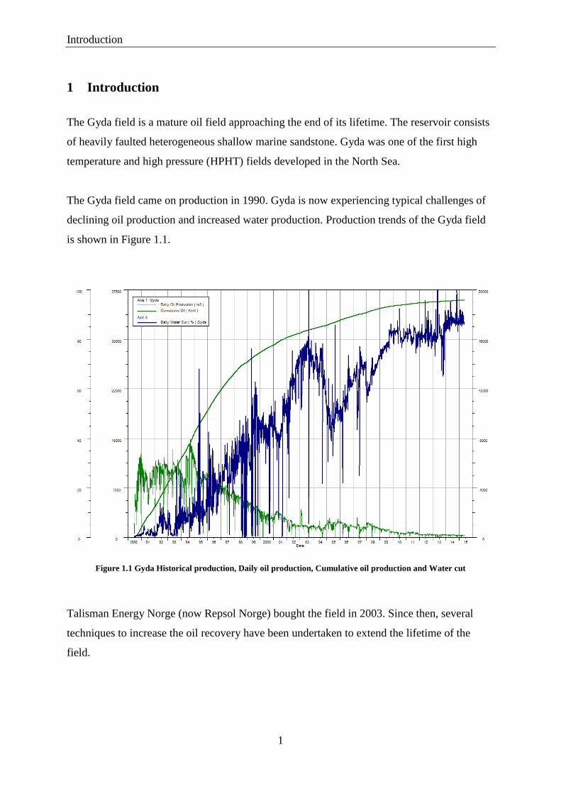
The Gyda field came on production in 1990. Gyda is now experiencing typical challenges of
declining oil production and increased water production. Production trends of the Gyda field
is shown in Figure 1.1.
Figure 1.1 Gyda Historical production, Daily oil production, Cumulative oil production and Water cut
Talisman Energy Norge (now Repsol Norge) bought the field in 2003. Since then, several
techniques to increase the oil recovery have been undertaken to extend the lifetime of the
field.
Introduction
2
Several previous EOR studies have been performed on Gyda. The first study was performed
by BP in 2002 and the second study was performed in 2007/2008 (Nishikiori et al., 2008).
The latest gas injection study was done by Talisman in 2014. All studies focused on different
gas injection strategies, and concluded that different types of gas injection could give
increased recovery on Gyda. It is important to note that the Gyda field is not abundant with
production of gas, and injection gas has to be imported from an outside source.
The gas injection study in 2007/2008 was performed on an extended four component black oil
reservoir simulator, and a main focus was to correctly model the Gyda heterogeneous
properties. It was concluded that gas injection represents the maximum recovery increment in
volume, but water alternating gas (WAG) and simultaneous WAG (SWAG) scheme
outperformed gas injection from the standpoint of voidage replacement efficiency and gas
utilization.
The gas injection study in 2014 was performed on a compositional reservoir model without
including hysteresis effects. It was done as a follow-up for a gas injection project in 2011, and
to support Talisman’s commercial offer to a nearby gas field tie-in. Purpose of the project was
to enhance Gyda’s production and ultimate recovery, prolong Gyda’s platform life and to look
at gas storage opportunities.
Based on observations and recommendations from the previous projects, the EOR potential
on Gyda is further investigated in this thesis.
In part 2 of this thesis, the different EOR methods are listed and described. In part 3, the Gyda
field is described and an early EOR screening of Gyda is executed. Based on Gyda EOR
requirements, WAG injection is the most promising EOR method, and is chosen for further
investigation.
In part 4, WAG experiences from the literature are investigated. WAG injection for
improving both macroscopic and microscopic is discussed, as well as different WAG
techniques. WAG experiences worldwide and in the North Sea are addressed, and examples
of WAG applications in the North Sea are briefly discussed. Operational challenges during
WAG injection are also addressed.
Introduction
3
Part 5 describes the transition from the black oil dynamic reservoir model received for this
project, to the compositional dynamic reservoir model.
Parts 6 and 7 introduce the background theory behind two- and three-phase relative
permeability hysteresis. Simulation sensitivities are performed for different three-phase
relative permeability models. Three different methods for capturing hysteresis effects in the
gas phase during WAG injection are tested.
In part 8 the WAG injection strategy is determined, and sensitivities around WAG cycle
lengths are performed.
This thesis ends with a short discussion part, followed by conclusions and recommendations.
EOR background
4
2 EOR background
2.1 EOR and IOR definition
This subchapter has been modified from the specialization project written by the author
(Albrigtsen, 2014).
Oil recovery is defined in three different phases; primary recovery, secondary recovery and
tertiary recovery (Sheng, 2011).
Primary recovery is the reservoir natural drive, and does not require any injected external
energy (Sheng, 2011). The most common reservoir drive mechanisms are solution gas drive,
gas-cap drive, natural water drive, gravity drainage and compaction drive (Dake, 1978).
Secondary recovery is the most used recovery process. The main purpose is pressure
maintenance and enhanced volumetric sweep efficiency. Secondary recovery includes water
and/or gas injection (Sheng, 2011). Secondary recovery is a recovery process with fluids that
already is present in the reservoir.
Tertiary recovery is the more advanced recovery processes, which includes injection of
chemical fluids, injection of thermal energy and/or injection of miscible gases (Sheng, 2011).
EOR, Enhanced Oil Recovery, as a term that should be used when some other method than
plain water or brain injection is used. EOR should not be used as a synonym for tertiary
recovery, as some EOR methods work quite well as either secondary recovery or tertiary
recovery, such as CO2 flooding, while other are most effective as secondary recovery, such as
steam or polymer flooding (Taber, Martin, & Seright, 1997b).
In the industry, the term Increased Oil Recovery (IOR), is also widely used. IOR is a wider
concept that not only includes EOR processes, but oil recovery by any means (Hite & Bondor,
2004). There are many different definitions of IOR and EOR in the literature. An
informational survey within the SPE’s EOR/IOR Technical Interest Group (EOIO TIG)
revealed a wide range of views (Hite & Bondor, 2004), which shows that the concept should
be better defined in order to improve the technical communication.
EOR background
5
IOR covers all EOR processes. In addition to EOR processes, it includes normal secondary
recovery such as water and immiscible gas injection, well stimulation and near wellbore
conformance control and infill wells. Well stimulation can be acidizing or fracturing. Near
wellbore conformance control can be cement plug/gel treatment for water and gas shut off.
(Sheng, 2011)
2.2 EOR classification
Parts of this subchapter has been modified from the specialization project by the author
(Albrigtsen, 2014)
The different EOR methods can be divided in to two main categories: Improving sweep
efficiency or improving displacement efficiency (Hite & Bondor, 2004). These two categories
can in other words be described as macroscopic and microscopic recovery. Macroscopic
recovery refers to how well the displacing fluid has come in contact with the oil-bearing parts
of the reservoir. Microscopic recovery refers to a measure of how well the displacing fluid
mobilizes the residual oil, once the fluid has come in contact with the oil.
Displacing additional oil with an injected fluid, can according to Taber et al. (1997) be
divided into three main mechanisms:
1. Solvent extraction to achieve or approach miscibility
2. Interfacial-tension (IFT) reduction
3. Viscosity change of either the oil or the water, for mobility control.
To approach miscibility, it is most common to use miscible gas flooding (Zerafat, Ayatollahi,
Mehranbod, & Barzegari, 2011).
The interfacial-tension reduction can be achieved by chemical flooding, such as surfactant
flooding, alkaline flooding and alkali polymer surfactant (ASP) flooding (Zerafat et al., 2011).
Viscosity changes, for mobility control, can be achieved by thermal oil recovery methods,
such as steam injection, both cyclic and continuous and hot water injection (Zerafat et al.,
2011), or by the chemical method; polymer flooding (Taber et al., 1997b).
EOR background
6
It is not always as simple as this to classify EOR processes. There are overlaps between the
different mechanisms. For example, interfacial tension is reduced as miscibility is approached
(Taber et al., 1997b).
Before further description of the different EOR processes, the main factors affecting the
macroscopic and microscopic displacement are discussed.
2.2.1 Main factors affecting macroscopic sweep efficiency
Macroscopic sweep efficiency is a measure of how well the displacing fluid has come in
contact with the oil-bearing parts of the reservoir. It is also referred to in the literature as
sweep efficiency.
Anisotropy and heterogeneity in the reservoir affects the fluid flow capacity in the reservoir,
and therefore the sweep efficiency (Petrowiki.org, 2014a).
Macroscopic sweep efficiency is a strong function of mobility ratio. If the mobility of the
displacing fluid is much greater than the mobility of the displaced fluid, the phenomenon
called viscous fingering takes place. A mobility ratio less than 1 is favorable for god sweep
efficiency.
The apparent mobility of a fluid is defined as (Petrowiki.org, 2014a):
𝜆𝑖 =
𝑘𝑖
𝜇𝑖 (2.1)
Where 𝑘𝑖 is the permeability to phase i, and 𝜇𝑖 is the viscosity of phase i. The mobility is
given as:
𝑀 =
𝜆𝑑𝑖𝑠𝑝𝑙𝑎𝑐𝑖𝑛𝑔 𝑓𝑙𝑢𝑖𝑑
𝜆𝑑𝑖𝑠𝑝𝑙𝑎𝑐𝑒𝑑 𝑓𝑙𝑢𝑖𝑑 (2.2)
EOR background
7
The physical arrangements of injectors and producers in the field affect the sweep efficiency.
Rock matrix is also a main factor. (Terry, 2001). The reservoir thickness, permeability, flow
rate and fluid contacts are other affecting factors (Slb.com, 2014c).
2.2.2 Main factors affecting microscopic displacement efficiency
The microscopic displacement efficiency is a measure of how well the displacing fluid
mobilizes the residual oil, once the fluid has come in contact with the oil. It is also referred to
in the literature as displacement efficiency. Factors affecting the displacement efficiency is
interfacial tension, relative permeability, wettability and capillary pressure.
Interfacial tension (IFT) is the force that holds the surface of a particular phase together, and
it exists when two phases are present. The phases can be gas/oil, gas/water or water/oil
(Petrowiki.org, 2014b).
Relative permeability is a dimensionless number between 0 and 1. It is the ratio of effective
permeability of a fluid, at a given saturation, relative to the absolute permeability of the fluid
at total saturation (Slb.com, 2014b). Relative permeabilities change with changing interfacial
tension. This sensitivity of relative permeability to decreasing interfacial tension is of great
interest for enhanced oil recovery processes (Petrowiki.org, 2014c). Relative permeability can
be described with both drainage curves and imbibition curves. In a water-wet system,
drainage is the process where the wetting phase (water) is decreasing. For the same system,
imbibition is the process where the wetting phase (water) saturation is increasing.
Wettability is the preference of a solid to be in contact with one fluid rather than another. It
describes the balance of surface and interfacial forces. (Slb.com, 2014a). The reservoir
wettability is important in determining the recovery factor. Waterflooding in water-wet
system is more efficient and oil recovery is higher. During waterflood of an oil-wet system,
the water-relative permeability increases and the oil relative permeability decreases. Water
will then flow easier than the oil, and this can lead to earlier water break-through. (Meybodi,
Kharrat, & Wang, 2008)
EOR background
8
Capillary pressure in a pore is given by:
𝑃𝑐 =
2𝜎𝑐𝑜𝑠𝜃
𝑅
(2.3)
Where 𝑃𝑐 is the capillary pressure, 𝜎 is the interfacial tension, 𝑐𝑜𝑠𝜃 is the contact angle
measured through the aqueous phase, that is formed at the junction at the tree phases
(oil/water/solid), and 𝑅 is the pore radius (Schramm, 2000).
Capillary forces are the reason why the residual oil in primary oil recovery is high. Both
secondary recovery and tertiary recovery is also intended to overcome these forces. In smaller
pores, the viscous forces from waterflooding, can not always overcome the capillary forces,
holding a lot of the oil trapped in place (Schramm, 2000).
2.2.3 Relative permeability correlations
Relative permeability measurements from laboratory is both time consuming and costly. Due
to this a series of relative permeability correlations has been developed. Relative permeability
correlations can be used if core data is unavailable, or for verification of experimentally
determined curves (Torabi, Zarivnyy, & Mosavat, 2013). Both modified Brooks-Corey
(MBC) and LET correlation has been used under development of the relative permeabilities
on Gyda.
2.2.3.1 Modified Brooks-Corey correlation
The most widely used relative permeability correlation in the oil industry is the modified
Brooks-Corey correlation, also called the power law model. The model is explicitly a function
of relative permeability endpoints (Goda & Behrenbruch, 2004).
The MBC model describes the relative permeabilities as:
EOR background
9
𝐾𝑟𝑜 = 𝐾𝑟𝑜,𝑚𝑎𝑥(
𝑆0 − 𝑆𝑜𝑟
1 − 𝑆𝑜𝑟 − 𝑆𝑤𝑐 − 𝑆𝑔𝑐)𝑛𝑜 (2.4)
𝐾𝑟𝑤 = 𝐾𝑟𝑤,𝑚𝑎𝑥(
𝑆𝑤 − 𝑆𝑤𝑐
1 − 𝑆𝑜𝑟 − 𝑆𝑤𝑐 − 𝑆𝑔𝑐)𝑛𝑤 (2.5)
𝐾𝑟𝑔 = 𝐾𝑟𝑔,𝑚𝑎𝑥(
𝑆𝑔 − 𝑆𝑔𝑐
1 − 𝑆𝑜𝑟 − 𝑆𝑤𝑐 − 𝑆𝑔𝑐)𝑛𝑔 (2.6)
Where 𝐾𝑟𝑜 , 𝐾𝑟𝑤, 𝐾𝑟𝑔 is the relative permeability to oil, water and gas respectively. 𝑆𝑜𝑟 is the
residual oil saturation, 𝑆𝑤𝑐 is the critical water saturation and 𝑆𝑔𝑐 is the critical gas saturation.
The exponents 𝑛𝑜 , 𝑛𝑤, 𝑛𝑔 is the Corey exponents ranging from 1 to 6. The maximum relative
permeabilities 𝐾𝑟𝑜,𝑚𝑎𝑥, 𝐾𝑟𝑤,𝑚𝑎𝑥, 𝐾𝑟𝑔,𝑚𝑎𝑥 ranges between 0 and 1.
(Petrowiki.org, 2015)
2.2.3.2 LET correlation
Lomeland, Ebeltoft and Thomas first proposed the LET expression of relative permeability in
2005 at the International Symposium of the Society of Core Analyst in Toronto. The
correlation was proposed as a flexible 3 parameter analytical correlation. It influences
different parts of the relative permeability thereby captures variable behavior across the entire
saturation range. The parameters L, E and T are empirical parameters, used to describe the
relative permeability development in the different saturation zones. The L describes the lower
part of the curve. The L values are comparable to the Corey parameter. The T describes the
upper part of the curve. The E describes the elevation part of the curve. From experiments it is
shown that L ≥ 1, E>0 and T ≥ 0.5.
The correlation for oil and water relative permeability with water injection is:
𝑘𝑟𝑜𝑤 = 𝑘𝑟𝑜
𝑥 ∗(1 − 𝑆𝑤𝑛)𝐿𝑜
𝑤
(1 − 𝑆𝑤𝑛)𝐿𝑜𝑤
+ 𝐸𝑜𝑤𝑆𝑤𝑛
𝑇𝑜𝑤 (2.7)
EOR background
10
𝑘𝑟𝑤 = 𝑘𝑟𝑤
𝑜 ∗𝑆𝑤𝑛
𝐿𝑤𝑜
𝑆𝑤𝑛𝐿𝑤
𝑜
+ 𝐸𝑤𝑜 (1 − 𝑆𝑤𝑛)𝑇𝑤
𝑜
(2.8)
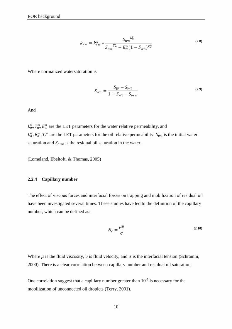
Where normalized watersaturation is
𝑆𝑤𝑛 =
𝑆𝑊 − 𝑆𝑊𝑖
1 − 𝑆𝑊𝑖 − 𝑆𝑜𝑟𝑤 (2.9)
And
𝐿𝑤𝑜 , 𝑇𝑤
𝑜, 𝐸𝑤𝑜 are the LET parameters for the water relative permeability, and
𝐿𝑜𝑤, 𝐸𝑜
𝑤, 𝑇𝑜𝑤 are the LET parameters for the oil relative permeability. 𝑆𝑊𝑖 is the initial water
saturation and 𝑆𝑜𝑟𝑤 is the residual oil saturation in the water.
(Lomeland, Ebeltoft, & Thomas, 2005)
2.2.4 Capillary number
The effect of viscous forces and interfacial forces on trapping and mobilization of residual oil
have been investigated several times. These studies have led to the definition of the capillary
number, which can be defined as:
𝑁𝑐 =𝜇𝜐
𝜎 (2.10)
Where 𝜇 is the fluid viscosity, 𝜐 is fluid velocity, and 𝜎 is the interfacial tension (Schramm,
2000). There is a clear correlation between capillary number and residual oil saturation.
One correlation suggest that a capillary number greater than 10-5 is necessary for the
mobilization of unconnected oil droplets (Terry, 2001).
EOR background
11
2.3 EOR methods description
This subchapter has been modified from the specialization project written by the author
(Albrigtsen, 2014).
With a few minor exceptions, all EOR methods fall distinctly into one of three categories:
chemical, thermal or solvent methods. The following chapter describes the conventional EOR
methods.
2.3.1 Chemical flooding
Chemical EOR flooding has so far made a relatively small contribution to the world’s oil
production. Only polymer flooding has been applied on a significant scale, and applications of
surfactants/polymer or alkaline-surfactant-polymer (ASP) has been limited to multiwall pilots
or small field scale (Stoll et al., 2010)
Despite this, results from the laboratory shows that chemical flooding is one of the most
successful EOR methods for depleted reservoirs at low pressure (Schramm, 2000). The
economical aspect has been the reason why chemical flooding is not more tested in the field.
Chemical flooding can both be used for interfacial tension reduction and viscosity changes for
mobility control. Surfactants and polymers are the principal components in chemical flooding
(Schramm, 2000), were surfactants is mostly used for interfacial tension reduction and
polymers mostly used for viscosity change.
2.3.1.1 Polymer flooding
Polymer flooding consists of adding polymer to the water in a waterflood, to increase the
water viscosity, and with that, decrease the mobility ratio between displacing agent and
displaced agent. Polymers increase the volumetric sweep efficiency. (Lake, 2010)
Commercially attractive polymers fall into two main categories; polyacrylamides and
polysaccharides (biopolymers).
EOR background
12
Polymers main target is to improve the sweep efficiency, by lowering the mobility ratio. The
conventional belief is that polymers do not reduce residual oil in a micro scale (Sheng, 2011).
Schneider and Owens (1982) and Chen and Chen (2002) have conducted several experiments
to prove the relation between polymer flooding and relative permeability. It is proven that
polymer flooding decreases the relative permeability to water, while the relative permeability
to oil is less affected, and thereby affect the microscopic oil recovery.
2.3.1.2 Surfactant flooding
Surfactants have the ability to influence the properties of surfaces and interfaces. When
surfactant molecules adsorb at an interface, they provide and expanding force acting against
the normal interfacial tension, and tend to lower the interfacial tension. Anionic surfactants
can lower the interfacial tension between oil and water by a factor more than 1000 in the two-
phase area (Schramm, 2000). Surfactants can alter the wettability (Hirasaki, Miller, & Puerto,
2008).
Surfactant flooding has had some technical successes in the field, but few economic. Because
of the high cost of surfactants, there has been an effort to lower the cost by injecting alkali.
This resulted in alkaline-surfactant-polymer (ASP) flooding. (Taber et al., 1997b)
2.3.1.3 Alkaline-Surfactant-Polymer flooding
In ASP flooding, alkaline, surfactant and polymers is mixed together to achieve a high
recovery factor. Because of the synergy of these three components, ASP is the current world-
wide focus of research and field trial in chemical enhanced oil recovery (Sheng, 2013a)
The synergy between alkaline, surfactants and polymers is strong, and combined they can
increase the oil recovery much more than they can do alone.
Alkaline solutions convert naturally occurring naphthenic acids in crude oils to soaps. The use
of alkali also reduces adsorption of ionic surfactants on sandstones because of the high pH.
High pH reverses the charge of the positively charged clay sites where adsorptions also
EOR background
13
occurs. (Liu, Li, Miller, & Hirasaki, 2008). The mixture of soap, that is generated from the
alkaline and surfactant has a wider range of salinity tolerance (Sheng, 2013a).
Soap and surfactants create stable emulsions and reduced IFT. Polymers help these emulsions
staying stable. Polymers reduce surfactant absorption on rock surfaces, and surfactants
reduce polymer adsorption. Polymer improves the sweep efficiency, due to mobility control.
ASP projects usually suffer from low injectivity (mostly due to the alkaline), polymer
degradation, difficulties to separate produced water from oil, pump failures, bacterial growth,
corrosion and problems related to logistics and chemicals handling (Sheng, 2013a).
2.3.2 Thermal flooding
Thermal flooding accounts for the biggest share of the worlds enhanced oil production, and
have been active for over 40 years(Taber et al., 1997b).
Thermal methods involve many mechanisms to displace additional oil, but the main
mechanism is the reduction of crude viscosity with increasing temperature. Heavy crude (10-
20 API) that undergoes a temperature increase from 300 to 400 K (27C to 127C), which is
easily achieved by thermal methods will produce a viscosity that is well within the flowing
range (Lake, 2010). For lighter crudes the viscosity decrease is less, and for very heavy oil,
thermal methods will not be able to create low enough viscosity.
For a reservoir with a temperature over 150C (423 K) the viscosity changes are smaller than
for colder reservoirs. Thermal methods will therefore not be discussed further in this project.
2.3.3 Miscible flooding
Gas flooding can be used by means of miscibility development between gas and reservoir oil.
Gas flooding can improve both macroscopic and microscopic recovery. It is a mature
technology, with commercial success since early 1980s (Sheng, 2013b).
EOR background
14
Two types of miscibility can occur. First contact miscibility occurs when injected fluid is
mixed with the oil, and a single phase is formed. Multiple contact miscibility occur as the
injected fluid moves though the reservoir, and miscible conditions are developed in situ,
through composition alteration of the injected fluid or crude oil. (Arshad, Al-Majed, Menouar,
Muhammadain, & Mtawaa, 2009)
In the perfect scenario miscible processes decrease the interfacial tension to zero, if full
miscibility is achieved, and the capillary number becomes infinite. This leads to a maximized
microscopic displacement (Terry, 2001). As secondary recovery mechanisms gas flooding
also contributes to swelling and oil viscosity reduction. Swelling improves the relative
permeability to oil (Arshad et al., 2009). The secondary recovery mechanisms lead to
increased macroscopic recovery. Because of the differences in density and viscosity between
injected fluid and reservoir fluid, viscous fingering is a frequent problem, and can create poor
sweep efficiency.
For a good designed miscible flooding project, a very important design criterion is the
minimum miscibility pressure (MMP). This is the MMP at which the reservoir fluid develops
miscibility with the injected fluid (Arshad et al., 2009). The pressure must therefore be higher
than MMP to achieve miscibility between oil and gas. The MMP depends on the oil gravity,
reservoir depth and reservoir pressure (Taber et al., 1997b). The MMP is typically smaller for
low viscosity oils. The reservoir pressure must usually be near or above the minimum
pressure for miscibility to achieve good displacement efficiency (Sheng, 2013b).
Minimum miscibility enrichment (MME) is another important parameter in terms of
miscibility conditions. This is the minimum possible enrichment of the injection gas with C2-4
were miscibility with the reservoir oil can be attained (Gao, Towler, & Pan, 2010).
To achieve miscibility, it is important to stay on or over both MMP and MME.
For miscible gas flooding purposes, it is most common to use Nitrogen and flue-gas injection,
hydrocarbon injection or CO2 injection. CO2 displacement is usually the most effective (Taber
et al., 1997b)
Gas injection, both miscible and immiscible can have the following benefits for EOR:
EOR background
15
1. Vaporizing the lighter components of the crude oil.
2. Generating miscibility if the pressure is high enough.
3. Enhancing gravity drainage in dipping reservoirs.
4. Increasing the oil volume by swelling.
5. Decreasing oil viscosity.
6. Immiscible gas displacement.
7. Displacement of attic oil.
8. Lowering the interfacial tension between oil and gas in the near-miscible regions.
9. If gas break through, give gas lift effect in high water-cut wells.
(Taber, Martin, & Seright, 1997a)
2.3.3.1 WAG
WAG injection is an oil recovery method initially aimed to improve the macroscopic sweep
efficiency during gas injection (Christensen, Stenby, & Skauge, 2001). WAG injection can
improve both the macroscopic and microscopic oil recovery.
Gyda field
16
3 Gyda field
3.1 About Gyda
The Gyda field is a mature oil field located between Ula and Ekofisk in the southern part of
the North Sea. The field has been developed with a combined drilling, accommodation and
processing facility with a steel jacket. Gyda is producing with water injection as the main
drive mechanism on the main field. Gas-cap drive and water-drive from an aquifer give
pressure support to smaller parts of the Gyda reservoir. The main challenge on Gyda is the
increased water production on the exciting wells. (Npd.no, 2015) IOR such as infill wells, gas
lift installations and EOR techniques are under investigation on Gyda in order to prolong the
lifetime of the field.
The Gyda field was one of the first HPHT fields to be developed in the North Sea.
The virgin reservoir pressure was 600 bar at 4100 m TVDSS. The virgin temperature was
155◦ C at the same depth. (Talisman, 2014)
The initial oil in place on Gyda was 90.2 mill Sm3. 30 May 2015 the cumulative oil
production is 35.998 mill sm3 (OFM production database), which gives an overall recovery
factor of 39.9 %.
3.2 Gyda geological description, reservoir and fluid
The Gyda reservoir consists of shallow marine Jurassic deposits in the Ula-formation. The
reservoir is subdivided into three depositional packages, named A-, B- and C-sand. The grains
in the Gyda reservoir are very fine to finely grained and moderately well sorted. Syn-
depositional fault movements have controlled depositional facies and thickness variation,
resulting into a westward thickening of the Gyda reservoir wedge. (Talisman, 2014)
The A-sand is of good reservoir quality, with permeability up to 1D. The B-sand has poor
reservoir quality, with permeabilities varying from 1mD to 30mD. The reservoir is heavily
faulted and heterogeneous. As a measure of heterogeneity, a Dykstra-Parson’s coefficient
(Vdp) of more than 0.8 has been measured from core plug data (Nishikiori et al., 2008). Gyda
porosity ranges from 10% to 25% (Dong, 2012).
Gyda field
17
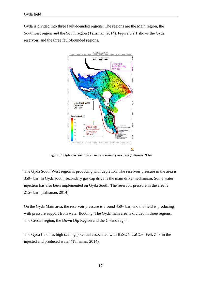
Gyda is divided into three fault-bounded regions. The regions are the Main region, the
Southwest region and the South region (Talisman, 2014). Figure 5.2.1 shows the Gyda
reservoir, and the three fault-bounded regions.
Figure 3.1 Gyda reservoir divided in three main regions from (Talisman, 2014)
The Gyda South West region is producing with depletion. The reservoir pressure in the area is
350+ bar. In Gyda south, secondary gas cap drive is the main drive mechanism. Some water
injection has also been implemented on Gyda South. The reservoir pressure in the area is
215+ bar. (Talisman, 2014)
On the Gyda Main area, the reservoir pressure is around 450+ bar, and the field is producing
with pressure support from water flooding. The Gyda main area is divided in three regions.
The Crestal region, the Down Dip Region and the C-sand region.
The Gyda field has high scaling potential associated with BaSO4, CaCO3, FeS, ZnS in the
injected and produced water (Talisman, 2014).
Gyda field
18
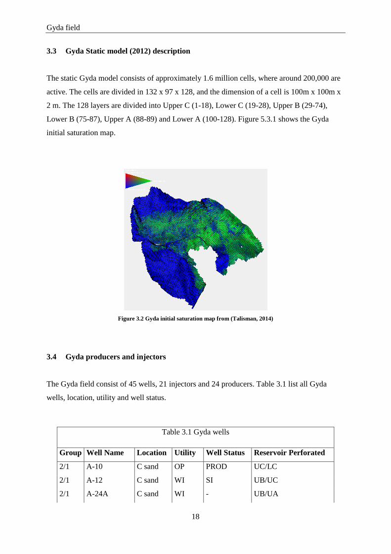
3.3 Gyda Static model (2012) description
The static Gyda model consists of approximately 1.6 million cells, where around 200,000 are
active. The cells are divided in 132 x 97 x 128, and the dimension of a cell is 100m x 100m x
2 m. The 128 layers are divided into Upper C (1-18), Lower C (19-28), Upper B (29-74),
Lower B (75-87), Upper A (88-89) and Lower A (100-128). Figure 5.3.1 shows the Gyda
initial saturation map.
Figure 3.2 Gyda initial saturation map from (Talisman, 2014)
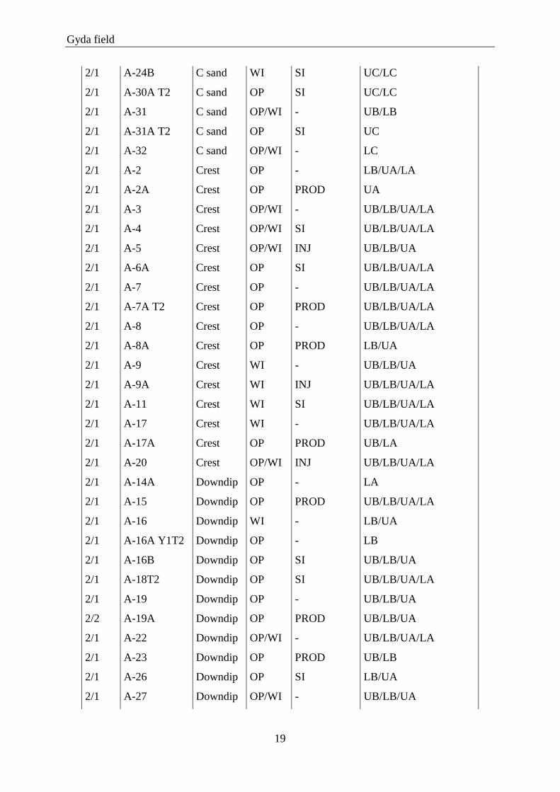
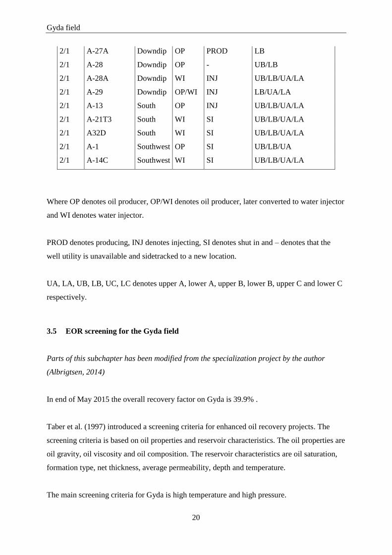
3.4 Gyda producers and injectors
The Gyda field consist of 45 wells, 21 injectors and 24 producers. Table 3.1 list all Gyda
wells, location, utility and well status.
Table 3.1 Gyda wells
Group Well Name Location Utility Well Status Reservoir Perforated
2/1 A-10 C sand OP PROD UC/LC
2/1 A-12 C sand WI SI UB/UC
2/1 A-24A C sand WI - UB/UA
Gyda field
19
2/1 A-24B C sand WI SI UC/LC
2/1 A-30A T2 C sand OP SI UC/LC
2/1 A-31 C sand OP/WI - UB/LB
2/1 A-31A T2 C sand OP SI UC
2/1 A-32 C sand OP/WI - LC
2/1 A-2 Crest OP - LB/UA/LA
2/1 A-2A Crest OP PROD UA
2/1 A-3 Crest OP/WI - UB/LB/UA/LA
2/1 A-4 Crest OP/WI SI UB/LB/UA/LA
2/1 A-5 Crest OP/WI INJ UB/LB/UA
2/1 A-6A Crest OP SI UB/LB/UA/LA
2/1 A-7 Crest OP - UB/LB/UA/LA
2/1 A-7A T2 Crest OP PROD UB/LB/UA/LA
2/1 A-8 Crest OP - UB/LB/UA/LA
2/1 A-8A Crest OP PROD LB/UA
2/1 A-9 Crest WI - UB/LB/UA
2/1 A-9A Crest WI INJ UB/LB/UA/LA
2/1 A-11 Crest WI SI UB/LB/UA/LA
2/1 A-17 Crest WI - UB/LB/UA/LA
2/1 A-17A Crest OP PROD UB/LA
2/1 A-20 Crest OP/WI INJ UB/LB/UA/LA
2/1 A-14A Downdip OP - LA
2/1 A-15 Downdip OP PROD UB/LB/UA/LA
2/1 A-16 Downdip WI - LB/UA
2/1 A-16A Y1T2 Downdip OP - LB
2/1 A-16B Downdip OP SI UB/LB/UA
2/1 A-18T2 Downdip OP SI UB/LB/UA/LA
2/1 A-19 Downdip OP - UB/LB/UA
2/2 A-19A Downdip OP PROD UB/LB/UA
2/1 A-22 Downdip OP/WI - UB/LB/UA/LA
2/1 A-23 Downdip OP PROD UB/LB
2/1 A-26 Downdip OP SI LB/UA
2/1 A-27 Downdip OP/WI - UB/LB/UA
Gyda field
20
2/1 A-27A Downdip OP PROD LB
2/1 A-28 Downdip OP - UB/LB
2/1 A-28A Downdip WI INJ UB/LB/UA/LA
2/1 A-29 Downdip OP/WI INJ LB/UA/LA
2/1 A-13 South OP INJ UB/LB/UA/LA
2/1 A-21T3 South WI SI UB/LB/UA/LA
2/1 A32D South WI SI UB/LB/UA/LA
2/1 A-1 Southwest OP SI UB/LB/UA
2/1 A-14C Southwest WI SI UB/LB/UA/LA
Where OP denotes oil producer, OP/WI denotes oil producer, later converted to water injector
and WI denotes water injector.
PROD denotes producing, INJ denotes injecting, SI denotes shut in and – denotes that the
well utility is unavailable and sidetracked to a new location.
UA, LA, UB, LB, UC, LC denotes upper A, lower A, upper B, lower B, upper C and lower C
respectively.
3.5 EOR screening for the Gyda field
Parts of this subchapter has been modified from the specialization project by the author
(Albrigtsen, 2014)
In end of May 2015 the overall recovery factor on Gyda is 39.9% .
Taber et al. (1997) introduced a screening criteria for enhanced oil recovery projects. The
screening criteria is based on oil properties and reservoir characteristics. The oil properties are
oil gravity, oil viscosity and oil composition. The reservoir characteristics are oil saturation,
formation type, net thickness, average permeability, depth and temperature.
The main screening criteria for Gyda is high temperature and high pressure.
Gyda field
21
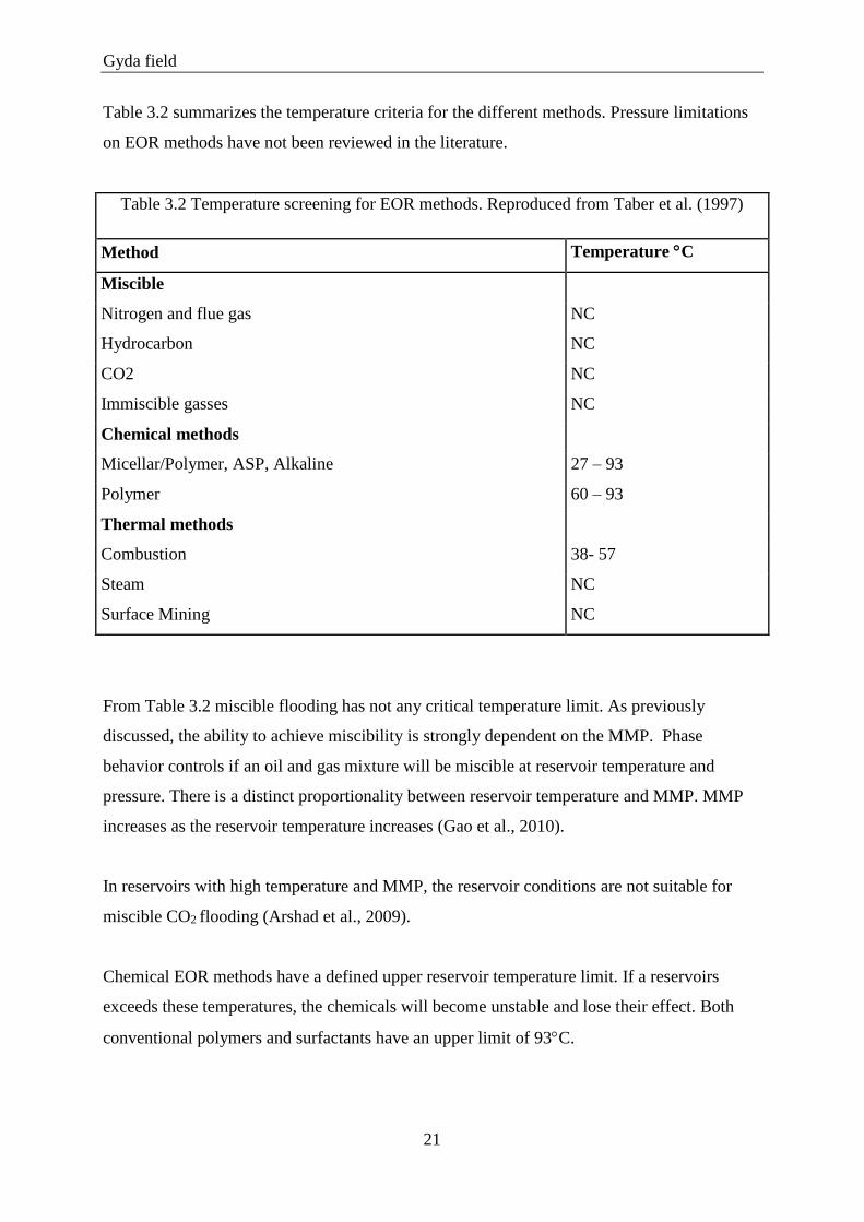
Table 3.2 summarizes the temperature criteria for the different methods. Pressure limitations
on EOR methods have not been reviewed in the literature.
Table 3.2 Temperature screening for EOR methods. Reproduced from Taber et al. (1997)
Method Temperature C
Miscible
Nitrogen and flue gas NC
Hydrocarbon NC
CO2 NC
Immiscible gasses NC
Chemical methods
Micellar/Polymer, ASP, Alkaline 27 – 93
Polymer 60 – 93
Thermal methods
Combustion 38- 57
Steam NC
Surface Mining NC
From Table 3.2 miscible flooding has not any critical temperature limit. As previously
discussed, the ability to achieve miscibility is strongly dependent on the MMP. Phase
behavior controls if an oil and gas mixture will be miscible at reservoir temperature and
pressure. There is a distinct proportionality between reservoir temperature and MMP. MMP
increases as the reservoir temperature increases (Gao et al., 2010).
In reservoirs with high temperature and MMP, the reservoir conditions are not suitable for
miscible CO2 flooding (Arshad et al., 2009).
Chemical EOR methods have a defined upper reservoir temperature limit. If a reservoirs
exceeds these temperatures, the chemicals will become unstable and lose their effect. Both
conventional polymers and surfactants have an upper limit of 93C.
Gyda field
22
Even though there is no critical upper temperature limit for thermal methods, thermal methods
will not give the same effect on high temperature reservoirs, that as for low temperature
reservoirs.
From the EOR screening, any type of gas/water injection is the best alternative for EOR
projects on Gyda. Any IOR projects to be implemented on Gyda must follow the following
criteria:
Minimal topside modifications
Low investment cost
Rapid pay-back
As mentioned in the introduction, the Gyda field is not abundant with production of gas, and
injection gas has to be imported by an outside source. Previous studies conclude that WAG
and SWAG scheme outperform gas injection from the standpoint of voidage replacement
efficiency and gas utilization, even though gas injection represents the maximum recovery
increment in volume.
Only a few applications of SWAG have been reported worldwide, and it seems that WAG is
more beneficial and easy to implement than SWAG. WAG is a mature technology and
reservoir engineers are confident with it because it is simple to design and easy to implement
(Teigland & Kleppe, 2006).
From the EOR screening and Gyda EOR criteria, it is decided to investigate the effects of
WAG injection. Since the pressure, volume, temperature (PVT) properties of the possible
injection gas are unknown, the WAG injection is simulated immiscible.
WAG review
23
4 WAG review
Water alternating gas injection is an oil recovery method initially aimed to improve the
macroscopic sweep efficiency during gas injection (Christensen et al., 2001). WAG injection
can improve both the macroscopic and microscopic oil recovery.
In WAG coreflood studies, extreme low endpoint oil saturations are observed. After two pore
volumes, (PVs), of WAG are injected, the residual oil saturation has in some cases been lower
than 5%. In comparison with continuous gas injection, or water injection, where remaining oil
saturation is 20 to 40 %, after the same amount of PV is injected, WAG injection can be a
very good candidate for EOR (Larsen & Skauge, 1998).
4.1 WAG for improving macroscopic and microscopic recovery.
As previously mentioned, gas injection can suffer from poor mobility ratio. Because the
displacing fluid (gas) has higher mobility than the displaced fluid (oil), this can lead to
viscous fingering, and lower oil recovery.
The mobility ratio depends on the fluid viscosity and the fluid relative permeability (see
chapter 2.2.1). During a WAG flood the water and gas phases will increase and decrease
alternately. This gives special demands for the relative permeability description of oil, gas and
water (Christensen et al., 2001). Relative permeability is considered to be dependent on
saturation and saturation history. This is described in the literature as relative permeability
hysteresis (Larsen & Skauge, 1998). In WAG injection, reduction of relative permeability is
achieved by the hysteresis phenomena where alternating injection of water and gas reduces
the relative permeability of the displacing phase (Arogundade, Shahverdi, & Sohrabi, 2013).
When the relative permeability of the displacing phase is reduced, the mobility ratio is
reduced. Reduced mobility ratio is favorable for a stable displacement. The three-phase
relative permeability hysteresis will be discussed in more detail in chapter 6.
The macroscopic recovery is improved by better mobility control by the water and by
contacting unswept zones. The gas flood improves the microscopic recovery. Both fluid
WAG review
24
densities and viscosities can also be changed by a WAG flood, and can improve the oil
recovery. (Christensen et al., 2001)
Recent simulation studies have shown that the inclusion of gas trapping, reduced phase
mobility, and lower residual oil saturation in the three-phase zones may influence the extent
of the WAG zone in the reservoir and lead to higher oil recovery.
It has been shown that porosity and permeability increasing downward can be advantageous
for the WAG injection because this combination increases the stability of the front
(Christensen et al., 2001).
4.2 WAG techniques
WAG injection success is dependent on rock type, injection strategy (gas and water cycle
lengths), miscible/immiscible gas and well spacing (Christensen et al., 2001).
WAG can be implemented in different ways. The most common is Miscible WAG (MWAG)
and Immiscible WAG (IWAG). Hybrid WAG (HWAG), Simultaneous WAG (SWAG) and
Water Alternating Steam Process are less common (Arogundade et al., 2013).
HWAG is when a large slug of gas is injected followed by a number of small slugs of water
and gas (Christensen et al., 2001). SWAG is when the gas and oil are injected into the
reservoir at the same time. SWAG requires mixing the gas with water at a pressure sufficient
to maintain bubble flow of a gas dispersed in a water flow. To maintain such pressure is a
main challenge because gas and water presence in the well bore lowers bottom hole pressure
and hence injectivity (Teigland & Kleppe, 2006).
It can be hard to distinguish whether the gas flood in the WAG injection is miscible or
immiscible, as multi contact miscibility can occur. In field cases, it may oscillate between
miscible and immiscible during the lifetime of the injection. (Christensen et al., 2001)
If it is not possible to stay over the MMP limit, immiscible WAG flooding occurs. Immiscible
WAG flooding has in many cases been chosen where the injection gas resources are limited,
WAG review
25
or where strong reservoir heterogeneity or low dipping is limiting the gravity-stable gas
injection. (Christensen et al., 2001)
4.3 WAG experience worldwide
The first known WAG field experience was in Canada in 1957 (Arogundade et al., 2013).
WAG flooding has mostly been applied to high-permeability sandstone reservoirs, but there
are also examples from low permeability chalk (Christensen et al., 2001). Christensen et al
(2001) reviewed approximately 60 field cases, where very few were unsuccessful. Recovery
is reported to be increased by 5% from WAG injection, and the WAG process is mostly
reported as a tertiary recovery process.
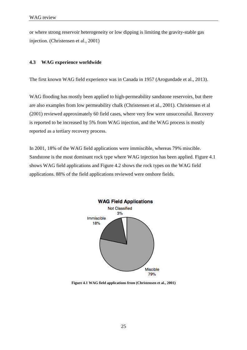
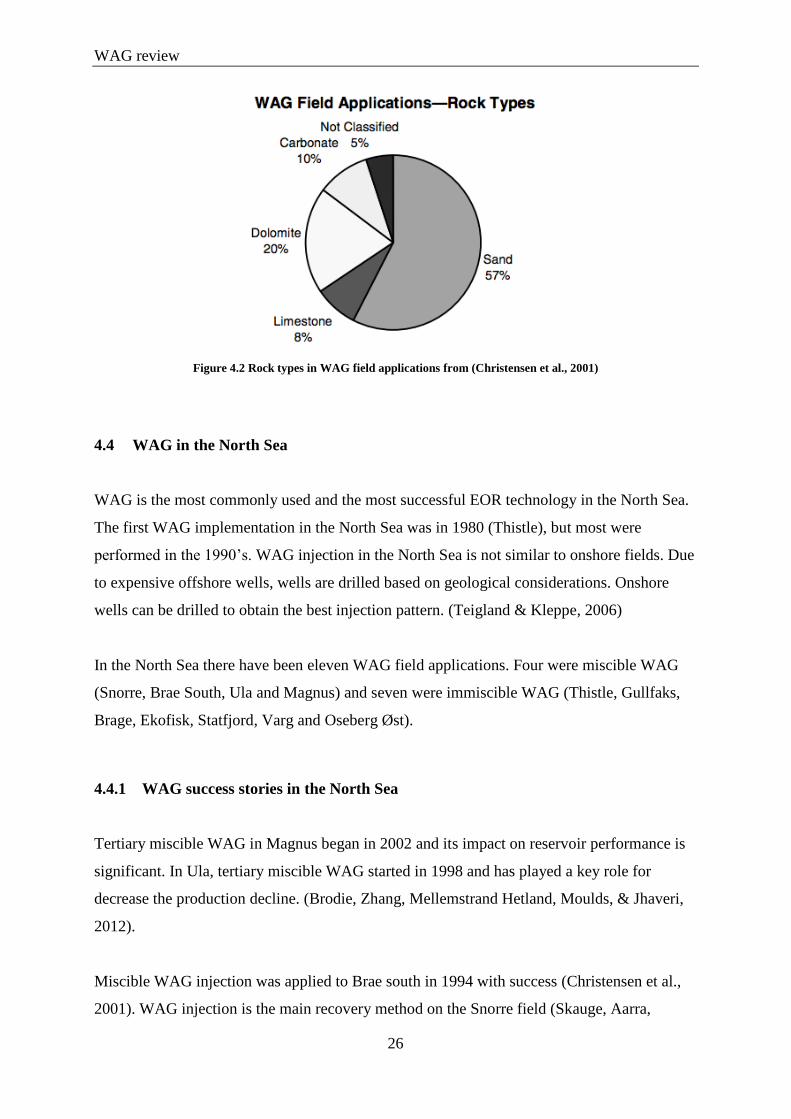
In 2001, 18% of the WAG field applications were immiscible, whereas 79% miscible.
Sandstone is the most dominant rock type where WAG injection has been applied. Figure 4.1
shows WAG field applications and Figure 4.2 shows the rock types on the WAG field
applications. 88% of the field applications reviewed were onshore fields.
Figure 4.1 WAG field applications from (Christensen et al., 2001)
WAG review
26
Figure 4.2 Rock types in WAG field applications from (Christensen et al., 2001)
4.4 WAG in the North Sea
WAG is the most commonly used and the most successful EOR technology in the North Sea.
The first WAG implementation in the North Sea was in 1980 (Thistle), but most were
performed in the 1990’s. WAG injection in the North Sea is not similar to onshore fields. Due
to expensive offshore wells, wells are drilled based on geological considerations. Onshore
wells can be drilled to obtain the best injection pattern. (Teigland & Kleppe, 2006)
In the North Sea there have been eleven WAG field applications. Four were miscible WAG
(Snorre, Brae South, Ula and Magnus) and seven were immiscible WAG (Thistle, Gullfaks,
Brage, Ekofisk, Statfjord, Varg and Oseberg Øst).
4.4.1 WAG success stories in the North Sea
Tertiary miscible WAG in Magnus began in 2002 and its impact on reservoir performance is
significant. In Ula, tertiary miscible WAG started in 1998 and has played a key role for
decrease the production decline. (Brodie, Zhang, Mellemstrand Hetland, Moulds, & Jhaveri,
2012).
Miscible WAG injection was applied to Brae south in 1994 with success (Christensen et al.,
2001). WAG injection is the main recovery method on the Snorre field (Skauge, Aarra,
WAG review
27
Surguchev, Martinsen, & Rasmussen, 2002). Miscible WAG injection was applied to Snorre
in 1994 with success (Teigland & Kleppe, 2006)
Tertiary immiscible WAG injection was implemented as a supplement to water injection at
the Statfjord field in 1997, and became a success (Crogh, Eide, & Morterud, 2002).
Also on the Gullfaks field, tertiary immiscible WAG injection was implemented after a longer
period of water injection. The main objectives for the WAG injection was to avoid reduced oil
production during periods of gas export limitations and reduce storage cost and CO2 tax. The
EOR purposes was to drain attic oil, reduce residual oil saturation and reach areas that water
injection would not displace. The pilot injection started in 1991. The WAG injection is
considered successful and a significant contributor to improved oil recovery. (Instefjord &
Todnem, 2002).
On the Brage field, immiscible WAG injection started shortly after production startup. The
pilot was considered a success, despite in one well. The well was connected to the injector by
a thin high permeable zone, which acted as a thief zone. It was concluded to continue WAG
injection with focus on avoiding the high permeable zone in the Upper Frensfjord (Lien, Lie,
Fjellbirkeland, & Larsen, 1998). Today WAG injection effects on Brage is not well
summarized (Repsol, 2015)
Oseberg Sør is supported by WAG injection. Reservoir simulation rank WAG as a major
increased recovery contributor (Aasheim, 2000). The start date of the immiscible WAG
injection project was in 1999, and it was considered successful.
On the Ekofisk field hydrocarbon WAG injection was found to have significant reserves
potential (Jensen, Harpole, & Østhus, 2000). A field trial was unsuccessful in 1996 (Teigland
& Kleppe, 2006).
WAG review
28
4.4.2 Varg- increased oil recovery from a mature field by WAG injection
Varg is a mature oil reservoir located in the North Sea, 200 km West of Stavanger. It is a
faulted reservoir with multiple compartments, with different oil water contacts. The oil is
light, 35◦ API, and under saturated with a bubble point pressure of 180-220 bar. The initial
reservoir pressure was 340 bar. The reservoir quality is good, with Darcy sand in some areas,
and poorer reservoir quality in other areas.
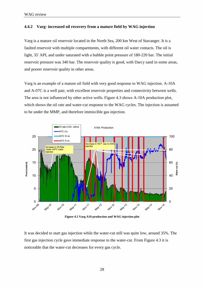
Varg is an example of a mature oil field with very good response to WAG injection. A-10A
and A-07C is a well pair, with excellent reservoir properties and connectivity between wells.
The area is not influenced by other active wells. Figure 4.3 shows A-10A production plot,
which shows the oil rate and water-cut response to the WAG cycles. The injection is assumed
to be under the MMP, and therefore immiscible gas injection.
Figure 4.3 Varg A10 production and WAG injection plot
It was decided to start gas injection while the water-cut still was quite low, around 35%. The
first gas injection cycle gave immediate response to the water-cut. From Figure 4.3 it is
noticeable that the water-cut decreases for every gas cycle.
WAG review
29
The main drive mechanism to increased oil recovery is assumed to be increased sweep. The
assumption is based on the quick response in oil production. The gas is assumed to sweep
attic areas, where the water was not able to access. Oil swelling and oil viscosity changes are
assumed to be second drive mechanism for the increased oil recovery.
The increased oil recovery is assumed to be at least 2 mmbl oil in A-10A due to WAG
injection in A-07C.
The gas injected is excess gas, and from calculations almost all gas is assumed to be
reproduced. Net lost gas volume to IOR is low.
(Matre, Rasmussen, Hettervik, & Hongbua, 2015)
4.5 Operational challenges
The Gyda field has a mature offshore production platform. There are various challenges to the
management of a WAG EOR project on mature offshore platforms. These include keeping the
plant in a stable operating condition, maintaining operational efficiency and acquiring reliable
surveillance data. (Brodie et al., 2012). The Magnus field in the North Sea, operated by BP,
summarizes the following sub systems that needs to be managed to optimize the WAG
injection:
Gas volume available to inject
Number of wells lined-up to inject gas
Staggered schedule for WAG cycles
Balance plant gas handling
Reservoir pressure within target
If any of these five sub systems fail, it will affect the entire WAG injection scheme, and can
be negative for the EOR process. The high level of interdependence between sub-systems for
the WAG EOR project causes the need for good engineering planning and execution.
WAG review
30
The Gyda field is dependent on imported gas for gas injection. Experiences from the Magnus
field show that the third-party gas import rate is often unstable and the long term forecast can
be highly uncertain (Brodie et al., 2012). This results in difficulties to maintain the scheduled
WAG cycle rate.
On an offshore platform, there is no more space than needed, and the space constrains make
the switching from water to gas injection difficult and time consuming. On the Magnus
platform, switching from water to gas injection takes about three days.
If one of the WAG injector wells suddenly must be shut in, there must be a plan for handling
the excess gas.
The Varg field, described in chapter 4.4.2 hardly needed any topside modifications in order to
implement WAG injection.
Other operational problems during WAG injection are summarized by Christensen et al.
(2001) and Kleppe & Teigland (2006)
Early breakthrough in production wells. Reservoir heterogeneities and high
permeability zones can lead to gas channeling.
Reduced injectivity. A common trend is that gas injectivity after a water slug is good,
but water injectivity after a gas slug can suffer more. Hydrate formation as
experienced on Ekofisk, can also give injectivity problems.
Corrosion problems. Because WAG often is used as a secondary or tertiary recovery,
and old production and injection facility is more likely to be corroded. Corrosion can
also be an issue in case of CO2.
Scale formation. Mostly found when CO2 is the gas source.
Asphaltene formation.
Different temperatures of injected phases. Can result in stress-related tubing failures.
Experienced on the Brage field.

WAG review
31
Except for some operational challenges related to WAG injection, WAG injection is a
relatively cheap EOR method. Already existing water injectors can easily be transformed into
WAG injector wells.
Compositional dynamic reservoir model for WAG simulations
32
5 Compositional dynamic reservoir model for WAG simulations
5.1 Converting from black oil to compositional model
To be able to capture the compositional effects during WAG injection, this study is performed
on the Eclipse 300 Compositional Model reservoir simulator. The model received for this
project is a history matched Eclipse 300 Black Oil model.
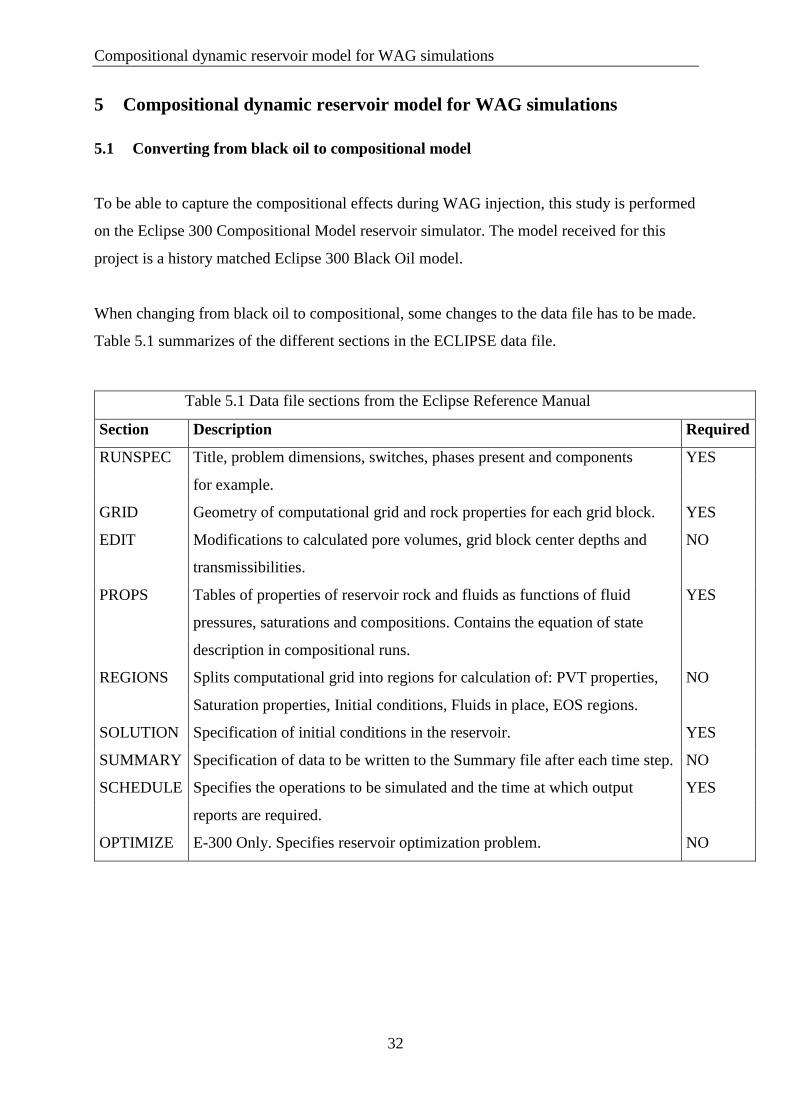
When changing from black oil to compositional, some changes to the data file has to be made.
Table 5.1 summarizes of the different sections in the ECLIPSE data file.
Table 5.1 Data file sections from the Eclipse Reference Manual
Section Description Required
RUNSPEC Title, problem dimensions, switches, phases present and components YES
for example.
GRID Geometry of computational grid and rock properties for each grid block. YES
EDIT Modifications to calculated pore volumes, grid block center depths and NO
transmissibilities.
PROPS Tables of properties of reservoir rock and fluids as functions of fluid YES
pressures, saturations and compositions. Contains the equation of state
description in compositional runs.
REGIONS Splits computational grid into regions for calculation of: PVT properties, NO
Saturation properties, Initial conditions, Fluids in place, EOS regions.
SOLUTION Specification of initial conditions in the reservoir. YES
SUMMARY Specification of data to be written to the Summary file after each time step. NO
SCHEDULE Specifies the operations to be simulated and the time at which output YES
reports are required.
OPTIMIZE E-300 Only. Specifies reservoir optimization problem. NO
Compositional dynamic reservoir model for WAG simulations
33
5.1.1 Black Oil versus Compositional reservoir simulation
The main difference between black oil reservoir simulation and compositional reservoir
simulation is how the hydrocarbons are described. In black oil simulations, the hydrocarbons
are described as gas or oil (Kleppe, 2015). Black oil models are used in reservoirs where fluid
properties can be expressed as a function of pressure and bubble-point pressure. In reservoirs
where fluid properties is dependent on composition also, compositional model should be used
(Young & Stephenson, 1983). Equilibrium flash calculations using K values or an equation of
state (EOS) must be used to determine hydrocarbon phase compositions in these reservoirs
(Kleppe, 2015).
Black oil reservoir simulation is widely used in the petroleum industry, due to the less need
for computational power (Ghorayeb & Holmes, 2005). Compositional reservoir simulation is
far more Central Processing Unit (CPU) intensive. The reason why it is more CPU intensive
is the amount of computations in each run. In compositional runs, the mass balance is
calculated for each hydrocarbon component, and not for only gas and oil.
When injecting gas into a reservoir, compositional simulation is the best for capturing the
compositional effects.
5.1.2 Changing the Gyda model from Black Oil to Compositional.
Gyda simulations are mainly done with black oil models. Since this study includes gas
injection, compositional effects needs to be accounted for. Following is the main changes
done to the dynamic model, before running predictions.
5.1.2.1 Runspec section
In the Runspec section, compositional mode is requested through the COMPS keyword. The
study is performed with the following pseudo-components: N2+C1, CO2+C2+C3, C4-C6,
C7-C13, C14-C25 and C26-C80.
Compositional dynamic reservoir model for WAG simulations
34
5.1.2.2 Props section
The keywords in the PROPS section depends whether Eclipse 100, Eclipse 300 Black Oil or
Eclipse 300 Compositional model is used. (Schlumberger, 2014a).
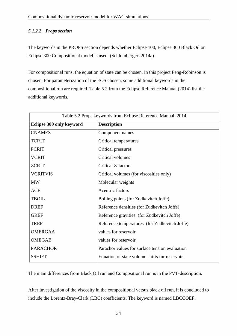
For compositional runs, the equation of state can be chosen. In this project Peng-Robinson is
chosen. For parameterization of the EOS chosen, some additional keywords in the
compositional run are required. Table 5.2 from the Eclipse Reference Manual (2014) list the
additional keywords.
Table 5.2 Props keywords from Eclipse Reference Manual, 2014
Eclipse 300 only keyword Description
CNAMES Component names
TCRIT Critical temperatures
PCRIT Critical pressures
VCRIT Critical volumes
ZCRIT Critical Z-factors
VCRITVIS Critical volumes (for viscosities only)
MW Molecular weights
ACF Acentric factors
TBOIL Boiling points (for Zudkevitch Joffe)
DREF Reference densities (for Zudkevitch Joffe)
GREF Reference gravities (for Zudkevitch Joffe)
TREF Reference temperatures (for Zudkevitch Joffe)
OMERGAA values for reservoir
OMEGAB values for reservoir
PARACHOR Parachor values for surface tension evaluation
SSHIFT Equation of state volume shifts for reservoir
The main differences from Black Oil run and Compositional run is in the PVT-description.
After investigation of the viscosity in the compositional versus black oil run, it is concluded to
include the Lorentz-Bray-Clark (LBC) coefficients. The keyword is named LBCCOEF.
Compositional dynamic reservoir model for WAG simulations
35
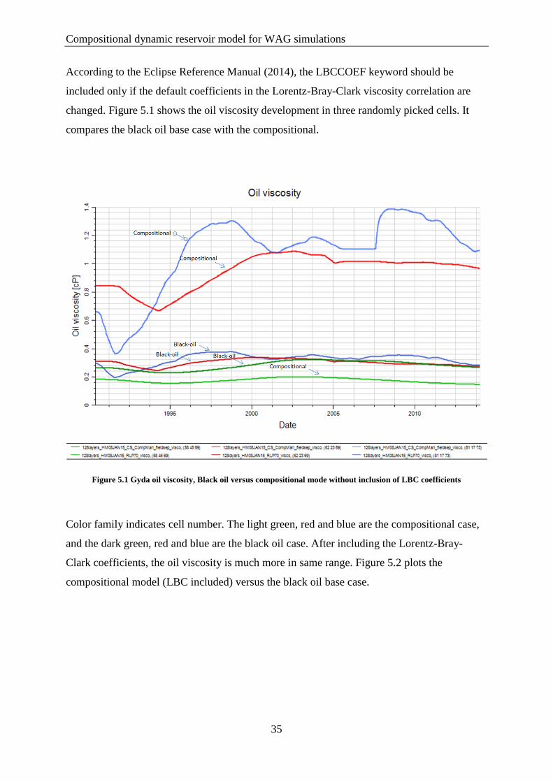
According to the Eclipse Reference Manual (2014), the LBCCOEF keyword should be
included only if the default coefficients in the Lorentz-Bray-Clark viscosity correlation are
changed. Figure 5.1 shows the oil viscosity development in three randomly picked cells. It
compares the black oil base case with the compositional.
Figure 5.1 Gyda oil viscosity, Black oil versus compositional mode without inclusion of LBC coefficients
Color family indicates cell number. The light green, red and blue are the compositional case,
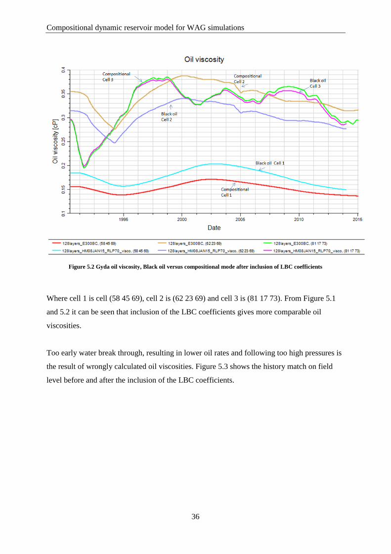
and the dark green, red and blue are the black oil case. After including the Lorentz-Bray-
Clark coefficients, the oil viscosity is much more in same range. Figure 5.2 plots the
compositional model (LBC included) versus the black oil base case.
Compositional dynamic reservoir model for WAG simulations
36
Figure 5.2 Gyda oil viscosity, Black oil versus compositional mode after inclusion of LBC coefficients
Where cell 1 is cell (58 45 69), cell 2 is (62 23 69) and cell 3 is (81 17 73). From Figure 5.1
and 5.2 it can be seen that inclusion of the LBC coefficients gives more comparable oil
viscosities.
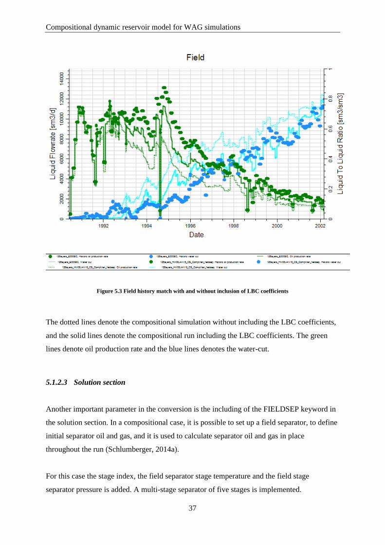
Too early water break through, resulting in lower oil rates and following too high pressures is
the result of wrongly calculated oil viscosities. Figure 5.3 shows the history match on field
level before and after the inclusion of the LBC coefficients.
Compositional dynamic reservoir model for WAG simulations
37
Figure 5.3 Field history match with and without inclusion of LBC coefficients
The dotted lines denote the compositional simulation without including the LBC coefficients,
and the solid lines denote the compositional run including the LBC coefficients. The green
lines denote oil production rate and the blue lines denotes the water-cut.
5.1.2.3 Solution section
Another important parameter in the conversion is the including of the FIELDSEP keyword in
the solution section. In a compositional case, it is possible to set up a field separator, to define
initial separator oil and gas, and it is used to calculate separator oil and gas in place
throughout the run (Schlumberger, 2014a).
For this case the stage index, the field separator stage temperature and the field stage
separator pressure is added. A multi-stage separator of five stages is implemented.
Compositional dynamic reservoir model for WAG simulations
38
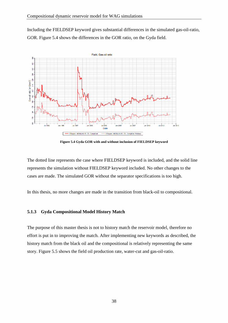
Including the FIELDSEP keyword gives substantial differences in the simulated gas-oil-ratio,
GOR. Figure 5.4 shows the differences in the GOR ratio, on the Gyda field.
Figure 5.4 Gyda GOR with and without inclusion of FIELDSEP keyword
The dotted line represents the case where FIELDSEP keyword is included, and the solid line
represents the simulation without FIELDSEP keyword included. No other changes to the
cases are made. The simulated GOR without the separator specifications is too high.
In this thesis, no more changes are made in the transition from black-oil to compositional.
5.1.3 Gyda Compositional Model History Match
The purpose of this master thesis is not to history match the reservoir model, therefore no
effort is put in to improving the match. After implementing new keywords as described, the
history match from the black oil and the compositional is relatively representing the same
story. Figure 5.5 shows the field oil production rate, water-cut and gas-oil-ratio.
Compositional dynamic reservoir model for WAG simulations
39
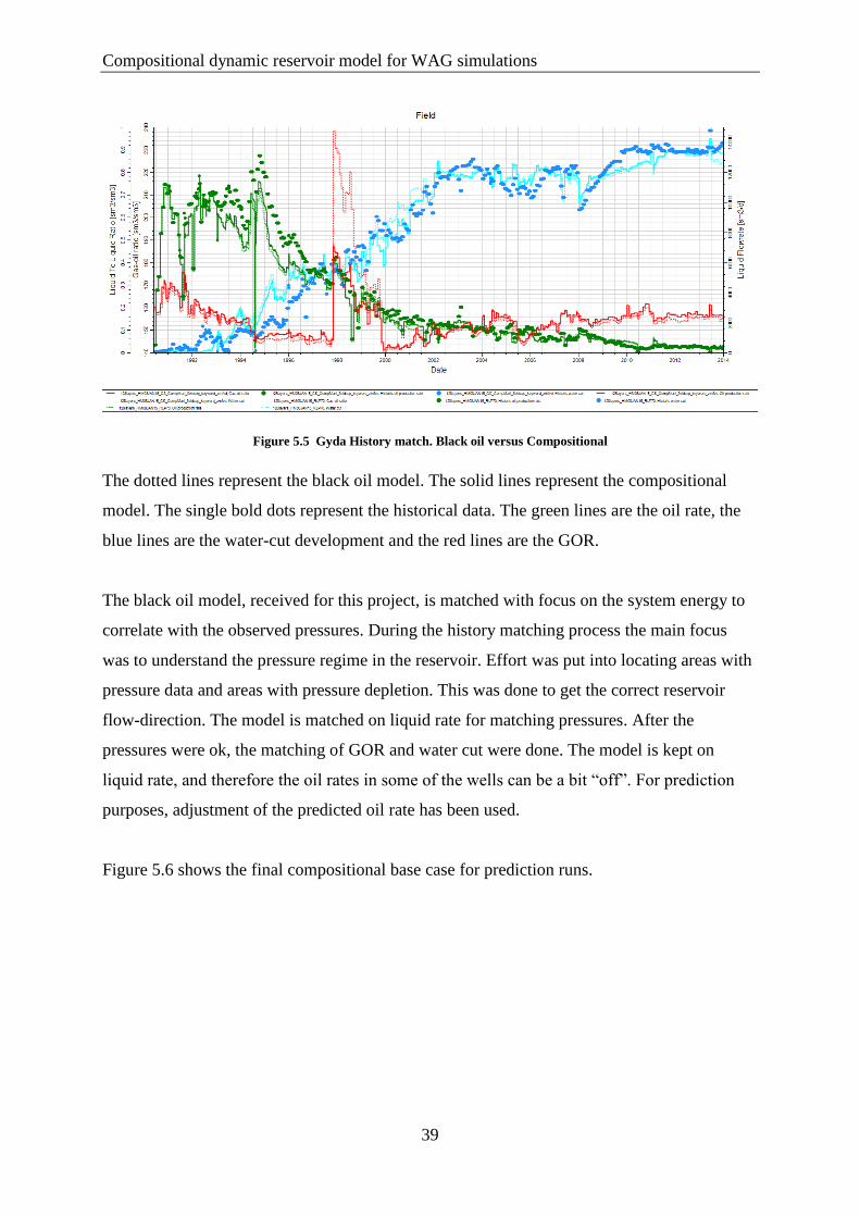
Figure 5.5 Gyda History match. Black oil versus Compositional
The dotted lines represent the black oil model. The solid lines represent the compositional
model. The single bold dots represent the historical data. The green lines are the oil rate, the
blue lines are the water-cut development and the red lines are the GOR.
The black oil model, received for this project, is matched with focus on the system energy to
correlate with the observed pressures. During the history matching process the main focus
was to understand the pressure regime in the reservoir. Effort was put into locating areas with
pressure data and areas with pressure depletion. This was done to get the correct reservoir
flow-direction. The model is matched on liquid rate for matching pressures. After the
pressures were ok, the matching of GOR and water cut were done. The model is kept on
liquid rate, and therefore the oil rates in some of the wells can be a bit “off”. For prediction
purposes, adjustment of the predicted oil rate has been used.
Figure 5.6 shows the final compositional base case for prediction runs.
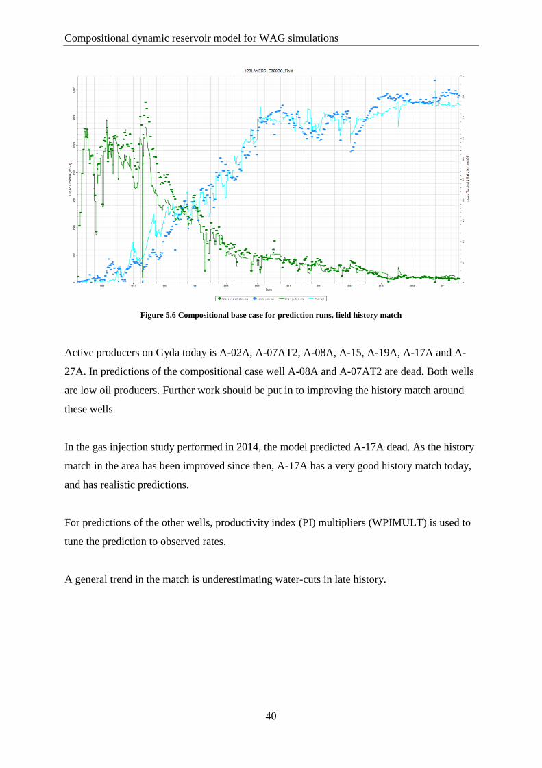
Compositional dynamic reservoir model for WAG simulations
40
Figure 5.6 Compositional base case for prediction runs, field history match
Active producers on Gyda today is A-02A, A-07AT2, A-08A, A-15, A-19A, A-17A and A-
27A. In predictions of the compositional case well A-08A and A-07AT2 are dead. Both wells
are low oil producers. Further work should be put in to improving the history match around
these wells.
In the gas injection study performed in 2014, the model predicted A-17A dead. As the history
match in the area has been improved since then, A-17A has a very good history match today,
and has realistic predictions.
For predictions of the other wells, productivity index (PI) multipliers (WPIMULT) is used to
tune the prediction to observed rates.
A general trend in the match is underestimating water-cuts in late history.
Three-phase relative permeability hysteresis, background
41
6 Three-phase relative permeability hysteresis, background
6.1 Three-phase relative permeability hysteresis
Estimation of three-phase relative permeability is needed for a variety of oil recovery
techniques, such as WAG methods (Shahverdi & Sohrabi, 2012).
In a two-phase relative permeability set, there are only two principal displacement paths. One
can for example consider an oil and water saturated core. If water displaces oil, the water
saturation increases whilst the oil saturation decreases. In a three-phase relative permeability
set, with oil, gas and water present, there are an infinite number of displacement paths. This is
because any three-phase displacement involves the variation of two independent saturations
(Shahverdi & Sohrabi, 2012).
Measurement of the three-phase relative permeability is costly and time consuming, and is
usually interpolated from two-phase data. The current standard approach in the industry is
Stone’s first method and Stone’s second method. Experimental and theoretical experiments
shows that relative permeability is not only dependent on saturation, but also on rock
wettability, fluid viscosity, interfacial tension, flow rate and last but not least saturation path.
Saturation path and saturation history are described in the literature as relative permeability
hysteresis. (Spiteri & Juanes, 2004)
Hysteresis must be considered to facilitate modeling the variety of saturations, which are
encountered in alternate injection of wetting and non-wetting phases (Carlson, 1981). The
problem of hysteresis increases significantly when moving from two-phase to three-phase
systems for two main reasons: the number of saturation directions increases and the definition
of hysteresis becomes ambiguous (Larsen & Skauge, 1998).
Hysteresis can occur both in capillary pressure and in relative permeability. Relative
permeability hysteresis is divided in two physical phenomena. The first phenomenon is
referred to as directional hysteresis, where the hysteresis occur due to switching from
imbibition to drainage or drainage to imbibition. The second phenomenon is the cyclic
hysteresis that happens between the different cycles of one injection process. (Shahverdi &
Sohrabi, 2013)
Three-phase relative permeability hysteresis, background
42
Most reservoir simulators use two-phase hysteresis models to predict the imbibition non-
wetting phase relative permeability from the drainage curve. The most common methods are
Killough’s hysteresis model and Carlson’s hysteresis model.
6.2 Stone’s first model
Stone (1970) proposed a method of interpolating between two sets of two-phase data to obtain
three-phase relative permeability. The method was proposed for a water-wet system, but can
be extended to a preferentially oil-wet system. Assumptions made in developing Stone’s first
method were based on the channel flow theory. The channel flow theory states there is at
most only one mobile fluid in a flow channel (Stone, 1970).
In order to estimate the three-phase relative permeability, water-oil and gas-oil relative
permeability are required. Stone (1970) suggested that water-relative permeability and water-
oil capillary pressure in the three-phase system are functions of water saturations alone, not
dependent on the relative saturations of oil and gas. They are the same function in the three-
phase system as in the two-phase water-oil system. This assumption is also suggested for gas
relative permeability. The gas phase relative permeability and gas-oil capillary pressure are
the same functions of gas saturation in the three-phase system as in the two-phase system.
Following is a summarization of the above statements expressed by formulas:
𝐾𝑟𝑤 = 𝑓(𝑆𝑤) (6.1)
𝐾𝑟𝑔 = 𝑓(𝑆𝑔) (6.2)
𝐾𝑟𝑜 = 𝑓(𝑆𝑤, 𝑆𝑔) (6.3)
Stone (1970) states that hysteretic effects are taken into consideration, by employing the
appropriate two-phase data, and that it is not generally feasible to treat complicated hysteretic
effects caused by oscillating saturations.
Three-phase relative permeability hysteresis, background
43
In Eclipse 300 (2015) Stones first model is modified, and the oil relative permeability is
calculated using the following formulas:
𝑘𝑟𝑜 = 𝑘𝑟𝑜𝑐𝑤𝑆𝑆𝑜𝐹𝑤𝐹𝑔 (6.4)
𝑆𝑆𝑜 =
(𝑆𝑜 − 𝑆𝑜𝑚)
(1 − 𝑆𝑤𝑐𝑜 − 𝑆𝑜𝑚) 𝑤ℎ𝑒𝑛 𝑆𝑜 > 𝑆𝑜𝑚 (6.5)
𝐹𝑤 =
𝑘𝑟𝑜𝑤
𝑘𝑟𝑜𝑐𝑤 ∗ (1 − 𝑆𝑆𝑤) (6.6)
𝐹𝑔 =
𝑘𝑟𝑜𝑔
𝑘𝑟𝑜𝑐𝑤 ∗ (1 − 𝑆𝑆𝑔) (6.7)
𝑆𝑆𝑤 =
(𝑆𝑤 − 𝑆𝑤𝑐𝑜)
(1 − 𝑆𝑤𝑐𝑜 − 𝑆𝑜𝑚) 𝑤ℎ𝑒𝑛 𝑆𝑤 > 𝑆𝑤𝑐𝑜 (6.8)
𝑆𝑆𝑔 =
𝑆𝑔
1 − 𝑆𝑤𝑐𝑜 − 𝑆𝑜𝑚 (6.9)
Where 𝑆𝑔 , 𝑆𝑤 and 𝑆𝑜 denote block average values for gas, water and oil. 𝑘𝑟𝑜𝑔 denotes the oil
relative permeability for a system with oil, gas and connate water, 𝑘𝑟𝑜𝑤 denotes a system
with only water and oil, and 𝑘𝑟𝑜𝑐𝑤 denotes the oil relative permeabily when only connate
water is present. 𝑆𝑜𝑚 is the minimum residual oil saturation.
For Stones first model, the minimum oil saturation must be chosen 𝑆𝑜𝑚 , which is an
adjustable parameter. According to Shahverdi and Sohrabi (2013) this reduces the reliability
of the model (Shahverdi & Sohrabi, 2013). Larsen and Skauge (1998) state that choosing this
parameter is beneficial in numerical simulations.
Three-phase relative permeability hysteresis, background
44
6.3 Stone’s second model
Stone proposed a second model in 1973. This model was proposed to yield improved
estimates of three phase relative permeability (Stone, 1973). The second model also uses two
sets of two-phase data, like the first model, and compares favorably with experimental data,
including data on the dependence of waterflood residual oil saturation on trapped gas
saturations. This results in better agreement with experimental data in regions with low oil
saturations. Stone continues with describing that this approach is capable of providing
estimates of residual oil saturation.
Stone suggests that hysteresis is taken into consideration by employing the appropriate two
phase data.
In Eclipse 2014, the oil relative permeability is calculated from the following formula, if the
Stone’s second method is used.
𝑘𝑟𝑜 = 𝑘𝑟𝑜𝑐𝑤 [(
𝑘𝑟𝑜𝑤
𝑘𝑟𝑜𝑐𝑤+ 𝑘𝑟𝑤) (
𝑘𝑟𝑜𝑔
𝑘𝑟𝑜𝑐𝑤+ 𝑘𝑟𝑔) − 𝑘𝑟𝑤 − 𝑘𝑟𝑔] (6.10)
Where 𝑘𝑟𝑜𝑔 is the oil relative permeability for a system with oil, gas and connate water, and
𝑘𝑟𝑜𝑤 is the oil relative permeability for a system with oil and water only.
The two-phase relative permeabilities are evaluated at the same saturation values in Stone’s
first and Stone’s second model. Spiteri et al. (2004) states that predicted values in the region
of low oil saturation are much lower than those obtained with Stone’s first method.
Three-phase relative permeability hysteresis, background
45
6.4 Land’s trapping model
A trapping model is a mathematical model expressing the relationship between the initial non-
wetting phase saturation and the trapped non-wetting phase saturation during an imbibition
process (Shahverdi & Sohrabi, 2013).
Land’s trapping model is the most used empirical model for gas trapping (Shahverdi &
Sohrabi, 2013). From published data, Land found an empirical relation between residual non-
wetting phase saturation after water imbibition and initial non-wetting phase saturation. From
this empirical relation, he created expressions for trapped and mobile non-wetting phase
saturation (Land, 1968).
𝑆𝑔𝑟 =
𝑆𝑔𝑖
1 + 𝐶 ∗ 𝑆𝑔𝑖 (6.11)
Where 𝑆𝑔𝑟 is the residual gas saturation, 𝑆𝑔𝑖 is the initial gas saturation and C is the Land
trapping parameter expressed by:
𝐶 =
1
𝑆𝑔𝑟−
1
𝑆𝑔𝑖 (6.12)
6.5 Killough’s Hysteresis model
Killough (1976) developed a history dependent model for saturation functions, combined with
a three-dimensional, three-phase, semi-implicit reservoir simulator. The model is based upon
remembering the saturation history of the reservoir, with smooth transitions of both relative
permeability and capillary pressures from drainage-to-imbibition or imbibition-to-drainage
states. The model take into consideration the effect of trapped gas saturation and oil saturation
on relative permeability and capillary pressures.
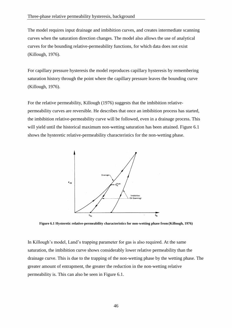
Three-phase relative permeability hysteresis, background
46
The model requires input drainage and imbibition curves, and creates intermediate scanning
curves when the saturation direction changes. The model also allows the use of analytical
curves for the bounding relative-permeability functions, for which data does not exist
(Killough, 1976).
For capillary pressure hysteresis the model reproduces capillary hysteresis by remembering
saturation history through the point where the capillary pressure leaves the bounding curve
(Killough, 1976).
For the relative permeability, Killough (1976) suggests that the imbibition relative-
permeability curves are reversible. He describes that once an imbibition process has started,
the imbibition relative-permeability curve will be followed, even in a drainage process. This
will yield until the historical maximum non-wetting saturation has been attained. Figure 6.1
shows the hysteretic relative-permeability characteristics for the non-wetting phase.
Figure 6.1 Hysteretic relative-permeability characteristics for non-wetting phase from (Killough, 1976)
In Killough’s model, Land’s trapping parameter for gas is also required. At the same
saturation, the imbibition curve shows considerably lower relative permeability than the
drainage curve. This is due to the trapping of the non-wetting phase by the wetting phase. The
greater amount of entrapment, the greater the reduction in the non-wetting relative
permeability is. This can also be seen in Figure 6.1.
Three-phase relative permeability hysteresis, background
47
The wetting phase relative permeability exhibit a far smaller dependence on the trapped non-
wetting saturation, but Killough (1976) points out that the greater the tapped saturation, the
greater the imbibition wetting phase relative permeability when compared to the same
drainage saturation at the same saturation.
For three-phase relative permeability, the model incorporates the revised Stone three-phase
relative permeability model. Since the two-phase relative permeabilities reflect hysteresis, the
three-phase relative permeability model obtained by Stones will also reflect hysteresis
(Killough, 1976).
When running simulations that does not change saturation path, in example switching from
drainage to imbibition, the simulations should give the same results as conventional
simulation without hysteresis.
Killough’s method requires both endpoints of the experimental imbibition curve.
6.6 Carlson’s Hysteresis model
Carlson (1981) developed a method for calculation of imbibition relative permeability starting
at any saturation. All the imbibition curves (scanning curves) were shown to be parallel. The
method proposes a solution for calculating the residual non-wetting phase saturation without a
complete experimental specification of the imbibition curve.
The main purpose of his paper was to establish a procedure that required only:
A drainage curve
The historical maximum non-wetting saturation
Minimum one point on the imbibition curve
Land’s parameter.
For the calculation of the imbibition curve from this method, neither the pore size distribution
nor the value from Killough’s method was required.
Three-phase relative permeability hysteresis, background
48
6.7 Hysteresis model developed for WAG simulations
Larsen and Skauge (1998) emphasized the importance of including the cycle-dependent
relative permeability for numerical simulation of WAG flooding. They stated that the original
two-phase hysteresis models, such as Killough’s and Carlson’s model, was generally not able
to describe the relative permeabilities during saturation oscillations, as obtained from core
floods.
Their model accounts for reduced mobility and irreversible hysteresis loops during three-
phase flow. It uses experimental wetting and non-wetting relative permeabilities as input, and
knowledge of relations between maximum non-wetting saturation and trapped non-wetting
saturation.
The model developed by Larsen and Skauge is the only model currently available in reservoir
simulators for capturing cyclic hysteresis effect in the relative permeability of the WAG
process (Shahverdi & Sohrabi, 2013).
The main feature of Larsen and Skauges model is reduction of gas mobility during hysteresis
loops in the presence of increasing water saturation. The gas relative permeability can be
reduced because of trapping. The non-wetting phase relative permeability is history dependent
on both the wetting phase saturation and the non-wetting phase saturation. The wetting phase
relative permeability is history dependent on the non-wetting phase saturation. (Larsen &
Skauge, 1998)
For calculation the gas relative permeability, following input is required:
Two-phase gas relative permeability of the primary gas injection performed in
presence of irreducible water and oil.
Endpoint value for krg off the former water injection.
A tuning parameter , selected to ensure the least mismatch between calculated and
experimental data.
Lands coefficient, C.

Three-phase relative permeability hysteresis, background
49
The oil relative permeability in Larsen and Skauges model is estimated by use of Stones first
model. The water relative permeability is calculated from the inputs: primary water relative
permeability curve and secondary water relative permeability curve, after gas flood.
Evaluation of hysteresis models for WAG injection
50
7 Evaluation of hysteresis models for WAG injection
As mentioned in chapter 6, it is important to evaluate the hysteresis effect during WAG
injection. According to Shahverdi & Sohrabi (2013) there are two different approaches for
modeling hysteresis numerically in WAG injection:
1. Apply two-phase hysteresis models like Killough or Carlson to the three-phase
relative permeability models like Stone or Baker.
2. Directly use a three-phase hysteresis model specifically developed for WAG
simulation, like the model developed by Larsen and Skauge, described in chapter 6.7
In these thesis both approaches are executed. Stone’s first model is evaluated against Stone’s
second model for thre-phase relative permeabilities. Then both Killough, Carlson and the
WAG hysteresis option in eclipse, developed by Larsen an Skauge is applied.
7.1 Stone 1 versus Stone 2 for thre-phase relative permeability estimation
The Gyda model consist of two sets of two-phase relative permeability. The current standard
approach in the industry is implementing either Stone’s first or Stone’s second method for
estimating three-phase relative permeability.
For better investigation of Stone’s first and Stone’s second model, gas injection is
implemented in three injectors.
Figure 7.1 shows the field oil production rate, gas-oil-ratio and water-cut development after
gas injection.
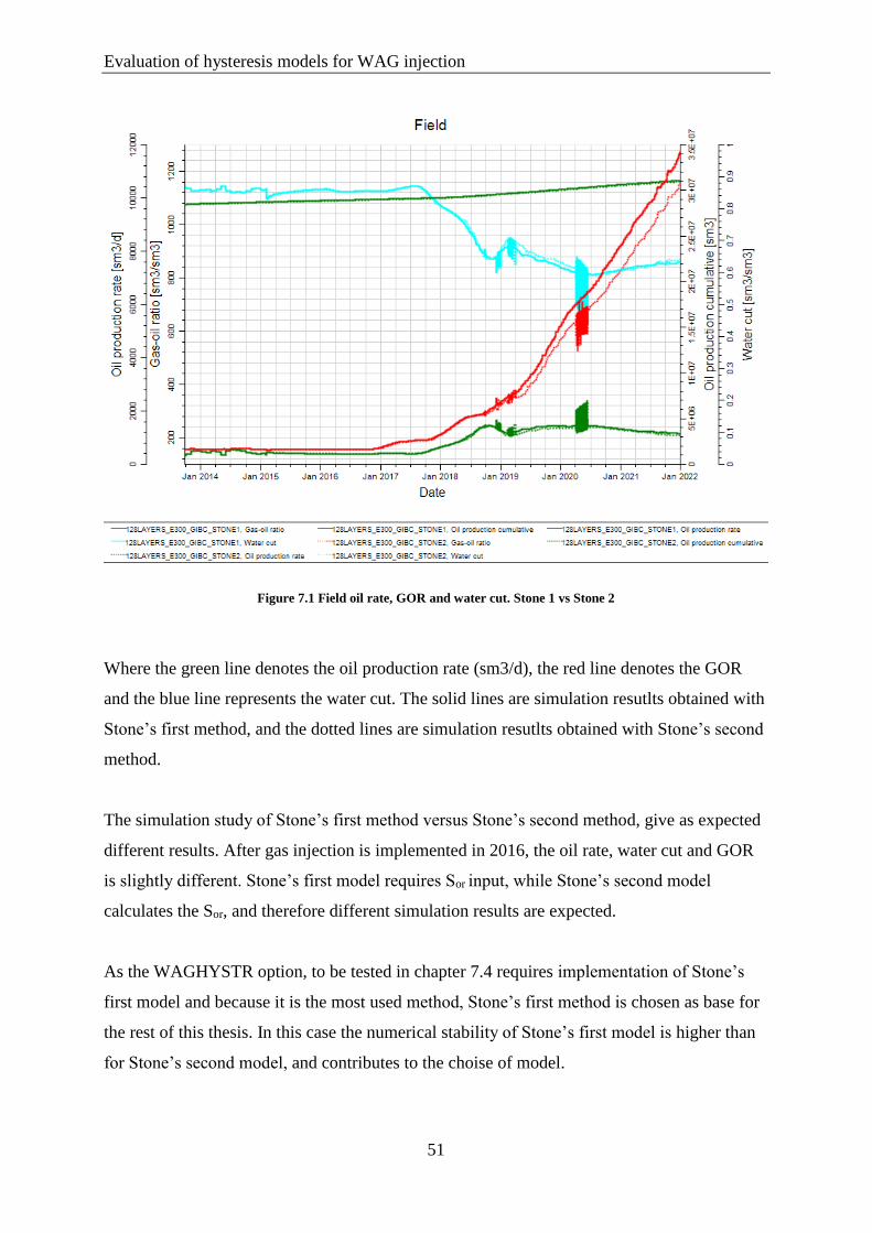
Evaluation of hysteresis models for WAG injection
51
Figure 7.1 Field oil rate, GOR and water cut. Stone 1 vs Stone 2
Where the green line denotes the oil production rate (sm3/d), the red line denotes the GOR
and the blue line represents the water cut. The solid lines are simulation resutlts obtained with
Stone’s first method, and the dotted lines are simulation resutlts obtained with Stone’s second
method.
The simulation study of Stone’s first method versus Stone’s second method, give as expected
different results. After gas injection is implemented in 2016, the oil rate, water cut and GOR
is slightly different. Stone’s first model requires Sor input, while Stone’s second model
calculates the Sor, and therefore different simulation results are expected.
As the WAGHYSTR option, to be tested in chapter 7.4 requires implementation of Stone’s
first model and because it is the most used method, Stone’s first method is chosen as base for
the rest of this thesis. In this case the numerical stability of Stone’s first model is higher than
for Stone’s second model, and contributes to the choise of model.
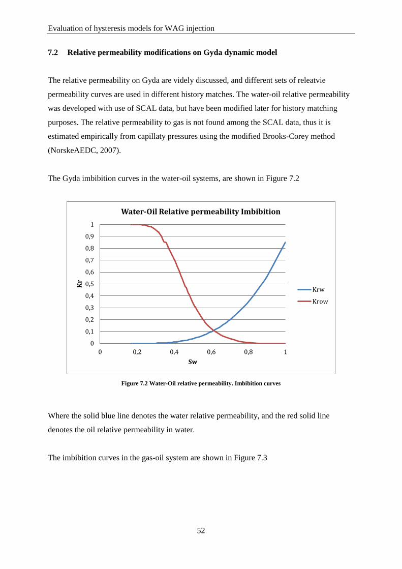
Evaluation of hysteresis models for WAG injection
52
7.2 Relative permeability modifications on Gyda dynamic model
The relative permeability on Gyda are videly discussed, and different sets of releatvie
permeability curves are used in different history matches. The water-oil relative permeability
was developed with use of SCAL data, but have been modified later for history matching
purposes. The relative permeability to gas is not found among the SCAL data, thus it is
estimated empirically from capillaty pressures using the modified Brooks-Corey method
(NorskeAEDC, 2007).
The Gyda imbibition curves in the water-oil systems, are shown in Figure 7.2
Figure 7.2 Water-Oil relative permeability. Imbibition curves
Where the solid blue line denotes the water relative permeability, and the red solid line
denotes the oil relative permeability in water.
The imbibition curves in the gas-oil system are shown in Figure 7.3
0
0,1
0,2
0,3
0,4
0,5
0,6
0,7
0,8
0,9
1
0 0,2 0,4 0,6 0,8 1
Kr
Sw
Water-Oil Relative permeability Imbibition
Krw
Krow
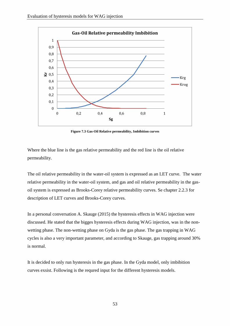
Evaluation of hysteresis models for WAG injection
53
Figure 7.3 Gas-Oil Relative permeability, Imbibition curves
Where the blue line is the gas relative permeability and the red line is the oil relative
permeability.
The oil relative permeability in the water-oil system is expressed as an LET curve. The water
relative permeability in the water-oil system, and gas and oil relative permeability in the gas-
oil system is expressed as Brooks-Corey relative permeability curves. Se chapter 2.2.3 for
description of LET curves and Brooks-Corey curves.
In a personal conversation A. Skauge (2015) the hysteresis effects in WAG injection were
discussed. He stated that the bigges hysteresis effects during WAG injection, was in the non-
wetting phase. The non-wetting phase on Gyda is the gas phase. The gas trapping in WAG
cycles is also a very important parameter, and according to Skauge, gas trapping around 30%
is normal.
It is decided to only run hysteresis in the gas phase. In the Gyda model, only imbibition
curves exsist. Following is the requred input for the different hysteresis models.
0
0,1
0,2
0,3
0,4
0,5
0,6
0,7
0,8
0,9
1
0 0,2 0,4 0,6 0,8 1
Kr
Sg
Gas-Oil Relative permeability Imbibition
Krg
Krog

Evaluation of hysteresis models for WAG injection
54
Table 7.1 Required input for hysteresis models
Model Required input
Killough Drainage curves, Imbibition curves, Land's trapping parameter.
Carlson Drainage curves, historical maximum non-wetting saturation,
minimum one point on the imbibition curve, Land's parameter.
WAGHYSTR Land's coefficient C, two-phase gas relative permeability of
the primary gas injection performed in presence of irreducible
water and oil, endpoint value for krg off the former water
injection, tuning parameter α to ensure least miss match
between calculated and experimental data.
As the Gyda model only has imbibition curves, drainage curves are made in order to run
hysteresis simulations. The different hysteresis methods create scanning curves from the input
bounding drainage and imbibition curve, as described in chapter 6.
In the REGIONS section in the Eclipse data file, both SATNUM and IMBNUM regions is
defined. The SATNUM region is used to specify the drainage relative permeability for each
cell. The IMBNUM region is used to specify the imbibition relative permeability for each
cell. If the imbibition and drainage table numbers for a cell are the same, no hysteresis will
occur for that cell. (Schlumberger, 2014b)
As it is decided to only run hysteresis in the gas phase, the imbibition and drainage relative
permeability for oil and water phases input are identical. Gas imbibition and drainage curves
are made with the modified Brooks-Corey method as described in chapter 2.2.3.
Many characteristics curves for non-wetting phase relative permeability have been published.
Killough published a characteristic curve in 1976, se figure 6.1 in chapter 6. A characteristic
curve from the Eclipse Technical description manual is presented in figure 7.4.
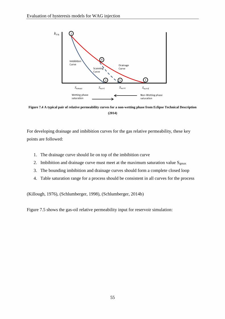
Evaluation of hysteresis models for WAG injection
55
Figure 7.4 A typical pair of relative permeability curves for a non-wetting phase from Eclipse Technical Description
(2014)
For developing drainage and imbibition curves for the gas relative permeability, these key
points are followed:
1. The drainage curve should lie on top of the imbibition curve
2. Imbibition and drainage curve must meet at the maximum saturation value Sgmax
3. The bounding imbibition and drainage curves should form a complete closed loop
4. Table saturation range for a process should be consistent in all curves for the process
(Killough, 1976), (Schlumberger, 1998), (Schlumberger, 2014b)
Figure 7.5 shows the gas-oil relative permeability input for reservoir simulation:
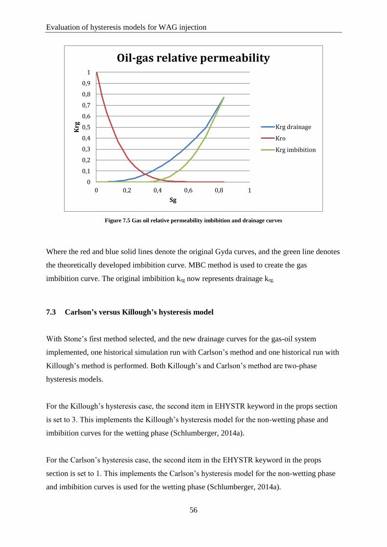
Evaluation of hysteresis models for WAG injection
56
Figure 7.5 Gas oil relative permeability imbibition and drainage curves
Where the red and blue solid lines denote the original Gyda curves, and the green line denotes
the theoretically developed imbibition curve. MBC method is used to create the gas
imbibition curve. The original imbibition krg now represents drainage krg.
7.3 Carlson’s versus Killough’s hysteresis model
With Stone’s first method selected, and the new drainage curves for the gas-oil system
implemented, one historical simulation run with Carlson’s method and one historical run with
Killough’s method is performed. Both Killough’s and Carlson’s method are two-phase
hysteresis models.
For the Killough’s hysteresis case, the second item in EHYSTR keyword in the props section
is set to 3. This implements the Killough’s hysteresis model for the non-wetting phase and
imbibition curves for the wetting phase (Schlumberger, 2014a).
For the Carlson’s hysteresis case, the second item in the EHYSTR keyword in the props
section is set to 1. This implements the Carlson’s hysteresis model for the non-wetting phase
and imbibition curves is used for the wetting phase (Schlumberger, 2014a).
0
0,1
0,2
0,3
0,4
0,5
0,6
0,7
0,8
0,9
1
0 0,2 0,4 0,6 0,8 1
Krg
Sg
Oil-gas relative permeability
Krg drainage
Kro
Krg imbibition
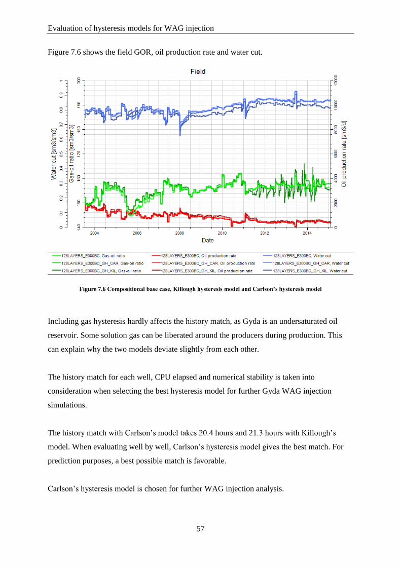
Evaluation of hysteresis models for WAG injection
57
Figure 7.6 shows the field GOR, oil production rate and water cut.
Figure 7.6 Compositional base case, Killough hysteresis model and Carlson’s hysteresis model
Including gas hysteresis hardly affects the history match, as Gyda is an undersaturated oil
reservoir. Some solution gas can be liberated around the producers during production. This
can explain why the two models deviate slightly from each other.
The history match for each well, CPU elapsed and numerical stability is taken into
consideration when selecting the best hysteresis model for further Gyda WAG injection
simulations.
The history match with Carlson’s model takes 20.4 hours and 21.3 hours with Killough’s
model. When evaluating well by well, Carlson’s hysteresis model gives the best match. For
prediction purposes, a best possible match is favorable.
Carlson’s hysteresis model is chosen for further WAG injection analysis.
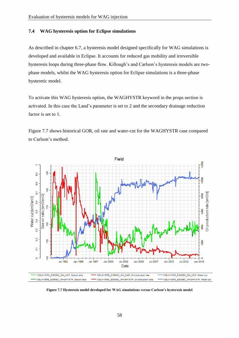
Evaluation of hysteresis models for WAG injection
58
7.4 WAG hysteresis option for Eclipse simulations
As described in chapter 6.7, a hysteresis model designed specifically for WAG simulations is
developed and available in Eclipse. It accounts for reduced gas mobility and irreversible
hysteresis loops during three-phase flow. Killough’s and Carlson’s hysteresis models are two-
phase models, whilst the WAG hysteresis option for Eclipse simulations is a three-phase
hysteretic model.
To activate this WAG hysteresis option, the WAGHYSTR keyword in the props section is
activated. In this case the Land’s parameter is set to 2 and the secondary drainage reduction
factor is set to 1.
Figure 7.7 shows historical GOR, oil rate and water-cut for the WAGHYSTR case compared
to Carlson’s method.
Figure 7.7 Hysteresis model developed for WAG simulations versus Carlson’s hysteresis model
Evaluation of hysteresis models for WAG injection
59
There are extremely small differences in the history match between the WAGHYSTR case
and Carlson’s hysteresis case. This result is as expected. The major difference between two-
phase and three-phase hysteretic models should not appear before the second gas injection
phase in a WAG flood. This is because three-phase hysteretic models account for the
reduction in the gas relative permeability, whereas the two-phase models do not (Spiteri &
Juanes, 2004).
In this case, the main difference between the historical run with Carlson’s and the
WAGHYSTR option is the CPU required. The WAGHYSTR model takes around six days to
finish. The model is extremely sensitive to numerical instabilities.
The WAGHYSTR option requires two-phase gas relative permeability for the primary gas
injection performed in presence of irreducible water and oil and endpoint value krg of the
former water injection. In addition it requires Land’s coefficient and the tuning parameter.
The special needs for proper input in this model, make the range of uncertainties even bigger
for this option.
WAG injection studies in the literature (Spiteri & Juanes, 2004) conclude that ultimate oil
recovery predicted from three-phase models are higher than from two-phase. Reduced gas
mobility results in better sweep efficiency, and therefore higher oil recovery.
The two-phase Carlson’s hysteretic model is chosen for further WAG injection study. This is
due to the high range of input parameters uncertainties in WAGHYSTR option, CPU required
and numerical instability. The fact that three-phase hysteretic models give more optimistic
predictions than two-phase hysteretic-models is also a decisive factor.
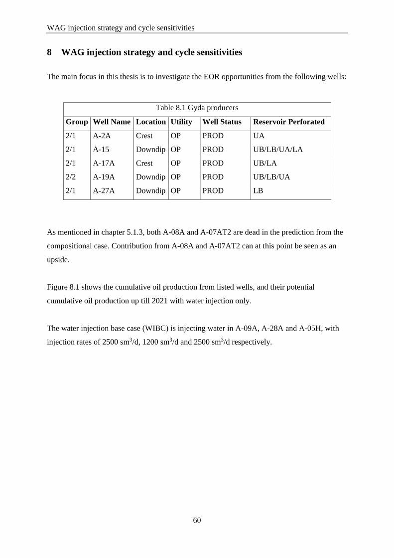
WAG injection strategy and cycle sensitivities
60
8 WAG injection strategy and cycle sensitivities
The main focus in this thesis is to investigate the EOR opportunities from the following wells:
Table 8.1 Gyda producers
Group Well Name Location Utility Well Status Reservoir Perforated
2/1 A-2A Crest OP PROD UA
2/1 A-15 Downdip OP PROD UB/LB/UA/LA
2/1 A-17A Crest OP PROD UB/LA
2/2 A-19A Downdip OP PROD UB/LB/UA
2/1 A-27A Downdip OP PROD LB
As mentioned in chapter 5.1.3, both A-08A and A-07AT2 are dead in the prediction from the
compositional case. Contribution from A-08A and A-07AT2 can at this point be seen as an
upside.
Figure 8.1 shows the cumulative oil production from listed wells, and their potential
cumulative oil production up till 2021 with water injection only.
The water injection base case (WIBC) is injecting water in A-09A, A-28A and A-05H, with
injection rates of 2500 sm3/d, 1200 sm3/d and 2500 sm3/d respectively.

WAG injection strategy and cycle sensitivities
61
Figure 8.1 Oil production cumulative from active producers
A-15 is the best oil producer. The second best is A-02A followed by A-17, A-27A and A-
19A.
The injectors available for injection are summarized in Table 8.2.
Table 8.2 Gyda injectors
Injector Date Pressure top perf [bar] Simulation BHP [bar] Reservoir perforated
A-4 11.02.2014 493 454 UB/LB/UA/LA
A-5 10.03.2014 544 505 UB/LB/UA
A-9A 11.02.2014 544 512 UB/LB/UA/LA
A-20 17.01.2014 580 558 UB/LB/UA/LA
A-28A 28.02.2014 500 489 UB/LB/UA/LA
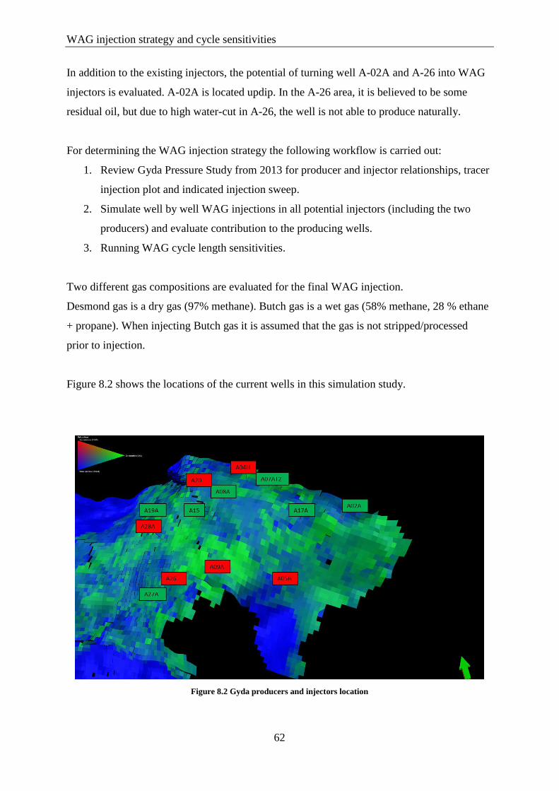
WAG injection strategy and cycle sensitivities
62
In addition to the existing injectors, the potential of turning well A-02A and A-26 into WAG
injectors is evaluated. A-02A is located updip. In the A-26 area, it is believed to be some
residual oil, but due to high water-cut in A-26, the well is not able to produce naturally.
For determining the WAG injection strategy the following workflow is carried out:
1. Review Gyda Pressure Study from 2013 for producer and injector relationships, tracer
injection plot and indicated injection sweep.
2. Simulate well by well WAG injections in all potential injectors (including the two
producers) and evaluate contribution to the producing wells.
3. Running WAG cycle length sensitivities.
Two different gas compositions are evaluated for the final WAG injection.
Desmond gas is a dry gas (97% methane). Butch gas is a wet gas (58% methane, 28 % ethane
+ propane). When injecting Butch gas it is assumed that the gas is not stripped/processed
prior to injection.
Figure 8.2 shows the locations of the current wells in this simulation study.
Figure 8.2 Gyda producers and injectors location

WAG injection strategy and cycle sensitivities
63
8.1 Key points from Gyda Pressure Study 2014
A thorough pressure study of the Gyda field was carried out in December 2013 (Talisman,
2013). The pressure study included Gyda historical pressure trending and Repeat Formation
Tester (RFT) pressure trending.
Preliminary conclusions from Gyda Pressure study in the Crestal area:
- Good pressure communication and injection support in the area.
- Significant pressure contrast between A-17A and A-02A.
- A-02A and A-17A is pressure supported by injection in A-04A.
Preliminary conclusions from Gyda Pressure study in the Downdip area:
- A-15 pressure increase probably due to A-09/A-09A injection and possibly A-28A
and A04H.
- Injection in A-28A gives pressure maintenance in A-19A and pressure increase in A-
27A and A-26.
- Good pressure communication between A-26 and A-27A.
- The Downdip region shows generally significant layer isolation and heterogeneous
pressures.
No wells in C-sand, South West or Gyda South are included in this study. Following Figures
8.3 and 8.4 show Gyda indicated injection sweep and tracer data, respectively.
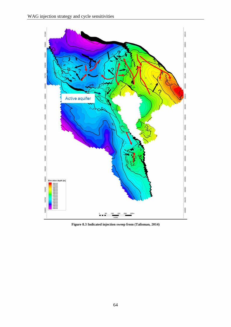
WAG injection strategy and cycle sensitivities
64
Figure 8.3 Indicated injection sweep from (Talisman, 2014)

WAG injection strategy and cycle sensitivities
65
Figure 8.4 Gyda tracer data from (Talisman, 2014)
Tracers from injector well A-05 are shown in both A-17A, A-15, A-19A and A-27A.
8.2 Injector by injector potential
To minimize the potential investment cost on gas compressor, a gas compressor capacity of
450 bar is set as the basis for the reservoir simulations. The average gas column in each
injector is estimated to be around 100 bar. Since no lift curves for the injectors are available at
WAG injection strategy and cycle sensitivities
66
the moment of simulation, a bottom hole pressure limit of 550 bar is set for the reservoir
simulations.
The following WAG injection scheme is used for the injector by injector study:
1. Water injection in A-05H, A-09A and A-28A (from the WIBC) is on until January
2016.
2. WAG injection is turned on in March 2016.
a. Gas injection rate is set to be 428 000 sm3/d.
b. Water injection rate is set to be 1200 sm3/d.
c. WAG cycle lengths are 3 months of gas followed by 3 months of water.
d. BHP limitation is 550 bar for both gas and water injection.
3. Only one active WAG injector in each simulation.
The injector-by-injector study is performed on the compositional base case, with no hysteresis
effects in the gas phase taken into consideration. The simulation study is performed with dry
gas from the Desmond field. The Desmond gas consists of 97% methane.
Following is a summary of conclusions from the simulation study:
Injection capacity:
- Due to too high reservoir pressures, it is not possible to inject in injector A-05 or A-
09A.
- Both A-28A, A-20 and A-2A is able to inject the requested WAG cycles under the
given conditions. The water injection in all cases is low, due to the BHP restriction.
- A-26A has low pressure, and large volumes of both gas and water can be injected in
this well.
Benefits from WAG injection in producers:
- Because neither A-05 nor A-09A were able to inject in this case, A-02A is not getting
pressure support from any injectors.
- Effects from WAG injection are low in A-15. Some effects from injection in A-20 and
A-28A can be shown. The effects are late.
- A-17A benefits from injection in A-02A.
- A-19A benefits from injection in both A-28A and A-20.
WAG injection strategy and cycle sensitivities
67
- A-27A can get large benefits from WAG injection in A-26. Due to the direct
communication and short geographical distance, it is important to not inject too much
water.
Based on these conclusions, further work is conducted:
1. Since A-09A, A-05 and A-04 are all supporting the Crestal area, sensitivities are run
in order to get one of the wells to inject.
2. The A-26 and A-27A relationship is investigated, and WAG cycles length sensitivities
are run.
3. Full field WAG cycle sensitivity is performed.
The final WAG schedule is run on both the compositional base case and on the Carlson’s
hysteresis case.
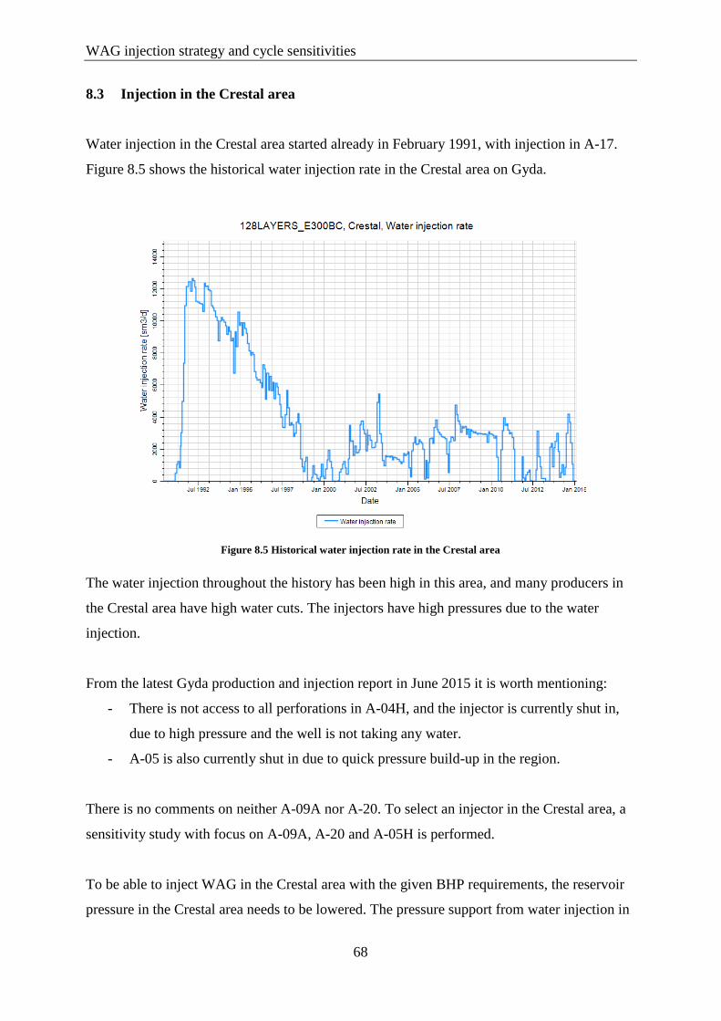
WAG injection strategy and cycle sensitivities
68
8.3 Injection in the Crestal area
Water injection in the Crestal area started already in February 1991, with injection in A-17.
Figure 8.5 shows the historical water injection rate in the Crestal area on Gyda.
Figure 8.5 Historical water injection rate in the Crestal area
The water injection throughout the history has been high in this area, and many producers in
the Crestal area have high water cuts. The injectors have high pressures due to the water
injection.
From the latest Gyda production and injection report in June 2015 it is worth mentioning:
- There is not access to all perforations in A-04H, and the injector is currently shut in,
due to high pressure and the well is not taking any water.
- A-05 is also currently shut in due to quick pressure build-up in the region.
There is no comments on neither A-09A nor A-20. To select an injector in the Crestal area, a
sensitivity study with focus on A-09A, A-20 and A-05H is performed.
To be able to inject WAG in the Crestal area with the given BHP requirements, the reservoir
pressure in the Crestal area needs to be lowered. The pressure support from water injection in
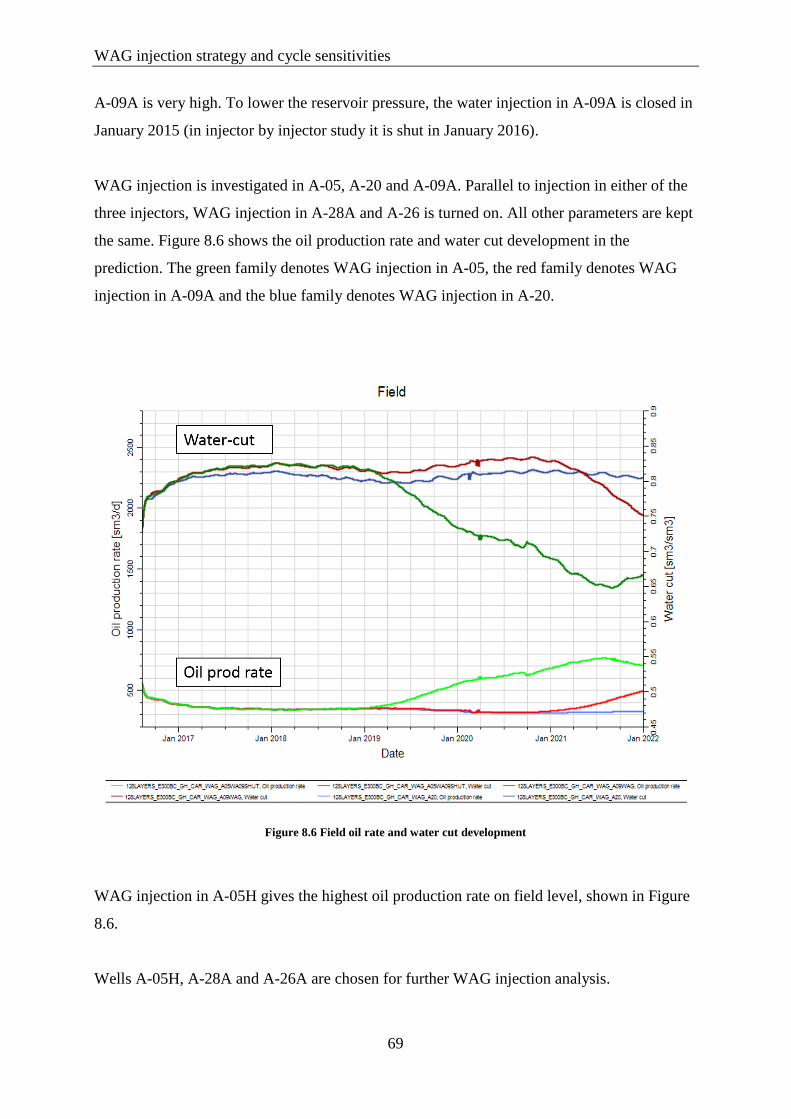
WAG injection strategy and cycle sensitivities
69
A-09A is very high. To lower the reservoir pressure, the water injection in A-09A is closed in
January 2015 (in injector by injector study it is shut in January 2016).
WAG injection is investigated in A-05, A-20 and A-09A. Parallel to injection in either of the
three injectors, WAG injection in A-28A and A-26 is turned on. All other parameters are kept
the same. Figure 8.6 shows the oil production rate and water cut development in the
prediction. The green family denotes WAG injection in A-05, the red family denotes WAG
injection in A-09A and the blue family denotes WAG injection in A-20.
Figure 8.6 Field oil rate and water cut development
WAG injection in A-05H gives the highest oil production rate on field level, shown in Figure
8.6.
Wells A-05H, A-28A and A-26A are chosen for further WAG injection analysis.
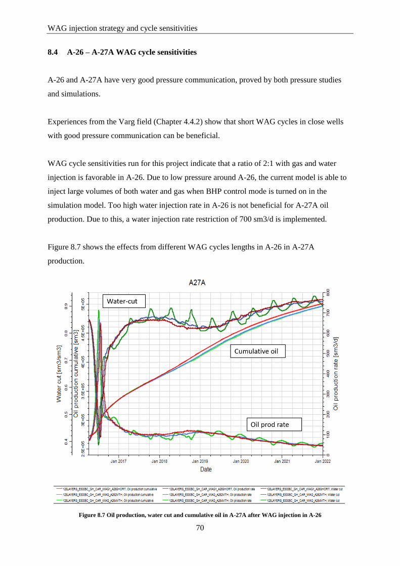
WAG injection strategy and cycle sensitivities
70
8.4 A-26 – A-27A WAG cycle sensitivities
A-26 and A-27A have very good pressure communication, proved by both pressure studies
and simulations.
Experiences from the Varg field (Chapter 4.4.2) show that short WAG cycles in close wells
with good pressure communication can be beneficial.
WAG cycle sensitivities run for this project indicate that a ratio of 2:1 with gas and water
injection is favorable in A-26. Due to low pressure around A-26, the current model is able to
inject large volumes of both water and gas when BHP control mode is turned on in the
simulation model. Too high water injection rate in A-26 is not beneficial for A-27A oil
production. Due to this, a water injection rate restriction of 700 sm3/d is implemented.
Figure 8.7 shows the effects from different WAG cycles lengths in A-26 in A-27A
production.
Figure 8.7 Oil production, water cut and cumulative oil in A-27A after WAG injection in A-26
WAG injection strategy and cycle sensitivities
71
Figure 8.7 shows the following cases:
- Red: 2 weeks with gas injection and 1 week with water injection
- Blue: 2 moths of gas injection and 1 month of water injection
- Green: 4 months of gas injection and 2 months of water injection
Short cycle length is concluded as best for the A-27A and A-26 well pair, from cumulative oil
production seen in Figure 8.7. In A-27A a large spike in oil-production appears right after
WAG injection in A-26 starts. This indicates gas sweep of attic zones.
Other sensitivities show that if the water injection rate is not too high, the oil recovery is not
too sensitive to cycle length.
8.5 Field WAG cycle sensitivities
WAG cycle sensitivity on field scale is performed. Experiences from the North Sea conclude
that WAG cycles of 2-3 months or more are favorable (A.Skauge, 2015) (Teigland & Kleppe,
2006). Different scenarios are investigated. Figure 8.8 shows the predicted cumulative oil
production on field level with three different injection schedules.
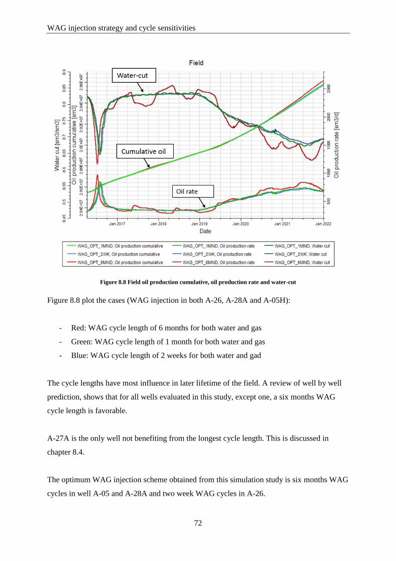
WAG injection strategy and cycle sensitivities
72
Figure 8.8 Field oil production cumulative, oil production rate and water-cut
Figure 8.8 plot the cases (WAG injection in both A-26, A-28A and A-05H):
- Red: WAG cycle length of 6 months for both water and gas
- Green: WAG cycle length of 1 month for both water and gas
- Blue: WAG cycle length of 2 weeks for both water and gad
The cycle lengths have most influence in later lifetime of the field. A review of well by well
prediction, shows that for all wells evaluated in this study, except one, a six months WAG
cycle length is favorable.
A-27A is the only well not benefiting from the longest cycle length. This is discussed in
chapter 8.4.
The optimum WAG injection scheme obtained from this simulation study is six months WAG
cycles in well A-05 and A-28A and two week WAG cycles in A-26.
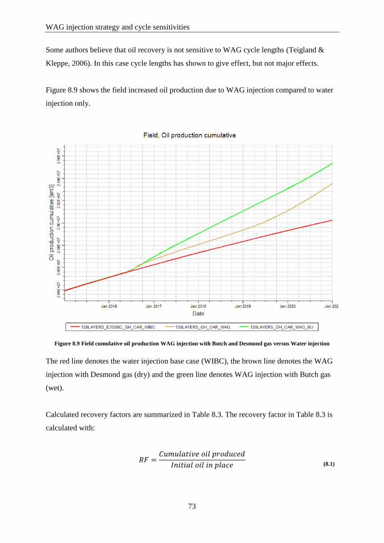
WAG injection strategy and cycle sensitivities
73
Some authors believe that oil recovery is not sensitive to WAG cycle lengths (Teigland &
Kleppe, 2006). In this case cycle lengths has shown to give effect, but not major effects.
Figure 8.9 shows the field increased oil production due to WAG injection compared to water
injection only.
Figure 8.9 Field cumulative oil production WAG injection with Butch and Desmond gas versus Water injection
The red line denotes the water injection base case (WIBC), the brown line denotes the WAG
injection with Desmond gas (dry) and the green line denotes WAG injection with Butch gas
(wet).
Calculated recovery factors are summarized in Table 8.3. The recovery factor in Table 8.3 is
calculated with:
𝑅𝐹 =
𝐶𝑢𝑚𝑢𝑙𝑎𝑡𝑖𝑣𝑒 𝑜𝑖𝑙 𝑝𝑟𝑜𝑑𝑢𝑐𝑒𝑑
𝐼𝑛𝑖𝑡𝑖𝑎𝑙 𝑜𝑖𝑙 𝑖𝑛 𝑝𝑙𝑎𝑐𝑒
(8.1)
WAG injection strategy and cycle sensitivities
74
Table 8.3 Recovery factor
Case RF Jan 15 RF Jan 21 % increase 2015 to 2021
CarHyst_WAG_D 0.386 0.400 1.359
CarHyst_WAG_B 0.386 0.402 1.607
CarHyst_WIBC 0.386 0.395 0.907
Nohyst_WAG_D 0.392 0.404 1.155
Where CarHyst_WAG_D and CarHyst_WAG_B denote WAG injection with Desmond and
Butch gas respectively. CarHyst_WIBC denotes the water injection base case and
Nohyst_WAG_D denotes WAG injection with no hysteresis effects.
The best recovery factor is obtained with WAG injection of Butch gas.
As mentioned, this recovery factor is based on actual oil production and initial oil in place,
and does not take injected gas composition into consideration. Since Butch gas is a wet gas,
some oil components are injected.
The oil recovery efficiency when injecting Butch gas is lower than for both WIBC and
Desmond gas WAG. Figure 8.10 shows the oil recovery efficiency factor.
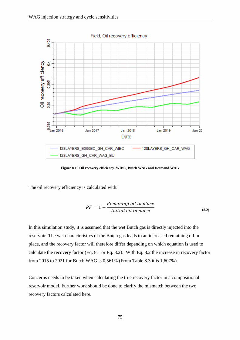
WAG injection strategy and cycle sensitivities
75
Figure 8.10 Oil recovery efficiency. WIBC, Butch WAG and Desmond WAG
The oil recovery efficiency is calculated with:
𝑅𝐹 = 1 −
𝑅𝑒𝑚𝑎𝑛𝑖𝑛𝑔 𝑜𝑖𝑙 𝑖𝑛 𝑝𝑙𝑎𝑐𝑒
𝐼𝑛𝑖𝑡𝑖𝑎𝑙 𝑜𝑖𝑙 𝑖𝑛 𝑝𝑙𝑎𝑐𝑒
(8.2)
In this simulation study, it is assumed that the wet Butch gas is directly injected into the
reservoir. The wet characteristics of the Butch gas leads to an increased remaining oil in
place, and the recovery factor will therefore differ depending on which equation is used to
calculate the recovery factor (Eq. 8.1 or Eq. 8.2). With Eq. 8.2 the increase in recovery factor
from 2015 to 2021 for Butch WAG is 0,561% (From Table 8.3 it is 1,607%).
Concerns needs to be taken when calculating the true recovery factor in a compositional
reservoir model. Further work should be done to clarify the mismatch between the two
recovery factors calculated here.
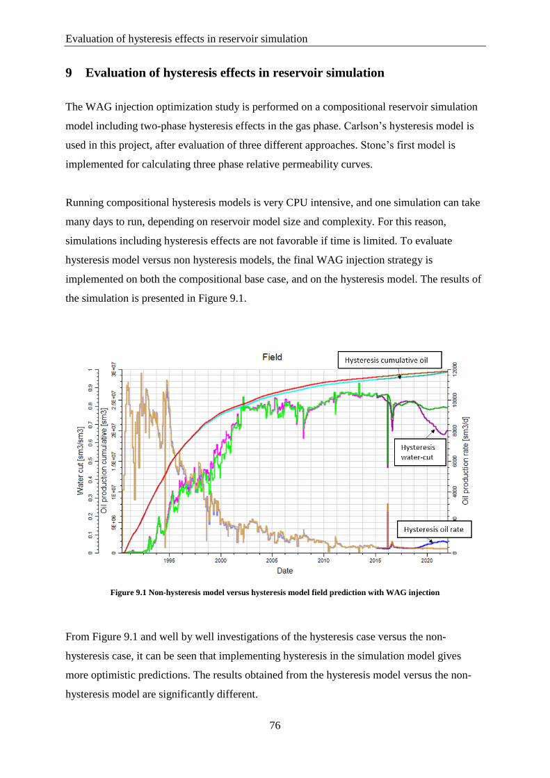
Evaluation of hysteresis effects in reservoir simulation
76
9 Evaluation of hysteresis effects in reservoir simulation
The WAG injection optimization study is performed on a compositional reservoir simulation
model including two-phase hysteresis effects in the gas phase. Carlson’s hysteresis model is
used in this project, after evaluation of three different approaches. Stone’s first model is
implemented for calculating three phase relative permeability curves.
Running compositional hysteresis models is very CPU intensive, and one simulation can take
many days to run, depending on reservoir model size and complexity. For this reason,
simulations including hysteresis effects are not favorable if time is limited. To evaluate
hysteresis model versus non hysteresis models, the final WAG injection strategy is
implemented on both the compositional base case, and on the hysteresis model. The results of
the simulation is presented in Figure 9.1.
Figure 9.1 Non-hysteresis model versus hysteresis model field prediction with WAG injection
From Figure 9.1 and well by well investigations of the hysteresis case versus the non-
hysteresis case, it can be seen that implementing hysteresis in the simulation model gives
more optimistic predictions. The results obtained from the hysteresis model versus the non-
hysteresis model are significantly different.
Evaluation of hysteresis effects in reservoir simulation
77
Implementing hysteresis in a reservoir simulator is a complex and difficult task. In Eclipse
there are nine different two-phase hysteresis options. These include the ability to select which
hysteresis model to be used, which phases the hysteresis model should be applied to, if the
drainage or imbibition curve should be used on the wetting phase and if hysteresis should be
applied to relative permeability, capillary pressure or both. (Schlumberger, 1998)
The vide variation of choices can confuse the user. To properly simulate hysteresis in oil
reservoirs, one must understand the physics of the process (the fluid flow) and the numerical
model used to simulate the process (Schlumberger, 1998). Schlumberger (1998) recommends
to not use the hysteresis option unless there is a valid reason, since it may impact the
efficiency of the simulation runs.
WAG injection prediction study is a valid reason for using the hysteresis option. This has
been shown in this thesis and frequently described in literature (Larsen & Skauge, 1998),
(Spiteri & Juanes, 2004), (Shahverdi & Sohrabi, 2013). The hysteresis option should be used
with great care.
Results from this study show that including hysteresis gives more optimistic predictions.
Inclusion of hysteresis is therefore not critical for an early screening of WAG injection
potential on field level, since it only represents an upside compared to a non-hysteresis
simulation.
Since Gyda initially only consisted of water and oil, the gas relative permeability hysteresis is
hard to predict. Hysteresis in the water phase is easier to implement on Gyda. This is because
simulations of all hysteresis models can be compared to historical data, and the method with
the best match can be implemented.
Further discussion
78
10 Further discussion
The EOR methods listed and described in this report are the conventional EOR methods.
Other methods such as microbial EOR, foam injection, ultrasonic wave, low salinity water
injection and newer methods such as smart fluid and nanofluids are not discussed. As any
EOR project on Gyda must have low investment cost and must be easy to implement, no
effort in investigating unconventional EOR methods has been undertaken.
From the definition of EOR, a WAG injection project is only considered as EOR if the gas
injection is miscible. For this project, the injection gas PVT properties and MMP are
unknown, so the injection is simulated as IWAG, immiscible WAG injection. Miscible WAG
injection is considered better for enhanced oil recovery purposes, as the interfacial tension can
reduce to zero, if full miscibility is achieved. In the Gyda gas injection study performed in
2007/2008, MMP and other miscibility parameters for simulations was unknown, and it was
concluded that recovery from miscible flood is considered as upside potential. They requested
fluid analysis including slim tube test for MMP and reservoir oil swelling including viscosity
measurements test for mitigation of uncertainty range. These parameters should be in place in
order to evaluate a WAG project as miscible, as miscible WAG projects usually gives higher
recovery.
The reservoir model received for this project, is a history matched black oil model. When
changing from black oil to compositional, the history match should in principle not change.
After inclusion of the Lorents-Bay-Clark coefficients, for oil viscosity calculations, and the
field separator keyword, the history match obtained from the black oil and the compositional
model are slightly different. This can be due to small compositional effects in the oil phase.
Well A-08A and A-07A which are dead in prediction from the compositional case should be
better matched in order to get the right predictions. As they are low oil producers, they can be
considered upside at this point.
As the only relative permeability set avaiable on Gyda is imbibition curves, theroretically
developed drainage curves for the gas-oil system are made with use of the modified Brooks-
Corey metod. The theoretically developed curves are made with basis on general drainage and
imbibition curve relationships described in the litterature. In order to get more reliable results,
experimental drainage and imbibition curves should have been implemented.
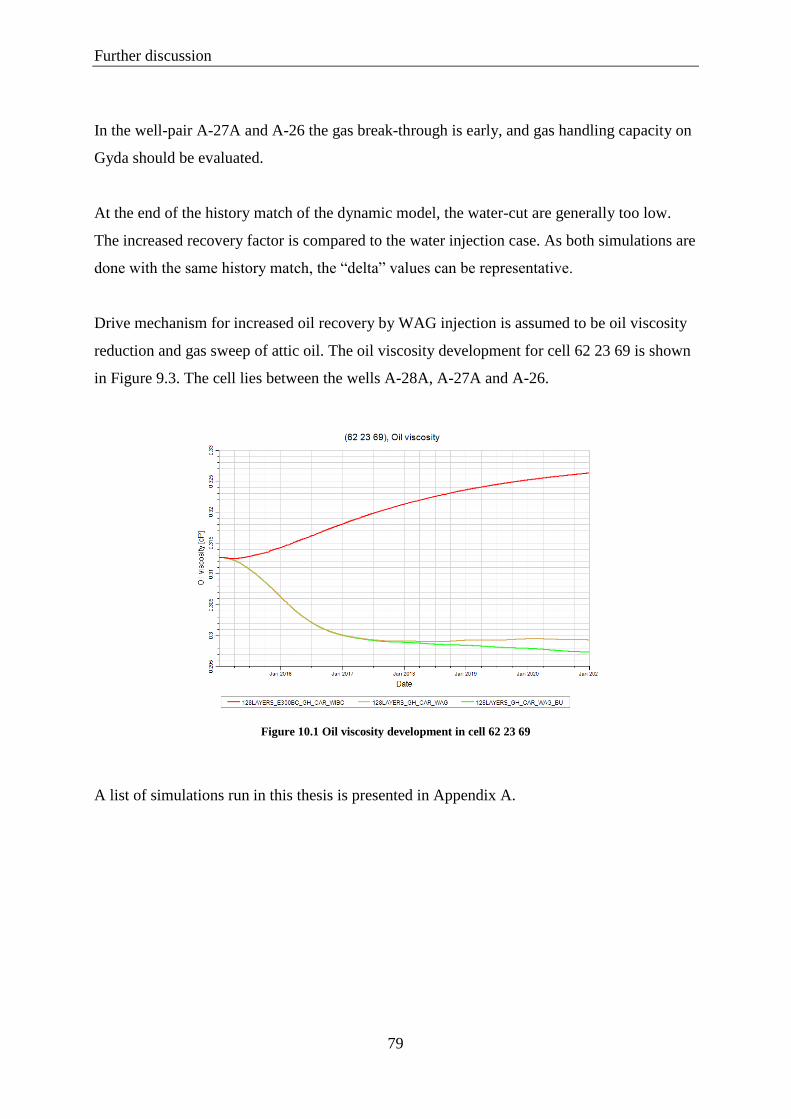
Further discussion
79
In the well-pair A-27A and A-26 the gas break-through is early, and gas handling capacity on
Gyda should be evaluated.
At the end of the history match of the dynamic model, the water-cut are generally too low.
The increased recovery factor is compared to the water injection case. As both simulations are
done with the same history match, the “delta” values can be representative.
Drive mechanism for increased oil recovery by WAG injection is assumed to be oil viscosity
reduction and gas sweep of attic oil. The oil viscosity development for cell 62 23 69 is shown
in Figure 9.3. The cell lies between the wells A-28A, A-27A and A-26.
Figure 10.1 Oil viscosity development in cell 62 23 69
A list of simulations run in this thesis is presented in Appendix A.
Conclusions and recommendations
80
11 Conclusions and recommendations
Conventional EOR methods can be divided into chemical, thermal and miscible
methods. These different methods increase the oil recovery on both macroscopic and
microscopic level.
From Gyda EOR screening criteria and conclusions from previous Gyda EOR studies
a WAG injection study is performed the Gyda dynamic reservoir model.
The study is implemented as immiscible WAG injection, as miscibility parameters are
unknown.
For capturing compositional effects the simulations are performed on a compositional
reservoir model. The simulations are run in Eclipse 300.
Hysteresis in the gas phase during WAG injection is simulated with the two-phase
Carlson’s hysteresis option. Three-phase relative permeability curves are created with
Stone’s first method.
A three-phase hysteretic option is available in Eclipse for WAG simulations. Three-
phase hysteretic options account for the reduction in the gas relative permeability
during WAG floods.
Due to the far more need for computational power and a bigger uncertainty range
regarding input parameters, the three-phase hysteretic option is not further evaluated.
Inclusion of hysteresis effects in WAG injection simulations give more optimistic
predictions than not including hysteresis effects.
Hysteresis should be implemented for correct WAG injection predictions.
The biggest hysteresis effects during WAG injection, are in the non-wetting relative
permeability.
WAG cycles of 6 months are shown to be beneficial with a substantial distance
between injector and producer. Shorter WAG cycles are shown to be beneficial when
producer and injector are closer and have good communication. WAG cycle lengths
has shown to give effect on oil recovery, but not major effects.
WAG injection on Gyda with a dry injection gas (Desmond) can increase the recovery
by 1.4% by 2021.
Effort should be put in to improving the history match on the compositional reservoir
model.

Conclusions and recommendations
81
To get more reliable prediction results from WAG injection, the gas relative
permeability curves should be experimentally determined.
To run miscibility predictions, miscibility parameters should be determined.
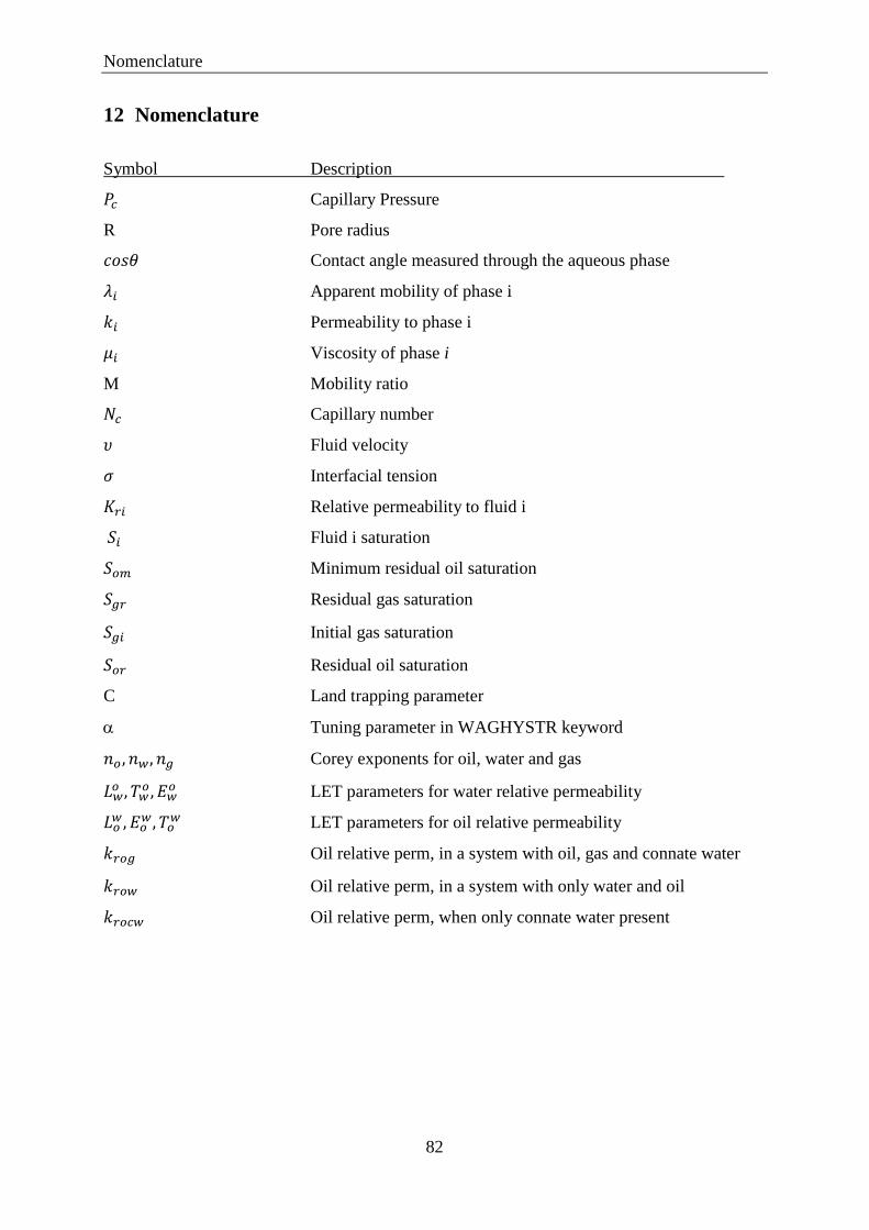
Nomenclature
82
12 Nomenclature
Symbol Description
𝑃𝑐 Capillary Pressure
R Pore radius
𝑐𝑜𝑠𝜃 Contact angle measured through the aqueous phase
𝜆𝑖 Apparent mobility of phase i
𝑘𝑖 Permeability to phase i
𝜇𝑖 Viscosity of phase i
M Mobility ratio
𝑁𝑐 Capillary number
𝜐 Fluid velocity
𝜎 Interfacial tension
𝐾𝑟𝑖 Relative permeability to fluid i
𝑆𝑖 Fluid i saturation
𝑆𝑜𝑚 Minimum residual oil saturation
𝑆𝑔𝑟 Residual gas saturation
𝑆𝑔𝑖 Initial gas saturation
𝑆𝑜𝑟 Residual oil saturation
C Land trapping parameter
Tuning parameter in WAGHYSTR keyword
𝑛𝑜 , 𝑛𝑤, 𝑛𝑔 Corey exponents for oil, water and gas
𝐿𝑤𝑜 , 𝑇𝑤
𝑜, 𝐸𝑤𝑜 LET parameters for water relative permeability
𝐿𝑜𝑤, 𝐸𝑜
𝑤, 𝑇𝑜𝑤 LET parameters for oil relative permeability
𝑘𝑟𝑜𝑔 Oil relative perm, in a system with oil, gas and connate water
𝑘𝑟𝑜𝑤 Oil relative perm, in a system with only water and oil
𝑘𝑟𝑜𝑐𝑤 Oil relative perm, when only connate water present
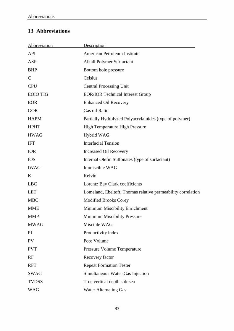
Abbreviations
83
13 Abbreviations
Abbreviation Description
API American Petroleum Institute
ASP Alkali Polymer Surfactant
BHP Bottom hole pressure
C Celsius
CPU Central Processing Unit
EOIO TIG EOR/IOR Technical Interest Group
EOR Enhanced Oil Recovery
GOR Gas oil Ratio
HAPM Partially Hydrolyzed Polyacrylamides (type of polymer)
HPHT High Temperature High Pressure
HWAG Hybrid WAG
IFT Interfacial Tension
IOR Increased Oil Recovery
IOS Internal Olefin Sulfonates (type of surfactant)
IWAG Immiscible WAG
K Kelvin
LBC Lorentz Bay Clark coefficients
LET Lomeland, Ebeltoft, Thomas relative permeability correlation
MBC Modified Brooks Corey
MME Minimum Miscibility Enrichment
MMP Minimum Miscibility Pressure
MWAG Miscible WAG
PI Productivity index
PV Pore Volume
PVT Pressure Volume Temperature
RF Recovery factor
RFT Repeat Formation Tester
SWAG Simultaneous Water-Gas Injection
TVDSS True vertical depth sub-sea
WAG Water Alternating Gas
Bibliography
84
14 Bibliography
Aasheim, I. (2000). Oseberg: Increased recoverable resources by optimal reservoir
management and use of new technology. SPE-65163-MS. doi: 10.2118/65163-MS
Arogundade, O. A., Shahverdi, H.-R., & Sohrabi, M. (2013). A Study of Three Phase Relative
Permeability and Hysteresis in Water Alternating Gas (WAG) Injection. SPE-165218-
MS. doi: 10.2118/165218-MS
Arshad, A., Al-Majed, A. A., Menouar, H., Muhammadain, A. M., & Mtawaa, B. (2009).
Carbon Dioxide (CO2) Miscible Flooding in Tight Oil Reservoirs: A Case Study.
SPE-127616-MS. doi: 10.2118/127616-MS
Brodie, J. A., Zhang, P., Mellemstrand Hetland, S., Moulds, T. P., & Jhaveri, B. S. (2012). BP
North Sea Gas Injection Projects: Sustaining Offshore Production. SPE-161189-MS.
doi: 10.2118/161189-MS
Carlson, F. M. (1981). Simulation of Relative Permeability Hysteresis to the Nonwetting
Phase. SPE-10157-MS. doi: 10.2118/10157-MS
Christensen, J. R., Stenby, E. H., & Skauge, A. (2001). Review of WAG Field Experience.
SPE-71203-PA. doi: 10.2118/71203-PA
Crogh, N. A., Eide, K., & Morterud, S. E. (2002). WAG Injection at the Statfjord Field, A
Success Story. SPE-78348-MS. doi: 10.2118/78348-MS
Dake, L. (1978). Fundamentals of reservoir engineering (Vol. 17).
Dong. (2012). Gyda Geological Background. Talisman internal document
Gao, P., Towler, B. F., & Pan, G. (2010). Strategies for Evaluation of the CO2 Miscible
Flooding Process. SPE-138786-MS. doi: 10.2118/138786-MS
Ghorayeb, K., & Holmes, J. A. (2005). Black Oil Delumping. SPE-96571-MS. doi:
10.2118/96571-MS
Goda, H. M., & Behrenbruch, P. (2004). Using a Modified Brooks-Corey Model to Study Oil-
Water Relative Permeability for Diverse Pore Structures. SPE-88538-MS. doi:
10.2118/88538-MS
Hirasaki, G. J., Miller, C. A., & Puerto, M. (2008). Recent Advances in Surfactant EOR. SPE-
115386-MS. doi: 10.2118/115386-MS
Hite, J. R., & Bondor, P. L. (2004). Planning EOR Projects. SPE-92006-MS. doi:
10.2118/92006-MS
Instefjord, R., & Todnem, A. C. (2002). 10 Years of WAG Injection in Lower Brent at the
Gullfaks Field. SPE-78344-MS. doi: 10.2118/78344-MS
Jensen, T. B., Harpole, K. J., & Østhus, A. (2000). EOR Screening for Ekofisk. SPE-65124-
MS. doi: 10.2118/65124-MS
Killough, J. E. (1976). Reservoir Simulation With History-Dependent Saturation Functions.
SPE-5106-PA. doi: 10.2118/5106-PA
Kleppe, J. (2015, 17/02/2015). Introduction to compositional simulation. Hand-out note.
Retrieved 23/05/15, 2015, from http://www.ipt.ntnu.no/~kleppe/TPG4160/note14.pdf
Lake, L. W. (2010). Enhanced oil recovery. Richardson, Tex.: Society of Petroleum
Engineers.
Land, C. S. (1968). Calculation of Imbibition Relative Permeability for Two- and Three-
Phase Flow From Rock Properties. SPE-1942-PA. doi: 10.2118/1942-PA
Larsen, J. A., & Skauge, A. (1998). Methodology for Numerical Simulation With Cycle-
Dependent Relative Permeabilities. SPE-38456-PA. doi: 10.2118/38456-PA
Bibliography
85
Lien, S. C., Lie, S. E., Fjellbirkeland, H., & Larsen, S. V. (1998). Brage Field, Lessons
Learned After 5 Years of Production. SPE-50641-MS. doi: 10.2118/50641-MS
Liu, S., Li, R. F., Miller, C. A., & Hirasaki, G. J. (2008). ASP Process: Wide Range of
Conditions for Good Recovery. SPE-113936-MS. doi: 10.2118/113936-MS
Lomeland, F., Ebeltoft, E., & Thomas, W. H. (2005). A new versatile relative permeability
correlation. Paper presented at the International Symposium of the Society of Core
Analysts, Toronto, Canada.
https://www.researchgate.net/publication/242724867_A_NEW_VERSATILE_RELA
TIVE_PERMEABILITY_CORRELATION
Matre, B., Rasmussen, J., Hettervik, K., & Hongbua, D. (2015). Increased Oil Recovery from
a Mature Oil Field by Gas injection. Paper presented at the 18th European
Symposium on Improved Oil Recovery, Dresden, Germany.
Meybodi, H. E., Kharrat, R., & Wang, X. (2008). Study of Microscopic and Macroscopic
Displacement
Behaviors of Polymer Solution in Water-Wet
and Oil-Wet Media.
Nishikiori, N., Sugai, K., Normann, C., Onstein, A., Melberg, O., & Eilertsen, T. (2008). An
Integrated workflow for gas injection EOR and a successful application for a
heterogeneous sandstone reservoir in the Southern North Sea{bullet operator}.
NorskeAEDC. (2007). Gyda Attic Modelling and EOR study.
Petrowiki.org. (2014a). Conformance Improvement.
Petrowiki.org. (2014b). interfacial tension. Retrieved 06/12/2014, from
http://petrowiki.org/Interfacial_tension
Petrowiki.org. (2014c). Relative permeability. Retrieved 08/11/2014, from
http://petrowiki.org/Relative_permeability
Petrowiki.org. (2015). Relative Permeability Models. Retrieved 25/05, 2015, from
petrowiki.org/Relative_permeability_models#cite_note-r2-1
Schlumberger. (1998). Eclipse user guide for hysteresis.
Schlumberger. (2014a). Eclipse Reference Manual.
Schlumberger. (2014b). Eclipse Technical description.
Schramm, L. L. (2000). Surfactants: Fundamentals and Applications in the Petroleum
Industry. Cambridge: Cambridge University Press.
Shahverdi, H., & Sohrabi, M. (2012). Three-Phase Relative Permeability and Hystresis Model
for Simulation of Water Alternating Gas (WAG) Injection. SPE-152218-MS. doi:
10.2118/152218-MS
Shahverdi, H., & Sohrabi, M. (2013). Modelling of Cyclic Hysteresis of Three-Phase Relative
Permeability during Water-Alternating-Gas (WAG) Injection. SPE-166526-MS. doi:
10.2118/166526-MS
Sheng, J. J. (2011). Modern Chemical Enhanced Oil Recovery - Theory and Practice:
Elsevier.
Sheng, J. J. (2013a). A Comprehensive Review of Alkaline-Surfactant-Polymer (ASP)
Flooding. SPE-165358-MS. doi: 10.2118/165358-MS
Sheng, J. J. (2013b). Enhanced Oil Recovery - Field Case Studies: Elsevier.
Skauge, A., Aarra, M. G., Surguchev, L., Martinsen, H. A., & Rasmussen, L. (2002). Foam-
Assisted WAG: Experience from the Snorre Field. SPE-75157-MS. doi:
10.2118/75157-MS
Slb.com. (2014a). Fundamentals of Wettability. Retrieved 08/11/2014, from
http://www.slb.com/~/media/Files/resources/oilfield_review/ors07/sum07/p44_61.ash
x
86
Slb.com. (2014b). Relative permeability. Retrieved 08/11/2014, from
http://www.glossary.oilfield.slb.com/en/Terms/r/relative_permeability.aspx
Slb.com. (2014c). Sweep efficiency. Retrieved 09/11/2014, from
http://www.glossary.oilfield.slb.com/en/Terms/a/areal_sweep_efficiency.aspx
Spiteri, E. J., & Juanes, R. (2004). Impact of Relative Permeability Hysteresis on the
Numerical Simulation of WAG Injection. SPE-89921-MS. doi: 10.2118/89921-MS
Stoll, M., Al-Shureqi, H., Finol, J., Al-Harthy, S. A., Oyemade, S. N., de Kruijf, A., . . .
Faber, M. J. (2010). Alkaline-Surfactant-Polymer Flood: From the Laboratory to the
Field. SPE-129164-MS. doi: 10.2118/129164-MS
Stone, H. L. (1970). Probability Model for Estimating Three-Phase Relative Permeability.
doi: 10.2118/2116-PA
Stone, H. L. (1973). Estimation of Three-Phase Relative Permeability And Residual Oil Data.
doi: 10.2118/73-04-06
Taber, J. J., Martin, F. D., & Seright, R. S. (1997a). EOR Screening Criteria Revisited—Part
2: Applications and Impact of Oil Prices. SPE-39234-PA. doi: 10.2118/39234-PA
Taber, J. J., Martin, F. D., & Seright, R. S. (1997b). EOR Screening Criteria Revisited - Part
1: Introduction to Screening Criteria and Enhanced Recovery Field Projects. SPE-
35385-PA. doi: 10.2118/35385-PA
Talisman. (2013). Gyda Pressure Study. Talisman internal document
Talisman. (2014). Gyda History Matching Jan 2014.Talisman internal document
Teigland, R., & Kleppe, J. (2006). EOR Survey in the North Sea. SPE-99546-MS. doi:
10.2118/99546-MS
Terry, R. E. (2001). Enhanced Oil Recovery. Retrieved 08/12/2014, from
http://www.firp.ula.ve/archivos/cuadernos/01_Chap_Terry_EOR.pdf
Torabi, F., Zarivnyy, O., & Mosavat, N. (2013). Developing New Corey-Based Water/Oil
Relative Permeability Correlations for Heavy Oil Systems. SPE-165445-MS. doi:
10.2118/165445-MS
Young, L. C., & Stephenson, R. E. (1983). A Generalized Compositional Approach for
Reservoir Simulation. SPE-10516-PA. doi: 10.2118/10516-PA
Zerafat, M. M., Ayatollahi, S., Mehranbod, N., & Barzegari, D. (2011). Bayesian Network
Analysis as a Tool for Efficient EOR Screening. SPE-143282-MS. doi:
10.2118/143282-MS
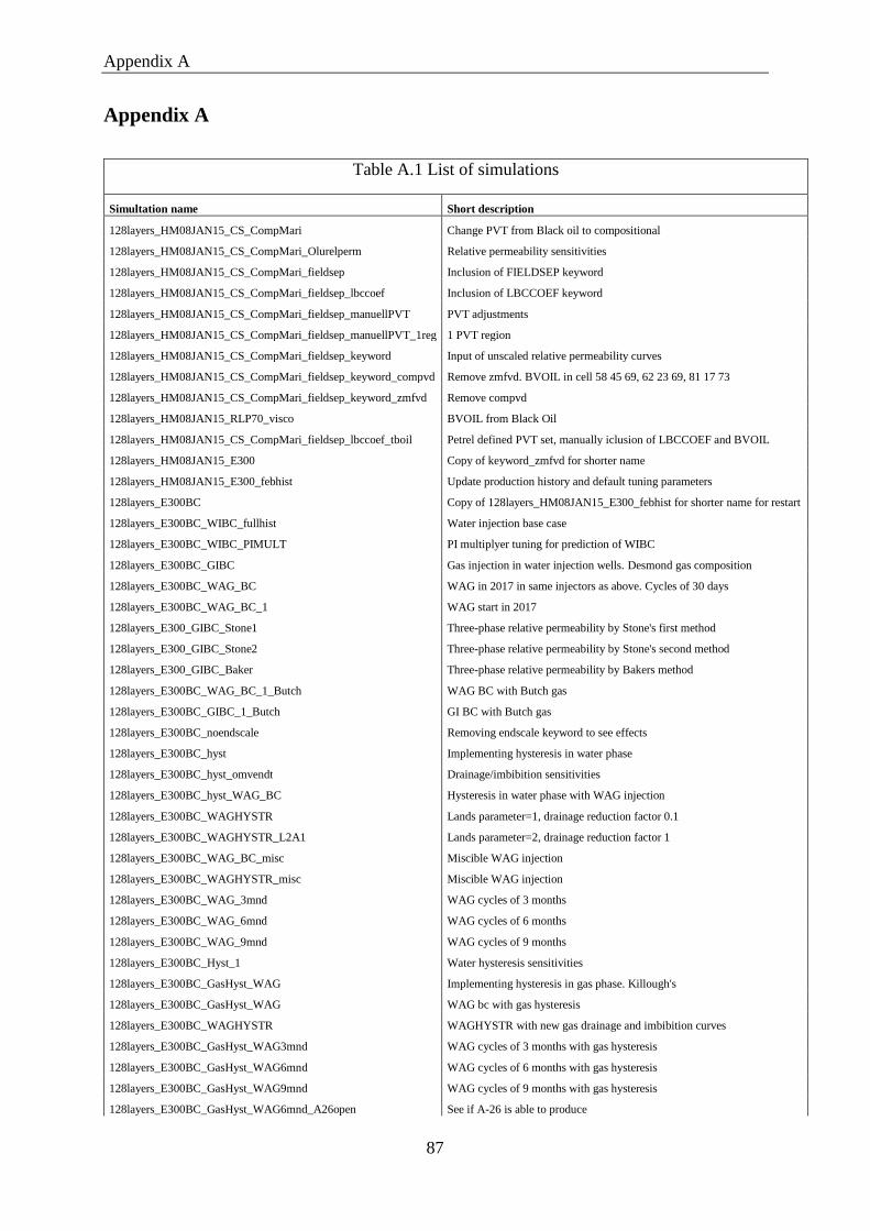
Appendix A
87
Appendix A
Table A.1 List of simulations
Simultation name Short description
128layers_HM08JAN15_CS_CompMari Change PVT from Black oil to compositional
128layers_HM08JAN15_CS_CompMari_Olurelperm Relative permeability sensitivities
128layers_HM08JAN15_CS_CompMari_fieldsep Inclusion of FIELDSEP keyword
128layers_HM08JAN15_CS_CompMari_fieldsep_lbccoef Inclusion of LBCCOEF keyword
128layers_HM08JAN15_CS_CompMari_fieldsep_manuellPVT PVT adjustments
128layers_HM08JAN15_CS_CompMari_fieldsep_manuellPVT_1reg 1 PVT region
128layers_HM08JAN15_CS_CompMari_fieldsep_keyword Input of unscaled relative permeability curves
128layers_HM08JAN15_CS_CompMari_fieldsep_keyword_compvd Remove zmfvd. BVOIL in cell 58 45 69, 62 23 69, 81 17 73
128layers_HM08JAN15_CS_CompMari_fieldsep_keyword_zmfvd Remove compvd
128layers_HM08JAN15_RLP70_visco BVOIL from Black Oil
128layers_HM08JAN15_CS_CompMari_fieldsep_lbccoef_tboil Petrel defined PVT set, manually iclusion of LBCCOEF and BVOIL
128layers_HM08JAN15_E300 Copy of keyword_zmfvd for shorter name
128layers_HM08JAN15_E300_febhist Update production history and default tuning parameters
128layers_E300BC Copy of 128layers_HM08JAN15_E300_febhist for shorter name for restart
128layers_E300BC_WIBC_fullhist Water injection base case
128layers_E300BC_WIBC_PIMULT PI multiplyer tuning for prediction of WIBC
128layers_E300BC_GIBC Gas injection in water injection wells. Desmond gas composition
128layers_E300BC_WAG_BC WAG in 2017 in same injectors as above. Cycles of 30 days
128layers_E300BC_WAG_BC_1 WAG start in 2017
128layers_E300_GIBC_Stone1 Three-phase relative permeability by Stone's first method
128layers_E300_GIBC_Stone2 Three-phase relative permeability by Stone's second method
128layers_E300_GIBC_Baker Three-phase relative permeability by Bakers method
128layers_E300BC_WAG_BC_1_Butch WAG BC with Butch gas
128layers_E300BC_GIBC_1_Butch GI BC with Butch gas
128layers_E300BC_noendscale Removing endscale keyword to see effects
128layers_E300BC_hyst Implementing hysteresis in water phase
128layers_E300BC_hyst_omvendt Drainage/imbibition sensitivities
128layers_E300BC_hyst_WAG_BC Hysteresis in water phase with WAG injection
128layers_E300BC_WAGHYSTR Lands parameter=1, drainage reduction factor 0.1
128layers_E300BC_WAGHYSTR_L2A1 Lands parameter=2, drainage reduction factor 1
128layers_E300BC_WAG_BC_misc Miscible WAG injection
128layers_E300BC_WAGHYSTR_misc Miscible WAG injection
128layers_E300BC_WAG_3mnd WAG cycles of 3 months
128layers_E300BC_WAG_6mnd WAG cycles of 6 months
128layers_E300BC_WAG_9mnd WAG cycles of 9 months
128layers_E300BC_Hyst_1 Water hysteresis sensitivities
128layers_E300BC_GasHyst_WAG Implementing hysteresis in gas phase. Killough's
128layers_E300BC_GasHyst_WAG WAG bc with gas hysteresis
128layers_E300BC_WAGHYSTR WAGHYSTR with new gas drainage and imbibition curves
128layers_E300BC_GasHyst_WAG3mnd WAG cycles of 3 months with gas hysteresis
128layers_E300BC_GasHyst_WAG6mnd WAG cycles of 6 months with gas hysteresis
128layers_E300BC_GasHyst_WAG9mnd WAG cycles of 9 months with gas hysteresis
128layers_E300BC_GasHyst_WAG6mnd_A26open See if A-26 is able to produce
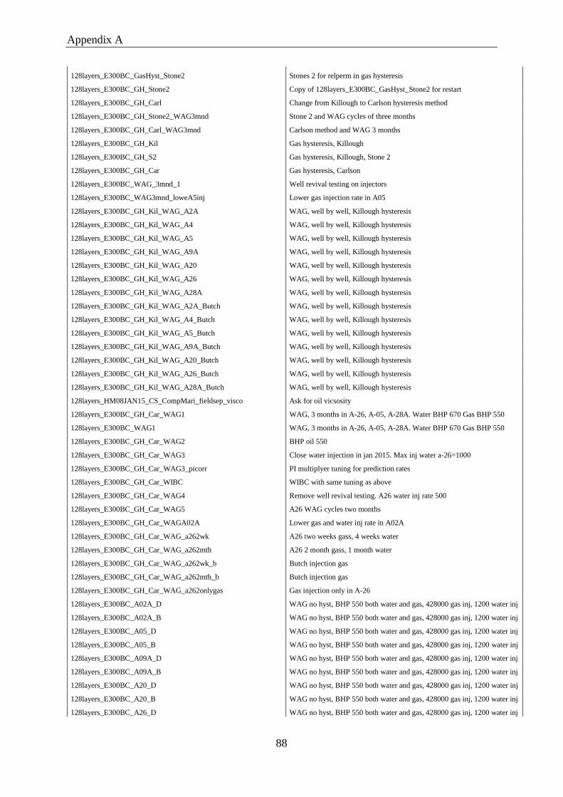
Appendix A
88
128layers_E300BC_GasHyst_Stone2 Stones 2 for relperm in gas hysteresis
128layers_E300BC_GH_Stone2 Copy of 128layers_E300BC_GasHyst_Stone2 for restart
128layers_E300BC_GH_Carl Change from Killough to Carlson hysteresis method
128layers_E300BC_GH_Stone2_WAG3mnd Stone 2 and WAG cycles of three months
128layers_E300BC_GH_Carl_WAG3mnd Carlson method and WAG 3 months
128layers_E300BC_GH_Kil Gas hysteresis, Killough
128layers_E300BC_GH_S2 Gas hysteresis, Killough, Stone 2
128layers_E300BC_GH_Car Gas hysteresis, Carlson
128layers_E300BC_WAG_3mnd_1 Well revival testing on injectors
128layers_E300BC_WAG3mnd_loweA5inj Lower gas injection rate in A05
128layers_E300BC_GH_Kil_WAG_A2A WAG, well by well, Killough hysteresis
128layers_E300BC_GH_Kil_WAG_A4 WAG, well by well, Killough hysteresis
128layers_E300BC_GH_Kil_WAG_A5 WAG, well by well, Killough hysteresis
128layers_E300BC_GH_Kil_WAG_A9A WAG, well by well, Killough hysteresis
128layers_E300BC_GH_Kil_WAG_A20 WAG, well by well, Killough hysteresis
128layers_E300BC_GH_Kil_WAG_A26 WAG, well by well, Killough hysteresis
128layers_E300BC_GH_Kil_WAG_A28A WAG, well by well, Killough hysteresis
128layers_E300BC_GH_Kil_WAG_A2A_Butch WAG, well by well, Killough hysteresis
128layers_E300BC_GH_Kil_WAG_A4_Butch WAG, well by well, Killough hysteresis
128layers_E300BC_GH_Kil_WAG_A5_Butch WAG, well by well, Killough hysteresis
128layers_E300BC_GH_Kil_WAG_A9A_Butch WAG, well by well, Killough hysteresis
128layers_E300BC_GH_Kil_WAG_A20_Butch WAG, well by well, Killough hysteresis
128layers_E300BC_GH_Kil_WAG_A26_Butch WAG, well by well, Killough hysteresis
128layers_E300BC_GH_Kil_WAG_A28A_Butch WAG, well by well, Killough hysteresis
128layers_HM08JAN15_CS_CompMari_fieldsep_visco Ask for oil vicsosity
128layers_E300BC_GH_Car_WAG1 WAG, 3 months in A-26, A-05, A-28A. Water BHP 670 Gas BHP 550
128layers_E300BC_WAG1 WAG, 3 months in A-26, A-05, A-28A. Water BHP 670 Gas BHP 550
128layers_E300BC_GH_Car_WAG2 BHP oil 550
128layers_E300BC_GH_Car_WAG3 Close water injection in jan 2015. Max inj water a-26=1000
128layers_E300BC_GH_Car_WAG3_picorr PI multiplyer tuning for prediction rates
128layers_E300BC_GH_Car_WIBC WIBC with same tuning as above
128layers_E300BC_GH_Car_WAG4 Remove well revival testing. A26 water inj rate 500
128layers_E300BC_GH_Car_WAG5 A26 WAG cycles two months
128layers_E300BC_GH_Car_WAGA02A Lower gas and water inj rate in A02A
128layers_E300BC_GH_Car_WAG_a262wk A26 two weeks gass, 4 weeks water
128layers_E300BC_GH_Car_WAG_a262mth A26 2 month gass, 1 month water
128layers_E300BC_GH_Car_WAG_a262wk_b Butch injection gas
128layers_E300BC_GH_Car_WAG_a262mth_b Butch injection gas
128layers_E300BC_GH_Car_WAG_a262onlygas Gas injection only in A-26
128layers_E300BC_A02A_D WAG no hyst, BHP 550 both water and gas, 428000 gas inj, 1200 water inj
128layers_E300BC_A02A_B WAG no hyst, BHP 550 both water and gas, 428000 gas inj, 1200 water inj
128layers_E300BC_A05_D WAG no hyst, BHP 550 both water and gas, 428000 gas inj, 1200 water inj
128layers_E300BC_A05_B WAG no hyst, BHP 550 both water and gas, 428000 gas inj, 1200 water inj
128layers_E300BC_A09A_D WAG no hyst, BHP 550 both water and gas, 428000 gas inj, 1200 water inj
128layers_E300BC_A09A_B WAG no hyst, BHP 550 both water and gas, 428000 gas inj, 1200 water inj
128layers_E300BC_A20_D WAG no hyst, BHP 550 both water and gas, 428000 gas inj, 1200 water inj
128layers_E300BC_A20_B WAG no hyst, BHP 550 both water and gas, 428000 gas inj, 1200 water inj
128layers_E300BC_A26_D WAG no hyst, BHP 550 both water and gas, 428000 gas inj, 1200 water inj

89
128layers_E300BC_A26_B WAG no hyst, BHP 550 both water and gas, 428000 gas inj, 1200 water inj
128layers_E300BC_28A_D WAG no hyst, BHP 550 both water and gas, 428000 gas inj, 1200 water inj
128layers_E300BC_A28A_B WAG no hyst, BHP 550 both water and gas, 428000 gas inj, 1200 water inj
128layers_E300BC_GH_Car_WAG_A09WAG Close water injection jan 15 A-09A, WAG A-09A march 2016
128layers_E300BC_GH_Car_WAG_A05wa09shut Close water injection jan 15 A-09A, WAG A-05 march 2016
128layers_E300BC_GH_Car_WAG_A26short A-26 2 week gas one week water
128layers_E300BC_GH_Car_WAG_A26short_b Butch injection gas
128layers_E300BC_GH_Car_WAG_A20 Close water injection jan 15 A-09A, WAG A-20 march 2016
128layers_E300BC_A26mth For comparing with hysteresis
128layers_E300BC_GH_Car_WAG_a264mth 4 month gas, 2 month water
128layers_E300BC_GH_Car_WAG_OPT_6MND WAG field 6 months
128layers_E300BC_GH_Car_WAG_OPT_1MND WAG field 1 month
128layers_E300BC_GH_Car_WAG_OPT_2WK WAG field 2 week
128layers_E300BC_CAR_BVOIL Oil viscosity
128layers_GH_CAR_WAG 6 months in A28A, A05H. 2 weeks in A26. Water inj rate 700 A26