Three Phase Relative Permeability Models for WAG Simulation

IMPERIAL COLLEGE LONDON

Department of Earth Science and Engineering

Centre for Petroleum Studies

Three Phase Relative Permeability Models for WAG Simulation

By

Baasir Tasleem

A report submitted in partial fulfilment of the requirements for

the MSc and/or the DIC.

September 2010

ii [Three Phase Relative Permeability Models for WAG Simulation]

DECLARATION OF OWN WORK

I declare that this thesis “Three Phase Relative Permeability Models for WAG Simulations” is

entirely my own work and that where any material could be construed as the work of others, it is fully

cited and referenced, and/or with appropriate acknowledgement given.

Signature:.....................................................................................................

Name of student: Baasir Tasleem

Name of supervisor: Dr. Jonathan Carter

Name of the company supervisor: Marie Ann Giddins, Schlumberger

[Three Phase Relative Permeability Models for WAG Simulations] iii

Abstract Enhanced Oil Recovery (EOR) projects are becoming extremely important to oil companies as the

conventional hydrocarbon resources are depleted. Water alternating gas (WAG) has been a renowned

EOR process for more than fifty years. Fluid flow in a WAG injection process has been regarded as a

complex phenomenon. This is because of the dependence of fluid flow on the saturation history. The

oscillations in saturation history give rise to complex effects such as hysteresis which are more significant

during three phase flow.

The hysteresis effects are generally modelled in conjunction with empirical three phase relative

permeability models. Recently new empirical (Blunt, 2000) and complex pore network models (Suicmez

et al., 2007) have been developed that predict the lab measured data in good agreement. However the

current industrial practice still utilizes the earlier developed models, namely: Stone 1 (Stone, 1970), Stone

2 (Stone, 1973) and Saturated Weighted Interpolation method which is defaulted in the commercial

reservoir simulator1 (Eclipse Technical Description). The performance of these empirical models has

been the centre of debate for a long time. Selection of the most suitable method and choice of parameters

may be a compromise between the need to match measured physical data and the need to obtain good

performance from the simulator.

In this study an attempt is made to model the hysteresis effects during an immiscible and miscible WAG

flood by using different options present in a commercial compositional reservoir simulator. A

comparative analysis on realistic data by using different empirical three phase relative permeability

models has been performed. The results indicate that all available options present in the simulator should

be utilized with history matching before deciding on which option to be used. Multiple sensitivity studies

on various parameters and their effect on total oil recovery have been presented which would be helpful

for an engineer to accurately manage and model the hysteresis effects in WAG simulations. Several

recommendations for further studies have also been made. This work can be taken as a reference for

initial test runs or pilot project studies when planning for a full field scale WAG flood.

1 Shall be referred as ECL default.

iv [Three Phase Relative Permeability Models for WAG Simulation]

Acknowledgements

I would like to offer heartfelt gratitude and appreciation to my supervisor Marie Ann Giddins

(Schlumberger). Her insight, encyclopaedic knowledge and support made this project possible. I owe a

large debt to Mr. Syed Zeeshan Jilani (Schlumberger) for his exceptional mentoring and sparing time to

answer all my questions during never ending discussions.

Special thanks to my family for their infinite support, prayers and constant encouragement throughout the

MSc program which made it possible for me to reach to this extent.

I wish to thank Abingdon Technology Centre for giving me this opportunity, for providing an excellent

professional environment and for all the necessary resources during the course of this project.

I am also grateful to Mr. Sofyan Salem (Schlumberger) for his valuable guidance and Mr. Raheel Baig

(Schlumberger) for his continuous help throughout the research, for doing a critical review and for proof

reading my thesis.

It is my pleasure to also record the debts of Dr. Jonathan Carter (Imperial College) and Shiva Farmahini

Farahani (Schlumberger) for her constant appreciation of my work and valuable comments.

Appreciation goes to my wife for her infinite patience, understanding, cooperation and motivation

without which this MSc program and research project would not have been meaningful and successful.

[Three Phase Relative Permeability Models for WAG Simulations] v

Table of Contents Abstract ........................................................................................................................................................................................ iii

Acknowledgements ...................................................................................................................................................................... iv

List of Figures .............................................................................................................................................................................. vi

List of Figures-Appendix ............................................................................................................................................................. vi

List of Tables ............................................................................................................................................................................... vi

List of Tables-Appendix ............................................................................................................................................................. vii

Introduction ................................................................................................................................................................................... 8

Simulation Study ..........................................................................................................................................................................10

Hysteresis Options in Black Oil Simulator ..................................................................................................................................10

WAG Hysteresis Model in Compositional Simulator ..................................................................................................................12

Model Description. ...................................................................................................................................................................13

WAG Hysteresis Input Curves. ................................................................................................................................................13

Immiscible WAG (IWAG) Simulation Results. .......................................................................................................................15

Miscible WAG (MWAG) Simulation Results. ........................................................................................................................19

Sensitivity Analysis......................................................................................................................................................................20

Land Parameter. .......................................................................................................................................................................20

Secondary Drainage Factor. .....................................................................................................................................................21

Length of Water and Gas Cycles..............................................................................................................................................21

Discussion ....................................................................................................................................................................................22

Black Oil Simulation. ...............................................................................................................................................................22

IWAG Simulation. ...................................................................................................................................................................23

MWAG Simulation. .................................................................................................................................................................23

Conclusions and Recommendations for Future Research ............................................................................................................23

Nomenclature ...............................................................................................................................................................................23

Acknowledgement .......................................................................................................................................................................24

References ....................................................................................................................................................................................24

APPENDIX A ................................................................................................................................................................................ I

Critical Literature Review .............................................................................................................................................................. I

SPE 951145-G (1951) ............................................................................................................................................................... II

SPE 1942 (1968) ......................................................................................................................................................................III

SPE 5106 (1974) ..................................................................................................................................................................... IV

SPE 10157 (1981) ..................................................................................................................................................................... V

SPE/DOE 20183 (1990) .......................................................................................................................................................... VI

SPE 38456 (1997) .................................................................................................................................................................. VII

SPE 63147 (2000) ................................................................................................................................................................. VIII

SPE 67950 (2000) ................................................................................................................................................................... IX

SPE 89921 (2004) ..................................................................................................................................................................... X

APPENDIX B ............................................................................................................................................................................. XI

Appendix C ................................................................................................................................................................................ XV

APPENDIX D ........................................................................................................................................................................ XVIII

vi [Three Phase Relative Permeability Models for WAG Simulation]

List of Figures Figure 1: Input relative permeability curves for the wetting (water) phase when using WAGHYSTR keyword

Figure 2: Conventional input for standard hysteresis model of DRAINAGE and IMBIBITION curves for the wetting phase,

when using EHYSTR keyword.

Figure 3: Previous input of TWO PHASE and THREE PHASE curves for the wetting phase when using WAGHYSTR

keyword.

Figure 4: Modified input of TWO PHASE and THREE PHASE curves for the wetting phase when using WAGHYSTR

keyword.

Figure 5: Inherited model with the injector and producer wells placed in the two corners of the model.

Figure 6: Modified model with the injector and producer well replaced in the same horizontal row.

Figure 7: Three phase water relative permeability curve generated using Corey exponents.

Figure 8: Two phase and three phase curves used as input for this study.

Figure 9: Input relative permeability curve (primary drainage curve) and the generation of the secondary drainage curve.

Figure 10: Comparison of water relative permeability for the grid block (4, 2, 1) VS Time

Figure 11: Water relative permeability for the grid block (4, 2, 1) VS Time predicted by ST2.

Figure 12: Comparison of water saturation for the grid block (4, 2, 1) VS Time.

Figure 13: Water saturation for the grid block (4, 2, 1) VS Time predicted by ST2.

Figure 14: Comparison of oil relative permeability for the grid block (4, 2, 1) VS Time.

Figure 15: Oil relative permeability for the grid block (4, 2, 1) VS Time predicted by ST2.

Figure 16: Comparison of oil saturation for the grid block (4, 2, 1) VS Time.

Figure 17: Oil saturation for the grid block (4, 2, 1) VS Time predicted by ST 2.

Figure 18: Gas saturation behaviour predicted by three methods.

Figure 19: Comparison of gas relative permeability for the grid block (4, 2, 1) VS Time

Figure 20: Trapped gas saturation for the grid block (4, 2, 1) VS Time predicted by three methods used.

Figure 21: Cumulative water production.

Figure 22: Cumulative oil production.

Figure 23: Cumulative gas production.

Figure 24: Oil surface tension for the grid block (4, 2, 1) VS Time

Figure 25: Pressure for the grid block (4, 2, 1) VS Time

Figure 26: Water saturation (BWSAT), gas saturation (BGSAT) and oil saturation (BOSAT) for the grid block (4, 2, 1) VS

Time

Figure 27: Water relative permeability (BWKR), gas relative permeability (BGKR) and oil relative permeability (BOKR) for

the grid block (4, 2, 1) VS Time.

Figure 28: Variation of land parameter.

Figure 29: Impact of land parameter on cumulative oil production.

Figure 30: Variation of secondary drainage factor with time

Figure 31: Impact of secondary drainage factor on cumulative oil production.

List of Figures-Appendix Figure C1: Input relative permeability curves for water (wetting phase)

Figure C2: Input relative permeability curves for gas (non-wetting phase)

Figure C3: Input relative permeability curves for oil (intermediate wetting) in the presence of water (krow).

Figure C4: Input relative permeability curves for oil (intermediate wetting) in the presence of gas (krog).

Figure C5: Water relative permeability VS Water saturation for the grid block (4, 2, 1) predicted by ST 1

Figure C6: Water relative permeability VS Water saturation for the grid block (4, 2, 1) predicted by ECL Default


Figure C8: Gas relative permeability VS Gas Saturation for the grid block (4, 2, 1)

List of Tables Table 1: Model and Wetting Phase Choices when using EHYSTR keyword for Water-Wet Systems

Table 2: Simulation Parameters for WAG injection process using WAGHYSTR keyword.

Table 3: IWAG sensitivity analysis for WAGHYSTR keyword, EHYSTR keyword and with no hysteresis. The percentages

represent the total oil recovery in each case.

Table 4: MWAG sensitivity analysis for WAGHYSTR keyword and with no hysteresis. The percentages represent the total oil

recovery in each case.

[Three Phase Relative Permeability Models for WAG Simulations] vii

List of Tables-Appendix Table B1: Cases (User Manual) used for simulating WAG hysteresis.

Table B2: Detailed analysis of the results of different hysteresis models in three different cases.

Table B3: Cases with unexpected results from the analysis.

Three Phase Relative Permeability Models for WAG Simulations Baasir Tasleem Imperial College supervisor – Dr. Jonathan Carter Company supervisor – Marie Ann Giddins, Schlumberger

Abstract Enhanced Oil Recovery (EOR) projects are becoming extremely important to oil companies as the conventional hydrocarbon

resources are depleted. Water alternating gas (WAG) has been a renowned EOR process for more than fifty years. Fluid flow

in a WAG injection process has been regarded as a complex phenomenon. This is because of the dependence of fluid flow on

the saturation history. The oscillations in saturation history give rise to complex effects such as hysteresis which are more

significant during three phase flow.

The hysteresis effects are generally modelled in conjunction with empirical three phase relative permeability models. Recently

new empirical (Blunt, 2000) and complex pore network models (Suicmez et al., 2007) have been developed that predict the lab

measured data in good agreement. However the current industrial practice still utilizes the earlier developed models, namely:

Stone 1 (Stone, 1970), Stone 2 (Stone, 1973) and Saturated Weighted Interpolation method which is defaulted in the

commercial reservoir simulator2 (Eclipse Technical Description). The performance of these empirical models has been the

centre of debate for a long time. Selection of the most suitable method and choice of parameters may be a compromise

between the need to match measured physical data and the need to obtain good performance from the simulator.

In this study an attempt is made to model the hysteresis effects during an immiscible and miscible WAG flood by using

different options present in a commercial compositional reservoir simulator. A comparative analysis on realistic data by using

different empirical three phase relative permeability models has been performed. The results indicate that all available options

present in the simulator should be utilized with history matching before deciding on which option to be used. Multiple

sensitivity studies on various parameters and their effect on total oil recovery have been presented which would be helpful for

an engineer to accurately manage and model the hysteresis effects in WAG simulations. Several recommendations for further

studies have also been made. This work can be taken as a reference for initial test runs or pilot project studies when planning

for a full field scale WAG flood.

Introduction Many hydrocarbon resources of the world have now passed through their primary and secondary production phases. Therefore,

these reservoirs have become good candidates for application of EOR methods where it is aimed to improve the hydrocarbon

recovery as much as possible. There are large varieties of EOR or tertiary recovery processes available that range from simple

fluid injection combinations to complex mixtures that have been either used in a pilot test or have been implemented on full

field scale studies.

WAG injection is one of the tertiary recovery processes that is used to enhance the initial estimated oil recovery. This is

achieved by doing alternate water and gas injection cycles where water injection controls the macroscopic sweeping efficiency

and the gas cycle increases the microscopic displacement of oil. The history of application of WAG injection dates back to

1957 (Christensen et al, 2001) and has been the cornerstone of all major enhanced oil recovery processes since then.

Whenever a field is considered for a tertiary recovery process, the first point of consideration is to evaluate the effectiveness of

that process using simulation studies. This might be done on a full field scale model or most likely on a sector model to save

computational time. The main challenges while simulating the WAG flood are the hysteresis effects that arise due to

continuous saturation changes of the injection fluids in three phase flow. Largely these saturation changes affect the relative

2 Shall be referred as ECL default.

[Three Phase Relative Permeability Models for WAG Simulations] 9

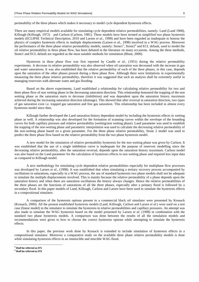
permeability of the three phases which makes it necessary to model cycle dependent hysteresis effects.

There are many empirical models available for simulating cycle dependent relative permeabilities, namely: Land (Land 1968),

Killough (Killough, 1972) and Carlson (Carlson, 1981). These models have been termed as simplified two phase hysteresis

models (ECLIPSE Technical Description, 2010 and Larsen et al., 1998) and have been regarded as inadequate to honour the

physics of complex hysteresis effects in multiple displacements (Larsen et al., 1998) involved in a WAG process. Moreover

the performance of the three phase relative permeability models, namely: Stone13, Stone2

4 and ECL default, used to model the

oil relative permeability in three phase flow, has been debated in the literature on many occasions. Among the three methods,

Stone1 and ECL default are regarded as the most suitable methods for simulation (Blunt, 2000).

Hysteresis in three phase flow was first reported by Caudle et al., (1951) during the relative permeability

experiments. A decrease in relative permeability was also observed when oil saturation was decreased with the increase in gas

and water saturations. It was also established that the relative permeability of each of the three phases, in this case, depends

upon the saturation of the other phases present during a three phase flow. Although there were limitations in experimentally

measuring the three phase relative permeability, therefore it was suggested that such an analysis shall be extremely useful in

managing reservoirs with alternate water and gas flooding.

Based on the above experiments, Land established a relationship for calculating relative permeability for two and

three phase flow of non wetting phase in the decreasing saturation direction. This relationship honoured the trapping of the non

wetting phase as the saturation starts to decrease (imbibition) and was dependent upon the saturation history maximum

achieved during the increasing saturation direction (drainage). This showed that after reversal in saturation direction, two types

of gas saturation exist i.e. trapped gas saturation and free gas saturation. This relationship has been included in almost every

hysteresis model since then.

Killough further developed the Land saturation history dependent model by including the hysteresis effects in wetting

phase as well. A relationship was also developed for the formation of scanning curves within the envelope of the bounding

curves for both capillary pressure and relative permeability (wetting/non wetting phase). Land parameter was used to establish

the trapping of the non-wetting phase and parametric interpolation was used to calculate the decreasing relative permeability of

the non-wetting phase based on a given parameter. For the three phase relative permeability, Stone 2 model was used to

predict the three phase flow based on the relative permeability from the two phase hysteresis model.

A new model for the simulation of relative permeability hysteresis for the non wetting phase was given by Carlson. It

was established that the use of a single imbibition curve is inadequate for the purpose of reservoir modelling since the

decreasing relative permeability, after the saturation reversal, depends upon the saturation history maximum. Carlson model

was also based on the Land parameter for the calculation of hysteresis effects in non wetting phase and required less input data

as compared to Killough model.

A new methodology for simulating cycle dependent relative permeabilities especially for multiphase flow processes

was developed by Larsen et al., (1998). It was established that when simulating a tertiary recovery process accompanied by

oscillations in saturations, especially in a WAG process, the use of standard hysteresis two phase models shall not be adequate

to simulate the multiple displacements involved. This is mainly because the relative permeability of a phase depends upon the

saturation history and when there are saturation oscillations the history always changes. Hence the relative permeabilities of

the three phases are the functions of saturations of all the three phases, especially after a primary flood is followed by a

secondary flood. In this paper models of Land, Killough, Carlson and Larsen have been used to simulate the hysteresis effects

in a compositional simulator.

A comparison of the hysteresis options present in a commercial black oil simulator were presented by Kossack

(Kossack, 2000). All the present established hysteresis models (Land, Killough, Carlson and Larsen et al.) were used on a test

case (linear model) in the simulator to simulate the hysteresis in relative permeabilities and capillary pressures. An attempt was

also made to simulate the WAG hysteresis based on the model presented by Larsen et al. (1998) in combination with the

standard two phase hysteresis models. A comparison was done between the results of all the simulation models and

recommendations were given to how to choose the correct hysteresis options while attempting to simulate the hysteresis

effects.

In this paper, the previous work done by Kossack is extended to include simulation of hysteresis effects in a

compositional simulator. Moreover a comparative study on the available three phase relative permeability models is done

while simulating hysteresis effects in an immiscible and miscible WAG flood.

3 Shall be referred as ST1 4 Shall be referred as ST2

10 [Three Phase Relative Permeability Models for WAG Simulation]

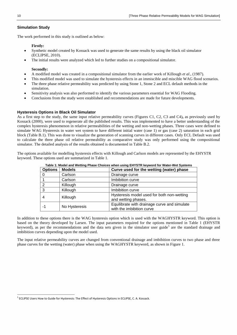
Simulation Study

The work performed in this study is outlined as below:

Firstly:

Synthetic model created by Kossack was used to generate the same results by using the black oil simulator

(ECLIPSE, 2010).

The initial results were analyzed which led to further studies on a compositional simulator.

Secondly:

A modified model was created in a compositional simulator from the earlier work of Killough et al., (1987).

This modified model was used to simulate the hysteresis effects in an immiscible and miscible WAG flood scenarios.

The three phase relative permeability was predicted by using Stone 1, Stone 2 and ECL default methods in the

simulation.

Sensitivity analysis was also performed to identify the various parameters essential for WAG Flooding.

Conclusions from the study were established and recommendations are made for future developments.

Hysteresis Options in Black Oil Simulator As a first step to the study, the same input relative permeability curves (Figures C1, C2, C3 and C4), as previously used by

Kossack (2000), were used to regenerate all the published results. This was implemented to have a better understanding of the

complex hysteresis phenomenon in relative permeabilities of the wetting and non-wetting phases. Three cases were defined to

simulate WAG Hysteresis in water wet system to have different initial water (case 1) or gas (case 2) saturation in each grid

block (Table B.1). This was done to visualize the generation of scanning curves in different cases. Only ECL Default was used

to calculate the three phase oil relative permeability as comparative study was only performed using the compositional

simulator. The detailed analysis of the results obtained is documented in Table B.2.

The options available for modelling hysteresis effects with Killough and Carlson models are represented by the EHYSTR

keyword. These options used are summarized in Table 1.

Table 1: Model and Wetting Phase Choices when using EHYSTR keyword for Water-Wet Systems

Options Models Curve used for the wetting (water) phase

0 Carlson Drainage curve

1 Carlson Imbibition curve

2 Killough Drainage curve

3 Killough Imbibition curve

4 Killough Hysteresis model used for both non-wetting and wetting phases.

-1 No Hysteresis Equilibrate with drainage curve and simulate with the imbibition curve

In addition to these options there is the WAG hysteresis option which is used with the WAGHYSTR keyword. This option is

based on the theory developed by Larsen. The input parameters required for the options mentioned in Table 1 (EHYSTR

keyword), as per the recommendations and the data sets given in the simulator user guide5 are the standard drainage and

imbibition curves depending upon the model used.

The input relative permeability curves are changed from conventional drainage and imbibition curves to two phase and three

phase curves for the wetting (water) phase when using the WAGHYSTR keyword, as shown in Figure 1.

5 ECLIPSE Users How to Guide for Hysteresis: The Effect of Hysteresis Options in ECLIPSE, C. A. Kossack.


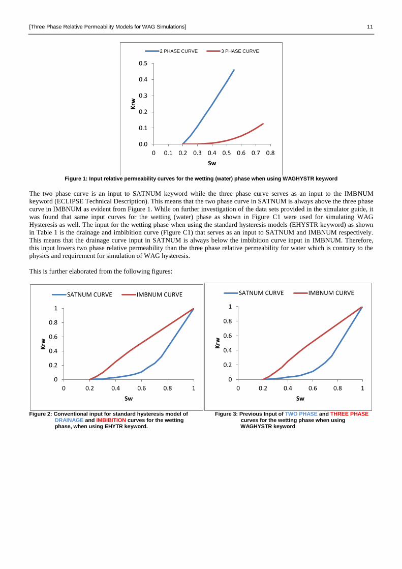
Figure 1: Input relative permeability curves for the wetting (water) phase when using WAGHYSTR keyword

The two phase curve is an input to SATNUM keyword while the three phase curve serves as an input to the IMBNUM

keyword (ECLIPSE Technical Description). This means that the two phase curve in SATNUM is always above the three phase

curve in IMBNUM as evident from Figure 1. While on further investigation of the data sets provided in the simulator guide, it

was found that same input curves for the wetting (water) phase as shown in Figure C1 were used for simulating WAG

Hysteresis as well. The input for the wetting phase when using the standard hysteresis models (EHYSTR keyword) as shown

in Table 1 is the drainage and imbibition curve (Figure C1) that serves as an input to SATNUM and IMBNUM respectively.

This means that the drainage curve input in SATNUM is always below the imbibition curve input in IMBNUM. Therefore,

this input lowers two phase relative permeability than the three phase relative permeability for water which is contrary to the

physics and requirement for simulation of WAG hysteresis.

This is further elaborated from the following figures:

Figure 2: Conventional input for standard hysteresis model of Figure 3: Previous Input of TWO PHASE and THREE PHASE DRAINAGE and IMBIBITION curves for the wetting curves for the wetting phase when using phase, when using EHYTR keyword. WAGHYSTR keyword

0.0

0.1

0.2

0.3

0.4

0.5

0 0.1 0.2 0.3 0.4 0.5 0.6 0.7 0.8

Krw

Sw

2 PHASE CURVE 3 PHASE CURVE

0

0.2

0.4

0.6

0.8

1

0 0.2 0.4 0.6 0.8 1

Krw

Sw

SATNUM CURVE IMBNUM CURVE

0

0.2

0.4

0.6

0.8

1

0 0.2 0.4 0.6 0.8 1

Krw

Sw

SATNUM CURVE IMBNUM CURVE


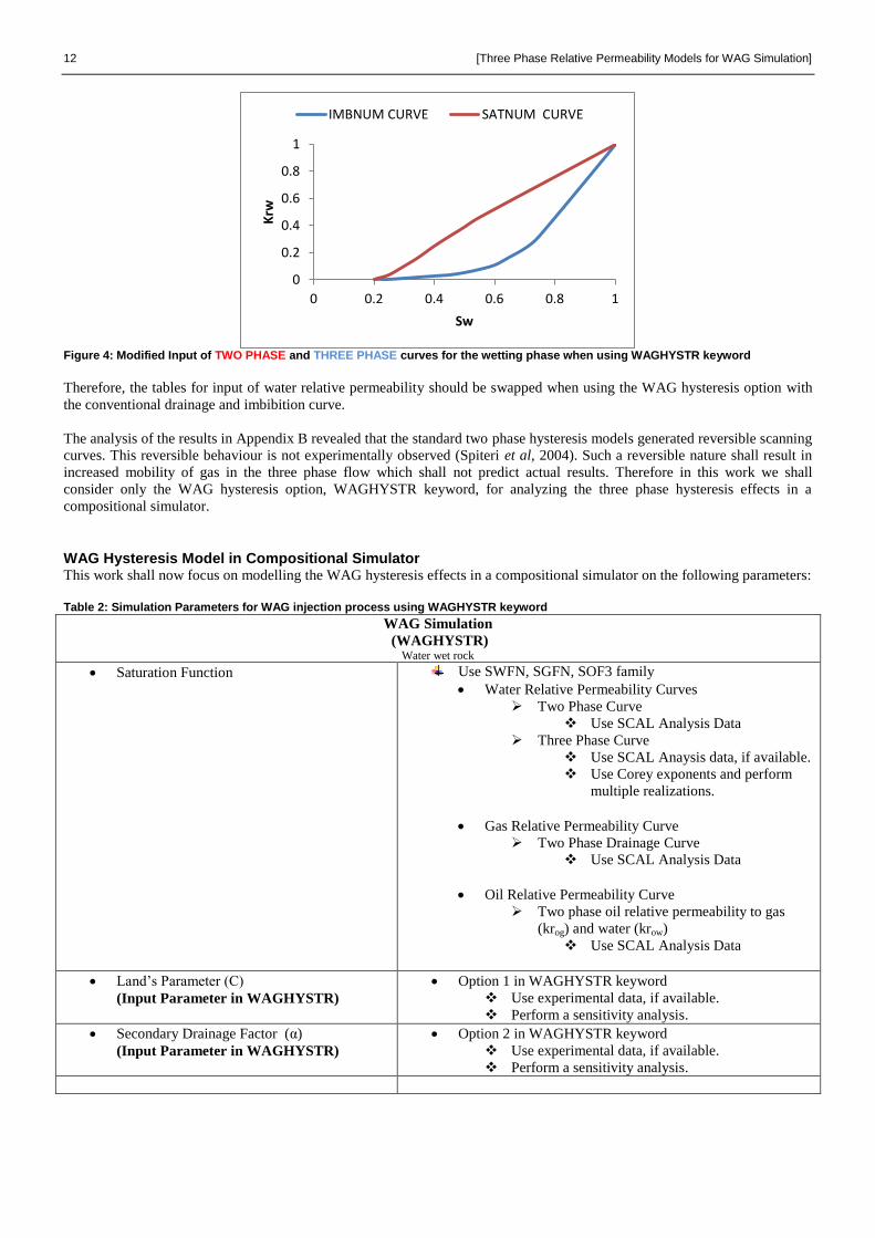
Figure 4: Modified Input of TWO PHASE and THREE PHASE curves for the wetting phase when using WAGHYSTR keyword

Therefore, the tables for input of water relative permeability should be swapped when using the WAG hysteresis option with

the conventional drainage and imbibition curve.

The analysis of the results in Appendix B revealed that the standard two phase hysteresis models generated reversible scanning

curves. This reversible behaviour is not experimentally observed (Spiteri et al, 2004). Such a reversible nature shall result in

increased mobility of gas in the three phase flow which shall not predict actual results. Therefore in this work we shall

consider only the WAG hysteresis option, WAGHYSTR keyword, for analyzing the three phase hysteresis effects in a

compositional simulator.

WAG Hysteresis Model in Compositional Simulator This work shall now focus on modelling the WAG hysteresis effects in a compositional simulator on the following parameters:

Table 2: Simulation Parameters for WAG injection process using WAGHYSTR keyword

WAG Simulation

(WAGHYSTR) Water wet rock

Saturation Function Use SWFN, SGFN, SOF3 family

Water Relative Permeability Curves

Two Phase Curve

Use SCAL Analysis Data

Three Phase Curve

Use SCAL Anaysis data, if available.

Use Corey exponents and perform

multiple realizations.

Gas Relative Permeability Curve

Two Phase Drainage Curve


Oil Relative Permeability Curve

Two phase oil relative permeability to gas

(krog) and water (krow)


Land’s Parameter (C)

(Input Parameter in WAGHYSTR)

Option 1 in WAGHYSTR keyword

Use experimental data, if available.

Perform a sensitivity analysis.

Secondary Drainage Factor (α)



Use experimental data, if available.

Perform a sensitivity analysis.

0

0.2

0.4

0.6

0.8

1

0 0.2 0.4 0.6 0.8 1

Krw

Sw

IMBNUM CURVE SATNUM CURVE


Three Phase Model Threshold Saturation



The water saturation fraction above the connate

water saturation at which the gas phase hysteresis

shifts from two phase to three phase curve.

i.e: In three Phase Curve

(Sw)cr - Swc

Three Phase Oil Relative Permeability Model Use STONE1, STONE2 an d ECLIPSE Default

Analyze results of all the methods and compare it

with the esablished physics of WAG

Residual Oil Modification Fraction

(Valid only for STONE1)


Use experimentally determined value, if available.

Perform sensitivity analysis.

Length of WAG Injection Cycle First Injection Cycle: Gas (Recommended)

Perform sensitivity analysis.

Timestep and Tuning Simulation Time Step should be kept small to honour the

saturation oscillations (e.g 1 Day in this case)

Convergence issues, as experienced, might occur in finer

models

Use TUNING keyword.

Use TSCRIT and CVCRIT keywords.

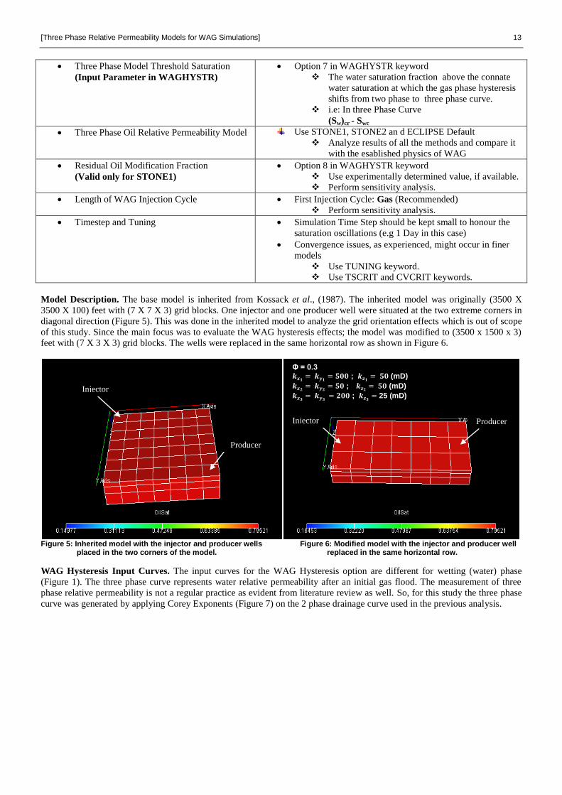
Model Description. The base model is inherited from Kossack et al., (1987). The inherited model was originally (3500 X

3500 X 100) feet with (7 X 7 X 3) grid blocks. One injector and one producer well were situated at the two extreme corners in

diagonal direction (Figure 5). This was done in the inherited model to analyze the grid orientation effects which is out of scope

of this study. Since the main focus was to evaluate the WAG hysteresis effects; the model was modified to (3500 x 1500 x 3)

feet with (7 X 3 X 3) grid blocks. The wells were replaced in the same horizontal row as shown in Figure 6.

Figure 5: Inherited model with the injector and producer wells Figure 6: Modified model with the injector and producer well placed in the two corners of the model. replaced in the same horizontal row.

WAG Hysteresis Input Curves. The input curves for the WAG Hysteresis option are different for wetting (water) phase

(Figure 1). The three phase curve represents water relative permeability after an initial gas flood. The measurement of three

phase relative permeability is not a regular practice as evident from literature review as well. So, for this study the three phase

curve was generated by applying Corey Exponents (Figure 7) on the 2 phase drainage curve used in the previous analysis.

Injector

Producer

Producer Injector

Φ = 0.3

𝒌𝒙𝟏= 𝒌𝒚𝟏

= 𝟓𝟎𝟎 ; 𝒌𝒛𝟏= 𝟓𝟎 (mD)

𝒌𝒙𝟐= 𝒌𝒚𝟐

= 𝟓𝟎 ; 𝒌𝒛𝟐= 𝟓𝟎 (mD)

𝒌𝒙𝟑= 𝒌𝒚𝟑 = 𝟐𝟎𝟎 ; 𝒌𝒛𝟑

= 25 (mD)


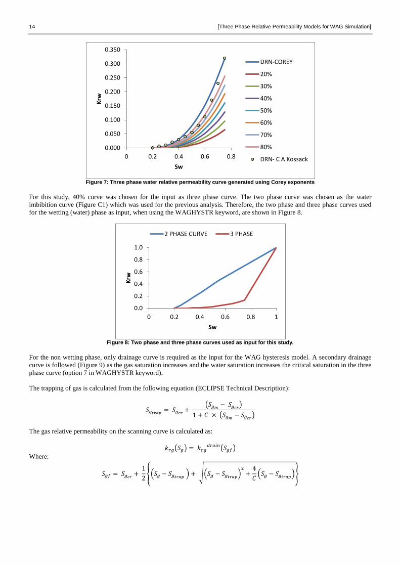
Figure 7: Three phase water relative permeability curve generated using Corey exponents

For this study, 40% curve was chosen for the input as three phase curve. The two phase curve was chosen as the water

imbibition curve (Figure C1) which was used for the previous analysis. Therefore, the two phase and three phase curves used

for the wetting (water) phase as input, when using the WAGHYSTR keyword, are shown in Figure 8.

Figure 8: Two phase and three phase curves used as input for this study.

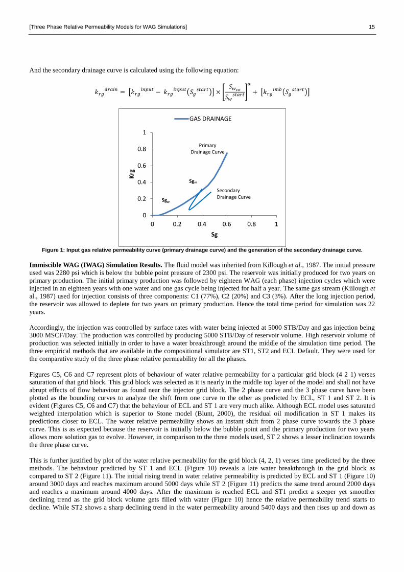
For the non wetting phase, only drainage curve is required as the input for the WAG hysteresis model. A secondary drainage

curve is followed (Figure 9) as the gas saturation increases and the water saturation increases the critical saturation in the three

phase curve (option 7 in WAGHYSTR keyword).

The trapping of gas is calculated from the following equation (ECLIPSE Technical Description):

𝑆𝑔𝑡𝑟𝑎𝑝= 𝑆𝑔𝑐𝑟

+ (𝑆𝑔𝑚

− 𝑆𝑔𝑐𝑟)

1 + 𝐶 × (𝑆𝑔𝑚− 𝑆𝑔𝑐𝑟

)

The gas relative permeability on the scanning curve is calculated as:

𝑘𝑟𝑔(𝑆𝑔) = 𝑘𝑟𝑔𝑑𝑟𝑎𝑖𝑛(𝑆𝑔𝑓)

Where:

𝑆𝑔𝑓 = 𝑆𝑔𝑐𝑟+

1

2{(𝑆𝑔 − 𝑆𝑔𝑡𝑟𝑎𝑝

) + √(𝑆𝑔 − 𝑆𝑔𝑡𝑟𝑎𝑝)

2

+4

𝐶(𝑆𝑔 − 𝑆𝑔𝑡𝑟𝑎𝑝

)}

0.000

0.050

0.100

0.150

0.200

0.250

0.300

0.350

0 0.2 0.4 0.6 0.8

Krw

Sw

DRN-COREY

20%

30%

40%

50%

60%

70%

80%

DRN- C A Kossack

0.0

0.2

0.4

0.6

0.8

1.0

0 0.2 0.4 0.6 0.8 1

Krw

Sw

2 PHASE CURVE 3 PHASE


And the secondary drainage curve is calculated using the following equation:

𝑘𝑟𝑔𝑑𝑟𝑎𝑖𝑛 = [𝑘𝑟𝑔

𝑖𝑛𝑝𝑢𝑡 − 𝑘𝑟𝑔𝑖𝑛𝑝𝑢𝑡(𝑆𝑔

𝑠𝑡𝑎𝑟𝑡)] × [𝑆𝑤𝑐𝑜

𝑆𝑤𝑠𝑡𝑎𝑟𝑡]

𝛼

+ [𝑘𝑟𝑔𝑖𝑚𝑏(𝑆𝑔

𝑠𝑡𝑎𝑟𝑡)]

Figure 1: Input gas relative permeability curve (primary drainage curve) and the generation of the secondary drainage curve.

Immiscible WAG (IWAG) Simulation Results. The fluid model was inherited from Killough et al., 1987. The initial pressure

used was 2280 psi which is below the bubble point pressure of 2300 psi. The reservoir was initially produced for two years on

primary production. The initial primary production was followed by eighteen WAG (each phase) injection cycles which were

injected in an eighteen years with one water and one gas cycle being injected for half a year. The same gas stream (Kiilough et

al., 1987) used for injection consists of three components: C1 (77%), C2 (20%) and C3 (3%). After the long injection period,

the reservoir was allowed to deplete for two years on primary production. Hence the total time period for simulation was 22

years.

Accordingly, the injection was controlled by surface rates with water being injected at 5000 STB/Day and gas injection being

3000 MSCF/Day. The production was controlled by producing 5000 STB/Day of reservoir volume. High reservoir volume of

production was selected initially in order to have a water breakthrough around the middle of the simulation time period. The

three empirical methods that are available in the compositional simulator are ST1, ST2 and ECL Default. They were used for

the comparative study of the three phase relative permeability for all the phases.

Figures C5, C6 and C7 represent plots of behaviour of water relative permeability for a particular grid block (4 2 1) verses

saturation of that grid block. This grid block was selected as it is nearly in the middle top layer of the model and shall not have

abrupt effects of flow behaviour as found near the injector grid block. The 2 phase curve and the 3 phase curve have been

plotted as the bounding curves to analyze the shift from one curve to the other as predicted by ECL, ST 1 and ST 2. It is

evident (Figures C5, C6 and C7) that the behaviour of ECL and ST 1 are very much alike. Although ECL model uses saturated

weighted interpolation which is superior to Stone model (Blunt, 2000), the residual oil modification in ST 1 makes its

predictions closer to ECL. The water relative permeability shows an instant shift from 2 phase curve towards the 3 phase

curve. This is as expected because the reservoir is initially below the bubble point and the primary production for two years

allows more solution gas to evolve. However, in comparison to the three models used, ST 2 shows a lesser inclination towards

the three phase curve.

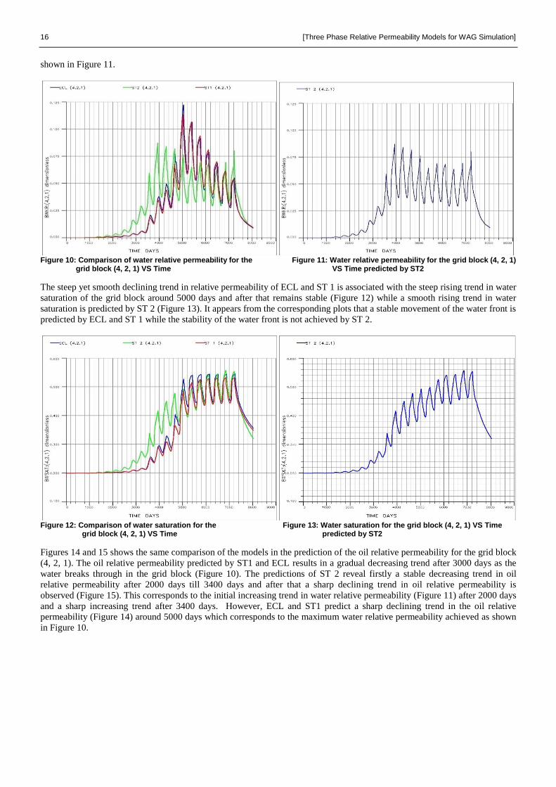
This is further justified by plot of the water relative permeability for the grid block (4, 2, 1) verses time predicted by the three

methods. The behaviour predicted by ST 1 and ECL (Figure 10) reveals a late water breakthrough in the grid block as

compared to ST 2 (Figure 11). The initial rising trend in water relative permeability is predicted by ECL and ST 1 (Figure 10)

around 3000 days and reaches maximum around 5000 days while ST 2 (Figure 11) predicts the same trend around 2000 days

and reaches a maximum around 4000 days. After the maximum is reached ECL and ST1 predict a steeper yet smoother

declining trend as the grid block volume gets filled with water (Figure 10) hence the relative permeability trend starts to

decline. While ST2 shows a sharp declining trend in the water permeability around 5400 days and then rises up and down as

0

0.2

0.4

0.6

0.8

1

0 0.2 0.4 0.6 0.8 1

Krg

Sg

GAS DRAINAGE

Sgcr

Primary Drainage Curve

Secondary Drainage Curve

Sgm


shown in Figure 11.

Figure 10: Comparison of water relative permeability for the Figure 11: Water relative permeability for the grid block (4, 2, 1) grid block (4, 2, 1) VS Time VS Time predicted by ST2

The steep yet smooth declining trend in relative permeability of ECL and ST 1 is associated with the steep rising trend in water

saturation of the grid block around 5000 days and after that remains stable (Figure 12) while a smooth rising trend in water

saturation is predicted by ST 2 (Figure 13). It appears from the corresponding plots that a stable movement of the water front is

predicted by ECL and ST 1 while the stability of the water front is not achieved by ST 2.

Figure 12: Comparison of water saturation for the Figure 13: Water saturation for the grid block (4, 2, 1) VS Time grid block (4, 2, 1) VS Time predicted by ST2

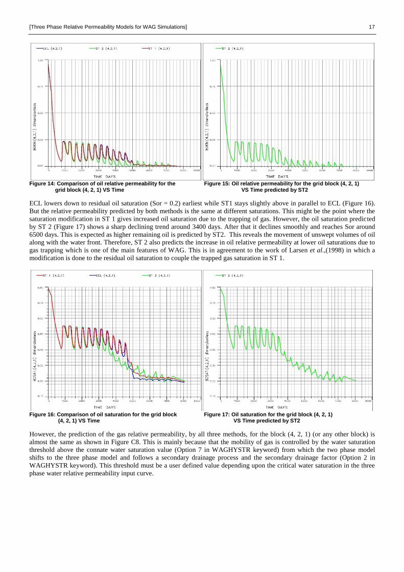
Figures 14 and 15 shows the same comparison of the models in the prediction of the oil relative permeability for the grid block

(4, 2, 1). The oil relative permeability predicted by ST1 and ECL results in a gradual decreasing trend after 3000 days as the

water breaks through in the grid block (Figure 10). The predictions of ST 2 reveal firstly a stable decreasing trend in oil

relative permeability after 2000 days till 3400 days and after that a sharp declining trend in oil relative permeability is

observed (Figure 15). This corresponds to the initial increasing trend in water relative permeability (Figure 11) after 2000 days

and a sharp increasing trend after 3400 days. However, ECL and ST1 predict a sharp declining trend in the oil relative

permeability (Figure 14) around 5000 days which corresponds to the maximum water relative permeability achieved as shown

in Figure 10.


Figure 14: Comparison of oil relative permeability for the Figure 15: Oil relative permeability for the grid block (4, 2, 1) grid block (4, 2, 1) VS Time VS Time predicted by ST2

ECL lowers down to residual oil saturation (Sor = 0.2) earliest while ST1 stays slightly above in parallel to ECL (Figure 16).

But the relative permeability predicted by both methods is the same at different saturations. This might be the point where the

saturation modification in ST 1 gives increased oil saturation due to the trapping of gas. However, the oil saturation predicted

by ST 2 (Figure 17) shows a sharp declining trend around 3400 days. After that it declines smoothly and reaches Sor around

6500 days. This is expected as higher remaining oil is predicted by ST2. This reveals the movement of unswept volumes of oil

along with the water front. Therefore, ST 2 also predicts the increase in oil relative permeability at lower oil saturations due to

gas trapping which is one of the main features of WAG. This is in agreement to the work of Larsen et al.,(1998) in which a

modification is done to the residual oil saturation to couple the trapped gas saturation in ST 1.

Figure 16: Comparison of oil saturation for the grid block Figure 17: Oil saturation for the grid block (4, 2, 1) (4, 2, 1) VS Time VS Time predicted by ST2

However, the prediction of the gas relative permeability, by all three methods, for the block (4, 2, 1) (or any other block) is

almost the same as shown in Figure C8. This is mainly because that the mobility of gas is controlled by the water saturation

threshold above the connate water saturation value (Option 7 in WAGHYSTR keyword) from which the two phase model

shifts to the three phase model and follows a secondary drainage process and the secondary drainage factor (Option 2 in

WAGHYSTR keyword). This threshold must be a user defined value depending upon the critical water saturation in the three

phase water relative permeability input curve.


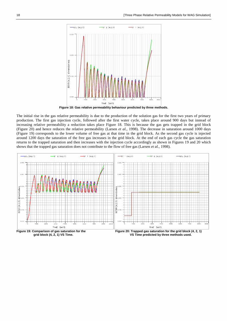
Figure 18: Gas relative permeability behaviour predicted by three methods.

The initial rise in the gas relative permeability is due to the production of the solution gas for the first two years of primary

production. The first gas injection cycle, followed after the first water cycle, takes place around 900 days but instead of

increasing relative permeability a reduction takes place Figure 18. This is because the gas gets trapped in the grid block

(Figure 20) and hence reduces the relative permeability (Larsen et al., 1998). The decrease in saturation around 1000 days

(Figure 19) corresponds to the lower volume of free gas at that time in the grid block. As the second gas cycle is injected

around 1200 days the saturation of the free gas increases in the grid block. At the end of each gas cycle the gas saturation

returns to the trapped saturation and then increases with the injection cycle accordingly as shown in Figures 19 and 20 which

shows that the trapped gas saturation does not contribute to the flow of free gas (Larsen et al., 1998).

Figure 19: Comparison of gas saturation for the Figure 20: Trapped gas saturation for the grid block (4, 2, 1) grid block (4, 2, 1) VS Time. VS Time predicted by three methods used.


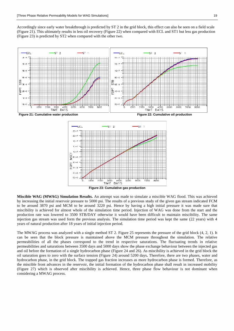
Accordingly since early water breakthrough is predicted by ST 2 in the grid block, this effect can also be seen on a field scale

(Figure 21). This ultimately results in less oil recovery (Figure 22) when compared with ECL and ST1 but less gas production

(Figure 23) is predicted by ST2 when compared with the other two.

Figure 21: Cumulative water production Figure 22: Cumulative oil production

Figure 23: Cumulative gas production

Miscible WAG (MWAG) Simulation Results. An attempt was made to simulate a miscible WAG flood. This was achieved

by increasing the initial reservoir pressure to 5000 psi. The results of a previous study of the given gas stream indicated FCM

to be around 3870 psi and MCM to be around 3220 psi. Hence by having a high initial pressure it was made sure that

miscibility is achieved for almost whole of the simulation time period. Injection of WAG was done from the start and the

production rate was lowered to 3500 STB/DAY otherwise it would have been difficult to maintain miscibility. The same

injection gas stream was used form the previous analysis. The simulation time period was kept the same (22 years) with 4

years of natural production after 18 years of initial injection period.

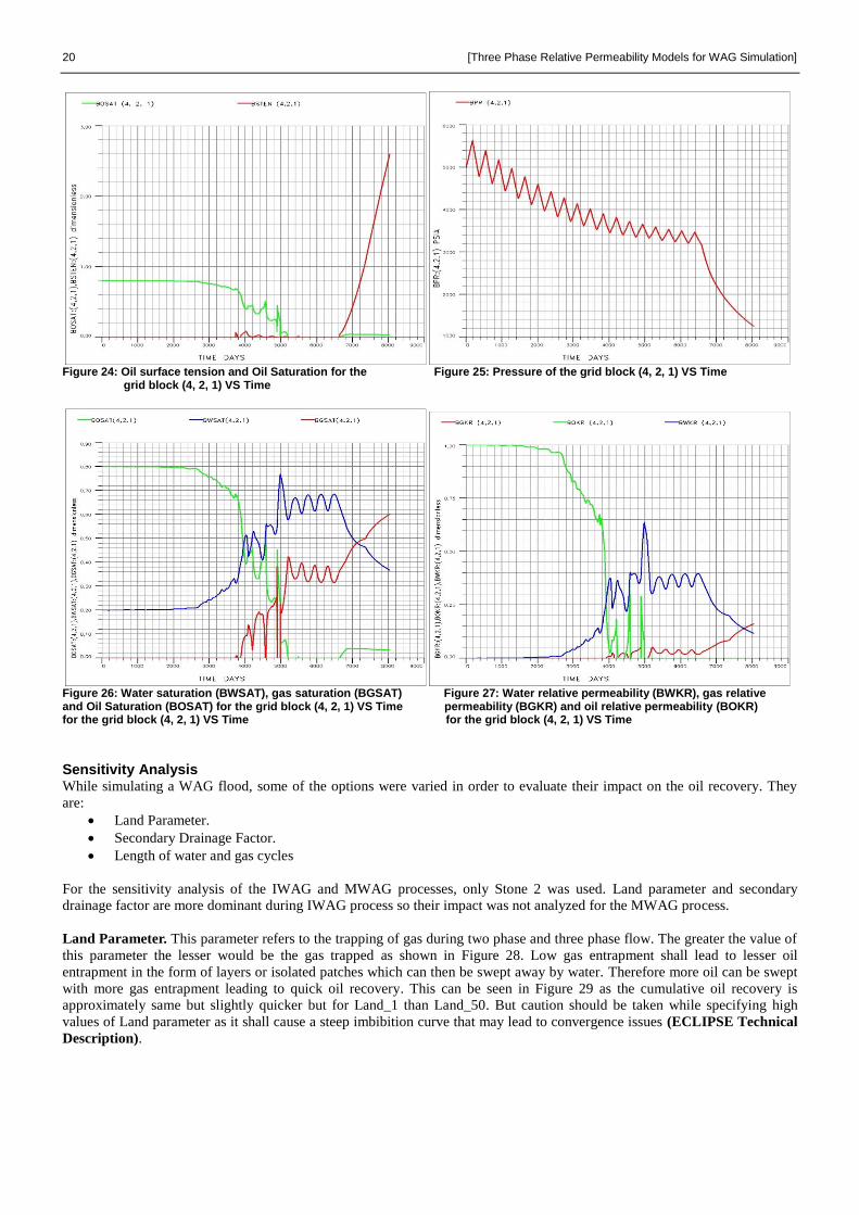
The MWAG process was analyzed with a single method ST 2. Figure 25 represents the pressure of the grid block (4, 2, 1). It

can be seen that the block pressure is maintained above the MCM pressure throughout the simulation. The relative

permeabilities of all the phases correspond to the trend in respective saturations. The fluctuating trends in relative

permeabilities and saturations between 3500 days and 5000 days show the phase exchange behaviour between the injected gas

and oil before the formation of a single hydrocarbon phase (Figure 24 and 26). As miscibility is achieved in the grid block the

oil saturation goes to zero with the surface tension (Figure 24) around 5200 days. Therefore, there are two phases, water and

hydrocarbon phase, in the grid block. The trapped gas fraction increases as more hydrocarbon phase is formed. Therefore, as

the miscible front advances in the reservoir, the initial formation of the hydrocarbon phase shall result in increased mobility

(Figure 27) which is observed after miscibility is achieved. Hence, three phase flow behaviour is not dominant when

considering a MWAG process.


Figure 24: Oil surface tension and Oil Saturation for the Figure 25: Pressure of the grid block (4, 2, 1) VS Time grid block (4, 2, 1) VS Time

Figure 26: Water saturation (BWSAT), gas saturation (BGSAT) Figure 27: Water relative permeability (BWKR), gas relative and Oil Saturation (BOSAT) for the grid block (4, 2, 1) VS Time permeability (BGKR) and oil relative permeability (BOKR) for the grid block (4, 2, 1) VS Time for the grid block (4, 2, 1) VS Time

Sensitivity Analysis While simulating a WAG flood, some of the options were varied in order to evaluate their impact on the oil recovery. They

are:

Land Parameter.

Secondary Drainage Factor.

Length of water and gas cycles

For the sensitivity analysis of the IWAG and MWAG processes, only Stone 2 was used. Land parameter and secondary

drainage factor are more dominant during IWAG process so their impact was not analyzed for the MWAG process.

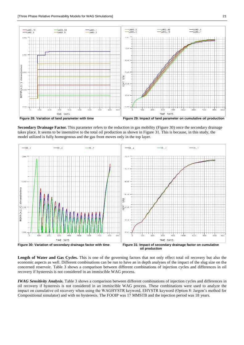
Land Parameter. This parameter refers to the trapping of gas during two phase and three phase flow. The greater the value of

this parameter the lesser would be the gas trapped as shown in Figure 28. Low gas entrapment shall lead to lesser oil

entrapment in the form of layers or isolated patches which can then be swept away by water. Therefore more oil can be swept

with more gas entrapment leading to quick oil recovery. This can be seen in Figure 29 as the cumulative oil recovery is

approximately same but slightly quicker but for Land_1 than Land_50. But caution should be taken while specifying high

values of Land parameter as it shall cause a steep imbibition curve that may lead to convergence issues (ECLIPSE Technical

Description).


Figure 28: Variation of land parameter with time Figure 29: Impact of land parameter on cumulative oil production

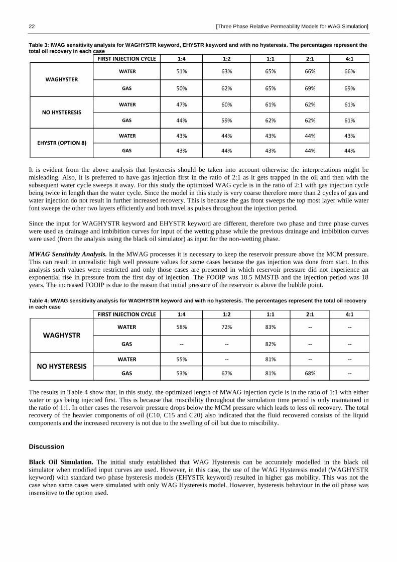
Secondary Drainage Factor. This parameter refers to the reduction in gas mobility (Figure 30) once the secondary drainage

takes place. It seems to be insensitive to the total oil production as shown in Figure 31. This is because, in this study, the

model utilized is fully homogenous and the gas front moves only in the top layer.

Figure 30: Variation of secondary drainage factor with time Figure 31: Impact of secondary drainage factor on cumulative oil production

Length of Water and Gas Cycles. This is one of the governing factors that not only effect total oil recovery but also the

economic aspects as well. Different combinations can be run to have an in depth analyses of the impact of the slug size on the

concerned reservoir. Table 3 shows a comparison between different combinations of injection cycles and differences in oil

recovery if hysteresis is not considered in an immiscible WAG process.

IWAG Sensitivity Analysis. Table 3 shows a comparison between different combinations of injection cycles and differences in

oil recovery if hysteresis is not considered in an immiscible WAG process. These combinations were used to analyze the

impact on cumulative oil recovery when using the WAGHYSTR keyword, EHYSTR keyword (Option 8: Jargon’s method for

Compositional simulator) and with no hysteresis. The FOOIP was 17 MMSTB and the injection period was 18 years.


Table 3: IWAG sensitivity analysis for WAGHYSTR keyword, EHYSTR keyword and with no hysteresis. The percentages represent the total oil recovery in each case

It is evident from the above analysis that hysteresis should be taken into account otherwise the interpretations might be

misleading. Also, it is preferred to have gas injection first in the ratio of 2:1 as it gets trapped in the oil and then with the

subsequent water cycle sweeps it away. For this study the optimized WAG cycle is in the ratio of 2:1 with gas injection cycle

being twice in length than the water cycle. Since the model in this study is very coarse therefore more than 2 cycles of gas and

water injection do not result in further increased recovery. This is because the gas front sweeps the top most layer while water

font sweeps the other two layers efficiently and both travel as pulses throughout the injection period.

Since the input for WAGHYSTR keyword and EHYSTR keyword are different, therefore two phase and three phase curves

were used as drainage and imbibition curves for input of the wetting phase while the previous drainage and imbibition curves

were used (from the analysis using the black oil simulator) as input for the non-wetting phase.

MWAG Sensitivity Analysis. In the MWAG processes it is necessary to keep the reservoir pressure above the MCM pressure.

This can result in unrealistic high well pressure values for some cases because the gas injection was done from start. In this

analysis such values were restricted and only those cases are presented in which reservoir pressure did not experience an

exponential rise in pressure from the first day of injection. The FOOIP was 18.5 MMSTB and the injection period was 18

years. The increased FOOIP is due to the reason that initial pressure of the reservoir is above the bubble point.

Table 4: MWAG sensitivity analysis for WAGHYSTR keyword and with no hysteresis. The percentages represent the total oil recovery in each case

The results in Table 4 show that, in this study, the optimized length of MWAG injection cycle is in the ratio of 1:1 with either

water or gas being injected first. This is because that miscibility throughout the simulation time period is only maintained in

the ratio of 1:1. In other cases the reservoir pressure drops below the MCM pressure which leads to less oil recovery. The total

recovery of the heavier components of oil (C10, C15 and C20) also indicated that the fluid recovered consists of the liquid

components and the increased recovery is not due to the swelling of oil but due to miscibility.

Discussion

Black Oil Simulation. The initial study established that WAG Hysteresis can be accurately modelled in the black oil

simulator when modified input curves are used. However, in this case, the use of the WAG Hysteresis model (WAGHYSTR

keyword) with standard two phase hysteresis models (EHYSTR keyword) resulted in higher gas mobility. This was not the

case when same cases were simulated with only WAG Hysteresis model. However, hysteresis behaviour in the oil phase was

insensitive to the option used.

FIRST INJECTION CYCLE 1:4 1:2 1:1 2:1 4:1

WATER 51% 63% 65% 66% 66%

GAS 50% 62% 65% 69% 69%

WATER 47% 60% 61% 62% 61%

GAS 44% 59% 62% 62% 61%

WATER 43% 44% 43% 44% 43%

GAS 43% 44% 43% 44% 44%

WAGHYSTER

NO HYSTERESIS

EHYSTR (OPTION 8)

FIRST INJECTION CYCLE 1:4 1:2 1:1 2:1 4:1

WATER 58% 72% 83% -- --

GAS -- -- 82% -- --

WATER 55% -- 81% -- --

GAS 53% 67% 81% 68% --

WAGHYSTR

NO HYSTERESIS


IWAG Simulation. The comparative study of the empirical three phase relative permeability models show that ST 1 with the

oil modification factor predicts the behaviour in agreement with ECL Default. The predictions of ST2 result in total oil

recovery which is less when compared with the other two models. However, ST 2 also predicts increased oil relative

permeability at lower oil saturations. The sensitivity analysis shows that the total oil recovery is insensitive to variations in the

Land parameter and secondary drainage factor. However, the rate of recovery might be increased with the increasing trapping

and reduction of gas mobility. The length of the injection cycles can be an essential parameter to optimize the total oil

production and the economics of the process.

MWAG Simulation. The MWAG simulations showed that as miscibility is achieved in the reservoir, two phase flow

behaviour is dominant. The sensitivity analysis resulted in increased total oil recoveries with less injection of water and gas.

However, to maintain pressure above the MCM for the whole production time period may not be feasible. As the pressure

reduces, three phase flow behaviour can be observed similar to the immiscible case.

For a full field study, it is possible that different hysteresis behaviour may occur in different areas of the reservoir. The present

options in the simulator do not allow for the simulation of simultaneous two phase and three phase hysteresis in separate

regions.

Conclusions and Recommendations for Future Research In this work, hysteresis effects have been modelled in WAG simulation and multiple sensitivity studies on various parameters

and their effect on total oil recovery have been presented. From this study we conclude:

The WAG hysteresis model is effective for presenting the effects of gas trapping in a WAG flood.

For the models used in this study, the effect of combining the standard two phase hysteresis models with WAG

Hysteresis model was not significant.

Multiple realizations can be created for future studies by selecting different reduced water relative permeabilities to

be input as the three phase curve when using the WAGHYSTR keyword.

In this study the cumulative oil recovery was insensitive to variation of the Land parameter and secondary drainage

factor.

Three phase hysteresis effects are not dominant in the MWAG process. Higher oil recoveries due to increased trapped

gas fraction and miscibility with equal volumes of injection phases were observed in this study. Further detailed

analysis can be performed by using different two phase hysteresis models.

Provisions should be made in the simulator to model two phase and three phase hysteresis in different regions. This

shall help in modelling miscible and immiscible regions in MWAG process.

Further study is required by developing a fine scale model to quantify the physical and numerical dispersion effects

along with visualizing the frontal advancement.

More studies in simulating the hysteresis effects in an oil-wet or a mixed-wet system are required. The recently

developed complex three phase pore network models that predict lab data in good agreement for all wettability

conditions may be used for this purpose.

Selection of options available for the empirical three phase relative permeability models, in conjunction with the

options available for hysteresis can depend on data and processes considered in the study. Detailed analysis with

history matching should be performed before any specific method is selected.

Considering options in available to model the hysteresis effects, multiple sensitivity analysis with multiple

combinations can be performed to analyze the impact on the cumulative oil recovery.

Nomenclature BGKR Block Gas Relative Permeability krog Relative Permeability of oil in gas

BGSAT Block Gas Saturation krow Relative Permeability of oil in water

BGTRP Block Gas Trapped Saturation MCM Multi Contact Miscible BPR Block Pressure MSCF Million Standard Cubic Feet

BOKR Block Oil Relative Permeability psi Pressure per square inch

BOSAT Block Oil Saturation SCAL Special Core Analysis BSTEN Block Surface Tension Sg Saturation of gas

BWKR Block Water Relative Permeability So Saturation of oil

BWSAT Block Water Saturation Sor Residual Oil Saturation krg Relative Permeability of gas Sw Saturation of Water

FCM First Contact Miscible (Sw)cr Critical Water Saturation

FGPT Total Field Gas Production Swc Connate Water Saturation FOPT Total Field Oil Production STB Stock Tank Barrel

FWPT Total Field Water Production FOOIP Field Oil Originally In Place

Krw Relative Permeability of water


Acknowledgement I would like to offer heartfelt gratitude and appreciation to my supervisor Marie Ann Giddins (Schlumberger). Her insight,

encyclopaedic knowledge and support made this project possible. I owe a large debt to Mr. Zeeshan Jilani (Schlumberger) for

his exceptional mentoring and sparing time to answer all my questions during never ending discussions. I am also grateful to

Mr. Raheel Baig (Schlumberger) for his valuable advice throughout the research, for doing a critical review and for proof

reading my thesis. I wish to thank Abingdon Technology Centre for giving me this opportunity, for providing an excellent

professional environment and for all the necessary resources during the course of this project.

References Blunt M. J.: “An Empirical Model for Three-Phase Relative Permeability,” paper SPE 67950, SPEJ 5 (4), presented at the 1999 SPE Annual

Technical Conference and Exhibition held in Houston, 3-6 October.

Carlson, Francais M.: “Simulation of Relative Permeability Hysteresis to the Nonwetting Phase,” paper SPE 10157, presented at the 56th

Annual Fall Technical Conference and Exhibition of the Society of Petroleum Engineers of AIME, held in San Antonio, Texas,

October 5-7, 1981.

Christensen, J. R., Stenby, E.H. and Skauge, A.: “Review of WAG Field Experience,” paper SPE 71203, presented at the 1998 SPE

International Petroleum Conference and Exhibition of Mexico, Villahermosa, Mexico, 3-5 March. April 2001 SPE Reservoir

Evaluation and Engineering.

Caudle, B.H., Slobod, R. L. and Brownscombe, E. R.: “Further Developments in the Laboratory Determination of Relative Permeability,”

paper SPE 951145

ECLIPSE Reference Manual and ECLIPSE Technical Description, Copyright 2010, Schlumberger

Elilzabeth J. Spiteri., Ruben Juanes,: “Impact of Relative Permeability hysteresis on Numerical simulation of WAG Injection,” paper SPE

89921, prepared for presentation at the SPE Annual Technical Conference and Exhibition held in Houston, Texas, USA, 26-29

September 2004.

Killough, J. E.: “Reservoir Simulation with History-Dependent Saturation Functions,” paper SPE 5105, was presented at the SPE-AIME 49th

Annual Fall Meeting, held in Houston, October 6-9, 1974.

Killough, J. E., Kossack, C. A.: “Fifth Comparative Solution Project: Evaluation Of Miscible Flood Simulators,” paper SPE 16000, prepared

for presentation at the Ninth SPE Symposium on Reservoir Simulation held in San Antonio, Texas, February 1-4, 1987.

Kossack, C. A.: “Comparison of Reservoir Simulation Hysteresis Options,” paper SPE 63147, prepared for presentation at the 2000 SPE

Annual Technical Conference and Exhibition held in Dallas, Texas, 1-4 October 2000.

Land, C. S.: “Calculation of Imbibition relative Permeability for Two and Three-Phase Flow from Rock Properties,” paper SPE 1942,

presented at the SPE 42nd Annual Fall Meeting held in Houston, Texas, USA, October 1-4, 1967.

Larsen, J. A., Skauge, A.: “Methodology for Numerical simulation with Cycle-Dependent relative Permeabilities,” paper SPE 38456, SPEJ,

June 1998.

Oak, M. J.: “Three Phase Relative Permeability of Water-wet Berea,” paper SPE/DOE 20183, prepared for presentation at the SPE/DOE

Seventh Symposium on Enhanced Oil Recovery held in Tulsa, Oklahama, April 22-25, 1990.

Stone H. L.: “Estimation of Three-Phase Relative Permeability and Residual Oil Data,” JCPT 12(4), Page 214-218, May 1973.

Stone H.L.: “Probability Model for Estimating Three-Phase Relative Permeability,” paper SPE 2116, February 1970.

Sander Suicmez, V., Mohammed Piri, Blunt, M. J.: “Pore-scale Simulation of Water Alternate Gas Injection,” Transport in Porous Media

(2007) 66:259-286, copyright Springer 2007.

[Three Phase Relative Permeability Models for WAG Simulations] I

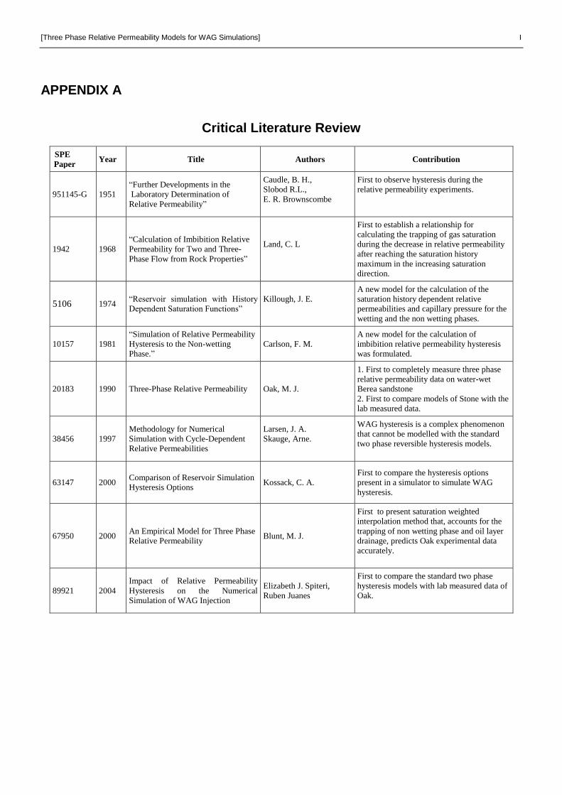
APPENDIX A

Critical Literature Review

SPE

Paper Year Title Authors Contribution

951145-G 1951

“Further Developments in the

Laboratory Determination of

Relative Permeability”

Caudle, B. H.,

Slobod R.L.,

E. R. Brownscombe

First to observe hysteresis during the

relative permeability experiments.

1942 1968

“Calculation of Imbibition Relative

Permeability for Two and Three-

Phase Flow from Rock Properties”

Land, C. L

First to establish a relationship for

calculating the trapping of gas saturation

during the decrease in relative permeability

after reaching the saturation history

maximum in the increasing saturation

direction.

5106 1974 “Reservoir simulation with History

Dependent Saturation Functions”

Killough, J. E.

A new model for the calculation of the

saturation history dependent relative

permeabilities and capillary pressure for the

wetting and the non wetting phases.

10157 1981

“Simulation of Relative Permeability

Hysteresis to the Non-wetting

Phase.” Carlson, F. M.

A new model for the calculation of

imbibition relative permeability hysteresis

was formulated.

20183 1990 Three-Phase Relative Permeability Oak, M. J.

1. First to completely measure three phase

relative permeability data on water-wet

Berea sandstone

2. First to compare models of Stone with the

lab measured data.

38456 1997

Methodology for Numerical

Simulation with Cycle-Dependent

Relative Permeabilities

Larsen, J. A.

Skauge, Arne.

WAG hysteresis is a complex phenomenon

that cannot be modelled with the standard

two phase reversible hysteresis models.

63147 2000 Comparison of Reservoir Simulation

Hysteresis Options Kossack, C. A.

First to compare the hysteresis options

present in a simulator to simulate WAG

hysteresis.

67950 2000 An Empirical Model for Three Phase

Relative Permeability Blunt, M. J.

First to present saturation weighted

interpolation method that, accounts for the

trapping of non wetting phase and oil layer

drainage, predicts Oak experimental data

accurately.

89921 2004

Impact of Relative Permeability

Hysteresis on the Numerical

Simulation of WAG Injection

Elizabeth J. Spiteri,

Ruben Juanes

First to compare the standard two phase

hysteresis models with lab measured data of

Oak.

II [Three Phase Relative Permeability Models for WAG Simulation]

SPE 951145-G (1951)

Further Developments in the Laboratory Determination of Relative Permeability

Author: Caudle, B. H., Slobod R.L., and E. R. Brownscombe

Contribution to the understanding of three phase relative permeability models for WAG injections:

First to observe hysteresis during the relative permeability experiments.

Objective of the paper:

To present further developments in the laboratory determination of relative permeability.

Methodology used:

Experimental techniques for obtaining two phase relative permeability data in the presence of solution

gas, to describe the mechanism of fluid flow through porous media and preliminary results for measuring

three phase relative permeability.

Conclusion reached:

1. The complete measurement of two phase relative permeability in the presence of solution gas by

using dynamic displacement methods.

2. In this case the relative permeability of three phases was found to be dependent upon all the three

phases.

3. Hysteresis was observed to be a contributing factor, especially during three phase flow.

Comments:

Hysteresis was first time reported in a preliminary laboratory experiment. Although there were

limitations on measuring three phase flow experimentally but it was specified that such an analysis shall

be extremely useful in managing reservoirs with alternate water and gas flooding.

[Three Phase Relative Permeability Models for WAG Simulations] III

SPE 1942 (1968)

Calculation of Imbibition Relative Permeability for Two and Three-Phase Flow from Rock Properties

Author: Land, C. L


First to establish a relationship for calculating the trapping of gas saturation during the decrease in

relative permeability after reaching the saturation history maximum in the increasing saturation direction.


To formulate the calculation of imbibition relative permeability of the non wetting phase while honouring

the hysteresis effects.

Methodology used:

Used the Corey-Burdine equation as a general case for the calculation of capillary pressure during two

and three phase flow.

Developed a relationship, known as the Land’s parameter, for calculation of the trapping of gas during

the imbibition cycle.

Conclusion reached:

1. The trapping of gas is a necessary parameter that should be experimentally determined.

2. The wetting phase relative permeability is greater in the imbibition direction than in drainage.

3. A distinct path is traced in the imbibition direction by the relative permeability of the non-wetting

phase after reaching the saturation history maximum in the drainage direction.

4. During three phase flow, the water relative permeability is influenced by the change in direction

of the gas relative permeability.

Comments:

Land’s parameter formed the basis of many hysteresis models that were formulated since then. It was

established that two types of gas saturation exists, once the reversal in direction takes place, namely:

trapped gas saturation and flowing gas saturation.

IV [Three Phase Relative Permeability Models for WAG Simulation]

SPE 5106 (1974)

Reservoir simulation with History Dependent Saturation Functions

Author: Killough, J. E.


A new model for the calculation of the saturation history dependent relative permeabilities and capillary

pressure for the wetting and the non wetting phases.


Simulation of saturation function hysteresis by allowing smooth transitions in either direction between

drainage and imbibition of the wetting and the non wetting phase.

Methodology used:

Used the concept of smooth transitions from drainage to imbibition curves and that these transitions are

reversible.

Conclusion reached:

Models presented for:

1. Simulation of capillary pressure including the hysteresis effects for the wetting and non wetting

phase

2. Simulation of two relative permeabilities including the hysteresis effects for the wetting and non

wetting phase.

3. Simulation of three phase relative permeabilities including the hysteresis effects by using second

model of Stone.

4. Trapped gas saturation effects the residual oil saturation and must be accounted during

simulations.

Comments:

Simulation model for encountering the hysteresis effects in capillary pressure and relative permeabilities

for all the phases was presented for the first time. This model assumed that the imbibition curves for the

non-wetting phase are reversible in the same direction which is not supported experimentally.

[Three Phase Relative Permeability Models for WAG Simulations] V

SPE 10157 (1981)

Simulation of Relative Permeability Hysteresis to the Non-wetting Phase.

Author: Carlson, F. M.


A new model for the calculation of imbibition relative permeability hysteresis was formulated.


Simulation of the hysteresis in relative permeability of the non wetting phase with only drainage curve as

input.

Methodology used:

Since the imbibition relative permeability is a function of the saturation maximum achieved during the

drainage cycle therefore no single imbibition curve for the non wetting phase should be used for reservoir

modelling.

Conclusion reached:

Simulation of the relative permeability hysteresis of the non wetting phase can be done with the input of

drainage curve only and by specifying the Land’s parameter.

Comments:

This technique can only be used when only dealing with the hysteresis of the non wetting phase. If the

imbibition curve is not steeper than the drainage curve then the scanning curves shall cross the bounding

curves. It also assumed that the imbibition curve of the non wetting phase is re-tractable which is not

supported experimentally.

VI [Three Phase Relative Permeability Models for WAG Simulation]

SPE/DOE 20183 (1990)

Three-Phase Relative Permeability of Water-Wet Berea

Author: Oak, M. J.

Contribution to the understanding of three phase relative permeability models:

The predictions of Stones’ models are unsatisfactory when compared with the experimentally measured

results of water wet Berea Sandstone.


To experimentally measure the three phase relative permeabilities for eight saturation histories. Then

compare the measured results with prediction models of Stone.

Methodology used:

Automated steady state laboratory experiments were carried out for predicting two and three phase

relative permeabilities for eight different saturation histories. About 1800 data points were collected for

both two and three phase relative permeabilities.

Conclusion reached:

1. Water and gas relative permeabilities are the functions of their own saturations.

2. Oil relative permeability is dependent on the other two phases.

3. The results from Stone’s models are unsatisfactory.

Comments:

Automated three phase relative permeability experiments for eight saturation histories was performed for

the first time. This led to the experimental verification of the models of Stone. Before this much debate

was done on the predictions but this was the first conclusive check of the models.

[Three Phase Relative Permeability Models for WAG Simulations] VII

SPE 38456 (1997)

Methodology for Numerical Simulation with Cycle-Dependent Relative Permeabilities

Author: Larsen, J. A. and Skauge, Arne.

Contribution to the understanding of three phase WAG hysteresis model:

WAG hysteresis is a complex phenomenon that cannot be modelled with the standard two phase

reversible hysteresis models.


To develop a WAG hysteresis model that takes into account the complex flow behaviour with saturation

history changes.

Methodology used:

Modifications were done to the standard hysteresis models of Killough and Carlson to encounter

secondary and tertiary displacements

Conclusion reached:

1. Water relative permeability is reduced following a gas flood. Therefore a three phase curve should

be used as an input.

2. Hysteresis models for three phase relative permeability that account for the irreversibility of the

scanning curves were developed.

3. A new modification to the residual oil saturation was suggested for the first model of Stone. This

was done to honour the increase in oil mobility at lower saturations due to the trapping of gas.

Comments:

A model for the complex WAG hysteresis phenomena was developed for the first time. The residual oil

modification for the first model of Stone is not necessary as the increase in oil mobility can be obtained

by the second model of Stone.

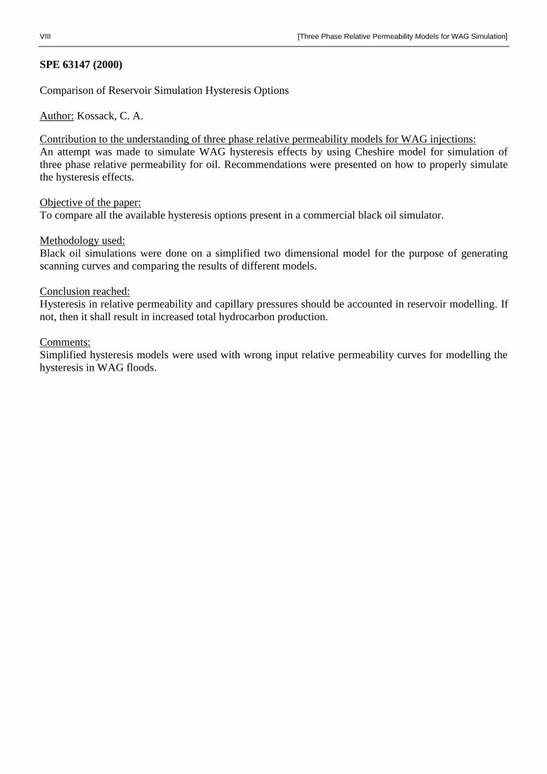
VIII [Three Phase Relative Permeability Models for WAG Simulation]

SPE 63147 (2000)

Comparison of Reservoir Simulation Hysteresis Options

Author: Kossack, C. A.


An attempt was made to simulate WAG hysteresis effects by using Cheshire model for simulation of

three phase relative permeability for oil. Recommendations were presented on how to properly simulate

the hysteresis effects.


To compare all the available hysteresis options present in a commercial black oil simulator.

Methodology used:

Black oil simulations were done on a simplified two dimensional model for the purpose of generating

scanning curves and comparing the results of different models.

Conclusion reached:

Hysteresis in relative permeability and capillary pressures should be accounted in reservoir modelling. If

not, then it shall result in increased total hydrocarbon production.

Comments:

Simplified hysteresis models were used with wrong input relative permeability curves for modelling the

hysteresis in WAG floods.

[Three Phase Relative Permeability Models for WAG Simulations] IX

SPE 67950 (2000)

An Empirical Model for Three Phase Relative Permeability

Author: Blunt, M. J.


A saturation weighted interpolation method that, accounts for the trapping of non wetting phase and oil

layer drainage, predicts Oak experimental data accurately.


To develop an empirical model for three phase relative permeability that can be tested with Oak’s

measured data.

Methodology used:

An extension is made to the saturation weighted interpolation method of Baker by including trapping of

non wetting phase.

Conclusion reached:

1. Saturated weighted interpolation is the best method to predict three phase relative permeability

when compared with the models of Stone.

2. Accurate predictions of the measured three phase relative permeability data of Oak.

Comments:

The method was limited to predictions of three phase flow in a strong water wet rock. It cannot be used

for predictions of three phase WAG hysteresis due to the uncertainties in saturation histories and

especially with non-uniform wettability.

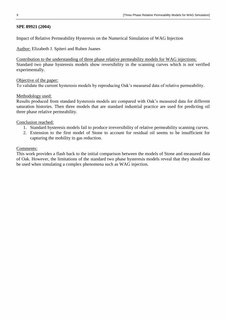
X [Three Phase Relative Permeability Models for WAG Simulation]

SPE 89921 (2004)

Impact of Relative Permeability Hysteresis on the Numerical Simulation of WAG Injection

Author: Elizabeth J. Spiteri and Ruben Juanes


Standard two phase hysteresis models show reversibility in the scanning curves which is not verified

experimentally.


To validate the current hysteresis models by reproducing Oak’s measured data of relative permeability.

Methodology used:

Results produced from standard hysteresis models are compared with Oak’s measured data for different

saturation histories. Then three models that are standard industrial practice are used for predicting oil

three phase relative permeability.

Conclusion reached:

1. Standard hysteresis models fail to produce irreversibility of relative permeability scanning curves.

2. Extension to the first model of Stone to account for residual oil seems to be insufficient for

capturing the mobility in gas reduction.

Comments:

This work provides a flash back to the initial comparison between the models of Stone and measured data

of Oak. However, the limitations of the standard two phase hysteresis models reveal that they should not

be used when simulating a complex phenomena such as WAG injection.

[Three Phase Relative Permeability Models for WAG Simulations] XI

APPENDIX B Table B.1: Cases (ECLIPSE Users Guide) used for Simulating WAG Hysteresis

Cases Saturation Distribution (from Injector to Producer)

Case 1 Sw = 0.8 – 0.2

Sg = 0.0 So = 0.8

Case 2 Sw = 0.2

Sg = 0.6 – 0.0 So = 0.8

Case 3 (THE REAL WAG) Sw = 0.2 Sg = 0.0 So = 0.8

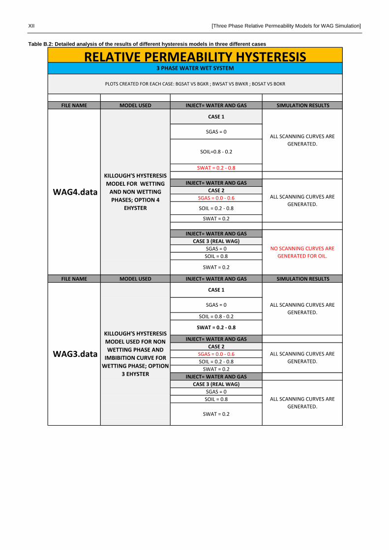
XII [Three Phase Relative Permeability Models for WAG Simulation]

Table B.2: Detailed analysis of the results of different hysteresis models in three different cases

FILE NAME MODEL USED INJECT= WATER AND GAS SIMULATION RESULTS

CASE 1

SGAS = 0

SOIL=0.8 - 0.2

SWAT = 0.2 - 0.8

INJECT= WATER AND GAS

CASE 2

SGAS = 0.0 - 0.6

SOIL = 0.2 - 0.8

SWAT = 0.2


CASE 3 (REAL WAG)

SGAS = 0

SOIL = 0.8


SOIL = 0.8 - 0.2


CASE 2

SGAS = 0.0 - 0.6

SOIL = 0.2 - 0.8

SWAT = 0.2


CASE 3 (REAL WAG)

SGAS = 0

SOIL = 0.8

WAG4.data

KILLOUGH'S HYSTERESIS

MODEL FOR WETTING

AND NON WETTING

PHASES; OPTION 4

EHYSTER

ALL SCANNING CURVES ARE

GENERATED.


GENERATED.

SGAS = 0

SWAT = 0.2 - 0.8


GENERATED.

NO SCANNING CURVES ARE

GENERATED FOR OIL.

SWAT = 0.2

CASE 1


GENERATED.


GENERATED.

SWAT = 0.2

WAG3.data


MODEL USED FOR NON

WETTING PHASE AND

IMBIBITION CURVE FOR

WETTING PHASE; OPTION

3 EHYSTER

RELATIVE PERMEABILITY HYSTERESIS3 PHASE WATER WET SYSTEM

PLOTS CREATED FOR EACH CASE: BGSAT VS BGKR ; BWSAT VS BWKR ; BOSAT VS BOKR

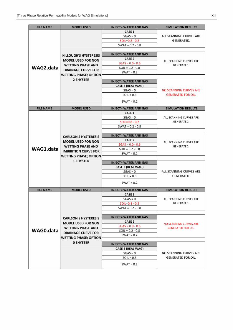
[Three Phase Relative Permeability Models for WAG Simulations] XIII


CASE 1

SGAS = 0

SOIL=0.8 - 0.2

SWAT = 0.2 - 0.8


CASE 2

SGAS = 0.0 - 0.6

SOIL = 0.2 - 0.8

SWAT = 0.2


CASE 3 (REAL WAG)

SGAS = 0

SOIL = 0.8


CASE 1

SGAS = 0

SOIL=0.8 - 0.2

SWAT = 0.2 - 0.8


CASE 2

SGAS = 0.0 - 0.6

SOIL = 0.2 - 0.8

SWAT = 0.2


CASE 3 (REAL WAG)

SGAS = 0

SOIL = 0.8


GENERATED FOR OIL.

WAG2.data


MODEL USED FOR NON

WETTING PHASE AND

DRAINAGE CURVE FOR


2 EHYSTER


GENERATED.


GENERATED.

SWAT = 0.2

SWAT = 0.2

WAG1.data

CARLSON'S HYSTERESIS

MODEL USED FOR NON

WETTING PHASE AND

IMBIBITION CURVE FOR


1 EHYSTER


GENERATED.


GENERATED.


GENERATED.


CASE 1

SGAS = 0

SOIL=0.8 - 0.2

SWAT = 0.2 - 0.8


CASE 2

SGAS = 0.0 - 0.6

SOIL = 0.2 - 0.8

SWAT = 0.2


CASE 3 (REAL WAG)

SGAS = 0

SOIL = 0.8


GENERATED FOR OIL.

SWAT = 0.2

WAG0.data

CARLSON'S HYSTERESIS

MODEL USED FOR NON

WETTING PHASE AND

DRAINAGE CURVE FOR


0 EHYSTER


GENERATED.


GENERATED FOR OIL.

XIV [Three Phase Relative Permeability Models for WAG Simulation]

It was felt that mostly oil scanning curves were not generated (Table B3). Since oil is treated as an intermediate wetting phase

to gas (by default) in the presence of oil, gas and water; then no scanning curves should be generated. But there were two cases

(Table B3) in which all scanning curves were generated.

Table B2: Cases with unexpected results from the analysis in Table B3

Cases Simulation Results

WAG4_CASE3 No scanning curves for oil

WAG3 Scanning curves for all required cases


WAG1 Scanning curves for all required cases



*Please refer to Table B2 to view the hysteresis options used in simulation.

As these models were already classified as simple two phase hysteresis models (Larsen et al., and ECLIPSE Technical

Description) no further investigation was carried out for the root cause of this behaviour.

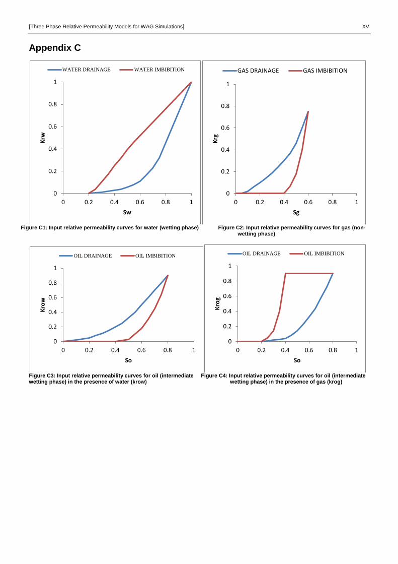
[Three Phase Relative Permeability Models for WAG Simulations] XV

Appendix C

Figure C1: Input relative permeability curves for water (wetting phase) Figure C2: Input relative permeability curves for gas (non-

wetting phase)

Figure C3: Input relative permeability curves for oil (intermediate Figure C4: Input relative permeability curves for oil (intermediate wetting phase) in the presence of water (krow) wetting phase) in the presence of gas (krog)

0

0.2

0.4

0.6

0.8

1

0 0.2 0.4 0.6 0.8 1

Krw

Sw

WATER DRAINAGE WATER IMBIBITION

0

0.2

0.4

0.6

0.8

1

0 0.2 0.4 0.6 0.8 1

Krg

Sg

GAS DRAINAGE GAS IMBIBITION

0

0.2

0.4

0.6

0.8

1

0 0.2 0.4 0.6 0.8 1

Kro

w

So

OIL DRAINAGE OIL IMBIBITION

0

0.2

0.4

0.6

0.8

1

0 0.2 0.4 0.6 0.8 1

Kro

g

So

OIL DRAINAGE OIL IMBIBITION

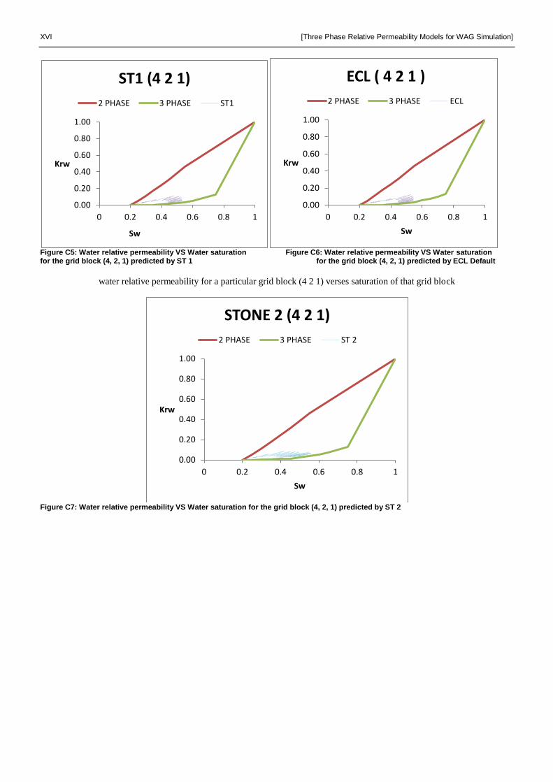
XVI [Three Phase Relative Permeability Models for WAG Simulation]

Figure C5: Water relative permeability VS Water saturation Figure C6: Water relative permeability VS Water saturation for the grid block (4, 2, 1) predicted by ST 1 for the grid block (4, 2, 1) predicted by ECL Default

water relative permeability for a particular grid block (4 2 1) verses saturation of that grid block


0.00

0.20

0.40

0.60

0.80

1.00

0 0.2 0.4 0.6 0.8 1

Krw

Sw

ST1 (4 2 1)

2 PHASE 3 PHASE ST1

0.00

0.20

0.40

0.60

0.80

1.00

0 0.2 0.4 0.6 0.8 1

Krw

Sw

ECL ( 4 2 1 )

2 PHASE 3 PHASE ECL

0.00

0.20

0.40

0.60

0.80

1.00

0 0.2 0.4 0.6 0.8 1

Krw

Sw

STONE 2 (4 2 1)

2 PHASE 3 PHASE ST 2

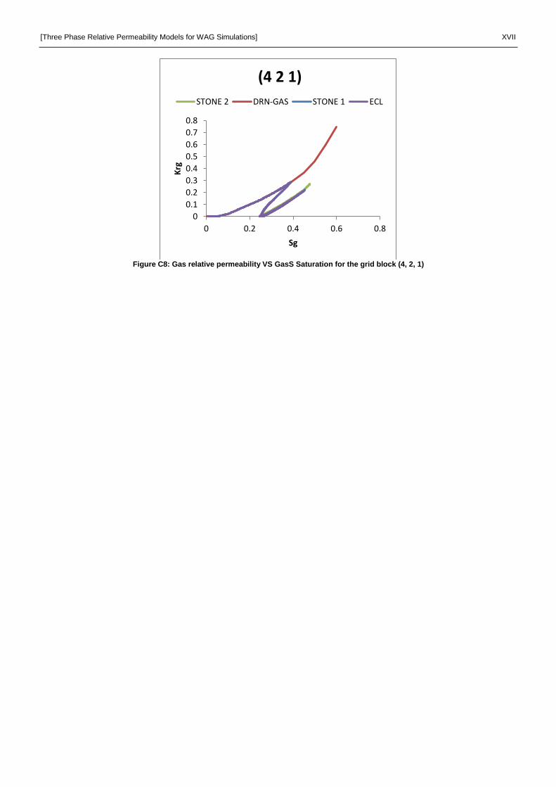
[Three Phase Relative Permeability Models for WAG Simulations] XVII

Figure C8: Gas relative permeability VS GasS Saturation for the grid block (4, 2, 1)

0

0.1

0.2

0.3

0.4

0.5

0.6

0.7

0.8

0 0.2 0.4 0.6 0.8

Krg

Sg

(4 2 1)

STONE 2 DRN-GAS STONE 1 ECL

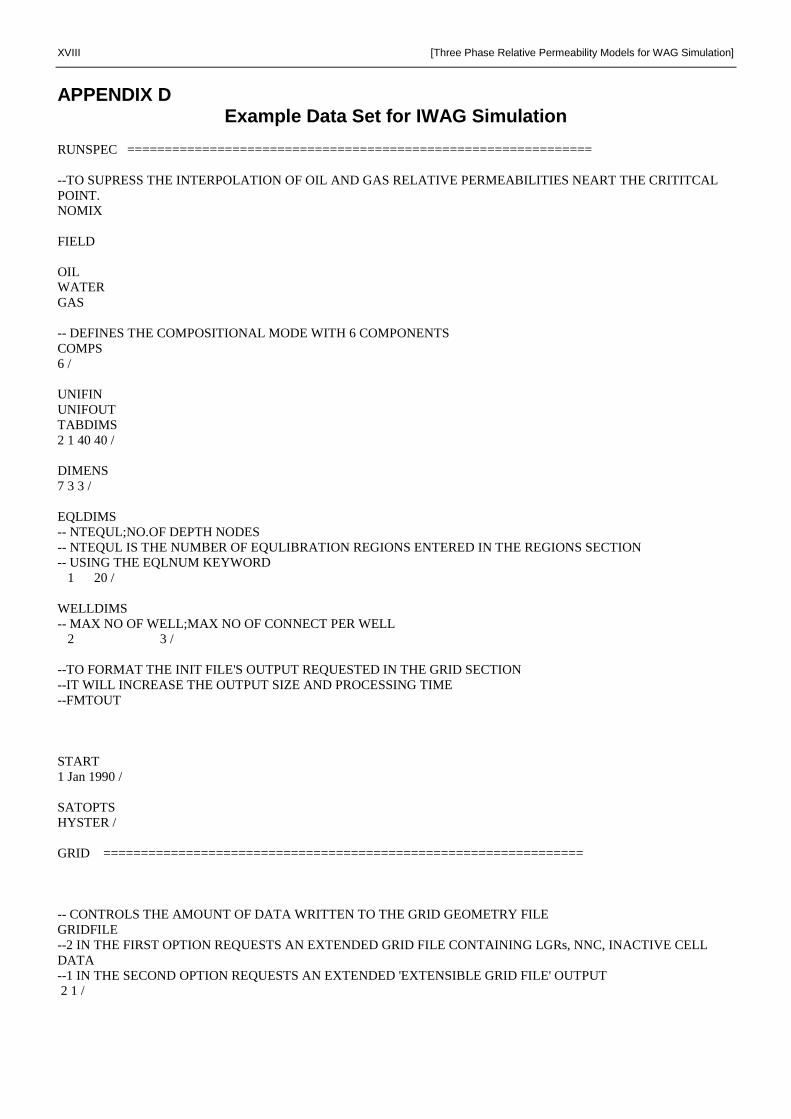
XVIII [Three Phase Relative Permeability Models for WAG Simulation]

APPENDIX D Example Data Set for IWAG Simulation

RUNSPEC ==============================================================

--TO SUPRESS THE INTERPOLATION OF OIL AND GAS RELATIVE PERMEABILITIES NEART THE CRITITCAL

POINT.

NOMIX

FIELD

OIL

WATER

GAS

-- DEFINES THE COMPOSITIONAL MODE WITH 6 COMPONENTS

COMPS

6 /

UNIFIN

UNIFOUT

TABDIMS

2 1 40 40 /

DIMENS

7 3 3 /

EQLDIMS

-- NTEQUL;NO.OF DEPTH NODES

-- NTEQUL IS THE NUMBER OF EQULIBRATION REGIONS ENTERED IN THE REGIONS SECTION

-- USING THE EQLNUM KEYWORD

1 20 /

WELLDIMS

-- MAX NO OF WELL;MAX NO OF CONNECT PER WELL

2 3 /

--TO FORMAT THE INIT FILE'S OUTPUT REQUESTED IN THE GRID SECTION

--IT WILL INCREASE THE OUTPUT SIZE AND PROCESSING TIME

--FMTOUT

START

1 Jan 1990 /

SATOPTS

HYSTER /

GRID ================================================================

-- CONTROLS THE AMOUNT OF DATA WRITTEN TO THE GRID GEOMETRY FILE

GRIDFILE

--2 IN THE FIRST OPTION REQUESTS AN EXTENDED GRID FILE CONTAINING LGRs, NNC, INACTIVE CELL

DATA

--1 IN THE SECOND OPTION REQUESTS AN EXTENDED 'EXTENSIBLE GRID FILE' OUTPUT

2 1 /

[Three Phase Relative Permeability Models for WAG Simulations] XIX

INIT

--THE SIZE OF THE BLOCKS IN X DIRECTIONS CREATED AS VECTORS

DXV

7*500 /

DYV

3*500 /

DZV

20 30 50 /

TOPS

--SPECIFIES THE DEPTHS AT THE TOP OF EACH GRIDBLOCK

--49 IS X INTO Y

-- THREE DEPTHS HAVE BEEN MENTIONED CUZ OF 3 BLOCKS GIVEN IN Z DIRECTION

21*8325 21*8345 21*8375 /

PORO

--49 INTO 3

63*0.3 /

PERMX

21*500 21*50 21*200 /

PERMY

21*500 21*50 21*200 /

PERMZ

21*50 21*50 21*25 /

RPTGRID

-- Report Levels for Grid Section Data

--

'DX'

'DY'

'DZ'

'PERMX'

'PERMY'

'PERMZ'

'PORO'

'TOPS'

'PORV'

'DEPTH'

'TRANX'

'TRANY'

'TRANZ'

'COORDSYS'

'COORD'

/

EDIT

PROPS ============================================================

STONE2

--STONE1

EOS

XX [Three Phase Relative Permeability Models for WAG Simulation]

PR /

-- REQUESTS MODFICATION IN PR WITH THE ACCENTRIC FACTOR

PRCORR

RTEMP

160 /

--STANDARD CONDITIONS

STCOND

60 14.7 /

PARACHOR

74.912

153.48

271.304

404.882676

534.80002

722.26694

/

CNAMES

C1

C3

C6

C10

C15

C20

/

TCRIT

343.0

665.7

913.4

1111.8

1270.0

1380.0

/

PCRIT

667.8

616.3

436.9

304.0

200.0

162.0

/

ZCRIT

0.290

0.277

0.264

0.257

0.245

0.235

/

MW

16.04

44.10

[Three Phase Relative Permeability Models for WAG Simulations] XXI

86.18

149.29

206.00

282.00

/

--ACCENTRIC FACTOR

ACF

0.013

0.1524

0.3007

0.4885

0.6500

0.8500

/

--BINARY INTERACTION COEFFICIENTS

-- IT IS ENTERED IN THE LOWER TRIANGLE FORMAT

--THE NUMBER OF VALUES ENTERED DEPEND UPON THE NUMBER OF COMP MENTIONED IN THE COMPS

KEYWORD

BIC

0.0

0.0 0.0

0.0 0.0 0.0

0.05 0.005 0.0 0.0

0.05 0.005 0.0 0.0 0.0 /

SWFN

--2 PHASE CURVE

--table 1

--Sw Krw Pc

0.2 0.000 6

0.25 0.052 3

0.3 0.112 2

0.35 0.177 1.15

0.4 0.245 0.6

0.45 0.315 0.3

0.5 0.387 0.12

0.55 0.460 0

1 1 0

/

--Sw Krw Pc

--0.200 0.000 3

--0.250 0.002 0.6

--0.300 0.009 0.35

--0.350 0.018 0.23

--0.400 0.032 0.12

--0.450 0.049 0.06

--0.500 0.069 0.024

--0.550 0.110 0

--1.000 1.000 0

--/

--3 PHASE CURVE-40%DRN

--table 2

--Sw Krw Pc

XXII [Three Phase Relative Permeability Models for WAG Simulation]

0.2 0.000 2.4

0.25 0.000 2

0.3 0.001 1.6

0.35 0.003 1.2

0.4 0.008 0.96

0.45 0.014 0.76

0.5 0.023 0.56

0.55 0.036 0.4

0.6 0.052 0.28

0.65 0.073 0.16

0.7 0.098 0.1

0.75 0.128 0.04

1 1.000 0

/

SGFN

--Drainage curves

--Table 1 for SATNUM

--Sg Krg Pcog note must have connate gas sat = 0

0 0 0

0.05 0 0.09

0.10 0.022 0.20

0.15 0.06 0.38

0.20 0.10 0.57

0.25 0.14 0.83

0.30 0.188 1.08

0.35 0.24 1.37

0.40 0.30 1.69

0.45 0.364 2

0.50 0.458 2.36

0.55 0.60 2.70

0.60 0.75 3

0.80 1.0 3

/

--Imbibition curves

--Table 2 for IMBNUM

--Sg Krg Pcog

-- 0.0 0 0

-- 0.40 0 0

-- 0.45 0.066 0.80

-- 0.50 0.177 1.56

-- 0.55 0.40 2.24

-- 0.60 0.75 3

/

--Sgcr=0.05 critical gas saturation

--the highest for which Krg is zero

--Sgco=0.0 connate gas saturation

--minimum gas sat in the table

--value below the GOC

--Sgmax max gas sat in the table

--Sgmax=1-Swco=1-0.20=0.80

--value above the gas transition zone

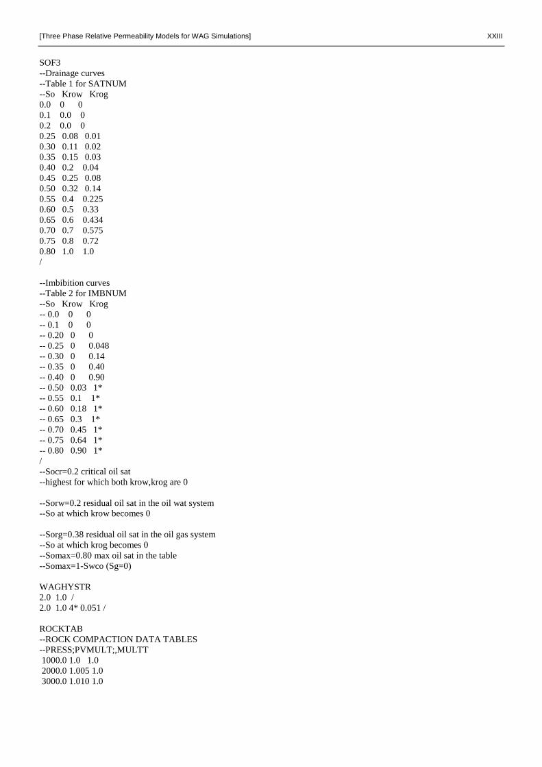
[Three Phase Relative Permeability Models for WAG Simulations] XXIII

SOF3

--Drainage curves

--Table 1 for SATNUM

--So Krow Krog

0.0 0 0

0.1 0.0 0

0.2 0.0 0

0.25 0.08 0.01

0.30 0.11 0.02

0.35 0.15 0.03

0.40 0.2 0.04

0.45 0.25 0.08

0.50 0.32 0.14

0.55 0.4 0.225

0.60 0.5 0.33

0.65 0.6 0.434

0.70 0.7 0.575

0.75 0.8 0.72

0.80 1.0 1.0

/

--Imbibition curves

--Table 2 for IMBNUM

--So Krow Krog

-- 0.0 0 0

-- 0.1 0 0

-- 0.20 0 0

-- 0.25 0 0.048

-- 0.30 0 0.14

-- 0.35 0 0.40

-- 0.40 0 0.90

-- 0.50 0.03 1*

-- 0.55 0.1 1*

-- 0.60 0.18 1*

-- 0.65 0.3 1*

-- 0.70 0.45 1*

-- 0.75 0.64 1*

-- 0.80 0.90 1*

/

--Socr=0.2 critical oil sat

--highest for which both krow,krog are 0

--Sorw=0.2 residual oil sat in the oil wat system

--So at which krow becomes 0

--Sorg=0.38 residual oil sat in the oil gas system

--So at which krog becomes 0

--Somax=0.80 max oil sat in the table

--Somax=1-Swco (Sg=0)

WAGHYSTR

2.0 1.0 /

2.0 1.0 4* 0.051 /

ROCKTAB

--ROCK COMPACTION DATA TABLES

--PRESS;PVMULT;,MULTT

1000.0 1.0 1.0

2000.0 1.005 1.0

3000.0 1.010 1.0

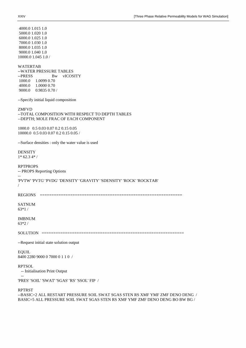
XXIV [Three Phase Relative Permeability Models for WAG Simulation]

4000.0 1.015 1.0

5000.0 1.020 1.0

6000.0 1.025 1.0

7000.0 1.030 1.0

8000.0 1.035 1.0

9000.0 1.040 1.0

10000.0 1.045 1.0 /

WATERTAB

--WATER PRESSURE TABLES

--PRESS Bw vICOSITY

1000.0 1.0099 0.70

4000.0 1.0000 0.70

9000.0 0.9835 0.70 /

--Specify initial liquid composition

ZMFVD

--TOTAL COMPOSITION WITH RESPECT TO DEPTH TABLES

--DEPTH; MOLE FRAC OF EACH COMPONENT

1000.0 0.5 0.03 0.07 0.2 0.15 0.05

10000.0 0.5 0.03 0.07 0.2 0.15 0.05 /

--Surface densities : only the water value is used

DENSITY

1* 62.3 4* /

RPTPROPS

-- PROPS Reporting Options

--

'PVTW' 'PVTG' 'PVDG' 'DENSITY' 'GRAVITY' 'SDENSITY' 'ROCK' 'ROCKTAB'

/

REGIONS =============================================================

SATNUM

63*1 /

IMBNUM

63*2 /

SOLUTION =============================================================

--Request initial state solution output

EQUIL

8400 2280 9000 0 7000 0 1 1 0 /

RPTSOL

-- Initialisation Print Output

--

'PRES' 'SOIL' 'SWAT' 'SGAS' 'RS' 'SSOL' FIP /

RPTRST

--BASIC=2 ALL RESTART PRESSURE SOIL SWAT SGAS STEN RS XMF YMF ZMF DENO DENG /

BASIC=5 ALL PRESSURE SOIL SWAT SGAS STEN RS XMF YMF ZMF DENO DENG BO BW BG /

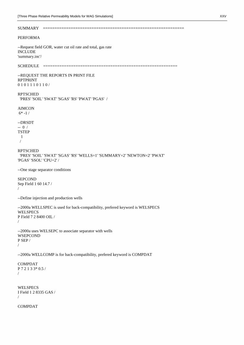
[Three Phase Relative Permeability Models for WAG Simulations] XXV

SUMMARY =============================================================

PERFORMA

--Request field GOR, water cut oil rate and total, gas rate

INCLUDE

'summary.inc'/

SCHEDULE ==========================================================

--REQUEST THE REPORTS IN PRINT FILE

RPTPRINT

0 1 0 1 1 1 0 1 1 0 /

RPTSCHED

'PRES' 'SOIL' 'SWAT' 'SGAS' 'RS' 'PWAT' 'PGAS' /

AIMCON

6* -1 /

--DRSDT

-- 0 /

TSTEP

1

/

RPTSCHED

'PRES' 'SOIL' 'SWAT' 'SGAS' 'RS' 'WELLS=1' 'SUMMARY=2' 'NEWTON=2' 'PWAT'

'PGAS' 'SSOL' 'CPU=2' /

--One stage separator conditions

SEPCOND

Sep Field 1 60 14.7 /

/

--Define injection and production wells

--2000a WELLSPEC is used for back-compatibility, prefered keyword is WELSPECS

WELSPECS

P Field 7 2 8400 OIL /

/

--2000a uses WELSEPC to associate separator with wells

WSEPCOND

P SEP /

/

--2000a WELLCOMP is for back-compatibility, prefered keyword is COMPDAT

COMPDAT

P 7 2 1 3 3* 0.5 /

/

WELSPECS

I Field 1 2 8335 GAS /

/

COMPDAT

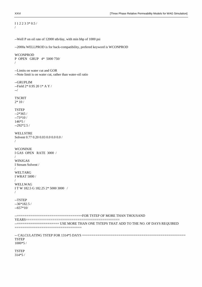
XXVI [Three Phase Relative Permeability Models for WAG Simulation]

I 1 2 2 3 3* 0.5 /

/

--Well P on oil rate of 12000 stb/day, with min bhp of 1000 psi

--2000a WELLPROD is for back-compatibility, prefered keyword is WCONPROD

WCONPROD

P OPEN GRUP 4* 5000 750/

/

--Limits on water cut and GOR

--Note limit is on water cut, rather than water-oil ratio

--GRUPLIM

--Field 2* 0.95 20 1* A Y /

--/

TSCRIT

2* 10 /

TSTEP

--2*365 /

--73*10 /

146*5 /

--292*2.5 /

WELLSTRE

Solvent 0.77 0.20 0.03 0.0 0.0 0.0 /

/

WCONINJE

I GAS OPEN RATE 3000 /

/

WINJGAS

I Stream Solvent /

/

WELTARG

I WRAT 5000 /

/

WELLWAG

I T W 182.5 G 182.25 2* 5000 3000 /

/

--TSTEP

--36*182.5 /

--657*10/

--==================================FOR TSTEP OF MORE THAN THOUSAND

YEARS=================================================

--====================== USE MORE THAN ONE TSTEPS THAT ADD TO THE NO. OF DAYS REQUIRED

===================================

-- CALCULATING TSTEP FOR 1314*5 DAYS ======================================================

TSTEP

1000*5 /

TSTEP

314*5 /

[Three Phase Relative Permeability Models for WAG Simulations] XXVII

--

=========================================================================================

-- CALCULATING TSTEP FOR 2628*2.5 DAYS =====================================================

--TSTEP

--1000*2.5 /

--TSTEP

--1000*2.5 /

--TSTEP

--628*2.5 /

--

==========================================================================================

=

WCONINJE

I GAS SHUT RATE 3000 /

/

TSTEP

--4*182.5 /

--73*10/

146*5 /

--292*2.5 /

END

Three Phase Relative Permeability Models for WAG Simulation

Documents

Transcript of Three Phase Relative Permeability Models for WAG Simulation