Enhancing Stream Processing and Complex Event ...
182
No d’ordre NNT: 2019LYSE012 THESE DE DOCTORAT DE L’UNIVERSITE DE LYON opérée au sein de L’UNIVERSITE JEAN MONNET Ecole Doctoral N o 488 Sciences, Ingénierie et Santé Spécialité de doctorat: Discipline : Informatique Soutenue publiquement le 08/07/2019, par: Abderrahmen Kammoun Enhancing Stream Processing and Complex Event Processing Systems Devant le jury composé de : Jean-Marc Petit, PR, Institut National des Sciences Appliquées de Lyon, Rapporteur Yann Busnel, PR, École Nationale Supérieure Mines-Télécom Atlantique Bretagne Pays de la Loire, Rapporteur Frédérique Laforest, PR, Institut National des Sciences Appliquées de Lyon, Examinatrice Jacques Fayolle, PR, Université Jean Monnet, Directeur de thèse Kamal Singh, MCF, Université Jean Monnet, Co-Directeur
-
Upload
khangminh22 -
Category
Documents
-
view
2 -
download
0
Transcript of Enhancing Stream Processing and Complex Event ...
No d’ordre NNT: 2019LYSE012
THESE DE DOCTORAT DE L’UNIVERSITE DE LYONopérée au sein de
L’UNIVERSITE JEAN MONNET
Ecole Doctoral N o 488Sciences, Ingénierie et Santé
Spécialité de doctorat:Discipline : Informatique
Soutenue publiquement le 08/07/2019, par:Abderrahmen Kammoun
Enhancing Stream Processing andComplex Event Processing Systems
Devant le jury composé de :
Jean-Marc Petit, PR, Institut National des Sciences Appliquées de Lyon, RapporteurYann Busnel, PR, École Nationale Supérieure Mines-Télécom Atlantique Bretagne
Pays de la Loire, RapporteurFrédérique Laforest, PR, Institut National des Sciences Appliquées de Lyon,
ExaminatriceJacques Fayolle, PR, Université Jean Monnet, Directeur de thèse
Kamal Singh, MCF, Université Jean Monnet, Co-Directeur

Je dédie cette thèse :À mon père Habib Kammoun. Merci pour tous les sacrifices consentis pour moi.
c’est grâce à toi que je suis ce que je suis.À la mémoire de ma mère Chédia Kammoun et mon grand-père Hedy Kammoun,qui seront contents d’apprendre que leur fils a enfin terminé ces études. que leurs
âmes reposent en paix.Aux familles KAMMOUN, BOUGHARIOU et GARGOURI.

Acknowledgements
Il me sera très difficile de remercier tout le monde car c’est à l’aide de nombreusespersonnes que j’ai pu mener cette thèse à son terme.
Je voudrais tout d’abord remercier mes encadrants, Jacques Fayolle et KamalSingh, pour leur aide et leurs conseils tout au long de ce travail de recherche.
Je remercie également Jean-Marc Petit et Yann Busnel d’avoir accepté de relirecette thèse et d’en être les rapporteurs
Je tiens à remercier Frédérique Laforest pour avoir accepté de participer àmon jury de thèse et pour sa participation scientifique ainsi que le temps qu’ellea consacré à ma recherche.
Je remercie toutes personnes avec qui j’ai partagé mes études, notammentpendant ces années de thèse.
Je tiens à remercier particulièrement Syed Gillani pour toutes nos discussions etses conseils qui m’ont accompagné tout au long des recherches et de la rédaction decette thèse. Il m’est impossible d’oublier Christophe Gravier, Julien Subercaze etTanguy Raynaud que j’ai régulièrement côtoyées pendant ces années, pour leursconseils précieux et leur aide.
Mer derniers remerciements vont à ma famille: Soutouty, Chouchou, Mi7ou,Kouka et Fattouma, qui a tout fait pour m’aider, qui m’a soutenu et surtoutsupporté pendant les moments les plus difficiles.

iv
Abstract
As more and more connected objects and sensory devices are becoming part ofour daily lives, the sea of high-velocity information flow is growing. This massiveamount of data produced at high rates requires rapid insight to be useful in variousapplications such as the Internet of Things, health care, energy management, etc.Traditional data storage and processing techniques are proven inefficient. This givesrise to Data Stream Management (DSMS) and Complex Event Processing (CEP)systems, where the former employs stateless query operators while the later usesexpressive stateful operators to extract contextual information.
Over the years, a large number of general purpose DSMS and CEP systemshave been developed. However,(i) they do not support complex queries that pushthe CPU and memory consumption towards exponential complexity, and (ii) theydo not provide a proactive or predictive view of the continuous queries. Both ofthese properties are of utmost importance for emerging large-scale applications.
This thesis aims to provide optimal solutions for such complex and proactivequeries. Our proposed techniques, in addition to CPU and memory efficiency,enhance the capabilities of existing CEP systems by adding predictive featurethrough real-time learning. The main contributions of this thesis are as follows:
• We proposed various techniques to reduce the CPU and memory requirementsof expensive queries with operators such as Kleene+ and Skip-Till-Any.These operators result in exponential complexity both in terms of CPUand memory. Our proposed recomputation and heuristic-based algorithmreduce the costs of these operators. These optimizations are based on enablingefficient multidimensional indexing using space-filling curves and by clusteringevents into batches to reduce the cost of pair-wise joins.
• We designed a novel predictive CEP system that employs historical informationto predict future complex events. To efficiently employ historical information,we employ an N-dimensional historical matched sequence space. Hence,prediction can be performed by answering the range queries over the historicalsequence space. We transform N-dimensional space into 1-dimension usingspace filling Z-order curves, enabling us to exploit 1-dimensional range searchalgorithms. We propose a compressed index structure, range query processingtechniques and an approximate summarizing technique over the historicalspace.

vi
• To showcase the value and flexibility of our proposed techniques, we employthem over multiple real-world challenges organized by the DEBS conference.These include designing a scalable system for the Top-k operator over non-linear sliding windows and a scalable framework for accelerating situationprediction over spatiotemporal event streams.
The applicability of our techniques over the real-world problems presentedhas produced further customize-able solutions that demonstrate the viability ofour proposed methods.

Résumer
Alors que de plus en plus d’objects et d’appareils sensoriels connectés font partiede notre vie quotidienne, la masse d’information circulante à grande vitesse necesse d’augmenter. Cette énorme quantité de données produites à des débits élevésexige une compréhension rapide pour être utile dans divers domaines d’activitételles que l’internet des objets, la santé, la gestion de l’énergie, etc. Les techniquestraditionnelles de stockage et de traitement de données se sont révélées inefficacesou inadaptables pour gérer ce flux de données.
Cette thèse a pour objectif de proposer des solutions optimales à deux problèmesde recherche sur la gestion de flux de données. La première concerne l’optimisationde la résolution de requêtes continues complexes dans les systèmes de détectiond’évènements complexe (CEP). La deuxième aux problèmes liées à la prédictiondes événements complexes fondée sur l’apprentissage de l’historique du système.
Premièrement, nous avons proposé un modèle de recalcule pour le traitement derequêtes complexes, basé sur une indexation multidimensionnelle et des algorithmesde jointures optimisés. Deuxièmement, nous avons conçu un CEP prédictive quiutilise des informations historiques pour prédire des événements complexes futurs.Pour utiliser efficacement l’information historique, nous utilisons un espace deséquences historiques à N dimensions. Par conséquence, la prédiction peut êtreeffectuée en répondant aux requêtes d’intervalles sur cet espace de séquences.
La pertinence des résultats obtenus, notamment par l’application de nos algo-rithmes et approches lors de challenges internationaux démontre la viabilité desméthodes que nous proposons.

viii
Contents
List of Figures xiii
List of Tables xv
I Introduction & Background 1
1 Introduction 31.1 Motivation . . . . . . . . . . . . . . . . . . . . . . . . . . . . . . . . 31.2 Research Challenges and Contributions . . . . . . . . . . . . . . . . 5
1.2.1 Optimizing Expensive Queries for Complex Event Processing 51.2.2 Predictive complex event processing . . . . . . . . . . . . . . 71.2.3 Applying and testing our event processing solutions: challeng-
ing queries from the research community . . . . . . . . . . . 81.3 Structure . . . . . . . . . . . . . . . . . . . . . . . . . . . . . . . . 91.4 List of publications . . . . . . . . . . . . . . . . . . . . . . . . . . . 9
2 Background 112.1 Introduction . . . . . . . . . . . . . . . . . . . . . . . . . . . . . . . 122.2 Stream processing . . . . . . . . . . . . . . . . . . . . . . . . . . . . 14
2.2.1 Active Database . . . . . . . . . . . . . . . . . . . . . . . . . 142.2.2 Data Stream Management System . . . . . . . . . . . . . . . 15
2.3 Complex event processing . . . . . . . . . . . . . . . . . . . . . . . 162.3.1 Complex event processing Architectures . . . . . . . . . . . 172.3.2 Event Processing models and definitions . . . . . . . . . . . 192.3.3 Selection Policy and Query Operator . . . . . . . . . . . . . 212.3.4 Event Detection models . . . . . . . . . . . . . . . . . . . . 24
2.4 Query Optimization in CEP Systems . . . . . . . . . . . . . . . . . 292.4.1 Optimizations according to predicates . . . . . . . . . . . . . 302.4.2 Optimization of query plan generation . . . . . . . . . . . . 312.4.3 Optimization of memory . . . . . . . . . . . . . . . . . . . . 34
2.5 Predictive Analytics & Complex Event Processing . . . . . . . . . . 352.5.1 Predictive Analytics for optimal decision making . . . . . . . 37
ix
x Contents
2.5.2 Predictive Analytics for automatic rules generation . . . . . 372.5.3 Predictive Analytics for complex events prediction . . . . . . 38
2.6 Processing Top-k queries . . . . . . . . . . . . . . . . . . . . . . . . 392.6.1 Definitions . . . . . . . . . . . . . . . . . . . . . . . . . . . . 392.6.2 Top-K Algorithms . . . . . . . . . . . . . . . . . . . . . . . 39
2.7 Conclusion . . . . . . . . . . . . . . . . . . . . . . . . . . . . . . . . 41
II Enhancing Complex Event Processing 43
3 Enabling Efficient Recomputation Based Complex Event Process-ing for Expensive Queries 453.1 Introduction . . . . . . . . . . . . . . . . . . . . . . . . . . . . . . . 463.2 Motivating examples . . . . . . . . . . . . . . . . . . . . . . . . . . 463.3 Related Works . . . . . . . . . . . . . . . . . . . . . . . . . . . . . . 483.4 Preliminaries and definitions . . . . . . . . . . . . . . . . . . . . . . 51
3.4.1 Definitions . . . . . . . . . . . . . . . . . . . . . . . . . . . . 513.4.2 Query Tree . . . . . . . . . . . . . . . . . . . . . . . . . . . 53
3.5 Baseline Algorithm . . . . . . . . . . . . . . . . . . . . . . . . . . . 553.6 RCEP: Recomputational based CEP . . . . . . . . . . . . . . . . . 57
3.6.1 The Event Tree . . . . . . . . . . . . . . . . . . . . . . . . . 573.6.2 Creating the Complex Matches . . . . . . . . . . . . . . . . 59
3.7 RCEP: General Recomputation Model . . . . . . . . . . . . . . . . 653.7.1 Multidimensional Events . . . . . . . . . . . . . . . . . . . . 653.7.2 Multidimensional Event Tree . . . . . . . . . . . . . . . . . 663.7.3 Joins between Z-addresses . . . . . . . . . . . . . . . . . . . 683.7.4 Handling Sliding Windows . . . . . . . . . . . . . . . . . . . 723.7.5 Optimising Z-address Comparison . . . . . . . . . . . . . . . 74
3.8 Experimental Evaluation . . . . . . . . . . . . . . . . . . . . . . . . 743.8.1 Setup and Methodology . . . . . . . . . . . . . . . . . . . . 743.8.2 Performance of Indexing and Join Algorithms . . . . . . . . 763.8.3 Performance of Sliding Windows . . . . . . . . . . . . . . . . 783.8.4 CEP Systems’ Comparison . . . . . . . . . . . . . . . . . . . 79
3.9 Conclusion . . . . . . . . . . . . . . . . . . . . . . . . . . . . . . . . 83
4 A Generic Framework for Predictive Complex Event Processingusing Historical Sequence Space 854.1 Introduction . . . . . . . . . . . . . . . . . . . . . . . . . . . . . . . 854.2 Contribution . . . . . . . . . . . . . . . . . . . . . . . . . . . . . . . 874.3 Our Approach . . . . . . . . . . . . . . . . . . . . . . . . . . . . . . 88

Contents xi
4.3.1 Querying Historical Space for Prediction . . . . . . . . . . . 894.3.2 Summarisation of Historical Space Points . . . . . . . . . . . 91
4.4 Implementation . . . . . . . . . . . . . . . . . . . . . . . . . . . . . 934.4.1 System Architecture . . . . . . . . . . . . . . . . . . . . . . 934.4.2 User Interface . . . . . . . . . . . . . . . . . . . . . . . . . . 93
4.5 Experimental Evaluation . . . . . . . . . . . . . . . . . . . . . . . . 944.5.1 Experiment Setup . . . . . . . . . . . . . . . . . . . . . . . . 944.5.2 Datasets and CEP Queries . . . . . . . . . . . . . . . . . . . 964.5.3 Accuracy Metrics . . . . . . . . . . . . . . . . . . . . . . . . 964.5.4 Precision of Prediction with Summarisation . . . . . . . . . 964.5.5 Comparison with other Techniques: . . . . . . . . . . . . . . 96
4.6 Conclusion . . . . . . . . . . . . . . . . . . . . . . . . . . . . . . . . 97
III Real World Event Processing Challenges 99
5 High Performance Top-K Processing of Non-Linear Windows overData Streams 1035.1 Introduction . . . . . . . . . . . . . . . . . . . . . . . . . . . . . . . 1035.2 Input Data Streams and Query definitions . . . . . . . . . . . . . . 105
5.2.1 Input Data Streams . . . . . . . . . . . . . . . . . . . . . . . 1055.2.2 Query definitions . . . . . . . . . . . . . . . . . . . . . . . . 105
5.3 Architecture . . . . . . . . . . . . . . . . . . . . . . . . . . . . . . . 1065.4 Query 1 Solution . . . . . . . . . . . . . . . . . . . . . . . . . . . . 107
5.4.1 Data structures . . . . . . . . . . . . . . . . . . . . . . . . . 1085.4.2 Algorithms . . . . . . . . . . . . . . . . . . . . . . . . . . . 110
5.5 Query 2 Solution . . . . . . . . . . . . . . . . . . . . . . . . . . . . 1125.5.1 Data Structures . . . . . . . . . . . . . . . . . . . . . . . . . 1125.5.2 Algorithms . . . . . . . . . . . . . . . . . . . . . . . . . . . 115
5.6 Evaluation . . . . . . . . . . . . . . . . . . . . . . . . . . . . . . . . 1175.6.1 Experimental Settings . . . . . . . . . . . . . . . . . . . . . 1185.6.2 Queues implementation . . . . . . . . . . . . . . . . . . . . . 1195.6.3 Analysis of Query 1 Performance . . . . . . . . . . . . . . . 1195.6.4 Analysis of Query 2 Performance . . . . . . . . . . . . . . . 121
5.7 Conclusion . . . . . . . . . . . . . . . . . . . . . . . . . . . . . . . . 122

xii Contents
6 A Scalable Framework for Accelerating Situation Prediction overSpatio-temporal Event Streams 1236.1 Introduction . . . . . . . . . . . . . . . . . . . . . . . . . . . . . . . 1236.2 Input Data Streams and Query definitions . . . . . . . . . . . . . . 125
6.2.1 Input Data Streams . . . . . . . . . . . . . . . . . . . . . . . 1256.2.2 Query 1: Predicting destinations of vessels . . . . . . . . . . 1266.2.3 Query 2: Predicting arrival times of vessels . . . . . . . . . . 126
6.3 Preliminaires . . . . . . . . . . . . . . . . . . . . . . . . . . . . . . 1276.4 The Framework . . . . . . . . . . . . . . . . . . . . . . . . . . . . . 1276.5 Experimental Evaluation . . . . . . . . . . . . . . . . . . . . . . . . 129
6.5.1 Evaluation [Gul+18b] . . . . . . . . . . . . . . . . . . . . . . 1296.5.2 Results and GC Benchmark . . . . . . . . . . . . . . . . . . 130
6.6 Conclusion . . . . . . . . . . . . . . . . . . . . . . . . . . . . . . . . 131
IV Conclusion 133
7 Conclusion and Future Works 1357.1 Enhancing CEP performance . . . . . . . . . . . . . . . . . . . . . 1357.2 Predictive CEP . . . . . . . . . . . . . . . . . . . . . . . . . . . . . 1367.3 Real world use cases and challenges . . . . . . . . . . . . . . . . . . 137
Appendices
A Upsortable an Annotation-Based Approach 141A.1 Introduction . . . . . . . . . . . . . . . . . . . . . . . . . . . . . . . 141A.2 The Case For Upsortable . . . . . . . . . . . . . . . . . . . . . . . 142A.3 Upsortable solution . . . . . . . . . . . . . . . . . . . . . . . . . . . 143
A.3.1 AST modifications . . . . . . . . . . . . . . . . . . . . . . . 144A.3.2 Bookkeeping . . . . . . . . . . . . . . . . . . . . . . . . . . . 144A.3.3 Garbage Collection . . . . . . . . . . . . . . . . . . . . . . . 146
A.4 Discussion . . . . . . . . . . . . . . . . . . . . . . . . . . . . . . . . 147
B DETAILED ANALYSIS 149B.1 Evaluating Kleene+ Operator . . . . . . . . . . . . . . . . . . . . . 149B.2 Proof Sketches . . . . . . . . . . . . . . . . . . . . . . . . . . . . . . 150B.3 Optimising Z-address Comparison . . . . . . . . . . . . . . . . . . . 153B.4 Operations over Virtual Z-addresses . . . . . . . . . . . . . . . . . . 154
B.4.1 Correctness of Comparing Virtual Z-addresses . . . . . . . . 154B.4.2 NextJumpIn and NextJumpOut Computation . . . . . . . . 155
Works Cited 157

List of Figures
2.1 A high-level view of a CEP system [CM12b] . . . . . . . . . . . . . 172.2 Typical Complex Event Processing Architecture . . . . . . . . . . . 182.3 Sliding Window and Tumbling Window . . . . . . . . . . . . . . . . 212.4 Results found based on the selection strategies . . . . . . . . . . . . 252.5 Non-deterministic Finite Automaton example from [ZDI14a] . . . . 262.6 Finite State Machine example from [AÇT08] . . . . . . . . . . . . . 272.7 A left-deep tree plan for Stock Trades Query [MM09] . . . . . . . . 282.8 Sequence Scan and Construction Optimazation [WDR06] . . . . . . 312.9 Postponing with early filters Optimazation [ZDI14b] . . . . . . . . . 322.10 shared versioned buffer Optimization [Agr+08] . . . . . . . . . . . . 35
3.1 (a) Events stream S1 for the Stock Market, (b) matches for Query 1over S2, (c) Events stream S2 of a patient’s heart beat, (d) matchesfor Query 3 over S2 and three windows. . . . . . . . . . . . . . . . 49
3.2 (a) Left-deep and (b) Right-deep Query tree for Query 1 in Example 1 533.3 An Event Tree for the stock market events (price and timestamps)
within a window ω . . . . . . . . . . . . . . . . . . . . . . . . . . . 583.4 Hybrid-Join execution between two events sequences ~Ei and ~Ej . . 623.5 Execution of the Kleene+ operator using the Banker’s sequence and
generated binary numbers . . . . . . . . . . . . . . . . . . . . . . . 643.6 (a) Two-dimensional Z-order curve, (b) Event Tree indexing of Z-order
Curve . . . . . . . . . . . . . . . . . . . . . . . . . . . . . . . . . . 663.7 The dominance test between different Z-regions . . . . . . . . . . . 693.8 Insertion and Query Time: Comparative Analysis of Event Tree and
RTree . . . . . . . . . . . . . . . . . . . . . . . . . . . . . . . . . . 773.9 Analysis of Join Algorithms over different Data Distributions . . . . 783.10 Sliding Window Comparison . . . . . . . . . . . . . . . . . . . . . . 793.11 Memory Performance. . . . . . . . . . . . . . . . . . . . . . . . . . 803.12 Throughput Performance. . . . . . . . . . . . . . . . . . . . . . . . . 813.13 Average Detetion Latency . . . . . . . . . . . . . . . . . . . . . . . . 82
4.1 Z-value encoding and calculation of gsb over a point in Hspace (left)and the range query point (right) with two known dimensions. . . . 90
xiii

xiv List of Figures
4.2 Range Query Processing with Summarisation . . . . . . . . . . . . 914.3 System Architecture of Pi-CEP . . . . . . . . . . . . . . . . . . . . 944.4 Interface of Pi-CEP . . . . . . . . . . . . . . . . . . . . . . . . . . . 954.5 (a) Credit Card Dataset (b) Activity Dataset: Accuracy comparison
of prediction for the number of matched sequence; . . . . . . . . . 974.6 (a) Accuracy comparison of prediction for the number of matched
1-dimensional sequences (Credit Card Dataset); (b) Execution timein seconds for the insertion and prediction . . . . . . . . . . . . . . 97
5.1 Abstract Architecture of the System . . . . . . . . . . . . . . . . . 1075.2 Computational complexity for the different operations on the various
data structures of Query 1. (DESC: Descendent) . . . . . . . . . . . 1085.3 Storage of the comments related to a post. The offset gives the index
of the first valid comment. . . . . . . . . . . . . . . . . . . . . . . . 1105.4 A sample array of sorted dense comment ids for a user. On the left
is the state of the array before an insertion. On the right, is the newstate of the array after an insertion occurs at a timestamp for whichthe older comment in the window has a dense id value of 9. . . . . . 115
5.5 Buffered Linked Blocking Queue. . . . . . . . . . . . . . . . . . . . 1205.6 Linked Blocking Queue. . . . . . . . . . . . . . . . . . . . . . . . . 1205.7 Lock Free Blocking Queue. . . . . . . . . . . . . . . . . . . . . . . . 121
6.1 labelInTOC . . . . . . . . . . . . . . . . . . . . . . . . . . . . . . . 1266.2 The use of thescore and historical index to predict the destination of
a vessel . . . . . . . . . . . . . . . . . . . . . . . . . . . . . . . . . . 1286.3 System Design for predicting vessels’ destinations and arrival time . 1286.4 Comparing average earliness rate and general accuracy with the
percentage of training dataset used . . . . . . . . . . . . . . . . . . 131
A.1 labelInTOC . . . . . . . . . . . . . . . . . . . . . . . . . . . . . . . 143A.2 labelInTOC . . . . . . . . . . . . . . . . . . . . . . . . . . . . . . . 145
B.1 Mapping of the Banker’s sequences and a bitvector . . . . . . . . . 150

List of Tables
2.1 CEP Optimisation Strategies & Detection Models . . . . . . . . . . 36
3.1 Definition of notations . . . . . . . . . . . . . . . . . . . . . . . . . 54
5.1 Main data structure used in Query 2 . . . . . . . . . . . . . . . . . 1135.2 Performance of our solution on the large dataset for Query 2 only
provided by the organizers with respect to variation of window size (d)in minutes, number of elements in top-k, and different event passingqueues (LinkedBlockingQueue, BufferedLinkedBlockingQueue andLockFreeQueue). Throughput values (T column) are expressed inkilo-events per seconds, latencies (L column) in 10−4 seconds, andexecution time (time column) in miliseconds. . . . . . . . . . . . . . 118
6.1 DEBS GC Results from Hobbit platform (ns: nano seconds) . . . . 131
B.1 Banker Sequence for an events sequence 〈b1, b2, b3〉 . . . . . . . . . . 150
xv

xvi

Part I
Introduction & Background
1


1Introduction
Contents1.1 Motivation . . . . . . . . . . . . . . . . . . . . . . . . . . 31.2 Research Challenges and Contributions . . . . . . . . . 5
1.2.1 Optimizing Expensive Queries for Complex Event Pro-cessing . . . . . . . . . . . . . . . . . . . . . . . . . . . . 5
1.2.2 Predictive complex event processing . . . . . . . . . . . 71.2.3 Applying and testing our event processing solutions: chal-
lenging queries from the research community . . . . . . 81.3 Structure . . . . . . . . . . . . . . . . . . . . . . . . . . . 91.4 List of publications . . . . . . . . . . . . . . . . . . . . . 9
1.1 Motivation
In recent years, we have seen an unprecedented increase in continuously collectingdata from social networks, telecommunication networks, the stock market, sensornetworks, etc. The proliferation of data collected from these domains paves theway towards building various smart services. These emerging smart services will beenablers of the integration of the physical and the digital world. This will help usto make more informative decisions by analyzing large volumes of data streams.
The integration of smart services provides tangible value to the day-to-day livesof people by providing detailed and real-time observations of the physical world.However, it also leads to various novel and challenging research problems. One ofsuch problems is the management of data with high volume and velocity. ExistingDatabase Management systems (DBMS) do not provide an efficient solution to this
3
4 1.1. Motivation
problem since such solutions assume that data is static and rarely updated. From aDBMS point of view: (i) the data processing stage comes after storing and indexingdata, (ii) data querying is initiated each time by the user, i.e., in a pull manner.
In order to address these shortcomings, Data Stream Management Systems(DSMSs) were introduced. Their primary goal is to process arriving data itemscontinuously by employing the main memory and running continuous queries. Thedifferentiating characteristic of this system class is the notion of data itself. Data isassumed to be a continuous and possibly infinite resource, instead of resemblingstatic facts organized and collected together for future pull-based queries. DSMSshave been an active research field for decades and a large number of highly-scalablesolutions have been proposed. However, DSMSs do not extract the situationalcontext from the processed data since they were initially considered for monitoringapplications: the main aim of DSMSs is to process query operators originating fromSQL such as selection, joins, etc. They leave the heavy task of extracting contextualinformation to the end users. Conversely, in today’s increasingly connected world,businesses require expressive tools to intelligently exploit highly dynamic datawith various different contexts.
The shortcomings of DSMS leads to a new class of systems referred as ComplexEvent Processing (CEP). These systems are based on the notion of events, i.e.,each incoming data item represent the happening of an event. These events depictprogressively minor changes about situations that when combined with others canbe turned into meaningful contextual knowledge. CEP aims to detect complexevents from incoming primitive events based on temporal and stateful operators.The examples include temporal pattern matching of credit-card transaction streamsto detect fraudulent transactions [AAP17; Art+17a]; detecting Cardiac Arrhythmiadisease by analyzing heart beats [Pop+17]; monitoring Hadoop cluster logs to detectcluster bottlenecks and unbalanced load distributions [Agr+08], etc.
In the last decade or so, a large number of industrial and academic CEP systemshave been proposed [WDR06; ZDI14b; MZZ12; Bre+07; MM09; ESP; Ani+12;Agr+08; RLR16]. Due to the complexity of the patterns to be matched, the aimof these systems is to reduce the time and space complexity over high volumeand velocity event streams. Since the complexity of CEP systems can becomeexponential in terms of time and space, most of the provided solutions only targetthe simplest query patterns. The existing optimization of these systems do nothandle the complex query patterns that are frequent in the aforementioned domainswell. For example, the space and time complexity of query execution for detectingCardiac Arrhythmia disease is exponential in nature. This leads to various challengesto be addressed. Another functionality, which is missing in these existing solutions,is the predictive or proactive matching of complex events. That is, these system

1. Introduction 5
are not able to predict if a complex pattern can happen in the future based onhistorical behaviour: such advanced analysis is at the core of many smart servicesand can provide a reactive insight to the problem at hand.
1.2 Research Challenges and Contributions
This section summarizes the research challenges and contributions of this thesis. Themain questions focus on whether CEP systems can handle higher amounts of datafor detecting complex patterns and if such systems can integrate more intelligentpredictive functionality. Based on the aforementioned shortcomings of existing CEPsystems, this thesis is focused on two main research challenges: high throughput CEPfor detecting complex patterns and predictive CEP. Finally, we adapted and testedour algorithms on real-world problems and challenges proposed in internationalconferences. This, in turn, generated ideas which helped us to refine our algorithmsfurther. We provide an overview of our contributions in the following text.
1.2.1 Optimizing Expensive Queries for Complex Event Pro-cessing
Complex Event Processing (CEP) systems incrementally extract complex temporalmatches from an incoming event stream using a CEP query pattern. The general ideaof these systems is to incrementally produce query matches while first constructingpartial matches with the arrival of events. Hence, when a new event arrives,the system (i) creates a partial match and (ii) checks with all existing partialmatches if a full match can be constructed. For example, let us consider anapplication that monitors the incoming event stream of temperature and energyconsumption of server racks in a datacenter to detect anomalies. Let us assumethe pattern which we want to detect is as follows: two temperature events thatexceed a certain predefined threshold plus an increase in energy consumption.To detect that existing CEP systems create a set of partial matches to store allhigh temperature events that can later be matched with an energy consumptionevent when it arrives to complete the match. The number of partial matchesgrow over time as a function of query expressive and complexity. The querycomplexity depends on the number of attributes and relations defined betweenthese attributes. This renders the management of partial matches as costly interms of memory and computation resources.
Challenge: The CEP engines show poor performance in terms of CPU andmemory consumption when executing expressive queries, referred to as expensive

6 1.2. Research Challenges and Contributions
queries. Thus, the needs are as follows: How to design efficient algorithms forefficient CPU and memory utilisation while processing expensive queries?
Traditional approaches compress partial matches to minimize redundancies andcommonalities between partial matches. First, the system tracks the commonalitiesbetween partial matches and compresses them using an additional data structure.Later, it constructs complete matches while decompressing the set of commonpartial matches. This can reduce memory consumption at the added cost of thecompression or decompression operations and redundant computation of partialmatches. Thus, existing CEP solutions fail to scale over real-world datasets dueto their space and time complexity.
In this thesis, we advocate a new type of model for CEP where instead of storingthe partial matches, we just store the events. Then, we compute matches onlywhen there is a possibility of finding a complete match. A system based on suchtechniques reduces the memory and CPU complexity. This is because, contraryto the incremental model, we do not have to keep all possible combinations ofthe matches and only useful matches are produced. However, to materialise thesepoints, we require efficient indexing and querying techniques. Hence, our journey toprovide efficient techniques led us to explore various diverse fields such as theta-joins( which allow the comparison of relationships such as ≤ and ≥), multidiemsnionalindexing and range query processing. Our provided techniques are generic in natureand can be employed in general streaming-based systems.
Our key contributions are as follows:
• We provide a novel recomputation model for processing expressive CEP queries.Our algorithms reduce space and time complexity for expensive queries.
• To efficiently employ a recomputation model, we propose a heuristic algorithmto produce final matches from events in a batch mode.
• We provide multiple optimisation techniques for storing events using space-filling curves enabling us to use efficient multidimensional indexing in streamingenvironments.
• We experimentally demonstrate the performance of our approach againststate-of-the-art solutions in terms of memory and CPU costs under heavyworkloads.
1. Introduction 7
1.2.2 Predictive complex event processing
Analytic systems are evolving towards proactive systems, where machines willsimply do the work and leave strategy and vision to us. Proactive systems needpredictive capabilities, but existing CEP systems lack them. Predictive ComplexEvent Processing (CEP) could become the next generation of CEP systems andit could provide future complex events. That is, given a partial match, predictiveCEP should be able to provide future possible matches. The predictive CEPproblem resembles that of sequence pattern mining and prediction. However, onthe shelf data mining algorithms are use case specific. Moreover, they also requireconsiderable efforts to model each dataset. This is unlike CEP which are supposedto be generic and can extract matches from any type of dataset.
Challenge: The questions are as follows: how to add predictive capabilitiesto CEP systems, how to design algorithms to handle complex multi-dimensionalsequences, how to manage such complex data structures in a dynamic environmentand how to ensure accuracy and efficiency?
This thesis designs a novel predictive CEP system and shows that this problemcan be solved while leveraging existing data modelling, query execution andoptimisation frameworks. We model the predictive detection of events over anN-dimensional historical matched sequence space. Hence, a predictive set of eventscan be determined by answering the range queries over the historical sequence space.We design range query processing techniques and an approximate summarisationtechnique over the historical space.
Our design is based on two ideas:
• History can be a mirror of future and, thus, we can use historical matchesand events to predict future matches.
• Simply storing historical events and matches while operating in the mainmemory is not scalable and therefore not possible for data stream settings. Onthe other hand, discarding historical points may degrade prediction accuracy.Thus, we summarised the older matches according to their importance as willbe defined in the later chapters.
Our experimental evaluation over two real-world datasets shows the significanceof our indexing, querying and summarising techniques for prediction. Our systemoutperforms competitors by a considerable margin in terms of prediction accuracyand performance.
8 1.2. Research Challenges and Contributions
1.2.3 Applying and testing our event processing solutions:challenging queries from the research community
The research community has proposed a series of challenges to test stream eventprocessing techniques on real use cases. Such challenges allow researchers todemonstrate the performance of their event processing systems and algorithms onreal datasets. Each year the tasks evolve considerably. They allow us to test andapply some of our systems and algorithms to real data and use-cases.
Challenge: Are our algorithms generic enough to solve varying and challengingreal tasks, can our systems be adapted to different specific tasks and how do we fairas compared to other competitive researchers, their systems and algorithms?
We participated in the challenges proposed by the Distributed and Event-BasedSystem (DEBS) community. The first challenge that we tackled was proposed in2016. The DEBS Grand Challenge (GC) 2016 [Gul+16b] focused on processingsocial networking data in real time. The aim was to design efficient top-k algorithmsfor analysing social network data consisting of live content, evolving users andtheir interactions.
While designing our solution, we carefully paid attention on optimizing everypart of the system. Fast data parsing, efficient message-passing queues, as well asdevising efficient fast lower and upper bounds to avoid costly computation, werekey to the success of our approach. Similarly, the choice and design behind themost common data structures largely contributed to overall system performance.In addition, we developed Upsortable, a data structure that offers developers asafe and time-efficient solution for developing top-k queries on data streams whilemaintaining full compatibility with standard Java[Sub+17].
Another challenge in which we participated was the DEBS GC 2018 [Gul+18a].The DEBS community was interested in processing spatio-temporal streaming data.The goal was to predict the destination of a vessel and its arrival time. We provideda novel view of using historical data for the prediction problem in the streamingenvironment. Our solution was based on predictive CEP system, efficient indexing,querying and summarising techniques in a streaming environment.
These two challenges had an important impact on the work in this thesis. Thefirst challenge gave us the idea of using a lazy approach for efficient processing of eventstreams. The idea of using lazy approach was carried forward in the recomputationbased approach and it will be seen in Chapter 3. The second challenge helped usto further enhance our predictive CEP solution described in Chapter 4.
1. Introduction 9
1.3 StructureThe remainder of this thesis is organized as follows. In Chapter 2, we introducethe necessary background on stream processing and complex event processing. InChapter 3, we present the techniques used to optimize expensive queries in complexevent processing. In Chapter 4, we present the design of our predictive CEP systemand show that this problem can be solved while leveraging existing data modelling,query execution and optimisation frameworks. In Chapter 5 and 6, we demonstratethat the proposed techniques, along with some additional ones, can be applied tosolve different challenges. We conclude in Chapter 7 and discuss future work.
1.4 List of publicationsParts of the work presented herein have been published in various internationalworkshops and conferences. We briefly introduce them as follows:
• At EDBT 2018, we presented a comparison of different event detection modelsand concluded that traditional approaches, based on partial matches’ storage,are inefficient for expressive queries. We advised a simple yet efficient approachthat experimentally outperforms traditional approaches on both CPU andmemory usage.
• At ICDM 2017 Workshops, we presented the design of our novel predictiveCEP system and showed that this problem can be solved while leveragingexisting data modelling, query execution and optimisation frameworks.
• We have also participated in different challenges in which we were inspiredfrom our proposed techniques to find solutions. Highlights include a paperpresented at ACM DEBS, providing a scalable system for top-k operatorover non-linear sliding windows using incremental indexing for relational datastreams. Furthermore, another paper proposed a Scalable Framework forAccelerating Situation Prediction over Spatio-temporal Event Streams. Oursolution provides a novel view of the prediction problem in streaming settings.Hence, the prediction is not just based on recent data, but on the whole usefulhistorical dataset.
• Moreover, much of the work will be submitted for review for the VLDBconference, where we advocate a new type of model for CEP wherein wereduce the memory and CPU cost, by providing efficient join techniques,multidimensional indexing and range query processing.
Below is the complete list of related publications:

10 1.4. List of publications
• Abderrahmen Kammoun, Tanguy Raynaud, Syed Gillani, Kamal Singh,Jacques Fayolle, Frédérique Laforest: A Scalable Framework for AcceleratingSituation Prediction over Spatio-temporal Event Streams. DEBS 2018: 221-223
• Abderrahmen Kammoun, Syed Gillani, Julien Subercaze, Stéphane Frénot,Kamal Singh, Frédérique Laforest, Jacques Fayolle: All that Incremental isnot Efficient: Towards Recomputation Based Complex Event Processing forExpensive Queries. EDBT 2018: 437-440
• Julien Subercaze, Christophe Gravier, Syed Gillani, Abderrahmen Kammoun,Frédérique Laforest: Upsortable: Programming TopK Queries Over DataStreams. PVLDB 10(12): 1873-1876 (2017)
• Syed Gillani, Abderrahmen Kammoun, Kamal Singh, Julien Subercaze,Christophe Gravier, Jacques Fayolle, Frédérique Laforest:Pi-CEP: PredictiveComplex Event Processing Using Range Queries over Historical Pattern Space.ICDM Workshops 2017: 1166-1171
• Abderrahmen Kammoun, Syed Gillani, Christophe Gravier, Julien Subercaze:High performance top-k processing of non-linear windows over data streams.DEBS 2016: 293-300
2Background
Contents
2.1 Introduction . . . . . . . . . . . . . . . . . . . . . . . . . 122.2 Stream processing . . . . . . . . . . . . . . . . . . . . . . 14
2.2.1 Active Database . . . . . . . . . . . . . . . . . . . . . . 142.2.2 Data Stream Management System . . . . . . . . . . . . 15
2.3 Complex event processing . . . . . . . . . . . . . . . . . 162.3.1 Complex event processing Architectures . . . . . . . . . 172.3.2 Event Processing models and definitions . . . . . . . . . 192.3.3 Selection Policy and Query Operator . . . . . . . . . . . 212.3.4 Event Detection models . . . . . . . . . . . . . . . . . . 24
2.4 Query Optimization in CEP Systems . . . . . . . . . . 292.4.1 Optimizations according to predicates . . . . . . . . . . 302.4.2 Optimization of query plan generation . . . . . . . . . . 312.4.3 Optimization of memory . . . . . . . . . . . . . . . . . . 34
2.5 Predictive Analytics & Complex Event Processing . . 352.5.1 Predictive Analytics for optimal decision making . . . . 372.5.2 Predictive Analytics for automatic rules generation . . . 372.5.3 Predictive Analytics for complex events prediction . . . 38
2.6 Processing Top-k queries . . . . . . . . . . . . . . . . . . 392.6.1 Definitions . . . . . . . . . . . . . . . . . . . . . . . . . 392.6.2 Top-K Algorithms . . . . . . . . . . . . . . . . . . . . . 39
2.7 Conclusion . . . . . . . . . . . . . . . . . . . . . . . . . . 41
11
12 2.1. Introduction
2.1 Introduction
Our society has unequivocally entered the era of data analysis. Used exclusively inlarge companies as well as institutional and scientific organisations for decades, dataanalysis is now common in many disciplines. Moreover, new paradigms are emergingwhich highly benefit from data analysis such as the Internet of Things (IoT). Asmentioned in the introduction to this dissertation, IoT reinforces the presence ofdata that changes regularly over time and must be processed continuously, dueto the massive presence of sensors. To this end, it is a realistic step to considerthe representation of data in the form of flows and to use processing modelscorresponding to such information. Moreover, according to some estimates, theflow of information through the Internet of Things will be very significant and willinvolve complex operations on large flows and high throughput.
In a general context, an increasing number of applications require continuousprocessing of streaming data sensed in different locations, at different times andrates, in order to obtain added value in their business and service domains. Realtime analytics is nowadays at the centre of companies’ concerns. This is an essentialpractice to significantly increase turnover, but also to remain competitive in mostindustries. Real time Analytics is the science of examining raw data in real time inorder to draw conclusions from this information without delay. Analytics tools areused to enable companies and organisations to make better decisions. Analyticsover big data is one of the important tasks for success in many business and servicedomains. Some examples of these domains include health [Blo+10], finance[Adi+06],energy [Hil+08], security and emergency response[RED12], where several big dataapplications in these domains rely on fast and timely analytics based on availabledata to make quality decisions.
Regarding IoT scenarios, you will find that it is deeply embedded in the realtime analytics world.
• Businesses can send targeted incentives when prospective customers are nearby,by tracking data from their locations sensed by their mobile devices.
• Financial institutions can monitor stock market fluctuations in real timeand rebalance investments based on carefully and precisely measured marketvaluations to the nearest second. In addition, they could set up this samecapability, as an added-value service, for clients who want a more powerfulway to manage their investments.
• E-commerce companies can detect fraud the moment it happens by definingpatterns that might be suspicious and watching machine-driven algorithms.
2. Background 13
From the above examples, we can glean some key benefits of real time analytics:
• It can open the way for more advanced data analysis.
• It can work in addition to machine learning techniques to provide furtherguidance for all kinds of companies.
• It can help companies improve their profitability, thereby reducing their costsand increasing production.
• It can support brands to provide more relevant consumer experiences, whichis a key to success in the age of digital everything.
• It can provide new skills when it comes to fraud detection and management,both in and outside the financial industry.
The domain of data analysis and data management has seen significant evolution.Database management systems (DBMS) based on the OLTP (On Line TransactionProcessing) model have emerged to provide optimal management of this data.The objective of OLTP is to allow insertion and modification in a fast and safeway. DBMSs are especially suited to responding to requests for a small portionof the data stored in the database. In this perspective, it is standard practice tostate that database systems allow basic data processing. In contrast, this modelhas limitations in terms of providing an efficient and consistent timely analysisof the collected data. To this end, Information Flow Processing (IFP) [CM12b]paradigm has been developed through the work of several communities movingfrom active databases [MD89] to complex events processing [LF98]. InformationFlow Processing aims to extract new knowledge as soon as new information isbeing reported. The idea is to move the active logic from the application layer tothe database layer. This avoids redundancy of monitoring functionality in caseof a distributed application and a wrong verification frequency in the case of astand-alone monitoring application[MD89].
Real time data analysis can mean applying some simple or complex operationson data, it could also mean extracting the most significant events, etc. Simpleoperations can use basic stream processing techniques, whereas complex operationslike detecting patterns use complex events processing techniques. For tracking mostsignificant events, top-k monitoring systems can be used. Thus, the research aspectof Information Flow Processing may be approached from several points of view. Tomore suitably align the state of the art with my research goals, the following areaswere explored and are thus discussed in the following text: Real-time Analytics,the Stream processing domain, Complex Event Processing, Optimization trendsfor CEP, Predictive CEP, and Top-k queries.
14 2.2. Stream processing
2.2 Stream processing
Stream processing is about handling continuous information as it flows to the engineof a stream processing system. In this paradigm, the user inserts a persisting queryin the form of a rule in the main memory that will be executed by the engine toretrieve incrementally significant information from the stream. Indeed, the eventprocessing system requires that information be processed, asynchronously withrespect to its arrival, before it is stored and indexed if necessary. Both aspectscontrast with the requirements of the traditional database management system(DBMS). DBMSs store and index data so they can be queried by users on demand.While this is useful in case of low data update frequencies, in the context of IoTreal-time applications, it is not necessarily efficient. These applications requirecontinuous and timely processing of information in order to efficiently extract newknowledge as soon as relevant information flows from the periphery to the centreof the system. For example, water leak detection applications should be capableof detecting the existence of a leak as fast as possible so timely actions can betaken. Therefore, indexing and then requesting sensor data from a database, todetect if a leak has happened or not, may not only delay the repair, but alsoburden the workload and complicate the tasks.
2.2.1 Active Database
The roots of Stream Processing or Event processing can be traced back to thearea of Active Database Management Systems[MD89] (ADBMS). Active databasemanagement systems were developed to overcome the passive nature of the databasemanagement systems, in the sense that DBMSs are explicitly and synchronouslyinvoked by users or application layer initiated operations. In other words, using onlya DBMS, it is not possible to automatically take an action or send a notificationafter the occurrence of a specific situation. Active database is a DBMS endowedwith an active behaviour, that has been moved from the application layer. Theapplication layer uses polling techniques to determine changes to data that must befine-tuned so as not to flood the DBMS with too frequent queries that mostly returnthe same answers or, in the case of too infrequent polling, that the application notmiss important changes to data. The active behaviour of database managementsystems supports rules with three components, listed below:
• Event: an event is an occurence that stimulates an action. This stimulatorcan be an internal operator to the database, like a tuple update or insertion,or an external stimulator such as the new value of an attribute or a clocknotification.
2. Background 15
• Condition: a condition defines the context in which the event occurs, forexample if the new value exceeds a pre-defined threshold.
• Action: an action is a list of tasks that should be carried out when boththe stimulator events and conditions have taken place. The action can beinternal to the database, such as the deletion of a tuple, or an external one,like sending an alert to an external application.
Even though a series of applications such as tracking financial transactions [CS94]and identifying unusual patterns of activity [SS04] have been made possible thanksto the presence of active database. The active database is built around persistentstorage, like traditional DBMS, where irrelevant data can be kept and it can sufferfrom poor performance in the case of a high rate of events and a significantnumber of rules [Ter+92].
2.2.2 Data Stream Management System
As mentioned before, the massive presence of sensors reinforces the presence of anunbounded high rate of events which must be processed continuously. It is notoptimal to load arriving data (event) into a traditional database management system(DBMS) and operate on it from there. Traditional DBMSs do not support continuousqueries, and they are not designed for rapid and continuous loading of individualdata items. To achieve this, the database community has developed a new classof system to handle continuous and unbounded data items in a timely way: DataStream Management Systems (DSMSs) [BW01; Bab+02] comes with an orthogonalquery processing mechanism compared to DBMS, where it processes continuouslyarriving data items in the main memory and persists only defined queries.
To excel at a variety of real-time stream processing applications, the DSMSbrings new requirements [SÇZ05], listed below:
• To achieve low latency, DSMSs must keep data moving to avoid the expensivecost of storage before initiating the knowledge extraction process.
• For expressive processing on continuous streams of data, a high level query lan-guage expanding upon the SQL language with extended streaming operationsmust be supported.
• To provide resiliency against stream imperfections, frequently present inthe real world data, a mechanism must be provided to handle missing andout-of-order data.
16 2.3. Complex event processing
• To guarantee predictable and repeatable outcomes, meaning the system mustcompute the same results for equivalent streams, a deterministic processingmust be maintained throughout the entire processing pipeline.
• To provide interesting features by integrating stateful operations, such asaggregates and sequences.
• To ensure high availability and data safety. Where failure or loss of informationcan be too costly, one must use a high-availability (HA) solutions with hotbackup and real-time failover schemes. [BGH87].
• To achieve incremental scalability by distributing processing across multipleprocessors and machines.
• To enable a real-time response, the DSMS core employs optimized query plansand minimizes processing overheads.
The above features are required for any system that will be used for high-volumelow-latency stream processing applications. We can see that most of the requirementsfor generic stream processors are handled by [Aba+03; ABW06; Ara+03], with avarying degree of success. In addition, it is necessary to deal with complex scenariosby integrating dynamic operators (5th requirement), which give rise to the definitionof Complex Event Processing (CEP) [Luc08]. This requires better management ofCPU and memory to maintain the requirements of a flow processing system.
2.3 Complex event processing
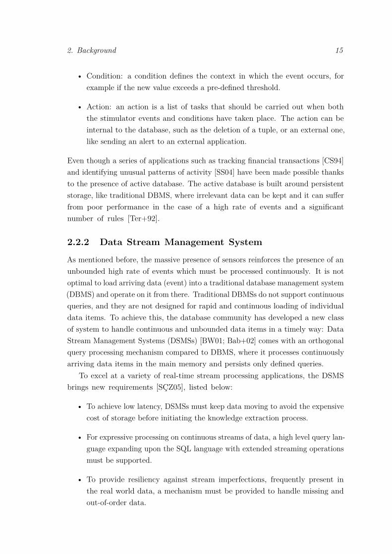
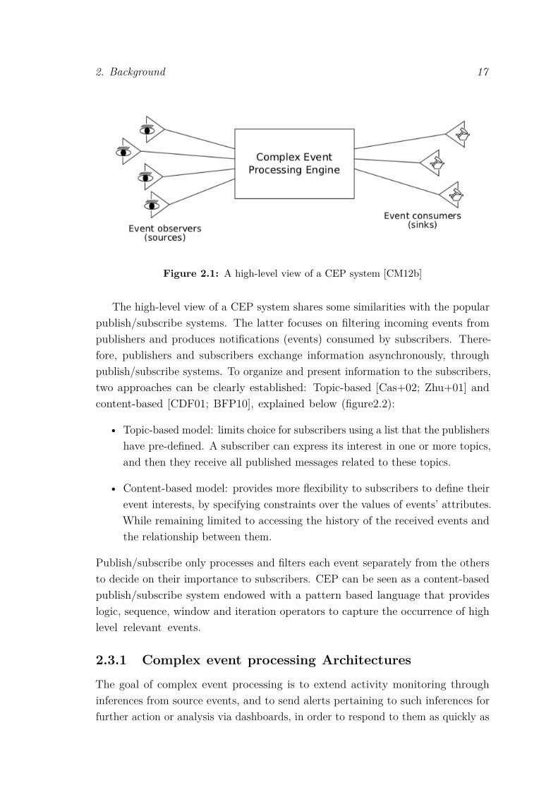
A subset of event processing applications may involve detecting complex events suchas anomaly detection, pattern detection, etc. They are termed as complex eventprocessing (CEP) systems. The incoming events have specific semantics. Theydescribe something that happens in the real world, and CEP systems are in charge offiltering, correlating and combining them. CEP systems detect patterns and extracthigher knowledge from raw events and then notify to event consumers (figure2.1).Thus, it is quite different from the data processing done by simpler event processingsystems, where the operations are as light as filtering and transformation.
2. Background 17
Figure 2.1: A high-level view of a CEP system [CM12b]
The high-level view of a CEP system shares some similarities with the popularpublish/subscribe systems. The latter focuses on filtering incoming events frompublishers and produces notifications (events) consumed by subscribers. There-fore, publishers and subscribers exchange information asynchronously, throughpublish/subscribe systems. To organize and present information to the subscribers,two approaches can be clearly established: Topic-based [Cas+02; Zhu+01] andcontent-based [CDF01; BFP10], explained below (figure2.2):
• Topic-based model: limits choice for subscribers using a list that the publishershave pre-defined. A subscriber can express its interest in one or more topics,and then they receive all published messages related to these topics.
• Content-based model: provides more flexibility to subscribers to define theirevent interests, by specifying constraints over the values of events’ attributes.While remaining limited to accessing the history of the received events andthe relationship between them.
Publish/subscribe only processes and filters each event separately from the othersto decide on their importance to subscribers. CEP can be seen as a content-basedpublish/subscribe system endowed with a pattern based language that provideslogic, sequence, window and iteration operators to capture the occurrence of highlevel relevant events.
2.3.1 Complex event processing Architectures
The goal of complex event processing is to extend activity monitoring throughinferences from source events, and to send alerts pertaining to such inferences forfurther action or analysis via dashboards, in order to respond to them as quickly as
18 2.3. Complex event processing
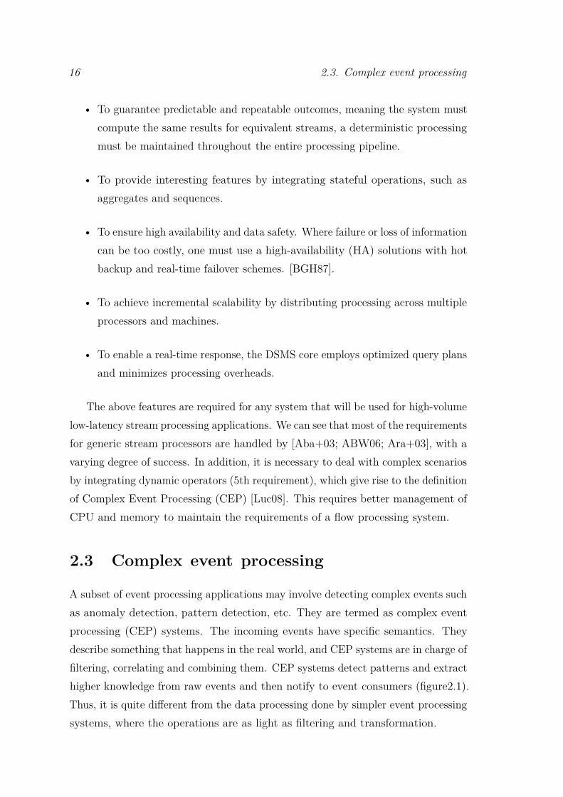
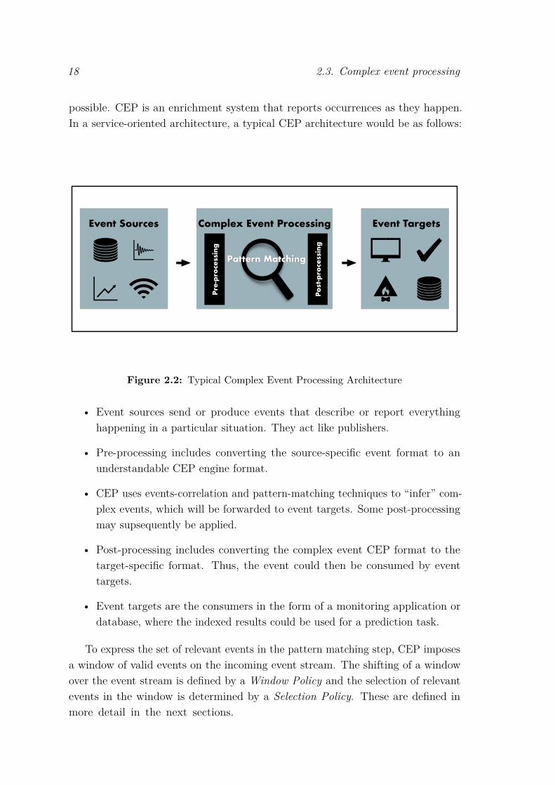
possible. CEP is an enrichment system that reports occurrences as they happen.In a service-oriented architecture, a typical CEP architecture would be as follows:
Event Sources Complex Event Processing Event TargetsPr
e-pr
oces
sing
Post
-pro
cess
ing
Pattern Matching
Figure 2.2: Typical Complex Event Processing Architecture
• Event sources send or produce events that describe or report everythinghappening in a particular situation. They act like publishers.
• Pre-processing includes converting the source-specific event format to anunderstandable CEP engine format.
• CEP uses events-correlation and pattern-matching techniques to “infer” com-plex events, which will be forwarded to event targets. Some post-processingmay supsequently be applied.
• Post-processing includes converting the complex event CEP format to thetarget-specific format. Thus, the event could then be consumed by eventtargets.
• Event targets are the consumers in the form of a monitoring application ordatabase, where the indexed results could be used for a prediction task.
To express the set of relevant events in the pattern matching step, CEP imposesa window of valid events on the incoming event stream. The shifting of a windowover the event stream is defined by a Window Policy and the selection of relevantevents in the window is determined by a Selection Policy. These are defined inmore detail in the next sections.
2. Background 19
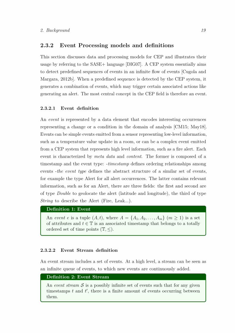
2.3.2 Event Processing models and definitions
This section discusses data and processing models for CEP and illustrates theirusage by referring to the SASE+ language [DIG07]. A CEP system essentially aimsto detect predefined sequences of events in an infinite flow of events [Cugola andMargara, 2012b]. When a predefined sequence is detected by the CEP system, itgenerates a combination of events, which may trigger certain associated actions likegenerating an alert. The most central concept in the CEP field is therefore an event.
2.3.2.1 Event definition
An event is represented by a data element that encodes interesting occurrencesrepresenting a change or a condition in the domain of analysis [CM15; May18].Events can be simple events emitted from a sensor representing low-level information,such as a temperature value update in a room, or can be a complex event emittedfrom a CEP system that represents high level information, such as a fire alert. Eachevent is characterized by meta data and content. The former is composed of atimestamp and the event type: -timestamp defines ordering relationships amongevents -the event type defines the abstract structure of a similar set of events,for example the type Alert for all alert occurrences. The latter contains relevantinformation, such as for an Alert, there are three fields: the first and second areof type Double to geolocate the alert (latitude and longitude), the third of typeString to describe the Alert (Fire, Leak...).
Definition 1: Event
An event e is a tuple (A, t), where A = {A1, A2, . . . , Am} (m ≥ 1) is a setof attributes and t ∈ T is an associated timestamp that belongs to a totallyordered set of time points (T,≤).
2.3.2.2 Event Stream definition
An event stream includes a set of events. At a high level, a stream can be seen asan infinite queue of events, to which new events are continuously added.
Definition 2: Event Stream
An event stream S is a possibly infinite set of events such that for any giventimestamps t and t′, there is a finite amount of events occurring betweenthem.
20 2.3. Complex event processing
2.3.2.3 Event sequence definition
An Event sequence is a chronologically ordered sequence of events, based ontimestamps given by T, is represented as ~E = 〈e1, e2, . . . , en〉 with e1 referringto the first event and en to the last.
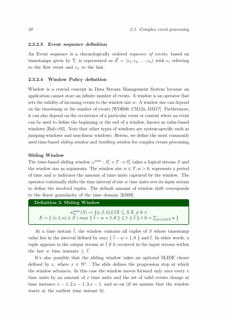
2.3.2.4 Window Policy definition
Window is a crucial concept in Data Stream Management System because anapplication cannot store an infinite number of events. A window is an operator thatsets the validity of incoming events to the window size w. A window size can dependon the timestamp or the number of events [WDR06; CM12a; DM17]. Furthermore,it can also depend on the occurrence of a particular event or content where an eventcan be used to define the beginning or the end of a window, known as value-basedwindows [Bab+02]. Note that other types of windows are system-specific such asjumping-windows and non-linear windows. Herein, we define the most commonlyused time-based sliding window and tumbling window for complex events processing.
Sliding WindowThe time-based sliding window ωtime : Slτ × T → Slτ takes a logical stream S andthe window size as arguments. The window size w ∈ T,w > 0, represents a periodof time and w indicates the amount of time units captured by the window. Theoperator continually shifts the time interval of size w time units over its input streamto define the involved tuples. The default amount of window shift correspondsto the finest granularity of the time domain [KS09].
Definition 3: Sliding Window
wtimew (S) := {(e, t, n))|∃X ⊆ S.X 6= 0 ∧X = { (e, t, n) ∈ S | max { t− w + 1, 0 } ≤ t ≤ t } ∧ n = ∑
(e,t,n)∈X n }
At a time instant t, the window contains all tuples of S whose timestampvalue lies in the interval defined by max { t− w + 1, 0 } and t. In other words, atuple appears in the output stream at t if it occurred in the input stream withinthe last w time instants ≤ t.
It’s also possible that the sliding window takes an optional SLIDE clausedefined by x, where x ∈ N+. The slide defines the progression step at whichthe window advances. In this case the window moves forward only once every xtime units by an amount of x time units and the set of valid events change attime instance x − 1, 2.x − 1, 3.x − 1, and so on (if we assume that the windowstarts at the earliest time instant 0).
2. Background 21
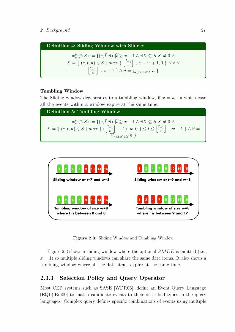
Definition 4: Sliding Window with Slide x
wtimew,x (S) := {(e, t, n))|t ≥ x− 1 ∧ ∃X ⊆ S.X 6= 0 ∧X = { (e, t, n) ∈ S | max {
⌊t+1x
⌋. x− w + 1, 0 } ≤ t ≤⌊
t+1x
⌋. x− 1 } ∧ n = ∑
(e,t,n)∈X n }
Tumbling WindowThe Sliding window degenerates to a tumbling window, if x = w, in which caseall the events within a window expire at the same time.
Definition 5: Tumbling Window
wtimew,x (S) := {(e, t, n))|t ≥ x− 1 ∧ ∃X ⊆ S.X 6= 0 ∧X = { (e, t, n) ∈ S | max { (
⌊t+1w
⌋− 1) .w, 0 } ≤ t ≤
⌊t+1w
⌋. w − 1 } ∧ n =∑
(e,t,n)∈X n }
7 9 10 14 16421 9 10 14 161 742
Sliding window at t=7 and w=8 Sliding window at t=9 and w=8
7 9 10 14 16421 9 10 14 161 742
Tumbling window of size w=8 where t is between 0 and 8
Tumbling window of size w=8 where t is between 9 and 17
Figure 2.3: Sliding Window and Tumbling Window
Figure 2.3 shows a sliding window where the optional SLIDE is omitted (i.e.,x = 1) so multiple sliding windows can share the same data items. It also shows atumbling window where all the data items expire at the same time.
2.3.3 Selection Policy and Query Operator
Most CEP systems such as SASE [WDR06], define an Event Query Language(EQL)[Bui09] to match candidate events to their described types in the querylanguages. Complex query defines specific combinations of events using multiple

22 2.3. Complex event processing
event-queries and the conditions to describe the correlation between them. Con-sidering the example of water leak detection, LowPressure(subregion(r1)) 7→LowConsumption(subregion(r1)) is a high-level event that may represent aleak event. That is, if the low-pressure event is followed by (7→) low consumptionin the sub-region r1 then it may point to a water leak. Typically, the expressivityof EQLs is measured by their capabilities to detect patterns. Therefore, eventqueries are a feature group that consists of:
• Conjunction operator: two or more events occur at the same time or duringthe same period.
• Disjunction operator: one of two or more events occurs without having anyorder constraints.
• Negation operator: the non-existence of an event.
• ANY operator: any event may occur.
• Kleene Closure (A∗/A+/Anum): an event may occur one or more times (+)or zero or more times(*).
• Sequence Operator: a sequence of two events (SEQ(E1; E2)), means that E1occurs before E2.
SASE [Agr+08; ZDI14a] has provided various selection strategies that overlapthe sequence operator with some constraints to mix relevant and irrelevant eventoccurrence. In the following, the provided selection strategies are described andcompared with each other in the context of the example of a sensor data streamin Figure 2.4. An event selection policy defines how a query submitted to a CEPsystem will specify which of the candidate events will be selected to build thecorresponding complex event match based on a given pattern. Event selectionpolicy adds a certain functionality in the detection of high-level events, rather thanbeing limited to a regular expression’s operators.
• Strict Contiguity (SC): requires the two selected events within a sequence tobe contiguous in the events stream. This means that the input stream cannotcontain any other events in between, similar to regular expression matchingagainst strings.
• Partition Contiguity (PC): is a relaxation of strict contiguity strategy, toremove SC where the sequence of events is portioned based on a condition, Forexample when the partition condition is based on the region R1 (Region==R1),all the events that do not hold this condition will be skipped.
2. Background 23
• Skip-Till-Next (STN): In this strategy, the two relevant events do not needto be contiguous in a relevant partition. STN is a relaxation of the strictcontiguity strategy, where certain events considered as noise in the inputstream are ignored.
• Skip-Till-Any (STA): is a relaxation of Skip-Till-Next to compute transitiveclosure over relevant events allowing non-determinism on relevant events. Suchthat for a sequence (E1;E2) all the patterns where E2 follows E1 are output.
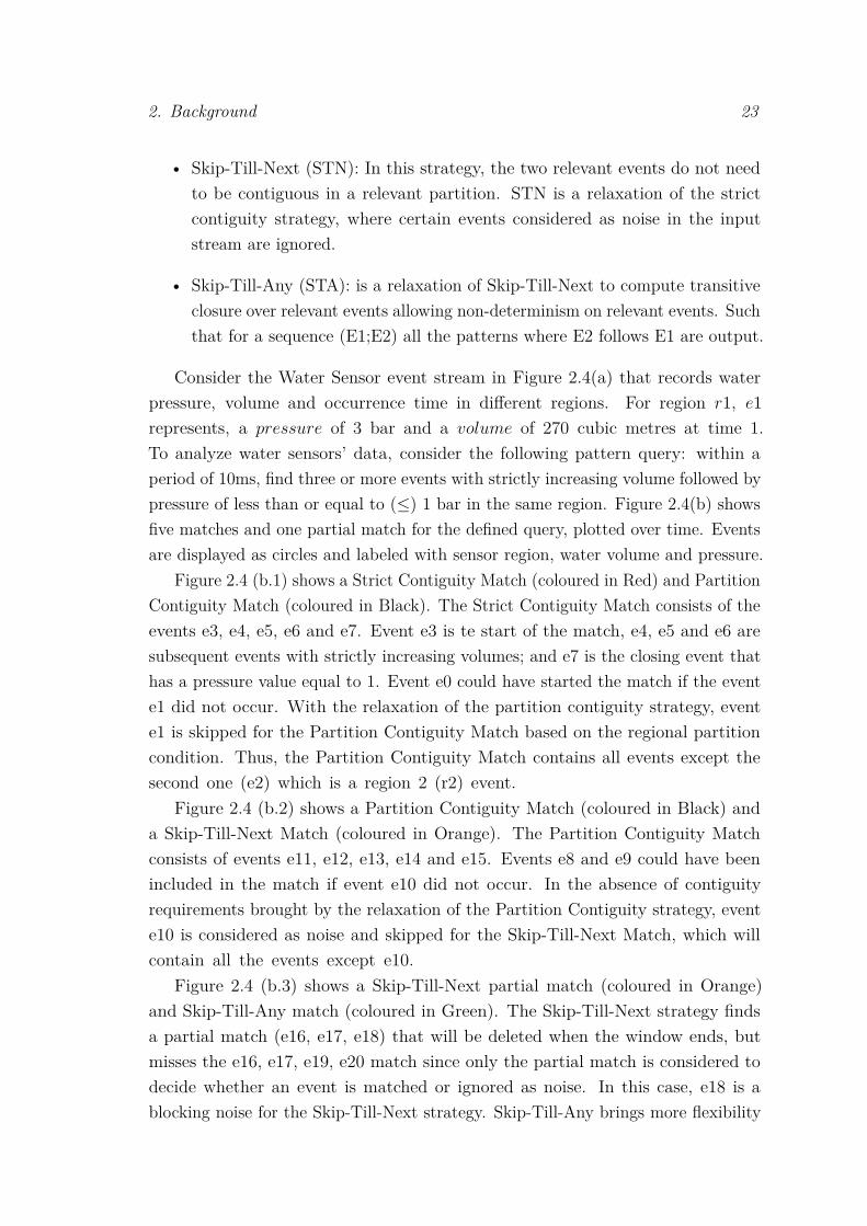
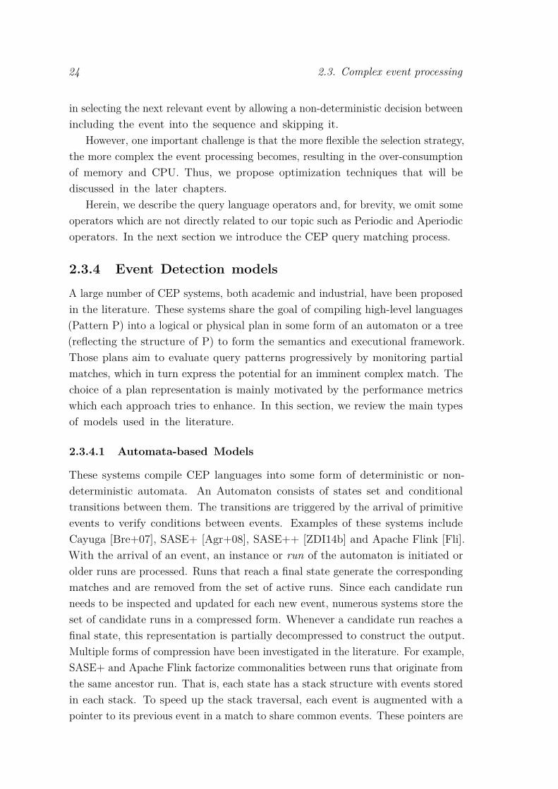
Consider the Water Sensor event stream in Figure 2.4(a) that records waterpressure, volume and occurrence time in different regions. For region r1, e1represents, a pressure of 3 bar and a volume of 270 cubic metres at time 1.To analyze water sensors’ data, consider the following pattern query: within aperiod of 10ms, find three or more events with strictly increasing volume followed bypressure of less than or equal to (≤) 1 bar in the same region. Figure 2.4(b) showsfive matches and one partial match for the defined query, plotted over time. Eventsare displayed as circles and labeled with sensor region, water volume and pressure.
Figure 2.4 (b.1) shows a Strict Contiguity Match (coloured in Red) and PartitionContiguity Match (coloured in Black). The Strict Contiguity Match consists of theevents e3, e4, e5, e6 and e7. Event e3 is te start of the match, e4, e5 and e6 aresubsequent events with strictly increasing volumes; and e7 is the closing event thathas a pressure value equal to 1. Event e0 could have started the match if the evente1 did not occur. With the relaxation of the partition contiguity strategy, evente1 is skipped for the Partition Contiguity Match based on the regional partitioncondition. Thus, the Partition Contiguity Match contains all events except thesecond one (e2) which is a region 2 (r2) event.
Figure 2.4 (b.2) shows a Partition Contiguity Match (coloured in Black) anda Skip-Till-Next Match (coloured in Orange). The Partition Contiguity Matchconsists of events e11, e12, e13, e14 and e15. Events e8 and e9 could have beenincluded in the match if event e10 did not occur. In the absence of contiguityrequirements brought by the relaxation of the Partition Contiguity strategy, evente10 is considered as noise and skipped for the Skip-Till-Next Match, which willcontain all the events except e10.
Figure 2.4 (b.3) shows a Skip-Till-Next partial match (coloured in Orange)and Skip-Till-Any match (coloured in Green). The Skip-Till-Next strategy findsa partial match (e16, e17, e18) that will be deleted when the window ends, butmisses the e16, e17, e19, e20 match since only the partial match is considered todecide whether an event is matched or ignored as noise. In this case, e18 is ablocking noise for the Skip-Till-Next strategy. Skip-Till-Any brings more flexibility
24 2.3. Complex event processing
in selecting the next relevant event by allowing a non-deterministic decision betweenincluding the event into the sequence and skipping it.
However, one important challenge is that the more flexible the selection strategy,the more complex the event processing becomes, resulting in the over-consumptionof memory and CPU. Thus, we propose optimization techniques that will bediscussed in the later chapters.
Herein, we describe the query language operators and, for brevity, we omit someoperators which are not directly related to our topic such as Periodic and Aperiodicoperators. In the next section we introduce the CEP query matching process.
2.3.4 Event Detection models
A large number of CEP systems, both academic and industrial, have been proposedin the literature. These systems share the goal of compiling high-level languages(Pattern P) into a logical or physical plan in some form of an automaton or a tree(reflecting the structure of P) to form the semantics and executional framework.Those plans aim to evaluate query patterns progressively by monitoring partialmatches, which in turn express the potential for an imminent complex match. Thechoice of a plan representation is mainly motivated by the performance metricswhich each approach tries to enhance. In this section, we review the main typesof models used in the literature.
2.3.4.1 Automata-based Models
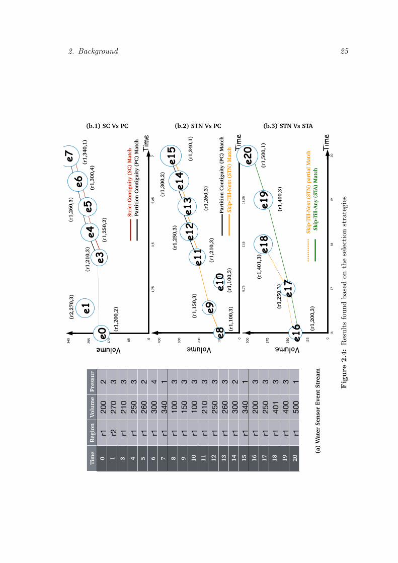
These systems compile CEP languages into some form of deterministic or non-deterministic automata. An Automaton consists of states set and conditionaltransitions between them. The transitions are triggered by the arrival of primitiveevents to verify conditions between events. Examples of these systems includeCayuga [Bre+07], SASE+ [Agr+08], SASE++ [ZDI14b] and Apache Flink [Fli].With the arrival of an event, an instance or run of the automaton is initiated orolder runs are processed. Runs that reach a final state generate the correspondingmatches and are removed from the set of active runs. Since each candidate runneeds to be inspected and updated for each new event, numerous systems store theset of candidate runs in a compressed form. Whenever a candidate run reaches afinal state, this representation is partially decompressed to construct the output.Multiple forms of compression have been investigated in the literature. For example,SASE+ and Apache Flink factorize commonalities between runs that originate fromthe same ancestor run. That is, each state has a stack structure with events storedin each stack. To speed up the stack traversal, each event is augmented with apointer to its previous event in a match to share common events. These pointers are
2. Background 25
Tim
eRe
gion
Volu
me
Pres
sur
e0
r120
02
1r2
270
33
r121
03
4r1
250
35
r126
02
6r1
300
47
r134
01
8r1
100
39
r115
03
10r1
100
311
r121
03
12r1
250
313
r126
03
14r1
300
215
r134
01
16r1
200
317
r125
03
18r1
401
319
r140
03
20r1
500
1
(a)
Wat
er S
enso
r Ev
ent S
trea
m
(b.1) SC Vs PC
Time
Stri
ct C
ontig
uity
(SC
) M
atch
Part
ition
Con
tigui
ty (
PC)
Mat
ch
(r1,
200,
2)
(r2,
270,
3)
(r1,
210,
3)
(r1,
250,
2)(r1,
260,
3)
(r1,
300,
4)(r
1,34
0,1)
Volume
085170
255
340
01,75
3,5
5,25
7
e0e1
e3e4
e5e6
e7
Part
ition
Con
tigui
ty (
PC)
Mat
chSk
ip-T
ill-N
ext (
STN
) M
atch
(r1,
100,
3)(r
1,10
0,3)
(r1,
210,
3)
(r1,
250,
3)
(r1,
260,
3)
(r1,
150,
3)
(r1,
300,
2)
(r1,
340,
1)
Time
Volume
0
100
200
300
400
89,75
11,5
13,25
15
e8e9
e10
e11
e12
e13
e14
e15
(b.2) STN Vs PC (b.3) STN Vs STA
Skip
-Till
-Nex
t (ST
N)
part
ial M
atch
Skip
-Till
-Any
(ST
A) M
atch
(r1,
200,
3)(r1,
250,
3)(r
1,40
0,3)
(r1,
500,
1)(r
1,40
1,3)
Time
Volume
0
125
250
375
500
1617
1819
20
e16
e17
e18
e19
e20
Figure2.4:
Results
foun
dba
sedon
theselectionstrategies
26 2.3. Complex event processing
traversed using depth-first-search (DFS) to extract all complex matches. SASE++
breaks the query evaluation into pattern matching and results construction phases
and only stores so-called maximal runs from which other runs can be efficiently
computed. The pattern matching process computes the main runs of an automaton
with certain predicates postponed. Result construction derives all Kleene+ matches
by applying the postponed predicates to remove non-viable runs. Although these
compression techniques reduce the memory cost, the number of runs can still exceed
memory and CPU resources for large windows and frequent prefixed events that
would initiate a match. These techniques risk generating and updating many
candidate runs that are afterwards discarded without generating output. This may
be circumvented by delaying the evaluation of partial matches using so-called lazy
automata [KSS15a]. However, this requires precomputed selectivity measures of
the prefixed events. Furthermore, the cost of cloning runs on-the-fly for the partial
matches without common prefixed events and repeated operations of computing
events’ predicates remain the same.
Figure 2.5: Non-deterministic Finite Automaton example from [ZDI14a]
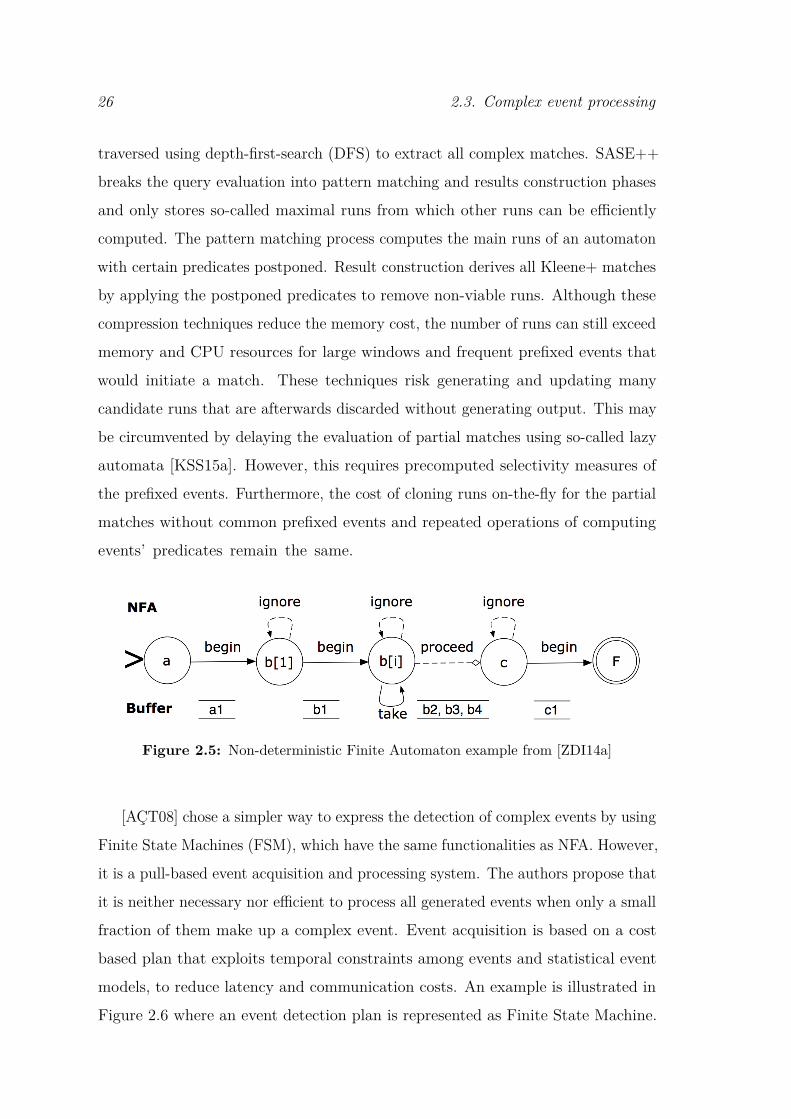
[AÇT08] chose a simpler way to express the detection of complex events by using
Finite State Machines (FSM), which have the same functionalities as NFA. However,
it is a pull-based event acquisition and processing system. The authors propose that
it is neither necessary nor efficient to process all generated events when only a small
fraction of them make up a complex event. Event acquisition is based on a cost
based plan that exploits temporal constraints among events and statistical event
models, to reduce latency and communication costs. An example is illustrated in
Figure 2.6 where an event detection plan is represented as Finite State Machine.
2. Background 27
Figure 2.6: Finite State Machine example from [AÇT08]
Automata-based techniques limit the adaptation of optimization techniquesprovided by DSMSs, for which Tree-based models are usually used, but they alsoprovide new approaches inspired by the field of the regular expression.
2.3.4.2 Tree-based Models
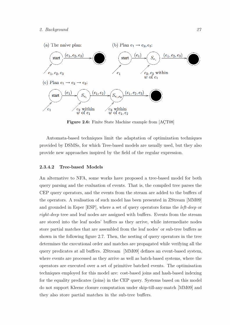
An alternative to NFA, some works have proposed a tree-based model for bothquery parsing and the evaluation of events. That is, the compiled tree parses theCEP query operators, and the events from the stream are added to the buffers ofthe operators. A realisation of such model has been presented in ZStream [MM09]and grounded in Esper [ESP], where a set of query operators forms the left-deep orright-deep tree and leaf nodes are assigned with buffers. Events from the streamare stored into the leaf nodes’ buffers as they arrive, while intermediate nodesstore partial matches that are assembled from the leaf nodes’ or sub-tree buffers asshown in the following figure 2.7. Then, the nesting of query operators in the treedetermines the executional order and matches are propagated while verifying all thequery predicates at all buffers. ZStream [MM09] defines an event-based system,where events are processed as they arrive as well as batch-based systems, where theoperators are executed over a set of primitive batched events. The optimisationtechniques employed for this model are: cost-based joins and hash-based indexingfor the equality predicates (joins) in the CEP query. Systems based on this modeldo not support Kleene closure computation under skip-till-any-match [MM09] andthey also store partial matches in the sub-tree buffers.
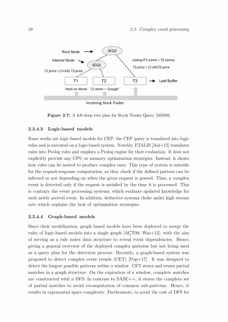
28 2.3. Complex event processing
Figure 2.7: A left-deep tree plan for Stock Trades Query [MM09]
2.3.4.3 Logic-based models
Some works use logic-based models for CEP: the CEP query is translated into logicrules and is executed on a logic-based system. Notably, ETALIS [Ani+12] translatesrules into Prolog rules and employs a Prolog engine for their evaluation. It does notexplicitly provide any CPU or memory optimisation strategies. Instead, it showshow rules can be nested to produce complex ones. This type of system is suitablefor the request-response computation, as they check if the defined pattern can beinferred or not depending on when the given request is posted. Thus, a complexevent is detected only if the request is satisfied by the time it is processed. Thisis contrary the event processing systems, which evaluate updated knowledge foreach newly arrived event. In addition, deductive systems choke under high streamrate which explains the lack of optimisation strategies.
2.3.4.4 Graph-based models
Since their modelization, graph based models have been deployed to merge therules of logic-based models into a single graph [AÇT08; Was+12], with the aimof serving as a rule index data structure to reveal event dependencies. Hence,giving a general overview of the deployed complex patterns but not being usedas a query plan for the detection process. Recently, a graph-based system wasproposed to detect complex event trends (CET) [Pop+17]. It was designed todetect the longest possible patterns within a window. CET stores and reuses partialmatches in a graph structure. On the expiration of a window, complete matchesare constructed with a DFS. In contrast to SASE++, it stores the complete setof partial matches to avoid recomputation of common sub-patterns. Hence, itresults in exponential space complexity. Furthermore, to avoid the cost of DFS for
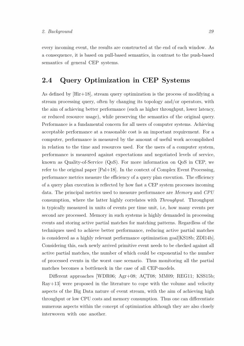
2. Background 29
every incoming event, the results are constructed at the end of each window. Asa consequence, it is based on pull-based semantics, in contrast to the push-basedsemantics of general CEP systems.
2.4 Query Optimization in CEP Systems
As defined by [Hir+18], stream query optimization is the process of modifying astream processing query, often by changing its topology and/or operators, withthe aim of achieving better performance (such as higher throughput, lower latency,or reduced resource usage), while preserving the semantics of the original query.Performance is a fundamental concern for all users of computer systems. Achievingacceptable performance at a reasonable cost is an important requirement. For acomputer, performance is measured by the amount of useful work accomplishedin relation to the time and resources used. For the users of a computer system,performance is measured against expectations and negotiated levels of service,known as Quality-of-Service (QoS). For more information on QoS in CEP, werefer to the original paper [Pal+18]. In the context of Complex Event Processing,performance metrics measure the efficiency of a query plan execution. The efficiencyof a query plan execution is reflected by how fast a CEP system processes incomingdata. The principal metrics used to measure performance are Memory and CPUconsumption, where the latter highly correlates with Throughput. Throughputis typically measured in units of events per time unit, i.e, how many events persecond are processed. Memory in such systems is highly demanded in processingevents and storing active partial matches for matching patterns. Regardless of thetechniques used to achieve better performance, reducing active partial matchesis considered as a highly relevant performance optimization goal[KS18b; ZDI14b].Considering this, each newly arrived primitive event needs to be checked against allactive partial matches, the number of which could be exponential to the numberof processed events in the worst case scenario. Thus monitoring all the partialmatches becomes a bottleneck in the case of all CEP-models.
Different approaches [WDR06; Agr+08; AÇT08; MM09; REG11; KSS15b;Ray+13] were proposed in the literature to cope with the volume and velocityaspects of the Big Data nature of event stream, with the aim of achieving highthroughput or low CPU costs and memory consumption. Thus one can differentiatenumerous aspects within the concept of optimization although they are also closelyinterwoven with one another.
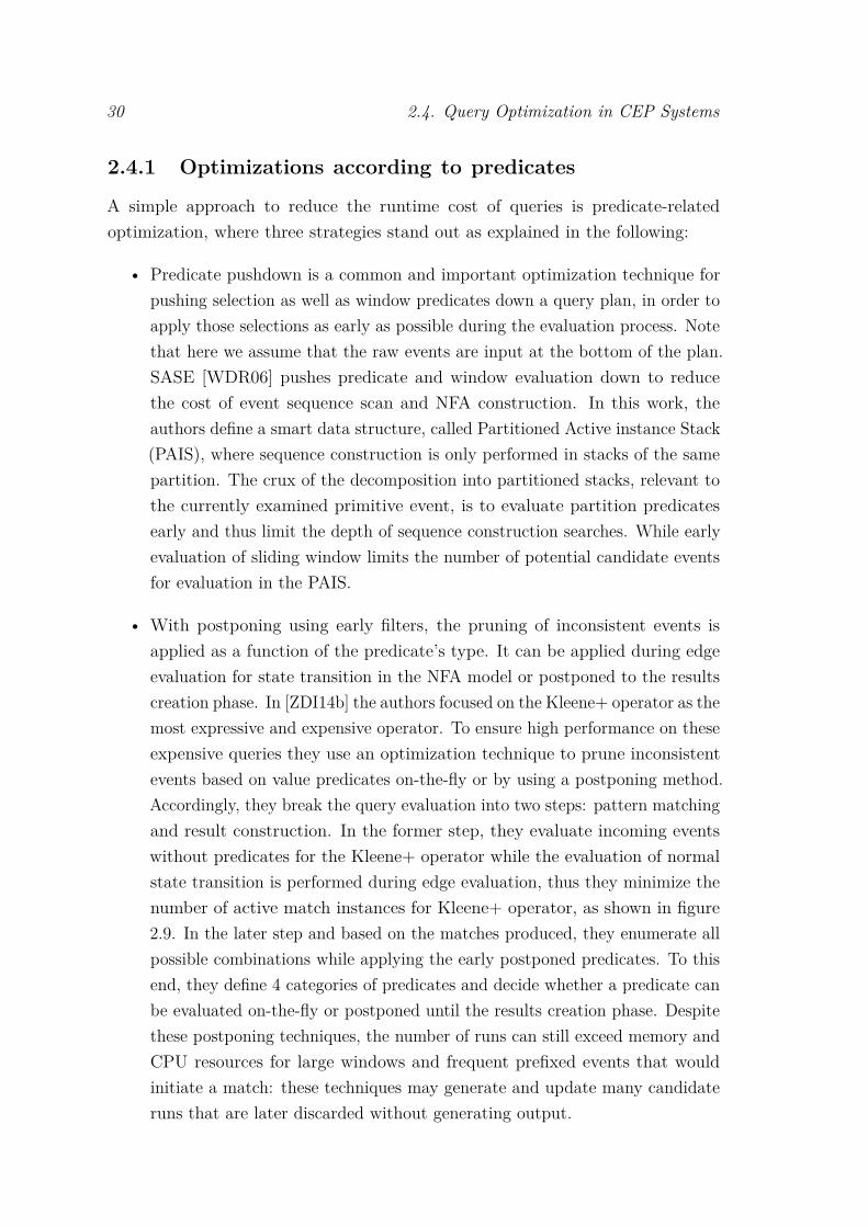
30 2.4. Query Optimization in CEP Systems
2.4.1 Optimizations according to predicates
A simple approach to reduce the runtime cost of queries is predicate-relatedoptimization, where three strategies stand out as explained in the following:
• Predicate pushdown is a common and important optimization technique forpushing selection as well as window predicates down a query plan, in order toapply those selections as early as possible during the evaluation process. Notethat here we assume that the raw events are input at the bottom of the plan.SASE [WDR06] pushes predicate and window evaluation down to reducethe cost of event sequence scan and NFA construction. In this work, theauthors define a smart data structure, called Partitioned Active instance Stack(PAIS), where sequence construction is only performed in stacks of the samepartition. The crux of the decomposition into partitioned stacks, relevant tothe currently examined primitive event, is to evaluate partition predicatesearly and thus limit the depth of sequence construction searches. While earlyevaluation of sliding window limits the number of potential candidate eventsfor evaluation in the PAIS.
• With postponing using early filters, the pruning of inconsistent events isapplied as a function of the predicate’s type. It can be applied during edgeevaluation for state transition in the NFA model or postponed to the resultscreation phase. In [ZDI14b] the authors focused on the Kleene+ operator as themost expressive and expensive operator. To ensure high performance on theseexpensive queries they use an optimization technique to prune inconsistentevents based on value predicates on-the-fly or by using a postponing method.Accordingly, they break the query evaluation into two steps: pattern matchingand result construction. In the former step, they evaluate incoming eventswithout predicates for the Kleene+ operator while the evaluation of normalstate transition is performed during edge evaluation, thus they minimize thenumber of active match instances for Kleene+ operator, as shown in figure2.9. In the later step and based on the matches produced, they enumerate allpossible combinations while applying the early postponed predicates. To thisend, they define 4 categories of predicates and decide whether a predicate canbe evaluated on-the-fly or postponed until the results creation phase. Despitethese postponing techniques, the number of runs can still exceed memory andCPU resources for large windows and frequent prefixed events that wouldinitiate a match: these techniques may generate and update many candidateruns that are later discarded without generating output.
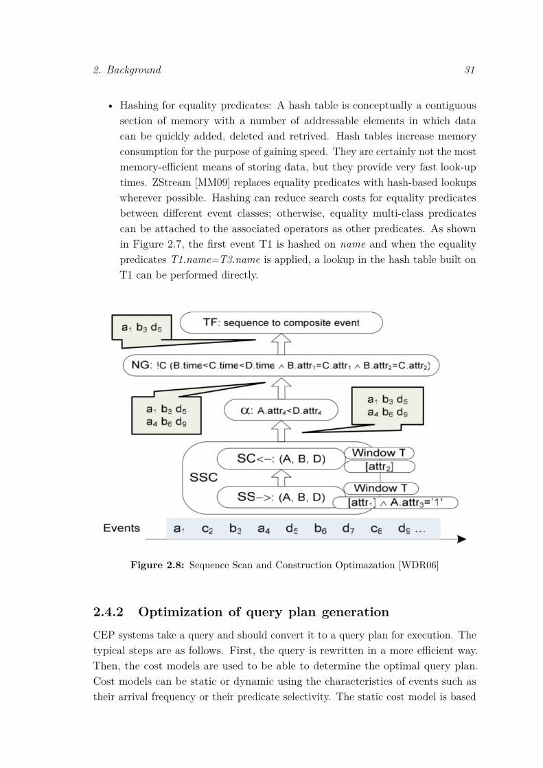
2. Background 31
• Hashing for equality predicates: A hash table is conceptually a contiguoussection of memory with a number of addressable elements in which datacan be quickly added, deleted and retrived. Hash tables increase memoryconsumption for the purpose of gaining speed. They are certainly not the mostmemory-efficient means of storing data, but they provide very fast look-uptimes. ZStream [MM09] replaces equality predicates with hash-based lookupswherever possible. Hashing can reduce search costs for equality predicatesbetween different event classes; otherwise, equality multi-class predicatescan be attached to the associated operators as other predicates. As shownin Figure 2.7, the first event T1 is hashed on name and when the equalitypredicates T1.name=T3.name is applied, a lookup in the hash table built onT1 can be performed directly.
Figure 2.8: Sequence Scan and Construction Optimazation [WDR06]
2.4.2 Optimization of query plan generation
CEP systems take a query and should convert it to a query plan for execution. Thetypical steps are as follows. First, the query is rewritten in a more efficient way.Then, the cost models are used to be able to determine the optimal query plan.Cost models can be static or dynamic using the characteristics of events such astheir arrival frequency or their predicate selectivity. The static cost model is based
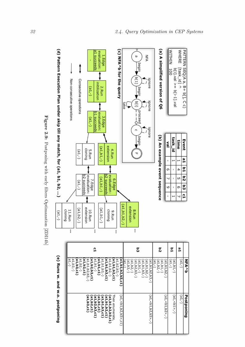
32 2.4. Query Optimization in CEP Systems
Figure
2.9:Postponing
with
earlyfilters
Optim
azation[ZD
I14b]
2. Background 33
on fixed assumptions of events characteristics. Dynamic cost models are updatedand used on-the-fly based on such characteristics to swap to a new optimal plan.This dynamic system must also take into account the cost of regenerating a newplan. Automata-based CEP [Bre+07; SMP09], described in section 2.3.4.1, usethe order-based-plan to set the order in which arriving events will be processed.The Order-based-plan consists of a permutation of primitive event types definedby a pattern. While Tree-based CEP [MM09] use the tree-based plan to findthe optimal physical trees (e.g., left-deep, right-deep or bushy), that can be usedto evaluate the defined pattern.
[AÇT08] were the first to explore cost-based planning for complex event detectionwith the aim of minimizing network traffic across distributed event sources, whilealso helping to reduce the processing cost. The defined cost model was based ontemporal constraints among constituent events and events frequency statistics. InNextCEP [SMP09], authors limit the query rewriting for three operators OR, SEQand NOT. For the OR operator, they use a greedy Huffman algorithm [Huf52]to create a tree and the optimal order of the OR operator is generated with adepth first traversal. For the NEXT and NOT operator they use a dynamicprogramming solution where the lowest cost pattern can be found by enumeratingall the equivalent patterns and computing each cost. The NextCEP cost modelwas based on the arrival frequency of the primitive events. In ZStream[MM09],authors define a series of rules that generate an exponential number of equivalentexpressions, called algebraic rules, in order to avoid exhaustive searches of allthese expressions as done by NextCEP[SMP09]. Once a query expression has beensimplified using the algebraic rewrites, i.e. (SEQ(A,AND(!B,!C),D) is translatedsimply to SEQ(A,!OR(B,C),D)), and hashing has been applied on the equalityattributes, the authors use a cost model for optimal tree-based plan generations,where they apply a dynamic programming solution to enumerate all possible treetopology costs. In contrast to NextCEP the cost model takes into account the arrivalrates of primitive events and the selectivity of their predicates. In addition, theydefine a constant threshold t for the monitored statistics to trigger plan regeneration.In [KSS15a; KSK16], authors propose a lazy evaluation approach where events ofhigh frequency are buffered until the rare event type instance is received. In casethe selectivity of events is already known and remains invariant, they use a simpleNFA structure to determine potential pattern matches. Otherwise, if the selectivityof events may change over time they use a Tree-NFA, an NFA backed by a treestructure, which reorganizes itself according to the present observed events rates,similarly to Eddies[AH00]. The most important strength of these approaches is thatthe optimal evaluation plan is guaranteed for any given set of events. However, itresults in an overload of plan generation where the process of creating and deploying
34 2.4. Query Optimization in CEP Systems
a new evaluation plan is very expensive. As discussed before, this was proposed inZStream[MM09] to avoid this overload, however, some re-optimization opportunitiesmay have been missed. Recently, [KS18a] presented a novel method for detectingre-optimization opportunities by verifying a set of distances on the monitored datacharacteristics. They formally prove that they avoid launching re-optimization plangeneration that does not improve the currently employed plan. To do this, theydefine a list of in-variant distances. The idea is to use margins instead of a simplethresholds to avoid the ping-pong effect i.e. keep changing query plan due to noise.Thus in-variant distances are defined between events having the closest arrival rates,in case even a slight oscillation in the events rates causes the event types to swappositions periodically when ordered according to this statistic. They use some dataanalysis methods to discover the minimal distance that will be used as a violationconstraint. However, finding the right distance remains as always a difficult taskand depends on the data and keeping in mind the overload of this method if it wereapplied on-the-fly. These contributions aim to reduce the number of active partialmatches by rewriting/reordering the queries based on statistical characteristics ofthe primitive events. However, the number of partial matches remains one of itsmajor problems, especially when dealing with expensive queries or large windows,even if some existing work focused on their smart indexing.
2.4.3 Optimization of memory
In the context of CEP, memory management is critical for performance measurementwhere workers aim to optimize throughput and not to shed the storage load directly.With the arrival of primitive events, the number of storage data structures growproportionally, such as events’ buffers and partial active matches’ data structures. In[Agr+08], the evaluation plan is set to the initial order of the sequence pattern, butthey design efficient data structures to enable smart runtime memory management.They define a versioned system of shared buffer to compactly encode all activepartial and complete matches instead of having a single buffer for each one. Toavoid erroneous results they use version numbers that share the same prefix withall the events of the same partial match, and a pointer to the previous event, asshown in the figure 2.10. In addition, they incrementally prune all the used datastructures based the window size and reuse the expired instance whenever possible.This strategy can reduce memory requirements from exponential to polynomial,at the cost of the compression/decompression operations.
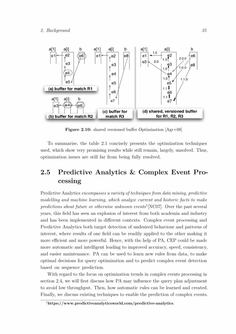
2. Background 35
Figure 2.10: shared versioned buffer Optimization [Agr+08]
To summarise, the table 2.1 concisely presents the optimization techniquesused, which show very promising results while still remain, largely, unsolved. Thus,optimization issues are still far from being fully resolved.
2.5 Predictive Analytics & Complex Event Pro-cessing
Predictive Analytics encompasses a variety of techniques from data mining, predictivemodelling and machine learning, which analyze current and historic facts to makepredictions about future or otherwise unknown events1[NC07]. Over the past severalyears, this field has seen an explosion of interest from both academia and industryand has been implemented in different contexts. Complex event processing andPredictive Analytics both target detection of undesired behaviour and patterns ofinterest, where results of one field can be readily applied to the other making itmore efficient and more powerful. Hence, with the help of PA, CEP could be mademore automatic and intelligent leading to improved accuracy, speed, consistency,and easier maintenance. PA can be used to learn new rules from data, to makeoptimal decisions for query optimization and to predict complex event detectionbased on sequence prediction.
With regard to the focus on optimization trends in complex events processing insection 2.4, we will first discuss how PA may influence the query plan adjustmentto avoid low throughput. Then, how automatic rules can be learned and created.Finally, we discuss existing techniques to enable the prediction of complex events.
1https://www.predictiveanalyticsworld.com/predictive-analytics.

36 2.5. Predictive Analytics & Complex Event Processing
Approach
Optim
izationStrategies
PredicateRelated
Optim
izationQuery
rewriting
Mem
oryManagem
entPush
Dow
nPostponing
Hashing
Detection Models
Autom
atabased
Akdere
[AÇT08]
√φ
φ√
φCayaga
[Bre+07]
φφ
φ√
√
SASE
[WDR06]
√φ
√φ
φSA
SE+[A
gr+08]
√φ
√φ
√
SASE+
+[ZD
I14b]√
√√
φ√
FLINK
[Fli]√
φ√
φ√
LazyNFA
[KSS15a;K
S18a]√
φφ
√φ
NextC
EP[SM
P09]φ
φφ
√φ
TreeBased
Zstream[M
M09]
√φ
√√
√
Graph
BasedCET
[Pop+17]
√√
φφ
√
logicbased
Etalis[A
ni+12]
φφ
φφ
φ
Table 2.1: CEP Optimisation Strategies & Detection Models
2. Background 37
2.5.1 Predictive Analytics for optimal decision making
Predictive Analytics technologies are also implemented to improve performanceof complex event processing systems. As discussed previously, in [MM09; KSK16;KS18a], statistics were used for query plan adaptation to avoid low throughput. Aslightly different approach is followed in [LG16], where workers assume that thehistory could be a mirror to the future. They propose ACEP as an approximatecomplex event processing system with the aim of maximizing the number of fullmatches found. Their idea is to represent a history of past matches concisely into adata structure. Then at run time they discard some matches that are unlikely toresult in a final full match. In the same context, other works deal with uncertaintyin the occurrence of events and prune intermediate results (partial matches) duringpattern matching process [Art+12]. Finally, PA is also used in a distributed CEPcontext to reduce communication costs incurred while exchanging event informationbetween distributed systems [AÇT08].
2.5.2 Predictive Analytics for automatic rules generation
Faced with the complexity of defining complex queries and with the aim of reducinghuman involvement, different works [TGW09; SSS10; MP12; MCT14; MTZ17] havefocused on the automatic generation of CEP rules. Thus they extract rules thatare driven by data and learned from history. [MP12] introduces a domain expertdependent method based on hidden Markov models (HMM). The expert reports theoccurrence of a relevant complex event at a specific point in time, the system thenautomatically deducts the rule allowing the recognition of such events in the future.Similarly, [MCT14] proposed a framework that analyzes historical traces to inferthe hidden causality between received events and detected situations, and uses themto automatically generate CEP rules. On the other hand, they solve the learningproblem by modelling rules and time series as a set of constraints and calculatingtheir intersections. Recently, [MTZ17] developed a generic system that extractspredictive temporal patterns with time and sequence constraints and then transformsthese patterns on-the-fly into predictive CEP rules. To achieve this, they use aShapelet-based classification for rules discovery over multivariate (multi-dimensional)time series [Lii91]. Most of these contributions were in complete agreement andhighlight the importance of handling multidimensional data mining algorithms.
38 2.5. Predictive Analytics & Complex Event Processing
2.5.3 Predictive Analytics for complex events prediction
Complex Event prediction aims to provide the possible future events of partiallymatched sequences which can be turned into a full match. This would enableusers to mitigate or eliminate undesired future events or states and identify futureopportunities. The problem of predictive CEP has remarkable similarities withthe sequence pattern mining and prediction. In this context, a large body ofsequence prediction models have been proposed including: Prediction By PartialMatching (PPM) [CW84], All-K-Order-Markov [PP99] and the Probabilistic SuffixTree [BYY04]. These models are based on the Markov property and suffer fromthe catastrophic forgetting of older sequences [Kir+17]. Only k recent items oftraining sequences are used for performing prediction: increasing k often induces avery high state complexity and consequently such techniques become impracticalfor many real-life applications [Gue+15].
2.5.3.1 Sequence Pattern Mining and Prediction
A large number of sequence prediction methods [BYY04; CW84; Gue+15; PP99]come from the field of temporal/time-series pattern mining, where patterns aredefined using association rules or as frequent episodes. These methods employvariants of decision trees and probabilistic data structures. Most of them are basedon the Markov property and suffer from the issue of forgetting older models andhave high computation costs. Recently, two methods CPT and CPT+ [Gue+15]have been proposed, which keep all historic data in a compressed format andoffer increased accuracy. It is based on the prefix tree (aka trie) data structureand supports only one dimensional sequences. Furthermore, these models are notoptimised for streaming applications, where the training dataset is unknown; alarge number of events arrive at a high rate; events occur at random intervalsrather than at the regular tick-tock intervals of traditional time series and, thus,a real-time response is required.
2.5.3.2 Machine Learning-based Predictions
Further directions for tackling this problem are incremental (online) machinelearning algorithms which learn incrementally over event streams, such as SupportVector Machines, recurrent Neural Networks and Bayesian Networks [FB12; AÇU10;MRT12]. For these algorithms, classifiers are updated each time a new traininginstance is found to provide a predictive response. The main disadvantages ofthese algorithms in the context of CEP are as follows: (i) they are use-case specificand require considerable effort (and training datasets) to model each dataset,e.g. a model can either be based on recent history or is updatable based on
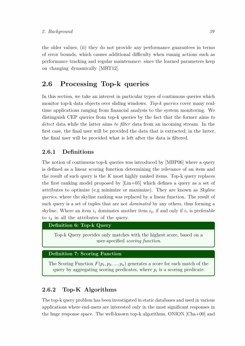
2. Background 39
the older values; (ii) they do not provide any performance guarantees in termsof error bounds, which causes additional difficulty when runnig actions such asperformance tracking and regular maintenance: since the learned parameters keepon changing dynamically [MRT12].
2.6 Processing Top-k queriesIn this section, we take an interest in particular types of continuous queries whichmonitor top-k data objects over sliding windows. Top-k queries cover many real-time applications ranging from financial analysis to the system monitoring. Wedistinguish CEP queries from top-k queries by the fact that the former aims todetect data while the latter aims to filter data from an incoming stream. In thefirst case, the final user will be provided the data that is extracted; in the latter,the final user will be provided what is left after the data is filtered.
2.6.1 Definitions
The notion of continuous top-k queries was introduced by [MBP06] where a queryis defined as a linear scoring function determining the relevance of an item andthe result of such query is the K most highly ranked items. Top-k query replacesthe first ranking model proposed by [Lin+05] which defines a query as a set ofattributes to optimize (e.g minimize or maximize). They are known as Skylinequeries, where the skyline ranking was replaced by a linear function. The result ofsuch query is a set of tuples that are not dominated by any others, thus forming askyline. Where an item i1 dominates another item i2, if and only if i1 is preferableto i2 in all the attributes of the query.
Definition 6: Top-k Query
Top-k Query provides only matches with the highest score, based on auser-specified scoring function.
Definition 7: Scoring Function
The Scoring Function F (p1, p2, ..., pn) generates a score for each match of thequery by aggregating scoring predicates, where pi is a scoring predicate.
2.6.2 Top-K Algorithms
The top-k query problem has been investigated in static databases and used in variousapplications where end-users are interested only in the most significant responses inthe huge response space. The well-known top-k algorithms, ONION [Cha+00] and
40 2.6. Processing Top-k queries
PREFER[HKP01], cannot be directly used in static databases nor can they be easilyadapted to fit streaming environments. Indeed, given the considerable volume ofdata, the core of the problem which they have solved is as follows. How can the databe pre-analyzed to prepare the appropriate meta-information, in order to effectivelyrespond to the top-k queries? Clearly, in a streaming environment, computingcomplete changes for each update and re-initializing the process of identifying top-kelements for each newly observed change is too expensive. Therefore, the mainchallenge is to provide an incremental process that can effectively update top-kresults, even at extremely high throughput and in very large query windows. Theworkers’ advanced efforts in continuous top-k query on data streams fall into twogroups, namely multi-pass approaches and single-pass approaches. The former isa re-computation approach while the latter is an incremental approach.
2.6.2.1 Multi-pass-based approaches:
In Multi-pass-based approaches [Yi+03], the idea is to maintain a larger numberk
′ as a candidate set C instead of maintaining k objects in the current window,where k ≤ k
′ ≤ kmax and kmax is the maximum capacity of C. Whenever a queryresult expires from the window then recomputation of the top-k results is onlyperformed when the top-k′ window has less than k objects (|C| < k). This isbecause recomputing the top-k results is the most expensive operation for top-kmaintenance. [MBP06] proposes the TMA algorithm (Top-k Monitoring Algorithm)to reduce the re-computation cost by maintaining a “grid structure" to access onlya few cells by defining an influence region. The influence region of a query specifiesthe data space to which an object must belong in order to modify the results ofthe query. Therefore, any update in the influence region will modify the result ofthe query. The re-computation process is involved only when some of the existingtop-k objects expire and new arrivals have a lower score than the expired records(so that the influence region expands). The main drawback of this algorithm isthat it is data distribution dependent. At the same time, [MBP06] proposes aSMA (Skyband Monitoring Algorithm to address the problem of re-computationbottlenecks in the TMA algorithm. The authors use the K-Skyband as the minimalset of objects required to be maintained in order to answer top-k queries whereK-Skyband consists of every object that is dominated by at most (k-1) other objects.SMA is required to be faster than TMA at the expense of memory consumptionused to index K-Skyband objects, while both need to conduct expensive top-kre-computations from scratch in certain cases.
2. Background 41
2.6.2.2 One-pass-based approaches:
In one-pass-based approaches, [Yan+11] proposed their algorithm named MinTopK.This algorithm eliminates the re-computation bottleneck and thus realizes completelyincremental computations and minimal memory usage. Based on the assumptionthat the life span of an incoming object is known upon its arrival, it is possible topredict if its score allows it to be in the future top-k window sets. Thus it enablesthe maintenance of partitioned sub-window candidate sets and to immediatelyeliminate all objects that will never be in the top-k sets. MinTopK is highlysensitive to data distribution, especially when the sliding window is too small,thus the number of insertions/deletions required to maintain the candidates isdramatically increasing. SAP [Zhu17] enhanced the MinTopk algorithm with adynamic self-adaptive partition of the window based on different query parametersand data distributions. To the best of our knowledge, MinTopK and SAP are thebest solutions in the case of top-k algorithms that output exact results, with respectto approximate ones such as [Zhu+17]. [Zhu+17] proposes a (ε, δ)-approximatecontinuous top-k system that filters out arrived objects which have a probabilityless than 1 - δ of being a query result, and generates summary information oncandidates with roughly the same scores.
All algorithms previously mentioned cover the needs for major top-k queryprocessing systems, but one size does not fit all and more complex top-k systemshave requirements that cannot be met by this paradigm. These conditions include,for example, if the ranking score is related to the arrival time of the object, second,if the arrival of a new object may change the scores of old ones in top-k or thecandidate set, and third, if the data expiration is not linear with the time, systemsbased on sliding-windows are not adequate as they can only treat linear dataexpiration. Therefore these real-world data stream processing applications requiread hoc developments with standard programming languages.
2.7 ConclusionIn this chapter, we provided the concepts and the background to the topicsaddressed in this thesis. We also provided specific background to understandthe challenges of processing expensive queries and designing predictive systems. Wediscussed the recent advances and related works ranging from query optimizationto predictive analyses.
Obtaining high performance at reasonable cost is a key concern for streamprocessing systems. Thus, different works address the big data aspects such asvolume and velocity of event streams. Some works focus on throughput optimizationand some works optimise memory consumption. They aim to reduce the number
42 2.7. Conclusion
of active partial matches, which consume memory, by rewriting/reordering thequeries or based on statistical characteristics of the primitive events. However, thememory consumption due to a large amount of partial matches remains one of themajor problems. This is especially true when dealing with expensive queries orlarge windows. Even if some existing works use smart indexing techniques withpromising results, still there are performance issues which are largely unsolved.Thus, optimization issues remain fairly unexplored. Thus, in this thesis one ofthe focus is on optimizing CEP performance by eliminating partial matches andusing intelligent indexing technique.
We also saw that one of the trends is to combine Predictive Analysis (PA)with Complex Event Processing (CEP) systems. Hence, with the help of PA, CEPcould be made more automatic and intelligent leading to improved accuracy, speed,consistency, and easier maintenance. PA can be used to make optimal decisionsfor query optimization, to learn new rules from data, and to predict complex eventdetection based on sequence prediction. In this thesis we focus on predictingfuture complex events. For this problem, some of the existing solutions are notsuitable for streaming applications. Other works are use-case specific and requireconsiderable effort to model each dataset.
Finally, we consider also a particular type of continuous queries which monitortop-k data objects over sliding windows to identify k highest-ranked data items.Top-k queries face several challenges because they have to maintaining a candidatelist of data items that can be the part of top-k list in stream settings. Due to streamsettings, the regular arrival of new data may change the state of existing top-kcandidate list. Thus, it requires efficient incremental algorithms and data structures.
Above research gaps now set the context for the remaining chapters that willdetail our contributions.
Part II
Enhancing Complex EventProcessing
43

3Enabling Efficient Recomputation BasedComplex Event Processing for Expensive
Queries
Contents
3.1 Introduction . . . . . . . . . . . . . . . . . . . . . . . . . 463.2 Motivating examples . . . . . . . . . . . . . . . . . . . . 463.3 Related Works . . . . . . . . . . . . . . . . . . . . . . . . 483.4 Preliminaries and definitions . . . . . . . . . . . . . . . . 51
3.4.1 Definitions . . . . . . . . . . . . . . . . . . . . . . . . . 513.4.2 Query Tree . . . . . . . . . . . . . . . . . . . . . . . . . 53
3.5 Baseline Algorithm . . . . . . . . . . . . . . . . . . . . . 553.6 RCEP: Recomputational based CEP . . . . . . . . . . . 57
3.6.1 The Event Tree . . . . . . . . . . . . . . . . . . . . . . . 573.6.2 Creating the Complex Matches . . . . . . . . . . . . . . 59
3.7 RCEP: General Recomputation Model . . . . . . . . . 653.7.1 Multidimensional Events . . . . . . . . . . . . . . . . . . 653.7.2 Multidimensional Event Tree . . . . . . . . . . . . . . . 663.7.3 Joins between Z-addresses . . . . . . . . . . . . . . . . . 683.7.4 Handling Sliding Windows . . . . . . . . . . . . . . . . . 723.7.5 Optimising Z-address Comparison . . . . . . . . . . . . 74
3.8 Experimental Evaluation . . . . . . . . . . . . . . . . . . 743.8.1 Setup and Methodology . . . . . . . . . . . . . . . . . . 743.8.2 Performance of Indexing and Join Algorithms . . . . . . 763.8.3 Performance of Sliding Windows . . . . . . . . . . . . . 783.8.4 CEP Systems’ Comparison . . . . . . . . . . . . . . . . 79
3.9 Conclusion . . . . . . . . . . . . . . . . . . . . . . . . . . 83
45
46 3.1. Introduction
3.1 IntroductionAs discussed earlier, traditional strategies of Complex Event Processing (CEP)require extensive utilization of memory and CPU to extract complex temporalmatches from events stream defined via a CEP query pattern. This is mainlydue to the way in which complex temporal correspondences are extracted froman event flow. In fact, matches incrementally emerge over time while partialmatches accumulate in the memory and then they are processed sequentially forincoming events. The number of partial matches for expressive CEP queries canbe polynomial or exponential to the number of events within a window (proof: 3).Reducing the number of partial matches by compressing them is not a satisfactorysolution because it is highly use case dependent and only aggravates the repeatedcalculation of matches when they are compressed.
In this chapter, we demonstrate how the recomputation of matches, withoutrelying on the partial matches, can be made into a first-order CEP strategy forcomplex operators such as skip-till-any-match and Kleene+. In particular, we showhow to efficiently store and query multi-attributed events within a window and howto join them in batches to efficiently recompute matches for an incoming event.Our hybrid-join algorithm reuses previously computed joins to further economiseon recomputation of matches. The proposed techniques result in the reduction ofmemory and CPU requirements while increasing the throughput by many orders ofmagnitude compared to existing solutions. Our experimental observations supportour arguments and the vast advantages of our techniques over previous methodshave been confirmed through experimentation.
3.2 Motivating examplesWe now provide three real-world examples that use complex operators for CEP.
• (1) Stock Market Analytics: Stock market analytics platforms evaluateexpressive CEP queries against an events stream to identify and then exploitopportunities in real time. A common query in this context is the V-shapedor inverted V-shaped pattern [ZDI14a; Agr+08; Pop+17; MM09]. For suchpatterns, we look for stock events that consist of downticks (denoted as a)followed by one or more monotonically increasing upticks (denoted as b),which is then followed by a downtick (denoted as c), thus an inverted V-shapedpattern. Query 1 expresses such pattern, where a Kleene+ operator is used

3. Enabling Efficient Recomputation Based Complex Event Processing forExpensive Queries 47
to select one or more monotonically increasing events (Stock + b[]) for eachdistinct [comapnyID] within a window of 30 mins which slides every 2 minutes.
Query 1 . PATTERN SEQ (Stock a, Stock+ b[], Stock c)WHERE [companyID] AND a.price < b.price AND
b.price < NEXT(b.price) AND c.price < FIRST(b.price)WITHIN 30 mins SLIDE 2 mins
• (2) Credit-Card Fraud Analytics. The goal of credit card fraud managementis to detect fraud within a very short time, in order to prevent financialloss [Art+17b]. A common query in this context is to detect the “Big afterSmall” fraudulent transaction [AAP17; Art+17b]. That is, the attacker firstwithdraws a large amount of money after one or a series of small amounts.Query 2 shows such pattern, where it is matched for each distinct [cardID]over the defined window and the granularity it slides with.
Query 2 . PATTERN SEQ (Card a, Card+ b[])WHERE [cardID] AND a.amount ≥ b.amount * 5 AND
b.amount > NEXT(b.amount) WITHIN 30 mins SLIDE 5 mins
• (3) Health-Care Analytics. Cardiac arrhythmia is a group of serious heartdiseases in which the heartbeat is irregular, too fast or too slow. It can leadto life-threatening complications such as stroke or heart failure.
Query 3 . PATTERN SEQ ( Activity a, Activity+ b[] )WHERE [personID] AND a.rate*2 < b.rate AND b.rate < NEXT(b.rate) AND
b.type = ‘passive’ WITHIN 10 mins SLIDE 1 mins
Query 3 monitors physical activity per patient and detects life-threateningconditions when the heart rate gradually increases until it doubles in compar-ison to the first measurement, despite passive physical activity. The matchedpatterns provide lifesaving monitoring in real-time during the critical stagesof cardiac arrhythmia [Pop+17].
48 3.3. Related Works
Complex Operators From the CEP Queries
In contrast to general regular expression matching, CEP employs complex operatorssuch as event selection strategies to select events within a matched pattern thatare not contiguous to each other. These event selection strategies are classified aspartition contiguity (PC), skip-till-next match (STN) and skip-till-any match (STA),as explained in chapter 2. PC partitions the matches according to certain definedattributes and requires an event to directly follow another given type of event in amatch. Both STN match and STA strategies determine how events can be skippedbetween the produced matches. STN skips events until a relevant event arrives,while STA skips all the events to find all possible combinations, and is the mostflexible of them all. Fig. 3.1 (a,b,c,d) shows the execution of Query 1 and Query 3over events streams. From Fig. 3.1 (a,b), the execution of Query 1 with the STNstrategy would only produce the first two matches, while STA strategy provides allcombinations. Similarly from Fig. 3.1 (c,d), only the first match (in window W1)is produced for the STN and remaining are produced for the STA strategy. Theuse of STA strategy is essential in many use cases since it provides the flexibilityto skip local fluctuations. For instance, match number 9 (and its enumerations 3 -8) in Fig. 3.1 (b) can only be produced with the STA strategy.
3.3 Related WorksProcessing Model: Plenty of algorithms and CEP systems have been proposedas discussed in the 2nd chapter. A common strategy used by these systems is toincrementally produce query matches while first producing partial matches withthe arrival of events. Hence, when a new event arrives, the system (i) creates apartial match and (ii) checks with all existing partial matches if a full match can beconstructed. The strategy may seem viable at first glance; to incrementally processmatches would seem to avoid the recomputation cost. However, the number ofpartial matches to be stored and processed can be exponential to the number ofevents within a window for the STA and Kleene+ operators. The system cannotdiscard any partial match unless the window expires since each partial match canlead to a possible match. For these reasons, existing CEP systems do not performwell when stressed over the real-world work loads and expressive queries as describedabove. One common remedy proposed to optimise the incremental approach is tofactorise the commonalities between partial matches that originate from the sameset of events [ZDI14a; KSS15a; Agr+08]. For this, the query evaluation is brokeninto two phases. The first phase tracks commonalities between partial matches andcompresses them using an additional data structure. The second phase constructscomplete matches while decompressing the set of common partial matches. This
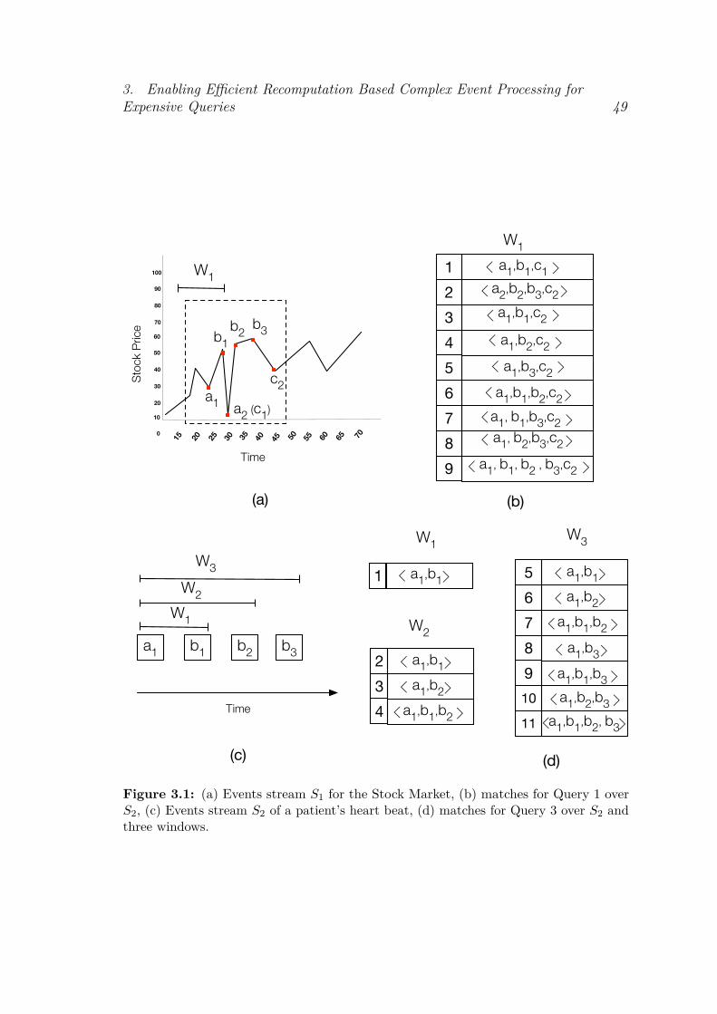
3. Enabling Efficient Recomputation Based Complex Event Processing forExpensive Queries 49
(c) (d)
a1 b1 b2 b3
W3
W2
W1
Time
a1,b1 < >1
a1,b1,b2 < >432
W1
W2
W3
a1,b1 < >a1,b2 < >
a1,b1,b2 < >
111098765 a1,b1 < >
a1,b2 < >
a1,b3< >a1,b1,b3 < >a1,b2,b3 < >
a1,b1,b2, b3 < >
(a) (b)
a1,b1,c1 < >a2,b2,b3,c2 < >a1,b1,c2 < >a1,b2,c2 < >a1,b3,c2 < >
a1,b1,b2,c2 < >< >
a1, b2,b3,c2 < >a1, b1, b2 , b3,c2 < >
a1, b1,b3,c2
987654321
0
10
20
30
40
60
70
80
90
100
50
Sto
ck
Pric
e
252015 30 35 40 45 50 55 60 7065
Time
a1
b2b1
b3
c2
a2 (c1)
W1
W1
Figure 3.1: (a) Events stream S1 for the Stock Market, (b) matches for Query 1 overS2, (c) Events stream S2 of a patient’s heart beat, (d) matches for Query 3 over S2 andthree windows.
50 3.3. Related Works
strategy can reduce the memory cost. Nonetheless, it results in the added cost ofthe compression/decompression operations and redundant computation of partialmatches that are shared by multiple complete matches.
Scalability: Existing CEP solutions fail to scale over real-world datasets dueto their space and time overheads. For example, SASE+ [ZDI14a] and ApacheFlink [Fli] require an index space that is two to three orders of magnitude largerthan the number of events in a window. This renders these solutions only applicableon small size datasets and simple CEP queries.
Proposed Approach
In this chapter, we advocate a new type of model for CEP wherein we identifytwo key points: (i) storing partial matches is expensive both in terms of CPU andmemory cost, hence only events within a certain window should be stored; (ii) thematches should be recomputed from those set of events only when we are sure oftheir existence.To materialise these points, we require efficient indexing and queryingtechniques. That is, we need to avoid the recomputation process on all storedevents, and the existence of new matches for an incoming event should be identifiedbefore starting the complete recomputation process. Hence, our journey to provideefficient techniques led us to explore various diverse fields such as theta-joins ( whichallows comparison relationship such as ≤ and ≥), multidiemsnional indexing andrange query processing. We employ space filling curve [Mor66] and a B+tree indexfor events within a window, and provide multiple optimisation techniques so sushan index is a viable option for the streaming settings. We also provide a hybrid-joinalgorithm for theta-joins with inequality predicates. These optimisations enabledus to efficiently prune events before starting the recomputation process, but also toexecute such process only when it is required. Our provided techniques are genericin nature and can be employed in general streaming-based systems.
Contributions
Our key contributions are as follows:
• (1) We provide a novel recomputation model for processing expressive CEPqueries. Our algorithms reduce the time and space costs for complex querieswith Kleene+ and STA operators.
• (2) To efficiently employ a recomputation model, we propose a hybrid-joinalgorithm to produce final matches from events in a batch mode. Our algorithmleverages the dominance property between set of events and joins the clusteredevents in batches to reduce the cost of pair-wise joins.
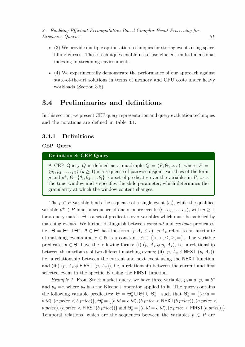
3. Enabling Efficient Recomputation Based Complex Event Processing forExpensive Queries 51
• (3) We provide multiple optimisation techniques for storing events using space-filling curves. These techniques enable us to use efficient multidimensionalindexing in streaming environments.
• (4) We experimentally demonstrate the performance of our approach againststate-of-the-art solutions in terms of memory and CPU costs under heavyworkloads (Section 3.8).
3.4 Preliminaries and definitionsIn this section, we present CEP query representation and query evaluation techniquesand the notations are defined in table 3.1.
3.4.1 DefinitionsCEP Query
Definition 8: CEP Query
A CEP Query Q is defined as a quadruple Q = (P,Θ, ω, s), where P =〈p1, p2, . . . , pk〉 (k ≥ 1) is a sequence of pairwise disjoint variables of the formp and p+, Θ={θ1, θ2, . . . θl} is a set of predicates over the variables in P . ω isthe time window and s specifies the slide parameter, which determines thegranularity at which the window content changes.
The p ∈ P variable binds the sequence of a single event 〈ei〉, while the qualifiedvariable p+ ∈ P binds a sequence of one or more events 〈e1, e2, . . . , en〉, with n ≥ 1,for a query match. Θ is a set of predicates over variables which must be satisfied bymatching events. We further distinguish between constant and variable predicates,i.e. Θ = Θc ∪ Θv. θ ∈ Θc has the form (p.Ax φ c): p.Ax refers to an attributeof matching events and c ∈ N is a constant, φ ∈ {>,<,≤,≥,=}. The variablepredicates θ ∈ Θv have the following forms: (i) (pi.Ax φ pj.Ax), i.e. a relationshipbetween the attributes of two different matching events; (ii) (pi.Ax φ NEXT (pi.Ax)),i.e. a relationship between the current and next event using the NEXT function;and (iii) (pi.Ax φ FIRST (pi.Ax)), i.e, a relationship between the current and firstselected event in the specific ~E using the FIRST function.
Example 1: From Stock market query, we have three variables p1= a, p2 = b+
and p3 =c, where p2 has the Kleene+ operator applied to it. The query containsthe following variable predicates: Θ = Θv
a ∪ Θvb ∪ Θv
c , such that Θva = {(a.id =
b.id), (a.price < b.price)}, Θvb = {(b.id = c.id), (b.price < NEXT(b.price)), (a.price <
b.price), (c.price < FIRST(b.price))} and Θvc ={(b.id = c.id), (c.price < FIRST(b.price))}.
Temporal relations, which are the sequences between the variables p ∈ P are
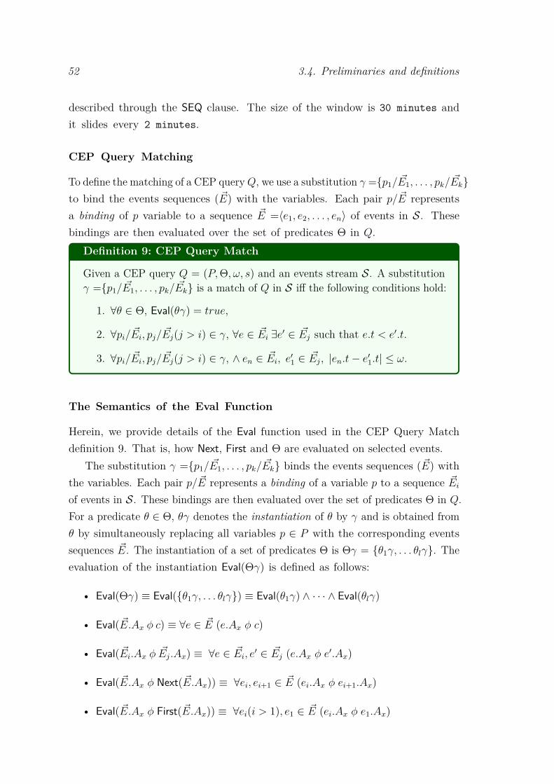
52 3.4. Preliminaries and definitions
described through the SEQ clause. The size of the window is 30 minutes andit slides every 2 minutes.
CEP Query Matching
To define the matching of a CEP queryQ, we use a substitution γ ={p1/ ~E1, . . . , pk/ ~Ek}to bind the events sequences ( ~E) with the variables. Each pair p/ ~E representsa binding of p variable to a sequence ~E =〈e1, e2, . . . , en〉 of events in S. Thesebindings are then evaluated over the set of predicates Θ in Q.
Definition 9: CEP Query Match
Given a CEP query Q = (P,Θ, ω, s) and an events stream S. A substitutionγ ={p1/ ~E1, . . . , pk/ ~Ek} is a match of Q in S iff the following conditions hold:
1. ∀θ ∈ Θ, Eval(θγ) = true,
2. ∀pi/ ~Ei, pj/ ~Ej(j > i) ∈ γ, ∀e ∈ ~Ei ∃e′ ∈ ~Ej such that e.t < e′.t.
3. ∀pi/ ~Ei, pj/ ~Ej(j > i) ∈ γ, ∧ en ∈ ~Ei, e′1 ∈ ~Ej, |en.t− e′1.t| ≤ ω.
The Semantics of the Eval Function
Herein, we provide details of the Eval function used in the CEP Query Matchdefinition 9. That is, how Next, First and Θ are evaluated on selected events.
The substitution γ ={p1/ ~E1, . . . , pk/ ~Ek} binds the events sequences ( ~E) withthe variables. Each pair p/ ~E represents a binding of a variable p to a sequence ~Eiof events in S. These bindings are then evaluated over the set of predicates Θ in Q.For a predicate θ ∈ Θ, θγ denotes the instantiation of θ by γ and is obtained fromθ by simultaneously replacing all variables p ∈ P with the corresponding eventssequences ~E. The instantiation of a set of predicates Θ is Θγ = {θ1γ, . . . θlγ}. Theevaluation of the instantiation Eval(Θγ) is defined as follows:
• Eval(Θγ) ≡ Eval({θ1γ, . . . θlγ}) ≡ Eval(θ1γ) ∧ · · · ∧ Eval(θlγ)
• Eval( ~E.Ax φ c) ≡ ∀e ∈ ~E (e.Ax φ c)
• Eval( ~Ei.Ax φ ~Ej.Ax) ≡ ∀e ∈ ~Ei, e′ ∈ ~Ej (e.Ax φ e′.Ax)
• Eval( ~E.Ax φ Next( ~E.Ax)) ≡ ∀ei, ei+1 ∈ ~E (ei.Ax φ ei+1.Ax)
• Eval( ~E.Ax φ First( ~E.Ax)) ≡ ∀ei(i > 1), e1 ∈ ~E (ei.Ax φ e1.Ax)
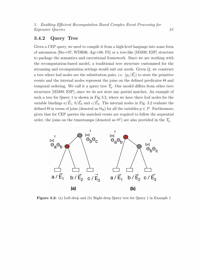
3. Enabling Efficient Recomputation Based Complex Event Processing forExpensive Queries 53
3.4.2 Query Tree
Given a CEP query, we need to compile it from a high-level language into some formof automaton [Bre+07; WDR06; Agr+08; Fli] or a tree-like [MM09; ESP] structureto package the semantics and executional framework. Since we are working withthe recomputation-based model, a traditional tree structure customised for thestreaming and recomputation settings would suit our needs. Given Q, we constructa tree where leaf nodes are the substitution pairs, i.e. (pi/ ~Ei) to store the primitiveevents and the internal nodes represent the joins on the defined predicates Θ andtemporal ordering. We call it a query tree Tq. Our model differs from other tree-structures [MM09; ESP], since we do not store any partial matches. An example ofsuch a tree for Query 1 is shown in Fig 3.2, where we have three leaf nodes for thevariable bindings a/ ~E1, b/ ~E2 and c/ ~E3. The internal nodes in Fig. 3.2 evaluate thedefined Θ in terms of joins (denoted as 1Θ) for all the variables p ∈ P . Furthermore,given that for CEP queries the matched events are required to follow the sequentialorder, the joins on the timestamps (denoted as 1t) are also provided in the Tq.
!"
ΘaΘb
#a / E
1
#b / E
2
#c / E
3
#a / E
1
#b / E
2
#c / E
3
(a) (b)
!"
ΘbΘc
!"
ΘaΘb !
"
ΘbΘc
Figure 3.2: (a) Left-deep and (b) Right-deep Query tree for Query 1 in Example 1

54 3.4. Preliminaries and definitions
Notation DefinitionS An event streamei An eventQ QueryA A set of attributesP A sequence of pairwise disjoint variables: 〈p1, p2, . . . , pk〉
of the form p and p+
pi A variable used in the query such as a, b+ and c in theexamples. See the definition of P above
p+i A variable with Kleene+
Θ A set of predicates: {θ1, θ2, . . . θl} over the variables inP
Θc Set of constant predicatesΘv Set of variable predicatesθ A predicate. See the definition of Θ aboveφ An operator ∈ {>,<,≤,≥,=}~E An event sequence
pi/ ~Ei A substitution pair representing a leaf node to store theprimitive events
γ A set of substitution pairs = {p1/ ~E1, . . . , pk/ ~Ek} to bindthe events sequences ( ~E) with the variables
Tq Query TreeTe Event Tree1Θ The leaf nodes evaluate the defined Θ in terms of joins1t Join on the timestampB BitvectorBu,v Indicates whether a u element in ~Ei is joined with the
vth of ~Ej using the predicates` Operator denoting dominance (Dominance is defined
later in the chapter)0 Operator denoting not dominatedz Z-address
gtj(z) A function which takes a Z-address and returns abitstring by extracting tMSB bits for every j bits skipped
∨ XOR operatorω The time windoww Size of the windows The slide parameter of the time window
Table 3.1: Definition of notations

3. Enabling Efficient Recomputation Based Complex Event Processing forExpensive Queries 55
3.5 Baseline Algorithm
The aim of baseline algorithm is to evaluate the query tree over events within adefined window without storing partial matches and recomputing the matches foreach incoming event. Hence, it first stores events in the relevant leaf nodes (eventssequences) of the query tree. Second, it triggers the query evaluation to producecomplex matches. Given a query tree Tq, each incoming event e ∈ S can result inthe following main steps.
Algorithm 1: Baseline AlgorithmInput: Query Tree Tq and an events stream SOutput: Set of Matched Sequences
1 Q← (P,Θ, ω, s) ; // CEP Query2 ~E ← { ~E1, ~E2, . . . , ~Ek}, k = |P | ; // Events sequences from Tq
3 for each e ∈ S do4 for each ~Ei ∈ ~E do5 if isCompatible( ~Ei,e) then6 ~Ei = ~Ei ∪ e ; // Step 1
7 if isCompatible( ~Ek,e) then8 ExecuteJoins( ~E, Θ); // Step 29 ExecuteKleenePlus( ~E, Θ); // Step 3
Step 1. Add e to the compatible events sequence ~Ei, so that constant predicates Θc
filter unwanted events for each ~Ei in Tq. This step corresponds to the accumulationof events within a defined window. See Algorithm 1 from lines 4-6.
Step 2. For each incoming event e, check if such an event can trigger the queryevaluation to produce matches. That is, if e can be part of ~Ek (i.e. last eventsequence), it can complete a set of matches; since it contains the highest timestampwithin the window. Hence, execute the query tree by joining the events within each~Ei using the predicates Θ and timestamps. This step assembles all the events foreach ~Ei that can produce the set of matches. See Algorithm 1 from lines 7-8.
Step 3. For a p+i ∈ P , compute all the combinations for events in p+
i / ~Ei, i.e. apower set of events in ~Ei. This step groups all the combinations by following the oneor more semantics of the Kleene+ operator. See Figure 3.5 and Algorithm 1 line 9.
We now present details of the two main processes of Algorithm 1, i.e. joiningthe set of events and computing the power set of events for the Kleene+ operator.

56 3.5. Baseline Algorithm
Execution of Joins
Let ~Ei and ~Ej be two event sequences with theta-join ~Ei 1tΘ ~Ej over the timestampt and predicates Θ. Hence, we have joins on multiple relations in Step 2. Thegeneric cost of such joins, i.e. pairwise joins, is O(| ~Ei|| ~Ej|) and the problem of itsefficient evaluation resembles that of traditional theta-joins with inequality predi-cates [Kha+17]. The wide range of methods for this problem include: the textbookmerge-sort, hash-based, band-join and various indices such as Bitmap [GUW02].These techniques are mostly focused on equality joins using a single join relation.Inequality joins on multiple join relations are notoriously slow and multi-passprojection-based strategies [BF79; Kha+17] are usually employed. These strategies,however, require multiple sorting operations, each for a distinct relation, and areonly optimised for static datasets, where indexing time is not of much importance.Even with these strategies, the worst-case complexity of these algorithms remainsO(| ~Ei|| ~Ej|) as the output size can be as large as | ~Ei|| ~Ej|, where all events share thesame join keys and the join degenerates into a cartesian product. Considering this, weemploy the general nested-loop join for our preliminary algorithm. Our experimentalanalysis showcases that even such algorithms provide competitive performance.
Execution of Kleene+ Operator
For Step 3, we need to create all the possible combinations of matches over thejoined events. That is, enumerating the powerset of event sequences with p+ bindings.In this context, we used Banker’s sequence [LvHS00] to generate sequences of eventswith p+ bindings, where we need only to count from 1 to 2m − 1. That is, we checkthe number of events in event sequences with p+ bindings after the join process.For |m| number of such events, we create 1 to 2m − 1 matches.
Complexity Analysis
Herein, we briefly present the complexity analysis for the three steps described inAlgorithm 1. Step 1 results in a constant time operation, since an incoming eventcan be directly added to an event sequence. Step 2 has a polynomial time cost(pair-wise joins) and depends on the number of patterns P defined in a CEP query.For n events in a window and k = |P |, we have O(nk). Step 3 requires the creationof an exponential number of matches for Kleene+ operators. For n events in awindow, we have O(2n). However, this would require storing predecessor matchesto produce the next one and would result in an extra load on memory resources.
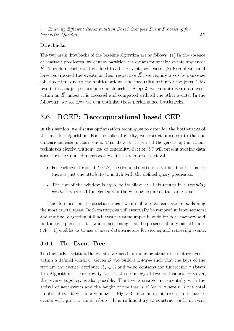
3. Enabling Efficient Recomputation Based Complex Event Processing forExpensive Queries 57
Drawbacks
The two main drawbacks of the baseline algorithm are as follows. (1) In the absenceof constant predicates, we cannot partition the events for specific events sequences~Ei. Therefore, each event is added to all the events sequences. (2) Even if we couldhave partitioned the events in their respective ~Ei, we require a costly pair-wisejoin algorithm due to the multi-relational and inequality nature of the joins. Thisresults in a major performance bottleneck in Step 2, we cannot discard an eventwithin an ~Ei unless it is accessed and compared with all the other events. In thefollowing, we see how we can optimise these performance bottlenecks.
3.6 RCEP: Recomputational based CEPIn this section, we discuss optimisation techniques to cater for the bottlenecks ofthe baseline algorithm. For the sake of clarity, we restrict ourselves to the onedimensional case in this section. This allows us to present the generic optimisationstechniques clearly, without loss of generality. Section 3.7 will present specific datastructures for multidimensional events’ storage and retrieval.
• For each event e = (A, t) ∈ S, the size of the attribute set is |A| = 1. That is,there is just one attribute to match with the defined query predicates.
• The size of the window is equal to its slide: ω. This results in a tumblingwindow, where all the elements in the window expire at the same time.
The aforementioned restrictions mean we are able to concentrate on explainingthe most crucial ideas. Both restrictions will eventually be removed in later sections;and our final algorithm still achieves the same upper bounds for both memory andruntime complexities. It is worth mentioning that the presence of only one attribute(|A| = 1) enables us to use a linear data structure for storing and retrieving events.
3.6.1 The Event Tree
To efficiently partition the events, we need an indexing structure to store eventswithin a defined window. Given S, we build a B+tree such that the keys of thetree are the events’ attribute Ax ∈ A and value contains the timestamp τ (Step1 in Algorithm 1). For brevity, we use this topology of keys and values. However,the reverse topology is also possible. The tree is created incrementally with thearrival of new events and the height of the tree is ≤ log n, where n is the totalnumber of events within a window ω. Fig. 3.3 shows an event tree of stock marketevents with price as an attribute. It is rudimentary to construct such an event
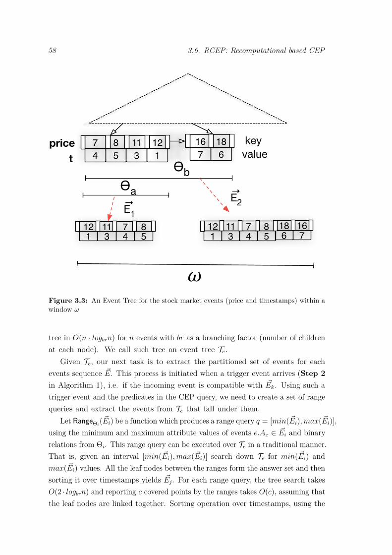
58 3.6. RCEP: Recomputational based CEP
keyvalue
!
54 3 17 128 11
7 616 18
tprice
ϴbϴa
31 4 512 811 7
6 718 16
31 4 512 811 7
E1→ E2
→
Figure 3.3: An Event Tree for the stock market events (price and timestamps) within awindow ω
tree in O(n · logbrn) for n events with br as a branching factor (number of childrenat each node). We call such tree an event tree Te.
Given Te, our next task is to extract the partitioned set of events for eachevents sequence ~E. This process is initiated when a trigger event arrives (Step 2in Algorithm 1), i.e. if the incoming event is compatible with ~Ek. Using such atrigger event and the predicates in the CEP query, we need to create a set of rangequeries and extract the events from Te that fall under them.
Let RangeΘi( ~Ei) be a function which produces a range query q = [min( ~Ei),max( ~Ei)],
using the minimum and maximum attribute values of events e.Ax ∈ ~Ei and binaryrelations from Θi. This range query can be executed over Te in a traditional manner.That is, given an interval [min( ~Ei),max( ~Ei)] search down Te for min( ~Ei) andmax( ~Ei) values. All the leaf nodes between the ranges form the answer set and thensorting it over timestamps yields ~Ej. For each range query, the tree search takesO(2 · logbrn) and reporting c covered points by the ranges takes O(c), assuming thatthe leaf nodes are linked together. Sorting operation over timestamps, using the

3. Enabling Efficient Recomputation Based Complex Event Processing forExpensive Queries 59
traditional algorithms, can be performed in O(c · logc) to produce ~Ej . The followingexample explains the construction and execution of such range queries.
Example 2:Consider Te in Fig.3.3 and Tq in Fig.3.2 (b). Now consider that a trigger event
ei = (6, 9) (price = 6 and t = 9) arrives (note that we are detecting an invertedV-shaped pattern). We use ei for the right-most leaf node c/ ~E3 in Tq; since it cancomplete a set of matches. Next, we need to extract the events for b/ ~E2 that canbe joined with events in c/ ~E3. Hence, we create a range query q1 = [7, 18] (18 is themax price) while considering the binary relation for predicate θb = c.price < b.price
and ei = (6, 9) in c/ ~E3. The events covered by q1 are shown in Fig. 3.3. Wesort them by timestamp to produce b/ ~E2. Finally we are left with a/ ~E1. Hence,we create another range query using the predicate θa = a.price < b.price. Sincethe maximum value of the price in b/ ~E2 is price = 18, the boundaries of thisrange queries are as follows: q2 = [0, 18 − 1] (considering t an integer in thisexample). The events covered by q2 are shown in Fig. 3.3 and sorting them bytimestamp yields the final contents of a/ ~E1.
The event tree solves our problem of filtering unnecessary events before the joinprocess. Next, we see how to optimise the execution of joins between filteredevents sequences.
3.6.2 Creating the Complex Matches
The set of range queries produces a set of events sequences for a query tree. Toproduce a set of matches, we need to employ theta-joins between them since weare dealing with both constant and variable predicates.
Problem Description
Considering the discussion in section 3.5 on theta-join execution problem, we proposea light-weight hybrid-join algorithm that solves this problem heuristically, providingsignificant performance gains over its counterparts. We first define the dominanceproperty between events, which is the backbone of our algorithm.
Definition 10: Event’s Dominance
Given two events e, e′ ∈ S and a binary condition φ, e dominates e′ iffe.Ax φ e
′.Ax = true.
The dominance property can easily be extended for the set of attributes A withinan event and the set of binary conditions in Θ as described in Section 3.7.2. Wedenote that e dominates e′ by e ` e′ and if not by e 0 e′. The dominance propertyalso enables the transitivity property: given e, e′, e′′, if e ` e′ and e′ ` e′′ then e ` e′′.
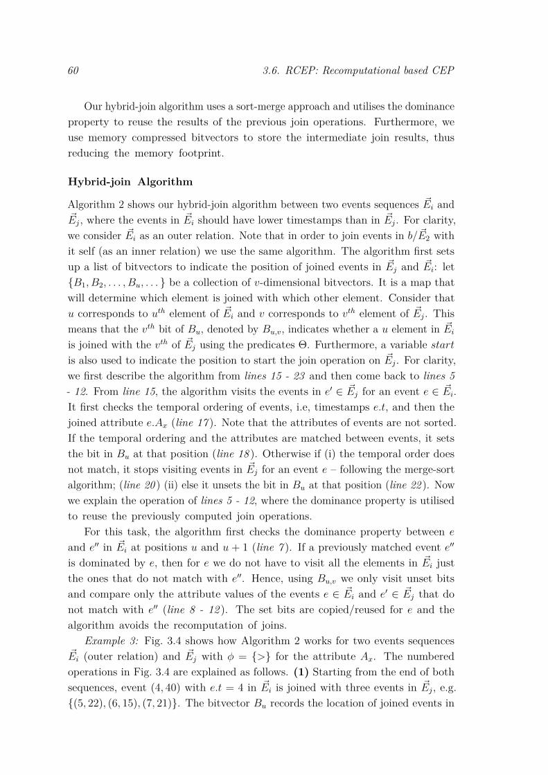
60 3.6. RCEP: Recomputational based CEP
Our hybrid-join algorithm uses a sort-merge approach and utilises the dominanceproperty to reuse the results of the previous join operations. Furthermore, weuse memory compressed bitvectors to store the intermediate join results, thusreducing the memory footprint.
Hybrid-join Algorithm
Algorithm 2 shows our hybrid-join algorithm between two events sequences ~Ei and~Ej, where the events in ~Ei should have lower timestamps than in ~Ej. For clarity,we consider ~Ei as an outer relation. Note that in order to join events in b/ ~E2 withit self (as an inner relation) we use the same algorithm. The algorithm first setsup a list of bitvectors to indicate the position of joined events in ~Ej and ~Ei: let{B1, B2, . . . , Bu, . . . } be a collection of v-dimensional bitvectors. It is a map thatwill determine which element is joined with which other element. Consider thatu corresponds to uth element of ~Ei and v corresponds to vth element of ~Ej. Thismeans that the vth bit of Bu, denoted by Bu,v, indicates whether a u element in ~Ei
is joined with the vth of ~Ej using the predicates Θ. Furthermore, a variable startis also used to indicate the position to start the join operation on ~Ej. For clarity,we first describe the algorithm from lines 15 - 23 and then come back to lines 5- 12. From line 15, the algorithm visits the events in e′ ∈ ~Ej for an event e ∈ ~Ei.It first checks the temporal ordering of events, i.e, timestamps e.t, and then thejoined attribute e.Ax (line 17 ). Note that the attributes of events are not sorted.If the temporal ordering and the attributes are matched between events, it setsthe bit in Bu at that position (line 18 ). Otherwise if (i) the temporal order doesnot match, it stops visiting events in ~Ej for an event e – following the merge-sortalgorithm; (line 20 ) (ii) else it unsets the bit in Bu at that position (line 22 ). Nowwe explain the operation of lines 5 - 12, where the dominance property is utilisedto reuse the previously computed join operations.
For this task, the algorithm first checks the dominance property between e
and e′′ in ~Ei at positions u and u + 1 (line 7 ). If a previously matched event e′′
is dominated by e, then for e we do not have to visit all the elements in ~Ei justthe ones that do not match with e′′. Hence, using Bu,v we only visit unset bitsand compare only the attribute values of the events e ∈ ~Ei and e′ ∈ ~Ej that donot match with e′′ (line 8 - 12 ). The set bits are copied/reused for e and thealgorithm avoids the recomputation of joins.
Example 3: Fig. 3.4 shows how Algorithm 2 works for two events sequences~Ei (outer relation) and ~Ej with φ = {>} for the attribute Ax. The numberedoperations in Fig. 3.4 are explained as follows. (1) Starting from the end of bothsequences, event (4, 40) with e.t = 4 in ~Ei is joined with three events in ~Ej, e.g.{(5, 22), (6, 15), (7, 21)}. The bitvector Bu records the location of joined events in

3. Enabling Efficient Recomputation Based Complex Event Processing forExpensive Queries 61
Algorithm 2: Hybrid-Join Algorithm between ~Ei and ~Ej
Input: Events sequences ~Ei, ~Ej , events in e ∈ ~Ei should follow events in e′ ∈ ~Ej , joinpredicate e.Ax φ e
′.Ax
1 Initialise a Bitvector Bu, where u, v represents the joined events in ~Ei and ~Ej respectively,and set all the bits to 0 ;
2 start← | ~Ej |3 for u ← | ~Ei| to 1 do4 e← ~Ei[u];5 if u 6= | ~Ei| then6 e′′ ← ~Ei[u+ 1]7 if e.a ` e′′.a then8 Bu ← Bu+1;9 foreach unset bit at index v ∈ Bu and v ≤ start do
10 e′ ← ~Ej [v]11 if e.Ax φ e
′.Ax then12 Bu,v ← 1;
13 else14 start← | ~Ej |;
15 while start > 0 do16 e′ ← ~Ej [start];17 if e′.t > e.t AND e.Ax φ e
′.Ax then18 Bu,start ← 1;19 else if e′.t < e.t then20 break the while loop;21 else22 Bu,start ← 0;23 start← start - 1;
~Ej. (2) Since the event (3, 50) at e.t = 3 in ~Ei dominates the event at e.t = 4(e.Ax > e′′.Ax) in the same events sequences, i.e. ~Ei, we reuse the results ofpreviously computed joins (in step (1)) using Bu. (3) Since the event at e.t = 2does not dominate the event at e.t = 3 in ~Ei, we restart the comparison processfrom the end of ~Ej. (4) The event at e.t = 1 dominates the event at e.t = 2in ~Ei. Therefore, we reuse the joins evaluated in step 3 and continue the joinprocedure until the timestamps ordering fails.
The performance of the hybrid-join algorithm is highly dependent on thedistribution of events’ within the events sequences. We will see in Section 3.7.3 howto arrange such distribution to get the benefits of a hybrid-join algorithm. Thecomplexity analysis of the algorithm is as follows: the outer loop in Algorithm 2(line 3 ) in the worst case takes O(| ~Ei| · | ~Ej|), while it is clear to see that theextra space complexity is only O(| ~Ei| · | ~Ej|) bits of space, which is one of themain advantages of our algorithm.
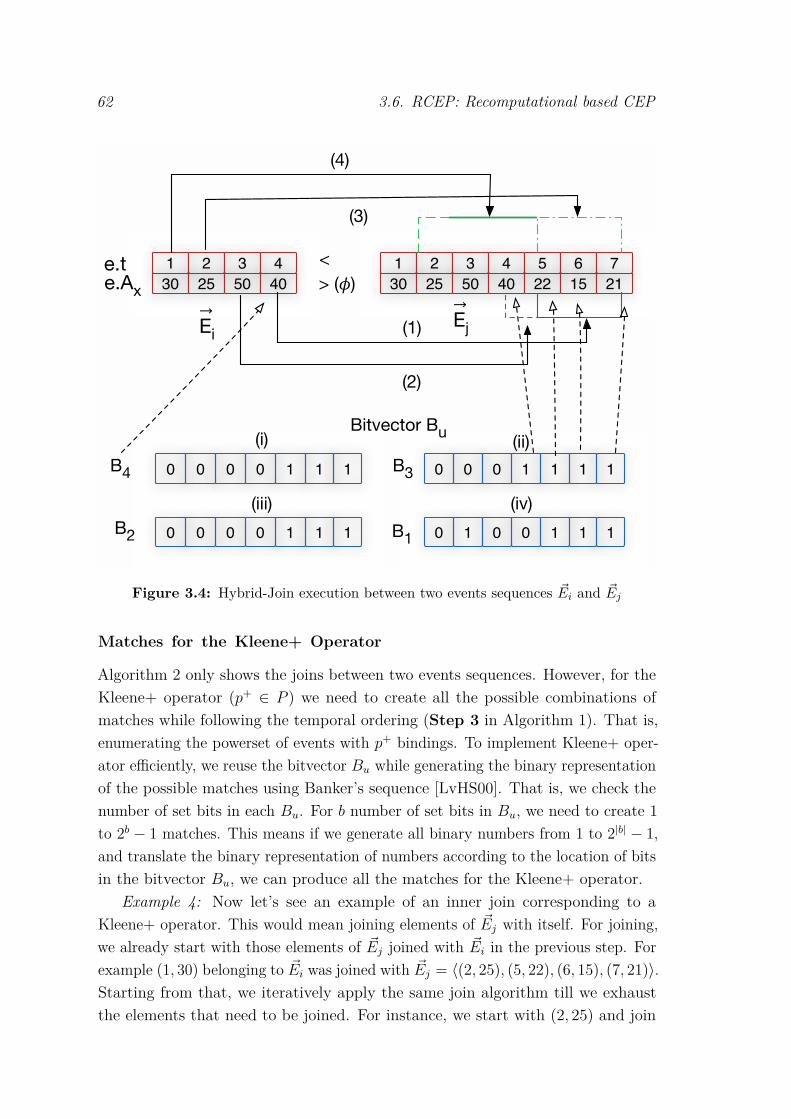
62 3.6. RCEP: Recomputational based CEP
40
2 43
25
1
30 50
2
25 40
7
30
3
15
4 51 6
2150 22
<
> (!)e.te.Ax
(1)
(2)
(3)
(4)
(i)
0 11 1000
Bitvector Bu(ii)
110 1100
(iii)
110 1000
(iv)
110 1001
B4 B3
B2 B1
" Ei
" Ej
Figure 3.4: Hybrid-Join execution between two events sequences ~Ei and ~Ej
Matches for the Kleene+ Operator
Algorithm 2 only shows the joins between two events sequences. However, for theKleene+ operator (p+ ∈ P ) we need to create all the possible combinations ofmatches while following the temporal ordering (Step 3 in Algorithm 1). That is,enumerating the powerset of events with p+ bindings. To implement Kleene+ oper-ator efficiently, we reuse the bitvector Bu while generating the binary representationof the possible matches using Banker’s sequence [LvHS00]. That is, we check thenumber of set bits in each Bu. For b number of set bits in Bu, we need to create 1to 2b − 1 matches. This means if we generate all binary numbers from 1 to 2|b| − 1,and translate the binary representation of numbers according to the location of bitsin the bitvector Bu, we can produce all the matches for the Kleene+ operator.
Example 4: Now let’s see an example of an inner join corresponding to aKleene+ operator. This would mean joining elements of ~Ej with itself. For joining,we already start with those elements of ~Ej joined with ~Ei in the previous step. Forexample (1, 30) belonging to ~Ei was joined with ~Ej = 〈(2, 25), (5, 22), (6, 15), (7, 21)〉.Starting from that, we iteratively apply the same join algorithm till we exhaustthe elements that need to be joined. For instance, we start with (2, 25) and join
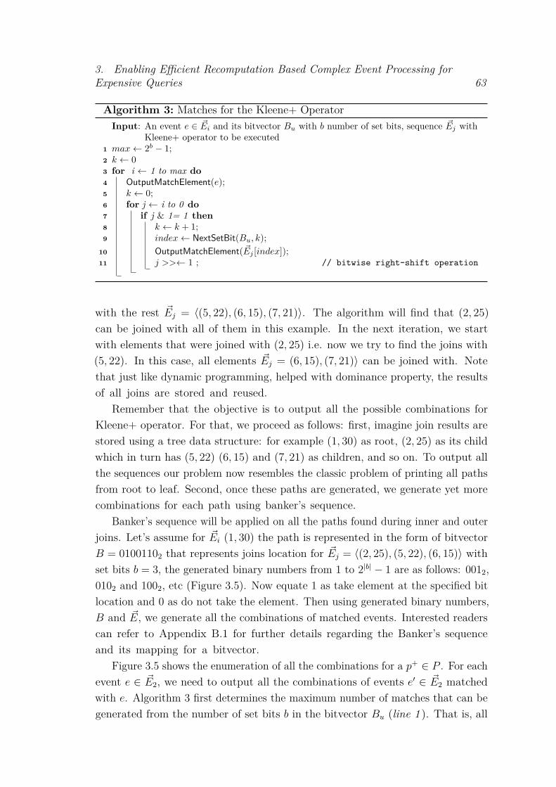
3. Enabling Efficient Recomputation Based Complex Event Processing forExpensive Queries 63
Algorithm 3: Matches for the Kleene+ OperatorInput: An event e ∈ ~Ei and its bitvector Bu with b number of set bits, sequence ~Ej with
Kleene+ operator to be executed1 max← 2b − 1;2 k ← 03 for i ← 1 to max do4 OutputMatchElement(e);5 k ← 0;6 for j ← i to 0 do7 if j & 1= 1 then8 k ← k + 1;9 index← NextSetBit(Bu, k);
10 OutputMatchElement( ~Ej [index]);11 j >>← 1 ; // bitwise right-shift operation
with the rest ~Ej = 〈(5, 22), (6, 15), (7, 21)〉. The algorithm will find that (2, 25)can be joined with all of them in this example. In the next iteration, we startwith elements that were joined with (2, 25) i.e. now we try to find the joins with(5, 22). In this case, all elements ~Ej = (6, 15), (7, 21)〉 can be joined with. Notethat just like dynamic programming, helped with dominance property, the resultsof all joins are stored and reused.
Remember that the objective is to output all the possible combinations forKleene+ operator. For that, we proceed as follows: first, imagine join results arestored using a tree data structure: for example (1, 30) as root, (2, 25) as its childwhich in turn has (5, 22) (6, 15) and (7, 21) as children, and so on. To output allthe sequences our problem now resembles the classic problem of printing all pathsfrom root to leaf. Second, once these paths are generated, we generate yet morecombinations for each path using banker’s sequence.
Banker’s sequence will be applied on all the paths found during inner and outerjoins. Let’s assume for ~Ei (1, 30) the path is represented in the form of bitvectorB = 01001102 that represents joins location for ~Ej = 〈(2, 25), (5, 22), (6, 15)〉 withset bits b = 3, the generated binary numbers from 1 to 2|b| − 1 are as follows: 0012,0102 and 1002, etc (Figure 3.5). Now equate 1 as take element at the specified bitlocation and 0 as do not take the element. Then using generated binary numbers,B and ~E, we generate all the combinations of matched events. Interested readerscan refer to Appendix B.1 for further details regarding the Banker’s sequenceand its mapping for a bitvector.
Figure 3.5 shows the enumeration of all the combinations for a p+ ∈ P . For eachevent e ∈ ~E2, we need to output all the combinations of events e′ ∈ ~E2 matchedwith e. Algorithm 3 first determines the maximum number of matches that can begenerated from the number of set bits b in the bitvector Bu (line 1 ). That is, all
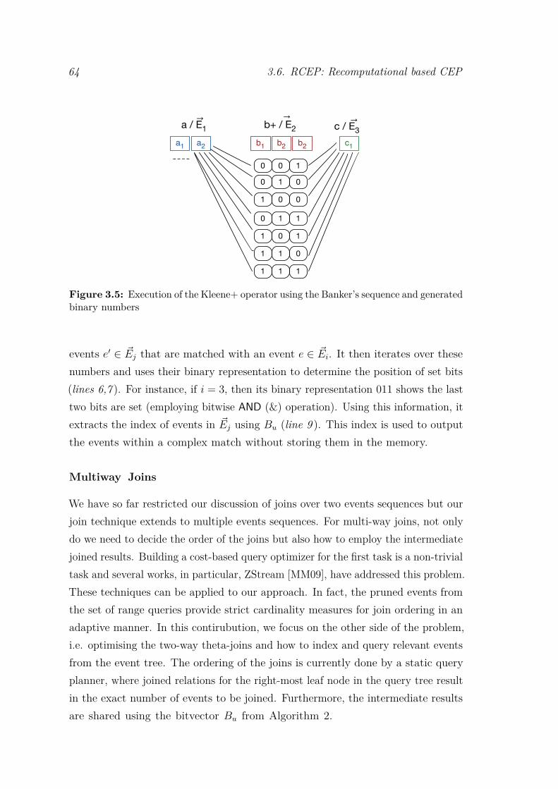
64 3.6. RCEP: Recomputational based CEP
c1b2b1a2a1 b2
0 0 1
0 1 0
1 0 0
0 1 1
1 0 1
1 1 0
1 1 1
a / E1 b+ / E2 c / E3
Figure 3.5: Execution of the Kleene+ operator using the Banker’s sequence and generatedbinary numbers
events e′ ∈ ~Ej that are matched with an event e ∈ ~Ei. It then iterates over thesenumbers and uses their binary representation to determine the position of set bits(lines 6,7 ). For instance, if i = 3, then its binary representation 011 shows the lasttwo bits are set (employing bitwise AND (&) operation). Using this information, itextracts the index of events in ~Ej using Bu (line 9 ). This index is used to outputthe events within a complex match without storing them in the memory.
Multiway Joins
We have so far restricted our discussion of joins over two events sequences but ourjoin technique extends to multiple events sequences. For multi-way joins, not onlydo we need to decide the order of the joins but also how to employ the intermediatejoined results. Building a cost-based query optimizer for the first task is a non-trivialtask and several works, in particular, ZStream [MM09], have addressed this problem.These techniques can be applied to our approach. In fact, the pruned events fromthe set of range queries provide strict cardinality measures for join ordering in anadaptive manner. In this contirubution, we focus on the other side of the problem,i.e. optimising the two-way theta-joins and how to index and query relevant eventsfrom the event tree. The ordering of the joins is currently done by a static queryplanner, where joined relations for the right-most leaf node in the query tree resultin the exact number of events to be joined. Furthermore, the intermediate resultsare shared using the bitvector Bu from Algorithm 2.
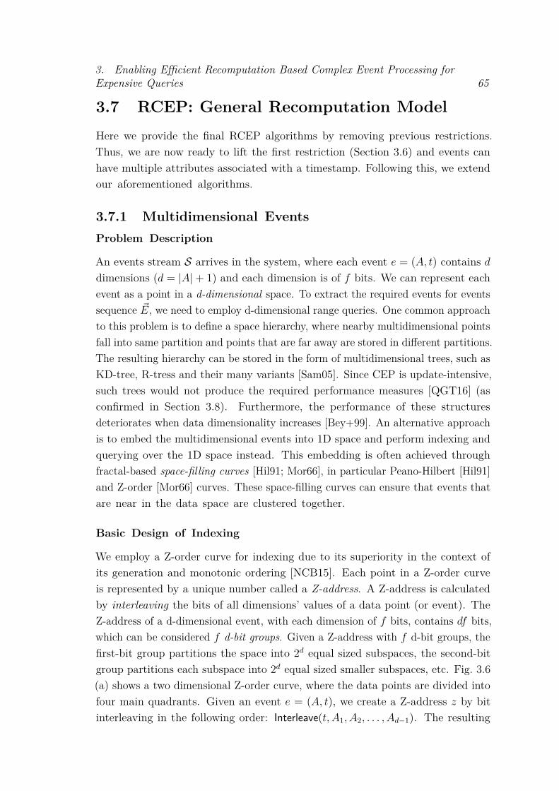
3. Enabling Efficient Recomputation Based Complex Event Processing forExpensive Queries 65
3.7 RCEP: General Recomputation Model
Here we provide the final RCEP algorithms by removing previous restrictions.Thus, we are now ready to lift the first restriction (Section 3.6) and events canhave multiple attributes associated with a timestamp. Following this, we extendour aforementioned algorithms.
3.7.1 Multidimensional EventsProblem Description
An events stream S arrives in the system, where each event e = (A, t) contains ddimensions (d = |A|+ 1) and each dimension is of f bits. We can represent eachevent as a point in a d-dimensional space. To extract the required events for eventssequence ~E, we need to employ d-dimensional range queries. One common approachto this problem is to define a space hierarchy, where nearby multidimensional pointsfall into same partition and points that are far away are stored in different partitions.The resulting hierarchy can be stored in the form of multidimensional trees, such asKD-tree, R-tress and their many variants [Sam05]. Since CEP is update-intensive,such trees would not produce the required performance measures [QGT16] (asconfirmed in Section 3.8). Furthermore, the performance of these structuresdeteriorates when data dimensionality increases [Bey+99]. An alternative approachis to embed the multidimensional events into 1D space and perform indexing andquerying over the 1D space instead. This embedding is often achieved throughfractal-based space-filling curves [Hil91; Mor66], in particular Peano-Hilbert [Hil91]and Z-order [Mor66] curves. These space-filling curves can ensure that events thatare near in the data space are clustered together.
Basic Design of Indexing
We employ a Z-order curve for indexing due to its superiority in the context ofits generation and monotonic ordering [NCB15]. Each point in a Z-order curveis represented by a unique number called a Z-address. A Z-address is calculatedby interleaving the bits of all dimensions’ values of a data point (or event). TheZ-address of a d-dimensional event, with each dimension of f bits, contains df bits,which can be considered f d-bit groups. Given a Z-address with f d-bit groups, thefirst-bit group partitions the space into 2d equal sized subspaces, the second-bitgroup partitions each subspace into 2d equal sized smaller subspaces, etc. Fig. 3.6(a) shows a two dimensional Z-order curve, where the data points are divided intofour main quadrants. Given an event e = (A, t), we create a Z-address z by bitinterleaving in the following order: Interleave(t, A1, A2, . . . , Ad−1). The resulting
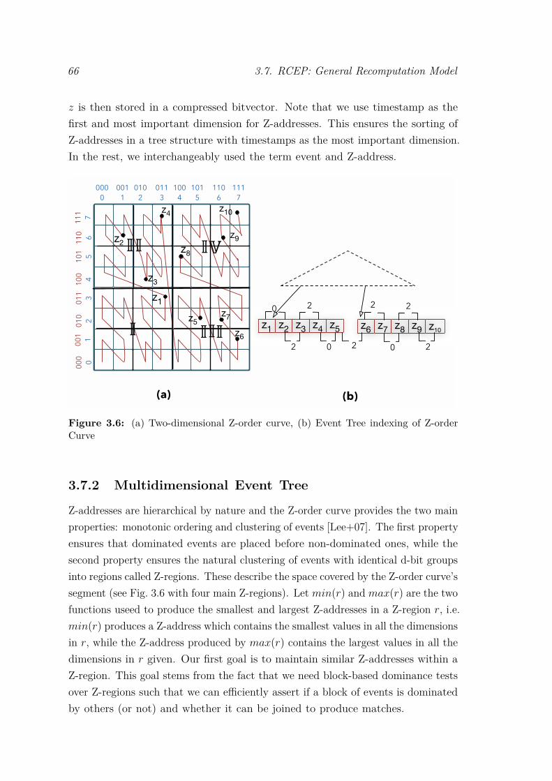
66 3.7. RCEP: General Recomputation Model
z is then stored in a compressed bitvector. Note that we use timestamp as thefirst and most important dimension for Z-addresses. This ensures the sorting ofZ-addresses in a tree structure with timestamps as the most important dimension.In the rest, we interchangeably used the term event and Z-address.
000
0
001
1
010
2
011
3
100
4
101
5
110
6
111
7
111
7
110
6
101
5
100
4
011
3
010
2
001
1
000
0
!!!
"
!
!! !
z1
z2
z3
z4
z9
z5
z6
z7
z8
z5
z4
z3
z1
z2 z
10z7
z6
z9
z8
0
2
2 2
0
2
(a) (b)
0 2
z10
2
Figure 3.6: (a) Two-dimensional Z-order curve, (b) Event Tree indexing of Z-orderCurve
3.7.2 Multidimensional Event Tree
Z-addresses are hierarchical by nature and the Z-order curve provides the two mainproperties: monotonic ordering and clustering of events [Lee+07]. The first propertyensures that dominated events are placed before non-dominated ones, while thesecond property ensures the natural clustering of events with identical d-bit groupsinto regions called Z-regions. These describe the space covered by the Z-order curve’ssegment (see Fig. 3.6 with four main Z-regions). Let min(r) and max(r) are the twofunctions useed to produce the smallest and largest Z-addresses in a Z-region r, i.e.min(r) produces a Z-address which contains the smallest values in all the dimensionsin r, while the Z-address produced by max(r) contains the largest values in all thedimensions in r given. Our first goal is to maintain similar Z-addresses within aZ-region. This goal stems from the fact that we need block-based dominance testsover Z-regions such that we can efficiently assert if a block of events is dominatedby others (or not) and whether it can be joined to produce matches.
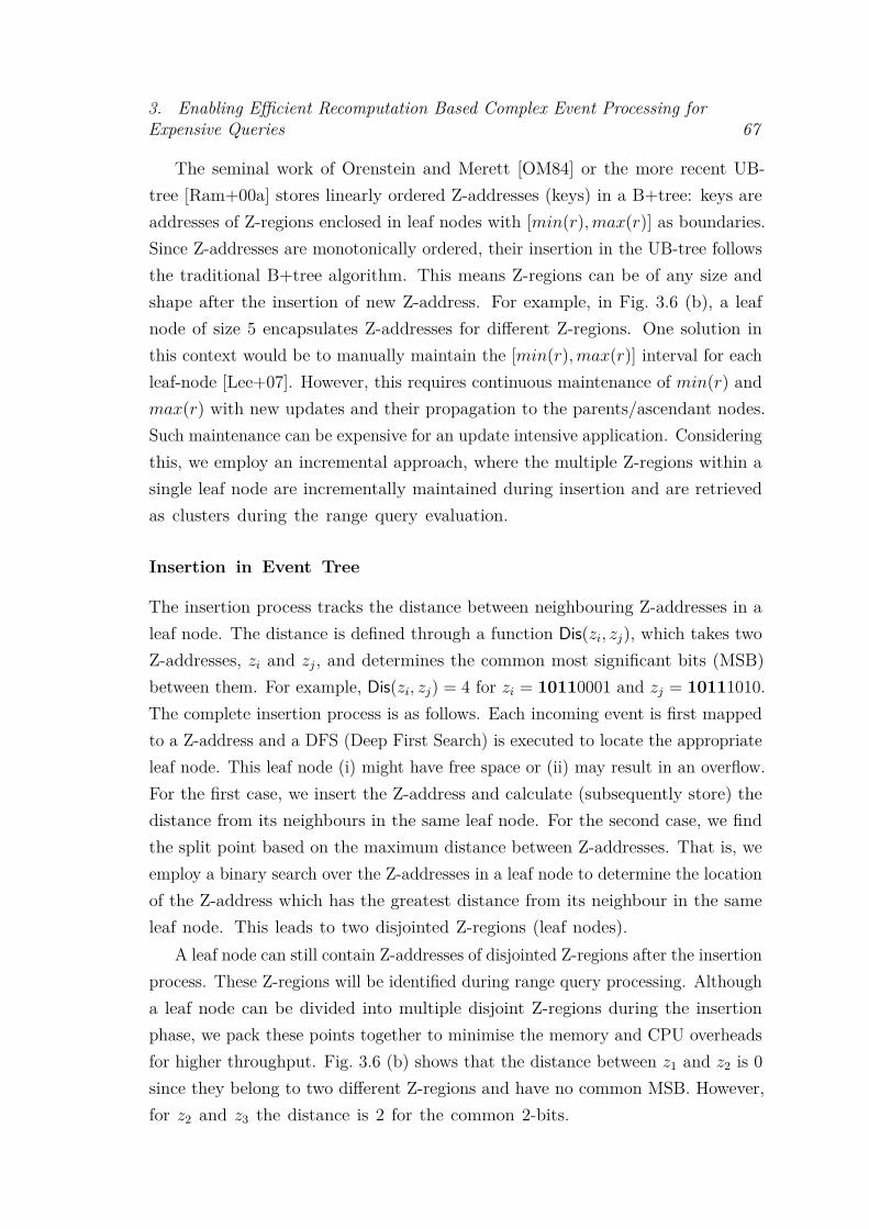
3. Enabling Efficient Recomputation Based Complex Event Processing forExpensive Queries 67
The seminal work of Orenstein and Merett [OM84] or the more recent UB-tree [Ram+00a] stores linearly ordered Z-addresses (keys) in a B+tree: keys areaddresses of Z-regions enclosed in leaf nodes with [min(r),max(r)] as boundaries.Since Z-addresses are monotonically ordered, their insertion in the UB-tree followsthe traditional B+tree algorithm. This means Z-regions can be of any size andshape after the insertion of new Z-address. For example, in Fig. 3.6 (b), a leafnode of size 5 encapsulates Z-addresses for different Z-regions. One solution inthis context would be to manually maintain the [min(r),max(r)] interval for eachleaf-node [Lee+07]. However, this requires continuous maintenance of min(r) andmax(r) with new updates and their propagation to the parents/ascendant nodes.Such maintenance can be expensive for an update intensive application. Consideringthis, we employ an incremental approach, where the multiple Z-regions within asingle leaf node are incrementally maintained during insertion and are retrievedas clusters during the range query evaluation.
Insertion in Event Tree
The insertion process tracks the distance between neighbouring Z-addresses in aleaf node. The distance is defined through a function Dis(zi, zj), which takes twoZ-addresses, zi and zj, and determines the common most significant bits (MSB)between them. For example, Dis(zi, zj) = 4 for zi = 10110001 and zj = 10111010.The complete insertion process is as follows. Each incoming event is first mappedto a Z-address and a DFS (Deep First Search) is executed to locate the appropriateleaf node. This leaf node (i) might have free space or (ii) may result in an overflow.For the first case, we insert the Z-address and calculate (subsequently store) thedistance from its neighbours in the same leaf node. For the second case, we findthe split point based on the maximum distance between Z-addresses. That is, weemploy a binary search over the Z-addresses in a leaf node to determine the locationof the Z-address which has the greatest distance from its neighbour in the sameleaf node. This leads to two disjointed Z-regions (leaf nodes).
A leaf node can still contain Z-addresses of disjointed Z-regions after the insertionprocess. These Z-regions will be identified during range query processing. Althougha leaf node can be divided into multiple disjoint Z-regions during the insertionphase, we pack these points together to minimise the memory and CPU overheadsfor higher throughput. Fig. 3.6 (b) shows that the distance between z1 and z2 is 0since they belong to two different Z-regions and have no common MSB. However,for z2 and z3 the distance is 2 for the common 2-bits.
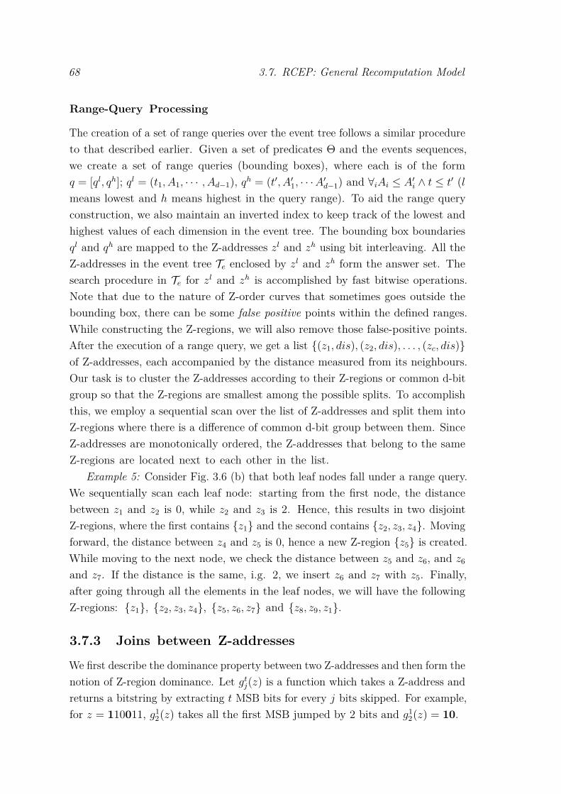
68 3.7. RCEP: General Recomputation Model
Range-Query Processing
The creation of a set of range queries over the event tree follows a similar procedureto that described earlier. Given a set of predicates Θ and the events sequences,we create a set of range queries (bounding boxes), where each is of the formq = [ql, qh]; ql = (t1, A1, · · · , Ad−1), qh = (t′, A′1, · · ·A′d−1) and ∀iAi ≤ A′i ∧ t ≤ t′ (lmeans lowest and h means highest in the query range). To aid the range queryconstruction, we also maintain an inverted index to keep track of the lowest andhighest values of each dimension in the event tree. The bounding box boundariesql and qh are mapped to the Z-addresses zl and zh using bit interleaving. All theZ-addresses in the event tree Te enclosed by zl and zh form the answer set. Thesearch procedure in Te for zl and zh is accomplished by fast bitwise operations.Note that due to the nature of Z-order curves that sometimes goes outside thebounding box, there can be some false positive points within the defined ranges.While constructing the Z-regions, we will also remove those false-positive points.After the execution of a range query, we get a list {(z1, dis), (z2, dis), . . . , (zc, dis)}of Z-addresses, each accompanied by the distance measured from its neighbours.Our task is to cluster the Z-addresses according to their Z-regions or common d-bitgroup so that the Z-regions are smallest among the possible splits. To accomplishthis, we employ a sequential scan over the list of Z-addresses and split them intoZ-regions where there is a difference of common d-bit group between them. SinceZ-addresses are monotonically ordered, the Z-addresses that belong to the sameZ-regions are located next to each other in the list.
Example 5: Consider Fig. 3.6 (b) that both leaf nodes fall under a range query.We sequentially scan each leaf node: starting from the first node, the distancebetween z1 and z2 is 0, while z2 and z3 is 2. Hence, this results in two disjointZ-regions, where the first contains {z1} and the second contains {z2, z3, z4}. Movingforward, the distance between z4 and z5 is 0, hence a new Z-region {z5} is created.While moving to the next node, we check the distance between z5 and z6, and z6
and z7. If the distance is the same, i.g. 2, we insert z6 and z7 with z5. Finally,after going through all the elements in the leaf nodes, we will have the followingZ-regions: {z1}, {z2, z3, z4}, {z5, z6, z7} and {z8, z9, z1}.
3.7.3 Joins between Z-addresses
We first describe the dominance property between two Z-addresses and then form thenotion of Z-region dominance. Let gtj(z) is a function which takes a Z-address andreturns a bitstring by extracting t MSB bits for every j bits skipped. For example,for z = 110011, g1
2(z) takes all the first MSB jumped by 2 bits and g12(z) = 10.
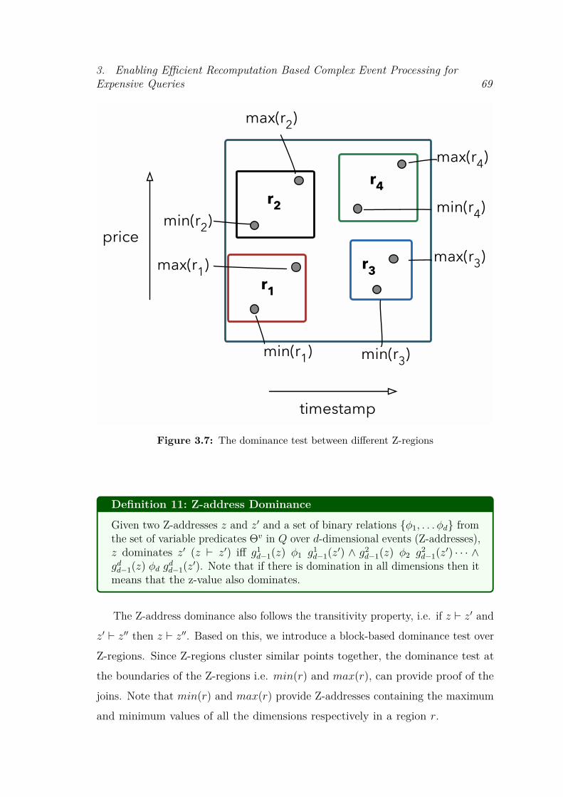
3. Enabling Efficient Recomputation Based Complex Event Processing forExpensive Queries 69
min(r1)
max(r1)
min(r2)
max(r2)
min(r3)
max(r3)
min(r4)
max(r4)
r2
r1
r3
r4
timestamp
price
Figure 3.7: The dominance test between different Z-regions
Definition 11: Z-address Dominance
Given two Z-addresses z and z′ and a set of binary relations {φ1, . . . φd} fromthe set of variable predicates Θv in Q over d-dimensional events (Z-addresses),z dominates z′ (z ` z′) iff g1
d−1(z) φ1 g1d−1(z′) ∧ g2
d−1(z) φ2 g2d−1(z′) · · · ∧
gdd−1(z) φd gdd−1(z′). Note that if there is domination in all dimensions then itmeans that the z-value also dominates.
The Z-address dominance also follows the transitivity property, i.e. if z ` z′ and
z′ ` z′′ then z ` z′′. Based on this, we introduce a block-based dominance test over
Z-regions. Since Z-regions cluster similar points together, the dominance test at
the boundaries of the Z-regions i.e. min(r) and max(r), can provide proof of the
joins. Note that min(r) and max(r) provide Z-addresses containing the maximum
and minimum values of all the dimensions respectively in a region r.

70 3.7. RCEP: General Recomputation Model
lemma 1
Given two Z-regions (r and r′) and a set of binary relations {φ1, . . . φd} fromthe variable predicates Θv in Q over d-dimensional events (Z-addresses), rdominates r′ (r ` r′) iff
1. ∀igid−1(max(r)) φi gid−1(min(r′)) if φi = {<,≤}
2. ∀igid−1(min(r)) φi gid−1(max(r′)) if φi = {>,≥}
lemma 2
Given two Z-regions (r and r′) and a set of binary relations from Lemma 1,r partially dominates r′ (r ∼ r′) iff Lemma 1 does not hold and only if thefollowing conditions hold:
1. ∀igid−1(min(r)) φi gid−1(max(r′)) if φi = {<,≤}
2. ∀igid−1(max(r)) φi gid−1(min(r′)) if φi = {>,≥}
To keep the discussion brief, we prove Lemmas 1 and 2 in appendix B. Herein,we outline their intuition. The transitivity property and monotonic ordering ofZ-addresses in Z-regions dictate that if conditions 1 and 2 are satisfied regardingmax(r) and min(r) points, then ∀zi ∈ r also follows the same properties. However,in this case, we have to check the binary conditions φ for each dimension to selectthe appropriate boundaries. If Lemma 1 does not hold then it means that twoZ-regions either overlap, or that they do not. Lemma 2 checks if two Z-regionsoverlap and hence some events that can be joined. If Z-regions do not overlap,we are sure that no events can be joined between them. From Lemma 1 andLemma 2 we have the following theorem.
theorem 1
Given two Z-regions r and r′ and a CEP query Q, if Lemma 1 holds thenr ` r′ and all the events in r can be joined with all the events in r′. Otherwise,if only Lemma 2 holds then r ∼ r′ and some events in r can be joined withsome other events in r′. If both Lemmas 1 and 2 do not hold then r 0 r′ andno events in r can be joined with any event in r′.
Example 6: Consider two predicates θ1 = a.price < b.price with φ = {<}and θ2 = a.time > b.time with φ = {>}. Using these predicates and binaryconditions, we determine the dominance property between Z-regions in Fig. 3.7.(1) Z-regions r3 ` r2 (subsequently r2 0 r3) since all the events in r3 have pricesless and timestamps greater than all the events in r2. This compiles to Lemma 1(2) r3 partially dominates r4, since for r3 all the events have lower prices but some

3. Enabling Efficient Recomputation Based Complex Event Processing forExpensive Queries 71
have equal or greater timestamps. Similarly r1 partially dominates r4. Thiscompiles to Lemma 2.
Using Theorem 1, we present the join algorithm for the sets of Z-regions. LetR and R′ be two sets of Z-regions, generated from the lists Z and Z ′ respectivelyusing the range queries as described in Section 3.7.2.
Algorithm for Joining Z-regions
Based on Theorem 1, Algorithm 4 presents how the events within the set of Z-regionsR and R′ are joined in a batch manner. It takes bitvector Bu as in Algorithm 2, tostore the intermediate joined results. Furthermore, it uses the lists of Z-addressesZ and Z ′ (for result construction), that is covered by the range queries and areused to produce the set of Z-regions R and R′. Finally, it initialises pointers startrand endr to keep track of the bits to toggle in Bu . The algorithm iterates overZ-regions r ∈ R, and for each region it evaluates the three cases in Theorem 1 overZ-regions r′ ∈ R (lines 5-13 ). For Lemma 1, it sets all the bits using the pointers ofeach region and using bit-level parallelism in the function setBits (a function thatset the bits between two given positions in a bitvector)(lines 7,8 ). For Lemma 2, itsimply uses Algorithm 2 since there can be some events in each Z-region that can bejoined (lines 9,10 ). Finally if Lemmas 1 and 2 do not hold, since no events in theZ-regions can be joined, it unsets the bits in Bu using the aforementioned pointers(lines 11, 12 ). Note that the unsetBits function is employed for brevity only, Ingeneral, we do not have to unset the bits after the initialisation of a bitvector.
Algorithm 4: Join between the set of Z-regions R and R′Input: Sets of Z-regions R, R′, Bitvector Bu, List Z and Z ′ of all the points in R and R′
respectively1 Initialise a Bitvector Bu, where |Bu| = |Z| and each Bu,v = |Z ′|;2 Initialise List pointers startr, endr, startr′ , endr′
3 for each r ∈ R do4 endr ← |r|5 for each r′ ∈ R′ do6 endr′ ← |r′|7 if Lemma 1 holds then8 setBits(Bu, startr, endr, startr′ , endr′)9 else if Lemma 2 holds then
10 Use Algorithm 2 to determine the joins between Z-addresses in r and r′;11 else if Lemmas 1 and 2 do not hold then12 unsetBits(Bu, startr, endr, startr′ , endr′)13 startr′ ← endr′ + 114 startr ← endr + 1

72 3.7. RCEP: General Recomputation Model
Complexity Analysis of Join Algorithm The performance of joins betweenthe set of Z-regions R and R′ depends on the predicates and the data distribution.For all types of predicates and data distribution combinations, we can alwaysidentify 3 cases, which are named and explained as follows:
• Dominated regions: A type of data distribution that will have many regionsdominating other regions.
• Skipped regions: Another type of data distribution that will have many largeregions not satisfying the predicates and thus joining them can be skipped.
• Independent: Finally, there will be data distributions with mostly overlappingregions. There will still be some dominating regions, which can be batchjoined. Other points will still need to be pairwise joined.
1- Dominated Regions data: In this case, only a few Z-regions within R and R′
have to be pair-wise joined (using Algorithm 2). The majority of Z-regions in Rand R′ would follow the dominance property and will be joined in a batch manner,i.e. lines 7-8 in Algorithm 4. Consider if only r1 ∈ R and r2 ∈ R′ have to bepair-wise joined, then the runtime complexity is O(|r1||r2|+ |
⋃R \ {r1}|), where
|⋃R \ {r1}| is the cost of setting bits in the remaining Z-regions of R that arejoined in a batch manner with Z-regions in R′.2- Skipped Regions data. In this case, most of the Z-regions in R′ are not dominatedby R, nevertheless, they will be skipped in a batch manner, i.e. lines 11-12 inAlgorithm 4. Using the same reasoning of the Dominated regions data points, thiscase follows the same run-time complexity measures.3- Independent data. For this case, m out of n Z-regions in R have to be pairwisejoined with the Z-regions in R′. The remaining can either pass or fail the dominancetest, i.e. lines 7-8 or lines 11-12 in Algorithm 4. Hence, the run-time complexityis as follows: O(|⋃mR||⋃mR′| + |⋃mR \ ⋃n−mR|). In the worst case, it followsthe run-time complexity measures of the hybrid-join algorithm, i.e. O(|⋃R||⋃R′|)runtime measures and O(|⋃R||⋃R′|) bits of space.
3.7.4 Handling Sliding WindowsWe are now ready to lift the final constraint of the sliding windows. That is, thesize of the window ω and slide s can be of different sizes. This means with thearrival of an event, we need to re-calculate the boundaries of the new window afterapplying the sliding factor. This can result in some events in the event tree Te tobe outside the boundary of the window and hence to be deleted. We propose CPUand memory friendly methods for this task. Let ValidTime(Te) be a function whichprovides the validity time of Te, i.e. the insertion time of the newly arrived eventplus the window size.

3. Enabling Efficient Recomputation Based Complex Event Processing forExpensive Queries 73
Memory Friendly Method
The first method deletes the expired events as soon as possible. It consists ofthe following two steps: (i) if ValidTime(Te) > s, create a range query over Te todetermine the expired events; (ii) delete events covered by the range query. Thisoperation may trigger re-distribution and merge operations over Te. However, olderevents are deleted as soon as possible.
CPU Friendly Method
For our second technique, we circumvent the cost of re-distribution and mergeoperations by resorting to a technique based on the logarithmic method [BS80].This technique is based on two event trees T 1
e and T 2e and is described as follows.
1. At the beginning, we start with an empty T 1e . For now, the insertion and
range query processing is only applied over T 1e .
2. With the arrival of new events, we check if ValidTime(T 1e ) > s. If so, it means
some expired events are present in T 1e . We keep these events and initiate T 2
e .For now, the insertion will take place in T 2
e and range query processing inboth T 1
e and T 2e . The temporal predicates in the range query make sure that
expired events in T 1e are not selected.
3. With the arrival of new events, if ValidTime(T 1e ) > ω it means that all events
in T 1e are outside of the window. Hence, we discard the older event tree and
all operations are executed over T 2e .
4. With the arrival of further new events, if ValidTime(T 2e ) > s, we recycle T 1
e
and use it as secondary storage. Hence, we keep rotating between these twoevent trees.
This second technique avoids the rebuilding cost of an event tree in the streamingsettings and results in a slight increase in memory by keeping the older events,which still costs far less than maintaining the partial matches.
74 3.8. Experimental Evaluation
3.7.5 Optimising Z-address Comparison
We also used some optimisation techniques to save the cost of the bit interleavingand comparison of Z-addresses during insertion, as well as range query processingover an event tree. We do not provide details here, but full details are in theappendix B.4. The idea is to avoid the cost of decoding the Z-values for comparisonand thus we used algorithms that can directly compare Z-addresses.
A second optimisation was used to address the nature of the Z-order curve:it contains jumps and can go out of the bounding box of a range query. Hencewhen calculating the range queries, we can have some false positive points, i.e.Z-addresses that are not part of the result, within the answer set. Please referto [OM84; Ram+00a] for the detailed discussion on this problem. We used algorithmsto calculate such boundaries without going through the process of bit interleavingand de-leaving called them NextJumpIn (NJI) and NextJumpOut (NJO).
3.8 Experimental Evaluation
3.8.1 Setup and Methodology
Experimental Infrastructure: Our proposed techniques have been implementedin Java and our system is called RCEP. All the experiments were performed on amachine equipped with an Intel Xeon E3 1246v3 processor, 32 GB of memory and250 GB PCI express SDD. It runs a 64-bit Linux 3.13.0 kernel with Oracle’s JDK8u05. For robustness, each experiment was performed several times and we reportmedian values.
Datasets: We employ both real and synthetic datasets to compare the performanceof our proposed techniques.
Synthetic Stock Dataset (S-SD):We use the SASE+ generator, as used in [Agr+08],to produce the synthetic dataset. Each event carries a timestamp, company-id,volume and the price of stock. This dataset enables us to tweak the selectivity mea-sures #ofMatches
#ofevents to evaluate the performance of the systems at different workloads.In total, the generated dataset contains 1 million events.
Real Credit Card Dataset (R-CCD): We use a real dataset of credit cardtransactions [AAP17; Art+17b]. Each event is a transaction accompanied byseveral arguments, such as the time of the transaction, the card ID, the amount ofmoney spent, etc. The total number of transactions in this summary datasetwas around 1.5 million.
Synthetic Correlation Dataset (S-CD): To compare our join techniques, asdescribed in Section 3.7.3, we generated a synthetic dataset [GB01] based on
3. Enabling Efficient Recomputation Based Complex Event Processing forExpensive Queries 75
dominated and independent distributions. The data dimensionality (or joinedrelations) varied from 2 - 6 and data cardinality from 10K to 100K.
Physical Activity Monitoring Dataset(PAM): We use a real dataset of physicalactivity monitoring [Pop+17]. It contains data of 18 different physical activities(such as walking, cycling, playing soccer, etc.) with inertial measurement sensorsand a heart rate monitor.Queries: We consider the 3 different Queries as defined at the beginning of thischapter (Section 3.2). Each of them is executed on the different datasets to comparethe performance of our system.
For our evaluations, we specifically chose an additional variation of query 2(credit card) which has a constant predicate on a/ ~E1 to control the selectivity ofstarting match a, which in turn also controls the produced matches. For example,we used a.amount%17 = 0 which controls the starting match and in turn determinesthe number of final matches. We used this to provide a worst case scenario forour batch processing based algorithm. Our hypothesis is that a low number ofstarting events (a/ ~E1) penalise our lazy approach. Thus, in the results, we call theoriginal query 2 as the case with high selectivity which equates to a high numberof matches in the data. We call the above variation of query 2 as the case withlow selectivity, which results in low number of matches.Methodology: We compare our CEP system with ZStream [MM09], SASE+ [Agr+08]and the open source industrial system Apache Flink [Fli]. Note that CEP moduleof Flink is based on the optimizations proposed by SASE++ [ZDI14a]. All of thesesystems support skip-till-any-match and Kleene+ operator. Note that, we do notcompare CET [Pop+17] due to the dissimilarity in semantics and its exponentialmemory complexity. The executional model of Apache Flink is based on theNFA design of SASE++ [ZDI14a] and CEP queries in Flink were expressed asFlink operators. These operators are processed in parallel by Flink, however,the events’ order is maintained. Unless otherwise specified, all experiments usea slide granularity s = 1 and we employ the CPU friendly method of slidingwindows for our system. To demonstrate the effectiveness of our join evaluationtechniques, denoted as HJoin in figures, we compare it with the projection-basedIEJoin [Kha+17] and nested-loop join (NLJoin). To achieve a fair comparison, wehave implemented these join techniques on the top of our system. In a nutshell,IEJoin sorts events in a set of lists according to all the join relations and thendetermines the intersection of such lists; and the NLJoin is a standard join withnested loops. Note that under certain parameters, SASE+, Apache Flink andZStream do not produce results for several hours. Thus, we discontinued the resultsin the charts for these systems, for such cases.
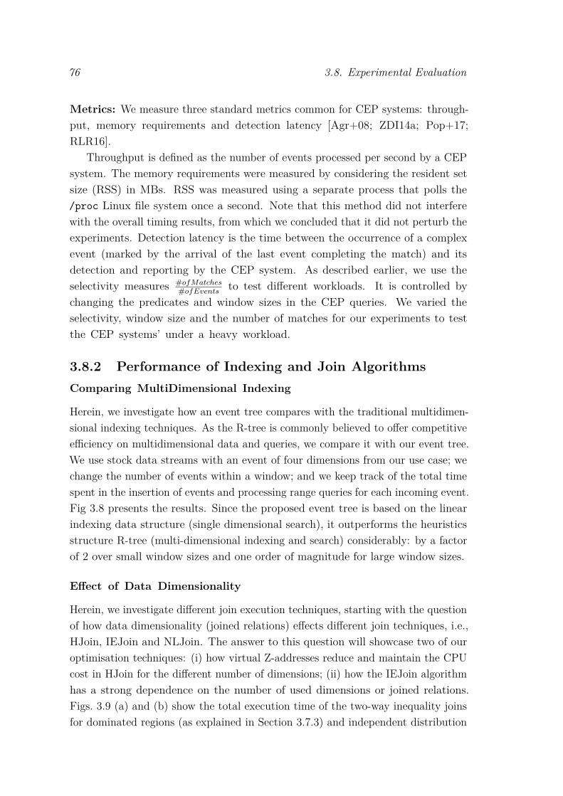
76 3.8. Experimental Evaluation
Metrics: We measure three standard metrics common for CEP systems: through-put, memory requirements and detection latency [Agr+08; ZDI14a; Pop+17;RLR16].
Throughput is defined as the number of events processed per second by a CEPsystem. The memory requirements were measured by considering the resident setsize (RSS) in MBs. RSS was measured using a separate process that polls the/proc Linux file system once a second. Note that this method did not interferewith the overall timing results, from which we concluded that it did not perturb theexperiments. Detection latency is the time between the occurrence of a complexevent (marked by the arrival of the last event completing the match) and itsdetection and reporting by the CEP system. As described earlier, we use theselectivity measures #ofMatches
#ofEvents to test different workloads. It is controlled bychanging the predicates and window sizes in the CEP queries. We varied theselectivity, window size and the number of matches for our experiments to testthe CEP systems’ under a heavy workload.
3.8.2 Performance of Indexing and Join AlgorithmsComparing MultiDimensional Indexing
Herein, we investigate how an event tree compares with the traditional multidimen-sional indexing techniques. As the R-tree is commonly believed to offer competitiveefficiency on multidimensional data and queries, we compare it with our event tree.We use stock data streams with an event of four dimensions from our use case; wechange the number of events within a window; and we keep track of the total timespent in the insertion of events and processing range queries for each incoming event.Fig 3.8 presents the results. Since the proposed event tree is based on the linearindexing data structure (single dimensional search), it outperforms the heuristicsstructure R-tree (multi-dimensional indexing and search) considerably: by a factorof 2 over small window sizes and one order of magnitude for large window sizes.
Effect of Data Dimensionality
Herein, we investigate different join execution techniques, starting with the questionof how data dimensionality (joined relations) effects different join techniques, i.e.,HJoin, IEJoin and NLJoin. The answer to this question will showcase two of ouroptimisation techniques: (i) how virtual Z-addresses reduce and maintain the CPUcost in HJoin for the different number of dimensions; (ii) how the IEJoin algorithmhas a strong dependence on the number of used dimensions or joined relations.Figs. 3.9 (a) and (b) show the total execution time of the two-way inequality joinsfor dominated regions (as explained in Section 3.7.3) and independent distribution
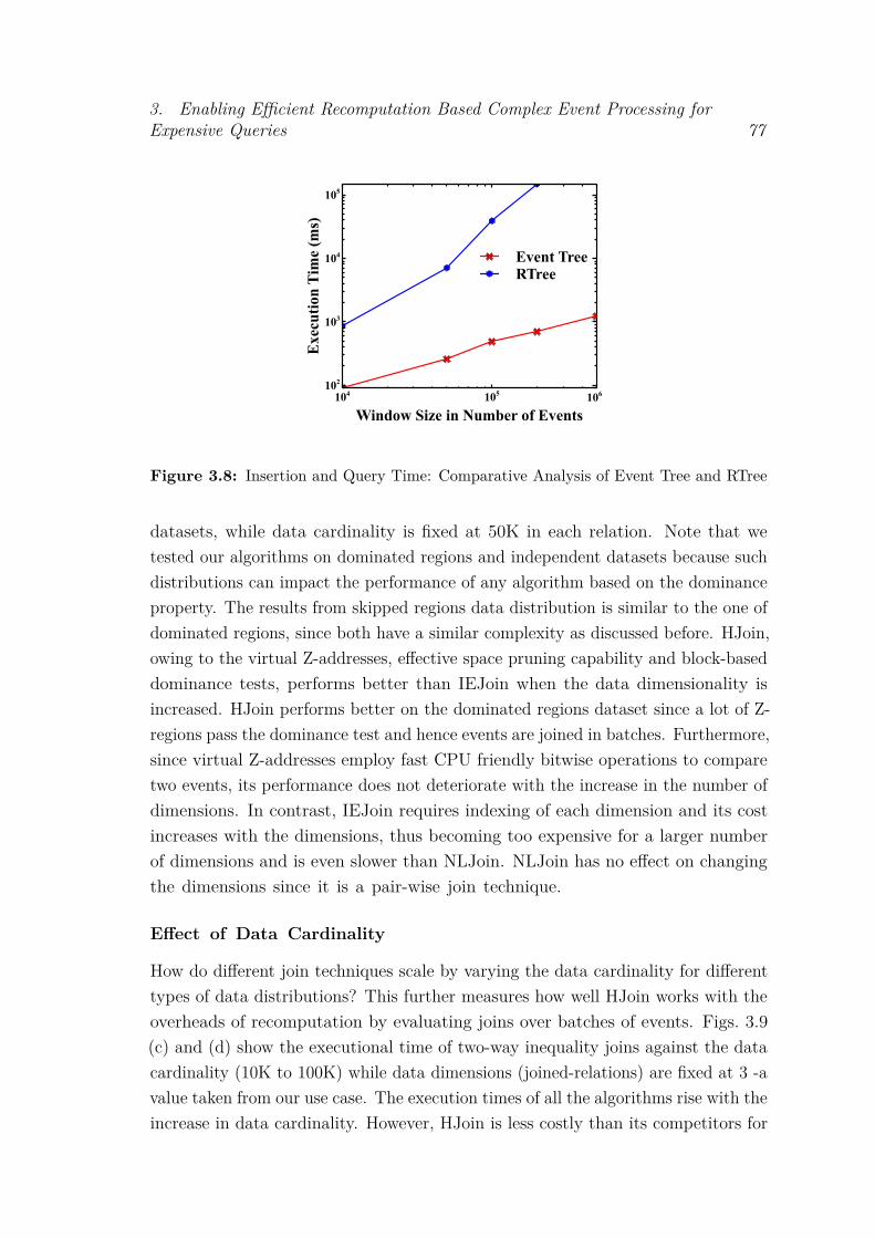
3. Enabling Efficient Recomputation Based Complex Event Processing forExpensive Queries 77
Figure 3.8: Insertion and Query Time: Comparative Analysis of Event Tree and RTree
datasets, while data cardinality is fixed at 50K in each relation. Note that wetested our algorithms on dominated regions and independent datasets because suchdistributions can impact the performance of any algorithm based on the dominanceproperty. The results from skipped regions data distribution is similar to the one ofdominated regions, since both have a similar complexity as discussed before. HJoin,owing to the virtual Z-addresses, effective space pruning capability and block-baseddominance tests, performs better than IEJoin when the data dimensionality isincreased. HJoin performs better on the dominated regions dataset since a lot of Z-regions pass the dominance test and hence events are joined in batches. Furthermore,since virtual Z-addresses employ fast CPU friendly bitwise operations to comparetwo events, its performance does not deteriorate with the increase in the number ofdimensions. In contrast, IEJoin requires indexing of each dimension and its costincreases with the dimensions, thus becoming too expensive for a larger numberof dimensions and is even slower than NLJoin. NLJoin has no effect on changingthe dimensions since it is a pair-wise join technique.
Effect of Data Cardinality
How do different join techniques scale by varying the data cardinality for differenttypes of data distributions? This further measures how well HJoin works with theoverheads of recomputation by evaluating joins over batches of events. Figs. 3.9(c) and (d) show the executional time of two-way inequality joins against the datacardinality (10K to 100K) while data dimensions (joined-relations) are fixed at 3 -avalue taken from our use case. The execution times of all the algorithms rise with theincrease in data cardinality. However, HJoin is less costly than its competitors for
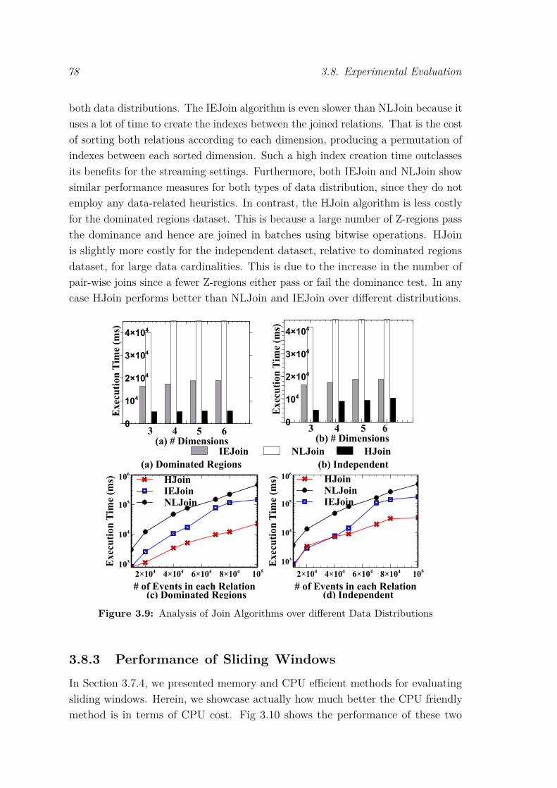
78 3.8. Experimental Evaluation
both data distributions. The IEJoin algorithm is even slower than NLJoin because ituses a lot of time to create the indexes between the joined relations. That is the costof sorting both relations according to each dimension, producing a permutation ofindexes between each sorted dimension. Such a high index creation time outclassesits benefits for the streaming settings. Furthermore, both IEJoin and NLJoin showsimilar performance measures for both types of data distribution, since they do notemploy any data-related heuristics. In contrast, the HJoin algorithm is less costlyfor the dominated regions dataset. This is because a large number of Z-regions passthe dominance and hence are joined in batches using bitwise operations. HJoinis slightly more costly for the independent dataset, relative to dominated regionsdataset, for large data cardinalities. This is due to the increase in the number ofpair-wise joins since a fewer Z-regions either pass or fail the dominance test. In anycase HJoin performs better than NLJoin and IEJoin over different distributions.
Figure 3.9: Analysis of Join Algorithms over different Data Distributions
3.8.3 Performance of Sliding Windows
In Section 3.7.4, we presented memory and CPU efficient methods for evaluatingsliding windows. Herein, we showcase actually how much better the CPU friendlymethod is in terms of CPU cost. Fig 3.10 shows the performance of these two
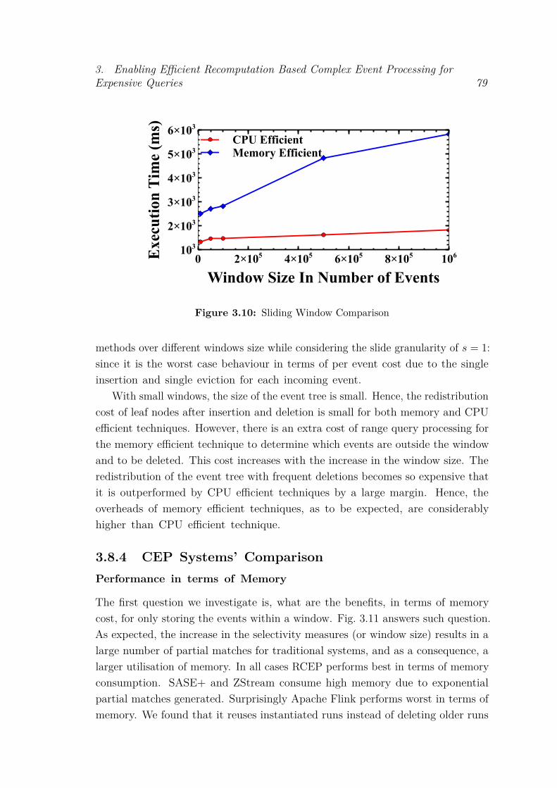
3. Enabling Efficient Recomputation Based Complex Event Processing forExpensive Queries 79
Figure 3.10: Sliding Window Comparison
methods over different windows size while considering the slide granularity of s = 1:since it is the worst case behaviour in terms of per event cost due to the singleinsertion and single eviction for each incoming event.
With small windows, the size of the event tree is small. Hence, the redistributioncost of leaf nodes after insertion and deletion is small for both memory and CPUefficient techniques. However, there is an extra cost of range query processing forthe memory efficient technique to determine which events are outside the windowand to be deleted. This cost increases with the increase in the window size. Theredistribution of the event tree with frequent deletions becomes so expensive thatit is outperformed by CPU efficient techniques by a large margin. Hence, theoverheads of memory efficient techniques, as to be expected, are considerablyhigher than CPU efficient technique.
3.8.4 CEP Systems’ ComparisonPerformance in terms of Memory
The first question we investigate is, what are the benefits, in terms of memorycost, for only storing the events within a window. Fig. 3.11 answers such question.As expected, the increase in the selectivity measures (or window size) results in alarge number of partial matches for traditional systems, and as a consequence, alarger utilisation of memory. In all cases RCEP performs best in terms of memoryconsumption. SASE+ and ZStream consume high memory due to exponentialpartial matches generated. Surprisingly Apache Flink performs worst in terms ofmemory. We found that it reuses instantiated runs instead of deleting older runs
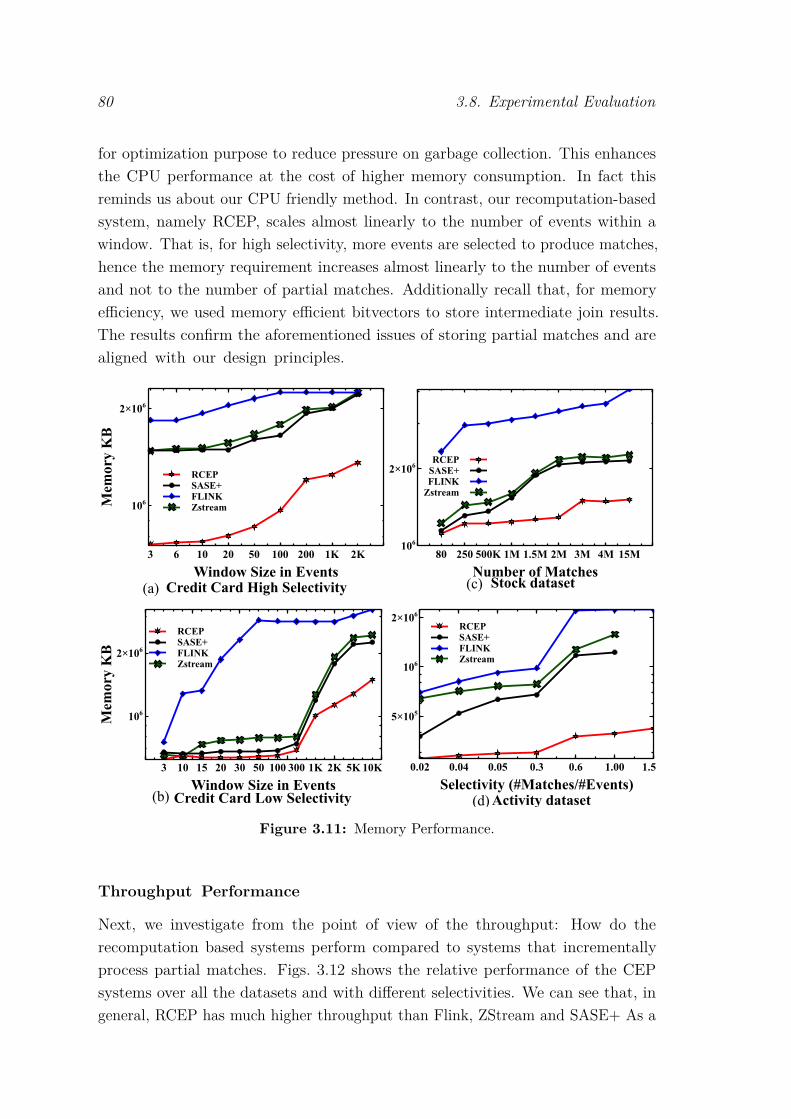
80 3.8. Experimental Evaluation
for optimization purpose to reduce pressure on garbage collection. This enhancesthe CPU performance at the cost of higher memory consumption. In fact thisreminds us about our CPU friendly method. In contrast, our recomputation-basedsystem, namely RCEP, scales almost linearly to the number of events within awindow. That is, for high selectivity, more events are selected to produce matches,hence the memory requirement increases almost linearly to the number of eventsand not to the number of partial matches. Additionally recall that, for memoryefficiency, we used memory efficient bitvectors to store intermediate join results.The results confirm the aforementioned issues of storing partial matches and arealigned with our design principles.
Figure 3.11: Memory Performance.
Throughput Performance
Next, we investigate from the point of view of the throughput: How do therecomputation based systems perform compared to systems that incrementallyprocess partial matches. Figs. 3.12 shows the relative performance of the CEPsystems over all the datasets and with different selectivities. We can see that, ingeneral, RCEP has much higher throughput than Flink, ZStream and SASE+ As a
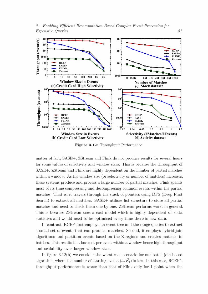
3. Enabling Efficient Recomputation Based Complex Event Processing forExpensive Queries 81
Figure 3.12: Throughput Performance.
matter of fact, SASE+, ZStream and Flink do not produce results for several hoursfor some values of selectivity and window sizes. This is because the throughput ofSASE+, ZStream and Flink are highly dependent on the number of partial matcheswithin a window. As the window size (or selectivity or number of matches) increases,these systems produce and process a large number of partial matches. Flink spendsmost of its time compressing and decompressing common events within the partialmatches. That is, it travers through the stack of pointers using DFS (Deep FirstSearch) to extract all matches. SASE+ utilises list structure to store all partialmatches and need to check them one by one. ZStream performs worst in general.This is because ZStream uses a cost model which is highly dependent on datastatistics and would need to be optimised every time there is new data.
In contrast, RCEP first employs an event tree and the range queries to extracta small set of events that can produce matches. Second, it employs hybrid-joinalgorithms and partition events based on the Z-regions and creates matches inbatches. This results in a low cost per event within a window hence high throughputand scalability over larger window sizes.
In figure 3.12(b) we consider the worst case scenario for our batch join basedalgorithm, where the number of starting events (a/ ~E1) is low. In this case, RCEP’sthroughput performance is worse than that of Flink only for 1 point when the
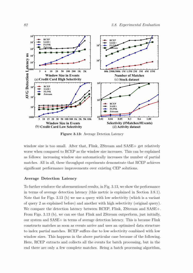
82 3.8. Experimental Evaluation
Figure 3.13: Average Detetion Latency
window size is too small. After that, Flink, ZStream and SASE+ get relativelyworse when compared to RCEP as the window size increases. This can be explainedas follows: increasing window size automatically increases the number of partialmatches. All in all, these throughput experiments demonstrate that RCEP achievessignificant performance improvements over existing CEP solutions.
Average Detection Latency
To further reinforce the aforementioned results, in Fig. 3.13, we show the performancein terms of average detection latency (this metric is explained in Section 3.8.1).Note that for Figs. 3.13 (b) we use a query with low selectivity (which is a variantof query 2 as explained before) and another with high selectivity (original query).We compare the detection latency between RCEP, Flink, ZStream and SASE+.From Figs. 3.13 (b), we can see that Flink and ZStream outperform, just initially,our system and SASE+ in terms of average detection latency. This is because Flinkconstructs matches as soon as events arrive and uses an optimised data structureto index partial matches. RCEP suffers due to low selectivity combined with lowwindow sizes. This happens in the above particular case because of the following.Here, RCEP extracts and collects all the events for batch processing, but in theend there are only a few complete matches. Being a batch processing algorithm,
3. Enabling Efficient Recomputation Based Complex Event Processing forExpensive Queries 83
our fixed cost is slightly higher than SASE+, ZStream and Flink as we have tocollect all the events for batch processing and getting only a few complete matchesin the end does not compensate for the high fixed cost. In any case this correspondsto very special case of very low window sizes and low selectivity. However, afterthe window size is more than 100, then RCEP performs better for this special caseof low selectivity query. Also note that the performance of Flink degrades veryrapidly with the increasing number of partial matches. This is due to the factthat Flink has to compress and decompress more and more partial matches. Forsame reasons we can see that Flink initially performs slightly better than RCEPon activity dataset as shown in Figs. 3.13 (d). However, the performance of Flinkdecreases with the increasing number of partial matches. In other cases RCEPalways performs better that other systems.
3.9 ConclusionIn this chapter, we proposed an efficient re-computation based, complex eventprocessing system for expensive queries. We observed that traditional systemssuffer from performance degradation as they store all partial matches in theirmemory. Thus, they waste memory and additionally computation resources toperform searches on these partial matches.
To solve this problem, we introduced an efficient multidimensional B-tree basedindexing of events. Instead of storing all partial matches, which are the differentcombinations of matching events, we just store the events. When an event arrivesthat can complete the match, we collect and process the events in batches to find thecomplete matches. For events with multiple attributes, we employ a Z-address basedindexing scheme that converts multi-dimensional attributes into a single value. Thisallows us to adapt the B-tree based indexing scheme for multi-dimensional eventsand use range queries to extract a small set of events that can produce matches. Weemploy a heuristic-based algorithm for theta-joins (HJoin) and partitioned eventsbased on Z-regions to join events and create matches in batches. Hence, RCEPdoes not waste computational resources on sequential scans of large number ofpartial matches and decompression operations of matches.
Results show that RCEP performs much better and consumes less memory thanexisting systems such as SASE+, ZStream and Flink. This is consistent with ouranalysis, and partial matching techniques result in a much higher cost per eventcompared with recomputation-based techniques.

84
4A Generic Framework for Predictive
Complex Event Processing usingHistorical Sequence Space
Contents4.1 Introduction . . . . . . . . . . . . . . . . . . . . . . . . . 854.2 Contribution . . . . . . . . . . . . . . . . . . . . . . . . . 874.3 Our Approach . . . . . . . . . . . . . . . . . . . . . . . . 88
4.3.1 Querying Historical Space for Prediction . . . . . . . . . 894.3.2 Summarisation of Historical Space Points . . . . . . . . 91
4.4 Implementation . . . . . . . . . . . . . . . . . . . . . . . 934.4.1 System Architecture . . . . . . . . . . . . . . . . . . . . 934.4.2 User Interface . . . . . . . . . . . . . . . . . . . . . . . . 93
4.5 Experimental Evaluation . . . . . . . . . . . . . . . . . . 944.5.1 Experiment Setup . . . . . . . . . . . . . . . . . . . . . 944.5.2 Datasets and CEP Queries . . . . . . . . . . . . . . . . 964.5.3 Accuracy Metrics . . . . . . . . . . . . . . . . . . . . . . 964.5.4 Precision of Prediction with Summarisation . . . . . . . 964.5.5 Comparison with other Techniques: . . . . . . . . . . . . 96
4.6 Conclusion . . . . . . . . . . . . . . . . . . . . . . . . . . 97
4.1 Introduction
Today, analytics are moving towards a model of proactive computing [EE11],and CEP is also experiencing a paradigm shift towards proactive and predictive
85
86 4.1. Introduction
computations. That is, given a partial match, predictive CEP systems provide thepossible future events of partially matched sequences which can then be convertedinto full matches. This can enable users to mitigate or eliminate undesired futureevents or states and identify future opportunities. Associating prediction andautomated decision making enables progressing towards proactive event-drivencomputing. Proactive applications have attracted the attention of researchers fromdifferent fields. The problems of predictive CEP bear remarkable similarities tothose of sequence pattern mining and prediction. Sequence prediction consists ofpredicting the next element for a given input sequence by only observing its previousitems. The number of applications related to this problem is quite large. It coversapplications such as consumer product recommendations, i.e. given a sequence ofa consumer past purchases, it can predict its next purchases, weather forecasting,i.e. given a sequence of observations about the weather over time, it can predictthe expected weather tomorrow; web page prefetching, i.e. given the history ofaccess data, it can predict the data that will be requested next time, and stockmarket prediction, i.e. given a sequence of movements of a stock over time, itcan predict the next movement of said stock.
In this context, a large body of sequence prediction models have been pro-posed, such as: Prediction By Partial Matching (PPM) [CW84], All-K-Order-Markov [PP99], Dependancy Graph (DG) and Probabilistic Suffix Tree [BYY04].Some important limitations are present in each of these models. First and foremost,these models are based on the Markovion hypotheses that an event is only dependenton its predecessor, however this is not the case in our application and many others.Second, these models suffer from the catastrophic forgetting of older sequences,where only the k recent items of training sequences are used to perform predictions:increasing k often induces a very high state complexity and consequently suchtechniques become impractical for many real-life applications [Gue+15]. Theselimitations can have a major impact on the outcome of the prediction, causingpoor accuracy.
There are several challenges to build a swift and efficient approach. First, itis necessary to have an efficient data structure in terms of memory to index allsequences. The second challenge is in designing algorithms to handle complex data,i.e. multidimensional sequences. Third, the data structure should be updatedefficiently when adding a new sequence. Finally, an algorithm must be preciselydefined to perform fast and more accurate sequence prediction.
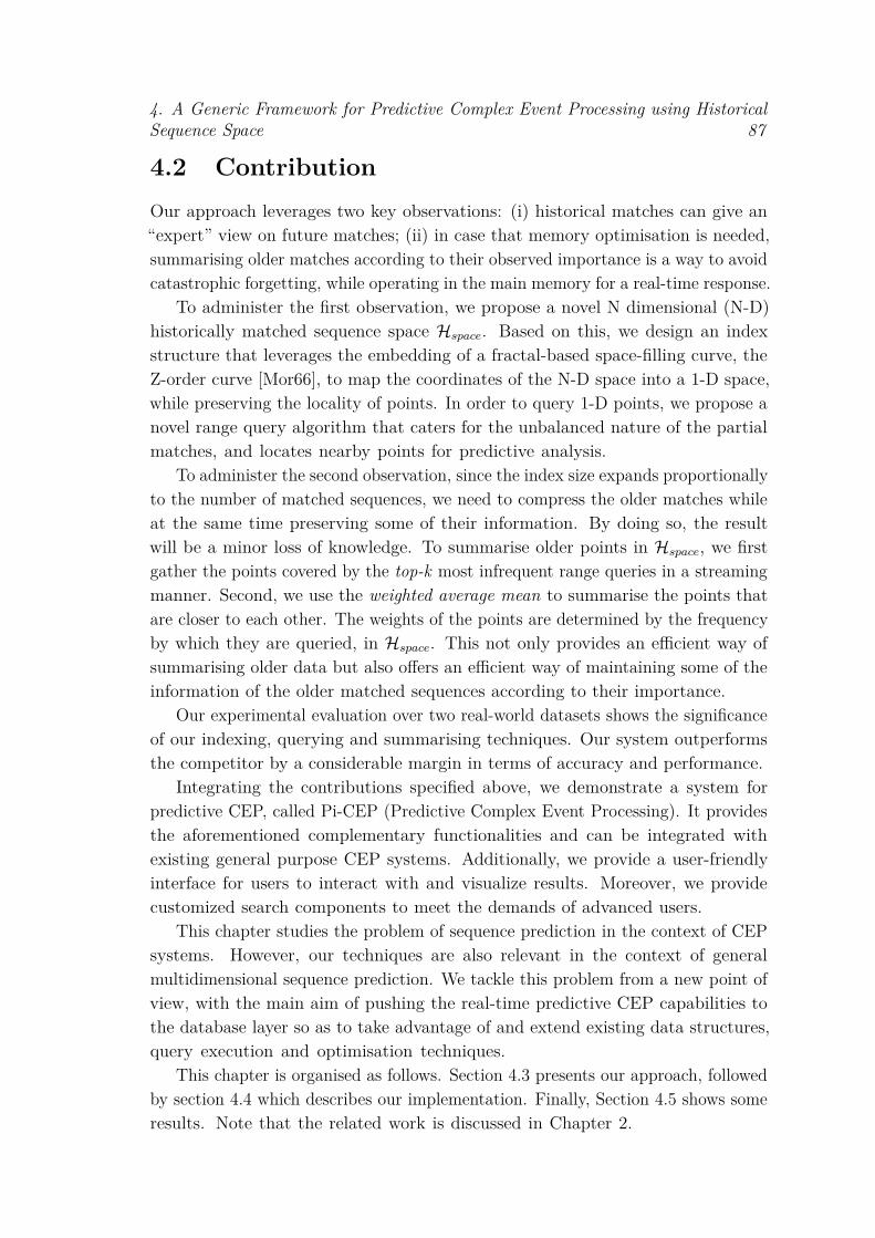
4. A Generic Framework for Predictive Complex Event Processing using HistoricalSequence Space 87
4.2 ContributionOur approach leverages two key observations: (i) historical matches can give an“expert” view on future matches; (ii) in case that memory optimisation is needed,summarising older matches according to their observed importance is a way to avoidcatastrophic forgetting, while operating in the main memory for a real-time response.
To administer the first observation, we propose a novel N dimensional (N-D)historically matched sequence space Hspace. Based on this, we design an indexstructure that leverages the embedding of a fractal-based space-filling curve, theZ-order curve [Mor66], to map the coordinates of the N-D space into a 1-D space,while preserving the locality of points. In order to query 1-D points, we propose anovel range query algorithm that caters for the unbalanced nature of the partialmatches, and locates nearby points for predictive analysis.
To administer the second observation, since the index size expands proportionallyto the number of matched sequences, we need to compress the older matches whileat the same time preserving some of their information. By doing so, the resultwill be a minor loss of knowledge. To summarise older points in Hspace, we firstgather the points covered by the top-k most infrequent range queries in a streamingmanner. Second, we use the weighted average mean to summarise the points thatare closer to each other. The weights of the points are determined by the frequencyby which they are queried, in Hspace. This not only provides an efficient way ofsummarising older data but also offers an efficient way of maintaining some of theinformation of the older matched sequences according to their importance.
Our experimental evaluation over two real-world datasets shows the significanceof our indexing, querying and summarising techniques. Our system outperformsthe competitor by a considerable margin in terms of accuracy and performance.
Integrating the contributions specified above, we demonstrate a system forpredictive CEP, called Pi-CEP (Predictive Complex Event Processing). It providesthe aforementioned complementary functionalities and can be integrated withexisting general purpose CEP systems. Additionally, we provide a user-friendlyinterface for users to interact with and visualize results. Moreover, we providecustomized search components to meet the demands of advanced users.
This chapter studies the problem of sequence prediction in the context of CEPsystems. However, our techniques are also relevant in the context of generalmultidimensional sequence prediction. We tackle this problem from a new point ofview, with the main aim of pushing the real-time predictive CEP capabilities tothe database layer so as to take advantage of and extend existing data structures,query execution and optimisation techniques.
This chapter is organised as follows. Section 4.3 presents our approach, followedby section 4.4 which describes our implementation. Finally, Section 4.5 shows someresults. Note that the related work is discussed in Chapter 2.
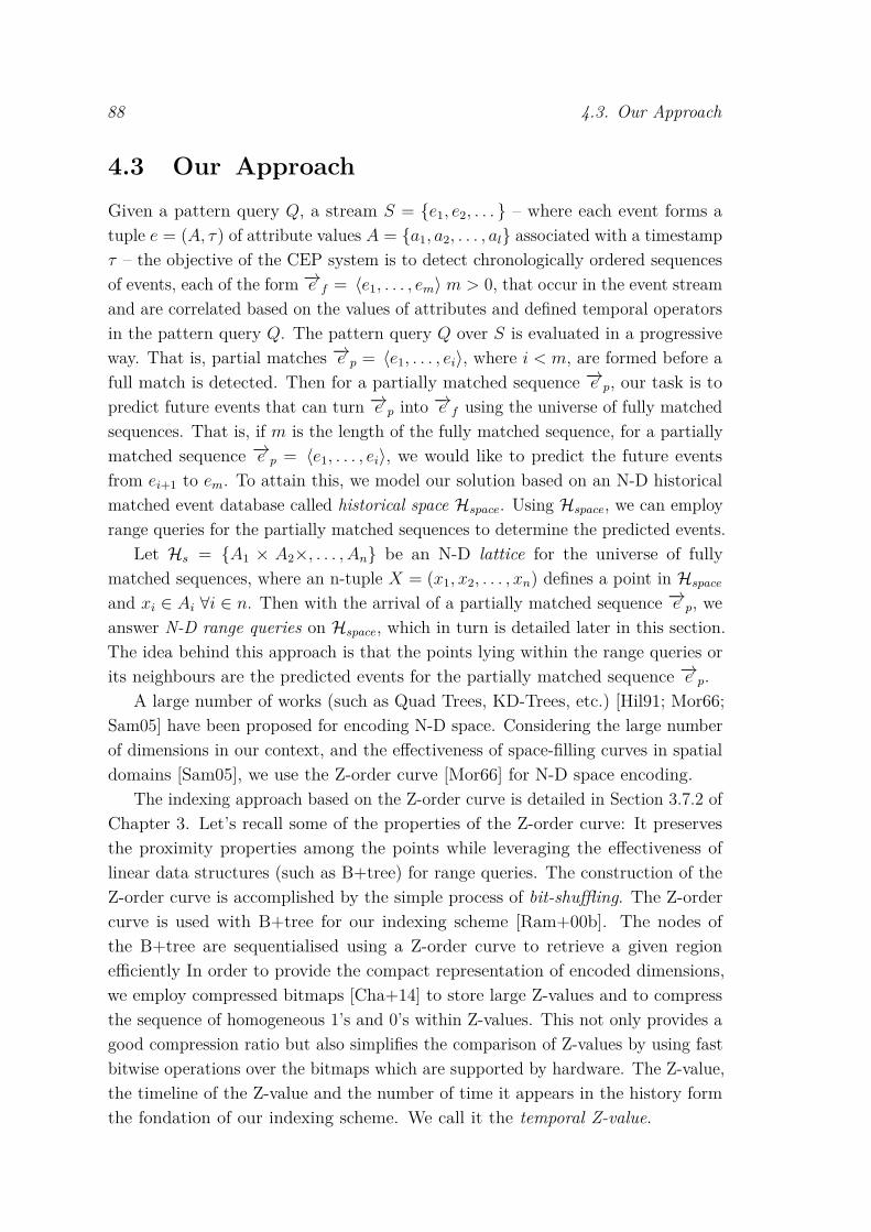
88 4.3. Our Approach
4.3 Our ApproachGiven a pattern query Q, a stream S = {e1, e2, . . . } – where each event forms atuple e = (A, τ) of attribute values A = {a1, a2, . . . , al} associated with a timestampτ – the objective of the CEP system is to detect chronologically ordered sequencesof events, each of the form −→e f = 〈e1, . . . , em〉 m > 0, that occur in the event streamand are correlated based on the values of attributes and defined temporal operatorsin the pattern query Q. The pattern query Q over S is evaluated in a progressiveway. That is, partial matches −→e p = 〈e1, . . . , ei〉, where i < m, are formed before afull match is detected. Then for a partially matched sequence −→e p, our task is topredict future events that can turn −→e p into −→e f using the universe of fully matchedsequences. That is, if m is the length of the fully matched sequence, for a partiallymatched sequence −→e p = 〈e1, . . . , ei〉, we would like to predict the future eventsfrom ei+1 to em. To attain this, we model our solution based on an N-D historicalmatched event database called historical space Hspace. Using Hspace, we can employrange queries for the partially matched sequences to determine the predicted events.
Let Hs = {A1 × A2×, . . . , An} be an N-D lattice for the universe of fullymatched sequences, where an n-tuple X = (x1, x2, . . . , xn) defines a point in Hspace
and xi ∈ Ai ∀i ∈ n. Then with the arrival of a partially matched sequence −→e p, weanswer N-D range queries on Hspace, which in turn is detailed later in this section.The idea behind this approach is that the points lying within the range queries orits neighbours are the predicted events for the partially matched sequence −→e p.
A large number of works (such as Quad Trees, KD-Trees, etc.) [Hil91; Mor66;Sam05] have been proposed for encoding N-D space. Considering the large numberof dimensions in our context, and the effectiveness of space-filling curves in spatialdomains [Sam05], we use the Z-order curve [Mor66] for N-D space encoding.
The indexing approach based on the Z-order curve is detailed in Section 3.7.2 ofChapter 3. Let’s recall some of the properties of the Z-order curve: It preservesthe proximity properties among the points while leveraging the effectiveness oflinear data structures (such as B+tree) for range queries. The construction of theZ-order curve is accomplished by the simple process of bit-shuffling. The Z-ordercurve is used with B+tree for our indexing scheme [Ram+00b]. The nodes ofthe B+tree are sequentialised using a Z-order curve to retrieve a given regionefficiently In order to provide the compact representation of encoded dimensions,we employ compressed bitmaps [Cha+14] to store large Z-values and to compressthe sequence of homogeneous 1’s and 0’s within Z-values. This not only provides agood compression ratio but also simplifies the comparison of Z-values by using fastbitwise operations over the bitmaps which are supported by hardware. The Z-value,the timeline of the Z-value and the number of time it appears in the history formthe fondation of our indexing scheme. We call it the temporal Z-value.

4. A Generic Framework for Predictive Complex Event Processing using HistoricalSequence Space 89
Definition 12: Temporal Z-value
Zτ = (Z, T, f) contains a Z-value Z, a set of timestamps T to denote itstimeline, and the frequency f of times Z appears in the historical space Hspace.
The essence of the temporal Z-value is that, due to the iterative nature of theunderlying fractal, it imposes the required sequential order of matched sequences onHspace. One other attractive feature of our indexing technique is that Hspace can beefficiently stored and retrieved from the disk due to the linear properties of B+trees.
4.3.1 Querying Historical Space for Prediction4.3.1.1 Pre-processing Stage
We first consider the case in which all the matched sequences in the Hspace areof equivalent length (i.e. of same dimensions). In the pre-processing stage, wefirst construct the range queries and their corresponding Z-values. For this task,we maintain an inverted index to record the minimum and maximum values ofall dimensions in the Hspace. That is, if there are dp known dimensions in −→e pand dm is the expected total dimensions of a −→e f , the minimum and maximumvalues of the range query are defined as follows:
Xmin =(x1, . . . , xdp ,min(xdp+1), . . . ,min(xdm)
)Xmax =
(x1, . . . , xdp ,max(xdp+1), . . . ,max(xdm)
),
where ∀xi ∈ Ai,min(xi) ≤ xi ∧ max(xi) ≥ xi and note that x1, . . . , xdp arealready known as they correspond to the already known points in the partiallymatched query. Also note that in case of summarisation, the procedure of trackingminimum and maximum values is not affected because the values are not discarded,but rather summarised. The range query points are then mapped onto the Z-values,i.e. Zmin = Zval(Xmin) and Zmax = Zval(Xmax). These range query points areused to traverse the B+tree. Furthermore, since both have the same values forknown dimensions, any of them can be used to determine if a point in the Hspace
can be enclosed by the range query points.In the case of determining range queries when the Hspace contains variable
lengths (dimensions) matched sequences may be addressed in a similar way. Forexample, if −→e f1= 〈e1, e2, e3〉 and −→e f2= 〈e1, e2, e3, e4〉 are two matched sequences inthe Hspace, a single range query will not cover both of them. One solution usedfor this problem is to create different historical spaces and a set of range queriescovering different matched sequences of specific dimensions.
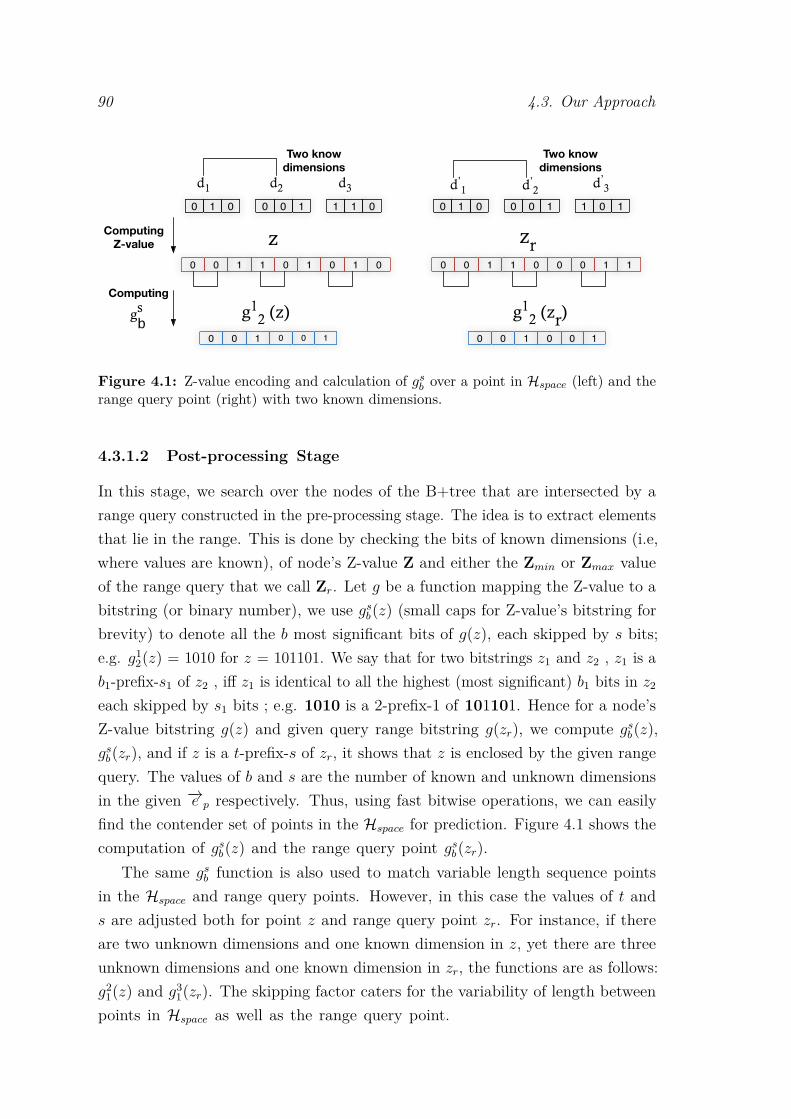
90 4.3. Our Approach
010101100
010 100 011
110001100
010 100 101
d1 d2 d3 d’1 d’
2d’
3
z zr
Two know dimensions
10 010 0
g12 (z) g1
2 (zr)10 010 0
Computing Z-value
Computing gs
Two know dimensions
b
Figure 4.1: Z-value encoding and calculation of gsb over a point in Hspace (left) and therange query point (right) with two known dimensions.
4.3.1.2 Post-processing Stage
In this stage, we search over the nodes of the B+tree that are intersected by arange query constructed in the pre-processing stage. The idea is to extract elementsthat lie in the range. This is done by checking the bits of known dimensions (i.e,where values are known), of node’s Z-value Z and either the Zmin or Zmax valueof the range query that we call Zr. Let g be a function mapping the Z-value to abitstring (or binary number), we use gsb(z) (small caps for Z-value’s bitstring forbrevity) to denote all the b most significant bits of g(z), each skipped by s bits;e.g. g1
2(z) = 1010 for z = 101101. We say that for two bitstrings z1 and z2 , z1 is ab1-prefix-s1 of z2 , iff z1 is identical to all the highest (most significant) b1 bits in z2
each skipped by s1 bits ; e.g. 1010 is a 2-prefix-1 of 101101. Hence for a node’sZ-value bitstring g(z) and given query range bitstring g(zr), we compute gsb(z),gsb(zr), and if z is a t-prefix-s of zr, it shows that z is enclosed by the given rangequery. The values of b and s are the number of known and unknown dimensionsin the given −→e p respectively. Thus, using fast bitwise operations, we can easilyfind the contender set of points in the Hspace for prediction. Figure 4.1 shows thecomputation of gsb(z) and the range query point gsb(zr).
The same gsb function is also used to match variable length sequence pointsin the Hspace and range query points. However, in this case the values of t ands are adjusted both for point z and range query point zr. For instance, if thereare two unknown dimensions and one known dimension in z, yet there are threeunknown dimensions and one known dimension in zr, the functions are as follows:g2
1(z) and g31(zr). The skipping factor caters for the variability of length between
points in Hspace as well as the range query point.
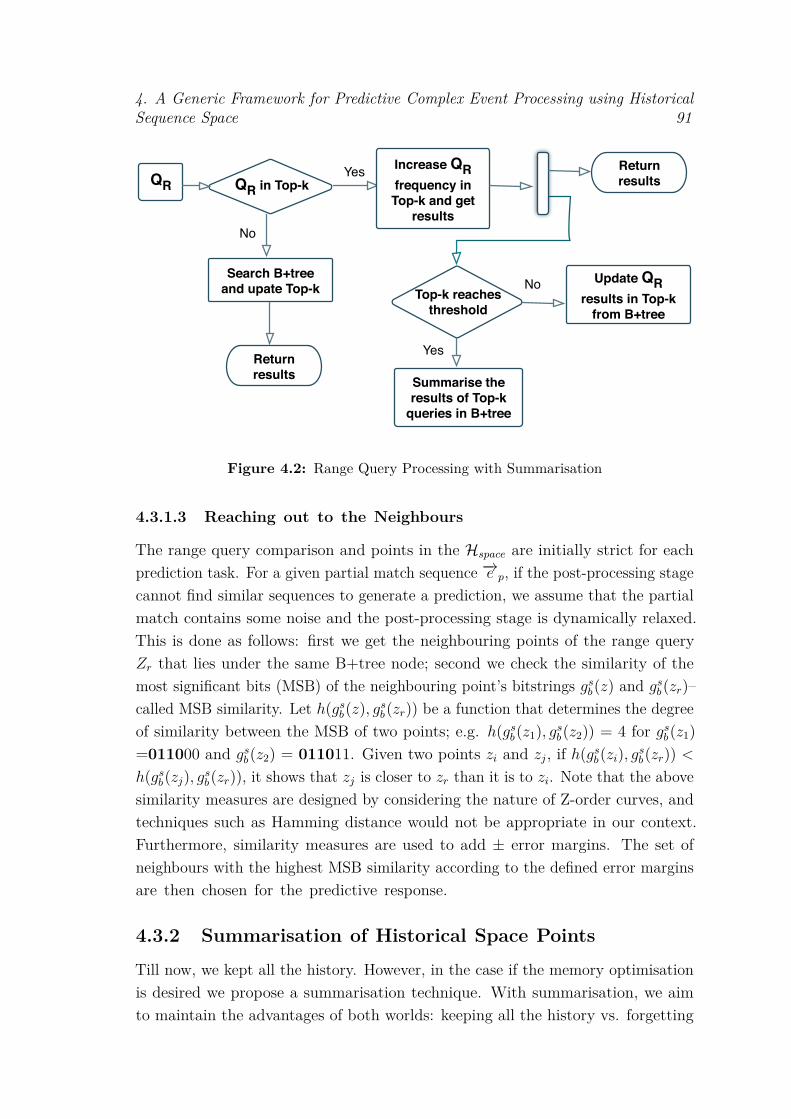
4. A Generic Framework for Predictive Complex Event Processing using HistoricalSequence Space 91
QR QR in Top-k
No
Yes Increase QR frequency in Top-k and get
results
Top-k reaches threshold
Yes
Summarise the results of Top-k
queries in B+tree
Update QR results in Top-k
from B+tree
Return results
NoSearch B+tree
and upate Top-k
Return results
Figure 4.2: Range Query Processing with Summarisation
4.3.1.3 Reaching out to the Neighbours
The range query comparison and points in the Hspace are initially strict for eachprediction task. For a given partial match sequence −→e p, if the post-processing stagecannot find similar sequences to generate a prediction, we assume that the partialmatch contains some noise and the post-processing stage is dynamically relaxed.This is done as follows: first we get the neighbouring points of the range queryZr that lies under the same B+tree node; second we check the similarity of themost significant bits (MSB) of the neighbouring point’s bitstrings gsb(z) and gsb(zr)–called MSB similarity. Let h(gsb(z), gsb(zr)) be a function that determines the degreeof similarity between the MSB of two points; e.g. h(gsb(z1), gsb(z2)) = 4 for gsb(z1)=011000 and gsb(z2) = 011011. Given two points zi and zj, if h(gsb(zi), gsb(zr)) <h(gsb(zj), gsb(zr)), it shows that zj is closer to zr than it is to zi. Note that the abovesimilarity measures are designed by considering the nature of Z-order curves, andtechniques such as Hamming distance would not be appropriate in our context.Furthermore, similarity measures are used to add ± error margins. The set ofneighbours with the highest MSB similarity according to the defined error marginsare then chosen for the predictive response.
4.3.2 Summarisation of Historical Space Points
Till now, we kept all the history. However, in the case if the memory optimisationis desired we propose a summarisation technique. With summarisation, we aimto maintain the advantages of both worlds: keeping all the history vs. forgetting
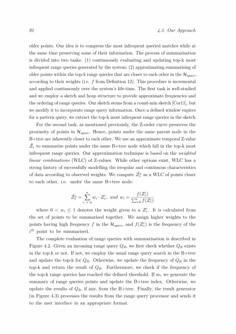
92 4.3. Our Approach
older points. Our idea is to compress the most infrequent queried matches while atthe same time preserving some of their information. The process of summarisationis divided into two tasks: (1) continuously evaluating and updating top-k mostinfrequent range queries generated by the system; (2) approximating summarising ofolder points within the top-k range queries that are closer to each other in the Hspace,according to their weights (i.e. f from Definition 12). This procedure is incrementaland applied continuously over the system’s life-time. The first task is well-studiedand we employ a sketch and heap structure to provide approximate frequencies andthe ordering of range queries. Our sketch stems from a count-min sketch [Cor11], butwe modify it to incorporate range query information. Once a defined window expiresfor a pattern query, we extract the top-k most infrequent range queries in the sketch.
For the second task, as mentioned previously, the Z-order curve preserves theproximity of points in Hspace. Hence, points under the same parent node in theB+tree are inherently closer to each other. We use an approximate temporal Z-valueZτ to summarise points under the same B+tree node which fall in the top-k mostinfrequent range queries. Our approximation technique is based on the weightedlinear combinations (WLC) of Z-values. While other options exist, WLC has astrong history of successfully modelling the irregular and continuous characteristicsof data according to observed weights. We compute Znτ as a WLC of points closerto each other, i.e. under the same B+tree node:
Znτ =n∑
i = 0wi · Z iτ , and wi =
f(Z iτ )∑ni=0 f(Z iτ )
where 0 < wi ≤ 1 denotes the weight given to a Z iτ . It is calculated fromthe set of points to be summarised together. We assign higher weights to thepoints having high frequency f in the Hspace, and f(Z iτ ) is the frequency of theith point to be summarised.
The complete evaluation of range queries with summarisation is described inFigure 4.2. Given an incoming range query QR, we first check whether QR existsin the top-k or not. If not, we employ the usual range query search in the B+treeand update the top-k for QR. Otherwise, we update the frequency of QR in thetop-k and return the result of QR. Furthermore, we check if the frequency ofthe top-k range queries has reached the defined threshold. If so, we generate thesummary of range queries points and update the B+tree index. Otherwise, weupdate the results of QR, if any, from the B+tree. Finally, the result generator(in Figure 4.3) processes the results from the range query processor and sends itto the user interface in an appropriate format.
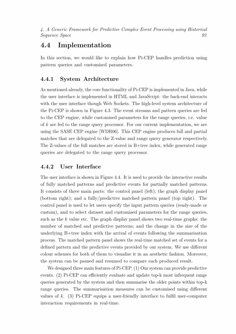
4. A Generic Framework for Predictive Complex Event Processing using HistoricalSequence Space 93
4.4 Implementation
In this section, we would like to explain how Pi-CEP handles prediction usingpattern queries and customised parameters.
4.4.1 System Architecture
As mentioned already, the core functionality of Pi-CEP is implemented in Java, whilethe user interface is implemented in HTML and JavaScript: the back-end interactswith the user interface though Web Sockets. The high-level system architecture ofthe Pi-CEP is shown in Figure 4.3. The event streams and pattern queries are fedto the CEP engine, while customised parameters for the range queries, i.e. valueof k are fed to the range query processor. For our current implementation, we areusing the SASE CEP engine [WDR06]. This CEP engine produces full and partialmatches that are delegated to the Z-value and range query generator respectively.The Z-values of the full matches are stored in B+tree index, while generated rangequeries are delegated to the range query processor.
4.4.2 User Interface
The user interface is shown in Figure 4.4. It is used to provide the interactive resultsof fully matched patterns and predictive events for partially matched patterns.It consists of three main parts: the control panel (left); the graph display panel(bottom right); and a fully/predictive matched pattern panel (top right). Thecontrol panel is used to let users specify the input pattern queries (ready-made orcustom), and to select dataset and customised parameters for the range queries,such as the k value etc. The graph display panel shows two real-time graphs: thenumber of matched and predictive patterns; and the change in the size of theunderlying B+tree index with the arrival of events following the summarisationprocess. The matched pattern panel shows the real-time matched set of events for adefined pattern and the predictive events provided by our system. We use differentcolour schemes for both of them to visualise it in an aesthetic fashion. Moreover,the system can be paused and resumed to compare each produced result.
We designed three main features of Pi-CEP. (1) Our system can provide predictiveevents. (2) Pi-CEP can efficiently evaluate and update top-k most infrequent rangequeries generated by the system and then summarise the older points within top-krange queries. The summarisation measures can be customised using differentvalues of k. (3) Pi-CEP equips a user-friendly interface to fulfil user-computerinteraction requirements in real-time.
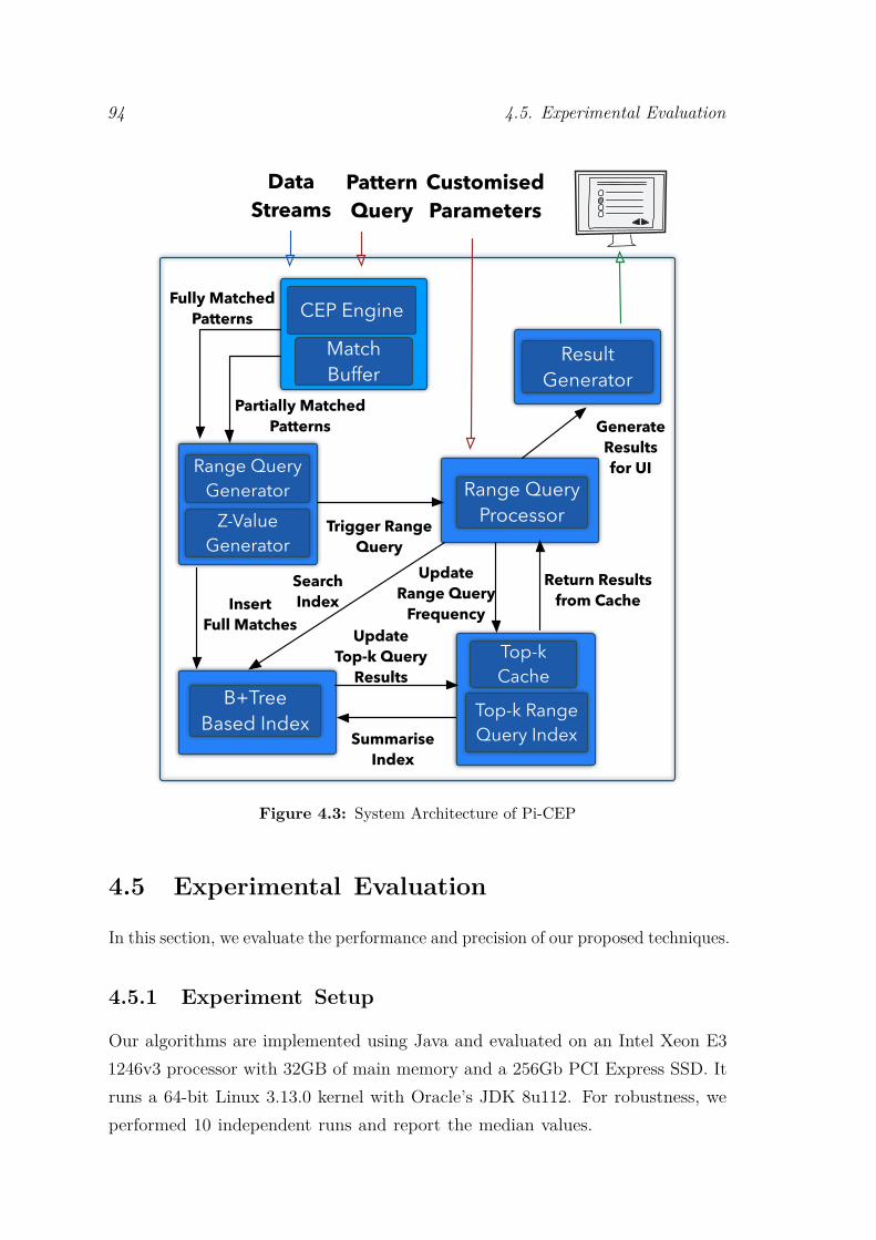
94 4.5. Experimental Evaluation
Z-ValueGenerator
Range QueryGenerator
B+Tree Based Index
Range QueryProcessor
Top-k Cache
Top-k Range Query Index
CEP Engine
Match Buffer
Fully Matched Patterns
Partially MatchedPatterns
Trigger RangeQuery
Search Index
Update Top-k Query
Results
SummariseIndex
Update Range Query
Frequency
Return Resultsfrom Cache
Result Generator
Generate Resultsfor UI
Pattern Query
Data Streams
CustomisedParameters
Insert Full Matches
Figure 4.3: System Architecture of Pi-CEP
4.5 Experimental Evaluation
In this section, we evaluate the performance and precision of our proposed techniques.
4.5.1 Experiment Setup
Our algorithms are implemented using Java and evaluated on an Intel Xeon E31246v3 processor with 32GB of main memory and a 256Gb PCI Express SSD. Itruns a 64-bit Linux 3.13.0 kernel with Oracle’s JDK 8u112. For robustness, weperformed 10 independent runs and report the median values.
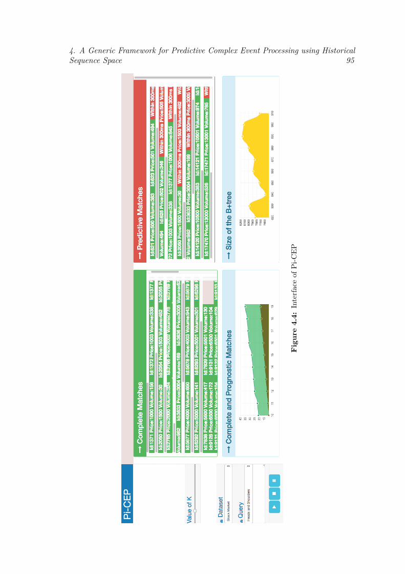
4. A Generic Framework for Predictive Complex Event Processing using HistoricalSequence Space 95
Figure4.4:
Interfaceof
Pi-C
EP
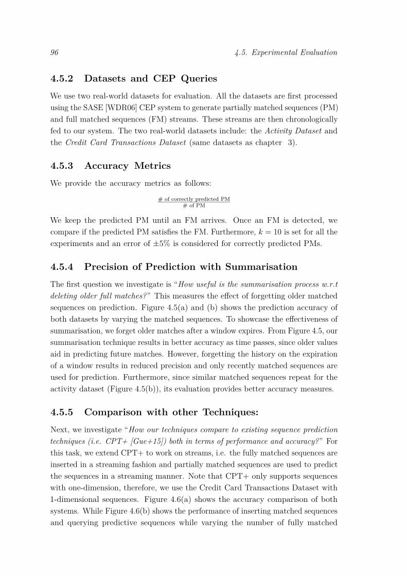
96 4.5. Experimental Evaluation
4.5.2 Datasets and CEP Queries
We use two real-world datasets for evaluation. All the datasets are first processedusing the SASE [WDR06] CEP system to generate partially matched sequences (PM)and full matched sequences (FM) streams. These streams are then chronologicallyfed to our system. The two real-world datasets include: the Activity Dataset andthe Credit Card Transactions Dataset (same datasets as chapter 3).
4.5.3 Accuracy Metrics
We provide the accuracy metrics as follows:
# of correctly predicted PM# of PM
We keep the predicted PM until an FM arrives. Once an FM is detected, wecompare if the predicted PM satisfies the FM. Furthermore, k = 10 is set for all theexperiments and an error of ±5% is considered for correctly predicted PMs.
4.5.4 Precision of Prediction with Summarisation
The first question we investigate is “How useful is the summarisation process w.r.tdeleting older full matches?” This measures the effect of forgetting older matchedsequences on prediction. Figure 4.5(a) and (b) shows the prediction accuracy ofboth datasets by varying the matched sequences. To showcase the effectiveness ofsummarisation, we forget older matches after a window expires. From Figure 4.5, oursummarisation technique results in better accuracy as time passes, since older valuesaid in predicting future matches. However, forgetting the history on the expirationof a window results in reduced precision and only recently matched sequences areused for prediction. Furthermore, since similar matched sequences repeat for theactivity dataset (Figure 4.5(b)), its evaluation provides better accuracy measures.
4.5.5 Comparison with other Techniques:
Next, we investigate “How our techniques compare to existing sequence predictiontechniques (i.e. CPT+ [Gue+15]) both in terms of performance and accuracy?” Forthis task, we extend CPT+ to work on streams, i.e. the fully matched sequences areinserted in a streaming fashion and partially matched sequences are used to predictthe sequences in a streaming manner. Note that CPT+ only supports sequenceswith one-dimension, therefore, we use the Credit Card Transactions Dataset with1-dimensional sequences. Figure 4.6(a) shows the accuracy comparison of bothsystems. While Figure 4.6(b) shows the performance of inserting matched sequencesand querying predictive sequences while varying the number of fully matched
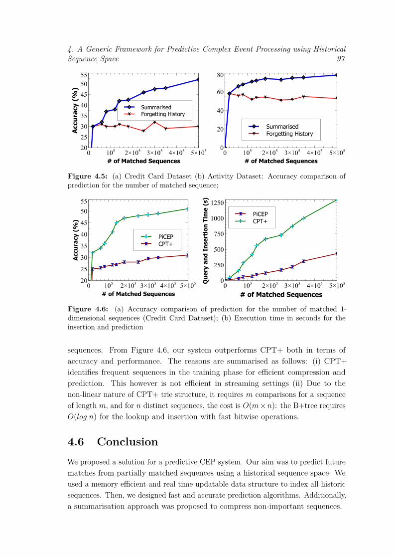
4. A Generic Framework for Predictive Complex Event Processing using HistoricalSequence Space 97
Figure 4.5: (a) Credit Card Dataset (b) Activity Dataset: Accuracy comparison ofprediction for the number of matched sequence;
Figure 4.6: (a) Accuracy comparison of prediction for the number of matched 1-dimensional sequences (Credit Card Dataset); (b) Execution time in seconds for theinsertion and prediction
sequences. From Figure 4.6, our system outperforms CPT+ both in terms ofaccuracy and performance. The reasons are summarised as follows: (i) CPT+identifies frequent sequences in the training phase for efficient compression andprediction. This however is not efficient in streaming settings (ii) Due to thenon-linear nature of CPT+ trie structure, it requires m comparisons for a sequenceof length m, and for n distinct sequences, the cost is O(m×n): the B+tree requiresO(log n) for the lookup and insertion with fast bitwise operations.
4.6 ConclusionWe proposed a solution for a predictive CEP system. Our aim was to predict futurematches from partially matched sequences using a historical sequence space. Weused a memory efficient and real time updatable data structure to index all historicsequences. Then, we designed fast and accurate prediction algorithms. Additionally,a summarisation approach was proposed to compress non-important sequences.

98 4.6. Conclusion
Our experimental analysis demonstrated the potential of our approach andsuggested that predictive CEP may well be best viewed as a distinct predictivetask. Our preliminary research indicates that the study of sequence mining andprediction in CEP systems is promising and represents a new application of sequenceprediction in the field of the internet of things and sensor networks. Moreover, itpaves the way for further research possibilities on both predictive CEP systemsand sequential pattern mining algorithms. In future, we would like to improve theprediction accuracy even more. We would like to also study if integrating machinelearning approaches with our system can improve the performance.
Part III
Real World Event ProcessingChallenges
99

Introduction to DEBS Grand Challenges
In order to demonstrate the ability of our approaches, we participated in differentchallenges. The overall goal of these Challenges is to provide a common groundfor researchers to evaluate and compare event-driven systems.
The ACM Conference on Distributed Event-Based Systems1 is a conference inthe area of event processing and offers a forum for researchers to exchange recentdevelopments around event-based systems.
The 2016 DEBS Grand Challenge [Gul+16a] focused on reasoning over socialnetwork data to drive meaningful insights in real-time by defining two challengingqueries. These queries, each for a different reason, cannot be handled by traditionaltechniques and therefore call for the development of specific architecture and datastructures. The main novel features of this challenge were defined as follows: Inthe first query, the novelty was the non-linearity of the expiration of the elements.Since a traditional sliding window is not suitable, we investigated data structuresoffering the best tradeoffs for all the required operations. In the second query, unliketraditional approaches where no persistent data is stored over the stream, we had tomanage a friendship graph which was persistent throughout the system execution.Due to the centrality of this structure, a careful design was therefore required.
The 2018 DEBS Grand Challenge [Gul+18b] focused on spatio-temporal stream-ing data. The novelty of this challenge was the combination of event processingand predictive analytics. The goal of the challenge was to make the naval trans-portation industry more reliable by providing predictions on vessel destinationsand arrival times.
Following this, in this part of this thesis, we present the questions asked in the twoDebs Grand challenges and the proposed techniques, which enabled as to contributeto overcoming these challenges and to develop Upsortable – a portmanteau ofupdate and sort –. Upsortable is an annotation-based approach that allowsthe use of existing sorted collections from the standard Java API for dynamicdata management.
The remainder of this part is structured as follows. Chapter 5 presents oursolution for the 2016 Debs Grand challenge. Chapter 6 presents our solution for the2018 Debs Grand challenge which was ranked second in this challenge. AppendixA provides guidance on the annotation-based approach Upsortable.
1http://debs.org.
101

102
5High Performance Top-K Processing of
Non-Linear Windows over Data Streams
Contents5.1 Introduction . . . . . . . . . . . . . . . . . . . . . . . . . 1035.2 Input Data Streams and Query definitions . . . . . . . 105
5.2.1 Input Data Streams . . . . . . . . . . . . . . . . . . . . 1055.2.2 Query definitions . . . . . . . . . . . . . . . . . . . . . . 105
5.3 Architecture . . . . . . . . . . . . . . . . . . . . . . . . . 1065.4 Query 1 Solution . . . . . . . . . . . . . . . . . . . . . . . 107
5.4.1 Data structures . . . . . . . . . . . . . . . . . . . . . . . 1085.4.2 Algorithms . . . . . . . . . . . . . . . . . . . . . . . . . 110
5.5 Query 2 Solution . . . . . . . . . . . . . . . . . . . . . . . 1125.5.1 Data Structures . . . . . . . . . . . . . . . . . . . . . . . 1125.5.2 Algorithms . . . . . . . . . . . . . . . . . . . . . . . . . 115
5.6 Evaluation . . . . . . . . . . . . . . . . . . . . . . . . . . . 1175.6.1 Experimental Settings . . . . . . . . . . . . . . . . . . . 1185.6.2 Queues implementation . . . . . . . . . . . . . . . . . . 1195.6.3 Analysis of Query 1 Performance . . . . . . . . . . . . . 1195.6.4 Analysis of Query 2 Performance . . . . . . . . . . . . . 121
5.7 Conclusion . . . . . . . . . . . . . . . . . . . . . . . . . . 122
5.1 Introduction
Stream processing has matured into an influential technology over the past decades,having a wide range of application domains including sensor networks and socialnetworks. As a result, we have seen a flurry of attention in the area of data stream
103
104 5.1. Introduction
processing. However, issues such as the identification of the most frequent elements(top-k) over graph structured networks, while considering the non-linear dynamicwindow model has not gained much attention in previous studies.
The 2016 DEBS Grand Challenge [Gul+16a] surfaced such issues, where a socialnetwork use case is considered. We herein summarize the two main queries/re-quirements for this challenge.
1. The identification of the top-3 active posts according to their scores whichare computed in streaming settings: Scores of posts are increased with thearrival of new post-related comments and are decreased on expiration ofrelated-comments and own score. This conforms to a non-linear windowmodel.
2. The identification of social contagion in dynamic streaming settings. Thatis, given a window and the value of k, determining the top-k commentsshared/liked between friends in the neighbourhood. The size of the largestclique determines the influence of a certain comment posted by a person.
Both the aforementioned queries present two orthogonal domains of interestand require different techniques to satisfy their requirements; however the basicconstraints of stream processing are shared by both.
One naïve way of addressing the requirements of both queries is to compute theentirety of changes on each update and to reinitialize the process of identifying thetop-k element for each newly observed change. Clearly, this naive method is tooexpensive in a streaming environment. In addition, the discussed state of the art Top-K algorithms in section 2.6.2 are adequate only in the case of linear data expirationand append-only data streams. However, to efficiently find the top-k posts accordingto their scores and the top-k comments with the highest influence in the connectednetwork, the system should utilize certain guarantees to prune the search spacebased on some upper bound scores, and postpone the evaluation of query operators.
In this chapter, we present the solutions to the questions asked in the DEBS GC2016. We propose several efficient and effective methods of enabling a lazy evaluationof non-linear window elements in Query 1. For this, we devise an easily computedupper-bound based on the temporal evolution of the posts. For Query 2, we rely onTuran’s theorem [Tur41] to obtain guarantees on the absence of k-cliques in a graph.This lower-bound saves on numerous useless computations, especially in streamingsettings. To store the global friendship graph, we propose two alternatives based onroaring bitmaps and Bloom-filter to handle the frequent updates and access in thecommunity graph (i.e., friendship graph). The community graph is implemented by
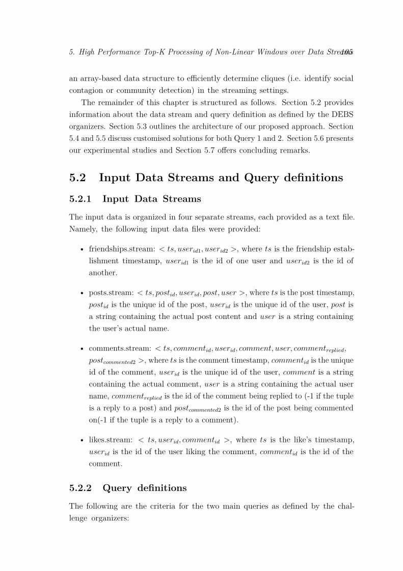
5. High Performance Top-K Processing of Non-Linear Windows over Data Streams105
an array-based data structure to efficiently determine cliques (i.e. identify socialcontagion or community detection) in the streaming settings.
The remainder of this chapter is structured as follows. Section 5.2 providesinformation about the data stream and query definition as defined by the DEBSorganizers. Section 5.3 outlines the architecture of our proposed approach. Section5.4 and 5.5 discuss customised solutions for both Query 1 and 2. Section 5.6 presentsour experimental studies and Section 5.7 offers concluding remarks.
5.2 Input Data Streams and Query definitions
5.2.1 Input Data Streams
The input data is organized in four separate streams, each provided as a text file.Namely, the following input data files were provided:
• friendships.stream: < ts, userid1, userid2 >, where ts is the friendship estab-lishment timestamp, userid1 is the id of one user and userid2 is the id ofanother.
• posts.stream: < ts, postid, userid, post, user >, where ts is the post timestamp,postid is the unique id of the post, userid is the unique id of the user, post isa string containing the actual post content and user is a string containingthe user’s actual name.
• comments.stream: < ts, commentid, userid, comment, user, commentreplied,
postcommented2 >, where ts is the comment timestamp, commentid is the uniqueid of the comment, userid is the unique id of the user, comment is a stringcontaining the actual comment, user is a string containing the actual username, commentreplied is the id of the comment being replied to (-1 if the tupleis a reply to a post) and postcommented2 is the id of the post being commentedon(-1 if the tuple is a reply to a comment).
• likes.stream: < ts, userid, commentid >, where ts is the like’s timestamp,userid is the id of the user liking the comment, commentid is the id of thecomment.
5.2.2 Query definitions
The following are the criteria for the two main queries as defined by the chal-lenge organizers:

106 5.3. Architecture
5.2.2.1 Goal of Query 1
The goal of query 1 is to compute the top-3 scoring active posts, producing anupdated result every time they change. The total score of an active post (P ) iscomputed as the sum of its own score plus the score of all its related comments.Active posts with the same total score should be ranked based on their timestamps(in descending order), and if their timestamps are also equal, they should be rankedbased on the timestamps of their last received related comments (in descendingorder). A comment (C) is related to a post (P ) if it is a direct reply to P orif the chain of C’s preceding messages links back to P . Each new post has itsown initial score of 10 which decreases by 1 each time a span of 24 hours elapsessince the post’s creation. Each new comment’s score is also initially set to 10 anddecreases by 1 in the same way (every 24 hours since the comment’s creation).Both post and comment scores are non-negative numbers. That is, they cannotdrop below zero. A post is considered no longer active (that is, no longer partof present and future analysis) as soon as its total score reaches zero, even if itreceives additional comments in the future.
5.2.2.2 Goal of Query 2
Given an integer k and a duration d (in seconds), find the k comments with thelargest range, where the range of a comment is defined as the size of the largestconnected component in the graph defined by persons who (i) have liked thatcomment (see likes, comments), (ii) know each other (friendships), and (iii) wherethe comment was created no more than d seconds ago.
5.3 Architecture
Figure 5.1 illustrates the overall architecture of our system. In order to parallelizequery processing, the first step is to divide the system into a set of threads (i.e.,Query 1 and 2 processors, input handler and output handlers for both queries), andreplace the method calls between task boundaries with queues accordingly. Thus,given a set of files/streams containing events from Comment, Like, Friendship andPost streams, the data parser efficiently parses the events for these streams. Theevents are reordered according to their timestamps and queued into the respectivequeues: Query 1 only takes events from the Post and Comment streams, whileQuery 2 takes events from Likes, Friendship and Comment streams. We employ aset of different types of queues (blocking, non-blocking) to determine bottlenecksand the efficiency of our systems. Such discussion and explanations of queuesis provided in the later sections.
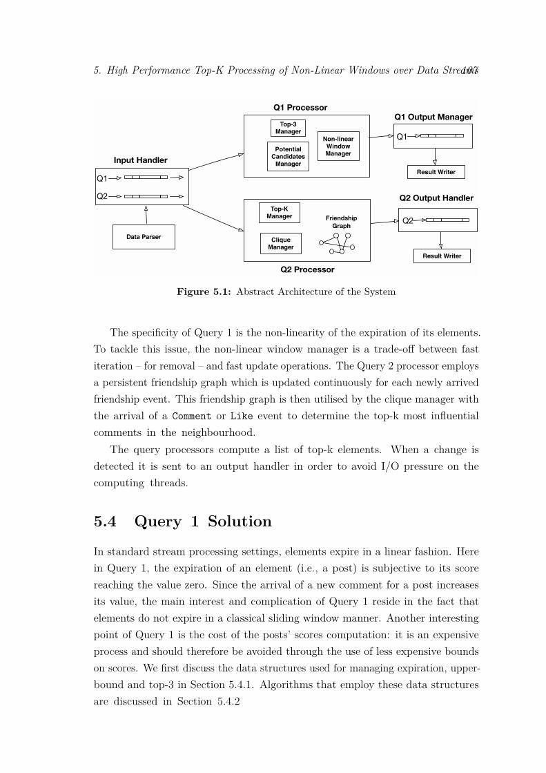
5. High Performance Top-K Processing of Non-Linear Windows over Data Streams107
Data Parser
Q1
Q2
Input Handler
Result Writer
Q2
Q1 Processor
Q2 Processor
Top-K Manager
CliqueManager
Friendship
Graph
Result Writer
Q1
Q1 Output Manager
Q2 Output Handler
Potential Candidates
Manager
Non-linear Window Manager
Top-3 Manager
Figure 5.1: Abstract Architecture of the System
The specificity of Query 1 is the non-linearity of the expiration of its elements.To tackle this issue, the non-linear window manager is a trade-off between fastiteration – for removal – and fast update operations. The Query 2 processor employsa persistent friendship graph which is updated continuously for each newly arrivedfriendship event. This friendship graph is then utilised by the clique manager withthe arrival of a Comment or Like event to determine the top-k most influentialcomments in the neighbourhood.
The query processors compute a list of top-k elements. When a change isdetected it is sent to an output handler in order to avoid I/O pressure on thecomputing threads.
5.4 Query 1 Solution
In standard stream processing settings, elements expire in a linear fashion. Herein Query 1, the expiration of an element (i.e., a post) is subjective to its scorereaching the value zero. Since the arrival of a new comment for a post increasesits value, the main interest and complication of Query 1 reside in the fact thatelements do not expire in a classical sliding window manner. Another interestingpoint of Query 1 is the cost of the posts’ scores computation: it is an expensiveprocess and should therefore be avoided through the use of less expensive boundson scores. We first discuss the data structures used for managing expiration, upper-bound and top-3 in Section 5.4.1. Algorithms that employ these data structuresare discussed in Section 5.4.2
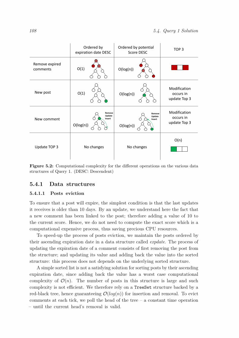
108 5.4. Query 1 Solution
Remove expired comments
Ordered by expiration date DESC
Ordered by potential Score DESC
O(1) O(log(n))
New post
New comment
O(1) O(log(n))
TOP 3
Modification occurs in
update Top 3
Modification occurs in
update Top 3
Remove Update Insert
O(log(n))
Update TOP 3 No changes No changes
O(n)
Remove Update Insert
O(log(n))
Figure 5.2: Computational complexity for the different operations on the various datastructures of Query 1. (DESC: Descendent)
5.4.1 Data structures5.4.1.1 Posts eviction
To ensure that a post will expire, the simplest condition is that the last updatesit receives is older than 10 days. By an update, we understand here the fact thata new comment has been linked to the post; therefore adding a value of 10 tothe current score. Hence, we do not need to compute the exact score which is acomputational expensive process, thus saving precious CPU resources.
To speed-up the process of posts eviction, we maintain the posts ordered bytheir ascending expiration date in a data structure called expdate. The process ofupdating the expiration date of a comment consists of first removing the post fromthe structure; and updating its value and adding back the value into the sortedstructure: this process does not depends on the underlying sorted structure.
A simple sorted list is not a satisfying solution for sorting posts by their ascendingexpiration date, since adding back the value has a worst case computationalcomplexity of O(n). The number of posts in this structure is large and suchcomplexity is not efficient. We therefore rely on a TreeSet structure backed by ared-black tree, hence guaranteeing O(log(n)) for insertion and removal. To evictcomments at each tick, we poll the head of the tree – a constant time operation– until the current head’s removal is valid.

5. High Performance Top-K Processing of Non-Linear Windows over Data Streams109
5.4.1.2 Score management
The potentialScore data structure holds the posts that are the candidates toenter the top-3 structure. Since the computation of the exact score is an expensiveprocess, we aim to use a less expensive upper-bound to sort the candidates to avoidthe exact score computation as much as possible.
Following the procedure of the posts’ eviction, posts are sorted by their upperbound albeit in descending order. When a post has a sufficient upper-bound to enterthe top-3 list, its exact score is computed to affirm such hypothesis. We rely on aTreeSet structure to guarantee worst case O(log(n)) for all required operations:
Post expiration The post may be at any place in the tree, therefore complexityis O(log(n)).
New post The post has a score of 10, which is neither guaranteed to be an uppernor lower value in the tree, hence a O(log(n)) complexity.
New comment If the upper-bound of the related post has increased, we firstremove the post, update its upper-bound, and add it back to the structure.Insertion and removal are both in O(log(n)).
Therefore the posts belong to two data structures: one for the management ofeviction process and the second for score management. The algorithm of Query1 ensures that both structures remains consistent.
5.4.1.3 Comments related to posts
To store comments related to a post, we decided to use a compact representation: weonly store the ids of the comments into a list. Comments are added in chronologicalorder, and their expiration is also chronological. It provides the guarantee that anearlier comment will expire before a later one, which is not the case for the posts.We could only retain the valid comments by checking and removing commentswhen required. This operation is costly and unnecessary, although keeping expiredcomments in memory does not require much space, and the space-time trade-off is definitely worth it. Comments related to a post are thus only removedwhen the post expires.
Comments are stored in an array-list of long next to their time of arrival. Thetime of arrival is used to determine whether a comment is still considered valid.Figure 5.3 depicts this structure. At time 11, the first comment has expired, theoffset is set to 3. At time 21, the second comment also expired, thus the offsetpoints to the first valid comment at index 5.
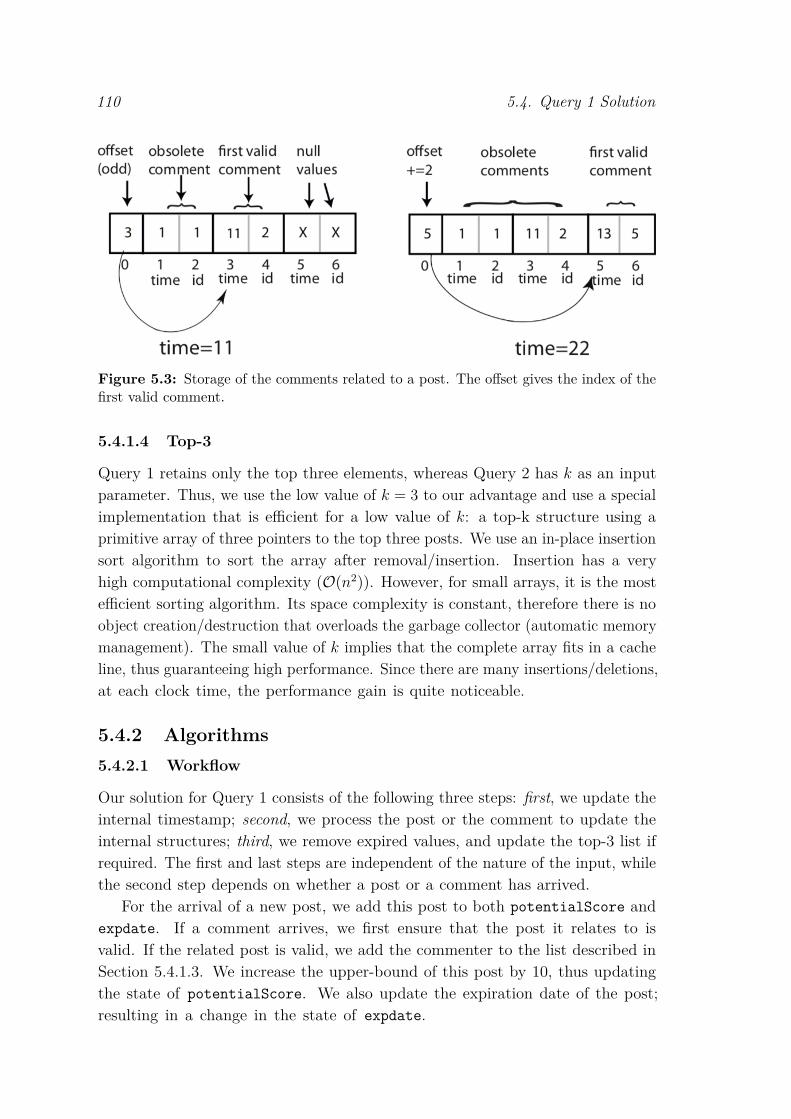
110 5.4. Query 1 Solution
Figure 5.3: Storage of the comments related to a post. The offset gives the index of thefirst valid comment.
5.4.1.4 Top-3
Query 1 retains only the top three elements, whereas Query 2 has k as an inputparameter. Thus, we use the low value of k = 3 to our advantage and use a specialimplementation that is efficient for a low value of k: a top-k structure using aprimitive array of three pointers to the top three posts. We use an in-place insertionsort algorithm to sort the array after removal/insertion. Insertion has a veryhigh computational complexity (O(n2)). However, for small arrays, it is the mostefficient sorting algorithm. Its space complexity is constant, therefore there is noobject creation/destruction that overloads the garbage collector (automatic memorymanagement). The small value of k implies that the complete array fits in a cacheline, thus guaranteeing high performance. Since there are many insertions/deletions,at each clock time, the performance gain is quite noticeable.
5.4.2 Algorithms5.4.2.1 Workflow
Our solution for Query 1 consists of the following three steps: first, we update theinternal timestamp; second, we process the post or the comment to update theinternal structures; third, we remove expired values, and update the top-3 list ifrequired. The first and last steps are independent of the nature of the input, whilethe second step depends on whether a post or a comment has arrived.
For the arrival of a new post, we add this post to both potentialScore andexpdate. If a comment arrives, we first ensure that the post it relates to isvalid. If the related post is valid, we add the commenter to the list described inSection 5.4.1.3. We increase the upper-bound of this post by 10, thus updatingthe state of potentialScore. We also update the expiration date of the post;resulting in a change in the state of expdate.

5. High Performance Top-K Processing of Non-Linear Windows over Data Streams111
5.4.2.2 Top-3 entrance
As stated in the previous section, we delay the computation of the exact scoreusing an upper-bound to filter out useless computations.
In order to determine the top-3 candidates, we iterate over the posts storedin potentialScore until the current post’s potential score – an upper-bound onthe exact score – is smaller than the third element in the top-3. If a post is apotential candidate, we compute its exact score, update the value of the potentialscore to this score and, if the score is larger than the smallest one in the top-3,the post is added to the top-3 array.
A trivial upper-bound can be computed by simply adding 10 to a post valueevery time a new related comment arrives. However, such a bound, while correct,is not efficient enough to avoid useless computation. We refine this upper limit bycalculating when the post will see its score decrease. This value, called nextDecay,is initialized a day and a millisecond after the timestamp of the post. An associatedvalue, called maxDecay, indicates by how much the upper-bound can be refined.These values are used to refine the upper-bound in the following way: at thecurrent timestamp ts, we use nextDecay to compute the number of days nDayselapsed between ts and nextDecay. We can then safely decrease the value of theupper-bound (potentialScore) while determining the minimum value betweennDays and maxDecay. maxDecay is used to avoid the following pitfall: the currenttimestamp being 15 days after nextDecay (nDays = 15). It is impossible that thedecrease in the score, inputed to a single comment or to the post, be larger thanthe days this comment/post has before expiration: nextDecay is updated duringthe exact score computation. The next decay is computed for the post and eachof its valid comments, the minimum value is then kept.
5.4.2.3 Lazy commenters evaluation
The most costly operation, during the computation of the exact score of a post,is to compute the set of commenters. A naive approach would use a multisetto store the commenters of the post and to maintain this structure throughoutthe life-time of a post. This method proves to be ineffective in practice due tounnecessary computations. As we presented before in Section 5.4.1.3, we maintainan array-list of long to store the id of the commenters along with their timestamp.Hence, we use a lazy evaluation strategy for the set of commenters. The set (ahashset), is initialized only when the score computation takes place and there is atleast one valid comment. On this first call to this set building method, all validcommenters are added to the set. On subsequent calls, if some comments havebeen flagged as expired by changing the offset during preceding steps, the set iscleared. Otherwise, we add the newly added comments.
112 5.5. Query 2 Solution
In addition to this, we have to clear the set if some comments have expired,since removing the commenter from the existing set could corrupt the data. Thus,if a commenter has commented twice on the same post and his/her first commentexpires, he/she remains a commenter of the post.
5.5 Query 2 Solution
5.5.1 Data Structures
Given the Query 2 complexity, it is quite evident that several data structures arerequired to provide a tractable solution – each catering for different level of indexes.
5.5.1.1 Dense Numbering and main indices
To store comment and user identifiers, we opt for a dense numbering scheme, whichhas been proven to be very effective for real-time applications especially for thestreaming databases [Sub+16; Che+15]. This technique is summarized here forcompleteness. Query 2 maintains two counters initialized with the value of 1 – onefor users and one for comments – which are the two dense number generators forcomments and users long identifier mapping to int values.
Using a dense numbering scheme not only prevents the explosion of memoryfootprint (it’s upper bound is 8 Gigabyte for the setting of Grand Challenge), butalso serves the purpose of an array-based data structure for storing comments likedby each user. Such details are discussed in subsection 5.5.1.5.
Table 5.1 presents the preliminaries of our two dense numbering schemes, anda list of the main data structures utilised for Query 2.
5.5.1.2 Friendship graph
The friendship graph is a crucial data structure for Query 2 as it grows monotonically(friendship links are added and never deleted), and its size evolves with time as newusers enter the system. It is highly solicited for testing friendships between users andto determine who is affected by the arrival of a new event. Thus, it has to scale wellwith respect to the number of users while maintining an acceptable memory footprint.
We tested several solutions, each providing a different space/time trade-off. Werecall first that the users are identified by a dense number, which could be usedas an index in a data structure. A first naive solution is to store the similaritymatrix of friendship between users as a two-dimensional array of boolean values.Each cell is initialized to zero, and one entry encodes a friendship relation for the
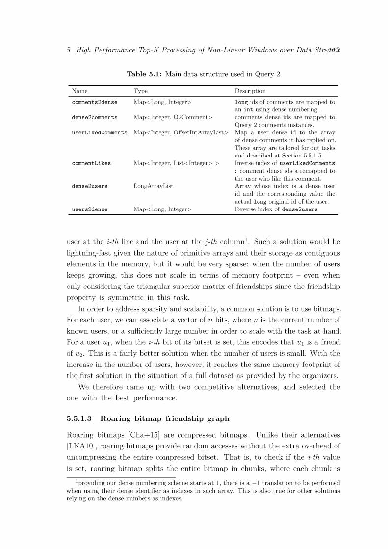
5. High Performance Top-K Processing of Non-Linear Windows over Data Streams113
Table 5.1: Main data structure used in Query 2
Name Type Descriptioncomments2dense Map<Long, Integer> long ids of comments are mapped to
an int using dense numbering.dense2comments Map<Integer, Q2Comment> comments dense ids are mapped to
Query 2 comments instances.userLikedComments Map<Integer, OffsetIntArrayList> Map a user dense id to the array
of dense comments it has replied on.These array are tailored for out tasksand described at Section 5.5.1.5.
commentLikes Map<Integer, List<Integer> > Inverse index of userLikedComments: comment dense ids a remapped tothe user who like this comment.
dense2users LongArrayList Array whose index is a dense userid and the corresponding value theactual long original id of the user.
users2dense Map<Long, Integer> Reverse index of dense2users
user at the i-th line and the user at the j-th column1. Such a solution would belightning-fast given the nature of primitive arrays and their storage as contiguouselements in the memory, but it would be very sparse: when the number of userskeeps growing, this does not scale in terms of memory footprint – even whenonly considering the triangular superior matrix of friendships since the friendshipproperty is symmetric in this task.
In order to address sparsity and scalability, a common solution is to use bitmaps.For each user, we can associate a vector of n bits, where n is the current number ofknown users, or a sufficiently large number in order to scale with the task at hand.For a user u1, when the i-th bit of its bitset is set, this encodes that u1 is a friendof u2. This is a fairly better solution when the number of users is small. With theincrease in the number of users, however, it reaches the same memory footprint ofthe first solution in the situation of a full dataset as provided by the organizers.
We therefore came up with two competitive alternatives, and selected theone with the best performance.
5.5.1.3 Roaring bitmap friendship graph
Roaring bitmaps [Cha+15] are compressed bitmaps. Unlike their alternatives[LKA10], roaring bitmaps provide random accesses without the extra overhead ofuncompressing the entire compressed bitset. That is, to check if the i-th valueis set, roaring bitmap splits the entire bitmap in chunks, where each chunk is
1providing our dense numbering scheme starts at 1, there is a −1 translation to be performedwhen using their dense identifier as indexes in such array. This is also true for other solutionsrelying on the dense numbers as indexes.

114 5.5. Query 2 Solution
an uncompressed bitmap. This is a valuable property that can be utilised inour case, since the friendship graph is accessed frequently. At the same time,the compression offered by the roaring bitmaps makes it possible to scale interms of memory footprint.
5.5.1.4 Friendship graph with hashmap and bloom-filter
As an alternative to roaring bitmaps, we utilise a combination of hashmaps and abloom filter for the friendship graph. The basic idea is as follows: the friendshipgraph is a hashmap with int to Friend mappings, where the object Friend containsa set of users that are friends of a user identified by a dense number (int) i =dense(uk). This enables the addition of new friendship relations and to test thefriendship relation between two users. This may sound counter-intuitive to mapprimitive data-types to an object (given objects instantiation time and garbagecollection), but keep in mind that we would only instantiate this object once peruser in the entire timeframe of the system. The interesting point therefore is howthe Friend object handles the collection of user’s friendship. In our implementation,each Friend object holds a hashset to group the set of friends – each identifiedwith a dense generated number – for a specific user uk. This structure handlesthe insertion of users’s new friends. To prevent frequent costly access to thehashset and to test whether a user is a member of the hashset, we employ a bloomfilter. Since users are more likely not to know each other, bloom Filter presentsan interesting data structure increase in speed.
We evaluated them using the test set provided by the organizers2. The valuefor parameter d (sliding window size) was set to 12 hours (as recommended bythe organizers) and k to 10. It follows that the roaring bitmap approach, on theaverage of 10 runs, is significantly outperformed by the combination of hashmaps,hashset, and the bloom filter approach – this makes it the solution of choice forthe friendship graph data structure in our submission.
5.5.1.5 Comments liked by each user
The friendship graph provides the basic building block for processing Query 2.However, to compute the maximal friendship clique (i.e. community) for a commentposted by a user, we require an additional data structure. The new data structurestores comments liked by each user and is subjected to high insertion rates (eachtime a Like event is received) with frequent read operations; the score of a commentis updated by determining the neighbourhood it has influenced. For this task,we employ an array-based data structure. The only issue is that the comments
2http://bit.ly/1QRZkU3
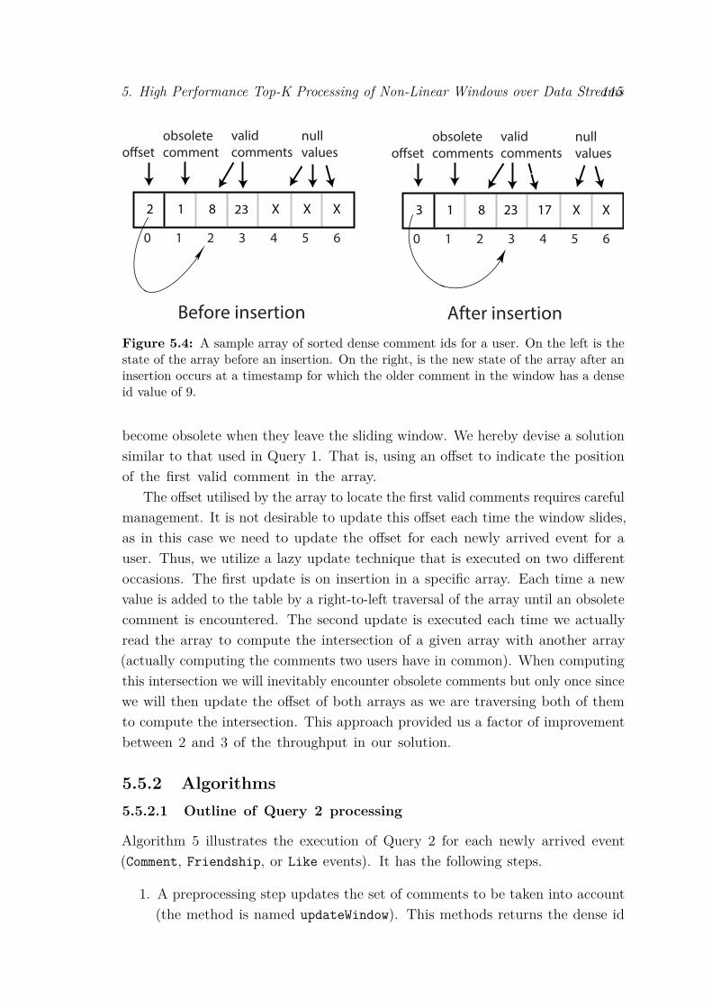
5. High Performance Top-K Processing of Non-Linear Windows over Data Streams115
2 1 238 XX X
Before insertion
0 1 2 3 4 5 6
o�setobsoletecomment
validcomments
nullvalues
3 1 238 X17 X
After insertion
0 1 2 3 4 5 6
o�setobsoletecomments
validcomments
nullvalues
Figure 5.4: A sample array of sorted dense comment ids for a user. On the left is thestate of the array before an insertion. On the right, is the new state of the array after aninsertion occurs at a timestamp for which the older comment in the window has a denseid value of 9.
become obsolete when they leave the sliding window. We hereby devise a solutionsimilar to that used in Query 1. That is, using an offset to indicate the positionof the first valid comment in the array.
The offset utilised by the array to locate the first valid comments requires carefulmanagement. It is not desirable to update this offset each time the window slides,as in this case we need to update the offset for each newly arrived event for auser. Thus, we utilize a lazy update technique that is executed on two differentoccasions. The first update is on insertion in a specific array. Each time a newvalue is added to the table by a right-to-left traversal of the array until an obsoletecomment is encountered. The second update is executed each time we actuallyread the array to compute the intersection of a given array with another array(actually computing the comments two users have in common). When computingthis intersection we will inevitably encounter obsolete comments but only once sincewe will then update the offset of both arrays as we are traversing both of themto compute the intersection. This approach provided us a factor of improvementbetween 2 and 3 of the throughput in our solution.
5.5.2 Algorithms5.5.2.1 Outline of Query 2 processing
Algorithm 5 illustrates the execution of Query 2 for each newly arrived event(Comment, Friendship, or Like events). It has the following steps.
1. A preprocessing step updates the set of comments to be taken into account(the method is named updateWindow). This methods returns the dense id
116 5.5. Query 2 Solution
of the oldest comment in the window (any comment whose id is lower thenthis threshold will be discarded). This is useful in preventing an unnecessaryfull scan of users for each iteration. Simply, we remove the comments’ Id auser has replied to, if the returned comment Id is lower than the threshold.However, this maintenance would be too expensive, and thus is only doneperiodically. Due to memory footprint reasons, we cannot afford to keep allcomments’ Id in the other data structures. Hence, all the obsolete commentids are removed from the remaining data structures using a call to the clean()method. This is also a mandatory step as the obsolete comments may havebeen inserted as a top-k item. Thus, the method clean ensures that the top-klist no longer contains obsolete items for this new clock tick.
2. A second step implements the main procedure for processing events fromComment, Friendship or Like by employing the corresponding process. Thecall to processComment() is very straightforward; a new dense Id is associatedto the new comment, the dense numbering indexes are updated accordinglyand the comment is added to the current window. The remaining processes(processFriendship() and processLike()) encompass a complex behaviourand are presented in the aforementioned discussion.
3. The last step is performed regardless of the type of event (e.g. Comment,Friendship or Like). We first insert new items in the top-k if the cardinalityof the list is less than k. This happens if we removed comments in top-k inthe preprocessing step, and where the processing of the event did not allowfor the top-k to complete. In this case, older comments – which are still invalid – should be promoted in the top-k. We first identify those commentsand then insert them in the top-k. This process is triggered when callingupdateTopkIfNecessary(). It is slightly tedious. It in fact relies on a sortedlist of the minimal size of the largest clique for each valid comment, SeeSection 5.5.2.4 for detail on the lower bound used to minimize computation.The second post-processing task is straightforward; if there is a change in thetop-k values/order, the results are passed on to the result-serialization thread,as previously described in the global architecture (see Figure 5.1).
5.5.2.2 Process likes
Whenever a like is processed, we add the like to the list of integers in commentLikes.We then recompute the friendship subgraph for the curren comment. If the numberof edges is larger than the lower-bound (see Section 5.5.2.4), the largest cliqueis computed using the implementation of McCreesh [MP13], based on Tomita’salgorithm [TS03], which is very efficient on dense numbered nodes.

5. High Performance Top-K Processing of Non-Linear Windows over Data Streams117
Algorithm 5: Outline of query 2 processing an eventInput: DebsRecord : event
1 � preprocessing threshold← updateWindow(event)2 clean(event.getT imeStamp())3 � actual event processing w.r.t its type4 if the event type is comment then5 processComment(event)6 else if the event type is friendship then7 processFriendship(event)8 else if the event type is like then9 processLike(event)
10 � postprocessing11 updateTopkIfNecessary()12 writeResult()
5.5.2.3 Process friendship
An incoming friendship modifies the state of the global friendship graph, andconsequently the subgraphs of the comments that are liked by the two users whoare now friends. We therefore compute the list of comments concerned and applyfor each of them the same process as the comment concerned by Process like.
5.5.2.4 Lower bound on clique computation
Turan’s Theorem [Tur41] gives an upper bound on the number of edges for a nnodes graph to contain a r-clique, i.e. a clique of r nodes.
theorem 2: Turan’s Theorem
To find k-clique in G(V,E) with n vertices : k � n(n-1)/2 and k�E Theoremof Turan: Let G(V,E), n vertices without k-cliques, then |E|� [(k-2)n2 ]/[2(k-1)]
Whenever a change occurs and a comment is a candidate to enter the top-k, we first validate that its number of edges is sufficient to contain a clique ofr nodes, where r is larger than the clique of the last comment from the top-k.This provides a very quick way to determine if it is worth computing the sizeof the maximal clique for this graph.
5.6 EvaluationA global system evaluation was performed by the organizers and our system exhibitsthe following performance: 142K events/second and 1 and 0.7 millisecond averagelatency for the first and second queries, respectively. We therefore use this sectionto detail query specific evaluations, with a particular focus on the impact ofthe message-passing queues.
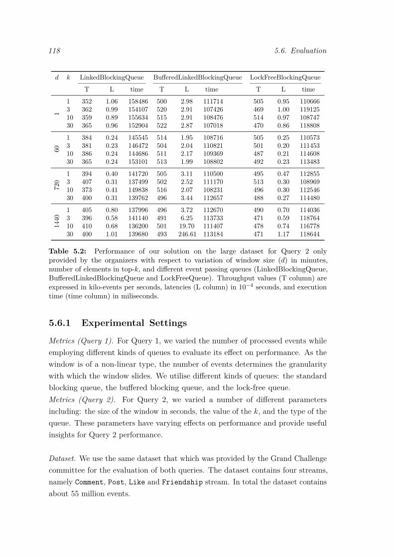
118 5.6. Evaluation
d k LinkedBlockingQueue BufferedLinkedBlockingQueue LockFreeBlockingQueue
T L time T L time T L time
1
1 352 1.06 158486 500 2.98 111714 505 0.95 1106663 362 0.99 154107 520 2.91 107426 469 1.00 11912510 359 0.89 155634 515 2.91 108476 514 0.97 10874730 365 0.96 152904 522 2.87 107018 470 0.86 118808
60
1 384 0.24 145545 514 1.95 108716 505 0.25 1105733 381 0.23 146472 504 2.04 110821 501 0.20 11145310 386 0.24 144686 511 2.17 109369 487 0.21 11460830 365 0.24 153101 513 1.99 108802 492 0.23 113483
720
1 394 0.40 141720 505 3.11 110500 495 0.47 1128553 407 0.31 137499 502 2.52 111170 513 0.30 10896910 373 0.41 149838 516 2.07 108231 496 0.30 11254630 400 0.31 139762 496 3.44 112657 488 0.27 114480
1440
1 405 0.80 137996 496 3.72 112670 490 0.70 1140363 396 0.58 141140 491 6.25 113733 471 0.59 11876410 410 0.68 136200 501 19.70 111407 478 0.74 11677830 400 1.01 139680 493 246.61 113184 471 1.17 118644
Table 5.2: Performance of our solution on the large dataset for Query 2 onlyprovided by the organizers with respect to variation of window size (d) in minutes,number of elements in top-k, and different event passing queues (LinkedBlockingQueue,BufferedLinkedBlockingQueue and LockFreeQueue). Throughput values (T column) areexpressed in kilo-events per seconds, latencies (L column) in 10−4 seconds, and executiontime (time column) in miliseconds.
5.6.1 Experimental Settings
Metrics (Query 1). For Query 1, we varied the number of processed events whileemploying different kinds of queues to evaluate its effect on performance. As thewindow is of a non-linear type, the number of events determines the granularitywith which the window slides. We utilise different kinds of queues: the standardblocking queue, the buffered blocking queue, and the lock-free queue.Metrics (Query 2). For Query 2, we varied a number of different parametersincluding: the size of the window in seconds, the value of the k, and the type of thequeue. These parameters have varying effects on performance and provide usefulinsights for Query 2 performance.
Dataset. We use the same dataset that which was provided by the Grand Challengecommittee for the evaluation of both queries. The dataset contains four streams,namely Comment, Post, Like and Friendship stream. In total the dataset containsabout 55 million events.
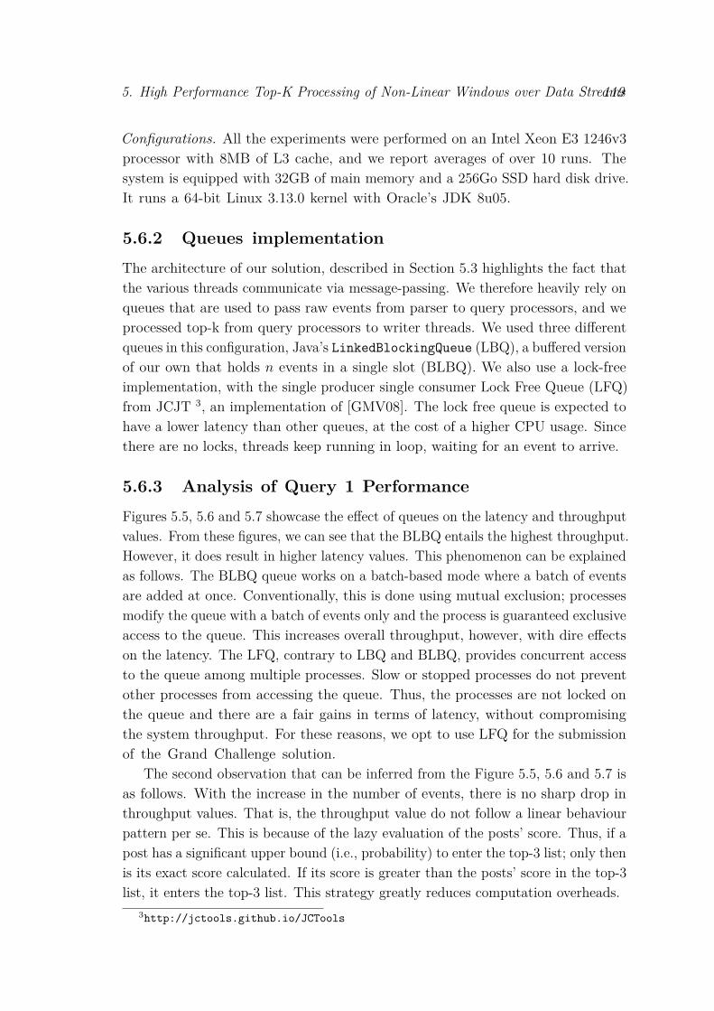
5. High Performance Top-K Processing of Non-Linear Windows over Data Streams119
Configurations. All the experiments were performed on an Intel Xeon E3 1246v3processor with 8MB of L3 cache, and we report averages of over 10 runs. Thesystem is equipped with 32GB of main memory and a 256Go SSD hard disk drive.It runs a 64-bit Linux 3.13.0 kernel with Oracle’s JDK 8u05.
5.6.2 Queues implementation
The architecture of our solution, described in Section 5.3 highlights the fact thatthe various threads communicate via message-passing. We therefore heavily rely onqueues that are used to pass raw events from parser to query processors, and weprocessed top-k from query processors to writer threads. We used three differentqueues in this configuration, Java’s LinkedBlockingQueue (LBQ), a buffered versionof our own that holds n events in a single slot (BLBQ). We also use a lock-freeimplementation, with the single producer single consumer Lock Free Queue (LFQ)from JCJT 3, an implementation of [GMV08]. The lock free queue is expected tohave a lower latency than other queues, at the cost of a higher CPU usage. Sincethere are no locks, threads keep running in loop, waiting for an event to arrive.
5.6.3 Analysis of Query 1 Performance
Figures 5.5, 5.6 and 5.7 showcase the effect of queues on the latency and throughputvalues. From these figures, we can see that the BLBQ entails the highest throughput.However, it does result in higher latency values. This phenomenon can be explainedas follows. The BLBQ queue works on a batch-based mode where a batch of eventsare added at once. Conventionally, this is done using mutual exclusion; processesmodify the queue with a batch of events only and the process is guaranteed exclusiveaccess to the queue. This increases overall throughput, however, with dire effectson the latency. The LFQ, contrary to LBQ and BLBQ, provides concurrent accessto the queue among multiple processes. Slow or stopped processes do not preventother processes from accessing the queue. Thus, the processes are not locked onthe queue and there are a fair gains in terms of latency, without compromisingthe system throughput. For these reasons, we opt to use LFQ for the submissionof the Grand Challenge solution.
The second observation that can be inferred from the Figure 5.5, 5.6 and 5.7 isas follows. With the increase in the number of events, there is no sharp drop inthroughput values. That is, the throughput value do not follow a linear behaviourpattern per se. This is because of the lazy evaluation of the posts’ score. Thus, if apost has a significant upper bound (i.e., probability) to enter the top-3 list; only thenis its exact score calculated. If its score is greater than the posts’ score in the top-3list, it enters the top-3 list. This strategy greatly reduces computation overheads.
3http://jctools.github.io/JCTools
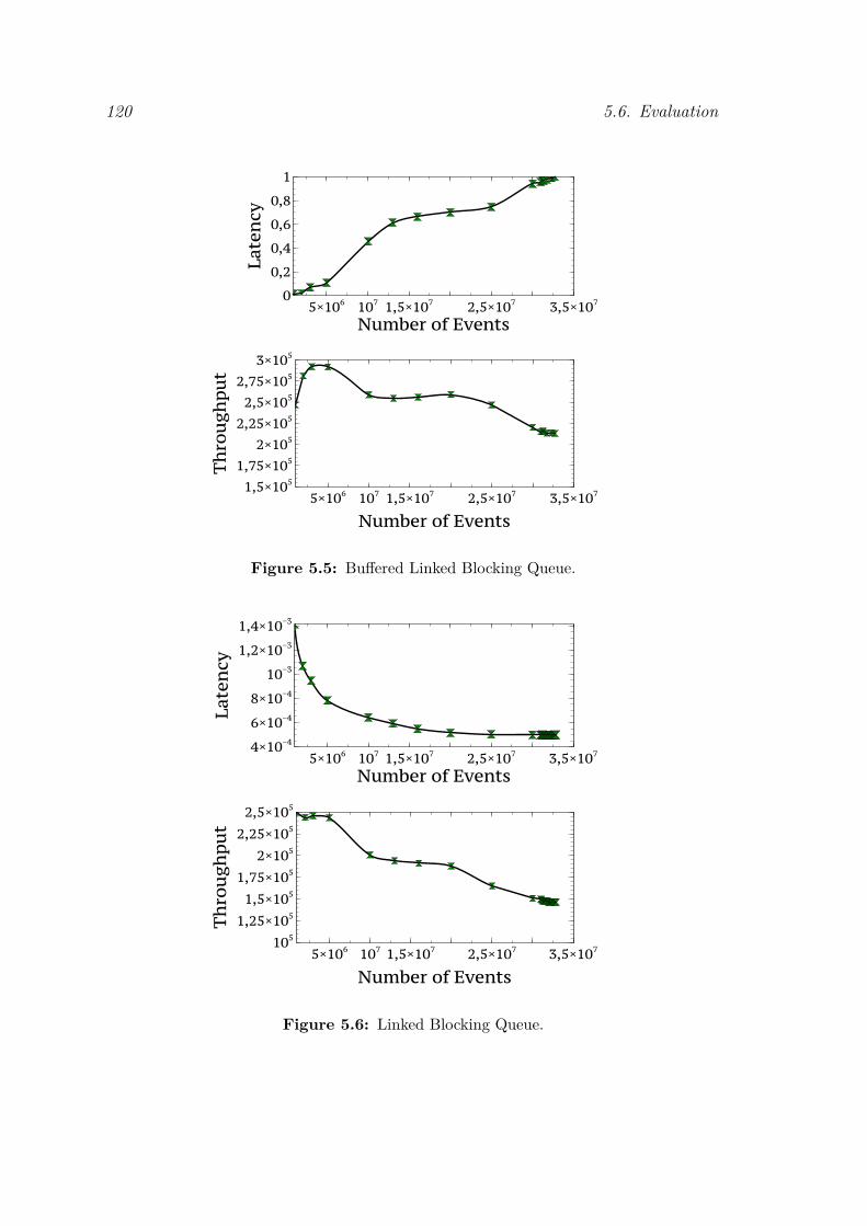
120 5.6. Evaluation
Figure 5.5: Buffered Linked Blocking Queue.
Figure 5.6: Linked Blocking Queue.
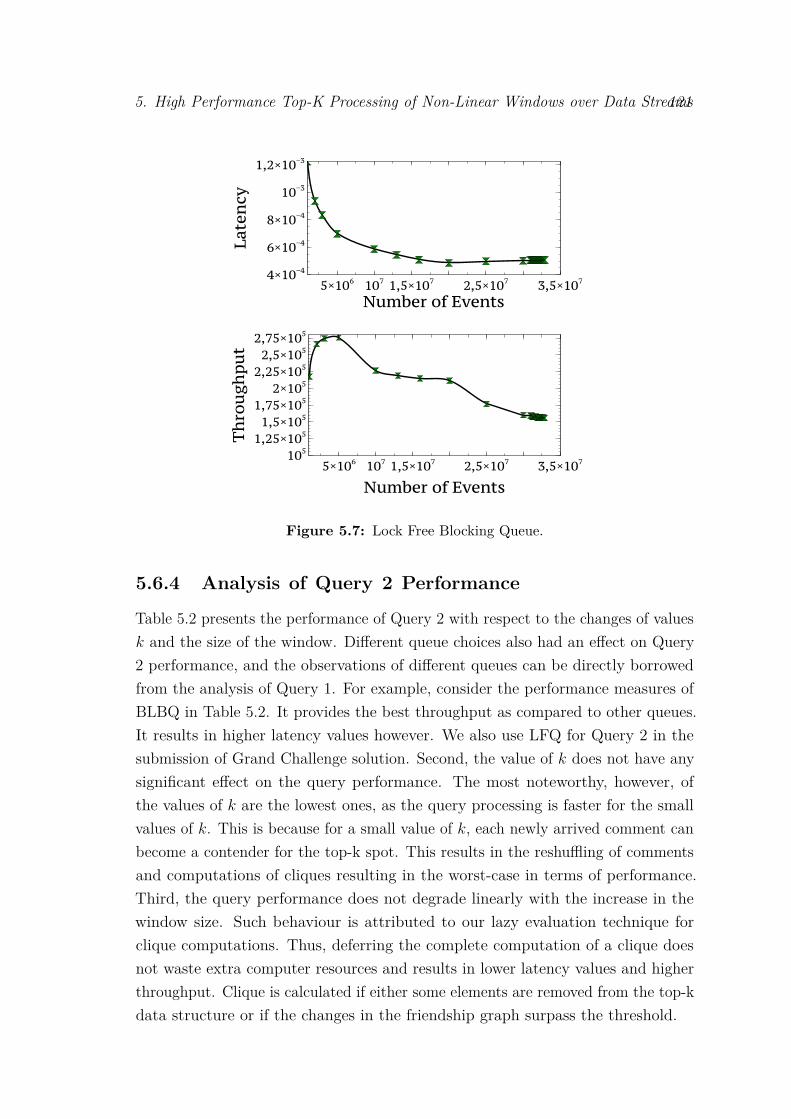
5. High Performance Top-K Processing of Non-Linear Windows over Data Streams121
Figure 5.7: Lock Free Blocking Queue.
5.6.4 Analysis of Query 2 Performance
Table 5.2 presents the performance of Query 2 with respect to the changes of valuesk and the size of the window. Different queue choices also had an effect on Query2 performance, and the observations of different queues can be directly borrowedfrom the analysis of Query 1. For example, consider the performance measures ofBLBQ in Table 5.2. It provides the best throughput as compared to other queues.It results in higher latency values however. We also use LFQ for Query 2 in thesubmission of Grand Challenge solution. Second, the value of k does not have anysignificant effect on the query performance. The most noteworthy, however, ofthe values of k are the lowest ones, as the query processing is faster for the smallvalues of k. This is because for a small value of k, each newly arrived comment canbecome a contender for the top-k spot. This results in the reshuffling of commentsand computations of cliques resulting in the worst-case in terms of performance.Third, the query performance does not degrade linearly with the increase in thewindow size. Such behaviour is attributed to our lazy evaluation technique forclique computations. Thus, deferring the complete computation of a clique doesnot waste extra computer resources and results in lower latency values and higherthroughput. Clique is calculated if either some elements are removed from the top-kdata structure or if the changes in the friendship graph surpass the threshold.
122 5.7. Conclusion
5.7 ConclusionIn this chapter, we described our solution to the 2016 edition of the DEBS GrandChallenge. In the design of our solution, we carefully took care of optimizing everypart of the system. Fast data parser, efficient message-passing queues as well asdevising efficient fast lower and upper bounds to avoid costly computation, werethe keys to the success of our approach. Similarly, the choices and designs behindthe most frequently used data structures (sorted elements, friendship graph) largelycontributed to overall system performance. On the basis of this experience, wehave realized that Programming languages have evolved to answer the need fordata stream processing. Be it with Domain Specific Languages [Bos+14; Su+14;TKA02], language extensions [SB13; EJ09] or with the developement of standardAPIs like Stream for Java. This field demonstrated many advances in the last fewyears. However, the existing data structures of these languages have been designedfor static data processing and their correct use with evolving data is cumbersome– top-k query processing requires maintaining sorted collections. We identifiedthat maintaining sorted collections of dynamic data is particularly error-proneand leads to hard-to-detect bugs. Thus, in the Appendix A, we tackle the issueof maintaining dynamically sorted collections in Java in a safe and transparentmanner for the application developer. For this purpose, we developed an annotation-based approach called Upsortable – a portmanteau of update and sort – that usescompilation-time abstract syntax tree modifications and runtime bytecode analysis.Upsortable is fully compatible with standard Java and is therefore available tothe greatest number of developers.
6A Scalable Framework for Accelerating
Situation Prediction over Spatio-temporalEvent Streams
Contents6.1 Introduction . . . . . . . . . . . . . . . . . . . . . . . . . 1236.2 Input Data Streams and Query definitions . . . . . . . 125
6.2.1 Input Data Streams . . . . . . . . . . . . . . . . . . . . 1256.2.2 Query 1: Predicting destinations of vessels . . . . . . . . 1266.2.3 Query 2: Predicting arrival times of vessels . . . . . . . 126
6.3 Preliminaires . . . . . . . . . . . . . . . . . . . . . . . . . 1276.4 The Framework . . . . . . . . . . . . . . . . . . . . . . . 1276.5 Experimental Evaluation . . . . . . . . . . . . . . . . . . 129
6.5.1 Evaluation [Gul+18b] . . . . . . . . . . . . . . . . . . . 1296.5.2 Results and GC Benchmark . . . . . . . . . . . . . . . . 130
6.6 Conclusion . . . . . . . . . . . . . . . . . . . . . . . . . . 131
6.1 Introduction
The tremendous increase in the use of cellular phones, GPS-like devices and RFIDshas resulted in the rapid increase in new spatiotemporal applications. Examples ofthese applications include traffic monitoring, supply chain management, enhanced911 services, etc. These applications continuously receive data from mobile objectsin the form of event streams that are processed in a continuous manner. Anotherextension of these applications is to enable predictive analysis to envision proactive
123
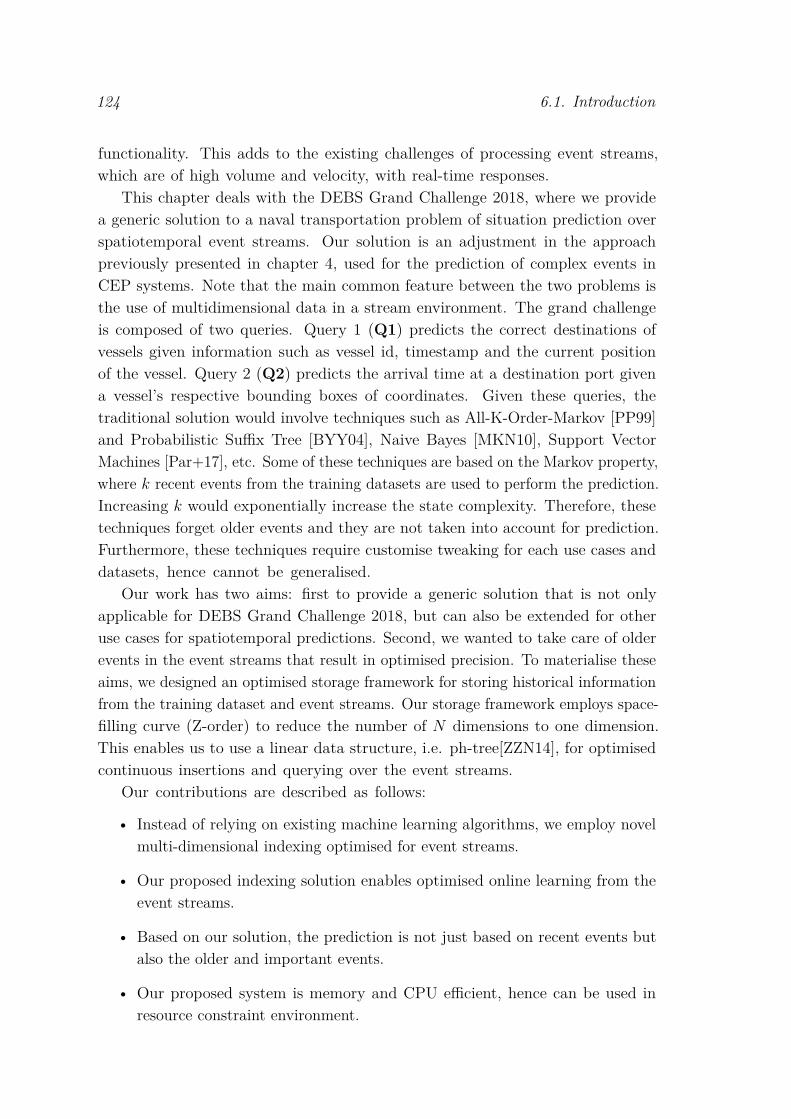
124 6.1. Introduction
functionality. This adds to the existing challenges of processing event streams,which are of high volume and velocity, with real-time responses.
This chapter deals with the DEBS Grand Challenge 2018, where we providea generic solution to a naval transportation problem of situation prediction overspatiotemporal event streams. Our solution is an adjustment in the approachpreviously presented in chapter 4, used for the prediction of complex events inCEP systems. Note that the main common feature between the two problems isthe use of multidimensional data in a stream environment. The grand challengeis composed of two queries. Query 1 (Q1) predicts the correct destinations ofvessels given information such as vessel id, timestamp and the current positionof the vessel. Query 2 (Q2) predicts the arrival time at a destination port givena vessel’s respective bounding boxes of coordinates. Given these queries, thetraditional solution would involve techniques such as All-K-Order-Markov [PP99]and Probabilistic Suffix Tree [BYY04], Naive Bayes [MKN10], Support VectorMachines [Par+17], etc. Some of these techniques are based on the Markov property,where k recent events from the training datasets are used to perform the prediction.Increasing k would exponentially increase the state complexity. Therefore, thesetechniques forget older events and they are not taken into account for prediction.Furthermore, these techniques require customise tweaking for each use cases anddatasets, hence cannot be generalised.
Our work has two aims: first to provide a generic solution that is not onlyapplicable for DEBS Grand Challenge 2018, but can also be extended for otheruse cases for spatiotemporal predictions. Second, we wanted to take care of olderevents in the event streams that result in optimised precision. To materialise theseaims, we designed an optimised storage framework for storing historical informationfrom the training dataset and event streams. Our storage framework employs space-filling curve (Z-order) to reduce the number of N dimensions to one dimension.This enables us to use a linear data structure, i.e. ph-tree[ZZN14], for optimisedcontinuous insertions and querying over the event streams.
Our contributions are described as follows:
• Instead of relying on existing machine learning algorithms, we employ novelmulti-dimensional indexing optimised for event streams.
• Our proposed indexing solution enables optimised online learning from theevent streams.
• Based on our solution, the prediction is not just based on recent events butalso the older and important events.
• Our proposed system is memory and CPU efficient, hence can be used inresource constraint environment.

6. A Scalable Framework for Accelerating Situation Prediction over Spatio-temporalEvent Streams 125
6.2 Input Data Streams and Query definitions
The challenge was co-organized by MarineTraffic, the BigDataOcean project andthe HOBBIT 1 project represented by AGT International 2. Grand Challenge datawas provided by MarineTraffic and hosted by Big Data Ocean while the automatedevaluation platform was provided by the HOBBIT project.
6.2.1 Input Data Streams
The data is an anonymized collection of sensor data from vessels’ Automated Identi-fication System (AIS), the internationally accepted standard for self-identification ofbig vessels. AIS transponders periodically send time-series data points to coastal-,aircraft- or satellite-based AIS receivers. Data points of the provided dataset containstatic information (ship identifier, ship type) as well as dynamic one (coordinates,speed, heading, course, draught, departure port name).Figure 6.1, shows the vessels’trajectories in graphical form, where each colour represents a starting port and eachcircle is a port. The schema of the tuples in the dataset is composed by attributes:
• SHIP ID, the anonymized id of the ship
• SHIP TY PE, the vessel type
• SPEED, speed measured in knots
• LON , the longitude of the current ship position
• LAT , the latitude of the current ship position
• COURSE, the direction in which the ship moves
• HEADING, the cardinal direction in which the ship is to be steered 3
• TIMESTAMP , the time at which the message was sent (UTC)
• DEPARTURE PORT NAME, the name of the last port visited by thevessel
• REPORTED DRAUGHT , the vertical distance between the waterline andthe bottom of the ship’s hull
1https://project-hobbit.eu/2http://www.agtinternational.com/3https://en.wikipedia.org/wiki/Course_(navigation)
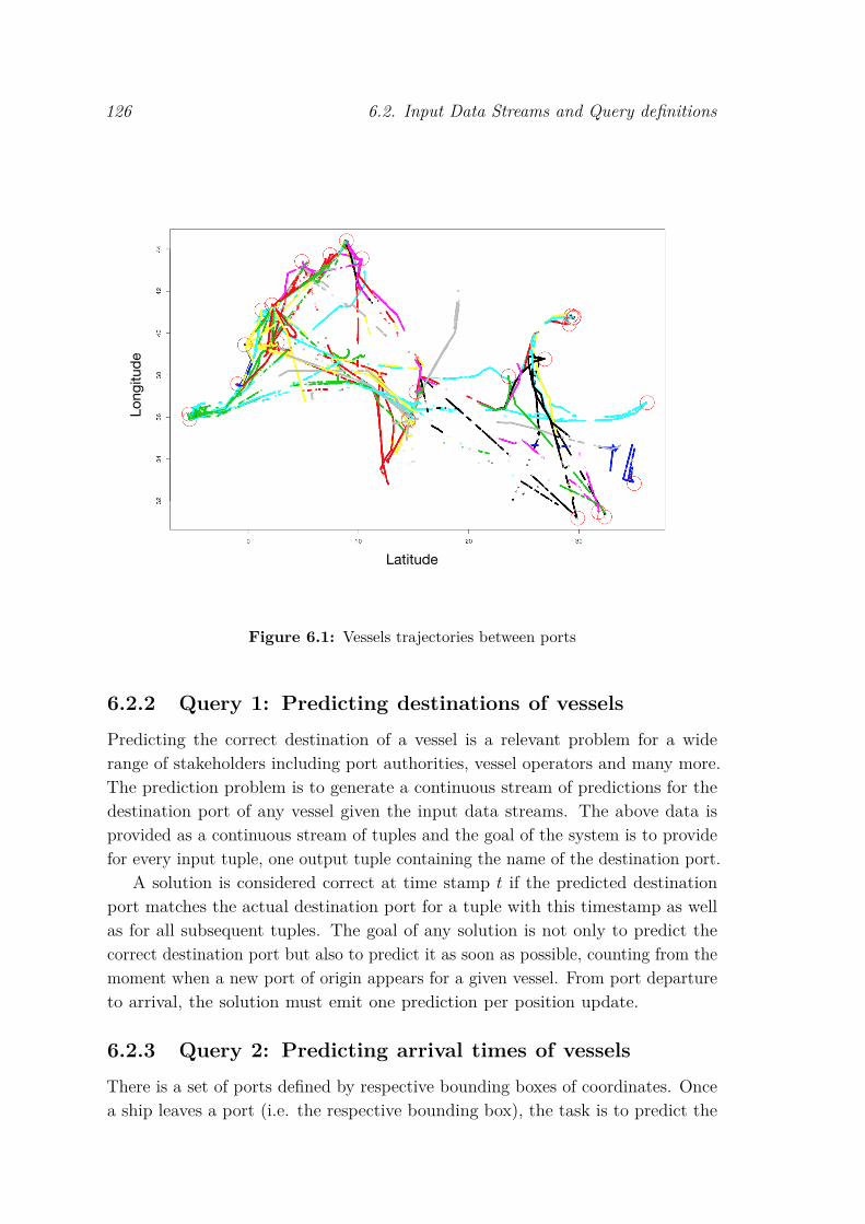
126 6.2. Input Data Streams and Query definitions
Latitude
Long
itude
Figure 6.1: Vessels trajectories between ports
6.2.2 Query 1: Predicting destinations of vesselsPredicting the correct destination of a vessel is a relevant problem for a widerange of stakeholders including port authorities, vessel operators and many more.The prediction problem is to generate a continuous stream of predictions for thedestination port of any vessel given the input data streams. The above data isprovided as a continuous stream of tuples and the goal of the system is to providefor every input tuple, one output tuple containing the name of the destination port.
A solution is considered correct at time stamp t if the predicted destinationport matches the actual destination port for a tuple with this timestamp as wellas for all subsequent tuples. The goal of any solution is not only to predict thecorrect destination port but also to predict it as soon as possible, counting from themoment when a new port of origin appears for a given vessel. From port departureto arrival, the solution must emit one prediction per position update.
6.2.3 Query 2: Predicting arrival times of vesselsThere is a set of ports defined by respective bounding boxes of coordinates. Oncea ship leaves a port (i.e. the respective bounding box), the task is to predict the

6. A Scalable Framework for Accelerating Situation Prediction over Spatio-temporalEvent Streams 127
arrival time at its destination port (i.e. when the next defined bounding boxeswill be entered). Like for query 1, from port departure to arrival, the solutionmust emit one prediction per position update.
6.3 PreliminairesIn this section, we introduce the notion used in the paper and provide the backgroundon the datasets; queries used to evaluate our framework and the space-filling curvesfor indexing.
Notations. Let E = [e1, e2, . . . ei] donates a discrete stream of events and ei denotesan individual event. Each event is a tuple (A, t), where A is a set of attributes,such as vessel id, vessel location, port, etc., and t is the associated timestamp ofthe event. Let H = {A1 × A2×, . . . , An} is an N-D lattice for the universe of allthe events in the training dataset, where an n-tuple X = (x1, x2, . . . , xn) defines apoint in H and xi ∈ Ai ∀i ∈ n. This N-D lattice is used to find the nearest pointsgiven the input tasks for both queries for prediction.
Space-filling Curve (Z-order). As discussed in chapter 3, the Z-order curvepreserves the proximity properties among the points while leveraging the effectivenessof linear data structures (such as B+tree) for range queries. The construction ofthe Z-order curve, i.e, Z-values generation, is accomplished by the simple process ofbit-shuffling and this is one of its main advantages over other space-filling curves.Considering this, we have employed the Z-order curve to map all the attributesassigned to an event. The resulted mapping is added in the ph-tree for efficientstorage and processing of the given queries.
6.4 The FrameworkIn this section, we present our framework and the evaluation of DEBS GrandChallenge 2018 queries. Fig.6.2 shows all the components of our framework. Theinput manager parses the training dataset and incoming event streams beforeindexing it. The historical store employs the Ph-Tree to index the main attributesincluding longitude, latitude, heading, course, speed and reported draught. Thescore index is used to prioritise the vessels that are custom to follow the sameroutine. That is, if we are asked to predict the destination of a vessel A, yet vesselA is usually following a certain path, then we give priority to this vessel ratherthan ones which usually deviate from their path. From Fig.6.3, P1 is the newevent to find the destination of a vessel. Then from the historical index, we havethree possible destinations for such vessel. Hence, we update the destination and
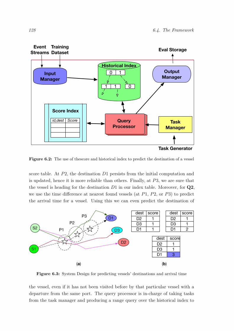
128 6.4. The Framework
Input Manager
Query Processor
Output Manager
Task Manager
Training Dataset
Event Streams
Task Generator
Eval Storage
0
1 1
1
0
Historical Index
id,dest Score
Score Index
Figure 6.2: The use of thescore and historical index to predict the destination of a vessel
score table. At P2, the destination D1 persists from the initial computation andis updated, hence it is more reliable than others. Finally, at P3, we are sure thatthe vessel is heading for the destination D1 in our index table. Moreover, for Q2,we use the time difference at nearest found vessels (at P1, P2, or P3) to predictthe arrival time for a vessel. Using this we can even predict the destination of
S1
D1
D2
1D1D3 1
1D2dest score
2D1D3 1
1D2dest score
3D1D3 1
1D2dest score
D3
(a) (b)
P1P2
P3
S2
Figure 6.3: System Design for predicting vessels’ destinations and arrival time
the vessel, even if it has not been visited before by that particular vessel with adeparture from the same port. The query processor is in-charge of taking tasksfrom the task manager and producing a range query over the historical index to
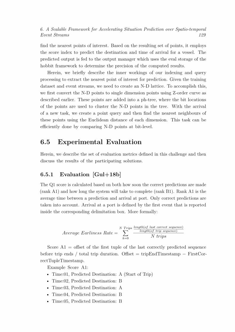
6. A Scalable Framework for Accelerating Situation Prediction over Spatio-temporalEvent Streams 129
find the nearest points of interest. Based on the resulting set of points, it employsthe score index to predict the destination and time of arrival for a vessel. Thepredicted output is fed to the output manager which uses the eval storage of thehobbit framework to determine the precision of the computed results.
Herein, we briefly describe the inner workings of our indexing and queryprocessing to extract the nearest point of interest for prediction. Given the trainingdataset and event streams, we need to create an N-D lattice. To accomplish this,we first convert the N-D points to single dimension points using Z-order curve asdescribed earlier. These points are added into a ph-tree, where the bit locationsof the points are used to cluster the N-D points in the tree. With the arrivalof a new task, we create a point query and then find the nearest neighbours ofthese points using the Euclidean distance of each dimension. This task can beefficiently done by comparing N-D points at bit-level.
6.5 Experimental Evaluation
Herein, we describe the set of evaluation metrics defined in this challenge and thendiscuss the results of the participating solutions.
6.5.1 Evaluation [Gul+18b]
The Q1 score is calculated based on both how soon the correct predictions are made(rank A1) and how long the system will take to complete (rank B1). Rank A1 is theaverage time between a prediction and arrival at port. Only correct predictions aretaken into account. Arrival at a port is defined by the first event that is reportedinside the corresponding delimitation box. More formally:
Average Earliness Rate =N Trips∑k=0
length(of last correct sequence)length(of trip sequence)
N trips
Score A1 = offset of the first tuple of the last correctly predicted sequencebefore trip ends / total trip duration. Offset = tripEndTimestamp − FirstCor-rectTupleTimestamp.
Example Score A1:• Time:01, Predicted Destination: A (Start of Trip)• Time:02, Predicted Destination: B• Time:03, Predicted Destination: A• Time:04, Predicted Destination: B• Time:05, Predicted Destination: B

130 6.5. Experimental Evaluation
• Time:06, Predicted Destination: B (Arrival at B)Score A1: (06-04)/(06-01) [higher is better] The overall ranking for query 1
(Rank Q1) is then computed as Rank Q1 = 0.75*Rank A1 + 0.25*Rank B1.The Q2 evaluation is calculated based on the accuracy of predictions (Rank
A2) and the total runtime (Rank B2). Score A2 is the mean average error of allpredicted arrival times while Rank B2 ranks according to the total runtime. Moreformally:
Mean Average Error =Ntuples∑k=0
|error per tuple|Ntuples
The overall ranking for Query 2 (Rank Q2) is then computed as Rank Q2 =0.75*Rank A2 + 0.25*Rank B2. Finally, The final ranking is given by the sumof ranks Rank Q1 and Rank Q2.
6.5.2 Results and GC Benchmark
We use the given dataset and the two queries from the DEBS Grand Challenge 2018.Herein, we showcase how we can use a subset of the training dataset to predictthe destination port of the vessels with the arrival of new tasks. Fig.6.4 showsthat general accuracy and average earliness rate in relation with the percentage ofdata used from the training dataset for prediction task. Thus, even with a smallpercentage of training dataset, we are able to have a higher average earliness rateand general accuracy.
General Average = Correct predictions
totalnumber of predictions
The following table 6.1 summarizes the best participants’ results, where twotypes of systems are found, in which machine learning approaches[NVA18; Bac+18;Ros+18; Bod+18] and indexing [Ama+18] are used. Various experiments havebeen carried out using different real datasets. [NVA18] (MT Detector) uses asequence-to-sequence model based on a Long Short Term Memory (LSTM) network,[Ros+18] (KNN) uses a nearest neighbour search to find the training routes thatare closer to the AIS query point based on LAT/LONG only, [Bod+18] (VEL) usesa Voting Ensemble Learning based on Random Forest: Gradient Boosting DecisionTrees (GBDT), XGBoot Trees and Extremely Randomized Trees (ERT), and the[Bac+18] (Venilia) prediction mechanism is based on a variety of machine learningtechniques including Markov models and supports on-line continuous training. Thetwo best systems were based on indexing techniques, where the first (CellGrid)was based on a sequence of hash tables specifically built for the targeted use caseand the second was our system (TrajectPM).
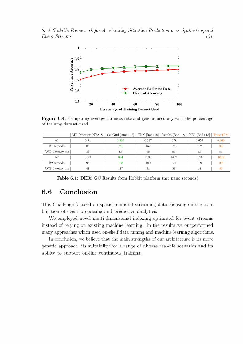
6. A Scalable Framework for Accelerating Situation Prediction over Spatio-temporalEvent Streams 131
Figure 6.4: Comparing average earliness rate and general accuracy with the percentageof training dataset used
MT Detector [NVA18] CellGrid [Ama+18] KNN [Ros+18] Venilia [Bac+18] VEL [Bod+18] TrajectPMA1 0,54 0,685 0,647 0,5 0,653 0,668
B1 seconds 86 99 157 129 102 102AVG Latency ms 36 ns ns ns ns ns
A2 5193 894 2193 1482 1328 1002B2 seconds 95 108 180 147 109 165
AVG Latency ms 41 117 51 38 48 93
Table 6.1: DEBS GC Results from Hobbit platform (ns: nano seconds)
6.6 ConclusionThis Challenge focused on spatio-temporal streaming data focusing on the com-bination of event processing and predictive analytics.
We employed novel multi-dimensional indexing optimised for event streamsinstead of relying on existing machine learning. In the results we outperformedmany approaches which used on-shelf data mining and machine learning algorithms.
In conclusion, we believe that the main strengths of our architecture is its moregeneric approach, its suitability for a range of diverse real-life scenarios and itsability to support on-line continuous training.

132

Part IV
Conclusion
133

7Conclusion and Future Works
In this dissertation, we focused on enhancing the capabilities of Complex EventProcessing (CEP) systems, whose goal is to detect patterns over incoming eventstreams. Existing CEP systems suffer from poor performance due to high memoryand high computation resource consumption for expensive pattern query operatorssuch as Kleene+ and Skip-Till-Any. In addition most of them cannot providepredictive behaviour. The main contributions of this thesis is to propose a newbreed of CEP systems that can handle higher amounts of data for detecting complexpatterns and integrate more intelligent predictive behaviour. The main resultsare described in the following text.
7.1 Enhancing CEP performanceIn order to enhance the performance of CEP systems, we focused on optimizingthe memory and CPU performance for expensive queries. We provided multi-ple optimization techniques. Our approaches leveraged concepts and methodsfrom multidimensional indexing techniques, dominance relationship analysis andbatch processing.
We provided a novel recomputation approach called RCEP for processingexpressive CEP queries. RCEP eliminates the need for storing partial matcheswhich were identified as the bottleneck of existing incremental approaches.
To efficiently store and process multi-attribute events, we employed space-filling curves combined with B+tree indexing techniques. This enabled us to useefficient multidimensional indexing in streaming environments. We then exploitedmultidimensional indexing properties by constructing range queries to perform arange search and retrieve potential events that can be part of complete matches.
135
136 7.2. Predictive CEP
To produce final matches from range query results, we proposed a heuristicbased join algorithm. Our algorithm leverages the dominance property between setof events and joins the clustered events in batches to reduce the cost of pair-wisejoins. Additionally, dominance property allows to reuse previously computed joinsto further economize on recomputation of matches.
We proposed a transformation of online window management to batch-basedwindow management. Where instead of using traditional incremental deletionsof events outside the sliding window, we implemented batch deletion of expiredevents. We called it CPU Friendly method which avoids the rebuilding cost ofthe B+Tree in the streaming settings. This CPU friendly approach results in aslight increase in memory consumption because of having to keep the older events,nevertheless, it is still far better in memory performance as compared to whenmaintaining the partial matches. Various experiments using various datasets havedemonstrated that our system outperforms existing approaches by several ordersof magnitude and consume less memory.
Perspectives: To go further, the work can be extended by exploring multi-queryoptimizations, by exploiting sharing opportunities such as sharing the results ofone sub-query by another to reduce computational cost or by decomposing queries.Another future idea is to treat the case of lossy data or out of order data. The outof order problem can be easily solved by our system as our approach is based on lazyapproach. Our system waits till the final matching event arrives before processingthe relevant events. Thus, any out of order event will eventually arrive and will beenqueued for being processed at a later time when the final matching event arrives.
7.2 Predictive CEPContinuing in the direction of improving the functionalities of the CEP systems,we investigated an open issue of designing a predictive CEP which permits betterunderstanding and proactively acting in response to potential upcoming futurecomplex events.
We addressed this issue from a new perspective, with the main objective ofbringing the real-time predictive CEP capabilities to the database layer. Forthis objective, we extended the existing data structures, query execution andoptimization techniques.
Predictive CEP problem has a parallel in the domain of sequence prediction.Some existing approaches for sequence prediction based on Markov Models dependonly on the previous state. Other models, including also Markov models, sufferfrom catastrophic forgetting of older sequences, where only some recent items of
7. Conclusion and Future Works 137
training sequences are used to perform predictions. This makes these approachesas lossy as some of the past information relevant for prediction is lost. Suchlossy techniques impact the prediction accuracy. Prediction with multidimensionalsequences becomes even worse.
In order to design an efficient predictive CEP, we used the following approaches:First, we used a memory efficient data structure to index all historic sequences.This data structure allowed our predictor to be updated, in real time, at each stepof new sequence detection. Secondly, we designed algorithms to perform fast as wellas accurate sequence prediction and handle complex data, i.e., multidimensionalsequences. Thirdly, in order to be memory efficient for storing the historicalsequences we proposed a summarisation approach, that results on minor loss ofinformation. Nevertheless, our algorithm looses only non important informationby tracking the less frequently retrieved or used historical sequences. We thusproposed a generic solution for incorporating Predictive Analytics into any ComplexEvent Processing system.
Preliminary results, show that our system outperforms an existing recentsequence prediction approach in terms of accuracy and execution time.
Perspectives: In future, we would like to explore the integration of machinelearning techniques with our approach. Machine learning can help CEP in automa-tisation of some processes like automatic query-pattern generation. Constructingquery-patterns is a difficult task which needs the intervention of an expert. Moreover,we only output the future possible matches, but we do not provide the probability oftheir occurrence. We would like to explore machine learning techniques to outputthe occurrence probability.
7.3 Real world use cases and challengesAs a final contribution, we showed the ability of our approaches to be appliedon real use cases and different challenges proposed by the research community.Such challenges provided a common ground for us to evaluate and compare ourevent-driven systems with other systems of other researchers.
We participated to the 2016 DEBS Grand Challenge, which focused on reasoningover social networks data to drive meaningful insights from it in real-time. Onenovelty was the non-linearity of the expiration of the elements. We proposedseveral efficient and effective techniques to enable a lazy evaluation of non-linearwindow elements. In another part of the problem, we had to manage a graphof ever growing social network data. Due to the centrality of this structure, acareful design was therefore required.
138 7.3. Real world use cases and challenges
In the design of our solution, we carefully took care of optimizing every part ofthe system. Fast data parser, efficient message-passing queues as well as devisingefficient fast lower and upper bounds to avoid costly computation, were the keysto the success of our approach. Similarly, the choice and designs behind themost frequently data structures (sorted elements, graph) largely contributed tothe overall system performance.
The 2018 DEBS Grand Challenge focused on spatio-temporal streaming data.This challenge was about the combination of event processing and predictiveanalytics. The goal of the challenge was to perform spatio-temporal prediction.
We employed novel multi-dimensional indexing optimized for event streamsinstead of relying on existing machine learning. Our proposed solution had followingadvantages: it performed optimized online learning, prediction, the prediction wasnot just based on the recent events but also the older and important events, oursolution was memory and CPU efficient.
In addition, the main strengths of our architecture was its suitability for manydifferent real-life scenarios and its ability to support on-line continuous training.
In conclusion, we believe that real-time data processing is finally becoming animportant part of data management domain. Our work has widespread impactson a variety of applications: fraud detection, water management, event processingin different types of networks. The results of our research have been publishedin a number of international conferences.

Appendices
139


AUpsortable an Annotation-Based
Approach
ContentsA.1 Introduction . . . . . . . . . . . . . . . . . . . . . . . . . 141A.2 The Case For Upsortable . . . . . . . . . . . . . . . . . . 142A.3 Upsortable solution . . . . . . . . . . . . . . . . . . . . . 143
A.3.1 AST modifications . . . . . . . . . . . . . . . . . . . . . 144A.3.2 Bookkeeping . . . . . . . . . . . . . . . . . . . . . . . . 144A.3.3 Garbage Collection . . . . . . . . . . . . . . . . . . . . . 146
A.4 Discussion . . . . . . . . . . . . . . . . . . . . . . . . . . . 147
A.1 IntroductionTop-k queries over data streams are well studied problems. There are numeroussystems allowing the continuous processing of queries over sliding windows. Atthe opposite, non-append only streams call for ad-hoc solutions, e.g. tailor-madesolutions implemented in a mainstream programming language. In the meantime,the Stream API and lambda expressions have been added in Java 8, thus gainingpowerful operations for data stream processing. However, the Java CollectionsFramework does not provide data structures to safely and conveniently supportsorted collections of evolving data. In this chapter, we explain Upsortable, anannotation-based approach to allow the use of existing sorted collections fromthe standard Java API for dynamic data management. Our approach relies on acombination of pre-compilation abstract syntax tree modifications and the runtime
141
142 A.2. The Case For Upsortable
analysis of bytecode. Upsortable1 offers the developer a safe and time-efficientsolution for developing top-k queries on data streams while maintaining a fullcompatibility with standard Java.
A.2 The Case For Upsortable
The standard Java Collections API contains three implementations of sorted datastructures: the java.util.TreeSet backed by a Red-Black tree, the java.util.PriorityQueuethat implements a priority heap and, for thread-safety purposes, the “java.util.concurrent.ConcurrentSkipListSet” implements a concurrent variant of Skip List. Thesestructures especially implement add and remove primitives, as well as methods tonavigate within these collections. These structures are therefore well-suited forthe implementation of exact top-k queries: elements are kept sorted accordingto either a comparator provided at the creation time of the data structure orby the natural ordering of the elements. In both cases, a pairwise comparisonmethod is used to sort the objects and this method must provide a total ordering.When dealing with data streams, the value of some fields of an object are subjectto evolution and this may require a reordering within the collections this objectbelongs to. With the aforementioned sorted data structures – as well as third-partyJava Collections APIs such as Guava2 or Eclipse Collections3 – the developer mustfirst remove the object from each sorted collections, update its internal fields andreinsert the object in these collections. The sorted collections may otherwise becomeirredeemably broken. Figure A.1 depicts such an example. Hence, this remove,update and then insert process is very error-prone, especially in large codebaseswhere objects belong to different sorted collections, depending on the state of theapplication. Broken sorted collections are also hard to identify at runtime andmay go undetected for a while. This is typical for the top-k queries, where thecollections might be broken after the k-th element. The behaviour of the corrupteddata structure is unpredictable, it ranges from inconsistent results to wrong insertsand impossible removals – as depicted in Figure A.1 where the removal of D isimpossible since it cannot be reached.
To circumvent this issue, the standard solution is to rely on the Observer designpattern. This pattern implies that the objects must keep track of the collectionsthey belong to. This requires adding an extra data structure within the objects tostore pointers to the collections they belong to. The field setters must be updatedto remove, update and insert the object (acting as the notify in the pattern). Using
1https://github.com/jsubercaze/Upsortable2https://github.com/google/guava3https://www.eclipse.org/collections/
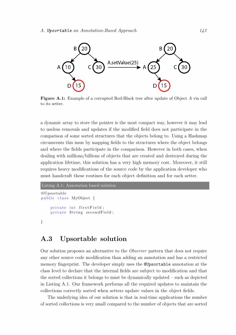
A. Upsortable an Annotation-Based Approach 143
Figure A.1: Example of a corrupted Red-Black tree after update of Object A via callto its setter.
a dynamic array to store the pointer is the most compact way, however it may leadto useless removals and updates if the modified field does not participate in thecomparison of some sorted structures that the objects belong to. Using a Hashmapcircumvents this issue by mapping fields to the structures where the object belongsand where the fields participate in the comparison. However in both cases, whendealing with millions/billions of objects that are created and destroyed during theapplication lifetime, this solution has a very high memory cost. Moreover, it stillrequires heavy modifications of the source code by the application developer whomust handcraft these routines for each object definition and for each setter.
Listing A.1: Annotation based solution
@Upsortablepub l i c c l a s s MyObject {
p r i va t e i n t f i r s t F i e l d ;p r i va t e S t r ing secondFie ld ;
}
A.3 Upsortable solutionOur solution proposes an alternative to the Observer pattern that does not requireany other source code modification than adding an annotation and has a restrictedmemory fingerprint. The developer simply uses the @Upsortable annotation at theclass level to declare that the internal fields are subject to modification and thatthe sorted collections it belongs to must be dynamically updated – such as depictedin Listing A.1. Our framework performs all the required updates to maintain thecollections correctly sorted when setters update values in the object fields.
The underlying idea of our solution is that in real-time applications the numberof sorted collections is very small compared to the number of objects that are sorted
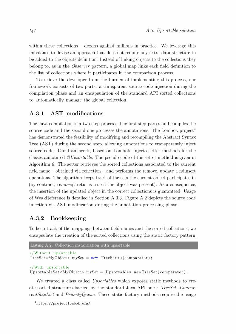
144 A.3. Upsortable solution
within these collections – dozens against millions in practice. We leverage thisimbalance to devise an approach that does not require any extra data structure tobe added to the objects definition. Instead of linking objects to the collections theybelong to, as in the Observer pattern, a global map links each field definition tothe list of collections where it participates in the comparison process.
To relieve the developer from the burden of implementing this process, ourframework consists of two parts: a transparent source code injection during thecompilation phase and an encapsulation of the standard API sorted collectionsto automatically manage the global collection.
A.3.1 AST modifications
The Java compilation is a two-step process. The first step parses and compiles thesource code and the second one processes the annotations. The Lombok project4
has demonstrated the feasibility of modifying and recompiling the Abstract SyntaxTree (AST) during the second step, allowing annotations to transparently injectsource code. Our framework, based on Lombok, injects setter methods for theclasses annotated @Upsortable. The pseudo code of the setter method is given inAlgorithm 6. The setter retrieves the sorted collections associated to the currentfield name – obtained via reflection – and performs the remove, update a ndinsertoperations. The algorithm keeps track of the sets the current object participates in(by contract, remove() returns true if the object was present). As a consequence,the insertion of the updated object in the correct collections is guaranteed. Usageof WeakReference is detailed in Section A.3.3. Figure A.2 depicts the source codeinjection via AST modification during the annotation processing phase.
A.3.2 Bookkeeping
To keep track of the mappings between field names and the sorted collections, weencapsulate the creation of the sorted collections using the static factory pattern.
Listing A.2: Collection instantiation with upsortable
//Without upsor tab l eTreeSet<MyObject> mySet = new TreeSet<>(comparator ) ;
//With upsor tab l eUpsortableSet<MyObject> mySet = Upsortab les . newTreeSet ( comparator ) ;
We created a class called Upsortables which exposes static methods to cre-ate sorted structures backed by the standard Java API ones: TreeSet, Concur-rentSkipList and PriorityQueue. These static factory methods require the usage
4https://projectlombok.org/
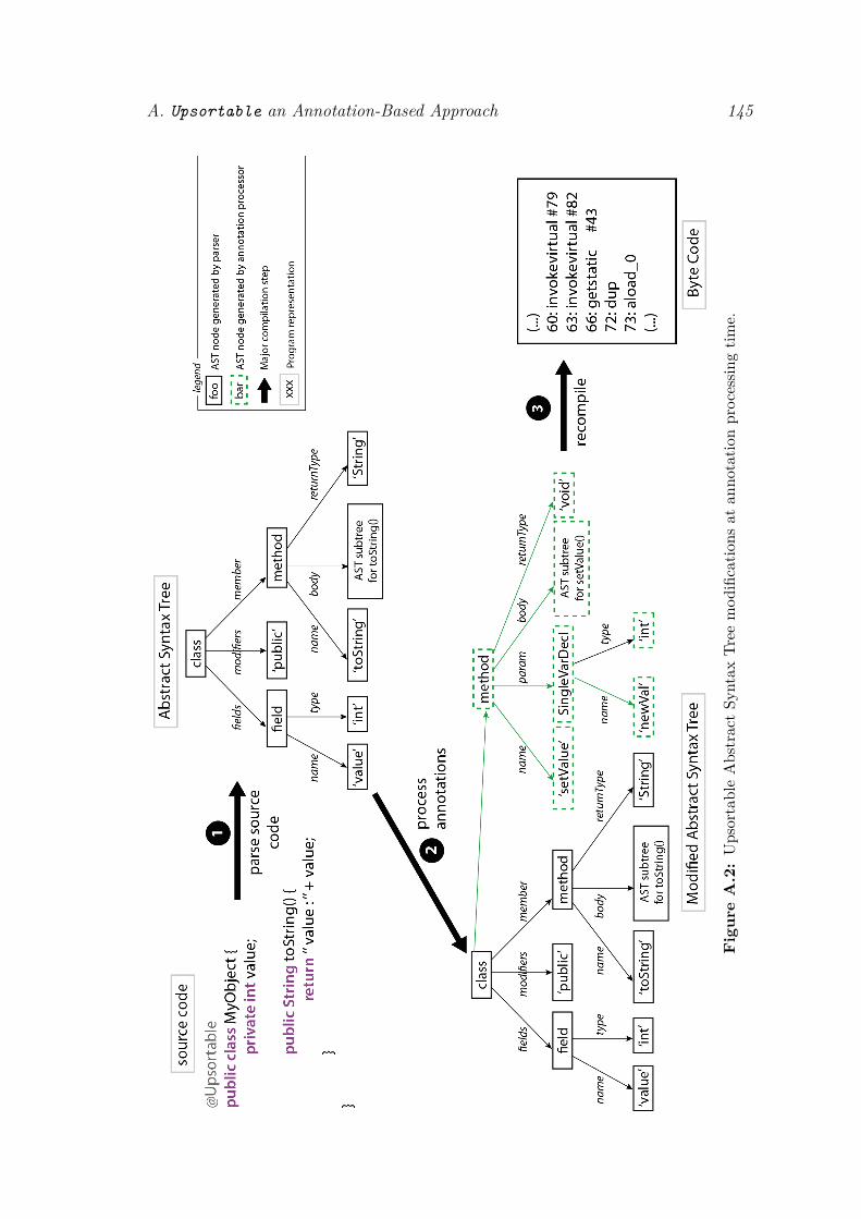
A. Upsortable an Annotation-Based Approach 145
FigureA.2:UpsortableAbstractSy
ntax
Tree
mod
ificatio
nsat
anno
tatio
nprocessin
gtim
e.
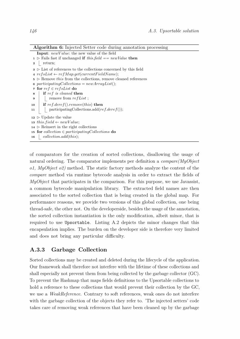
146 A.3. Upsortable solution
Algorithm 6: Injected Setter code during annotation processingInput: newV alue: the new value of the field
1 � Fails fast if unchanged if this.field == newValue then2 return;3 � List of references to the collections concerned by this field4 refsList← refMap.get(currentF ieldName);5 � Remove this from the collections, remove cleaned references6 participatingCollections = newArrayList();7 for ref ∈ refsList do8 if ref is cleaned then9 remove from refList ;
10 if ref.deref().remove(this) then11 participatingCollections.add(ref.deref());
12 � Update the value13 this.field← newV alue;14 � Reinsert in the right collections15 for collection ∈ participatingCollections do16 collection.add(this);
of comparators for the creation of sorted collections, disallowing the usage ofnatural ordering. The comparator implements per definition a compare(MyObjecto1, MyObject o2) method. The static factory methods analyze the content of thecompare method via runtime bytecode analysis in order to extract the fields ofMyObject that participates in the comparison. For this purpose, we use Javassist,a common bytecode manipulation library. The extracted field names are thenassociated to the sorted collection that is being created in the global map. Forperformance reasons, we provide two versions of this global collection, one beingthread-safe, the other not. On the developerside, besides the usage of the annotation,the sorted collection instantiation is the only modification, albeit minor, that isrequired to use Upsortable. Listing A.2 depicts the minor changes that thisencapsulation implies. The burden on the developer side is therefore very limitedand does not bring any particular difficulty.
A.3.3 Garbage Collection
Sorted collections may be created and deleted during the lifecycle of the application.Our framework shall therefore not interfere with the lifetime of these collections andshall especially not prevent them from being collected by the garbage collector (GC).To prevent the Hashmap that maps fields definitions to the Upsortable collections tohold a reference to these collections that would prevent their collection by the GC,we use a WeakReference. Contrary to soft references, weak ones do not interferewith the garbage collection of the objects they refer to. ’The injected setters’ codetakes care of removing weak references that have been cleaned up by the garbage

A. Upsortable an Annotation-Based Approach 147
collector. By relying on the ListIterator, we are able to both process valid referencesand remove cleaned ones in a single iteration over the list of weak references.
A.4 DiscussionThe Upsortable approach offers a convenient and safe solution to manage dynamicallysorted collections. Naturally, safety and convenience have a performance impact.Keeping track of the relation between fields and sorted collections in Upsortable hasa very limited memory fingerprint – especially compared to the Observer designpattern – and the CPU impact is also limited. Since we leverage the imbalancebetween the number of objects and collections, this leads to very few useless removes(a O(log(n)) operation for three data structures) and has a very limited impact ofseveral percents (< 5%) of the runtime in the practice, depending on the input data.

148
BDETAILED ANALYSIS
ContentsB.1 Evaluating Kleene+ Operator . . . . . . . . . . . . . . . 149B.2 Proof Sketches . . . . . . . . . . . . . . . . . . . . . . . . 150B.3 Optimising Z-address Comparison . . . . . . . . . . . . 153B.4 Operations over Virtual Z-addresses . . . . . . . . . . . 154
B.4.1 Correctness of Comparing Virtual Z-addresses . . . . . . 154B.4.2 NextJumpIn and NextJumpOut Computation . . . . . . 155
In this appendix as mentioned before we provide detailed analysis on algorithmsand proofs of the different theorem and lemmas defined in chapter3.
B.1 Evaluating Kleene+ Operator
The Kleene+ operator is executed after the joins evaluation and it employs thebitvector Bu and Banker’s sequence for the set bits in Bu. An example of a Bankerssequence for three set bits for an events sequence b+/ 〈b1, b2, b3〉 is shown in Table B.1.
The creation of sequences from the generated binary number requires mappingto the Bu when there are unset bits in Bu. That is, the join size is less than the totalnumber of events in an events sequence. For instance, Fig. B.1 shows a bitvectorB1 = 01001012, where only three bits are set. Hence we need to map the index of theset bit with the generated Banker’s sequence. Fig. B.1 shows such mapping for twosequences. Such mapping is part of the Algorithm 3, where at line 9 a NextSetBitfunction is employed to skip the unset bits during the generation of the matches.
149
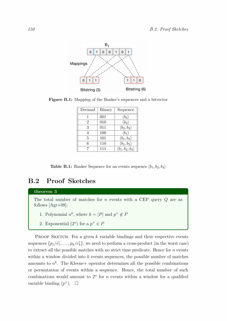
150 B.2. Proof Sketches
010 1001
B1
0 1 1 1 1 0
Bitstring (3) Bitstring (6)
Mappings
Figure B.1: Mapping of the Banker’s sequences and a bitvector
Decimal Binary Sequence1 001 〈b3〉2 010 〈b2〉3 011 〈b2, b3〉4 100 〈b1〉5 101 〈b1, b3〉6 110 〈b1, b2〉7 111 〈b1, b2, b3〉
Table B.1: Banker Sequence for an events sequence 〈b1, b2, b3〉
B.2 Proof Sketchestheorem 3
The total number of matches for n events with a CEP query Q are asfollows [Agr+08]:
1. Polynomial nk, where k = |P | and p+ /∈ P
2. Exponential (2n) for a p+ ∈ P
Proof Sketch. For a given k variable bindings and their respective eventssequences {p1/~e1, . . . , pk/~ek}, we need to perform a cross-product (in the worst case)to extract all the possible matches with no strict time predicate. Hence for n eventswithin a window divided into k events sequences, the possible number of matchesamounts to nk. The Kleene+ operator determines all the possible combinationsor permutation of events within a sequence. Hence, the total number of suchcombinations would amount to 2n for n events within a window for a qualifiedvariable binding (p+). �

B. DETAILED ANALYSIS 151
lemma: 1
Given two Z-regions r and r′ and a set of binary relations {φ1, . . . φd} fromthe variable predicates Θv in Q over d-dimensional events (Z-addresses), rdominates r′ (r ` r′) iff
1. ∀igid−1(max(r)) φi gid−1(min(r′)) if φi = {<,≤}
2. ∀igid−1(min(r)) φi gid−1(max(r′)) if φi = {>,≥}
Proof. We prove the aforementioned points case by case. Let us assume a pointz from region r and a point z′ from region r′. Furthermore, for brevity, we usezl = min(r) and zh = max(r) The following is true:
∀igid−1(zhr ) ≤ gid−1(z) ≤ gid−1(zlr) (B.1)
∀igid−1(zhr′) ≤ gid−1(z′) ≤ gid−1(zlr′) (B.2)
since by definition, zhr and zlr represent the extremities of region r havingmaximum and minimum values in all dimensions and we follow the transitivityproperty and monotonic ordering of Z-addresses in a Z-region.Case 1. In the case i ∈ Φ<,≤ meaning φi = {<,≤} and thus, from the assumedcondition in the lemma, gid−1(zhr ) φi gid−1(zlr′) true. Which in turn means thatgid−1(zhr ) ≤ gid−1(zlr′) or gid−1(zhr ) < gid−1(zlr′) respectively depending on φi.Combining this with eq.(B.1) and (B.2), it follows that gid−1(z) ≤ gid−1(z′) orgid−1(z) < gid−1(z′) depending on φi. Which means that for these i,
gid−1(z) φi gid−1(z′) is true.
Case 2. Lets now take the case where i ∈ Φ>,≥ meaning φi = {>,≥} andthus, from the assumed condition in the lemma, gid−1(zlr) φi g
id−1(zhr′) is true.
Which means that gid−1(zlr) ≥ gid−1(zhr′) or gid−1(zlr) > gid−1(zhr′) respectivelydepending on φi. Combining this with eq.(B.1) and (B.2), it follows that gid−1(z) ≥gid−1(z′) or gid−1(z) > gid−1(z′) depending on φi. Which means that for thesei, gid−1(z) φi g
id−1(z′) is true.
Thus, after combining cases 1 and 2, it follows that∀i gid−1(z) φi g
id−1(z′),
which in turn forms Definition 5, which defines dominance, means that for anygiven point z from region r and z′ from region r′, given the above conditions,z ` z′ and hence r ` r′.

152 B.2. Proof Sketches
lemma: 2
Given two Z-regions r and r′ and a set of binary relations from Lemma 1 rpartially dominates r′ (r ∼ r′) iff Lemma 1 does not holds and only followingconditions hold
1. ∀igid−1(min(r)) φi gid−1(max(r′)) if φi = {<,≤}
2. ∀igid−1(max(r)) φi gid−1(min(r′)) if φi = {>,≥}
Proof. We prove the lemma as follows.Case 1. In the case i ∈ Φ<,≤ meaning φi = {<,≤} and thus, from the assumedcondition in the lemma, gid−1(zlr) φi gid−1(zhr′) is true. Now lets take the regiondefined by the range having the following bits same as the extremities gid−1(zlr) andgid−1(zhr′). Lets arbitrarily divide this region into two sub-regions s1 and s′
1. This isdone by arbitrarily choosing 4 range values, lying inside the above range, such thatthe following is true:gid−1(zlr) φi gid−1(zls1) φi gid−1(zhs1) φi gid−1(zs′
1)lφi gid−1(zhs′
1) φi gid−1(zhr′).
Also, the division is done in a way that the sub-regions are not empty andthey only contain points from r and r′. There exists at least one division wheresub-regions are not empty as, in the extreme case, the two regions can have at leasta single common point each with the bits gid−1(zlr) and gid−1(zhr′), respectively. Fromthe above way of dividing, it is ensured that gid−1(zhs1) φi gid−1(zls′
1).
Case 2. Now for other remaining i ∈ Φ>,≥ meaning φi = {>,≥} and thus, fromthe assumed condition in the lemma, gid−1(zhr ) φi gid−1(zlr′) is true. Again lets takethe region defined by the range having the following bits same as the extremitiesgid−1(zlr′) and gid−1(zhr ). Lets arbitrarily divide it into two sub-regions s2 and s
′2.
This is done by arbitrarily choosing 4 range values, lying inside the above range,such that the following is true:gid−1(zlr′) φi gid−1(zsl
2′) φi gid−1(zsh
2′) φi gid−1(zls1)
φi gid−1(zhs1) φi g
id−1(zhr ).
Again, the division is done in a way that the sub-regions are not empty andthey only contain points from r and r′. There exists at least one division wheresub-regions are not empty as, in the extreme case, the two regions can have at leasta single common point each with bits gid−1(zhr ) and gid−1(zlr′), respectively. Fromthe above way of dividing, it is ensured that gid−1(zls2) φi gid−1(zhs′
2).
Now, let’s define a sub-region s = s1 ∩ s2 and another sub-region s′ = s′1 ∩ s
′2.
The sets s and s′ are non empty. As from the last lines of the above cases, s at leasthas a single point having bits gid−1(zlr)∀i ∈ Φ<,≤ and gid−1(zhr )∀i ∈ Φ>,≥. Similarly,s′ at least has a single point having bits gid−1(zhr′)∀i ∈ Φ<,≤ and gid−1(zlr′)∀i ∈ Φ>,≥.
From the above 2 cases:
B. DETAILED ANALYSIS 153
∀i, gid−1(zhs1) φi gid−1(zls′1) and gid−1(zls2) φi gid−1(zhs′
2) are true.
As s consists in the common points of s1 and s2, and s′ consists in commonpoints of s′
1 and s′2, it implies that ∀i, gid−1(zhs ) φi gid−1(zls′) and gid−1(zls) φi gid−1(zhs′)
are true. Using lemma 2 s ` s′. Thus, there are some points in r that dominatesome points in r′ and hence r ∼ r′.
B.3 Optimising Z-address ComparisonHerein, we describe an optimisation technique to save on the cost of the bitinterleaving and comparison of Z-addresses during insertion, as well as range queryprocessing over an event tree.
The aim of the bit-interleaving process is to compute the binary relations overZ-addresses while inserting and querying in an event tree. That is, locating the MSBdifference between the Z-addresses in questions. For instance, if z1 = 001010 andz2 = 001110 then z2 > z1. This means we have to (i) generate a Z-address using bitinterleaving for each event; (ii) de-interleave the Z-addresses to find the difference inthe MSB between them; and (iii) decode the Z-address to get their original values.The first and third tasks can be performed using bit-level parallelism if the resultingbitstring (of a Z-address) fits in the registers of the CPU at hand, e.g. |z| < 64 bitson a 64-bit CPU. However, if |z| > 64, we need to iterate over the bits within eachdimension in a traditional manner. Our aim is to avoid this by getting rid of bitinterleaving and de-interleaving while still retaining the properties of Z-order curve.
Examining the comparison process between two Z-addresses (keys) reveals thatwe do not have to actually interleave bits to determine the MSB difference. Instead,we can directly compute and compare the MSB difference of each dimension (in keys)independently and then following up by comparing just the dimension that wonthe comparison, i.e. which has the leftmost MSB. The MSB comparison between adimension from each key can be performed using a bitwise XOR operation. We callthis process virtual Z-address comparison and, for brevity, Algorithm 7 presentsthis process for 2-dimensional keys.
Algorithm 7 takes the two keys and first calculates the bitwise XOR (denoted as∨) between the respective dimensions of both keys (lines 1,2 ). This provides themeans to determine the position of the MSB contributed by both dimensions. It thenfinds out which dimension is responsible for the MSB bit in the virtual Z-addresses(line 3 ). If the XOR between the first dimensions of the keys is less than the otherdimension, we are sure that the second dimension contributed to the MSB in thevirtual Z-addresses (lines 4-7 ). Otherwise, it is the first dimension (lines 9 -12 ).Depending on the comparison result, it then checks which key’s dimension (first orsecond) is greater or less than the other. This would provide us with the final results
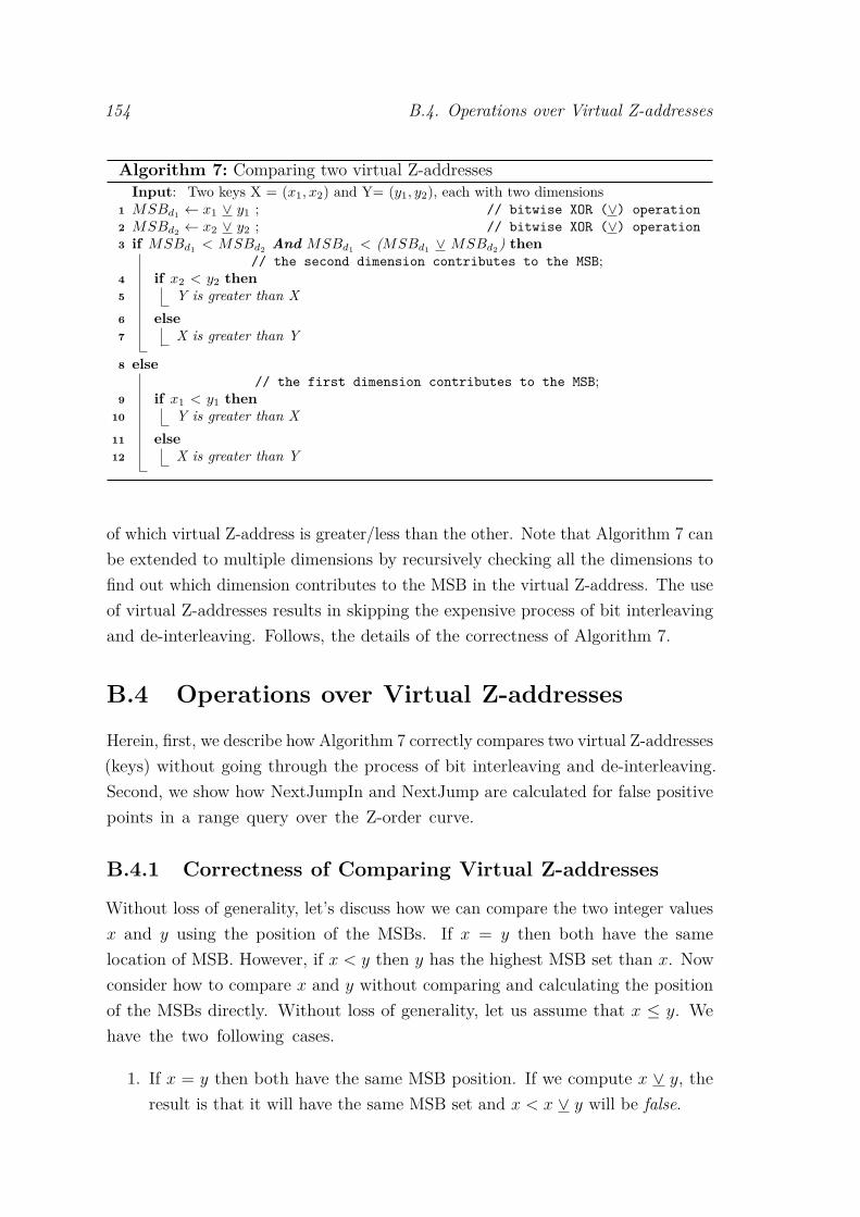
154 B.4. Operations over Virtual Z-addresses
Algorithm 7: Comparing two virtual Z-addressesInput: Two keys X = (x1, x2) and Y= (y1, y2), each with two dimensions
1 MSBd1 ← x1 ∨ y1 ; // bitwise XOR (∨) operation2 MSBd2 ← x2 ∨ y2 ; // bitwise XOR (∨) operation3 if MSBd1 < MSBd2 And MSBd1 < (MSBd1 ∨ MSBd2) then
// the second dimension contributes to the MSB;4 if x2 < y2 then5 Y is greater than X6 else7 X is greater than Y
8 else// the first dimension contributes to the MSB;
9 if x1 < y1 then10 Y is greater than X11 else12 X is greater than Y
of which virtual Z-address is greater/less than the other. Note that Algorithm 7 canbe extended to multiple dimensions by recursively checking all the dimensions tofind out which dimension contributes to the MSB in the virtual Z-address. The useof virtual Z-addresses results in skipping the expensive process of bit interleavingand de-interleaving. Follows, the details of the correctness of Algorithm 7.
B.4 Operations over Virtual Z-addresses
Herein, first, we describe how Algorithm 7 correctly compares two virtual Z-addresses(keys) without going through the process of bit interleaving and de-interleaving.Second, we show how NextJumpIn and NextJump are calculated for false positivepoints in a range query over the Z-order curve.
B.4.1 Correctness of Comparing Virtual Z-addresses
Without loss of generality, let’s discuss how we can compare the two integer valuesx and y using the position of the MSBs. If x = y then both have the samelocation of MSB. However, if x < y then y has the highest MSB set than x. Nowconsider how to compare x and y without comparing and calculating the positionof the MSBs directly. Without loss of generality, let us assume that x ≤ y. Wehave the two following cases.
1. If x = y then both have the same MSB position. If we compute x ∨ y, theresult is that it will have the same MSB set and x < x ∨ y will be false.

B. DETAILED ANALYSIS 155
2. If x < y then x does not have the same position of the MSB than y, and theposition of y MSB will be higher than x. Then if we compute x ∨ y, it willhave same MSB of y and x < x ∨ y will be true.
The logic of the above-mentioned cases is used to describe the working ofAlgorithm 7. In particular, line 3 of Algorithm 7 which determines the dimensionto compare in the virtual Z-address. Hence the first bitwise XOR (∨) operationsbetween each of the dimensions in Algorithm 7 (lines 1,2 ) are used to comparethe dimensions itself. That is, which dimension in the virtual Z-address wouldhave contributed to the MSB: this comparison is done at the first part of the ifstatement on line 3. The second part of the if statement at line 3 is then usedto compare MSB difference between them, i.e. which dimensions have the highestMSB between the two virtual Z-addresses.
B.4.2 NextJumpIn and NextJumpOut Computation
Due to the nature of the Z-order curve, it contains jumps and can go out of thebounding box. Hence when calculating the range queries, we can have some falsepositive points, i.e. Z-addresses that are not part of the result, within the answer set.To resolve this problem, cursor-driven approaches are proposed to skip those falsepositive points. This includes calculating the boundaries of next set of elements thatcan be reached while skipping the false positive. Please refer to [OM84; Ram+00a]for the detailed discussion on this problem. Herein, we discuss how to calculate suchboundaries without going through the process of bit interleaving and de-leaving.These boundaries are called NextJumpIn (NJI) and NextJumpOut (NJO).
Algorithm 8: NextJumpIn and NextJumpOut ComputationInput: A Range query with q = [X,Y ], X = (x1, x2) and Y= (y1, y2), each with two
dimensions1 NJI← X;2 NJO← Y ;3 dim← DimToCompare(NJI,NJO);4 cmsb← CommonMSB(NJI[dim],NJO[dim]);5 mask ← ((¬(1 << (cmsb+ 1))− 1) & 0xFF ;6 NJI[dim]← Y [dim] & mask) | (1 << cmsb)) // bitwise OR (|) and shif operator
(<<);7 NJO[dim]← Y [dim] & mask) | (1 << cmsb)− 1)
Algorithm 8 presents the procedure of calculating NJI and NJO for a rangequery. Without loss of generality, it shows the operations on 32 bits integers. It firstinitialises the NJI and NJO points with that of the range query boundaries. When itfinds a value that comes out of the bounding boX. It then determines the dimensionin both NJI and NJO that contributes to the MSB. Then computes the common MSB

156 B.4. Operations over Virtual Z-addresses
for such dimension using both NJI and NJO. This common MSB is used to create amask, which later will be used to create the new values of the dimension in question.Using the mask and common MSB, it changes the values of the dimension in bothNJI and NJO. This results in the new range value that can skip the false positives.
Works Cited
[Aba+03] Daniel J Abadi et al. “Aurora: a new model and architecture for datastream management”. In: VLDBJ (2003), pp. 120–139.
[Adi+06] Asaf Adi et al. “Complex event processing for financial services”. In:Services Computing Workshops, 2006. SCW’06. IEEE. IEEE. 2006,pp. 7–12.
[Agr+08] Jagrati Agrawal et al. “Efficient Pattern Matching over Event Streams”. In:Proceedings of the 2008 ACM SIGMOD International Conference onManagement of Data. SIGMOD ’08. Vancouver, Canada: ACM, 2008,pp. 147–160. url: http://doi.acm.org/10.1145/1376616.1376634.
[AÇT08] Mert Akdere, Ugur Çetintemel, and Nesime Tatbul. “Plan-based complexevent detection across distributed sources”. In: Proceedings of the VLDBEndowment 1.1 (2008), pp. 66–77.
[AÇU10] Mert Akdere, Uur Çetintemel, and Eli Upfal. “Database-support forContinuous Prediction Queries over Streaming Data”. In: VLDB (2010).
[AAP17] Elias Alevizos, Alexander Artikis, and George Paliouras. “EventForecasting with Pattern Markov Chains”. In: Proceedings of the 11thACM International Conference on Distributed and Event-based Systems.DEBS ’17. Barcelona, Spain: ACM, 2017, pp. 146–157. url:http://doi.acm.org/10.1145/3093742.3093920.
[Ama+18] Ciprian Amariei et al. “Cell Grid Architecture for Maritime RoutePrediction on AIS Data Streams”. In: Proceedings of the 12th ACMInternational Conference on Distributed and Event-based Systems, DEBS2018, Hamilton, New Zealand, June 25-29, 2018. 2018, pp. 202–204. url:https://doi.org/10.1145/3210284.3220503.
[Ani+12] Darko Anicic et al. “Stream Reasoning and Complex Event Processing inETALIS”. In: Semant. web 3.4 (Oct. 2012), pp. 397–407. url:http://dl.acm.org/citation.cfm?id=2590208.2590214.
[ABW06] Arvind Arasu, Shivnath Babu, and Jennifer Widom. “The CQL continuousquery language: semantic foundations and query execution”. In: The VLDBJournal 15.2 (2006), pp. 121–142.
[Ara+03] Arvind Arasu et al. “STREAM: the stanford stream data manager(demonstration description)”. In: Proceedings of the 2003 ACM SIGMODinternational conference on Management of data. ACM. 2003, pp. 665–665.
[Art+12] Alexander Artikis et al. “Event processing under uncertainty”. In:Proceedings of the 6th ACM International Conference on DistributedEvent-Based Systems. ACM. 2012, pp. 32–43.
157
158 Works Cited
[Art+17a] Alexander Artikis et al. “A Prototype for Credit Card Fraud Management:Industry Paper”. In: DEBS. 2017, pp. 249–260.
[Art+17b] Alexander Artikis et al. “A Prototype for Credit Card Fraud Management:Industry Paper”. In: Proceedings of the 11th ACM InternationalConference on Distributed and Event-based Systems. DEBS ’17. Barcelona,Spain: ACM, 2017, pp. 249–260. url:http://doi.acm.org/10.1145/3093742.3093912.
[AH00] Ron Avnur and Joseph M Hellerstein. “Eddies: Continuously adaptivequery processing”. In: ACM sigmod record. Vol. 29. 2. ACM. 2000,pp. 261–272.
[Bab+02] Brian Babcock et al. “Models and issues in data stream systems”. In:Proceedings of the twenty-first ACM SIGMOD-SIGACT-SIGARTsymposium on Principles of database systems. ACM. 2002, pp. 1–16.
[BW01] Shivnath Babu and Jennifer Widom. “Continuous queries over datastreams”. In: ACM Sigmod Record 30.3 (2001), pp. 109–120.
[Bac+18] Moti Bachar et al. “Venilia, On-line Learning and Prediction of VesselDestination”. In: Proceedings of the 12th ACM International Conference onDistributed and Event-based Systems, DEBS 2018, Hamilton, New Zealand,June 25-29, 2018. 2018, pp. 209–212. url:https://doi.org/10.1145/3210284.3220505.
[BGH87] Joel Bartlett, Jim Gray, and Bob Horst. “Fault tolerance in tandemcomputer systems”. In: The Evolution of Fault-Tolerant Computing.Springer, 1987, pp. 55–76.
[BYY04] Ron Begleiter, Ran El-Yaniv, and Golan Yona. “On Prediction UsingVariable Order Markov Models”. In: J. Artif. Int. Res. 22.1 (Dec. 2004),pp. 385–421. url:http://dl.acm.org/citation.cfm?id=1622487.1622499.
[BF79] Jon Louis Bentley and Jerome H. Friedman. “Data Structures for RangeSearching”. In: ACM Comput. Surv. 11.4 (Dec. 1979), pp. 397–409. url:http://doi.acm.org/10.1145/356789.356797.
[BS80] Jon Louis Bentley and James B. Saxe. “Decomposable Searching ProblemsI: Static-to-Dynamic Transformation.” In: Journal of Algorithms 1.4 (1980),pp. 301–358. url:http://dblp.uni-trier.de/db/journals/jal/jal1.html#BentleyS80.
[Bey+99] Kevin S. Beyer et al. “When Is ”Nearest Neighbor” Meaningful?” In: ICDT.1999, pp. 217–235.
[BFP10] Silvia Bianchi, Pascal Felber, and Maria Gradinariu Potop-Butucaru.“Stabilizing distributed r-trees for peer-to-peer content routing”. In: IEEETransactions on Parallel and Distributed Systems 21.8 (2010),pp. 1175–1187.
[Blo+10] Marion Blount et al. “Real-time analysis for intensive care: developmentand deployment of the artemis analytic system”. In: IEEE Engineering inMedicine and Biology Magazine 29.2 (2010), pp. 110–118.
Works Cited 159
[Bod+18] Oleh Bodunov et al. “Real-time Destination and ETA Prediction forMaritime Traffic”. In: Proceedings of the 12th ACM InternationalConference on Distributed and Event-based Systems, DEBS 2018, Hamilton,New Zealand, June 25-29, 2018. 2018, pp. 198–201. url:https://doi.org/10.1145/3210284.3220502.
[Bos+14] Jeffrey Bosboom et al. “StreamJIT: A commensal compiler forhigh-performance stream programming”. In: OOPSLA. 2014, pp. 177–195.
[Bre+07] Lars Brenna et al. “Cayuga: A High-performance Event ProcessingEngine”. In: SIGMOD. 2007, pp. 1100–1102.
[Bui09] Hai-Lam Bui. “Survey and comparison of event query languages usingpractical examples”. In: Ludwig Maximilian University of Munich (2009).
[Cas+02] Miguel Castro et al. “SCRIBE: A large-scale and decentralizedapplication-level multicast infrastructure”. In: IEEE Journal on SelectedAreas in communications 20.8 (2002), pp. 1489–1499.
[Cha+14] Samy Chambi et al. “Better bitmap performance with Roaring bitmaps”.In: CoRR (2014).
[Cha+15] Samy Chambi et al. “Better bitmap performance with Roaring bitmaps”.In: Software: Practice and Experience (2015).
[CS94] Rakesh Chandra and Arie Segev. “Active databases for financialapplications”. In: Research Issues in Data Engineering, 1994. ActiveDatabase Systems. Proceedings Fourth International Workshop on. IEEE.1994, pp. 46–52.
[Cha+00] Yuan-Chi Chang et al. “The onion technique: indexing for linearoptimization queries”. In: ACM Sigmod Record. Vol. 29. 2. ACM. 2000,pp. 391–402.
[Che+15] Jules Chevalier et al. “Slider: an Efficient Incremental Reasoner”. In:SIGMOD. ACM. 2015, pp. 1081–1086.
[CW84] John G. Cleary and Ian H. Witten. “Data Compression using AdaptiveCoding and Partial String Matching”. In: IEEE Transactions onCommunications 32.4 (1984), pp. 396–402.
[Cor11] Graham Cormode. “Sketch techniques for approximate query processing”.In: Foundations and Trends in DB. 2011.
[CDF01] Gianpaolo Cugola, Elisabetta Di Nitto, and Alfonso Fuggetta. “The JEDIevent-based infrastructure and its application to the development of theOPSS WFMS”. In: IEEE transactions on Software Engineering 27.9 (2001),pp. 827–850.
[CM12a] Gianpaolo Cugola and Alessandro Margara. “Low latency complex eventprocessing on parallel hardware”. In: Journal of Parallel and DistributedComputing 72.2 (2012), pp. 205–218.
[CM12b] Gianpaolo Cugola and Alessandro Margara. “Processing flows ofinformation: From data stream to complex event processing”. In: ACMComputing Surveys (CSUR) 44.3 (2012), p. 15.
160 Works Cited
[CM15] Gianpaolo Cugola and Alessandro Margara. “The complex event processingparadigm”. In: Data Management in Pervasive Systems. Springer, 2015,pp. 113–133.
[DM17] Tiziano De Matteis and Gabriele Mencagli. “Parallel patterns forwindow-based stateful operators on data streams: an algorithmic skeletonapproach”. In: International Journal of Parallel Programming 45.2 (2017),pp. 382–401.
[DIG07] Yanlei Diao, Neil Immerman, and Daniel Gyllstrom. “Sase+: An agilelanguage for kleene closure over event streams”. In: UMass TechnicalReport (2007).
[EE11] Yagil Engel and Opher Etzion. “Towards Proactive Event-drivenComputing”. In: DEBS. 2011, pp. 125–136.
[ESP] ESPER. http://www.espertech.com/esper/.[EJ09] Patrick Eugster and KR Jayaram. “EventJava: An extension of Java for
event correlation”. In: ECOOP. Springer. 2009, pp. 570–594.[Fli] Apache Flink. https://flink.apache.org/.[FB12] Lajos Jenő Fülöp and Beszédes. “Predictive Complex Event Processing: A
Conceptual Framework for Combining Complex Event Processing andPredictive Analytics”. In: BCI. 2012.
[GUW02] Hector Garcia-Molina, Jeffrey D. Ullman, and Jennifer Widom. Databasesystems - the complete book (international edition). Pearson Education,2002, pp. I–XXVII, 1–1119.
[GB01] Dimitrios Georgakopoulos and Alexander Buchmann, eds. Proceedings ofthe 17th International Conference on Data Engineering, April 2-6, 2001,Heidelberg, Germany. IEEE Computer Society, 2001. url: http://ieeexplore.ieee.org/xpl/mostRecentIssue.jsp?punumber=7304.
[GMV08] John Giacomoni, Tipp Moseley, and Manish Vachharajani. “FastForwardfor efficient pipeline parallelism: a cache-optimized concurrent lock-freequeue”. In: SIGPLAN. ACM. 2008, pp. 43–52.
[Gue+15] Ted Gueniche et al. “CPT+: Decreasing the Time/Space Complexity of theCompact Prediction Tree”. In: PAKDD. 2015, pp. 625–636. url:http://dx.doi.org/10.1007/978-3-319-18032-8_49.
[Gul+16a] Vincenzo Gulisano et al. “The DEBS 2016 Grand Challenge”. In: to bepublished in the DEBS 2016 proceedings. ACM. 2016, pp. 1–8.
[Gul+16b] Vincenzo Gulisano et al. “The DEBS 2016 grand challenge”. In: Proceedingsof the 10th ACM International Conference on Distributed and Event-basedSystems, DEBS ’16, Irvine, CA, USA, June 20 - 24, 2016. 2016,pp. 289–292. url: http://doi.acm.org/10.1145/2933267.2933519.
[Gul+18a] Vincenzo Gulisano et al. “The DEBS 2018 Grand Challenge”. In:Proceedings of the 12th ACM International Conference on Distributed andEvent-based Systems, DEBS 2018, Hamilton, New Zealand, June 25-29,2018. 2018, pp. 191–194. url:http://doi.acm.org/10.1145/3210284.3220510.
Works Cited 161
[Gul+18b] Vincenzo Gulisano et al. “The DEBS 2018 Grand Challenge”. In:Proceedings of the 12th ACM International Conference on Distributed andEvent-based Systems, DEBS 2018, Hamilton, New Zealand, June 25-29,2018. 2018, pp. 191–194. url:https://doi.org/10.1145/3210284.3220510.
[Hil91] David Hilbert. Ueber stetige abbildung einer linie auf ein flachenstuck.Mathematische Annalen. 1891.
[Hil+08] Matthew Hill et al. “Event detection in sensor networks for modern oilfields”. In: Proceedings of the second international conference onDistributed event-based systems. ACM. 2008, pp. 95–102.
[Hir+18] Martin Hirzel et al. “Stream Query Optimization”. In: (2018).[HKP01] Vagelis Hristidis, Nick Koudas, and Yannis Papakonstantinou. “PREFER:
A system for the efficient execution of multi-parametric ranked queries”. In:ACM Sigmod Record. Vol. 30. 2. ACM. 2001, pp. 259–270.
[Huf52] David A Huffman. “A method for the construction of minimum-redundancycodes”. In: Proceedings of the IRE 40.9 (1952), pp. 1098–1101.
[Kha+17] Zuhair Khayyat et al. “Fast and Scalable Inequality Joins”. In: The VLDBJournal (2017), pp. 125–150.
[Kir+17] James Kirkpatrick et al. “Overcoming catastrophic forgetting in neuralnetworks”. In: Proceedings of the national academy of sciences (2017),p. 201611835.
[KS18a] Ilya Kolchinsky and Assaf Schuster. “Efficient Adaptive Detection ofComplex Event Patterns”. In: arXiv preprint arXiv:1801.08588 (2018).
[KS18b] Ilya Kolchinsky and Assaf Schuster. “Join Query Optimization Techniquesfor Complex Event Processing Applications”. In: arXiv preprintarXiv:1801.09413 (2018).
[KSK16] Ilya Kolchinsky, Assaf Schuster, and Danny Keren. “Efficient Detection ofComplex Event Patterns Using Lazy Chain Automata”. In: arXiv preprintarXiv:1612.05110 (2016).
[KSS15a] Ilya Kolchinsky, Izchak Sharfman, and Assaf Schuster. “Lazy EvaluationMethods for Detecting Complex Events”. In: DEBS. 2015, pp. 34–45.
[KSS15b] Ilya Kolchinsky, Izchak Sharfman, and Assaf Schuster. “Lazy evaluationmethods for detecting complex events”. In: Proceedings of the 9th ACMInternational Conference on Distributed Event-Based Systems. ACM. 2015,pp. 34–45.
[KS09] Jürgen Krämer and Bernhard Seeger. “Semantics and implementation ofcontinuous sliding window queries over data streams”. In: ACMTransactions on Database Systems (TODS) 34.1 (2009), p. 4.
[Lee+07] Ken C. K. Lee et al. “Approaching the Skyline in Z Order”. In: VLDB.2007, pp. 279–290.
[LKA10] Daniel Lemire, Owen Kaser, and Kamel Aouiche. “Sorting improvesword-aligned bitmap indexes”. In: Data & Knowledge Engineering 69.1(2010), pp. 3–28.

162 Works Cited
[LG16] Zheng Li and Tingjian Ge. “History is a mirror to the future: Best-effortapproximate complex event matching with insufficient resources”. In:Proceedings of the VLDB Endowment 10.4 (2016), pp. 397–408.
[Lii91] Helmut Liitkepohl. “Introduction to multiple time series analysis”. In:Berlin et al (1991).
[Lin+05] Xuemin Lin et al. “Stabbing the sky: Efficient skyline computation oversliding windows”. In: Data Engineering, 2005. ICDE 2005. Proceedings.21st International Conference on. IEEE. 2005, pp. 502–513.
[LvHS00] J. Loughry, J.I. van Hemert, and L. Schoofs. “Efficiently Enumerating theSubsets of a Set”. In: Applied-math (2000).
[Luc08] David Luckham. “The power of events: An introduction to complex eventprocessing in distributed enterprise systems”. In: International Workshopon Rules and Rule Markup Languages for the Semantic Web. Springer.2008, pp. 3–3.
[LF98] David C Luckham and Brian Frasca. “Complex event processing indistributed systems”. In: Computer Systems Laboratory Technical ReportCSL-TR-98-754. Stanford University, Stanford 28 (1998).
[MCT14] Alessandro Margara, Gianpaolo Cugola, and Giordano Tamburrelli.“Learning from the past: automated rule generation for complex eventprocessing”. In: Proceedings of the 8th ACM International Conference onDistributed Event-Based Systems. ACM. 2014, pp. 47–58.
[MKN10] Steven Mascaro, Kevin B Korb, and Ann E Nicholson. “Learning abnormalvessel behaviour from ais data with bayesian networks at two time scales”.In: Tracks a Journal of Artists Writings (2010), pp. 1–34.
[May18] Ruben Mayer. “Window-based data parallelization in complex eventprocessing”. In: (2018).
[MD89] Dennis McCarthy and Umeshwar Dayal. “The architecture of an activedatabase management system”. In: ACM Sigmod Record. Vol. 18. 2. ACM.1989, pp. 215–224.
[MP13] Ciaran McCreesh and Patrick Prosser. “Multi-threading a state-of-the-artmaximum clique algorithm”. In: Algorithms 6.4 (2013), pp. 618–635.
[MM09] Yuan Mei and Samuel Madden. “ZStream: A Cost-based Query Processorfor Adaptively Detecting Composite Events”. In: SIGMOD. 2009,pp. 193–206.
[MRT12] Mehryar Mohri, Afshin Rostamizadeh, and Ameet Talwalkar. Foundationsof Machine Learning. MIT Press, 2012.
[Mor66] G. M. Morton. “A Computer Oriented Geodetic Data Base; and a NewTechnique in File Sequencing”. In: IBM. 1966.
[MBP06] Kyriakos Mouratidis, Spiridon Bakiras, and Dimitris Papadias.“Continuous monitoring of top-k queries over sliding windows”. In:SIGMOD. 2006, pp. 635–646.

Works Cited 163
[MTZ17] Raef Mousheimish, Yehia Taher, and Karine Zeitouni. “Automatic learningof predictive cep rules: bridging the gap between data mining and complexevent processing”. In: Proceedings of the 11th ACM InternationalConference on Distributed and Event-based Systems. ACM. 2017,pp. 158–169.
[MZZ12] Barzan Mozafari, Kai Zeng, and Carlo Zaniolo. “High-performanceComplex Event Processing over XML Streams”. In: Proceedings of the 2012ACM SIGMOD International Conference on Management of Data.SIGMOD ’12. Scottsdale, Arizona, USA: ACM, 2012, pp. 253–264. url:http://doi.acm.org/10.1145/2213836.2213866.
[MP12] Christopher Mutschler and Michael Philippsen. “Learning event detectionrules with noise hidden markov models”. In: Adaptive Hardware andSystems (AHS), 2012 NASA/ESA Conference on. IEEE. 2012, pp. 159–166.
[NCB15] Parth Nagarkar, K. Selçuk Candan, and Aneesha Bhat. “CompressedSpatial Hierarchical Bitmap (cSHB) Indexes for Efficiently ProcessingSpatial Range Query Workloads”. In: VLDB (2015).
[NVA18] Duc-Duy Nguyen, Chan Le Van, and Muhammad Intizar Ali. “VesselDestination and Arrival Time Prediction with Sequence-to-SequenceModels over Spatial Grid”. In: Proceedings of the 12th ACM InternationalConference on Distributed and Event-based Systems, DEBS 2018, Hamilton,New Zealand, June 25-29, 2018. 2018, pp. 217–220. url:https://doi.org/10.1145/3210284.3220507.
[NC07] Charles Nyce and A Cpcu. “Predictive analytics white paper”. In:American Institute for CPCU. Insurance Institute of America (2007),pp. 9–10.
[OM84] J. A. Orenstein and T. H. Merrett. “A Class of Data Structures forAssociative Searching”. In: PODS-SIGMOD. 1984, pp. 181–190.
[Pal+18] Saravana Murthy Palanisamy et al. “Preserving Privacy and Quality ofService in Complex Event Processing through Event Reordering”. In:Proceedings of the 12th ACM International Conference on Distributed andEvent-based Systems. ACM. 2018, pp. 40–51.
[Par+17] I Parolas et al. “Prediction of vessels’ estimated time of arrival (ETA)using machine learning–a port of Rotterdam case study”. In: The 96thAnnual Meeting of the Transportation Research Board January. 2017.
[PP99] James Pitkow and Peter Pirolli. “Mining Longest Repeating Subsequencesto Predict World Wide Web Surfing”. In: USENIX Symposium on InternetTechnologies and Systems. 1999, pp. 13–13. url:http://dl.acm.org/citation.cfm?id=1251480.1251493.
[Pop+17] Olga Poppe et al. “Complete Event Trend Detection in High-Rate EventStreams”. In: SIGMOD. 2017, pp. 109–124.
[QGT16] Miao Qiao, Junhao Gan, and Yufei Tao. “Range Thresholding on Streams”.In: Proceedings of the 2016 International Conference on Management ofData. SIGMOD ’16. San Francisco, California, USA: ACM, 2016,pp. 571–582. url: http://doi.acm.org/10.1145/2882903.2915965.

164 Works Cited
[REG11] Ella Rabinovich, Opher Etzion, and Avigdor Gal. “Pattern rewritingframework for event processing optimization”. In: Proceedings of the 5thACM international conference on Distributed event-based system. ACM.2011, pp. 101–112.
[Ram+00a] Frank Ramsak et al. “Integrating the UB-Tree into a Database SystemKernel”. In: VLDB. 2000, pp. 263–272.
[Ram+00b] Frank Ramsak et al. “Integrating the UB-Tree into a Database SystemKernel”. In: VLDB. 2000.
[RLR16] Medhabi Ray, Chuan Lei, and Elke A. Rundensteiner. “Scalable PatternSharing on Event Streams*”. In: Proceedings of the 2016 InternationalConference on Management of Data. SIGMOD ’16. San Francisco,California, USA: ACM, 2016, pp. 495–510. url:http://doi.acm.org/10.1145/2882903.2882947.
[Ray+13] Medhabi Ray et al. “High-performance complex event processing usingcontinuous sliding views”. In: Proceedings of the 16th InternationalConference on Extending Database Technology. ACM. 2013, pp. 525–536.
[RED12] Suchet Rinsurongkawong, Mongkol Ekpanyapong, and Matthew N Dailey.“Fire detection for early fire alarm based on optical flow video processing”.In: Electrical engineering/electronics, computer, telecommunications andinformation technology (ecti-con), 2012 9th international conference on.IEEE. 2012, pp. 1–4.
[Ros+18] Valentin Rosca et al. “Predicting Destinations by Nearest Neighbor Searchon Training Vessel Routes”. In: Proceedings of the 12th ACM InternationalConference on Distributed and Event-based Systems, DEBS 2018, Hamilton,New Zealand, June 25-29, 2018. 2018, pp. 224–225. url:https://doi.org/10.1145/3210284.3220509.
[Sam05] Hanan Samet. Foundations of Multidimensional and Metric DataStructures. Morgan Kaufmann Publishers Inc., 2005.
[SB13] Gereon Schueller and Andreas Behrend. “Stream fusion using reactiveprogramming, LINQ and magic updates”. In: FUSION. 2013,pp. 1265–1272.
[SMP09] Nicholas Poul Schultz-Møller, Matteo Migliavacca, and Peter Pietzuch.“Distributed complex event processing with query rewriting”. In:Proceedings of the Third ACM International Conference on DistributedEvent-Based Systems. ACM. 2009, p. 4.
[SSS10] Sinan Sen, Nenad Stojanovic, and Ljiljana Stojanovic. “An approach foriterative event pattern recommendation”. In: Proceedings of the FourthACM International Conference on Distributed Event-Based Systems. ACM.2010, pp. 196–205.
[SS04] Alex Spokoiny and Yuval Shahar. “A knowledge-based time-oriented activedatabase approach for intelligent abstraction, querying and continuousmonitoring of clinical data.” In: Medinfo. 2004, pp. 84–88.
[SÇZ05] Michael Stonebraker, Ugur Çetintemel, and Stan Zdonik. “The 8requirements of real-time stream processing”. In: ACM Sigmod Record 34.4(2005), pp. 42–47.
Works Cited 165
[Su+14] Xueyuan Su et al. “Changing engines in midstream: A Java streamcomputational model for big data processing”. In: PVLDB (2014),pp. 1343–1354.
[Sub+16] Julien Subercaze et al. “Inferray: fast in-memory RDF inference”. In:PVLDB 9.6 (2016), pp. 468–479.
[Sub+17] Julien Subercaze et al. “Upsortable: programming top-k queries over datastreams”. In: Proceedings of the VLDB Endowment 10.12 (2017),pp. 1873–1876.
[Ter+92] Douglas Terry et al. Continuous queries over append-only databases.Vol. 21. 2. ACM, 1992.
[TKA02] William Thies, Michal Karczmarek, and Saman Amarasinghe. “StreamIt: Alanguage for streaming applications”. In: International Conference onCompiler Construction. 2002, pp. 179–196.
[TS03] Etsuji Tomita and Tomokazu Seki. “An efficient branch-and-boundalgorithm for finding a maximum clique”. In: Discrete mathematics andtheoretical computer science. 2003.
[Tur41] Paul Turán. “On an extremal problem in graph theory”. In: Mat. Fiz.Lapok 48.436-452 (1941), p. 137.
[TGW09] Yulia Turchin, Avigdor Gal, and Segev Wasserkrug. “Tuning complex eventprocessing rules using the prediction-correction paradigm”. In: Proceedingsof the Third ACM International Conference on Distributed Event-BasedSystems. ACM. 2009, p. 10.
[Was+12] Segev Wasserkrug et al. “Efficient processing of uncertain events inrule-based systems”. In: IEEE Transactions on Knowledge and DataEngineering 24.1 (2012), pp. 45–58.
[WDR06] Eugene Wu, Yanlei Diao, and Shariq Rizvi. “High-performance ComplexEvent Processing over Streams”. In: SIGMOD. 2006.
[Yan+11] Di Yang et al. “An optimal strategy for monitoring top-k queries instreaming windows”. In: Proceedings of the 14th International Conferenceon Extending Database Technology. ACM. 2011, pp. 57–68.
[Yi+03] Ke Yi et al. “Efficient maintenance of materialized top-k views”. In: DataEngineering, 2003. Proceedings. 19th International Conference on. IEEE.2003, pp. 189–200.
[ZZN14] Tilmann Zäschke, Christoph Zimmerli, and Moira C. Norrie. “The PH-tree:A Space-efficient Storage Structure and Multi-dimensional Index”. In:Proceedings of the 2014 ACM SIGMOD International Conference onManagement of Data. SIGMOD ’14. Snowbird, Utah, USA: ACM, 2014,pp. 397–408. url: http://doi.acm.org/10.1145/2588555.2588564.
[ZDI14a] Haopeng Zhang, Yanlei Diao, and Neil Immerman. “On Complexity andOptimization of Expensive Queries in Complex Event Processing”. In:SIGMOD. 2014, pp. 217–228.

166 Works Cited
[ZDI14b] Haopeng Zhang, Yanlei Diao, and Neil Immerman. “On complexity andoptimization of expensive queries in complex event processing”. In:Proceedings of the 2014 ACM SIGMOD international conference onManagement of data. ACM. 2014, pp. 217–228.
[Zhu17] Ruiand others Zhu. “SAP: Improving Continuous Top-K Queries overStreaming Data”. In: TKDE (2017).
[Zhu+17] Rui Zhu et al. “Approximate Continuous Top-k Query over SlidingWindow”. In: Journal of Computer Science and Technology 32.1 (2017),pp. 93–109.
[Zhu+01] Shelley Q Zhuang et al. “Bayeux: An architecture for scalable andfault-tolerant wide-area data dissemination”. In: Proceedings of the 11thinternational workshop on Network and operating systems support fordigital audio and video. ACM. 2001, pp. 11–20.