arX

iv:1

407.

3147

v1 [

q-bi

o.T

O]

11

Jul 2

014

1

Emerging Allee effect in tumor growth

Katrin Bottger1, Haralambos Hatzikirou2, Anja Voss-Boehme1, Miguel A. Herrero3, AndreasDeutsch1,∗

1 Center for Information Services and High Performance Computing, Technische

Universitat Dresden, 01062 Dresden, Germany

2 Center for Advancing Electronics, Technische Universitat Dresden, 01062

Dresden, Germany

3 Departamento de Matematica Aplicada, Facultad de Matematicas, Universidad

Complutense, 28040 Madrid, Spain

∗ E-mail: andreas.deutsch@tu-dresden.de

Abstract

Tumor cells develop different features to adapt to environmental conditions. A prominent ex-ample is the ability of tumor cells to switch between migratory and proliferative phenotypes, aphenomenon known as go-or-grow mechanism. It is however unclear how this particular pheno-typic plasticity affects overall tumor growth. To address this problem, we formulate and study amathematical model of spatio-temporal tumor dynamics where different responses to local celldensity mediate the go-or-grow dichotomy. Our analysis reveals that two dynamic regimes canbe distinguished. If cell motility is allowed to increase with local cell density, any tumor cellpopulation will persist in time, irrespective of its initial size. On the contrary, if cell motilityis assumed to decrease with respect to local cell density, an Allee effect emerges, so that anytumor population below a certain size threshold eventually extinguishes. These results suggestthat strategies aimed at hindering migration, for instance by enhancing contact inhibition, areworth to be explored as alternatives to those mainly focused at checking tumor proliferation.

Author Summary

Controlling tumor growth remains a major medical challenge. Current clinical therapies focuseson strategies to reduce tumor cell proliferation. However, tumor cells may switch betweenproliferative and migratory behavior thereby allowing adaptation to environmental conditionssuch as local cell density. With a mathematical model, we determine the consequences of thismigration-proliferation plasticity on tumor growth. Our work shows that small tumors can bedriven to extinction by their intrinsic cell population dynamics if cell motility decreases withlocal cell density. In contrast, if cell motility increases with cell density, the tumor inevitablygrows. Our model suggests that regulation of cell migration plays a key role in tumor growthas a whole, making this feature a potential target for clinical studies.

Introduction

Tumor cells possess a remarkable phenotypic plasticity that allows adaptation to changing envi-ronmental conditions [1,2]. Well-known examples are the epithelial-mesenchymal transition [3,4]

2

and the shift from ATP generation through oxidative phosphorylation to an anaerobic, glycolyticmetabolism, often referred to as the Warburg effect [5]. A further example is phenotypic plas-ticity with respect to cell proliferation and migration [6], a phenomenon known as go-or-growmechanism. Such a migration-proliferation dichotomy has been observed for non-transformedcells [7, 8] as well as in the course of tumor development [9–12]. The precise molecular mech-anisms underlying this dichotomy remain poorly understood. However, it has been suggestedthat the switch between migrating and proliferative phenotypes is dependent on the cells’ mi-croenvironment such as growth factor gradients [7], properties of the extracellular matrix [13] oraltered energy availability [14]. In this context, several mathematical models have shown thatthe migration-proliferation plasticity has a major impact on tumor spread [15–20]. It turns outthat local cell density, which is known to be correlated with the gradient of nutrients, secretedfactors, oxygen or toxic metabolites [21, 22], is a core factor for analyzing the dependence ofthe switch on tumor microenvironment. However, while the consequences of density-dependentmigration-proliferation plasticity on tumor spread have been explored already, potential effectsof this plasticity type on tumor growth and persistence have not been investigated so far.

Here, we predict unexpected consequences of phenotypic plasticity between migratory andproliferative phenotypes for tumor growth with the help of mathematical modeling. Mathe-matical models have proven successful for analyzing various aspects of tumor dynamics, see forexample [23–25]. We develop a cellular automaton model which incorporates the microenviron-mental effect by a local cell density dependence of the phenotypic switch. Model analysis revealsthat two dynamically different regimes can be distinguished. If cell motility increases with localcell density, even a small initial tumor population will always grow. This regime can be associ-ated to a biological situation where contact inhibition of cell migration (CIM) is downregulated.On the contrary, if cell motility decreases with local cell density, which is the case if CIM ispresent, tumor colonies which are small enough can be driven to extinction by the intrinsic cellpopulation dynamics. We unveil that this behavior is a consequence of negative growth ratesemerging at low densities, a phenomenon called Allee effect in ecology [26]. Hence, the controlof cell migration behavior has direct consequences not only for tumor dissemination, but alsofor intrinsic tumor growth, a fact that might open a window for new therapeutic approaches. Infact, our work predicts that tumors displaying this type of plasticity can potentially be drivento extinction if contact inhibition of migration is externally enhanced. However, loss of suchtype of inhibition will invariably lead to tumor persistence.

Materials and Methods

Model definition

We develop a stochastic, spatio-temporal cell-based model to study the effects of density-dependent phenotypic plasticity. In this way we account for single cell behavior that depends onthe local, spatial microenvironment and for microscopic fluctuations which reflect cellular andmicroenvironmental heterogeneity. To do that, a discrete model, namely a lattice-gas cellularautomaton (LGCA) is defined. LGCA models are well-suited to model cell-cell interaction andcell migration [27–29].

The LGCA algorithm is described on a discrete d-dimensional regular lattice L with periodic

3

boundary conditions. Each lattice node r is connected to its b nearest neighbors by unit vectorsci, i = 1, ..., b, called velocity channels. The total number of channels per node is defined byK ≥ b, where K − b is an arbitrary number of channels with zero velocity, called rest channels.Each channel can be occupied by at most one cell at a time. We consider a tumor population oftwo mutually exclusive cell phenotypes, moving (m) and resting (r). Moving cells reside on thevelocity channels, indexed by i = 1, ..., b, while resting cells are located within the rest channels,indexed by i = b+1, ...,K, of the lattice. The total number of cells at time k and node r is givenby n(r, k) = nm(r, k) + nr(r, k), where nm and nr denote the moving and resting cell numbers,respectively. The parameter K is a local cell number bound. This constraint is imposed sincethe maximal cell number in a given volume is limited in a biological tissue.

The time evolution of our model is defined by the following rules:

(R1) cells of both phenotypes undergo apoptosis with probability rd,

(R2) resting cells proliferate with probability rb unless all rest channels are occupied,

(R3) cells change their phenotype with probability rs resp. 1 − rs depending on the local nodedensity,

(R4) moving cells perform independent random walks.

In the LGCA, rules (R1)-(R4) are realized by applying three operators: A cell reactions operatorchanges the local cell numbers nr, nm on each node according to (R1)-(R3). A reorientationoperator randomly shuffles the configuration within the velocity channels at each node. By ap-plying a propagation operator, moving cells are shifted one lattice unit in directions determinedby their velocities. Both reorientation and propagation steps define cell movement, (R4). Ateach discrete time point k, the composition of the three operators is applied independently atevery node on the lattice to compute the configuration at time k + 1, see Fig. 1(a)-(b) and SI.

We hypothesize that the phenotypic switch between proliferative and migratory cell behav-ior depends on the local cell density. We do not aim to reproduce the switch process in allintracellular detail. Rather we decide on simple cell-based mechanisms to provide a basic un-derstanding of the underlying dynamics. In particular, we assume that the dependence on thecell density is monotonous. Then, two complementary types of plasticity can be distinguished:attraction towards or repulsion from highly populated areas. In the attraction case, cell motil-ity decreases with local cell density, so that proliferation is favored in densely populated areas.In the repulsion case, cells tend to escape from highly populated regions, that is cell motilityincreases with local cell density, and proliferation is favored in sparsely populated areas. Theswitch probability rs() (respectively 1− rs()) that a moving cell becomes resting (or a restingcell becomes moving) is modeled as a sigmoidal shaped function rs : [0, 1] → (0, 1) that dependson the cell density = n/K at the given node and two parameters κ ∈ R and θ ∈ (0, 1),

rs() =1

2(1 + tanh(κ( − θ))), ∈ [0, 1]. (1)

The absolute value of κ specifies the intensity of the switch’ density dependence while its signdetermines whether the attraction case (κ > 0) or the repulsion case (κ < 0) is given. Theparameter θ defines the critical cell density value at which the probabilities to switch from resting

4

to moving and vice versa are equal. It determines the position of the switch, that is the densityvalues with highest impact. We remark that the switch mechanisms are similar to those proposedin other studies on the density-dependent migration and proliferation dichotomy [15,19]. A plotof the switching probabilities (1) is given in Fig. 1(c)-(d).

Model analysis

We simulate the LGCA model on a two-dimensional lattice. We explore the effect of the switchintensity κ and the switch position θ on the persistence of an invasive tumor population. Tothis end, we investigate the total population growth rates in the (κ, θ)-parameter space andidentify the parameter regimes for population survival and extinction. Proliferation and deathprobabilities are chosen such that 0 < rd ≪ rb ≪ 1. Simulations are performed on a squarelattice with 104 nodes. The initial model condition reflects a biological situation where thetumor is small and spatially constrained. At the initial time a fixed number of moving andresting cells per node is placed in a predefined radius from the lattice center. The initial celldensity is varied by changing the percentage of occupied nodes within this radius.

Results

Emergent population growth dynamics

Figure 2 gives an overview of the observed cell population dynamics. In the repulsive case(κ < 0), the population always persists, independently of the initial population density. In theattraction case (κ > 0), either survival or extinction may be observed, where the particularbehavior is dependent on the specific values of κ and θ.

Further, we investigate the survival of low density populations in the transition region be-tween both regimes (κ ≈ 0). For a wide range of different initial population densities, we recordthe frequency of extinction events in each case. Sufficiently long simulation runs are performedto ensure that survival, when observed, is not a transient dynamical behavior. The results de-picted in Fig. 3(a) show that the smaller the initial population density the higher the probabilityof population extinction. Above a critical initial population density, the population always sur-vives. Additionally, we record the population size distributions after a number of time steps fordifferent initial cell densities, see Fig. 3(b). One observes that low-density initial populations inthe critical regime show bimodal stationary size distribution, indicating the possibility of eitherpopulation extinction or persistence.

The observed population behavior can be understood intuitively by considering the feedbackmechanisms on cell behavior (proliferative or migratory) for the different types of phenotypicplasticity (attractive or repulsive). In the repulsion case (κ < 0), increasing local cell densityhas a negative feedback on proliferation. In a sparsely populated environment, cells are pre-dominantly resting. Cell replication leads to an increase in local cell density which in turntriggers the switch to a migratory phenotype. Migration of cells decreases local cell densitywhich again triggers the switch towards the resting cell phenotype. As a consequence, prolif-eration and migration phases alternate, and the population always persists. In the attractioncase (κ > 0), increasing local cell density has a positive feedback on proliferation. Accordingly,

5

cell proliferation leads to increased cell density which implies further proliferation. On the otherhand, migration of cells locally decreases cell density that leads to more migratory cells. If theportion of resting cells in sparse environment is large enough, cell replication domains cell death.Thus, the positive feedback on proliferation might result in population growth. However, if cellsin sparse environment almost exclusively migrate, they eventually die by apoptosis. Thus, theresult is population extinction.

Phenotypic plasticity determines the existence of an extinction threshold

The intuitive picture just described is supported by a mean-field theory. To this end, we derivea mean-field description of the cell-based model which was set up above. It allows us to analyt-ically investigate the existence of an extinction threshold. The LGCA model is composed of abirth-death process describing the single-node cell reactions and a cell-movement process whichdescribes the exchange of cells between neighboring nodes. Therefore, we derive mean-field ap-proximations for each process separately first and then combine the resulting descriptions intoa partial differential equation for the whole tumor growth process. We demonstrate that thesedescriptions allow to explain the behaviors observed in the simulation study and that they giveadditionally insight into the mechanisms of tumor persistence.

If cell migration is neglected in the LGCA dynamics, the deterministic net changes occurringin the cell density of a given node between two consecutive times k and k + 1 are given by cellreactions only. Scaling time and transition rates appropriately such that the microscopic timek corresponds to the macroscopic time t = τk, τ ≪ 1, one obtains two ordinary differentialequations for the migratory and proliferative cell density, respectively. However, such system ishard to analyze analytically because of non-linearities which arise from the phenotypic switching.In order to facilitate analytical treatment, like bifurcation analysis, we assume that the switchdynamics is much faster than cell proliferation and death. In that case, we consider the system tobe in equilibrium with respect to the switching. Hence, for low cell density, the fractions of cellsthat are in the resting and moving compartments are given by rs(ρ) and 1− rs(ρ), respectively(see SI). The overall macroscopic growth term of the LGCA model can then be approximatedby

F (ρ) = Rbrs(ρ)ρ (1− ρ)−Rdρ, (2)

with ρ := ρm + ρr, where ρm and ρr is the mean cell density of moving and resting cells,respectively, at a given position. The parameters Rb and Rd relate the models’ proliferation anddeath parameter, rb and rd, to the corresponding real time step length τ . If the average cellcycle time of a cell is given by Tb and the average life time of a cell by Td, then Rb = 1/Tb ≈ rb/τand Rd = 1/Td ≈ rd/τ (see SI).

Stability analysis of the macroscopic net growth term F (ρ) shows that the behavior dependsmainly on the type of phenotypic plasticity, attractive (κ > 0) or repulsive (κ < 0) (see SI).More precisely, one finds that there are essentially two regimes, a monostable one for κ < 0 andthose values of κ > 0 for which rs()rb > rd for small density values , and a bistable one forκ > 0 and

rs()rb < rd. (3)

In the monostable regime, the cell density stabilizes at high density values where the exactlocation of the stable state is determined by the logistic growth restriction. In the bistable

6

regime, the extinction state is stable, additionally to the stable high-density state that is dueto the logistic growth restriction. The critical region where κ > 0 and rs()rb = rd for smalldensity values is depicted in Fig. 2 for = 0.25. It shows good agreement with the simulationresults. The stability of the extinction state in the bistable regime is due to the fact that theper capita growth rate F (ρ)/ρ is negative for small density values, see Fig. 4. Such negativedensity-dependence is termed Allee effect in the ecology literature and has been attributed strongimpact on population persistence and invasion properties [30]. Here, the Allee effect emergesas a consequence of the phenotypic plasticity with respect to migratory and proliferative tumorphenotypes.

Phenotypic plasticity leads to density-dependent migration

The mean-field approximation for the LGCA cell movement process, detailed in SI, is alsoderived under the assumption that the switch dynamics are much faster than cell proliferationand death. Since then, for low cell densities, a density-dependent portion rs(ρ) of cells is in theresting state, the diffusion coefficient turns out to be density-dependent. The LGCA migrationprocess is isotropic with respect to the principal lattice direction. Along any direction, thediffusion equation for the mean-field cell migration in the macroscopic limit is given by

∂tρ = ∂x (D(ρ)∂xρ) , t ≥ 0. (4)

where the diffusion coefficient satisfies

D(ρ) = D

(

1− rs(0)

2− r′s(0)ρ −

3

2r′′s (0)ρ

2

)

, ρ ≪ 1, (5)

with D being the diffusive scaling constant that is related to the single cell motility.Combining the mean-field descriptions for the cell reactions and the cell migration processes,

we obtain a single partial differential equation (PDE),

∂tρ = ∂x (D(ρ)∂xρ) + F (ρ). (6)

where the macroscopic growth term is given in (2) and the density-dependent diffusion coefficientis given in (5).

Analysis of (6) with respect to the existence and speed of traveling wave solutions allowsto characterize the tumor cell population dispersal that results from the phenotypic plasticitybetween proliferative and migratory phenotypes. The findings depend most notably on thestability behavior of the reaction term which in turn is a result of the presence (bistable reactionterm) or absence (monostable reaction term) of the Allee effect. The dynamics of a simplified,semilinear version of (6) where the diffusion coefficient D(ρ) is constant has been studied bothfor monostable and the bistable reaction terms [35]. In particular, it was shown that such asemilinear equation admits front travelling waves of the form u(x, t) = U(x − ct) = U(z) withU(z) = 1 as z → −∞ and U(z) = 0 as z → +∞ for some wave speed c. In the bistable case, thewave speed is uniquely determined and can be positive or negative, depending on the preciseform of F (ρ). In contrast, in the monostable case, infinitely many (only positive) wave speedsare possible, all of which should satisfy an explicit lower bound [31,32]. A related fact is that in

7

the monostable case invasion cannot be stopped once it starts [33,34], whereas sufficiently smallinitial populations may eventually become extinct in the bistable case [36]. The full equation(6) where the diffusion coefficient depends on the cell density cannot be analytically treated yet.

Discussion

To study the effect of plasticity between migratory and proliferative behaviors on tumor growth,we developed a cellular automaton model. The trigger for the phenotypic switch was assumedto depend on the microenvironment, in particular the local cell density. We found that thismigration-proliferation plasticity has dramatic consequences for tumor growth. In more detail,two parameter regions with respect to the migratory cell behavior can be distinguished wherefundamentally different tumor growth dynamics at the tissue scale are observed. In one case,called repulsive regime here, the tumor cell population will inevitably grow. In the other case,called attractive regime, we identified parameter regions, where sufficiently small tumors die outand tumor growth is only observed if the tumor size is above a certain threshold. We revealedthat the extinction behavior is a consequence of the negative net cell growth rate at low celldensities, a phenomenon known as Allee effect in ecology.

The Allee effect emerges from the specific regulation of the migration-proliferation plasticityat the cellular scale and has not been assumed a priori. It has been overlooked so far in thecontext of tumor growth and persistence. Since the Allee effect has been shown in ecologyto change optimal control decisions, costs of control and the estimation of the risk posed bypotentially invasive species [30], we believe it to be critical for tumor growth control as well.The Allee effect observed here is actually stochastic, displayed by the discrete cellular automatonmodel. This means that it is not an artifact arising from the mean-field approximation wherestochastic effects are averaged out. It reflects stochastic fluctuations which may be dominantfor populations not too large, as it is the case for an early-stage tumor.

It can be expected from ecological studies that the Allee effect has also implications for tumorspread. Here, we derived a mean-field description for the tumor cell density which is given by areaction-diffusion equation with density-dependent diffusion coefficient and a potentially bistablereaction term. It will serve as a basis to investigate the resulting spreading behavior. Existingtheoretical results, for example in [37], indicate that equation (6) has a very rich behavior. Incontrast to related reaction-diffusion systems with constant diffusion coefficient, which wouldapply to a non-density-dependent switch, standing waves and oscillatory front solutions canbe expected for equation (6) besides monotonic traveling wave front solutions. The numericalstudy of a model similar to equation (6) with bistable growth term shows that the inclusion ofdispersal effects can lead to different propagation speeds dependent on the initial cell densitiesin the simulations [38]. Thus, we speculate that the Allee effect significantly affects tumordissemination.

The microenvironmental influence on the phenotypic switch between moving and proliferativecell behaviors is incorporated in our model through a local cell density dependence. This isa plausible assumption since further potential environmental influences such as nutrient andoxygen supply, molecular signal gradients or other cell-cell interactions are mediated throughand correlate with the local cell density. Therefore, we expect that our model reveals key

8

features of population dynamics when a migration-proliferation plasticity exists. Note that thisreduction of the underlying complexity is not a drawback of the model but allows to revealinherent organizational principles.

The stochasticity of our model incorporates heterogeneity of the microenvironment in itssimplest form. Studying the implications of heterogeneity was not the focus of our investigation.However, ecological studies show that environmental heterogeneity has minor effects in growthdynamics where the Allee effect is present [39,40]. Further investigations are required to analyzethe importance of heterogeneity for specific tumors.

Our results might have implications for the interpretation of recent experiments on tumorprogression. It has been observed for low-grade cell line cultures, in vivo and in vitro that theyhave low chances of persistence and low reproducibility [41,42]. On the contrary, tumor estab-lishment in high-grade cell lines is repeatedly observed. Until now, the underlying mechanismsthat lead to such different behaviors are unclear. We conjecture that the behavior of low-gradetumors resembles the attractive regime in our model while high-grade tumors behave as in therepulsive model regime. We suggest that the emergence of an Allee effect in low-grade tumorsexplains the existence of subcritical populations with low persistence probabilities. In contrast,the high-grade tumor cells always persists. Thus, we propose that the progression to malig-nancy may result from altered adaptions to the cellular microenvironment with respect to theregulation of cell migration and proliferation.

The theoretical findings in our study might also provide suggestions for the design of newtumor therapies. Standard tumor therapy, such as chemo-and radio-therapy, is directed towardscontrolling cell proliferation. However, a recent study found out that neoadjuvant chemotherapyselects for more migratory phenotypes at the expense of proliferative ones [43]. Our studyshows that a possible therapeutic suggestion for malignant tumors is to combine conventionaltherapies with adjuvant treatments that restore sufficient contact inhibition of cell migration.In particular, if contact inhibition of migration is enforced, a sufficiently small tumor may dieout due to the intrinsic cell population dynamics. On the contrary, if contact inhibition of cellmigration is downregulated, any tumor inevitably grows and recurrence cannot be prevented. Itis well known that malignant tumor cells lose sensitivity to contact inhibition of migration [44,45].Our study shows that this is not only a bystander effect but a key determinant of tumor’s fate.Further investigations are required for the experimental validation of our hypothesis.

Acknowledgments

This work was supported by the Free State of Saxony and European Social Fund of the Eu-ropean Union (ESF, grant GlioMath-Dresden). MAH has been has been partially supportedby MINECO Grant MTM2011-22656. HH acknowledges the support of the German ResearchFoundation (DFG) within the Cluster of Excellence ’Center for Advancing Electronics Dresden’and the German Ministry of Education and Research (BMBF) within the project SYSIMIT-01ZX1308D. We thank Ada Cavalcanti-Adam for helpful comments on the manuscript.

9

References

[1] Klein CA. Selection and adaptation during metastatic cancer progression. Nature 2013;501:365-72.

[2] Meacham CE, Morrison SJ. Tumour heterogeneity and cancer cell plasticity. Nature 2013;501:328-37.

[3] Friedl P, Wolf K. Tumour-cell invasion and migration: diversity and escape mechanisms.Nat Rev Cancer 2003; 3:362-74.

[4] Friedl P, Alexander S. Cancer invasion and the microenvironment: plasticity and peciproc-ity. Cell 2011; 147:992-1009.

[5] Cairns RA, Harris IS, Mak TW. Regulation of cancer cell metabolism. Nat Rev Cancer2011; 11:85-95.

[6] Gao CF, Xie Q, Su YL, Koeman J, Khoo SK, Gustafson M, Knudsen B, Hay R, ShinomiyaN, Vande Woude GF. Proliferation and invasion: Plasticity in tumor cells. PNAS 2005;120:10528-10533.

[7] De Donatis A1, Comito G, Buricchi F, Vinci MC, Parenti A, Caselli A, Camici G, ManaoG, Ramponi G, Cirri P. Proliferation versus migration in platelet-derived growth factorsignaling: the key role of endocytosis. J Biol Chem 2008; 283:19948-56.

[8] Zheng P, Severijnen L, van der Weiden M, Willemsen R, Kros JM. Cell proliferation andmigration are mutually exclusive cellular phenomena in vivo: Implications for cancer ther-apeutic strategies. Cell Cycle 2009; 8:950-1.

[9] Farin A, Suzuki SO, Weiker M, Goldman JE, Bruce JN, Canoll P. Transplanted gliomacells migrate and proliferate on host brain vasculature: a dynamic analysis. Glia 2006;53:799-808.

[10] Garay T, Juhasz E, Molnar E, Eisenbauer M, Czirok A, Dekan B, Lszl V, Hoda MA,Dme B, Timr J, Klepetko W, Berger W, Hedegus B. Cell migration or cytokinesis andproliferation?–revisiting the “go or grow” hypothesis in cancer cells in vitro. Exp Cell Res2013; 319:3094-103.

[11] Hoek KS, Eichhoff OM, Schlegel NC, Dobbeling U, Kobert N, Schaerer L, Hemmi S, Dum-mer R. In vivo switching of human melanoma cells between proliferative and invasive states.Cancer Res 2008; 68:650-6.

[12] Jerby L, Wolf L, Denkert C, Stein GY, Hilvo M, Oresic M, Geiger T, Ruppin E. Metabolicassociations of reduced proliferation and oxidative stress in advanced breast cancer. CancerRes 2012; 72:5712-20.

[13] Giese A, Bjerkvig R, Berens ME, Westphal M. Cost of migration: invasion of malignantgliomas and implications for treatment. J Clin Oncol 2003; 21:1624-36.

10

[14] Godlewski J, Bronisz A, Nowicki MO, Chiocca E A, Lawler S. microRNA-451: A conditionalswitch controlling glioma cell proliferation and migration. Cell Cycle 2010; 9:2742-8.

[15] Chauviere A, Preziosi L, Byrne H. A model of cell migration within the extracellular matrixbased on a phenotypic switching mechanism. Math Med Biol 2010; 27:255-81.

[16] Hatzikirou H, Basanta D, Simon M, Schaller K, Deutsch A. ’Go or grow’: the key to theemergence of invasion in tumour progression? Math Med Biol 2012; 29:49-65.

[17] Kim Y, Roh S, Lawler S, Friedman A. miR451 and AMPK mutual antagonism in gliomacell migration and proliferation: a mathematical model. PLoS One 2011; 6:e2829.

[18] Martınez-Gonzalez A, Calvo GF, Perez Romasanta LA , Perez-Garcıa VM. Hypoxic cellwaves around necrotic cores in glioblastoma: a biomathematical model and its therapeuticimplications. Bull Math Biol 2012; 74:2875-96.

[19] Pham K, Chauviere A, Hatzikirou H, Li X, Byrne HM, Cristini V, Lowengrub J. Density-dependent quiescence in glioma invasion: instability in a simple reaction-diffusion modelfor the migration/proliferation dichotomy. J Biol Dyn 2012; 6:54-71.

[20] Tektonidis M, Hatzikirou H, Chauviere A, Simon M, Schaller K, Deutsch A. Identificationof intrinsic in vitro cellular mechanisms for glioma invasion. J Theor Biol 2011; 287:131-47.

[21] Favaro E, Nardo G, Persano L, Masiero M, Moserle L, Zamarchi R, Rossi E, Esposito G,Plebani M, Sattler U, Mann T, Mueller-Klieser W, Ciminale V, Amadori A, Indraccolo S.Hypoxia inducible factor-1alpha inactivation unveils a link between tumor cell metabolismand hypoxia-induced cell death. Am J Pathol 2008; 173:1186-201.

[22] Vultur A, Cao J, Arulanandam R, Turkson J, Jove R, Greer P, Craig A, Elliot B, RaptisL. Cell-to-cell adhesion modulates Stat3 activity in normal and breast carcinoma cells.Oncogene 2004; 23:2600-16.

[23] Anderson AR, Quaranta V. Integrative mathematical oncology. Nat Rev Cancer 2008;8:227-34.

[24] Byrne HM. Dissecting cancer through mathematics: from the cell to the animal model. NatRev Cancer 2010; 10:221-30.

[25] Gatenby RA, Maini PK. Mathematical oncology: cancer summed up. Nature 2003; 421:321.

[26] Courchamp F, Clutton-Brock T, Grenfell B. Inverse density dependence and the Allee effect.Trends Ecol Evol 2012; 14:405-410.

[27] Deutsch A, Dormann S. Cellular Automaton Modeling of Biological Pattern Formation.Birkhauser, 2005.

[28] Dormann S, Deutsch A. Modeling of self-organized avascular tumor growth with a hybridcellular automaton. In Silico Biol 2002; 2:393-40.

11

[29] Hatzikirou H, Deutsch A. Cellular automata as microscopic models of cell migration inheterogeneous environments. Curr Top Dev Biol 2008; 81:401-34.

[30] Taylor CM, Hastings A. Allee effects in biological invasions. Ecol Lett 2005; 8:895-908.

[31] Mikhailov AS. Foundations of synergetics I. Springer, 1994.

[32] Murray JD. Mathematical Biology II: spatial models and biomedical applications. Springer,2003.

[33] Aronson DG, Weinberger HF. Multidimensional nonlinear diffusion arising in populationgenetics. Adv Math 1978; 30:33-76.

[34] Hamel F, Nadin G. Spreading properties and complex dynamics for monostable reaction-diffusion equations. Comm Part Diff Eq 2012; 37:511-537.

[35] Murray JD. Mathematical Biology: I. An Introduction. Springer, 2002

[36] Du Y, Matano H. Convergence and sharp thresholds for propagation in nonlinear diffusionproblems. J Eur Math Soc 2010; 12:279-312.

[37] Sanchez-Garduno F, Maini PK, Perez-Velazquez J. A non-linear degenerate equation fordirect aggregation and traveling wave dynamics. Discrete Continuous Dyn Syst Ser B 2010;13:455-487.

[38] Cherubini C, Gizzi A, Bertolaso M, Tambone V, Filippi S. A bistable field model of cancerdynamics. Commun Comput Phys 2012; 11:1-18.

[39] Dewhirst S, Lutscher F. Dispersal in heterogeneous habitats: thresholds, spatial scales, andapproximate rates of spread. Ecology 2009; 90:1338-45.

[40] Vergni D, Iannaccone S, Berti S, Cencini M. Invasions in heterogeneous habitats in thepresence of advection. J Theor Biol 2012;301:141-52.

[41] Huszthy PC, Daphu I, Niclou SP, Stieber D, Nigro JM, Sakariassen PØ, Miletic H, ThorsenF, Bjerkvig R. In vivo models of primary brain tumors: pitfalls and perspectives. NeuroOncol 2012; 14(8):979-93.

[42] Tilkorn D, Daigeler A, Stricker I, Schaffran A, Schmitz I, Steinstraesser L, Hauser J, RingA, Steinau HU, Al-Benna S. Establishing efficient xenograft models with intrinsic vascular-isation for growing primary human low-grade sarcomas. Anticancer Res 2011; 31:4061-6.

[43] Almendro V, Cheng YK, Randles A, Itzkovitz S, Marusyk A, Ametller E at al. Inferenceof tumor evolution during chemotherapy by computational modeling and in situ analysis ofgenetic and phenotypic cellular diversity. Cell Rep 2014; 6:514-527.

[44] Abercrombie M. Contact inhibition and malignancy. Nature 1979; 281:259-262.

[45] Takai Y, Miyoshi J, Ikeda W, Ogita H. Nectins and nectin-like molecules: roles in contactinhibition of cell movement and proliferation. Nat Rev Mol Cell Biol 2008; 9:603-15.

12

Figures

Figure 1: CA model dynamics arise from repeated application of cell reactions and cell mi-gration. (a) (left) Local state space at a given node is divided into rest channels and velocitychannels. The cells in the rest channels, marked in green, are of proliferative phenotype. Thecells in the velocity channels, marked in orange, have the migratory phenotype. White channelsdenote absence of tumor cells. (b) (right) Schematic illustration of model reactions. (b) Exam-ple of cell propagation in the LGCA model. Cells in the velocity channels before and after apropagation step; orange arrows denote the presence of a cell in the respective velocity channel.(c) and (d) Phenotypic plasticity in the CA model. Schematic illustration of the phenotypicswitch probability rs which depends on the cell density in the microenvironment. The sign ofthe phenotypic switch parameter κ determines the dynamic regime, κ > 0 results in attractivebehavior while repulsive behavior arises for κ < 0.

13

Figure 2: Total population growth rate of the resting cell population depends on the phenotypicswitch parameters κ and θ. Initially, in a radius of 10 [unit length] from the center one rest andone velocity channel per node are occupied. Parameters are rb = 0.2, rd = 0.01, K = 8 (1000simulation time steps). The color indicates the total population growth rate of the resting cellpopulation. The dark purple region denotes population extinction. The black curve is givenby the inequality rs() < rd/rb, with = 0.25. The inequality derived in (3) approximates the(θ, κ)-parameter region for which population extinction is observed. The white star representsthe specific (κ, θ)-values for which subsequent analysis of the frequency of population extinctionin Fig. 3 is performed.

14

Figure 3: Frequency of population extinction in the CA model depends on the initial populationsize. (a) Stochastic fluctuations lead to extinction or growth given a fixed small initial condition.The figure shows the frequency of extinction events depending on averaged cell density ˜ =|L|−1

∑

r∈L(r). (b) Probability density function of the averaged cell density after 5000 LGCA

time steps for three different initial population sizes, derived by kernel density estimates (seeSI). For each initial configuration 40 simulation runs are performed. Model parameters areκ = 4.4, θ = 0.75, rb = 0.2, rd = 0.01,K = 8.

Figure 4: Per capita growth rate of the mean-field description (2) depends on the type ofphenotypic plasticity. In the repulsion case (κ < 0), the per-capita growth rate is alwayspositive (green line). In the attraction case (κ > 0), the per-capita growth rate is reduced atlow density (blue line) and can even become negative (Allee effect, red line). Model parametersare rb = 0.2, rd = 0.01,K = 8.

arX

iv:1

407.

3147

v1 [

q-bi

o.T

O]

11

Jul 2

014

Supplementary Information

Symbol Explanation

L ⊂ Zd d-dimensional regular square lattice

r ∈ L node on the lattice

σ ∈ {m, r} cell type in the model (moving m and resting r)

K ≥ 2d capacity of each lattice node (2d velocity channels and K− 2dresting channels)

n(r, k) ∈ {0, . . . ,K} cell number at a node r and time k

(r, k) = n(r, k)/K cell density at a node r and time k (0 ≤ (r, k) ≤ 1)

ρ(r, k) = 〈n(r, k)〉/K mean cell density at a node r and time k (0 ≤ ρ(r, k) ≤ 1)

k ∈ N automaton time step

rd probability that a cell dies

rb probability that a resting cell undergoes mitosis

rs probability that a moving cell changes to resting

1− rs probability that a resting cell changes to moving

κ ∈ R intensity of the phenotypic switch

θ ∈ (0, 1) critical cell density value at which the probabilities to switchfrom resting to moving and vice versa are equal

P(·) probability

Tb average cell cycle time

Rb real birth rate (Tb = 1/Rb)

Td average life time of a cell

Rd real death rate (Td = 1/Rd)

Table 1: List of symbols

1 LGCA model description

Our LGCA is defined on a 2-dimensional square lattice L ⊂ Z2. To every lattice node r ∈ L,

velocity channels (r, ci), i = 1, . . . , b, are associated. The parameter b defines the number ofnearest neighbors on the lattice. Here, we choose b = 4 and ci ∈ {(1, 0), (0, 1), (−1, 0), (0,−1)}.In addition, a fixed number of rest channels, (r, ci), i = b+ 1, . . . ,K with ci = {(0, 0)} is intro-duced. The LGCA imposes an exclusion principle on channel occupation, i.e. at any time at mostone cell is allowed in each channel at every lattice node. Thus K defines the maximal capacity of

1

cells per node. We represent the healthy cells by empty channels and model explicitly two tumorcell phenotypes, denoted by σ ∈ {m, r}: moving (m) and resting (r) tumor cells. The occupationnumbers at time k, ηi(r, k), i = 1, . . . ,K, are random Boolean variables that indicate the pres-ence (ηi = 1) or absence (ηi = 0) of a tumor cell in the channel (r, ci). The local configurationof cells at a node r at time k is described by a vector η(r, k) = (η1(r, k), . . . , ηK(r, k)) ∈ {0, 1}K .The total number of tumor cells at a node r and time k is defined by

n(r, k) = nm(r, k) + nr(r, k) =

b∑

i=1

ηi(r, k) +

K∑

i=b+1

ηi(r, k),

where nm(r, k) and nr(r, k) are the number of moving and resting cells at a node r at time k,respectively.

The dynamics of our LGCA arise from the repeated application of three operators: prop-

agation (P), reorientation (O) and cell reactions (R). The propagation and reorientationoperators define cell movement, whereas the cell reactions operator changes the local number ofcells on a node. The composition R ◦ O ◦ P of the three operators is applied independently atevery node r of the lattice and at each time k to evaluate the configuration at time k + 1.

The cell reactions operator comprises cell death and cell proliferation where the latter isaffected by the migration-proliferation dichotomy. In detail, we consider three stochastic pro-cesses: phenotypic switching (S), cell death(D) and proliferation(B). For the sake of simplicity,the interaction between cells is restricted to the node itself. Moreover, we consider interactionrules which are independent of the cells’ distribution to channels and solely depend on the totalnumber of cells n(r, k) within the node. During one automaton time step, the number of cellson a node r changes by subsequent application of a switch (S), death (D) and proliferation (B)step,

n = (nm, nr)S−→ (n′

m, n′r)

D−→ (n′′

m, n′′r )

B−→ (n′′

m, n′′′r ) = nR. (1)

The precise update rules are described below. Since we assume that individual decide to cellsswitch, die or divide independently from each other, the corresponding transition probabilitiesfor the cell number per node follow a binomial distribution.

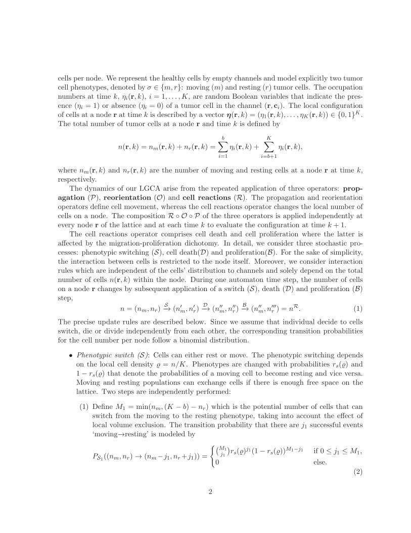
• Phenotypic switch (S): Cells can either rest or move. The phenotypic switching dependson the local cell density = n/K. Phenotypes are changed with probabilities rs() and1 − rs() that denote the probabilities of a moving cell to become resting and vice versa.Moving and resting populations can exchange cells if there is enough free space on thelattice. Two steps are independently performed:

(1) Define M1 = min(nm, (K − b) − nr) which is the potential number of cells that canswitch from the moving to the resting phenotype, taking into account the effect oflocal volume exclusion. The transition probability that there are j1 successful events‘moving→resting’ is modeled by

PS1((nm, nr) → (nm−j1, nr+j1)) =

{(M1

j1

)rs()

j1(1− rs())M1−j1 if 0 ≤ j1 ≤ M1,

0 else.

(2)

2

(2) Define M2 = min(nr, b− nm) which is the potential number of cells that can switchfrom the moving to the resting phenotype, taking into account the effect of localvolume exclusion. The transition probability that there are j2 successful events‘resting→moving’ is given by

PS2((nm, nr) → (nm+j2, nr−j2)) =

{(M2

j2

)(1− rs())

j2rs()M2−j2 if 0 ≤ j2 ≤ M2,

0 else.

(3)

Finally, the difference between successful switches ‘moving→resting’ and ‘resting→moving’is used to update the number of moving and resting cells so that (nm, nr) → (nm − (j1 −j2), nr + (j1 − j2)) = (n′

m, n′r). Note that the switching process does not change the total

number of cells but the ratio of moving and resting cells.

• Cell death (D): Each tumor cell is assumed to die with probability rd, independently fromthe other cells. Thus, the probability that j1 moving and j2 resting cells die, starting withn′ cells is

PD((n′m, n′

r) → (n′m− j1, n

′r − j2)) =

{(n′

j

)rjd(1− rd)

n′−j if j1 ≤ n′m and j2 ≤ n′

r, j = j1 + j2,

0 else.

(4)

• Cell proliferation (B): Birth of cells is dictated by the migration-proliferation dichotomy,which means that cells are allowed to proliferate only when they rest, i.e. when they arepositioned on a rest channel. In addition, there must be empty rest channels to placethe offspring into. Therefore, M = min(n′′

r , (K − b)− n′′r) defines the potential number of

resting cells that are allowed to proliferate starting from n′′ cells after the switch and deathprocesses. The transition probability that there are j new cells after the proliferation stepis then given by

PB((n′′m, n′′

r) → (n′′m, n′′

r + j)) =

{(Mj

)rjb(1− rb)

M−j if j′ ≤ M,

0 else.(5)

Altogether changes occurring in the cell number of a given node between two consecutive timesk and k + 1 can be encoded in a transition matrix P with

P = PSPDPB, (6)

where the entries of the transition matrix of the switch process PS is determined by (2) and (3),and the transition matrices PD and PB of the death and proliferation processes, respectively, aredefined by (4) and (5).

Subsequent to the cell reactions step, a reorientation step takes place where cells are randomlyredistributed to the channels, providing a new local cell configuration at each node. Because ofthe migration-proliferation dichotomy, only the cells of migratory phenotype move. Therefore,moving cells are distributed to the velocity channels, while resting cells are distributed to theresting channels, resulting in a configuration ηR◦O(r).

3

The final update step is the application of a propagation operator. Cells in the velocitychannels, i.e. moving cells, are transported one lattice unit in directions determined by theirvelocities. The movement of cells in the propagation step is purely deterministic. The spatio-temporal automaton dynamics is therefore completely described by the mircodynamical equation

ηi(r+ ci, k+1)− ηi(r, k) = ηR◦Oi (r, k)− ηi(r, k) ∈ {−1, 0, 1}, r ∈ L, i = 1, . . . ,K, k = 0, 1, . . . ,

(7)where the change in the occupation numbers is −1 if a channel looses a cell, 0 if nothing ischanged and 1 if a channel gains a cell, respectively.

2 Scaling of the LGCA

We have chosen a nondimensional scaling with unit lattice spacing and unit time scale k ∈ N inour LGCA simulation. Thus, cells residing at velocity channels move one lattice unit per unittime step. Our dimensionless simulations can easily be rescaled such that the temporal andspatial scales fit to specific applications. In our case, cell death and proliferation probabilitiesare related to the real dimensional average life time Td of a cell and the average cell cycle timeTb, respectively, by

rd(τ) =τ

Td, rb(τ) =

τ

Tb, (8)

where τ is a sufficient small real dimensional time step length. This scaling is chosen becauseof the following arguments, detailed for the case of cell death. Let X1,X2, . . . be independentBernoulli trials with possible outcomes “cell dies” (Xi = 1) and “cell survives” (Xi = 0). Thecorresponding probability distribution is given by P(Xi = 1) = rd. Let N be the number oftrials up to the first time a cell dies, i.e. N := min{n|X1 = . . . Xn−1 = 0,Xn = 1}. Then N isgeometrically distributed such that P(N = n) = (1− rd)

n−1rd with expected value E[N ] = 1/rd.If τ is the real dimensional time step length, the life time of a cell is given by τN . Hence,the average cell life time in the model is T = E[τN ] = τ/rd which must be related to the realdimensional average life time Td.

Similar arguments hold for the real macroscopic time taken for a cell to proliferate (cell cycletime) and for a cell to change its phenotype. Please note that if the LGCA parameters rs, rd andrb depend on time τ , the transition matrix of the the cell reactions becomes time-dependent:

P = P (τ) = PS(τ)PD(τ)PB(τ). (9)

Besides scaling the LGCA time intervals, also the lattice spacing can be adjusted. If thelattice spacing is ǫ, the mean square displacement of a cell per time step τ in the LGCA isproportional to ǫ2/τ . Thus, by scaling x = ǫr ∈ R, the relationship between the LGCA motilityand measured movement of cells is characterized by the diffusion constant D = ǫ2/τ .

3 Equilibrium state under fast switching assumption

When deriving the mean-field equation, we assume that the switch dynamics is much faster thanthe cell number changes due to proliferation and cell death, that is rs, 1− rs ≫ rb, rd. Further,

4

we consider the low density regime where the carrying-capacity effects can be neglected whenconsidering the switching. Then, by time scale separation, the fractions pσ := nσ/n, σ ∈ {r,m}of resting and moving cells, respectively, are in detailed balance with respect to the switchdynamics. This amounts to

pr(1− rs) = pmrs

= (1− pr)rs.

Hence pr = rs or, equivalently,nr = rsn. (10)

4 Mean-field approximation of the LGCA dynamics

The LGCA model is composed of a cell movement and a cell reaction process. In the following,we separate the two processes and derive mean-field approximations for each one. We show thatthe cell movement in the automaton model can be approximated by a degenerate diffusion term,while cell reaction in the automaton leads to a nonlinear reaction term in the resulting partialdifferential equation description.

4.1 Scaling limit of the cell reaction process

In the following, we are interested in the time evolution of the cell density. For that reason, weneglect any spatial dependence between nodes. We assume that the system is in equilibriumwith respect to the switching (fast switching assumption, see section 3). We consider the theMarkov process (Nk)k≥0 which describes the number of cells at a node r ∈ L in the discretephase space {0, . . . ,K}. The transition matrix of this process, derived from (6) with utilizationof (10), is given by W = WDWB, where

WD(i, j) =

{(ij

)(1− rd)

jri−jd if j ≤ i,

0 else(11)

and

WB(i, j) =

{(M

rsj−rsi

)rrsj−rsib (1− rb)

M−rsj+rsi if rsj − rsi ≤ M = min(rsi,K − i),

0 else,(12)

Here, the minimum function min(x,K − x) ≈ x(K − x) 1K, x ∈ (0,K). This approximation

underestimates the minimum function but provides an intuitive explanation as it describes thefraction of cells that are able to proliferate times the fraction of space that can be filled. Pleasenote that, for simplicity, we use a notation where the dependence of the switch function rs fromthe node density is dropped.

The probability to be in state j after one time step is

Pk+1(j) := P(Nk+1 = j) =K∑

i=0

W (i, j)P(Nk = i) =K∑

i=0

W (i, j)Pk(i)

5

and in matrix notationPk+1 = WPk.

The transition of a microscopic process to a macroscopic description requires a temporal scalingrelation between the macroscopic and microscopic variables (see section 2 for details). Weassume a small parameter τ > 0 that scales the time variable t = kτ such that

Pt+τ = W (τ)Pt,

where now the transition matrix W depends on the real dimensional time step size τ . Rearrang-ing terms gives

Pt+τ − Pt = (W (τ)− I)Pt,

Pt+τ − Pt

τ=

W (τ)− I

τPt.

Then, for τ ↓ 0∂

∂tPt = QPt (13)

with intensity matrix Q := limτ↓0

W (τ)−Iτ

= ∂∂τW (τ)

∣∣τ=0

. Since W (τ) = WD(τ)WB(τ) it follows

that

Q =∂

∂τW (τ)

∣∣∣∣τ=0

=

[(∂

∂τWD(τ)

)

WB(τ) +WD(τ)

(∂

∂τWB(τ)

)]∣∣∣∣τ=0

=∂

∂τWD(τ)

∣∣∣∣τ=0

+∂

∂τWB(τ)

∣∣∣∣τ=0

= QD +QB, (14)

where QD and QB are the intensity matrices for the death and birth processes, respectively. Adirect calculation gives

QD = limτ↓0

1

τWD(τ ; i, j) = lim

τ↓0

1

τ

{(ij

)(1− rd(τ))

jrd(τ)i−j if 0 ≤ j ≤ i,

0 else,

(8)= lim

τ↓0

1

τ

(ij

) (

1− τTd

)j (τTd

)i−j

if 0 ≤ j ≤ i,

0 else,

= limτ↓0

1Td

(il

) (

1− τTd

)j (τTd

)i−j

if 0 ≤ j ≤ i,

0 else,

=

{iTd

if j = i− 1,

0 else(15)

and similarly

QB = limτ↓0

1

τWB(τ ; i, j) =

{1Tbrsi

(1− i

K

)if rsj = rsi− 1,

0 else.(16)

6

From the master equation (13), the temporal evolution of the mean cell density ρt = 〈Nt〉/K isobtained by

∂

∂tρt =

1

K

K∑

j=0

j∂

∂tPt(j) =

1

K

K∑

j=0

jK∑

i=0

Q(i, j)Pt(i). (17)

=1

K

K∑

i=0

Pt(i)

K∑

j=0

jQ(i, j)

(14)=

1

K

K∑

i=0

Pt(i)K∑

j=0

jQD(i, j) +1

K

K∑

i=0

Pt(i)K∑

j=0

jQB(i, j)

(15),(16)=

1

K

1

Td

K∑

i=0

(−i)Pt(i) +1

K

1

Tb

K∑

i=0

rsi

(

1−i

K

)

Pt(i)

= −1

Tdρ+ rs

1

Tbρ− rs

1

K

1

Tb

K∑

i=0

i2Pt(i) (18)

Assuming that E[N2t ] = E[Nt]

2, which holds if the variance of Nt is small, for instance if K islarge, we finally arrive at a macroscopic description of the LGCA birth-death process

∂

∂tρt = −Rdρ+ rsRbρ(1− ρ), (19)

where Rd = 1/Td and Rb = 1/Tb are the real death and proliferation rates, respectively, seesection 2.

4.2 Scaling limit of the cell migration process

In the following, we consider the automaton cell migration process without cell reaction, underthe fast switching assumption, see section 3. In our LGCA, the probability of a cell to jumpfrom one node r to a neighboring node r+ ci is equal to the probability of a cell residing in therespective velocity channel. In the isotropic case, cells within velocity channels are redistributedwith probability 1/b. To connect the discrete mechanism with a continuum model we considerthe expected cell density of a node r at time k, defined by ρ(r, k) = 〈(r, k)〉, in the scaling limitwhen time step length and lattice spacing goes to 0.

The change in average occupancy of a moving cell at site r during the next time step is givenby

(20)ρ(r, k + 1) =

b∑

i=1

1− rs(ρ(r+ ci, k))

bρ(r+ ci, k) + rs(ρ(r, k))ρ(r, k),

where the terms can be interpreted as the probability that a cell at site r + ci, i = 1, . . . , b,is moving to site r and the probability that a moving cell at site r does not attempt to leavethe site. In the following, for simplicity, we will analyze a one-dimensional motility mechanismwhere motility events only take place in the horizontal direction. This approach can easily beextended to higher dimensions, because of the model isotropy.

7

In one dimension, equation (20) reduces to

ρ(r, k + 1) =1− rs(ρ(r− 1, k))

2ρ(r− 1, k) +

1− rs(ρ(r+ 1, k))

2ρ(r+ 1, k) + rs(ρ(r, k))ρ(r, k),

(21)

where the terms correspond to the probability that a cell at site r − 1 is moving and moves tothe right, the probability that a a cell at site r + 1 is moving and moves to the left and theprobability that a moving cell at site r does not attempt to leave the site. Approximation ofrs(ρ) around ρ ≪ 1 such that rs(ρ) = rs(0) + r′s(0)ρ+ r′′s (0)ρ

2 +O(ρ3), equation (21) becomes

(22)

ρ(r, k + 1) =1

2(ρ(r+ 1, k) + ρ(r− 1, k)) −

1

2rs(0)(ρ(r + 1, k) + ρ(r− 1, k))

−1

2r′s(0)(ρ

2(r+ 1, k) + ρ2(r− 1, k)) −1

2r′′s (0)(ρ

3(r+ 1, k) + ρ3(r− 1, k))

+ rs(0)ρ(r, k) + r′s(0)ρ2(r, k) + r′′s (0)ρ

3(r, k)

To convert (22) into a continuous macroscopic partial differential equation (PDE), we identify theaverage density ρ(r, k) by its continuous counterpart ρ(x, t), where x = rǫ ∈ R and t = kτ ∈ R+,with ǫ, τ ∈ R+, which gives

(23)

ρ(x, t+ τ) =1

2(ρ(x+ ǫ, t) + ρ(x− ǫ, t))−

1

2rs(0)(ρ(x + ǫ, t) + ρ(x− ǫ, t))

−1

2r′s(0)(ρ

2(x+ ǫ, t) + ρ2(x− ǫ, t))−1

2r′′s (0)(ρ

3(x+ ǫ, t) + ρ3(x− ǫ, t))

+ rs(0)ρ(x, t) + r′s(0)ρ2(x, t) + r′′s (0)ρ

3(x, t),

Expanding all terms in (23) in a truncated Taylor series in powers of ǫ and τ up to second ordergives

(24)

ρ+ τ∂tρ+τ2

2∂ttρ = ρ+

ǫ2

2∂xxρ− rs(0)ρ −

rs(0)ǫ2

2∂xxρ− r′s(0)ρ

2 − r′s(0)ǫ2(∂xρ)

2

− r′s(0)ρǫ2∂xxρ−

r′s(0)ǫ4

2(∂xxρ)

2 − r′′s (0)ρ3 − 3r′′s (0)ρǫ

2(∂xρ)2

−3r′′s (0)ǫ

2

2ρ2∂xxρ−

3r′′s (0)ǫ4

2(∂xρ)

2∂xxρ−3r′′s (0)ǫ

4

4ρ(∂xxρ)

2

−r′′s (0)ǫ

4

2(∂xxρ)

3 + rs(0)ρ + r′s(0)ρ2 + r′′s (0)ρ

3,

To proceed, we consider the diffusive limit, i.e. ǫ → 0, τ → 0 and limǫ,τ→0

ǫ2

τ= const := D. This

gives

(25)

∂tρ =D

2−

D

2rs(0)∂xxρ− r′s(0)D(∂xρ)

2 − r′s(0)Dρ∂xxρ− 3r′′s (0)Dρ(∂xρ)2 −

3D

2r′′s (0)ρ

2∂xxρ

= D∂xxρ

(1− rs(0)

2− r′s(0)ρ −

3

2r′′s (0)ρ

2

)

︸ ︷︷ ︸

=:D(ρ)

+D(∂xρ)2(−r′s(0)− 3r′′s (0)ρ

)

︸ ︷︷ ︸

=D′(ρ)

8

Finally, the jump process of our LGCA can be approximated by a degenerate diffusion equation

∂tρ = D∂x(D(ρ)∂xρ) . (26)

5 Kernel density estimation of the averaged cell density

The kernel density estimation, also known as Parzen-Rosenblatt density estimation, is a wellknown nonparametric way of estimating the probability density function underlying a finiteset of observations [1, 2]. We use a built-in Mathematica function to estimate the kerneldensity of the averaged cell density. For details see the Wolfram Demonstrations Projecthttp://demonstrations.wolfram.com/KernelDensityEstimation/and http://reference.wolfram.com/mat

6 Stability analysis of cell reaction mean-field equation

In the following we analyze the stability behavior of the macroscopic growth equation

∂tρ = F (ρ), (27)

withF (ρ) = rs(ρ)rbρ(1− ρ)− rdρ, (28)

where 0 < rd ≪ rb ≪ 1 and rs() =12(1 + tanh(κ(− θ))), ρ ∈ [0, 1], θ ∈ (0, 1) and κ ∈ R.

Obviously, ρ∗1 = 0 is a fixed point of (27) and

F ′(0) =rb2(1− tanh(κθ))− rd,

where

F ′(0)

> 0 if κ < 0,

> 0 if κ > 0 and 1− 2 rdrb

< tanh(κθ),

< 0 if κ > 0 and 1− 2 rdrb

> tanh(κθ).

(29)

Thus, the fixed point ρ∗1 = 0 is always unstable in the repulsive case (κ > 0). In the attractivecase (κ > 0), ρ∗1 = 0 is stable if and only if 1−2 rd

rb> tanh(κθ) but unstable if 1−2 rd

rb< tanh(κθ).

Now, for ρ > 0 we definef(ρ) := rbrs(ρ)(1− ρ)− rd, (30)

which is the per capita growth rate of F . Fixed points ρ∗ > 0 of equation (27) are equivalent tozeros of the function f(ρ) = 0, that is if they satisfy

rs(ρ)(1 − ρ) =rdrb. (31)

In addition, for fixed points ρ∗ of equation (27) it holds that

F ′(ρ∗) = rbrs(ρ∗)(1 − ρ∗)− rbρ

∗rs(ρ∗) + rbρ

∗(1− ρ∗)r′s(ρ∗)− rd

(31)= rbr

′s(ρ

∗)ρ∗(1− ρ∗)− rbrs(ρ∗)ρ∗

= f ′(ρ∗) ρ∗︸︷︷︸

>0

. (32)

9

Hence, the stability of a fixed point ρ∗ > 0 of (27) is determined by the slope of f at this root.An illustration of the stability behavior is given in Fig. 1.

In the repulsive case (κ < 0), the switch function rs(ρ) is monotonically decreasing andtherefore f is monotonically decreasing in [0, 1] as well. Since

f(0) = rb1

2(1− tanh(κθ)

︸ ︷︷ ︸

∈(−1,0)

)− rd > 0,

and f(1) = −rd < 0, function f has exactly one zero ρ∗2 and f ′(ρ∗2) < 0, see Fig. 1(a). Hence, inthe repulsive case, there exists exactly one fixed point ρ∗2 > 0 which is stable.

In the attractive case (κ > 0), the switch function is monotonically increasing and the percapita growth rate f has a local maximum in (0, 1), as illustrated in Fig. 1(b). If rs(ρ)(1− ρ) <rd/rb for all ρ, which is the case for very large θ values, function f has no zero. If values of ρexists for which rs(ρ)(1− ρ) > rd/rb, then the extistence of zeros depends on the value of f(0),

f(0) =rb2(1− tanh(κθ)

︸ ︷︷ ︸

∈(0,1)

)− rd

{

> 0 if 1− 2 rdrb

< tanh(κθ),

< 0 if 1− 2 rdrb

> tanh(κθ).(33)

In the first case, the function f has one zero for ρ∗2 ≈ 1 which is stable since f ′(ρ∗2) < 0 forρ∗2 ≈ 1. In the second case, the function f has two zeros, ρ∗2 ≈ 0 and ρ∗3 ≈ 1, which are unstableand stable, respectively, since f ′(ρ∗2) > 0 for ρ∗2 ≈ 0 and f ′(ρ∗3) < 0 for ρ∗3 ≈ 1.

Finally, we conclude that in the repulsive case (κ < 0), equation (27) has one unstable(ρ∗1 = 0) and one stable (ρ∗2 > 0) steady state. In the attractive case (κ > 0), three cases haveto be distinguished: Equation (27) has (i) one stable fixed point (ρ∗1 = 0) if rs(ρ)(1− ρ) < rd/rbfor all ρ, (ii) one unstable (ρ∗1 = 0) and one stable (ρ∗2 ≈ 1) fixed point if 1 − 2rd

rb< tanh(κθ)),

(iii) two stable (ρ∗1 = 0, ρ∗3 ≈ 1) and one stable (ρ∗2 ≈ 0) fixed points if 1 − 2rdrb

> tanh(κθ).In case (iii), the growth term (28) shows a bistable behavior and population extinction can beobserved for small densities if

rs(ρ) <rdrb

(34)

holds.

References

[1] Rosenblatt M (1959) Remarks on some nonparametric estimates of a density function. AnnMath Stat 27:832837.

[2] Parzen E (1962) On estimation of a probability density function and mode. Ann Math Stat33(3):10651076.

Figures

10

Figure 1: Stability analysis of the per capita growth rate function f defined in (30). The dottedline represents the constant value rd/rb. The colored lines represent the function rs(ρ)(1 − ρ)for different values of κ and θ. Intersection of both graphs indicate zeros of the function fwhich correspond to fixed points of the LGCA cell reaction mean-field equation (27). The signof the slope of function rs(ρ)(1 − ρ) at the intersection point reveals the stability behavior ofthe equivalent fixed point. (a) In the repulsive case (κ < 0), there is exactly one intersectionpoint. Parameters are κ = −12 and θ = 0.25. (b) In the attractive case (κ > 0), three casescan be distinguished: (i) no intersection point (red line, κ = 12, θ = 0.95), (ii) one intersectionpoint (blue line, κ = 12, θ = 0.05) or (iii) two (green line, κ = 12, θ = 0.25) intersection pointsbetween rd/rb and rs(ρ)(1 − ρ).

11