Electrica - İstanbul Üniversitesi

1

Electricaelectrica.istanbul.edu.tr Official journal of İstanbul University Faculty of Engineering

EISSN 2619-9831

VOLUME 18 » ISSUE 2 » 2018

I

Editorial Board

Advisory Board

Editor in Chief

Sıddık YARMANIstanbul University, Engineering Faculty, Electrical-Electronics Department

Associate Editors

Mukden UĞURAysel ERSOY YILMAZ

Assistant EditorAbdurrahim AKGÜNDOĞDU

AKAN Aydınİzmir Katip Çelebi University, TR

ALÇI EminBoğaziçi University, TR

ARSOY Aysen B.Kocaeli University, TR

BUYUKAKSOY AlinurOkan University, TR

CHAPARRLO Luis F.University of Pittsburg, USA

ÇİÇEKOĞLU OğuzhanBoğaziçi University, TR

DIMIROVSKI Gregory M.SSC. And Methodius University, MAC

FABRE AlainIMS-ENSEIRB Bordeux, FR

GÖKNAR I. CemDogus University, TR

HARBA RachildLESI, FR

HIZIROĞLU HüseyinKattering University, USA

KABAOĞLU Nihatİstanbul Medeniyet University, TR

KAÇAR FıratIstanbul University, TR

KALENDERLİ ÖzcanIstanbul Technical University, TR

KARADY GeorgeArizona State University, USA

KILIÇ RecaiErciyes University, TR

KIRKICI HülyaAuburn University, USA

KOCAARSLAN İlhanIstanbul University, TR

KUNTMAN AytenIstanbul University, TR

KUNTMAN HakanIstanbul Technical University, TR

MUMCU Tarık VeliIstanbul University, TR

METİN BilginBoğaziçi University, TR

OSMAN OnurIstanbul Arel University, TR

ÖNAL EmelIstanbul Technical University, TR

SANKUR BülentBoğaziçi University, TR

SENANI Raj,NSIT, India

SERTBAŞ AhmetIstanbul University, TR

ŞENGÜL MetinKadir Has University, TR

TAVSANOGLU VedatIşık University, TR

TSATSANIS MichailVoya Technology Institute, USA

TÜRKAY B. EmreIstanbul Technical University, TR

UÇAN Osman N.Istanbul Kemerburgaz University, TR

UZGÖREN GökhanGedik University, TR

YILDIRIM TülayYildiz Technical University, TR

YILMAZ ReyatDokuz Eylül University, TR

Secreteriat, Web CoordinatorATALAR Fatih,Istanbul University, TR

Publisherİbrahim KARA

Publication DirectorAli ŞAHİN

Finance and AdministrationZeynep YAKIŞIRER

Deputy Publication DirectorGökhan ÇİMEN

Editorial DevelopmentGizem KAYAN

Publication CoordinatorsBetül ÇİMENÖzlem ÇAKMAKOkan AYDOĞANİrem DELİÇAYBüşra PARMAKSIZ

Project AssistantsEcenur ASLIMNeslihan KÖKSALCansu ASLAN

Graphics DepartmentÜnal ÖZERDeniz DURAN

ContactAddress: Buyukdere Street No: 105/9 34394 Mecidiyekoy, Sisli, Istanbul, TURKEYPhone: +90 212 217 17 00Fax : +90 212 217 22 92E-mail : [email protected]

II

Aims and Scope

Electrica is an international, scientific, open access periodical published in accordance with independent, unbiased, and dou-ble-blinded peer-review principles. The journal is the official publication of İstanbul University Faculty of Engineering and it is published biannually on January and July. The publication language of the journal is English.

Electrica aims to contribute to the literature by publishing manuscripts at the highest scientific level on all fields of electrical and elec-tronics engineering. The journal publishes original research and review articles that are prepared in accordance with ethical guidelines.

The scope of the journal includes but not limited to; electronics, microwave, transmission, control sytems, electrical machines, energy transmission and high voltage.

The target audience of the journal includes specialists and professionals working and interested in all disciplines of electrical and electronics engineering.

The editorial and publication processes of the journal are shaped in accordance with the guidelines of the Institute of Electrical and Electronics Engineers (IEEE), the World Commission on the Ethics of Scientific Knowledge and Technology (COMEST), Council of Science Editors (CSE), Committee on Publication Ethics (COPE), European Association of Science Editors (EASE), and National Information Standards Organization (NISO). The journal is in conformity with the Principles of Transparency and Best Practice in Scholarly Publishing (doaj.org/bestpractice).

The journal is currently indexed in Web of Science-Emerging Sources Citation Index, Scopus, Compendex, Gale and TUBITAK ULAK-BIM TR Index.

All expenses of the journal are covered by İstanbul University. Processing and publication are free of charge with the journal. No fees are requested from the authors at any point throughout the evaluation and publication process. All manuscripts must be submitted via the online submission system, which is available at electrica.istanbul.edu.tr. The journal guidelines, technical infor-mation, and the required forms are available on the journal’s web page.

Statements or opinions expressed in the manuscripts published in the journal reflect the views of the author(s) and not the opin-ions of the Electrica editors, editorial board, and/or publisher; the editors, editorial board, and publisher disclaim any responsibility or liability for such materials.

All published content is available online, free of charge at electrica.istanbul.edu.tr. Printed copies of the journal are distributed free of charge.

İstanbul University Faculty of Engineering holds the international copyright of all the content published in the journal.

Editor in Chief : Sıddık YARMANAddress : İstanbul Üniversitesi Mühendislik Fakültesi Elektrik-Elektronik Mühendisliği Bölüm Başkanlığı Avcılar Kampüsü, Avcılar, İstanbul, TurkeyPhone : +90 212 4737070Fax : +90 212 4737064E-mail : [email protected]

Publisher : AVESAddress : Büyükdere Cad. 105/9 34394 Mecidiyeköy, Şişli, İstanbul, TurkeyPhone : +90 212 217 17 00Fax : +90 212 217 22 92E-mail : [email protected] page : avesyayincilik.com

III

Instructions for Authors

Electrica is an international, scientific, open access periodical published in accordance with independent, unbiased, and dou-ble-blinded peer-review principles. The journal is the official publication of İstanbul University Faculty of Engineering and it is published biannually on January and July. The publication language of the journal is English.

Electrica aims to contribute to the literature by publishing manuscripts at the highest scientific level on all fields of electricity. The journal publishes original research and review articles that are prepared in accordance with ethical guidelines.

The scope of the journal includes but not limited to; electronics, microwave, transmission, control sytems, electrical machines, energy transmission and high voltage.

The target audience of the journal includes specialists and professionals working and interested in all disciplines of electrical and electronics engineering.

The editorial and publication processes of the journal are shaped in accordance with the guidelines of the Institute of Electrical and Electronics Engineers (IEEE), the World Commission on the Ethics of Scientific Knowledge and Technology (COMEST), Council of Science Editors (CSE), the Committee on Publication Ethics (COPE), the European Association of Science Editors (EASE), and National Information Standards Organization (NISO). The journal conforms to the Principles of Transparency and Best Practice in Scholarly Publishing (doaj.org/bestpractice).

Originality, high scientific quality, and citation potential are the most important criteria for a manuscript to be accepted for publi-cation. Manuscripts submitted for evaluation should not have been previously presented or already published in an electronic or printed medium. The journal should be informed of manuscripts that have been submitted to another journal for evaluation and rejected for publication. The submission of previous reviewer reports will expedite the evaluation process. Manuscripts that have been presented in a meeting should be submitted with detailed information on the organization, including the name, date, and location of the organization.

Manuscripts submitted to Electrica will go through a double-blind peer-review process. Each submission will be reviewed by at least two external, independent peer reviewers who are experts in their fields in order to ensure an unbiased evaluation process. The editorial board will invite an external and independent editor to manage the evaluation processes of manuscripts submitted by editors or by the editorial board members of the journal. The Editor in Chief is the final authority in the decision-making process for all submissions.

The authors are expected to submit researches that comply with the general ethical principles which include; scientific integrity, collegiality, data integrity, institutional integrity and social responsibility.

All submissions are screened by a similarity detection software (iThenticate by CrossCheck).

In the event of alleged or suspected research misconduct, e.g., plagiarism, citation manipulation, and data falsification/fabrication, the Editorial Board will follow and act in accordance with COPE guidelines.

AuthorshipBeing an author of a scientific article mainly indicates a person who has a significant contribution to the article and shares the responsibility and accountability of that article. To be defined as an author of a scientific article, researchers should fulfil below criteria:

IV

• Making a significant contribution to the work in all or some of the following phases: Research conception or design, acquisi-tion of data, analysis and interpretation.

• Drafting, writing or revising the manuscript• Agreeing on the final version of the manuscript and the journal which it will be submitted• Taking responsibility and accountability of the content of the article

Outside the above mentioned authorship criteria, any other form of specific contribution should be stated in the Acknowledge-ment section.

In addition to being accountable for the parts of the work he/she has done, an author should be able to identify which co-authors are responsible for specific other parts of the work. In addition, authors should have confidence in the integrity of the contribu-tions of their co-authors.

If an article is written by more than one person, one of the co-authors should be chosen as the corresponding author for han-dling all the correspondences regarding the article. Before submission, all authors should agree on the order of the authors and provide their current affiliations and contact details. Corresponding author is responsible for ensuring the correctness of these information.

Electrica requires corresponding authors to submit a signed and scanned version of the authorship contribution form (available for download through http://electrica.istanbul.edu.tr) during the initial submission process in order to act appropriately on au-thorship rights and to prevent ghost or honorary authorship. If the editorial board suspects a case of “gift authorship,” the submis-sion will be rejected without further review. As part of the submission of the manuscript, the corresponding author should also send a short statement declaring that he/she accepts to undertake all the responsibility for authorship during the submission and review stages of the manuscript.

Electrica requires and encourages the authors and the individuals involved in the evaluation process of submitted manuscripts to disclose any existing or potential conflicts of interests, including financial, consultant, and institutional, that might lead to poten-tial bias or a conflict of interest. Any financial grants or other support received for a submitted study from individuals or institutions should be disclosed to the Editorial Board. Cases of a potential conflict of interest of the editors, authors, or reviewers are resolved by the journal’s Editorial Board within the scope of COPE guidelines.

The Editorial Board of the journal handles all appeal and complaint cases within the scope of COPE guidelines. In such cases, authors should get in direct contact with the editorial office regarding their appeals and complaints. When needed, an ombud-sperson may be assigned to resolve cases that cannot be resolved internally. The Editor in Chief is the final authority in the deci-sion-making process for all appeals and complaints.

When submitting a manuscript to Electrica authors accept to assign the copyright of their manuscript to İstanbul University Faculty of Engineering. If rejected for publication, the copyright of the manuscript will be assigned back to the authors. Electrica requires each submission to be accompanied by a Copyright Transfer Form (available for download at http://electrica.istanbul.edu.tr). When using previously published content, including figures, tables, or any other material in both print and electronic formats, authors must obtain permission from the copyright holder. Legal, financial and criminal liabilities in this regard belong to the author(s).

Statements or opinions expressed in the manuscripts published in Electrica reflect the views of the author(s) and not the opinions of the editors, the editorial board, or the publisher; the editors, the editorial board, and the publisher disclaim any responsibility or liability for such materials. The final responsibility in regard to the published content rests with the authors.

MANUSCRIPT PREPARATION

Manuscripts can only be submitted through the journal’s online manuscript submission and evaluation system, available at http://electrica.istanbul.edu.tr. Manuscripts submitted via any other medium will not be evaluated.

Manuscripts submitted to the journal will first go through a technical evaluation process where the editorial office staff will ensure that the manuscript has been prepared and submitted in accordance with the journal’s guidelines. Submissions that do not con-form to the journal’s guidelines will be returned to the submitting author with technical correction requests.

V

Authors are required to submit the following:

• Copyright Transfer Form,• Author Contributions Form, and

during the initial submission. These forms are available for download at http://electrica.istanbul.edu.tr.

Preparation of the ManuscriptTitle page: A separate title page should be submitted with all submissions and this page should include:

• The full title of the manuscript as well as a short title (running head) of no more than 50 characters,• Name(s), affiliations highest academic degree(s) and ORCID iD’s of the author(s),• Grant information and detailed information on the other sources of support,• Name, address, telephone (including the mobile phone number) and fax numbers, and email address of the corresponding

author,• Acknowledgment of the individuals who contributed to the preparation of the manuscript but who do not fulfill the author-

ship criteria.

Biography page: A separate page should be submitted providing short biographies of the contributing authors with their pho-tographs included.

Abstract: An abstract should be submitted with all submissions except for Letters to the Editor. The abstract of articles should be structured without subheadings. Please check Table 1 below for word count specifications.

Keywords: Each submission must be accompanied by a minimum of three to a maximum of six keywords for subject indexing at the end of the abstract. The keywords should be listed in full without abbreviations.

Manuscript TypesOriginal Articles: This is the most important type of article since it provides new information based on original research. The main text of original articles should be begun with an Introduction section and finalized with a Conclusion section. The remaining parts can be named relevantly to the essence of the research. Please check Table 1 for the limitations for Original Articles.

Review Articles: Reviews prepared by authors who have extensive knowledge on a particular field and whose scientific back-ground has been translated into a high volume of publications with a high citation potential are welcomed. These authors may even be invited by the journal. Reviews should describe, discuss, and evaluate the current level of knowledge of a topic in the field and should guide future studies. sections Please check Table 1 for the limitations for Review Articles.

Letters to the Editor: This type of manuscript discusses important parts, overlooked aspects, or lacking parts of a previously pub-lished article. Articles on subjects within the scope of the journal that might attract the readers’ attention, may also be submitted in the form of a “Letter to the Editor.” Readers can also present their comments on the published manuscripts in the form of a “Letter to the Editor.” Abstract, Keywords, and Tables, Figures, Images, and other media should not be included. The text should be unstructured. The manuscript that is being commented on must be properly cited within this manuscript.

Table 1. Limitations for each manuscript type

Type of manuscript Word limit Abstract word limit Reference limit Table limit Figure limit

Original Article 3500 250 (Structured) 30 6 7 or total of 15 images

Review Article 5000 250 50 6 10 or total of 20 images

Letter to the Editor 500 No abstract 5 No tables No media

VI

TablesTables should be included in the main document, presented after the reference list, and they should be numbered consecutively in the order they are referred to within the main text. A descriptive title must be placed above the tables. Abbreviations used in the tables should be defined below the tables by footnotes (even if they are defined within the main text). Tables should be created using the “insert table” command of the word processing software and they should be arranged clearly to provide easy reading. Data presented in the tables should not be a repetition of the data presented within the main text but should be supporting the main text.

Figures and Figure LegendsFigures, graphics, and photographs should be submitted as separate files (in TIFF or JPEG format) through the submission system. The files should not be embedded in a Word document or the main document. When there are figure subunits, the subunits should not be merged to form a single image. Each subunit should be submitted separately through the submission system. Images should not be labeled (a, b, c, etc.) to indicate figure subunits. Thick and thin arrows, arrowheads, stars, asterisks, and similar marks can be used on the images to support figure legends. Like the rest of the submission, the figures too should be blind. Any informa-tion within the images that may indicate an individual or institution should be blinded. The minimum resolution of each submitted figure should be 300 DPI. To prevent delays in the evaluation process, all submitted figures should be clear in resolution and large in size (minimum dimensions: 100 × 100 mm). Figure legends should be listed at the end of the main document.

EquationsThe equations must be stated separated from the text by a blank line. They should be numbered consecutively in parenthesis at the right side of the equation. Symbols and variables as well as in the main text should be written in italics while vectors and matrices should be written in bold type.

All acronyms and abbreviations used in the manuscript should be defined at first use, both in the abstract and in the main text. The abbreviation should be provided in parentheses following the definition.

When a product, hardware, or software program is mentioned within the main text, product information, including the name of the product, the producer of the product, and city and the country of the company (including the state if in USA), should be pro-vided in parentheses in the following format: “Discovery St PET/CT scanner (General Electric, Milwaukee, WI, USA)”

All references, tables, and figures should be referred to within the main text, and they should be numbered consecutively in the order they are referred to within the main text.

References

While citing publications, preference should be given to the latest, most up-to-date publications. If an ahead-of-print publication is cited, the DOI number should be provided. Authors are responsible for the accuracy of references. In the main text of the manu-script, references should be cited using Arabic numbers in square brackets. The reference styles for different types of publications are presented in the following examples.

Journal Article: J.K. Author, “Name of the article”, Abbrev. Title of Periodical, vol. x, no. x, pp. xxx-xxx, Abbrev. Month, year.

Book Section: J. K. Author, “Title of chapter in the book,” in Title of His Published Book, xth ed. City of Publisher, Country: Abbrev. of Publisher, year, ch. x, sec. x, pp. xxx–xxx.

Books with a Single Author: J.K. Author, “Title of the Book”, Abbrev. Of Publisher, City of Publisher, Country, Year.

Conference Proceedings: J. K. Author, “Title of paper,” in Unabbreviated Name of Conf., City of Conf., Abbrev. St ate (if given), year, pp. xxx-xxx.

Report: J. K. Author, “Title of report,” Abbrev. Name of Co., City of Co., Abbrev. State, Rep. xxx, year.

Thesis: J. K. Author, “Title of thesis,” M.S. thesis, Abbrev. Dept., Abbrev. Univ., City of Univ., Abbrev. State, year.

Standards: Title of Standard, Standard number, date.

VII

Manuscripts Accepted for Publication, Not Published Yet: J. K. Author, “Title of paper,” unpublished.

Manuscripts Published in Electronic Format: J. K. Au thor. (year, month). Title. Journal [Ty pe of medium]. volume(issue), pag ing i f g iven. A vailable: site/path/file

REVISIONS

When submitting a revised version of a paper, the author must submit a detailed “Response to the reviewers” that states point by point how each issue raised by the reviewers has been covered and where it can be found (each reviewer’s comment, followed by the author’s reply and line numbers where the changes have been made) as well as an annotated copy of the main document. Revised manuscripts must be submitted within 30 days from the date of the decision letter. If the revised version of the manuscript is not submitted within the allocated time, the revision option may be cancelled. If the submitting author(s) believe that additional time is required, they should request this extension before the initial 30-day period is over.

Accepted manuscripts are copy-edited for grammar, punctuation, and format. Once the publication process of a manuscript is completed, it is published online on the journal’s webpage as an ahead-of-print publication before it is included in its scheduled issue. A PDF proof of the accepted manuscript is sent to the corresponding author and their publication approval is requested within 2 days of their receipt of the proof.

Editor in Chief : Sıddık YARMANAddress : İstanbul Üniversitesi Mühendislik Fakültesi Elektrik-Elektronik Mühendisliği Bölüm Başkanlığı Avcılar Kampüsü, Avcılar, İstanbul, TurkeyPhone : +90 212 4737070Fax : +90 212 4737064E-mail : [email protected]

Publisher : AVESAddress : Büyükdere Cad. 105/9 34394 Mecidiyeköy, Şişli, İstanbul, TurkeyPhone : +90 212 217 17 00Fax : +90 212 217 22 92E-mail : [email protected] page : avesyayincilik.com

VIII

Contents

RESEARCH ARTICLES

121 Reducing Processing Time for Histogram PMHT Algorithm in Video Object Tracking Ahmet Güngör Pakfiliz

133 New Optimization Algorithms for Application to Environmental Economic Load Dispatch in Power Systems Özge Pınar Akkaş, Ertuğrul Çam, İbrahim Eke, Yağmur Arıkan

143 Field Programmable Gate Arrays Based Real Time Robot Arm Inverse Kinematic Calculations and Visual Servoing Barış Çelik, Ayça Ak, Vedat Topuz

151 Generalised Model of Multiphase Tesla’s Egg of Columbus and Practical Analysis of 3-Phase Design Atamer Gezer, Mehmet Onur Gülbahçe, Derya Ahmet Kocabaş

159 A Circuit Model-Based Analysis of Magnetically Coupled Resonant Loops in Wireless Power Transfer Systems Seyit Ahmet Sis

167 Hybrid Micro-Ring Resonator Hydrogen Sensor Based on Intensity Detection Kenan Çiçek

172 Cognitive AF Relay Networks over Asymmetric Shadowing/ Fading Channels in the Presence of Low-Rate Feedback Eylem Erdoğan

177 Exudates Detection in Diabetic Retinopathy by Two Different Image Processing Techniques Sara S. Aldeeb, Selçuk Sevgen

187 Investigation of The Effects of Eccentricity on Induction Motor via Multi-Resolution Wavelet Analysis Abdullah Polat, Abdurrahman Yılmaz, Lale Tükenmez Ergene

198 Modeling and Control of an Offshore Wind Farm connected to Main Grid with High Voltage Direct Current Transmission Ahmet Mete Vural, Auwalu İbrahim İsmail

210 ECEbuntu - An Innovative and Multi-Purpose Educational Operating System for Electrical and Computer Engineer-ing Undergraduate Courses

Bilal Wajid, Ali Rıza Ekti, Mustafa Kamal AlShawaqfeh

218 A Self-Tuning PID Control Method for Multi-Input-Multi-Output Nonlinear Systems Barış Bıdıklı

227 Dynamic Threshold Selection Approach in Voting Rule for Detection of Primary User Emulation Attack Abbas Ali Sharifi, Mohammad Mofarreh-Bonab

234 Probabilistic Placement of Wind Turbines in Distribution Networks Tohid Sattarpour, Mohammad Sheikhi, Sajjad Golshannavaz, Daryoush Nazarpour

242 Neural Network Based Classification of Melanocytic Lesions in Dermoscopy: Role of Input Vector Encoding Gökhan Ertaş

249 Chronic Kidney Disease Prediction with Reduced Individual Classifiers Merve Doğruyol Başar, Aydın Akan

256 Prefrontal Brain Activation in Subtypes of Attention Deficit Hyperactivity Disorder: A Functional Near-Infrared Spectroscopy Study

Miray Altınkaynak, Ayşegül Güven, Nazan Dolu, Meltem İzzetoğlu, Esra Demirci, Sevgi Özmen, Ferhat Pektaş

IX

Contents

263 Noise-Assisted Multivariate Empirical Mode Decomposition Based Emotion Recognition Pinar Özel, Aydın Akan, Bülent Yılmaz

275 Load Profile-Based Power Loss Estimation for Distribution Networks Nassim Iqteit, Ayşen Basa Arsoy, Bekir Çakır

284 A Canonical 3-D P53 Network Model that Determines Cell Fate by Counting Pulses Gökhan Demirkıran, Güleser Kalaycı Demir, Cüneyt Güzeliş

292 Design of a New Non-Singular Robust Control Using Synergetic Theory for DC-DC Buck Converter Yakoub Nettari, Serkan Kurt

300 MUSIC Algorithm for Respiratory Rate Estimation Using RF Signals Can Uysal, Tansu Filik

310 Cloning of Presenilin 2 cDNA and Construction of Vectors Carrying Effective Mutations in the Pathogenesis of Familial Alzheimer's Disease

Gözde Öztan, Baki Yokeş, Halim İşsever

321 Examination of Wind Effect on Adss Cables Aging Test İbrahim Güneş

REVIEW

325 Design of Micro-Transformer in Monolithic Technology for High Frequencies Fly-back Type Converters Abdeldjebbar Abdelkader, Hamid Azzedine

121

Electrica 2018; 18(2): 121-132

RESEARCH ARTICLE

Reducing Processing Time for Histogram PMHT Algorithm in Video Object TrackingAhmet Güngör Pakfiliz Department of Electrical and Electronics Engineering, Başkent University School of Engineering, Ankara, Turkey

Corresponding Author: Ahmet Güngör Pakfiliz

E-mail: [email protected]

Received: 27.08.2017

Accepted: 10.05.2018

© Copyright 2018 by Electrica Available online at http://electrica.istanbul.edu.tr

DOI: 10.26650/electrica.2018.36247

Cite this article as: Pakfiliz AG. “Reducing Processing Time for Histogram PMHT Algorithm in Video Object Tracking”, Electrica, vol. 18, no: 2, pp. 121-132, 2018.

ABSTRACT

This paper describes a novel approach for reducing the processing time of the histogram probabilistic multi-hypothesis tracker (H-PMHT) algorithm in video applications. Video data of flying vehicles is taken from surface to air, and a temporal difference-based technique is applied to video frames for meeting the intensity demands of H-PMHT algorithm. This technique also enables discrimination between objects and eliminates clutter. Variations between the structures of the standard and the improved version of H-PMHT algorithms are described. In addition, the improved H-PMPT is compared with the standard H-PMHT and another approved tracking algorithm to evaluate the performance and processing time reduction ratings.Keywords: Improved H-PMHT, Pixel Wise Difference, Surface to air, Video Tracking

Introduction

TRACKING requires high precision and real-time applications. For sensors taking continuous and bulky data streams such as video data, real-time operation is difficult to achieve using whole sensor data. When conventional tracking algorithms are used for video object tracking real-time may be achieved, but only at the expense of some level of precision due to transfor-mation of the data into a suitable measurement domain [1-3]. These transformations also take the physical shapes of the targets, which are projected onto the image frame, up to a level and convert them to point measurement, thus adding to measurement error. Coping with a high amount of data streams is necessary in order to reach high precision rates in video object tracking. Therefore, target shape and intensity-based algorithms get the edge on point-mea-surement trackers [4, 5]. Reliable and uninterrupted track information is essential for most of the applications, especially in a background of a high clutter environment and a lack of sen-sor capacity. In order to detect the target location from the data stream, high intensity pixel clusters should be searched from data streams, and it should be decided whether or not they emerge from target or clutter. H-PMHT is a feasible method for handling data streams, and for tracking objects reliably and uninterruptedly.

The H-PMHT is basically an Expectation Maximization (EM) based algorithm which was devel-oped for target tracking in dense clutter environment by processing a considerable amount of data streams [6]. H-PMHT is a track-before-detect (TkBD) algorithm and entire video data is used as the measurement. It processes detection and tracking operations simultaneously. H-PMHT maintains tracking performance for low SNR values, where the target is not easily distinguished from the noise-cluttered background of any given frame. The original H-PMHT assumes that the signature of each target in the sensor frame area is known. In this particular case, the signatures are in the Gaussian distribution, and the means of these Gaussians are linearly related to the states of the targets. In imagery applications, the target signature is the physical shape of the target projected onto the image frame. This shape can be time-varying and complicated [7]. H-PMHT provides considerably satisfactory results for one dimensional and two dimensional applications [8-10]. In these applications spreading of the target inten-

https://orcid.org/0000-0002-5901-228X

122

Electrica 2018; 18(2): 121-132Pakfiliz A.G. Reduction of H-PMHT Process Time

sities presents almost a linear-Gaussian distribution. Moreover, for non-linear and non-Gaussian applications a particular solu-tion is presented in with particle filters. In addition, a video tracking application is presented in with a specially processed video data, and a modified H-PMHT, which is called H-PMHT with Random Matrices (H-PMHT-RM) [11, 12].

The main purpose of this study is to reduce the processing time of the H-PMHT algorithm without deterioration in per-formance. For this purpose, we needed to obtain available and reliable measurement data in order to discriminate moving objects and represent them with a higher intensity area than the stationary background. Firstly, video data belonging to air vehicles is taken in true color (RGB) from surface to ground. Then a temporal difference processing technique is applied to filter moving objects from the stationary background. Thereby, proper data streams composed of moving objects and back-ground are obtained for processing with H-PMHT.

Two important obstacles need to be overcome to reduce the processing time of H-PMHT. One of them is the dynamic struc-ture of the video data, because in video tracking applications tracker processes data sequentially, not in a batch structure. The other is the long processing time, which is due to the structure of H-PMHT. By setting the batch number to one and replacing the smoother filter by a Kalman filter it becomes pos-sible to overcome the issue of data processing sequence. On the other hand, dealing with the long processing time is a chal-lenge. The aim of this study is not to completely eliminate this issue, but to reduce the processing time by improving H-PMHT algorithm. For this purpose, not only algorithm improvement, but also an amendment needs to take place in the basic struc-ture of the H-PMHT in order to reduce the processing time while continuing tracking and keeping estimation error within a reasonable limit. The resulting algorithm is called Improved H-PMHT (I/H-PMHT).

The tracking performance of I/H-PMHT for video data is given in the experimental study section. In this section, the obtained results are also compared in terms of processing time and esti-mation error with standard H-PMHT, and Interacting Multi Model Probabilistic Data Association with Amplitude Information (IM-MPDA-AI) algorithms for different conditions and cases [13].

Measurement Model

This study intends to reduce the processing time of H-PMHT al-gorithm. To that end, RGB video is taken for various aircrafts and each frame is processed separately according to time sequence. First of all, RGB images are converted into intensity images. Na-tional Television System Committee (NTSC) standard for trans-forming RGB to grayscale, defined in, is given as follows,

I x, y( ) = 0.2989R x, y( )+0.587G x, y( )+0.114B x, y( ) (1)

After that, pixel-wise difference function is obtained using a similar process as that described in [14, 15]. The aim of this process is to obtain frame data for frames k and k+Δ, then sub-tract them and take the absolute value of the difference. This

is followed by the thresholding process, and the remaining values give information about the movement. k represents the instantaneous frame time, and Δ represents the sampling peri-od of frames. As long as the object does not move too fast, the detected regions of the object are reduced. However, this pro-cess leaves a ghost where the object was located, and a large part of the object cannot be detected unless the object moves fast [16]. Additional processing is required to reduce the ghost effect by adapting the measurement data to the situation. For this purpose, we obtained the difference from the former to the following time sequence as follows.

Idif (x, y) = Ik (x, y)− Ik+Δ(x, y) (2)

There are two additional steps that must be performed to ob-tain the measurement model. The first step is thresholding the unwanted ghosts due to the former time k. As a result of the operation in equation (2), negative and positive intensity dif-ferences are obtained. Indeed, high magnitude negative values are out of the scope of this work, because they are the reflec-tions of former target echo. In order to get rid of these spurious intensities, negative values are converged to noise floor, and positive values are taken directly. Thus the intensity level of each cell M(x,y) is given as follows,

(3)M x, y( ) =

INoise_ floor + rand , Idif x, y( ) ≤ 0Idif x, y( ) = Idif x, y( ) , Idif x, y( ) > 0⎧⎨⎪

⎩⎪

where INoise_floor represents the intensity of the noise floor, which is defined as the intensity level of pixels that do not originate from the target or the clutter. Idif(x,y) represents the intensity of differences, and rand is the uniformly distributed pseudoran-dom number.

The second step taken in order to obtain the measurement mod-el is intensity pruning. The square root of M(x,y) values of intensi-ties are taken as in equation (4). Thus, an excessive increment in dynamic range and high intensity clutters are prevented.

(4)IPDIM x, y( ) = M x, y( )

The measurement model is achieved after obtaining pixel intensity levels for each pixel of the sensor area. Because the data is obtained using the difference of pixel intensities of the sequential video frames, it is defined as Pixel-wise Difference Intensity Modulated (PDIM) data. RGB images of sequential video frames of an aircraft, intensity images related to them, and resulting PDIM data image are given in Figure 1. The scan steps between them are 3 frames, in other words Δ=3.

Using PDIM method, stationary parts of the image can be elim-inated or reduced to acceptable levels, since intensity levels of

123


pixels related to stationary parts will remain the same at con-secutive times and the difference of the intensity levels will be zero, small motions on some parts of stationary objects or a slight vibration of camera will result in a non-zero difference level, and it is taken into calculations as background clutter. In this study PDIM data is used for surface to air video object tracking with improved H-PMHT algorithm.

Basic Structure of H-PMHT

The H-PMHT algorithm is introduced in [6, 8, 9] with its theory and derivations. Before entering the details of H-PMHT algo-rithm, its parametric TkBD structure is discussed. In tradition-al tracking methods, thresholding, clustering, extracting and

tracking procedures are carried out consecutively. On the oth-er hand, TkBD method performs all the steps concurrently [17, 18]. TkBD merges detection and estimation phases by eliminat-ing the detection algorithm from the process and supplying the whole sensor frame directly to the tracker. This increases trace accuracy and allows the tracker to keep track for low SNR targets [19]. The H-PMHT algorithm inherently includes the TkBD capability and makes it possible to obtain extended ob-ject traces directly from an image sequence.

Only a general structural outline for H-PMHT is given here. H-PMHT is mainly developed from PMHT, and all derivations of PMHT arise from Expectation Maximization (EM) method [20]. The purpose of using the EM process in the H-PMHT algorithm is to assign histogram distribution to the model components and to designate the precise position of the shots as missing data. It also allows for unobserved cells with abstract sensor pixels that do not convey any data. The probability of the miss-ing data is determined in the E-step and the state estimates are refined in the M-step. Initialization and iteration steps of H-PM-HT according to E and M-steps are given below.

Initialization of H-PMHT Algorithm

Initialization steps must be defined before iterations are de-scribed. At the beginning of each iteration mixing proportions (

π tk0( ) are determined for background and all target models (k=0,

1,…, M), and for batch sequence t = 1 = 1,K,T, for which T≥1 denotes the number of scans in a batch of measurement, as follows,

(5)π tk

0( ) > 0 and π t00( ) + π t1

0( ) +!+ π tM0( ) =1

In addition, for k =1,…,M , for which M≥1 denotes the number of targets, the following is initialized,

- Target State Sequence: x0k0( ) , x1k

0( ) ,…, xTk0( )

- Measurement Covariance Sequence: R1k0( ) ,…, RTk

0( )

- Target Covariance: Qk0( )

The H-PMHT algorithm consists of repeated iteration steps for each batch sequence t =1,…,T . Some of these iteration steps stem from Expectation and Maximization, the remainder comes from Kalman smoothing filter. Throughout the iterations the dynamic matrix F and measurement matrix H are assumed as constant or time invariant. Iteration steps with respect to Ex-pectation, Maximization, and Kalman smoothing processes are given in the following subsections.

Expectation

Step 1. Total Sensor Probabilities (TSPs)

First, Target Cell Probabilities (TCP) are calculated for batch length t=1,...,T for all cells ℓ=1,…,S and for all target models, including background k=0,1,…,M . S represents the number of

Figure 1. Proposal structure video images for an aircraft at k and k+3 frames (above); Intensity images of them [middle, and PDIM (bottom)] data obtained using them

K

124


whole cells in the sensor area. For the background and targets TCPs are calculated as follows,

(6)Ptkℓ

i+1( ) =

1S

if k = 0

N τ ;Htk xtki( ) , Rtk

i( )( )dτ if k =1,…,MBℓ t( )∫

⎧

⎨⎪⎪

⎩⎪⎪

where τ represents the variable term of N(∙) Gaussian PDF.

Total cell probabilities are obtained by summing the product of TCPs and mixing proportions for all target models and back-ground as in equation (7).

(7)Ptℓi+1( ) = π tk

i( )Ptkℓi+1( )

k=0

M

∑

Finally, TSPs are attained using only displayed cells or cells with measurement ℓ=1,…,L(t) as follows;

(8)Pti+1( ) = Ptℓ

i+1( )

ℓ=1

L t( )

∑

Step 2. Expected Measurements (EMs)

EMs are calculated as in equation (9) for t=1,...,T, and ℓ=1,…,S.

(9)ztℓi+1( ) =

ztℓ 1≤ ℓ ≤ L t( )

ZtPtℓi+1( )

Pti+1( )

⎛

⎝⎜⎜

⎞

⎠⎟⎟ L t( )+1≤ ℓ ≤ S

⎧

⎨⎪⎪

⎩⎪⎪

where Zt represents L1 norm of displayed cells B1 t( ) ,…,BL(t ) t( ) and it is defined as follows,

Zt = ztℓℓ=1

L t( )

∑ (10)

Maximization

Step 3. Cell-level Centroids (CCs):

CCs are calculated by using equation (11).

(11)!ztkℓi+1( ) =

1Ptkℓi+1( ) τ N τ ;Htk xtk

i( ) , Rtki( )( )

Bℓ t( )∫ dτ

Using CCs, synthetic measurements are obtained as follows;

!ztki+1( ) =

ztℓi+1( ) ℘tkℓ( )⎡

⎣⎤⎦!ztkℓ

i+1( )ℓ=1

S∑

ztℓi+1( ) ℘tkℓ( )⎡

⎣⎤⎦ℓ=1

S∑

→ ℘tkℓ =Ptkℓi+1( )

Ptℓi+1( )

⎧⎨⎪

⎩⎪

⎫⎬⎪

⎭⎪

(12)

Step 4. Synthetic Covariance Matrices

Synthetic measurement matrices given in equation (13) are ob-

tained for t = 1,...,T, and k = 1,...,M.

(13)!Rtki+1( ) =

Rtki( )

π tki( ) ztℓ

i+1( ) ℘tkℓ( )⎡⎣

⎤⎦ℓ=1

S∑

Also, for t = 0,1,...,T–1 synthetic measurement covariance ma-trices are calculated as follows:

(14)!Qtki+1( ) =

Pt+1i+1( )

Zt+1Qk

i( )

Step 5. Mixing Proportions

Mixing proportions are calculated for t = 1,...,T and k = 0,1,...,M:

(15)π tki+1( ) =

π tki( ) ztℓ

i+1( ) ℘tkℓ( )⎡⎣

⎤⎦ℓ=1

S∑π t ʹk

i( ) ztℓi+1( ) ℘tkℓ( )⎡

⎣⎤⎦ℓ=1

S∑

ʹk =0

M∑

Kalman Smoothing Filter

To obtain estimated target states a Kalman smoother filter is applied. This portion of the algorithm is composed of forward and backward filters.

Step 6. Forward Filter

The forward Kalman smoother filter for t=0, 1,…, T-1 is applied using synthetic measurements in order to refine target state es-timates. At this point dummy expectation is taken as !y00

i+1( ) k( ) = 0 and dummy covariance is P00

i+1( ) k( ) = 0 . The equations of forward filter are given in (16)-(18)

Pt+1ti+1( ) k( ) = FPt t

i+1( ) k( )F ∗ + !Qtki+1( )

(16)

Wt+1i+1( ) k( ) = Pt+1t

i+1( ) k( )H H Pt+1ti+1( ) k( )H ∗ + Rt+1,k

i+1( )( )−1

(17)

Pt+1t+1i+1( ) k( ) = Pt+1t

i+1( ) k( )−Wt+1i+1( ) k( )H Pt+1t

i+1( ) k( ) (18)

!yt+1t+1i+1( ) k( ) = F!yt t

i+1( ) k( )+Wt+1i+1( ) k( ) !zt+1,k

i+1( ) −H!yt ti+1( ) k( )( )

(19)

where Wt+1(i+1) is filter gain, and F is state transition matrix,

which are defined in [4, 5].

125


Step 7. Backward Filter

The equation of backward filter for t = T – 1,....1 is given as follows:

(20)

xtki+1( ) = !yt t

i+1( ) k( )+ Pt ti+1( ) k( )F ∗ Pt+1t

i+1( ) k( )( )−1

In( )where In = xt+1,k

i+1( ) − F!yt ti+1( ) k( )

Step 8. Estimated Covariance Matrices

First cell-level measurement covariance is calculated,

(21)Rtkℓi+1( ) =

N τ ;Htk xtki( ) , Rtk

i( )( )E E∗ dτBℓ t( )∫

Ptkℓi+1( )

where E = τ −Htk xtki+1( )

The estimated measurement covariance matrix is calculated as given in equation (22):

(22)Rtki+1( ) =

ztℓi+1( ) ℘tkℓ( )⎡

⎣⎤⎦ℓ=1

S∑ Rtkℓ

i+1( )

ztℓi+1( ) ℘tkℓ( )⎡

⎣⎤⎦ℓ=1

S∑

And the last operation shown in equation (23) of the iteration is to obtain estimated target covariance matrices for all the target models except for the background.

(23)Qk

i+1( ) =

ZtPti+1( )

⎛

⎝⎜⎜

⎞

⎠⎟⎟ xtk

i+1( ) − Fxt−1,ki+1( )( ) xtki+1( ) − Fxt−1,k

i+1( )( )∗

t=1

T∑

ZtPti+1( )

⎛

⎝⎜⎜

⎞

⎠⎟⎟t=1

T∑

Variations of the Algorithm

Histogram probabilistic multi-hypothesis tracker is a strong and reliable tracking algorithm and originally developed for data streams. However, it is not conformed to real time appli-cations. The aim of this study is to converge real time tracking or reduce the processing time of H-PMHT algorithm without terminating tracking for video applications. First of all, video data is converted to PDIM data in order to clutter effects and enhance target detectability. Then some improvements are ap-plied to mathematical operations, in particular by taking the practical advantage of two-dimension, and also some amend-ments are applied to the algorithm itself. This work was done by adding intensity information that can be thought of as a third dimension in two-dimensional space. For this reason, this study is regarded as a two-dimensional application and the assumptions in [10] can be implemented. The most important aspect of these assumptions is that x and y axes are statisti-

cally independent of each other. Another assumption for the process is that there is no pre-information about point spread function of the objects. They mostly retain their original shape and this shape is not similar to linear-Gaussian distribution.

It will be proper to state that there is no revision on the se-quence of EM based iteration steps. The main difference takes place in the batch structure of EM iteration. In this study batch structure is eliminated and its structure is converted to single scan algorithm. To overcome a priori information absence, a priori density obtained via earlier measured data is used as stated in [6]. Using single scan structure is more viable than batch structure for converging real-time video object tracking applications. By using single scan structure, smoothing filter turns to Kalman Filter (KF), but in this case not much processing time reduction takes place. This is the first step for the reduc-tion of processing time. The improvements and amendments are described separately in the following subsections.

Operational Improvements

In this section, no algorithmic amendments, but operation im-provements of the algorithm are described. To achieve this aim the batch structure is turned into single scan algorithm, but multi iteration structure is preserved. The inspected part in this section is the most time-consuming fragment of the H-PMHT process which is spent in calculation of integration operations. These operations are

- Target Cell Probabilities Ptkℓi+1( ) ,

- Cell Level Centroids ztkℓi+1( ) ,

- Cell Level Meas. Covariance Contributions Rtkℓi+1( )

.

In two-dimensional case these three expressions are normally calculated for x and y axes separately, then corresponding values of each pixel are multiplied with each other to obtain the overall value. The total number of integration (NoI) is calculated by sum-ming up NoI of the above three expressions. In this context NoI of a sensor area with “200 x 200 pixels” is calculated as follows.

For x-axis:

NoI Ptkℓ xi+1( ) = NoI !ztkℓ x

i+1( ) = NoI Rtkℓ xi+1( ) = 40000

For y-axis:

NoI Ptkℓ yi+1( ) = NoI !ztkℓ y

i+1( ) = NoI Rtkℓ yi+1( ) = 40000

For two dimensions:

NoI Ptkℓi+1( ) = NoI !ztkℓi+1( ) = NoI Rtkℓi+1( ) = 2×40000

= 80000Total NoI:

Total − NoI = 6×80000 = 480000

126


This phase increases the process time exponentially for linear increasing of sensor dimensions. To decrease the processing time, an improvement method is applied to H-PMHT operation in order to obtain Target Cell Probabilities, Cell Level Centroids, and Cell Level Measurement Covariance Contributions. For this purpose, only the elements of the first row of x axis contribu-tion and only the elements of the first column of y axis contri-bution are calculated. Thus, NoI for sensor area with “200 x 200” pixels can be shown as follows.

For x-axis:

NoI Ptkℓ xi+1( ) = NoI !ztkℓ x

i+1( ) = NoI Rtkℓ xi+1( ) =

No.of RowNoR( )

For y-axis:

NoI Ptkℓ yi+1( ) = NoI !ztkℓ y

i+1( ) = NoI Rtkℓ yi+1( ) =

No.of ColumnNoC( )

For two dimensions:

NoI Ptkℓi+1( ) = NoI !ztkℓi+1( ) = NoI Rtkℓi+1( ) = NoR+ NoC

= 2×200 = 400 Total NoI:

Total − NoI = 6× pixel − no.= 6×400 = 2400

After finding the elements of the first row of x axis contribution for the three expressions, we then selected the other rows in the same way as the first row and established Target Cell Prob-abilities, Cell Level Centroids, and Cell Level Measurement Co-variance Contributions. Similarly, for y axis contribution, other columns are taken in the same way as the first column. In fact, the results obtained by taking integration for whole pixels of the sensor area using the classical method is the same as the reduced one. Thus, the NoI reduces from 480000 to 2400. A remarkable reduction in processing time is obtained and no reduction in accuracy occurs Applying this improvement ap-proximately 34 - 63% (differs for different sensor area) process time reducing with respect to standard H-PMHT is obtained. The results are given in the experimental study section.

Algorithm Amendments

In addition, some algorithm amendments were used in order to decrease processing time and adjust the algorithm structure to dynamic and real time conditions. These amendments are given in the following items.

Item 1. First of all, the batch structure of the H-PMHT algorithm is converted to single scan algorithm, and the algorithm be-comes more suitable for dynamic applications, such as video object tracking [19]. A result of this conversion that backward filter is removed and the smoothing filter turns into KF. Because smoother filer turns to KF, the estimated target states !yt|t

( i+1) (k) and dummy covariance matrix ( 1)

| ( )it tP k+ are picked up from

the previous frame step instead of initiate them for each itera-

tion. Also, the initiation process is eliminated and the output of the previous time will be the input of the next time.

Item 2. Reducing iteration number is another amendment for reducing processing time. But reducing iteration number with-out taking necessary measures may be resulted with conver-gence insufficiency of state estimates to true position. In order to mitigate this risk, measurement covariance sequences in the initialization phase Rtk

0( ) are selected compatible with the tar-gets. Compatible means selecting initial measurement covari-ance low for small targets, and high for large targets.

Item 3. In order to reduce iteration number without increasing the estimation error more than an allowable amount, an addi-tional measure is taken. In the fundamental theory of H-PMHT [6], some expressions are calculated for only displayed cells (B1(t),...,BL(t)(t)), without using the truncated ones (BL(t)+1(t),...,BS(t)). These expressions are; L1 norm of measurements tZ , total sensor probabilities Pt

i+1( ) , and expected measurements ztℓi+1( )

. The border level between displayed and truncated cells can be regarded as threshold level which comes from the struc-ture of H-PMHT. In fact, this is not exactly a threshold, because truncated cells are also counted in the calculations except the above expressions. Thus it may be called as Displayed Cell Threshold-DCT. Selecting a higher DCT value will reduce the number of steps required to converge the state estimates to the correct position. On the other hand, increasing the DCT ex-cessively may cause some target-based measurements to be incomplete.

Item 4. Using compatible initial measurement covariance Rtk0( )

and proper DCT, the iteration number may be reduced to one, and an additional reduction in processing time can be reached. Calculation of estimated measurement matrix Rtk

i+1( ) is not nec-essary for one iteration case.

-By using compatible initial measurement covariance Rtk0( ) and

proper DCT, iteration number may be reduced to one, and an additional reduction in processing time can be reached. Calcu-lation of estimated measurement matrix Rtk

i+1( ) is not necessary for one iteration case.

After making these amendments approximately 8 -29% addi-tional process time reducing (differs for different sensor area) is obtained. This reduction takes place after operational im-provement, and the reduction rate is based on the CPU time of operational improvement applied H-PMHT, not the total CPU time rate. This case is different from operational improvements, because algorithm amendments result in sacrificing some ac-curacy, especially in low DCTs.

At the end of the improvement and amendment process the total decreasing process time converges to approximately 65%. The reduction amount decreases with big sensor area, and it increases with small sensor area. The detailed results are also given in the simulation section. The new version of the al-gorithm is named as improved H-PMHT (I/H-PMHT), and sche-matic structure is given in Table 1.

127


Experimental Study

The experimental trials were conducted for different scenari-os of single aircraft and chopper videos taken from surface to air. Video data was captured in true color (RGB) format with “640x480” pixels, using a 14.1 Mega-pixel camera. In the simu-lations the dimensions of sensor areas are selected “200x200”, “250x250”, and “300x300” pixels in order to evaluate CPU reduc-tion rate for different sensor areas.

The study is conducted in two-dimensional case, and the as-sumptions made in [10] are used. Additionally, pre-information about point spread function of the objects does not exist. They mostly retain their original shape and these shapes are quite different from the linear-Gaussian distribution.

To perform the operation, first the PDIM data is obtained us-ing the video data taken from surface to air in daylight. Then tracking process is applied to each PDIM data using I/H-PMHT algorithm. For benchmarking the obtained results in terms of process time reduction and performance each scenario is re-applied to standard H-PMHT and a trustworthy probabilistic algorithm IMMPDA-AI. This algorithm is a combination of IMM estimator and PDA technique [4, 5], and by adding amplitude information, the results obtained with IMMPDA-AI will be prop-er for a fair comparison with the results of I/H-PMHT. Thus, pro-cessing time shortening and tracking performances of I/H-PM-HT are compared with the counterparts of standard H-PMHT and IMMPDA-AI.

Table 1. Structural Comparison between Standard H-PMHT and I/H-PMHT

Phase of the Algorithms Standard H-PMHT

I/H-PMHT Multi Iteration (Only Operational

Improvement)

I/H-PMHT One Iteration (Both Operational Improvement and

Algorithmic Amendment)

Initialization for batch length t = 1,....T

x0k0( ) , x1k

0( ) ,…, xTk0( )

π t00( ) + π t1

0( ) +!+ π tM0( )

R1k0( ) ,…, RTk

0( ) and Qk0( )

no batch for each scan

xtk0( ) , π tk

0( )

Rtk0( ) and Qk

0( )

no batch for each scan

xtk , π tk

Rtk0( ) and Qk

0( )

ExpectationPtkℓi+1( )

, Ptℓi+1( )

Pti+1( ) , ztℓ

i+1( )

Ptkℓi+1( ) (Operational impr.)

Ptℓi+1( ) , Pt

i+1( ) , ztℓi+1( )

Ptkℓi+1( ) (Operational impr.)

Ptℓi+1( ) , Pt

i+1( ) , ztℓi+1( )

Maximization!ztkℓi+1( )

, ztki+1( )

,

!Rtki+1( )

, !Qtki+1( )

, π tk

i+1( )

!ztkℓi+1( )

(Operational impr.)

ztki+1( )

, !Rtki+1( )

!Qtki+1( )

, π tk

i+1( )

!ztkℓi+1( )

(Operational impr.)

ztki+1( )

, !Rtki+1( )

!Qtki+1( )

, π tk

i+1( )

Kalman Smoothing Filter Forward Filter

!yt+1|t+1( i+1) (k)

Backward Filter

xtki+1( )

Forward Filter

xtki+1( )

Backward Filter (No Backward Filter)

Forward Filter

xtki+1( )

Backward Filter (No Backward Filter)

Covariance EstimationRtkℓi+1( )

Rtki+1( )

Qtki+1( )

Rtkℓi+1( ) (Operational impr.)

Rtki+1( )

Qtki+1( )

Rtkℓi+1( ) (not necessary)

Rtki+1( ) (not necessary)

Qtki+1( )

128


Interacting Multi Model Probabilistic Data Association with Am-plitude Information is a point tracker method. PDIM data was adapted to meet the requirements without violating fair com-parison. To obtain measurement data suitable with IMMPDA-AI, first the mean value of total sensor area (say, nxn) intensity ratio ( SAI ) is calculated. Threshold is selected 10% higher than the mean value, and the resulting value is taken as amplitude infor-mation threshold (TAI ). Hence the number of point measurements is brought into a reasonable level for comparison. Then the whole the sensor area is divided into 5x5 pixel units and mean intensity values of each pixel unit ( PUI ) are calculated as follows,

(24)

ISA =I x, y( )all−pxl∑

n× nTAI =1.1× ISA

IPU 5×5( ) =I x, y( )5×5∑5×5

The mean intensity values of each pixel unit compare with the threshold magnitude. If the mean intensity of a pixel unit is great-er than the threshold of amplitude information IPU ≥TAI

then

it is accepted as a measurement, otherwise it is not taken as a measurement. For each measurement, the mean intensity of the related pixel unit (

PUI ) is taken as amplitude information.

In the experimental study the target parameters of interest are the location and velocity according to x and y axes, and the state vector is as follows,

(25)Xtk = xtk xtk( )•

ytk ytk( )•⎡

⎣⎢⎢

⎤

⎦⎥⎥

T

at time t and for target k. k = 1 is selected because single target is assumed. For the obtained four-state Markov model, state transition and process covariance matrices are as follows:

(26)F =

1 ∆ 0 00 1 0 00 0 1 ∆0 0 0 1

⎡

⎣

⎢⎢⎢⎢

⎤

⎦

⎥⎥⎥⎥

Qk =σ2

∆3 3 ∆2 2 0 0∆2 2 ∆ 0 00 0 ∆3 3 ∆2 20 0 ∆2 2 ∆

⎡

⎣

⎢⎢⎢⎢⎢

⎤

⎦

⎥⎥⎥⎥⎥

where Δ represents the frame numbers between samples of video data, and σ is the process noise standard deviation or scale factor as defined in [21]. Measurement matrix H, and mea-surement covariance matrix Rtk are defined as follows:

(27)H = 1 0 0 00 0 1 0

⎡

⎣⎢

⎤

⎦⎥ Rtk = ρ

2 1 00 1

⎡

⎣⎢

⎤

⎦⎥

where ρ2 is measurement error variance.

The performances of I/H-PMHT, standard H-PMHT and IMMP-DA-AI were analyzed using real-life records surface to air vid-eo data with single chopper or aircraft. Various scenarios were employed to assess the performances of algorithms in differ-ent environments, speeds and target geometries. The envi-ronmental conditions directly affect the signal-to-noise ratio (SNR), so different SNR values are used in the study. In addition to different aircraft types, different speed ratios, different pix-el propagation levels and deviations from the linear-Gaussian shape were also taken into account. In order to establish PDIM data, different frame numbers between samples (Δ) were also used. Each scenario was defined for 20 scans. Also, four iter-ations were used for both standard H-PMHT and operational improvements applied I/H-PMHT. Thus, an optimal operation was reached, which means sufficient convergence of state es-timates to target centroids was obtained without excessively increasing CPU time. Generalized scenario parameters are sum-marized in Table 2.

Before submitting the performance results of the tracking process for the inspected scenarios, state estimations of the algorithms and target trajectory for a particular scenario are presented. In this way we aimed to show the tracking perfor-mance after operational improvement and algorithmic amend-ment. Target centroids and estimation trajectories only of oper-ational improvement applied I/H-PMHT, standard H-PMHT and

Table 2. General Summary of the Simulation Scenarios

Scenario Number

No.of Sampling Frame (Δ)

Sensor Area (pxl2)

Area of Air Object

(pxl2)

Mean Velocity

(pxl/frame)Noise Level (PDIM) (dB)

SNR (PDIM) (dB)

Noise Level (AI) (dB)

SNR (AI) (dB)

1 4 250x250 240 2.5 1 8.8 0.84 8.1

2 3 300x300 126 3.8 0.75 8.9 1.17 7.85

3 3 250x250 280 3.3 0 9.89 0.46 8.35

4 2 200x200 78 3 0 8.54 0 6.15

5 2 200x200 88 2.5 0.67 8.3 0.6 5.7

6 3 250x250 40 1.35 0.98 9.74 1.34 6.5

7 3 250x250 434 3.5 1.15 9.93 1.7 7.96

8 2 250x250 450 4.23 0 9.8 0.5 8.26

129


IMMPDAFAI algorithms throughout the fifth scenario are given in Figure 2. The figures are given for Displayed Cell Threshold (DCT) 5 dB over noise level.

Moreover, in Figure 3 the estimation trajectories were obtained using four iterations for standard H-PMHT and one iteration for I/H-PMHT. In this case I/H-PMHT was subjected to both oper-ational improvements and algorithm amendments, and DCT was selected 5 dB.

The performances of the algorithms are evaluated by hit on the target (HoT), and RMS position estimation error with respect to target centroid. If HoT is greater than 80%, tracking process is as-sumed as successful. After evaluating the performances of the al-gorithms, processing time is taken into account. Processing time is represented with CPU time, and this value is taken as a third

component for evaluation. The processor of the computer used in simulations is Intel-Core i5-3470 CPU with 4 cores at 3.20 GHz. The computer has 4 GB RAM, the OS is Win 7 Professional, and its instruction set is 64-bit. In Table 3 simulation results of algorithms with respect to scenarios are given for evaluation and compari-son. In the table mean values of the algorithms RMS estimation errors with reference to target centroids throughout the scenari-os are given as deviation from target centroid (Dev.Trg.Cent.).

Histogram probabilistic multi-hypothesis tracker and I/H-PMHT simulations were conducted for two different Displayed Cell Threshold (DCT) levels, which are 3 dB and 5 dB over noise level. For amplitude information of point measurement data, which is used in IMMPDA-AI simulations, AI Threshold (AIT) levels were also selected 3 dB and 5dB over noise level. A fair comparison was made between the performances of the algorithms.

The results obtained in the simulation study are summarized as follows;

- The simulation results show that standard H-PMHT and only operational improvement applied I/H-PMHT both outperform on IMMPDA-AI in terms of estimation error and HoT for whole scenarios. If we compare the results obtained with I/H-PMHT (operational improvement and algorithmic amendment ap-plied) and the results obtained with IMMPDA-AI, they show similar performance for DCT 3 dB over noise level, and I/H-PM-HT shows better performance for DCT 5 dB over noise level. In terms of processing time, IMMPDA-AI is unquestionably supe-rior to the other algorithms. After attempting the operational improvement and algorithmic amendment, I/H-PMHT provides a respectable processing time decrease, but is still not suffi-cient for real-time tracking.

- When only operational improvement is applied, standard H-PMHT gives better results than I/H-PMHT at 3 dB higher level DCT, and worse results at 5 dB higher level DCT. The only excep-tion takes place in the sixth scenario, which has a relatively small object area. These results show that only operational improve-ment applied I/H-PMHT (single scan, multi iteration structure) is more suitable for video object tracking than the standard H-PM-HT algorithm. In this case CPU time reduction is relatively high.

- When both operational improvement and algorithmic amend-ment occur standard H-PMHT outperforms I/H-PMHT for 3 dB higher level DCT. On the other hand, for 5 dB higher level DCT the performance of I/H-PMHT is similar to the performance of the standard H-PMHT, and outperforms for high intensity tar-get cases (scenarios 1, 6, 7).

- Using PDIM data with Standard H-PMHT and I/H-PMHT gives satisfactory results, and this shows that PDIM data is suitable for video object tracking.

- When the decreased processing time is taken into account from Standard H-PMHT to only operational improvement ap-plied I/H-PMHT, and both operational improvement and algo-rithmic amendment applied to I/H-PMHT, then the amount of increased or decreased estimation error rate must also be tak-

Figure 2. Target Centroids and State Estimations throughout Sce-nario 5 (only operational improvement is applied to I/H-PMHT)

Figure 3. Target Centroids and Estimations throughout Scenario 5 (applied both operational improvements and algorithm amend-ment to I/H-PMHT)

130


en into account. For this purpose, Table 4 was prepared using the results of the simulation study.

Table 4 shows that a decrease in processing time is directly re-lated to the sensor area. In wider sensor areas processing time decreasing is low, and vice versa. Also converging to target cen-troids with standard H-PMHT occurs rapidly for small sensor ar-eas (scenarios 4 and 5), even if target intensities are not high. I/H-PMHT requires high target intensities, and especially for DCT’s 5 dB higher than noise level has sufficient success. Esti-mation errors of I/H-PMHT obtained for all scenarios are within acceptable limits for track continuation.

Conclusion

This study has provided a new approach for reducing the CPU time of H-PMHT algorithm. For this purpose, operational im-

provement and algorithmic amendment processes were applied to standard H-PMHT algorithm, and I/H-PMHT algorithm was ob-tained. Measurement data used in the study is defined as PDIM data. The PDIM data was obtained from true color video data of flying objects taken from the ground. PDIM data is very useful and easily processed for filtering moving objects from the sta-tionary ones, and for use with H-PMHT and its variations.

In the experimental study using PDIM data, standard H-PMHT and operational improvement applied I/H-PMHT and both op-erational improvement and algorithmic amendment applied I/H-PMHT algorithms present satisfactory tracking results. The comparison was made between standard H-PMHT, operational improvement applied I/H-PMHT, and operational improvement and algorithmic amendment applied I/H-PMHT algorithms. Furthermore IMMPDA-AI algorithm was used for comparison purposes. The results show that improvement on processing

Table 3. Overall Performance of Algorithms

Scenario Number

St. H-PMHT (4-Iterations)

I/H-PMHT (4-Iterations) Only Opr.Improvement

I/H-PMHT (1-Iteration) Both Opr.Imp.and Algo.

Amendment IMMPDA-AI

DCT 3dB DCT 5dB DCT 3dB DCT 5dB DCT 3dB DCT 5dB AIT 3dB AIT 5dB

1

D=4 H=100

C=539.7

D=4.04 H=100 C=547

D=5.3 H=85

C=234.9

D=2.6 H=100 C=238

D=10.6 H=70

C=185.7

D=3.95 H=100 C=191

D=10.2 H=80

C=0.65

D=10.7 H=80

C=0.23

2

D=3.5 H=100

C=1190.7

D=2.78 H=100 C=1163

D=3.75 H=90 C=777

D=1.6 H=100

C=726.3

D=6 H=80 C=673

D=3.13 H=100

C=670.6

D=11.8 H=15 C=0.8

D=11.8 H=30 C=0.8

3

D=7.2 H=85

C=533.5

D=4.1 H=95 C=533

D=8.4 H=80 C=236

D=4.27 H=90 C=235

D=11.4 H=70

C=194.2

D=4.34 H=90

C=185.6

D=10 H=100 C=0.5

D=10 H=100 C=0.5

4

D=7 H=70

C=303.3

D=1.8 H=100

C=301.2

D=7.4 H=65

C=111.2

D=1.6 H=100

C=112.1

D=10.2 H=50

C=80.2

D=4.5 H=100 C=79.7

D=7.8 H=65

C=0.51

D=8.25 H=60

C=0.51

5

D=5.3 H=80

C=294.6

D=2.14 H=100

C=297.5

D=5.7 H=80 C=110

D=2.9 H=100

C=110.8

D=9.5 H=60

C=78.6

D=7.26 H=70

C=78.9

D=6 H=85 C=0.5

D=6 H=80

C=0.36

6

D=4.8 H=75

C=530.4

D=5.1 H=75 C=534

D=4.2 H=85 C=235

D=2.2 H=100

C=238.4

D=6 H=75

C=186.7

D=3.6 H=90

C=186.1

D=4.37 H=95 C=0.5

D=4.4 H=100 C=0.5

7

D=4.5 H=100

C=529.8

D=4.34 H=100

C=528.4

D=8.6 H=85

C=236.3

D=3.37 H=100

C=234.7

D=9.4 H=85

C=185.9

D=3.65 H=100

C=185.6

D=9.5 H=100 C=0.46

D=9.47 H=95

C=0.47

8

D=4.23 H=100

C=532.7

D=3.6 H=100

C=535.6

D=4.4 H=100

C=236.4

D=3.7 H=100

C=235.5

D=4.5 H=100

C=186.7

D=4.1 H=100

C=185.5

D=6.5 H=100 C=0.53

D=6.5 H=100 C=0.54

D: mean deviation from target centroid throughout tracking process (in pixels); H: hit on target-HoT throughout tracking process (%); C: CPU time usage throughout tracking process (in seconds); DCT 3 dB: displayed cell threshold is in the level of 3 db higher than noise level; DCT 5 dB: displayed cell threshold is in the level of 5 db higher than noise level; AIT: amplitude information threshold

131


time up to 73.5% (with respect to sensor area dimensions) is possible. Also, further reducing the sensor area will result in further decrease in processing time. The tracking performance after improvements is also sufficient for tracking continuity.

In this work processing time reduction was achieved, but these results are still not sufficient for real time video tracking. It is assumed that without changing the structure of H-PMHT the lowest CPU time usage border is reached. In the light of these indications future work is planned in which an FPGA based technique in addition to I/H-PMHT will be used in order to achieve real time tracking. In this study only single-target sce-narios have been taken into account, however in some prac-tical circumstances multiple target tracking is required. Also implementing multi-target tracking with I/H-PMHT using PDIM data is another subject for future work.

Peer-review: Externally peer-reviewed.

Conflict of Interest: The author have no conflicts of interest to declare.

Financial Disclosure: The author declared that the study has received no financial support

References

1. S. J. Davey, M. G. Rutten, B. Cheung, “A Comparison of Detection Performance for Several Track-before-Detect Algorithms”, EUR-ASIP J. Adv. Signal Process, 2008.

2. C. Kathirvel, D. Mohanapriya, K. Mahesh, “A Novel Robust Ap-proach for Moving Object Detection and Tracking in Video Sur-veillance System”, IJSRST, vol. 3, no. 8, pp.1235-1241, 2017.

3. X, Dong, J. Shen, D. Yu, W. Wang, J. Liu, H. Huang, “Occlusion-Aware Real-Time Object Tracking”, IEEE Transactions On Multimedia, vol. 19, no. pp. 763-771, 2017

4. S. S. Blackman, R. Popoli, “Design and Analysis of Modern Tracking Systems”, Artec House, Norwood, MA, USA, 1999.

5. Y. Bar-Shalom, X. R. Li, “Multitarget-Multisensor Tracking: Princi-ples and Techniques”, YBS, Storrs, CT, USA, 1995.

6. R. L. Streit, “Tracking on Intensity-Modulated Data Streams, NU-WC-NPT Technical Report 11.221, Naval Undersea Warfare Center Division” Newport, Rhode Island, USA, 2000.

7. H. X. Vu, S. J. Davey, “Track-Before-Detect using Histogram PMHT and Dynamic Programming, In Digital Image Computing Tech-niques and Applications”, International Conference (DICTA 2012), Fremantle, WA, 2012.

8. M. J. Walsh, M. L. Graham, R.L. Streit, T.E. Luginbuhl, L. E. Mathews, “Tracking on Intensity-Modulated Data Streams, Proceedings of the 2001”, IEEE Aerospace Conference, Big Sky, MT, 2001.

9. R. L. Streit, M.L. Graham, M. J. Walsh, “Tracking in Hyper-Spectral Data, Information Fusion 2002”, Annapolis, MD, USA, 2002, pp.852-859.

10. A. G. Pakfiliz, M. Efe, “Multi-Target Tracking in Clutter with Histo-gram Probabilistic Multi-Hypothesis Tracker, In Proc.” IEEE Conf Syst Eng, Las Vegas, USA, pp.137-142, 2005.

11. S. J. Davey, “Histogram PMHT with Particles”, In Proceedings of the 14th International Conference on Information Fusion”, Chicago, Illi-nois, USA, 2011.

12. M. Wieneke, S. J. Davey, “Histogram PMHT with Target Extent Es-timates Based on Random Matrices”, In Proceedings of the 14th International Conference on Information Fusion, Chicago, Illinois, USA, July 2011.

13. Y. Bar-Shalom, T. Kirubarajan, X. Lin, “Probabilistic Data Association Techniques for Target Tracking with Applications to Sonar, Radar and EO Sensors”, IEEE Aerospace and Electronic Systems Magazine, vol. 20, no. 8, pp.37-56, 2005.

14. R. C. Gonzalez, R.E. Woods, “Digital Image Processing. 2nd ed. Pren-tice Hall, New Jersey (USA), 2002.

15. A.J. Lipton, H. Fujiyoshi, R. S. Patil, “Moving target Classification and Tracking from Real-Time Video”. Proc of Workshop Applications of Computer Vision, Princeton, New Jersey, USA, pp. 129-136, 1998.

16. C. Stauffer, W. Eric, L. Grimson, “Learning Patterns of Activity Using Real-Time Tracking”. IEEE Transactions on Pattern Analysis and Ma-chine Intelligence, vol. 22, no. 8, pp. 747-757, 2000.

Table 4. Offset Compromise between Processing Time and Performance of Standard and Improved H-PMHT Algorithms

Scn. No.

Sensor Area pxl2

CPU Time Decrease After Opr. Imp. (%)

CPU Time Decrease After Algo.Amdt. (%)

Total CPU Time Decrease (%)

Total Estimation Error Rate (DSt/DImp)

DCT 3dB DCT 5dB DCT 3dB DCT 5dB DCT 3dB DCT 5dB DCT 3dB DCT 5dB

1 250x250 56.5 56.5 20.9 19.7 65.6 65.1 0.38 1.02

2 300x300 34.7 37.5 15.4 7.7 43.4 42.3 0.58 0.88

3 250x250 55.7 56 17.7 21 63.6 65.2 0.63 0.94

4 200x200 63.3 62.8 28 29 73.5 73.5 0.68 0.4

5 200x200 62.6 62.7 28.5 28.8 73.3 73.4 0.56 0.29

6 250x250 55.7 55.3 20.5 22 64.8 65.1 0.8 1.41

7 250x250 55.4 55.6 21.3 21 64.9 64.8 0.48 1.19

8 250x250 55.6 56 21 21.2 65 65.4 0.94 0.87

DSt: mean deviation of standard H-PMHT (in pixels); DImp: mean deviation of I/H-PMHT-both operational improvement and algorithmic amendment applied (in pixels); Opr. Imp.: operational improvement; Algo. Amdt.: algorithmic amendment

132


17. Y. Boers, F. Ehlersand, W. Koch, T. Luginbuhland, L. D. Stone, R. L. St-reit, “Track before Detect Algorithms”, EURASIP J Adv Signal Process, 2008.

18. S. J. Davey, H. X. Gaetjens, “Track-Before-Detect Using Expecta-tion Maximisation: The Histogram Probabilistic Multi-hypothesis Tracker: Theory and Applications”, Springer, Singapore, 2018.

19. S. J. Davey, M. Wieneke, “Tracking Groups of People in Video with

Histogram-PMHT” Defense Apps. of Signal Processing (DSAP) 2011 Workshop, Coolum, Queensland, Australia, 2011.

20. R. L. Streit, T. E. Luginbuhl, “Probabilistic Multi Hypothesis track-ing, Technical Report NUWC-NPT 10,428, Naval Undersea Warfare Center Division”, Newport, Rhode Island, USA, 1995.

21. Y. Bar-Shalom, T.E. Fortmann, “Tracking and Data Association” Aca-demic Press, NY, USA, 1988.

Ahmet Güngör Pakfiliz received his B.S. degree in Electrical Engineering from Yıldız Technical University in 1991, M.S. degree in Electrical and Electronics Engineering from Middle East Technical University in 1997 and Ph.D. degree in Electronics Engineering from Ankara University in 2004. He is currently an Assistant Professor at the Department of Electrical and Electronics Engineering of Başkent University.

133

Electrica 2018; 18(2): 133-142

RESEARCH ARTICLE

New Optimization Algorithms for Application to Environmental Economic Load Dispatch in Power Systems Özge Pınar Akkaş , Ertuğrul Çam , İbrahim Eke , Yağmur Arıkan Department of Electrical and Electronics Engineering, Kırıkkale University School of Engineering, Kırıkkale, Turkey

Corresponding Author: Özge Pınar Akkaş





DOI: 10.5152/iujeee.2018.1825

Cite this article as: Ö.P. Akkaş, E. Çam, İ. Eke, Y. Arıkan, “New Optimization Algorithms for Application to Environmental Economic Load Dispatch in Power Systems”, Electrica, vol. 18, no: 2, pp. 133-142, 2018.

ABSTRACT

The determination of the most economical generation dispatch in an electrical power system has become a very important issue globally. However, economical dispatch can no longer be considered alone because of environmental problems that are derived from emissions such as nitrogen oxide, carbon dioxide, and sulfur dioxide. In this study, the problem of environmental economic load dispatch (EELD) in a power system of six generators is addressed both by neglecting and including line transmission losses using a modified genetic algorithm and a modified artificial bee colony optimization method. The results of these modified algorithms are compared with those of the unmodified versions. The results demonstrate that the proposed new methods have better economic and environmental distribution performances. Accordingly, it can be concluded that the new methods are more effective and should be adopted.

Keywords: Environmental economic dispatch, optimization, power systems, genetic algorithm, artificial bee colony.

Introduction

Energy is the infrastructure of industrialization and an indispensable factor of daily life and as such it has become increasingly important in a world of fast population growth and ever-devel-oping technology. The need to generate secure, cheap, clean, and sufficient energy has become more and more important due to the progressive reduction of resources, external dependence and environmental impacts. Economic operation and planning of power generation systems are necessary to make the most efficient use of electrical energy. In this way, electricity demand will be met and power generation at minimum fuel cost and reduced environmental pollution will be provided. Economic load dispatch (ELD) is one of the most important problems that is necessary to be solved in the power system operation. The purpose of economic load dispatch is the sharing of power demand among generation units at minimum cost by considering phys-ical limitation of system [1]. The economic dispatch model minimizes generation cost over time by meeting the generator operating conditions and fuel price [2]. In the days in which we live the whole world is exposed to environmental pollution, energy shortage and climate change [3]. The general use of fossil fuel resources for electrical energy generation causes environmen-tal pollution. Fossil fuel power plants spread waste gases such as CO2, SO, SO2, NOx into the air. The effects of an increase in environmental pollution will cause global warming which will have negative consequences on human health. Air pollutants mainly affect the area surrounding the source, and negatively affect health, materials, crops and visibility [4]. Therefore, it is important to generate power in a way which reduces damage to the environment, and environmental pollution must be considered at the same time as economic load dispatch [5]. Environmental economic load dispatch is an optimization problem that minimizes both fuel cost and quantity of emission. It aims at keeping the environment clean by reducing the amount of emissions generated by generator units. Units that generate minimum emissions are used more to do this. The required load is dispatched via various generator units using environmental economic load dispatch in order to provide minimum emission and keep fuel costs down [5].

https://orcid.org/0000-0001-5704-4678

https://orcid.org/0000-0001-6491-9225

https://orcid.org/0000-0003-4792-238X

https://orcid.org/0000-0003-0947-2832

134

Electrica 2018; 18(2): 133-142Akkaş et al. Optimization of Environmental Economic Load Dispatch Problem

Many research groups have proposed a lot of methods to de-crease emissions. Song et al. [6] used fuzzy logic controlled genetic algorithm to provide environmental economic dis-patch on a six-generator system. Pandit et al. [7] proposed an improved differential evolution method for EELD in a multi-area power system by studying three test case systems. Sivasubramani and Swarup presented a new multi-objective harmony search algorithm for EELD problem and tested it on the standard IEEE 30 bus and 118 bus systems [8]. Güvenç et al. [9] proposed Gravitational Search Algorithm (GSA) to provide the optimal solution for Combined Economic and Emission Dispatch (CEED) problems and it was applied on four different test cases, taking into consideration no valve point effect without transmission loss and valve point affect with transmission loss. Bhattacharya and Chattopadhyay pre-sented the combination of Biogeography-based Optimiza-tion (BBO) algorithm and differential evolution (DE) to solve complex EELD [10]. Abdelaziz et al. [11] implemented Flower Pollination Algorithm (FPA) to analyze ELD and Combined Economic Emission Dispatch problems. Chen et al. [12] used a nonlinear fractional programming approach in thermal sys-tems to deal with the problem of EELD. Singh and Kumar used a new particle swarm optimization technique to create both economic and environmental emission dispatch at a thermal power system [13]. Gherbi et al. [14] used the firefly algorithm and bat algorithm to minimize the generation cost and the emission of NOx for a 3-unit, 6-unit, and 14-unit system. Liu et al. [15] applied a novel CMOQPSO algorithm to solve mul-tiobjective EELD problems. In this algorithm, they introduced cultural evolution mechanism into quantum-behaved parti-cle swarm optimization.

In this study, two new algorithms were proposed and tried out with the aim of dealing with the problem of environmen-tal economic load distribution in a 6-generator power system. Since many optimization algorithms will require some prede-termined parameters to obtain good results, the proposed Genetic Algorithm and the Artificial Bee Colony optimization methods were introduced in the study. The parameters of the proposed Genetic Algorithm such as population size, number of elite individuals with the best fitness values in the current generation that are guaranteed to survive to the next genera-tion, crossover rate, number of generations and the parameters of the proposed Artificial Bee Colony algorithm such as colony size, number of food sources, limit, maximum cycle, run time were adjusted by simulation experiments to get the optimum result. The problem was solved both by ignoring transmission line losses and by taking them into account. The results of the proposed methods were compared with the unmodified ver-sions of Genetic Algorithm and Artificial Bee Colony Algortihm. The results show that the proposed methods have better per-formance than unmodified Genetic Algortihm and unmodified Artificial Bee Colony Algorithm.

This paper is arranged as follows: Section 2 explains the formu-lation of EELD problem; Section 3 introduces the methods. Our

simulation and results are shown in Section 4, and Section 5 concludes the paper.

Problem Description

In this section, the environmental economic load dispatch problem, which plays a crucial role in power systems, will be defined. For this purpose, the fitness function used in this study will first be explained . Then, the constraints of the power sys-tem will be explained.

Fitness function

Environmental load dispatch problem can be calculated by adding the emission parameters to the ELD problem. Economic load dispatch formula is shown in equation (1).

(1)

where F is the total fuel cost (Rs/h), ai, bi, ci are the fuel cost co-efficients of generator i, Pi is the power generated by i-th unit, and n is the number of generators [16].

In the ELD problem, the amount of active power that differ-ent units generate to meet load demand is established. Emis-sion and emission cost are excluded in pure ELD. The quantity of emission that thermal generator units based on fossil fuel cause depends on the quantity of power generated by these units. Emission can be formulated by a quadratic function depending on the active power output of the generator. It is shown in equation (2).

(2)

where E is the total amount of emission (lb/h or kg/h), di, ei, fi are the NOx emission coefficients of generator i [16].

Fuel cost and amount of emission formulas are used to get the formula of EELD problem. This formula is shown in equation (3).

(3)

where T is the total cost, w1 and w2 are weight factors, h is the price penalty factor [16].

When w1 is 1 and w2 is 0, the problem becomes pure economic dispatch, when w1 is 0 and w2 is 1, the problem becomes pure environmental dispatch, when w1 is 1 and w2 is 1, the problem becomes environmental economic dispatch [16].

The calculation of the price penalty factor h is explained in the following steps. It is discussed by Kulkarni et al. [17].

135


i. The average cost of the each generator at maximum power output is found as shown in equation (4).

(4)

where Fi,ave is the average cost of i-th generator.

ii. The average emission of each generator at maximum power output is found as shown in Equation (5).

(5)

where Ei,ave is the average emission of i-th generator.

iii. Average cost of each generator is divided by its average emission and it equals to price penalty factor h that belongs to each generator as shown in equation (6).

(6)

iv. The value of hi of each generator is sorted in ascending or-der.

v. Maximum power output of each generator is added one at a time starting from the smallest hi unit until equation (7) is sat-isfied.

(7)

where PD is the power demand.

vi. The value of h associated with the last unit in the addition process is taken as price penalty factor for the given load.

The calculated h value is used in equation (3), the value of w1 and w2 weight factors are taken as 1 and environmental eco-nomic dispatch is formulated.

Constraints

In the environmental economic dispatch problem, there are some constraints that must be taken into consideration while solving the problem and they are listed below [16].

i. When transmission line losses are not included in the prob-lem, equation (8) must be satisfied. The sum of the all gener-ated powers must be equal to power demanded by the load.

(8)

When transmission line losses are included in the problem, equation (9) must be satisfied. The sum of the all generated powers must be equal to power demand by the load and total line losses.

(9)

where PL is the transmission loss power [18].

ii. Power output of the generators must be above or below a certain limit value. Therefore, use of the generators is limited to the minimum and maximum powers. Thus inequality con-straint is expressed as shown in equation (10).

(10)

where Pi(min) is the minimum power output of the generator i and Pi(max) is the maximum power output of generator i.

Methods

Power flow analysis has an important place in solving ELD and EELD problems. The voltage amplitude and the phase angle of each bar are computed in power flow analysis. Different meth-ods are used for this [18]. Gauss-Seidel, Newton Raphson, Fast Heterogeneous (Fast-Decoupled) are traditional methods that are widely used in power flow analysis. However, it is not ben-efitial to use traditional methods in the solution of such prob-lems because of high cost, slow convergence and more com-putational time. Therefore, heuristic methods are preferred for these problems. While heuristic methods have a better ability to reach near global optimal solution compared to tradition-al methods, the results can be improved by modifying them. Thus, more optimal solution can be obtained. Various tech-niques can be applied to improve the results. In this study, Ge-netic Algorithm and Artificial Bee Colony Algorithm from heu-ristic methods are modified and new optimization methods are proposed for the problem. They are modernized by generating an initial population with some prior knowledge and choosing the parameters properly. The parameters were chosen with the aim of getting the optimal solution. These optimization meth-ods are explained below.

Genetic Algorithm

Genetic Algorithm (GA) is an heuristic algorithm based on evo-lutionary ideas of natural selection and searches for the best solution at the complex multi-dimensional space. John Holland formally presented Genetic algorithms in the 1970s in the Unit-ed States [19].

Genetic algorithms search very large problem spaces and while doing this, they evaluate a small number of the total possibili-ties [19]. In genetic algorithm, random initial population is cre-

136


ated by chromosomes. The fitness value of each chromosome is calculated separately. If the termination criterion is met, the algorithm is finished. Otherwise, new solutions are generated for future generations by applying genetic algorithm operators. These operators are elitism, selection, crossover, and mutation. Fitness values are calculated again and the algorithm continues to search until a stopping condition is satisfied and an optimal solution is found. When the condition is met, the program is stopped and the best solution in the population is collected. The process of genetic algorithm is explained as follows [20].

• Step 1. Establish the count of chromosomes and genera-tion.

• Step 2. Establish the value of mutation rate and crossover rate.

• Step 3. Initialize the population with a random value.• Step 4. Do steps 5-9 until the termination criteria is met.• Step 5. Evaluate the fitness value of individuals by calculat-

ing objective function.• Step 6. Select individuals.• Step 7. Crossover.• Step 8. Mutation.• Step 9. New individuals.• Step 10. Take the best individuals.

These steps are shown in Figure 1 [20].

Initialization of populationInitial population of genetic algorithms is usually created by a random number generator. However, if some solutions for problems are roughly known, the initial population can be formed using them. It is also necessary to determine the pop-ulation size. If there is a large population, genetic algorithm reduces the chance of getting local minimum and searches broader solution areas but it slows the working of the algo-rithm. In a small population, although the algorithm works quickly, the area of search space narrows and the chance of obtaining an efficient solution declines.

Calculation of fitness valueEvery problem with solution has a fitness function. A fitness value is calculated for each individual by using fitness function and identifies the quality of the solution. If a fitness value of the solution is better, its chance of survival, reproduction and rate of representation in the next population is high.

ElitismThis is the process of transferring the best individuals to the next population without any change. The best individuals en-ter the new generation with the help of these elite individuals that are transferred to the population so improved results can be caught.

SelectionHigh quality individuals ensure survival and the number of them increases with selection in genetic algorithm. However,

the number of low quality individuals decreases and thus they become lost. Genetic algorithm has different types of selection.

CrossingCrossing is the process of producing new individuals from two individuals that are selected from the new population which is obtained at the end of multiplication process. It is used to cre-ate new individuals that have better quality than the previous generation.

MutationThis is the process of changing the bits in the chromosomes. According to mutation rate, bits are convert so 1 becomes 0, 0 becomes 1. Mutation gives diversity to the population.

In this study, a new Genetic Algorithm is proposed by forming some parameters to get optimal results. These parameters are population size, number of elite individuals, crossover rate, and number of generations that stop the algorithm (criterion). They are important parameters of the algorithm providing an

Figure 1. Genetic algorithm process

137


optimal result. The suitable values of parameters are set using simulation experiments.

Artificial bee colony algorithmArtificial Bee Colony (ABC) is an algorithm inspired from the clever behaviour of bees and it is described by Derviş Karaboğa in 2005 [21]. In the ABC algorithm, there are three groups of bees in the colony. They are employed bees, onlookers and scouts. The first half of the colony consists of employed arti-ficial bees and the second half consists of the onlookers. One employed bee is responsible for each food source. Therefore, the number of food sources and the number of employed bees are equal to each other. If the food source of the employed bee has been discarded by the bees, it becomes a scout [22].

ABC optimization algorithm tries to find the place that has the source of the most amount of nectar, thereby finding solutions that maximize or minimize the problem [23]. The steps of algo-rithm process may be as follows [24].

• Step 1. The count of employed bees and onlookers is gen-erated by creating random food sources. Moreover, the limit value is determined and the counter variable is creat-ed for control.

• Step 2. The solution value of each food that belongs to cre-ated food sources is calculated based on the type of objec-tive function.

• Step 3. The maximum number of cycles is determined and employed bees are sent to the food source. The employed bees head towards the food randomly and begin to ex-ploit this food. After this, a new solution belonging to this food is calculated. If the new solution value is better than the previous one, this food and information about it are stored. If the solution value is improved, the limit value is reset. Otherwise, it is increased by one.

• Step 4. Onlookers are activated after the employed bees. The onlookers start to work on a food source that is select-ed based on the fitness value of the food. After it is treated, the new solution value of this food is calculated. Unlike the employed bees, they make a choice based on the fitness value. Whether or not the new solution value is better than the former solution, this food and information about it are stored. If the solution value is improved, the limit value is reset. Otherwise, it is increased by one.

• Step 5. At this stage, scouts that prevent algorithm to be in local minimum or maximum, which are the least or high-est values that locate within a set of points which may or may not be a global minimum or maximum and may not be the lowest or highest value in the entire set, are activat-ed. The resulting solution is eliminated completely, or limit values are reset, and it provides the generation of a new solution. The new solution and the value of the solution that was previously stored are compared. The best one of the two solution values is kept in the memory.

• Step 6. The algorithm continues to work until it reaches a maximum number of cycles. When the criteria for termina-tion are met, the algorithm is terminated.

Initialization of food sourcesA random value is generated for each parameter between the lower and upper limits. The location of food sources corre-sponding to solutions is found using equation (11).

(11)

SN represents number of food sources, D represents the num-ber of variables that will be optimized, is the lower limit of the parameter of j, is the upper limit of the parameter of j in equation (11) [23].

Sending employed bees to food sourcesA new food source is detected by the employed bees in the neighborhood of the food source where they work and the quality of it is appraised. If the new source is better than the previous source, they memorize the new source. The simula-tion of the specification of a new source in the available neigh-borhood is defined by equation (12) [23].

(12)

vi source in the neighborhood of xi is found with changing j that is the only parameter of the solution for each source that is indicated by xi. j is an integer that is generated randomly be-tween [1,D]. The randomly selected parameter j is changed and j. parameter of available source is differed from j. parameter of random xk neighborhood solution (k ε 1,2,…SN). It is weighed with ∅ij that takes a random value between [-1,1]. Then, it is added to j. parameter of available source [23].

If generated vij exceeds the limit of the parameter that is al-ready determined, it is deferred to lower or upper limits of the parameter as shown in equation (13) [23].

(13)

vi represents the new source and its quality is calculated as shown in equation (14). A fitness value is calculated. Calcula-tion of fitness varies depending on whether the problem is maximization or minimization [23].

(14)

fi is the cost value of the solution of vi in equation (15). If the re-sulting solution is worse than the previous one, the limit value is increased by one. Otherwise, the limit value is reset.

After the employed bees have completed the research and returned to the hive, they transfer the information about the

138


amount of source of nectar and its location to the onlookers in the dance area. The onlookers select an area with the probabil-ity that is proportional to the amount of nectar. The probabi-listic selection process that is performed depending on the fit-ness value is done with a roulette wheel. The ratio of the fitness value of one source to the sum of all fitness values of sources gives the ratio of the selection of this source according to other sources as shown in equation (15) [23].

(15)

fitnessi represents the quality of i. source, SN indicates the number of employed bees in equation (15). When the nectar amount of the source increases, the probability of its election rises also [23].

Sending onlookers to food sourcesAfter the onlookers leave the hive, they tend to go to food sourc-es that are related to the calculated fitness value and they then calculate the new value of solution. The new value of the solution is compared with the old value. If the new one is better than the old one, the limit value is reset. Otherwise, it is increased by one. When all onlookers go to the food source, the process is finished.

Leaving of food source and generation of scoutsAt this stage, if the value of the solution cannot be improved, thus meaning that the value of the limit exceeds the maximum value, the scouts take on the task. The new food source is composed thanks to the scouts and the solution value of this source is cal-culated. The value of the new food source is compared with the value of the old one. If the new one is better than the old one, it is memorized. Otherwise, it is ignored. All these stages continue until the criteria for stopping the process are satisfied, at which point the algorithm stops working and leaves the cycle.

In this study, a new Artificial Bee Colony algorithm is proposed by modifying the parameters of the algorithm. These parameters are the size of the colony (employed bees + onlooker bees), the number of food sources, the limit (a food source that could not be developed through “limit” trials is left by its employed bee), maximum cycle (the number of cycles for foraging-stopping criteria) and run time. These are important parameters of the al-gorithm in terms of reaching the optimal solution. The suitable values of parameters are set with simulation experiments.

Simulations and Results

Environmental economic dispatch is applied on a 6-generator test system with 3 load demands 500, 700, and 900 MW. Fuel cost coefficients, generator limits and NOx emission coeffi-cients are taken from the study [25].

The value of h used in the solution of environmental econom-ic dispatch problem is calculated as 43.8983 for 500 MW load, 44.7880 for 700 MW load, 47.8222 for 900 MW load.

In this paper, both transmission line without losses and trans-mission line with losses are solved. The proposed Genetic Al-gorithm and Artificial Bee Colony algorithm are applied to two different situations, and the results are explained below.

Results of Environmental Economic Dispatch Without Loss-es Using the Proposed Genetic AlgorithmEnvironmental economic load dispatch problem is solved us-ing the proposed Genetic algorithm with the help of MATLAB program. The parameters of the proposed Genetic Algorithm and their values are shown in Table 1. The transmission line losses are neglected. The results for 500, 700 and 900 MW load conditions are shown in Table 2.

Results of Environmental Economic Dispatch without Loss-es Using the Proposed Artificial Bee Colony Algorithm Environmental economic load dispatch problem is solved us-ing the proposed Artificial Bee Colony algorithm with the help of MATLAB program. The parameters of proposed Artificial Bee Colony algorithm and their values are shown in Table 3. The transmission line losses are neglected. The results for 500, 700 and 900 MW load conditions are shown in Table 4.

Table 1. Parameters of the proposed genetic algorithm and their values

Parameters of the proposed Genetic Algorithm Values

Population size 100

Number of elit individuals 10

Crossover rate 0.4

Number of generations that stop the algorithm (criterion) 55

Table 2. Results of environmental economic dispatch problem without losses and using the proposed genetic algorithm

Unit (MW)

Demand (MW)

500 700 900

P1 (MW) 31.6061 59.6819 89.4139

P2 (MW) 23.6848 56.1309 89.7192

P3 (MW) 88.0526 116.4225 143.9294

P4 (MW) 89.2854 116.7638 145.1156

P5 (MW) 134.9353 176.5053 215.1937

P6 (MW) 132.4359 174.4956 216.6281

Total generation (MW) 500.0000 700.0000 900.0000

Fuel cost (Rs/h) 27187 36619 46806

NOx emission (kg/h) 257.4830 423.1776 656.6952

139


Results of Environmental Economic Dispatch with Losses Using the Proposed Genetic Algorithm Environmental economic load dispatch problem including trans-mission line losses is solved using the proposed Genetic algorithm with using MATLAB program. The parameters of the proposed Ge-netic Algorithm and their values are shown in Table 5. The results for 500, 700 and 900 MW load conditions are shown in Table 6 [26].

Results of Environmental Economic Dispatch with Losses Using the Proposed Artificial Bee Colony Algorithm Environmental economic load dispatch problem including transmission line losses is solved using the proposed Artificial Bee Colony algorithm with the help of MATLAB program. The values of the parameters of the proposed Artificial Bee Colony algorithm in Table 3 are used. The results for 500, 700 and 900 MW load conditions are shown in Table 7.

Table 3. Parameters of the proposed artificial bee colony algorithm and their values

Parameters of the proposed Artificial Bee Colony algorithm Values

Colony size (employed bees+onlooker bees) 20

Number of food sources 10

Limit 100

Maximum cycle (Stopping criteria) 2500

Run time 3

Table 4. Results of environmental economic dispatch problem without losses and using the proposed artificial bee colony algorithm

Unit (MW)

Demand (MW)

500 700 900

P1 (MW) 42.0642 38.3017 110.3992

P2 (MW) 32.8695 70.7661 71.9325

P3 (MW) 74.0628 125.8842 148.5211

P4 (MW) 94.3425 86.0948 154.5025

P5 (MW) 130.2502 179.7173 218.3618

P6 (MW) 126.4151 199.3042 196.3007


Fuel cost (Rs/h) 27330 36656 47026

NOx emission (kg/h) 257.6095 438.4085 660.4282

Table 5. Parameters of the proposed Genetic Algorithm and their values

Parameters of proposed Genetic Algorithm Values

Population size 100

Number of elit individuals 10

Crossover rate 0.4

Number of generations that stop the algorithm (criterion) 10

Table 6. Results of environmental economic dispatch problem with losses and using the proposed genetic algorithm

Unit (MW)

Demand (MW)

500 700 900

P1 (MW) 57.2500 94.9434 124.3750

P2 (MW) 39.8750 67.2451 101.5482

P3 (MW) 68.0352 83.1904 101.9688

P4 (MW) 80.1084 112.1353 137.5000

P5 (MW) 143.5679 203.7607 266.5801

P6 (MW) 134.0322 177.0393 230.6904


Losses (MW) 22.8681 38.3135 62.6621

Fuel cost (Rs/h) 28510 39047 50766

NOx emission (kg/h) 276.8340 471.7438 764.3676

Table 7. Results of environmental economic dispatch problem with losses and using the proposed artificial bee colony algorithm

Unit (MW)

Demand (MW)

500 700 900

P1 (MW) 57.4055 94.0712 125.0000

P2 (MW) 37.3212 67.2152 96.0000

P3 (MW) 65.0613 83.1354 104.1139

P4 (MW) 81.9516 110.9599 138.0000

P5 (MW) 147.0000 204.0000 273.0068

P6 (MW) 133.5921 179.0000 225.6305


Losses (MW) 22.3318 38.3789 61.8483

Fuel cost (Rs/h) 28456 39028 50637

NOx emission (kg/h) 277.7753 472.1017 765.9759

140


The results of environmental economic dispatch problem on six-generator test system are compared with the unmodified versions of Genetic Algorithm and unmodified Artificial Bee Colony Algortihm. The comparison is shown in Table 8.

Conclusion

When environmental economic load dispatch is applied on a 6-generator test system ignoring line losses and using the pro-posed Genetic Algorithm, the fuel cost is 27187 Rs/h, and the emission output is 257.4830 kg/h for a 500 MW load. For a 700 MW load the fuel cost is 36619 Rs/h, and the emission output is 423.1776 kg/h. For a 900 MW load the fuel cost is 46806 Rs/h, and the emission output is 656.6952 kg/h. Using the proposed Artificial Bee Colony algorithm, the fuel cost is 27330 Rs/h, and the emission output is 257.6095 kg/h for a 500 MW load. For a 700 MW load the fuel cost is 36656 Rs/h, and the emission output is 438.4085 kg/h, and for a 900 MW load the fuel cost is 47026 Rs/h, and the emission output is 660.4282 kg/h, . When the results are examined, it can be observed that the proposed Genetic Algorithm offers better results than the proposed Arti-ficial Bee Colony algorithm in terms of providing greater reduc-tion in fuel cost and emission output in the solution of EELD on a six-generator test system.

When environmental economic load dispatch is applied on a six-generator test system including line losses and using the proposed Genetic Algorithm, the fuel cost is 28510 Rs/h, the emission output is 276.8340 kg/h, and line losses are 22.8681 MW for a 500 MW load. For a 700 MW load the fuel cost is 39047 Rs/h, the emission output is 471.7438 kg/h, and the line losses are 38.3135 MW, and for a 900 MW load the fuel cost is 50766 Rs/h, the emission output is 764.3676 kg/h, and the line losses

are 62.6621 MW.. the Using the proposed Artificial Bee Col-ony algorithm, the fuel cost is 28456 Rs/h, the emission out-put is 277.7753 kg/h, and the line losses are 22.318 MW for a 500 MW load. For a 700 MW load the fuel cost is 39028 Rs/h, the emission output is 472.1017 kg/h, and the line losses are 38.3789 MW , and for a 900 MW load the fuel cost is 50637 Rs/h, the emission output is 765.9759 kg/h, and the line losses are 61.8483 MW. When the results are examined, it can be seen that the proposed Genetic Algorithm is better than the proposed Artificial Bee Colony Algorithm in terms of emission output for all three cases.

Table 8 shows that the proposed Genetic Algorithm and Arti-ficial Bee Colony algorithm optimization methods give better results than unmodified versions of Genetic Algorithm and un-modified Artificial Bee Colony algorithm. Comparison of results shows that using the proposed Genetic Algorithm and Artificial Bee Colony algorithm in the solving of environmental econom-ic dispatch provides a reduction of fuel cost and NOx emission.


Conflict of Interest: The authors have no conflicts of interest to de-clare.

Financial Disclosure: The authors declared that this study has re-ceived no financial support.

References

1. L.D.S. Coelho, C. Lee, “Solving economic load dispatch problems in power systems using chaotic and Gaussian particle swarm optimi-zation approaches”, Electrical Power and Energy Systems, vol. 30, no. 5, pp. 297-307, 2008.

Table 8. Comparison resuls for environmental economic load dispatch

Demand (MW) Method Fuel cost (Rs/h) NOx emission (kg/h) Line losses (MW)

500 The Proposed Genetic Algorithm 28510 276.8340 22.8681

The Proposed Artificial Bee Colony 28456 277.7753 22.3318

Unmodified Genetic Algorithm 28551 283.9519 25.7529

Unmodified Artificial Bee Colony 28613 282.2662 29.1090









141


2. J. Novacheck, J.X. Johnson, “The environmental and cost impli-cations of solar energy preferences in Renewable Portfolio Stan-dards”, Energy Policy, vol. 86, pp. 250-261, November 2015.

3. H. Zhong, Q. Xia, Y. Chen, C. Kang, “Energy-saving generation dis-patch toward a sustainable electric power industry in China”, En-ergy Policy, vol. 83, pp. 14-25, 2015.

4. A. Galetovic, C.M. Munoz, “Wind, coal, and the cost of environmen-tal externalities”, Energy Policy, vol. 62, pp. 1385-1391, 2013.

5. D. Gupta, “Environmental Economic Load Dispatch Using Hopfield Neural Network”, M.S. thesis, Thapar University, Patiala, 2008.

6. Y.H. Song, G.S. Wang, P.Y. Wang, A.T. Johns, “Environmental/eco-nomic dispatch using fuzzy logic controlled genetic algorithms”, IEE Proc. Gener. Transm. Distrib, vol. 144, no. 4, pp. 377-382, 1997.

7. M. Pandit, L. Srivastava, M. Sharma, ”Environmental economic dis-patch in multi-area power system employing improved differen-tial evolution with fuzzy selection”, Applied Soft Computing, vol. 28, pp. 498-510, 2015.

8. S. Sivasubramani, K.S. Swarup, “Environmental/economic dis-patch using multi-objective harmony search algorithm”, Electric Power Systems Research, vol. 81, no. 9, pp. 1778-1785, 2011.

9. U. Güvenç, Y. Sönmez, S. Duman, N. Yörükeren, ”Combined eco-nomic and emission dispatch solution gravitational search algo-rithm”, Scientia Irenica, vol. 19, no. 6, pp. 1754-1762, 2012.

10. A. Bhattacharya, P.K. Chattopadhyay, “Solving economic emission load dispatch problems using hybrid differential evolution”, Ap-plied Soft Computing, vol. 11, no. 2, pp. 2526-2537, 2011.

11. A. Y. Abdelaziz, E. S. Ali, S. M. Abd Elazim, “Combined economic and emission dispatch solution using flower pollination algo-rithm”, International Journal of Electrical Power & Energy Systems, vol. 80, pp. 264-274, 2016.

12. F. Chen, G. H. Huang, Y. R. Fan, R. F. Liao, “A nonlinear fractional programming approach for environmental-economic power dis-patch”, International Journal of Electrical Power & Energy Systems, vol. 78, pp. 463-469, June 2016.

13. N. Singh, Y. Kumar, “Multiobjective Economic Load Dispatch Prob-lem Solved by New PSO”, Advances in Electrical Engineering, vol. 2015, 2015.

14. Y. A. Gherbi, H. Bouzeboudja, F. Z. Gherbi, “The combined eco-nomic environmental dispatch using new hybrid metaheuristic”, Energy, vol. 115, part 1, pp. 468-477, 2016.

15. T. Liu, L. Jiao, W. Ma, J. Ma, R. Shang, “Cultural quantum-behaved particle swarm optimization for environmental/economic dis-patch”, Applied Soft Computing, vol. 48, pp. 597-611, 2016.

16. K.K. Mandal, S. Mandal, B. Bhattacharya, B., N. Chakraborty, ”Non-convex emission constrained economic dispatch using a new self-adaptive particle swarm optimization technique”, Ap-plied Soft Computing, vol. 28, pp. 188-195, 2015.

17. P.S. Kulkarni, A.G. Kothari, D. P. Kothari, “Combined economic and emission dispatch using improved backpropagation neural network”, Electrical Machines & Power Systems, vol. 28, no. 1, pp. 31-44, 2010.

18. H. Saadat, “Power Systems Analysis”, McGraw Hill, Boston, 1999.19. J. H. Holland, “Adaptation in Natural and Artificial Systems”, The

University of Michigan Press, Ann Arbor, 1975.20. A. Kunjur, A. Genetic Algorithms in Mechanical Synthesis. Avail-

able: http://www.ecs.umass.edu/mie/labs/mda/mechanism/pa-pers/genetic.html.

21. D. Karaboğa, “An idea based on honey bee swarm for numerical optimization”, Technical Report-TR06, Erciyes University, Engineer-ing Faculty, Computer Engineering Department, 2005.

22. D. Karaboğa, B. Baştürk, “Artificial Bee Colony (ABC) Optimization Algorithm for Solving Constrained Optimization Problems”, IFSA ‘07 Proceedings of the 12th international Fuzzy Systems Associa-tion world congress on Foundations of Fuzzy Logic and Soft Com-puting, 2007, pp. 789-798.

23. D. Karaboğa, “Yapay Zeka Optimizasyon Algoritmaları”, Nobel Yayın Dağıtım, 2004.

24. M. Özdemir. Artificial Bee Colony Algorithm. Available: http://www.muhlisozdemir.com/blog/yapay-ari-kolonisi-algoritmasi.

25. J. S. Dhillon, S. C. Parti, D. P. Kothari, “Stochastic economic emission load dispatch”, Electric Power Systems Research, vol. 26, no. 3, pp. 179-186, 1993.

26. Ö. P. Arslan, Y. Arıkan, E. Çam, İ. Eke, “An application of environmen-tal economic dispatch using genetic algorithm”, TOJSAT, vol. 6, no. 1, pp. 1-4, 2016.

142


İbrahim Eke, received the B.Sc degree in Electrical and Electronics Engineering from Fırat University in 2000, the M.Sc degree in Electrical and Electronics Engineering from Kırıkkale University in 2004 and the Ph.D de-gree in Electrical and Electronics Engineering from Gazi University in 2011. He is currently working as a Assis-tant Professor at Kırıkkale University. His research areas consist of Power System Control, Renewable Energy Sources, Power Flow.

Özge Pınar Akkaş, received the B.Sc degree in Electrical and Electronics Engineering from Eskişehir Osmangazi University in 2012 and M.Sc degree in Electrical and Electronics Engineering from Kırıkkale University in 2015. She is currently a Research Assistant and Ph.D student at Kırıkkale University. Her research interests include Power System Optimization, Optimal Power Flow, Renewable Energy Sources, Economic Load Dispatch, Unit Commitment.

Yağmur Arıkan, received the B.Sc and M.Sc degree in Electrical and Electronics Engineering from Kırıkkale University in 2011 and 2014, respectively. She is currently a Research Assistant and Ph.D student at Kırıkkale University. Her research interests include Power Systems, Renewable Energy Sources, Wind Power Plants, Rail-way Systems.

Ertuğrul Çam, received the B.Sc degree in Electrical and Electronics Engineering from Dokuz Eylul University in 1996, the M.Sc degree in Electrical and Electronics Engineering from Ege University in 1999 and the Ph.D degree in Mechanical Engineering from Kırıkkale University in 2004. He is currently working as a Professor at Kırıkkale University. His research areas consist of Power System Control, Renewable Energy Sources, Fuzzy Logic.

143

Electrica 2018; 18(2): 143-150

RESEARCH ARTICLE

Field Programmable Gate Arrays Based Real Time Robot Arm Inverse Kinematic Calculations and Visual ServoingBarış Çelik1 , Ayça Ak2 , Vedat Topuz2 1Department of Electric Electronic Engineering, Marmara University School of Engineering, İstanbul, Turkey 2Vocational School of Technical Sciences, Marmara University, İstanbul, Turkey

Corresponding Author: Barış Çelik





DOI: 10.26650/electrica.2018.49877

Cite this article as: B. Çelik, A. Ak, V. Topuz. “Field Programmable Gate Arrays Based Real Time Robot Arm Inverse Kinematic Calculations and Visual Servoing”, Electrica, vol. 18, no: 2, pp. 143-150, 2018.

ABSTRACT

Reliability and precision are very important in space, medical, and industrial robot control applications. Recently, researchers have tried to increase the reliability and precision of the robot control implementations. High precision calculation of inverse kinematic, color based object recognition, and parallel robot control based on field programmable gate arrays (FPGA) are combined in the proposed system. The precision of the inverse kinematic solution is improved using the coordinate rotation digital computer (CORDIC) algorithm based on double precision floating point number format. Red, green, and blue (RGB) color space is converted to hue saturation value (HSV) color space, which is more convenient for recognizing the object in different illuminations. Moreover, to realize a smooth operation of the robot arm, a parallel pulse width modulation (PWM) generator is designed. All applications are simulated, synthesized, and loaded in a single FPGA chip, so that the reliability requirement is met. The proposed method was tested with different objects, and the results prove that the proposed inverse kinematic calculations have high precision and the color based object recognition is quite successful in finding coordinates of the objects.

Keywords: Video processing, robot arm control, inverse kinematic, CORDIC Algorithm, field programmable gate arrays

Introduction

Image sensors on robots are able to provide more information than other sensors. This advan-tage of the image processing in robot control makes it attractive [1]. Traditional robot vision systems consist of an image sensor and a single CPU-based computer [2]. However, this type of vision system is not able to process large amounts of video data because it works with one processor and sequential software. Field Programmable Gate Arrays (FPGA), or in other words fine-grained reconfigurable architecture that can perform any processing operation at a hardware level, satisfactory real-time requirements of image and video processing and take on more intensive tasks than general microprocessors [3].

Robot arms are currently used in operations which should have high accuracy, repeatability, and stability. Although many industrial and space robots can work with high precision, researchers try to develop robotic manipulators which have more precision than old ones. Especially in areas such as the design of grippers, control systems, and image processing systems for more precise robotic applications [4]. Self-moving robots have been made possible with improved technol-ogy. They are able to do work that people cannot afford or which is located in places to which people have no access [5]. The robot needs to receive information about what is happening around so that it can make decisions for itself and move itself. Image processing is more instruc-tive than other types of sensor. However, image processing systems are expensive and also in-volve a great deal of image information which takes a long time to process. This causes the main system to run slowly. FPGAs are faster at image processing and cheaper than other technologies. Therefore, FPGA technology is appropriate for use in self-controlled robots.

Red, green, and blue (RGB), YUV, YCbCr and hue saturation value (HSV) have been widely used in the traditional image processing field. Commonly, within RGB space, little intensity change

https://orcid.org/0000-0001-8370-0843

https://orcid.org/0000-0002-3429-4962

https://orcid.org/0000-0001-7461-1849

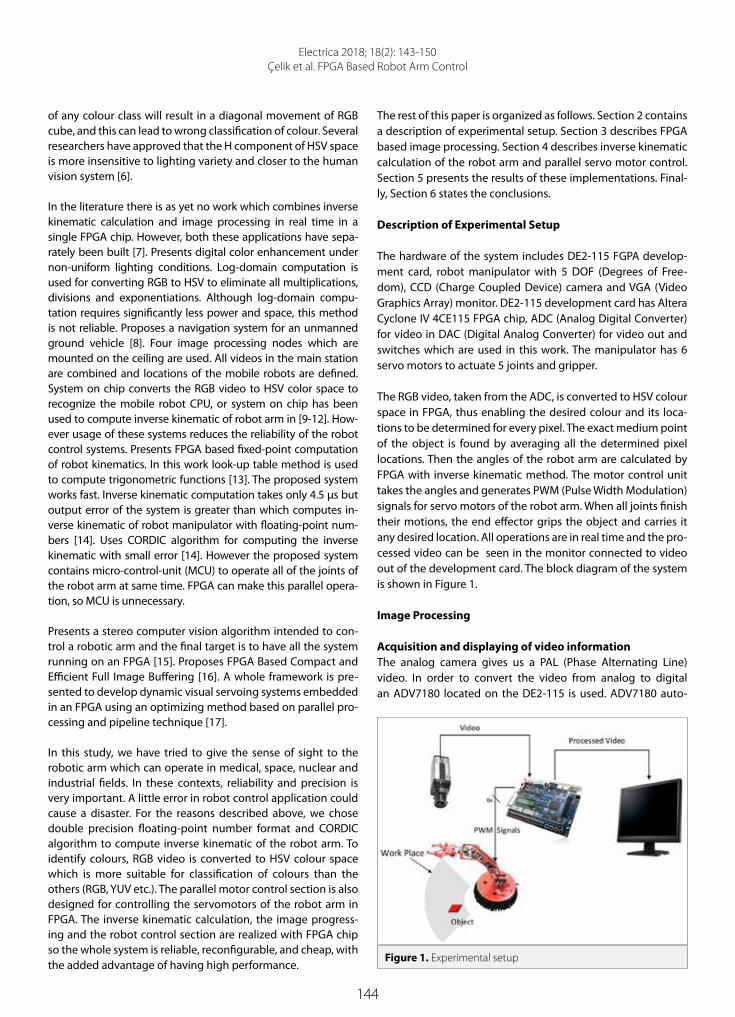
144

Electrica 2018; 18(2): 143-150Çelik et al. FPGA Based Robot Arm Control

of any colour class will result in a diagonal movement of RGB cube, and this can lead to wrong classification of colour. Several researchers have approved that the H component of HSV space is more insensitive to lighting variety and closer to the human vision system [6].

In the literature there is as yet no work which combines inverse kinematic calculation and image processing in real time in a single FPGA chip. However, both these applications have sepa-rately been built [7]. Presents digital color enhancement under non-uniform lighting conditions. Log-domain computation is used for converting RGB to HSV to eliminate all multiplications, divisions and exponentiations. Although log-domain compu-tation requires significantly less power and space, this method is not reliable. Proposes a navigation system for an unmanned ground vehicle [8]. Four image processing nodes which are mounted on the ceiling are used. All videos in the main station are combined and locations of the mobile robots are defined. System on chip converts the RGB video to HSV color space to recognize the mobile robot CPU, or system on chip has been used to compute inverse kinematic of robot arm in [9-12]. How-ever usage of these systems reduces the reliability of the robot control systems. Presents FPGA based fixed-point computation of robot kinematics. In this work look-up table method is used to compute trigonometric functions [13]. The proposed system works fast. Inverse kinematic computation takes only 4.5 μs but output error of the system is greater than which computes in-verse kinematic of robot manipulator with floating-point num-bers [14]. Uses CORDIC algorithm for computing the inverse kinematic with small error [14]. However the proposed system contains micro‐control‐unit (MCU) to operate all of the joints of the robot arm at same time. FPGA can make this parallel opera-tion, so MCU is unnecessary.

Presents a stereo computer vision algorithm intended to con-trol a robotic arm and the final target is to have all the system running on an FPGA [15]. Proposes FPGA Based Compact and Efficient Full Image Buffering [16]. A whole framework is pre-sented to develop dynamic visual servoing systems embedded in an FPGA using an optimizing method based on parallel pro-cessing and pipeline technique [17].

In this study, we have tried to give the sense of sight to the robotic arm which can operate in medical, space, nuclear and industrial fields. In these contexts, reliability and precision is very important. A little error in robot control application could cause a disaster. For the reasons described above, we chose double precision floating-point number format and CORDIC algorithm to compute inverse kinematic of the robot arm. To identify colours, RGB video is converted to HSV colour space which is more suitable for classification of colours than the others (RGB, YUV etc.). The parallel motor control section is also designed for controlling the servomotors of the robot arm in FPGA. The inverse kinematic calculation, the image progress-ing and the robot control section are realized with FPGA chip so the whole system is reliable, reconfigurable, and cheap, with the added advantage of having high performance.

The rest of this paper is organized as follows. Section 2 contains a description of experimental setup. Section 3 describes FPGA based image processing. Section 4 describes inverse kinematic calculation of the robot arm and parallel servo motor control. Section 5 presents the results of these implementations. Final-ly, Section 6 states the conclusions.

Description of Experimental Setup

The hardware of the system includes DE2-115 FGPA develop-ment card, robot manipulator with 5 DOF (Degrees of Free-dom), CCD (Charge Coupled Device) camera and VGA (Video Graphics Array) monitor. DE2-115 development card has Altera Cyclone IV 4CE115 FPGA chip, ADC (Analog Digital Converter) for video in DAC (Digital Analog Converter) for video out and switches which are used in this work. The manipulator has 6 servo motors to actuate 5 joints and gripper.

The RGB video, taken from the ADC, is converted to HSV colour space in FPGA, thus enabling the desired colour and its loca-tions to be determined for every pixel. The exact medium point of the object is found by averaging all the determined pixel locations. Then the angles of the robot arm are calculated by FPGA with inverse kinematic method. The motor control unit takes the angles and generates PWM (Pulse Width Modulation) signals for servo motors of the robot arm. When all joints finish their motions, the end effector grips the object and carries it any desired location. All operations are in real time and the pro-cessed video can be seen in the monitor connected to video out of the development card. The block diagram of the system is shown in Figure 1.

Image Processing

Acquisition and displaying of video informationThe analog camera gives us a PAL (Phase Alternating Line) video. In order to convert the video from analog to digital an ADV7180 located on the DE2-115 is used. ADV7180 auto-

Figure 1. Experimental setup

145


matically performs video format detection. It detects NTSC, PAL or SECAM video formats and converts them from PAL to 4:2:2 component video data compatible with the 8-bit ITU-R BT.656 interface standard. In PAL video format the even num-bered lines are scanned before the odd-numbered lines. The odd-numbered lines need to be saved and then combined with the even-numbered lines. The PAL video format uses YUV 4:2:2 colour space and the VGA uses RGB colour space. It is nec-essary to convert these colour spaces. All conversion processes are shown in Figure 2.

Conversion Red, green, and blue (RGB) to hue saturation value (HSV)The object can be segmented using its colour information if it has a unique colour. We can detect the image using a suitable reference value, and the object having a unique colour can eas-ily be distinguished from other objects in different colours. We have used the HSV colour space to determine the desired ob-ject because HSV colour space is more suitable for colour seg-mentation and intuitive to the human vision system.

Each pixel is represented by three components in the HSV co-lour space: Hue, saturation and value. The nature of colour is defined by a hue component. The brightness of the colour is represented by the ‘value’ component. The range of the hue component is from 0 to 360. The “Saturation” and “Value” range from 0 to 1. The advantage of the HSV is the small variability of the hue component with different lighting conditions so the il-lumination system does not need to have specific features. The following formulas are used to transform RGB to HSV.

Max = max(R, G, B) (1)

Min=min (R, G, B) (2)

Value = Max (3)

(4)

(5)

The equations of conversion from RGB to HSV are redesigned for FPGA implementation. Hue, Saturation and Value range from 0 to 360, from 0 to 100 and from 0 to 255 respectively. They should be parallel for real time video processing. The par-allel realization of the formulas can be seen in Figure 3.

Finding the coordinates of the objectAfter the conversion of the colour space to HSV the desired co-lour is compared to each pixel colour in one picture for recog-nition of the object. The desired colour can be red, green, cyan, purple etc. For this study red was chosen as the desired colour. The centre of the red object should be found so that it can be grasped by the robot arm. Finding the centre of the object is expressed by the equations below:

(6)

(7)

In PAL video format 25 pictures are scanned in one second. After ending the line scanning for one frame the mean of red pixel lo-cations is calculated to find the centre of the object. In the above equations χ

1, χ

2, ϒ1

, and ϒ2 represent the location of the red

Figure 2. Conversion video from PAL to VGA

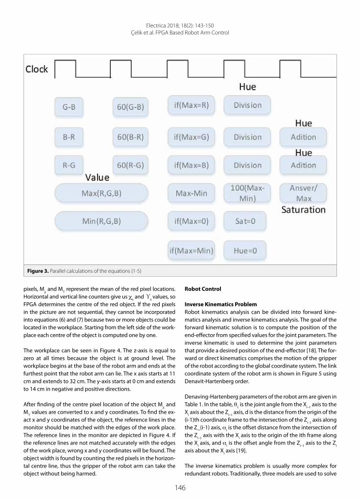
146


pixels, Mχ and M

ϒ represent the mean of the red pixel locations.

Horizontal and vertical line counters give us χn and ϒn values, so FPGA determines the centre of the red object. If the red pixels in the picture are not sequential, they cannot be incorporated into equations (6) and (7) because two or more objects could be located in the workplace. Starting from the left side of the work-place each centre of the object is computed one by one.

The workplace can be seen in Figure 4. The z-axis is equal to zero at all times because the object is at ground level. The workplace begins at the base of the robot arm and ends at the furthest point that the robot arm can lie. The x axis starts at 11 cm and extends to 32 cm. The y-axis starts at 0 cm and extends to 14 cm in negative and positive directions.

After finding of the centre pixel location of the object Mχ and

Mϒ values are converted to x and y coordinates. To find the ex-

act x and y coordinates of the object, the reference lines in the monitor should be matched with the edges of the work place. The reference lines in the monitor are depicted in Figure 4. If the reference lines are not matched accurately with the edges of the work place, wrong x and y coordinates will be found. The object width is found by counting the red pixels in the horizon-tal centre line, thus the gripper of the robot arm can take the object without being harmed.

Robot Control

Inverse Kinematics ProblemRobot kinematics analysis can be divided into forward kine-matics analysis and inverse kinematics analysis. The goal of the forward kinematic solution is to compute the position of the end-effector from specified values for the joint parameters. The inverse kinematic is used to determine the joint parameters that provide a desired position of the end-effector [18]. The for-ward or direct kinematics comprises the motion of the gripper of the robot according to the global coordinate system. The link coordinate system of the robot arm is shown in Figure 5 using Denavit-Hartenberg order.

Denaving-Hartenberg parameters of the robot arm are given in Table 1. In the table, θ

1 is the joint angle from the Xi–1

axis to the Xi axis about the Zi–1

axis, d is the distance from the origin of the (i-1)th coordinate frame to the intersection of the Zi–1

axis along the Z_(i-1) axis, ai is the offset distance from the intersection of the Zi–1

axis with the Xi axis to the origin of the ith frame along the Xi axis, and ai is the offset angle from the Zi–1

axis to the Zi axis about the Xi axis [19].

The inverse kinematics problem is usually more complex for redundant robots. Traditionally, three models are used to solve

Figure 3. Parallel calculations of the equations (1-5)

147


the inverse kinematics problem, these being the geometric, algebraic and iterative models [4]. In this work the geometric model is used to compute the inverse kinematic problem. A detailed explanation about the inverse kinematics of the robot arm is omitted and only the computational procedure is given as follows. The coordinates of the object x and y values are the input of the following equations and joint angles of the robot arm are the output of the equations. Also, a

2, a

3, a

4 and d

1 are

in D-H parameters and z is equal to zero because the object is always at the bottom. is the angle of the robot arm approach to the object having been previously determined according to the distance between the robot arm and the object (X’). Inverse kinematic equations are simplified by values and optimized for FPGA implementation. In Table 2, p are given as shown:

θ4 = P - θ3 (17)

Inverse kinematic solutions contain mainly trigonometric functions (cos, sin, arctan etc.) which have to be computed

Figure 4. Work Place Dimensions (Left) Reference Lines in Monitor (Right)

Table 1. D-H Parameters of the Robot Arm

Joint i ai−1 ai−1 di θi

1 90 0 9 θ1

2 0 8 0 θ2

3 0 8 0 θ3

4 -90 17 0 θ4

5 0 0 0 θ5

Table 2. Approach angles table for X’ values

X’ P

11-16 cm-80°

17-19 cm-70°

20-22 cm-60°

23-28 cm -40°

29-32 cm-30°

(8)

(9)

(10)

(11)

(12)

(13)

(14)

(15)

(16)

(17)

148


Table 3. Analysis of the inverse kinematic solution

Input to In-verse Kine-matic

Angles of the Robot Arm Calculated

Outputs of the Proposed Inverse Kinematic Calculation Error

x=29 y=10

θ1

19,02560603756870 19,02560603777450 -2,05802E-10

θ2

-87,80028882245060 -87,80028799234560 -8,30105E-07

θ3

82,01028215959120 82,01028287942240 -7,19831E-07

θ4

-24,20999333714060 -24,20999924561230 5,90847E-06

x=12 y=-5

θ1

-22,61986494804040 -22,61986494985630 -1,81587E-09

θ2

-14,83273900666030 -14,83273993654120 9,29881E-07

θ3

14,89228119041620 14,89228033264130 8,57775E-07

θ4

-80,05954218375590 -80,05959565613210 5,34724E-05

Table 4. FPGA resource usage

Combinational functions

Dedicated logic registers Memory bits

Embedded multiplier

9-bit elements PLLs

Image processing 2708 1603 42448 18 1

PWM generator 426 209 2576 0 0

Inverse kinematic calculation 54839 22151 30300 343 0

Total 57993 23963 75324 361 1

Figure 5. Link coordinates of the robot arm

149


separately for each joint angle. The CORDIC algorithm is used to compute these complicated functions because it basical-ly allows the computation of transcendental functions using shift and add operations only and can be implemented very efficiently in simple hardware [20]. Also the implemented COR-DIC architectures are based on the IEEE-754 standard and work with 64 bit double precision.

Parallel Pulse Width Modulation GeneratorThe robot arm has 6 servomotors which actuate its joints. Each of the servomotors is controlled with single pulse width modulation (PWM) signal. All the PWM outputs should be parallel to enable smooth movement of the robot arm. The parallel controller is described using Verilog HDL with modules that are designed for each of the servomotors’ output. The servomotors are controlled 50 Hz PWM signals which have a duty cycle of between 0.5 ms and 2.5 ms. A 32 bit counter is programmed to get precision mo-tor motions. This variable’s value changed between (6666666)16 and (1FFFFFFE) 16 and the servomotor shaft varies between 0 and 180 degrees. A step of servomotors is 4, 19E-7 degrees.

Results

The overall experimental system is depicted in Figure 1. The pro-posed FPGA implementation of robot arm control with image processing was coded in Verilog HDL. The system simulation was performed using ModelSim (Version 10.1d) and synthesized us-ing Quartus II 13.1 software. The designed system implement-ed DE2-115 FPGA development board and was tested in varied light conditions with objects in different shapes and sizes. In Figure 6 the objects used in the test are shown. In the tests the objects were located randomly in the work place and the success of the proposed system was observed. Each object was tried out 500 times, and the first and second objects were grasped by the robot arm with a success rate of 100%. The success rates of the third and fourth objects were 95.6% and 96.8% respectively.

If two or more objects were located in the work place at the same time, the image processing unit determined this situation and sep-

arately computed centre coordinates of the objects in the work place and sent them to inverse kinematic calculation. Thus, the robot arm could take the objects from the work place one by one.

An application was developed to evaluate the precision of the proposed inverse kinematic solution. Inputs to inverse kinematic were manually entered and outputs from the inverse kinematic of the proposed application were observed. The application was loaded in the FPGA development board and the results were observed from seven segment displays on the board. In Table 3, analysis of the inverse kinematic solution is given.

The FPGA used in the proposed implementation had 114 480 logic elements. Only 3% and 1% of the logic elements were used by image processing and parallel PWM generator respectively. All implementation was realized with 57 993 (%51 of the FPGA) logic elements. FPGA resource usage is explained in table 4.

Conclusion

In this study, a hardware implementation of robot arm control with real time image processing is presented. The proposed im-plementation combines high precision inverse kinematic calcu-lation, colour based object recognition and robot arm control. The aim of this paper is to advance the precision of space and industrial robot arms, where reliability is a substantial require-ment. To improve precision of the inverse kinematic calculation, CORDIC algorithm based on double precision IEEE 754 floating point number format is used. To recognize the object in different illumination, RGB colour space is converted to HSV colour space. The parallel PWM generator is also designed for the smooth op-eration of the robot arm. All applications are combined and im-plemented in FPGA development board. It was confirmed that the inverse kinematic calculation is very precise, and the tests carried out show that the proposed system works well.



Figure 6. Objects used in tests

150


Barış Çelik was born in Bursa, Turkey. He received the M.Sc. degree in electronic and communication education from Mar-mara University, Istanbul, Turkey. He is currently pursuing the Ph.D. degree in electric and electronic engineering with the University of Marmara, Istanbul, Turkey.

Dr. Ayça Ak received her B.Sc. and MSc. degree from the Firat University, Electrical Electronics Engineering Department, in 1993 and 1997 respectively, Ph.D degrees from the Yildiz Technical University, Control and Automation Department of Electrical Engineering in 2008. She is currently working as faculty member, phd. in Electronics and Automation Depart-ment in Vocational School of Technical Sciences, Marmara University, Istanbul-Turkey. Her research expertise is Robotic, Control, Neural Network, Fuzzy Logic, Web-Based Education and Applications. She has many international and national books, articles and project works.

Vedat Topuz received his B.Sc. and M.Sc. degrees from Marmara University, Electronics and Computer Education Depart-ment 1984 and 1995 respectively, Ph.D degrees from Marmara University Computer Systems Education Department in 2003. He is currently working as Assoc. Prof.Dr. in Computer Department in Vocational School of Technical Sciences, Mar-mara University, Istanbul-Turkey. Her research expertise is Artificial Intelligence, Robotics, Control, Fuzzy Logic, Web-Based Education and Applications. He has many international and national books, articles and project works.


References

1. W. He, K. Yuan, H. Xiao, Z. Xu, “A high speed robot vision system with GigE vision extension”, IEEE International Conference on Mechatronics and Automation, 2011, pp. 452-457.

2. X. Zhang, M.H. Lee, “A Developmental Robot Vision System”, IEEE Interna-tional Conference on Systems, Man and Cybernetics, 2006, pp. 2024-2029.

3. P.R. Possa, S.A. Mahmoudi, N. Harb, C. Valderrama, P. Manneback, “A Multi-Resolution FPGA-Based Architecture for Real-Time Edge and Cor-ner Detection”, IEEE Transactions on Computers, 2014, pp. 2376-2388.

4. R. Köker, “A genetic algorithm approach to a neural-network-based inverse kinematics solution of robotic manipulators based on er-ror minimization”, Information Sciences, 222, pp. 528-543.

5. Y.H. Yu, N.M. Kwok, Q.P. Ha, “Color tracking for multiple robot con-trol using a system-on-programmable-chip,” Automation in Con-struction, 20(6), pp. 669-676, 2013.

6. X. Lu, D. Ren, S. Yu, “FPGA-based real-time object tracking for mo-bile robot,”, International Conference on Audio, Language and Im-age Processing, 2010, pp. 1657-1662.

7. M. Z. Zhang, M.J. Seow, L. Tao, V.K. Asari, “A tunable high-perfor-mance architecture for enhancement of stream video captured under non-uniform lighting conditions”, Microprocessors and Mi-crosystems, 32(7), pp. 386-393, 2008.

8. J. Rodríguez-Araújo, J.J. Rodríguez-Andina, J. Fariña, M.Y. Chow, “Field-Programmable System-on-Chip for Localization of UGVs in an Indoor iSpace”, IEEE Transactions on Industrial Informatics, 10(2), pp. 1033-1043, 2014.

9. X. He, Z. Wang, H. Fang, K. He, R. Du, “An embedded robot control-ler based on ARM and FPGA”, 4th IEEE International Conference on Information Science and Technology, 2014, pp. 702-705.

10. Y.S. Kung, H. Cheng-Ting, C. Hsin-Hung, T. Tai-Wei, “FPGA-realiza-tion of a motion control IC for wafer-handling robot”, 8th IEEE Inter-national Conference on Industrial Informatics, 2010, pp. 493-498.

11. S. Seok, D.J. Hyun, S. Park, D. Otten, S. Kim, “A highly parallelized control system platform architecture using multicore CPU and FPGA for multi-DoF robots”, IEEE International Conference on Ro-botics and Automation (ICRA), 2014, pp. 5414-5419.

12. Y. Zheng, H. Sun, Q. Jia, G. Shi, “Kinematics control for a 6-DOF space manipulator based on ARM processor and FPGA Co-processor”, 6th IEEE International Conference on Industrial Informatics, 2008, pp. 129-134.

13. M. K. Wu, Y. S. Kung, Y. H. Huang, T. H. Jung, “Fixed-point computa-tion of robot kinematics in FPG”, International Conference on Ad-vanced Robotics and Intelligent Systems (ARIS), 2014, pp. 35-40.

14. Y. S. Juang, T. Y. Sung, L. T. Ko, C. I. Li, “FPGA implementation of a CORDIC-based joint angle processor for a climbing robot”, Interna-tional Journal of Advanced Robotic Systems, 10(4), p. 195, 2013.

15. R. Szabo, A. Gontean, A., “Robotic Arm Control Algorithm Based on Stereo Vision Using RoboRealm Vision”, Advances in Electrical and Computer Engineering, 15(2), pp. 65-74, 2015.

16. M. Kazmi, A. Aziz, P. Akhtar, D. Kundi, “FPGA based compact and efficient full image buffering for neighborhood operations”, Adv. Electr. Comput. Eng, 15(1), pp. 95-104, 2015.

17. A. Alabdo, J. Pérez, G.J. Garcia, J. Pomares, F. Torres, “FPGA-based architecture for direct visual control robotic systems”, Mechatron-ics, 39, pp. 204-216, 2016.

18. R. P. Paul, “Robot manipulators: mathematics, programming, and control: the computer control of robot manipulators”, Cambridge, London, MIT Press, 1983.

19. J. Rigelsford, “Robotics: Control, Sensing, Vision andIntelligence”, Industrial Robot: An International Journal, vol. 26, no. 2, 1999.

20. C. Krieger, B. J. Hosticka, “Inverse kinematics computations with modified CORDIC iterations,” IEE Proceedings - Computers and Digital Techniques, vol. 143, no. 1, pp. 87-92, 1996.

151

Introduction

Nikola Tesla first introduced rotating field theory to science in 1882. In 1883, he invented the first induction motor that operates by rotating field principle. In 1888, he secured his patent for his polyphase alternating current motors, generators and rotating filed principles [1]. He named his project “Tesla’s Egg of Columbus” which describes the basic principles of rotating magnetic field and induction motors and he presented it to the World Colombian Exhibition in 1893. The name “Egg of Columbus” comes from the real story of Christopher Columbus who asked for ship support from the Queen of Spain for his journey to India. The Queen wanted him to make an egg stand vertical in balance. He broke the sharper edge of the egg, used that side to enable the egg to keep standing vertically, and thus he earned support from the Queen. In Tesla’s project, an egg made of copper rotates around a vertical axis while it keeps its balance on a surface placed over the space inside a circular iron core. This proves the existence of rotating magnetic field [1].

The basic operational principle of Tesla’s Egg depends on the rotation of total magnetic flux density vectors created at the centre of the stator core which are induced by the magnetomo-tive force (mmf) created by two phase alternating current winding. With this project, Nikola Tesla managed to keep the copper egg rotating vertically around its main axis with a gyro-scopic motion. This provided the effects of rotating field in a practical way. The printed sketch in his paper, published in 1919 in the Electrical Experimenter journal, is shown in Figure 1 [2].

In the project, two separated alternating current windings placed with an angle of 90° be-tween their axes were wound around a toroidal iron core. Tesla introduced the production of rotating field in the air-gap inside the stator core when two-phase voltage with an electrical phase difference of 90° was applied to these windings. He placed an oval engraved wooden layer (egg-board) towards the centre over the whole air-gap inside the core. He analysed the

Electrica 2018; 18(2): 151-158

RESEARCH ARTICLE

Generalised Model of Multiphase Tesla’s Egg of Columbus and Practical Analysis of 3-Phase Design Atamer Gezer1, Mehmet Onur Gülbahçe2, Derya Ahmet Kocabaş2

1Ford Otosan R&D Center, Istanbul, Turkey2Department of Electrical Engineering, Faculty of Electrical and Electronics Engineering, Istanbul Technical University, Istanbul, Turkey

Corresponding Author: Mehmet Onur Gülbahçe





DOI: 10.5152/iujeee.2018.1824

Cite this article as: A. Gezer, M.O. Gülbahçe, D.A. Kocabaş, “Generalised Model of Multiphase Tesla’s Egg of Columbus and Practical Analysis of 3-Phase Design”, Electrica, vol. 18, no: 2, pp. 151-158, 2018.

ABSTRACT

“Tesla’s Egg of Columbus” is the name given to the experiment conducted in 1893 by Nikola Tesla that proved the existence of rotating magnetic field produced by two-phase AC winding. In this study, a generalized mathematical magnetic field model for m-phase “Tesla’s Egg of Columbus” is presented in detail, and a novel 3-phase model of “Tesla’s Egg of Columbus” is designed analytically by means of generalized expressions. Electrical and geometric quantities are calculated, and the system is analyzed by finite element analysis (FEA). The designed system is manufactured and tested for rated current and for constant and variable frequency with eggs made of different materials. Optimized frequency for materials and geometries are obtained and compared.

Keywords: Tesla’s Egg of Columbus, 3-phase rotating magnetic field, mathematical model

152

Electrica 2018; 18(2): 151-158Gezer et al. 3-Phase Design of Tesla’s Egg of Columbus

effects of rotating magnetic field on a copper egg, brass balls and iron disks when they were placed on the wood. The supply frequency fluctuated between 25-300 Hz and the ideal operat-ing frequency was found to be 35-40 Hz [2].

A design for Tesla’s two-phase inductor was given in order to demonstrate a rotating field based on the famous Tesla’s Egg of Columbus without establising a generalised model for multi-phase structure [3].

In this study, generalised mathematical expression of mmf created inside the air-gap was derived for polyphase windings having been inspired by Tesla’s Egg of Columbus that was re-alised by two-phase ac winding and basic principles of design criteria for m-phases. Starting from this point, a 3-phase ver-sion of the system that does not exist in previous studies was designed analytically by calculating the necessary electrical and mechanical quantities. The design was then analysed by Finite Elements Method (FEM). Various rotating objects made of different materials (copper, aluminium, brass) with different geometries (egg, disc) were manufactured. Test setup was in-stalled and was supplied by variable frequency voltage while keeping the current constant. The most efficient geometry, material and supply frequency for a geometry were measured and observed.

Generalised Ampere-Turn Expression of Multi-Phase Tesla’s Egg of Columbus

The idea of installing more than one winding to a single machine paved the way for multi-phase alternating current machines. The proof of rotating field by Tesla’s Egg of Columbus opened the way to the design of rotating alternating current machines. In previous studies, only two-phase design details are given with-out generalising the design criteria [3]. Multi-phase electric mo-tors are more advantagous in terms of power density and utility factor. But as the number of phases increases, the need for multi-phase power supplies arises. 3 phase is the accepted common number of phases in the engineering world. Therefore, in this pa-per, a generalised model is given and practical implementation is performed only for a 3-phase system.

In order to produce a rotating field with m phase winding, all phase windings have to be placed in a symmetrical geometry and all phase spreads should be of the same widths. Windings must be supplied with a m phase symmetrical alternating cur-rent. In 2 poles (2p=2) and m phases symmetric structure, a to-tal of (2π/m) radian section for each phase is reserved. For each phase, (π/m) radian phase bands are formed by dividing this part into two, which are placed on reverse sides of stator at an angle of 180°. Under each pole, an electrical phase difference between the phase winding axes is created by placing the windings at a geometrical difference of (2π/m) [4-7]. The number of turns of the phases (N) must be equal for symmetry. Nm(θ) represents the phase position of N number of turns for mth phase winding (1).

(1)

N1 θ( ) = N

N2 θ( ) = N.e− j2πm

N3 θ( ) = N.e− j4πm

M

Nm θ( ) = N.e− j2π(m−1)

m

When the number of poles are 2, the geometric angle (αgeo) and electrical angle (αelec) are the same. If the number of poles are more than two, then the geometric angle and electrical angle differ from each other and the structure given for two poles is repeated for each pole by accepting the width of each pole “elec-trically 180°”. Geometric angle can be converted into electrical angle by multiplying it with a coefficient of p as in (2) [6]. In gen-eral, phase spreads must have a width of [2π/(m.2p)] in radians.

aelec = ageoP (2)

The value and the direction of the ampere-turn (mmf) of one phase winding which is positioned on the axis of phase wind-ing depends on the instantaneous value of the sinusoidal phase current. When m-phase alternating voltage is applied to each phase of the m-phase winding with a phase difference of (2π/m) radians, m different mmf phasors are located within the gap each having their own instantaneous values [7]. The instantaneous values of the phase currents can be seen in (3). I is the effective value, Im(ωt) is the the instantaneous value of the mth phase.

(3)

I1(ωt) = 2 I.cos(ωt)

I2(ωt) = 2 I.cos(ωt − 2πm)

I3(ωt) = 2 I.cos(ωt − 4πm)

M

Im(ωt) = 2 I.cos(ωt − 2π(m −1)m

)

Figure 1. The sketch of Tesla’s Egg of Columbus experiment that was published in the journal of Electrical Experimenter in March 1919 [2]

153


Individual and resultant ampere-turn expressions created by one and m phases are given in (4) and (5-6), respectively.

F1(θ, t) = N1 θ( ).I1(ωt) (4)

F(θ, t) = F1 θ, t( )+ F2 θ, t( )+ F3 θ, t( )+L L Fm θ, t( ) (5)

(6)F(θ, t) = N1 θ( ).I1(ωt)+N2 θ( ).I2(ωt)

+N3 θ( ).I3(ωt)+L L Nm θ( ).Im (ωt)

When (1) and (2) are substituted in (5), (7) is obtained for the resultant mmf by means of necessary trigonometric (Euler) transformations [4]. (7)F(θ, t) = m

2NI.e jωt

As can be seen in (7), the amplitude of total ampere-turn does not change according to time while the position of resultant magnetic field changes. The complex position vector rep-resents the change of position. This vector accepts the centre of stator as the origin of the coordinate system. The geomet-rical locus of the end-point of the field vector is a circle. The expression in (7) is the mathematical expression of the rotating magnetic field that is produced by m-phase winding.

The speed of the rotating field is called synchronous speed (ns). As the currents of m-phase winding complete one period, the rotating field travels along two poles. When there are more than 2 poles, the rotating field completes its path by f/p times in seconds. Since the general unit for rotation is rpm or min-1, synchronous speed can be calculated in terms of (8).

(8)ns =60 ⋅ fp

When a closed loop made of conductive material (coils, cast iron, disk, etc.) is placed inside a rotating magnetic field that is generated by the currents flowing through the m-phase stator windings, voltage is induced in the conductive object due to the relative motion. Current flows through the conductive material via closed paths and force is induced on the current carrying conductive material. A tangential force is applied to the conduc-tors to force the material to rotate by the rotating field. Vectorel interattraction between magnetic field provided by the induced currents and magnetic field provided by stator currents causes a torque production on the rotating object. When using con-ductive materials such as an egg, spin top, disk or a coil wound around a cylinder, rotation begins. The egg, spin top, disk type materials can stand upright by the centrifugal force induced.

Design of the Three Phase Tesla’s Egg of Columbus Basically, generalized electric machine design consists of a two-step recursive method. The first step includes the obtainment

of main dimensions, winding arrangement, etc. by assump-tions, and the second step includes the necessary corrections and experimental verification studies [3]. Electromagnetic design will start with determination of the magnetic flux and current density under the fixed magnetic core dimensions and required number of turns will be calculated. The procedure is completed after validation of the proposed air-gap flux density by finite element analysis (FEA).

In this paper, a three-phase and two-pole version of Tesla’s Egg of Columbus is designed and design steps are given. Phase spreads for one phase is 60° as explained above. Design of Magnetic Circuit and Calculation of Air-Gap Reluctance

The laminated magnetic core to be used is toroidal shaped with its geometric dimensions given in Table 1 and the top and side views shown in Figure 2 where “D” represents the out-er diameter of the core, “d”, the inner diameter, “h”and “a”, the cross-section height and width, respectively.

Stator top view of three phase Tesla’s Egg of Columbus, includ-ing one phase winding that is wound around the core along its phase spread, and winding arrangement for two poles are given in Figure 3. In order to accommodate three phase wind-ings, the stator is divided into 6 phase bands of 60°. Each coil is wound in reverse directions but connected in series and two windings are complementary to each other. These two wind-ings produce equal and opposite magnetic fields with respect to each other.

The magnetic circuit has symmetry and the total magnetic flux within the air-gap (Φg) is the sum of the equal fluxes (Φµ) produced by winding parts on opposite sides of the core. By assuming the permeability of magnetic core as infinite, the equivalent magnetic circuit in Figure 4 is obtained.

By assuming the flux to be equal within the air-gap, the circuit becomes easier to solve and the air-gap reluctance (ℜg) and the air-gap flux (Φg) must be calculated using the magnetic cir-cuit dimensions. Since the air-gap flux produced by one phase winding passes through the air-gap with inconstant width, the total reluctance of the gap must be calculated by evaluating in-tegral. The mean value of the cross-section area is used for ap-

Table 1. Core Dimensions

Symbol Unit Value

Outer diameter of the core (D) mm 300

Inner diameter of the core (d) mm 170

cross-section height (h) mm 80

cross-section width (a) mm 65

154


proximate calculation. The air-gap through the toroid is sliced

into k pieces by 1 cm and the cross-section area of each slice is

calculated by multiplying the toroid height by the width of ith

slice (i=1,2,,…k) given in (9). The sum of the slice sections and the arithmetic average of all sections are calculated as in (10). The drawing used for calculating the mean value of air-gap area is given in Figure 5.

The width of ath slice in k slices is calculated by means of trigo-nometric relations in (9).

xa = 2 d ⋅a ⋅k−a2 ⋅k2 (9)

According to (9), the average cross-sectional area of the air-gap (Ag-mean) is calculated by (10).

(10)Agort =

h ⋅ xaa=1

k−1

∑k−1

The circuit shown in Figure 4 can be solved by calculating the total magnetic resistance related to the reluctance equation given in (11), and the average value of the air-gap magnetic flux density can be calculated as in (12).

Figure 3. Magnetic Circuit and winding positions for one phase

Figure 4. Magnetic Equivalent Circuit for one phase

Figure 5. Calculation of width of a. slice when diameter is divided into k parts in order to obtain average air-gap crossection area (a=1,2,...k)

Figure 2. Top and side view of magnetic core

155


(11)ℜg =FΦg

(12)Bg =Φg

Agort Validation of Air-Gap Flux and Calculation of Number of Turns Per Phase

Before calculating the number of turns per phase, the values of current density and air-gap magnetic flux density must be cho-sen. The current density was accepted as 4 A / mm2 and the mag-netic flux density (Bg) in the air-gap as 400 mT. The conductor dimensions and rated current are determined according to the selected current density. The number of turns per phase was cal-culated as 250 by using (7) and (11) for the selected initial condi-tions. The location of the calculated number of turns on the mag-netic core is given in Figure 6. For the other two phase windings, conductor distribution is shifted 120° geometrically which is already equal to electrical angle since the design has two poles.

Finite Element Analysis of the 3 phase-Tesla’s Egg of Columbus

In this section, the design that is composed of the core and windings is imported to a finite element analysis (FEA) soft-ware after being sketched in a 3D drawing tool. This design is analysed by FEM while the windings are supplied by a current source at 50 Hz. During the numerical magnetic analysis, the egg and the egg-board is neglected depending on their mag-netic properties. The used structure for the analysis is given in Figure 7 with the neglected egg and the egg-board in order to help in understanding.

After the analysis, the existence of the rotating field and the value of the calculated air-gap field is confirmed. As a visual-ised result, an instantaneous distribution and vectorial repre-sentation of magnetic flux density at the instant of ωt =3π/4 is given in Figure 8, 9; respectively.

After the analysis result confirmed the calculated flux density within the air-gap , the manufacturing stage was started.

Manufacturing of The Three Phase Tesla’s Egg of Columbus

The manufacturing stage of The Three Phase Tesla’s Egg of Co-lumbus has four parts, namely productions of the toroidal core, egg and egg-board and winding the coils around the core [8].

The core is produced using laminated steel. The windings are wound around the core in phase spreads of three phases us-ing a toroidal winding machine. The air-gap is covered by the placed egg-board made of pertinax. The egg-board is an oval engraved wooden layer (egg-board) situated towards the cen-

tre of the whole air-gap inside the core. This engraving helps the egg to be exposed to a more magnetic field. It also im-proves the stability of the egg during rotation.

The dimensions of the egg are inspired from a previous design for one phase and are given in Figure 10 [8]. For an easier pro-duction, the egg is manufactured in two pieces that are the top and the bottom parts. This kind of production also helps to in-crease the weight of the egg by fitting additional pieces made of the same material.

The final product for the Three Phase Tesla’s Egg of Columbus is given in Figure 11.

Laboratory Stage

The test stage is performed in two sub-stages, namely constant and variable frequency supply at the calculated rated current of the system.

Figure 6. Winding distribution diagram for each phase

Figure 7. 3D Transient Magnetic Model of Tesla’s Egg of Columbus

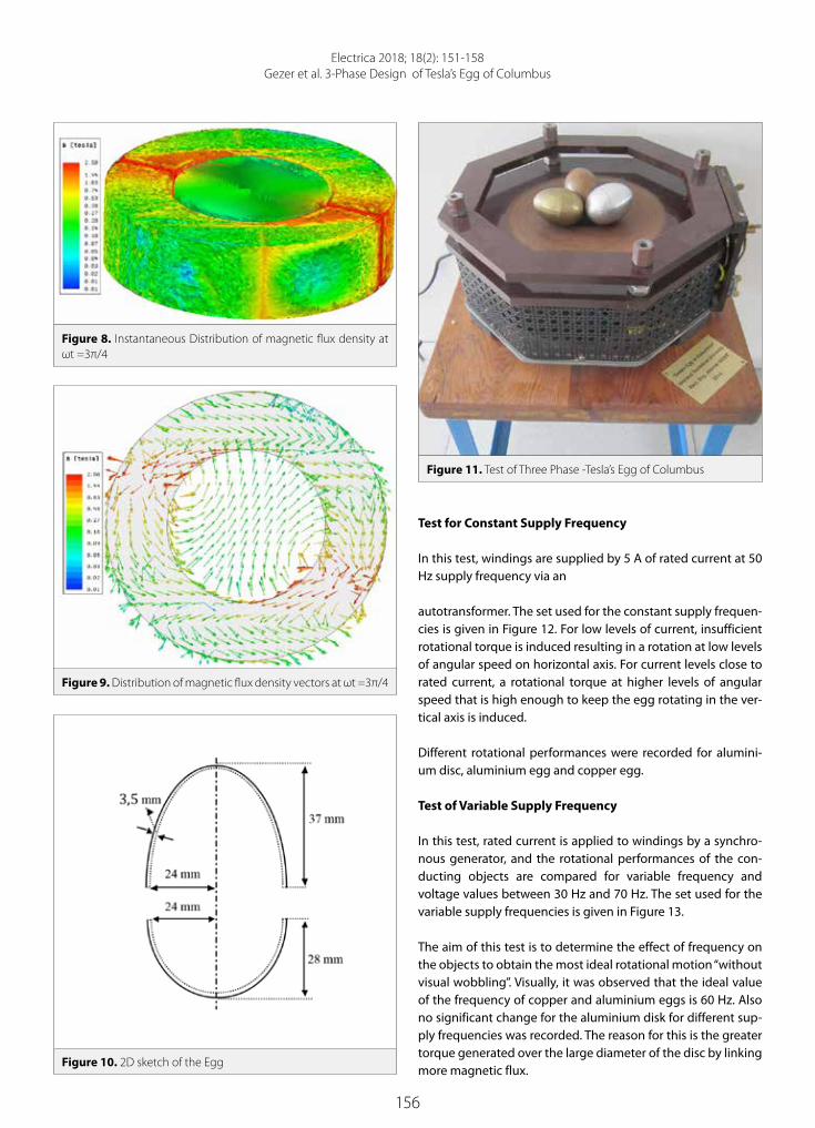
156


Test for Constant Supply Frequency In this test, windings are supplied by 5 A of rated current at 50 Hz supply frequency via an autotransformer. The set used for the constant supply frequen-cies is given in Figure 12. For low levels of current, insufficient rotational torque is induced resulting in a rotation at low levels of angular speed on horizontal axis. For current levels close to rated current, a rotational torque at higher levels of angular speed that is high enough to keep the egg rotating in the ver-tical axis is induced.

Different rotational performances were recorded for alumini-um disc, aluminium egg and copper egg.

Test of Variable Supply Frequency In this test, rated current is applied to windings by a synchro-nous generator, and the rotational performances of the con-ducting objects are compared for variable frequency and voltage values between 30 Hz and 70 Hz. The set used for the variable supply frequencies is given in Figure 13.

The aim of this test is to determine the effect of frequency on the objects to obtain the most ideal rotational motion “without visual wobbling”. Visually, it was observed that the ideal value of the frequency of copper and aluminium eggs is 60 Hz. Also no significant change for the aluminium disk for different sup-ply frequencies was recorded. The reason for this is the greater torque generated over the large diameter of the disc by linking more magnetic flux.

Figure 9. Distribution of magnetic flux density vectors at ωt =3π/4

Figure 10. 2D sketch of the Egg

Figure 11. Test of Three Phase -Tesla’s Egg of Columbus

Figure 8. Instantaneous Distribution of magnetic flux density at ωt =3π/4

157


Conclusion

In this study, a generalised mathematical model was created for the project called “Egg of Columbus” which, when the the-ory was introduced by Tesla, was intended only for two phase. A three-phase version, which does not exist in the literature, was designed analytically. Calculated design information was confirmed by numerical simulations based on FEM.

In the manufacturing stage, designed windings were wound around a laminated toroid and a pertinaks board was placed over the air-gap inside the toroid to enable the egg to rotate firmly. Copper and aluminium eggs and an aluminium disc were manufactured to use as rotating objects. Tests were per-formed to obtain the effect of the geometry and the material

while the coils were supplied by the calculated rated current at constant and variable frequencieAmong all the materials, the most efficient rotation was obtained for aluminium. The best rotational performance was obtained for 60 Hz for the egg made of aluminium. Aluminium disc was seen to be the most stable and firmly rotating geometry among the objects due to higher linked magnetic flux.



Financial Disclosure: The authors declared that this study has re-ceived no financial support

References

1. N. Tesla, “Electro-Magnetic Motor“, US Patent Office, Aachen, US381968, 1888.

2. N. Tesla, “Tesla’s Egg of Columbus”. MECHATRONIKA, Electrical Ex-perimenter, 6, 774-808, 1919.

3. M.L. Dorde, R.M. Petar, “ Design of Tesla’s Two-Phase Inductor “, In-ternational Symposium on Industrial Electronics, Banja Luka- Bos-nia and Herzegovina, 115-122, 2014.

4. A.E. Fitzgerald, C.J. Kingsley. “Electric Machinery”, The McGraw-Hill, USA, 2003.

5. S.J. Chapman, “Electric Machinery Fundamentals”, The Mc-Graw-Hill, USA, 2011.

6. A.F. Mergen, D.A. Kocabas “Windings in Electrical Machines”, Birs-en Publisher, Istanbul, Turkey 2012.

7. A.F. Mergen, S. Zorlu “Electrical Machines-II”, Birsen Publisher, Is-tanbul, Turkey 2009.

8. “Tesla’s Egg of Columbus–Production of working replicas”. http://www.rt17.hr/teslas-egg-of-columbus/. (16.04.2016).

Figure 12. a-c. Rotational behaviour for different objects made of different materials in different geometrical shapes Copper egg (a); Alu-minum egg (b); Aluminum disc (c)

a b c

Figure 13. The set used for the tests for Supplying by Variable Fre-quency and Voltage

158


Mehmet Onur Gulbahce received the B.S. degree in electrical engineering from Istanbul University, Istanbul, Turkey, in 2010. He received the M.Sc. degree in 2013 in Electrical Engineering Programme, Institute of Science and Technology, ITU and since 2013 he has been a Ph.D. student in the same programme. He is also a research assistant in the Department of Electrical Engineering, Electrics and Electronics Faculty, ITU since 2011. His main subjects of concern are high-speed electrical machines, drive system and dc-dc converters.

Derya Ahmet Kocabas received the B.S. degree in electrical engineering from ITU, Istanbul, Turkey, in 1994. He received the M.Sc. and Ph.D. degrees from Electrical Engineering Programme, Institute of Science and Tech-nology, ITU, in 1997 and 2004, respectively. His main subjects of concern are design and control of electrical machines, space harmonics, drive systems and power electronics. He joined to Department of Electrical Engi-neering, Electrics and Electronics Faculty, ITU in 1995 and since January 2009 he has been an Assistant Professor.

Atamer Gezer received the B.S. degree in electrical engineering from Istanbul Technical University, Istanbul, Tur-key, in 2016. He is a student the M.Sc. degree from 2018 in Electrical Engineering Programme, Institute of Science and Technology, ITU. He is also an Electrical Distribution System Engineer on heavy commercial vehicles harness design, Ford Otosan since 2016. His main subjects of concern are electrical machines, low voltage power distri-bution system and harness components about automotive.

159

Introduction

Wireless power transfer (WPT) systems can be categorized into radiative and non-radiative systems [1, 2]. Radiative systems utilize highly directed receiver and transmitter antenae and work at microwave frequencies. Their efficiency is usually lower than that of non-radiative sys-tems and a line of sight propagation is needed; however, power can be transferred to very long distances. On the other hand, non-radiative systems usually exhibit greater efficiency, but they are limited to very short power transfer distances. In these systems, power transfer is car-ried out via near-field coupling. Coupling is achieved through either electric field (capacitive coupling) or magnetic field (inductive coupling).

Today, due to very broad coverage of existing electrical grids, long-range wireless power transfer systems are not needed in all but several very specific applications. However, widespread use of mobile devices and battery powered vehicles open up a new usage for wireless power transfer at medium range (midrange) distances, from several centimetres to a couple of meters. For mid-range applications, radiative systems are not convenient as they are based on far-field radiation. Capacitive coupling based non-radiative systems are not safe for daily use applications as the electric field near the transmitter and receiver devices interacts strongly with surrounding objects including humans. Magnetic field interacts weakly with surrounding objects, yet the power trans-fer distances in traditional inductive coupling systems are quite low (a couple of centimetres) for charging mobile devices and electric vehicles compared with several tens of centimetres.

The magnetically coupled loops, when resonated out, was proposed for use in midrange pow-er transfer [1, 3]. It has been shown that one can transfer power at a distance several times the radius or the length of the loops in magnetically coupled resonant loops [4, 5]. Moreover, when the loops operate in a strongly coupled regime, it is almost possible to achieve a dis-tance-independent power transfer efficiency.

Electrica 2018; 18(2): 159-166

RESEARCH ARTICLE

A Circuit Model-Based Analysis of Magnetically Coupled Resonant Loops in Wireless Power Transfer Systems Seyit Ahmet Sis Department of Electrical-Electronics Engineering, Balıkesir University School of Engineering, Balıkesir, Turkey

Corresponding Author: Seyit Ahmet Sis





DOI: 10.26650/electrica.2018.55345

Cite this article as: S. A. Sis, “A Circuit Model Based Analysis of Magnetically Coupled Resonant Loops in Wireless Power Transfer Systems “, Electrica, vol. 18, no: 2, pp. 159-166, 2018.

ABSTRACT

Magnetically coupled resonant loops can be represented by a lumped element circuit model. Each parameter in the lumped element model can be expressed as a function of loop geometry and the separation between the loops; therefore, the geometry can be systematically changed, and the power transfer efficiency of the coupled loops can be predicted. This paper presents a simulation-based efficiency analysis for wireless power transfer systems utilizing magnetically coupled resonant loops. The behavior of power transfer efficiency is studied for various loop geometry parameters, and the simulation results are presented in detail. These results clearly show that there is a trade-off between peak efficiency and critical coupling distance, both of which depend on the loop size, frequency of operation, and source-load impedances. To verify the accuracy model, two identical circular loops are fabricated and measured, and the measurement results agree well with the model.

Keywords: Wireless power transfer systems, magnetically coupled loops, power transfer efficiency

https://orcid.org/0000-0002-3740-2391

160

Electrica 2018; 18(2): 159-166Sis SA. Analysis of Magnetically Coupled Resonant Loops

Magnetically coupled resonant loops can be analysed either by a coupled mode theory (CMT) [6,7] or by using an equiva-lent circuit model. It has been shown that an equivalent circuit model is simpler and quite accurate for the analysis of resonant magnetically coupled loops [7]. Numerous works, based on equivalent circuit models, have been reported [7-15].

This paper presents an equivalent circuit model based analysis for WPTs using magnetically coupled resonant loops. As com-pared to previously reported works on circuit model based analysis of WPTs, this work presents comprehensive simulation results by systematically changing the geometry parameters and source & load resistances. Using these simulation results, the effect of loop size and source & load resistancess on effi-ciency response in both weakly and strongly coupled regimes is presented. The conditions for operating in each of these re-gimes are examined in terms of loop size and load & source resistances for circular loops. To verify the model, two identical circular loops are fabricated and measured. Measurement re-sults exhibit good agreement with the model.

An Equivalent Circuit Model for Inductively Coupled Resonant Loops

The magnetically coupled resonant loops, as in Figure 1 a, can be represented by a circuit model shown in Figure 1 b. In this model, the magnetic coupling between the loops is represent-ed by a mutual inductance (M). The components L1, R1 and C1 are the self-inductance, parasitic resistance and the resonance capacitance for the transmitting loop, respectively. Similarly, L2, R2 and C2 are the same parameters for the receiving loop. Each component in the circuit is dependent on the geometry parameters of the loops.

The self-inductance (L1,2) for a circular loop as a function of loop radius (r), radius of the wire (a) and number of turns (N) can be found as follows [4]:

(1.a)L1,2 = N2µ0 (r - a)(r + a) (

2k- k)K(k) - ( 2

k)E(k)

⎡

⎣⎢

⎤

⎦⎥

where K and E are the complete elliptic integrals of the first and second kind as follows

(1.b) K(k) = dβ

1- k 2 sin2 β0

π /2∫

(1.c)E(k) = dβ 1- k 2 sin2 β0

π /2∫

(1.d)k = 4(r - a)(r + a)(2r)2 + (2a)2

.

where μ0 is the magnetic permeability of the air. The parasitic resistance (R1,2) includes the effect of both conductor loss (Rc) and the radiation loss (Rr) and can be calculated as follows [16]:

Rr = 20N2π 2(2πr

λ)4 (Ω)

(2.a)

(2.b)Rc =

2πrN2πρ

µ0ω2σ

(Ω)

(2.c)R = Rc +Rr

where ω is the radial frequency, λ is the wavelength at the op-erating frequency and σ is the conductivity of the wire. The mutual inductance between the loops can be calculated as function of loop geometry and separation between the loops (d) as follows [4]:

(3a)M = N 2µ0 r1r2 ((2l− l)F(l)− 2

lE(l)) H

where K and E are the complete elliptic integrals of the first and second kind as follows:

(3b)F(l) = dβ

1− l2 sin2 β0

π /2∫

(3c)E(l) = dβ 1− l2 sin2 β

0

π /2∫

(3d)l =4r1r2

(r1+ r2 )2 + d 2

.

Analysis of Circuit Model for Efficiency Calculations

For efficiency calculations, an RF source with an internal re-sistance (RS) and a load resistance (RL) are connected to the input and output of the model, respectively, as shown in Fig-

Figure 1. a, b. General depiction of magnetically coupled reso-nant loops (a); and its circuit model (b)

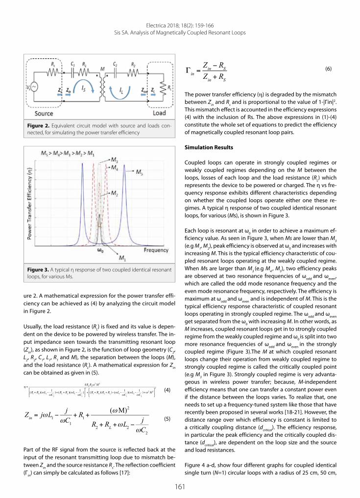
161


ure 2. A mathematical expression for the power transfer effi-ciency can be achieved as (4) by analyzing the circuit model in Figure 2.

Usually, the load resistance (RL) is fixed and its value is depen-dent on the device to be powered by wireless transfer. The in-put impedance seen towards the transmitting resonant loop (Zin), as shown in Figure 2, is the function of loop geometry (C2, L2, R2, C1, L1, R1 and M), the separation between the loops (M), and the load resistance (RL). A mathematical expression for Zin can be obtained as given in (5).

(4)η =

4RSRLω2M 2

(R1+ RS )(ωL2 -1

ωC2)+ (R2 + RL )(ωL1 -

1ωC1

)⎡

⎣⎢

⎤

⎦⎥

2

+ (R1+ RS )(R2 + RL ) - (ωL1 -1

ωC1)(ωL2 -

1ωC2

)+ω 2M 2⎡

⎣⎢

⎤

⎦⎥

2

(5)Zin = jωL1 −

jωC1

+ R1+(ωM)2

R2 + RL +ωL2 −j

ωC2

Part of the RF signal from the source is reflected back at the input of the resonant transmitting loop due to mismatch be-tween Zin and the source resistance Rs. The reflection coefficient (Γin) can simply be calculated as follows [17]:

(6)Γin =

Zin − RSZin + RS

The power transfer efficiency (η) is degraded by the mismatch between Zin and Rs and is proportional to the value of 1-|Γin|2. This mismatch effect is accounted in the efficiency expressions (4) with the inclusion of Rs. The above expressions in (1)-(4) constitute the whole set of equations to predict the efficiency of magnetically coupled resonant loop pairs.

Simulation Results

Coupled loops can operate in strongly coupled regimes or weakly coupled regimes depending on the M between the loops, losses of each loop and the load resistance (RL) which represents the device to be powered or charged. The η vs fre-quency response exhibits different characteristics depending on whether the coupled loops operate either one these re-gimes. A typical η response of two coupled identical resonant loops, for various (Ms), is shown in Figure 3.

Each loop is resonant at ω0 in order to achieve a maximum ef-ficiency value. As seen in Figure 3, when Ms are lower than M3 (e.g M1, M2), peak efficiency is observed at ω0 and increases with increasing M. This is the typical efficiency characteristic of cou-pled resonant loops operating at the weakly coupled regime. When Ms are larger than M3 (e.g M4 , M5), two efficiency peaks are observed at two resonance frequencies of ωodd and ωeven, which are called the odd mode resonance frequency and the even mode resonance frequency, respectively. The efficiency is maximum at ωodd and ωeven and is independent of M. This is the typical efficiency response characteristic of coupled resonant loops operating in strongly coupled regime. The ωodd and ωeven

get separated from the ω0 with increasing M. In other words, as M increases, coupled resonant loops get in to strongly coupled regime from the weakly coupled regime and ω0 is split into two more resonance frequencies of ωodd and ωeven in the strongly coupled regime (Figure 3).The M at which coupled resonant loops change their operation from weakly coupled regime to strongly coupled regime is called the critically coupled point (e.g M3 in Figure 3). Strongly coupled regime is very advanta-geous in wireless power transfer; because, M-independent efficiency means that one can transfer a constant power even if the distance between the loops varies. To realize that, one needs to set up a frequency-tuned system like those that have recently been proposed in several works [18-21]. However, the distance range over which efficiency is constant is limited to a critically coupling distance (dcritical). The efficiency response, in particular the peak efficiency and the critically coupled dis-tance (dcritical), are dependent on the loop size and the source and load resistances.

Figure 4 a-d, show four different graphs for coupled identical single turn (N=1) circular loops with a radius of 25 cm, 50 cm,

Figure 2. Equivalent circuit model with source and loads con-nected, for simulating the power transfer efficiency

Figure 3. A typical η response of two coupled identical resonant loops, for various Ms.

162


75 cm and 100 cm, respectively. The loops are resonant with series connected capacitances at 5 MHz. Each graph depicts a simulated efficiency (η) vs frequency data for various separa-tion distances (d) between the loops. Here the simulations are performed for the same load and source resistance values of 2 Ω (Rs= RL = 2 Ω).

Figure 5-7, show similar efficiency graphs for 10 Ω, 25 Ω and 50 Ω source & load resistance values, respectively.

In Figure 4, where source and load resistances are 2 Ω, peak efficiencies at strongly coupled regime are 86 %, 77 %, 68 % and 59 %, for loops with radius of 25 cm, 50 cm, 75 cm and 100 cm, respectively. It can clearly be seen that the peak efficiency is significantly reduced with increasing loop sizes. The critical coupling distance, on the other hand, increases from 35 cm to 250 cm as loop size increases from 25 cm to 100 cm. Such be-haviour of peak efficiency and critical coupling distance can be explained as follows:

• As the size of the loops increases, larger M values are ob-tained for the same loop separations; therefore, loops can stay in strongly coupled regime for larger separations be-tween the loops (dcritical increases). This is advantageous be-cause one can operate with almost distance-independent efficiency in larger loop separations. However, due to fre-quency splitting phenomena in strongly coupled opera-

tion, one needs a frequency tuned wireless power transfer system.

• As the size of the loops increases, the radiation loss resis-tance (Rrad) and conductor loss resistance (Rc) increases; hence the peak efficiency decreases due to these larger loss resistances.

It should be remembered that the efficiency plots in Figure 4 are for source and load resistances of 2 Ω. Figure 5-7, show effi-ciency graphs for source & load resistances (RS and RL) of 10 Ω, 25 Ω and 50 Ω, respectively. To analyze the effect of RS and RL

on peak efficiency and critical coupling distance, one can focus on the efficiency response for the same loop size in each figure. For example, in Figure 4 d, Figure 5 d, Figure 6 d and Figure 7 d, where loop radius is 100 cm, it can clearly be seen that the peak efficiency increases as RS and RL increase. However, the critical coupling distance decreases with increasing RS and RL.

A major conclusion from these simulation results is that one can increase critical coupling distance by either increasing loop size or by decreasing RS and RL values. In either case, any increase in critical coupling distance would be at the cost of re-duced peak efficiency. Therefore, loop sizes and input & output matching circuits should be carefully designed considering this tradeoff. Figure 8 a, b show peak efficiency (ηmax) and critical coupling distance (dcritical) as a function of loop radius for various RS and RL.

Figure 4. a-d. Efficiency (η) vs Frequency graphs for circular loops of radius of 25 cm (a); 50 cm (b); 75 cm (c) and 100 cm. RS=RL= 2 Ω(d)

163


Figure 5. a-d. Efficiency (η) vs Frequency graphs for circular loops of radius of 25 cm (a); 50 cm (b); 75 cm (c) and 100 cm (d) RS=RL= 10 Ω

Figure 6. a-d. Efficiency (η) vs Frequency graphs for circular loops of radius of 25 cm (a); 50 cm (b); 75 cm (c) and 100 cm (d) RS=RL= 25 Ω.

164


Model Verification through Measurements of Coupled Circular Loops

In the previous section, a significant analysis was performed using circuit model and geometry-dependent analytic equa-tions. In this section, we fabricated two multiturn circular loops to verify the accuracy of the model utilized in simulations. The loops are fabricated by winding solid copper wires on an ep-oxyglass. The radius of the loops is 25 cm and the number of turns is 5. Each loop’s self-inductance L is measured using a RLC meter. Then each loop is resonated out using a series con-

nected capacitor at 1 MHz. Simulations were performed at 5 MHz. Here, we intentionally resonated out the loops at 1 MHz to reduce the inter-winding parasitic capacitance in multiturn loops. Table 1 shows the theoretical and measured self-induc-tance values of each 5 turn loops. The required values of series connected capacitors to form a resonance at 1 MHz are also shown in Table 1.

The S-parameters of magnetically coupled resonant loops are measured from 100 kHz to 5 MHz using Rohde & Schwarz FSH8 Spectrum +Network analyzer as shown in Figure 9.

Figure 7. a-d. Efficiency (η) vs Frequency graphs for circular loops of radius of 25 cm (a); 50 cm (b); 75 cm (c) and 100 cm (d) RS=RL= 50 Ω

Figure 8. a, b. Efficiency (η) (a) and ciritical coupling distance (dcritical) vs loop radius (r) for various source & load resistances (b)

165


The efficiency is extracted from the measured S-parameters by taking the square of S21 as follows:

η = S212

(7)

Measured efficiency as a function of frequency for various loop separations are shown in Figure 10 a-f. RS and RL resistances in these measurements are 20 Ω and 10 Ω, respectively. Fig-ure 11 shows the plot of peak efficiency vs distance for both simulation and measurement results. As seen in Figure 10, 11; the measurement results agree well with the simulation results specifically in strongly coupled regime. The critical coupling distance dcritical is approximately 30 cm. The difference between the simulations and the measurement results could be at-tributed to some losses that are not considered in the model, such as the proximity effect of multi-turn loops and the loss of series connected resonance capacitors.

Conclusion

In this paper we have presented a circuit model based analy-sis of magnetically coupled resonant loops for use in wireless

Table 1. Theoretical and Measured Values of Self Inductances for Fabricated Loops

Theoretical Measured

Loop 1 L1 = 35.8 μ H C1 = 707 pF L1 = 29.1 μ H C1 = 875 pF

Loop 2 L2 = 35.8 μ H C2 = 707 pF L2 = 28.8 μ H C2 = 875 pF

Figure 9. S-parameter measurement setup for magnetically cou-pled loops

Figure 10. Comparison of simulation and measurement results for magnetically coupled resonant loops with RS = 20 Ω and RL = 10 Ω.

166


power transfer systems. The model employs analytical equa-tions for loop’s inductive parameters such as self and mutual inductances, and loss parameters such as conductor and radi-ation loss resistances. Hence overall power transfer efficiency was accurately predicted using this model. A thorough anal-ysis was also performed showing how the peak efficiency and the critical coupling distance changes as loop size and load & source resistances vary. The trade off between peak efficiency and critical coupling distance is discussed in detail. To validate the model’s accuracy, two 5 turn identical loops are fabricated and their efficiencies are measured. Future work would be to employ the proximity loss effects into the model and to con-duct a study on reducing the electrical losses in the loops.


Conflict of Interest: The authors have no conflicts of interest to declare.

Financial Disclosure: This research is supported by The Scientific and Technical Research Council of Turkey (TUBITAK-EEEAG-115E001).

Acknowledgements: The authors would like to thank to EMC Elec-tronics Company, specifically Refik Alemdar and Dr. Bektas Colak from Gebze, Turkey, for letting us compare our measurement results using their instruments.

References

1. A. Kurs, A. Karalis, R. Moffatt, J. D. Joannopoulos, P. Fisher, M. Solja-cic, “Wireless power transfer via strongly coupled magnetic reso-nances”, Science, vol. 317, no. 5834 pp. 83-86, 2007.

2. F. Zhang, S. A. Hackworth, W. Fu, C. Li, Z. Mao, M. Sun, “Relay effect of wireless power transfer using strongly coupled magnetic resonances”, IEEE Transactions on Magnetics, vol. 47, no. 5, pp. 1478-1481, 2011.

3. A. Karalis, J. D. Joannopoulos, M. Soljačić, “Efficient wireless non-radiative mid-range energy transfer”, Annals of Physics, vol. 323, no. 1, pp. 34-48, 2008.

4. E. M. Thomas, J. D. Heebl, C. Pfeiffer, A. Grbic, “A power link study of wireless non-radiative power transfer systems using resonant shielded loops”, IEEE Transactions on Circuits and Systems I: Regular Papers, vol. 59, no. 9 pp. 2125-2136, 2012.

5. J. D. Heebl, E. M. Thomas, R. P. Penno, A. Grbic, “Comprehensive anal-ysis and measurement of frequency-tuned and impedance-tuned wireless non-radiative power-transfer systems”, IEEE Antennas and Propagation Magazine, vol. 56, no. 5, pp. 131-148, 2014.

6. C. G. Pope, “Coupled Mode Theory and Wireless Energy Transfer”, 2012.7. J. Huh, W. Lee, S. Choi, G. H. Cho, C. T. Rim, “Explicit static circuit

model of coupled magnetic resonance system”, 8th International Conference on Power Electronics - ECCE Asia, 2011.

8. A. Robichaud, M. Boudreault, D. Deslandes, “Theoretical Analysis of Resonant Wireless Power Transmission Links Composed of Elec-trically Small Loops”, PIER, vol. 143, pp. 485-501, 2013.

9. C. J. Chen, T. H. Chu, C. L. Lin, Z. C. Jou, “A study of loosely coupled loops for wireless power transfer”, IEEE Transactions on Circuits and Systems II: Express Briefs, vol. 57, no. 7, pp. 536-540, 2010.

10. S. H. Lee, R. D. Lorenz. “Development and validation of model for 95%-efficiency 220-W wireless power transfer over a 30-cm air gap”, IEEE Transactions on Industry Applications, vol. 47, no.6, pp. 2495-2504, 2011.

11. S. H. Lee, R. D. Lorenz. “A design methodology for multi-kW, large air-gap, MHz frequency, wireless power transfer systems”, Energy Conversion Congress and Exposition (ECCE), 2011.

12. T. Imura, H. Okabe, T. Uchida, Y. Hori, “Study on open and short end helical antennas with capacitor in series of wireless power trans-fer using magnetic resonant couplings”, 35th Annual Conference of IEEE Industrial Electronics, 2009.

13. J. Kim, J. Jeong, “Range-adaptive wireless power transfer using multiloop and tunable matching techniques”, IEEE Transactions on Industrial Electronics, vol. 62, no. 10, pp. 6233-6241, 2015.

14. X. Wei, Z. Wang, H. Dai, “A critical review of wireless power transfer via strongly coupled magnetic resonances”, Energies, vol. 7, no. 7 pp. 4316-4341, 2014.

15. B. J. Jang, S. Lee, H. Yoon, “HF-band wireless power transfer sys-tem: Concept, issues, and design”, Progress in Electromagnetics Re-search, vol. 124, pp. 211-231, 2012.

16. C. A. Balanis, Antenna theory: analysis and design, John Wiley & Sons, 2016.

17. D. M. Pozar, Microwave engineering, John Wiley & Sons, 2009.18. Y. Gao, C. Zhou, J. Zhou, X. Huang and D. Yu, “Automatic Frequency

Tuning with Power-Level Tracking System for Wireless Charging of Electric Vehicles”, IEEE Vehicle Power and Propulsion Conference (VPPC), 2016.

19. D.P. Kar, P.P. Nayak, S. Bhuyan, S.K. Panda, “Automatic frequency tuning wireless charging system for enhancement of efficiency,” in Electronics Letters, vol. 50, pp. 1868-1870, November 2014.

20. S. A. Sis, S. Bicakci, “A resonance frequency tracker and source frequen-cy tuner for inductively coupled wireless power transfer systems”, 46th European Microwave Conference (EuMC), 2016, pp. 751-754.

21. S. Bıçakçı, S. A. Sis, “Design Of A Resonance Frequency Tracking System For Rf Applications”, GU J Sci, vol. 5, no. 2, pp. 211-221, 2017.

Seyit Ahmet Sis (S’07) received the B.S. degree in electronics engineering from the Gebze Institute of Technology, Kocaeli, Turkey, in 2005, the M.S. degree in electrical engineering from Syracuse University, Syracuse, NY, in 2008, and the Ph.D. degree from The University of Michigan at Ann Arbor, in 2014. From August 2005 to February 2007, he was with the Scientific and Technical Research Council of Turkey (TUBITAK-UEKAE). He is currently Assistant Professor of Electrical-Electronics Engineering Department at the Balikesir University, Balikesir, Turkey. His cur-rent research interests include wireless power transfer systems, high frequency passive circuits and amplifier design switchable and tunable microwave components.

Figure 10. Peak efficiency ηmax vs distance for simulation and measurement results

167

Introduction

Hydrogen is the most common element, making up 75 % of the mass of the entire universe and has been used as a fuel for many decades in a wide range of applications. Hydrogen re-quires a high sensitive detection for human safety not only because it possesses a wide flam-mability range of an explosive nature (lower and upper explosive limits of 4% and 75% in air, respectively) but also it’s great leaking tendency feature [1]. Many studies have been carried out for the purpose of hydrogen detection including fiber-based sensors, chemical sensors, photonic crystal sensors and micro-cavity optical sensors [2-5]. Among these, the micro-cavi-ty/micro-resonator sensors have high potential in high sensitive detection [6, 7]. Hybrid struc-tures of micro-resonators which might in hold different materials such as Pd is considered as a high-sensitive, low-cost, compact, durable, and high performance hydrogen detector com-pared to conventional hydrogen gas detecting instruments [5, 8].

Typical Pd involved optic micro-ring resonator (MRR) hydrogen sensor utilizes resonance-shift analysis to probe the presence of hydrogen in the sensing chamber. In such a sensing scheme the resonance wavelength/frequency alters with the change in hydrogen concentration of the sensor system. In order to detect low concentration levels, a generally high quality factor is required for a detectable resonance-shift [9]. It is well-known that due to the absorption feature of metals, the quality factor of a metal involved optical sensing system is typically low, which consequently leads to a lower detection limit [10, 11]. In addition, the perceptibility of the resonance-shift of this kind of optical sensor becomes smaller as the bandwidth of the resonance decreases, which also results in a lower detection limit [12].

As an alternative, intensity-based optical sensors may be advantageous over those based on resonance-shift. The intensity-based sensors measure the output intensity variation of a resonance peak such that the absorption due to the metal component helps to increase the performance rather than to decrease. In addition, such sensors are free from bandwidth re-strictions so that they can operate in a wide-range of wavelength.

Electrica 2018; 18(2): 167-171

RESEARCH ARTICLE

Hybrid Micro-Ring Resonator Hydrogen Sensor Based on Intensity DetectionKenan Çiçek Department of Electrical and Electronic Engineering, Iğdır University School of Engineering, Iğdır, Turkey Department of Electrical and Electronic Engineering, University of Bristol School of Engineering, Bristol, UK

Corresponding Author: Kenan Çiçek





DOI: 10.26650/electrica.2018.56722

Cite this article as: K. Çiçek, “Hybrid Micro-Ring Resonator Hydrogen Sensor Based on Intensity Detection”, Electrica, vol. 18, no: 2, pp. 167-171, 2018.

ABSTRACT

In this paper, a photonic integrated device fabricated on a silicon-on-insulator (SOI) platform is studied numerically to investigate its hydrogen sensing potential based on intensity variations. A single-slot hybrid structure consisting of a coaxial micro-ring resonator (MRR) and a palladium (Pd) disk is utilized for this purpose. The results of the numerical study reveal a hydrogen sensing ability of 2.83×10-4/(v/v-% hydrogen) and limit of detection (LOD) of 9.93×10-3 which is more than 10 times of that of the hydrogen sensors based on the traditional resonance shift. The proposed hydrogen sensing technique presents a compatible SOI-based technology and also provides a reliable detection of the slightest changes from the zero concentration in an analytical procedure.

Keywords: Hydrogen sensor, micro-ring resonator, optic sensor, intensity-based sensor.

https://orcid.org/0000-0001-5686-6872

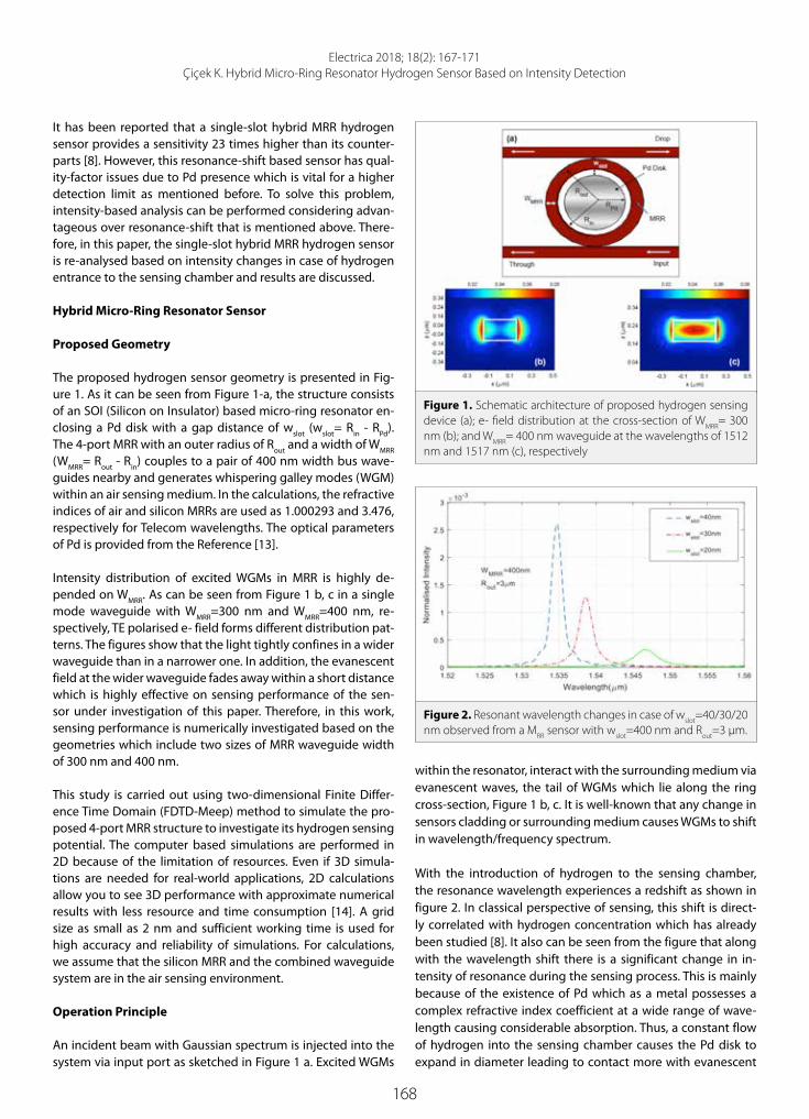
168

Electrica 2018; 18(2): 167-171Çiçek K. Hybrid Micro-Ring Resonator Hydrogen Sensor Based on Intensity Detection

It has been reported that a single-slot hybrid MRR hydrogen sensor provides a sensitivity 23 times higher than its counter-parts [8]. However, this resonance-shift based sensor has qual-ity-factor issues due to Pd presence which is vital for a higher detection limit as mentioned before. To solve this problem, intensity-based analysis can be performed considering advan-tageous over resonance-shift that is mentioned above. There-fore, in this paper, the single-slot hybrid MRR hydrogen sensor is re-analysed based on intensity changes in case of hydrogen entrance to the sensing chamber and results are discussed.

Hybrid Micro-Ring Resonator Sensor

Proposed Geometry

The proposed hydrogen sensor geometry is presented in Fig-ure 1. As it can be seen from Figure 1-a, the structure consists of an SOI (Silicon on Insulator) based micro-ring resonator en-closing a Pd disk with a gap distance of wslot (wslot= Rin - RPd). The 4-port MRR with an outer radius of Rout and a width of WMRR (WMRR= Rout - Rin) couples to a pair of 400 nm width bus wave-guides nearby and generates whispering galley modes (WGM) within an air sensing medium. In the calculations, the refractive indices of air and silicon MRRs are used as 1.000293 and 3.476, respectively for Telecom wavelengths. The optical parameters of Pd is provided from the Reference [13].

Intensity distribution of excited WGMs in MRR is highly de-pended on WMRR. As can be seen from Figure 1 b, c in a single mode waveguide with WMRR=300 nm and WMRR=400 nm, re-spectively, TE polarised e- field forms different distribution pat-terns. The figures show that the light tightly confines in a wider waveguide than in a narrower one. In addition, the evanescent field at the wider waveguide fades away within a short distance which is highly effective on sensing performance of the sen-sor under investigation of this paper. Therefore, in this work, sensing performance is numerically investigated based on the geometries which include two sizes of MRR waveguide width of 300 nm and 400 nm.

This study is carried out using two-dimensional Finite Differ-ence Time Domain (FDTD-Meep) method to simulate the pro-posed 4-port MRR structure to investigate its hydrogen sensing potential. The computer based simulations are performed in 2D because of the limitation of resources. Even if 3D simula-tions are needed for real-world applications, 2D calculations allow you to see 3D performance with approximate numerical results with less resource and time consumption [14]. A grid size as small as 2 nm and sufficient working time is used for high accuracy and reliability of simulations. For calculations, we assume that the silicon MRR and the combined waveguide system are in the air sensing environment.

Operation Principle

An incident beam with Gaussian spectrum is injected into the system via input port as sketched in Figure 1 a. Excited WGMs

within the resonator, interact with the surrounding medium via evanescent waves, the tail of WGMs which lie along the ring cross-section, Figure 1 b, c. It is well-known that any change in sensors cladding or surrounding medium causes WGMs to shift in wavelength/frequency spectrum.

With the introduction of hydrogen to the sensing chamber, the resonance wavelength experiences a redshift as shown in figure 2. In classical perspective of sensing, this shift is direct-ly correlated with hydrogen concentration which has already been studied [8]. It also can be seen from the figure that along with the wavelength shift there is a significant change in in-tensity of resonance during the sensing process. This is mainly because of the existence of Pd which as a metal possesses a complex refractive index coefficient at a wide range of wave-length causing considerable absorption. Thus, a constant flow of hydrogen into the sensing chamber causes the Pd disk to expand in diameter leading to contact more with evanescent

Figure 1. Schematic architecture of proposed hydrogen sensing device (a); e- field distribution at the cross-section of WMRR= 300 nm (b); and WMRR= 400 nm waveguide at the wavelengths of 1512 nm and 1517 nm (c), respectively

Figure 2. Resonant wavelength changes in case of wslot=40/30/20 nm observed from a MRR sensor with wslot=400 nm and Rout=3 µm.

169


field and resulting an exponential decrease in intensity of the WGMs as shown in Figure 3.

It is clear from the figure that the slope of intensity plot de-creases as wslot decreases (RPd increases). This means that the rate of intensity change exponentially decreases as the Pd disk approaching the MRRs inner face. This phenomenon occurs in resonance-shift based sensors in such a way that any change in wslot emerges an inversely proportional effect on resonance wavelength shift, as shown in Figure 3.

In the following section, the hydrogen sensing potential of in-tensity-based hybrid MMR sensor is investigated for a hydro-gen concentration range of 0% to 1%, a range that allows a reversible expansion in Pd.

Results

It is a fact that, palladium lattice expends 0.087 % within 1 % H2 sensing environment [15]. In the reference of this, numerical calculations are performed for various geometry parameters of sensor. Each sensor geometry is simulated changing the Pd radius for each calculation loop assuming the change is due to the hydrogen absorption. However, the 2 nm grid size em-ployed in this study is not sufficient for pico-meter level chang-es. Therefore, the simulations are performed changing the Pd size with 5 nm intervals at each calculation loop. Then, result-ed ΔI (intensity change) values are interpolated by non-linear curve fitting to observe at the pico-meter level corresponding to small hydrogen concentration changes as presented in Fig-ure 3. Under all this assumption, the relation between hydro-gen concentration (Chyd), in volume/volume percent (v/v - %), and ΔI is investigated.

Figure 4 shows ΔI values as a function of Chyd observed from drop port of the sensors for a range of geometric parameters.

From the figure, it is seen that, both wslot and WMRR have a large effect on ΔI. Figure 4 a, shows that, when a 300 nm wide MRR with Rout=1 µm and wslot=40 nm is employed, ΔI gradually in-creases up to 1.4×10-4 along with the hydrogen concentra-tion increment in the range of Chyd=0 % to Chyd=1 %. This val-ue reaches to 1.01×10-4 and 0.7×10-4 with smaller slot sizes of wslot= 30 nm and wslot= 20 nm, respectively. While Rout increases from 1 µm to 3 µm the rate of ΔI increases directly with the wslot size. As presented in Figures 4 b, c; ΔI reaches higher values of 1.8×10-4 and 2.2×10-4 for devices with Rout=2 µm and Rout=3 µm, respectively when wslot=40 nm. It is evidence from the Figures 4 a-c, that regardless of Rout, the highest ΔI rates are observed when wslot=40 nm. On the other hand, the rate of ΔI in response to hydrogen concentration slightly increases for WMRR=400 nm wide MRRs as compared to WMRR=300 nm, as shown in Figure 4 e, f. As such, the highest shift can be obtained for a design where wslot=40 nm and Rout=3 µm is around 2.8×10-4. It needs to be noted that, in Figure 4 d the observed ΔI for the geome-try with wslot=20 nm and Rout=1 µm is higher than the one with wslot=40 nm for the same radius.

This is due to the decreasing behaviour of the slope of the in-tensity plot for this particular geometry through the wslot; other computed geometries (presented in other sub- figures) exhibit an increasing trend for the same plot. The reason for this in-tensity trend difference might be because of the loss (includes scattering, bending and absorption losses) rate in case of each wslot value [6].

In order to determine the efficiency of the sensor, the sensi-tivity (S= ΔI/ΔChyd) as function of hydrogen concentration is calculated. According to the calculations, hydrogen could be detected with a sensitivity of as high as 2.20×10-4/(v/v - % hy-drogen) employing an Rout=3 µm MRR system where wslot= 40 nm and WMRR= 300 nm. In addition, S could be further increased up to 2.83×10-4/(v/v - % hydrogen) with same Rout and wslot but a wider resonator width of WMRR=400 nm.

Another factor to describe the performance of an optical sensor is the Limit of detection (LOD) which is the lowest concentration of hydrogen that can be distinguished from the zero concentration level. LOD of proposed intensi-ty-based sensor is calculated based on the standard devia-tion of the response (Lr) of each linear curve and the slope of the calibration curve (Lsl) of ΔI vs Chyd at levels approximating the LOD according to the formula LOD=(3.3×Lr)/Lsl [16]. Lr is determined based on the standard deviation of y-intercepts of regression lines and both Lr and Lsl are computed via MS Excel. It is found that the intensity-based hybrid MMR sen-sor offers an LOD of 9.93×10-3 for a geometry that present highest sensitivity. In comparison with this study, the LOD of the most sensitive geometry in reference [8] is also calculat-ed with the same theory and found to be 7.16×10-2 which is around 10 times higher than the one with intensity- based sensing.

Figure 3. Interpolation of intensity (left hand side y-axis)/wave-length (right hand side y-axis) based simulated data for a geom-etry where Rout= 1 µm, RPd= 0.66 µm, WMRR= 300 nm and wslot= 30 nm. For these geometry values 5 nm RPd intervals (ΔRPd) corre-sponds to Chyd= 8.57 % assuming linear volumetric expansion of Pd with H2

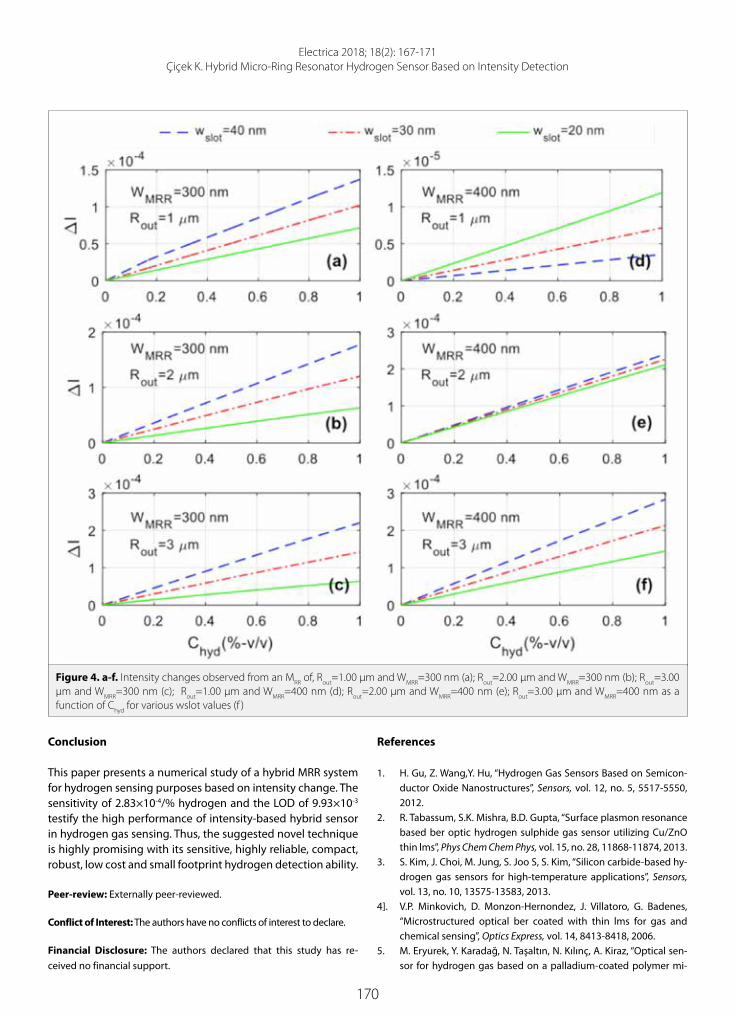
170


Conclusion

This paper presents a numerical study of a hybrid MRR system for hydrogen sensing purposes based on intensity change. The sensitivity of 2.83×10-4/% hydrogen and the LOD of 9.93×10-3 testify the high performance of intensity-based hybrid sensor in hydrogen gas sensing. Thus, the suggested novel technique is highly promising with its sensitive, highly reliable, compact, robust, low cost and small footprint hydrogen detection ability.




References

1. H. Gu, Z. Wang,Y. Hu, “Hydrogen Gas Sensors Based on Semicon-ductor Oxide Nanostructures”, Sensors, vol. 12, no. 5, 5517-5550, 2012.

2. R. Tabassum, S.K. Mishra, B.D. Gupta, “Surface plasmon resonance based ber optic hydrogen sulphide gas sensor utilizing Cu/ZnO thin lms”, Phys Chem Chem Phys, vol. 15, no. 28, 11868-11874, 2013.

3. S. Kim, J. Choi, M. Jung, S. Joo S, S. Kim, “Silicon carbide-based hy-drogen gas sensors for high-temperature applications”, Sensors, vol. 13, no. 10, 13575-13583, 2013.

4]. V.P. Minkovich, D. Monzon-Hernondez, J. Villatoro, G. Badenes, “Microstructured optical ber coated with thin lms for gas and chemical sensing”, Optics Express, vol. 14, 8413-8418, 2006.

5. M. Eryurek, Y. Karadağ, N. Taşaltın, N. Kılınç, A. Kiraz, “Optical sen-sor for hydrogen gas based on a palladium-coated polymer mi-

Figure 4. a-f. Intensity changes observed from an MRR of, Rout=1.00 µm and WMRR=300 nm (a); Rout=2.00 µm and WMRR=300 nm (b); Rout=3.00 µm and WMRR=300 nm (c); Rout=1.00 µm and WMRR=400 nm (d); Rout=2.00 µm and WMRR=400 nm (e); Rout=3.00 µm and WMRR=400 nm as a function of Chyd for various wslot values (f )

171


croresonator” Sensors and Actuators B: Chemical, vol. 212, 78-83, 2015.

6. L. Zhou, X. Sun, X. Li, J. Chen, “Miniature Microring Resonator Sen-sor Based on a Hybrid Plasmonic Waveguide”, Sensors, vol. 11, no. 7, 6856-6867, 2011.

7. A. Daraei, M. E. Daraei, “Thin cylindrical slot in an optical micro-disk cavity for sensing biomaterials”, Appl Phys A, vol. 123, 216-222, 2017.

8. K. Cicek, M. Eryrek, A. Kiraz, “Single-slot hybrid microring resona-tor hydrogen sensor” J. Opt. Soc. Am. B, VOL. 34, NO. 7, 1465-1470, 2017.

9. P.S. Pedersen, P. S. Nunes, S. Xiao, N.A. Mortensen, “Material Lim-itations on the Detection Limit in Refractometry” Sensors, vol. 9, 8382-8390, 2009.

10. L. Huang, H. Yan, X. Xu, S Chakravarty, N Tang, H Tian, R. T. Chen, “Improving the detection limit for on-chip photonic sensors based on subwavelength grating racetrack resonators” Optics Ex-press, vol. 25, 10527-10535, 2017.

11. Y. Liu, W. Zhou, Y. Sun, “Optical Refractive Index Sensing Based on High-Q Bound States in the Continuum in Free-Space Coupled Photonic Crystal Slabs”, Sensors, vol. 17, 1861-1873, 2017.

12. Z. Xia, Y. Chen, Z. Zhou, “Dual Waveguide Coupled Microring Res-onator Sensor Based on Intensity Detection”, IEEE J Quantum Elect, vol. 44, 100-107, 2008.

13. A. D. Rakic, A B. Djurisic, J. M. Elazar, M. L. Majewskii, “Optical prop-erties of metallic lms for vertical-cavity optoelectronic devices”, Appl Opt, vol. 37, 5271-5283, 1998.

14. M. Gabalis, D. Urbonas, R. Petruskevicius, “A perforated microring resonator for optical sensing applications”, Journal of Optics, vol. 2016, 105003-105009, 2017.

15. J. S. Noh, J. M. Lee, W. Lee, “Low-Dimensional Palladium Nano-structures for Fast and Reliable Hydrogen Gas Detection” Sensors, vol. 11, 825-851, 2011.

16. A. Shrivastava, V. Gupta, “Methods for the determination of limit of detection and limit of quantitation of the analytical methods” Chronicles of Young Scientists, vol. 2, 21-25, 2011.

Kenan Çicek, I have been graduated from University of Bristol with a PhD degree in 2016. Currently I am an assis-tant professor in Iğdır University, Turkey. My specialty is integrated optics and photonic devices.

172

Introduction

Wireless data traffic has grown tremendously over the past years as the number of users and applications have increased. To meet the data traffic, several promising technologies have been developed. Among them, relay aided communication (also known as cooperative com-munication) and cognitive radio (CR) have been recognized as two of the most important en-ablers [1].

Cognitive radio proposes the spectrum-sharing paradigm to enhance the radio frequency spectrum efficiency in wireless systems while keeping the harmful interference between pri-mary and secondary networks at a minimum level [2]. Different techniques have been consid-ered for spectrum sharing so far. Among them, underlay model, which allows the secondary user (SU) to transmit simultaneously with the primary user (PU) in the PU’s frequency band, has become a practical solution for next generation wireless systems.

Relay aided transmission on the other side, can provide a reliable communication for the sec-ondary networks by placing intermediate relay nodes between the secondary source and des-tination. Hence, it can exploit the spatial diversity. In relay-aided communication, amplify and forward (AF) and decode and forward (DF) relaying techniques have been considerably investi-gated. In DF, the relay detects the received signal and forwards the uncoded signal to the des-tination. However, in the AF mode, relay simply scales and then transmits the scaled version of the signal [3]. Hence, due to its simple structure, relay aided communication has been adopted into several standards such as 3GPP LTE-Advanced and IEEE 802.16j [4]. In this respect, a wide range of studies in the literature have been considered cognitive cooperative structures (see, e.g., and the references therein) [5-12]. AF method was studied in a CR relay network where outage probability was examined for Rayleigh fading channels [5]. A general case of was con-sidered where both outage and error probability were derived for Nakagami-m fading channels [5, 6]. Considering DF relaying in Nakagami-m fading, outage probability was examined in and

Electrica 2018; 18(2): 172-176

RESEARCH ARTICLE

Cognitive AF Relay Networks over Asymmetric Shadowing/Fading Channels in the Presence of Low-Rate FeedbackEylem Erdoğan Department of Electrical and Electronics Engineering, İstanbul Medeniyet University School of Engineering and Natural Science, İstanbul, Turkey

Corresponding Author: Eylem Erdoğan





DOI: 10.26650/electrica.2018.65047

Cite this article as: E. Erdoğan, “Cognitive AF Relay Networks over Asymmetric Shadowing/Fading Channels in the Presence of Low-Rate Feedback”, Electrica, vol. 18, no: 2, pp. 172-176, 2018.

ABSTRACT

This study investigates the performance of a cognitive amplify-and-forward (AF) relay network over composite asymmetric multipath/shadowing fading channels, whereby a new power allocation method is adopted at the secondary source and relay, assuming the mean-value interference channel. To quantify the performance of the proposed structure, closed-form outage probability and ergodic capacity expressions are derived. Moreover, asymptotic ergodic capacity analysis is performed to observe the effects of limited feedback and fading/shadowing severity in the system. The analytical results are validated with Monte-Carlo simulations, and they show that the proposed structure can be a realistic scenario for next-generation wireless systems, and a system designer can test the overall performance of the proposed system without dealing with complex prototypes.

Keywords: Cognitive radio, multipath/shadowing fading channels, cooperative communication

https://orcid.org/0000-0003-3657-1721

173

Electrica 2018; 18(2): 172-176Erdoğan E. Cognitive AF Relaying over Shadowing/Fading Channels

the diversity gains of AF and DF CR systems was investigated in [7, 8]. Moreover, physical layer secrecy performance of CR DF re-lay network was investigated in [9]-[10]. Yang et al. [11] derived the outage probability performance of dual-hop AF CR network over η−µ fading channels in and Li et al. [12] studied the impact of uncorrelated fading channels on CR relay networks in.

As can be seen above, none of the works above have focused on a cognitive cooperative scheme under practical multipath/shadowing propagation conditions. Herein, we considered an AF cognitive relaying scheme where the transmission between secondary source (S) and relay (R) is impaired by fading and shadowing effects. To do so, generalized-K composite fading model which can incorporate both fading and shadowing ef-fects is used [13]. Considering that the second hop is modelled with Nakagami-m fading due to asymmetric traffic conditions, we derived closed form expressions of outage probabilitty and ergodic capacity and analyzed the outage probability in the presence of low-rate feedback.

System Model

This paper considers a cognitive underlay AF relaying scheme in which the communicates with the secondary destination (D) over single relay (R) terminal in the presence of a prima-ry receiver (PR) over asymmetric fading channels. The direct path between S to D is not avaliable as the transmission is per-formed in a time-division multiple access (TDMA) fashion in two time slots. In the proposed structure, we assume that the S→R path is detoriarated by the shadowing/fading effects and hence follows the Generalized-K composite fading model. On the other side, R→D path is modelled as Nakagami-m fading channel with ρR,D severity parameter.

In the first hop, both shadowing and fading effects between S→R path are modeled as i.i.d. Gamma distribution with and fading ζκSR and ζλSR shadowing parameters respectively.

In the first time slot, S transmits its information to the R. The received signal at the R can be written as

(1)

where κSR and λSR denote the shadowing and channel informa-tion respectively and χs is the the source signal. In the second time slot, R transmits the amplified signal to the D. The received signal at the D can be written as

(2)

where hRD denotes the channel information between R and, D, nR and nD are the additive white Gaussian noises modeled with zero-mean and unit variance and scaling gain G is given as

(3)

Mean-Value Power Allocation at Secondary Source and Relay

In underlay CR networks, it is generally assumed that the PR knows the interference gain of the channel instantaneously. However, this assumption cannot be used in practical wireless networks as it brings huge feedback burden and feedback er-rors. To reduce the feedback burden and to prevent feedback errors, the practical mean-value (MV) power allocation tech-nique can be used. In MV power allocation, the PR obtains the mean value of the feedback gain and feeds back to the sec-ondary system. Therefore, S and R powers can be written as Ps Min and , where κSP and λSP show the shadowing and channel informations between S and PR, hR,P is the channel information between R and PR, Qp is the maximum tolerable interference power of the PR and Pmax shows the max-imum power available in the system.

End-to-End Signal to Noise Ratio Calculation

By substituting (1) and (3) into (2), end-to-end (e2e) SNR can be written as

(4)

where ϒSR and ϒRD can be written as

(5)

As the analysis of (4) is theoretically complicated, obtaining the statistics of SNR can not be possible. However, (4) can be sim-plified as

(6)

Performance Analysis

In this section, outage probability and ergodic capacity expres-sions are obtained for the proposed structure.

Outage Probability As both λSR and κSR are independent and Gamma distributed, the CDF of ϒSR can be expressed as

(7)

174


With the aid of [14], FKSR can be given as can be seen in (8) at

the top of the next page. In (8), ϒ (.,.) shows the lower incomplete Gamma function [14, eqn. 8.350.1]. The derivative of FKSR(χ) can be obtained as

(8)

can be found similarly by changing the variables in (8) as

(9)

(10)

By substituting (9) and (10) into (7) with the help of [14, eqn. 3.471.9] and after few manipulations, FϒSR (ϒ) can be obtained as can be seen in (11) at the top of the page. In (11) Kv(.) shows the modified Bessel function of the second kind [15, 51]. On the other hand, the CDF of the ϒRD can be obtained as

(11)

(12)

and with the aid of (6), FϒUP (ϒ) can be expresed as

(13)

Outage probability is defined as the probability of SNR falling below a predefined threshold, ϒth and can be expressed as Pout=FϒUP (ϒth). It can be obtained easily by substituting (11) and (12) into (13).

Ergodic Capacity

Ergodic capacity is one of the most important performance indicators in wireless systems. Ergodic capacity is the maxi-mum achievable rate that a communication system can obtain. Mathematically speaking, it can be expressed as where E [.] de-notes the expectation operation. To the best of our knowledge, there is no direct

(14)

method to find the closed form solution of ergodic capacity. However, a tight upper bound can be obtained by adopting γup to the above expression as

(15)

where the simple form of Fϒup(ϒ), Fϒup(ϒ) denotes the comple-mentary CDF of ϒup i.e., Fϒup(ϒ)=1−Fϒup(ϒ). By subsituting Fϒup(ϒ) into (15) and after few manipulations, CE can be found as given in (16) at the top of the next page. In (16), Monte-Carlo simula-tions show that I3 can be negligible at medium and high SNRs as it is the multiplication of two CDF expressions. I2, can be ob-tained by using [14, eqn. 3.383.10] as can be seen in (17). Note that, Γ(.,.) denotes the upper incomplete Gamma function [14, eqn. 8.350.2]. and Γ(.) stands for the Gamma function [14, eqn. 8.339.1]. I1 on the other hand can be derived in closed form by using well known software programs such as MAPLE or MATH-EMATICA as can be seen in (18). Note that, ø1, ø2, ø3 and ø4 can be obtained as given in (19-22).

(16)

(17)

(18)

(19)

175


(20)

(21)

(22)

In (18), pFq(.) denotes the generalized hypergeometric func-tion and in (20, 21), J.(.) stands for the modified Bessel function of the first kind [15]. By substituting (18) and (17) into (16), er-godic capacity can be obtained as .

Moreover, a tight asymptotic bound on the CE can be obtained (23) by using Jensen’s inequality as

(23)

After several manipulations, CE∞ can be obtained as given at the

top of the next page in (24).

(24)

Impact of Limited Feedback

In wireless systems, feedback link is always assumed as full-rat-ed. However, if a network suffers from power constraints, lim-ited feedback occurs. Herein, we assume that the R→D path is modelled with Rayleigh distribution (special case of Nak-agami-m when m=1) and the feedback path between R to D is limited. Therefore, the PDF of ϒRD can be expressed as [16] where ∈ shows the rate of feedback, i.e. ∈=0 denotes the full rate feedback. F_(γ_(R,D))^Lim (γ) can be obtained by integrat-ing (25) with respect to γ as

(25)

(26)

By substituting (26) into (13) and by adopting the theoretical steps described above, both outage probability and ergodic capacity can be obtained.

Numerical Results

In this section, Monte-Carlo simulations are carried out to demonstrate the impact of asymmetric fading/shadowing channels in cognitive AF relaying scheme and the theoretical results are validated with Monte-Carlo simulations. Moreover, for analytical brevity, and Figure 1 illustrates the outage probability performance of the considered scheme. As can be seen, there is almost 10 dB difference between intense fading/shadowing environ-ment i.e., 1 and light fading/shadowing i.e., 4 at 5 × 10−1 dB. Moreover, after 24 dB, there is no performance gain and the diversity goes to 0 as PS and PR reaches to Pmax.

Figure 2 depicts the ergodic capacity performance of the pro-posed scheme. The dash/dot curves (theoretical and asymp-totic results) show good agreement with the marker symbols of the Monte- Carlo simulations. It is observed that, there is almost 4 dB difference between intense and light fading/shad-owing environments at 4 bits/channels use.

Figure 3 shows the impact of limited feedback on the perfor-mance of ergodic capacity. As seen from the figure, there is almost 10 dB difference between full-rated feedback (a = 0) and very limited feedback (a = 0.9). Therefore, we can infer that low-rate feedback can degrade the performance of wireless systems.

Conclusion

In this paper, we propose and analyze a cognitive AF relaying scheme in the presence of intense and light fading/shadowing environments. We believe that the proposed model can be a reliable scheme for next generation wireless systems and a sys-tem designer can have a quick idea about the system perfor-mance with the help of the theoretical results, without dealing with complex prototypes.

Figure 1. Closed form and theoretical outage probability for dif-ferent fading/shadowing severity parameters.

176




Financial Disclosure: This study was supported by the Research Fund of Istanbul Medeniyet University, Project Number: F-GAP-2017-1056.

References

1. C. X. Wang, F. Haider, X. Gao, X. H. You, Y. Yang, D. Yuan, H. M. Ag-goune, Harald Haas, s. Fletcher, “Cellular architecture and key technologies for 5G Wireless Communication Networks”, IEEE Commun Mag, vol. 52, no. 2, pp. 122-130, 2014.

2. A. Goldsmith, S.A. Jaffar, I. Maric, S. Srinivasa “Breaking spectrum gridlock with cognitive radios: An information theoretic perspec-tive”, Proceedings of the IEEE, vol. 97, no. 5, pp. 894-914, 2014.

3. X. Tao, X. Xu, Q. Cui, “An Overview of Cooperative Communica-tions”, IEEE Commun Mag, vol. 50, no. 6, pp. 65-71, 2012.

4. E. Dahlman, S. Parkvall, J. Skold, P. Beming, “3G Evolution: HSPA and LTE for Mobile Broadband”, New York, Academic Press, 2010.

5. T. Q. Duong, V. N. Q. Bao, H.-J. Zepernick, “Exact outage probability of cognitive AF relaying with underlay spectrum sharing”, Electron Lett, vol. 47, no. 17, pp. 1001-1002, 2011.

6. T. Q. Duong, D. B. da Costa, M. Elkashlan, V. N. Q. Bao, “Cognitive amplify-and-forward relay networks over Nakagami-m fading”, IEEE Trans Veh Technol, vol. 61, no. 5, pp. 2368-2374, 2012.

7. C. Zhong, T. Ratnarajah, K.K. Wong, “Outage analysis of de-code-and-forward cognitive dual-hop systems with the interfer-ence constraint in Nakagami-m fading channels”, IEEE Trans Veh Technol, vol. 60, no. 6, pp. 2875-2879, 2011.

8. H. Ding, J. Ge, D.B. da Costa, Z. Jiang, “Asymptotic analysis of coop-erative diversity systems with relay selection in a spectrum shar-ing scenario”, IEEE Trans Veh Technol, vol. 60, no. 2, pp. 457-472, 2011.

9. R. Zhao, Y. Yuan, L. Fan, Y.C. He, “Secrecy performance analysis of cognitive decode-and-forward relay networks in Nakagami-m fading channels”, IEEE Trans Veh Technol, vol. 65, no. 2, pp. 547-563, 2017.

10. D. Chen, Y. Chang and W. Yang, “Physical layer security in cognitive untrusted relay networks”, IEEE Access, vol. 6, pp. 7055-7065, Oct. 2017.

11. J. Yang, L. Chen, X. Lei, K. Peppas, T.Q. Duong, “Dual-hop cognitive amplify-and-forward relaying networks over η-μ fading channels”, IEEE Trans Veh Technol, vol. 65, no. 8, pp. 6290-6300, 2016.

12. M. Li, H. Yin, Y. Huang, Y. Wang, “Impact of correlated fading chan-nels on cognitive relay networks with generalized relay selection”, IEEE Access, vol. 6, pp: 6040-6047, 2017.

13. P.S. Bithas, N.C. Sagias, P.T. Mathiaopoulos, G.K. Karagiannidis, A. A. Rontogiannis, “On the performance analysis of digital commu-nications over generalized-K fading channels”, IEEE Commun Lett, vol. 10, no. 5, pp. 353-355, 2006.

14. I. S. Gradshteyn, I.M. Ryzhik, “Table of integrals, series and prod-ucts,” 7th ed. New York: Academic Press, 2007.

15. K.B. Oldham, J. Myland, J. Spanier, “An atlas of functions”, 2nd ed. Berlin, Germany: Springer-Verlag, 2008.

16. Y. Ma, D. Zhang, A. Leith, Z. Wang, “Error performance of transmit beamforming with delayed and limited feedback.”, IEEE Trans. Wireless Commun, vol. 8, no. 3, pp: 1164-1170, 2009.

Figure 2. Closed form, theoretical and asymptotic ergodic capac-ity performance.

Figure 3. Impact of limited feedback on the performance of the proposed scenario.

Eylem Erdoğan received B.Sc. and M.Sc. degree from Işık University, Istanbul, Turkey in 2003 and 2006 and the Ph.D. degree from Kadir Has University, İstanbul, Turkey, all in electronics engineering. He is currently an Assis-tant Professor in the Department of Electrical and Electronics Engineering, İstanbul Medeniyet University. He was a Post-Doctoral Fellow in Electrical Engineering Department, Lakehead University, Thunder Bay, ON, Canada from 2015 to 2016. He has authored or coauthored around 20 papers in peer reviewed journals and international conferences. His research interests are in the broad areas of wireless communications, including signal process-ing for wireless communications, the performance analysis of cooperative relaying in cognitive radio networks, mmWave communications and optical frequency bands.

177

Introduction

Blood vessel assessment and segmentation play a key role in the diagnosis of many different kinds of diseases such as retinal disorders in diabetic retinopathy, macular degeneration, and glaucoma that may cause a gradual loss of eyesight and could be a reason for blindness. The manual detection of narrow blood vessels on retinal images is time-consuming and may result in erroneous output. Hence, automated systems, computer aided, robust performance-ori-ented algorithms are all required to detect and segment the blood vessels and diagnose their associated diseases efficiently.

Segmentation, detection, and measuring the diameter of retinal blood vessels are essential for an accurate diagnosis and precise treatment of many ocular diseases such as diabetic ret-inopathy (DR) [1].

Diabetic retinopathy was selected for the purpose of this study. By applying an automated algorithm from an obtained retinal fundus image it could be classified as healthy (normal) or unhealthy (suffers from DR). DR is categorized as one of the most severe eye diseases world-wide. The symptoms could badly affect the vision of patients and could be escalated to reach blindness in some cases if neglected.

Diabetic retinopathy is identified and characterized by the growth of retinal microaneurysms, hemorrhages, and exudates which are all main aspects to be tracked during a DR diagnosis.

The more micro-aneurysms, hemorrhages, and exudates in number, the more severe the dis-ease is [2-4]. Exudate detection was the main focus of this study since it is a significant sign of

Electrica 2018; 18(2): 177-186

RESEARCH ARTICLE

Exudates Detection in Diabetic Retinopathy by Two Different Image Processing TechniquesSara S. Aldeeb, Selçuk SevgenDepartment of Computer Engineering, İstanbul University School of Engineering, İstanbul, Turkey

Corresponding Author: Selçuk Sevgen





DOI: 10.5152/iujeee.2018.1822

Cite this article as: S.S. Aldeeb, “Exudates Detection in Diabetic Retinopathy by Two Different Image Processing Techniques”, Electrica, vol. 18, no: 2, pp. 177-186, 2018.

ABSTRACT

Different techniques developed in the previous decades are used for blood vessel detection. Different kinds of image processing approaches in the detection and analysis of blood vessels can be applied to diagnose many human diseases and help in various medical and health diagnoses. Image processing for blood vessels could be used in areas such as disease diagnosis, severity measurement of specific diseases, and in biometric security.This study compares two different techniques to accurately diagnose a specific disease according to some selective features. Diabetic retinopathy is used for this comparative study as it is one of the most severe eye disorders and chronic diseases to cause blindness. Classifications and accurate measurements for blood vessel abnormalities (exudates, hemorrhages, and micro-aneurysms) enabled the correct and accurate diagnosis in retina and diabetic retinopathy. To avoid blindness, it is essential to utilize fundus image processing application to facilitate the early discovery of a diseased retinal. Throughout the fundus automated image process, the retinal features are extracted. The techniques applied in this study are a morphological-based image processing technique and an edge detection technique using Kirsch’s template. First, the application of these image processing techniques are described and explained in detail. Subsequently, a classification process is proposed to assess and evaluate the performance of each technique.

Keywords: Diabetic retinopathy, optic disc, exudates, morphology, Kirsch’s template

178

Electrica 2018; 18(2): 177-186Aldeeb and Sevgen. Exudates Detection in Diabetic Retinopathy

diabetic retinopathy and an indication of the co-existence with retinal edema. Vision could be lost in case of exudate expan-sion into the macular area.

In the traditional method of DR diagnosis, the patient’s pupil is dilated using the chemical, Tropicamide 1%, which could cause side-effects in some patients. It is a time-consuming, inconve-nient method of diagnosis for ophthalmologists [5].

Recently, some automated image processing techniques have been developed and applied to retinal images for exudate de-tection and analysis as a substitution for the traditional diag-nostic method.

In the study of Sinthanayothin et al. [6] the RRGS algorithm was applied. The basis of RRGS depends on the identification of similar pixels within a certain region so that the boundary location could be determined. The adjacent pixels of the same regions tend to have homogeneous gray-level characteristics.

Usher et al. [7] applied an adaptive intensity thresholding be-side RRGS for detecting exudate areas. After extracting the can-didate regions, they were used as input to an artificial neural network. By applying the RRGS algorithm, the separation re-sults of dark and bright lesions were affected by the poor-qual-ity images using exudate feature extraction and thresholding. Gardner et al. [8] applied an artificial neural network technique to propose an automated detection for diabetic retinopathy.

Mainly the candidate exudate regions are recognized from the gray-level images. Back-propagation neural network was primarily used for analyzing the retinal fundus images but this technique was not reliable enough for the low contrast images. Thus, RRGS and thresholding techniques are more widely ap-plied in this study area.

Liu et al. [9] presented an automated exudate detection tech-nique that used a region-growing and thresholding algorithm where the optic disc and fovea were identified using Hough transform and blood vessels that were traced by a Gaussian filter. Osareh et al. [10] used fuzzy C-means clustering that followed some preprocessing steps. From a colored retinal image, it classified the segmented regions into exudative and non-exudative areas. Also, an artificial neural network classifier was investigated. On the LUV color space, the system perfor-mance is good despite the low level of detection accuracy in the non-uniform illumination case. Mitra et al. [11] used the Naïve Bayes classifier to diagnose diabetic retinopathy from the retinal fundus image. The performed system could help ophthalmologists as a tool of decision support. For this pro-posed automated diagnosis of the disease, two different fun-damental image processing approaches have been applied. The first technique is using Morphological operators and the second is applying Edge detection using Kirsch’s template. The final resulting images from the previously applied techniques were passed through a classification phase.

Materials and Method

All retinal images used in this study were digital and belong to non-dilated pupils from diabetic retinopathy patients. The im-ages used for testing purposes are taken from the DIARETDB1 v2.1 and STARE database [12, 13]. They are both public datasets and mainly used as a point of reference for detecting diabetic retinopathy. Figure 1 represents an example of a retinal fundus image which includes exudates and some other retinal compo-nents such as microaneurysms, the optic disc, etc.

Methods used and applied in this study depend on two major image processing techniques: Morphological Technique and Edge Detection Technique using Kirsch’s template. The final output from both algorithms are shown and a comparative analysis will be illustrated showing which technique achieved higher performance rates and the reason behind each. The classifiers used for evaluating each technique are, the Support Vector Machine (SVM) and the Naïve Bayes (NB). Prior to this classification phase some features were extracted as well.

Morphological Technique

The Morphological technique uses operators such as closing, opening, erosion, and dilation. This technique includes three stages: preprocessing, optic disc elimination, and exudate de-tection.

The pre-processing stage can be regarded as the foundation of this work as shown in Figure 2. The main goal of pre-process-ing is minimizing the noise effect, contrast enhancement, and refining the inconsistent illumination. Pre-processing includes RGB conversion to HSI followed by a median filter to reduce noise. The resulting image is submitted to CLAHE to enhance the contrast of small regions [14]. Contrast enhancement as-signs high-intensity values of the optic-disc and exudates that are usually shown in the I-band of the same objects [5-6].

Figure 1. Full retinal image includes Optic Disc, Exudates, Mi-cro-aneurysms, and Hemorrhages.

179


Optic Disc Elimination

The optic disc should be removed prior to the exudate detec-tion, as it appears similar in intensity; color, and contrast to the exudates on the retinal image [5, 15-18].

Although blood vessels appear with a high contrast, the optic disc is distinguished by the largest circular area with the same high contrast compared with the nearby smaller areas that rep-resent blood vessels. To eliminate the remaining blood vessels inside the optic disc a morphological closing operator (φ) has been applied with a structuring element (Se1) that is shaped as a flat disc. The result after applying the closing operator is shown in Figure 3 a, and Equation (1) and was applied in [15].

(1)

where OI is the original fundus image. A threshold (α1) was applied to the resulting image as shown in Figure 3 b. The re-sultant bi-image was used as a mask. To remove the candidate bright regions, the whole obtained pixels from the previously applied mask were inverted and then overlaid on the original image. Figure 3 c, shows the result in OD2. A morphological di-lation D was then applied after that to the overlaid image.

(2)

A repeatable morphological dilation was applied to the marker image (OD2) and under the mask image (OI) until both of the contours fit together. The resultant reconstructed image is shown in Figure 3 d. The difference between the original image (OI) and the dilated image (reconstructed) (OD3) is thresholded at a gray level α2 as illustrated in the next equation.

(3)

Note that, the value of α2 is not fixed and varies according to the automated selection while applying Otsu algorithm. As shown in Figure 3 e, areas with high intensity are reconstruct-ed while others are eliminated. The optic disc in normal cases can be identified and recognized as the greatest bulk among the other areas. Sometimes in cases of severe exudates and advanced DR, some areas may appear larger than the optic disc. Due to the roundness of the shape of the optic disc, the selection process for the optic disc is specified by the largest shape among other regions that also have a circular structure. The circularity of a certain shape is computed and identified by the value of compactness, CP, as illustrated using the fol-lowing equation.

(4)

where the area is the whole number of pixels that form a cer-tain shape and the perimeter is the total number of pixels that belong to the surrounding line or border of a shape. A binary dilation was applied to the resulting largest circular shape OD5 among others using a binary dilation operator (δ) in Equation (5). At this step, a flat disk-shape (Se2) is used to ensure that all pixels belong to the optic disc are mostly covered.

(5)

Figure 3 f, shows that the whole optic disc is masked out in the original image. Then, the optic disc was masked out from the original image so that the final result could be shown as Figure 3 g. The final result from the optic disc detection and elimina-tion phase was inverted with black-white inversion. Hence, this last output will be the main input image to be used for Exudate Detection in the following phase. Figure 3 h, represents the final result of the optic disc detection and elimination phase.

Exudate detection

By using a closing operator, high contrast vessels can be re-moved similar to the previously performed steps. The result from this dilation is demonstrated in Equation (6) as E1 and is shown in Figure 4 a. To show exudates inside the retinal image with all of their main characteristics clustered in a close distri-bution form, a local variation operator is applied and the result-ing image, E2, is shown in Figure 4 b [15].

(6)

Using the Otsu algorithm, the previous result was automat-ically thresholded at the gray level α3 to erase the regions of low-local variation. Using a flat disc structure element (Se3) a binary dilation was applied to make sure that all the neigh-boring pixels of the thresholded result are also included in the candidate regions. Equation (7) indicates the previous process. Figure 4 c, shows the result.

Figure 2. The exudates detection procedures

180


(7)

Some of the previously detected candidate regions contain holes inside them. To have these regions in a solid block form, a flood- filling technique was applied. (E4) represents this image and the result is shown in Figure 4 d. Prior to OD elimination from the previous resulting image (E4), a binary morphological dila-tion was applied to the final result from OD elimination. (ODfin) using a flat disc structure element (Se4), Equation (8) illustrates this processing and the result E5 is shown in Figure 4 e,

(8)

The result E5 is then used as a mask and a marker image is cre-ated in E6 and shown in Figure 4(f ). Similarly, as shown in the

previous steps, a morphological reconstruction has been per-formed on E6 and the result E7 is displayed in Figure 4 g.

The difference between the original image (OI) and the recon-structed image (E7) is thresholded using a constant gray level α4. The final obtained image is (Efin) and mathematically illus-trated by Equation (9). Figure 4 h, shows the final obtained image that includes only the detection exudates from a retinal fundus image.

(9)

Edge Detection Technique Using Kirsch’s Template

One of the major keys for the identification of exudates, the optic disc, and blood vessels in the retinal fundus image is IM-

Figure 3. Optic Disc detection and elimination. Morphological closing on I-band image(a); Thresholded image (binary conversion) (b); Mark-er image (c); Dilation of the marker image (d); Final image after thresholding (e); Biggest blob selection (f ); Elimination of Optic disc from the enhanced contrast image(g); Inverted BW after eliminating OD from the retinal image (h)

181


AGE SEGMENTATION and edge detection is a part of this image segmentation [19].

Kirsch’s template is one of the fundamental approaches in edge detection and here it is used for blood vessel detection from the obtained retinal images. Out of several templates, it tends to find the maximum edge strength in a few present di-rections [20]. Similar to the preprocessing committed before in the first discussed technique, the obtained retinal images from a dataset are subjected to a pre-processing stage in order to prepare them for the core process. After preprocessing with three different algorithms; Edge detection, Otsu thresholding and Morphological Operations are then applied for an efficient extraction of the retinal exudates and the optic disc regions. The proposed algorithm is schematically designed in Figure 5 for exudate detection using the Kirsch’s template.

The original colored image in RGB color space was acquired from the selected datasets and is shown in Figure 6 a. First, the RGB image is converted into grayscale shown in Figure 6 b. Then, a contrast enhancement is committed on the previously obtained grayscale image using Adaptive Histogram Equaliza-tion (AHE) as shown in Figure 6 c. This algorithm uses contrast enhancement limits, namely ‘clipLimit’ as 0.001 [21].

The resulting image is then binarized by selecting an appro-priate threshold level using Otsu’s algorithm shown in Figure 6 d. This step helps in detecting the hard exudates from the contrast enhanced retinal fundus image. A binary dilation has been applied on the thresholded image using a flat disk-shaped structuring element as shown in Figure 6 e. The previously de-tected areas are flood-filled to fill all gaps inside the optic disc so it can be shown as a solid compact as in Figure 6 f. The optic

Figure 4. Exudates detection Blood Vessels eliminated by closing (a); Image from local variation(b); Thresholded image (binary conversion) (c); Applying flood-filling on enclosed areas(d); Removing the optic disc (e); Marker image(f ); Image dilation (reconstructed) (g); Detected exudates from the final image (h)

182


disc will be eliminated by selecting the biggest blob algorithm that was previously applied, with the result shown in Figure 6 g. The same contrast enhanced retinal fundus image has then undergone a binary opening operator as shown in Figure 6 h. A morphological opening is applied using disk-shaped structur-ing elements to enhance the blood vessel and exudate edges. The previous result is then subjected to Kirsch’s template for blood vessel and exudates extraction, as shown in Figure 6 i. For edge detection, the operator uses eight templates, which are successively rotated by 45 degrees [20]. Thereafter, a median filter is applied on the image to reduce the effect of salt and pepper noise and the resulting image is shown in Figure 6 j.

Then, the filtered image with the extracted blood vessels and ex-udates is subtracted from the binarized image (obtained using Otsu’s algorithm) to locate the regions where exudates only have

been formed as shown in Figure 6 k. The resulting image con-tains both exudates and the optic disc. For that reason, an extra enhancement step was performed to get a final output image with only the detected exudates. A second subtraction from the resulting image for the result of the biggest blob is done so the final obtained output image from this technique is a binary im-age with only the retinal detected exudates shown in Figure 6 k.

In the literature, previously completed experiments and stud-ies using Kirsch’s template were used for detection of both ex-udates and OD. No optic disc elimination process was applied in the final obtained result shown in Figure 6 l. In other words, all processes related to OD elimination were recently added to this algorithm as a part of its enhancements. Thus, the final examined binary image contains only the detected exudates.

Finally, the performance parameters are measured to evaluate the efficiency of the proposed algorithm.

Results

In this study, fifty images were tested on a Lenovo idea pad 700 Intel Core i7 6700HQ 2.60 Hz. / 2.59 GHz 16 GB notebook comput-er using MATLAB. The total processing time taken for each image was approximately 10.63 sec. (considering the elimination of the optic disc that took around 5.32 seconds) while applying the first morphological technique. However, the processing time for each image was 9.25 seconds obtained from Kirsch’s templates.

Accuracy (Acc.), Recall/ sensitivity (Rec.), and Precision (PPR) criteria were chosen for performance measurement of the pre-viously applied techniques in in this study. Classification algo-rithms are used to calculate these criteria. Two different classifi-cation algorithms have been chosen for that purpose:

• Support Vector Machine• Naive Bayes

Feature extraction is a retrieval characteristic of an object image which is a unique value differentiator to compare with another object. It has been found that there are many features, around 18 [22], including color, shape, texture, area, and perimeter, etc. These features should be considered in the retinal image while detecting diabetic retinopathy. Finally, among all of these fea-tures, three are empirically selected as they reflect the best char-acteristics that ophthalmologists depend on through their pri-mary diagnosis according to many medical sources and literature reviews for this phase; which are area, perimeter, and number of white pixels as they were the most obvious features found in the binary images. These group of selected features achieved rela-tively high rates of accuracy and the lowest misclassification.

First, a literary survey using illustration tables has been done to show a comparative study on various performance parameters of the previously proposed techniques as shown in Table 1 and Table 2.

Figure 5. Flow chart for blood vessel extraction and exudate de-tection

183


From the previously obtained numerical results of the per-formance measurements and the visual results of both tech-niques, Morphological algorithm and Kirsch’s template algo-rithms, three different criteria explain which technique is more reliable in practice. They are as follows:

Time Kirsch’s template algorithms processing time was 9.25 seconds while Morphological operator algorithm processing time was 10.63 seconds. That means in terms of time that Kirsch’s template

Figure 6. The retinal fundus image in RGB (a); Gray-scale conversion (b); Applying AHE on the image (c); Binarized image, obtained using Otsu’s algorithm (d); Dilate the thresholded image (e); Filling holes in the optic disc (f ); Eliminate the optic disc by removing the biggest blob (g); Opening on contrast-enhanced image(h); Extracted blood vessels using Kirsch’s templates(i); Noise removal using median filtering (j); Detected exudates including the optic disc(k); Final detected exudates while removing the optic disc (l

184


techniques achieve higher time-saving rates despite the slight dif-ference between both processing time durations per one image.

Preciseness

After examining the final visual results (binary image) from both techniques by an ophthalmologist, we are convinced that Kirsch’s template technique are more precise and accurate in its final result for the shapes and detected texture of the exudates than the Morphological technique as shown in Figure 7.

Efficiency

According to the performance measurements resulting from the selected classifiers, Kirsch’s template techniques gains over the Morphological techniques with its higher rates of accuracy, recall, and precision with both classifiers SVM and NB as illus-trated in Table 1, 2.

The optic disc and exudates both have similar intensity charac-teristics, therefore, optic disc detection and elimination was per-formed before the exudate detection commenced. Around fifty non-dilated fundus retinal images with relatively high rates of accuracy, recall and low misclassification portion produce a guar-anteed and trusted automated system for the diagnosis of DR.

The ophthalmologist’s workload could be minimized while us-ing this system for disease detection. It could provide an early and fast diagnosis of DR especially if there are few available ophthalmologists in an area. These techniques and automated system will help ophthalmologists significantly with a fast and easy detection of DR symptoms throughout the screening pro-cess. Hence, it is a more reliable method for diagnosis. Accord-ing to the demonstrated results given here, the DR automated detection system could be very effective in detecting exudates based on the intensity of retinal fundus images.

However, human intervention and ophthalmologists help are still required for some few cases where the identified results are not clear enough.

Conclusion

This study presents professional detection of the optic disc in retinal fundus images while considering the similar intensity of both exudates and the optic disc (high-intensity areas). Thus, the optic disc is eliminated before exudate detection to avoid contradiction. It also detects the existing retinal exudates, mea-sures the amount of these exudates by the number of pixels displayed in white color inside the binarized processed image, and lastly calculates its area and perimeter.

This automated detection system can precisely diagnose the existence of DR so that there is no need to apply any chemicals to dilate the retina and cause patients pain. Thus, it decreases the human interference in the process of disease diagnosis to its lowest level. However, in some cases, additional diagnosis is still needed. This automated system depends on non-dilat-ed retinal fundus digital images instead of the classical anal-ysis used for DR diagnosis which mainly relies on dilating

Figure 7. Original fundus image (a); Final result obtained from Morphological technique (b); Final result obtained from Kirsch’s technique (c)

Table 1. Accuracy, Recall and Precision % for both techniques using SVM classifier

Technique Acc. Rec. PPRMis.

Portion

Morphological Technique %96.66 %96.7 %96.9 %3.33

Kirsch’s templates technique %96.875 %96.9 %97.1 %3.125

Table 2. Accuracy, Recall and Precision % for both techniques using NB classifier

Technique Acc. Rec. PPRMis.

Portion

Morphological Technique %96.66 %96.7 %96.9 %3.33

Kirsch’s templates technique %100 %100 %100 %0

185


the patient’s pupil by chemicals. Hence, it could be helpful in two ways. First, it avoids the use of chemicals that may cause side-effects and hurt the patient and second, it saves time for the ophthalmologists.

There are some factors that would affect the detection abili-ties of this automated system and the final output such as; low-quality retinal images, no unified degree of intensity due to poor capturing equipment for the fundus images, the exis-tence of very faint retinal exudates or exudates that are so close to blood vessels that they would be misclassified as normal (no existence for DR), and the existence of high contrasted choroi-dal blood vessels that may be detected as exudates even when using closing operators to reduce high contrast. All of these factors could affect the sensitivity of the automated system and lead to a lower DR detection rate.

In the future, it is intended to expand and improve the detec-tion ability of the automated DR system to include localized micro-aneurysms, hemorrhages, and measuring the degree of severity of DR.

Furthermore, multi-classification is intended as a proposal for future work in which to measure and determine the DR degree of severity. Thus, the diagnosis system from the obtained reti-nal image will not only determine the existence of DR but will also define the degree of DR severity the patient has. Basically, there are three stages of DR severity: Normal, Moderate NPDR, and Severe NPDR. For the future, updating the previously dis-cussed techniques to be able to diagnose the DR’s stage, blood vessels and hemorrhages detection will be considered beside exudate detection. Additional features will be added to the previously discussed three features for a complete, accurate, and efficient classification and system evaluation. These are the perimeter and the area of both hemorrhages and blood vessels at each of R, G, and B color components. Present ranges used by ophthalmologists for the input values of area and perimeter of both blood vessels and hemorrhages determine at which stage the diabetic retinopathy patient is.



Financial Disclosure: The authors declared that this study has received no financial support.

References1. T. Chanwimaluang, G. Fan, "An efficient blood vessel detection

algorithm for retinal images using local entropy thresholding in Circuits and Systems”, ISCAS'03. Proceedings of the 2003 In-ternational Symposium on IEEE, 2003.

2. M. Humayun, H. Lewis, H. W. Flynn, P. Sternberg, M. S. Blumen-kranz, "Management of submacular hemorrhage associated with retinal arterial macroaneurysms", Am J Ophthalmol, vol. 126, no. 3, pp. 358-36, 1998.

3. J. Kanski, "Diabetic retinopathy, clinical ophthalmology", Ox-ford: Butterworth-Heimann, 1997.

4. P. G. Swann, "Non‐retinal ocular changes in diabetes", Clin Exp Optom, vol. 82, no. 2‐3, pp. 43-46, 1999.

5. M. Niemeijer, B. Van Ginneken, Staal, J. Stall, M. S. Sut-torp-Schulten, M. D. Abràmoff, "Automatic detection of red le-sions in digital color fundus photographs." IEEE Trans on Med imaging, vol. 24, no. 5, pp. 584-592, 2005.

6. C. Sinthanayothin, J. F. Boyce, T. H. Williamson, H. L. Cook, E. Mensah, S. Lal, and D. Usher, "Automated detection of diabetic retinopathy on digital fundus images", Diabet Med, vol. 19, no. 2, pp.105-112, 2002.

7. D. Usher, M. Dumskyj, M. Himaga, TH. Williamson, S. Nussey, J. Boyce. "Automated detection of diabetic retinopathy in digital retinal images: a tool for diabetic retinopathy screening", Dia-bet Med, vol. 21, no. 1, pp.84-90, 2004.

8. G.G. Gardner, D. Keating, T.H. Williamson, A.T. Elliott, "Automat-ic detection of diabetic retinopathy using an artificial neural network: a screening tool", Br J Ophthalmol, vol. 80, no. 11, pp.940-944, 1996.

9. Z. Liu, C. Opas, and S.M. Krishnan, "Automatic image analysis of fundus photograph.", In Engineering in Medicine and Biolo-gy Society, Proceedings of the 19th Annual International Con-ference of the IEEE 1997, pp. 524-525.

10. A. Osareh, M. Mirmehdi, B. Thomas, R. Markham, "Auto-mated identification of diabetic retinal exudates in digital colour images", Br J Ophthalmol, vol. 87, no. 10, pp.1220-1223, 2003.

11. S.K. Mitra, T.W. Lee, and M. Goldbaum, "A Bayesian network based sequential inference for diagnosis of diseases from ret-inal images.", Pattern Recognition Lett, vol. 26, no. 4, pp.459-470, 2005.

12. T. Kauppi, V. Kalesnykiene, J.K. Kamarainen, L. Lensu, I. Sorri, H. Uusitalo, H. Kälviäinen, and J. Pietilä, "DIARETDB0: Evalua-tion database and methodology for diabetic retinopathy al-gorithms", Machine Vision and Pattern Recognition Research Group, Lappeenranta University of Technology, Finland, 73, 2006.

13. STARE Project Website. Clemson, SC, Clemson Univ. [Online]. Available: http://www.ces.clemson.edu/~ahoover/stare/

14. R.C. Gonzales, R.E. Woods, "Digital image processing", New York: Addison- Wesley; 1993. p. 75-140.

15. A. Sopharak, B. Uyyanonvara, S. Barman, T.H. Williamson, "Automatic detection of diabetic retinopathy exudates from non-dilated retinal images using mathematical morphology methods", Comput Med Imaging Graph, vol. 32, no. 8, pp.720-727, 2008.

16. T. Walter, J.C. Klein, P. Massin, A. Erginay, "A contribution of image processing to the diagnosis of diabetic retinopathy-de-tection of exudates in color fundus images of the human ret-ina.", IEEE Trans Med Imaging, vol. 21, no. 10, pp.1236-1243, 2002.

17. C.I. Sánchez, R. Hornero, M.I. Lopez, and J. Poza, "Retinal image analysis to detect and quantify lesions associated with diabet-ic retinopathy", Engineering in Medicine and Biology Society, IEMBS'04. 26th Annual International Conference of the IEEE, 2004, pp. 1624-1627.

18. Z. Xiaohui, and A. Chutatape, "Detection and classification of bright lesions in color fundus images", In Image Processing,

186


Selçuk Sevgen is currently an Assistant Professor at the Dept. of Computer Engineering in Istanbul University. He received his M.Sc. and Ph.D. degrees at the same department in 2003 and in 2009, respectively. His main interests are Neural Networks, CNNs

Sara S. Aldeeb is currently a researcher at the Dept. of Computer Engineering in Istanbul University. She received her M.Sc. in 2017. Her main interests are Pattern Recognition, Artificial Intelligence and Image Processing

2004. ICIP'04. 2004 International Conference on IEEE, 2004, pp. 139-142.

19. A.K. Jain, "Fundamentals of digital image processing", Pren-tice-Hall, Inc., 1989.

20. S. Badsha, A.W. Reza, K.G. Tan, K. Dimyati, "A new blood vessel extraction technique using edge enhancement and object classification.", J Digit Imaging, vol. 26, no. 6, pp.1107-1115, 2013.

21. R. Akhavan, and K. Faez, , "A novel retinal blood vessel seg-

mentation algorithm using fuzzy segmentation", IJECE, vol. 4,

vol. 4, pp.561-572, 2014.

22. M. García, C.I. Sánchez, M.I. López, D. Abásolo, R. Hornero,

"Neural network-based detection of hard exudates in retinal

images.", Comput Methods Programs Biomed, vol. 93, no. 1,

pp.9-19, 2009.

187

Introduction Induction motors are preferred in many applications because of their ease of maintenance, affordable price and robustness. Moreover squirrel cage induction motors are currently domi-nating the market since they can even be operated under faulty conditions [1, 2]. Motor faults are mainly caused by the windings, rotor, bearings, and air gap eccentricity and they have been analyzed and published by different researchers for many years [3, 4]. In this paper, the focus will be on faults cused by air gap eccentricity.

Various studies have been conducted on eccentricity faults and its detection since the first quarter of the 20th century. In the early years, researchers were focused on the mechanical reasons leading to faults and the magnetic and mechanical problems resulting from faults. Dating from the 1970s, different diagnostic methods have been developed to predict faults that might happen due to eccentricity. There are many diagnostic methods in the literature such as electromagnetic field monitoring, noise, vibrations, temperature measurements, and infrared recognition, etc. [4-6]. However, vibrations and motor current signals are predominant to detect eccentricity faults and have been preferred in applications [7]. The analysis of motor current to diagnose faults has been the subject of much research in the 1990s. The researchers addressed the modeling of the dynamic and/or static eccentricity faults with different eccen-tricity levels for different types of motors and investigated the motor parameters [8-10]. Finite element method (FEM) based programs have routinely been utilized to model such eccentrici-ty faults. The work on eccentricity harmonics were the basis of the studies in the 2000s [11, 12].

Until today, many studies have been conducted to detect faults in induction motors. One of the simplest procedures applied to fault detection is Fast Fourier Transforming (FFT) on the stator phase currents due to the fact that it includes many of the motor harmonics whose properties on faulty conditions (this is a fragment - finish the sentence please - Revise for clari-ty) [13]. A challenge can occur while using FFT analysis because the signals to be analyzed con-

Electrica 2018; 18(2): 187-197

RESEARCH ARTICLE

Investigation of The Effects of Eccentricity on Induction Motor via Multi-Resolution Wavelet Analysis Abdullah Polat1 , Abdurrahman Yılmaz2 , Lale T. Ergene1 1Department of Electrical Engineering, İstanbul Technical University School of Engineering, İstanbul, Turkey2Department of Control and Automation Engineering, İstanbul Technical University School of Engineering, İstanbul, Turkey

Corresponding Author: Lale Tükenmez Ergene





DOI: 10.5152/iujeee.2018.1821

Cite this article as: A. Polat, A. Yılmaz, L.T. Ergene, “Investigation of The Effects of Eccentricity on Induction Motor via Multi-Resolution Wavelet Analysis”, Electrica, vol. 18, no: 2, pp. 187-197, 2018.

ABSTRACT

In this paper, a 2.2 kW squirrel cage induction motor having different degrees of static eccentricity is analyzed for fault detection using multi-resolution wavelet analysis (MRWA). The reference squirrel cage induction motor was simulated by using finite element method (FEM) and verified with the test results for the reference. Multi-resolution wavelet analysis was applied to decompose the high frequency components of flux density and current of the induction motor with different levels of eccenctricity. The effects of these components on the torque and vibration characteristics were also examined. The results show that MRWA could be a good alternative to fast fourier transform (FFT) in detecting air gap eccentricity in motors.

Keywords: Induction motor, eccentricity, finite element method, multi-resolution wavelet analysis, diagnosis

https://orcid.org/0000-0003-1804-2738

https://orcid.org/0000-0001-8946-6664

https://orcid.org/0000-0003-4142-032X

188

Electrica 2018; 18(2): 187-197Polat et al. Eccentricity on Induction Motor via MRWA

tain many non-stationary and transitory components. That’s why, for fault detection or estimation, wavelet analysis based methods have recently been preferred. Three basic and signifi-cant motivations for using the new generation methodologies (including wavelet analysis) are listed as follows [14]:

• Requirement of non-stationary signal observation;• Necessity of precise fault detection by acquired features

even in light-load conditions;• Challenge in fault detection by FFT feature extraction un-

der harmonics caused by power electronic converters sup-plying induction motors.

Wavelet analysis is a promising technique that provides a powerful tool for fault analysis and has been used since the late 1980s. Wavelet transformation gives both time and time frequency analysis with multiresolution characteristics. It is possible to obtain the desired part of the signal in both time and frequency domains. Therefore, fault diagnosis based on wavelet analysis is becoming a trend for electrical machine de-signers [15].

The word “wavelet” was firstly used in the literature at the be-ginning of the 20th century and many related studies which contribute to wavelet theory have been conducted till the end of 1980s. The main algorithm of the theory is based on Mallat’s work from 1988 [16].

Wavelet analysis in fault detection of electrical machines first started to be used from the mid-1990s. The current and vibra-tion signals in healthy and faulty situations have been investi-gated using different wavelet analysis methods, e.g. Discrete Wavelet Transform (DWT), Continuous Wavelet Transform (CWT), Wavelet Packet Transform (WPT) and MRWA] to deter-mine the faults caused by rotor bar failures, switching errors in inverter-fed machines, and eccentricity [17-21]. The re-search on fault diagnosis has gained a different perspective owing to the combined use of wavelet analysis and artificial neural network methods from the 2000s onwards [22]. These advancements are currently being performed in the work on PMSM and BLDC electric motors, which are becoming wide-spread, as well as for 3-phase asynchronous motors, which are widely used in the industry [23]. As a result, wavelet analysis is commonly used in fault diagnosis, online monitoring and protection areas.

In this study, an induction motor was simulated using a two di-mensional (2D) finite-element analysis. The stator current was analyzed by means of the MRWA via MATLAB/Wavelet Toolbox. In the literature, there is no approach for the eccentricity fail-ures with the wavelet analysis, they were investigated from either the tests or FEM based results [3, 9]. The results were compared in terms of machine performance characteristics such as current, flux density, torque etc. Simulations were also compared with experimental results, and were used to verify the validity of the approach.

Dynamic Modeling of Induction Motor Air Gap Eccentricity in Induction Motor

Eccentricity is defined as the condition of un equal air gap that exists between the stator and rotor. There are three types of eccentricity: static, dynamic and mixed of which the later is the combination of the previous two. The stator center is located at the first axis and the rotor center is located at the second axis as shown in Figure 1. The eccen-tricity is named as dynamic or static eccentricity if the center of rotation is at the first or second axis respectively. The rotation axis can be placed anywhere between the first and second axis. Such a situation is called mixed eccentricity [3]. For correctly operating motors (healthy case), however, the center of the ro-tor and stator must be coincident.

One of the reasons for non-uniform air gap of an induction motor is due to manufacturing defects. The stator bore and/or rotor face may not be manufactured in ‘a perfectly cylindrical shape’. Another reason is bad mechanical bearing accouple-ment as the center of rotor and stator may not be concentric. Beside these reasons, there are other causes of eccentricity such as bearing wear, rotor shaft bending, or resonance at crit-ical speeds, etc.

Finite Element Method (FEM) The use of numerical models to analyze electrical machines for the purpose of calculating electric and magnetic fields is rapidly changing. When the difficulty of performing analytical solutions due to the complex structures of electrical machines and non-linear characteristics of used materials is considered, it is clearly comprehended why numerical solutions are frequently used.

Figure 1. Cross-section of the eccentric motor

189


Finite element method is one of the most suitable numerical methods for this purpose since it is preferred to solve problems that are time dependent or include nonhomogeneous, direc-tional and nonlinear components where analytical methods are inadequate [24]. The unknown parameters in the finite number are expressed in terms of known parameters of the system in FEM based analysis. The procedure to solve a prob-lem using FEM is as follows;

• Separate solution region to finite elements;• Write fundamental equations for each element;• Combine all elements in solution region;• Solve achieved equation set.

Finite element method simulations are principally based on the solutions of Maxwell equations including the expressions of magnetic flux density, magnetic field intensity, electrical flux density and current density.

To simplify the solution of field problems, the vector potential A is used in the calculations instead of the field. The relation between magnetic vector potential and magnetic flux density can be given as shown below.

(1)

Flux density components of the air gap in the Cartesian coordi-nates are expressed as follows;

(2)

(3)

(4)

2-D finite element analysis was chosen for electrical machines since it decreases the computation memory requirement and reduces computational time. In this case, the components in z direction are assumed as zero and only x and y directions are used for magnetic vector potential A. The magnetic flux density is stated in two dimensional space as shown below.

(5)

For the two dimensional model, the relationship between the magnetic vector potential and current density due to the Max-well Equation is given as:

(6)

where A, μ and Js are magnetic vector potential, magnetic per-meability and current density respectively.

A two-dimensional problem region is bounded point by point and the points are joined with line segments. More points and consequently smaller line segments should be preferred in order to represent the real boundary accurately. The density of network elements affects the accuracy of the solution and the element density is scattered into fields with respect to its structure [24]. Smaller and more frequent elements are used in the regions with small radius of curvature where the field values change rapidly, while larger and less frequent elements are preferred in the regions with larger radius of curvature as in Figure 2.

Boundary conditions need to be assigned carefully in order to solve electromagnetic field problems that affect accuracy and precision. There are three type of the boundary conditions for the solution of electromagnetic problems: Neumann, Dirichlet and mixed boundary conditions. Neumann boundary condi-tions are defined by setting all point values of the potential of the boundary to the specified value, and only interior nodes are unknowns. Dirichlet boundary condition can be applied by using additional equations at the boundary which requires boundary point values to be equal to the nearest interior neighbor. In this study, the boundary condition of the motor was set to zero by applying Dirichlet boundary condition.

Finite Element Method Simulation Results

The squirrel cage induction motor used in this study had the following ratings: 3 phase, 2.2 kW, 4 poles, 36 slots, 28 rotor bars, 50 Hz, 400 V, 5 A, 1440 min-1. Stator windings were con-nected using delta connection. The different degrees of stat-ic eccentric cases of the induction motor were simulated and compared with the results of a healthy motor by using FEM based commercial software FLUX 2D .

The induction motor simulation results were obtained under rated operating conditions with no asymmetry. Figure 3, 4 show the equi-flux lines for a two-pole pairs induction motor and radial/tangential components of the flux density in the middle of the air gap, respectively.

In Figure 5, the color spectrum of flux density was obtained as well as equi-flux lines.

Figure 2. Mesh Topology

190


The achieved experimental results using the test motor veri-fied the simulation studies for healthy condition since the dif-ference between the simulation and experimental results in

terms of rated current, rated torque, and output power was below 1%. The obtained motor characteristics for the healthy condition were utilized in the analysis of asymmetrical oper-ating conditions where the models with different degrees of static eccentricity were produced.

Eccentric motor characteristics were investigated by defining the rotor and its rotation axes seperately. Asymmetrical con-ditions were obtained by offsetting the rotor and its rotation axes by 10%, 30%, 50% and 80%, respectively. The geometry of the highest degree of the eccentric condition (80%) is given in Figure 6.

Overview of Wavelet Analysis

In this section, wavelet transformation for discrete signals is explained briefly. The easy localization of the signal in the time and frequency plane in the wavelet analysis makes the method suitable for the analysis of non-stationary signals and a good alternative to conventional Short Time Fourier Transform (STFT).

In classical approaches, the frequency components of the sig-nal are determined and it is assumed that the components are identical in each part of the signal. However, this approach may not always be valid. The idea of analyzing the signal in short time windows was revealed to eliminate this deficiency and was successfully applied by Gabor in 1946. However, the win-dow size affects the accuracy of the application since it remains constant. The frequency resolution is better when the window size is large. So the size of the window is very important in or-der to get a more accurate result in terms of frequency or time components from the analyzed signal parts.

Wavelet analysis is based on a windowing technique for vari-able-sized regions. Moreover, it allows to get results in both high and low frequencies at short and long time intervals re-spectively.

Fourier analysis is achieved by means of Fourier Transforma-tion which is the sum of the multiplications of the signal and complex exponential multipliers. The purpose of Fourier trans-formation is to calculate Fourier coefficients. Thus, the signal is divided into components each having a separate amplitude and frequency. Similarly, the wavelet function is shifted and summed over time after being multiplied by a scaling factor in wavelet analysis. The mathematical expression is,

(7)

where ‘a’ and ‘b’ are scaling and shifting parameters respec-tively. The translation parameter ‘b’ refers to the position of the wave in time and the scale parameter ‘a’ refers to the change in different frequencies. In this context, the following conditions must be satisfied.

Figure 3. Equi-flux lines of healthy motor case

Figure 4. Air gap flux density radial-tangential components, the healthy motor case

Figure 5. Color spectrum of flux density & air gap detail

191


(8)

(9)

(10)

Energy conservation and completeness are guaranteed by a real wavelet transformation on the weak admissibility condi-tion is satisfied.

A wavelet is like an oscillation with an amplitude that starts at zero, increases to its maximum, and then goes back to zero. Wavelet analysis is generally focused in time unlike Fourier transformation for the decomposition of a signal. While the Fourier transformation using sine functions is only shown in frequency domain, wavelet provides an analysis of the signal in both time and frequency domains.

In practice, DWT transforms discrete signals to discrete coeffi-cients in the wavelet domain. This transformation is basically a sampled version of CWT [25]. The length of the signal satisfies N = 2J for a positive J in the case of DWT. The transformation can be performed efficiently using Mallat’s algorithm [16]. The decomposition of the signal into different scales can be consid-ered as different frequency bands.

The high-pass (HP) and low-pass (LP) filters utilized in the algorithm are chosen due to the mother wavelet in use. The outputs of the LP filters are assigned as the approximation coefficients, and the out-puts of the HP filters are assigned to the detail coefficients.

Each decomposition level of the produced signal by the filters covers the half of the frequency band. This helps to increase the frequency resolution so that the frequency uncertainty can be reduced. Hence, each filter output can be reduced by a factor of two by using Nyquist’s theorem. Frequency resolution gives good outputs at low frequencies. However, time resolution be-comes better at high frequencies. The number of decomposi-tion steps should be decided by considering the properties of the signal.

One of the discrete wavelet transformations is MRWA. Wavelet filters, called H and G, are utilized in MRWA for decomposition and reconstruction of the signal to be analyzed. Figure 7 shows a one-level fundamental procedure of the decomposition and reconstruction of the signal. It should be noted that it may not be possible to obtain the desired frequency region by wavelet decomposition at once, so it can be applied repeatedly.

Methodology

The decomposed signal which was achieved by wavelet analysis needed to be reprocessed according to the desired frequency band since the effects of the fundamental and high frequency harmonic components on the flux, current and torque characteristics were being investigated in this re-search. Although, as explained previously, using Mallat’s al-gorithm gave the fundamental component of the signal and the algorithm was not able to completely show the effects of high frequency components. The characteristic including fundamental component of the signal was expressed in the approximation a3, whereas the details d1, d2 and d3 did not represent the highest frequency harmonic components as in Figure 8. Therefore, the algorithm needed to be iterated again to decompose d1 and d2.This process helped to ob-serve the effects of high frequency harmonic components separately.

In this direction, the decomposition process seen in Figure 9 was performed and the signals in the frequency range 7f1-8f1 which belong to the harmonic components was compared for both healthy and faulty cases.

In this work, Daubechies-25 (Db-25) wavelet filter is used in all decompositions. An example of Db scaled and wavelet func-tions are taken from MATLAB (Figure 10).

Simulation Results

A set of tests are applied to achieve a dynamic model of the induction motor. MRWA is utilized in the analysis of some per-formance characteristics such as air gap flux density, current and torque.

Figure 7. Mallat's algorithm demonstration

Figure 6. The geometry of static eccentric motor

192


The current and torque characteristics are obtained for the faulty (with static eccentricity) models and healthy model by using the finite elements method (FEM). In this study, wave-let analysis is used to determine how the fundamental com-ponent and high frequency components of some parameters such as flux density, torque and current were going to change in the case of eccentricity.

Flux Results

The harmonics components of the reference motor are ob-tained by using Fourier decomposition [3, 9]. The amplitudes of the basic harmonic components of the reference motor are given in Table 1. The 7th and 11th belt harmonics and 17th and 19th space harmonics in the spectrum are increased with the increased eccentricity.Fourier analysis gave the amplitude of the harmonic components in the frequency band as seen in Figure 11 (the blue bars show healthy conditions and the red bars show the eccentric conditions).

As seen in Figure 12, the positions where the flux density took its largest and lowest values varied with respect to fault de-grees. The small windows have been identified as ‘a’ and ‘b’ in Figure 12 to show this inconsistency.

For instance, the largest flux value in the window ‘a’ occurred for the model with 80% static eccentricity whereas the largest flux value in the window ‘b’ belonged to the healthy model as shown in Figure 13 respectively.

Besides the above mentioned results, the simulation results of the flux density for the healthy and eccentric conditions were

Figure 8. Decomposition of base signal (Mallat’s algorithm)

Figure 9. Decomposition of base signal (determined strategy)

Figure 10. Daubechies-25 scaling function and its wavelet

Figure 11. Comparison of normal component of air gap flux den-sity spectrum for the healthy and 50% eccentric motors

Table 1. Comparison of air gap flux density for the healthy and eccentric induction motor

Harmonic Order

Bgap [T] (Healthy)

Bgap [T] (50 SE) ε [%]

7 0.03532 0.03623 2.49

11 0.02994 0.03273 8.502

17 0.22724 0.23130 1.758

19 0.13133 0.13371 1.779

193


decomposed by using wavelet analysis and the flux character-istics of the fundamental components were plotted compara-tively as shown in Figure 14 and given in Table 2.

The consistency between FFT analysis and MRWA results showed the validity of MRWA results. The effects of high fre-quency components was also clearly seen with an increase of 26% in MRWA results.

Current Results

The current characteristics for the healthy motor obtained via simulation study are given in Figure 15.

The steady-state current signal is taken between 0.1 to 0.175 s of the current characteristic given in Fig 15 to analyze (Figure 16).

Based on the strategy described above, the current values of the fundamental component and high frequency components are obtained. The current characteristics after decomposition is shown broadly in Figure 17.

0-f1 fundamental component and 7f1-8f1 high frequency com-ponent intervals are separately examined and the interval in-cluding the fundemantal component of the current character-istic is shown in Figure 18.

Figure 12. Radial flux density variations in the air gap for different cases

Figure 14. Fundamental components of the flux density for healthy and eccentric motors

Figure 13. a,b. The detail of flux density for healthy and eccentric conditions (referring Figure 12)

Table 2. Flux density values for the healthy and eccentric motors

Fundamental Component

Healthy10%

SE30%

SE50%

SE80%

SE

Flux Density [T] 0.529 0.528 0.525 0.524 0.523

Error [%] - -0.23 -0.85 -1.04 -1.15

Harmonic Components

Healthy10%

SE30%

SE50%

SE80%

SE

Flux Density [T] 0.066 0.068 0.072 0.079 0.089

Error[%] - 3.52 8.37 16.62 26.01

194


The expected increase in the fundamental component is ob-served in the stator current with the increasing eccentricity as given in Table 3. Additionally, the components that distort the sinusoidal form of the current signal caused by high frequency components increased up to 5%.

Torque Results

A similar approach is applied to the torque signal given in Fig-ure 19 for the healthy condition. Wavelet analysis is employed and the effects of the decomposed high frequency compo-nents under different failure levels are obtained.

The results are presented in Figure 20 and Table 4.

As the fault condition increased, the effect of the high frequen-cy harmonics on torque signal also increased up to 8%.

Test Results

The current profile is obtained for the healthy condition in or-der to compare it to the simulation results.

Figure 15. Current characteristic for the healthy motor (Transient)

Figure 16. Current characteristics for the healthy motor (Steady-State)

Figure 17. The decomposed current characteristics

Figure 18. Fundamental component of current

Table 3. Current values for healthy and eccentric conditions (SE: Static Eccentricity)


Healthy 10% SE 30% SE 50% SE 80% SE

Current [A] 4.383 4.39 4.4 4.4 4.40

Error[%] - 0.18 0.33 0.37 0.39

Harmonic Components


Current [A] 0.421 0.42 0.43 0.43 0.44

Error[%] - 0.49 1.36 3.04 4.9

Table 4. Torque values for healthy and eccentric conditions



Torque [Nm] 14.976 14.978 14.98 14.985 14.995

Error[%] - 0.013 0.026 0.06 0.126

Harmonic Components


Torque [Nm] 1.748 1.759 1.780 1.795 1.883

Error [%] - 0.64 1.82 2.68 7.72

195


The healthy motor airgap is distorted with a hammer to get a non-uniform rotor surface for the asymmetric conditions. The distorted rotor is given in Figure 21.

The current profiles of the healthy and faulty motor are given in Figure 22.

The high frequency components that could be seen in Figure 23 were decomposed with MRWA. The fundamental compo-nents were obtained as shown in Figure 24.

The fundamental and high frequency components of the cur-rent show an increasing trend in both the test and simulation results with the faulty condition. The results are given in Table 5.

The vibration values for the healthy and faulty conditions were obtained by experimental setup with an increase of 8.4% as 0,49 m/s2 and 0,535 m/s2, respectively.

High frequency components in the range of 1200-1600 Hz show a significant difference compared to those of the lower frequency components (Figure 25). The increase trends with the increasing eccentricity in terms of the flux density, current and torque are given in Figure 26.

Figure 20. Fundamental component of torque

Figure 19. Torque characteristic for healthy condition

Figure 21. a, b. The rotor of test motor: serial production (a); without bearing balance spacer+ hammered(b); test setup (c)

a b

Figure 22. Stator current (test result)

Figure 23. High frequency components of current for healthy and eccentric conditions (test results)

Table 5. Current test values for healthy and eccentric conditions

Healthy Faulty


Current [A] 4.437 4.671

Error [%] - 5.27

Healthy Faulty

Harmonic Components

Current [A] 0.023 0.032

Error [%] - 41.1

196


Conclusion

In this study, a 2.2 kW squirrel cage induction motor having dif-ferent levels of static eccentricity was analyzed by using FEM and MRWA. The healthy motor was also analyzed with FEM and tested to verify the FEM modeling consistency. The air gap flux

density, current, torque and vibration parameters were the key parameters used to detect the eccentricity in the motor and these parameters show an increasing trend with increasing air gap eccentricity. The results were decomposed via MRWA and the high frequency components were obtained. The pa-rameters, decomposed by using MRWA, gave more significant information about the increasing fault signal because of the inclusion of the higher frequency components.

The slot harmonics in the flux density, current characteristics and the torque pulsation caused by these harmonics were observed separately from the fundamental component with MRWA. The decomposition of the signal could be seen with wavelet analysis while only the magnitude of harmonic components and harmon-ic order could be seen with FFT. The results showed that wavelet analysis can potentially be more powerful than FFT in the diagno-sis and monitoring of electrical machines.


Acknowledgments: The authors would like to thank Arçelik AŞ Çerkez-köy Motor Plant Team Leader Hakan Gedik, MSc,EE for his support in completing the tests of the motor.



References

1. G.M. Joksimovic, M.Duvoric, J. Penman, N. Arthur, “Dynamic sim-ulation of dynamic eccentricity in induction machines - Winding Function Approach”, IEEE Transaction on. 143- 148.

2. S. Nandi, R. M. Bharadwaj, H. A. Toliyat, “Mixed Eccentricity in Three Phase İnduction Machines: Analysis, Simulation and Experiments”, Industry Applications Conference, 2002, pp. 1525-1532.

3. A. Polat, Y.D. Ertuğrul, L.T. Ergene, ‘’Static, Dynamic and Mixed Ec-centricity of Induction Motor’’, IEEE International Symposium on Diagnostics for Electric Machines, Power Electronics and Drives, 2015, pp. 284-288.

4. A. J. Ellison, S. J. Yang, ‘’Effects of rotor eccentricity on acoustic noise from induction machines’’, Proc. IEE, vol. 118, no. 1, 1971, pp. 174-184.

5. S. P. Verma and R. Natarajan, ‘’Effects of eccentricity in induction motors’’, Proceedings of International Conference on Electrical Ma-chines, vol. 3, 1982, pp. 930-933.

6. A. C. Smith, D. G. Dorrell, ‘’Calculation and measurement of unbal-anced magnetic pull in cage induction motors with eccentric ro-tors. Part 1: Analytical model’’, IEE Proc. Electr.Power Appl, vol. 143, no. 3, 1996, pp. 193-201.

7. J. R. Cameron, W. T. Thomson, A. B. Dow, ‘’Vibration and current monitoring for detecting airgap eccentricity in large induction motors’’, IEE Proceedings B Electric Power Applications, vol. 133, no.3, 1986, pp. 155-163.

8. S. Salon, K. Sivasubramaniam, L.T. Ergene, ‘’The Effect of Asymme-try on Torque in Permanent Magnet Motors’’, The Proceedings of IEEE International Electric Machines and Drives Conference, 2001, pp. 208-217.

Figure 24. Fundamental components of stator current for healthy and eccentric conditions (test results)

Figure 25. Vibration values on frequency band

Figure 26. Fundamental components of current for healthy and eccentric conditions (test results)

197


9. A. Polat, Y.D. Ertuğrul, L.T. Ergene, ‘’Analysis of Static Eccentricity in Squirrel Cage Induction Motors’’, The Proceedings of IEEE Inter-national Conference on Power Engineering Energy and Electrical Drives, 2013, pp. 1504-1508.

11. S. Nandi, S. Ahmed, H.A. Toliyat, ‘’Detection of Rotor Slot and Other Eccentricity Related Harmonics in a Three Phase Induction Motor with Different Rotor Cages, IEEE Transactions on Energy Conversion, vol. 16, no. 3, 2001, pp. 253-260.

12. P. Frauman, A. Burakov, A. Arkkio, ‘’Effects of the Slot Harmonics on the Unbalanced Magnetic Pull in an Induction Motor With an Eccentric Rotor, IEEE Transactions on Magnetics, vol. 43, No. 8, 2007, pp. 3441-3444.

13. Z. Chen, J. Meng, B. Liang, D. Guo, “Fault Diagnosis of AC Squir-rel-cage Asynchronous Motors based on Wavelet Packet-Neural Network”, EUROCON, 2007.

14. H. Bae, Y.T. Kim, S.H. Lee, S. Kim, ‘’Fault Diagnostic of İnduction Motors for Equipment Reliability and Health Maintenance Based upon Fourier and Wavelet Analysis’’, Artifical Life and Robotics, vol.9, no. 3, 2005, pp.112-116.

15. A. Bouzida, O. Touhami, R. Ibtiouen, A. Belouchrani, M. Fadel, A. Rezzoug, ‘’ Fault Diagnosis in Industrial Induction Machines Through Discrete Wavelet Transform’’, IEEE Transactions on Indus-trial Electronics, vol. 58, no. 9, 2011, pp. 4385-4395.

16. S.G. Mallat, “A Theory for Multiresolution Signal Decomposition: The Wavelet Representation”, IEEE, 1989.

17. I.P. Georgokopuolos, E.D. Mitronikas, A.N. Safacas, I.P. Tsoumas, “Detection of Eccentricity in Inverter-Fed Induction Machines us-ing Wavelet Analysis of the Stator Current”, IEEE Power Electronics Specialists Conference, 2008.

18. J. Seshadrinath, B. Singh, B.K. Panigrahi, ‘’Single-Turn Fault Detec-tion in Induction Machine Using Complex-Wavelet-Based Meth-od’’, IEEE Transactions on Industry Applications, vol. 48, no. 6, 2012, pp. 1846-1854.

19. G.A. Jimenez, A.O. Munoz, M.A. Duarte-Mermoud ‘’Fault detection in induction motors using hilbert and wavelet transforms’’, Electri-cal Engineering, vol.89, no. 3, 2007,pp. 205-220.

20. J.P. Llinares, J.A. Daviu, J.R. Folch, D.M. Sotelo, O.D. Perez, ‘’Eccen-tricity Diagnosis in Inverter - Fed Induction Motors via the Analytic Wavelet Transform of Transient Currents’’, IEEE International Con-ference on Electrical Machines, 2010.

21. E. Ayaz, A. Öztürk, S. Şeker, ‘’Continuous Wavelet Transform for Bearing Damage Detection in Electric Motors, MELECON- IEEE Mediterranean Electrotechnical Conference, 2006, pp. 1130-1133.

22. D. Bayram, S. Şeker, ‘’Wavelet Based Neuro-Detector for Low Fre-quencies of Vibration Signals in Electric Motors”, Applied Soft Com-puting, vol.13, no. 5, 2013, pp. 2683-2691.

23. J. Rosero, J.L. Romeral, J. Cusida, J. A. Ortega, A. Garcia, “Fault De-tection of Eccentricity and Bearing Damage in a PMSM by means of Wavelet Transforms Decomposition of the Stator Current”, IEEE Applied Power Electronics Conference and Exposition, 2008, pp. 1048-2334.

24. N. Bianchi, ‘’Electrical Machine Analysis Using Finite Elements’’, CRC Press, Taylor & Francis Group, 2005.

25. C. Yılmaz, M. İşcan, A. Yılmaz, ‘’A Fully Automatic Novel Method to Determine QT Interval Based on Continuous Wavelet Transform’’, IU - JEEE, vol. 17, no. 1, 2017, pp. 3093-3099.

Lale T. Ergene received her BS and M.Sc. degrees in Electrical Engineering at Istanbul Technical University (ITU) in 1992 and 1995 respectively and Ph.D. degree in Electrical Power Engineering at Rensselaer Polytechnic Institute (RPI), NY, USA in 2003. She worked as consultant engineer at MAGSOFT Corporation during 1999-2004. She was also an adjunct assistant professor at RPI in 2004. From 2004 to 2009, she was an assistant professor at the In-formatics Institute, ITU. She joined to the faculty of Electrical Engineering, Istanbul Technical University in 2009. She is currently an associate professor at the same department. Her current research interests include design, analysis, control of electrical machines and alternative energy technologies.

Abdurrahman Yılmaz was born in Muğla. He received bachelors degree from Istanbul Technical University (ITU) Electronics Engineering Program in 2014. At the beginning of 2011, he also enrolled Control & Automation En-gineering by means of double major program. Before graduation, he has started to work for "ASELSAN" which is the biggest defense industry company in Turkey. He currently works as a research assistant at Control & Automa-tion Engineering Department in ITU, and he is also a Ph.D. student at the same department. His current research areas include interpretation of ECG signals and applications of mobile robotics.

Abdullah Polat received the B.S. and M.S. degrees in Electrical Engineering from Istanbul Technical University, Istanbul, Turkey in 2010 and 2013, respectively. He is currently a Ph.D. student and work as a research assistant at the same department. His current research interests include the design, analysis, control and diagnostic of electrical machines, optimization methods and renewable energy technologies.

198

Introduction

Renewable energy as a natural source of power for people offers infinite opportunities as well as challenges to power system architecture. One of the many benefits derived from renewable energy sources is that free energy is available and that it can be exploited in its natural form, thereby providing economical sources of energy [1]. Conventional energy sources like coal, nu-clear or natural gas can contaminate the environment, whereas fuel cell, wind, geothermal and solar energy - all being renewable sources - are fresh and richly available in nature. Among these renewable energy sources, wind energy is the best option because of the large wind energy po-tential, especially in European countries. In 2008 alone, about 27 GW of wind power was installed worldwide, which amounted to around 120.8 GW of the total installed capacity [2].

Wind energy industries experienced a strong growth a few years ago, which has led to great improvements in offshore application [3]. This development is set to be a huge step forward for Europe’s power system planning. Offshore wind farms have been a growing trend com-pared to onshore wind farms because of the unavailability of onshore sites and wind is more powerful and persistent on offshore sites. 1100 MW of power was developed for 25 projects in five European countries in the year 2007 all of which were big and completely marketed projects [3,4]. Wind farm exploitation requires an installation of a number of wind turbines located at a distance from the shoreline in excess of hundred of kilometers. The installation mostly employs doubly fed induction generators (DFIGs), which involves decouple control of back-to-back (BTB) converters so as to permit adjustable speed operation of the turbine and a cost effectiveness.

High voltage direct current transmission has become a feasible solution economically and tech-nologically for connecting an offshore wind farm and its load over a long distance taking into

Electrica 2018; 18(2): 198-209

RESEARCH ARTICLE

Modeling and Control of an Offshore Wind Farm connected to Main Grid with High Voltage Direct Current Transmission Ahmet Mete Vural , Auwalu İbrahim İsmail Department of Electrical and Electronics Engineering, University of Gaziantep, Gaziantep, Turkey

Corresponding Author: Mete Vural





DOI: 10.26650/electrica.2018.73966

Cite this article as: A. M. Vural A. İ. İsmail, , “Modeling and Control of an Offshore Wind Farm Connected to Main Grid with High Voltage Direct Current Transmission”, Electrica, vol. 18, no: 2, pp. 198-209, 2018.

ABSTRACT

Offshore wind farms inherently need alternating current (AC) grid connection with undersea cables. However, this requires reactive power compensation, which is costly and not practical. Moreover, it threads the stability of the system. For these reasons, high voltage direct current (HVDC) transmission is a promising solution since no reactive power is needed. Furthermore, the DC power flow between offshore and onshore locations as well as the reactive power at either side can easily be controlled by voltage source converters (VSCs). In this paper, the modeling and control of an offshore wind farm connected to the mainland grid power with HVDC transmission is proposed. A control strategy is proposed to control active and reactive power at the offshore wind farm converter and DC voltage at the onshore converter. The overall system, including wind farm, offshore and onshore converters, HVDC transmission, and AC grid side, were tested and verified in a simulation environment. The designed control systems of the VSCs were tested by various case studies.

Keywords: Offshore wind farm, doubly fed induction generator, high voltage direct current, undersea DC cable

https://orcid.org/0000-0003-2543-4019

https://orcid.org/0000-0002-0343-0191

199

Electrica 2018; 18(2): 198-209Vural and İsmail. Modeling and Control of an Offshore Wind Farm Connected to Main Grid with HVDC Transmission

account an increase in demand for the capacity of the offshore wind farms [5]. Generally an offshore wind farm is located far away from an onshore grid point of common coupling (PCC) which makes the HVDC use VSC as a preferable solution [6]. HVDC transmission is a more suitable solution for connecting the two converter stations due to the weakness of the connection as a result of long distance transmission. HVDC transmission using VSCs was first launched in Sweden in 1997 which was rated at 3 MW as a trail [7]. It covered a distance of 10 km. During that year the project went into operation to demonstrate the feasibility of the technology to operate in a network. The 50 MW Gotland HVDC light project covering a distance of 70 km, transports wind power from southern Gotland to the center of the island. It has been in operation since November 1999 [8]. Directlink is a 180 MVA HVDC light project that connects the regional electricity markets of new South Wales and Queensland [9].

In current years, one of the fastest growing renewable-energy resources is wind energy which has many benefits such as be-ing clean and sustainable [10]. Offshore locations are very suit-able for wind energy production by for following reasons: 1) in most countries, the best onshore locations for wind energy production are already occupied or soon to become new wind farm locations, 2) higher wind speeds (up to 20% greater) are available above the sea when compared to land location, as a result more power (up to 70%) can be extracted from wind, 3) the absence of obstacles such as hills and the smooth surface of the sea make wind energy more reliable when compared to a land location. An offshore wind farm inherently needs AC grid connection with undersea cables. However AC transmission of electrical power with these cables requires a high amount of reactive power which is impractical, expensive, and difficult to control for stable operation [1]. Due to these limitations, the HVDC transmission option is ideal for undersea power transfer between the offshore wind farm and the onshore power sub-station. Many projects of this type exist such as the BorWin [10] and DolWin [11] projects in Europe. HVDC power transmission inherently requires no reactive power and it is reliable. More-over DC power flow can easily be controlled by means of VSCs located both offshore and onshore, between the two ends of the undersea cable. Another advantage of the HVDC power transmission option is that it can be connected to weak radi-al systems [12]. In order to fully benefit an offshore wind farm connected with HVDC, the control system of the VSCs should be designed so as to satisfy reliable operation with high sus-tainability and efficiency of energy [13].

Turkey does not have an offshore wind farm installation yet. So this is our main motivation. This study suggests a simulation model for an offshore wind farm connected to the main AC grid with HVDC transmission under the sea as shown in Figure 1. The overall control system of the VSCs of HVDC transmission was studied and verified in this work. This paper is organized as follows: Section 2 gives a general overview of the components of an offshore wind farm. Section 3 discusses HVDC transmis-sion connecting an offshore wind farm to the grid. Section 4

proposes the control strategy for HVDC VSCs. The simulation study is explained in Section 5. Finally, Section 6 draws a con-clusion.

Understanding Offshore Wind Farm with High Voltage Direct Current

Wind Turbine Overview

Generally there are two types of wind turbine generators: Con-stant speed wind turbine generators and fixed speed wind turbine generators. The performance and construction of constant-speed wind turbines depends solely on mechanical sub-circuit features such as pitch-control, time constant and maximum switching rate of the main circuit breaker. Today’s high power wind turbines are generally capable of variable speed operation [15].

Type of Adjustable Speed Generators (ASG)

The most common type of ASG is the direct-in-line system [15]. In this scheme, a synchronous generator generates variable frequency AC power. This power is transformed using power converters connected in series with an ASG into fixed-frequen-cy AC power.

As wind power industries rapidly increase, three types of wind turbine generators are widely used for offshore application. Based on their operational speed, these generators are differ-entiated into three categories, namely fixed, limited and vari-able speed. The generators are:

Squirrel Cage Induction Generator (SCIG)

Frequency regulation of local generator grid side makes the SCIG the simplest choice for offshore generators in order to

Figure 1. Offshore wind farm connected to main grid system through VSC-HVDC [14]

200


achieve power for the turbines. This advantage of SCIG makes it simpler to use when choosing generators for offshore wind farm application. It should be noted that effective cost and losses in generators are much higher for structures with sep-arate converter arrangements than those with a common sin-gle converter arrangement. Also wind speed variation for wind turbines can affect their operating condition irrespective of the common frequency of the generators. Maximum power point tracking (MPPT) cannot be possible when the turbine genera-tors are connected separately [14].

Permanent Magnet Synchronous Generator (PMSG)

In this type of generator arrangement, an AC/DC/AC converter connected to BTB is used to convert the generator output pow-er to a nominal frequency of local grid, which is later conveyed to an offshore rectifier station. PMSGs do not have gearboxes and have multiple poles, which makes them efficient and reli-able. However they are expensive.

Doubly Fed Induction Generator (DFIG)

This is the most common turbine generator system used in off-shore wind farms [14]. These generators are capable of variable speed operation and have lower cost and losses compared to other variable speed turbine generators. One drawback of DFIG over PMSG is its limited speed variation range, but this can be overcome by regulating the generator side local frequency thereby increasing the range of its allowed speed variation.

In this paper, a DFIG is considered, where the rotor winding is fed through BTB variable frequency VSC [14]. The configuration of DFIG is schematically shown in Figure 2.

Understanding the VSC-HVDC System

For short distance cable transmission of power, high voltage AC is a suitable solution because it is cheaper since it needs no

converters or filters. But when cable transmission exceeds 70 km, HVDC becomes more economical because it reduces the use of bulk transmission cables and does not require reactive power compensation equipment like STATCOM in order to de-liver real energy to the land over such a long distance [17].

HVDC based VSC technology is a promising solution for trans-mitting bulk power from an offshore location to the onshore AC main grid [18]. It uses power electronic converters that employ insulated gate bipolar transistors (IGBT), aiming at decoupling control of active and reactive power. It allows the connection of two or more AC systems that are operating at different frequen-cies. It also permits connection to a weak AC system network.

VSC based HVDC transmission represents an important im-provement over classical HVDC [19],[20]. It is broadly divided into two categories, based on the operating principle:

1. Line commutated converters that need AC system for their operation. AC voltage can force the current to commutate from one phase to another.

2. Self commutated converters that do not need AC system for their operation. They are further divided into VSC and current source converters (CSC). In CSC, the reactors pro-vide smooth DC current for proper operation. In VSC, the storage capacitor provides a smooth DC voltage for proper operation.

The VSC, which is a self-commutated converter, has emerged as a solution to classical converters because of the advantages mentioned below:• Fast and independent active and reactive power control• Black start capability• Capacity of variable frequency operation• Allowance of multiterminal network structure • Constant improvement of control quality instabilities

Converter Topology

Converter topologies are divided based on their circuit topolo-gy and the number of voltage levels at output [21].

1. Two-level VSC topologyThis is the simplest form of VSC configuration, which generates two-voltage level. It consists of 6 IGBTs and 6 anti-parallel con-nected diodes at each IGBT. It uses pulse width modulation to control its AC output waveform.

2. Three-level VSC topologyThis comprises 4 valves in one phase leg .The switching rule is that any two valves that are directly connected in the series cannot be switched at the same time.

3. Modular Multilevel ConverterModular multilevel converter is suitable for high or medi-um-voltage power conversion because of its simpler construc-

Figure 2. DFIG wind turbine basic configuration [16]

201


tion and flexibility in converter design. It is based on cascaded connection of multiple bi-directional chopper-cells per leg, thus requiring voltage-balancing control of the multiple float-ing DC capacitors.

Design and Control of Offshore Wind Farms

The mechanical power of aerodynamic model that can be ob-tained after wind blows is given as

2 21 ( ,2w pP R v Cr p q l )= (1)

where, wP is the wind power in watt, is the density of air in (kg/m3), v is the wind speed in (m/s), Cp is the power coefficient which is a function of the pitch angle of rotor blades θ (deg), R is the radius of the blade in (m), and λ is the tip speed ratio, given as

(2)

where is the wind turbine speed.

(3)

(4)

Eqns (1-4) can be used to derive the power curves for differ-ent wind speeds. The wind turbine control is to allow the ide-al power factor to capture optimum power in case of low to moderate speeds. But in higher wind speeds, the pitch angle controller performs the function of preventing the rotor speed being very extreme. A turbine speed at any given wind velocity obtains the optimal output power [22],[23].

Drive train model

A two-mass drive train model is suitable for a comparative study of wind turbine systems for different models of drive train[11]. Drive train model is described as (5)

(6)

where,

wT is wind turbine aerodynamic torque (N m)

gT is the loading torque of the generator

wJ represent wind turbine inertia constant

gJ is generator inertia constant

is the angle between generator and turbine rotor (deg)

is wind turbine speed (m/s)

is generator rotor speed (rad/ s)

D is the mutual damping between two masses (N ms/rad)

K is the elastic characteristics of the shaft (N m/rad)

Modeling of DFIG

The DFIG employs a wound rotor induction generator, where the rotor winding is fed via BTB variable frequency VSCs [24]. An over-current ‘crowbar’ circuit and a voltage limiter are em-ployed to protect the machine and converters. Decoupled con-trol of power system electrical frequency and rotor mechanical frequency are achieved through the converter system provid-ing the variable speed operation of wind turbines. It consists of two VSCs. A rotor side converter (RSC) that is used to gener-ate three-phase voltage with variable amplitude and frequen-cy achieves the control of generator torque, the exchange of power between the stator and the grid. The grid side convert-er (GSC) acts to exchange active power extracted by the RSC to the grid. Capacitors are placed between the converters for maintaining DC link voltage [25].

Grid Side Converter (GSC) This converter is a three-phase one consisting of double-pole VSC employing six IGBT switches. GSC allows bi-directional pow-er flow. It is a force-commutated converter with pulse width modulation (PWM). The current control method is also used for GSC. The current drawn by the converter from the grid is kept constant. Capacitors are placed between the converters for maintaining dc-link voltage. A current control strategy is em-ployed as GSC control. It comprises two control loops, the inner current loop and the outer current loop shown in Figure 3. The inner current loop ensures grid reactive power and the outer cur-rent loop keeps the DC voltage to a continuous value. The real value of the DC link voltage is compared with the reference DC voltage [26].

PI processes the error signal. PI controller output is compared to the actual current element of the VSC. Also, grid reactive power and reactive current element of the inverter are compared and their error values are computed using this controller [27]. Refer-ence values of d-q and abc frames are converted using voltage input reference. Then the modulation index is computed at the

202


PI controller output. The converter AC terminals and the ma-chine stator are linked via the transformer. Space vector pulse width modulation (SVPWM) receives its reference signal from the PI controller to produce pulses to the GSC controls.

The control of power in the stator is achieved by the RSC. Ref-erence signal is generated to control stator power, which de-pends on the power reference. Vector control technique is used for RSC control [28]. Field-oriented control (FOC) is used for RSC control, which is later modified to direct power control (DPC). The DPC is based on direct control of active and reactive power of the DFIG stator that is determined by the following current and voltage equations:

3 ( . )2s e s sP R V I= (7)

3 ( . )2s m s sQ I V I= (8)

where

sP and sQ are the stator real and reactive power,

sV and sI are the voltage and current components of stator.

Using d-q transformation of voltage and current, stator active and reactive power are calculated thus:

3 ( . . )2s ds ds qs qsP v i v i= +

(9)

3 ( . . )2s qs ds ds qsQ v i v i= + (10)

dsv , qsv and dsi , qsi are respectively the stator voltages and currents component in d-q reference frame.

Active and reactive power of the stator from equations (7) and (8) are compared by their reference values and the error is pro-cessed with the PI controller to generate a dq component of grid voltage reference. This grid voltage reference is then trans-formed to abc reference frame which gives a three phase volt-age reference to the SVPWM system of the RSC. The structure of RSC is shown in Figure 4.

Modeling and Control System of VSC-HVDC A three level VSC with SVPWM is considered in this work. The VSC configuration is an arrangement of single IGBTs and di-odes components connected in parallel. The configuration is illustrated in Figure 5.

The VSC design specification is the same for both the wind farm and the GSC. Furthermore, the control scheme for these converters depends on the requirement for control objectives at hand. Transformers are connected between AC system and converters. It is used to upgrade the AC voltage to a level ap-propriate to the converter. AC filters are employed to remove the voltage harmonics injected into the AC system. They are arranged as connected in shunt high pass filter arranged in the order of PWM frequency. Reactors are used to control ac-tive and reactive power by controlling currents through them, then minimizing the frequency harmonic parts for primary line-current of the converter that is caused by the switching of the VSCs. When modeling the DC cable, shunt capacitance and resistance are ignored. Only the series resistance is mod-eled as lumped resistive element. Series inductance is also ignored.

Figure 3. GSC control structure [14]

Figure 4. RSC control structure [14]

Figure 5. VSC-HVDC configuration [29]

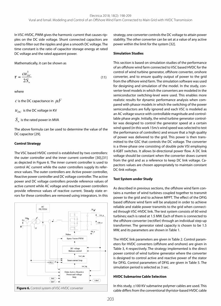
203


In VSC-HVDC, PWM gives the harmonic current that causes rip-ples on the DC side voltage. Shunt connected capacitors are used to filter out the ripples and give a smooth DC voltage. The time constant is the ratio of capacitor storage energy at rated DC voltage and the rated apparent power.

Mathematically, it can be shown as

(11)

where

c is the DC capacitance in

DCu is the DC voltage in KV

nS is the rated power in MVA

The above formula can be used to determine the value of the DC capacitor [29].

Control Strategy

The VSC based HVDC control is established by two controllers: the outer controller and the inner current controller [30],[31] as depicted in Figure 6. The inner current controller is used to control AC current while the outer controllers supply its refer-ence values. The outer controllers are: Active power controller, Reactive power controller and DC voltage controller. The active power and DC voltage controllers provide reference values of active current while AC voltage and reactive power controllers provide reference values of reactive current. Steady state er-rors for these controllers are removed using integrators. In this

strategy, one converter controls the DC voltage to attain power stability. The other converter can be set at a value of any active power within the limit for the system [32].

Simulation Studies

This section is based on simulation studies of the performance of an offshore wind farm connected to VSC based HVDC for the control of wind turbine generator, offshore converter, onshore converter, and to ensure quality output of power to the grid from the offshore wind farm. The simulation software was used for designing and simulation of the model. In the study, con-verter-level models in which the converters are modeled in the semiconductor switching-level were used. This enables more realistic results for dynamic performance analysis when com-pared with phasor models in which the switching of the power semiconductors are fully ignored and each VSC is modeled as an AC voltage source with controllable magnitude and control-lable phase angle. Initially, the wind turbine generator control-ler was designed to control the generator speed at a certain wind speed (in this work 15m/s wind speed was selected to test the performance of controllers) and ensure that a high quality of power was delivered to the grid. This power is then trans-mitted to the GSC that controls the DC voltage. The converter is a three-phase one consisting of double pole VSI employing 6-IGBT switches. It allows bi-directional power flow. A DC link voltage should be constant when the converter draws current from the grid and as a reference to keep DC link voltage. Ca-pacitors values are chosen appropriately to maintain constant DC-link voltage.

Test System under Study

As described in previous sections, the offshore wind farm con-tains a number of wind turbines coupled together to transmit power to the grid and to achieve MPPT. The effect of the DFIG based offshore wind farm will be analyzed in order to achieve reliable and stable power transmits to the grid when connect-ed through VSC-HVDC link. The test system consists of 60 wind turbines; each is rated at 1.5 MW. Each of them is connected to the offshore converter (rectifier) through an individual step-up transformer. The generator rated capacity is chosen to be 1.5 MW, and its parameters are shown in Table 1.

The HVDC link parameters are given in Table 2. Control param-eters for HVDC converters (offshore and onshore) are given in Table 3, 4 respectively. The strategy implemented is the direct power control of wind turbine generator where the converter is designed to control active and reactive power of the stator for DFIG. Control parameters of DFIG are given in Table 5. The simulation period is selected as 3 sec.

HVDC Submarine Cable Selection

In this study, ±100 KV submarine polymer cables are used. This cable differs from the conventional thyristor-based HVDC cable

Figure 6. Control system of VSC-HVDC converter

204


which uses self-contained oil filled or mass impregnated paper

insulated cable. Power reversal is achieved by changing the di-

rection of the current flow.

Dynamic Performance of the System

Case 1: Steady State Performance

The active and reactive power generated by the wind farm for a nominal wind speed of 11m/s is shown in Figure 7. As the wind speed is increased from 11 to 15m/s, the generator speed and air gap torque both increase while the stator flux link remains constant. Also generator active power and reac-tive power tend to increase because of the constraints arising from changes in the system voltage and frequency. This is a result of the control effort of the HVDC rectifier since it limits and also stabilizes the changes in measured value of system frequency at the rectifier end.

In Figure 7, nominal DC voltage of the DFIG is set as 1150V and the output is shown with some ripples at the start up which is caused by charging and discharging of capacitors.

Table 1. DFIG Parameters

Parameter Rating

Power rated 1.5 MW

Base voltage 575 V

Base frequency 50 Hz

Base impedence on stator 0.2381

Base stator current 2.37 kA

Base speed 1400 r/min

Torque 11.9 kNm

Rotor voltage 690 V

Rotor current 1.5 kA

Table 2. HVDC transmission Parameters

Parameter RatingPer unit

value

Base generated power 90 MW 1.0

Base DC voltage 100 KV 1.0

Converter transformer rating 200 MVA -

Simple AC system at offshore station 230 KV / 50Hz 1.0

Offshore side transformer ratio 25KV/230 KV/100 KV -

DC transmission line 2*75km Pi section -

DC line Inductance per kilometer 0.156H/km -

DC line resistance per kilometer 0.517/km -

DC line capacitance per kilometer 2.85 F/km -

Phase reactor inductance 0.024 H 0.15

Phase reactor resistance 0.075Ω 0.015

Onshore side transformer rating

100KV/230KV

200MVA -

AC filter40 MVar at 27th and 54th harmonics -

AC Grid system 230kV/ 50Hz 1.0

Table 3. Control parameter for offshore converter

Controllers Ki Kp Kf

P regulator 20 - -

P control 3.0 3.0 -

Q regulator 20 -

Inner current regulator 0.6 6.0 0.3

Table 4. Control parameter for onshore converter

Controllers Ki Kp Kf

DC voltage regulator 40 20 -

Q regulator 20 - -

Q control 3.0 3.0 -

Inner current regulator 6.0 0.6 0.3

DC voltage balance control 0.03 0.2 -

Table 5. DFIG control parameters

Parameter gain Kp Ki

GSC current regulator gains 0.83 5

DC voltage regulator gains 8 400

Speed regulator gains 3 0.6

RSC current regulators gains 0.6 8

Q and V regulator gains 0.05Var 20 volt

Pitch controller gain 150 -

Pitch compensation gains 3 30

205


It is observed that the voltage reaches its steady-state value at approximately 0.3 seconds. The DC link voltage at HVDC side is shown in Figure 8. The nominal voltage is set at 1p.u (100KV)

Case 2: Response to change in wind speed

Initially, wind speed was predetermined at 11m/s and it rapidly increased to 15m/s. Also in this time interval, the active power generated tended to rise smoothly until at 1 sec it reached its rated value as shown in Figure 9. Step changes to HVDC Controllers

In the following case studies, the design of controllers involves two strategies:

1. Offshore converter controller is designed to control active power (P) and reactive power (Q) 2. Onshore converter controller is designed to control reactive power (Q) and DC voltage (Vdc).

Case 3: Step change to active power controller

The wind farm VSC controller reference is set to 1p.u. At 0.3s the power is ramped up slowly to reach its set value of active pow-er reference (90 MW at 0.9 power factor) at 1.0 sec. Also at 1.5 sec, a -0.1p.u step is applied to the active controller reference and response is observed. Figure 10 shows that the controller can respond to any change in the system. Subsequently the measured active power follows its reference active power at any instant in the simulation process. Similarly, an active power reference (Pref ) is set to 0.5p.u and at 1.5sec, a step change of 0.1p.u is applied to the controller reference and the response is observed.

Case 4: Step change to reactive power controller

A step change of 0.1p.u is applied at 1.5sec for reactive refer-ence power and the response from Figure 11 shows that the measured reactive power follows its reference power at any

Figure 7. a-d. Waveforms for generator at nominal wind speed to (a) active power (b) reactive power (c) DC link voltage (d) gen-erator speed.

Figure 8. HVDC link voltage

Figure 9. Response to change in wind speed to (a) active power (b) reactive power

206


instant. Also step change to the decrease in reactive power at 1.5sec is also observed. The reactive power can be controlled to a null value in an offshore converter station since it is a com-mon control at both converter stations.

Case 5: Step change to DC voltage controller

The GSC controller is established to control reactive power and ensures constant DC voltage at the HVDC side. The DC volt-age reference is set to 1p.u. Steady state is reached at about 0.15sec. The controller performance to the change in DC voltage is observed and it showed that there is a decrease in voltage to about 0.05p.u (5 KV) at 1.5 sec because of the step change in the DC reference voltage from 1 p.u to 0.95 p.u as shown in Figure 12.

Fault Analysis

Case 6: Voltage sag at Offshore side of the Wind Farm

A three-phase programmable voltage source is employed at the offshore side of the wind farm and voltage sag is applied at

1.5 s. As a result, the active power delivered from the wind farm tends to deviate from the pre-disturbance state by 0.2 p.u and reactive power also by 0.2 p.u. The system returns back to its normal operation after 0.14s from the perturbation as shown in Figure 13. The simulation time is 3sec. Response to HVDC con-trollers at HVDC link under this fault is shown in Figure 14. Also response to fault at the wind farm side for active and reactive power is shown in Figure 15.

Case 7: Three-Phase to Ground Fault at the Onshore AC Main Grid

A three phase to ground fault is applied at the grid side of the wind farm and at 1.5s, the DC power delivered by the wind farm almost ceased DC voltage rose to 1.2p.u as shown in Figure 16 due to excessive charging of the DC capacitors. The recovery time from perturbation is 0.12s as shown from the simulation diagrams in Figure 17. DC voltage control override, which is a function in the active power controller, limits the DC voltage to a specified range. Wind farm active and reactive power under this fault is shown in Figure 18.

Figure 10. Response to step changes in active power at HVDC rectifier station (increase and decrease)

Figure 11. Response to step changes in reactive power at HVDC rectifier station (increase and decrease)

207


The power generated from the offshore wind farm delivered the required amount of energy to the grid through HVDC transmission, which is converted to three-phase AC and ready consumption. In this work, a simple AC system of 230 KV is modeled that operates at 50Hz frequency. It is observed

that the voltage at offshore converter bus is 1.0p.u (230 KV), which is sufficient to supply energy to consumer terminal voltage.

Figure 12. Response to step change of DC voltage at onshore bus station

Figure 14. Response to the fault at the HVDC side

Figure 15. a, b. Response to fault at offshore wind farm to (a) active power (b) reactive power

Figure 16. HVDC-link voltage at onshore under fault condition

Figure 13. Voltage sag at offshore converter Station

208


Conclusions

In this paper, design and control of an offshore wind farm con-nected through HVDC transmission is implemented. The off-shore wind farm is designed to deliver power to an AC main grid using HVDC by an undersea cable transmission. Unlike the con-ventional thyristor based converters that use thyristor valves, a VSC employing IGBT switches with SVPWM techniques are used. A DFIG is used for driving the wind turbines due to its variable speed operation. The transmission of power is achieved by the use of converter (rectifier station) at offshore side for convert-ing the AC voltage supplied by wind turbine generators into DC and then transmitted through undersea cables. This transmitted power is then converted back (inverter station) to AC to feed the grid. The control of this system is achieved through the control of wind turbine generators and wind speed by ensuring that high quality power is delivered to the grid.

The developed control strategy verified the dynamic and tran-sient operation of the system to VSC-based-HVDC transmission. It involved control of active and reactive power at the offshore

side and maintaining DC voltage and reactive power at the on-shore side. It has been verified that active and reactive power can be controlled independently from one another and by in-creasing and decreasing step changes to their reference value. Also variation in wind speed can have an effect on the dynamic performance of the system. In addition, the performance of the controllers is analyzed during fault and it is verified that three-phase fault could be very critical with regard to the the system when compared to an unbalance fault.




References

1. J. Lin, “Integrating the First HVDC-Based Offshore Wind Power into PJM System - A Real Project Case Study”, PJM Interconnection, Audubon, PA 19403, USA, pp. 1-8, 2015.

2. L. Wang, K.-H. Wang, W.-J. Lee, Z. Chen “Power-flow control and stability enhancement of four parallel-operated offshore wind farms using a line-commutated HVDC link”, IEEE Transactions on Power Delivery, vol. 25, no. 2, pp. 1190-1202, 2010.

3. F. Careri, S. Member, C. Genesi, P. Marannino, “Centralized coordi-nated control of VSC-HVDC link and DFIGs in very large offshore wind power plants”, IEEE Trondheim PowerTech, pp. 1-8, 2011.

4. J. Lin, “Integrating the First HVDC-Based Offshore Wind Power into PJM System - A Real Project Case Study”, IEEE Industry Applica-tions Society Annual Meeting, pp. 1-8, 2015.

5. D. Elliott, K. R. W. Bell, S. J. Finney, R. Adapa, C. Bronzio, J. Yu, K. Hus-sain, “A Comparison of AC and HVDC Options for the Connection of Offshore Wind Generation in Great Britain”, IEEE Transactions on Power Delivery, vol. 31, no. 2, pp. 798-809, 2016.

6. X. Rong, D. E. Macpherson,J. K. H. Shek, “The Effect of High Power DC-DC Converter in Offshore Multi-Terminal Medium and High Voltage DC Networks”, International Conference on Renewable Power Generation (RPG 2015), 2015.

7. G. Asplund, K. Eriksson, H. Jiang, J. Lindberg, R. Pålsson, K. Svens-son, “DC Transmission Based on Voltage Source Converters,” ABB Power Syst AB, pp.1-10, 1997.

8. G. Asplund, “Sustainable energy systems with HVDC transmission,” pp. 1-5, 1999.

9. D. Stanley, “The Directlink VSC-Based HVDC Project and its Com-missioning”, Cigre, vol. 14, no.108, pp. 9-18, 2002.

10. H. Light, “The world ‘ s most remote offshore wind farm BorWin1 HVDC Light ® offshore wind farm link”, 2011.

11. Z. Chen, Y. Hu, F. Blaabjerg, “Stability improvement of induction generator-based wind turbine systems,”IET Renew Power Gener, vol. 1, no.1, pp. 81-93, 2007.

12. S. Lauria, M. Schembari, F. Palone, M. Maccioni, “Very long distance connection of gigawatt- size offshore wind farms : extra high-volt-age AC versus high-voltage DC cost comparison”, IET Renewable Power Generation, vol. 1, pp. 713-720, 2015.

13. Y. Keche, V. K. Chandrakar, “Integrated operation of Grid and HVDC connected Offshore Wind Farm”, International Conference on Com-putation of Power, Energy Information and Communication (ICCPE-IC), pp. 666-674, 2016.

Figure 17. Three-phase to ground fault at onshore converter station

Figure 18. Wind farm active and reactive power under fault con-dition

209


14. R. Safaeian, S. Ebrahimi, M. Parniani, “Performance Improvement of Steady-State and Transient Operation of Offshore Wind Farm HVDC Power Transmission”, IEEE 16th Workshop on Control and Modeling for Power Electronics (COMPEL), 2015.

15. S. Muller, M. Diecke, W. Rik, “Doubly fed induction Generator sys-tems for wind turbine,” IEEE Industry Application, vol. 2, no. 1, pp. 26-33, 2002.

16. J. B. Ekanayake, L. Holdsworth, N. Jenkins, “Comparison of 5th order and 3rd order machine models for doubly fed induction generator wind turbines,” Electr Power Syst Res, vol. 67, pp. 207-215, 2003.

17. S. Bozhko, G. Asher, R. Li, J. Clare, S. Member, L. Yao, “Large Off-shore DFIG-Based Wind Farm With Line-Commutated HVDC Con-nection to the Main Grid : Engineering Studies”, IEEE Trans Energy Convers, vol. 23, no. 1, pp. 119-127, 2008.

18. P. Bresesti, W. L. Kling, R. L. Hendriks, R. Vailati, “HVDC Connection of Offshore Wind Farms to the Transmission System”, IEEE Trans En-ergy Convers, vol. 22, no. 1, pp. 37-43, 2007.

19. R. Iravani, A. Yazdani, “Voltage-Sourced Converters in Power Systems:Modeling, Control, and Applications”, New York, NY: Wi-ley-IEEE Press, 2010.

20. N. Flourentzou, S. Member, V. G. Agelidis, S. Member, G. D. Deme-triades, “VSC-Based HVDC Power Transmission Systems : An Over-view”, IEEE Transtactions Power Electron, vol. 24, no. 3, pp. 592-602, 2009. [21] A. Irina Stan, D. Ioan Stroe “Control of VSC-Based HVDC Transmission System for Offshore Wind,” Master Thesis, Aalborg university Denmark, 2010.

22. F. Deng, Z. Chen, “An Offshore Wind Farm with DC Grid Connec-tion and Its Performance under Power System Transients”, IEEE Power and Energy Society General Meeting, 2011.

23. M. Zhao. Z. Chen. F. Blaabjerg, “Optimisation of electrical system for offshore wind farms via genetic algorithm,” IET Renew. Power Gener, vol. 3, no.2, pp. 205-216, 2009.

24. J. Bhukya, V. Mahajan, “The controlling of the DFIG based on vari-able speed wind turbine modeling and simulation”, IEEE 6th Inter-national Conference on Power Systems (ICPS), 2016.

25. Y. Li, Z. Xu, J. Ostergaard, D. J. Hill, “Coordinated Control Strategies for Offshore Wind Farm Integration via VSC - HVDC for System Fre-quency Support”, IEEE Trans. Energy Convers, vol. 32, no. 3, pp. 843-856, 2017.

26. S. Dinesh, R. Meenakshi, M. S. Suhanya, M. S. Kumaran, R. Muthu, “Modeling and Direct Power Control of DFIG for Wind Energy Conversion System with a Back to Back Converter”, International Conference on Green Computing Communication and Electrical Engineering (ICGCCEE), 2014.

27. L. Xu, S. Member, L. Yao, and C. Sasse, “Grid Integration of Large DFIG-Based Wind Farms Using VSC Transmission,” IEEE Trans Power Syst, vol. 22, no. 3, pp. 976-984, 2007.

28. M. M. Z. Moustafa, O. Nzimako, A. Dekhordi, “Modelling of Wind Energy Sources in Real Time Platform”, 28th International Confer-ence on Microelectronics (ICM), 2016.

29 T. M. Haileselassie, “Control of Multi-terminal VSC-HVDC Systems”, Master Thesis, Norwegian Univ of Tech., 2008.

30. K. Karthi, R. Radhakrishnan, J. M. Baskaran, L. S. Titus, “Perfor-mance Analysis on Various Controllers of VSC - HVDC Transmission Systems”, IEEE International Conference on Computational Intelli-gence and Computing Research, 2016.

31. C. Zhao, C. Guo, “Complete-Independent Control Strategy of Ac-tive and Reactive Power for VSC Based HVDC System”, IEEE Power & Energy Society General Meeting, 2009.

32. Ch.Yaswanth, A.Vijayasri “VSC Based HVDC Sytem Design and Pro-tection against Over Voltages”, International Journal of Engineering Research and Development, vol. 10, no. 12, pp. 46-57, 2014.

Ahmet Mete Vural holds a PhD degree in Electrical and Electronics Engineering, from Çukurova University, Tur-key in 2012. He received his Bsc and Msc degree in Electrical and Electronics Engineering, University of Gaziantep in 1999 and 2001, respectively. He worked as a research assistant in University of Gaziantep and Wuppertal University, Germany. Now he is working as a full-time Associative Professor in University of Gaziantep, Depart-ment of Electrical and Electronics Engineering, Turkey. His research interests are power quality, micro/smartgrid, renewable energy, multi-level converters, energy storage, and FACTS devices.

Auwalu İbrahim Ismail was born in Kano, Nigeria in 1986. He received his B.Tech/HND in Electrical and Elec-tronics Engineering from Kano State Polytechnic University in 2012 and M.Sc in Electrical and Electronics Engi-neering from University of Gaziantep in 2018. He is an IEEE student member. His research interest include High Voltage Direct Current transmission system, Renewable energy, Power system and control.

210

Introduction

A school, college or university can deliver good educational programs by adopting intelligent software platforms that promote effective and good teaching strategies. Engineering as a dis-cipline assumes an applied nature and engineering students are often required to design, im-plement and test systems and circuits. Such a hands-on experience can be offered on a large scale by adopting free-distribution software packages that allow students to access program-ming tools, circuit design and analysis tools, and mathematical and numerical analysis tools. For efficient transmission of knowledge and information, it is highly recommended that any course make use of the following teaching modalities:

i) visuals (demonstrations, descriptions, words, pictures)ii) auditory sensations (dialogues, discussions, working out the problem audibly)iii) tactile perceptions (taking notes, labs, hands-on work)iv) kinesthetic impressions (movement).

Including all the above modalities in a course or laboratory session promotes a better learning experience as the student’s learning faculties are distributed across all the four modalities.

Recent developments in online platforms and courses have produced significant progress to-wards global education. For instance, Khan Academy provides a broad range of topics in Math-ematics, Science, Arts and Humanities for primary, secondary and high-school education, all for free. MIT Open Courseware (MIT-OCW) provides online lectures, assignments, exams and solutions for undergraduate and professional courses in Engineering, Architecture and Plan-ning, Sciences, Humanities, Arts, Social Sciences and even Management. Other universities have also started to provide free online coursework.

Electrica 2018; 18(2): 210-217

RESEARCH ARTICLE

ECEbuntu - An Innovative and Multi-Purpose Educational Operating System for Electrical and Computer Engineering Undergraduate Courses Bilal Wajid1 , Ali Rıza Ekti2 , Mustafa Kamal AlShawaqfeh3 1Department of Electrical Engineering, University of Engineering and Technology, Lahore, Pakistan2Department of Electrical-Electronics Engineering, Balıkesir University School of Engineering, Balıkesir, Turkey3School of Electrical Engineering and Information Technology, German Jordanian University, Amman, Jordan

Corresponding Author: Ali Rıza Ekti





DOI: 10.5152/iujeee.2018.1820

Cite this article as: B. Wajid, A. R. Ekti, M. K. AlShawaqfeh, “ECEbuntu - An Innovative and Multi-Purpose Educational Operating System for Electrical and Computer Engineering Undergraduate Courses”, Electrica, vol. 18, no: 2, pp. 210-217, 2018.

ABSTRACT

ECEbuntu is a free, easily distributable, customized operating system based on Ubuntu 12.04 long term support (LTS) designed for electrical/electronic and computer engineering (ECE) students. ECEbuntu is aimed at universities and students as it represents a cohesive environment integrating more than 30 pre-installed software and packages all catering to undergraduate coursework offered in ECE and Computer Science (CS) programs. ECEbuntu supports a wide range of tools for programming, circuit analysis, printed circuit board design, mathematical and numerical analysis, network analysis, and RF and microwave transmitter design. ECEbuntu is free and effective alternative to the existing costly and copyrighted software packages. ECEbuntu attempts to reduce the duplication of efforts on building software workstations in laboratories and is intended to serve as a good teaching resource in a classroom setting.

Keywords: Electrical and computer engineering, Ubuntu, circuit design, programming micro-controllers, microwave and RF transmission line analysis, computer networks, numerical computation and visualization, PCB design, computer programming, remote access, latex

https://orcid.org/0000-0003-0220-7788

https://orcid.org/0000-0003-0368-0374

https://orcid.org/0000-0003-2170-6830

211

Electrica 2018; 18(2): 210-217Wajid et al. ECEBUNTU: Operating System for ECE

In terms of engineering education, the above mentioned on-line courses do a very good job of engaging the visual and auditory faculties of students. However, the tactile and kin-esthetic impressions are limited, primarily because engineer-ing courses are often associated with lab work. The lab work requires resources and software packages that often are not available for free, and therefore, limits in-depth understanding of some courses. However, within the Electrical and Computer Engineering (ECE) and Computer Science (CS) curricula, the on-line courses do offer the possibility of engaging the students in all four modalities for improved learning. To compensate for the lack of a free and comprehensive educational software for ECE and CS students, this paper presents ECEbuntu, a specially designed Ubuntu based educational operating system encom-passing software which is useful for the training of undergrad-uate students from the ECE and CS Programs.

ECEbuntu

ECEbuntu was designed to help faculty engage students in all four learning modalities. As an addendum to online courses, ECEbuntu may be used by faculty to test students’ learning via lab works, projects and homework assignments, all within the framework of the same software package. ECE-buntu may also be used effectively in a traditional face-to-face learning environment as all four years of undergraduate course work have been covered. Courses covered include cir-cuit analysis, analog and digital electronics, pcb design, com-puter programming, micro-controllers, computer networks, microwave and radio frequency (RF) transmission line analy-sis and numerical computations. In addition, Latex tools like Texmaker and Tex Live, Putty for remote access, and popular tools like Google Chromium browser and VLC media player have also been added. Details of software have been referred to in Table 1, 2; (main manuscript) and Section 4, Supplemen-tary section.

ECEbuntu was designed to facilitate free global education for all. Since most courses in ECE require technical software that is expensive, students are either expected to spend increased amounts of time in labs to complete their work or pay for software themselves to have their own personal copy. Unfor-tunately, most students end up pirating software. Software piracy is especially high in countries where students cannot afford to buy software or the universities that do not have a 24 hour open lab policy [1]. Table 3 and Figure 1 provide a glimpse into the gravity of this situation. Therefore, to allevi-ate some of these problems ECEbuntu have been made free for everyone to use, modify, update and distribute. Should universities or labs choose to use ECEbuntu as their primary educational OS it will help them to significantly reduce cost because all software dependencies within ECEbuntu have been resolved and all the technical software packaged is free. Naturally, some of these free products are not as profes-sional as their equivalent costly counterparts; however, they do fill in the gap very nicely.

Additionally, ECEbuntu allows for easy distribution as there are no copyright restrictions. This is notable for countries where power outages are a daily routine and the download band-width is limited [2, 3]. Table 3 shows some countries where such complications (limited bandwidth, power outages) persist. ECEbuntu can be easily distributed using DVD or USB stick (see Sections 1 and 2 in the Supplementary Section). Furthermore, virtualization ECEbuntu may be used in parallel with Windows or MAC operating systems, though it is recommended that us-ers install ECEbuntu separately to ensure maximum usage of memory and processing power (see Section 3, Supplementary Section for further details).

Discussion

In order to integrate all four learning modalities (visuals, audi-tory, tactile and kinesthetics) in formal coursework, institutions adopt one of two frameworks. i) Students bring their own devic-es (BYOD) and download/install/maintain necessary software based on the requirements laid out in the syllabus, ii) The labs provide the necessary framework in which the students can work. The server broadcasts and installs software to all work-stations. Additionally, the lab-manager is in charge of main-taining/updating the OS and software installed on all worksta-tions. As BYOD approach is generally costly for engineering, our motivation was to simplify routine activities of lab-managers by taking part of the responsibilities onto ourselves. These in-clude searching for potential freeware and integrating the best software as a cohesive Ubuntu 12.04 LTS based platform for ECE/CS education. Ubuntu LTS was carefully chosen because the Ubuntu community is committed to maintaining Ubuntu

Figure 1. Percentage of Profit Loss per Country for Using Pirated Software

212


Table 1. Software tools in ECEbuntu

Name(s) of the Course(s) Software tools

Electrical Circuit Theory Fritzing: Electronic design software [4].

Introduction to Digital System Design gEDA: Electronic design software [5].

Semiconductor Devices GTKWave: Waveform viewer

Analog Electronic Circuits Gwave: waveform viewer e.g., for spice simulators [6].

Operational Amplifiers Kicad: Electronic schematic and PCB design [7, 8].

Power Electronics Oregano: Tool for schematical capture of electronic circuits [9, 10].

VLSI Circuit Design PCB: Printed circuit board design program (http://pcb.gpleda.org/).

PCB Design Visolate: Tool for engraving PCBs using CNC machine (https://sourceforge.net/projects/visolate/).

Programming -controllers Emu8051: Emulator and simulator for 8051 -controllers [11].

MCU8051: IDE for MCS-51 based micro-controllers (https://sourceforge.net/projects/mcu8051ide/).

SPIM: MIPS R2000/R3000 emulator (http://pages.cs.wisc.edu/~larus/spim.html).

Electromagnetic Field Theory LinSmith: Tool to generate Smith Charts (http://jcoppens.com/soft/linsmith/index.en.php).

Microwave and RF transmission line analysis

TransCalc: Microwave and RF transmission line calculator (http://transcalc.sourceforge.net/).

Antenna Engineering

Computer Networks/Network Analysis

Dynamips: Cisco 7200/3600/3725/3745/2600/1700 router emulator [12, 13].

GNS3: Graphical network simulator [14, 15].

NetEmul: Program for simulating computer networks (http://netemul.sourceforge.net/).

Putty: Telnet/SSH client for X (http://www.putty.org/).

Random Signals and Systems GeoGebra: Dynamic mathematics software for education [16, 17].

Stochastic Processes GNU Octave: High level programming language, primarily intended for numerical computations

Signals and Systems KmPlot: Mathematical function plotter for KDE (https://edu.kde.org/kmplot/).

Digital Signal Processing QtOctave: Qt front-end to Octave. An environment for numerical computations [18, 19].

Linear Control Systems RKWard: KDE frontend to the R statistics language [20, 21].

Digital Image Processing SciLab: Scientific software package for numerical computations [22-24].

Numerical Analysis Spatial Statistics: GNU R package for spatial statistics [25].

Programming Eclipse: for C/C++ and Java (may be updated for Andriod applications) [25-28].

Data Structures Design and Analysis of Algorithms

IDLE: IDE for Python using Tkinter (http://www.python.org/).

Technical Report Writing

Texmaker: Cross-platform LaTeX editor (http://www.xm1math.net/texmaker/).

Tex Live: A decent selection of the TeX Live package (http://www.tug.org/texlive/).

213


Table 2. Software tools in ECEbuntu can cater to all four years of the engineering program. Some of the tools are suitable for all four years of the program and are therefore mentioned more than once (Continue) Year Name(s) of the Course(s) Software tools Freshman Year

Electrical Circuit Theory Eclipse: for C/C++ and Java (may be updated for other languages) [26, 27]. Semiconductor Devices Fritzing: Electronic design software [4]. PCB Design gEDA: Electronic design software [5]. Computer Fundamentals IDLE: IDE for Python (http://www.python.org/).

Kicad: Electronic schematic and PCB design [7, 8]. Oregano: Tool for electronic circuits [9, 10]. PCB: Printed circuit board design (http://pcb.gpleda.org/). Visolate: Tool for engraving PCBs using CNC machine (https://sourceforge.net/projects/visolate/).

Sophomore Year

Electrical Circuit Theory Eclipse: for C/C++ and Java Introduction to Digital System Design

Fritzing: Electronic design software [4].

Semiconductor Devices gEDA: Electronic design software [5]. Analog Electronic Circuit IDLE: IDE for Python (http://www.python.org/). Programming Languages Kicad: Electronic schematic and PCB design [7, 8]. Data Structure Oregano: Tool for schematical capture of electronic circuits [9,10]. Design and Analysis of Algorithms

PCB: Printed circuit board design (http://pcb.gpleda.org/).

Writing Skills Texmaker: Cross-platform LaTeX editor.

Tex Live: A decent selection of the TeX Live package Visolate: Tool for engraving PCBs using CNC machine (https://sourceforge.net/projects/visolate/).

Junior Year Operational Amplifier Emu8051: IDE for 8051 -controllers [11]. Programming µ-Controllers Fritzing: IDE for Electronic system design [4]. Random Signals and Systems KmPlot: Mathematical function plotter for KDE (https://projects.kde.org/projects/

kde/kdeedu/kmplot). Stochastic Processes LinSmith: Tool to generate Smith Charts (http://jcoppens.com/soft/linsmith/index.

en.php). Signals and Systems gEDA: Electronic design software [5]. Numerical Analysis GeoGebra: Dynamic mathematics software for education [16, 17, 29]. Electromagnetic Field Theory GNU Octave: programming language intended for numerical analysis.

Kicad: Electronic schematic and PCB design [7,8]. MCU8051: IDE for MCS-51 -controllers (http://mcu8051ide.sourceforge.net/). Oregano: IDE for electronic circuits [9, 10]. PCB: IDE for PCBs (http://pcb.gpleda.org/). QtOctave: IDE for numerical analysis [18, 19]. RKWard: KDE frontend to the R statistics language [20, 21]. SciLab: IDE for numerical computations [22, 23]. Spatial Statistics: GNU R package for spatial statistics [25]. SPIM: MIPS R2000/R3000 emulator (http://pages.cs.wisc.edu/~larus/spim.html). TransCalc: Microwave and RF transmission line calculator (http://transcalc.sourceforge.net/). Visolate: Tool for engraving PCBs using CNC machine (https://sourceforge.net/projects/visolate/).

Senior Year VLSI Circuit Design Dynamips: Cisco 7200/3600/3725/3745/2600/1700 router emulator [12, 13]. Power Electronics Fritzing: IDE for Electronic design [4]. Linear Control gEDA: IDE for Electronic design [5]. Computer Networks/ Network Analysis

GeoGebra: IDE for numerical analysis [16, 17].

214


Table 2. Software tools in ECEbuntu can cater to all four years of the engineering program. Some of the tools are suitable for all four years of the program and are therefore mentioned more than once (Continue) Year Name(s) of the Course(s) Software tools

Antenna Engineering GNS3: Graphical network simulator [14, 15]. Microwave and RF transmission line analysis

GNU Octave: programming language for numerical analysis.

Digital Signal Processing Kicad: IDE for electronic design [7, 8]. Image Processing LinSmith: Tool to generate Smith Charts (http://jcoppens.com/soft/linsmith/index.

en.php).

NetEmul: Program for simulating computer networks (http://netemul.sourceforge.net/). Oregano: IDE for electronics design [9, 10]. PCB: IDE for PCBs (http://pcb.gpleda.org/). Putty: Telnet/SSH client for X (http://www.putty.org/). QtOctave: Qt front-end to Octave. An environment for numerical computations [18, 19]. RKWard: KDE frontend to the R statistics language [20, 21]. SciLab: Scientific software package for numerical computations [22, 23]. Spatial Statistics: GNU R package for spatial statistics [25]. TransCalc: Microwave and RF transmission line calculator (http://transcalc.sourceforge.net/). Visolate: Tool for engraving PCBs using CNC machine (https://sourceforge.net/projects/visolate/).

Table 3. Statistical Values of Percentage of Piracy, Value of Piracy, Average Bandwidth per Country, Electricity Outages Days and Durations per Country [1-3]

Argentina Australia Brazil Canada China Germany India Japan Jordan Pakistan Romania Russia Turkey U.K. U.S.A.

% of Pirated Software Usage

69 21 50 25 74 24 60 19 57 85 62 62 60 24 18

Value of the Pirated Software ($Million)

950 743 2851 1089 8767 2158 2911 1349 35 344 208 2658 504 2019 9773

Average Internet Broadband Connection Speed Per User (mbps)

4.2 6.9 2.9 10.3 3.8 8.7 2 15 3.09 2.31 11.3 9.1 5.5 10.7 11.5

Number of days per month with electricity outages

1.9 0.4 1.6 NA 0.1 NA 13.8 NA 0.2 30 1.4 0.3 1.7 NA NA

Average number of hours per electricity outage

1.2 1 1.8 NA 0.5 0.8 1.1 NA 0.2 2.1 1.1 0.9 0.7 NA NA

215


Table 4. Comparison of Different Linux Distributions: The table compares different linux distributions.

Operating system Free Reliable Base OS Software

Open source LTS GUI Security

Threat detection 86/64 Cloud

Baari √ √ Ubuntu 13.10

30+ Genome Assembly tools √ √ Unity √ √ 64 x

Lxtoo √ √ Gentoo Linux 11

Sequence Analysis, Protien-Protien interactions

√ √ X11 Desktop

√ √ x86/64 x

Open Discovery 3

x √ Fedora Sulphur 9

molecular dynamics, docking, sequence analysis

√ √ GNOME 2.22

√ √ 86/64 √

PhyLIS √ √ Ubuntu 8 Phylogenetics √ x Unity √ √ 86/64 x

DNALinux √ √ Xubuntu DNA and protein analysis. Also contains Virtual Desktop

√ x XFCE 4.2.2

√ √ 86 √

BioLinux 7 √ √ Ubuntu 12.04

500+ Bioinformatics application with 7 Assembly tools

√ √ Unity √ √ 64 √

ECEbuntu √ √ Ubuntu 12.04

OS for ECE/CS education √ √ Unity √ √ 64 x

Table 5. Questionnaire: Please respond to the following statements by using the 5-point rating scale to indicate the extent to which you agree or disagree with each statement. Please circle the number that applies

S. No. Question

5 = Strongly

Agree4 =

Agree3 =

Neutral2 =

Disagree

1 = Strongly Disagree

1 Objectives of ECEbuntu are stated clearly and met. 1 2 3 4 5

2 The information provided by ECEbuntu was relevant and useful. 1 2 3 4 5

3 ECEbuntu facilitated my learning of Electrical and Computer Engineering. 1 2 3 4 5

4 The instruction manual is well written, organized and fulfils its purpose. 1 2 3 4 5

5 It is easy to install ECEbuntu. 1 2 3 4 5

6 More software and packages should be added to ECEbuntu 1 2 3 4 5

7 ECEbuntu’s interface is user friendly. 1 2 3 4 5

8 ECEbuntu is successful in performing its intended task. 1 2 3 4 5

9 ECEbuntu is an appropriate OS for courses in ECE. 1 2 3 4 5

10 Given that ECEbuntu is free, will you recommend ECEbuntu to your colleagues? 1 2 3 4 5

11 What do you like best about this software?

12 Do you think it is a good software tool to teach graduate students and researchers?

13 Areas/topics about which you would like to receive further software?

14 What did you think was the most important feature introduced by ECEbuntu?

15 What do you dislike about ECEbuntu?

16 Did you experience any problem with this software? If yes, what kind of problem did you have?

17 Suggestions for improving ECEbuntu

216


12.04 OS for the long term, hence the term ‘LTS’ which stands for ‘Long-Term-Support’. The OS maintenance routinely comes up as an update which the lab-manager has to install on the server. This automatically updates all workstations connected to the server. Furthermore, based on the recommendations of users, teachers, students and lab-managers ECEbuntu will be routinely updated to install the latest software packages and remove the ones not needed. As far as the authors are aware, ECEbuntu is a unique solution as no similar prior work has been conducted within ECE. However, similar practice involving in-tegration of multiple software platforms has been conducted extensively in Life-Sciences. These ‘Life-Linux distros’ (Life Sci-ences Linux based OS) have saved biologists from spending increasing amount of time and resources in installing, config-uring and maintaining software rather than spending the same on research. We hope that ECEbuntu will serve the same role for ECE as life-Linux distros have served for life sciences (Table 4 lists some examples). Table 5 provides a questionnaire for users to rate and give feedback on ECEbuntu.

Conclusion

We highlight a free, easily distributable, customized Ubun-tu based OS that contributes to ECE/CS education. ECEbuntu attempts to fulfill the software requirements of four years of undergraduate coursework. This may help teachers who incor-parate ECEbuntu into their syllabus and homework. Further-more, installing ECEbuntu in the laboratories may help with the smooth operation of lab assignments. Additionally, ECEbuntu will continue to be routinely upgraded with the help of sugges-tions and feedback from faculty and students. Future work may include a software package for Windows.

Peer-review: Externally peer-reviewed



References

1. “BSA Global Software Survey”, http://globalstudy.bsa.org/2013/ , 2013.

2. “Infrastructure”,http://www.enterprisesurveys.org/data/explore-Topics/Infrastructure, 2013.

3. “State of internet”, http://www.akamai.com/stateoftheinternet/, 2014.

4. A. Knörig, R. Wettach, J. Cohen, “Fritzing: a tool for advancing electronic prototyping for designers”, Proc of the 3rd Intl Conf on Tangible and Embedded Interaction, Cambridge, UK, 2009, pp. 351-358.

5. S. Brorson, “Circuit design on your Linux box using gEDA”, Linux Journal, vol. 2006, no. 141, 2006.

6. C. Medrano, I. Plaza, M. Castro, F. Garcia-Sevilla, J. Martiinez-Calero, J. Felix, M. Corbalan, “A review of electronic engineering design

free software tools”, Proc of the 1st Intl Conf on IEEE Education En-gineering (EDUCON), Madrid, Spain, 2010, pp. 1867-1871.

7. J. C. Borg, X. T. Yan, N. P. Juster, “A KICAD Tool for Pro-Active Ex-ploration Support to ‘Design Synthesis for Multi-X’”, Knowledge Intensive Computer Aided Design, Springer, 2000, pp. 295-322.

8. R. Halvick, “KiCad: a high level tool. Electronic CAD available to all,” Elektor Electronics, vol. 33, no. 367, p. 134, 2007.

9. B. Zapirain, A. Zorrilla, I. Ruiz, A. Muro, “Learning electronics using image processing techniques for describing circuits to blind stu-dents,” Proc. of the IEEE Intl Sym Signal Processing and Informa-tion Technology (ISSPIT), Luxor, Egypt, 2010, pp. 156-160.

10. M. Neruda, L. Vojtech, “Modeling of smart textile materials for ESD applications”, Proc of the IEEE ELMAR, Zadar, Croatia, 2012, pp. 145-148.

11. T. Reinbacher, D. Gückel, S. Kowalewski, M. Horauer, “Testing mi-crocontroller software simulators”, http://www.user.tu-berlin.de/komm/CD/paper/061433.pdf, 2011.

12. Y. P. Wu, W. Zheng, “Application and Analysis of Packet Tracer and Dynamips in Computer Network Simulation Experiment [J]”, Com-puter Era, vol. 10, p. 8, 2010.

13. L. Wen-Chi, “On the Configuration and Application of Dynamips Virtual Network [J],” Journal of Nanjing Institute of Industry Technol-ogy, vol. 2, p. 17, 2007.

14. W. Makasiranondh, P. S. Maj, D. Veal, “Pedagogical evaluation of simulation tools usage in Network Technology Education,” Engi-neering and Technology, vol. 8, pp. 321-326, 2010.

15. V. Autefage, D. Magoni, “Network emulator: a network virtualization testbed for overlay experimentations”, Proc. of the IEEE 17th Intl. Work-shop Computer Aided Modeling and Design of Communication Links and Networks (CAMAD), Barcelona, Spain, 2012, pp. 266-270.

16. M. Hohenwarter, J. Preiner, “Dynamic mathematics with GeoGebra,” Journal of Online Mathematics and its Applications, vol. 7, 2007.

17. L. Fahlberg-Stojanovska, V. Stojanovski, “GeoGebra-Freedom to explore and learn”, Teaching Mathematics and its Applications, vol. 28, no. 2, pp. 69-76, 2009.

18. P. L. Luis, “QtOctave, Octave para todos los públicos,” Todo linux: la re-vista mensual para entusiastas de GNU/LINUX, no. 84, pp. 37-41, 2007.

19. M. P. L. del Castillo, P. L. L. Rosado, and A. S. Muñoz, “QtOctave: el MatLab de los pobres”, Actas de las I Jornadas en Innovación y TIC Educativas-JITICE 2010, p. 29.

20. S. Rödiger, T. Friedrichsmeier, P. Kapat, M. Michalke, “Rkward: A comprehensive graphical user interface and integrated develop-ment environment for statistical analysis with r”, Journal of Statisti-cal Software, vol. 49, no. 9, pp. 1-34, 2012.

21. D. Wick, “Free and open-source software applications for mathe-matics and education”, Proc. of the 21st Annual Intl Conf Technolo-gy in Collegiate Mathematics, New Orleans, LA, 2009, pp. 300-304.

22. S. L. Campbell, J. P. Chancelier, R. Nikoukhah, “Modeling and simu-lation in SCILAB”, Springer, 2010.

23. C. Gómez, “Engineering and Scientific computing with Scilab”, Springer, 1999.

24. K. Chine, “Learning math and statistics on the cloud, towards an ec2-based google docs-like portal for teaching/learning collabo-ratively with r and scilab”, Proc. of the 10th IEEE Intl. Conf. Advanced Learning Technologies (ICALT), 2010, pp. 752-753.

217


25. W. Venables, B. D. Ripley, “S Programming”, Springer, 2000. 26. J. desRivieres, J. Wiegand, “Eclipse: A platform for integrating de-

velopment tools,” IBM Systems Journal, vol. 43, no. 2, pp. 371-383, 2004.

27. D. Geer, “Eclipse becomes the dominant Java IDE”, IEEE Computer, vol. 38, no. 7, pp. 16-18, 2005.

28. J. Edmondson, W. Anderson, J. Gray, J. Loyall, K. Schmid, J. White, “Next-Generation Mobile Computing”, IEEE Software, vol. 31, no. 2, pp. 44-47, 2014.

29. M. Boule, “The role of Finite Element Method software in the teaching of electromagnetics”, Proc of the 4th Interdisciplinary Engineering De-sign Education Conference (IEDEC), Santa Clara, CA, 2014, pp. 44-51.

Mustafa Alshawaqfeh received his B.S. degree in communication engineering from Yarmouk University, Irbid, Jordan, in 2007, M.S., degree in electrical engineering/wireless communication from the Jordan University of Sci-ence and Technology, Irbid, Jordan, in 2010, and Ph.D., degree in electrical engineering from Texas A&M Univer-sity, College Station, Texas, USA. He joined the German Jordanian University since 2017 as an Assistant Professor at the electrical and communication engineering department. His research interests span the areas of wireless communications, signal processing, machine learning, and bioinformatics.

Ali Rıza Ekti is from Tarsus, Turkey. He received B.Sc. degree in Electrical and Electronics Engineering from Mersin University, Mersin, Turkey, (September 2002-June 2006), also studied at Universidad Politechnica de Valencia, Valencia, Spain in 2004-2005, received M.Sc. degree in Electrical Engineering from the University of South Flori-da, Tampa, Florida (August 2008-December 2009) and received Ph.D. degree in Electrical Engineering from De-partment of Electrical Engineering and Computer Science at Texas A&M University (August 2010-August 2015). He is currently an assistant professor at Balikesir University Electrical and Electronics Engineering Department and also senior researcher at TUBITAK BILGEM. His current research interests include statistical signal processing, convex optimization, machine learning, resource allocation and traffic offloading in wireless communications in 4G and 5G systems and smart grid design and optimization.

Bilal Wajid completed his B.Sc. Electrical Engineering from University of Engineering and Technology (UET), La-hore, Pakistan in 2007 and his Ph.D. in Electrical Engineering from Texas A&M University (TAMU), College Station, TX, USA in 2015. He his currently serving as an Assistant Professor at Dept. of Electrical Engineering, UET, KSK Campus. He has previously taught at Texas A&M University, CS (TX, USA), Texas A&M International University, Laredo (TX, USA) and DUKE University, Durham (North Carolina, USA). His research interests include Application of Engineering in Medicine, Bioinformatics and Cloud computing.

218

Introduction

Despite significant improvements in the field of control, proportional-integral-derivative (PID) type controllers still preserve their popularity and importance in scientific and indus-trial applications. Their simple design procedure, as well as their robustness and ability to control many different types of linear and nonlinear systems efficiently, can be considered as the main reasons for this. In the literature on this area of research, it can be seen that PID controllers are still widely preferred for the control of many different types of systems in the last decade.

An improved PID switching control strategy was proposed for the closed-loop control sys-tem of an artificial pancreas to cope with Type 1 Diabetes in [1]. A deduced model based self-tuning PID control strategy was proposed for implementing a motion control system that stabilizes the two-wheeled vehicle and follows the desired motion commands in [2]. Velocity and orientation tracking control of a nonholonomic mobile robot was provided via an adaptive controller of nonlinear PID-based neural networks in [3]. A direct current (DC) motor speed control was provided via a particle swarm optimization supported by an opti-mal PID controller in [4]. Adaptive fuzzy PID controllers were utilized for the speed control of a DC motor in [5-6]. The overall performance of the electro-hydraulic position servo system of a servo hydraulic press was improved by means of a fuzzy PID control method while a hy-brid fuzzy-PID controller was utilized to provide the position control of a hydraulic actuation system in [7-8]. A PID-type fuzzy adaptive controller was utilized for the control of an expert heating, ventiliating and air-conditioning system having two different zones with variable flow-rate in [9]. A real-time particle-swarm-optimization-based PID controlller was designed for the levitated balancing and propulsive positioning of a magnetic-levitation transporta-tion system in [10]. A PID controller was utilized for position and orientation control, as well as for the attitude and position trackings of unmanned quadrotors in [11, 12]. In addition to these, a gain-scheduled PID control based active fault-tolerant technique was developed and applied to a similar vehicle in [13]. PID and linear quadratic regulator based optimal

Electrica 2018; 18(2): 218-226

RESEARCH ARTICLE

A Self-Tuning PID Control Method for Multi-Input-Multi-Output Nonlinear SystemsBarış Bıdıklı Department of Mechatronics Engineering, School of Engineering and Architecture, Izmir Katip Çelebi University, İzmir, Turkey

Corresponding Author: Barış Bıdıklı





DOI: 10.26650/electrica.2018.79181

Cite this article as: B. Bıdıklı, “A Self-Tuning PID Control Method for Multi-Input-Multi-Output Nonlinear Systems”, Electrica, vol. 18, no: 2, pp. 218-226, 2018.

ABSTRACT

In this study, an artificial neural network (ANN) model-based self-tuning PID control method is proposed for the control of multi-input-multi-output (MIMO) nonlinear systems. A single layer, feed-forward ANN structure is trained via input and output data randomly collected from the system and classified as learning, test, and validation data to obtain the system model. The obtained model is utilized in an adaptive PID control scheme in conjunction with two different optimization methods for PID tuning and control. Using this scheme, PID parameters can be tuned to their optimum values and the system can be controlled simultaneously. The performance of the proposed method is demonstrated via experimental studies.

Keywords: Multi-input-multi-output nonlinear systems, proportional-integral-derivative tuning, proportional-integral-derivative control

https://orcid.org/0000-0001-8994-0012

219

Electrica 2018; 18(2): 218-226Bıdıklı B. A Self-Tuning PID Control Method for MIMO Nonlinear Systems

control techniques were proposed to control the nonlinear in-verted pendulum dynamical system in [14, 15]. A combination of an industrial linear PID controller and a neural compensa-tor was used to minimize steady-state error with respect to uncertainties in robot control in [16]. An interval type-2 fuzzy PID controller was utilized for the trajectory tracking task of a 5 degree-of-freedom (DOF) redundant robot manipulator while the global finite-time regulation of robotic manipula-tors was provided via a nonlinear PID controller in [17, 18]. PID control was proposed as a solution for the feedback control problem of fully-constrained cable driven parallel manipula-tors in [19]. A novel fuzzy-PID approach based on feedforward control was utilized to regulate the oxygen excess ratio of the proton exchange membrane fuel cell system, while another feedforward PID control system was proposed to enhance the practical positioning performance of a piezo-actuated flexi-ble 2-DOF micromanipulator integrated with a pair of mod-ified differential lever displacement amplifiers in [20, 21]. An adaptive robust hybrid PID and sliding control optimized by multi-objective genetic algorithm optimization was present-ed to control a biped robot walking in the lateral plane on a slope in [22]. The aim was to control the blade pitch angle of a wind turbine at different wind speeds and to hold the output power stable at a specific set point by utilizing fuzzy logic PID controller in [23]. A new control method of combin-ing a novel positive temperature coefficient material with PID control algorithm was proposed in [24]. A PID-based active

vibration control system of an aluminum plate was designed, developed and experimentally verified in [25]. A new control design for an autonomous underwater vehicle was presented in [26]. In order to do this the researchers utilized a nonlinear auto-regressive moving-average exogeneous model of the vehicle and the PID controller.

As can be seen from the given examples PID and PID-based controllers can be used to control many different types of sys-tems in a wide variety of areas, ranging from daily life to bio-medical applications, from military applications to transporta-tion. At this point it should also be noted that the mentioned studies are only a selection of the numerous PID control studies available in the literature. Although, the PID controller has been widely used for the control of many different types of systems, optimum tuning of the PID parameters (i.e., proportional, inte-gral and derivative gains), which can be considered as the main issue of the PID control process, still remains a problem. PID parameters that are not tuned properly negatively affect the control performance. In some cases the stability of the system may be negatively affected by the tuning. This problem can be observed in most of the aforementioned studies and other PID control applications. As a result of this, proposing tuning methods for PID parameters has become a popular topic in the research area of the control. Detailed surveys on this topic can be found in [27, 28]. This topic has also preserved its popularity in the last decade. A new robust PID tuning method for the op-

Figure 1. ANN model based PID tuning and control scheme

220


timal closed-loop performance with specified gain and phase margins based on nonlinear optimization was developed in [29]. A stochastic, multi-parameters, divergence optimization method for the auto-tuning of PID controllers according to a fractional-order reference method was presented in [30]. Gain and phase margin specifications of the inner and outer loop based internal model control plus PID tuning procedure was proposed in [31]. A new model reduction method and an ex-plicit PID tuning rule for the purpose of PID auto-tuning based on a fractional order plus time delay model are presented in [32]. A Newmark method based PID control rule was proposed for the active vibration control of multi-DOF flexible systems in [33]. One could easily add to these examples. However, the aforementioned studies are enough to clarify these issues. PID control can be considered to be a feasible solution for the con-trol of nonlinear systems, and combining the PID control with an appropriate gain tuning method increases this feasibility.

One of the most suitable approaches was proposed to cope with these issues [34]. In the mentioned study, a PID based con-trol scheme that can be used for the control of single-input-sin-gle-output nonlinear systems was proposed. In this scheme, control was provided via a digital PID controller combined with a nonlinear auto-regressive exogeneous (NARX) system model of the controlled system. Using this structure PID gains were ad-justed online during the control process by utilizing the NARX model of the system. The control of the system was provided by utilizing a correction term that was computed by using the NARX model during the control gain adjusting process. Accord-ing to the given structure when the gains reach their optimum values, the NARX model is deactived and the control process is continued with the classical PID approach. The structure of the proposed scheme provides an opportunity for the control-ler to adapt the changes in the system and/or enviromental factors during the control process. The proposed method is a suitable method when considering its ability to control non-linear systems. However, most of the nonlinear systems have more than one input and output. As a result of this they are modeled as multi-input-multi-output (MIMO) systems. It is not possible to apply the above-mentioned method to these types of system with its current structure. This situation can be seen as the possible weakness of the proposed method. Moreover, performance of the proposed method was not experimental-ly verified in [34]. The main purpose of this study is to elimi-nate all of the above-mentioned deficiencies and to make the proposed method usable for a broader class of nonlinear sys-tems. The system is brought into the appropriate structure for MIMO nonlinear systems. Since it is necessary to make a lot of changes to the structure of the system it is a challenging task. Performance of the newly proposed method is experimentally verified by utilizing from it to provide the joint space control of a rigid link 2-DOF robot manipulator. This experimental verifi-cation can be seen as another contribution of this study.

The rest of the paper is organized as follows. In section 2, the structure of the proposed artificial neural network (ANN) mod-

el based PID tuning and control scheme is presented and ex-plained in a detailed manner. In section 3, the architecture and the learning algorithm of the utilized ANN is summarized. In section 4, the performance of the proposed method is demon-strated via experimental studies Finally, conclusions are given in section 5.

Artificial Neural Network (ANN) Model Based PID Tuning and Control Method

The structure of the proposed scheme is shown in Figure 1. As mentioned in the previous section, this structure is the rear-ranged version of the structure given in accordance with the structures of MIMO systems [34]. Jacobian calculation block used for computing the correction term of the control signal and another Jacobian calculation block used for PID tuning are rearranged according to MIMO systems having m inputs and m outputs. Moreover, the structure of the PID controller, ANN model and Line Search blocks were made available for MIMO systems. As a result of this, PID parameters denoted by Kp, KI, and KD, became m × m diagonal matrices. In this structure de-sired trajectory, outputs of the ANN model, the plant and the error are denoted by yd, ŷ, y, and en ∈ respectively. The time index is represented by while the control input and its corrections are denoted by, Un+1, δun+1µ , respectively. As a result of these structure and dimension changes, math-ematical analysis and design must be completely rearranged.

The control input is updated according to the update rule of the digital PID controller given as

(1)

Tuning the PID parameters starting from zero to their proper values is the main purpose of the proposed structure. The K – step ahead prediction of the plant’s behavior is employed for this purpose. This prediction is produced by applying the con-trol input given in (1) to the ANN model of the plant K times. It is attempted to minimize the following objective function for each output of the system by updating the PID parameters based on these predictions

(2)

221


where the subscript i = 1, ..., m and the diagonal matrix whose diagonal elements are equal to penalty terms and the pre-diction horizon are denoted by and , respectively. The Levenberg-Marquardt (LM) rule is utilized as the minimization algorithm in the proposed structure and this rule realizes the minimization according to the following equation

(3)

where denotes the standard identity ma-trix, while the parameter that provides the transition between the steepest-descent and the Gauss-Newton algorithms is denoted by . The Jacobian matrix represented by

is defined as

(4)

and that contains the prediction errors and the input related optimization terms is defined as

(5)

The aim is to iteratively provide optimum tuning of the PID parameters during the control process according to the given structure and algorithms. In addition, obtaining an efficient control performance during the transient-state, increasing ro-bustness against possible disturbances and adaptivity of the proposed method are other aims. All of these situations are realized by utilizing correction term. This term compensates the deficiency of the control input when it cannot be provided by the controller, otherwise it disables. Mathematically, it can be said that the corrector block tries to minimize the elements of the objective functions’ vector denoted by Ji with respect to (i.e., correction term of the control input that

specifically affects the output) based on the second-order Taylor approximation of this element given as

(6)

Values of terms that minimize the objective function can be found by taking the derivative of (6) with respect to this term and equalizing the result to zero as

(7)

The term in (7), corresponds to the Newton direction and this provides a quadratic convergence to the local minimum when the Hessian terms in the Taylor expansion are positive and the higher order terms are negligible [35]. The following

matrix proposed by a Jacobian approxima-tion is utilized to avoid the time consuming calculation of sec-ond-order derivatives

(8)

The gradient term can exactly be represented and the Hessian term can approximately be represented via the matrix given in (8) as

(9)

(10)

where the operator represents the order derivative of a vector or a matrix with respect to the variable . The vector of the correction terms can be computed as

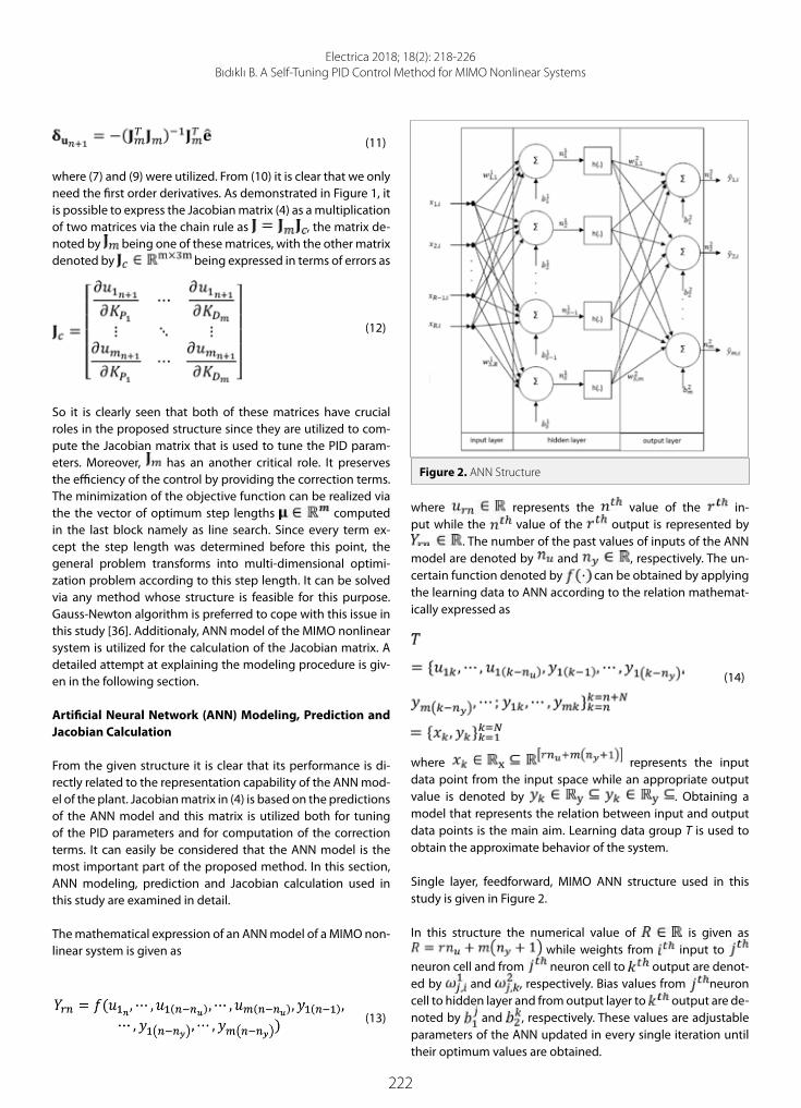
222


(11)

where (7) and (9) were utilized. From (10) it is clear that we only need the first order derivatives. As demonstrated in Figure 1, it is possible to express the Jacobian matrix (4) as a multiplication of two matrices via the chain rule as , the matrix de-noted by being one of these matrices, with the other matrix denoted by being expressed in terms of errors as

(12)

So it is clearly seen that both of these matrices have crucial roles in the proposed structure since they are utilized to com-pute the Jacobian matrix that is used to tune the PID param-eters. Moreover, has an another critical role. It preserves the efficiency of the control by providing the correction terms. The minimization of the objective function can be realized via the the vector of optimum step lengths computed in the last block namely as line search. Since every term ex-cept the step length was determined before this point, the general problem transforms into multi-dimensional optimi-zation problem according to this step length. It can be solved via any method whose structure is feasible for this purpose. Gauss-Newton algorithm is preferred to cope with this issue in this study [36]. Additionaly, ANN model of the MIMO nonlinear system is utilized for the calculation of the Jacobian matrix. A detailed attempt at explaining the modeling procedure is giv-en in the following section.

Artificial Neural Network (ANN) Modeling, Prediction and Jacobian Calculation

From the given structure it is clear that its performance is di-rectly related to the representation capability of the ANN mod-el of the plant. Jacobian matrix in (4) is based on the predictions of the ANN model and this matrix is utilized both for tuning of the PID parameters and for computation of the correction terms. It can easily be considered that the ANN model is the most important part of the proposed method. In this section, ANN modeling, prediction and Jacobian calculation used in this study are examined in detail.

The mathematical expression of an ANN model of a MIMO non-linear system is given as

(13)

where represents the value of the in-put while the value of the output is represented by

. The number of the past values of inputs of the ANN model are denoted by and , respectively. The un-certain function denoted by can be obtained by applying the learning data to ANN according to the relation mathemat-ically expressed as

(14)

where represents the input data point from the input space while an appropriate output value is denoted by . Obtaining a model that represents the relation between input and output data points is the main aim. Learning data group T is used to obtain the approximate behavior of the system.

Single layer, feedforward, MIMO ANN structure used in this study is given in Figure 2.

In this structure the numerical value of is given as while weights from input to

neuron cell and from neuron cell to output are denot-ed by and , respectively. Bias values from neuron cell to hidden layer and from output layer to output are de-noted by and , respectively. These values are adjustable parameters of the ANN updated in every single iteration until their optimum values are obtained.

Figure 2. ANN Structure

223


The input-output relationship of an ANN model is expressed as

(15)

where represents the sigmoidal activation function expressed as . Number of neurons in the hidden layer are denoted by and is computed as

(16)

The following objective function is minimized by updating the adjustable parameters in every single iteration

(17)

The LM rule is utilized in every iteration to optimize the adjust-able parameters as

(18)

where represents the vector that contains learning errors and defined as

(19)

is a vector of weights and biases

(20)

and is a Jacobian matrix whose structure is given as

(21)

The ANN model can be obtained by utilizing the given equa-tions and realizing the necessary number of iterations until the value of the objective function in (15) reaches the desired level. The future behavior of the plant can be predicted by utilizing (14), after the ANN model has been obtained.

Algorithm of the ANN Model-Based PID Tuning and Control

After the necessary arrangements are realized on the structure and mathematical design, the algorithm given in [34] can be used directly. The steps of the proposed algorithm can be item-ized as follows:

Step 1: The minimum and maximum input values umin and umax that can be applied to the plant are determined. Then the mod-eling data is collected from the system by applying random in-puts from the interval given as [umin, umax] and measuring the outputs of the plant.

Step 2: A set of training data is formed after the nu and ny values of the ANN model (13) are determined. Then, the set of input and output values are normalized to the interval .

Step 3: From the collected N data from the plant, data pairs are randomly selected as the learning data for the ANN model, the remaining data are used as test and validation data pairs.

Step 4: PID tuning and control are realized by applying the fol-lowing algorithm at each iteration:

• The corresponding control input is computed according to the measured error .

• The K-step future behavior of the system is predicted by utilizing the ANN model of the plant. To realize this pre-diction the K-step input sequence is applied to the ANN model.

• The Jacobian matrix is calculated by utilizing ANN model and then the correction term is determined by

Figure 3. Phantom OMNI Haptic Device

224


utilizing both the ANN model and the calculated Jaco-bian matrix.

• The vector of optimum step sizes of the correction terms µ is founded via the Gauss-Newton algorithm.

• Summation of the control input and the correction term (i.e., ) is applied to the system.

• The general Jacobian matrix (4) is calculated and the PID parameters are updated utilizing (3).

Experimental Results

Phantom OMNI haptic device shown in Figure 3 was used as an experimental setup. A 2-DOF rigid link robot manipulator structure was obtained by mechanically stopping the first joint whose angle was denoted by . Joint space control ap-plication of the remaining links, whose angles were denoted by

and , respectively, was realized for the performance demonstration of the proposed method.

At this point it should be stated that each of the previously men-tioned parameters has a crucial role for the proposed method and all of them should be selected appropriately. However, proposing different suitable methods for all of the selections is a hard and time consuming task. Moreover, it increases the computational complexity. Some of these parameters were fixed to some con-stant values by considering these issues. The prediction horizon and the matrix of weigthing factors were fixed to K = 10 and λ = 0.01I2. Since, it was observed during the experiments that 5-step

Figure 4. Selection of Number of Hidden Neurons

Figure 5. Control Gains for u1(t)

Figure 6. Control Gains for u2(t)

Figure 7. Actual (line) and Reference (dashed) Trajectories

Figure 8. Link Tracking Errors

Figure 9. Control Inputs

225


previous values of the inputs and the outputs provide the best validation error, the number of the past values of the inputs and the outputs were selected as nu and ny = 5, respectively.

The number of hidden neurons directly affects the modeling performance of the ANN. As a result of this, it can directly be related to the performance of the proposed method. Both of the selections that are less or more than the optimum value decrease the representation capability of the ANN model. The number of hidden neurons were selected to reduce the norm of the matrix containing the validation errors. To reach this pur-pose, ANN modeling was realized 1000 times for each number of neurons and the means of the norm values were marked on Figure 4. As it can be seen from Figure 4, any significant change was not observed in this value after 23 neurons. As a result of this, the optimum number of hidden neurons was selected as 23. At this point it should be stated that all of this process was applied to 1000 learning, 500 test and 500 validation data that were randomly selected from the collected input output data pairs from both links of the experimental system.

The control objective is to make and follow a si-nusoidal desired trajectory chosen as

(22)

The adjustment process of the control gains can be seen from Figure 5 and Figure 6 for and , respectively. From these figures it can be seen that the control gains were tuned to their optimum values approximately in 4 seconds. Optimum values of control gains were obtained as Kp = diag ([0.005, 0.02]), Kı = diag ([0.008, 0.013]) and KD = diag (0.025, 0.04).

The desired and the actual trajectories are shown together in Figure 7, while the tracking errors and the control inputs are given in Figure 8 and Figure 9, respectively. From Figure 7 and Figure 8, it can be seen that the control objective was met.

Conclusion

In this study, a self-tuning PID control scheme was proposed for the control of MIMO nonlinear systems. A number of op-timization methods were used in conjuction with the ANN model of the system to ensure the self-tuning structure. First, the ANN model of the system was obtained via input and output data pairs collected from the system. These data pairs were randomly classified as learning, test and validation data and they were used to train a single layer, feedforward MIMO ANN structure. Then, the obtained ANN model was utilized for both PID tuning and control purposes. A vector of correction term computed via the Gauss-Newton algorithm was used to provide control until the PID parameters reach their optimum values. As a result of this, the control objective was met during the PID tuning process. Once the PID parameters reached their optimum values, the correction term was disabled and the pro-

cess was continued with the classical PID control. Performance of the proposed method was demonstrated via a joint-space control application of a rigid link 2-DOF robot manipulator. In the experiments, it was observed that PID parameters were tuned to their optimum values in 4 seconds. However, from the actual and desired trajectories and the link tracking errors it was also seen that the control objective was met before this process and it continued after the optimum parameter values were provided. From these results, it can be said that all of the previously mentioned purposes were reached in the experi-mental studies.




References

1. T. Marchetti, M. Barolo, L. Jovanovic, H. Zisser, D. E. Seborg, “An im-proved PID switching control strategy for Type 1 Diabetes”, IEEE Trans on Biomed Eng, vol. 55, no. 3, pp. 857-865, 2008.

2. T. J. Ren, T. C. Chen and C. J. Chen, “Motion control for a two-wheeled vehicle using a self-tuning PID controller”, Control Engi-neering Practice, vol. 16, no. 3, pp. 365-375, 2008.

3. J. Ye, “Adaptive control of nonlinear PID-based analog neural net-works for a nonholonomic mobile robot”, Neurocomputing, vol. 71, no. 7-9, pp. 1561-1565, 2008.

4. B. Allaoua, B. Gasbaoui, B. Mebarki, “Setting up PID DC motor speed control alteration parameters using particle swarm optimi-zation strategy”, Leonaro Electronic J. of Practices and Technologies, no. 14, pp. 19-32, 2009.

5. R. Kandiban, R. Arulmozhiyal, “Design of adaptive fuzzy PID con-troller for speed control of BLDC motor”, International Journal of Soft Computing and Engineering, vol. 2, no. 1, pp. 386-391, 2012.

6. U. K. Bansal and R. Narvey, “Speed control of DC motor using fuzzy PID controller”, Advance in Electronic and Electric Engineering, vol. 3, no. 9, pp. 1209-1220, 2013.

7. J. M. Zheng, S. Zhao, S. Wei, “Application of self-tuning fuzzy PID controller for a SRM direct drive volume control hydraulic press”, Control Engineering Practice, vol. 17, no. 12, pp. 1398-1404, 2009.

8. Ş. Çetin, A. V. Akkaya, “Simulation and hybrid fuzzy-PID control for positioning of a hydraulic system”, Nonlinear Dynamics, vol. 61, no. 3, pp. 465-476, 2010.

9. S. Soyguder, M. Karakose, H. Alli, “Design and simulation of self-tuning PID-type fuzzy adaptive control for an expert HVAC system”, Expert Systems with Applications, vol. 36, no. 3, pp. 4566-4573, 2009.

10. R. Wai, J. Lee, K. Chuang, “Real-time PID control strategy for mag-lev transportation system via particle swarm optimization”, IEEE Transactions on Industrial Electronics, vol. 58, no. 2, pp. 629-646, 2011.

11. J. Li, Y. Li, “Dynamic analysis and PID control for a quadrotor”, IEEE International Conference on Mechatronics and Automation Chi-na, 2011.

12. I. Sadeghzadeh, A. Mehta, A. Chamseddine, Y. Zhang, “Active fault tolerant control of a quadrotor UAV based on gainscheduled PID

226


control”, IEEE Canadian Conference on Electrical and Computer Engineering, Montreal, QC, Camada, 2012.

13. F. Goodarzi, D. Lee, T. Lee, “Geometric nonlinear PID control of a quadrotor UAV on SE(3),” European Control Conference, Zurich, Switzerland, 2013.

14. L. B. Prasad, B. Tyagi, H. O. Gupta, “Modelling and simulation for optimal control of nonlinear inverted pendulum dynamical sys-tem using PID controller and LQR”, Asia Modelling Symposium, Bali, Indonesia, 2012.

15. L. B. Prasad, B. Tyagi, H. O. Gupta, “Optimal control of nonlinear in-verted pendulum system using PID controller and LQR: Performance analysis without and with disturbance input”, International Journal of Automation and Computing, vol. 11, no. 6, pp. 661-670 2014.

16. W. Yu, J. Rosen, “Neural PID control of robot manipulators with ap-plication to an upper limb exoskeleton”, IEEE Trans Cybern, vol. 43, no. 2, pp. 673-684 2013.

17. A. Kumar, V. Kumar, “Evolving and interval type-2 fuzzy PID con-troller for the redundant robotic manipulator”, Expert Systems with Applications, vol. 73, pp. 161-177, 2017.

18. Y. Su, C. Zheng, “PID control for global finite-time regulation of ro-botic manipulators,” International Journal of Systems Science, vol. 48, no. 3, pp. 547-558, 2017.

19. M. A. Khosravi, H. D. Taghirad, “Robust PID control of fully-con-strained cable driven parallel robots”, Mechatronics, vol. 24, no. 2, pp. 87-97, 2014.

20. K. Ou, Y. Wang, Z. Li, Y. Shen, D. Xuan, “Feedforward fuzzy-PID con-trol for air flow regulation of PEM fuel cell system,” International Journal of Hydrogen Energy, vol. 40, no. 35, pp. 11686-11695, 2015.

21. H. Tang, Y. Li, “Feedforward nonlinear PID control of a novel micro-manipulator using Presiach hysteresis compensator,” Robotics and Computer-Integrated Manufacturing, vol. 34, pp. 124-132, 2015.

22. M. Taherkhorsandi, M. J. Mahmoodabadi, M. Talebipour, K. K. Cas-tillo-Villar, “Pareto design of an adaptive robust hybrid of PID and sliding control for a biped robot via genetic algorithm optimiza-tion”, Nonlinear Dynamics, vol. 79, pp. 251-263, 2015.

23. Z. Civelek, M. Lüy, E. Çam, N. Barışçı, “Control of pitch angle of wind turbine by fuzzy pid controller”, Intelligent Automation & Soft Computing, vol. 22, no. 3, pp. 463-471, 2016.

24. J. Song, W. Cheng, Z. Xu, S. Yuan, M. Liu, “Study on PID temperature control performance of a novel PTC material with room tempera-

ture Curie point”, International Journal of Heat and Mass Transfer, vol. 95, pp. 1038-1046, 2016.

25. A. M. Simonovic, N. N. Jovanovic, N. S. Lukic, N. D. Zoric, S. N. Stupar, S. S. Ilic, “Experimental studies on active vibration control of smart plate using a modified PID controller with optimal orien-tation of piezoelectric actuator,” Journal of Vibration and Control, vol. 22, no. 1, pp. 2619-2631, 2016.

26. R. Rout, B. Subudhi, “Inverse optimal self-tuning PID control de-sign for an autonomous underwater vehicle”, International Journal of Systems Science, vol. 48, no. 2, pp. 367-375, 2017.

27. K. J. Aström, T. Hagglund, C. C. Hang, W. K. Ho, “Automatic tuning and adaptation for PID controllers - a survey,” Control Engineering Practice, vol. 1, no. 4, pp. 699-714, 1993.

28. P. Cominos, N. Munro, “PID controllers: recent tuning methods and design to specification,” Control Theory and Applications, vol. 149, no. 1, pp. 46-53, 2002.

29. K. Li, “PID tuning for optimal closed-loop performance with speci-fied gain and phase margins”, IEEE Transactions on Control, Systems Technology, vol. 21, no. 3, pp. 1024-1030, 2013.

30. B. B. Alagoz, A. Ates, C. Yeroglu, “Auto-tuning of PID controller ac-cording to fractional-order reference model approximation for DC rotor control”, Mechatronics, vol. 23, pp. 789-797, 2013.

31. A. T. Azar, F. E. Serrano, “Robust IMC-PID tuning for cascade control systems with gain and phase margin specifications”, Neural Com-puting and Applications, vol. 25, pp. 983-995, 2014.

32. C. Y. Jin, H. R. Kyung, S. W. Sung, J. Lee, I. B. Lee, “PID auto-tuning using new model reduction method and explicit PID tuning rule for a fractional order plus time delay model,” Journal of Process Control, vol. 24, pp. 113-128, 2014.

33. Ş. Yavuz, L. Malgaca, H. Karagülle, “Analysis of active vibration control of multi-degree-of-freedom flexible systems by Newmark method”, Simulation, Modelling and Practice Theory, vol. 69, pp. 136-148, 2016.

34. S. Iplikci, “A comparative study on a novel model-based PID tuning and control mechanism for nonlinear systems”, International Journal of Robust and Nonlinear Control, vol. 20, no. 13, pp. 1483-1501, 2010.

35. J. Nocedal, S. J. Wright, Numerical Optimization, Springer: New York, 1999.

36. P. Venkatamaran, Applied Optimization with MATLAB Program-ming, Wiley-Interscience: New York, 2002.

Barış Bıdıklı was born in İzmir, Turkey on September 14th, 1989. He received his BSc, MSc and PhD degrees in Electrical & Electronics Engineering from Pamukkale University, Denizli, Turkey in 2011, in Electrical & Electronics Engineering from İzmir Institute of Technology, İzmir, Turkey in 2013 and 2016, respectively. He is currently an Assist. Prof. Dr. at the department of Mechatronics Engineering, Faculty of Engineering and Architecture, İzmir Katip Çelebi University, İzmir, Turkey. His research interests include observer design, adaptive and robust control of uncertain nonlinear dynamical systems, partial state feedback and output feedback control techniques, non-linear control techniques for mechatronic systems and dynamic simulations of mechatronic systems.

227

Introduction

Cognitive Radio (CR) networks are promising wireless networks and new technology in com-munication systems in order to resolve the spectrum scarcity issue [1]. Spectrum sensing is one of the main enabling functions of a CR device to make an intelligent decision about spectrum usage [2]. Cooperative Spectrum Sensing (CSS) has been confirmed to be an effi-cient approach to promote the sensing performance by providing a spatial form of diversity [3]. In the CSS process, each CR sensor separately senses the desired spectrum and then sends its measurement to a Fusion Center (FC). Due to the special structure of a CR net-work, it is vulnerable to security attacks. Two important security attacks include the Spec-trum Sensing Data Falsification (SSDF) attack and the Primary User Emulation Attack (PUEA) [4]. During SSDF attacks, CR attackers send falsified spectrum sensing results to the FC and disrupt the global sensing decision. To overcome the impact of SSDF attacks, several differ-ent solutions have been proposed in previously [5-7]. In PUEA, a malicious attacker mimics some characteristics of the legitimate PU’s signal. Whenever the PU transmitter does not send in the desired channel, the PUEA transmits its fake signal to the CR sensors, deceiving them to believe that the channel is occupied by the PU. This type of attack has been studied extensively [8-14].

The CSS procedure in the presence of a PUEA was considered in [8]. A proper dynamic collabo-rative weight was assigned to each CR sensor and then the received reports were aggregated in the FC with a weighted combined algorithm in order to maximize the performance of PU’s signal detection in Neyman-Pearson (N-P) algorithm. The omnipresent attacker was assumed which is not practical due to the added power consumption [8]. A smart PUEA was considered in the case that it is located near the PU tower and adjusts its transmitted power to be the

Electrica 2018; 18(2): 227-233

RESEARCH ARTICLE

Dynamic Threshold Selection Approach in Voting Rule for Detection of Primary User Emulation AttackAbbas Ali Sharifi , Mohammad Mofarreh-Bonab Department of Electrical Engineering, University of Bonab, Bonab, Iran

Corresponding Author: Abbas Ali Sharifi





DOI: 10.5152/iujeee.2018.1819

Cite this article as: AA. Sharifi, M. Mofarreh-Bonab. "Dynamic Threshold Selection Approach in Voting Rule for Detection of Primary User Emulation Attack". Electrica, vol. 18, no. 2, pp. 227-233, 2018.

ABSTRACT

Cognitive radio (CR) technology presents a mechanism for efficient spectrum usage. Spectrum sensing is an essential CR function which includes an intelligent signal processing algorithm to identify the vacant frequency bands. Cooperative spectrum sensing (CSS) has been widely adopted to improve the performance of CR networks. Unfortunately, CR networks are vulnerable to security threats. In this study, we propose an optimal threshold selection approach to address one of the most important attacks called primary user emulation attack (PUEA). In PUEA, a malicious attacker mimics some important primary signal features and deceives CR sensors to prevent them from accessing the available channels. In this study, we assume a malicious PUEA which is relatively located near the potential user (PU) transmitter and senses the spectrum and accurately detects the vacant frequency bands to transmit its fake signal. We estimate attack strength and then apply the K-out-of-N rule to obtain an optimum and dynamic threshold K, minimizing the global error probability. Here, the attack strength is defined as the ratio of the average transmission power of the PUEA to the average power of the PU. The achieved simulation results indicate that the performance of the suggested method is satisfactory in detecting the malicious PUEA compared with conventional methods.

Keywords: Cognitive Radio (CR); Cooperative Spectrum Sensing (CSS); Primary User Emulation Attack (PUEA); K-out-N rule.

https://orcid.org/0000-0002-7777-0412

https://orcid.org/0000-0001-7086-0725

228

Electrica 2018; 18(2): 227-233Sharifi and Mofarreh-Bonab. Dynamic Threshold Selection Approach for Detection of PUEA

same as the PU’s power [9]. The malicious incumbent emula-tor only occupies a portion of the vacant frequency band and the channel occupancy rate of the attacker was estimated and applied in N-P criteria to improve the performance of cooper-ative sensing. In order to enhance the CSS performance, in the coexistence of a PUEA, a tow-level database-assisted spectrum sensing was proposed in [10]. Energy detection and location verification are combined for fast and consistent detection of PU signals. Game theory approach was proposed to mitigate the impact of PUEA [11]. The Nash Equilibrium (NE) was calcu-lated and it was achieved that the NE depends on the avail-able spectrum and the attacker’s behavior. The Attack-Aware Threshold Finding method was introduced to defense against the PUEA [12]. Two important PUEA parameters, probabilities of PUEA activity in both occupied and unoccupied frequency bands, were estimated and used to derive the optimal thresh-old values. The authors proposed Multi-Level Hypotheses Test (MLHT) [13]. They partitioned the decision space into four dif-ferent areas and then applied the Bays cost criteria to specify the PU channel status. Statistical characteristics of the received power from CR sensors were used to address the PUEA [14].

In this paper, we assume a centralized CR network with a ma-licious PUEA and propose an attack-aware CSS method based on a new hard-decision combining scheme. In the proposed method, the cooperative sensing process is performed in two stages: in the first stage, the CR users individually sense the frequency spectrum and then send their measured energies to the FC. In this stage, the FC estimates the attack strength. In the second round, each CR sensor sends its one bit hard decision about PU signal presence. In this round of cooperative sensing, the obtained attack strength is innovatively applied the K-out-of-N data fusion rule to obtain an optimal value of threshold K that minimizes the global error probability. In the proposed system model, the attacker only sends its fake signal in vacant frequency bands which is an important task of power saving strategy, unlike previous research [8, 12].

The rest of the paper is prepared as follows: Sec. II describes the considered system model and energy detection method. In Sec. III, we review the CSS process. Sec. IV explains the pro-posed optimal K-out-of-N rule. Sec. V provides simulation re-sults. Finally, Sec. VI concludes the paper.

System Model and Energy Detection Scheme

The planned system model for a centralized CR network is shown in Figure 1. The proposed system model considers a wireless CR network with N number of collaborative CR sen-sors. In order to get a higher priority than other CR users in accessing unoccupied frequency bands, a malicious PUEA emulates some important characteristics of the legitimate PU’s signal to defraud other CR users into believing that the PU’s transmission is in process. It is further assumed that the whole CR network is in the communication range of PU and PUEA transmitters.

We assume that the PUEA is located near the PU transmitter. Consequently, the spectrum sensing error caused by multi-path fading and shadowing is ignored for the attacker. We fur-ther assume that the attacker is smart and only transmits its fake signal in unoccupied frequency bands. The transmission process of the PU and PUEA in several different time slots are shown in Figure 2.

The presence and absence of PU signal are denoted by PUon and PUoff, respectively. Similarly, Eon and Eoff indicate that the PUEA fake signal is present and absent, respectively.

It is assumed that each CR sensor has a local energy detector to sense its surrounding area. Spectrum sensing is a binary hypothesis between H0 and H1, which are the hypotheses of absence and presence of the PU signal, respectively. In the ab-sence of PUEA (No attack scenario), two well-known hypothe-ses can be written in general as:

The first state H0 indicates that the channel is free of any PU signals and the second hypothesis H1 declares that the PU sends its legitimate signal through the channel. Considering the above mentioned hypotheses, the received signal at the ith sample of the jth sensor, i

jx , can be written as [15, 16]

(1)

Figure 1. Network Layout

Figure 2. The transmission process of the PU and PUEA

229


where ijn is the received noise sample at the jth sensor. The

parameter belongs to the PU signal with a power value

jg . The noise and PU signal samples ( ijn , i

jp ) are assumed to γj be identically independent distributed Gaussian random variables with zero mean and unit variance. Therefore, γj can be defined as the average SNR of PU signal at the jth spectrum sensor. We further assume that the CR sensors are randomly deployed in a small area and both PU and PUEA transmitters are relatively far away from the CR network. Hence, the average SNR is almost the same for each CR receiver. Thus, the index j

is omitted from γj. With regard to the equation (1) and con-sidering the above assumptions, the received signal i

jx is a Gaussian distributed variable as [15],

(2)

Furthermore, each CR sensor uses M samples for its local ener-gy detection. The decision statistics associated with the output of an energy detector for jth CR Ej is obtained as follows:

(3)

where two parameters ja and jb are two central Chi-square

distributed random variables with M degrees of freedom. But, according to the Central Limit Theorem, when M is large enough (i.e., M > 10), Ej can be approximated as a Gaussian random variable as follows [17]:

(4)

where

The measured energy of each sensor is compared with a pre-defined threshold T

and then the CR sensor makes a binary

decision uj about the PU channel status: 1ju = (the channel is occupied) if Ej > T

and uj = 0 (the PU channel is vacant) other-

wise. The obtained binary decision of the jth sensor uj is sent to the FC. The communication channel between the CR users and FC is assumed to be an error-free reporting channel. The proba-bilities of PU signal detection and false alarm are computed by

(5)

where (.)Q is the tail probability of standard normal distribu-tion.

Cooperative Spectrum Sensing

After comparing the local received energy Ej with a threshold T, a binary decision of each sensor is sent to the FC. The FC fus-es the received decisions by using the K-out-of-N rule (voting rule) to make a global decision about the PU activity. In the K-out-of-N rule, all of the binary sensing reports are collected and compared with the threshold value K. A threshold value N is an AND fusion rule, a threshold 1 is an OR rule and N/2 is a majority fusion rule.

The AND fusion rule announces the occupancy of the PU chan-nel only when all of the CR sensors report PU signal presence. For the AND rule the global detection and false alarm probabil-ities are calculated as [18]:

(6)

The global error probability is defined as the average of detec-tion and false alarm probabilities by each hypothesis:

(7)

The AND rule has a very low false alarm rate which makes an efficient spectrum utilization, however it may not protect the PU from strong interferences from the CR users.

(8)

For the OR fusion rule, the global detection and false alarm probabilities at the FC are respectively given by:

(9)

The OR rule has a very high detection probability which is help-ful to protect the PU. In contrary, it has a relatively high false alarm probability which makes an inefficient spectrum con-sumption.

(10)

In the majority fusion rule, the FC confirms the presence of the PU signal when at least half the of sensors report the occupan-cy of the PU channel. The majority rule has a compromised characteristic of OR and AND rules and its detection and false alarm probabilities are

230


(11)

In the current study, we present the K-out-of-N rule which leads the presence of a PU signal when more than K sensors out of N sensors confirm the presence of PU signal. The global detection and false alarm probabilities the of the K-out-of-N rule are re-spectively given by:

(12)

The Proposed Optimal K-out-of-N Rule Under PUEA

Based on the presence of the PUEA and with regard the pro-posed system model, two different possible hypotheses can be expressed as:

The first state H0 occurs when the PUEA transmits the fake sig-nals in vacant frequency bands. In this case, the parameter i

jx can be formulated as:

(13)

where the parameter is the received PUEA signal with the power λj. The parameter ρ = λ/γ is considered as PUEA strength. For a more powerful PUEA, we obtain a larger value of ρ. Obviously, in the absence of PUEA (ρ = 0), the hypothe-sis H0 corresponds to the state H0. As mentioned before, in the presence of the PUEA, we have

(14)

and

(15)

Thus,

(16)

where

In this case, the false alarm probability will be changed and can be written as:

(17)

With regard the proposed system model, we have

Assuming the presence of PUEA in vacant frequency bands, the parameter faP is parameterized by attack strength ρ. Thus, the FC needs to be estimate of attack parameter ρ to obtain an op-timal threshold Kopt in the K-out-of-N rule. In the initial stages of the cooperative sensing, the measured energies of all CR users are sent to the FC and the FC calculates the average of the re-ceived sensing reports to derive the attack strength ρ.

The average value of received energy reports M is defined as

(18)

The mathematical expectation of M is

(19)

where

(20)

It should be noted that p (H0) = p (H0),thus,

231


(21)

From the above equations, the values of unknown attack strength ρ is estimated as

(22)

where two parameters A and B are defined as

After the estimation of the parameters ρ, the FC obtain an op-timal threshold Kopt in the K-out-of-N rule to minimize the to-tal error probability. Assuming that ( )eQ K represents a single minimum, the optimum value of K will be obtained based on the following optimization problem

(23)

By substituting (12) into (7), the global error probability ( )eQ k is rewritten as:

(24)

As ( )eQ K is a convex function of K, we use a simple linear equation

(25)

Substitution of (24) to (25) gives the following result

(26)

Taking the logarithm on (26), Kopt is obtained as

(27)

where

It should be noted that the two parameters y and j depend on the probabilities dp and fap . Hence, the false alarm prob-ability fap is parameterized by attack strength ρ. Therefore, for different values of and ρ, we will have different values for optK .

Simulation Results

In the considered CR network model, there are N = 20 cooper-ative CR sensors. Each sensor uses M = 30 samples for its local spectrum sensing. The local false alarm probability of each sen-sor is considered to be 0.1 to obtain the local detection thresh-old T. The average SNR of each sensor received from PU signal (γ) is assumed to be -5 dB. The two probabilities p(H0) and p(H1) are considered as 0.8 and 0.2, respectively.

Figures 3 and Figure 4 show the estimation of attack strength for ρ = 0.3 and ρ = 0.7, respectively. The obtained values for ρ are reached to the constant values after using almost 200 iter-ations of spectrum sensing. Therefore, in computer simulation, we use about 200 sensing intervals in the initial stage to esti-mate the attack strength and then apply the K-out-of-N fusion rule to achieve an optimal threshold K that minimizes the glob-al error probability.

Figure 5 displays the total error probability versus threshold K for No-Attack scenario and several different values of attack strength. It is clearly shown that for a given values of ρ there is an optimum value of K that indicates the minimum global error probability and confirms the convexity of equation (23).

Figure 6 depicts the total error probability versus the attack strength ρ. In the conventional hard decision combining schemes (AND rule, OR rule and the Majority Fusion Rule), in-

Figure 3. The convergences of attack parameters (ρ = 0.3)

232


creasing the attack strength causes high error probability. The obtained error probabilities for AND and OR fusion rules are in-dependent of attack strength ρ and they are fixed in constant values p(H1) andp(H1), respectively. This confirms equations (8) and (10). In contrast, with the proposed method, increasing at-tack strength yields a slight change in total error probability.

Conclusion

This study has investigated the Primary User Emulation At-tack (PUEA) in Cognitive Radio (CR) networks. In our scheme, a smart and malicious PUEA was assumed, in which, the attacker carefully senses the spectrum and sends its fake signal in the vacant frequency bands. In the initial stage of Cooperative Spectrum Sensing (CSS), the CR sensors sent their measured energies to the Fusion Center (FC) and the FC estimated the attack strength. The attack strength was defined as the ratio

of the average transmission power of the malicious attacker to the average emitted power of the legitimate PU. After estima-tion of the attack strength, the CR users sent their hard one bit decision about PU signal presence to the FC. The FC applied the estimated attack strength in the K-out-of-N fusion rule to obtain an optimal threshold K that minimizes the global error probability. Computer simulation results depicted that the pro-posed method provides less error detection probability com-pared with other hard decision combining schemes such as AND, OR, and majority fusion rules.




References

1. J. Mitola, G. Q. Maguire, “Cognitive radio: making software radios more personal”, IEEE Personal Communication, vol. 6, no. 4, pp. 13-18, 1999.

2. S. Haykin, “Cognitive radio: brain-empowered wireless communi-cations”, IEEE Journal on Selected Areas in Communications, vol. 23, no. 2, pp. 201-220, 2005.

3. I. F. Akyildiz, B. F. Lo, R. Balakrishnan, “Cooperative spectrum sens-ing in cognitive radio networks: A survey,” Physical Communica-tion, vol. 4, no. 1, pp. 40-62, 2011.

4. R. Chen, J. M. Park, Y. T. Hou, J. H. Reed, “Toward secure distributed spectrum sensing in cognitive radio networks,”IEEE Communica-tions Magazine, vol. 46, no. 4, pp. 50-55, 2008.

5. A. A. Sharifi, M. J. Musevi Niya, “Defense against SSDF attack in cognitive radio networks: attack-aware collaborative spectrum sensing approach”, IEEE Communications Letters, vol. 20, no. 1, pp. 93-96, 2016.

6. A. A. Sharifi, M. Sharifi, J. Musevi Niya, “Reputation-based Likeli-hood Ratio Test with Anchor Nodes Assistance”, International Symposium on Telecommunications, 2016.

Figure 4. The convergences of attack parameters (ρ = 0.7)

Figure 5. Probability of error versus K for several different values of ρ

Figure 6. Probability of error versus attack strength ( ρ )

233


7. A. A. Sharifi, J. Musevi Niya, “Securing collaborative spectrum sensing against malicious attackers in cognitive radio networks”, Wireless Personal Communications, vol. 90, no. 1, pp. 75-91, 2016.

8. C. Chen, H. Cheng. H, Y.D. Yao, “Cooperative spectrum sensing in cognitive radio networks in the presence of the primary user em-ulation attack,” IEEE Transactions on Wireless Communications, vol. 10, no. 7, 2135-2141, 2011.

9. A. A. Sharifi, M. Sharifi, M. J. Musevi Niya. “Collaborative spectrum sensing under primary user emulation attack in cognitive radio net-works,” IETE Journal of Research, vol. 62, no. 2, pp. 205-211, 2016.

10. R. Yu, Y. Zhang, Y. Liu, S. Gjessing, M. Guizani, “Securing cognitive radio networks against primary user emulation attacks”, IEEE Net-work, vol. 30, no. 6, pp. 62-69, 2016.

11. A. Ahmadfard, A. Jamshidi, A. Keshavarz-Haddad, “Game theoretic approach to optimize the throughput of cognitive radio networks in physical layer attacks”, Journal of Intelligent and Fuzzy Systems, vol. 28, no. 3, pp. 1281-1290, 2015.

12. A. A. Sharifi, M. Sharifi, M. J. M. Niya, “Secure cooperative spectrum sensing under primary user emulation attack in cognitive radio networks: Attack-aware threshold selection approach”, Interna-tional Journal of Electronics and Communications (AEU), vol. 70, no. 1, 95-104, 2016.

13. M. Sharifi, A. A. Sharifi, M. J. M. Niya, “Cooperative spectrum sens-ing in the presence of primary user emulation attack in cognitive radio networks: multi-level hypotheses test approach,” Wireless Networks, vol. 24, no. 1, pp. 61-68, 2018.

14. M. Ghaznavi, A. Jamshidi, “Defence against primary user emula-tion attack using statistical properties of the cognitive radio re-ceived power”, IET Communications, vol. 11, no. 9, pp. 1535-1542, 2017.

15. J. Ma, G. Zhao, Y. Li, “Soft combination and detection for cooper-ative spectrum sensing in cognitive radio networks”, IEEE Trans-actions on Wireless Communications, vol. 7, no. 11, pp. 4502-4507, 2008.

16. M. Sharifi, A. A. Sharifi, M. J. M. Niya, “A new weighted energy de-tection scheme for centralized cognitive radio networks”, Interna-tional symposium on telecommunications, 2014.

17. F.F. Digham, M.S. Alouini, M.K. Simon, “On the energy detection of unknown signals over fading channels”, IEEE International Confer-ence on Communications, vol. 5, pp. 3575–3579, 2003.

18. P. K. Varshney, “Distributed detection and data fusion,” Spring-er-Verlag, 1997.

Mohammad Mofarreh-Bonab received the B.Sc. and M.Sc. degrees both in telecommunication engineering from K.N.Toosi University of technology (KNTU) and Iran university of Science and technology (IUST), respectively. His research interests span the areas of wireless communications, image and video processing, signal processing, cognitive radio and Image compression.

Abbas Ali Sharifi received the B.Sc. degree in electronic engineering from Amir Kabir University of Technology and the M.Sc. and Ph.D. degrees in telecommunication engineering from Malek Ashtar University of Technology and University of Tabriz, respectively. His current research interests include wireless communication and net-working, cognitive radio, security, and signal processing.

234

Introduction

Ensuring the secure planning of power systems has become an important and critical matter in recent years, along with the development of smart and complex systems [1]. Distributed generations (DGs) are new technologies supporting the evolution of smart distribution grids. These units sensibly contribute to increased system reliability and en-hanced power quality metrics [2]. The most general kinds of DGs are the renewable-based and conventional diesel-based units [3]. As societies are faced with environmental and economic hurdles ahead of soaring energy demands, deployment of green energy tech-nology is now at the center of attention. Furthermore, significant technical problems such as improving the voltage profile and minimizing the power loss are contemplated as DG-driven technical achievements.

The role of wind turbines (WTs) in minimizing power losses and improving the voltage profile has been carefully assessed in the literature [4]. The main concern in regard of green ener-gy technologies, such as WTs, has to do with their intermittent power generation. To avert such technical flaws, distribution network operators (DNOs) need to establish efficient tools to investigate existing uncertainties. There are different approaches for accommodating the uncertainties of distribution networks. The Monte Carlo simulation (MCS) technique, although portraying a high-resolution and precise manner, is a high computational approach [5]. Sce-nario tree modeling is one of the best techniques to include the impact of uncertainties. This approach reduces the computational burden of the analyses and maintains an adequate ac-curacy of the computation procedure [6].

Electrica 2018; 18(2): 234-241

RESEARCH ARTICLE

Probabilistic Placement of Wind Turbines in Distribution NetworksTohid Sattarpour1, Mohammad Sheikhi2, Sajjad Golshannavaz1, Daryoush Nazarpour1

1Department of Electrical Engineering, Urmia University, Urmia, Iran2Department of Electrical and Computer Engineering, Gazi-Tabatabayi Engineering Faculty, West

Corresponding Author: Tohid Sattarpour





DOI: 10.26650/electrica.2018.001

Cite this article as: T. Sattarpour, M. Sheikhi, S. Golshannavaz, D. Nazarpour, “Probabilistic Placement of Wind Turbines in Distribution Networks”, Electrica, vol. 18, no: 2, pp. 234-241, 2018.

ABSTRACT

This study presents an efficient approach for determining the optimal locations of wind turbines (WTs) in distribution systems, which considers the existing uncertainties in the power generation of WTs and the load demand of consumers. The daily load profiles of the seasonal and geographical-dependent behaviors of WTs are also considered. The proposed probabilistic approach is based on scenario tree modeling, and each scenario is assessed in regard to power loss minimization. Then, the TOPSIS (technique for order preference by similarity to an ideal solution) method is adopted to regulate the optimal placement of WTs considering the average value and the standard deviation of active power losses as possible attributes. This approach enables a multi-attribute analysis of the search space to yield a more efficient solution. Detailed simulation studies, conducted on IEEE 33-bus test system, are utilized to examine the effectiveness of the proposed method. The results of this study are discussed in depth.

Keywords: Wind turbine, uncertainty, scenario tree modeling, optimal placement

235

Electrica 2018; 18(2): 234-241Sattarpour et al. Probabilistic Placement of Wind Turbines

Several studies have focused on optimizing the impacts of renewable energies in distribution networks. The authors have presented a probabilistic model of WTs and photo-voltaics (PV) comparing their possible impacts [7]. The re-sults, based on this approach, have been compared to that of the symmetric two point estimate method (S2PEM), the Gram-Charlie method, and the Latin hypercube sampling method. Probabilistic operational management of a microg-rid was investigated [8]. A self-adaptive gravitational search algorithm was utilized to tackle the optimization proce-dure. A multi-objective programming method is proposed for reserve and energy planning of intelligent distribution systems [9]. A probabilistic load flow method was devised based on the PEM [3]. In a long-term fashion, analyzed the incorporation of WTs based on a combined MCS method and market-based optimal power flow (OPF) approach [11]. Authors have presented efficient methods for probabilistic calculation of wind energy injections to distribution systems [12]. This aim is pursued based on MCS and particle swarm optimization (PSO) techniques. Although a considerable effort has been dedicated in uncertainty analyses of inter-mittent wind energy generation and the load profile of the network, their concurrent analyses have not been tailored accurately.

This study aims at establishing an efficient probabilistic ap-proach to determine the optimal location of WTs in distri-bution systmes. In this manner, the existing uncertainties in both power generation of the WTs and load demand of the consumer are modeled with suitable probability density func-tions (PDFs). Daily load profile for each season and the geo-graphical-dependent behavior of WTs are taken into account as well. The proposed probabilistic approach deploys scenar-io tree modeling within which each scenario is investigated in regard of power loss minimization. Afterwards, the technique in order of preference by similarity to ideal solution (TOPSIS) is triggered to regulate the optimal placement strategy based on the average value and the standard deviation of the ac-tive power losses. As can be seen, a multi-attribute analysis of the search space is contemplated to yield in a more efficient solution. Detailed simulation studies, conducted on IEEE 33-bus test system, are deployed to scrutinize the effectiveness of the proposed approach.

This paper continues as follows. The uncertainties which are in-volved in the proposed probabilistic approach are introduced in section II. The mathematical skeleton of the proposed place-ment approach is thoroughly addressed in section III. The eval-uation of the model with a case study is described in section IV. Section V eventually concludes the manuscript.

Uncertainity Modeling

As mentioned earlier, the uncertainties in the load demand pro-file and the generated power of WTs are considered here. These

profiles are extracted on an hourly basis for each of the seasonal periods. Each of these uncertainties is modeled as follows.

Load Demand Uncertainty

The amount of demand, which is consumed in each hour needs to be forecasted. Generally, it is modeled with a normal PDF [13]. The following representation is considered:

(1)

Here, shD is the power demand. Also, and represent

the mean and standard deviation of demand, respectively. Scenario tree modeling is deployed for the uncertainty han-dling process. The states number is sensibly designated, as the number of small intervals decreases the modeling accu-racy while the number of large intervals increases the com-putational burden and provokes problem complexity. The mean value of each state is used to compute the variables of output in that specific state. The probability of each interval is designed as follows:

(2)

Where, DL1 and DL2 are respectively, the minimum and maxi-mum bounds of load demand at each interval.

Wind Turbine Modeling

In this study, the WT intermittent power generation is demon-strated as a Rayleigh PDF. A Rayleigh PDF is a special case of Weibull PDF in which the shape index is equal to 2. Such an assumption is widely applied in similar studies as a appropriate explanation of wind speed performance [13]. This behavior is represented as follow:

(3)

Where, k is the shape factor which is equal to 2 (k=2). shV and

shC denote the wind speed forecasted value and its scale fac-

tor, respectively. Therefore, the scaling index can be modeled as follows:

236


(4)

(5)

The generated power of a typical WT in each hour is deter-mined based on a WT power curve. This feature is interpreted as follows:

(6)

In (6), Pwr speaks to the rated power of WT and is its gen-

erated power in hour h and season s. As well, coutv is the cut-out

speed, cinv is the cut-in speed, and ratedv is the rated speed of

the WT.

The output power in each interval is achieved by the mean val-ue of each state. The probability of each interval is calculated as follows:

(7)

Where, VL1 and VL2 represent the lower and upper bounds of each interval, respectively. Moreover, C stands for the scale fac-tor and Vmean is the mean value of wind speed.

Scenario Tree Formation

Scenario tree modeling is deployed to define a set of scenarios in the optimal placement of WTs. The combination of load de-mand and wind speed states end in different scenarios. Each scenario contains two levels of demand value and wind gen-eration accompanied with a particular probability value. The probability of each scenario is calculated based on (8) whose terms are calculated in (2) and (7). As shown in (9), the cumula-tive summation of all scenarios is equal to one.

(8)

(9)

Where, is the probability of each scenario and SN is the number of scenarios.

The Proposed Methodology

Objective Functions

As the proposed approach establishes a TOPSIS-based multi-at-tribute approach, two objectives are determined as the main attributes of the proposed study. In this context, the first ob-jective function in (10) minimizes the active power losses in distribution feeders and the second one seeks a solution with the minimized variation of the active power losses. It will be assumed that the total power loss of the network is obtained as follow:

(10)

Where, and K denote the set and index of branches, respec-tively. kI and kR show the current magnitude and resistance of branches, respectively. By determing of the active power losses and probability of each scenario, the expected value (EV) and standard deviation (SD) of different scenarios in each hour are calculated as follows:

(11)

(12)

Here, (loss)sP represents the distribution system power losses in scenario s. Both (11) and (12) are considered as the inves-tigated attributes in the proposed TOPSIS-based probabilistic approach. Accurate forecast of wind power generation or load demand is important for distribution companies. An erroneous estimation ends with an additional energy transfer from the substation transformer, which poses monetary losses. Addi-tionally, this point ends in technical hurdles. Therefore, SD of the power losses is recognized as one of the attribute inaccu-rate evaluations of the results. The minimum value contribute to a better solution in regard of WT placement.

Constraints

In each of the scenarios, the nodal power balance should be satisfied. This necessity is denoted based on the constraints represented in (13) and (14). These equations are modified to include the power generation of WTs, load demands, and the transferred power from the main substation.

(13)

(14)

Where, , ,i h sWTP is active power generation of WT. , ,i h sLP and

237


, ,i h sLQ represent the active and reactive power loading of each

bus, respectively. ,h sV indicates the bus. Finally, and ijY

show the phase angle and magnitude of the feeder’s admit-

tance, respectively.

In this study, some other constraints, such as the permissible

range of voltage magnitude, the rated capacity of substation

transformer, and the permissible range of apparent power flow

through each distribution feeder, have been considered.

TOPSIS Approach

Prioritizing the candidate buses for the optimal probabilistic placement of WTs is assessed based on the TOPSIS approach. In this manner, a three-level hierarchy is shown in Figure 1. As it can be seen, the objective is located in the first level, attributes are located in the second level, and the third level is considered as alternatives (candidate buses). Regarding the power losses obtained at each scenario and the standard deviation of the results as the attributes, the following steps are conducted.

Step (1): Making a decision matrix based on an entropy technique for three alternatives and two attributes as shown in Table. 1.

In this table, EV and SD are the attributes. Furthermore, the three candidate buses are the alternatives. The average values of EV and SD at each candidate bus can be calculated as fol-lows:

(15)

Figure 1. The three-level hierarchy for sorting the possible candidates

Table 1. EV and SD of power losses in spring season

Spring

Bus 16 Hour 1 2 3 4 5 6 7 8 9 10 11 12

EV 13.80 11.04 10.26 8.39 9.01 8.97 13.37 17.77 22.91 25.20 26.47 29.13

SD 2.35 1.81 1.63 1.57 1.56 1.55 2.09 2.85 3.89 4.36 4.63 5.20

Hour 13 14 15 16 17 18 19 20 21 22 23 24

EV 36.58 49.55 68.49 105.45 120.57 125.32 130.42 109.27 82.09 53.60 34.04 14.01

SD 6.71 9.07 12.30 18.12 20.19 20.67 20.30 16.83 12.60 7.96 5.54 2.42

Bus 25 Hour 1 2 3 4 5 6 7 8 9 10 11 12

EV 15.74 12.57 11.54 9.01 9.80 9.81 15.39 20.94 27.48 30.36 31.93 35.15

SD 1.91 1.51 1.35 1.02 1.13 1.12 1.85 2.53 3.36 3.71 3.91 4.32

Hour 13 14 15 16 17 18 19 20 21 22 23 24

EV 44.05 58.66 80.42 122.04 136.87 140.89 142.81 119.12 89.18 57.51 37.40 15.86

SD 5.42 7.19 9.84 14.86 16.62 17.03 16.94 14.08 10.51 6.64 4.42 1.92

Bus 32 Hour 1 2 3 4 5 6 7 8 9 10 11 12

EV 13.90 10.92 9.85 7.71 8.34 8.36 13.07 17.51 22.84 25.25 26.61 29.44

SD 2.51 1.97 1.71 1.23 1.36 1.37 2.39 3.28 4.33 4.77 5.02 5.55

Hour 13 14 15 16 17 18 19 20 21 22 23 24

EV 37.32 50.90 70.58 108.81 124.13 128.81 133.37 111.61 83.71 54.54 34.73 14.18

SD 6.91 9.08 12.06 17.54 19.40 19.84 19.43 16.15 12.22 7.60 5.40 2.52

238


(16)

Step (2): Decision matrix [A] is normalized based on (17):

(17)

Where, lua is a decision matrix element and m is an alternatives quantity.

Step (3): Making the matrix named weighted normalized as X.

(18)

(19)

It should be noted that each of the two attributes in this study takes a similar weight. Each attribute’s weight is considered to be 0.5 (W1=W2= 0.5).Step (4): The best and worst answer regarding each attribute are determined in this step. uX + as the best answer is measured for the positive and negative criteria as the maximum and min-imum values. Also, as the worst answer is measured for the positive norm as the minimum value and for the negative norm as the maximum value.

(20)

(21)

Where, u and l show the u-th attribute and l-th alternative, re-spectively.

Step (5): In this step, the distance of each alternative with the best and worst answers are modeled by lS + and as follows:

(22)

(23)

Step (6): The mean distance between worst answer and each alternative are modeled as follows:

(24)

Step (7): Sorting the alternatives by considering the values which obtained as lC . It should be noted that a higher lC with its higher distance with worst answer is selected as candi-date bus (the most effective alternative).

Model of Evaluation on A Case Study

The proposed probabilistic approach is tested on IEEE 33-bus, depicted in Figure 2. The load point’s reactive and active pow-ers and the branches information are taken from [14]. Gath-ered daily load profiles corresponding to different seasons are shown in Figure 3. Considering the typical distribution system in its basic structure, the total peak demand is equal with 3.715 MW and 2.3 MVA. As it is clearly seen, peak hours are different in different seasons. The mean value of normal PDF is taken equal to the forecasted value. Moreover, the standard devia-tion of load demand is supposed to be equal to 5%. Bus 1 is supposed to be the substation bus and linked to the sub-trans-mission grid. Three different candidate buses are nominated as the placement locations of WTs. These buses include 16, 25, and also 32. Since there is a limited budget for placement of

Figure 2. Single line diagram of IEEE-33 bus test system

Figure 3. Daily load curves at different seasons

239


WTs, only one WT is implanted on the network. WTs are oper-ating in unity power factor, i.e., they have not participated in reactive power exchanges. The WT rated capacity is assumed

as 500 kW. Regarding the power curve specifications, the cut-in speed is equal to 3 m/s, rated speed is determined as 12 m/s, and cut-out speed is denoted as 25 m/s. The average hourly wind speed at each season is shown in Figure 4.

Table 1 shows the EV and SD of power losses attained in differ-ent buses and at each hour of a day in spring season. Due to hourly differences in wind speed and load demand, different values of EV and SD are attained. For instance, at hour 16, load demand is at 80% of peak load and the wind speed’s mean val-ue is 9.2 m/s. Accordingly, the EV and SD of power losses in bus-es 16, 25, or 32 are attained as (105.45, 18.12), (122.04, 14.86), and (108.81, 17.54), respectively. These differences reflect the impact of WT placement in different buses. As shown in Table 2, three candidate buses have different results considering the average values of EV and SD. It has been earlier elucidated that the optimal placement solution should portray the minimum EV as well as the minimum SD.

Based on TOPSIS approach, the priorities of WT placement can-didates are determined based on (24). In this way, the results for each season are presented in Table 3. Moreover, the largest distance from the worst answer is considered as the final rank-ing. Consequently, this bus is designated as the best location for installation. Therefore, bus 25 is selected as the best installa-tion location of WT satisfying the minimum power losses.

Also, Table 4, shows the effect of installed WT on the ex-pected mean power loss at each season. In this table, base plan represents the basic structure of the test case without placing WT. This solution is in line with the minimum power losses in the network and portrays a minimum standard de-

Figure 4. Mean values of wind speed in different seasons

Figure 5. Optimum results for PDF of power losses

Table 2. Attributes and alternatives in WT placement

Bus EVaverage SDaverage

Spring 16 46.9073 7.7619

25 53.1108 6.3785

32 47.7805 7.6630

Summer 16 85.4810 13.2103

25 93.9387 11.2007

32 87.0475 12.8606

Autumn 16 70.7984 11.8479

25 81.0212 9.8031

32 72.7659 11.5566

Winter 16 65.9510 10.8804

25 73.9491 8.8625

32 67.3537 10.4717

Table 3. Ranking of the candidate buses for WT placement based on TOPSIS approach

Bus Cl Final Rank

Spring 16 0.3982 2

25 0.6018 1

32 0.3904 3

Summer 16 0.3721 3

25 0.6279 1

32 0.4087 2

Autumn 16 0.4241 2

25 0.5759 1

32 0.4207 3

Winter 16 0.3671 3

25 0.6329 1

32 0.4278 2

240


viation of power losses throughout the investigated hours on a yearly base. In this regard, the PDF of power losses for each season considering the installed WT at bus 25 are depicted in Figure 5.

Conclusion

A probabilistic approach was devised for WTs optimal place-ment in distribution systems. In this process, the uncertain-ties in both load demand and power generation of wind tur-bines were accommodated through the proposed strategy. Suitable PDFs were constructed for representing the uncer-tain nature of these variables. Scenario tree modeling was applied for proper segmentation of the PDFs and yielding to a set of scenarios. This approach resulted in a number of sce-narios to assess the established approach in a probabilistic manner. It was shown that, each of the scenarios results in different EV and SD of power losses. Thus, the placement lo-cation of WT was affected in different seasons and candidate installation buses. Accordingly, the TOPSIS approach was deployed to determine the optimal installation buses of WTs considering the EV and SD values as the decision attributes. It was shown that the three installation candidate buses as the possible alternatives contribute to different trends in the reduction of EV and SD values. The proposed approach al-located the optimal installation buses of WTs based on the largest distance from the worst answer. Consequently, the minimized EV and SD values were granted. These remarks are recognized as impressive factors to be concerned by the DNOs in renewable-based DGs optimal placement in distri-bution systems.


Acknowledgements: The authors would like to thank the respected editor and reviewers for their valuable time in reading the paper and providing constructive comments.

Conflict of Interest: No conflict of interest was declared by the au-thors.


References

1. M. Mezaache, K. Chikhi, C. Fetha, “UPFC Device: optimal loca-tion and parameter setting to reduce losses in electric-power systems using a genetic-algorithm method”, Transactions on Electrical and Electronic Materials, vol. 17, no. 1, pp. 1-6, 2016.

2. A. Kumar Bohre, G. Agnihotri, M. Dubey, “Optimal sizing and sit-ting of DG with load models using soft computing techniques in practical distribution system”, IET Generation, Transmission & Distribution, vol. 10, no. 11, pp. 2606-2621, 2016,

3. H. Kirkici, B. Bernstein, “Energy policies and research/develop-ment trends in the USA”, Transactions on Electrical and Electronic Materials, vol. 11, no. 5, pp. 197-201, 2010.

4. U. Sultana, A. B. Khairuddin, M.M. Aman, A.S. Mokhtar, N. Zareen, “A review of optimum DG placement based on minimization of power losses and voltage stability enhancement of distribution system”, Renewable and Sustainable Energy Reviews, vol. 63 pp. 363-378, 2016.

5. D. Šošic, M. Žarkovic, G. Dobric, “Fuzzy-based Monte Carlo simula-tion for harmonic load flow in distribution networks”, IET Genera-tion, Transmission & Distribution, vol. 9, no. 3, pp. 267-275, 2015.

6. S. Seguin, S. E. Fleten, P. Cote, A. Pichler, C. Audet, “Stochastic short-term hydropower planning with inflow scenario trees”, European Journal of Operational Research, 2016,.

7. A. Soroudi, M. Aien, M. Ehsan”, A Probabilistic modeling of pho-to voltaic modules and wind power generation impact on distri-bution networks”, IEEE System Journal, vol. 6, no. 2, pp. 254-259, 2012.

8. T. Niknam, F. Golestaneh, A. Malekpour, “Probabilistic energy and operation management of a microgrid containing wind/ photovoltaic/ fuel cell generation and energy storage devices based on point estimate method and self-adaptive gravitation-al search algorithm”, Energy, vol. 43, pp. 427-437, 2012.

9. A. Zakariazadeh, S. Jadid, P. Siano, “Economic environmental energy and reserve scheduling of smart distribution systems: A multiobjective mathematical programming approach”, Energy Conversion and Management, , vol. 78, pp. 151-164, 2014.

10. G. Mokryani, P. Siano, “Evaluating the integration of wind pow-er into distribution networks by using Monte Carlo simulation”, Electrical Power and Energy Systems, vol. 53, pp. 244-255, 2013.

11. P. Siano, G. Mokryani, “Probabilistic assessment of the impact of wind energy integration into distribution networks,” IEEE Trans-actions on Power Systems, vol. 28, no. 4, pp. 4209-4217, 2013.

12. S. Surender Reddy, P. R. Bijwe, A. R. Abhyankar, “Joint energy and spinning reserve market clearing incorporating wind power and load forecast uncertainties”, IEEE Systems Journal, vol. 9, no. 1, pp. 152-164, 2015,

13. S. Shojaabadi, S. Abapour, M. Abapour, A. Nahavandi, “Simul-taneous planning of plug-in hybrid electric vehicle charging stations and wind power generation in distribution networks considering uncertainties”, Renewable Energy, 2016, vol. 99, pp. 237-252.

14. S. Chandramohan, N. Atturulu, R.P. Kumudini Devi, B. Venkatesh, “Operating cost minimization of a radial distribution system in a deregulated electricity market through reconfiguration using NSGA method”, Electrical Power and Energy Systems, 2010, vol. 32, no. 2, pp. 126-132.

Table 4. Expected results of the case study

Mean Value of Power Losses

Loss ReductionBase Plan WT Placement

Spring 56.70 kW 53.11 kW 6.33 %

Summer 98.36 kW 93.93 kW 4.50 %

Autumn 86.44 kW 81.02 kW 6.27%

Winter 78.28 kW 73.94 kW 5.54 %

241


Mohammad Sheikhi received the B.Sc. degree from the Urmia univertsity, Urmia, Iran,. and M.Sc. degrees from Azad university of Tehran, His research interests are in smart distribution grid, renewable energies, and optimal operation of distribution networks.

Sajjad Golshannavaz received the B.Sc. (Hons.) and M.Sc. (Hons.) degrees, both in electrical engineering from Urmia University, Urmia, Iran, in 2009 and 2011, respectively. He is currently pursuing the Ph.D. degree at the School of Electrical and Computer Engineering, College of Engineering, University of Tehran, Tehran, Iran. Since 2014 he has been collaborating with the smart electric grid research laboratory, Department of Industrial Engi-neering, University of Salerno, Salerno, Italy.

Daryoosh Nazarpour received the B.Sc. degree from the Iran University of Science and Technology, Tehran, Iran, in 1982 and the M.Sc. and Ph.D. degrees from University of Tabriz, Tabriz, Iran, in 1988 and 2005, respectively, all in electrical engineering. He is currently an Associate Professor with the School of Electrical and Computer Engineering, Urmia University, Urmia, Iran. His research interests are primarily centered in advanced power elec-tronics and FACTS applications in power systems as well as smart electric grids.

Tohid Sattarpur received the B.Sc. and M.Sc. (Hons.) degrees in electrical engineering from Urmia University, Urmia, Iran, in 2012 and 2014, respectively. Currently, he is a Ph.D. student in electrical engineering in the same university. His research interests are centered in smart grid technologies, optimal operation and planning of active distribution networks, and renewable energies.

242

Introduction Melanocytic lesions are the pigmented lesions of the human skin that require utmost attention due to the risk of skin cancer. During cancer development, the cells of these lesions change their behavior resulting in different types of lesions: common nevus (the most benign lesion), atypical nevus (benign lesion but mimics most of the physical characteristics of malignancy) and melanoma (the malignant lesion). Melanoma is the most aggressive and life-threatening form of skin cancer [1]. To cure melanomas, current drug discoveries and targeted therapies in-dicate evidence for possible opportunities. However, drug resistance can make the outcomes cumbersome [2]. Early detection and diagnosis still remain the key to decreasing the mortality rate [3].

In diagnosis of melanocytic lesions, especially in detecting the early phase of melanoma, der-moscopy is reported to be a beneficial technique that may reveal the morphological struc-tures and patterns of a lesion by performing imaging based on optical principles [4]. The imag-es captured are evaluated by experienced dermatologists to determine several dermoscopic measures which are next entered to an algorithm for cancer diagnosis. The ABCD rule, the Menzies method and the 7-point checklist are among the main algorithms used [5-7].

The ABCD method relies on the interpretation of the measures of asymmetrical lesion shape, lesion border, number of colors and presence of different structural components in the lesion [5]. A total dermoscopy score (TDS) is calculated using a formula that incor-porates points assessed for each measure. Diagnosis is made with respect to communi-ty-recognized thresholds. In Menzies scoring, the measures of asymmetry of colors and/or structures in the lesion are considered in adjunct to the number of colors and the presence

Electrica 2018; 18(2): 242-248

RESEARCH ARTICLE

Neural Network Based Classification of Melanocytic Lesions in Dermoscopy: Role of Input Vector EncodingGökhan Ertaş Department of Biomedical Engineering, Yeditepe University, İstanbul, Turkey

Corresponding Author: Gökhan Ertaş





DOI: 10.26650/electrica.2018.97856

Cite this article as: G. Ertaş, “Neural Network Based Classification of Melanocytic Lesions in Dermoscopy: Role of Input Vector Encoding”, Electrica, vol. 18, no: 2, pp. 242-248, 2018.

ABSTRACT

Melanocytic lesions are the main cause of death from skin cancer, and early diagnosis is the key to decreasing the mortality rate. This study assesses the role of input-vector encoding in neural network-based classification of melanocytic lesions in dermoscopy. Twelve dermoscopic measures from 200 melanocytic lesions are encoded by compact encoding, ACD encoding, 1-of-N encoding, normalized encoding, and raw encoding, resulting in five different input-vector sets. Feed-forward neural networks with one hidden layer and one output layer are designed with several neurons in the hidden layer, ranging from two to twenty-two for each type of input-vector set, to classify a melanocytic lesion into common nevus, atypical nevus, and melanoma. Accordingly, 105 networks are designed and trained using supervised learning and then tested by performing a 10-fold cross validation. All the neural networks achieve high sensitivities, specificities, and accuracies in classification. However, the network with seven neurons in the hidden layer and raw encoded dermoscopic measures as the input vector realizes the highest sensitivity (97.0%), specificity (98.1%), and accuracy (98.0%). The practical use of the network can facilitate lesion classification by retaining the needed expertise and minimizing diagnostic variability among dermatologists.

Keywords: Dermoscopy, melanocytic lesion, multilayer perceptron, encoding, classification

https://orcid.org/0000-0002-3331-9152

243

Electrica 2018; 18(2): 242-248Ertaş G. Neural Network Melanocytic Lesion Classification

of different structural components in the lesion [6]. All of the measures are scored as categorically present or absent. A decision-tree based approach is used to diagnose malig-nancy. A 7-point checklist considers the presence of differ-ent structural components in the lesion as the measures [7]. Any measure may take one or two points depending on its pre-defined importance. A total score is given by calculating the points taken. Diagnosis is made with respect to a com-munity-recognized threshold value. The performances of the algorithms mentioned above are limited, and recently machine learning based algorithms have been gaining in-creased interest to improve classification of melanocytic le-sions in dermoscopy [8-11].

In this study, we aim to assess the performances of several feed-forward neural networks in classifying melanocytic le-sions considering dermoscopic measures encoded by different schemes as the inputs to the networks.

Materials and Methods

Study Dataset This retrospective study employs PH2 dataset established by a group of researchers from the Technical Universities of Por-to and the Dermatology Service of Pedro Hispano Hospital in Portugal to be used as ground truth in the evaluation of clas-sification algorithms [12]. The dataset covers 200 melanocytic lesions: 80 common nevi, 80 atypical nevi and 40 melanomas. For each lesion, a total of 12 measures extracted from the der-moscopic image of the lesion are provided. These measures are listed with attributed values in Table 1.

Neural Network Design The current study involves the design of multiple feed-forward neural networks inherited from a multilayer perceptron with one hidden layer and one output layer as seen in Figure 1. The output vector, y is written in terms of the input vector, p using

f ( ) softmax( tanh( ) )= = + +y p B Ap a b (1)

here A and a denote the matrix of weights for the neurons and the bias vector in the hidden layer while B and b are the matrix of weights for the neurons and the bias vector in the output layer, respectively. The hidden layer owns a hyperbolic tangent sigmoid activation function while a softmax activation function sits in the output layer. The dimensions of the matrices and the length of the vectors are assigned by the number of elements in the input vector (R), the number of neurons placed in the hidden layer (Nh), and the number of neurons placed in the output layer (No).

Figure 1. Multilayer perceptron having one hidden layer with hyperbolic tangent sigmoid activation function and one output layer with softmax activation function

Table 1. Dermoscopic measures and attributed values

Measure Symbol Value Meaning

Asymmetry ma 0/1/2 0: Symmetric, 1: Symmetric in 1-axes or 2: Asymmetric

Color white mcw 0/1 0: Absent or 1: Present

red mcr 0/1 0: Absent or 1: Present

light brown mclb 0/1 0: Absent or 1: Present

dark brown mcdb 0/1 0: Absent or 1: Present

blue-gray mcbg 0/1 0: Absent or 1: Present

black mcb 0/1 0: Absent or 1: Present

Structure pigment network mp 0/1 0: Atypical or 1:Typical

dots/globules mdg 0/1/2 0: Absent, 1: Atypical or 2: Typical

streaks ms 0/1 0: Absent or 1: Present

regression areas mr 0/1 0: Absent or 1: Present

blue-whitish veil mv 0/1 0: Absent or 1: Present

244


In the current study, considering the three different classes of melanocytic lesions, namely common nevus, atypical nevus and melanoma, No was set to three. However, Nh was set to range between two and twenty-two to test the classification performance with respect to the number of neurons in the hid-den layer and R took values from three to sixteen according to the five different input vector sets studied.

Input Vector Encoding The input vector for a neural network was formed by applying four different encoding schemes to the measures supplied in the study dataset for the melanocytic lesions. These are com-pact encoding, ACD encoding, 1-of-N encoding, normalized scale encoding and raw encoding. In the raw encoding scheme, all the measures are directly employed in the input vector. The normalized scale encoding is very similar to raw encoding, i.e. all the measures are directly used in the input vector, but they are divided by their possible maximum values so that all the measures are limited to be between 0 and 1. The 1-of-N en-coding considers binary values for any measure and therefore for the measures taking more than two values supplementary measures are defined as:

(2a)

(2b)

ACD encoding relies on the concept of the well-recognized ABCD evaluation method that looks at the total number of col-ors among the pre- defined color types and the total number of structures among the pre-defined structure types present within the lesion [5]. To implement this method, supplementa-ry measures are defined as follows:

(3a)

(3b)

The compact encoding method compresses the measure data while performing normalization preserving all measures. The following measures obtained from the raw measures are of-fered by this method:

(4a)

(4b)

Table 2 shows the input vector and the number of elements in the input vector obtained for each encoding scheme studied.

Neural Network Training and Testing

For each neural network designed, training and testing tasks were performed using 10-fold cross validation [13]. The input vector set covering all cases in the study dataset was first di-vided into ten partitions. Next, nine of these partitions were assigned to the training dataset while the remaining one parti-tion was allocated as the test dataset.

Using the training dataset, a supervised based training was initiated by assigning weights for the neurons and the bias randomly and the optimal values for the weights and the bias were obtained by a backpropagation algorithm using scaled conjugate gradient optimization and cross-entropy loss func-tion between the outputs of the network and the target out-puts (i.e. lesion classes) [14, 15]. The training was stopped when the number of epochs reached its maximum of 103 or the gradi-ent of the cross-entropy reached its minimum of 10-10. Follow-

Table 2. Encoding schemes and resulting input vectors

Encoding Raw Normalized 1-of-N ACD Compact

p

ma ma/2 ma,0 ma ma/2

mcw mc

w ma,1 mC mCC

mcr mc

r ma,2 mD mDC

mclb mc

lb mcw

mcdb mc

db mcr

mcbg mc

bg mclb

mcb mc

b mcdb

mp mp mcbg

mdg mdg/2 mcb

ms ms mp

mr mr mdg,0

mv mv mdg,1

mdg,2

ms

mr

mv

R 12 12 16 3 3

245


ing training, the network was tested with the testing dataset unknown to the network. The outputs of the network were re-corded to assess the classification performance of the network. The folding process, explained in the details above, was repeat-ed ten times to be able to consider each partition generated during the 10-fold cross validation as the test dataset.

Assessing the Performance of Classification Classification performance is assessed by sensitivity (Se), spec-ificity (Sp) and accuracy (Acc) metrics obtained by computing the arithmetic mean of these metrics determined for each fold-ing process. For the k-th folding process, the overall sensitivity, specificity and accuracy for that fold can be calculated using

(5a)

(5b)

(5c)

Here n denotes the class number and ranges from 1 to 3 ac-cording to the three classes (c1: common nevus, c2: atypical ne-vus and c3: melanoma). Pr(n) is the probability of a lesion being in class n. Se(k,n), Sp(k,n) and Acc(k,n) are calculated consider-ing the classification results by the neural network for the n-th class for the k-th fold by [16]

(6a)

(6b)

(6c)

The neural networks designed were numerically implement-ed and classifications were performed on a standard desktop PC (Intel i5-4460 3.20GHz processor, 6GB memory and 64-bit operating system) using our in-house computer software tools developed using MATLAB (v8.2; Natick, MA).

Results

A total of five different input vectors were analyzed in the clas-sification of melanocytic lesions into common nevus, atypical nevus and melanoma by feed-forward neural networks hav-ing one hidden layer and one output layer inherited from a multi-layer perceptron. Each type of input vector was fed into a dedicated neural network while the number of neurons in the hidden layer of the network was changed from two to twen-ty-two. This led to the design and analysis of 105 neural net-works in total.

Table 3 tabulates the classification performances of the neu-ral networks fed by the input vectors formed using raw en-coding, normalized scale encoding, 1-of-N encoding, ACD encoding and compact encoding with respect to the number of neurons employed in the hidden layer of the networks. Corresponding plots for the performances are seen in Figures 2a-2c. The raw encoding and the normalized scale encoding let the neural networks provide the same very high sensitivi-ties (96.1%-97.0%), specificities (97.7%-98.1%) and accuracies (97.4%-98.0%). On the other hand, the neural networks fed by the input vectors formed using 1-of-N encoding achieve very high sensitivities (95.9%-97.1%), specificities (97.5%-98.1%) and accuracies (97.2%-98.0%), too. However, ACD encoding induces lower sensitivities (85.9%-87.5%), specificities (91.8%-92.5%) and accuracies (90.3%-91.3%). For compact encoding, a wide range of sensitivities, specificities and accuracies are de-termined, and better values are obtained when the numbers of neurons in the hidden layer of the networks are increased. In

Figure 2. a-c. Plots for classification sensitivity (a); specificity (b) and accuracy obtained for the neural networks (c)

246


contrast to this, very similar performance values are offered by the networks fed by the input vectors formed using the other encoding schemes, independent of the number of neurons in the hidden layer.

The highest classification accuracy value is considered to de-termine the best classification performance achieved for each encoding scheme. Raw and the normalized scale encodings offer the same best classification performance: Se= 97.0%, Sp= 98.1% and Acc= 98.0%. This performance is provided by two networks both employing seven neurons in the hidden layer. The 1-of-N encoding offers the best performance with Se= 97.1%, Sp= 98.1% and Acc= 98.0% and a network having ten hidden neurons delivers this performance. For the ACD encod-ing, the best performance is Se= 87.5%, Sp= 92.6% and Acc= 91.3% by a network with ten hidden neurons. The compact en-coding delivers the best performance as Se= 95.6%, Sp= 97.2%

and Acc= 96.9% when a network having twenty hidden neu-rons is considered.

Conclusion Feed-forward neural networks obtained from a multilayer per-ceptron with one hidden layer and one output layer can classify melanocytic lesions from dermoscopic measures of the lesions with quite high sensitivity, high specificity and high accuracy. However, the specificity is always higher than the sensitivity. The input vectors of the networks can be formed by applying different encoding schemes to the measures. This process re-quires utmost attention since it has a remarkable impact on the classification performance.

The ACD encoding that relies on the concept of well-recognized ABCD evaluation method offers limited classification sensitivity,

Table 3. Classification performances of the neural networks for the encoding schemes

Raw Encoding Normalized Encoding 1-of-N Encoding ACD Encoding Compact Encoding

Nh Se Sp Acc Se Sp Acc Se Sp Acc Se Sp Acc Se Sp Acc

2 96.1 97.7 97.4 96.1 97.7 97.4 95.9 97.5 97.2 85.9 91.8 90.3 83.3 90.2 88.1

3 96.8 98.0 97.9 96.8 98.0 97.9 96.5 97.8 97.6 87.2 92.4 91.1 83.5 90.1 88.2

4 96.8 97.9 97.8 96.8 97.9 97.8 96.8 98.0 97.8 87.3 92.5 91.1 84.5 90.7 88.8

5 96.7 98.0 97.8 96.7 98.0 97.8 96.6 97.9 97.7 87.2 92.4 91.1 86.2 91.7 89.9

6 96.8 98.0 97.9 96.8 98.0 97.9 96.9 98.1 97.9 87.4 92.5 91.2 87.8 92.5 91.0

7 97.0 98.1 98.0 97.0 98.1 98.0 96.7 97.9 97.8 87.4 92.5 91.2 88.2 92.8 91.4

8 97.0 98.1 98.0 97.0 98.1 98.0 96.9 98.0 97.9 87.4 92.4 91.2 89.6 93.3 92.2

9 96.7 97.9 97.8 96.7 97.9 97.8 96.8 98.0 97.9 87.4 92.5 91.2 90.7 94.0 93.0

10 96.8 98.0 97.9 96.8 98.0 97.9 96.8 98.0 97.9 87.5 92.6 91.3 90.8 94.1 93.1

11 96.9 98.0 97.9 96.9 98.0 97.9 97.0 98.1 97.9 87.3 92.4 91.2 92.4 95.1 94.4

12 97.0 98.1 98.0 97.0 98.1 98.0 96.8 98.0 97.9 87.4 92.5 91.2 92.4 95.2 94.4

13 96.8 98.0 97.8 96.8 98.0 97.8 96.7 98.0 97.8 87.3 92.4 91.2 91.8 94.7 93.8

14 96.9 98.0 97.9 96.9 98.0 97.9 96.9 98.0 97.9 87.5 92.5 91.3 93.3 95.7 95.1

15 97.0 98.1 98.0 97.0 98.1 98.0 96.8 98.0 97.8 87.5 92.5 91.3 93.0 95.5 94.9

16 96.8 98.0 97.8 96.8 98.0 97.8 97.1 98.1 98.0 87.4 92.5 91.2 93.4 95.7 95.2

17 97.0 98.1 98.0 97.0 98.1 98.0 96.9 98.0 97.9 87.5 92.5 91.3 94.7 96.6 96.2

18 96.9 98.0 97.9 96.9 98.0 97.9 97.0 98.1 98.0 87.4 92.5 91.2 94.5 96.4 96.0

19 96.7 97.9 97.8 96.7 97.9 97.8 96.8 98.0 97.9 87.4 92.5 91.2 95.0 96.8 96.4

20 96.9 98.0 97.9 96.9 98.0 97.9 96.8 98.0 97.9 87.4 92.5 91.2 95.6 97.2 96.9

21 96.9 98.0 97.9 96.9 98.0 97.9 96.9 98.0 97.9 87.4 92.5 91.2 94.8 96.7 96.3

22 96.9 98.0 97.9 96.9 98.0 97.9 96.8 98.0 97.9 87.4 92.5 91.2 95.0 96.8 96.4

247


specificity and accuracy. This is due to the fact that the ABCD method looks at the dermoscopic measures as the asymmetry of the lesion, the total number of colors among the prede-fined color types and the total number of structures among the pre-defined structure types present within the lesion. When compared to the ACD encoding, the compact encoding reveals better sensitivity, specificity and accuracy. This may be as a result of using normalized lesion asymmetry in addition to the com-pressed and then normalized data of the presence of each col-or and each pre-defined structure within the lesion separately. On the other hand, the raw encoding that relies on direct use of the lesion asymmetry and the presence of each color and each pre-defined structure within the lesion as the measures delivers the highest sensitivity, specificity and accuracy. Very similar per-formances are achieved when the data are encoded in a normal-ized fashion (i.e. normalized scale encoding) or encoded in the binary form (i.e. 1-of-N encoding). Since it requires no additional process such as normalization or binary transformation, use of raw encoding would be preferable.

There are a number of studies in the literature that employ ma-chine learning techniques to classify melanocytic lesions into common nevus, atypical nevus and melanoma using the der-moscopic measures of the lesions mentioned above. The find-ings demonstrate that artificial neural networks perform better than support vector machines, K-nearest neighbor classifiers and also decision tree classifiers [10, 11]. A feed-forward neural network having eighteen neurons in the hidden layer is illus-trated to offer 92.5% accuracy when fed by the dermoscopic measures encoded using 1-of-N encoding scheme [11]. On the other hand, a deep neural network with a Softmax activation function is reported to achieve 91.9% classification accuracy for the measures encoded using normalized scale encoding [10]. Meanwhile, a feed-forward neural network with fifteen neurons in the hidden layer is reported to offer 93.3% classi-fication accuracy for the measures applied with raw encoding method [9]. This network is equipped with a linear activation function at the output layer. In the current study, we report an improved accuracy of 98.0% from a feed-forward neural net-work with seven neurons in the hidden layer for the measures applied with raw encoding method. This network houses a Softmax activation function at the output layer.

The Softmax activation function is habitually employed in the output layer of the neural networks aiming at multiclass classification [17]. Therefore, its use in the network developed during the current study makes the classification of the three different types of melanocytic lesions possible. On the other hand, the output of a Softmax activation function is a proba-bility distribution. Accordingly, cross-entropy loss function was used during the training of the designed network. Due to the cooperative use of cross-entropy loss function and Softmax activation function, the network obtained carries out a nonlin-ear variant of multinomial logistic regression that leads to an improved classification performance with a small number of neurons in the hidden layer.

There are some limitations of the current study. The results are for the melanocytic lesions from the PH2 dataset that delivers histological diagnoses only for the lesions considered highly suspicious by dermatologists. The dataset offers several der-moscopic measures but measures for border characteristics of the lesion, diameter of the lesion or occurrence of atypical vas-cular pattern in the lesion, are not covered which may allow for further improvements in the classification performance. The neural networks developed are all trained using scaled con-jugate gradient optimization and cross-entropy loss function. Other optimization algorithms such as Marquardt-Levenberg and other loss functions such as mean square may improve the classification performance further.

In conclusion, the classification of melanocytic lesions of the human skin, especially of melanomas, requires the utmost at-tention since melanoma is the most aggressive and life-threat-ening form of skin cancer. Early diagnosis is the key to decreas-ing the mortality rate. A feed-forward neural network fed by the lesion measures from dermoscopy can perform cancer detection while discriminating the non-cancerous types with quite high accuracy. However, for improved classification per-formance, the measures need to be encoded properly and then fed into the network. Practical use of such a network setup may facilitate lesion classification by minimizing the need for exper-tise and also by reducing the diagnostic variability among the dermatologists.




References

1. P. Corrie, M. Hategan, K. Fife, C. Parkinson, “Management of mela-noma”, Br Med Bull, vol. 111, no. 1, pp. 149-162, 2014.

2. C. Cerchia, A. Lavecchia, “Small molecule drugs and targeted ther-apy for melanoma: Current strategies and future directions”, Curr Med Chem, vol. 24, pp. 2312-2344, 2017.

3. V. Gray-Schopfer, C. Wellbrock, R. Marais, “Melanoma biology and new targeted therapy”, Nature, vol. 445, no. 7130, pp. 851-857, 2007.

4. V. P. Silva, J. K. Ikino, M. M. Sens, D. H. Nunes, G. Di Giunta, “Dermo-scopic features of thin melanomas: a comparative study of mel-anoma in situ and invasive melanomas smaller than or equal to 1mm”, An Bras Dermatol, vol. 88, no. 5, pp. 712-717, 2013.

5. R. J. Friedman, D. S. Rigel, A. W. Kopf, “Early detection of malignant melanoma: the role of physician examination and self-examina-tion of the skin”, CA: Cancer J Clin, vol. 35, no. 3, pp. 130-151, 1985.

6. S. W. Menzies, C. Ingvar, K. A. Crotty, W. H. McCarthy, “Frequency and morphologic characteristics of invasive melanomas lacking specific surface microscopic features”, Arch Dermatol, vol.132, no. 10, pp. 1178-1182, 1996.

7. G. Argenziano, G. Fabbrocini, P. Carli, V. De Giorgi, E. Sammarco, M. Delfino, “Epiluminescence microscopy for the diagnosis of

248


doubtful melanocytic skin lesions: comparison of the ABCD rule of dermatoscopy and a new 7-point checklist based on pattern analysis”, Arch Dermatol, vol. 134, pp. 1563-1570, 1998.

8. C. Carrera, M. A. Marchetti S. W. Dusza, G. Argenziano, R. P. Braun, A. C. Halpern, N. Jaimes, H. J. Kittler, J. Malvehy, S. W. Menzies, G. Pellacani, S. Puig, H. S. Rabinovitz, A. Scope, H. P. Soyer, W. Stolz, R. Hofmann-Wellenhof, I. Zalaudek, A. A. Marghoob, “Validity and reliability of dermoscopic criteria used to differentiate nevi from melanoma: A web-based international dermoscopy society study”, JAMA Dermatol, vol. 152, no. 7, pp 798-806, 2016.

9. U. Fidan, I. Sari, R. K. Kumrular, “Classification of skin lesions using ANN”, Medical Technologies National Congress (TIPTEKNO), 2016, pp. 1-4.

10. A. Bastürk, M. E. Yuksel, H. Badem, A. Calışkan, “Deep neural net-work based diagnosis system for melanoma skin cancer”, Signal Processing and Communications Applications Conference (SIU), 2017, pp. 1-4.

11. I. A. Özkan, M. Koklu, “Skin Lesion Classification using Machine Learning Algorithms”, International Journal of Intelligent Systems and Applications in Engineering, vol. 5, no. 4, pp 285-289, 2017.

12. T. Mendonça, P. M. Ferreira, J. S. Marques, A. R. Marcal, J. Rozeira, “PH 2-A dermoscopic image database for research and bench-marking”, Engineering in Medicine and Biology Society (EMBC), 35th Annual International Conference of the IEEE, 2013, pp. 5437-5440.

13. T. T. Wong, N. Y. Yang, “Dependency analysis of accuracy estimates in k-fold cross validation”, IEEE Transactions on Knowledge and Data Engineering, vol. 29, no. 11, 2017.

14. M. F Moller, “A scaled conjugate gradient algorithm for fast super-vised learning”, Neural Networks, vol. 6, no. 4, pp. 525-533, 1993.

15. P. T. de Boer, D. P. Kroese, S. Mannor R. Y. Rubinstein, “A tutorial on the cross-entropy method”, Annals of Operations Research, vol. 134, no. 1, pp. 19-67, 2005.

16. T. Kautz, B. M. Eskofier, C. F. Pasluosta, “Generic performance mea-sure for multiclass-classifiers”, Pattern Recognition, vol. 68, pp. 111-125, 2017.

17. M. Nabian, “A comparative study on machine learning classifica-tion models for activity recognition”, J Inform Tech Softw Eng, vol. 7, no. 4, p. 209, 2017.

Gökhan Ertaş received his B.S. from Erciyes University in Electronics Engineering in 1998 and his M.S. and Ph.D. degrees from Bogazici University in Biomedical Engineering in 2001 and 2007, respectively. He led efforts in developing computational methods for comparing breast images at the Institute of Cancer Research and the Royal Marsden Hospital, UK. He is currently the vice chairman of the Biomedical Engineering Department at Yeditepe University. His current interests include neural networks as applied to medicine.

249

Introduction

Chronic Kidney Disease (CKD), which is a universal public health problem, describes the deg-radation of renal function. Kidneys filter fluids from the blood to produce urine [1]. When the glomerular filtration rate (GFR) reaches a lower stage, high residual urine and wastes can accu-mulate in the body. Primarily, when the deprivation of nephrons and detraction of operational renal mass reaches a certain point, the surviving nephrons initiate a period of irrecoverable sclerosis that causes an onward regression in GFR [2-4].

In Turkey, there is a rising rate of kidney failure, with serious implications including a high amount of fund waste. At the same time, CKD is mainly associated with the elderly population. In our country, despite the lower number of elderly people, the CKD ratio is considerably high. However, for some younger patients and patients over 65 years of age, CKD typically causes the progressive loss of kidney function. Cardiovascular disease and chronic renal failure risk factors have increased and are also associated with CKD. Kidney disease is one of the top caus-es of death in Turkey [5, 6].

Chronic Kidney Disease can easily be cured in the early stages. However, degenerative changes in kidney tissue progresses very rapidly and incurable inflammation in the kidneys accumulates in a short period of time. It develops into many complications such as malnutrition deficiency, loss of body mass, muscle weakness, edema, hypertension, fatigue, attenuated exercise capacity, disrupted cognitive and immune function, lower quality of life, advancement of cardiovascular disease, heart failure, enhanced cardiovascular mortality, pericarditis, lupus, peripheral neuropa-thy, gastrointestinal symptoms, loss of appetite, skin manifestations and malnutrition [6, 7].

Patients with CKD need to get comprehensive treatment. Furthermore, some therapies can overcome the symptoms, decrease and slow the development of the disease. CKD may be the

Electrica 2018; 18(2): 249-255

RESEARCH ARTICLE

Chronic Kidney Disease Prediction with Reduced Individual ClassifiersMerve Doğruyol Başar1 , Aydın Akan2 1Department of Electrical and Electronics Engineering, Istanbul University Cerrahpaşa School of Engineering, İstanbul, Turkey2Department of Biomedical Engineering Department, İzmir Katip Celebi University School of Engineering, İzmir, Turkey

Corresponding Author: Merve Doğruyol Başar





DOI: 10.26650/electrica.2018.99255

Cite this article as: M. Doğruyol Başar, A. Akan, “Chronic Kidney Disease Prediction with Reduced Individual Classifiers”, Electrica, vol. 18, no: 2, pp. 249-255, 2018.

ABSTRACT

Chronic kidney disease is a rising health problem and involves conditions that decrease the efficiency of renal functions and that damage the kidneys. Chronic kidney disease may be detected with several classification techniques, and these have been classified using various features and classifier combinations. In this study, we applied seven different classifiers (Naïve Bayes, HoeffdingTree, RandomTree, REPTree, Random Subspaces, Adaboost, and IBk) for the diagnosis of chronic kidney disease. The classification performances are evaluated with five different performance metrics, i.e., accuracy, kappa, mean absolute error (MAE), root mean square error (RMSE), and F measures. Considering the classification performance analyses of these methods, six reduced features provide a better and more rapid classification performance. Seven individual classifiers are applied to the six features and the best results are obtained using individual random tree and IBk classifiers.

Keywords: Chronic kidney disease, reduced individual classifiers, data mining, classification

https://orcid.org/0000-0001-6134-741X

https://orcid.org/0000-0001-8894-5794

250

Electrica 2018; 18(2): 249-255Başar and Akan. Prediction of Kidney Disease by Using Reduced Classifiers

cause of many related problems in the community, such as eco-nomic, social and medical problems. Ultrasound, CT scan, kid-ney biopsy, and a greater rate of drug consumption can cause economical and medical problems. In addition, the constant use of drugs and the ensuing complications can cause social problems as well [7].

In the last few decades, numerous studies have been conduct-ed in order to understand and examine CKD. In the literature, many scholars have used different classification techniques for the perception of CKD. Data mining is the process of pulling out intended data from the major dataset. These techniques are used in various applications such as medical diagnosis, face recognition and data filtering.

Data mining techniques, such as clustering, classification and so on, play a big role in the extraction of unknown knowledge from the major databases. Classification is a supervised learn-ing technique and predefines subgroups. Classification algo-rithm necessitates the classes to be identified based on the data attribute value. It defines the classes taking into account the characteristics of the data. The training algorithm uses these predefined specimens to determine the set of parame-ters required for appropriate segregation [8].

Jena and Kamila [9] predicted and analyzed kidney disease us-ing Waikato Environment for Knowledge Analysis (Weka) tool and they used different algorithms such as Support Vector Machine (SVM), J48 classifier, Naïve Bayes classifier, Multilayer perceptron, conjunctive rule and decision table [10].

Chaudhary and Garg [11] developed a prediction system using A-priori and k-means algorithms for prediction and these algo-rithms were also used to predict patients with kidney failure. The authors analyzed 42 attributes of the data using machine learning tools and evaluated the data using Receiver Operating Characteristic (ROC) plots.

Baby and Vital [12] proposed a diagnosis and prediction sys-tem and analyzed the data using the Weka tool. The authors used AD Trees, J48 classifier, K-Star algorithm, Naïve Bayes clas-sifier and Random Forest and evaluated ROC plots. Their study showed that K-Star algorithm and Random Forest classifier were the best methods for their dataset.

Sinha [13] proposed the performance evaluation of two data mining techniques. They used K-Nearest Neighbor (KNN) and SVM to compare accuracy and precision. The authors showed that the KNN classifier provided better results than SVM in terms of accuracy and precision values [13].

Vijayarani and Dhayanand [14] used SVM and Artificial Neural Network (ANN) for the diagnosis of kidney disease. The authors compared the performance of two classifiers in terms of accuracy and execution time and used Weka tool for execution. After the performance a comparison of the two data mining techniques

was undertaken and the authors concluded that ANN is better than the other algorithm for the diagnosis of kidney stone.

Against this background, in this work, we use seven different classification techniques to evaluate the existence of CKD in humans. With this purpose, we focus on Naïve Bayes, Hoeff-ding Tree, Random Tree, REP Tree, Random Subspaces, Ada-boost and IBk classifiers and compare their accuracy, kappa, root mean square error (RMSE), mean absolute error (MAE) and F measure values.

Our analyses show that classifiers can be applied to all features and reduced features. After that, the best results are obtained using individual Random Tree and IBk classifiers using 6 best reduced features. The aim of this work is to reduce the number of classifiers and thus help early treatment of the CKD patients.

Methodology

In this section, we provide the considered methodology with the purpose of analyzing the data.

Material

Chronic Kidney Disease dataset was created for the analysis of kidney disease and obtained from “UC Irvine Machine Learning Repository” database. This dataset contains twenty-four features and four hundred instances are used in this comparative anal-ysis. The features in the CKD dataset are age, blood pressure, specific gravity, albumin, sugar levels, cerum creatinine, hemo-globin, hypertension, red blood cells, pus cell, pus cell clumps, bacteria, blood glucose, blood urea, cerum creatinine, sodium, potassium, hemoglobin, packed cell volume, white blood cell count, red blood cell count, hypertension, diabetes mellitus, cor-onary artery disease, appetite, pedal edema and anemia.

Our features contain 11 numeric and 13 nominal parts. Table 1 shows the description of the features in CKD. These factors are closely associated with kidney disease [15].

Kidney Disease Factors

Chronic Kidney Disease occurs slowly and gradually over many years. In deficient kidney function, the conditions cannot oper-ate as in their former stages. Five stages of kidney disease can be given. As shown in Table 2, the GFR number is a reference for the kidney function activation. If the GFR number decreases, kidney disease becomes worse [16].

Classification Techniques In this work, we use seven different classification techniques for the CKD data [17].

Naïve Bayes: The Naive Bayes algorithm is based on Bayes the-orem and is a probabilistic classifier. It calculates a set of proba-

251


bilities by calculating the frequency and combinations of values in the data. It is exemplified by a vector 1 2( , ,.... )nX x x x= representing n features (independent variables) and appoints to this sample probabilities 1( ,.... )k np C x x for each of k possible outcomes or classes.

Using Bayes’ theorem, the conditional probability can be de-composed as follows:

(1)( ) ( )

( )( )

k kk

p C p X Cp C X

p X=

The Naive Bayes algorithm performs well and learns rapidly in several supervised classification processes.

Hoeffding Tree

A Hoeffding tree is an algorithm that is competent at learning from a big dataset. Hoeffding trees take advantage of small samples to choose a proper splitting feature. This idea is assist-ed by the Hoeffding bound, which quantifies the number of observations needed to estimate some statistics within a de-tected precision. The bound states probability is 1 - d, the mean of a random variable of range R will not differ from the esti-mated mean after n independent observations by more than,

(2)

where R is the base of the number of possible classes, n is the number of observations and e is the bound.

Random Tree (RT)

Random Tree is a supervised classifier and an ensemble learn-ing algorithm. RT can generate many individual learners and cope with both classification and regression problems. Ran-

Table 1. Feature properties of CKD data

Features Type Abbr. Results

Age num. age Avg. 51,5

Blood pressure (mm/Hg) num. bp 76.5

Blood glucose (mgs/dl) num. bgr 148.04

Blood urea (mgs/dl) num. bu 57.43

Serum Creatinine (mgs/dl) num. sc 3.07

Sodium (mEq/L) num. sod Avg.137.53

Potassium (mEq/L) num. pot Avg. 4.63

Hemoglobin (gms) num. hemo Avg. 12.53

Packed cell volume num. pcv Avg. 38.88

White blood cell count (cells/cumm)

num. wbc Avg. 8406.12

Red blood cell count (millions/ cmm)

num. rbc Avg. 4.71

Specific gravity (1.005, 1.010, 1.015, 1.020, 1.025)

nom. sg 1.005 7 1.010 84 1.015 75 1.020 106 1.025 81

Albumin (0,1,2,3,4,5)

nom. al 0 1 2 3 4 5 199 44 43 43 24 1

Sugar Degree (0,1,2,3,4,5)

nom. su 0 1 2 3 4 5 290 1318 14 13 3

Red Blood Cells (normal, abnormal)

nom. rbc 47 abnormal

Pus cell (normal, abnormal) nom. pc 76 abnormal

Pus cell clumps (present/ notpresent)

nom. pcc 42 present

Bacteria (present/ notpresent)

nom. ba 22 present

Hypertension (yes/no) nom. htn 147 yes

Diabetes Mellitus (yes/no) nom. dm 137 yes

Coronary artery disease (yes/no)

nom. cad 34 yes

Appetite (good/poor) nom. appet 82 poor

Pedal edema (yes/no) nom. pe 76 yes

Anemia (yes/no) nom. ane 60 yes

Table 2. GFR and CKD relation

Stages of CKD GFR (min/1.73m2)

Stage 1 Normal kidney function 90 +

Stage 2 Digestible loss of kidney function 89 - 60

Stage 3a Digestible to slight loss of kidney function

59 - 45

Stage 3b Slight to severe loss of kidney function

44 - 30

Stage 4 Severe loss of kidney function 29 - 15

Stage 5 Kidney failure or dialysis - 15

252


dom trees are an ensemble of tree estimators called forest. RT takes the input features and classifies all the trees in the forest. The classifier reply is the average of the replies over all the trees in the forest.

Reduce Error Pruning Tree (REPTree)

REPTree makes a regression tree by reducing the data gain as well as pruning the regression tree. It only sorts the data by considering numeric values and copes with deficient values by splitting the data into smaller pieces, as J48 does.

Random SubSpace

Random Subspace classifier is based on the ensemble learning algorithm. It constitutes a decision tree-based classifier that maintains the highest accuracy on training data. The classifier involves multi-trees and constructs them systematically with the feature vector and trees structured in chosen subspaces randomly.

Adaboost Algorithm

This is an ensemble learning algorithm to determine data clas-sification and degradation. At first, it starts with an equal data distribution, then it finds the best classifier which has a weight below the threshold. Then, the algorithm updates the weights and focuses on erroneously classified samples. Therefore, after a certain number of iterations, the most powerful classifiers are combined to improve the overall performance of the classifi-cation.

IBk

IBk is a KNN classifier that uses a number of nearest neighbors. Furthermore, it can be specified using leave-one-out cross-val-idation focalize to an upper limit given by the determined val-ue. Different kinds of search algorithms can be used to acceler-ate the search of nearest neighbors. For instance, KD-trees, ball trees and cover trees are further options than linear search. In this algorithm, the distance function is used a parameter of the search method. Performance Measures

In this work, we used five performance measures such as accu-racy, kappa, MAE, RMSE and F measures.

Accuracy: Accuracy is described as the percentage of correctly classified instances. Additionally, accuracy is one of the most popular classification metrics in classification data and given by, (3)

TN TPAccuracy

TP FP FN TN+

=+ + +

where TN ; true negative, TP ; true positive, FN ; false neg-ative and FP ; false positive.

Kappa statistic

This is a classifier performance measure between two sets of classified data. Kappa result values are between 0 to 1. The results become meaningful with increasing values of kappa, which is expressed as,

(4)

Mean absolute error (MAE)

MAE is a quantity used to measure the predictions which de-viate from the true probability. ( , )P i j is the estimated prob-ability of i coefficient to be of class j . MAE takes values of between 0 to 1, and is given by,

(5)

Precision

This is given as the correlation number between the correctly classified modules to entire classified fault-prone modules. Pre-cision is the number of correctly prescribed as faulty:

(6)TP

precisionTP FP

=+

Recall

Recall is given as the average probability of complete retrieval, and given by,

(7)TP

recallTP FN

=+

Root Mean Square Error (RMSE)

RMSE is the square root of the mean distance between predict-ed and observed data. Denoting the estimated probability of the suitable data i and the target value for the suitable data j by ( , )P i j and Tj, respectively, RMSE is given as follows:

(8)

253


F-measure

F- measure is the one the combination of both precision and recall. F-measure uses the field of information retrieval in order to estimate classification performance, and is calculated by,

(9)

where precision andrecall are as defined in (6) and (7). Experimental Results In this work, we perform seven different classification metrics to show the performance of classification systems. The result of the classification metrics is based on five performance mea-sures, such as accuracy, kappa, MAE, RMSE and F measures, and these are shown in Table 3-6. All data is produced by the WEKA tool during the classification process. For the classification of healthy and sick people, “notckd” and “ckd” labels are used, re-spectively.

In our previous work, we used all features as well as the re-duced features for the evaluation of two performance mea-sures (accuracy and kappa values). Furthermore, we analyzed the performance measure differences of individual and en-semble classifiers. We showed that both ensemble algorithms and proposed feature selection methods are efficient tools to classify CKD. However, our performance measurement metrics changed differently [18, 19].

In this paper, a 70% training test is first completed for 24 fea-tures using 10-fold cross validation. Naïve Bayes, Hoeffding-Tree, RandomTree, REPTree, Random Subspaces, Adaboost and IBk classifiers are used to compare the CKD data. Performance measure metrics of the obtained data are shown in Tables 3-6. Then, we reduce 24 features to 12, 6 and 3 features and analyze the performance measurement metrics.

In Table 3, Random Tree and REPTree classifiers have the same quantity of accuracy, kappa and F measure values. At the same time, these values are the highest scores in all classifier meth-ods. We also show that MAE and RMSE have the smallest values in other classifier methods.

Table 3. Classification with Twenty-four Features

Performance Measures

Accuracy Kappa MAE RMSE F Measure

Classifiers

Naive Bayes 94.17 0.879 0.057 0.230 avg: 0.942

HoeffdingTree 95 0.896 0.051 0.223 avg: 0.951

Random Tree 96.67 0.929 0.047 0.161 avg: 0.967

REPTree 99.17 0.982 0.047 0.095 avg: 0.992

Random SubSpace 99.17 0.982 0.071 0.117 avg: 0.992

Adaboost 98.33 0.964 0.021 0.084 avg: 0.983

IBk 95.83 0.912 0.045 0.204 avg: 0.959

Table 4. Classification with Twelve Features



Classifiers

Naive Bayes 96.67 0.929 0.029 0.141 avg: 0.967

HoeffdingTree 96.67 0.930 0.030 0.143 avg: 0.967

Random Tree 98.33 0.967 0.027 0.114 avg: 0.983

REPTree 99.17 0.982 0.047 0.095 avg: 0.992


Adaboost 98.33 0.964 0.017 0.095 avg: 0.987

IBk 97.5 0.947 0.028 0.158 avg: 0.975

254


In Table 4, we reduce 24 features to 12 by using Information Gain Attribute Evaluator Feature Selection method. Then, we analyze the data and use the following reduced features: spe-cific gravity, diabetes mellitus, hypertension, red blood cells, albumin, and hemoglobin, packed cell volume, pus cell, pedal edema, appetite, anemia and red blood cell count features. As seen from Table 4, Random Tree and REPTree classifiers have the same quantity of accuracy. Kappa and F measure values as shown in Table 3. In addition, these values are the highest scores in all reduced classifier methods

In Table 5, we reduce 12 features to 6, which are specific grav-ity, diabetes mellitus, hypertension, red blood cells, albumin, and hemoglobin. Then, we analyze the performance metrics of the data with reduced features. Random Tree and IBk classifiers have the highest accuracy, kappa and F measure values than other classifiers. Random Tree, REPTree and Adaboost classifi-ers have the same quantity of accuracy, and kappa and F mea-sure values as in the previous comparisons. We also observe that MAE and RMSE values of Adaboost and IBk have smaller values than other techniques.

Finally, in Table 6, in order to analyze the data, 6 features are re-duced to 3, which are specific gravity, diabetes mellitus, and hy-pertension. Naïve Bayes, Random Tree and Random SubSpaces classifiers have the same and the highest quantity of accuracy, and kappa and F measure values. On the other hand, IBk classifi-er has smaller MAE and RMSE values than the other parameters. Conclusion In this paper, chronic kidney diseases were classified using vari-ous features and classifier combinations. Initially, seven individ-ual classifiers were applied to twenty-four features and the best results were obtained using individual REPTree and Random Sub-Spaces classifiers as 99.17%. Then, the effect of Information Gain Attribute Evaluator Feature Selection method was observed and analyzed on the CKD data. Consequently, twelve, six and three best features with the best information values were selected and then seven classifiers were applied to these reduced features.

The best accuracy and kappa values were calculated with Random Tree and IBk classifiers as 100% by using the six best features. More-

Table 5. Classification with Six Features



Classifiers

Naive Bayes 97.5 0.947 0.026 0.114 avg: 0.975


Random Tree 100 1 0.028 0.095 avg: 1

REPTree 99.17 0.982 0.047 0.095 avg: 0.992


Adaboost 99.17 0.982 0.017 0.085 avg: 0.992

IBk 100 1 0.003 0.003 avg: 1

Table 6. Classification with Three Features



Classifiers

Naive Bayes 94.17 0.879 0.093 0.223 avg: 0.942


Random Tree 94.17 0.876 0.090 0.222 avg: 0.942

REPTree 93.33 0.859 0.111 0.236 avg: 0.934


Adaboost 93.3 0.859 0.165 0.260 avg: 0.934

IBk 93.3 0.862 0.088 0.221 avg: 0.934

255


over, it was shown that Random SubSpace technique has the high-est accuracy and kappa values in every reduced type of features.

The early detection stages of CKD can help in the treatment period of the patients, and at the same time, this may help to prevent the disease from getting worse.

Classification techniques considered in this paper can be used and evaluated to find rapid solutions for the patient. The main aim of this study is to reduce the number of classifiers used so that CKD can be diagnosed efficiently and rapidly.


Conflict of Interest: The authors declared that this study has received no financial support.


References

1. A. S. Levey, J. Coresh, E. Balk, A. T. Kausz, A. Levin, M. W. Steffes, R. J. Hogg, R. D. Perrone, J. Lau, G. Eknoyan, “National Kidney Foun-dation Practice Guidelines for Chronic Kidney Disease: Evaluation, Classification, and Stratification”, Ann Intern Med, vol. 139, no. 2, pp. 137-147, 2003.

2. A. S. Levey, J. P. Bosch, J. B. Lewis, T. Greene, N. Rogers, D. Roth, “A More Accurate Method To Estimate Glomerular Filtration Rate from Serum Creatinine: A New Prediction Equation”, Ann Intern Med, vol. 130, no. 6, 461-470, 1999.

3. J. B. Arlet, J. A. Ribeil, G. Chatellier, D. Eladari, S. de Seigneux, J. C. Souberbielle, G. Friedlander, M. de Montalembert, J. Pouchot, D. Prie, M. Courbebaisse, “Determination of the best method to estimate glomerular filtration rate from serum creatinine in adult patients with sickle cell disease: a prospective observational co-hort study”, BMC Nephrology, vol. 13, no. 1, 2012.

4. K. Sumida, M. Z. Molnar, P. K. Potukuchi, F. Thomas, J. L. Lu, J. Jing, V. A. Ravel, M. Soohoo, C. M. Rhee, E. Streja, K. Kalantar Zadeh, C. P. Kovesdy, “Association of Slopes of Estimated Glomerular Filtration Rate With Post-End-Stage Renal Disease Mortality in Patients With Advanced Chronic Kidney Disease Transitioning to Dialysis”, Mayo Clin Proc, vol. 91, no. 2, pp. 196-207, 2016.

5. A. S. Go, G. M. Chertow, D. Fan, C. E. McCulloch, C. Y. Hsu, “Chron-ic kidney disease and the risks of death, cardiovascular events,

and hospitalization”, N Engl J Med, vol. 351, no. 13, pp. 1296-1305, 2004.

6. Ş. Şengul, Y. Erdem, V. Batuman, Ş. Erturk, “Hypertension and Chn-oniz Kidney Disease in Turkey”, Kidney Int Suppl (2011), vol. 3, no. 4, pp. 308-311, 2013.

7. T. Liyanage, T. Ninomiya, V. Jha, B. Neal, H. M. Patrice, I. Okpechi, M. Zhao, J. Lv, A. X Garg, J. Knight, A. Rodgers, M. Gallagher, S. Kotwal, A. Cass, V. Perkovic, “Worldwide access to treatment for end-stage kidney disease: a systematic review”, Lancet, vol. 385, no. 9981, pp. 1975-1982, 2015.

8. N. R. Hill, S. T. Fatoba, J. L. Oke, J. A. Hirst, C. A. O’Callaghan, D. S. Lass-erson, F. D. Hobbs, “Global Prevalence of Chronic Kidney Disease-A Systematic Review and Meta-Analysis”, PloS One, vol. 11, no. 7, 2016

9. L. Jena, N. K. Kamila, “Distributed Data Mining Classification Algo-rithms for Prediction of Chronic- Kidney-Disease”, International Journal of Emerging Research in Man & Tech, Vvol. 4, no. 11, pp. 110-118, 2015.

10. Weka 3: Data Mining Software in Java. (n.d.). Retrieved February 24, 2018, from http://www.cs.waikato.ac.nz/ml/weka/.

11. A. Chaudhary, P. Garg, “Detecting and Diagnosing a Disease by Pa-tient Monitoring System”, International Journal of Mechanical Engi-neering and Information Technology, vol. 2, no. 6, pp. 493-499, 2014.

12. P. Baby, T. P. Vital, “Statistical Analysis and Predicting Kidney Dis-eases using Machine Learning Algorithms”, International Journal of Engineering and Technical Research, vol. 7, no. 7, 2015.

13. P. Sinha, P. Sinha, “Comparative Study of Chronic Kidney Disease Prediction using KNN and SVM”, International Journal of Engineer-ing and Technical Research, vol. 4, no. 12, 2015.

14. S. Vijayarani, S. Dhayanand, “Data Mining Classification Algorithms for Kidney Disease Prediction”, International Journal on Cybernetics & Informatics, vol. 4, no. 4, pp. 13-25, 2015.

15. M. Lichman, UC Irvine Machine Learning Repository, University of California “http://archive.ics.uci.edu/ml”, Irvine, School of Informa-tion and Computer Sciences, 2013.

16. Chronic Kidney Disease Overview. Retrieved February 24, 2018, from https://www.webmd.com/a-to-z-guides/tc/chronickidney-dis-ease-topic-overview.

17. S. Mitra, Introduction to machine learning and bioinformatics. Boca Raton: CRC Press, 2008.

18. M. Doğruyol Başar, P. Sarı, N. Kılıç, A. Akan, “Detection of Chronic Kidney Disease by Using Adaboost Ensemble Learning Approach”, 24th Signal Processing and Communication Application Conference (SIU), 2016.

19. M. Doğruyol Başar, A. Akan, “Detection of Chronic Kidney Disease by Using Ensemble Classifiers”, 10th International Conference on Electrical and Electronics Engineering (ELECO), pp. 544-547, 2017.

Aydın Akan received the B.Sc. degree from the University of Uludag, Bursa, in 1988, the M.Sc. degree from the Technical University of Istanbul, Istanbul, Turkey in 1991, and the Ph.D. degree from the University of Pittsburgh, Pittsburgh, PA, USA, in 1996, all in electrical engineering. He was with the Department of Electrical and Electronics Engineering, University of Istanbul, between 1996 and 2017. He is currently a Professor at the Department of Biomedical Engineering, Izmir Katip Celebi University, Izmir, Turkey. His current research inter-ests include nonstationary signal processing, time-frequency signal analysis methods and their applications to wireless communications and biomedical engineering. He is a senior member of the IEEE Signal Processing Society and an Associate Editor of the Digital Signal Processing Journal.

Merve Doğruyol Başar was born was born in Istanbul, Turkey. She received the B.S. Degree from Marmara Uni-versity, Istanbul, Turkey, in 2012, and the M.S. Degree from the Istanbul Technical University, Istanbul, Turkey, in 2014. She is currently a research assistant at Istanbul University - Cerrahpasa while pursuing her Ph.D. De-gree at Istanbul University. Her primary research interests include biomedical signal processing and machine learning. She is a student member of the IEEE.

256

Introduction

Attention Deficit Hyperactivity Disorder (ADHD) is a common, heterogeneous, neurodevel-opmental disorder in school age children, which is characterized by inattention, hyperactivity and impulsivity symptoms [1]. The clinical symptoms of ADHD are categorized as persistent in-attention (ADHD-I), hyperactivity-impulsivity (ADHD-H) and a combination of both (ADHD-C) according to DSM-IV or DSM-V criteria [2].

Recent neuroimaging studies have demonstrated new approaches for assessment of the ADHDs’ brain functions. While some of these studies indicated structural abnormalities, some other studies illustrated functionally reduced activity in the frontal lobe of patients suffering from ADHD [3-6]. However, these studies often disregarded the differences between subtypes. Differences of brain structure and functions between ADHD subtypes were investigated in a few neuroimaging studies. The existing, limited literature is inconsistent; some of these studies did not detect differences on neuroimaging measures while some showed significant differ-ences between subtypes. Saad et al. [7] investigated global brain network measures and grey matter volume of ADHD subtypes and healthy controls by Magnetic resonance imaging (MRI) and found clinical distinction between the ADHD-I and ADHD-C subtypes. Vilgis [8] used also MRI to examine brain volume differences between ADHD subtypes and found no significant

Electrica 2018; 18(2): 256-262

RESEARCH ARTICLE

Prefrontal Brain Activation in Subtypes of Attention Deficit Hyperactivity Disorder: A Functional Near-Infrared Spectroscopy StudyMiray Altınkaynak1 , Ayşegül Güven1 , Nazan Dolu2 , Meltem İzzetoğlu3 , Esra Demirci4 , Sevgi Özmen4 , Ferhat Pektaş5 1Department of Biomedical Engineering, Erciyes University School of Engineering, Kayseri,Turkey2Department of Physiology, Başkent University School of Medicine, Ankara, Turkey3Department of Electrical and Computer Engineering, Villanova University School of Engineering, Villanova, USA4Department of Child and Adolescent Psychiatry, Erciyes University School of Medicine, Kayseri, Turkey5Department of Physiology, Altınbaş University School of Medicine, İstanbul, Turkey

Corresponding Author: Miray Altınkaynak





DOI: 10.26650/electrica.2018.99730

Cite this article as: M. Altınkaynak, A. Güven, N. Dolu, M. İzzetoğlu, E. Demirci, s. Özmen, F. Bektaş, “Prefrontal Brain Activation in Subtypes of Attention Deficit Hyperactivity Disorder: A Functional Near-Infrared Spectroscopy Study”, Electrica, vol. 18, no: 2, pp. 256-262, 2018.

ABSTRACT

According to clinical symptoms, attention deficit and hyperactivity disorder (ADHD) is categorized into three groups: the predominantly inattentive subtype (ADHD-I), the predominantly hyperactive-impulsive subtype (ADHD-HI), and the combined subtype (ADHD-C). Recent advances in neuroimaging have demonstrated new approaches for assessing the ADHD subtypes with underlying pathophysiology. This study aims to examine the hemodynamic response and reaction time (RT) in healthy children and the ADHD subtypes as measured by functional near-infrared spectroscopy (fNIRS) during an auditory oddball attention task. The sample was made up of 40 children divided into four groups: control group (n=14), ADHD-I group (n=9), ADHD-HI group (n=6), and ADHD-C group (n=11). The target responses were identified and were grand-averaged for each participant. Right prefrontal cortex hemodynamic responses and groups performances on RT were compared between subtypes and between controls and subtypes. Functional near-infrared spectroscopy indicated that while control subjects exhibited higher activation than all ADHD subtypes, the ADHD subtypes did not differ from one another. Relative to control subjects, a longer RT was observed in all ADHD subtypes. The ADHD-I group showed significantly longer RTs compared to the ADHD-HI and ADHD-C groups. This study can bring a new perspective to the continuing controversy about ADHD subtypes, and the findings may help in the evaluation of fNIRS, RT, and RT variability studies in ADHD.

Keywords: ADHD subtype, functional near-infrared spectroscopy, reaction time, oxyhemoglobin

https://orcid.org/0000-0002-0258-2804

https://orcid.org/0000-0001-8517-3530

https://orcid.org/0000-0002-3104-7587

https://orcid.org/0000-0002-1528-0127

https://orcid.org/0000-0002-8424-4947

https://orcid.org/0000-0002-7545-2824

https://orcid.org/0000-0002-1862-9515

257

Electrica 2018; 18(2): 256-262Altınkaynak et al. Prefrontal Brain Activation in Subtypes of ADHD: A fNIRS Study

differences. A task-based functional MRI (fMRI) study indicated more dysfunctions in ADHD-I compared to the ADHD-C sub-type [9]. Seidman et al. [10] reviewed heterogeneity of exec-utive functions among subtypes of ADHD and reported that there were more similarities than differences. Barkley [11] found differences between subtypes of ADHD in terms of executive functions, memory, and focused attention. In this current study we investigated neuroimaging profiles of ADHD subtypes with optical brain imaging using functional near-infrared spectros-copy (fNIRS). fNIRS measures the event related hemodynamic response of the brain with concentration changes of oxygenat-ed and deoxygenated hemoglobin. fNIRS provides advantages due to its safety, sensitivity, cost-effectiveness and tolerance to body motion, thus is considered suitable for the clinical evalu-ations of ADHD [12]. Various fNIRS studies have sought to as-sess the hemodynamic changes of ADHD patients. These stud-ies are particularly focused on prefrontal cortex (PFC) activity and consistently showed neural dysfunctions in children with ADHD compared to healthy controls [13-15]. In this study we investigated ADHDs’ frontal brain functions during an auditory stimulation with hemodynamic changes, specifically in oxy-Hb.

Another more consistent finding in ADHD children is that they have slower and more variable reaction times (RTs) on a num-ber of different tasks compared to healthy controls [16]. RT is the length of time between the presentation of the stimulus and the initiation of the subject’s response. It is an important and infor-mative tool in the study of cognitive ability in psychology and other disciplines. Studies have demonstrated that increased RT variability in ADHD is mostly related to extremely slow respons-es that are caused by periodic lapses of attention in goal-direct-ed processing [17]. The literature is inconsistent with respect to differences between ADHD subtypes in terms of inhibitory control, where some of these studies showed the ADHD-C type had longer RTs and increased commission errors, some showed the ADHD-I subtype had slower processing speed compared to other subtypes and some others found no differences among subtypes in terms of RT and task errors [18]. Thus more work is also needed to evaluate differences in the RT of ADHD subtypes.

Because the results of neurocognitive studies are unclear about whether the ADHD subtypes are variants of the same condition (as current clinical view) or completely different disorders, in this study, we used fNIRS to provide new insights into the eva-lution of distinction among the subtypes in terms of oxygen-ation of PFC and RT to target trials during an auditory oddball attention task.

Material and Methods

Participants

The subjects were comprised of 40 children that were clas-sified into four groups: control group with 14 participants (mean=10.33; SD = 2.12; range 7-12 years); ADHD-I group with 9 participants (mean age=9.66±2.95; range 7-12 years);

ADHD-HI group with 6 participants 8.16 (mean age: 8.16±0.75; range 7-12 years); and ADHD-C group with 11 participants 8.16 (mean=10±1.61; range 7-12 years). ADHD subtypes were care-fully identified by two experienced pediatric psychiatrists ac-cording to the DSM IV diagnostic criteria. All ADHD participants were medication naïve. Controls were included in the study af-ter a standard clinical assessment including neurological, en-docrine and psychiatric evaluations. Participants were all right handed, Turkish and had normal hearing functions according to the Rinne and Weber test. According to The Wechsler In-telligence Scale for Children-Revised (WISC-R), IQ scores of all participants were over 80 [19]. The study was approved by the local ethics committee of Erciyes University and was in accor-dance with the Declaration of Helsinki. All participants assent and parental permission were obtained.

Task

fNIRS recordings were obtained while participants performed the auditory ‘oddball’ paradigm. In this study 160 auditory stimu-li that contain standard (2000 Hz) and target (1500 Hz) trials were presented in a random order. The target trials comprised 20% of the whole stimuli. The interstimulus intervals were randomized between 1250 and 2500 msec. Prior to the first run of the exper-iment, the participants were asked to respond to target trials by pressing the button. During the experiment the participants in-structed not to move, speak or blink too much in order to avoid noises and stabilize the blood flow in the fNIRS channels.

fNIRS Data Acquisition and Pre-processing

In this study, we used a 16 channel (CH) continuous wave fNIRS system that has four light sources at two different wavelengths with 730 nm and 850 nm and ten photo detectors separated from the sources by 2.5 cm. The sampling frequency was 2Hz. Hemodynamic changes were calculated using the modified Beer-Lambert law [20]. 16 channel fNIRS signal belongs to a participant in the control group presented in Figure 1. First, the raw fNIRS intensity measurements were low-pass filtered with a cut-off set to 0.14 Hz [21] to remove noises derived from move-ment artifacts, heart pulsation and respiration. Then the data of each channel were averaged across 32 target responses for each subject. Target responses identified 3 s before the target stimuli period onset to 10 s after the target stimuli (Figure 2). RT of participants to correctly identified target trials were detect-ed with Matlab R2015a automatically by calculating the length of time between the presentation of the target stimulus and the initiation of the subject’s response. Mean RT (MRT) for each participant was computed by averaging RTs.

Region of Interest

Inconsistent with previous studies (see results) the analyses of fNIRS revealed that compared to healthy controls, ADHD children (in all subtypes), showed reduced increases in the concentration of oxy-Hb particularly for channels located in the right PFC. So,

258


we defined this region as region of interest (ROI) and focused on these channels (CHs 9,10,11,12,13,14,15,16) (Figure 3). We calcu-lated the average of the integral value of oxy-Hb for the selected region of interest (ROI) for each participant.

Statistical Analyses

We compared the variables between the ADHD subtypes and

the control group using a student’s t-test. Shapiro-Wilk nor-mality test was used to confirm the normal distribution of vari-ables. The statistical threshold was chosen as 0.05. Statistical analyses were performed using the SPSS (Statistical Package for Social Sciences) for Windows Version 16.0 (SPSS Inc.; Chica-go IL, USA) software.

Results

Grand average of integrated oxy-Hb for all target responses be-longing to one participant of each group are illustrated in Figure 4. fNIRS indicated that while control subjects exhibited higher activation than all ADHD subtypes, ADHD subtypes did not differ statistically from one another. All ADHD subtypes showed longer RT (p<0.01) than controls. ADHD-I group showed significantly longer RTs compared to ADHD-HI and ADHD-C group. Statistical analysis results are presented in Table 1-3, separately.

Conclusion

The present study aimed to investigate whether ADHD sub-types and healthy controls differ in terms of RT and oxygen-ation of PFC during an auditory oddball attention task. Our fNIRS results were inconsistent with previous studies revealed that ADHD children (in all subtypes) showed reduced activa-tion for channels located in the right PFC compared to healthy controls [13, 14]. Although the ADHD-I group had lower oxy-Hb values compared to the other subtypes the differences were statistically non-significant (Figure 4). ADHD subtypes did not differ from one another in terms of concentration of oxy-Hb. This finding confirms that inattentive symptomatology is com-mon to all subtypes of ADHD [22]. In RT results; relative to con-trol subjects, a longer RT was observed in all ADHD subtypes. The ADHD-I group showed significantly longer RTs compared to the ADHD-HI and ADHD-C groups. The results are consistent with previous studies [11, 16]. Barkley indicated that ADHD-I

Figure 2. a, b. Filtered fNIRS signal for channel 13 (a) and averaged target responses (b)

Figure 1. 16 channel raw fNIRS signal belongs to a participant in the control group

Table 1. Values of variables for each group (mean±standart deviation)

Control ADHD-I ADHD-HI ADHD-C

Oxy-Hb 1.87±0.72 1.02±0.5 1.021±0.65 1.21±0.51

RT(ms) 513±77.7 1046±379 728.4±376.5 717±225

259


reflected impaired speed of processing compared to ADHD-C [11]. Our results in RT propose it will be better to distinguish ADHD subtypes in RT and RT variability studies to obtain more reliable results.

Recently, right prefrontal activation served as an objective biomarker for fNIRS measurement in ADHD patients in many studies [13-15]. So we focused on this region. In many studies it has been shown that oxy-Hb is more sensitive and reliable than deoxy-Hb and total heamoglobin for the assessment of cortical activation during a cognitive task [23, 24] The oxy-Hb has been identified as a discriminatory feature for ADHD and controls in many previous fNIRS studies [13-15]. We se-lected an easy, short task containing a standard and target paradigm with random squence that can be appropriate for ADHD children. This current study was one of a few studies

using the selective auditory attention task to investigate the fNIRS in ADHD children.

Neuroimaging and neuropsychological studies on distinctive-ness of the ADHD subtypes are inconsistent and unclear and more study is needed [25]. Recently this topic has been stud-ied often with different neuroimaging methods including, MRI, fMRI, Diffusion Tensor imaging (DTI) by examining structural and functional differences among groups. Recently Al Amin et al. [26] found more reduction in hippocampal volumes in the ADHD-C compared to the ADHD-I group. Geurts et al. [27] in-vestigated executive and non-executive functioning in ADHD subtypes and found deficits in all subtypes that do not differ from another. Ercan et al. [28] examined microstructural prop-erties of white matter in ADHD subtypes with DTI and found no significant difference among ADHD subtypes. Barkley [11] found differences among subtypes of ADHD in terms of exec-utive functions, memory, and attention and hypothesized that these subtypes are completely different disorders. Similarly, Dobson-Patterson et al. [29] found statistically significant dif-ferences among ADHD subtypes in attention, memory and ex-ecutive functions. Seidman et al. [10] reviewed heterogeneity of executive functions among subtypes of ADHD and reported that there were more similarities than differences. Solanto et al. [30] observed no significant group differences among the subgroups of ADHD in task (go/no-go paradigm) performance in fMRI. Similarly Altınkaynak et al. [31] found no differences in hemodynamic measures of subtypes of ADHD during a cogni-tive task. As seen in the above mentioned literature the results of neurocognitive studies are inconsistent and there is a con-tinuing controversy of whether ADHD subtypes are different disorders or as in the current clinical view, they are variants of the same condition. We investigated this problem with the re-cently popular imaging method: fNIRS. In summary, our results show ADHD subtypes did not differ significantly from another in prefrontal cortex oxygenation during an executive task. So we suggest the subtypes are variants of the same condition.

Figure 3. Specified ROI

Table 2. Comparison between controls and ADHD subtypes

Control vs. ADHD-I

Control vs. ADHD-HI

Control vs. ADHD-C

t p t p t p

Oxy-Hb 3.36 0.003* 2.4 0.025* 2.57 0.017*

RT 5.34 0.000* 2.18 0.042* 3.25 0.003*

Table 3. Comparison between ADHD subtypes

ADHD-I vs ADHD-C

ADHD-I vs ADHD-HI

ADHD-C vs ADHD-HI

t p t p t p

Oxy-Hb 0.96 0.348 0.007 0.994 0.72 0.486

RT 2.29 0.035* 1.55 0.147 0.06 0.948

*: significant

260


The study will bring a new perspective to the continuing con-troversy about ADHD subtypes and the findings may help in the reliable evaluation of fNIRS, RT and RT variability studies in ADHD.

A limitation of the present study was the relatively small sam-ple size. Anyway, the ADHD-HI group was less compared to the others. This is because the ADHD-HI subtype diagnosis is far less common and generally ADHD subtype studies are conducted on the ADHD-C and ADHD-I groups. Notwithstanding the lower population of the group, we included the ADHD-HI group in the study in order to evaluate all three subtypes of ADHD.

Ethics Committee Approval: Ethics committee approval was received for this study from Erciyes University.

Informed Consent: Informed consent was obtained from the patients who participated in this study.


Conflict of Interest: The Authors have no conflicts of interest to de-clare.

Financial Disclosure: This study was supported by the TUBITAK under project number 114S47.

References

1. J. Biederman, S.V. Faraone, “Attention-deficit hyperactivity disor-der”, Lancet, vol. 366, no. 9481, pp. 237-248, 2005.

2. American Psychiatric Association, “Diagnostic and Statistical Man-ual of Mental Disorders”, 4th edition, 2000.

3. K. S. Rosch, D. Crocetti, K. Hirabayashi, M. B. Denckla, S. H. Mostof-sky, E. M. Mahone, “Reduced subcortical volumes among pre-school-age girls and boys with ADHD”, Psychiatry Res Neuroimag-ing, vol. 271, pp. 67-74, 2018.

4. C. Sridhar, S. Bhat, U. R. Acharya, H. Adeli, G. M. Bairy, “Diagnosis of attention deficit hyperactivity disorder using imaging and signal processing techniques”, Comput Biol Med, vol. 88, pp. 93-99, 2017.

5. Y. Monden, H. Dan, M. Nagashima, I. Dan, D. Tsuzuki, Y. Kyutoku, Y. Gunji, T. Yamagata, E. Watanabe, M.Y. Momoi, “Right prefrontal activation as a neuro-functional biomarker for monitoring acute

effects of methylphenidate in ADHD children: An fNIRS study”, Neuroimage Clin, vol. 1, no.1, pp. 131-140, 2012.

6. G. Bush, E. M. Valera, L. J. Seidman, “Functional neuroimaging of attention-deficit/hyperactivity disorder: A reviewand suggested fu-ture directions”, Biol Psychiatry, vol. 57, no. 11, pp. 1273-1284, 2005.

7. J. F. Saad, K.R. Griffiths, M. R. Kohn, S. Clarke., L. M. Williams, M. S. Korgaonkar, “Regional brain network organization distinguishes the combined and inattentive subtypes of Attention Deficit Hyperactiv-ity Disorder”, Neuroimage Clin, vol. 22, no.15, pp. 383-390, 2017.

8. V. Vilgis, L. Sun, J. Chen, T. J. Silk, A. Vance, “Global and local grey matter reductions in boys with ADHD combined type and ADHD inattentive type”, Psychiatry Res Neuroimaging, vol. 254, pp. 119-126, 2016.

9. A. J. Orinstein, M. C. Stevens, “Brain activity in predominantly-inat-tentive subtype attention-deficit/hyperactivity disorder during an auditory oddball attention task”, Psychiatry Res. Neuroimaging, vol. 223, no. 2, pp. 121-128.2014.

10. L. J. Seidman, “Neuropsychological functioning in people with ADHD across the lifespan”, Clin Psychol Rev, vol. 26, no. 4, pp.466-485, 2006.

11. R. A. Barkley, “Behavioral inhibition, sustained attention, and exec-utive functions: constructing a unifying theory of ADHD”, Psychol Bull, vol. 121, no. 1, pp.65-94, 1997.

12. A. C. Ehlis, S. Schneidera, T. Dresler, A. J. Fallgatter, “Application of functional near-infrared spectroscopy in psychiatry”, NeuroImage, vol. 85, no. 1, pp. 478-488, 2014.

13. Y. Monden, I. Dan, M. Nagashima, H. Dan, M. Uga, T. Ikeda, D. Tsu-zuki, Y. Kyutoku, Y. Gunji, D. Hirano, T. Taniguchi, H. Shimoizumi, E. Watanabe, T. Yamagata, “Individual classification of ADHD children by right prefrontal hemodynamic responses during a go/no-go task as assessed by fNIRS”, Neuroimage Clin, vol.9, pp.1-12, 2015.

14. S. Jourdan Moser, S. Cutini, P. Weber, M. L. Schroeter, “Right prefron-tal brain activation due to Stroop interference is altered in atten-tion-deficit hyperactivitydisorder-A functional near-infrared spec-troscopy study” Psychiatry Res, vol. 173, no. 3, pp. 190-19, 2009.

15. Y. Monden, H. Dan, M. Nagashima, I. Dan, D. Tsuzuki, Y. Kyutoku, Y. Gunji, T. Yamagata, E. Watanabe, M. Y. Momoi, “Right prefrontal activation as a neuro-functional biomarker for monitoring acute effects of methylphenidate in ADHD children: An fNIRS study” NeuroImage Clin, vol. 1, no. 1, pp. 131-140, 2012.

16. D. R. Coghill, S. Seth, S. Pedroso, T. Usala, J. Currie, A Gagliano, “Effects of Methylphenidate on Cognitive Functions in Children and Adolescents with Attention-Deficit/Hyperactivity Disorder: Evidence from a Systematic Review and a Meta-Analysis”, Biol Psy-chiatry, vol. 76, no. 8, pp. 603-15, 2014.

17. L. Tamm, M. E. Narad, T. N. Antonini, K. M. O’Brien, L. W. Hawk, J. N. Epstein, “Reaction time variability in ADHD: A review”, Neurothera-peutics, vol. 9, no. 3, pp. 500-508, 2012.

18. M. V. Solanto, S. N. Gilbert, A. Raj, J. Zhu, S. Pope-Boyd, B. Stepak, L. Vail, J. H. Newcorn “Neurocognitive functioning in AD/HD, Pre-dominantly Inattentive Subtype”, J Abnorm Child Psychol, vol. 35, no. 5, pp.729-744, 2007.

19. D. Wechsler, “WISC-R Manuel for the Wechsler Intelligence Scale for Children Revised”, New York: Psychological Corporation, 1972.

20. M. Cope, D. T. Delpy, “System for long-term measurement of ce-rebral blood flow and tissue oxygenation on newborn infants by infrared transillumination”, Med Biol Eng Comput, vol. 26, no. 3, pp.289-294, 1988.

21. M. Izzetoglu, K. Izzetoglu, S. Bunce, H. Ayaz, A. Devaraj, B. Onaral, K. Pourrezaei, “Functional near-infrared neuroimaging”. IEEE Trans Neural Syst Rehabil Eng, vol. 13, no. 2, pp.153-9, 2005.

Figure 4. The average of target responses of oxy- Hb signal of ADHD subtypes and control in the right PFC

261


22. E. G. Willcutt, J. T. Nigg, B. F. Pennington, M. V. Solanto, L. A. Rohde, R. Tannock, S. K. Loo, C. L. Carlson, K. McBurnett, B. B. Lahey, “Va-lidity of DSM-IV attention-deficit/hyperactivity disorder symptom dimensions and subtypes”, J Abnorm Psychol, vol. 121, no. 4, pp. 991-1010, 2012.

23. A. C. Ehlis, C. G. Bahne, C. P. Jacob, M. J. Herrmann, A. J Fallgat-ter, “Reduced lateral prefrontal activation in adult patients with attention-deficit/hyperactivity disorder (ADHD) during a work-ing memory task: a functional near-infrared spectroscopy (fNIRS) study”, J Psychiatry Res, vol. 42, NO. 13, pp. 1060-1067, 2008.

24. Y. Hoshi, “Functional near-infrared optical imaging: utility and lim-itations in human brain mapping”, Psychophysiology, vol. 40, no. 4, pp. 511-520, 2003.

25. D. A. Fair, J. T. Nigg, S. Iyer, D. Bathula, K. L. Mills, N. U. Dosenbach, B. L. Schlaggar, M. Mennes, D. Gutman, S. Bangaru, J. K. Buitelaar, D. P. Dickstein, A. Di Martino; D.N. Kennedy, C. Kelly, B. Luna, J. B. Schweitzer, K. Velanova, Y. F. Wang YF, S. Mostofsky, F. X. Castella-nos, M. P. Milham, “Distinct neural signatures detected for ADHD subtypes after controlling for micro-movements in resting state functional connectivity MRI data”, Front Syst Neurosci, vol. 6, no. 80, pp. 1-31, 2012.

26. M. Al-Amin, A. Zinchenko, T. Geyer, “Hippocampal subfield volume changes in subtypes of Attention Deficit Hyperactivity Disorder”, Brain Res, vol. 1685, pp. 1-8, 2018.

27. H. M. Geurts, S. Verté, J. Oosterlaan, H. Roeyers, J. A. Sergeant, “ADHD subtypes: do they differ in their executive functioning pro-file?” Arch Clin Neuropsychol, vol.20, no.4, pp. 457-77, 2005.

28. E. S. Ercan, S. Suren, A. Bacanlı, K. U. Yazıcı, C. Callı, U. A. Ardic, D. Aygunes, B. Kosova, O. Ozyurt, C. Aydın, L. A. Rohde, “Altered struc-tural connectivity is related to attention deficit/hyperactivity sub-types: A DTI study”. Psychiatry Res Neuroimaging, vol.30, no. 256, pp. 57-64, 2016.

29. R. Dobson-Patterson, J. G. O’Gorman, R. C. Chan, D. H. Shum, “ADHD subtypes and neuropsychological performance in an adult sample” Res Dev Disabil, vol. 55, pp. 55-63, 2016.

30. M. V. Solanto, K. P. Schulz, J. Fan, C. Y. Tang, J. H. Newcorn, “Event-re-lated fMRI of inhibitory control in the Predominantly Inattentive and Combined Subtypes of AD/HD”, J Neuroimaging, vol. 19, no. 3, pp. 205-212, 2009.

31. M. Altınkaynak, A. Guven, N. Dolu, M. İzzetoğlu, E. Demirci, S. Ozmen, F. Pektaş “ Investigating prefrontal hemodynamic responses in ADHD subtypes: A fNIRS study”, 10th International Conference on Electrical and Electronics Engineering (ELECO), 2017, pp. 611-614.

262


Miray Altınkaynak recieved her BSc degree from Atatürk University Electrical and Electronics Engineering and Mechanical Engineering in 2009 and 2010 respectively. She received the MSc. degree in Biomedical Engineer-ing from Erciyes University, in 2013. She is currently a PhD student and research assistant at Biomedical Engi-neering Department, Erciyes University. Her research interests include biomedical signal analysis, biomedical optics and machine learning.

Ayşegül GÜVEN received respectively her BSc, MSc and PhD degrees from Erciyes University Electrics and Electronics Engineering in 1996, 1999 and 2006. She is currently an associate professor at the Biomedical Engineering Department of Erciyes University. Her current research interests include biomedical signal pro-cessing, medical imaging, classification and machine learning.

Nazan Dolu received her medical training from İstanbul University Cerrahpaşa School of Medicine, in 1989 and completed her post-doctorate research in Psychology at the Erciyes University School of Medicine, Kay-seri in 1996. She worked at the Erciyes University from 1993 to 2016. Then she retired from Department of Psychology, Erciyes University Scool of Medicine in 2015. She is currently a professor at Department of Psy-chology, Başkent University School of Medicine. Her specific teaching and research interests are neuroscience, electrophysiology, neurophysiology and molecular biology. She authored or co-authored in 145 papers pub-lished in scientific journals and conference proceedings combined.

Meltem İzzetoğlu received the B.S. and the M.S. degrees both in Electrical and Electronics Engineering from Middle East Technical University, Ankara, Turkey, in 1992 and 1995, respectively. She received the Ph.D. degree in Electrical and Computer Engineering from Drexel University, Philadelphia, Pennsylvania, in 2002. She was a research faculty at School of Biomedical Engineering, Science and Health Systems, Drexel University, Philadel-phia, PA between 2002 and 2017 where she has been an active member of Cognitive Neuroengineering and Quantitative Experimental Research (Conquer) Collaborative. Dr. Izzetoglu is currently a research professor at Electrical and Computer Engineering Department, Villanova University, Villanova, PA. Her research interests include biomedical signal analysis, neuroimaging and cognitive neuroscience, adaptive and optimal signal processing, biomedical optics, noise removal and information extraction in functional near infrared spectros-copy applications.

Esra DEMİRCİ received her medical training from Uludag University, Faculty of Medicine, Bursa in 2006 and completed her post-doctorate research in Child and Adolescent Psychiatry at the Erciyes University School of Medicine, Kayseri in 2013. She has been working at the Department of Child and Adolescent Psychiatry, Erciyes University School of Medicine, from 2013. Her specific teaching and research interests are child and adolescent mental health, neurodevelopmental disorders especially ADHD, neuroscience, neuroimaging and also child abuse. She authored or co-authored in 97 papers published in scientific journals and conference proceedings combined.

Sevgi Özmen received her medical training from Erciyes University School of Medicine, Kayseri in 2006 and completed her post-doctorate research in Child and Adolescent Psychiatry at the Erciyes University, Faculty of Medicine, Kayseri in 2012. She has been working at the Department of Child and Adolescent Psychiatry, Erciyes University School of Medicine, from 2013. Her specific teaching and research interests are child and adolescent mental health, neurodevelopmental disorders especially ADHD, neuroscience and neuroimaging.

Ferhat Pektaş recieved the BSc degree, from department of biology, İnönü University in 2012, Turkey. He re-ceived the MSc. degree in Physiology department of Health Science institute from Erciyes University, in 2016. He is currently a PhD student at Department of PhysiologyErciyes University School of Medicine and research assistant at Department of Physiology, Altınbaş University School of Medicine. His research interests include neurophysiology, neuroscience, electrophysiology.

263

Introduction

Electroencephalography (EEG), introduced by Hans Berger in 1924, is a noninvasive method that utilizes electrical potential recordings on the scalp at different locations at microvolt level. A brain-computer interface (BCI), an innovation based on computer-assisted controls utiliz-ing brain activity, depends on EEG signals and provides a means to discover a variety of uses ranging from bioengineering to neuro-prosthetics. These new advancements in human-com-puter interaction applications also focalize the transfusion of emotional states regarding in-formation between the brain and the computer. Thus, in the literature, there are numerous studies on emotional state modeling [1-3]. Yet, the most commonly used two-dimensional or three-dimensional space is a circumplex model that shows the emotional state as continuous points. In the two-dimensional space, emotions are displayed by arousal-valence map and with respect to three-dimensional space, they are modelled as arousal-valence-dominance (VAD) map. In these models of emotions, emotional states are one of the qualities of physi-ological-neural aspects of emotions, which are isolated from each other, and are represent-ed as a blend of these dimensions. Arousal is defined as the power or intensity of sensation (emotional arousal), valence is defined as the satisfaction or dissatisfaction grade (emotional valence), and dominance is defining as the power of controlling emotion internally (emotion-al dominance). For example, anger is shown as a combination of negative valence and high arousal [4].

Traditional time-frequency representation algorithms, such as short-time Fourier transform (STFT) and continuous wavelet transform (CWT), have been utilized to frequently examine the emotional state data [5].Yet such methods restrict the representations in time-frequency space depending on the projection of data onto the fixed arrangement of the fundamental

Electrica 2018; 18(2): 263-274

RESEARCH ARTICLE

Noise-Assisted Multivariate Empirical Mode Decomposition Based Emotion RecognitionPınar Özel1, 4 , Aydın Akan2 , Bülent Yılmaz3 1Department of Electrical and Electronics Engineering, Nevşehir Hacı Bektaş Veli University School of Engineering, Nevşehir, Turkey2Department of Biomedical Engineering, İzmir Katip Celebi University School of Engineering, İzmir, Turkey3Department of Electrical and Electronics Engineering, Abdullah Gul University School of Engineering, Kayseri, Turkey4Biomedical Engineering Program, Institute of Science, İstanbul University, İstanbul, Turkey

Corresponding Author: Pınar Özel





DOI: 10.26650/electrica.2018.00998

Cite this article as: P. Özel, A. Akan, B. Yılmaz, “Noise-Assisted Multivariate Empirical Mode Decomposition Based Emotion Recognition”, Electrica, vol. 18, no: 2, pp. 263-274, 2018.

ABSTRACT

Emotion state detection or emotion recognition cuts across different disciplines because of the many parameters that embrace the brain's complex neural structure, signal processing methods, and pattern recognition algorithms. Currently, in addition to classical time-frequency methods, emotional state data have been processed via data-driven methods such as empirical mode decomposition (EMD). Despite its various benefits, EMD has several drawbacks: it is intended for univariate data; it is prone to mode mixing; and the number of local extrema must be enough before the EMD process can begin. To overcome these problems, this study employs a multivariate EMD and its noise-assisted version in the emotional state classification of electroencephalogram signals.

Keywords: Emotion recognition, electroencephalography, empirical mode decomposition, multivariate empirical mode decomposition, noise assisted multivariate empirical mode decomposition

https://orcid.org/0000-0002-9688-6293

https://orcid.org/0000-0001-8894-5794

264

Electrica 2018; 18(2): 263-274Özel et al. Noise Assisted MEMD Based Emotion Recognition

functions. Recently, improvements have been presented using several techniques for time-frequency analysis depending on the data itself.

The empirical mode decomposition (EMD) transforms the sig-nal into an arrangement of band-limited segments leaving well-localized patterns at the instantaneous frequency level. There are no previous assumptions for the basic signal prop-erties, which are adapted for nonlinear and nonstationary data analysis in EMD method. In other words, in contrast to fixed fundamental functions in Fourier and wavelet transforms, EMD expands a given time series x(k) to a set of narrowband oscil-lation modes, called intrinsic mode functions (IMFs) naturally occurring from self-existing oscillations in the signal x(k) [6]. It provides great superiority in executing real-world signals because it is data-adaptive, comprehensive, and much more flexible than Fourier and wavelet-based functions. The non-lin-earity inherent in the EMD algorithm also gives a compact representation possibility. Subsequently, normalized Hilbert Transforms, and quadratic methods can be used to acquire more precise time-frequency representations [7]. However, the operation of EMD has underestimated certain issues, such as specific mode mixing and overlapping.

In this paper, section 2 summarizes the related works about the proposed model. Section 3 explains the content of the data set and gives an explanation of the algorithms related to EMD, multivariate EMD (MEMD), and noise-assisted multivar-iate EMD (NA-MEMD). In section 4, we present a broad set of simulations and emotional state classification results for real emotional state data compared to NA-MEMD. Finally, in section 5, the implementations of NA-MEMD to non-stationary EEG sig-nals are outlined in discussion and conclusions. Related Work

To date, EMD-based emotional recognition methods have been developed using standard single and multiple channel EEG sig-nals [8-17]. In addition, the researchers whose studies are cited in performed emotional state recognition using multivariate EMD due to the idea of multiple channel approach [18-22]. Despite the advantages of the EMD method for linear and non-stationary data, it has the disadvantage that it is practically not arithmetical [6]. The susceptibility of the EMD algorithm to local signal chang-es can often bring about decompositions [23]. However, the process of the EMD method tends to cause “mode-mixing” and “aliasing” due to sub-Nyquist extreme sampling, which is often caused by overlaid IMF spectra. In order to overcome these dis-advantages a new approach called noise-assisted multivariate empirical mode decomposition (NA-MEMD) has recently been developed [24]. As an important step in data-adaptive analysis, the applications of NA-MEMD have so far been utilized resulting in positive outcomes, which are based on time-frequency axes with Doppler radar signals computer simulations and motor im-age EEG data from the BCI competition IV data set in time-fre-quency analysis of neuronal populations with instantaneous

resolution phase synchronization using EEG-based prediction of epileptic seizures, in lung-heart sound discrimination, mul-tichannel EMG signals, and rejecting the unwanted noise con-tained within the VLF-EM (very low-frequency electromagnetic method) data, which produced NA-MEMD [25-31]. Additionally, as an improved noise assisted method for multivariate signals decomposition, partial noise assisted multivariate EMD is pro-posed by Huang et al. [32]. In this study on emotional state analysis, NA-MEMD is evaluat-ed as a potential method for the processing of EEG signals and the results are compared with MEMD and EMD methods. That is, we present the applications of NA-MEMD, as well as the al-gorithm of EMD, which seems not enough for multivariate time series, and MEMD contribution as its multivariate extension. We will relate the decomposition by emphasizing the contribu-tion of the IMF differences via the noise subspace added to the input data to demonstrate the mode-alignment and filter bank properties of NA-MEMD.

Methodology

Dataset

The DEAP database was utilized in this investigation which consists of the dimensional features-valence, arousal, and dominance- to depict distinctive emotional diversity for 32 participants [33]. While creating the database the subjects first viewed 120 videos and 40 of them were selected as suitable stimulants because they displayed the most stable emotions with reference to the cognitive affective map. The ratio to the standard deviation of the averages of the values given for each video was fixed for the experiment credibility indicator. During the video viewing 32-channel EEG data were acquired. Thus, our data set consisted of 32-channel EEG data and the corresponding questionnaire answers using self-assessment mannequin (SAM) that showed the participant’s responses to valence, arousal and dominance.

Empirical Mode Decomposition

EMD is a completely data-driven method that achieves highly localized time-frequency estimation for linear and non-station-ary signals. Thus, the signal is converted into a finite set of IMFs, which are amplitude and frequency modulated (AM and FM) waves. Two requirements are essential for a signal to be regard-ed as an IMF.

1) The number of extrema and the number of zero crossings should be different only by one.

2) The average envelope that connects the local maxima and minima, respectively, is roughly zero.

Therefore, as an advantage of EMD compared to Fourier tech-niques, each IMF can be treated as a narrow-band signal exter-nalizing a different time-scale specific to the data set CITATION

265


Nor98 \l 1055 [6](Norden E. Huang, 1998). EMD process is sum-marized below:

Algorithm 1: Standard EMD algorithm

1) Assume that ( )v t is the initial signal, let ( ) ( )v t v t= 2) The local maximum and local minimum of ( )v t are found.3) A lower ‘envelope’ exists as ( )le t that interpolates all local

minima.4) A higher ‘envelope’ is found as ( )ue t , which interpolates all

local maxima.5) As ( ) ( ( ) ( )) 2l um t e t e t= + , the local average is calculated.6) The local average is subtracted from ( )v t ,

(where i . is the first order of the IMF).

7) ( )v t is assigned as ( )ic t , and it is passed to the second step after ci(t) is IMF.

The first IMF is removed from the initial data, , and this is executed repeatedly until no more oscillations are present or it is fixed. This process, referred to as ‘sifting process’, is controlled appropriately by a defined stopping criterion. The signal ( )v t is defined in equation 1.

(1)

where ( )ic t , 1,......,i M= are IMFs and ( )r t is the residual. The narrowband structure of IMFs is suitable for the Hilbert Transform which can be operated to acquire localized time-fre-quency spectrograms.

(2)

where the symbol P denotes the Cauchy principal value and the analytical signal is obtained as:

(3)

And the amplitude and phase functions are defined as ( )ia t and

( )iQ t respectively. The phase function ( )iQ t is used to derive the

instantaneous frequency ( )( ) i

idQ t

w tdt

= . The graph of the amplitude

versus time, t, and the instantaneous frequency ( )iw t more pre-

cisely, the determination of the amplitude curve over the time

frequency axis is known as the Hilbert-Huang Transform (HHT).

Multivariate Empirical Mode Decomposition

Multivariate EMD is the extension of the standard, bivariate and trivariate EMD developed by Rehman and Mandic [34]. The stan-dard EMD calculates the local average applying the average of the up and down envelopes. Nevertheless, the local average of an n-dimensional signal cannot be computed in a direct way, and

multidimensional envelopes are obtained by projecting the sig-nal in variable spaces along different directions, then averaging these reflections to attain the local average. For the set of direc-tion vectors utilized to reflect the input of a multivariate signal, low discrepancy Hammersley sequences were exploited to make semi-uniform dots on high-dimensional spheres, giving uniform-ly distributed direction vectors (V) on n spheres and making the resulting strategy precise and computationally effective [34].

Notwithstanding, the issue of selecting a reasonable arrange-ment of direction vectors for performing signal projections in n-dimensional space necessitates a caution. The prediction of the local mean along multiple directions in an n-dimensional space can be viewed as a calculation of the integral of all the envelopes and the precision of calculation arises from the direction vectors being selected consistently, particularly for a restricted quantity of direction vectors. Because the direction vectors in n-dimen-sional spaces may be identically symbolized as points on the relating unit (n – 1) spheres, the issue of selecting an appropri-ate arrangement of direction vectors may be treated as that of discovering a uniform sampling scheme on n sphere. Once an appropriate arrangement of direction vectors on the n sphere is produced, projections of the signal are ascertained along that arrangement; the extremum of projected signals are interpolated to provide the required multidimensional envelopes of the signal. The average of multiple envelope curves, each having a special direction vector, is taken to get the multivariate signal mean.

The details of the MEMD are summarized below:

Algorithm 2: Multivariate EMD algorithm (MEMD)

1) An appropriate point for sampling over (n – 1) sphere is selected.

2) For all k (all clusters of direction vectors), to give as a reflection set, is calculated by the reflection of input signal along direction vector kQx .

3) The time constant kQjt corresponding to the maximum of

the reflected signals is found.4) Interpolation is performed using to obtain

highly variable envelope curves . 5) For a set of K direction vectors, the average of the enve-

lope curves is computed as 6) Where ‘ i ’ is the order of the IMF, ‘detail’ ( )ic t is extract-

ed utilizing, . If ‘detail’ ( )ic t satisfies the stopping criterion for a multivariate IMF, the above proce-dure is applied to , if not, it is applied to ( )ic t .

Limitations of Single and Multichannel Data Analysis with EMD

When the EMD is applied separately for each EEG channel, the IMFs acquired from different EEG channels are dissimilar in

266


number and have distinct statistical characteristics due to the EEG signals problem of uniqueness. Moreover, the EMD is re-flected by different decompositions acquired from the signals of similar statistics, and thus, mode-mixing phenomenon oc-curs in the EMD process at similar frequencies for different IMFs. In the MEMD, the first IMFs acquired from different EEG chan-nels have parallel frequency fluctuations, bandwidths, or auto-correlation features. However, MEMD still exhibits an amount of mode-mixing sensitivity. Mode mixing occurs with a single IMF carrying signals of essentially different modes or a single mode in more than one IMF [18]. This is a consequence of the signal spacing that causes the IMF spectrum to intersect and overlap in the time-frequency domain. Two sources of overlap-ping are i) extremum sampling or sub-Nyquist sampling which is an important step in EMD filtering, and ii) the equivalent in-terpolation filter (e.g. a cubic spline) of the EMD away from the ideal low-pass filter creates more overlapping. It is important to emphasize that the EMD filtering process is strongly depen-dent on the sampling of the signal extremum points, and thus, the existence of a sufficient number of extrema in an input is a precondition for the initiation and successful execution of the EMD approach. For example, a standard EMD fails to work on a Dirac pulse because there are not enough extrema for an expressive EMD. To get an equivalent noise response from the EMD filter, Flandrin et al. [35] considered the limit of the noise pulse to be an idealized impulse pulse and executed the EMD.

The addition of noise to the Dirac pulse gives rise to addition-al extremum points for the signal that assists the commence-ment of the EMD filtering process and acquires its equivalent impulse response. The concept of adding a noise set into the signal forms the basis of ensemble empirical mode decompo-sition (EEMD) [36]. The EEMD works by adding many indepen-dent noise sets to the data and applies EMD to each member of the resulting ensemble. In doing so, the EEMD uses the dyadic filter bank feature of the EMD when applied to the white gauss-ian noise (WGN). In addition to the analysis without mode-mix-ing, EEMD reveals the more localized modes inherent in the data. However, because of adding noise in a direct way to the data, it is probable that residual noise effects remain in IMFs. The amplitude of these remaining depends on the number of implementations averaged over the ensemble size, risking the completeness of the remaining signal. Various changes in the EEMD have been recommended to overcome this issue. Torres et al. [37] worked on carefully selected noise at each analysis stage to calculate a single residue. Complementary ensemble empirical mode decomposition (CEEMD) removes residuals from the WGN through the complementary ensemble IMF pairs acquired from positive and negative sections of the add-ed noise [38].

Noise-Assisted Multivariate Empirical Mode Decomposition.Noise is normally a substance added in that it adds to the data bearing signal. A model of the received signal with additive noise is represented as:

Considering signal to noise ratio is given by:

..

S S PN N P

= (4)

Where S stands for signal and N stands for noise and also .S P and .N P are abbreviations of Signal and Noise Power.

The signal to noise ( )SNR in dB expressed by:

(5)

Additive WGN utilized in this study is a basic and usually ac-cepted noise model in signal processing and is the arrange-ment of assumptions that the noise samples have a Gaussian distribution and are white which means power spectral den-sity is horizontally stable and hence the autocorrelation of the noise in time domain is zero for any non-zero time offset. Ad-ditionally, the noise is additive where the noise is statistically independent of the signal and the received signal equals the transmit signal plus some noise as can be seen in Figure 1.

Hence, the NA-MEMD first runs by forming a multivariate sig-nal containing one or more input data channels and adjacent independent events of the WGN in separate channels. The multivariate signal, which consists of data and noise channels, is processed utilizing the MEMD method and the IMFs corre-sponding to the initial data are reconstituted to obtain the de-sired decomposition. In this way, unlike the EEMD, physically separate input and noise subspaces in the NA-MEMD prevent direct noise artifacts. In the multivariate data shifting process, when all reflected signals meet any stopping criteria accept-ed in the standard EMD, IMF can be stopped. The MEMD algo-rithm, when applied by adding WGN to a multidimensional signal, acts as a dyadic filter bank on each channel, showing a greatly improved rank order of IMFs corresponding to different channels over the same frequency range when compared to EMD as can be seen in Figures 2, 3. Using this feature of MEMD, Rehman and Mandic [34] proposed the noise assisted MEMD method to further improve the mixing problem CITATION Nav13 \l 1055 [24]. This is accomplished by including a sub-space with multivariate independent WGN and increasing the size of the data, and the resulting composite signal is processed using MEMD. In this way, the noise will remain in a different

Figure 1. The representation of the additive noise

267


subspace and be used in raising the filter bank structure, never interfering with the useful data channels, thereby reducing the issue of mode-mixing and providing a better definition of the frequency bands. Only the IMFs corresponding to the initial in-put signal are preserved by subtracting the noise-dependent IMF subspace. Due to the noise subspace, the alignment of the IMFs adapts to the dyadic filter bank structure, thus providing an important tool for non-stationary analysis of narrow band biomedical signals and aligning the IMFs related to the origi-nal input signal. Regardless of the differentiation between the EEMD and NA-MEMD, the main reason behind both methods is to use the dyadic filter bank structure of the (M) EMD, both

EMD and MEMD approaches, by adding the WGN to the signal for reformed efficiency of the standard EMD. The NA-MEMD al-gorithm’s output depends on the power level of the attached noise channels. The algorithm performs like the standard EMD for infinite small noise amplitudes. Enhancing the power of noise will further strengthen the structure of the dyadic filter bank on the input data, but it overrides the data adaptive ca-pability of the (M) EMD-based algorithms. The ideal noise levels for NA-MEMD are within 2-10% of the input data power (vari-ance) [24].

Algorithm 3: Noise Assisted Multivariate EMD

1) Create a series of uncorreleted white Gaussian noises with the same length as the input ( q channels).

2) Add the noise channel ( q channel) obtained in step 1 apart from multivariable signal ( n channel) as an input, and obtain a signal of ( )n q+ channel.

3) Using the MEMD algorithm summarized in Algorithm 2, the resulting ( )n q+ channel multivariate signal is pro-cessed.

4) The resulting ( )n q+ variable IMF, the q channel corre-sponding to the noise is removed, thus, the cluster of IMFs corresponding to the original signal as n channel remains.

Recently, different methods have also been proposed in which the assistant signal for the input signal (a fractional gaussian noise and sinusoidal signal apart from WGN are utilized [39-41]. The details of the NA-MEMD are as Figure 2 and Figure 3.

Proposed Methods

Mod Mixing Definition and Demonstration

Considering signal x(n), the MEMD and NA-MEMD algorithms were applied to the emotional EEG signal, yielding the IMFk (n) for modes 1,.....,k K= for MEMD and the IMFl(n) for modes

1,.....,l L= , for NA-MEMD, mod mixing problem is demon-strated below:

(6)

Accordingly, the EEG signals taken from the 10th participant’s 20th video in DEAP dataset expanded to their IMFs utilizing MEMD is presented in Figure 4 and the expansion of the same EEG sig-nal to IMFs using NA-MEMD is presented in Figure 5. In total, the first 10 IMFs, which seemed to be meaningful, were presented visually. It seemed as if there are no differences between the expansion of IMFs oscillations between MEMD and NA-MEMD, presented in Figure 4, 5. However, to better understand the issue between IMF expansions obtained using these methods, the dif-ferences (having been acquired by subtracting IMFs oscillations of NA-MEMD (Figure 5) from IMFs oscillations of MEMD (Figure 4) were taken into consideration and Figure 6 is presented.

Figure 2. Mod mixing demonstration on IMFs using EMD as a fil-ter bank

Pow

er S

pect

ral D

ensi

ty

Figure 3. Mod mixing demonstration on IMFs using MEMD as a filter bank

Pow

er S

pect

ral D

ensi

ty

268


Indeed, as can be seen in Figure 6, the difference began with the first IMF, due to NA-MEMD, and other inherent oscillations in the signal appeared. If looked at closely, new oscillations be-gin to emerge from the IMF 5 in Figure 5 as well as the easily noticed oscillations in Figure 6.

Accordingly, it is predicted that the NA-MEMD method would provide better results than the MEMD in emotional state clas-sification studies.

Furthermore, to indicate the success of the MEMD method in fil-ter bank structure, the well-defined instant frequencies for each IMF were shown and the mode-mixing state was presented in the channels used. Accordingly, as can be seen in Figure 7, the MEMD in terms of dyadic filter bank was successful, but more satisfactory results are obtainable. Additionally, considering EEG signals ex-panded to their IMFs, the oscillations are decreasing starting from the IMF 5 and almost no oscillations are observed in the IMF9.

Moreover, to show the success of the dyadic filter structure for the NA-MEMD used in the proposed emotion model, the mode-mix-ing state is demonstrated versus the well-defined instant frequen-cies for each IMF in the channels used in Figure 8. Accordingly, the dyadic filter bank structure in the NA-MEMD method was more successful than the MEMD dyadic filter bank when Figures 7, 8 were compared. It appeared that after IMF 5, the mode-mixing phenomenon diminished, and the mode alignment and oscilla-tions increased.

Accordingly, a second definition for mode mixing phenomena may be evaluated depending on filter bank properties of NA-MEMD and MEMD methods, demonstrated in Figure 7, 8 as:

(7)

Where “ i ” stands for i.th indexed IMF for the modes and “j” stands for j.th for the number of channel

1,2,3,.....,j J= . With respect to the PSD, it represents the pow-er spectral density in log scale.

As such, in this study our goal is to utilize these inherent fea-tures of the signal which appeared thanks to NA-MEMD meth-od, as can be seen in Figure 4-8.

Channel Selection and Operating MEMD and Algorithms

Considering the EEG signals of the 40 videos of 32 participants in DEAP dataset utilized in the study, a total of 26 channel data for each participant were used. For each video viewing, 8000 data samples were selected. The 26 channels employed here were the channels on the left frontal-weighted lobe (Fp1, AF3,

Figure 4. Expansions of EEG signal to IMF oscillations, using MEMD

Figure 5. Expansions of EEG signal to IMF oscillations, using NA-MEMD

Figure 6. Expansions of EEG signal to IMF, using the differences between IMF oscillations of NA-MEMD and MEMD algorithms

269


F3, F7, FC1, FC5, T7, C3), right frontal-weighted lobe (Fp2, AF4, F4, F8, FC2, FC6, T8, C4), right and left frontal-weighted lobe differences, and 2 central channels (Fz, Cz) CITATION Ahm16 \l 1055 [21].This data set is arranged as an input to the MEMD algorithm as can be seen in Figure 9. Thus, the obtained data set had a size of almost three-dimensional matrix as [26(chan-nel) x15(IMF number) x 8000(data)]. Here, the center number demonstrates the number of IMFs. In this investigation, our IMF numbers varied between 13 and 17, and because the average mode number is 15 different video viewing sessions. The mode selected was 15 in our study.

Then, NA-MEMD method was executed. However, for this pro-cess, before the computation starts, the key issue was to pick a variance (power) of 2-10% of the variance of the input on the EEG signals recorded during every video of each participant. According to Algorithm 3 presented in section 3.4, n=26 (mul-tivariable signal channel) and q=2 (number of channels used in noise addition) were prepared before the running process of the MEMD algorithm. As such, two noise channels correspond-ing to SNR ranging from 0.2 to 0.5 dB were employed in the noise subspace of and added to our “n” channel. Hence, (n+q) channels for data were acquired as (26+2=28). The number of direction vectors in NA-MEMD was 128 and stopping criteria was [σ1=0.05, σ2=0.5, α=0.05]. However, there is no restriction on the amount of noise channels to attach to the data set. NA-MEMD method was executed for each video of each participant. In the content of q = 2 and N = 8000 (data length), independent noise sets were produced for WGN channels. Hereby, the ob-tained data was approximately three-dimensional matrix as [28 (channel) x15 (IMF number) x 8000(data)]. The number of IMFs do not affect the result due to the NA-MEMD calculation com-pared to MEMD results. The last two channels were eliminated due to the rule for the NA-MEMD method. Finally, the result as [(26 (channel)x 15 (IMF number) x8000(data)])] was obtained in the NA-MEMD method as well as in MEMD method.

Classification

Prior to the classification steps, the three-dimensional data set was converted into a one-dimensional data set. A total of 32 participants’ dimensional feature sets were extracted utilizing the proposed NA-MEMD and MEMD method. At that point, the singular value decomposition (SVD) method was used for dimension reduction, which resulted in 1280 feature set, con-sidering the first four IMF numbers [14]. For the classification steps, only the amplitudes of IMFs were applied compared to the reference in which further operations were executed after IMF computations [21]. After this process, for the data coming from 32 subjects, an input data was formed (each video of a participant was arranged as a row of sub-platforms), and the input matrix was composed. In terms of the output, for each label (valence-arousal-dominance) scale, it was resolved that the numbers ranging from 1 to 9 was changed as high and low labels. When the number was greater than 5 it was assigned as high, otherwise low. Then, with three different 1280x1 matrices

Figure 8. Mod mixing demonstration on IMFs using NA-MEMD as a filter bank with using our all channels (V=128) (10th participant’s 20th video)

Pow

er S

pect

ral D

ensi

ty in

Log

arith

mic

Sca

le

Figure 9. Representation of EEG electrode setting for the DEAP dataset

Figure 7. Mod mixing demonstration on IMFs using MEMD as a filter bank with using our all channels (V=128) (10th participant’s 20th video)

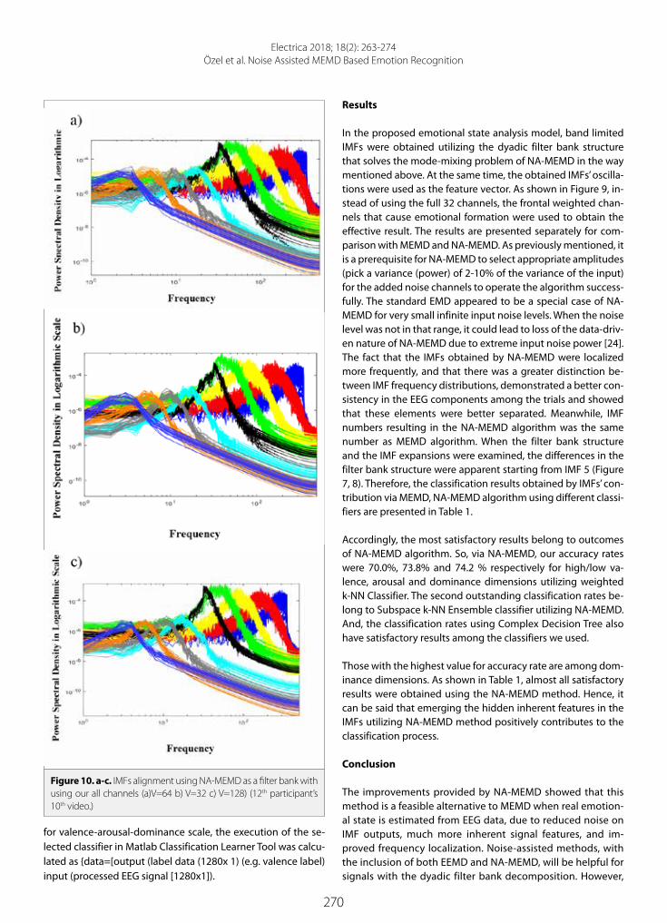
270


for valence-arousal-dominance scale, the execution of the se-lected classifier in Matlab Classification Learner Tool was calcu-lated as data=[output (label data (1280x 1) (e.g. valence label) input (processed EEG signal [1280x1]).

Results

In the proposed emotional state analysis model, band limited IMFs were obtained utilizing the dyadic filter bank structure that solves the mode-mixing problem of NA-MEMD in the way mentioned above. At the same time, the obtained IMFs’ oscilla-tions were used as the feature vector. As shown in Figure 9, in-stead of using the full 32 channels, the frontal weighted chan-nels that cause emotional formation were used to obtain the effective result. The results are presented separately for com-parison with MEMD and NA-MEMD. As previously mentioned, it is a prerequisite for NA-MEMD to select appropriate amplitudes (pick a variance (power) of 2-10% of the variance of the input) for the added noise channels to operate the algorithm success-fully. The standard EMD appeared to be a special case of NA-MEMD for very small infinite input noise levels. When the noise level was not in that range, it could lead to loss of the data-driv-en nature of NA-MEMD due to extreme input noise power [24]. The fact that the IMFs obtained by NA-MEMD were localized more frequently, and that there was a greater distinction be-tween IMF frequency distributions, demonstrated a better con-sistency in the EEG components among the trials and showed that these elements were better separated. Meanwhile, IMF numbers resulting in the NA-MEMD algorithm was the same number as MEMD algorithm. When the filter bank structure and the IMF expansions were examined, the differences in the filter bank structure were apparent starting from IMF 5 (Figure 7, 8). Therefore, the classification results obtained by IMFs’ con-tribution via MEMD, NA-MEMD algorithm using different classi-fiers are presented in Table 1.

Accordingly, the most satisfactory results belong to outcomes of NA-MEMD algorithm. So, via NA-MEMD, our accuracy rates were 70.0%, 73.8% and 74.2 % respectively for high/low va-lence, arousal and dominance dimensions utilizing weighted k-NN Classifier. The second outstanding classification rates be-long to Subspace k-NN Ensemble classifier utilizing NA-MEMD. And, the classification rates using Complex Decision Tree also have satisfactory results among the classifiers we used.

Those with the highest value for accuracy rate are among dom-inance dimensions. As shown in Table 1, almost all satisfactory results were obtained using the NA-MEMD method. Hence, it can be said that emerging the hidden inherent features in the IMFs utilizing NA-MEMD method positively contributes to the classification process.

Conclusion

The improvements provided by NA-MEMD showed that this method is a feasible alternative to MEMD when real emotion-al state is estimated from EEG data, due to reduced noise on IMF outputs, much more inherent signal features, and im-proved frequency localization. Noise-assisted methods, with the inclusion of both EEMD and NA-MEMD, will be helpful for signals with the dyadic filter bank decomposition. However,

Figure 10. a-c. IMFs alignment using NA-MEMD as a filter bank with using our all channels (a)V=64 b) V=32 c) V=128) (12th participant’s 10th video.)

271


if the desired signal is in multiple sub-bands, selecting noise-based methods for analysis can “spread” the desired signal to multiple IMFs, causing undesirable mode mixing. In such cases, the implementation of a dyadic filter bank structure in the input signal can decrease the inherent data adaptive ca-pability of EMD-based algorithms. Therefore, it is very crucial to choose the noise variance according to the input data. Our analysis also shows that the ideal noise levels for NA-MEMD are within 2-10% of the input data power (variance) [24]. This remark is represented in the simulations for the filter bank property belonging to the 10th participant’s 20th video data (Figure 4-8) and the 12th participant’s 10th video data (Figure 10, 11) in DEAP dataset. The NA-MEMD algorithm gave bet-ter results than the MEMD algorithm in classification results, although there were some uncertainties. In the simulation re-sults shown for the filter bank property in Figure 10, it is seen that choosing direction vector number 128 contributes to more meaningful IMF results. Optimal results were obtained by selecting both the number of direction vector 128 and

using NA-MEMD. The disadvantage of large selection of the number of direction vector is that as the number of direction vector enhances, the time required to decompose the signal also enhances. In the IMF expansions obtained after analyz-ing EEG signals, it is important to note that the method is flex-ible, that the physically meaningful components of the analy-sis result are generated, and that the noisy noise power added to this data supervises the operation of the algorithm. NA-MEMD’s filter bank structures are illustrated in Figure 8, 10; in terms of noise interference and mode mixing, compared with the standard MEMD method. However, the disadvantage of the method is that after finding the variance of all the chan-nels of EEG data the calculation of which is time consuming, adding the process of the variance noise ranging from 2-10% is computationally expensive and must be implemented with caution. To acquire a physically meaningful result from such data sets, all observed variables should be decomposed to the same number as the IMF components at similar scales. In such cases, NA-MEMD application provides great chan-

Table 1. Classification results obtained by IMFs’ contribution via MEMD and NA-MEMD algorithm using Support Vector Machine, Decision Tree, k-Nearest Neighbor and Ensemble Classifier

High-Low Valence Arousal Dominance Method

Support Vector Machine (Fine Gaussian SVM) 60.9% 55.5 % 63.5 % MEMD

Support Vector Machine (Fine Gaussian SVM) 63.1% 56.4% 66.2% NA-MEMD

Decision Tree (Complex Tree) 66.3% 65.0% 69.7% MEMD

Decision Tree (Complex Tree) 68.4% 67.2% 71.9% NA-MEMD

k-Nearest Neighbor (Weighted k-NN) 67.3% 71.6% 72.1% MEMD

k-Nearest Neighbor (Weighted k-NN) 70.0% 73.8% 74.2% NA-MEMD

Ensemble (Subspace k-NN) 66.4% 69.6% 70.0% MEMD

Ensemble (Subspace k-NN) 68.1% 72.3% 72.5% NA-MEMD

Table 2. The comparison of the NA-MEMD based emotion recognition with previous MEMD based studies

Study DatasetEmotion Recognition Accuracy Rates Methods Classifiers

Xu IAPS Positively excited, Negatively excited, Neutral

MEMD-statistical; k-NN(81.39; LDA(59.18) MEMD-NBP;k-NN (82.62);LDA(63.49) MEMD-HOC;k-NN(90.77);LDA(79.64) MEMD-Wavelet;k-NN(77.4);LDA(55,99)

Memd-based features,

k-NN, LDA

Mert and Akan DEAP High-Low Valence High-Low Arousal High-Low Valence High-Low Arousal

67.00±9.60, , k-NN 51.01±15.69, k-NN 72.87±4.68, ANN 75.00±7.48, ANN

Memd-based features, ICA,

k-NN, ANN

Guitton Self-Dataset Happy Relaxed Neutral Fear

MEMD,(SCA -FFA), SVM 72.2- 83.3 77.8-66.7 72.2-83.3 66.7 -55.6

Memd-based features, SVM, k-NN LDA

272


nel-based advantages because it provides the same number of IMFs compared to MEMD. NA-MEMD method is better but the fact that NA-MEMD is preferred is directly related to the user’s desire to work and to time planning. Nevertheless, the multivariable extensions of the EMD have the advantage of being more practical in handling the multichannel signals than EMD processing of each channel.

Considering MEMD based emotion recognition studies sum-marized in Table 2, our study is significant in that it uses em-bedded oscillations of MEMD within itself, evacuating via NA-MEMD method. We acquired the best results 70.0%, 73.8% and 74.2% respectively for high/low valence, arousal and domi-nance (the mean rate was 72.6%) dimensions utilizing weight-ed k-NN Classifier.

Study MEMD combined with Synchrony Cluster Analysis (SCA), Frequency Flows Analysis (FFA) and the spectrogram and ob-tain the maximum mean rate of 73% utilizing SCA calculated on the IMFs along with a SVM classifier [22]. Moreover, Mert and Akan take out Hjorth’s parameters, entropy, power, PSD, correlation, and asymmetry power difference, power ratios, relative entropy, correlation, coherence of IMFs as features via MEMD and acquired the best results as 75.00±7.48, ANN clas-sification rates for high/low arousal. The presented method differs in that while our study uses and focuses on the inher-ent features during MEMD process. In addition, proposed their method based on MEMD however, they examine separately their feature extraction methods after obtaining IMFs [19, 22]. It is important to note that the choice of EEG channels, IMF selection, dimension reduction methods, the use of different datasets can cause different results.

The computation times necessary for the execution of the MEMD and NA-MEMD approaches with a personal computer were almost 8, and 16 hours respectively for all video record-ings of a participant. So, that utilizing NA-MEMD depends on the researcher’s own preference even if the nature of data is appropriate for NA-MEMD method.

It should be noted that the multivariate signal processing ap-proach is preferred in many applications. In this respect, EEG data are naturally multivariate and form an important link be-tween different channels and multi-variate methods. As a re-sult, for the analysis of multivariate data, the advantages of the NA-MEMD method over MEMD in the field of emotion-state classification are demonstrated using the fundamental issues of standard EMD - frequency localization, noise interference and mode-mixing. In addition, using EEG analysis using NA-MEMD, due to the non-stationary and multichannel structure, the ability to explain the uncertainty over the methods using classic time frequency methods has been uncovered.



Financial Disclosure: This study was supported by İzmir Katip Çelebi University Scientific Research Projects Coordination Unit. Project num-ber: 2017-ÖNAP-MÜMF-0002.

References

1. P. Ekman, W. V. Friesen, M. O’Sullivan, A. Chan, I. Diacoyanni-Tarla-tzis, K. Heider, R. Krause, W. A. LeCompte, T. Pitcairn, P. E. Ricci-Bitti, “Universals and cultural differences in the judgments of facial ex-pressions of emotion”, J Pers Soc Psychol , vol. 53, no. 4, pp. 712-717, 1987

2. I. Bakker, T. V. der Voordt , P. Vink, J. de Boon, “Pleasure, Arousal, Dominance: Mehrabian revisited”, Curr Psychol, vol 33, no. 3, pp. 405-421, 2014.

3. M. Othman, A. Wahab, I. Karim, M. A. Dzulkifli, I. F. T. Alshaiklia, “EEG emotion recognition based on the dimensional models of emo-tions”, Procedia-Social and Behavioral Sciences , vol 97, pp. 30-37, 2013.

4. G. K. Verma, U. S. Tiwary, “Affect representation and recognition in 3D continuous valence-arousal-dominance space”, Multimedya Tools Appl, vol. 76, no. 2, pp. 2159-2183, 2016.

5. Y. Liu, O. Sourina, “EEG Databases for Emotion Recognition”, Inter-national Conference on Cyberworlds, 2013.

6. N. E. Huang, Z. Shen, S. R. Long, M. C. Wu,H. H. Shih, Q. Zheng, N. C. Yen, C. C. Tung, H. H. Liu, “The emprical mode decomposition and the Hilbert spectrum for nonlinear and non-stationary time series anaylsis”, Proc Math Phys Eng Sci, vol. 454, NO. 1971, pp. 903-995, 1998.

7. N. E. Huang, Z. Wu, S. R. Long, K. C. Arnold, X. Chen, K. Blank, “On instantaneous frequency”, Advanced Adaptive Data Anaysis , vol. 1, no. 2, pp. 177-229, 2009.

8. A. Khasnobish, S. Bhattacharyya, G. Singh, A. Jati, A. Konar, D. N. Ti-barewala, R. Janarthanan, “The role of Emprical Mode Decomposıtıon on Emotion Classification Using Stimulated EEG signals”, Advances in Computing and Information Technology , vol. 178, pp. 55-62, 2013.

9. A. Santillan-Guzman, M. Fischer, U. Heute, G. Schmidt, “Real-time Empirical Mode Decomposition for EEG signal enhancement”, 21st European Signal Processing Conference (EUSIPCO 2013), 2013.

10. P. C. Petrantonakis, L. J. Hadjileontiadis, “EEG-based emotion rec-ognition using hybrid filtering and higher order crossings”, 3rd International Conference on Affective Computing and Intelligent Interaction and Workshops, 2009.

Figure 11. IMFs alignment using MEMD as a filter bank (V=128) (12th participant’s 10th video.)

273


11. P. C. Petrantonakis, L. J. Hadjileontiadis, “Emotion Recognition from Brain Signals Using Hybrid Adaptive Filtering and Higher Or-der Crossings Analysis”, IEEE Transactions on Affective Computing, vol. 1, no. 2, pp. 81-97, 2010.

12. P. C. Petrantonakis, L. J. Hadjileontiadis, “Adaptive Emotional In-formation Retrieval From EEG Signals in the Time-Frequency Domain”, IEEE Transactions on Signal Processing, vol. 60, NO. 5, pp. 2604-2616, 2012.

13. C. Shahnaz, S. B. Masud, S. M. S. Hasan, “Emotion recognition based on wavelet analysis of Empirical Mode Decomposed EEG signals responsive to music videos”, IEEE Region 10 Conference (TENCON), 2016.

14. Y. Zhang, X. Ji, S. Zhang, “ An approach to EEG-based emotion recognition using combined feature extraction method”, Neurosci Lett, vol. 633, pp. 152-157, 2016.

15. M. S. Hosseini, A. Pouyan, S. Ferdowsi, H. Mashayekhi,”EEG-Based Emotion Recognition using Deep Belief Network and Empirical Mode Decomposition”, 3rd National Conference on Applied Research in Electrical, Mechanical and Mechatronic, 2015.

16. T. M. Rutkowski, A. Cichocki, A. L. Ralescu, D. P. Mandic, “Emotional States Estimation from Multichannel EEG Maps”, Advances in Cog-nitive Neurodynamics ICCN 2007, 2008, pp. 695-698.

17. V. Bajaj, R. B. Pachori, “EEG Signal Classification Using Empirical Mode Decomposition and Support Vector Machine”, International Conference on Soft Computing for Problem Solving, 2011.

18. P. Ozel, A. Akan, B. Yılmaz, “Emotional State Analysis from EEG signals via Noise-Assisted Multivariate Empirical Mode Decom-position Method”, 10th International Conference on Electrical and Electronics Engineering, 2017.

19. H. Xu, “Towards Automated Recognition of Human Emotion using EEG”, Thesis, Toronto, Canada: University of Toronto, 2012.

20. Y. Tonoyan, D. Looney, D. P. Mandic, M. M. Van Hulle, “Discriminat-ing Multiple Emotional States from EEG Using a Data-Adaptive, Multiscale Information-Theoretic Approach”, Int J Neural Syst, vol. 26, no. 2, p. 1650005, 2016.

21. A. Mert, A.Akan, “Emotion recognition from EEG signals by using multivariate empirical mode decomposition”, Pattern Analysis and Applications, vol. 21, no. 1, pp. 81-89, 2016.

22. C. Guitton, “Emotions Estimation from EEG Recordings”, London: Imperial Collage of Science, Technology & Medicine Department of Electrical&Electronic Engineering, 2010.

23. H. T. Wu, P. Flandrin, I. Daubeschies, “One or two frequencies? The Synchrosqueezing Answers”, Advances in Adaptive Data Anaylsis, vol. 3, no. 01n02, pp. 29-39, 2011.

24. N. U. Rehman, C. Park, N. E. Huang, D. P. Mandic, “Emd via Memd:-Multivariate Noise Aided Computation of Standard Emd” Advanc-es in Adaptive Data Analysis, vol. 5, no. 2, p. 1350007, 2013.

25. A. Ahrabian, D. Looney, F. A. Tobar, J. Hallatt, D. P. Mandic, “Noise Assisted Multivariate Empirical Mode Decomposition Applied to Doppler Radar Data”, Sensor Signal Processing for Defence (SSPD 2012), 2012.

26. Q. S. She, Y. L. Ma, M. Meng, X. G. Xi, Z. Z. Luo, “Noise-assisted MEMD based relevant IMFs identification and EEG classification”, Journal of Central South University , vol. 24, no. 3, p. 599-608, 2017.

27. J. Alegre-Cortés, S. Sánchez, A. G. Pizá, A. L. Albarracín, F. D. Farfán, C. J. Felice, E. Fernández, “Time-frequency analysis of neuronal

populations with instantaneous resolution based on noise-assist-ed multivariate empirical mode decomposition”, J Neuroscie Meth-ods, vol. 267, pp. 35-44, 2016.

28. D. Cho, B. Min, J. Kim, B. Lee, “EEG-based Prediction of Epileptic Seizures Using Phase Synchronization Elicited from Noise-Assist-ed Multivariate Empirical Mode Decomposition”, IEEE Transs Neu-ral Syst Rehabil Eng, vol. 25, no. 8, pp. 1309-1318, 2017.

29. Lin,C.S, Tanumihardja, W.A., Shih,H.H., “Lung-heart sound separa-tion using noise assisted multivariate empirical mode decompo-sition”, International Symposium on Intelligent Signal Processing and Communication Systems, 2013.

30. Y. Zhang, P. Xu, P. Li, K. Duan, Y. Wen, Q. Yang, T. Zhang, D. Yao, “Noise Assisted Multivariate Empirical Mode Decomposition for Multichannel EMG Signals,” BioMedical Engineering Online, vol. 16, no. 107, pp. 1-17, 2017.

31. S. Sungkono, B. J. Santosa, A. S. Bahri, F. M. Santos, A. Iswahyu-di, “Application of Noise Assisted Multivariate Empirical Mode Decomposition in VLF-EM Data to Identify Underground River”, Advances in Data Science and Adaptive Analysis, vol. 9, no. 1, p. 1650011, 2017.

32. W. Huang, J. Zeng, Z. Wang, J. Liang, “Partial noise assisted multi-variate EMD:An improved noise assisted method for multivariate signals decomposition”, Biomedical Signal Processing and Control, vol. 36, pp. 205-220, 2017.

33. S. Koelstra, C. Muhl, M. Soleymani, J. S. Lee, A. Yazdani, T. Ebrahimi, T. Pun, A. Nijholt, I. Patras, “DEAP: A database for emotion analysis; using physiological signals”, IEEE transactions on affective comput-ing, vol. 3, no. 1, pp. 18-31, 2012.

34. N. Rehman, D. P. Mandic, “Multivariate empirical mode decompo-sition”, Proc Math Phys Eng Sci, vol. 466, no. 2117, pp. 1291-1302, 2009.

35. P. Flandrin, P. Gonçalves, G. Rilling, “EMD equivalent filter banks, from interpetation”, Hilbert-Huang Transform and Its Applications, Singapore , World Scientific, 2005, pp. 67-87.

36. Z. Wu, N. E. Huang, “Ensemble Emprical Mode Decomposition : A Noise Assisted Data Analysis Method”, Advances in Adaptive Data Analysis, vol. 1, no. 1, pp. 1-41, 2009.

37. M. E. Torres, M. A. Colominas, G. Schlotthauer, P. Flandrin, “A com-plete ensemble empirical mode decomposition with adaptive noise”, IEEE International Conference on Acoustics, Speech and Signal Processing (ICASSP) Prague, 2011.

38. J. R. Yeh, J. S. Shieh, N. E. Huang, “Complementary ensemble em-pirical mode”, Advanced Adaptive Data Anaylsis, vol. 2, no. 2, pp. 135-156, 2010.

39. Hao, H., Wang, H., Rehman, N.U., Tian, H., “A Study of the Charac-teristics of MEMD for Fractional Gaussian Noise” IEICE Transactions on Fundamentals of Electronics, Communications and Computer Sciences, vol E99.A, no. 6, pp. 1228-1232, 2016.

40. S. Ge, Y. H. Shi, R. M. Wang, P. Lin, J. F. Gao, G. P. Sun, K. Iramina, Y. K. Yang, Y. Leng, H. Wang, W. Zheng, “Sinusoidal Signal Assisted Multivariate Empirical Mode Decomposition for Brain-Computer Interfaces”, IEEE Journal of Biomedical and Health Informatics , 2017.

41. N. ur Rehman, D. P. Mandic, “Filter bank property of multivariate empirical mode decomposition”, IEEE transactions on signal pro-cessing, vol. 59, no. 5 , pp. 2421-2426., 2011.

274

Pınar Özel received her BS degree in 2007 in Erciyes University and MS degree in 2011 from Bogazici Universi-ty. She started her PhD studies in 2013 in Istanbul University and she’s continuing her studies. As professional experience, she worked as a product manager. Her research areas are signal processing, techniques to bio-medical signals.

Aydın Akan received the B.Sc. degree from the University of Uludag, Bursa, in 1988, the M.Sc. degree from the Technical University of Istanbul, Istanbul, Turkey in 1991, and the Ph.D. degree from the University of Pittsburgh, Pittsburgh, PA, USA, in 1996, all in electrical engineering. He was with the Department of Electrical and Electronics Engineering, University of Istanbul, between 1996 and 2017. He is currently a Professor at the Department of Biomedical Engineering, Izmir Katip Celebi University, Izmir, Turkey. His current research inter-ests include nonstationary signal processing, time-frequency signal analysis methods and their applications to wireless communications and biomedical engineering. He is a senior member of the IEEE Signal Processing Society and an Associate Editor of the Digital Signal Processing Journal.

Bülent Yılmaz received his BS and MS degrees in Electrical-Electronics Engineering from the Middle East Tech-nical University, Ankara, in 1997 and 1999. He obtained his PhD degree from the Bioengineering Department of the University of Utah, Salt Lake City, Utah. He has been working as a faculty member since 2011 in Abdul-lah Gül University, Department of Electrical-Electronics Engineering, Kayseri. His current research interests include biomedical signal and image processing applications on brain-computer interfaces, texture analysis on colonoscopic and PET/CT images.


275

Introduction

The load profiles in conventional networks can be estimated from the database of the distri-bution system, while those in smart networks can be obtained directly on time from the smart systems. Estimated load profiles in conventional distribution networks help electrical com-panies in many fields through such assistance as covering the energy demands of consum-ers, taking on economic and management decisions, and improving the performance of net-works, among others. Many studies were carried out to determine the model of load profiles; the analytical model for determining uncertainty in distribution loads presented in depends on the calculation of mean and variance of the loading profile in each distribution transformer [1]. Daily load profiles for all load types carried out in are modeled depending on the mean, the standard deviation, and the normal distribution of load profiles [2]. The daily load profile in different seasons were also studied in [3]. Previous studies on load profiles needed to find the mean and standard deviation in constructing a load profile model. The proposed load profile model in this paper consists of a small amount of load data; the type of demands and their av-erage values, the minimum and maximum limitations, and the probability of load distribution between the given limitations.

The estimation of active and reactive power loss in distribution systems is one of the main goals for any electric utility company. For example, a reduction of real power loss increases the performance of distribution networks and decreases their financial costs. Additionally, a reduction of reactive power loss reduces decreased voltage and reactive power consumption, while improving the load ability of networks [4]. Subsequently, many equations which depend on generated or consumed power have been proposed to calculate the power loss in trans-mission and distribution systems, such as: Kron’s loss equation, the Branch power loss equa-tion, and Elgerd’s loss equation [5-7]. These equations were used in the calculation of power loss in the electrical system, the economic dispatch analysis, and in determining the optimal size and location of distributed generators or capacitors in primary distribution networks [4-6, 8, 9-12]. These equations relate to single values of power (load, generation, or injections pow-

Electrica 2018; 18(2): 275-283

RESEARCH ARTICLE

Load Profile-Based Power Loss Estimation for Distribution NetworksNassim Iqteit , Ayşen Basa Arsoy , Bekir Çakır Department of Electrical Engineering, Kocaeli University School of Engineering, Kocaeli, Turkey

Corresponding Author: Nassim Iqteit





DOI: 10.26650/electrica.2018.02248

Cite this article as: N. Iqteit, A. Basa Arsoy, B. Çakır, “Load Profile-Based Power Loss Estimation for Distribution Networks”, Electrica, vol. 18, no: 2, pp. 275-283, 2018.

ABSTRACT

In this paper, simple approximate formulas are established to estimate active and reactive power losses in distribution networks. The developed formulas based on load profiles are derived from Elgerd’s power loss formulas. A simple model is also proposed to estimate the load profile while considering several parameters, such as the average load demand and the load limitations. Derivation of the load model and the loss formulas are presented along with their applications on two distribution networks. The results show that the loss formulas, which depend on the proposed load profile, can estimate the power losses in distribution networks with high precision.

Keywords: load profile model; power losses; distribution network; distribution generator

https://orcid.org/0000-0002-2444-6600

https://orcid.org/0000-0002-5729-0366

https://orcid.org/0000-0002-9238-8107

276

Electrica 2018; 18(2): 275-283Iqteit et al. Power Loss Estimation in Distribution Networks

er), but they do not have load profile functions with time (i.e. daily, monthly or yearly load profiles) in order to calculate the average power losses in electrical networks. This paper, along with the article in [13], presents the full derivation of simple ap-proximation power loss formulas to estimate active and reac-tive power loss, taking load profiles into account. Additionally, the validity of these formulas is examined in this article by two distribution systems.

This article sheds light on: a simple model of load profiles and power loss formulas based on load demand profiles, modified power flow equations based on power profiles, an algorithm to find active and reactive power loss profiles, and applications on 13 and 69 bus distribution test systems and their simulation results. Finally, the article summarizes the contributions and conclusions of this work.

Simple Approximated Model of Load Profiles

The profiles of residential, commercial, and industrial load de-mands were modeled through field measurements and statis-tical study [2]. The daily load profiles of P (t) or Q (t) at specific probability can be obtained using normal distribution, where the Equation (1) is the general daily load profile.

(1)

where: XG (t) : general daily load profile, μ(t) : the mean curve of certain consumer, σ(t): the standard deviation curve of a cer-tain consumer based on daily load curves, and κ1: the Gaussian distribution value at specific probability Pr(%). For example, κ1=1.3 at Pr =90% and κ1 = 1.65, Pr = 95%. The following pro-posed procedures present a simple and approximated model of daily load profile, and depend upon a small amount of load data:

- According to Equation (1), if the σ(t) = 0, the daily load curve is equal to the mean curve. Under this condition, the daily load profile can be defined as XG (t) = μ(t) = μpu (t) × average μ(t). At zero standard deviation, we can assume μpu (t) is the general behavior of residential, commercial, or industrial load profiles in a per unit system where

(2).

- The per-unit mean residential, commercial, and industrial profiles were obtained through the results of [2], where the area under each curve is equal to one. Figure 1 shows the per unit mean profiles of residential, commercial, and industrial load demands.

- Approximated load profiles can be derived which are based on the values of average and minimum-maximum limits of load demands, as shown below:

(3)

where

(4)

where (5)

E(Xr) = μ is the mean value of Xr . Xr is the random variable in the set x1,x2,…,xNd. The subset xmax(t), μ(t), xmin(t) represents the maximum deviation in the set of Xr. This subset can be used to find out the approximate value of the λ ratio. The approximate value of λ is shown in Equation (6):

(6)

Figure 2 clarifies the relationship between the maximum, min-imum, and mean functions of general load demands and their average values. Replacing the average values of these func-tions instead of those of the general load functions is the sec-ond approximation that can be used to simplify the calculation of the λ ratio where the symbol is the average of x (t). Equation (7) represents the approximate value of λ, based on the range of load limits:

(7)

Now Equation (1) can be reformulated based on the approxi-mate value of λ as shown in Equation (8). Table 1 displays three numerical examples and the comparison between exact and approximated values of the λ ratio, and profile values of XG.

Figure 1. The per unit mean load profiles based on:(*) the measurement data [2](**) 5th order polynomial function of curves in (*)(***)10th order polynomial function of curves in (*)

277


(8)

Power Loss

Exact Power Loss Formulas

The total active and reactive power lost in a distribution net-work with N buses can be calculated by Elgerd’s Equations (9) and (10), respectively [4]. The equations show the power loss depending on the active and reactive power injections,

(9)

(10)

where

and α = [αij], β = [βij], γ = [γij] and ξ = [ξij]. While the size of matrices α, β, γ and ξ is N×N, the coefficients αij, βij, γij and ξij are functions of the magnitude and angle of phasor voltage. Also, αij and βij depend on the resistive entries rij of the impedance matrix [Zij], while γij and ξij depend on the reactance entries xij. Pi and Pj are the active power injections of buses i and j, respectively; Qi and Qj are the reactive power injections of buses i and j, respective-ly, where the power injection is the difference between the power generations and load demands for the same bus.

Power Loss Formulas Based on Load Profiles

Figure 3 displays the change of the power injections on the nodes of a distribution network at each moment of time. The distribution system was assumed perfectly balanced in the three-phase system. The load profiles and the line segments were supposed to be perfectly balanced as well. The line im-pedance of each segment was consistent with the time, but the state variables (Vi (t) and δi (t)) were not consistent because they depend on the power demands.

Linearization Principle and Average Integral of Power Profiles

A linearization technique and an additive property of integrals were used to derive a simple power loss equation based on power profiles. Profiles of active and reactive load demands, power injections, and power loss are nonlinear functions with time variables. Additionally, active and reactive power loss re-lations are nonlinear with profiles of active and reactive pow-er injections. Figure 4 shows a general nonlinear function X(t), where X(t) could represent the power profiles of load demands (PDi (t), QDi (t)), power generations (PGi (t), QGi (t)), power injections (Pi (t), Qi (t)) at node i, or power loss (PLT (t), QLT (t)).

Through one period T the function X (t) is divided by M regu-lar intervals with a length of ∆t for each one. The length of the regular interval depends on the power measurement devices (smart, digital, or conventional meters) or the accura-

Figure 2. Maximum, minimum, and mean functions of the gener-al load demand based on random subset of Xr(m)

Figure 3. Load profiles on a distribution network

Table 1. Examples compare between exact and approximate values of load profiles at specific times.

Profile of set Xr at time m Subset of Xr

λ ratio The value of profile XG

Exact Appx Exact Appx

0.9, 1.075, 1.1, 0.95, 0.9, 1, 0.97, 0.94, 1.085, 0.96 1.1, 0.9, 0.988 Range ≈ ±10% 1.00512 1.00675 1.080 1.094

0.8, 1.25, 0.75, 0.7, 1.3, 1, 1.1, 1.2, 1.15, 0.85 1.3, 0.7, 1.01 Range ≈ ±30% 1.04304 1.05962 1.282 1.331

1.4, 1.3, 0.55, 0.7, 1.49, 1, 0.51, 0.86, 1.39, 0.86 1.49, 0.51, 1.006 Range ≈ ±50% 1.11992 1.15944 1.459 1.528

278


cy of analysis. X(t) was considered approximate linear function through each interval m, where Xm(t) is the linear approxima-tion of X(t) over interval m. Xm_avi is the average integral value of Xm(t) through time ∆t. Xm is the weight of the average integral value of X(t) in interval m.

The following relations were obtained by using Figure 4:- The length of the regular interval m is and the end-

ings of this interval are and , where m= 1, 2,…, M.- If X(t) is assumed a linear function along interval m, then

the values of Xm_avi and Xm can be approximated by Equa-tion (11).

(11)

- The average integral of X(t) through the period T is approx-imated in Equation (12)

(12)

Approximated Power Loss Formulas Based on Load Profiles

According to Equation (11), over interval m the average inte-gral of the power injection profile (Pi (t), Qi (t), Pj (t) or Qj (t)) can be represented by single point and constant value at time

. Dependent on approximated values of power injection profiles, the active power loss profile for each interval m was derived in the following equation:

(13)

Similarly, the reactive power profile for each interval m can be calculated using Equation (13) only by replacing γm and ξm in-stead of αm and βm, respectively.

According to Equations (12) and (13), the average approxima-tion of active and reactive power loss based on load profiles is obtained using Equations (14) and (15), respectively

(14)

(15)

where

where the size of matrices αm, βm, γm and ξm is N×N. The coef-ficients αmij , βmij , γmij and ξmij are calculated for each interval m,

where

(16a)

(16b)

(16c)

(16d)

where

Algorithm of Power Loss Estimation

The coefficients αmij, βmij, γmij, and ξmij are calculated for each in-terval m. Power flow equations in reference [5] were revised to include the state variables and power injections at each value of m, where the state variables Vmi and δmi can be calculated by solving the modified power flow equations (17) and (18). Numerical methods such as the Newton-Raphson method are used to solve equations (17) and (18). The power injections Pmi and Qmi are calculated by Equation (11).

(17)

Figure 4. Linearization principle of the general nonlinear function X(t)

279


(18)

where Ymij is the entry of admittance matrix at values of m, i, and j. Figure 5 represents an algorithm to find the profiles and the total average of active and reactive power loss.

Applied Examples

The 13 Bus System

A test system in [13] having 18MVA and 12.5kV specifications is shown in Figure 6. This system load data is given in Table 2. The base power of this network is 10 MVA at 12.5kV.

The 69 Bus System

The 69 bus distribution system (IEEE test system) displayed in Figure 7 has a total active load of 3.8021 MW and a total reac-tive load of 2.6945 MVAr. The system data information is given in reference [14]. The base power of this system is 100MVA at 12.66kV. The proposed loss formulas and estimated load model were tested on this system while two wind DGs and one pho-tovoltaic DG were used. The location and ratings of these DGs are given in Table 3. Also, the generation profiles of the DGs are given in reference [9].

Simulation Results and Discussion

The proposed load profile model has been used to estimate the load profiles at each node of the 13 and 69 bus systems. The type of load, the minimum and maximum limitations, and the probability of load distribution as tabulated in Table 2 were considered, along with the mean load value to estimate each load profile at each node of the 13 bus system. The load pro-files and DGs of the 69 bus system were estimated by using the type of loads and DGs with their mean values. It’s clear that the factor λ was assumed equal to one in this system.

Simulation Results of the 13 Bus System

Figure 8 shows the estimated active and reactive load profiles of the 13 bus system at each node of the network. Table 4 shows the average values of load profiles displayed in Figure 8. The

Figure 5. Algorithm to find active and reactive power loss using sim-ple formulas

Table 2. Load data of a 13 bus radial distribution network

BUS P (pu) Q (pu)Range ± R%

Probability (Pr%) Type of load

1 0 0 - - -

2 0 0 - - -

3 0.3045 0.1828 5 90 R

4 0.4059 0.2435 30 90 R

5 3.0351 2.2519 15 90 80%R+20%I

6 0.7060 0.4353 10 90 C

7 1.0509 0.7006 20 90 I

8 1.0631 0.6571 10 90 R

9 0.4578 0.2861 13 90 C

10 0.8299 0.5532 15 90 R

11 0.4450 0.2966 50 90 75%R+25%C

12 1.0580 0.6172 20 90 R

13 0.3046 0.1521 5 90 R

R: Residential C : Commercial I: Industrial

280


effects of limitations on load profiles can be noted by compar-ing the values of P and Q in Tables 2, 4. The estimated load pro-files increase by an increasing mean of load demand, a range of load limitations, and a probability factor of κ1.

The algorithm for power loss calculations is achieved using MATLAB. Table 5 includes the results of the average power loss of the 13 node radial distribution network. The results were

estimated using the load profile and their average and maxi-mum values. Table 5 confirms that the results of the power loss equations are very close to the results of the power lost when it is directly calculated by power flow programs. The power loss values are different when using single values’ average/maxi-mum demand and power profiles because the power loss of

Figure 8. Active and Reactive load profiles of a 13 bus radial dis-tribution network

Figure 9. Comparison between the power loss profiles of the 13 bus system using the discrete load model versus the 5th order polynomial load model

Figure 7. The 69 bus radial distribution network

Figure 6. The 13 bus radial distribution network

Table 3. The rating and location of DGs in the 69 bus system

DG type Wind wind PV

Location (bus No.) 17 27 61

Size (MVA) 0.559 0.613 1.7

Power factor 0.894 0.898 0

Table 4. Average values of the proposed load profile model

bus P proposed model (pu) Q proposed model (pu)

1 0 0

2 0 0

3 0.3207 0.1925

4 0.5346 0.3207

5 3.5194 2.6112

6 0.7815 0.4818

7 1.2750 0.8500

8 1.1761 0.7270

9 0.5210 0.3256

10 0.9623 0.6415

11 0.6812 0.4541

12 1.2830 0.7484

13 0.3207 0.1601

281


the network is a nonlinear function of load profiles. For exam-ple, the active power loss based on the load profiles is equal to 0.0407pu, but when based on the average values of these load profiles it is equal to 0.03453pu. The active power loss based on maximum values of the load profiles is equal to 0.1466pu. The calculation of active power loss using Equation (14) is more accurate and effective than using Equation (9); likewise, the method of calculating reactive power loss using Equation (15) is more accurate and effective than using Equation (10).

According to the computed loss profiles, the maximum active and reactive power losses are 0.11pu and 0.19pu, respectively at 20:00. Figure 9 shows the real power loss profiles based on two types of load models: 1) a discrete load model as shown in Figure 1(*) and 2) the 5th order polynomials load model as shown in Figure 1 (**). The average active power loss in dis-crete mode is 0.04070pu, whereas in the polynomial model it is 0.040707pu. These are almost the same.

Simulation Results of the 69 Bus System

The estimated active and reactive load profiles of the 69 bus system at each node of the network are illustrated in Figure 10.

The estimated load profiles increase by increasing their mean values. This figure also clarifies that the 69 bus system load is an industrial network.

The active and reactive power losses of the 69 bus system using average/maximum demands, and using load profiles as shown in Figure 10, are represented in Table 6. Additionally, the esti-mated losses based on the load profiles using Equations (14) and (15) are more precise than the load profiles using Equa-tions (9) and (10), respectively. As can be seen by Table 6, the total system loss after integrating DGs into the system, is lower than the total loss of the system without DG.

According to the calculated loss profiles, the maximum active power loss is 0.003671pu at 13:00. Whereas the maximum re-active loss is 0.001689pu at 9:00. Figure 11 illustrates the real power loss profiles based on the discrete load model and the 10th order polynomials load model as shown in Figure 1(***).

Figure 10. Active and Reactive load profiles of a 69 bus radial dis-tribution network

Figure 11. Comparison between the power loss profiles of the 69 bus system using the discrete load model versus the 10th order polynomial load model

Table 5. Power losses in the 13 bus radial distribution network

Calculations based on

Active/Reactive

losses formula

Power flow calculation

Maximum load demands

P(pu) 0.14660 0.14660

Q(pu) 0.26761 0.26762

Average load demands

P(pu) 0.03452 0.03453

Q(pu) 0.06502 0.06561

Load power profiles

P(pu) 0.04070 0.04070

Q(pu) 0.07622 0.07615

Table 6. Power losses in a 69 bus radial distribution network with two wind DGs and one PV DG

Calculations based on

Active/Reactive

loss formula

Power flow calculation

Maximum load demands

P(pu) 0.004111 0.004111

Q(pu) 0.001905 0.001905

Average load demands

P(pu) 0.000738 0.000738

Q(pu) 0.000343 0.000344

Load power profilesP(pu) 0.001566 0.001566

Q(pu) 0.000719 0.000718

The losses of the system without DG based on load profiles are:

Ploss= 0.004463pu Qloss= 0.002009pu

282


The average active power losses computed for both models are 0.001566pu and 0.001540pu, respectively.

Conclusion

This paper presents approximate formulas to estimate the ac-tive and reactive power loss in distribution networks based on load demand profiles obtained by a simple approximated model. The load profile model and power loss formulas are ex-amined through the 13 and the 69 bus distribution networks. Types, mean, deviation, and the normal distribution factor of load are the main variables that impact the load profile. The developed loss formulas give more precise results when compared to the power loss formula based on the average/maximum load demand. The presented formulas of active and reactive power loss offer the following benefits: Easy to apply, capable of using discrete load profiles, and a simulation of re-sults generating only a small error when using an appropriate number of time intervals. The results show that when DGs are integrated into the distribution network the power loss is di-minished.

The advantage of the simple approximated formulas can be used not only in power loss analysis but also in economic dis-patch analysis and to estimate the optimal setting of distribut-ed generators that can be inserted into distribution networks.



Financial Disclosure: This study was supported by the TUBITAK under project number 114S47.

References

1. D. T. Nguyen, “Modeling Load Uncertainty in Distribution Network Monitoring”, IEEE Trans Power Syst, vol. 30, no. 5, pp. 2321-2328, 2015.

2. J. A. Jardini, C. M. V. Tahan, M. R. Gouvea, S. U. Ahn, F. M. Figueiredo, “Daily load profiles for residential, commercial and industrial low voltage consumers”, IEEE Trans Power Delivery, vol. 15, no. 1, pp. 375-380, 2000.

3. E. C. Bobric, G. Cartina, G. Grigoras, “Clustering Techniques in Load Profile Analysis for Distribution Stations”, Adv Electr Comput Eng, vol. 9, no. 1, pp. 63-66, 2009.

4. D. Q. Hung, N. Mithulananthan, “Loss reduction and loadability enhancement with DG: A dual-index analytical approach”, Appl Energ, vol. 115, pp. 233-241, 2014.

5. H. Saadat, “Power Systems Analysis”, PSA Publishing, USA, 2010. 6. C. F. Chang, “Reconfiguration and Capacitor Placement for Loss

Reduction of Distribution Systems by Ant Colony Search Algo-rithm”, IEEE Trans Power Syst, vol. 23, no. 4, pp. 1747-1755, 2008.

7. O. Elgerd, “Electric Energy Systems Theory: An Introduction”, New York: McGraw-Hill, 1971.

8. L. Wang, C. Singh, “Environmental/economic power dispatch us-ing a fuzzified multi-objective particle swarm optimization algo-rithm”, Elec Power Syst Res, vol. 77, no. 12, pp. 1654-1664, 2007.

9. D. Q. Hung, N. Mithulananthan, R. C. Bansal, “Analytical strategies for renewable distributed generation integration considering en-ergy loss minimization”, Appl Energ, vol. 105, pp. 75-85, 2013.

10. D. Q. Hung, N. Mithulananthan, R. Bansal, “Analytical Expressions for DG Allocation in Primary Distribution Networks”, IEEE Trans En-ergy Convers, vol. 25, no. 3, pp. 814-820, 2010.

11. D. Q. Hung, N. Mithulananthan, “Multiple Distributed Generator Placement in Primary Distribution Networks for Loss Reduction”, IEEE Trans Ind Electron, vol. 60, no. 4, pp. 1700-1708, 2013.

12. M. Shahzad, I. Ahmad, W. Gawlik, P. Palensky, “Load Concentration Factor Based Analytical Method for Optimal Placement of Multi-ple Distribution Generators for Loss Minimization and Voltage Profile Improvement”, Energies, vol. 9, no. 4, p. 287, 2016.

13. N. A. Iqteit, A. B. Arsoy, B. Çakir, “A Simple Method to Estimate Pow-er Losses in Distribution Networks”, 10th International Conference on Electrical and Electronics Engineering (ELECO), 2017, pp 135-140.

14. N. Mohandas, R. Balamurugan, L. Lakshminarasimman, “Optimal location and sizing of real power DG units to improve the voltage stability in the distribution system using ABC algorithm united with chaos”, Int J Elec Power Energ Syst, vol. 66, pp. 41-52, 2015.

283


Ayşen BASA ARSOY received her B.Sc. degree from Istanbul Technical University, Turkey, in 1992, an M.S de-gree from the University of Missouri-Rolla in 1996, and a PhD from Virginia Polytechnic Institute and State University in 2000, all in electrical Engineering. She is currently an Associate Professor at Kocaeli University in Turkey. Her research interests include power system modeling and analysis, power system protection, distrib-uted generation, energy storage, and power electronics applications in Power Systems.

Bekir Çakır received his B.Sc. and M.Sc. degrees from Berlin Technical University, Germany, in 1986 and 1990, respectively, and his PhDs from Yıldız Technical University as well as Kocaeli University, Turkey 1995. In 1991, he joined Kocaeli University’s Engineering Faculty as a Research Assistant. He was first Assistant Professor, then Associate Professor at Kocaeli University, 1995 and 2002, respectively. Since 2006, he has been a Profes-sor in the Engineering Faculty, Kocaeli University. His research interests are embedded system design, power electronic driver circuits, renewable energy production systems, and smart grids.

Nassim Ahmad IQTEIT received his B.Sc. in Industrial Automation Engineering from Palestine Polytechnic Uni-versity (PPU), Palestine, in 2006 and his M.S. degree in Electric Power Engineering from Yarmouk University, Jordan, in 2011. Currently, he is a PhD candidate in Electrical Power Engineering in Kocaeli University, Kocaeli, Turkey. He worked in the Electrical Engineering Department at PPU. His research interests include SEIG mod-eling, applications of DGs, and distribution system modeling.

284

Introduction P53 gene regulatory network responds to Double Strand Breaks (the most deleterious type of DNA damage) by regulating the necessary biological processes such as DNA repair, cell cycle arrest (i.e. the cell stops growing to avoid passing the damaged DNA to baby cells) and apop-tosis (i.e. programmed cell death) [1]. Experiments show that these processes are associated with different dynamical modes of p53 concentration level. More specifically:

i) Low level of p53 indicates that there is no DNA damage in the cell so the cell can continue its normal cell cycle progression [2]. In other words, the cell may eventually proliferate since there is no DNA damage.

ii) Oscillation of p53 level is the indicator of DSBs in DNA [3-6]. It has been shown that oscil-lation of p53 level helps to repair DSBs and also causes cell cycle arrest [7]. The oscillation of p53 lasts until the DSBs are repaired, and goes to low level after the repair. However, if the repair takes too long, then the dynamical mode of p53 switches from the oscillation to a high level [8].

iii) High level of p53 triggers apoptosis, thus removing the irreparable cell from the organism [9-11].

To regulate the response to DSBs, there are three different dynamical modes (low level equilib-rium, oscillations, and high level equilibrium) and three critical mode transitions. The first tran-sition is from low level to oscillations upon the formation of DSBs; the second transition is from oscillations to low level upon the repair of DSBs; and the third transition is from oscillations to high level if the repair takes too long. According to discussions in the literature, there is no direct transition from low level to high level of p53. In other words, p53 level goes to high level

Electrica 2018; 18(2): 284-291

RESEARCH ARTICLE

A Canonical 3-D P53 Network Model that Determines Cell Fate by Counting PulsesGökhan Demirkıran1 , Güleser Kalaycı Demir2 , Cüneyt Güzeliş1 1Department of Electrical and Electronics Engineering, Yaşar University School of Engineering, İzmir, Turkey 2Department of Electrical and Electronics Engineering, Dokuz Eylül University School of Engineering, İzmir, Turkey

Corresponding Author: Gökhan Demirkıran





DOI: 10.26650/electrica.2018.02664

Cite this article as: G. Demirkıran, G. Kalaycı Demir, C. Güzeliş, “A Canonical 3-D P53 Network Model that Determines Cell Fate by Counting Pulses”, Electrica, vol. 18, no: 2, pp. 284-291, 2018.

ABSTRACT

From a system theory perspective, p53 network dynamics is interesting since it can exhibit three dynamical modes of p53, namely low-level equilibrium, oscillation, and high-level equilibrium. Each of these modes are associated with different cell fate outcomes: cell survival, cell cycle arrest, and apoptosis. The literature reveals that a high level (apoptosis) is seen only after ending the oscillation phase, so called two-phase dynamics, which provides the decision of apoptosis depending on the oscillation duration. This paper proposes that a negative feedback can keep time by counting the pulses of oscillation to take the decision of apoptosis or cell survival. P53DINP1, which is the mediator of this feedback, is added as a variable to a 2-D oscillator model of the p53 network. The resulting canonical 3-D model successfully replicates the two-phase dynamics. That is, it possesses temporary oscillatory behavior, in which first oscillations (first phase) and then high level state (second phase) are observed. By introducing a new variable to the core oscillator in the p53 network, this study demonstrates that p53 network can be considered a modular structure, which consists of an oscillator and other variables that control this oscillator to contribute to cell fate determination.

Keywords: Oscillators, p53 network, two-phase dynamics, gene regulatory networks, cell fate, P53DINP1

https://orcid.org/0000-0002-0076-6036

https://orcid.org/0000-0003-3808-5305

https://orcid.org/0000-0001-5416-368X

285

Electrica 2018; 18(2): 284-291Demirkıran et al. A Canonical 3-D P53 Network Model that Determines Cell Fate by Counting Pulses

only after an oscillatory phase. This mechanism is considered to be useful due to the fact that it will try to repair DNA damage giving the cell a chance of surviving before taking the decision of apoptosis [3, 8]. In the literature several oscillator models have been proposed based on ATM inhibition of p53 inhibitor Mdm2 [3, 6]. Models based on the feedback loop interaction between ATM and Wip1 dynamics have also been proposed in keeping with experimental studies demonstrating that coact-ion of ATM and Wip1 is crucial in the regulation of cell cycle checkpoints and apoptosis [6, 12-15].

Although oscillatory dynamics of p53 alone have been stud-ied extensively, the study of three dynamical modes of p53 in the same model is restricted to only a few studies [16]. The study in [17] proposes a model that exhibits these modes in a two-phase dynamics fashion in which the high level of p53 (the second phase) is observed only after the oscillation of p53 (the first phase). In the model by [17], the duration of DSB repair activity determines if there will be a mode transition from the oscillations to high level of p53. In this sense, the model of [17] understands the duration of DSB repair activ-ity by a pulse counting mechanism which counts the pulses of oscillation. If the number of pulses passes a certain value while the repairing process continues, then the decision of apoptosis is made. If the DSBs are repaired before a certain number of pulses are exhibited, then p53 goes to low level and the cell survives.

Although the model by successfully shows these three dis-tinct modes, the intuitive understanding of the model is very hard since the model is 17 dimensional and has too many tuned parameters [17]. Recently, Demirkıran et al. [18] suc-cessfully reduced the two-phase dynamics model by into a 2-dimensional model with rational terms, which is capable of showing these three distinct modes when the critical pa-rameters of the model are changed externally [17, 18]. The reduced 2-D model is shown to be a relaxation oscillator model which enhances the understanding of oscillations as well making corrections on the interpretation of the original 17-D model [19].

Although the reduced 2-D model with rational terms has pro-vided a greater depth of understanding, the terms of the mod-el are too complex [19]. Thus, Demirkıran et al. [18] proposed a simple canonical 2-D model of polynomial type, whose pa-rameters are interpreted from p53 network interactions [20]. This simple canonical 2-D model is also capable of exhibiting 3 distinct modes when the critical parameters of the model are changed externally in the solver algorithm. In the study pre-sented by this paper, we have extended the model in [20] by introducing new variables that automatically manipulate those critical parameters, so that a response in a two-phase dynam-ics fashion can be obtained. The main goal of this paper is to provide mechanistic insights into the two-phase dynamics and into the pulse counting mechanism. In this regard, our contri-butions in this paper are as follows:

• We propose a simple 3-D model extending the canonical 2-D model in [20], which makes the decision of apoptosis by a pulse counting mechanism.

• The 3-D model which we introduce suggests a new minimal motif as a decision block for gene regulatory networks.

• We show that a simple negative feedback (not necessarily a bistable hysteretic switch) can also cause a switching action, thus suggesting a new Oscillation Accumulation Triggered Genetic Switch (OATGS) mechanism.

The outline of the paper is as follows. In Section 2, we intro-duce the model and how new parameters can be tuned by giving mechanistic insights. In Section 3, we discuss that the introduced model is a new compact motif with the property of coincidence detection. In Section 4, we conclude with an em-phasis on the modular perspective of p53 network. Model Description

The schematic illustration of the interaction between the com-ponents of the model are illustrated in Figure 1. P53DINP1 was introduced as a new component to the ATM*-Wip1 system in [20] to inform ATM*-Wip1 system about the duration of DSB repair activity. The working mechanism of the resulting system is as follows. When there are DSBs in DNA, the repair molecules form complexes with DSBs, so-called DSB-complexes (DSBCs), until the repair finishes. These complexes act as external stimuli that excite the system such that [ATM*] (active ATM level) and [Wip1] oscillate. As [ATM*] oscillates, it promotes the accumu-lation of P53DINP1 protein, which is revealed as an accumu-lating component in two-phase dynamics model in another paper [19]. If DSBCs disappear, meaning that DSBs are repaired, then the ATM level goes down. If DSBCs persist long enough then P53DINP1 accumulates to a certain threshold level that cuts off Wip1 feedback loop as illustrated in Figure 1. Thus, in contrast to the model in [20], the proposed model in this study responds to DSBs in a two-phase dynamics fashion by consid-ering the duration of oscillations via a pulse counting mecha-nism. This is not in keeping with the study conducted in [20] in which the response is obtained by manipulating the parame-ters externally in the solver.

Figure 1. The schematic illustration of the interaction among the model components

286


In the proposed model (Table 1), [ATM*], [Wip1] and [P53DINP1] represent the concentrations of the corresponding proteins. In (1)-(4), ATM protein has auto-activation property modelled by the terms “rd[ATM*]” and a[ATM*]^2. This auto-activation property is responsible for the rapid activation of ATM [21, 22]. The term “–b[ATM*]” is for the self-degradation. The term “–r[ATM*]3” is needed to obtain the bistability property of ATM [21, 23], which can be obtained from a 3rd order polynomial [24, 25] and also stays for the self-degradation of ATM. Wip1 is known to be a strong inhibitor of ATM [12]. Therefore, the term “–c[ATM*][Wip1]” is included to represent the deactiva-tion property of Wip1.

[Wip1] is regulated positively by ATM with the term “mf[P-53DINP1][ATM]” where mf ([P53DINP1]) is a function with pos-itive values as given in (4). Furthermore, [Wip1] feedback loop model (Equation (2) of Table 1) is constructed with the con-stant production term “z”, a self-degradation term “n”, follow-ing the steps of [20] in modelling Wip1 feedback loop. Not in keeping with [20], the constant parameter is replaced by (4) to take P53DINP1 dynamics into account. Also, a new variable [P53DINP1], new parameters ε, b and a new scalar repressor function mf([P53DINP1]) are introduced as detailed below.

The model variables are [ATM*], [Wip1], and [P53DINP1]. Equa-tions (1)-(2) are taken from [20], with one exception, name-ly that the constant parameter m is replaced by the function mf(P53DINP1). The model in [20] was based on the interaction between ATM* and Wip1 isolated from P53DINP1 effect. The model was capable of exhibiting three distinct modes, namely low level equilibrium, oscillations and high level equilibrium. Following a minimalist approach, the model in [20] was de-signed not to have p53 as a variable since ATM is the upstream mediator of p53 and oscillations of p53 result from oscillations

of ATM as detailed in the references [18-20]. Thus, [ATM*] was chosen as the representative variable of p53 network dynam-ics. In our study, we follow the same approach again. Thus, in this minimal approach of modelling p53 network dynamics, p53 is not introduced as a dynamic variable but assumed to follow ATM dynamics.

To model the distraction of Wip1 feedback loop by P53DINP1, mf([P53DINP1]) must be in reverse proportion with the level of [P53DINP1]. Thus, we choose the function as in (4). Although more complex kinetic terms may be introduced, we choose a simple yet effective function that models the repressing effect.

The parameters ε and b determine the accumulation char-acteristics of [P53DINP1] as will be detailed in Section 2.1. In (3), [ATM*] enhances [P53DINP1]. The parameters ε and b are chosen such that [P53DINP1] is enhanced quickly but decays slowly to model its accumulation over oscillations. The param-eter values are a = 5,b = 10,c = 15,d = 70,z=0.5,m=1.25,n = 0.8, ε=0.02, b = 1 and the parameter r is an external stimulus in-dicating the status of DSBC activity. r = 1 means there is a full DSBC activity whilst r = 0 means there is no DSBC activity (i.e. no DSBs in DNA). These values of the parameters will be used throughout the paper unless stated otherwise. The numerical simulation of the model demonstrating the two-phase dynam-ics and accumulation of [P53DINP1] is shown in Figure 2. In the time interval [0, 10], there is no DSBC activity indicated with r = 0. In the interval [10, 20], there is a short duration of DSBC activity which stimulates the oscillations. In the interval [20, 60], there is no DSB so r = 0 and [ATM*] is at low level. In a long time interval of [60, 120], there is DSBC activity. In this interval, oscillations are first observed (in [60, 75]) and after four pulses [ATM*] level goes to a high level indicating apoptosis.

The change in [P53DINP1] can be observed as in Figure 2. It ac-cumulates over oscillations and distracts Wip1 feedback loop when its level passes above a certain threshold level, which is around 1. Thus, [P53DINP1] functions as a switch when its level passes above a certain threshold level.

Tuning the Parameters for P53DINP1

Equation (3) is a simple example of a negative autoregulation observed in gene regulatory networks [26]. The change of [P53DINP1], i.e. derivative, is equal to the difference between its production due to [ATM*] and self-degradation. To investi-gate (3) better with the meaning of parameters ε and b, we take [ATM*] as constant at its two extreme values: the maximum and minimum peaks of the [ATM*] pulses which are around 15 and zero, respectively. In the constant [ATM*] case, the solution to (3) is as below:

(5)

Where SSS = [ATM*]constant/b indicating the steady state value of [P53DINP1], S0 is the initial condition and [ATM*]constant is one of

Table 1. The model equations

287


the two extreme values of [ATM*]. So [ATM*]constant and b deter-mine the steady state of [P53DINP1]. The product of the param-eters ε and b appears as a time constant. Thus, the product εb determines how fast [P53DINP1] will decay. Also, it determines how fast [P53DINP1] will increase. The reason we introduce two parameters ε and b as in (3) is to give the flexibility of control over the steady state and the response time of [P53DINP1] sep-arately when tuning the parameters.

As illustrated in Figure 3, we numerically solve (3) for dif-ferent [ATM*] and ε values with an initial condition of [P53DINP1] = 0 when b = 1. To make our point we assume a hypothetical threshold value of 10. As can be seen, the constant [ATM*] value has effect on the steady state level of [P53DINP1]. This implies that a large [ATM*] may speed up

the reaching of a certain threshold by means of increasing the steady state level of [P53DINP1]. The value of ε directly determines how fast [P53DINP1] will reach the steady state for a fixed b value. Negative Feedback Loop Naturally Accumulates over Oscillations as a Counting Mechanism

An important property of a simple negative feedback loop is that it does not decay from an arbitrary state to an initial con-dition. At the same time, it reaches that arbitrary state if the latter state is smaller than the steady state (Figure 4). To make this point, we have solved the below equation for different ar-bitrary states of Ti.

Figure 2. Demonstration of two-phase dynamics and pulse count-ing mechanism by the proposed 3-D model in Table 1. (Note that a.u. stands for arbitrary unit)

Figure 4. a, b. Time to reach to arbitrary states (a) and time to decay from those arbitrary states to initial condition of zero (b). When [ATM*]is zero, Equation (6) represents a pure decaying problem

Figure 3. [P53DINP1] trajectories of (5) for different [ATM*] and ε values. b = 1

288


Subject to:

(6)

Where

If we look at Figure 4 a, b, it reaches the state of T1 = 30 of [P53DINP1] (which is around 4.5) at 30 hours, however it does not decay to the initial condition of zero at the same time. In fact, there is a large difference. In the case of T4 = 150, the dif-ference between the decay and reach time is smaller since that arbitrary state (T4) is closer to the steady state.

In order to demonstrate this we take [ATM*] as a sine wave and solve the below equation:

where

Figure 5 demonstrates that a negative feedback loop can be used as a counting mechanism. It counts the pulses, and after passing a threshold the target network can change the mode. Herein ε determines how fast [P53DINP1] will move towards the threshold while εb determines how fast it will decay. Since b de-termines the steady state value, with a proper guess we guaran-tee that [P53DINP1] will eventually pass the threshold and with ε we may tune the number of counts until the threshold. A Compact Motif Capable of Exhibiting Two-phase Dynamics

Several motifs have been proposed in the literature, such as os-cillator motifs and switch motifs [26, 27]. These simple motifs are the building blocks of more complex gene regulatory sys-tems. In this paper, we introduce a new motif depicted in Fig-ure 6. It consists of i) a bistable switch (ATM), ii) a fast negative feedback loop (Wip1) responsible for the oscillations together with ATM, and iii) a slow negative feedback loop (P53DINP1) responsible for counting the pulses to give the decision of apoptosis. This compact motif with only essential components models the response mechanism of p53 network to DSBs.

In this compact motif, oscillations occur due to the interaction between bistable switch of ATM and negative feedback of Wip1 upon the stimulus [19]. The high level is observed when P53DINP1 level accumulates above a certain threshold value which distracts the feedback loop of Wip1. In this case, the system is left only with bistable ATM dynamics, thus ATM level switches to high state and stays there (Figure 7). Low level is observed due to the fact that bistable ATM do not receive in-put stimulus thus staying at low level. This notion emphasizes

the importance of ATM characteristics on the formation of re-sponse to DSBs. That is, other variables in the motif control the ATM dynamics. More specifically, i) Wip1 feedback loop allows for oscillations by frustrating bistable ATM [19], ii) P53DINP1 makes ATM switch from oscillations to high level by distracting Wip1 feedback loop (Figure 8), and iii) the extinction of stimu-lus make ATM switch to low level.

The compact motif capable of exhibiting two-phase dynamics is a new one: We have shown that a negative feedback can be used as both a counting mechanism and as a switch. Similar to

Figure 5. Tuning the number of pulses with different ε guaran-teed that b is chosen such that the trajectories will eventually pass the threshold

Figure 6. A compact motif capable of exhibiting two-phase dy-namics

289


our study, a generic OATGS, which is able to exhibit transient oscillations, was studied in [28]. However, our mechanism is substantially different from theirs. For instance, [28] proposed a 7-D model that only allows the transitions from low level equi-librium to oscillation and oscillation to low level equilibrium. That is, as the input stimulus persists for a long time, the oscil-lator causes accumulation of a protein which then shuts off the oscillator to low value. In contrast, in our case, accumulating protein P53DINP1 shuts off the oscillator to a high level if the input stimulus persists for a long time. So, our proposed model, although with lower dimensionality, is richer in dynamics: the proposed model allows for the transitions from low level to os-

cillation, oscillation to low level and oscillation to high levels, which are relevant to two-phase dynamics. Both the schematic diagram from [28] and ours are sketched in Figure 9.

Coincidence Detection

An interesting property of the proposed model is its ability of coincidence detection [26]. Coincidence detection is the phe-nomenon that describes the support from the past signal to the current signal. We re-simulate Figure 2 with more adjacent pulses of DNA damage as given in Figure 10. This time, apopto-sis is observed after 3 pulses as opposed to 4 pulses of [ATM*]. This is due to the simple fact that between time interval 20 and 30 there is not enough time for [P53DINP1] to drop to basal level. So, if new DSBs occur before the cell fully gets rid of the signs of a prior DNA damage, then the cell takes the apoptosis decision earlier than normal. This may give the organism sur-vival advantage, since frequent DNA damage in the cell may be

Figure 7. High level of [ATM*] is observed when Wip1 feedback loop is distracted by [P53DINP1]. Only Equation (1) is solved with [Wip1] as constant of 0.1 and r=1 for different initial conditions of [ATM*]

Figure 8. Equations (1) and (2) are solved for [P53DINP1] = t/12, where t is time. As [P53DINP1] increases with time, the function mf([P53DINP1]) decreases eventually distracting Wip1 feedback loop and apoptosis is initiated

Figure 9. a, b. Schematic diagram of (a); OATGS by [28] and the mo-tif proposed in this paper (b)

Figure 10. Demonstration of the coincidence detection property of the proposed motif

290


a signal for some serious failure in the repair mechanism or in some biological functions. Thus, the cell takes the decision of apoptosis quickly.

Conclusion In our previous studies, we have emphasized the importance of re-considering p53 network as an integrated system consisting of an oscillator and other subsystems that control this oscillator to contribute to cell fate [18-20]. In this direction, this paper has introduced a novel subsystem that informs the duration of the repair activity to p53 network oscillator system to determine cell fate. A negative feedback can provide an accumulating variable which can be used as a pulse counting mechanism to keep the information about the duration of oscillations. The resulting modular system consists of a minimum number of components: two variables for oscillations and one for keeping time. As new findings are revealed from p53 network exper-iments, the proposed mathematical models can be extend-ed and used modularly. Although we investigate the specific case of the count and decide a mechanism for p53 network, the model can be applied to other gene regulatory networks where the decision is based on an accumulating variable.




References

1. F. Murray-Zmijewski, E. A. Slee, X. Lu, “A complex barcode under-lies the heterogeneous response of p53 to stress,” Nat Rev Mol Cell Biol, vol. 9, no. 9, pp. 702-712, 2008.

2. D. Michael, M. Oren, “The p53-Mdm2 module and the ubiquitin system,” Semin Cancer Biol, vol. 13, no. 1, pp. 49-58, 2003.

3. G. Lahav, N. Rosenfeld, A. Sigal, N. Geva-Zatorsky, A. J. Levine, M. B. Elowitz, U. Alon, “Dynamics of the p53-Mdm2 feedback loop in individual cells,” Nat Genet, vol. 36, no. 2, pp. 147-150, 2004.

4. E. Batchelor, A. Loewer, C. Mock, G. Lahav, “Stimulus‐dependent dynamics of p53 in single cells,” Mol Syst Biol, vol. 7, no. 1, p. 488, 2011.

5. E. Batchelor, A. Loewer, G. Lahav, “The ups and downs of p53: Un-derstanding protein dynamics in single cells”, Nat Rev Cancer, vol. 9, no. 5, pp. 371-377, 2009.

6. E. Batchelor, C. S. Mock, I. Bhan, A. Loewer, G. Lahav, “Recurrent initiation: a mechanism for triggering p53 pulses in response to DNA damage”, Mol Cell, vol. 30, no. 3, pp. 277-289, 2008.

7. J. E. Toettcher, A. Loewer, G. J. Ostheimer, M. B. Yaffe, B. Tidor, G. Lahav, “Distinct mechanisms act in concert to mediate cell cycle arrest”, Proc Natl Acad Sci, vol. 106, no. 3, pp. 785-790, 2009.

8. G. Lahav, “The strength of indecisiveness: oscillatory behavior for better cell fate determination”, Send to Sci STKE, vol. 2004, no. 264, pp. pe55, 2004.

9. F. Essmann, I. H. Engels, G. Totzke, K. Schulze-Osthoff, R. U. Jänicke, “Apoptosis resistance of MCF-7 breast carcinoma cells to ionizing

radiation is independent of p53 and cell cycle control but caused by the lack of caspase-3 and a caffeine-inhibitable event”, Cancer Res, vol. 64, no. 19, pp. 7065-7072, 2004.

10. N. D. Marchenko, A. Zaika, U. M. Moll, “Death signal-induced local-ization of p53 protein to mitochondria a potential role in apoptot-ic signaling”, J Biol Chem, vol. 275, no. 21, pp. 16202-16212, 2000.

11. M. Mihara, S. Erster, A. Zaika, O. Petrenko, T. Chittenden, P. Pancos-ka, U. M. Moll, “p53 has a direct apoptogenic role at the mitochon-dria”, Mol Cell, vol. 11, no. 3, pp. 577-590, 2003.

12. S. Shreeram, W. K. Hee, O. N. Demidov, C. Kek, H. Yamaguchi, A. J. Fornace, D. V. Bulavin, “Regulation of ATM/P53-dependent sup-pression of myc-induced lymphomas by Wip1 phosphatase”, J Exp Med, vol. 203, no. 13, pp. 2793-2799, 2006.

13. S. Shreeram, O. Demidov, W. Hee, H. Yamaguchi, N. Onishi, C. Kek, O. Timofeev, C. Dudgeon, A. Fornace, C. Anderson, Y. Minami, E. Appella, D. V. Bulavin, “Wip1 phosphatase modulates ATM-depen-dent signaling pathways”, Mol cell, vol. 23, no. 5, pp. 757-764, 2006.

14. Y. Darlington, T. Nguyen, S. H. Moon, A. Herron, P. Rao, C. Zhu, X. Lu and L. A. Donehower, “Absence of Wip1 partially rescues Atm deficiency phenotypes in mice”, Oncogene, vol. 31, no. 9, pp. 1155-1165, 2012.

15. Y. Xia, P. Ongusaha, S. W. Lee, Y. C. Liou, “Loss of Wip1 sensitizes cells to stress-and DNA damage-induced apoptosis”, J Biol Chem, vol. 284, no. 26, pp. 17428-17437, 2009.

16. T. Sun, J. Cui, “Dynamics of P53 in response to DNA damage: Math-ematical modeling and perspective”, Prog Biophys Mol Biol, vol. 119, no. 2, pp. 175-182, 2015.

17. X. P. Zhang, F. Liu, W. Wang, “Two-phase dynamics of p53 in the DNA damage response”, Proc Natl Acad Sci USA, vol. 108, no. 22, pp. 8990-8995, 2011.

18. G. Demirkıran, G. Kalaycı Demir, C. Güzeliş, “A 2-dimensional Re-duced Oscillator Model with Rational Nonlinearities for p53 Dy-namics”, 10th International Conference on Electrical and Electron-ics Engineering (ELECO), 2017, pp. 593-597.

19. G. Demirkıran, G. Kalaycı Demir, C. Güzeliş, “Revealing Determi-nants of Two-Phase Dynamics of P53 Network under Gamma Irra-diation Based On A Reduced 2-D Relaxation Oscillator Model”, IET Syst Biol, vol. 12, no. 1, pp. 26-38, 2018.

20. G. Demirkıran, G. Demir and C. Güzeliş, “A 2-Dimensional Model of Polynomial Type for Oscillatory ATM-Wip1 dynamics in p53 net-work”, 10th International Conference on Electrical and Electronics Engineering (ELECO), 2017, pp. 598-601.

21. L. Ma, J. Wagner, J. J. Rice, W. Hu, A. J. Levine, G. A. Stolovitzky., “A plausible model for the digital response of p53 to DNA damage,” Proc Natl Acad Sci USA, vol. 102, no. 40, pp. 14266-14271, 2005.

22. T. Uziel, Y. Lerenthal, L. Moyal, Y. Andegeko, L. Mittelman, Y. Shi-loh, “Requirement of the MRN complex for ATM activation by DNA damage”, EMBO J, vol. 22, no. 20, pp. 5612-5621, 2003.

23. K. Mouri, J. C. Nacher, T. Akutsu, “A mathematical model for the detec-tion mechanism of DNA double-strand breaks depending on auto-phosphorylation of ATM”, PLoS One, vol. 4, no. 4, p. e5131, 2009.

24. N. Avcu, G. Kalaycı Demir, F. Pekergin, H. Alyürük, L. Çavaş and C. Güzeliş, “Discriminant-based bistability analysis of a TMG-induced lac operon model supported with boundedness and local stability results”, Turkish Journal of Electrical Engineering & Computer Scienc-es, pp. 719-732, 2016.

25. N. Avcu, H. Alyürük, G. Kalaycı Demir, F. Pekergin, L. Cavas, C. Gü-zeliş., “Determining the bistability parameter ranges of artificially induced lac operon using the root locus method”, Comput Biol Med, pp. 75-91, 2015.

26. U. Alon, An Introduction to Systems Biology: Design Principles of Biological Circuits, Boca Raton: CRC Press, 2006.

291


27. J. J. Tyson, K. C. Chen, B. Novak, “Sniffers, buzzers, toggles and blinkers: dynamics of regulatory and signaling pathways in the cell,” Curr Opinn Cell Biol, vol. 15, no. 2, pp. 221-231, 2003.

28. Q. He, Z. Liu, “Investigation of oscillation accumulation triggered genetic switch in gene regulatory networks,” Journal of theoretical biology, vol. 353, no. 2014, pp. 61-66, 2014.

Güleser Kalaycı Demir received her M.Sc. and Ph.D. degrees in Electrical and Electronics Engineering from Dokuz Eylül University (DEU), Izmir, Turkey, in 1996 and 2001, respectively. She worked in the Department of Computer Science and Engineering at University of Minnesota as a Visiting Researcher. She is currently an Assistant Professor in the Department of Electrical and Electronics Engineering at the DEU. Her research interests include control, pattern recognition, systems biology, and machine vision.

Cüneyt Güzeliş received the B.Sc., M.Sc., and Ph.D. degrees in electrical engineering from İstanbul Technical University, İstanbul, Turkey, in 1981, 1984, and 1988, respectively. He was with İstanbul Technical University from 1982 to 2000 where he became a full professor. He worked between 1989 and 1991 in the Department of Electrical Engineering and Computer Sciences, University of California, Berkeley, California, as a visiting researcher and lecturer. He was with the Department of Electrical and Electronics Engineering from 2000 to 2011 at Dokuz Eylül University, İzmir, Turkey. He was with İzmir University of Economics, Faculty of Engi-neering and Computer Sciences, Department of Electrical and Electronics Engineering from 2011 to 2015. He is currently working in Yaşar University, Faculty of Engineering, Department of Electrical and Electronics Engineering. His research interests include artificial neural networks, biomedical signal and image processing, nonlinear circuits-systems, and control, systems biology, and educational systems.

Gökhan Demirkıran received his B.S., M.Sc. and Ph. D. Degree from the Department of Electrical and Electron-ics Engineering, Dokuz Eylül University. He worked as a research assistant in the Department of Electrical and Electronics Engineering, Yaşar University between the years 2009-2016. He is currently employed as a lecturer in the same department since 2016. His current research interests include systems biology, mathematical modeling, and neural networks.

292

Introduction

There is an ever-increasing demand for sound robust controller converters due to their wide variety of applications. Despite the undesirable chattering phenomenon, one of the most widely used techniques designed for a robust controller is the sliding mode control, used in a collection of applications varying from dishwashers to military equipment. Numerous efforts have been made to reduce or eliminate this major drawback of chattering. Listed among some of the most critical methods are Slotine’s bounding layer and Levant’s higher-order sliding modes [1, 2].

Sliding mode, as a proven robust control approach, led to a significant effort to deal with its main drawback, chattering, due to its discontinuous law constituent, many techniques have been proposed in an attempt to eliminate the chattering phenomenon but these have most-ly been harmful to the robustness of the system [1, 3, 4]. Synergetic control, similar to SMC, is based on the concept of forcing a system to the selected manifold by chosen dynamics. Furthermore, synergetic theory achieves identical performance as SMC without carrying the deficiency of chattering to accomplish a non-chattering desired performance, and synergetic control elaborates a manifold after choosing a pertinent macro variable.

It was shown that we can choose the macro-variable function in Synergetic Control as a func-tion of system state variables precisely as sliding surface in Sliding Mode Control [5]. Even though there are similarities between those techniques in terms of decoupling and system order reduction, its chatter-free characteristics enable chatter-free operation, which increases its practical value. Nevertheless, convergence attained via this approach is only asymptotic. We propose to build on recent work on finite time convergence and apply a similar scheme to elaborate a terminal synergetic controller for a DC-DC buck converter [6].

The latter not only has the advantage of fast convergence but also offers a small steady state error [7, 8]. However, some terms in conventional finite time sliding mode or synergetic control have the drawback of singularity [9]. Nonsingular terminal synergetic control can prevent singu-

Electrica 2018; 18(2): 292-299

RESEARCH ARTICLE

Design of a New Non-Singular Robust Control Using Synergetic Theory for DC-DC Buck ConverterYakoub Nettari, Serkan KurtDepartment of Electronics and Communications Engineering, Yıldız Technical University Faculty of Electrical and Electronics Engineering, İstanbul, Turkey

Corresponding Author: Yakoub Nettari

E-mail: [email protected], [email protected]




DOI: 10.26650/electrica.2018.03052

Cite this article as: Y. Nettari, S. Kurt, “Design of a New Non-Singular Robust Control Using Synergetic Theory for DC-DC Buck Converter”, Electrica, vol. 18, no: 2, pp. 292-299, 2018.

ABSTRACT

DC-DC converters control has gained much attention because of their broad uses in various fields, ranging from hand-held calculators to sophisticated airborne vehicles. Robustness in control systems, in spite of parametric variations, is an absolute requirement in many such applications. We propose a new controller to realize a robust performance despite the uncertainties on system parameter values. The controller employs an adaptive non-singular finite-time synergetic control method to tackle disturbances, which enhances the robustness and enables better performance during the transient phase compared to the terminal sliding mode control. A finite-time convergence is therefore achieved, while Lyapunov synthesis guarantees stability. Extensive simulation results of the DC-DC converter under harsh operating conditions confirm the effectiveness of the proposed controller.

Keywords: Synergetic control, finite time convergence, adaptive, DC-DC converter, sliding mode

293

Electrica 2018; 18(2): 292-299Nettari and Kurt. Adaptive Non-singular Terminal Robust control

larity, but the disturbances variety must be limited, to define the switching gain value [10-11].

Another important approach in dealing with uncertain non-linear systems is adaptive control, which has proven very use-ful in tackling control problems [12, 13]. This study proposes an adaptive estimation scheme, which is integrated with the controller that realizes fast convergence even in the presence of boundary disturbances. The proposed controller also over-comes the singularity problems which are a feature of synchro-nous terminal synergetic control design.

This paper is organized as follows: in Sections II and III, we dis-cuss general synergetic controller procedure and give a quick overview of DC-DC buck converter modeling respectively. Then, in Sections IV and V, we cover the topic of terminal syner-getic control design, which is followed by a detailed discussion of adaptive terminal synergetic control, and a development of adaptive laws. Next, in Section VI we present simulation results, and finally in Section VII we discuss our results/findings and make our concluding remarks.

Synergetic Control

Though introduced relatively recently, synergetic control, has a lot of advantages compared to Sliding mode control, and it has achieved full acceptance both from the control community as well as from industry, as demonstrated by its extensive use in power electronics and industrial battery charging [14-18].

We briefly recall that synergetic control synthesis consists of the following steps:

• We define a macro variable as:

y(t) = y(t,χ) (1)

which forces the system to operate on a pre-selected man-ifold, y = 0. The designer selects the characteristics of this macro-variable according to the control specifications.

• The dynamic evolutions of the macro-variables are fixed to ensure a designer chosen constraint, such as

Ty + y = 0 (2)

where T > 0 is, the design parameter, which defines the speed of convergence to y = 0. • The control law is synthesized according to Equation2

and also the system’s dynamic model.

Briefly, each manifold, which reduces the system order, submits a new constraint. Suitable choice of the macro-variables and their characteristics enables the designer to achieve the target-ed performances for the system design including stability and parameter sensitivity.

Consequently, the synergetic control theory ensures global stability, i.e., once the system reaches the manifold, it stays on it even for large signal fluctuations [14].

DC-DC Buck Converter Modelling

A primary DC buck converter circuit is shown in Figure 1, con-sisting of a resistor R, a capacitor C, a self-inductance L, a fast diode, and an IGBT or MOSFET transistor which implements the switching action in the circuit.

When the converter operates in continuous conduction mode (CCM), the system is shown as follows [19, 15]:

(3)

When the switching state u is equal to one, the switch turns on, and when u = 0, T is off.

Equation 4 (below) represents the output voltage uc and its de-rivative as the system state variables:

(4)

If the ripples are small with the switching frequency being rel-atively high and the duty ratio of the switching cycle being d, then the state space average model can be presented as: [19]:

(5)

Taking into account the disturbances generated by paramet-ric variation, the dynamic model of the buck converter can be adjusted as:

(6)

Figure 1. DC Buck converter schematics

294


where F represents all the disturbances which the system can endure.

Non-Singular Terminal Synergetic Control

Initially, we considered the DC Buck converter modeled in Equation5 to design a non-singular terminal SYC. At that point, we did not consider the disturbance effect. If we suppose the reference tracking voltage to be , then the tracking error and its derivative are as follows:

(7)

(8)

The non-linear macro-variable function of this Non-singular Terminal Synergetic Control is chosen as:

(9)

where b > 0, p and q are positive odd constants, and Equa-tion10 must be satisfied.

(10)

When the system reaches the macro-variable, y = 0, its dynam-ics can be by:

(11)

Note that Equation 11 reduces to ė = – B e, for p/g = 1, which is the form of conventional synergetic control as in [14].

It was shown in [20], that e = 0 is a terminal attractor for Equa-tion (11), which we can rewrite as;

(12)

Taking integral of both sides of Equation12 on the time interval (e(0) ≠ 0, e(ts) = 0) gives the following equation [6]:

(13)

Equation (13) indicates that, when the system reaches the ter-minal synergetic mode at t = tr, the system state error converg-es to zero in finite-time .

In Equation 5, f , and are known, and the control law is easily derived:

(14)

Using the synergetic approach,

(15)

where

(16)

By substituting (7), (8) in (15), and because b >0, p and q are pos-itive odd constants, when there exists [19,21]:

(17)

Thus,

(18)

It is therefore easy to derive the terminal synergetic control law given by:

(19)

To prove stability, we chose the following Lyapunov function candidate:

(20)

After differentiation, this leads to:

(21)

Because Equation 18 is satisfied and T > 0, stability is therefore guaranteed for we now have:

(22)

Generally, the nonlinear system functions ƒ and g are difficult to determine precisely, thus parameter variations and uncer-tainties can be lumped as F as in Equation 6.

Adaptive Nonsingular Terminal Synergetic Design

Here we desire to strengthen system control robustness against the lumped disturbance F, which is estimated in an adaptive scheme. Let the estimated error be defined as:

(23)

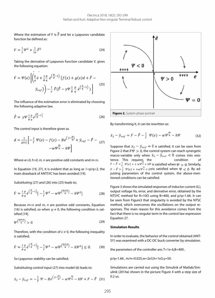
295


Where the estimation of F is and let a Lyapunov candidate function be defined as:

(24)

Taking the derivative of Lyapunov function candidate V, gives the following equation:

(25)

The influence of the estimation error is eliminated by choosing the following adaptive law.

(26)

The control input is therefore given as

(27)

Where w>0, h>0, m, n are positive odd constants and m<n.

In Equation (19, 27), it is evident that as long as 1<p/q<2, the main drawback of ANTSYC has been avoided [19].

Substituting (27) and (26) into (25) leads to;

(28)

Because m<n and m, n are positive odd constants, Equation (16) is satisfied, so when y ≠ 0, the following condition is sat-isfied [19].

(29)

Therefore, with the condition of ė ≠ 0, the following inequality is satisfied;

(30)

So Lyapunov stability can be satisfied.

Substituting control input (27) into model (6) leads to:

(31)

By transforming it, it can be rewritten as:

(32)

Suppose that is satisfied, it can be seen from Figure 2 that if , the control system can reach synergetic macro-variable only when comes into exis-tence. This requires the condition of

is satisfied when . Similarly, is satisfied when . By ad-

justing parameters of the control system, the above-men-tioned conditions can be satisfied.

Figure 3 shows the simulated responses of inductor current (iL), output voltage Vo, error, and derivative error, obtained by the NTSYC method for R=10Ω using B=400, and p/q=1.66. It can be seen from Figure3 that singularity is avoided by the NTSC method, which overcomes the oscillations on the output re-sponses. The main reason for this avoidance comes from the fact that there is no singular term in the control law expression Equaiton 27.

Simulation Results

In order to evaluate, the behavior of the control obtained (ANT-SY) was examined with a DC-DC buck converter by simulation.

the parameters of the controller are; T=1e-6,B=400 ,

p/q=1.66 , m/n=0.025,w=2e3,h=1e3,γ=50.

Simulations are carried out using the Simulink of Matlab/Sim-ulink (2014a) shown in the picture Figure 4 with a step size of 0.2 us.

Figure 2. System phase portrait

296


The parameters of the buck converter are given in Table 1.

Figure 5 presents the simulated results when the variation takes place in input voltage E, at t=0.2s from 10 V to 9V in The proposed controller gives excellent performances during the step changes in R from 10 Ω to 5 Ω in Figure 5(a), and yref from 5 V to 7 V Figure 5(b). In addition, Figure 5 (c, d), obtained by the NTSYC and NTSMC, these two methods result in a small steady-state error. However, the NTSC method leads to less steady-state error than the NTSC method.

The trajectory in Figure 6 (a), was obtained with B = 400 and different values of (p/q). It is clear that when (p/q) is high, the inclination of the macro-variable line is small, and

consequently there is a slower dynamic response. Further-more, we get faster responses whenever the value of (p/q) is small.

In Figure 6 (b) the trajectory is obtained with (p/q=1.66) and different values of B. Clearly, there is an Inverse relationship be-tween (B) and the slope of y line, but an overshoot probably occurs when the value of B is too high, and even with the high value of B, still no shattering problem on the output voltage although, fast convergence.

Figure 7 shows the simulated responses of the output voltage and the inductor current iL to step load resistance changes in R from 10Ω to 5 Ω, from 5Ω to 10 Ω, and from 10Ω to 5 Ω, re-spectively. At t =0.1s, the first step load change occurs, and as a result, the inductor current iL changes from 1A to 0.5A and an acceptable overshoot appears in the output voltage respons-es. The second load variation occurs at t=0.2s which causes a change in iL from 0.5A to 1A and a drop in the output voltage. And the same behavior mentioned in the first load change ap-pears in the third load change. These results clearly show the robust performance of the NTSMC method.

Conclusion

First, the Terminal Synergetic approach shows that we can achieve proper performance with regard to response time and

Figure 3. a-d. Response of, output voltage (uc) (A); inductor current (iL) (B); the output voltage error (err) (C); the rate of change of the output voltage error (derr) (D), obtained by ATSYC method

Table 1. Parameters of the DC buck converter.

Description Nominal value

Inductance (L) 13 mH

Capacitance (C) 2000 uF

Load resistance (R) 10-5Ω

Reference output voltage(yref ) 5-7V

Input voltage (E) 10-9V

297


overshoot, but during this study we discovered the main disad-vantage of the synergetic theory, namely, it uses a model of the system for control synthesis, which was solved by an adaptive estimation method.

As a result, we have proposed a novel “no singular terminal adaptive synergetic” DC-DC buck converter controller and eval-

uated its performance thoroughly using simulation for differ-ent perturbed operating conditions.

Our results indicate that with this design one can attain proper tracking, and insensitivity to perturbations. Concerning robust-ness, the results obtained in the existence of load and input voltage changes also show excellent performance.

Figure 4. Simulink model of buck converter with the ANTSYC method

Figure 5. a-d. Output voltage responses due to the step changes in R, yref and E, obtained via NTSYC methods: Step change in R from 10 Ω to 5 Ω (a); Step change in yref from 5V to 7V(b) and Step change in E from 10V to 9V with ANTSYC (c); Step change in E from 10V to 9V with ANTSMC (d)

298


We consider that our suggested robust approach could be imple-mented easily, as it does not rely on a discontinuous control com-ponent in contrast to SMC. Therefore, we aim to experimentally validate the controller developed in this work in a future study.




References

1. J. E. Slotine, W.P. Li, “Applied nonlinear control”, Prentice-Hall, En-glewood Cliffs, NJ, 1991.

2. A. Levant, “Higher-order sliding modes, differentiation, and out-put-feedback control,” Int J Control, vol. 76, no 9-10, 924-941, 2003.

3. V. I. Utkin, “Sliding modes in control and optimization’’, New York, Springer, 1992.

4. H. F. Ho, Y. K. Wong, A. B. Rad, “Adaptive fuzzy sliding mode control with chattering elimination for nonlinear SISO systems”, Simula-tion Modelling Practice and Theory, vol. 17, no. 7, pp. 1199-1210, 2009.

5. Y. D. Son, T. W. Heo, E. Santi, A. Monti, “Synergetic control approach for induction motor speed control”, 30th Annual Conference of the IEEE Industrial EIectronics Society, 2004.

6. M. Zhihong, A.P. Paplinski, H.R. Wu, “A robust MIMO terminal sliding mode control scheme for rigid robotic manipulator”, IEEE Transactions on Automatic Control, vol. 39, no. 12, pp. 2464-2469, 1994.

7. F. Liping, Y. Yazhou, K Boshnakov, “Adaptive backstepping based terminal sliding mode control for DC-DC convertor”, International Conference on Computer Application and System Modelling (IC-CASM 2010), 2010, pp. 323-327.

8. D. Zhao, S. Li, F. Gao, “A New Terminal Sliding Mode Control for Robotic Manipulators”, Int J Control, vol. 82, no. 10, pp.1804-1813, 2009.

9. M. Jin, J. Lee, P. H. Chang, C. Choi, “Practical Nonsingular Terminal Sliding-Mode Control of Robot Manipulators for High-Accuracy Tracking Control”, IEEE Transactions on Industrial Electronics, vol. 56, no. 9, pp. 3593-3601, 2009.

10. Y. Feng, S. Bao, X. Yu, “Inverse Dynamics Nonsingular Terminal Sliding Mode Control of Two-Link Flexible Manipulators”, International Jour-nal of Robotics and Automation, vol. 19, pp. 91-102, 2004.

11. J. F. Tsai, Y. P. Chen, “Sliding Mode Control and Stability Analysis of Buck DC-DC Converter”, Int J Elect, vol. 94, no. 3, pp. 209-222, 2007.

12. O. Barambones, P. Alkorta, A. J. Garrido, I. Garrido, F. J. Maseda, “An Adaptive Sliding Mode Control Scheme for Induction Motor Drives”, International Journal of Circuits, Systems and Signal Pro-cessing, vol. 1, no. 1, pp. 73-79, 2007.

13. F. Qiao, Q. Zhu, A. F. T. Winfield, C. Melhuish, “Adaptive Sliding Mode Control for MIMO Nonlinear Systems based on a Fuzzy Log-ic Scheme”, International Journal of Automation and Computing. vol.1, no. 1, pp. 51-62. 2004.

14. E. Santi, A. Monti, D. Li, K. Proddutur, R. Dougal, “Synergetic control for DC-DC boost converter: implementation op-tions”, IEEE Transactions on Industry Applications, vol. 39, no. 6, pp. 1803-1813, 2003.

15. A. A. Kolesnikov, “Modern Applied Control Theory: Synergetic approach in control theory”, vol. 2, Russian, Moscow-Taganrog, TSURE Press, 2000.

16. Q. Wang, J. Feng, T. Li, “Analysis of the Synergetic Control Based on Variable Structure and Application of Power Electronics”, In-ternational Conference on Information Engineering and Computer Science, 2009, pp. 1-4.

Figure 6. a, b. State trajectories with different values of (p/q) when B is constant (a); State trajectories with different values of B when (p/q) is constant (b)

Figure 7. Simulated responses of the output voltage and the in-ductor current iL to load variations in R from 10Ω to 5 Ω, from 5 Ω to 10 Ω, and from 10 Ω to 5 Ω.

299


17. E. Santi, A. Monti, D. Li, K. Proddutur, R. A. Dougal, “Synergetic control for power electronics applications: A comparison with the sliding mode approach”, J Circuits Syst Comput, vol. 13, no. 4, pp. 737-760, 2004.

18. L. Medjbeur, M. N. Harmas, “Adaptive fuzzy terminal synergetic control”, International Conference on Communications, Comput-ing and Control Applications (CCCA), 2011.

19. L. Fan, Y. Yu, “Adaptive Non-singular Terminal Sliding Mode Con-trol for DC-DC Converters”, Advances in Electrical and Computer Engineering, vol. 11, no. 2, pp. 119-122, 2011.

20. M. Zak, “Terminal Attractors for Addressable Memory in Neural Networks”, Phys Lett A, vol. 133, no. 1-2, pp. 18-22, 1988.

21. H. Komurcugil, “Non-singular terminal sliding-mode control of DC-DC buck converters”, Control Engineering Practice, vol. 21, no. 3, pp. 321-332, 2013

Serkan Kurt was born in Kırıkkale in 1976. He has obtained his B.Sc in Electrical and Electronics Engineering from İstanbul University in 1999. He has obtained M.Sc degree in Computer Engineering from Gebze Techni-cal University in 2002. He has obtained Phd degree in Electrical Engineering in Yıldız Technical University in 2007. His areas of research includes Sensor Network, Control and Automation, Robotics, System Design. He has been working at Yıldız Technical University since 2002.

Yakoub Nettari was born in Touggourt, Algeria in 1987. He has obtained his Engineer degree in Electrome-chanical Engineering from M’sila University in 2010. He has obtained M.Sc degree in Control and Automatic Engineering from Setif University in 2014. He is PhD student in Electrical Engineering at Yıldız Technical Uni-versity since 2015. His current research is on Robust and intelligent Control, Automation, Robotics, DC-DC converters and Renewable Energy.

300

Introduction

Continuous monitoring of respiratory rate (cycle) during sleep for diseases such as, sleep ap-nea, sudden infant death syndrome (SIDS) and chronic obstructive pulmonary disease (COPD) can be life saving [1-3]. When we breathe, air is inhaled into the lungs through the mouth or nose due to muscle contraction and then exhaled by muscle relaxation. The respiratory cycle consists of two parts as inhalation and exhalation. The respiratory rate is defined as the num-ber of respiratory cycles per minute.

There are various methods to continuously monitoring respiratory rate. In literature, these methods can be categorized into two groups: contact-based and contactless. In the con-tact-based methods, as the name implies, the respiratory rate is estimated via sensors or de-vices attached to the human body [4]. In clinical environments, for example, capnography that measures the carbon dioxide intensity in the exhaling air via nasal cannula or mask and pho-toplethysmogram (PPG) which detects the volumetric changes in blood via a sensor which is attached to a finger are commonly used [5, 6]. Besides, some methods are developed for the non-clinical environments. For example, respiratory rate estimates are made by analysing the sounds of a person during respiratory via microphones. It is also possible to estimate the respi-ratory rate by using the strap with accelerometer which is attached to the chest [7-9].

All of these contact-based systems restrict patients’ mobility, comfort and sleep patterns. There-fore, contactless respiratory rate monitoring methods have been to developed. Contrary to con-tact-based methods, there is no need to attach any device or sensor to the human body for the respiratory monitoring in contactless methods. Developed methods can be grouped into two classes: vision based and radio frequency (RF) based. Vision based methods are based on analysis and processing of images [10-12]. These methods require line of sight, depend on day-light, violate the privacy of private life and have high computational complexity. In recent years, electromagnetic RF signals have begun to be used to sense respiratory activity. While RF signals

Electrica 2018; 18(2): 300-309

RESEARCH ARTICLE

MUSIC Algorithm for Respiratory Rate Estimation Using RF SignalsCan Uysal , Tansu Filik Department of Electrical and Electronics Engineering, Anadolu University School of Engineering, Eskişehir, Turkey

Corresponding Author: Can Uysal





DOI: 10.26650/electrica.2018.03405

Cite this article as: C. Uysal, T. Filik, “MUSIC Algorithm for Respiratory Rate Estimation Using RF Signals”, Electrica, vol. 18, no: 2, pp. 300-309, 2018.

ABSTRACT

Continuous monitoring of respiratory rate (cycle) during sleep for diseases such as sleep apnea and sudden infant death syndrome (SIDS) can be lifesaving. Wireless radio communications signals are everywhere and can be harnessed for contactless monitoring of the respiratory rates. The amplitude of the received signal strength changes periodically depending on the exhalation and inhalation of the subject. In this paper, subspace-based multiple signal classification (MUSIC) algorithm is applied to estimate the respiratory rate for better results. The proposed method and the other power spectral density (PSD) methods for respiratory estimations are compared with the real laboratory measurements. It is demonstrated that the proposed method estimates the respiratory rate with high accuracy and outperforms the other PSD-based methods which are commonly used in the literature.

Keywords: MUSIC, contactless, respiratory rate, wireless signals, software defined radios

https://orcid.org/0000-0003-0927-3892

https://orcid.org/0000-0003-0205-5059

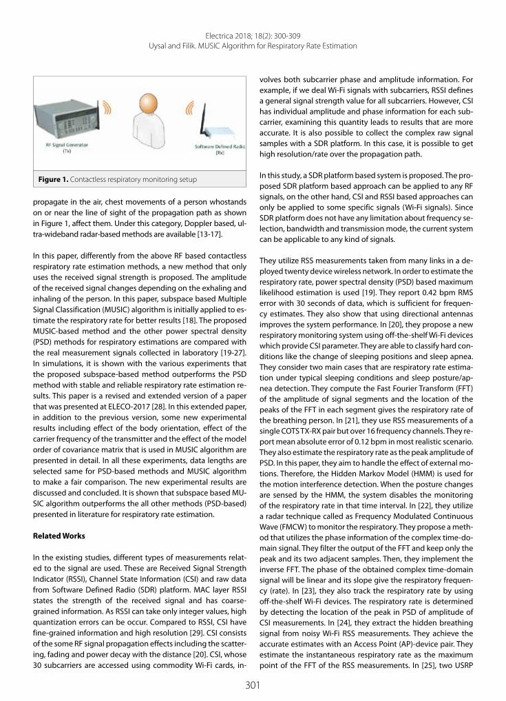
301

Electrica 2018; 18(2): 300-309Uysal and Filik. MUSIC Algorithm for Respiratory Rate Estimation

propagate in the air, chest movements of a person whostands on or near the line of sight of the propagation path as shown in Figure 1, affect them. Under this category, Doppler based, ul-tra-wideband radar-based methods are available [13-17].

In this paper, differently from the above RF based contactless respiratory rate estimation methods, a new method that only uses the received signal strength is proposed. The amplitude of the received signal changes depending on the exhaling and inhaling of the person. In this paper, subspace based Multiple Signal Classification (MUSIC) algorithm is initially applied to es-timate the respiratory rate for better results [18]. The proposed MUSIC-based method and the other power spectral density (PSD) methods for respiratory estimations are compared with the real measurement signals collected in laboratory [19-27]. In simulations, it is shown with the various experiments that the proposed subspace-based method outperforms the PSD method with stable and reliable respiratory rate estimation re-sults. This paper is a revised and extended version of a paper that was presented at ELECO-2017 [28]. In this extended paper, in addition to the previous version, some new experimental results including effect of the body orientation, effect of the carrier frequency of the transmitter and the effect of the model order of covariance matrix that is used in MUSIC algorithm are presented in detail. In all these experiments, data lengths are selected same for PSD-based methods and MUSIC algorithm to make a fair comparison. The new experimental results are discussed and concluded. It is shown that subspace based MU-SIC algorithm outperforms the all other methods (PSD-based) presented in literature for respiratory rate estimation.

Related Works

In the existing studies, different types of measurements relat-ed to the signal are used. These are Received Signal Strength Indicator (RSSI), Channel State Information (CSI) and raw data from Software Defined Radio (SDR) platform. MAC layer RSSI states the strength of the received signal and has coarse-grained information. As RSSI can take only integer values, high quantization errors can be occur. Compared to RSSI, CSI have fine-grained information and high resolution [29]. CSI consists of the some RF signal propagation effects including the scatter-ing, fading and power decay with the distance [20]. CSI, whose 30 subcarriers are accessed using commodity Wi-Fi cards, in-

volves both subcarrier phase and amplitude information. For example, if we deal Wi-Fi signals with subcarriers, RSSI defines a general signal strength value for all subcarriers. However, CSI has individual amplitude and phase information for each sub-carrier, examining this quantity leads to results that are more accurate. It is also possible to collect the complex raw signal samples with a SDR platform. In this case, it is possible to get high resolution/rate over the propagation path.

In this study, a SDR platform based system is proposed. The pro-posed SDR platform based approach can be applied to any RF signals, on the other hand, CSI and RSSI based approaches can only be applied to some specific signals (Wi-Fi signals). Since SDR platform does not have any limitation about frequency se-lection, bandwidth and transmission mode, the current system can be applicable to any kind of signals.

They utilize RSS measurements taken from many links in a de-ployed twenty device wireless network. In order to estimate the respiratory rate, power spectral density (PSD) based maximum likelihood estimation is used [19]. They report 0.42 bpm RMS error with 30 seconds of data, which is sufficient for frequen-cy estimates. They also show that using directional antennas improves the system performance. In [20], they propose a new respiratory monitoring system using off-the-shelf Wi-Fi devices which provide CSI parameter. They are able to classify hard con-ditions like the change of sleeping positions and sleep apnea. They consider two main cases that are respiratory rate estima-tion under typical sleeping conditions and sleep posture/ap-nea detection. They compute the Fast Fourier Transform (FFT) of the amplitude of signal segments and the location of the peaks of the FFT in each segment gives the respiratory rate of the breathing person. In [21], they use RSS measurements of a single COTS TX-RX pair but over 16 frequency channels. They re-port mean absolute error of 0.12 bpm in most realistic scenario. They also estimate the respiratory rate as the peak amplitude of PSD. In this paper, they aim to handle the effect of external mo-tions. Therefore, the Hidden Markov Model (HMM) is used for the motion interference detection. When the posture changes are sensed by the HMM, the system disables the monitoring of the respiratory rate in that time interval. In [22], they utilize a radar technique called as Frequency Modulated Continuous Wave (FMCW) to monitor the respiratory. They propose a meth-od that utilizes the phase information of the complex time-do-main signal. They filter the output of the FFT and keep only the peak and its two adjacent samples. Then, they implement the inverse FFT. The phase of the obtained complex time-domain signal will be linear and its slope give the respiratory frequen-cy (rate). In [23], they also track the respiratory rate by using off-the-shelf Wi-Fi devices. The respiratory rate is determined by detecting the location of the peak in PSD of amplitude of CSI measurements. In [24], they extract the hidden breathing signal from noisy Wi-Fi RSS measurements. They achieve the accurate estimates with an Access Point (AP)-device pair. They estimate the instantaneous respiratory rate as the maximum point of the FFT of the RSS measurements. In [25], two USRP

Figure 1. Contactless respiratory monitoring setup

302


are used one for the transmitting and one for the receiving the wireless signal at 2.4 GHz. They combine four different algo-rithms, which are zero-crossing, FFT maximum selection, linear predictive coding, least squares harmonic analysis, to estimate the respiratory rate. In [26], they use CSI data provided by com-modity Wi-Fi devices. In order to detect the stationary human presence, they take into consideration respiratory of a person as an indicator. The motion interference module first detects whether there is a motion in the environment. If there is no motion, the stationary human detection module performs to find the answer to the question whether there is a human or not. In this section, the respiratory rate that is the location of the peak in the PSD is estimated. If the estimated respiratory frequency (rate) is within the nominal range (0.1-0.5 Hz), a hu-man presence in the environment is detected. Most of the ex-isting respiratory rate estimation methods in literature use the PSD approach that has many disadvantages although it is a fast method. Since PSD can be easily affected by noise, the proba-bility of error increases. The frequency resolution of PSD is re-stricted to the number of samples in a measurement window. Therefore, the error value cannot decrease below a certain lim-it. In addition, it is evaluated that this method is not effective in estimating the respiratory rate of multiple people.

System Overview

In this section, the basics of respiratory, the effect of inhaling/exhaling of a person to the received RF signal’s strength are discussed. Also the experimental setup used to take real mea-surements and the measurement model for the respiratory rate estimation are presented.

Basics of Respiration

Respiration is the process of human’s taking oxygen in the air and releasing carbon dioxide to the air to survive. It consists of two phases as inhalation and exhalation as seen in Figure 2. During inhalation, air is inhaled through the mouth or nose and travels towards the lungs. In the meantime, the chest wall expands, the diaphragm contracts and the chest volume increases. During ex-halation, this process works in the opposite direction, and it con-tinues cyclically. The processes during inhalation and exhalation are given in Table 1. In a healthy adult the number of breaths per minute is between 12-20, 16-22 in children, and 18-40 in infants.

The Effect of Respiratory to the RF Signal Amplitude

In this section, the effect of the respiratory to the RF signal am-plitude is discussed in detail. The transmitting and receiving an-tennas are located as shown in Figure 1. The distance traveled by the signals that are reflected (attenuated) from a stationary person on the transmission channel between the transmitter and the receiver changes depending on the breathing of that person. The nominal distance between the transmitter and the receiver is defined as do and it is expected that the periodic dis-placement of chest wall changes the traveled distance of the

reflected signal as periodically [30],

(1)

where d(t) is the time-varying distance which is traveled by the signal during the respiratory. Since it is assumed that the dis-placement of the chest wall is a sinusoidal function of time [31], this distance also varies periodically with the same frequency as the respiratory rate,

(2)

where ƒR represents the respiratory rate, ΔA is the maximum displacement of the chest wall. The propagation delay accord-ing to the traveled distance is defined as follows,

(3)

where c is the speed of light. If the environment is assumed stationary, the time-varying channel impulse response can be modelled as follows,

(4)

where ai is the amplitude value belong to static paths, is the

Figure 2. Inhalation and exhalation phases [22]

Table 1. The processes during inhalation and exhalation.

During Inhalation During Exhalation

-diaphragm contracts -diaphragm relaxes

-chest expands -chest contracts

-air flows in -air flows out

-volume increases -volume decreases

-pressure decreases -pressure increases

303


amplitude of the path which is affected by respiratory. t and τ represent fast and slow varying times, respectively. The re-ceived signal is obtained with the convolution of the source signal and the channel impulse response as follows,

(5)

As seen from (5), the amplitude of the received signal periodi-cally varies with the same frequency as the respiratory rate.

The displacement of the chest wall along the anteroposteri-or dimension is approximately 4.2 mm ~ 5.4 mm at the nor-mal breathing and 12.6 mm at the deep breathing [27], [31]. The chest wall expands outwards when the air is inhaled and contracts inwards when the air is exhaled, as expected. These arguments are also observed and verified with real measure-ments in our laboratory. The person sitting on the chair in Figure 3, holds his breath (after exhalation) between the 17th and 30th seconds. Then he continues to breathing until the 43rd second. Afterwards, he holds his breath again (after inhala-tion) between the 43rd and 52nd seconds. As shown in Figure 4 (Top), these planned movements can be easily monitored with variations on the received signal strength. Figure 4 (Bot-

tom) shows the received signal strength in the absence of the person. In this case, the signal level does not show a periodic change. The received RF signal’s amplitude level changes with inhaling/exhaling of the person and this causes a periodicity on the received signal due to the breathing movements. Even though the received signal is affected by the ambient noise, it preserves its periodic structure. The respiratory monitoring methods estimate the respiratory rate taking advantage of pe-riodicity of the received signal.

Laboratory Experimental Setup

In this study, the HP 8647A signal generator is used to gener-ate a continuous wave signal at 900 MHz as the transmitter. Ettus USRP B210 software defined radio is configured as a re-ceiver. USRP (Universal Software Radio Peripheral) is an SDR platform developed by Ettus Research. The experimental set-up established for the measurements is shown in Figure 3. A 900 MHz carrier signal with constant amplitude is generated from the transmitter. The power of transmitted signal is ad-justed as 0 dbm. VERT900 omni-directional vertical antenna with 3 dBi gain is used as an antenna in both transmitter and receiver.

Measurement Model

Propagation path between the transmitter and receiver is shown in Figure 1. It is assumed that the transmitted signal is a (phase or frequency) modulated signal with a constant peak amplitude which is a reasonable assumption for wireless com-munication signals. In this case, the averaged received signal strength are assumed constant during communications. On the other hand, the breathing of a person on the propagation path of the signal (as shown in Figure 1, 3) will change the am-plitude level of the received signal which is already observed in literature [19, 20]. If there is no movement between transmitter and receiver, the received signal’s averaged amplitude should be,

(6) where µ is the mean of received signal, w is assumed additive zero-mean noise signal. If a breathing person exists in the envi-ronment, the magnitude of the baseband complex signal can be modelled as follows,

(7)

(8)

Ac, ƒR, are the amplitude, respiratory frequency (rate) and phase, respectively. Since breathing requires a periodic action in the form of inhaling and exhaling the cosine model in (8) is suitable to model respiratory. Then the respiratory rate estima-tion evolves to the frequency estimation (ƒR) of the baseband received signal.

Figure 3. Experimental setup in laboratory

Figure 4. (Top) The effect of the exhalation, inhalation and breath holding on the received signal amplitude. (Bottom) The signal in the absence of the person.

304


Respiratory Rate Estimation System

In this section, the proposed respiratory rate estimation sys-tem is discussed. Firstly, the pre-processing steps, which are required to make an accurate estimate are given. Then, the pro-posed subspace-based MUSIC algorithm is presented in detail. Finally, PSD-based MLE algorithm, which is commonly used in literature is considered.

Pre-processing Steps

In order to make the respiratory rate estimation algorithm properly with real measurements, some pre-processing steps are required. In this section, the basic pre-processing steps such as Outlier Removal, Downsampling and DC Removal are briefly summarized.

Since the data used is from actual/real measurements, in some cases, due to hardware deterioration several extreme points (spurious peaks) which are not originated from the chest move-ments can also be observed on the received signal strength. These spurious peaks are refered to as outliers. In Figure 5 (Top), the outliers can be seen that near 8, 10, 38, 46, 55 and 59 seconds. In order to eliminate these spiky peaks (outliers), the well-known Hampel identifier is used [32] in this study. Hampel identifier calculates the median (µ) and median absolute devi-ation (σ) of the samples in the measurement window. Then, it determines an upper and lower bound using µ and σ. Upper and lower bounds are set to µ + 3σ and µ – 3σ, respectively. A new sample, which is out of these bounds, is qualified as an outlier. The outliers are detected and removed from the origi-nal signal as seen from the Figure 5 (Bottom).

The received signal is sampled by the USRP at 1200 Hz. Since the respiratory rate is below 1 Hz, high sampling rate makes difficult to distinguish the breathing signal in the frequency spectrum. Moreover, high sampling rate increases the com-

putational cost. Due to these reasons, the received signal is downsampled without distorting its waveform and periodic form. After downsampling, the sampling rate of the received signal is reduced to 1 Hz.

When the spectral analysis is carried out, it is seen that the first component of the signal in frequency domain contains high energy. This DC component that is the average value of the sig-nal in frequency domain suppresses the other frequency com-ponents. Besides, DC component does not contain any infor-mation about the respiratory. For removing the DC component from signal, the average value is subtracted from entire signal. After DC removal process, the component at 0 Hz is removed from the frequency spectrum of the signal,

(9)

where is the average amplitude of the received signal and y(t) is the output of the DC removal system.

MUSIC Algorithm

In this section, we consider the estimation of the respiratory rate using Multiple Signal Classification (MUSIC) algorithm which is a subspace based method [18]. MUSIC algorithm is commonly used to estimate the direction of arrival of signals as well as the frequency of the periodic signals. MUSIC is a su-per-resolution technique and since it works by separating sig-nal and noise subspaces, it estimates the respiratory frequency more accurate than sample windowed PSD based methods. The m samples collected from the measured and pre-processed signal are modeled as follows,

(10)

(11)

here, x(t) defines the sinusoidal source signals. A matrix con-tains the sinusoidal source signals and is defined as follows,

(12)

where m is a positive integer which is the number of samples in the sequence and it also defines the model order of the cova-riance matrix. n is the number of unknown sinusoidal compo-nent. In subspace-based methods, the number of component must be known to decompose the signal and noise subspace. So, it is assumed that n is known. The covariance matrix of y(t) is defined as,

Figure 5. (Top) The original signal with outliers. (Bottom) Thesignal whose outliers are removed using Hampel identifier.

305


(13)

With the combining of (10) and (13), the covariance matrix be-comes,

(14)

where

(15)

where Rs and Rw are the signal and noise correlation matrices, respectively. σ2 is the noise power and I is the identity matrix. The eigendecomposition of R contains the information on the respiratory frequencies .

MUSIC is derived from the covariance model in (13) with m > n. The eigenvalues of R matrix are obtained as

and is a set of or-thogonal eigenvectors corresponding to and

are the orthonormal eigenvectors associated with . The eigenvectors of R can be divided into two subsets as shown in the following,

(16)

where S and G denote signal and noise subspace, respectively. As the noise subspace G is orthogonal to A matrix, the follow-ing definition can be used,

(17)

where A is a function of the frequencies . The columns of G belong to the null space of A as shown in (17). The true respiratory frequencies are the only solutions of the equation for any m > n. The MUSIC algo-rithm is defined in two steps as follows,

• Step-1: Compute the sample covariance matrix

(18)

and its eigendecomposition. Ŝ and Ĝ are the signal and noise eigenvectors obtained from matrix.

• Step-2: Using Ĝ noise subspace which is obtained in Step-1 determine the respiratory frequency estimates as the lo-cations of the n highest peaks of the estimation function

(19)

In this study, since there is a single patient, the number of sinu-soidal signals is assumed one (n = 1). It is also possible to moni-tor multiple patients (n > 1) with the MUSIC algorithm.

PSD-Based MLE

In this section, the power spectral density (PSD)-based maxi-mum likelihood estimation (MLE) is given as an extension of the classical sinusoidal parameter estimation problem [19]. In [19], a respiratory rate estimator which estimates the respira-tory rate as the frequency at the maximum of the PSD is pro-posed. The MLE of frequency is defined as,

(20)

In the power spectrum, the frequencies close to zero are ex-cluded specifically. They determine the sampling rate to satisfy the Nyquist criterion.

Experimental Results

In this part, we design some experiments in laboratory in or-der to observe the performance of the respiratory monitoring system. In order to get statistically significant performance results, a total of 270 measurements (trials) are collected in laboratory. In order to analyse the effect of carrier frequen-cies and body orientations of a participant to respiratory rate estimation, the distances between the transmitter and the receiver, the transmit powers and carrier frequencies are changed in a controlled manner while collecting data. Each measurement is one and half and three minutes long. In all these measurements, the distances between the transmitter & subject and subject & receiver are taken equal, as the par-ticipants are sitting the midpoint of the distance as shown in Figure 3. The different length sliding window is shifted along the signal and the respiratory rate is estimated from each measurement window. The proposed subspace-based MUSIC method is first time applied to estimate respiratory rates us-ing received signal strength. The mean absolute error (MAE) is used as a performance metric, which measures the accuracy of the system. The participants try to keep their respiratory rates fixed using a chronometer.

In order to analyse the effect of selected window length, trans-mitter frequency and body orientations of a participant to re-spiratory rate estimation, different experiments are carried out. For all these different experiments, the proposed subspace based MUSIC method are compared with the commonly used PSD-based MLE method in [19].

306


In Figure 6, normalised spectrum estimations, which are ob-tained using MUSIC and the PSD algorithms, are compared. The number of samples (window durations) are selected as W = 40 seconds for these two algorithms. In this experiment, actual re-spiratory rate is 15 bpm (0.25 Hz). As seen from the figure, the peaks in both spectrums occur at the frequencies correspond-ing to the respiratory rate of the person. It can be seen that the peak in the MUSIC spectrum has narrower (sharp) main lobe width according to PSD spectrum. As expected, it is observed that the MUSIC spectrum has higher frequency resolution than the PSD spectrum that is commonly used in respiratory rate es-timation literature.

In Figure 7, the window duration is decreased to W = 16 sec-onds and the actual respiratory rate is 20 bpm (0.33 Hz). In this

case, although the main lobe width of the peak at the MUSIC spectrum expands, it is not significantly effected by the de-crease in window duration. However, it can be seen that the main lobe width increases excessively in the PSD spectrum. It can be seen that the frequency resolution of the PSD decreases with the shortening of window duration. In the case of low sig-nal to noise ratio (SNR), it is evaluated that the MUSIC algorithm will be more accurate and robust. Besides, in multiple person case, PSD-based method cannot distinguish different frequen-cies due to its low resolution.

Effect of the Body Orientation

In the first experiment, the participant is sitting on the LOS be-tween the transmitter and the receiver as in position-1 (front). In second experiment, the participant swaps his position to the position-2 (side). The positions are shown in Figure 8. In Figure 9, the estimation accuracies of the proposed MUSIC and PSD based MLE methods for W = 20 are shown. It is shown in the fig-ure that better performances are obtained in case of position-1. Fig. 10 shows the effect of the body orientations relative to the transmitter (front and side) on the estimation performances of the subspace-based MUSIC method and PSD-based MLE meth-od. In both positions of the participant, it can be seen that all methods can estimate the respiratory frequency. During respi-ration, the displacement of the chest wall is 4.2 ~ 5.4 mm in the anteroposterior dimension and 0.6 ~ 1 mm in the mediolateral dimension [27], [31]. Therefore, as the change in the anteropos-terior dimension is greater than the change in the mediolateral dimension, with more variation in the amplitude level of the received signal is observed in this case. The obtained greater variation reveals that more distinct sine wave and better per-formances are obtained in case of position-1.

In addition, it can be seen in the figure, error rates decrease with the increasing of window duration. However, selection of the

Figure 7. (Top) The power spectrum of the PSD-based MLE meth-od. (Bottom) Pseudospectrum estimation using MUSIC algorithm. In both cases, window duration W = 16 sec and actual respiratory rate ƒR = 0.33 Hz (20 bpm).

Figure 8. The positions of the user during body orientation exper-iments. Top and bottom figures show position-1 and position-2, respectively.

Figure 6. (Top) The power spectrum of the PSDbased MLE meth-od. (Bottom) Pseudospectrum estimation using MUSIC algorithm. In both cases, window duration W = 40 sec and actual respiratory rate ƒR = 0.25 Hz (15 bpm).

307


long window duration reveals some disadvantages. We take the samples from the received signal for a duration W before esti-mating the respiratory rate. Therefore, window duration W is im-portant because it determines the waiting time. Moreover, the long window duration causes to miss sudden changes in respi-ratory rate. The proposed MUSIC based method outperforms the PSD-based MLE method for all window durations. As seen from the Figure 10, while the MAE of the proposed method is lower than 0.1 breaths per minute (bpm) for all window durations W > 30 seconds, the PSD-based method cannot reach this rate for all window durations. Especially for short window duration (W < 30), the performance of our proposed method is quite better than the PSD-based MLE method. This is important for the respi-ratory monitoring system requiring low latency.

Effect of the Carrier Frequency

This experiment is designed to show the effect of the carrier frequency of the transmitted signal to the estimation perfor-mances. Figure 11 shows the MAE values in terms of bpm of different carrier frequencies for W = 30. Carrier frequencies of the transmitter are set to 900 MHz, 2.4 GHz and 4 GHz, re-spectively. Distance between the transmitter and the receiv-er is specified as 2 meters and the transmitted power is ad-justed as 0 dBm. We observe that respiratory rate estimation accuracy decreases with the increasing of the frequency of the radio signal. This is because the effect of human respira-tory on radio signal propagation decreases as the frequency of the radio signal increases. As seen from the Figure 11, the best performance is obtained when the carrier frequency is selected as 900 MHz. In this case, the proposed MUSIC meth-od can estimate the respiratory rate with 0.1 bpm accuracy. The lowest accuracy is obtained with PSD-based method for all carrier frequencies.

Figure 9. The effect of body orientation for W = 20

Figure 10. Performance comparison between PSD and MUSIC methods according to the W in the body orientation experiment.

Figure 11. MAE (bpm) values according to the carrier frequencies.

Figure 12. Respiratory rate estimation performance of MUSIC method according to the covariance matrix model order, W is se-lected 40 sec

308


Effect of the Covariance Matrix Model Order

Figure 12 shows the effect of the covariance matrix model order (m) to the respiratory rate estimation accuracy m. corre-sponds the number of samples in the sequence which are used to construct the covariance matrix. As the subspace-based methods use the eigendecomposition of the covariance ma-trix, the model order is a critical parameter. The sliding window duration is set to 40 seconds. It can be seen from the figure, the highest accuracy is obtained when m is selected as 10. Select-ing a large value for m not only reduces the system accuracy but also increases the computational complexity because the size of the matrix increases.

Conclusion

In this study, we present a contactless respiratory monitoring system that requires no devices or sensing module on the hu-man body. The proposed system uses subspace based MUSIC algorithm to estimate the respiratory rate using only a single TX/RX pair. In the laboratory, we designed some experiments using real measurements to show the performance of the pro-posed respiratory rate estimation system. The proposed system uses complex raw data collected with SDR platform that does not any limitation about frequency selection, bandwidth, etc. In the experiments, many cases including the effect of carrier frequency, the effect of the covariance matrix model order, the effect of the body orientation are investigated. Our proposed MUSIC-based respiratory rate estimation method is compared with the PSD-based MLE method for the different measure-ment window durations and scenarios. It is shown with several experiments that the proposed MUSIC-based method can esti-mate the respiratory rate of a person with 0.08 bpm mean abso-lute error in ideal case. It is also shown that the MUSIC method outperforms the commonly used PSD-based MLE method. The performances of the MUSIC algorithm, which provide more ac-curate estimates with low signal strength and limited number of samples, are shown through real measurements.



Financial Disclosure: This work was supported by Anadolu University Scientific Research Projects Fund with projects 1705F416.

References

1. M. Younes, “Role of respiratory control mechanisms in the patho-genesis of obstructive sleep disorders”, J Appl Physiol (1985), vol. 105, no. 5, pp. 1389-1405, 2008.

2. A. N. Vgontzas, A. Kales, “Sleep and its disorders”, Annu Rev Med, vol. 50, pp. 387-400, 1999.

3. T. Rantonen, J. Jalonen, J. Grönlund, K. Antila, D. Southall, I. Välimä-ki, “Increased amplitude modulation of continuous respiration precedes sudden infant death syndrome -Detection by spectral

estimation of respirogram”, Early Human Development, vol. 53, no. 1, pp. 53-63, 1998.

4. F. Q. AL-Khalidi, R. Saatchi, D. Burke, H. Elphick, S. Tan, “Respiration rate monitoring methods: A review”, Pediatr Pulmonol, vol. 46, no. 6. pp. 523-529, 2011.

5. W. Karlen, C. J. Brouse, E. Cooke, J. M. Ansermino, G. A. Dumont, “Respiratory rate estimation using respiratory sinus arrhythmia from photoplethysmography”, Annual International Conference of the IEEE Engineering in Medicine and Biology Society, 2011.

6. A. Gaucher, D. Frasca, O. Mimoz, B. Debaene, “Accuracy of respi-ratory rate monitoring by capnometry using the Capnomask® in extubated patients receiving supplemental oxygen after surgery”, Br J Anaesth, vol. 108, no. 2, pp. 316-320, 2012.

7. Y. Nam, B. A. Reyes, K. H. Chon, “Estimation of Respiratory Rates Using the Built-in Microphone of a Smartphone or Headset”, IEEE J Biomed Health Inform, vol. 20, no. 6. pp. 1493-1501, 2016.

8. P. Corbishley, E. Rodríguez-Villegas, “Breathing detection: Towards a miniaturized, wearable, battery-operated monitoring system”, IEEE Trans Biomed Eng, vol. 55, no. 1, pp. 196-204, 2008.

9. J. Hernandez, D. McDuff, R. Picard, “BioWatch: Estimation of Heart and Breathing Rates from Wrist Motions”, EAI Endorsed Transac-tions on Pervasive Health and Technology, vol. 15, no. 3, 2015.

10. M. Bartula, T. Tigges, J. Muehlsteff, “Camera-based system for con-tactless monitoring of respiration”, 35th Annual International Con-ference of the IEEE Engineering in Medicine and Biology Society (EMBC), 2013, pp. 2672-2675.

11. K. Nakajim, Y. Matsumoto, T. Tamura, “Development of real-time image sequence analysis for evaluating posture change and re-spiratory rate of a subject in bed”, Physiol Meas, vol. 22, no. 3, pp. 21-28, 2001.

12. K. S. Tan, R. Saatchi, H. Elphick, D. Burke, “Real-time vision based respiration monitoring system”, 7th International Symposium on Communication Systems, Networks & Digital Signal Processing (CSNDSP 2010), pp. 770-774, 2010.

13. A. Lazaro, D. Girbau, R. Villarino, “Analysis of Vital Signs Monitoring Using an IR-UWB Radar”, Prog Electromagn Res, vol. 100, pp. 265-284, 2010.

14. A. D. Droitcour, O. Boric-Lubecke, G. T. A. Kovacs, “Signal-to-Noise Ratio in Doppler Radar System for Heart and Respiratory Rate Measurements”, IEEE Transactions on Microwave Theory and Tech-niques, vol. 57, no. 10. pp. 2498-2507, 2009.

15. C. Li, J. Ling, J. Li, J. Lin, “Accurate doppler radar noncontact vital sign detection using the RELAX algorithm”, IEEE Transactions on In-strumentation and Measurement , vol. 59, no. 3, pp. 687-695, 2010.

16. M. Ascione, A. Buonanno, M. D’Urso, L. Angrisani, R. S. Lo Moriel-lo, “A new measurement method based on music algorithm for through-the-wall detection of life signs”, IEEE Transactions on In-strumentation and Measurement, vol. 62, no. 1. pp. 13-26, 2013.

17. C. Li, J. Lin, “Recent advances in Doppler radar sensors for perva-sive healthcare monitoring”, Asia-Pacific Microwave Conference (APMC), 2010, pp. 283-290.

18. R. Schmidt, “Multiple emitter location and signal parameter esti-mation”, IEEE Trans. Antennas Propag, vol. 34, no. 3, pp. 276-280, Mar. 1986.

19. N. Patwari, J. Wilson, S. Ananthanarayanan, S. K. Kasera, D. R. West-enskow, “Monitoring breathing via signal strength in wireless net-works”, IEEE Transactions on Mobile Computing, vol. 13, no. 8, pp. 1774-1786, 2014.

20. X. Liu, J. Cao, S. Tang, J. Wen, P. Guo, “Contactless Respiration Mon-itoring Via Off-the-Shelf WiFi Devices”, IEEE Transactions on Mobile Computing, vol. 15, no. 10. pp. 2466-2479, 2016.

309


21. O. Kaltiokallio, H. Yiğitler, R. Jäntti, and N. Patwari, “Non-invasive respiration rate monitoring using a single COTS TX-RX pair,” IPSN 2014 - Proceedings of the 13th International Symposium on Informa-tion Processing in Sensor Networks, 2014, pp. 59-69,

22. F. Adib, H. Mao, Z. Kabelac, D. Katabi, R. C. Miller, “Smart Homes that Monitor Breathing and Heart Rate”, Proceedings of the 33rd An-nual ACM Conference on Human Factors in Computing Systems, pp. 837-846, 2015.

23. J. Liu, Y. Wang, Y. Chen, J. Yang, X. Chen, J. Cheng, “Tracking Vital Signs During Sleep Leveraging Off-the-shelf WiFi,” Proceedings of the 16th ACM International Symposium on Mobile Ad Hoc Network-ing and Computing, pp. 267-276, 2015.

24. H. Abdelnasser, K. A. Harras, M. Youssef, “UbiBreathe: A Ubiquitous non-invasive WiFi-based Breathing Estimator”, Proceedings of the 16th ACM International Symposium on Mobile Ad Hoc Networking and Computing, pp. 277-286, 2015

25. R. Ravichandran, E. Saba, K. Y. Chen, M. Goel, S. Gupta, S. N. Patel, “WiBreathe: Estimating respiration rate using wireless signals in natural settings in the home”, IEEE International Conference on Pervasive Computing and Communications (PerCom), 2015, pp. 131-139, 2015.

26. C. Wu, Z. Yang, Z. Zhou, X. Liu, Y. Liu, J. Cao, “Non-invasive detec-tion of moving and stationary human with WiFi,” IEEE Journal on

Selected Areas in Communications, vol. 33, no. 11, pp. 2329-2342, 2015.

27. H. Wang, D. Zhang, J. Ma, Yasha Wang, Yuxiang Wang, D. Wu, T. Gu, B. Xie, “Human respiration detection with commodity wifi devic-es: Do User Location and Body Orientation Matter?”, Proceedings of the 2016 ACM International Joint Conference on Pervasive and Ubiquitous Computing, 2016, pp. 25-36.

28. C. Uysal and T. Filik, “Contactless respiration rate estimation using MUSIC algorithm,” in Electrical and Electronics Engineering (ELECO), 2017 10th International Conference on, 2017, pp. 606-610.

29. Z. Yang, Z. Zhou, Y. Liu, “From RSSI to CSI”, ACM Computing Surveys (CSUR), vol. 46, no. 2, pp. 1-32, 2013.

30. S. Venkatesh, C. R. Anderson, N. V. Rivera, R. M. Buehrer, “Imple-mentation and analysis of respiration-rate estimation using im-pulse-based UWB”, IEEE Military Communications Conference, 2005.

31. C. Lowanichkiattikul, M. Dhanachai, C. Sitathanee, S. Kha-chonkham, and P. Khaothong, “Impact of chest wall motion caused by respiration in adjuvant radiotherapy for postoperative breast cancer patients,” Springerplus, vol. 5, no. 1, pp. 1-8, 2016.

32. L. Davies and U. Gather, “The identification of multiple outliers”, J Am Stat Assoc, vol. 88, no. 423, pp. 782-792, 1993.

Tansu Filik received the B.S. degree from the Anadolu University in 2002, the integrated M.S. and Ph.D. degree from the Middle East Technical University (METU) in 2010, all in electrical engineering. From 2002 to 2010, he was withSensor Array and Multichannel Signal Processing (SAM) Group of METU. From 2010 to 2012, he was with Aselsan Inc., at Radar, Electronic Warfare and Intelligence Systems Division. Currently, he is with Anadolu University at Department of Electrical Engineering. His research interest includes statistical signal processing, array signal processing, signal processing for communications and renewable energy. He is the founder of the Sensor Array Signal Processing Laboratory in the Department of Electrical and Electronics Engineering.

Can Uysal received his B.S. degree in Electronics and Communications Engineering from Kocaeli University in 2009 and his M.S. degree from the Electrical and Electronics Engineering from Anadolu University in 2015. He is currently a Ph.D. candidate at Anadolu University in department of Electrical and Electronics Engineering. His research interests include sensor array processing, RF-sensing, biomedical applications of signal processing.

310

Introduction

Alzheimer’s Disease

Alzheimer’s disease is a common neurodegenerative disease, and the elderly make up more than 80% of the world’s dementia cases. It leads to the gradual decline of mental, behavioral, functional regression and learning ability. Two hundred thousand people with AD under six-ty-five years old constitute the younger onset AD population; five million are sixty-five years old or older [1].

Two pathological lesions called abnormal plaques and neurofibrillary tangles (NFT) are sus-pected of scathing neuronal cells and are identified as the principal pathologic markers of AD. Senile plaques are identified Aβ42 and Aβ40 peptides. Brain amyloidosis is consist of accumu-lation in spaces among neural cells. Aβ peptides are effective in impairing the survival of nerve cells and it is the most important reason for the emergence of AD. Neurofibrillary tangles are spun fibres of tau protein in cells [2].

Alzheimer’s disease is most often associated with episodic memory impairment and language deficiency, visual abilities and functional disorders that occur in the course of the disease. Alz-heimer’s disease is not “normal” or an expected occurrence of aging [3].

AD is identified by the accumulation of paired helical fibers formed by abnormal tau proteins and deposits of Aβ plaques. These plaques are include APOE, heparan sulfate proteoglycans, and α-antichymotrypsin [4]. The dementia is caused by synaptic damage subsequent to neu-

Electrica 2018; 18(2): 310-320

RESEARCH ARTICLE

Cloning of Presenilin 2 cDNA and Construction of Vectors Carrying Effective Mutations in the Pathogenesis of Familial Alzheimer's DiseaseGözde Öztan1 , Baki Yokeş2 , Halim İşsever1 1Department of Public Health, İstanbul University School of Medicine-Çapa, İstanbul, Turkey2AMBRD Laboratories, İstanbul, Turkey

Corresponding Author: Gözde Öztan





DOI: 10.26650/electrica.2018.12050

Cite this article as: G. Öztan, B. Yokeş, H. İşsever, “Cloning of Presenilin 2 cDNA and Construction of Vectors Carrying Effective Mutations in the Pathogenesis of Familial Alzheimer's Disease”, Electrica, vol. 18, no: 2, pp. 310-320, 2018.

ABSTRACT

Alzheimer's disease (AD) is a neurodegenerative disease and is identified by the detection of amyloid-plaques and neurofibrillary tangles in the brain. Amyloid precursor protein gene, presenilin 1 (PSEN1) gene, and presenilin 2 (PSEN2) gene are responsible for this disease. PSEN2 and amyloid precursor protein (APP) gene mutations are a much rarer cause of familial AD patients. This study aims to clone the PSEN2 gene and create vectors with different mutations by directed mutagenesis. As a result of the experiments, the PSEN2 cDNA was cloned between the BamHI and KpnI cut-off points of the pBluescript II sk (+) vector. PSEN1 and PSEN2 homologs have a role in cell destiny decision and AD progress. We studied some of the PSEN2 mutations (Ala252Thr and Pro334Arg) and provided expression analysis in eukaryotic cell cultures. Amyloid β-protein (Aβ), which is produced by endoproteolytic cleavage of the APP, is considered to play a role in AD. While nominal concentration of Aβ40 is 10 times of Aβ42, the last peptide is firmly linked to AD pathogenesis. Amyloid β-protein is generated by the γ-secretase cleavage of APP onset and the progression of AD, and it is the primary ingredient of the senile plaques. The Aβ42 dodecamer plays a central role in AD. In future studies, it will be determined if there is an increase in Aβ42 protein levels, and the effect on this early onset AD can be identified.

Keywords: Alzheimer's disease, presenilin 2 gene, Aβ, pathogenesis, XL- 1 Blue

https://orcid.org/0000-0002-2970-1834

https://orcid.org/0000-0002-9440-4561

https://orcid.org/0000-0002-5435-706X

311

Electrica 2018; 18(2): 310-320Öztan et al. Presenilin 2 cDNA Mutations in the Pathogenesis of Alzheimer's Disease

ronal loss. This damage is caused by microglial cell reproduc-tion, astrogliosis and neurofibrillary tangles [5].

Alzheimer’s disease pathogenesis involves the advancing ac-cumulation of amyloid-β protein. This abnormal accumulation is the consequence of an instability between the levels of Aβ production, clearance, and aggregation [5].

Alzheimer’s disease is a multifactorial disease, and Alzheimer’s disease progression is related to a few alterable and unalter-able risk factors. Age is the most important risk factor for the progress of Alzheimer’s disease. The probability of progres-sive Alzheimer’s disease rises exponentially with age. The vast majority of individuals suffering from AD are aged 65 or older and have ‘late-onset’ or ‘sporadic’ AD (> 95% of all cases). Rare genetic mutations are associated with the development of AD before age 65, which is known as ‘early-onset’ or ‘familial’ AD (< 5% of all cases).

Apolipoprotein E is a serum lipoprotein (34.2 kDa). It is secret-ed by adrenals of the kidneys and macrophages but is mainly synthesized by liver. Apolipoprotein E plays a role in the metab-olization of phospholipid and cholesterol. It is capable of trans-porting lipids in cells over interplay with receptors [6].

The βAPP gene is associated with Alzheimer’s disease in terms of hereditary predisposition. The β-Amyloid Precursor Protein gene encodes a single transmembrane including polypeptide (770 amino acids) [7]. β-Amyloid Precursor Protein is a mem-ber of the family of APP-like proteins. The βAPP is a single transmembrane protein. This protein has a 23 residue hydro-phobic stretch and functions as an APP in the phospholipid bilayer of internal and external membranes [6]. βAPP pioneer protein is exposed to a number of endoproteolytic moieties. One of these is mediated by a putative membrane-associated α-secretase, which cleaves βAPP695 in the middle of the Aβ peptide domain and liberates the extracellular N-terminus of βAPP. The first divides β-Amyloid Precursor Protein 695 in the middle of the Aβ peptide domain and rescues the extracellular N-terminus of β-APP. The latter pathway includes consecutive cleavages by β- and γ-secretases and creates 40/42 amino acid Aβ peptide [7]. The extracellular domain of Amyloid Precursor Protein links to a series of proteoglycan molecules. This condi-tion allows it to function as a regulator of cell-cell or cell-matrix interplays, cell expansion and synaptic flexibility. Amyloid Pre-cursor Protein functions like a cell surface receptor [4].

Researchers detected PS1 gene and PS2 gene mutations in ear-ly onset familial AD in 1995. So far, nearly 160 mutations in PS1 and 10 mutations in PS2 genes are associated with familial AD [8]. The PS1 gene is transcribed at low levels in the non-neu-rological tissues and central nervous system. Presenilin 1 en-codes a polytopic integral membrane protein [9].

The PS1 protein is located within intracellular membranes in the Golgi apparatus, the endoplasmic reticulum, the perinu-

clear envelope and the intracytoplasmic vesicles [7]. PS2 is ex-pressed in skeletal muscle, cardiac muscle, and pancreas. The topology of Presenilin 2 is analogous to that of Presenilin 1; however, multimeric protein complexes include β-catenin [9].

PS1 encodes 467 amino acid transmembrane proteins and PS2 encodes 448. Presenilin 1 and Presenilin 2 are subunits of γ-secretase. γ-secretase forms a spectrum of peptides (varying in length, ≥Aβ42 and ≤Aβ40), termed Ab, which accumulates in the brains of Alzheimer’s disease cases [8].

The presenilin gene mutations cause of familial autosomal dominant early-onset AD. Mutant presenilins can increase Aβ production and conduce to AD progression. PS2 plays less of a role than PS1 [10]. PS1 mutations increase the production of Aβ-42 [6]. PS2 mutations are related to autosomal dominant early-onset AD and late-onset AD. PSEN2 mutations have a wide series in the age of onset from 40-80 ages [10].

The first PS1 mutation related to familial Alzheimer’s disease was reported in 1995 [11-13]. Thenceforth, 120 types of PS1 mutation have been announced in 260 families around the world. All of PSEN1 mutations are missense and this condition gives increase to the substitution of a single amino acid. Just two splicing defect mutations have been announced [14, 15]. Moreover, the mutations are very often investigated in exon 5 “28 mutations”, exon 7 “23 mutations”, exon 8 “20 mutations”. Intron mutation were also identified to be able to generate Alz-heimer’s disease [16].

Alzheimer’s disease related with PS1 mutation was found in 18 families on codon 206 “Gly206Ala”. The other mutations are “Met146Len” in 12 families, “Glu280Ala” in 12 families, “His-163Arg” in 10 families, and “Pro264Leu” in 8 families. All of the PS1 mutations were identified to cause early onset Alzheimer’s disease. The PS1 mutation on codon 318 “Glu318Gly” was de-termined in 6 families with sporadic Alzheimer’s disease and 4 families with Familial Alzheimer’s disease [16, 17]. This muta-tion is identified as a fractional pathogenetic factor. The Prese-nilin 2 gene was first identified on chromosome 1 and this gene has a total 62% being homologous to Presenilin 1 gene [18, 19].


In this study, cDNA of the Presenilin 2 gene, which has been cloned to the SmaI restriction enzyme site of pcDNA3, was cut out by BamHI and KpnI enzymes. The cDNA fragment was fur-ther inserted between the BamHI and KpnI sites of the pBlue-script II SK (+) vector.

XL-1 Blue E.coli cells were transformed with the vector and pos-itive colonies on LB/Agar medium were selected for plasmid DNA isolation.

The transformation was confirmed by DNA sequence analysis. The cloned cDNA sequence was changed by the site-directed

312


mutagenesis method to construct vectors carrying Ala252Thr and Pro334Arg mutations. The XL- 1 Blue cells were trans-formed by the mutant clones to obtain pure colonies. In the fu-ture, the necessary vectorial infrastructure has been provided in order to study the effects of mutations in cell culture studies.

Examples of XL-1 Bacteria, DNA and RNA

XL-1 Blue bacterium, pBluescript II sk (+) phagemid vector (Figure 1), pWhitescript vector were provided by Haliç University Molec-ular Biology and Genetics Department. The pcDNA3 vector car-rying the PSEN2 cDNA (Promega) that was cloned into the SmaI restriction enzyme cutting site (Figure 2) was provided by the Neurogenetic Laboratory of the Flanders Interuniversity Institute of Biotechnology (Antwerp University, Belgium) (Table 1).

Primers

Primer sequences used in the study for PCR and directed muta-genesis are given in Table 2.

Used Chemicals

All reagents used in this study (Table 3) Stratagene (USA), Roche (Germany), Fermentas (EI) and the Eczacibasi (Turkey) are the products of the company. The chemicals and their con-tents are shown in Table 3.

Cleavage of pBluescript II sk (+) Vector with BamHI and KpnI Enzymes

The PSEN2 cDNA from the Neurogenetics Laboratory of the Uni-versity of Antwerp was cloned into the pcDNA3 vector. However, this vector leads to low transformation efficiency due to its size in bacterial transformation at a base size of 7306. For this reason, the PSEN2 cDNA sequence in pcDNA3 was extracted from this vector and cloned into the smaller pBluescript II sk (+) vector. Mutations that were desired to be generated on the coding re-gion were generated by the directed mutagenesis method after cloning into the PSEN2 sequence pBluescript II sk (+) vector.

Cutting the pcDNA3 Vector with BamHI and KpnI Restriction Enzymes

1 ng pcDNA3 vector was cut with 10 units of BamHI restriction enzyme at 37 ° C for 3 hours. The reaction mixture consisted of 1 μl pcDNA3 solution, 1.5 μl reaction buffer solution, 0.2 μl BamHI enzyme, and 17.3 μl ddH2O. After cutting, the products were run on a 0.7% agarose gel at 150 V for 35 min. The cut vector band was cut with agarose jelly bistur in UV light, and a 1.5ml eppendorf tube was placed. The isolated vector was dis-solved in 15 μl ddH2O. The vector cut with BamHI was cut with 10 units of KpnI restriction enzyme for 3 hours at 37°C. The re-action solution was prepared by dissolving the vector solution in 15 μl of ddH2O, 1 μl of KpnI enzyme, 2 μl reaction buffer solu-tion, and 2 μl of ddH2O. After cutting, the products were run on a 0.7 % agarose gel at 150 V for 35 min. The DNA band carrying the PSEN2 sequence was cut with agarose jelly bisturia in UV light and placed in a 1.5 mL eppendorf tube. The vector was isolated from the agarose gel using a plasmid isolation kit. The isolated vector was dissolved in 15 μl ddH2O.

Figure 1. pBluescript II SK (+/-) Phagemids

Figure 2. pBluescript II SK (+/-) Multiple Cloning Region (representing sequence 598-826)

313


Cleavage of pBluescript II sk (+) Vector with BamHI and KpnI Enzymes

1 ng pBluescript II sk (+) vector was cut with 10 unit of Bam-HI restriction enzyme for 3 hours at 37°C. The reaction mixture consisted of 1 μl pBluescript II sk (+) solution, 1.5 μl reaction buffer solution, 0.2 μl BamHI enzyme, and 17.3 μl ddH2O. After cutting, the products were run on 0.7% agarose gel at 150 V for 35 min. The cut vector band was cut in UV light by agarose jelly bisturia and placed in a 1.5 mL eppendorf tube. The vector was isolated from the agarose gel using a plasmid isolation kit. The isolated vector was dissolved in 15 μl ddH2O. The vector cut with BamHI was cut with 10 units of KpnI restriction enzyme at 37°C for 3 hours. The reaction solution was prepared by dissolv-ing the vector solution in 15 μl of ddH2O, 1 μl of KpnI enzyme, 2 μl of reaction buffer solution, and 2 μl of ddH2O. The reaction solution was prepared by dissolving the vector solution in 15 μl of ddH2O, 1 μl of KpnI enzyme, 2 μl of the reaction buffer solu-tion, and 2 μl of ddH2O. After cutting, the products were run on a 0.7 % agarose gel at 150 V for 35 min. The cut vector band was

cut in UV light by agarose jelly bisturia and placed in a 1.5 mL eppendorf tube. The vector was isolated from the agarose gel using a plasmid isolation kit. The isolated vector was dissolved in 15 μl ddH2O.

Cloning of PSEN2 cDNA Sequence into pBluescript II sk (+) Vector

Transformation of Xl-1 Cells

XL-1 Blue supercompetent E. coli cells were transformed with the pBluescript vector containing PSEN2. In this step, E. coli cells that were transformed with the vector without PSEN2 for control purposes and untransformed E. coli cells were sown. Each transformation was carried out separately in 15 ml falcon tubes. Stock XL-1 Blue stocks stored at -80C were solved on ice. From the falcon tubes previously cooled on ice, the first tube held 100 μl XL-1 Blue cell and 1 μl pBluescript, the second tube held 100 μl XL-1 Blue cell and 15 μl PSEN2 pBluescript vector solution, and the third tube only held 100 μl XL-1 Blue cell. The tubes, which were stirred without heating on ice, were again placed on ice for 30 minutes. Then, after waiting 45 seconds in the water bath at 42ºC, they were put in the bucket immediate-ly and stayed for 2 minutes.

The tubes were then incubated for 1 hour at 37°C with 900 μl pre-warmed SOC medium at 37°C. After the incubation, 200μl of each tube was incubated overnight at 37 ° C on solid agar medium containing ampicillin, IPTG, and X-Gal.

Plasmid Isolation from Xl-1 Transform Bacteria

The selected colony on the agar plate was transferred with a sterile loop in a falcon tube to a 10 mL ampicillinous fluid containing LB. After 4 hours of incubation at 37°C, the falcon tubes were centrifuged at 5000 g for 10 minutes at 4°C. The DNA Isolation Mini Kit product was used for isolation. After centrifugation, the supernatant was discarded and a total of 4 mL of RNase and RNase suspensions was added to the pellet and the mixture was gently shaken. The matt white suspension was filtered through the filtered columns by adding lysis buf-fer and neutralization buffer into the tubing. The column was

Table 1. pBluescript II SK (+/-) Vector

FeatureNucleotide Position

The f1 (+) origin of ss-DNA replication [pBluescript SK (+)]

135-441

The f1 (-) origin of the ss-DNA replication [pBluescript SK (-)]

21-327

The β-galactosidase α-fragment coding sequence (lacZ ')

460-816

Multiple cloning sites 653-760

T7 promoter transcription initiator region 643

T3 promoter transcription initiator region 774

Lac promoter 817-938

pUC replication origin 1158-1825

Ampicillin resistant (bla) ORF 1976-2833

Table 2. Primer sequences

Procedure Primer Sequence Tm

PCR PS2cF1 CTGAAGGAACCTGAGACAG 52.2°C

PS2cF2 GCAAGCTATTGGAGCTGAAG 53.9°C

Mutagenesis Ala252Thr_F TACCTCCCAGAGTGGTCCACGTGGGTCATCCTGGGCG 72.2°C

Ala252Thr_R CGCCCAGGATGACCCACGTGGACCACTCTGGGAGGTA 72.5°C

Pro334Arg_F GACAGTTTTGGGGAGCGTTCATACCCCGAAGTC 65.8°C

Pro334Arg_R GACTTCGGGGTATGAACGCTCCCCAAAACTGTC 66.0°C

314


washed with a new falkon placed colon washing buffer so that the target plasmid external molecules were removed from the column.

The solution in the falcon tube contained the intended tar-get plasmids. The resulting plasmids were precipitated with 3.6 mL of isopropanol at room temperature. Immediately af-ter, centrifugation was carried out for 60 minutes at 13000 g at 4°C. After centrifugation, the supernatant was carefully removed. The plasmids were centrifuged at 13000 g for 20 minutes with 3 ml of 70% ethanol previously cooled at 4°C. After centrifugation, the ethanol was removed and the pellet remaining in the bottom of the tubes was dried for about 10 minutes. 50 µl TE buffer solution was added to pellet in each tube containing plasmid DNA. 2μl of the obtained DNA solution was run on a 0.7% agarose gel and the quality was checked.

Sequence Analysis

The PSEN2 cDNA sequence that was cloned and that was not cloned into the pBluescript vector was determined by DNA se-quencing data analysis. 10 μl of the resulting vector solution was submitted to MACROGEN (South Korea) for sequence anal-

ysis along with T3 primers located on the 3’ side and T7 primers located on the 5’ side of the pBluescript multiple cloning site. A sequence analysis was performed from both sides. The analysis results were evaluated using the Chromas Pro (Technelysium) program.

Directed Mutation Creation on PSEN2 cDNA

The QuikChange® XL Site-Directed Mutagenesis Kit (Strata-gene) was used to generate Val89Leu and Ile439Val mutations on the PSEN2 CDNA. The directed mutagenesis reaction was performed with 5 μl of the reaction buffer solution, 5 μl of the pBluescript vector solution containing PSEN2, 2 μl of the linear primer, 2 μl of the reverse primer, 1 μl of the dNTP mixture, 3 μl of QuickSolution, 32 μl of ddH2O, and 1 μl of the PfuTurbo polymerase enzyme.

A reaction tube was prepared to control the directed muta-genesis reaction. Into this tube, pWhiteScript (2 μl) and control primers (1.25 μl each) were placed instead of pBlueScript and PSEN2 primers. These control primers translate the pWhite-Script sequence into the pBlueScript sequence by correct-ing the STOP codon mutation in the LacZ gene found in the pWhiteScript.

Table 3. Chemicals

Enzymes DNA modifying enzymes T4 DNA Ligase, Alkaline phosphatase

Polymerases DNA polymerases (Pfu DNA polymerase, Taq DNA polymerase, Tgo DNA Polymerase; Roche, Germany)

Restriction enzymes BamHI Restriction Enzyme (Fermentas)

KpnI Restriction Enzyme [Roche, 3000U(10U/ μl)]

PCR chemicals dATP, dTTP, dGTP, dCTP Fermentas (100 mM each)

Sterile water (dH2O) Roche, Mannheim, Germany

Gel electrophoresis chemicals

10X TBE Buffer 1M Tris-HCl, 900 mM Boric Acid, 20 mM Na2EDTA

6X Loading Buffer 0.2 % BPB, 0.2 % xylene cyanol FF, 60 % glycerol, 60 mM EDTA

Ethidium Bromide 10mg/mL

1% agarose gel 100 ml 0.5X TBE+1 gr agarose

Agarose Prona Agarose Basica Le

1 Kb DNA Marker Fermentas

DNA extraction Alcohol 70% Ethanol, Absolute Ethanol

TE buffer 20 mM Tris (pH 8.0), 0.1 mM Na2EDTA (pH 8.0)

E. coli Broth LB Agar 7 g NaCl, 7 g tryptone, 3.5 g yeast extract, 1 L distilled water, tetracycline (15mg/mL), ampicillin (50mg/ml), 100ul IPTG (10mM), 100ul X-Gal (2%)

LB Broth 10 g NaCl, 10 g tryptone, 5 g yeast extract, 1 L distilled water, tetracycline (15 mg/ml), ampicillin (50 mg/mL)

315


If the directed mutagenesis reaction is successfully applied, the E. coli cells transformed with this vector will form blue colonies instead of white. The prepared tubes were added to the poly-merase chain reaction apparatus, and mutant chain synthesis was provided according to the conversion protocol given in Table 4.

The resulting solution obtained by mutagenesis was incubated at 37 ° C for 1 hour with the addition of 1 μl (10 units) of DpnI restriction enzyme. DpnI identifies the 5’-Gm6ATC-3 ‘sequenc-es on the methylated DNA and cuts A-T smoothly. Thus, while the methylated template DNA molecule was fragmented, the newly synthesized mutant DNA chain remained a single frag-

ment. XL-1 Blue cells were transformed with vectors truncated with DpnI and incubated overnight with plates containing am-picillin, IPTG, and X-Gal.

Mutant Plasmid Isolation from Xl-1 Transform Bacteria and DNA Sequence Analysis

The plasmid was isolated from the transformed bacterial colonies suspected of carrying the mutation and the 0.7% agarose gel was checked for quality. 10 μL of the mutant plasmid was sent to the MACROGEN (South Korea) compa-ny along with the primers surrounding the mutation, and the sequence from both sides of the mutated region. Anal-ysis results were evaluated using the Chromas Pro (Techne-lysium) program.

Results

Any mutation in the PSEN1, PSEN2, APP and APOE genes can cause early-onset AD. While some of the mutations that occur in the field are unrelated (do not show any protein increase causing the disease), many of them are meaningful mutations (which cause disease or altered protein production). The allele in the APOE gene is a risk factor for the disease. The Aβ42 pep-tide, which is formed by the secretase enzymes of amyloid-be-ta peptides due to incorrect clippings, causes early onset AD. Although the total amount of Aβ in the mutations occurring in the coding regions of the PSEN2 gene does not change, it is argued that Aβ42 ratio is caused by the increase.

However, no increase in Aβ42 was observed in studies per-formed in cell cultures on point mutations. This suggests that PSEN2 mutations may lead to the disease with different mech-anisms. It is seen that experimental studies in this subject are inadequate in the literature. In order to understand the role of PSEN2 mutations in the mechanism of the disease, cell cultures carrying the PSEN2 mutation are needed. Our study was aimed at cloning the PSEN2 gene in our laboratory and create vectors with different mutations by directed mutagenesis. As a result of the experiments, the PSEN2 cDNA was cloned between the BamHI (Figure 3) and KpnI (Figure 4) cut-off points of the pBlue-script II sk (+) vector (Figure 5, 6).

Continuous mutations of Ala252Thr (252. base Alanine → Thre-onine mutation on cDNA) (Figure 7) with Pro334Arg (334 base Proline → Arginine mutation on cDNA) (Figure 8) were success-fully generated on the inset PSEN2 cDNA. The vector contain-ing the insert is purified and stored as a stock solution at -80°C for further work. In addition, XL-1 Blue E. coli cells bearing this vector were also made competitively and stored at -80°C. These two consecutive meaningful mutations can be subsequently used for expression analysis in eukaryotic cell cultures. It is pos-sible to determine whether there is any increase in Aβ42 level as a result of protein expression, and the effect on this early onset AD can be discussed.

Table 4. Directed mutagenesis conditions

Segment Cycle Temperature Time

1 1 95°C 1 min

2 18 95°C 50 sec

60°C 50 sec

68°C 6 min

3 1 68°C 7 min

Figure 3. truncation of pcDNA3 and pBlueScript II sk (+) vectors with the BamHI restriction enzyme. 1) truncated pBlueScript II sk (+); 2) 1 kb Marker; 3) truncated pcDNA3, 4) untruncated pcDNA3

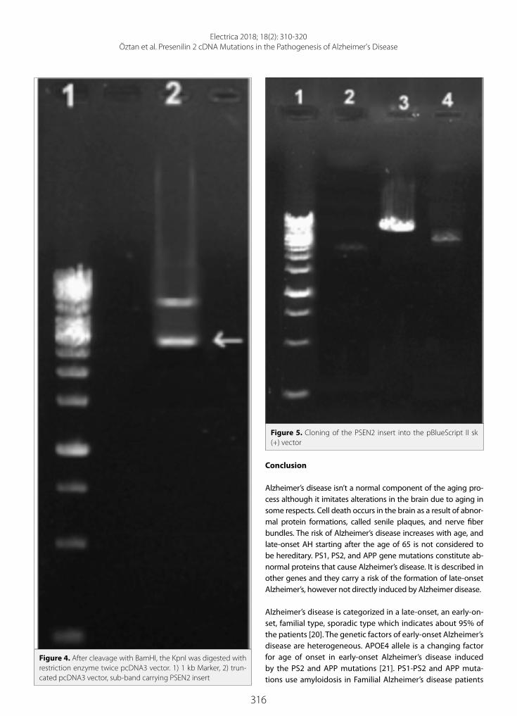
316


Conclusion

Alzheimer’s disease isn’t a normal component of the aging pro-cess although it imitates alterations in the brain due to aging in some respects. Cell death occurs in the brain as a result of abnor-mal protein formations, called senile plaques, and nerve fiber bundles. The risk of Alzheimer’s disease increases with age, and late-onset AH starting after the age of 65 is not considered to be hereditary. PS1, PS2, and APP gene mutations constitute ab-normal proteins that cause Alzheimer’s disease. It is described in other genes and they carry a risk of the formation of late-onset Alzheimer’s, however not directly induced by Alzheimer disease.

Alzheimer’s disease is categorized in a late-onset, an early-on-set, familial type, sporadic type which indicates about 95% of the patients [20]. The genetic factors of early-onset Alzheimer’s disease are heterogeneous. APOE4 allele is a changing factor for age of onset in early-onset Alzheimer’s disease induced by the PS2 and APP mutations [21]. PS1-PS2 and APP muta-tions use amyloidosis in Familial Alzheimer’s disease patients

Figure 4. After cleavage with BamHI, the KpnI was digested with restriction enzyme twice pcDNA3 vector. 1) 1 kb Marker, 2) trun-cated pcDNA3 vector, sub-band carrying PSEN2 insert

Figure 5. Cloning of the PSEN2 insert into the pBlueScript II sk (+) vector

317


through modifying the brain metabolism of Aβ peptides that

support the production of pathogenic aggregates [22]. PS1

gene mutations were contributed to 18- 55% of early-onset fa-

milial Alzheimer’s disease cases [21].

150 RNA samples from the entorhinal and auditory cortex and

the hippocampal areas of Alzheimer’s disease patients and con-

trol groups were analyzed using RT- PCR in the study performed

by Delabio et al. [23]. They didn’t observe differences between

Figure 6. Sequence analysis of the vector pBlueScript II sk (+) bearing PSEN2, Upper panel: 5 'end where the PSEN2 cDNA sequence starts, 3' end where the bottom panel line ends

Figure 7. Ala252Thr mutation generated on the PSEN2 cDNA sequence. Top panel wild-type array, bottom panel mutant array, arrow mutation location

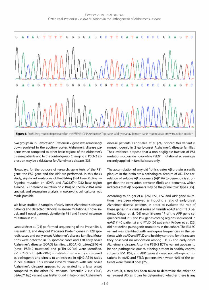
318


two groups in PS1 expression. Presenilin 2 gene was remarkably downregulated in the auditory cortex Alzheimer’s disease pa-tients when compared to other brain regions of the Alzheimer’s disease patients and to the control group. Changing in PSEN2 ex-pression may be a risk factor for Alzheimer’s disease [23].

Nowadays, for the purpose of research, gene tests of the PS1 gene, the PS2 gene and the APP are performed. In this thesis study, significant mutations of Pro334Arg (334 base Proline → Arginine mutation on cDNA) and Ala252Thr (252 base region Alanine → Threonine mutation on cDNA) on PSEN2 cDNA were created, and expression analysis in eukaryotic cell cultures was made possible.

We have studied 2 samples of early-onset Alzheimer’s disease patients and detected 10 novel missense mutations, 1 novel in-del, and 1 novel genomic deletion in PS1 and 1 novel missense mutation in PS2.

Lanoiselée et al. [24] performed sequencing of the Presenilin 1, Presenilin 2, and Amyloid Precursor Protein genes in 129 spo-radic cases and early-onset Alzheimer’s disease families. Muta-tions were detected in 18 sporadic cases and 170 early-onset Alzheimer’s disease (EOAD) families. c.850A>G, p.(Arg284Gly) (novel PSEN2 mutation) and p.(Thr122Pro) were identified. PS1 c.236C>T, p.(Ala79Val) substitution is recently considered as pathogenic and directs to an increase in Aβ42-Aβ40 ratios in cell cultures. This variant (several families with late-onset Alzheimer’s disease) appears to be related to a later onset compared to the other PS1 variants. Presenilin 2 c.211T>C, p.(Arg71Trp) variant was firstly found in late-onset Alzheimer’s

disease patients. Lanoiselée et al. [24] noticed this variant is nonpathogenic in 2 early-onset Alzheimer’s disease families. Their evidence propose that a non-negligible fraction of PS1 mutations occurs de novo while PSEN1 mutational screening is recently applied in familial cases only.

The accumulation of amyloid fibrils creates Aβ protein as senile plaques in the brain are a pathological feature of AD. The cor-relation of soluble Aβ oligomers (Aβ*56) to dementia is stron-ger than the correlation between fibrils and dementia, which indicates that Aβ oligomers may be the prime toxic types [25].

According to Krüger et al. [26], PS1, PS2 and APP gene muta-tions have been observed as inducing a ratio of early-onset Alzheimer disease patients. In order to evaluate the role of these genes in a clinical series of Finnish eoAD and FTLD pa-tients. Krüger et al. [26] exon16-exon 17 of the APP gene se-quenced and PS1 and PS2 genes coding regions sequenced in eoAD (140 patients) and FTLD (66 patients). Krüger et al. [26] did not define pathogenic mutations in the cohort. The E318G variant was identified with analogous frequencies in the pa-tients with eoAD and FTLD and healthy controls, for this reason, they observed no association among E318G and early-onset Alzheimer’s disease. Also, the PSEN2 R71W variant appears to be non-pathogenic, due to it being present in healthy control subjects. PS1, PS2, and APP genes showed no pathogenic mu-tations in eoAD and FTLD patients even when 40% of the pa-tients were familial ones [26].

As a result, a step has been taken to determine the effect on early-onset AD as it can be determined whether there is any

Figure 8. Pro334Arg mutation generated on the PSEN2 cDNA sequence. Top panel wild-type array, bottom panel mutant array, arrow mutation location

319


increase in Aβ42 in the protein level. Oligomerization and the structure mechanism of Aβ oligomers are very important for growing efficient therapeutics.

Lindquist et al. [27] presented a patient with neuropatholog-ically approved early‐onset AD described by deep language corruption. The case was heterozygous for a novel missense mutation in exon 11 of the PS2 gene leadingto a foreboded amino acid substitution from valine to methionine in position 393. In vitro expression of PSEN2 V393M cDNA didn’t result in detectable enhancing of the secreted Aβ42/40 peptide rate. The mutation wasn’t detected in 384 control subjects. It has been determined that amino acid substitution between methi-onine and valine is a conserved residue at position 393 in het-erozygous patients for the new missense mutations in PSEN2 gene in exon 11 [27].

Neuropathology and the clinical process of sporadic Alzhei-mer’s disease and familial Alzheimer’s disease are extremely identifiable, and FAD patients compose a unique population in which to conduct treatment and especially interception trials with new pharmaceutical entities. Our study suggests that in the future, the role of PSEN mutations on cellular phenotypes and understanding of molecular mechanisms will shed light on the potential effects of presenilin mutations on therapeutic strategies targeting the Amyloid beta peptide.

PSEN1 mutations are usually more related to an earlier onset of the disease than PSEN2 mutations even when they consist of homologous residues. Walker et al. [28] guessed that PSEN2 FAD mutations would have a impressive effect on the Aβ 42/40 ratio so that have an observable effect on Aβ levels in the pres-ence of normal PSEN1 alleles. To trial this hypothesis they ex-pressed PSEN2 and PSEN1 Familial Alzheimer’s disease mutant arrangements in fibroblasts derived from PSEN1 -/- mice and PSEN2 -/- mice, therefore the mutant presenilin protein was the only resource of presenilin available in the cells [28].

Their functional analyses of putative PSEN2 FAD mutations in-dicated that M239V, M239I, T122P, and N141I meaningfully in-creased Aβ-42 levels and Aβ 42-40 ratio as expected for FAD mu-tations. These mutations also produce a significant reduction in Aβ-40 levels. R62H, S130L, V148I, and D439A have no substantial impact on either Aβ 40/42 levels or Aβ 42/40 ratio [28].

Tomita et al. [29] showed cDNAs for wild-type PSEN2 and PSEN2 Volga German mutation (N141I) in culture cells and sub-sequently investigated the metabolism of the transfected pro-teins and their impact on the C-terminal features of excreted Aβ protein. This mutation (N141I) didn’t induce any substantial change in the metabolism of PSEN2 [29].

COS-1 cells two times transfected with cDNAs for N141I mu-tant PSEN2 and human β-APP or a C-end fragment, also mouse Neuro2a cells transfected with N141I mutant PS2 alone, secret-ed 1.5- to 10-fold more Aβ 42-43 compared with those express-

ing the wild-type PSEN2. Therefore, N141I mutation linked to familial Alzheimer’s disease modifies the metabolism of Aβ-βAPP to encourage the production the form of Aβ that easily deposits in amyloid plaques [29].

Following studies are required to explain the mechanisms re-sponsible for the effects of PS mutations on Aβ production and the progression of AD. Additionally, the available results en-sure strong assistance that the formation and deposition of Aβ 42/43 plays a critical pathogenetic role in Alzheimer’s disease.


Acknowledgements: The authors are grateful to Christine Van Broeck-hoven and Marc Cruts (VIB-UAntwerp Center for Molecular Neurology) for providing pcDNA3 vector carrying PSEN2 cDNA. This study is fund-ed by Halic Universtiy Research Fund.



References

1. A Kumar, S. A. Ekavali, “A review on Alzheimer’s disease patho-physiology and its management: an update”, Pharmacol Rep, vol. 67, no. 2, pp. 195-203, 2015.

2. J. Guo, J. Cheng, B. J. North, W. Wei, “Functional analyses of major cancer-related signaling pathways in Alzheimer’s disease etiolo-gy”, Biochimica et Biophysica Acta (BBA) - Reviews on Cancer, vol. 1868, no. 2, pp. 341-358, 2017.

3. P. A. Defina, R. S. Moser, M. Glenn, J. D. Lichtenstein, J Fellus, “Alz-heimer’s Disease Clinical and Research Update for Health Care Practitioners”, J Aging Res, 2013.

4. S. Parvathy, D. J. Buxbaum, “Molecular Genetics of Alzheimer Dis-ease”, Neuropsychopharmacology: The Fifth Generation of Prog-ress, pp. 1199-1213, 2002.

5. L. Crews, E. Masliah, “Molecular mechanisms of neurodegenera-tion in Alzheimer’s disease”, Human Molecular Genetics, vol. 19, no. R1, pp. 12-20, 2010.

6. M. B. Yokes, “Molecular genetics of Alzheimer’s Disease”, J Cell Mol Biol, vol. 6, no. 2, pp. 73-97, 2007.

7. P. H. St George-Hyslop, A. Petit, “Molecular biology and genetics of Alzheimer’s disease”, Comptes Rendus Biologies, vol. 328, no. 2, pp. 119-130, 2004.

8. M. Plečkaitytė, “Alzheimer’s disease: a molecular mechanism, new hypotheses, and therapeutic strategies”, Medicina, vol. 46, no. 1, 2010.

9. P. H. St George-Hyslop. “Molecular Genetics of Alzheimer’s Dis-ease”, Biol Psychiatry, vol. 47, no. 3, pp. 183-199, 2000.

10. Y. Cai, S. S. An, S. Kim, “Mutations in presenilin 2 and its implica-tions in Alzheimer’s disease and other dementiaassociated disor-ders”, Clin Interv Aging, vol. 10, pp. 1163-1172, 2015.

11. G. D. Schellenberg, T. D. Bird, E. M. Wijsman, H. T. Orr, L. Anderson, E. Nemens, J. A. White, L. Bonnycastle, J. L. Weber, M. E. Alonso, H. Potter, L. L. Heston, G. M. Martin, “Genetic linkage evidence for a familial Alzheimer’s disease locus on chromosome 14”, Science, vol. 258, pp. 668-671, 1992.

320


12. D. Campion, J. M. Flaman, A. Brice, D. Hannequin, C. Martin, V. Moreau, F. Charbonnier, O. Didierjean, S. Tardieu, C. Penet, M. Puel, F. Pasquier, F. Le Doze, G. Bellis, A. Calenda, R. Heilig, M. Martinez, J. Mallet, M. Bellis, F. C. Darpoux, Y. Agid, T. Frebourg, “Mutations of the presenilin I gene in families with early-onset Alzheimer’s disease”, Hum Mol Genet, vol. 4, no. 12, pp. 373- 377, 1995.

13. R. F. Clark, M. Cruts, K. M. Korenblat, C. He, C. Talbot, C. Van Broeck-hoven, A. M. Goate, “A yeast artificial chromosome contig from hu-man chromosome 14q24 spanning the Alzheimer’s disease locus AD3”, Hum Mol Genet, vol. 4, no. 8, pp. 1347-1354, 1995.

14. J. B. Kwok, K. Taddei, M. Hallupp, C. Fisher, W. S. Brooks, G. A. Broe, J. Hardy, M. J. Fulham, G. A. Nicholson, R. Stell, P. H. St George Hyslop, P. E. Fraser, B. Kakulas, R. Clarnette, N. Relkin, S. E. Gandy, P. R. Scho-field, R. N. Martins, “Two novel (M233T and R278T) presenilin-1 mutations in early-onset Alzheimer’s disease pedigrees and pre-liminary evidence for association of presenilin-1 mutations with a novel phenotype”, Neuroreport, vol. 8, no. 6, pp. 1537-1542, 1997.

15. C. Tysoe, D. Galinsky, D. Robinson, C. Brayne, F. A. Huppert, T. Den-ing, E. S. Paykel, D. F. Easton, D. C. Rubinsztein, “Apo E and Apo CI loci are associated with dementia in younger but not older late-onset cases”, Dement Geriatr Cogn Disord, vol. 9, no. 4, pp. 19119-19118, 1998.

16. N. Suzuki, T. T. Cheung, X. D. Cai, A. Odaka, L. Otvos, C. Eckman, T. E. Golde, S. G. Younkin, “An increased percentage of long amy-loid β protein secreted by familial amyloid β protein precursor (β APP717) mutants”, Science, vol. 264, pp.1336-1340, 1994.

17. K. Taddei, C. Fisher, S. M. Laws, G. Martins, A. Paton, R. M. Clarnette, C. Chung, W. S. Brooks, J. Hallmayer, J. Miklossy, N. Relkin, P. H. St George-Hyslop, S. E. Gandy, R. N.Martins, “Association between presenilin-1 Glu318Gly mutation and familial Alzheimer’s disease in the Australian population”, Mol Psychiatry, vol. 7, no. 7, pp. 776-781, 2002.

18. E. Levy-Lahad, W. Wasco, P. Poorkaj, D. M. Romano, J. Oshima, W. H. Pettingell, C. E. Yu, P. D. Jondro, S. D. Schmidt, K. Wang, A. C. Crowley, Y. Hui Fu, S. Y. Guenette, D. Galas, E. Nemens, E. M. Wijs-man, T. D. Bird, G. D. Schellenberg, R. E. Tanzi, “Candidate gene for the chromosome 1 familial Alzheimer’s disease locus”, Science, vol. 269, pp. 973-977, 1995.

19. E. I. Rogaev, R. Sherrington, E. A. Rogaeva, G. Levesque, M. Ikeda, Y. Liang, H. Chi, C. Lin, K. Holman, T. Tsuda, L. Mar, S. Sorbi, B. Na-cmias, S. Piacentini, L. Amaducci, I. Chumakov, D. Cohen, L. Lan-nfelt, P. E. Fraser, J. M. Rommens, P. H. Hyslop-St George, “Famil-ial Alzheimer’s disease in kindreds with missense mutations in a gene on chromosome 1 related to the Alzheimer’s disease type 3 gene”, Nature, vol. 376, no. 6543, pp. 775-778, 1995.

20. H. J. Birnbaum, D. Wanner, A. F. Gietl, A. Saake, T. M. Kündig, C. Hock, R. M. Nitsch, C. Tackenberg. “Oxidative stress and altered mi-tochondrial protein expression in the absence of amyloid-β and tau pathology in iPSC-derived neurons from sporadic Alzheimer›s disease patients”, Stem Cell Res, vol. 27, pp. 121-130, 2018.

21. C. Zekanowski, M. Styczyńska, B. Pepłońska, T. Gabryelewicz, D. Religa, J. Ilkowski, B. Kijanowska-Haładyna, S. Kotapka-Minc, S. Mikkelsen, A. Pfeffer, A. Barczak, E. Łuczywek, B. Wasiak, M. Choda-kowska-Zebrowska, K. Gustaw, J. Łaczkowski, T. Sobów, J. Kuźnicki, M. Barcikowska, “Mutations in presenilin 1, presenilin 2 and amy-loid precursor protein genes in patients with early-onset Alzhei-mer’s disease in Poland”, Experimental Neurology, vol. 184, no. 2, pp. 991-996, 2003.

22. S. Weggen, D. Beher, “Molecular consequences of amyloid precursor protein and presenilin mutations causing autosomal-dominant Alz-heimer’s disease”, Alzheimer’s Res Ther, vol. 4, no. 2, p. 9, 2012.

23. R. Delabio, L. Rasmussen, I. Mizumoto, G. A. Viani, E. Chen, J. Villares, I. B. Costa, G. Turecki, S. A Linde, M. C. Smith, S. L. Payão, “PSEN1 and PSEN2 Gene Expression in Alzheimer’s disease Brain: A New Ap-proach”, J Alzheimers Dis, vol. 42, no. 3, pp. 757-760, 2014.

24. H. M. Lanoiselée, G. Nicolas, D. Wallon, A. Rovelet-Lecrux, M. La-cour, S. Rousseau, A. C. Richard, F. Pasquier, A. Rollin-Sillaire, O. Martinaud, M. Quillard-Muraine, V. de la Sayette, C. Bouto-leau-Bretonniere, F. Etcharry-Bouyx, V. Chauviré, M. Sarazin, I. le Ber, S. Epelbaum, T. Jonveaux, O. Rouaud, M. Ceccaldi, O. Félician, O. Godefroy, M. Formaglio, B. Croisile, S. Auriacombe, L. Chamard, J. L. Vincent, M. Sauvée, C. Marelli-Tosi, A. Gabelle, C. Ozsancak, J. Pariente, C. Paquet, D. Hannequin, D. Campion, “APP, PSEN1, and PSEN2 mutations in early-onset Alzheimer disease: A genetic screening study of familial and sporadic cases”, PLoS Med, vol. 14, no. 3, p. e1002270, 2017.

25. S. Ngo, Z. Guo, “Key residues for the oligomerization of Aβ42 pro-tein in Alzheimer’s disease”, Biochem Biophys Res Commun, vol. 414, no. 3, pp. 512-516, 2011.

26. J. Krüger, V. Moilanen, K. Majamaa, A. M. Remes, “Molecular Genet-ic Analysis of the APP, PSEN1, and PSEN2 Genes in Finnish Patients With Early-onset Alzheimer Disease and Frontotemporal Lobar Degeneration”, Alzheimer Dis Assoc Disord, vol. 26, no. 3, pp. 272-276, 2012.

27. S. G. Lindquist, L. Hasholt, J. M. Bahl, N. H. Heegaard, B. B. Anders-en, A. Nørremølle, J. Stokholm, M. Schwartz, M. Batbayli, H. Laurs-en, R. Pardossi-Piquard, F. Chen, P. St George-Hyslop, G. Waldemar, J. E. Nielsen “A novel presenilin 2 mutation (V393M) in early-onset dementia with profound language impairment”, Eur J Neurol, vol. 15, no. 10, pp. 1135-1139, 2008.

28. E. S. Walker, M. Martinez, A. L. Brunkan, A. Goate, “Presenilin 2 familial Alzheimer’s disease mutations result in partial loss of function and dramatic changes in Ab 42/40 ratios. J Neurochem, vol.92, no. 2, 294-301. 2005;

29. T. Tomita, K. Maruyama, T. C. Saido, H. Kume, K. Shinozaki, S. Tokuhiro, A. Capell, J. Walter, J. Grünberg, C. Haass, T. Iwatsubo, K. Obata K, “The presenilin 2 mutation (N141I) linked to familial Alz-heimer disease (Volga German families) increases the secretion of amyloid beta protein ending at the 42nd (or 43rd) residue”, Proc Natl Acad Sci USA, vol. 94, no. 5. 2025-2030, 1997.

321

Introduction

ADSS cables are used in transmission lines and installed 3m-6m below the high voltage con-ductors [1]. Throughout their service life ADSS cables, stretched between poles of a high voltage transmission line, have to suffer several degradation mechanisms, such as humidity, pollution, ice load, wind, temperature variations, etc., which have a vital effect on the ageing and degradation process of the cable [2, 3]. In addition to the necessary tensile strength, cable manufacturers have also to consider the electrical stress mechanisms, which lead to accelerat-ed aging and finally damage or destruction of the cable jacket [4].

Wind causes a mechanical stresses on ADSS cables and hence stretches the outer insulation of the fiber- optic cable. This mechanical effect together with the corona discharge decreases the lifetime of the cable jacket considerably. In this study the effect of wind speed on the aging behavior of ADSS cables is investigated.

Wind might oscillate ADSS cables and hence decrease the distance between the ADSS cable and HV conductor, which eventually increases the electrical field that an ADSS cable has to suffer [1, 5]. A severe and extreme wind loading is usually observed by hurricanes, cyclones or other ocean born storms. In this paper, according to Turkey’s average wind conditions, sever-al levels of wind forces are generated in the laboratory artificially. Generally wind speed will cause the cable to deflect horizontally, hence the vertical sag according to the wind speed will be very small [5].

The damage analysis has been performed in order to establish a relation between the wind speed and life time of ADSS cable. The cable damage was observed as an erosion of the cable’s PE sheath between the clamps. Due to the rapid drying of the liquid, hot spots with a very high temperature are created on the surface of the cable. This process leads to the generation of dry ring zones and partial arcing. Damage is usually observed in the form of small holes and spongy residues similar to the classical tree pictures found in many track-ing and erosion tests [6]. Wind forces the liquid contaminant to settle down behind the

Electrica 2018; 18(2): 321-324

RESEARCH ARTICLE

Examination of Wind Effect on Adss Cables Aging Testİbrahim GüneşDepartment of Electrical & Electronics Engineering, İstanbul University School of Engineering, İstanbul, Turkey

Corresponding Author: İbrahim Güneş





DOI: 10.5152/iujeee.2018.1818

Cite this article as: Güneş İ, “Examination of Wind Effect on Adss Cables Aging Test”, Electrica, vol. 18, no:2, pp.321-324, 2018.

ABSTRACT

ADSS (All dielectric self supporting) cables are generally installed on high voltage transmission lines and mostly used under different environmental effects, such as temperature, wind, UV radiation, etc. In this study, wind affect on ADSS cables was investigated by using dry band arcing (IEEE 1222 Electrical surface degradation) test method. A wind source was implemented to the test setup to evaluate the performance of PE (Poly-ethylene) cable jacket on ADSS cable under different wind speeds. Test results indicate that life time of the ADSS cable decreases while the wind speed is increasing.

Keywords: Wind, ADSS, fiber-optic cable, aging, transmission lines

322

Electrica 2018; 18(2): 321-324Güneş İ. Examination of Wind Effect on Adss Cables Aging Test

cable, in contrast to the normal conditions where the con-taminant drops under the cable.

The main purpose of the present paper was to study the data-sets produced according to IEEE 1222 test standard and to find out whether the effect of wind could be integrated in a simpli-fied set of surface degradation test method [7].


In this study IEEE 1222 test standard ‘Dry-Band Arcing’ test method was used. To simulate the wind effect under laborato-ry conditions, a 24 W fan was added to the test set up and the wind speed is varied between 2,34m/s and 5,65m/s. The lim-its are chosen according to the average wind levels measured throughout Turkey [8]. The evaluated test system, which is giv-en in Figure 1, includes a 220V/36kV HV (high voltage) trans-former. To limit the current flowing on the ADSS cable, R and C components are chosen as 13.1 MΩ and 200 pF respective-ly. This RC values help to simulate medium pollution level for ADSS cables. To control the liquid contaminant spraying time and level, a flow control equipment was used. A similar test set up could be seen in some previous studies in more detail [9]. In order to vary the wind speed throughout the experiments, the distance between wind source and test sample was changed, where wind speed was measured by using YK-80AP Lutron An-emometer.

Wind effect produce a tensile strength on the ADSS cable, which eventually decreases the service life of ADSS cable. All tests are performed with samples prepared 46 cm in length. The distance between two electrodes was fixed 10.2 cm and they were placed on the middle of the test samples. By using an aluminum foil as an electrode, 25kV HVAC was applied one of the electrodes, where the other electrode is connected to the ground with a 50Ω resistor. [7]. The conductivity of the liq-uid contaminant, which is prepared by adding salt to deionized water, is measured as 17.2 mS ± %3 by using YK-22CT Lutron conductivity / TDS meter. During experiments initially test samples were sprayed by liquid contaminant up to 2 minutes and then allowed to dry for 28 minutes. The total 30-minute time period is called as one cycle and the measurement of the arc resistance is defined by the number of cycles needed to puncture the jacket.

According to IEEE 1222 standart, experiments were done until the ADSS cable get failed. The number of cycles determine the lifetime of the cable.

In the second part of the study a wind source was added to test set up. Initially wind speed is measured as a function of distance of the wind source (external fan) to test sample. Ta-ble 1 shows the variation of wind speed according to the dis-tance between the wind source and cable samples. During experiments temperature was continuously recorded and kept steady at 28 oC.

HV insulators and transmission lines located at mountains or similar rural areas are usually subjected to severe wind force, which cause an additional weight on the whole mechanical system. Especially by severe windstorms an HV transmission line located between two poles, might move considerably either to the left or right compared to its original position, which eventually reduces the security distance between lines and also alters the electromagnetic field. However since the wind force is applied perpendicular (from one side) to the transmission line and the weight of the conductor is quite high compared to the wind speed the HV transmission line can change its location only at high wind pressures. As shown in Table 2, the ADSS cable (D=16.5mm) has a unit weight of 2,2kg/m, hence with the application of artificial wind, the ca-ble has altered its location up to 0,86 degree, which seems eventually has not any affect on the total electrical field.

Test set up with the wind source is given in Figure 2 and the measurement technique is shown in Figure 3.

Min.5 cables were tested for each wind speed level, which were selected as 0, 2.34, 2.61, 2.76, 3.21, 4.03, 4.70 and 5.65 m/s to

Figure 1. Block diagram of the modified test set up for measuring the wind effect

Figure 2. Wind source added to the test set up

323


simulate the different regions in Turkey respectively. Each time the number of cycles for total failure was recorded and final-ly the average number of cycles and standard deviation were calculated.

Results

In this study the effect of wind speed on ADSS cable degrada-tion process is studied. The ADSS cables are generally located at 10m above the ground, hence according to standards the minimum wind level for this height should be selected as 12,2 m/s. However in order to simulate the real average wind speeds measured in Turkey much lower values are used throughout the experiments [10,11]. The measured lifetime of ADSS cable according to wind speed is given in Table 3. During the exper-iments the wet layer observed after spraying process is drifted through the back of cable surface depending on the pressure of the wind speed. This wind pressure forced the drops to stay on the cable and hence produce a conducting channel be-tween HV and ground electrode. As a result, due to the heat increase, the cable damaged faster than the conditions with-out wind pressure. The measured life cycles according to wind speed is given in Figure 4.

Conclusion

This study represents the actual behavior of ADSS cables used in Turkey at different wind speed levels. All the experiments were done under isolated conditions in the laboratory. Ag-ing tests indicate that life time of ADSS cables decrease with

Figure 3. Wind speed measurement system

Table 1. Wind speed (m/s) and distance to the wind source

Distance to the wind source (cm)

Measured wind speed (m/sec) Temperature (°C)

5 5.65 28

10 4.70 28

15 4.03 28

20 3.21 28

25 2.76 28

30 2.61 28

35 2.34 28

Table 2. Wind force and maximum deviation

Measured wind speed

(m/s)

Wind pressure (kg/m2)

Wind force

(kg/m)

Unit weight (kg/m)

Deviation (degree)

5.65 1.99 0.0328 2.2 0.85

4.70 1.38 0.0227 2.2 0.59

4.03 1.01 0.0166 2.2 0.43

3.21 0.65 0.0107 2.2 0.27

2.76 0.47 0.0077 2.2 0.20

2.61 0.42 0.0069 2.2 0.18

2.34 0.34 0.0056 2.2 0.14

Figure 4. Wind pressure and the life time of ADSS cables accord-ing to wind speed

( ¡) W

ind

Pres

sure

(kg/

m2 )

( ) Life time (m

in)

Wind Speed (m/s)

0.00 1.00 2.00 3.00 4.00 5.00 6.00

900.00

800.00

700.00

600.00

500.00

400.00

2.50

2.00

1.50

1.00

0.50

0.00

Table 3. Life time of ADSS cables at different wind speed.

Measured wind speed (m/s)

Average lifetime of the ADSS cable(cycle)

5.65 16.70

4.70 17.44

4.03 19.20

3.21 19.91

2.76 21.10

2.61 23.56

2.34 24.09

0 26.80

324


increasing values of wind speed. The wind speed of 2.61m/s, which is the average value for east region of Turkey, is the critical level for decrease of life time for ADSS cable. Over this value the aging process is accelerated rapidly. During experiments without any wind effect, water drops take place under the cable jacket. Continuous sparks and arcs damage the cable sheath after approximately 26,80 cycles. For higher wind speeds, water drops split to the back of the cable jacket which is opposite to wind direction, and hence the arcs occur behind the cable jacket. Wind can establish a lateral force on ADSS cables, which can cause mechanical fatigue and also alter the electrical field. However as stated in Table 2, at low wind speeds, only the location of the wet layer is changed rather than the position of the whole conductor, hence in such cases the cable is only degraded due to continuous arcs. Low values of wind speed changes the electrical field and tensile force slightly, hence they do not have any consid-erable effect on the lifetime of the ADSS cable.




References

1. G. Karady, E. Al-Ammar, B. Shi, M.W. Tuominen, ‘Experimental Verification of The Proposed IEEE Performance and Testing

Standard for ADSS Fiber Optic Cable for Use on Electric Utility

Power Lines’, IEEE Trans Power Del, vol. 21, no. 1, pp. 450-455,

Jan. 2006.

2. G. Karady, D. Srinivasan, ‘Algorithm to predict dry-band arcing in

fiber-optic cables’, IEEE Trans Power Del, vol. 16, no. 2, pp. 286-291,

Apr. 2001.

3. NASA Scientific and Technical Aerospace Report, Volume 42, Issue

5, March 12, 2004.

4. US Patent 6519396, ‘Aerial cable containing optical transmission

elements and process for the manufacture of an aerial cable’, US

Patent Issued on February 11, 2003.

5. Applications Engineering Note, Sag and Tension, Corning Cable

Systems, November 2002.

6. F.G. Kaidanov, ‘ADSS Cables Recognizing the Problems and Solu-

tions’, Transmission and Distribution World, Oct 1, 2002.

8. IEEE 1222 standarts ‘IEEE Standard for All Dielectric Self Support-

ing Fiber Optic Cable’, 2004.

9. R. Kose, M.A. Ozgur, O. Erbas, A. Tugcu, ‘The Analysis of Wind

Data and Wind Energy Potential in Kutahya, Turkey, Renewable

& Sustainable Energy Review; vol. 8(3), p.277- 288, 2004.

10. S. Kucuksari, Gunes I., G. Karady, ‘A Novel Method to Test the

Quality of ADSS Fiber Optic Cables Installed in Transmission

Lines’, IEEE Powertech 2009, Bucharest, Romania , 28 June-2 July

2009.

11. G.G. Karady, Q. Huang, D. Srinivasan, M. Tuominen, M. Reta-Her-

nandez, ‘Sensor Design for Leakage Current Measurement on

ADSS Fiber-Optic Cable’, Power Engineering Society Winter Meet-

ing, IEEE, 28 Jan-1 Feb 2001

Ibrahim Gunes, was born in Edirne, Turkey. He received his B.Sc., M.Sc. and Ph. D. degrees in Electrical and Electronics Engineering from Istanbul University in 1999 ,2005 and 2010, Currently, he is an Asist. Prof. Istan-bul University- Cerrahpaşa in Electrical-Electronics Engineering Department. , His research interests are high voltage insulation materials and high voltage technology.

325

Introduction

The passive components occupy 80% of the surface of a low-power converter. They have several roles, such as the temporary storage of electrical energy, filtering, electrical isolation, energy transfer as well as impedance matching. Today, only the integration of passive com-ponents is achievable, especially with inductive components. The barrier of integrating active components remains the most persistent obstacle that slows the rush to miniaturization [1, 2]. At the heart of isolated converters, there exists an essential element, the transformer. By reducing the dimensions, conventional coils are limited since they are wound with copper wire which prevents size reduction. The micro-transformers are formed from a thin magnetic circuit, usually made of ferrite, and on which conductive coils are inserted. The aim is to inte-grate the transformer in a micro-converter of flyback type for low voltages, low powers and high frequencies. The conception of a transformer goes through several phases: analysis of specifications, calculation and dimensioning of transformer parameters and validation by nu-merical simulation. In this work, the micro-transformer is presented under a form completely different to the geometric form of a classical transformer. This geometry is a square spiral and it adapts to the integrated technology [3, 4].

Dimensioning of the Micro Transformer

Presentation of the Micro Transformer

The micro converter fly-back presented in Figure 1, is the starting point for the design of passive components and especially, the micro transformer. This converter was chosen be-cause it is composed of a transformer and few passive components. It operates in discon-tinuous conduction when the current demanded by the load is low, and in continuous conduction for higher currents. To produce such a device, we start with conventional trans-former windings. To implement this function, it is necessary to have a magnetic core around

Electrica 2018; 18(2): 325-332

REVIEW

Design of Micro-Transformer in Monolithic Technology for High Frequencies Fly-back Type ConvertersAbdeldjebbar Abdelkader , Hamid Azzedine Department of Electrical Engineering, USTO-MB University School of Engineering, Oran, Algeria

Corresponding Author: Abdeldjebbar Abdelkader





DOI: 10.26650/electrica.2018. 96182

Cite this article as: A. Abdelkader, H. Azzedine, ”Design of Micro-Transformer in Monolithic Technology for High Frequencies Fly-back Type Converters”, Electrica, vol. 18, no: 2, pp. 325-332, 2018.

ABSTRACT

This article describes the design of a micro-transformer in monolithic technology for high frequencies comprising planar type coil and a magnetic circuit made of several layers of materials. This micro-transformer is integrated into a micro-converter of fly-back type. The Mohan method was used to determine the geometric parameters and the S-parameters were used to calculate technological parameters. The study of electromagnetic effects allowed us to show the role of ferrite, which is used to confine the magnetic field lines and minimize disruption of the neighbor ship. To validate the dimensioning of the geometrical and technological parameters, with the help of the software PSIM6.0, we simulated the equivalent electrical circuit of the converter containing the electrical circuit of the dimensioned planar micro-transformer

Keywords: Fly-back converter, Planar Micro-Transformer, S-parameters, inductive elements, passive

https://orcid.org/0000-0001-9462-898X

326

Electrica 2018; 18(2): 325-332Abdelkader and Azzedine. Design of Micro-Transformer in Monolithic Technology

which the primary and secondary windings are placed. This transformer, due to the magnetic coupling, naturally induces the effects of leakage mainly related to the choice of place-ment of windings.

The Specifications of the Micro-Converter

We selected the following set of specifications:Input voltage Vin = 10v ,Output voltage Vout = 4vCurrent output means Is = 1.5AAverage power Ps = 6W, Operating frequency f = 40MHz

The Characteristics of the Materials Used

The Table 1 below shows the characteristics of the materials constituting the coil layers.

It shows the different geometric and electrical parameters that constitute the micro transformer Figure 2 [6]. A core with a square form for the windings has been chosen due to the lim-itation of surface and volume.

Dimensioning of the Magnetic Circuit

From the specifications, we define the characteristics of the micro-converter which is the starting point for the design of micro-transformer. It consists of two inductors placed on a magnetic material and separated by a dielectric, which also provides magnetic coupling. The values of the frequency f and the input voltage Ve allow us to calculate the value of the pri-mary and secondary inductances Lt and Lb of our transformer [7, 8].

(1)

(2)

m: turn ratio=0.4 , Lt = 52nH and Lb = 8.3nH

Calculation of the Energy Stored In The Magnetic Core

The dimensioning of the magnetic core depends on the vol-ume required to store energy which is calculated from the vol-umetric energy density given by equation (3) [9].

(3)

Calculation of the Volume Density Of Energy

To determine the volume V of permalloy (NiFe) necessary for this storage, we need to know the volume density of energy of this material. This volume V is given by relationship (4) [10].

(4)

Figure 1. Schematic diagram of fly back converter [5]

Figure 2. The different parameters characterizing the micro-trans-former [7]

Table 1. Characteristics of used materials

Materiel Copper NiFe SiO2

Conductivityσ (S/m) 5,99.107 2,2.104 0

Resistivity ρ (Ω.m) 1,7.10-8 20.10-8 106

Relative Permittivity εr 1 10 3,9

Relative permeability μr 1 800 1

327


With a relative permeability µr =800 and saturation induc-tion Bmax=0.6T of permalloy, we obtain: Wmax=179jm-3, and V=0.052mm3 of Nife is needed to store 0.937 µJ.

Core Dimensions

With the volume of the ferromagnetic core being evaluated as V=0.052mm2, the core as a block is considered as having a thickness of Nifee and a section of A=dout

2, S is the section on which we will put the spiral coil. To define the dimensions of the core see Figure 3, dout=1800 µm was opted for and we sec-tion A and the thickness core Nifee was calculated by using equation “7”

(5)

Calculating of Turn’s Number

The primary and secondary values of inductance are given by the following formulas (method Mohan) [12, 13].

(6)

(7)

Dmoy is the average diameter of the inductor defined from the inner diameter and outer diameter dout and din equation (8) [14].

(8)

ρ is the form factor, defined by relationship “9”

(9)

C1, C2, C3, C4 are the constants of Mohan given by Table 2.

Table 2. The constants of mohan

Geometry C1 C2 C3 C4

Square 1.27 2.07 0.18 0.13

The primary and secondary turn’s numbers are calculated by using expressions 10 and 11

(10)

(11)

After calculation, we find: nt = 5, nb = 2

Calculating the width of the primary and secondary conductors

To eliminate the skin effect so that the electrical current is dis-tributed over the entire section of the conductor, one of the following conditions must be satisfied: W≤2δ or t≤2δ

Where w and t the width and thickness of the conductor. For a frequency f = 40 MHz, ρcopper=1.7.10-8 [Ω.m] and µr=1 [H/m] a skin thickness δ is obtained by used of equation “12”, [15].

(12)

We impose one of two values W or t and compute the second. It is preferable to impose the value of the thickness “t” of the con-ductor, since the width W should be optimized to reduce the parasitic effects linked to the substrate and the core. By assign-ing to “t” a value that verifies ≤2δ , the width can be calculated by the use of equation (13).

=S W .t (13)

When a current I flows in a conductor of section S its current density Javg is given by expression (14).

(14)

(15)

Figure 3. Geometric form of the magnetic core [11]

328


In most cases, the micro-wires are in contact with a semicon-ductor substrate that has good heat conduction properties. This allows boundary conditions of 9 2

oJ 10 A / m= [14].

by considering the same surface current density in the two windings, and the same thickness value of the primary and sec-ondary conductors t, we obtain the following results. Results are obtained by putting t=20.76 µm, Wt and Wb

Calculation of primary and secondary Inter-turn’s spacing St and Sb

(16)

(17)

Calculation of primary and secondary Conductorlength

(18)

(19)

All parameters that go into the design of the micro-transformer are represented in the summary Table 3 below.

The results ontained are in agreement with integration, be-cause the values of the different geometric parameters are within the recommended dimensions for the integration in low power electronics.

Modeling of Micro Transformer

The use of S-parameters will help to determine the values of the primary and secondary inductances, the primary and sec-ondary series resistors and the quality factor. The calculation with the S-parameters is made from the π-electric model of the micro-transformer “Figure 4”.

S11, S12, S21, S22 are the S parameters. Z0 = 50 Ω is the characteris-tic impedance of the line.

From the low-frequency S-parameters, the Z-parameters at each frequency point are determined. This can be shown as follows:

From these equations we find the variables that make up the model Pi shown in “Figure 4” and the inductances of the prima-ry Lt and secondary Lb. These inductances are taken from the imaginary part of the impedances, are expressed by expression (20) [16, 17].

(20)

And series resistors of the integrated inductors rst primary and rsb secondary are extracted from the real part of the impedanc-es and are expressed by expression “21”

(21)

Table 3. Values of the geometrical parameters

Geometrical parameters Values

Outer diameter: dout 1800 µm

Inner diameter: din 900 µm

Core thickness: e 16.15 µm

Skin thickness: δ 10.38 µm

Number of primary turns: nt 5

Number of secondary turns: nb 2

Width of the primary Wt 45 µm

Width of the secondary: Wb 196.87 µm

Thickness of the primary: tt 20.76 µm

Thickness of the secondary: tb 20.76 µm

Primary spacing: St 56.25 µm

Secondary spacing: Sb 56.25 µm

Primary total length: lt 2.7 cm

Secondary total length: lb 1.07 cm

Figure 4. Network Model of integrated transformer [7]

329


The expressions of quality factors extracted from the real and imaginary part of the impedances are given by expressions “22”

(22)

The transformer model Figure 5 is similar to the model of a spi-ral inductor. Indeed, the transformer is simply a pair of spiral inductor magnetically coupled. This model includes the series inductances of the primary and secondary coils (Lt , Lb), the se-ries resistances of second primary coil (rst,rsb), the coupling ca-pacitances between the turns (Cov1,2), the capacities between the secondary and primary coils and the substrate (Coxt, Coxb), the substrate capacity of primary and secondary coils (Cst,Csb)

Calculation of the Electrical Parameters

Presented now are the analytical expressions of the electrical circuit’s different elements [7].The series resistance: rst ,rsb

(23)

The oxide capacities: Coxt, Coxb

(24)

The coupling capacitance between the turns Covt ,Covb Cov1,2 :

(25)

(26)

The substrate capacity of primary and secondary coils: Cst,Csb :

(27)

The substrate resistance of the primary and secondary coils: Rst, Rsb

(28)

(29)

3.2. Results of Electrical Parameter’s Calculation

The Table 4 summarizes the different calculated electrical pa-rameters.

Figure 5. Model of the equivalent electrical circuit of micro-trans-former [13]

Table 4. Values of micro-transformer's electrical parameters

Electrical parameters Values

primary inductance Lt 52 nH

secondary inductance Lb 8.3 nH

Primary serial resistance rst 1.11Ω

Secondary serial resistance rsb 0.10 Ω

Primary oxide capacitance Coxt 2.96 pF

Secondary oxide capacitance Coxb 5.08 pF

Primary résistance of substrate Rst 2.99 KΩ

Secondary résistance of substrate Rsb 1.74 KΩ

Primary capacitance of du substrat Cst 0.64 pF

Secondary capacitance of substrate Csb 1.10 pF

Capacitance inter-spacing of primary Covt 0.16 pF

Capacitance inter-spacing of secondary Covb 0.064 pF

Coupling capacitance between the primary and secondary coils Cov1

5.45 pF

Coupling capacitance between the secondary and primary coils Cov2

10.05 pF

Primary magnetic resistance Rmt 5.22 µΩ

Secondary magnetic resistance Rmb 3.04 µΩ

330


The Influence of Frequency on the Inductances of the Pri-mary and Secondary

“Figure 6” shows the influence of the frequency on the induc-tances of the primary Lt and secondary Lb. These inductances are extracted from the imaginary part of the impedances and are given by the expressions (20).

The figure above shows two distinct zones specific to the op-eration of the integrated inductors (primary and secondary). At the operating frequency (40MHz), the inductive behavior is recognized. Beyond the resonance frequency (80MHz), it is the capacitive behavior.

Influence of Frequency on the Series Resistances of the Pri-mary and Secondary

“Figure 7” shows the influence of the frequency on the series resistors rst of primary and rsb of secondary. These resistances are extracted from the real part of the impedances and are ex-pressed as (21).

The resistances rst and rsb have very low values at the operating frequency (40 MHz), so the losses by Joule effects are very low. At resonance, the primary and secondary series resistances re-sult in a peak.

Influence of Frequency on the quality Factor of Primary and Secondary Inductances

“Figure 8” shows the influence of the frequency on the quality factors of inductors primary and secondary. The expressions of quality factors extracted from the real and imaginary imped-ances are given by the expression “22”.

Simulation of the Equivalent Electrical Circuit

Simulations were conducted to determine the influence of losses on the micro converter. The PSIM 6.0 software has been selected to simulate the operation of the converter. The follow-ing three electrical parameters of the micro converter had to be calculated [10].Load resistance of the Fly-back converter

(30)

Capacity of the fly-back converter, for a voltage undulation equal to 0.01V, the capacitor C is equal to:

(31)

Magnetizing inductance

(32)

The integrated Transformer

The transformer that we will be placed in the converter is loss-less (integrated). Now the equivalent circuit of the converter containing the micro transformer is simulated.

The electrical circuit of the assembly is given in Figure 9.The simulation of voltages and currents are calculated by using the PCIM6.0 software.

Figure 6. Influence of the operating frequency on the value of Lt and Lb inductors

Figure 7. Influence of primary and secondary series resistance versus frequency

331


For the integrated transformer, the results Figure 10 are encour-aging because a continuous output voltage and a continuous output current are obtained and their values are very close to those of the specifications (Vs= 4.2V and Is = 1.6A).

Therefore, it can be concluded that the geometrical dimension-ing of the transformer gave good results.

Simulation of Different Effects on the Micro Transformer

In this section, we the distribution of magnetic field lines in the micro-coils of the micro transformer will be presented.

Using the FEMLAB 3.1 software, an overflow of the magnetic field lines in all directions can be observed in Figure 11. These lines occupy all the space and are stopped only by the simula-tion boundaries of a coil in the air. This distribution can induce disturbances of the components located in the immediate vi-cinity of the micro transformer.

In Figure 12, the coils are deposited on a magnetic core, the majority of these field lines being confined in this core. This is explained by the high permeability of ferrite. The insertion of

Figure 8. Quality factor of primary and secondary versus frequency Figure 10. Output voltage of the micro converter containing the integrated transformer

Figure 11. Magnetic field distribution in the micro-transformer without magnetic core

Figure 9. Equivalent electrical circuit of the micro converter contain-ing the integrated transformer

332


the ferrite layers thus makes it possible to increase the number of magnetic field lines and to limit their overflow.

Conclusion

The aim of this study is to integrate the geometrical dimen-sioning of a micro-transformer and its electromagnetic model-ing, into a micro-converter. This micro-transformer is intended for the field of mobile and embedded electronics requiring a conversion of energy of low power and a very high frequency range. The integrated micro-transformer is composed of sever-al stacked layers, namely: two copper square planar coil wind-ings, insulating layers, layers of ferrite magnetic material and a semiconductor layers.

As a starting point for this study, the specifications of the fly-back type micro-converter was chosen. In the second part, ac-cording to the operating conditions of the system based on the method of Mohan, the geometrical dimensioning of the planar transformer was carried out.

In the third part, the geometric parameters to extract the var-ious electrical parameters were used. In the last step, we inte-grated the dimensioned micro-transformer into a micro-con-verter. This step facilitated the testing of the operation of the micro-transformer. In order to validate our results, a simulation with PSIM6.0 was pwerformed using FEMLAB 3.1 simulation software to visualize the dispersion of the magnetic field lines for two different transformer models, a model with a core, and the second without a core.


Conflict of Interest: The authors declared that this study has received no financial support.


References

1. K. Youssouf, “Modélisation des transformateurs planaires intègres. Optics Photonic”, Université Jean Monnet-Saint- Etienne, France, 2014.

2. D. D. Yaya, “Conception, réalisation et caractérisation d’induc-tances planaires à couches magnétiques”, Université Jean Mon-net-Saint-Etienne, France, 2013.

3. B. Vallet, «Étude et conception d’une nouvelle alimentation à découpage à transfert d’énergie mixte basée sur un composant passif LCT intégré” Université Joseph Fourier, 2008.

4. A. Besri, “Modélisation analytique et outils pour l’optimisation des transformateurs de puissance haute fréquence planars”, Universi-té de Grenoble, 2011.

5. T. H. Trinh, “Réseaux de micro convertisseurs, les premiers pas vers le circuit de puissance programmable”, Energie électrique, Univer-sité de Grenoble, 2013.

6. R. Melati, A. Hamid, F. Baghdad, F. Taibi, “Simulation d’une micro bobine”, 4ème Conférence Internationale sur l’Electrotechnique, Oran, Algeria, 2009.

7. S. Verma, J. M. Cruz, “On-chip Inductors and Transformers”, Biblio-metrics, 1999.

8. F. K. Wong, B. Eng, M. Phil, “High Frequency Transformer for Switch-ing Mode Power Supplies”, School of Microelectronic Engineering, Faculty of Engineering and Information Technology, Griffith Uni-versity, Brisbane, Australia, 2004.

9. V. Boyer, N. Godefroy, “Alimentation à découpage Flyback”, M1-IUP GEII, Université Joseph Fourier IEEE.

10. M. Derkaoui, A. Hamid,T. Lebey, R. Melati, “Design and Modeling of an Integrated Micro-Transformer in a Flyback Converter”, TELKOM-NIKA, vol. 11, no. 4, pp. 669-682 , 2013.

11. D. M. Pozar “Microwave Engineering”, 2nd Edition, Johnwiley and Sons Inc., 1998, pp.19-20, pp. 182-250.

12. S. Mohan, C.P. Yue, M. Del Mar Hershenson, S. Wong, T.H. Lee, “Modeling and characterization of on-chip transformers”, Interna-tional Electron Devices Meeting 1998, 1998, pp. 531-534.

13. S. S. Mohan, “The design modeling and optimization of on-chip inductor and transformer circuits”, 1999.

14. C Alonso, “Contribution à l’optimisation, la gestion et le traitement de l’énergie”, Université Paul Sabatier Toulouse III, 2003.

15. X. Margueron “Elaboration sans prototypage du circuit équivalent des transformateurs de type planar”, Université Joseph Fourier, 2006.

16. R. Thüringer “Characterization of Integrated Lumped Inductors and Transformers”, Wien, 2002.

17. A. Weisshaar. “Analysis and Modeling of Monolithic On- Chip Transformers on Silicon”, Oregon State University, 2005.

Figure 12. Magnetic field distribution in the micro-transformer with a magnetic core

Abdeldjebbar Abdelkader, Diploma in Electrical Engineer 1997, Diploma of magister in plasma 2009, Student in the doctorate from 2010 to date

Electrica - İstanbul Üniversitesi

Documents

Transcript of Electrica - İstanbul Üniversitesi