Eindhoven University of Technology MASTER Inventory ...

Eindhoven University of Technology

MASTER

Inventory control for a lost-sales system with joint-replenisment in an e-commerceenvironment

Buying, R.A.L.

Award date:2017

Link to publication

DisclaimerThis document contains a student thesis (bachelor's or master's), as authored by a student at Eindhoven University of Technology. Studenttheses are made available in the TU/e repository upon obtaining the required degree. The grade received is not published on the documentas presented in the repository. The required complexity or quality of research of student theses may vary by program, and the requiredminimum study period may vary in duration.

General rightsCopyright and moral rights for the publications made accessible in the public portal are retained by the authors and/or other copyright ownersand it is a condition of accessing publications that users recognise and abide by the legal requirements associated with these rights.

• Users may download and print one copy of any publication from the public portal for the purpose of private study or research. • You may not further distribute the material or use it for any profit-making activity or commercial gain

https://research.tue.nl/en/studentTheses/3f9d636f-be3a-42d4-bf58-2afb6783d9bf

Inventory Control for a Lost-sales system with

Joint-replenishment in an e-commerce

environment

A Master Thesis Project at Optiply: Supply Management Software

By Roel Buying

BSc Industrial Engineering & Innovation Sciences – TU/e 2014

Student ID 0740236

In partial fulfilment of the requirements for the degree of

Master of Science

in Operations Management and Logistics

Master thesis (1CM96)

Eindhoven University of Technology, March 2017

Supervisors TU/e - OPAC

Dr. Ir. H.P.G. (Henny) van Ooijen

Prof. Dr. A.G. (Ton) de Kok

Dr. K.H. (Karel) van Donselaar

Supervisors Optiply

Ir. S. (Sander) van den Broek

Ir. W. (Wiebe) Konter

Series Master Theses Operations Management and Logistics

Key terms: e-commerce, replenishment, replenishment model, inventory control, stock control, inventory

control system, inventory management, joint replenishment, JRP, lost-sales system, target service level, fill

rate, ready rate, SKU classification, ABC classification, demand forecasting, exponential smoothing, process

control, SPC,

i

Abstract Abstract

Companies with webshops in an e-commerce environment face many different uncertainties

regarding inventory control. Uncertainties such as lost-sales resulting from excess demand,

stochastic joint replenishment, highly variable but slow demand and stochastic lead-times. This

report describes the development of a model and associated decision support tool that address

these uncertainties. The model includes replenishment policies that were developed throughout

the design process. Functions from the model were verified and validated based on a scenario

analysis and a model comparison with the use of a self-developed simulation tool. The findings

and results of this analysis are combined in the development of a decision support that assists in

making inventory control decisions by estimating fill rates, inventory cost and other relevant

parameters for as many products as desired.

ii

Management summary Management summary

In this master thesis report we present our research on inventory control in a single-echelon lost-

sales system that takes into account joint replenishment under stochastic highly variable demand

and stochastic lead-times. As a case study the supply chain of Company B Webshops B.V. is

chosen from the customer network of the supervising company Optiply B.V.

Problem statement

Optiply is an innovative young company operating in an business-to-consumer e-commerce

environment. Their customer network mainly consists of companies that own one or more

webshops. These so called e-tailers sell their products online and rarely own a physical shop but

do store their products. The core business model of Optiply is designed to automate the

replenishment process of their customers such that inventory control is of a high standard and

does not need much expertise nor manual labor. In this way the Optiply attempts to ‘replace the

logistic experts of this world’ with their model. The case study company we call ‘Company B’ is a

company that manages numerous webshops and has an assortment of thousands of different

products. Companies such as Company B order their products to multiple suppliers from all over

the world. They face challenges such as high uncertainty in demand of their products, uncertainty

in the lead-times of their suppliers and a rapidly growing e-commerce market with many

competitors. Within this uncertain environment inventory levels have to be maintained correctly

and the replenishment process for all products has to be cost efficiently coordinated.

Based on the problem analysis and the gained business insight on the problem similarities of the

companies in the customer network of Optiply, we defined a research assignment that has the

goal to solve the different problems that these companies face in their daily inventory control.

This main assignment is defined as:

Develop a decision support tool that assists in minimizing total inventory cost in a single-echelon

lost-sales system taking into account joint-replenishment under lead-time, order moment and

demand uncertainty for a given target service level.

Analysis of inventory control in the e-commerce environment

Inventory control problems in the as-is situation of the case study company were found to be a

combination of business environmental factors and the fact that inventory control is often

overlooked because companies are rapidly growing and putting all business effort in this growth

only. By environmental factors we refer to uncertainties in demand making it difficult to forecast,

variable lead-times from suppliers and online customers that are price and delivery time sensitive.

Because customers can compare prices or check delivery times online with great ease, switching

to competitors occurs often and products are rarely backordered. As a result, excess demand is

typically lost and the related inventory system is transformed from a backorder system into a lost-

sales system. Lost-sales result in the fact that demand in periods without stock on hand is not

iii

known. This unobserved demand is difficult to uncover and replenishment decisions are therefore

often based on historical sales, if it is based on anything at all. Taking into account the holding

cost of holding stock on hand, the ordering cost of ordering to the suppliers and aiming at

satisfying customer demand (i.e. target service level), the replenishment process results in a joint

replenishment problem in a lost-sales system where inventory and replenishment has to be

coordinated tightly. Therefore, the four main components of the inventory control problem are:

1. Taking into account lost-sales (i.e. unobserved demand)

2. Which replenishment model(s) to use for the 𝑛 replenishment problems

3. Coordinating replenishments by joint replenishment

4. Target service level and 𝑠-level setting

New model development

During the design phase of our research we considered different solution concepts which we

described extensively in this report. In solving the inventory control problems we combined or

adapted some of these concepts and developed a new inventory control model. This model

includes two approaches that estimate the unobserved demand in periods without stock on hand,

a method to determine the supplier review period and product order quantities to coordinate

product replenishment and two periodic replenishment policies. These two policies are largely

based on the (𝑅, 𝑆) and (𝑅, 𝑠, 𝑆) replenishment policies but differ in their parameters. We

therefore defined 𝑅𝛿 as the review period that is determined for a supplier 𝛿. This review period

is based on the demand and cost from all products 𝑖 ordered to that supplier and coordinates

the replenishment of all these products to the supplier. Furthermore, we defined reorder level 𝑠𝑖

and order-up-to-level 𝑆𝑖 which are both based on a specific product 𝑖. Once, every review period

the inventory position (i.e. stock on hand plus inventory on order in a lost-sales system; stock on

hand plus inventory on order minus backorders in a backorder system) is brought back up to this

order-up-to level. However, in the (𝑅𝛿 , 𝑠𝑖, 𝑆𝑖) replenishment policy the inventory position is only

is brought back up to the order-up-to level if the inventory position is below the reorder level 𝑠𝑖.

The calculations of both policies in the new model were found to be accurate under highly variable

stochastic demand and stochastic lead-times. By using the new model policies, reorder level

calculations, cost calculations and other output parameters, calculations become more tractable

and rational within the decision making process. Furthermore, we described multiple 𝑠-level

correction methods to achieve target service levels when demand is forecasted or simulated.

However, these correction methods are not one-on-one applicable to the inventory system with

characteristics such as lost-sales, compound renewal demand and more complex forecasting

methods than simple exponential smoothing.

Case study

Additional to a scenario analysis where we verified the calculations of the new model, we

compared the performance of the new model compared with the model currently utilized by

Optiply. In almost all simulated scenarios, the new model policies outperformed the policies from

the Optiply model with respect to inventory cost efficiency and achieved fill rate. Moreover, we

iv

showed that the new model policies perform acceptable under highly variable and unpredictable

demand taking demand forecasts as input parameter. Comparing the two replenishment policies

within the new model only, the (𝑅𝛿 , 𝑆𝑖) replenishment policy outperformed the (𝑅𝛿 , 𝑠𝑖, 𝑆𝑖)

replenishment policy with respect to total inventory cost and achieved fill rate. The reason for this

is that the order-up-to level (i.e. reorder level plus economic ordering quantity) is calculated in

such a way that there should be enough inventory to last for the whole replenishment cycle. In

the (𝑅𝛿 , 𝑠𝑖, 𝑆𝑖) replenishment policy the inventory level is sometimes not brought back to the

order-up-to level due to variability in demand during the review period. Therefore, the inventory

level is lower in the coming replenishment cycle and the probability of a stock-out is higher

resulting in a lower fill rate. Only focusing on holding cost and ordering cost, the (𝑅𝛿 , 𝑆𝑖) policy

obviously performed worse because the inventory position is brought back to the order-up-to

level in almost every review period which results in ordering more frequently and higher inventory

levels. An interesting finding is that the 95% confidence intervals of the simulated output

parameters of the (𝑅𝛿 , 𝑆𝑖) replenishment policy were tighter in almost every scenario, which

means that in the long term the different inventory cost and the achieved fill rate are less variable

under the (𝑅𝛿 , 𝑆𝑖) replenishment policy than under the (𝑅𝛿 , 𝑠𝑖, 𝑆𝑖) replenishment policy.

Additionality we research target service level setting for the fill rate service level and the ready

rate service level and how both service level relate to each other. We showed that if we increase

the variability of demand in a compound renewal process, the deviation between the fill rate and

the ready rate becomes larger (i.e. 𝑃2 < 𝑃3).

Decision support tool

We developed a decision support tool that encompasses the calculations and decision rules of

the new model and its components. This tool can be integrated into the model of Optiply or be

used independently. The tool enables the calculation of reorder levels, order-up-to levels, supplier

review periods, order quantities and other relevant inventory parameters for as many products as

desired. In the basis, the tool only requires position of sales data (POS data), stock changes data

and cost and target fill rate setting. Based on demand input parameter calculations, a forecast

method and an approach to take into account unobserved demand, the tool determines the

continuous demand parameters. Thereafter the tool calculates all relevant output parameters and

provides the user with suggestions on the setting of supplier review periods, economic order

quantities, reorder-levels and order-up-to levels for every product. Additionally, the tool provides

estimations for the holding cost, ordering cost, average inventory levels and service levels.

v

Preface Pr eface

Six months, and therefore approximately 15% of my time at the Eindhoven University of

Technology, were spend on conducting my Master Thesis Project. One could say that it is the

largest project that I have undertaken in my whole life up until this moment, and I think this is

indeed the case. This report describes the results of that Master Thesis Project, which I conducted

at Optiply Supply Management Software in Eindhoven. It concludes my Master in Operations

Management and Logistics and brings my time at the Eindhoven University of Technology to an

end.

I would like to thank the people that supervised me during my Master Thesis Project. First of all, I

would like to thank Henny van Ooijen, for being my first supervisor. I am grateful for having him

as my mentor during the whole process of conducting my Master Thesis Project. I could always

come to you if I had questions or wanted to discuss certain design choices related to the project.

Your feedback throughout my project was very helpful and constructive.

Secondly, I would like to thank my second supervisor Ton de Kok for his feedback and suggestions

throughout my project. During the end of my project I got very familiar with the ladies of the eSCF

secretary due to the fact that they helped me with the intensive process of planning my meetings

with you.

I would also like to thank my third supervisor Karel van Donselaar for taking the time to review my

report and showing interest in my work.

Lastly, I would like to show appreciation to both my supervisors of Optiply, Sander van den Broek

and Wiebe Konter. Thanks to you both I was able to conduct my project at a young, innovative

and interesting company where I learned much about inventory control in an e-commerce

environment. It has been a good time discussing how we could overcome problem situations by

looking at it from different perspectives and attempting to find the best practical solution. I am

grateful to have learned so much about programming in R and applying it in the field of inventory

control and replenishment planning.

For me personally, this is an end of an era. My struggle against the Ragnarøk has ended (Lindholm,

1991). It is time to earn back my student loan.

Roel Buying

Eindhoven, March 2017

vi

List of content List of content Abstract ...........................................................................................................................................................................................i

Management summary ............................................................................................................................................................. ii

Preface ........................................................................................................................................................................................... v

List of content ............................................................................................................................................................................. vi

List of figures ............................................................................................................................................................................... ix

List of tables ..................................................................................................................................................................................x

List of abbreviations ................................................................................................................................................................... xi

Introduction................................................................................................................................................................................... 1

1. Optiply & Company B ........................................................................................................................................................... 2

1.1 Supervising company introduction - Optiply .......................................................................................................... 2

1.2 Case study company introduction – Company B ................................................................................................. 3

1.3 Problem statement ......................................................................................................................................................... 5

2. Research assignment ............................................................................................................................................................ 6

2.1 Literature review & first considerations .................................................................................................................... 6

2.2 Assignment ...................................................................................................................................................................... 8

2.3 Deliverables ...................................................................................................................................................................... 9

2.4 Scope ................................................................................................................................................................................. 9

2.5 Methodologies .............................................................................................................................................................. 10

2.6 Thesis outline ................................................................................................................................................................. 10

3. Analysis of the case situation ........................................................................................................................................... 12

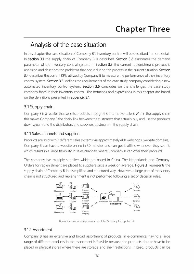
3.1 Supply chain ................................................................................................................................................................... 12

3.2 Demand .......................................................................................................................................................................... 14

3.3 The replenishment process ....................................................................................................................................... 16

3.4 Current key performance indicators....................................................................................................................... 18

3.5 Conclusion ...................................................................................................................................................................... 18

4. Model development ........................................................................................................................................................... 19

Part one – Conceptual solutions.......................................................................................................................................... 19

4.1 Lost-sales problem ....................................................................................................................................................... 19

4.2 Replenishment policy .................................................................................................................................................. 20

4.3 Joint replenishment ..................................................................................................................................................... 21

4.4 Service level and s-level setting ............................................................................................................................... 23

vii

4.5 Conclusion ...................................................................................................................................................................... 26

Part two – The modified replenishment policies ............................................................................................................ 27

4.6 The 𝑹𝜹, 𝑺𝒊 and (𝑹𝜹, 𝒔𝒊, 𝑺𝒊) replenishment policy .............................................................................................. 27

5. Case study ............................................................................................................................................................................. 31

5.1 Components of the model ......................................................................................................................................... 31

5.2 Verification ..................................................................................................................................................................... 36

5.3 Comparison with the Optiply model ...................................................................................................................... 38

5.4 Service level setting ..................................................................................................................................................... 44

5.5 Conclusion ...................................................................................................................................................................... 47

6. Implementation of the Decision support tool ............................................................................................................. 48

7. Conclusions & Recommendations .................................................................................................................................. 49

7.1 Conclusions ..................................................................................................................................................................... 49

7.2 Recommendations ....................................................................................................................................................... 52

7.3 Recommendations for future research .................................................................................................................. 54

A. E-commerce characteristic environment ..................................................................................................................... 57

B. Literature review .................................................................................................................................................................. 59

B.2 Joint replenishment ..................................................................................................................................................... 61

B.3 s-level adjustments ...................................................................................................................................................... 62

B.4 SKU classification .......................................................................................................................................................... 65

B.5 Process control ............................................................................................................................................................. 67

B.6 Demand forecasting & underlying demand distribution ................................................................................. 67

C. Detailed deliverables .......................................................................................................................................................... 68

D. Methodologies ..................................................................................................................................................................... 70

E. Single-echelon inventory model ..................................................................................................................................... 72

E.1 Definitions ....................................................................................................................................................................... 72

E.2 Generic expressions for single-item single-echelon replenishment policies .............................................. 74

F. Classic joint replenishment problem (JRP) ................................................................................................................... 75

F.1 Definitions ........................................................................................................................................................................ 75

F.2 Assumptions ................................................................................................................................................................... 77

G. Solution concepts ............................................................................................................................................................... 78

H. Optiply review period on a supplier level .................................................................................................................... 86

I. Impute demand data heuristic .......................................................................................................................................... 87

J. Derivations of relevant parameters ................................................................................................................................. 89

J.1 Demand during lead-time .......................................................................................................................................... 89

viii

J.2 Demand during the review period .......................................................................................................................... 92

J.3 Undershoot ..................................................................................................................................................................... 92

J.4 Expected stock on hand .............................................................................................................................................. 93

J.5 Service levels .................................................................................................................................................................. 94

K. Derivations of cost functions ............................................................................................................................................ 97

K.1 Holding cost function .................................................................................................................................................. 97

K.2 Ordering cost function ............................................................................................................................................... 98

K.3 Shortage cost function ............................................................................................................................................. 102

L. Company specific cost specifications ........................................................................................................................... 105

M. Fill rate calculation verification ..................................................................................................................................... 107

N. Cost functions calculation verification ......................................................................................................................... 112

N.1 Holding cost function ................................................................................................................................................ 112

N.2 Ordering cost function ............................................................................................................................................. 113

O. Simulation model input parameters ............................................................................................................................ 115

P. Implementation Decision support tool ........................................................................................................................ 116

P.1 Input & output parameters ....................................................................................................................................... 116

P.2 Features ......................................................................................................................................................................... 118

P.3 User manual................................................................................................................................................................. 120

P.4 Tool user interface ..................................................................................................................................................... 123

Q. Detailed elaboration of underlying research objectives ....................................................................................... 126

References ................................................................................................................................................................................ 129

ix

List of figures List of figures

Figure 1: The stock value of the stock on hand in Euros from 2015-10-21 to 2016-09-01 .................................... 4

Figure 2: Scope of the Master Thesis Project................................................................................................................... 10

Figure 3: A structured representation of the Company B’s supply chain ................................................................ 12

Figure 4: Pareto curves of percentage of total revenue in case situation ............................................................... 13

Figure 5: Sales per day of product "269452" and product "1272290" from 2015-09-01 to 2016-09-01 ......... 14

Figure 6: Sales per day of product "270498" from 2015-11-01 to 2016-09-01 ........................................................ 16

Figure 7: Inventory level (𝑅, 𝑠, 𝑆) replenishment policy in a backorder system and lost-sales system .......... 60

Figure 8: The reflective cycle including the regulative cycle (Heusinkveld & Reijers, 2009) .............................. 70

Figure 9: Operations research model (Mitroff et al., 1974) ...........................................................................................71

Figure 10: Welch graphical method .................................................................................................................................. 108

Figure 11: Decision support tool features in IDEF0 notation ....................................................................................... 118

Figure 12: A3. Output parameter calculation in IDEF0 notation................................................................................ 118

Figure 13: Basic flowchart of Decision Support Tool .................................................................................................... 125

x

List of tables List of tables

Table 1: Characteristics of the current environment of Optiply and Company B ................................................... 4

Table 2: Mean and standard deviation of supplier's lead-times ................................................................................ 18

Table 3: Differences between SJRP in the case situation and the SJRP literature ................................................. 22

Table 4: Replenishment policy parameters ...................................................................................................................... 30

Table 5: Relevant parameters of products comparison between Optiply model and the New model ......... 40

Table 6: Simulation results Optiply model vs. New model under generated demand target fill rate 95% .. 41

Table 7: Simulation results Optiply model vs. New model under real sales data target fill rate 95% ............ 43

Table 8: Simulation results Optiply model vs. New model under actual experienced sales with imputed

demand on the days without stock and target fill rate 95% ....................................................................................... 44

Table 9: Simulation results scenario 4 ................................................................................................................................ 45

Table 10: Requirements of Company B considering an inventory control system ............................................... 69

Table 11: Holding cost representation for 10 randomly chosen SKUs ..................................................................... 105

Table 12: Shortage cost representation for 10 randomly chosen SKUs .................................................................. 106

Table 13: Simulation results scenario 1 ............................................................................................................................. 109

Table 14: Simulation results of relevant parameters scenario 1 ................................................................................. 110

Table 15: Simulation results scenario 2 ............................................................................................................................. 110

Table 16: Simulation results scenario 3 ..............................................................................................................................111

Table 17: Holding cost simulation results ......................................................................................................................... 112

Table 19: Simulation model input parameters ................................................................................................................ 115

Table 20: Simulation model input parameters ............................................................................................................... 115

xi

List of abbreviations List of abbreviati ons

CV: Coefficient of Variation

DGS: Direct Grouping Strategy

EM: Expectation Maximization

EOQ: Economic Order Quantity

ETS: Exponential Smoothing State Space Model

IGS: Indirect Grouping Strategy

iid: Independent and Identically Distributed

JRP: Joint Replenishment Problem

KPI: Key Performance Indicator

LSP: Lost-Sales Problem

MAD: Mean Absolute Deviation

MASE: Mean Absolute Scaled Error

ME: Mean Error

MSE: Mean Squared Error

POS: Point Of Sale

RMSE: Root Mean Squared Error

NBD: Negative Binomial Distribution

NN: Neural Network

nOO: Number of Outstanding Orders

OPAC: Operations Planning Accounting & Control

Rδ: Review period on a supplier level based on all product ordered to supplier 𝛿

SJRP: Stochastic Joint Replenishment Problem

SKU: Stock Keeping Unit

TPOP: Time Phased Order Point

1

Introduction Introduc tion

In this master thesis report we present our research on inventory control in a single-echelon lost-

sales system taking into account joint replenishment under stochastic highly variable demand and

stochastic lead-times. The research is conducted at Optiply Supply Management Software in

Eindhoven. Optiply operates in an innovative and agile e-commerce environment. Customers in

the network of Optiply are mostly webshops that vary in assortment from hundreds to thousands

of different SKUs. These companies operate in an environment that is rapidly growing, where

products have short lifecycles and demand is difficult to predict.

Optiply’s core business is based on an innovative developed inventory control model that includes

several approximation algorithms to estimate relevant parameters. The algorithm is separated in a

tactical and an operational model. The tactical model includes replenishment models with sampled

demand which are used to determine relevant parameters required for inventory control. In the

operational model these replenishment models are combined with demand forecasting models to

estimate output parameters including safety stocks and order quantities. Optiply would like to

improve their algorithms and its fit on replenishment in an e-commerce environment. With the

current model it seems that target service levels are not met and inventory levels suggested by the

model are not accurate enough. Moreover, the model is based on sales only and the company

would like to take into account the demand in periods without stock on hand.

Scientific research on the application of existing replenishment models and demand forecasting

methods in an e-commerce environment is scarce and in reality, inventory control is often outdated

or even overlooked by e-commerce companies. This Master Thesis therefore addresses the

problem of companies in an e-commerce environment that face many uncertainties in their

replenishment process but do not have the knowledge to improve their inventory control and grip

on the replenishment process. In this project, a mathematical model is developed that attempts to

minimize the total inventory cost of an inventory control system under certain assumptions and a

target fill rate. Thereafter, a decision support tool is developed for Optiply that assists in the decision

process regarding inventory control. The tool takes sales/demand data and stock changes data as

input parameters and provides the user with relevant output parameters such as reorder levels,

holding cost, ordering cost and expected inventory levels.

2

Chapter One

1. Optiply & Company B

This first chapter introduces two companies. First, an introduction is made to Optiply, the

supervising company of the Master Thesis Project. Thereafter, an introduction is made to Company

B, a company that inspired us to perform a case study on. Company B therefore, will be referred

to as the case study company in this Master Thesis Project. In section 1.1 the supervising company

Optiply is briefly introduced. Section 1.2 introduces the case study company ‘Company B’ and the

environment the company is working in. In section 1.3 the problem statement and the as-is situation

of Company B is described briefly.

1.1 Supervising company introduction - Optiply

Optiply specializes in inventory optimization and focuses their business on the e-commerce

industry. The e-commerce industry has several large market segments such as B2B e-commerce

and B2C e-commerce. Customers in the customer network of Optiply include companies such as

webshops and retailers with a focus on online sales (e-tailers). The company developed a model

that helps in decision making with regard to inventory control. The improved decision making may

reduce inventory levels and increases revenue by helping webshops to determine when and how

much to order of which product. Certain parameters in the model can be adjusted to make it useful

in different inventory control situations that are experienced by customers. The model is sold as a

service package in combination with potential replenishment advice, implementation and training.

The company was founded in 2015 by two freshly graduated students and has grown into a current

team of seven. These seven persons come from different technology backgrounds such as

Operations Management & Logistics, Software Science, Data Science and Data Engineering. The

company is growing and increasingly hiring employees and graduation interns.

Optiply has always been looking to improve and strengthen their inventory control model. The

most relevant problems that occur in this process are focused on process control, replenishment

models, cost setting and demand forecasting. One of the next steps for Optiply is to improve their

inventory control model by using big data techniques to implement external data such as the

weather, Google positions and web analytics in the algorithm. This external data could help

enhance the forecasts by explaining a larger part of the variance in the demand data. Optiply is a

company that is located on the intersection between replenishment models, data science and e-

commerce.

1.1.1 Office locations and processes of Optiply

The main office is based in Eindhoven and is located on the campus of the Eindhoven University

of Technology. This location focusses on development processes. Located in the Multi Media

Pavilion of the university, the company is close to information and knowledge that flows from the

3

Operations Planning Accounting & Control (OPAC) department of the university. Furthermore,

appropriate new members for their team can be attracted from the university. Marketing processes

are being outsourced for approximately 90% and are supervised by the main Office in Eindhoven.

The second office is based in Amsterdam and is especially focused on data science. Some of the

development is performed here by integrating the achieved external data into the inventory control

model. The location of this office is chosen because studies such as Data Science and Econometrics

are located in Amsterdam. It is possible for employees to work on both locations.

1.1.2 Inventory control model of Optiply

Optiply developed an inventory control model that is based on a statistical approximation

algorithm, which is separated in a tactical model and an operational model. The tactical model

contains replenishment models and is used to determine important parameters such as the safety

time and the order quantity time which are the safety stock and order quantity expressed in time.

The operational model involves a combination of the tactical model with certain forecasting

methods. These forecasting methods are based on historical sales or demand data and are able to

cope with trends and seasons in demand.

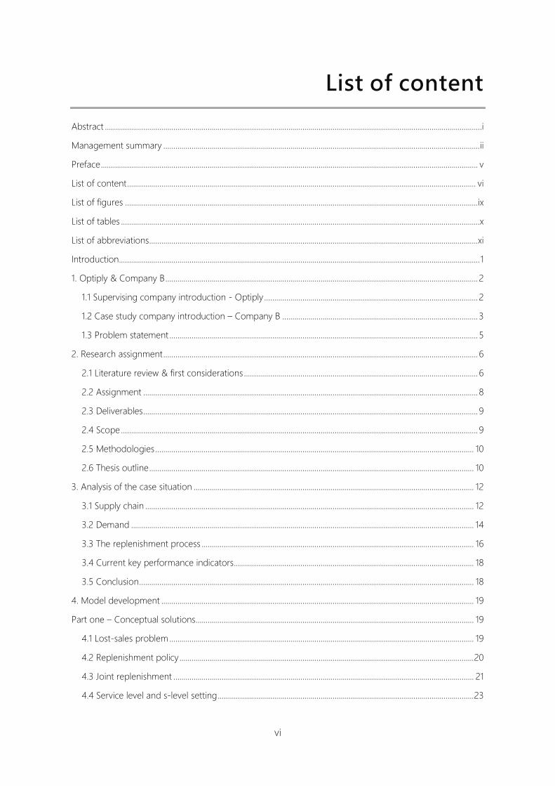
1.2 Case study company introduction – Company B

Company B is a company from within the customer network of Optiply. The company’s main office

is located in Groningen and manages approximately 400 webshops in The Netherlands and

Germany. Their product assortment throughout the year consists of more than 3000 SKUs ranging

from computer accessories to household appliances and from cleaning products to food

supplements. Approximately 40% of their assortment is non-active. Products are offered for sale

on their own websites and on larger webshop platforms such as Bol.com, Coolblue.nl and

Markplaats.nl. Company B has been rapidly growing throughout the last years and introduced

some fast selling products since the fall of 2016. The average stock on hand of Company B has a

value ranging from 180,000 to 190,000 euros and Company B orders on average 120 different SKUs

per day. Figure 1 shows the value of the stock on hand from 2015-10-21 to 2016-09-01. The

warehouse management system (WMS) that is used by Company B is called Picqer. Picqer is an

online warehouse tool that helps in managing the warehouse and sales channels and is focused

on webshops. Picqer was implemented on 2015-10-21 and for this reason the graph starts at this

date. Stock data for analysis in the Master Thesis Project is therefore available since this date.

The black line in figure 1 represents the total stock value in Euros. The large peak around the middle

of May 2016 is due to a large purchase of four products that were expected to sell in the coming

periods. We see that the stock value has an increasing trend, which is due to the fact that the

company is growing.

4

Figure 1: The stock value of the stock on hand in Euros from 2015-10-21 to 2016-09-01

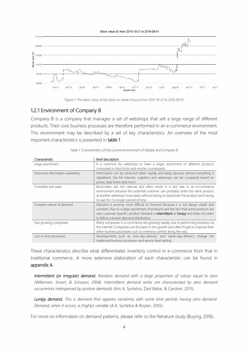
1.2.1 Environment of Company B

Company B is a company that manages a set of webshops that sell a large range of different

products. Their core business processes are therefore performed in an e-commerce environment.

This environment may be described by a set of key characteristics. An overview of the most

important characteristics is presented in table 1.

Table 1: Characteristics of the current environment of Optiply and Company B

Characteristic Brief description

Large assortment It is common for webshops to have a larger assortment of different products

compared to their brick-and-mortar counterparts.

Improved information availability Information can be retrieved rather rapidly and easily because almost everything is

digitalized. Via the internet, suppliers and webshops can be compared based on

prices, lead-times and more.

Complete lost-sales Backorders are not rational and often result in a lost sale in an e-commerce

environment because the potential customer can probably order the same product

at another webshop more easily without having to backorder the product and having

to wait for it a longer period of time.

Complex nature of demand Demand is proving more difficult to forecast because it is not always stable and

constant. Due to a large assortment of products and the fact that some products are

very customer specific, product demand is intermittent or lumpy and does not seem

to follow a known demand distribution.

Fast growing companies Many companies in e-commerce are growing rapidly due to performing business via

the internet. Companies are focused on this growth and often forget to improve their

other business processes such as inventory control along the way.

Just-in-time processes Developments such as ‘one-day-delivery’ and ‘same-day-delivery’ change the

traditional business processes and service level setting.

These characteristics describe what differentiates inventory control in e-commerce from that in

traditional commerce. A more extensive elaboration of each characteristic can be found in

appendix A.

Intermittent (or irregular) demand. Random demand with a large proportion of values equal to zero

(Willemain, Smart, & Schwarz, 2004). Intermittent demand series are characterized by zero demand

occurrences interspersed by positive demands (Aris A. Syntetos, Zied Babai, & Gardner, 2015).

Lumpy demand. This is demand that appears randomly with some time periods having zero demand.

Demand, when it occurs, is (highly) variable (A.A. Syntetos & Boylan, 2005).

For more on information on demand patterns, please refer to the literature study (Buying, 2016).

5

1.3 Problem statement

Company B manages a very large variety of products and sells these products through

approximately 400 webshops. Some of these webshops offer many different products and some

only offer one product (i.e. one product webshops). A large part of the assortment consists of slow

moving products that only sell a couple times per year. These products often follow demand

patterns that are hard to forecast, resulting in inappropriate stock levels. Some products have an

unnecessary high stock level, while many other products have zero stock because these products

are simply forgotten about.

The large number of different products is ordered to a relatively small number of suppliers, which

means that for in some situations hundreds of products are ordered to the same supplier. The

ordering of these products has to be coordinated due to fixed ordering cost that are made every

time an order is placed to the supplier. Therefore, using a replenishment policy that takes into

account this coordination of placing orders for the different products is important. However, the

process of deciding which policy to use and how to implement it may prove difficult. Standard

replenishment policies may not be applicable and an adapted or extended replenishment policy is

required. The inventory control problem we have here can be described as a joint replenishment

problem (JRP). The standard form of the JRP is described in appendix F. More case specific

elaboration on the JRP can be found in section 4.3 and appendix B.2.

Demand in the case situation is not forecasted. Replenishment of products is performed based on

managerial judgment, what in the case situation boils down to ordering what is deemed to sell in

the coming period based on sales in the past. Factors such as historical demand of the product,

historical demand of other products and supplier information may be essential in the demand

forecasting process, but is left out in the case situation. Because backorders are not rational in the

environment Company B is working in, a non-sale typically results in a lost-sale. Whenever a

product is out of stock, the product is typically removed from the website of the webshop. In this

way potential customers cannot find the product and essential information about the demand for

the specific product is lost. An inventory control system where excess demand results in lost-sales

can be seen as a lost-sales system and is described extensively in section 4.1 and appendix B.1 (K.

Van Donselaar, De Kok, & Rutten, 1996).

Currently, the fixed ordering cost is not clearly specified. It is not specified per supplier or per

product group or individual product. Fixed ordering cost is an important parameter in the inventory

control system. This parameter is included in the trade-off between ordering products and holding

products in storage. Moreover, the decision of which replenishment policy to use is, among other

parameters, also based on the fixed ordering cost.

6

Chapter Two

2. Research assignment

This chapter describes the research assignment that is foundation of the Master Thesis Project and

the gaps in the literature that led to this assignment. Section 2.1 elaborates on the scientific papers

that were analyzed in the literature study and in the preparation of the modeling phase of the

project. Section 2.2 defines the main assignment of the project and defines the underlying research

objectives. The deliverables of the project are described in section 2.3. In section 2.4 the scope of

the project is described. Section 2.5 elaborates on the used methodologies in the project. The last

section, section 2.6, provides the outline of the thesis. The notations and expressions in this chapter

are largely based on the definitions and expressions by de Kok et al. (2012) and are presented in

appendix E.1.

2.1 Literature review & first considerations

This section briefly describes the relevant literature from the literature study that was performed in

preparation of the Master Thesis Project. Note that numerous relevant additional scientific papers

were analyzed during the project. A review on this literature can be found in appendix B. We would

also like to refer to the literature study itself (Buying, 2016). This section will only elaborate on the

main findings from reviewing the literature. Note that much of the reviewed literature will function

as an input for the model development in chapter four.

2.1.1 Literature study conclusions

This section describes what relevant gaps could be found in the scientific literature. The performed

analysis combines the scientific literature reviewed in the literature study and the scientific papers

reviewed throughout the first part of the Master Thesis Project.

In the stochastic joint replenishment literature demand if often assumed to be (compound) Poisson

and excess demand is completely backordered in the inventory systems, which makes them

backorder systems. Lead-times are often assumed to be fixed, deterministic or a multiple integer

of the review period, which itself is also assumed deterministic or fixed. In almost every paper a

major fixed ordering cost is incurred per order in combination with minor ordering cost per

product. In practice, this is not always the case. Furthermore, many scientific papers focus on finding

the optimal solution to the 𝑠-levels while according to Khouja and Goyal (2008) researchers should

focus more on developing applicable models for the real life inventory problems (Khouja & Goyal,

2008).

While lost-sales systems are relevant in real world practices, most scientific papers on stochastic

inventory models assume excess demand being backordered. The reason for this limited attention

for lost-sales system in the scientific literature is the fact that discrete-time inventory models in

7

combination with stochastic demand are very difficult and (optimal) solutions always include

dynamic programming (Zipkin, 2008).

In line with this complexity, scientific papers on periodic lost-sales systems often assume the lead-

time to be a fixed or a random integral multiple of the review period. Only a few papers address a

periodic inventory system with fractional lead-times; i.e., the lead time is smaller than the length of

a review period. Models with fractional lead-times may prove useful in an e-commerce

environment for the products that are slow moving (i.e. these products have a long review period

because they are only sold once or twice per year; the lead-time is likely to be smaller than the

review period for such products). Sezen (2006) studied he impact of the review period length on

the average stock on hand and the fill rate through a simulation approach in case of fractional

lead-times. The results show that the variability in the demand process is the most important factor

to set the duration of a review period. No analytical procedure is proposed to determine the length

of a review period or on how to set the order-up-to level (Bijvank & Vis, 2011). Furthermore, most

developed models focus on inventory systems in which no fixed order cost is charged. Although

many papers proposed properties and bounds on the optimal order quantities, they still require

much computational effort to find the optimal order quantities, especially for large inventory

systems. The combination of a stochastic joint replenishment problem in a lost-sales system is rarely

studied in the scientific literature. All lost-sales literature that was reviewed, led us to believe that

providing an optimal solution for the joint replenishment lost-sales problem is very computational

intensive and an heuristic or self-developed approach would be useful in the conceptual model of

our research.

SKU classification may be performed on two different levels. Firstly, SKU classification considering

demand forecast methods. Fast selling products experience a different demand pattern than slow

selling products. Therefore, products with certain characteristics may be forecasted differently than

other products. Secondly, SKU classification considering replenishment policies and service level

setting. Products differ in characteristics such as supplier, fixed ordering cost and holding cost.

Therefore, it seems intuitive to classify products based on different relevant characteristics rather

than only on demand value and demand volume or no classification at all.

What is missing in the demand forecasting literature is a trade-off between error performance of

a demand forecasting method and other performance measures such as service levels and

inventory costs. Demand forecasting methods are often evaluated considering forecasting errors

such as MAD, MSE and RMSE. However, the output of these errors is rarely combined with inventory

control parameters to represent the impact of the forecasting method on the performance of the

inventory system. Related to combining demand forecasting performance and inventory control

performance, is the earlier described statistical process control (SPC). An interesting future research

direction would be to develop a method that can trigger changing the safety stock levels or reorder

levels when experienced demand deviates from demand forecasts so greatly that the difference

between experienced demand and forecasted demand reaches a certain threshold. When this

threshold value is reached, safety stock or reorder levels have to be adjusted. In this way it can be

8

decided when and how much the safety stocks, and possible other safety measures, have to be

adjusted to guard against future demand uncertainties. The same holds for deviations in target

service levels.

2.2 Assignment

The characteristics of the environment, the as-is situation at Company B and the described issues

in inventory control, led us to define the following main assignment:




2.2.1 Underlying research objectives

In this section the underlying research objectives are described that will help in accomplishing the

main assignment of our Master Thesis Project. Every underlying research objective is divided into

a set of research questions or tasks to clarify what actions should be performed to complete the

underlying research objective. The underlying research objectives form the structure of our project.

1. Describe the as-is situation of inventory control at Company B.

(a) What are the they characteristics of the environment Company B is working in and what

are the characteristics of Company B itself?

(b) What are the processes that are carried out by Company B for inventory control in the

case situation? (e.g. replenishment, inventory management)

(c) How does Company B measure the performance of their inventory control and which

KPIs are defined?

(d) What are the problems that occur in the case situation of inventory control and in which

areas is there a scope for improvement?

(e) What requirements does Company B have considering improving their inventory

control?

2. Provide conceptual solutions aimed at the joint replenishment problem, complete lost-sales

and the other problem areas by combining theoretical and practical knowledge and model

these solutions into a mathematical model

(a) Which model can be used as input in the process of developing a solution for the overall

joint replenishment problem and what adaptions or extensions have to be made?

(b) Which model can be used as input in the process of developing a solution for the

complete lost-sales component and what adaptions or extensions have to be made?

(c) What are relevant parameters in the conceptual model and how should these

parameters be measured?

(d) How are the key components of the conceptual model connected to each other?

(e) Develop a mathematical model where the conceptual solutions for the different

components and parameters of the inventory control system are modeled.

9

3. Analyze the inventory control model developed by Optiply and relate it to the conceptual

solutions in the process of developing an inventory control model that can perform in an e-

commerce characteristic environment.

(a) In what way can the existing inventory control model of Optiply be used as input for

the development of decision support tool that takes into account the characteristics of

an e-commerce environment?

(b) What relevant (new) inventory control components can be adapted or developed to

integrate into the inventory control model?

4. How can the current inventory control model and the suggested improvements of the

conceptual model be combined into a decision support tool that takes into account the

components of an e-commerce characteristic environment?

(a) Combine the different components of the conceptual model and integrate the

components into a decision support tool with different parameters that can be altered.

(b) Define the relevant KPI of the model and the decision support tool.

(c) Test the decision support tool and simulate different inventory control situations by

measuring their KPI output under an service level or cost efficiency constraint.

(d) Compare the output of the new inventory control situations with the as-is situation of

Company B and test what settings of parameters achieve the best results.

(e) Perform a sensitivity analysis to test the importance of the different parameters in the

model and determine measures of uncertainty for the model.

(f) Develop and generalize the decision support tool such that it can be utilized to analyze

(demand) data from other companies within and outside of the customer network of

Optiply.

5. Write an implementation plan on the recommended use of the decision support tool for

inventory control.

(a) Describe the features of the tool and how Optiply or customers in the network from

Optiply can use these features.

(b) What actions need to be performed by Optiply to implement the usage of the decision

support tool?

2.3 Deliverables

The deliverables of this Master Thesis Project are based on the five underlying questions and have

the objective of answering them for the case situation in chapter four. The description of the

deliverables and our research setup can be found in appendix C.

2.4 Scope

In this section of the report, the scope of our research is described. The project will be conducted

in a time period of approximately six months. Due to this time limit, the project should be

converged accordingly. In this section of the scope and the level of detail of the project are

described. The project is carried out within the Development team of Optiply, therefore Data

10

Science implementations such as external data are excluded from the scope of this research.

Company B will be analyzed as case study company and the developed model and decision

support tool that result from this analysis will thereafter be generalized into a tool that can be used

by Optiply and potential other companies. Figure 2 represents the scope of the our research and

is divided in the case study and the generalization. Moreover, Optiply and its customer network is

displayed and Company B, as one of the customer companies, is shown with its customers and

suppliers.

Optiply

Customer

Company B

Customercompany

Customercompany

Customercompany

Customercompany

Customercompany

CustomerCustomer

Supplier

Supplier

Figure 2: Scope of the Master Thesis Project

Within the replenishment process of company B and other companies in the customer network of

Optiply, we see that the only incurred ordering cost are fixed ordering cost per replenishment

order. No additional fixed ordering cost are incurred per product. Lead-times are assumed to be

stochastic and vary per supplier. Lastly, backorders are out of scope in this project due the reason

described in section 1.2 and section 1.3.

2.5 Methodologies

The methodologies that will be used in carrying out the project are the reflective cycle including

the regulative cycle as by Heusinkveld & Reijers (2009) and the operations research model by

Mitroff et al. (1974). More information on these methodologies and how they are utilized in our

project can be found in appendix D.

2.6 Thesis outline

Chapter one of this report gave a brief introduction on the supervising company Optiply and the

case study company. It elaborates on the environment the case study company is working in and

defines the problem statement. In chapter two relevant literature from the performed literature

study was combined with literature that was studied throughout our research. This studied scientific

literature led to considerations on how to solve the inventory control problem in the case situation.

The chapter also defined the main assignment of the project and its deliverables, scope and

methodology. Chapter three describes the analysis of the case study company. The analysis is

focused on the current inventory control in the case situation. Chapter four part one proposes

11

different solution concepts for the inventory control problem described in chapter two and chapter

three. The literature in this chapter functions as an important input for the solution concepts

proposed in chapter four. Chapter four part two defines a new inventory model including two newly

modified replenishment policies that address the components of the inventory control problem. In

developing a mathematical model, expressions were derived for all relevant parameters of the

inventory system under these replenishment policies including the fill rate calculation and cost

calculations. The chapter concludes with defining the cost functions for both replenishment policies.

In the case study of chapter five the derived expressions and functions of the mathematical model

are verified by simulating multiple scenarios. These simulations also show the performance of the

newly modified replenishment policies with data from the case situation. Chapter six describes the

functions and components of the developed decision support tool in the form of an

implementation plan. In the last chapter, which is chapter seven, our research is concluded and

recommendations are given to the supervising company and for potential future research.

12

Chapter Three

3. Analysis of the case situation

In this chapter the case situation of Company B’s inventory control will be described in more detail.

In section 3.1 the supply chain of Company B is described. Section 3.2 elaborates the demand

parameter of the inventory control system. In Section 3.3 the current replenishment process is

analyzed and describes the problems that occur during this process in the current situation. Section

3.4 describes the current KPIs utilized by Company B to measure the performance of their inventory

control system. Section 3.5 defines the requirements of the case study company considering a new

automated inventory control system. Section 3.6 concludes on the challenges the case study

company faces in their inventory control. The notations and expressions in this chapter are based

on the definitions presented in appendix E.1.

3.1 Supply chain

Company B is a retailer that sells its products through the internet (e-tailer). Within the supply chain

this makes Company B the chain-link between the customers that actually buy and use the products

downstream and the distributors and suppliers upstream in the supply chain.

3.1.1 Sales channels and suppliers

Products are sold with 3 different sales systems via approximately 400 webshops (website domains).

Company B can have a website online in 30 minutes and can get it offline whenever they see fit,

which results in a large flexibility in sales channels where Company B can offer their products.

The company has multiple suppliers which are based in China, The Netherlands and Germany.

Orders for replenishment are placed to suppliers once a week on average. Figure 3 represents the

supply chain of Company B in a simplified and structured way. However, a large part of the supply

chain is not structured and replenishment is not performed following a set of decision rules.

Customer

Customer

Customer

Warehouse

Supplier

Supplier

Transportcompany

Supplier

Transportcompany

Transportcompany

Manufacturer

Manufacturer

Manufacturer

Company B

Figure 3: A structured representation of the Company B’s supply chain

3.1.2 Assortment

Company B has an extensive and broad assortment of products. In e-commerce, having a large

range of different products in the assortment is feasible because the products do not have to be

placed in physical stores where there are storage and shelf restrictions. Instead, products can be

13

put on a website of a webshop and the product itself can be put in storage in a warehouse.

Company B manages approximately 3000 products that vary in characteristics such as sales price,

cost price, supplier origin and demand volume. In the case situation approximately 1600 of these

products were active in the case situation. Because of this large assortment many of their products

exist in the long tail, which implicates that such products have a non-voluminous and often non-

stable demand. These long tail products typically make up for 80% of the total assortment in

product quantity but only add 20% to the total revenue from product sales. Products in the long

tail often have long periods of zero demand interspersed with some periods of non-zero demand.

Demand patterns such as intermittent demand and lumpy demand are more difficult to forecast

and result in poor estimations and higher forecasting errors. In the case situation this does not fully

hold because one fastmoving product takes up almost 80% of the total revenue as we can see in

figure 4. On the left we see a graph inclusive the fastmover and on the right a graph is shown

without the fastmover. Although companies focus the most attentions to the 20% of the products

that make up for 80% of the total revenue, our research will focus on all products. If the fastmover

is not taken into account, there are still 500 products that would be needed to manage to make

up for 80% of the total revenue without the fastmover. Therefore, these products are still relevant.

Figure 4: Pareto curves of percentage of total revenue in case situation

Because of high forecasting errors, safety stocks and other inventory levels deviate from the level

that is required in operations. Inventory control becomes less cost efficient because inventory levels

are higher or lower than they have to be and orders are placed to suppliers to frequently. In the

case of shortage occurrences, service levels such as the fill rate or the ready rate may become

lower because stock is insufficient.

Fill rate. The fill rate is a trivial expression for the 𝑃2 service level, which is the long run fraction of total

demand which is being delivered from stock on hand immediately. This specific service is also often referred

to as the customer service level.

Ready rate. The ready rate is a trivial expression for 𝑃3 service level, which is the probability of no stock-out

in a replenishment cycle.

Offering a broad assortment of products often results in holding more stock. If the stock is large

and contains products that are not sold often, this may result in excess stock. In the case situation

excess stock amounts a little more than 16,000 euros. This excess stock includes products that will

probably not sell for the original selling price or worse, never sell and have to be depreciated.

14

3.2 Demand

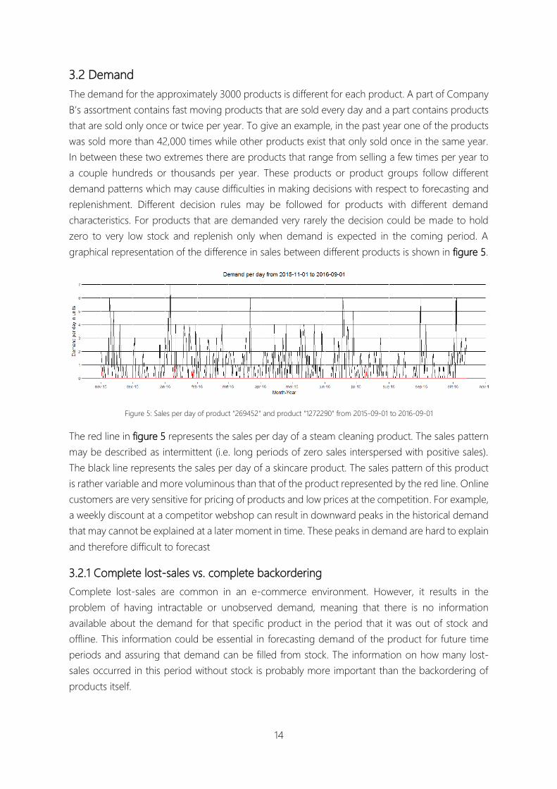
The demand for the approximately 3000 products is different for each product. A part of Company

B’s assortment contains fast moving products that are sold every day and a part contains products

that are sold only once or twice per year. To give an example, in the past year one of the products

was sold more than 42,000 times while other products exist that only sold once in the same year.

In between these two extremes there are products that range from selling a few times per year to

a couple hundreds or thousands per year. These products or product groups follow different

demand patterns which may cause difficulties in making decisions with respect to forecasting and

replenishment. Different decision rules may be followed for products with different demand

characteristics. For products that are demanded very rarely the decision could be made to hold

zero to very low stock and replenish only when demand is expected in the coming period. A

graphical representation of the difference in sales between different products is shown in figure 5.

Figure 5: Sales per day of product "269452" and product "1272290" from 2015-09-01 to 2016-09-01

The red line in figure 5 represents the sales per day of a steam cleaning product. The sales pattern

may be described as intermittent (i.e. long periods of zero sales interspersed with positive sales).

The black line represents the sales per day of a skincare product. The sales pattern of this product

is rather variable and more voluminous than that of the product represented by the red line. Online

customers are very sensitive for pricing of products and low prices at the competition. For example,

a weekly discount at a competitor webshop can result in downward peaks in the historical demand

that may cannot be explained at a later moment in time. These peaks in demand are hard to explain

and therefore difficult to forecast

3.2.1 Complete lost-sales vs. complete backordering

Complete lost-sales are common in an e-commerce environment. However, it results in the

problem of having intractable or unobserved demand, meaning that there is no information

available about the demand for that specific product in the period that it was out of stock and

offline. This information could be essential in forecasting demand of the product for future time

periods and assuring that demand can be filled from stock. The information on how many lost-

sales occurred in this period without stock is probably more important than the backordering of

products itself.

15

3.2.1.1 Sales data

The available data for analysis is sales data. In a situation where excess demand is backordered

completely, the number of sales is approximately equal to the demand and a part of this demand

may be backordered.

In the case situation backorders are not accepted and we have a lost-sales system (K. Van Donselaar

et al., 1996). The paper states that a target service level should be set in each period in a lost-sales

system. Because excess demand is not backordered, demand is equal to a sale if and only if the

stock on hand positive. Moreover, there is no information available about demand in situations

without stock on hand because products are often removed from the website of the webshop and

a customer cannot place an order for that product. It could be possible to have experienced

demand, and therefore sales, in the period without stock on hand if there had been stock on hand

to satisfy the demand. Therefore, the sales of product 𝑖 can be expressed as:

𝑊𝑖(𝑡) = { 𝐷𝑖(𝑡)

0

𝑖𝑓 𝑋𝑖(𝑡) > 0

𝑖𝑓𝑋𝑖(𝑡) = 0 𝑓𝑜𝑟 𝑡 = 1,2, …

𝑓𝑜𝑟 𝑡 = 1,2, …

(3.1)

An intuitive assumption would be that in a period without stock on hand, the demand for that

period is the same as the demand in periods with positive stock on hand or follows the same

probability distribution. This assumption is further elaborated in chapter four.

3.2.1.2 Demand through time

Demand for some products follows a trend, which means that demand may be increasing or

decreasing over time. Moreover, for some product demand follows a seasonal trend, meaning that

demand may increase or decrease in the same time periods and with the same seasonal pattern

every year, every month or even every day of the week. Demand shows high peaks and lows over

time. Some demand is highly variable when we look at demand on a daily basis. An example of

this can be seen in figure 6, where the line represents the daily sales of a food supplement product.

If we analyze the first two moments of the demand in periods with positive stock we see that a

large part of the assortment experiences demand with a high coefficient of variation (𝐶𝑉). The 𝐶𝑉

of demand is defined as:

𝜎𝐷

𝜇𝐷

(3.2)

Only two products have a 𝐶𝑉 below 1. Approximately 40 products have a 𝐶𝑉 between 1 and 2 and

the rest of the approximately 1600 products have a 𝐶𝑉 ranging from 2 to 17. Therefore, the demand

for products in the assortment can be seen as rather (highly) variable.

3.2.1.3 Demand distribution

Demand is stochastic and not fixed. The exact demand per period is not known and expected

future demand needs to be forecasted. Furthermore, demand is not stationary. The average

demand in period 𝑡 + 1 may be higher or lower than the average demand in period 𝑡. Moreover,

the variance of the demand in period may be less or more than in period t. Figure 6 shows the

variable daily demand pattern of a food supplement product.

16

Figure 6: Sales per day of product "270498" from 2015-11-01 to 2016-09-01

Due to different demand patterns, of which some may be highly variable or intermittent, controlling

processes such as determining the safety stock and replenishment may prove to be more

troublesome than in situations where demand is voluminous and rather stable. Calculating safety

stocks to guard for the variability of demand in the coming period, is not performed by Company

B. The number of products held in inventory is based on common sense and often products are

ordered if the stock on hand equals zero or when it is expected that a product will sell in the

comping period because it sold reasonably in past periods. This setup can be enhanced by setting

the right set of parameters at the appropriate moment in time.

3.2.1.4 New product introductions

It is common that Company B introduces new products into the webshop assortment throughout

the year. As described before, the assortment is large and new products are added to this

assortment throughout the year. New products lack direct information about historical demand,

stock and service levels. To forecast such parameters certain assumptions are required.

Assumptions including correlations of the newly introduced product with current available products

in the assortment and the underlying demand distribution of the newly introduced product. Other

relevant input information could be external data such as Google positions and Google test

advertisements.

3.3 The replenishment process

3.3.1 Ordering

The current replenishment process does not include fixed ordering moments. However, it is

preferred by the company to review the inventory of the products approximately once a week and

orders are placed to the supplier if deemed necessary. Replenishment is performed considering

individual products; there is not much attention in checking which product comes from which

supplier. Situations occur that only fastmoving products or products that have a net stock of zero

are ordered for replenishment. This is due to the fact that orders are placed on common sense and

not of fixed decision rules such as: ‘order if the inventory level is below a certain point’. Net stock

in this situation is equivalent to the stock on hand because backorders are not accepted. Note that

not all products are individually reviewed for their stock on hand and ordered if needed (not

specified by a certain decision rule). The ordering process and the number of products ordered is

based on product sales from the past periods instead. The ordered amount is based on what the

17

purchaser deems to be reasonable to order. An order-up-to level 𝑆 or an economic order quantity

𝑄∗ does not exist in the ordering process. The order quantity is not based on historical demand

data, current review period and the lead-time of a products. It is based on gut feel taking into

account the past sales of the product. Often it occurs that the stock on hand of such a product is

zero (sometimes it is zero for a longer time period). This ordering process is performed by hand

which means that nothing is automated by a system that is based on a replenishment policy with

decision rules. No attention is paid to characteristics of products such as demand volume, holding

costs, shortage costs and the average order quantity. Orders should be interconnected and

decisions have to be made how many products should be ordered when and to which supplier.

3.3.2 Deliveries

Products that are ordered at a certain moment in time are delivered in one batch at the same

moment. For example, an order for 20 products is not delivered in two sets of 10 products on two

subsequent days but rather in one batch on the same day. There is an uncertainty present in the

number of products actually delivered. It may be possible that a supplier does not deliver the fully

ordered number of products due to miscommunication, machine failures or delivery problems.

Note that this ‘yield’ is not in the scope of our project. For some suppliers the restriction holds that

the transportation and delivery of products is bound to fixed moments in time. Suppliers in China

send their orders via container shipping or air mail. Especially container shipping takes time and is

bound to fixed shipments. In the replenishment process, this sort of transportation restrictions

should be taken into account.

Every supplier has a certain lead-time for production, procurement or delivery. This lead-time varies

per supplier and is available to us through historical ordering data. Lead-times are non-

deterministic and may vary due to uncertainties such as availability of products and transport. The

lead-time is not dependent on the ordered number of products if the number is small. When large

numbers of products need to be ordered, the lead-time may increase because a full pallet of

products has to be send in a different way than just one box of products. The lead-time parameters

of 16 relevant suppliers are shown in table 2. As can be seen in the table, the mean lead-time of

the suppliers varies from 1 to 17 days and some suppliers have a rather low delivery reliability and

result a higher standard deviation and 𝐶𝑉. Supplier lead-times with a 𝐶𝑉 higher than 1,0 are

displayed in bold. We performed Kolmogorov-Smirnov tests on a sample of the lead-times and

most of the lead-times were not found to come from a Gamma distribution nor from a Normal

distribution. However, in our research we will assume that lead-times are Gamma distributed which

is described in chapter four. Note that the lead-time standard deviations are sometimes assumed

to be 0,25 times the mean lead-time due to lack of data.

18

Table 2: Mean and standard deviation of supplier's lead-times

Supplier Mean lead-time

(days)

Std. dev. lead-time

(days)

CV lead-time

(𝝈/𝝁)

1 858 4,00 10,00 2,50

2 862 6,33 11,55 1,82

3 863 17,00 5,66 0,33

4 865 7,00 1,75 0,25

5 868 4,00 1,00 0,25

6 869 3,00 0,75 0,25

7 872 1,67 1,15 0,69

8 873 4,00 1,00 0,25

9 874 6,50 0,71 0,11

10 879 7,00 1,75 0,25

11 880 2,50 2,12 0,85

12 881 2,66 1,15 0,43

13 882 1,00 0,25 0,25

14 884 1,75 0,50 0,29

15 889 1,00 0,25 0,25

16 897 10,33 10,00 0,97

3.4 Current key performance indicators

Considering inventory control, the only parameter that was measured and monitored by Company

B was the total stock value of the products in storage. The cost price and the amount of products

in stock on hand were known and in that way the stock value could be calculated. If we consider

KPIs outside the context of pure inventory control, three other KPIs arise that were measured by

Company B: (1) sales of products: the number of products that were sold in a certain time period,

(2) revenue: the amount of money that was earned by selling products during normal operations

and (3) profit: the surplus (or loss) in a certain period that is equivalent to the revenue deducted by

total costs and after taxes. These KPIs were not further used in their inventory control system. Only

sales KPI was in a way used to decide on how much to order a product: if the number of sales of a

product were deemed good, the product was weekly reviewed and an order was placed to the

supplier such that the product’s inventory level was deemed enough for the coming period

3.5 Conclusion

Summarizing chapter three, where the relevant components of the current inventory control

system were analyzed, the case study company faces the following inventory control challenges:

Stochastic demand. In some situations demand is highly variable and unpredictable,

making it even more difficult to forecast and to control for.

Stochastic lead-times. Lead-times vary per supplier and are not fixed.

Review periods are not fixed and may be dependent on exogenous factors such as delivery

moments and day of the week (weekends). Review periods for all products ordered to the

same supplier are not coordinated.

Excess demand is lost due to the fact that backorders are not accepted. Due to these lost-

sales demand in periods without stock on hand is unobserved.

Abundant different products are ordered from a relative small set of suppliers. Due to

ordering cost of placing an order to a supplier, the ordering process should be coordinated.

Lack of an automated inventory control system that suggest which product to order at

which moment.

19

Chapter Four

4. Model development

This chapter defines the model that incorporates the different components of our inventory control

problem. The main issue is:

Determining appropriate inventory levels for many different products which are ordered to a small

set of suppliers, taking into account unobserved stochastic demand and stochastic lead-times in a

lost-sales system.

This main issue can be split into four problem components:




4. Service level and s-level setting

Part one of this chapter elaborates what the possibilities are for the different components of the

inventory control problem and describes the decision process of choosing appropriate solutions

concepts. In part two of this chapter we describe the process of combining the chosen solution

concepts into two newly modified replenishment policies. For these two replenishment policies all

derivations of relevant parameters and cost functions will be defined and formed into a

mathematical model. The notation in this chapter is largely based on the notation from de Kok et

al. (2012) and can be found in appendix E.1.

Part one – Conceptual solutions

Section 4.1 on lost-sales describes different solution approaches to the lost-sales problem. Relevant

related information can be found in appendix B.1 on the lost-sales problem. Section 4.2 and 4.3 on

replenishment policies and joint replenishment describe the considerations for appropriate

replenishment policies for the case situation. Relevant related information can be found appendix

B.2 on the joint replenishment problem. Section 4.4 elaborates on service levels and s-level setting

in an inventory system were stochastic demand is forecasted or simulated. Section 4.6 concludes

part one of chapter 4.

4.1 Lost-sales problem

The characteristics of a lost-sales system are described in appendix B.1 of this report. Different

approaches for the lost-sales problem are briefly discussed in this section. More information on

these approaches and our considerations related to these approaches are described in appendix

G.1. The different approaches are the following and the chosen option is displayed bold:

20

1. Assume that sales equal demand and do not take into account demand in period without stock

on hand.

2. Correct the fill rate due to the fact that backorder system equations and decision rules are used

in a lost-sales system.

3. Uncensoring of unobserved demand in the periods without stock such that the model can be

based on demand data instead of sales data.

4. Taking into account the unobserved demand by using a method that makes an assumption

about the demand in periods without stock on hand.

Our preference is focused on uncensoring or untruncating the unobserved demand in periods

where stock-outs occurred. The main reason for this preference is because we would like to take

into account the demand in periods without stock. This demand should be satisfied in the best way

possible. Only basing the inventory system on sales and correcting the fill rate such is not the

solution concept that will be used in this project. However, the process of uncensoring unobserved

demand data is rather complex and researched iterative algorithms result in NP-hard problems if

the number of products becomes large. Furthermore, the available customer preferences data is

not sufficient to say something relevant about product substitution.

Therefore, we decided to work with option 3 and make the assumption in our project that the

demand in periods without stock can be estimated by using the sales in the periods close to the

stock-out period without taking into account substitution effects. By making this assumption, we

assume that the demand in periods without stock resembles the same characteristics as the

demand in periods with positive stock on hand (i.e. sales). The approach to impute sales data in

the periods without stock based on sales in the periods with positive stock on hand is elaborated

on in the section 4.6 of this chapter. More background information on the method can be found

in appendix G. A simplified version of the code of the method can be found in appendix I.

Using the impute demand method in attempting to estimate the demand in a time period instead

of using sales only, makes for a more realistic demand parameter that can be utilized in setting

parameters including the reorder level, the order quantity 𝑄 the order-up-to level 𝑆 and the review

period 𝑅. Additionally, it aims at setting more realistic 𝑃2 service levels per product or product

group and should result in more genuine holding, ordering and shortage cost. Note that by taking

into account this demand in periods without stock, no correction is needed on the fill rate to take

into account the fact that we operate in a lost-sales system. In chapter 5 we elaborate on a method

that resembles the same steps as this method but where the demand in periods without stock is

imputed based on the same distribution (Gamma distribution) as the demand in periods with

positive stock on hand.

4.2 Replenishment policy

The decision on which replenishment policy to use and to incorporate joint replenishment are

closely related. Deciding on the nature of reviewing is dependent on the environment in which the

replenishment policy is to be implemented. Additionally, may be restrictions and requirements that

21

influence the decision between certain replenishment policies. The different possibilities for a

replenishment policy are based on two main components and the chosen option is displayed bold:

1. Order-up-to policy or Fixed order quantity policy

2. Continuous policy or Periodic policy

Fixed order quantities 𝑄 are not often seen in the e-commerce. Replenishment policies with a fixed

order quantity 𝑄 such as the (𝑠, 𝑄) and (𝑅, 𝑠, 𝑄) replenishment polices are out of scope in our

research. This is due to the fact that the WMS of the case study company does not allow for fixed

order quantities but rather sets a minimum and maximum for every product in the assortment.

Therefore, we will focus our research on order-up-to policies only.

If products are ordered to the same supplier or shipped in the same transportation mode,

coordination of replenishments may be appealing. In such cases periodic review is particularly

appealing because all items in the group can be given the same ordering interval. Because of the

periodic property of the (𝑅, 𝑆) and (𝑅, 𝑠, 𝑆) replenishment policies, they are more preferred to

continuous systems such as the (𝑠, 𝑆) policy in terms of coordinating the replenishments of related

products. In addition, the periodic policies offers a regular opportunity (every 𝑅 units of time) to

adjust the 𝑠-level(s), which is a wanted property if the demand pattern is changing over time.

4.3 Joint replenishment

The joint replenishment problem results from the fact that many products have to be ordered to a

handful of suppliers and that with every order fixed ordering cost are incurred. Furthermore, every

supplier has its own lead-time with a certain lead-time uncertainty. To coordinate the

replenishment of every product in the assortment in a cost efficient manner we have the following

options and the chosen option is displayed bold:

1. Replenishment on a company level; the same review period is set for all products in the

assortment and economic order quantities per product are calculated accordingly.

2. Replenishment on a supplier level; the same review period is set for all products ordered to the

same supplier and economic order quantities are calculated per product based on this review

period.

3. Replenishment on the product level; a review period is calculated for every product individually

and economic order quantities are calculated accordingly.

Products are ordered to different suppliers and fixed ordering cost are incurred every time an order

is placed. The products have different demand parameters and differ in holding cost. Because we

do not want to order for every product individually an want to replenish cost efficient and, the third

option is eliminated from our spectrum. Another reason for not using the first option is that in all

reviewed JRP literature, the replenishment problem is based on a major and minor fixed ordering

cost. The minor fixed ordering cost are often used to determine the optimal review period for every

individual product. One of the most relevant differences with the JRP literature is that in the case

situation no additional costs are made when adding one or more products to the order that is

22

placed to the supplier (i.e. no minor fixed ordering cost). The first option is also eliminated because

we want to be more flexible in setting the review period per supplier. In setting a companywide

period, the different characteristics of the supplier and its products are not taken into account. We

therefore will determine a method to find the appropriate review period on a supplier level. The

parameter setting of the different products ordered to the same supplier can be seen as 𝑛 single-

item replenishment problems that each follow an (𝑅, 𝑆) or (𝑅, 𝑠, 𝑠) replenishment policy

(Federgruen, Groenevelt, & Tijms, 1984). In our research for finding an appropriate joint

replenishment method we found several differences with our problem and what was described in

the JRP literature. The most important differences between the case situation and the paper of

Atkins and Iyogun (1988) and other relevant literature on joint-replenishment are shown in table 3.

Table 3: Differences between SJRP in the case situation and the SJRP literature

Atkins & Iyogun (1988) and other relevant JRP

literature

Case situation

Demand In the JRP literature demand is often assumed to

be (compound) Poisson. Atkins and Iyogun

assume that demand follows a Poisson

distribution.

In the case situation demand follows a compound renewal

process with Gamma inter-arrivals and Gamma order sizes (as

we will elaborate later on in this report).

Inventory

system

Backorder system: excess demand is completely

backordered.

Lost-sales system: excess demand is completely lost.

Lead-times Lead-times are assumed to be deterministic or

Normally distributed and often an integer

multiple integer of the review period.

Lead-times are stochastic and follow a Gamma distribution (as

we will elaborate later on in this report).

Review

periods

The review periods 𝑅 are assumed to be

deterministic and fixed.

Review periods are in some situations bounded by exogenous

factors (e.g. delivery moments, weekends without deliveries).

Review periods may depend on the demand of products

coming from the same supplier. More information on this topic

is given in section 4.6.

Ordering

cost

The ordering cost include a fixed major and minor

cost part. This minor ordering cost is product

specific but is fixed in the context of that it does

not matter how many products of that specific

product are ordered; the minor ordering cost

remains the same.

In the case situation this minor ordering cost does not exist. No

additional ordering cost are made when ordering more

products to the same supplier. Furthermore, the extra time of

placing an order of 2,3,… , 𝑛 and putting the order in the

warehouse is negligible.

s-levels Order-up-to level 𝑀𝑖 Order-up-to-level 𝑆𝑖 and if suitable for a certain supplier or

product a reorder level 𝑠𝑖 .

More information on the decision process of choosing which replenishment policy to use for the

individual replenishment problems and how to incorporate joint replenishment can be found in

appendix B.2.

A method that is currently used by Optiply is elaborated on in appendix G. The method calculates

the total economic order quantity (𝐸𝑂𝑄) and review period on a supplier level and then translates

this back to an 𝐸𝑂𝑄 on product level for the products that are ordered to the same supplier. The

problem with this method is that it calculates the 𝐸𝑂𝑄 on a supplier level by simply adding all the

demand and costs from different products that are ordered to the same supplier. Note that the

𝐸𝑂𝑄 calculation uses costs and average demand from an individual product as input; simply

summing up these parameters is meaningless. A new method to determine the review period per

supplier is elaborated on in section 4.6 of this chapter.

23

4.4 Service level and s-level setting

In our research, the expressions for certain inventory control parameters such as the demand

during lead-time or during the review period are derived based on the assumption that demand

is stationary. In practice however, demand is often non-stationary and future demand is based on

forecasts. Strijbosch et al. (1997) conclude that even in the simplest possible setting that the

standard procedures from the literature do not guarantee the desired service levels. In a situation

with non-stationary demand this may only exacerbate (Strijbosch, Moors, & de Kok, 1997). This

section briefly elaborates on service level setting under both stationary and non-stationary demand

and the difference between the 𝑃2 and 𝑃3 service level.

4.4.1 Service levels

The 𝑃2 service level or fill rate can be described as the long-run fraction of total demand which is

being delivered from stock on hand immediately. The fill rate is most commonly used as the target

service level an inventory system. Based on this target service level the inventory levels such as the

reorder level 𝑠 or order-up-to level 𝑆 are set. The fill rate requires the knowledge of the demand

in a replenishment cycle as we will see in section 4.6 where we derive the expressions for the fill

rate. The 𝑃3 service level, also denoted as the ready rate, is defined as the fraction of time during

which the system has positive net stock, which is the same as the probability of no stock-out at the

end of an arbitrary period. Net stock in our situation, is equal to the stock on hand. The ready rate

as by Køhler-Gudum and de Kok (2002) can be expressed as:

𝑃3 = 𝑃{𝑋(𝑡) ≥ 0} = 1 −𝑁𝐵

𝑁𝑃

(4.1)

where 𝑁𝐵 is the number of periods with additional backordered demand and 𝑁𝑃 is the total number

of time periods considered. Therefore, the ready rate represents a time dimension of demand

satisfied without backorders (or in our case, no lost-sales). In case of continuous Poisson distributed

demand the 𝑃2 and 𝑃3 service levels are equal. Hence, for 𝐶𝑉𝐷 = 1, it holds that 𝑃2 = 𝑃3. This can

also be shown by deriving the functions for the 𝑃3 service level under the (𝑅, 𝑆) and (𝑅, 𝑠, 𝑆)

replenishment policy as we will show in section 5.4 where we relate the 𝑃3 service level to the 𝑃2

service level.

In practice, having a 𝐶𝑉𝐷 equal to 1 is often not the case and customer demands vary in size. If the

stock on hand contains a small number of units on hand most of the time, the ready rate can be

high. Still, the fill rate may be low if there are some large customer demand sizes (i.e. demand sizes

are (highly) variable). For Normally distributed demand the fill rate is also equivalent to the ready

rate according to Axsäter (2006). It is easy to reason that the more variable daily demand, the larger

the difference 𝑃2 − 𝑃3 becomes. We will verify this by simulation in section 5.4. as well.

Let us define:

𝑏 = shortage cost per unit per unit time

𝑝 = shortage cost per unit

24

A shortage cost of type 𝑏, for example, is relevant for a spare part when a shortage implies that a

machine has to stop working until the spare part is available again. The costs are proportional to

the customer waiting time. The shortage cost of type 𝑝 can be interpreted as a cost per average

number of backorders. It is very important to mention here that the shortage cost of type 𝑏 can

only be used in a backorder system because the time that the backorders are present needs to be

tracked to calculate the shortage cost per replenishment cycle or per unit time. Backorders at time

𝑡 are equal to the net stock when it is below zero (i.e. −𝑋(𝑡)). In a lost-sales system this is not

possible because the stock on hand is at least zero. The whole idea of a customer ‘waiting’ for his

backordered product does not exist.

In the optimal solution, the optimal reorder level 𝑠 can be characterized as the largest reorder level

providing a ready rate not higher than 𝑏𝑖

𝑏𝑖+ℎ𝑖. This fractile is also called the Newsvendor fractile. An

advantage of the newsvendor fractile is that it does not need information on the demand in a

replenishment cycle like with the other service levels. Note that the shortage cost 𝑏𝑖 is a shortage

cost per unit per time unit just like the holding cost ℎ𝑖 is a holding cost per unit per time unit.

Assuming compound Poisson demand and if 𝑠𝑖∗ is the optimal reorder level for product 𝑖, we have:

𝑃3(𝑠𝑖∗) ≤

𝑏𝑖

𝑏𝑖 + ℎ𝑖

< 𝑃3(𝑠𝑖∗ + 1)

(4.2)

This relation also holds for the fill rate if demand is purely Poisson. For Normally distributed

demand, it is shown that the optimal solution entails:

𝑃2 = 𝑃3 =𝑏𝑖

𝑏𝑖 + ℎ𝑖

(4.3)

Given a certain shortage cost 𝑏𝑖 for product 𝑖, we can determine from (4.3) the service level

providing exactly the same reorder level:

𝑏𝑖 =ℎ𝑖𝑃2

1 − 𝑃2

=ℎ𝑖𝑃3

1 − 𝑃3

(4.4)

This also works the other way around, i.e., given a target service level, we can determine the implicit

shortage cost. However, as described before, the shortage cost of type 𝑏 can only be used in a

backorder system because the time that the backorders are present needs to be tracked. The

number of backorders is equal to the negative stock on hand. In a lost-sales system this is not

possible because the stock on hand is at least zero. In our situation, we have shortage cost of type

𝑝, which are incurred over the number of shortages per replenishment cycle. For this kind of

shortage cost, the scientific literature focusses especially on solving for the 𝑃1 service level instead

of the 𝑃2 or 𝑃3 service level (Axsäter, 2006; Silver, Pyke, & Peterson, 1998).

De Kok (1991) also suggest another form of the 𝑃3 service level in one of his 6 research reports

from 1991 on the basics of inventory management. He describes the 𝑃3 service level as the long-

run average shortage at an arbitrary moment in time. This is equivalent to the average backorders

25

during a replenishment cycle. In the compound renewal demand case under an (𝑅, 𝑆)

replenishment policy, the 𝑃3 based on a certain order-up-to-level 𝑆 can be expressed as:

𝑃3(𝑆) = 𝐸[𝑋] − (𝑆 − (𝐸[𝐿] +𝑅

2)𝐸[𝐷]

𝐸[𝐴])

(4.5)

In the inventory system under an (𝑅, 𝑠, 𝑆) or (𝑅, 𝑆) replenishment policy and a target service level

constraint, one particularly considers linear holding cost and fixed ordering cost. The holding cost

are derived from the average stock on hand and the ordering cost depend on the review period

𝑅. Shortage cost are incurred implicitly by achieving a target service level. Because shortage cost

are typically hard to obtain, often a service level approach is utilized. However, once the inventory

cost associated with the replenishment policy under a target service level are known, the

expressions for the 𝑃2 and 𝑃3 service levels can be used to obtain the implicit shortage cost that is

assumed. This can be done by taking the shortage cost per unit or per unit time as a variable and

determine the value of this variable for which the replenishment policy is cost-optimal (de Kok,

1991).

If we set a certain target fill rate and set the reorder level 𝑠 or order-up-to level 𝑆 accordingly, we

can use expression (4.5) to calculate the expected shortage per replenishment cycle and the

related shortage cost per replenishment cycle. Taking both cost into account, we should then be

able determine the cost-efficient target fill rate. We will perform a verification analysis on expression

(4.5) in section 5.4.

4.4.2 s-levels

If we want to calculate a dynamic reorder level or order-up-to level under forecasted demand, de

Kok (1991) rewrites the random variables 𝐷(0, 𝑅] and 𝐷(0, 𝐿] as follows:

𝐷(0, 𝑅] = 𝐷𝐹(0, 𝑅] + 휀(0, 𝑅]

(4.6)

𝐷(0, 𝐿] = 𝐷𝐹(0, 𝐿] + 휀(0, 𝐿]

(4.7)

Here 𝐷𝐹(0, 𝑅] and 𝐷𝐹(0, 𝐿] are forecasts and therefore known constants. The forecast error or

deviation from the forecast is given by 휀(0, 𝑅] and 휀(0, 𝐿], which are random variables. Often, the

forecast error is assumed to be Normally distributed. A more robust approach is to assume that

(4.3) and (4.4) are Gamma distributed. Then, the method to determine the appropriate s-level is

the following:

1. Determine 𝐷𝐹(0, 𝑅] and 𝐷𝐹(0, 𝐿].

2. Determine 𝜎(휀(0, 𝑅]) and 𝜎(휀(0, 𝐿]).

3. Calculate the reorder level 𝑠 and/or order-up-to level 𝑆 using the PDF-method, assuming

the Gamma distribution.

The expected average stock on hand during a replenishment cycle is then given by (de Kok, 1991):

𝐸[𝑋] ≅ 𝑆 − 𝐷𝐹(0, 𝐿] −𝐷𝐹(0, 𝑅]

2

(4.8)

26

Silver et al. (1998) and Axsäter (2006) suggest multiple methods to incorporate the forecast error

in the process of setting appropriate safety stocks. One of these methods is described in appendix

B.3.1. The cost effect of using estimated standard deviation instead of the true forecast error value

and suggestions for making adjustments to the s-levels is research by Strijbosch, Moors and de

Kok (1997).

Strijbosch et al. (1997) suggest a heuristic to improve the setting of the order-up-to level under an

(𝑅, 𝑆) replenishment policy if demand is forecasted and under a 𝑃1 service level. They state the

standard procedure of setting the reorder level 𝑠 (i.e. quantile of the distribution of demand during

lead-time or review period plus lead-time)does not guarantee stock-out probabilities smaller than

1 − 𝑃1 and that they can deviate substantially. The procedure of the heuristic involves correcting

the order-up-to level 𝑆 under the assumption of Normally distributed demand and a Simple

Exponential Smoothing (SES) forecast method (Strijbosch et al., 1997). The relevant expressions can

be found in appendix B.3.2.

Køhler-Gudum and de Kok (2002) propose a technique, called the safety stock adjustment

procedure (SSAP), which enables the determination of safety stocks to ensure target service levels

in simulation studies of inventory systems where demand is forecasted (i.e. non-stationary). The

procedure can be used for the 𝑃1, 𝑃2 and 𝑃3 service level. An essential constraint in the usage of

the technique is that excess demand is backordered. If not, the important property of the safety

stock being independent cannot be maintained. A more extensive description of this work can be

found in appendix B.3.3.

We can conclude that reorder levels and order-up-to levels need to be updated throughout the

replenishment process due to non-stationary demand. Note that this is even required if demand is

stationary, as Strijbosch et al. (1997) showed. Demand forecasts may be run daily and 𝑠-levels

should be updated in-between review periods such that the replenishment policy becomes a

cyclical policy where every replenishment cycle performs under a target service level constraint.

4.5 Conclusion

We found that the standard (𝑅, 𝑆) and (𝑅, 𝑠, 𝑆) replenishment policies can be used in solving the

𝑛 single-item replenishment problems in the aggregate joint replenishment problem. Within these

single-item replenishment problems, excess demand is completely lost, making the inventory

system a lost-sales system. Therefore, the sales data needs to be corrected such that lost-sales in

periods without stock on hand are taken into account to the best of our abilities. Updating of 𝑠-

levels based on demand forecasts may be performed in-between review periods. However,

updating the 𝑠-levels too frequent, could lead to the fact that the inventory system reacts to ‘noise’

too much.

27

Part two – The modified replenishment policies

This part focusses on the mathematical model concerning the newly modified replenishment

policies and the derivations of the expressions for the relevant parameters of the policies. Section

4.6 introduces the (𝑅𝛿 , 𝑆𝑖) replenishment policy and the (𝑅𝛿 , 𝑠𝑖, 𝑆𝑖) replenishment policy that take

into account stochastic demand sizes 𝐷𝑖 and stochastic demand inter-arrivals 𝐴𝑖 for every product

𝑖, joint replenishment, complete lost-sales, stochastic lead-times 𝐿 and supplier based review

periods 𝑅𝛿.

4.6 The (𝑹𝜹, 𝑺𝒊) and (𝑹𝜹, 𝒔𝒊, 𝑺𝒊) replenishment policy

In this section we introduce our model with two modified replenishment policies. The subscript 𝑖

relates to the fact that for every product 𝑖 a reorder level 𝑠𝑖 and order-up-to level 𝑆𝑖 is determined.

The 𝑅𝛿 represents the aggregated review period of all products 𝑖 that are ordered to the same

supplier. We start with a brief introduction to the two replenishment policies and the assumptions

that hold in the analysis of both policies. In section 4.6.1 the relevant parameters of the

replenishment policies are introduced including the demand during lead-time, demand during the

review period, the undershoot, the expected average stock on hand and the service levels. This

section also describes the cost functions of the relevant costs of the inventory system under each

of the replenishment policies. All derivations of the expressions and formulas can be found in

appendix J and appendix K. The notation used in the derivations of the expressions of the relevant

parameters of both replenishment policies are for a large part based on the notation of de Kok et

al. (2012). The notation can be found in appendix E.1 of this report.

The following assumptions were made in deriving the expressions of the relevant parameters of

both replenishment policies:

(i) Demand is stochastic but stationary. Demand over time intervals of fixed length does not depend

on time itself. Although this assumption may appear somewhat unrealistic, note that the decision

rules can be adapted (i.e. they can be updated through time to learn from more recent historical

demand data). Demand is continuously distributed with demand inter-arrivals and demand order

sizes. Therefore, the demand for a product follows a compound renewal process.

(ii) Replenishment orders do not cross in time (i.e. an order placed at a later moment in time cannot

arrive earlier).

(iii) Lead-times are stochastic and independent .

(iv) Time between review moments (i.e. the review period) is independent. Review periods are based on

the review period determination method described in section 4.6.1.2.

(v) All excess demand is lost (i.e. excess demand is not backordered but results in a lost sale).

(vi) The entire ordered quantity of a replenishment order is delivered at the same time (i.e. there is no

variance in the delivery time within the order).

(vii) When placing an order, only major fixed ordering cost are incurred; there are no minor fixed

ordering cost based on the number of products ordered.

(viii) The unit variable cost of any of the products does not depend on the quantity; there are no discounts

in either the unit purchase cost or the unit transportation cost.

28

4.6.1 Mathematical model

4.6.1.1 Lost-sales component (more details in appendix G.1.3)

Let us define:

𝐷𝑖𝑑 = daily demand of product 𝑖 (i. e. NOT demand order size as in continuous demand)

𝑗 = number of days back in the historical data 𝑋𝑖(𝑡 − 𝑗) = stock on hand from every historical date that is used in the calculation

𝐼𝑥𝑖(𝑡−𝑗) = an indicator function that indicates if the stock on hand of product 𝑖 was positive on day 𝑗;

(𝐼𝑥𝑖(𝑡−𝑗) ≔ {1 𝑖𝑓 𝑋𝑖(𝑡 − 𝑗) > 0

0 𝑖𝑓 𝑋𝑖(𝑡 − 𝑗) = 0 )

𝑁 = total number of days that is looked back in the historical data

Imputed demand on days without stock can be expressed as:

𝐷𝑖𝑑(𝑡) =

∑ 𝐷𝑖𝑑(𝑡 − 𝑗)𝑁

𝑗=1

∑ 𝐼𝑥𝑖(𝑡−𝑗)𝑁𝑗=1

𝑓𝑜𝑟 𝑡 = 1,2, … , 𝑛

𝑓𝑜𝑟 𝑗 = 1,2, … , 𝑁

(4.9)

subject to:

10 < ∑ 𝐼𝑥𝑖(𝑡−𝑗)

𝑁

𝑗=1≤ 𝑁

4.6.1.2 Review period component (more details in appendix G.2.1)

Let us define the subset 𝑉𝛿 = {1,2,… , 𝑖, … , 𝑛} which contains all the product 𝑖 that are ordered to

the same supplier 𝛿 and 𝐷𝑖𝑑 as the daily demand of product 𝑖 (i.e. NOT demand order size as in continuous

demand). Then, the review period for all products 𝑖 in 𝑉𝛿 is given by:

𝑅𝛿

= √2𝐾

∑ ℎ𝑖𝐷𝑖𝑑 𝑖∈𝑉𝛿

(4.10)

The economic order quantity for every product 𝑖 in 𝑉𝛿 becomes:

𝑄𝑖∗ = 𝑅𝛿 ∗

𝐸[𝐷𝑖]

𝐸[𝐴𝑖]

(4.11)

4.6.1.3 Derivations of relevant parameters (more details in appendix J)

1. The first two moments of the demand during lead-time: 𝐸[𝐷(0, 𝐿]] and 𝜎2(𝐷(0, 𝐿)),

2. The first two moments of the demand during the review period: 𝐸[𝐷(0, 𝑅]] and 𝜎2(𝐷(0, 𝑅)).

3. The first two moments of the demand: 𝐸[𝑈] and 𝜎2(𝑈).

4. The expected stock on hand: 𝐸[𝑋].

5. The service levels: 𝑃1 and 𝑃2.

4.6.1.4 Holding cost (more details in appendix K.1)

The total expected daily holding cost for the (𝑅𝛿 , 𝑠𝑖, 𝑆𝑖) replenishment policy can be expressed as:

𝑇𝐸𝐷𝐻𝐶𝑅𝑠𝑆

= ∑ ℎ𝑖 ∗ 𝑐𝑖 ∗ (𝑠𝑖 − 𝐸[𝐷(0, 𝐿]] −𝐸[𝑈𝑖]

2+

𝐸 [𝐷(0, 𝑅𝛿]]

2)

𝑛

𝑖=1

(4.12)

29

The total expected daily holding cost for the (𝑅𝛿 , 𝑆𝑖) replenishment policy can be expressed as:

𝑇𝐸𝐷𝐻𝐶𝑅𝑆

= ∑ ℎ𝑖 ∗ 𝑐𝑖 ∗ (𝑆𝑖 − 𝐸[𝐷(0, 𝐿]] −𝐸 [𝐷(0, 𝑅𝛿]]

2)

𝑛

𝑖=1

(4.13)

with:

𝑛 = number of products ℎ𝑖 = holding cost rate for one unit of product 𝑖 for one time unit 𝑐𝑖 = cost price of one unit of product 𝑖

An alternative for the term between brackets (i.e. 𝐸[𝑋𝑖]) is a term based on de Kok (2002):

𝐸[𝑋] = 𝑠𝑖 +

((𝑆𝑖 − 𝑠𝑖)

2

2−

𝐸2[𝑈𝑖] + 𝜎2(𝑈𝑖)2

+𝐸2 [𝐷(0, 𝑅𝛿]] + 𝜎2(𝐷(0, 𝑅𝛿])

2𝐸[𝐷(0, 𝑅𝛿]]((𝑆𝑖 − 𝑠𝑖) + 𝐸[𝑈𝑖]))

(((𝑆𝑖 − 𝑠𝑖) + 𝐸[𝑈𝑖]) −𝐸[𝐷𝑖]𝐸[𝐴𝑖]

𝐸[𝐿] − 𝑃2

𝐸[𝐷(0, 𝑅𝛿]]2

)

In chapter five we show that this approximation is more accurate than the approximation by Silver

et al. (1998).

4.6.1.5 Ordering cost (more details in appendix K.2)

The total expected daily ordering cost for ordering products to a supplier 𝛿 under a (𝑅𝛿 , 𝑠𝑖, 𝑆𝑖)

replenishment policy can be expressed as:

𝑇𝐸𝐷𝑂𝐶𝑅𝑠𝑆 = ∑𝑂𝐶2(𝜌𝑖)

𝐸[𝑅𝛿]

𝑁

𝛿=1

(4.14)

with

𝑂𝐶2(𝜌𝑖) = 𝐾 (1 − ∏(1 − 𝜌𝑖)

𝑖∈𝑉𝛿

)

𝜌𝑖 = ordering probability =𝐸[𝐷𝑖]𝐸[𝑅𝛿]

(𝑆𝑖−𝑠𝑖+𝐸[𝑈𝑖])𝐸[𝐴𝑖].

(4.15)

𝑁 = number of suppliers

The total expected daily ordering cost under a (𝑅𝛿 , 𝑆𝑖) replenishment policy can be expressed as:

𝑇𝐸𝐷𝑂𝐶𝑅𝑆 = ∑ 𝐸𝐷𝑂𝐶𝑅𝑆𝛿

𝑁

𝛿=1

= ∑𝑂𝐶1

𝐸[𝑅𝛿]

𝑁

𝛿=1

(4.16)

with:

𝑂𝐶1 = 𝐾


4.6.1.6 Shortage cost (more details in appendix K.3)

The total daily expected shortage cost for the (𝑅𝛿 , 𝑠𝑖, 𝑆𝑖) replenishment policy can be expressed

as:

30

𝑇𝐸𝐷𝑆𝐶𝑅𝑠𝑆 = ∑ ∑(𝐸[𝐷(0, 𝐿] + 𝑈𝑖 − 𝑠𝑖)

+] − 𝐸[𝐷(0, 𝐿] − 𝑆𝑖)+])

𝑅𝛿𝑖∈𝑉𝛿

𝑁

𝛿=1

(4.17)

with:


The total daily expected shortage cost for the (𝑅𝛿 , 𝑆𝑖) replenishment policy can be expressed as:

𝑇𝐸𝐷𝑆𝐶𝑅𝑆 = 𝑃𝑖 ∑ ∑(𝐸 [(𝐷(0, 𝑅𝛿 + 𝐿] − 𝑆𝑖)

+] − 𝐸[(𝐷(0, 𝐿] − 𝑆𝑖)

+])


𝑁

𝛿=1

(4.18)

with:


4.6.2 Cost minimization

The total cost (𝑇𝐶) of the inventory system consists of the holding, ordering and shortage cost.

Hence, we want to:

min(TC) ⟺ min (𝑇𝐸𝐷𝐻𝐶 + 𝑇𝐸𝐷𝑂𝐶 + 𝑇𝐸𝐷𝑆𝐶)

(4.19)

The three cost components are minimized by determining the appropriate cost efficient review

period (i.e. review determination method) and calculating the appropriate reorder level 𝑠𝑖 and/or

order-up-to-level for every product 𝑖 under a target fill rate 𝑃2, as we can see in table 5.

Table 4: Replenishment policy parameters

(𝑅𝛿∗, 𝑠𝑖

∗, 𝑆𝑖∗) (𝑅𝛿∗

, 𝑆𝑖∗)

Review period; 𝐸𝑂𝑄: 𝑅𝛿∗= √

2𝐾


𝑅𝛿∗= √

2𝐾


Reorder level: 𝑠𝑖∗ = �̂�𝐿,𝑖 + 𝑘�̂�𝑅+𝐿,𝑖

-

Order-up-to level: 𝑆𝑖∗ = �̂�𝑅+𝐿,𝑖 + 𝑘�̂�𝑅+𝐿,𝑖

= 𝑠𝑖 + (𝑆𝑖 − 𝑠𝑖) = 𝑠𝑖 + 𝑄𝑖 − 𝑈𝑖

𝑆𝑖∗ = �̂�𝑅+𝐿,𝑖 + 𝑘�̂�𝑅+𝐿,𝑖

with:

�̂�𝐿,𝑖 = forecasted or expected demand during leadtime for product 𝑖 �̂�𝑅+𝐿,𝑖 = forecasted or expected demand during the review period for product 𝑖 �̂�𝐿,𝑖 = forecasted or expected std. deviation of demand during lead time for product

�̂�𝑅+𝐿,𝑖 = forecasted or expected std. deviation of demand during the review period for product 𝑖

𝑘 = safety factor specified based on the target fill rate; depends on 𝐿, 𝜇𝐷, 𝜎𝐷 and 𝑄𝑖

If shortage cost are taken into account with the service level setting, this results in the 𝑃3 service

level (i.e. 𝑃{𝑋𝑖 > 0}) which can be defined as the Newsvendor fractile: 𝑏𝑖

𝑏𝑖+ℎ𝑖. Note that this can only

be implemented if the shortage cost 𝑏𝑖 have the dimension cost per unit per unit time and that the

inventory system is a backorder system. Expression (4.5) could be used to determine the shortage

cost per replenishment cycle under a certain target service level. Based on the shortage cost and

holding cost per replenishment cycle, a cost-efficient target service level could be determined.

31

Chapter Five

5. Case study

Chapter four described the chosen solution concepts and derived expressions for the relevant

parameters of our inventory control model. This chapter describes the case study where we

implement the inventory control solutions in the problem situation of the case study company. The

case study will involve simulating day by day behavior of the inventory control system that results

from utilizing the newly modified replenishment policies. This simulating is performed by a

simulation tool that we developed for our research. Section 5.1 of this chapter starts with the

description of the different components of the simulation model and the assumptions used in the

case study. Simulation is performed because: (1) some of the derived expressions for the different

relevant parameters have to be verified, which is done is section 5.2; (2) the performance of the

new policies should be compared with the performance of the Optiply model during the same time

period, which is done in section 5.3; (3) useful or interesting scenarios can be simulated that may

assist in the inventory control decision making process, which are simulated in section 5.3 as well.

The initial goal was to additionally compare the new model with the old situation at the case study

company before they became a customer at Optiply. However, no target fill rates were set by the

company in that period, which means that although we can calculate the inventory cost over a

certain period before 2016-09-01, we cannot compare the performance of the new model over this

period. If target fill rates (and actual experiences fill rates) are unknown, we cannot set the

parameters of the new model to simulate over the same period. However, by knowing that Optiply

improved inventory control at the case study company since 2016-09-01, we can assume that the

new model improves inventory control compared to the old situation if we show that our model

outperforms the Optiply model. Therefore, this chapter will show that the new model outperforms

the current Optiply model.

The simulation tool is developed in the software program R and simulates daily demand and the

response of the two newly modified policies on this demand. Parameters are tracked and simulated

per product. These parameters include the daily stock on hand, daily inventory position, stochastic

lead-times, replenishment orders, replenishment deliveries, the undershoot and daily lost-sales. At

the end of every simulation run the simulation tool creates 3 tables with relevant input and output

parameters. This information is then automatically written to Excel files.

5.1 Components of the model

This section provides an overview of the different components of the simulation tool and describes

how these components were integrated into the model. The replenishment process is simulated

day by day and the sequence of events is the following:

32

1. Determine starting stock on hand and starting inventory position

2. Demand occurs

3. Place replenishment orders

4. Determine ending inventory position

5. Receive replenishment orders

6. Determine ending stock on hand

7. Determine lost-sales and cost calculation

Demand only decreases the inventory position and the stock on hand only and only if both the

stock on hand and the inventory position are positive. Lost-sales occur if demand occurs when the

stock on hand is zero. A replenishment order is placed to the supplier based on the inventory

position and placing an order increases the inventory position. Hence, the ending inventory point

of every day can be determined after ordering. Receiving a replenishment order (i.e. replenishment

delivery) increases the stock on hand. Hence, the ending stock on hand of every day can be

determined after receiving the replenishment order.

5.1.1 Historical data

Historical data from the period 2015-10-21 to 2016-09-01 is used as input for setting the 𝑠-levels

(reorder level and order-up-to-level) of the different products. Data from this period will typically

be used unless stated otherwise. Since 2015-10-21 the case study company started using a new

warehouse management system (WMS) called “Picqer” and historical data is extracted from this

WMS. The historical data includes point of sale (POS) collection data such that the inter-arrival time

of demand and the size of the demand order could be determined in periods with positive stock.

For a large part of the assortment stock data is available including order and delivery moments

such that the average supplier lead-times and uncertainty of supplier lead-times could be

determined.

The following assumptions are made when using the historical data:

1. Sales (demand) data and stock data over de period 2015-10-21 to 2016-09-01 was used to

determine the input parameters and perform forecasts. Note that not all 1800 products have

data over the full period because some products were introduced into the assortment during

this period (see next assumption).

2. Only products that have enough data to forecast with are used in the analysis and simulation.

Some of the newly introduced products are therefore excluded. Note that this is not too

relevant since we will only simulate for several products due to limited time and the fact that

if the verification holds for multiple products with varying characteristics, it holds for all

products.

5.1.2 Demand generation

For the tool to work, demand has to be given as an input parameter. Relevant parameters such as

the order quantity, reorder level 𝑠 and the order-up-to-level 𝑆 are determined by using demand

or sales data as an input. This data is used for initial parameter setting. The dataset to test the

33

model on should be new historical data which has not been used for parameter setting. We will

simulate demand data for the period 2016-09-01 to 2017-01-15. For this period we generate

demand which is based on a products specific distribution. Historical sales/demand data is split up

in demand inter-arrivals and demand order sizes (i.e. continuous demand parameters). Therefore,

the demand follows a compound renewal process. The following section describes which demand

distribution will be used throughout the model and the simulations.

5.1.2.1 Demand distribution

Heinecke et al. (2013) performed a Kolmogorov-Smirnov test on underlying demand distributions

for 13.000 products. They concluded that the Poisson distribution gives a good estimation for all

average demand intervals and a relatively low 𝐶𝑉. For a 𝐶𝑉 in the range of 0 to 1 the Normal

distribution showed a good fit, but fits poorly for erratic demand data and is therefore only

appropriate for more smooth demand patterns. Additionally, the Normal distribution would

generate negative demand due to its characteristics and therefore an additional assumption should

be made that removes the generated negative values. The Gamma distribution showed a good fit

for demand data with high inter-arrival times and high 𝐶𝑉 values and therefore the Gamma

distribution can be used for generation of variable demand (Heinecke, Syntetos, & Wang, 2013).

According to Burgin (1975) Gamma distribution is appropriate to represent demand in multiple

situations. The distribution covers a wide range of distribution shapes, is defined for non-negative

values only and is mathematically tractable in inventory control applications. An important note to

make is that the Gamma distribution requires estimation of the mean and variance only and that

the use of the distribution in practical applications is supported by ample empirical evidence

(Burgin, 1975). The following assumptions are made for demand generation:

1. Demand inter-arrival times follow a Poisson distribution. By assuming that the demand inter-

arrivals are Poisson distributed we assume that the inter-arrivals of demand are independent

and identically distributed. Because testing for independence of all 1800 products, we

therefore implicitly assume iid demand inter-arrivals in case we generate demand data.

Demand order sizes follow a Gamma distribution.

2. Seasonality and trends are not taken into account because there is not enough historical data

to make relevant assumptions about them. However, in the practical simulation scenarios in

section 5.3 we do perform a forecast and therefore take into account trends and seasonality.

3. The time scale is 7 days per week.

In we assume that demand is Gamma distributed with mean 𝛼𝛽 and variance 𝛼𝛽2, then the pdf is

equal to:

𝑓(𝑥|𝛼, 𝜆) =𝑒−𝛽𝑥𝑥𝛼−1

Γ(𝛼)𝛽𝛼

(5.1)

With the ‘Gamma function’:

Γ(𝛼) = ∫ 𝑦𝛼−1𝑒−𝑦𝑑𝑦∞

0

(5.2)

34

Furthermore, we will use the fact that Γ(𝛼 + 1) = αΓ(𝛼) and the cdf of the Gamma distribution

𝐹(𝑥|𝛼, 𝛽). The Gamma distribution is defined with a so called shape and a scale parameter which

can be described as follows:

𝑠𝑐𝑎𝑙𝑒 = 𝜆 =𝜎𝐷

2

𝜇𝐷

(5.3)

𝑠ℎ𝑎𝑝𝑒 = 𝛼 =𝜇𝐷

2

𝜎𝐷2

(5.4)

These shape and scale parameters can be used when there is data available to estimate 𝜇𝐷 and 𝜎𝐷

or when 𝜇𝐷 and 𝜎𝐷 are given. In our case the 𝜇𝐷 and 𝜎𝐷 from the historical data can be used to

generate Gamma distributed demand data for simulation. Note that the scale parameter can also

be described by the rate parameter 𝛽 =1

𝜆=

𝜇𝐷

𝜎𝐷2 .

5.1.3 Ordering process

The simulation tool simulates the whole replenishment process: inventory levels are reviewed,

replenishment orders are placed and received and inventory levels are updated accordingly. The

starting state on 2016-09-01 is the moment of the first review moment 𝑅0 = 0. The starting stock

on hand and starting inventory position are assumed to be equal to the actual stock on hand on

that day. Furthermore, it is assumed that there are no outstanding orders at that moment in time.

Hence, the first replenishment order that is received is the order placed at 𝑅0. In case of the

(𝑅𝛿 , 𝑠𝑖, 𝑆𝑖) replenishment policy, the inventory of every product 𝑖 that is ordered to the same

supplier is reviewed at the review moment 𝑅𝑡. If the inventory position of a product 𝑖 is below 𝑠𝑖, a

replenishment order of size 𝑆𝑖 − 𝑌𝑖(𝑅𝑡) is placed to the supplier. In case of the (𝑅𝛿 , 𝑆𝑖)

replenishment policy, a replenishment order is expected to be placed to the supplier every review

period. The size of the replenishment order of a product 𝑖 is 𝑆𝑖 − 𝑌𝑖(𝑅𝑡). Every replenishment order

is given a lead-time for delivery that follows a Gamma distribution. The replenishment order is

received ‘a lead-time time units’ later.

The following assumptions were made for the receiving and placing of replenishment orders:

1. The replenishment process is performed according to the newly modified replenishment

policies.

2. For every replenishment order the ordered quantity is equal to the delivered quantity (i.e.

there is a yield of 100 percent).

3. Lead-times of suppliers are assumed to follow Gamma distribution with the first two moments

based on historical data or based on test data.

5.1.4 Cost calculation

With respect to the ordering process described in section 5.1.3, three different inventory cost are

made: (1) holding cost, which are equal to the cost price of the product multiplied with the holding

cost rate (2) ordering cost, which are equal to the fixed ordering cost incurred per order to a

35

supplier and (3) shortage cost, which are incurred when demand cannot be met from stock on

hand immediately and which is equal to the margin of a product multiplied with a certain goodwill

factor 𝛼.

The following assumptions were made in the cost calculation:

1. Ordering cost are incurred per replenishment order to a supplier (i.e. major fixed ordering

cost). No ordering cost are incurred based on the number of products in the replenishment

order (i.e. minor fixed ordering cost).

2. Holding cost are based on invested capital. Therefore, the holding cost incurred are

determined on the average inventory position level of each day.

3. Shortage cost are incurred when excess demand cannot be satisfied from stock on hand

immediately; shortage cost are not taken into account in minimizing the inventory cost

because we minimize cost under a target fill rate. Hence, we accept that a part of the demand

is lost.

4. No form of trade credit is allowed (i.e. replenishment orders are paid when ordered and sold

products are paid by customers when bought).

5. The goodwill factor 𝛼 is set to 1 for all simulations since it is not relevant for cost minimization

under a target fill rate.

For a brief description of the Company B specific cost specifications, please refer to appendix L.

5.1.5 Key Performance Indicators

In the analysis of the inventory system we will consider the following relevant KPIs:

1. 𝑃2 service level (fill rate);

2. Expected (daily) holding cost, based on expected stock on hand;

3. Expected (daily) ordering cost;

4. Expected (daily) total cost.

This section will describe some of the KPIs in more detail because they need further explanation on

their content and on their underlying distribution.

5.1.5.1 𝑷𝟐 service level

The 𝑃2 service level is calculated by using expression (𝐽. 24) from appendix J.5.2. For a given

reorder level 𝑠 and order quantity 𝑄, Silver et al. (1998) fit a Gamma distribution to the expression

for the 𝑃2 service level.

(𝑹, 𝒔, 𝑺) replenishment policy

If we fit a Gamma distribution to the first two moments of the demand during lead-time and the

demand during lead-time plus undershoot, the expression becomes:

𝑃2 = 1 −(𝐸 [(𝐷(0, 𝐿] + 𝑈𝑅𝛿 − 𝑠)

+] − 𝐸[(𝐷(0, 𝐿] − 𝑆)+])

(𝑆 − 𝑠 + 𝐸[𝑈𝑅𝛿])

(5.5)

36

with:

𝐸 [(𝐷(0, 𝐿] + 𝑈𝑅𝛿 − 𝑠)+]

= 𝛼𝛽 (1 − Γ𝛼+1,𝛽(𝑠)) − 𝑠 (1 − Γ𝛼,𝛽(𝑠)) (5.6)

𝐸[(𝐷(0, 𝐿] − 𝑆)+]

= 𝛼𝛽 (1 − Γ𝛼+1,𝛽(𝑆)) − 𝑆 (1 − Γ𝛼,𝛽(𝑠))

(𝑹, 𝑺) replenishment policy

If we fit a Gamma distribution to the first two moments of the demand during lead-time and the

demand during the review period plus lead-time, the expression becomes:

𝑃2 = 1 −(𝐸[(𝐷(0, 𝑅 + 𝐿] − 𝑆)+] − 𝐸[(𝐷(0, 𝐿] − 𝑆)+])

𝐸[𝐷(0, 𝑅]]

(5.7)

with:

𝐸[(𝐷(0, 𝑅 + 𝐿] − 𝑆)+]

= 𝛼𝛽 (1 − Γ𝛼+1,𝛽(𝑆)) − 𝑆 (1 − Γ𝛼,𝛽(𝑆))

(5.8)

𝐸[(𝐷(0, 𝐿] − 𝑆)+]

= 𝛼𝛽 (1 − Γ𝛼+1,𝛽(𝑆)) − 𝑆 (1 − Γ𝛼,𝛽(𝑆)) (5.9)

5.1.5.2 Expected stock on hand

Expected stock on hand 𝐸[𝑋] is the stock on hand at the beginning of an arbitrary replenishment

cycle just after a potential replenishment (i.e. at time 𝑡 = 𝐿) subtracted by the stock on hand at the

end of an arbitrary replenishment cycle just before a potential replenishment (i.e. at time 𝑡 =

(𝑅 + 𝐿)−). It is common in scientific literature on periodic review systems to take the expected stock

on hand at time 𝑡 = (𝑅 + 𝐿)− as KPI for the stock on hand. However, if the review period is very

large compared to the average order quantity (i.e. 𝑆 − 𝑠 under an (𝑅, 𝑠, 𝑆) replenishment policy),

it is desired to take into account the expected stock on hand at the beginning of the replenishment

cycle. This is accomplished by taking the average of 𝐸[𝑋(𝐿)] and 𝐸[𝑋(𝑅 + 𝐿)−]. Heijden and de

Kok (1998) developed a trapezoidal rule that linearly approximates the average stock on hand in

a replenishment cycle (Heijden & Kok, 1998). Appendix J.4 elaborates on the approximation of the

expected stock on hand in our research.

5.2 Verification

This section describes the verification of the expressions which we derived in part two of chapter

four. Although we will verify both our mathematical model and our simulation tool in section 5.2.1

and section 5.2.2, we feel the need to verify how accurate the output from our functions of the

mathematical model is compared to the simulated output. Therefore the content of this verification

section is the following: in section 5.2.1 we describe the verification of the model in general. Section

5.2.2 describes the verification of the simulation tool. Section 5.2.3 elaborates on the fill rate

calculation verification. In section 5.2.4 the cost functions verification is described. Both verifications

are performed by comparing the simulation results with the analytical results.

In the process of verifying the analytical fill rate and cost functions, different scenarios were

simulated. These scenarios vary on the values of the input parameters: lead-time, review period,

37

inter-arrivals of demand orders and the demand order size. The cost functions are verified in all of

the scenarios. The scenarios that are simulated for verification are the following:

1. Constant lead-time with Poisson distributed demand inter-arrivals and Gamma distributed

demand sizes under an (𝑅, 𝑠, 𝑆) replenishment policy (section 5.2.3 and 5.2.4).

2. Non-constant lead-time with Poisson distributed demand inter-arrivals and Gamma

distributed demand sizes under an (𝑅, 𝑠, 𝑆) replenishment policy (section 5.2.3. and 5.2.4).

3. Constant and non-constant lead-time with Poisson distributed demand inter-arrivals and

Gamma distributed demand sizes under an (𝑅, 𝑆) replenishment policy (section 5.2.3 and

5.2.4).

In section 5.3 we simulate joint-replenishment with 𝑛 products under non-constant lead-times with

Poisson distributed inter-arrivals of demand and Gamma distributed demand sizes. This scenario

is performed for both the (𝑅𝛿 , 𝑆𝑖) and (𝑅𝛿 , 𝑠𝑖, 𝑆𝑖) replenishment policy. We also compare the

Optiply model with our New model in this section where we simulate with both generated demand

and real demand data.

We have chosen these scenarios because it is relevant to show how the tool performs under varying

lead-times and using different decision rules based on the replenishment policy. Additionally, it is

important to show that the tool functions for more than one product because it has to be used for

all products 𝑖 ordered to the same supplier 𝛿. The closer the scenarios come to real-life inventory

control, the more relevant the verification of our tool is for practical applications.

5.2.1 Model verification

We verified that the different functions of our model are correctly programmed into our decision

support tool in R by comparing the output of calculating the functions manually with the output of

the decision support tool. Furthermore, we verified the complex functions such as the fill rate

function with the spreadsheet of de Kok (2002). The holding cost functions is largely based on the

expected average stock on hand 𝐸[𝑋]. The expected average stock on hand approximation by

Silver et al. (1998) as well as the expected average stock on hand approximation by de Kok (2002)

could be verified by comparing the output of our tool with the spreadsheet from de Kok (2002)

and manually calculating it. The ordering probability 𝜌𝑖 and the related ordering cost were verified

manually by calculating them for one product and comparing with the output of the decision

support tool.

5.2.2 Simulation tool verification

The verification of the simulation tool is shown by the simulation output of table 13 in appendix M.

The table shows the simulation output of the relevant parameters of scenario 1.1. All parameters of

demand in certain periods are calculated accurately with differences of about 0,15% from the

simulated parameters, except the undershoot parameters. This difference is probably caused by

the fact that the inventory system we have simulated is a lost-sales system: both the inventory

position and the stock on hand cannot be negative. Therefore, the distance −𝑚𝑖𝑛 {0, 𝑌(𝑡) − 𝑠}

cannot be larger than 𝑠 and the average undershoot will have a value between 0 and 𝑠 instead of

38

between −𝑚𝑖𝑛 {0, 𝑌𝑖(𝑡)} and 𝑠. Hence, the expected undershoot 𝐸[𝑈] is lower in our simulation

model.

Two other relevant parameters are the expected average stock on hand 𝐸[𝑋] and the ordering

probability 𝜌𝑖. The calculated 𝐸[𝑋] amounted 24,96 and the simulated 𝐸[𝑋] amounted 25,49 with

a 95% confidence interval of ±0,0587. The calculated 𝜌𝑖 amounted 0,48 and the simulated 𝜌𝑖

amounted 0,47 with a 95% confidence interval of ±0,0036. Showing that all these output

parameters are accurate, verifies that our simulation tool simulates accurately. All output of the

simulation runs will be handed in as proof for our verification.

5.2.3 Cost functions verification

In the last sections we verified our model functions, the simulation tool and showed that the fill rate

calculations are accurate in the larger part of the scenarios. To show the accuracy of the cost

functions we performed verifications within the same simulation scenarios. The verification of the

cost functions and relevant conclusions on this verification can be found in appendix N. All input

parameters used for the different scenarios can be found in appendix O.

5.2.4 Conclusion

This section and the related appendices described the verification of the mathematical model, the

simulation tool, fill rate calculation functions, the inventory cost functions and other relevant

parameter calculations. All calculations were found accurate by comparing them with the simulation

output. Expected fill rate calculations often deviated less than 1% from the simulated values. Only

in scenarios with high variable lead-time the deviation increased to approximately 2%. The initial

expected holding cost function based on Silver et al. (1998) deviated too much from the simulated

values to our liking. Therefore, the equations from de Kok (2002) were integrated which resulted in

accurate expected holding cost calculation in all scenarios. Lastly, the expected ordering cost were

verified by showing that both the ordering probability 𝜌𝑖 and ordering cost itself were accurately

calculated with differences often less than 1% compared to the simulated values. The verification in

this section provides us with the opportunity to use the new model and its modified replenishment

policies for other simulations and comparisons. Comparison with the performance of the new

model with the performance of the Optiply model and the case situation.

5.3 Comparison with the Optiply model

In this section the new model will be tuned in such a way that it resembles the model from Optiply.

First a simulation will be performed for both the (𝑅𝛿 , 𝑠𝑖, 𝑆𝑖) and (𝑅𝛿 , 𝑆𝑖) replenishment policy with

generated discrete demand data (Gamma distributed). Thereafter a simulation with actual

experienced demand data is performed. All input parameters such as the aggregated review

period, the demand parameters and reorders level are based on actual historical data. The target

fill rate in every scenario is 95% for all products. Because this section compares the new model with

the Optiply model, we will first briefly described certain relevant aspects of the Optiply model:

39

Undershoot is not taken into account in the process of calculating the reorder level 𝑠𝑖 or the

order-up-to level 𝑆𝑖 under the target fill rate.

In situations with highly variable demand the iteration method does not find the appropriate

reorder level 𝑠𝑖 because the iteration process is not large enough. The method of calculating

the reorder level is based on an iteration method of de Kok (2002). In our new model we

extended this method to search in an interval of such that it is somewhat more reliable in

finding the appropriate reorder level.

The expected inter-arrival times of demand are estimated by correcting the inter-arrival times

of sales based on the historical service levels. Unobserved and actual demand is probably

underestimated.

The review period for all products 𝑖 ordered to the same supplier is determined by calculating

an 𝐸𝑂𝑄 on supplier level without weighted averages (see appendix H).

The expected stock on hand is calculated based on Silver et al. (1998), which underestimates

the expected stock on hand.

Review period determination

Comparing the supplier review periods that result from the Optiply method described in appendix

H with the supplier review periods that result from method, we concluded that the newly calculated

review periods are often shorter. Three advantages of shorter review periods are that: (1) the

holding cost are lower because less stock on hand has to be held to overcome the review period,

(2) the model becomes more flexible to changes in demand or delivery uncertainties and (3) the

horizon where we need to forecast demand over becomes shorter which results in lower

uncertainty in the forecast. A disadvantage of shorter review periods is that because replenishment

orders are placed more often, the total ordering cost increase.

Simulation

The products being analyzed are the 5 products coming from a Chinese supplier. The relevant

information of the 5 products is given in table 4. Note that the reorder level 𝑠𝑖 is not relevant for

the simulation of the (𝑅𝛿 , 𝑆𝑖) replenishment policy.

As we can see in table 5 the products are very different with respect to their demand parameters.

Some products are slow movers and some products are fast movers. Moreover, some of the

products such as product 4 is highly variable with respect to its inter-arrivals of demand. Therefore,

the 5 products from this supplier represent a good sample for the overall products population in

the assortment.

40

Table 5: Relevant parameters of products used for comparison between Optiply model and the New model

Optiply model

Product 𝐸[𝐷𝑖] (𝑑𝑎𝑦𝑠)

𝜎(𝐷𝑖) (𝑑𝑎𝑦𝑠)

𝐸[𝐴𝑖] (𝑑𝑎𝑦𝑠)

𝜎(𝐴𝑖) (𝑑𝑎𝑦𝑠)

𝑅 (𝑑𝑎𝑦𝑠)

𝐸[𝐿] (𝑑𝑎𝑦𝑠)

𝜎(𝐿) (𝑑𝑎𝑦𝑠)

𝑠𝑖 𝑆𝑖 Target 𝑃2

1 1,7143 3,8076 2,6411 3,0809 9 7 1,75 16 22 95%

2 1,0588 0,2365 2,6831 3,6927 9 7 1,75 6 10 95%

3 1,9496 1,9034 0,0046 0,0713 9 7 1,75 4131 8587 95%

4 1,1364 0,4087 4,4158 8,2256 9 7 1,75 3 16 95%

5 1,3544 0,8479 0,9232 1,9259 9 7 1,75 17 44 95%

New model

Product 𝐸[𝐷𝑖] (𝑑𝑎𝑦𝑠)




𝑅𝛿 (𝑑𝑎𝑦𝑠)



𝑠𝑖 𝑆𝑖 Target 𝑃2

1 1,7143 3,8076 2,4804 3,2994 1 7 1,75 34 35 95%

2 1,0588 0,2365 2,3473 4,2634 1 7 1,75 12 13 95%

3 1,9496 1,9034 0,0046 0,0732 1 7 1,75 5854 6278 95%

4 1,1364 0,4087 4,4158 8,2256 1 7 1,75 9 10 95%

5 1,3544 0,8479 0,9232 1,9259 1 7 1,75 32 34 95%

5.3.1 Generated demand – Theoretical model comparison

Demand is generated for a simulation horizon of 𝑚 = 1000 days, a warm-up period of 𝑙 = 20

days and 𝑛 = 30 replicas. The input parameter are set based on historical data from the period

2015-10-21 until 2016-09-01. A practical simulation horizon of 1000 days is chosen, being a

simulation horizon of about 3 years. The starting state for all 5 products in the simulation is at time

𝑅0 with a stock on hand of zero (i.e. 𝑋(0) = 0). The confidence interval for the different simulation

output for one specific model is equal to (Law, 2007):

𝐶𝐼95% = �̅�(𝑛) ± 𝑡𝑛−1,1−

𝛼2

√𝜎2(𝑛)

𝑛 = �̅�(30) ± 𝑡29,0.975√

𝜎2(30)

30

(5.11)

Comparisons of the different simulation output from the two models can be compared based on

the following 95% confidence interval:

𝐶𝐼95% = �̅�1(𝑛1) − �̅�2(𝑛2) ± 𝑡�̂�,1−

𝛼2√

𝜎12(𝑛1)

𝑛1

+𝜎2

2(𝑛2)

𝑛2

(5.12)

with 𝑓 being the estimated degrees of freedom: 𝑓 =

[ 𝜎1

2(𝑛1)

𝑛1+

𝜎22(𝑛2)

𝑛2

[𝜎12(𝑛1)

𝑛1]

2

(𝑛1−1)+

[𝜎22(𝑛2)

𝑛2]

2

(𝑛2−1) ]

Table 6 shows the simulation results from the Optiply model and the New model under an

(𝑅𝛿 , 𝑠𝑖, 𝑆𝑖) and (𝑅𝛿 , 𝑆𝑖) replenishment for the 5 described products with generated demand under

a target fill rate of 95%. With the results in table 7 we should keep in mind that the demand inter-

arrival parameters of product 1 and 2 are somewhat different between the two models. The reason

for this difference is the fact that both models estimate these parameters differently based on the

unobserved demand estimation. However, we can still compare the different costs and the fill rate

41

taking into account that the total demand over the simulation horizon is a little higher for product

1 and 2 in the New model.

The different columns from left to right are the total holding cost, total ordering cost, total shortage

cost and the fill rate. If we use the results from table 6 and compare the new (𝑅𝛿 , 𝑠𝑖, 𝑆𝑖)

replenishment policy with the policy in the Optiply model, the holding cost are somewhat higher

for the majority of the products within the new model. Also the ordering cost are higher because

the review period is shorter in the new model. However, where the new model really comes to play

is the actual experienced fill rate and the resulting shortage cost. If we assume that the shortage

cost are equal to every lost-sales multiplied by its margin, the cost savings are very large. Note that

the extent of the cost savings is dependent on the fixed ordering cost, the cost price of the products,

the margin of the products and the demand volume. If we would only look at products 3, 4 and 5,

where the demand inter-arrival parameters are equal in both models, we also see a large difference

in fill rate and shortage cost. For the (𝑅𝛿 , 𝑆𝑖) replenishment policy we can draw the same conclusion

although the cost differences are somewhat smaller. Additionally, almost all the 95% confidence

intervals of the fill rate are much tighter in the new model than in the Optiply model meaning that

the new model is more reliable.

Table 6: Simulation results Optiply model vs. New model under generated demand and target fill rate 95%

(2016-09-01 + 𝑚 = 1000 𝑑𝑎𝑦𝑠 , 𝑙 = 0 𝑑𝑎𝑦𝑠, 𝑛 = 30)

Optiply model New model

Product ℎ𝑖 𝐾 𝑐𝑜𝑠𝑡 𝑏𝑖 𝑐𝑜𝑠𝑡 𝑃2 ℎ𝑖 𝑐𝑜𝑠𝑡 𝐾 𝑐𝑜𝑠𝑡 𝑏𝑖 𝑐𝑜𝑠𝑡 𝑃2

target: 95%

1 €1,00 - €640,13 83,06% €2,09 - €172,84 96,83%

(𝑅𝛿 , 𝑠𝑖 , 𝑆𝑖)) 𝐶𝐼95% (±€0,01) (±€87,00) (±2,21%) (±€0,02) (±€49,14) (±1,16%)

1 €1,09 - €596,67 84,55% €2,12 - €141,85 96,56%

(𝑅𝛿 , 𝑆𝑖) 𝐶𝐼95% (±€0,02) (±€119,90) (±2,91%) (±€0,90) (±€51,48) (±1,15%)

2 €9,95 - €2682,75 85,07% €19,43 - €866,77 95,93%

(𝑅𝛿 , 𝑠𝑖 , 𝑆𝑖) 𝐶𝐼95% (±€0,11) (±€221,12) (±1,21%) (±€0,76) (±€206,28) (±0,93%)

2 €11,58 - €1810,26 90,01% €22,67 - €804,65 96,23%

(𝑅𝛿 , 𝑆𝑖) 𝐶𝐼95% (±€0,13) (±€196,35) (±1,02%) (±€4,63) (±€193,14) (±0,88%)

3 6925,08 - €2.451.327,75 78,64% €6472,95 - €611.598,00 94,52%

(𝑅𝛿 , 𝑠𝑖 , 𝑆𝑖) 𝐶𝐼95% (±€66,63) (±€140.307,73) (±1,21%) (±€87,00) (±€65.757,24) (±0,57%)

3 €8245,74 - 893.157,81€ 92,16% €6662,51 - €497.793,60 95,50%

(𝑅𝛿 , 𝑆𝑖) 𝐶𝐼95% (±€122,71) (±€92.203,61) (±0,79%) (±€85,64) (±€55.411,34) (±0,50%)

4 €9,03 - €503,54 87,00% €352,38 - €112,37 97,19%

(𝑅𝛿 , 𝑠𝑖 , 𝑆𝑖) 𝐶𝐼95% (±€0,15) (±€51,27) (±1,23%) (±€262,91) (±€43,97) (±1,06%)

4 €14,24 - €50,52 98,69% €475,69 - €45,09 98,79%

(𝑅𝛿 , 𝑆𝑖) 𝐶𝐼95% (±€0,13) (±€28,59) (±0,74%) (±€223,75) (±€31,07) (±0,84%)

5 €21,65 - €2708,30 85,83% €22,90 - €736,30 96,20%

(𝑅𝛿 , 𝑠𝑖 , 𝑆𝑖) 𝐶𝐼95% (±€0,30) (±€274,18) (±1,40%) (±€0,37) (±€148,37) (±0,74%)

5 €29,66 - €812,51 95,85% €23,58 - €633,88 96,67%

(𝑅𝛿 , 𝑆𝑖) 𝐶𝐼95% (±€28,91) (±€177,33) (±0,84%) (±€0,38) (±€123,71) (±0,65%)

Total

(𝑅𝛿 , 𝑠𝑖 , 𝑆𝑖)

€6966,71 €2003,33 €2.457.862,48 €6869,75 €14.488,00 €613.486,27

Total

(𝑅𝛿 , 𝑆𝑖)

€8301,56 €2220,00 €896.427,77 €7186,58 €20.000,00 €499.419,05

If focus our attention purely to the new model in table 6, we can conclude that the (𝑅𝛿 , 𝑆𝑖)

replenishment policy performs better than the (𝑅𝛿 , 𝑠𝑖, 𝑆𝑖) replenishment policy with respect to the

fill rate and cost efficiency. Furthermore, the (𝑅𝛿 , 𝑆𝑖) replenishment policy results in much tighter

42

95% confidence intervals for the different inventory cost and the fill rate. One of the reasons for

this is that the probability of ordering in a replenishment cycle is always close to one. This lets us

to conclude that in the new model the (𝑅𝛿 , 𝑆𝑖) replenishment policy is more reliable than the

(𝑅𝛿 , 𝑠𝑖, 𝑆𝑖) replenishment policy.

We calculated the ordering probability 𝜌𝑖 for the 5 products in the new model under the (𝑅𝛿 , 𝑠𝑖, 𝑆𝑖)

and (𝑅𝛿 , 𝑆𝑖) replenishment policy and compared it with the simulated 𝜌𝑖 for the 5 products. For

the (𝑅𝛿 , 𝑠𝑖, 𝑆𝑖) replenishment policy the calculated ordering probability amounted 𝜌𝑖 = 0,7800 and

the simulated ordering probability amounted 𝜌𝑖 = 0,7244. For the (𝑅𝛿 , 𝑆𝑖) replenishment policy

the calculated ordering probability amounted 𝜌𝑖 = 0,9756 and the simulated amounted 𝜌𝑖 =

1,0000. Taking into account the somewhat short simulation horizon, this lets us to conclude that

the calculated ordering probability 𝜌𝑖 is good approximation for the probability that an order is

placed in a replenishment cycle taking into account joint replenishment of multiple products.

5.3.2 Real sales data – Practical model comparison

This section compares the Optiply model and the new model under actual experienced demand in

the period of 2016-10-23 until 2017-01-23 (i.e. 3 months). The input parameter are set based on

historical data from the period 2015-10-21 until 2016-10-23. We ran 𝑛 = 30 replicas with a warm-

up period of 𝑙 = 0 days. The same 5 products from the Chinese supplier are used in the simulation.

Note that the parameters of the 5 products are different from what we saw in section 5.3.1 because

more data is used as input for this simulation. The simulation starts at time 𝑅0 and the starting stock

on hand of every product equals the actual stock on hand on 2015-10-23. In section 5.3.2.1 the that

is used for simulation is the sales data that is based on the inventory control by the Optiply model.

We mean by that, that due to inventory control from Optiply the stock of the products was zero

on some days. Hence, no sales could be made on these days and therefore there is no demand

data available on these days. The input data is based on the sales where demand is imputed in the

periods without stock based on the ImputeDemanData function described in our research. In

section 5.3.2.2 the same simulation is performed but here demand is imputed on the days with

zero stock. By doing this, the dataset includes demand on the days without stock which follows the

same distribution as the demand from the days with positive stock. The same holds for the input

parameters for the new model.

5.3.2.1 Model comparison under sales data

Table 7 shows the output of the simulation for both models. The fill rate of product 1 is equal to 1

because there were no sales in the period since 2016-10-23. Table 8 shows us that the new model

replenishment policies provide higher fill rates and lower overall inventory cost than the policies in

the Optiply model. For both the (𝑅𝛿 , 𝑆𝑖) replenishment policy and the (𝑅𝛿 , 𝑠𝑖, 𝑆𝑖) replenishment

policy, the results are much better. Note that in some situations the actual experienced fill rate is

higher or lower than the 95% target fill rate. This is caused by two things: (1) the demand for the

products is very unpredictable (which is something different than variable) and does not necessarily

follow a statistical distribution exactly (which is often the case for constant and voluminous demand)

and (2) in reality, forecasts are ran every night such that new data can be processed into the forecast

43

of demand and the replenishment process can be adapted accordingly. For this simulation we

assumed that the order quantity, reorder level 𝑠𝑖 and order-up-to level 𝑆𝑖 were fixed for the period

of 3 months. Hence, peaks or trend patterns in demand during this time period were not taken

into account in the forecasting process in between days. However, the conclusion that the new

model performs better than the Optiply model with respect to the fill rate and cost efficiency still

holds. Also in this practical scenario, we see that the 95% confidence intervals of the fill rate under

both replenishment policies are tighter in the new model than in the Optiply model. Therefore, we

can conclude that the replenishment policies in the new model are more reliable.

Table 7: Simulation results Optiply model vs. New model under real sales data and target fill rate 95%

(2016-10-23 + 𝑚 = 3 𝑚𝑜𝑛𝑡ℎ𝑠 , 𝑙 = 0 𝑑𝑎𝑦𝑠, 𝑛 = 30 𝑟𝑒𝑝𝑙𝑖𝑐𝑎𝑠)



target: 95%

1 €0,10 - €0,00 100% €0,26 - €0,00 100%

(𝑅𝛿 , 𝑠𝑖 , 𝑆𝑖)) 𝐶𝐼95% (±€0,00) (±€0,00) (±0,00%) (±€0,00) (±€0,00) (±0,00%)

1 €0,14 - €0,00 100% €0,26 - €0,00 100%

(𝑅𝛿 , 𝑆𝑖) 𝐶𝐼95% (±€0,00) (±€0,00) (±0,00%) (±€0,00) (±€0,00) (±0,00%)

2 €0,69 - €437,10 82,01% €28,32 - €0,00 100%

(𝑅𝛿 , 𝑠𝑖 , 𝑆𝑖) 𝐶𝐼95% (±€0,02) (±€47,35) (±2,38%) (±€0,00) (±€0,00) (±0,00%)

2 €0,84 - €290,38 88,05% €28,81 - €0,00 100%

(𝑅𝛿 , 𝑆𝑖) 𝐶𝐼95% (±€0,02) (±€27,37) (±1,28%) (±€0,00) (±€0,00) (±0,00%)

3 €389,02 - €822.896,53 53,03% €263,29 - €410.250,53 76,59%

(𝑅𝛿 , 𝑠𝑖 , 𝑆𝑖) 𝐶𝐼95% (±€9,41) (±€14.067,42) (±1,51%) (±€4,28) (±€10.927,41) (±0,81%)

3 €345,36 - €669.245,20 61,80% €263,68 - €398.652,80 77,25%

(𝑅𝛿 , 𝑆𝑖) 𝐶𝐼95% (±€10,09) (±€19.279,88) (±1,78%) (±€3,11) (±€11.486,38) (±0,85%)

4 €0,44 - €434,93 37,64% €78,51 - €0,00 100%

(𝑅𝛿 , 𝑠𝑖 , 𝑆𝑖) 𝐶𝐼95% (±€0,02) (±€10,09) (±3,85%) (±€17,35) (±€0,00) (±0,00%)

4 €0,52 - €426,21 38,89% €75,99 - €0,00 100%

(𝑅𝛿 , 𝑆𝑖) 𝐶𝐼95% (±€0,01) (±€7,46) (±2,75%) (±€15,96) (±€0,00) (±0,00%)

5 €3,93 - €7095,31 38,09% €3,34 - €6492,70 43,35%

(𝑅𝛿 , 𝑠𝑖 , 𝑆𝑖) 𝐶𝐼95% (±€0,07) (±€157,89) (±3,62%) (±€0,03) (±€125,58) (±2,53%)

5 €4,09 - €7005,09 38,88% €3,40 - €6449,10 43,73%

(𝑅𝛿 , 𝑆𝑖) 𝐶𝐼95% (±€0,10) (±€112,95) (±2,54%) (±€0,03) (±€96,81) (±1,93%)

Total


€394,22 €194,67 €830.863,87 €373,72 €1482,00 €416.743,23

Total


€350,95 €228,67 €676.966,88 €371,64 €1682,67 €405.101,90

5.3.2.2 Model comparison under sales data with imputed demand

The same simulation is performed as in section 5.3.2.2 but here the assumption is made that the

demand in the periods without stock follows the same distribution as the demand on the days with

positive stock. Therefore demand is imputed on the days without stock based on the demand of

the days with positive stock. This results in both higher demand parameters in the historical data

where the model is set on and in the 3 months where is simulated over.

Table 8 shows the simulation output of both the Optiply model and the new model. Like in section

5.3.2.1 both models do not reach their target fill rate of 95% for some of the products (in particular

the Optiply model). This mainly has to do with the fact that all parameters are set based on historical

data of only less than one year and because parameters are set on demand forecasts. For almost

all products the replenishment policies in the new model are more cost efficient and have a higher

44

achieved fill rate. The only exception is product 5, where the two models perform roughly equal.

Moreover, the 95% confidence intervals of the inventory cost and fill rates are tighter under both

replenishment policies in the new model, meaning that the replenishment policies of the new model

are more reliable compared to the replenishment policies of the Optiply model. Focusing on the

new model only, we see that for almost all products the (𝑅𝛿 , 𝑆𝑖) replenishment policy outperforms

the (𝑅𝛿 , 𝑠𝑖, 𝑆𝑖) replenishment policy with respect to cost and achieved fill rate. Again, product 5

forms a slight exception to this fact.

Table 8: Simulation results Optiply model vs. New model under actual experienced sales with imputed demand on the days without

stock and target fill rate 95% (2016-10-23 + 𝑚 = 3 𝑚𝑜𝑛𝑡ℎ𝑠 , 𝑙 = 0 𝑑𝑎𝑦𝑠, 𝑛 = 30 𝑟𝑒𝑝𝑙𝑖𝑐𝑎𝑠)



target: 95%

1 €0,10 - €77,86 79,22% €0,09 - €53,49 87,06%

(𝑅𝛿 , 𝑠𝑖 , 𝑆𝑖)) 𝐶𝐼95% (±€0,00) (±€22,73) (±6,00%) (±€0,00) (±€30,41) (±6,33%)

1 €0,10 - €55,55 85,33% €0,09 - €50,90 88,89%

(𝑅𝛿 , 𝑆𝑖) 𝐶𝐼95% (±€0,00) (±€22,28) (±5,65%) (±€0,00) (±€22,66) (±5,22%)

2 €0,74 - €408,07 83,21% €28,41 - €0,00 100%

(𝑅𝛿 , 𝑠𝑖 , 𝑆𝑖) 𝐶𝐼95% (±€0,03) (±€50,08) (±2,48%) (±€0,12) (±€0,00) (±0,00%)

2 €0,84 - €235,36 90,31% €28,42 - €0,00 100%

(𝑅𝛿 , 𝑆𝑖) 𝐶𝐼95% (±€0,02) (±€28,28) (±1,22%) (±€0,10) (±€0,00) (±0,00%)

3 €393,05 - €812.429,80 53,63% €244,37 - €416.831,13 76,21%

(𝑅𝛿 , 𝑠𝑖 , 𝑆𝑖) 𝐶𝐼95% (±€9,73) (±€21.850,02) (±2,33%) (±€4,61) (±€10.975,03) (±0,82%)

3 €345,67 - €653.666,00 62,29% €247,66 - €409.896,07 76,61%

(𝑅𝛿 , 𝑆𝑖) 𝐶𝐼95% (±€7,84) (±€12.540,39) (±1,14%) (±€4,49) (±€10.438,59) (±0,78%)

4 €0,45 - €431,54 38,12% €86,66 - €0,00 100%

(𝑅𝛿 , 𝑠𝑖 , 𝑆𝑖) 𝐶𝐼95% (±€0,01) (±€7,69) (±2,89%) (±€18,82) (±€0,00) (±0,00%)

4 €0,53 - €417,50 40,14% €81,47 - €0,00 100%

(𝑅𝛿 , 𝑆𝑖) 𝐶𝐼95% (±€0,01) (±€6,71) (±2,40%) (±€19,77) (±€0,00) (±0,00%)

5 €1,87 - €8580,20 50,72% €1,33 - €8273,54 51,01%

(𝑅𝛿 , 𝑠𝑖 , 𝑆𝑖) 𝐶𝐼95% (±€0,07) (±€565,04) (±3,59%) (±€0,08) (±€473,39) (±2,87%)

5 €1,97 - €8172,55 51,76% €1,31 - €8580,89 50,59%

(𝑅𝛿 , 𝑆𝑖) 𝐶𝐼95% (±€0,13) (±€500,42) (±2,91%) (±€0,08) (±€713,43) (±3,99%)

Total


€396,20 €193,33 €821.927,47 €360,87 €1568,67 €425.158,16

Total


€349,87 €210,00 €662.546,96 €358,94 €1793,93 €418.527,85

If we compare the holding cost, ordering cost and shortage cost made by the Optiply model in

table 7 and table 8 we see that the differences are rather small. This has to do with the fact that the

stock on hand of product 2,3,4 and 5 almost included no days without stock. Therefore, not that

much demand was imputed extra in the scenario of table 8 compared to the scenario of table 7.

For product 1 however, we see that the achieved fill rate is much lower under both policies of the

Optiply model in table 8 compared to table 7. The reason that cost are not always lower in table 8

for the Optiply model has to do with the variability of the lead-time and the variability of the

imputed Gamma distributed demand in both scenarios.

5.4 Service level setting

In this section we will describe the simulation setup and simulation output of multiple scenarios that

we simulated to compare the fill rate (i.e. 𝑃2) and the ready rate (i.e. 𝑃3) under different levels of

demand variability. Scenario 4.1, 4.2 and 4.3 only differ based on their demand input parameters.

45

The parameters used for scenario 4.1, 4.2 and 4.3 are presented in table 9 in appendix O and we

assume that the demand parameters follow a compound renewal process with Poisson distributed

demand inter-arrivals and Gamma distributed demand sizes just as in the verification sections of

chapter five. Moreover, the simulation setup is the same as in the fill rate calculation verification

scenarios (i.e. 𝑚 = 20.000 days, 𝑙 = 2000 days, 𝑛 = 10 replicas).

Based on a meeting with prof. de Kok about service levels, the 𝑃2 and 𝑃3 under an (𝑠, 𝑄)

replenishment policy were given by:

𝑃2 = 1 −𝐸[(𝐷(0, 𝐿] + 𝑈 − 𝑠)+] − 𝐸[𝐷(0, 𝐿] + 𝑈 − (𝑠 + 𝑄)]

𝑄

(5.13)

𝑃3 = 1 −

𝐸 [(𝐷(0, 𝐿] +𝐸[𝐷]𝐸[𝐴]

− 𝑠)+

] − 𝐸 [𝐷(0, 𝐿] +𝐸[𝐷]𝐸[𝐴]

− (𝑠 + 𝑄)]

𝑄

(5.14)

This would indicate that if 𝑈 >𝐸[𝐷]

𝐸[𝐴], then 𝑃2 < 𝑃3 and hence, when the 𝐶𝑉 of daily demand is larger

than 1 (i.e. 𝐶𝑉𝐷𝑑 > 1). For the periodic replenishment policies the following should hold: if 𝑈 >

𝐸[𝐷(0, 𝑅]] then 𝑃2 < 𝑃3 and hence, when 𝜎(𝐷(0,𝑅))

𝐸[𝐷(0,𝑅]]> 1 (i.e. 𝐶𝑉𝑅 > 1). Note that for the (𝑅, 𝑆)

policy the 𝑈 parameter is the undershoot from the perspective of the order-up-to-level 𝑆 and not

the reorder level 𝑠. In scenario 4.1 it holds that 𝑈 = 𝐸[𝐷(0, 𝑅]] ⟺ 𝐶𝑉𝑅 = 1 and the input demand

parameters should result in an undershoot that is equal to the expected demand during the review

period according to the spreadsheet of de Kok (2002). We increased the variability of demand in

every subsequent scenario as can be seen in table 9. Our expectation prior to the simulation was

that the difference between the fill rate and the ready rate would increase if the variability of

demand increased.

The relevant simulation results are shown in table 9. The table presents the target fill rate, the

adjusted target fill rate due to rounding up the order-up-to level to the nearest integer, the

calculated order-up-to level, the achieved fill rate, the achieved ready rate and the simulated

difference between the fill rate and the ready rate under the (𝑅, 𝑆) replenishment policy.

Table 9: Simulation results scenario 4 (𝑚 = 20.000, 𝑙 = 2000, 𝑛 = 10)

Scenario 𝑃2 (𝑡𝑎𝑟𝑔𝑒𝑡)

𝑃2 (𝑎𝑑𝑗. 𝑡𝑎𝑟𝑔𝑒𝑡)

𝑆 𝑃2 (𝑎𝑐ℎ𝑖𝑒𝑣𝑒𝑑)

𝑃3 (𝑎𝑐ℎ𝑖𝑒𝑣𝑒𝑑)

𝐷𝑖𝑓𝑓.

4.1 95,00% 95,23% 48 95,95% 96,00% 0,05%

(𝑅, 𝑆) 𝐶𝐼95% (±0,1158%) (±0,1277%)

𝐶𝑉𝑅 = 1

4.2 95,00% 95,29% 44 96,24% 98,16% 1,92%

(𝑅, 𝑆) 𝐶𝐼95% (±0,1089%) (±0,1050%)

𝐶𝑉𝑅 = 1,65

4.3 95,00% 95,24% 58 96,48% 98,74% 2,26%

(𝑅, 𝑆) 𝐶𝐼95% (±0,2377%) (±0,0638%)

𝐶𝑉𝑅 = 2

4.3 95,00% 95,01% 121 96,37% 99,99% 3,62%

(𝑅, 𝑆) 𝐶𝐼95% (±0,3984%) (±0,0059%)

𝐶𝑉𝑅 = 3,16

46

This table shows us that our expectations hold for our compound renewal process with Poisson

demand inter-arrivals and Gamma distributed demand sizes under an (𝑅, 𝑆) replenishment policy.

In scenario 4.1 we see that the achieved fill rate and the achieved ready rate are close to being

equal. In scenario 4.2 we see that the achieved fill rate is lower than the achieved ready rate, which

was expected based on the fact that the 𝐶𝑉𝑅 is around 1,65 . In scenario 4.3 and 4.4 this difference

is even larger because the 𝐶𝑉𝑅 is around 2 and 3 in those scenarios respectively. Due to the

variability of demand, it is especially the achieved ready rate that starts to deviate from the target

service level. This lets us to conclude what we already expected: the deviation between the achieved

ready rate and fill rate increases with increasing the variability of demand. Moreover, we see in

table 9 that the deviation of the achieved fill rate compared to the target fill rate also increases with

increasing the variability of demand. Lastly, we can conclude that the 95% confidence interval of

the achieved fill rate also increases with increasing the variability of demand.

We now briefly return to the expression of the average shortage during a replenishment cycle by

de Kok (1991):

𝑃3(𝑆) = 𝐸[𝑋] − (𝑆 − (𝐸[𝐿] +𝑅

2)𝐸[𝐷]

𝐸[𝐴])

(4.5)

In the attempt to verify the calculation of the average shortage in a replenishment cycle with the

spreadsheet of de Kok (2002) for varying demand parameters, expression (4.5) gave irrational or

even negative values. This made us wondering if the expression worked for all demand input

parameters. We found that the expression provides realistic approximations if the demand is rather

constant (i.e. 𝐶𝑉𝑅 ≤ 1) and that the expression provides negative and hence, unrealistic

approximations when demand is (highly) variable (i.e. 𝐶𝑉𝑅). Therefore, the expression cannot be

applied in our problem situation. However, we would like to describe the fact that it would be

possible to determine a cost-optimal service level in lost-sales system with (highly) variable demand

and stochastic lead-times. The procedure would be a procedure that is performed in between

review periods (i.e. a cyclical ordering policy) and the steps would be the following:

1. Set a target fill rate of 𝑥𝑗% = 99% and determine the resulting holding cost and shortage

cost based on the calculated reorder level 𝑠, order-up-to level 𝑆 and other parameters.

2. Set a target fill rate of 𝑥𝑗+1% = (𝑥𝑗 − 1)% and determine the resulting holding cost and

shortage cost based on the calculated reorder level 𝑠, order-up-to level 𝑆 and other

parameters.

3. Redo step 2 until reaching a practical and acceptable lowest target fill rate (depending on

context and managerial judgment; e.g. until 80%).

4. Determine which target fill rate results in the lowest total inventory cost and use this as

target fill rate for the next review period.

5. After the next review period, redo all 5 steps to update the cost-optimal service level and

𝑠-levels accordingly (i.e. in-between review periods).

47

5.5 Conclusion

With the simulation results and comparisons made throughout section 5.3, we can conclude that

the two newly modified replenishment policies of the new model outperform the replenishment

policies from the Optiply model. Additionally, we showed that both newly modified policies

performed reliable and adequate in the scenarios with generated demand and acceptable in the

scenarios with actual experienced sales. We can conclude from our simulations that it is very difficult

to promise the customer to achieve a target fill rate (this is probably only possible for fastmoving

products with a rather constant demand pattern). The new model is able to perform the same

calculations for as many products as desired. Therefore, the calculations (and simulations) made

for 5 products also work for hundreds or thousands of products.

Throughout all calculations and simulations in section 5.3 the (𝑅𝛿 , 𝑆𝑖) replenishment policy

outperformed the (𝑅𝛿 , 𝑠𝑖, 𝑆𝑖) replenishment policy with respect to total inventory cost and achieved

fill rate. Note that these results would change in a context with different setting of holding, ordering

and shortage costs. As described at the start of this section, comparing the new model with the

inventory control situation before Optiply was not possible due to lack of ‘inventory control’ with

target service levels or any logistic decision rules. However, by knowing that the Optiply model

improved the old situation and showing that the new model outperforms the Optiply model we

can assume that the new model improves inventory control compared to the old situation as well.

Taking into account that in practice forecasts are performed daily and 𝑠-levels can be adapted

accordingly, we conclude that the new model is useful for joint replenishment inventory control in

a situation with characteristics such as stochastic highly variable demand, lost-sales and stochastic

lead-times.

In section 5.4 we showed that the equalities between the 𝑃2 and 𝑃3 service level hold in a situation

with compound renewal demand with Poisson distributed demand inter-arrivals and Gamma

distributed order sizes. In the scientific literature this equalities were only shown for Poisson,

Compound Poisson and Normally distributed demand. Moreover, we attempted to show that

setting a target 𝑃3 service level based on shortage cost per unit per time unit and holding cost per

unit per time unit (i.e. Newsvendor fractile) leads to cost-optimal inventory control. However, this

is not possible in a lost-sales system because in order to calculate the shortage cost per unit per

time unit, one must know the number of backorders that are outstanding every time unit. However,

it is possible to calculate the average shortage cost and average holding cost per replenishment

cycle and determine the cost-optimal target service level based on these parameters.

48

Chapter Six

6. Implementation of the Decision support tool

This chapter describes the decision support tool that was developed for Optiply and potential

customer webshops in the customer network of Optiply. The tool is designed in such a way that it

can be used by non-experts (i.e. no extensive knowledge on inventory control is required to use

the tool). The tool calculates required inventory control parameters based on the inserted input

parameters and provides suggestions on how to set the supplier review period, ordering quantities,

reorder levels, order-up-to levels and approximates the expected long-run holding and ordering

cost. The tool is built in R which makes it a fast and reliable tool that enables the user to determine

relevant inventory control parameters for as many products as desired. Determining the just

described parameters for 1000 products takes less than 10 seconds on an average computer with

4gb RAM and an Intel i5 processor. Moreover, in contrast to often used programs such as Excel

and Arena, R is an open source software program that can be used by any company or individual.

All add-ons and required software packages are available on the internet and are free.

All relevant information on the parameters of the tool, the features of the tool and its user interface

can be found in appendix P.

49

Chapter Seven

7. Conclusions & Recommendations

The last chapter of the Master Thesis Project describes the main findings of our research and the

conclusions and recommendations based on these findings. This research was performed to

accomplish the following main assignment:




In section 7.1 the general and case specific conclusions of the research are described. In section 7.2

we provide our recommendations for Optiply. The last section, section 7.3, provides our

recommendations for future research.

7.1 Conclusions

This section briefly describes the main conclusion of our research. More detailed elaboration on

the underlying research objectives of our research can be found in appendix Q. While we focused

on a specific case study company with respect to historical data, the same conclusions hold for

more general inventory control situations.

Causes of the inventory control problem were found to be a combination of the environment

for webshops to work in and the fact that inventory control is often overlooked when

companies are rapidly increasing. In an e-commerce environment, backorders are often not

accepted resulting in lost-sales when demand exceeds the stock on hand. The complex

nature of demand and the fact that backorders are often not accepted, results in high

inventory levels or more lost-sales than desired.

We described how the aggregate joint replenishment problem can be approached by

splitting it up in 𝑛 single-item replenishment problems with a supplier aggregate review

period to coordinate the ordering process. We concluded that the single-item problem

solution concept should be of a periodic nature because the aggregate review period is the

controlling variable in the joint replenishment process.

With respect to the lost-sales problem we developed a method to take into account the

demand in periods without stock based on the assumption that demand in periods without

stock on hand follows the same demand pattern as demand in periods without stock on

hand. Within this method two options can be chosen: (1) impute Gamma distributed demand

on the days without stock on hand based on the days with positive stock on hand or (2)

50

impute demand based on the last 10 to 30 days with positive stock on hand on the days

without stock on hand.

Relevant KPIs were found to be the (target) fill rate (implicitly taking shortage cost into

account), demand during lead-time, demand during the review period, expected average

stock on hand, expected daily holding cost and the expected daily ordering cost.

Product demand is often highly variable and in some cases probably dependent on

seasonality, trends or competitor pricing. Therefore, demand for all products has to be partly

based on historical data and partly on demand forecasts.

The expected average stock on hand approximation by Silver et al. (1998) often

underestimated the actual average stock on hand.

The fill rate calculations and other relevant parameter calculations of both the (𝑅𝛿 , 𝑆𝑖) and

(𝑅𝛿 , si, 𝑆𝑖) replenishment policy were found accurate under (highly) variable stochastic

demand and stochastic lead-times; under highly variable stochastic lead-times the fill rate

calculations somewhat underestimated the actual experienced fill rate.

The inventory cost calculations of both replenishment policies in the new model were found

accurate under (highly) variable stochastic demand and stochastic lead-times. Both the

holding cost and the ordering cost function provides good approximations for the expected

inventory cost. Therefore, we can conclude that both policies minimize total inventory cost

under a target fill rate.

In situations with highly variable demand the iteration method by de Kok (2002) does not

find the appropriate reorder level 𝑠𝑖 because the iteration process is not large enough. In our

new model we extended this method to search in a larger interval such that is it more reliable

in finding the appropriate reorder level. It searches in the interval 𝑠𝑖 = [0; 60 ∗ 𝐸[𝐷(0, 𝐿]]]

and performs 80 iterations in calculating a reorder level that achieves the set target service

level instead of 20 iterations.

We showed that the achieved ready rate and fill rate are equal under an (𝑅, 𝑆) replenishment

policy where 𝐶𝑉𝑅 = 1 if demand follows a compound renewal process with Poisson

distributed demand inter-arrivals and Gamma distributed demand sizes. In the literature this

was only showed for Poisson, Compound Poisson or Normally distributed demand.

Furthermore, we concluded that that the more variable demand in a replenishment cycle (i.e.

𝐶𝑉𝑅 > 1 𝑡𝑜 𝐶𝑉𝑅 ≫ 1), the larger the difference between the achieved ready rate and the

achieved fill rate (i.e. 𝑃2 < 𝑃3).

51

If shortage cost have the dimension cost per unit per time unit, the 𝑃3 target service level can

be specified as: 𝑃3 = 𝑃{𝑋𝑖 > 0} =𝑏𝑖

𝑏𝑖+ℎ𝑖. Under this target 𝑃3 service level, the inventory cost

can be minimized in a backorder system.

The approximation by de Kok (1991) for the expected shortage in a replenishment cycle (i.e.

𝑃3(𝑆)) does not seem to provide realistic estimates if demand is (highly) variable.

Conclusions that may be drawn on the performance of the new model compared to the Optiply

model and the replenishment policies of the new model in general are:

In both theoretical and practical situations the undershoot variable should be taken into

account, not only for the (𝑅𝛿 , 𝑠𝑖, 𝑆𝑖) replenishment policy but also for the (𝑅𝛿 , 𝑆𝑖)

replenishment to achieve the target fill rate (this was not done by Optiply before).

In almost all simulation situations, both replenishment policies in the new model

outperformed those in the Optiply model with respect to achieved fill rates, total inventory

cost and reliability (i.e. tighter 95% confidence intervals); note that the cost efficiency is highly

dependent on how the different cost parameters are set.

In almost every simulation situation, the (𝑅𝛿 , 𝑆𝑖) replenishment policy outperformed the

(𝑅𝛿 , 𝑠𝑖, 𝑆𝑖) replenishment policy regarding achieved fill rates, total inventory cost and

reliability (i.e. tighter 95% confidence intervals); note that the cost efficiency is highly

dependent on how the different cost parameters are set.

Both policies in the new model performed reasonably under ‘real demand data’ in the

simulation analysis with respect to achieved fill rate and cost efficiency, especially taken into

account that replenishment was performed without new data information in between and

was simulated for a 3 month horizon.

The developed decision support tool uses historical sales/demand data and potential

demand forecasts as input to provide appropriate inventory control parameters and

inventory cost such as the reorder level, holding cost and ordering cost. The tool is able to

perform this calculations for as many products and supplier as desired.

Summarizing, we approached a difficult joint replenishment problem in a lost-sales system under

stochastic lead-times and uncertain demand, and split it up in smaller easier to solve problems. We

then solved these problems individually and combined them back into the aggregate joint

replenishment problem. The main (business) contributions we have made during this research are:

the development of a method to determine the supplier review period and product order quantities

for coordinated joint replenishment, two methods to estimate unobserved demand under certain

assumptions, the development of a model which describes all relevant KPIs and parameters of the

inventory control situation, a decision support tool associated to the model that may assist in

52

making inventory control decisions and is able to calculate relevant output parameters for as many

products as desired at the same time, the application of existing theoretical replenishment rules

and new practical solutions in an e-commerce environment, a simulation tool that allows for test

product and real product simulations under the (𝑅, 𝑆) and (𝑅, 𝑠, 𝑆) replenishment policies (which

may be utilized by Optiply or other future graduation students).

Lastly, we would like to share a graphical representation of the service levels of Company B

throughout the last 12 months. In October 2016 Optiply implemented our Impute Demand function

and in January 2017 Optiply implemented our Review period determination method and the

Determine output parameter function which, among other things, takes into account the

undershoot and suggest appropriate 𝑠-level setting. ‘A picture says more than a thousand words’.

7.2 Recommendations

Based on our performed research and gained insights, we would like to make the following

recommendations to Optiply:

1. It is recommended to use the decision support tool to assist in the decision making process

regarding the supplier review period and the product economic order quantities. Using the

tool will lead to rational setting of the order moments to every supplier and calculate the

appropriate economic order quantity of every product ordered to that supplier. Moreover,

in the case study, the tool led to shorter review period which makes the inventory system

more flexible to changes in demand or lead-times.

2. The tool is recommended to be used for all products in the assortment. The tool suggests

reorder levels, order-up-to levels and when and how much to order in every replenishment

cycle based on the used forecast method and historical data. Therefore, less manual

calculations or judgmental decisions are required, making the inventory control decision

process and related calculations more tractable. Although many products have non-

stationary demand in the e-commerce environment, the decision support tool can give a

good estimate of the adjusted fill rate, the holding cost, ordering cost and the expected stock

on hand. Especially when the tool is used in combination with a demand forecast method

that takes into account seasonality and other trends. Note that the output parameters are

long-run approximations.

53

3. We recommend using the (𝑅𝛿 , 𝑆𝑖) replenishment policy above the (𝑅𝛿 , 𝑠𝑖, 𝑆𝑖) replenishment

policy because it results in a higher achieved fill rate which is closer to the target fill rate.

Furthermore, it results in lower overall inventory cost and tighter confidence intervals of the

parameter estimates (i.e. more reliable). Note that this depends on the cost setting of the

company (e.g. high ordering cost may results in a higher total inventory cost, especially under

the (𝑅𝛿 , 𝑆𝑖) replenishment policy).

4. The tool is built in such a way that it can easily be generalized such that I can be used in other

inventory control situations. The tool is and its replenishment policies is applicable in a wide

range of inventory control problems because it takes into account stochastic (highly variable)

demand, stochastic lead-times and may function in both a lost-sales system and backorder

system. Therefore the tool is advised to be used by Optiply in other company problem

situations.

5. We recommend to make use of the two impute demand functions that are integrated into

the tool. Using one of these functions results in a smaller probability of underestimating future

demand. Furthermore, it is recommended to perform more research on including external

data into the process of uncovering unobserved demand. Although this uncovering is a

difficult process, this unobserved demand could shed more light on the number of lost-sales.

Only then can the real achieved fill rate be accurately determined. Essential information about

clicks per webpage or per product (i.e. online visitors looking for a certain product) may be

used as an input. If clicks are monitored over a certain time period in combination with the

sales in that period (i.e. demand if stock on hand is positive), a conversion rate could be

calculated that entails the relation between clicks and sales. In that way demand in periods

without stock on hand can be estimated even better resulting in more accurate demand

forecasts and improved inventory control.

6. By recommending to use the decision support tool we implicitly recommend to take into

account the undershoot in the process of calculating the reorder levels and other output

parameters under a target fill rate. Furthermore, it implicitly recommends to increase the

iteration method to find the ‘optimal’ reorder level for every product. This is integrated in the

function 𝐷𝑒𝑡𝑒𝑟𝑚𝑖𝑛𝑒𝑂𝑢𝑡𝑝𝑢𝑡𝑃𝑎𝑟𝑎𝑚𝑒𝑡𝑒𝑟𝑠(𝑥) and sub function 𝐶𝑎𝑙𝑐𝑢𝑙𝑎𝑡𝑒𝑅𝑒𝑜𝑟𝑑𝑒𝑟𝑙𝑒𝑣𝑒𝑙(𝑥).

7. With the use of a demand forecasting method, comes the problem of having a certain

forecast error because forecasted demand deviates from actual experienced demand. We

recommend Optiply to conduct further research on integrating the forecast error into their

demand forecasting process and relating the forecast error to inventory control. Suggestions

based on SES, Normally distributed demand or backorder systems were given in section 4.4.

By taking the accuracy of the demand forecast into account, the safety stocks can be adjusted

in such a way that target service levels can be achieved with more success. Note that none

of the described procedures in our research can be used one-on-one in the situation of

54

Optiply due to different distributed demand, lost-sales and a much more complex demand

forecasting method than SES.

8. Regarding (cost) parameter setting we would like to recommend that Optiply communicates

closely with its customers. Holding cost, ordering cost, shortage cost and the target fill rate

have a large impact on inventory control because input and output parameters are based on

these cost and target fill rate. If customers prioritize low inventory levels for example, more

emphasis should be put on the holding cost rate by increasing it. If customers find it important

that demand is satisfied, fill rates should be higher which typically leads to higher holding and

ordering cost but less shortage.

9. The shortage cost is an important component of the total inventory cost, just as the holding

cost and ordering cost. We recommend that Optiply discusses the setting of shortage cost

per product closely with their customers. In a lost-sales system without backorders the

shortage cost could be set as a cost per unit short and by calculating the holding cost and

shortage under specific target service levels, a cost-optimal target service level could be

determined. In case a client of Optiply works with a backorder system, the shortage cost

could be set as a cost per unit per time unit. Then, the shortage cost can be integrated in the

review period and order quantity calculation. The SKU classification by Teunter et al. (2010)

which we described in this report would then be a good option to use instead of the standard

ABC classification. When the shortage cost is defined as a cost per unit per time unit, the

shortage cost could be used in setting a Newsvendor fractile: 𝑃3 = 𝑃{𝑋𝑖 > 0} =𝑏𝑖

𝑏𝑖+ℎ𝑖, instead

of the common used fill rate 𝑃2. By taking shortage cost into account the Newsvendor fractile

can be determined per product and the reorder level can be set such that it is cost-optimal.

Note that setting such a target service level is only enabled in a backorder system.

10. Lastly, we would like to make the recommendation for Optiply to research statistical process

control (SPC) for their parameter setting. A method that alerts the user of the model when

demand forecasts deviate ‘too much’ from actual experienced demand such that the user

may update the forecast. Based on the updated forecast the user could then adapt certain

inventory control parameters such as the reorder levels or order quantities of products to

meet the updated expected demand.

7.3 Recommendations for future research

By reviewing the literature on relevant subjects including joint replenishment, lost-sales systems,

replenishment models and demand forecasting we gained much insight on what research was

performed in these fields and what would be interesting for our research. According to our

knowledge, no research was performed before on minimizing the total inventory cost in a single-

echelon taken into account joint replenishment with only major fixed ordering cost under highly

variable stochastic demand and stochastic lead-times. Adding the fact that the inventory control

system in our research entailed a lost-sales system with unobserved demand (due to an e-

55

commerce environment), made our SJRP more than ordinary. We proposed a newly developed

inventory control model including the (𝑅𝛿 , 𝑆𝑖) and (𝑅𝛿 , 𝑠𝑖, 𝑆𝑖) replenishment policy. The model

performs well under highly variable demand, stochastic Gamma distributed lead-times and in

combination with an ETS forecasting method. However, the model is not without flaws and in

reality, demand is often not stationary, forecasting is subdue to errors and lead-times are not

Gamma distributed. Based on our Master Thesis Project, we would like to make the following

recommendations for future research in the context of our Operations Management and Logistics

field:

1. Analysis of the relation between demand forecasting and inventory control for the 𝑃2 or 𝑃3

service level in combination with current forecasting methods. The two replenishment policies

in our new model were verified for stationary demand with respect to fill rate calculation, cost

calculations and other relevant inventory control parameters. We also performed a scenario

analysis where we tested our model under real data and based our input parameters on a

demand forecast method (i.e. exponential smoothing state space model). In this process, no

extra inventory level precaution was taken with respect to the forecast error. Forecasts can

deviate from actual experienced demand and this error should be taken into account in the

parameter setting for inventory control. This probably results in setting higher reorder levels

to achieve the same target service levels. Among others, much relevant research was already

performed by de Kok (de Kok, 1991; Kohler-Gudum & de Kok, 2002; Strijbosch et al., 1997) for

periodic replenishment policies. We would like to suggest more research on more practical

exponential smoothing methods than the SES method and their effect on the 𝑃2 or 𝑃3 service

level and 𝑠-level setting. Moreover, the applicability of these methods in a lost-sales system

instead of a backorder system needs more attention.

2. Analysis of different demand forecasting methods. Due to limited data and limited time to

perform our research, we let empirical and practical research on the performance of different

forecasting methods out of scope in our project. However, much theoretical research was

performed on forecasting in our literature study (Buying, 2016). Other forecasting methods

than the ETS forecasting method could be analyzed and compared to find answers to the

questions: which forecasting method performs best for which demand pattern and results in

the smallest forecasting errors? What underlying demand distribution can be used apart from

the Gamma, Normal and Poisson distribution in the demand forecasting process (we found

in our literature study that the Negative Binomial distribution would be a good option for

intermittent demand)? Two new TU/e graduation students at Optiply will perform research in

the following directions: (1) New product introductions, where new product demand may be

forecasted based on historical demand data from other products and (2) Different demand

forecasting methods for replenishment, where different forecasting method will be tested

regarding their forecast error and relation to inventory control.

3. Analysis of shortage cost integration. Unfortunately, shortage cost per product were not

specified clearly by the supervising company nor by the case study company during our

56

research. We did make an assumption for the shortage cost which states that the shortage

cost is equal to the margin of a product (i.e. penalty in the form of an opportunity cost equal

to the margin of a product). If the shortage cost are specified as a cost per unit per time unit

or a cost per time unit (de Kok, 1991), SKU classifications based on shortage cost, holding cost,

ordering quantity and demand could be used instead of an SKU classification based on just

demand value and demand volume (Teunter, Babai, & Syntetos, 2010). More research on

shortage cost per unit (i.e. type 𝑝) in combination with the 𝑃2 and 𝑃3 service level would be

interesting.

57

Appendix A A. E-commerce characteristic environment

E-commerce characteristic environment

The characteristics of the environment Company B is working in was briefly described in section 1.3

of this report. The following section will elaborate on these characteristics more extensively.

A.1 Large assortment of products

Webshops tend to have a very large assortment of products in e-commerce. This large assortment

often includes all sorts of products with different characteristics with respect to demand volume,

demand value and other characteristics. The webshop tries to enlarge its market share by satisfying

as many customers as possible with their large assortment. However, having such a wide variety of

products results in having products with very slow demand or even intermittent demand. More

about demand patterns can be found in appendix A.4.

A.2 Extensive information availability

Information and knowledge within the company (and the supply chain) about products is largely

digitalized. Communication and data collection constraints are reduced due to web-based

production and procurement of products and services. Data such as demand data, sales data,

supplier and product data is easily accessible. The key however, is to retrieve the right data and

process this into useful information that can help adjusting the relevant parameters in the inventory

control system.

The online customer has an increased amount of digital information available as well. Relevant

information about products or services and its price are retrieved with great ease. Prices of products

of different e-tailers for example, can be compared very easily. This fact can have both a positive

and a negative impact on the webshop that tries to sell its products or services.

Moreover, the relationship between suppliers, retailers and customers may be closer with respect

to information sharing. Websites enable companies to keep suppliers and customers informed

about developments that concern them in their practices (Turban, King, Lee, Liang, & Turban, 2015).

A.3 Backorders are not rational

In e-commerce, a non-sale (nee verkoop) is equivalent to a lost sale. If a product is out of stock at

a certain webshop, the online customer can often easily buy the product at another webshop.

Although there may be a slight price increase involved in this purchase, it is often more desired

than waiting a longer time period for a backordered product. Therefore, the likelihood that a

product is backordered is close to zero in this context.

58

A.4 Complex nature of demand

Where in traditional logistics demand is often stable and constant, demand in e-commerce may

be seasonal, erratic, slow moving, intermittent and/ or lumpy. Erratic demand for example, is

difficult to forecast because it is highly variable in demand size, while intermittent demand is difficult

to forecast due to long periods of zero demand occurrences (A.A. Syntetos, 2001), (A.A. Syntetos

& Boylan, 2005). Intermittent demand is a demand pattern that is commonly experienced in the

service part industry where there is a demand for service parts that are needed for repairing broken

down vehicles, machines or products (Willemain et al., 2004). Demand patterns such as the ones

described above are more challenging to forecast because it proves to be more difficult to fit an

underlying lying demand distribution to the demand data.

A.5 Fast growing companies

Many companies in the e-commerce market were fast growing throughout the last decade and

the business processes were focused on growth. Some key business processes that grow more

important when a company is maturing were somewhat forgotten throughout this time period.

Resulting are underdeveloped business processes such as inventory control and replenishment.

Companies often estimate their demand based on ‘gut-feel’ and do not make use of an efficient

inventory control system to control their stock levels.

A.6 Just-in-time processes

In e-commerce, customers expect their products delivered very fast. Recent developments are

‘one-day delivery’ and even ‘same-day delivery’. To satisfy these customer demands, webshops

must adapt their business processes. These forms of delivery have an impact on the service levels

that a webshop can guarantee to their customers and furthermore influence service levels and

processes upstream in the e-commerce supply chain. Webshops want their stock minimized even

more than traditional companies with examples where the webshop does not have stock at all

When a retailer applies drop shipping to satisfy demand, the retailer forwards customers’ order to

the manufacturer who fills the orders directly to the customers and is paid a predetermined price

by the retailer (Khouja, 2001).

Transport is often outsourced and products are produced or procured with a Just-in-time mentality.

The production, procurement and purchasing cycles are reduced significantly due to e-

procurement, which is the online purchase of supplies, materials, energy, labor and services (Turban

et al., 2015). This makes that the total cycle time of a product is shorter than it would be in traditional

commerce.

59

Appendix B B. Literature review

Literature review and solution concepts

B.1 Lost-sales systems

Lost-sales were briefly described in the problem statement of chapter one. Complete lost-sales in

is not new to the world but is researched extensively throughout the last decades in a retail

environment. The irrationality of backordering in some parts of the retail business can best be

explained by the example of going to the bakery buying a bread. If the bread is not available at

that moment, it seems rather senseless to backorder the bread. One would just buy another bread

or go to another bakery.

Corsten and Gruen (2003) show that, in a retail environment, only 15% of all customers delay the

purchase of a product if there is a stock-out for their preferred product (i.e. backorder the product).

The other 85% of the customers decide to buy another product, buy the product at another shop

or not buy the product at all. In all cases of this 85% the excess demand is lost (Corsten & Gruen,

2003). If excess demand is lost instead of being backordered, this is called complete lost-sales (Silver

et al., 1998) and the resulting inventory control system can be described as a lost-sales system (K.

Van Donselaar et al., 1996).

Generally the net stock can be described as (Silver et al., 1998):

Net stock = (𝑜𝑛 ℎ𝑎𝑛𝑑) − (𝑏𝑎𝑐𝑘𝑜𝑟𝑑𝑒𝑟𝑠)

Backorders are not accepted and therefore:

Net stock = (𝑜𝑛 ℎ𝑎𝑛𝑑)

In a backorder model, the inventory position is used as the main indicator of the inventory status

and is given by:

Inventory position = (𝑜𝑛 ℎ𝑎𝑛𝑑) − (𝑜𝑛 𝑜𝑟𝑑𝑒𝑟) − (𝑏𝑎𝑐𝑘𝑜𝑟𝑑𝑒𝑟𝑠)

In a lost-sales system this becomes:

Inventory postion = (𝑜𝑛 ℎ𝑎𝑛𝑑) + (𝑜𝑛 𝑜𝑟𝑑𝑒𝑟)

The inventory position increases when an order is placed to the supplier and is decreases when a

demand occurs. Backorders are typically included in the definition for the inventory position. When

the demand is lost instead of being backordered, the inventory position does not decrease when

the system is out of stock. It no longer holds that the amount of inventory after the lead time equals

the inventory position after the order placement minus the demand during lead-time. For an (𝑅, 𝑆)

replenishment policy this means that:

60

𝑋((𝑅1 + 𝐿1)−) ≠ 𝑆 − 𝐷(0, 𝑅1 + 𝐿1]

And for an (𝑅, 𝑠, 𝑆) replenishment policy:

𝑋((𝑅1 + 𝐿1)−) ≠ 𝑠 − 𝑈1,𝑅 − 𝐷(𝑅1, 𝑅1 + 𝐿1]

For an (𝑅, 𝑆) inventory system this is shown in figure 7. An order is placed to the supplier to bring

the inventory position to the order-up-to level 𝑆 since the inventory position is less than the reorder

level 𝑠 at review moment 𝑅. In the backorder model, the inventory level (solid line) is based solely

on the inventory position (dashed line) and the demand during lead-time 𝐷𝐿. While in the lost-

sales model the inventory position depends on the individual outstanding orders. For general

information on the differences and similarities of the standard replenishment policies, please refer

to (Silver et al., 1998) and (De Kok, Fortuin, & Donselaar, 2012)

Figure 7: Inventory level under an (𝑅, 𝑠, 𝑆) replenishment policy in a backorder system and lost-sales system

Contrary to the backorder model, it is not possible to track the changes in the inventory position

independently of the on hand inventory level when excess demand is lost. Therefore, a lost-sales

model has to keep track of the available inventory on hand and the quantities of the individual

outstanding orders that were placed in the past and have not yet arrived. The information vector

for a lost-sales model has a length equal to the lead-time and the state space to describe the

inventory system increases exponentially fast with the length of the lead-time. This makes inventory

models with a lost-sales assumption on excess demand more difficult to analyze compared to

models where excess demand is backordered. To keep the analysis tractable, the exact approaches

often assume that at most one (or two) order(s) can be outstanding at the same time. In practice,

these assumptions cannot always be met.

The backorder model that is described in the paper by Tijms & Groenevelt (1984) is often used in

practice. However, the backorder assumption for excess demand is not realistic in a retail

environment, especially not in an e-commerce environment where the chance that a potential

customer waits for the product to be on stock again is close to zero (Bijvank & Vis, 2011). According

to Bijvank & Vis (2011), adding a minimal service level restriction to an inventory model with lost-

sales makes the model more realistic to represent a retail environment, but the analysis and

computations become more difficult. Hardly any scientific papers are available that studies this

problem. Aardal et al. (1989) examine an (𝑠, 𝑄) replenishment policy with a service level constraint.

61

They show by using Lagrange multipliers that any service level restriction implies a penalty cost for

lost-sales and relate the lost-sales model to the backorder model (Aardal, Jonsson, & Jönsson,

1989).

Tijms & Groenevelt (1984) propose a procedure to determine the 𝑠-levels of an inventory system

under a service level restriction in a backorder model. In their paper both a continuous as well as

a periodic review replenishment policy is proposed. They consider a stochastic inventory system in

which the sequence of arrivals of demand can be described by a renewal process (i.e. the successive

arrivals of demand form a sequence of positive, independent and identically distributed random

variables). They define 𝑁(𝑡) as the number of arrivals of demand in the interval (0, 𝑡] with the

counting process {𝑁(𝑡), 𝑡 ≥ 0} as a renewal process. The successive demand arrivals for a single

product are nonnegative, independent random variables with common probability distribution

function 𝐹 with given mean 𝜇𝐿 and standard deviation 𝜎𝐿. Successive demand arrivals are assumed

to be independent of the process 𝑁(𝑡) which generates the demand arrivals. Their periodic review

inventory replenishment policy follows equivalent decision rules as an (𝑅, 𝑠, 𝑆) policy where excess

demand is completely backordered and demand follows a renewal process. In the paper 𝑆 − 𝑠 is

set equal to the 𝐸𝑂𝑄 to determine the order-up-to level 𝑆 and the authors show that their

approximation procedure performs well for backordering systems (Tijms & Groenevelt, 1984).

Bijvank and Vis (2012) proposed an approximation procedure to determine the order-up-to-level

𝑆 for an (𝑅, 𝑠, 𝑆) replenishment policy in a lost-sales system (i.e. where excess demand is lost). They

partly follow the procedure of Tijms and Groenevelt (1984) to set the value of the reorder level 𝑠,

but use the order-up-to level 𝑆 resulting from an approximation procedure instead of the 𝐸𝑂𝑄

(Bijvank & Vis, 2012).

B.2 Joint replenishment

In standard inventory models, the total cost is composed of two parts: (1) The (fixed) ordering cost;

the cost of preparing and receiving the order and the transportation cost and (2) the holding cost;

the cost of holding inventory which includes the cost of capital tied up in inventory, taxes and

insurance.

In the case situation, large numbers of products have to be ordered to a relatively small number

of suppliers. Attempting to optimize the replenishment process of every individual product and

ordering the products following this optimization may not be the best solution if cost efficiency is

considered. A multi-product problem such as this can be described as a Joint Replenishment

Problem (JRP) and abundant scientific papers are written on the subject (Khouja & Goyal, 2008).

Joint replenishment is focused on minimizing cost while satisfying demand. Joint replenishment

considering cost efficiency may be helpful in making replenishment decisions such as when and

how much to order of which product to which supplier. Within a classic JRP, the cost of placing an

order for a number of different products to the supplier has two components: (1) The major fixed

ordering cost independent of the number of different products in the order and (2) the minor fixed

ordering cost which depends on the number of products in the order. The assumptions of the

classic JRP are similar to that of the standard 𝐸𝑂𝑄 assumptions. These assumptions include

62

deterministic and uniform demand, no shortages allowed, no quantity discounts and linear holding

cost. The classic JRP and its assumptions are defined in appendix F and is largely based on Khouja

and Goyal (2008).

B.2.1 Stochastic joint replenishment

The JRP under stochastic demand (SJRP) involves demand that is stochastic but stationary in the

mean and has the objective to minimize the expected total cost per unit time. Two main policies

have been most common in the scientific literature on solving such SJRP: (1) Can-order joint

replenishment policies and (2) Periodic joint replenishment policies (Khouja & Goyal, 2008).

Can-order policies are replenishment policies with a must-order level 𝑠𝑖, can-order level 𝑐𝑖 and an

up-to inventory level 𝑆𝑖. When the inventory position of any item drops to or below its 𝑠𝑗 an order

is placed to bring its inventory level to 𝑆𝑗 and for all items 𝑖 ≠ 𝑗 with inventory level below 𝑐𝑖,

inventory levels are replenished to 𝑆𝑖. This policy is known as the (𝑠𝑖, 𝑐𝑖 , 𝑆𝑖) policy (Johansen &

Melchiors, 2003). Note that the earlier described can-order policies can be of a periodic nature as

well. Can-order systems such as the (𝑠𝑖, 𝑐𝑖, 𝑆𝑖) policy are especially focused on the situation where

savings in the ordering costs are of primary concern as opposed to achieving a specified total

replenishment size, which may be required for a quantity discount purpose. Our attention will be

converged to periodic replenishment policies because they are more relevant to our research.

Federgruen et al. (1984) stated that the joint replenishment problem can be seen as 𝑛 single-item

problems which may be combined as one JRP where the joint replenishment cost is part of the

total cost functions that should be minimized (Federgruen et al., 1984; Silver et al., 1998). Atkins and

Iyogun (1988) developed periodic replenishment policies under unit Poisson demand. Their

procedure outperforms the can-order policies and is easier to compute. One of their policies is

called the periodic (𝑅, 𝑇) policy. In this policy items of a base set are brought up to 𝑅 at every

review interval 𝑇, while other items are brought up to their 𝑅𝑖 level every 𝑛𝑖𝑇 time (as in the classic

JRP where it is defined as 𝑘𝑖𝑇). Joint cost 𝐾 are allocated to items so that item 𝑖 receives 𝛼𝑖𝐾 where

𝛼𝑖 ≥ 0 and ∑𝛼𝑖 = 1. The problem can be seen as 𝑛 single-item inventory problem for which every

item 𝑖 incurs fixed cost of 𝛼𝑖𝐾 + 𝑘𝑖. The minimum common cycle time is termed the common base

period 𝑇 (review period) and all items with 𝛼𝑖 > 0 is called the base set. All items in the base set

have a common cycle time of length 𝑇, all other items is given a period of 𝑛𝑖𝑇 closest to its cycle

time (with 𝑛𝑖 being an integer). For all items, 𝑅𝑖 is chosen to minimize expected holding cost and

shortage cost during the period 𝑇𝑖 + 𝐿𝑖 .

B.3 s-level adjustments

This section describes two s-level adjustment procedures by de Kok and other scientific authors.

Although the adjustments are not fully applicable in our research, we will elaborate on them

because they are relevant for the general problem of the inaccuracy of forecasted or simulated

demand.

63

B.3.1 Safety stock correction (Axsäter, 2006; Silver et al., 1998)

A measure of variability of forecasts that is often used in fitting of squared errors of a straight line

to the historical data is the mean square error (MSE). The MSE is given by:

𝑀𝑆𝐸 =1

𝑛∑(𝑥𝑡 − �̂�𝑡−1,𝑡)

2𝑛

𝑡=1

(𝐵. 1)

where 𝑥𝑡 is the actual observed demand and 𝑥𝑡−1 the period ahead forecast of demand.

The standard deviation of the forecast errors, for the purpose of setting safety stocks, is given by

the relation between the true value of 𝜎1 and the true MSE:

𝜎1 = √𝑡𝑟𝑢𝑒 𝑀𝑆𝐸

(𝐵. 2)

An estimate of 𝜎1 (i.e. �̂�1) is the square root of the MSE: RMSE. In theory, (𝐵. 2) could be used to

update the estimate of MSE each time an additional period’s information becomes available.

However, Silver et al. (1998) propose a simple exponential smoothing updating method:

𝑀𝑆𝐸𝑡 = 𝜔(𝑥𝑡 − �̂�𝑡−1,𝑡)2+ (1 − 𝜔)𝑀𝑆𝐸𝑡

(𝐵. 3)

where 𝑀𝑆𝐸𝑡 is the estimate of MSE at the end of period 𝑡 and 𝜔 is a smoothing constant.

Thereafter, the authors suggest to derive a relation between the standard deviation of the forecast

error for the next L periods (in continue replenishment policies) and R+L periods (in periodic

replenishment policies) and the demand forecast for the next L or R+L periods. For situations with

enough historical data this relationship is given by:

�̂�𝐿 = 𝐿𝑐�̂�1

(𝐵. 4)

where:

�̂�𝐿 = estimate of std. dev. of forecast errors over a leadtime of 𝐿 periods �̂�1 = estimate of std. dev. of forecast errors over one period

𝑐 = coefficient that must be estimated empirically

Assuming that the forecast errors in consecutive periods are independent and each has standard

deviation �̂�1 , the estimate �̂�𝐿 can be approximated by:

�̂�𝐿 = √𝐿�̂�1

(𝐵. 5)

According to Axsäter (2006), the markup on top of the safety stock due to forecasted demand with

SES is equal to:

𝑀𝜎 , 𝑆𝐸𝑆 = √1 +𝐿𝛼

(2 − 𝛼)

(𝐵. 6)

with 𝛼 being the smoothing constant. This markup is increasing in 𝐿 and 𝜎 .

64

B.3.1 Safety Stock Adjustment Procedure SSAP (Kohler-Gudum & de Kok, 2002)

The technique is based on a netting procedure constructed so that the net requirement process

and the replenishment process are independent of the safety stock and that the inventory process

satisfies an invariance relation. The procedure does not require knowledge about the demand

distribution compared to other traditional inventory models. Inventory levels are controlled

according to a Time Phased Order Point (TPOP) policy which means that ordering decisions are

made periodically based on the information on so-called net requirements. Prior to the simulation,

initial safety stock levels and net stock levels are specified. Within the simulation, at the beginning

of each period demand is forecasted over the forecast horizon. Based on the outstanding orders,

the current net stock and forecasted demand, net requirements are calculated. The expressions for

the different parameters only hold in a system where demand is completely backordered.

For stationary Normally distributed demand, the safety stock Ψ0 is determined as:

Ψ0 = 𝑘 ∗ √𝐿 ∗ 𝜎(𝐷)

(𝐵. 7)

where 𝑘 is the safety factor depending of the target service level.

In the safety stock adjustment procedure the safety stock Ψ∗ level required to achieve the target

service level is determined by adding the adjustment quantity to the initial calculated safety stock

Ψ0. (Silver et al., 1998). The safety stock is determined ‘a posteori’ meaning that the safety stock is

adjusted retrospectively based on a sample path analysis of the historical data assuming that the

demand process and lot sizing decisions will be similar in the future. The only assumption made in

the paper is that the historical demand pattern, (i.e. the forecast error pattern), in a stochastic sense

represents the pattern to be expected in the future, for which a decision is made on which rules to

use on the safety stocks and lot sizing. Therefore, the data does not need be derived from some

statistical model. The main constraint of using the SSAP procedure is that it requires using the Time

Phased Order Point (TPOP) netting procedure to calculate net requirements and that excess

demand needs to be backordered.

B.3.3 Forecasting correction for inventory control (Strijbosch et al., 1997)

The authors show that the actual stock-out probability may greatly exceed the target stock-out

probability even in a simple case with stationary Normally distributed demand. In their heuristic for

determining the reorder level and/or order-up-to level, they express the order-up-to level as:

𝑍∗ = 𝑆𝑡 + (𝑢1−𝛾 − 𝑐(𝛼, 𝜔, 𝛾)) 𝑘(𝛼,𝜔, 𝛾)√𝑉𝑡

(𝐵. 8)

with:

𝑆𝑡 = 𝛼𝐸𝑡 + 𝑆𝑡−1 = forecasted order − up − to level 𝐸𝑡 = 𝑋𝑡 − 𝑆𝑡−1 = last known forecast error 𝑉𝑡 = 𝜔𝐸𝑡

2 + (1 − 𝜔)𝑉𝑡−1 = variance of the forecast error

𝛾 = 1 − 𝑃1 = probability of stock − out; 1 − 𝛾 = 𝑠ervice level

𝑢1−𝛾 ⟺ Φ(𝑢1−𝛾) = 1 − 𝛾; 𝐹(𝜃1−𝛾) is known, e. g. 𝑋𝑖~𝑁(𝜇, 𝜎2)

𝛼 = smoothing constant 𝜔 = smoothing constant

65

By multiple regression the following relations were established:

𝑐(𝛼, 𝜔, 𝛾) = 0,63𝛼 − 0,39𝜔 − 0,08𝛾 − 2,26𝛼𝛾 + 1,66𝜔𝛾

(𝐵. 9)

𝑘(𝛼, 𝜔, 𝛾) = 1 + 0,29𝛼 + 0,75𝜔 − 4,07𝜔𝛾

(𝐵. 10)

B.4 SKU classification

A number of authors have considered the usage of multiple criteria and developed multi-criteria

SKU classifications. In a paper by Teunter, Babai and Syntetos, the authors perform an inventory

cost analysis and show that for achieving a cost optimal solution, a single criterion is sufficient and

simpler. This single criterion takes into account four parameters: demand volume, holding cost,

shortage cost and the average order quantity. Across three large datasets, the cost criterion

outperformed all other methods in minimizing the safety stock cost, considering target service

levels (95% and 99%), and types of demand distribution (Normal and Gamma distribution). Both

the demand value and the demand volume criteria more than doubled the safety stock cost in all

considered situations. The most common criterion, the demand value criterion, resulted in the worst

performance (Teunter et al., 2010).

Different approaches for inventory control may be required for different products in the

assortment. A product that is only sold once or twice per year may require a different set of decision

rules regarding replenishment than a product that is sold several times per day or per week. Often

important decision rules and performance measures guided by a replenishment policy or a demand

forecasting method are set for the assortment of products as a whole or for large groups (e.g. ABC

classification). Service levels are probably the most important service measure in inventory control

(Silver et al., 1998). Target service levels such as the fill rate drive the determination of the safety

stocks and therefore the capital invested in inventory and the responsiveness of the inventory

system to changes. Setting an appropriate fill rate is difficult and if often based on ‘expert opinion’.

The historical sales data used for analysis resulted from an inventory system without product

classification and without specified fill rates per product group or per product. In the current

situation Optiply implemented a classification of products based on demand value and demand

volume only, not taking into account costs such as inventory cost and shortage cost. A product

that has a high selling price and sells daily may seem attractive to focus on and is classified as an

A product. However, if the cost price is relatively high compared to this selling price the margin on

the product is low and furthermore, keeping stock of the product is expensive.

Teunter et al. (2016) suggest setting the target fill rate related to the individual SKU level. Safety

stocks and ordering calculations are in theory performed at the individual item level, which makes

it an intuitive decision to also set a target fill rate on the individual SKU level. In practice,

organizations often deal with large numbers of SKUs in their assortment and targets are being set

at an aggregate (system) level (Teunter, Syntetos, & Babai, 2016a). For more background

information on the papers on the classification criterion and setting target fill rates on an individual

SKU level, please refer to (Buying, 2016).

66

The SKU classification method that was considered to be used in our project is based on the cost

criterion proposed by Teunter, Babai and Syntetos (2010). The classification was slightly modified

to make it useful in the our situation by using shortage cost for a lost sale instead of using a penalty

cost for backordering the product. The criterion then became the following:

𝑏𝑖𝐷𝑖

ℎ𝑖𝑄𝑖

(𝐵. 11)

with:

𝑏𝑖 = shortage cost of on item of product 𝑖

𝐷𝑖 = demand rate for product 𝑖

ℎ𝑖 = inventory holding cost of product 𝑖

𝑄𝑖 = order quantity for product 𝑖

The cost criterion can be applied through the following these steps:

(1) Rank all SKUs in descending order of 𝑏𝑖𝐷𝑖

ℎ𝑖𝑄𝑖

(2) Divide the SKUs into classes A,B and so on. The best results are given by using increasing

class sizes of 20%, 30% and 50% for three classes and 4%, 7%, 10%,16%, 25% and 38% for

six classes. Six classes always lead to better results regarding safety stock cost.

(3) Fix the target service level for each class, where A should have the highest service level,

followed by B, and so on.

(4) An extension based on (Teunter et al., 2016a) could be: Fix the target service level for each

SKU, where A should have the highest service level, followed by B, and so on. This process is

time consuming and therefore products are often classified in groups.

Teunter et al. (2010) show that using their SKU classification method classifying the products in the

assortment and specifying fill rates to every product class accordingly leads to significant cost

reductions compared to using the standard ABC classification (Teunter et al., 2010). Not only the

fill rate could be specified differently for the various product classes. The type of replenishment

policy utilized per product class may be specified differently as well. Silver (1998) for example

suggests, in case of periodic review, using an (𝑅, 𝑠, 𝑆) replenishment policy for higher classified

products and an (𝑅, 𝑆) replenishment policy for lower classified products. In the case situation

shortage cost are not specified in such a way that the cost are paid as a percentage over a Euro

per time unit. Moreover, showing that the Teunter classification performs better than the standard

ABC classification is difficult and subjective. Fill rate setting remains a judgmental aspect of inventory

control.

Ranking SKUs from inventory is typically based on demand value and demand volume (ABC

classification). These classes are then receiving a certain service level based on their ranking. Service

level targets determine safety stocks and hence, inventory investments. In practice, these service

67

level targets are often not related to individual SKUs, while safety stock and ordering calculations

are performed at the individual level. Based on this, it should be intuitively interesting to give

distinctive items different treatments. In a yet unpublished study by Teunter, Syntetos and Babai

that was requested for analysis, this problem is addressed (Teunter, Syntetos, & Babai, 2016b).

B.5 Process control

The term statistical process control (SPC) is often used in a quality and reliability engineering

environment ( e.g. (Jiang, 2015) or in a supply chain environment where the bullwhip effect is the

primary subject (Costantino, Di Gravio, Shaban, & Tronci, 2015, 2016). SPC can be applied to

inventory monitoring purposes according to Watts et al. (1994) and Pfohl et al. (1999). The key

objective of SPC inventory management is to use historical inventory and demand data to optimize

replenishment ordering and inventory levels in the future. When calculating replenishment orders,

SPC takes into account the deviations of expected demand in the future periods and the variations

in lead-time (Pfohl, Cullmann, & Stolzle, 1999). Lee & Wu (2006) developed an SPC-based inventory

system based on the research of Pfohl et al. (1999). In their system, the replenishment quantities

are adjusted dynamically according to a set decision rules. These rules trigger the changing of

replenishment quantities and communicate high or low alert levels for reviewing inventory and

demand.

B.6 Demand forecasting & underlying demand distribution

Comparing different demand forecasting methods and their performance under different demand

patterns is done in research by Syntetos (2001) and Syntetos & Boylan (2005). In this research

different demand patterns are categorized and the best fitting demand forecasting method is

assigned accordingly. Most recent work is by Babai et al. (2014) where several demand forecasting

methods are tested. These methods are all modifications of Croston’s method and apply

exponential smoothing separately to the inter-arrival intervals of demand and the size of demand

when it occurs (Babai, Syntetos, & Teunter, 2014). Automatic forecasting for large time series that

takes into account trend, seasonality and other characteristics of the demand data without the need

for human intervention is studied by Hyndman et al. (2002). Moreover, relevant research on state

space models exponential smoothing is also carried out by R.J. Hyndman. In collaboration with

other researchers, he provides a combination of all material related to innovations state space

models and exponential smoothing and other forecasting methods in forecasting time series data

(R.J. Hyndman, Koehler, Ord, & Snyder, 2008).

Relevant work on fitting underlying demand distributions to non-normal demand patterns,

especially intermittent demand, is performed by Syntetos (2001), Syntetos (2012), Heinecke et al.

(2013) and Syntetos et al. (2015). These studies result in a Negative Binomial Distribution (NBD) and

a Gamma distribution to be appropriate fitting underlying compound distributions to the demand

data in both theoretical and real world testing (Heinecke et al., 2013; A.A. Syntetos, 2001; Aris A.

Syntetos, Babai, & Altay, 2012; Aris A. Syntetos et al., 2015).

68

Appendix C C. Detailed deliverables

Detailed deliverables

The inventory control system in the case situation is a lost-sales system. Some issues have to be

taken into account about demand, service levels and other relevant inventory control components.

An assumption or model has to be made that takes into account the demand during the periods

without stock on hand. Historical demand data is not available because demand in periods without

stock is unobserved. Therefore, only sales data is available and sales data equals demand data in

the periods with positive stock on hand. The main issue is can be described as:

Determining appropriate inventory levels for many different products which are ordered to a small

set of suppliers, taking into account unobserved stochastic demand and stochastic lead-times in a

lost-sales system.

This main issue can be split into three problem components:




The first action is to:

(1) develop a solution for the fact that excess demand is completely lost and there is only sales

data available for analysis. Note that this solution has to be combined with certain demand

distributions for the inter-arrival times and the size of demand when it occurs.

Service levels are often set for two or three SKU groups based on demand value and demand

volume. Using the 𝑃3 service level, a service level could be set per SKU based on the holding cost

and shortage cost of that product. Therefore a second action is to:

(2) Set target service levels on an SKU level. Research the utilization of the 𝑃3 service level (i.e.

ready rate) compared to the 𝑃2 service level (i.e. fill rate).

If the required demand data is made available by a correction method, the following step is

deciding on an appropriate replenishment policy and type of joint replenishment:

(3) determine what type of replenishment policies may be considered and develop a policy or

heuristic that can be used for a lost-sales system in a joint replenishment situation. Extensions

of the standard assumptions such as single-item, fixed lead-time, fixed review period and

deterministic demand are:

(i) Joint replenishment with only major fixed ordering cost.

(ii) Stochastic demand, inter-arrivals that follow a compound renewal process with Gamma

distributed demand size (i.e. non-negative).

69

(iii) Stochastic lead-times that vary per supplier.

(iv) Review periods may be based on demand of products ordered to the same supplier.

For the company to use the solutions to the inventory control problems, the conceptual model

should be used as input for:

(1) development of a decision support tool that includes a modified replenishment policy with one

or more of the above described components. The decision support tool should first be adapted

and improved for the case situation.

(2) the decision support tool has to be generalized such that it can be used other inventory control

situations in environments with similar characteristics.

Summarizing this section, the deliverables that will be completed throughout the Master Thesis

Project are the following:

(1) A decision support tool that assist in making inventory control decisions in an environment that

is characterized by a broad assortment of products, uncertain long tail demand, variable lead-

times and where excess demand often results in lost-sales.

(2) A simulation report including the verification, validation and performance of the decision

support tool.

(3) An implementation plan that describes how to implement and use the decision support tool.

(4) A Master Thesis that elaborates on the complete process of developing the decision support

tool.

Requirements from Company B

Table 10 shows the requirements from the case study company for their inventory control.

Table 10: Requirements of Company B considering an inventory control system

Requirement Brief description

Service level specification Define total 𝑃2 service levels (fill rate) and possibly define a fill rate specified on

SKU group level or individual SKU level.

SKU classification Implement product classification such as ABC classification or another self-

developed classification framework.

Reduce inventory levels Reduce inventory levels and thereby lower excess stock while keeping customer

satisfaction the same or increasing it and keep costs the same or lower them.

Set fixed reviewing period Reviewing product inventories once a week if ordering processes have to be

performed manually.

Process automation Automate the replenishment process to cut (personnel) costs and increase control

of the exponential growth of the company.

70

Appendix D D. Methodologies

Methodologies

According to van Aken (2005), knowledge produced by academic management can be of a

descriptive or a prescriptive nature. The development of descriptive knowledge is generally theory-

driven focusing on existing situations. The development of prescriptive knowledge however, is

more field-problem driven and solution-oriented. It involves research in the called design sciences

and it analyzes alternative courses of action in dealing with certain organizational problems. The

typical research product in a design science is the technological rule, a set of general knowledge

linking an intervention with an expected outcome or performance in a certain field of application.

In other words, this technological rule is the solution concept for a certain organizational problem

or even a set of problems (Van Aken, 2005). This research is based on this design sciences and has

the objective to develop prescriptive knowledge in the form of a set of solution concepts. To

accumulate the required design knowledge, the reflective cycle as proposed by van Aken (2004)

and extracted from van Aken et al. (2012) will be used in this research (Van Aken, Berends, & Van

Der Bij, 2012). Figure 8 represents the reflective cycle as proposed by Heusinkveld and Reijers

(2009). As can be seen in the figure 12, selected problem cases will be addressed based on the

regulative cycle by van Strien (1997), which involves a structured organizational problem solving

process (Van Strien, 1997). The output of the regulative cycle involves a theory of practice, a so

called mini theory. This theory is applicable to the individual case 𝑁 = 1.

Regulative cycle

Case selection

Develop design knowledge

Implement

Reflect

Evaluate

Design

Problem diagnosis

Problem selection

Design knowledge- Foundations

- Methodologies

Generates

Input for

Mini theoryN = 1

N = k

Figure 8: The reflective cycle including the regulative cycle (Heusinkveld & Reijers, 2009)

These organizational designs and interventions are studied by evaluating and classifying a set of

selected and successful 𝑁 = 1 theories. In the process of reflecting, these 𝑁 = 1 theories may be

generalized to 𝑁 = 𝑘 theories, such that they can be applied in a wider context (Heusinkveld &

Reijers, 2009). The methodology that will be used for the quantitative part of this research is the

updated operations research model by Mitroff et al. (1974) as suggested by Bertand and Fransoo

(2002). The model is represented in figure 9. The classic operations research model was first

71

proposed by Sagasti and Mitroff (1973). The model can be used for quantitative research where a

mathematical model is developed. In this model, the operational research approach consists of

four structured phases (Mitroff, Betz, Pondy, & Sagasti, 1974):

(1) Conceptualization. In the conceptualization phase, a conceptual model of the problem and

system is made. Decisions are made about the variables that need to be included in the

model and about the scope of the problem and the model.

(2) Modeling. In the modeling phase, the quantitative model is built and causal relationships

between the variables are established. The controllable and uncontrollable variables are

defined in exact operational terms.

(3) Model solving. In de model solving phase, the quantitative model is solved for one or more

situations defined in the scope of the research.

(4) Implementation. In de implementation phase, the quantitative model can be implemented

and conclusions can be formed. Based on the conclusion, recommendations can be made to

the company or for potential future research.

Other important steps are validation, where the scientific model is compared with reality and its

degree of fit (accuracy) is established and feedback, where the relevance of the solutions can be

tested by comparing them with the initial conceptualization of the problem situation.

Conceptual model

RealityProblem situation

Scientific model

Solution

Conceptualization Modeling

Model solvingImplementation

Validation

Feedback

Figure 9: Operations research model (Mitroff et al., 1974)

The research methods that will be conducted in practice are:

Desk research. A literature study will be performed on relevant scientific papers to the project.

Furthermore, data from within the supervising and case study company will be analyzed. This

research will be performed partly in phase 1 and partly in phase 2.

Field research. Multiple meetings and interviews will take place to gain more insight in the issues

of current inventory control. This research will be performed throughout the first 3 phases of

the project.

Modeling. A conceptual (theoretical) model will be developed during phase 2 of the project.

Simulation. A decision support tool will be developed that is tested by simulation. By simulation

a sensitivity analysis can be performed such that the impact of the tool and its parameters can

be measured.

72

Appendix E E. Si ngle-echel on inventory model

Single-echelon inventory model

E.1 Definitions

Variables and expressions largely extracted from de Kok et al. (2012). The subscript 𝑖 is only used

in situations with more than one product ordered to the same supplier, making the problem a joint

replenishment problem

𝑖 ≔ 𝑖𝑡ℎ product

𝑋𝑖(𝑡) ≔ stock on hand of product 𝑖 at time 𝑡

𝑌𝑖(𝑡) ≔ inventory position of product 𝑖 at time 𝑡

𝑊𝑖 ≔ sales per customer or sales per period of product 𝑖

𝐷𝑖 ≔ demand size per order or per period for product 𝑖

𝐷𝑖(𝑡1, 𝑡2] ≔ demand for product 𝑖 during the interval (𝑡1, 𝑡2]; (𝑡1, 𝑡2] = {𝑥|𝑡1 < 𝑥 ≤ 𝑡2}

𝑠𝑖 ≔ reorder level of product 𝑖

𝑆𝑖 ≔ order up to level of product 𝑖; equals 𝑠𝑖 + 𝑄𝑖

𝑄𝑖 ≔ order quantity of product 𝑖

𝜏𝑖

≔ ithreplenishment order moment after time t = 0; (i = 1,2, … )

𝐿𝑡 ≔ moment of delivery of order placed to a supplier at time 𝑡; 𝐿0 = first delivery moment of order placed at time 0

𝐿

≔ lead time of order in days

𝐵(𝑡1, 𝑡2]

≔ demand for product 𝑖 backordered during the interval (𝑡1, 𝑡2]

𝑅𝑡

≔ review moment with a potential order to a supplier at time 𝑗; 𝑅0 = first review moment at time 0

𝑅𝛿

≔ time between successive review moments with a potential order to supplier δ; review period

𝐴𝑖

≔ inter arrival time of demand orders for product 𝑖 in days

𝑠𝑠𝑖 ≔ expected stock on hand of product 𝑖 immediately before the arrival of an order; safety stock

𝑈𝑖,𝑡 ≔ undershoot of product 𝑖 at time 𝑡

73

𝑐𝑖 ≔ cost price of one product 𝑖

ℎ𝑖

≔ holding cost rate for holding inventory of one product 𝑖 (%/€/ 𝑡𝑖𝑚𝑒 𝑢𝑛𝑖𝑡)

𝐾

≔ major fixed ordering cost of placing an order to a supplier

𝑏𝑖

≔ penalty cost for a one unit shortage of product 𝑖

𝑃{… } ≔ Probability {… }

𝐸[… ] ≔ Expectation[… ] (first moment)

𝜎2(… ) ≔ Variance(… ) (second moment)

𝑥+ ≔ 𝑚𝑎𝑥 (0, 𝑥)

𝑥(𝑡−) ≔ 𝑥 just before time 𝑡 𝑥(𝑡−) = 𝑙𝑖𝑚𝑡↑𝑡−

𝑥(𝑡)

�̅� ≔ the average of variable 𝑥

𝑥|𝑦

≔ 𝑥 holds, given that 𝑦; 𝑥 is dependent on 𝑦

𝑓(𝑥) ≔ probability density function of random variable 𝑋

𝐹(𝑥) ≔ cumulative distribution function of random variable 𝑋

𝑃1 ≔ probability of not being out of stock just before a order arrives

𝑃2 ≔ long run fraction of total demand,which is being satisfied directly from stock

𝜇𝐷𝑖 ≔ average demand per period of product 𝑖

𝜇𝐿𝑗 ≔ average lead time in time units



𝑗=1


≔ average demand of the last 𝑁 days before time 𝑡

with positive stock on hand with a given N

𝜎𝐷2 ≔ standard deviation of demand per period

𝑖

≔ 1,2, … , 𝑛; product index

𝑗 ≔ 1,2, … ,∞; days

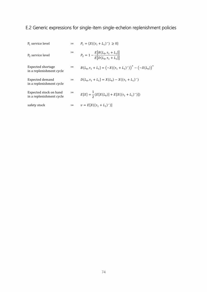
74

E.2 Generic expressions for single-item single-echelon replenishment policies

P1 service level

≔ 𝑃1 = {𝑋((𝜏𝑖 + 𝐿1)−) ≥ 0}

P2 service level

≔ 𝑃2 = 1 −

𝐸[𝐵(𝐿0, 𝜏1 + 𝐿1]]

𝐸[𝐷(𝐿0, 𝜏1 + 𝐿1]]

Expected shortage

in a replenishment cycle

≔ 𝐵(𝐿0, 𝜏1 + 𝐿1] = (−𝑋((𝜏1 + 𝐿1)−))

+− (−𝑋(𝐿0))

+

Expected demand in a replenishment cycle

≔ 𝐷(𝐿0, 𝜏1 + 𝐿1] = 𝑋(𝐿0) − 𝑋((𝜏1 + 𝐿1)−)

Expected stock on hand in a replenishment cycle

≔ 𝐸[𝑋] =

1

2(𝐸[𝑋(𝐿0)] + 𝐸[𝑋((𝜏1 + 𝐿1)

−)])

safety stock

≔ 𝑣 = 𝐸[𝑋((𝜏1 + 𝐿1)−)]

75

Appendix F F. Classic joint replenishment problem (J RP)

Classic joint replenishment problem (JRP)

Joint replenishment is focused on inventory decision making and aims at minimizing cost while

satisfying demand. The joint replenishment problem involves the coordination of when and how

much to order at which supplier and is a problem that exists in every logistics environment where

more than one different product is ordered to the same supplier. Additionally, fixed ordering cost

are incurred with every order placed to the supplier. Joint replenishment models and method have

successfully been utilized in different sectors and types of industry (e.g. spare parts, retail), which

could make it a useful method for our joint replenishment problem in an e-tailing environment

(Khouja & Goyal, 2008).

F.1 Definitions

Variables and expressions are largely extracted from Khouja and Goyal (2008) and are partly

redefined for clarity.

𝑇 ≔ time between successive replenishments (years)

𝑂 ≔ major fixed ordering cost associated with each replenisment (€/year)

𝑇𝐶 ≔ total annual holding and ordering costs for all the products (€/year)

𝑖 ≔ 1,2, … , 𝑛; a product index

𝑛 ≔ number of products

𝑘𝑖 ≔ 𝑘𝑖𝑡ℎ review moment with a potential order for product 𝑖

𝐾 ≔ set containing all 𝑘𝑖; 𝐾 = {𝑘1, 𝑘2, … 𝑘𝑛} ∈ ℕ𝑛

𝐷𝑖 ≔ annual demand for product 𝑖 (units/year)

ℎ𝑖 ≔ annual holding cost of product 𝑖 (€/unit/year)

𝑜𝑖 ≔ minor fixed ordering cost incurred if product i is ordered in a replenishment (€/order)

𝑄𝑖 ≔ order quantity of product 𝑖

𝑇𝑖 ≔ time interval between successive replenishments of product 𝑖 (years)

Strategies for solving the JRP can be classified into two types: (1) a direct grouping strategy (DGS)

and (2) an indirect grouping strategy (IGS). Under DGS, products are partitioned into a

predetermined number of sets and the products within each set are jointly replenished with the

76

same cycle time. Under IGS, a replenishment is performed at regular time intervals and every

product has a replenishment quantity sufficient to be enough for exactly an integer multiple of the

regular time interval.

Under IGS the cycle time for every product is an integer multiple 𝑘𝑖 of the replenishment cycle time

𝑇. Hence, the cycle time for product 𝑖 is:

𝑇𝑖 = 𝑘𝑖𝑇

(𝐸. 1)

The order quantity for product 𝑖 is:

𝑄𝑖 = 𝑇𝑖𝐷𝑖 = 𝑇𝑘𝑖𝐷𝑖

(𝐸. 2)

The total annual holding costs are:

𝐶𝐻 = ∑𝑄𝑖ℎ𝑖

2=

𝑇

2∑ 𝑘𝑖𝐷𝑖ℎ𝑖

𝑛

𝑖=1

𝑛

𝑖=1

(𝐸. 3)

The total annual fixed ordering costs are:

𝐶𝑂 =𝑂

𝑇+ ∑

𝑜𝑖

𝑘𝑖𝑇

𝑛

𝑖=1

=(𝑂 + ∑

𝑜𝑖

𝑘𝑖

𝑛𝑖=1 )

𝑇

(𝐸. 4)

In equation (𝐸. 4), cycles without replenishments (i.e. 𝑘𝑖 ≥ 2, 𝑖 = 1,2, … , 𝑛) still incur a major fixed

ordering cost of 𝑂.

The total annual cost are:

𝑇𝐶(𝑇, 𝐾) = 𝐶𝐻 + 𝐶𝑂 =𝑇

2∑𝑘𝑖𝐷𝑖ℎ𝑖

𝑛

𝑖=1

+(𝑂 + ∑

𝑜𝑖

𝑘𝑖

𝑛𝑖=1 )

𝑇

(𝐸. 5)

where 𝐾 is a set of integer multipliers. The policies defined by the basic cycle time and a set of

multipliers are can be described as cyclic policies. There are two classes of cyclic policies for the

JRP. Let 𝜌𝑐 be the set of cyclic policies which can be expressed as:

𝜌𝑐 ≔ (𝑇, 𝐾) ∶ 𝑇 > 0

𝐾 = (𝑘1, 𝑘2, … , 𝑘𝑛) ∈ ℕ𝑛 (𝐸. 6)

A cyclic policy is called a strict cyclic policy 𝜌𝑠𝑐 if at least one product 𝑖 has an integer multiplier

𝑘𝑖 = 1, which mean it is included in every order. Therefore, 𝜌𝑠𝑐 ⊆ 𝜌𝑐 and 𝜌𝑠𝑐 can be expressed as:

𝜌𝑠𝑐 ≔ (𝑇, 𝐾) ∶ 𝑇 > 0

𝐾 = (𝑘1, 𝑘2, … , 𝑘𝑛) ∈ ℕ𝑛 𝑘𝑖 = 1 𝑓𝑜𝑟 𝑠𝑜𝑚𝑒 1 ≤ 𝑖 ≤ 𝑛

(𝐸. 7)

This boils down to two optimization problems:

min(𝑇,𝐾)∈𝜌𝑠𝑐

𝑇𝐶(𝑇, 𝐾)

(𝐽𝑅𝑃𝑆𝐶)

min(𝑇,𝐾)∈𝜌𝑐

𝑇𝐶(𝑇, 𝐾) (𝐽𝑅𝑃𝐶)

77

Arkin et al. (1989) proved that the JRP is an NP-hard problem and there probably is no polynomial

time algorithm to solve the JRP. For a fixed 𝐾 = (𝑘1, 𝑘2, … , 𝑘𝑛) ∈ ℕ𝑛, the optimization problem

becomes:

min𝑇>0


(𝐽𝑅𝑃𝑇)

For a given 𝑇 > 0, the optimization problem can be expressed as:

min𝑇>0


(𝐽𝑅𝑃𝐾)

Solutions to both optimization problems are provided in Goyal (1974). Goyal also developed an

algorithm to find the optimal solution to minimize (𝐵. 5). In other words, Goyal’s approach results

in an optimal solution to the JRPSC. However, it may be computationally prohibitive for large

problems.

F.2 Assumptions

The assumptions of the classic JRP as by Silver et al. (1998):

1. The demand rate of each item is constant and deterministic.

2. The replenishment quantity of an item need not be an integral number of units.

3. The unit variable cost of any of the items does not depend on the quantity; there are no

discounts in either the unit purchase cost or the unit transportation cost.

4. The replenishment lead-time is zero; The extension with a fixed, known, nonzero lead-time

that is independent of the magnitude of the replenishment, is easily made.

5. The entire order quantity is delivered at the same time.

78

Appendix G G. Soluti on c oncepts

Solution concept information

G.1 Lost-sales solution concept information

In this section we elaborate on the solution concepts for the lost-sales problem briefly described in

chapter four.

G.1.1 𝑷𝟐 service level in a lost-sales system

The excess demand that is lost due to the fact that backorders are not accepted is important for

the total cost function in the form of shortage cost and to the service levels; the 𝑃2 service level in

particular. The 𝑃2 service level is the long run fraction of demand that is satisfied directly from stock;

i.e. excess demand in our lost-sales system is the fraction of demand that is not satisfied directly

from stock and therefore lost. Van Donselaar and Broekmeulen (2013) reason that in a lost-sales

system the average sales will be lower than in a model in which excess demand is backordered. As

a result the average stock on hand and the service level in a lost-sales model will be higher than in

a similar backordering system. The different methods to correct the 𝑃2 service level in a lost-sales

system based on a backorder system are described hereunder.

To approximate the 𝑃2 service level in a lost-sales system the simplest assumption would be that

the 𝑃2 service level of a lost-sales system is equal to that of a backorder system and is called the

P2BO-approximation (K. H. Van Donselaar & Broekmeulen, 2013):

�̂�2𝐿𝑆 = 𝑃2

𝐵𝑂

(𝐺. 1)

Silver and Peterson (1985) suggest that this is a reasonable approximation if the customer service

level is high. An improvement on this first approximation was proposed by Silver and Peterson

(1985) for continuous review lost-sales systems with an (𝑠, 𝑄) replenishment policy and by Tijms

and Groenevelt (1984) for the (𝑠, 𝑆) replenishment policy. The approximation of the fill rate in a

lost-sales system is called the P2SPTG-approximation (𝑃2𝐿𝑆1) and is suggested to be (Tijms &

Groenevelt, 1984):

1 − 𝑃2𝐿𝑆1

𝑃2𝐿𝑆1 = 1 − 𝑃2

𝐵𝑂 ⟺ 𝑃2𝐿𝑆1 =

1

2 − 𝑃2𝐵𝑂

(𝐺. 2)

For the first approximation the fill rate in the lost-sales system is always at least as high as in the

backorder system. However, in some situations the difference between the fill rate in the lost-sales

system and the fill rate in the backorder system becomes rather large (e.g. 𝑃2𝐿𝑆1 is 90% while 𝑃2

𝐵𝑂

is only 60%). According to van Donselaar and Broekmeulen (2013) the service level in the lost-sales

system for a given safety stock is always at least as high as the service level in the backordering

system, since the actual sales per period in the lost-sales system (equal to 𝑃2𝐿𝑆1𝜇) are less than the

actual sales in a backordering system (equal to 𝜇). Hence, with the same amount of inventory in

79

the system, due to lower sales the same or a higher service level can be achieved in the lost-sales

system.

Two important factors to take into account for determining the fill rate of a periodic lost-sales

system are: (1) the uncertainty of demand during lead-time and the review period and (2) the

number of outstanding orders. The first can be measured via the 𝐶𝑉 of the demand during lead-

time plus the review period. If demand is identically and independently distributed, the 𝐶𝑉 is equal

to:

𝐶𝑉𝑅+𝐿 =𝜎

𝜇√𝑅 + 𝐿

(𝐺. 3)

We described in section 2.1.1 and appendix B.1, that for lost-sales systems it is necessary to take

into account the number of outstanding orders and the times at which the orders are placed to

the supplier. A simple and intuitive measure to take into account the outstanding orders is the

variable 𝑛𝑂𝑂, which stands for number of outstanding orders. In case of a periodic fixed quantity

replenishment policy this variable is defined as the ratio between the expected demand during

lead-time 𝐿𝜇 and an expression for the expected order size (max (𝑄, 𝑅𝜇)) (K. H. Van Donselaar &

Broekmeulen, 2013):

𝑛𝑂𝑂 =𝐿𝜇

max (𝑄, 𝑅𝜇)

(𝐺. 4)

This approximation is exact if 𝑄 = 1, excess demand is backordered and discrete demand in every

review period is strictly larger than zero. In case of a periodic order-up-to replenishment policy,

the average order quantity is equal to 𝑅𝜇 and therefore:

𝑛𝑂𝑂 =𝐿𝜇

max (𝑅𝜇, 𝑅𝜇)=

𝐿𝜇

𝑅𝜇=

𝐿

𝑅

(𝐺. 5)

The relationship between 𝑃2𝐿𝑆 and 𝑃2

𝐵𝑂 for a given value of 𝑛𝑂𝑂 and 𝐶𝑉𝑅+𝐿 is given by the following

relations:

𝑃2𝐿𝑆2 = 𝛼(𝑛𝑂𝑂) + 𝛽(𝑛𝑂𝑂) ∗ 𝑃2

𝐿𝑆3

(𝐺. 6)

and

𝑃2𝐵𝑂 = 𝛼′(𝐶𝑉𝑅+𝐿) + 𝛽′(𝐶𝑉𝑅+𝐿) ∗ 𝑃2

𝐿𝑆3

(𝐺. 7)

Where 𝑃2𝐿𝑆3 is the third and last approximation for the 𝑃2 service level. The parameters 𝛼, 𝛼′, 𝛽 and

𝛽′ are the linear regression coefficients to be estimated. 𝑃2𝐿𝑆2 is also called 𝑃2

𝐷𝑜𝐵𝑟 and is found by

an iteration process (K. H. Van Donselaar & Broekmeulen, 2013). Important findings based on this

relationship are that if 𝑛𝑂𝑂 < 5, the relationship between 𝑃2𝐿𝑆 and 𝑃2

𝐵𝑂 takes an almost linear

relationship and the estimates are given by:

𝛽(𝑛𝑂𝑂) = 0,062𝑛𝑂𝑂 + 0,87

and

80

𝛼(𝑛𝑂𝑂) = 0,9980 − 𝛽(𝑛𝑂𝑂)

This leads to the following approximation for the fill rate in a lost-sales system with 𝑛𝑂𝑂 ≥ 5:

𝑃2𝐿𝑆3

= 𝑃2𝐿𝑆2 −

𝛼(𝑛𝑂𝑂)

𝛽(𝑛𝑂𝑂)

𝑖𝑓 𝑛𝑂𝑂 < 5

(𝐺. 8)

= 𝑃2

𝐿𝑆2 −(0,128 − 0,062𝑛𝑂𝑂)

0,062𝑛𝑂𝑂 + 0,87

However, if 𝑛𝑂𝑂 ≥ 5, the relationship is not linear and the estimates are found to be:

𝛽′(𝐶𝑉𝑅+𝐿) = 𝐶𝑉𝑅+𝐿−0,552𝑒0,279

and

𝛼′(𝐶𝑉𝑅+𝐿) = 1,0172 − 𝛽′(𝐶𝑉𝑅+𝐿)

This leads to the following approximation for the fill rate in a lost-sales system with 𝑛𝑂𝑂 ≥ 5:

𝑃2𝐿𝑆3

= 𝑃2𝐵𝑂 −𝛼′(𝐶𝑉𝑅+𝐿)

𝛽′(𝐶𝑉𝑅+𝐿)

𝑖𝑓 𝑛𝑂𝑂 ≥ 5

(𝐺. 9)

= 𝑃2𝐵𝑂 −

(1.0172 − 𝐶𝑉𝑅+𝐿−0,552𝑒0,279)

𝐶𝑉𝑅+𝐿−0,552𝑒0,279

Assume that the target fill rate is at least 95% and the safety stocks are determined using formulas

which assume excess demand being backordered. Van Donselaar and Broekmeulen (2013) take all

the 𝑃2𝐵𝑂 ≥ 95% from their simulation and compare them with the 𝑃2

𝐿𝑆3 (i.e. the true service level

as measured by the service in the simulated lost-sales system). As shown earlier in this section, the

difference between 𝑃2𝐵𝑂 and 𝑃2

𝐿𝑆3 depends on 𝐶𝑉𝑅+𝐿 and 𝑛𝑂𝑂. They show that for very high values

of 𝐶𝑉𝐿+𝑅, both the new formula as the old P2PSTG-approximation can be used (i.e. 𝑃2𝐿𝑆1 =

1

2−𝑃2𝐵𝑂).

For lower values of 𝐶𝑉𝐿+𝑅 (i.e. 𝐶𝑉𝑅+𝐿 < 1), the new formula adds the most value. Furthermore, the

higher the value of 𝑛𝑂𝑂, the less accurate 𝑃2𝐵𝑂.

Van Donselaar and Broekmeulen (2013) found that if 𝐶𝑉𝑅+𝐿 < 0.5 and 𝑛𝑂𝑂 ≥ 1, the service level

which results from using the P2BO-approximation with a target service level of 95% led to a an

actual service level in a lost-sales system that deviated at least 1% from the target service level,

meaning it would generate a service level between 96% and 100%. If products come from far (e.g.

long distance sea transportation from China) the lead-time is often longer than the review period

and in almost all cases with order-up-to levels (i.e. inventory position is brought back to a constant

order-up-to level 𝑆), 𝑛𝑂𝑂 =𝐿

𝑅 is larger than 1. The 𝐶𝑉𝑅+𝐿 is smaller than 0,5 is all cases simulated

by van Donselaar and Broekmeulen (2013), except for the cases where the lead-time is rather small

and the demand uncertainty is large.

81

G.1.2 Demand uncensoring

According to Vulcano et al. (2012) two important problems in retail demand forecasting are: (1)

estimating the turned-away demand when products are out of stock (lost-sales) and (2) properly

accounting for substitution effects among related products. If excess demand is lost and forecasts

are based on sales data only, the resulting demand forecasts may be negatively biased. This

underestimation exacerbates if products are out of stock for a longer period of time. Additionally,

stock-out based substitution will increase sales of substitute products that are available (called

recaptured demand). Not taking into account this recaptured demand may lead to overestimation

bias among the available products. The recapture rate in retail can be rather high (e.g. supermarket

where the customer chooses another type of potato chips because the one he prefers is out of

stock) (Corsten & Gruen, 2003). Spilled and substituted demand is not directly observable from

sales transactions. Numerous statistical techniques have been proposed to estimate this demand.

These techniques are known as demand untruncation or demand uncensoring methods. One of

the most popular methods is the expectation-maximization (𝐸𝑀) algorithm. EM uses iterative

methods to estimate the underlying relevant parameters (product demand across a historical data

set in our situation). The 𝐸𝑀 methods works by using alternating steps of computing conditional

expected values of the parameter estimates to obtain an expected log-likelihood function (the E-

step) and then maximizes this function to obtain improved demand estimates (the M-step).

However, retail forecasts that utilize the 𝐸𝑀 approach have been limited to uncensoring historical

sales data for individual products. The 𝐸𝑀 method and other newly developed methods are of a

high complexity. Furthermore, knowledge is required on the set products customers are

considering when making the decision for a certain product (Conlon & Mortimer, 2013). This

knowledge is based on the aggregate estimate of the market share of those products (Vulcano,

van Ryzin, & Ratliff, 2012).

Additionally, substitution in an e-commerce environment is less likely because the customer

performs an online search for a specific product instead of going to a physical store. If the product

is not available at a certain webshop the product is often removed from the website(s) of the

webshop. Therefore, the product does not show on the internet at all and the customer will not

notice that the preferred product is out of stock. Another situation may be that the customer

actually sees that the preferred product is out of stock at a certain webshop. In this situation, the

customer can go to other webshops with the ease of one mouse click and order the product there.

Products that are bought online are often more specific than buying something in the supermarket

to put on your bread or buying a pair of pants in a clothing shop.

G.1.3 The impute demand method

In this section we describe an approach developed for estimating the unobserved demand for

products in periods without stock. The approach assumes realistic data: observed sales data and

stock data such that it is known when products were available and when they were out of stock.

There are two important aspects about the demand input parameter to describe in this section.

82

The first aspect is that the model is based on forecasting the demand for the coming period. This

period is currently set to 90 days. There are several reasons for forecasting: (1) because we want to

take into account potential trends and seasonal factors of demand per product because demand

does not often behave stationary, (2) the more data is fed to the model as an input, the better the

demand forecast (i.e. the model is learning from the data). The second aspect is that the demand

input for forecasting in the model of Optiply should be a time series with a value at every time unit

of the time series. If we would only use the demands (sales) of the periods with positive stock on

hand (i.e. point of sales POS data), the model would not work. This POS data only contains the

times when sales were made and how many sales were made at that time. We make the POS data

a time series by manipulating the data by adding zero sales to every day without sales. For example,

if we have had 4 days with sales in the past week, we should impute a value of zero sales to the 3

days without sales to make sure that every day of the input data has a value.

The reasons that we want to say something about the demand in periods without stock are that:

(1) we want to take this demand into account to the best of our abilities and (2) because the forecast

tends to go to zero if the input demand parameter includes many days with zero demand in the

recent past. Demand for such products is variable which results in high safety times set by Optiply

(i.e. safety stock expressed in time). Once there is demand for such products after a long period of

time, the model picks up this demand and advises to replenish many items of the product because

of the high safety times. This results in too much stock on hand and extra costs. Therefore, we want

to create a more stable input demand parameter by imputing demand on the days without stock

on hand.

The procedure of the method

Let us define:

𝐷𝑖𝑑 = daily demand of product 𝑖 (i. e. NOT demand order size as in continuous demand)

𝑗 = number of days back in the historical data 𝑋𝑖(𝑡 − 𝑗) = stock on hand from every historical date that is used in the calculation 𝐼𝑥𝑖(𝑡−𝑗) = an indicator function that indicates if the stock on hand was positive on day 𝑗;

(𝐼𝑥𝑖(𝑡−𝑗) ≔ {1 𝑖𝑓 𝑋𝑖(𝑡 − 𝑗) > 0

0 𝑖𝑓 𝑋𝑖(𝑡 − 𝑗) = 0 )

𝑁 = total number of days that is looked back in the historical data

Average expected demand data is imputed in the sales dataset on the days without stock on hand

(i.e. days where 𝑋𝑖(𝑡) = 0). The demand that is imputed is equal to the average of the sales of the

last 𝑗 days with a total value of 30 days where the stock on hand is larger than zero. A value of

maximal 30 days is chosen such that any annual seasonal trend can be taken into account. With

this seasonal trend we aim for example at the annual returning increasing or decreasing of sales

during the summer months or Christmas. Moreover, we only include products in our analysis that

have more than 10 days with positive stock on hand. We make the assumption that the demand

information of products with less than 10 days with positive stock on hand is insufficient for

analyzing. Therefore, the average may be calculated with less than 30 values because sales were

not made on every day and sales could only be made on days with stock on hand (this is elaborated

later on in this paragraph). The imputed demand for product 𝑖 at time 𝑡 can be expressed as

83

Imputed demand on days without stock can be expressed as:



𝑗=1


𝑓𝑜𝑟 𝑡 = 1,2, … , 𝑛

𝑓𝑜𝑟 𝑗 = 1,2, … , 𝑁

(𝐺. 10)

subject to:

10 < ∑ 𝐼𝑥𝑖(𝑡−𝑗)

𝑁

𝑗=1≤ 𝑁

If the availability is not appropriate (𝑗 < 10), the imputed demand is set equal to zero. Furthermore,

forecasting for products with too little data gives inaccurate forecasts and special methods for new

products introductions should be implemented.

G.2 JRP solution concept information

In chapter four we briefly described the possibilities in solving the joint replenishment problem. This

section elaborates more on these possibilities.

Based on the paper of Atkins and Iyogun (1988), an option that was considered is to set a base

review period for every supplier 𝛿 by using the smallest integer that is divisible by all the optimal

review periods of the products 𝑖 that are in the same order to supplier 𝛿 (i.e. least common

multiple). Using this procedure the base review period is 𝑅 and every product 𝑖 ordered to the

same supplier has a review period 𝑘𝑖𝑅 with 𝑘𝑖 being the 𝑘𝑖𝑡ℎ review moment with a potential order

for product 𝑖.

A first problem is the fact that many of these problem solutions are based on the fact that there

exists a major fixed ordering cost and a minor fixed ordering cost per product each time that an

order is placed to the supplier. In the case situation there are no minor fixed ordering cost: no extra

fixed ordering cost are incurred by adding one extra product to the order to the supplier. Van Eijs

et al. (1992) compared solutions of the direct (DGS) and indirect (IGS) grouping strategies Under

DGS, products are partitioned into a predetermined number of sets and the products within each

set are jointly replenished with the same cycle time. Under IGS, a replenishment is performed at

regular time intervals and every product has a replenishment quantity sufficient to be enough for

exactly an integer multiple of the regular time interval(Khouja & Goyal, 2008). They measured the

solution quality of each strategy by percentage savings in total cost over the total cost of the

independent 𝐸𝑂𝑄 strategy. The authors found that two factors are important in determining the

relative performance of using DGS or IGS: (1) the ratio of the major ordering cost 𝐾 to the average

minor ordering cost �̅�𝑖: 𝐾

�̅�𝑖 and (2) the number of products 𝑛. They found that for values of

𝐾

�̅�𝑖 above

75, DGS and IGS became the same because only a single replenishment group was created. This

lets us to believe that if there are no minor fixed ordering cost 𝑘𝑖 or if they are very small, the term 𝐾

�̅�𝑖 becomes very large and the solution will result in placing the products in one replenishment

group.

84

A second problem is that finding the 𝑠-levels for every product 𝑖 is difficult process and in the

scientific literature often bounds or at best approximations for the order-up-to level 𝑆 are realized.

The computational complexity increases exponentially when the size of the set of 𝑘𝑖′𝑠 is increased.

In our case situation there are suppliers where hundreds of different products are ordered to.

Algorithms that give an optimal solution in a joint replenishment problem with up to 50 items, have

a hard time with problems where the number of items increase to 100 or more (Bijvank & Vis, 2011;

Wang, Dun, Bi, & Zeng, 2012). Linear programming has infinitely feasible solutions. A Greedy

algorithm is efficient if it searches in a continuous spectrum but does not consider most of the

feasible solutions. Finding optimal 𝑠-levels for 300 products that are ordered to the same supplier

with an algorithm such as the Greedy algorithm results in 10300 combinations and may not even

result in a global optimum.

Review period determination method

Taking into account the fact that there are only major fixed ordering cost (i.e. no minor fixed

ordering cost per product) in our JRP and knowing that the current method for coordinated

ordering is not fully correct, we propose a new method for determining the review period per

supplier. This section describes the determination of this review period which can be used in

determining the relevant parameters per product 𝑖 ordered to the same supplier. The difference

with the current method utilized by Optiply is that our method takes into account the costs and

demand from the different products 𝑖 ordered to the same supplier 𝛿 by taking the weighted

average.

Let us define the subset 𝑉𝛿 = {1,2,… , 𝑖, … , 𝑛} which contains all the product 𝑖 that are ordered to

the same supplier 𝛿 and 𝐷𝑖𝑑 as the daily demand of product 𝑖 (i.e. NOT demand order size as in continuous

demand).

Then the total inventory costs for these products can be expressed as:

𝐶(𝑄)

= ∑ℎ𝑖𝑄𝑖

2+

𝐷𝑖𝑑𝐾𝑖

𝑄𝑖𝑖∈𝑉𝛿

(𝐺. 11)

We then substitute the order quantity with the order quantity interval 𝑇𝑖 =𝑄𝑖

𝐷𝑖:

𝐶(𝑇)

= ∑ℎ𝑖𝐷𝑖

𝑑𝑇𝑖

2+

𝐾𝑖

𝑇𝑖𝑖∈𝑉𝛿

(𝐺. 12)

We want to place all the different products in one predetermined group because we only have one

major fixed ordering costs (Khouja & Goyal, 2008). Therefore, we can write expression (𝐺. 12) as:

𝐶(𝑇)

= ∑ℎ𝑖𝐷𝑖

𝑑𝑇

2+

𝐾

𝑇𝑖∈𝑉𝛿

(𝐺. 13)

If we then rewrite this expression and minimize the total cost by taking the first derivative with

respect to 𝑇 and setting it equal to zero:

85

𝐶(𝑇)

= 𝑇 (1

2∑ ℎ𝑖𝐷𝑖

𝑑 𝑖∈𝑉𝛿

) +𝐾

𝑇

(𝐺. 14)

𝐶′(𝑇) = 0

⟺1


𝑑 𝑖∈𝑉𝛿

−𝐾

𝑇2

(𝐺. 15)

⟺1


𝑑

𝑖∈𝑉𝛿=

𝐾

𝑇2

𝑇∗

= √2𝐾


(𝐺. 16)

The 𝑇∗ can be used as the review period for all the products 𝑖 ordered to the same supplier.

Therefore we state for every supplier 𝛿 with product subset 𝑉𝛿 = {1,2, … , 𝑖, … , 𝑛}:

𝑅𝛿 = 𝑇∗

(𝐺. 17)

The order quantity for every product 𝑖 ordered to the same supplier therefore becomes:

𝑄𝑖∗ = 𝑅𝛿 ∗

𝐸[𝐷𝑖]

𝐸[𝐴𝑖]

(𝐺. 18)

86

Appendix H

H. Opti ply review period on a supplier level

Optiply review period on a supplier level

The following method is a description of a method that was implemented in the model used by

Optiply. Every product 𝑖 is ordered to a specific supplier and multiple products may be ordered to

the same supplier. The review period for a certain supplier 𝛿 is based on historical demand data

and is determined by the following method:

1. Calculate the total average annual demand of every individual product 𝑖 (𝑇𝐴𝐴𝐷𝑖) ordered to

the same supplier based on the average inter-arrival time of demand and average demand

size in an order of product 𝑖:

𝑇𝐴𝐴𝐷𝑖 = 365 ∗E[Di]

E[Ai]

(𝐻. 1)

2. Calculate the total average demand on a supplier basis by summing the annual demand of

all products 𝑖 that are ordered to the same supplier 𝛿 (𝑇𝐴𝐴𝐷𝛿) :

𝑇𝐴𝐴𝐷𝛿 = ∑ 𝑇𝐴𝐴𝐷𝑖𝑖∈𝑉𝛿

(𝐻. 2)

3. Calculate the average selling price cost price average cost price of the products 𝑖 that are

ordered to the same supplier and calculate the average annual holding cost by multiplying

the annual interest rate with the average cost price and the average fixed ordering cost by

setting it equal to the fixed ordering cost.

avg. selling price supplier δ =∑ 𝑇𝐴𝐴𝐷𝑖𝑖∈𝑉𝛿 ∗ selling price 𝑖

𝑇𝐴𝐴𝐷𝛿

(𝐻. 3)

avg. cost price supplier δ =∑ 𝑇𝐴𝐴𝐷𝑖𝑖∈𝑉𝛿 ∗ cost price 𝑖

𝑇𝐴𝐴𝐷𝛿

𝐶ℎ̅ = avg. holding cost supplier δ = holding cost rate ∗ avg. cost price supplier δ 𝐶�̅� = avg. fixed ordering cost supplier δ = fixed ordering cost

4. Calculate the economic order quantity (𝑄𝛿) on supplier level based on demand, fixed ordering

cost and holding cost and determine the review period on a supplier level:

𝑄𝛿 = √2 ∗ 𝑇𝐴𝐴𝐷𝛿 ∗ 𝐶�̅�

𝐶ℎ̅

(𝐻. 4)

𝑅𝛿 = review period of supplier 𝛿 =𝑄𝛿

𝑇𝐴𝐴𝐷𝛿∗ 365

(𝐻. 5)

5. Calculate the 𝑄𝑖 on product level based on the review period of supplier 𝛿 and the inter-

arrival time of demand and the demand size for product 𝑖:

𝑄𝑖 = 𝑅𝛿E[Di]

E[Ai]

87

Appendix I I. Impute demand data heuristic

Impute demand data heuristic

Input: Sales_data (POS data), Stock_data

Output: Sales_data_imputed_demand

Function: 𝐼𝑚𝑝𝑢𝑡𝑒𝐷𝑒𝑚𝑎𝑛𝑑𝑑𝑎𝑡𝑎(𝑥)

Note: In case of using the 𝐼𝑚𝑝𝑢𝑡𝑒𝐺𝑎𝑚𝑚𝑎𝐷𝑒𝑚𝑎𝑛𝑑 function instead of the Impute, a Gamma distribution is

fit to the product demand on the days with positive stock on hand. Then, demand is imputed on the days

without stock on hand based on this Gamma distribution.

1. Create a function available (indicator function) that states the availability of data with positive stock on hand

(stock_on_hand).

Simplified R code:

available = ifelse(test = stock_on_hand == 0,

yes = 0,

no = 1))

Output: 𝐵𝑖𝑛𝑎𝑟𝑦()

2. Create a function nonzero_lags that counts how many days have had positive stock on hand in the last

𝑁 + 1 days (with 𝑁 = 30 and +1 for the day itself. 𝑁 = 30 is chosen not larger than 30 days because of

the seasonal aspect and not smaller than 10 days so it is not too sensitive for sudden changes or has too

little data. This variable cumulatively sums the availability variable over the last 𝑁 + 1 days. To do this, it

checks back into the last 𝑁 + 1 days of historical data; if less than 𝑁 + 1 days available: check back into

the historical data until the boundary of the data set is reached.

Simplified R code:

nonzero_lags = roll_sum(available, N = min(31, length(!is.na(sales))), fill = 0))

Output: 𝐼𝑛𝑡𝑒𝑔𝑒𝑟(0,1, … 𝑁,𝑁 + 1)

3. Create a variable demand that represents demand on a specific day.

• If stock on hand is zero on that specific day and there are more than 𝑗 = 10 historical data points with

positive stock on hand in the last 30 days, take the average of the number of sales of those data points

and return this average as the demand output of the specific day. If we look at the dataset as a whole,

this means that the function that calculates the average is a summation of the moving average (SMA)

that rolls over the days of the dataset. The number 10 is to account for noise and makes the imputed

demand not too dependent on recent historical data points (i.e. if the last one or two historical data

points are outliers in the sense of being very high or very low compared to the average and the value

of 𝑗 is chosen small, the value for the imputed demand is too sensitive to these outliers).

88

• Moreover, ff stock on hand is zero on that specific day and there are less than 10 historical data points

with positive stock on hand in the last 30 days, there is too little data to base a forecast on. Forecasting

demand of a product based on a few days results in inaccurate forecasts. If this is the case, the demand

on the days without stock on hand is set equal to the sales (i.e. zero).

Simplified R code:

demand = ifelse(test = stock_on_hand == 0,

yes = ifelse(test = nonzero_lags > 10,

yes = SMA(x = sales, N = min(30, length(!is.na(sales)))),

no = sales)

Output: 𝑛𝑢𝑚𝑒𝑟𝑖𝑐()

4. Lastly, as set of additional checks are performed on the dataset after imputing the artificial expected

demand.

• If the stock on hand is not known (NA; i.e. not available), set the demand of that day equal to the

number of sales. If the stock on hand is known, set demand equal to demand that was imputed.

• If demand is not known (NA), set the demand of that day equal to zero. If demand is known, set

demand equal to demand that was imputed.

• Some sales are entered manually by Company B. Some of these sales are made on days where,

according to the system, there was no stock on hand. However, these sales have to be accounted

for in the expected demand. Therefore: if the number of sales on a day is larger than zero and the

stock on hand is zero as well, we know that this is such a situation and the impute demand can be

set equal to the number of sales. In all other situations the demand can be set equal to the imputed

demand (which obviously can be equal to the number of sales of that day).

Simplified R code:

demand = ifelse(test = is.na(stock_on_hand),

yes = sales,

no = demand),

demand = ifelse(test = is.na(demand),

yes = 0,

no = demand),

demand = ifelse(test = sales > 0 & (stock_on_hand == 0 | is.na(on_hand_correct)),

yes = sales,

no = demand)

Output: 𝑛𝑢𝑚𝑒𝑟𝑖𝑐()

89

Appendix J J. Derivations of relevant parameters

Derivations of relevant parameters

For the derivations of the relevant components of the model it is assumed that the inventory system

analyzed is a single-item single-echelon inventory system. Therefore, the subscript 𝑖 that depicts

the concerning product 𝑖 is removed throughout this section as it becomes irrelevant here. The

demand during lead-time, demand during the review period, the undershoot, the expected stock

on hand and the service levels are therefore derived for the (𝑅, 𝑠, 𝑆) and (𝑅, 𝑆) replenishment

policy.

The generic functions for relevant parameters in an inventory system are given in appendix E.2 and

hold for every single-item single-echelon inventory system. Let us define the potential ordering

cycle (or review period) as the time interval between two subsequent review moments (𝜏, 𝑅] with

𝜏 being the review moment at the beginning of the ordering cycle (because of the assumption that

we have identically and independent review periods we can also write (0, 𝑅] here). Then let us

define the (potential) replenishment cycle as the time interval (𝐿, 𝑅 + 𝐿]. Ordering and

replenishment is potential under an (𝑅, 𝑠, 𝑆) replenishment policy because not every cycle a

replenishment order will be placed to the supplier. If the inventory position is above the reorder

level at a review moment, no replenishment order will be placed.

Furthermore, it is assumed that the inventory system is analyzed from the moment in time that a

potential order is placed. This moment in time is the start time 𝑡 = 𝑅0 = 0. This moment can be

any point in time. The (potential) order that is placed at time 𝑡 = 0 arrives at time 𝑡 = 𝐿0. The next

(potential) order after 𝑡 = 𝑅0 is placed at time 𝑡 = 𝑅1 and this order will arrive at time 𝑡 = 𝑅1 + 𝐿1.

Therefore, the analysis will focus on one full ordering cycle and one full replenishment cycle; the

time at which the first potential order is placed until the time that the second placed order is

delivered.

J.1 Demand during lead-time

The first parameter to analyze is the demand during lead-time. In this section the first two moments

of the demand during lead-time are derived. An order placed at time 𝑅0 is delivered at time 𝐿0.

Assuming that 𝐷(𝑅0, 𝐿0] and 𝐷(𝑅1, 𝐿1] follow the same Gamma distribution, the problem of

finding the first two moments of the demand during lead-time is reduced to finding an expression

for 𝐸[𝐷(0, 𝐿0]] (mean) and one for 𝜎2(𝐷(0, 𝐿0]) (variance). These expressions lead to correct

parameters of the Gamma distribution and are elaborated on in chapter five. If we take a step back

for now and only assume that both the demand and the lead-times are stochastic variables, we

require estimates of the mean and variance of the demand during lead-time.

Let us assume that the lead-time 𝐿 equals an constant and integer number of days and define the

inter-arrivals of demand in the time period (0, 𝐿] as 𝐾 and the demand sizes of an inter-arrival as

90

𝐷𝑘 with 𝑘 being the 𝑘𝑡ℎ inter-arrival of demand. The demand during this period is given by the

sum of the demand sizes of each of the inter-arrivals and can be expressed as ∑ 𝐷𝑘𝐾𝑘=1 . If we

assume that 𝐷𝑘 is an independent and identically distributed stochastic variable the mean and

variance can be expressed as:

𝐸[𝐷(0, 𝐿]] = 𝐿 ∗ 𝐸[𝐷]

(𝐽. 1)

𝜎2(𝐷(0, 𝐿]) = 𝐿 ∗ 𝜎2(𝐷)

(𝐽. 2)

If we then relax the assumption that 𝐿 is constant and only assume it equals an integer number of

days, the mean of the demand during lead-time can be derived as follows:

𝐸[𝐷(0, 𝐿]]

= 𝐸 [∑ 𝐷𝑗

𝐾

𝑘=1

]

(𝐽. 3)

= ∑ 𝐸 [∑ 𝐷𝑘

𝑛

𝑘=1

] 𝑃{𝐾 = 𝑛}

∞

𝑛=0

= ∑ 𝑛𝐸[𝐷]𝑃{𝐾 = 𝑛}

∞

𝑛=0

= 𝐸[𝐷] ∑ 𝑛𝑃{𝐾 = 𝑛}

∞

𝑛=0

= 𝐸[𝐷]𝐸[𝐾]

The following expression holds for a random variable: 𝜎2[𝑋] = 𝐸[𝑋2] − 𝐸[𝑋]2. This expression can

be rewritten as 𝐸[𝑋2] = 𝜎2[𝑋] + 𝐸[𝑋]2 and may be used in deriving the expression for the variance

of the demand during lead-time. First the expressions for 𝐸[𝐷2(0, 𝐿]] is derived:

𝐸[𝐷2(0, 𝐿]]

= 𝐸 [(∑ 𝐷𝑘

𝐾

𝑘=1

)

2

]

(𝐽. 4)

= ∑ 𝐸 [(∑ 𝐷𝑘

𝑛

𝑘=1

)

2

] 𝑃{𝐾 = 𝑛}

∞

𝑛=0

= ∑ (𝜎2 (∑ 𝐷𝑘

𝑛

𝑘=1

) + 𝐸2 [∑ 𝐷𝑘

𝑛

𝑘=1

]) 𝑃{𝐾 = 𝑛}

∞

𝑛=0

= ∑(𝑛𝜎2(𝐷) + 𝑛2𝐸2[𝐷]) 𝑃{𝐾 = 𝑛}

∞

𝑛=0

= 𝜎2(𝐷) ∑ 𝑛𝑃{𝐾 = 𝑛} + 𝐸2[𝐷] ∑ 𝑛2𝑃{𝐾 = 𝑛}

∞

𝑛=0

∞

𝑛=0

= 𝜎2(𝐷)𝐸[𝐾] + 𝐸2[𝐷]𝐸[𝐾2]

91

With the use of the expression 𝜎2(𝐷(0, 𝐿]) = 𝐸[𝐷2(0, 𝐿]] − 𝐸2[𝐷(0, 𝐿]], the variance can be

derived thereafter:

𝜎2(𝐷(0, 𝐿])

= 𝐸[𝐾]𝜎2(𝐷) + 𝐸[𝐾2]𝐸2[𝐷] − 𝐸2[𝐾]𝐸2[𝐷] (𝐽. 5)

= 𝐸[𝐾]𝜎2(𝐷) + 𝜎2(𝐾)𝐸2[𝐷]

Taking one step back and using the expressions from de Kok (1991a) for 𝐸[𝐾] and 𝐸[𝐾2] based on

a renewal process, the expressions for the mean and the variance of demand during lead-time can

be derived. The mean of the demand during lead-time is expressed as:

𝐸[𝐷(0, 𝐿]]

=𝐸[𝐿]

𝐸[𝐴]𝐸[𝐷]

(𝐽. 6)

Then, with the use of the expression for 𝐸[𝐷2(0, 𝐿]]:

𝐸[𝐷2(0, 𝐿]] = 𝐸2[𝐷] [𝐸[𝐿2]

𝐸2[𝐴]+

𝐸[𝐿]

𝐸[𝐴]∗ (𝐶𝑉𝐴

2 + 𝐶𝑉𝐷2) +

(1 − 𝐶𝑉𝐴4)

6]

(𝐽. 7)

= 𝐸2[𝐷]

[ 𝐸[𝐿2]

𝐸2[𝐴]+

𝐸[𝐿]

𝐸[𝐴]∗ ((

𝜎(𝐴)

𝐸[𝐴])

2

+ (𝜎(𝐷)

𝐸[𝐷])

2

) +

(1 − (𝜎(𝐴)𝐸[𝐴]

)4

)

6

]

and the expression 𝜎2(𝐷(0, 𝐿]) = 𝐸[𝐷2(0, 𝐿]] − 𝐸2[𝐷(0, 𝐿]], the variance of the demand during

lead-time can be derived as follows:

𝜎2(𝐷(0, 𝐿])

= 𝐸2[𝐷]

[ 𝐸[𝐿2]

𝐸2[𝐴]+

𝐸[𝐿]

𝐸[𝐴]∗ ((

𝜎(𝐴)

𝐸[𝐴])

2

+ (𝜎(𝐷)

𝐸[𝐷])

2

) +

(1 − (𝜎(𝐴)𝐸[𝐴]

)4

)

6

]

− (𝐸[𝐿]

𝐸[𝐴]𝐸[𝐷])

2

(𝐽. 8)

= 𝐸2[𝐷]

[ 𝐸[𝐿2]

𝐸2[𝐴]+

𝐸[𝐿]

𝐸[𝐴]∗ ((

𝜎(𝐴)

𝐸[𝐴])

2

+ (𝜎(𝐷)

𝐸[𝐷])

2

) +

(1 − (𝜎(𝐴)𝐸[𝐴]

)4

)

6−

𝐸2[𝐿]

𝐸2[𝐴]

]

= 𝐸2[𝐷]

[ 𝐸[𝐿2]

𝐸2[𝐴]+

𝐸[𝐿]

𝐸[𝐴]∗

𝜎2(𝐴)

𝐸2[𝐴]+

𝐸[𝐿]

𝐸[𝐴]∗

𝜎2(𝐷)

𝐸2[𝐷]−

𝐸2[𝐿]

𝐸2[𝐴]+

(1 − (𝜎(𝐴)𝐸[𝐴]

)4

)

6

]

=

𝐸[𝐿]

𝐸[𝐴]𝜎2(𝐷) + 𝐸2[𝐷]

[ 𝐸[𝐿2]

𝐸2[𝐴]+

𝐸[𝐿]

𝐸[𝐴]∗𝜎2(𝐴)

𝐸2[𝐴]−

𝐸2[𝐿]

𝐸2[𝐴]+

(1 − (𝜎(𝐴)𝐸[𝐴]

)4

)

6

]

=

𝐸[𝐿]

𝐸[𝐴]𝜎2(𝐷) + 𝐸2[𝐷]

[ 𝐸[𝐿2] − 𝐸2[𝐿]

𝐸2[𝐴]+

𝐸[𝐿]


𝐸2[𝐴]+

(1 − (𝜎(𝐴)𝐸[𝐴]

)4

)

6

]

92

=𝐸[𝐿]

𝐸[𝐴]𝜎2(𝐷) + 𝐸2[𝐷]

[ 𝜎2(𝐿)

𝐸2[𝐴]+

𝐸[𝐿]

𝐸[𝐴]∗

𝜎2(𝐴)

𝐸2[𝐴]+

(1 − (𝜎(𝐴)𝐸[𝐴]

)4

)

6

]

J.2 Demand during the review period

In an inventory system under an continuous replenishment policy, only demand during lead-time

is relevant for analysis. However, when under an periodic replenishment policy the demand during

the review period 𝑅 is relevant as well because parameters such as the safety stock have to take

into account the demand during the whole replenishment cycle 𝑅 + 𝐿. In case of an (𝑅, 𝑠, 𝑆)

replenishment policy, an order is placed at time 𝑅0 and the next order can be placed at time 𝑅1.

As for the demand during lead-time, we need the first two moment of the demand during the

review period for analysis. Based on de Kok (1991a), the expressions for the mean and variance of

the demand during the review period can be expresses as (de Kok, 1991):

𝐸[𝐷(0, 𝑅]] =𝐸[𝑅]

𝐸[𝐴]𝐸[𝐷]

(𝐽. 9)

and

𝜎2(𝐷(0, 𝑅]) =𝐸[𝑅]

𝐸[𝐴]𝜎2(𝐷) + 𝐸2[𝐷]

[ 𝜎2(𝑅)

𝐸2[𝐴]+

𝐸[𝑅]


𝐸2[𝐴]+

(1 − (𝜎(𝐴)𝐸[𝐴]

)4

)

6

]

(𝐽. 10)

J.3 Undershoot

Under a continuous can-order replenishment policy, the inventory position at the moment of

ordering is not necessarily equal to 𝑠 but rather equal to 𝑠 − 𝑈, where 𝑈 is a non-negative

stochastic variable called undershoot. Under a periodic can-order replenishment policy such as the

(𝑅, 𝑠, 𝑆) replenishment policy, this fact is enhanced because, due to periodic reviewing, an order

may be placed several time units after the moment that the inventory position went below 𝑠. The

undershoot at the moment of placing an order at time 𝑡 is equal to (𝑠 − 𝑌(𝑡))+

. The first two

moments of the undershoot involve approximation due to complexity of finding the mean and

variance of the undershoot. The approximations are based on de Kok (2002), which at their turn

are based on Tijms (1994). The approximations can be expressed as (De Kok, 2002):

𝐸[𝑈]

≈𝜎2(𝐸[𝐷(0, 𝑅]]) + 𝐸[𝐷(0, 𝑅]]

2

2𝐸[𝐷(0, 𝑅]]

(𝐽. 11)

and

𝜎2(𝑈)

≈ (1 + (𝜎(𝐸[𝐷(0, 𝑅]])

𝐸[𝐷(0, 𝑅]])

2

) ∗ (1 + 2(𝜎(𝐸[𝐷(0, 𝑅]])

𝐸[𝐷(0, 𝑅]])

2

) ∗𝐸[𝐷(0, 𝑅]]

2

3− 𝐸[𝑈]2

(𝐽. 12)

93

J.4 Expected stock on hand

The general expression for the expected stock on hand in a replenishment cycle is given by:

𝐸[𝑋] =1

2(𝐸[𝑋(𝐿0)] + 𝐸[𝑋((𝜏1 + 𝐿1)

−)])

(𝐽. 13)

And for a periodic replenishment policy:

𝐸[𝑋] =1

2(𝐸[𝑋(𝐿0)] + 𝐸[𝑋((𝑅1 + 𝐿1)

−)])

(𝐽. 14)

In order to determine the expected stock on hand we need to derive the expressions for the

expected stock at the beginning of a replenishment cycle just after the arrival of a replenishment

order 𝐸[𝑋(𝐿0)] and the expected stock at the end of the replenishment cycle just before the arrival

of a replenishment order 𝐸[𝑋((𝜏1 + 𝐿1)−)]. We assume that every replenishment cycle is

stochastically identical and independent.

Furthermore, we assumed that replenishment orders do not cross in time and therefore we know

that an order placed at time 𝑅0 = 0 will arrive at time 𝐿0. The subsequent potential replenishment

order arrives at time 𝑅1 + 𝐿1. Between these two order arrivals no other orders arrive and only

demand takes place in the interval (𝐿0,𝑅1 + 𝐿1] which reduces the stock on hand. The stock on

hand at time 𝐿0 is equal to the inventory position at time 𝑅0 = 0 minus the demand during 𝐷(0, 𝐿0]

and the expression for the stock on hand at time 𝐿0 for both the (𝑅, 𝑠, 𝑆) and the (𝑅, 𝑠)

replenishment policy is given by:

𝑋(𝐿0) = 𝑌(0) − 𝐷(0, 𝐿0]

(𝐽. 15)

= 𝑆 − 𝐷(0, 𝐿]


At the moment of ordering at time 𝑅1 the inventory position was equal to 𝑌(𝑅1) = 𝑠 − 𝑈1. Because

of the assumptions that orders do not cross in time, no orders will arrive before time (𝑅1 + 𝐿1)−

and only demand has to be subtracted from 𝑌(𝑅1) during the interval (𝑅1, 𝑅1 + 𝐿1]. Furthermore,

we assume that every cycle is stochastically identical and independent such that 𝐷(𝑅1, 𝑅1 + 𝐿1] =

𝐷(0, 𝐿]. Therefore, the expression for 𝑋((𝑅1 + 𝐿1)−) becomes:

𝑋((𝑅1 + 𝐿1)−)

= 𝑠 − 𝑈1 − 𝐷(𝑅1, 𝑅1 + 𝐿1]

(𝐽. 16)

= 𝑠 − 𝑈 − 𝐷(0, 𝐿]

The same expression can be found by rewriting 𝑋((𝑅1 + 𝐿1)−) = 𝑋(𝐿0) − 𝐷(𝐿0, 𝑅1 + 𝐿1].

We find the expected stock on hand in a replenishment cycle by substituting the expressions (𝐽. 15)

and (𝐽. 16) into (𝐽. 14) and rewriting:

𝐸[𝑋]

=1

2(𝐸[𝑆 − 𝐷(0, 𝐿]] + 𝐸[𝑠 − 𝑈 − 𝐷(0, 𝐿]])

(𝐽. 17)

94


At the moment of ordering at time 𝑅1 the inventory position was equal to 𝑌(𝑅1) = 𝑆 − 𝐷(0, 𝑅1].

Because of the assumptions that orders do not cross in time, no orders will arrive before time

(𝑅1 + 𝐿1)− and only demand has to be subtracted from 𝑌(𝑅1) during the interval (𝑅1, 𝑅1 + 𝐿1].

Furthermore, we assume that every cycle is stochastically identical and independent such that

𝐷(𝑅1, 𝑅1 + 𝐿1] = 𝐷(0, 𝐿]. Therefore, the expression for 𝑋((𝑅1 + 𝐿1)−) becomes:

𝑋((𝑅1 + 𝐿1)−) = 𝑆 − 𝐷(0, 𝑅1] − 𝐷(𝑅1, 𝑅1 + 𝐿1]

(𝐽. 18)

= 𝑆 − 𝐷(0, 𝑅1 + 𝐿1]

We find the expected stock on hand in a replenishment cycle by substituting the expressions (𝐽. 15)

and (𝐽. 18) into (𝐽. 14) and rewriting:

𝐸[𝑋]

=1

2(𝐸[𝑆 − 𝐷(0, 𝐿]] + 𝐸[𝑆 − 𝐷(0, 𝑅1 + 𝐿1]])

(𝐽. 19)

=

1

2(2𝑆 − 2𝐸[𝐷(0, 𝐿]] − 𝐸[ 𝐷(𝐿0, 𝑅1 + 𝐿1]])

= 𝑆 − 𝐸[𝐷(0, 𝐿]] −

𝐸[𝐷(0, 𝑅]]

2

J.5 Service levels

Service levels are required for evaluating the performance of an inventory system under a certain

replenishment policy. Therefore, this section describes the derivations of the service levels required

to evaluate the modified (𝑅𝛿 , 𝑆𝑖) and (𝑅𝛿 , 𝑠𝑖, 𝑆𝑖) replenishment policy.

J.5.1 The 𝑷𝟏 service level

The general expression for 𝑃1 is given by:

𝑃1 = 𝑃{𝑋((𝑅1 + 𝐿1)−) ≥ 0}

(𝐽. 20)


The expression for the expected stock at the end of the replenishment cycle just before the arrival

of a replenishment order 𝐸[𝑋((𝜏1 + 𝐿1)−)] was already derived in appendix I.4 and is given by:

𝐸[𝑋((𝜏1 + 𝐿1)−)] = 𝑠 − 𝑈 − 𝐷(0, 𝐿]

(𝐽. 21)

Substituting the expression of (𝐽. 21) into expression (𝐽. 20) we obtain:

𝑃1

= 𝑃{𝑠 − 𝑈 − 𝐷(0, 𝐿] ≥ 0} (𝐽. 22)

= 𝑃{𝐷(0, 𝐿] + 𝑈 ≤ 𝑠}

In the previous sections we derived expressions for the first two moments of the demand during

lead-time and the undershoot. Because we assumed that demand is mutually independent and

identically distributed we define the variable 𝑍 which is the sum of the first two moments of demand

during lead-time and the undershoot (De Kok, 2002):

95

𝐸[𝑍] = 𝐸[𝐷(0, 𝐿]] + 𝐸[𝑈] = 𝐸[𝐷(0, 𝐿] + 𝑈]

(𝐽. 23)

and

𝜎2(𝑍) = 𝜎2(𝐷(0, 𝐿]) + 𝜎2(𝑈) = 𝜎2(𝐷(0, 𝐿] + 𝑈)

(𝐽. 24)


The expression for the expected stock at the end of the replenishment cycle just before the arrival

of a replenishment order 𝐸[𝑋((𝜏1 + 𝐿1)−)] was already derived in appendix I.4 and is given by:

𝐸[𝑋((𝜏1 + 𝐿1)−)] = 𝑆 − 𝐷(0, 𝑅1 + 𝐿1]

(𝐽. 25)

Substituting the expression of (𝐽. 25) into expression (𝐽. 20) we obtain:

𝑃1

= 𝑃{𝑆 − 𝐷(0, 𝑅1 + 𝐿1] ≥ 0} (𝐽. 26)

= 𝑃{𝐷(0, 𝑅 + 𝐿] ≤ 𝑆}

= 𝑃{𝐷(0, 𝐿] + 𝐷(0, 𝑅] ≤ 𝑆}

J.5.2 The 𝑷𝟐 service level

The 𝑃2 service level is described as the long run fraction of total demand which is being delivered

from stock on hand immediately. This service level is often referred to as the customer service level

or the fill rate. The long run fraction refers to the behavior of demand and the inventory position

in every replenishment cycle. By assuming that every replenishment cycle is stochastically identical

and independent, we can use the following the expressions of de Kok (2012) for the 𝑃2 service level:

𝑃2 = 1 −𝐸[𝐵(𝐿, 𝑅 + 𝐿]]

𝐸[𝐷(𝐿, 𝑅 + 𝐿]]

(𝐽. 27)

which means that:

𝑃2 = 1 −the expected shortage in a replenishment cycle

total demand in a replenishment cycle

(𝐽. 28)


The expression for the expected shortage in a replenishment cycle 𝐸[𝐵[𝐿, 𝑅 + 𝐿]] can be derived

by taking the expected number of backorders at the end of the replenishment cycle just before an

order arrives (i.e. at time (𝑅 + 𝐿)−) and subtracting the expected number of backorders that were

present at the beginning of the replenishment cycle (i.e. at time 𝐿). The expression for

𝐸[𝐵(𝐿, 𝑅 + 𝐿]] is then given by:

𝐸[𝐵(𝐿, 𝑅 + 𝐿]]

= 𝐸 [(−𝑋((𝑅1 + 𝐿1)−))+ − (−𝑋(𝐿0))

+] (𝐽. 29)

= 𝐸 [(−(𝑠 − 𝑈 − 𝐷(0, 𝐿]))+ − (−(𝑆 − 𝐷(0, 𝐿]))+]

= 𝐸[(𝐷(0, 𝐿] + 𝑈 − 𝑠)+ − (𝐷(0, 𝐿] − 𝑆)+]

= 𝐸[(𝐷(0, 𝐿] + 𝑈 − 𝑠)+] − 𝐸[(𝐷(0, 𝐿] − 𝑆)+]

96

Thereafter, the expression for the total demand in a replenishment cycle 𝐸[𝐷(𝐿, 𝑅 + 𝐿]] can be

derived by taking the stock on hand at hand just after delivery of an order (i.e. at time 𝐿) and

subtracting the stock on hand just before the subsequent delivery of an order (i.e. at time (𝑅 + 𝐿)−).

The expression for 𝐸[𝐷(𝐿, 𝑅 + 𝐿]] is then given by:

𝐸[𝐷(𝐿, 𝑅 + 𝐿]] = 𝐸[𝑋(𝐿0) − 𝑋((𝑅1 + 𝐿1)−)]

(𝐽. 30)

= 𝐸[(𝑆 − 𝐷(0, 𝐿]) − (𝑠 − 𝑈𝑅 − 𝐷(0, 𝐿])]

= 𝑆 − 𝑠 + 𝐸[𝑈]

If we combine the two expressions we get the expression for the 𝑃2 service level:

𝑃2 = 1 −(𝐸[(𝐷(0, 𝐿] + 𝑈 − 𝑠)+] − 𝐸[(𝐷(0, 𝐿] − 𝑆)+])

(𝑆 − 𝑠 + 𝐸[𝑈])

(𝐽. 31)


The expression for the expected shortage in a replenishment cycle 𝐸[𝐵[𝐿, 𝑅 + 𝐿]] can be derived

by taking the expected number of backorders at the end of the replenishment cycle just before an

order arrives (i.e. at time (𝑅 + 𝐿)−) and subtracting the expected number of backorders that were

present at the beginning of the replenishment cycle (i.e. at time 𝐿). The expression for

𝐸[𝐵(𝐿, 𝑅 + 𝐿]] is then given by:

𝐸[𝐵(𝐿, 𝑅 + 𝐿]]

= 𝐸 [(−𝑋((𝑅1 + 𝐿1)−))+ − (−𝑋(𝐿0))

+]

(𝐽. 32)

= 𝐸 [(−(𝑆 − 𝐷(0, 𝑅 + 𝐿]))+ − (−(𝑆 − 𝐷(0, 𝐿]))+]

= 𝐸[(𝐷(0, 𝑅 + 𝐿] − 𝑆)+ − (𝐷(0, 𝐿] − 𝑆)+]

= 𝐸[(𝐷(0, 𝑅 + 𝐿] − 𝑆)+] − 𝐸[(𝐷(0, 𝐿] − 𝑆)+]

Thereafter, the expression for the total demand in a replenishment cycle 𝐸[𝐷(𝐿, 𝑅 + 𝐿]] can be

derived by taking the stock on hand at hand just after delivery of an order (i.e. at time 𝐿) and

subtracting the stock on hand just before the subsequent delivery of an order (i.e. at time (𝑅 + 𝐿)−).

The expression for 𝐸[𝐷(𝐿, 𝑅 + 𝐿]] is then given by:

𝐸[𝐷(𝐿, 𝑅 + 𝐿]] = 𝐸[𝑋(𝐿0) − 𝑋((𝑅1 + 𝐿1)−)]

(𝐽. 33)

= 𝐸[(𝑆 − 𝐷(0, 𝐿]) − (𝑆 − 𝐷((0, 𝑅 + 𝐿])]

= 𝐸[𝐷(0, 𝑅 + 𝐿] − 𝐷(0, 𝐿]]

= 𝐸[𝐷(0, 𝑅]]

If we combine the two expressions we get the expression for the 𝑃2 service level:

𝑃2 = 1 −(𝐸[(𝐷(0, 𝑅 + 𝐿] − 𝑆)+] − 𝐸[(𝐷(0, 𝐿] − 𝑆)+])

𝐸[𝐷(0, 𝑅]]

(𝐽. 34)

97

Appendix K K. Derivati ons of cos t func tions

Derivations of cost functions

In this section the relevant cost involved in performing operational inventory control at the case

study company, that is within the scope of the project, are described. The objective of the newly

defined replenishment policies is to minimize the total inventory cost under a target service level

constraint. The cost described in this section are holding cost, ordering cost and shortage cost. For

each of these cost, a cost function will be derived is used in evaluating the current situation and

the newly defined policy. This section is based on the aggregated stochastic joint replenishment

problem and therefore the subscript 𝑖 comes into play again.

K.1 Holding cost function

The cost of holding inventory are based on the amount of inventory held, the cost price of that

inventory and the holding cost rate. Because of the assumption that every replenishment cycle is

stochastically identical and independent, the expected stock on hand derived in appendix I.4 is a

good approximation of the average stock on hand in a replenishment cycle and therefore in any

arbitrary time period.

(𝑹𝜹, 𝒔𝒊, 𝑺𝒊) replenishment policy

The expected stock on hand for the (𝑅, 𝑠, 𝑆) replenishment policy was described as:

𝐸[𝑋] =1

2(𝐸[𝑆 − 𝐷(0, 𝐿]] + 𝐸[𝑠 − 𝑈 − 𝐷(0, 𝐿]])

(𝐾. 1)

The (𝑅, 𝑠, 𝑆) replenishment policy assumes that there is a minimum order quantity (𝑀𝑂𝑄) equal to

𝑆 − 𝑠 + 1 for discrete demand and 𝑆 − 𝑠 for continuous demand (K. H. Van Van Donselaar &

Broekmeulen, 2014). If we use this to rewrite the expression for the expected stock on hand we get:

𝐸[𝑋]

=1

2(𝑆 + 𝑠 − 𝐸[𝑈] − 2𝐸[𝐷(0, 𝐿]])

(𝐾. 2)

=

1

2(𝑆 − 𝑠 + 2𝑠 − 𝐸[𝑈] − 2𝐸[𝐷(0, 𝐿]])

=

1

2(𝑀𝑂𝑄 + 2𝑠 − 𝐸[𝑈] − 2𝐸[𝐷(0, 𝐿]])

= 𝑠 − 𝐸[𝐷(0, 𝐿]] −

𝐸[𝑈]

2+

𝑀𝑂𝑄

2

Using the expected stock on hand 𝐸[𝑋], the holding cost rate ℎ and 𝑐𝑖, the cost price of one

product 𝑖 the expected daily holding cost of one product 𝑖 under the (𝑅𝛿 , 𝑠𝑖, 𝑆𝑖) replenishment

policy (𝐸𝐷𝐻𝐶𝑅𝑠𝑆) can be expressed as:

𝐸𝐷𝐻𝐶𝑅𝑠𝑆 = ℎ𝑖 ∗ 𝑐𝑖 ∗ 𝐸[𝑋𝑖] (𝐾. 3)

98

= ℎ𝑖 ∗ 𝑐𝑖 ∗ (𝑠𝑖 − 𝐸[𝐷(0, 𝐿]] −𝐸[𝑈𝑖]

2+

𝐸 [𝐷(0, 𝑅𝛿]]

2)

The total expected daily holding cost (𝑇𝐸𝐷𝐻𝐶𝑅𝑠𝑆) can be expressed as:

𝑇𝐸𝐷𝐻𝐶𝑅𝑠𝑆

= ∑ ℎ𝑖 ∗ 𝑐𝑖 ∗ (𝑠𝑖 − 𝐸[𝐷(0, 𝐿]] −𝐸[𝑈𝑖]

2+

𝐸 [𝐷(0, 𝑅𝛿]]

2)

𝑛

𝑖=1

(𝐾. 4)

With 𝑛 being the total number of products.

(𝑹𝜹, 𝑺𝒊) replenishment policy

The expected stock on hand for the (𝑅, 𝑆) replenishment policy was described as:

𝐸[𝑋] = 𝑆 − 𝐸[𝐷(0, 𝐿]] −𝐸[𝐷(0, 𝑅]]

2

(𝐾. 5)

Using the expected stock on hand 𝐸[𝑋], the holding cost rate ℎ and 𝑐𝑖, the cost price of one

product 𝑖 the expected daily holding cost of one product 𝑖 under an (𝑅𝛿 , 𝑆𝑖) replenishment

policy (𝐸𝐷𝐻𝐶𝑅𝑆) can be expressed as:

𝐸𝐷𝐻𝐶𝑅𝑆 = ℎ𝑖 ∗ 𝑐𝑖 ∗ 𝐸[𝑋𝑖] (𝐾. 6)

= ℎ𝑖 ∗ 𝑐𝑖 ∗ (𝑆𝑖 − 𝐸[𝐷(0, 𝐿]] −𝐸 [𝐷(0, 𝑅𝛿]]

2)

The total expected daily holding cost (𝑇𝐸𝐷𝐻𝐶𝑅𝑆) can be expressed as:

𝑇𝐸𝐷𝐻𝐶𝑅𝑆

= ∑ ℎ𝑖 ∗ 𝑐𝑖 ∗ (𝑆𝑖 − 𝐸[𝐷(0, 𝐿]] −𝐸 [𝐷(0, 𝑅𝛿]]

2)

𝑛

𝑖=1

(𝐾. 7)

With 𝑛 being the total number of products.

Note that with the simulation results from chapter five, we changed the term between brackets for

both policies into (De Kok, 2002):

𝐸[𝑋] = 𝑠𝑖 +


2

2−

𝐸2[𝑈𝑖] + 𝜎2(𝑈𝑖)2

+𝐸2 [𝐷(0, 𝑅𝛿]] + 𝜎2(𝐷(0, 𝑅𝛿])

2𝐸[𝐷(0, 𝑅𝛿]]((𝑆𝑖 − 𝑠𝑖) + 𝐸[𝑈𝑖]))


𝐸[𝐿] − 𝑃2

𝐸[𝐷(0, 𝑅𝛿]]2

)

K.2 Ordering cost function

The fixed ordering cost is incurred every time that an order is placed to the supplier. In the case

situation there are no minor fixed ordering cost and therefore the size of the ordered quantity has

no effects on the ordering cost. If this was the case, the ordering cost functions should be adapted

accordingly. However, for generalization, expressions for the first two moments of the stochastic

random variable order quantity (𝑄𝑖) are derived in this section. These expressions are useful if there

are indeed minor fixed ordering cost or price discounts related to the ordered quantity.

99

Based on review period on a supplier level elaborated in section 4.6 we can describe the ordering

process of product 𝑖 ordered to supplier 𝛿 by deriving expressions for the frequency of the review

moments and the ordering frequency.


For the (𝑅𝛿 , 𝑠𝑖, 𝑆𝑖) replenishment policy we introduce a new variable 𝜌𝑖. Note that this variable is

only relevant for the for the (𝑅, 𝑠, 𝑆) replenishment policy. The variable 𝜌𝑖 is introduced to take into

account the fact that if there is a review moment 𝑅𝑡𝛿 and an order is allowed to be placed, the

inventory position could be equal or higher than the reorder level 𝑠𝑖 which results in not placing

an order (i.e. 𝑌𝑖(𝑡) ≥ 𝑠𝑖). In other words, we would like to know the probability that an order for

product 𝑖 is placed in a review period at the review moment. This is equal to the probability that in

period (0, 𝑅1𝛿] the inventory position just before time 𝑅1

𝛿 is less than the reorder level 𝑠𝑖. The

inventory position at time (𝑅1𝛿)

− is equal to the inventory position at time 𝑅0

𝛿 = 0 (just after the

review moment) minus the demand during the review period. The inventory position at time 𝑅0𝛿 =

0 is given by 𝑌𝑖(0) = 𝑆𝑖. Assuming that subsequent review moments are independent and demand

is stochastically independent and identical, the expressions for this probability is given by:

𝜌𝑖 = 𝑃{𝑆𝑖 − 𝐷𝑖(0, 𝑅𝛿] < 𝑠𝑖}

(𝐾. 8)

= 𝑃{𝐷𝑖(0, 𝑅𝛿] > 𝑆𝑖 − 𝑠𝑖}

The review frequency for product 𝑖 can be expressed as:

Review frequency

=1

𝐸[𝑅𝛿]

The ordering frequency is dependent on the expected demand size of an order, the expected inter-

arrival times between orders and the expected order quantity (i.e. the expected demand size of an

order combined with the expected inter-arrival times between orders results in the expected

demand in a time period).

Ordering frequency

=𝐸[𝐷𝑖]

𝐸[𝑄𝑖]𝐸[𝐴𝑖]

(𝐾. 9)

=

𝐸[𝐷𝑖]

(𝑆𝑖 − 𝑠𝑖 + 𝐸[𝑈𝑖])𝐸[𝐴𝑖]

Therefore, the variable 𝜌𝑖 can be expressed as:

𝜌𝑖

=

𝐸[𝐷𝑖](𝑆𝑖 − 𝑠𝑖 + 𝐸[𝑈𝑖])𝐸[𝐴𝑖]

1𝐸[𝑅𝛿]

(𝐾. 10)

=

𝐸[𝐷𝑖]𝐸[𝑅𝛿]

(𝑆𝑖 − 𝑠𝑖 + 𝐸[𝑈𝑖])𝐸[𝐴𝑖]

100

The expected order quantity 𝑄𝑖 is a stochastic random variable. In the case situation this variable

𝑄𝑖 is only relevant because we want to know if an order is placed in the review period. The fixed

ordering cost are taken into account with the derivation of the supplier based review period. We

can cope with the ordering cost in two ways: (1) derive an expression for the probability that one

of the products 𝑖 of the set of products ordered to the same supplier has an inventory position

lower than the reorder level 𝑠𝑖 or (2) assume that there is always one product 𝑖 in the set of products

ordered to the same supplier that has an inventory position lower than the reorder level 𝑠𝑖.

Let us define the subset 𝑉𝛿 = {1,2,… , 𝑖, 𝑖 + 1, 𝑛} which contains all the product 𝑖 that are ordered

to the same supplier 𝛿. The probability that one of the products 𝑖 in 𝑉𝛿 has an inventory position

lower than the reorder level 𝑠𝑖 at the review moment and hence, an order is placed to the supplier,

is equal to one minus the probability that none of the product 𝑖 in 𝑉𝛿 has an inventory position

lower than the reorder level 𝑠𝑖 at the review moment. This probability can be expressed as:

𝑃{𝑜𝑛𝑒 𝑝𝑟𝑜𝑑𝑢𝑐𝑡 𝑖 ∈ 𝑉𝛿𝑤ℎ𝑒𝑟𝑒 𝐷𝑖(0, 𝑅𝛿] > 𝑆𝑖 − 𝑠𝑖} = 1 − ∏(1 − 𝜌𝑖)

𝑖∈𝑉𝛿

(𝐾. 11)

If there is only one product 𝑖 in the set of products ordered to the same supplier, the ordering cost

function would be with fixed ordering cost 𝐾 becomes:

𝑂𝐶1,𝑖(𝜌𝑖) = 𝜌𝑖𝐾

(𝐾. 12)

If we indeed assume that there is always one product 𝑖 in the set of products ordered to the same

supplier that has an inventory position lower than the reorder level 𝑠𝑖, then the ordering cost

function per supplier becomes:

𝑂𝐶1 = 𝐾

(𝐾. 13)

If we do not make this assumption, the ordering cost function per supplier becomes:

𝑂𝐶2(𝜌𝑖) = (1 − ∏(1 − 𝜌𝑖)

𝑖∈𝑉𝛿

)𝐾

(𝐾. 14)

with 𝜌𝑖 =𝐸[𝐷𝑖]𝐸[𝑅𝛿]

(𝑆𝑖−𝑠𝑖+𝐸[𝑈𝑖])𝐸[𝐴𝑖].

For product 𝑖, the probability that an order of size 𝐸[𝑄𝑖] is placed at a review moment is equal to

𝜌𝑖. Hence, the expected order quantity of product 𝑖 ordered to the supplier at a review moment is

given by:

𝐸[𝑄𝑅𝑠𝑆,𝑖]

= 𝜌𝑖𝐸[𝑄𝑖]

(𝐾. 15)

= 𝜌𝑖𝐸[𝑆𝑖 − 𝑠𝑖 + 𝑈𝑖]

The expression for the variance of order quantity can be derived by using 𝜎2(𝑄𝑖) = 𝐸[𝑄𝑖2] − 𝐸[𝑄𝑖

2]

in our derivation:

101

𝜎2(𝑄𝑅𝑠𝑆,𝑖)

= 𝜌𝑖𝐸[(𝑆𝑖 − 𝑠𝑖 + 𝑈𝑖)2] − 𝐸[𝜌𝑖(𝑆𝑖 − 𝑠𝑖 + 𝑈𝑖)]

2 (𝐾. 16)

= 𝜌𝑖(𝜎2(𝑆𝑖 − 𝑠𝑖 + 𝑈𝑖) + 𝐸[(𝑆𝑖 − 𝑠𝑖 + 𝑈𝑖)]

2) − 𝐸[𝜌𝑖(𝑆𝑖 − 𝑠𝑖 + 𝑈𝑖)]2

= 𝜌𝑖(𝜎2(𝑆𝑖 − 𝑠𝑖 + 𝑈𝑖) + 𝐸[𝑆𝑖 − 𝑠𝑖 + 𝑈𝑖]

2) − 𝜌𝑖2𝐸[𝑆𝑖 − 𝑠𝑖 + 𝑈𝑖]

2

= 𝜌𝑖𝜎2(𝑈𝑖) + 𝜌𝑖𝐸[𝑆𝑖 − 𝑠𝑖 + 𝑈𝑖]

2 − 𝜌𝑖2𝐸[𝑆𝑖 − 𝑠𝑖 + 𝑈𝑖]

2

= 𝜌𝑖(1 − 𝜌𝑖)𝐸[𝑆𝑖 − 𝑠𝑖 + 𝑈𝑖]2 + 𝜌𝑖𝜎

2(𝑈𝑖)

We now derived the first two moments of 𝑄𝑖 . If a distribution is fit to these two moments, the

resulting pdf can be used to determine the expected daily ordering cost for the (𝑅𝛿 , 𝑠𝑖, 𝑆𝑖)

replenishment policy.

The expected daily ordering cost function for ordering products to a supplier 𝛿 can be expressed

as:

𝐸𝐷𝑂𝐶𝑅𝑠𝑆𝛿 =

𝑂𝐶2(𝜌𝑖)

𝐸[𝑅𝛿]

(𝐾. 17)

The total expected daily ordering cost are given by:

𝑇𝐸𝐷𝑂𝐶𝑅𝑠𝑆 = ∑ 𝐸𝐷𝑂𝐶𝑅𝑠𝑆𝛿

𝑁

𝛿=1

= ∑𝑂𝐶2(𝜌𝑖)

𝐸[𝑅𝛿]

𝑁

𝛿=1

(𝐾. 18)

With 𝑁 being the set of suppliers placing an order to.


The review frequency for product 𝑖 under the (𝑅𝛿 , 𝑆𝑖) replenishment policy can be expressed as:

Review frequency

=1

𝐸[𝑅𝛿]

(𝐾. 19)

Let us assume that there is at least one demand order for a product 𝑖 in a review period. Then the

ordering frequency for product 𝑖 under an (𝑅𝛿 , 𝑆𝑖) replenishment policy is the same as the review

frequency:

Ordering frequency

=1

𝐸[𝑅𝛿]

(𝐾. 20)

For he (𝑅𝛿 , 𝑆𝑖) replenishment policy it holds that if we assume that we have at least one demand

in a review period of one of the products 𝑖 that is in the set of products 𝑖 that is ordered to the

same supplier 𝛿, the ordering frequency is equal to the review frequency. Furthermore, the order

quantity is always equal to the demand in the most recent review period, assuming that demand

is stationary (K. H. Van Van Donselaar & Broekmeulen, 2014). Therefore the mean and variance of

the order quantity can be expressed as:

102

𝐸[𝑄𝑅𝑆,𝑖]

= 𝐸[𝑄𝑖] (𝐾. 21)

= 𝐷(0, 𝑅𝛿]

=

𝐸[𝑅𝛿]

𝐸[𝐴𝑖]𝐸[𝐷𝑖]

and

𝜎2(𝑄𝑅𝑆,𝑖) = 𝜎2(𝐷(0, 𝑅𝛿])

(𝐾. 22)

=𝐸[𝑅𝛿]

𝐸[𝐴𝑖]𝜎2(𝐷𝑖) + 𝐸2[𝐷𝑖]

[ 𝜎2(𝑅𝛿)

𝐸2[𝐴𝑖]+

𝐸[𝑅𝛿]

𝐸[𝐴𝑖]∗

𝜎2(𝐴𝑖)

𝐸2[𝐴𝑖]+

(1 − (𝜎(𝐴𝑖)𝐸[𝐴𝑖]

)4

)

6

]

Let us use the subset 𝑉𝛿 with all product 𝑖 ordered to the same supplier 𝛿 which we defined in this

section for an (𝑅𝛿 , 𝑠𝑖, 𝑆𝑖) replenishment policy. Because of the assumption that there is at least one

product 𝑖 in 𝑉𝛿 that has at least one demand in the duration of a review period, the ordering cost

function can be expressed as:

𝑂𝐶1 = 𝐾

(𝐾. 23)

The expected daily ordering cost function for ordering products to a supplier 𝛿 can be expressed

as:

𝐸𝐷𝑂𝐶𝑅𝑆𝛿 =

𝑂𝐶1

𝐸[𝑅𝛿]

(𝐾. 24)

The total expected daily ordering cost are given by:

𝑇𝐸𝐷𝑂𝐶𝑅𝑆 = ∑ 𝐸𝐷𝑂𝐶𝑅𝑆𝛿

𝑁

𝛿=1

= ∑𝑂𝐶1

𝐸[𝑅𝛿]

𝑁

𝛿=1

(𝐾. 25)

With 𝑁 being the set of suppliers placing an order to.

K.3 Shortage cost function

Excess demand results in a lost-sales because backorders are not accepted. We set a penalty cost

𝑝𝑖 for not being able to deliver the product from stock. This penalty cost is set equal to the margin

of the product. Additionally, it could be multiplied by a so called goodwill factor 𝛼. This 𝛼 is to take

into account the fact that a lost-sale does not only result in a penalty cost (lost margin) but may

also result in a customer that will not return for the next potential purchase, or worse, never returns

for any potential purchase. Let us assume that the goodwill factor can be set by the company based

on the importance of the product and can vary between 1 and 2. For example, if losing a customer

of a certain product is rather important, 𝛼 could be set somewhere between 1.5 and 2, while if it

is not, it could be set close to 1. Hence, not satisfying a demand for a product results in a shortage

cost equal to 𝛼 multiplied by the sales price minus the cost price of the product. In the derivations

of the cost function this 𝛼 is not taken into account.

103

We aim at minimizing inventory cost under a target fill rate which implicitly mean that we accept

that a percentage of demand is not satisfied from stock (immediately). This accepted percentage

of lost demand is equal to 1 − 𝑃2 and shortage cost become irrelevant in minimizing the inventory

cost. However, if we want to minimize the inventory cost taking into account the shortage cost per

product and aim at finding the ‘optimal’ fill rate per product, the shortage cost functions could be

useful.


The expected excess demand in a replenishment cycle can be described by the expression for the

expected backorders in a replenishment cycle or by multiplying the expected demand in a

replenishment cycle with 1 − 𝑃2. The expression for the expected backorders in a replenishment

cycle were derived in appendix J5. The daily expected shortage cost of a product 𝑖 in a

replenishment can then be expressed as:

𝐸𝐷𝑆𝐶𝑅𝑠𝑆,𝑖 = 𝑏𝑖

(𝐸[(𝐷(0, 𝐿] + 𝑈𝑖 − 𝑠𝑖)+] − 𝐸[(𝐷(0, 𝐿] − 𝑆𝑖)

+])

𝑅𝛿

(𝐾. 26)

If we define the stochastic random variables 𝑍 = 𝐷(0, 𝐿] + 𝑈 and 𝑌 = 𝐷(0, 𝐿], we get the following

expression:

𝐸𝐷𝑆𝐶𝑅𝑠𝑆,𝑖 =1

𝑅𝛿𝑏𝑖 ∫ (𝑧 − 𝑠𝑖)𝑓(𝑥)𝑑𝑥

∞

𝑠𝑖

− ∫ (𝑦 − 𝑆𝑖)𝑓(𝑦)𝑑𝑦∞

𝑆𝑖

(𝐾. 27)

with 𝑓(𝑥) and 𝑓(𝑦) being the probability density functions (pdf) of 𝑍 and 𝑌 respectively.

The total expected daily shortage cost can be expressed as:

𝑇𝐸𝐷𝑆𝐶𝑅𝑠𝑆 = 𝑏𝑖 ∑ ∑(𝐸[(𝐷(0, 𝐿] + 𝑈𝑖 − 𝑠𝑖)

+] − 𝐸[(𝐷(0, 𝐿] − 𝑆𝑖)+])


𝑁

𝛿=1

(𝐾. 28)


The expression for the expected backorders in a replenishment cycle are derived in appendix J.5.

The expected daily shortage cost (𝐸𝐷𝑆𝐶𝑖) of a product 𝑖 in a replenishment cycle can then be

expressed as:

𝐸𝐷𝑆𝐶𝑅𝑆,𝑖 = 𝑏𝑖

(𝐸 [(𝐷(0, 𝑅𝛿 + 𝐿] − 𝑆𝑖)+] − 𝐸[(𝐷(0, 𝐿] − 𝑆𝑖)

+])

𝑅𝛿

(𝐾. 29)

Because of the assumption that replenishment cycles are independent and identical, we can define

the stochastic random variables 𝑉 = 𝐷(0, 𝑅 + 𝐿] = 𝐷(0, 𝑅] + 𝐷(0, 𝐿] and 𝑌 = 𝐷(0, 𝐿] and get the

following expression:

𝐸𝐷𝑆𝐶𝑅𝑆,𝑖 =1

𝑅𝛿𝑏𝑖 ∫ (𝑉 − 𝑆𝑖)𝑓(𝑣)𝑑𝑣

∞

𝑆𝑖

− ∫ (𝑦 − 𝑆𝑖)𝑓(𝑦)𝑑𝑦∞

𝑆𝑖

(𝐾. 30)

The expected daily shortage cost for products ordered to the same supplier can be expressed as:

104

𝐸𝐷𝑆𝐶𝑅𝑆𝛿

=1

𝑅𝛿𝑏𝑖 ∑ (𝐸 [(𝐷(0, 𝑅𝛿 + 𝐿] − 𝑆𝑖)

+] − 𝐸[(𝐷(0, 𝐿] − 𝑆𝑖)

+])𝑖∈𝑉𝛿

(𝐾. 31)

=

1

𝑅𝛿𝑏𝑖 ∑ ∫ (𝑉 − 𝑆𝑖)𝑓(𝑣)𝑑𝑣

∞

𝑆𝑖

− ∫ (𝑦 − 𝑆𝑖)𝑓(𝑦)𝑑𝑦∞

𝑆𝑖𝑖∈𝑉𝛿

The total expected shortage cost (𝑇𝐸𝐷𝑆𝐶) can be expressed as:

𝑇𝐸𝐷𝑆𝐶𝑅𝑆

= 𝑏𝑖 ∑ ∑

(𝐸 [(𝐷(0, 𝑅𝛿 + 𝐿] − 𝑆𝑖)+] − 𝐸[(𝐷(0, 𝐿] − 𝑆𝑖)

+])


𝑁

𝛿=1

(𝐾. 32)

= 𝑏𝑖 ∑

1

𝑅𝛿 ∑ ∫ (𝑉 − 𝑆𝑖)𝑓(𝑣)𝑑𝑣

∞

𝑆𝑖

− ∫ (𝑦 − 𝑆𝑖)𝑓(𝑦)𝑑𝑦∞

𝑆𝑖𝑖∈𝑉𝛿

𝑁

𝛿=1

105

Appendix L L. Company specific cos t specifications

Company specific cost specifications

Holding cost

The holding cost can be determined by the cost of capital of the products in the assortment. In the

case situation, the company works with a holding cost rate of 20% per Euro per year (%/€/year) to

calculate the cost of invested capital. The first reason for using such a high percentage is the fact

that the company wants to keep inventory as low as possible while keeping service levels at a target

level. A second reason is that the same amount of money could have been invested in marketing

for products in the form of Google ads or increasing Google ranking for a certain time period.

Hence, the holding cost rate is not just the cost of not having the amount of money on the bank

with a certain interest rate. The holding cost can be calculated by multiplying the cost of goods sold

(COGS) with holding cost rate. Hence, The total annual holding cost can be calculated by summing

all the annual holding cost of the different products in the assortment. To illustrate the holding cost,

table 11 shows the cost price and holding cost per year of 10 randomly chosen SKUs.

Table 11: Holding cost representation for 10 randomly chosen SKUs

Ordering cost

For every order placed to a supplier, a fixed ordering cost is incurred. However, fixed ordering cost

are not precisely specified per supplier or per product. Every supplier has its own fixed ordering

cost that is based on processes including order picking, administration and transportation.

Knowing, or at least estimating this fixed ordering cost is required for decisions about which

replenishment policy to utilize and how to set parameters such as the size and the timing of the

order. For the case situation, the company sets the fixed ordering cost to equal to an amount of

20 Euros (€20) per order placed to the supplier. This fixed ordering cost was therefore used in the

calculations.

Shortage cost

Excess demand results in a lost-sales because backorders are not accepted. We set the penalty

cost for not being able to deliver the product from stock to account for the lost-sales in the lost-

sales system. This penalty cost is set equal to the margin of the product multiplied by a so called

SKU name Cost price

(€/unit)

Holding cost

(€/year)

803 46,75 9,35

1410 5,70 1,14

2546 340,22 68,04

3862 138,05 27,61

4201 4,88 0,98

1621 14,85 2,97

1084 48,29 9,66

3474 2,52 0,50

387 66,00 13,2

3829 78,41 15,68

106

goodwill factor 𝛼. This 𝛼 is to take into account the fact that a lost-sale does not only result in a

penalty cost (lost margin) but may also result in a customer that will not return for the next potential

purchase, or worse, never returns for any potential purchase. Let us assume that the goodwill factor

can be set by the company based on the importance of the product and can vary between 1 and

2. For example, losing a customer of a certain product is rather important, 𝛼 could be set

somewhere from 1,5 to 2, while if it is not, it could be set close to zero. Hence, not satisfying a

demand for a product results in a shortage cost equal to 𝛼 multiplied by the sales price minus the

cost price of the product. The shortage cost of the same randomly chosen SKUs is presented in

table 12.

Table 12: Shortage cost representation for 10 randomly chosen SKUs

SKU name Cost price

(€/unit)

Sales price

(€/unit)

Margin

(€/unit)

Shortage cost

(€/unit)

803 46,75 99,13 52,38 52,38𝛼

1410 5,7 15,66 9,96 9,96 𝛼

2546 340,22 616,49 276,27 276,27 𝛼

3862 138,05 138,05 139,59 139,59 𝛼

4201 4,88 14,83 9,95 9,95 𝛼

1621 14,85 33,02 18,17 18,17 𝛼

1084 48,29 80,12 31,83 31,83 𝛼

3474 2,52 10,7 8,18 8,18 𝛼

387 66 107,4 41,4 41,4 𝛼

107

Appendix M M. Fill rate calculati on verificati on

Fill rate calculation verification

This section describes the verification and the simulation results of the fill rate calculation functions

and all other relevant parameters such as demand during lead-time, demand during the review

period and the reorder level.

Note that the simulation tool is built in such a way that it simulates daily demand. R functions that

are used for generating demand therefore simulate a discrete demand process. Nevertheless, we

use an R function called momentCompound that provides us with the first two moments of a

compound distribution. The functions takes as input a parent distribution and its parameter(s), a

compound distribution and its parameters and the choice of which moment to calculate. This

function takes for example the Poisson distribution as the compound distribution and the Gamma

distribution as the parent distribution and provides us with the first two moments of the

compounding distribution (Nadarajah, Popović, & Ristić, 2013). The accuracy of the R functions is

checked with help of the extended spreadsheet by de Kok (2002) where both discrete and

continuous demand can be used as input for the (𝑅, 𝑠, 𝑆) replenishment policy.

For the verification of the fill rate calculation and cost functions, multiple scenarios were simulated.

For each scenarios we ran 𝑛 = 10 replications with a length of 𝑚 = 20.000 days. Every replication

has a warm-up period of 𝑙 = 2000 days. The warm-up period is determined by using the Welch

graphical method by Welch (1983) on the fill rate. Described briefly, we ran 5 replicates with a

moving average of 𝑤 = 1 day and simulation horizon of 𝑚 = 10.000 days to be able to see when

the fill rate converges to a steady state. The moving average should be smaller or equal to 𝑚

4 and

𝑚 should be chosen as large as practical regarding to the problem and the simulation time. If we

simulate to test for the warm-up period with 𝑚 = 10.000 days with a moving average of 𝑤 = 1

day, the period is long enough to allow for infrequent events (Law, 2007). Figure 10 shows the

graphical representation of the Welch graphical method. The line that represents the average fill

rate per day over in the 5 replicas evens out after approximately 2000 days. For the determination

of simulation results this warm-up period of 2000 days is removed from the simulation output data.

The simulation horizon should be as large as practical and should be significantly larger than the

warm-up period (Law, 2007). A simulation horizon of 20.000 days is long enough to minimize

potential outliers and provides simulations results that are close to identical. Taking this into account

combined with the fact that time is limited, the number of simulation replications is set to 𝑛 = 10.

This results in a 95% confidence interval (i.e. 𝛼 = 0,05) for the fill rate and other simulation output

equal to:

𝐶𝐼95% = �̅�(𝑛) ± 𝑡𝑛−1,1−

𝛼2

√𝜎2(𝑛)

𝑛 = �̅�(10) ± 𝑡10,0.975√

𝜎2(10)

10

(𝑀. 1)

108

Where �̅� is the average simulation output, 𝜎2 the variance of the simulation outpur, 𝑛 is the number

of replicas and 𝑡𝑛−1,1−𝛼

2 is the 𝑡-statistic for an 100(1 − 𝛼) confidence interval with 𝑛 replicas.

The fill rate calculation verification is performed for one product. If the fill rate calculation holds for

one product, it also holds for joint replenishment situations because the replenishment problem of

the different products can be seen as 𝑛 single-item problems. Only ordering cost are dependent

on the joint replenishment process which will be described in section 5.2.2. All verifications,

simulation scenarios and relevant conclusions are presented in appendix M. All input parameters

used for the different scenarios can be found in appendix O.

Figure 10: Welch graphical method

The first three scenarios are simulated under compound Poisson demand, with Poisson demand

inter-arrivals and Gamma distributed order sizes. Hence, the 𝐶𝑉 of the inter-arrival times of

demand orders is equal to 1 (i.e. 𝜎(𝐴)

𝐸[𝐴]= 1). Scenario 4 focusses on joint replenishment and

simulation is done for multiple products from the same supplier. For each scenario a table with

verification input and output is presented divided over two rows:

The first row shows the fill rate according to the spreadsheet of de Kok (2002) based on the

non-simulated input parameters which were used in every simulation run.

The second row shows the average post simulation input parameters that result from the 10

simulations runs. The value for the analytical reorder level 𝑠 on the second row is calculated

beforehand based on the input parameters. The value for the fill rate on the second row is

calculated with the average of all the post simulation input parameters. Note that this fill rate

can therefore deviate from the target fill rate.

The third row shows the average post simulation input parameters that result from the 10

simulations runs. The value for the reorder level 𝑠 is calculated with the average of all post

simulation input parameters under the initial target fill rate. The value for the fill rate on the

lower row is the post simulation average fill rate that resulted from the 10 simulation runs.

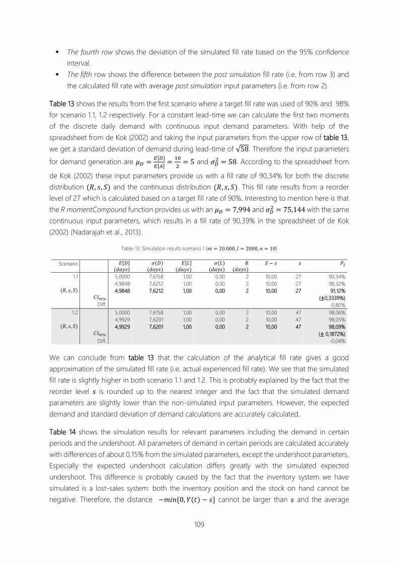
109

The fourth row shows the deviation of the simulated fill rate based on the 95% confidence

interval.

The fifth row shows the difference between the post simulation fill rate (i.e. from row 3) and

the calculated fill rate with average post simulation input parameters (i.e. from row 2).

Table 13 shows the results from the first scenario where a target fill rate was used of 90% and 98%

for scenario 1.1, 1.2 respectively. For a constant lead-time we can calculate the first two moments

of the discrete daily demand with continuous input demand parameters. With help of the

spreadsheet from de Kok (2002) and taking the input parameters from the upper row of table 13,

we get a standard deviation of demand during lead-time of √58. Therefore the input parameters

for demand generation are 𝜇𝐷 =𝐸[𝐷]

𝐸[𝐴]=

10

2= 5 and 𝜎𝐷

2 = 58. According to the spreadsheet from

de Kok (2002) these input parameters provide us with a fill rate of 90,34% for both the discrete

distribution (𝑅, 𝑠, 𝑆) and the continuous distribution (𝑅, 𝑠, 𝑆). This fill rate results from a reorder

level of 27 which is calculated based on a target fill rate of 90%. Interesting to mention here is that

the R momentCompound function provides us with an 𝜇𝐷 = 7,994 and 𝜎𝐷2 = 75,144 with the same

continuous input parameters, which results in a fill rate of 90,39% in the spreadsheet of de Kok

(2002) (Nadarajah et al., 2013).


Scenario 𝐸[𝐷] (𝑑𝑎𝑦𝑠)

𝜎(𝐷) (𝑑𝑎𝑦𝑠)




𝑆 − 𝑠 𝑠 𝑃2

1.1 5,0000 7,6158 1,00 0,00 2 10,00 27 90,34%

4,9848 7,6212 1,00 0,00 2 10,00 27 90,32%

(𝑅, 𝑠, 𝑆) 4,9848 7,6212 1,00 0,00 2 10,00 27 91,12%

𝐶𝐼95%

Diff.

(±0,3339%)

-0,80%

1.2 5,0000 7,6158 1,00 0,00 2 10,00 47 98,06%

4,9929 7,6201 1,00 0,00 2 10,00 47 98,05%

(𝑅, 𝑠, 𝑆)

𝐶𝐼95%

4,9929 7,6201 1,00 0,00 2 10,00 47

98,09%

(± 0,1872%)

Diff. -0,04%

We can conclude from table 13 that the calculation of the analytical fill rate gives a good

approximation of the simulated fill rate (i.e. actual experienced fill rate). We see that the simulated

fill rate is slightly higher in both scenario 1.1 and 1.2. This is probably explained by the fact that the

reorder level 𝑠 is rounded up to the nearest integer and the fact that the simulated demand

parameters are slightly lower than the non-simulated input parameters. However, the expected

demand and standard deviation of demand calculations are accurately calculated.

Table 14 shows the simulation results for relevant parameters including the demand in certain

periods and the undershoot. All parameters of demand in certain periods are calculated accurately

with differences of about 0,15% from the simulated parameters, except the undershoot parameters.

Especially the expected undershoot calculation differs greatly with the simulated expected

undershoot. This difference is probably caused by the fact that the inventory system we have

simulated is a lost-sales system: both the inventory position and the stock on hand cannot be

negative. Therefore, the distance −𝑚𝑖𝑛 {0, 𝑌(𝑡) − 𝑠} cannot be larger than 𝑠 and the average

110

undershoot will have a value between 0 and 𝑠 instead of between −𝑚𝑖𝑛 {0, 𝑌𝑖(𝑡)} and 𝑠. Hence,

the expected undershoot 𝐸[𝑈] is lower in our simulation model. The calculated fill rates are partly

based on the expected undershoot and are therefore important to incorporate. Although the

simulated undershoot parameters are not very accurate, the calculated fill rate and other relevant

parameter are.

Table 14: Simulation results of relevant parameters scenario 1 (𝑚 = 20.000, 𝑙 = 2000, 𝑛 = 10)

Scenario Variable 𝐸[𝐷(0, 𝐿]]

(𝑑𝑎𝑦𝑠)

𝜎(𝐷(0, 𝐿]) (𝑑𝑎𝑦𝑠)

𝐸[𝐷(0, 𝑅]]

(𝑑𝑎𝑦𝑠)

𝜎(𝐷(0, 𝑅]) (𝑑𝑎𝑦𝑠)

𝐸[𝑈] 𝜎(𝑈)

1.1 Analytical 5,0000 7,6158 10,0000 10,7703 10,8000 11,0635

Simulated 4,9848 7,6212 9,9696 10,7780 6,2240 9,9151

(𝑅, 𝑠, 𝑆) 𝐶𝐼95% (±0,0480) (±0,1038) (±0,0960) (±0,1468) (±0,0647) (±0,0701)

Diff. 0,30% -0,07% 0,30% -0,07% 42,37% 10,38%

1.2 Analytical 5,0000 7,6158 10,0000 10,7703 10,8000 11,0635

Simulated 4,9929 7,6201 9,9857 10,7764 7,2874 12,3258

(𝑅, 𝑠, 𝑆) 𝐶𝐼95% (±0,0782) (±0,1374) (±0,1564) (±0,1943) (±0,1647) (±0,1831)

Diff. 0,14% -0,06% 0,14% -0,06% 32,52% -11,41%

Because the accuracy of the calculated input parameters is verified by the simulations performed

for scenario 1.1 and 1.2, the simulation results of the input parameters expected daily demand and

the standard deviation of daily demand are not included in the simulations results that follow in the

remainder of this section. The simulated undershoot parameters are also excluded from the

remainder of this section because they are not relevant for the simulated fill rate and inventory

costs. Only the beforehand calculated parameters are dependent on the beforehand calculated

undershoot parameters and these are verified by the spreadsheet from de Kok (2002).

In the case situation the lead-time is stochastic. Therefore stochastic lead-times have to be verified

as well. Table 15 shows the simulation results of scenario 2.1 and 2.2. Both scenarios are run based

on a target fill rate of 98% due to the fact that a target fill rate of 98% seems realistic for practical

situations. Both scenarios include variable lead-time, a review period of 𝑅 = 4 days and the

demand input parameters are equal to those of scenario 1.1 and 1.2 (𝐸[𝐷] = 5, 𝜎(𝐷) = √58). The

difference between scenario 2.2 and 2.1 is that in scenario 2.2 the lead-time variability is much

higher. The reason for the post simulation expected lead-time to be higher than 12.00 is that the

Gamma generated lead-times are rounded up to the nearest integer number of days.


Scenario 𝐸[𝐿] (𝑑𝑎𝑦𝑠)


𝐸[𝐷(0, 𝐿]]

(𝑑𝑎𝑦𝑠)


𝐸[𝐷(0, 𝑅]]

(𝑑𝑎𝑦𝑠)



𝑠 𝑃2

2.1 12,0000 2,0000 60,0000 28,2135 20,0000 15,2315 4 140 98,00%

12,5011 2,0177 62,3507 28,6703 19,9505 15,1856 4 140 97,69%

(𝑅, 𝑠, 𝑆) 12,5011 2,0177 62,3507 28,6703 19,9505 15,1856 4 144 98,30%

𝐶𝐼95% (±0,1546%)

Diff. -0,61%

2.2 12,0000 10,0000 60,0000 56,5332 20,0000 15,2315 4 212 98,00%

12,5365 10,0478 62,5758 56,8479 19,9660 15,1156 4 212 97,87%

(𝑅, 𝑠, 𝑆) 12,5365 10,0478 62,5758 56,8479 19,9660 15,1156 4 215 99,81%

𝐶𝐼95% (±0,0703%)

Diff. -1,94%

111

In both scenarios we can see that the fill rate is underestimated with the calculations. The post

simulation fill rate is on average 0,61% and 1,94% higher in scenario 2.1 and 2.2 respectively.

However, all the input parameters are very accurate if we compare the calculated input parameters

with the average post simulation input parameters. Only the expected lead-time and expected

demand during lead-time are slightly higher but this is due to rounding up the lead-time to the

nearest integer in the lead-time generation process. Furthermore, if we use the post simulation

input demand parameters 𝐸[𝐷], 𝜎(𝐷), 𝐸[𝐿] and 𝜎(𝐿) from table 15 in the spreadsheet of de Kok

(2002), the resulting parameters such as 𝐸[𝐷(0, 𝐿]], 𝜎(𝐷(0, 𝐿]), 𝐸[𝐷(0, 𝑅]] and 𝜎(𝐷(0, 𝑅]) are

almost exactly the same as those resulting from simulation. Hence, all parameters are correctly

calculated beforehand and are very close to the simulated parameters, which lets us to believe that

the beforehand set reorder level 𝑠 is probably set too high and results in a fill rate that is a little bit

higher than expected. Additionally, it could be due to the large variability of the lead-time.

Table 16 shows the simulation results of scenario 3.1 and 3.2. Scenario 3.1 simulates the (𝑅, 𝑆)

replenishment policy with constant lead-times while scenario 3.2 simulates the (𝑅, 𝑆) replenishment

policy with variable lead-times. Both scenarios have a target fill rate of 98%. An interesting finding

with analyzing the (𝑅, 𝑆) replenishment policy was that Optiply was not using the undershoot in

the calculation of the order-up-to level 𝑆. Using the undershoot under an (𝑅, 𝑆) replenishment

policy sounds irrational because there is no reorder level 𝑠. However, we can use the (𝑅, 𝑠, 𝑆)

replenishment policy calculations for the (𝑅, 𝑆) replenishment policy by setting (𝑆 − 𝑠) = 0 and

the order-up-to-level 𝑆 equal to the expected demand and standard deviation of demand during

lead-time and during the review period under a target fill rate. If the undershoot is not taken into

account in calculating the reorder level 𝑠 or order-up-to-level 𝑆 under a certain target fill rate, one

does not take into account the variance of the demand during the review period. This results in a

lower actual experienced fill rate than was expected beforehand. Furthermore, both the

spreadsheet from de Kok (2002) as the Optiply model were not performing enough iterations to

find the optimal reorder level or order-up-to-level. A simple addition of performing more iterations

in a larger search interval solved this problem (see chapter five for more details). Also for the (𝑅, 𝑆)

replenishment policy we can conclude that the fill rate calculations and calculations of the other

relevant parameters are accurate. Only the fill rate calculation for scenario 3.2 is somewhat off. This

probably has to do with the set reorder level which is set to high or the high lead-time variability.


Scenario 𝐸[𝐿] (𝑑𝑎𝑦𝑠)


𝐸[𝐷(0, 𝐿]]

(𝑑𝑎𝑦𝑠)


𝐸[𝐷(0, 𝑅]]

(𝑑𝑎𝑦𝑠)



𝑆 𝑃2

3.1 1,00 0,00 5,0000 7,6168 10,0000 10,7703 2 55 98,15%

1,00 0,00 5,0102 7,6221 10,0204 10,7792 2 55 98,15%

(𝑅, 𝑆) 1,00 0,00 5,0102 7,6221 10,0204 10,7792 2 55 98,48%

𝐶𝐼95% (±0,1313%)

Diff. -0.33%

3.2 12,0000 10,0000 60,0000 56,5332 10,0000 10,7703 2 203 98,02%

12,4506 9,9641 62,3009 56,6316 10,0078 10,7631 2 203 97,63%

(𝑅, 𝑆) 12,4506 9,9641 62,3009 56,6316 10,0078 10,7631 2 207 99,91%

𝐶𝐼95% (±0,0275%)

Diff. -2,1%

112

Appendix N N. Cost functi ons calculation verification

Cost functions calculation verification

The following section describes the verification and simulation results of the developed cost

functions of the new model. Section N.1 is on the verification of the holding cost function and

section N.2 is on the verification of the ordering cost function.

N.1 Holding cost function

Table 17 shows the simulation results of the holding cost for all different scenarios. We see that the

holding cost calculations in the 6th column (SPP) by Silver et al. (1998) are not very accurate

compared to the simulated holding cost, especially the holding cost calculation from scenario 1.1.

Such a difference in cost made us wondering if it would be better to use the expected stock on

hand approximation by de Kok (2002) instead of the expected stock on hand approximation by

Silver et al. (1998). Using the expected stock on hand approximations by de Kok (2002) takes the

stock on hand at the beginning (i.e. 𝑋(𝐿0)) and the end of the replenishment cycle just before a

replenishment order arrives (i.e. 𝑋(𝑅1 + 𝐿1)−). As can be seen in table 16 in the 3rd column this

approximation resulted in much better estimations of the holding cost. The best holding cost

approximation in ever scenario is displayed in bold. All holding cost simulation results have a 95%

confidence interval smaller than ±1% with a minimum of ±0.1473% and a maximum of

±0,7287%.

Table 17: Holding cost simulation results (𝑚 = 20.000, 𝑙 = 2000, 𝑛 = 10)

The holding cost approximation by de Kok (2002) is the most accurate in estimating the expected

stock on hand. Therefore the 𝐸[𝑋] term in the holding cost functions becomes:

Scenario Analytical

(de Kok, 2002)

Simulated Diff. % Analytical

(SPP, 1998)

Simulated Diff. %

1.1 Total €984,63 €1005,49 -2,12% €852,16 €1005,49 -17,99%

(𝑅, 𝑠, 𝑆) 𝐶𝐼95% (±€1,6565) (±€1,6565)

Daily €0,0547 €0,0559 €0,0473 €0,0559

1.2 Total €1757,89 €1764,83 -0,39% €1641.21 €1764,83 -7,53%

(𝑅, 𝑠, 𝑆) 𝐶𝐼95% (±€3,4285) (±€3,4285)

Daily €0,0977 €0,0980 €0.0912 €0,0980

2.1 Total €3362,55 €3303,09 -1,98% €3239.01 €3303,09 -4,96%

(𝑅, 𝑠, 𝑆) 𝐶𝐼95% (±€14,6428) (±€14,6428)

Daily €0,1868 €0,1835 €0.1799 €0,1835

2.2 Total €6203,10 €6094,00 1,76% €6079,56 €6094,00 -0,24%

(𝑅, 𝑠, 𝑆) 𝐶𝐼95% (±€44,41) (±€44,41)

Daily €0,3446 €0,3386 €0,3378 €0,3386

3.1 Total €1768,77 €1819,99 -2,90% €1956.82 €1819,99 6,99%

(𝑅, 𝑆) 𝐶𝐼95% (±€2,6805) (±€2,6805)

Daily €0,0983 €0,1011 €0.1087 €0,1011

3.2 Total €5437,81 €5386,81 0,94% €5625,86 €5386,81 4,25%

(𝑅, 𝑆) 𝐶𝐼95% (±€14,21) (±€14,21)

Daily €0,3021 €0,2993 €0,3125 €0,2993

113

𝐸[𝑋] = 𝑠𝑖 +


2

2−

𝐸2[𝑈𝑖] + 𝜎2(𝑈𝑖)2

+𝐸2 [𝐷(0, 𝑅𝛿]] + 𝜎2(𝐷(0, 𝑅𝛿])

2𝐸[𝐷(0, 𝑅𝛿]]((𝑆𝑖 − 𝑠𝑖) + 𝐸[𝑈𝑖]))


𝐸[𝐿] − 𝑃2

𝐸[𝐷(0, 𝑅𝛿]]2

)

(𝑁. 1)

where 𝑃2 is the target fill rate and (𝑆 − 𝑠) is the expected order quantity in every replenishment

cycle. From the simulation results we can conclude that the newly defined holding cost functions

give an accurate estimate of the holding cost.

N.2 Ordering cost function

Table 18 shows the simulation results for the ordering cost functions. It also shows the calculated

𝜌𝑖 and the simulated 𝜌𝑖, which is the probability that an actual replenishment order is placed in a

replenishment cycle. We also calculated and simulated this 𝜌𝑖 for the (𝑅, 𝑆) replenishment policy

where we assumed that it is equal to 1. However, in scenario 3.2 the 𝜌𝑖 was smaller than 1 meaning

that an order is not necessarily placed in every replenishment cycle . All ordering cost simulation

results have a 95% confidence interval which is smaller than ±1% with a minimum of ±0% and a

maximum of ±0.7717%. We can conclude that the ordering cost functions provide accurate

ordering cost estimations according to the simulation of these cost.

Table 18: Ordering cost simulation results (𝑚 = 20.000, 𝑙 = 2000, 𝑛 = 10)

Scenario Analytical Simulated Diff. %

1.1 Total €85.538,46 €84.516,00 2,34%

(𝑅, 𝑠, 𝑆) 𝐶𝐼95% (±€462,33)

Daily €4,81 €4,70

𝑝𝑖 0,4808 0,4695 2,34%

1.2 Total €86,538.46 €86216,00 0,37%

(𝑅, 𝑠, 𝑆) 𝐶𝐼95% (±€826,55)

Daily €4,81 €4,79

𝑝𝑖 0,4808 0,4790 0,37%

2.1 Total €50279,33 €49598,00 1,36%

(𝑅, 𝑠, 𝑆) 𝐶𝐼95% (±€369.,91)

Daily €2,79 €2,76

𝑝𝑖 0,5587 0,5512 1,36%

2.2 Total €50,279,33 €50.078,00 0,40%

(𝑅, 𝑠, 𝑆) 𝐶𝐼95% (±€386,45)

Daily €2,79 €2,78

𝑝𝑖 0,5587 0,5564 0,40%

3.1 Total €180.000 €180.000 0,00%

(𝑅, 𝑆) 𝐶𝐼95% (±€0,00)

Daily €10,00 €10,.00

𝑝𝑖 1 1 0,00%

3.2 Total €180.000 €179.972 0,02%

(𝑅, 𝑆) 𝐶𝐼95% (±€44.90)

Daily €10,00 €10,00

𝑝𝑖 1 0,9998 0,02%

In case of joint replenishment, the review period 𝑅𝛿 is set for all products in the subset 𝑉𝛿 =

{1,2,… , 𝑖, 𝑛}. The probability of placing an order for product 𝑖 in a replenishment cycle 𝜌𝑖 should

be calculated for every product 𝑖 in subset 𝑉𝛿. Because the calculations of 𝜌𝑖 and the other relevant

114

parameters are accurate, we can use the ordering cost function from section 4.6.2.2 for a joint

replenishment situation under a (𝑅𝛿 , 𝑠𝑖, 𝑆𝑖) replenishment policy:

𝑂𝐶2(𝜌𝑖) = (1 − ∏(1 − 𝜌𝑖)

𝑖∈𝑉𝛿

)𝐾

(𝑁. 2)

Let us give a short example: if we have 3 products: 𝑉𝛿 = {1,2,3} with 𝜌1 = 0.5, 𝜌2 = 0.6 and 𝜌3 =

0.8. The probability of placing an order to the supplier in a replenishment cycle is equal to: 1 −

∏ (1 − 𝜌𝑖)𝑖∈𝑉𝛿 = 1 − ((1 − 0.5)(1 − 0.6)(1 − 0.8)) = 1 − 0.04 = 0.96. The expected ordering

cost per replenishment cycle is then equal to 0.96𝐾. For the (𝑅𝛿 , 𝑆𝑖) replenishment policy we have

shown that 𝜌𝑖 ≈ 1 and therefore the ordering cost function for a replenishment cycle is:

𝑂𝐶1 = 𝐾

(𝑁. 3)

A practical case of the probability in a joint replenishment situation is given in section 5.3.

115

Appendix O O. Simulation m odel input parameters

Simulation model input parameters

The input parameters of the different scenarios are shown in table 19 and table 20.

Table 19: Simulation model input parameters

Scenario 𝐸[𝐷𝑖] (𝑑𝑎𝑦𝑠)







𝑠𝑖

𝑆𝑖 𝑃2 (𝑡𝑎𝑟𝑔𝑒𝑡)

1.1 10 4 2 2 1 0 2 27 - 90%

1.2 10 4 2 2 1 0 2 47 - 98%

2.1 10 4 2 2 12 2 4 140 - 98%

2.2 10 4 2 2 12 10 4 212 - 98%

3.1 10 4 2 2 1 0 2 - 55 98%

3.2 10 4 2 2 12 10 2 - 203 98%

Table 20: Simulation model input parameters

Scenario 𝐸[𝐷𝑖] (𝑑𝑎𝑦𝑠)







𝐶𝑉𝑅 𝑠𝑖

𝑆𝑖 𝑃3 (𝑡𝑎𝑟𝑔𝑒𝑡)

4.1 10 0 1 1 1 0 1 1 - 48 95%

4.2 10 6 2 2 1 0 1 1,65 - 44 95%

4.3 10 10 2 2 1 0 1 2 - 58 95%

4.4 10 20 2 2 1 0 1 3,16 - 121 95%

116

Appendix P P. Implementa tion Decision support tool

Implementation Decision support tool

Section P.1 describes the input parameters that are required for the tool such that it can provide

the user the output parameters. In section P.2 the different features of the tool are elaborated on.

Section P.3 provides a user manual on how to use the tool correctly, including explanation on how

to read, write and update the input and output data. Section P.4 briefly describes the user interface

of the tool.

Simulation tool

As described in chapter five, additional to the decision support tool we developed a simulation tool

that is able to simulate daily replenishment operations for the (𝑅𝛿 , 𝑆𝑖) and (𝑅𝛿 , si, 𝑆𝑖) replenishment

policy. This simulation tool can be used for test products by inserting test data into the tool or for

real products by inserting historical data or forecasted data. The simulation tool is not relevant for

the decision support tool and will therefore not be explained in too much detail. However, all

versions of the simulation tool will be made available for Optiply and its current and future

graduation students. The simulation tool simulates stochastic demand (or real demand), stochastic

lead-times, the daily stock on hand, the daily inventory position, daily undershoot, daily lost-sales,

review moments, replenishment orders and replenishment deliveries. Simulation can be done for

one or more products from the same supplier such that inventory cost such as holding cost,

ordering cost and shortage cost can be simulated for a time period chosen by the user (e.g. 1000

days, 20.000 days etc.).

P.1 Input & output parameters

P.1.1 Input parameters

The decision support tool requires several input parameters to provide the output that is needed

for the desired inventory control. The most important input parameters are the demand input

parameters. Demand parameters are split up in demand inter-arrivals and demand order sizes (i.e.

continuous demand). Therefore, demand is assumed to follow a compound renewal process.

P.1.1.1 Demand forecasting

Because in practice demand does not behave stationary, the demand parameters from the

historical data are combined with an ETS forecast software package which combines 16 different

forecasting methods that take into account any seasonal and trend factors (R.J. Hyndman et al.,

2008; Rob J. Hyndman, Akram, & Archibald, 2008; Rob J. Hyndman, Koehler, Snyder, & Grose,

2002). Forecasting is performed over a horizon of 90 days. The forecast method in combination

with the developed impute demand methods provide an estimation of the demand parameters

and only requires the POS data and stock changes data. The demand input parameters are then

balanced based on the historical data and the forecast. Hence, we could state that we only require

117

POS data and stock changes data to determine the input demand parameters. Note that in practice,

the forecasted variance of demand during lead-time in one period may be substituted into the

model as the variance of demand during lead-time (i.e. direct substitution of the forecast error).

Other methods include corrections of demand during lead-time based on the forecast error and

assumes the demand during lead-time to be normally distributed. This leads to corrected safety

stocks based on forecast errors such as the RMSE or the MASE (Axsäter, 2006; Prak, Teunter, &

Syntetos, 2017; Silver et al., 1998). From the stock data we acquire the lead-time information per

supplier and in combination with the demand parameters this provides us with the mean and

standard deviation of demand during lead-time. The decision support requires the following input

parameters to function:

1. Product name or Product ID

2. Supplier name or Supplier ID

3. POS data, wherefrom the following parameters are calculated:

a. Mean and standard deviation of the inter-arrival time of sales orders in days

b. Mean and standard deviation of the sales order sizes in units

c. Supplier aggregate review period for all products ordered to the same supplier

4. Demand forecast based on a 3-month forecast horizon, wherefrom the following parameters are

calculated:

a. Mean and standard deviation of the inter-arrival time of demand order in days

b. Mean and standard deviation of the demand order sizes in units

5. Stock (changes) data, wherefrom the following parameters are calculated:

a. Mean and standard deviation of the time between replenishment order and replenishment

delivery per supplier in days (i.e. lead-time)

6. Current stock on hand of a product in units

7. Current purchase price of a product in preferred currency

8. Current selling price of a product in preferred currency

9. Annual holding cost rate in % per year; the daily holding cost rate can be calculated by taking annual

holding cost rate divided by number of days in a year

10. Fixed ordering cost per replenishment order to a supplier in preferred currency

11. Shortage cost per product in preferred currency

12. Target fill rate (i.e. 𝑃2 service level)

P.2.2 Output parameters

The output parameters of the tool include the reorder levels, order-up-to-levels and inventory cost

of the different products. All output is saved in R data frames and can easily be written to Excel files

if required. The decision support tool provides the following output parameters:

1. Suggested supplier review period per supplier

2. Suggested order quantity per product

3. Reorder level per product (in case of can order policy only)

4. Order-up-to level per product

5. Expected average stock on hand

6. Expected stock on hand just after replenishment delivery

7. Expected daily holding cost

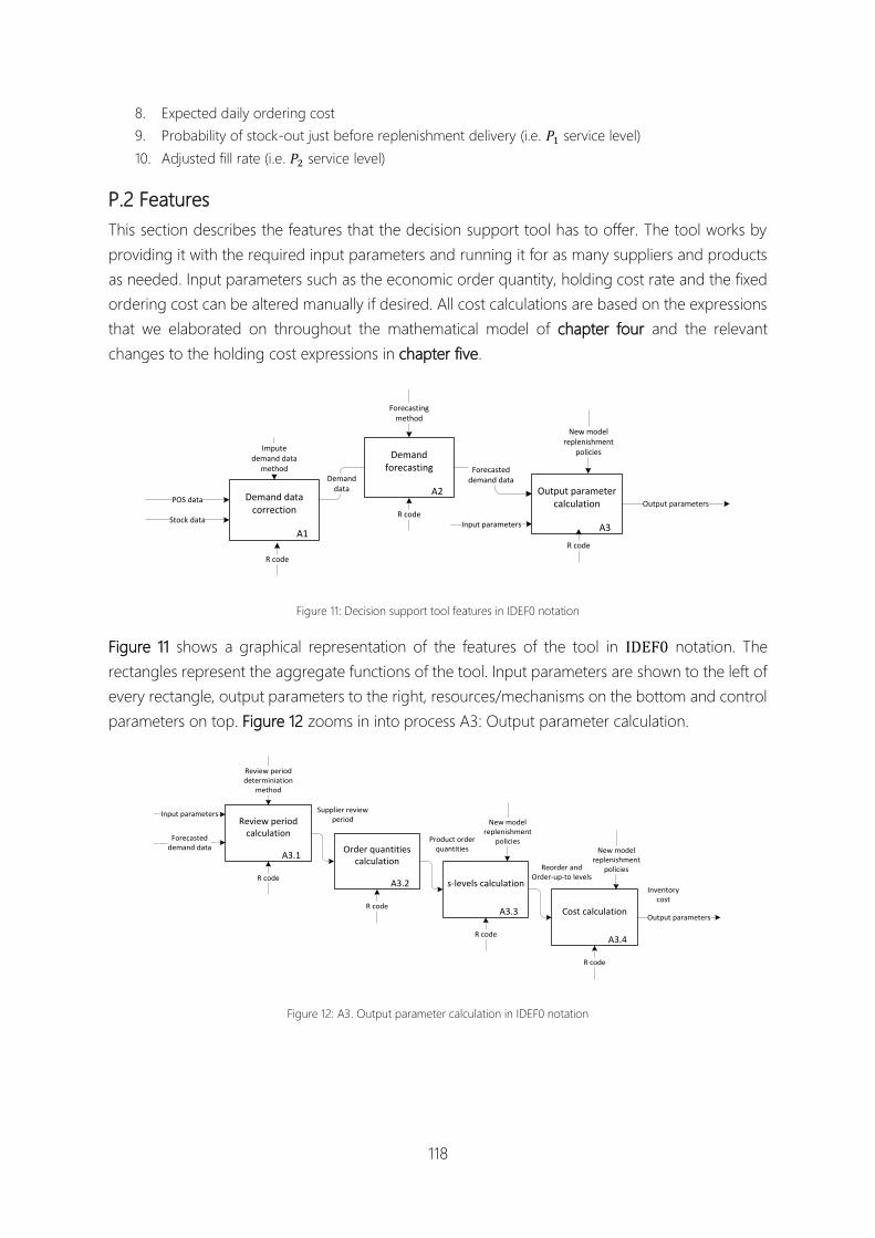
118

8. Expected daily ordering cost

9. Probability of stock-out just before replenishment delivery (i.e. 𝑃1 service level)

10. Adjusted fill rate (i.e. 𝑃2 service level)

P.2 Features

This section describes the features that the decision support tool has to offer. The tool works by

providing it with the required input parameters and running it for as many suppliers and products

as needed. Input parameters such as the economic order quantity, holding cost rate and the fixed

ordering cost can be altered manually if desired. All cost calculations are based on the expressions

that we elaborated on throughout the mathematical model of chapter four and the relevant

changes to the holding cost expressions in chapter five.

A3

Output parameter calculation

A1

Demand data correction

A2

Demand forecasting

POS data

Imputedemand data

method

Input parameters

New modelreplenishment

policies

Output parametersR code

Demanddata

Forecasteddemand data

R code

R code

Forecastingmethod

Stock data

Figure 11: Decision support tool features in IDEF0 notation

Figure 11 shows a graphical representation of the features of the tool in IDEF0 notation. The

rectangles represent the aggregate functions of the tool. Input parameters are shown to the left of

every rectangle, output parameters to the right, resources/mechanisms on the bottom and control

parameters on top. Figure 12 zooms in into process A3: Output parameter calculation.

A3.4

Cost calculation

A3.2

Order quantities calculation

A3.1

Review period calculation

A3.3

s-levels calculation

Output parameters

Input parameters

Forecasteddemand data

R code

R code

R code

R code

Review perioddeterminiation

method

Reorder and Order-up-to levels

Product orderquantities

Supplier reviewperiod

Inventorycost


policies


policies

Figure 12: A3. Output parameter calculation in IDEF0 notation

119

P.2.1 Output parameter calculation

P.2.1.1 Supplier aggregate review period calculation and product ordering quantities

The supplier aggregate review period is calculated per supplier based on the average daily

demand of all products ordered to the same supplier, their daily holding cost and the major

fixed ordering cost of placing an order to the supplier (see section 4.6). All products ordered

to the same supplier follow this review period for their replenishment process.

Based on the supplier aggregate review period, the economic order quantity of every product

is calculated (see section 4.6).

P.2.1.2 Reorder level and order-up-to level calculation

The following parameters are calculated with the 𝐷𝑒𝑡𝑒𝑟𝑚𝑖𝑛𝑒𝑂𝑢𝑡𝑝𝑢𝑡𝑃𝑎𝑟𝑎𝑚𝑒𝑡𝑒𝑟𝑠(𝑥)

function based on lead-times, review period and demand input parameters (see section P.3.2

for an extensive explanation of the functions):

o mean and standard deviation of demand during lead-time; 𝐸[𝐷(0, 𝐿]] and 𝜎(𝐷(0, 𝐿])

o mean and standard deviation of demand during the review period; 𝐸 [𝐷(0, 𝑅𝛿]] and

𝜎(𝐷(0, 𝑅𝛿])

o mean and standard deviation of the undershoot; 𝐸[𝑈𝑖] and 𝜎(𝑈𝑖)

o mean and standard deviation of demand during lead-time plus the undershoot;

𝐸[(0, 𝐿] + 𝑈] and 𝜎(𝐷(0, 𝐿] + 𝑈)

Based on the input parameters the tool calculates the reorder level 𝑠𝑖 required to achieve the

target fill rate 𝑃2. The order-up-to level 𝑆𝑖 equals the reorder level plus the economic order

quantity 𝐸𝑂𝑄.

P.2.1.3 Other relevant output parameters

Additionally, the tool calculates the safety stock, the expected average stock on hand, the

expected ordering probability of a product in an ordering cycle, the expected order quantity,

the adjusted target fill rate, the expected daily shortage and the 𝑃1 service level.

o The safety stock 𝑠𝑠𝑖 is defined as the stock on hand just before the arrival of a

replenishment order (i.e. the stock that is kept to guard for the demand variability during

the replenishment cycle and the variability of the lead-time).

o The expected average stock on hand 𝐸[𝑋𝑖] is defined as the stock on hand just after the

arrival of a replenishment order subtracted by the stock on hand just before the arrival

of a replenishment order.

o The expected ordering probability 𝜌𝑖 is defined as the probability that an order for

product 𝑖 is placed to the supplier in an ordering cycle.

o The expected average ordering quantity 𝐸[𝑄𝑖] is defined as the expected difference

between the inventory position and the order-up-to-level just before placing a

replenishment order to the supplier (i.e. 𝜌𝑖𝐸[𝑆𝑖 − 𝑠𝑖 + 𝑈𝑖] or 𝜌𝑖𝐸[𝐷(0, 𝑅𝛿] + 𝑈𝑖]).

o The adjusted target fill rate 𝑃2 is the target fill rate that results from calculating the reorder

level 𝑠𝑖 that satisfies the target fill rate. Because the reorder level is rounded up to the

nearest integer, the adjusted fill rate is often slightly higher than the initial target fill rate.

120

o The expected daily shortage is defined as the fraction of daily demand that cannot be

satisfied from stock on hand immediately. (i.e. adjusted 𝑃2 ∗𝐸[𝐷𝑖]

𝐸[𝐴𝑖]).

o The 𝑃1 service level is defined as the probability of no stock-out just before the arrival of

a replenishment order.

P.2.1.4 Cost calculations

With respect to expected cost, the tool calculates the expected daily holding cost per product

and the expected daily ordering cost per supplier.

o The expected daily holding cost per product is defined as the expected average stock on

hand multiplied by the purchase price of a product and the daily holding cost rate.

o The expected daily ordering cost are defined as the product of the expected ordering

probabilities of the products ordered to the same supplier multiplied by the major fixed

ordering cost divided by the review period. Note that the ordering cost are on the

aggregate supplier level and not on the individual product level.

P.2.2 Demand input parameters

Demand forecasting, 𝐸𝑂𝑄 calculations, reorder level and cost calculations can be based on

3 types of demand input which are all based on historical sales data.

o Sales data: all calculations are based on historical sales data. Note that sales data only

includes demand from the days where stock on hand was positive (there were no sales

on days without stock and hence, demand is not known on such days);

o Sales data with Gamma imputed demand: a Gamma distribution is fit to the historical

sales data from the days with positive stock on hand. Thereafter demand is imputed on

the historical days without stock based on this Gamma demand distribution.

o Sales data with imputed demand from last month: demand is imputed on the historical

days without stock on hand. This imputed demand is based on the historical sales from

the last 10 to 30 days where stock on hand was positive (i.e. demand from the last 10 to

30 days). This procedure was elaborated on in section 4.6 and a simplification of the R

code can be found in appendix I.

P.3 User manual

The different calculations should be made with the appropriate input parameters and it is important

that the user knows which functionalities the different functions have. This section describes the

different functions of the tool and how to use them. Note that all data manipulation processes in

between the described functions are important but are performed automatically if all the code is

run as a whole. Data manipulation includes steps such as filtering of relevant data, combining data

and calculating parameters.

P.3.1 Supplier aggregate review period and product ordering quantities calculation

The supplier aggregate review period is based on the average daily demand of all products ordered

to the same supplier, their daily holding cost and the major fixed ordering cost of placing an order

to the supplier. Taking into account the fact that demand for products is changing through time it

121

may be valuable to adapt the supplier review period throughout the year. In the current situation,

this is done every 90 days. Calculating the supplier review period and the corresponding product

ordering quantities is performed by two developed functions that should be called subsequently:

The function 𝐷𝑒𝑡𝑒𝑟𝑚𝑖𝑛𝑒𝑆𝑢𝑝𝑝𝑙𝑖𝑒𝑟𝑅𝑒𝑣𝑖𝑒𝑤𝑃𝑒𝑟𝑖𝑜𝑑(𝑥) takes as input a data frame with the

major fixed ordering cost per supplier, product information such as the purchase price, the

holding cost rate, product demand data and provides as output a data frame with the review

period per supplier.

The function 𝐷𝑒𝑡𝑒𝑟𝑚𝑖𝑛𝑒𝑃𝑟𝑜𝑑𝑢𝑐𝑡𝐸𝑐𝑜𝑛𝑜𝑚𝑖𝑐𝑂𝑟𝑑𝑒𝑟𝑄𝑢𝑎𝑛𝑡𝑖𝑡𝑖𝑒𝑠(𝑥) takes as input the data

frame with the review period per supplier and product demand data and provides as output

a data frame with the economic order quantities per product.

P.3.2 Reorder level and order-up-to-level calculation

The decision support tool may be used on a daily basis if desired by the user. In theory, adapting

the reorder levels and order-up-to levels of products is also possible every day. In practice however,

it is recommended to perform the calculations with the tool every 30, 60 or 90 days, set the

inventory control parameters accordingly and register the performance of the tool by gathering

data on inventory control resulting from the tool. It is important to mention here that all

calculations, approximations and suggestions made by the tool are based on long-run inventory

control. Therefore, the tool will especially show positive results over a longer period of time. The

reorder level and order-up-to level calculation is based on two developed functions with two sub

functions:

The function 𝐷𝑒𝑡𝑒𝑟𝑚𝑖𝑛𝑒𝑂𝑢𝑡𝑝𝑢𝑡𝑃𝑎𝑟𝑎𝑚𝑒𝑡𝑒𝑟𝑠(𝑥) takes as input parameter the data frame

with input demand parameters, the calculated supplier aggregate review period and

economic order quantities per product and provides the user with all output parameters and

cost calculations described in section P.2.1. Furthermore, the functions requires specification

of: which replenishment policy to use, if backorders are accepted and if undershoot should

be taken into account. Calling on the function 𝐷𝑒𝑡𝑒𝑟𝑚𝑖𝑛𝑒𝑂𝑢𝑡𝑝𝑢𝑡𝑃𝑎𝑟𝑎𝑚𝑒𝑡𝑒𝑟𝑠(𝑥) for the

(𝑅𝛿 , 𝑠𝑖, 𝑆𝑖) replenishment policy with undershoot and no backorders would look like:

𝐷𝑒𝑡𝑒𝑟𝑚𝑖𝑛𝑒𝑂𝑢𝑡𝑝𝑢𝑡𝑃𝑎𝑟𝑎𝑚𝑒𝑡𝑒𝑟𝑠(Input_data = data, Policy = "RsS",

Backorders = FALSE , Type_of_service = "P2", Undershoot = TRUE)

Note that the reorder level and order-up-to level are calculated differently if undershoot is

taken into account compared to when undershoot is not taken into account.

Within the 𝐷𝑒𝑡𝑒𝑟𝑚𝑖𝑛𝑒𝑂𝑢𝑡𝑝𝑢𝑡𝑃𝑎𝑟𝑎𝑚𝑒𝑡𝑒𝑟𝑠(𝑥) function two sub functions are automatically

called upon, which together provide the ‘optimal’ reorder level based on the input

parameters and the set target fill rate. For very slow moving products or products with too

little data, the reorder level is set to 1 and not 0. If stock on hand is zero there is no demand

information at all. The two sub functions of the 𝐷𝑒𝑡𝑒𝑟𝑚𝑖𝑛𝑒𝑂𝑢𝑡𝑝𝑢𝑡𝑃𝑎𝑟𝑎𝑚𝑒𝑡𝑒𝑟𝑠(𝑥) are:

o 𝐶𝑎𝑙𝑐𝑢𝑙𝑎𝑡𝑒𝑅𝑒𝑜𝑟𝑑𝑒𝑟𝑙𝑒𝑣𝑒𝑙(𝑥), which performs an iteration process to find the ‘optimal’

reorder level based on the input parameters and the target fill rate. This iteration process

sets a minimal reorder level (𝑠𝑖 = 0) and a maximal reorder level (𝑠𝑖 = 12 ∗ 𝐸[𝐷(0, 𝐿]])

and calculates different reorder levels until a reorder level is found that achieves the

122

target fill rate (De Kok, 2002). The fill rate is calculated using the other sub function: the

𝐶𝑎𝑙𝑐𝑢𝑙𝑎𝑡𝑒𝐹𝑖𝑙𝑙𝑟𝑎𝑡𝑒(𝑥) function.

o 𝐶𝑎𝑙𝑐𝑢𝑙𝑎𝑡𝑒𝐹𝑖𝑙𝑙𝑟𝑎𝑡𝑒(𝑥), which calculates the expected achieved target fill rate based on

the different reorder levels calculated by the 𝐶𝑎𝑙𝑐𝑢𝑙𝑎𝑡𝑒𝑅𝑒𝑜𝑟𝑑𝑒𝑟𝑙𝑒𝑣𝑒𝑙(𝑥) function.

Relevant to mention for some of the output parameters described in section P.2.1.3 is the

following:

o Expected average stock on hand 𝐸[𝑋𝑖]: If undershoot is taken into account the expected

average stock on hand is calculated with the formula by de Kok (2002). If undershoot is

not taken into account the expected average stock on hand is calculated with the formula

by Silver et al. (1998). The calculation of the expected average stock on hand has a direct

effect on the expected daily holding cost 𝐸𝐷𝐻𝐶.

o The 𝑃1 service level is calculated differently if undershoot is taken into account compared

to when undershoot is not take into account.

Output is saved in an R data frame that can easily be written to an Excel fil if needed.

Moreover, after saving this Excel file, the user may change parameters such as the period of

historical data, the order quantity per product or the holding and ordering cost. Thereafter,

the function 𝐷𝑒𝑡𝑒𝑟𝑚𝑖𝑛𝑒𝑂𝑢𝑡𝑝𝑢𝑡𝑃𝑎𝑟𝑎𝑚𝑒𝑡𝑒𝑟𝑠(𝑥) can be called again and will provide a new

data frame with adapted output parameters. In this way, the user may compare the output

and decide on making potential changes in the input parameters due to future promotions

or increasing/decreasing holding and ordering cost.

P.3.3 Cost calculations

The (long-term) expected daily holding cost 𝐸𝐷𝐻𝐶 calculations per product are also

integrated into the 𝐷𝑒𝑡𝑒𝑟𝑚𝑖𝑛𝑒𝑂𝑢𝑡𝑝𝑢𝑡𝑃𝑎𝑟𝑎𝑚𝑒𝑡𝑒𝑟𝑠(𝑥) function. Once the functions is called

it will include the holding cost calculations in the output data frame.

To calculate the (long-term) expected daily ordering cost 𝐸𝐷𝑂𝐶 per supplier the user has to

call the function 𝐶𝑎𝑙𝑐𝑢𝑙𝑎𝑡𝑒𝐷𝑎𝑖𝑙𝑦𝑂𝑟𝑑𝑒𝑟𝑖𝑛𝑔𝐶𝑜𝑠𝑡(𝑥) because all the before described

calculation are on a product bases while the calculation of the ordering cost is on a supplier

basis. The function 𝐶𝑎𝑙𝑐𝑢𝑙𝑎𝑡𝑒𝐷𝑎𝑖𝑙𝑦𝑂𝑟𝑑𝑒𝑟𝑖𝑛𝑔𝐶𝑜𝑠𝑡(𝑥) takes as input the data frame resulting

from the 𝐷𝑒𝑡𝑒𝑟𝑚𝑖𝑛𝑖𝑛𝑒𝑂𝑢𝑡𝑝𝑢𝑡𝑃𝑎𝑟𝑎𝑚𝑒𝑡𝑒𝑟𝑠(𝑥) function and provides the user with a data

frame with al inventory control parameters including the just calculated expected daily

ordering cost per supplier.

P.3.4 Demand input parameters

The 3 forms of demand input can be created as follows:

o Demand input parameters based on only sales data do not need any further function

call. POS data contains the sales that were made on specific moments in time. The only

step taken is impute zero demand on the days without sales to make the sales data a

time series.

o Demand input parameters based on sales data with Gamma imputed demand can be

created by calling the function 𝐼𝑚𝑝𝑢𝑡𝑒𝐺𝑎𝑚𝑚𝑎𝐷𝑒𝑚𝑎𝑛𝑑𝑑𝑎𝑡𝑎(𝑥). The function takes the

sales data and stock data as input and provides the user with a data frame with demand

123

data on the days with positive stock (i.e. sales) and Gamma distributed demand on the

days without stock (i.e. imputed demand).

o Demand input parameters based on sales data with imputed demand from last month

can be created by calling the function 𝐼𝑚𝑝𝑢𝑡𝑒𝐷𝑒𝑚𝑎𝑛𝑑𝑑𝑎𝑡𝑎(𝑥). The function takes the

sales data and stock data as input and provides the user with a data frame with demand

data on the days with positive stock (i.e. sales) and demand on the days without stock

based on the demand of the last 10 to 30 days with positive stock (i.e. imputed demand).

After creating the appropriate type of demand input parameters the demand input can be

used in the demand forecasting method and thereafter for the supplier review period

determination, 𝐸𝑂𝑄 calculation, 𝑠-level calculation, fill rate calculation and cost calculations.

P.3.4.1 Demand forecasting

As described in section P.1.1.1, demand forecasting is used for all products. By relaxing the

assumption that demand for products is stationary, all developed calculations are not more than

approximations. However, all calculations were compared with simulated values and under

stochastic lead-times and unpredictable variable demand the new model replenishment policies

performed reasonably. Due to limited historical forecast data and information on the used method,

it is advised to use the forecast method in combination with the ImputeDemand functions and

adapting the 𝑠-levels not more than once per review period because this has no effect. In short,

this would mean that forecasts are performed daily and that 𝑠-levels of the different products could

be adapted between subsequent review periods or once in a larger time interval (2,3,… review

periods). Adapting the aggregate supplier review periods is recommended to be done with a

frequency larger than 90 days due to the demand forecasting horizon of 90 days.

P.4 Tool user interface

This section will briefly describe the user interface of the decision support tool. The tool includes

two scripts: (1) Decision support tool (DST): a script with all function calls and automatic data

manipulation steps and (2) Functions: a script with all the code of the functions used in the decision

support tool script. It is not recommended to make changes to the functions script because this

script functions as a source for the decision support tool script. The different parts of code can be

run in the decision support tool script to create data frames with the output parameters. Therefore,

the tool is not an Excel of VBA tool where product and supplier data has to be imported manually

or displayed on one tab. Product data of as many products required can be imported into R and

the tool calculates the output parameters for every product that has enough historical data. We

describe which output parameters are presented in which data frame. If required, these data frames

can easily be written to an Excel file.

Sales_data_imputed_demand_table

The Sales_data_imputed_demand_table data frame is created after the functions

𝐼𝑚𝑝𝑢𝑡𝑒𝐷𝑒𝑚𝑎𝑛𝑑𝐷𝑎𝑡𝑎(𝑥) or 𝐼𝑚𝑝𝑢𝑡𝑒𝐺𝑎𝑚𝑚𝑎𝐷𝑒𝑚𝑎𝑛𝑑𝐷𝑎𝑡𝑎(𝑥) are called upon. The data frame

includes the products and their historical daily stock on hand and daily demand. Based on this data,

the historical sales data is corrected and we have the mean and standard deviation of demand

124

inter-arrivals and the mean and standard deviation of demand sizes which will be used in the

forecast and the calculations that follow.

Review_period_supplier_table

The Review_period_supplier_table data frame is created after calling on the function

𝐷𝑒𝑡𝑒𝑟𝑚𝑖𝑛𝑒𝑆𝑢𝑝𝑝𝑙𝑖𝑒𝑟𝑅𝑒𝑣𝑖𝑒𝑤𝑝𝑒𝑟𝑖𝑜𝑑(𝑥) and shows the suppliers and their calculated supplier

aggregate review period. This review period is then linked to the different products coming from

the corresponding supplier.

EOQ_product_table

The EOQ_product_table data frame is created by calling on the function

𝐷𝑒𝑡𝑒𝑟𝑚𝑖𝑛𝑒𝑃𝑟𝑜𝑑𝑢𝑐𝑡𝐸𝑐𝑜𝑛𝑜𝑚𝑖𝑐𝑂𝑟𝑑𝑒𝑟𝑄𝑢𝑎𝑛𝑡𝑖𝑡𝑖𝑒𝑠(𝑥) and shows the products and their economic

order quantities and review period.

Calculated_output_parameters_table

The data frame Calculated_output_parameters_table shows all output parameters except the

expected daily ordering cost per supplier and is created by calling on the function

𝐷𝑒𝑡𝑒𝑟𝑚𝑖𝑛𝑒𝑂𝑢𝑡𝑝𝑢𝑡𝑃𝑎𝑟𝑎𝑚𝑒𝑡𝑒𝑟𝑠(𝑥).

Total_calculated_output_parameters_table

The data frame Total_calculated_output_parameters_table presents all the output parameters

including the expected daily ordering cost per supplier and is created by calling on the function

𝐶𝑎𝑙𝑐𝑢𝑙𝑎𝑡𝑒𝐷𝑎𝑖𝑙𝑦𝑂𝑟𝑑𝑒𝑟𝑖𝑛𝑔𝐶𝑜𝑠𝑡(𝑥) with the Calculated_output_parameters_table as input.

The tool can easily be linked to other R code and to the WMS databases in the backend and an

application or website in the frontend. With respect to updating the data, new POS and stock data

can automatically be imported into the tool and therefore calculations can be made on a daily

basis if desired. However, changing parameters such as the reorder level and target fill rate is not

recommended on a daily basis because the performance of the tool under certain set parameters

takes some time to present itself.

Figure 13 shows a flowchart of the different steps of the tool. The different functions in the tool can

be run as a whole to calculate the output parameters in one run. The functions can also be run

step by step such that changes to input parameters may be made manually in between the different

steps

125

Open DST and Functions script

StartImport relevant

data

Decide on Impute demand data

method

WMSDatabase

Demand forecast

Calculate step by step?

Determine supplier review period

Determine product economic order

quantities

Make manual changes to input

parameters?

Determine all output parameters

POS dataStock data

Yes

Make manual changes to input

parameters

No

Yes

Determine output parameters

excluding EDOC

Determine output parameters

including EDOCOutput data

No

Utilize output data End

Figure 13: Basic flowchart of Decision Support Tool

.

126

Appendix Q Q. Detailed elaborati on of underlying research objectives

Detailed elaboration of underlying research objectives

In this section we give a more detailed elaboration of accomplishing the underlying research

objectives of our research. A large part of the conclusions in this section can also be found in

chapter seven.

1. Describe the as-is situation of inventory control at Company B.

Company B functioned as a good example for an e-tailer where almost all inventory control and

purchasing process were performed manually and without strict decision rules. The as-is situation

was analyzed in chapter one and chapter three. We thereby focused on the inventory control

processes and identified the problems that occurred in these processes. Problems were found to

be a combination of the environment for webshops to work in and the fact that inventory control

is often overlooked when companies are rapidly increasing. In an e-commerce environment,

backorders are often not accepted resulting in lost-sales when demand exceeds the stock on hand.

The complex nature of demand and the fact that backorders are often not accepted, results in high

inventory levels or more lost-sales than desired. The main components that were deemed relevant

in analyzing the inventory control situation and the first literature review were periodic joint

replenishment, lost-sales systems and stochastic demand and lead-times.

2. Provide conceptual solutions aimed at the joint replenishment problem, complete lost-sales

and the other problem areas by combining theoretical and practical knowledge and model

these solutions into a mathematical model.

Reviewed literature on replenishment policies, joint replenishment and lost-sales systems in

combination with the problem analysis of Company B and Optiply resulted in the development of

two newly modified replenishment policies. The (𝑅𝛿 , 𝑆𝑖) and (𝑅𝛿 , 𝑠𝑖, 𝑆𝑖) replenishment policies

were introduced in chapter four after careful consideration of different solution concepts that had

the purpose of solving the different components of the inventory control problem. We described

how the aggregate joint replenishment problem can be approached by splitting it up in 𝑛 single-

item replenishment problems with a supplier aggregate review period to coordinate the ordering

process. We concluded that the single-item problem solution concept should be of a periodic

nature because the aggregate review period is the controlling variable in the joint replenishment

process. With respect to the lost-sales problem, we pointed out multiple solution concepts that had

to do with correcting the fill rate in a lost-sales system or with uncovering unobserved demand that

occurs when the stock on hand of a product equals zero.

3. Analyze the inventory control model developed by Optiply and relate it to the conceptual

solutions in the process of developing an inventory control model that can perform in an e-

commerce characteristic environment.

127

4. How can the current inventory control model and the suggested improvements of the

conceptual model be combined into a decision support tool that takes into account the

components of an e-commerce characteristic environment? (i.e. define KPIs, test the tool,

compare output, generalize tool)

The Optiply model was analyzed throughout the project and for different components of the model

we provided improvements to existing components or came up with new components. In chapter

four we introduced a method to take unobserved demand into account such that future demand

is less underestimated. Based on the solution concepts we described in our research, we developed

a method to take into account the demand in periods without stock based on the assumption that

demand in periods without stock on hand follows the same demand pattern as demand in periods

without stock on hand. Within this method two options can be chosen: (1) impute Gamma

distributed demand on the days without stock on hand based on the days with positive stock on

hand or (2) impute demand based on the last 10 to 30 days with positive stock on hand on the

days without stock on hand. Furthermore, we suggested a different method to determine the

review period that all products ordered to the same supplier should follow. This supplier aggregate

review period is calculated based on the fixed ordering cost, holding cost per product and the

average demand per product. We admit of course, that this method could also overestimate actual

demand. However, because the method is based on a historical data set that is growing every day,

the method will improve with every day because it ‘learns’ from the data.

Relevant KPIs were found to be the (target) fill rate (implicitly taking shortage cost into account),

demand during lead-time, demand during the review period, expected average stock on hand,

expected daily holding cost and the expected daily ordering cost.

Product demand is often highly variable and in some cases probably dependent on seasonality,

trends or competitor pricing. Therefore, demand for all products has to be partly based on historical

data and partly on demand forecasts.

The expected average stock on hand approximation by Silver et al. (1998) often underestimated

the actual average stock on hand.

The fill rate calculations and other relevant parameter calculations of both the (𝑅𝛿 , 𝑆𝑖) and

(𝑅𝛿 , si, 𝑆𝑖) replenishment policy were found accurate under (highly) variable stochastic demand

and stochastic lead-times; under highly variable stochastic lead-times the fill rate calculations

somewhat underestimated the actual experienced fill rate.

The inventory cost calculations of both replenishment policies in the new model were found

accurate under (highly) variable stochastic demand and stochastic lead-times. Both the holding

cost and the ordering cost function provides good approximations for the expected inventory cost.

Therefore, we can conclude that both policies minimize total inventory cost under a target fill rate.

128

In both theoretical and practical situations the undershoot variable should be taken into account,

not only for the (𝑅𝛿 , 𝑠𝑖, 𝑆𝑖) replenishment policy but also for the (𝑅𝛿 , 𝑆𝑖) replenishment to achieve

the target fill rate (this was not done by Optiply before).

In almost all simulation situations, both replenishment policies in the new model outperformed

those in the Optiply model with respect to achieved fill rates, total inventory cost and reliability (i.e.

tighter 95% confidence intervals); note that the cost efficiency is highly dependent on how the

different cost parameters are set.

In almost every simulation situation, the (𝑅𝛿 , 𝑆𝑖) replenishment policy outperformed the (𝑅𝛿 , 𝑠𝑖, 𝑆𝑖)

replenishment policy regarding achieved fill rates, total inventory cost and reliability (i.e. tighter

95% confidence intervals); note that the cost efficiency is highly dependent on how the different

cost parameters are set.

Both policies in the new model performed reasonably under ‘real demand data’ in the simulation

analysis with respect to achieved fill rate and cost efficiency (see section 5.3.2), especially taken into

account that replenishment was performed without new data information in between and was

simulated for a 3 month horizon.

The developed decision support tool uses historical sales/demand data and potential demand

forecasts as input to provide appropriate inventory control parameters and inventory cost such as

the reorder level, holding cost and ordering cost. The tool is able to perform this calculations for

as many products and supplier as desired.

5. Write an implementation plan on the recommended use of the decision support tool for

inventory control.

Chapter six provided an extensive description of the decision support tool and discussed the

features of the tool and recommended use. The tool is built up in such a way that it is easily

generalized and can be used in other inventory control situations. Its only true input parameters

are POS data and Stock changes data. Therefore, the only aspects that need changing are the

different variable names and the input for certain specifics such as the holding cost rate or the fixed

ordering cost. Note that the ordering cost should be calculated differently once minor fixed

ordering cost play a role in the replenishment process as well. For Optiply, the R code of the tool

can be integrated into the Optiply model with little effort. Small additions such as variable names

should be changed for smooth integration and some explanation on the different components

may be given.

129

References References

Aardal, K., Jonsson, O., & Jönsson, H. (1989). Optimal Inventory Policies with Service-Level Constraints. The

Journal of the Operational Research Society, 40(1), 65–73.

Axsäter, S. (2006). Inventory Control. Springer’s Intenational Series (2nd ed.). Springer.

http://doi.org/10.1017/CBO9781107415324.004

Babai, M. Z., Syntetos, A., & Teunter, R. (2014). Intermittent demand forecasting: An empirical study on

accuracy and the risk of obsolescence. International Journal of Production Economics, 157(1), 212–219.

http://doi.org/10.1016/j.ijpe.2014.08.019

Bijvank, M., & Vis, I. F. A. (2011). Lost-sales inventory theory: A review. European Journal of Operational

Research, 215(1), 1–13. http://doi.org/10.1016/j.ejor.2011.02.004

Bijvank, M., & Vis, I. F. A. (2012). Lost-sales inventory systems with a service level criterion. European Journal

of Operational Research, 220(3), 610–618. http://doi.org/10.1016/j.ejor.2012.02.013

Conlon, C. T., & Mortimer, J. H. (2013). Demand estimation under limited product availability. American

Economic Journal: Microeconomics, 5(4), 1–30. http://doi.org/10.1080/13504850601018650

Corsten, D., & Gruen, T. (2003). Desperately seeking shelf availability: an examination of the extent, the causes,

and the efforts to address retail out-of-stocks. International Journal of Retail & Distribution

Management, 31(12), 605–617. http://doi.org/10.1108/09590550310507731

Costantino, F., Di Gravio, G., Shaban, A., & Tronci, M. (2015). SPC forecasting system to mitigate the bullwhip

effect and inventory variance in supply chains. Expert Systems with Applications, 42(3), 1773–1787.

http://doi.org/10.1016/j.eswa.2014.09.039

Costantino, F., Di Gravio, G., Shaban, A., & Tronci, M. (2016). Smoothing inventory decision rules in seasonal

supply chains. Expert Systems with Applications, 44, 304–319. http://doi.org/10.1016/j.eswa.2015.08.052

de Kok, A. G. (1991). Basics of inventory management (Part 2): The (R,S)-model. Tilburg University.

Federgruen, A., Groenevelt, H., & Tijms, H. C. (1984). Coordinated Replenishments in a Multi-Item Inventory

System with Compound Poisson Demands. Management Science, 30(3), 344–357.

Heijden, M. C. va. der, & Kok, T. de. (1998). Estimating stock levels in periodic review inventory systems.

Operations Research Letters, 22(4), 179–182. http://doi.org/10.1016/S0167-6377(98)00020-0

Heinecke, G., Syntetos, A. A., & Wang, W. (2013). Forecasting-based SKU classification. International Journal

of Production Economics, 143(2), 455–462. http://doi.org/10.1016/j.ijpe.2011.11.020

Heusinkveld, S., & Reijers, H. a. (2009). Reflections on a reflective cycle: Building legitimacy in design

knowledge development. Organization Studies, 30(8), 865–886.

http://doi.org/10.1177/0170840609334953

Hyndman, R. J., Akram, M., & Archibald, B. C. (2008). The admissible parameter space for exponential

smoothing models. Annals of the Institute of Statistical Mathematics, 60(2), 407–426.

http://doi.org/10.1007/s10463-006-0109-x

Hyndman, R. J., Koehler, A. B., Ord, J. K., & Snyder, R. D. (2008). Forecasting with Exponential Smoothing.

Springer Series in Statistics. Springer. http://doi.org/10.1007/978-3-540-71918-2

Hyndman, R. J., Koehler, A. B., Snyder, R. D., & Grose, S. (2002). A state space framework for automatic

forecasting using exponential smoothing methods. International Journal of Forecasting, 18(3), 439–454.

http://doi.org/10.1016/S0169-2070(01)00110-8

Jiang, R. (2015). Introdution to Quality and Reliability Engineering. Risk Management. Springer.

130

Johansen, A. S. G., & Melchiors, P. (2003). Can-order policy for the periodic-review joint replenishment

problem. The Journal of the Operational Research Society, 54(3), 283–290.

Khouja, M. (2001). The evaluation of drop shipping option for e-commerce retailers. Computers and Industrial

Engineering, 41(2), 109–126. http://doi.org/10.1016/S0360-8352(01)00046-8

Khouja, M., & Goyal, S. (2008). A review of the joint replenishment problem literature: 1989-2005. European

Journal of Operational Research, 186(1), 1–16. http://doi.org/10.1016/j.ejor.2007.03.007

Kohler-Gudum, C., & de Kok, A. G. (2002). A safety stock adjustment proceudre to enable target service levels

in simulation of generic inventory systems. BETA Publicatie: Working Papers, (71), 1–31.

http://doi.org/10.1016/S0195-5616(99)50088-0

Law, A. M. (2007). Simulation modeling & analysis. International Journal of Production Economics (4th ed.).

New York: Elsevier. http://doi.org/10.1016/j.ijpe.2011.05.020

Nadarajah, S., Popović, B. V., & Ristić, M. M. (2013). Compounding: An R package for computing continuous

distributions obtained by compounding a continuous and a discrete distribution. Computational

Statistics, 28(3), 977–992. http://doi.org/10.1007/s00180-012-0336-y

Pfohl, H. C., Cullmann, O., & Stolzle, W. (1999). Inventory management with statistical process control :

Simulation and evaluation. Journal of Business Logistics, 20(1), 101–120.

Prak, D., Teunter, R., & Syntetos, A. (2017). On the calculation of safety stocks when demand is forecasted.

European Journal of Operational Research, 256(2), 454–461. http://doi.org/10.1016/j.ejor.2016.06.035

Silver, E. A., Pyke, D. F., & Peterson, R. (1998). Inventory Management and Production Planning and

Scheduling. International Journal of Production Economics (3rd ed.). Elsevier.

Strijbosch, L. W. G., Moors, J. J. A., & de Kok, A. G. (1997). On the interaction between forecasting and

inventory control, (742), 33.

Syntetos, A. A. (2001). Forecasting of intermittent demand. Brunel University.

Syntetos, A. A., Babai, M. Z., & Altay, N. (2012). On the demand distributions of spare parts. International

Journal of Production Research, 50(8), 2101–2117. http://doi.org/10.1080/00207543.2011.562561

Syntetos, A. A., & Boylan, J. E. (2005). The accuracy of intermittent demand estimates. International Journal

of Forecasting, 21, 303–314. http://doi.org/10.1016/j.ijpe.2010.07.005

Syntetos, A. A., Zied Babai, M., & Gardner, E. S. (2015). Forecasting intermittent inventory demands: Simple

parametric methods vs. bootstrapping. Journal of Business Research, 68(8), 1746–1752.

http://doi.org/10.1016/j.jbusres.2015.03.034

Teunter, R. H., Babai, M. Z., & Syntetos, A. A. (2010). ABC Classification: Service levels and inventory costs.

Production and Operations Management, 19(3), 343–352. http://doi.org/10.1111/j.1937-

5956.2009.01098.x

Teunter, R. H., Syntetos, A. A., & Babai, M. Z. (2016a). Stock keeping unit fill rate specification - Article in Press.

European Journal of Operational Research, 1–9. http://doi.org/10.1016/j.ejor.2016.11.017

Teunter, R. H., Syntetos, A. A., & Babai, M. Z. (2016b). Stock Keeping Unit fill rate specification - Working

Paper. Journal of Operational Research, 1–24.

Tijms, H. C., & Groenevelt, H. (1984). Simple Approximations for the Reoder Point in Periodic and Continuous

Review (s, S) Inventory Systems with Service Level Constraints. European Journal of Operational

Research, 17, 175–190.

Turban, E., King, D., Lee, J. K., Liang, T., & Turban, D. C. (2015). Electronic commerce: A Managerial and Social

Networks Perspective (Eight Edit, Vol. 8). Switzerland: Springer.

http://doi.org/http://dx.doi.org/10.1016/S0267-3649(03)00504-1

Van Aken, J. E. (2005). Management research as a design science: Articulating the research products of mode

131

2 knowledge production in management. British Journal of Management, 16(1), 19–36.

http://doi.org/10.1111/j.1467-8551.2005.00437.x

Van Donselaar, K., De Kok, T., & Rutten, W. (1996). Two replenishment strategies for the lost sales inventory

model: A comparison. International Journal of Production Economics, 46–47, 285–295.

http://doi.org/10.1016/0925-5273(95)00066-6

Van Donselaar, K. H., & Broekmeulen, R. A. C. . (2013). Determination of safety stocks in a lost sales inventory

system with periodic review, positive lead-time, lot-sizing and a target fill rate. International Journal of

Production Economics, 143(2), 440–448. http://doi.org/10.1016/j.ijpe.2011.05.020

Van Donselaar, K. H. Van, & Broekmeulen, R. A. C. M. (2014). Stochastic inventory models for a single item at

a single location. BETA Publicatie: Working Papers, 447, 1–71.

Vulcano, G., van Ryzin, G., & Ratliff, R. (2012). Estimating Primary Demand for Substitutable Products from

Sales Transaction Data. Operations Research, 60(2), 313–334. http://doi.org/10.1287/opre.1110.1012

Wang, L., Dun, C. X., Bi, W. J., & Zeng, Y. R. (2012). An effective and efficient differential evolution algorithm

for the integrated stochastic joint replenishment and delivery model. Knowledge-Based Systems, 36,

104–114. http://doi.org/10.1016/j.knosys.2012.06.007

Willemain, T. R., Smart, C. N., & Schwarz, H. F. (2004). A new approach to forecasting intermittent demand

for service parts inventories. International Journal of Forecasting, 20(3), 375–387.

http://doi.org/10.1016/S0169-2070(03)00013-X

Zipkin, P. (2008). Old and New Methods for Lost-Sales Inventory Systems. Operations Research, 56(5), 1256–

1263. http://doi.org/10.1287/opre.

Eindhoven University of Technology MASTER Inventory ...

Documents

Transcript of Eindhoven University of Technology MASTER Inventory ...