Adv. Sci. Res., 3, 105–112, 2009www.adv-sci-res.net/3/105/2009/© Author(s) 2009. This work is distributed underthe Creative Commons Attribution 3.0 License.

Advances inScience and

Research

8th

EM

SA

nn

ua

lMe

etin

ga

nd

7th

Eu

rop

ea

nC

on

fere

nce

on

Ap

plie

dC

lima

tolog

y2

00

8

Efficient high-resolution 3-D interpolation ofmeteorological variables for operational use

C. Lussana1, M. R. Salvati1, U. Pellegrini1, and F. Uboldi2

1ARPA Lombardia, Milano, Italy2Consultant, Novate Milanese, Italy

Received: 19 December 2008 – Revised: 7 June 2009 – Accepted: 8 June 2009 – Published: 5 August 2009

Abstract. In recent years, the use of mesoscale meteorological network data has been growing. An OptimalInterpolation (OI) method is used to interpolate on a regular grid the hourly averaged values of temperature,relative humidity, wind vector, atmospheric pressure, and hourly cumulated precipitation. For all variables,except precipitation, the background (i.e. first guess) information is obtained by detrending the observationsusing the geographical parameters. For precipitation, the M. Lema radar-derived best estimate of precipitationrate at the ground is used. The characteristics of the OI schemes are shown in several test cases using data fromARPA Lombardia’s mesoscale meteorological network. Finally, a quantitative diagnostics for temperature andrelative humidity is carried out by using Cross Validation (CV) scores computed with large sets of data.

1 Introduction

This document describes a spatial interpolation schemebased on Optimal Interpolation (OI;Gandin, 1963) appliedto the data collected by a mesoscale meteorological network.OI is a method widely used in meteorology and climatologyand it is based on a linear combination of the observed valueswith a background field weighting their respective uncertain-ties. For a review of OI and its comparison with other datainterpolation techniques see for exampleDaley (1991) andKalnay (2003). In the presented work, the analyzed fieldsare mostly intended as support to nowcasting and forecastingin an operational meteorological centre. Forecasters requireeasy access to several different variables to gain better insightinto meteorological phenomena: for this reason the OI is ap-plied to hourly averaged observations of temperature, wind,relative humidity, pressure, and to the hourly cumulated pre-cipitation.

The observing system is ARPA Lombardia’s mesoscalemeteorological network, managed by the local publicweather service. The meteorological network is character-ized by a high space and time resolution of observations (au-tomatic stations), but with strong inhomogeneities in sensors’distribution. As an example, Fig.1 shows raingauges andanemometers observation locations. Lombardy itself is char-

Correspondence to:C. Lussana(c.lussana@arpalombardia.it)

acterized by a very complex orography and by different landuses: the representativity component of the observational er-ror plays an important role and must be properly handled.

The interpolation is performed over a regular grid. Thespatial domain measures roughly 200 km×200 km. A gridresolution of 1.5 km has been chosen: it is the coarser reso-lution that can be used without having significant differencesbetween grid and station elevation. It is worth remarkingthat it is the grid resolution that accounts for most of the to-pographic detail of the analysis maps, and that the grid reso-lution is higher than the observation network resolution.

About three years of operational use have proven the algo-rithm to be efficient (in using computer resources) and stable(with respect to the observing system’s anomalies or mal-functionings). Furthermore, the OI procedures themselveshave revealed some of the network’s problems.

Once available, analysis maps are also useful for a vari-ety of operational and practical applications, such as forecastverification, environmental monitoring, land and water man-agement, heatwave warnings, fire prevention and as a supportfor civil protection authorities. Furthermore, a reliable analy-sis procedure is a powerful tool for the data quality assurancesystem of any observational network.

Published by Copernicus Publications.

106 C. Lussana et al.: High-resolution interpolation of meteorological data

Manuscript prepared for Adv. Sci. Res.with version 3.0 of the LATEX class copernicus2.cls.Date: 5 June 2009

Efficient high-resolution 3-D interpolation ofmeteorological variables for operational use

C. Lussana1, M. R. Salvati1, U. Pellegrini1, and F. Uboldi2

1ARPA Lombardia, Milano, Italy2consultant, Novate Milanese, Italy

In recent years, the use of mesoscale meteorological net-work data has been growing. An Optimal Interpolation (OI)method is used to interpolate on a regular grid the hourlyaveraged values of temperature, relative humidity, wind vec-tor, atmospheric pressure, and hourly cumulated precipita-tion. For all variables, except precipitation, the background(i.e. first guess) information is obtained by detrending theobservation using the geographical parameters. For precip-itation, the M. Lema radar-derived best estimate of precipi-tation rate at the ground is used. The characteristics of theOI schemes are shown in several test cases using data fromARPA Lombardia’s mesoscale meteorological network. Fi-nally, a quantitative diagnostics for temperature and relativeis carried out by using Cross Validation (CV) scores com-puted with large sets of data.

1 Introduction

This document describes a spatial interpolation schemebased on Optimal Interpolation (OI; Gandin, 1963) appliedto the data collected by a mesoscale meteorological network.OI is a method widely used in meteorology and climatologyand it is based on a linear combination of the observed valueswith a background field weighting their respective uncertain-ties. For a review of OI and its comparison with other datainterpolation techniques see for example Daley (1991) andKalnay (2003). In the presented work, the analyzed fieldsare mostly intended as support to nowcasting and forecastingin an operational meteorological centre. Forecasters requireeasy access to several different variables to gain better insightinto meteorological phenomena: for this reason the OI is ap-plied to hourly averaged observations of temperature, wind,relative humidity, pressure, and to the hourly cumulated pre-cipitation.

The observing system is ARPA Lombardia’s mesoscalemeteorological network, managed by the local publicweather service. The meteorological network is character-

Correspondence to: C. Lussana(c.lussana@arpalombardia.it)

Figure 1. Orography and station locations in the domain. Trian-gles: raingauges. Circles: anemometers. The bold black line is theadministrative boundary. The inset shows the geographicalloca-tion of Lombardy (Italy), longitude 8.5 to 11.5◦E, latitude 44.6 to45.7◦N

ized by a high space and time resolution of observations (au-tomatic stations), but with strong inhomogeneities in sensors’distribution. As an example, Fig. 1 shows raingauges andanemometers observation locations. Lombardy itself is char-acterized by a very complex orography and by different landuses: the representativity component of the observationaler-ror plays an important role and must be properly handled.

Figure 1. Orography and station locations in the domain. Trian-gles: raingauges. Circles: anemometers. The bold black line is theadministrative boundary. The inset shows the geographical loca-tion of Lombardy (Italy), longitude 8.5 to 11.5◦ E, latitude 44.6 to45.7◦ N.

2 Optimal Interpolation schemes

The statistical interpolation scheme used for this work is de-scribed inUboldi et al.(2008), where it is applied to temper-ature and relative humidity. Generally, OI schemes use anobservation independent background field. This scheme usesinstead a 3-D background obtained by observations detrend-ing; this field is representative of the larger scale captured bythe network. The present manuscript describes the evolutionof the OI scheme and its application to other meteorologicalquantities. It is worthwhile remarking that the OI schemedescribed inUboldi et al. (2008) can also make use of anindependent background, as it is done here for precipitation.

Table2 summarizes the choices made in OI implementa-tion for the variables treated in this work. All the spatial cor-relation functions used are isotropic except for the improvedOI algorithm for temperature. The last three columns of Ta-ble 2 report the values forDh, Dz andε2. The de-correlationlength scales in the horizontal direction and in the vertical di-rection,Dh andDz respectively, are used in the backgrounderror spatial correlation functions to determine the volume

2 C. Lussana et al.: High-resolution interpolation of meteorological data

Figure 2. 20 Jan 2006, 12:00 LT (Local Time=UTC+1). Tempera-ture analysis. The isoline 0◦C is shown in gray; the white contoursmark urban areas.

The interpolation is performed over a regular grid. Thespatial domain measures roughly 200 Km x 200 Km. A gridresolution of 1.5 Km has been chosen: it is the coarser reso-lution that can be used without having significant differencesbetween grid and station elevation. It is worth remarkingthat it is the grid resolution that accounts for most of the to-pographic detail of the analysis maps, and that the grid reso-lution is higher than the observation network resolution.

About three years of operational use have proven the algo-rithm to be efficient (in using computer resources) and stable(with respect to the observing system’s anomalies or mal-functionings). Furthermore, the OI procedures themselveshave revealed some of the network’s problems.

Once available, analysis maps are also useful for a vari-ety of operational and practical applications, such as forecastverification, environmental monitoring, land and water man-agement, heatwave warnings, fire prevention and as a supportfor civil protection authorities. Furthermore, a reliableanaly-sis procedure is a powerful tool for the data quality assurancesystem of any observational network.

2 Optimal Interpolation schemes

The statistical interpolation scheme used for this work is de-scribed in Uboldi et al. (2008), where it is applied to temper-ature and relative humidity. Generally, OI schemes use anobservation independent background field. This scheme usesinstead a 3D background obtained by observations detrend-ing; this field is representative of the larger scale captured by

the network. The present manuscript describes the evolutionof the OI scheme and its application to other meteorologicalquantities. It is worthwhile remarking that the OI schemedescribed in Uboldi et al. (2008) can also make use of anindependent background, as it is done here for precipitation.

Table 2 summarizes the choices made in OI implementa-tion for the variables treated in this work. All the spatial cor-relation functions used are isotropic except for the improvedOI algorithm for temperature. The last three columns of Tab.2 report the values forDh, Dz and ε2. The de-correlationlength scales in the horizontal direction and in the vertical di-rection,Dh andDz respectively, are used in the backgrounderror spatial correlation functions to determine the volumeinfluencing the analysis at each point inside the domain. Theε2 parameter is defined as the ratio between observation andbackground uncertainties.

The choices regarding the background must be variabledependent, and are also summarized in Tab. 2. In the contextof statistical interpolation, precipitation must be regarded asa variable apart from the others because of its specific sta-tistical properties. The OI implementation used in this workcombines raingauge measurements and the M. Lema radar-derived Best Estimate of Precipitation rate at the ground(BEP; Joss et al., 1998). Due to the extremely discontin-uous nature of the precipitation field, the availability of abackground from radar data is very important in reconstruct-ing the analysis field. An effort is made to integrate the twosources of information without degrading them.

For all the other variables, the choice is to build a ’pseudo’background field using the data themselves: a least-squareminimization procedure is applied at each observation timeand the background is calculated as a linear function of thespatial coordinates. For temperature, relative humidity andwind a change in the vertical derivative is allowed, becauseof frequent decoupling between the atmospheric flow in thePo plain and the flow in the other regions of the domain. Sucha background represents the main spatial trends detected bythe observations. It is worth remarking that this ’pseudo’background field is not suggested here in substitution of amodel field. Instead, because a model field may be for var-ious reasons unavailable, the ’pseudo’ background is meantas a viable alternative that makes use of the only availableinformation. Besides, a model-independent analysis can beaconvenient choice for studying network’s characteristics, andin the case of model verification studies.

In Uboldi et al. (2008) the OI implementation for temper-ature and relative humidity is described. With respect to thatwork, here, in order to account for the urban heat island ef-fect, some anisotropy is introduced in the spatial correlationfunctions for temperature. Urban (grid point/station) loca-tions are decorrelated from non-urban locations dependingon the land use in their surroundings. In principle, such aprocedure can be extended to other variables.

The interpolation scheme constrains the wind vector to belocally tangent to the grid orography, by making its nor-

Adv. Sci. Res. www.adv-sci-res.net

Figure 2. 20 January 2006, 12:00 LT (Local Time=UTC+1). Tem-perature analysis (unit◦C). The isoline 0◦C is shown in gray; thewhite contours mark urban areas.

influencing the analysis at each point inside the domain. Theε2 parameter is defined as the ratio between observation andbackground uncertainties.

The choices regarding the background must be variabledependent, and are also summarized in Table2. In thecontext of statistical interpolation, precipitation must be re-garded as a variable apart from the others because of itsspecific statistical properties. The OI implementation usedin this work combines raingauge measurements and the M.Lema radar-derived Best Estimate of Precipitation rate at theground (BEP;Joss et al., 1998). Due to the extremely dis-continuous nature of the precipitation field, the availabilityof a background from radar data is very important in recon-structing the analysis field. An effort is made to integrate thetwo sources of information without degrading them.

For all the other variables, the choice is to build a “pseudo”background field using the data themselves: a least-squareminimization procedure is applied at each observation timeand the background is calculated as a linear function of thespatial coordinates. For temperature, relative humidity andwind a change in the vertical derivative is allowed, becauseof frequent decoupling between the atmospheric flow in thePo plain and the flow in the other regions of the domain. Sucha background represents the main spatial trends detected bythe observations. It is worth remarking that this “pseudo”background field is not suggested here in substitution of amodel field. Instead, because a model field may be for var-ious reasons unavailable, the “pseudo” background is meantas a viable alternative that makes use of the only available

Adv. Sci. Res., 3, 105–112, 2009 www.adv-sci-res.net/3/105/2009/

C. Lussana et al.: High-resolution interpolation of meteorological data 107

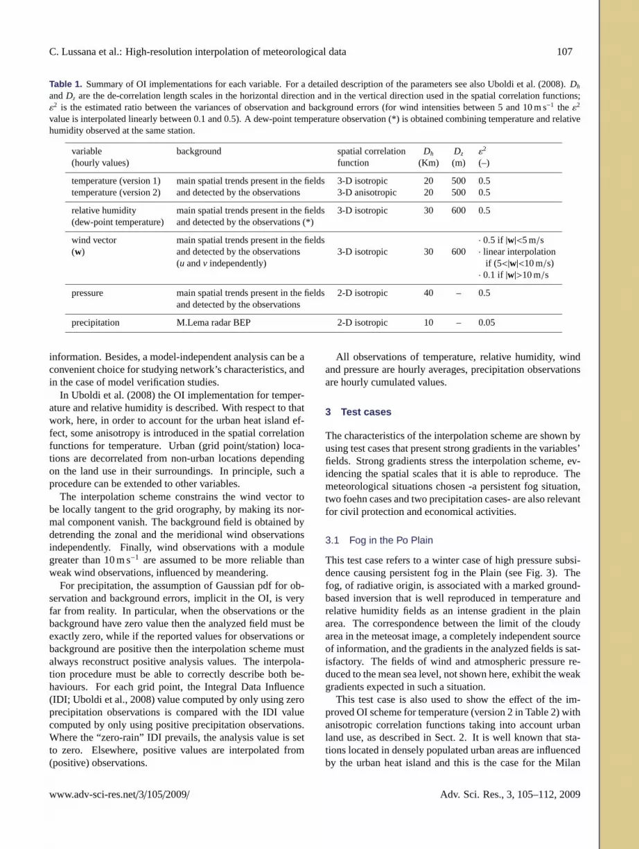
Table 1. Summary of OI implementations for each variable. For a detailed description of the parameters see alsoUboldi et al.(2008). Dh

andDz are the de-correlation length scales in the horizontal direction and in the vertical direction used in the spatial correlation functions;ε2 is the estimated ratio between the variances of observation and background errors (for wind intensities between 5 and 10 m s−1 the ε2

value is interpolated linearly between 0.1 and 0.5). A dew-point temperature observation (*) is obtained combining temperature and relativehumidity observed at the same station.

variable background spatial correlation Dh Dz ε2

(hourly values) function (Km) (m) (–)

temperature (version 1) main spatial trends present in the fields 3-D isotropic 20 500 0.5temperature (version 2) and detected by the observations 3-D anisotropic 20 500 0.5

relative humidity main spatial trends present in the fields 3-D isotropic 30 600 0.5(dew-point temperature) and detected by the observations (*)

wind vector main spatial trends present in the fields · 0.5 if |w|<5 m/s(w) and detected by the observations 3-D isotropic 30 600· linear interpolation

(u andv independently) if(5<|w|<10 m/s)· 0.1 if |w|>10 m/s

pressure main spatial trends present in the fields 2-D isotropic 40 – 0.5and detected by the observations

precipitation M.Lema radar BEP 2-D isotropic 10 – 0.05

information. Besides, a model-independent analysis can be aconvenient choice for studying network’s characteristics, andin the case of model verification studies.

In Uboldi et al.(2008) the OI implementation for temper-ature and relative humidity is described. With respect to thatwork, here, in order to account for the urban heat island ef-fect, some anisotropy is introduced in the spatial correlationfunctions for temperature. Urban (grid point/station) loca-tions are decorrelated from non-urban locations dependingon the land use in their surroundings. In principle, such aprocedure can be extended to other variables.

The interpolation scheme constrains the wind vector tobe locally tangent to the grid orography, by making its nor-mal component vanish. The background field is obtained bydetrending the zonal and the meridional wind observationsindependently. Finally, wind observations with a modulegreater than 10 m s−1 are assumed to be more reliable thanweak wind observations, influenced by meandering.

For precipitation, the assumption of Gaussian pdf for ob-servation and background errors, implicit in the OI, is veryfar from reality. In particular, when the observations or thebackground have zero value then the analyzed field must beexactly zero, while if the reported values for observations orbackground are positive then the interpolation scheme mustalways reconstruct positive analysis values. The interpola-tion procedure must be able to correctly describe both be-haviours. For each grid point, the Integral Data Influence(IDI; Uboldi et al., 2008) value computed by only using zeroprecipitation observations is compared with the IDI valuecomputed by only using positive precipitation observations.Where the “zero-rain” IDI prevails, the analysis value is setto zero. Elsewhere, positive values are interpolated from(positive) observations.

All observations of temperature, relative humidity, windand pressure are hourly averages, precipitation observationsare hourly cumulated values.

3 Test cases

The characteristics of the interpolation scheme are shown byusing test cases that present strong gradients in the variables’fields. Strong gradients stress the interpolation scheme, ev-idencing the spatial scales that it is able to reproduce. Themeteorological situations chosen -a persistent fog situation,two foehn cases and two precipitation cases- are also relevantfor civil protection and economical activities.

3.1 Fog in the Po Plain

This test case refers to a winter case of high pressure subsi-dence causing persistent fog in the Plain (see Fig.3). Thefog, of radiative origin, is associated with a marked ground-based inversion that is well reproduced in temperature andrelative humidity fields as an intense gradient in the plainarea. The correspondence between the limit of the cloudyarea in the meteosat image, a completely independent sourceof information, and the gradients in the analyzed fields is sat-isfactory. The fields of wind and atmospheric pressure re-duced to the mean sea level, not shown here, exhibit the weakgradients expected in such a situation.

This test case is also used to show the effect of the im-proved OI scheme for temperature (version 2 in Table2) withanisotropic correlation functions taking into account urbanland use, as described in Sect.2. It is well known that sta-tions located in densely populated urban areas are influencedby the urban heat island and this is the case for the Milan

www.adv-sci-res.net/3/105/2009/ Adv. Sci. Res., 3, 105–112, 2009

108 C. Lussana et al.: High-resolution interpolation of meteorological data4 C. Lussana et al.: High-resolution interpolation of meteorological data

Figure 3. 20 Jan 2006, 12:00 LT. Left: Temperature. Center: Meteosat-8 Channel 12 (HRV) image. Right: relative humidity. Thetemperature scale is the same as in Fig. 2.

main range; the southern slopes and the Po valley are cloudfree with strong and gusty foehn winds, and local heating dueto adiabatic compression. The observational network has inthis case sufficient spatial resolution to measure these localphenomena. As it can be seen from Fig. 4, the warming inthe north-west and the correspondent minimum in relativehumidity are correctly reconstructed by the analysis. Thewind analysis shows a strong intensification, which is wellcorrelated with the other independently analyzed fields (notshown here).

3.2.2 12 March 2006

The meteorological situation for the second foehn case -12March 2006- is similar to the previous one. However, inthis case the eastern part of the region is still under the in-fluence of a cyclonic circulation. Very low temperature val-ues were observed in the mountain areas to the northeast,and light snowfall occurred during the morning in the south-eastern plain. As can be seen in Fig. 5, the wind field pat-tern is in agreement with the analyzed pressure gradient; thewind intensity maxima correctly correspond to the dry andwarm areas in the temperature and relative humidity analysis(not shown here). It is worth remarking that all the variablesare analyzed independently: their consistency is a qualitativeconfirmation that the OI does not introduce large errors.

3.3 Precipitation cases

The results for OI of cumulated precipitation are presentedin two very different cases: a case of convective precipita-tion and a case of stratiform precipitation. Convective andstratiform precipitation have different spatial and temporalcoherence, but in both cases the integrated field retains thegood features of raingauges observations and post-processed

radar background information. The realistic appearance ofthe 24 hours cumulated fields also shows that any systematicerror introduced by the interpolation algorithm must be ofsmall amplitude. In fact, even summing-up many precipita-tion fields, unrealistic features do not appear.

In order to show the characteristics of the integration ofthe available information, the precipitation analysis fields forthe test cases chosen are compared with the OI of raingaugesobservation only and with the M. Lema best estimate of pre-cipitation rate at the ground (Joss et al., 1998).

3.3.1 Convective precipitation

Convective precipitation is characterized by small horizontalscales and high vertical extension of the precipitating vol-ume. As can be seen in Fig. 6, in this case the radar estimateof the rain field (center panels) is more realistic than whatcan be obtained with raingauges only (leftmost panels). Inthe latter, the spatial pattern is clearly mainly determined bythe station distribution and the symmetrical correlation func-tions. The analysis in the rightmost panels, integrating thetwo sources, maintain the radar’s realistic features.

By cumulating the analysis fields over 24 hours, the peakof precipitation observed in the radar estimate is correctlyconserved in the integrated map.

3.3.2 Stratiform precipitation

A stratified precipitation case, of frontal origin, is repre-sented in Fig. 7. In such cases the radar signal may bestrongly attenuated, especially in areas far from the radarsite (as the north-eastern area of the domain, central pan-els). The raingauges measurements, where available, allowin these cases a better reconstruction of the precipitationfieldthan what can be obtained by radar estimation alone. The

Adv. Sci. Res. www.adv-sci-res.net

Figure 3. 20 January 2006, 12:00 LT. Left: Temperature. Center: Meteosat-8 Channel 12 (HRV) image. Right: relative humidity (unit %).The temperature scale is the same as in Fig.2.

C. Lussana et al.: High-resolution interpolation of meteorological data 5

Figure 4. 21 Jan 2005, 12:00 LT. Left: temperature. Right: relative humidity. See Figs. 2 and 3 for temperature and relative humidity scales,respectively.

Figure 5. 12 March 2006, 08:00 LT. Left: wind vectors (white boxes contain observations and mark station locations). Right: pressure(reduced to the mean sea level).

point-wise observations are in this case more representativeof an area because of the larger spatial scales that character-ize stratiform precipitation.

4 Cross Validation scores

The CV score is routinely computed for each analysis timefor temperature and relative humidity. The CV score repre-sents an estimate of the analysis error, based on the idea thateach observation is used as an independent verification of

www.adv-sci-res.net Adv. Sci. Res.

Figure 4. 21 January 2005, 12:00 LT. Left: temperature. Right: relative humidity. See Figs.2 and3 for temperature and relative humidityscales, respectively.

area, in the western part of the region. By integrating landuse information in the OI scheme, it is possible to recognizeand decorrelate urban from non-urban locations. The finaleffect can be seen by comparing the left panel in Fig.3 withFig. 2 in the Milan area. A careful inspection of the me-teosat picture shows better agreement with the field in Fig.2,especially for the Milan area, and a quantitative diagnosticsusing Cross Validation (CV) scores confirms this qualitativeevaluation.

3.2 Foehn cases

3.2.1 21 January 2005

The first case, well documented on-line (Eumetsat, 2008),refers to 21 January 2005. The Alps are under the influence

of a strong northerly flow with marked stau cloudiness on themain range; the southern slopes and the Po valley are cloudfree with strong and gusty foehn winds, and local heating dueto adiabatic compression. The observational network has inthis case sufficient spatial resolution to measure these localphenomena. As it can be seen from Fig.4, the warming inthe north-west and the correspondent minimum in relativehumidity are correctly reconstructed by the analysis. Thewind analysis shows a strong intensification, which is wellcorrelated with the other independently analyzed fields (notshown here).

Adv. Sci. Res., 3, 105–112, 2009 www.adv-sci-res.net/3/105/2009/

C. Lussana et al.: High-resolution interpolation of meteorological data 109

C. Lussana et al.: High-resolution interpolation of meteorological data 5

Figure 4. 21 Jan 2005, 12:00 LT. Left: temperature. Right: relative humidity. See Figs. 2 and 3 for temperature and relative humidity scales,respectively.

Figure 5. 12 March 2006, 08:00 LT. Left: wind vectors (white boxes contain observations and mark station locations). Right: pressure(reduced to the mean sea level).

point-wise observations are in this case more representativeof an area because of the larger spatial scales that character-ize stratiform precipitation.

4 Cross Validation scores

The CV score is routinely computed for each analysis timefor temperature and relative humidity. The CV score repre-sents an estimate of the analysis error, based on the idea thateach observation is used as an independent verification of

www.adv-sci-res.net Adv. Sci. Res.

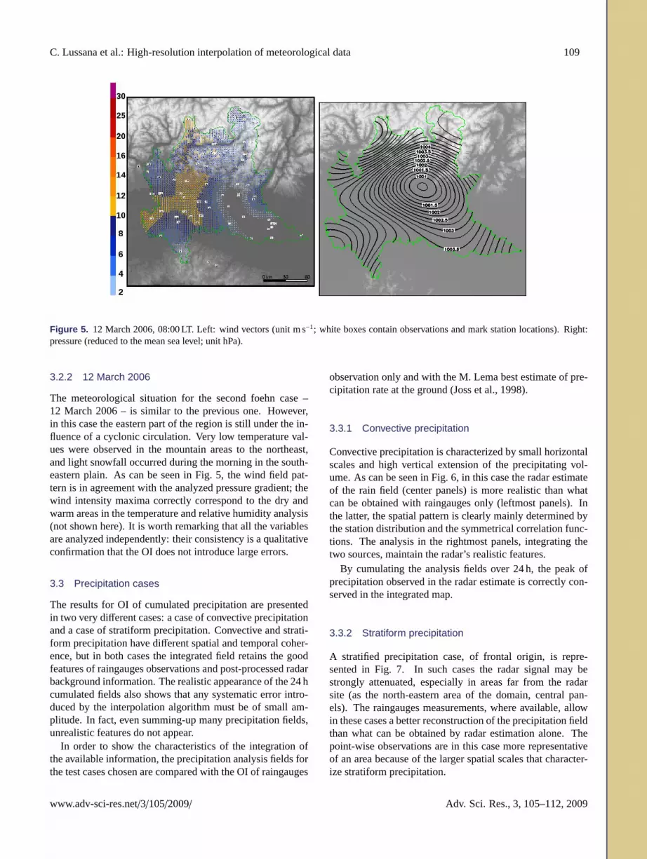
Figure 5. 12 March 2006, 08:00 LT. Left: wind vectors (unit m s−1; white boxes contain observations and mark station locations). Right:pressure (reduced to the mean sea level; unit hPa).

3.2.2 12 March 2006

The meteorological situation for the second foehn case –12 March 2006 – is similar to the previous one. However,in this case the eastern part of the region is still under the in-fluence of a cyclonic circulation. Very low temperature val-ues were observed in the mountain areas to the northeast,and light snowfall occurred during the morning in the south-eastern plain. As can be seen in Fig.5, the wind field pat-tern is in agreement with the analyzed pressure gradient; thewind intensity maxima correctly correspond to the dry andwarm areas in the temperature and relative humidity analysis(not shown here). It is worth remarking that all the variablesare analyzed independently: their consistency is a qualitativeconfirmation that the OI does not introduce large errors.

3.3 Precipitation cases

The results for OI of cumulated precipitation are presentedin two very different cases: a case of convective precipitationand a case of stratiform precipitation. Convective and strati-form precipitation have different spatial and temporal coher-ence, but in both cases the integrated field retains the goodfeatures of raingauges observations and post-processed radarbackground information. The realistic appearance of the 24 hcumulated fields also shows that any systematic error intro-duced by the interpolation algorithm must be of small am-plitude. In fact, even summing-up many precipitation fields,unrealistic features do not appear.

In order to show the characteristics of the integration ofthe available information, the precipitation analysis fields forthe test cases chosen are compared with the OI of raingauges

observation only and with the M. Lema best estimate of pre-cipitation rate at the ground (Joss et al., 1998).

3.3.1 Convective precipitation

Convective precipitation is characterized by small horizontalscales and high vertical extension of the precipitating vol-ume. As can be seen in Fig.6, in this case the radar estimateof the rain field (center panels) is more realistic than whatcan be obtained with raingauges only (leftmost panels). Inthe latter, the spatial pattern is clearly mainly determined bythe station distribution and the symmetrical correlation func-tions. The analysis in the rightmost panels, integrating thetwo sources, maintain the radar’s realistic features.

By cumulating the analysis fields over 24 h, the peak ofprecipitation observed in the radar estimate is correctly con-served in the integrated map.

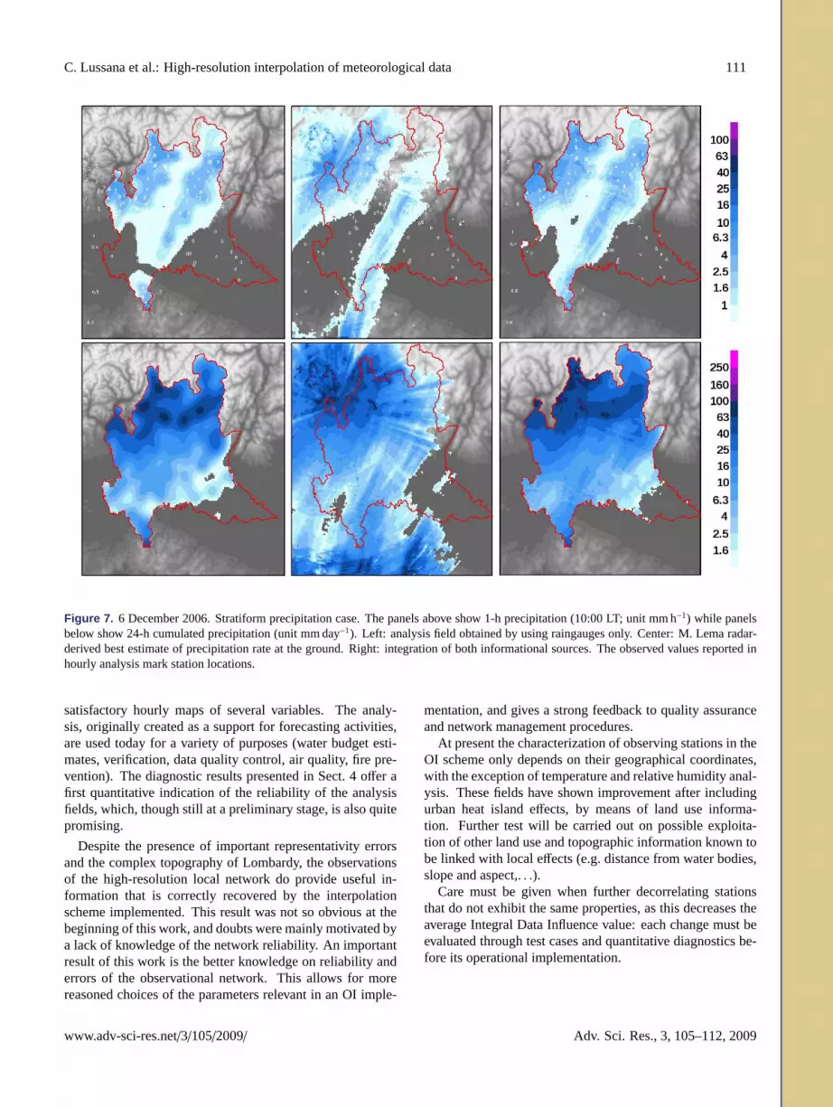
3.3.2 Stratiform precipitation

A stratified precipitation case, of frontal origin, is repre-sented in Fig.7. In such cases the radar signal may bestrongly attenuated, especially in areas far from the radarsite (as the north-eastern area of the domain, central pan-els). The raingauges measurements, where available, allowin these cases a better reconstruction of the precipitation fieldthan what can be obtained by radar estimation alone. Thepoint-wise observations are in this case more representativeof an area because of the larger spatial scales that character-ize stratiform precipitation.

www.adv-sci-res.net/3/105/2009/ Adv. Sci. Res., 3, 105–112, 2009

110 C. Lussana et al.: High-resolution interpolation of meteorological data6 C. Lussana et al.: High-resolution interpolation of meteorological data

Figure 6. 24 Aug 2006. Convective precipitation case. The panels above show 1-hour precipitation (23:00 LT; unit mm/h) while panelsbelow show 24-hour cumulated precipitation (unit mm/day). Left: analysis field obtained by using raingauges only. Center: M. Lema radar-derived best estimate of precipitation rate at the ground. Right: integration of both informational sources. The observed values reported inhourly analysis mark station locations.

the analysis field. The CV score distribution for temperaturehas been computed for the entire 2006: the overall medianis 1.45◦C and the interquartile range is 0.50◦C. By group-ing stations according to the IDI, stations belonging to denseareas of coverage has a CV score distribution median lessthan 1◦C. Largest errors are more probable for isolated sta-tions with the third quartile having a value close to 2◦C. Inany case, the median is always larger than 0◦C because localscales affecting the observation are filtered out by the inter-polation.

The same diagnostic is computed for relative humidity: themedian for the year 2006 CV score distribution is 10.4% andthe correspondent interquartile range is 2.45%. However,it must be remembered that, in ARPA Lombardia’s meteo-rological network, the spatial distribution of hygrometers isless dense than the distribution of thermometers.

5 Conclusions

An Optimal Interpolation (OI) scheme for the different vari-ables measured by surface weather stations has been herepresented. Given the characteristics of this OI implementa-tion, the analysis fields -with the exception of precipitation-

depend only on point-wise observations. The method is thenwidely applicable, model-independent and particularly wellsuited for interpolation of observations from high-density au-tomatic networks, being also robust and efficient.

The presented scheme has been running daily for overtwo years in ARPA Lombardia’s weather service, produc-ing satisfactory hourly maps of several variables. The analy-sis, originally created as a support for forecasting activities,are used today for a variety of purposes (water budget esti-mates, verification, data quality control, air quality, firepre-vention). The diagnostic results presented in Sec. 4 offer afirst quantitative indication of the reliability of the analysisfields, which, though still at a preliminary stage, is also quitepromising.

Despite the presence of important representativity errorsand the complex topography of Lombardy, the observationsof the high-resolution local network do provide useful in-formation that is correctly recovered by the interpolationscheme implemented. This result was not so obvious at thebeginning of this work, and doubts were mainly motivated bya lack of knowledge of the network reliability. An importantresult of this work is the better knowledge on reliability anderrors of the observational network. This allows for more

Adv. Sci. Res. www.adv-sci-res.net

Figure 6. 24 August 2006. Convective precipitation case. The panels above show 1-h precipitation (23:00 LT; unit mm h−1) while panelsbelow show 24-h cumulated precipitation (unit mm day−1). Left: analysis field obtained by using raingauges only. Center: M. Lema radar-derived best estimate of precipitation rate at the ground. Right: integration of both informational sources. The observed values reported inhourly analysis mark station locations.

4 Cross Validation scores

The CV score is routinely computed for each analysis timefor temperature and relative humidity. The CV score repre-sents an estimate of the analysis error, based on the idea thateach observation is used as an independent verification ofthe analysis field. The CV score distribution for temperaturehas been computed for the entire 2006: the overall medianis 1.45◦C and the interquartile range is 0.50◦C. By group-ing stations according to the IDI, stations belonging to denseareas of coverage has a CV score distribution median lessthan 1◦C. Largest errors are more probable for isolated sta-tions with the third quartile having a value close to 2◦C. Inany case, the median is always larger than 0◦C because localscales affecting the observation are filtered out by the inter-polation.

The same diagnostic is computed for relative humidity: themedian for the year 2006 CV score distribution is 10.4% and

the correspondent interquartile range is 2.45%. However,it must be remembered that, in ARPA Lombardia’s meteo-rological network, the spatial distribution of hygrometers isless dense than the distribution of thermometers.

5 Conclusions

An Optimal Interpolation (OI) scheme for the different vari-ables measured by surface weather stations has been herepresented. Given the characteristics of this OI implementa-tion, the analysis fields – with the exception of precipitation –depend only on point-wise observations. The method is thenwidely applicable, model-independent and particularly wellsuited for interpolation of observations from high-density au-tomatic networks, being also robust and efficient.

The presented scheme has been running daily for overthree years in ARPA Lombardia’s weather service, producing

Adv. Sci. Res., 3, 105–112, 2009 www.adv-sci-res.net/3/105/2009/

C. Lussana et al.: High-resolution interpolation of meteorological data 111C. Lussana et al.: High-resolution interpolation of meteorological data 7

Figure 7. 06 Dec 2006. Stratiform precipitation case. The panels above show 1-hour precipitation (10:00 LT; unit mm/h) while panels belowshow 24-hour cumulated precipitation (unit mm/day). Left: analysis field obtained by using raingauges only. Center: M. Lema radar-derivedbest estimate of precipitation rate at the ground. Right: integration of both informational sources. The observed values reported in hourlyanalysis mark station locations.

reasoned choices of the parameters relevant in an OI imple-mentation, and gives a strong feedback to quality assuranceand network management procedures.

At present the station characterization in the OI schemedepends only on their geographical coordinates, with the ex-ception of temperature and relative humidity analysis. Thesefields have shown improvement after including urban heatisland effects, by means of land use information. Furthertest will be carried out on possible exploitation of other landuse and topographic information known to be linked withlocal effects (e.g. distance from water bodies, slope andaspect,. . .).

Care must be given when further decorrelating stationsthat do not exhibit the same properties, as this decreases theaverage Integral Data Influence value: each change must beevaluated through test cases and quantitative diagnosticsbe-fore its operational implementation.

References

Daley, R.: Atmospheric Data Analysis, Cambridge UniversityPress, 1991.

Eumetsat: Strong North Foehn over the Alps (21 Jan-uary 2005), http://oiswww.eumetsat.org/WEBOPS/iotm/iotm/20050121foehn/20050121foehn.html, 2008.

Gandin, L. S.: Objective Analysis of Meteorological Fields,Gidromet, Leningrad. English translation by Israeli Program forScientific Translations, Jerusalem., 1963.

Joss, J., Schadler, B., Galli, G., Cavalli, R., Boscacci, M., Held,E., Bruna, G. D., Kappenberger, G., Nespor, V., and Spiess,R.: Operational Use of Radar for Precipitation Measurementsin Switzerland, Verlag der Fachvereine Hochschulverlag AGander ETH Zurich, 1998.

Kalnay, E.: Atmospheric Modeling, Data Assimilation and Pre-dictability, Cambridge University Press, 2003.

Uboldi, F., Lussana, C., and Salvati, M.: Three-dimensional spatialinterpolation of surface meteorological observations from high-resolution local networks, Meteorological Applications,15, 331–345, 2008.

www.adv-sci-res.net Adv. Sci. Res.

Figure 7. 6 December 2006. Stratiform precipitation case. The panels above show 1-h precipitation (10:00 LT; unit mm h−1) while panelsbelow show 24-h cumulated precipitation (unit mm day−1). Left: analysis field obtained by using raingauges only. Center: M. Lema radar-derived best estimate of precipitation rate at the ground. Right: integration of both informational sources. The observed values reported inhourly analysis mark station locations.

satisfactory hourly maps of several variables. The analy-sis, originally created as a support for forecasting activities,are used today for a variety of purposes (water budget esti-mates, verification, data quality control, air quality, fire pre-vention). The diagnostic results presented in Sect.4 offer afirst quantitative indication of the reliability of the analysisfields, which, though still at a preliminary stage, is also quitepromising.

Despite the presence of important representativity errorsand the complex topography of Lombardy, the observationsof the high-resolution local network do provide useful in-formation that is correctly recovered by the interpolationscheme implemented. This result was not so obvious at thebeginning of this work, and doubts were mainly motivated bya lack of knowledge of the network reliability. An importantresult of this work is the better knowledge on reliability anderrors of the observational network. This allows for morereasoned choices of the parameters relevant in an OI imple-

mentation, and gives a strong feedback to quality assuranceand network management procedures.

At present the characterization of observing stations in theOI scheme only depends on their geographical coordinates,with the exception of temperature and relative humidity anal-ysis. These fields have shown improvement after includingurban heat island effects, by means of land use informa-tion. Further test will be carried out on possible exploita-tion of other land use and topographic information known tobe linked with local effects (e.g. distance from water bodies,slope and aspect,. . .).

Care must be given when further decorrelating stationsthat do not exhibit the same properties, as this decreases theaverage Integral Data Influence value: each change must beevaluated through test cases and quantitative diagnostics be-fore its operational implementation.

www.adv-sci-res.net/3/105/2009/ Adv. Sci. Res., 3, 105–112, 2009

112 C. Lussana et al.: High-resolution interpolation of meteorological data

References

Daley, R.: Atmospheric Data Analysis, Cambridge UniversityPress, 1991.

Eumetsat: Strong North Foehn over the Alps (21 Jan-uary 2005), http://oiswww.eumetsat.org/WEBOPS/iotm/iotm/20050121foehn/20050121foehn.html, 2008.

Gandin, L. S.: Objective Analysis of Meteorological Fields,Gidromet, Leningrad. English translation by Israeli Program forScientific Translations, Jerusalem, 1963.

Joss, J., Schadler, B., Galli, G., Cavalli, R., Boscacci, M., Held,E., Bruna, G. D., Kappenberger, G., Nespor, V., and Spiess,R.: Operational Use of Radar for Precipitation Measurementsin Switzerland, Verlag der Fachvereine Hochschulverlag AG ander ETH Zurich, 1998.

Kalnay, E.: Atmospheric Modeling, Data Assimilation and Pre-dictability, Cambridge University Press, 2003.

Uboldi, F., Lussana, C., and Salvati, M.: Three-dimensional spatialinterpolation of surface meteorological observations from high-resolution local networks, Meteorol. Appl., 15, 331–345, 2008.

Adv. Sci. Res., 3, 105–112, 2009 www.adv-sci-res.net/3/105/2009/