Effect of loss on the dispersion relation of photonic and phononic crystals

Vincent Laude,1, ∗ Jose Maria Escalante,2 and Alejandro Martınez2

1Institut FEMTO-ST, Universite de Franche-Comte and CNRS, Besancon, France2Nanophotonics Technology Center, Universitat Politecnica de Valencia, Valencia 46022, Spain

A theoretical analysis is made of the transformation of the dispersion relation of waves in artificialcrystals under the influence of loss, including the case of photonic and phononic crystals. Consid-ering a general dispersion relation in implicit form, an analytic procedure is derived to obtain thetransformed dispersion relation. It is shown that the dispersion relation is generally shifted in thecomplex (k, ω) plane, with k the wavenumber and ω the angular frequency. The value of the shiftis obtained explicitly as a function of the perturbation of material constants accounting for loss.The method is shown to predict correctly the transformation of the complex band structure k(ω).Several models of the dispersion relation near a symmetry point of the Brillouin zone are analyzed.A lower bound for the group velocity, related to the local shape of the band around symmetrypoints, is derived for each case.

PACS numbers:

I. INTRODUCTION

Wave propagation in heterogeneous artificial crystalscomposed of two or more materials that differ in theirmaterial constants has received great attention duringthe last two decades. Artificial crystals include in par-ticular the cases of photonic crystals for optical waves1

and of phononic crystals for elastic waves2,3. Thanksto advances in nano-fabrication, photonic crystals in thevisible and near IR, and phononic crystals in the giga-hertz spectral range are now available. They can beused to manipulate, to guide, and to confine light orsound, or even both type of waves at same time (phox-onic crystals)4,5. One important property of this typeof structure is slow wave propagation6–8. Many devicesmay potentially take advantage of slow wave effects, e.g.,for amplification, optical buffering, acousto-optic mod-ulation, sensing, pulse compression, or enhanced non-linear effects. Numerous experimental results, mainly inthe field of photonic crystals, have however demonstratedthat despite tremendous fabrication efforts, reducing thegroup velocity beyond two orders of magnitude still re-mains elusive.9 One limitation imposed on the minimumattainable group velocity of both photonic and phononiccrystals has its origin in propagation losses.

Losses can be due to fabrication disorder or to in-trinsic material losses.10–14 There exist many differentmodels of loss, that are adapted to different situations.With Helmholtz-type propagation equations, obtainedwith the assumption of monochromatic waves, it is conve-nient to introduce loss via the imaginary part of materialconstants that are implicitly dependent on frequency. Inthe photonic crystal case, the position dependent dielec-tric tensor is written as12

ε(r) = ε′(r)− ıε′′(r). (1)

In the phononic case, the elastic tensor is written as14

C(r) = C ′(r) + ıC ′′(r). (2)

In either case, the real part of the material constants isthe value in the absence of loss and the imaginary partis assumed to be relatively small, i.e., ε′′/ε′ << 1 andC ′′/C ′ << 1. In addition, the imaginary part can dependon frequency. This dependence is explicit in viscoelasticmodels where C ′′ = ηω with η the viscoelasticity tensorand ω the angular frequency. The sign of the imaginaryparts in (1) and (2) is consistent with the time-harmonicdependence exp(ı(ωt− k · r)) where k is the wavevector.

The transformation of dispersion relations when loss isincluded is a general question with both theoretical andpractical implications. With homogeneous media, theanalysis is straightforward. In artificial crystals, however,periodicity introduces a strong dispersion that makes theproblem more intricate. This is especially true at degen-eracy points of the dispersion relation where the groupvelocity becomes very small or even vanishes. Pedersenet al. studied how material losses induce a lower boundfor the group velocity in photonic crystals.12 The methodof analysis considers an approximate model of the disper-sion relation near a band edge, at a symmetry point ofthe first Brillouin zone. The exact shape of the disper-sion relation can quite complex, but in the vicinity of apoint where the group velocity vanishes in the absence ofloss, the band structure can be approximated as

ω = ω0 + α(k − k0)2. (3)

The wavenumber k is here a component of the wavevectorin a particular propagation direction. From first-orderperturbation theory, Pedersen et al. obtained that whenloss is added

vg ≥√|α|ωF ε

′′

ε′(4)

where F is the filling fraction. This result is quite gen-eral and is in particular independent of the details ofthe photonic crystal lattice and of its composition. Forthe case of phononic crystals, no similar result has beenfound so far, to the best of our knowledge. Moiseyenko

arX

iv:1

309.

0080

v2 [

phys

ics.

optic

s] 2

0 Se

p 20

13

2

and Laude investigated numerically the transformationof the complex band structure when loss is introducedand obtained a expression for the group velocity at anypoint of the dispersion relation.14 Although the result isgeneral and independent of the details of the phononiccrystal, the limitation of the group velocity by loss wasa numerical observation but was not given an explicitexpression.

In this paper, we attempt to give a general theory ofthe influence of loss on dispersion relations in artificialcrystals, encompassing and extending the results above.Considering implicit rather than explicit dispersion rela-tions proves to be an adequate way of tackling the prob-lem. In section II, we show how the classical and thecomplex band structures can be cast in implicit form,and how the first variations of frequency and wavenum-ber can be estimated when loss is introduced as a per-turbation of material constants. In section III, we applythe theory to different approximate models of dispersionrelations, first following the typology introduced by Fig-otin and Vitebskiy15 and then introducing a model of thecomplex dispersion relation in a Bragg band gap. In eachcase, an analytical expression of the lower bound set byloss on the group velocity is given. Our results hold ingeneral for a Helmholtz-type equation (a monochromaticwave equation), including periodicity and anisotropy.

II. PERTURBATION OF DISPERSIONRELATIONS

A. Dispersion relations

A general dispersion relation has the implicit form

D(ω, k, µ) = 0 (5)

where µ represents any material constant. A band struc-ture is a plot of a set of such dispersion relations for fixedµ. The first differential of the dispersion relation is

∂D∂ω

dω +∂D∂k

dk +∂D∂µ

dµ = 0. (6)

The group velocity (at fixed µ, i.e., for a given set ofmaterial constants) can then be obtained as

vg =dω

dk

∣∣∣∣µ

= −∂D∂k∂D∂ω

. (7)

Similarly, we can look at the variation of angular fre-quency (at fixed k) caused by a variation in materialconstants as

dω

dµ

∣∣∣∣k

= −∂D∂µ

∂D∂ω

(8)

and the converse variation of k (at fixed ω) caused by avariation in material constants as

dk

dµ

∣∣∣∣ω

= −∂D∂µ

∂D∂k

. (9)

Figure 1: Schematic representation of a dispersion relation inthe wavenumber-frequency plane and its transformation un-der a perturbation of the material constants µ. A point (k, ω)on the perturbed (lossy) dispersion relation can be tracedbackward to the initial (lossless) dispersion relation by eithera vertical shift −δω or a horizontal shift −δk.

All these relations are valid for infinitesimal variations ofthe variables of the dispersion relation and hold exactlyon it, i.e., at (ω, k, µ) points where (5) is satisfied.

Suppose now we solve for the dispersion relation for agiven set of material constants µ and then for a slightlyperturbed set µ + δµ, e.g., without/with including loss.In practice, we would first solve D(ω, k, µ) = 0, thenD(ω, k, µ+ δµ) = 0. As figure 1 illustrates, the distancebetween the initial dispersion relation and the perturbedone is δω in the vertical direction and δk in the horizontaldirection. For a small perturbation δµ, the two disper-sion relations are almost parallel in the (k, ω) plane, asexpressed by the two equalities

D(ω, k, µ+ δµ) = D(ω − δω|k, k, µ) (10)

= D(ω, k − δk|ω, µ), (11)

as can be readily obtained by considering first-order Tay-lor expansions around the point (ω, k, µ) in each variableand using (6). They mean that we can go from one point(k, ω) of the perturbed dispersion relation to the initialdispersion relation by a backward shift along either axisof the band structure. They are the basic ingredientsthat are needed to complexify dispersion relations whenloss is added, as we illustrate in Section III. Each equal-ity is then valid only if the first derivatives with respectto the involved variable does not vanish.

B. Band structure, ω(k)

The master equations for electromagnetic waves in di-electric media, and hence in photonic crystals, are of theform

∇∧(

1

ε∇∧H

)=(ωc

)2H (12)

3

Table I: Expression of matrix elements for the ω(k)-type dis-persion relations for photonic and phononic crystals. Thenotation < | · · · | > indicates integration over the unit-cell ofthe crystal.

Crystal type Amn(k) Bmn

Phononic < ∇fm|C|∇fn > < fm|ρ|fn >Photonic < ∇∧ fm| 1ε |∇ ∧ fn > < fm| 1c2 |fn >

where H is the magnetic field vector and c is the celerityof light in a vacuum. For elastic waves in solids, andhence in phononic crystals, the elastodynamic equationsare

−∇ · (C : ∇u) = ω2ρu (13)

where u is the displacements vector and ρ is the massdensity.

In order to obtain a numerical solution, the un-known fields are expanded over a given functional ba-sis, e.g., Fourier exponentials for the plane wave expan-sion (PWE) method, or piecewise continuous polynomi-als for the finite element method (FEM). As a result of aGalerkin type procedure, we end up with an eigenvalueproblem of the form

A(k)x = ω2Bx (14)

where x is the vector of the unknown coefficients in theexpansion, and A and B are square and symmetric matri-ces that are formed from material constants and expan-sion functions. Periodicity is accounted for via the use ofthe Bloch-Floquet theorem. Specifically, writing the ex-pansion as H(r, t) or u(r, t) =

∑n xnfn(r) exp(ı(ωt− k ·

r)) with (fn(r)) a basis of periodic functions and denot-ing fn = fn exp(−ık ·r)), the form of the matrix elementsis given in Table I.

From the eigenvalue problem, a scalar dispersion re-lation for each eigenvalue ω can be obtained by left-multiplying with the left-eigenvector y. The left-eigenvector is a right-eigenvector of the transposes ofmatrices A and B. Generally, x and y associated tothe same eigenvalue are different, unless the matrices aresymmetric16, which is the case here. We thus obtain thedispersion relation in implicit form as

D(ω, k, µ) = xTA(k)x− ω2xTBx (15)

where the subscript T denotes transposition.Note that the eigenvector depends on ω, k, and µ. Be-

cause it satisfies (14) along the dispersion relation, how-ever, we obtain

∂D∂ω

= xT∂A(k)

∂ωx− 2ωxTBx, (16)

∂D∂k

= xT∂A(k)

∂kx, (17)

∂D∂µ

= xT∂A(k)

∂µx− ω2xT

∂B

∂µx, (18)

at every point of the dispersion relation. Since we knowexplicit expressions for all matrices, these formulas allowfor a very efficient evaluation of the group velocity and ofthe variations by (7–9) at every (k, ω) point of the disper-sion relation, given only the knowledge of the eigenvalueand eigenvector. For instance, the group velocity can becalculated without any approximation along the disper-sion relation by the formula

vg =xT ∂A(k)

∂k x

2ωxTBx− xT ∂A(k)∂ω x

. (19)

Similarly, when the material constants are changed bya very small amount, the first variation of ω at constant kand the first variation of k at constant ω can respectivelybe estimated as

δω|k =xT δA(k)x− ω2xT δBx

2ωxTBx− xT ∂A(k)∂ω x

, (20)

δk|ω = −xT δA(k)x− ω2xT δBx

xT ∂A(k)∂k x

. (21)

A particularly appealing formula can be obtained for thefirst variation δω|k for the case of loss. For both photonic

and phononic problems, δB = 0. Furthermore, xT ∂A(k)∂ω x

is generally negligible as compared to 2ωxTBx, becausethe former term originates only from a possible depen-dence of loss with frequency. In the photonic case, wehave

ω2xTBx = xTAx =< ∇∧H|ε−1|∇ ∧H > (22)

and

xT δAx =< ∇∧H|ıε′′/ε′2|∇ ∧H > . (23)

The bra-ket notation < | · · · | > indicates integration overthe unit-cell of the crystal. Considering the case of aphotonic crystal of air holes in a dielectric material, wedefine the loss factor L = ε′′/ε′ and the filling fraction

F =< ∇∧H|ε′−1|∇ ∧H >dielectric

< ∇∧H|ε′−1|∇ ∧H >crystal. (24)

The filling fraction is a dimensionless number smallerthan 1 measuring the proportion of optical energy insidethe dielectric as compared to the total optical energy.Since the loss factor is assumed constant within the di-electric, we obtain at once

δω|k = ıω

2FL. (25)

The same equation is obtained for a phononic crystal oflossless inclusions in a lossy matrix, with the definitionsL = C ′′/C ′ and

F =< ∇u|C ′|∇u >matrix

< ∇u|C ′|∇u >crystal. (26)

4

In the case of air holes, F = 1 since all elastic energy isconcentrated in the matrix. Equation (25) was obtainedpreviously by Pedersen et al.12 for photonic crystals andis here seen to hold for a general Helmholtz equation. Ithas a very simple structure and periodicity is not imme-diately apparent in it. As Table I shows, the wavevectorenters the filling fraction value through the spatial deriva-tives of the expansion functions fn = fn exp(−ık · r)).Because of the spatial averages over the unit-cell of thecrystal, F does not vary much with frequency. Henceδω|k/ω is almost a constant if the loss factor is indepen-dent of frequency22.

A similar derivation for δk|ω could be attempted from(21). It would not lead, however, to a result as simpleas (25), since matrix A(k) is a second degree polynomialin k. Furthermore, at dispersion points where vg = 0,

xT ∂A(k)∂k x = 0 from (19), and hence δk|ω is seen to di-

verge from (21). Thus, at such points the first-order per-turbation result collapses for δk|ω. In contrast, δω|k/ωis always small, which means that the first-order pertur-bation result is valid whatever the frequency. In SectionIII, we will discuss how knowledge of the local topologyof the dispersion relation can be used to infer δk|ω fromδω|k.

C. Complex band structure, k(ω)

Complex band structures can be found by search-ing for the wavenumber as a function of frequency, asdemonstrated for photonic17 and phononic18,19 crystals.Whether the approach relies on the extended plane waveexpansion (EPWE) or on FEM, a generalized eigenvalueproblem of the form

C(ω)x = kD(ω)x (27)

is obtained. Matrices C and D account for periodicitywhere required, are non symmetric in general, and im-plicitly depend on the material constants. For brevity,we don’t give the detailed expression of the matrices, butthey can be found in the quoted references.

As before, we can obtain an implicit dispersion relationfor each particular eigenvalue k, by left-multiply by theleft-eigenvector y. The left-eigenvector satisfies

yTC(ω) = kyTD(ω). (28)

The dispersion relation in implicit form is thus

D(ω, k, µ) = yTC(ω)x− kyTD(ω)x (29)

whose first differentials when evaluated on the dispersionrelation are

∂D∂ω

= yT∂C

∂ωu− kyT ∂D

∂ωx, (30)

∂D∂k

= −yTDx, (31)

∂D∂µ

= yT∂C

∂µx− kyT ∂D

∂µx. (32)

Again, since we know the explicit expressions for all ma-trices, these formulas allow for a very efficient evaluationof the group velocity and the variations by (7–9) at ev-ery (ω, k) point of the dispersion relation, given only theknowledge of the eigenvectors y and x. For instance, werecover the group velocity expression of Ref.14

vg =yTDx

yT ∂C∂ω x− kyT∂D∂ω x

. (33)

Similarly, when the material constants are changed by avery small amount, the first variation of ω at constant kand the first variation of k at constant ω can respectivelybe estimated as

δω|k = −yT δCx− kyT δDx

yT ∂C∂ω x− kyT∂D∂ω x

, (34)

δk|ω =yT δCx− kyT δDx

yTDx. (35)

As previously, we could explicit further these variations,but the result would not be different from the previoussubsection since the classical band structure and the com-plex band structure are just but two representations ofthe same physical reality.

III. SPECIAL DISPERSION RELATIONMODELS

A. Local models

In this section, we make use of the tools developedin Section II to obtain analytical results given only theknowledge of the shape of the dispersion relation arounda given point. Around any point (k0, ω0) of the dispersionrelation where the group velocity doesn’t vanish, a localapproximation limited to first order can be considered as

D(ω, k, µ) = ω − ω0 − α(k − k0) = 0. (36)

Parameter α here equals the group velocity vg, as canbe checked by direct application of (7). Under an arbi-trary but small perturbation of the material constants,the transformed dispersion relation is given by applica-tion of (10) or (11). Both equalities apply here since∂D∂ω 6= 0 and ∂D

∂k 6= 0. Specifically,

− δω = αδk. (37)

Thus, from (25), we obtain at once that

δk = −ı 1

α

ω

2FL. (38)

The spatial decay thus varies linearly with loss and is in-versely proportional to the group velocity, i.e., flat bandsin the band structure are more sensitive to loss as com-pared to steep bands, as expected.

5

Let us now consider the case of points (k0, ω0) of thedispersion relation where the group velocity vanishes.This occurs at symmetry points of the Brillouin zone,but also whenever a band is extremal at the particularpoint. Figotin and Vitebskiy15 introduced the followingmodel dispersion relation

D(ω, k, µ) = ω − ω0 − α(k − k0)n = 0, n ≥ 2. (39)

If n = 2, this is a model of a regular band edge (RBE), ormore generally of a second-order stationary point, wheretwo bands become degenerate. If n = 3, the model isthat of a stationary inflection point (SIP) with triple de-generacy. If n = 4, the model is that of a degenerateband edge (BDE), implying quadruple degeneracy. Thealgebraic equation (39) defines at once n branches of thedispersion relation, as can be seen by solving it for k asa function of ω in explicit form. Figotin and Vitebskiyconsidered in great detail the properties of these modelsin the case of lossless materials. Let us apply to themthe procedure outlined above. The group velocity easilyfollows by (7)

vg = nα(k − k0)n−1. (40)

Since ∂D∂k = 0 at point (k0, ω0), (11) doesn’t hold. Equa-

tion (10) alone, however, can be used to obtain the trans-formed dispersion relation as

D(ω, k, µ+ δµ) = ω − ω0 − δω − α(k − k0)n = 0. (41)

This equation obviously yields the band structure ω(k),but by inverting it we can in addition obtain the complexband structure k(ω) as

k = k0 + ((ω − ω0 − δω)/α)1/n. (42)

The last equation actually has n different complexbranches. Of special interest is the departure of k fromk0 at frequency ω = ω0, which we still denote δk. Itsvalue is

δk = γmn (ω0FL/(2|α|))1/n,m = 0, · · · , n− 1 (43)

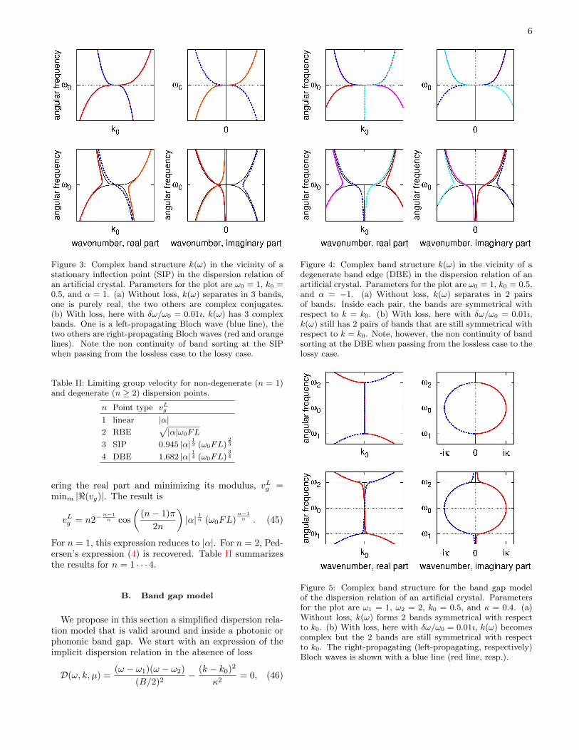
with γmn = exp(∓ıπ(2m+1/2)/n) the n-roots of ∓ı. Thechoice of sign in the previous expression must be madeaccording to minus the sign of α. As a result, the spatialdecay of Bloch waves close to a stationary point is pro-portional to the n-th root of the loss factor and to then-th root of the local curvature of the band as measuredby 1/|α|. Figures 2, 3, and 4 display the complex bandstructure for RBE, SIP, and DBE, respectively.

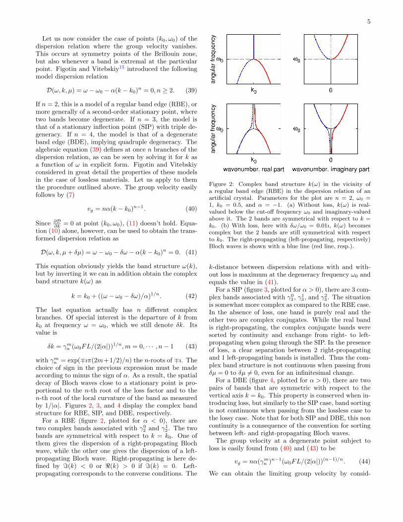
For a RBE (figure 2, plotted for α < 0), there aretwo complex bands associated with γ02 and γ12 . The twobands are symmetrical with respect to k = k0. One ofthem gives the dispersion of a right-propagating Blochwave, while the other one gives the dispersion of a left-propagating Bloch wave. Right-propagating is here de-fined by =(k) < 0 or <(k) > 0 if =(k) = 0. Left-propagating corresponds to the converse conditions. The

Figure 2: Complex band structure k(ω) in the vicinity ofa regular band edge (RBE) in the dispersion relation of anartificial crystal. Parameters for the plot are n = 2, ω0 =1, k0 = 0.5, and α = −1. (a) Without loss, k(ω) is real-valued below the cut-off frequency ω0 and imaginary-valuedabove it. The 2 bands are symmetrical with respect to k =k0. (b) With loss, here with δω/ω0 = 0.01ı, k(ω) becomescomplex but the 2 bands are still symmetrical with respectto k0. The right-propagating (left-propagating, respectively)Bloch waves is shown with a blue line (red line, resp.).

k-distance between dispersion relations with and with-out loss is maximum at the degeneracy frequency ω0 andequals the value in (41).

For a SIP (figure 3, plotted for α > 0), there are 3 com-plex bands associated with γ03 , γ13 , and γ23 . The situationis somewhat more complex as compared to the RBE case.In the absence of loss, one band is purely real and theother two are complex conjugates. While the real bandis right-propagating, the complex conjugate bands weresorted by continuity and exchange from right- to left-propagating when going through the SIP. In the presenceof loss, a clear separation between 2 right-propagatingand 1 left-propagating bands is installed. Thus the com-plex band structure is not continuous when passing fromδµ = 0 to δµ 6= 0, even for an infinitesimal change.

For a DBE (figure 4, plotted for α > 0), there are twopairs of bands that are symmetric with respect to thevertical axis k = k0. This property is conserved when in-troducing loss, but similarly to the SIP case, band sortingis not continuous when passing from the lossless case tothe lossy case. Note that for both SIP and DBE, this noncontinuity is a consequence of the convention for sortingbetween left- and right-propagating Bloch waves.

The group velocity at a degenerate point subject toloss is easily found from (40) and (43) to be

vg = nα(γmn )n−1(ω0FL/(2|α|))(n−1)/n. (44)

We can obtain the limiting group velocity by consid-

6

Figure 3: Complex band structure k(ω) in the vicinity of astationary inflection point (SIP) in the dispersion relation ofan artificial crystal. Parameters for the plot are ω0 = 1, k0 =0.5, and α = 1. (a) Without loss, k(ω) separates in 3 bands,one is purely real, the two others are complex conjugates.(b) With loss, here with δω/ω0 = 0.01ı, k(ω) has 3 complexbands. One is a left-propagating Bloch wave (blue line), thetwo others are right-propagating Bloch waves (red and orangelines). Note the non continuity of band sorting at the SIPwhen passing from the lossless case to the lossy case.

Table II: Limiting group velocity for non-degenerate (n = 1)and degenerate (n ≥ 2) dispersion points.

n Point type vLg

1 linear |α|2 RBE

√|α|ω0FL

3 SIP 0.945 |α|13 (ω0FL)

23

4 DBE 1.682 |α|14 (ω0FL)

34

ering the real part and minimizing its modulus, vLg =minm |<(vg)|. The result is

vLg = n2−n−1n cos

((n− 1)π

2n

)|α| 1n (ω0FL)

n−1n . (45)

For n = 1, this expression reduces to |α|. For n = 2, Ped-ersen’s expression (4) is recovered. Table II summarizesthe results for n = 1 · · · 4.

B. Band gap model

We propose in this section a simplified dispersion rela-tion model that is valid around and inside a photonic orphononic band gap. We start with an expression of theimplicit dispersion relation in the absence of loss

D(ω, k, µ) =(ω − ω1)(ω − ω2)

(B/2)2− (k − k0)2

κ2= 0, (46)

Figure 4: Complex band structure k(ω) in the vicinity of adegenerate band edge (DBE) in the dispersion relation of anartificial crystal. Parameters for the plot are ω0 = 1, k0 = 0.5,and α = −1. (a) Without loss, k(ω) separates in 2 pairsof bands. Inside each pair, the bands are symmetrical withrespect to k = k0. (b) With loss, here with δω/ω0 = 0.01ı,k(ω) still has 2 pairs of bands that are still symmetrical withrespect to k = k0. Note, however, the non continuity of bandsorting at the DBE when passing from the lossless case to thelossy case.

Figure 5: Complex band structure for the band gap modelof the dispersion relation of an artificial crystal. Parametersfor the plot are ω1 = 1, ω2 = 2, k0 = 0.5, and κ = 0.4. (a)Without loss, k(ω) forms 2 bands symmetrical with respectto k0. (b) With loss, here with δω/ω0 = 0.01ı, k(ω) becomescomplex but the 2 bands are still symmetrical with respectto k0. The right-propagating (left-propagating, respectively)Bloch waves is shown with a blue line (red line, resp.).

7

where ω1 and ω2 are the angular frequencies at the en-trance and at the exit of the band gap, and k0 is theband gap wavenumber (e.g., k0 = π/a at the X point ofthe first Brillouin zone). κ has units of wavenumbers andmeasures the band gap depth. B = ω2 − ω1 is the gapwidth. We also introduce ω0 = (ω1 + ω2)/2 the center ofthe band gap. It is easy to check that

k = k0 ±2κ

B

√(ω − ω1)(ω − ω2), ω /∈ [ω1, ω2], (47)

= k0 ∓2ıκ

B

√|(ω − ω1)(ω − ω2)|, ω ∈ [ω1, ω2].(48)

For angular frequency ω0, k = k0∓ıκ. The group velocityis from (7)

vg =

(B

2κ

)2k − k0ω − ω0

. (49)

It can be checked by inspection that the group velocityvanishes at the entrance and at the exit of the band gap,and that it goes to infinity at the center of the band gap.

The dispersion relation can be easily complexified inthe case of loss through (10) and (25) as exemplified withthe models in the previous subsections. We skip the de-tails and give the main results. At the entrance of theband gap, for ω = ω1, we have

δk|ω ≈ ±(1 + ı)κ√ω1FL/B (50)

and

vg ≈ ∓1 + ı

2κ

√ω1BFL. (51)

The limiting minimum group velocity is thus

vLg =

√ω1BFL

2κ. (52)

At the exit of the band gap, for ω = ω2, we have

δk|ω ≈ ±(1− ı)κ√ω2FL/B (53)

and

vg ≈ ±1− ı2κ

√ω2BFL. (54)

The limiting minimum group velocity is thus

vLg =

√ω2BFL

2κ. (55)

Another interesting point is the center of the band gap,for ω = ω0. Indeed, at this point, the group velocity isinfinite in the lossless case, in connection with the clas-sical Hartman effect. When loss is added, we still havek ≈ k0 ∓ ıκ, but now

<(vg) ≈ ±B2

2κω0FL. (56)

As a consequence, loss limits the maximum group veloc-ity at the center of the band gap, forbidding it to reachinfinite values as would be expected in the lossless case.This effect was observed experimentally and numericallyin a study of tunneling in a band gap of a phononic crys-tal with a finite thickness.20

IV. CONCLUSION

We have investigated the transformation of the dis-persion relation of waves propagating in artificial crys-tals under the addition of loss. The results presentedin this paper apply to a general anisotropic Helmholtzequation with periodic coefficients, including the casesof photonic and phononic crystals. The considerationof an implicit form for the dispersion relation simpli-fies the analysis and makes it easier to construct rulesfor the complexification of the dispersion relation whenloss is added. As a general rule, this complexificationmainly amounts to a small shift in the complex (k, ω)plane, providing first-order perturbation theory applies.It turns out that the complex frequency shift can alwaysbe given a very simple expression that generalizes a resultby Pedersen et al.12 Periodicity implies that at stationarypoints where the group velocity vanishes, first-order per-turbation theory breaks down for the complex wavenum-ber shift. The sole knowledge of the complex frequencyshift, however, is sufficient to obtain the lossy complexband structure, as we have illustrated with the exam-ple of a family of degenerate dispersion points. Finally,an analytical model of a Bragg-type frequency band gapwas constructed and complexified for the case of loss.For all considered models, analytical expressions weregiven for the limiting group velocity, i.e., for the lowerbound of the group velocity that is imposed by loss.These analytical expressions are in excellent agreementwith the transformations of the complex band structureof phononic crystals subject to material loss that wereobserved numerically.14 Furthermore, and although wepresented our approach in the frame of periodic media(photonic and phononic crystals), it could be useful toanalyze the influence of loss on the dispersion of waveg-uides and more generally of structures presenting disper-sion resulting from the spatial distribution of materials.For instance, plasmonic waveguides in the form of silvernanorods were shown to present mode transformationssimilar to the RBE model.21

Acknowledgments

Financial support from the European Community’sSeventh Framework program (FP7/2007-2013) undergrant agreement number 233883 (TAILPHOX) is grate-fully acknowledged. VL acknowledges the support of theLabex ACTION program (contract ANR-11-LABX-01-01).

8

∗ Electronic address: vincent.laude@femto-st.fr1 J. Joannopoulos and J. Winn, Photonic crystals: molding

the flow of light (Princeton Univ. Press, 2008).2 M. S. Kushwaha, P. Halevi, L. Dobrzynski, and B. Djafari-

Rouhani, Phys. Rev. Lett. 71, 2022 (1993).3 Y. Pennec, J. O. Vasseur, B. Djafari-Rouhani, L. Do-

brzynski, and P. A. Deymier, Surface Science Reports 65,229 (2010).

4 M. Maldovan and E. Thomas, Appl. Phys. Lett. 88, 251907(2006).

5 S. Sadat-Saleh, S. Benchabane, F. Baida, M. Bernal, andV. Laude, J. Appl. Phys. 106, 074912 (2009).

6 T. Baba, Nat. Photon. 2, 465 (2008).7 L. Thevenaz, Nature Photonics 2, 474 (2008).8 V. Laude, J.-C. Beugnot, S. Benchabane, Y. Pennec,

B. Djafari-Rouhani, N. Papanikolaou, J. M. Escalante, andA. Martinez, Opt. Express 19, 9690 (2011).

9 Y. A. Vlasov, M. O’Boyle, H. F. Hamann, and S. J. Mc-Nab, Nature 438, 65 (2005).

10 S. Hughes, L. Ramunno, J. F. Young, and J. E. Sipe, Phys.Rev. Lett. 94, 033903 (2005).

11 L. O’Faolain, T. P. White, D. O’Brien, X. Yuan, M. D.Settle, and T. F. Krauss, Opt. Express 15, 13129 (2007).

12 J. G. Pedersen, S. Xiao, and N. A. Mortensen, Phys. Rev.

B 78, 153101 (2008).13 M. I. Hussein, Phys. Rev. B 80, 212301 (2009).14 R. P. Moiseyenko and V. Laude, Phys. Rev. B 83, 064301

(2011).15 A. Figotin and I. Vitebskiy, Waves in Random and Com-

plex Media 16, 293 (2006).16 R. N. Thurston, IEEE Trans. Sonics and Ultrason. 24, 109

(1977).17 Y.-C. Hsue, A. J. Freeman, and B. Y. Gu, Phys. Rev. B

72, 195118 (2005).18 V. Laude, Y. Achaoui, S. Benchabane, and A. Khelif, Phys.

Rev. B 80, 092301 (2009).19 V. Laude, R. P. Moiseyenko, S. Benchabane, and N. F.

Declercq, AIP Advances 1, 041402 (2011).20 S. Yang, J. H. Page, Z. Liu, M. L. Cowan, C. T. Chan, and

P. Sheng, Phys. Rev. Lett. 88, 104301 (2002).21 A. R. Davoyan, W. Liu, A. E. Miroshnichenko, I. V.

Shadrivov, Y. S. Kivshar, and S. I. Bozhevolnyi, Photon-ics and Nanostructures-Fundamentals and Applications 9,207 (2011).

22 Within the frame of the viscoelastic model, δω|k/ω =ıFL/2 is almost a linear function of frequency.