This is an author-deposited version published in: http://oatao.univ-toulouse.fr/

Eprints ID:5092

To link to this article: DOI: 10. 1016/j.compchemeng.2011.09.016

http://dx.doi.org/10.1016/j.compchemeng.2011.09.016

To cite this version: Ouattara, Adama and Pibouleau, Luc and Azzaro-

Pantel, Catherine and Domenech, Serge and Baudet, Philippe and Yao

Kouassi, Benjamin Economic and environmental strategies for process

design. (2012) Computers & Chemical Engineering, vol. 36 . pp. 174-188.

ISSN 0098-1354

Open Archive Toulouse Archive Ouverte (OATAO)OATAO is an open access repository that collects the work of Toulouse researchers and

makes it freely available over the web where possible.

Any correspondence concerning this service should be sent to the repository

administrator: staff-oatao@inp-toulouse.fr

Economic and environmental strategies for process design

Adama Ouattara a, Luc Pibouleau a, Catherine Azzaro­Pantel a,∗,Serge Domenech a, Philippe Baudetb, Benjamin Yao c

a LGC­CNRS­INPT, Université de Toulouse, 4, Allée Emile Monso, BP 84234, F­31432 Toulouse 1, Franceb ProSim, Stratège Bâtiment A, BP 27210, F­31672 Labège Cedex, Francec Institut National Polytechnique Houphouët­Boigny, Département de génie chimique et agro­alimentaire, BP 1093 Yamoussoukro, Cote d’Ivoire

Keywords:

Multiobjective optimization

Genetic algorithm

Eco­efficiency

Economic criterion

Environmental impact

a b s t r a c t

This paper first addresses the definition of various objectives involved in eco­efficient processes, tak­

ing simultaneously into account ecological and economic considerations. The environmental aspect at

the preliminary design phase of chemical processes is quantified by using a set of metrics or indicators

following the guidelines of sustainability concepts proposed by IChemE (2001). The resulting multiob­

jective problem is solved by a genetic algorithm following an improved variant of the so­called NSGA

II algorithm. A key point for evaluating environmental burdens is the use of the package ARIANETM, a

decision support tool dedicated to the management of plants utilities (steam, electricity, hot water, etc.)

and pollutants (CO2, SO2, NO, etc.), implemented here both to compute the primary energy require­

ments of the process and to quantify its pollutant emissions. The well­known benchmark process

for hydrodealkylation (HDA) of toluene to produce benzene, revisited here in a multiobjective opti­

mization way, is used to illustrate the approach for finding eco­friendly and cost­effective designs.

Preliminary biobjective studies are carried out for eliminating redundant environmental objectives.

The trade­off between economic and environmental objectives is illustrated through Pareto curves. In

order to aid decision making among the various alternatives that can be generated after this step, a

synthetic evaluation method, based on the so­called Technique for Order Preference by Similarity to

Ideal Solution (TOPSIS) (Opricovic & Tzeng, 2004), has been first used. Another simple procedure named

FUCA has also been implemented and shown its efficiency vs. TOPSIS. Two scenarios are studied; in

the former, the goal is to find the best trade­off between economic and ecological aspects while the

latter case aims at defining the best compromise between economic and more strict environmental

impacts.

1. Introduction

In traditional chemical process design, attention has been

focused primarily upon the economic viability. Yet, chemical plants

can no longer be designed on the unique basis of technico­

economic concerns and the other dimensions of sustainability –

environmental and social – leading to the so­called “Triple Bot­

tom line”, must be part and parcel of the design phase. This study

aims at the development of a design framework for eco­efficient

processes, following the guidelines of the environmentally con­

scious design (ECD) methodology proposed by Allen and Shonnard

(2002).

∗ Corresponding author.

E­mail addresses: luc.pibouleau@ensiacet.fr (L. Pibouleau),

Catherine.AzzaroPantel@ensiacet.fr (C. Azzaro­Pantel),

Philippe.Baudet@ProSim.net (P. Baudet), beyao@yahoo.fr (B. Yao).

A major difficulty to tackle the problem is that there are many

independent but often competing objectives that have to be consid­

ered simultaneously. Lots of ongoing researches aim at developing

a set of metrics or indicators as proposed by IChemE (2001). In

the dedicated literature, the amount of metrics may vary from

10 (AIChE, 1998) to 134 (CSD, 1996) to draw a quantitative pro­

file of sustainability. The implementation of a process­oriented

sustainability metrics has been carried out in parallel with the

development of a design framework for eco­efficient processes,

following the guidelines of the environmentally conscious design

(ECD) methodology proposed by Allen and Shonnard (2002). For

this purpose, several indexes of environmental impact including

ozone depletion, Global Warming Potential, human and aquatic

toxicity, photochemical oxidation as well as acid rain potentials

have to be taken into account. Such problems lead to multiple

and most often conflicting goals and must be solved by means

of efficient multiobjective optimization tools. Many recent works

used the combination of multiobjective optimization and life cycle

assessment approach for the eco­design of chemical processes.

Nomenclature

AP Atmospheric Acidification Potential (eq t SO2/y)

Di distillate flow rate in column of distillation i (kg/h)

EP Eutrophication Potential (eq t PO43−/y)

EBi ith environmental burden

Fi alimentation flow rate (kg/h)

FUCA French acronym for “Faire Un Choix Adéquat”

GWP Global Warming Potential (eq t CO2/y)

HDA benzene production from toluene hydrodealkyla­

tion

Hi, Ho enthalpies of input and output steams (kJ/kg)

HP high pressure (Bar)

HTP Human Toxicity Potential (t C6H6/y)

hDi enthalpy of distillate flow rate in device i (kJ/kg)

hFi enthalpy of alimentation flow rate in device i (kJ/kg)

hwi enthalpy of waste flow rate in device i (kJ/kg)

1Hstmi enthalpy of vapourization of water in unit i (kJ/kg)

1Hstri enthalpy of vapourization of chemical stream i

(kJ/kg)

LP low pressure (Bar)

MCDM multiple­criteria decision making

MILP mixed integer linear programming

MINLP mixed integer non linear programming

MP medium pressure (Bar)

NLP non linear programming

mFO consumed flow rate of fuel oil (t/h)

mstmi steam flow rate demand for device i (t/h)

m consumed flow rate of natural gas fuel (NM3/h)

NSGA non­sorted genetic algorithm

PCOP PhotoChemical Oxidation or smog formation Poten­

tial (eq t C2H4/y)

PEI potential environmental impact

Qbi heat supplied to reboiler i (kJ/h)

Qci heat extracted from the unit i (kJ/h)

R reflux ratio

ratio fuel ratio (%)

SBX simulated binary crossover

TOPSIS Technique for Order Preference by Similarity to Ideal

Solution

WAR Waste Reduction Algorithm

Wi waste flow rate (kg/h)

� furnace or boiler yield (%)

� correlation coefficient

This approach is increasingly being used in the literature (Azapagic

& Clift, 1999; Berhane, Gonzalo, Laureano, & Dieter, 2009, 2010;

Gonzalo, 2011).

This work aims at developing a design framework incorporat­

ing environmental issues during the preliminary stages of a process

design. The environment component is identified as several design

objective functions at the level of a process flow sheet synthesis.

First, a brief literature survey dedicated to eco­friendly process

design via modelling and optimization formulation is proposed in

this paper. Then, the methodological framework adopted in this

work for eco­efficient chemical process design is developed. In this

study, optimization is performed by a genetic algorithm imple­

mented in the Multigen library (Gomez et al., 2010) that turned out

to be particularly well­suited for multiobjective process optimiza­

tion. The well­known benchmark process for hydrodealkylation

(HDA) of toluene to produce benzene (Douglas, 1988) is revis­

ited in a multiobjective mode and illustrates the usefulness of the

approach in finding environmentally friendly and cost­effective

designs. A key point of the methodology is to capture in the

modelling approach both process and utility production units, since

the environmental impact of a chemical process is not only embed­

ded in the products involved in the process but is also related to the

energy consumption, the effect of flow recycle, percent conversion

and so on. The trade­off between the seven considered objectives

(production, annual cost and five environmental impacts) begins

by a biobjective economic optimization (production, annual cost).

Then, for a given production, the annual cost is deduced from

the Pareto curve. Biobjective optimizations are implemented to

establish multilinear relations between some objectives in order

to reduce the multiobjective problem size to three antagonist cri­

teria. Two cases are finally studied. In the former case study, under

a fixed production level, the aim is to find the operating conditions

for globally improving the environmental impacts. In the latter sce­

nario, the objective is to satisfy environmental requirements as

those that might be defined by an Environmental Protection in

order to have a GWP (Global Warning Potential) value less than

a given threshold; the other environmental impacts are required

to be inferior to the values obtained in the first scenario.

2. Literature review related to eco­friendly process design

In recent years, eco­design, which consists in taking into

account environmental assessment at the preliminary stage of

process design, has been recognized as an efficient environmen­

tally friendly alternative to traditional process design. Currently,

there is no standardized methodology and almost no practical

experience in integrating sustainable criteria into process design

(Azapagic, Millington, & Collett, 2006). Generally, in this kind of

problem, the objective is to simultaneously maximize profit while

minimizing environmental impacts. Two approaches are generally

considered in chemical system modelling, the first one is based on

mathematical programming methods including either determinis­

tic algorithms such as MINLP, NLP, MILP formulations or stochastic

optimization techniques to solve this kind of problems. Some inter­

esting references include: Surya and Alex (2002), Jia, Zhang, Wang,

and Han (2006), Tveit and Fogelholm (2006), and Vasilios and Shang

(2008). The second technique to model chemical processes is the

use of simulators. Flowsheeting program packages, like CHEMCAD,

Aspen Plus, HYSYS, PRO/II, and ProSimPlus, are commonly used

in chemical engineering for process design. They can be used in

an outer optimization loop to optimize different criteria. Some

significant works can be found in Stanislav (2003), Lim, Dennis,

Murthy, and Rangaiah (2005), Othman, Repke, Wozny, and Huang

(2010), and Iskandar and Rajagopalan (2011). Carvalho, Gani, and

Matos (2008) developed a generic and systematic methodology for

identifying the feasible retrofit design alternatives of any chemical

process. This systematic methodology has been implemented into

an EXCEL­based software called Sustain­pro.

More generally, sustainable development takes into account

the concept of life cycle assessment (LCA), which is a method for

analysing and assessing the environment impact of a material,

product or service throughout the entire life cycle. A whole life cycle

includes all processes from the cradle to the grave, i.e. raw material,

extraction, processing, transportation, manufacturing, distribution,

use, reuse, maintenance, recycling and waste treatment. Björk and

Rasmuson (2002) develop a new approach to design environmen­

tal impact as cumulative formation of ecopoints. They show that

LCA is a valuable tool for environmental optimization of energy

systems. The application of the whole life cycle assessment may

be considered as very tedious due to the lack of information at

some stage of its development. To circumvent this difficulties, a set

of metrics or indicators following the guidelines of sustainability

concepts have been developed, IChemE (2001), AIChE (1998), CSD

(1996) and so on. These indicators use the concept of environmental

burdens defined as a quantitative measure of the potential contri­

bution of substances released, to a particular environmental poten­

tial impact. It must be yet highlighted that they are often limited to

a cradle­to­gate or gate­to­gate study. The environmental burdens

are used to evaluate the environmental impacts in some strate­

gies like the Waste Reduction Algorithm (WAR) (Chen & Li, 2008;

Douglas & Heriberto, 1999; Heriberto, Jane, & Subir, 1999; Teresa,

Raymond, Douglas, & Carlos, 2003), the IChemE sustainability met­

rics (Diniz da Costa & Pagan, 2006; Labuschagne, Brent, & van Erck,

2005) the Sustainable Process Index (SPI) (Ku­Pineda & Tan, 2006;

Narodoslawsky & Krotscheck, 2004; Sandholzer & Narodoslawsky,

2007). For a given process, the potential environmental impacts

are calculated from stream mass flow rates, stream composition

and emissions from utility systems and a relative potential envi­

ronmental score (index) for each chemical compound is deduced.

The Sustainable Process Index (SPI) is an ecological evaluation sys­

tem index specially developed for the requirements of process

engineering. Narodoslawsky and Krotscheck (2004) used this envi­

ronmental evaluation methodology to study the sustainability of

energy production systems. The WAR algorithm is a methodol­

ogy for determining the potential environmental impact (PEI) of

a chemical process. The PEI balance is a quantitative indicator of

the environmental friendliness or unfriendliness of a manufactur­

ing process. The WAR algorithm was first introduced by Hilaly and

Sikdar (1994). They introduced the concept of a pollution balance

which was the precursor to the PEI balance. Douglas, Richard, and

Heriberto (2000) used the WAR algorithm to evaluate the environ­

ment impact of an allyl chloride production facility. A systematic

approach for sustainable assessment of chemical and energy pro­

duction process which incorporates exergy analysis to quantify the

efficiency of a process and an enhanced inherent safety index to

quantify the societal impact of a process, has been proposed by Li,

Zanwar, Jayswal, Lou, and Huang (2011). According to Chen and Li

(2008), this method generally divided the impact categories into

two general areas with four categories. The first general area is

the global atmospheric level involving Global Warming Potential

(GWP), Ozone Depletion Potential (ODP), Acidification and acid­

rain Potential (AP), PhotoChemical Oxidation or smog formation

Potential (PCOP). The second general area is related to the local toxi­

cological impact level and is associated with Human Toxicity Poten­

tial by Ingestion (HTPI), Human Toxicity Potential by either inhala­

tion or dermal Exposure (HTPE), Aquatic Toxicity Potential (ATP)

and Terrestrial Toxicity Potential (TTP). Like the WAR algorithm, the

methodology developed by IChemE (2001), also uses the concept of

potency factors for different types of pollutants. The total environ­

mental burden related to an environmental impact category is cal­

culated by summing the product of different potency factors of pol­

lutant with the mass flow rate of pollutants which contribute to this

environmental burden. Vasilios and Shang (2008) used the IChemE

(2001) method to calculate the environmental impacts of utility

production systems. This technique is also adopted in this study

for the environmental evaluation, since these criteria have been

identified as representative of the process industries. At the final

stage of the optimization step, it may be necessary to help decision

makers in determining trade­off solutions, several decision anal­

ysis methods can be implemented. Pirdashti, Ghadi, Mohammadi,

and Shojatalab (2009) and Zhou and Poh (2006) classify decision

analysis methods into three main groups: single objective decision

making (SODM) methods, Multi­Criteria Decision Making (MCDM)

methods, and decision support systems (DSS). Their analysis high­

lights that MCDM methods that are structural approach to analyse

problems with several criteria and alternatives are the most widely

used strategies. They help decision makers to make consistent deci­

sions by taking all the important objective and subjective factors

into account. A comparison can be found in Gough and Ward (1996).

Among the available techniques, the so­called Technique for Order

Preference by Similarity to Ideal Solution (TOPSIS) which belongs to

MCDM group is used for identifying the set of optimal parameters

in numerous investigations. Li, Zhang, Zhang, and Suzuki (2009),

Jia et al. (2006), Ren, Zhang, Wang, and Sun (2007) used TOPSIS as

multicriteria decision method to trade­off solutions.

3. Eco­efficient chemical process design

3.1. General framework

The design of eco­efficient chemical processes proposed in this

study (see Fig. 1) integrates a mathematical model for the consid­

ered process, coupled with an impact assessment model, which

is embedded in an outer multiobjective optimization loop. For

process modelling, commercial design and flowsheeting packages

could be classically used. The proposed framework is an alterna­

tive design methodology for waste minimization to the so­called

WAR algorithm (Cabezas, Bare, & Mallick, 1999; Young, Scharp, &

Cabezas, 2000), which has been extensively used in the literature.

Let us recall that this method is based on a potential environmen­

tal impact (PEI) balance for chemical processes. The PEI is a relative

measure of the potential for a chemical to have an adverse effect

on human health and the environment (e.g. aquatic ecotoxicolgy,

global warming, etc.). The result of the PEI balance is an impact (pol­

lution) index that provides a quantitative measure for the impact

of the waste generated in the process.

Recently, several systematic methodologies have become avail­

able for the detailed characterization of the environmental impacts

of chemicals, products, and processes, which include Life Cycle

Assessment. The idea is to use their potential to develop a Life

Cycle Analysis method dedicated to process development. Since

our approach focuses on decreasing the environmental impacts of

the manufacturing stage and utility systems, only a “cradle­to­gate”

analysis is performed.

A key point of the methodology implemented here is the use

of ARIANETM (http://www.prosim.net/en/energy/ARIANE.html,

2005) a decision support tool dedicated to the management of

plants that produce energy under the form of utilities (steam,

electricity, hot water, etc.) included in the PlessalaTM module

developed by ProSim S.A. (2005). ARIANETM is used here both to

compute the primary energy requirements of the process and to

quantify the pollutant emissions due to energy production.

3.2. Multiobjective optimization

Like many real world examples, the problem under consid­

eration involves several competing measures of performance, or

objectives (Collette & Siarry, 2002). Using the formulation of mul­

tiobjective constrained problems of Fonseca and Fleming (1998),

a general multiobjective problem is made up a set of n criteria fk,

k = 1, . . ., n, to be minimized or maximized. Each fk may be nonlin­

ear, but also discontinuous with respect to some components of the

general decision variable x in an m­dimensional universe U.

f (x) = (f1(x), . . . , fn(x)) (1)

This kind of problem has not a unique solution in general, but

presents a set of non­dominated solutions named Pareto­optimal

set or Pareto­optimal front. The Pareto­domination concept lies on

two basic rules: in the universe U a given vector u = (u1, . . ., un)

dominates another vector v = (v1, . . ., vn), if and only if,

∀i ∈ {1, . . . , n} : ui ≤ vi ∧ ∃ i ∈ {1, . . . , n} : ui < vi (2)

For a concrete mathematical problem, Eq. (2) gives the follow­

ing definition of the Pareto front: for a set of n criteria, a solution

f(x), related to a decision variable vector x = (x1, . . ., xm), dominates

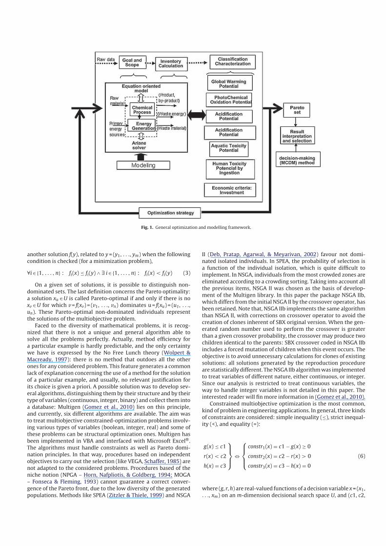
Fig. 1. General optimization and modelling framework.

another solution f(y), related to y = (y1, . . ., ym) when the following

condition is checked (for a minimization problem),

∀i ∈ {1, . . . , n} : fi(x) ≤ fi(y) ∧ ∃ i ∈ {1, . . . , n} : fi(x) < fi(y) (3)

On a given set of solutions, it is possible to distinguish non­

dominated sets. The last definition concerns the Pareto optimality:

a solution xu ∈ U is called Pareto­optimal if and only if there is no

xv ∈ U for which v = f(xv) = (v1, . . ., vn) dominates u = f(xu) = (u1, . . .,

un). These Pareto­optimal non­dominated individuals represent

the solutions of the multiobjective problem.

Faced to the diversity of mathematical problems, it is recog­

nized that there is not a unique and general algorithm able to

solve all the problems perfectly. Actually, method efficiency for

a particular example is hardly predictable, and the only certainty

we have is expressed by the No Free Lunch theory (Wolpert &

Macready, 1997): there is no method that outdoes all the other

ones for any considered problem. This feature generates a common

lack of explanation concerning the use of a method for the solution

of a particular example, and usually, no relevant justification for

its choice is given a priori. A possible solution was to develop sev­

eral algorithms, distinguishing them by their structure and by their

type of variables (continuous, integer, binary) and collect them into

a database: Multigen (Gomez et al., 2010) lies on this principle,

and currently, six different algorithms are available. The aim was

to treat multiobjective constrained­optimization problems involv­

ing various types of variables (boolean, integer, real) and some of

these problems can be structural optimization ones. Multigen has

been implemented in VBA and interfaced with Microsoft Excel®.

The algorithms must handle constraints as well as Pareto domi­

nation principles. In that way, procedures based on independent

objectives to carry out the selection (like VEGA, Schaffer, 1985) are

not adapted to the considered problems. Procedures based of the

niche notion (NPGA – Horn, Nafpliotis, & Goldberg, 1994; MOGA

– Fonseca & Fleming, 1993) cannot guarantee a correct conver­

gence of the Pareto front, due to the low diversity of the generated

populations. Methods like SPEA (Zitzler & Thiele, 1999) and NSGA

II (Deb, Pratap, Agarwal, & Meyarivan, 2002) favour not domi­

nated isolated individuals. In SPEA, the probability of selection is

a function of the individual isolation, which is quite difficult to

implement. In NSGA, individuals from the most crowded zones are

eliminated according to a crowding sorting. Taking into account all

the previous items, NSGA II was chosen as the basis of develop­

ment of the Multigen library. In this paper the package NSGA IIb,

which differs from the initial NSGA II by the crossover operator, has

been retained. Note that, NSGA IIb implements the same algorithm

than NSGA II, with corrections on crossover operator to avoid the

creation of clones inherent of SBX original version. When the gen­

erated random number used to perform the crossover is greater

than a given crossover probability, the crossover may produce two

children identical to the parents: SBX crossover coded in NSGA IIb

includes a forced mutation of children when this event occurs. The

objective is to avoid unnecessary calculations for clones of existing

solutions: all solutions generated by the reproduction procedure

are statistically different. The NSGA IIb algorithm was implemented

to treat variables of different nature, either continuous, or integer.

Since our analysis is restricted to treat continuous variables, the

way to handle integer variables is not detailed in this paper. The

interested reader will fin more information in (Gomez et al., 2010).

Constrained multiobjective optimization is the most common,

kind of problem in engineering applications. In general, three kinds

of constraints are considered: simple inequality (≤), strict inequal­

ity (<), and equality (=):

g(x) ≤ c1

r(x) < c2

h(x) = c3

⇔

constr1(x) = c1 − g(x) ≥ 0

constr2(x) = c2 − r(x) > 0

constr3(x) = c3 − h(x) = 0

(6)

where (g, r, h) are real­valued functions of a decision variable x = (x1,

. . ., xm) on an m­dimension decisional search space U, and (c1, c2,

c3) are constant values. In the more general case, these constraints

are written as vectors of the type:

coEnstr1(x) = ((c1 − g(x))1, . . . , (c1 − g(x))n1)

= (constr1(x)1, . . . , constr1(x)n1) ≥ 0

coEnstr2(x) = ((c2 − r(x))1, . . . , (c2 − r(x))n2)

= (constr2(x)1, . . . , constr2(x)n2) > 0

coEnstr3(x) = (−|(c3 − h(x))|1, . . . , −|(c3 − h(x))|n3)

= (constr3(x)1, . . . , constr3(x)n3) = 0

(7)

where n1, n2, and n3 are respectively, the number or inequal­

ity, strict inequality and equality constraints. This formulation

implies that each constri value will be negative if and only if this

constraint is violated. The conversion of Eq. (6), that is a clas­

sical representation of constraints set, to Eq. (7) representation

constitutes the first step of a unified formulation of constrained­

optimization problems. In practice, due to round­off error on

real numbers, the equality constraint constr3 was modified as

follows:

coEnstr3(x)′= (−|(c3 − h(x))|1 + ε1, . . . , −|(c3 − h(x))|n3 + εn3)

= (coEnstr3(x)) + Eε = 0

Eε = (ε1, . . . , εn3), ∀i ∈ {1, . . . , n3}, εi ∈ R

(8)

Eε is called a “precision vector” of the equality vector, and takes

low values (less than 10−6 for example). This approximation is not

necessary when equality constraint involves only integer or binary

variables.

From Eqs. (7) and (8), the constraint satisfaction implies the

maximization of violated constraints in vectors constr1, constr2,

and constr3. According to Fonseca and Fleming (1998), the satisfac­

tion of a number of violated inequality constraints is, from Eq. (7),

a multiobjective maximization problem. From a theoretical point

of view, a constrained multiobjective optimization problem can

be formulated as a two­step optimization problem. The first step

implies the comparison of constraint satisfaction degrees between

two solutions, using the Pareto’s domination definition of Eq. (3),

but a more simple solution consists in comparing the sum of val­

ues of violated constraints only, as in NSGA II algorithm of Deb

et al. (2002), which implies there are no priority rules between

constraints.

3.3. Multiple­criteria decision making (MCDM)

3.3.1. Introduction

MCDM approaches are major parts of decision theory and anal­

ysis. MCDM are analytic methods to evaluate the advantages and

disadvantages of alternatives based on multiple­criteria. The objec­

tive is to help decision­makers to learn about the problems they

face, and to identify a preferred course of action for a given prob­

lem. Huang, Poh, and Ang (1995) mentioned that decision analysis

(DA) was first applied to study problems in oil and gas exploration

in the 1960s and its application was subsequently extended from

industry to the public sector. Till now, MCDM methods have been

widely used in many research fields. Different approaches have

been proposed by many researchers, including single objective

decision­making (SODM) methods, MCDM methods, and decision

support systems (DSS). Literature shows that among MCDM

methods, DA strategies are the most commonly used (Zhou & Poh,

2006). The selection of a single Pareto point from the Pareto fron­

tier may be difficult as the number of objectives increases. Some

intuitive methods such as the so­called “knee­method” could be

efficient for a binary case. This is why other methods are necessary

to tackle the multicriteria nature of the results generated by

the GA.

3.3.2. Finding knees

Branke, Deb, Dierolf, and Osswald (2004), and Taboada and Coit

(2006) suggest picking the knees in the Pareto front, that is to say,

solutions where a small improvement in one objective function

would lead to a large deterioration in at least one other objective.

3.3.3. TOPSIS

In practice, the Technique for Ordering Preference by Similarity

to Ideal Solutions (TOPSIS method) and other multiple attribute

decision making (OMADM) methods are the most popular (Ren

et al., 2007; Yoon & Hwang, 1995). In this work, the TOPSIS

methodology was used as decision making tool. After the gener­

ation of the Pareto­optimal set, the TOPSIS method is used to aid

decision–maker in trade­offing the whole alternatives. The basic

principle of TOPSIS is that the chosen alternative should have the

shortest distance from the ideal solution and the farthest distance

from the negative­ideal solution (Opricovic & Tzeng, 2004; Ren

et al., 2007; Saaty, 1980).

Steps used in TOPSIS as described by Ren et al. (2007) are briefly

described in what follows:

Step 1: All the original criteria receive tendency treatment. That

consist in transforming the cost criteria into benefit criteria, which

is shown in detail as follows:

(i) The reciprocal ratio method (X ′ij

= 1/Xij) refers to the absolute

criteria;

(ii) The difference method (X ′ij

= 1 − Xij), refers to the relative cri­

teria.

After tendency treatment, construct a matrix

X ′[X ′ij]n×m

, i = 1, 2, . . . , n; j = 1, 2, . . . , m. (9)

Step 2: Calculate the normalized decision matrix A as follows:

A = [aij]n×m

aij =X

′ij

max(X′ij

)(j = 1, 2 . . . , m.) for a criterion to be maximized

(10a)

aij = 1 −X

′ij

max(X′ij

)(j = 1, 2 . . . , m.) for a criterion to be minimized

(10b)

Step 3: Determine the positive ideal and negative ideal solution

from the matrix A

A+ = (a+i1

, a+i2

, . . . , a+im

), a+ij

= max1≤i≤n

(aij), j = 1, 2, . . . , m (11)

A− = (a−i1

, a−i2

, . . . , a−im

), a−ij

= min1≤i≤n

(aij), j = 1, 2, . . . , m (12)

Step 4: Calculate the separation measures, using the n­

dimensional Euclidean distance. The separation of each alternative

from the positive ideal solution is given as

D+i

=

√

√

√

√

m∑

j=1

Wj(a+ij

− aij)2

(13)

Similarly, the separation from the negative ideal solution is

given as

D−i

=

√

√

√

√

m∑

j=1

Wj(a−ij

− aij)2

(14)

Step 5: For each alternative, calculate the ratio Ri as

Ri =D−

i

D−i

+ D+i

, i = 1, 2, . . . , n (15)

Step 6: Rank alternatives in increasing order according to the

ratio value of Ri in step 5

3.3.4. FUCA

FUCA is the French acronym for Faire Un Choix Adéquat (Make

An Adequate Choice). This simple method is based on individual

rankings of objectives; for a given criterion, rank one is assigned to

its best value and rank n (n being the number of points of the Pareto

front) to the worst one. Then, for each point of the front, a weighted

summation (the weights representing the preferences) of ranks is

performed, and the choice is carried out according to the lowest

values of the sum. In a recent paper (Moralez­Mendoza, Perez­

Escobedo, Aguilar­Lasserre, Azzaro­Pantel, & Pibouleau, 2011) the

FUCA method was compared with classical MCDM procedures on a

tricriteria problem related to the portfolio management in a phar­

maceutical industry. For each solution found by ELECTRE (Teixeiro

de Almeida, de Miranda, & Cabral Seixas Costa, 2004), PROMETHEE

(Zhaoxa & Min, 2010) and TOPSIS, the FUCA ranking is also reported.

A very good agreement between the three classical MCDM meth­

ods and FUCA can be observed, showing the efficiency of the FUCA

procedure, which always finds the best solution selected by one of

the others.

3.4. Utility production modelling

ARIANETM software tool has been developed by ProSim

Company (French chemical engineering Software Company) for

designing assistance and optimal operation of power plants.

ARIANETM makes it possible to optimize and model any energy

combined production plant (steam, hot water, electricity, com­

pressed air, cooling), whatever its size and complexity. ARIANETM

is a decision support tool dedicated to the management of plants

that produce energy under the form of utilities (steam, electric­

ity, hot water, etc.). ARIANETM, written in VBA, presents a standard

library of unit operations involved in power plants: boilers (mono­

fuel, bi­fuel, electrical), turboalternators (backpressure turbines,

sidestream turbines, condensating turbines), switchable or per­

mutable turbines (in parallel with electric motors), fuel turbines

and thermal engines (with or without recovery heat exchanger,

with or without post combustion boiler), valves, heat exchangers

and deaerators. All these unit operations can be described, from

the simplest (minimalist modelling, with default values) to the

most complex (very fine modelling of the characteristics and tech­

nical constraints); the complexity of physical models requiring in

many cases to use nonlinear equations. The inherent model com­

plexity and its associated equations are totally transparent for the

user. In the framework of eco­design modelling, the problem lies

in integrating environmental aspects inside ARIANE software, so

that emissions can be taken into account in the global energy bal­

ance. Estimation methods, to evaluate the emissions of all involved

power plants equipment items have then to be compatible with

existing routines that not require numerous and complex input

data. In ARIANE, classical pollutants as nitrogen oxides, carbon and

sulphur oxides, and also solid particles like dusts, are well known.

The emissions modelling process starts from the calculation of

pollutant amounts in the smokes of each equipment item, global

emission flow rate is finally the sum of all flow rates, for all site

smoke emitters. Another problem lies then in the accurate mod­

elling of the combustion phenomena in all equipment items of a

power plant. We give below some of the equations of units oper­

ations implemented in ARIANETM and used at the eco­efficient

modelling stage.

4. Application to HDA (hydrodealkylation of toluene)

process

4.1. Overview of the HDA process

The traditional method of manufacturing benzene from the

distillation of light oils produced during the manufacturing of coke

has been overtaken by a number of processes: The sources are

now: catalytic reforming, hydrodealkylation of toluene (HDA) and

toluene disproportionation. The global world benzene production

capacity will rise from estimated 41.8 Mt/y in 2009 to 55.8 Mt/y

in 2015: http://marketpublishers.com/lists/5873/news.html,

http://mcgroup.co.uk/researches/B/028500/Benzene.html. In

2005, the French production capacity was estimated at one

Mt/year on seven industrial sites, i.e. mean of 143,000 t/year per

site (www.ineris.fr/rsde/fiches/fiche benzene 2005.pdf).

The Hydrodealkylation (Douglas, 1988) process for producing

benzene, a classical benchmark in chemical process synthesis stud­

ies, is used in this paper (HDA process). This process involves two

reactions: the conversion of toluene to benzene (Eq. (16)) and the

equilibrium between benzene and diphenyl (Eq. (17)).

Toluene + H2 → Benzene + CH4 (16)

2Benzene ↔ Diphenyl + H2 (17)

Douglas (1988) has first extensively studied this process by

using a hierarchical design/synthesis approach. The hydrogen feed

stream has a purity of 95% and involves 5% of methane; this stream

is mixed with a fresh inlet stream of toluene, recycled toluene, and

recycled hydrogen. The feed mixture is heated in a furnace before

being fed to an adiabatic reactor. The reactor effluent contains

unreacted hydrogen and toluene, benzene (the desired product),

biphenyl, and methane; it is quenched and subsequently cooled

in a high­pressure flash separator to condense the aromatics from

the non­condensable hydrogen and methane. The vapour steam

from the high­pressure flash unit contains hydrogen and methane

that is recycled. The liquid stream contains traces of hydrogen and

methane that are separated from the aromatics in a low­pressure

flash drum. The liquid stream from the low­pressure flash drum

consisting of benzene, biphenyl and toluene is separated in two

distillation columns. The first column separates the product, ben­

zene, from biphenyl and toluene, while the second one separates

the biphenyl from toluene, which is recycled back at the reac­

tor entrance. Energy is saved by using the outlet stream leaving

the reactor as its temperature is in the range of 620 ◦C, to pre­

heat the feed stream coming from the mixer, via a heat exchanger

(Fehe) some energy integration is achieved (Cao, Rossiter, Edwards,

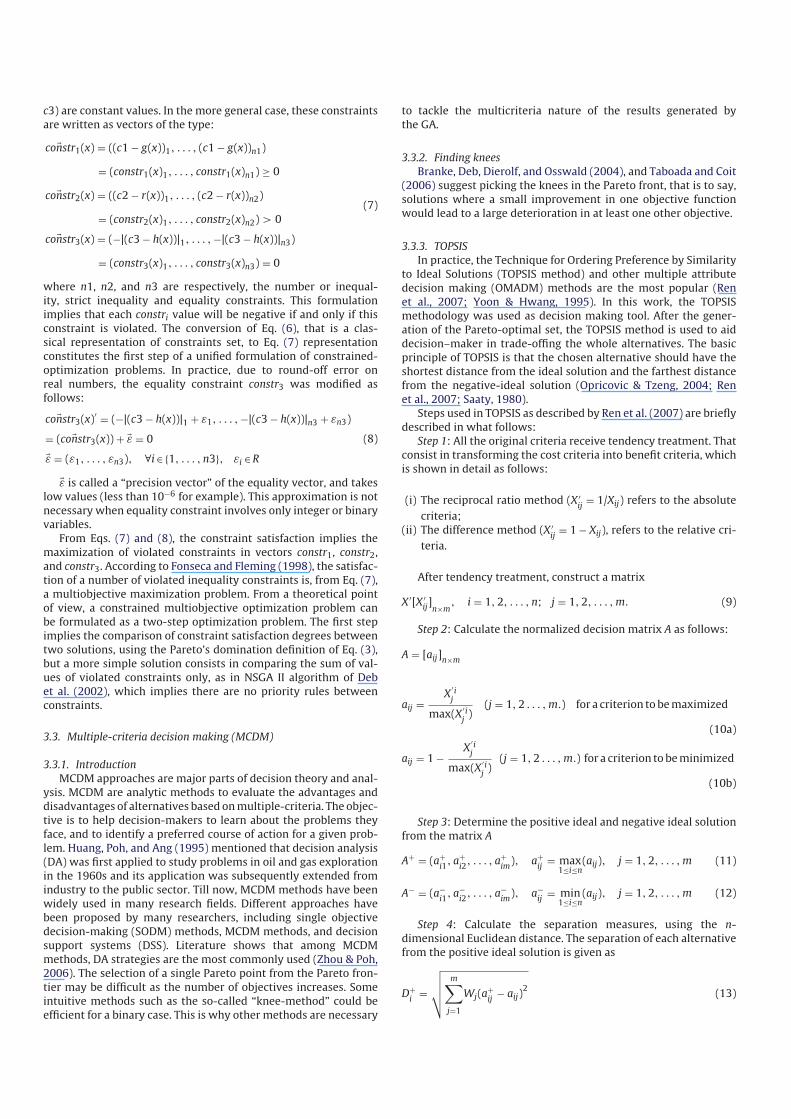
Knechtel, & Owens, 1998) (see Fig. 2).

As abovementioned, ARIANETM is used here both to compute

the primary energy requirements of the process and to quantify

the pollutant emissions related to energy production. A typical

steam generating facility is considered: steam is produced from

a conventional mono­fuel fired boiler (40 bar and 400 ◦C) and let

down to lower pressure levels (respectively, 10 bar, 336 ◦C and

5 bar, 268 ◦C) through turbines which produce electricity used in

the plant. ARIANETM is also used to model the fired heater (fur­

nace) of the process as a bi­fuel fired heater (mix of natural gas and

fuel).

Fig. 2. HDA plant with is utility production unit.

To model the HDA process, commercial design and flowsheeting

packages could be used in order to compute the objective functions.

However, rather than using such packages, the equations proposed

by Douglas (1988) have been directly implemented and solved by

the Excel® solver. Biphenyl has been considered as a pollutant, and

the environmental impact contributions for the components in the

HDA process have been taken from Sikdar and El­Halwagi (2001).

4.2. Interaction between HDA process and utility production

system

From the studies of Douglas (1988) and Turton, Bailie, Whiting,

& Shaeiwitz (1997, 2009), seven variables were selected for HDA

process because of their influence on the economic and environ­

mental optimization criteria. These variables are initially used to

compute the overall material balance of the main chemical com­

pounds and as well as the associated thermodynamic properties

(enthalpy, density, heat capacity, etc.) at various process nodes,

with use of Simulis® Thermodynamics as a calculation server of

thermodynamic properties. They serve finally to compute the size

of all equipment items involved in the process for carrying out the

required unit operations. Fig. 3 shows the interaction between the

variables of the HDA process and the utility production system.

HDA process operation needs thermal and electrical utilities. The

thermal demand is formulated in terms of fuel flow rate to meet

the need of heating the mixture in the furnace as well as of steam

to meet the heating demands for the exchangers, reboiler and other

items of the process. Eqs. (18)–(20) describe the demand of steam in

the case of a reboiler. These requirements obtained from the energy

balances of the HDA simulator are transmitted via PlessalaTM as

variables to the unit operations involved, which are modelled by

use of ArianeTM (boiler, furnace). Then, fuel oil flow rate of, the nat­

ural gas flow rate and steam flow rate become secondary variables

for ArianeTM. The use of ArianeTM provides typical results related to

the thermal power plant i.e. the power produced by the turbine and

the flow rates of all the pollutants resulting from fuel combustion.

mstmi =Qbi

1Hstmi(18)

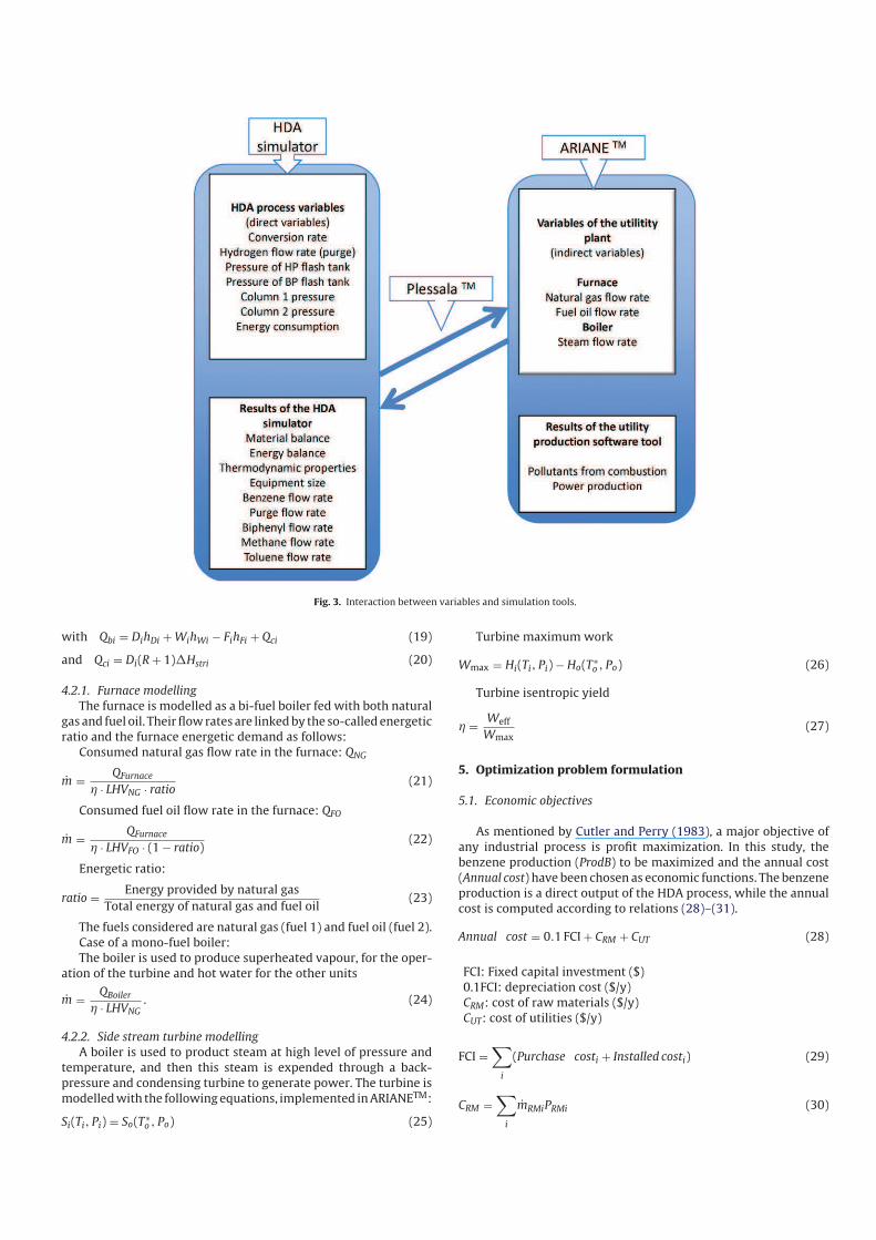
Fig. 3. Interaction between variables and simulation tools.

with Qbi = DihDi + WihWi − FihFi + Qci (19)

and Qci = Di(R + 1)1Hstri (20)

4.2.1. Furnace modelling

The furnace is modelled as a bi­fuel boiler fed with both natural

gas and fuel oil. Their flow rates are linked by the so­called energetic

ratio and the furnace energetic demand as follows:

Consumed natural gas flow rate in the furnace: QNG

m =QFurnace

� · LHVNG · ratio(21)

Consumed fuel oil flow rate in the furnace: QFO

m =QFurnace

� · LHVFO · (1 − ratio)(22)

Energetic ratio:

ratio =Energy provided by natural gas

Total energy of natural gas and fuel oil(23)

The fuels considered are natural gas (fuel 1) and fuel oil (fuel 2).

Case of a mono­fuel boiler:

The boiler is used to produce superheated vapour, for the oper­

ation of the turbine and hot water for the other units

m =QBoiler

� · LHVNG. (24)

4.2.2. Side stream turbine modelling

A boiler is used to product steam at high level of pressure and

temperature, and then this steam is expended through a back­

pressure and condensing turbine to generate power. The turbine is

modelled with the following equations, implemented in ARIANETM:

Si(Ti, Pi) = So(T∗o , Po) (25)

Turbine maximum work

Wmax = Hi(Ti, Pi) − Ho(T∗o , Po) (26)

Turbine isentropic yield

� =Weff

Wmax(27)

5. Optimization problem formulation

5.1. Economic objectives

As mentioned by Cutler and Perry (1983), a major objective of

any industrial process is profit maximization. In this study, the

benzene production (ProdB) to be maximized and the annual cost

(Annual cost) have been chosen as economic functions. The benzene

production is a direct output of the HDA process, while the annual

cost is computed according to relations (28)–(31).

Annual cost = 0.1 FCI + CRM + CUT (28)

FCI: Fixed capital investment ($)

0.1FCI: depreciation cost ($/y)

CRM: cost of raw materials ($/y)

CUT: cost of utilities ($/y)

FCI =∑

i

(Purchase costi + Installed costi) (29)

CRM =∑

i

mRMiPRMi (30)

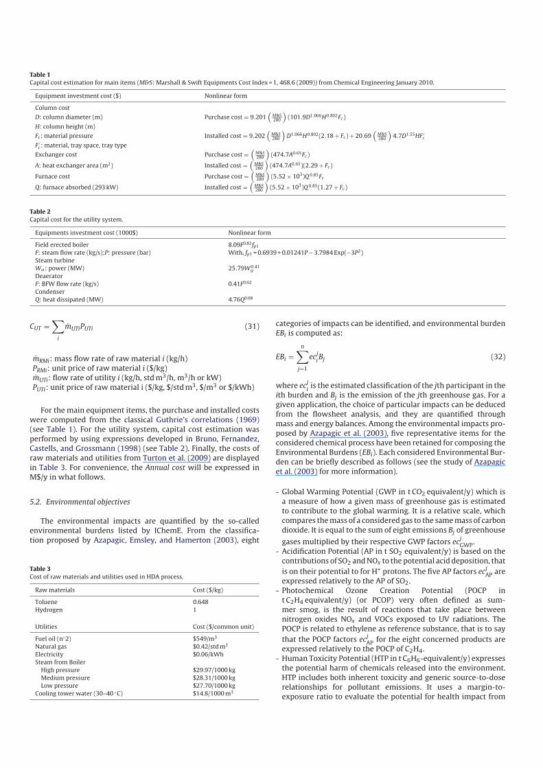
Table 1

Capital cost estimation for main items (M&S: Marshall & Swift Equipments Cost Index = 1, 468.6 (2009)) from Chemical Engineering January 2010.

Equipment investment cost ($) Nonlinear form

Column cost

D: column diameter (m) Purchase cost = 9.201(

M&S280

)

(101.9D1.066H0.802Fc)

H: column height (m)

Fc: material pressure Installed cost = 9.202(

M&S280

)

D1.066H0.802(2.18 + Fc) + 20.69(

M&S280

)

4.7D1.55HF ′c

F ′c: material, tray space, tray type

Exchanger cost Purchase cost =(

M&S280

)

(474.7A0.65Fc)

A: heat exchanger area (m2) Installed cost =(

M&S280

)

(474.7A0.65)(2.29 + Fc)

Furnace cost Purchase cost =(

M&S280

)

(5.52 × 103)Q 0.85Fc

Q: furnace absorbed (293 kW) Installed cost =(

M&S280

)

(5.52 × 103)Q 0.85(1.27 + Fc)

Table 2

Capital cost for the utility system.

Equipments investment cost (1000$) Nonlinear form

Field erected boiler 8.09F0.82fp1

F: steam flow rate (kg/s);P: pressure (bar) With, fp1 = 0.6939 + 0.01241P − 3.7984 Exp(−3P2)

Steam turbine

Wst: power (MW) 25.79W0.41st

Deaerator

F: BFW flow rate (kg/s) 0.41F0.62

Condenser

Q: heat dissipated (MW) 4.76Q0.68

CUT =∑

i

mUTiPUTi (31)

mRMi: mass flow rate of raw material i (kg/h)

PRMi: unit price of raw material i ($/kg)

mUTi: flow rate of utility i (kg/h, std m3/h, m3/h or kW)

PUTi: unit price of raw material i ($/kg, $/std m3, $/m3 or $/kWh)

For the main equipment items, the purchase and installed costs

were computed from the classical Guthrie’s correlations (1969)

(see Table 1). For the utility system, capital cost estimation was

performed by using expressions developed in Bruno, Fernandez,

Castells, and Grossmann (1998) (see Table 2). Finally, the costs of

raw materials and utilities from Turton et al. (2009) are displayed

in Table 3. For convenience, the Annual cost will be expressed in

M$/y in what follows.

5.2. Environmental objectives

The environmental impacts are quantified by the so­called

environmental burdens listed by IChemE. From the classifica­

tion proposed by Azapagic, Emsley, and Hamerton (2003), eight

Table 3

Cost of raw materials and utilities used in HDA process.

Raw materials Cost ($/kg)

Toluene 0.648

Hydrogen 1

Utilities Cost ($/common unit)

Fuel oil (n◦2) $549/m3

Natural gas $0.42/std m3

Electricity $0.06/kWh

Steam from Boiler

High pressure $29.97/1000 kg

Medium pressure $28.31/1000 kg

Low pressure $27.70/1000 kg

Cooling tower water (30–40 ◦C) $14.8/1000 m3

categories of impacts can be identified, and environmental burden

EBi is computed as:

EBi =

n∑

j=1

ecjiBj (32)

where ecjiis the estimated classification of the jth participant in the

ith burden and Bj is the emission of the jth greenhouse gas. For a

given application, the choice of particular impacts can be deduced

from the flowsheet analysis, and they are quantified through

mass and energy balances. Among the environmental impacts pro­

posed by Azapagic et al. (2003), five representative items for the

considered chemical process have been retained for composing the

Environmental Burdens (EBi). Each considered Environmental Bur­

den can be briefly described as follows (see the study of Azapagic

et al. (2003) for more information).

­ Global Warming Potential (GWP in t CO2 equivalent/y) which is

a measure of how a given mass of greenhouse gas is estimated

to contribute to the global warming. It is a relative scale, which

compares the mass of a considered gas to the same mass of carbon

dioxide. It is equal to the sum of eight emissions Bj of greenhouse

gases multiplied by their respective GWP factors ecjGWP

.

­ Acidification Potential (AP in t SO2 equivalent/y) is based on the

contributions of SO2 and NOx to the potential acid deposition, that

is on their potential to for H+ protons. The five AP factors ecjAP

are

expressed relatively to the AP of SO2.

­ Photochemical Ozone Creation Potential (POCP in

t C2H4 equivalent/y) (or PCOP) very often defined as sum­

mer smog, is the result of reactions that take place between

nitrogen oxides NOx and VOCs exposed to UV radiations. The

POCP is related to ethylene as reference substance, that is to say

that the POCP factors ecjAP

for the eight concerned products are

expressed relatively to the POCP of C2H4.

­ Human Toxicity Potential (HTP in t C6H6­equivalent/y) expresses

the potential harm of chemicals released into the environment.

HTP includes both inherent toxicity and generic source­to­dose

relationships for pollutant emissions. It uses a margin­to­

exposure ratio to evaluate the potential for health impact from

exposure to harmful agents, both carcinogens and non carcino­

gens. It is calculated by adding human toxic releases to three

different media, i.e. air, water and soil. The toxicological factors

are calculated using the acceptable daily intake or the tolerable

daily intake of the toxic substances. The human toxicological fac­

tors (26 from Azapagic et al., 2003) are still at development stage,

so that HTP can only be taken as an indication and not as an

absolute measure of the toxicity potential.

­ Eutrophication Potential (EP in t PO43− equivalent/y) is defined as

the potential of nutrients to cause over­fertilisation of water and

soil which in turn can result in increased growth of biomass.

It must be emphasized at this level that the approach presented

here does not account for the entire life cycle of the process since

the environmental burdens are associated with the emissions gen­

erated by the process both from the material components and from

the energy vectors. For instance, the outcome of benzene is not

considered here as it is viewed as the desired product for the pro­

cess. We are thus aware that the approach developed here does not

embed the whole life cycle of the product. Moreover, the extrac­

tion resource associated with raw materials such as toluene is not

included. Briefly, only the process contribution is considered in this

study.

Of course, a life cycle assessment methodology could be attrac­

tive to be more general and the abovementioned drawbacks

could be partially overcome by using standard environmental

databases available in the literature (e.g. EcoInvent for instance

http://www.ecoinvent.ch/) implemented in life cycle assessment

software tools. This issue will constitute a perspective of this work.

5.3. Multiobjective problem formulation

Using the previous economic and environmental objective

functions defined above, the following multiobjective nonlinear

optimization problem is formulated as follows: determine decision

variables (process operating conditions) in order to:

Max (ProdB) (33)

Min (Annual cost) (34)

Min (EBi), i = 1, 5 (35)

s.t.

Mass and energy balances (Excel® and ARIANETM)

Bounds on decision variables

ProdB represents the benzene production at the top of column

2 (in kmol/h).

The additional following constraints have been considered in the

Multigen interface, the numerical values value have been deduced

from the analysis of Douglas (1988) and Turton et al. (1997).

­ The purity of the benzene product is at least 99.97%

­ The hydrogen feed must have a purity of 95%

­ The reactor outlet temperature is less than 704.50 ◦C

­ The quencher outlet temperature is less than 621.16 ◦C

­ The conversion rate C is bounded as: 0.5 ≤ C ≤ 0.9

­ The hydrogen flow rate purged FPH (kmol/h) is bounded as:

30 ≤ FPH ≤ 300

­ All pollutants, CO2, NOx, CO, SO2, dusts flow rate (kg/h) must take

only positive values.

5.4. GA parameters

The two classes of optimization problems presented below have

been solved by using the code NSGA IIb of the Multigen toolbox,

with the following operating parameters: population size = 200,

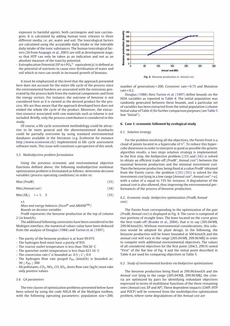
Fig. 4. Benzene production vs. Annual cost.

number of generations = 200, Crossover rate = 0.75 and Mutation

rate = 0.2.

Douglas (1988) then Turton et al. (1997) define bounds on the

HDA variables as reported in Table 4. The initial population was

randomly generated between these bounds, and a particular set

of variables has been extracted from the initial population (column

Initial value of Table 4) for further comparison purposes (see Table 5

line “Initial”).

6. Case 1: economic followed by ecological study

6.1. Solution strategy

For the problem involving all the objectives, the Pareto front is a

cloud of points located in a hypercube of ℜ7. To reduce this hyper­

cube dimension in order to interpret as good as possible the genetic

algorithm results, a two steps solution strategy is implemented.

In the first step, the biobjective problem ((33) and (34)) is solved

to obtain an efficient trade­off (ProdB*, Annual cost*) between the

maximal benzene production and the minimal investment cost.

Then the benzene production, being fixed at a value ProdB* obtained

from the Pareto curve, the problem ((33)–(35)) is solved for the

investment cost lying in a low range [Annual cost*, Annual cost* + ˛],

with a value of equal to 15% for instance. A degradation of the

annual cost is also allowed, thus improving the environmental per­

formances of the process of benzene production.

6.2. Economic study: biobjective optimization (ProdB, Annual

cost)

The Pareto front corresponding to the optimization of the pair

(ProdB, Annual cost) is displayed in Fig. 4. The curve is composed of

two portions of straight lines. The knee located on the curve gives

the best trade­off (Branke et al., 2004), that is to say (205.04 M$,

299.96 kmol/h). Without environmental considerations, this solu­

tion would be adopted for plant design. In the following, the

benzene production will be lower bounded at 300 kmol/h and the

annual cost will vary in the range [205.04 M$, 299.96 M$] in order

to compete with additional environmental objectives. The values

of all considered objectives for the first point (204.5, 299.9) noted

“First” of the flat line of Fig. 4 and the initial point described in

Table 4 are used for comparing objectives in Table 5.

6.3. Study of environmental burdens via biobjective optimizations

The benzene production being fixed at 299.96 kmol/h and the

Annual cost lying in the range [205.04 M$, 299.96 M$], the crite­

ria are optimized by pairs for identifying redundant objectives

expressed in terms of multilinear functions of the three remaining

ones (Annual cost, EP and AP). These dependent impacts (GWP, HTP

and POCP) will be removed from the multiobjective optimization

problem, where some degradations of the Annual cost are

Table 4

Decision variables for the HDA process.

Decision variables Lower bound Initial value Upper bound

Conversion rate (%) 0.5 0.75 0.9

Hydrogen purge flow rate (kmol/h) 31 198 308

Flash pressure (bar) 30 34 34

Stabilizer pressure (bar) 4 10 10

Column 1 pressure (bar) 2 2 4

Column 2 pressure (bar) 1 1 2

Ratio (bi­fuel furnace) (%) 0.1 0.85 0.9

Table 5

Values of objectives.

Objective ProdB t/y Annual cost M$/y EP t PO43−/y AP t C2H4/y GWP t CO2/y HTP t C6H6/y POCP t C2H4/y

Initial 305.00 277.42 9759.06 11,190.34 1,884,528.48 18,699.58 2472.32

First 299.96 205.04 13,831.12 4829.26 1,410,428.13 26,537.88 1944.11

Gain vs. initial (%) −1.62 26.00 −29.44 56.85 25.16 −41.91 21.36

1410500

1411000

1411500

1412000

1412500

1413000

1413500

205,34205,32205,3205,28205,26205,24205,22205,2205,18205,16

Annual cost (M$/y)

GW

P (

t C

O2 /

y)

Fig. 5. GWP vs. Annual cost.

0

5000

10000

15000

20000

25000

30000

235230225220215210205200

Annual cost (M$/y)

HT

P (

t C

6H

6 /

y)

Fig. 6. HTP vs. Annual cost.

for globally improving all the environmental impacts (including the

redundant ones).

(GWP, Annual cost): Non dominated points appear only in low

ranges for the two objectives (see Fig. 5), suggesting a strong rela­

tion between them (see section 5.4). (HTP, Annual cost): The Pareto

front is displayed in Fig. 6, where the two objectives have opposite

effects. (EP, Annual cost): The results are shown in Fig. 7. The curves

displayed in Figs. 6 and 7 exhibit very similar trends, due to a strong

link between them (see Section 5.4). (AP, Annual cost): The Pareto

0

2000

4000

6000

8000

10000

12000

14000

235230225220215210205200

Annual cost (M$/y)

EP

(t

PO

4

3- /y

)

BT2

BT1

Fig. 7. EP vs. Annual cost.

4300

4400

4500

4600

4700

4800

4900

235230225220215210205200

Annual cost (M$/y)

AP

(t

SO

4/y

)

BT1

BT2

Fig. 8. AP vs. Annual cost.

1910

1915

1920

1925

1930

1935

1940

1945

1950

222220218216214212210208206204

Annual cost (M$/y)

PC

OP

(t

C2H

4 /y)

Fig. 9. POCP vs. Annual cost.

front is displayed in Fig. 8. (POCP, Annual cost): the results reported

in Fig. 9 show that non dominated points appear only in a low range

for the POCP objective, suggesting a strong relation between these

two functions. (AP, EP): concerning the pair (AP, EP), the biobjec­

tive optimization gives the front displayed in Fig. 10, where it can

be pointed out that the two impacts exhibit antagonist behaviours.

0

1000

2000

3000

4000

5000

6000

7000

8000

9000

1600014000120001000080006000400020000

EP (t PO43-/y)

AP

(t

SO

2/y

)

BT1

BT2

Fig. 10. AP vs. EP.

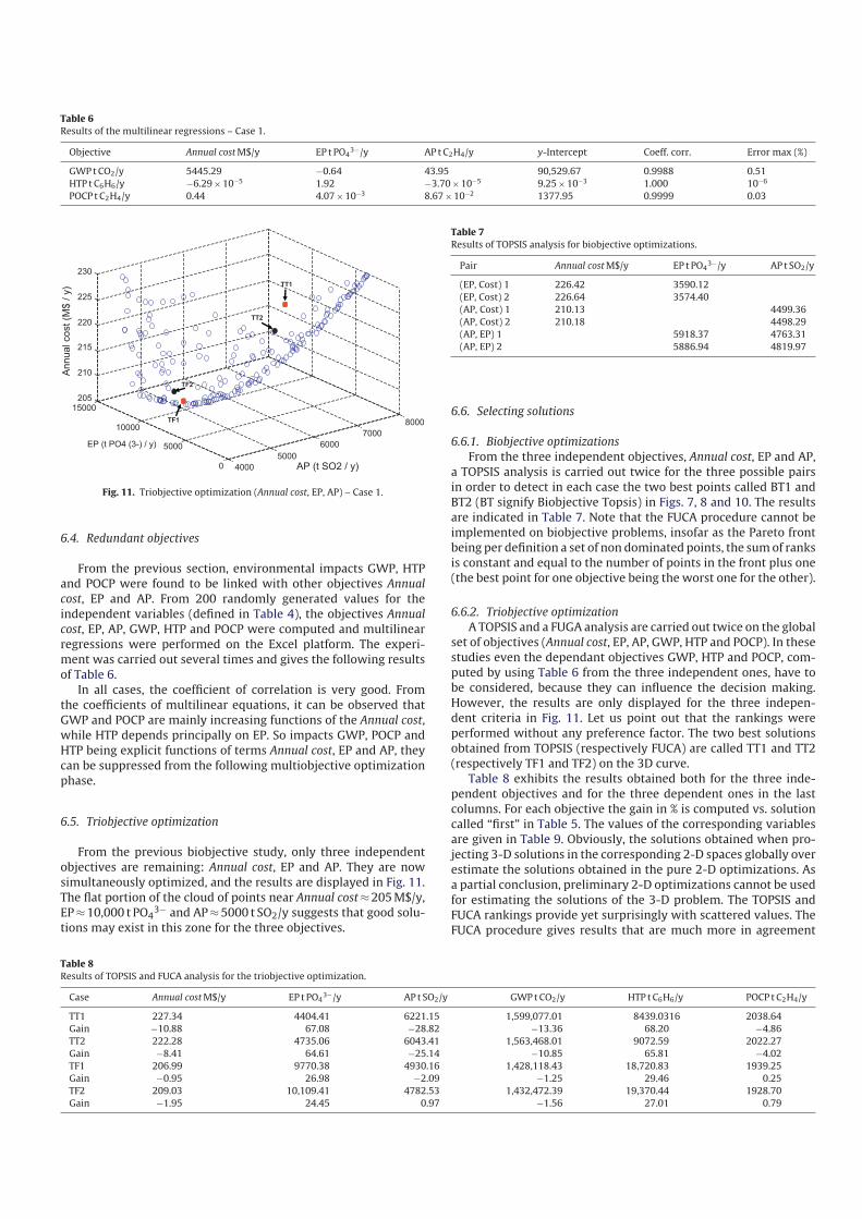
Table 6

Results of the multilinear regressions – Case 1.

Objective Annual cost M$/y EP t PO43−/y AP t C2H4/y y­Intercept Coeff. corr. Error max (%)

GWP t CO2/y 5445.29 −0.64 43.95 90,529.67 0.9988 0.51

HTP t C6H6/y −6.29 × 10−5 1.92 −3.70 × 10−5 9.25 × 10−3 1.000 10−6

POCP t C2H4/y 0.44 4.07 × 10−3 8.67 × 10−2 1377.95 0.9999 0.03

4000

5000

6000

7000

8000

0

5000

10000

15000205

210

215

220

225

230

AP (t SO2 / y)

EP (t PO4 (3-) / y)

An

nu

al co

st

(M$

/ y

) TT1

TT2

TF1

TF2

Fig. 11. Triobjective optimization (Annual cost, EP, AP) – Case 1.

6.4. Redundant objectives

From the previous section, environmental impacts GWP, HTP

and POCP were found to be linked with other objectives Annual

cost, EP and AP. From 200 randomly generated values for the

independent variables (defined in Table 4), the objectives Annual

cost, EP, AP, GWP, HTP and POCP were computed and multilinear

regressions were performed on the Excel platform. The experi­

ment was carried out several times and gives the following results

of Table 6.

In all cases, the coefficient of correlation is very good. From

the coefficients of multilinear equations, it can be observed that

GWP and POCP are mainly increasing functions of the Annual cost,

while HTP depends principally on EP. So impacts GWP, POCP and

HTP being explicit functions of terms Annual cost, EP and AP, they

can be suppressed from the following multiobjective optimization

phase.

6.5. Triobjective optimization

From the previous biobjective study, only three independent

objectives are remaining: Annual cost, EP and AP. They are now

simultaneously optimized, and the results are displayed in Fig. 11.

The flat portion of the cloud of points near Annual cost ≈ 205 M$/y,

EP ≈ 10,000 t PO43− and AP ≈ 5000 t SO2/y suggests that good solu­

tions may exist in this zone for the three objectives.

Table 7

Results of TOPSIS analysis for biobjective optimizations.

Pair Annual cost M$/y EP t PO43−/y AP t SO2/y

(EP, Cost) 1 226.42 3590.12

(EP, Cost) 2 226.64 3574.40

(AP, Cost) 1 210.13 4499.36

(AP, Cost) 2 210.18 4498.29

(AP, EP) 1 5918.37 4763.31

(AP, EP) 2 5886.94 4819.97

6.6. Selecting solutions

6.6.1. Biobjective optimizations

From the three independent objectives, Annual cost, EP and AP,

a TOPSIS analysis is carried out twice for the three possible pairs

in order to detect in each case the two best points called BT1 and

BT2 (BT signify Biobjective Topsis) in Figs. 7, 8 and 10. The results

are indicated in Table 7. Note that the FUCA procedure cannot be

implemented on biobjective problems, insofar as the Pareto front

being per definition a set of non dominated points, the sum of ranks

is constant and equal to the number of points in the front plus one

(the best point for one objective being the worst one for the other).

6.6.2. Triobjective optimization

A TOPSIS and a FUGA analysis are carried out twice on the global

set of objectives (Annual cost, EP, AP, GWP, HTP and POCP). In these

studies even the dependant objectives GWP, HTP and POCP, com­

puted by using Table 6 from the three independent ones, have to

be considered, because they can influence the decision making.

However, the results are only displayed for the three indepen­

dent criteria in Fig. 11. Let us point out that the rankings were

performed without any preference factor. The two best solutions

obtained from TOPSIS (respectively FUCA) are called TT1 and TT2

(respectively TF1 and TF2) on the 3D curve.

Table 8 exhibits the results obtained both for the three inde­

pendent objectives and for the three dependent ones in the last

columns. For each objective the gain in % is computed vs. solution

called “first” in Table 5. The values of the corresponding variables

are given in Table 9. Obviously, the solutions obtained when pro­

jecting 3­D solutions in the corresponding 2­D spaces globally over

estimate the solutions obtained in the pure 2­D optimizations. As

a partial conclusion, preliminary 2­D optimizations cannot be used

for estimating the solutions of the 3­D problem. The TOPSIS and

FUCA rankings provide yet surprisingly with scattered values. The

FUCA procedure gives results that are much more in agreement

Table 8

Results of TOPSIS and FUCA analysis for the triobjective optimization.

Case Annual cost M$/y EP t PO43−/y AP t SO2/y GWP t CO2/y HTP t C6H6/y POCP t C2H4/y

TT1 227.34 4404.41 6221.15 1,599,077.01 8439.0316 2038.64

Gain −10.88 67.08 −28.82 −13.36 68.20 −4.86

TT2 222.28 4735.06 6043.41 1,563,468.01 9072.59 2022.27

Gain −8.41 64.61 −25.14 −10.85 65.81 −4.02

TF1 206.99 9770.38 4930.16 1,428,118.43 18,720.83 1939.25

Gain −0.95 26.98 −2.09 −1.25 29.46 0.25

TF2 209.03 10,109.41 4782.53 1,432,472.39 19,370.44 1928.70

Gain −1.95 24.45 0.97 −1.56 27.01 0.79

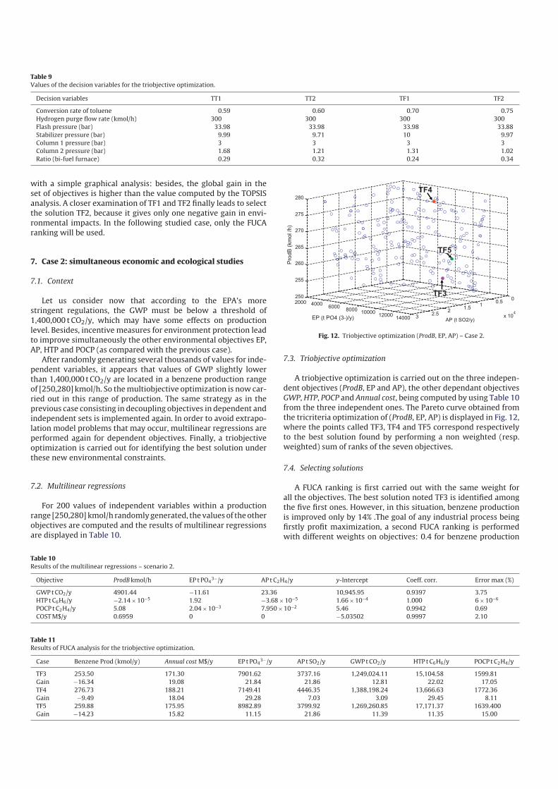
Table 9

Values of the decision variables for the triobjective optimization.

Decision variables TT1 TT2 TF1 TF2

Conversion rate of toluene 0.59 0.60 0.70 0.75

Hydrogen purge flow rate (kmol/h) 300 300 300 300

Flash pressure (bar) 33.98 33.98 33.98 33.88

Stabilizer pressure (bar) 9.99 9.71 10 9.97

Column 1 pressure (bar) 3 3 3 3

Column 2 pressure (bar) 1.68 1.21 1.31 1.02

Ratio (bi­fuel furnace) 0.29 0.32 0.24 0.34

with a simple graphical analysis: besides, the global gain in the

set of objectives is higher than the value computed by the TOPSIS

analysis. A closer examination of TF1 and TF2 finally leads to select

the solution TF2, because it gives only one negative gain in envi­

ronmental impacts. In the following studied case, only the FUCA

ranking will be used.

7. Case 2: simultaneous economic and ecological studies

7.1. Context

Let us consider now that according to the EPA’s more

stringent regulations, the GWP must be below a threshold of

1,400,000 t CO2/y, which may have some effects on production

level. Besides, incentive measures for environment protection lead

to improve simultaneously the other environmental objectives EP,

AP, HTP and POCP (as compared with the previous case).

After randomly generating several thousands of values for inde­

pendent variables, it appears that values of GWP slightly lower

than 1,400,000 t CO2/y are located in a benzene production range

of [250,280] kmol/h. So the multiobjective optimization is now car­

ried out in this range of production. The same strategy as in the

previous case consisting in decoupling objectives in dependent and

independent sets is implemented again. In order to avoid extrapo­

lation model problems that may occur, multilinear regressions are

performed again for dependent objectives. Finally, a triobjective

optimization is carried out for identifying the best solution under

these new environmental constraints.

7.2. Multilinear regressions

For 200 values of independent variables within a production

range [250,280] kmol/h randomly generated, the values of the other

objectives are computed and the results of multilinear regressions

are displayed in Table 10.

00.5

11.5

22.5 x 103

4

2000 40006000

800010000

1200014000

250

255

260

265

270

275

280

AP (t SO2/y)EP (t PO4 (3-)/y)

Pro

dB

(km

ol /h

)TF3

TF4

TF5

Fig. 12. Triobjective optimization (ProdB, EP, AP) – Case 2.

7.3. Triobjective optimization

A triobjective optimization is carried out on the three indepen­

dent objectives (ProdB, EP and AP), the other dependant objectives

GWP, HTP, POCP and Annual cost, being computed by using Table 10

from the three independent ones. The Pareto curve obtained from

the tricriteria optimization of (ProdB, EP, AP) is displayed in Fig. 12,

where the points called TF3, TF4 and TF5 correspond respectively

to the best solution found by performing a non weighted (resp.

weighted) sum of ranks of the seven objectives.

7.4. Selecting solutions

A FUCA ranking is first carried out with the same weight for

all the objectives. The best solution noted TF3 is identified among

the five first ones. However, in this situation, benzene production

is improved only by 14% .The goal of any industrial process being

firstly profit maximization, a second FUCA ranking is performed

with different weights on objectives: 0.4 for benzene production

Table 10

Results of the multilinear regressions – scenario 2.

Objective ProdB kmol/h EP t PO43−/y AP t C2H4/y y­Intercept Coeff. corr. Error max (%)

GWP t CO2/y 4901.44 −11.61 23.36 10,945.95 0.9397 3.75

HTP t C6H6/y −2.14 × 10−5 1.92 −3.68 × 10−5 1.66 × 10−4 1.000 6 × 10−6

POCP t C2H4/y 5.08 2.04 × 10−3 7.950 × 10−2 5.46 0.9942 0.69

COST M$/y 0.6959 0 0 −5.03502 0.9997 2.10

Table 11

Results of FUCA analysis for the triobjective optimization.

Case Benzene Prod (kmol/y) Annual cost M$/y EP t PO43−/y AP t SO2/y GWP t CO2/y HTP t C6H6/y POCP t C2H4/y

TF3 253.50 171.30 7901.62 3737.16 1,249,024.11 15,104.58 1599.81

Gain −16.34 19.08 21.84 21.86 12.81 22.02 17.05

TF4 276.73 188.21 7149.41 4446.35 1,388,198.24 13,666.63 1772.36

Gain −9.49 18.04 29.28 7.03 3.09 29.45 8.11

TF5 259.88 175.95 8982.89 3799.92 1,269,260.85 17,171.37 1639.400

Gain −14.23 15.82 11.15 21.86 11.39 11.35 15.00

Table 12

Values of the decision variables for the triobjective optimization – Case 2.

Decision variables TF3 TF4 TF5

Conversion rate of toluene 0.74 0.71 0.76

Hydrogen purge flow rate (kmol/h) 299.30 299.92 299.92

Flash pressure (bar) 29.27 28.73 32.57

Stabilizer pressure (bar) 8.60 6.02 7.00

Column 1 pressure (bar) 2.13 2.03 2.21

Column 2 pressure (bar) 1.02 1.33 1.74

Ratio (bi­fuel furnace) 0.16 0.24 0.17

and 0.1 for the six criteria. As in the previous case, the best solution

noted TF4 is identified among the five first ones. Finally, a compro­

mise solution TF5 generated with the respective weights of 0.35 for

the benzene production, 0.15 for the GWP and 0.1 for all the others

is also determined.

Table 11 exhibits the results obtained both for the three inde­

pendent objectives and for the three dependent ones. For each

objective the gain in % is computed vs. solution TF2 of Table 8. The

values of the corresponding variables are given in Table 12.

8. Conclusions

This paper has presented a methodology for eco­design and

optimization of a chemical process taking into account the contri­

bution of utility generation, via the industrial software ARIANETM.

The well­known benchmark HDA process first developed by

Douglas (1988) illustrates the approach, which is totally different

with the traditional end­of­pipe treatment methods. The process

was designed under classical engineering objectives like benzene

production and total annual cost, by also considering classical

environmental burdens as the Global Warming Potential, the Acid­

ification Potential, the Photochemical Ozone Creation Potential, the

Human Toxicity Potential and the Eutrophication Potential. A vari­

ant of the classical multiobjective genetic algorithm NSGA II was

used for solving the various multiobjectives problems.

In a preliminary study, a good value of the benzene production

was identified on a limited range of costs, then a possible degra­

dation of the annual cost in this range, and thus of the benzene

production were allowed to improve the environmental perfor­

mances of the process. Instead of searching for a Pareto front on the

whole set of objectives, a preliminary study of objectives was car­

ried out for determining a sub­set of dependent criteria expressed

as multilinear functions of the remaining independent ones. So the

multiobjective problem was reduced to a tricriteria one. The val­

ues of corresponding dependent objectives were computed from

the independent ones, and a TOPSIS and FUCA analyses were per­

formed on the whole set of objectives, FUCA giving much better

results than TOPSIS. An alternative would be to identify an ideal

point on the Pareto front by defining a metric distance to an utopia

point (i.e. minimizing all objectives for instance) as an objective

function using a single objective GA.

A second scenario is based on another formulation for which

a more stringent environmental regulation has to be satisfied,

expressed as the GWP criterion to be lower than a given thresh­

old. The objective also has positive gains over all environmental

objectives EP, AP, HTP and POCP. Multilinear regressions were per­

formed again, to obtain a new tricriteria problem, solved again by

means of NSGA II. By simply tuning the weighting factors used in

the FUCA ranking, several solutions offering a good trade­off can be

deduced for objectives. Here three solutions corresponding respec­

tively to high, medium and low ranges of benzene production are

generated. This methodology can be applied to a wide spectrum of

chemical process design problems with multiple and environmen­

tal objectives and makes explicit the trade­offs between them.

References

AIChE (1998). Sustainability metrics. http://www.aiche.org/cwrt.Allen, D. T. & Shonnard, D. R. (2002). Green engineering environmentally conscious

design of chemical processes. Upper Side River, NJ: Prentice Hall PTR.ARIANETM . http://www.prosim.net/en/energy/ARIANE.html.Azapagic, A. & Clift, R. (1999). Life cycle assessment and multiobjective optimisation.

Journal of Cleaner Production, 7(2), 135–143.Azapagic, A., Emsley, A. & Hamerton, I. (2003). Polymers: The environment and sus­

tainable development. John Wiley & Sons.Azapagic, A., Millington, A. & Collett, A. (2006). A methodology for integrating sus­

tainability considerations into process design. Chemical Engineering Research andDesign, 84(A6), 439–452.

Berhane, H. G., Gonzalo, G.­G., Laureano, J. & Dieter, B. (2009). Design of environmen­tally conscious absorption cooling systems via multi­objective optimization andlife cycle assessment. Applied Energy, 86(9), 1712–1722.

Berhane, H. G., Gonzalo, G.­G., Laureano, J. & Dieter, B. (2010). A systematic tool forthe minimization of the life cycle impact of solar assisted absorption coolingsystems. Energy, 35(9), 3849–3862.

Björk, H. & Rasmuson, A. (2002). A method for life cycle assessment environmen­tal optimisation of a dynamic process exemplified by an analysis of an energysystem with a superheated steam dryer integrated in a local district heat andpower plant. Chemical Engineering Journal, 87(3), 381–394.

Branke, J., Deb, K., Dierolf, H. & Osswald, M. (2004). Finding knees in multiobjectiveoptimization, parallel problems solving from nature. LNCS, 3242, 722–731.

Bruno, J. C., Fernandez, F., Castells, F. & Grossmann, I. E. (1998). Rigorous MINLPmodel fort he optimal synthesis and operation of utility plants. Chemical Engi­neering Research and Design, 76, 246–258.

Cabezas, H., Bare, J. C. & Mallick, S. K. (1999). Pollution prevention with chemicalprocess simulators: The generalized waste reduction (WAR) algorithm – Fullversion. Computers and Chemical Engineering, 23, 623–634.

Cao, Y., Rossiter, D., Edwards, D. W., Knechtel, J. & Owens, D. (1998). Modellingissues for control structure selection in chemical plants. Computers and ChemicalEngineering, 22 Suppl., S411–S418.

Carvalho, A., Gani, R. & Matos, H. (2008). Design of sustainable chemical processes:Systematic retrofit analysis generation and evaluation of alternatives. ProcessSafety and Environmental Protection, 86(5), 328–346.

Chen, Q. & Li, W. (2008). An approach to potential environmental impact reductionin chemical reaction processes. Clean Technologies and Environmental Policy, 10,97–105.

Collette, Y. & Siarry, P. (2002). Optimisation multiobjective. Eyrolles.CSD (1996). Indicators of Sustainable Development, New York. www.un.org/esa/

dsd aofw ind/ind index.shtml.Cutler, C. R. & Perry, R. T. (1983). Real time optimization with multivariable control is

required to maximize profits. Computers and Chemical Engineering, 7, 663–667.Deb, K., Pratap, A., Agarwal, S. & Meyarivan, T. (2002). A fast and elitist multiobjective

genetic algorithm: NSGA­II. IEEE Transactions on Evolutionary Computation, 2,182–197.

Diniz da Costa, J. C. & Pagan, R. J. (2006). Sustainability metrics for coal powergeneration in Australia. Process Safety and Environmental Protection, 84(2),143–149.

Douglas, J. M. (1988). Conceptual design of chemical process. New York: McGraw Hill.Douglas, M. Y. & Heriberto, C. (1999). Designing sustainable processes with simula­

tion: The waste reduction (WAR) algorithm. Computers and Chemical Engineering,23, 1477–1491.

Douglas, Y., Richard, S. & Heriberto, C. (2000). The waste reduction (WAR) algorithm:Environment impacts, energy consumption, and engineering economicals.Waste Management, 20, 605–615.

Fonseca, C. M. & Fleming, P. J. (1993). Genetic algorithms for multiobjective opti­mization: Formulation, discussion and generalization. In Proceedings of the 5thinternational conference on genetic algorithms (pp. 416–423).

Fonseca, C. M. & Fleming, P. J. (1998). Multiobjective optimization and multipleconstraint handling with evolutionary algorithm: Part I. A unified formulation.IEEE Transactions on Systems Man and Cybernetics Part A: Systems and Humans, 1,26–37.

Gomez, A., Pibouleau, L., Azzaro­Pantel, C., Domenech, S., Latgé, C. & Haubensack,D. (2010). Multiobjective genetic algorithm strategies for electricity productionfrom generation IV nuclear technology. Energy Conversion and Management, 51,859–871.

Gonzalo, G.­G. (2011). A novel MILP­based objective reduction method for multi­objective optimization: Application to environmental problems. Computers andChemical Engineering, 35(8), 1469–1477.

Gough, J. D. & Ward, J. C. (1996). Environmental decision making and lake manage­ment. Journal of Environmental Management, 48(1), 1–15.

Guthrie, K. M. (1969). Capital cost estimating. Chemical Engineering, 76, 114–142.Heriberto, C., Jane, C. B. & Subir, K. M. (1999). Pollution prevention with chemi­

cal process simulators: The generalized waste reduction (WAR) algorithm­fullversion. Computers and Chemical Engineering, 23, 623–634.

Hilaly, A. K. & Sikdar, S. K. (1994). Pollution balance: A new method for minimiz­ing waste production in manufacturing processes. Journal of the Air and WasteManagement Association, 44, 1303–1308.

Horn, J., Nafpliotis, N. & Goldberg, D. (1994). A niche Pareto genetic algorithm formultiobjective optimization. In Proceedings of the 1st IEEE conference on evolu­tionary computation (pp. 82–87).

Huang, J. P., Poh, K. L. & Ang, B. W. (1995). Decision analysis in energy and environ­mental modelling. Energy, 20, 843–855.

IChemE (2001). The sustainability metrics. http://www.icheme.org/sustainability/.Iskandar, H. & Rajagopalan, S. (2011). A knowledge­based simulation­optimization

framework and system for sustainable process operations. Computers and Chem­ical Engineering, 35, 92–105.

Jia, X., Zhang, T., Wang, F. & Han, F. (2006). Multi­objective modelling and opti­mization for cleaner production processes. Journal of Cleaner Production, 14,146–151.

Ku­Pineda, V. & Tan, R. R. (2006). Environmental performance optimization usingprocess water integration and Sustainable Process Index. Journal of Cleaner Pro­duction, 14(18), 1586–1592.

Labuschagne, C., Brent, A. C. & van Erck, R. P. G. (2005). Assessing the sustainabilityperformances of industries. Journal of Cleaner Production, 13(4), 373–385.

Li, X., Zanwar, A., Jayswal, A., Lou, H. H. & Huang, Y. L. (2011). Incorporating exergyanalysis and inherent safety analysis for sustainability assessment of biofuels.Industrial and Engineering Chemistry Research, 50(5), 2981–2993.

Li, C., Zhang, X., Zhang, S. & Suzuki, K. (2009). Environmentally conscious of chem­ical process and products: Multi­optimization method. Chemical EngineeringResearch and Design, 87, 233–243.

Lim, K. H., Dennis, N. V. S. N., Murthy, K. & Rangaiah, G. P. (2005). Synthesis and designof chemical processes. Journal of the Institution of Engineer, Singapore, 45(6)

Moralez­Mendoza, L. F., Perez­Escobedo, J. L., Aguilar­Lasserre, A., Azzaro­Pantel, C. &Pibouleau, L. (2011). Selecting the best alternative based on a hybrid multiobjec­tive GA­MCDM approach for new product development in the pharmaceuticalindustry. In IEEE Symposium on Swarm Intelligence Paris, 11–15 May.

Narodoslawsky, M. & Krotscheck, Ch. (2004). What can we learn from ecologicalvaluation of processes with the Sustainable Process Index (SPI) – The case studyof energy production systems. Journal of Cleaner Production, 12, 111–115.

Opricovic, S. & Tzeng, G. (2004). Compromise solution by MCDM methods: A com­parative analysis of VIKOR and TOPSIS. European Journal of Operational Research,156, 445–455.

Othman, M. R., Repke, J. U., Wozny, G. & Huang, Y. (2010). A modular approachto sustainability assessment and decision support in chemical process design.Industrial and Engineering Chemistry Research, 49, 7870–7881.

Pirdashti, M., Ghadi, A., Mohammadi, M. & Shojatalab, G. (2009). Multi­criteriadecision­making selection model with application to chemical engineeringmanagement decisions. International Journal of Human and Social Sciences, 4(15).

ProSim (2005). Plessala Automation Server. http://www.prosim.net/en/energy/ARIANE.html.

Ren, L., Zhang, Y., Wang, Y. & Sun, Z. (2007). Comparative analysis of a NovelM­TOPSIS Method and TOPSIS. Applied Mathematics Research Express, 10doi:10.1093/amrx/abm005 (article ID abm005)

Saaty, T. L. (1980). The analytic hierarchy process. New York: McGraw­Hill.Sandholzer, D. & Narodoslawsky, M. (2007). SPIonExcel – Fast and easy calcula­

tion of the sustainable process index via computer. Resources, Conservation andRecycling, 50(2), 130–142.

Schaffer, J. (1985). Multi­objective optimization with vector evaluated genetic algo­rithms. In Proceedings of the International Conference on Genetic Algorithms andtheir Applications (pp. 93–100).

Sikdar, S. K. & El­Halwagi, M. M. (2001). Process design tools for the environment. NewYork: Taylor and Francis.

Stanislav, V. E. (2003). An examination of a modified hierarchical design structure ofchemical processes, http://www.che.ttu.edu/classes/che5000/EmetsThesis.pdf.

Surya, K. C. & Alex, Z. (2002). A definition of Steady­state plantwide controllability.Industrial and Engineering Chemistry Research, 41

Taboada, H. & Coit, D. (2006). Data mining techniques to facilitate theanalysis of the Pareto­optimal set for multiple objective problems. InProceedings of the Industrial Engineering Research Conference Orlando, FL,(pp. 43–48).

Teixeiro de Almeida, A., de Miranda, C. M. G. & Cabral Seixas Costa, A. P. (2004). Mul­ticriteria model for prioritization of research and development projects. Journalof the Academy of Business and Economicals, (March)

Teresa, M. M., Raymond, L. S., Douglas, M. Y. & Carlos, A. V. C. (2003). Evaluatingthe environmental friendliness, economicals and energy efficiency of chemi­cal processes: Heat integration. Clean Technologies and Environmental Policy, 5,302–309.

Turton, R., Bailie, R. C., Whiting, W. B. & Shaeiwitz, J. A. (1997). Analysis, synthesis anddesign of chemical processes. Upper Side River, NJ: Prentice Hall.

Turton, R., Bailie, R. C., Whiting, W. B. & Shaeiwitz, J. A. (2009). Analysis, synthesis anddesign of chemical processes (3rd ed.). Upper Side River, NJ: Prentice Hall.

Tveit, T.­M. & Fogelholm, C.­j. (2006). Multi­period steam turbine network optimiza­tion: Part II. Development of a multi­period MINLP model of a utility system.Applied Thermal Engineering, 26, 1730–1736.

Vasilios, P. & Shang, Z. (2008). A multi­criteria optimization approach for thedesign of sustainable utility systems. Computers and Chemical Engineering, 32,1589–1602.

Wolpert, D. H. & Macready, W. G. (1997). No free lunch theorems for optimization.IEEE. Trans. Evolut. Comput., 1, 67–82.

Yoon, K. P. & Hwang, C. L. (1995). Multiple attribute decision making: An introduction.Thousand Oaks, CA: Sage.

Young, D., Scharp, R. & Cabezas, H. (2000). The waste reduction (WAR) algorithm:Environmental impacts, energy consumption, and engineering economicals.Computers and Chemical Engineering, 20, 605–615.

Zhaoxa, S. & Min, H. (2010). Multicriteria decision making based on PROMETHEEmethod. In Computing, Control and Industrial Engineering, 2010 International Con­ference Wuhan, China.

Zhou, P. A. & Poh, B. W. (2006). Decision analysis in energy and environmentalmodelling: An update. Energy, 31, 2604–2622.

Zitzler, E. & Thiele, L. (1999). Multiobjective evolutionary algorithm: A comparativecase study and the strength Pareto approach. IEEE Transactions on EvolutionaryComputation, 3, 257–271.