i

ECONOMIC VIABILITY AND ECONOMIC IMPACT OF MKINDO

IRRIGATION SCHEME IN MVOMERO DISTRICT, TANZANIA

LUGENDO PRUDENCE YAMINDINDA

A DISSERTATION SUBMITTED IN PARTIAL FULFILLMENT OF THE

REQUIREMENTS FOR DEGREE OF MASTER OF SCIENCE IN

AGRICULTURAL ECONOMICS OF SOKOINE UNIVERSITY OF

AGRICULTURE, MOROGORO, TANZANIA.

2013

ii

ABSTRACT

This study was about economics of small scale irrigation schemes funded by TASAF. The

study was conducted at the Mkindo irrigation scheme in Mvomero District, Morogoro.

The main objective of the study was to analyze the economic viability and determine the

impact of the irrigation scheme on household income and food security. Specifically

study: (i) analyzed the economic viability of the irrigation scheme; (ii) determined the

impact of the irrigation scheme on household income and income distribution and (iii)

determined the impact of the irrigation scheme on household food security. Data were

collected using structured questionnaires administered to random samples of 80

households practicing irrigation at Mkindo and 80 households depending on rainfed

agriculture at Dakawa. Cost Benefit analysis and with and without approaches were

employed to determine economic viability and impact respectively. The calculated NPV,

BCR and IRR values were TZS 2 396 687 745, 5.56 and 16.0% respectively. The average

household income for irrigators was significantly (p<0.005) higher than that of non

irrigators. The Gini coefficients for irrigators and non-irrigators were found to be 0.386

and 0.496 respectively. Amount of food consumed or stored from own produced food by

irrigators was not significant (p>0.005), compared to non irrigators, the number of month

which a household was able to feed themselves from own produced food was significantly

(p<0.005) higher for irrigators than non irrigators and irrigators households were having

significantly (p<0.005) more meals per day than non- irrigators. The regression results

indicate that irrigation practice to be one of the factors significantly affects crop yield

positively. These suggest that it is worthwhile for the government and development

partners to support small scale irrigation schemes in the country. However the support

should be accompanied by promoting use of fertilizers because they complement each

other.

iii

DECLARATION

I, Lugendo Prudence Yamindinda, do hereby declare to the Senate of Sokoine University

of Agriculture that this dissertation is my original work and that to the best of my

knowledge it has not been submitted to any other university for a degree award.

_________________________ _________________

Lugendo Prudence Yamindinda Date

(MSc. Candidate)

The above declaration is confirmed

_________________________ _________________

Prof. N.S.Y. Mdoe Date

(Supervisor)

iv

COPYRIGHT

No part of this dissertation may be reproduced, stored in any retrieval system, or

transmitted in any form or by any means without prior written permission of the author or

Sokoine University of Agriculture in that behalf.

v

ACKNOWLEDGEMENTS

This study would not have been accomplished without the help and encouragement of

many people. Acknowledgements are hereby extended to the following individuals and

organizations.

I wish to express my sincere acknowledgement to my father, Mr. Barnabas Lugendo for

financial support that enabled me to carry out this study.

I owe my supervisor, Prof. N.S.Y. Mdoe of the Department of Agricultural Economics

and Agribusiness, for accepting to shoulder this task. I am indebted to his tireless

guidance, encouragement, constructive criticisms and patience throughout my study. I feel

privileged to have had the opportunity to work under him.

I would also like to express my sincere thanks to farmers and leaders of the Mkindo

irrigation scheme, Mr. Matemu the Principal of Mkindo Farmers Training College and

Dakawa village office and farmers for their great support, which included giving me

proper and complete information that enabled me to accomplish this study.

I finally extend my heart appreciation to all other individuals, organizations and

institutions that have not been mentioned above for their assistance in the course of

accomplishing this study. May God bless you all.

vi

DEDICATION

This dissertation is dedicated to my father Mr. Barnabas Lugendo and my mother Mrs.

Monica Yohana Lugendo, whom together laid the foundation of my education.

vii

TABLE OF CONTENTS

ABSTRACT ....................................................................................................................... ii

DECLARATION ............................................................................................................. iii

COPYRIGHT ................................................................................................................... iv

ACKNOWLEDGEMENTS .............................................................................................. v

DEDICATION ................................................................................................................. vi

TABLE OF CONTENTS ............................................................................................... vii

LIST OF TABLES ........................................................................................................... xi

LIST OF FIGURES ........................................................................................................ xii

LIST OF APPENDICES ............................................................................................... xiii

LIST OF ABBREVIATIONS ....................................................................................... xiv

CHAPTER ONE ................................................................................................................ 1

INTRODUCTION ............................................................................................................. 1

1.1 Background Information ................................................................................................ 1

1.2 Statement of the Problem and Justification ................................................................... 2

1.3 Objective of the Study ................................................................................................... 3

1.3.1 Specific objectives of the study ........................................................................ 3

1.4 Research Hypotheses ..................................................................................................... 4

1.5 Organization of Dissertation .......................................................................................... 4

CHAPTER TWO ............................................................................................................... 5

LITERATURE REVIEW ................................................................................................. 5

2.1 Measuring Economic Viability of Investments/Projects ............................................... 5

2.2 Approaches and Methods for Measuring Impact of Investments/Projects .................. 11

viii

2.3 Impacts of Irrigation Project ........................................................................................ 16

2.3.1 The impact of irrigation on household income ............................................... 17

2.3.2 The impact of irrigation on food security ....................................................... 18

2.4 Previous Irrigation Related Studies in Tanzania .......................................................... 20

2.4.1 Studies on management of irrigation schemes .......................................... 20

2.4.2 Studies on technical aspects of irrigation and productivity of irrigation

schemes ...................................................................................................... 20

2.4.3 Economic valuation of irrigation water ..................................................... 21

2.4.4 Studies on socio-economic impact of irrigation schemes .......................... 22

CHAPTER THREE ......................................................................................................... 24

RESEARCH METHODOLOGY ................................................................................... 24

3.1 The Study Area ............................................................................................................ 24

3.3 Conceptual Framework ................................................................................................ 25

3.4 Research Design .......................................................................................................... 26

3.5 Data for the study ......................................................................................................... 27

3.5.1 Secondary data ................................................................................................ 27

3.5.2 Primary data .................................................................................................... 27

3.5.3 Questionnaire design ....................................................................................... 27

3.5.4 Sampling and sample size ............................................................................... 28

3.5.5 Recruitment and training of enumerators .................................................. 29

3.5.6 Questionnaire administration .......................................................................... 29

3.6 Data Analysis ............................................................................................................... 29

3.6.1 Economic viability of Mkindo irrigation scheme ........................................... 30

3.6.1.1 Net present value ................................................................................. 30

3.6.1.2 Benefit-cost ratio ................................................................................. 31

ix

3.6.1.3 Net benefit per capita in the scheme ................................................... 32

3.6.1.4 Internal Rate of Return ........................................................................ 32

3.6.2 Impact of Mkindo irrigation scheme ........................................................................ 33

3.6.2. 1 Analysis of impact of irrigation on household income ...................... 33

3.6.2.2 Analysis of impact of irrigation on income distribution ..................... 34

3.6.2.3 Analysis of the impact of Mkindo Irrigation Scheme on

food security ........................................................................................ 34

3.6.2.4 Econometric analysis of the factors influencing paddy yield ............. 35

3.6.2.5 Explanation of variables and prior expectations ................................. 36

CHAPTER FOUR ............................................................................................................ 38

RESULTS AND DISCUSSION ...................................................................................... 38

4.1 Overview ...................................................................................................................... 38

4.2 Socio-economic characteristics of households heads .................................................. 38

4.3 Land owned by sampled farmers ................................................................................. 41

4.3 Crop production ........................................................................................................... 41

4.3.2 Crop yield per acre (kg/acre) in the 2010/11 cropping season ................................. 42

4.4 Livestock production in the study area ........................................................................ 43

4.5 Type of irrigation practiced in the study area .............................................................. 44

4.6 Labor use in the study area .......................................................................................... 44

4.7 Fertilizer use in the study area ..................................................................................... 45

4.8 Cost of inputs used in production ................................................................................ 46

4.9 Long-term economic viability of the Mkindo irrigation scheme ................................. 47

4.9.1 Sensitivity analysis .......................................................................................... 48

4.10 The economic impact of irrigation in the study area ................................................. 50

4.10.1 The impact of irrigation on household income ............................................. 50

x

4.10.2 The impact of irrigation on income distribution ........................................... 51

4.10.3 Impact of irrigation on household food security ........................................... 52

4.11 Asset ownership ......................................................................................................... 54

4.12 Results of regression analysis .................................................................................... 55

CHAPTER FIVE ............................................................................................................. 57

CONCLUSIONS AND RECOMMENDATION .............................................................. 57

5.1 Conclusions .................................................................................................................. 57

5.1.1 Economic viability of the Mkindo scheme ...................................................... 57

5.1.2 Impact of irrigation on household income ...................................................... 57

5.1.3 Impact of irrigation on income distribution .................................................... 58

5.1.4 Impact of irrigation on household food security ............................................. 58

5.2 Recommendations ........................................................................................................ 58

5.2.1 Promoting and up scaling small scale farmer managed irrigation

schemes ...................................................................................................... 58

5.2.2 Promoting fertilizer use ............................................................................. 59

REFERENCE ................................................................................................................... 60

APPENDICES .................................................................................................................. 78

xi

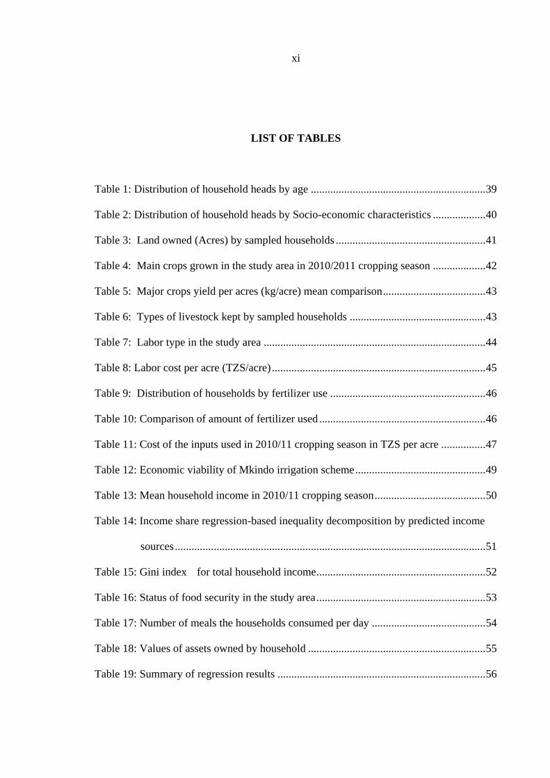
LIST OF TABLES

Table 1: Distribution of household heads by age ............................................................... 39

Table 2: Distribution of household heads by Socio-economic characteristics ................... 40

Table 3: Land owned (Acres) by sampled households ...................................................... 41

Table 4: Main crops grown in the study area in 2010/2011 cropping season ................... 42

Table 5: Major crops yield per acres (kg/acre) mean comparison ..................................... 43

Table 6: Types of livestock kept by sampled households ................................................. 43

Table 7: Labor type in the study area ................................................................................ 44

Table 8: Labor cost per acre (TZS/acre) ............................................................................. 45

Table 9: Distribution of households by fertilizer use ........................................................ 46

Table 10: Comparison of amount of fertilizer used ............................................................ 46

Table 11: Cost of the inputs used in 2010/11 cropping season in TZS per acre ................ 47

Table 12: Economic viability of Mkindo irrigation scheme ............................................... 49

Table 13: Mean household income in 2010/11 cropping season ........................................ 50

Table 14: Income share regression-based inequality decomposition by predicted income

sources ................................................................................................................ 51

Table 15: Gini index for total household income ............................................................. 52

Table 16: Status of food security in the study area ............................................................. 53

Table 17: Number of meals the households consumed per day ......................................... 54

Table 18: Values of assets owned by household ................................................................ 55

Table 19: Summary of regression results ........................................................................... 56

xii

LIST OF FIGURES

Figure 1: Location of Mkindo study area, Tanzania ...................................................... 25

Figure 2: Conceptual framework .................................................................................... 26

xiii

LIST OF APPENDICES

Appendix 1: Questionnaire on Economic Viability and Economic Impact of

Mkindo Irrigation Scheme in Mvomero District, Tanzania ....................... 78

Appendix 2: Questionnaire for Non Irrigator Farmers. Questionnaire on Economic

Viability and Economic Impact of Mkindo Irrigation Scheme In

Mvomero District, Tanzania ....................................................................... 84

Appendix 3: Discounted Cost and Benefit ...................................................................... 89

xiv

LIST OF ABBREVIATIONS

AfDB African Development Bank

AIDS Almost Ideal Demand System

ASDP Agricultural Sector Development Programme

ASDS Agricultural Sector Development Strategy

BCR Benefit Cost Ratio

BOT Bank of Tanzania

CBA Cost Benefit Analysis

CV Contingent Valuation

CVM Contingent Valuation Method

DFID Department for International Development

DP Development Partners

EAC East African Community

FAO Food and Agricultural Organization

FIVIMS Food Insecurity and Vulnerability Information and Mapping Systems

IFAD International Fund for Agricultural Development

IMT Irrigation Management Transfer

IRR Internal Rate of Return

JICA Japan International Cooperation Agency

LES Linear Expenditure System

MKUKUTA Mkakati wa Kukuza Uchumi na Kupunguza Umaskini

MOFEA Ministry of Finance and Economic Affairs

xv

NIMP National Irrigation Master Plan

NPV Net Present Value

NSGRP National Strategy for Growth and reduction of poverty

PA Performance Adequacy

PD Performance Dependability

PE Performance Equity

RDS Rural Development Strategy

SAM Social Accounting Matrix

SCGE Simple Computational General Equilibrium Model

SCI Structure Condition Index

SPSS Statistical Package for Social Scientists

SWMRG Soil Water Management Research Group

TASAF Tanzania Social Action Fund

TFP Total Factor Productivity

TZS Tanzania Shillings

UNDP United Nations Development Programme

USA United States of America

WFP World Food Programme

WTP Willingness to Pay

1

CHAPTER ONE

INTRODUCTION

1.1 Background Information

The last century has seen unprecedented growth in irrigation projects on a global level,

but much of this growth has been in the developing countries, including Tanzania. In

Tanzania, the government has taken several measures to ensure the development of

irrigation schemes. These measures include the formulation of the National Irrigation

Policy of 2009 and National Irrigation Master Plan (NIMP) of 2002. The National

Irrigation Policy of 2009 considers irrigation development in Tanzania to be critically

important in ensuring that the nation attains a reliable and sustainable crop production and

productivity as a move towards food security and poverty reduction.

These measures have been accompanied by government investments in irrigation projects

through government budget and support from various development partners, including the

World Bank, UNDP, FAO, JICA, IFAD, AfDB and others. These investments have

contributed to the expansion of irrigated land which has increased from 0.264 million ha

in 2006 to 0.370 million ha in 2010 (MOFEA, 2010). It is envisaged that the area under

irrigation will increase from 0.370 million ha in 2010 to 1 million ha by 2015 (MOFEA,

2010). However, most of these irrigation schemes have been established without

thorough analysis of their economic viability. There are costs associated with irrigation

projects and expansion of irrigation which need to be weighed against the benefits. The

benefits and costs of irrigation vary with the scale of the irrigation scheme and

management of the resources that have accompanied its development.

This study is concerned with the analysis of economic viability and the impact of small-

scale irrigation projects supported by the World Bank through the Tanzania Social Action

2

Fund (TASAF). TASAF was established by the government of Tanzania in 2000, with a

funding facility that allows local and village governments to respond to community

demands for interventions that will contribute to the attainment of specific Millennium

Development Goals. Towards this endeavor, TASAF contributes to achieving the goals of

Tanzania poverty reduction strategy (MKUKUTA I and II). TASAF has been

implemented in phases. The first phase (TASAF-I) was implemented in 40 districts (local

government authorities) in Tanzania Mainland as well as in Zanzibar since 2000 and

ended in December 2004. It was financed by the World Bank, Tanzanian Government and

community contributions. The second phase which commenced in 2005 covered all the

districts (local government authorities) in Tanzania and ended in 2010. TASAF is now in

the third phase (TASAF III) which started in 2011 and will end in 2015. This Phase is

funded by the World Bank and other Development Partners (DP), including the

Department for International Development (DFID) and World Food Program (WFP).

Almost all the regions in the country have received some funds for irrigation schemes

from TASAF. Mkindo irrigation scheme in Mvomero District is one of the small-scale

irrigation schemes in Morogoro region which have been rehabilitated using funds from

TASAF.

1.2 Statement of the Problem and Justification

As already pointed out, the importance of expanding irrigation cannot be overemphasized

especially in areas where rainfall is increasingly becoming unreliable. Irrigation has the

potential of allowing double cropping, decreasing the uncertainty of water supplied by

rainfall, increasing the yields on the existing cropland and eventually, improving and

ensuring food security and reliable income from agriculture. To justify investments in

irrigation, the costs associated with irrigation need to be weighed against the benefits. The

costs associated with irrigation will vary with the scale and management of the irrigation

3

scheme. TASAF has supported investments in small-scale irrigation schemes in several

parts of Tanzania on grounds of improving the welfare of rural people. However, there is

scanty information on the economic viability and the impact of irrigation schemes on the

welfare of smallholder farmers in Tanzania. Studies on economic viability include studies

by Kabbiri et al. (2008); Denis (2008) and Germana (1993) who analyzed the economic

viability of different technologies used by small farmers in farming activities in Tanzania.

With regard to the impact of irrigation, Shitundu and Luvanga (1998); Cosmas and

Tamilwai (2005); Mkavidanda and Kaswamila (2001) and Kadigi et al. (2003) have

analyzed the impact of irrigation technology on food security and household income.

Besides the scale of irrigation scheme, the economic viability and the impact of irrigation

will likely vary from one location to another. Thus there is need for location specific

studies on viability and the impact of irrigation on welfare of smallholder farmers. The

study analyzed the economic viability and the impact of Mkindo irrigation smallholder

scheme on household income and food security. The Mkindo smallholder irrigation

scheme is found in the Mkindo Watershed in the Wami River Basin. The irrigation

scheme was initiated by government of Tanzania in collaboration with JICA in 1984.

1.3 Objective of the Study

The general objective of the study was to analyze the economic viability and determine

the impact of Mkindo irrigation scheme on household income and food security.

1.3.1 Specific objectives of the study

(i) To analyze the economic viability of Mkindo irrigation scheme in Mvomero

district,

(ii) To determine the impact of irrigation on household income and income on

distribution, and

4

(iii) To determine the impact of irrigation on household food security.

1.4 Research Hypotheses

(i) Investments in smallholder irrigation projects/schemes are not economically

viable.

(ii) Investments in smallholder irrigation projects/schemes have no positive impact on

household income and income distribution.

(iii) Investments in smallholder irrigation projects/schemes have no positive impact

household food security.

1.5 Organization of Dissertation

This study is organized into five chapters including this chapter which presents the

background information, problem statements, general objective, specific objectives and

research hypotheses. The second chapter reviews literature relevant to the study while the

third chapter presents the methodologies used to assess the extent to which the study

hypotheses hold. Chapter four presents and discusses the findings of the study while the

last chapter presents conclusions and recommendations based on the major findings of the

study.

5

CHAPTER TWO

LITERATURE REVIEW

2.1 Measuring Economic Viability of Investments/Projects

Various methods ranging from discounting to non-discounting methods are used to

analyze the economic viability of investment projects. Discounting measures include cost-

benefit ratio, net present value and internal rate of return, while non-discounting measures

include payback period, rate of return, contingent valuation, Hedonic Pricing Method,

Travel Cost Method, Production Factor Method and Averting Behavior Method

(Hoevenagel, 1994).

Discounting measures of project’s worthiness such as cost-benefit ratio, net present value

and internal rate of return explicitly take into account the time value of money, based on

the economic fact that money today is worth more than a promise of money in the future.

Cost-benefit analysis (CBA) is a discounting measure of project worthiness which

originated in the USA in 1936 and has become a world-wide tool to evaluate choices

between alternative projects in decision making (Pearce et al., 1993). Traditionally, it is

associated with government interventions and the evaluation of public policies and

projects (Zerbe and Dively, 1994). It is an assessment method that quantifies the monetary

value of all policy or project consequences for the society in which the program is being

run (Boardman et al., 2001). It is particularly useful when a choice has to be made out of

several projects (selection), and when the project involves a stream of benefits and costs

over time.

Despite being useful, erroneous cost-benefit analysis can result into wrong investment

decisions. Arrow et al. (1996) points out the advantages and limitations of cost-benefit

analysis. Cost-benefit analysis can be dangerous if taken literally on large issues, and on

6

large timescales. This is because some of the largest items, such as water resources and

their services are difficult to price. Cost-benefit analysis based on pricing of costs and

pricing of benefits: each given a money value, and then costs and benefits are compared.

If there is net loss, then one turns the project down. Otherwise one accepts it. The prices

usually come from the markets but some of the most important environmental assets have

no market prices (Chichilnisky, 1996b). The problem is serious because errors in prices

can radically change the results: a project can turn from positive to negative, when the

wrong prices are applied. When property rights are ill-defined, as they are for the most

important environmental assets such as water and the atmosphere, prices can be highly

inaccurate (Chichilnisky, 1994). Therefore, it is very important to make sure that, price

are determined accurately in all cost-benefit analyses of projects involving some of the

most important environmental resources known to humankind.

Another problem that emerges in doing cost-benefit analysis of projects across a long

period of time is the issue of discount factor. Anything discounted at a rate of 3-6 per cent

becomes meaningless after 50-100 years, i.e. the economic income of the entire planet

shrinks down to the value of a car when so discounted (Chichilnisky, 1997). Yet some of

the most important environmental problems-risks like nuclear power plants, global

warming and biodiversity destruction-are only meaningful over such a timescale. Arrows

et al. ( 1996) reported that, “Both economic efficiency and intergenerational equity

require that benefits and costs experienced in future years be given less weight in

decision-making than those experienced today”. This statement could be dangerous if

taken literally; definitely it can be said to be plainly wrong. As an economist would wish

to be eligible what is said here, and correct for the wrong inferences that can be drawn

from this testimonial by thinking of cases where it holds true. Discounting the future is

neither necessary nor sufficient for efficiency and intergenerational equity. All this could

7

be taken into account when doing cost-benefit analysis. Therefore, policy-makers and

researchers should take into account those uncertainties.

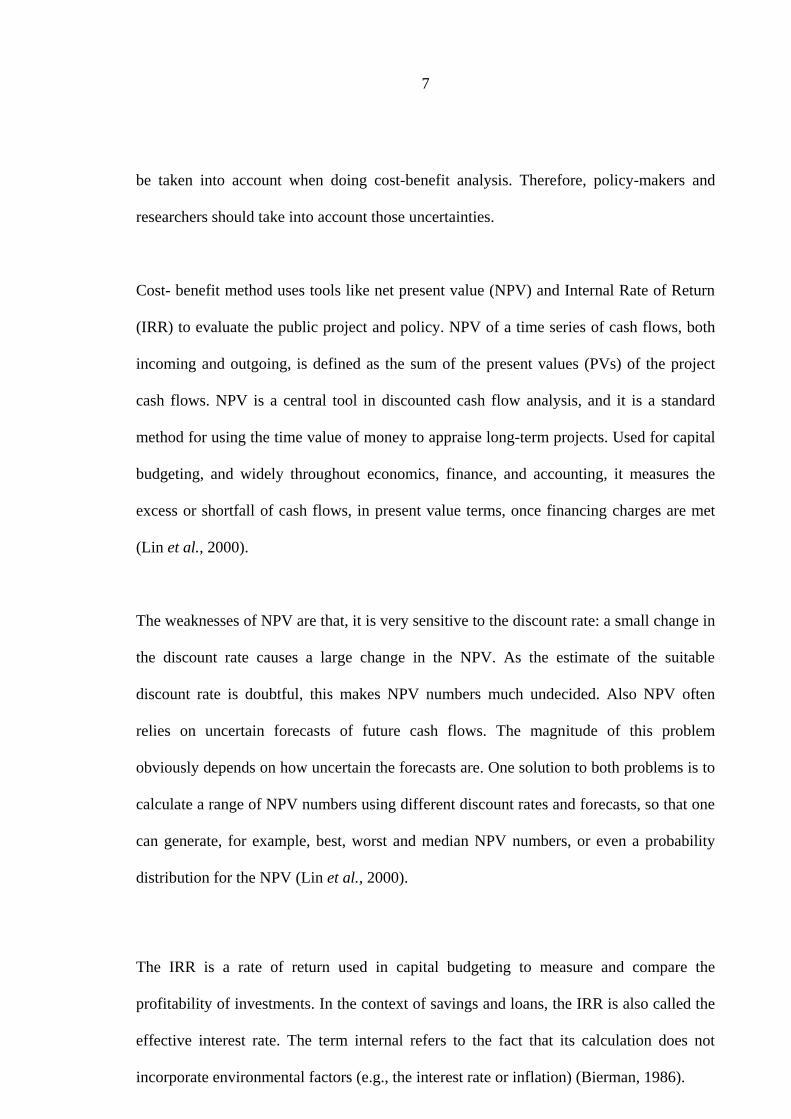
Cost- benefit method uses tools like net present value (NPV) and Internal Rate of Return

(IRR) to evaluate the public project and policy. NPV of a time series of cash flows, both

incoming and outgoing, is defined as the sum of the present values (PVs) of the project

cash flows. NPV is a central tool in discounted cash flow analysis, and it is a standard

method for using the time value of money to appraise long-term projects. Used for capital

budgeting, and widely throughout economics, finance, and accounting, it measures the

excess or shortfall of cash flows, in present value terms, once financing charges are met

(Lin et al., 2000).

The weaknesses of NPV are that, it is very sensitive to the discount rate: a small change in

the discount rate causes a large change in the NPV. As the estimate of the suitable

discount rate is doubtful, this makes NPV numbers much undecided. Also NPV often

relies on uncertain forecasts of future cash flows. The magnitude of this problem

obviously depends on how uncertain the forecasts are. One solution to both problems is to

calculate a range of NPV numbers using different discount rates and forecasts, so that one

can generate, for example, best, worst and median NPV numbers, or even a probability

distribution for the NPV (Lin et al., 2000).

The IRR is a rate of return used in capital budgeting to measure and compare the

profitability of investments. In the context of savings and loans, the IRR is also called the

effective interest rate. The term internal refers to the fact that its calculation does not

incorporate environmental factors (e.g., the interest rate or inflation) (Bierman, 1986).

8

In many situations, the IRR procedure will lead to the same decision as the NPV

procedure, but there are also times when the IRR may lead to different decisions from

those obtained by using the net present value procedure. When the two methods lead to

different decisions, the NPV method tends to give better decisions. It is sometimes

possible to use the IRR method in such a way that it gives the same results as the NPV

method. For this to occur, it is necessary that the rate of discount at which it is appropriate

to discount future cash proceeds be the same for all future years. If the appropriate rate of

interest varies from year to year, then the two procedures may not give identical answers.

It is easy to use the NPV method correctly, but it is much more difficult to use the IRR

method correctly (Bierman, 1986).

Despite the disadvantages, the method has been used in many development projects,

especially in developing countries like Tanzania. Kabbiri et al. (2008); Denis (2008);

Balkema et al. (2010); EAC (2010); Brenters and Henny (2002); Akyoo and Lazaro

(2008) and Germana (1993) have used cost-benefit analysis methods to analyse the

economic viability of different projects in Tanzania and Kenya. This shows that, the

method is very powerful in appraisal of development projects despite its weakness.

Unlike the discounting measures, non-discounting measures of project worthiness do not

explicitly consider the time value of money. In other words, each dollar earned in the

future is assumed to have the same value as each dollar that was invested many years

earlier. The payback period, accounting rate of return or return on investment are two

examples of methods used in capital budgeting that do not involve discounting future cash

amounts (Averkamp, 2011).

9

The Contingent Valuation Method (CVM) technique is a non-discounting hypothetical-

direct valuation technique requiring the active involvement of respondents (Awad et al.,

2010). This method can be used to evaluate the policy option on the natural resource

which can’t be evaluated by pricing mechanism. The CVM develops a framework of a

hypothetical market used to elicit valuations for environmental and/or public goods

preference, expressed in terms of Willingness to Pay (WTP). It mainly asks people what

they are willing to pay for a benefit. The technique has great flexibility that can allow

valuation of a wider variety of non-market goods and services than all the indirect

valuation techniques. In the meantime, the CV technique is the only approach available

for estimating non-use values (Mitchell and Carson, 1989; and McConnell and Haab,

2003).

However, the method has some weaknesses. First, it does not produce valid measurements

when it concerns the goods that people are not used to, and when people reject

responsibility for the goods in question. If people are asked, for example, about their

willingness to pay for clean soil, they may state that it is zero, because they feel the

polluter should pay. Puttaswamaiah (2002); Hoevenagel (1994); Wierstra et al. (1996)

indicate that CVM works best where it is least needed. It does not provide valid estimates

when people are unfamiliar and inexperienced with the goods. Validity may be a problem,

since it is very difficult to describe a natural good in such a way that all its attributes are

accounted for. Puttaswamaiah (2002) observe that CVM works best for those goods

resembling ordinary commodities which means that it is best suited for valuing

consumption goods that people consume more as their income increases.

Also when goods are not easily commoditized, as in choices concerning entire

ecosystems, CVM results are doubtful. Supporters of this argument believe that an

10

environmental good has several properties and that compressing the values of these

attributes into a single metric (such as willingness to pay) leads to an information loss.

The same argument is, however, also relevant to private goods, but in that case, people

seem to accept their prices as their true value. The idea behind this is that people have

experience in valuing and making trade-offs for attributes of private goods, whereas they

do not have any experience in valuing environmental goods. In fact, they may not even be

aware of all the attributes. This situation makes people liable to construct their values

heuristically on the basis of the information provided by the elicitation setting (Vatn and

Bromley, 1994).

In spite of the criticisms, considerable research has established the CVM as a sound

technique for estimating values for public policy decisions. Some examples of these

studies are by Rendall et al. (1974); Bishop and Heberlein (1979); Bishop et al. (1983);

Seller et al. (1986); Cameron and James, (1987); Bowker and Stoll (1988); Cameron,

(1988); McConnel (1990); Balderas and Laarrnan (1990); Donaldson et al. (1997); Rollins

(1997); Rayn (1997); Willis and Powe (1998); Hayes and Hayes (1999); Carlson and

Johansson (2000); Shackley and Dixon (2000); Loomis et al. (2000) and Scarpa (2000);

Anastasios (2006) and Bamidele et al. (2010). These researchers have used this method to

analyse the economic viability of irrigation projects.

The choice between discounting and non-discounting measures of project worthiness

depends on the nature of investment/project to be evaluated. For projects like irrigation,

that take a long time period for the benefits to return the investments, discounting

measures are used because of the time value of money. Therefore, based on this theory,

the study used Cost-benefit approach. NPV, BCR and IRR were used to analyse the

economic viability of Mkindo irrigation scheme.

11

2.2 Approaches and Methods for Measuring Impact of Investments/Projects

Economic impact analysis examines the effect of a policy, program, project, activity or

event on the economy of a given area. Economic impact is usually measured in terms of

changes in economic growth and associated changes in livelihoods improvement. The

proper analysis of the impact requires a counterfactual or before and after situation of

what those outcomes would have been in the absence of the intervention (World Bank,

2006). Haile (2008) argues that, “impact assessment of any development intervention is a

methodologically difficult and complex task to undertake”. Ravallion (2005) and Baker,

(2000) suggest that no single method should dominate the impact evaluation of any

development project, but instead rigorous impact evaluations should be open-minded in

the choice of methodology. According to Baker (2000) the most important thing in impact

evaluations is to derive robust and meaningful close proxies or indicative estimates that

are comparable between and within individuals or groups, based on the aims of a

particular development intervention so that, they can examines it impact to the given area.

To achieve the process of deriving close and meaningful proxies or indicative estimates

that can be compared between and within groups, two approaches namely, before and

after or with and without experimental design are used (Ravallion 2005; Johnson et al.,

2003 and Baker 2000). In order to determine the counterfactual, it is necessary to net out

the effect of the interventions from other factors. This is accomplished through the use of

comparison or control groups; those who do not participate in a program or receive

benefits, which are afterward compared to the treatment group or individuals who

received the intervention. Control groups are selected randomly from the same population

as the program participants, whereas the comparison group is more simply the group that

does not receive the program under investigation. Both the comparison and control group

12

should resemble the treatment group in every way, with the only difference between them

being program participation (Baker, 2000).

Determining the counterfactual is at the core of evaluation design (Baker, 2000). This can

be accomplished using several methodologies which fall into two broad categories,

experimental designs (randomized), and quasi experimental designs (none randomized).

According to Baker (2000), it is, however, quite tricky to net out the program impact from

the counterfactual conditions which can be affected by history, selection bias, and

contamination. Qualitative and participatory methods can also be used to assess the

impact, with these techniques often providing critical insights into beneficiaries’

perspectives, the value of programs to beneficiaries, the processes which may have

affected outcomes, and a deeper interpretation of the results observed in quantitative

analysis. The strengths and weaknesses of each of these methods are discussed in more

detail below.

Experimental designs, also known as randomization, are generally considered the most

robust of the evaluation methodologies (Baker, 2000). By randomly allocating the

intervention among eligible beneficiaries, the assignment process itself creates

comparable treatment and control groups that are statistically equivalent to one another,

given appropriate sample sizes.

While experimental designs are considered the optimum approach to estimating the

project impact, in practice there are several problems. First, randomization may be

unethical due to the denial of benefits or services to otherwise eligible members of the

population for the purposes of the study. An extreme example would be the denial of

medical treatment which can turn out to be life-saving to some members of the

13

population. Second, it can be politically difficult to provide an intervention to one group

and not another. Third, the scope of the program may mean that there are no non-

treatment groups such as with a project or policy change that is broad in scope. Examples

include an adjustment loan, or programs administered at a national level. Fourth,

individuals in control groups may change certain identifying characteristics during the

experiment which could invalidate or contaminate the results. If, for example, people

move in and out of a project area, they may move in and out of the treatment or control

group. Alternatively people who were denied a program benefit may seek it through

alternative sources, or those being offered a program may not take up the intervention.

Fifth, it may be difficult to be assured that the assignment is truly random. An example of

this might be administrators who exclude high risk applicants to achieve better results.

And finally, experimental designs can be expensive and time-consuming in certain

situations, particularly in the collection of new data (Baker, 2000).

Baker (2000) argues that, “with careful planning, some of these problems can be

addressed in the implementation of experimental designs”. One way is with the random

selection of beneficiaries. This can be used to provide both a politically-transparent

allocation mechanism and the basis of a sound evaluation design, as budget or information

constraints often make it impossible to accurately identify and reach the most eligible

beneficiaries. A second way is bringing control groups into the program at a later stage,

once the evaluation has been designed and initiated. Using this technique, the random

selection determines when the eligible beneficiary receives the program, not if they

receive it. Finally, randomization can be applied within a sub-set of equally-eligible

beneficiaries, while reaching all of the most eligible and denying benefits to the least

eligible (Pradhan et al., 1998). However, if this latter suggestion is implemented, one must

14

keep in mind that the results produced from the evaluation will only be applicable to the

group from which the randomly-generated sample was selected.

If it is not possible to construct treatment and comparison groups through experimental

design, quasi-experimental (non-random) methods can be used to carry out an impact

analysis. These techniques generate comparison groups which resemble the treatment

group, at least in observed distinctiveness, through econometric methodologies which

include: matching methods, double difference methods, instrumental variables methods,

and reflexive comparisons. Using these techniques, the treatment and comparison groups

are usually selected after the intervention using non-random methods. Therefore,

statistical controls must be applied to address the differences between the treatment and

comparison groups and/or sophisticated matching techniques must be used to construct a

comparison group that is as similar as possible to the treatment group. In some cases, a

comparison group is also chosen before the treatment though the selection is not

randomized (Baker, 2000).

According to Baker (2000), the main benefit of quasi-experimental designs is that they

can draw on the existing data sources and are thus often quicker and cheaper to

implement, and can be performed after a program has been implemented, given sufficient

existing data. The principal disadvantages of quasi-experimental techniques are as

follows:

i) The reliability of the results is often reduced as the methodology is less robust

statistically;

ii) The methods can be statistically complex; statistical complexity requires

considerable expertise in the design of the evaluation, analysis and interpretation

of the results.

15

iii) There is a problem of selection bias. When generating a comparison group rather

than randomly assigning one, there are many factors which can affect the

reliability of results (Greene, 1997).

Besides quantitative techniques, qualitative techniques are also used for carrying out

impact evaluation with the target to find out impact by the reliance on something other

than the counterfactual to make a causal inference (Mohr, 1995). The focus in qualitative

techniques is on sympathetic processes, behaviors, and conditions as they are perceived by

the individuals or groups being studied (Valadez and Bamberger, 1994). For example,

qualitative methods and particularly participant observation can provide insight into the

ways in which households and local communities perceive a project and how they are

affected by it. Because measuring the counterfactual is at the core of impact analysis

techniques, qualitative designs have generally been used in juxtaposition with other

evaluation techniques. Qualitative data can also be quantified. Among the methodologies

used in qualitative impact assessments are the techniques developed for rapid rural

assessment which rely on participants knowledge of the conditions surrounding the

project or program being evaluated, or participatory evaluations where stakeholders are

involved in all stages of the evaluation, determining the objectives of the study,

identifying and selecting indicators to be used, and participating in data collection and

analysis (Baker, 2000).

Like any other technique, the qualitative techniques have their own advantages and

disadvantages. The advantages of qualitative assessments are as follow, they are flexible,

can be specifically modified to the needs of the evaluation using open-ended approaches,

they can be carried out quickly using rapid techniques, and can greatly enhance the

findings of an impact evaluation through providing a better understanding of the

16

stakeholders’ perceptions and priorities, and the conditions and processes which may have

affected the program impact. On the other hand, the main drawbacks are the subjectivity

involved in data collection, the lack of a comparison group, and the lack of statistical

robustness given mainly small sample sizes making it difficult to generalize to a larger

representative population (Baker, 2000).

The validity and reliability of qualitative data are very dependent on the methodological

skills, sensitivity, and training of the evaluator. If field staffs are not sensitive to specific

social and cultural norms and practices, and non-verbal messages, the data collected may

be misinterpreted. And finally, without a comparison group, it is impracticable to

determine the counterfactual and thus, causality of project impact (Baker, 2000; Mohr,

1995).

Considering the advantages and disadvantages of the various approaches and methods of

impact assessment, this study adopted with and without intervention approach and used a

combination of quantitative and qualitative methods to assess the impact of Mkindo

irrigation scheme on household income and food security.

2.3 Impacts of Irrigation Project

Historically, irrigation originated as a method of increasing the productivity of available

land and thereby expanding total agricultural production, especially in the arid and semi-

arid regions of the world (Bhattarai et al., 2002). In addition to increasing crop production

and farm and family incomes, improved irrigation access significantly contributes to rural

poverty reduction through improved employment and livelihoods within a region. Indirect

benefits, such as more stable rural employment as well as higher rural wage rates, help

landless farm laborers obtain a significant share of the improved agricultural production.

17

In addition to yield improvement and intensive production practices, better irrigation

infrastructure and reliable water supply also enhance uses of other inputs like fertilizers

and high yielding varieties. Therefore, irrigation is important in rural poverty reduction

strategy.

The irrigation induced benefits are not limited to farming households but also affect

broader sectors of the economy, by providing increased opportunities to growing rural

service sectors and other off-farm employment activities (Bhattarai et al., 2002; Lipton,

2007; Hussain, 2007). Hussain (2007) argues that, indirect irrigation benefits could be

larger than direct benefits through the multiplier effect and distribution of irrigation

benefits also varies widely by type of the benefit and the socio-economic status of the

beneficiaries. The direct benefits generally accrue to landholders, while a significant part

of the indirect benefits accrue to the landless and small farmers, positively contributing to

their livelihoods. Further, the overall benefits of irrigation are large when irrigation

improving interventions, investments in infrastructure, improvements in system

management and service delivery to farmers, are implemented in an integrated manner.

Examples of such benefits are additional employment creation for landless laborers in

agro-industries, rural marketing and other off-farm activities like house construction and

basic infra-structural building.

2.3.1 The impact of irrigation on household income

Improvement in access to irrigation water serves as a reliable tool to increase income,

branch out livelihoods and reduce vulnerability, since irrigation water creates options for

extended production across the year, increases yields and outputs, and creates

employment opportunities (McCartney et al., 2010; Hussain et al., 2004; Berhanu and

Peden, 2002). Nonetheless, irrigation benefits may accrue unevenly across socio-

18

economic groups (Hussain et al., 2004). Therefore in analysis of irrigation impact to

household income, the issue of income inequality should also be considered. These show

how irrigation improves household income and distribution of the income to the society.

In this study, the impact analysis framework, with and without, will be used to assess

income impact and inequality between user and non-user of Mkindo irrigation scheme.

2.3.2 The impact of irrigation on food security

Food security is one of the positive impacts of irrigation. But achieving food security in its

totality continues to be a challenge, not only for the developing nations, but also for the

developed world (Mwaniki, 2006). The difference lies in the magnitude of the problem in

terms of its severity and proportion of the population affected. But, it is well documented

that irrigated land leads to increased agricultural productivity. Irrigated areas are 2.5 times

more productive comparing to rain-fed agricultural areas (Stockle, 2001). Therefore

irrigation has been found to be a central key part in curbing food scarcity and reducing the

level of poverty, not only in Tanzania but also in many other developing countries

(Mwakalila 2004; Cosmas and Tamilwai, 2005; Mkavidanda and Kaswamila, 2001;

SWMRG, 2005; Shitundu and Luvanga, 1998).

The definition of food security, agreed upon at the 1996 World Food Summit is “a

situation that exists when all people, at all times, have physical, social and economic

access to sufficient, safe and nutritious food that meets their dietary needs and food

preferences for an active and healthy life.” Food security is commonly conceptualized as

resting on three pillars: availability, access, and utilization. These concepts are inherently

hierarchical, with availability necessary but not sufficient to ensure access, which is in

turn necessary but not sufficient for effective utilization. Availability reflects the supply

side. Access reflects food demand, as mediated by cash availability, prices, and intra-

19

household resource allocation. Utilization reflects whether individuals and households

make good use of the food to which they have access, commonly focused on the intake of

essential micronutrients. Some consider stability to be a fourth dimension of food

insecurity capturing individuals’ susceptibility to food insecurity due to interruptions in

access, availability or utilization (Barrett et al., 2009).

The temporal aspect of stability links to the oft-made distinction between chronic and

transitory food insecurity. Chronic food insecurity reflects a long-term lack of access to

adequate food, and is typically associated with structural problems of availability, access

or utilization, especially poor access due to chronic poverty. Most food insecurity is

chronic (Barrett, 2002). Transitory food insecurity, by contrast, is associated with sudden

and temporary disruptions. The most serious episodes of transitory food insecurity are

commonly labeled “famine”, typically caused by simultaneous or sequential availability,

access, and humanitarian response failures.

Hence, based on the concept of food security, several approaches are employed to assess

its state. The first approach is indicator-based, emphasizing the indicators focusing on

food security dimensions such as food availability, food accessibility and variability, and

those based on FIVIMS (Food Insecurity and Vulnerability Information and Mapping

Systems). The second approach relies on the general equilibrium point of view, using the

Social Accounting Matrix (SAM) and the Simple Computational General Equilibrium

Model (SCGE) to make policy simulations. The third approach focuses on the

econometric estimation of consumer demand by applying the Linear Expenditure System

(LES) and the Almost Ideal Demand System (AIDS) to assess elasticities, nutrition related

measures and welfare indicators (Jrad et al., 2010).

20

Based on the concept of food security and the impact of irrigation on food security, this

study employed the food security indicator-based approach, and these indicators are food

availability and food accessibility.

2.4 Previous Irrigation Related Studies in Tanzania

Irrigation-related studies have been undertaken in different parts of the country. These

include studies on management of irrigation schemes, technical and productivity

efficiently, social economic impact and economic valuation of irrigation.

2.4.1 Studies on management of irrigation schemes

The issue of irrigation management has got its rules in making sure that these irrigation

schemes are performing well. Some of the studies in Tanzania have addressed the issue of

management and its role. Tarimo et al. (2010) conducted study on evaluation of water

distribution systems at Igomelo irrigation scheme to assess the performance of the scheme

after intervention of the Irrigation Management Transfer (IMT). Irrigation performance

indicators, such as Dependability (PD), Equity (PE) and Adequacy (PA) of water supply,

Conveyance efficiency and Structure Condition Index (SCI) were used to evaluate the

system. It was found that all these were indicators of a system that was performing well

(Magayane et al., 2003).

2.4.2 Studies on technical aspects of irrigation and productivity of irrigation

schemes

Mahoo et al. (2007) conducted a study in the Ruaha River Sub-basin of the Rufiji basin to

assess knowledge, attitudes and practices in measuring productivity among the

stakeholders. They found that, “there is a lack of general understanding and a wide

disparity in practices related to the concept of productivity of water”. The concept of

21

productivity of water is poorly understood, with inconsistent and incomplete monitoring,

reporting and auditing among the stakeholders. Policy makers, engineers and researchers

define productivity in one way and smallholder farmers apply their own definitions and

descriptions, to assess productivity. This results in a lack of realistic analyses of water

requirements and water values in various water sectors for fostering and implementing

strategies for improved water allocation. Also Magayane et al. (2003) conducted a study

that explore how water use efficiency and productivity of irrigation systems practicing

water reuse, could be related to the efficiency and productivity of individuals farms within

the water reuse systems.

Two irrigation systems having a chain of three users (Top, Middle and End users) reusing

the runoff from upstream farms were sampled for investigation in the Ruaha river sub-

basin. It was observed that the system which consisted of farmers with lower individual

efficiency and productivity resulted in lower water reuse efficiency (90%) and

productivity (0.55kg/m3). Alternatively, the system which consisted of individuals with

relatively higher efficiency resulted in higher water reuse efficiency of about (93%) and

productivity (0.72kg/m3). Magayane et al. (2003) concluded that, “current methods of

assessing irrigation efficiency and productivity of water reuse does not accurately assess

key conditions inspired by the Usangu situation and which affect the irrigation efficiency

and productivity of water reuse in the area”. Lastly it concluded that, “irrigation efficiency

and productivity of individual farms in any water reuse system are the major contributors

to high water reuse efficiency and productivity”.

2.4.3 Economic valuation of irrigation water

On the issue of economic valuation, Ngaga et al. (2005) conducted a study in Pangani

River Basin to provide estimates of the value of water in different uses and reviewed

22

various issues and economic tools pertaining to water resource allocation and financing

mechanisms in the basin. They found that, “on the value of water in alternative uses

indicated that for irrigated agriculture such as coffee, the estimated average value was

about TZS. 700 – 6 000/m3. Water was estimated to be worth TZS. 30–100/m

3 in large

scale sugar production, TZS. 3 500–5 300/m3 for greenhouse-based cut-flower production,

TZS. 200–600/m3 for small scale traditional furrow irrigation agriculture, and TZS. 600–1

400/m3 for improved irrigation agriculture schemes and for domestic consumption were

equivalent to TZS. 1500 and 1250 per m3 in the highlands and lowlands respectively. Also

Kadigi et al. (2003) also conducted a study on economic analysis of value of irrigated

paddy in Usangu basin. They found that,” if farmer in Usangu stopped producing irrigated

paddy about 576 Mm3 of water that was currently used in irrigation or 345.6 Mm

3 traded

inter-regionally as virtual water would be utilized in alternative ways, either as

evaporation from seasonal swamps within the basin or made available for other uses. Also

there would be shrinkage in annual paddy production of about 105 000 tonnes of paddy

which is equivalent to 66 000 tonnes of rice which is equivalent to 14.4% of the total

annual paddy production in Tanzania. The opportunity cost of about TZS 16.4 billion will

be incurred annually and the country balance of payments will be affected by an average

of US$ 15.9 million per annum.

2.4.4 Studies on socio-economic impact of irrigation schemes

Previous studies on social economic impact have addressed the issues of income and food

security. Chiza (2005) argue that, “Irrigation has a multi-facetted role in contributing to

food security, self-sufficiency, food production and exports. In order to achieve good

returns to investment, effort must be made to change from subsistence to commercial

farming. There is therefore need to expand land under irrigation while intensifying crop

production. These efforts, coupled with good market arrangements, will result into

23

increased profits from farm produce and thereby reducing poverty at both household and

national levels. Mwakalila (2004) found that irrigated agriculture is, therefore, a poverty-

reducing intervention in the irrigation schemes of Igurusi. Though paddy production in the

area is asserted as utilizing too much of the available water resources, the same is also

playing an important role in enhancing food security, income and livelihoods of the local

people in the area. Cosmas and Tamilwai (2005) found that Ndiwa indigenous traditional

irrigation system contributes to poverty alleviation as it enables upland farmers to produce

products, especially vegetables during the dry season. This not only rescues farmers from

unreliable rain-fed agriculture, but also generates higher incomes since farmers can grow

high value crops more frequently. They also found that Ndiwa farmers were better off

compared to non-Ndiwa farmers in their possession of material assets such as better

houses, more livestock, fields, durable household items and farm implements. Other

studies on social economic aspect are from Mwakalila (2004); Mkavidanda and

Kaswamila (2001); Shitundu and Luvanga (1998) and Kissawike (2008).

2.4.5 Chapter summary

In summary the following can be drawn from the review of literature: Firstly, despite its

weakness the BCR method has been widely used as a criterion for project worthiness in

evaluation of many investment projects. For this reason, the method was adopted in the

evaluation of Mkindo irrigation scheme. Secondly, the literature has shown the before and

after approach to be the most appropriate approach for measuring impact of project

interventions. However, this study adopted the with and without due to absence of

baseline data. Lastly most of the literature has indicated that irrigation has significantly

impact on agriculture productivity and hence improving household’s income and food

security. But more research needs to be done especially on the viability, management and

efficient use of irrigation schemes and its adverse impact on environment.

24

CHAPTER THREE

RESEARCH METHODOLOGY

3.1 The Study Area

The study was conducted at Mkindo farmer-managed irrigation scheme found in northern

part of Mvomero District in Tanzania. It is located at latitude 60 16’ and 6

0 18’ South,

longitude 370 32’and 37

0 36’east and its altitude ranges between 345 to 365 metres above

sea level, about 85km from Morogoro. The average annual temperature is 240C with a

minimum of 15.10C in July and a maximum of 32.1

0C in February. The mean relative

humidity is 67.5% while the mean annual sunshine hours are 7.0 per day. The soils are

sandy clay loam. Mvomero District is one of five districts in Morogoro region composed

of 101 villages with a total population of 260 535 (Mboera et al., 2007). Rainfall in the

district is bimodal, with a long wet season from March to May and a short wet season

from October to December. The northern area has a humid to sub-humid climate, and

annual rainfall ranges from 1500 to 2000 mm (Lyimo et al., 2004), while the southern part

of the district is much drier, with annual rainfall between 600 mm and 1 200 mm

(Karimuribo et al., 2005).

The majority of the district’s population derive livelihood from crop production. Major

crops grown include paddy and maize. Only the population in the southern part of the

district depends primarily on pastoralist livestock keeping, raising goats and traditional

zebu cattle. Apart from Mkindo scheme, there are other schemes in Mvomero District

including Mhonda, Mgeta, Mlali, Mgongola, Patel, Mbigiri, Dakawa, Ndole, and Mtibwa

Sugar Estate. Mkindo scheme has been selected because it is one of the schemes which

have received funds from TASAF. Figure 1 below shows a map of Mkindo catchment

which is found in the Wami basin, Tanzania. As indicated in the map, the Mkindo

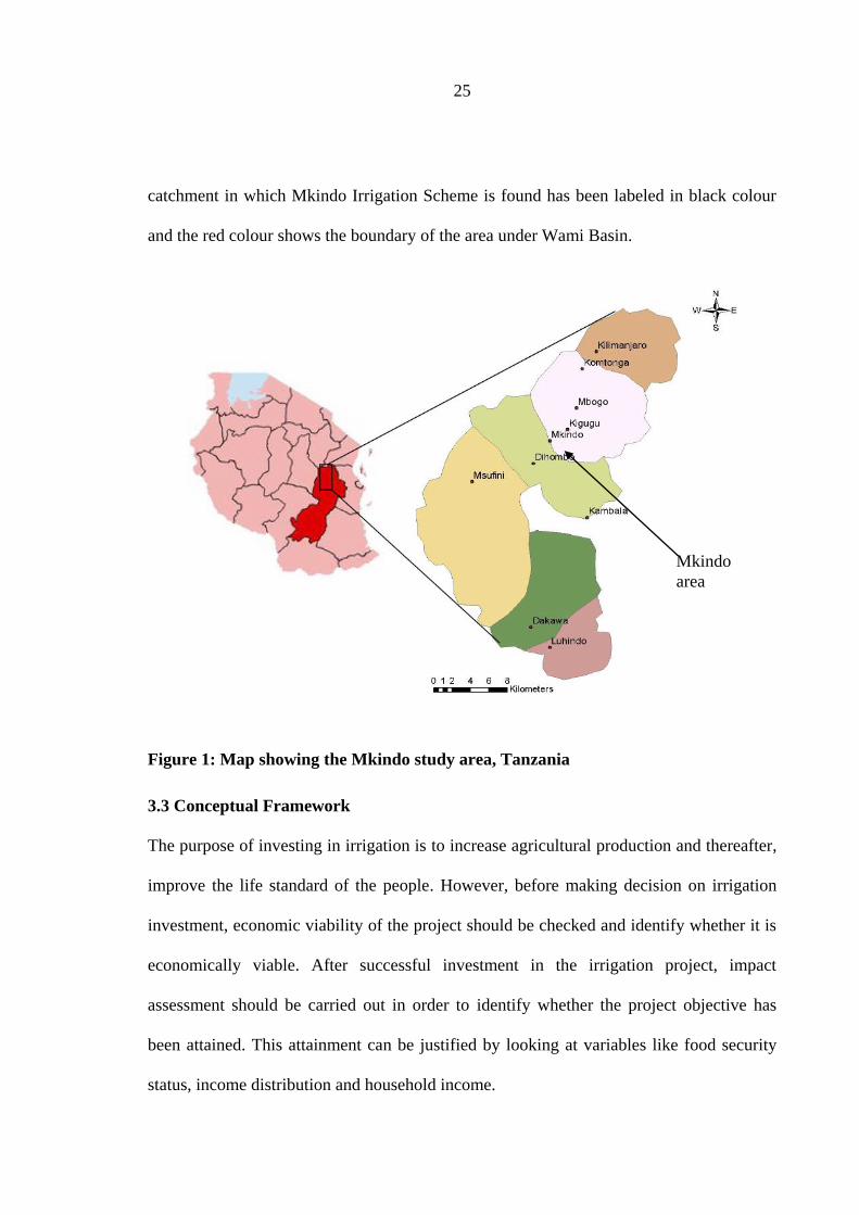
25

catchment in which Mkindo Irrigation Scheme is found has been labeled in black colour

and the red colour shows the boundary of the area under Wami Basin.

Figure 1: Map showing the Mkindo study area, Tanzania

3.3 Conceptual Framework

The purpose of investing in irrigation is to increase agricultural production and thereafter,

improve the life standard of the people. However, before making decision on irrigation

investment, economic viability of the project should be checked and identify whether it is

economically viable. After successful investment in the irrigation project, impact

assessment should be carried out in order to identify whether the project objective has

been attained. This attainment can be justified by looking at variables like food security

status, income distribution and household income.

Mkindo

area

26

Figure 2: Conceptual framework for the study

3.4 Research Design

There are two approaches that can be used to assess the impact of adopting certain

technologies like irrigation. These are before and after the introduction of the technology

or with and without the use of the technology. This study employed the with and without

design, which involved observations of a group of farmers practicing irrigation (with) and

another group which was practicing rainfed agriculture (without), at one specific point in

time. The before and after design is better compared to with and without design because it

captures the spillover effects, but due to the unavailability of baseline data, with and

without design was used in this study.

Irrigation

investment

Economic

viability

(Appraisin

g)

Impact

Assessmen

t

(Evaluation

)

Food security

status

Household

income

Income

distribution

27

3.5 Data for the study

Data for the study were obtained from both secondary and primary sources as described

below.

3.5.1 Secondary data

Secondary data were obtained from records kept by the former Chairman of Mkindo

Farmer-Managed Irrigation Scheme, Mr. Moses Kimosa. These data include initial

investment cost, number of farmers using the scheme, production costs, crop yields

obtained by users of the scheme since it was in 2008/09 rehabilitated by TASAF.

3.5.2 Primary data

Primary data were collected using structured questionnaires administered to farmers

selected from a list of farmers practicing irrigation at the Mkindo Irrigation Scheme and

farmers practicing rainfed agriculture at Dakawa as described in the following sections.

3.5.3 Questionnaire design

Questionnaires presented as Appendices 1 and 2 were designed to obtain information

required for answering the stated objectives. They were designed to capture both

qualitative and quantitative data for farmers inside the scheme and those outside the

scheme. They were divided into the following sections, as shown in Appendices 1 and 2.

i) Section A: General information about farmers household.

ii) Section B: Crop and livestock production activities.

iii) Section C: Irrigation practices, for irrigator questionnaire only.

iv) Section D: Resource use.

v) Section E: Impact of practicing and not practicing irrigation farming, to the lives

of farmers.

28

3.5.4 Sampling and sample size

The target populations were farmers who were practicing irrigation farming at Mkindo

Irrigation Scheme and farmers who were practicing rainfed farming at Dakawa. A sample

of 80 farmers practicing irrigation was randomly selected from a sampling frame of 106

farmers practicing irrigation at the Mkindo Irrigation Scheme. The same sample size was

selected from farmers practicing rainfed agriculture at Dakawa in order to make a

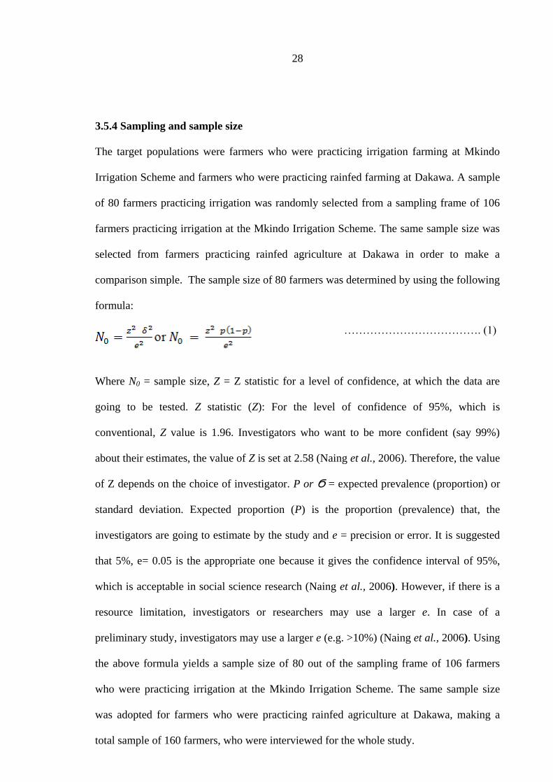
comparison simple. The sample size of 80 farmers was determined by using the following

formula:

Where N0 = sample size, Z = Z statistic for a level of confidence, at which the data are

going to be tested. Z statistic (Z): For the level of confidence of 95%, which is

conventional, Z value is 1.96. Investigators who want to be more confident (say 99%)

about their estimates, the value of Z is set at 2.58 (Naing et al., 2006). Therefore, the value

of Z depends on the choice of investigator. P or Ϭ = expected prevalence (proportion) or

standard deviation. Expected proportion (P) is the proportion (prevalence) that, the

investigators are going to estimate by the study and e = precision or error. It is suggested

that 5%, e= 0.05 is the appropriate one because it gives the confidence interval of 95%,

which is acceptable in social science research (Naing et al., 2006). However, if there is a

resource limitation, investigators or researchers may use a larger e. In case of a

preliminary study, investigators may use a larger e (e.g. >10%) (Naing et al., 2006). Using

the above formula yields a sample size of 80 out of the sampling frame of 106 farmers

who were practicing irrigation at the Mkindo Irrigation Scheme. The same sample size

was adopted for farmers who were practicing rainfed agriculture at Dakawa, making a

total sample of 160 farmers, who were interviewed for the whole study.

………………………………. (1)

29

3.5.5 Recruitment and training of enumerators

Prior to administration of the questionnaire as described in Section 3.5.6, three

enumerators with experience in data collection using questionnaires were recruited and

trained. The training took one day and covered the following aspects (i) importance and

objectives of the research, (ii) familiarizing the enumerators with the questionnaire to

ensure common understanding of all the questions in the questionnaire, (iii) how to ask

sensitive questions (iv) probing of options during the interviews, (v) how to record data

and (vi) building rapport with the respondents.

3.5.6 Questionnaire administration

The questionnaires were administered by the researcher with the help of three enumerators

who were already trained as indicated above. The administration of the questionnaires

took 12 days, between 6 February and 17 February 2012. The questionnaires were

administered using face-to-face interviews with the heads of households, and responses to

the questions were recorded immediately. The questionnaire was in English but the

interviews were conducted in Swahili. The enumerators were closely supervised during

data collection to make sure that quality data were collected.

3.6 Data Analysis

The SPSS software version 16 was used to generate the descriptive statistics such as

means, frequencies, cross tabulations, ratios, t-tests and chi squire analyses, to determine

significance differences between irrigators and non-irrigators. Other analyses carried out

to achieve the study objectives include discounting measures of project worthiness, Gini

coefficient and regression analysis as described in the subsequent sections below.

30

3.6.1 Economic viability of Mkindo irrigation scheme

The budgeting technique was used to analyze the long-term economic viability of Mkindo

Irrigation Scheme. The assumptions made in the analysis include: (i) Time horizon of 18

years was chosen, because irrigation projects are long-run in nature, therefore forecasting

for the future years is necessary (ii) A discount rate of 12% was used according to Central

Bank of Tanzania (BOT), as indicated in the “Economic Bulletin” for the quarter ending

March, 2012. With these assumptions, the financial streams of revenues from crop sales

and costs incurred were discounted to determine the NPV, BCR and IRR. The

computation of NPV, BCR and IRR were done in Ms Excel software using built-in

command. The mathematical equations underlying the computation of NPV, BCR and

IRR and the criteria for accepting an investment project using each indicator worthiness

are given in subsequent subsections.

3.6.1.1 Net present value

The NPV is calculated as the present value of the project's cash inflows minus the present

value of the project's cash outflows. Cash inflows are the revenue obtained from selling

crops obtained from the irrigation scheme and the cash outflow are the inputs cost for

producing crops and initial investment cost. This relationship is expressed by the

following formula:

Whereby, NPV is the value of the net present value, Bt is the benefit at time t, Ct are costs

incurred in production at time t, r is the interest rate and n is the time horizon. The project

with higher positive number is the one which is selected.

…………………...…………………………………. (2)

31

3.6.1.2 Benefit-cost ratio

The benefit-cost ratio (BCR) is the ratio of all the discounted (yearly) incremental benefits

and costs of a project. Thus, it expresses the benefit generated by the project per unit of

cost of the project expressed in present values. The ratio was obtained by using the

following formula:

The BCR expresses the benefit generated per unit of cost and it was interpreted as

follows:

i) BCR > 1: present value of benefits exceeds the present value of costs.

ii) BCR = 1: present value of benefits equals present value of costs.

iii) BCR < 1 the present value of costs exceeds the present value of benefits.

Selection criterion: projects with a BCR of 1 or greater are economically acceptable

when the costs and benefit streams were discounted at the opportunity cost of capital. The

absolute value of the BCR varies depending on the discount rate chosen; the higher the

discount rate, the smaller the BCR.

…………………………………………… (3)

32

3.6.1.3 Net benefit per capita in the scheme

Net benefit per capita is the average benefit per person obtained within the irrigation

scheme. Therefore, it involved only farmers at all farmers at the Mkindo irrigation

scheme. It was calculated by taking the total sum of net benefits and dividing it by the

number of farmers who were using the Mkindo Irrigation Scheme. It does not attempt to

reflect the distribution of the income or wealth.

Where by R = Total net revenue, N= total numbers of irrigators farmers who interviewed

and X= Net benefit per capita

3.6.1.4 Internal rate of return

The internal rate of return (IRR) is a rate of return used in capital budgeting to measure

and compare the profitability of investments. The internal rate of return of an investment

or project is the annualized effective compounded return rate or rate of return that makes

the net present value of all cash flows (both positive and negative) from a particular

investment equal to zero. In more specific terms, the IRR of an investment is the discount

rate at which the net present value of costs (negative cash flows) of the investment equals

the net present value of the benefits (positive cash flows) of the investment. The formula

or IRR is as follow.

Whereby, rn+1 = internal rate of return, rn is considered the nth

approximation of the IRR.

…………..….………………………………………………. (4)

..………………………. (5)

33

Decision criterion

If the IRR is greater than the cost of capital, accept the project.

If the IRR is less than the cost of capital, reject the project

3.6.2 Impact of Mkindo irrigation scheme

This section is divided into four sub-sections. The first sub-section describes the method

that was used to determine the impact of the irrigation scheme on income. The second

sub-section describes the method used to analyze income distribution. The third sub-

section describes how the impact of Mkindo Irrigation Scheme on food security was

determined, while the last sub-section describes econometric analysis which captures the

effect of practicing irrigation on crop yield.

3.6.2. 1 Analysis of impact of irrigation on household income

With and without design for impact analysis was used to measure the impact of irrigation

on household income by comparing incomes of users of Mkindo Irrigation Scheme and

non-users of the Scheme practicing rainfed agriculture at Wami Dakawa, who were not

practicing irrigation farming. Their income from agriculture and other sources were

compared by using t-test statistics. The unpaired, or "independent samples" t-test” method

was used between the treatment group (farmers within the Mkindo Irrigation Scheme) and

control group (farmers who were not practicing irrigation farming at Wami Dakawa).

………………………………………………………………... (6)

34

The numerator equals the difference between two sample means, and the denominator, is

called the standard error of difference, which equals the combined standard deviation of

both samples.

3.6.2.2 Analysis of impact of irrigation on income distribution

The Gini coefficient was used to measure income distribution among the irrigators and

non-irrigators in the study area. It is defined as a ratio with values between 0 and 1. The

Gini coefficient is often used to measure income inequality. Here, 0 corresponds to perfect

income equality (i.e. everyone has the same income) and 1 corresponds to perfect income

inequality (i.e. one person has all the income, while everyone else has zero income). The

Gini coefficient can also be used to measure wealth inequality. Therefore, the model was

adapted to determine whether there was a difference in income distribution between

irrigators at Mkindo and non-irrigators at Dakawa.

3.6.2.3 Analysis of the impact of Mkindo Irrigation Scheme on food security

The impact of irrigation on food security was determined by comparing food availability

between the irrigators and non-irrigators. Food availability which reflects food supply,

and the amount of own food consumed or stored and length of time able to feed

themselves in the year were used as proxies for food availability. Also number of meals

which household consume per day was also computed and then compared between

irrigators and non irrigators respondents. T-test (amount of food and income used by

household) and Chi-square (number of meals household consume per day and

number of month whereby household are food secure) statistical test were carried out to

determine if there is significant difference in food availability between irrigator and non

irrigator respondents.

35

3.6.2.4 Econometric analysis of the factors influencing paddy yield

All the benefits that exist in farming were determined by the amount of the output

produced. But the output produced is influenced by number of factors which need to

examine their influence on the output. For this reason, the key independents variable like

irrigator dummy, education dummy, labor force used and fertilizer were assessed in order

to check their influence on dependent variable. Using the multiple linear regression

models, the relationship between dependent variable and independent variables in the

scheme was assessed. Multiple linear regression model applies to the data taken on a

dependent variable Y and a set of k predictor or explanatory variables X1, X2, …, Xk with i

sets of data. In matrix form, the formula was presented as follows:

Yi = βiXi+ U

Whereby Yi represents the matrix of output and βi represents the matrix of the beta

coefficients, which explain how, change in independent influence change in dependent

variable. Xi is a matrix with i rows and k +1 column and u is the matrix of error term.

Thus, the formula can be expanded to fit our prediction between independent and

dependent variable as follows:

Y = ß0 + ß1X1 + ß2X2 + ß3X3 + ß4X4 + U

Where Y = Production of main crop/Ha

ß0 = Intercept

X1 = Irrigation dummy variable taking the value of 1 for farmers practicing

irrigation in the scheme and 0 for farmers practicing rainfed agriculture

outside the scheme.

X2 = Education dummy variable taking the value of 1 for those who received

formal education and 0 for those who did not receive formal education.

X3 = Labor force used in farming activities measured in number of people

employed

…………………………………………………………….. (7)

…………………………….. (8)

36

X4 = Amount of fertilizer used measured in kg.

U = Error term.

3.6.2.5 Explanation of variables and prior expectations

Irrigator dummy: Irrigator dummy variable was included in the model to show the

difference on the influence of irrigation on dependent variable between users of the

Mkindo scheme and non-users of Mkindo scheme. Irrigation has been found to have

positive impact on crop production (Ozdogan, 2011). Thus the dummy coefficient for

irrigation was hypothesized to be positive.

Education dummy: Respondents’ exposure to education will increase the farmers’ ability

to obtain, process and utilize information relevant for improving his/her productivity in

agriculture. Arrow (1973) suggests that, education adds to an individual’s productivity

and therefore increases the productivity of agriculture. The education variable was

therefore, expected to have a positive influence on yield per acre.

Fertilizer use: The use of fertilizer has been found to increase yield per acre (Abdoulaye

and Sanders, 2005; FAO, 2002). According to Fox and Rockstrom (2000) irrigation

together with fertilizer use has positive impact on crop yield. Therefore the fertilizer use

variable was included in the model to capture the effect of using fertilizer in the irrigation

scheme and the coefficient of the variable was expected to be positive.

Labor (Number of people employed): Increase in the number of people employed is

assumed to increase production. This is because an increase in number of people

employed increase labor force. Labor force determines the size of land to be cultivated

and timeliness of farm operation like planting and weeding and consequently

37

improvement in farm output and productivity (Steven et al, 2012). Therefore, the

coefficient of the variable labor was expected to have a positive effect.

38

CHAPTER FOUR

RESULTS AND DISCUSSION

4.1 Overview

This chapter is organized into four sections. The first section presents the socio-economic

characteristics of respondents; the second section presents results on crop and livestock

activities in study area; the third section presents results on irrigation practices; and the

fourth section presents results on economic impact and viability of irrigation scheme.

Fourth section is divided into four sub-sections which are impact on household income

and income distribution, impact on food security and econometric analysis which has been

employed to capture the effect of using irrigation on crop yield.

4.2 Socio-economic characteristics of households heads

Table 1 presents the distribution of the household’s heads according to age. The age of the

household’s heads has an influence on food production and consumption. As it is shown

in Table 1, most (37.7%) of the household’s heads were in the age group of 36-50 years.

Very few household’s heads were above 60 years old. This suggests that, most of the

household heads were in the active age group that can participate effectively in production

activities.

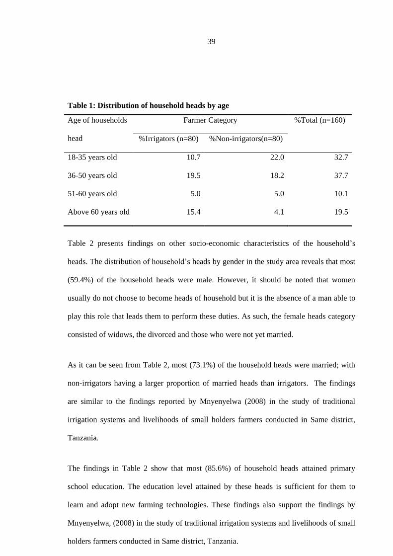
39

Table 1: Distribution of household heads by age

Age of households

head

Farmer Category %Total (n=160)

%Irrigators (n=80) %Non-irrigators(n=80)

18-35 years old 10.7 22.0 32.7

36-50 years old 19.5 18.2 37.7

51-60 years old 5.0 5.0 10.1

Above 60 years old 15.4 4.1 19.5

Table 2 presents findings on other socio-economic characteristics of the household’s

heads. The distribution of household’s heads by gender in the study area reveals that most

(59.4%) of the household heads were male. However, it should be noted that women

usually do not choose to become heads of household but it is the absence of a man able to

play this role that leads them to perform these duties. As such, the female heads category

consisted of widows, the divorced and those who were not yet married.

As it can be seen from Table 2, most (73.1%) of the household heads were married; with

non-irrigators having a larger proportion of married heads than irrigators. The findings

are similar to the findings reported by Mnyenyelwa (2008) in the study of traditional

irrigation systems and livelihoods of small holders farmers conducted in Same district,

Tanzania.

The findings in Table 2 show that most (85.6%) of household heads attained primary

school education. The education level attained by these heads is sufficient for them to

learn and adopt new farming technologies. These findings also support the findings by

Mnyenyelwa, (2008) in the study of traditional irrigation systems and livelihoods of small

holders farmers conducted in Same district, Tanzania.

40

Lastly, Table 2 indicates that most (98.8%) of the households head reported agriculture to

be their main occupation. This suggests that agriculture is the major economic activity in

the study area. Only a few heads depend on business as their main occupation. In the case

of secondary occupation most (26.9%) of the household heads participate in petty

business as their other economic activity apart from agriculture. Other secondary

occupations reported by the interviewed household heads were wage employment and

livestock keeping.

Table 2: Distribution of household heads by Socio-economic characteristics

Farmer Category %Total (n=160)

%Irrigators(n=80) %Non-irrigators(n=80)

Gender of

respondent:

Male 30 29.4 59.4

Female 20 20.6 40.6

Marital status

Married 35.2 38.4 73.6

Single 9.4 7.5 17

Widowed 5.7 3.8 9.4

Education level:

Primary 46.3 39.4 85.6

Secondary 1.3 7.5 8.8

College 0.6 1.3 1.9

No formal education 1.9 1.9 3.8

Primary Occupation

Agriculture 50 48.8 98.8

Business 0 1.2 1.2

Secondary

Occupation:

Business 6.3 22.6 26.9

Livestock keeper 0 1.9 1.9

Employee 0 3.8 3.8

41

4.3 Land owned by sampled farmers

Table 3 presents results on the amount of land owned by households. On average the non-

irrigators own significantly larger land area per household than irrigators. This is because

the land for irrigation at Mkindo Scheme is limited and subdivided into small plots among

the farmers while at Dakawa there is a plenty of land for rain-fed farming and thus, enable

people to cultivate larger areas.

Table 3: Land owned (Acres) by sampled households

Statistical measure Irrigators Non irrigators

Mean 2.7 5.2

Minimum 1 1

Maximum 9 24

Std. deviation 1.6 3.9

T-test = 5.291 significant at 95% level of confidence

4.3 Crop production

Maize and paddy were the main crops grown in the study area as shown in Table 4, which

compares proportion of irrigators and non-irrigators who grow these crops. Most (87.5%)

of all respondents grew paddy during the 2010/11 cropping season, while 43.1% of all

respondents grew maize during the same cropping season. Irrigators grew maize in the dry

land while non irrigators grew their paddy and maize in the dry land.

Apart from the two main crops, farmers in the study area grow other minor crops such as

cassava, vegetables (tomatoes, onions, egg plant, okra and cabbages) and sunflower. As

shown in Table 4, only one irrigator reported to grow cassava, while two non irrigators

reported to grow vegetables and sunflower each, during the 2010/11 cropping season.

42

Table 4: Main crops grown in the study area in 2010/2011 cropping season

Main crop Farmer Category %Total(n=160)

%Irrigators(n=80) %Non-irrigators(n=80)

Paddy 50 37.5 87.5

Maize 17.5 25.6 43.1

Other crops

Cassava 0.6 0 0.6

Vegetable 0 0.6 0.6

Sunflower 0 0.6 0.6

Chi square = 22.857 significant at 95% level of confidence

4.3.2 Crop yield per acre (kg/acre) in the 2010/11 cropping season

Table 5 presents findings on yield per acre (kg/acre) for maize and paddy. As shown in

Table 5 below the mean yield per acre for irrigators was significant higher than that of non

irrigators. This implies that, irrigator farmers obtain more yields per acre compared to non

irrigator farmers. This suggests that, irrigation farming increases crop yield compared to

rainfed farming. The findings of this study support the findings by Droogers and Kite

(2001), Evenson et al. (1999) and FAO (1996) who found that productivity, was higher in

the irrigated area compared to the area where non-irrigated crops were cultivated.

Therefore, there is indisputable evidence that irrigating land leads to increased

productivity. One acre of irrigated cropland is worth multiple acres of rainfed cropland.

Irrigation allows farmers to apply water at the most beneficial times for the crop, instead

of being subject to the erratic timing of rainfall.

However, the mean yield per acre for maize was not significant as it is shown in Table 5.

This implies that, their productivity was more or less the same between irrigators and non

irrigators. This is due to the fact that, irrigators grew maize in the dry land areas which is

the same as non irrigators who grew maize and paddy in the dry land. The mean yields of

43

other crops cultivated in the study area were not computed because only one respondent

grew cassava, sunflowers and vegetable each.

Table 5: Major crops yield per acres (kg/acre) mean comparison

Crop Statistical

measure

Irrigators Non

irrigators

T- ratio Sig

Paddy Mean(kg/acre) 2 664.40 1 126.83 12.12 .000

Min(kg/acre) 1 040.00 .00

Max(kg/acre) 4 080.00 2 400.00

Std. Deviation 630.97 618.28

Maize Mean(kg/acre) 745.70 767.13 -0.12 0.901

Min(kg/acre) 120.00 0.00

Max(kg/acre) 1 440.00 3 000.00

Std. Deviation 340.63 733.15

4.4 Livestock production in the study area

Cattle, goats, chickens and ducks were the major livestock types kept in the study area as

shown in Table 6. The table shows that most (66.3%) of the respondents in the study area

kept chicken. The chi square value implies that, there was significant difference in the

number of livestock kept between the irrigators and non-irrigators with irrigators raising

significantly more livestock than non-irrigators.

Table 6: Types of livestock kept by sampled households

Types of livestock Farmer Category %Total(n=160)

%Irrigators(n=80) %Non-irrigators(n=80)

Chicken 43.1 23.1 66.3

Cattle 0 1.3 1.3

Ducks 0.6 0.6 1.3

Goats 0.6 2.5 3.1

Pigs 0 0.6 0.6

Chi square = 29.824 significant at 95% level of confidence

44

4.5 Type of irrigation practiced in the study area

Farmers at Mkindo irrigation scheme practiced furrow irrigation. Furrow irrigation

involves creating small parallel channels along the field length in the direction of main

slope. Water is applied to the top end of each furrow and flows down the field under the

influence of gravity. The speed of water movement is determined by many factors such as

slope, surface roughness and furrow shape, but most notably by the inflow rate and soil

infiltration rate.

4.6 Labor use in the study area

Table 7 presents the type of labor used in the study area during the 2010/2011 cropping

season. The table reveals that most farmers used hired labor compared to family labor.

Hired labor was used for both major and minor crops. The difference in hired and family

labor use, between irrigators and non-irrigators was not significant at 95% level of

confidence.

Table 7: Labor type in the study area

Crop type Labor

type

%Irrigators

(n=80)

%Non irrigators

(n=80)

%Total

(n=160)

Paddy Hired 53.8 41.3 95.1

Family 1.4 3.5 4.9

Maize and

other crop

Hired 65.9 29.5 95.5

Family 4.5 0 4.5

Chi- square = 2.118 not significant at 95% level of confidence

Table 8 presents finding on the labor cost incurred per acre during the 2010/2011 cropping

season. As shown in the table the average labor cost per acre for irrigators who grow

irrigated paddy was significantly higher compared to non irrigators who grow dry land

paddy. This implies that irrigators incur more labor cost per acre than non irrigators in the

case of paddy. For the case of maize and other crops the difference of labor cost per acre

was not statistically significant at 95% level of confidence.

45

Table 8: Labor cost per acre (TZS/acre)

Labor Statistical

measure

Irrigators Non

irrigators

T-

test

Sig

Labor cost for

the paddy

Mean(TZS/acre) 36 6178.1 1 596 431.2 7.49 .000

Std. deviation 103 320.8 1 464 261.9

Labor cost for

maize and

other crop

Mean(TZS/acre) 924 426.1 1 018 625.0 0.62 .533

Std. deviation 738 801.6 653 178.5

4.7 Fertilizer use in the study area

Table 9 compares the proportion of irrigators and non-irrigators who applied fertilizer on

their farms during the 2010/11 cropping season. Most (67.5%) of respondents used

fertilizer during 2010/11 cropping season with irrigators accounting for significantly a

larger proportion of the farmers who used fertilizer in their farms. This finding suggests

that, there is complementarity between irrigation and fertilizer use. These results also

indicate that non irrigators’ are rational because they know the risk of using fertilizer on

rainfed agriculture. Using fertilizer in rainfed farming is risky resulting due to the

likelihood of incurring loss if it fails to rain.

The complementarities relationship between fertilizer use and irrigation from this study

support previous findings from different studies like those of Abdoulaye and Sanders

(2005); FAO (2002); Fox and Rockstrom (2000); Morris et al. (2007); Shah and Singh

(2001); Smith (2004); Wichelns (2003) and Yao and Shively (2007). These studies

suggest strong complementarity between irrigation and fertilizer and argue that, fertilizer

and water are issues that need to be handled simultaneously. This is because when water is

a limiting factor, fertilizer may have no positive effect or may indeed have an adverse

effect.

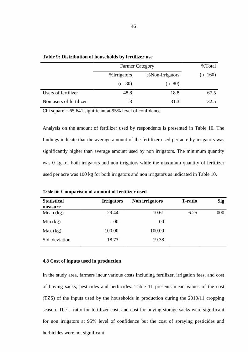
46

Table 9: Distribution of households by fertilizer use

Farmer Category %Total

(n=160) %Irrigators

(n=80)

%Non-irrigators

(n=80)

Users of fertilizer 48.8 18.8 67.5

Non users of fertilizer 1.3 31.3 32.5

Chi square = 65.641 significant at 95% level of confidence

Analysis on the amount of fertilizer used by respondents is presented in Table 10. The

findings indicate that the average amount of the fertilizer used per acre by irrigators was

significantly higher than average amount used by non irrigators. The minimum quantity

was 0 kg for both irrigators and non irrigators while the maximum quantity of fertilizer

used per acre was 100 kg for both irrigators and non irrigators as indicated in Table 10.

Table 10: Comparison of amount of fertilizer used

Statistical

measure

Irrigators Non irrigators T-ratio Sig

Mean (kg) 29.44 10.61 6.25 .000

Min (kg) .00 .00

Max (kg) 100.00 100.00

Std. deviation 18.73 19.38

4.8 Cost of inputs used in production

In the study area, farmers incur various costs including fertilizer, irrigation fees, and cost

of buying sacks, pesticides and herbicides. Table 11 presents mean values of the cost

(TZS) of the inputs used by the households in production during the 2010/11 cropping

season. The t- ratio for fertilizer cost, and cost for buying storage sacks were significant

for non irrigators at 95% level of confidence but the cost of spraying pesticides and

herbicides were not significant.

47

Table 11: Cost of the inputs used in 2010/11 cropping season in TZS per acre

Cost (TZS) Irrigators

(mean)

Non

irrigators

(mean)

T-ratio Sig Mean

difference

Fertilizer cost 64 215.2 161 483.3 -3.7 .000 -97 268.1

Cost of spraying 9 884.6 19 125.0 -2.3 .029 -9 240.3

Fees of water 5 000.0 .0

Sacks cost 10 634.2 30 948.6 -5.3 .000 -20 314.4

Note: No t-statistic for water fees because only irrigators were paying that fee.

4.9 Long-term economic viability of the Mkindo irrigation scheme

Table 12 presents findings on the values of the indicators used for assessing economic

viability of the Mkindo Irrigation Scheme. As can be seen from the table, the NPV of the

project was positive, indicating that it was economically viable. The BCR was also

positive and according to decision criteria, projects with BCR which are positive and

greater than one are economically viable because the discounted benefits are higher than

the discounted costs. The IRR was greater than the discount rate used to compute NPV

and BCR, and as we know, a project with an IRR higher than the discount rate is deemed

to be acceptable. The net benefit per unit capital invested was TZS 1 224 867.9.

These results support the findings by Vorgelegt (2001) who found that, NPV was a

positive number, BCR was positive number greater than one and IRR was greater than the

discount rate used in their study of costs and benefits of adopting runoff irrigation systems

which was conducted in Kakuma, northern Kenya. However, the results are contrary to

the finding by Hotes (1984), who argues that, the benefit/cost ratio of many irrigation

projects, especially in developing countries, is unfavorable because the primary benefits

are less than expected and primary costs. Kortenhorst (1983) supports Hote’s statements

by indicating that many projects were initiated on political grounds, with little attention

given to farmer’s needs or motivations. However, the findings and suggestion of Hotes

and Kortenhorst should be considered with great attention because the study which was

48

done by Inocencio et al, (2007) in assessing the costs and performance of irrigation

projects, by comparing Sub-Saharan Africa (SSA) and other developing regions, suggest

that, the popular view that SSA irrigation projects are expensive and not economically

viable has to be understood in its proper context. Using simple regional averages, the unit

costs in SSA appear to be higher than those for other regions. However, a careful look at

the details reveals that under certain conditions, unit costs of irrigation projects in sub-

Saharan Africa are not statistically different from those in non-SSA regions. Therefore,

this finding by Inocencio et al, (2007), suggests that projects should reflect specific

characteristics consistent with lower unit investment costs. Despite the argument of Hotes

(1984), Kortenhorst (1983) and Inocencio et al (2007) still, irrigation projects in Sub

Saharan Africa are viable and the missing requirements are to improve market

infrastructure and credit facilities for purchasing agricultural inputs.

4.9.1 Sensitivity analysis

The problem of uncertainty in cost-benefit analysis may be addressed, to some extent,

through sensitivity analysis. This type of analysis shows the variation in the measure of

the project worthiness, for example NPV, IRR and BCR, as changes are made to the

values of particular variables. Sensitivity analysis was carried out in this study to

determine the effects on the above-mentioned measures of project worthiness by varying

the different variables at different levels. As shown in Table 12, levels of 25%, 50% and

75% for variable cost, increase in yield and decrease in price were used to compute NPV,

BCR and IRR. The values of NPV and BCR were positive, and value of IRR was greater

than discount rate indicating that variation of variable cost, price and yield at those levels

will not affect the viability of the project.

49

Table 12: Economic viability of Mkindo irrigation scheme

Item Current

Status

25 50 75

%Increase in paddy yield:

Sum of discounted

revenues(TZS)

2 921 697 008

2 995 859 681 3 595 031 617 4 194 203 554

Sum of discounted

costs (TZS)

525 009 263 656 261 579 787 513 895 918 766 211

NPV (TZS) 2 396 687 745 2 305 818 102 2 773 737 722 3 241 657 342

BCR 5.56 4.56 4.56 4.56

IRR (%) 16.1 195 262

294

Net benefit per

capita(TZS)

353 748

1 531 084 1 837 301 2 143 518

% Increase in cost:

Sum of discounted

revenues(TZS)

2 921 697 008

2 921 697 008

2 921 697 008

2 921 697 008

Sum of discounted

costs (TZS)

525 009 263 656 261 579 787 513 895 918 766 211

NPV (TZS) 2 396 687 745 2 339 598 101 2 208 345 786 2 077 093 470

BCR 5.56 4.56 3.80 3.26

IRR (%) 16.1 149 152 132

Net benefit per

capita(TZS)

353 748

1 531 084 1 837 301 2 143 518

% Decrease in price of paddy

Sum of discounted

revenues(TZS)

2 921 697 008

6 371 336 538 4 247 557 692 2 123 778 846

Sum of discounted

costs (TZS)

525 009 263 525 009 263 525 009 263 525 009 263

NPV (TZS) 2 396 687 745 5 846 327 275 3 722 548 429 1 598 769 583

BCR 5.56 12.13 8.09 4.04

IRR (%) 16.1 183 117 52

Net benefit per

capita(TZS)

353 748

1 531 084 1 837 301 2 143 518

50

4.10 The economic impact of irrigation in the study area

4.10.1 The impact of irrigation on household income

Table 13 presents the mean incomes in TZS, obtained from crops sales, livestock sales,

wages and salaries, pensions and other sources of income. The table shows that the mean

income from crops for irrigators was significantly higher than the mean income from

crops of non-irrigators. However, there is no significant difference between irrigators and

non irrigators for income from livestock, petty business, wages, pension and other

sources. The high crop incomes obtained by irrigators are associated with high crop yields

per acre for irrigated crops. This suggests that irrigation has had positive impact on

household income because crop income account for the largest proportion of the total

household income. This finding supports the findings by Lipton (2007) in the study of

farm water and rural poverty in developing countries; Hussain (2005) in the study of pro-

poor intervention strategies in irrigated agriculture in Asia; Mwakalila (2004) and Cosmas

and Tamilwai (2005) in their studies done in Tanzania, who found that, the presence of

irrigation increased crop productivity and hence rural household income.

Table 13: Mean household income in 2010/11 cropping season

Income

source

Irrigators

(mean TZS)

Non irrigators

(mean TZS)

T-

ratio

Sig Min Max

Total income 1 891 700.0 2 582 100.0 -1.9 .053 .00 13 640 000.0

Crops 714 857.1 347 135.9 -5.7 .000 .00 13 040 000.0

Livestock 61 637.5 341 662.5 -2.5 .012 .00 5 452 000.0

Petty

business

90 893.7 197 850.0 -1.9 .058 .00 3 000 000.0

Wages 125.0 35 250.0 -2.6 .009 .00 800 000.0

Pension .0 2 187.5 - - .00 110 000.0

Other sources 7 812.5 1 875.0 1.0 .283 .00 400 000.0

Note: t-statistic was not computed for pension income because none of the irrigators

reported pension income

51

4.10.2 The impact of irrigation on income distribution

Table 14 presents finding on the income share regression-based inequality decomposition

by predicted income sources. It shows that the respondents in the study area depend

heavily on income from crops which they cultivate and that income contributes about

83.5% to the total income. Income share to total income from livestock and small business

activities were about 9% and 6.5% respectively. This means that the crop sub sector was

the main source of household income in the study area. Therefore, more investment

priority should be given to crop production projects in order to improve the welfare of the

people in the study area.

Table 14: Income share regression-based inequality decomposition by predicted

income sources

Sources Income Absolute Relative

Constant 0 0 0

Income from crops 0.834752 0.384342 0.824822

Income from livestock 0.090146 0.047531 0.102005

Income petty business 0.06454 0.027562 0.05915

Wages 0.007907 0.005434 0.011661

Pension 0.000489 0.000079 0.000169

Other income source 0.002165 0.001022 0.002193

Residual 0 0 0

Total 1 0.465969 1

Table 15 presents finding on the income distribution between irrigators and non-irrigators

in the study area. Gini coefficient was used to measure income distribution. Non-irrigators

had higher Gini coefficient compared to irrigators. Their values were 49.6% and 38.6%

for non-irrigators and irrigators respectively. This implies that income inequality among

non-irrigators was higher than income inequality among irrigators. This suggests that

irrigation schemes decreases the level of income inequality among famers and therefore

improve income distribution.

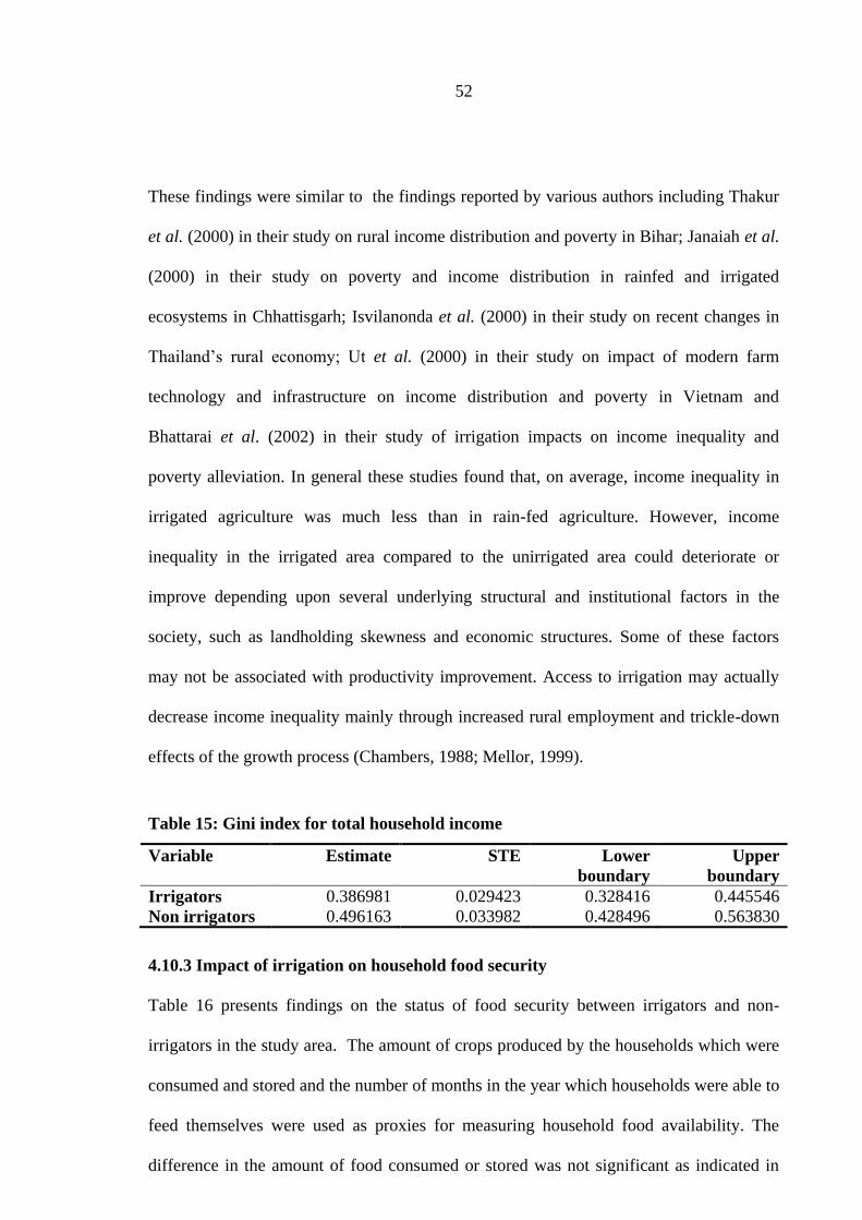
52

These findings were similar to the findings reported by various authors including Thakur

et al. (2000) in their study on rural income distribution and poverty in Bihar; Janaiah et al.

(2000) in their study on poverty and income distribution in rainfed and irrigated

ecosystems in Chhattisgarh; Isvilanonda et al. (2000) in their study on recent changes in

Thailand’s rural economy; Ut et al. (2000) in their study on impact of modern farm

technology and infrastructure on income distribution and poverty in Vietnam and

Bhattarai et al. (2002) in their study of irrigation impacts on income inequality and

poverty alleviation. In general these studies found that, on average, income inequality in

irrigated agriculture was much less than in rain-fed agriculture. However, income

inequality in the irrigated area compared to the unirrigated area could deteriorate or

improve depending upon several underlying structural and institutional factors in the

society, such as landholding skewness and economic structures. Some of these factors

may not be associated with productivity improvement. Access to irrigation may actually

decrease income inequality mainly through increased rural employment and trickle-down

effects of the growth process (Chambers, 1988; Mellor, 1999).

Table 15: Gini index for total household income

Variable Estimate STE Lower

boundary

Upper

boundary

Irrigators 0.386981 0.029423 0.328416 0.445546

Non irrigators 0.496163 0.033982 0.428496 0.563830

4.10.3 Impact of irrigation on household food security

Table 16 presents findings on the status of food security between irrigators and non-

irrigators in the study area. The amount of crops produced by the households which were

consumed and stored and the number of months in the year which households were able to

feed themselves were used as proxies for measuring household food availability. The

difference in the amount of food consumed or stored was not significant as indicated in

53

Table 16. However, the number of months in which households were able to feed

themselves was significant at 95% level of confidence as indicated in Table 16, implying

that irrigators were having significantly more months which they can feed themselves

from own produced food compared to non-irrigators. Based on food availability, these

findings imply that irrigators are more food secure than non-irrigators. Furthermore these

finding support the findings of previous studies by Lipton (2007) in his study on farm

water and rural poverty in developing countries; Hussain (2005) in his study on pro-poor

intervention strategies in irrigated agriculture in Asia; Mwakalila (2004) and Cosmas and

Tamilwai (2005) in their studies done in Tanzania; Ninno and Dorosh (2005) in their

study on food aid and food security in the short and long run in Asia and Sub-Saharan

Africa; Jean et al. (2005) in their study of food security and agricultural development in

Sub-Saharan Africa and Lipton et al. (2003) in their study of effects of irrigation on

poverty. Lipton et al. (2003) found that irrigation development improves the status of food

security because through irrigation farmers can improve production and can produce twice

a year.

Table 16: Status of food security in the study area

Food status Irrigators

(mean)

Non-irrigators

(mean)

T-ratio Sig

Crops consumed and

stored(bags)

9.775

9.337

0.323

0.747

Months feed from own

produce(months)

10.690

9.340

-5.399

0.000

Table 17 shows the number of meals households consumed per day. Most (73.6%) of the

households consumed three meals per day, with irrigators and non-irrigators accounting

for 47.2% and 26.4% of the households that, consumed three meals per day respectively.

The difference in the percentage of the number of meals households consume per day was

significant implying that irrigator’s households had more meals per day than non-

irrigators.

54

Table 17: Number of meals the households consumed per day

Number of meals Farmer Category %Total

(n=160) %Irrigators

(n=80)

%Non-irrigators

(n=80)

Three 47.2 26.4 73.6

Two 2.5 22.0 24.5

One 0 1.9 1.9

Chi square = 36.944 significant at 95% level of confidence

4.11 Asset ownership

Table 18 presents finding on values of assets owned by respondents. On average irrigators

owned assets with a value of TZS 1 857 862.5 while non-irrigators owned assets with a

value of TZS 2 392 262.5 but, the difference in the value of assets owned by the two

categories of farmers was not significant. The distribution of the asset values was

measured by using Gini index and the finding suggest that, distribution of assets among

irrigators was fair compared to non-irrigators as indicated by Gini coefficients of 67.2%

and 69.4% for irrigators and non-irrigators respectively. These finding supports the

finding by Tong et al. (2011) who suggest that irrigation, was unlikely to have a positive

impact on the amount of durable assets. Nevertheless the finding was contrary to the

finding by Dillon (2011) and Hussain and Hanjra (2004) who found that irrigation

development has positive effects on assets holding. Also Hagos and Holden (2003),

indicate that physical assets endowment, were reported to have a positive significant

effect on improving household welfare and food security status. Cheryl et al. (2009) states

that, “Ownership and control over assets such as land and housing provide multiple

benefits to individuals and households, including secured livelihoods, protection during

emergencies and collateral”.

55

Table 18: Values of assets owned by household

Statistical Measure Irrigators Non-irrigators T- ratios Sig

Mean(TZS) 1 857 862.5 2 392 262.5 0.748 0.456

Min 0.0 0.0

Max 29 215 000.0 42 250 000.0

Std. deviation 3 775 905.5 5 160 245.7

Gini index 0.6 0.7

4.12 Results of regression analysis

Table 19 presents findings of regression analysis. The model shows that only 72.7% of the

variation in paddy yields is explained by the variables included in the model. Only two of

the variables included in the regression model were influencing paddy yield significantly

at 95% level of confidence. These variables are irrigation dummy and amount of fertilizer

used. The coefficients of education and labor were found to be insignificant. The

irrigation dummy variable was included in the model to capture the effect of practicing

irrigation farming versus not practicing irrigation farming. The value of coefficient was

580.454 and was statistically significant at 95% confidence interval which indicates that

increasing the volume of irrigation water by 1% would increase paddy yield by about 580

kg. This finding supports studies done by Lipton (2007); Hussain (2005); Mwakalila

(2004) and Cosmas and Tamilwai (2005) who found that, the use of irrigation increases

crop productivity.

The amount of fertilizer per acre was another variable which significantly affect paddy

productivity. As shown in Table 19, there is a significant positive relationship between

amount of fertilizer used per acre and paddy yield per acre. Increasing fertilizer by

1kg/acre would increase paddy yield by 71.3 kg/acre. But this finding should be

interpreted carefully because there are necessary conditions for using fertilizer in order to

improve crop productivity as indicated by Abdoulaye and Sanders (2005); FAO (2002);

56

Fox and Rockstrom (2000); Morris et al. (2007); Shah and Singh (2001); Smith (2004);

Wichelns (2003); Yao and Shively (2007) who conducted studies on the efficient use,

productive efficiency, technical change and adverse impact of the fertilizers use in

different areas.

Table 19: Summary of regression results

Model variables

Unstandardized

Coefficients

t Sig.

Collinearity

Statistics

B Std. Error Tolerance VIF

Constant 488.85 199.92 2.44 0.016

Irrigators dummy 580.45 101.82 5.70 0.000 0.475 2.106

Education

dummy

65.42 188.05 0.34 0.728 0.964 1.037

Amount of

fertilizer in kg

0.71 0.41 1.72 0.000 0.720 1.388

Labor(number of

people

employed)

-0.87 4.50 -0.19 0.846 0.858 1.166

F= 34.541significant at 95% level of confidence; R= 0.727; R2 = 0.529

57

CHAPTER FIVE

CONCLUSIONS AND RECOMMENDATION

This study was concerned with the economics of small-scale irrigation in Tanzania. The

study was conducted at Mkindo Farmer Managed Irrigation Scheme in Mvomero District,

Morogoro Region. The main objective of the study was to analyze the economic viability

and determine the impact of the irrigation scheme on household income and food security.

The specific objectives of the study were (i) To analyse the economic viability of the

irrigation scheme; (ii) To determine the impact of the irrigation scheme on household

income and income distribution; and (iii) To determine the impact of the irrigation scheme

on household food security. This chapter presents the conclusions and recommendations

emerging from the major findings of the study.

5.1 Conclusions

5.1.1 Economic viability of the Mkindo scheme

An investment project is said to be economically viable if the magnitudes of the net

present value (NPV), benefit cost ratio (BCR) and internal rate of returns (IRR) are

positive, greater than one and greater than the used discount rate respectively. Since the

calculated NPV, BCR and IRR values of the Mkindo irrigation scheme were positive,

greater than one and greater than the discount rate respectively, it can be concluded that

Mkindo the irrigation scheme is economically viable.

5.1.2 Impact of irrigation on household income

The findings of the study indicate that crop production contributes more to the total

household income compared to other income sources, implying that many farmers in the

study area depend on crop production as their main source of income. Furthermore

irrigators were found to obtain significantly higher income from crops compared to non-

58

irrigators leading into significantly higher total household incomes among irrigators than

non-irrigators. Therefore it can be concluded that irrigation has had positive impact on

household income.

5.1.3 Impact of irrigation on income distribution

Gini index results indicate that Gini coefficient for irrigators was significantly lower than

that of non-irrigator, which implies that irrigation is inequality reducing leading into fair

income distribution among farmers practicing irrigation. Therefore it can be concluded

that irrigation had the positive impact on income distribution.

5.1.4 Impact of irrigation on household food security

The findings of the study show that irrigators were able to feed themselves from own

produced food for many months of the year compared to non-irrigators. Also the

proportion of irrigators who consumed three meals per day was significantly higher than

the proportion of non-irrigators who consumed three meals per day. Therefore, based on

food availability indicator, it can be concluded that, irrigation has positive impact on

household food security.

5.2 Recommendations

The following are recommendations based on the major findings of the study.

5.2.1 Promoting and up scaling small scale farmer managed irrigation schemes

The findings of the study indicate that Mkindo irrigation scheme was economically viable

and had positive impact on household income, income distribution and food security. This

suggests that it is worth investing in small scale irrigation schemes in the country. It is

therefore recommended that the government and development partners should promote

and upscale small scale irrigation in the country through increased resource allocation to

59

irrigation projects. Irrigation development will bring about increased agricultural

production and consequently improve the well-being of the rural population. However,

ex-ante economic viability analysis should be carried for each potential irrigation scheme

before making investments.

5.2.2 Promoting fertilizer use

The results of the regression analysis indicated the coefficient of fertilizer use to have a

significant positive effect on productivity of irrigated crops. This suggests that, promotion

of smallholder irrigation schemes should be accompanied by creating awareness on

benefits of using fertilizer to boost productivity of irrigated crops among smallholder

farmers. But also, creation of awareness should be accompanied by strategies to ensure

timely availability of fertilizers in rural areas at affordable price.

60

REFERENCE

Anastasios, M. (2006). Impact Analysis of Irrigation Projects: an Application of

Contingent Valuation Method. The American Journal of Agricultural and

Biological Sciences 1(1): 17 – 21.

Abdoulaye, T. and Sanders, J. H. (2005). Stages and determinants of fertilizer use in

semiarid African agriculture: The Niger experience. Agricultural Economics

32(2): 167–179.

Akyoo, A. and Lazaro, L. A. (2008). An Accounting Method-Based Cost-Benefit

Analysis of Conformity to Certified Organic Standards for Species in Tanzania.

DIIS Working Paper No. 30. Copenhagen, Denmark, 2008. 76pp.

Arrow K. J. (1973). Higher Education as a Filter. Journal of Public Economics 2 (3): 193

– 216.

Arrow, K.J., Cropper, M.L., Eads, G.C., Hahn, R.W., Lave, L.B., Noll, R.G., Portney,

P.R., Russell, M., Schmalensee, R., Smith, V.K. and Stavins, R.N. (1996). Is

there a role for benefit-cost analysis in environment, health, and safety regulation?

The Science 272: 221 – 222.

Averkamp, H. (2011). Evaluating Business Investments. [http://blog.Accounting

coach.com/payback-non discounted-capital-budgeting/] site visited on 11/10/2011.

61

Baker, J. L. (2000). Evaluating the Impact of Development Projects on Poverty. A

Handbook for Practitioners. The World Bank, USA. 217pp.

Balkema, A., Karoli, N. N., Henny, R. and Ralph, R. (2010). Socio-economic analysis of

constructed wetlands systems for hygienic sanitation in Tanzania. The Water

Practice and Technology 5(1): 6 – 8.

Bamidele, F., Ogunlade, I., Ayinde, O. and Olabode, P. (2010). Factors Affecting

Farmers’ Ability to Pay for Irrigation Facilities in Nigeria: The Case of Oshin

Irrigation Scheme in Kwara State. The Journal of Sustainable Development in

Africa 12(1): 339 – 340.

Barrett, C.B. (2002). “Food Security and Food Assistance.” In Handbook of Agricultural

Economics. Agricultural and Food Policy. Elsevier Ltd, Amsterdam. 628pp.

Barrett, C., Bell, R., Lentz, E., & Maxwell, D. (2009). Market Information and Food

Insecurity Response Analysis. Food Security (1): 151-168.

Berhanu, G. and Peden, D. (2002). Policies and Institutions to Enhance the Impact of

Irrigation Development in Mixed Crop–Livestock Systems. International

Livestock Research Institute Addis Ababa, Ethiopia. 260pp.

Bhattarai, M., Sakthivadivel, R. and Hussain, I. (2002). Irrigation Impacts on Income

Inequality and Poverty Alleviation: Policy issues and options for improved

management of irrigation systems. International Water Management Institute.

Working Paper No. 39. Colombo, Sri Lanka. 15pp.

62

Bierman, H. J. (1986). Implementation of Capital Budgeting Techniques. Financial

Management Survey and Synthesis Series 22 (3): 1- 24.

Bishop, R. C. and Heberlei, T.A. (1979). Measuring value of extramarket goods. The

American Journal of Agricultural Economics 61: 926 – 930.

Bishop, R. C., Heberlei, T. A. and Kealy, M. (1983). Contingent valuation of

environmental assets: comparisons with a simulated market. The Natural Resource

Journal 23: 619 – 633.

Boardman, D. H., Greenberg, A.R. and Vining, D.L. (2001). Cost–Benefit Analysis:

Collins College Publishers, New York. 526pp.

Bowker, J.M. and Stoll, J.R. (1988). Use of dichotomous choice nonmarket methods to

value of whooping crane resource. American Journal of Agricultural Economics

70: 372 – 381.

Brenters, J. and Henny, R. (2002). A Sub-Sector Approach to Cost Benefit Analysis:

Small-Scale Sisal Processing In Tanzania. Working Paper No. 4. Eindhoven

Centre for Innovation Studies, Netherlands. 22pp.

Bruce J. Feibel. (2003). Investment Performance Measurement. New York: Wiley, 2003

Cameron, T. A. and James, M.D. (1987). Efficient estimation methods for use with

c1osed-ended contingent valuation survey data. Review of Economic Statistics 69:

269 – 276.

63

Cameron, T. A. (1988). A new paradigm for valuation nonmarket goods using referendum

data: maximum likelihood estimation by censored logistic regression. Journal of

Environmental Economics and Management 13: 355 – 379.

Carlsso, F. and Johansson, S. O. (2000). Willingness to pay for air quality in Sweden.

Applied Economics 32: 661 – 669.

Chambers, R. (1988). Managing Canal Irrigation: Practical analysis from South Asia.

IBH Publishing Co. Pvt. Ltd., New Delhi, India. 281pp.

Cheryl, D., Caren, G. and Carmen, D. D. (2009). Collecting individual level asset data for

gender analysis of poverty and rural employment. Paper Presented at the FAO-

IFAD-ILO Workshop on Gaps. Rome, Italy, 31 March - 2 April 2009. 16pp.

Chiza, C. (2005): The Role of Irrigation in Agriculture, Food Security and Poverty

Reduction. Proceeding of the Discourse on Engineering Contribution in Poverty

Reduction. 18 - 19 March 2005, Dar es salaam, Tanzania. 28pp.

Chichilnisky, G. (1996b). The economic value of the earth's resources. Trends in Ecology

and Evolution 11: 135 – 139.

Chichilnisky, G. (1994). North-South trade and the global environment. American

Economic Review 84: 851 – 874.

Chichilnisky, G. (1997). The cost and benefit of benefit-cost analysis. Environment and

Development Economics 2: 202 – 206.

64

Cosmas, H. S. and Tamilwai, C. S. (2005). Changes in the Upland Irrigation System and

Implications for Rural Poverty Alleviation: A Case of the Ndiwa Irrigation

System, West Usambara Mountains Research Report No. 5. Mkuki Na Nyota

Publishers Ltd., Dar es Salaam, Tanzania. 55pp.

Denis, G. M. (2008). Adaptive Adoption of Rainwater Storage Systems by Farmers: A

Case of Makunga Ward in Same District. Dissertation for Award of MSc Degree

at Sokoine University of Agriculture, Morogoro, Tanzania.

Dillon, A. (2011). The Effect of Irrigation on Poverty Reduction: Asset Accumulation,

and Informal Insurance: Evidence from Northern Mali. The World Development

39 (12): 2165 – 2175.

Donaldson, C., Thomas, R. and Torgerso, D. (1997). Validity of open-ended and payment

scale approaches to eliciting willingness to pay. Applied Economics 29: 79 – 84.

Droogers, P. and Kite, G. ( 2001). Estimating productivity of water at different spatial

scales using simulation modeling. Research Report No. 53. International Water

Management Institute, Colombo, Sri Lanka. 16pp.

EAC (2010). Feasibility Study for a Natural Gas Pipeline from Dar es Salaam to Tanga

(Tanzania) and Mombasa (Kenya). Methodology for Financial and Economic

Analysis report. 28pp.

Evenson, R. E., Pray, C.E. and Rosegrant, M.W. (1999). Agricultural Research and

Productivity Growth in India. IFPRI Research Report No. 109. International Food

Policy Research Institute, Washington, USA. 103pp.

65

FAO (2002). Water and Fertilizer Use in Selected Countries. Discussion Paper. United

Nations, Rome, Italy. 91pp.

FAO (2009). Rome Declaration on World Food Security. World Food Summit, 13- 17

November 1996 Rome, Italy. 2pp.

FAO (2002). The report on world food day. A FAO report, 14 November 2002, Bangkok,

Thailand. 28pp.

FAO (1996). Agriculture and Food Security. World Food Summit, 15- 17 November

1996, United Nations, Rome, Italy. 15pp.

Fox, P. and Rockstrom, J. (2000). Water-harvesting for supplementary irrigation of cereal

crops to overcome intra-seasonal dry-spells in the Sahel. Physics and chemistry of

the earth. Hydrology Oceans and Atmosphere 25(3): 289 – 296.

Germana, C. L. (1993). A Socio- Economic Analysis of Modern Irrigation Projects under

Small Scale Farming: A Case of the Lower Moshi Irrigation Project in Kilimanjaro

Region. Dissertation for Award of MSc Degree at Sokoine University of

Agriculture, Morogoro, Tanzania, 117pp.

Greene, W. H., (1997). Econometric Analysis, New Jersey, Prentice Hall Press, 1997.

Hagos, F. Holden, S. (2003). Rural Household Poverty Dynamics in Northern Ethiopia

1997- 2000. Paper for CPRC Conference, Manchester, UK. 35pp.

66

Haile, T. H. (2008). Impact of Irrigation Development on Poverty Reduction in Northern

Ethiopia. Thesis for Award of PhD Degree at National University of Ireland, Cork,

289pp.

Hayes, C. and Hayes, A. (1999). Willingness to pay versus willingness to travel:

Assessing the recreational benefits from Dartmoor National Park. Journal of

Agricultural Economics 50(1): 124 – 139.

Hoevenagel R. (1994). An assessment of the contingent valuation method. In Valuing the

Environment: Methodological and Measurement Issues, Pethig, R. (Ed.). Kluwer

Publisher, Dordrecht. 372pp.

Hotes F.L. (1984). World Bank Irrigation Experience. Network paper 9d. Overseas

Development institute. ODI, London. 14pp.

Hussain, I. (2007). Direct and indirect benefits and potential Disbenefits of irrigation:

Evidence and lessons. Irrigation and Drainage 56: 179–194.

Hussain, I. and Hanjra, M. (2004). Irrigation and poverty alleviation: Review of the

empirical evidence. Irrigation and Drainage 53(1): 1 – 15.

Hussain, I., Mark, G. and Munir A. H. (2004). Agricultural Water and Poverty Linkages:

Case Studies on Large and Small Systems. International Water Management

Institute, Colombo, Sri Lanka. 108pp.

67

Hussain, I. (2005). Pro-poor Intervention Strategies in Irrigated Agriculture in Asia.

Poverty in Irrigated Agriculture: Issues, Lessons, Options and Guidelines, Final

Synthesis Report: International Water Management Institute (IWMI), Colombo,

Sri Lanka. 73pp.

Inocencio, A., Kikuchi, M.; Tonosaki, M.; Maruyama, A.; Merrey, D.; Sally, H.; de Jong,

I. (2007). Costs and performance of irrigation projects: A comparison of sub-

Saharan Africa and other developing regions. IWMI Research Report 109

Colombo, Sri Lanka: International Water Management Institute. 81pp.

Isvilanonda S., Ahmad A. and Hossain, M. (2000). Recent changes in Thailand’s rural

economy: Evidence from six villages. Economic and Political Weekly, December

30 : 4644 – 4649.

Janaiah, A., Bose, M.L. and Agrawal, A.G. (2000). Poverty and income distribution in

rainfed and irrigated ecosystems: Village studies in Chhattisgarh. Economic and

Political Weekly 30: 4664 – 4669.

Jean-Marc, B., Benoit, D., Françoise, G. and Tancrède, V. (2005). Food Security and

Agricultural Development in Sub-Saharan Africa: Building for More Support.

CIRAD Final Report, for FAO, Rome, Italy. 113pp.

Jrad S., Bashar N. and Hajar B. (2010). Food Security Models. National Agricultural

Policy Centre. Policy Brief No 33. Damascus, Syria. 32pp.

68

Johnson, N. L., Lilja, N. and Ashby, J. A. (2003). Measuring the impact of user

participation in agricultural and natural resource management research. Agricultural

Systems 78(2): 287 – 306.

Kadigi, M.J.K., Kashagili, J.J. and Mdoe, N.S.Y. (2003). The Economics of irrigated

paddy in Usangu basin in Tanzania: water utilization, productivity, income and

livelihood implications. Fourth WaterNets/Warfsa Symposium: water, science

technology and policy convergence and action by all, 15-17 October 2003,

Morogoro, Tanzania. 6pp.

Karimuribo, E.D., Kusiluka, L.J., Mdegela, R.H., Kapaga, A.M., Sindato, C., Kambarage,

D.M. (2005). Studies on mastitis, milk quality and health risks associated with

consumption of milk from pastoral herds in Dodoma and Morogoro regions,

Tanzania. Journal of Veterinary Science 6: 213-221.

Kabbiri R., Senkondo, E.M.M., Aboud, A.A., Israel, S.H., Mbaga, S., Msaky, J.J.T. and

Mkomwa, S.A. (2008). Profitability of Draught Power in Semi Arid Tanzania: A

case study of Hai, Kongwa and Siha districts. Food and energy crises 8 (271):

107-114.

Kissawike, K. (2008). Irrigation-based Livelihood Challenges and Opportunities. A

gendered technography of the Lower Moshi irrigation scheme in Tanzania. PhD

thesis submitted at Wegeningen University, Netherland. 235pp.

Kortenhorst L.F. (1983). Summary report on a workshop on small-scale irrigation in

Kenya. Proceedings of international Institute for Land Reclamation and

Improvement workshop, Nairobi, Kenya, 14 – 18 February, 1983. 55pp.

69

Lin, Grier C. I.; Nagalingam, Sev V. (2000). CIM justification and optimization. London:

Taylor & Francis. 36pp.

Lipton, M. (2007). Farm water and rural poverty reduction in developing Asia. Irrigation

and Drainage 56: 127–146.

Lipton, M., Litchfield, J. and Faurès, J.M. (2003). The Effects of Irrigation on Poverty: A

Framework for Analysis. Water Policy 5: 413 – 427.

Loomis, J., Pierce, C. and Manfredo, M. (2000). Using the demand for hunting licenses

to evaluate contingent valuation estimates of willingness to pay. Applied

Economics Letter 7: 435 – 438.

Lyimo, N. L., Mtenga, H., Kimambo, L. A., Hvelplund, A. E., Laswai, T. and

Weisbjerg, G.H. (2004). A survey on calf feeding systems, problems and

improvement options available for the smallholder dairy farmers of Turiani in

Tanzania. Livestock Research for Rural Development. An article,

[http://www.cipav.org.co/lrrd/lrrd16/4/lyim16023] Visited on 15th

March 2012.

Mahoo, H. F.; Mkoga, Z. J.; Kasele, S. S.; Igbadun, H. E.; Hatibu, N.; Rao, K. P. C.;

Lankford, B. (2007). Productivity of water in agriculture: Farmers’ perceptions and

practices. Comprehensive Assessment of Water Management in Agriculture

Discussion Paper 5 Colombo, Sri Lanka: International Water Management Institute.

37pp.

70

Magayane, M. D., Lankford, B. and Mahoo, H. F. (2003). Real or Imagined Water

Competition? The case of rice irrigation in the Usangu basin and Mtera/Kidatu

hydropower, Tanzania. 10pp.

Mboera, L.E.G., Mlozi, M.R.S., Senkoro, K.P., Rumisha, S.F., Mayala, B.K., Shayo,

E.H., Senkondo E., Mwingira, V.S. and Maerere A. (2007). Malaria and

Agriculture in Tanzania: Impact of Land Use and Agricultural Practices on

Malaria Burden in Mvomero district. National Institute for Medical Research,

Tanzania. 134pp.

McConnell, K.E. (1990). Models for referendum data: The Structure of discrete choice

models for contingent valuation. Journal of Environmental Economics and

Management 18: 19-24.

McConnell, K. and Haab, T. (2003). Valuing Environmental and Natural Resources. The

Econometrics of Non-Market. Edward Elgar Publishing Limited, Northampton,

USA. 326pp.

McCartney, M., Rebelo, L.M., Senaratna S. and de Silva, S.S. (2010). Wetlands,

agriculture and poverty reduction. IWMI Research Report 137.Colombo, Sri

Lanka. 39pp.

Mellor, J. W. (1999). Faster more equitable growth: The relationship between growth in

agriculture and poverty reduction. A conference paper presented at Harvard

Institute for International Development. Cambridge, USA. September 1999. 33pp.

.

71

Mitchell R. and R. Carson (1989). Using Surveys to Value Public Goods: The Contingent

Valuation Method, Resources for the Future. Resources for the Future Washington

DC. 488pp.

Mkavidanda, T.A.J. and Kaswamila, A.L. (2001). The Role of Traditional Irrigation

Systems (Vinyungu) In Alleviating Poverty in Iringa Rural District, Tanzania.

Repoa Research Report No. 01.2. Mkuki na Nyota Publishers, Dar es Salaam,

Tanzania. 45pp.

Mlozi, M.R.S, Shayo, E.H., Senkoro, K.P., Mayala, B.K., Rumisha, S.F., Mutayoba, B.,

Senkondo, E., Maerere, A. and Mboera, L.E.G. (2006). Participatory involvement

of farming communities and public sectors in determining malaria control

strategies in Mvomero District, Tanzania. Tanzania Hlth Res Bull. 8: 134pp.

Mnyenyelwa M.A. (2008). Traditional irrigation systems and livelihoods of small holder

farmers in Same district, Kilimanjaro Tanzania. A dissertation submitted in partial

fulfillment of the requirements for the degree of masters of Science in agricultural

economics of SUA. 94pp.

MOFEA (2010): National Strategy for Growth and Reduction of Poverty II. Government

document. 186pp.

Mohr, L. B. (1995). The Qualitative Method of Impact Analysis. Evaluation Review.

The American Journal of Evaluation 20 (1): 69-84.

72

Morris M, Kelly V.A., Kopicki R.J., Byerlee D. (2007). Fertilizer Use in African

Agriculture: Lessons Learned and Good Practice Guidelines. The International

Bank for Reconstruction and Development / World Bank, Washington D.C.

144pp.

Mwakalila S. (2004). Socio-Economic Aspects of Irrigated Agriculture in Mbarali District

of Tanzania. Research report. Department of Geography, University of Dar es

Salaam, Tanzania. 19pp.

Mwaniki, A. (2006). Achieving food security in Africa: Challenges and issues. Issue brief.

The United Nations. [http://www.un.org/africa/osaa/reports/Achieving Food

Security in Africa Challenges and Issues.pdf.] Site visited on 10/10/2011.

Ngaga, Y.M., Turpie J.K., and Karanja F.K. (2005). Preliminary economic assessment of

water resources of the Pangani River Basin, Tanzania: economic values and

incentives. East African Integrated River Basin Management Conference,

Morogoro, Tanzania. 9pp.

Naing, L., Winn, T. Rusli, B.N. (2006). Practical issues in calculating the sample size for

prevalence studies. Archives of Orofacial Sciences 1: 9 – 14.

Ninno, C. and Dorosh, P. A. (2005). Food Aid and Food Security in the Short and Long

Run: Country Experience from Asia and sub-Saharan Africa Food Aid and Food

Security in the Short- and Long Run. SP discussions paper no 0538. 122pp.

Ozdogan, M. (2011). Exploring the potential contribution of irrigation to global

agricultural primary productivity. Global Biogeochem. Cycles, Vol 25, 3016 –

3720.

73

Pradhan, M., Laura R. and Geert R. (1998). The Bolivian Social Investment Fund: An

Analysis of Baseline Data for Impact Evaluation. World Bank Economic Review,

12(3). 457- 82.

Pearce D., Marglin, S. and Sen, A.K. (1993). Guidelines for project evaluation. UNIDO,

New York, 1972. 383pp.

Puttaswamaiah K., (2002). On assessing the State of the art of the Contingent Valuation

Method for Valuing Environmental Changes. Cost-Benefit Analysis:

Environmental and Ecological Perspectives. Transaction Publishers. 430pp.

Ravallion, M. (2005). Assessing the Poverty Impact of Assigned Program In; The Impact

of Economic Policies on Poverty and Income Distribution: Evaluation Techniques

and Tools. (Edited by Bourguignon, F., Luiz A. and Da silva P.), Co publication of

the World Bank and Oxford University Press, New York: 103 – 122.

Rendall, A., B.C. Lyes and C. Eastman. (1974). Bidding games for valuation of aesthetic

environmental improvement. Journal of Environmental Economics and

Management 1: 132 – 149.

Rollins, K (1997). Wilderness canoeing in Ontario: Using cumulative results to update

dichotomous choice contingent valuation offer amounts. Ca: nmJian Joumal of

Agricultural Economics 45: 1-16.

Ryan, M. (1997). Should government fund Assisted Reproductive Techniques? A study

using willing to pay. Applied Economics 29: 841 – 849.

74

Scarpa R. (2000). Contingent valuation versus choice experiments: estimating the benefits

of environmentally sensitive areas in Scotland. Joumal of Agricultural Economics

51(1): 122-128.

Seller, C., J.P. Chavas and J.R. Stoll. (1986). Specification of the logic model. The case of

valuation of nonmarket goods. Journal of Environmental Economics and

Management 13: 382-390.

Shackley, P. and S. Dixon. (2000). Using contingent valuation to elicit public preferences

for water fluoridation. Applied Economics 32: 777-787.

Shah, T. and Singh, O. P. (2001). Can Irrigation Eradicate Rural Poverty in Gujarat?

Water Policy Research Highlight No.10. 8 p.

Shitundu, J. and Luvanga, N. (1998). The Use of Labour-Intensive Irrigation

Technologies in Alleviating Poverty in Majengo. Mbeya Rural. Research reports

no 93.3 Research on Poverty Alleviation, Dar es salaam, Tanzania. 49pp.

Smith L.E.D. (2004). Assessment of the contribution of irrigation to poverty reduction and

sustainable livelihoods. International journal of water resources development.

20(2): 243-257.

Steven Z., Tom H., Peter D. and Maureen R. (2012). The Potential Impact of Changes in

Immigration Policy on U.S. Agriculture and the Market for Hired Farm Labor: A

Simulation Analysis. Economic Research Report Number 135. USDA, USA.

42pp.

75

Stockle C. O. (2001). Environmental impacts of irrigation: A review paper. State of

Washington Water Research Center. 15pp.

SWMRG (2005). Experiences with Micro Agricultural Water Management Technologies:

Tanzania. Research report. The International Water Management Institute (IWMI),

Southern Africa Sub-regional Office, Pretoria, South Africa. 28pp.

Tarimo, A.K.P.R, Amy Mchelle, R. and Nganga, I. (2010). Evaluation of water

distribution systems at Igomelo Farmer-Managed Irrigation Scheme in Tanzania.

Second RUFORUM Biennial Meeting 20 - 24 September 2010, Entebbe, Uganda,

3pp.

Thakur, J., Bose, M.L., Hossain, M. and Jinaiah, A. (2000). Rural income distribution and

poverty in Bihar: Insights from village studies. Economic and Political Weekly 30:

4657- 4663.

Tong K. Hem S. Paulo S. (2011). The Impact of Irrigation on Household Assets. CDRI

Working Paper Series No. 57 (10): 25pp.

Ut T.T, Hossain, M. and Janaiah, A. (2000). Modern farm technology and infrastructure in

Vietnam: Impact on income distribution and poverty. The Economic and Political

Weekly 30: 4638-4643.

Valadez, J. and Bamberger, M. (1994). Monitoring and evaluating social programmes in

developing Countries: A handbook for policymakers, managers and researchers:

The World Bank, 1818 H Street, N.W., Washington, DC, USA. 407pp.

76

Vatn, A. and Bromley D.W. (1994). Choices without prices without apologies. The

Journal of Environmental Economics and Management 26 (2): 129-148.

Vorgelegt C. B. (2001). Costs and Benefits of Adopting Runoff Irrigation Systems. A case

study from Kakuma, northern Kenya.79pp.

Willis, K. and Powe, N.A. (1998). Contingent valuation and real economic commitments:

A private good experiment. The Journal of Environmental Planning and

Management 45(5): 611- 619.

Wierstra, E., van der Veen en A. and Geurts P. (1996), “Monetaire waardering van

milieuverandering: de Contingent Valuation methode”. Maandschrift Economie

60: 155 – 176.

Wichelns D. (2003). Policy Recommendations to Enhance Farm-Level Use of Fertilizer

and Irrigation Water in Sub-Saharan Africa. The Journal Sustainable Agriculture

23(2): 53-77.

World Bank (2006). Outline of Principles of Impact Evaluation: International Workshop

on Impact Evaluation for Development, 15 November 2006 - World Bank and the

DAC Evaluation, Network, USA. 9pp.

World Bank (1980). Economic and Social Analysis of Projects and of Price Policy: The

World Bank Staff Working Paper No. 369. 65pp.

Yao R.T, Shively G.E. (2007). Technical Change and Productive Efficiency: Irrigated

Rice in the Philippines. The Asian Econ. J. 21(2): 155-168.

77

Zerbe R. and Dively D. (1994). Calculations of Costs and Benefits in Partial Equilibrium.

Benefit–Cost Analysis: In Theory and Practice. Harper Collins, 1994.

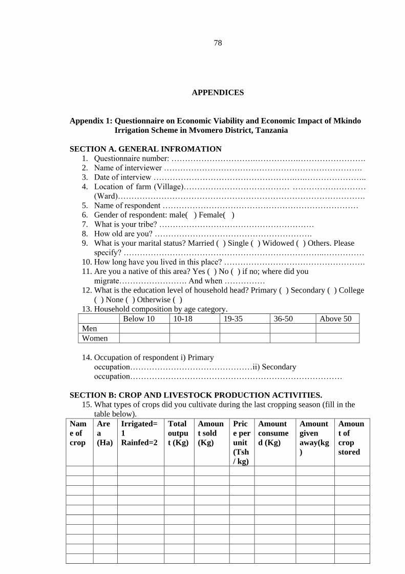
78

APPENDICES

Appendix 1: Questionnaire on Economic Viability and Economic Impact of Mkindo

Irrigation Scheme in Mvomero District, Tanzania

SECTION A. GENERAL INFROMATION

1. Questionnaire number: ………………………….…………….…………………….

2. Name of interviewer ……………………………………………………………….

3. Date of interview …………………………………………….….…………………..

4. Location of farm (Village)………………………………… ………………………

(Ward)……………………………………………………………………………….

5. Name of respondent ………………………………………………………………

6. Gender of respondent: male( ) Female( )

7. What is your tribe? …………………………………………………

8. How old are you? ………………………………………………….

9. What is your marital status? Married ( ) Single ( ) Widowed ( ) Others. Please

specify? ………………………………………………………………..……………

10. How long have you lived in this place? …………………………………………….

11. Are you a native of this area? Yes ( ) No ( ) if no; where did you

migrate……………………. And when ……………

12. What is the education level of household head? Primary ( ) Secondary ( ) College

( ) None ( ) Otherwise ( )

13. Household composition by age category.

Below 10 10-18 19-35 36-50 Above 50

Men

Women

14. Occupation of respondent i) Primary

occupation………………………………………ii) Secondary

occupation……………………………………………………………………

SECTION B: CROP AND LIVESTOCK PRODUCTION ACTIVITIES.

15. What types of crops did you cultivate during the last cropping season (fill in the

table below).

Nam

e of

crop

Are

a

(Ha)

Irrigated=

1

Rainfed=2

Total

outpu

t (Kg)

Amoun

t sold

(Kg)

Pric

e per

unit

(Tsh

/ kg)

Amount

consume

d (Kg)

Amount

given

away(kg

)

Amoun

t of

crop

stored

79

16. What types of livestock are you keeping?

Type of livestock Number at the

beginning of

2011

Number sold

in 2011

Price per unit Number

remaining at the

end of 2011

17. Please fill the table below for 2011.

Type of

livestock

Product

produced

Amount of

product sold

Per unit

price (Tsh)

of the

product

Amount

given

away

Amount

consumed

IRRIGATION PRACTICES

18. Please fill the table below:

Total land owned by

household

Amount of land that can be

irrigated

Amount of land that was

irrigated last season

19. What irrigation method do you use? Center-Pivot ( ); Drip ( ); Flood ( );

Furrow ( ); Gravity ( ); Rotation ( ); Sprinkler ( ); Sub irrigation ( );

Traveling Gun ( ); Supplemental ( ); Surface ( ) or otherwise; Explain

………………………………………………………………………………………

………………………………………………………………………………………

……...............

20. Water for irrigation is readily available? Yes ( ) or No ( ) if no, what mechanism

is used to ensure fairy distribution of water for irrigation to farmers?

………………………………………………………………………………………

………………………………………………………………………………………

………………………………………………………………………………………

………………………………………………………………………………………

21. What crops do you grow in irrigated land?

.....................................................................................................................................

.....................................................................................................................................

.....................................................................................................................................

80

Is there any crop that you grow and harvest twice a year? Yes ( ) or No ( ) if yes

what crop(s)? Please fill the table below:

Irrigated crop Acreage Output (specify units)

First crop

Second crop

Third crop

SECTION C: ECONOMIC IMPACT OF THE IRRIGATION SCHEME

22. How much money did your household earn from the following non-farm income

sources in 2010/2011 cropping season?

Source of income

Monthly income in TSH.

Petty business

Wages and salaries (employment)

Retirement pensions

23. Has your agricultural income increased ( ), remained the same, ( ) or declined (

) after the commencement of the irrigation scheme?

24. For either a answer, provide above give an

explanation…………………………………………………………………………

………………………………………………………………………………………

………………………………………………………………………………………

25. 26. How reliable is income obtained from agriculture now compared to the period

before irrigation? (i) Very reliable ( ) (ii) .Reliable ( ) (iii) Less reliable ( )

(iv) Not reliable at all ( ).

27. Would you say you spend more time now in the field compared to years before

commencement of the irrigation scheme? ( )Yes or( ) No

28. If you spend more time on the field now, what are the reasons for that?

……….….…………………………………………………………………………

………………………………………………………………………………………

29. How much time do you spend in the field per day?........................................

30. Please fill the table below.

Activity Number of

persons

Number of days

used

Type of

labor

(family,

exchange or

hired labor)

Indicate if

fulltime,

partime or

both

Ploughing

Planting

Cultivating

Weeding

Fertilization

Spraying

Irrigating

Harvesting

81

31. How do you pay them?

Type of payment Per hours Per day Per week Per month

Amounts in

(Tsh)

32. Please provide information on variable costs of inputs (including hired labour)

used during last (2010/2011) season.

Crop/Livestock

enterprises

Inputs used, amounts and costs

Type of

input

Amount (specify

e.g.(Bags/kg/litre)

Cost per unit

e.g. Tsh/Bag

Total cost

1.

2.

3.

4.

33. Has the number of people employed in your farm

increased ( )

remained the same ( )

Or declined ( ) compared to the years before irrigation.

34. If the number of employees has either increased or decreased, please explain the

reason(s) for that.

……………………………….………....………………………………

………………………………………………..………….…………………………

………

……………………………………………..………….……………………………

………

FOOD SECURITY

35. Comparing the period before and after your involvement in irrigation, is your

household? (a) More food secure ( ) (b) no change ( ) (c) less food secure (

).

36. Do your household members sometimes go hungry? ( )Yes or ( )No

37. Are you able to feed yourself from own produced food throughout the year until

the next harvest? Yes ( ) or No ( ).

82

38. If No, how many months in a year is your household able to adequately feed itself

from own produced food? Tick on the mentioned months.

Months Put tick on the mentioned months

January

February

March

April

May

June

July

August

September

October

November

December

39. How many meals does your household consume per day? a) three ( )b) two( ) c)

one( ) d) sometimes no meal at all( ) e) other (

)(state)………………………………………………………………………………

………………………………………………………………………………………

………………………………………………………………………………………

………………………

40. How much money does your household spend on food per month?

TSH…………...……………………………………………………………………

……..

41. Please rank the sources of food in your household in 2010/11 in order of

importance (Most important =1)

Source of food Rank

Own farm production

Purchase

Given by

neighbours/friends/relatives

Government food relief

42. If you purchase food, how do you compare the amount of food purchase with the

amount you used to purchase before being involved in irrigation? (i) Increased (

) (ii) Remained the same ( ) (iii) Decreased ( ).

43. Please fill the table below.

Total Income

earned

Income for

food

Income for

health service

Income for

children

education

Others activity

83

44. Please indicate household assets (and their value) which were purchased since you

started irrigated agriculture?

Type of assets Number Value

Physical e.g. land, livestock, new house construction or rehabilitation of old house etc

Land

New house constructed

(Indicate stage of new house)

Rehabilitation of old house

Livestock purchase

Equipment and tools acquired e.g. ox-carts, TV, radio, mobile phone, plough, hand hoe

etc

Other (specify)

84

Appendix 2: Questionnaire for Non Irrigator Farmers. Questionnaire on Economic

Viability and Economic Impact of Mkindo Irrigation Scheme In

Mvomero District, Tanzania

SECTION A. GENERAL INFROMATION

1. Questionnaire number: …………………………….……………………………….

2. Name of interviewer ……………………………………………………………….

3. Date of interview …………………………………………………………………..

4. Location of farm (Village)………………………………… ………………………

(Ward)……………………………………………………….

5. Name of respondent

…………………………………………………………………

6. Gender of respondent: male( ) Female( )

7. What is your tribe? …………………………………………………

8. How old are you? ………………………………………………….

9. What is your marital status? Married ( ) Single ( ) Widowed ( ) Others. Please

specify? ……………………………………………………………………………

10. How long have you lived in this place? …………………………………………….

11. Are you a native of this area? Yes ( ) No ( ) if no; where did you

migrate……………………. And when ……………

12. What is the education level of household head? Primary ( ) Secondary ( ) College

( ) None ( ) Otherwise ( )

13. Household composition by age category.

Below 10 10-18 19-35 36-50 Above 50

Men

Women

14. Occupation of respondent i) Primary

occupation………………………………………ii) Secondary

occupation……………………………………………………………………

SECTION B: CROP AND LIVESTOCK PRODUCTION ACTIVITIES.

15. What types of crops did you cultivate during the last cropping season (fill in the

table below).

Nam

e of

crop

Are

a

(Ha)

Irrigated=

1

Rainfed=2

Total

outpu

t (Kg)

Amoun

t sold

(Kg)

Pric

e per

unit

(Tsh

/ kg)

Amount

consume

d (Kg)

Amount

given

away(kg

)

Amoun

t of

crop

stored

85

16. What types of livestock are you keeping?

Type of livestock Number at the

beginning of

2011

Number sold

in 2011

Price per unit Number

remaining at the

end of 2011

17. Please fill the table below for 2011.

Type of

livestock

Product

produced

Amount of

product sold

Per unit

price (Tsh)

of the

product

Amount

given

away

Amount

consumed

SECTION C: ECONOMIC IMPACT OF THE IRRIGATION SCHEME

18. How much money did your household earn from the following non-farm/farm

income sources in 2010/2011 cropping season?

Source of income

Monthly income in TSH.

Petty business

Wages and salaries (employment)

Retirement pensions

19. How reliable is income obtained from agriculture now compared to other

activities? (i) Very reliable ( ) (ii) .Reliable ( ) (iii) Less reliable ( ) (iv) Not

reliable at all ( ).

20. For either a answer, provide above give an

explanation…………………………………………………………………………

………………………………………………………………………………………

………………………………………………………………………………………

86

21. How much time do you spend in the field? ……………………………………

22. Please fill the table below.

Activity Number of

persons

Number of days

used

Type of

labor

(family,

exchange or

hired labor)

Indicate if

fulltime,

partime or

both

Ploughing

Planting

Cultivating

Weeding

Fertilization

Spraying

Irrigating

Harvesting

23. How do you pay them?

Type of payment Per hours Per day Per week Per month

Amounts in

(Tsh)

24. Please provide information on variable costs of inputs (including hired labour)

used during last (2010/2011) season.

Crop/Livestock

enterprises

Inputs used, amounts and costs

Type of

input

Amount (specify

e.g.(Bags/kg/litre)

Cost per unit

e.g. Tsh/Bag

Total cost

1.

2.

3.

4.

25. Do you employ people during the farming season? Yes ( ) No ( )

26. If Yes how many people? ( )

87

FOOD SECURITY

27. Do your household members sometimes go hungry? ( )Yes ( )No

28. Are you able to feed yourself from own produced food throughout the year until

the next harvest? Yes ( ) No ( ).

29. If No, how many months in a year is your household able to adequately feed itself

from own produced food? Tick on the mentioned months.

Months Put tick on the mentioned months

January

February

March

April

May

June

July

August

September

October

November

December

30. How many meals does your household consume per day? a) thrice ( ) b) twice(

) c) once( ) d) sometimes no meal at all( ) e) other

;explain………………………….

………………………………………………………………………………………

………………………………………………………………………………………

31. How much money does your household spend on food per month?

TSH…………...……………………………………………………………………

32. Please rank the sources of food in your household in 2010/11 in order of

importance (Most important =1)

Source of food Rank

Own farm production

Purchase

Given by

neighbours/friends/relatives

Government food relief

33. Please fill the table below.

Total Income

earned

Income for

food

Income for

health service

Income for

children

education

Others activity

88

34. Please indicate household assets (and their value) which were purchased since

2009?

Type of assets Number Value

Physical e.g. land, livestock, new house construction or rehabilitation of old house etc

Land

New house constructed

(Indicate stage of new house)

Rehabilitation of old house

Livestock purchase

Equipment and tools acquired e.g. ox-carts, TV, radio, mobile phone, plough, hand hoe

etc

Other (specify)

89

Appendix 3: Discounted Cost and Benefit

Forecasted Cost

Forecasted

Revenue Net Revenue Year Discounted net Revenue

47935150 84725000 36789850 1 32848080.36

47385750 205820000 158434250 2 126302814.1

94771500 224607500 129836000 3 92414700.26

80926780.64 450422920.6 369496140 4 234821476.9

77907470.41 488239270.2 410331799.8 5 232833283

77282094.76 511367824.6 434085729.8 6 219921340

77152563.63 525571870 448419306.4 7 202842121.4

77125734.45 534373334.9 457247600.4 8 184674636.9

77120177.45 539886670.1 462766492.7 9 166878236.5

77119026.45 543379286.9 466260260.4 10 150123325.1

77118788.05 545617011.9 468498223.9 11 134682044.2

77118738.67 547063284.7 469944546 12 120623060

77118728.44 548006063.1 470887334.7 13 107915223.6

77118726.32 548623459.7 471504733.4 14 96479210.19

77118725.88 549031117.5 471912391.6 15 86216629.59

77171123.25 549300822.1 472129698.9 16 77014581.08

77129578.62 549479543.6 472349965 17 68795099.35

78191024.33 549600403.7 471409379.4 18 61301882.47