1

FEASIBILITY AND ECONOMIC VIABILITY OF ESTABLISHING A WINE GRAPE

VINEYARD IN MORAGA, CA

Presented to the

Faculty of the Agribusiness Department

California Polytechnic State University

In Partial Fulfillment

Of the Requirements for the Degree

Bachelor of Science

By

Vincent Joseph Bruzzone

June 2012

© 2012 Vincent Joseph Bruzzone

2

ABSTRACT

This study was undertaken to determine the feasibility of establishing a wine grape

vineyard in Moraga, CA, and whether or not it would be economically viable within a ten year

period. The proposed vineyard site consists of 30 acres of grazing land.

A price forecasting model for wine grapes was intended to aid in revenue analysis, but

due to a faulty model, a simple trend analysis was utilized instead. The microclimate was

analyzed and yielded several different varietals that were suitable for the area. Net Present Value

and Break-even analysis were used to see if the vineyard was profitable by year ten of

establishment. Production and establishment costs were taken from a UC Davis cost study of a

Sonoma County Vineyard with similar features.

The study concluded suitable grape varietals of Pinot Noir and Chardonnay could be used

on the vineyard. The Net Present Value for either a Pinot Noir vineyard or a Chardonnay

vineyard was negative at year ten of production. Further analysis showed that the NPV of the

Pinot Noir vineyard became positive by year twelve of production. The Pinot Noir vineyard also

broke even in year ten, and the Chardonnay vineyard was still at a negative profit by year ten of

production.

3

TABLE OF CONTENTS

Chapter Page

I. INTRODUCTION 1 Statement of the Problem 2 Hypotheses 2 Objectives of the Study 4 Significance of the Study 4 II. REVIEW OF THE LITERATURE 6 The Wine Industry Today 6 History of California Vineyards 7 Trends in the California Wine Grape Industry 8 Wine Budget Studies 9 Vineyard Establishment Costs 10 Initial Varietal Selection Factors: Soil and Climate 10 Varietal Yield 12 Rootstocks 12 Predicting California Wine Grape Prices 13 III. METHODOLOGY 15 Procedures for Data Collection 15 Procedures for Data Analysis 16 Assumptions and Limitations 19 IV. DEVELOPMENT OF THE STUDY 20 Microclimate Analysis 20 Soil Analysis 21 Varietal and Rootstock Selection 23 Wine Grape Price Forecasting 25 Cost Analysis 29 Net Present Value Analysis 33 Break-Even Analysis 35 Interpretation of Results 34 V. SUMMARY, CONCLUSIONS, AND RECOMMENDATIONS 36 Summary 36 Conclusions 37 Recommendations 38 References Cited 40 APPENDIX 43

LIST OF TABLES

4

Table Page 1. Ideal Climate for Chardonnay, White Riesling, Viognier, Sauvignon Blanc,

Cabernet Sauvignon, and Pinot Noir Grapes 8 2. Annual Yields of Cabernet Sauvignon, Pinot Noir, and Chardonnay 12 3. Moraga Degree Days 21

4. Physical Soil Sample Results 23

5. Rootstock Selection 25 6. Projected Grape Prices 2012 – 2026 28

7. Vineyard Establishment Cost and Cost to Produce Wine Grapes 30 8. Pinot Noir Net Returns 31 9. Chardonnay Net Returns 31 10. Projected Yearly Revenues Pinot Noir 32 11. Projected Yearly Revenues Chardonnay 32 12. Net Present Value Pinot Noir Vineyard (Year 1-10) 33 13. Net Present Value Chardonnay Vineyard (Year 1-10) 34 14. Further Net Present Value Pinot Noir Vineyard (Year 1-12) 35

15. Break-even for Pinot Noir Vineyard 35

16. Break-even for Chardonnay Vineyard 35

5

LIST OF FIGURES

Figure Page 1. Graph of Break-even Yield 3 2. California Market Prices Received by Grower of Pinot Noir, Zinfandel,

Chardonnay, and Sauvignon Blanc (1991-2011) 26 3. Pinot Noir Price Range 2012-2026 27

4. Chardonnay Price Range 2012-2026 28

6

CHAPTER I

INTRODUCTION

Upon being accepted into the Cal Poly AgriBusiness program, I felt somewhat out of

place, having no agricultural experience or background like many of the other students did.

Throughout my time here I have come to learn that it may have been a blessing in disguise to

stick with the major I had chosen. Russell Bruzzone, my grandfather, was a visionary and a

pioneer who helped build and develop what is now the town of Moraga, California in Contra

Costa County. His specialties included commercial and residential developments in the area

when the land was sparsely populated by a few farmers. In doing this, he acquired plots of land

throughout the area as the town began to grow in size.

Over time governmental restrictions of real estate development and land use have

noticeably increased to the highly regulated form we see today. Restrictive zoning enforced by

the local government has essentially ruled out any feasible housing developments on the specific

parcel in question in southwest Moraga. Landowners should have the right to manage their land

as they wish within reason. It becomes a losing battle trying to fight the local government agency

in a courtroom over land use rights when they are armed with taxpayers’ money at their disposal,

and the landowner is using hard earned money out of his pocket. With increasing property taxes,

there is subsequent pressure to instill some sort of income generating operation in the near future.

Further, there have been efforts by the local government agency to gain an open space easement

on the land, which essentially signs over all developmental rights of the land to the local

government. This has encouraged the consideration of finding a viable alternative to housing

7

developments in the regulated plot. With the land just sitting and accumulating property taxes,

something should be done.

A premium wine grape vineyard could very well be the solution. One of the key features

in vineyard establishment is grape varietal selection. The decision is based upon a wide range of

variables which includes the complexities of microclimate, and soil composition. Careful

analysis of these site factors as well as favorable future conditions will ultimately affect whether

high quality grapes suitable for wine production can be produced.

The terrain of the property in question includes a hillside that flows into the valley below.

Years ago, a walnut orchard was planted and maintained in the valley floor, though it has been

neglected and is not suitable for further production. The ideal vineyard location for this property

is on the lower to middle hillsides approaching the ridge, most of which are already zoned for

Agricultural use.

Problem Statement

What varietal of premium wine grape would be most environmentally, and economically

viable on 30 acre plot of land in Moraga? What will the market price of this specific grape

resemble fifteen years from now?

Hypotheses

The grape of choice will be Cabernet Sauvignon, Pinot Noir, or Chardonnay with varying

rootstocks. The market price of the grape selected will likely increase over the next fifteen years.

8

A positive net present value will show that the vineyard is economically viable (NPV >0), and a

break-even analysis will show that a profit can be made after year ten of establishment with a

break-even yield of 4.5 tons per acre.

Figure 1 - Graph of Break-even Yield

4.5

BE Yield

Tons

$/Ton

0

Revenu

Cost

9

Objectives

1) To identify a premium wine grape variety and rootstock that would thrive on a plot of land in Moraga, out of the 100+ wine varietals produced in California.

2) To forecast the market price (revenue side) of the selected grape for the upcoming fifteen years.

3) To evaluate the cost factors of establishing the vineyard, and to determine its economic feasibility in the predicted market conditions.

Significance of the Study

As laws and regulations on real estate use continually become stricter, land owners,

farmers, and developers are looking for new ways to generate income from their land. In smaller

towns similar to Moraga, new zoning laws have restricted building houses on ridgelines, along

with several other anti-development regulations. Instead of this land collecting property tax over

the years, a hillside vineyard would not only add to the beauty of the landscape, it would provide

income to the landowner. There are many California landowners in this same position due in part

to the progressive restrictions placed upon real estate today. The unique climate and landscape of

California provides these landowners with the option to pursue agricultural uses for their land

when their original intention to develop is thwarted. Fisher (2010) found that there were 6,223

wineries in the United States, while 3,047 reside in California alone. The high quality wine grape

10

producing areas of California are North Coast, Central Coast, and Sacramento Valley (Fisher

2010).

Moraga is contained in Crush District 6, which includes Alameda, Contra Costa, Santa

Clara, San Francisco, San Mateo, and Santa Cruz Counties (Grape Crush Report 2011).

Although grape production in this area is often shadowed by the established growers to the north,

the viticulture business has the potential to thrive in smaller towns like Moraga. Prior to the

recession, wine grape prices were on the rise, especially Pinot Noir and Chardonnay (Grape

Crush Report 1991-2011). The trends in price increase have prompted people to enter the grape

production industry over the last few years. A vineyard such as this would not only bring

seasonal and permanent grape production jobs to the area, it would increase tourism and

ultimately benefit the town as a whole. The results of this study will provide an insight on the

research process, overall cost, and market analysis of establishing a small scale vineyard in

Contra Costa County.

11

CHAPTER II

REVIEW OF THE LITERATURE

The Wine Industry Today

Wineries in California today are moving towards vertically integrating all aspects of the

wine making and selling process by incorporating grape farming, wine production, and wine

distribution into their businesses. Some modern day vineyards are also leaning more towards a

sustainable and organic approach to the grape growing process to keep up with consumer trends.

In the changing economy, wine businesses must adapt “historic survival lessons learned from

their past” (Geraci 2004). Wine entrepreneurs of the past were forced to rebuild each time the

wine market was devastated by events including the Great Depression, Prohibition, and World

War II. In the last several years we have seen the greatest economic downturn in our nation’s

history since 1929, which has made people think twice before investing their money while this

real estate driven recession still looms.

Increasing wine grape prices would present opportunities for landowners to invest in this

prominent industry, although there is a certain way to go about doing so. Geraci recalls the time

when California wineries were beginning to populate the area saying, “Small wineries that did

not consolidate had to adapt by forming local niche markets” or they simply went out of

business. While the wine market today is dominated by large companies, a large competitive

fringe of small scale vineyards and wineries still seem to profit. Although these smaller wineries

demand a price premium for their product, people are still willing to purchase these smaller

12

production wines. Consumer trends are leaning more toward craft and locally produced products,

which presents a small niche market in the wine industry today.

History of California Vineyards

Looking back on the growth of the wine industry, expansion caused wine growers to seek

out the best location that would be able to sustain the increased demand for wine grapes. Peters

(1984) described how the Central Valley was flooded with vineyards, but the overall goal for

them was high production of lower quality wine grapes. Most of the areas that produced

premium wine grapes are “coastal inland valleys”, where climates are “distinctly cooler than the

Central Valley” (Peters 1984). These coastal areas have very similar microclimates to the famous

wine regions of the world (Peters 1984). For example, “Oakville in the Napa Valley averages

2,300 degree days, similar to Beaune in Burgundy with its 2,400 degree days” (Peters 1984). In

California, the different climates for wine grape production are classified using a heat-

summation index of the number of degrees over 50oF for each day of the growing season, which

tends to run from April 1 to October 31. These degree days are characterized into five different

regions of California.

• Region I: Below 2,500 degree days

• Region II: 2,500 – 3,000 degree days

• Region III: 3,000 – 3,500 degree days

• Region IV: 3,500 – 4,000 degree days

• Region V: Over 4,000 degree days

Source: Winkler 1949

13

The following table shows the climate required and the more prominent growing regions

for several grapes grown in California.

Table 1 - Ideal Climate for Chardonnay, White Riesling, Viognier, Sauvignon Blanc, Cabernet

Sauvignon, and Pinot Noir Grapes

Wine Grape Ideal Climate Concentration

Chardonnay 2,500 Degree Days or Fewer – 3,000

Monterey, Napa, Sonoma County

White Riesling 2,500 Degree Days or Fewer Monterey, Santa Barbara County

Viognier 3,000 – 3,500 Degree Days Alexander Valley

Sauvignon Blanc 2,500 Degree Days or Fewer Napa, Sonoma County

Cabernet Sauvignon 3,000 – 3,500 Degree Days Alexander Valley, Sonoma County

Pinot Noir 2,500 Degree Days or Fewer Mendocino, San Luis Obispo, Sonoma County

Source: Peters 1984

Trends in the California Wine Grape Industry

California accounts for 92 percent of wine grape production in the United States, with

four major wine producing regions in the state: the North Coast (Napa and Sonoma Valleys),

Central Coast (San Mateo County to Santa Barbara), Central Valley (Sacramento and San

Joaquin Valleys), and the Southern Valley (Kern and San Bernardino Counties) (Green et al.,

2008). According to Green et al (2008), the past 30 years have seen wine grape acreage,

14

production, and prices received by the growers steadily increase. More importantly, prices

received for Pinot Noir grapes have raised above the rest of the California red wine grapes.

While acreage for Cabernet Sauvignon has increased dramatically, acreage for Pinot Noir has

stayed relatively low, providing significant demand for Pinot Noir grapes. Prices received for

Chardonnay grapes has been downward sloping for the past couple years, but is currently on an

upward trend. This can be explained by the high acreage of Chardonnay planted in the 1990’s,

to a plateau from 2000 to 2010. The demand for grapes used in ultra-premium wines will

increase in the future, prompting further productions of Pinot Noir, Cabernet Sauvignon, and

Merlot grapes (Green et al 2008).

Wine Budget Studies

Past studies shed light on the methodology and conclusions reached for similar tests of

feasibility. Pauli (2009) analyzed whether a Mendocino family pear ranch could be converted

into a premium wine grape vineyard. With break-even analysis he concluded that it would take

six years in full production to cover set up costs, and that the property should be converted to

grow grapes. Snodgrass (1985) sought to develop an econometric price forecast model to predict

future wine grape prices. He started with multiple regression analysis, but found them to be

ineffective. After turning to simple trend analysis he found wine grape prices would continue to

decrease, and advised a potential investor to wait for successive changes over time until a better

market equilibrium was reached to enter the vineyard business. Hanson (1976) detailed the

process and costs to convert a 25 acre walnut orchard to a premium wine vineyard. He found

conversion and set up costs were too great to allow a profit within projection of his study. Even

15

though his study was conducted a several years ago, his detailed description on vineyard

establishment inputs will prove useful.

Vineyard Establishment Costs

Once a grape is selected and a forecasted market price for that grape has been found, a

break-even analysis and net present value analysis will be conducted. DeMoura and Klonsky

(20010) focused on a proposed Sonoma County vineyard and determined it would cost $29,138

per acre to establish a Cabernet Sauvignon vineyard in the first year. The proposed site to be

established was 30 acres of existing vines, so costs in the first year of establishment will be lower

once vineyard removal is factored out. In this study the vineyard was removed because the vines

were old and not meeting adequate production. Adjustments of land lease costs, property taxes,

and other various expenses will also lower the overall cost per acre for establishment. In order to

maintain this vineyard and produce wine grapes the yearly costs per acre are $12,304 (DeMoura

and Klonsky 2010).

Initial Varietal Selection Factors: Soil and Climate

There are many factors that constitute the suitable microclimate and weather conditions

for premium grape production. Winkler (1949) described how table wines were better when the

ideal varieties are grown in cool regions, as this achieves a high degree of acidity, low pH, and

the development of good color. Even though this source is dated, modern wine grape growers

16

still refer to his research on climate and degree days as a standard of measurement. The town of

Moraga remains relatively cool because of its location just over the hill from Berkeley and

Oakland, and its close relation to the San Leandro Reservoir. The summer weather in this area of

Moraga tends to be warm during the day, and is cooled at night by coastal fog that comes over

the hill from the bay.

Soil type is the next crucial factor when considering site selection. According to Winkler

(1949), grapes are suitable for growth in a wide range of soils, but he mentions a suspicion that

better wine grapes attain a higher quality when grown in soils of limited fertility and depth,

though not all growers agree.

Smith (2003) evaluated the growth and the soil adaptability of the Pinot Noir vine, stating

that the vine must be aggressively managed to maintain crop level. She reiterates most California

grown Pinot Noir is found in a wide variety of soils, from heavy clays to sandy loams, but deep

fertile soils are not considered optimal.

Growth of the Chardonnay vine varies depending on climatic region, soil, virus status,

and rootstock selection (Bettiga 2003). Deep valley bottom soils with high moisture availability

produce very high vigor vines, and in cooler coastal climates wind can reduce growth and yield

capacity (Bettiga 2003).

Wolpert (2003) evaluated the growth and soil adaptability of the Cabernet Sauvignon

vine, emphasizing that the vine tends to be very vigorous, so spacing between vines must be

considered. He urges that Cabernet Sauvignon does not perform well on poorly drained soils.

Varietal Yield

17

Upon establishment, vineyards most often do not see any grape production until the third

year. Although yields depend on location and site factors, The UC Davis Cooperative Extension

has documented annual yields of different varietals, and an article about some of the top

California producers of Pinot Noir shed light on what yields to expect. The following table

shows the projected yields for Cabernet Sauvignon, Pinot Noir, and Chardonnay.

Table 2 – Annual Yields of Cabernet Sauvignon, Pinot Noir, and Chardonnay

Yield (tons/acre)

Year Cabernet Sauvignon

Pinot Noir Chardonnay

0 0.0 0.0 0.0

3 1.5 1.0 2.5

4 3.5 3.0 4.5

5+ 5.0 4.5 6.0

Source: Demoura and Klonsky 2010, Cutler 2008

Rootstocks

The second step in the planting process is selecting a rootstock to graft upon. Modern

vineyards have vines grafted to rootstocks that are not their own. According to Christensen

(2003), most California vines are of Vitis vinifera parentage, which are very susceptible to attack

from the root pests grape phylloxera and parasitic nematodes. To combat this, rootstocks from

other vine species that are resistant to these sorts of pests are used, and Vitis Vinifera vines are

grafted upon them. Not only are rootstocks necessary in pest prevention, “they may be used to

overcome vineyard problems such as drought, excess water, and salinity”.

18

Christensen (2003) evaluated twenty rootstocks and their corresponding phylloxera

resistance, nematode resistance, soil tolerances, influence on scion, soil adaptation, and ease of

propagation. Once the soil for the vineyard site is analyzed, this will prove as a good reference

for selecting a rootstock.

Rootstocks must also be selected to interact with the scion (grafted vine) in a desired

way. Bettiga (2003) found high-vigor rootstocks are usually selected for Chardonnay to improve

vine growth during vineyard establishment. In cooler areas, rootstock 110R grafted to Pinot Noir

should not be used because it delays the development of ripe fruit characteristics (Smith 2003).

Rootstocks 110R and 3309C grafted to Chardonnay are susceptible to damage in cold winter

weather (Bettiga 2003). Wolpert (2003) found Cabernet Sauvignon rootstocks were usually

selected to counteract scion vigor and growth as seen in rootstocks 3309C, 101-14 Mgt, and

1616C.

Predicting California Wine Grape Prices

The understanding of the California wine grape supply cycle benefits all members of this

expansive industry. Bill Turrentine (2005), a wine and grape broker, discussed the wine business

cycles and the effects they have on bottle price, grape price received by grower, and planting

decisions (Cuellar and Lucey 2005). The inherent problem is that it is hard to identify which

cycle the industry is at a given point of time. Cuellar and Lucey (2005) devised a price

forecasting formula using acres planted, tons yielded, and market prices to find cyclicality in the

wine industry. Economic theory alone does not grasp the entirety of what affects the supply and

19

demand of a given product. Modeling techniques like this provide crucial insight to determine

the right time to plant wine grapes to take full advantage of the present wine market.

CHAPTER III

20

METHODOLOGY

Procedures for Data Collection

In order to fulfill the first objective of rootstock and wine grape variety selection, the

microclimate data of Moraga including local air temperature, precipitation, humidity, soil

temperature, evapo-transpiration, and degree days from a weather station database in Moraga

from 1992 to 2012 will be collected. The microclimate affects wine grape variety selection,

while a conducting a soil analysis of the plot of land is crucial to determine the correct rootstock

and any potential pests in the area.

The USDA online soil survey database enables a user to select a specific parcel of land

and see subsequent soil characteristics on an interactive map of the property. Physical soil tests

are needed to find specific mineral content, soil horizon, water-holding capacity, soil pH, and

potential soil-borne pests in the area.

To contrast this research with established enterprises, a personal interview over spring

break with Salah Captain, a local vineyard manager at Captain Vineyards in Moraga, will

provide further insight on rootstock and variety selection specific to the area. The information

provided can be used to see if anything has been overlooked. An interview over spring break

with Jeff Runquist, an established local winemaker, will provide specific insight on what it takes

to make a living within the local wine grape growing industry and the costs involved in doing so.

Interviews will be documented with physical notes. See Appendixes 1 and 2 for interview

questions.

21

Variables to forecast prices of the grape selected include yearly data for the past 20 years

of market price, quantity produced, price of substitute grapes, and acres planted (all specific to

Crush District 6 and the California market). A price forecasting model will be formulated for the

primary grape of choice and for the secondary grape of choice for the vineyard. This will assist

in viewing relevant trends to help determine if the model is feasible.

Economic feasibility of establishing a vineyard should define inputs including costs of

land preparation, environmental preparation, vines, trellis system, irrigation, training/pruning,

frost protection, pest management, fertilization, harvest, equipment, buildings, land rent,

government fees, miscellaneous expenses, and labor. A 2010 UC Davis cost study for the

establishment of a 30 acre Cabernet Sauvignon vineyard in Sonoma County will be a base to

define input costs on a per acre basis. Inputs such as labor costs, trellis materials, and irrigation

from the 2010 study will be cross referenced with a 2012 UC Davis cost study for the

establishment of Cabernet Sauvignon in Napa County to ensure current price trends.

Considerations specific to the plot of land in question will be added to this base cost.

Procedures for Data Analysis

“Wine Grape Varieties in California”, which details grapes that thrive in certain

conditions along with input from local wine growers will provide a starting point to determine

the wine grape variety that will thrive in the microclimate of Moraga. A USDA Soil Map along

with physical soil samples will help to narrow down the choice of rootstock, and will identify

any unfavorable soil conditions.

22

Data from a weather station no more than five miles from the vineyard site provides

monthly readings of evapotranspiration, average solar radiation, average max/min air

temperature, and average soil temperature for the past 20 years. The standard units of measure

for heat summation are Growing Degree Days. The degree days for a region are calculated by

several ways, but the “Winkler Scale” is most commonly used. In the northern hemisphere, the

growing season runs from April 1 to October 31. It is believed that when the air temperature is

below 50 degrees Fahrenheit, grapes vines do not grow. Thus, when the day’s average

temperature exceeds 50 degrees, one degree day per degree Fahrenheit is added to the running

total for the growing season. After degree days are calculated for Moraga, the weather data will

be referenced with the climate requirements for different varietals. Discussion from personal

interviews will provide further insight on whether existing local vineyards have success with

similar varieties, how well they produce in the given climate, and any unforeseen problems with

the selected variety.

In order to forecast a future market price of the selected wine grape, price forecasting

techniques and statistical analysis will be used to generate the most practical price model.

Minitab 16 is a statistical package that can be used to generate an estimated price model and will

be used alongside Microsoft Excel. The variables used in the model are listed in the section

below. The model will be used to forecast specific wine grape prices for the next fifteen years.

Price Model

The price models the primary choice grape and the secondary choice are specific to Crush

District 6, which includes Contra Costa County. The variables include the yearly price per ton of

23

wine grape (P6Xt-1) as well as quantity (Q6Xt-1) in tons of grapes for Crush District 6, the yearly

California market price (PMXt-1) and quantity (QMXt-1) in tons, the bearing acres planted in the

California for each grape on a yearly basis (AcresCAXt-1), and the price of substitute grapes

yearly (PsubXt-1). Substitute grapes will be identified once the primary grape and secondary

grape are selected. The factors for substitute selection will include similar growing climate,

production quantity, and whether it is a red or white grape.

PXt = B0 +/- B1 (P6Xt-1) +/- B2 (Q6Xt-1) +/- B3 (PMXt-1) +/- B4 (QMXt-1) +/-B5 (AcresCAXt-1) +/- B6

(PsubXt-1)

PYt = B0 +/ -B1 (P6Yt-1) +/- B2 (Q6Yt-1) +/- B3 (PMYt-1) +/- B4 (QMYt-1) +/-B5 (AcresCAYt-1) +/- B6

(PsubYt-1)

Cost Analysis

To determine economic feasibility, the total cost base from the UC Davis source along

with add/less costs, the forecasted prices received per ton, and the production average per acre

specific to the varietal will be analyzed in a cost-benefit analysis. Break-even analysis and Net

Present Value will be utilized to determine if the operation is feasible. Financial statements will

be used to provide the reader with a clear depiction of cash flows and costs. Current and local

costs will be incorporated to provide an accurate cost depiction of the specific site.

Ho: In the predicted market conditions, Net Present Value will be positive after ten years, and

gross profit will be greater or equal to investment costs by year ten of establishment.

24

Assumptions

This study assumes that there is an adequate source of water on the property, which

would be a well producing at least 300 gallons per minute. In order to incorporate costs for well

installation, a well specialist or geologist would need to survey the site and determine an

estimate. It is assumed that there is no devastating pest damage, and that severe conditions such

as drought, do not occur throughout the forecast of the study. It also assumes that all necessary

inputs for vineyard establishment are readily available for cost purposes, and that there will be a

buyer for the grapes produced at the determined price. The cost studies being used are for the

planting and establishment of a vineyard on land that was previously planted with grapes. Thus

for the cost analysis, it will be assumed that no major alterations to the land are necessary due to

slope, erosion, and drainage.

Limitations

The methodology developed will benefit studies in other parts of California where

vineyard input supply is more common and affordable. Also, the costs associated with

establishment and production is based upon a study in Sonoma County, so costs for Contra Costa

County could have minimal variation.

Chapter IV

DEVELOPMENT OF THE STUDY

25

Vineyard Site Analysis

Microclimate and Degree Days:

Daily weather data from the past ten years (2002-2011) from a CIMIS weather station in

Moraga, CA was gathered from the California Department of Water Resources website. For

grape growing, the time frame for calculating degree days for an area runs from April 1 to

October 31 in the northern hemisphere. There are several different ways to calculate degree days,

so two of them were utilized and the results were averaged. The first method used was

essentially an Excel based summation method using the daily weather data collected to find

yearly degree day counts for Moraga. The second method used was provided by the UC Davis

Integrated Pest Management Program website. They use a “degree day calculator” that takes the

same CIMIS weather station data, and measures the degree days for the area using different

methods of calculation. The single sine method of calculation was chosen because it was

recommended by the UCD IPM website saying that it was the most common method used in

California agriculture. This method uses “a day's minimum and maximum temperatures to

produce a sine curve over a 24-hour period, and then estimates degree-days for that day by

calculating the area above the threshold and below the curve” (Statewide 2012). This calculation

was performed with data from 2002 – 2011, and the degree day output was averaged with the

summation method to find the yearly average degree days, and a 10 year degree day average for

Moraga.

Table 3 – Moraga Degree Days

26

Degree Days - Station # 178 Moraga, CA

Year CIMIS UCD IPM Yearly AVG

2002 2191.5 2690.7 2441.1

2003 2394.3 2852.1 2623.2

2004 2296.3 2727.5 2511.9

2005 2313.7 2741.7 2527.7

2006 2347.7 2781.1 2564.4

2007 2107.1 2587.5 2347.3

2008 2321.2 2879.8 2600.5

2009 2289.6 2754.3 2521.9

2010 1886.3 2372.4 2129.3

2011 1855.8 2410.9 2133.4

Total 10 YR Average: 2440.1

*UCD IPM Single Sine Method

*CIMIS Summation Method

Soil Analysis:

A USDA NCRS web soil survey was conducted to identify the type of soil that is present

on the property. Three different soil series are found on the property which includes: Cropley

Clay, Los Osos Clay Loam, and Millsholm Loam.

The base of the valley contains mostly Cropley Clay series. According to the NCRS

official series descriptions, this soil series consists of very deep, moderately well and well

drained soils that formed in alluvium from mixed rock sources. They can be found in floodplains

and small basins on alluvial fans (USDA NCRS 2012).

Los Osos Clay Loam encompasses the majority of the hillside, especially in the lower

regions. It consists of moderately deep, well drained soils that formed in material weathered from

sandstone and shale, and are mostly found on uplands (USDA NCRS 2012).

27

The higher slopes of the hillside just below the crest contain Millsholm Loam. This soil

series consists of shallow, well drained soils that formed in material weathered from sandstone,

mudstone, and shale, and is most often found on hills and mountains (USDA NCRS 2012).

Physical Soil samples were taken from different locations on the property: One in the

valley floor Cropley Clay Series, three on the lower and middle hillside Los Osos Clay Loam

series, and two on the higher hillside Millsholm Loam series. Each sample was extracted with a

shovel, and was 18 inches in depth, isolated in approximately 6 inch segments to ascertain

horizon characteristics.

According to a viticulture consultant, complete physical soil analysis would require a

backhoe hole of several feet in each location which would require machinery rental and operator

expenses (Rodrigues 2012). Due to time and financial constraints, this low tech alternative soil

sample analysis was conducted.

The Sand-Silt-Clay ratio of a soil is a good indicator of the soil’s ability to hold nutrients

and moisture. Every six inch segment of the six samples was analyzed for sand-silt-clay ratio and

ph.

Procedure: The 6 inch segments were each sifted of large rocks, put into separate jars,

mixed with equal amounts of distilled water, and shaken for several minutes. After a couple of

days, the material settled, and the total amount of sediment was measured with a ruler. Sand

particles are the heaviest, settling at the bottom first, followed by Silt which is a darker color

than the sand. Clay is the lightest particle and found on top of the sand, and tends to be very fine

and light in color. Each layer of sediment was carefully measured with a ruler and divided by the

28

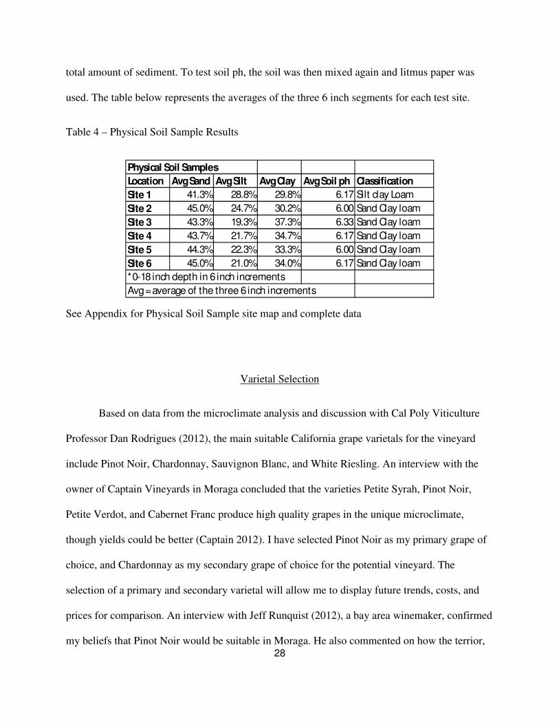
total amount of sediment. To test soil ph, the soil was then mixed again and litmus paper was

used. The table below represents the averages of the three 6 inch segments for each test site.

Table 4 – Physical Soil Sample Results

Physical Soil Samples

Location Avg Sand Avg Silt Avg Clay Avg Soil ph Classification

Site 1 41.3% 28.8% 29.8% 6.17 Silt clay Loam

Site 2 45.0% 24.7% 30.2% 6.00 Sand Clay loam

Site 3 43.3% 19.3% 37.3% 6.33 Sand Clay loam

Site 4 43.7% 21.7% 34.7% 6.17 Sand Clay loam

Site 5 44.3% 22.3% 33.3% 6.00 Sand Clay loam

Site 6 45.0% 21.0% 34.0% 6.17 Sand Clay loam

*0-18 inch depth in 6 inch increments

Avg = average of the three 6 inch increments

See Appendix for Physical Soil Sample site map and complete data

Varietal Selection

Based on data from the microclimate analysis and discussion with Cal Poly Viticulture

Professor Dan Rodrigues (2012), the main suitable California grape varietals for the vineyard

include Pinot Noir, Chardonnay, Sauvignon Blanc, and White Riesling. An interview with the

owner of Captain Vineyards in Moraga concluded that the varieties Petite Syrah, Pinot Noir,

Petite Verdot, and Cabernet Franc produce high quality grapes in the unique microclimate,

though yields could be better (Captain 2012). I have selected Pinot Noir as my primary grape of

choice, and Chardonnay as my secondary grape of choice for the potential vineyard. The

selection of a primary and secondary varietal will allow me to display future trends, costs, and

prices for comparison. An interview with Jeff Runquist (2012), a bay area winemaker, confirmed

my beliefs that Pinot Noir would be suitable in Moraga. He also commented on how the terrior,

29

which is the special characteristic that the geography, geology, and climate yield to a crop, is

widely expressed in the Pinot Noir grape. I believe that the unique microclimate of Moraga

would yield a spectacular style of Pinot Noir grape.

Rootstock Selection

In order to identify the perfect rootstock match for a specific vineyard, extensive soil

analysis must be undertaken. Some of the key soil aspects for the rootstock include active lime,

salinity, soluble calcium, cation exchange capacity, and soil borne pests/disease (Rodrigues

2012). Due to the aforementioned constraints, these factors were not measured in the soil present

in the vineyard site. However, an interview conducted with a local vineyard owner shed some

light on rootstocks being used in the area. The soil structure present the vineyard is very similar

to that of the proposed vineyard site. The rootstock used at Captain Vineyards for Pinot Noir is

101-14, which has low to moderate vigor, and is highly resistant to phylloxera among other

qualities (Captain 2012, Christensen 2003).

Dan Rodrigues (2012) provided insight on rootstock selection based on the basic soil data

that had been analyzed. He provided four types of rootstocks that could thrive in the area,

although in order to be exact with the match, more soil tests would need to be performed.

Table 5 – Rootstock Selection

Rank Rootstock Vigor Ease of Propagation

Soil Adaptation Characteristics

30

1. 101-14 Med High Moist, Clay Soils Advances maturities of late varieties

2. 110-R Med Low-Med Hillside Soils, Acid Soils

Develops slowly in wet soils

3. 5BB Med High Moist, Clay Soils Susceptible to phytopthora root rot, adapted to high vigor varieties

4. 1103P Med-High

High Adapted to drought and saline soils

Influences late maturity

Source: Rodrigues 2012, Christensen 2003

For this study, two rootstocks will be considered for use. Rootstock 101-14 is ideal for

the clay soil located on the valley floor because of its high water content. For hillside plantings,

rootstock 110-R is ideal.

Wine Grape Price Forecasting

Selection of Substitute Grapes:

Zinfandel is the substitute wine grape for the Pinot Noir price model. It is often grown in

California climates that are warm with cool evenings, similar to that of Pinot Noir. If the climate

is too hot, the grapes tend to shrivel because of their thin skin. This sort of climate is similar to

that needed to grow Pinot Noir, so it will aid in forecasting prices.

Sauvignon Blanc is the substitute wine grape for the Chardonnay price model. In

California, it tends to be grown in cooler climates, similar to that of Chardonnay. Also, it is

currently the second highest crushed white grape in California behind Chardonnay, which will

31

prove useful as a substitute grape. The relationship between the market prices of my primary and

secondary grapes of choice and their corresponding substitutes are shown below.

Figure 2 – California Market Prices Received by Grower of Pinot Noir, Zinfandel, Chardonnay, and Sauvignon Blanc (1991-2011)

$0.00

$500.00

$1,000.00

$1,500.00

$2,000.00

$2,500.00

Dollars

per

Ton

Blue: Pinot Noir Red: Zinfandel Green: Chardonnay Purple: Sauvignon Blanc

Source: Crush Report 1991-2011

Fifteen Year Price Forecast Pinot Noir and Chardonnay

In order to forecast the California prices for Pinot Noir and Chardonnay for the next

fifteen years, historical price data from the past twenty years was analyzed. The data includes the

32

price per ton of Pinot Noir and Chardonnay received by growers in Crush District 6, and the

California Market price received per ton for Pinot and Chardonnay. The original econometric

price forecast model from the previous chapter could not be used because it resulted in extremely

high forecasted prices for both varietals. Because the prices generated were thought to

misrepresent the future market, five and ten year averages were taken from each set of price data

to form a range of future prices for each grape. The prices are shown below:

Figure 3 – Pinot Noir Price Range 2012-2026

Figure 4 – Chardonnay Price Range 2012-2026

33

See Appendix for complete price data.

The four price points for each varietal were averaged to suggest the future price to be

used in the cost study.

Table 6 – Projected Grape Prices 2012 - 2026

Grape Pinot Noir Chardonnay

Price Range: $ 1683.81 $ 726.99

$ 1721.25 $ 747.87

$ 1863.29 $ 752.42

$ 1990.09 $ 863.09

Average: $ 1814.61 $ 772.59

Vineyard Establishment Cost Analysis

34

Several adjustments have been made to the UC Extension cost study in order to

customize the sample costs to establish a vineyard and produce wine grapes on this specific piece

of land. Because the sample cost study included costs per acre to remove the old vineyard on the

property, these values were taken out. One hundred dollars per acre was added to the existing

cost to disk the vineyard to account for the increase in slope seen in the proposed vineyard, as

opposed to the 5% slope in the cost study. The Sonoma County Assessment cost was removed

along with the cost of property insurance because both would need to be customized to this

operation. Office expenses and building costs were removed because the existing structures on

the property can be renovated and utilized. Sanitation fees were also removed because of existing

restrooms, and any restrooms needed for harvest are incorporated in a contracted harvest price.

The cost of wind machines for frost protection was removed because there is a good chance that

they would not be needed. The yearly property taxes for the 35 acre parcel were calculated using

the most recent tax rate for the area of 1.0901 %. The manager’s salary was removed because

employment is considered specific to this operation, and would be determined after

establishment. All costs pertinent to vineyard establishment can be found in the appendix.

Vineyard Design

For the sake of the study, the proposed vineyard will mirror the design used in the UC

Davis cost study. The vineyard consists of three blocks in which each block contains 40 rows.

Each row is 1,000 feet in length and has 198 vines per row. The vine spacing is 8-feet between

rows, and 5-feet between vines. The vines are to be trained to bilateral cordons and will be spur

pruned (Demoura and Klonsky 2010).

35

Cost to Produce Wine Grapes

The changes made to the cost study for vineyard establishment are carried through to the

production costs. The table below displays the yearly cost to produce wine grapes after

establishment in year one. All costs incurred for grape production are found in the appendix.

Table 7 – Vineyard Establishment Cost and Cost to Produce Wine Grapes

Vineyard Costs Per Acre 30 Acres

Accumulated Cost

Establishment: $23,566 $706,980 $706,980

Cost to Produce:

Year 1: $23,566 $706,980 $706,980

Year 2: $2,221 $66,630 $773,610

Year 3: $3,040 $91,200 $864,810

Year 4: $3,999 $119,970 $984,780

Year 5: $3,999 $119,970 $1,104,750

Year 6: $3,999 $119,970 $1,224,720

Year 7: $3,999 $119,970 $1,344,690

Year 8: $3,999 $119,970 $1,464,660

Year 9: $3,999 $119,970 $1,584,630

Year 10: $3,999 $119,970 $1,704,600

Projected Returns Based on Yield

36

The following tables show the net returns per acre above total costs to produce an acre of

wine grapes. The prices per ton Pinot Noir and Chardonnay used in the ranging analysis come

from the forecasted five and ten year averages for the California market and District 6.

Table 8 – Pinot Noir Net Returns

PRICE YIELD (ton/acre)

$/ton 2 3 4 5 6 7 8

1685 -629 1056 2741 4426 6111 7796 9481

1720 -559 1161 2881 4601 6321 8041 9761

1865 -269 1596 3461 5326 7191 9056 10921

1990 -19 1971 3961 5951 7941 9931 11921

Table 9 – Chardonnay Net Returns

PRICE YIELD (ton/acre)

$/ton 2 3 4 5 6 7 8

730 -2539 -1809 -1079 -349 381 1111 1841

750 -2499 -1749 -999 -249 501 1251 2001

755 -2489 -1734 -979 -224 531 1286 2041

865 -2269 -1404 -539 326 1191 2056 2921

The wine grape prices used for the study are $1865 per ton Pinot Noir, and $755 per ton

Chardonnay. These were selected because they are closest to the average prices calculated earlier

in the chapter. The following tables show the projected yearly revenues for a Pinot Noir vineyard

and a Chardonnay vineyard based on yield and the selected price received per ton.

Table 10 – Projected Yearly Revenues Pinot Noir

37

Pinot Noir

Price per Ton: $1865

Revenues: Yield (tons/acre) Per Acre 30 Acres

Year 1: 0 $0.00 $0.00

Year 2: 0 $0.00 $0.00

Year 3: 1 $1,865.00 $55,950.00

Year 4: 3 $5,595.00 $167,850.00

Year 5: 4.5 $8,392.50 $251,775.00

Year 6: 4.5 $8,392.50 $251,775.00

Year 7: 4.5 $8,392.50 $251,775.00

Year 8: 4.5 $8,392.50 $251,775.00

Year 9: 4.5 $8,392.50 $251,775.00

Year 10: 4.5 $8,392.50 $251,775.00

Table 11 – Projected Yearly Revenues Chardonnay

Chardonnay Price per Ton: $773

Revenues: Yield (tons/acre) Per Acre 30 Acres

Year 1: 0 $0.00 $0.00

Year 2: 0 $0.00 $0.00

Year 3: 2.5 $1,932.50 $57,975.00

Year 4: 4.5 $3,478.50 $104,355.00

Year 5: 6 $4,638.00 $139,140.00

Year 6: 6 $4,638.00 $139,140.00

Year 7: 6 $4,638.00 $139,140.00

Year 8: 6 $4,638.00 $139,140.00

Year 9: 6 $4,638.00 $139,140.00

Year 10: 6 $4,638.00 $139,140.00

Net Present Value Analysis

38

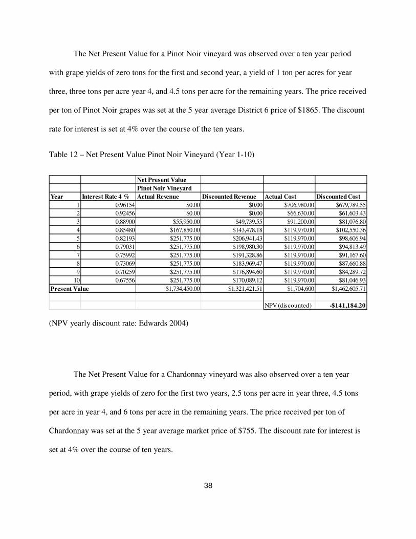
The Net Present Value for a Pinot Noir vineyard was observed over a ten year period

with grape yields of zero tons for the first and second year, a yield of 1 ton per acres for year

three, three tons per acre year 4, and 4.5 tons per acre for the remaining years. The price received

per ton of Pinot Noir grapes was set at the 5 year average District 6 price of $1865. The discount

rate for interest is set at 4% over the course of the ten years.

Table 12 – Net Present Value Pinot Noir Vineyard (Year 1-10)

Net Present Value

Pinot Noir Vineyard

Year Interest Rate 4 % Actual Revenue Discounted Revenue Actual Cost Discounted Cost

1 0.96154 $0.00 $0.00 $706,980.00 $679,789.55

2 0.92456 $0.00 $0.00 $66,630.00 $61,603.43

3 0.88900 $55,950.00 $49,739.55 $91,200.00 $81,076.80

4 0.85480 $167,850.00 $143,478.18 $119,970.00 $102,550.36

5 0.82193 $251,775.00 $206,941.43 $119,970.00 $98,606.94

6 0.79031 $251,775.00 $198,980.30 $119,970.00 $94,813.49

7 0.75992 $251,775.00 $191,328.86 $119,970.00 $91,167.60

8 0.73069 $251,775.00 $183,969.47 $119,970.00 $87,660.88

9 0.70259 $251,775.00 $176,894.60 $119,970.00 $84,289.72

10 0.67556 $251,775.00 $170,089.12 $119,970.00 $81,046.93

Present Value $1,734,450.00 $1,321,421.51 $1,704,600 $1,462,605.71

NPV (discounted) -$141,184.20

(NPV yearly discount rate: Edwards 2004)

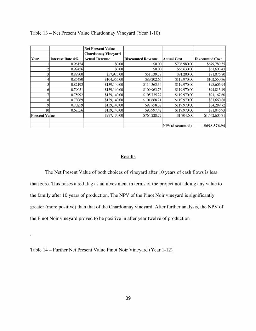
The Net Present Value for a Chardonnay vineyard was also observed over a ten year

period, with grape yields of zero for the first two years, 2.5 tons per acre in year three, 4.5 tons

per acre in year 4, and 6 tons per acre in the remaining years. The price received per ton of

Chardonnay was set at the 5 year average market price of $755. The discount rate for interest is

set at 4% over the course of ten years.

39

Table 13 – Net Present Value Chardonnay Vineyard (Year 1-10)

Net Present Value

Chardonnay Vineyard

Year Interest Rate 4% Actual Revenue Discounted Revenue Actual Cost Discounted Cost

1 0.96154 $0.00 $0.00 $706,980.00 $679,789.55

2 0.92456 $0.00 $0.00 $66,630.00 $61,603.43

3 0.88900 $57,975.00 $51,539.78 $91,200.00 $81,076.80

4 0.85480 $104,355.00 $89,202.65 $119,970.00 $102,550.36

5 0.82193 $139,140.00 $114,363.34 $119,970.00 $98,606.94

6 0.79031 $139,140.00 $109,963.73 $119,970.00 $94,813.49

7 0.75992 $139,140.00 $105,735.27 $119,970.00 $91,167.60

8 0.73069 $139,140.00 $101,668.21 $119,970.00 $87,660.88

9 0.70259 $139,140.00 $97,758.37 $119,970.00 $84,289.72

10 0.67556 $139,140.00 $93,997.42 $119,970.00 $81,046.93

Present Value $997,170.00 $764,228.77 $1,704,600 $1,462,605.71

NPV (discounted) -$698,376.94

Results

The Net Present Value of both choices of vineyard after 10 years of cash flows is less

than zero. This raises a red flag as an investment in terms of the project not adding any value to

the family after 10 years of production. The NPV of the Pinot Noir vineyard is significantly

greater (more positive) than that of the Chardonnay vineyard. After further analysis, the NPV of

the Pinot Noir vineyard proved to be positive in after year twelve of production

.

Table 14 – Further Net Present Value Pinot Noir Vineyard (Year 1-12)

40

Net Present Value

Pinot Noir Vineyard

Year Interest Rate 4 % Actual Revenue Discounted Revenue Actual Cost Discounted Cost

10 0.67556 $251,775.00 $170,089.12 $119,970.00 $81,046.93

11 0.64958 $251,775.00 $163,548.00 $119,970.00 $77,930.11

12 0.6246 $251,775.00 $157,258.67 $119,970.00 $74,933.26

Present Value $2,238,000.00 $1,642,228.17 $1,944,540.00 $1,615,469.08

NPV (discounted) $26,759.09

Break-even Analysis

The yearly projected costs and revenues used in the NPV analysis have been accumulated

for both the Pinot Noir vineyard and the Chardonnay vineyard to show when the project is

expected to break –even and thus begin to make a profit.

Table 15 – Break-even for Pinot Noir Vineyard

Break-Even Pinot Noir Vineyard

Max Yield: 4.5 tons/acre Price Received: $1865/ ton

Year 1 2 3 4 5 6 7 8 9 10

Accumulated Cost $706,980 $773,610 $864,810 $984,780 $1,104,750 $1,224,720 $1,344,690 $1,464,660 $1,584,630 $1,704,600

Accumulated Revenue $0 $0 $55,950 $223,800 $475,575 $727,350 $979,125 $1,230,900 $1,482,675 $1,734,450

Total Profit -$706,980 -$773,610 -$808,860 -$760,980 -$629,175 -$497,370 -$365,565 -$233,760 -$101,955 $29,850

The above table shows that the Pinot Noir vineyard is expected to break-even in year ten

of production.

Table 16 – Break-even for Chardonnay Vineyard

Break-Even Chardonnay Vineyard

Max Yield: 6 tons/acre Price Received: $773/ ton

Year 1 2 3 4 5 6 7 8 9 10

Accumulated Cost $706,980 $773,610 $864,810 $984,780 $1,104,750 $1,224,720 $1,344,690 $1,464,660 $1,584,630 $1,704,600

Accumulated Revenue $0 $0 $57,975 $162,330 $301,470 $440,610 $579,750 $718,890 $858,030 $997,170

Total Profit -$706,980 -$773,610 -$806,835 -$822,450 -$803,280 -$784,110 -$764,940 -$745,770 -$726,600 -$707,430

The above table shows that the Chardonnay vineyard remains at a significant negative

total profit in year ten of production.

Chapter V

41

SUMMARY, CONCLUSIONS, AND RECOMMENDATIONS

Summary

This study has accomplished several tasks that must be sought out when considering

entering the wine grape growing business. It began with thorough research on the topic at hand,

ranging from a broad perspective of the wine industry to the unique niche markets of California

wine grape production.

The microclimate of Moraga was first analyzed to help determine which wine grape

varietals would thrive in the area. The degree days for the area were calculated and averaged

from two sources in order to provide an accurate measure of climate. Based on this data and

interviews with Dan Rodrigues, Salah Captain, and Jeff Runquist, Pinot Noir and Chardonnay

were selected out of the compatible varietals. Physical soil sample testing and soil map analysis

provided a reference point of soil quality and composition in the proposed vineyard site. This

information was used to determine several types of rootstocks to be used.

Price forecasting for the two varietals selected did not go as planned in the previous

chapter. The econometric price model yielded extremely high future prices that could not be used

in the study, so five and ten year price averages for District 6 and the California Market were

used. This provided a more realistic range of future prices to be used in the study. Out of the

respective price ranges for Pinot Noir and Chardonnay, the price nearest the average of all four

price points was selected and used in the cost study.

42

Costs involved with establishing a vineyard and producing wine grapes were taken from

a UC Davis cost study and adjusted specifically for the proposed vineyard. Yield ranging

analysis and Net Present Value analysis were used to see if the vineyard would be profitable, and

whether or not it would break-even by year 10 of production.

Conclusions

The selection of Pinot Noir as my primary grape of choice, and Chardonnay as my

secondary grape of choice only partially proves my hypothesis correct. I had originally thought

that Cabernet Sauvignon would be a worthy candidate, but results show that the climate required

for the grape is unlike that of Moraga’s. It remains difficult to provide the perfect match of

varietal and vineyard site, but microclimate analysis and consultation with experts in the industry

has helped to narrow down the selection. Once the vineyard is established only time will tell if

the selected varietal is favored in the specific climate.

The price forecasts for the selected grapes can’t be used to test against the hypothesis

because they only provide a range of price data to be referenced, instead of a regression line that

was originally intended. The failed regression analysis was not providing realistic prices, and it

seems that to accurately forecast the prices of wine grapes requires an entire research project in

itself.

The financial analysis of the proposed vineyard proved useful, though my hypothesis was

partially correct. At a yield of 4.5 tons of Pinot Noir grapes per acre and $1865 per ton, NPV for

a Pinot Noir vineyard remained negative, meaning that the project would not add any value to

43

the family after year ten of production in terms of the time value of money. On the other hand, a

break-even analysis concluded that the Pinot Noir vineyard would break-even in year ten, and

begins to make a profit thereafter. Further analysis suggests that after year twelve of production,

the NPV of a Pinot Noir vineyard would be positive.

Net Present Value for a Chardonnay vineyard after year ten remained extremely

negative, and break-even analysis proved that it was far from generating a profit by the tenth

year of production. This is due to the low price received per ton of Chardonnay compared to

Pinot Noir. Ranging analysis shows that in order for the Chardonnay vineyard to become a

profitable endeavor by year 10, a higher price per ton received and higher yield would be needed.

Recommendations

Selling bulk grapes from this proposed operation on the open market is subject to many

pressures. Because this project requires an immense amount of start-up capital and adequate

returns aren’t seen for several years, another option would be to downsize the proposed number

of acres planted to reduce initial establishment costs, and create a winery on site to make

premium wine from the high quality grapes produced. When Jeff Runquist was asked what he

would have done differently in the past, he replied “Slow and steady, build a market before

investing in a physical plant” (Runquist 2012).

After speaking with Dan Rodrigues, he mentioned an option that I had not previously

thought about. He explained that in some cases well established wineries who have a shortage of

grapes will reach out to vineyard and land owners to contract future grape production. An

44

opportunity such as this would spread the financial risk of establishment and yearly production,

while locking in a desired price to be received by the grower. Any sort of cultivation operation is

a gamble for the grower because they are subject to fluctuating market prices and trends.

Further research would be aided by a reliable econometric price forecasting model for

wine grapes. Extending wine grape price forecasting research would prove useful for anyone

entering the wine grape growing business. Anyone considering expanding this study may look to

compare the projected revenues of selling bulk grapes to buyers, and the projected revenues

received if the grapes were kept, made into wine, and sold by an on-site winery.

45

References Cited

Bettiga, L. (2003). “Chardonnay” Wine Grape Varieties in California. University of California Agricultural and Natural Resources Publication. pp 44-49

California Irrigation Management Information System. (1991-2011). Department of Water

Resources: Office of Water Use and Efficiency. Station: San Francisco Bay - Moraga - 178

Captain, Salah. (2012). Owner Captain Vineyards. Personal Interview, Moraga (March 25) Cuellar, Steven and Aaron Lucey. (2005). “Forecasting Wine Grape Supply Cycles.” Wine Business Monthly. December 2005. pp. 1-4 Christensen, L. Peter. (2003). “Rootstock Selection.” Wine Grape Varieties in California.

University of California Agricultural and Natural Resources Publication 3419. pp 11-15 Cutler, Lance. (2008). “Industry Roundtable: Pinot Noir: Wine’s Holy Grail” Wine Business

Monthly. July 2008. pp 1-3 De Moura, Richard and Karen Klonsky. (2010). “Sample Costs to Establish a Vineyard and

Produce Winegrapes (Sonoma County: Cabernet Sauvignon)” University of California Cooperative Extension pp 1-20 Edwards, William M. and Ronald D Kay. (1994). “Farm Management: Third Edition” pp 439 Fisher, Cathy. (2010). “Number of U.S. Wineries Reaches 6,223.” Wine Business Monthly. February 2010. pp. 1-5 Geraci, Victor W. (2004). "Fermenting a Twenty-First Century California Wine Industry." Agricultural History 78.4: 438-65 Grape Crush Report (2011). California Department of Food and Agriculture, and NASS. USDA

46

Green, Richard, Richard Volpe, Dale Heien, and Richard Howitt. (2008). “Recent Trends in the

California Wine Grape Industry.” Agricultural and Resource Economics Update. (11:4) University of California Giannini Foundation of Agricultural Economics.

Hanson, Jaime. (1976). “Conversion of a 25 Acre Walnut Orchard into a Wine Grape Vineyard.”

Published Senior Project. California Polytechnic State College, San Luis Obispo #01-0235

Pauli, Frost. (2009). “Implementation Plan and Cost Study for a Wine Grape Vineyard in

Mendocino County.” Published Senior Project. California Polytechnic State College, San Luis Obispo #09-0188

Peters, Gary L. (1984). “Trends in California Viticulture.” Geographical Review 455-67 Rodrigues, Dan. (2012). Viticulture Professor: Cal Poly, Vineyard Consultant. Personal Interview, San Luis Obispo (April 6) Runquist, Jeff. (2012). Owner and Winemaker: Jeff Runquist Wines. Email Interview (May 1) Smith, Rhonda. (2003). “Pinot Noir” Wine Grape Varieties in California. University of California Agricultural and Natural Resources Publication 3419. pp. 106-111 Snodgrass, Wayne. (1985). “Developing a Price Forecasting Model for California Grapes.”

Published Senior Project. California Polytechnic State College, San Luis Obispo #85-1503

Statewide Integrated Pest Management Program. (2012). “Weather Models and Degree Days” University of California Agriculture and Natural Resources. Moraga, CA Turrentine, Bill. (2005). “Forecasting Wine Grape Supply Cycles.” Wine Business Monthly. December 2005. pp. 1 United States Department of Agriculture, Natural Resources Conservation Service. (2012).

47

“Custom Soil Resource Report: Contra Costa County. Feb 17, 2012 pp 1-19 Winkler, A.J. (1949). “Grapes and Wine.” Economic Botany pp.46-70 Wolpert, J. (2003). “Cabernet Sauvignon” Wine Grape Varieties in California. University of California Agricultural and Natural Resources Publication 3419. Pgs. 36-39

APPENDIX

48

Intensive Depth Interview #1 - Discussion Guide

Objective: To ascertain the overall features, production, liabilities, and unexpected inputs of a working vineyard in Moraga.

Expert: Salah Captain, Captain Vineyards Moraga, CA

• What is the total acreage of your vineyard with grapes planted on them?

2.5 acres

• What soil is present in your vineyard?

4 ft of topsoil to sandstone below. Orinda Moraga Clay Loam (50% Clay, 25% Sand, 25% Silt)

• What varietals and paired rootstocks are planted?

Petite Syrah: 1500 vines (3309C), Petite Verdot: 650 (#400/101-14), Cabernet Sauvignon: 200 (169), Cabernet Franc: 450 (3309C), Pinot Noir: 600 (101-14)

o How did you decide on these specific varietals and rootstocks?

Extensive research, consultation, classes at UC Davis and Sonoma, soil analysis. Rootstocks selected for dry-farming intention. All scions and rootstocks certified.

o How many vines of varietal?

See above

o What is the vine spacing and density per acre?

3’ x 5’: 5 feet between vines, 3 feet between rows

Density varies 1500 – 2000 vines per acre *******

o Which has been most productive (T/acre)? Profitable?

o Which has produced the highest quality? Any disappointing varietals?

All high quality grapes: based on genetics (root, scion), maintenance (water, fertilizer)

Downside: Low quantities, about 1/5th of what production should be.

• How long from planting until first commercial production?

Petite Syrah: Following year

All other vines: 3 years

• Any pest problems (soil borne or animal)?

Moles and gophers.

No contamination because not going vineyard to vineyard.

• Any unique pros / cons of microclimate in Moraga?

Pros: 10 -12 hrs sunlight/ day in summer, Day temp 70-80 degrees Night temp 40 degrees, Fog cools vineyard at night.

49

Cons: none

• What type of trellis system and irrigation system do you use?

Vertically shoot positioned trellis system.

• Any unexpected overhead costs?

None so far, but potential costs include disease, and heavy rains/topsoil loss.

• What sorts of improvements have you made to become more sustainable (green)?

Efficient Rainwater collection system, Erosion control for creek and hillside, No pesticides/fertilizer, only mulch and soil, Dry-farming water conservation.

• Looking back, would you have done differently?

More spacing (6-7 ft),wider lanes, attention to lane orientation NE-SW to prevent burning and reduce terracing.

Interview #2 - Discussion Guide

50

Objective: To find what is necessary to maximize profits and establish a sustainable vineyard operation in Moraga, CA.

Expert: Jeff Runquist, Jeff Runquist Wines Plymouth, CA

• What are the key things you look for when sourcing grapes from a specific vineyard?

When I look to purchase grapes and select a vineyard to do business with I base my decision primarily on my past history. I have made wine for 35+ years in six regions of CA and so I have developed a network of growers I have had success with in the past as a winemaker for another winery. So when I try something new it is usually with a grower I have already done business with. Also, recommendations from other winemakers have worked for me before. If I was starting out fresh I would consider chasing after wines I liked to drink, say Russian River Pinot Noir, and I would ask around winemakers using those grapes what they thought of particular growers. We are a fairly open group and one usually gets a good read on who to do business with and who to steer clear of.

• Do you believe there is (or will be) a market for locally produced Contra Costa County wine grapes and wines?

Contra Costa has not set the winemaking world on fire, but you never know. With the fashion of eating and drinking locally and the demographics of Contra Costa it does sound promising.

• The microclimate for Moraga is effected by the fog that comes up from the reservoir and keeps the temperature 5-10 degrees cooler than Lafayette:

o What grape varieties would you plant?

As for grape growing, I don't. I purchase all of the grapes I use to make wine. I do not grow any. This allows me to focus my limited resources on winemaking and I have not made a huge investment in ground that I will not know the results from for a decade. If I buy grapes and the variety I choose loses favor I can move on without too much trouble.

o Is Pinot Noir feasible?

Pinot Noir is known for being a grape that expresses the terrior of the site upon which it grows. It also has a wide range of styles and it is a well-respected and prestigious grape. It is known for growing well in cooler climates and I suspect it would do okay in Moraga. I suspect the real issue will be protecting the vines from the deer.

o What would ideal vine spacing and vineyard density per acre be?

Spacing and density are often copied from Europe but without knowing why the Europeans plant so many vines per acre. My understanding is not so much a quality issue as a ripening issue. More dense plantings, where each vine carries a smaller number of clusters, tend to ripen faster and earlier than a bigger vine. I saw this in Burgundy where the same vines where planted side by side and the smaller more dense vines ripened their grapes two to three weeks earlier than the bigger CA style of spacing. I don't think that ripening will be an issue in Moraga so I think something on the order of 60-70 square feet per vine should be appropriate.

• How does a vineyard go about contracting a grape buyer?

Most small vineyards are local and know the local winemakers and will by word of mouth find a buyer. On a larger scale there are brokers that will put grape sellers and buyers together.

51

• What determines the price received by wine grape growers, and what is the process of purchasing grapes?

Pricing is really determined by the market. If your grapes produce wine that can sell for $20 per bottle they are more valuable that grapes making wine that sells for $10 per bottle. Beauty is in the eye of the beholder, but if you can't make a profit then the price paid for the grapes may be an issue. To this end some contracts are based on the bottle price. Say a wine sells for $20 per bottle then the grape grower would be compensated by some multiplier of the bottle price. I have an arrangement with one grower where we split the profits on the wine sold 70:30; 70% to me the winery and 30% to the grower. This grower gets $3,500 per ton for Carnero’s Pinot Noir which isn't too shabby. The state of CA reports on grape prices by growing region and the publication is called the grape crush report and is available on line at the CA Dept of Food and Agriculture.

• What are the market considerations (for viable grape varieties) of the various grape types? ie. Chardonnay versus Sauvignon Blanc? Pinot Noir versus Cabernet?

UC Davis put together the degree day system to help grape growers determine what variety would grow best in a particular region. This system is based on the high and low temperatures during the growing season and has helped guide growers determine what to plant. The prices paid for a particular variety also plays a big row in what growers decide to plant. If the vineyard is associated with a winery then the wine style and reputation or desire of the owner will play a role.

• What do you believe the next 30 years holds for the California wine industry?

The CA wine industry is known for a very cyclic pattern of boom and bust. Overplanting followed by bankruptcies and vineyards being pulled out lead to shortages which then fuel the next round of speculative plantings. The cycles typically last seven to eleven years and are very dependable. We are just now leaving a period of glut where there was an oversupply of grapes and depressed prices. The ocean of surplus wine is now gone and since no one has been planting grapes for the past seven years but sales for wine have been strong we are now looking for all the grapes to have a buyer and prices starting to rise. CA is well positioned to continue to grow its wine and grape industries but global competition from Australia, Argentina, New Zealand, and Chile as well and Europe will keep things interesting. Here in CA we are not as restricted by regulations as are growers in Europe, and this has allowed us to try new and varied production practices and often with great success.

• Are there any unexpected vineyard or winemaking input costs you have come across?

As for unexpected costs I must tell you that there is plenty of truth to the saying that goes, "How do you make a small fortune in the wine business? Start with a large one." Vineyards are like Yachts, women and racehorses. They are not for the faint hearted and always have unexpected twists and turns.

• What are the biggest mistakes first time wine grape growers make?

Some mistakes: Planting the wrong variety. Not having a buyer for the grapes before you plant. Trying to produce too much too fast. Not having enough capital to do it right.

52

• Looking back, is there anything you would do differently?

Looking back I wouldn't do much differently. Slow steady. Build a market before investing in physical plant.

53

Contra Costa County 2012

Table 1. COSTS PER ACRE TO ESTABLISH A VINEYARD

Cost per Acre

Year: 1st 2nd 3rd

Tons per Acre: 0 0 1.5

Land Preparation Costs:

Site Determination: Development Fee 31

Site Prep: Soil Test (1 per 10 acres x 3 depths) 18

Site Prep: Nematode Sampling (1 per 10 acres) 7

Site Prep: Plant Removal, Pickup rocks 350

Site Prep: Fertilize (Lime, Gypsum & Compost) 700

Site Prep: Rip 3X 350

Site Prep: Disk 6X (smooth ground for planting) 250

Cover Crop: Plant cover crop (Barley) & spread straw 50

Cover Crop: Mow cover crop 18

Cover Crop: Disk cover crop 3X 44

Plant: Mark , Layout, Stake Vineyard 325

Trellis: Install Trellis (over 2 years) 10000

Irrigation: Install Drip & Submains (includes materials) 3200

Plant: (vines, labor, cartons) 5826

TOTAL SITE PREP AND PLANTING COSTS 21169

Cultural Costs:

Irrigate: (water & labor) 64 81 130

Weed: Vine Row Spray (Buccaneer) 27 25 25

Plant: Replant 2% Yr 1, 1% Yr 2 (vines, labor, cartons) 102 59

Fertilize: (4X Yrs 1 & 2. 1X Yr 3) Through drip (3-18-18) 76 76 19

Weed: Hand Weed Vine Row 213

Cover Crop: Disc CC centers (cover crop preparation) 8 8 8

Cover Crop: Plant & Roll CC centers (Yrs 1-2, Barley. Yr 3, Legume/Grass Mixture) 24 24 34

Labor: Miscellaneous labor after planting 250

Train: Prune to 2 buds 603

Train: Train vines & tie 1000

Weed: Vine Row Winter Spray (Yr 2 Buccaneer, Prowl) (Yr 3 Buccaneer, Chateau) 28 67

Weed: Mow CC & NC centers (Yr 3 includes shred prunings) 32 32

Weed: Disc Centers (Yr 2, CC & NC. Yr 3 CC) 33 8

Weed: Mow NC centers 16

Fertilize: 1X Through drip (12-26-26) 44

Prune: Winter 289

Frost Protection: 10X 240

Train: Tie Cordons 161

Sucker: Sucker Cordons 322

Disease: Mildew (Thiolux, Champ) 2X 91

Disease: Mildew (Sulfur Dust) Alternate Rows 42

Fertilize: Petiole Analysis 5

Train: Move Wires & Stuff Shoots 3X 498

Prune: Crop Adjustment (thin fruit) 64

Disease: Mildew @ Prebloom (Pristine). Fertilize: (Zn, B) 96

Disease: Mildew @ Preveraison (Rally) 69

PCA 70

Pickup Use 114 114 114

ATV Use 23 23 23

TOTAL CULTURAL COSTS 901 2106 2467

Harvest Costs:

Harvest and Haul 473

TOTAL HARVEST COSTS 473

Interest On Operating Capital @ 5.75% 1270 82 67

TOTAL OPERATING COSTS/ACRE 23340 2188 3007

CASH OVERHEAD:

Property Taxes 33 33 33

TOTAL CASH OVERHEAD COSTS 33 33 33

TOTAL CASH COSTS/ACRE 23373 2221 3040

INCOME/ACRE FROM PRODUCTION 2797.5

NET CASH COSTS/ACRE FOR THE YEAR 23373 2221 242.5

PROFIT/ACRE ABOVE CASH COSTS

ACCUMULATED NET CASH COSTS/ACRE 23373 25594 25836.5

NON-CASH OVERHEAD (Capital Recovery):

Fuel Tanks 10 10 10

Shop Tools 11 11 11

Equipment 172 156 216

TOTAL INTEREST ON INVESTMENT 193 177 237

TOTAL COST/ACRE FOR THE YEAR 23566 2398 479.5

INCOME/ACRE FROM PRODUCTION 0 0 0

TOTAL NET COST/ACRE FOR THE YEAR 23566 2398 479.5

NET PROFIT/ACRE ABOVE TOTAL COST

TOTAL ACCUMULATED NET COST/ACRE 23566 25964 26443.5

CC=Cover Crop Centers, NC=Non Cover Crop Centers

Income = $1815 per ton Pinot Noir

$773 per ton Chardonnay

54

Contra Costa County 2012

Table 2. COSTS PER ACRE to PRODUCE WINEGRAPES

Operation Cash and Labor Costs per acre

Time Labor Fuel,Lube Material Custom/ Total

Operation (Hrs/A) Cost & Repairs Cost Rent Cost

Cultural:

Weed: Spray Vine Row (Goal, Chateau) 0.84 20 2 102 0 124

Prune: Winter Pruning 18.00 289 0 0 0 289

CM: Tie Cordons 10.00 161 0 0 0 161

Weed: Mow NC centers (shred prunings @ March mowing) 0.43 10 6 0 0 16

Weed: Mow CC centers 0.43 10 6 0 0 16

Weed: Disc CC centers 1X/3 Yrs 0.32 8 3 0 0 11

Disease: Mildew (Thiolux [S]. Champ [Cu]) 2X 0.76 18 9 64 0 91

Frost Protection: Windmachines 10X 5.57 90 0 150 0 240

CM: Cordon Sucker 20.00 322 0 0 0 322

Disease: Mildew (Sulfur Dust) 1.18 28 11 12 0 51

Weed: Disc & Roll CC centers 1X/3 Yrs 0.16 4 2 0 0 6

Weed: Disc CC centers 2X/3 Yrs 0.32 8 3 0 0 11

Fertilize: through drip (CAN17) 0.03 0 0 8 0 8

Fertilize: Petiole Sampling & Analysis @ bloom 0.00 0 0 5 0 5

CM: Move Wires 29.00 466 0 0 0 466

Disease: Mildew (Pristine). Fertilize: Foliar (Solubor [B], Zinc [Zn]) 1.15 28 13 55 0 96

Weed: Vine Row (Buccaneer) 0.84 20 2 2 0 24

Fertilize: through drip (12-26-26) 0.05 1 0 90 0 91

Weed: Mow CC centers 2X/3 Yrs 0.57 14 7 0 0 21

Weed: Mow NC centers 0.86 21 11 0 0 32

CM: Leaf Removal (machine) 0.00 0 0 0 75 75

CM: Hedge Vines (machine) 0.00 0 0 0 50 50

CM: Clean Up (check if vines open) 6.00 96 0 0 0 96

CM: Crop Adjustment (thin fruit) 12.50 201 0 0 0 201

Irrigate: (water & labor) 3.30 53 0 99 0 152

Insect: Mites (Acramite) 1X/3 Yrs. 1/3 cost each year 0.38 9 4 23 0 36

Disease: Mildew @ preveraison (Rally) 1.15 28 13 28 0 69

CM: Crop Adjustment (green drop) 7.00 113 0 0 0 113

Fertilize: Petiole Sampling & Analysis (at veraison) 1X/3 Yrs 0.00 0 0 2 0 2

Pest Control Adviser 0.00 0 0 0 70 70

Pickup Truck Use 3.33 80 33 0 0 113

ATV 0.85 21 2 0 0 23

TOTAL CULTURAL COSTS 125.02 2119 127 640 195 3081

Harvest:

Harvest-Hand Labor & Haul 0 0 0 0 450 450

TOTAL HARVEST COSTS 0 0 0 56 450 506

Postharvest:

Fertilize: Petiole Sampling & Analysis 1X/3 Yrs 0 0 0 2 0 2

Weed: Rip Cover Crop Centers (custom) 1X/3 Yrs 0 0 0 0 21 21

Amendment: (Gypsum) CC centers 1X/3 Yrs 0 0 0 37 0 37

Weed: Disc CC centers 1X/3 Yrs 0.16 4 2 0 0 6

Weed: Plant Cover Crop in CC centers 1X/3 Yrs 0.08 2 1 9 0 11

TOTAL POSTHARVEST COSTS 0.24 6 3 48 21 77

Interest on operating capital @ 5.75% 78

TOTAL OPERATING COSTS/ACRE 2125 130 744 666 3742

CASH OVERHEAD:

Property Taxes 33

TOTAL CASH OVERHEAD COSTS 33

TOTAL CASH COSTS/ACRE 3775

NON-CASH OVERHEAD:

Per Producing Acre Annual Cost Capital Recovery

Fuel Tanks 150 10 10

Shop Tools 83 11 11

Equipment 2087 203 203

TOTAL NON-CASH OVERHEAD COSTS 2320 224 224

TOTAL COSTS/ACRE 3999

CM=Canopy Management. X=number of times as 2X= 2 times or 2 passes. CC=Cover Crop, NC=Non Cover

Costs for operations not done each year are allocated each year accordingly.

55

Contra Costa County 2012

COSTS PER ACRE AT VARYING YIELDS TO PRODUCE WINEGRAPES

Table 5. RANGING ANALYSIS

YIELD (ton/acre)

2 3 4 5 6 7 8

OPERATING COSTS:

Cultural Cost 3081 3081 3081 3081 3081 3081 3081

Harvest Cost 450 450 450 450 450 450 450

Postharvest Cost 77 77 77 77 77 77 77

Interest on operating capital @ 5.75% 78 78 78 78 78 78 78

TOTAL OPERATING COSTS/ACRE 3742 3742 3742 3742 3742 3742 3742

Total Operating Costs/ton 1871 1247 936 748 624 535 468

CASH OVERHEAD COSTS/ACRE 33 33 33 33 33 33 33

Total Cash Costs/ton 17 11 8 7 6 5 4

NON-CASH OVERHEAD COSTS/ACRE 224 224 224 224 224 224 224

TOTAL COSTS/ACRE 3999 3999 3999 3999 3999 3999 3999

Total Costs/ton 2000 1333 1000 800 667 571 500

Table 6. WHOLE FARM ANNUAL EQUIPMENT, INVESTMENT, AND BUSINESS OVERHEAD COSTS

Contra Costa County 2012

ANNUAL EQUIPMENT COSTS

Cash Overhead

Yrs Salvage Capital

Year Description Price Life Value Recovery Insurance Taxes Total

12 60HP4WDNarrowTract 45000 16 8060 3731 203 265 4199

12 ATV 4WD 6700 5 3003 991 37 49 1077

12 Brush Shredder 6 ft 8500 15 816 767 36 47 850

12 Disc - Offset 5 ft 7500 15 720 676 32 41 749

12 Duster - 3 pt 5000 12 693 512 22 28 562

12 Air Blast Sprayer 300 gal 16000 10 2829 1819 72 94 1985

12 Pickup Truck 1/2 ton 32000 7 12139 3978 169 221 4368

12 Ringroller 5 ft 1500 20 78 115 6 8 129

12 Seed Drill 5 ft 8000 10 1415 910 36 47 993

12 Sprayer ATV 20 gal 350 10 62 40 2 2 44

TOTAL 130550 29815 13539 615 802 14956

60% of New Cost * 78330 17889 8123.4 369 481.2 8973.6

*Used to reflect a mix of new and used equipment

56

Physical Soil Samples

0-18 inch depth in 6 inch increments

Location

Sand Silt Clay Total Soil Classification Soil PH

Site 1

0-6 42.8% 28.5% 28.5% 100% Silt clay Loam 6

6-12 41.0% 29.0% 30.0% 100% 6.5

12-18 40.0% 29.0% 31.0% 100% 6

Site 2

0-6 45.0% 25.0% 29.5% 100% Sand Clay loam 6

6-12 45.0% 25.0% 30.0% 100% 6

12-18 45.0% 24.0% 31.0% 100% 6

Site 3

0-6 45.0% 20.0% 35.0% 100% Sand Clay loam 7

6-12 45.0% 18.0% 37.0% 100% 6

12-18 40.0% 20.0% 40.0% 100% 6

Site 4

0-6 44.0% 22.0% 34.0% 100% Sand Clay loam 6

6-12 44.0% 21.0% 35.0% 100% 6

12-18 43.0% 22.0% 35.0% 100% 6.5

Site 5

0-6 45.0% 22.0% 33.0% 100% Sand Clay loam 6

6-12 45.0% 22.0% 33.0% 100% 6

12-18 43.0% 23.0% 34.0% 100% 6

Site 6

0-6 47.0% 20.0% 33.0% 100% Sand Clay loam 6.5

6-12 45.0% 21.0% 34.0% 100% 6

12-18 43.0% 22.0% 35.0% 100% 6

57

Year PPinot(6)/ ton % change Ppinot(6) / ton/yr QPinot(6)/ tonscr Mkt PPinot/ ton Mkt QPinot/ tonAcresPinot PsubZ/ ton

1991 $533.22 379.2 $804.00 34396.3 8,522.0 363

1992 $598.72 12.28% 277.8 $767.51 37060.4 8,492.0 438.08

1993 $604.16 0.91% 206.3 $775.68 35377.7 8,576.0 434.13

1994 $832.54 37.80% 152.1 $834.53 31916.9 8,727.0 476.55

1995 $1,075.21 29.15% 186.1 $1,018.49 28986.1 8,503.0 521.15

1996 $1,684.04 56.62% 228.2 $1,341.30 36641.8 8,264.0 564.83

1997 $1,508.91 -10.40% 465.3 $1,540.01 48319.1 8,085.1 502.93

1998 $2,035.93 34.93% 198 $1,632.29 28922.9 8,179.0 460.32

1999 $1,748.01 -14.14% 302.2 $1,721.85 36653.4 9,183.0 494.23

2000 $1,650.72 -5.57% 413.3 $1,779.86 53050.1 11,769.0 464.15

2001 $2,016.91 22.18% 524.3 $1,855.74 63420.9 14,651.0 526.5

2002 $2,187.71 8.47% 379.4 $1,778.90 54156.4 16,815.0 476.15

2003 $2,097.04 -4.14% 265.5 $1,615.24 58184.8 20,093.0 427.83

2004 $2,064.96 -1.53% 428.7 $1,620.14 70067.9 22,645.0 473.56

2005 $2,101.84 1.79% 382.9 $1,751.26 94918.2 23,323.0 472.31

2006 $2,132.87 1.48% 710.8 $2,027.91 105971 24,188.0 507.96

2007 $2,302.80 7.97% 687.1 $2,093.82 89518.6 24,427.0 466.58

2008 $2,115.80 -8.12% 936 $1,962.03 105678.1 25,737.0 462.65

2009 $1,769.16 -16.38% 1443.3 $1,641.33 156703.5 30,339.0 464

2010 $1,761.64 -0.43% 1369.7 $1,449.99 147741.6 33,343.0 442.68

2011 $1,367.05 -22.40% 1276.7 $1,271.87 170448.6 36,988.0 560.31

10 YR AVG $1,990.09 6.52% 533.95 $1,489.70 70863.54 17183.29 $476.19

Year PChard(6)/ ton % change Pchard(6) / ton/yr QChard(6)/ tonscr Mkt PChard/ ton Mkt QChard/ tonAcresChard PsubSB/ ton

1991 $1,178.04 3832.4 $1,121.60 216890.4 44,040 541

1992 $1,206.93 2.45% 4551.4 $1,038.19 242822.8 48,696 514.24

1993 $1,178.73 -2.34% 3272.4 $888.73 262684.4 53,309 553.55

1994 $1,044.27 -11.41% 3557.7 $851.04 306381.5 56,257 502.04

1995 $1,157.45 10.84% 3272.3 $893.29 286989.1 58,649 530.7

1996 $1,397.16 20.71% 5479.9 $1,129.75 309463.9 62,883 703.38

1997 $1,467.52 5.04% 7909.2 $1,161.07 491406.3 65,057.50 788.24

1998 $1,372.59 -6.47% 6462.4 $1,087.86 428827.2 70,629 827.14

1999 $1,377.28 0.34% 8071.9 $995.68 458273 80,998 800.1

2000 $1,308.53 -4.99% 8433.6 $895.07 650524.7 89,272 839.54

2001 $1,311.37 0.22% 8286.5 $845.83 568295.2 93,316 868.1

2002 $1,033.81 -21.17% 6521.4 $682.64 594904.5 92,193 816.13

2003 $1,071.03 3.60% 5212.2 $665.01 561648.5 94,164 754

2004 $907.79 -15.24% 7246.6 $693.77 524732.1 93,431 691.69

2005 $993.02 9.39% 7294.6 $714.38 742582.6 92,089 705.44

2006 $885.88 -10.79% 4580.5 $752.01 549502.5 92,091 722.09

2007 $661.51 -25.33% 5977 $717.54 589664 91,348 687.9

2008 $830.83 25.60% 5834.8 $816.62 566306.3 91,522 774.2

2009 $792.64 -4.60% 7307.6 $757.82 727078.1 90,434 714.7

2010 $701.05 -11.56% 7975.9 $716.18 656297.6 91,625 709.1

2011 $753.31 7.45% 5481.8 $753.95 558793 92,791 764.97

10 YR AVG $863.09 -1.41% 6026.77 $865.62 490193.70 78323.55 $705.15