Dynamics of a velocity strengthening fault region: Implications for slow earthquakes and postseismic...

Dynamics of a velocity strengthening fault region: Implications for

slow earthquakes and postseismic slip

Hugo Perfettini1 and Jean-Paul Ampuero2

Received 24 September 2007; revised 7 May 2008; accepted 2 July 2008; published 26 September 2008.

[1] We consider the effect of permanent stress changes on a velocity strengtheningrate-and-state fault, through numerical simulations and analytical results on 1-D, 2-D, and3-D models. We show that slip transients can be triggered by perturbations of sizeroughly larger than Lb = G dc/bs, where G is the shear modulus, dc and b are thecharacteristic slip distance and the coefficient of the evolution effect of rate-and-statefriction, respectively, and s is the effective normal stress. Perturbations that increase theCoulomb stress lead to the strongest transients, but creep bursts can also be triggered byperturbations that decrease the Coulomb stress. In the latter case, peak slip velocity isattained long after the perturbation, so that it may be difficult in practice to identify theirorigin. The evolution of slip in a creep transient shares many features with the nucleationprocess of a rate-and-state weakening fault: slip initially localizes over a region of size notsmaller than Lb and then accelerates transiently and finally expands as a quasi-staticpropagating crack. The characteristic size Lb implies a constraint on the grid resolution ofnumerical models, even on strengthening faults, that is more stringent than classicalcriteria. In the transition zone between the velocity weakening and strengthening regions,the peak slip velocity may be arbitrarily large and may approach seismic slip velocities.Postseismic slip may represent the response of the creeping parts of the fault to a stressperturbation of large scale (comparable to the extent of the main shock rupture) and highamplitude, while slow earthquakes may represent the response of the creeping zones toa more localized stress perturbation. Our results indicate that superficial afterslip,observed at usually seismogenic depths, is governed by a rate-strengthening rheologyand is not likely to correspond to stable weakening zones. The predictions of the fullrate-and-state framework reduce to a pure velocity strengthening law on a timescalelonger than the duration of the acceleration transient, only when the triggeringperturbation extends over length scales much larger than Lb.

Citation: Perfettini, H., and J.-P. Ampuero (2008), Dynamics of a velocity strengthening fault region: Implications for slow

earthquakes and postseismic slip, J. Geophys. Res., 113, B09411, doi:10.1029/2007JB005398.

1. Introduction

[2] Since the advent of continuous GPS and densestrainmeter networks, the role of the slow portions of activefaults has been highlighted by high-resolution observationsof postseismic slip, transient creep episodes, and silent (orslow) earthquakes. Postseismic slip is often observed afterlarge earthquakes, in all type of tectonic settings (crustal andsubduction earthquakes), and can be considered as a generalfeature of the seismic cycle. In some cases postseismicmoment can even exceed the coseismic moment [Yagi et al.,2003]. During the postseismic period, slip rate decaysroughly in inverse proportion to time, with typical durations

of a few years and slip mostly located immediately belowthe seismogenic zone of the fault. Postseismic slip seems tobe principally controlled by the dynamics of the transitionregion that connects the brittle zone of the fault to theductile zone at greater depth and higher temperature,roughly between the isotherms 250�C and 450�C [Blanpiedet al., 1995; Perfettini and Avouac, 2004]. Ample evidenceis provided by the postseismic slip of the 1992 Landersearthquake [Savage and Svarc, 1997; Fialko, 2004], the1999 Chi-Chi earthquake [Hsu et al., 2002], the 1999Izmit earthquake [Burgmann et al., 2002], the 1995Antofagasta earthquake [Chlieh et al., 2004], and the2004 Sumatra sequence [Chlieh et al., 2007; Hsu et al.,2006]. Shallower afterslip is sometimes significant and hasbeen observed in areas and depth ranges that are commonlythought as seismogenic [Miyazaki et al., 2004; Chlieh et al.,2007, 2008; Hsu et al., 2006; Pritchard and Simons,2006b].[3] Slow slip transients, lasting from days to years

(A. Lowry et al., The fault slip budget in Guerrero, southern

JOURNAL OF GEOPHYSICAL RESEARCH, VOL. 113, B09411, doi:10.1029/2007JB005398, 2008ClickHere

for

FullArticle

1Institut de Recherche pour le Developpement, Laboratoire desMecanismes de Transfert en Geologie, Toulouse, France.

2Seismological Laboratory, California Institute of Technology,Pasadena, California, USA.

Copyright 2008 by the American Geophysical Union.0148-0227/08/2007JB005398$09.00

B09411 1 of 22

http://dx.doi.org/10.1029/2007JB005398

Mexico, unpublished manuscript, 2008), involving slip ratesas large as 100 cm a�1 [Miyazaki et al., 2006], have nowbeen observed in the Cascadia subduction zone [Dragert etal., 2001], in northern California [Miller et al., 2002;Szeliga et al., 2004], in Mexico [Lowry et al., 2001], onthe San Andreas fault [Linde et al., 1996], in Japan [Hiroseet al., 1999; Ozawa et al., 1997; Katsumata et al., 2002;Miyazaki et al., 2006], in New Zealand [Douglas et al.,2005], and in Italy [Crescentini et al., 1999]. As forpostseismic slip, slow earthquakes are observed not onlyin subduction zones but on all type of active faults, and theirslip is located at the brittle/ductile transition zone of thefault. One of the most intriguing features of some of theseslow earthquakes is their very regular periodicity, in partic-ular in Cascadia [Rogers and Dragert, 2003]. Moreover,their occurrence often coincides with nonvolcanic seismictremor [Obara, 2002; Rogers and Dragert, 2003; Obara etal., 2004], probably induced by fluid circulation [Chouet,1992; Kao et al., 2005]. It has been suggested that tremorsin subduction faults have a metamorphic origin [Rogers andDragert, 2003; Szeliga et al., 2004] because of the abun-dance of fluids associated to the dehydration process of theslab, but this is less clear for the similar tremors observed onthe San Andreas fault [Nadeau and Dolenc, 2005]. Deeplow-frequency earthquakes have also been observed incoincidence with tremor and episodic slow slip in subduc-tion zones, with focal mechanism and location consistentwith interplate slip [Shelly et al., 2006, 2007]. An emergingview [Dragert, 2007; Ito et al., 2007] is that the slow sliptransient, which propagates on a creeping section of thefault, breaks isolated brittle asperities on its way producinglocalized low-frequency earthquakes and squeezes fluidsout producing diffused tremor activity on and above theplate interface. In this view the slow slip transient, whateverits origin, takes a prominent role.[4] This article explores mechanical models of slip tran-

sients based on laboratory-derived friction laws. One-dimensional models of the relaxation of a fault region withvelocity strengthening frictional properties, in response tothe sudden stress change induced by the main shock,provide a fair description of postseismic deformation timeseries [Marone et al., 1991; Perfettini and Avouac, 2004;Perfettini et al., 2005]. Three-dimensional numericalmodels have been successful in modeling the postseismicGPS deformation field of the Izmit [Hearn et al., 2002]and Landers earthquakes [Perfettini and Avouac, 2007].These models assume a rate-strengthening rheology wherestress changes Dt are related to deformation rate _�through

Dt ¼ A ln _� ð1Þ

where A > 0. Such a relation is verified by an interface slidingin steady state under rate-and-state friction [Dieterich, 1979;Ruina, 1983] with A = s(a � b), where b and a are twofrictional parameters, and s is the effective normal stress.Equation (1) is also characteristic of a large class of thermallyactivated processes such as diffusion creep, dislocation creep[Turcotte and Schubert, 2002], or pressure solution creep[Shimizu, 1995], which could be active in the temperaturerange of the transition zone. The rate and state formalismmay

also be interpreted as a thermally activated process[Nakatani, 2001]. Therefore, even if the real deformationlaw was a mixture of rate-and-state friction and for examplepressure-solution creep, the overall law will still keep theform of equation (1), where A is a lumped parameterassociated with all those competing processes.[5] As in previous modeling approaches [Liu and Rice,

2005], we will consider faults governed by the laboratorymotivated rate-and-state friction laws [Dieterich, 1979;Ruina, 1983; Marone, 1998], for which the brittle/ductilerheological transition corresponds to the transition fromvelocity-weakening to velocity-strengthening behavior. Wediscuss in section 5.5 possible extensions of our results toother type of rheologies such as power law creep. Ratherthan studying specific geometries and friction parameterdistributions we focus on simple canonical cases, for whichthe vast parameter space can be explored exhaustively, andfor which analytical or asymptotic solutions can be obtainedin closed form to provide a physical insight into differentpossible scenarios.[6] The remainder of this article is organized as follows.

In section 2 we introduce the basic assumptions of ourmodels. In section 3 we summarize previous results onearthquake nucleation on rate-and-state weakening faults. Insection 4 these results are extended to strengthening faults,and we study systematically their response to abrupt stressperturbations. In particular we show that in contrast to theclassical expectation that strengthening faults are stable,strong slip acceleration transients can be generated there,even by apparently unfavorable (negative) loads. Section 4.3summarizes important analytical results. Section 5 discussestheir implications on the properties of postseismic slip andslow earthquakes.

2. Model Formulation

[7] We consider a fault governed by rate-and-state frictionembedded in a linear elastic crust. We do not attempt toinclude in the model all the geometrical features associatedwith subduction faults. We rather focus on a basic canonicalgeometry, a planar fault embedded in an unbounded elasticmedium. In particular we exclude the free surface and thenormal stress changes it might induce on the fault because itis a second-order effect at the depth range we are interestedin. We also neglect rake rotations and, in our 3-D models,we consider only the along-dip components of stress andslip. The crust is assumed homogeneous and isotropic, withshear modulus G and shear wave speed cs.[8] We adopt the usual quasi-dynamic approximation

[Rice, 1993]. The shear stress t(r, t) at a point r on thefault and time t is related to the stress t0(r, t) resulting fromexternal loads, to the current slip rate V(r, t) and to thespatial distribution of slip D(r, t) by

t r; tð Þ ¼ t0 r; tð Þ � G

2csV r; tð Þ � K D½ � r; tð Þ; ð2Þ

The second term of the right-hand side is the so-calledradiation damping term describing the instantaneouselastodynamic response to changes of V. The last termencapsulates the elastostatic stress transfer along the faultinduced by spatially nonuniform slip. It is a linear

B09411 PERFETTINI AND AMPUERO: DYNAMIC OF A RATE STRENGTHENING REGION

2 of 22

B09411

integral operator, derived from a representation theorem,e.g., in 3-D:

K D½ � r; tð Þ ¼Z Z

GK r; r0ð ÞD r0; tð Þ d2r0 ð3Þ

where the integral is taken over the fault surface G and thekernel K(r, r0) is the static fault shear stress a point r inducedby slip at point r0.Wewill selectively study 1-D, 2-D, and 3-Dmodels, all of these embraced by equation (2) with a stiffnesskernel K specific to each dimension. In the remainder we willdrop the argument (r, t) when the context is unambiguous.[9] In the rate-and-state formalism [Ruina, 1983] the

shear stress is equated to the frictional strength:

t ¼ ms: ð4Þ

where s is the effective normal stress on the fault and thefriction coefficient m is given by:

m ¼ m* þ a lnV

V*

� �þ b ln

qV*dc

� �: ð5Þ

where V is slip velocity; q is a fault state variable; a, b, anddc are constitutive parameters; and m* is the steady statefriction coefficient at an arbitrarily fixed reference velocityV*. Without loss of generality we choose V* = Vpl where Vpl

is the long-term slip velocity. Because in the geometries weconsider the normal stress is invariant the actual value of m*

is irrelevant.[10] Two empirical evolution laws for the state variable q

are in common use, the aging law [Dieterich, 1981]

dqdt

¼ 1� Vqdc

; ð6Þ

and the slip law [Ruina, 1983]

dqdt

¼ �Vqdc

lnVqdc

� �: ð7Þ

We will mostly present results obtained considering theaging law because it is much easier to deal with this lawanalytically and numerically, but the differences with theslip law will be discussed when relevant results areavailable. We emphasize that these laws are of empiricalorigin, based on laboratory observations. None of the twofits the ensemble of observations, although recent experi-mental results with large velocity jumps [Bayart et al.,2006], as relevant at the tips of propagating ruptures, are in

favor of the slip law. The most appropriate state evolutionlaw for crustal faults is still uncertain.[11] Steady-state sliding, _q = 0 and _V = 0, implies for

both evolution laws q = dc/V and

m ¼ m* þ a� bð Þ ln V

V*

� �; ð8Þ

We define a dimensionless variable (a shorthand notation),

W¼: Vqdc

; ð9Þ

that quantifies how far or close from steady state a fault isW = 1 corresponds to steady state sliding, W < 1 and W > 1to sliding below and above steady state, respectively. Thequantity W can be referred to as the ‘‘distance to steadystate.’’[12] Unless stated otherwise, the frictional properties are

taken uniform along the fault. Although we will work withdimensionless quantities, typical values are given for refer-ence in Table 1.[13] The governing equations are solved numerically with

the same approach as Perfettini and Avouac [2007] andRubin and Ampuero [2005], among others. Equations (2) to(6) or (7) are spatially discretized on a regular Cartesiangrid. The discrete version of the kernel K is computed usingthe analytical solutions of Okada [1992] in 3-D and usingthe spectral approach of Cochard and Rice [1997] in 2-D.The resulting system of ordinary differential equations areintegrated in time by a fifth-order Runge-Kutta algorithm orthe Bulirsch-Stoer algorithm, with adaptive time step [Presset al., 1992].[14] The grid spacing Dx is chosen as a small fraction of

the length scale Lb (equation (10)) defined by Rubin andAmpuero [2005]. We typically set Dx = Lb/20 for the aginglaw and Dx = Lb/200 for the slip law. Whereas the criterionDx Lb has been previously applied for rate-and-stateweakening faults [Hillers et al., 2007; Ampuero and Rubin,2008], we show in Appendix A that it also applies tostrengthening fault regions. We emphasize that, for usualvalues of a/b, this criterion for numerical resolution is morestringent than the one introduced by Rice [1993], which isbased on the critical length scale Lc (equation (19)) andhas been widely used in previous numerical work [e.g.,Liu and Rice, 2005]. This is a critical issue close tostability transition zones, where a/b 1, as illustrated inFigures A1 and A2.

3. Summary of Nucleation on Rate-and-StateFaults

[15] Earthquake nucleation on faults governed by rate-and-state friction with velocity-weakening has been thor-oughly studied by Dieterich [1992], Rubin and Ampuero[2005], and Ampuero and Rubin [2008]. On an infinitelylong planar fault embedded in a 2-D elastic medium aperturbation from uniform sliding eventually leads to aseismic instability. Under the aging law, slip evolvesthrough the following consecutive stages:[16] 1. The first stage is early expansion. If the initial

perturbation is broad and smooth, the nucleation zone

Table 1. Reference Model Parameters

Variable Value

m* 0.6Vpl 10�9 mG 30 GPav 0.25cs 3 km/ss 100 MPab 0.01


3 of 22

B09411

extends laterally, roughly until its size L satisfies L/Lb Vout/(V � Vout), where Vout(t) and V(t) are slip rates outsideand at the center of the perturbation, respectively, and

Lb¼: Gdcbs

ð10Þ

This stage is not clearly observed under more heterogeneousinitial conditions and involves weak slip rates that would behard to detect geodetically.[17] 2. The second stage is localization. The nucleation

zone shrinks until it reaches a minimal size, not smaller than

Ln ¼ 1:3774Lb ð11Þ

The closer the minimal length gets to Lv the farther abovesteady state the fault has been able to evolve. This in turndepends on the strength of the initial conditions and on a/b(the return to steady state is faster for higher a/b; seeequation (16)).[18] 3. The third stage is localized self-acceleration. Slip

accelerates on a patch of fixed size Lv. The evolution isidentical to the self-acceleration of a spring block system farabove steady state [Dieterich, 1994], with stiffness

Kn ¼ 0:6219 Kb ð12Þ

where

Kb¼:G=Lb ¼ bs=dc ð13Þ

For instance, if the tectonic loading rate is neglected aninverse time-to-failure singularity is obtained:

V tð Þ ¼ V 0ð Þ1� t=t*

; ð14Þ

where V(0) is the initial sliding velocity, the failure time being

t* ¼ 2:6448a

b

dc

V 0ð Þ ð15Þ

Localized self-acceleration is possible for any value of a/b(even if a > b, as will be discussed later). However, theoccurrence of a finite-time instability requires the fault toremain far above steady state. As shown by Rubin andAmpuero [2005], this can be accomplished only if a/b >0.3781 because

W / V 1�2:6448 a=b ð16Þ

With reference to the spring block model the numericalfactor in equations (15) and (16) can be expressed as2.6448 = 1/(1 � Kv/Kb).[19] 4. The fourth stage is quasi-static crack growth. If

a/b > 0.3781, the nucleation zone eventually comes backclose to steady state at its center and starts expanding, takingthe form of a crack that grows up to a limit size

L1 ¼ 2

pb

b� a

� �2

Lb ð17Þ

The rupture speed Vprop is related to the peak slip rate at thecrack tip Vmax by Ampuero and Rubin [2008]:

Vprop G

bsVmax

ln Vmaxqi=dcð Þ ð18Þ

where qi is the value of the state variable before the arrivalof the rupture front.[20] A fault segment is unstable if its size L is larger than

a critical size that scales with

Lc¼: Gdc

b� að Þs ð19Þ

This critical length scale is obtained from linear stabilityanalysis in a infinitely long fault [Ruina, 1983; Rice andRuina, 1983] and from nonlinear analysis of quasi-staticspring block models [Gu et al., 1984; Ranjith and Rice,1999].[21] Some aspects of nucleation depend on the chosen

evolution law for the state variable or, more fundamentally,on how fracture energy scales with V. Under the slip law themain differences are [Ampuero and Rubin, 2008]:[22] 1. During localization the nucleation patch keeps

shrinking and its size Lb0 is given by

L0

b ¼ Lb lnVmaxqi=dcð Þ�1: ð20Þ

The contraction factor is at most of the order of 20,considering Vmax 1 m/s and qi/dc Vpl = 45 mm a�1.[23] 2. In the final stage the nucleation zone can take the

form of a crack or a pulse, depending on details of initialconditions and background stress.[24] 3. The transition from localized acceleration to quasi-

static crack/pulse propagation occurs at higher a/b.[25] 4. There is no limiting size L1.

4. Dynamics of a Rate-and-State StrengtheningFault

4.1. Response to Positive Coulomb StressPerturbations

[26] We consider a rate-and-state strengthening region ofa fault, a square patch of size L = 15 Lb with uniformfriction properties (b/a = 0.9), surrounded by steady slip atprescribed velocity Vpl. Initially, the patch is sliding atsteady state with slip rate Vpl. At t = 0 it is perturbed byan instantaneous step in shear stress with Gaussian spatialdistribution:

Dt x; zð Þ ¼ Dt0 exp � x2 þ z2

2R20

� �; ð21Þ

where x and z are the along-strike and along-dip positions,respectively, relative to the patch center.[27] Figure 1 shows the evolution of the maximum

sliding velocity Vmax as a function of time, under the aginglaw (equation (6)), for Dt0 = 10 as and R0 = 4 Lb. Slipvelocity initially jumps, then accelerates, and finally relaxesback to Vpl. The transient acceleration phase is in contrast tothe response of a pure velocity strengthening fault (b = 0) to


4 of 22

B09411

a stress step, for which Vmax decreases monotonically[Perfettini and Avouac, 2007].[28] Figure 1 also shows the spatial distribution of slip

velocity at various times indicated by numbered labels inthe Vmax(t) plot. Slip acceleration is initially peaked at thepatch center and concentrates on an area that shrinks downto a size of order Lb (snapshots 1 and 2). Close to the time ofmaximum velocity (snapshots 3 and 4) and during most ofthe relaxation stage (snapshot 5) slip spreads over the faultpatch and velocity is peaked at the spreading front. Afterreaching the edges of the patch, the fronts are reflected back(points 6 and 7). Upon coalescence, they induce a secondarytransient (point 8) of modest amplitude that vanishes forlarge L.[29] The response of a strengthening fault to stress

perturbations follows the same stages as the nucleationprocess of weakening faults summarized in section 3: sliplocalization, localized acceleration, and quasi-static crackpropagation. In fact, as noted by Rubin and Ampuero[2005], the conditions leading to slip localization andacceleration are independent of the sign of a � b. A

sufficient requirement is that the initial stress perturbationpushes the fault far enough above steady state (W 1). Themain difference is that the strengthening fault eventuallyrelaxes back to steady state, as expected from its intrinsicstability properties. The frustrated instability takes theappearance of a transient propagating creep episode.[30] Figure 2 shows slip localization, acceleration

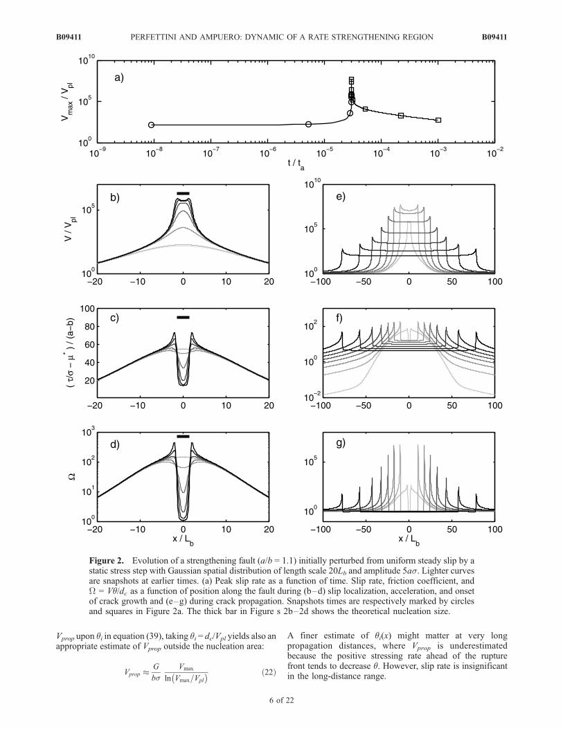
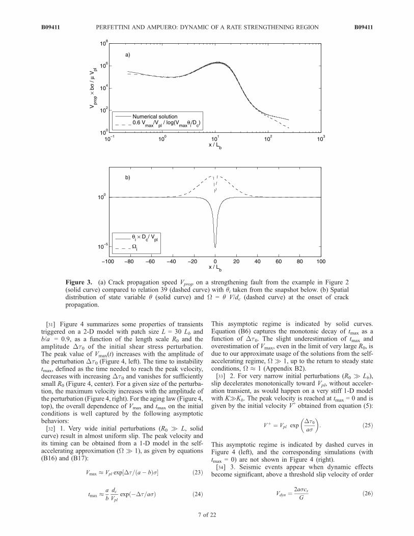
(Figure 2, left) and crack propagation (Figure 2, right) ona 2-D simulation with similar parameters and initial con-ditions as in the previous 3-D example. Figure 3a shows theevolution of the propagation speed of the crack front, Vprop.The crack accelerates when it leaves the nucleation patch,driven mainly by the increasing stress drop induced by therelaxation to steady state inside the crack (on a strengtheningfault stress decreases when slip decelerates). When the crackfront moves beyond the edge of the region of initial stressexcess it enters a region of negative stress drop and slowsdown. As shown in Figure 3a, during most of the transientVprop andVmax are consistent with equation (39) where qi(x) istaken as the fault state at the onset of crack propagation(Figure 3b). Owing to the weak logarithmic dependence of

Figure 1. Evolution of slip velocity on a square fault patch following a stress perturbation of Gaussianshape, with characteristic length R0 = 4Lb and amplitude Dt0 = 10as. (top) Evolution of the maximumslip velocity, with transient acceleration and subsequent relaxation. (bottom) Velocity snapshots(normalized by the loading velocity Vpl) at times indicated by labels in Figure 1 (top).


5 of 22

B09411

Vprop upon qi in equation (39), taking qi = dc/Vpl yields also anappropriate estimate of Vprop outside the nucleation area:

Vprop G

bsVmax

ln Vmax=Vpl

� � ð22Þ

A finer estimate of qi(x) might matter at very longpropagation distances, where Vprop is underestimatedbecause the positive stressing rate ahead of the rupturefront tends to decrease q. However, slip rate is insignificantin the long-distance range.

Figure 2. Evolution of a strengthening fault (a/b = 1.1) initially perturbed from uniform steady slip by astatic stress step with Gaussian spatial distribution of length scale 20Lb and amplitude 5as. Lighter curvesare snapshots at earlier times. (a) Peak slip rate as a function of time. Slip rate, friction coefficient, andW = Vq/dc as a function of position along the fault during (b–d) slip localization, acceleration, and onsetof crack growth and (e–g) during crack propagation. Snapshots times are respectively marked by circlesand squares in Figure 2a. The thick bar in Figure s 2b–2d shows the theoretical nucleation size.


6 of 22

B09411

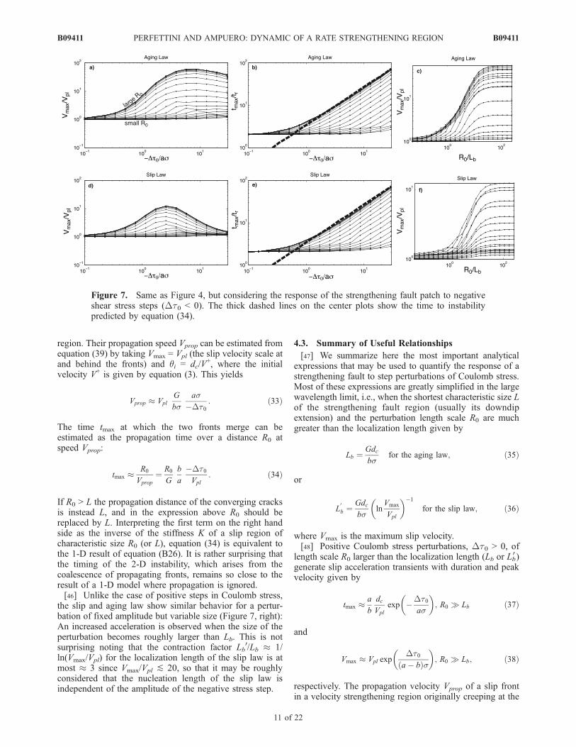
[31] Figure 4 summarizes some properties of transientstriggered on a 2-D model with patch size L = 30 Lb andb/a = 0.9, as a function of the length scale R0 and theamplitude Dt0 of the initial shear stress perturbation.The peak value of Vmax(t) increases with the amplitude ofthe perturbation Dt0 (Figure 4, left). The time to instabilitytmax, defined as the time needed to reach the peak velocity,decreases with increasing Dt0 and vanishes for sufficientlysmall R0 (Figure 4, center). For a given size of the perturba-tion, the maximum velocity increases with the amplitude ofthe perturbation (Figure 4, right). For the aging law (Figure 4,top), the overall dependence of Vmax and tmax on the initialconditions is well captured by the following asymptoticbehaviors:[32] 1. Very wide initial perturbations (R0 L, solid

curve) result in almost uniform slip. The peak velocity andits timing can be obtained from a 1-D model in the self-accelerating approximation (W 1), as given by equations(B16) and (B17):

Vmax Vpl exp Dt= a� bð Þs½ � ð23Þ

tmax a

b

dc

Vpl

exp �Dt=asð Þ ð24Þ

This asymptotic regime is indicated by solid curves.Equation (B6) captures the monotonic decay of tmax as afunction of Dt0. The slight underestimation of tmax andoverestimation of Vmax, even in the limit of very large R0, isdue to our approximate usage of the solutions from the self-accelerating regime, W 1, up to the return to steady stateconditions, W 1 (Appendix B2).[33] 2. For very narrow initial perturbations (R0 Lb),

slip decelerates monotonically toward Vpl, without acceler-ation transient, as would happen on a very stiff 1-D modelwith K Kb. The peak velocity is reached at tmax = 0 and isgiven by the initial velocity V+ obtained from equation (5):

Vþ ¼ Vpl expDt0as

� �: ð25Þ

This asymptotic regime is indicated by dashed curves inFigure 4 (left), and the corresponding simulations (withtmax = 0) are not shown in Figure 4 (right).[34] 3. Seismic events appear when dynamic effects

become significant, above a threshold slip velocity of order

Vdyn ¼2ascsG

ð26Þ

Figure 3. (a) Crack propagation speed Vprop on a strengthening fault from the example in Figure 2(solid curve) compared to relation 39 (dashed curve) with qi taken from the snapshot below. (b) Spatialdistribution of state variable q (solid curve) and W = q V/dc (dashed curve) at the onset of crackpropagation.


7 of 22

B09411

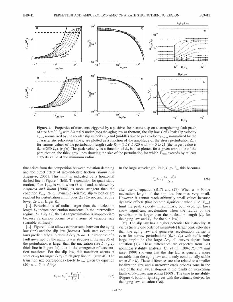
that arises from the competition between radiation dampingand the direct effect of rate-and-state friction [Rubin andAmpuero, 2005]. This limit is indicated by a horizontaldashed line in Figure 4 (left). The condition for quasi-staticmotion, V Vdyn, is valid when W 1 and, as shown byAmpuero and Rubin [2008], is more stringent than thecondition Vprop cs. Dynamic (seismic) slip velocities arereached for perturbation amplitudes Dt0 as, and requirelower Dt0 at larger R0.[35] Perturbations of radius larger than the nucleation

length Lb induce acceleration transients. In the intermediateregime, Lb < R0 < L, the 1-D approximation is inappropriatebecause relaxation occurs over a zone of variable size(variable stiffness).[36] Figure 4 also allows comparisons between the aging

law (top) and the slip law (bottom). Both state evolutionlaws predict large slip rates if Dt0 as. The response of afault governed by the aging law is stronger if the size R0 ofthe perturbation is larger than the nucleation size Lb (greythick line in Figure 4c), due to the emergence of accelera-tion transients. For the slip law, this transition occurs atsmaller R0 for larger D t0 (thick grey line in Figure 4f). Thetransition size corresponds closely to Lb

0 given by equation(20) with qi dc/Vpl,

L0

b Lb lnVmax

Vpl

� ��1

: ð27Þ

In the large wavelength limit, L Lb, this becomes

L0

b Lba� bð ÞsDt0

ð28Þ

after use of equation (B17) and (27). When a b, thenucleation length of the slip law becomes very small.However, it cannot reach arbitrarily small values becausedynamic effects (that become significant when V ^ Vdyn)limit the peak velocity. In summary, both evolution lawsshow significant acceleration when the radius of theperturbation is larger than the nucleation length (Lb forthe aging law and Lb

0 for the slip law).[37] The slip law has a higher potential for instability. It

yields (nearly one order of magnitude) larger peak velocitiesthan the aging law and generates acceleration transientseven for narrow perturbations (R0 < Lb) with sufficientlylarge amplitude (for large Dt0 all curves depart fromequation (3)). These differences are expected from 1-Dnonlinear stability analysis [Gu et al., 1984; Ranjith andRice, 1999] showing that the slip law is generally moreunstable than the aging law and is only conditionally stablewhen K > Kc. These differences are also related to a smallerlocalization size and a narrower crack process zone in thecase of the slip law, analogous to the results on weakeningfaults of Ampuero and Rubin [2008]. The time to instability(Figure 4, bottom right) agrees with the estimate derived forthe aging law, equation (B6).

Figure 4. Properties of transients triggered by a positive shear stress step on a strengthening fault patchof size L = 30 Lb with b/a = 0.9 under (top) the aging law or (bottom) the slip law. (left) Peak slip velocityVmax normalized by the secular slip velocity Vpl and (middle) time to peak velocity tmax normalized by thecharacteristic relaxation time tr are plotted as a function of the amplitude of the stress perturbation Dt0for various values of the perturbation length scale R0 = (1.5)n Lb/20 with n = 0 to 21 (the largest value isR0 250 Lb). (right) The peak velocity as a function of R0 is also plotted for a given amplitude of theperturbation, the thick grey lines showing the size of the perturbation for which Vmax exceeds by at least10% its value at the minimum radius.


8 of 22

B09411

[38] The peak propagation speed of the transient can beestimated by combining equations (22) and (23):

Vprop Vpl expDt

a� bð Þs

� �G

Dta� b

bð29Þ

The exponential term gives a very strong dependence on theamplitude Dt of the stress trigger. The susceptibility isstronger at high fluid pressure, low effective normal stresss, or near the transition zone where a b. This estimate isquasi-static and breaks down when Vmax Vdyn (defined inequation (26)), that is when

Dt a� bð Þs ln 2acSs=GVpl

� �ð30Þ

At that point the propagation speed is

Vprop 2a

bcS= ln 2ascS=GVpl

� �ð31Þ

For reasonable parameter values this gives Vprop/cs 1/20,which is much higher than the average propagation speedsof postseismic, episodic slow slip and tremor swarms.However, this is of the same order as the typical speed ofthe so-called slow rupture fronts observed in laboratoryexperiments of dynamic rupture [Rubinstein et al., 2004].

4.2. Response to Negative Coulomb StressPerturbations

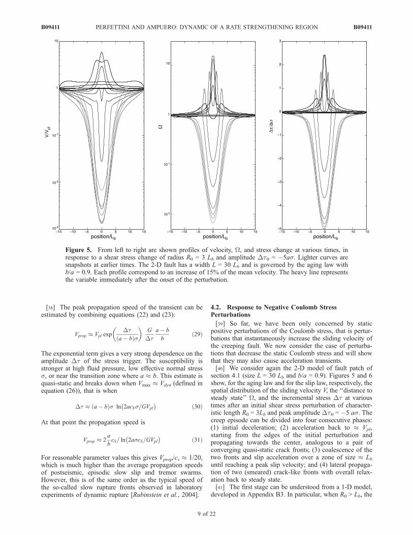
[39] So far, we have been only concerned by staticpositive perturbations of the Coulomb stress, that is pertur-bations that instantaneously increase the sliding velocity ofthe creeping fault. We now consider the case of perturba-tions that decrease the static Coulomb stress and will showthat they may also cause acceleration transients.[40] We consider again the 2-D model of fault patch of

section 4.1 (size L = 30 Lb and b/a = 0.9). Figures 5 and 6show, for the aging law and for the slip law, respectively, thespatial distribution of the sliding velocity V, the ‘‘distance tosteady state’’ W, and the incremental stress Dt at varioustimes after an initial shear stress perturbation of character-istic length R0 = 3Lb and peak amplitude Dt0 = �5 as. Thecreep episode can be divided into four consecutive phases:(1) initial deceleration; (2) acceleration back to Vpl,starting from the edges of the initial perturbation andpropagating towards the center, analogous to a pair ofconverging quasi-static crack fronts; (3) coalescence of thetwo fronts and slip acceleration over a zone of size Lbuntil reaching a peak slip velocity; and (4) lateral propaga-tion of two (smeared) crack-like fronts with overall relax-ation back to steady state.[41] The first stage can be understood from a 1-D model,

developed in Appendix B3. In particular, when R0 > Lb, the

Figure 5. From left to right are shown profiles of velocity, W, and stress change at various times, inresponse to a shear stress change of radius R0 = 3 Lb and amplitude Dt0 = �5as. Lighter curves aresnapshots at earlier times. The 2-D fault has a width L = 30 Lb and is governed by the aging law withb/a = 0.9. Each profile correspond to an increase of 15% of the mean velocity. The heavy line representsthe variable immediately after the onset of the perturbation.


9 of 22

B09411

timescale for initial deceleration is of the order of (seeequation (B23) with Kb/K R0/Lb)

t1 ¼dc

Vpl

R0

Lb� 1

� �: ð32Þ

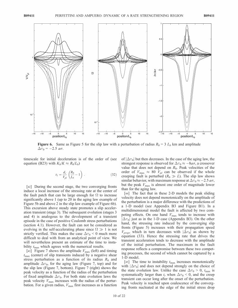
[42] During the second stage, the two converging frontsinduce a local increase of the stressing rate at the center ofthe fault patch that can be large enough for W to increasesignificantly above 1 (up to 20 in the aging law example ofFigure 5b and above 2 in the slip law example of Figure 6b).This excursion above steady state promotes a slip acceler-ation transient (stage 3). The subsequent evolution (stages 3and 4) is analogous to the development of a transientepisode in the case of positive Coulomb stress perturbations(section 4.1). However, the fault can not be considered asevolving in the self-accelerating phase since W 1 is notstrictly verified. This makes the case Dt0 < 0 much moredifficult to deal with from an analytical point of view. Wewill nevertheless present an estimate of the time to insta-bility tmax which agrees with the numerical results.[43] Figure 7 shows the amplitude Vmax (left) and timing

tmax (center) of slip transients induced by a negative shearstress perturbation as a function of its radius R0 andamplitude Dt0, for the aging law (Figure 7, top) and forthe slip law (Figure 7, bottom). Figure 7 (right) shows thepeak velocity as a function of the radius of the perturbationof fixed amplitude Dt0. For both state evolution laws thepeak velocity Vmax increases with the radius of the pertur-bation. For a given radius, Vmax first increases as a function

of jDt0j but then decreases. In the case of the aging law, thestrongest response is observed forDt0 �8as, a crossovervalue that does not depend on R0. Peak velocities of theorder of Vmax 80 Vpl can be observed if the wholecreeping fault is perturbed (R0 L). The slip law showssimilar behavior, with maximum response atDt0�2.5 as,but the peak Vmax is almost one order of magnitude lowerthan for the aging law.[44] The fact that in these 2-D models the peak sliding

velocity does not depend monotonically on the amplitude ofthe perturbation is a major difference with the predictions ofa 1-D model (see Appendix B3 and Figure B1). In amultidimensional model the fault is affected by two com-peting effects. On one hand Vmax tends to increase withjDt0j just as in the 1-D case (Appendix B3). On the otherhand, the stressing rate induced by the converging slipfronts (Figure 5) increases with their propagation speedVprop, which in turn decreases with jDt0j as shown byequation (33). Hence the stressing rate that drives thetransient acceleration tends to decrease with the amplitudeof the initial perturbation. The maximum in the faultresponse reflects a compromise between these two compet-ing processes, the second of which cannot be captured by a1-D model.[45] The time to instability tmax increases monotonically

with jDt0j and does not depend strongly on the choice ofthe state evolution law. Unlike the case Dt0 > 0, tmax issystematically larger than tr when Dt0 < 0, and the creeptransient can occur long after the onset of the perturbation.Peak velocity is reached upon coalescence of the converg-ing fronts nucleated at the edge of the initial stress drop

Figure 6. Same as Figure 5 for the slip law with a perturbation of radius R0 = 3 Lb km and amplitudeDt0 = �2.5 as.


10 of 22

B09411

region. Their propagation speed Vprop can be estimated fromequation (39) by taking Vmax = Vpl (the slip velocity scale atand behind the fronts) and qi = dc/V

+, where the initialvelocity V+ is given by equation (3). This yields

Vprop Vpl

G

bsas

�Dt0: ð33Þ

The time tmax at which the two fronts merge can beestimated as the propagation time over a distance R0 atspeed Vprop:

tmax R0

Vprop

¼ R0

G

b

a

�Dt0Vpl

: ð34Þ

If R0 > L the propagation distance of the converging cracksis instead L, and in the expression above R0 should bereplaced by L. Interpreting the first term on the right handside as the inverse of the stiffness K of a slip region ofcharacteristic size R0 (or L), equation (34) is equivalent tothe 1-D result of equation (B26). It is rather surprising thatthe timing of the 2-D instability, which arises from thecoalescence of propagating fronts, remains so close to theresult of a 1-D model where propagation is ignored.[46] Unlike the case of positive steps in Coulomb stress,

the slip and aging law show similar behavior for a pertur-bation of fixed amplitude but variable size (Figure 7, right):An increased acceleration is observed when the size of theperturbation becomes roughly larger than Lb. This is notsurprising noting that the contraction factor Lb

0/Lb 1/ln(Vmax/Vpl) for the localization length of the slip law is atmost 3 since Vmax/Vpl ] 20, so that it may be roughlyconsidered that the nucleation length of the slip law isindependent of the amplitude of the negative stress step.

4.3. Summary of Useful Relationships

[47] We summarize here the most important analyticalexpressions that may be used to quantify the response of astrengthening fault to step perturbations of Coulomb stress.Most of these expressions are greatly simplified in the largewavelength limit, i.e., when the shortest characteristic size Lof the strengthening fault region (usually its downdipextension) and the perturbation length scale R0 are muchgreater than the localization length given by

Lb ¼Gdc

bsfor the aging law; ð35Þ

or

L0

b ¼Gdc

bslnVmax

Vpl

� ��1

for the slip law; ð36Þ

where Vmax is the maximum slip velocity.[48] Positive Coulomb stress perturbations, Dt0 > 0, of

length scale R0 larger than the localization length (Lb or Lb0 )

generate slip acceleration transients with duration and peakvelocity given by

tmax a

b

dc

Vpl

exp �Dt0as

� �; R0 Lb ð37Þ

and

Vmax Vpl expDt0

a� bð Þs

� �; R0 Lb; ð38Þ

respectively. The propagation velocity Vprop of a slip frontin a velocity strengthening region originally creeping at the

Figure 7. Same as Figure 4, but considering the response of the strengthening fault patch to negativeshear stress steps (Dt0 < 0). The thick dashed lines on the center plots show the time to instabilitypredicted by equation (34).


11 of 22

B09411

long term velocity Vpl is related to the peak slip velocityVmax at the rupture front by

Vprop Vmax

G

bslnVmax

Vpl

� ��1

: ð39Þ

[see Ampuero and Rubin, 2008, equation (53)]. In the caseof a negative step in Coulomb stress, the time to peak slipvelocity is

tmax � b

a

R0Dt0GVpl

; ð40Þ

and the propagation velocity is

Vprop Vpl

G

bs� as�Dt0

; ð41Þ

5. Discussion

5.1. Possible Origins of the Perturbations

[49] In this work, we have studied the response of acreeping fault to a sudden change in Coulomb stressinduced by an external perturbation. We discuss here thepossible origins of such perturbations.[50] Postseismic slip is unambiguously triggered by the

coseismic stress changes induced by the main shock. Anearthquake induces significant stress changes over an areaof size comparable to the rupture size. Since significantpostseismic slip is only observed following large earth-quakes, that rupture the whole thickness of the seismogeniczone, postseismic slip corresponds to large scale (>10 km)stress changes.[51] Slow slip events, such as those observed in the

Cascadia subduction zone, seem to be induced by stressperturbations of much smaller wavelengths. J.-P. Ampueroand H. Perfettini (manuscript in preparation, 2008) discussthe triggering of creep events by brittle asperities present inthe creeping region. Nevertheless, this mechanism is diffi-cult to reconcile with the existence of the seismic tremorsrelated to slow slip events [Obara, 2002; Rogers andDragert, 2003; Obara et al., 2004; Kao et al., 2005]. Amore complete model should incorporate variables such asporosity and pore pressure, together with an evolution lawrelating porosity and creep rate. Although such modeling isbeyond the scope of the present article, we outline nextsome basic ideas.[52] Volcanic tremors are usually interpreted as due to the

circulation of fluids [Chouet, 1992; Ferrazzini and Aki,1992]. The nonvolcanic tremors connected to slow earth-quake have been sometimes attributed to metamorphicdehydration reactions. Fluids are released by metamorphicreactions over a broad range of depths. Part of those fluidsmigrate updip the subduction interface, channeled by thefault zone itself, until they encounter less permeable materi-als. In the fault valve model proposed by Sibson [1992],ductile creep within mostly sealed fault zones compacts thefault gouge and increases fluid pressure [Sleep, 1995], untilthe reduction of the effective normal stress is large enoughfor the accumulated shear stress to counteract the frictional

resistance. Then slip occurs and changes the mechanicalstate of the fault from undrained to drained, resulting in anincrease of the porosity. After the slip episode the fault zonestarts to compact again for another cycle. Such a mechanismhas been advocated to explain the cyclic behavior of eventsin the seismogenic zone [Sleep and Blanpied, 1992; Sleep,1995].[53] Because ductile creep is even more active in the

transition zone, due to higher temperatures, the fault valvemechanism seems even more likely in this part of the faultand is consistent with the generation of seismic tremors bythe expulsion of fluids away from the fault zone. This fluidrelease would induce a drop in pore pressure and a negativeCoulomb stress perturbation that may be sufficient togenerate a transient creep episode such as those studied insection 4.2. The propagation of the slow earthquake wouldincrease the creep rate along its way, increasing the com-paction rate, and eventually trigger secondary creep insta-bilities in areas where the shear stress was already close tothe frictional stress.

5.2. Estimate of the Size and Time to Instability forNatural Cases

[54] In order to discuss the relevance of our results forreal faulting, it is necessary to bound the parameters tmax

and Lb. There are large uncertainties about the appropriatevalue of dc, which ranges from 1 mm to 1 cm in laboratoryexperiments [Marone, 1998]. Assuming a b and takingtypical laboratory values a = 10�3�10�2 [Marone, 1998],and effective normal stress s 100 MPa, or the rangeas = 0.1–1 MPa inferred from aftershock and postseismicobservations, yields rather small localization length scalesLb = 3 cm to 3 km. Large earthquakes induce large-scale(several tens of kilometers) stress perturbations. This suggestthat the large-scale limit (L Lb) applies.[55] At the top of the transition zone, where a b, the

time to instability in response to a positive Coulomb stressstep is tmax dc/V

+ (from equation (B17)), where thesliding velocity V+ immediately after the stress step mayvary from typical postseismic values (e.g., 103 Vpl asdiscussed by Perfettini and Avouac [2004] and Perfettiniet al. [2005]) to seismic rupture velocities (1 m/s). Thereforetmax may span an enormous range of short timescales, from10�6 s to 2 days. At the lower end of this range, slipacceleration would be too short to be considered as post-seismic slip and would rather qualify as part of the mainshock or as an early aftershock. At the higher end, thedetection of short acceleration transients still requires high-quality, high sampling rate geodetic data. Recent analysis ofthe postseismic slip of the 2004 Parkfield earthquake byLangbein et al. [2006], consistent with a velocity-strength-ening rheology except in the first hour of relaxation [see,e.g., Langbein et al., 2006, Figure 3], suggests values oftmax shorter than one hour. An earthquake catalog of theChi-Chi aftershocks obtained from accelerometric records[Chang et al., 2007] shows that the seismicity rate decaysmonotonically as 1/time, starting as early as 2–3 mn afterthe main shock (J.-P. Avouac, personal communication,2008), suggesting a value of tmax lower than 2 mn.[56] Large earthquakes can induce slip transients, as was

the case for the 23 June 2001 Arequipa (Mw 8.4), Peru,earthquake [Melbourne and Webb, 2002]. Its largest after-


12 of 22

B09411

shock, the 7 July (Mw 7.6) event, was preceded by 18 h byan aseismic transient consistent with slip acceleration (about2 cm in 18 h) in the downdip vicinity of the 7 Julyhypocenter, presumably at the top of the transition zone[Melbourne and Webb, 2002]. The postseismic phase of the30 July 1995 (Mw 8.1) Antofagasta, Chile, earthquakepresents a similar case. Pritchard and Simons [2006a]observed the growth of an aseismic slip pulse at the down-dip termination of the main shock coseismic slip, starting inNovember 1996 and lasting 1 year. The transient may havetriggered the Mw7.1 earthquake on 30 January 1998. Inthese two examples, the time delay between the main shockand the transient peak velocity ranges from 2 weeks to2 years. These slip transients could be either due to anincrease or a decrease in Coulomb stress. We now examinethose two scenarios.[57] The observed delay times are much longer than our

previous estimates of tmax for positive Coulomb stress steps(10�6 s to 2 days). Since tmax dc/V

+ at the top of thetransition zone, then either dc is at least metric or V+ is muchsmaller. The latter is not an option because the initialvelocity needs to be significant (V+ ^ 100 Vpl) in orderfor the transient to be detectable. Values of dc of the order ofone meter are much larger than laboratory values. However,there is a notorious lack of laboratory experiments atpressure and temperature conditions relevant for the top ofthe transition zone. If dc scales with fault zone width or withcumulative slip [Marone and Kilgore, 1993], it may reachlarger values than commonly thought in the transition zone,due to the many tens of kilometers of slip accumulatedduring subduction. Still, for an exhumed mature section ofthe San Andreas fault, Marone and Kilgore [1993] proposesvalues of dc that are only millimetric. Moreover, values ofdc ^ 1 m imply huge localization lengths (Lb or Lb

0 )inconsistent with the spatial extent of the creep pulsementioned by Pritchard and Simons [2006a]. Hence, trig-gering of these slip transients by an increase of Coulombstress is an unlikely scenario.[58] If the transients were initiated by a decrease in

Coulomb stress, then we have to identify a possible causefor such a perturbation. The main shock itself can notgenerate directly a negative step in Coulomb stress, but itmight do so indirectly by inducing secondary processes.Among them is the breakage of isolated fluid pockets. Ifprior to the main shock the fault was undrained, then someareas might have been overpressured. The main shockrupture may have broken some of those pockets, allowingthe pressurized fluids to escape rapidly. This would result infault clamping, a rapid increase in effective normal stressfrom a value near 0 to a value close to the lithostaticpressure. According to the results of section 4.2, a sliptransient will follow long after the main shock. The strongerthe drop in fluid pressure the longer the delay time,plausibly as large as 2 weeks or 2 years.[59] Among the two speculative scenarios considered

above, only clamping of the fault due to the breakage ofoverpressured fluid pockets induced by seismic rupture isconsistent with the observations of Melbourne and Webb[2002] and Pritchard and Simons [2006a]. Similar examplesmight soon become quite common with the increase ofdense continuous GPS network observations.

[60] Slip acceleration transients, such as frictional after-slip or slow slip transients, significantly increase the loadingrate on their vicinity, decreasing the recurrence time of thenearby locked patches. If a brittle area of the fault is already atthe end of its earthquake cycle, the occurrence of such eventsis very likely to trigger them. Postseismic slip can triggerearthquakes as in the case of 1994 Sanriku-haruka-oki,Japan, earthquake (Mw7.7) [Yagi et al., 2003]. The largestaftershock of this event, a Mw6.9 earthquake, occurred 10 dlater, and its hypocenter was located on the edge of thepostseismic patch. Yagi et al. [2003] mention an initial phaseof slip acceleration up to 30 mm/day during the periodpreceding the Mw6.9 event. It is likely that this aftershockoccurred in a region already preloaded by the main shock,the reloading by the nearby afterslip (which locallyincreases the loading rate by many orders of magnitude)bringing it to failure.

5.3. Equivalence Between Pure Velocity-Strengtheningand Complete Rate-and-State Formulations DuringPostseismic Slip

[61] Numerous studies have shown that postseismic de-formation is consistent with slip on portions of the fault withpure velocity strengthening friction [Marone et al., 1991;Hearn et al., 2002; Perfettini and Avouac, 2004; Perfettiniet al., 2005; Hsu et al., 2006; Perfettini and Avouac, 2007]:

m ¼ m*þ a0 lnV

V*

� �ð42Þ

with a0 > 0. It is clear from equations (8) and (42) that purevelocity strengthening friction is equivalent to rate-and-state friction at steady state with parameters a and b suchthat a0 = a� b. However it is not immediately obvious underwhich circumstances the steady state assumption is a goodapproximation of the complete rate-and-state fault response.[62] In a spring block (1-D model) with pure velocity-

strengthening friction, initially sliding at steady state, theslip velocity in response to a step in shear stress decreasesmonotonically as [Perfettini et al., 2005]

V tð Þ ¼ Vþ et=tr

1þ Vþ

Vpl

et=tr � 1� � ð43Þ

with decay time tr and initial velocity V+ given by equations(B5) and (3), respectively, changing a by a0. In the completerate-and-state case we have shown in section and inAppendix B1 that a fault of size L Lb responds insteadby an initial acceleration up to maximum velocity Vmax,over a timescale tmax, and then relaxes in steady state. Theslip evolution during the relaxation stage, given in equation(B20), is exactly the same as in equation (43) after obviousparameter identifications are made (V+ =Vmax and a

0 = a� b).[63] In practice, the timescale tmax of the acceleration

transient is short (at most a few days as discussed in section5.2) compared to the characteristic duration tr of postseismicslip (typically a few years). The correspondence betweenthe pure velocity-strengthening and the complete rate-and-state rheologies is warranted during most of the postseismicperiod if L Lb.


13 of 22

B09411

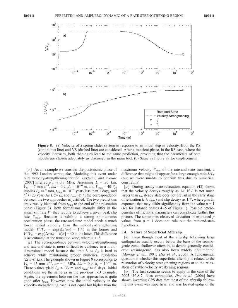
[64] As an example we consider the postseismic phase ofthe 1992 Landers earthquake. Modeling this event underpure velocity-strengthening friction, Perfettini and Avouac[2007] inferred a0s 0.5 MPa. Assuming L = 30 km,Vpl = 7 mm a�1, b/a = 0.9, dc = 10�6 m, and Vmax = 40 Vpl

implies Lb 7 mm, tmax 10�4 year (less than 1 day), andtr0 23 year. As L Lb and tmax tr, the correspondence

between the two approaches is justified. The two predictionsare virtually identical from tmax to the end of the relaxationphase (Figure 8). Both formalisms strongly differ in theinitial slip rate V+ they require to achieve a given peak sliprate Vmax. Because it exhibits a strong spontaneousacceleration phase, the rate-and-state model needs a muchlower initial velocity than the velocity-strengtheningmodel: V+/Vpl = exp(Dt/as) = 1.45 in the former andV+/Vpl = exp[Dt/(a� b)s] = 40 in the latter. This differenceis accentuated at the transition zone, where a b.[65] The correspondence between velocity-strengthening

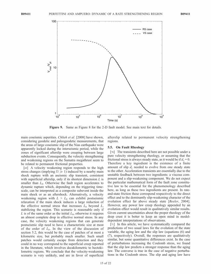
and rate-and-state is more difficult to evidence in a multi-dimensional model because the limit L Lb is hard toachieve while maintaining proper numerical resolution(D x Lb). The example shown in Figure 9 corresponds toVpl = 45 mm a�1, as = 1 MPa, b/a = 0.9, dc = 10�3 m.These values yield Lb 33 m and tmax 6 days. Initialconditions are the same as in the previous 1-D example.Again, the agreement between the two approaches is quitegood after tmax. However, now the initial velocity in thevelocity-strengthening case is not equal but higher than the

maximum velocity Vmax of the rate-and-state transient, adifference that might disappear for a large enough ratio L/Lb(but we were unable to confirm this due to numericalconstraints).[66] During steady state relaxation, equation (43) shows

that the velocity decays roughly as 1/t. If L is not muchlarger than Lb steady state does not prevail in the early stageof relaxation (t ^ tmax) and slip decays as 1/tp, where p is anexponent that may differ significantly from the value p = 1(see for instance phases 4–5 of Figure 1). Possible hetero-geneities of frictional parameters can complicate further thispicture. The sometimes observed deviation of estimated pvalues from p = 1 does not rule out the rate-and-statehypothesis.

5.4. Nature of Superficial Afterslip

[67] Even though most of the afterslip following largeearthquakes usually occurs below the base of the seismo-genic zone, shallower afterslip, at depths generally consid-ered seismogenic, has also been widely documented[Marone et al., 1991; Hsu et al., 2006]. A fundamentalquestion is whether this superficial afterslip is related to therelaxation of velocity strengthening regions or to the relax-ation of stable velocity weakening regions.[68] The first scenario seems to apply in the case of the

2005, Mw8.7, Nias earthquake. Hsu et al. [2006] haveshown inverting GPS data that most of the afterslip follow-ing this event was superficial and was located updip of the

Figure 8. (a) Velocity of a spring slider system in response to an initial step in velocity. Both the RS(continuous line) and VS (dashed line) are considered. After a transient phase, in the RS case, where thevelocity increases, both rheologies lead to the same prediction, providing that the parameters of bothmodels are chosen adequately as discussed in the main text. (b) Same as Figure 8a for displacement.


14 of 22

B09411

main coseismic asperities. Chlieh et al. [2008] have shown,considering geodetic and paleogeodetic measurements, thatthe areas of large coseismic slip of the Nias earthquake wereapparently locked during the interseismic period, while thezones of significant afterslip were creeping between largesubduction events. Consequently, the velocity strengtheningand weakening regions on the Sumatra megathrust seem tobe related to permanent frictional properties.[69] A velocity weakening region responds to the high

stress changes (implying W 1) induced by a nearby mainshock rupture with an aseismic slip transient, consistentwith superficial afterslip, only if its shortest dimension L issmaller than Lb. Otherwise the fault region accelerates todynamic rupture which, depending on the triggering time-scale, can be interpreted as a composite subevent inside themain shock or as an aftershock. Alternatively, a velocityweakening region with L > Lb can exhibit postseismicrelaxation if the main shock induces a large reduction ofthe effective normal stress that increases Lb beyond L,stabilizing the region. This scenario is reasonable only ifL is of the same order as the initial Lb, otherwise it requiresan almost complete drop in effective normal stress. In anycase, the velocity weakening regions that can generatepostseismic slip need to have a characteristic size at mostof the order of Lb. In the view of the discussion ofsection 5.2, this would be the case of patches of at most akilometric size, but probably much smaller. Such smallpatches would certainly escape from detection and theycould in no way correspond to the superficial creep reportedin the literature, which involves decakilometric to hectoki-lometric regions. We conclude that the velocity-weakeningscenario is very unlikely, and are in favor of superficial

afterslip related to permanent velocity strengtheningregions.

5.5. On Fault Rheology

[70] The transients described here are not possible under apure velocity strengthening rheology, or assuming that thefrictional stress is always steady state, as it would be if dc = 0.Therefore a key ingredient is the existence of a finiteamount of slip dc needed to evolve from one steady stateto the other. Acceleration transients are essentially due to theunstable feedback between two ingredients: a viscous com-ponent and a slip-weakening component. We do not expectthe particular mathematical form of the fault zone constitu-tive law to be essential for the phenomenology describedhere, as long as these two ingredients are present. In rate-and-state friction these correspond respectively to the directeffect and to the dominantly slip-weakening character of theevolution effect far above steady state [Beeler, 2004].However, any power law creep rheology appended by anevolution effect would result in qualitatively similar results.Given current uncertainties about the proper rheology of thedeep crust it is better to keep an open mind in model-dependent interpretations of observations.[71] In this article, we have systematically compared the

predictions of two usual laws for the evolution of the statevariable, the aging law and the slip law (equations (6) and(7), respectively). Overall, the responses are qualitativelysimilar, but some quantitative differences exist. In the caseof perturbations increasing the Coulomb stress, we foundthat the slip law predicts a stronger response than the aginglaw. The converse is true in the case of negative perturba-tions in the Coulomb stress. The slip and aging law have

Figure 9. Same as Figure 8 for the 2-D fault model. See main text for details.


15 of 22

B09411

were originally motivated by laboratory experiments withsmall to moderate velocity steps. Recently, Bayart et al.[2006] performed finite velocity steps (up to 100 times theloading velocity) and found that only the slip law couldproperly model their data. Such large velocity steps corre-spond to W 1 as expected near the rupture front. It shouldbe kept in mind that the results of Bayart et al. [2006] wereobtained at room temperature. Velocity step experiments inthe velocity strengthening regime close to the transitionzone (a ^ b), in the temperature range 250–300�C forgranite, should allow the discrimination of the evolutionlaws. The analytical results presented here should be par-ticularly helpful to analyze those laboratory results.

6. Conclusion

[72] We have studied the dynamics of a rate-and-statestrengthening fault in response to localized static stressperturbations. Positive Coulomb stress changes induce slipacceleration followed by relaxation toward steady state. Oursimulations and theoretical arguments show that the evolu-tion of slip during such transients is strikingly similar to theearthquake nucleation process on a weakening fault, with aninitial phase of slip localization and acceleration, followedby the propagation of a quasi-static crack. On strengtheningfaults; however, slip rate eventually relaxes back to steadystate.[73] In fault zones close to velocity neutral (a b), as

expected right below the seismogenic zone, the peak slidingvelocity can be extremely large and reach dynamic scales.Large-amplitude transients could propagate updip and trig-ger a seismic event in the seismogenic region above,especially near the end of the seismic cycle, as proposedby Rogers and Dragert [2003]. The time to peak velocitydecreases with increasing amplitude and wavelength of thepositive stress perturbation, consistently with the behaviorof a spring block model.[74] The short duration of the slip acceleration transient

justifies the usual practice of modeling postseismic slipunder the steady state approximation, which reduces therate-and-state rheology to a pure velocity-strengtheningrheology. This approach yields a constraint on the frictionalparameter a � b, but the apparent initial velocity should beinterpreted as the peak velocity of the short initial transient.Conversely, modeling postseismic geodetic data with thecomplete rate-and-state rheology is justified if the initialacceleration transient is observable. In this approach, properresolution requires, even on strengthening regions, gridsizes smaller than Lb = G dc/bs with the aging law andup to 20 times smaller with the slip law. This is morestringent than the resolution criterion based on the criticallength Lc = Gdc/(b � a)s [Rice, 1993] commonly adopted inthe literature [e.g., Hirose and Hirahara, 2004; Liu andRice, 2005]. In full rate-and-state inversions, current limi-tations on computational resources will tend to bias theparameter space to high values of dc/bs.[75] Our results suggest that shallow afterslip observed at

expectedly seismogenic depths occurs on intrinsicallycreeping zones, with rate-and-state strengthening rheology.This is consistent with the observed location of postseismicslip of the 2005 Mw 8.7 Nias earthquake [Hsu et al., 2006],

in areas that were also creeping during the interseismicperiod [Chlieh et al., 2008].[76] Creep transients can be also triggered by negative

Coulomb stress changes, representing for example a suddenincrease in effective normal stress induced by the rupture ofa high pressure fluid pocket. Their peak slip velocity isattained at much longer timescales and remains limited to afew orders of magnitude larger than the plate velocity.Because they occur long after their cause, these transientsmay be misinterpreted as spontaneous slow earthquakes.Some slow events exhibiting a rather modest peak velocitymay be triggered by sudden episodes of fluid release.

Appendix A: Condition for Well Resolved SpatialDiscretization

[77] The presence of a characteristic slip scale dc in theaging state evolution law (equation (6)) implies a finiteeffective slip-weakening rate bs/dc for sliding far abovesteady state, which in turn implies the existence of acharacteristic length scale Lb (equation (10)). The smallestscale of slip localization is Lv = 1.3774 Lb [Rubin andAmpuero, 2005] and the size of the crack tip process zone is0.7Lb [Ampuero and Rubin, 2008, Figure 10]. Obviously,these length scales must be well resolved by the spatialdiscretization of the governing elasticity and rate-and-stateequations (Dx Lb) in order to obtain an accuratenumerical solution. A more subtle issue, illustrated in theremainder of this appendix, is that the risk of numericalinstabilities is high if the condition Dx Lb is not verified,even on a strengthening fault. In all our simulations with theaging law we have set Dx � Lb/20.[78] Figure A1 shows the evolution of the maximum

velocity on a rate-and-state strengthening fault segment ofsize L = 300 Lb, with b/a = 0.9 and governed by the aginglaw, following a perturbation of size R0 = 150 Lb andamplitude Dt0 = 10 as. The different curves result fromthe numerical solution of the 2-D model with different gridsizes, Dx/Lb = 1/16, 1/4, 4, and 16. The heavy grey line isthe solution for Dx/Lb = 1/16 and further reduction of Dxdoes not yield visible changes. Looking at the inset ofFigure A1 near the peak velocity of the well resolved case(thick line), periodic fluctuations of the sliding velocityaround the maximum value are observed when the numer-ical grid is too coarse. The amplitude and period of thoseoscillations increase with the size of the grid. These arenumerical artifacts that are not present on a sufficientlyrefined grid. Figure A2 shows the result of a similar exercisenow with Dt0 = �10as. In this case, a coarse mesh yieldssecondary maxima in slip velocity in some cases one orderof magnitude larger than the well resolved case. As in thecase Dt0 = +10as, the period and amplitude of thesecondary velocity peaks are increasing with the size ofthe grid and disappear for a sufficiently refined grid.Consequently, the effect of a rough discretization is worsein the case of negative steps in Coulomb stress that it is inthe case of positive steps in Coulomb stress.[79] The properties of the secondary peaks in Figure A2

can be understood by the following reasoning. When Dx >Lb each cell can slip independently from its neighbors. Asthe slip front is propagating towards the center of the fault,it triggers the acceleration of each individual point it


16 of 22

B09411

encounters. Therefore, the period of those secondary peakscorresponds roughly to Dx/Vprop, the time needed for thefront to propagate from one point to its immediate neighbor,an estimate of Vprop being given in equation (33). Aspredicted by a 1-D model, the larger the ratio Dx/Lb, thehigher the velocity of a secondary peak.[80] For the slip law, equation (7), the grid resolution

requirements are more stringent. The localization length andthe size of the process zone are smaller than Lb by a factorthat depends logarithmically on slip rate, and that typicallyreaches 20 during fast slip [Ampuero and Rubin, 2008].Moreover, the slip law is more unstable to finite amplitude

perturbations than the aging law. In all our simulations withthe slip law we have set Dx < Lb/200.[81] According to the criterion introduced by Rice [1993],

whenDx is larger than the critical length Lc of equation (19)the continuity of the medium is lost and the numericalcalculation becomes ‘‘inherently discrete’’: a numerical cellcan generate an instability independently of the neighboringcells. A stability criteria based on Lc fails to explain ourresults of Figures A1 and A2, because Lc is undefined(negative) on a velocity strengthening region. The criticallength Lc obtained from a linear stability analysis is notrelevant for the perturbations of finite amplitude considered

Figure A2. Same as Figure A1 for an unloading stress change Dt0 = �10as.

Figure A1. Response of a 2-D creeping fault of size L = 300 Lb, with b/a = 0.9 and governed by theaging law, following a perturbation of size R0 = 150 Lb and amplitude Dt0 = 10as. Various grid size areconsidered (Dx/Lb = 1/16, 1/4, 4, and 16). The stable solution (thick solid grey line) is achieved when thegrid size becomes significantly smaller than Lb.


17 of 22

B09411

here. The same conclusions have been reached by Dieterich[1992] and Rubin and Ampuero [2005] considering rate-and-state weakening faults.[82] Examples of low resolution (low Lb/Dx) in rate-and-

state simulations are unfortunately abundant, due to thewidespread adoption of a criterion based on Lc [Rice, 1993].Values of Lb/Dx at seismogenic depths and in part of thetransition zones are typically of order 1 in many recentsimulations exploring specifically slow slip phenomena [Liuand Rice, 2005; Hirose and Hirahara, 2004; Shibazaki andShimamoto, 2007].[83] The stability problems may not affect the timing of

the episode of slip increase (regular earthquakes or creepbursts) as illustrated in Figure A1. Nevertheless, a carefullook at the numerical data reveals the existence of secondaryoscillations, which period and amplitude increase as Dx/Lbdecrease. A lack of resolution can lead to dramatic numericalartifacts as illustrated by Figure A2, that may be misinter-preted as physically sound slip instabilities.

Appendix B: Slip Instabilities in a 1-D Model

B1. Self-Accelerating Instabilities on a WeakeningSpring Block

[84] We consider a single spring block system withoutinertia nor radiation damping. This 1-D model temptativelyrepresents a spatial average of a higher dimensional faultmodel, with effective stiffness K scaled as

K ¼ gG

L; ðB1Þ

where L is a typical shortest dimension of the slippingregion and g is a factor of the order of unity that depends onthe patch shape, on the sliding mode and on Poisson’s ratio.For the purpose of comparison with multidimensionalmodels we set g = p. However, the analogy must beexercised with caution when the dimensions of the slippingpatch are evolving with time.[85] During fast sliding rate-and-state faults evolve often

far above steady state, W = Vq/dc 1. This is typically thecase when a fault initially sliding at steady state velocity Vpl

is perturbed by a large increase of shear stress Dt0 assince, from equation (3),

Wþ ¼ Vþ=Vpl ¼ exp Dt0=asð Þ: ðB2Þ

If the state variable is governed by the aging law, thecondition W 1 allows for the so-called self-acceleratingapproximation, in which equation (6) becomes _q �W. Inthis regime [Dieterich, 1994] obtained the followingsolution for slip velocity

V tð Þ ¼ Vþ

1þ Lð Þ e�t=tr � L; ðB3Þ

where the initial velocity V+ is given by equation (3),

L ¼ Kb � K

K

Vþ

Vpl

; ðB4Þ

the characteristic stiffness Kb is given in equation (13) andthe characteristic time tr is defined as

tr ¼asKVpl

: ðB5Þ

If K < Kb slip accelerates and becomes unbounded at failuretime

t* ¼ tr ln 1þ 1=Lð Þ: ðB6Þ

It can be shown, following the formalism developed byPerfettini et al. [2003], that equation (B6) gives a lowerbound of the time to instability when the self-acceleratingapproximation is relaxed. The approximation relies on theassumption that W 1 persists until failure, and we verifynext its self-consistency by seeking an expression for W(t).[86] The equation of equilibrium for the spring block

model, a balance between frictional and elastic forces, is

sm V ; qð Þ ¼ K Vpl t � D� �

; ðB7Þ

where s is the normal stress (assumed constant), the frictioncoefficient m is given by the rate-and-state law (5), Vpl is thelong-term loading velocity and D is slip. Deriving withrespect to time the equilibrium equation (B7) and thedefinition W = Vq/dc, we obtain

as_V

Vþ bs

_qq¼ K Vpl � V

� �ðB8Þ

_WW¼

_V

Vþ

_qq

ðB9Þ

respectively. When W 1, we can insert _q/q �V/dc in theequations above and, after some algebra,

_WW¼ Kc � K

Kb � K

_V

Vþ K

Kb � K

Vpl

dcðB10Þ

where

Kc ¼b� að Þsdc

ðB11Þ

Upon time integration and considering equation (B5), weobtain

W tð ÞWþ ¼ V tð Þ

Vþ

� �Kc�KKb�K

expKb � Kc

Kb � K

t

tr

� �ðB12Þ

or, eliminating t in favor of V(t) with the aid ofequation (B3),

W tð ÞWþ ¼ V tð Þ

Vþ

� �Kc�KKb�K 1þ L

Vþ=V tð Þ þ L

� �Kb�Kc

Kb�K

ðB13Þ

Whereas equation (B3) shows that slip initially accel-erates toward failure if K < Kb, it appears from equation(B13) that the fault is guaranteed to remain above steadystate (increasing W) up to failure time only if K < Kc. If


18 of 22

B09411

Kc < K < Kb the evolution of W is eventually dominated bythe decay of the first term of equation (B13) and theinstability is frustrated, although it can reach high velocities ifthe initial perturbation is strong enough. If K > Kb noinstability develops: according to equation (B3), V relaxestoward�V+/L and the second term in equation (B13) decays,bringing the fault back to steady state.[87] The critical stiffness Kc for self-accelerating insta-

bilities appears also in classical linear stability analysis, butit is obtained here from a more general, nonlinear analysisconsistent with the results of Ranjith and Rice [1999]. Rubinand Ampuero [2005] and Ampuero and Rubin [2008]presented a similar discussion but assuming slow loading(Vpl V in equation (B8), which implies the second term inequation (B13) is neglected).

B2. Response of a Strengthening Spring Block toPositive Stress Perturbations

[88] The sign of a � b is not involved in equation (B3)so, although originally derived for weakening faults, thisself-accelerating regime also exists for strengthening faultsif the initial conditions are such that W 1. The maindifference on a strengthening fault is that, as Kc < 0, it isalways the case that K > Kc and instabilities do not fullydevelop. However, although V(t) remains finite its transientexcursions can be large. We focus next on the extremalproperties of these transients, their peak velocity Vmax andthe time tmax needed to attain peak velocity.[89] When K > Kb the slip velocity decays monotonically

if (K � Kb)V+/KVpl > 1 and the peak velocity Vmax = V+ is

reached at tmax = 0. When K < Kb transients with initialacceleration occur and Vmax is reached close to the timewhen steady state is recovered. At the expense of a slightoverestimation of Vmax and underestimation of tmax, equation(B13) obtained under the assumption W 1 can becombined with the condition W 1 to yield an implicitrelation for Vmax:

Vmax

Vpl

¼ Vþ

Vpl

1þ LVþ=Vmax þ L

� �Kb�Kc

K�Kc

: ðB14Þ

A close form expression,

Vmax

Vpl

¼ Vþ

Vpl

1þ 1=Lð Þ� �Kb�Kc

K�Kc

; ðB15Þ

is obtained when Vmax V+/L = Vpl � K/(Kb � K), whichcan be shown to be generally valid if K and V+ are not tooclose to Kb and Vpl, respectively. Moreover, under theseconditions, the time of peak velocity, tmax, is given by thetime to instability t* of equation (B6).[90] Further simplifications can be obtained in the limit

K Kb:

Vmax

Vpl

Vþ

Vpl

� � aa�b

¼ expDt

a� bð Þs

� �; ðB16Þ

tmax a

b

dc

Vþ ¼ trK

Kb

exp �Dtas

� �ðB17Þ

Close to velocity neutral (a b), the maximum velocity canbe much larger than the loading velocity Vpl, and reached ona timescale much shorter than tr.[91] We now focus on the relaxation phase. Close to tmax,_V 0, W 1 and, for a strong transient, V Vpl, thusequation (B8) yields

_q tmaxð Þ � K

Kb

ðB18Þ

Using �q = � _W together with equation (B9) gives �q =�W( _qq þ

_VV), which simplifies into

�q tmaxð Þ K

Kb

1

q tmaxð Þ ¼Vmax

dc

K

Kb

; ðB19Þ

after use of equation (B18), W(tmax) 1, and q(tmax) dcVmax

.In the limit K Kb equations (B18) and (B19) predict that_q(tmax) ! 0 and �q(tmax) ! 0. Consequently, a verycompliant system relaxes in steady state once it has reachedits peak velocity and its frictional stress decays withvelocity according to (8) for t > tmax. This behavior isanalogous to the relaxation of a pure rate-strengthening fault(a > 0, b = 0) for which the parameter a would be replacedby a � b. Following Perfettini et al. [2005], from time tmax

the velocity decreases as

V t0ð Þ ¼ Vmax et0=t0r

1þ Vmax

Vpl

et0=t0r � 1

� � ; ðB20Þ

where Vmax is given by (B15), t0 = t � tmax, and

t0r ¼a� bð ÞsKVpl

: ðB21Þ

Typically, tmax tr0, so t0 t. We emphasize, however, that

if the condition K Kb is not fulfilled then the relaxationphase starts with an incursion above steady state.

B3. Response of a Strengthening Spring-Block toNegative Stress Perturbations

[92] Immediately after a large unloading shear stress step,Dt �as, on a fault initially sliding at the steady statevelocity Vpl, fault slip slows down dramatically, V+/Vpl 1(from equation (3)). To a good approximation during mostof the subsequent motion _q 1 (implying q(t) dc/Vpl + t)and the fault is practically at rest (V Vpl, except nearinstability). These approximations also hold on a rate-and-state weakening fault that has just ruptured, and remainsvalid during most of the interseismic period until it isviolated at the end of the earthquake cycle, when nucleationis underway.[93] Equation (B8) reduces to

_V

V 1

tr1� Kb=K

1þ Vpl t

dc

!: ðB22Þ


19 of 22

B09411

This predicts initial deceleration if K < Kb, followed byacceleration towards instability after time

t1 ¼ Kb=K � 1ð Þ dcVpl

ðB23Þ

[94] Equations (B8) and (B9) with V Vpl give

_WW¼ b� a

b

_V

Vþ K

bsVpl: ðB24Þ

Integrating with respect to time,

W tð ÞWþ V tð Þ

Vþ

� �b�ab

expa

b

t

tr

� �; ðB25Þ

The second term on the right side of equation (B25) isalways positive so that it contributes to increase W and todrive the fault toward instability. The first term increaseswith V when b > a, so that on a weakening fault W will notcease to increase, ultimately leading to instability. On a

strengthening fault (a > b) this term tends to decrease Wwhen V increases, so it has instead a stabilizing effect. Theconsiderations following equation (B24) are valid for boththe aging and the slip law.[95] The time of peak transient velocity tmax is of the

same order as the time to reach again steady state. For largedecreases in shear stress (W+ = V+/Vpl 1) the exponentialterm in equation (B25) dominates and a rough estimate,setting W(tmax) 1 and considering also equation (B2), is

tmax � b

a

Dt0KVpl

; ðB26Þ

If a = b, equation (B26) agrees with the prediction of aCoulomb failure model, for which failure occurs at a fixedstress threshold: it is the time needed for the tectonic loadto reload a fault at rest by an amount equal to the stressdrop Dt0.[96] Figure B1 shows numerical simulation results on a

spring block model with radiation damping in response to aperturbation of amplitude Dt < �as (weaker perturbations

Figure B1. Time to instability and maximum velocity as a function of the amplitude of theperturbation Dt < 0 considering a 1-D model. The horizontal dashed line corresponds to the velocityVdyn

0 =2cs a�bð Þs

Gabove which dynamic effects are significant. The continuous line is the prediction of

equation (B26) for the time to instability.


20 of 22

B09411

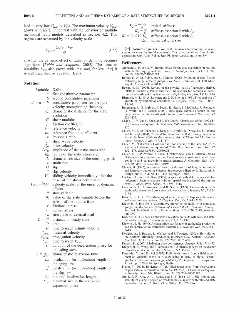
lead to very low Vmax Vpl). The maximum velocity Vmax

grows with jDtj, in contrast with the behavior on multidi-mensional fault models described in section 4.2. Tworegimes are separated by the velocity scale

V0

dyn ¼2cs a� bð Þs

G; ðB27Þ

at which the dynamic effect of radiation damping becomessignificant [Rubin and Ampuero, 2005]. The time toinstability tmax also grows with jDtj and, for low jDtj, itis well described by equation (B26).

Notation

Variable Definitiona first constitutive parameterb second constitutive parameter

a0 = a � b constitutive parameter for the purevelocity strengthening rheology

dc characteristic distance for the stateevolution

G shear modulusm friction coefficientV* reference velocitym* reference friction coefficientv Poisson’s ratiocs shear wave velocityVpl plate velocity

Dt0 amplitude of the static stress stepR0 radius of the static stress stepL characteristic size of the creeping patch_� strain rateD slipV slip velocityV+ sliding velocity immediately after the

onset of the stress perturbationVdyn =

2ascsG

velocity scale for the onset of dynamiceffects

q state variableqi value of the state variable before the

arrival of the rupture frontt frictional stresss normal stresst0 stress due to external load

W = Vqdc

distance to steady statet timet* time to reach infinite velocity

Vmax maximal velocityVprop propagation velocitytmax time to reach Vmax

t1 duration of the deceleration phase forunloading steps

tr =asKVpl

characteristic relaxation time

Lb localization (or nucleation) length forthe aging law

Lb0 localization (or nucleation) length for

the slip lawLv minimal localization lengthL1 maximal size in the crack-like

expansion phase

Kc =b�að Þsdc

critical stiffness

Kb =bsdc

stiffness associated with LbKv = 0.6219 Kb stiffness associated with Lv

Dx numerical grid size

[97] Acknowledgments. We thank the associate editor and an anon-ymous reviewer for useful comments. This paper benefited from fruitfuldiscussions with Allan Rubin, Jean-Philippe Avouac, and Alon Ziv.

ReferencesAmpuero, J. P., and A. M. Rubin (2008), Earthquake nucleation on rate andstate faults: Aging and slip laws, J. Geophys. Res., 113, B01302,doi:10.1029/2007JB005082.

Bayart, E., A. M. Rubin, and C. Marone (2006), Evolution of fault frictionfollowing large velocity jumps, Eos Trans. AGU, 87(52), Fall Meet.Suppl., Abstract S31A–0180.

Beeler, N. M. (2004), Review of the physical basis of laboratory-derivedrelations for brittle failure and their implications for earthquake occur-rence and earthquake nucleation, Pure Appl. Geophys., 161, 1853–1876.

Blanpied, M. L., D. A. Lockner, and J. D. Byerlee (1995), Frictional slip ofgranite at hydrothermal conditions, J. Geophys. Res., 100, 13,045–13,064.

Burgmann, R., S. Ergintav, P. Segall, E. Hearn, S. McClusky, R. Reilinger,H. Woith, and J. Zschau (2002), Time-space variable afterslip on anddeep below the Izmit earthquake rupture, Bull. Seismol. Soc. Am., 92,126–137.

Chang, C., Y. Wu, L. Zhao, and F. Wu (2007), Aftershocks of the 1999 Chi-Chi Taiwan Earthquake: The first hour, Bull. Seismol. Soc. Am., 96, 807–820.

Chlieh, M., J. de Chabalier, J. Ruegg, R. Armijo, R. Dmowska, J. Campos,and K. Feigl (2004), Crustal deformation and fault slip during the seismicslip in the North Chile subduction zone, from GPS and InSAR observa-tions, Geophys. J. Int., 157, 1–17.

Chlieh, M., et al. (2007), Coseismic slip and afterslip of the Great (Mw 9.15)Sumatra-Andaman earthquake of 2004, Bull. Seismol. Soc. Am., 97,152–173, doi:10.1785/0120050631.

Chlieh, M., J.-P. Avouac, K. Sieh, D. Natawidjaja, and J. Galetzka (2008),Heterogeneous coupling on the Sumatran megathrust constrained fromgeodetic and paleogeodetic measurements, J. Geophys. Res., 113,B05305, doi:10.1029/2007JB004981.

Chouet, B. (1992), A seismic model for the source of long-period eventsand harmonic tremor, in Volcanic Seismology, edited by P. Gasparini, R.Scarpa, and K. Aki, pp. 133–156. Springer, Berlin.

Cochard, A., and J. R. Rice (1997), A spectral method for numerical elas-todynamic fracture analysis without spatial replication of the ruptureevent, J. Mech. Phys. Solids, 45, 1393–1418.

Crescentini, L., A. Amoruso, and R. Scarpa (1999), Constraints on slowearthquake dynamics from a swarm in central Italy, Science, 286, 2132–2134.

Dieterich, J. H. (1979), Modeling of rock friction: 1. Experimental resultsand constitutive equations, J. Geophys. Res., 84, 2161–2168.

Dieterich, J. H. (1981), Constitutive properties of faults with simulatedgouge, in Mechanical Behavior of Crustal Rocks, Geophys. Monogr.Ser., vol. 24, edited by N. L. Carter et al., pp. 103–120. AGU, Washing-ton, D.C.

Dieterich, J. H. (1992), Earthquake nucleation on faults with rate- and state-dependent strength, Tectonophysics, 211, 115–134.

Dieterich, J. H. (1994), A constitutive law for rate of earthquake productionand its application to earthquake clustering, J. Geophys. Res., 99, 2601–2618.

Douglas, A., J. Beavan, L. Wallace, and J. Townend (2005), Slow slip onthe northern Hikurangi subduction interface, New Zealand, Geophys.Res. Lett., 32, L16305, doi:10.1029/2005GL023607.

Dragert, H. (2007), Mediating plate convergence, Science, 315, 471–472.Dragert, H., K. Wang, and T. James (2001), A silent slip event on the deeperCascadia subduction interface, Science, 292, 1525–1528.

Ferrazzini, V., and K. Aki (1992), Preliminary results from a field experi-ment on volcanic events at Kilauea using an array of digital seismo-graphs, in Volcanic Seismology, edited by P. Gasparini, R. Scarpa, andK. Aki, pp. 168–189. Springer, Berlin.

Fialko, Y. (2004), Evidence of fluid-filled upper crust from observationsof postseismic deformation due to the 1992 Mw7.3 Landers earthquake,J. Geophys. Res., 109, B08401, doi:10.1029/2004JB002985.

Gu, J., J. R. Rice, A. L. Ruina, and S. T. Tse (1984), Slip motion andstability of a single degree of freedom elastic system with rate and statedependent friction, J. Mech. Phys. Solids, 32, 167–196.


21 of 22

B09411

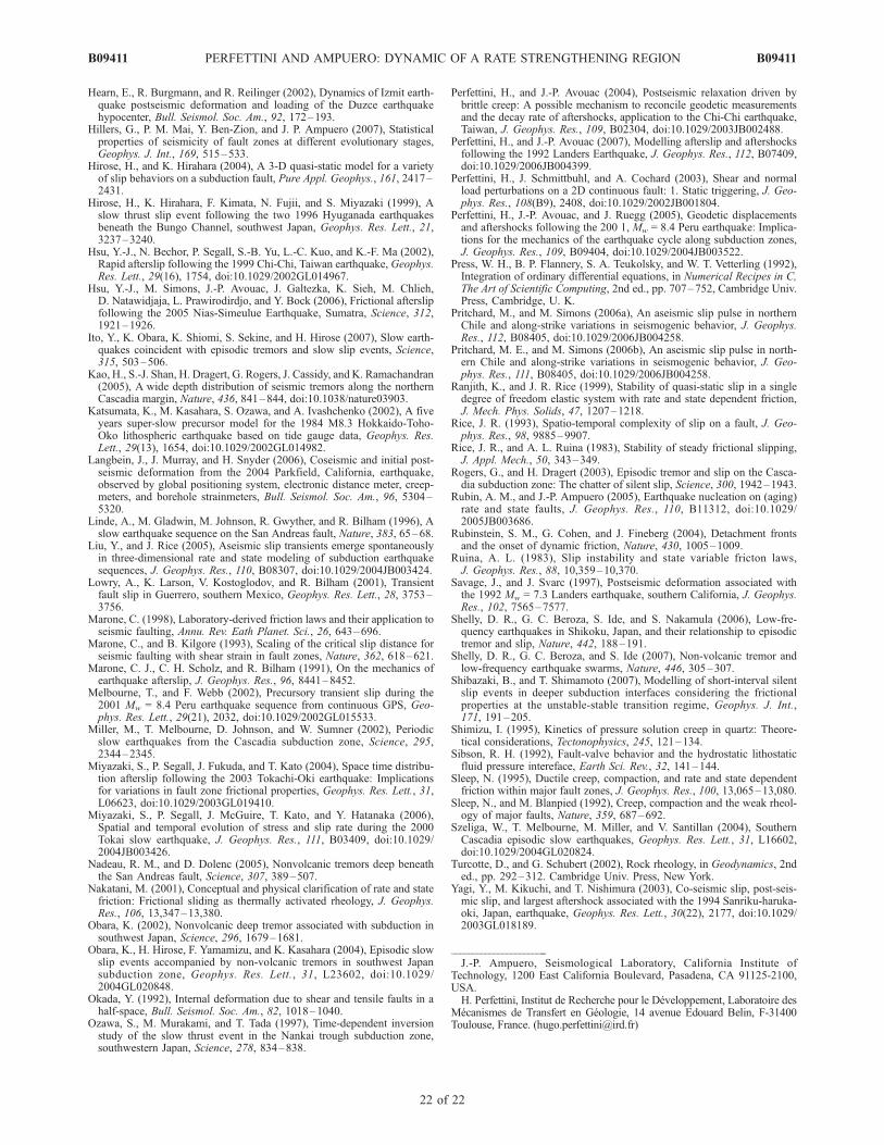
Hearn, E., R. Burgmann, and R. Reilinger (2002), Dynamics of Izmit earth-quake postseismic deformation and loading of the Duzce earthquakehypocenter, Bull. Seismol. Soc. Am., 92, 172–193.

Hillers, G., P. M. Mai, Y. Ben-Zion, and J. P. Ampuero (2007), Statisticalproperties of seismicity of fault zones at different evolutionary stages,Geophys. J. Int., 169, 515–533.

Hirose, H., and K. Hirahara (2004), A 3-D quasi-static model for a varietyof slip behaviors on a subduction fault, Pure Appl. Geophys., 161, 2417–2431.

Hirose, H., K. Hirahara, F. Kimata, N. Fujii, and S. Miyazaki (1999), Aslow thrust slip event following the two 1996 Hyuganada earthquakesbeneath the Bungo Channel, southwest Japan, Geophys. Res. Lett., 21,3237–3240.

Hsu, Y.-J., N. Bechor, P. Segall, S.-B. Yu, L.-C. Kuo, and K.-F. Ma (2002),Rapid afterslip following the 1999 Chi-Chi, Taiwan earthquake, Geophys.Res. Lett., 29(16), 1754, doi:10.1029/2002GL014967.

Hsu, Y.-J., M. Simons, J.-P. Avouac, J. Galtezka, K. Sieh, M. Chlieh,D. Natawidjaja, L. Prawirodirdjo, and Y. Bock (2006), Frictional afterslipfollowing the 2005 Nias-Simeulue Earthquake, Sumatra, Science, 312,1921–1926.

Ito, Y., K. Obara, K. Shiomi, S. Sekine, and H. Hirose (2007), Slow earth-quakes coincident with episodic tremors and slow slip events, Science,315, 503–506.

Kao, H., S.-J. Shan, H. Dragert, G. Rogers, J. Cassidy, and K. Ramachandran(2005), A wide depth distribution of seismic tremors along the northernCascadia margin, Nature, 436, 841–844, doi:10.1038/nature03903.

Katsumata, K., M. Kasahara, S. Ozawa, and A. Ivashchenko (2002), A fiveyears super-slow precursor model for the 1984 M8.3 Hokkaido-Toho-Oko lithospheric earthquake based on tide gauge data, Geophys. Res.Lett., 29(13), 1654, doi:10.1029/2002GL014982.

Langbein, J., J. Murray, and H. Snyder (2006), Coseismic and initial post-seismic deformation from the 2004 Parkfield, California, earthquake,observed by global positioning system, electronic distance meter, creep-meters, and borehole strainmeters, Bull. Seismol. Soc. Am., 96, 5304–5320.

Linde, A., M. Gladwin, M. Johnson, R. Gwyther, and R. Bilham (1996), Aslow earthquake sequence on the San Andreas fault, Nature, 383, 65–68.

Liu, Y., and J. Rice (2005), Aseismic slip transients emerge spontaneouslyin three-dimensional rate and state modeling of subduction earthquakesequences, J. Geophys. Res., 110, B08307, doi:10.1029/2004JB003424.

Lowry, A., K. Larson, V. Kostoglodov, and R. Bilham (2001), Transientfault slip in Guerrero, southern Mexico, Geophys. Res. Lett., 28, 3753–3756.

Marone, C. (1998), Laboratory-derived friction laws and their application toseismic faulting, Annu. Rev. Eath Planet. Sci., 26, 643–696.

Marone, C., and B. Kilgore (1993), Scaling of the critical slip distance forseismic faulting with shear strain in fault zones, Nature, 362, 618–621.

Marone, C. J., C. H. Scholz, and R. Bilham (1991), On the mechanics ofearthquake afterslip, J. Geophys. Res., 96, 8441–8452.

Melbourne, T., and F. Webb (2002), Precursory transient slip during the2001 Mw = 8.4 Peru earthquake sequence from continuous GPS, Geo-phys. Res. Lett., 29(21), 2032, doi:10.1029/2002GL015533.

Miller, M., T. Melbourne, D. Johnson, and W. Sumner (2002), Periodicslow earthquakes from the Cascadia subduction zone, Science, 295,2344–2345.

Miyazaki, S., P. Segall, J. Fukuda, and T. Kato (2004), Space time distribu-tion afterslip following the 2003 Tokachi-Oki earthquake: Implicationsfor variations in fault zone frictional properties, Geophys. Res. Lett., 31,L06623, doi:10.1029/2003GL019410.

Miyazaki, S., P. Segall, J. McGuire, T. Kato, and Y. Hatanaka (2006),Spatial and temporal evolution of stress and slip rate during the 2000Tokai slow earthquake, J. Geophys. Res., 111, B03409, doi:10.1029/2004JB003426.

Nadeau, R. M., and D. Dolenc (2005), Nonvolcanic tremors deep beneaththe San Andreas fault, Science, 307, 389–507.

Nakatani, M. (2001), Conceptual and physical clarification of rate and statefriction: Frictional sliding as thermally activated rheology, J. Geophys.Res., 106, 13,347–13,380.

Obara, K. (2002), Nonvolcanic deep tremor associated with subduction insouthwest Japan, Science, 296, 1679–1681.

Obara, K., H. Hirose, F. Yamamizu, and K. Kasahara (2004), Episodic slowslip events accompanied by non-volcanic tremors in southwest Japansubduction zone, Geophys. Res. Lett., 31, L23602, doi:10.1029/2004GL020848.

Okada, Y. (1992), Internal deformation due to shear and tensile faults in ahalf-space, Bull. Seismol. Soc. Am., 82, 1018–1040.

Ozawa, S., M. Murakami, and T. Tada (1997), Time-dependent inversionstudy of the slow thrust event in the Nankai trough subduction zone,southwestern Japan, Science, 278, 834–838.

Perfettini, H., and J.-P. Avouac (2004), Postseismic relaxation driven bybrittle creep: A possible mechanism to reconcile geodetic measurementsand the decay rate of aftershocks, application to the Chi-Chi earthquake,Taiwan, J. Geophys. Res., 109, B02304, doi:10.1029/2003JB002488.

Perfettini, H., and J.-P. Avouac (2007), Modelling afterslip and aftershocksfollowing the 1992 Landers Earthquake, J. Geophys. Res., 112, B07409,doi:10.1029/2006JB004399.

Perfettini, H., J. Schmittbuhl, and A. Cochard (2003), Shear and normalload perturbations on a 2D continuous fault: 1. Static triggering, J. Geo-phys. Res., 108(B9), 2408, doi:10.1029/2002JB001804.

Perfettini, H., J.-P. Avouac, and J. Ruegg (2005), Geodetic displacementsand aftershocks following the 200 1, Mw = 8.4 Peru earthquake: Implica-tions for the mechanics of the earthquake cycle along subduction zones,J. Geophys. Res., 109, B09404, doi:10.1029/2004JB003522.

Press, W. H., B. P. Flannery, S. A. Teukolsky, and W. T. Vetterling (1992),Integration of ordinary differential equations, in Numerical Recipes in C,The Art of Scientific Computing, 2nd ed., pp. 707–752, Cambridge Univ.Press, Cambridge, U. K.

Pritchard, M., and M. Simons (2006a), An aseismic slip pulse in northernChile and along-strike variations in seismogenic behavior, J. Geophys.Res., 112, B08405, doi:10.1029/2006JB004258.

Pritchard, M. E., and M. Simons (2006b), An aseismic slip pulse in north-ern Chile and along-strike variations in seismogenic behavior, J. Geo-phys. Res., 111, B08405, doi:10.1029/2006JB004258.

Ranjith, K., and J. R. Rice (1999), Stability of quasi-static slip in a singledegree of freedom elastic system with rate and state dependent friction,J. Mech. Phys. Solids, 47, 1207–1218.

Rice, J. R. (1993), Spatio-temporal complexity of slip on a fault, J. Geo-phys. Res., 98, 9885–9907.

Rice, J. R., and A. L. Ruina (1983), Stability of steady frictional slipping,J. Appl. Mech., 50, 343–349.

Rogers, G., and H. Dragert (2003), Episodic tremor and slip on the Casca-dia subduction zone: The chatter of silent slip, Science, 300, 1942–1943.

Rubin, A. M., and J.-P. Ampuero (2005), Earthquake nucleation on (aging)rate and state faults, J. Geophys. Res., 110, B11312, doi:10.1029/2005JB003686.

Rubinstein, S. M., G. Cohen, and J. Fineberg (2004), Detachment frontsand the onset of dynamic friction, Nature, 430, 1005–1009.

Ruina, A. L. (1983), Slip instability and state variable fricton laws,J. Geophys. Res., 88, 10,359–10,370.

Savage, J., and J. Svarc (1997), Postseismic deformation associated withthe 1992 Mw = 7.3 Landers earthquake, southern California, J. Geophys.Res., 102, 7565–7577.

Shelly, D. R., G. C. Beroza, S. Ide, and S. Nakamula (2006), Low-fre-quency earthquakes in Shikoku, Japan, and their relationship to episodictremor and slip, Nature, 442, 188–191.

Shelly, D. R., G. C. Beroza, and S. Ide (2007), Non-volcanic tremor andlow-frequency earthquake swarms, Nature, 446, 305–307.

Shibazaki, B., and T. Shimamoto (2007), Modelling of short-interval silentslip events in deeper subduction interfaces considering the frictionalproperties at the unstable-stable transition regime, Geophys. J. Int.,171, 191–205.

Shimizu, I. (1995), Kinetics of pressure solution creep in quartz: Theore-tical considerations, Tectonophysics, 245, 121–134.

Sibson, R. H. (1992), Fault-valve behavior and the hydrostatic lithostaticfluid pressure intereface, Earth Sci. Rev., 32, 141–144.

Sleep, N. (1995), Ductile creep, compaction, and rate and state dependentfriction within major fault zones, J. Geophys. Res., 100, 13,065–13,080.

Sleep, N., and M. Blanpied (1992), Creep, compaction and the weak rheol-ogy of major faults, Nature, 359, 687–692.

Szeliga, W., T. Melbourne, M. Miller, and V. Santillan (2004), SouthernCascadia episodic slow earthquakes, Geophys. Res. Lett., 31, L16602,doi:10.1029/2004GL020824.

Turcotte, D., and G. Schubert (2002), Rock rheology, in Geodynamics, 2nded., pp. 292–312. Cambridge Univ. Press, New York.

Yagi, Y., M. Kikuchi, and T. Nishimura (2003), Co-seismic slip, post-seis-mic slip, and largest aftershock associated with the 1994 Sanriku-haruka-oki, Japan, earthquake, Geophys. Res. Lett., 30(22), 2177, doi:10.1029/2003GL018189.

��J.-P. Ampuero, Seismological Laboratory, California Institute of

Technology, 1200 East California Boulevard, Pasadena, CA 91125-2100,USA.H. Perfettini, Institut de Recherche pour le Developpement, Laboratoire des

Mecanismes de Transfert en Geologie, 14 avenue Edouard Belin, F-31400Toulouse, France. ([email protected])


22 of 22

B09411

Dynamics of a velocity strengthening fault region: Implications for slow earthquakes and postseismic...

Documents

Transcript of Dynamics of a velocity strengthening fault region: Implications for slow earthquakes and postseismic...