econstorMake Your Publications Visible.

A Service of

zbwLeibniz-InformationszentrumWirtschaftLeibniz Information Centrefor Economics

Lackner, Stephanie

Working Paper

Earthquakes and economic growth

FIW Working Paper, No. 190

Provided in Cooperation with:FIW - Research Centre International Economics, Vienna

Suggested Citation: Lackner, Stephanie (2018) : Earthquakes and economic growth, FIWWorking Paper, No. 190, FIW - Research Centre International Economics, Vienna

This Version is available at:http://hdl.handle.net/10419/194225

Standard-Nutzungsbedingungen:

Die Dokumente auf EconStor dürfen zu eigenen wissenschaftlichenZwecken und zum Privatgebrauch gespeichert und kopiert werden.

Sie dürfen die Dokumente nicht für öffentliche oder kommerzielleZwecke vervielfältigen, öffentlich ausstellen, öffentlich zugänglichmachen, vertreiben oder anderweitig nutzen.

Sofern die Verfasser die Dokumente unter Open-Content-Lizenzen(insbesondere CC-Lizenzen) zur Verfügung gestellt haben sollten,gelten abweichend von diesen Nutzungsbedingungen die in der dortgenannten Lizenz gewährten Nutzungsrechte.

Terms of use:

Documents in EconStor may be saved and copied for yourpersonal and scholarly purposes.

You are not to copy documents for public or commercialpurposes, to exhibit the documents publicly, to make thempublicly available on the internet, or to distribute or otherwiseuse the documents in public.

If the documents have been made available under an OpenContent Licence (especially Creative Commons Licences), youmay exercise further usage rights as specified in the indicatedlicence.

www.econstor.eu

FIW – Working Paper

Earthquakes and Economic Growth

Stephanie Lackner1

Natural disasters are known to have devastating immediate impacts, but their long-run effect on

economic growth is not well understood. For the natural hazard of earthquakes, this paper

provides the first global empirical study on this topic that applies a measure of the exogenous

physical hazard responsible for earthquake impacts, earthquake ground shaking. I exploit the

random within-country year-to-year variation of shaking to identify the causal effect of

earthquakes on economic growth. To construct a panel dataset with country-year observations

of earthquake exposure and socioeconomic variables, I combine the universe of relevant

earthquake ground shaking data from 1973 to 2015 with country-level World Bank indicators. I find

negative long-run growth impacts for an average country comparable with recent findings for

climate related natural disasters. A typical earthquake reduces GDP per capita by 1.6% eight

years later, with substantial heterogeneity by country categories. In particular, low and middle-

income countries experience the greatest long-run economic damages while high-income

countries may even experience some positive “building back better” effects. Based on an

analysis of alternative spatial aggregation approaches, I find earthquake impacts are driven by

local high-intensity events rather than spatially diffuse exposure to lower intensity shaking.

1 Postdoctoral Research Associate, Woodrow Wilson School, Princeton University,

E-mail: slackner@princeton.edu

Abstract

The author

FIW Working Paper N° 190

December 2018

The Research Centre International Economics FIW is a project of WIFO, wiiw and WSR on behalf of the Federal Ministry

for Digital and Economic Affairs. The FIW cooperation with Austrian Universities is supported by the Federal Ministry of

Education, Science and Research.

Earthquakes and Economic Growth

Stephanie Lackner ⇤†

Working Paper

This version: November 11, 2018The most recent version is available at slackner.com/eeg

Abstract

Natural disasters are known to have devastating immediate impacts, but their long-

run e↵ect on economic growth is not well understood. For the natural hazard of earth-

quakes, this paper provides the first global empirical study on this topic that applies a

measure of the exogenous physical hazard responsible for earthquake impacts, earth-

quake ground shaking. I exploit the random within-country year-to-year variation of

shaking to identify the causal e↵ect of earthquakes on economic growth. To construct

a panel dataset with country-year observations of earthquake exposure and socioeco-

nomic variables, I combine the universe of relevant earthquake ground shaking data

from 1973 to 2015 with country-level World Bank indicators. I find negative long-run

growth impacts for an average country comparable with recent findings for climate-

related natural disasters. A typical earthquake reduces GDP per capita by 1.6% eight

years later, with substantial heterogeneity by country categories. In particular, low

and middle-income countries experience the greatest long-run economic damages while

high-income countries may even experience some positive “building back better” e↵ects.

Based on an analysis of alternative spatial aggregation approaches, I find earthquake

impacts are driven by local high-intensity events rather than spatially di↵use exposure

to lower intensity shaking.

⇤Postdoctoral Research Associate, WoodrowWilson School, Princeton University, slackner@princeton.edu†I am grateful to my advisors John Mutter, Douglas Almond, Michael Oppenheimer, and Art Lerner-Lam.

I also want to thank Geo↵rey Heal, Rodrigo Soares, George Deodatis, Donald Davis, Je↵rey Shrader, SureshNaidu, Timothy Foreman, Jesse Anttila-Hughes, Amir Jina, Anouch Missirian, Markus Riegler, TatyanaDeryugina and other participants of the 2018 Heartland Environmental and Resource Economics Workshopat Illinois, my paper discussant Saudamini Das at the 2018 World Congress of Environmental and ResourceEconomists, seminar participants at Columbia University, and many students and alumni of the ColumbiaUniversity Sustainable Development PhD program for valuable feedback and discussions on this paper.

1

1 Introduction

Earthquakes and other natural disasters cause considerable destruction and tremendous

human su↵ering every year. For any given natural hazard type, population growth and

urbanization will further increase their impacts in the future. The number of climate-related

extreme events is also likely to increase with climate change. It will therefore become even

more relevant in the future than it is already today to understand the immediate and long-

run impacts of natural disasters. Earthquakes are a natural hazard with almost no warning

time. In some regions of the world with well developed warning systems, a couple of minutes

of warning is possible in the best case scenarios. But in many cases, especially in poor

regions of the world, no warning exists. This fact is a major reason for why earthquakes are

the most fatal natural hazard type, and they are particularly fatal in low-income countries

(Wallemacq and House, 2018). They are not only a global concern in terms of capital

destruction and human casualties, but they can also a↵ect institutions (Belloc et al., 2016)

and impact inequality within and across countries. Earthquakes and other natural disasters

impose a disproportionately large burden on poor countries (Wallemacq and House, 2018),

which can contribute to non-converging GDP per capita trajectories between rich and poor

countries.

With this work, I provide the first global empirical study on the long-run economic im-

pacts of earthquakes that utilizes a disaster measure which represents the exogenous physical

hazard of earthquake ground shaking. This paper has three main contributions. First, I iden-

tify and quantify the long-run impacts of earthquakes on economic growth on a global level

and with respect to countries’ income categories. These quantifications can aid in a better

understanding of long-run impacts of earthquakes, which is important for decision making

on disaster planning and preparation. A significant long-run impact on GDP per capita

suggests that earthquakes can be an essential component in determining growth in coun-

tries that are repeatedly exposed to strong earthquakes. Second, earthquakes provide the

unique opportunity to study economic shocks through a completely exogenous natural ex-

periment and hence provide a cleaner identification than previous literature on other types

of shocks. Earthquakes are not predictable, and unlike climate-related hazards, they are not

significantly a↵ected by society. This paper therefore contributes to the general literature

on long-run impacts of macroeconomic shocks such as fiscal shocks (Cerra and Saxena, 2008;

Reinhart and Rogo↵, 2009; Romer and Romer, 2010), civil war (Cerra and Saxena, 2008),

and climate-related shocks (Dell et al., 2012; Hsiang and Jina, 2014). Third, this paper also

provides a measurement and spatial methods contribution. I improve earthquake exposure

2

measurement by using exogenous physical hazard data instead of endogenous direct impact

data. I also improve on the exogenous earthquake measure by using quantifications of sur-

face shaking exposure, the immediate cause of earthquake impacts, instead of earthquake

magnitude, which only correlates with impacts through the surface phenomenon of ground

shaking. Connected to the measurement of natural hazard exposure is the choice of a spatial

data aggregation approach. Calculating an admin-region level exposure from gridded natural

hazard data requires to apply a spatial aggregation approach, which always implies certain

assumptions (e.g. about non-linearities). Since high-resolution gridded data is still relatively

new, there is no standard method yet on how to choose spatial aggregation approaches. I

contribute to filling this gap in the literature by explicitly discussing and comparing di↵erent

spatial aggregation approaches. I show that the choice of the spatial aggregation approach

is indeed highly relevant.

While the immediate impacts of natural disasters are undoubtedly negative, some studies

have suggested that they have no or even positive long-run e↵ects on the economy through

technological upgrading and increased economic activity from rebuilding e↵orts (Albala-

Bertrand, 1993; Skidmore and Toya, 2002). A standard Solow-Swan model would predict a

return to the previous trend after a disaster exposure through temporarily increased growth

rates. Davis and Weinstein (2002) find indeed that long-run city size is robust to large

temporary shocks, suggesting a temporarily increased growth rate which o↵sets the nega-

tive impacts. Nevertheless, Hornbeck and Keniston (2017) present evidence for a creative

destruction e↵ect after the Boston fire of 1872 leading to a long-run positive net impact on

land value. Agrawal (2011) argues that disasters are a natural reset button which can allow

the transition to an alternative social trajectory. A transition to a better social trajectory

might not always be possible though.

Many studies based on macro and micro-level empirical analyses as well as theoretic

models have presented evidence that low-income populations a↵ected by disasters are subject

to particular constraints that can a↵ect their recovery. Crespo Cuaresma et al. (2008) find

that only rich countries benefit from capital upgrading after a natural disaster and Hallegatte

and Dumas (2009) suggest that natural disasters may be an explanation for poverty traps,

when disaster damages exceed the reconstruction capacity of the a↵ected economy. However,

the dynamics of how a country can get locked into a low-level equilibrium after a natural

disaster are complicated. Based on data for Vietnam, Noy and Vu (2010) show that disasters

have net negative impacts on the a↵ected regions but that relatively more destructive than

lethal events have less negative e↵ects, suggesting a form of “reconstruction boom”. De Mel

et al. (2011) find that grants allocated to microenterprises in Sri Lanka were e↵ective in

3

supporting recovery after the 2004 tsunami, concluding that lack of access to capital inhibits

the recovery process. However, McSweeney and Coomes (2011) demonstrate that even poor

communities can in some cases benefit in the long-run from a disaster.

The empirical literature on the global impacts of natural disasters on long-run economic

productivity is full of studies that use endogenous or suboptimal disaster exposure mea-

sures. This body of literature is relatively young and the methodology is still developing.

The exisiting inconsistent results in the literature are therefore not surprising, with studies

suggesting large negative, no, or even positive e↵ects as well as disagreements about poten-

tial heterogeneities in the e↵ects (Hsiang and Jina, 2014; Felbermayr and Groschl, 2014).

Skidmore and Toya (2002) conducted the first empirical study on the long-run growth im-

pacts of natural disasters. However, the study is based on cross-country regression analyses,

which su↵er from endogeneity biases. Other studies have addressed this issue by utilizing

panel datasets to be able to make conclusions about causality (e.g. Raddatz, 2007; Cre-

spo Cuaresma et al., 2008; Cavallo et al., 2013). The applied disaster exposure measures

have usually been based on the EM-DAT disaster database1, either using the number of

events or the reported damages. However, disaster impact data is endogenous, whereas an

exogenous measure for the intensity of the natural hazard is required for an unbiased esti-

mation. A number of publications have pointed out the shortcomings of using the EM-DAT

database for studying long-run impacts (Noy, 2009; Felbermayr and Groschl, 2014; Hsiang

and Jina, 2014). To overcome these shortcomings, Felbermayr and Groschl (2014) develop

a database of disaster exposure that is based on geophysical measures of the natural hazard

and apply it in a panel data analysis of long-run growth impacts. However, to accomplish the

extensive task of creating country-level exposure variables for five di↵erent types of natural

hazards they apply very simplified approaches for measuring the individual natural hazards.

For the case of earthquakes, for example, they use an approach based on magnitude which

is not a good proxy for surface shaking - the actual cause of earthquake impacts (Lackner,

2018b).

Considering the exogenous physical hazard is crucial to accurately identify the long-

run growth impacts of natural disasters. It is therefore necessary to su�ciently take into

account the specific geophysical characteristics and spatial patterns of the individual natural

hazard types. Before combining various types of natural hazards in one study on natural

disasters, it is therefore advisable to first study hazards individually. Besides prudence of

applying sound scientific geophysical measures for the natural hazards, studying di↵erent

1The EM-DAT International Disaster Database contains reported information on events that exceedcertain impact thresholds and is maintained by the Centre for Research on the Epidemiology of Disasters(CRED).

4

hazard types separately also has an additional advantage. The mechanisms of how disasters

a↵ect economies in the long-run might be specific or at least correlated to the hazard type.

Studying them separately can help to identify these di↵erences. There are several reasons

for how the natural hazard type can be a determinant of mechanisms and thus of long-run

impacts. First, di↵erent types of natural hazards might have systematic di↵erences in what

kind of immediate impacts they cause (e.g. a flooded house vs. losing the roof in a storm).

The long-run impacts could therefore also di↵er for di↵erent types of events. Second, di↵erent

hazards have inherently di↵erent warning times. Cyclones, for example, come with a couple

of days of warning, while earthquakes have a maximum warning time of a couple of minutes

in the best case scenarios. Last minute (or rather last day) measures that are possible for

cyclones (e.g. evacuation or boarding up windows) will never be able to completely prevent

impacts, but they do have the potential to significantly change not just the size but also

the nature of direct impacts, thus resulting in potentially systematic long-run di↵erences in

growth impacts. The lack of warning for earthquakes, for example, makes them particularly

deadly. Earthquakes therefore have relatively more human capital impacts than capital

impacts compared to storms. Furthermore, the spatial pattern of the natural hazard are

specific to the hazard type. This study will show evidence that spatially more concentrated

impacts might be responsible for most of the long-run impacts of earthquakes. If this holds

in general for natural disasters, the spatial pattern of a hazard has a significant relationship

with long-run impacts.

While climate-related natural hazards are intensely studied in the literature, geologic

natural hazards have received less attention. An increasing body of literature examines

how di↵erent climate variables a↵ect economic outcomes by taking advantage of exogenous

variation over time within a given spatial unit (Dell et al., 2014). Hsiang and Jina (2014)

provide a comprehensive analysis of the long-run growth impacts of cyclones and Dell et al.

(2012) have investigated the role of temperature shocks in determining growth. No com-

parable study on the long-run growth impacts of earthquakes exists so far. Only relatively

few empirical studies have analyzed the long-run impacts of earthquakes on GDP or other

welfare-related economic variables. Except for some local case studies (e.g. Gignoux and

Menendez, 2016; Kirchberger, 2017), all empirical studies on the subject are not earthquake

specific but consider a range of di↵erent natural disasters. No global study on long-run

impacts of earthquakes on economic growth (or other macroeconomic variables) has utilized

a quantification of surface shaking for the natural hazard of earthquakes. While earthquake

magnitude is commonly used to quantify the exogenous natural hazard, it has been shown

that it is not a good proxy for surface shaking and is therefore a suboptimal measure (Lack-

5

ner, 2018b). With this work I also demonstrate that using a measure that is based on ground

shaking instead of magnitude is crucial for identifying long-run impacts.

I exploit the random within-country variation of earthquake shaking over years to identify

the causal e↵ect of earthquakes on economic growth. Lackner (2018a) introduces a dataset

which represents the universe of global relevant earthquake shaking for 1973-2015. Here,

I combine this dataset with World Bank indicators to construct a panel dataset with an-

nual country level earthquake exposure linked with economic variables. Based on the results

in Lackner (2018b), I use peak ground acceleration (PGA) to quantify ground shaking. I

particularly investigate potential heterogeneities in the e↵ects as well as non-linearities. Fur-

thermore, I assess the relevance of spatially di↵use nuisance exposure compared to spatially

concentrated high level exposure by applying di↵erent spatial aggregation approaches for the

natural hazard.

I find significant global net long-run economic growth impacts with substantial hetero-

geneities in the e↵ects. Eight years later an average (non-zero) earthquake exposure reduces

GDP per capita by 1.6%, a 90% percentile exposure even by 3.8%. However, low-income

countries are strongly negatively a↵ected while high-income countries might even be able to

benefit from “building back better” e↵ects. I simulate alternative GDP per capita trajecto-

ries without earthquakes for low and lower-middle income countries and compare them to

their actual trajectories. This comparison reveals that GDP per capita among all low and

lower-middle income countries would have been on average 2.4% higher in 2015 if earth-

quakes would not have had a negative e↵ect on their economic growth in the preceeding

four decades. Among regularly exposed countries of this group of countries, the di↵erence

between actual and simulated GDP per capita is even 7.7%. Furthermore, I find that local-

ized disaster events are the drivers behind impacts compared to more widespread nuisance

exposure.

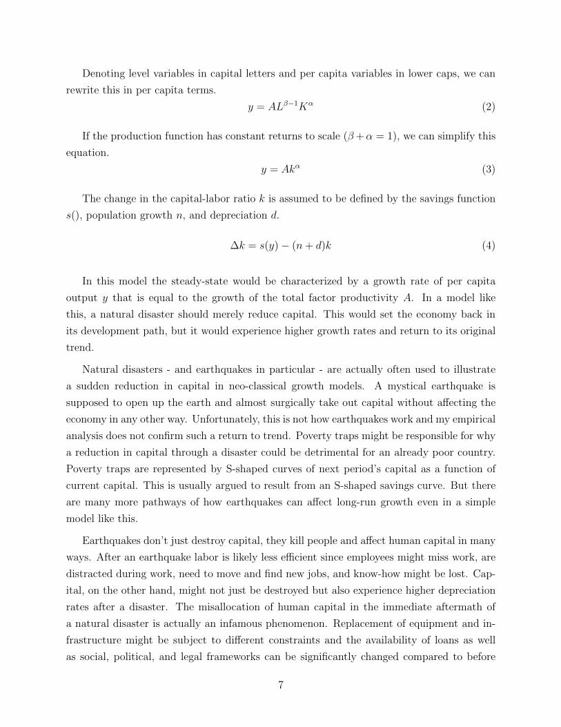
2 Theoretical Framework

We can start with a simple growth model to illustrate the theoretical relationship between

natural disasters and economic growth. The following Cobb-Douglas production function

describes economic output Y as a function of labor L and capital K.

Y = AL�K↵ (1)

6

Denoting level variables in capital letters and per capita variables in lower caps, we can

rewrite this in per capita terms.

y = AL��1K↵ (2)

If the production function has constant returns to scale (�+↵ = 1), we can simplify this

equation.

y = Ak↵ (3)

The change in the capital-labor ratio k is assumed to be defined by the savings function

s(), population growth n, and depreciation d.

�k = s(y)� (n+ d)k (4)

In this model the steady-state would be characterized by a growth rate of per capita

output y that is equal to the growth of the total factor productivity A. In a model like

this, a natural disaster should merely reduce capital. This would set the economy back in

its development path, but it would experience higher growth rates and return to its original

trend.

Natural disasters - and earthquakes in particular - are actually often used to illustrate

a sudden reduction in capital in neo-classical growth models. A mystical earthquake is

supposed to open up the earth and almost surgically take out capital without a↵ecting the

economy in any other way. Unfortunately, this is not how earthquakes work and my empirical

analysis does not confirm such a return to trend. Poverty traps might be responsible for why

a reduction in capital through a disaster could be detrimental for an already poor country.

Poverty traps are represented by S-shaped curves of next period’s capital as a function of

current capital. This is usually argued to result from an S-shaped savings curve. But there

are many more pathways of how earthquakes can a↵ect long-run growth even in a simple

model like this.

Earthquakes don’t just destroy capital, they kill people and a↵ect human capital in many

ways. After an earthquake labor is likely less e�cient since employees might miss work, are

distracted during work, need to move and find new jobs, and know-how might be lost. Cap-

ital, on the other hand, might not just be destroyed but also experience higher depreciation

rates after a disaster. The misallocation of human capital in the immediate aftermath of

a natural disaster is actually an infamous phenomenon. Replacement of equipment and in-

frastructure might be subject to di↵erent constraints and the availability of loans as well

as social, political, and legal frameworks can be significantly changed compared to before

7

the event (Belloc et al. (2016) show that earthquakes can a↵ect institutions). A disaster

can essentially introduce frictions into the economy in numerous ways. In our model, this

could mean that the population growth rate n or the depreciation rate d are endogenous and

subject to the state of the economy which could be a↵ected by a disaster.

A permanent increase in n or d would imply a new steady state with the same growth

rate as before, but the event would shift down the trajectory of the GDP per capita level.

Depending on the growth rate ✓ of the total factor productivity, this shift can either imply

an actual reduction of the GDP per capita level, or just a growth rate below ✓ for a number

of periods until the new steady state is established. The long-run GDP per capita level

trajectory would be lower but parallel to the counterfactual trajectory without the disaster.

Furthermore, a natural disaster might change how e↵ectively capital or labor can be

employed for production and thus change the output elasticities of capital or labor (↵ and

�), resulting in decreasing returns to scale. Equation 3 would no longer hold, since it depends

on the assumption of constant returns to scale.

Finally, a disaster could also change the growth rate ✓ of the total factor productivity

A and hence also change the steady state accordingly. After a disaster it is likely that

investments in research and development are reduced and risk aversion by entrepreneurs

could be increased. This would result in a reduction of technological growth ✓ and therefore

also a reduction in GDP per capita growth. If this change is temporary, the change in

the GDP per capita trajectory is equivalent as in the example of an increase in population

growth n or depreciation rate d. In the case of a permanent change in ✓ it would also imply

a reduced steady state growth rate of GDP per capita.

Country characteristics such as culture, geography, or income category could a↵ect which

of these discussed changes would be experienced by an economy and to what extend. It is

therefore not straightforward to conclude how earthquakes would a↵ect economic productiv-

ity in the long-run.

3 Data

For this study, a panel dataset of country-year observations of shaking and economic variables

is constructed. The dataset can be considered to contain the universe of global relevant

ground shaking for the years 1973 - 2015. Since the shaking data is restricted to these years,

and at least eight lags - as well as three leads - of shaking will be included in the analysis the

dataset for the analysis spans the 32 years from 1981 to 2012. The availability of economic

8

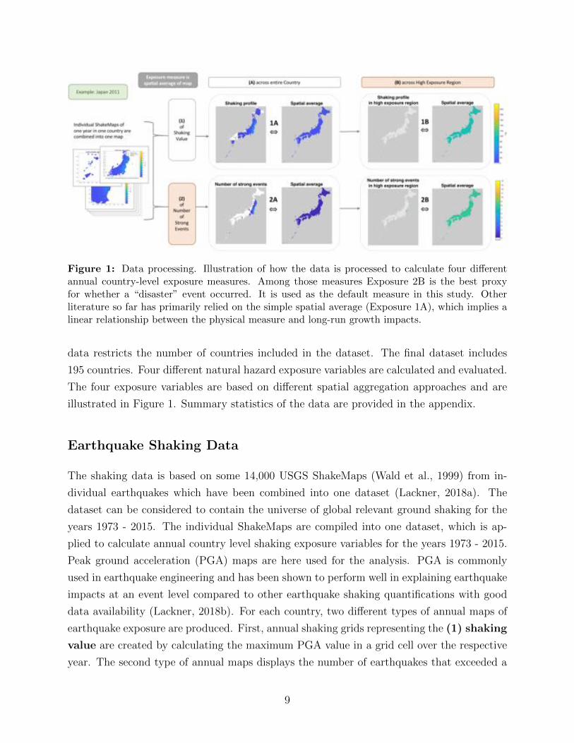
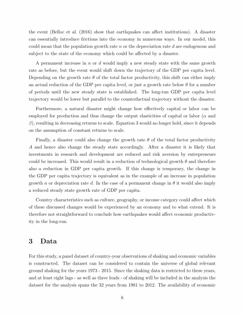
Figure 1: Data processing. Illustration of how the data is processed to calculate four di↵erentannual country-level exposure measures. Among those measures Exposure 2B is the best proxyfor whether a “disaster” event occurred. It is used as the default measure in this study. Otherliterature so far has primarily relied on the simple spatial average (Exposure 1A), which implies alinear relationship between the physical measure and long-run growth impacts.

data restricts the number of countries included in the dataset. The final dataset includes

195 countries. Four di↵erent natural hazard exposure variables are calculated and evaluated.

The four exposure variables are based on di↵erent spatial aggregation approaches and are

illustrated in Figure 1. Summary statistics of the data are provided in the appendix.

Earthquake Shaking Data

The shaking data is based on some 14,000 USGS ShakeMaps (Wald et al., 1999) from in-

dividual earthquakes which have been combined into one dataset (Lackner, 2018a). The

dataset can be considered to contain the universe of global relevant ground shaking for the

years 1973 - 2015. The individual ShakeMaps are compiled into one dataset, which is ap-

plied to calculate annual country level shaking exposure variables for the years 1973 - 2015.

Peak ground acceleration (PGA) maps are here used for the analysis. PGA is commonly

used in earthquake engineering and has been shown to perform well in explaining earthquake

impacts at an event level compared to other earthquake shaking quantifications with good

data availability (Lackner, 2018b). For each country, two di↵erent types of annual maps of

earthquake exposure are produced. First, annual shaking grids representing the (1) shaking

value are created by calculating the maximum PGA value in a grid cell over the respective

year. The second type of annual maps displays the number of earthquakes that exceeded a

9

threshold of 10%g in the respective location and year, thus representing the (2) number of

strong events. Each of the two annual grids has a resolution of 1/120 x 1/120 of a degree2.

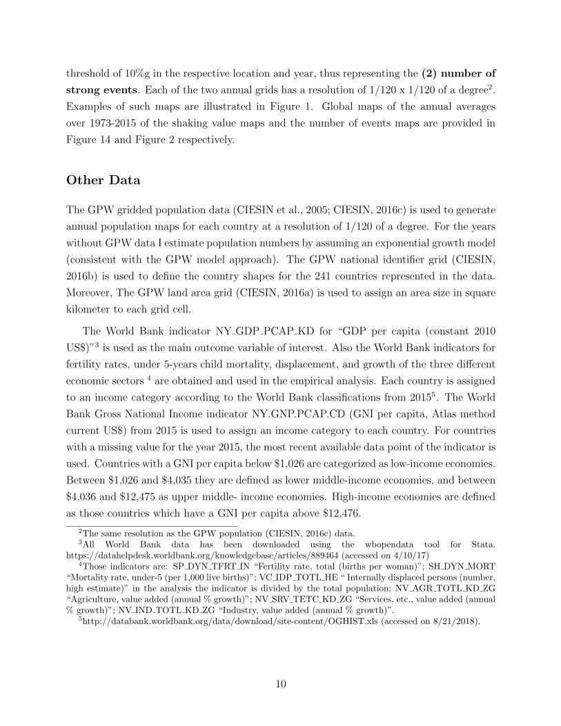
Examples of such maps are illustrated in Figure 1. Global maps of the annual averages

over 1973-2015 of the shaking value maps and the number of events maps are provided in

Figure 14 and Figure 2 respectively.

Other Data

The GPW gridded population data (CIESIN et al., 2005; CIESIN, 2016c) is used to generate

annual population maps for each country at a resolution of 1/120 of a degree. For the years

without GPW data I estimate population numbers by assuming an exponential growth model

(consistent with the GPW model approach). The GPW national identifier grid (CIESIN,

2016b) is used to define the country shapes for the 241 countries represented in the data.

Moreover, The GPW land area grid (CIESIN, 2016a) is used to assign an area size in square

kilometer to each grid cell.

The World Bank indicator NY GDP PCAP KD for “GDP per capita (constant 2010

US$)”3 is used as the main outcome variable of interest. Also the World Bank indicators for

fertility rates, under 5-years child mortality, displacement, and growth of the three di↵erent

economic sectors 4 are obtained and used in the empirical analysis. Each country is assigned

to an income category according to the World Bank classifications from 20155. The World

Bank Gross National Income indicator NY.GNP.PCAP.CD (GNI per capita, Atlas method

current US$) from 2015 is used to assign an income category to each country. For countries

with a missing value for the year 2015, the most recent available data point of the indicator is

used. Countries with a GNI per capita below $1,026 are categorized as low-income economies.

Between $1,026 and $4,035 they are defined as lower middle-income economies, and between

$4,036 and $12,475 as upper middle- income economies. High-income economies are defined

as those countries which have a GNI per capita above $12,476.

2The same resolution as the GPW population (CIESIN, 2016c) data.3All World Bank data has been downloaded using the wbopendata tool for Stata.

https://datahelpdesk.worldbank.org/knowledgebase/articles/889464 (accessed on 4/10/17)4Those indicators are: SP DYN TFRT IN “Fertility rate, total (births per woman)”; SH DYN MORT

“Mortality rate, under-5 (per 1,000 live births)”; VC IDP TOTL HE “ Internally displaced persons (number,high estimate)” in the analysis the indicator is divided by the total population; NV AGR TOTL KD ZG“Agriculture, value added (annual % growth)”; NV SRV TETC KD ZG “Services, etc., value added (annual% growth)”; NV IND TOTL KD ZG “Industry, value added (annual % growth)”.

5http://databank.worldbank.org/data/download/site-content/OGHIST.xls (accessed on 8/21/2018).

10

Figure 2: Overview of the exposure data. Panel (A) displays the average of the annual exposuremaps that are used to calculate exposures 2A and 2B. It shows the average annual number ofevents with shaking above the threshold of 10%g PGA based on the years 1973 - 2015. Panel (B)compares the di↵erent country-level exposure measures. The relationship between exposure 1Aand 1B (which is restricted by an upper and lower bound in red) in panel (B1) illustrates that thespatial average is not always a good proxy for whether a disaster event occurred. This becomeseven more obvious in panel (B2), which compares exposure 1A and 2B.

11

4 Spatial Aggregation of the Natural Hazard Data

Economic growth data is independent of country size and a single-valued annual exposure

measure that is also independent of country size is therefore needed. Hsiang and Jina (2014)

use the spatial average to aggregate wind speeds to a country-level variable to be able to link

the geophysical measurements with the economic measurements. This has two caveats. It re-

quires the assumption that long-run impacts increase in a linear manner with the geophysical

hazard, and it introduces a form of measurement error.

While a linear relationship between the geophysical hazard and long-run impacts might

hold for the case of cyclone wind speeds, we can not necessarily assume the same for earth-

quake shaking (measured by PGA). Previous results on the correlation between PGA and

impacts at an event level don’t refute that this might also be true for PGA, but they also

show that the ability to explain direct impacts for the spatial average decreases with an

increase in the area size considered (Lackner, 2018b). This suggest that small regions of

high intensity shaking are responsible for the bulk of damages and lower shaking values are

not that relevant. Nevertheless, other research (Shoaf et al., 1998) has found that injuries

in the 1994 Californian Northridge earthquake increased in an approximately linear manner

with PGA. However, even if direct impacts are linearly a↵ected by shaking, this does not

necessarily imply that a linear relationship applies for the long-run impacts on GDP per

capita. If the entire country is exposed to a uniform very low shaking value this might have

very di↵erent impacts than if only a very small part of the country is exposed to very strong

shaking, but the two scenarios could have the same spatial average exposure. The spatial

average alone can not tell us if an event that we would consider a “disaster” actually oc-

curred. The approach of Hsiang and Jina (2014) suggests that the occurrence of a “disaster”

is not necessarily relevant, but that a large spatial extent of low valued hazard exposure adds

up to similar impacts as a smaller spatial extent of a high valued exposure. On the other

hand, it might be true that a local high intensity event with a clustering of direct impacts

is necessary to be disruptive enough to the economy to a↵ect growth in a significant way.

The di↵erence between the physics of cyclones and earthquakes might a↵ect how well

of a proxy the spatial average is, for whether a (local) high intensity event (a “disaster”)

occurred. Cyclones are spatially larger phenomena than earthquakes and cyclone exposure

is concentrated in coastal regions in the tropics and mid latitudes (Hsiang and Jina, 2014).

For any specific year, the regions within a country that experience positive cyclone wind

speeds tend to be connected due to physics behind how and where cyclones form and travel.

Earthquakes on the other hand occur primarily along plate boundaries, which also tend to

12

be along coastlines, but the “earthquake history” is less concentrated than the “cyclone

climate”. Hsiang and Jina (2014) term the average annual pixel exposure to cyclone wind

speeds as the cyclone climate. In a similar way we can define the earthquake shaking history,

which is illustrated in Figure 146. Figure 2 provides an overview of the regions that have

experienced shaking above 10%g PGA. It is probably more common for earthquake shaking

exposure maps of a country to exhibit relatively large (often disconnected) areas of low

valued exposure than it is for cyclone wind speed exposure maps. The fact that a wind-

speed threshold defines whether a cyclone is classified as a cyclone, while no such threshold

exists for earthquakes is also partially responsible for this.

Relatively large spatial exposure of a country to positive cyclone wind speeds likely

correlates well with the maximum exposure (grid cell with the highest value in that year).

This correlation is not particularly strong for earthquakes. Whether the impacts of the

natural hazard are linear or whether local high intensities are the drivers of impacts, might

not matter much for applying spatial averages in the case of cyclones since the spatial average

is probably a good proxy for whether a (local) “disaster” occurred. For earthquakes on the

other hand, the spatial average might not be appropriate if high intensities are the main

source of long-run impacts.

The second issue with the use of the spatial average is that it introduces a form of

measurement error due to the di↵erences in land use in di↵erent countries and the spatial

di↵erences across events and countries. Individual natural disasters (no matter if earthquake

or cyclone) can di↵er a lot in how much they overlap with densely populated or capital

intense areas. Individual countries also vary a lot in how much of their territory is made

up by unpopulated, rural, or urban regions. For example Hong Kong has essentially no

unpopulated regions and a large share of the entire territory is urban while Russia has large

unpopulated regions and only a relatively small part of the country is urban. For any given

non-zero exposure calculated by the spatial average, it is relatively save to assume that an

event actually hit populated regions in the case of Hong Kong, but a large uncertainty exists

about whether this is the case for Russia. From a data perspective, the variance of the

shaking will be negatively correlated with the size of the country. This is not necessarily a

major concern, but it does introduce noise into the data. If the impacts don’t increase in a

linear manner with the natural hazard as discussed above, this will also have an additional

impact on the di↵erence between small and large countries, since the spatial mean of shaking

6In theory the term earthquake shaking climate could be used, but since earthquakes are not a climatephenomenon and past shaking is not equal to future earthquake risk. To avoid misinterpretation, I havetherefore chosen the term earthquake shaking history. For a map of the maximum exposure experienced seealso Figure 15.

13

is a better proxy for whether a “disaster” occurred for a small country than it is for a large

country.

Definition of the exposure measure

I compare four di↵erent definitions of annual earthquake exposure which are illustrated

in Figure 1. They are furthermore calculated across di↵erent interest areas (defined by

population distribution) across the country as well as the entire country. The populated

part of the country is used as the default area definition of a country.

As discussed before, two di↵erent types of annual exposure maps are produced from

the shaking data: (1) shaking value maps, and (2) number of strong events maps.

Each of the two types of annual maps are aggregated in two ways, as the spatial average

(A) across the country, and (B) across the high exposure region which is defined

as the (spatial) 1% of the country with the highest exposure in the respective year. The

four di↵erent measures are therefore labelled 1A, 1B, 2A, and 2B. The second version of

each component (2 and B) both give more emphasis to stronger shaking and thus are a

better measure for whether a more local strong disaster event occurred compared to more

widespread nuisance exposure. In the case of non-linearities these measures are assumed to

perform better than the spatial average in identifying impacts. Measure 2B is used as the

default exposure measure.

Restricting to only 1% of the country, but still considering the variable as a representation

of the exposure of the entire country is not a major concern for several reasons. First, it has

been repeatedly emphasized in the literature that natural hazard zones tend to also often

be economically attractive regions such as coastlines and are thus often densely populated.

This is also true for earthquakes, which is easy to see from a comparison of hazard maps

and population maps (e.g Figure 14 and Figure 27). It will therefore be uncommon that

a high exposure in 1% of the country will have only hit sparsely populated regions. This

is particularly true for the baseline case which only considers the populated regions of each

country. Second, if a high exposure is observed in the strongest 1% of a country it is unlikely

that the rest of the country was untouched by earthquake shaking. This is because (i) the

spatial extent of strong events can be quite large and even the area exposed to at least

90% of the maximum shaking is on average 171 square kilometers (Lackner, 2018a), and (ii)

earthquakes occur in clusters and have aftershocks that - while spatially close - are usually

not at the exact same location.

The di↵erence between the physics of cyclones and earthquakes might a↵ect how well of a

14

proxy the spatial average is, for whether a (local) high intensity event (a disaster) occurred.

To investigate this, Panel B1 in Figure 2 compares the averages over the entire (populated)

country with the average restricted to the strongest 1% region. The average shaking is

restricted by an upper bound (it can not be larger than the average in the strongest 1%)

and a lower bound (1% of the average shaking in the strongest 1%), which are depicted by

the red lines. The two variables do not show a strong linear relationship (the correlation is

0.6), suggesting that the overall spatial average is not a particularly good proxy for whether

a localized high intensity event occurred. For cyclones this correlation could be significantly

higher and the spatial average might thus be a reasonable proxy for whether a disaster

event occurred. However, given this relationship for earthquakes, if impacts are not linear, a

measure that summarizes the occurrence of strong shaking would be better suited than the

average over all shaking values. For this study, I therefore also create the number of events

maps to calculate exposure measures from. The average over these maps can be considered

an estimate for the spatial extent of strong shaking in the given year and country.

The spatial average approach is here extended by not just calculating spatial averages

over the entire country but also with respect to di↵erent spatial definitions of “the country”.

Hsiang and Jina (2014) omit Alaska from the calculation of the spatial average for the United

States, presumably because it is largely unpopulated. However, they do not apply a similar

approach for other sparsely populated regions of the world (e.g. Russia). To apply a more

systematic approach, I will define unpopulated regions for each country and omit those7

from the calculation of the spatial average in the populated part of the country. Details on

how these areas are defined can be found in Appendix B. A threshold of 1 person per square

kilometer is used in the default specification. While a population weighted exposure would

be a solution for the heterogeneity issue of how di↵erent events actually a↵ect society, it

would introduce endogeneity into the measure since it is very likely that population density

responds to natural hazard risks. However, I assume that it is unlikely that an otherwise

favorable location would be completely unpopulated due to such a risk.

5 Empirical Framework

I exploit the random within-country variation of earthquake shaking over years to identify

the causal e↵ect of earthquakes on economic productivity. The empirical approach is similar

to Hsiang and Jina (2014). An impulse-response function of growth (calculated as the first

7This includes most but not all of Alaska for the US.

15

di↵erences of log GDP per capita Yi,t = ln(GPDi,t)� ln(GPDi,t�1)) to earthquake shaking

exposure S for up to k lags is applied, while accounting for country i as well as year t specific

di↵erences by including country and year fixed e↵ects (�i and �t). Additionally a country-

specific linear time trend is included which accounts for country-specific rates of capital and

human capital accumulation.

Yi,t = �i + �t + ⌘it+kX

⌧=0

�⌧Si,t�⌧ + ✏i,t (5)

The error terms are allowed to be serially correlated within a country for up to 10 years

and spatially correlated across countries within the same year for up to 1000km (Hsiang,

2010). The coe�cients � can be summed up to calculate the cumulative reduction (in

percent) of GDP per capita after j years.

⌦j =jX

⌧=0

�⌧ (6)

The results will focus on these cumulative impacts on GDP per capita ⌦j. A lag length

k of eight years is used in the standard specification which is much shorter than the 20 years

considered by Hsiang and Jina (2014). However, the shorter time period of the earthquake

panel data does not allow for a similar number of lags. Furthermore, leads of shaking for up

to three years are included.

To distinguish between the impacts on di↵erent groups of countries the shaking exposure

is interacted with a dummy variable for the di↵erent groups.

Yi,t = �i + �t + ⌘it+kX

⌧=0

�⌧,c(i)Si,t�⌧ ⇥Dc(i) + ✏i,t (7)

This approach allows for a di↵erent response to shaking exposure for di↵erent groups c(i)

of countries. Countries are classified by income category, size of populated area, whether

they experience earthquakes on a regular basis, and population density in populated regions.

An overview of the number of countries in each group is provided in Table 1 in the appendix.

16

Figure 3: The cumulative impact of earthquake exposure on GDP per capita. A 95% confi-dence interval is included and the dotted zero-line represents the previous baseline trend (N =5586). Growth drops in the years following an exposure. While growth recovers after a few years,earthquakes still have negative long-run e↵ects on the level of GDP per capita after 8 years.

6 Results

To discuss the results, we will focus on plotting the cumulative impacts ⌦1 through ⌦8 of

earthquake shaking exposure on GDP per capita describing the percentage deviation from

the pre-disaster baseline trend. Result tables with the �⌧ coe�cent estimates are reported

in the appendix. Additionally to the lags, also the cumulative coe�cients of the leads are

included (⌦�1 through ⌦�3). A 95% confidence interval is plotted with the coe�cients. For

examples of the time-series of GDP per capita growth and the di↵erent shaking exposure

variables of individual countries see Figures 23 - 25 in the appendix.

Global Average Impact of Earthquakes

I will first discuss the results from the model with the default specifications. Figure 3

presents the results from the model described by Equation 5 with eight lags and three leads

and applying the earthquake exposure measure 2B (the average number of events with PGA

� 10%g in the most exposed 1% of the country) with respect to only the populated part of

each country. The plotted estimates describe the marginal response of GDP per capita to an

increase in the exposure measure 2B. The results suggest that earthquakes cause significant

long-run impacts on GDP per capita even eight years after an exposure. We observe a

significant drop in GDP per capita in the years after an earthquake exposure compared to

17

Figure 4: The impulse response to earthquake exposure by income categories. Low-income coun-tries are significantly a↵ected by earthquake exposure while high-income countries are potentiallyeven able to experience building back better e↵ects.

the baseline trend representing the counterfactual without an earthquake exposure. After

about 5 years the drop seems to stabilize but not return to the baseline trend (at least not

by year 8). The leads are not significant, which suggests that the model is well specified.

Varying the number of leads and lags does not a↵ect the results in a significant way (see

Figure 31). The shaking in unpopulated regions of countries should not matter much in

determining impacts, shaking exposure variables based on only the populated part of each

country are therefore used as the default. The results based on the entire country are reported

in Figure 33.

An earthquake that exposes 1% of a country to a shaking of at least 10%g is estimated

to cause a reduction in GDP per capita eight years later by almost 2%. An average non-zero

exposure would suggest a reduction of GDP per capita by 1.6% after eight years, a 90th

percentile non-zero exposure by 3.8%, and a 99th percentile exposure by even 10.2%. These

results represent a global net average of impacts across all countries. However, since disasters

can have a stimulating e↵ect on the economy in certain circumstances, it is possible that

heterogeneities in the e↵ects exist.

18

Figure 5: The impulse response to exposure di↵erentiated by country experience with earthquakes.The results suggests that adaptation is e↵ective in preventing at least some of the long-run impactsof earthquakes.

Figure 6: The impulse response to exposure di↵erentiated by country size (left) and countrypopulation density (right).

19

Heterogenous Response

Creative destruction and building back better are often argued to cause positive e↵ects after

a disaster. While the results here suggest that the global net e↵ects are negative, it is possible

that certain countries are actually able to faire better in the long-run or have neutral long-

run e↵ects under favorable circumstances. As the next step, we therefore consider the model

described by Equation 7 which allows for a country category specific response by interacting

the exposure measure with a country category dummy.

A primary concern is that low-income countries might not be able to take advantage of

the creative destruction and building back better opportunities that an extreme event can

o↵er. The results from the model with country income category specific e↵ects are shown

in Figure 4. Low-income and lower middle-income category countries are combined in the

lowest category. The results show that this category of countries is driving the average global

impacts of earthquakes. While upper middle-income countries have a similar estimated GDP

per capita trajectory, their estimates are not significant. High-income countries seem to

experience neutral or potentially even positive “building back better” e↵ects starting about

6 years after an exposure.

These results have shown that country income-level clearly matters for long-run impacts

of earthquakes. However, there are two distinct paths of how higher-income can a↵ect these

impacts; a reactive and a proactive one. First, high-income countries may be able to take

advantage of opportunities that open up after a disaster. This reactive response can support

growth in way that low-income countries might not be able to achieve. Second, it is relatively

cheaper for high-income countries to invest in defense mechanisms and they are therefore

more likely to proactively invest in infrastructure that can prevent major impacts in the case

of an event. This pathway is not increasing growth after an exposure, but preventing a drop

of growth that would occur in less prepared countries.

A natural next step is therefore to investigate if adaptation to earthquakes is e↵ective

in preventing negative impacts. Figure 5 presents the di↵erential response by country’s

earthquake experience. The group of most exposed countries is here defined by a median

exposure of measure 2B of 0.25 or greater. This group contains 14 countries. The medium

exposed countries are defined by having at least every second year some earthquake shaking

within the populated region of the country. This is the same as a median exposure of

measure 1A above 0. The point estimates confirm smaller impacts for countries with the

most earthquake experience. This suggests that adaptation to earthquakes is e↵ective in

preventing at least some of the long-run impacts of earthquakes. The estimates of the

20

Figure 7: The results for a simple magnitude approach, where each countries annual earthquakeexposure is defined as the maximum magnitude of an earthquake in the country.

countries with less earthquake experience is much noisier, due to the lower number of positive

exposures.

The panels of Figure 6 present the results for more country category specific e↵ects, other

than income. They illustrate the di↵erent impulse response functions of particular groups of

countries. Separating the smallest countries (smaller than 12,000km2) from the rest shows

that the small countries are not driving the overall results. Surprisingly, countries that have

lower population densities in their populated regions seem to be driving the overall average

impacts. This could be due to the fact that more urban countries might be more resilient

and better equipped for recovery. The population density threshold to distinguish between

the two groups of countries is here chosen as 100 people per square kilometer.

The Importance of the Measure

Applying an appropriate measure for the exposure to the natural hazard in the empirical

analysis, is crucial for several reasons. First, the measure is supposed to actually represent the

exogenous physical hazard of interest. Exposure measures based on direct impacts or even

population weighted measures of the physical hazard introduce potential endogeneity and

might bias the estimator. Nevertheless, also physical measures that are related to but don’t

actually represent the physical phenomenon of interest are suboptimal. Figure 7 illustrates

the value of applying a quantification of earthquake shaking instead of magnitude to identify

impacts. It provides the results for a simple magnitude approach, applying a similar model

21

as before, but using the maximum magnitude of the earthquakes with epicenter within the

country in a given year as the annual earthquake exposure. This approach ignores where

and what kind of shaking occurs. This approach results in no significant long-run impacts.

Using actual shaking data is therefore crucial for identifying the impacts of earthquakes.

Second, the chosen spatial aggregation approach needs to consider potential non-linearities

in the impacts. To be better able to identify whether the occurrence a “disaster” event oc-

curred, various exposure measures were defined. Using the two di↵erent maps - (1) the

shaking profile, and (2) the number of strong events - with each two aggregation approaches

- (A) across the country, and (B) across the 1% highest exposure region - resulted in four

di↵erent annual country-level earthquake exposure measures. The results of the model with

the default specifications are illustrated in Figure 30. For all four exposure definitions GDP

per capita experiences a drop compared to its baseline trend in the years after an earth-

quake exposure. The better performance of the exposure measures 1B and 2B, which focus

on shaking in the high-exposure region suggests that localized strong events might be driving

the impacts opposed to widespread lower level exposure. Since the four panels of Figure 30

stem from four di↵erent exposure measures, the y-axes of the individual graphs can not

be directly compared. Each panel therefore also displays the average and 90th percentile

exposure among all non-zero exposures.

To allow for a direct comparison of the implied e↵ects of the four exposure measures the

results are applied to the shaking observed in the dataset and plotted in Figure 34. The

Figure shows the distribution of expected impacts for each of the four exposure measures

given that a non-zero exposure occurs. Using the simple spatial average approach (1A)

would result in underestimating the long-run impacts of earthquakes compared to using an

approach that focuses on the high intensity exposure (e.g. 2B). While an average non-zero

exposure in the model with measure 2B is estimated to result in a reduction of GDP per

capita by 1.6% after eight years, the same model with exposure 1A suggests a reduction by

only 0.3% eight years after an average non-zero exposure.

Potential Mechanisms

To investigate potential mechanisms we can apply the model to di↵erent output variables.

Figure 8 compares the impacts on the three di↵erent economic sectors: services, industry,

and agriculture. The results suggest that primarily the services and industry sector are

a↵ected. Figure 9 distinguishes again by country income category and reveals that these

impacts are primarily born by low and lower-middle income countries.

22

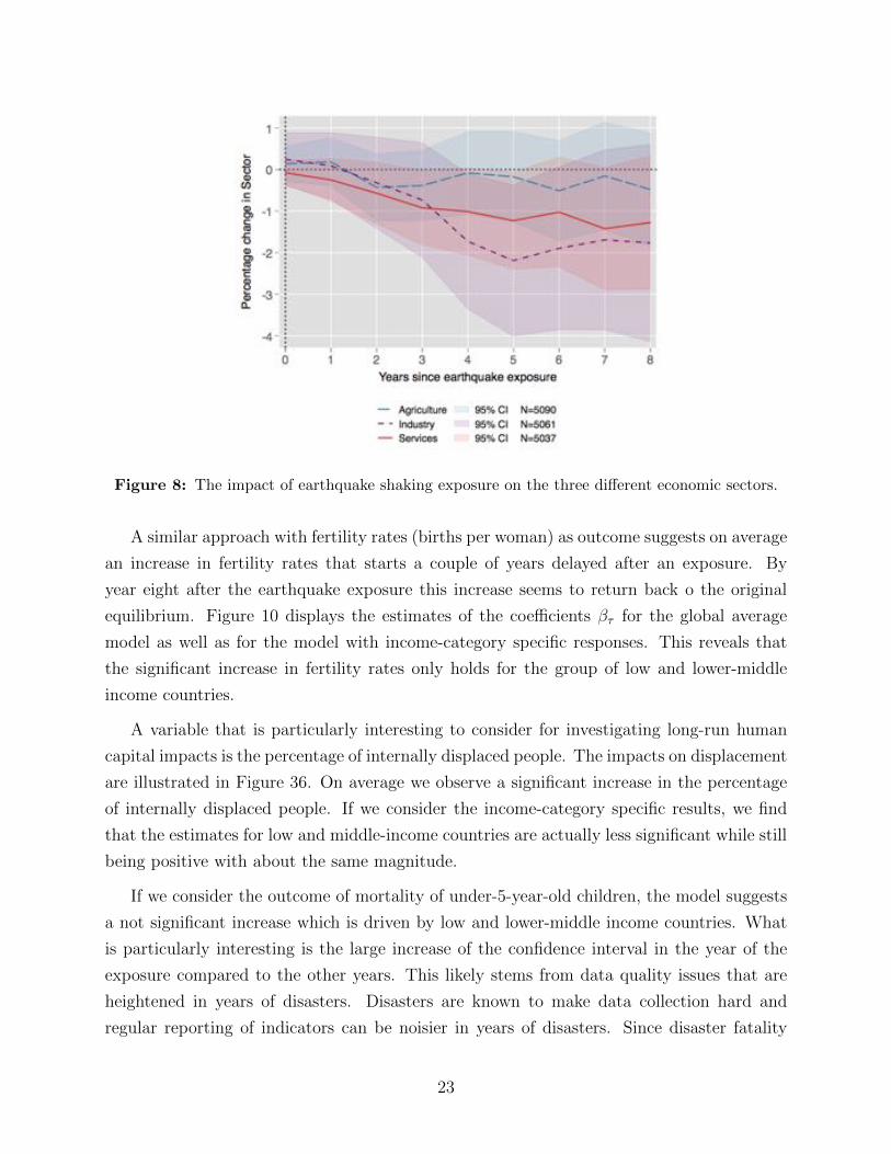
Figure 8: The impact of earthquake shaking exposure on the three di↵erent economic sectors.

A similar approach with fertility rates (births per woman) as outcome suggests on average

an increase in fertility rates that starts a couple of years delayed after an exposure. By

year eight after the earthquake exposure this increase seems to return back o the original

equilibrium. Figure 10 displays the estimates of the coe�cients �⌧ for the global average

model as well as for the model with income-category specific responses. This reveals that

the significant increase in fertility rates only holds for the group of low and lower-middle

income countries.

A variable that is particularly interesting to consider for investigating long-run human

capital impacts is the percentage of internally displaced people. The impacts on displacement

are illustrated in Figure 36. On average we observe a significant increase in the percentage

of internally displaced people. If we consider the income-category specific results, we find

that the estimates for low and middle-income countries are actually less significant while still

being positive with about the same magnitude.

If we consider the outcome of mortality of under-5-year-old children, the model suggests

a not significant increase which is driven by low and lower-middle income countries. What

is particularly interesting is the large increase of the confidence interval in the year of the

exposure compared to the other years. This likely stems from data quality issues that are

heightened in years of disasters. Disasters are known to make data collection hard and

regular reporting of indicators can be noisier in years of disasters. Since disaster fatality

23

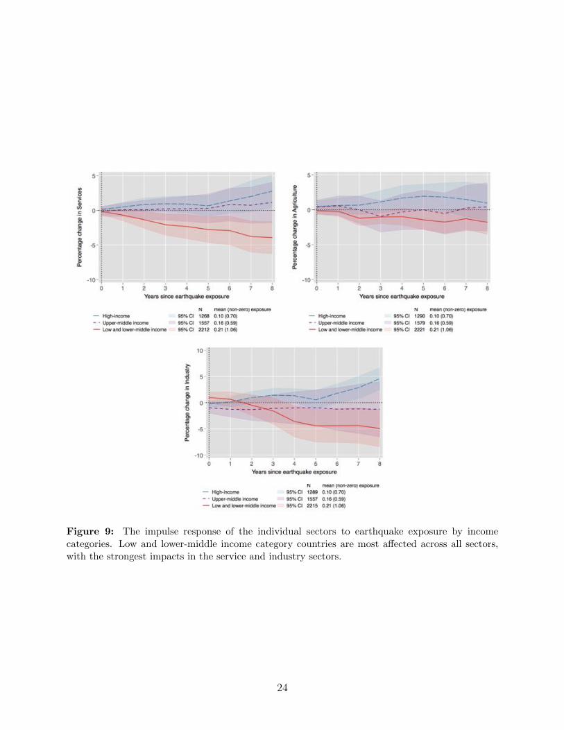
Figure 9: The impulse response of the individual sectors to earthquake exposure by incomecategories. Low and lower-middle income category countries are most a↵ected across all sectors,with the strongest impacts in the service and industry sectors.

24

Figure 10: The impact of earthquake shaking exposure on fertility rate as a global average (top)and by country-income categories (bottom).

Figure 11: The impact of earthquake shaking exposure on mortality of under-5-year old childrenas a global average (top) and by country-income categories (bottom).

25

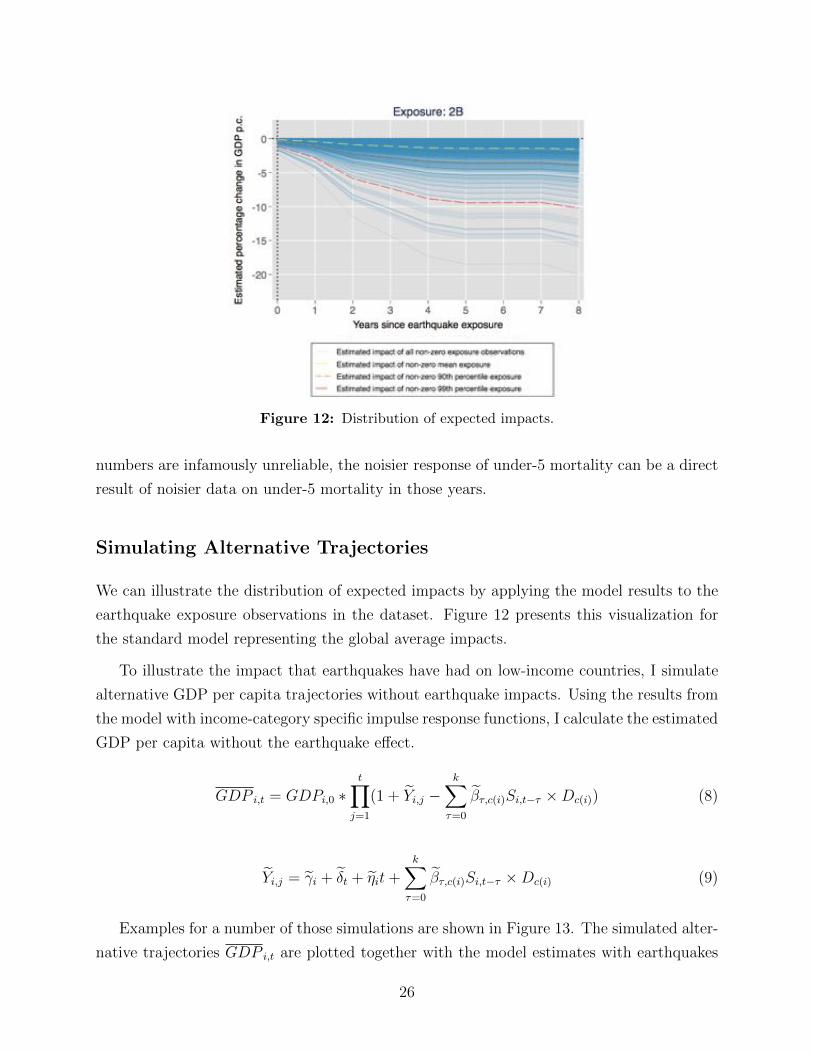
Figure 12: Distribution of expected impacts.

numbers are infamously unreliable, the noisier response of under-5 mortality can be a direct

result of noisier data on under-5 mortality in those years.

Simulating Alternative Trajectories

We can illustrate the distribution of expected impacts by applying the model results to the

earthquake exposure observations in the dataset. Figure 12 presents this visualization for

the standard model representing the global average impacts.

To illustrate the impact that earthquakes have had on low-income countries, I simulate

alternative GDP per capita trajectories without earthquake impacts. Using the results from

the model with income-category specific impulse response functions, I calculate the estimated

GDP per capita without the earthquake e↵ect.

GDP i,t = GDPi,0 ⇤tY

j=1

(1 + eYi,j �kX

⌧=0

e�⌧,c(i)Si,t�⌧ ⇥Dc(i)) (8)

eYi,j = e�i + e�t + e⌘it+kX

⌧=0

e�⌧,c(i)Si,t�⌧ ⇥Dc(i) (9)

Examples for a number of those simulations are shown in Figure 13. The simulated alter-

native trajectories GDP i,t are plotted together with the model estimates with earthquakes

26

Figure 13: Examples of simulation results for alternative GDP per capita trajectories.

27

GDP i,t and the actual GDP per capita World Bank indicators. These simulations reveal

that average GDP per capita in low and lower-middle income countries would have been

2.4% higher in 2015 if earthquakes would not have a↵ected these countries in the previous

four decades. If we only consider countries that are regularly exposed to earthquakes within

this group of countries, this di↵erence is even 7.7% with a maximum di↵erence above 30%.

Population Exposure

Population exposure is a crucial factor for determining impacts, but population is also en-

dogenous to society. Population can respond to natural hazard risk and it is likely that more

urban regions are relatively better prepared for natural disasters. This can make population

exposure correlated with resilience. Furthermore, the quality of population data is corre-

lated with countries’ income categories. Since the spatial resolution of population data is on

average higher in high-income countries, the high exposure measures will have a bias towards

high-income countries. Given that this study has found systematically di↵erent responses

for rich and poor countries, this can cause biased result. Nevertheless, we can still consider

population as an alternative or additional exposure measure in the model (see Figure 38).

Population as alternative exposure measure to shaking, does not result in significant

impacts. We can use the following model to include population exposure additionally with

shaking.

Yi,t = ↵ + �i + �t + ⌘it+kX

⌧=0

�S,⌧Si,t�⌧ +kX

⌧=0

�P,⌧Pi,t�⌧ + ✏i,t (10)

This approach reveals that shaking exposure is driving the results and not population

exposure. Population exposure in this combined model even appears to a↵ect growth pos-

itively in the long-run. This could be an artifact of the data quality issue overemphasizing

exposure of high-income countries.

Instead of using population exposure explicitly, we can use a higher threshold than 1

person per square kilometer to define the included regions of each country. I additionally

consider population density thresholds of 10, and 100 people per square kilometer. Figure 39

displays the results for increasing thresholds for exposure measure 1A and 2B. Again, em-

phasizing higher population density regions does not result in smaller confidence intervals.

This can have several reasons. Population density might just not be a good predictor for

vulnerability, or data quality issues favoring high-income countries could bias the results.

28

Alternative Empirical Approach

An alternative to the distributed lag model, is an approach following the method according

to Jorda (2005). In this alternative approach that is here applied as a robustness check, the

impulse response coe�cient �⌧ in each period is estimated through a separate regression.

Yi,t = �i + �t + ⌘it+ �⌧Si,t�⌧ + ✏i,t (11)

This approach would usually require to include not only the shaking in period ⌧ but also

before up to the number of periods for which an autocorrelation in the shaking data exists.

However, the earthquake exposure measures 2B as well as 1A are not autocorrelated. this

is confirmed by showing that the � coe�cient in the following model is not significantly

di↵erent from zero.

Si,t = �i + �Si,t�1 + ✏i,t (12)

The results are displayed in Figure 32 and confirm the pattern observed in the distributed

lag model. GDP per capita growth is significantly decreased in the first few years after an

earthquake exposure. It recovers after that, but does not experience a period of increased

growth that would o↵set the long-term e↵ect on GDP per capita.

Another alternative would be a multidimensional exposure approach that incorporates

several di↵erent exposure definitions. Similar to including population exposure with the

shaking measure, we can also combine two di↵erent shaking measures (1A and 2B) in one

model.

Yi,t = ↵ + �i + �t + ⌘it+kX

⌧=0

�1A,⌧S(1A)i,t�⌧ +kX

⌧=0

�2B,⌧S(2B)i,t�⌧ + ✏i,t (13)

Applying this approach confirms again that exposure measure 2B is preferred. While

the estimates suggest a negative and significant response to the shaking exposure 2B, the

estimates for the measure 1A are not significant (see Figure 37).

7 Conclusion and Discussion

This work is the first global empirical study on the long-run impacts of earthquakes on GDP

per capita growth that utilizes a measure based on ground shaking. Peak ground acceleration

data from USGS ShakeMaps are utilized to calculate di↵erent annual country level exposure

29

measures. I evaluate four di↵erent approaches to aggregate all earthquake ShakeMaps of one

year within one country into one variable. The four approaches are based on (1) maps of

the maximum shaking value over time, and (2) maps of the number of earthquakes above

a threshold, which are each aggregated as spatial average (A) across the entire (populated)

country, and (B) across the 1% region of the country with the highest exposure. The simple

spatial average (1A) implies a linear relationship between PGA and impacts. This means

that spatially di↵use low-level exposures should have the same long-run impacts as more

concentrated high intensity events as long as they have the same spatial average. This

approach is particularly compared to the measure (2B) which is the best proxy among the

four measures for whether a more localized disaster event occurred.

For all four measures, earthquakes are found to have a negative overall impact on GDP

per capita even eight years after an exposure. The results suggest that a measure that

is a better proxy for whether disaster event occurred compared to spatially large low-level

exposure is best suited to estimate long-run impacts. While growth rates seem to stabilize

after a few years, the lost growth is not recovered by year eight. This implies a permanent

reduction in GDP per capita level in the long-run. The results from the default exposure

measure (2B), the spatial average of the number of strong events in the most exposed 1%

of the country, suggest that an average exposure (among non-zero exposures) results in a

GDP per capita of 1.7% below the baseline trend and a 90th percentile exposure results in a

reduction by about 3.8% after eight years. Using instead the simple spatial average approach

(1A) would result in underestimating the long-run impacts of earthquakes.

The results suggest that the impacts are primarily incurred by low and middle-income

category countries and that high income countries are potentially even able to experience

positive ”building back better” e↵ects. This di↵erence can be caused by a number of dif-

ferent factors. First, it is relatively cheaper for high-income countries to invest in defense

mechanisms and they are therefore more likely to be better prepared for earthquakes. Com-

paring countries with di↵erent earthquake experience levels suggests that adaptation is in-

deed e↵ective in reducing impacts. Second, liquidity constraints and institutions that may

correlate with a country’s income category might be responsible for ine↵ective preparation

and could make it harder for low-income countries to take advantage of creative destruction

and building back better opportunities after an earthquake. Finally, lower level of prepara-

tion for low-income countries compared to high-income countries can also a↵ect the nature

of impacts incurred. Earthquakes are much more deadly in low-income countries than in

high-income countries. It is conceivable that earthquakes have a relatively larger impact on

human capital than capital for low-income countries than high-income countries not just in

30

terms of direct impacts, but also for long-term impacts.

The results show that the choice of the disaster measure is crucial. The geophysical nat-

ural hazard as well as potential non-linearities in impacts with regard to space and intensity

need to be considered to be able to accurately determine long-run impacts of natural haz-

ards. A comparison with an approach, that only uses magnitude and epicenter to quantify

the earthquake exposure, reveals that using actual shaking data is crucial to identify the

impacts of earthquake exposure.

Also the spatial aggregation approach applied to summarize the natural hazard is found

to be highly relevant. The results suggest that impacts are primarily driven by (local) high

intensity events and less by spatially large exposure to lower intensity shaking. Using a

simple spatial average of shaking across the entire country (Exposure 1A) instead of other

measures that put more emphasis on disaster events opposed to nuisance exposure, would

therefore result in underestimating the overall impact on GDP per capita. Furthermore,

I show that the spatial average is also not a good proxy in the case of earthquakes for

whether a local “disaster” event occurred, but it might be for other natural hazard types.

If such a relationship doesn’t exist and disaster events are the drivers behind impacts, then

the use of the spatial average is not adequate. For the case of cyclones Hsiang and Jina

(2014) only include wind speeds from cyclones, but not from weaker storms. This implies

that a maximum wind speed strong enough to receive the classification “cyclone” had to

occur. For earthquakes no such intensity thresholds exist. Additionally, cyclone exposure

maps compared to earthquake shaking exposure maps have a spatially larger and more

connected pattern. This implies that using the spatial average for the natural hazard of

cyclones will be a relatively good proxy for whether a high intensity exposure occurred. We

can conclude that the geophysical di↵erences between di↵erent natural hazard types might

require a systematically di↵erent approach to aggregate the spatial exposure maps to the

unit of observation (country).

There are several reasons for why the more local high intensity exposure would result

in higher impacts than spatially larger low-level exposure. First, the direct damages due to

the physical hazard might just not be linear, which is the least interesting scenario. Second,

the accumulation of big damages concentrated in a spatially small region might exceed the

local resilience capacity. This can be interpreted as a↵ected business being harmed further

by decreased demand and unreliable supply-chains. Furthermore, households would not just

be a↵ected themselves, but also their local social-safety network would be impaired. The

third and most concerning option is that large disaster events might trigger a misallocation of

resources. After such an event there are often large spendings on reconstruction and financial

31

aid for a↵ected people. However, these spendings are often ad-hoc, not well planned, and can

be highly political. This can result in ine�ciencies in the economy. Furthermore, displaced

population might also result in misallocation of human resources. Finally, adaptation (or

preparation) might be very e↵ective for low-level exposure, but less so for high intensity

exposure.

References

Agrawal, A. (2011). Economics: A positive side of disaster. Nature Publishing Group,

473(7347):291–292.

Albala-Bertrand, J. M. (1993). Natural disaster situations and growth: A macroeconomic

model for sudden disaster impacts. World Development, 21(9):1417–1434.

Belloc, M., Drago, F., and Galbiati, R. (2016). Earthquakes, religion, and transition to

selfgovernment in italian cities. Quarterly Journal of Economics, 131(4):1875–1926.

Cavallo, E., Galiani, S., Noy, I., and Pantano, J. (2013). Catastrophic natural disasters and

economic growth. Review of Economics and Statistics, 95(5):1549–1561.

Cerra, V. and Saxena, S. C. (2008). Growth Dynamics: The Myth of Economic Recovery.

The American Economic Review, 98(1):439–457.

Chomitz, K. M., Buys, P., and Thomas, T. S. (2005). Quantifying the Rural-Urban Gradient

in Latin America and the Caribbean. SSRN Electronic Journal.

CIESIN (2016a). Gridded Population of the World, Version 4 (GPWv4): Land and Water

Area. Technical report, Palisades, NY.

CIESIN (2016b). Gridded Population of the World, Version 4 (GPWv4): National Identifier

Grid. Technical report, Palisades, NY.

CIESIN (2016c). Gridded Population of the World, Version 4 (GPWv4): Population Count

Adjusted to Match 2015 Revision of UNWPP Country Totals. Technical report, Palisades,

NY.

CIESIN, United Nations Food and Agriculture Programme - FAO, and Centro Internacional

de Agricultura Tropical - CIAT (2005). Gridded Population of the World, Version 3

(GPWv3): Population Count Grid. Technical report, Palisades, NY.

32

Crespo Cuaresma, J., Hlouskova, J., and Obersteiner, M. (2008). Natural disasters as creative

destruction? Evidence from developing countries. Economic Inquiry, 46(2):214–226.

Davis, D. R. and Weinstein, D. E. (2002). Bones, Bombs, and Break Points: The Geography

of Economic Activity. The American Economic Review, 92(5):1269–1289.

De Mel, S., McKenzie, D., and Woodru↵, C. (2011). Enterprise Recovery Following Natural

Disasters. Economic Journal, 122(559):64–91.

Dell, M., Jones, B. F., and Olken, B. A. (2012). Temperature Shocks and Economic Growth:

Evidence from the Last Half Century. American Economic Journal: Macroeconomics,

4(3):66–95.

Dell, M., Jones, B. F., and Olken, B. A. (2014). What Do We Learn from the Weather? The

New Climate–Economy Literature. Journal of Economic Literature, 52(3):740–798.

Felbermayr, G. and Groschl, J. (2014). Naturally negative: The growth e↵ects of natural

disasters. Journal of Development Economics, 111:92–106.

Gignoux, J. and Menendez, M. (2016). Benefit in the wake of disaster: Long-run e↵ects of

earthquakes on welfare in rural Indonesia. Journal of Development Economics, 118:26–44.

Hallegatte, S. and Dumas, P. (2009). Can natural disasters have positive consequences?

Investigating the role of embodied technical change. Ecological Economics, 68(3):777–786.

Hornbeck, R. and Keniston, D. (2017). Creative Destruction: Barriers to Urban Growth and

the Great Boston Fire of 1872. American Economic Review, 107(6):1365–1398.

Hsiang, S. M. (2010). Temperatures and cyclones strongly associated with economic pro-

duction in the Caribbean and Central America. Proceedings of the National Academy of

Sciences, 107(35):15367–15372.

Hsiang, S. M. and Jina, A. (2014). The Causal E↵ect of Environmental Catastrophe on

Long-Run Economic Growth: Evidence From 6,700 Cyclones. Technical report, National

Bureau of Economic Research, Cambridge, MA, Cambridge, MA.

Jorda, O. (2005). Estimation and inference of impulse responses by local projections. Amer-

ican Economic Review, 95(1):161–182.

Kirchberger, M. (2017). Natural disasters and labor markets. Journal of Development

Economics, 125:40–58.

33

Lackner, S. (2018a). Earthquakes on the surface: Earthquake location and area based on

more than 14500 ShakeMaps. Natural Hazards and Earth System Science, 18(6):1665–

1679.

Lackner, S. (2018b). The Relationship between Earthquake Measures and Impact Data.

Unpuplished Working Paper.

McSweeney, K. and Coomes, O. T. (2011). Climate-related disaster opens a window of oppor-

tunity for rural poor in northeastern Honduras. In Proceedings of the National Academy

of Sciences of the United States of America, pages 5203–5208. Ohio State University,

Columbus, United States, National Academy of Sciences.

Noy, I. (2009). The macroeconomic consequences of disasters. Journal of Development

Economics, 88(2):221–231.

Noy, I. and Vu, T. B. (2010). The economics of natural disasters in a developing country:

The case of Vietnam. Journal of Asian Economics, 21(4):345–354.

Raddatz, C. (2007). Are external shocks responsible for the instability of output in low-

income countries? Journal of Development Economics, 84(1):155–187.

Reinhart, C. M. and Rogo↵, K. S. (2009). The Aftermath of Financial Crises. The American

Economic Review, 99(2):466–472.

Romer, C. D. and Romer, D. H. (2010). Estimates Based on a New Measure of Fiscal Shocks.

The American Economic Review, 100(3):763–801.

Shoaf, K. I., Sareen, H. R., Nguyen, L. H., and Bourque, L. B. (1998). Injuries as a result

of California earthquakes in the past decade. Disasters, 22(3):218–235.

Skidmore, M. and Toya, H. (2002). Do natural disasters promote long-run growth? Economic

Inquiry, 40(4):664–687.

Wald, D. J., Quitoriano, V., Heaton, T. H., Kanamori, H., Scrivner, C. W., and Worden,

C. B. (1999). TriNet “ShakeMaps”: Rapid Generation of Peak Ground Motion and Inten-

sity Maps for Earthquakes in Southern California. Earthquake Spectra, 15(3):537–555.

Wallemacq, P. and House, R. (2018). Economic Losses, Poverty & Disasters 1998-2017.

Technical Report by UNISDR and CRED.

34

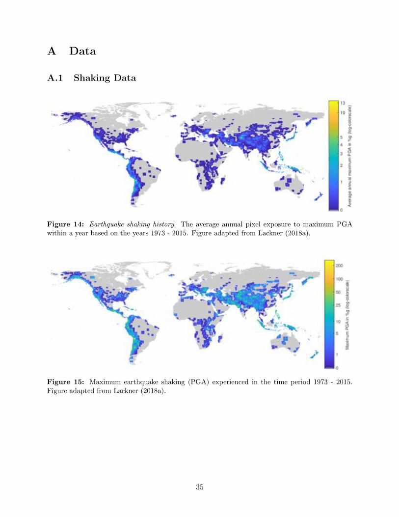
A Data

A.1 Shaking Data

Figure 14: Earthquake shaking history. The average annual pixel exposure to maximum PGAwithin a year based on the years 1973 - 2015. Figure adapted from Lackner (2018a).

Figure 15: Maximum earthquake shaking (PGA) experienced in the time period 1973 - 2015.Figure adapted from Lackner (2018a).

35

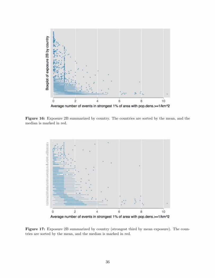
Figure 16: Exposure 2B summarized by country. The countries are sorted by the mean, and themedian is marked in red.

Figure 17: Exposure 2B summarized by country (strongest third by mean exposure). The coun-tries are sorted by the mean, and the median is marked in red.

36

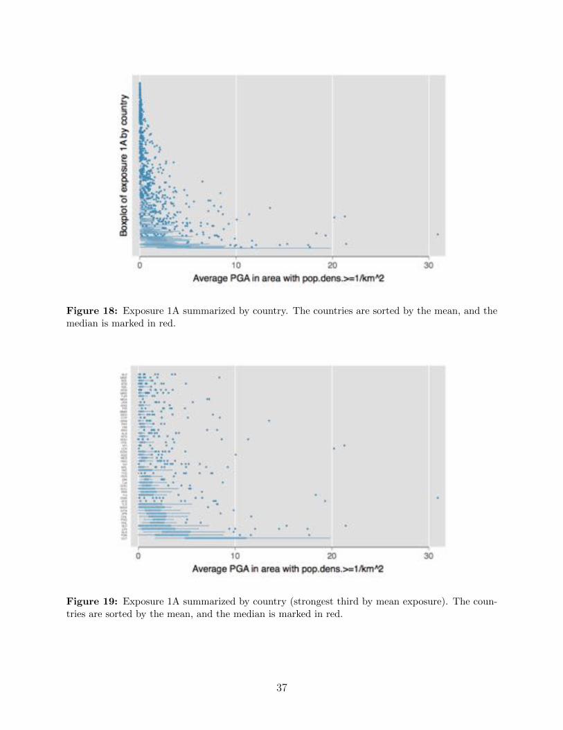
Figure 18: Exposure 1A summarized by country. The countries are sorted by the mean, and themedian is marked in red.

Figure 19: Exposure 1A summarized by country (strongest third by mean exposure). The coun-tries are sorted by the mean, and the median is marked in red.

37

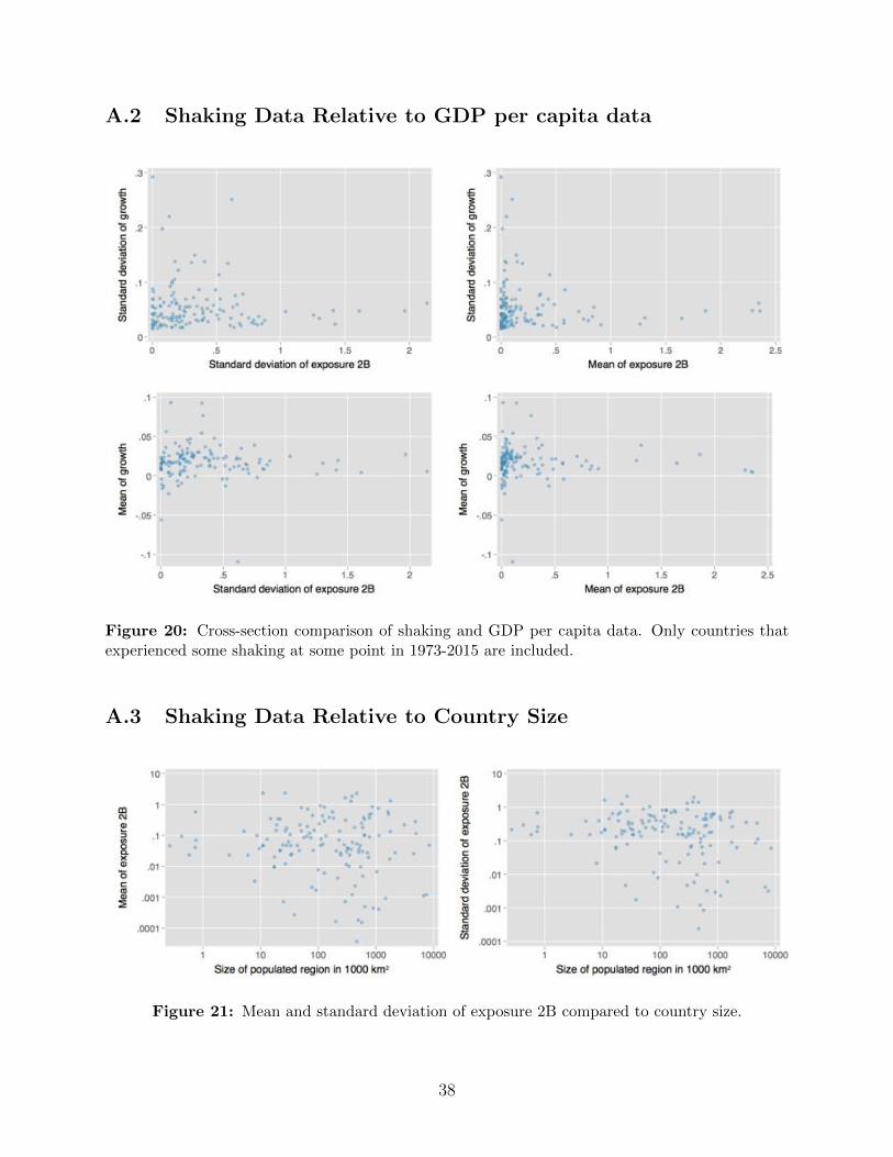
A.2 Shaking Data Relative to GDP per capita data

Figure 20: Cross-section comparison of shaking and GDP per capita data. Only countries thatexperienced some shaking at some point in 1973-2015 are included.

A.3 Shaking Data Relative to Country Size

Figure 21: Mean and standard deviation of exposure 2B compared to country size.

38

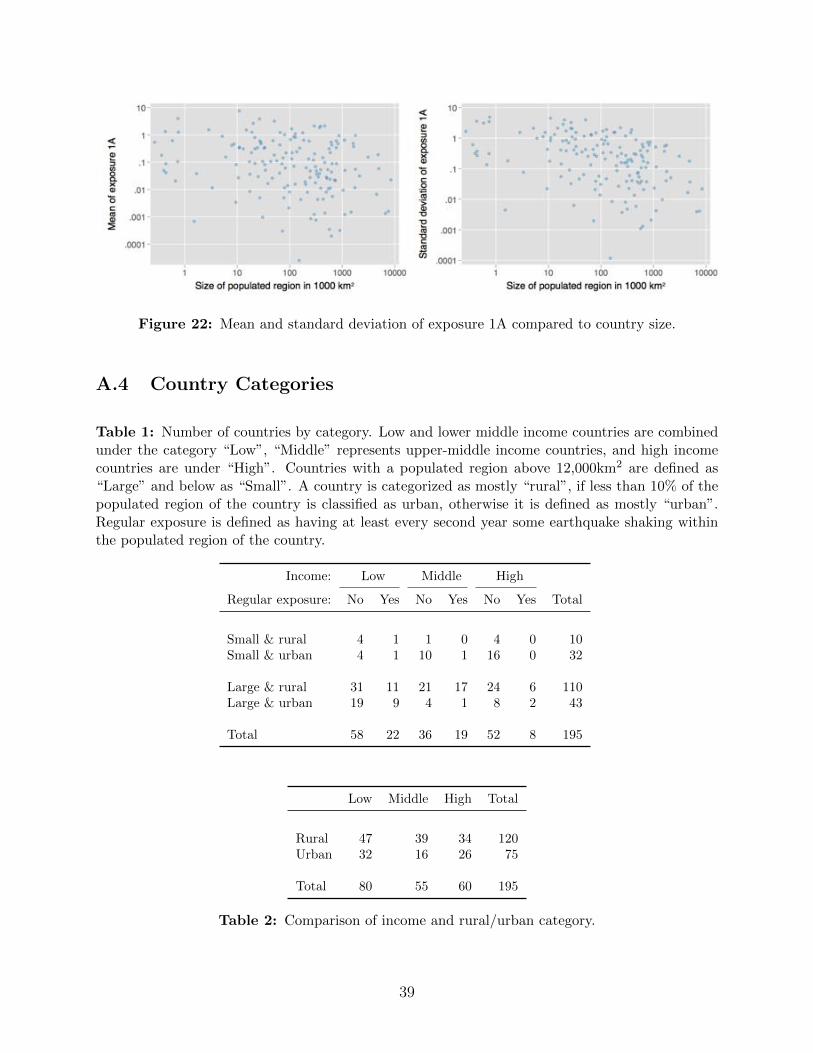
Figure 22: Mean and standard deviation of exposure 1A compared to country size.

A.4 Country Categories

Table 1: Number of countries by category. Low and lower middle income countries are combinedunder the category “Low”, “Middle” represents upper-middle income countries, and high incomecountries are under “High”. Countries with a populated region above 12,000km2 are defined as“Large” and below as “Small”. A country is categorized as mostly “rural”, if less than 10% of thepopulated region of the country is classified as urban, otherwise it is defined as mostly “urban”.Regular exposure is defined as having at least every second year some earthquake shaking withinthe populated region of the country.

Income: Low Middle High

Regular exposure: No Yes No Yes No Yes Total

Small & rural 4 1 1 0 4 0 10Small & urban 4 1 10 1 16 0 32

Large & rural 31 11 21 17 24 6 110Large & urban 19 9 4 1 8 2 43

Total 58 22 36 19 52 8 195

Low Middle High Total

Rural 47 39 34 120Urban 32 16 26 75

Total 80 55 60 195

Table 2: Comparison of income and rural/urban category.

39

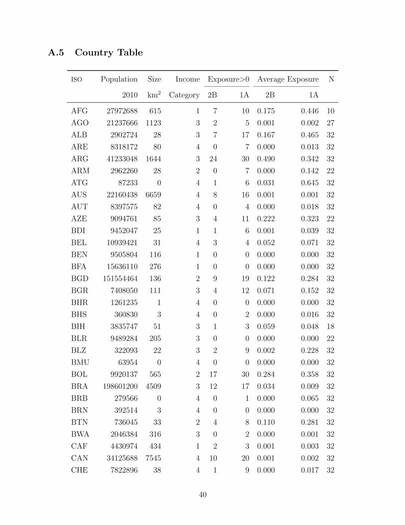
A.5 Country Table

ISO Population Size Income Exposure>0 Average Exposure N

2010 km2 Category 2B 1A 2B 1A

AFG 27972688 615 1 7 10 0.175 0.446 10

AGO 21237666 1123 3 2 5 0.001 0.002 27

ALB 2902724 28 3 7 17 0.167 0.465 32

ARE 8318172 80 4 0 7 0.000 0.013 32

ARG 41233048 1644 3 24 30 0.490 0.342 32

ARM 2962260 28 2 0 7 0.000 0.142 22

ATG 87233 0 4 1 6 0.031 0.645 32

AUS 22160438 6659 4 8 16 0.001 0.001 32

AUT 8397575 82 4 0 4 0.000 0.018 32

AZE 9094761 85 3 4 11 0.222 0.323 22

BDI 9452047 25 1 1 6 0.001 0.039 32

BEL 10939421 31 4 3 4 0.052 0.071 32

BEN 9505804 116 1 0 0 0.000 0.000 32

BFA 15636110 276 1 0 0 0.000 0.000 32

BGD 151554464 136 2 9 19 0.122 0.284 32

BGR 7408050 111 3 4 12 0.071 0.152 32

BHR 1261235 1 4 0 0 0.000 0.000 32

BHS 360830 3 4 0 2 0.000 0.016 32

BIH 3835747 51 3 1 3 0.059 0.048 18

BLR 9489284 205 3 0 0 0.000 0.000 22

BLZ 322093 22 3 2 9 0.002 0.228 32

BMU 63954 0 4 0 0 0.000 0.000 32

BOL 9920137 565 2 17 30 0.284 0.358 32

BRA 198601200 4509 3 12 17 0.034 0.009 32

BRB 279566 0 4 0 1 0.000 0.065 32

BRN 392514 3 4 0 0 0.000 0.000 32

BTN 736045 33 2 4 8 0.110 0.281 32

BWA 2046384 316 3 0 2 0.000 0.001 32

CAF 4430974 434 1 2 3 0.001 0.003 32

CAN 34125688 7545 4 10 20 0.001 0.002 32

CHE 7822896 38 4 1 9 0.000 0.017 32

40

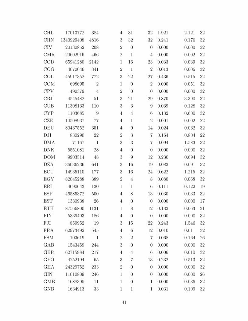
CHL 17013772 384 4 31 32 1.921 2.121 32

CHN 1340929408 4816 3 32 32 0.241 0.176 32

CIV 20130852 208 2 0 0 0.000 0.000 32

CMR 20602916 466 2 1 4 0.000 0.002 32

COD 65941280 2142 1 16 23 0.033 0.039 32

COG 4070046 341 2 1 2 0.013 0.006 32

COL 45917352 772 3 22 27 0.436 0.515 32

COM 698695 2 1 0 2 0.000 0.051 32

CPV 490379 4 2 0 0 0.000 0.000 32

CRI 4545482 51 3 21 29 0.870 3.390 32

CUB 11308133 110 3 3 9 0.039 0.128 32

CYP 1103685 9 4 4 6 0.132 0.600 32

CZE 10508937 77 4 1 2 0.001 0.002 22

DEU 80437552 351 4 9 14 0.024 0.032 32

DJI 830290 22 2 3 7 0.164 0.804 22

DMA 71167 1 3 3 7 0.094 1.583 32

DNK 5551081 28 4 0 0 0.000 0.000 32

DOM 9903514 48 3 9 12 0.230 0.694 32

DZA 36036236 641 3 16 19 0.083 0.091 32

ECU 14935110 177 3 16 24 0.622 1.215 32

EGY 82045288 389 2 4 8 0.080 0.068 32

ERI 4690643 120 1 1 6 0.111 0.122 19

ESP 46586372 500 4 8 13 0.030 0.033 32

EST 1330938 26 4 0 0 0.000 0.000 17

ETH 87566800 1131 1 8 12 0.132 0.063 31

FIN 5339493 186 4 0 0 0.000 0.000 32

FJI 859952 19 3 15 22 0.243 1.546 32

FRA 62973492 545 4 6 12 0.010 0.011 32

FSM 103619 1 2 2 7 0.068 0.164 26

GAB 1543459 244 3 0 0 0.000 0.000 32

GBR 62715984 217 4 4 6 0.006 0.010 32

GEO 4252194 65 3 7 13 0.232 0.513 32

GHA 24329752 233 2 0 0 0.000 0.000 32

GIN 11010809 246 1 0 0 0.000 0.000 26

GMB 1688395 11 1 0 1 0.000 0.036 32

GNB 1634913 33 1 1 1 0.031 0.109 32

41

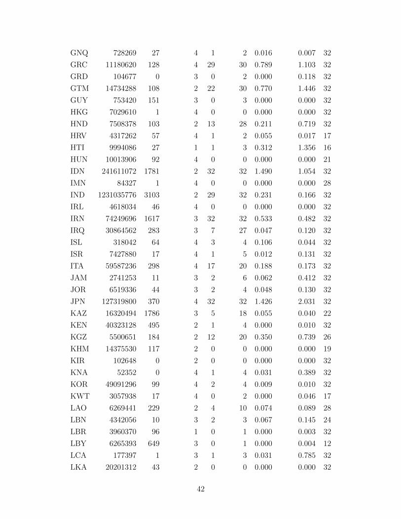
GNQ 728269 27 4 1 2 0.016 0.007 32

GRC 11180620 128 4 29 30 0.789 1.103 32

GRD 104677 0 3 0 2 0.000 0.118 32

GTM 14734288 108 2 22 30 0.770 1.446 32

GUY 753420 151 3 0 3 0.000 0.000 32

HKG 7029610 1 4 0 0 0.000 0.000 32

HND 7508378 103 2 13 28 0.211 0.719 32

HRV 4317262 57 4 1 2 0.055 0.017 17

HTI 9994086 27 1 1 3 0.312 1.356 16

HUN 10013906 92 4 0 0 0.000 0.000 21

IDN 241611072 1781 2 32 32 1.490 1.054 32

IMN 84327 1 4 0 0 0.000 0.000 28

IND 1231035776 3103 2 29 32 0.231 0.166 32

IRL 4618034 46 4 0 0 0.000 0.000 32

IRN 74249696 1617 3 32 32 0.533 0.482 32

IRQ 30864562 283 3 7 27 0.047 0.120 32

ISL 318042 64 4 3 4 0.106 0.044 32

ISR 7427880 17 4 1 5 0.012 0.131 32

ITA 59587236 298 4 17 20 0.188 0.173 32

JAM 2741253 11 3 2 6 0.062 0.412 32

JOR 6519336 44 3 2 4 0.048 0.130 32

JPN 127319800 370 4 32 32 1.426 2.031 32

KAZ 16320494 1786 3 5 18 0.055 0.040 22

KEN 40323128 495 2 1 4 0.000 0.010 32

KGZ 5500651 184 2 12 20 0.350 0.739 26

KHM 14375530 117 2 0 0 0.000 0.000 19

KIR 102648 0 2 0 0 0.000 0.000 32

KNA 52352 0 4 1 4 0.031 0.389 32

KOR 49091296 99 4 2 4 0.009 0.010 32

KWT 3057938 17 4 0 2 0.000 0.046 17

LAO 6269441 229 2 4 10 0.074 0.089 28

LBN 4342056 10 3 2 3 0.067 0.145 24

LBR 3960370 96 1 0 1 0.000 0.003 32

LBY 6265393 649 3 0 1 0.000 0.004 12

LCA 177397 1 3 1 3 0.031 0.785 32

LKA 20201312 43 2 0 0 0.000 0.000 32

42

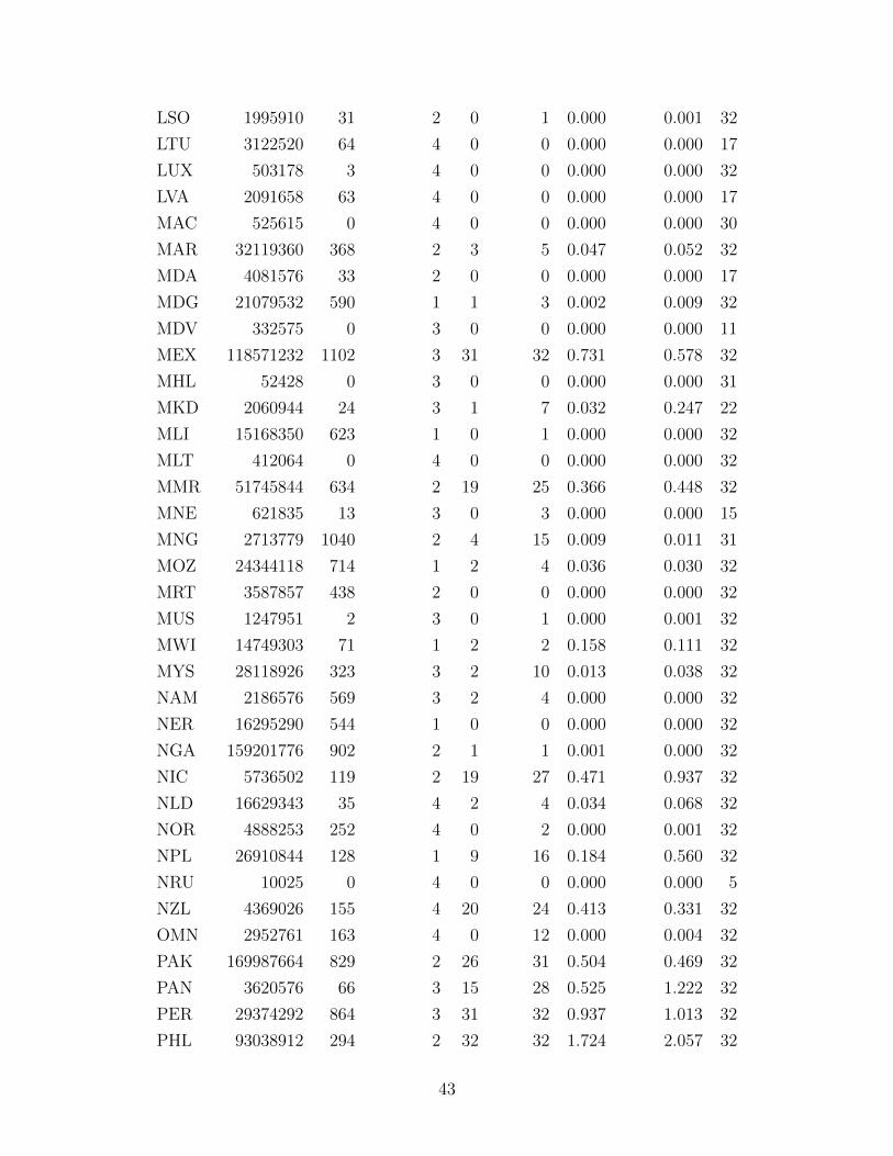
LSO 1995910 31 2 0 1 0.000 0.001 32

LTU 3122520 64 4 0 0 0.000 0.000 17

LUX 503178 3 4 0 0 0.000 0.000 32

LVA 2091658 63 4 0 0 0.000 0.000 17

MAC 525615 0 4 0 0 0.000 0.000 30

MAR 32119360 368 2 3 5 0.047 0.052 32

MDA 4081576 33 2 0 0 0.000 0.000 17

MDG 21079532 590 1 1 3 0.002 0.009 32

MDV 332575 0 3 0 0 0.000 0.000 11

MEX 118571232 1102 3 31 32 0.731 0.578 32

MHL 52428 0 3 0 0 0.000 0.000 31

MKD 2060944 24 3 1 7 0.032 0.247 22

MLI 15168350 623 1 0 1 0.000 0.000 32

MLT 412064 0 4 0 0 0.000 0.000 32

MMR 51745844 634 2 19 25 0.366 0.448 32

MNE 621835 13 3 0 3 0.000 0.000 15

MNG 2713779 1040 2 4 15 0.009 0.011 31

MOZ 24344118 714 1 2 4 0.036 0.030 32

MRT 3587857 438 2 0 0 0.000 0.000 32

MUS 1247951 2 3 0 1 0.000 0.001 32

MWI 14749303 71 1 2 2 0.158 0.111 32

MYS 28118926 323 3 2 10 0.013 0.038 32

NAM 2186576 569 3 2 4 0.000 0.000 32

NER 16295290 544 1 0 0 0.000 0.000 32

NGA 159201776 902 2 1 1 0.001 0.000 32

NIC 5736502 119 2 19 27 0.471 0.937 32

NLD 16629343 35 4 2 4 0.034 0.068 32

NOR 4888253 252 4 0 2 0.000 0.001 32

NPL 26910844 128 1 9 16 0.184 0.560 32

NRU 10025 0 4 0 0 0.000 0.000 5

NZL 4369026 155 4 20 24 0.413 0.331 32

OMN 2952761 163 4 0 12 0.000 0.004 32

PAK 169987664 829 2 26 31 0.504 0.469 32

PAN 3620576 66 3 15 28 0.525 1.222 32

PER 29374292 864 3 31 32 0.937 1.013 32

PHL 93038912 294 2 32 32 1.724 2.057 32

43

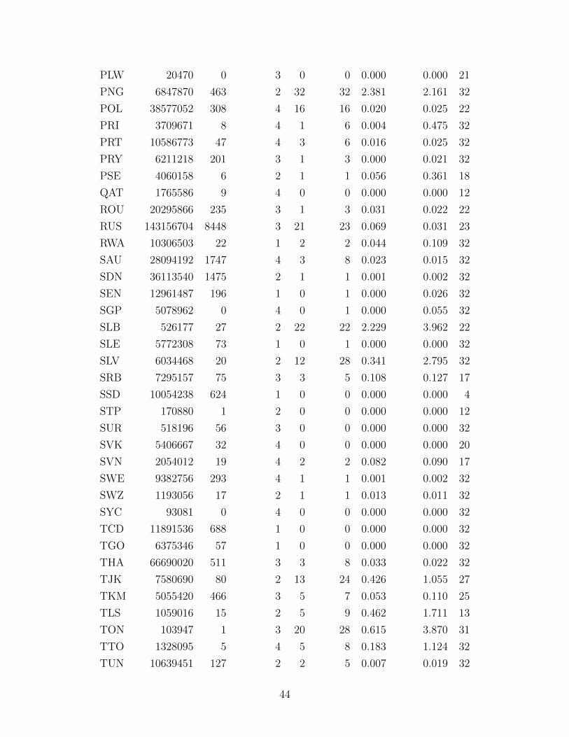
PLW 20470 0 3 0 0 0.000 0.000 21

PNG 6847870 463 2 32 32 2.381 2.161 32

POL 38577052 308 4 16 16 0.020 0.025 22

PRI 3709671 8 4 1 6 0.004 0.475 32

PRT 10586773 47 4 3 6 0.016 0.025 32

PRY 6211218 201 3 1 3 0.000 0.021 32

PSE 4060158 6 2 1 1 0.056 0.361 18

QAT 1765586 9 4 0 0 0.000 0.000 12

ROU 20295866 235 3 1 3 0.031 0.022 22

RUS 143156704 8448 3 21 23 0.069 0.031 23

RWA 10306503 22 1 2 2 0.044 0.109 32

SAU 28094192 1747 4 3 8 0.023 0.015 32

SDN 36113540 1475 2 1 1 0.001 0.002 32

SEN 12961487 196 1 0 1 0.000 0.026 32

SGP 5078962 0 4 0 1 0.000 0.055 32

SLB 526177 27 2 22 22 2.229 3.962 22

SLE 5772308 73 1 0 1 0.000 0.000 32

SLV 6034468 20 2 12 28 0.341 2.795 32

SRB 7295157 75 3 3 5 0.108 0.127 17

SSD 10054238 624 1 0 0 0.000 0.000 4

STP 170880 1 2 0 0 0.000 0.000 12

SUR 518196 56 3 0 0 0.000 0.000 32

SVK 5406667 32 4 0 0 0.000 0.000 20

SVN 2054012 19 4 2 2 0.082 0.090 17

SWE 9382756 293 4 1 1 0.001 0.002 32

SWZ 1193056 17 2 1 1 0.013 0.011 32

SYC 93081 0 4 0 0 0.000 0.000 32

TCD 11891536 688 1 0 0 0.000 0.000 32

TGO 6375346 57 1 0 0 0.000 0.000 32

THA 66690020 511 3 3 8 0.033 0.022 32

TJK 7580690 80 2 13 24 0.426 1.055 27

TKM 5055420 466 3 5 7 0.053 0.110 25

TLS 1059016 15 2 5 9 0.462 1.711 13

TON 103947 1 3 20 28 0.615 3.870 31

TTO 1328095 5 4 5 8 0.183 1.124 32

TUN 10639451 127 2 2 5 0.007 0.019 32

44

TUR 72316648 770 3 24 29 0.413 0.370 32

TUV 9827 0 3 0 0 0.000 0.000 22

TZA 45654440 775 1 9 11 0.126 0.120 24

UGA 33133356 206 1 3 6 0.043 0.083 30

UKR 45647772 586 2 1 2 0.027 0.020 25

URY 3371396 69 4 0 0 0.000 0.000 32

USA 309920832 4964 4 32 32 0.106 0.058 32

UZB 27687404 428 2 4 16 0.078 0.044 25

VCT 109316 0 3 0 2 0.000 0.067 32

VEN 28998782 592 3 17 22 0.169 0.183 32

VNM 88344488 326 2 2 6 0.004 0.011 28

VUT 236299 11 2 32 32 2.449 7.546 32

WSM 186029 3 2 1 20 0.033 1.750 30

YEM 23592026 309 2 2 10 0.009 0.098 22

ZAF 51638656 532 3 30 31 0.051 0.049 32

ZMB 13919025 743 2 9 22 0.008 0.018 32

ZWE 13968325 388 1 1 8 0.000 0.011 32

ANR 83128 0 4 0 0 0.000 0.000 32

ESH 514220 94 2 0 0 0.000 0.000 32

KOS 1764580 11 2 1 4 0.083 0.320 12

Table 3: List of countries in the data set. The table displays the population of the country in 2010,the size of the country area (in km2) with a population density of 1 person per square kilometeror greater, the income category of the country (1 - low income, 2 - lower middle income, 3 - uppermiddle income, 4 - high income), The number of years with earthquake exposure greater than zeroand the average exposure both for measure 1A and 2B, and the number of years with su�cientGDP per capita data to be included in the regressions.

45

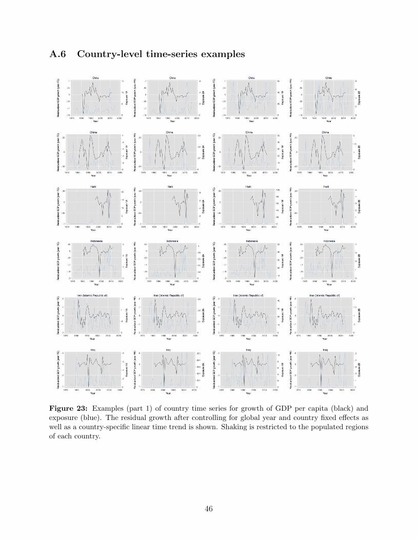
A.6 Country-level time-series examples

Figure 23: Examples (part 1) of country time series for growth of GDP per capita (black) andexposure (blue). The residual growth after controlling for global year and country fixed e↵ects aswell as a country-specific linear time trend is shown. Shaking is restricted to the populated regionsof each country.

46

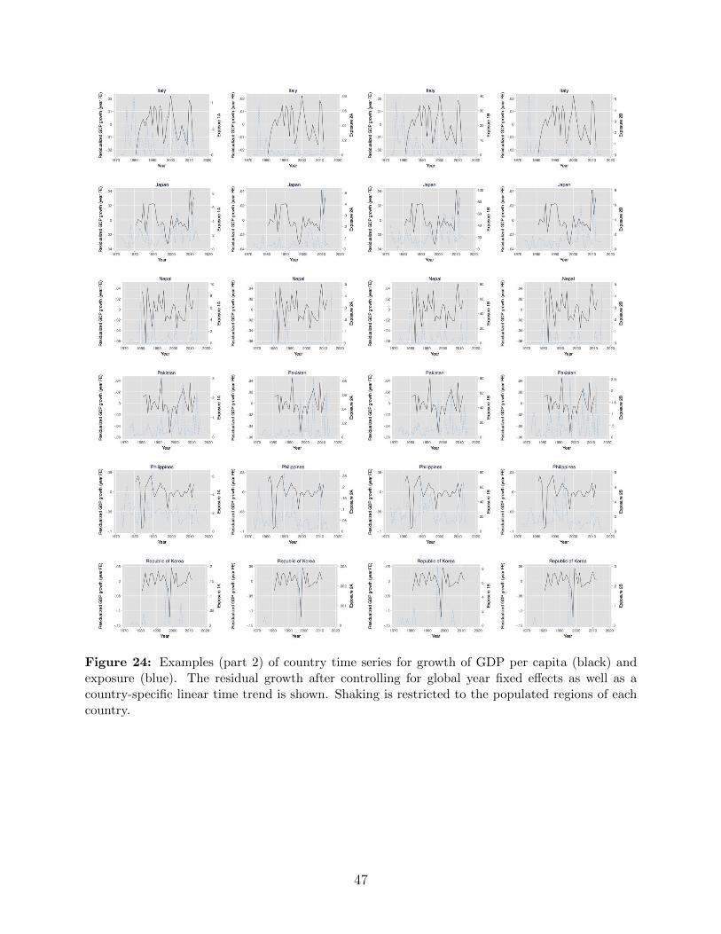
Figure 24: Examples (part 2) of country time series for growth of GDP per capita (black) andexposure (blue). The residual growth after controlling for global year fixed e↵ects as well as acountry-specific linear time trend is shown. Shaking is restricted to the populated regions of eachcountry.

47

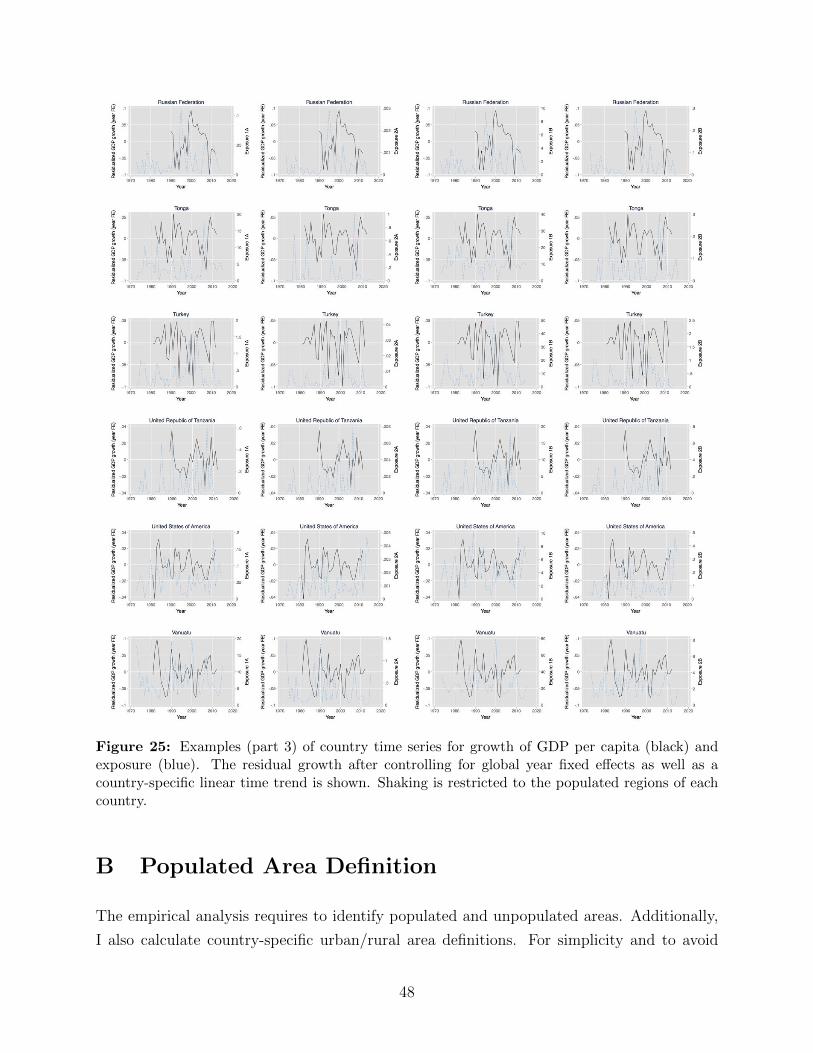
Figure 25: Examples (part 3) of country time series for growth of GDP per capita (black) andexposure (blue). The residual growth after controlling for global year fixed e↵ects as well as acountry-specific linear time trend is shown. Shaking is restricted to the populated regions of eachcountry.

B Populated Area Definition

The empirical analysis requires to identify populated and unpopulated areas. Additionally,

I also calculate country-specific urban/rural area definitions. For simplicity and to avoid

48

potential issues with inconsistent area definitions, these areas are here defined based on the

population data from 2010 and the same areas are used across years. This provides the ben-

efit of time-invariant spatial definitions for these classifications.8 The GPW data is based on

the smallest available unit of an administrative or census region for which population data is

available. The spatial size of these units varies significantly across countries and thus a↵ects

the data quality. The data does, therefore, not always show zero population for unpopulated

areas. The population density threshold for distinguishing whether a grid cell is considered

populated or unpopulated is defined as one person per km2. To distinguish between rural

and urban country-specific population density thresholds are determined. No global standard

definition of “urban” and “rural” exists and it has been argued that rurality (or urbanity)

should be considered a gradient and not a dichotomy (Chomitz et al., 2005). Nevertheless,

for the application here a discrete distinction is necessary to calculate a rural and an urban

exposure to shaking. O�cial country statistics usually provide a national definition for dis-

tinguishing between rural and urban regions. These definitions are seldom exclusively based

on population density, but commonly include absolute population thresholds for settlements,

infrastructure network connectivity, and economic activity. If population density thresholds

are used as a criterion, they take on a wide range of di↵erent values (between 150 to 1,500

people per km2) in di↵erent countries9. The choice of an appropriate threshold depends

on national characteristics. For the application here the average population density in the

populated region of each country is calculated and a country-specific threshold is defined

by adding one third of the standard deviation of the population density grid cells in the

populated area.

Since the GPW population grid is derived by area-weighting admin-unit population

counts, high population density numbers are more common in countries with highly dis-

aggregated population data (small admin-units). To prevent this from strongly a↵ecting the

calculation of the standard deviations, all grid cells in a country that have a population den-

sity above 1500 people per km2 are combined into one observation with population density

d � 1500 and area a. This observation is then split up into n observations with population

density d and area an such that a

n is equal to the average grid cell size in the country. This

is only done for the calculation of the standard deviation of population density within a

country. The threshold 1500 is chosen, since it is the largest commonly used population

density threshold in the literature to classify urban population.

8While population numbers did change over time and certain grid cells should probably be considered tohave switched their classifications over the years, the range of years that will be included in the regressionanalysis is not extensive enough that this measurement error problem would outweigh the benefit of a time-invariant definition.

9http://blogs.worldbank.org/sustainablecities/what-does-urban-mean (accessed 4/10/17)

49

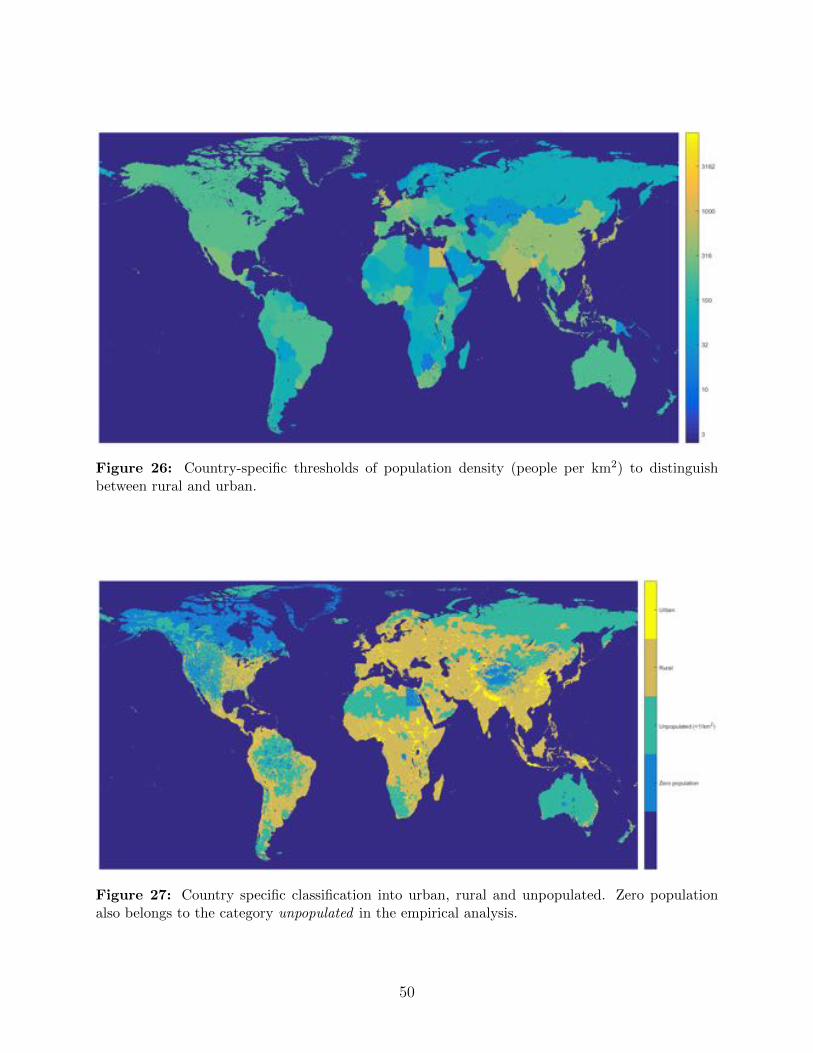
Figure 26: Country-specific thresholds of population density (people per km2) to distinguishbetween rural and urban.

Figure 27: Country specific classification into urban, rural and unpopulated. Zero populationalso belongs to the category unpopulated in the empirical analysis.

50

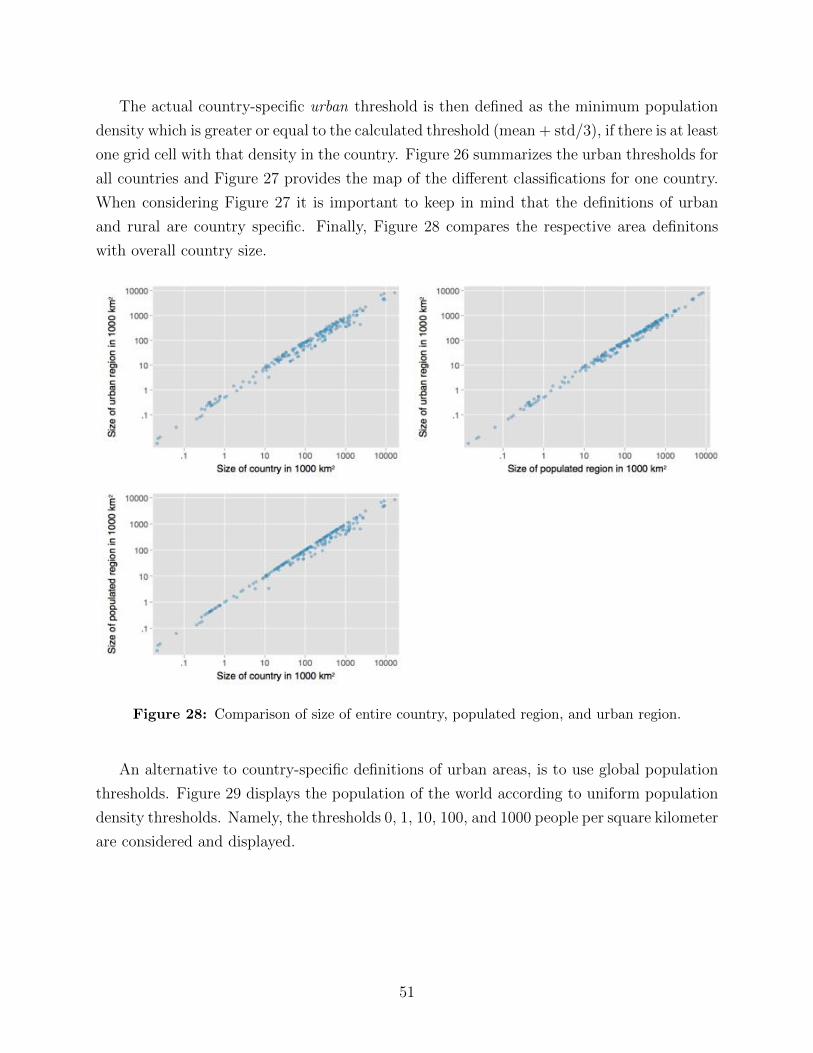
The actual country-specific urban threshold is then defined as the minimum population

density which is greater or equal to the calculated threshold (mean + std/3), if there is at least

one grid cell with that density in the country. Figure 26 summarizes the urban thresholds for

all countries and Figure 27 provides the map of the di↵erent classifications for one country.

When considering Figure 27 it is important to keep in mind that the definitions of urban

and rural are country specific. Finally, Figure 28 compares the respective area definitons

with overall country size.

Figure 28: Comparison of size of entire country, populated region, and urban region.

An alternative to country-specific definitions of urban areas, is to use global population

thresholds. Figure 29 displays the population of the world according to uniform population

density thresholds. Namely, the thresholds 0, 1, 10, 100, and 1000 people per square kilometer

are considered and displayed.

51

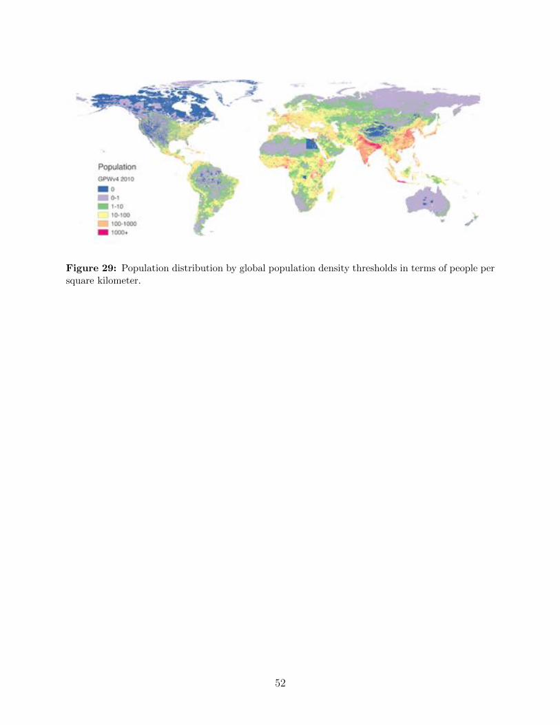
Figure 29: Population distribution by global population density thresholds in terms of people persquare kilometer.

52

(1) (2) (3) (4)VARIABLES 2B 1B 2A 1A

F1shaking 0.0011 -0.0000 -0.0144 -0.0002(0.0014) (0.0001) (0.0118) (0.0006)

F2shaking 0.0017 -0.0001 -0.0217 -0.0008(0.0016) (0.0001) (0.0106) (0.0005)

F3shaking -0.0000 -0.0002 -0.0100 -0.0006(0.0017) (0.0001) (0.0102) (0.0005)

shaking -0.0021 -0.0003 -0.0214 -0.0009(0.0022) (0.0002) (0.0141) (0.0007)

L1shaking -0.0033 -0.0003 -0.0159 -0.0006(0.0027) (0.0002) (0.0167) (0.0011)

L2shaking -0.0058 -0.0004 -0.0149 -0.0005(0.0021) (0.0002) (0.0142) (0.0008)

L3shaking -0.0027 -0.0004 -0.0100 -0.0007(0.0014) (0.0001) (0.0113) (0.0007)

L4shaking -0.0029 -0.0003 -0.0150 -0.0013(0.0023) (0.0002) (0.0235) (0.0014)

L5shaking -0.0012 -0.0000 0.0007 -0.0004(0.0017) (0.0001) (0.0122) (0.0006)

L6shaking 0.0001 0.0001 0.0151 0.0006(0.0017) (0.0001) (0.0125) (0.0007)

L7shaking 0.0001 0.0001 0.0063 0.0007(0.0016) (0.0001) (0.0130) (0.0007)

L8shaking -0.0016 -0.0001 0.0045 0.0003(0.0014) (0.0001) (0.0120) (0.0006)

Observations 5,586 5,586 5,586 5,586R-squared 0.1197 0.1218 0.1179 0.1181year FE X X X Xcountry FE X X X Xcountry time trend X X X XError terms are spatially correlated within one year acrosscountries for up to 1000km and serially correlated withinone country across years for up to 10 years.The dependent variable is the first di↵erence oflog GDP per capita.

Table 4: Regression results of the � coe�cients from the main model for the four di↵erent shakingexposure definitions.

53

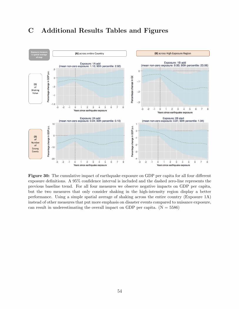
C Additional Results Tables and Figures

Figure 30: The cumulative impact of earthquake exposure on GDP per capita for all four di↵erentexposure definitions. A 95% confidence interval is included and the dashed zero-line represents theprevious baseline trend. For all four measures we observe negative impacts on GDP per capita,but the two measures that only consider shaking in the high-intensity region display a betterperformance. Using a simple spatial average of shaking across the entire country (Exposure 1A)instead of other measures that put more emphasis on disaster events compared to nuisance exposure,can result in underestimating the overall impact on GDP per capita. (N = 5586)

54

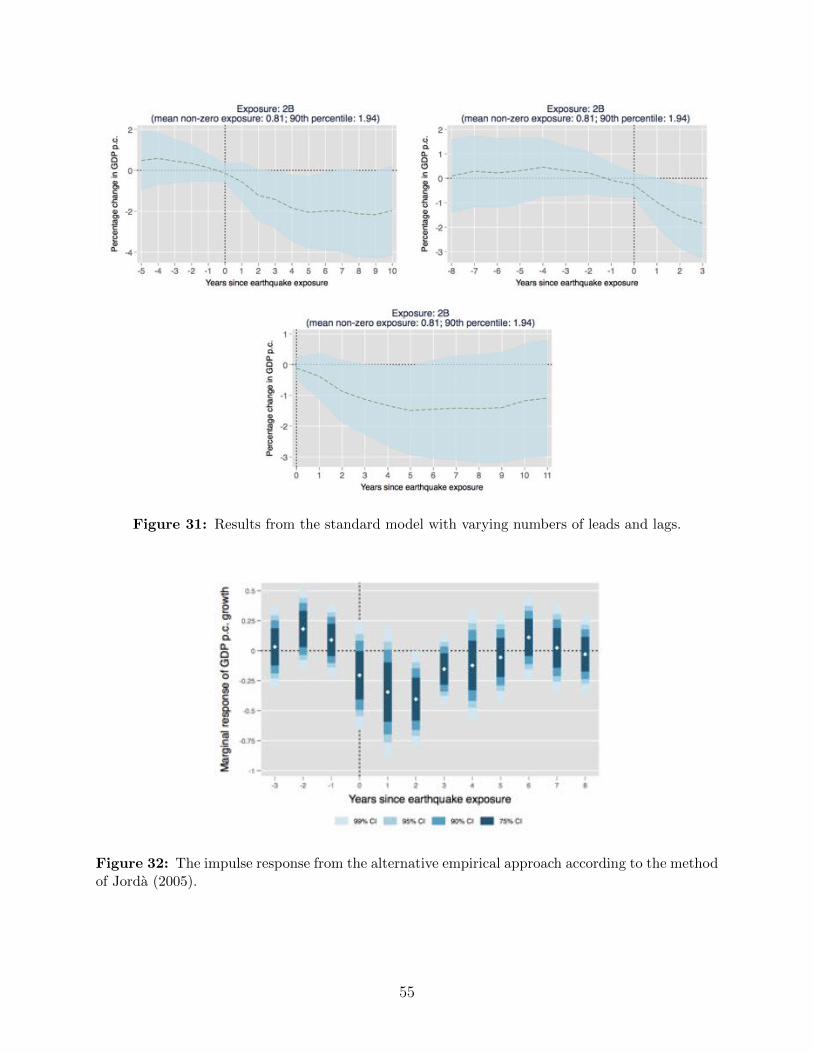
Figure 31: Results from the standard model with varying numbers of leads and lags.

Figure 32: The impulse response from the alternative empirical approach according to the methodof Jorda (2005).

55

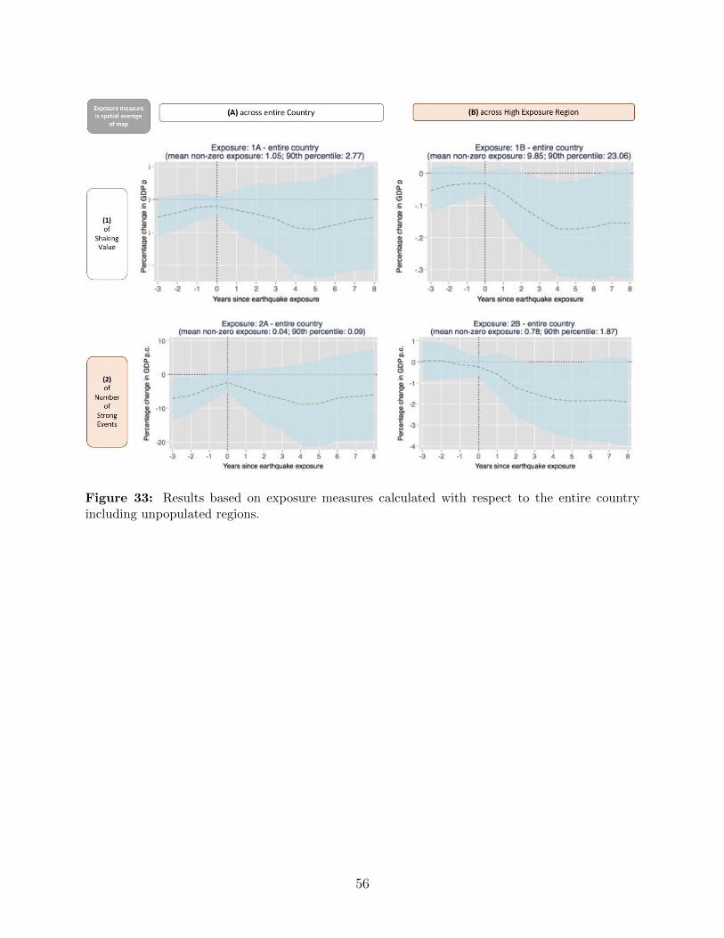
Figure 33: Results based on exposure measures calculated with respect to the entire countryincluding unpopulated regions.

56

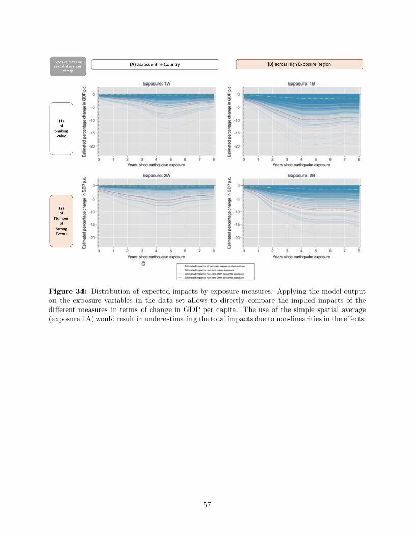
Figure 34: Distribution of expected impacts by exposure measures. Applying the model outputon the exposure variables in the data set allows to directly compare the implied impacts of thedi↵erent measures in terms of change in GDP per capita. The use of the simple spatial average(exposure 1A) would result in underestimating the total impacts due to non-linearities in the e↵ects.

57

Figure 35: Results based on exposure measures calculated with respect to only the urban regionsof each country. The results are not significant under this specification. This could be due to thefact that more rural countries are actually faring worse after an earthquake exposure and theywould actually receive lower exposure measures under this specification.

58

Figure 36: The impact of earthquake shaking exposure on displacement (percentage of internallydisplaced people of total population) as a global average (top) and by country-income categories(bottom).

Figure 37: Results from multidimensional exposure approach

59

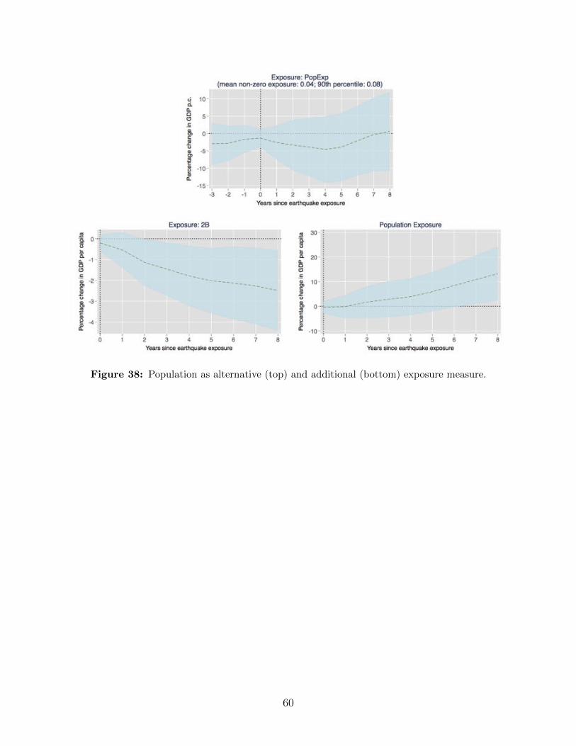
Figure 38: Population as alternative (top) and additional (bottom) exposure measure.

60

Figure 39: Comparing the model results for exposure measures 1A (left column) and 2B (rightcolumn) for increasing population density thresholds of the considered areas.

61