
DOCTORAL THESIS f O TEKNISKA Lal HÖGSKOLAN I LULEÅ
163
DOCTORAL THESIS 1985:41 D BOUNDARY LUBRICATION IN SCREW-NUT TRANSMISSIONS by LARS O. EKERFORS Division of Machine Elements fO TEKNISKA Lal HÖGSKOLAN I LULEÅ LULEÅ UNIVERSITY OF TECHNOLOGY
-
Upload
khangminh22 -
Category
Documents
-
view
0 -
download
0
Transcript of DOCTORAL THESIS f O TEKNISKA Lal HÖGSKOLAN I LULEÅ

DOCTORAL THESIS 1985:41 D
BOUNDARY LUBRICATION IN SCREW-NUT TRANSMISSIONS
b y
LARS O. EKERFORS Division of Machine Elements
f O TEKNISKA Lal HÖGSKOLAN I LULEÅ LULEÅ UNIVERSITY OF TECHNOLOGY
1985:410
BOUNDARY LUBRICATION IN
SCREW-NUT TRANSMISSIONS
av
LARS 0. EKERFORS
Inst i tu t ionen för Maskinteknik
Avdelningen för Maskinelement
AKADEMISK AVHANDLING
som med vederbörl igt t i l l s t å n d av Tekniska Fakultetsnämnden vid
Tekniska Högskolan i Luleå för avläggande Sv teknisk doktors
examen kommer a t t o f fent l igen försvaras i Tekniska Högskolans
hörsal E 246, E-huset, fredagen den 26 apr i l 1985, kl 09.00.

BOUNDARY LUBRICATION IN
SCREW-NUT TRANSMISSIONS
by
LARS 0. EKERFORS
Div is ion of Machine Elements
LULEÅ UNIVERSITY OF TECHNOLOGY
LULEÅ 1985

CONTENTS Page
ACKNOWLEDGEMENTS
ABSTRACT
1. INTRODUCTION 1
1.1 Background 1
1.2 Optimal function 1
1.3 Capabil i ty of performance 2
2. SYMBOLS 4
3. EXPERIMENTAL EQUIPMENT 7
3.1 Test r i g and test object 7
3.2 Gauges 14
3.3 Recording equipment 16
4. THE COEFFICIENT OF FRICTION 17
4.1 Theoretical model 17
4.2 Experimental invest igat ions 25
4.3 Analysis of experimental resul ts 29
4.4 Discussion and conclusions 43
5. THE HEAT CONDUCTION PROBLEM 48
5.1 Balance of developed power and heat 48
5.2 Theoretical model 49
5.3 The equation of heat conduction 50
5.4 Solution of the equation of heat conduction 52
5.5 Experimental invest igat ions 63
5.6 Discussion and conclusions 71

6. DESIGN OF SCREW-NUT TRANSMISSIONS 74
6.1 Cr i te r ia 74
6.2 Numerical examples 80
7. REFERENCES 95
8. APPENDICES 97
Tables TI Constants of material 98
T2.T3 Trapezoidal screw threads, 99
extracts from Swedish Standards
T4-T23 Experimental results 107
Diagrams D1-D16 127
Computer programs C1-C4 143

ACKNOWLEDGEMENTS
The research work here presented has been carried out at the Depart
ment of Machine Elements, Luleå University of Technology.
The work has been f inanc ia l l y supported by the National Swedish Board
for Technical Development (STU).
I would l i ke to take the opportunity to express my grat i tude to
Professor Bo Jacobson for his active in te res t , which has given r ise
to many st imulat ing and f r u i t f u l discussions.
Furthermore, I wish to thank Mr Sven-Erik Tiberg for his contr ibut ions
in connection with the construction of the electronic equipment and
for his assistance in programming.
In chapter 5, which deals with the heat conduction problem, Dr Anders
Grennberg has been of indispensable help in solving the heat conduc
t ion equation and providing diagrams.
I should also l i ke to thank Professor Håkan Gustavsson for the in te r
esting discussion concerning the mathematical formulation of the heat
conduction problem.
I thank Mr Allan Holmgren for his excellent help in the construction
and ca l ib ra t ion of the test ing equipment.
F ina l l y , I wish to thank Miss Rose-Marie Lövenstig and Miss Gunnel
Henriksson, who have typed the manuscripts so conscientiously.

ABSTRACT
This report deals with the function of screw-nut transmissions (power-
screws). Two aspects of th is function have been investigated.
Owing to d i f fe ren t running parameters, pr imari ly s l id ing speed and
average pressure between the s l id ing surfaces of the thread, the coef
f i c i e n t of f r i c t i o n and the ef f ic iency w i l l vary within wide l i m i t s .
The running parameters can be summarized in a dimensionless number,
the Sommerfeldt number S.
The problem, which has reference to boundary lubr i ca t ion , is solved by
a theoret ical model. The model is based on two types of interact ion
between the s l id ing surfaces, namely sol id f r i c t i o n at asperity peaks
and l i qu id f r i c t i o n in the voids between the asper i t ies. An optimal
interval of the Sommerfeldt number, where the coef f i c ien t of f r i c t i o n
i s at i t s minimum, has been established: 0.025 < S t < 0.042. opt
As a resul t of f r i c t i o n between the s l id ing surfaces, heat is deve
loped, which is conducted through the material of the screw and nut.
The developed heat can cause high temperatures on the s l id ing surfaces
of the thread.
The capabi l i ty of performance is l imi ted by the development of high
temperatures in the thread, where the running temperature of the
actual lubr icant must not be exceeded.
Physical ly, the phenomenon relates to heat conduction. A theoret ical
model is put forward. In the model the screw is replaced by a
cy l indr ica l rod and a hollow cyl inder corresponds to the nut. The
equation of heat conduction is stated and solved for the case of

steady state in the actual regions. I t is shown that an i n f i n i t e l y
th in wall of the hollow cyl inder is the most severe case with a maxi
mum r ise in temperature. The resul t is presented in the form of a
diagram with dimensionless temperature, rod speed and length of
cy l inder .
The report ends with recommendations for how the results can be used
for designing screw-nut transmissions. In th is context three numerical
examples are given.

1
1. INTRODUCTION
1.1 Background
The screw-nut transmission (power- or lead screws) is a machine ele
ment, which consists of a combination of screw and nut and is used
for power transmission.
The screw-nut transmission transforms rotat ion into t ranslat ion or
vice versa.
In the f i r s t case, great axial force is produced and the motion is
very accurate, even and easy to cont ro l . In the l a t t e r case, high
rotat ional speed w i l l be the resu l t .
The screw-nut transmission has many technical appl icat ions, such as
tes t machines for tensi le stress, feed screws in lathes, mechanical
jacks and separators.
1.2 Optimal function
When transmitted power and power loss are moderate, the screw-nut
transmission works with sat isfactory lubr icat ion wi th in a wide range
of load and speed. In th is context, the macro-mechanical qua l i t ies of
the surfaces of the thread flank are s ign i f i can t .
Qual i t ies such as the surface roughness and v iscosi ty of the lubr icant
are relevant here.
Screw-nut transmissions work with re la t i ve ly low e f f i c iency , so i t is
of great importance to f ind the i r optimal running range.

2
The external load, i . e . the axial load, is transferred to and d i s t r i
buted on the surfaces of the thread flanks as a pressure d i s t r i bu t i on .
When the surfaces of the thread flanks of the screw and nut s l ide
against each other f r i c t i o n appears, which manifests i t s e l f as a f r i c
t ional force. By d e f i n i t i o n , the f r i c t i o n is represented by the so
cal led coe f f i c ien t of f r i c t i o n .
The screw-nut transmission works optimally when the combination of
s l id ing speed and flank pressure results in as large a degree of e f f i
ciency as possible. This is equivalent to as small a coe f f i c ien t of
f r i c t i o n as possible.
In th is thesis chapter 4 treats the coe f f i c ien t of f r i c t i o n as i t is
affected by the s l id ing speed of the surfaces of the thread f lanks,
contact pressure, surface roughness and v iscosi ty of the lubr icant .
1.3 Capabil i ty of performance
One of the most important factors, l im i t i ng the capabi l i ty of perfor
mance of screw-nut transmissions, is the increase of temperature which
appears at the surfaces of the thread f lanks. This is caused by the
f r i c t i o n , mentioned above, and arises when the surfaces of contact
s l ide on each other. Since sol id or grease lubr icants are usually
used, the generated f r i c t i o n heat cannot be abducted by c i rcu la t ing
o i l , as is the case of, for instance, radial journal bearings, gear
pairs etc.
The f r i c t i o n heat, i . e . the power loss, which is dissipated by heat
conduction through the threads in screw-nut transmissions, can cause

3
a re la t i ve ly high working temperature. This temperature determines the
a b i l i t y of the lubr icant to form and maintain a sat isfactory bearing
f i l m . In boundary lubr icat ion i t is found that when the temperature is
raised there is a c r i t i c a l temperature above which the f r i c t i o n and
the surface damage increase markedly. [9]
In chapter 5 the heat conduction problem and the mechanism of how the
temperature d is t r ibu t ion is influenced by supplied power are studied.

4
SYMBOLS
A to ta l area of s l id ing surface - [m 2]
Arø area of c i rcu lar cyl inder [m 2]
A„ area of metal l ic contact [m21
A r ' geometry-dependent area [m 2]
a radius of c i rcu lar cyl inder [m]
B = l /u (0) [0]
b outer radius of hollow cy l inder , width of thread flank [m]
c speci f ic heat [Ws/(kg-K)j
dpdg constants of material [0]
F f r i c t i o n a l force [ N]
F_v axial force on nut [ Nl ax 1 J
H height of hollow cyl inder [m]
h average thickness of f i lm [m]
hQ f i lm thickness at beginning of asperity contact [m]
h* dimensionless f i lm thickness [0]
k slope of hydrodynamic l ine [0]
1 average length of the asperi t ies [m]
L ordinate at or ig in of coordinates for hydrodynamic [0] l i ne
M torque on nut [Nm]
N normal force [ N]
n rotat ional speed [ r /min]
p average pressure [N/m ] 2
Phd hydrodynamic pressure in the lubr icant [N/m ]
p' average increase in pressure at the asper i t ies [N/m ]
T / d . ( l - d „ 2 ) ' [N/m 2]
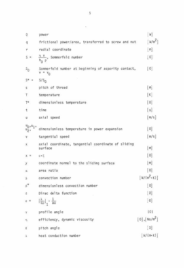
5
Q power [ W]
q f r i c t i ona l power/area, transferred to screw and nut [W/m ]
r radial coordinate [m]
S = n v , Sommerfeld number [0] h 0 P
Sq Sommerfeld number at beginning of asperity contact, [0] v = v 0
s* = s/s0
s pi tch of thread [m]
T temperature [K]
T* dimensionless temperature [0]
t time [s]
u axial speed [ m / s ]
u 0 ' u i •
Ug, dimensionless temperature in power expansion [0]
tangential speed [ m / s ] v
x axial coordinate, tangential coordinate of s l id ing surface [m]
x = £ - 5 [0]
y coordinate normal to the s l id ing surface [m]
area ra t io [0] a
ß convection number [W/(m -K)]
ß* dimensionless convection number [0]
6 Dirac delta function [0]
[—] • — [0] L cp J ^ au L J
Y p ro f i l e angle [0] o
n e f f i c iency , dynamic viscosi ty [0],[Ns/m ]
e p i tch angle [0]
X heat conduction number [W/(m-K)j
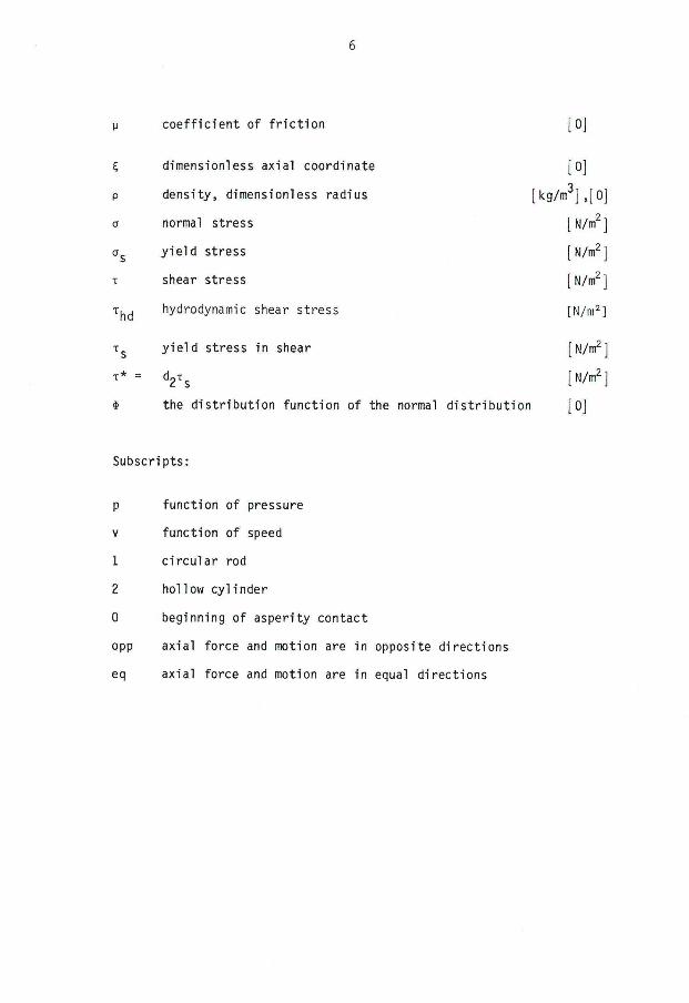
6
y coef f i c ien t of f r i c t i o n [0]
S dimensionless axial coordinate [0]
p density, dimensionless radius [kg/m ] , [ 0 ]
normal stress [N/m 2] o
a s y i e ld stress [N/m 2]
T shear stress [N/m 2]
Thd hydrodynamic shear stress [N/m 2]
T s y i e l d stress in shear [N/m 2 j
the d is t r ibu t ion function of the normal d is t r ibu t ion [0]
Subscripts:
p function of pressure
v function of speed
1 c i rcu lar rod
2 hollow cyl inder
0 beginning of asperity contact
opp axial force and motion are in opposite direct ions
eq axial force and motion are in equal direct ions

7
3. EXPERIMENTAL EQUIPMENT
3.1 Test r i g and test object
A test r i g has been designed and b u i l t . The central parts of the r ig
are two pa ra l l e l , ver t ica l and rotat ing screws where two nuts, the
tes t objects, can move along each screw.
The axial load coming from a hydraulic jack is transferred to the nuts
by two beams, where the beams are pressed apart by the jack. The beams
w i l l then in turn press against the four nuts.
Owing to the motion of the screws and the hydraulic jack, the test ob
jec ts w i l l be exposed to torque and axial load. The nuts are prevented
from rotat ion by an arrangement, here cal led torque r i ng , which f a c i
l i t a t e s measurement of the torque f igures 3.1.1 and 3 .1 .2 .
The two beams, the jack and the parts of the screws which are between
the nuts thus form a closed system of forces, f igure 3.1.3. The
screws, both ends of which are mounted in bearings, are coupled to
gether pa ra l le l l y by a chain transmission. The screws are operated by
a continuously variable e lec t r i c motor (ASEA LAC-315, 143 kW, 1800 rpm)
via a gear pair with intersect ing axes.
When the test r i g is in operation the pair of beams perform recipro
cating motion with simultaneous loading of the hydraulic jack. The
design of the test r i g is shown in f igures 3.1.4 and 3.1.5.
When loading the nuts i t is important to see to that they are exposed
to axial forces only. To eliminate the r isk of an unbalanced load, the
transfer of axial forces to each nut is done via a spherical thrust

8
r o l l e r bearing. To avoid transfer of torque to the support, the nut
also rests on a thrust bal l bearing, f igure 3.1.6. The resul t of th is
combination of bearings is that the torque transferred to the torque
r ing is very close to the total torque on the nut.
The material of the nuts is t i n bronze, SIS 5465, hardness HB = 95,
and the material of the screws is steel SIS 1672-01, hardness HV =
208.
According to measurements of the surface f i n i s h , the depth of p ro f i l e
of the thread flanks is H = 1.6-2.3 ym tangent ia l ly and H = 2.6-2.7 ym
rad ia l l y .
The lubr icant applied is an ordinary grease based on mineral o i l with
EP addi t ives, such as l i th ium soap etc. (commercial name ALEXOL HMP
2EP). The lubr icant has been analysed with respect to v iscosi ty in a
rotat ion viscosimeter of the type Rheotest, RV 2. The resu l ts , which
include temperature and shear rate dependence of the dynamic viscos
i t y , are shown in the diagram, f igure 3.1.7.

9
screw
ring
Figure 3 .1 .1 . Arrangement fo r determining torque.
Figure 3.1.2. Assembled torque r ing .

10
Figure 3.1.4. Diagram of the test r i g .

11
Figure 3.1.5. Test r i g .
Figure 3.1.6. Diagram of arrangement of nut support.

12
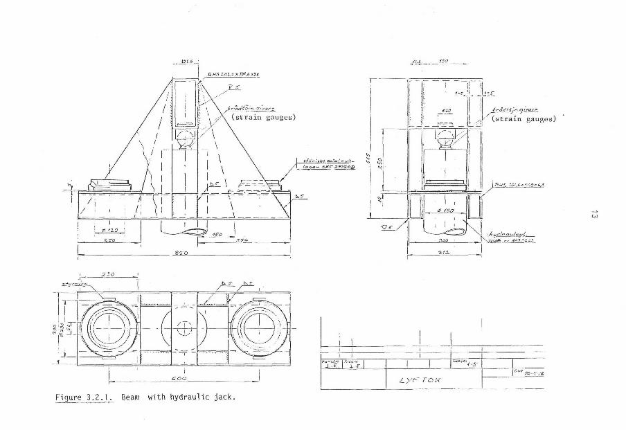
Figure 3 .2 .1 . Beam with hydraulic jack.

14
3.2 Gauges
Experimentally determined quantit ies in the invest igat ion were the
axial force and torque on the nuts, rotat ional speed of the screws and
temperature of the nuts.
The axial forces were determined by measuring the load of the hydrau
l i c jack. Measurements were done by cal ibrated s t ra in gauges attached
to the ball attachments of the jack. See f igures 3.1.3 and 3 .2 .1 .
The nut torque was measured by means of the torque r ing mentioned
ea r l i e r . This arrangement consists of a c i rcu la r steel r ing and a
radial lever attached to the r ing . The lever was equipped with one
s t ra in gauge on each side. Figures 3.1.1 and 3.1.2.
The rotat ional speed of the screws was determined using an optical
counter.
The temperature of the nuts was measured with thermocouples. The thermo
couples were welded to the bottom of channels, which were rad ia l l y
d r i l l e d into the wall of the nut to a depth of 1 mm from thread top.
The channels were placed one pitch of thread apart along a generatrix
at the outer surface of the nut. Figures 3.2.2 and 3.2.3.

15
Figure 3.2.2. Cross-section of wall of nut.
Figure 3.2.3. Nut f i t t e d with connections for thermocouples.
16
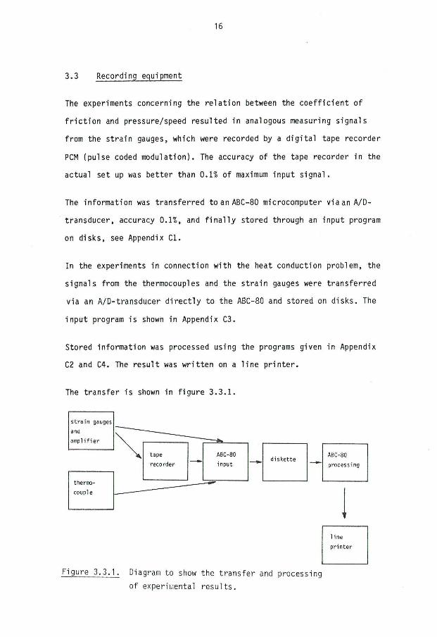
3.3 Recording equipment
The experiments concerning the re lat ion between the coef f i c ien t of
f r i c t i o n and pressure/speed resulted in analogous measuring signals
from the st ra in gauges, which were recorded by a d ig i ta l tape recorder
PCM (pulse coded modulation). The accuracy of the tape recorder in the
actual set up was better than 0.1% of maximum input s ignal .
The information was transferred to an ABC-80 microcomputer v iaanA/D-
transducer, accuracy 0.1%, and f i n a l l y stored through an input program
on disks, see Appendix Cl .
In the experiments in connection with the heat conduction problem, the
signals from the thermocouples and the s t ra in gauges were transferred
via an A/D-transducer d i rec t l y to the ABC-80 and stored on disks. The
input program is shown in Appendix C3.
Stored information was processed using the programs given in Appendix
C2 and C4. The resul t was wr i t ten on a l ine p r in te r .
The transfer is shown in f igure 3 . 3 . 1 .
I s t r a i n gauges!
thermo
couple
1 ine
p r i n t e r
Figure 3 .3 .1 . Diagram to show the transfer and processing
of experimental resu l ts .
17
4. THE COEFFICIENT OF FRICTION
4.1 Theoretical model
A model has been assumed in which the dependence of the coef f i c ien t of
f r i c t i o n on load and speed has been taken into account. The load is
here represented as the average pressure on the surfaces of thread
f lanks.
4.1.1 f_ujidlamentaj_s
By de f in i t i on
F U = N
according to [2] and [ 8 ] .
According to [ 1 ] , [3] and [16] the f r i c t i o n force is
F = A r . x s + ( A - A r h n d
and the normal force
N = A r - a s + ( A - A r ) p h d = A.p
where
p is the average pressure on the surfaces of the thread flanks
P n d is the hydrodynamic pressure in the lubr icant
o s is the y ie ld pressure of the softer metal
T s is the y ie ld stress in shear of the softer metal
is the hydrodynamic shear stress
A is the to ta l s l id ing surface
A is the surface with metal l ic contact.

18
Let
o (4.1)
This gives
[16] (4.2)
The area of the surface of contact is among other things dependent on
v and p.
This dependence is divided into
v A v
The i r r e g u l a r i t y , i . e . the asper i t ies , of the softer surface is taken
into consideration.
The area of the surface of metal l ic contact is a function of the o i l
f i l m thickness, h.
This function is influenced part ly by the geometry of every single
asperity and part ly by the d is t r ibu t ion of the heights of the asperi
t i e s .
(4.3)
4.1.2 J_he influence of_sj)eed
According to (4.1)
(4.4)
Assume that the asperi t ies are conical or pyramidal and that the i r
d i s t r ibu t ion over the surface of the flank is normal. [ 3 ] , [20] .

19
This can now be wr i t ten as
A r = A r ' [ l - k . * ( z ) ] = A r ' . *
where
A ' is the area of contact depending on geometry
o>fz) is the d i s t r i bu t ion funct ion of the normally
d is t r ibuted asperity peaks
k is a factor of correction
$ = l-k«<t>(z)
Figure 4 . 1 . 1 . Pyramidal asperi ty.
From f igure 4.1.1 is obtained
A v hQ
Putting in equation (4.4) gives
a = (J l ) = (1 - ^ - ) 2 . * (4.5) v A v h Q
The re la t ion between f i lm thickness, h, and s l id ing speed, v, is ob
tained from dimensional analysis of Reynolds' equation [18]
d_ ( h 3 dp_) . 6 n v dh dx dx dx
I ( h 3 £ l ) - n v H o 1 1 1
where 1 is the average length of asper i t ies
p' is the average increase in pressure at the asperi t ies

20
hO
With constant 1 , p ' , n and—we have
h 3 ~ v or h - ^
h* = f - = £ - ) (4.6) hO vO
where the subscript Q indicates the s tar t ing contact of asper i t ies.
4.1.3 The jn_f1 uence of_ay_erage_pressure
According to v. Mises and Bowden, Tabor [1] and [2]
Z.A 2 _ 2 _ H 2 + d l T - a s - d l T s
when v = 0 , a = a g .
While si iding a decreases due to T * 0.
Only the average pressure is taken into consideration, i .e . the hydro-
dynamic pressure, which is dependent on the s l id ing speed, is disregarded.
Then one obtains
_ N N _ p o - — - - J-—
(A„)_ a 'A a r p p p
Furthermore, a is assumed to be inversely proportional to the d i s t r i bu
t ion function of the normally d is t r ibuted asper i t ies
o = - P —
While s l id ing T = T * , which is assumed to be independent of p and
T * = d 2 x s [8]
Insert ing these expressions for o and x in to v. Mises equation gives
(JL-)2 • d l ( d 2 x s ) 2 = a /
21
From th is one obtains
a = - P — (4.7) P $.p*
where
p* = o s / l - d ?
2 ' = x s / d ^ l - d g 2 ) ' (4.8)
According to (4 .3) , and af ter insert ing (4 .5 ) , (4.6) and (4 .7 ) , one
obtains
a = a .« = £ - [1 - ( ^ - ) 1 / 3 ] 2 (4.9) P P v 0
4.1.4 J_he hydrody_nami_c_shear_s^res^
The relat ionship for internal f r i c t i o n in a viscous f l u i d as proposed
by Newton [14] is
*M (4.10)
where y is the coordinate normal to the s l id ing surface. Insert ing
(4.6)
h = h 0 ( ^ ) 1 / 3
° v 0
gives
^hd = ^ V ( ^ ) _ 1 / 3 ( 4 - U )
nO v 0
4.1.5 The equation of the coe f f i c ien t of f r i c t i o n
Regroup the re lat ion (4.2)
= a ( I i . I M ) + 1™ - a ll (1 ZM) + I M P P P P T s p

22
Thd The ra t io « 1 is disregarded and insert ion of equations (4.9) and
(4.10) gives
„ « I i [ i - ( V - ) 1 / 3 ] 2
+ m (4.12) vo P* 1 v n hp
Introduce the Sommerfeld number, S = 2 ^ - , and equation (4.8) n np
1 n iv ^ l / 3 n 2 A -v ,-1/3. u . _ = L _ [ i - ( f r - ] + % ) - - S
/ d ^ i - d g 2 ) vo vo
Also introduce S* = | - and / d ^ l - d ^ ) ' = B S 0
Then one obtains
y(S*) = 1 (1 - S * 1 / 3 ) 2 + S * 2 / 3 . S Q (4.13) B u
The equation is va l id in the regime of boundary lubr i ca t ion ,
0 < S* < 1.
In the regime S* > 1, i . e . hydrodynamic lub r i ca t ion , the re lat ion
between u and S* is assumed to be l inear ,
u = kS*+L
The derivat ive of u(S*) , equation (4.13), for S* = 1 gives the slope
of the "hydrodynamic l i n e " .
4H- = 2 ( l - S * 1 / 3 ) ( - I ) S * " 2 / 3 + i S n - S * ~ 1 / 3 (4.14) dS* B 3 3 0
Insert ing S* = 1 in the l inear re la t ion above and (4.14), we get
— = k = 4 s n dS* 3 0
and
^ = k = i s „ (4.15)

23
Thus
and
S 0 = f S0 + L
L = j S 0 (4.16)
Combining the assumed l inear re la t i on , (4.15) and (4.16) gives
„(S*) = JL (2S*+1) (4.17)
S* > 1
Stat ic f r i c t i o n is obtained by putt ing in S* = 0 in (4.13)
y(0) = I (4.18) B
In the regime S* < 1 n has a minimum, and = 0 in equation (4.14) dS*
gives
S - S = S ° 3 (4.19) 0 p t (1+BS 0)
3
and
S 0 u . = — (4.20) mi n /
1+BS0
The constants B and SQ are empir ical ly determined.
Example Karlebo Handbok [10] gives for the combination steel/bronze
s ta t i c f r i c t i o n y(0) = 0,18
s l id ing f r i c t i o n y ( l ) = 0,10

24
This gives
u . = — 9 A = 0,064 Mmi n
0,18
for
S = 0,1
(1 + ° ^ - ) 3
0,18
0,027
Figure 4.1.2 shows the curve of the coef f i c ien t of f r i c t i o n
according to the theoret ical model. The parameters B and SQ
are taken from the numerical example.
s* = S/SQ
boundary lubrication 1 hydrodynamic lubrication
Figure 4.1.2. The coef f i c ien t of f r i c t i o n according to the theoret ical model.
25
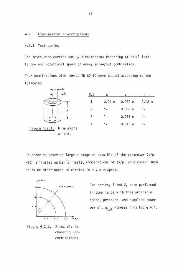
4.2 Experimental investigations
4.2.1 Test series
Two ser ies, 'l and 2, were performed
in compliance with th is p r inc ip le .
Speed, pressure, and supplied power
per m 2 , q! , appears from table 4 . 1 .
The tests were carried out by simultaneous recording of axial load,
torque and rotat ional speed of every screw/nut combination.
Four combinations with thread TR 80x10 were tested according to the
fol lowing
Nut H
1 0.04 m 0.060 m
2 "- 0.050 m
3 "- . 0.055 m
4 "- 0.045 m
0.12 m
Figure 4 . 2 . 1 . Dimensions
of nut.
In order to cover as large a range as possible of the parameter (v/p)
with a l imi ted number of tes ts , combinations of (v/p) were chosen such
as to be d is t r ibuted on c i rc les in a v-p diagram.
0 ,1 0 , 2 0 , 3 v m / a
Figure 4.2.2. Pr inc ip le fo r
choosing v /p-
combinations.
26
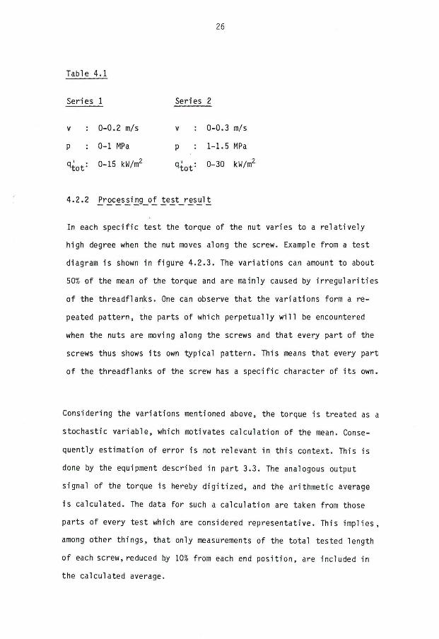
Table 4.1
Series 1
v : 0-0.2 m/s
p : 0-1 MPa
q' : 0-15 kW/m2
Series 2
v : 0-0.3 m/s
p : 1-1.5 MPa
q' : 0-30 kW/m2
4.2.2 Prrjcessing_o f_ tejs t_res_ul Jt
In each speci f ic test the torque of the nut varies to a re la t i ve ly
high degree when the nut moves along the screw. Example from a test
diagram is shown in f igure 4.2.3. The variat ions can amount to about
50% of the mean of the torque and are mainly caused by i r regu la r i t i es
of the threadflanks. One can observe that the var iat ions form a re
peated pat tern, the parts of which perpetually w i l l be encountered
when the nuts are moving along the screws and that every part of the
screws thus shows i t s own typical pat tern. This means that every part
of the threadflanks of the screw has a speci f ic character of i t s own.
Considering the variations mentioned above, the torque is treated as a
stochastic var iable, which motivates calculat ion of the mean. Conse
quently estimation of error is not relevant in th is context. This is
done by the equipment described in part 3.3. The analogous output
signal of the torque is hereby d i g i t i zed , and the arithmetic average
i s calculated. The data for such a calculat ion are taken from those
parts of every test which are considered representative. This impl ies,
among other things, that only measurements of the to ta l tested length
of each screw, reduced by 10% from each end pos i t ion , are included in
the calculated average.

rx3 •̂ 1
Figure 4.2.3. Variations in the torque of the nut. Example from a test diagram.

28
Ef f ic ienc ies , n, and coef f ic ients of f r i c t i o n , u, are then calculated
from averages of torque, M, and mutually related axial forces, F , by ax
the fol lowing formulas.
Motion and axial force direct ions opposite:
_ F a x ' s _ (l-n)cosy 2t t«M n/tane+tane
Motion and axial force direct ions equal:
2tmM (l-n)cosy n u = F «s n» tane+l/tane ax
Obtained coef f ic ients of f r i c t i o n are presented in Appendix, T4-T11
and Dl-016. Diagrams of u-values obtained from experiments with oppo
s i te or equal direct ions of motion and axial force respectively are
thus given separately. The reason for th is is that one can observe
certain differences in the relat ions of y-v/p in the two types of
motion, and th is in turn can be an indicat ion of s ign i f i can t physical
d i ss im i la r i t i es in the way of funct ioning. The fol lowing subscripts
are used,
opp opposite direct ions of motion and axial force
eq equal direct ions of motion and axial force.
No s ign i f icant difference between the results of series 1 and 2 can be
observed, so the results are shown together in the same diagrams.

29
4.3 Analysis of experimental results
The parameters S Q and 1/B are empir ical ly determined from the n - (v /p ) -
diagram by graphical construct ion.
I t appears from equation (4.16) that the ordinate at or ig in of coordi
nates for the "hydrodynamic" l ine is
Sq is graphical ly determined by f i t t i n g a stra ight l ine to the points
of measurement, which are judged to be wi th in the hydrodynamic regime.
The distance L is then measured, i .e . the intersect ion of the st ra ight
l ine and the y-axis. Figure 4.3.1 and 4.3.2. This then gives
S 0 = 3 L
The s tat ic f r i c t i o n y(0) = 1/B is obtained from u -p. The equations
(4.18) and (4.20) give
p ( 0 ) = l / B = — _ i (4.21)
u m l - n is determined from the curve, which is adjusted to the point of
measuring in the boundary lubr icat ion regime. Figure 4.3 .2 .
This method of determination of the coef f i c ien t of s ta t i c f r i c t i o n is
preferable to d i rect measurement in the diagram, since i t is "imposs
ib le to f ind a d i s t i nc t point corresponding to p (0 ) . Nor w i l l d i rect
determination from experiments give acceptable values since th is is
associated with great pract ical d i f f i c u l t i e s .

30
my Fax, 1.0
Nut no. 4
0.8
0.6
0.4
0.2
L= 173~S. r
s7"
— —
2.0 4.0 6.0
3(v/p) 140 2a—.1* -,(?=
8.0 IQjO v/p E-6 m /NS
Figure 4 . 3 . 1 . Graphical determination of SQ and the slope
of the "hydrodynamic" l i n e .
m y F a x o p P
0.20
Nut no. 4
0.16
0.12
0.08
0.04
0.4
/ y
y
y y
<^ v / p ^ O , > y
)2 = 0.31
0.8 1.2
Figure 4.3.2. Graphical determination of SQ and minimum
coef f i c ien t of f r i c t i o n .
1.6 2.0
v/p E-6-m3/Ns

31
Transformation of the variable (v/p) is done according to the
fo l 1 owing.
Def in i t ion
S = f . (1) h o P
Derivation
3S = i - . 3(1) h 0 P
Solve for
n _ aS
Develop the derivat ive
3S _ as as* ap
3(1) aS* 3y 3(1)
By de f i n i t i on
S* = — which leads to - — = S SQ 3S*
and from (4.15)
Insert ion gives
S = 1.5 • — — • (—) . 3(1) P
or
s* =hl . 3 a — (1) s o 3(1) P
o
3U- = ! s n one obtains l £ L = i i * aS* 3 u 3y S 0

32
Here — is the slope of the "hydrodynamic" l ine and is measured in
the y-(-jj-) diagram. See f igure 4 . 3 . 1 .
Graphically determined and calculated values of the parameters S Q
and — are given in table 4.3. The table also gives measured values
of u m l - n and corresponding values of ( v / p ) o p T /
In table 4.4 calculated values of y(0) according to (4.21) and values
of S ^ according to (4.19) and (4.20) are presented.
<: 3
s 0 - V m i n
0 p t " (1 + B S 0 ) 3 " S 0
2
In the f igures 4.3.3-4.3.10 test resul ts in dimensionless form and
curves of the theoretical model are combined. The test results are
also presented in Appendix, T12-T15.

Table 4.3 Graphically determined parameters.
Nut no 1 Nut no 2 Nut no 3 Nut no 4
F a X o P P
Fax eq
F ax opp
Fax eq
Fax opp
Fax eq
Fax opp
Fax eq
L = S 0/3 0.031 0.031 0.041 0.040 0.053 0.030 0.031 0.031
S 0 0.093 0.093 0.123 0.120 0.158 0.090 0.093 0.093
wmin 0.062 0.064 0.086 0.079 0.086 0.069 0.061 0.067
( v / P>op t
[m 3/Ns]-10~ 6
0.16 0.23 0.25 0.22 0.16 0.23 0.23 0.23
8u/a(J)
[Ns/m 3]10 3
101 80 107 89 104 98 96 94

34

my Fax
0.20
0.16 ^
0,12
0.08 r-
0.04
opp Nut no. 1
0.08 0.12 0.16
Figure 4.3.3. Theoretical curve of coef f ic ient of f r i c t i o n and experimental resu l ts .

36

37

38

39

40

s
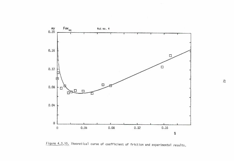
Figure 4.3.9. Theoretical curve of coef f i c ien t of f r i c t i o n and experimental resu l ts .
42

43
4.4 Discussion and conclusions
The coe f f i c ien t of f r i c t i o n (4.13) has been deduced with the assump
t ion that the average increase in pressure at the asper i t ies, p ' , and
the v iscos i ty , n, are constant. However, i t should be possible to
study the var iat ion in the coef f i c ien t of f r i c t i o n , u, according to
the parameter S i rrespect ive of the value of p' or p, as u is a func
t ion of the ra t io v/p and not of v and p separately [ 2 ] , [ 1 5 ] . Experi
ments that have been carried out also indicate t h i s .
The roughness of the s l id ing surfaces has influence on the f r i c t i o n
[ 4 ] . However, the experimental results confirm the assumption that the
theoret ical model is independent of the d is t r ibu t ion of the asperi
t i e s . The s ign i f i can t roughness parameter is probably the depth of
p ro f i l e which is included in the equation of the coef f i c ien t of f r i c
t ion (4.13) ,(4.17) in the constant S Q .
Concerning the assumed constancy of the v iscosi ty i t should be stated
that th is assumption is not correct.
I t - i s true that the temperature dependence of v iscosi ty of lubr icat ing
greases is less pronounced than that of the corresponding base o i l s
[11 ] . Nevertheless, the viscosi ty varies by more than 100% with present
var iat ions of temperature, see f igure 3.1.7.
However, the results of the present experiments with various powers
and coherent increases in temperature indicate that the coef f i c ien t of
f r i c t i o n is not affected by increasing temperature. This is an obser
vation also made by Hirst and Hollander; the f r i c t i o n remains constant
with r i s ing temperature unt i l a c r i t i c a l temperature is attained above
which i t r ises rapidly [ 9 ] .

44
This phenomenon may be explained according to the fo l lowing.
Increasing transfer of power gradually causes such an increase in tem
perature that the v iscosiy, n, w i l l be af fected. When normal l u b r i
cants are used, the viscosi ty decreases when the temperature is raised.
Simultaneously, however, as the carrying capacity of the lubr icant de
creases, the f i lm thickness, h, w i l l also decrease. This, in turn causes
a tendency of the ra t io n/h to a t ta in a constant value, thus resul t ing in
a re la t i ve ly small influence on the hydrodynamical shear stress.
According to equation (4.12) the coe f f i c ien t of f r i c t i o n can be wr i t ten
p*L vQ
j hp
in which the rat io n/h only appears in the las t term.
On the basis of the argument above, i t is clear that decreasing viscosi ty
w i l l not a f fect the coe f f i c ien t of f r i c t i o n to a larger extent.
A closer analysis of the re lat ion between supplied power and corre
sponding increase in temperature is given in chapter 5.
Analyt ical relat ions and experiments show that screw-nut transmissions
have a way of functioning that , in many respects, are reminiscent of
o i l lubricated journal bearings. In par t i cu la r , the re lat ion of u-S
shows t h i s . This re lat ion has the same character ist ic appearance as
journal bearings and is mentioned by a number of authors [ 5 ] , [ 16 ] .
An important difference in the way of functioning between the journal
bearing and the screw nut transmission is the increase in f i l m thickness
in connection with increasing S-values, which cannot be achieved in
screw-nut transmissions, i . e . a purely hydrodynamical behaviour can never
be achieved. This is clear from the fo l lowing.

45
With purely hydrodynamical lubr icat ion the fol lowing holds true when
S > S Q and a = 0.
From the equations (4.2) and (4.10) and the de f in i t i on of S , one obtains
u - — . S h 0 P
and the derivat ive
3p = n_
3(1) K
This re la t ion is sometimes cal led the "Petrov asymptote" [5 ] , [16 ]
In screw-nut transmissions the fol lowing holds true when S > S Q .
Transform the derivat ive
3y _ j ) y _ > _3_S*_ # 3S
3(1) 3S* 3S 3(1)
According to equation (4.15)
3y . 2 f 3S* 3 0 -
Def in i t ions and d i f f e ren t i a t i on give
S * = ^ , ^L-L. a n d
S 0 3S S 0
s = — . (-) , 1 L _ = iL h 0 P 3(1) h 0
Insert ing the derivatives in the transformed expression gives
3ja = 1 JJ_
3(1) 3 h Q
which is a l inear r e l a t i on , but the l ine does not pass through the o r i g i n .

46
When the results given in diagrams 4 . 3 . 3 - 4 . 3 . 1 0 are studied, one obser
ves that the coe f f i c ien t of f r i c t i o n has a minimum wi th in a l imi ted in ter
va l . The middle of the interval corresponds to S o p t according to chapter
4 . 3 . Within th is i n t e r va l , the screw-nut transmission operates at maximum
e f f i c iency . One can also note that the posit ion and the size of the in ter
val are almost independent of the level of coe f f i c ien t of f r i c t i o n .
S Q p t cannot be determined exactly owing to the semi-empirical charac
ter of the theoret ical model. However, i t is possible to estimate the
l im i t s of S Q p t with the obtained values given in table 4 . 4 as a
s tar t ing point . This is shown in table 4 . 5 .
Table 4 . 5
^opt^min ' Sopt'mv ^opt^max
calculated 0 . 0 2 6 0 . 0 3 4 0 . 0 4 2
graph.det. 0 . 0 2 5 0 . 0 3 1 0 . 0 4 1
Calculation of the l im i t s of S Q by combining the greatest and smallest
values of u m i - n and S Q is not correct owing to the fact that the com
bination u m j N / S Q i s specif ic to each nut.
When calculat ing coef f ic ients of f r i c t i o n numerically i t is necessary
to use relevant values of the constants B and S Q . As a basis for the
estimation of B and S Q , the greatest, smallest and mean values are
represented in table 4 . 6 . The values are taken from tables 4 . 3 and 4 . 4 .
Table 4 . 6
min mv max
1 / B 0 . 1 8 0 . 2 3 0 . 3 0
S n 0 . 0 9 0 0 . 1 0 1 0 . 1 2 3

47
From table 4.3 one can observe that the test resu l t , for nut no 3
running opposite F f l X , shows the value SQ = 0.158. This value d i f fe rs
from the other to such a great extent that i t cannot be considered
representative. The value has been omitted and thus does not influence
mean and maximum values.

48
5. THE HEAT CONDUCTION PROBLEM
5.1 Balance of developed power and heat
The f r i c t i o n and coherent development of power is pr imari ly located at
the i r r egu la r i t i es at the surfaces, asper i t ies , which appear on the
thread f lanks. The asperit ies cause local peaks of temperature, which
are quickly quenched to the ambient temperature. The local peaks of
temperature can reach about 1000°C but they have a very short duration
of 0.1 ms or less. [6] , [ 12 ] .
In th is context, the ambient regions are the threads themselves and
a zone, the boundary layer, consist ing of the contact surface of the
thread flanks and the inter jacent lubr icant .
The temperature of the contact surface region gradually increases as a
resu l t of development of power along the contact surface.
The balance of power can be wr i t ten
QF + Q + Qe
ax
is the to ta l supplied power
is the power to move axial force
/ qdA A
is the f r i c t i ona l power/unit area absorbed by nut and screw
is the f r i c t i ona l power transported away from the nut with
the lubr icant .
Q t o t
Where 0 t o t
ax Q

49
5.2 Theoretical model
H
hollow cylinder
rod (1)
(2)
3 b
Figure 5 .2 .1 . Rod and hollow cyl inder in the mathematical model.
The model consists of a c i rcu lar cy l indr ica l rod, corresponding to the
screw, which slides through a hollow c i rcu la r cy l inder , corresponding to
the nut in the screw-nut transmission, at constant speed with simulta
neous development of power. The zone where the development of power
takes place i s , in the model, represented by the c i rcu la r cy l indr ica l
contact surface between the rod and the hollow cyl inder. In the screw-
nut transmission th is contact surface corresponds to the -zone that
includes the threads of the nut and the screw.
The motion of the screw-nut transmission, rotat ion and t rans la t ion , is
replaced by pure t rans la t ion . This is a s impl i f i ca t ion which should
not influence the fundamental process.
The fol lowing re lat ion is taken into account
u = v • tan8
where v is the mean peripheral speed of the thread f lank
e is the mean pitch angle of the thread

50
I f the part of the power that is transported out of the hollow c y l i n
der by the lubr icant is not taken into consideration, the fol lowing is
val i d ,
q = qj + q 2 [W/m2] (5.1)
where q^ the part of the power conducted into the cy l indr ica l rod
q 2 the part of the power conducted through the hollow cy l inder .
5.3 The equation of heat conduction
The d i f f e ren t i a l equation of heat conduction in an isotropic medium can
be wr i t ten [13]
p C ( H + IT • vT) - XV2T = q • S(r-a) [W/m3l 1 +• L J
t is the time [s]
T i s the absolute temperature [K]
Q is the heat f lux [W/m2]
u is the veloci ty vector [m/s]
P i s the density [kg/m 3]
X i s the coef f i c ien t of thermal conductivity [W/(m-K)]
c is the heat capacity [Ws/(kg-K)]
and
S(r-a) = 0 for r * a
/ 6(r-a)dr = 1 a -
[1/m]
[0]

51
With cy l indr ica l coordinates and considering the c i rcu lar symmetry:
V2T + I I - ( r H ) 3x r 3r 3r
we get
o ,3T 3T. , ,3 1 , 1 3 , IT , , . , , pc(— + u — ) - x[—j + (r — ) ] = q 6(r-a) 3t 3x 3x r 3r 3r
The rod, region 1 , 0 l r i a
3T, ST. 3 2T, , 3T, P l c (—i + u - 1 ) - X j l — « i + -— (r —L)] = 0 ( 5 . 2 )
31 3x 3x r 3r 3r
Boundary layer, a" < r < a +
4 = ° 3X
a + a T A + 1 a a T A +
f pc — dr - / x i - ( r - ) d r = / q6(r-a)dr a- at a" r 3 r 3 r a"
- x 3 T / +
Tj = T 2
3 T 1 3 T 9
x (—i) - x 2 ( — ) = q(x) [W/mz] (the equation ( 5 . 3 ) 3 r r=a 3 r r=a of power)
which means that
A i £ dx - A 2 ^ dx = /q(x)dx = _ L ( Q t o t - Q F a x ) ( 5 . 4 )

52
The hollow cy l inder , region 2, a s r i b
3 To 3 To i « 3 To p c ? — - XJ—4 + - — (r —£)] = 0 (5.5)
3t 3x r 3r 3r
5 . 4 Solution of the equation of heat conduction
Dimensionless quant i t ies are introduced according to the fol lowing
r ap , x = a? and Tj = 2-1 T^*, T 2 = H T 2 *
where q' = — A
Study the case when t + « and a steady state has been reached, that is
3T at 3 T = 0
a) The rod
Equation (5.2) is then wr i t ten
a'T, J T, . 3T, 3T, e • ( - J - + — J - + - —) - — = 0
35 ap p ap ac
where
c l P l a u
The boundary conditions now become *
(——) = 0 for a l l 5 3P p=0
53
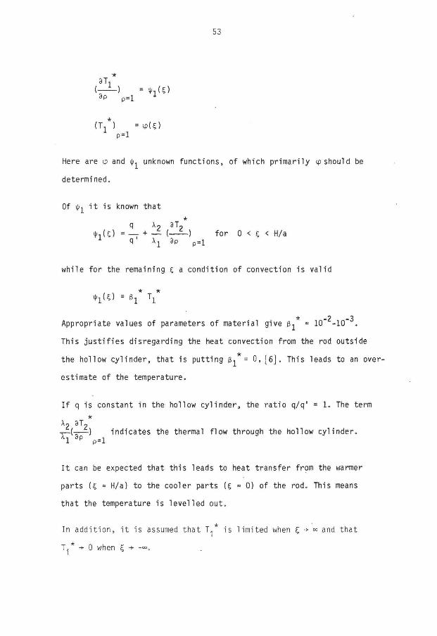
3P p=l 1
( T * ) = cp(5)
P=l
Here are cp and unknown funct ions, of which pr imari ly cp should be
determined.
Of i t is known that *
q X ? 3T?
<M5) = —r + — (——) for 0 < c < H/a 1 q Xx 3p p = 1
while for the remaining E. a condition of convection is val id
h U ) - B,* V
* -2 -3
Appropriate values of parameters of material give • 10" -10" .
This j u s t i f i e s disregarding the heat convection from the rod outside
the hollow cy l inder , that is putt ing = 0 , [ 6 ] . This leads to an over
estimate of the temperature.
I f q is constant in the hollow cy l inder , the ra t io q/q' = 1. The term *
X2 3To •Y—(-—) indicates the thermal flow through the hollow cyl inder. Xl 3 p p=l
I t can be expected that th is leads to heat transfer from the warmer
parts (5 » H/a) to the cooler parts U « 0) of the rod. This means
that the temperature is level led out.
In add i t ion , i t is assumed that T^* is l imi ted when £ •* °° and that
T * •+ 0 when g •*

54
The rod is assumed to be very long, which makes i t possible to disregard
3 2 T I *
the term — when compared with the remaining terms. I t appears that
is 0(e) and that the disregard of the second derivat ive leads to the
error 0 ( e ) . This is shown in [ 7 ] . Af ter th is s impl i f i ca t ion the heat
conduction equation can be wr i t ten o * * *
3 £T, 1 3T, 3T, E ( — J _ + - — L . ) _ _ _ L = Q
3p* P 3p 35
This equation is parabolic, and the variable 5 corresponds to the
"time var iab le" .
The boundary conditions become *
(—1-) = 0 for a l l 5 3P p=0
3T i
=i
( — l - ) = s 3P p=l
T X ( 5 , D =<P(e)
T x ( 5 , P ) = 0
* , J1 ( e . p l
0 < ? < H/a
C < 0 or 5 > H/a
unknown function
when 5 * -°°
1 i mi ted when 5 -H»
Since the boundary conditions of the parabolic equation are zero for
5 < 0 th is leads to Tj (<j,p) = 0 for a l l 5 < 0. Thus one can put
T ^ t O . p ) = 0 for 0 < p < 1.

55
Since the s impl i f ied equation is parabolic with % " t imel ike" no
boundary conditions on T. (H/a,p) are needed. The function ip(£)
and ^ ( O must be determined from the conditions in the hollow
cy l i nder.
b) The hollow cyl inder
With dimensionless quanti t ies and a steady state condition the equa
t ion (5.5) is wr i t ten
1 * 1 * * 3 T ? 3 To 1 3 T-,
+ — ± - + — = Q 2 2
35 3P P 3p
with the boundary conditions along the contact surfaces
T 2 (5,1) = Tj (5,1) = <P(e)
* 3 T,
-) 3P P = i
The surfaces facing out to the free a i r give a condit ion of convection
3 To X 2 T T = - ß 2 T 2 "
where n is the outward-looking normal of surfaces of the hollow c y l
inder. In dimensionless form th is w i l l be
* 3T 2 3 2" a * * *
To ~ - 3 o To 3n* X 2 '2 " ~ P 2 '2
Appropriate values of ß'2 are 5-10 W/m2K, A 2 = 70 W/mK, a = 0,04 m i . e .
0,003 < e 2 * < 0,006.

56
it -k "kO
By expanding L, = u Q + g 0 u^ + (ß 2 ) u 2 + . . . , according to the per
turbation method, we get the equations
* 3 T 2 3 u 0 * 3 u l * * — - = — + g 2 _ _ + . . . - - B ( u 0 + B u + . . . ) 3n 3n 3n
* 3 U 0 that i s , equating powers of ß 2 gives — ^ = 0, 3u, 3n — y = - U Q and so on. 3n
From the d i f f e ren t i a l equation follows that
3 U 0
2 3 2 U 0 j 3U Q
g— + 2~ u ' 3? 3p p 3p
I t is noted that UQ sa t is f ies the condition
ß 2 * • T 2 * with ß 2 * = 0 3T 2*
Owing to th is fac t , the convection from the hollow cyl inder to the a i r
i s disregarded. This causes a small overestimation of the temperature
To*. In the hollow cyl inder heat w i l l be transferred from the warmer
(5 = H/a) to the cooler part of the rod (5 = 0 ) . The thicker the wall
m of the hollow cyl inder the greater the amount of heat t ransferred.
Thus the maximum temperature of the rod increases when the thickness
of the hollow cyl inder decreases. Furthermore, a th in hollow cyl inder
exposes a smaller area to the a i r where heat can be abducted. However,
th is ef fect is disregarded by putt ing ß 2 * = 0.
The heat conduction in the rod and the hollow cyl inder can now be sum
marized by the fol lowing equations

57
3 2 T,* , 3T * 3T,* O < 5 < H/a e( — + - — — ) - = 0 , 0 < p < l
3p p 3p 3C
T^ fO.p) = O , O < p < 1
T 1 * ( 5 , l ) = ipU) 0 < 5 < H/a
3T * X
(——) = 1 + — • i M 5 ) , 0 < i < H/a 3P p=l Xj <=
3 2 T ? * 3 2 T ? * , 3T * O < 5 < H/a — + —f~ + - — 1 - = O , 1 < p < b/a 35 3p p 3p
T 2 * ( 5 . D = «P(5) O < i < H/a
3 T * ( ) = y ( ? ) s O < 5 < H/a 3p p=l f
3T 2* = O , n* is the outward-looking
3n normal in dimensionless form
These coupled d i f f e ren t i a l equations have been solved by f i n i t e d i f
ference approximations. [7]
Figure 5.4.1 shows isotherms from the solution of the case of a hollow
cyl inder with dimensionless radius r/a = 1 and dimensionless length
H/a = 3. The wall thickness of the hollow cyl inder is 1. There are 20
steps in the radial d i rect ion and 30 steps in the axial d i rec t ion . The
speed is 0.01 m/s, which corresponds to e = 0.018.
Figure 5.4.2 shows the same s i tuat ion except that the wall thickness
is 0.3. The radial and axial steps are the same as in the previous
f igure .

Figure 5 .4 .1 . Isotherms.

d i r e c t i o n of motion of the rod
Figure 5.4.2. Isotherms.

60
The temperature of the contact surfaces T j * ( l , g ) = T 2 * ( l , 5 ) = <p(e) at
d i f f e ren t wall thicknesses is i l l u s t r a t e d by f igure 5.4.3, where
H/a = 3 and e = 1.8-10~ 2.
0.40 . . . .
<P<€)
0.30
wall thickness: 1
0. 01 O.O 0.4 0 . 8 1 .2 1.6 2 . 0 2.4 2 . 8 3.0
Figure 5.4.3. The temperature of the contact surfaces i p ( £ ) as a
function of the wall thickness of the hollow cy l inder .
This shows that the most unfavourable case is a hollow cyl inder with
wall thickness 0 and no heat t ransfer along the rod. This s imp l i f i ca t ion
leads to the fol lowing condition on T. 1
32T L + ± I V ,
3T 1
3p' P 3p 35

61
and the boundary conditions
T^ fO.p) = 0 0 < p < 1
8 T * ( — - ) = 0 a l l e
3P p=0
3 T * ( ^ - ) = 1 0 < £ < H/a
d p p=l
This d i f f e ren t i a l equation can be solved exactly with the method of
separation of var iables, [ 7 ] . This gives
i " e _ J k £ S ° , J o ( j k p )
4 k=l j k - J 0 ( j k )
where Jq is the Bessel function of the f i r s t kind of order zero and
j k is the " k : t h " posit ive zero of the Bessel function J , . This gives
j 1 « 3.8, j 2 « . . .
In par t icu lar the boundary temperature sought for w i l l be
. 2 e k
cp(S) = T,*(£ ,1) = - + 2££ - 2 Z =— 4 w J k 2
As can be seen, the solution depends onl-y on the variable z = e£.
Thus, th is gives thatcpU) = G(e5) which is defined as
2.
1 °° e •Jk z
G(z) = 4 + 2z - 2 Z 5— for z > 0 4 k=l j 2
k
This function is shown in f igure 5.4.4.

G(z)
0.60
0.50
0.40
0.30
0.20
0.10
O. Ol 0.0 0-04 0.08 0.12 0.16
Figure 5.4.4. The temperature of the contact surfaces G(z). Exact so lu t ion.

63
5.5 Experimental investigations
5.5.1 Jßst_serie_s
The test object was represented by the nut No. 4 mentioned in chapter
4.2.1 (a = 0.04, b = 0.045, H = 0.12). The nut was equipped with 11
pc. thermo-couples mounted as described in chapter 3.2.
Besides the 11 thermocouples, temperature measuring probes (No. 12 and
14) were mounted outside the end surfaces of the nut. The probes,
touching the surfaces of the thread f lanks, were connected to the nut,
thus fol lowing the up- and downward movement of the nut with simulta
neous s l id ing on the thread flanks of the screw. This arrangement made
i t possible to measure the temperature of the screw at the entrance
and the e x i t .
The experiments were carr ied out with simultaneous recording of tem
peratures, axial load, torque and rotat ional speed.
The results reported here have been obtained with the axial force and
the axial motion ei ther in the opposite or in the same d i rec t ion .
Table 5.1 l i s t s the test series performed.
Table 5.1
v [m/s] u [m/s] p [MPa] v/p [m/(s.MPa)l
0.118 0.005 1.826 0.065
0.236 0.010 " - 0.129
0.353 0.015 " - 0.194
0.471 0.020 " - 0.258

64
5.5.2 £r£ces sing_o_f test results
The measuring equipment was very sensit ive to noise caused by the fact
that the signals from the thermocouples were approximately 40 yV/K.
Since no ampl i f iers of the "thermosignals" were used both analogous and
d ig i t a l f i l t e r s were introduced.
The analogous f i l t e r removed noise of frequencies higher than 160 Hz.
The remaining noise was assumed to have a normal d is t r ibu t ion and the
standard deviation was l imi ted by the d ig i ta l f i l t e r . The d ig i ta l
f i l t e r was of recursive type. In th is way, i t was possible to improve
the accuracy compared with the resolution of the A/D-transducer, which
was 50 uV/bi t = 1.22°C/bit. The improvement was achieved by calculat
ing the mean of the input s ignal , i . e . the temperature and the noise
s igna l . This was done according to the fol lowing formula
y n = ax n + ( l - a ) y n _ 1
where y n is the input value to the computer
a the f i l t e r constant (a < 1)
x n the AD-transduced signal
y i the preceding input value
The test results were processed in two steps. The f i r s t step involved
scrutiny of the primary results as a whole. I t was hereby observed
that the temperatures were stable during the las t t h i rd of every tes t ,
and i t was judged that approximate steady state conditions prevailed
during th is period. See f igure 5 .5 .1 .

65
i.38
-10.°3 -3.54 -14.44
-!0.?3 -14.54
-!0.9S -12.2 -».74
4 : 7 423
433 434 435 43a 43r
433 43= 44? 441 4 4 : 4 4 : 44' 445 4 4 : 4 4 ? 44= 449 450 451 4 : : 453 454
-6.1 -S.54 - 7 . 3 : - 7 . 3 : -4.88 - 7 . ~i -8.54 -7.32 -10.9B -4.88 -8.54 -14.44 -15.84 -15.84 -13.42 -13.42 -15.94
-12.2 -10.93 -10.93 -12.2 -15.84 -10.93" -13.4: -13.42 -9.74 -9.74 -12.2 -12.2 -12.: -8.54 -13.42 -14.44 -13.42 -12.2 -12.2 -13.42 -10.98 -12.2 -14.64 -19.52 -20.74 -15.86 -18.3 -17.08 -19.52 -20.74
-8.54 -9.74 -10.98
-14.44 -7.32 -14.44 -10.93 -12.2 -15.34 -17.08 -12.2
-a . l -10.98
-14.44 -14.44 -14.44, -13.42 -14.64 -15.86 -13.42 -17.08 -10.98 -13.42 -8.54 -13.42 -14.64 -14.64 -15.86 -10.93 -15.36 -19.52 -19.52 -21.96 -19.52 -1S.3 -17.08 - t o 52
-9.74 -10.98
-10.98 -10.93 -9.76 -8.54 -13.42 -7.32 -8.54 -10.98 -14.64 -7.32 -9.76 -10.98 -14.64
-14.44 -15.36 -15.86 -14.64 -13.42 -13.42 -10.98 -12.2 -12.2 -15.86 -15.86 -14.64 • -17.08 -14.64 -14.64 -12.2 -14.64 -14.64 -19.52 -15.84 -13.42 -15.86 -18.3 -20.74 20.74
-1.22 -2.44 -4.33 -3.66 -4.88 -6.1 -6.1 -7.32 -a. l -9.74 -7.32 -9.76 -9.74 -9.74 -10.98 -13.42 -12.2 -13.42 -12.2 -13.42 -14.64 -14.64 -15.96 -12.2 -13.42 -12.2 -12.2 -13.42 -14.44 -15.84 -14.54 -14.44 -18.3 -18.3 -1B.3 -17.08 -15.86 -14.64 -19.52
-1.33 -2.44
- 2 .44
:,: -4.23 -3.it 5 ; -2"?.2S ) 3.is -2, -2.44 9.54' -30-5 0 4.83 -2.44 -2.44 i . : -30.5 . i* 6.1 -4.39 -4.35 6.1 "A i : . iä -2.44 -3.66 3.66 -30.5 3 0 -2.44 -3. 66 2.44 -30.5 0 •..22 -2.44 -3.66 o -30.5 0 3.66 -1.22 -3.66 -31.72 A
1.22 -2.44 -3.66 i V) -30.5 0 0 9 -3.66 -2.44 -30.5 0
-4.38 -2.44 -8.54 -6.1 -6.1 -7.32 -10.98 -7.32 -7.32 -6.1 -10.98
-8.54 -6.1 -9.76 -9.76 -10.98 -13.42 -12.2 -13.42 -14.64 -13.42 -12.2 -14.64 -12.2 -13.42 -10.93 -12.2 -12.2 -17.08 -12.2 -13.42 -13.42 -12.2 -15.86
18.3
-3.66 -3.66 -4.38 -7.32 -3.66 -4.88 -7.32
-9.76 -10.98 -8.54 -8.54 -7.32 -7.32 -8.54 -9.76 -9.76 -4.88 -8.54 -3.54 -8.54 -9.76 -7.32 -7.32 -8.54 -10.98 -12.2 -12.2 -12.2 -10.98
13.4:
-3.66 -2.44 -3.66 -4.33 -7.32 -4.33 -4.98 -4.88 -6.1 -4.88 -4.1 -4.83 -4.1 -7.32 -3.64 -7.32 -4.83 -8.54 -9.54 -7.32 -7.32 -8.54 -3.66 -7.32 -8.54 -7.32 -4.88 -10.98 -12.2 -12.2 -7.32 -8.54 -12.2 •14.64
-1.22 2.44
-4.33
-4.93 -7.32 -3.66 -6.1 - o . i -9.76
-8.54
-4.99 -6.1 -6.1 -8.54 -7.32 0
-4.83 -6.1 -4.1 - i . ! -7.32 -7.32 -7.32 -4.1 -7.32 -12.2 -12.2 -12.2 -12.2 -12.2 -12.2 -14.64
' -2.4* -7.32 -4.99 -6.1 -4.1 -8.54 -4.88 -2.44 -1.22 -4.89 -4.98 -2.44 0
-4.83 -3.66 -3.44 -7.32 -4.88 -8.54 -8.54 -7.32 -3.64 -7.32 -7.32 -7.32 -8.54 -8.54 -a. 54 -12.2 -12.2 -12.2 -9.76 -4.88 -8.54
-4.33 -7.32 -7.32 -7.32 -6.1 -9.76 -4.33 -7.32
-9.74 -8.54 -9.74 -7.32 -7.32 -8.54 -7.32 -7.32 -8.54 -8.54 -7.3: -7.32 -7.32 -7.32 -7.32 -7.32 -8.54 -9.76 -12.2 -13.42 -13.42 -12.2 -10.93
-30.5 -31.72 -26.84 -29.29 -29.28 -28.06 -25.62 -29.23 -28.44 -28.04 -25.42 -26.84 -26.34 -28.06 -28.06 -29.28 -29.23 -28.04 -29.23 -29.56 -28.04 -29.23 -30.5 -29.23 -30.5 -30.5 -30.5 -31.72 -31.72 -28.06 -29.29 -29,28 -30.5 -31.72 -30.5 -29.58
i m -13,42 -21.94 -15.86 -21.96 -17.08 -19.52 -15.85 -14.64 -10.99 -12.2 -10.98 -29.23 0 45a -15.86 -15.84 -19.3 -19.52 -18.3 -1B.3 -15.86 -12.2 - i ? , : -10.99 -12.2 -30.5 0 457 -14,64 -17.08 -19.52 -17.08 -17.08 -17.08 -14.64 -12 i -12.2 -10.99 -13.42 -31.72 0 458 -13.3 -18.3 -23.18 -21.94 -18.3 -19.52 -17.09 -15.96 -13.42 -13.42 -13.42 -29.28 0 459 -17.08 - IB. 3 -23.18 -17.08 -18.3 -17.03 -13.42 -13.42 -12.2 -10.99 -13.42 -31.72 0
* 7 460 -13.3 -19.52 -21.96 -19.52 -18.3 -18.3 -14.64 -13.42 -9.76 -12.2 -13.42 -31.72 0
W 441 -13.42 -21.96 -19.52 -19.52 -15.86 -17.08/ -9.76 -13.42 -9.54 -10.98 -14.64 -32.94 0
- 4=2 -15.36 -25.42 -21.94 -19.5: -18.3 -13.4j) «12.2 -9.76 -10.98 -9.75 -15.86 -32.94 0 442 -19.52 -29.28 -24.84 -19.52 -21.96 -14-/I -17.08 -12.2 -15.86 -13.42 -19.52 -29.28 0
< 454 -23.18 -23.19 -24.94 -20.74 -20.74- -15.36 -13.42 -14.44 -13.42 -19.52 -30.5 8 465 -25.62 -25.62 -25.62 -17.09 cl8-3 V 'WS.86 -14.64 -14.64 -12.2 -12.2 -17.03 -31.72 0
w -24.4 -25.62 -19.52 -19.3 -14.64 -12.2 -13.42 -12.2 -9.76 -17.03 -32.94 0
r\« -25.62 -26.84 -23.19 -19.3 -JfB.3 -13.42 -13.42 -13.42 -10.98 -?.76< -15.94 -32.94 0
,<> 468 -23.13 -25.62 -21.96 -20. TA ̂ 14.64 -14.64 -12.2 -9.76 -12.2 -4.99 -17.09 -32.94 0 s 469 -21.94 -25.62 -23.19 -20.7tf -17.08 -14.54 -12.2 -10.99 -9.75 -9.54 -17.09 -32.94 0
472 -19.52 -26.84 -24.4 -20^74 -17.08 -15.36 -13.42 -12.2 -10.93 -9.54 -18.3 -32.94 0
*J 47! -19.52 -25.42 -21.96 -21.96 -15.84 -15.86 -13.42 -9.76 -12.2 -6.1 -18.3 -32.94 0 472 -21.94 -21.96 -23.19 -23.13 -17.08 -IB.3 -12.2 -12.2 -12.2 -9.54 -17.09 -32.94 0 4"7 -21.9a -24.4 -19.52 -23.19 -18.3 -13.42 -13.42 -12,2 -12.2 -9.76 -15.84 -32.94 0 474 -28.04 -2! . 94 -24.4 -25.62 -17.03 -17.08 -13.42 -14.44 -14.64 -12.2 -19.52 -30.5 0 475 -30.5 -23.19 -28.06 -25.62 -19.52 -19.52 -13.42 -14.64, -15.85 -13.42 -20.74 -29.23 « 4"; -29.23 -20.74 -28.06 -24.4 -17.08 -19.52 -14.54 -10.98 -15.86 -13.42 -20.74 _ao -o Ck-i
- " - O t -23.06 -25.42 -29.23 -25.62 -20.74 -21.96 -13.42 -14.44 -17.09 -14.54 -2! .96 - :8 .06 j j0
-! 5^2 -25.62 -24.4 -23.19 -!?.£: -ta M -13.42 -13.42 -14.64 -12.2 -19.32 -30.5 WO 479 -19,52 -:5.42 -24.4 -24.4 -19.52 -13.3 -13.42 -13.42 -13.42 -7.32 -17.09 -31. "'2 I 0 45« -20.74 -21.96 -25.62 -23.18 -19.5: -13.: -13.42 -9.76 -12.2 -8.54 -17.03 -31.72 U
-21.94 -20.74 -24.4 -20.74 - I T i>g -13.42 -3.54 -12.2 • -ig oa -17.03 -3!.?:Tv
.0! -fik !S,A
133,:64 23.13 133.433 21.94 156.312 19.52 135.27 19.52 126.536 18.3 119.905 13.3 117.902 19.3: 120.0-3 19.5: 114.3aa 19.52 M.'> « 4 13.7
104.375 21.95 104.542 19.52 '4.649 21.96 92.352 19.52
!6.713 19.52 .4.396 19.52
120."08 20.74 O 124.246 18.3 U 124.243 13.3
101.202 13.3 ?52 .959 18.3
•H 37.34: 20.74 N 102.705 20.74
•H 103.54 20.74 " j 104.203 20.74 'X) U1.222 19.52 [fl 113.73? 19.52
121.409 20.74 118.57 19.52
0) Ul U D
4-1 M
132.431 25.42 133.433 24.4 99.532 21.94 109.719 20.74 111.554 13.3 114.395 19.52 109.552 19.52 133.934 20.74 143.119 20.74 128.924 19.52 122.912 18.3 114.232 19.3 115.544 17.09 78.154 17.08 94.021 24.4
M 103.049 21.96 (U 116.566 19.52 C 117.563 24.4 "fj 121.576 21.96
132.097 25.s2 ^ i?n ? T ig I, 125.75! 21.96
—.121,9! 19.52 VD J13.23 21.9a ° 113.727 20.74 I 111.556 21.94
t - 113.393 19.52 CO 116.232 18.3 2. "7-558 13.3 ^ !17.553 J9.52
o\° 119.238 19.52 C 112.057 23.13
122.077 23.13 •J23 .245 20.74
TPS.745 19.52 41.516 2.44
LO ,,0
_ 1 J
Figure 5 .5 .1 . Example of primary resu l ts .

66
The second step involved analysis of the steady state part . The test
resul ts were computer-processed. The analysis comprised computation of
differences between the measured temperatures of the nut and the screw
entrance.
The power loss was calculated using the formula
Q = f b - < 2 * M - F a x - S >
The mean values of the temperature di f ferences, AT, and the power loss
were computed af ter which a dimensionless temperature, T*, was calcu
lated according to the formula
T* . £ 1 . i = 2TTHA • * I (5.6) q a Q
Presented results have been computed taking the conductivity of steel
t 0 b e * = 2 5 m •
The measured temperature on the thread flank cannot be d i rec t l y com
pared with the boundary temperature of the mathematical model. The
temperature differences have been adjusted as fol lows. See f igure 5.5.2.
Figure 5.5.2. Heat conduction through the thread p ro f i l e .
67
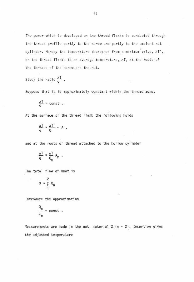
The power which is developed on the thread flanks is conducted through
the thread p ro f i l e part ly to the screw and part ly to the ambient nut
cy l inder . Hereby the temperature decreases from a maximum value, AT',
on the thread flanks to an average temperature, AT, at the roots of
the threads of the screw and the nut.
Study the ra t io — . q
Suppose that i t is approximately constant within the thread zone,
= const .
At the surface of the thread flank the fol lowing holds
* i = * r . A , q Q
and at the roots of thread attached to the hollow cyl inder
— = — A .
The to ta l flow of heat is
Q = I Qn
Introduce the approximation
x. n
— = const . n
Measurements are made in the nut, material 2 (n = 2) . Insertion gives
the adjusted temperature
68
A T = A T ' —— T — 7 7 — t (5.7)
Numerically for Tr 80x10
A = 0,01208 X1 = 25
A,,, = 0,03016 X 2 = 70
This gives
AT = 0,295 AT' .
5.5.3 Re^uUs
As explained in chapter 5.4 the temperature is presented as a function
of the independent dimensionless variable z, which is defined as
z = £ • I (5.8)
where
E = [ i - ] . . J - and 5 = 4 (5.9) L c p J l au a
In Appendix T16-T23 the experimental results are expressed in the
quant i t ies described here. Thermocouples nos 12 and 14 refer to the
temperature probes outside the end surfaces of the nut.
The results are also shown in diagrams, figures 5.5.3 and 5.5.4. Here
the sol id curve is the temperature d is t r ibu t ion along the contact sur
face according to the theoret ical model for the case of an insulated
hollow cyl inder and constant power d i s t r i bu t i on .

Figure 5.5.3. Experimentally determined temperatures and theoret ical temperature d i s t r i b u t i o n ,
isolated hollow cyl inder. Case: opposite d i rect ion of axial force and motion.

70
/

71
5.6 "Discussion and conclusions
The experimental results show that in the f i r s t loading case of axial
force and axial motion in the opposite d i rec t ion , the temperature
d i s t r i bu t ion agrees well with the theoret ical model with constant
power d i s t r i bu t i on .
The considerable decrease in temperature at the t r a i l i n g edge can be
explained by the fact that the test object is provided with a turned
c o l l a r , which acts as a cooling flange. A certain cooling should be
noticed at the t r a i l i n g edge even without a cooling f lange, for which
reason the temperature according to the mathematical model is over
estimated in th is region.
The mathematical treatment shows that a hollow cyl inder with a th in
wall tends to be more heat insulat ing than a cyl inder with thick wa l l .
This means that the heat flow is smaller in the thin-walled cyl inder,
which results in a higher temperature. Thus, an i n f i n i t e l y th in c y l i n
der wall should mean that a l l heat generated is conducted to the
screw.
The explanation of th is somewhat unexpected phenomenon is that the
material of the nut acts as a coolant. From t h i s , one can also con
clude that a th in nut is c lear ly more unfavourable than a thick walled
one from the temperature point of view. The "worst" case is then an
i n f i n i t e l y th in cyl inder w a l l , corresponding to a t o t a l l y insulated
nut without i n te r i o r heat f low.
Furthermore, i t is clear from the experimental results that i f the
wall of the hollow cyl inder is thinner than 0.12'a wi th in the range of

72
speed investigated here, the development is approximately the same as
in the insulated nut.
From an engineering point of view i t can be concluded, among other
th ings, that the designing case should be an insulated or a th in nut
because the greatest increase in temperature occurs in th is case.
Concerning the results from the second loading case of axial force and
motion in the same d i rec t ion , u = 0.005 and 0.01 m/s, appendix, tables
T20 and T21, the untreated primary results showed unreasonably low
temperatures of negative values at the entering edge. A probable ex
planation of th is is a systematic error when the reference temperature
was recorded. When processed, these measurements were corrected by an
estimated correction of such magnitude that the f i r s t measurement coin
cided with the theoretical curve. As can be seen in f igure 5.5.4, the
tendency of the two corrected test series is in total agreement with
the other resu l ts .
In the second loading case of axial force and motion in the same
d i rec t i on , the experimental results show the same tendency as in the
f i r s t loading case with in a range extending from the entering edge to
about 41% of the to ta l length of the nut. After th is the temperature
drops. This indicates that development of power has ceased in the
l a t t e r part of the nut, which in turn implies that the remainint 59%
does not convey any axial load. Here the mathematical model gives a
clear overestimate of the temperature.
One more conclusion can be drawn from the experimental resu l ts . The
temperature d is t r ibu t ion along the thread can be said to be an indica
t ion of the pressure d i s t r i bu t i on . One condition of the theoret ical

73
model is constant power d is t r ibu t ion along the tota l surface of con
tact between the rod and the hollow cyl inder. S'ince good agreement
prevai ls concerning the experimental resu l ts , th is shows that the
pressure d is t r ibu t ion is constant in the parts of the thread flanks
the screw and nut that are in contact.

74
6. DESIGN OF SCREW-NUT TRANSMISSIONS
This chapter provides a summary of the conclusions and results re
ported in the preceding chapters. This has been done in such a way as
to make i t possible to apply the results as dimensioning c r i t e r i a t o
gether with other points of view.
The chapter concludes with three sample problems.
6.1 Cr i te r ia
6.1.1 Dimensjoni_ng_r^gardi_ng_capabfl_jty of performance
From a dimensioning point of view, the maximal developed temperature
in the screw-nut transmission is of par t icu lar i n te res t .
The experimental invest igat ion shows that the increase of temperature
never exceeds the analyt ical AT-value at the t r a i l i n g edge of the nut.
This leads to the fol lowing dimensioning c r i t e r i o n :
Dimensioning power is the power which corresponds to maximum tempera
ture wi th in the region of the hollow cyl inder according to the mathe
matical model.
With given conditions and the dimensionless parameters T* = 2TTHX
X H and z x _ H = — • —=-, a "running point " , i . e . a point representing the
pc ua
running condit ions, is graphically derived by forming the intersect ion
of re la t ion T*-z and the curve of the d is t r ibu t ion of the temperature
according to the mathematical model, f igure 5.4.4. At higher speeds,
the running point often l i es in the interval z < 0,02. Thus, f igure

75
6.1.1 shows the temperature of the contact surface in th is i n te rva l ,
which f a c i l i t a t e s a more accurate determination of the current running
po in t .
6.1.2 Dime£sjojri £g_r£gar£i £JLO£t1mal_fin£tJL°Jl
I f possible, optimal running conditions should be pursued. This means
that the parameter S should be chosen in the range S o p t = 0.026-0.042,
according to table 4.4. From the de f in i t i on S = ^ - ~ , the required
re la t ion v = S — p is obtained. n
6.1.3 £imejisJ^ojnijig_rega_rd_i rig_d£ve_l£pme_nt_o_f £Owe_r
I f fur ther choices are possible, the least possible power loss is pur*
sued. The approximate power loss is obtained by the equation
Q = " Fax v
The coe f f i c ien t of f r i c t i o n is calculated according to equations (4.13)
and (4.17)
u = - ( 1 - S * 1 / 3 ) 2 + S * 2 / 3 • S 0 when 0 < S* < 1
u = _2. (2S*+1) when S* > 1 3
The values of the empirical constants are chosen according to table
4 .6 ,
S n = 0.10, I = 0.23 . 0 B

76

77
6.1.4 £ur;ther £oj j i ts_of view_of dimensioning
When dimensioning the wall thickness of the nut, one must consider the
fact that increasing thickness is favourable in view of capabi l i ty of
performance because the temperature is kept at a lower l eve l . This is
clear from chapter 5. The function is not otherwise af fected. Thus,
other requirements of design can be introduced here.
High speed should be pursued for two reasons.
The f i r s t reason is the fact that screw-nut transmissions generally
run at various speeds. This means deviation from the optimal running
range, which is re la t i ve ly narrow.
In th is connection, i t is desirable that the actual value of the par
ameter S should be, as much as possible, on "the r igh t side" of S o p t
i . e . S > S j . . This leads to considerably smaller var ia t ion in the
coe f f i c ien t of f r i c t i o n than is the case of small values of S where
S < S t . See f igure 4.1.2.
The second reason is connected with increasing axial speed, u, and the
simultaneously increasing supply of power. Owing to the increasing
speed, a cooling e f fec t also asserts i t s e l f . This cooling e f fec t
counteracts the increase in temperature, so that the temperature i n
creases at a slower rate, which is not proportional to the speed. This ,
i s also clear from the fol lowing dimensional consideration.
Heat conduction from the surface of contact (5.3)
q = x l * 3r

78
Suppose that the time t elapses when the rod traverses one length of
hollow cyl inder with the speed u. During th is time the temperature
increases AT.
Figure 6.1.2. Temperature gradients in the rod and the hollow
cy l inder .
The heatconduction equation can then be wr i t ten
_ _ , AT . , AT q = X, • + X 0 1 A r j 2 Ar 2
Here Ar is a length character is t ic of each mater ia l . This length can
be wr i t ten
Ar = const • / — PC
Insert ion gives

79
tT q = const • AT • — (/ X-ipiC.' + / x 0 p,c 0 ' ) = const • —
/ ? 1 1 1 2 2 2 / T
Furthermore,
u
Insert ing th is in the expression of q gives
q = const ' A T • /tT
With
q = const • v = const • u
one f i n a l l y obtains
A T = const • /Ti1 .
Generally speaking, the above mentioned c r i t e r i a of dimensioning can
not usually be simultaneously satisf ied-.
Whatever the actual combination of permitted temperature of lubr ican t ,
axial load, axial speed and further demands may be, the demand of
capabi l i ty of performance must always be sa t i s f i ed . Thereafter one or
more of the other c r i t e r i a can determine the dimensions of the screw-
nut transmission. Whether any of the other c r i t e r i a are used to deter
mine dimensioning is decided from case to case in connection with the
work of ca lcu la t ion .

80
6.2 Numerical examples
Example 1
5 A screw-nut transmission is to convey an axial load of F = v =10 N with a X
a minimum speed of u > 0.05 m/s. The running temperature of the l u b r i
cant is maximized to 200°C. The v iscosi ty of the lubr icant is n = 0.16
Ns/m 2. The running temperature of entering screw is assumed to be 40°C.
The depth of p ro f i l e of the thread flanks hg = 1 pm. The material
chosen for the screw is steel and for the nut bronze. The fol lowing
data are va l id for steel p = 7850 kg/m 3 , c = 450 Ws/(kg-K), A =
25 W/(m-K) and for bronze A = 70 W/(m-K).
Choose a suitable trapezoidal screw thread (Tr dxs) in which the ra t io
of length of nut and diameter of thread should not exceed H/d < 2.-
Optimal function
According to table 4.5 S Q p t = 0.032
de f i n i t i on S = • (-̂ )
This gives ( | ) = 0.032 • - J ^ -p opt
and v = p • 0.2 • 10~6 .
Equation (4.20) ^nrin = l \
and table 4.6 ( S Q ) m v = 0.10, (1 /B) f f l V = 0.23
give u • = 0.070 a pmm
and p = , A R i 2irab j

81
Capabil i ty of performance
According to the equations (5 .6 ) , (5.8) and (5.9) the dimensionless
parameters are
T* = 2TTX1 • H ^
,X, _ H _ Z x = H - V J1 ' u a 2 •
The power loss
Q = ^ F a x v
The re la t ion between tangential and axial speed
2ira v = u —
Correction of the temperature of the f lank according to (5.7)
where AT' = 200°-40° = 160°
and A = 2ua • H m
Eliminating the speed and the height of the nut and insert ing the
temperature give
P 1 C 1 AT' - 2 H p ( y v p F A X
This expression corresponds to a s t ra ight l ine in the T*-z diagram.
The intersect ion of th is l ine and the theoret ical temperature curve
according to f igure 6.2.1 and 6.2.2 gives one "running point" for every
trapezoidal thread in question.
82
Numerical ly
T* = 59.5 • 10 3 • ba • z x = H
Required height of nut and speed at optimal function
This is obtained numerically with
= f-Ll JL
V H - v r u a 2 and insert ion of optimal speed
H = — — • 53.2 ZT 2 i r / T
Insert ing the z-value of the "running point" gives the required height of
the nut of the trapezoidal thread in question.
Then, the easiest way of solving for the speed, is by the formula of
Z
X=H which gives
X . H . , \ H 1 u = —- • — -n and v = 2TT — • — • -pc , ,2 pc as z za
Numerically
u = 7.077 • 10" 6 • -Äy and v = 0.0445 • 10" 3 • — za^ z a s
83

84

85
86
Example 2
Calculate the greatest axial load, F, , which a given screw-nut-ax
transmission can transfer at optimal operation.
The transmission has the fol lowing data. Tr 60x9, depth of p ro f i l e
hg = 2 pm, height of nut H = 0.1 m. The material of the screw is
steel and the nut is bronze. The temperature of operation is 40°C. 2
The lubr icant has a viscosi ty of n = 0.32 Ns/m , and the highest
permitted temperature is 200°C. The v iscosi ty is assumed independent
of temperature.
Solution
Def in i t ion of the Sommerfeldt number
c _ n. v_
Fax H where the average pressure p = —^- and A = Trdmb • — . This gives the
optimal speed
v opt = S opt n A '
According to equation (5.8) and (5.9)
H 2
ua
where u = v s ird.
ru
According to equation (5.6)
T* = 2trH
The power loss can be wr i t ten approximately
87
Q f» y . F v Mm.n ax
The coe f f i c ien t of f r i c t i o n is obtained from equation (4.20)
'min '0
This expression of u is v a l i d , according to equation (4 .19) , when
S
s - s - 0
o p t ( 1 + B S 0 )J
Insert ion gives X TTHCI A
p c ' 1 7 I h ^ ' S opt F ax
and
T * 9 . H A n A T T * = 2rrX. • r - • T ' —-7 1 h n U m , - i> + r- ^ 0 mm opt F ax
Eliminating F and insert ing give ax
T - 4 . ( £ J ) . ^ . - ^ L _ . z 2 .
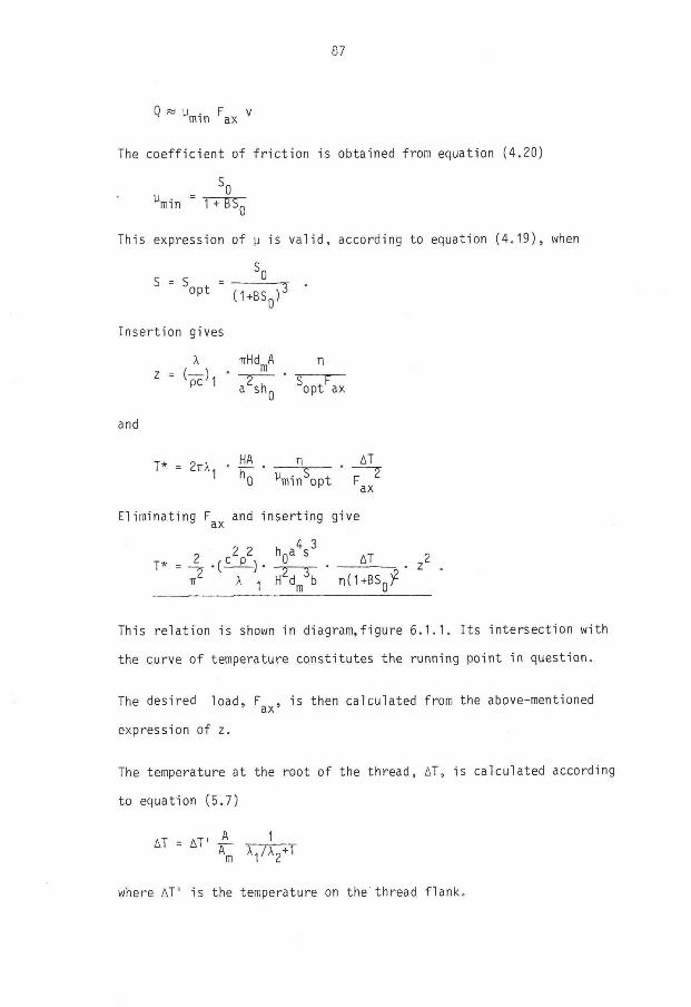
This re la t ion is shown in diagram,figure 6 .1 .1 . I t s intersect ion with
the curve of temperature constitutes the running point in question.
The desired load, F , is then calculated from the above-mentioned ax
expression of z.
The temperature at the root of the thread, AT, is calculated according
to equation (5.7)
AT = AT' A M X 1 / V 1
where AT' is the temperature on the thread f lank.

88
Numerical l y
According to Appendix, table T I ,
s tee l : X- = 25 ~ , c, = 450 ^ , p = 7850 kg/m3
b r o n z e : x 2 = 70 ^ .
According to Appendix, table T2, Tr 60x9 has the fol lowing data:
a = 0.03, s = 0.009, b = 0.004, d = 0.0555. ' m
According to table 4.6
SQ = 0.01 and 1/B = 0.23.
Oo-Hi+^A AT tonn /in. TT-0. 0555-0.004-0.1 1 n o , 0 Permitted AT = (200-40) 0 . 0 6 . 0 . 1 . 0 . Q 0 9 • 2377uTT =
j * _ 2 _ 450 2 .7850 2 ,2 -10" 6 - (0 .03) 4 - (0 .009) 3 . 48.5 . £ 2
IT 2 " 2 5 0. 1 2-(0.0555) 3-0.004 n i n 2 0.32(1+ U - 1 U n
0.23'
T* = 1.287 • 10 3 • z 2
z T*
0.004 0.0206 .006 .0463 .008 .0823 .010 .1287 .012 .185
The running point is obtained graphica l ly , see f igure 6.2.3,
z = 0.0098
T* = 1.17
From the expression of z one obtains

89
F = (—) , ax pcM
Hd 2 i m\
opt
Wi th
opt (1 +
0.10
OJCh 0.23 ;
= 0.034
one f i n a l l y obtains
25 , 0.1-0.0555, 2 0.004 0.32 1 ax " 450-7850 ' { 1 [ 0.03-0.009 ; ' 2 . i ( f 6 " ° - 0 3 4 ° - 0 0 9 8
= 56.7 kN
0.20
G(z) =
Figure 6.2.3. Running point , example 2.
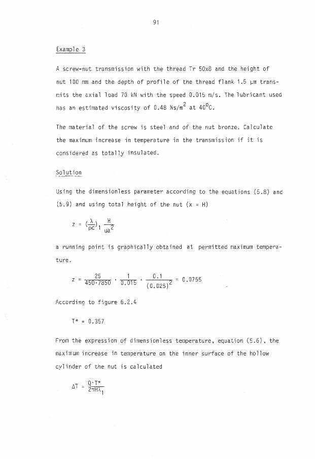
91
Example 3
A screw-nut transmission with the thread Tr 50x8 and the height of
nut 100 mm and the depth of p ro f i l e of the thread flank 1.5 ym trans
mits the axial load 70 kN with the speed 0.015 m/s. The lubr icant used
has an estimated viscosi ty of 0.48 Ns/m2 at 40°C.
The material of the screw is steel and of the nut bronze. Calculate
the maximum increase in temperature in the transmission i f i t is
considered as t o t a l l y insulated.
Using the dimensionless parameter according to the equations (5.8) and
(5.9) and using to ta l height of the nut (x = H )
a running point is graphical ly obtained at permitted maximum tempera
tu re .
According to f igure 5.2.4
T* = 0.357
From the expression of dimensionless temperature, equation ( 5 . 6 ) , the
maximum increase in temperature on the inner surface of the hollow
cyl inder of the nut is calculated
Solution
25 1 0.1 = 0.0755 z = 450-7850 ' 0.015 '
AT = Q-T* 2TTHA

92
On the thread f lank th is increase in temperature corresponds to an
increase in temperature according to equation (5.7)
A X, AT" - A T - f t j l +1)
The temperature of the thread f lank is then given by
T1 = AT' + T runm ng
The power loss is calculated according to the fol lowing
Q s« uF v ax
ud where v = — - u s
Equation (4.13) and (4.17)
1 ( 1 . S * 1 / 3 ) 2
+ S * 2 ' 3 • Sr
(2S +1)
S < 1
* S > 1
* S n v where S = •=— and S = -r— tr and p S0 h 0 P
F s ax •rrd bH m
Table 4.6 gives 1/B = 0.23, SQ = 0.10.
Numerical l y
According to Appendix, table T2, the fol lowing data are val id for
Tr 50x8:
d = 0.046, s = 0.008 and b = 0.0035.
70-10 -0.008 p n-O.046-0.0035-0. = 11.07 • 106 N/m2
v = ^ Q Q g 6 - 0.015 = 0.271 m/s

93
S = ° - 4 \ . ° - 2 7 1 , - 0 . 0 0 7 8
1 . 5 - 1 0 ~ B 1 1 . 0 7 - 1 0 °
S * = ^ 0 7 8 = 0 . 0 7 8 <
u = 0 . 2 3 ( 1 - 0 . 0 7 8 1 / 3 ) 2 + 0 .078 2 7 3 • 0.1 = 0.094
Q = 0 . 0 9 4 • 7 0 • 1 0 3 • 0 . 2 7 1 = 1 . 7 8 • 1 0 3 W
A T = 1 . 7 8 - 1 0 3 - 0 . 3 5 7 = 4 Q > 4 o
2 T T - 0 . 1 - 2 5
A T , . . T T - O . 0 5 - 0 . 1 - 0 . 0 0 8 , 2 5 . „ o
^ = 4 0 - 4 T f - 0 . 0 4 6 - 0 . 0 0 3 5 - 0 . 1 ( 7 Ö + 1 ) = ^ -
I f the running temperature is estimated to be 6 0 ° C , the resul t means
that the maximum temperature of the flank is
T' = 1 3 6 ° + 6 0 ° = 1 9 6 ° C .
This temperature is too high for ordinary lubricants based on mineral
o i l .
I f the load is 7 0 kN, the transmission should be redesigned. Greater
height of nut and diameter of screw could be chosen. This results in
a lower increase in temperature.
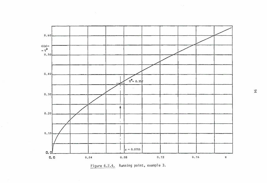
Figure 6.2.4. Running po in t , example 3.

95
REFERENCES
Bowden, F.P., Tabor, D., "The f r i c t i o n and lubr icat ion of
so l ids , part I " , Oxford University Press, 1963, p. 100, 102,
105, 222.
Bowden, F.P., Tabor, D., "The f r i c t i o n and lubr icat ion of
so l ids , part I I " , Oxford University Press, 1964, pp. 53-55, 72,
376-379.
Christensen, H., "A theory of mixed lub r i ca t ion " , Proc. Instn.
Mech. Engrs. 1972, 186 41/72.
Christensen, H., Shukla, J .B . , Kumar, S., "Generalized
Reynold's equation for stochastic lubr icat ion and i t s app l i
ca t ion " , Journ. Mech. Eng. I . Mech. E. 1975, 17, 5, p. 262.
Dowson, D., "History of t r ibo logy" , Longman Group Limited,
1974, pp. 304, 330-331, 339-340.
Gecim, B., Winer, W.D., "Transient temperatures in the v i c i n i t y
of an asperity contact", ASME Journ. Tr ib . 1984-Trib-15.
Grennberg, A., "Singular perturbations applied to a problem
in conduction-convection", Univ. of Luleå, Technical Report,
1984:42T.
Ha i l ing , J . , " Introduct ion to t r ibo logy" , Wykeham Publicat ions,
1976, p. 41 , 47.
H i rs t , W., Hollander, A.E., "Surface f in i sh and damage in
s l i d i n g " , Proc. Roy. Soc. of London, 1974, 337, pp. 379-394.

96
[10] Karlebo Handbok, edi t ion 11, p. 63.
[11] Klamann, D., "Lubricants and related products", Verlag Chemie,
Weinheim, 1984, p. 389.
[12] Krause, H., Chr is t , E., "Kontaktflächentemperaturen bei tech
nisch trockener Reibung und deren Messung", VDI-Z 118 (1976)
Nr. 11 - Juni ( I ) , p. 518, 519.
[13] Kreyszig, E., "Advanced engineering mathematics", John Wiley
and sons, New York, 1979, p. 450.
[14] Newton, I . , "Philosophiae naturales pr inc ip ia mathematica",
Imprimatur S. Pepys, Reg. Soc. Praeses, 5 J u l i i , 1686.
[15] Moore, D.F., "The f r i c t i o n and lubr icat ion of elastomers",
Pergamon Press, 1972, pp. 95-97.
[16] Moore, D.F., "Principles and applications of t r ibo logy" ,
Pergamon Press, 1975, pp. 133-136.
[17] Petrov, N.P., "Fr ic t ion in machines and the e f fec t of the
l ub r i can t " , Inzh. Zh., St-Peterb., 1883.
[18] Reynolds, 0 . , "On the theory of lubr icat ion and i t s appl icat ion
to Mr Beauchamp Towers experiments, including an experimental
determination of the viscosity of o l ive o i l " , Ph i l . Trans. R.
S o c , 1886, 177, pp. 157-234.
[19] SMS Handbok 104, edi t ion 1 and 4.
[20] Wu, C , "A numerical method for mixed l ub r i ca t i on " , Proc. I n t .
Conf. Univ. C o l l . , Swansea, 1981, 7-11 sept, p. 808.

97
8. APPENDICES

98
Table T l . Constants of material
steel bronze
p [-̂1] 7850 8820 m
c [-L-1 450 390 lkgK J
\ [—] 25 70 lmKJ

99
Table T2. Extract from Swedish Standards.
Svan»k standard
Sverigea Standardise ringikomraia
Trapetsgångor: Tr för en kel gängade skruvar och muttrar
Nominella mått
S M S 4 6
April 1924 j Uppl. 2
Reg, 14ÜÖ
DK 6 2 1 . 8 8 3 . 0 8 2 . 4
H = 1,866 i
c =0 ,26 •
Nominella profiler e a h m r k 0
3 1,26 i ,75 1.6 0,25 0,5 0 .25 4 1,76 2.26 2 0,25 0,5 0.25 5 2 2,76 2.25 0,25 0,75 0.25
6 2.6 3.25 2,75 0,26 0,75 0.26 7 3 3.75 3.25 0,25 0,75 0.25 8 3,6 4,25 3.75 0.25 0,75 0 ,26
S 4 4,75 4.25 0,25 0,75 0.26 10 4,5 5,2 S 4 ,75 0.25 0,75 0.26 12 6.6 6,26 5,75 0.25 0.75 0.26
14 6 7,5 6,5 0.5 1,5 0,5 I B 7 8.5 7,5 0.5 1,5 0,6 18 8 9.6 8.5 0.5 1.5 0.6
20 e 10,6 0.5 0,5 1,5 0.6 22 10 1 1.5 10.5 0.5 1.5 0.5 2 4 11 12.6 11.5 0.5 1.5 0,5
26 12 13.5 12.5 0,5 1.5 0,5
Gäng-batsck-
ning Tr d x *
5 k
T U V
dm
D m
M u l i a r Gäng-b otack-
nine T r d x a
S k r u v dm
Dm
M u t t e r Gäng-batsck-
ning Tr d x *
d « dm
D m D Oi
Gäng-b otack-
nine T r d x a
d di
dm
Dm D D (
Tr 1 0 X 3 10 6,6 8,5 10.5 7,5 T r 9 0 X 1 2 ) 90 77,5 8 4 90,6 79 T r 1 2 X 3 12 8,5 10,5 12,5 9.6 (Tr 9 2 X 1 2 ) 92 79.5 86 92,5 81 T r 1 4 x 4 14 9.5 12 14.6 10,5 T r 9 5 X 1 2 ) 96 82,6 89 95,5 84
Tr 1 6 X 4 16 11,6 14 16.5 12,5 (T r98X1 2) 98 85.5 02 08.5 87 T r 1 8 X 4 1 B 13,5 16 18.5 14.6 T r 1 0 0 X 1 2 100 87,5 9 4 100.5 89 Tr 2 0 X 4 20 16.5 18 20.5 16.5 (Tr 1 0 5 X 1 2 ) 105 92.5 09 105.5 94
Tr 2 2 X 5 22 T6.6 19,5 22,5 18 T r 1 1 0 X 1 2 110 97,5 104 110.5 99 Tr 2 4 X 5 2 4 18.5 21,5 24,5 20 (Tr 1 1 5 X 1 4 ) 116 100 108 116 103 T r 2 6 X 5 26 20.5 23.6 26,5 22 T r i 2 0 X 1 4 120 106 113 121 108
T r 2 8 X 5 28 22,5 25,5 28,5 24 (Tr 1 2 5 X 1 4 ) 125 110 118 126 113 Tr 3 0 X 6 30 23,5 27 30,5 25 T r i 3 0 X 1 4 130 115 123 131 118 T r 3 2 X 6 32 25.5 29 32,5 27 (Tr 1 3 5 X 1 4 ) 135 120 128 136 123
(Tr 3 4 X 6 ) 3 4 27,5 31 34.8 29 T r 1 4 0 X 1 4 140 126 133 141 128 Tr 3 6 X 6 36 29,5 33 36.6 31 (Tr 1 4 5 X 1 4 ) 145 130 138 146 133
(Tr 3 8 X 7 ) 38 30,5 34,5 38,5 32 T r 1 5 0 X 1 6 150 133 142 1 51 136
Tr 4 0 X 7 4 0 32.5 36.5 40,5 34 (Tr 1 5 5 X 1 6 ) 156 138 147 156 141 ( T r 4 2 X 7 ) 42 34.5 38,5 42,5 36 T M 6 0 X 1 6 160 143 152 161 146 Tr 4 4 X 7 4 4 36.5 40,5 44 ,5 38 (Tr 165X16 ) 165 148 157 166 151
( T r 4 6 X 8 ) 4 6 37,5 42 46,5 39 T r 1 7 0 X 1 6 170 153 162 171 156 T r 4 8 X 8 4 8 39.5 4 4 48.5 41 ( T r 1 7 5 X 1 6 ) 175 158 167 176 161 T r 5 0 X 8 50 41 ,5 4 6 50,5 4 3 T r I S O X I B 180 161 171 1 81 164
Tr 5 2 X 8 52 43 ,5 48 52,5 4 5 (Tr 1 8 5 X 1 8 ) 185 166 176 186 169 T r 5 5 X 9 55 45 ,5 50,5 55.5 4 7 T r 1 9 0 X 1 8 190 171 181 191 174
(Tr 5 8 X 9 ) 58 48 ,5 53.5 58,5 60 (Tr 1 9 5 X 1 8 ) 1 95 176 185 196 179
T r 6 0 X 9 60 50.5 55.5 60,5 52 T r 2 0 0 X 1 8 200 181 191 201 184 ( T r 6 2 X 9 ) 62 62,5 57,5 62.5 54 T r 2 1 0 X 2 0 210 1 89 2 0 0 211 192 T r 6 5 X 1 O 66 64,5 60 65.5 66 Tr 2 2 0 X 2 0 2 2 0 199 210 221 202
(Tr 6 8 X 1 0 ) 68 57.5 63 68,5 59 Tr 2 3 0 X 2 0 230 209 2 2 0 231 212 T r 7 0 X 1 0 70 59,5 65 70,5 61 T r 2 4 0 X 2 2 2 4 0 217 229 241 220
(Tr 7 2 X 1 0 ) 72 61.5 67 72,5 63 Tr 2 5 0 X 2 2 2 6 0 227 239 251 230
Tr 7 5 X 1 0 75 64,5 70 75.5 66 T r 2 6 0 X 2 2 2 6 0 237 249 261 240 (Tr 78X 1 0) 78 67,5 73 78,5 69 T r 2 7 0 X 2 4 270 2 4 5 258 271 248 Tr 8 0 X 1 0 80 69,5 75 80,5 71 Tr 2 8 0 X 2 4 280 2 5 5 268 281 258
(Tr 8 2 X 1 0 ) 82 71.5 77 82,5 73 Tr 2 9 0 X 2 4 2 9 0 2 6 5 278 291 268 T r 8 5 X 1 2 85 72,5 79 85,5 74 T r 3 0 0 X 2 6 300 273 287 301 276
(Tr 8 8 X 1 2 ) 88 75.5 82 88,6 77
Gångbatackning inom parenlee anger spaclalitandard, »om om möjlig! bör undvikaa.
Profilen galler Ivan för ganger mad flora ingångar, i vilket fall delningen år lika med enkelgängana aligning. Belackning för sådana gSngor, ee S M S 4 8 6 , rag. 14.05
Svenska Verkstadsindustrins Standardcentral, S M S
Omtryckt i sepl. 1947. Gångbateckningar införda. Figur, uppställning och taxi ändrade. Gangorna Tr 9 0 X 1 2 t.o.m. Tr 3 0 0 X 2 6 (tidigare på S M S 4 7 A ) införda. Upplagebsteckning A andrad INI Uppl. 2,
Eftertryck ston •ånfcllt medgivande förbjudet.

100
Table T3. Extract from Swedish Standards.
S I S - S T A N D A R D I S E R I N G S K O M M I S S I O N E N I S V E R I G E SVENSK STANDARD SS-ISO 2904 Standarden utarbetad tv Första giltig hatsdag Utgåva Sida Registrering
S M S , S V E R I G E S M E K A N S T A N D A R D I S E R I N G 1980-01-01 1 1(7) S M S R E G 1 4 . 5 1 5
S I S FASTSTÄLLER O C H UTGER S V E N S K S T A N D A R D S A M T S A U E R NATIONELLA OCH I N T E R N A T I O N E L L A S T A N D A R O P U B L I K A T I O N E R ©
Gängor — ISO metriska trapetsgängor — Basmått
Denna standard utgörs av den engelska versionen av den internationella standarden ISO 2904-1977, ISO metric trapezoidal screw threads.
Standarden innehåller dessutom en översättning till svenska av den engelska texten. Vid eventuella tolkningstvister gäller den engelska versionen.
Standarden ersätter den svenska standarden SMS 46. Gängor gjorda enligt SMS 46 är utbytbara mot gängor gjorda enligt denna standard.
De i standarden åberopade ISO-standarderna finns utgivna som svenska standarder med följande beteckningar och titlar.
E och Sv efter titlarna betecknar engelsk respektive svensk text.
ISO 2901
ISO 2902
ISO metric trapezoidal screw threads — Basic dimensions
This Swedish standard consists of the International Standard ISO 2904-1977, ISO metric trapezoidal screw threads Basic dimensions.
In addition the standard contains a Swedish translation of the English text. In case of interpretation disputes the English version applies.
The standard replaces the Swedish standard SMS 46. Screw threads manufactured according to SMS 46 are interchangeable with screw threads fulfilling this standard.
The ISO standards referred to in this standard are published as Swedish standards with the following designations and titles.
E and Sv after the titles stand for English and Swedish text respectively.
= SS- ISO 2901 (SMS reg 14.513), Gängor - ISO metriska trapetsgängor Basprofi] och max materialprofiler, E + Sv
= SS- ISO 2902 (SMS reg 14.511), Gängor - ISO metriska trapetsgängor Generalplan, E + Sv
UDK 621.882.082
Prefixet SS införs som beteckning för svensk standard utgiven 1978-01-01 och senare. Vid revidering av äldre standarder ersätter SS prefixen SEN, SISoch
SMS. Den numeriska delen behålls i regel oförändrad. Standard utarbetad av SEK fir 7-siffrig numerisk del med siffran 4 före de klassificerande sex siffrorna.

101
(T3)
G Ä N G O R — I S O M E T R I S K A T R A P E T S G Ä N G O R — B A S M Å T T S V E N S K S T A N D A R D S S - I S O 2 9 0 4
Utgiva 1 Sida 2
1 O M F A T T N I N G O C H T I L L Ä M P N I N G
Denna internationella standard anger basmått för ISO metriska trapetsgängor enligt ISO 2902.
Värdena hänför sig till basprofilen enligt ISO 2901.
1 SCOPE AND FIELD OF APPLICATION
This International Standard specifies the basic dimensions for ISO metric trapezoidal screw threads according to ISO 2902.
The values refer to the basic profiles according to ISO 2901.
R E F E R E N S E R 2 REFERENCES
ISO 2901, ISO metric trapezoidal screw threads — Basic profile and maximum material profiles.
ISO 2902. ISO metric trapezoidal screw threads - General plan.
3 B E R Ä K N I N G
Värdena i derma internationella standard har beräknats med utgångspunkt från följande formler:
3 CALCULATION
The values given in this International Standard have been calculated from the following formulae :
H, = 0.5 P
Ht=H, + a c = 0 . 5 P + « c
h3 = « , + a c = 0,5/> + « e
z =0.2S/» = « , / 2
Dy=d-2H^=d-P
Df=d + 2ae
d, = d-2h.
d2 = 0 ,
R. max. =
- 2 2 = d - 0,5 P
0,5 ar
där whf
* c = toppspe! a c
O* - ytterdiameter, invändig gänga DA
Di - medeldiameter, invändig gänga D2
Dt Ä innerdiameter, invändig gänga O,
d - ytterdiameter, utvändig gänga (nominell diameter) d
d2 - medeldiameter, utvändig gänga d 2
d3 = innerdiameter, utvändig gänga d2
Hi = gängtäckning
HA = gängdjup, invändig gänga W 4
h3 - gängdjup, utvändig gänga />3
P = delning P
= clearance on the crest
- major diameter for internal threads
• pitch diameter for internal threads : minor diameter for internal threads
- major diameter for external threads diameter
= pitch diameter for external threads
* minor diameter for external threads
= height of the overlapping
: height of internal threads
- height of external threads
: pitch
nominal

102
(T3)
G Ä N G O R - I S O M E T R I S K A T R A P E T S G Ä N G O R - B A S M Å T T S V E N S K S T A N D A R D S S - I S O 2 9 0 4
UTGÅVA 1 S I D A 3
4 B A S P R O F I L E R ( M O D I F I E R A D E ) 4 B A S I C P R O F I L E S ( M O D I F I E D )
Figur F I G U R E
TABELL 1 — BASMÄTT FOR GÄNGPROFILEN
T A B L E 1 - Basic dimvrmona for tho thraad prafila
MÅTT I M M
Dimension« in rnillima.tr«
p •c H 4 = / , , " i ffj max. /?2 max.
1.5 0,15 0,9 0,75 0.08 0.15
2 0.25 1.25 1 0,13 0,25
3 0.25 1.75 1.5 0.13 0.25
4 0.25 2.25 2 0,13 0,25
5 0.25 2.75 2.5 0.13 0.25
6 0,5 3.5 3 0.25 0.5
7 0,5 4 3.5 0,25 0.5
8 0.5 4.5 4 0,25 0.5
9 0.5 5 4,5 0,25 0.5
10 0,5 5.5 5 0.25 0.5
12 0.5 6.5 6 0.25 0.5
14 1 8 7 0,5 1
16 1 9 8 0.5 1
18 1 10 9 0.5 1
20 1 11 10 0.5 1
22 1 12 11 OS 1
24 1 13 12 0.5 1
28 1 15 14 0.5 1
32 1 17 16 0.5 1
36 1 19 18 0,5 1
40 1 21 20 0.5 1
44 1 23 22 0.5 1
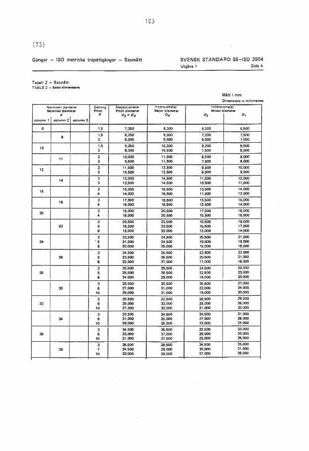
103
(T3)
G Ä N G O R - I S O M E T R I S K A TRAPETSGÄNGOR - B A S M Å T T S V E N S K S T A N D A R D S S - I S O 2 9 0 4
Utgåva 1 Sida 4
Tabell 2 - Basmått TABLE 2 — Bine dimension«
Mått i mm Dimeniions in millimetres
N< Nk
column 1
»mineli dian tminel diam
d
column 2
wter tt ar
column 3
Delning Pitch
*>
Medeldiameter Pitch diameter
d2 = Dx
Ytterdiameter Major diametee
0 *
Innerd Minor c
ameter iametar
O l
8 1.5 7.250 8.300 6.200 6.500
9 1.5 2
8.250 8.000
9.300 9.500
7.200 6.500
7.500 7,000
10 1.5 2
9.250 9.000
10400 10.500
8,200 7.500
8,500 8.000
11 2 3
10.000 9.500
11.500 11.500
8.500 7.500
9.000 8.000
12 2 3
11.000 10.500
12.500 12.500
9.500 8.500
10.000 9.000
14 2 3
13.000 12300
14,500 14.500
11,500 10.500
12.000 11,000
16 2 4
15.000 14.000
16.500 16.500
13.500 11.500
14.000 12.000
18 2 4
17,000 16.000
18.500 18.500
15.500 13.500
16.000 14.000
20 2 4
19,000 18.000
20.500 20.500
17.500 15.500
18.000 16.000
22 3 5 8
20.500 19.500 18.000
22.500 22.500 23.000
18.500 16.500 13.000
19,000 17,000 14.000
24 3
" 5 8
22.500 21.500 20.000
24.500 24.500 25.000
20.500 18.500 15.000
21.000 19.000 16.000
26 3 5 8
24.500 23.500 22,000
26.500 26.500 27.000
22.500 20.500 17.000
23,000 21.000 18.000
28 3 5 8
26.500 25,500 24.000
28.500 28.500 29.000
24.500 22.500 19.000
25.000 23.000 20.000
30 3 6
10
28,500 27.000 25.000
30.500 31.000 31.000
26.500 23.000 19.000
27.000 24.000 20.000
32 3 6
10
30.500 29.000 27.000
32.500 33.000 33.000
28.500 25.000 21.000
29.000 26.000 22.000
34 3 6
10
32.500 31.000 29.000
34.500 35.000 35.000
30.500 27,000 23.000
31.000 28.000 24.000
36 3 6
10
34.500 33,000 31.000
36.500 37.000 37.000
32.500 29.000 25.000
33.000 30.000 26.000
38 3 7
10
36.500 34.500 33.000
38.500 39,000 39.000
34.500 30.000 27.000
35.000 31.000 28.000

104
(T3)
G Ä N G O R - I S O M E T R I S K A TRAPETSGÄNGOR - B A S M Å T T S V E N S K S T A N D A R D S S - I S O 2 9 0 4
Utgåva 1 Sida 5
Nominell diameter Deining Medeidiameter Ytterdiameter Innerdiameter Nominel diameter Pitch Pitch diameter Major diameter Minor diameter
d P D2 = 0 2 O« 0-3 O l column 1 column 2 column 3
3 38.500 40.500 36.500 37.000
40 7 36.500 41.000 32,000 33.000
10 35.000 41.000 29.000 30,000
3 40.500 42.500 38.500 39,000
42 7 38,500 43.000 34.000 35.000
10 37.000 43.000 31.000 32.000
3 42.500 44.500 40.500 41.000
44 7 40,500 45.000 36.000 37.000
12 38.000 45.000 31.000 32.000
3 44.500 46.500 42.500 43.000
46 8 42.000 47.000 37.000 38.000
12 40,000 47.000 33.000 34.000
3 46.500 48.500 44.500 45.000
48 8 44.000 49.000 39.000 40.000
12 42.000 49.000 35,000 36.000
3 48.500 50.500 46.500 47.000
50 8 46.000 51,000 41.000 42.000
12 44.000 51.000 37,000 38.000
3 50.500 52.500 48.500 49.000
52 8 48.000 53.000 43,000 44,000
12 46.000 53.000 39,000 40,000
3 53.500 55.500 51.500 52,000
55 9 50.500 56.000 45.000 46,000
14 48.000 57,000 39.000 41,000
3 58.500 60.500 56.500 57.000
60 9 55.500 61,000 50.000 51.000
14 53.000 62.000 44.000 46.000
4 63.000 65.500 60,500 61.000
65 10 60.000 66.000 54.000 55,000
16 57,000 67,000 47.000 49.000
4 68,000 70,500 65.500 66,000
70 10 65.000 71,000 59.000 60.000
16 62.000 72.000 52.000 54.000
4 73.000 75.500 70,500 71.000
75 10 70,000 76.000 64.000 65.000
16 67.000 77.000 57.000 59.000
4 78.000 80.500 75.500 76.000
80 10 75.000 81.000 69,000 70.000
16 72.000 82.000 62.000 64.000
4 83.000 85.500 80.500 81.000
85 12 79.000 86.000 72.000 73.000
18 76.000 87.000 65.000 67.000
4 88.000 90.500 85.500 86.000
90 12 84.000 91.000 77.000 78.000
18 81.000 92.000 70,000 72.000
4 93.000 95.500 90.500 91.000
95 12 89.000 96.000 82.000 83.000
18 86.000 97.000 75.000 77,000

105
(T3)
G Ä N G O R - I S O M E T R I S K A T R A P E T S G Ä N G O R - B A S M Å T T S V E N S K S T A N D A R D S S - I S O 2 9 0 4
Utgåva 1 Sida 6
Nominell diameter Delning Medeldiameter Ytterdiameter Innerdiameter Nominel diameter Pitch Pitch diameter Major diameter Minor diameter
rf P rf2 = O j 04 "3 Ol column 1 column 2 column 3
4 98.000 100.500 95,500 96.000 100 12 94.000 101.000 87,000 88.000
20 90.000 102.000 78,000 80.000
4 103,000 105.500 100.500 101.000 105 12 99.000 106.000 92.000 93,000
20 95.000 ' 107.000 83.000 85.000
4 108.000 110.500 105.500 106,000 110 12 104,000 111.000 97.000 98.000
20 100.000 112,000 88.000 90.000
6 112.000 116,000 108.000 109.000'
115 14 108.000 117,000 99.000 101.000 22 104,000 117.000 91,000 93.000
6 117.000 121.000 113,000 114.000 130 14 113.000 122.000 104,000 106.000
22 109.000 122.000 96.000 98,000
6 122.000 126.000 118,000 119,000
125 14 118.000 127.000 109.000 111.000 22 114.000 127,000 101.000 103,000
6 127,000 131.000 123.000 124.000 130 14 123.000 132.000 114,000 116,000
22 119.000 132.000 106.000 108,000
6 132.000 136.000 128,000 129.000
135 14 128.000 137.000 119.000 121.000 24 123.000 137.000 109.000 111,000
6 137.000 141,000 133.000 134,000
140 14 133,000 142.000 124.000 126.000 24 128.000 142,000 114.000 116,000
6 142.000 146,000 138.000 139.000
145 14 138,000 147.000 129,000 131,000 24 133,000 147,000 119,000 121,000
6 147,000 151.000 143,000 144,000 ISO 16 142,000 152.000 132,000 134.000
24 138.000 152.000 124,000 126,000
6 152.000 156.000 148.000 149,000
155 16 147.000 157.000 137.000 139,000 24 143.000 157.000 129.000 131,000
6 157.000 161.000 153,000 154.000
160 16 152,000 162,000 142.000 144,000
28 146,000 162.000 130,000 132.000
6 162.000 166,000 158.000 159.000
165 16 157.000 167.000 147,000 149.000
28 151.000 167,000 135.000 137.000
6 167.000 171.000 163.000 164.000
170 16 162,000 172.000 152,000 154.000
28 156.000 172.000 140.000 142.000
8 171.000 176.000 166.000 167.000
175 16 167.000 177.000 157.000 159.000
28 161.000 177,000 145.000 147,000

106
(T3)
G Ä N G O R - I S O M E T R I S K A T R A P E T S G Ä N G O R - B A S M Å T T S V E N S K S T A N D A R D S S - I S O 2 9 0 4
Utgåva 1 Sida 7
Nominell diameter Delning Medeldiameter Vtterdiameter Innerdiameter Nominal diameter Pitch Pitch diameter Major diameter Minor diameter
d f d3 = 0 3 0, "3 ° 1 column 1 column 2 column 3
8 176.000 181.000 171.000 172,000
180 18 171,000 182.000 160.000 162.000
28 166.000 182.000 150,000 152.000
8 181.000 186.000 176,000 177,000 185 18 176.000 187.000 165.000 167,000
32 169.000 187.000 151.000 153,000
8 186.000 191.000 181.000 182.000 190 18 181.000 192.000 170.000 172,000
32 174.000 192.000 156,000 158,000
8 191.000 196.000 186.000 - 187,000
195 18 186.000 197.000 175,000 177,000
32 179.000 197,000 161.000 163.000
A 196.000 201.000 191.000 192.000
200 18 191.000 202.000 180.000 182.000
32 184.000 202.000 166.000 168.000
8 206.000 211.000 201.000 202.000
210 20 200.000 212.000 188.000 190.000
36 192,000 212.000 172.000 174,000
8 216.000 221.000 211.000 212,000
220 20 210.000 222.000 198.000 200.000
36 202,000 222.000 182.000 184.000
8 226.000 231.000 221.000 222.000
230 20 220.000 232.000 208.000 210.000
36 212.000 232.000 192.000 194.000
8 236.000 241.000 231,000 232.000
240 22 229.000 242.000 216,000 218.000
36 222.000 242.000 202.000 204.000
12 244.000 251.000 237.000 238.000
250 22 239.000 252.000 226.000 228.000
40 230.000 252.000 208,000 210.000
12 254.000 261.000 247,000 248,000
260 22 249.000 262.000 236.000 238.000 40 240.000 262.000 218.000 220.000
12 264.000 271.000 257.000 258,000
270 24 258.000 272.000 244.000 246.000
40 250,000 272.000 228.000 230,000
12 274.000 281.000 267.000 268,000
280 24 268.000 282.000 254,000 256.000
40 260.000 282.000 238.000 240.000
12 284.000 291.000 277.000 278.000
290 24 278.000 292.000 264.000 266.000
44 268.000 292,000 244.000 246.000
12 294.000 301.000 287.000 288.000
300 24 288.000 302.000 274.000 276.000 44 278.000 302.000 254,000 256.000

107
Table T4 a
Nut no. 1 Motion opposite F
a X
Series 1 Series 2
r/min N Nm r/min N Nm
10, ,6 11 194 23, ,08 3, 8 15 854 89 .67
30. 3 9 433 38. 66 26. 7 14 609 60, ,81
41, ,4 7 268 29. 81 36, ,2 13 581 55 .21
48. 1 5 133 22. 38 49. 1 11 644 47, ,54
49. 5 2 729 15. ,30 62, , 1 7 985 33 .88
49, 7 457 8. 81 65. ,7 5 817 27, ,22
70. 3 3 624 20, ,96
69. 0 2 784 19, ,73
69. ,8 1 455 15, .84
74. 4 389 14. ,33
Table T4 b
Nut no. 1
Motion equal F ax
Series 1 Series 2
n
r/min
Fax eq
N
M
NRI
n
r/min
F eq
N
M
Nm
0 11 197 23. ,08 1.8 15 815 48.60
10.6 11 055 20, ,12 25.2 14 650 21.99
28.8 9 448 9, 52 34.6 13 380 16.59
39.6 7 130 6, ,47 46.9 11 644 12.61
46.2 4 980 5, 73 59.3 7 904 8.84
47.6 2 675 5. 12 64.2 5 838 9.25
47.8 445 6. 63 67.2 3 605 6.03
67.2 2 736 6.95
66.0 1 331 8.47
71.8 552 8.05
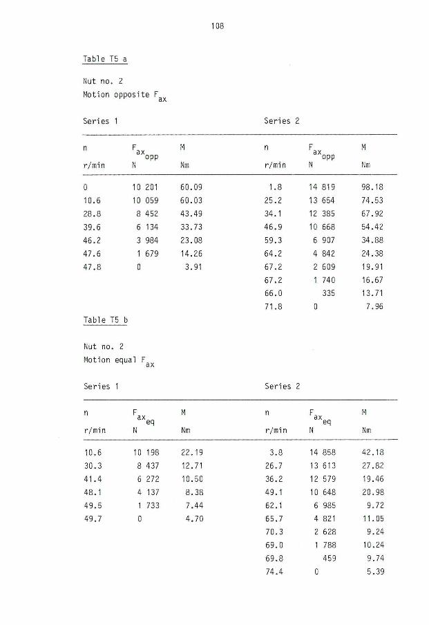
108
Table T5 a
Nut no. 2 Motion opposite F
ax
Series 1 Series 2
n
r/min F a X opp N
M
Nm
n
r/min F a X opp N
M
Nm
0 10 201 60.09 1.8 14 819 98, .18
10.6 10 059 60.03 25.2 13 654 74, ,53
28.8 8 452 43.49 34.1 12 385 67, ,92
39.6 6 134 33.73 46.9 10 668 54, .42
46.2 3 984 23.08 59.3 6 907 34, ,88
47.6 1 679 14.26 64.2 4 842 24. ,38
47.8 0 3.91 67.2 2 609 19. ,91
67.2 1 740 16. .67
66.0 335 13. .71
71.8 0 7 .96
Table T5 b
Nut no. 2
Motion equal F = v
a X
Series 1 Series 2
n
r/min
F eq
N
M
Nm
n
r/min
Fax eq
N
M
Nm
10.6 10 198 22. 19 3.8 14 858 42, 18
30.3 8 437 12. 71 26.7 13 613 27. ,82
41.4 6 272 10. ,50 36.2 12 579 19. ,46
48.1 4 137 8. 38 49.1 10 648 20, ,98
49.5 1 733 7, ,44 62.1 6 985 9. ,72
49.7 0 4, ,70 65.7 4 821 11. ,05
70.3 2 628 9, .24
69.0 1 788 10 .24
69.8 459 9, .74
74.4 0 5 .39

109
Table T6 a
Nut no. 3
Motion opposite F ax
Series 1 Series 2
n
r/min F a X opp N
M
Nm
n
r/min F a X opp N
M
Nm
10.6 11 194 59. 63 3.8 15 854 93.43
30.3 9 448 11. 71 26.7 14 609 73.55
41.4 7 268 41. 98 36.2 13 581 68.74
48.1 5 133 30. 01 49.1 11 644 62.95
49.5 2 729 18. 96 62.1 7 985 42.24
49.7 457 10. 27 65.7 5 817 34.18
70.3 3 624 24.52
69.0 2 784 22.43
69.8 1 455 16.72
74.4 389 14.76
Table T6 b
Nut no. 3
Motion equal F ax
Series 1 Series 2
n F M eq
r/min N Nm
0 11 197 30.75
10.6 11 055 21.18
28.8 9 448 11.71
39.6 7 130 8.41
46.2 4 980 6.92
47.6 2 675 6.87
47.8 445 7.31
n F M ax eq r/min N Nm
1 .8 15 815 50 .62
25 .2 14 650 24 .01
34 .6 13 380 17 ,81
46, .9 11 664 13 ,89
59, .3 7 904 8. ,84
64, ,2 5 838 9, .69
67, .2 3 605 8, ,70
67, ,2 2 736 9, 56
66. 0 1 331 10, ,36
71, 8 552 10, ,78
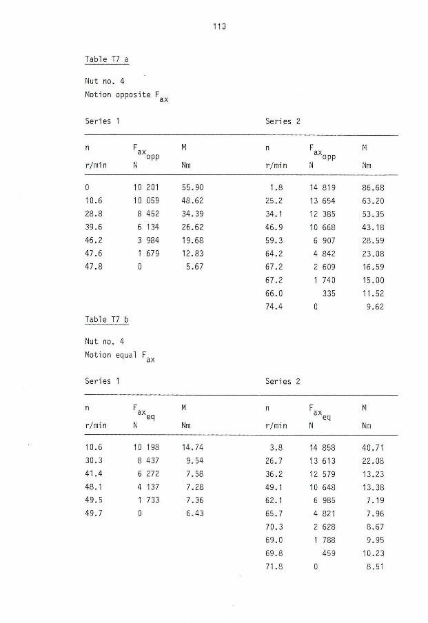
113
Table T7 a
Nut no. 4
Motion opposite F ax
Series 1 Series 2
n
r/mi n
F ax opp
N
M
Nm
n
r/min F a X opp N
M
Nm
0 10 201 55, .90 1.8 14 819 86.68
10.6 10 059 48, ,62 25.2 13 654 63.20
28.8 8 452 34, .39 34.1 12 385 53.35
39.6 6 134 26. 62 46.9 10 668 43.18
46.2 3 984 19, ,68 59.3 6 907 28.59
47.6 1 679 12. 83 64.2 4 842 23.08
47.8 0 5, 67 67.2 2 609 16.59
67.2 1 740 15.00
66.0 335 11.52
74.4 0 9.62
Table T7 b
Nut no. 4
Motion equal F ax
Series 1 Series 2
n F,„ M n F M ax„„ ax eq eq
r/min N Nm r/min N Nm
10.6 10 198 14, 74 3.8 14 858 40, ,71
30.3 8 437 9. 54 26.7 13 613 22, ,08
41.4 6 272 7. 58 36.2 12 579 13, ,23
48.1 4 137 7, ,28 49.1 10 648 13, .38
49.5 1 733 7, ,36 62.1 6 985 7. ,19
49.7 0 6. ,43 65.7 4 821 7, ,96
70.3 2 628 8, ,67
69.0 1 788 9, .95
69.8 459 10, .23
71.8 0 8, .51

111
Table T8 a
Nut no. 1 Motion opposite F
Series 1
v p v/p y q 3 p
m/s MPa 2 - kW/rn
0. 042 1. .049 0, ,040 0. 075 3.30
0. 120 0. .884 0, ,136 0, ,064 6.79
0. 164 0, ,681 0 .241 0. ,064 7.15
0. 190 0, ,481 0, ,395 0. 071 6.49
0. 196 0 .256 0 .866 0. ,103 5.17
0. 197 0, ,043 4, .581 0. 445 3.77
Series 2
v p v/p u q 3 o
m/s MPa ^ kW/ni
0. 015 1. 485 0. 010 0. 104 2. 32
0. 105 1, ,369 0. 077 0. ,066 9. ,49
0. 142 1, ,272 0. 112 0. 063 11, ,38
0. 193 1, ,091 0, ,177 0. ,064 13 .48
0, 244 0, ,748 0. 326 0. ,068 12, ,41
0. ,258 0, ,545 0. ,473 0, ,079 11 .11
0. 276 0, .340 0, ,813 0. ,107 10 .04
0. ,271 0 .261 1, .039 0, ,140 9 .90
0. 274 0 .136 2, ,010 0, ,236 8, .79
0, .292 0 .037 8 .000 0, ,870 9, .40

112
Table T8 b
Nut no. 1
Motion equal F
Series 1
v p v/p Ü q m 3 5
m/s MPa ^ kW/nT
0 1, ,049 0 0 .094 0
0, ,042 1, ,036 0. ,041 0 .088 3.829
0. 114 0, ,885 0, ,129 0 .067 6.760
0. 157 0, ,668 0. 235 0, ,064 6.712
0. 183 0, ,467 0, 392 0 .071 6.068
0. 188 0, ,251 0, ,749 0 ,090 4.247
0. 189 0. ,042 4. 500 0, ,431 3.421
Series 2
v p v/p u q m 3 9
m/s MPa ^ kW/rn
0. 007 1.482 0. ,005 0, ,120 1.24
0, ,099 1.373 0. ,072 0, ,080 10.87
0, ,136 1.254 0, .109 0. ,073 12.45
0. ,184 1.093 0. ,168 0. ,069 13.88
0, ,233 0.741 0. ,315 0. ,070 12.09
0. ,252 0.547 0. ,461 0. 082 11.30
0. 264 0.338 0, ,782 0. ,084 7.50
0. 264 0.256 1. ,030 0. ,107 7.23
0. ,259 0.125 2. 077 0. ,206 6.67
0. 282 0.052 5. ,444 0. ,423 6.20

113
Table T9 a
Nut no. 2 Motion opposite F
Series 1
v P
m/s MPa
0 0, 956 0 0, ,110 0
0. 042 0. .943 0.045 0. 112 4.44
0, 114 0, 792 0.144 0. ,091 8.22
0. 157 0. 575 0.273 0. 100 9.03
0. 183 0. 373 0.491 0. 107 7.30
0. 188 0. 157 1.197 0. 176 5.19
0, 189 0 - - -
v/p
Ns k W / n f
Series 2
v p v/p u q 3
m/s MPa • kW/m2
0. ,007 1. ,388 0, .005 0. ,129 1. 25
0. ,099 1. ,279 0, ,077 0. 099 12. 54
0, .134 1. ,160 0, ,116 0. ,100 15, ,54
0. ,184 0, ,999 0. ,184 0. 090 16. 54
0, ,233 0, ,647 0, .360 0. 088 13, ,27
0. 252 0, ,454 0, ,555 0. 088 10, 07
0, ,264 0, ,244 1, ,080 0. ,154 9. 92
0. ,264 0, 163 1, ,620 0. 203 8. 74
0, 259 0. 031 8, ,275 0. 969 7. 78
0. ,282 0 - - -

114
Table T9 b
Nut no. 2
Motion equal F dX
Series 1
v p v/p u q m 3 ?
m/s MPa ~ kW/rrf
0. 042 0.956 0, ,044 0, ,097 3.89
0. 120 0.791 0. ,152 0, ,080 7.59
0. 164 0.588 0, ,279 0, ,084 8.10
0. 190 0.388 0, ,490 0, ,093 6.86
0. 196 0.162 1, ,210 0. ,152 4.83
0. 197 0 - - -
Series 2
v
m/s
0.015
0.105
0.142
0.193
0.244
0.258
0.276
0.271
0.274
0.292
P
MPa
1.392
1.275
1.179
0.998
0.654
0.452
0.246
0.168
0.043
0
v/p
Ns
0.011
0.082
0.120
0.193
0.373
0.571
1.122
1.613
6.372
V
0.114
0.094
0.081
0.092
0.077
0.100
0.132
0.189
0.602
q
kW/m2
2.38
12.58
13.56
17.72
12.29
11.66
8.96
8.60
7.09

115
Table TIO a
Nut no. 3 Motion opposite F
ax
Series 1
v p v/p u q m 3 ?
m/s MPa kW/nT
0. 042 1.049 0. 040 0. 096 4, ,23
0. 120 0.884 0. 136 0. 087 9. ,23
0. 164 0.681 0. 241 0. 107 11, ,95
0. 190 0.481 0. 395 0. 109 9. ,96
0. 196 0.256 0. 766 0, 137 6, ,87
0, 197 9.043 4. 581 0. 524 4, 44
Series 2
v p v/p u q 3 ?
m/s MPa S- kW/rri
0. 015 1. 485 0, ,010 0. 110 2, 45
0. 105 1. 369 0. ,077 0. 088 12, 65
0. 142 1. 272 0, ,112 0. 089 16. 08
0. 193 1. 091 0, ,177 0. 098 20. ,64
0. 244 0. 748 0, ,326 0. 095 17, 34
0. 258 0. 545 0, .473 0, ,110 15, ,47
0. 276 0. 340 0, ,812 0. 132 12, 39
0. 271 0, 261 1, .038 0. ,165 11. ,67
0. 274 0. 136 2, .015 0. 253 9, ,43
0. 292 0, 365 8 .000 0, ,896 9, ,55

116
Table T10 b
Nut no. 3
Motion equal F i
Series 1
v p v/p u q m 3 7
m/s MPa kW/r/
0 1, ,049 0 0, ,112 0
0.042 1, ,036 0.041 0. ,090 3.92
0.114 0, ,885 0.129 0. .073 7.37
0.157 0, ,668 0.235 0, ,071 7.45
0.183 0, ,467 0.392 0. .077 6.58
0.188 0, ,251 0.749 0. ,107 5.05
0.189 0, ,042 4.500 0. .473 3.75
Series 2
v p v/p y q m 3 7
m/s MPa 2 - kW/nf
0.007 1. 482 0, ,005 0. ,124 1.29
0.099 1. ,373 0. ,72 0. ,083 11.28
0.136 1. ,254 0, 108 0. ,075 12.79
0.184 1. ,093 0. ,168 0. 072 14.48
0.233 0. ,741 0. ,314 0. 070 12.09
0.252 0. ,547 0. ,461 0. ,084 11.58
0.264 0, ,338 0. 781 0. 103 9.19
0.264 0, ,256 1. ,031 0, ,131 8.85
0.259 0, ,125 2. .072 0. 243 7.87
0.282 0, ,518 5. ,444 0. ,555 8.11

117
Table T11 a
Nut no. 4
Motion opposite F
Series 1
v p v/p u q m 3 ?
m/s MPa S - kW/rn
0 0, ,956 0 0.099 0
0, 042 0, ,943 0. ,045 0.083 3, ,29
0. 114 0, ,792 0, 144 0.063 5, ,69
0. 157 0. 575 0, 273 0.070 6, ,32
0. 183 0, ,373 0. ,491 0.082 5, ,60
0, 188 0. ,157 1. 197 0.154 4, ,55
0. 189 0 - - -
Series 2
v p v/p u q m 3 ?
m/s MPa ^ kW/nr
0, 007 1. ,388 0.005 0, ,109 1, ,06
0, 099 1. 279 0.077 0. 078 9, ,88
0, 134 1, ,160 0.116 0. 070 10, ,88
0. 184 0, ,999 0.184 0. 063 11, ,58
0, 233 0, ,647 0.360 0, ,065 9, ,80
0, 252 0, 454 0.555 0, ,081 9, ,27
0, 264 0. 244 1.080 0, 121 7. ,79
0, ,264 0. ,163 1.620 0. 179 7, ,70
0, 259 0. 031 8.355 0. 813 6, ,53
0, ,292 0 - - -
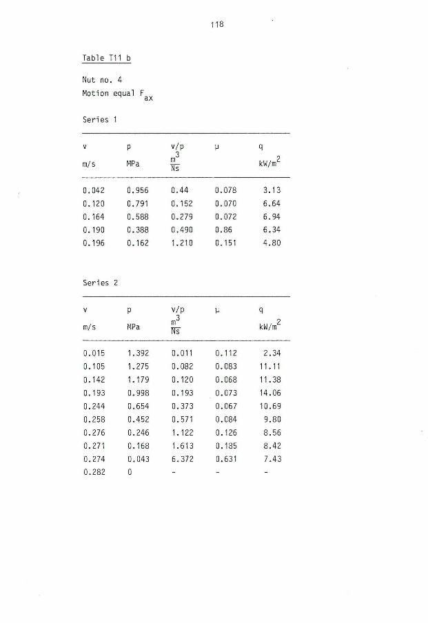
118
Table T11 b
Nut no. 4 Motion equal F
ax
Series 1
v p v/p u q m 3 7
m/s MPa S- kW/nT
0.042 0.956 0. ,44 0. ,078 3. ,13
0.120 0.791 0. ,152 0, ,070 6. ,64
0.164 0.588 0, ,279 0, ,072 6, ,94
0.190 0.388 0. ,490 0, ,86 6, .34
0.196 0.162 1, ,210 0, ,151 4, ,80
Series 2
v p v/p u q n 3 7
m/s MPa |k k W / m
0. 015 1. 392 0. ,011 0. 112 2.34
0. 105 1. 275 0. 082 0. 083 11.11
0. 142 1. 179 0, ,120 0. ,068 11.38
0. 193 0. 998 0. ,193 0-,073 14.06
0. 244 0. 654 0. 373 0. ,067 10.69
0. 258 0. 452 0. ,571 0, 084 9.80
0. 276 0. 246 1, .122 0, .126 8.56
0. 271 0. 168 1, .613 0, ,185 8.42
0. 274 0. 043 6, .372 0. .631 7.43
0. 282 0 - - -

119
Table T12
Nut no. 1
Motion opposite F Motion equal F aX
Q— = 101-103 Ns/m3
3 ( ?
S U S y
0 0.094 0 0.094
0.002 0.104 0.0001 0.120
0.006 0.075 0.005 0.088
0.012 0.066 0.009 0.080
0.017 0.063 0.013 0.073
0.021 0.064 0.015 0.067
0.027 0.064 0.020 0.069
0.036 0.064 0.028 0.064
0.049 0.068 0.038 0.070
0.060 0.071 0.047 0.071
0.072 0.079 0.055 0.082
0.116 0.103 0.090 0.090
0.123 0.107 0.093 0.084
0.158 0.140 0.123 0.107
0.305 0.236 0.248 0.206
0.692 0.445 0.537 0.431
1.212 0.870 0.650 0.423
3y
3 & 79.6-10 Ns/nf

120
Table T13
Nut no. 2
Motion opposite F Motion equal F ax ax
^ — = 107- 103 Ns/m3 = 87.9- 103 Ns/m3
3( f ) 3 ( f )
S V S V
0 0.110 0 0.110
0.0001 0.129 0.002 0.114
0.007 0.112 0.006 0.097
0.012 0.099 0.011 0.094
0.019 0.100 0.016 0.081
0.023 0.091 0.020 0.080
0.030 0.090 0.026 0.092
0.044 0.100 0.037 0.084
0.058 0.088 0.049 0.077
0.079 0.107 0.065 0.093
0.089 0.088 0.075 0.100
0.173 0.154 0.148 0.132
0.192 0.176 0.159 0.152
0.260 0.203 0.213 0.189
1.380 0.969 0.840 0.602

121
Table T14
Nut no. 3
Motion opposite F Motion equal F
= 103.6-10 3 Ns/m3 ^ — = 98.3-10 3 Ns/m3
^ *<f>
S u S
0 0 .112 0 0 .112
0.002 0 ,116 0.0001 0 .124
0.006 0 ,096 0 .006 0 .090
0.012 0 ,088 0 .011 0 .083
0.017 0, ,089 0, .016 0 .075
0.021 0. ,087 0 .019 0 .073
0.028 0, ,098 0, ,025 0, .072
0.037 0, ,107 0, ,035 0 .071
0.051 0. ,095 0. ,046 0, ,070
0.062 0. 109 0, 058 0, .077
0.074 0. 110 0. 068 0. ,084
0.119 0. 137 0. 111 0. 107
0.126 0, 132 0. 115 0. 103
0.162 0. 165 0. 152 0. 131
0.312 0. 253 0. 306 0. 243
0.710 0. 524 0. 664 0. 473
1.243 0. 896 0. 802 0. 555

122
Table T15
Nut no. 4
Motion opposite F Motion equal F ax ax
Q— = 95.7-10 3 Ns/m3 = 93.6-10 3 Ns/m3
3( f ) 3 ( f )
S u S P .
0 0.099 0 0.099
0.0001 0.109 0.002 0.112
0.001 0.083 0.006 0.078
0.011 0.078 0.012 0.083
0.017 0.070 0.017 0.068
0.021 0.063 0.021 0.070
0.026 0.063 0.027 0.073
0.039 0.070 0.039 0.072
0.052 0.065 0.052 0.067
0.070 0.082 0.069 0.086
0.080 0.081 0.080 0.084
0.155 0.121 0.157 0.126
0.172 0.154 0.170 0.151
0.233 0.179 0.227 0.185
1.234 0.813 0.895 0.631

123
Table T16
Motion opposite
u = 0.005 m/s,
e = 35.39-10" 3 ,
F
ax
Q = 206.7 W
7 u = 106.2-10
Table T17
Motion opposite
u = 0.010 m/s,
e = 17.69-10" 3 ,
Q = 417.4 W
z x = H = 53.09-10
thermocouple z T* no.
14 -0.0575 0
11 0.0089 0.121
10 0.0177 165
9 266 177
8 354 221
thermocouple z T* no.
14 -0.0288 0
11 0.0044 0.110
10 88 129
9 0.0133 144
8 177 150
6 531 291
5 620 341
4 708 355
3 796 372
2 885 324
1 0.0973 274
12 0.1143 0.233
6 265 195
5 310 224
4 354 251
3 398 272
2 442 283
1 487 240
12 0.0571 0.184

124
Table T18
Motion opposite F
ax
u = 0.015 m/s, Q = 608.0 W
£ = 11.80-10" 3 , z x = H = 35.39-10
Table T19
Motion opposite F
ax
u = 0.020 m/s, Q = 916.5 W
£ = 8.85-10" 3 , z x = H = 26.55-10
thermocouple z no.
14 -0.0192 0
11 0.0029 0.082
10 59 93
9 88 0.114
8 0.0118 117
6
5
4
3
2
1
12
177
206
236
265
295
324
0.0381
134
164
191
214
224
191
0.151
thermocouple z no.
14 -0.0144 0
11 0.0022 0.061
10 44 71
9 66 81
8 88 85
6 0.0133 0.100
5 155 120
4 177 137
3 199 157
2 221 162
1 243 150
12 0.0286 0.118

125
Table T20
Motion equal F dX
u = 0.005 m/s, Q = 264.5 W
e = 35.39-10" 3 , z _H = 106.2-10
Table T21
Motion equal F_„ dX
u = 0.01 m/s, Q = 452.7 W
e = 17.69-10" 3 , z x = H = 53.09-10
thermocouple no.
12 -0. 0081 0
1 0. 0089 0 ,111
2 0. 0177 164
3 265 198
4 354 228
5 442 270
6 531 275
8 708 300
9 796 281
10 885 283
11 973 278
14 0, ,1639 0, .185
thermocouple no.
12 -0. 0040 0
1 0, 0044 0.079
2 89 0.116
3 0. 0133 151
4 177 172
5 221 196
6 265 190
8 354 178
9 398 169
10 442 159
11 487 0.154
14 0. ,0819 0.088

126
Table T22
Motion equal F
u = 0.015 m/s, Q = 582.6 W
£ = 11.8-10~ 3, z x = H = 35.39-10
Table T23
Motion equal F
ax
u = 0.02 m/s, Q = 848.5 W
e = 8.85-10" 3 , z x = H = 26.55-10
thermocouple z T*
no.
12 -0. .0027 0
1 0, ,0030 0.051
2 59 66
3 89 0.109
4 0. ,0118 132
5 148 144
6 177 132
8 236 123
9 266 113
10 295 106
11 325 0.088
14 0, ,0546 0.031
thermocouple z T*
no.
12 -0, ,0021 0
1 0, ,0022 0.032
2 44 65
3 66 85
4 89 0.103
5 0, ,0111 112
6 133 0.096
8 177 82
9 199 72
10 221 65
11 243 55
14 0, ,0410 0.004

my Fax opp
Nut no. 1
( )
©
( )
•
2.0 4.0 6.0 8.0 10.0
v /p E-6 m3/sN
Diagram D1. Experimentally determined coef f ic ients of f r i c t i o n .

my Fax 0.20
0.16
0.12
0.08
0.04
opp Nut no. 1
D 0 D
0
0 ° G
0 )
0.4 0.8 1.2 1.6 2.0
v /p E-6 m3/sN
Diagram D2. Experimentally determined coef f ic ients of f r i c t i o n .
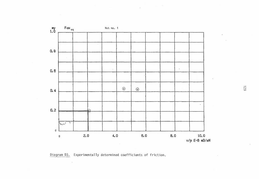
my FGXpr, N u t n o * 1
0.8
0.6
0 .4 0 ©
•
2.0 4.0 6.0 8.0 10.0
v /p E-6 ntf/sN
Diagram D3. Experimentally determined coef f ic ients of f r i c t i o n .
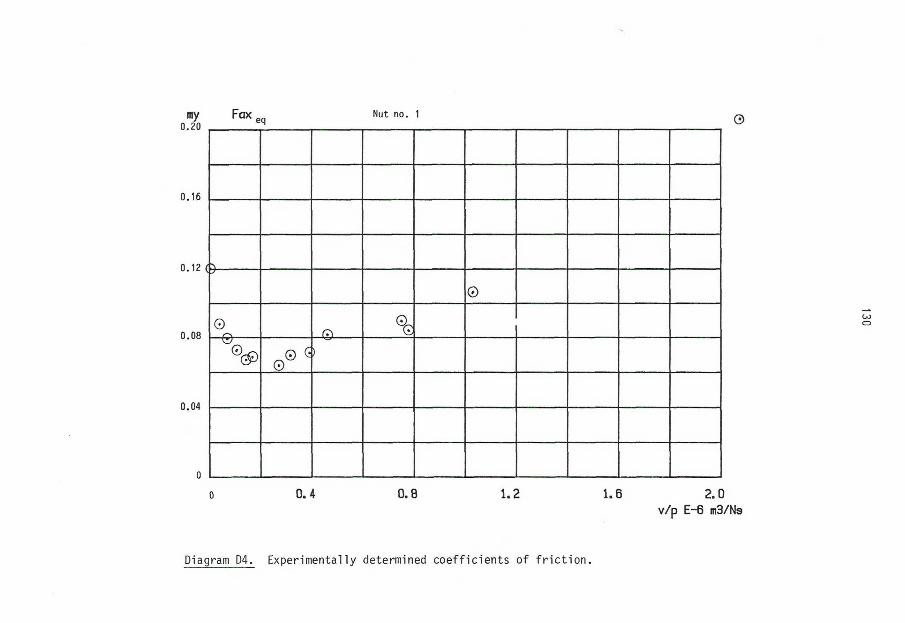
ray Fax Nut no. 1
J
0
0
o 0.4 0.8 1.2 1.8 2.0
v /p E-6 irfl/Ns
Diagram D4. Experimentally determined coef f ic ients of f r i c t i o n .

L I Fax
opp Nut no. 2
0
0.8
0.6
0.4
0 .2
2.0 4.0 6.0 8.0 10.0
v /p E-6 m3/N9
Diagram D5. Experimentally determined coef f ic ients of f r i c t i o n .

Nut no. 2
0.20
0.16
0.12
0.08
0.04
0
0
0 0
© W ©£ © 0
0.4 0 .8 1.2 1.6 2.0
v /p E-6 m3/N9
Diagram D6. Experimentally determined coef f ic ients of f r i c t i o n .

Nut no. 2
0.8
0.4
0.2
vy
o 2.0 4.0 6.0 8.0 10.0 v /p E-6
Diagram D7. Experimentally determined coef f ic ients of f r i c t i o n .

my Fax D „ Nut no. 2
( D
©
D
) ©
©
©
0 0.4 0.8 1.2 1.6 2.0
v /p E-6 m3/Ns
Diagram D8. Experimentally determined coef f ic ients of f r i c t i o n .

my Fax„ „ „ l i o p p
Nut no. 3
0.8
0 .6
©
0.4
0.2 ©
0 2.0 4.0 6.0 8.0
Diagram D9. Experimentally determined coef f ic ients of f r i c t i o n .
10.0
v /p E-6

my Fax 0,20
0.16
0.12
0.08
0.04
opp Mut no. 3
©
w (
D © 0 i ©
© w ©%
0
0.4 0.8 1.2 1.6 2 .0
v /pE-6 tn3/Ns
Diagram D10. Experimentally determined coef f ic ients of f r i c t i o n .
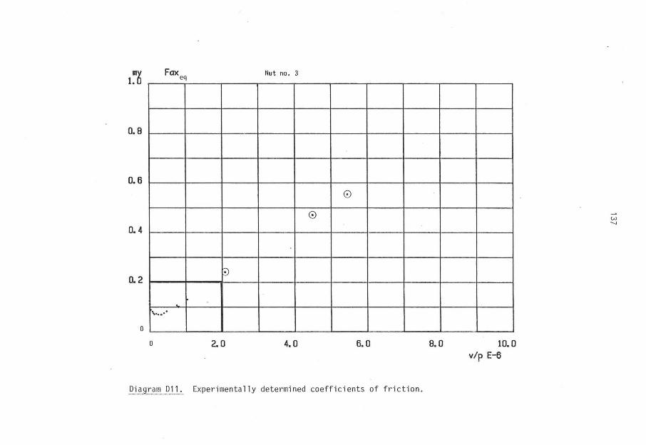
my Fax Nut no. 3
0.8
0.6
0.4
0 .2
0
©
o 2 .0 4.0 6.0 8.0 10.0
v /p E-6
Diagram D11. Experimentally determined coef f ic ients of f r i c t i o n .

my F a x e q Nut no. 3
0
© 0 ©
©33 ^ tt 0©
o 0.4 0.8 1.2 1.6 2.0
v /p E-6 m3/Ns
Diagram D12. Experimentally determined coef f ic ients of f r i c t i o n .

my Fax opp
Nut no. 4
*
2.0 4.0 6.0 8.0 10.0
v /p E-6 m3/Ns
Diagram D13. Experimentally determined coef f ic ients of f r i c t i o n .

ray F a x 0 D D Hut no. 4
( )
ft
Q- (7) (§>
©~ 0c? 0 0
0 0.4 0.8 1.2 1.6 2.0
v /pE-6 m3/Ns
Diagram D14. Experimentally determined coef f ic ients of f r i c t i o n .

my F a x e q Nut no. 4
0.8
0.6
0.4
0.2
0
•
•
0 2.0 4.0 6.0 8.0 10.0
v /p E-6
Diagram D15. Experimentally determined coef f ic ients of f r i c t i o n .

my F a x
e q
N u t n 0 - 4
©
©
.0 © © w r
0© ' 0 0
0.4 0.8 1.2 1.6 2.0
v /p H-6 m3/Ns
Diagram D16. Experimentally determined coef f ic ients of f r i c t i o n .

143
Computer program CI
10 REM I I I SlffiADAF! I I I 20 REM HIINLJ'SNING FRAN BAND VIA A/D-OHVANDLARE OCH A9C8Ü TILL DATAFIL I I I 39 ; "fintal kanaler pä aktuell da ta f i l : ' ; : INPUT K 40 FOR IZ=1 TO DS 50 PRINT "Kanal nuB«er 10 INPUT KZifZI 70 NEXT 17.
30 ! "Antal stag i ftrdräjningslpppen:"s : INPUT il 90 i'Z=INT(38O0Z/SZi 100 IF V?.!7i0 THEN Yt«7M 110 DIM A7.[YZ,QZi u o s:=o 130 OUT 11,07. MO XMNPI07.) 150 OUT «,07. 160 OUT 2Z,97. 170 OUT 02,02 180 XZ=!NP(1Z) 190 IF X7.M27 THEN 180 200 J2=INP(0) 210 IF ill AND 7IK1 THEN 160 220 ; "Jag startar nu" 230 SZ«Si*l 240 FOR IZ'IZ TO OZ 250 OUT 22,KZ(IZ>-!Z 240 OUT OZ.OZ 270 XZ=INP(1Z) 280 IF X7.M27Z THEN 270 290 AZ(SZ,IZ)=INP(OZ}*(X! AND 157.11254-2059 300 NEXT 17. 305 ZZ=0 310 REH M(KONTROLL AV TIDSSR1ND TILLIII 320 OUT 2Z.9Z 330 OUT OZ.OZ 335 3Z=ZZH 340 XZ'INP(IZ) 350 IF XIM27 THEN 340 355 I f ZZ.MOO THEN 420 340 IF (XZ AND 7ZX1 THEN 320 370 JZ=INP(0> 380 i SI;" "; 390 FOR IX»! TO JZ : NEXT IZ 400 FOR 11=11 TO SZ : ; ftZiS7.,IZ!;- ' ; : NEXT 17. 410 i : IF SK11 THEN 230 420 ; "Fortsatt inläsning? U/N)"j 430 SET AB : ; AS : IF AB*"J" OR AS="j" THEN 230 440 SET AS : ; AS : IF A»="J" OR AB="j" THEN 230 500 ; "Hätvärdsna skall lagras på datafilmed beteckning? (ex SN7.DAT1"; i INPUT FB 505 j "är du absolut säker'" 504 GET AB : ; AB i IF Afi="J" OR AB«"j" THEN 510 ELSE 230 510 PREPARE FB ASFILE 4 512 CLOSE 4 520 OPEN FB ASFILE 4 530 i *4,SZ 540 ; 14, SZ 550 FOR I7.= l TO SZ 540 j I4,KZ(IZ) 570 NEXT IZ 580 FOR !Z=1 TO SZ 590 FOR H7.=l TO OZ 400 i t4,AZ(IZ,H7.) 410 NEXT HZ 420 NEXT IZ s30 CLOSE 4

Computer program C2
10 REN III SNANALYS III :0 REN (cl Lsn Ekerfors 30 REN Maskinteknik 10 REN Tekniska Högskolan, 95187 LULE», Tel 0920/91284 50 OPEN "PR:" RSFILE 1 40 j "Vilken datafil (finge t.ex DATA.DAT)"; 70 INPUT FB 80 PREPARE F» ASFILE 4 90 CLOSE 4 100 ONERRORGOTO 340 110 PRINT "Antal kanaler på aktuell data f i l " ; 120 INPUT 07. 130 YZ=INT(3800Z/B7.) 140 I F YZMOOO THEN YZ=1000 150 D I N K Z I S Z H I 140 SIN OZ(OZ) 170 DIM AZIYZ.OX) 180 DIN F I Q Z )
190 DIN NZI25) 200 GOTO 340 210 ; "SKALL TABELLEN SKRIVAS IGEN J/N";
220 GET AU : ; AB : IF A»»"N" THEN 3 6 0
230 I F AB="n" THEN 3 6 0
240 ; "FRÄN RAD NUMMER I 1 TILL ( )" ; 250 INPUT LlZjHlZ 240 IF N1Z>SZ SOTO 240 270 FOR IZ=L1Z TO M1Z 280 ; IZ, 290 FOR JZ ' I Z TO SZ : ; AZ(IZ,JZ);" "; : NEXT J Z : PRINT 300 NEXT IZ 310 ; "SKALL TAB SKRIVAS PS PR:?"; 320 GET AB ; ; AB : IF AB="J" THEN SOSUB 1520 330 ; "Skall tab plattas pä PR:?'; 340 SET Al» i ; Al» : IF A1B»"J" OR AlB»"j" SOSUB 2830 350 ; "11111111111111111111111111111111111" 360 ; "Berikn. IY f r ik t .koeff . och verk- ningsgrad för »utter IN)" 370 ; "Nedelvärde5bildning av kanal nr (1,2,3,4,eller 6)" 380 i "ändring av OFFSET (01" 390 ; 'el ler ändring av skalfaktor,offset aed bevarande av inlästa tätvärden 400 ; "håjtning frän datafi l (H)" 410 ; "eller oiskrivning av föregående tabell I T ! "
420 ; "Utskrift av tabell på printer I P ) "
430 ; " eller oakirning led nya ingångs- data ( D ) ' 440 ; "11111111111111111111111111111111111111111111111111111111111111111111111111" 450 ; "Antal inlästa rader;";S7.;"st" 460 GET IB : ; XB : HZ»0Z 470 XZ=ASC(XB)-48 4B0 IF XB«"P" THEN SOSUB 1 5 2 0 490 IF X Z U THEN 450 500 IF XZ<9 THEN 5 8 0 510 IF XB="D" THEN 1240 520 IF XB»"0" THEN SOTO 2700 530 IF XB="ä" THEN GOTO 1290 540 IF XB'"N" THEN 1770 550 IF Xfi="H" THEN SOSUB 1400 540 IF XB>"T" THEN 240 570 SOTO 450 580 ; "Från iätning nr ( ,) t i l l nr ( )" 590 ; "Högsta värde är ";SZ 400 INPUT N7.,LZ 410 IF HZJL7.-17. THEN 580 420 IF LZ>SZ THEN 590 430 I F X7.<9 THEN GOSUB 2810 ELSE GOTO 440 640 I F Xfi='H" THEN SOSUB 2790

(C2) 14E
459 : "UppgSrig s i l e r nedgäng?!U,N!* 660 SET RS 470 FOR I2=1Z T0 OJ 480 IF K7.(IZ!=XZ THEN HZ=I2 690 NEXT 17. 700 IF »7.=07. THEN 360 710 : "Skall oregelbundet »ätvärde strykas ' IJ,NI" 720 GET ÖS 730 «1=0 : ö?.=0 740 IF ÖS="J" OR Ö5="j" THEN SOSUB 1680 750 T2=LI-n7.-öW 740 R(XX)=0 770 Hl«At«R,Hll ; H2=A7.!It2,tH 780 FOR I2=N2 TO LZ 790 RIX7.)=R(X2)+AZ<n,N7,)-DZ(K2) 800 äZ=0 810 H»»l»l B20 IF IZ--NZ(SZ) THEN 860 830 IF äZiöZ THEN 810 840 IF AZ(1Z,HZ1>H1 THEN H1=A2(IX,KZ! : 11=12 850 IF A7.IIZ,NZKH2 THEN H2=A2(IZ,«7.) : I2=IZ 860 NEXT IZ 870 U1IXZ)=(R(XZ)-A!)/TZ 880 U(IK)»(R(KI-»ll tF(K'l/Tl 390 U(XZ)=ABS(U(XZ)) 900 PRINT 910 H3=<H1-D7.INZ)>IF(HZ) 920 H4=IH2-DZINZ))IF(K2) 930 IF RB="U" THEN DB="(uppgång)" 940 IF R5="N" THEN DS="(nedgang)" 950 ; "Nedelvårdet för kanal ";X2;" är "jUIXZ); - ";DS;"(Rad nr";NZ;"-";U;"l' 960 : "Medelvärdet för kanal ";XX;"«R"jU(XZ) 970 ; *! ?B0 ; 11 990 ; »medelvärdet för kanal ";X2;" är ";UU1>;" CjUHXZ);" bits>";DB;MRad nr ' ;Nl;"-" ;Ll ;"> 1000 ; »I-Störst, värde :";H3;" (",'Hl;" bitsMrad nr " , ' l l i " ) , »insta värde: ,;H4(" ("(H2;" bits) (rad nr " ; I 2 j " ) " 1010 ,• »1 1020 i #rOffset:"(DZ(NZ) 1030 ; ]Q40 ! " ===3==33S=S"
1050 ; "mitt l l l l l l l l l i l l l l l i l l t l t t l l l l l l l" 1040 ; "önskas ber. av spridningen IS)" 1070 GET ä» 1080 IF Sfl="S" THEN GOSUB 2480 1090 ; l ! " !ant . strukna »ätvärden är";öZ;"st. sa»t felnängden ä r ' iA l ; " ) . " 1100 IF X5="«" THEN 1110 ELSE 360 1110 IF XZ=6 THEN 1350 1120 IF RB="U" THEN 1140 1130 IF RB="N" THEN 1140 1140 IF XX=1 OR XZ=3 THEN 1990 1150 IF XZ=2 OR XZ=4 THEN 2100 1140 IF XZ=1 OR XZ=3 THEN 2100 1170 IF XZ=2 OR XZ=4 THEN 1990 1180 GOTO 340 IWO REN KONTROLL AV TIDS-6RIND TILL 1200 OUT 22,92 1210 OUT 01,01 1220 XZ=INP(12) 1230 IF XZM27 GOTO 1220 1240 IF (XZ AND 7ZX! THEN 350 1250 60TO 350 1260 ; "VI SYNS EFTER FIKAT ?!!" 1270 CLOSE ! 1280 END 1290 FOR 12=1 TO OZ

146 (C2)
!JO'j j "kanalnr",("skalfaktor",,'"offset"
1310 j K7.UX>,F(IX!,MUH 1320 : "andras ( S I K ) '
1330 GET Ti : IF YB>'N" GOTO 1330
1340 IF ya="n" GOTO 1380 1350 i "kanal";Kl(lX)
1360 l "förstärkning") ! INPUT F i l l )
1370 i "offset"! i INPUT 01(11)
1380 NEU IX
1390 SOTO 340 1400 OPEN FB ASFILE 4
1410 INPUT 14,SZ 1420 INPUT »4,87. 1430 FOR 11=1 TO OX 1440 INPUT »4,KIIIX) 1450 NEU 17.
1440 FOR I M TO SX
1470 FOR HX=1 TO 01 1480 INPUT »4,A7.(1X,M)
1490 NEXT HX : NEXT U
1500 CLOSE 4 1510 RETURN
1520 REN m»SU8 PRINT"! TAB.»1*1
1530 ! "DATAFILs'lFB
1540 j i l 'MTHFI l i ' l F I 1550 i 1 1 " = « = = = = « = = = "
1540 i »1 1570 j "Från rad nri ,) t i l l rad nri )"
1580 INPUT LX,«X
1590 IF BUS! THEN 1570
1600 IF LX>«X THEN 1570
1410 FOR IZ=L1Z 70 «IX 1620 ; «1IX,
1630 FOR Jl=l TO OX 1640 i tlA7.(IX,J7.)j" "j
1650 NEXT J7. 1660 NEXT 17,
1670 RETURN 1680 i "Antal «itvirdesstrykningar?"; ! ONERRORGOTO 1680 i INPUT d7.
1690 A1=0 1700 FOR JZ=1 TO ol 1710 j "Strykning nr";äX;"har positionen: rad nr"; : INPUT NXU7.)
1720 Al'AHAZINZIM),«)
1730 ; "Efter ";ÄZ;" strykningar ä feUängden ";A1
1740 NEXT iX
1750 SET ÖB 1760 RETURN 1770 ; "RENtllBER.AW FRIKT.KOEFF. 0. VERKN.BRADIII"
1780 i »l'RENMIBER.AV FRIKT.KOEFF. 0. VERKN.GRADIII"
1790 j »l"Datafil:";FB 1800 ; i r t i i i i i i i i i i u n i n u i i i i i u i m t i t i i t t m t i u u i i n i i i u i i i u m m n i i "
1810 ; »1 : ; i l
1820 XX=6 : ; "Varvtal n="; : INPUT Nl 1S30 i "Ber. av axialkraft, kanal";JX
1840 GOTO 580 1350 ; I I '=======================================================================•
1360 ; »1 : ; 11 1870 j "Ber. av f r i k t .koe f f . , i y , verkn.grad,eta, för »utter nr"; : GET OB
1380 X7.=ASC(BS)-48 : ; XX : .; 11'Ber. av fr ikt .koeff . ,«y, verkn.grad,eta för »utter nr";X7. 1890 IF XK1 THEN GOTO 1850 1900 IF JI(9 THEN GOTO 1920
1910 IF XX>? THEN GOTO 1850
1920 IF XZ=1 OR XX=3 THEN C=387 ELSE C=-609
1930 FlUZ)=Ui4!/2*C 1940 j "F=";F!(X2)

147
(C2)
:?;o si=,oi !?*•) A=.9459 : HES A=COS!15IP!/!S0) 1970 5».0424 : SEN B"(S1/PI)/75/1000 1930 5072 470 1990 i "M(";X7.;")=";U(X7.>;* Na (F tot rorsiseriktn>" 2000 GOSUB 2190 2010 ; I T F=";FMliJli ' N";" ";"p=";Pi;" NPa",;"v/F=";S5s"IE-4" 2020 ; I I ' ptv>";S7j" N/»5 vtF=";S4;" N»/s" 2030 ; 11" NI";XZ;")=";UIXZ);" N» IF aot rSr . r i k tn . i " ; : E1=N1I.10472IU!XZ) : ; »1" «IH=';£1; - NI/S" 2040 i I !
2050 ZiXZ)=((FllXZ)ISl/2)/PI)/U(XZ) 2040 GOSUB 2210
2070 N!XZ! = !<l-ZÜZ))tA)/(Z(XZ)/8*B) 2080 N2=NIABSIZ1I!(1/(1-Z))K1/(Z*BÜ2Z)H) 2090 SOTQ 2290
2100 ; "H(";XZ;")»"iU(XX);" Na IF aed rö r . r i t t n . ) " 2110 GOSUB 2390 2120 i i l " F=';F1(XZ);" N":' ";"p=";Pl;" WPa",;•v/F»";S5{* »E-6• 2130 i tr plv=";S7;" N/as v«F=";S6;" N«/5" 2140 j I I " NC;XZj">=";U(XZ)j" Na (F aed rö r . r i k tn . I " ! : EI=N!t,10472IUIXZ) : ; 11* HI«=*;El;' Na/s' 2150 ; 11 2140 Z(X7.)=2IPI1UIXZ)/F1(XZ)/S1 2170 GOSUB 2210 2180 N(XZ> = l(!+Z(lZ)}IA>/!l-Z(X7.)i8> + (t/BI) 2190 N2=N(X7.)IABS(ZH((l/(l-Z(XZ))>t(l/<Z<XZ)+Bü(-2Z)))H 2200 GOTO 2290
2:0 2220 GOSUB 2480 2230
2240 2250 2240
i i ; 2230 RETURN
Verkn.graden eta=";Z(XZ>
"Spridningen i eta är";Z1 Kl" Verkn.graden eta«";Z!X7.) dl" Spridningen i eta är";Zl I]* = s a s s « s s s 3 c s "
"Prikt.koeff. «y=";N(XX) "Spridningen i «y är";N2 t i ' Frikt.koeff. ay=";N(XX)
11" Spridningen i ay är";N2
• i l
2290 2300 2310 2320
2330 2340 2350 2340 ; "önskas fortsatt beräkn. saaaa asialkraft och varvtal?(J,N)" 2370 GET EB 2330 IF E5="J" THEN 1350 ELSE 340 2390 ; 11" 2400 REN »Iber.av hast. v «/s I I I 2410 V1=.003953IN1
2420 ; 11" Varvtal n=";Nl,;"Hast. v=";Vi;" a/s 1
2430 S4=V1IF1(XZ) 2440 S5=V1/F1IX7.)I10Ü4Z 2450 P1=F1(XI)/10473.4 2440 S7=P1IV1 2470 RETURN 2480 ; "IIIBer. av spridningen!!!"
2490 R2=0 2500 FOR IZ=NZ TO LZ 2510 Rl=((«BS((ß(IZ,»Z!)«F(NZ)l-U(XIIlü27. 2520 R2=R2+S1 2530 NEXT IZ
2540 R3»0 2550 FOR U'\ TO 02 2540 R4=IABS(Al(NZ«Z),lilZ)IF(NZn-U(XZ))u2Z 2570 R3=R3<-R4 2530 NEXT äZ 2590 R2=R2-R3 2400 T:Z=7M 2410 V=R2/TTS

1 4 5
(C2)
Ü3k SÆsiSeSURtVl 2430 ; "Spridningen S=";S2(XZ) 2440 ; .["Spridningen S=";32(X7.) 2450 : F L ' » . « . » . « « « * « » » >
2440 SET VB
2470 RETURN 24B0 Z]«Z(XZ)IABSIS2(6)/U(4)-S2!XZ)/IJÜZ))
2490 RETURN
2700 FOR I!»! TO 5Z
2710 ; "Kanal nr" , j 'o f fset"
2720 ; K Z i m . n i Z l ) 2730 ; "ändras (J/N)" 2740 SET YB : IF Y» ,N" SOTO 2770
2750 j "Kanal'iKZIIZ)
2740 i "Offset"; ! INPUT DZ(IZ) 2770 NEXT IZ 2780 SOTO 340 2790 FI1K0878 ! F(2)=.0878 : F(3>=.0859 : F(4)=,0896 i F(5)=21.191 2800 RETURN
2810 F(l)=l : F(2)=l : F(3)=l ; F(4)=l : F(5)=l
2820 RETURN
2830 REN » I I SUS : PLOT TAB I I »
2840 ! "DATAFIL!"jFB
2850 i IL"DATAFIL!"[FB 2840 ! #1 " « = » = = s s * 5 s ! a
2S70 ! 1 1
2S30 ! "Frän rad nri ,) t i l l rad nri )"
2890 INPUT LZ,HZ
2900 IF HZ7SZ SOTO 2880
2910 IF LZ>NZ SOTO 2380 2920 FOR IZ=L17. TO H1Z
2930 ! I l l Z j 2940 FOR JZ«1 TO SZ
2950 Y7.=AZ(IZ,JZ)»(7/2000)HJZ-DI14H7
2940 ! IlTABlYZlj"."! 2970 NEXT JZ
2980 NEXT 17. 2990 RETURN

Computer program C3
1 RE« I (C! Lars Ekerfors 2 REH ) Maskinteknik 3 REK t Tekn Högskolan 4 REH I 951 3? LULEA Tel 0920/91286 5 01» KX<20X),S1(20) 10 RE» til SHBADAFT ttl 20 REH »»tlNLASNISS FRAN BAND VIA A/D-ONVANDLSRE DEH »BC80 TILL DATAFIL »tt 30 ; 'Antal kanaler pä aktuell da ta f i l : " ; : INPUT SZ 40 FOR 1Z=! TO SZ 50 PRINT "Kanal nu««er "; 60 INPUT K i l I I I 70 SI (17.1=0 : NEXT IZ 72 ; 'Koefficient för f i l t e r 0.0-1,0:'; : INPUT Kl : K2=1-K1 75 ; 'ANVÄNDER DU TIDS6RINDEN J/N' 77 SET TB 80 ; 'Antal steg i fördröjningsloopen:'; : INPUT AZ 35 NZ=PEEK(65053) 36 JZ=3800I 87 IF HZ=128Z THEN JZ=7600Z 90 YI=INTIJ7./SX> 100 IF YZ>760 THEN YZ=760 110 DIN AKYZ.BZ) 113 ; "Har Du resettat? J/N" : SET RB 114 IF R»="N" DR RB="n" B0T0 630 115 ; "Hur aänga rader v i l l Du köra? (»ax 500 st )* ; 116 INPUT 27. 118 IF ZZ>YZ SOTO 113 120 SZ=0 130 OUT 11,01 140 U=INPiOZ) 150 IF TBO"J" THEN OUT 3Z.0Z 152 IF TB="J" THEN OUT 4Z,0Z 155 IF mi'f SOTO 220 160 OUT 21,91 170 OUT 01,01 180 XZ=INP(1Z) 190 IF XIH27 THEN 180 200 JZ=INP(0) 210 IF (Xi AND 77.X1 THEN 160 220 ; "Jag startar nu' 230 SI=5Zrl 240 FOR 11=11 TO 87. 250 OUT 2Z,KZ(IZ)-1Z 260 OUT 01,01 270 X1=!NP(1Z) 280 IF XI7127Z THEN 270 290 AZ(SZ,I7.) = INP(0Z)t(XZ AND 15ZD256-2059 300 NEXT 17. 310 REN »»»KONTROLL AV TIDSSRIND TILL»»« 315 IF TSO'J" SOTO 380 320 OUT 21,91 330 OUT 01,01 340 XZ=INP!!Z) 350 IF XIM27 THEN 340 360 IF (XZ AND 7ZX1 THEN 420 . 370 JZ=INP(0) 380 ; 37.;' ' ; 390 FOR 1Z=1 TO AZ : NEXT IZ 400 FOR 11=11 TO SZ : S1(IZ)=S1(IZ)»K2*AZ(SZ,!Z) : AZ(SZ,!Z)=!NT(S1(IZ)»K1) 406 ; AZ(SZ,IZ); - "; : NEXT IZ 410 ; : IF SZ<2Z THEN 230 420 ; "Fortsatt inläsning? (J/N)"; 430 SET AB : AB : IF AB=*J" OR AS='j" THEN 130 450 : "Körningen kar skett sed rarvtalet n=-";~:-INPUT f t : ; ' v j r v / i i n " 460 ; "och tiydraultryctet p="; : INPUT P9 ; ; "kp/ca2" 500 ; "Mätvärdena skall lagras på datafil.ad beteckning' (ex SN7.DAT)"; : INPUT

(C3)
510 PREPARE FS ASFILE 4
512 CLOSE 4 320 OPEN FS ASFILE 4 521 ; 14, U 525 ; 14,V! 527 ; M,P9 530 j *4,SZ 540 ; 14, SZ 550 FOR IZ=1 TO SZ 560 i M.KZÜZ) 570 NEIT IZ 5S0 FOR 12=1 TO SZ 590 FOR HZ«! TO SZ 600 j I4,AZ(IZ,HZ) 610 NEXT HZ 616 NEXT 17. 630 CLOSE 4

151
Computer program C4
!0 REN I I I SNANAL14 I I I 20 REX (c) Lars Ekerfors 30 REN Nasfcinteknik 40 REN Tekniska Högskolan, 951 87 LULEA,Tel 0920/91286 50 OPEN 'PR:' ASFILE 1 60 ; "Mätvärden hä»tas frän datafil fe*. DATA.DAT)1; 70 INPUT FB 80 PREPARE FB ASFILE 4 90 CLOSE 4 100 ONERROR50TO 23? 110 PRINT "Antal kanaler pä aktuell data f i l " ; 120 INPUT ex 130 12=38002 : HX=PEEK!65053) 140 IF HZ=1282 THEN I!=7600X 150 YX=220I 170 DIN K2Ü62! 190 DI» ftKYMX)
"200 DIN F(15X),A9X!15I) 220 SOTO 230 230 ; ' t l l l l i l l l l l l l lUtlt l l l t tt lUIt l l l l l ' 240 ; "häatning av jätvärden frän datafil !H)" 250 ; "Teapdiffbildning. (A)" 270 ; "Medelvärden av teapdiff (O* 290 ; • i i i i t i i i i t i i i i i i t i t i i tni i t t i i i i i i i i t i tmit i i i i i i i t tni tni i i i i i iui t i i i f 300 ; "Antal inlästa rader:";SX;'st* 310 BET KB : ; KB : «=02 320 IF XB="H" THEN SOSUB 380 330 IF XB="A" THEN SOTO 530 350 IF XB="C" THEN SOTO 1040 370 BOTO 300 330 OPEN FB ASFILE 4 334 INPUT 44,Kl 390 INPUT #4,VI 400 INPUT *4,P9 410 INPUT «4,37. 415 ; "Anta! inlästa rader:";S2;"st" 420 INPUT #4,82 422 ; "Hästning frän rad nr "; : INPUT NIX 424 ; " t i l l rad nr ' ; : INPUT N22 426 IF H22-«12>2002 OR H227S2 BOTO 422 430 FOR H2=l TO 8X 440 INPUT #4,KXIH2) 450 SOSUB 1550 460 NEXT H2 465 SZ=H2Z-HIZH2 470 FOR 12=1 TO «I I 472 FOR HI=1 TO 81 474 INPUT 44,A9X(H2) 476 NEXT H2 : NEXT IX 473 REH 430 FOR I2=N12 TO N2X 482 FOR H2=l TO 82 484 INPUT I4,AZU2-MZ+!,H2) 436 NEXT H2 : NEXT 12 488 REN 510 CLOSE 4 520 RETURN 530 RE» IIITENPDIFFBILDNIN6 tit 534 ; "Offset pä «uttereonent 4 i N«"; : INPUT NO 536 ; "Offset pä ing.tesp"; : INPUT TO 540 DIN T7.!S2,S2)

(C4) 152
550 FOR 11=11 TG 31 560 IF AX US, OU) >0 THEN EZ'KIX 570 IF AXUX,K3XK=0 THEN EX=K2J 530 FOR HI=IZ TO 9X 590 IF HX=K4X OR HI=K5X SOTO 640 600 IF HX=K3I SOTO 640 610 REN tteapdiff deltal« 620 TI(II,HX)=AXUX,HI)-AXUX,EX) 630 SOTO 650 640 TX!IX,HX)=AXUX,HI) 650 NEXT HI 660 NEXT 17. 320 j "Skall tetpdiffarna skrivas pä printer?!,!,N)" 330 GET dä S40 IF Ö8="J" OR 08=" j" THEN SOTO 350 ELSE SOTO 230 850 P6=P9»15419.B1 352 ; irt>t«««*«ll»ti<«>«««tt««tttt«t«t«tt>tt««ttli»lt«)««l*«ttttl" 854 ; i l 856 ; 41CHRS(27,15I 360 j 41"Teapdiffar från körning P6=";P6j"N och n=";Vlj*r/ain. Koeff. för f i l t e r (0.0-1.0) Kl= "jK! 865 : »TOffset; No= ";N0;' To=";T0 870 • ilF» 880 ; i l 835 ; 11" 890 FOR IX=1X TO 8X 900 IF IK12X THEN ; i!TA8UXI8)KXIIX); 905 IF 11=121 THEN ; i!TA8<IZ«8)'T";EZ*l; 910 IF 11=137. THEN ; ilTAB(!II)«8>KXUX); 912 IF 11=141 THEN ; #lTAB!I7.«8)"N4"j 914 IF II=15X THEN ; itTAB(!7.«8!"To" 920 NEXT IX : j 11 930 FOR IX=!Z TO SI 940 i iUX*IUX-!Zj 950 FOR HX=!I TO 81 970 SOSUB 1550 980 IF HK 121 THEN ; i!TABIHX«aZ)TZ(IX,HZ)«FIHZ)j 985 IF HI=!21 THEN j I1TAB(HZ«8Z) (AZ(IZ,EZHF(EZ)-TOIs 990 IF H7.=13X THEN ; »lTAB(HXI8X)TZUZ,HZ)IF(HI)i 994 IF HI=!4Z THEN j llTAB(HZ«8Z><TZUZ,l4Z)«Fil4Z>-M0); 995 IF HI=15X THEN ; I1TAB(HXI8X)(TXUI,15I)IF(15I)-T0) 996 GOTO 1000 1000 NEXT HX 1010 NEXT IX 1020 i i l " 1030 GOTO 230 1040 REN « TEHPDIFFHEIIELVäRDEN « 1220 P6=P9I154«9.81 1230 Fl=P6/2-609 1240 i "Från aätning nr ( ,1 t i l l nr i 1" 1250 ; "Högsta radmiiier är";N2X 1260 INPUT NX,LX 1270 IF NX>LI-1I THEN 1240 1280 IF LI>N2I THEN 1250 1290 REN » antal aätvärden t 1300 T3I=LI-NU1X 1310 REN I teapsuaaa t 1320 i "Varvtalet n="jVl;" r/ain och hydraulkraften P6="iP6;" N saat axialkraften Fax="jFlj" N* 1322 i #1 1324 ; i l 1330 j i l 'Varvtalet n=";Vl;"r/ain och hydraulkraften P6=";P6j"N saat axialkraften Fax=";Flj*N" 1335 i i!"v= ";Vl».003927!"a/s p= "iFl/.0!208;'H/i2 v/p= "jVU.003927».01208/Fl;'»3/I.s axhast.u= ";V1I.000167 1337 ; i l 1340 i il'Hedelvärden frän datafi l "jFK;". Beräkningen gjord foa rad ";NX;" to» rad ";L7. 1345 ; i l 'Of fset pä N4, Ho= ";H0;" To="jT0 1350 ; i rkana l nr delta T' (uppaätt teapdi f f . ) -
1360 DIN T(QI) 1370 FOR HX=1I Tö 81 1375 IF HX=121 GOTO 1530 1380 60S0B 1550 1390 TiHIi=0

(C4) 153
1400 FOR IZ=».Z-Nil+lZ 10 LZ-HIWZ 1404 IF H1=EZ BOTO 1406 ELSE BOTO 1408 1406 Tl(il,Hl)=AZ(IZ,HI> 1407 SOTO 1410 1408 IF HZ=14Z SOTO 1409 ELSE SOTO 1411 1409 TZ(I1,HZ>=T1(II,14I)IF(14Z)-".Ö 1410 60T0 1418 141! IF HI=!5Z BOTO 1413 ELSE SOTO 1418 1413 TZ!IZ,Hll=TZ(IZ,15Z)tF(I5Z)-T0 1418 T(HZ)=T(HZHTZtIZ,HZ) 1420 NEXT 17. 1430 REN ( »Biel värdet I 1440 DIN V(QZ) 1450 V(HZ)=T(HZ)/T3Z 1460 Fl=P6/2-609 1465 IF HZ=EZ SOTO 1700 1470 IF HZ=14Z SOTO 1520 1472 IF HZ=15Z 60TO 1521 1480 i HZj : ; TAB(10)V(HZ)IF(HZ) 1434 IF HZ<7Z BOTO 1490 ELSE SOTO 1486 1486 IF HZ>=7Z SOTO 1492 1490 j HH! ; : BOTO 1500 1492 : tlHZ+i; 1500 ; I1TABU0>V<HZUF(H2)' 1510 BOTO 1530 1520 j »1H1+1;" autteraoaent «4= ,;V(14Z);" Na' : SOTO 1530 1521 ; tlHZ-H;" ref.teapfsaältande is>="fVf 1T5I);• grad C" 1522 60SU! 2000 1523 ; 1 1
1524 i t!'Verkn.graden eta=";i 1526 ; 11'Fnktionskoeff ay=';N 1528 ; »I-Effektförlusten 8= ' j 84 ; ' » Rel. effektförlusten g« • j83; ' «7»2' 1530 NEXT HZ 1535 SOSUB 3000 1540 SDTO 230 1550 REN I SKALFAKTORER F!HZ) t 1560 IF KIIH1I=12I THEN K1I=H1 1570 IF KI(HZ)=14Z THEN K2Z=HI 1580 IF KZ!HZ1=13Z THEN K31=HI 1590 IF KUHZ)=!5I THEN K4Z=HI 1600 IF KltHI>=161 THEN K51=H1 1610 F(HZ!=1.22 1620 IF HZ=K3Z F(H1)=1 1630 IF HZ=K4Z F(HI)=.167 1640 IF HI=K5I F(HI)=1.22 1650 RETURN 1700 REN t t * Nv ingående teap. t t t 1710 ; I1HZ+1;' av ing. teap T";E2-H;'= 1720 ; 4!TAB(10)(V(EZltF(EZ)-T01 1730 60T0 1530 2000 REN t t t VERKN.BRAD och FRIKT.KOEFF.ttt 2010 A=.9659 2012 B=.0424 2014 C=.001592 2020 «4=ABS(V(!4Z1) 2030 J W l t t W 2040 *2=H4/F1/C 2050 Nl=(l-älltA/((äl/B)tB) 2060 H2-(l«2)«A/H-J2«B)t»/B)) 2062 81=Vlt(2tPItH4-Flt.011/60 2064 82=V!t(2tPItN4tFlt.011/60 2070 IF £1=111 THEN SOTO 2100 2080 IF El=131 THEN 50T0 2150 2100 N=N2 2110 Ä=ä2 2112 83=82/.03016 2114 34=82 2120 BOTO 2200 2150 N=N1 2160 Ä=Si

(C4) 154
2142 83=81/.03016 2164 84=51 2170 SOTO 2200 2200 RETURN 300O REN I I * 'delta Ti/q tt» 3005 ; 11 3010 j 11-kanal nr delta T tkorr.teapi"; : ; I1TAB!40>' deltaTI" 3020 FOR H7.=1Z TO 81-21 3022 IF HZ<=6Z SOTO 3030 3023 IF HZWZ SOTO 3042 3024 IF H1=UZ OR HZ=13Z THEN SOTO 3025 ELSE SOTO 3050 3025 IF HZ=EZ THEN SOTO 3050 ELSE SOTO 3042 3030 ; 11HZ; 3040 i tlTA8UUV'HZ)iFfHZ)i.295; : i ,lTAB!40)V(HZI<F!HZ!t.295118.35/84 3041 SOTO 3050 3042 i il<HZ*!>; 3044 j ilTAB!ll)V(H7.)'F!HZ)t.295; : ; .1TA8(40)V(HZ)IF(HZ)'.295118.35/84 3050 NEXT HZ 3052 ; 11 3054 ; 9 i -utut tututnut i t tMn«uutt t *nt>i t t«t t iu i in iuuniununuttuntuutut«t t tut t t tntntut t t i t t t t" 3060 RETURN

I S S N 0 3 4 8 - 8 3 7 3
HÖGSKOLANS T R Y C K E R I LU LEA