Doctoral Thesis - Zdenek Becvar

Czech Technical University in Prague

Faculty of Electrical Engineering

Doctoral Thesis

December, 2009 Zdeněk Bečvář

Czech Technical University in Prague

Faculty of Electrical Engineering Department of Telecommunication Engineering

REDUCTION OF HANDOVER

INTERRUPTION IN MOBILE

NETWORKS

DOCTORAL THESIS

Ing. Zdeněk Bečvář

Prague, (December 2009)

Ph.D. Programme: Electrical Engineering and Information Technology Branch of study: Telecommunication Engineering

Supervisor: Doc. Ing. Boris Šimák, CSc.

Acknowledgement

I

ACKNOWLEDGEMENT

I would like thank to Prof. Boris Šimák for his guidance and useful helps and

advices during my doctoral study and for his support in research work.

Further, I thank to dr Robert Bešťák that introduce me into the research work on

international projects which are the basement of my thesis. Moreover, I thank him for

support in publication and research in mobile wireless networks.

This thesis has been performed in the framework of the FP6 and FP7 projects

FIREWORKS IST-27675 STP and ROCKET IST-215282 STP, which are funded by

the European Community. I would like to acknowledge all colleagues from

FIREWORKS and ROCKET Consortium for fruitful and enriching cooperation.

Last, but not least, I would like thank to my parents and friends that support me

during my doctoral study and provided me the motivation to finish this thesis.

Abstract

II

ABSTRACT

Wired networks provide stable and high quality connection to users. However the

users are limited in movement since the wired networks do not enable mobility. It gives

rise to mobile wireless networks. The history of mobile networks is dated to 80’s of 20th

century when several analog mobile networks were developed around Europe.

Former analog mobile networks were replaced by digital ones. Currently deployed

and utilized mobile networks in Europe are usually based on UMTS (Universal Mobile

Telecommunication System), denoted as third generation (3G) of mobile

communications systems. Concurrently, wireless networks based on IEEE 802.16

standards were developed at the end of 20th century. The networks based on these

standards are known as WiMAX. The first versions of IEEE 802.16 standard describe

wireless networks without support of mobility. The mobility was introduced in version

IEEE 802.16e, issued in 2006. Considering rising demands of users for higher quality of

service, the next versions of WiMAX are still developed. Developed versions have

defined particular system parts and features and minimum limit for its performance.

This thesis investigates a handover procedure. The handover enables full mobility

of users along area covered by a system due to automatic (without user's intervention)

change of serving base station. The handover procedure consists of several steps. The

first one is a monitoring of quality of physical channel parameters between user and all

neighboring base stations. Based on the observed parameters, the potential new serving

base station is selected. Consequently the connection to the new station is set up.

According to the time when the connection with current serving BS is closed, the

handover can be divided in two groups: i) hard handover and ii) soft handover. If the

hard handover is performed, the connection with the serving station is closed before an

establishment of connection with new base station noted as target base station. In case

of the soft handover, simultaneous connections with more than one base station can be

maintained. An advantage of the hard handover is higher simplicity of implementation

in comparison to the soft handover. Hence the hard handover is only mandatory type of

handover in WiMAX networks. In both cases, the handover procedure is controlled and

managed by medium access control layer in WiMAX. The handover management

procedure is defined by a sequence of management messages exchanged between the

mobile station and serving base station. An individual set of messages is utilized for

each of the handover stages. As the messages are exchanged consequently, a short

Abstract

III

interval during which the mobile station can not receive and/or transmit data occurs in

case of the hard handover. This interval is called handover interruption or handover

delay. An evaluation of the handover interruption duration is faced in the thesis.

As no data transmission is enabled during the handover, a quality of service

provided to users is temporarily impaired. It leads to a dissatisfaction of users with

connection. The impact of handover interruption duration on the quality of service is

also investigated in this thesis in form of voice over IP communication quality

assessment.

As the mobile wireless networks enable to monitor a huge set of parameters of

communication channel between a mobile station and neighboring base stations, the

evolution of this parameters can be utilized to predict in advance next station that will

serve the mobile station after accomplishing the handover. The prediction with high

ratio of correctly predicted target base stations enables to introduce novel handover

procedure that results into significant reduction of the handover interruption. With this

purpose, techniques for the handover prediction are investigated. Moreover, possible

improvement that leads to increase of the prediction efficiency is proposed.

Exploiting results of the target base station prediction, the handover procedure

that allows to reach low handover interruption is proposed. The proposal contains

definition of a flow of management messages together with a description of content of

new management messages. The novel procedure is analyzed not only from the

handover interruption point of view however its impact on a management overhead and

user's throughput are also discussed in the thesis.

Abstrakt

IV

ABSTRAKT

Pevné kabelové nebo optické sítě poskytují uživatelům stabilní a vysoce kvalitní

připojení. Nevýhodou tohoto typu připojení je omezení pohybu uživatelů. To bylo

důvodem vzniku mobilních bezdrátových sítí. Jejich historie se datuje do 80-tých let

dvacátého století, kdy v Evropě vznikaly první analogové mobilní systémy.

Původní analogové sítě byly postupně nahrazeny digitálními. V současné době

jsou v Evropě budovány a využívány sítě založené zpravidla na technologii UMTS

(Universal Mobile Telecommunication System). Tyto sítě jsou často označovány jako

sítě třetí generace neboli 3G. Na konci dvacátého století se začaly vyvíjet také

bezdrátové sítě založené na standardech IEEE 802.16. Tyto sítě jsou dnes označovány

jako sítě WiMAX. První verze standardu WiMAX byly navrhovány jako bezdrátové

sítě bez podpory mobility uživatelů. Ta byla umožněna až v roce 2006, kdy byl vydán

standard IEEE 802.16e. Jelikož nároky uživatelů na kvalitu služeb se stále zvyšují, tak

je i technologie WiMAX neustále vyvíjena. Nově připravované verze standardu však

musí zohledňovat požadavky uživatelů a definovat pro ně nároky na jednotlivé části

systému a limity pro jejich výkonnost.

Tato disertační práce je zaměřena na tzv. proceduru handover, která zajišťuje

plnou mobilitu uživatelů v oblasti pokryté danou technologií. Handover zajišťuje

automatickou změnu základnové stanice bez zásahu uživatele. Celá procedura je

rozdělena do několika kroků. Prvním krokem je monitorování kvality komunikačního

kanálu mezi uživatelem a okolními základnovými stanicemi. Na základě tohoto

pozorování je pak vybrána potenciální nová obsluhující stanice, se kterou je později

navázáno nové spojení.

Podle toho kdy dojde k ukončení spojení s obsluhující základnovou stanicí je

možné rozlišit dva typy handoveru: i) tvrdý handover a ii) měkký handover. V případě,

že se jedná o tvrdý handover, je spojení s obsluhující stanicí ukončeno ještě předtím,

než je navázáno spojení s novou základnovou stanicí. Ta je nazývána stanicí cílovou. V

případě měkkého handoveru je udržováno spojení s více základnovými stanicemi

současně. Výhodou tvrdého handoveru je jednodušší implementace oproti handoveru

měkkému. Zejména z toho důvodu je pouze tvrdý handover povinně implementován do

všech mobilních sítí WiMAX. U obou typů je celý proces handoveru v mobilních sítích

WiMAX řízen a kontrolován vrstvou pro řízení přístupu k médiu. Celá procedura je

definována jako sekvence řídících zpráv vyměňovaných mezi základnovou a mobilní

Abstrakt

V

stanicí. Každá z fází handoveru využívá jiné zprávy. Jelikož řídící zprávy jsou vysílány

postupně, objevuje se v případě tvrdého handoveru krátký časový interval během něhož

nemůže mobilní stanice vysílat ani přijímat data. Tento interval se nazývá přerušení v

důsledku handoveru. Výpočet doby trvání přerušení je prezentován a analyzován v

disertační práci.

Jelikož během tvrdého handoveru nejsou přenášena data, tak dochází k

dočasnému snížení kvality služeb poskytovaných uživateli. To může mít za následek

vyšší nespokojenost uživatelů s nabízeným spojením. Vliv handoveru na kvalitu služby

je proto v disertační práce také vyhodnocován formou hodnocení vlivu handoveru na

kvalitu hovoru při přenosu hlasu přes IP sítě.

Mobilní sítě průběžně monitorují velké množství parametrů komunikačních

kanálů mezi mobilní stanicí a sousedními základnovými stanicemi. Vývoj těchto

parametrů je možné využít k předpovědi následující základnové stanice, která bude

obsluhovat danou mobilní stanici po vykonání handoveru. Pokud je dosaženo

dostatečné úspěšnosti predikce, tak je možné provést úpravy procedury handoveru,

které povedou k výraznému zkrácení doby přerušení v důsledku handoveru. Za tímto

účelem jsou v disertační práci zkoumány některé metody predikce a zároveň je popsán a

analyzován nový způsob pro zvýšení úspěšnosti predikce cílové stanice.

Dále je navržena metoda handoveru, která díky využití výsledků predikce

dosahuje podstatně nižšího zpoždění v důsledku handoveru. Návrh se skládá z popisu

nových řídících zpráv a zároveň jejich výměny mezi zařízeními. Inovovaná procedura je

zkoumána z hlediska zkrácení přerušení v důsledku handoveru a zároveň z hlediska

vlivu na velikost záhlaví generovaného řídícími zprávami a vlivu na propustnost

mobilní stanice.

Table of Content

VI

TABLE OF CONTENT

ACKNOWLEDGEMENT ...................................................................................................... I

ABSTRACT .......................................................................................................................... II

ABSTRAKT ......................................................................................................................... IV

LIST OF TABLES ............................................................................................................ VIII

LIST OF FIGURES ............................................................................................................. IX

LIST OF ABBREVIATIONS .............................................................................................. XI

1 INTRODUCTION ............................................................................................................1

1.1 HANDOVER PROCEDURE ................................................................................................1 1.1.1 HANDOVER ACCORDING TO IEEE 802.16E .....................................................................1 1.1.2 HANDOVER ACCORDING TO IEEE 802.16J .....................................................................4 1.1.3 HANDOVER ACCORDING TO IEEE 802.16M ....................................................................5 1.2 RELATED WORKS ............................................................................................................5 1.2.1 HANDOVER IN WIMAX .................................................................................................5 1.2.2 PREDICTION OF TARGET BS ..........................................................................................6 1.2.3 REDUCTION OF HANDOVER INTERRUPTION ....................................................................8 1.3 MOTIVATION AND OBJECTIVES .................................................................................... 10 1.4 STRUCTURE OF THESIS ................................................................................................. 11

2 ANALYSIS OF HANDOVER INTERRUPTION ......................................................... 13

2.1 DURATION OF HANDOVER INTERRUPTION ................................................................... 13 2.1.1 IMPACT OF HANDOVER ON SPEECH QUALITY IN VOIP .................................................. 16 2.2 SUPPRESSION OF NEGATIVE IMPACT OF HANDOVER .................................................... 21 2.2.1 REDUCTION OF NUMBER OF REDUNDANT HANDOVERS ................................................. 21 2.2.2 MODIFICATIONS OF HANDOVER MAC MANAGEMENT PROCEDURE ............................... 28 2.3 CONCLUSION ................................................................................................................ 28

3 HANDOVER PREDICTION ......................................................................................... 30

3.1 PRINCIPLE OF PREDICTION ........................................................................................... 30 3.1.1 HANDOVER HISTORY ................................................................................................... 30 3.1.2 CHANNEL CHARACTERISTICS....................................................................................... 33 3.1.3 MOTION OF MS ........................................................................................................... 38 3.2 SCENARIOS FOR EVALUATION OF HANDOVER PREDICTION EFFICIENCY ..................... 39 3.2.1 HANDOVER HISTORY ................................................................................................... 39 3.2.2 CHANNEL CHARACTERISTICS....................................................................................... 41 3.3 RESULTS ....................................................................................................................... 43 3.3.1 HO HISTORY ............................................................................................................... 43 3.3.2 CHANNEL CHARACTERISTICS ...................................................................................... 46 3.4 CONCLUSION ................................................................................................................ 57

Table of Content

VII

3.4.1 HO HISTORY ............................................................................................................... 57 3.4.2 CHANNEL CHARACTERISTICS....................................................................................... 58

4 FAST PREDICTED HANDOVER................................................................................. 59

4.1 INTRODUCTION ............................................................................................................. 59 4.2 DESIGN OF FAST PREDICTED HANDOVER .................................................................... 59 4.3 EVALUATION OF FPHO INTERRUPTION ....................................................................... 65 4.4 ANALYSIS OF IMPACT OF FPHO ON HANDOVER OVERHEAD ....................................... 69 4.5 CONCLUSION ................................................................................................................ 71

5 CONCLUSIONS AND FUTURE WORK ...................................................................... 73

5.1 GENERAL CONCLUSIONS .............................................................................................. 73 5.2 FUTURE WORK .............................................................................................................. 75

RESEARCH CONTRIBUTIONS ........................................................................................ 76

REFERENCES ..................................................................................................................... 79

APPENDIX A ........................................................................................................................ 86

APPENDIX B ........................................................................................................................ 89

APPENDIX C ........................................................................................................................ 92

List of Tables

VIII

LIST OF TABLES

Table 1. Minimal and typical values of components of handover interruption .............. 17

Table 2. Parameters for calculation of handover duration ........................................... 18

Table 3. Parameters for network delay calculation ...................................................... 18

Table 4. Simulation parameters for evaluation of throughput of single MS .................. 25

Table 5. Example of matrix representing number of handovers among BSs ................. 31

Table 6. Matrix of handover probabilities among BSs ................................................. 32

Table 7. Simulation parameters and scenario definition for handover history .............. 39

Table 8. Simulation parameters and scenario definition for channel characteristics .... 41

Table 9. Best performing parameters of particular techniques ..................................... 53

Table 10. List of all simulation scenarios..................................................................... 54

Table 11. Maximum interruption times for hard handover ........................................... 59

Table 12. Structure of HO_PRED-INFO message ....................................................... 61

Table 13. Structure of Fast_HO-INFO message .......................................................... 63

Table 14. Parameters for evaluation of handover interruption duration ...................... 65

Table 15. List of frame durations that fulfil IEEE 802.16m requirements ..................... 69

Table 16. Standard deviation of SF for different path loss models ................................ 90

List of Figures

IX

LIST OF FIGURES

Figure 1. Hard handover ...............................................................................................2

Figure 2. Macro Diversity Handover .............................................................................3

Figure 3. Fast Base Station Switching ...........................................................................4

Figure 4. Inter BS vs. intra BS handover .......................................................................5

Figure 5. Interruption within hard handover ............................................................... 13

Figure 6. Phases of handover procedure ..................................................................... 14

Figure 7. Duration of handover interruption over frame duration ............................... 19

Figure 8. Dependence of VoIP speech quality over duration of handover interruption

and call duration ......................................................................................... 20

Figure 9. Impact of handovers on speech quality over frame duration ......................... 21

Figure 10. Handover initiation with HDT .................................................................... 24

Figure 11. Scenario for evaluation of impact of all techniques on throughput .............. 25

Figure 12. Impact of HDT duration on throughput of single MS .................................. 27

Figure 13. Impact of Window Size on throughput of single MS .................................... 27

Figure 14. Impact of HM duration on throughput of single MS .................................... 28

Figure 15. Joint impact of HDT and WS on throughput of single MS ........................... 28

Figure 16. The probabilities of handover among neighboring BSs ............................... 31

Figure 17. Definition of handover threshold (a) based on movement of MS along the

same direction (b)........................................................................................ 34

Figure 18. Utilization of map's knowledge to target BS prediction ............................... 38

Figure 19. Simulation scenario for handover prediction evaluation ............................. 40

Figure 20. Deployment of BSs in the simulation .......................................................... 42

Figure 21. Results of handover prediction for no Main Street ...................................... 44

Figure 22. Results of handover for Main Street TP = 0.75 ........................................... 44

Figure 23. Results of handover for Main Street TP= 0.9 ............................................. 45

Figure 24. Results of handover prediction for Main Street TP = 1 ............................... 45

Figure 25. Efficiency of target BS prediction over number of neighboring BSs ............ 46

Figure 26. Results of handover prediction based on the RSSI evolution, no channel

variation ...................................................................................................... 47

Figure 27. Results of handover prediction based on the RSSI evolution, with shadowing

and channel variation (σ = 0.8) ................................................................... 47

Figure 28. Target BS prediction hit ratio over HOZone ................................................. 48

List of Figures

X

Figure 29. Ratio of not predicted handover over HOZone .............................................. 48

Figure 30. Ratio of wrongly predicted target BS over HOZone ...................................... 48

Figure 31. Target BS prediction hit ratio over HOZone for a set of WS .......................... 50

Figure 32. Ratio of not predicted handover over HOZone for set of WS ......................... 50

Figure 33. Ratio of wrongly predicted target BS over HOZone for set of WS .................. 50

Figure 34. Target BS prediction hit ratio over HOZone for set of HM ............................ 51

Figure 35. Ratio of not predicted handover over HOZone for set of HM ........................ 51

Figure 36. Ratio of wrongly predicted target BS over HOZone for set of HM ................. 51

Figure 37. Target BS prediction hit ratio over HOZone for set of HDT .......................... 52

Figure 38. Ratio of not predicted handover over HOZone for set of HDT ....................... 52

Figure 39. Ratio of wrongly predicted target BS over HOZone for set of HDT ............... 53

Figure 40. Target BS prediction hit ratio over HOZone for set of combination of HDT,

HM and WS, (a) Scenario A−F, (b) Scenario G−L ...................................... 55

Figure 41. Ratio of not predicted handover over HOZone for set of combination of HDT,

HM and WS, (a) Scenario A−F, (b) Scenario G−L ...................................... 56

Figure 42. Ratio of wrongly predicted target BS over HOZone for set of combination of

HDT, HM and WS, (a) Scenario A−F, (b) Scenario G−L............................. 57

Figure 43. Flow of management messages during FPHO ............................................ 60

Figure 44. Handover interruption time over frame duration – scenario A .................... 67

Figure 45. Handover interruption time over frame duration – scenario B .................... 67

Figure 46. Handover interruption time over frame duration – scenario C ................... 68

Figure 47. Handover interruption reduction by FPHO ................................................ 68

Figure 48. PESQ principle .......................................................................................... 86

Figure 49. Process of calculation of handover impact on speech quality ..................... 87

Figure 50. Interpolation of shadowing factor .............................................................. 90

Figure 51: States in Probabilistic Random Walk Mobility Model................................. 92

Figure 52. Street deployment for MMM with parameterization .................................... 93

Figure 53. Turn Probability at a crossroad ................................................................. 93

List of Abbreviations

XI

LIST OF ABBREVIATIONS

AC Access Code

ACD Average Call Duration

ARQ Automatic Repeat reQuest

BS Base Station

CA Complete re-Authentication

CINR Carrier to Interface plus Noise Ratio

CID Connection IDentifier

CV Channel Variation

DCD Downlink Channel Descriptor

DPS Data Per Subchannel

ELT Expected Link Throughput

FBSS Fast Base Station Switching

FPHO Fast Predicted HandOver

GPS Global Positioning System

HDT Handover Delay Timer

HM Hysteresis Margin

HR Hit Ratio

IEEE Institute of Electrical and Electronics Engineers

IMT International Mobile Telecommunications

LOS Line Of Sight

LPM Last Packet Marking

LTE Long Term Evolution

LTE-A LTE-Advanced

MAC Medium Access Control

MCS Modulation Coding Scheme

MDHO Macro Diversity Handover

MMM Manhattan Mobility Model

MOS Mean Opinion Score

MS Mobile Station

NA Not re-Authenticated

NLOS Non-Line Of Sight

NPR Not Predicted handovers Ratio

List of Abbreviations

XII

NS Neighboring Set

OFDMA Orthogonal Frequency Division Multiple Access

PESQ Perceptual Evaluation of Speech Quality

PHO Passport HandOver

PHY Physical layer

PLC Packet Loss Concealment

PRWMM Probabilistic Random Walk Mobility Model

PUSC Partial Usage of Sub-Channels

QoS Quality of Service

RAHO Relay Assisted Hard handover

RASH Relay Assisted Soft Handover

RRC Radio Resource Cost

RS Relay Station

RSSI Receive Signal Strength Indicator

RTD Round Trip Delay

SA Security Association

SF Shadowing Factor

SNR Signal to Noise Ratio

TLV Type-Length-Value

ToCL Time of Code Life

TP Turn Probability

TTT Time To Trigger

UCD Uplink Channel Descriptor

UL-MAP UpLink map

UMTS Universal Mobile Telecommunication System

VoIP Voice over Internet Protocol

WiMAX Worldwide Interoperability for Microwave Access

WPR Wrong Predicted handovers Ratio

WS Window Size

Introduction

1

1 INTRODUCTION

WiMAX (Worldwide Interoperability for Microwave Access) is a broadband

wireless technology based on standards developed by IEEE 802.16 working group. The

first completed version of WiMAX is described in standard IEEE 802.16-2004 [1]. This

version was published in October 2004. Standard IEEE 802.16-2004 does not support

full mobility of users. To enable full mobility of users, a handover procedure is

introduced in consequent version of WiMAX defined by standard IEEE 802.16e [2]

issued in 2006. Following version of standard, IEEE 802.16j [3], introduces RSs into

network topology [4]. The next version, IEEE 802.16m [5], is currently under

development. The main objective of this version is to provide higher quality of service

and higher throughput. Both versions, IEEE 802.16j and IEEE 802.16m, assume full

mobility of users. Thus IEEE 802.16m defines among others strict requirements on the

handover procedure.

1.1 HANDOVER PROCEDURE

General purpose of the handover procedure is to ensure continuous connection to

a Mobile Station (MS) while it is moving among an area of several Base Stations (BSs).

Therefore, the BS that provides connection to the MS, denoted as serving BS, must be

updated. The new BS that will serve the MS after the handover is called target BS.

Following subsections provide an overview on the handover according to all

versions of WiMAX standards with support of full mobility.

1.1.1 HANDOVER ACCORDING TO IEEE 802.16E

This standard defines three basic types of handover [2]: hard handover, Macro

Diversity Handover (MDHO) and Fast Base Station Switching (FBSS). Hard handover

is mandatory in WiMAX systems. Other two types of handover are optional.

1.1.1.1 HARD HANDOVER

During the hard handover, a MS communicates with just one BS in each time. All

connections with a serving BS are broken before new connections to a target BS is

established. It means that there is a very short time interval when the MS is not

connected to any BS. Handover is executed after an observed channel parameter (e.g.

Introduction

2

signal strength) from a neighboring BS exceeds the same parameters from the serving

BS. This situation is shown in Figure 1.

Figure 1. Hard handover

This type of handover is less complex and fairly simple. However it causes higher

delay of packet [7].

1.1.1.2 MACRO DIVERSITY HANDOVER

When the MDHO is supported by a MS as well as by BSs, a diversity set (in some

publications, usually focused on UMTS or LTE (Long Term Evolution) [8], noted as

active set [9] [10]) is maintained by the MS and BSs. The diversity set is a list of BSs,

which are involved in the handover procedure. The diversity set is maintained by the

MS and by the BSs. It is updated via MAC (Medium Access Control) management

messages [2]. A transmission of these messages is usually based on a CINR (Carrier to

Noise plus Interface Ratio) level of BSs and it depends on two thresholds defined for

addition and deletion of a BS from the diversity set: Add Threshold and Delete

Threshold [2]. Threshold values are broadcasted in DCD (Downlink Channel

Descriptor) message [2]. The diversity set is defined for each MS in the network. The

MS continuously monitors all BSs in the diversity set and selects an anchor BS. The

anchor BS is one of the BSs from diversity set. The MS is synchronized, authorized and

registered to the anchor BS. Furthermore, the MS performs ranging and monitors a

downlink channel of anchor BS for control information. The MS communicates

simultaneously (including user traffic) with the anchor BS and with all active BSs in the

diversity set (see Figure 2).

Introduction

3

Figure 2. Macro Diversity Handover

In downlink direction, two or more BSs transmit data to the MS such that

diversity combining can be performed by the MS [11]. In uplink direction, the MS

transmission is received by multiple BSs. Consequently, a selection diversity of

received information is performed [12]. The BS, noted as neighbor BS, can receive

communication among the MS and other BSs, however signal level received by the MS

from this BS is not sufficient to add the neighbor BS to the diversity set.

1.1.1.3 FAST BASE STATION SWITCHING

In FBSS, the diversity set is maintained by a MS and by BSs exactly as in the case

of MDHO. Opposite to the MDHO, the MS communicates only with anchor BS for all

types of uplink and downlink traffic including management messages (see Figure 3).

When the MS is connected to just one BS, thus the diversity set contains only this one

BS that must be termed the anchor BS. The anchor BS can be changed on frame to

frame basis depending on a BS selection scheme. This means that every frame can be

sent via different BS in the diversity set. The anchor BS updating procedure is based on

the same principle as the diversity set update.

Introduction

4

Area of BSs in Diversity Set

UL and DL comm.

Include Traffic

Data are transmitt and received

but not processed in BS (MS)

Only signal strength measurement

No Traffic

* #

MS

Neighbor BS

Neighbor BSActive BS

Active BS

Active BS

Anchor BS

Figure 3. Fast Base Station Switching

1.1.2 HANDOVER ACCORDING TO IEEE 802.16J

The IEEE 802.16e standard defines a handover only among BSs. It does not

consider RS (Relay Station). The implementation of RSs into WiMAX networks is the

objective of standard IEEE 802.16j. This standard was released in June 2009. The RSs

are generally simplified BSs and may be used either to extend coverage of a BS or to

increase capacity in specific area [13]. There are two types of RS: fixed and mobile. The

fixed RS is permanently installed at the same place whereas the mobile RS is supposed

to be implemented into moving vehicles (e.g. bus, train, etc.) [14]. The RSs are

connected to a network via radio interface, i.e. there is no wired connection to the

backbone. Two systems from relay capability point of view can be distinguished:

centralized and decentralized relaying [15].

As mentioned in [16], several scenarios of the handover should be distinguished

according to serving BS, access station, target serving BS and target access station (see

Figure 4). Moreover, two types of handovers (according to the change of serving BS)

must be distinguished: i) inter BS handover and ii) intra BS handover.

The inter BS handover means the handover between cells of different BS (MS1 in

Figure 4). Contrary, the intra BS handover represents scenario in which a MS performs

handover in the area of one BS (MS2 in Figure 4).

The connection of a MS to a networks via a RS leads to so called multi-hop

communication, where the "multi" represents a number of parts of path between a MS

and its serving BS (e.g. two hop communication is depicted in Figure 4 between MS1

and BS1 or BS2 via RS2 or RS3 respectively). One hop communication is performed all

the time in networks according to IEEE 802.16e.

Introduction

5

Figure 4. Inter BS vs. intra BS handover

1.1.3 HANDOVER ACCORDING TO IEEE 802.16M

The IEEE 802.16m standard is in the middle stage of standardization process. At

this time, several documents that define requirements on a target system [17],

methodology for an evaluation of simulation for proposed techniques [18], system

description [19] and a working version of final standard [20] are available. Also the first

draft [21] is completed and works on the second draft [22] are in progress.

Generally, a goal of this version is to provide an advanced air interface for

operation in licensed bands. The standard should design a system with performance

improvements necessary to support future services and applications specified by IMT-

Advanced [23].

In target IEEE 802.16m system, the handover procedure shall be compatible with

all previous IEEE 802.16 standards (see [19]). The handover procedure has to be

improved (in comparison to IEEE 802.16e) especially in the meaning of minimization

of a handover interruption time, sometimes called handover latency or handover delay

(this is further addressed in section 2).

1.2 RELATED WORKS

Related works are divided into several subsections to address particular topics

investigated further in this thesis.

1.2.1 HANDOVER IN WIMAX

A general principle of handover in mobile WiMAX networks is described e.g. in

[2],[24].

Introduction

6

An implementation of RSs leads to the modification of handover procedure as no

wired connection is between BSs and RSs. The handover decision should be based on a

new metric that consider specifics of RSs. An example of such a modification is a relay

path and access station selection based on algorithm considering multiple QoS (Quality

of Service) parameters [25], Radio Resource Cost (RRC) [26] or Expected Link

Throughput (ELT) [27].

The new concept of hybrid handover in multihop radio access networks with RSs

is addressed in [28]. This paper compares reactive and proactive handover approach

from the overhead point of view. Complex modifications of handover procedure

considering RSs are presented e.g. in [16] [29] [30] [31] [32]. Paper [16] introduces and

describes the handover procedure for networks with RSs. This paper is further extended

by proposal on all particular stages of handover in [29] – [32].

Some of these proposals are further exploited e.g. in [33] [34] where scanning

overhead is reduced. The scanning overhead reduction is achieved by joint transmission

of scanning requests and reporting messages from all MSs by an access station.

Other proposals of an implementation of RS and its support for handover

procedure are described e.g. in [35] [36] [37].

1.2.2 PREDICTION OF TARGET BS

During the hard handover process a MS that is performing handover closes all

connections with the serving BS and subsequently initiates a negotiation with the

purpose of establishment of new connections with a target BS. After the connections

with the serving BS are closed the MS is disconnected from the network until new

connections to the target BS are setup. This short time break, known as handover

interruption, handover delay or handover latency [18], should be minimized since it

decreases QoS (see section 2.1.1). The handover interruption occurs if a hard handover

is executed, i.e. when the MS always communicates with just one BS. However, the MS

can be simultaneously connected to more then one BS. This type of communication

during handover is generally called soft handover. In WiMAX, the soft handover is

presented by MDHO and FBSS. To ensure an optimum performance of a network, the

size of diversity set (a number of BSs in the diversity set) needs to be optimized

according to the network conditions and signal quality in case of soft handover [38].

The minimization of interruption during hard handover as well as optimal size of

diversity set in case of soft handover can be achieved by handover prediction.

Introduction

7

Moreover, if proper and efficient handover prediction is performed, a number of

unnecessary handovers can be reduced. The unnecessary handovers can be caused by so

called "ping-pong" effect when the MS is continuously switched between two

neighboring BSs since it is moving along the edge of cells’ boundaries [39].

Another purpose of the handover prediction is to optimize an admission control as

presented in [40] [41]. The utilization of the handover prediction for resource

reservation for an admission control is also presented in [42]. The paper proposes two

schemes of the admission control to optimize a utilization of dedicated bandwidth.

In [43], authors analyze effectiveness of the prediction with power consumption

reduction purpose in adhoc networks. The reduction of power consumption is achieved

by delaying of communication until a MS becomes closer to a target BS. The prediction

is based on movement history of the MS. General approach of the prediction based on

movement history is to determine consequent positions of user’s based on its movement

in the past as it is addressed e.g. in [44]. It assumes that user’s are moving in

compliance with a specific pattern of movement. However, the behavior of users is very

variable and moreover this approach needs some time to adaptation to the individual

user’s. Several approaches that should improve the efficiency of this technique are

described in literature. One of proposed schemes, presented in [45], determines a MS’s

location based on its quasi-domestic mobility behavior stored in the MS’s profile.

Consequent extension of this technique, described in [46], utilizes a modeling of a MS’s

movement according to the MS’s previous elementary motion patterns. The prediction

of user’s position is further exploited for example in [47]. The paper presents advanced

algorithms for a prediction of user’s location. In [48], a multilayer neural network is

utilized for a motion prediction. The prediction efficiency of this technique is over 90%

for uniform user’s movement. Novel mobility prediction utilizing real-word maps and

user’s available information (e.g. user's profile, schedule, etc.) is presented in [49].

Several filtering methods for the handover prediction are evaluated in [50].

Authors compare efficiency of the handover prediction for Grey [51], Kalman [52],

Fourier [53] and Particle [54] filtering of RSSI (Receive Signal Strength Indication)

values. The results show the best performance (roughly 80% of successful handover

prediction) for no filtering and Grey filtering techniques. The Grey filtering technique is

also analyzed in [55]. The paper evaluates and proofs positive impact of Grey prediction

on the reduction of number of executed handovers. In [56], several techniques for

handover prediction such as handover history, mobility pattern, movement extrapolation

Introduction

8

or distance are compared. The paper shows that the best performance (highest ratio of

correct predictions) can be achieved by the prediction based on a mobility pattern or

movement extrapolation for road mobility model or random waypoint mobility model

[56] respectively. The prediction efficiency is approximately 60% in both cases.

Authors in [57] investigate two approaches of the handover prediction: cell and

user. The cell approach predicts a number of users in the cell whereas the user approach

utilizes a mobility prediction to determine information on next handover. The paper

summarizes advantages of both approaches and their suitability for utilization in

different scenarios. An extension of previous paper is presented in [58]. The authors

propose new resource allocation mechanism that shows better performance for users

approach if it dealing with reduction of the handover failures. On the other hand, the

cell approach together with proposed resource allocation mechanism improves cell

blocking probability.

In [59], authors describe a handover prediction based on a weighted combination

of several network parameters such as bit rate, latency or power consumption.

1.2.3 REDUCTION OF HANDOVER INTERRUPTION

An analytical analysis of handover is provided in [60]. It defines the impact of

signal averaging and handover hysteresis margin on the handover interruption and

handover overhead. The evaluation of handover interruption is presented in [61]. This

paper evaluates the handover interruption over cell load ratio in several scenarios

defined in IEEE 802.16e including e.g. fast ranging. The minimum achievable handover

delay according to [61] is approximately 60 ms while fast ranging is considered. The

analogical evaluation is described in [62] as well. It also provides further optimization

based on the similar principle as [61]. Proposed method reduces handover interruption

to 34 ms. Proposal of three different algorithms for the reduction of handover

interruption and minimization of an amount of scanning processes are described in [63].

The reduction of handover interruption is accomplished by utilization of a target BS

prediction. The evaluation is performed for two cell loads, i.e. 0% and 50%. The

minimum handover interruption duration is about 175 ms.

The handover overhead and handover interruption is analyzed in [64]. The paper

proposes relay assisted hard and soft handover (RAHO, RASH) procedures. According

to presented results, both techniques bring significant reduction of the handover

Introduction

9

interruption (RAHO and RASH roughly 140 ms and 25 ms respectively). On the other

hand, RASH and RSHO leads to the significant rise of overhead.

Different approach is defined in [65]. This paper proposes Last Packet Marking

(LPM) procedure to reduce handover interruption. However, the LPM merges MAC

layer and network layer features; therefore it is out of scope of IEEE 802.16 standards.

In [66], authors present three schemes for handover with reduced handover interruption

time. The most effective scheme, based on the reduction of time for uplink reservation

for initial ranging, enables minimum handover interruption of 34 ms.

The hard handover modification that allows receiving downlink data just after

synchronization with downlink channel of a target BS is proposed in [67]. The

reduction of interruption is accomplished by introduction of new MAC management

message called FastDL_MAP_IE. This message is used for the transmission of high

priority packets (packets with payload of delay sensitive services) by the target BS to

MS. This transmission can be used for sending of downlink packets before the MS

finishes uplink synchronization with the target BS and before CID (Connection

Identifier) update is completed. The CID assigned by a serving BS is used for a

communication with the target BS. Therefore, a collision with existing CID can occur in

the cell of the target BS.

The collision of CIDs can be solved by transport CID mapping scheme proposed

in [68]. The transport CID assignment uses 3 bits of CID to differentiate neighboring

BSs. The same paper introduces Passport Handover (PHO) to decrease the hard

handover interruption. The most significant difference between PHO procedure and

conventional IEEE 802.16e handover is in the ranging process. In the downlink, a

serving BS sends QoS parameters to a target BS via backbone. After receiving these

parameters, the target BS starts transmission using the same QoS parameters and the

same CID (assigned by using of transport CID mapping) as were used by the serving

BS. In the uplink direction, the MS checks the QoS level and starts data transmission

immediately after receiving RNG-RSP. Re-authorization and re-registration steps are

performed after the start of communication with the target BS. Hence, there is short

interval within the MS communicates without updated authorization and registration

with target BS. Another drawback is a significant reduction (eight times) of an amount

of CID in frame of one cell. Also an assumption of only 6 neighboring BSs can be

limiting especially in networks with RSs. The PHO reduces the handover interruption to

25 ms for downlink transmission and 80 ms for uplink for frame duration of 5 ms.

Introduction

10

1.3 MOTIVATION, OBJECTIVES AND METHODS

The area of user's mobility support in form of the handover procedure is heavily

investigated as described in previous section. One of the most challenging problem is an

optimization of the handover procedure to minimize its negative impact on a QoS and

thus fulfill the requirements on fourth generation of mobile wireless networks (4G)

defined by IMT-Advanced [23]. The minimization of this interruption is the main goal

of this thesis. To reach this general objective, three sub-objectives have to be addressed.

The first one is an analysis of dependence between duration of handover

interruption and physical layer frame duration. For this purpose, the duration of

handover procedure have to be determined. It enables to evaluate the impact of

handover interruption on a speech quality of Voice over IP (VoIP). The VoIP speech

quality represents a qualitative parameter of connection between a MS and a BS. This

parameter is selected since the VoIP is largely utilized technique for voice

communication nowadays.

Another sub-objective is a design of target BS prediction techniques that provides

maximum efficiency of consequent serving BS prediction. The maximum efficiency

means the as high as possible ratio of successfully predicted target BSs. The prediction

technique must be applicable on current mobile wireless networks as well as on

emerging ones.

The proposed target BS prediction technique has to enable to introduce novel

handover procedure with reduced duration of handover interruption to fulfill IEEE

802.16m requirements (see section 4.1 or [17]). The novel handover could support

conventional mobile networks as well as the networks with implemented RS. The

design of novel handover should consist of proposal on new MAC management

messages required for exchange of results of target BS prediction between BS and MS.

Moreover, it should include also and exploitation of the target BS prediction results by

modification of the conventional handover procedure. Besides the reduction of

handover interruption, the thesis is focused on the analysis of proposed technique on

overall overhead generated during a handover procedure. Furthermore, an analysis of

new target BS prediction method on the throughput of a single MS should be

considered. The proposed novel handover procedure should not increase the handover

overhead and its impact on the throughput of MS's should be minimal.

Introduction

11

The above mentioned goals have to be reached by conventionaly used working

methods in the area of mobile wireless research. Therefore, all models for simulations

are selected form the generally used models for evaluation. Moreover, most of them are

based on document that defines evaluation methodology for just developing standard

IEEE 802.16m [18]. This document is also in line with description of IMT-Advanced

systems [23].

All evaluations of proposed techniques are done via simulations in MATLAB

since it is common and universal simulation tool used for mobile networks. The

following models are used in evaluations and simulations:

� Path loss model

o Urban macrocell (see Appendix B1)

o Urban microcell (see Appendix B2)

o Models for shadowing (see Appendix B3) and channel variation (see

Appendix B4)

� Mobility models

o Probabilistic random waypoint/walk mobility model (see Appendix C1)

o Manhattan mobility model (see Appendix C2)

1.4 STRUCTURE OF THESIS

The thesis is separated into five chapters. Each of them is focused on a main

particular objective of this thesis. The rest of thesis is organized as follows.

The second chapter describes and analyzes the problem of handover interruption

occurrence. Moreover, it also defines parameters of a model for evaluation of the

handover interruption duration. This model is later utilized for analysis of the impact of

handover interruption on speech quality in VoIP communication and on the throughput

of single MS. The impact of techniques utilized for a reduction a number of handovers

is also investigated in this subsection.

The third chapter focuses on the prediction of target BS that will serve a MS after

the handover. Several techniques are discussed and than, prediction based on history of

handovers and based on channel characteristics are evaluated from the prediction

efficiency point of view. Novel approach to prediction using channel characteristics is

outlined. The description of scenarios for simulations is contained in this chapter.

Consequently, the simulation results are presented and analyzed. Further, efficiency of

Introduction

12

the prediction based on channel characteristics is improved by utilization of techniques

originally designed for a reduction of amount of handovers.

The fourth chapter deals with the implementation of the prediction, investigated

in third section, to the handover procedure to achieve minimal handover interruption.

The complete handover procedure that enables to exploit the results of prediction is

presented. The proposed handover technique includes the design of new MAC

management messages as well as the complete flow of MAC management messages

exchanged during the handover. Subsequently, evaluation of the duration of handover

interruption for proposed technique is performed. The results are compared to the

conventional IEEE 802.16e handover procedure. Moreover, the results for scenarios

with RSs are also included in this chapter. As the novel handover procedure leads to

several changes in MAC management message exchange in comparison to conventional

one, the impact of proposal on handover overhead and MS's throughput is discussed.

The fifth chapter presents general conclusions of the whole thesis. Furthermore, it

outlines possible ways of future investigation and future objectives of research work in

the field of handover optimization.

Analysis of Handover Interruption

13

2 ANALYSIS OF HANDOVER INTERRUPTION

2.1 DURATION OF HANDOVER INTERRUPTION

A handover interruption in mobile wireless systems is caused by switching of a

MS from a serving BS to a target BS. Explanation of the interruption caused by the hard

handover is presented in Figure 5. Before handover, the MS communicates with the

serving BS (Phase 1 in Figure 5). All connections with the serving BS are terminated if

the MS crosses a border of cells between the serving and target BSs (Phase 2 in Figure

5) and the MS has no connection to the network. Subsequently, new connections with

the target BS are established (Phase 3 in Figure 5). The short interruption in connection

begins when the MS gets disconnected from the serving BS and it lasts until the MS sets

up new connections with the target BS. During interruption, all packets must be

forwarded from the serving BS to the target BS via backbone. When the connections

between the MS and target BS are established, the packets are transmitted to the MS.

Figure 5. Interruption within hard handover

According to [2], the handover procedure can be separated into several stages:

network topology advertisement, scanning of MS's neighborhood, cell reselection,

handover decision and initiation, synchronization and network re-entry (see Figure 6).

First two stages, network topology advertisement and scanning of MS’s

neighborhood, are performed before the start of handover process. These stages enable

the MS to investigate and collect information on all neighboring BSs. Within scanning

process, the MS seeks for a suitable target BS or BSs that are appropriate to be added to

a diversity set. The scanning is accomplished in so called scanning intervals which

interleave normal operation of the MS. Once the scanning is finished, the MS sends

results back to the serving BS. The scanning results can be delivered to the serving BS


14

by two types of reporting. The first one is Event trigger reporting as the MS sends

reports when certain triggering condition is met (e.g. if CINR drops below or rise above

certain threshold). In the second type, Periodic reporting, the MS sends reports at

regular intervals.

Figure 6. Phases of handover procedure

The results obtained during the scanning process are used in the next step of the

handover procedure, i.e. cell reselection. In this step, a possible target BS is selected

based on channel parameters and/or offered QoS. Afterward, handover decision and

initiation phase is performed if all conditions and requirements for the handover are

fulfilled. The first step after the handover initiation is MS's synchronization to the

downlink channel of target BS. Before the synchronization is completed, all connections

with the serving BS are closed and the MS cannot neither receive nor transmit data.

This time corresponds to the beginning of handover interruption.

As soon as the synchronization with the downlink channel of target BS is finished,

the MS can start next stage of handover – network re-entry procedure. The network re-

entry consists of three substages: ranging, re-authorization and re-registration. At the

beginning of the ranging process, the MS obtains information on an uplink channel

through UCD (Uplink Channel Descriptor) message and information on resource

allocation by means of UL-MAP (Uplink MAP) message. Consequently, ranging

parameters (such as transmitting power, timing information or frequency offset) are

exchanged. The ranging process is followed by the re-authorization and re-registration

of the MS to the target BS. After the successful authorization and registration, the MS

can start with normal operation. It means that the MS can resume data exchange since


15

the handover interruption is over. All time intervals spent by interactions with the core

network (i.e. with all network entities beyond the radio access network) are assumed to

be zero according to [17].

The principle of both types of soft handovers (MDHO and FBSS) is based on a

simultaneous communication with more than one BS (see [2] for more details).

Therefore the duration of handover interruption is different in comparison to the hard

handover.

In case of the MDHO, a MS and BSs have to maintain a diversity set. The MS

communicates (including user traffic) simultaneously with all BSs in a diversity set.

Therefore, if the diversity set contains more than one BS, no delay of data packets is

introduced by the MDHO. The delay is similar as in case of the hard handover if just

one BS is included in the diversity set since the same MAC management messages as

during the hard handover are exchanged. Only the content of these messages is slightly

modified.

In case of the FBSS, a situation is analogical as in the MDHO. A MS and BSs

also have to maintain a diversity set. The MS transmits/receives data to/from all BSs in

the diversity set, however only a communication with anchor BS is performed. The

FBSS actually means just a switching of the anchor BS. This introduces no delay if the

diversity set contains two or more BSs. If the diversity set includes just one BS, the

handover interruption duration is the same as in the hard handover scenario.

A minimization of only hard handover interruption is considered for further

analysis and investigation in this thesis since no handover interruption is introduced by

the MDHO and FBSS with more than one BS contained in the diversity set. Moreover,

as the hard handover is only mandatory in WiMAX systems, then assumption that the

hard handover will be most often integrated type of handover in real networks must be

accepted.

The impact of handover interruption on speech quality in VoIP is considered for

further analysis in this thesis. The two facts support the selection of VoIP speech quality

as qualitative parameter. Firstly, the VoIP communication is becoming more and more

utilized and it is going to be the most profitable type of communication for users as well

as for operators [69]. Secondly, the VoIP is generally accepted and generally supposed

to be a major type of voice communication for 4G mobile networks [18].


16

2.1.1 IMPACT OF HANDOVER ON SPEECH QUALITY IN VOIP

As the hard handover procedure causes an interruption in connection, data flow of

packets with voice are delivered to a user with increased delay.

Generally, three types of degradation can occur in VoIP: packet delay, jitter and

packet loss. The packet loss can be solved by transmission of lost packet using ARQ

(Automatic Repeat reQuest) mechanism. On the other side, ARQ increases a packet

delay and a jitter. Thus, it is not usually used in VoIP communication. Hence, the

communication with disabled ARQ is assumed. All of three types of VoIP speech

quality degradation can be minimized or eliminated by some of Packet Loss

Concealment (PLC) techniques (see e.g. [70] [71] [72] [73] [74]).

The packet losses and jitter caused by network as well as PLC techniques are not

considered in consequent evaluation to separate only the impact of handover from other

negative effects.

2.1.1.1 DEGRADATION OF SPEECH BY HANDOVER

A packet delay is affected by many factors (e.g. routing, signal propagation, etc.).

Overall delay of packets during the handover can be defined by the following equation:

NETHOTOT DDD += (1)

Overall delay consists of a delay caused by handover DHO (handover interruption

time) and a delay caused by transport network DNET.

Duration of the handover interruption depends on a length of frames (frame

duration) used in network on physical layer (PHY) since it corresponds to the time

required for exchange of MAC management messages between a MS and a BS. Every

phase of handover lasts certain time interval. Therefore every stage can increase the

delay of packets. The overall delay caused by the hard handover can be expressed

(according to [68]) by the next formula:

regauthrngres_contsyncHO TTTTTD ++++= (2)

where Tsync is a synchronization time; Tcont_res corresponds to a time dedicated for

contention resolution procedure; Trng represents a time spent by ranging process; Tauth

expresses a time requested for re-authorization and Treg is a time used for MS's re-

registration.


17

The duration of every handover depends on a flow of MAC management

messages and on the length of PHY frame. Hence the duration of each stage is equal to

a sum of durations of particular messages exchanged within the stage. The length of

PHY frame is invariable within the communication [2]. Thus the lasting of each stage

(Tstage) is a multiplication of a number of frames utilized for the MAC message

exchange during particular stage and the frame duration. Therefore, the general duration

of a stage can be determined by the following formula:

FDnMMDnMMDT stageistage

n

i

istage

stage

×=×== ∑=1

(3)

where MMDi is a duration of particular MAC management message; nstage

represents a number of frames required for exchange of all messages in the stage; FD is

a frame duration. The FD is equal to the MMDi since each MAC management message

consumes just one frame [2]. Minimal and typical durations of all stages are

summarized in Table 1.

Table 1. Minimal and typical values of components of handover interruption

Delay Minimal value Typical value

Tsync 1 frame 1-2 frames

Tcont_res 0 ms (dedicated ranging slot) tens ms

Trng 5 frames 6-9 frames

Tauth 3 frames + 2 frames for an SA 5 frames for 1 SA

Treg 2 frames 2 frames

The ranging and re-authorization processes have the most significant impact on

the overall handover delay (see Table 1). The length of re-authorization depends on a

number of Security Associations (SAs) that have to be exchange. The SA defines a set

of security parameters describing each data connection. Note that several data

connections can use the same SA (for more details on SA see [2]).

The length of frame has to be considered in evaluation of the handover

interruption time. The WiMAX enables to use following frame lengths: 2; 2.5; 4; 5; 8;

10; 12.5 and 20 ms [2]. In this thesis, three scenarios are defined for the analytical

calculation of handover interruption (Table 2). Scenario A corresponds to the “typical

handover without dedicated ranging slot”. This means the numbers of frames are

selected with respect to the values usually assumed in practice or simulations [68] if the


18

utilization of dedicated ranging slot is not considered. The second scenario, scenario B,

is analogical to scenario A. Both scenarios differ just in consideration of the dedicated

ranging slot. The last scenario, Scenario C, represents “optimal handover” when all

values are set to minimal levels that can be theoretically reach in real WiMAX systems.

Table 2. Parameters for calculation of handover duration

Delay Duration of stage [frames]

Scenario A Scenario B Scenario C

Tsync 2 2 1

Tcont_res 2 0 0

Trng 7 7 5

Tauth 3 + 2 per SA 3 + 2 per SA 3 + 2 per SA

Treg 2 2 2

The delay of each packet due to the network, DNET, is calculated based on the next

equation (according to [75]):

CoreNetAcNetEndRcEndTrNET TTTTD +×++= 2 (4)

where TEndTr represents a delay caused by end-device at transmitting side (incl.

signal processing, packetization and serialization). Time TEndRc is a delay incurred by

receiving end-device. It is composed of speech processing and jitter buffer delay (no

jitter buffer delay is assumed since the jitter is not considered to separate out the impact

of handover). Parameter TAcNet is a delay originated in access networks (two access

networks are included in telecommunication chain, one access network at each

communicating side). Finally, TCoreNet represents a delay introduced by core network.

Parameters TAcNet and TCoreNet include signal propagation, data serialization and

queering. The parameters used for network delay evaluation are shown in Table 3. The

values are defined with respect to [75].

Table 3. Parameters for network delay calculation

Delay Duration

TEndTr 25 ms

TEndRc 5 ms

TAcNet 30 ms

TCoreNet 50 ms


19

The modification of speeches for evaluation of the handover impact on the speech

quality and its assessment are presented in Appendix A.

2.1.1.2 RESULTS

Relation between the PHY layer frame duration and the handover interruption

duration is shown in Figure 7. It is presented for 3 different values of SAs. The figure

shows a linear dependence between the frame duration and the handover interruption.

The minimal achievable value of handover interruption is 26 ms. This delay is caused

by the optimal handover (Scenario A) with 1 SA. This is only value that fulfills

requirements on IEEE 802.16m networks [17]. Significant impact of the number of SA

on the handover interruption can be also observed from Figure 7.

Figure 7. Duration of handover interruption over frame duration

The values of packet delay for speech quality evaluation are determined based on

the results presented in Figure 7. Therefore, durations of 25; 50; 75; 150; 250 and 350

ms are selected for further investigation.

The results of the handover impact on the speech quality in VoIP are depicted in

Figure 8. It presents the behavior of VoIP speech quality over duration of call with just

one handover occurrence (x axis). In other words, it expresses an average time interval

between two handovers that are results of multiple MS mobility model over 19 cell

scenario (see [18]). The values considered on x axis are with regard to a distribution of

Average Call Duration (ACD) presented in [76] and with taking into account a fact that

just one handover can occurs during one call. According to [76], the ACD observed


20

form one million calls is approximately 107 s. Moreover, roughly 35% of calls are

shorter than 50 s and the most of call durations is under 100 s.

As can be observed from Figure 8, the handover interruption has negative impact

on the speech quality. It is apparent especially in case of short calls (or short intervals

between two handovers) when the decrease of speech quality is between 0.2 and

0.9 MOS depending on the duration of handover interruption. Marked fall of the speech

quality is more noticeable with lengthening the duration of handover interruption.

Lowering speech quality is noticeable even for short durations of the handover

interruption simultaneously with long call durations (maximum speech quality of non

degraded speech in plotted by dash line in Figure 8). Nevertheless, average speech

quality for the handover interruption equal to 25 ms shows expressively lower drop of

the speech quality (between 0.2 and 0.05 MOS) over all call durations. The speech

quality degradation is significant for all longer duration of the handover interruption.

Figure 8. Dependence of VoIP speech quality over duration of handover interruption and call duration

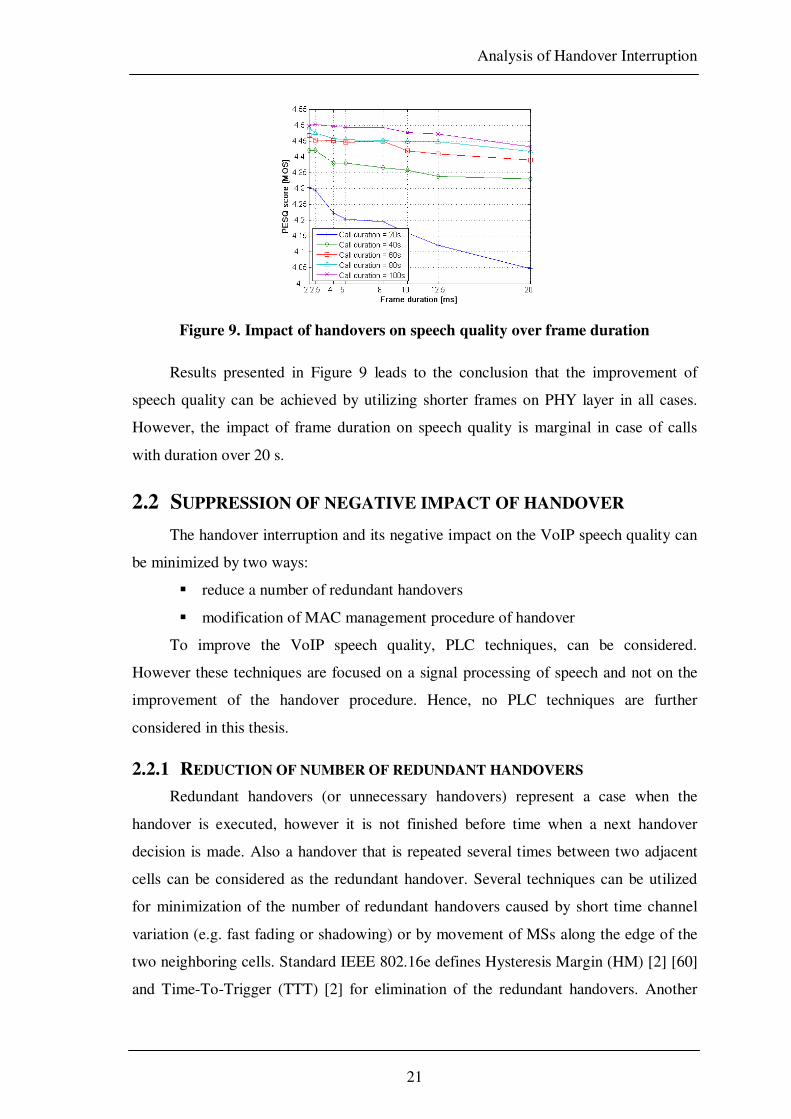
Considering results presented in Figure 7 and Figure 8, the negative impact of

frame duration on speech quality should be assumed. The exact evaluation of this effect

is presented in Figure 9. Five call durations (20, 40, 60, 80 and 100 s) and scenario B

are considered for evaluation.

The significant impact of frame duration is noticeable for short calls (20 s). The

difference in the speech quality between 2 ms and 20 ms frame durations is up to

approximately 0.25 MOS for this call duration. Increase of the call duration leads to the

less significant drop of the speech quality over the PHY layer frame duration. It is less

than 0.1 MOS in all other cases.


21

Figure 9. Impact of handovers on speech quality over frame duration

Results presented in Figure 9 leads to the conclusion that the improvement of

speech quality can be achieved by utilizing shorter frames on PHY layer in all cases.

However, the impact of frame duration on speech quality is marginal in case of calls

with duration over 20 s.

2.2 SUPPRESSION OF NEGATIVE IMPACT OF HANDOVER

The handover interruption and its negative impact on the VoIP speech quality can

be minimized by two ways:

� reduce a number of redundant handovers

� modification of MAC management procedure of handover

To improve the VoIP speech quality, PLC techniques, can be considered.

However these techniques are focused on a signal processing of speech and not on the

improvement of the handover procedure. Hence, no PLC techniques are further

considered in this thesis.

2.2.1 REDUCTION OF NUMBER OF REDUNDANT HANDOVERS

Redundant handovers (or unnecessary handovers) represent a case when the

handover is executed, however it is not finished before time when a next handover

decision is made. Also a handover that is repeated several times between two adjacent

cells can be considered as the redundant handover. Several techniques can be utilized

for minimization of the number of redundant handovers caused by short time channel

variation (e.g. fast fading or shadowing) or by movement of MSs along the edge of the

two neighboring cells. Standard IEEE 802.16e defines Hysteresis Margin (HM) [2] [60]

and Time-To-Trigger (TTT) [2] for elimination of the redundant handovers. Another


22

commonly used technique is windowing (known also as signal averaging) [60]. Last

method that will be considered is based on the similar principle as TTT. It is called

Handover Delay Timer (HDT) [77] [78]. All methods are based on delaying of the

handover for some time interval. During this interval, the MS is not connected to the

station providing the best quality of communication channel. Therefore, it has negative

impact on QoS provided to the MS due to the utilization of worse quality of the channel

than a quality available from other BS. On the other hand, each stand alone method

reduces the amount of redundant handover initiations.

2.2.1.1 TECHNIQUES FOR REDUCTION OF REDUNDANT HANDOVERS

The principle of all four techniques for reduction of amount of redundant

handovers is briefly introduced in following subsections.

2.2.1.1.1 HYSTERESIS MARGIN

The handover decision and initiation is based on a comparison of one or several

signal parameters (CINR, RSSI, Round Trip Delay (RTD) or relative delay) of a serving

and target BS. The handover is initiated if the signal parameter of target BS exceeds the

signal parameter of serving BS plus HM.

HMSS Ser

i

Tar

i+> (5)

where Ser

tS and Tar

tS represents a signal quality parameter of the serving and target

BS respectively.

The disadvantage of this principle is that it cannot eliminate rapid variation in

observed parameter (e.g. fast fading [79]). Moreover, it cannot cope with short time

shadowing with decrease of signal higher than HM as it compares only current values of

observed parameter.

2.2.1.1.2 TIME TO TRIGGER

The handover initiation is accomplished after short period within the signal

parameters from a target BS are higher than parameters of a serving BS. It can be

described by the following equation:

),( TTTtttSS HOHO

Ser

t

Tar

t +∈> (6)


23

where tHO corresponds to a time when the handover decision would be done if no

other technique for handover elimination is considered, and TTT is a duration of Time-

To-Trigger timer. Standard [2], enables to use TTT duration with following values:

TTT∈(0, 255 ms).

In comparison to the HM, this technique monitors signal parameters for a short

time interval. Therefore, it enables to deal with fast fading. On the other hand, a MS has

to monitor signal parameters for a whole duration of TTT. It leads to the reduction of

throughput during TTT. Furthermore, very low level of maximum duration of TTT

limits the effect of this technique (e.g. it cannot fully eliminate ping-pong effect or

shadowing with duration over 255 ms).

2.2.1.1.3 WINDOWING

The handover decision is done if an average value of observed signal parameter

from target BS drops under an average level of the same parameter at serving BS (see

formula (7)). The average value is calculated over a number of samples, denoted as

Window Size (WS).

WS

S

WS

SWS

i

Ser

i

WS

i

Tar

i ∑∑== > 11

(7)

The efficiency of elimination of redundant handovers that are result of ping-pong

effect, shadowing or fast fading depends heavily on the value of WS.

2.2.1.1.4 HANDOVER DELAY TIMER

Technique HDT is developed with purpose to cope especially with temporary

drop of a signal level due to fast fading or when a user is located on shadowed places

for a short time interval (longer than Reporting Period (RP)) [78]. Additionally, it

enables a reduction of ping-pong effect.

According to the IEEE 802.16e version of WiMAX [2], the handover starts

immediately after the channel conditions (e.g. signal levels) reach a threshold level.

However the handover must be canceled (if it has not finished yet) or must be

performed again (if it has finished) when a MS moves from the shadowed place.


24

Implementation of the HDT results into insertion of a short delay between the

time when handover conditions are met and the time when the handover initiation is

carried out (see Figure 10). This delay is noted as HDT (HDT=2×RP in Figure 10).

Figure 10. Handover initiation with HDT

These conditions for the handover have to be fulfilled over the whole duration of

HDT to execute handover initiation. Generally, the handover is performed only if:

)HDTt,t(tSS HOHO

Tar

t

Ser

t +∈< (8)

where HDT represents a duration of the handover delay timer.

As the signal level is measured and reported to the serving BS in discrete time

interval (not continuously), the handover decision is done if exact number of consequent

samples (nsamples) fulfills handover conditions as expresses the next equation:

)n,1(iSS samples

Tar

i

Ser

i ∈< (9)

The nsamples is equal to an amount of a channel quality reports sent during HDT

from the MS to the BS (nrep) as it is defined by the following formula:

rep

samplesn

HDTn = (10)

If the periodic reporting is considered, the reports are transmitted in regular time

intervals (equal to the reporting period RP). Then the nsamples can be derived as:

RP

HDTn

samples= (11)

As the HDT is based on the TTT, only HDT is considered for further evaluations.


25

2.2.1.2 IMPACT OF HM, HDT AND WINDOWING ON MS'S THROUGHPUT

All above mentioned techniques enable to reduce a number of handovers [80], however

it is at the cost of decrease of throughput since all of them results in a postponement of

handover execution. The delay of handover execution leads to the utilization of lower

Modulation and Coding Scheme (MCS) [2] for communication between a MS and its

serving BS. The impact of HM, HDT and windowing on the user's throughput is

investigated for scenario with single MS (see Figure 11).

Figure 11. Scenario for evaluation of impact of all techniques on throughput

The MS moves along the straight line crossing 5 BSs. Speed of the MS is 10 m/s.

The scanning reporting period is setup to 0.5 s since this value is close to an optimum

scanning interval for maximization of throughput [81]. All parameters for evaluation are

summarized in Table 4.

Table 4. Simulation parameters for evaluation of throughput of single MS

Parameter Value

Number of BS [-] 5

Number of MS [-] 1

BS transmitting power [dB] 36

BS height [m] 32

MS height [m] 2

MS speed [m/s] 10

Frequency band [GHz] 2.5

Frame duration [ms] 20

Data subcarriers per sub-channel 48

OFDMA symbols per frame 198

Bandwidth [MHz] 20

Hysteresis Margin [dB] 0-20

Window Size [samples] 1-20

Duration of HDT [s] 0-5

Scanning reporting period [s] 0.5

Path loss model 802.16m Urban Macrocell


26

The throughput of single MS is calculated based on the received signal quality.

The full buffer traffic model is assumed. It means that the MS has always a full queue

of data to transmission. This model is often used in simulation as it enables to evaluate

maximum efficiency of a system [82]. The strength of received signal is used for a

calculation of number of data carried per one downlink sub-channel (Data Per Sub-

channel − DPS).

CRNNoDSCDPSob

××= (12)

where NoDSC express a number of data subcarriers per a sub-channel in PUSC

(Partial Usage of Sub-Channels) OFDMA (Orthogonal Frequency Division Multiple

Access), CR represents Code Rate and Nob is a number of bits carried per one subcarrier

(depending on used modulation scheme). The Nob is derived from the next equation:

)N(logNStatesob 2= (13)

where Nstates is a number of modulation states.

Every frame can be divided into sub-channels and a number of frames transmitted

per second depends on the frame duration (FD). Therefore, the final bit rate in each step

(BRstep) can be evaluated by the following way:

FD

SPFDPSBR

step

×= (14)

where SPF represents number of sub-channels per frame.

The average throughput over the simulation duration (AvgBR) is calculated as a

weighted average of the all throughput obtained during simulation (see consequent

formula).

( )

SimD

StDBR

AvgBR

stepsN

Step

Step∑=

×

=1

(15)

where StD is a duration of a simulation step, SimD is a duration of whole

simulation and Nsteps represent overall number of steps during simulation. It can be

calculated according to the following equation:

StD/SimDN steps = (16)


27

Figure 12 and Figure 13 show results of the impact of HDT and windowing on the

throughput of single MS. The evaluation considers several levels of HM. Significant

decrease of the MS's throughput is noticeable form both figures especially with

increasing HM. In both cases, the reduction of throughput for low HM is not so rapid if

shorter duration of HDT or lower amount of averaged samples are considered. On the

other hand, the fall of throughput over the duration of HDT or WS is getting more linear

for higher level of HM.

The impact of only HM is depicted in Figure 14. The HM leads to the minor drop

of throughput at lower levels of HM. Then the reduction of MS’s throughput is more

significant.

Note that the impact of all techniques on throughput depends heavily on a

deployment of BSs described by function ΘBS and on a time interval between two

handovers (HOper). The HOper is influent by a speed of user (υMS) and a movement of

user (χMS). Therefore, the average bit rate can be expressed as the following function:

( )MSMSBSperBS ,,f)HO,(fAvgBR χνΘ=Θ= (17)

Higher υMS, higher density of BSs and more direct movement of MSs among BSs

leads to the decrease of the negative impact of all these techniques on the throughput of

single MS.

Combined efect of HDT and WS over HM on the throughput is depicted in Figure

15. The figure shows that the incresing of one of parameter while the others are constant

leads to nearly linear reduction of the throughput (compare the spacing between lines

with same color or with same marker at the constant HM).

Figure 12. Impact of HDT duration on throughput of single MS

Figure 13. Impact of Window Size on throughput of single MS


28

Figure 14. Impact of HM duration on throughput of single MS

Figure 15. Joint impact of HDT and WS on throughput of single MS

2.2.2 MODIFICATIONS OF HANDOVER MAC MANAGEMENT PROCEDURE

The second way of the reduction of handover interruption is to modify a flow of

MAC management message during the handover procedure. A lot of papers deal with

this idea as stated in section 1.2.3. Generally, minimization of the handover interruption

can be achieved either by a reduction of number of MAC management messages

exchanged during the handover or by a shifting of a part of the handover before time

when a MS close connections with serving BS. The way based on performing of a part

of the handover procedure before the MS closes all connections with serving BS can

exploits results of prediction of target BS (see section 1.2.2).

The prediction of the handover as well as the approach based on utilization of

prediction results with purpose to reduce the handover interruption are further analyzed

in the followings chapters of this thesis (chapter 3 and 4).

2.3 CONCLUSION

The duration of interruption caused by hard handover depends on the duration of

following stages: synchronization of a MS to a target BS, contention resolution and

network re-entry. The duration of each particular stage depends on the number of MAC

management messages exchanged between both stations and on the frame duration

utilized on PHY layer of WiMAX system. Moreover, another factor that influents the

handover interruption is a number of SA. The duration of handover interruption linearly

increases as rises the number of SA. Conventional handover procedure according to

IEEE 802.16e can fulfill requirements on the handover procedure defined in [17] only


29

for scenario with assumption of “optimal handover” and with the frame duration equal

to 2 ms.

Not only the handover interruption but also network delay must be considered to

determine the impact of handover interruption on VoIP speech quality. The speech

quality is decreased by the handover interruption. The level of speech quality

degradation depends on the duration of handover interruption as well as on the duration

of call within just one handover occurs. The result shows that the handover interruption

has negative impact on the speech quality even for its short durations and long-lasting

calls. Nevertheless, the average speech quality is increasing with shortening the

handover interruption.

The abovementioned results lead to the assumable conclusion that the speech

quality is influenced by the frame duration. The simulation results of the impact of

frame duration on the speech quality confirm this assumption. Rise of the speech quality

by utilization of shorter frames is reach over all call durations. Additionally, decreasing

of the positive impact of frame duration on speech quality with prolonging call duration

can be observed from presented results. However, the significant speech quality

improvement (0.25 MOS) is achieved only for call duration of 20 s. The calls with

duration over 20 s show only marginal increase of the speech quality (less than

0.1 MOS).

Moreover, the negative impact of handover can be minimized by reduction of a

number of handovers or by modification of MAC management message flow. The first

approach utilizes techniques developed exactly for this purpose. All of these techniques

lead to the postponement of the handover execution time instant. Hence, it results to the

decrease of MS’s throughput.

Following parts of the thesis are focused on the reduction of handover interruption

by approach based on the possible modification of handover procedure. A prediction of

target BS is considered as technique that can enable to cope with the handover

interruption.

Handover Prediction

30

3 HANDOVER PREDICTION

The minimization of handover interruption or minimization of overhead

generated due to the handover procedure can be accomplished by a prediction of

handover.

The prediction of handover is a process of estimation of next target BS for a

moving MS. Knowing in advance the target BS allows modifications in a handover

management that lead to a fast handover with minimal interruption. Besides, it allows a

reduction of MAC management overhead due to optimization of a list of neighboring

stations for scanning.

3.1 PRINCIPLE OF PREDICTION

Generally, the prediction of target BS can be based on several approaches. The

first one is a monitoring of pairs of serving and corresponding target BSs of MS's

handover in the past. The second approach is a handover prediction based on

characteristics of communication channel. The last way of the prediction is based on

knowledge of user's position and position of all neighboring BSs. The objective of the

last type of prediction is usually to forecast future motion of MS.

3.1.1 HANDOVER HISTORY

The prediction based on handover history utilizes results of a monitoring of pairs

of serving and corresponding target BSs of MS's handover procedure in the past. This

method requires to monitor and register all updates of the serving and target BSs of all

MSs in network. It means, if a MS performs handover, identification of the serving and

target BSs are stored into memory.

Handover history based prediction can be managed either by a MS or by BSs (by

network). However, as the MS has no access to up to date information on the handover

of another MSs, it is more efficient to manage it by BSs. Furthermore, the management

of prediction by the MS leads to the prolonging of time necessary for collection of

enough information in order to guarantee high probability of successful prediction.

Amounts of the handovers among BSs are represented by a matrix (see example

in Table 5). The matrix has the same number of rows (x) and columns (y). The number

of rows and columns corresponds to a number of neighboring BSs. Every field of the

Handover Prediction

31

matrix represents a count of handovers between BSx (serving BS) and BSy (target BS)

within observed time interval. For example, the field in the third row and sixth column

represents the amount of handovers from BS3 to BS6 (79 handovers). A number of

handovers performed in the opposite direction (from BS6 to BS3) is presented by field

in the sixth row and third column (21 handovers).

Table 5. Example of matrix representing number of handovers among BSs

HO count.

BS1 BS2 BS3 BS4 BS5 BS6 BS7

BS1 x 31 0 35 34 0 0

BS2 16 x 51 33 0 0 0

BS3 0 18 x 3 0 79 0

BS4 28 41 13 x 8 6 4

BS5 11 77 0 0 x 0 12

BS6 0 0 21 13 0 x 66

BS7 0 0 0 20 23 57 x

The situation that corresponds to Table 5 is depicted in Figure 16 for scenario

with 7 BSs.

BS 4

BS 5 BS 6

BS 1 BS 3

BS 2

BS 7

0,13

0,03

0,06

0,04

0,13

0,20

0,08

0,77

0,35

0,28

0,33

0,51

0,18

0,41

0,79

0,21

0,66

0,57

0,23

0,12

0.31

0,16

0,11

0,34

Figure 16. The probabilities of handover among neighboring BSs

The matrix of number of handovers is recalculated to the probability of handover

from a serving BSx to a target BSy (Px,y) according to the following formula:

Handover Prediction

32

∑∈

=

xNSy

y,x

y,x

y,xHO

HOP

(18)

where HOx,y represents a number of handovers form BSx to BSy; all neighboring

BSs of BSx are included in so called Neighbor Set of BSx denoted in thesis as NSx.

Based on the NS, the probability of handover from BSx to BSy can be rewritten as:

∉

∈=

x

x

yxNSy

NSyP

,0

,,

α (19)

where 10 ≤≤ α . The α depends not only on the number of BSs in the NS but also

on the layout of area where the situation is analyzed and monitored.

An example of the matrix of probabilities calculated according to Table 5 and

equation (18) is shown in Table 6.

Table 6. Matrix of handover probabilities among BSs

HO prob.

BS1 BS2 BS3 BS4 BS5 BS6 BS7

BS1 x 0.31 0 0.35 0.34 0 0

BS2 0.16 x 0.51 0.33 0 0 0

BS3 0 0.18 x 0.03 0 0.79 0

BS4 0.28 0.41 0.13 x 0.08 0.06 0.04

BS5 0.11 0.77 0 0 x 0 0.12

BS6 0 0 0.21 0.13 0 x 0.66

BS7 0 0 0 0.20 0.23 0.57 x

Figure 16 assumes the close area with no possibility of accomplishing the

handover to another BS except BS1 – BS7. The situation when all MSs performing

handover during monitored time interval is assumed. Thus, the sum of all probabilities

in rows of Table 6 is always equal to 1 as expresses the next equation:

1== ∑∈∀

=

xNSyy

y,xconstxy,xPP (20)

If the real system in which every BS has defined NS is considered, sum of the

probabilities of MS's handover from BSx to one of all neighboring BSs tends to 1 since

Handover Prediction

33

the handover in infinite future ( ∞→t ) is assumed. The probability can be lover than 1

if ∞<t since the MS can never perform handover. Therefore, the handover probability

between BSx and all neighboring BSs over finite and infinite time interval is:

10

1

,PP

PP

NSxyy

t

y,xty,x

NSxyy

y,xty,x

∈=

==

∑

∑

∈∀∞<

∈∀∞=

(21)

where ty,xP is a function of time t and NNSx represents a number of BSs in the NS

of BSx.

3.1.2 CHANNEL CHARACTERISTICS

The approach that uses channel parameters or characteristics to predict a target BS

assumes to store results of scanning of MSs’ neighborhood. Based on the stored

information, typical thresholds for the handover between two neighboring BSs are

derived. The results can be stored either in MSs or in BSs. Therefore, the prediction can

be done either by the MSs or by the BSs. Nevertheless, since a lot of data have to be

kept in station’s memory, it is preferred to perform prediction by the BSs due to a

memory limitation of MS. Further, the BSs can collect information from all MSs (BSs

has knowledge about all handovers in the network) whereas the MS can collect only

information on itself. The collection of information by the MS results in significant

prolonging of time necessary for collection of enough information in order to guarantee

high probability of successful prediction as in case of the prediction based on handover

history.

The typical thresholds are based on the observation of channel characteristics

corresponding to the signal level that triggers handover initiation. Figure 17a depicts

RSSI between a MS and several BSs during the MS's movement along a straight line

(red dashed trajectory in Figure 17b). The speed of MS is 20 m/s and observation time

is 100 s, i.e. the distance covered by the MS within one observation cycle is 2000 m.

Each curve in Figure 17a represents the set of RSSIs received by the MS from all BSs

obtained within several movements of the MS. Minor fluctuation of RSSI is caused by

variations of channel parameters among all runs of the MS. Simulation parameters and

channel model are taken from [18].

Handover Prediction

34

Usually, only one threshold for handover decision is defined as described e.g. in

[2] [26] [59]. The proposed improvement of this technique is based on definition of two

thresholds as depicted in Figure 17a.

Following two thresholds are defined: HO_ThrSerX,Y and HO_ThrTarX,Y. The first

one represents a typical RSSI level of serving BSx when a handover to target BSy is

initialized (see Figure 17a where the serving BS is BS4 and the target BS is BS2 at the

beginning phase of the MS's movement). The second threshold corresponds to a typical

RSSI level of the predicted target BSy when the MS initiates the handover from serving

BSx. Both threshold levels are usually very close in the most cases in praxis. In

principle, the level of HO_ThrTarX,Y is slightly higher as the handover decision is

generally done only if the target BS can provide higher quality of connection than the

serving BS. Moreover, both thresholds also differ due to non-stationary signal levels.

The monitoring and evaluation of signal evolution from all neighboring BSs is

performed in the following manner:

� If RSSI from the serving BS decreases and draws near to the HO_ThrSerX,Y,

the probability of handover from BSx to BSy increases (in Figure 17a BSx is

BS4, BSy is BS2 and HO_ThrSerX,Y is HO_ThrSer4,2).

� If RSSI from one of neighboring BSs increases and draws near to the

HO_ThrTarX,Y, the probability of handover from BSx to BSy increases (in

Figure 17a HO_ThrTarX,Y is HO_ThrTar4,2).

(a)

(b)

Figure 17. Definition of handover threshold (a) based on movement of MS along the same direction (b)

Handover Prediction

35

� If RSSI of the serving BS decreases under HO_ThrSerX,Y and simultaneously

RSSI of a neighboring BS exceeds HO_ThrThrX,Y, the result of prediction is

an estimation of MS’s handover from the BSx to BSy. It means, the BSy is

identified as “predicted target BS”.

Both groups of thresholds for each pair of BSx and BSy (thresholds HO_ThrSerX,Y

and thresholds HO_ThrThrX,Y) are averaged out in order to find one specific value for the

serving BS threshold as well as one value for the target BS threshold. The mean values

of typical thresholds for handover are calculated as an average of several previous

signal levels that leads to the handover initiation. Determination of sufficient number of

signal level samples is an object of investigation addressed further in this thesis. The

values of samples' signal level are obtained within MS’s scanning of its neighborhood.

The mean thresholds can be described by the next equations:

BSX,BSY

HOCount

1i

MS,BSX

SerX,YHOCount

RSSI

AvgHO_Thr

BSX,BSY

∑==

(22)

BSY,BSX

HOCount

i

BSY,MS

Y,TarXHOCount

RSSI

Thr_AvgHO

BSY,BSX

∑== 1

(23)

where HOCountBSX,BSY represents a number of handovers occurred between the

current serving BS and potential target BS during observed time interval.

The target BS cannot be predicted according to an exact level of typical thresholds

since the prediction would be done too late (not enough time in advance to exploit

results of prediction). Therefore, the handover should be predicted if the parameters of

channel between the MS and the serving and target BS are within intervals of HOZone

defined by following formulas:

BSXMSZoneYSerX RSSIHOThrHO ,,_ <+ (24)

BSYMSZoneYTarX RSSIHOThrHO ,,_ >− (25)

where HOZone represents an interval where the BSy is marked as the predicted

target BS (see Figure 17a), RSSIMS,BSX and RSSIMS,BSY correspond to a signal level

received by the MS from the serving and target BS respectively.

Handover Prediction

36

According to the NS, the probability of handover from BSx to BSy can be

formulated, likewise in the case of prediction based on the handover history, by the

consequent equation:

∉

∈=

x

x

yxNSBSy

NSBSyP

,0

,,

α (26)

where 10 ≤≤ α . The α depends not only on the number of BSs in NS but also on

the layout of area where the prediction is analyzed and monitored (e.g. layout of streets,

deployment of buildings and transmitters, etc.).

The Px,y is a function of HOZone as well as a function of current values of

RSSIMS,BSX and RSSIMS,BSY. If the α represents a value of probability Px,y, the

probability of handover from BSx to all BSs excluding BSy ( yxP , ) is 1-α. The

probability of case when the MS will not handover to the predicted BSy ( yxP , ) in spite

of the fact that the BSy fulfills the conditions according to (24) and (25), is expressed by

ξ function. This can happen e.g. when the MS randomly turns away from the assumed

direction. Then the probability of handover from BSx to BSy could be described by a

function formulated in the owing way:

),,,( ,,, ξZoneBSXMSBSXMSyx HORSSIRSSIfP = (27)

The ξ is directly proportional to the probability that the MS will not change

direction in subsequent time interval τ so significantly that the MS would perform

handover to the different BS. This probability is labeled as SD

MSP . Thus, the ξ can be

formulated as:

),( SD

MSPf τξ = (28)

and τ is a function of speed and distance as imply the next formula:

),( ,cellMSMS Distvf=τ (29)

where vMS is a velocity of the MS and DistMS,cell is a distance of the MS from the

place where the handover should be executed. Then the equation (27) can be rewrite as

follows:

Handover Prediction

37

)P,Dist,v,HO,RSSI,RSSI(fP SD

MScell,MSMSZoneBSX,MSBSX,MSy,x = (30)

The previous formula can be expressed in other way as the probability of

successful prediction of target BSy if the MS is moving out of the coverage area of

serving BSx. It is obvious that the probability of successful prediction is increasing

either with lowering DistMS,cell or with decreasing of difference between actual values of

RSSIMS,BSx and AvgHO_ThrSerX,Y as well as RSSIMS,BSy and AvgHO_ThrTarX,Y. On the

other hand, drop of SD

MSP or vMS can lower the probability of successful handover

prediction. The impact of HOZone is investigated later in this thesis.

Since the MS can arrive into the area in which more than one potential target BS

fulfill the conditions for prediction, a mechanism for selection of just one predicted

target BS should be defined. This mechanism is based on the calculation of minimum

difference of both thresholds (AvgHO_ThrSerX,Y and AvgHO_ThrSerX,Y) and current

RSSIs between the MS and serving and target BS. This is done for all possible target

BSs with RSSI values in the range defined by (24) and (25). These stations are listed in

ListOfTargetBS. The decision about target BS that will be labeled as the predicted target

BS is done according to the results of next equation:

BSYMSYTarXBSXMSYSerXBSYBSX RSSIThrAvgHORSSIThrAvgHODiff ,,,,, __ −+−= (31)

The differences of RSSI levels and thresholds for each of potential target BS are

compared afterwards and as the predicted target BS is selected the BS with minimum

DiffBSX,BSY (see next formula).

{ } )etBSListOfTargmin(etBSListOfTargYargetBSPredictedT Y == (32)

Other signal quality parameters such as CINR or SNR (Signal to Noise Ratio) or

other parameters that express the quality of channel between a MS and BS can be used

for prediction instead of RSSI. The parameter utilized for prediction has to correspond

to the metric used in scanning reports sent by the MS to serving BS (see [2]).

To achieve as high prediction efficiency as possible, the techniques for reduction

of redundant handovers (HM, HDT and Windowing) are considered and their impact is

analyzed later in the thesis.

Handover Prediction

38

3.1.3 MOTION OF MS

This type of prediction is based on the monitoring of users geographic location.

The general approach is to determine consequent positions of MSs based on its

movement in past as it is addressed e.g. in [44].

Three general assumptions must be fulfilled for efficient motion prediction of MS

[49]:

� knowledge of current and previous exact positions of the MS

� knowledge of users profile

� knowledge of profile of area in which the prediction is performed

The knowledge of exact position implies a utilization of localization equipment

such as GPS (Global Positioning System) [83] to ensure exact determination of MS's

position.

The second bullet results to requirement of acquisition of user’s information such

as area of interests, favorite places, time schedule, etc. It means that each user has to fill

up this information and keep it updated.

Last assumption requires the knowledge of real maps of area in which the

prediction is executed. This information can be acquired by a provider of network

connection and must be also keep updated. This principle of utilization of real maps is

depicted in Figure 18. The MS is connected to BS3, when it comes to the cross, it

should turn to the left or right. Then the knowledge of MS's direction enables to predict

target BS (turn to right or left leads to the prediction of BS2 or BS1 respectively).

Figure 18. Utilization of map's knowledge to target BS prediction

Fulfillment of all above mentioned assumptions lead to very high demands on

user, MS and network and it also makes the prediction not much comfortable for users.

Therefore, the prediction of MS’s movement is not furthermore an object of

investigation in this thesis.

Handover Prediction

39

3.2 SCENARIOS FOR EVALUATION OF HANDOVER PREDICTION

EFFICIENCY

The efficiency of target BS prediction is evaluated for specific scenarios

depending on the type of prediction.

3.2.1 HANDOVER HISTORY

A street scenario corresponding to the Manhattan Mobility Model (MMM) [84]

(see Appendix C2) is used for the simulation of efficiency of handover prediction based

on the handover history. The parameters of simulation scenario are presented in Table 7.

Table 7. Simulation parameters and scenario definition for handover history

Parameter Value

Number of BS [-] 15

Number of MS [-] 48


BS height [m] 32

MS height [m] 2

MS speed [m/s] 15



Scanning reporting period [s] 1

Simulation duration [s] 10800

Hysteresis margin [dB] 1

Path loss model 802.16m LOS/NLOS

Urban Microcell

Mobility model Manhattan

Turn Probability [-] 0.5 / 0.75 / 0.9 / 1

Number of vertical streets [-] 10

Number of horizontal streets [-] 11

Street width [m] 30

Size of block of building [m] 200 x 200

Size of simulated area [m] 2330 x 2100

The BSs are deployed regularly as presented in Figure 19. All BSs are placed in

streets, not on roofs of buildings. The 48 MSs is randomly dropped in the streets at

initiation of simulation. The signal strength among all MSs and BSs is calculated using

urban microcell path loss model defined by [18] (see Appendix B2). This model

distinguishes if a line of sight (LOS) between a MS and BS is enabled or not (Non-LOS

Handover Prediction

40

communication denoted as NLOS) [85]. The signal levels are calculated at each interval

of reporting of scanning results. It corresponds to the determination of parameters at

each second in abovementioned scenario.

Figure 19. Simulation scenario for handover prediction evaluation

Four different varieties of mobility model are defined to compare results of the

prediction. The first one represents conventional MMM with turn probability (TP) of

0.5. It means that each MS selects its next direction at each cross with 1−TP (= 0.5)

probability of direct movement and TP/2 (= 0.25) probability of turn to right and same

probability of turn to left. Next three scenarios define so called “Main Street” (red

vertical street no. 6 with x coordinate equal to 1165 m in Figure 19). The TP of a MS is

0.5 at all streets excluding the Main Street. While the MS comes to the cross with the

Main Street, the turn probability of belonging MS temporarily increases to TPMS = 0.75,

0.9 or 1 for three scenarios respectively. If the MS is moving on the Main Street, the

probability of direct movement is increased to TPMS (Turn Probability − Main Street)

and the probability of turn out of the Main Street is equal to 1-TPMS. The turn

probability is set back to TP while the MS reach end of the Main Street or if the MS

leaves the Main Street. This situation corresponds much more to the real movement in

the city centre with one busy street or with a main square.

Handover Prediction

41


The prediction of target BS based on channel characteristics is evaluated for

scenario where RSSI parameter is observed (as described in theoretical analysis in

section 3.1.2). The simulation parameters are summarized in Table 8.

Table 8. Simulation parameters and scenario definition for channel characteristics

Parameter Value

Number of BS [-] 15

Number of MS [-] 48


BS height [m] 32

MS height [m] 2

MS speed [m/s] 15



Scanning reporting period [s] 1

Simulation duration [s] 10800

HOZone[dB] 0−16

Hysteresis margin [dB] 4/8/12/16/20

HDT [s] 1/2/3/4/5

Window Size [samples] 5/8/10/15/20

LOS/NLOS path loss model 802.16m Urban Macrocell

Shadowing and channel variation 802.16m; σ = 0/0.3/0.6/0.8

Mobility model PRWMM

Size of simulated area [m] 2330 x 2100 (4.89km2)

All BSs are deployed in symmetric manner as presented in Figure 20. All BSs are

placed in the same height and all transmits wit the same power level. At the beginning

of simulation, the position of all 48 MSs is randomly generated. Probabilistic Random

Walk Mobility Model (PRWMM) [86] (see Appendix C1) is considered for the MSs’

movement. Signal strengths among all MSs and BSs are calculated using urban

macrocell path loss model defined in [18] (see Appendix B1). The signal parameters are

evaluated at each scanning reporting period which corresponds to the enumeration of

parameters every second in used scenario.

Handover Prediction

42

Figure 20. Deployment of BSs in the simulation

Several sets of simulations are performed considering different kind of scenarios.

The first one analyzes the impact of HOZone on the prediction efficiency if no other

technique for efficiency improvement is considered (i.e. HM, HDT or Windowing).

Next three sets of simulations are focused on analysis of the impact of individual

techniques on prediction efficiency. The last one determines an optimum setting of all

three techniques in cooperating mode to obtain maximum prediction efficiency.

Three parameters, from the analysis of results point of view, are considered: ratio

of successfully predicted handover HR (Hit Ratio), ratio of not predicted handovers

(NPR) and ratio of wrong prediction (WPR). The handover prediction is assumed to be

successful if the MS executes the handover to the predicted target BS. The number of

successfully predicted handover (SPHO) is used for calculation of prediction hit ratio

according to the following formula:

HOCount

SPHR HO= (33)

where HOCount represents a total number of all handovers in network. It can be

calculated as:

BSYBSX,HOCountHOCountBSCount

1BSX

BSCount

1BSY

BSX,BSY ≠= ∑ ∑= =

(34)

where BSCount is a total number of BSs in the network.

Not predicted handover occurs when the handover is done despite of the fact that

no target BS has been predicted since a time when the MS have performed previous

handover. This situation happens especially at the beginning of simulation as not

Handover Prediction

43

enough data is collected to successfully predict target BS (typical thresholds cannot be

setup since there are still either no information on previous handovers at all or the

gathered information are insufficient). The ratio of not predicted handovers is calculated

by the subsequent way:

HOCount

NPNPR HO= (35)

where NPHO is a total number of not predicted handovers.

An error in prediction (wrong prediction) occurs if the predicted target BS differs

from the real target BS of the MS. The ratio of wrong predictions can be expressed by

the following equation:

HOCount

WPWPR HO= (36)

where WPHO is a total number of wrong predictions of handover.

3.3 RESULTS

3.3.1 HO HISTORY

Simulation results are presented in Figure 21 – Figure 24. The probability of MS’s

handover from the BS8 to all neighboring BSs (BS4, 5, 7, 9, 11 and 12) is presented in

Figure 21a – Figure 24a.

The scenario with no Main Street (Figure 21a) shows that time required to collect

enough information on handovers is approximately 2000 s Then the probability is

getting stable and do not vary rapidly. Totally, about 2000 handovers occur per 1000 s

of simulation. The maximum efficiency of successful prediction corresponds to the

probability of handover as no other criterion is considered for the prediction. Therefore,

it can be assumed equal after the probability curves get stable. Based on Figure 21a can

be observed that BS12 is the most probable target BS for MS’s handover from BS8.

However the handover probability from BS8 to BS12 is only approximately 25%. The

lowest probability of the handover from the BS8 is to BS7 and BS9 (roughly 10%).

That low probability results to very low efficiency of the prediction.

The maximum efficiency of target BSs prediction for all serving BSs are

presented in Figure 21b. It expresses a ratio between efficient and failed target BS

prediction. Each curve corresponds to the one serving BS. Hence every curve copies the

Handover Prediction

44

maximum value of prediction probability for appropriate BS (e.g. maximum of all

curves in Figure 21a corresponds to the blue dash line in Figure 21b).

(a)

(b)

Figure 21. Results of handover prediction for no Main Street (a) Handover probability over duration of handover history collection for BS8

(b) Maximum probability of handover from all serving BS over observation time

The presence of Main Street results into an increase of ratio of correct target BS

prediction for a MS moving from the serving BS8 (see Figure 21b – Figure 24b) from

25% with no Main Street to nearly 45% with mostly visited Main Street (TPMS = 1).

The example of handover probability from BS8 shows an increase of handover

probability to BS7 or BS9 since both are neighbor BSs of BS8 deployed on the Main

Street. The probabilities of handover from BS8 to BS7/BS9 rise from 10% for no Main

Street to 40% for the mostly visited Main Street.

(a)

(b)

Figure 22. Results of handover for Main Street TP = 0.75 (a) Handover probability over duration of handover history collection for BS8


Handover Prediction

45

(a)

(b)

Figure 23. Results of handover for Main Street TP= 0.9 (a) Handover probability over duration of handover history collection for BS8


(a)

(b)

Figure 24. Results of handover prediction for Main Street TP = 1 (a) Handover probability over duration of handover history collection for BS8


From Figure 21b – Figure 24b can be further observed that the maximum ratio of

successful target BS prediction is achieved for the prediction of handover from BS6

(about 47%) and BS10 (about 42%). The lowest ratio is attained while the MS is

connected to the serving BS8 and BS9 (both about 25%). It leads to the conclusion that

the efficiency of target BS prediction depends on the number of neighboring BS (BS6

and BS10 have only 3 neighboring BSs however BS8 has 6 neighboring BSs).

The impact of number of neighboring BSs on the target BS prediction efficiency

depicted in Figure 25. The efficiency is significantly decreasing if the number of

neighboring BSs is increasing for scenario without Main Street (TP = 0.5) and with

Main Street with TPMS = 0.75 and TPMS = 0.9. In these scenarios, the ratio of

Handover Prediction

46

successfully predicted target BS decreases from about 45% to 24% while the number of

neighboring BSs rises from 3 to 6. In case of the Main Street with TPMS = 1, the

handover probability decreases only up to 4 neighboring BSs and then the increasing

number of neighbor BSs does not influent the efficiency of prediction. All evaluations

of the impact of neighboring BS count on the prediction efficiency are performed with

the same deployment of BSs as presented in Figure 19.

Figure 25. Efficiency of target BS prediction over number of neighboring BSs


Results obtained by simulations are separated into subsections according to the

techniques that are investigated.

3.3.2.1 DETERMINATION OF OPTIMAL HOZONE FOR RSSI BASED PREDICTION

Firstly, the impact of HOZone on prediction efficiency is analyzed. The results of

simulation are shown in Figure 26 and Figure 27. Both figures present the results of

handover prediction hit ratio, ratio of not predicted handovers anf ratio of wrong

prediction.

It is evident that if the ratio of wrong prediction together with the ratio of not

predicted handovers is decreasing, the overall ratio of successful prediction is increasing

proportionally. The time instant when sufficient number of data is collected is

approximately 1000 s (at that time, roughly 2000 handovers is already performed within

the simulation; it is roughly 10 handovers between each pair of neighboring BSs). At

this stage, the ratio of successful handover prediction (handover prediction hit ratio)

gets stable. The "get stable" means that the prediction ratio does not vary more than

±5% during following 3600 s.

Handover Prediction

47

Figure 26. Results of handover prediction based on the RSSI evolution, no channel variation

Figure 27. Results of handover prediction based on the RSSI evolution, with shadowing and channel variation (σσσσ = 0.8)

Individual presented figures differ in diverse parameters setting of channel model.

While Figure 26 assumes that the handover prediction is done only according RSSI

evolution, Figure 27 takes further into consideration another factor, i.e. channel

variation with standard deviation, σ = 0.8 [18] and shadowing, (see Appendix B3 and

B4). Windowing, HDT and HM are disabled in Figure 26 and Figure 27.

Overall results of the prediction hit ratio acquired during 3 hours (10 800 s) data

collection are summarized in Figure 28. This figure considers also other levels of

channel variation, i.e. σ = 0.3 and σ = 0.6. The maximum prediction hit ratio

(approximately 71%) is achieved if the channel variation is not considered. The higher

channel variation degrades maximum prediction hit ratio to 45%/41%/37% for

Handover Prediction

48

σ = 0.3/0.6/0.8 respectively. Additionally, Figure 28 demonstrates that the prediction

and its effectiveness significantly depend on the HOZone size. The prediction efficiency

is under 10% if no HOZone is taken into account. The optimal value of HOZone observed

from Figure 28 is 4 dB for all levels of channel variation. At this HOZone level, the

prediction mechanism shows highest ratio of successfully predicted target BS (71%)

and low ratio of not predicted (14%) and wrongly predicted handovers (15%) if no

channel variation is introduced. Figure 29 depicts that the channel variation increases

the ratio of not predicted handovers slightly over 30% for all levels of σ at

HOZone = 4 dB. The impact of channel variation level on ratio of not predicted

handovers is negligible. The ratio of the wrong prediction also rises to 25%/28%/31%

for σ = 0.3/0.6/0.8 respectively at HOZone = 4 dB (see Figure 30).

Figure 28. Target BS prediction hit ratio over HOZone

Figure 29. Ratio of not predicted handover over HOZone

Figure 30. Ratio of wrongly predicted target BS over HOZone

In the rest of simulations where a comparison of impact of windowing, MH and

HDT is addressed, the channel variation with σ = 0.8 will be taken into account (in

Handover Prediction

49

figures denoted as “CV on”). The results of scenario with not considered channel

variation (in figures denoted as “CV off”) are also depicted in following figures to

enable a comparison of results. The detailed behaviors of prediction ratios over

simulation time, as depicted in Figure 26 – Figure 27, are not presented in the following

subsections since the overall results are presented in form of separated results for hit

ratio, not predicted handover ratio and ratio of wrong prediction. This form of figures is

more transparent. If not stated otherwise, the ratio of successful handover prediction

gets stable approximately after 1000 s of simulation.

3.3.2.2 IMPACT OF WINDOWING ON PREDICTION EFFICIENCY

In order to suppress the negative impact of channel variation on prediction or to

increase the prediction efficiency, technique based on averaging of several samples of

RSSI (Windowing) can be used. Figure 31 illustrates that the prediction hit ratio is

distinguishable increased by windowing even if the channel model including channel

variation (σ = 0.8) is assumed (see appendix B). The WS is set to 5, 8, 10, 15 and

20 samples. The utilization of windowing technique with WS = 5 results in a rise of hit

ratio from 37% to 65% (38% increase of hit ratio) in comparison to the case with no

windowing. In the rest of this chapter, if the gain is for example 10%, it means that the

hit ratio increases e.g. from 50% to 60%.

Additional gain of 6% is introduced when the size o WS is further increased to

8 samples. In this case, the impact of channel variation is eliminated and the prediction

hit ratio for channel variation with σ = 0.8 and WS = 8 is equal to scenario with no

channel variation and no windowing. In both cases, maximum prediction hit ratio is

71%. Another gain of 2% and 5% is observed by increasing WS to 10 and 15 samples

respectively. The results for WS = 20 shows only marginal increase of the prediction hit

ratio. This indicates that further increase of WS is useless.

Analogical conclusions can be derived from Figure 32 and Figure 33. Figure 32

shows no noticeable decrease of not predicted handovers ratio for WS above

15 samples. Similarly, Figure 33 presents only marginal decrease of wrong prediction

ratio while higher values of WS than 15 samples are utilized. As it can be observed, the

number of not predicted handovers is decreasing while the level of HOZone is rising

since larger HOZone enables to perform the prediction earlier. However, sooner

prediction leads to the increase of ratio of wrong prediction as well. It is due to early

Handover Prediction

50

prediction that results to higher probability of MS's turn away from current direction

(see equation (30)).

Figure 31. Target BS prediction hit ratio over HOZone for a set of WS

Figure 32. Ratio of not predicted handover over HOZone for set of WS

Figure 33. Ratio of wrongly predicted target BS over HOZone for set of WS

3.3.2.3 IMPACT OF HYSTERESIS MARGIN ON PREDICTION EFFICIENCY

Another way of suppressing the negative impact of channel variation is to use

HM. The results of this investigation are presented in Figure 34 – Figure 36 with

utilization of following values of HM; HM = 4, 8, 12, 16, 20 dB.

The scenario with HM = 4 dB improves the prediction hit ratio by 41% (at

HOZone = 4 dB) in comparison to the scenario where HM is not considered. Note that the

ratio of successful prediction for HM = 4 dB at HOZone = 4 dB and channel variation

with σ = 0.8 is higher (roughly for 7%) in comparison to the scenario with no channel

variation. Additional gain is further reached by increase of HM up to 12 dB at

HOZone = 4 dB. The prediction efficiency gets as high as approximately 90%. If HM is

Handover Prediction

51

set either to 16 dB or to 20 dB no significant gain in prediction hit ratio is acquired at

HOZone = 4 dB in comparison to HM = 12 dB. The prediction hit ratio for HM over

12 dB reach its maximum at higher HOZone. The maximum for HM = 16 dB and

HM = 20 dB is achieved at HOZone = 6 dB (91%) and HOZone = 8 dB (92%).

Besides, Figure 35 and Figure 36 show that an increase of the HM above 12 dB

leads neither into significant improvement in the reduction of ratio of not predicted

handovers nor into considerable minimization of ratio of wrong predictions. The ratio of

not predicted handovers is even slightly higher for HM = 16 dB and HM= 20 dB than

for HM = 12 dB.

Another reason for utilization of lower level of HM is that the increasing the HM

can lead to major decrease of network throughput since it results in utilization of more

robust MCS for communication between MS and BS (see an explanation of this fact

described in section 2.2.1.2).

Figure 34. Target BS prediction hit ratio over HOZone for set of HM

Figure 35. Ratio of not predicted handover over HOZone for set of HM

Figure 36. Ratio of wrongly predicted target BS over HOZone for set of HM

Handover Prediction

52

The important aspect which should be considered is prolongation of the period

necessary for collection of enough handover information due to utilization of HM

higher than 4 dB. This period is extended roughly by 1000 s per 4 dB of HM for

HM > 4 dB in comparison to scenario with HM, HDT or windowing turned off.

3.3.2.4 IMPACT OF HANDOVER DELAY TIMER ON PREDICTION EFFICIENCY

The third way how to mitigate negative impact of the channel variation on

prediction efficiency is an application of HDT. The results of simulation are depicted in

Figure 37 – Figure 39 with channel model including channel variation with σ = 0.8 and

utilization of HDT with duration of 1, 2, 3, 4 and 5 s. As Figure 37 indicates, HDT

cannot fully eliminate the negative impact of channel variation. If the HDT is set to 1 s,

the prediction hit ratio is improved only by 2% at HOZone = 4 dB in comparison to the

scenario without HDT. Further increase of HDT duration up to HDT = 3 s brings rise of

the prediction hit ratio for 2% per 1 s of HDT duration. Then the improvement of

prediction hit ratio is negligible (less than 1% per 1 s of HDT duration). Figure 37

demonstrates minor continuous increase of the prediction hit ratio with rise of the

HOZone for HDT = 1 s.

The HDT increases ratio of not predicted handovers up to roughly 10%

(depending on HOZone) in comparison to scenario with no HDT, HM or windowing. The

duration of HDT has only minor impact on the ratio of not predicted handovers (see

Figure 38). On the other hand, the ratio of wrong prediction is improved approximately

by 15% (see Figure 39) by implementation of HDT. The wrong prediction ratio is also

influenced only marginally by HDT.

Figure 37. Target BS prediction hit ratio over HOZone for set of HDT

Figure 38. Ratio of not predicted handover over HOZone for set of HDT

Handover Prediction

53

Figure 39. Ratio of wrongly predicted target BS over HOZone for set of HDT

Utilization of HDT shortens the period required for collection of enough handover

information roughly to 500 s for all durations of HDT.

3.3.2.5 MAXIMIZATION OF HANDOVER PREDICTION EFFICIENCY

This section presents the results when all three methods cooperate in order to

improve overall prediction efficiency. A very high number of combinations of all

techniques can be set. Therefore, only the combinations which will potentially

guarantee best results are assumed. The selection of optimal parameters is based on the

results of individual techniques obtained in sections 3.3.2.2 – 3.3.2.4. If the system

performs similarly for two different values, the lower one is selected as optimal since

lower negative impact on the throughput can be assumed (see section 2.2.1.2). The

negative impact on throughput is a result of postponing of the handover by all three

techniques. Therefore, the MS can communicate with the BS that does not provide the

best signal quality (as explained in section 2.2.1.2). To find an optimal setting of all

parameters, the values of individual methods that show best performance of prediction

are summarized in the Table 9. The fist line in Table 9 presents values considered as

optimal.

Table 9. Best performing parameters of particular techniques

WS [samples] HM [dB] HDT [seconds]

15 @ HOZone = 4 dB 12 @ HOZone = 4 dB 1 @ HOZone = 10 dB



Handover Prediction

54

The complete list of all investigated scenarios is introduced in Table 10. Scenarios

are defined with respect the impact of each particular technique on overall cooperation

of more of them. The value of HM higher than 12 dB are not considered in the

following scenarios as this values results into significant decrease of throughput (see

Figure 15). Note that the minimal value for WS is 1 sample, for HM is 0 dB and for HM

is 0 s.

Table 10. List of all simulation scenarios

Scenario WS [samples]

HM [dB]

HDT [seconds]

A 15 12 3

B 15 12 1

C 15 12 0

D 1 12 3

E 1 12 1

F 1 12 0

G 10 12 1

H 2 12 1

I 2 1 1

J 15 1 1

K 8 4 0

L 3 2 0

In total, 12 scenarios are defined for an investigation of maximum prediction

efficiency. All results are distributed in two figures (the first one contains results of

scenario A−F, the second one presents scenario G−L) due to the higher clarity of plotted

curves.

As can be observed from Figure 40, the highest hit ratio can be achieved by

scenario C (prediction hit ratio is 93% for HOZone = 6 dB). This scenario corresponds to

the case when the optimum parameters of HM and WS are set up (see Table 9) while

HDT is disabled.

Furthermore, rising of optimal HOZone with rising HDT is noticeable from figure.

However, the maximum hit ratio is decreasing with increasing duration of HDT

(compare scenarios A, B and C or D, E and F). Another conclusion can be obtain by

comparison of scenario C with F, B with E, A with D and G with H. These scenarios

show that higher WS leads to the improvement of hit ratio only while the HDT is turn

Handover Prediction

55

off. Otherwise, it is better to utilize lower WS. From the scenarios I and J in Figure 40

can be observed that utilization of low HM together with enabled HDT leads to the hit

ratio under 50% and moreover hit ratio is nearly constant for HOZone higher than 4 dB.

Additionally, scenarios K and L reach very high hit ratio (89% and 82%) in spite of fact

that both utilize very low values of HM and WS simultaneously with HDT equal to

zero.

All combinations of techniques lead to the improvement of prediction efficiency

over all HOZone (compare all scenarios with green dash-dot line) and only very low

values of HM and WS enable to fully eliminate the impact of channel variation.

While the results presented in section 2.2.1.2 are considered, the negative impact

of scenario C (highest hit ratio) on throughput of a single MS is over 18%. The next

scenarios with very high hit ratio (roughly 89%), scenarios F and K, lead to the

significantly reduced drop of throughput (approximately 7% and 3.5% respectively).

Furthermore, scenario L utilize only very low values of all techniques (decrease of

throughput of single MS is roughly 1%) however it enables to reach hit ratio of 82%.

With relation to the prediction hit ratio and impact on the throughput of a single

MS, scenario K is considered as the best one of the evaluated scenarios. This scenario

and scenario F are evaluated also for disabled channel variation. The results show

insignificant impact of the channel variation on hit ratio. The improvement of hit ratio is

only approximately 3% for scenario F and 0.5 % for scenario K at HOZone = 4 dB.

(a)

(b)

Figure 40. Target BS prediction hit ratio over HOZone for set of combination of HDT, HM and WS, (a) Scenario A−F, (b) Scenario G−L

Note, that the impact of throughput is evaluated for a single MS with assumption

of full buffer traffic model and fixed amount of OFDMA symbols assigned to the MS.

Handover Prediction

56

The impact on overall network throughput is significantly lower as the radio resources

that are not utilized by the MS that is performing handover can be temporarily utilized

by another MSs. Moreover, the scenario considered for the evaluation of throughput of

single MS is set up to corresponds to the worse case scenario with very often handover

execution.

Figure 41 illustrates the ratio of not predicted handovers over HOZone for all

scenarios. As can be observed form Figure 41, the NPR is always decreasing with rising

HOZone. All scenarios with disabled HDT show only negligible level of ratio of not

predicted handovers for HOZone higher than 4 dB (it is nearly 0%). The scenarios with

enabled HDT indicate gradual lowering of NPR over HOZone. The NPR is getting higher

while the duration of HDT is increasing. The impact of channel variation on NPR is

insignificant in the case of best performing scenarios (F and K).

(a)

(b)

Figure 41. Ratio of not predicted handover over HOZone for set of combination of HDT, HM and WS, (a) Scenario A−F, (b) Scenario G−L

Exactly opposite behavior in comparison to Figure 41 can be derived from Figure

42. This figure presents the dependence of wrong prediction ratio over HOZone. All

scenarios perform significantly better than scenario with all techniques turn off. The

ratio of wrong prediction is between 4% and 17% at HOZone = 4 dB for all scenarios.

All scenarios with higher value of HM (HM = 12 dB) show the WPR under 9%.

Therefore, lower values of HM lead to the higher WPR. Figure 42 also shows

decreasing ratio of wrong prediction for increasing HM.

Turn off the channel variation results into slight decrease (up to 3% at

HOZone = 4 dB) of wrong prediction ratio in scenario F however in case of scenario K

the channel variation do not influence the ratio of wrong prediction.

Handover Prediction

57

(a)

(b)

Figure 42. Ratio of wrongly predicted target BS over HOZone for set of combination of HDT, HM and WS, (a) Scenario A−F, (b) Scenario G−L

3.4 CONCLUSION

The performance of two approaches is investigated in this chapter: i) Prediction

based on handover history and ii) Prediction based on channel characteristics. The third

approach, prediction based on knowledge of MS motion, is not evaluated as it assumes

to know exact position of user, user’s profile or profile of user’s location.

3.4.1 HO HISTORY

The advantage of prediction using handover history is the very simple

implementation. Only a simple modification of a control mechanism of BSs is required.

On the other hand, this method needs some time to adapt to the changes in environment

(e.g. installation of new BS, close a road, etc.) or changes of channel characteristics

(transmitting power, etc.) since the enough number of information must be collected. It

is approximately 2000 s that corresponds to 4000 handovers per 15 BSs in total

(roughly 19 handovers per each pair of BSs) in our simulation.

The prediction efficiency is strongly influent by the number of neighboring BSs.

The twice increase of neighboring BSs (from 3 to 6) leads to the drop of prediction

efficiency from about 45% to 24%.

In all cases, the prediction hit ratio varies between 20% and 47%. Hence this way

of prediction can be generally utilized as a supporting method for other techniques;

however its utilization as a stand alone method is very inefficient due to low prediction

efficiency.

Handover Prediction

58


This kind of prediction can be also implemented in a very simple manner into

network since no modifications at MAC layer or hardware are required. This method

needs some time to adapt to the changes in environment and to the fluctuations of

channel characteristics. The time necessary for adapting is approximately 1000 s

(roughly 2000 handovers in total and 10 handovers per each pair of BSs) for the

scenario excluding HM, HDT and windowing. This time is significantly (approximately

two times) lower in comparison to previous technique.

The maximum prediction hit ratio depends on the variation of channel

characteristics and on the level of HOZone. The best performance of prediction is usually

achieved for HOZone equal to 4 dB while HM, HDT and windowing prediction

techniques are disabled.

As the results of analysis of prediction efficiency improvement indicate, the level

of prediction hit ratio can be positively influenced by using of all these techniques (HM,

HDT and windowing). The most efficient one is HM since its utilization can increase

the prediction hit ratio from 37% to more than 90% if channel variation is considered.

However this technique prolongs the time for collection of information regarding to the

previous handover. Even the worst performing method, i.e. HDT, enables to increase

the prediction hit ratio to 45%. On the other hand, the advantage of HDT is in reduction

of the time interval necessary for collection of sufficient amount of data for efficient

prediction approximately to 500 s.

The maximum prediction hit ratio when individual techniques are combined

together is 93% at HOZone = 6 dB while WS = 15 samples, HM = 12 dB and HDT = 0 s.

Generally, enabling the HDT leads to the increasing of optimum HOZone and

simultaneously it lower the prediction efficiency. Therefore, more efficient is a

combination of only HM and windowing without using HDT. Lower efficiency of the

prediction while HDT is utilized is the result of higher ratio of not predicted handovers.

From the wrong prediction ratio point of view, the higher values of HM allow to reach

lower ratio of wrong prediction.

Considering the impact on throughput between a MS and BS, the scenarios with

lower values of HM, WS and HDT are preferred. Therefore, scenarios K and L can be

selected as the optimal ones. These scenarios provide prediction hit ratio 89% and 82%

while throughput of a single MS is decreased roughly for 3.5% and 1%.

Fast Predicted Handover

59

4 FAST PREDICTED HANDOVER

4.1 INTRODUCTION

The modifications of MAC management messages exchange flow is a possible

approach for handover optimization in term of handover interruption time point of view.

The duration of current hard handover interruption depends on frame duration. Its

minimum is approximately 32 ms for the real systems while frames with duration of

2 ms are utilized (see section 2.1.1.2). According to IEEE 802.16m requirements, it has

to be decreased below to 27.5 ms for intra-frequency handover [17]. Maximum target

values defined by [17] for inter and intra frequency handovers are presented in Table

11. Target handover interruption time is 27.5 ms for this thesis as the goal of the thesis

is to design universal procedure with no limitation to only one of the specific type of

handover (inter or intra frequency). Another reason is that the times for tune up

receivers and transceivers to the communication frequency are not considered.

Table 11. Maximum interruption times for hard handover

Handover type Maximum interruption

time [ms]

Intra-frequency 27.5

Inter-frequency within a spectrum band 40

between spectrum bands 60

4.2 DESIGN OF FAST PREDICTED HANDOVER

The handover interruption origins while a synchronization, contention resolution

and network re-entry are executed (see section 2.1). It is apparent that the time for

synchronization with BS's downlink channel can not be reduced by a modification of

handover MAC message flow. According to IEEE 802.16e, the time for contention

resolution can be eliminated (reduced to 0 ms) by utilization of dedicated ranging slot.

Additional reduction of the handover interruption can be accomplished via a

modification of network re-entry procedure (ranging, authorization and registration

stages). To purpose of design a fast handover with minimum interruption, the results of


60

target BS prediction presented in chapter 3 are exploited. The novel handover procedure

is called Fast Predicted Handover (FPHO).

The overall MAC management message flow and a principle of FPHO are shown

in Figure 43. The red parts in figure highlight the modifications and new parts in

comparison to IEEE 802.16e procedure.

Since the principle of handover in network with and without RSs is the same, this

section is focused on the description of FPHO for networks without RSs. However the

FPHO can be performed in the same manner even if the serving/target BS is replaced by

access/target access RS.

Figure 43. Flow of management messages during FPHO


61

All steps of FPHO are consequently executed as follows. During a normal

operation, a MS continuously scans its neighborhood as in conventional IEEE 802.16e.

Based on the results of scanning, a serving BS can predict most likely target BS using

some of the methods for target BS prediction (e.g. prediction based on the channel

characteristics as proposed in section 3). Consequently, the serving BS checks a

possibility of MS’s handover to the predicted target BS via messages HO_PRED-

NOTIF and HO-PRED-ACC for notification of handover and acceptance/rejection of

the MS respectively. The notification message contains identification of the MS and

information on requested resources. The second message consists of information on

acceptance or rejection of the handover request and information on time interval within

the MS will be accepted. The target BS has to ensure the reservation of resources for the

MS during whole time interval within the MS will be accepted at the target BS. The

communication between serving and target BS is performed over backbone. Thus, it do

not affect a network throughput. The backbone communication is out of scope of this

thesis since it is not defined by standards and it is manufacturer dependent. If the target

BS can accept the MS, the serving BS transmits message HO_PRED-INFO containing

identification of the predicted target BS and time within the predicated target BS will

enable the handover of MS (see Table 12). Moreover, the message can contain

additional information on resource or service availability in form of TLV (Type-Length-

Value) coded information.

Table 12. Structure of HO_PRED-INFO message

Syntax Size

(bites) Notes

HO_PRED-INFO{

Management Message Type = TBD

8

Target BSID 48 Identification of the target BS

TimeOfRR 16 Time of resource reservation. Time within the target BS will reserve the requested resources

TLV variable Additional information on resources can be included

}

Consequently, the MS initiates network re-entry procedure with the predicted

target BS. It is performed via current serving BS. In the thesis, this stage is entitled as

network pre-entry since it is executed before the conventional handover initiation stage


62

is accomplished (transmission of MOB_BSHO-REQ or MOB_MSHO-REQ by BS or

MS respectively). In the course of the network pre-entry, the MS performs an

authorization and registration to the target BS through the serving BS. Besides, the MS

obtains CID used for communication with the target BS. Furthermore, the MS can

obtain some of the ranging parameters like a predicted transmitting power, timing

information or frequency offset. These parameters can help to reduce duration of

conventional ranging procedure with the target BS.

The important issue is how to initiate the pre-entry procedure. Both, the serving

BS or MS can initiate the network pre-entry procedure by transmission of RNG_RSP or

RNG-REQ respectively. One of the eight reserved bits of these messages (see [2]) can

indicate if the message belongs to pre-registration procedure or to conventional IEEE

802.16e re-registration. Then the RNG-REG/RSP messages contain: 8-bits used for

information on message type, 1-bit for indication of conventional registration or fast

handover pre-registration (if bit = 0 then the conventional procedure takes place, if

bit = 1 then FPHO pre-registration procedure is going to be performed), 7 reserved bits

and finally TLV information. The pre-registration and pre-authorization procedures

should utilize new messages (PREG_REQ/RPS and PPKM_REQ/RPS respectively).

Except of “Management Message Type” field, the content of the mew messages should

be identical as the content of authorization and registration messages defined in

conventional IEEE802.16e. The new management messages have to be designed to

keep backward compatibility with previous versions of standard. The new messages for

authorization and registration have to be created due to no available bit for

distinguishing of the conventional entry and pre-entry procedure as no unused bit (e.g.

reserved bit) is available. The above described method does not increase overhead of

the handover procedure since proposed ranging, registration and authorization messages

have the same length as former IEEE 802.16e messages.

Another way of network pre-entry initiation is to design new messages that inform

the MS or serving BS that the following messages (up to Fast_HO-INFO) belong to

network-pre-entry procedure. This solution needs no modification in current IEEE

802.16e MAC management messages. However, it increases overhead as additional two

messages must be sent (info about beginning of pre-entry procedure and confirmation of

this message). Since the MS is still connected to the serving BS, both solutions do not

prolonging the handover interruption.


63

The network pre-entry process is finished by the reception of Fast_HO-INFO by

the MS. The structure of this message is presented in Table 13.

Table 13. Structure of Fast_HO-INFO message

Syntax Size

(bites) Notes

Fast_ HO-INFO{

Management Message Type = TBD

8

Access Code 24 Code for the fast access to the target BS

Originator 1 0... Target BS – assignment of the AC

1... MS –verification of the AC

If (Originator = 0) {

Time of Code Life 14 Indication of the time when the AC is valid. It is expressed as a number of frames up to 214-1.

}

If (Originator = 1) {

MS Address 48 MS MAC address

}

Reserved 1 or 7

Alignment to byte;

Length is 1 bit if Originator = 0;

and length is 7 bits if Originator =1.

}

The Fast_HO-INFO consists of randomly generated Access Code (AC). The

target BS generates AC in order to verify the MS. Furthermore, if the Fast_HO-INFO is

transmitted by the MS, the MS ID is included to facilitate easier check of the validity of

AC by the target BS. If the Fast_HO-INFO is transmitted by the target BS, it contains

information on the duration of AC's validity represented by Time of Code Life (ToCL).

The ToCL indicates a number of frames when the AC is valid and within it can be used

for the MS's verification. The duration of AC's validity is equal to FDToCL × . After an

expiration of ToCL, the MS has to ask for new AC or perform full (conventional)

handover management message exchange.

The maximum duration of AC's validity depends on the PHY frame duration, e.g.

for the frame duration of 2 ms, the AC is valid maximal 32.7 s ( ms2)12( 14 ×− ). The

minimum value has to consider a number of frames between the delivery of AC to the

MS and the beginning of verification procedure (transmission of AC by MS to target

BS). The ToCL timer ensures that the AC cannot be later exploited for unauthorized


64

network re-entry by another MS and it reduces the requirements on a storage capacity of

BS dedicated for ACs of all MSs.

The Fast_HO-INFO is transmitted to the MS via serving BS. The serving BS

forwards this message either appended to the end of MOB_BSHO-REQ message or as a

standalone message. The transmission of Fast_HO-INFO message embedded in the

MOB_BSHO-REQ requires two modifications in MOB_BSHO-REQ. The first one is a

utilization of one padding (reserved) bit to indicate the presence of Fast_HO-INFO

information and the second one is a copying of 2 fields from Fast_HO-INFO (AC and

ToCL) at the end of MOB_BSHO-REQ. As one of the reserved bits is used for

indication of AC and ToLC presence, the size of message is not increased if the

conventional IEEE 802.16e handover is performed instead of FPHO. However the size

of message is extended by 38 bits while FPHO is executed since AC and ToLC are

included in this message (see Table 13).

Although the first option (appended information to the MOB_BSHO-REQ)

increases overall duration of handover procedure, the length of handover interruption is

still the same since the MS is still connected to the serving BS. The second approach

(standalone transmission of Fast_HO-INFO) results in additional increase of the

overhead about 8 bits due to the introduction of new messages (the field “Management

Message Type” is sent redundantly). Therefore the first approach is considered in the

rest of paper.

After reception of MOB_BSHO-REQ with AC and ToCL, the MS releases all

connections with the serving BS (using MOB-HO-IND message) and executes a

synchronization with the target BS downlink. At this time, transmitted data in downlink

are stored in a buffer of new serving BS (previous target BS). When the synchronization

is completed, the ranging is performed. Simultaneously, the MS can start receiving the

data in downlink. The data are ciphered by new keys negotiated during pre-entry

procedure. Also new registration and communication parameters (e.g. CID) are utilized

for communication. During this communication, authentication of the MS is not

completed as the Fast_HO-INFO is not received by the target BS. The ranging process

is followed by the transmission of Fast_HO-INFO from the MS to the new serving BS

(former target BS). When the verification is successful, the new serving BS starts

transmission of the data stored in buffer. The MS is informed about successful

verification by the reception of first packet from the new serving BS. To guarantee that

the Fast_HO-INFO was not lost during transmission, which would increase the


65

interruption, the MS sends the Fast_HO-INFO repeatedly in every frame until it

receives the data or until the ToCL timer does not expire.

If the MS or BS needs an update of pre-registration and pre-authorization

parameters (e.g. due to change of cell load), the conventional re-registration and re-

authorization procedures can be called at any later time.

4.3 EVALUATION OF FPHO INTERRUPTION

The proposed technique can be applied on all handover scenarios according to

IEEE 802.16e and IEEE 802.16j [16]. Thus the evaluation considers inter BS as well as

intra BS handover (see section 1.1.2).

The minimization of handover interruption cannot be done for the major part of

handover stages due to no update of serving BS in all intra BS handover scenarios since

serving BS manages all MSs and RSs in its cell. As the serving BS is not updated in

intra BS handover, the MS need not accomplished whole network re-entry procedure.

All other scenarios of handover according to IEEE 802.16e or IEEE 802.16j introduce

the interruption composed of all handover stages subsequent to the handover decision

and initiation phase.

The same frame length and scenarios based on the same assumptions as in section

2.1.1.1 are considered for evaluation of the handover interruption. Exact values of each

stage of each scenario are summarized in Table 14.

Table 14. Parameters for evaluation of handover interruption duration

Delay Duration of stage [frames]

Scenario A Scenario B Scenario C

Tsync 2 2 1

Tcont_res 2 0 0

Trng 7 7 5

Tauth 5 5 5

Treg 2 2 2

TfastHO 1 1 1

The overall interruption as a result of FPHO can be derived from the exchange of

management messages presented in Figure 43. The FPHO interruption is defined by the

following equation:


66

fastHOrngres_contsyncFPHO TTTTD +++= (37)

where TfastHO represents a delay caused by the verification of MS by target BS

(delivery of Fast_HO-INFO). This value corresponds to the duration of just one frame.

Equation (37) is generally valid for both, uplink and downlink directions with

completely re-authenticated communication (i.e., the MS is completely authorized and

registered at the target BS). Nonetheless, sometimes the fast communication without

completed re-authentication in downlink is preferred. In this case, new serving BS can

begin data transmission to the MS immediately after the successful synchronization.

The ranging process is done later since it is related to the communication in uplink

channel. Therefore, the FPHO interruption in downlink direction without re-

authenticated communication (noted later in thesis as NA - Not re-Authenticated) is

defined by the following formula:

fastHOres_contsyncNA_FPHO TTTD ++= (38)

Equations (37) and (38) express the situation in inter BS handover scenario. As

noted above, the intra BS handover scenario does not require complete network re-entry

procedure as the serving BS stays identical. Thereupon the last term in (37) and (38) can

be neglected since network pre-entry procedure is not performed and hence Fast_HO-

INFO is not transmitted.

Figure 44 – Figure 46 show the behavior of handover interruption time over the

frame duration of conventional IEEE 802.16e and proposed FPHO procedures for all

individual scenarios. All scenarios are designed to be in line with typical durations of all

stages while no lost of message is assumed and no additional delay (e.g. due to network

overload) of management message is considered. This assumption enables to obtain

results not biased by effect of random packet losses. The dotted lines with circle mark

represent the handover interruption when handover procedure is performed according

conventional IEEE 802.16e. The difference in delay between IEEE 802.16e and IEEE

802.16j inter BS handover with two hops is equal to the sum of signal processing in

RSs. However, the signal processing delay is insignificant as the processing time of

management messages is negligible in comparison to the frame duration (see e.g. [87]).

The results of optimized procedure for the downlink with Completed re-Authentication

(CA) and for the uplink are presented by solid lines with x mark and dash-dotted lines


67

with plus mark for the intra BS handover and the inter BS handover respectively. The

dashed lines with diamond mark represent the results for inter and intra BS handover

while NA communication in the downlink direction between the MS and BS is enabled.

The results of scenario A and scenario B are illustrated in Figure 44 and Figure 45

respectively. Scenario B takes advantage over scenario A from the utilization of

dedicated ranging slot. As Figure 44 and Figure 45 depict, the conventional IEEE

802.16e handover can not be performed fast enough to achieve the handover

interruption under the level of IEEE 802.16m requirement (27.5 ms; depicted by orange

dashed line in all figures) independently on the frame duration. On the other hand,

FPHO enables the handover interruption less than 27.5 ms for frames with duration of 2

ms in downlink and uplink CA communication in scenario A. Moreover, Scenario B

leads to the handover interruption less than 27.5 ms for the frame duration of 2 and 2.5

ms for CA communication in both directions. The interruption achieved by FPHO

fulfills the IEEE 802.16m requirements up to 8 ms and 12.5 ms frame duration for the

NA downlink communication in scenario A and scenario B respectively.

Figure 44. Handover interruption time over frame duration – scenario A

Figure 45. Handover interruption time over frame duration – scenario B

From the results reached by Scenario C (Figure 46) can be observed that the IEEE

802.16m requirements are fulfilled for all frame durations if NA communication in

downlink channel is performed. The handover interruption for inter and intra BS

handover with CA downlink and uplink communication enables to meet the IEEE

802.16m requirements for the frames with duration up to 4 ms. If the conventional

handover is utilized, the IEEE 802.16m requirements are met only for frames with

length of 2 ms. Since the scenario C represents optimal scenario, the values of handover

interruption are minimum values that can be achieved in praxis only if ideal conditions

are attained.


68

Figure 46. Handover interruption time over frame duration – scenario C

The overall reduction of handover interruption in comparison to conventional

IEEE 802.16e handover is presented in Figure 8. The figure illustrates achieved

reduction of the handover interruption as a percentage of conventional IEEE 802.16e

handover interruption for all investigated scenarios. Since the dependence of handover

interruption duration over frame duration is linear, the percentage reduction is identical

for all frame durations. The FPHO enables reduction between 39% and 53% for intra

BS handover with the CA communication in the downlink and uplink direction and

between 32% and 46% for inter BS handover with the CA communication also in both

directions. The highest reduction, i.e. between 78% and 92%, is reached in the downlink

direction while using NA communication. The handover interruption reduction in

percentage rising with using more optimized scenario (Scenario A shows lowest

reduction whereas scenario C enables highest ratio of reduction).

Figure 47. Handover interruption reduction by FPHO

The duration of ranging procedure is affected by initial set up of ranging

parameters. Therefore, it can take more time than presented in Table 14. It leads to the

assumption that the conventional IEEE 802.16e handover interruption in real networks


69

will be more probable between results of scenario A and scenario B. On the other hand,

the FPHO enables to more precise set up of these parameters during network pre-entry.

Hence the results of the FPHO will be more likely between results of scenario C and

scenario B in practical cases.

The complete list of frame durations that fulfill the IEEE 802.16m requirements is

summarized in Table 15. Bold text highlights the improvements achieved by FPHO in

comparison to the conventional IEEE 802.16e handover. Note that the intra BS

handover is not defined in IEEE 802.16e since RSs are not considered. Therefore the

values in appropriate cells of table express the duration of handover according to

IEEE 802.16j while processing of signal by RS is neglected.

Table 15. List of frame durations that fulfil IEEE 802.16m requirements

HO Type Scenario A Scenario B Scenario C

Inter BS Intra BS Inter BS Intra BS Inter BS Intra BS

Conventional HO

NO 2; 2.5; ms

(802.16j)

NO 2; 2.5; ms

(802.16j)

2 ms 2; 2.5; 4 ms

(802.16j)

FPHO CA DL+UL

2 ms 2; 2.5 ms 2; 2.5 ms 2; 2.5 ms 2; 2.5; 4 ms

2; 2.5; 4 ms

FPHO NA DL

2; 2.5; 4; 5 ms

2; 2.5; 4; 5 ms

2; 2.5; 4; 5; 8; 10; 12.5 ms

2; 2.5; 4; 5; 8; 10; 12.5 ms

2; 2.5; 4; 5; 8; 10; 12.5; 20

ms

2; 2.5; 4; 5; 8; 10; 12.5; 20

ms

The results presented in Figure 44 – Figure 46 consider exchange of only one SA.

The proposed FPHO scheme is not influenced by a number of SAs as in case of

conventional handover (see section 2.1.1.2) since the number of SAs influences only the

duration of authorization phase. The authorization can be done for unlimited number of

SAs via serving BS in advance to the handover interruption in FPHO.

4.4 ANALYSIS OF IMPACT OF FPHO ON HANDOVER OVERHEAD

The overall overhead of a handover procedure is equal to the sum of overhead

generated during each stage (OHi) as described in the following equation:

∑=

=HOstagen

i

iHO OHOH1

(39)


70

where nHOstage represents a number of all stages that should be performed during

the handover procedure. Following messages are exchanged subsequently to the time

when the handover decision is done: MOB_BSHO-REQ (only if the handover is

initialized by BS), MOB_MSHO-REQ, MOB_BSHO-RSP, MOB_HO-IND, UL-MAP,

RNG-REQ, RNG-RSP, PKM-REQ, PKM-RSP, REG-REQ, REG-RSP. As can be

observed from [2], actual size of handover overhead heavily depends on configuration

of network, MS’s requirements, number of neighboring stations and number of

parameters that are exchanged between a MS and a serving BS.

The only additional messages transmitted over wireless interface between the MS

and BS are Fast_HO-INFO and HO_PRED-INFO. The size of first message is 48 bits or

88 bits if it is transmitted by the BS or by the MS respectively. The size of second

message is 72 bits. It results to the overall increase of overhead for 208 bits (48 + 88 +

72). The overall overhead created during handover according to [2] is in order of tens

kbits. Hence, the increase of overhead by both messages is negligible.

Another factor that influents the handover overhead of FPHO is efficiency of a

target BS prediction. The ratio of handover overhead produced by FPHO (OHFPHO) and

overhead of conventional IEEE 802.16e handover (OHconvHO) can be defined by next

equation:

RSOWPROH

OHOHWPR

OH

OH

convHO

FastHOPE

convHO

FPHO ×=+

×= (40)

where WPR represents ratio of wrongly predicted target BSs since only wrong

prediction affects additional overhead. If no prediction is performed, the FPHO cannot

be executed. Next part of (40) expresses a ratio between the overhead generated before

handover decision as the result of modification of handover procedure and the overhead

of conventional handover. The overhead generated before handover decision due to the

FPHO consists of the overhead of network pre-entry (OHPE) and overhead caused by

exchange of Fast_HO-INFO and HO-PRED-INFO (OHFastHO). This part of equation is

denoted as RSO (Ratio of Shifted Overhead).

Note that not all users need to use the FPHO since it is profitable especially for

delay sensitive services. To compare the impact of FPHO on handover overhead from

the system point of view, the ratio of users that execute FPHO should be considered as

shown in the following formula:


71

RURSOWPRNU

NURSOWPR

OH

OH

All

FPHO

convHO

FPHO ××=××= (41)

Last term, noted RU (Ratio of Users) represents a ratio between number of users

that accomplish FPHO (NUFPHO) and number of all users in the system (NUAll).

The above mentioned facts lead to the conclusion that the utilization of target BS

prediction scenario with minimum WPR is preferred. Than the utilization of low HOZone

seems more effective (see Figure 42). However, low level of HOZone results into

significant increase of not predicted handover that forbids the utilization of FPHO.

Therefore, the tradeoff between these statements must be considered.

Exact evaluation of the overhead can be easily expressed by example. If we

assume the utilization of scenario F and K from section 3 (see Table 10) with

WPR = 8% and 10% at HOZone = 4 dB, RSO = 2/3 and RO = 1/2, the rise of handover

overhead due to utilization of the FPHO is 2,66% (8% x 2/3 x 1/2) and 3.33% (10% x

2/3 x 1/2) respectively. This rise of overhead is marginal and can be neglected. The

insignificance of overhead increase is more obvious if the user’s throughput in order of

low level Mbps [88] [89] and overhead generated during a handover in order of tens

kbits per handover is assumed [2]. Moreover, handover occurrence is not often than few

times per minute (see e.g. section 3.3.2.1). Consequently, the impact of FPHO on user’s

throughput is not perceptible.

4.5 CONCLUSION

The proposed FPHO procedure enables to reach IEEE 802.16m requirements on

the duration of handover interruption for longer frame duration in comparison to

conventional IEEE 802.16e handover procedure.

The decrease of handover interruption duration is accomplished by the

exploitation of results of proposed target BS prediction. This prediction is performed by

serving BS. The results of prediction are delivered to the MS in form of the new MAC

management message that contains information on the target BS. It allows a negotiation

of parameters of connection, re-registration and re-authorization with the predicted

target BS before the MS is disconnected from the current serving BS. The negotiation of

parameters is performed via serving BS. The negotiation is completed by transmission

of the fast handover information (Fast_HO-INFO) from the target BS to MS. This

message can be delivered either as a stand alone message or it can be appended to the


72

MOB_BSHO-REQ that is transmitted in all handover cases. The content of

Fast_HO-INFO is later utilized to perform faster re-authentication of the MS.

The FPHO results into reduction of the handover interruption between 77% and

92% (depending on scenario) in downlink if not re-authenticated communication is

enabled. If the communication with completed re-authentication in downlink and uplink

is required, the FPHO decreases the handover interruption for 33% – 47% in case of

inter BS handover scenario. The interruption caused by intra BS handover is lowered

for 40% – 55% in both directions of communication. Fast handover that fulfils IEEE

802.16m requirements on the handover interruption is achieved for intra BS as well as

for intra BS handover in all considered scenarios. Moreover, the FPHO enables to

satisfy the requirements also for longer frame durations in comparison to the

conventional IEEE 802.16e standard. Considering the results obtained in 2.1.1.2, the

speech quality can be increased up to roughly 0.7 MOS. The exact level of

improvement varies with the frame and call durations.

The novel handover procedure leads to the transmission of several additional

information that increase overall overhead generated by the handover. The impact of

FPHO on the overhead depends mainly on the ratio of wrong predictions of target BS. If

the results of chapter 3 are considered, the rise of handover overhead is in order of ones

percents. Therefore it can be completely neglected as it absolutely does not influence

the user’s throughput.

The general principle of FPHO can be applied to other mobile wireless

technologies such as LTE. Moreover, the implementation of FPHO to existing networks

based on IEEE 802.16e standard need no modification of hardware of currently

provided equipment. An implementation of FPHO is only a question of update of

software related to the MAC management layer.

Conclusions and Future Work

73

5 CONCLUSIONS AND FUTURE WORK

This thesis addresses the problem of users' mobility in relation to the quality of

service known as the handover interruption.

5.1 GENERAL CONCLUSIONS

Important factors influencing the duration of handover interruption are i) number

of SA and ii) duration of frame utilized for communication on physical layer. Both

parameters influence the duration of handover interruption linearly. In optimal case, the

IEEE 802.16m requirements on handover (it means to reach the handover interruption

less than 27.5 ms) can be met only by using frames with duration of 2 ms and assuming

optimal handover procedure. However, these requirements cannot be fulfilled in any

more realistic scenarios. It results into the decrease of speech quality of VoIP

communication. The impact of handover interruption on VoIP speech quality depends

on the frame duration as well as on the intervals between handovers. Therefore, the

utilization of shorter frames and the reduction of number of handovers lead to the

improvement of speech quality.

The target BS prediction techniques are utilized to cope with the negative impact

of handover interruption. The efficiency of target BS prediction by two approaches

(utilization of handover history as well as exploiting of channel characteristics) is

investigated in this thesis. The implementation of both techniques into real network is

very simple and requires no modification of hardware. Only a simple modification of

BS's control mechanism is required. Both techniques need some time to adapt to

modifications in surrounding environment or to changes of channel characteristics since

enough number of information related to handovers must be collected. The first

technique (handover history based prediction) requires to perform roughly 19 handovers

per a BS to achieve stable prediction efficiency. The second technique enables to reduce

this amount to approximately 10 handovers per BS.

The efficiency of handover history based prediction depends strongly on the

number of neighboring BSs. The efficiency is up to roughly 47% for three neighboring

BSs. Therefore, this way of prediction does not achieve enough high level of efficiency

to utilize it for the prediction of handover as a standalone method.


74

The maximum hit ratio of prediction based on channel characteristics significantly

depends on the variation of channel characteristics and on the level of HOZone. As the

results of the analysis of prediction efficiency improvement indicate, the level of

prediction hit ratio can be positively influenced by using HM, HDT as well as

windowing techniques. The best performance is achieved by HM. On the other hand,

this technique prolongs the time for collection of information on previous handover.

Even the worst performing method, i.e. HDT, enables to increase the prediction hit ratio

in comparison to the case with no technique considered. Moreover, the advantage of

HDT is in a decrease of the time interval necessary for collection of sufficient amount

of data for efficient prediction. The maximum prediction hit ratio when individual

techniques are combined together is 93%. The utilization of only HM and windowing

results to the highest prediction efficiency as the HDT leads to the increase of ratio of

not predicted handovers.

The ratio of successfully predicted handover achieved by proposed technique

enables to design handover procedure with minimized interruption and with negligible

impact on the handover MAC management overhead. The proposed procedure, called

FPHO, allows to reach the IEEE 802.16m requirements on the duration of handover

interruption for higher frame duration in comparison to the conventional IEEE 802.16e

handover. The FPHO exploits the results of prediction to enable a negotiation of

connection parameters, re-registration and re-authorization with the predicted target BS

before the MS is disconnected from the current serving BS. The negotiation of

connection parameters, re-registration and re-authorization are performed via serving

BS. After the disconnection from the serving BS, the MS executes only accelerated re-

authorization that requires only a transmission of just one MAC management message.

Faster handover that fulfils IEEE 802.16m requirements on the handover interruption is

achieved for scenarios without RSs as well as for scenario with RSs (for both intra BS

handover and intra BS handover). The impact of FPHO on the management overhead

depends on several parameters such as the ratio of wrong predicted target BSs or ratio

between overhead generated during pre-registration and overall handover overhead. The

rise of overhead due to the FPHO is insignificant.

The general principles of FPHO as well as target BS prediction are not limited to

the utilization only in WiMAX networks. Both are applicable on the other mobile

wireless technologies such as LTE or LTE-A. The prediction technique is designed

completely with no relation to some network technology. Therefore, it is independent


75

on a type of utilized mobile wireless network. The FPHO is developed, described and

analyzed for MAC and PHY layers corresponding to the WiMAX technology, however

the general principle and exploitation of prediction results can be easily transferred to

other technology.

The proposed solution is designed with respect to possible adoption to the

currently developed IEEE 802.16m standard. Therefore, it is designed with no

requirements on modification of hardware of currently used WiMAX devices and

equipments manufactured according to IEEE802.16e standard. Only software

modifications of handover control procedure must be implemented to utilize the FPHO

in real mobile wireless networks.

5.2 FUTURE WORK

Future investigations in the area of handovers or general support of user's mobility

can be divided into three groups. The first one is to further improve the prediction

efficiency by all three techniques: handover history, channel characteristics and MS's

movement. Especially, the third one provides a lot of areas to further research (e.g.

utilization of advanced algorithms for prediction of user's movement together with

prediction of users profile evolution). Also the combination of those three methods can

lead to the improvement of prediction efficiency. Moreover, the results of prediction

can be exploited e.g. for optimization of resource allocation or admission control. Next

way of future investigation is related to the implementation of RSs into network since it

requires a new approach to the handover procedure. In this scenario, the handover is

more related to the selection of the best routing path. Therefore, the investigation of

innovative techniques to enable the handover initiation based on conditions on

individual hops between a MS and its serving BS can bring significantly more effective

assignment of radio resources. Another way of investigation can tackle the

minimization of MAC management overhead as it influence overall throughput of users.

This topics gets more relevancy for networks with RSs since in this scenario, each

message is transmitted repeatedly over each hop. It leads to the rapid rise of total

overhead transmitted over the wireless part of communication chain. Very promising

approach is a joint transmission of individual management messages, produced by MSs

connected to the network via the same RS, by the access RS.

Research Contributions

76

RESEARCH CONTRIBUTIONS

The thesis is focused on the innovation of handover procedure in mobile wireless

networks. The summarized contributions of the thesis into the area of handovers are

following:

Chapter 2

� exact evaluation of the handover interruption in WiMAX networks over the

frame duration

� proof and evaluation of the negative impact of handover interruption on the

VoIP speech quality

� analysis and evaluation of the impact of techniques originally proposed with

purpose of the reduction of handover amount on the throughput of a single

MS

Chapter 3

� analysis of the efficiency of handover history based prediction over a number

of neighboring BSs

� design of the channel characteristics based prediction technique for

determination of the next target BS

• this technique is applicable to the majority of handover related

parameters such as CINR, RSSI, RTD, etc.

• utilization of this technique is not limited only on WiMAX networks,

the same principle is applicable to other standards for mobile wireless

networks such as LTE, LTE-A

• the introduction of this technique into real systems need no hardware

modification of current IEEE 802.16e equipment

� improvement of the target BS prediction efficiency by techniques for

reduction an amount of redundant handovers

• generally, this is also applicable to other mobile wireless standards and

it needs no hardware modifications of current IEEE 802.16e equipment

Chapter 4

� design of the fast handover procedure with reduced handover interruption by

exploitation of the results of target BS prediction

• it contains designs of:

� new MAC management messages


77

� complete exchange of MAC management message flow during

handover procedure

• general principle and the basic idea of novel handover procedure is also

applicable to the other mobile wireless standards

• novel technique requires no modification of IEEE 802.16e equipment

� evaluation and analysis of the impact of proposed fast handover procedure

on:

• the duration of handover interruption including scenarios corresponding

to WiMAX networks with RSs

• MAC management overhead produced due to handover procedure

• throughput of a single MS

The topics investigated within the thesis result into several publications in

conferences and journals. The details of each paper are as follows.

All results are included in deliverables of FIREWORKS [90] and ROCKET [91]

projects funded by European Commission.

� Hoyman, C., et. al., "Advanced Radio Resource Management Algorithms for

Relay-based Networks," Deliverable 2D2 of IST FP6-027675 FIREWORKS

project, 2007.

� Sambale, K., Bečvář, Z., Mach, P., Ulvan, A., Bourdelles, M., “Mechanisms

for increasing the efficiency of MAC/PHY protocols,” Deliverable D8 of

ICT-215282 STP ROCKET project, November 2009.

Results related to chapter 2 are included in:

� Bečvář, Z., Zelenka, J., "Implementation of Handover Delay Timer into

WiMAX," 6th Conference on Telecommunications, Lisboa: Instituto de

Telecomunicaçoes, 2007, pp. 401-404.

� Bečvář, Z., Mach, P., Bešťák, R., "Impact of Handover on VoIP Speech

Quality in WiMAX Networks," The Eighth International Conference on

Networks (ICN 2009), Los Alamitos: IEEE Computer Society, 2009,

pp. 281-286.


� Bečvář, Z., "Efficiency of Handover Prediction Based on Handover History,"

Journal of Convergence Information Technology JCIT, Vol. 4, No. 4, 2009.


78

� Bečvář, Z., Mach, P., Šimák, B., "Improvement of Handover Prediction in

Mobile WiMAX by Using Two Thresholds," Computer Networks, Elsevier,

Vol. 55, No. 16, November 2011.


� Bečvář, Z., Mach, P., "Fast Predicted Handover in IEEE 802.16 Networks,"

European Transactions on Telecommunications Journal (ETT), John Wiley

& Sons, Vol. 22, No. 2, March 2011.

� Bečvář, Z., Mach, P., "Fast Predicted Handover," Contribution to IEEE

802.16m standard no. IEEE C80216m-09_2308, November 2009, available

at: < http://dot16.org/ul//upload/TGm_db/C80216m-09_2308.pdf >.

References

79

REFERENCES

[1] IEEE 802.16-2004, "Air Interface for Fixed and Mobile Broadband Wireless Access Systems," 2004.

[2] IEEE 802.16e-2005, "Air Interface for Fixed and Mobile Broadband Wireless Access Systems, Amendment 2: Physical and Medium Access Control Layers for Combined Fixed and Mobile Operation in Licensed Bands, and Corrigendum 1," New York, 2006.

[3] IEEE 802.16-2009: "IEEE Standard for Local and metropolitan area networks Part 16: Air Interface for Broadband Wireless Access Systems," June 2009.

[4] Okuda, M., Zhu, C., Viorel, D., "Multihop Relay Extension for WiMAX Networks - Overview and Benefits of IEEE 802.16j Standard," Fujitsu Sci. Tech., Vol. 44, Issue 3, July 2009, pp. 292-302.

[5] Standard IEEE802.16m Task Group: IEEE 802.16m proposals. Resource documents, available at: <http://www.ieee802.org/16/tgm/>, accessed in June 2009.

[6] WiMAX Forum, "Mobile WiMAX – Part I: A Technical Overview and Performance Evaluation," 2006, available at: <http://www.wimaxforum.org/sites/wimaxforum.org/files/document_library/mobile_wimax_part1_overview_and_performance.pdf>, accessed in June 2008.

[7] Ben-Mubarak, M. A., Mohd. Ali, B., Noordin, N. K., Ismail, A. Ng, C. K., "Review of Handover Mechanisms to Support Triple Play in Mobile WiMAX," IETE Tech Rev. 2009.

[8] Ekstrom, H., et. al., "Technical Solution for the 3G long-term evolution," IEEE Communications Magazine, Vol. 44, Issue: 3, March 2006, pp. 38-45.

[9] Holma, H., Toskala, A., "WCDMA for UMTS: Radio Access for Third Generation Mobile Communication, Second Edition," John Wiley & Sons, 2001.

[10] Lin, P., Lin, Y.-B., Chlamtac, I., "Overflow Control for UMTS High-speed Downlink Packet Access," IEEE Transaction on Wireless Communications 2004, Vol. 3, Issue 2, pp. 524 – 532, DOI: 10.1109/TWC.2003.821152.

[11] Hottinen, A., Tirkkonen, O., Wichman, R., "Multi-antenna Transceiver Techniques for 3G and Beyond," John Wiley & Sons, March 2003.

[12] Yue, L., "Analysis of generalized selection combining techniques," Vehicular Technology Conference Proceedings (VTC 2000 Spring), Tokyo, Japan, 2000, DOI: 10.1109/VETECS.2000.851313.

[13] Wei, Z., "Capacity Analysis for Multi-hop WiMAX Relay," Auswireless 2006. Sydney, Australia, 2006.

[14] Chou, C. M., Lin, T.-M., Ren, F.-C., Tseng, C.-C., Sheen, W.-H., "Handover scenariosfor 802.16 MMR," Proposal paper on IEEE 802.16j, IEEE C802.16mmr-06_005r1, January 2006.

References

80

[15] Hoymann, C., Klagges, K., "MAC frame concepts to support multihop communication in IEEE 802.16 Networks," Wireless World Research Forum, Shanghai, China, 2007.

[16] Lee H., Wong, W.C., Sydir, J., Johnsson, K., Yang, S., Lee, M., "Overview of the proposal for MS MAC Handover procedure in a MR Network," Proposal paper on IEEE 802.16j, IEEE C802.16j-06/217, November 2006.

[17] Cudak, M., "IEEE 802.16m System Requirements," Description of IEEE 802.16m system requirements, Rev. IEEE 802.16m-07/002r9, September 2009.

[18] Srinivasan, R., et. al, " IEEE 802.16m Evaluation Methodology Document (EMD)," Description of evalaution of IEEE 802.16m system performance, Rev. IEEE 802.16m-08/004r2, July 2008.

[19] Srinivasan, R., Hamiti, S., "IEEE 802.16m System Description Document (SDD)," System description document of IEEE 802.16m system, Rev. IEEE 802.16m-09/0034r2, September 2009.

[20] Amendment Working Document IEEE 802.16m, " Part 16: Air Interface for Fixed and Mobile Broadband Wireless Access Systems," Rev. IEEE 802.16m-09/0010r1a, March 2009.

[21] IEEE P802.16m/D1, "Draft Amendment to IEEE Standard for Local and metropolitan area networks; Part 16: Air Interface for Broadband Wireless Access systems; Advanced Air Interface," July 2009.

[22] IEEE P802.16m/D2, "Draft Amendment to IEEE Standard for Local and metropolitan area networks; Part 16: Air Interface for Broadband Wireless Access systems; Advanced Air Interface," November 2009.

[23] ITU-R Document 5D/TEMP/89r1, "Requirements related to technical system performance for IMT-Advanced radio interface(s)," Draft new Report ITU-R M.[IMT.TECH] , June 2008.

[24] Zhang, Y., Chen, H.-H., "Mobile Wimax: Toward Broadband Wireless Metropolitan Area Networks," Auerbach Publications, 2007.

[25] Li, D., Jin, H., "Relay Selection in Two-Hop IEEE 802.16 Mobile Multi-Hop Relay Networks," First International Workshop on Education Technology and Computer Science (ETCS), 2009, pp. 1007-1011.

[26] Mach, P., Bešťák, R., "WiMAX Throughput Evaluation of Conventional Relaying," Personal Wireless Communications (PWC), New York: Springer, 2007, pp. 75-86.

[27] Shrestha, D. S., Lee, S.-H., Kim, S.-C., Ko, Y.-B., "New approaches for Relay selection in IEEE 802.16 Mobile Multi-hop Relay Networks," Euro-Par 2007 Parallel Processing, pp.950-959, 2007, DOI: 10.1007/978-3-540-74466-5.

[28] Ghassemian, M., Friderikos, V., Aghvami, H., "Hybrid Handover in Multihop Radio Access Networks," IEEE Vehicular Technology Conference (VTC), 2005, pp. 2207- 2211, DOI:10.1109/VETECS.2005.1543726.

References

81

[29] Lee H., Wong, W.C., Sydir, J., Johnsson, K., Yang, S., Lee, M., "MS MAC Handover Procedure in an MR Network – Network Topology Advertisement," Proposal paper on IEEE 802.16j, IEEE C802.16j-06/218, November 2006.

[30] Lee H., Wong, W.C., Sydir, J., Johnsson, K., Yang, S., Lee, M.,"MS MAC Handover Procedure in an MR Network – Handover Decision and Execution," Proposal paper on IEEE 802.16j, IEEE C802.16j-06/219, November 2006.

[31] Lee H., Wong, W.C., Sydir, J., Johnsson, K., Yang, S., Lee, M.,"MS MAC Handover Procedure in an MR Network – Handover Execution," Proposal paper on IEEE 802.16j, IEEE C802.16j-06/220, November 2006.

[32] Lee H., Wong, W.C., Sydir, J., Johnsson, K., Yang, S., Lee, M.,"MS MAC Handover Procedure in an MR Network – Termination," Proposal paper on IEEE 802.16j, IEEE C802.16j-06/221, November 2006.

[33] Bečvář, Z., Mach, P., Bešťák, R., "Optimization of Handover Scanning Procedure in WiMAX Networks with Relay Stations," International Symposium on Wireless and Pervasive Computing (ISWPC). Piscataway: IEEE, 2008, pp. 581-585.

[34] Bečvář, Z., Mach, P., "Reduction of Scanning Reporting Overhead in IEEE802.16 Networks with Relays," submitted to International Conference on Networks (ICN), 2010.

[35] Kang, H., et. al., "MS-handover support directed by MMR-BS," Proposal paper on IEEE 802.16j, IEEE C802.16j-06/265, November 2006.

[36] Kang, H., " MS handover support by RS," Proposal paper on IEEE 802.16j, IEEE C802.16j-06/267, November 2006.

[37] Takatani, Y., Hanaoka, S., "Introducing the concept of mobile ad hoc network to 802.16j," Proposal paper on IEEE 802.16j, IEEE C802.16j-06/048, July 2006.

[38] Schinnenburg, M., Forkel, I., Haverkamp, B., "Realization and Optimization of Soft and Softer Handover in UMTS Networks," 5th European Personal Mobile Communications Conference, pp. 603 – 607, 2003.

[39] Zonoozi, M., Dassanayake, P., "Optimum hysteresis level and signal averaging time selection for minimizing unnecessary handovers," Australian Telecommunication Networks and Application Conference (ATNAC’96), Melbourne, 1996.

[40] Pla, V., Giménez-Guzmán, J. M., Martínez, J., Casares-Giner, V., "Optimal Admission Control Using Handover Prediction in Mobile Cellular Networks," 2nd International Working Conference on Performance Modeling and Evaluation of Heterogeneous Networks, 2004.

[41] Martinez-Bauset, J., Gimenez-Guzman, J. M., Pla, V., "Optimal Admission Control in Multimedia Mobile Networks with Handover Prediction," IEEE Wireless Communication, Vol. 15, No. 5, 2008, pp. 38 – 44.

References

82

[42] Lu, L.-L., Wu, J.-L. C., "Handoff Prediction by Mobility Characteristics in Wireless Broadband Networks," 6th IEEE Symposium on a World of Wireless Mobile and Multimedia Networks, pp. 469 – 471, 2005.

[43] Chakraborty, S., Dong, Y., Yau, D. K. Y., Lui, J. C. S., "On the Effectiveness of Movement Prediction To Reduce Energy Consumption in Wireless Communication," IEEE Transactions on Mobile Computing, Vol. 5, No. 2, pp. 157 – 169, 2006.

[44] Soh, W.S, Kim, H.S., "QOS Provisioning in Cellular Networks Based on Mobility Prediction Techniques," IEEE Communications Magazine, Vol. 41, Issue 1, pp. 86-92, 2003.

[45] Tabbane, S., "An Alternative Strategy for Location Tracking," IEEE Journal on Selected Areas in Communications, Vol. 13, Issue 5, 1955, pp. 880-892.

[46] Liu, G., Maguire, G., "A Class of Mobile Motion Prediction Algorithms for Wireless Mobile Computing and Communication," Mobile Networks and Applications, Vol. 1, Issue 2, 1996, pp. 113-121.

[47] Liang, B., Haas, Z. J., "Predictive distance-based mobility management for multidimensional PCS networks," IEEE/ACM Transactions on Networking, Vol. 11, Issue 5, 2003, pp. 718- 732, DOI: 10.1109/TNET.2003.815301.

[48] Kumar, V., Venkataram, P., “A Prediction Based Location Management Using Multi-Layer Neural Networks,” Journal of the Indian Institute of Science, Vol. 82, Issue 1, 2002, pp. 7-21.

[49] Samaan, N., Karmouch, A., "A Mobility Prediction Architecture Based on Contextual Knowledge and Spatial Conceptual Maps," IEEE Transaction on Mobile Computing, Vol.4, No. 6, 2005, pp. 537 – 551.

[50] Bellavista, P., Corradi, A., Giannelli, C., "valuating Filtering Strategies for Decentralized Handover Prediction in the Wireless Internet," 11th IEEE Symposium on Computers and Communications, 2006, pp.167 – 174.

[51] Lin, Y., Liu, S., "A historical introduction to grey systems theory," IEEE International Conference on Systems, Man and Cybernetics, 2004, pp. 2403- 2408, DOI: 10.1109/ICSMC.2004.1400689.

[52] Welch, G., Bishop, G., "An Introduction to the Kalman Filter," UNC-Chapel Hill, TR 95-041, 2004.

[53] Bloomfield, P., "Fourier Analysis of Time Series: An Introduction," John Wiley & Sons, 2nd edition, 2000.

[54] Van der Merwe, R., Doucet, A., De Freitas, J. F. G., Wan, E., "The Unscented Particle Filter," Advances in Neural Information Processing Systems (NIPS13), 2000.

[55] Rezaei, S. S. C., Khalaj, B. H., "Grey Prediction Based Handoff Algorithm," World Academy of Science, Engineering and Technology 2, 2005.

[56] Kwon, H., Yang, M.-J., Park, A.-S., Venkatesan, S., "Handover Prediction Strategy for 3G-WLAN Overlay Networks," IEEE Network Operations and Management Symposium, 2008, pp. 819-822, DOI: 10.1109/NOMS.2008.4575222.

References

83

[57] Perato, L., Al Agha, K., "andover Prediction: User Approach versus Cell Approach," 4th International Workshop on Mobile and Wireless Communications Network, 2002, pp. 492 – 496.

[58] Perato, L., Al Agha, K., "Handover Prediction for Cellular Systems in a Multi-services Context," 5th International Symposium on Wireless Personal Multimedia Communications, Vol. 1, 2002, pp.67- 71.

[59] Zhou, Q., Lv, W., Hu, S., Wang, J., "A Prediction-based Handover Decision for Wireless Networks," IEEE International Conference on Mobile Adhoc and Sensor Systems (MASS), 2006.

[60] Zonoozi, M., Dassanayake, P., Faulkner, M., "Optimum Hysteresis Level, Signal Averaging Time and Handover Delay," 47th IEEE Vehicular Technology Conference, 1997, pp. 310 - 313, DOI: 10.1109/VETEC.1997.596370.

[61] Wang, L., Liu, F., Ji, Y., "Performance Analysis of Fast Handover Schemes in IEEE 802.16e Broadband Wireless Networks," Asia Pacific Advanced Network 2007, 2007.

[62] Ulvan, A., Bešťák, R., "The Analysis of Scanning Time in IEEE802.16m’s Handover Procedure, 16th International Conference on Systems, Signal and Image Processing (IWSSIP 2009), Chalkida, Greece, 2009.

[63] Lee, D. H., Kyamakya, K., Umondi, J. P., "Fast Handover Algorithm for IEEE 802.16e Broadband Wireless Access System," 1st International Symposium on Wireless Pervasive Computing (ISWPC), 2006, DOI: 10.1109/ISWPC.2006.1613600.

[64] Cho, S., Kim, J., Kim, J. H., “Relay Assisted Soft Handover in Multihop Cellular Networks,” 2nd International Conference on Ubiquitous Information Management and Communication, 2008, pp. 136-139., DOI: 10.1145/1352793.1352821.

[65] Kim, K., Kim, C.-K., Kim, T., "A Seamless Handover Mechanism for IEEE 802.16e Broadband Wireless Access," Workshop on Wireless and Mobile Systems, pp. 527-534, 2005, DOI: 10.1007/11428848_69.

[66] Park, J. H., Son, J. J., Kang, C. G., "Improvement of Handover Break Time Performance for Wireless Broadband Access System, available at <http://wiselab.korea.ac.kr/data/publication/WBWF.pdf>, Accessed in April, 2009.

[67] Choi, S., Hwang, G.-H., Kwon, T., Lim, A.-R., Cho, D.-H., "Fast Handover Scheme for Real-Time Downlink Services in IEEE 802.16e BWA System," 61st IEEE Vehicular Technology Conference, 2005, pp. 2028- 2032, DOI: 10.1109/VETECS.2005.1543679.

[68] Jiao, W., Jiang, P., Ma, Y., "Fast Handover Scheme for Real-Time Applications in Mobile WiMAX, International Conference on Communication (ICC 2007), Glasgow, Scotland, 2007, pp. 6038 – 6042, DOI: 10.1109/ICC.2007.1000.

[69] Nyström, A-G., Hacklin, F., "Operator value-creation through technological convergence: the case of VoIP," 16th European Regional Conference, 2005, Porto, Portugal.

References

84

[70] Kondo, K., Nakagawa, K., "A Speech Packet Loss Concealment Method Using Linear Prediction," IEICE Transactions on Information and Systems, Vol. E89-D, Issue 2, 2006, pp. 806-813.

[71] Bouteille, F., Scalart, P., Kovesi, B., "Packet Loss Concealment Using Audio Morphing," European Signal Processing Conference (EUSIPCO), 2002, pp. 343-346.

[72] Tosun, L., Kabal, P., "Dynamically Adding Redundancy for Improved Error Concealment in Packet Voice Coding," European Signal Processing Conference (EUSIPCO), Antalya, Turkey, 2005.

[73] Perkins, C., Hodson, O., Hardman, V., "A Survey of Packet-Loss Recovery Techniques for Streaming Audio," IEEE Network, Vol. 12, Issue 5, 1998, pp.40-48.

[74] Bečvář, Z., Zelenka, J., Brada, M., Novák, L., "Comparison of Common PLC Methods Used in VoIP Networks," 14th International Conference on Systems, Signals and Image Processing (IWSSIP), Maribor, 2007.

[75] Astrom, H., "PlayOut Controller – QoS at the IP Edge Points: For networks with Packet Loss and Jitter," Speech Processing, Transmission and Quality Aspect (STQ) Workshop, 2003.

[76] Holub, J., Beerend, J. G., Šmíd, R., "A Dependence between Average Call Duration and Voice Transmission Quality: Measurement and Applications," Wireless Telecommunications Symposium, 2004, pp. 75-81.

[77] Hoyman, C., et. al., "Advanced Radio Resource Management Algorithms for Relay-based Networks," Deliverable 2D2 of IST FP6-027675 FIREWORKS project, 2007.

[78] Bečvář, Z., Zelenka, J., "Implementation of Handover Delay Timer into WiMAX," 6th Conference on Telecommunications, Lisbon, pp. 401-404, May 2007.

[79] Molisch, A. F., "Wireless Communications," John Wiley & Sons, 2005.

[80] Zonoozi, M., Dassanayake, P., " Handover delay and hysteresis margin in microcells and macrocells," The 8th IEEE International Symposium on Personal, Indoor and Mobile Radio Communications 'Waves of the Year 2000' (PIMRC '97), 1997, DOI: 10.1109/PIMRC.1997.630954.

[81] Mach, P., Bečvář, Z., Bešťák, R., "Acquisition of Channel State Information for Routing Purposes in Relay-based WiMAX Networks," 8th International Conference on Networks (ICN 2009), Los Alamitos: IEEE Computer Society, pp. 170-175, 2009.

[82] Oszmianski, J., Safjan, K., Dottling, M., Bohdanowicz, A.," Impact of Traffic Modeling and Scheduling on Delay and Spectral Efficiency of the WINNER System," IEEE Vehicular Technology Conference VTC Spring 2008, Singapore, pp. 2661-2665, 2008.

[83] GPS System Description, “Global Positioning System Precise Positioning Service Performance Standard”, 2007.

[84] ETSI UMTS 30.03, “Selection Procedures for the Choice of Radio Transmission Technologies of the UMTS”, ETSI Technical Report, 1998.

References

85

[85] WiMAX Forum, " WiMAX is technology for LOS and NLOS environments," August 2004, available at < http://www.wimaxforum.org/sites/wimaxforum.org/files/document_library/wimaxforumnlosgeneral-versionaug04.pdf>, accessed in November 2009.

[86] Camp, T., Boleng, J., Davies, V., "A Survey of Mobility Models for Ad Hoc Network Research," Wireless Communications & Mobile Computing, Vol. 2, Issue 5, 2002, DOI: 10.1002/WCM.72.

[87] Can, B., Portalski, M., Le Moullec, Y., "Hardware Aspects of Fixed Relay Station Designed for OFDM(A) Based Wireless Networks," Canadian Conference on Electrical and Computer Engineering, 2008.

[88] Mach, P., Bešťák, R., "WiMAX Throughput Evaluation of Conventional Relaying. Telecommunication Systems. Vol. 38, Issue 1-2, pp. 11-17, 2008.

[89] Mach, P., Bešťák, R., "Optimization of Frame Structure for WiMAX Multi-hop Networks. Wireless and Mobile Networking, Berlin, pp. 106-116, 2009.

[90] IST FP6-027675 FIREWORKS project, " Flexible Relay Wireless OFDM-Based Networks ," www.ist-fireworks.eu, 2006 -2007.

[91] ICT FP7-215282 STP ROCKET project, " Reconfigurable OFDMA-based Cooperative Networks Enabled by Agile Spectrum Use," www.ict-rocket.eu, 2007 - 2008.

[92] Bečvář, Z., Zelenka, J., Brada, M., Valenta, T., "Comparison of Subjective and Objective Speech Quality Testing Methodsin the VoIP Networks," 13th International Conference on Systems, Signal and Image Processing (IWSSIP), 2006, pp. 427-430.

[93] ITU-T Recommendation P.800.1, "Mean Opinion Score (MOS) terminology," 2003.

[94] ITU-T Recommendation P.862, "Perceptual Evaluation of Speech Quality (PESQ): An Objective Method for End-to end Speech Quality Assessment of Narrow-band Telephone Networks and Speech Codecs," 2001.

[95] ITU-T Recommendation P.862.1, "Mapping function for transforming P.862 raw result scores to MOS-LQO," 2003.

[96] ITU-T Recommendation P.830, "Subjective Performance Assessment of Telephone-Band and Wideband Digital Codecs," 1996.

[97] ITU-T Recommendation G.114: "General Recommendations on the Transmission Quality for an Entire International Telephone Connection," Geneva, 2000.

[98] Kyösti, P., et al., “WINNER II Interim Channel Models,” Deliverable D1.1.1 v1.1 of IST-WINNER II project, February 2007.

Appendix A

86

APPENDIX A

A1 − SPEECH QUALITY DEGRADATION END EVALUATION

During a VoIP communication, several complications such as a packet loss,

packet delay or jitter may be recognized. The most of these problems generally lead to

losses of data flow continuity and further to the losses of signal information elements.

From the point of human perception system view, these losses are represented as

dropouts in speech.

The speech quality can be evaluated either by subjective tests or by objective

methods [92]. Both, subjective and objective ways, usually use a parameter MOS (Mean

Opinion Score) [93] to a speech quality assessment. A MOS scale range used in

subjective tests is from 5 to 1 (Excellent = 5; Good = 4; Fair =3; Poor = 2; Bad = 1). In

practice, objective methods are usually used due to easier implementation than the

subjective ones. In this thesis, the objective method PESQ (Perceptual Evaluation of

Speech Quality) [94] is used for an evaluation of a quality of speeches affected by the

handover procedure. The PESQ is one of the most spread objective methods developed

for end-to-end speech quality assessment in a conversational voice communication.

The principle of PESQ is depicted in Figure 48. The PESQ method is based on the

comparison of original (non-degraded) signal X(t) with degraded signal Y(t). The signal

Y(t) is result of transmission of signal X(t) through a communication system. The PESQ

method generates a prediction of quality which would be given to signal Y(t) in

subjective listening test.

Figure 48. PESQ principle

The range of the PESQ MOS score (according to ITU-T P.862) is between -0.5

and 4.5. Since this range does not correspond to a scale used for the subjective test, the

ITU-T P.862.1 recommendation [95] enables to recalculate the PESQ MOS according

to formula (42) to better comport the results of subjective test (range from 1 to 4.55).

Appendix A

87

6607.4x4945.1e1

999.0999.4999.0y

+×−+

−+= (42)

where x is an objective PESQ MOS score and y is a matching ITU-T P.862.1

MOS score.

ITU-T P.862 recommendation describes all requirements on the tested speech

signal (e.g. the character of speech signals, duration of speech, etc.). Frequency

characteristics of the speech signal and signal level alignment must be in accordance

with recommendation ITU-T P.830 [96].

A2 − MODIFICATION OF SPEECHES FOR OBJECTIVE QUALITY ASSESSMENT

Speeches for the evaluation of handover impact are modified according to the

voice signal degradation caused by the handover in real mobile wireless network. Since

separated impact of only handover is investigated, core network packet losses and jitter

are neglected. All speech processing is done in MATLAB. Individual parts of speech

modification and evaluation are depicted in Figure 49.

Determination of beginning of

handover interruption position

Calculation of duration of

handover interruption

Packet losses generation

Splitting speeches into bursts

Evaluation of burst’s quality -

PESQ

Determination of quality of

complete speech

Figure 49. Process of calculation of handover impact on speech quality

The first step is a determination of all positions of handover interruptions

positions. This task corresponds to the determination of a time instant when the

handover occurs. Based on the mobility model defined for handover evaluation

according to IEEE 802.16m evaluation methodology [17], handover in periodic

Appendix A

88

intervals can be assumed. This simplification has only a negligible impact on the results

as a high number of speeches for the speech quality evaluation is used. This mobility

model assumes a direct movement of users with a constant speed among the regular

hexagonal cells with same radius. The calculation of duration of handover interruption

is based on the principle described in Appendix A1. Overall delay is converted to the

amount of lost VoIP packets (LP):

VoIP

TOT

PL

DLP = (43)

where PLVoIP is the length of VoIP data packet. The parameter PLVoIP is assumed

to be 20 ms since this value corresponds to the typical packet length used in real VoIP

communication [74]. Like the lost packet is considered each packet which delay is

higher than 150 ms. This value is defined as level of high quality speech communication

in ITU-T G.114 [97].

The packet losses are integrated into speeches by zeroing of speech samples at

appropriate positions. The whole speech is split into several bursts with an approximate

duration of 10 s to meet the requirements for evaluation by PESQ [94] [95]. The results

of PESQ method are recalculated according to ITU-T P.862.1 using (42). The quality of

whole speech (SQ) is calculated as the average of burst's quality (BQ) pertaining to the

same speech (see following equation).

burst

n

n

n

n

BQ

SQ

burst

∑== 1

(44)

where nburst represents an amount of burst of the speech. In total, 250 speeches is

generated for each length of intervals between two handovers and for each duration of

handover interruption. The results of all 250 speeches are averaged out to avoid the

impact of random drops of packet losses into silent parts of the speeches.

Appendix B

89

APPENDIX B

PATH LOSS MODELS

Two models for path loss calculation are utilized in the thesis: urban macrocell

and urban microcell. Both are described in IEEE 802.16m evaluation methodology [18].

B1 − URBAN MACROCELL

This model is defined for frequencies in range 2<f<6 GHz. Actual path loss is

determined according to the consequent equation:

)/f(log)d(log.]dB[PL macro_urban 22635235 1010 ++= (45)

where d is a distance between MS and BS.

B2 − URBAN MICROCELL

The model for urban microcell defines different calculation of path loss based on

the availability of line of sight between the BS and the MS.

The path loss for scenario with LOS is determined by the next formula:

))1,f/d013.0(max(log20

d0174.0)dlog(20)f(log204418.32]dB[PL

10

10LOS_micro_urban

+

+++= (46)

If only NLOS communication is available, the path loss is calculated by the

following way:

)PL,PLmin(]dB[PL Bergrooftop_the_overNLOS_micro_urban = (47)

where PLover_the_rooftop is a path loss of communication over the rooftops.

PLover_the_rooftop and PLBerg are calculated according to the next equations:

)20r(log4524PL Eu10rooftop_the_over ++= (48)

R0174.0)Rlog(20

))1,r/R(max(log20)d(log20)f(log204418.32PL bp10n1010Berg

++

+++= (49)

where R is a distance along streets between transmitter and receiver; rEu is the

Euclidean distance in meters from the transmitter to the receiver. The distance dn is the

illusory distance and it is defined by the recursive expression:

Appendix B

90

1j1jjj

1jj1jj

drkd

qdkk

−−

−−

+=

+= (50)

with 10 =k ; 00 =d and

5.1

j

jj90

)(q

=

θθ .

where θj is the angle between streets at junction j.

Further, rbp and R are calculated as describe following formulas:

)r,f67.76min(r 0bp = (51)

∑=

−=n

1j

1jrR (52)

The distance rj represents length of street between nodes j and j+1.

B3 − SHADOWING

Impact of shadowing is expressed by Shadowing Factor (SF). The SF has log-

normal distribution with standard deviation based on [98] (see Table 16).

Table 16. Standard deviation of SF for different path loss models

Path loss model Standard deviation [dB]

Urban microcell NLOS 4

Urban microcell LOS 3

Urban macrocell 8

The SF is obtained by interpolation by using the grid with uniform spacing is

generated for each BS as shown in Figure 50.

xpos

Dcor

S3,l S2,l

S1,lS0,l

gk,l

Figure 50. Interpolation of shadowing factor

Appendix B

91

In Figure 50, Sn,l represents SF corresponding to the BS l at the geographic

location n. The location is identified by coordinate (x, y). The overall number of BSs in

a simulation is denoted L. The distance between two closest nodes is denoted as de-

correlation distance Dcor. The SF from a MS at a specific location to the BS l is

evaluated by interpolation of the SF of four closest nodes (S0,l − S3,l in Figure 50). The

SF(gk,l) of BS l is calculated by the consequent equation:

cor

pos

cor

pos

l,

cor

pos

l,

cor

pos

l,

cor

pos

l,

cor

pos

l.k

D

x

D

yS

D

yS

D

yS

D

yS

D

x)g(SF

−++

−+

−=

1

11

21

30

(53)

B4 − CHANNEL VARIATION

Channel variation is represented by low signal level fluctuation [79]. The overall

path loss with channel variation is equal to:

)SCV(PL]dB[PLrandCV

×+= (54)

where PL is the path loss defined by (45), (46) or (47); CVrand is a random level of

fluctuation with value of CVrand randomly selected according to lognormal distribution

with µ = 0 and σ = 0.8 (or as defined in particular scenario) [79]; and S is a sign of

CVrand. The S is expressed by following formula:

=

−==−=

=

−===

−

−

−

−

120

1801

180

1201

1

1

1

1

i

i

i

i

i

iS.

S.)S(P

S.

S.)S(P (55)

Appendix C

92

APPENDIX C

MOBILITY MODELS

Two mobility models, PRWMM [86] or MMM [84], are utilized in simulations.

Those models are not defined in [18]; however both are generally used for mobility

simulations. The PRWMM is designed for simulation of movement in a free space

whereas the MMM corresponds to the behavior of users in the downtown with regular

deployment of streets.

C1 − PROBABILISTIC RANDOM WALK (WAYPOINT) MOBILITY MODEL

The PRWMM utilizes a probability matrix to determine the position of particular

MS in the next time which is represented by three different states for position x and

three different states for position y (see Figure 51).

Figure 51: States in Probabilistic Random Walk Mobility Model

State 0 represents the current (x or y) position of given MS, state 1 represents the

MS’s previous (x or y) position, and state 2 represents the MS’s following position. The

probability of next movement direction is described by subsequent matrix:

=

);(P);(P);(P

);(P);(P);(P

);(P);(P);(P

P

221202

211101

201000

(56)

Appendix C

93

The exact values set for the simulation are following:

=

80020

08020

50500

,,

,,

,,

P (57)

C2 − MANHATTAN MOBILITY MODEL

The MMM models urban environment as a two-dimensional rectangular grid of

streets and buildings. An example of a Manhattan grid with 5 horizontal and 7 vertical

streets is shown in Figure 52.

Block Street

200m

200m

30m

Figure 52. Street deployment for MMM with parameterization

The MMM is based on the direct movement of a MS until it reach a cross of two

streets [84]. The new direction is selected at every cross. The direct movement is

selected with probability 1−TP (usually TP = 0.5). The probability of turn to the right

and left is TP/2. This situation is depicted in Figure 53.

Figure 53. Turn Probability at a crossroad

Doctoral Thesis - Zdenek Becvar

Documents

Transcript of Doctoral Thesis - Zdenek Becvar