DOCTORAL THESIS Automatic extraction of behavioral ...

Hong Kong Baptist University

DOCTORAL THESIS

Automatic extraction of behavioral patterns for elderly mobility and dailyroutine analysisLi, Chen

Date of Award:2018

Link to publication

General rightsCopyright and intellectual property rights for the publications made accessible in HKBU Scholars are retained by the authors and/or othercopyright owners. In addition to the restrictions prescribed by the Copyright Ordinance of Hong Kong, all users and readers must alsoobserve the following terms of use:

• Users may download and print one copy of any publication from HKBU Scholars for the purpose of private study or research • Users cannot further distribute the material or use it for any profit-making activity or commercial gain • To share publications in HKBU Scholars with others, users are welcome to freely distribute the permanent URL assigned to thepublication

Download date: 12 Sep, 2022

https://scholars.hkbu.edu.hk/en/studentTheses/45f8d975-574c-41c8-b45c-92a274c30c35

HONG KONG BAPTIST UNIVERSITY

Doctor of Philosophy

THESIS ACCEPTANCE

DATE: June 8, 2018 STUDENT'S NAME: LI Chen THESIS TITLE: Automatic Extraction of Behavioral Patterns for Elderly Mobility and Daily Routine

Analysis This is to certify that the above student's thesis has been examined by the following panel members and has received full approval for acceptance in partial fulfillment of the requirements for the degree of Doctor of Philosophy. Chairman: Prof. Chiu Sung Nok

Professor, Department of Mathematics, HKBU (Designated by Dean of Faculty of Science)

Internal Members: Prof. Xu Jianliang Professor, Department of Computer Science, HKBU (Designated by Head of Department of Computer Science) Dr. Chen Li Assistant Professor, Department of Computer Science, HKBU

External Members: Prof. Poupart Pascal Professor David R. Cheriton School of Computer Science University of Waterloo Canada Prof. Lam Wai Professor Department of Systems Engineering and Engineering Management The Chinese University of Hong Kong

Proxy:

Dr. Tam Hon Wah Associate Professor, Department of Computer Science, HKBU

In-attendance:

Dr. Cheung Kwok Wai Associate Professor, Department of Computer Science, HKBU

Issued by Graduate School, HKBU

Automatic Extraction of Behavioral Patterns for

Elderly Mobility and Daily Routine Analysis

LI Chen

A thesis submitted in partial fulfillment of the requirements

for the degree of

Doctor of Philosophy

Principal Supervisor: Dr. William Kwok-Wai CHEUNG

Hong Kong Baptist University

June 2018

Abstract

The elderly living in smart homes can have their daily movement recorded and

analyzed. Given the fact that different elders can have their own living habits, a

methodology that can automatically identify their daily activities and discover their

daily routines will be useful for better elderly care and support. In this thesis re-

search, we focus on developing data mining algorithms for automatic detection of

behavioral patterns from the trajectory data of an individual for activity identifica-

tion, daily routine discovery, and activity prediction.

The key challenges for the human activity analysis include the need to consider

longer-range dependency of the sensor triggering events for activity modeling and

to capture the spatio-temporal variations of the behavioral patterns exhibited by

human. We propose to represent the trajectory data using a behavior-aware flow

graph which is a probabilistic finite state automaton with its nodes and edges at-

tributed with some local behavior-aware features. Subflows can then be extracted

from the flow graph using the kernel k-means as the underlying behavioral patterns

for activity identification. Given the identified activities, we propose a novel nomi-

nal matrix factorization method under a Bayesian framework with Lasso to extract

highly interpretable daily routines. To better take care of the variations of activity

durations within each daily routine, we further extend the Bayesian framework with

a Markov jump process as the prior to incorporate the shift-invariant property into

the model.

For empirical evaluation, the proposed methodologies have been compared with a

number of existing activity identification and daily routine discovery methods based

ii

on both synthetic and publicly available real smart home data sets with promising

results obtained. In the thesis, we also illustrate how the proposed unsupervised

methodology could be used to support exploratory behavior analysis for elderly

care.

Keywords: Human activity identification, daily routine discovery, nominal matrix

factorization, Bayesian inference, Markov jump process.

iii

Acknowledgements

When I first came to Hong Kong Baptist University as a new graduate student, I

knew little about research. During my undergraduate years, reading textbooks and

studying hard are all I was expected to do. But now I was expected not only to

understand the existing ideas, but also to come up with new ideas. The problem

is how to achieve that. Thanks to my thesis advisor William Kwok-Wai CHEUNG

who works closely with me on research and supports me on both academic and non-

academic matters during my PhD years. He kindly showed me the ways of doing

research, patiently went through my papers, and encouraged me. I have benefited

immensely from his ideas and his feedback.

I also would like to thank Joseph Kee-Yin NG for providing support and guidance

on my research projects. My thanks also go to Ji-Ming LIU, Byron Koon-Kau CHOI,

Li CHEN for help, comments and advices.

I also would like to thank all my dear friends for providing support and friendship

in all these years. Without you, the world is a wilderness. I also would like to thank

the colleagues of Computer Science Department for their help during various stages

of my studies.

I especially want to thank my mom Xiao LIANG, my dad Junping LI and my

wife Fei HUANG for their unconditional love and support. Without your endless

support, it was impossible to finish my studies abroad.

iv

Table of Contents

Declaration i

Abstract ii

Acknowledgements iv

Table of Contents v

List of Tables viii

List of Figures ix

Chapter 1 Introduction 1

1.1 Smart home and data mining for assisted living . . . . . . . . . . . . 1

1.2 Unsupervised learning for elderly mobility and daily routine analysis . 2

1.3 Thesis organization . . . . . . . . . . . . . . . . . . . . . . . . . . . . 6

Chapter 2 Related work 7

2.1 Process mining . . . . . . . . . . . . . . . . . . . . . . . . . . . . . . 8

2.2 Activity modeling . . . . . . . . . . . . . . . . . . . . . . . . . . . . . 9

2.3 Daily routine discovery . . . . . . . . . . . . . . . . . . . . . . . . . . 10

2.4 Markov jump process . . . . . . . . . . . . . . . . . . . . . . . . . . . 11

2.5 CASAS smart home test bed . . . . . . . . . . . . . . . . . . . . . . . 11

Chapter 3 Elderly mobility analysis based on behavior-aware flow

graph modeling 13

v

3.1 Introduction . . . . . . . . . . . . . . . . . . . . . . . . . . . . . . . . 13

3.2 Learning flow graph via a state-merging approach . . . . . . . . . . . 14

3.2.1 Inferring the behavior-aware mobility flow graph . . . . . . . . 15

3.2.2 Behavior-aware features as state attributes . . . . . . . . . . . 16

3.2.3 Detecting subflows as activities using the weighted kernel k-

means . . . . . . . . . . . . . . . . . . . . . . . . . . . . . . . 24

3.3 Experiments . . . . . . . . . . . . . . . . . . . . . . . . . . . . . . . . 25

3.3.1 Real indoor trajectory data sets . . . . . . . . . . . . . . . . . 26

3.3.2 Performance on activity identification . . . . . . . . . . . . . . 27

3.3.3 Periodic patterns of indoor movement behaviors . . . . . . . . 33

3.4 Summary . . . . . . . . . . . . . . . . . . . . . . . . . . . . . . . . . 38

Chapter 4 Daily routine pattern discovery via matrix factorization 41

4.1 Introduction . . . . . . . . . . . . . . . . . . . . . . . . . . . . . . . . 41

4.2 Bayesian nominal matrix factorization for mining daily routine patterns 42

4.2.1 Probabilistic nominal matrix factorization . . . . . . . . . . . 43

4.2.2 Label embedding . . . . . . . . . . . . . . . . . . . . . . . . . 44

4.2.3 An extended hierarchical model . . . . . . . . . . . . . . . . . 45

4.2.4 Bayesian Lasso . . . . . . . . . . . . . . . . . . . . . . . . . . 46

4.2.5 Inference . . . . . . . . . . . . . . . . . . . . . . . . . . . . . . 48

4.2.6 Folding up the d dimensions . . . . . . . . . . . . . . . . . . . 49

4.3 Experimental results . . . . . . . . . . . . . . . . . . . . . . . . . . . 49

4.3.1 Evaluation of daily activity routine discovery . . . . . . . . . . 49

4.3.2 Applicability to other data sets . . . . . . . . . . . . . . . . . 58

4.4 Summary . . . . . . . . . . . . . . . . . . . . . . . . . . . . . . . . . 67

Chapter 5 Discovering shift-invariant daily routine patterns using

Markov Jump Process 68

5.1 Introduction . . . . . . . . . . . . . . . . . . . . . . . . . . . . . . . . 68

5.2 Markov jump process (MJP) . . . . . . . . . . . . . . . . . . . . . . . 69

vi

5.3 Incorporating MJP for nominal matrix factorization . . . . . . . . . . 73

5.4 Experimental results on daily routine discovering . . . . . . . . . . . 76

5.5 Summary . . . . . . . . . . . . . . . . . . . . . . . . . . . . . . . . . 93

Chapter 6 Conclusions 94

6.1 Summary of thesis . . . . . . . . . . . . . . . . . . . . . . . . . . . . 94

6.2 Contributions . . . . . . . . . . . . . . . . . . . . . . . . . . . . . . . 95

6.3 Future work . . . . . . . . . . . . . . . . . . . . . . . . . . . . . . . . 95

Bibliography 97

Curriculum Vitae 108

vii

List of Tables

3.1 Statistics of real trajectory data sets. . . . . . . . . . . . . . . . . . . 27

3.2 Resulting entropies of real trajectory data sets. . . . . . . . . . . . . 28

3.3 The portion of activity labels in each identified subflow extracted

from dataset 1. . . . . . . . . . . . . . . . . . . . . . . . . . . . . . . 31

3.4 The portion of activity labels in each identified frequent pattern ex-

tracted from dataset 1. . . . . . . . . . . . . . . . . . . . . . . . . . . 31

3.5 The portion of activity labels in each identified subflow extracted

from dataset 2. . . . . . . . . . . . . . . . . . . . . . . . . . . . . . . 32

4.1 Mean MAE(±SD) of smart home data. . . . . . . . . . . . . . . . . . 55

4.2 Mean MAE(±SD) of subsets of dataset 1. . . . . . . . . . . . . . . . 57

4.3 Mean MAE(±SD) of the lenses data set. . . . . . . . . . . . . . . . . 67

5.1 Error rate(±SD) on activity prediction based on the smart home data

sets. . . . . . . . . . . . . . . . . . . . . . . . . . . . . . . . . . . . . 79

viii

List of Figures

1.1 Representing trajectories of two different activities represented using

i) frequent sequential patterns (left) and ii) our proposed method

(right). . . . . . . . . . . . . . . . . . . . . . . . . . . . . . . . . . . . 4

1.2 The flow chart of the proposed methodology. . . . . . . . . . . . . . . 6

2.1 A sample of sensor triggering events. . . . . . . . . . . . . . . . . . . 9

2.2 Part of a spaghetti-like process model inferred from. . . . . . . . . . . 9

3.1 A sensor triggering sequence involving sensors a, b and c. . . . . . . . 17

3.2 Three PTAs for three segments of sensor triggering events. . . . . . . 18

3.3 Frequencies of the unigrams in PTA 2 and PTA 3. . . . . . . . . . . . 18

3.4 Frequencies of the bigrams in PTA 2. . . . . . . . . . . . . . . . . . . 18

3.5 Frequencies of the bigrams in PTA 3. . . . . . . . . . . . . . . . . . . 18

3.6 The data structure of a PTA. . . . . . . . . . . . . . . . . . . . . . . 19

3.7 Visualization of the FBLM feature sets at different states (upper:

coarse grained; lower: fine grained). . . . . . . . . . . . . . . . . . . . 21

3.8 Visualization of the RFBLM feature set at different states (upper:

obtained from two overlapped segments X1 and X2; lower: combined

ones). . . . . . . . . . . . . . . . . . . . . . . . . . . . . . . . . . . . 21

3.9 A subflow discovered from a smart home data set. . . . . . . . . . . . 26

3.10 Sensitivity of subflow detection quality on different number of subflows. 28

3.11 Size of the resulting PDFA given different threshold values for state

merging. . . . . . . . . . . . . . . . . . . . . . . . . . . . . . . . . . . 29

3.12 Sensitivity of subflow detection quality on the threshold values. . . . 29

ix

3.13 Performance comparison on subflow detection quality given different

n-gram statistics adopted in RFBLM. . . . . . . . . . . . . . . . . . . 30

3.14 Similarity among activities of dataset 1 computed based on the KL

divergence of the corresponding ground-truth labels. (Cells in deep

blue color indicate pairs of similar activities.) . . . . . . . . . . . . . . 33

3.15 Similarity among activities of dataset 2 computed based on the KL

divergence of the corresponding ground-truth labels. (Cells in deep

blue color indicate pairs of similar activities.) . . . . . . . . . . . . . . 34

3.16 The coverage of the PDFA trained based on training data of different

days. . . . . . . . . . . . . . . . . . . . . . . . . . . . . . . . . . . . . 35

3.17 Entropy / Coverage values of the PDFA trained from one month’s

data (row) and tested on data of subsequent months (column). . . . . 35

3.18 Similarity matrices of the subflows obtained from 2010-12 and 2011-01. 36




3.22 Entropy / Coverage values of the PDFA trained from one week’s data

(row) and tested on data of subsequent weeks (column) . . . . . . . . 38

3.23 Similarity matrices of the subflows obtained from week1 and week1. . 39




4.1 The proposed Probabilistic Nominal Matrix Factorization for daily

routine discovery. . . . . . . . . . . . . . . . . . . . . . . . . . . . . . 44

4.2 The graphical model for factorization (daily routine discovery). . . . . 45

4.3 Weighted adjacency matrix of the labels for the synthetic data set. . . 52

4.4 Visualization of label embedding of synthetic data. . . . . . . . . . . 53

4.5 Basis vector reconstruction MAE of different algorithms at different

noise levels based on SD3. . . . . . . . . . . . . . . . . . . . . . . . . 53

x

4.6 Data reconstruction MAE of different algorithms at different noise

levels based on SD3. . . . . . . . . . . . . . . . . . . . . . . . . . . . 54

4.7 Performance of PNoMF on dataset 1 with different numbers of basis

vectors. . . . . . . . . . . . . . . . . . . . . . . . . . . . . . . . . . . 55

4.8 Performance of PNoMF on dataset 2 with different numbers of basis

vectors. . . . . . . . . . . . . . . . . . . . . . . . . . . . . . . . . . . 56

4.9 Daily routines (U) of DEC 2010 . . . . . . . . . . . . . . . . . . . . . 58

4.10 Coefficient matrix (V ) of DEC 2010 . . . . . . . . . . . . . . . . . . . 58

4.11 Daily routines (U) of JAN 2011 . . . . . . . . . . . . . . . . . . . . . 58

4.12 Coefficient matrix (V ) of JAN 2011 . . . . . . . . . . . . . . . . . . . 59

4.13 Daily routines (U) of FEB 2011 . . . . . . . . . . . . . . . . . . . . . 59

4.14 Coefficient matrix (V ) of FEB 2011 . . . . . . . . . . . . . . . . . . . 59

4.15 Daily routines (U) of MAR 2011 . . . . . . . . . . . . . . . . . . . . . 60

4.16 Coefficient matrix (V ) of MAR 2011 . . . . . . . . . . . . . . . . . . 60

4.17 Daily routines (U) of APR 2011 . . . . . . . . . . . . . . . . . . . . . 60

4.18 Coefficient matrix (V ) of APR 2011 . . . . . . . . . . . . . . . . . . . 61

4.19 Daily routines (U) of dataset 2 . . . . . . . . . . . . . . . . . . . . . 61

4.20 Coefficient matrix (V ) of dataset 2 . . . . . . . . . . . . . . . . . . . 61

4.21 Hamming distance matrix of the 435 representatives. . . . . . . . . . 62

4.22 Data reconstruction MAE. . . . . . . . . . . . . . . . . . . . . . . . . 63

4.23 Distributions of voting records of two parties in 16 political issues. . . 64

4.24 Voting patterns U obtained by TMF. . . . . . . . . . . . . . . . . . . 65

4.25 Voting patterns U obtained by PNoMF. . . . . . . . . . . . . . . . . 66

5.1 Visualization of an MJP path. . . . . . . . . . . . . . . . . . . . . . . 72

5.2 Comparison of different methodologies on basis vector reconstruction

MAE at different shift levels. . . . . . . . . . . . . . . . . . . . . . . . 80

5.3 Comparison of different methodologies on matrix reconstruction MAE

at different shift levels. . . . . . . . . . . . . . . . . . . . . . . . . . . 80

xi

5.4 Comparison of different methodologies on activity prediction error

rate at different shift levels. . . . . . . . . . . . . . . . . . . . . . . . 81

5.5 Comparison of different methodologies on basis vector reconstruction

MAE at different noise levels. . . . . . . . . . . . . . . . . . . . . . . 81

5.6 Comparison of different methodologies on matrix reconstruction MAE

at different noise levels. . . . . . . . . . . . . . . . . . . . . . . . . . . 82

5.7 Comparison of different methodologies on activity prediction error

rate at different noise levels. . . . . . . . . . . . . . . . . . . . . . . . 82

5.8 Visualization of activities in data set 2. . . . . . . . . . . . . . . . . . 84

5.9 Visualization of generator matrix of MJP corresponding to daily rou-

tine #1. . . . . . . . . . . . . . . . . . . . . . . . . . . . . . . . . . . 85

5.10 Visualization of instances of daily routine #1. . . . . . . . . . . . . . 86

5.11 Visualization of generator matrix of MJP corresponding daily rou-

tine#2. . . . . . . . . . . . . . . . . . . . . . . . . . . . . . . . . . . . 87


5.13 Visualization of generator matrix of MJP corresponding daily routine

#3. . . . . . . . . . . . . . . . . . . . . . . . . . . . . . . . . . . . . . 89


5.15 Visualization of generator matrix of MJP corresponding daily routine

#4. . . . . . . . . . . . . . . . . . . . . . . . . . . . . . . . . . . . . . 91


xii

Chapter 1

Introduction

The advent of ubiquitous computing and sensor technologies have enabled new op-

portunities for human activity analysis. Related applications include daily activity

pattern detection in city [34, 71], activity recognition [40], assisted living [74, 57, 48],

etc. In particular, for assisted living, the elderly living in a smart home equipped

with sensors can have their daily indoor movement logged and analyzed.

1.1 Smart home and data mining for assisted liv-

ing

In the literature, there are a number of smart home projects reported. HomeMesh

[27] aims to design a living spaces which can support the capabilities of elderly in

order to enhance their quality of life. CASAS [65] monitors the consistency and

completeness of a set of daily activity from dementia patients. IMMED [51] uses a

wearable camera to monitor the loss of cognitive capabilities of dementia patients

via assessing some instrumented activities of daily living. These projects are mostly

for assisted living where the elderly living in a smart home equipped with sensors

can have their daily indoor movement logged and analysed for better elderly care.

Analyzing the logs can help detect potential abnormal behaviors which could be

caused by unfavorable health situations [74, 57]. For related studies, daily routines

1

are often extracted to provide decision support for better elderly care [48]. In the

literature, different computational tools have been developed for the analysis. In

particular, a number of supervised learning methods have been adopted and found

effective for activity analysis and recognition [4, 13]. However, there are limitations

when putting them into practice. Manually creating labeled data for the training

is time-consuming. Also, analyzing human activities is often of exploratory na-

ture, where the activity labels are simply unknown in advance. Thus, unsupervised

learning methods have been explored for automatic activity identification [54, 67].

1.2 Unsupervised learning for elderly mobility and

daily routine analysis

In this thesis, we focus on elderly mobility and daily routine analysis using unsuper-

vised learning methods in a smart home setting. It means that we do not assume any

prior knowledge on the activities and the daily routines to be identified. The only

assumption we make is that a person when performing an activity at home (e.g.,

preparing a meal) should move around according to some regularity of his own. We

call this kind of regularity a behavioral pattern. Our first goal is to detect behav-

ioral patterns from the observed sensor triggering events to identify the underlying

activities. Furthermore, how such behavioral patterns (activities) appear within a

day should follow some routines (e.g., routines for ordinary days and routines for

weekends). Our second goal is to discover such daily routines from the data.

The activity identification task (Goal 1) is challenging as different activities of

the same person are performed in the same smart home. The trajectory segments,

even though corresponding to different activities, are highly likely to have some

short patterns of sensor triggering sharing among them. In order to differentiate the

trajectory segments and detect behavioral patterns which are more activity specific,

one needs to characterize each sensor triggering event by considering also the trig-

gering of its nearby sensors over a longer time window before and after its triggering

2

(or in other words a longer range). Also, a person seldom moves in exactly the same

way to perform the same activity, and spatio-temporal variations of the behavioral

pattern are unavoidable (e.g., one may occasionally stay at different positions in the

kitchen for occasionally longer or shorter time). All these make the conventional

frequent pattern based method which represents a particular activity as a cluster of

similar discrete frequent patterns not directly applicable. As an illustration, Figure

1.1 shows a few sequences of sensor triggering events of two different activities. Rep-

resentations obtained based on the frequent sequential pattern method are shown

on the lower left. It is obvious that the representations of the two activities are

hard to be distinguished. The key problem is that the ordering information of the

appearance of the sequential patterns is discarded.

To alleviate the aforementioned challenges, we propose to infer from the indoor

trajectory data (time-stamped sensor triggering events of an individual) a behavior-

aware mobility flow graph. We represent the mobility flow graph as a probabilistic

finite state automaton (PDFA) where its nodes are attributed with features char-

acterizing some local movement features. Behavioral patterns are represented as

subflows in the flow graph. Activities are identified by detecting subflows embedded

in the flow graph. Our conjecture is that an activity can be characterized by a

set of states (local movement patterns) where, once reached one of them, there is

a high chance of staying within and transiting among the states for a while before

leaving. To detect the subflows, we adopt a weighted kernel k-means algorithm. As

illustrated in Figure 1.1, using our proposed method, the flow graphs inferred for

the two activities can retain the ordering information and obviously end up with

two distinct enough representations.

For daily routine discovery (Goal 2), it is also non-trivial even though most of

the people simply apply matrix factorization techniques. On one hand, it carries the

errors from the preceding activity identification task. Also, the assumption that the

basis vectors extracted by existing matrix factorization methods are corresponding

to some interpretable daily routines may not be valid. Thirdly, different parts of

3

Figure 1.1: Representing trajectories of two different activities represented

using i) frequent sequential patterns (left) and ii) our proposed method (right).

a daily routine may not appear at exactly the same time each day. So, in general,

a more robust factorization technique is needed. And the problem will be further

complicated if interleaving activities are considered and the environment is dynamic

(say with moving objects or other individuals).

In this thesis, we first propose a probabilistic nominal matrix factorization method.

In particular, after detecting the subflows as activities, we tag each sensor triggering

event in the trajectory data with an activity label as detected. A matrix with each

column being a sequence of daily activity labels ordered by the time within a day is

first formed, can be factorized into basis factors as daily routines. While it is com-

mon to decompose each sequence of labels (nominal data) into multiple sequences of

binary data (one for each label) as in [14] to convert the matrix to binary, we factor-

ize the nominal data matrix directly. On one hand, we avoid multiplying the size of

the data. Also, we want to capture the correlation of the activities, which is hard to

be done after converting it into multiple binary matrices. In the literature, most of

the matrix factorization techniques deal with matrices with continuous real values

(with few exceptions [47, 55]). To perform nominal matrix factorization directly, we

assume that the similarity of detected subflows can be estimated. We embed the dis-

crete labels (or nominal values) onto a d-dimensional continuous space accordingly.

Then, a hierarchical probabilistic model is proposed for the factorization, which is

4

important as the activity labels identified for the sensor triggering events are noisy.

A Bayesian Lasso is introduced to ensure the sparsity of the coefficient matrix, and

thus the interpretability of the discovered basis factors (i.e. daily routines).

Further, we notice that people often carry out daily routines with variations in

activities start time and durations. Such dynamic properties impose a fundamental

challenge to all the existing daily routine discovery methods based on matrix fac-

torization. We need methods to alleviate the inaccuracy caused by the “shifts”. We

extend the nominal matrix factorization framework by modeling such variations for

extracting shift-invariant daily routines. Markov jump process which is a continu-

ous extension of discrete time Markov chain is introduced as the prior of the basis

vectors to model the variations of activity durations. Daily routines are formed by

observed instances with highest likelihood with respect to Markov jump process. To

carry out the model inference, we adopt Gibbs sampling.

Figure 1.2 shows a flow chart summarizing the key steps of the methodology

proposed in this thesis. In a nutshell, we first infer the mobility flow graph to

summarize the mobility traces of an individual. A set of “behavior-aware” features

that characterize the local movement patterns are proposed to guide the graph

inference so as to infer a compact flow graph and at the same time to preserve

the specificity of the “behavior-aware” features per state as far as possible. A

weighted kernel k-means algorithm is then utilized to detect subflows in the flow

graph for activity identification. With the labels of the identified activities marked

on the trajectory data, we rearrange the data in a matrix form and propose a

novel probabilistic nominal matrix factorization method and one of its extensions

for discovering daily routines with high interpretability.

We evaluate the effectiveness of the proposed methodology using several publicly

available smart home data sets that contain movement trajectories of an elder living

in a smart home. Our experimental results show that our proposed approach can

detect subflows which are more specific in terms of their correspondence to activities

when compared with an existing frequent pattern clustering approach [67]. Also, we

5

Figure 1.2: The flow chart of the proposed methodology.

benchmark the performance of the proposed nominal matrix factorization method

and its Markov jump process extension for daily routine discovery with a number

of existing matrix factorization methods using both synthetic and real smart home

data sets. Highly promising results in terms of the accuracy of the extracted basis

vectors of discrete labels and next activity prediction are obtained.

1.3 Thesis organization

The remaining thesis is organized as follows. Chapter 2 describes the related work.

Chapter 3 presents the proposed methodology for inferring the behavior-aware mo-

bility flow graph. For daily routine pattern discovery, a novel nominal matrix factor-

ization is proposed in Chapter 4. Chapter 5 presents a methodology of using Markov

jump process to achieve shift-invariant daily routine discovery by using Markov jump

process. Chapter 6 concludes the thesis with possible future extensions.

6

Chapter 2

Related work

In the literature, there have been quite some studies on human mobility analysis

using data mining methods. For instance, macroscopic human mobility patterns of

human were extracted from trajectories of mobile phones to support better urban

planning and infection control [25, 72]. Algorithms for better organizing trajectory

data have been developed so that important movement trends can be visualized and

tracked [56]. With the recent advent of location-aware social networks, data about

people’s whereabouts have become much more accessible. That further triggers new

applications like anomalous trajectory pattern detection [15], discovery of interesting

places [82], gathering pattern analysis [86], inferring social ties [80], discovering

urban functional zones [83], among others. The aforementioned projects focus on

outdoor activities. Indoor trajectory data can also be collected in a smart home

setting [71, 62]. Related applications include detection of behavioral deviations [68],

daily routine analysis [84], etc. In this thesis, we focus on developing data mining

methodologies for indoor mobility analysis. In the following, we provide literature

reviews on related topics including process mining, activity modeling, daily routine

discovery and Markov jump process.

7

2.1 Process mining

Process mining is a field highly related to this work. It aims to discover, monitor,

and improve real processes by extracting flow related knowledge from event logs

readily available in today’s information systems [77]. As compared with classical

data mining techniques like clustering, classification, regression and etc., process

mining was first proposed for business process modeling and analysis. There are

also some research groups in the process mining community focusing on human

behavior analysis [36, 37, 31] with the objective to capture the human’s reasoning

process behind their behaviors.

However, the process mining algorithms found in the literature face challenges

when applied to activity modeling. One issue is that it is hard to interpret the results

obtained by the conventional process mining algorithms [78]. Figures 2.1 and 2.2

show how a process model (in the form of a flow graph) can be recovered from a smart

home data set (Figure 2.1) using an existing process mining algorithm. Most of the

process mining algorithms use primarily the ordering information of the appearance

of Sensor id. So, the result could only reflect the local relationships between two

consecutive sensor triggerings. In reality, there are many other forms of variations

found in the mobility patterns which are however ignored. This motivates the need

for algorithms which can allow process models at different granularity levels to be

obtained so that one can gain better understanding of the underlying processes.

Another issue of applying process mining algorithms to indoor trajectory data is

that it is hard to separate concurrent and interleaved mobility traces [49, 18]. Due

to the privacy concern and/or limitation of sensor hardware, it is common that there

are no identifiers in the sensor events associating them to the corresponding indi-

viduals. While recovering the identities of the individuals is not the goal, properly

reconstructing the correspondence of the sensor triggering events could be essential

to gain correct understanding of the underlying human behaviors.

8

Figure 2.1: A sample of sensor triggering events.

Figure 2.2: Part of a spaghetti-like process model inferred from.

2.2 Activity modeling

As discussed in Chapter 1, modeling longer-range dependency among the sensor

triggering events is an important issue to address for modeling behavioral patterns.

Pastra et al. [59] explained the similarity between human activities and languages

with respect to the sequence representations and the grammatical structures they

share. In the literature, probabilistic grammar models have been widely used for

representing languages so that variations as well as longer-range dependency in the

observed sentences can be properly modeled and captured. They have also been

applied to human activity analysis, including activity recognition [60, 39], gesture

9

recognition [28], maneuver recognition [32], activity segmentation [61], and activity

prediction [44]. Also, different inference methods [7, 75] have been proposed for the

model estimation. In this thesis, we extend probabilistic finite state automata [79]

so that they can better model indoor human activities.

2.3 Daily routine discovery

For related work on daily routine discovery, different approaches have been pro-

pose in the literature. For example, matrix factorization (MF ) [14, 85] models the

human’s daily life as a set of basis vectors. The basis vectors with higher coeffi-

cient values correspond to the main routines of the person. Topic modeling [73, 17]

coupled location and time together as word has been applied to discover routines

as topics. Also the hybrid approach [16, 66] makes use of Latent Dirichlet Allo-

cation (LDA) to discover the routine patterns of all individuals and models some

selected groups of individuals by Author Topic model (ATM). In this thesis re-

search, we focus on MF framework, which is an effective data analysis approach

which has been studied for the past decades. Some recently proposed ones include

maximum-margin matrix factorization [81], probabilistic matrix factorization [70],

sparse probabilistic matrix factorization [35], as well as variants of nonnegative ma-

trix factorization (NMF ) [46, 6, 30, 23]. Most of them can only work for matrices

with continuous values. In our case, we need to factorize nominal matrices with

activity labels. In the literature, there exist few exceptions where factorization of

matrices with non-continuous values are studied. Boolean matrix factorization [52]

introduces the boolean operation to deal with binary valued matrices. It was then

extended to handle ordinal cases by introducing a new set of operations [2]. Ternary

matrix factorization (TMF ) [50] uses three-valued logic recursively to approximate

the discrete valued matrix with hard constraints such that each coefficient should

be either zero or one. Ordinal matrix factorization (OMF ) [55] can be formulated

under a hierarchical probabilistic framework to model matrices with their elements

taking a finite ordered set of values. The methodologies proposed in Chapters 4 and

10

5 are inspired by OMF. We leverage on a reasonable assumption that the similarity

among the discrete labels is known (or can be estimated) so that the underlying

nominal matrix can be factorized under a Bayesian framework.

2.4 Markov jump process

Discrete-time models have been wildly used for capturing the underlying mechanisms

of different dynamic systems based on some observed event sequences. Models such

as hidden Markov model [63] and its extensions such as dynamic Bayesian networks

[53], factorial hidden Markov model [20], infinite hidden Markov model [1], etc. have

been used for various applications. For example, location prediction can be achieved

by using a Markov model to considering both spatial and temporal information [19].

Markov chain can be used in [10] to recognize activities from sensor triggering event

sequences. However, all these models ignore the stochastic variation of duration

of staying at each state. While one can discretize the time line into a finite set of

consecutive time steps for the modeling, this is obviously not an effective approach

in general, especially when the inter-event intervals are highly non-uniform. Markov

jump process (MJP) is a continuous extension of discrete-time Markov chain where

the timing information is also modeled, which has been adopted to model the tran-

sitions among states of dynamic systems. For example, MJP was used in [45] to

model vehicular mobility among urban areas divided by the intersections of roads.

It was also used to detect the periods of time in which a particular event process is

active [33], and to model the interactions among chemical species [24]. In Chapter

5, we model the switchings between activities as the state changes in MJP so that

variations in activity duration can be captured accordingly.

2.5 CASAS smart home test bed

Two publicly available smart home data sets which were collected via two test

beds from Washington State University’s Center for Advanced Studies in Adaptive

11

Systems (CASAS) project [65] are used for this study. Each test bed is a single

resident apartment equipped with binary sensors (e.g., passive infrared sensors),

such sensor will be triggered if the resident in a corresponding area. There is one

resident aged over 73 years performs his/her normal activities in each test bed. The

CASAS collects these sensor triggering events in an unobtrusive way for further

analysis. The two data sets we obtained contain 200 and 52 days sensor triggering

events respectively, both of them are partially labeled with activity labels like meal

preparation, work, sleep, etc.

12

Chapter 3

Elderly mobility analysis based on

behavior-aware flow graph

modeling

3.1 Introduction

In this chapter, we propose an unsupervised learning methodology for extracting be-

havioral patterns as representations of human daily activities from indoor trajectory

data. The underlying challenges include the stochastic nature of human mobility,

in particular their spatial and temporal variations even for the same activity to be

repeated by the same person. Other challenges include the presence of sensor noises

and errors, dynamic properties of the environment (moving objects or other indi-

viduals), etc. All these make conventional frequent pattern mining methods which

represent a particular activity as a cluster of similar discrete frequent patterns not

directly applicable.

To address the abovementioned challenges, we propose the use of a behavior-

aware flow graph which is a probabilistic finite state automaton (PDFA) with

the nodes attributed with local behavioral features. A state-merging approach is

adopted for inferring a compact PDFA where states with similar local behavioral

13

features are merged during the inference. Behavioral patterns are then detected as

subflows in the flow graph. The conjecture is that an activity is characterized by a

set of states where, once reached one of them, there is a high chance of transiting

and staying among the states before leaving them. We adopt a weighted kernel

k-means algorithm in particular for the subflow extraction.

We evaluate the effectiveness of the proposed methodology using a publicly avail-

able smart home data set that contains digital trajectories of an elder living in a

smart house for 219 days. Our experimental results show that our proposed ap-

proach can detect subflows which are more specific in terms of their correspondence

to activities when compared with a recently proposed frequent pattern clustering

approach [67].

The remaining chapter is organized as follows. Section 3.2 presents the proposed

methodology for inferring the behavior-aware mobility flow model. Experimental

results and discussions can be found in Section 3.3. Section 3.4 concludes the chap-

ter.

3.2 Learning flow graph via a state-merging ap-

proach

Considering sequences of sensor triggering events as strings of alphabets generated

by a stochastic sequence model, we infer a sequence model so that the probability

distribution over the event sequences can be optimized. In principle, with the model

inferred, tasks like identifying the most probable movement in the next step given

a location can be supported. Among different sequence models, the probabilistic

automaton is one of the representative ones and adopted in this paper.

Definition 3.2.1. A Deterministic Finite Automaton (DFA) A is a 5-tuple,

(Q,E, δ, q0, F ), where Q is a finite set of states, E is an alphabet, q0 ∈ Q is the

initial state, δ : Q × E → Q is a transition function, and F ⊆ Q is the set of final

states. A Prefix Tree Acceptor (PTA) is a tree-like DFA generated by all the

14

prefixes of the observed strings as states, which can only accept the observed strings.

Definition 3.2.2. A Probabilistic Deterministic Finite Automaton (PDFA)

is a 5-tuple A = (Q,E, δ, π, q0,F) where Q is a finite set of states, E is an alphabet,

δ : Q× E → Q is a transition function, π : Q× E → [0, 1] is the probability of the

next symbol given a state, q0 ∈ Q is the initial state, and F : Q → [0, 1] is the end

of string probability function.

Among the existing PDFA inference algorithms, we adopt the ALERGIA algo-

rithm [7]. We first build a PTA from each observed sequence. To generalize for

strings other than those observed, the algorithm introduces a merge operation. Let

ni denote the number of strings arriving at state qi, fi(a) the number of strings

following edge δi(a) where a is the edge’s symbol, and fi(#) the number of strings

ending at state qi. The probabilities for the string terminating at or leaving state

qi can be computed as fi(#)/ni, and fi(a)/ni respectively. According to ALERGIA,

for each pair of states (qi, qj) with common outgoing edges, they are compatible

for merging if the probabilities of leaving them are close enough as controlled by a

threshold parameter θ as the confidence of the test. Specifically, the compatible test

of ALERGIA is defined as follow,

| fini− fjnj| < (

√1

ni+

√1

nj) ·√

1

2ln

2

θ

where fi equals either fi(#) or fi(a), fj is either fj(#) or fj(a), and the threshold θ

controls the confidence of the test. A smaller θ will block more merge operations,

resulting in a larger PDFA. The search-and-merge process continues until there is no

more possible state pair that can be merged. In the following sections, we explain

how we modify ALERGIA for our application.

3.2.1 Inferring the behavior-aware mobility flow graph

To infer a mobility flow graph from the trajectory data, we consider the temporally

ordered sensor triggering events over a fixed time interval per day as an observed

15

sequence, X = x1, x2, ..., xM where each element corresponds to a sensor ID.

Given N day observations, N observed sequences denoted as D = X1, X2, ..., XN.

We then infer a set of corresponding PTAs and the corresponding PDFA. As an

illustration, given X = a, b, a, b, a, b as visualized in Figure 3.1. We first define

for each of these sensor triggering events a particular edge. Then, we add a state

denoted as q = (SIDq, Iq, Oq, FIq , FOq) with a unique state ID (SID) between each

consecutive pair of the edges to link them up using the incoming and outgoing

edges stored in q as (Iq, Oq) to form an initial PTA. Initially, the frequencies of

encountering Iq and Oq (FIq FOq) are both set to be one, which are to be updated

during the flow graph inference. The corresponding PTA is depicted as PTA 3 in

Figure 3.2. Then, in principle, we can proceed with the state merging operation of

the standard ALERGIA algorithm to obtain the PDFA. However, this will end up

with a PDFA containing states which are not location specific, which is not desirable.

The main reason is that the ALERGIA algorithm pairs up and merges states with

the same outgoing edge labels. In our application, a state change happens when

the sensor event associated with an incoming edge is triggered. To maintain the

states after being merged to be location specific, states are paired up with the same

incoming edges labels Iq instead. In addition, we further propose a set of features

characterizing the local movement to attribute each state, and only the states with

their features close enough are to be merged. For the design of such “behavior-

aware” features, spatio-temporal properties of local movement are considered, as

detailed in the next section.

3.2.2 Behavior-aware features as state attributes

Merging states by considering only identical incoming edge labels will end up with

trajectories of different activities which cross each other to be “tied” up. We pro-

pose a set of “behavior-aware” features to differentiate the states based on the

spatio-temporal properties of their local movements. To compute that, we model

a trajectory as a sequence of segments where each segment is a locally maximal

16

subsequence of triggering events associated with T different labels. A subsequence

is locally maximal if any further sequential extension of the subsequence will end

up with more than T different labels. To allow the local behavioral context (sen-

sor triggering events before and after one particular sensor triggering event) to be

smoothed over time, we use overlapping segments. For instance, if there is a subse-

quence ‘aaabbbccc’, the two overlapping segments will be ‘aaabbb’ and ‘bbbccc’. If

the subsequence is ‘abababcccbc’, the two overlapping segments will be ‘ababab’ and

‘bcccbc’.

Figure 3.2 presents three segments of sensor triggering events represented by

three PTAs with T = 2. Referring to states q12 in PTA 1 and q34 in PTA 3, their

incoming edges are both labeled with sensor a. Considering merely their incoming

edges, the two states could be merged. If we look at the sensor triggering events

along the whole segment instead, q12 is a state corresponding to the situation of

staying still near sensor b, whereas q34 is corresponding to the situation of frequently

hopping between sensors a and b. The two situations are in fact quite different. We

need to define some “behavior-aware” features so that states like q12 and q34 should

not be merged.

Figure 3.1: A sensor triggering sequence involving sensors a, b and c.

The key idea is to make use of some statistics of the time spending near each of

the nearby sensors as the behavior-aware features. In particular, we first compute

the occurrence frequency of each sensor as the proxy of the estimated time staying

near the sensor. Then, the frequency value will be discounted if the corresponding

triggering events do not occur consecutively. For instance, Figure 3.3 shows the

occurrence frequencies of sensors a and b in PTA 2 and PTA 3, and their unigram

statistics are identical. We then consider length-2 sequential patterns, or bigrams, as

17

Figure 3.2: Three PTAs for three segments of sensor triggering events.

Figure 3.3: Frequencies of the unigrams in PTA 2 and PTA 3.

Figure 3.4: Frequencies of the bigrams in PTA 2.

Figure 3.5: Frequencies of the bigrams in PTA 3.

18

Figure 3.6: The data structure of a PTA.

shown in Figures 3.4 and 3.5. We use the bigram statistics to discount the unigram

statistics for more accurate estimation of the corresponding portion of time staying

close to each of nearby sensors. For instance, seeing more instances of pattern(a, b)

will end up with more discount on the time span near sensor a while seeing more

instances of pattern (a, a) should imply less discount.1

The mathematical formulation of the proposed behavior-aware feature set is

defined as follow.

Let X = (x1, x2, ..., xn) denote an observed segment represented as an ordered

set of sensor triggering events, Y = (y1, y2, ..., ym) the set of distinct sensor labels

within X, SP = (yi ∈ Y, yj≥i ∈ Y ) the set of distinct 2-length sequential patterns of

sensor IDs where (yi, yj) and (yj, yi) are considered equivalent and grouped,2 SP a

the subset of SP containing the sequential patterns in SP with at least one of

the events labeled as a, Fyi the occurrence frequency of yi in X, and F (SPij) the

occurrence frequency of the order-invariant sequential pattern (yi, yj) in X.

1And in general, one can consider n−gram statistics.2This is because we are considering the discounting factor.

19

For each sequential pattern SPij = (yi, yj), we define ρyx(SPij) as the portion of

time staying near yx ∈ Y within SPij, given as:

ρyx(SPij) =|yx ∩· SPij|length(SPij)

where yx ∩· SP denotes that the element yx performs an element-wise intersection

with the set SP .

So given a particular state q with the label of the incoming edge Iq ∈ Y , the

portion of time staying near yx averaged over X is estimated as:

%q(yx) =∑

SPij∈SP Iq

ρyx(SPij)P (SPij|SP Iq)

=∑

SPij∈SP Iq

ρyx(SPij)F (SPij)∑

SPij∈SP Iq F (SPij). (3.2.1)

Definition 3.2.3. Frequency Based Local Mobility (FBLM) feature set for

state q is defined as

f q =

(y1, fq(y1)), ..., (y|Y |, fq(y|Y |))

(3.2.2)

where

fq(yi) =%q(yi)F (yi)∑yl∈Y %q(yl)F (yl)

.

Note that this formulation implies that the states within a segment will share

the same feature set if they have the same incoming edge label. For more fine-

grained modeling of the local context within one segment, %q(yx) in Eq.3.2.1 can be

computed over a moving window with reference to state q instead of SP Iq . Figure

3.7 shows the two versions of the FBLM feature sets assigned to different states

within a segment. The upper ones correspond to the less fine-grained modeling

version and the lower ones correspond to the more fine-grained one.

Definition 3.2.3 can be further extended by leveraging the prior knowledge on the

spatial arrangement of the installed sensors so that nearby sensors (with different

labels) can still be matched where the missing feature values can be estimated via

20

Figure 3.7: Visualization of the FBLM feature sets at different states (upper:

coarse grained; lower: fine grained).

Figure 3.8: Visualization of the RFBLM feature set at different states (upper:

obtained from two overlapped segments X1 and X2; lower: combined ones).

“smoothing”. For instance, in PTA 2 of Figure 3.2, we extend the feature set from

a, b to a, b, c. More specifically, if sensor c is the common neighbor of sensors a

and b, we set the feature value fq(c) = ∆ for state q ∈ q22, q23, ...q27. If c is only the

neighbor of b, we set fq(c) = ∆ exp(−d(c, b)) for only q25, q26, q27 where d(c, b) is the

shortest path length between c and b. For 1-hop neighbors, d = 1. Also, overlapping

segments can be considered so as to allow a longer range of local behavioral context

propagation. As each state will have two FBLM feature sets defined, we combine

them via a weighted average based on the length of the overlapping segments as

shown in Figure 3.8. This version of feature set can give more robust results, with

the formal definition given as:

Definition 3.2.4. Robust Frequency Based Local Mobility (RFBLM): Let

C = ci denote the set of common neighbors of the sensors in Y and C ′ = c′i

21

denote the set of the neighbors of sensor Iq. We further define the Robust Frequency

Based Local Mobility (RFBLM) feature set for state q that exists in both segments

Xi and Xi+1 as

f rq = (y1, frq (y1)), ..., (y|Y |, f

rq (y|Y |)),

(c1, frcq (c1)), ..., (c|C|, f

rcq (c|C|)),

(c′1, frc′

q (c′1)), ..., (c′|C′|, frc′

q (c′|C′|)) (3.2.3)

where

f rq (yi) =|Xi| ∗ fq(yi)|Xi

+ |Xi+1| ∗ fq(yi)|Xi+1

|Xi|+ |Xi+1|f rcq (ci) = ∆

f rc′

q (c′i) = ∆ ∗ exp(−d(c′i, Iq))

where ∆ is the smoothing constant.

In this paper, we consider only 1-hop neighborhood. Depending on the spatial

arrangement of the sensors, wider neighborhood can also be exploited. Also, the

feature values in the feature set are normalized for each state before the next step

of processing.

The overall procedure of computing the behavior-aware flow graph are summa-

rized in Algorithms 1 and 2. We first divide the whole trajectory data into a set

of sequences, each corresponding to a trajectory for one day. Prefix Tree Acceptor

(PTA) is built based on such sequences as illustrated Algorithm 2, where xi,j cor-

responds to the j-th record of the i-th sequence. The RFBLM feature set for each

state would be calculated once the PTA is built. Figure 3.6 shows the data model

for each state in a PTA. After that, we scan the PTA to merge pairs of compatible

states so that (1) the labels on their incoming edges should be identical in order

to make sure they are corresponding to the same location, and (2) the L2 distance

computed between their RFBLM feature sets should be less than a threshold θ to

ensure only behaviorally similar states to be merged. The time complexity of our

approach is O(n2) and the space complexity is O(n) which is linear with the number

of records in the data set.

22

ALGORITHM 1: The Overall State-Merging Algorithm

Input: a set of observed sequences D, θ > 0

Output: a PDFA A

A ← BuildingPTA(D);

Red← q0;

Blue← qa : qa ∈ δ(q0, E);

while (qb ∈ Blue) is not empty do

if ∃qr ∈ Red : Iqr = Iqb&&|frqr − frqb |2 > θ then

A ← StateMerge(A, qr, qb);

else

Red← Red ∪ qb;

end

Blue← qa ∈ δ(qb, E) ∩ qb ∈ Red\Red;

end

ALGORITHM 2: Building Prefix Tree Acceptor (PTA)

Input: a set of observed sequences D

Output: a PTA A=(Q, E, q0, δ)

Q← q0, E ← ∅, QID ← 1;

for xi,j ∈ D do

QID ← QID + 1;

if j == 1 then

δ(q0, xi,j)← qQID

end

δ(qQID−1, xi,j)← qQID;

Q← Q ∪ qQID;

E ← E ∪ xi,j ;

end

Calculate RFBLM for q ∈ Q\q0 based on Eq. 3.2.3;

23

3.2.3 Detecting subflows as activities using the weighted

kernel k-means

The PDFA obtained as explained in the previous section summarizes the observed

sequences as a directed flow graph. With the conjecture that the mobility pattern

of an activity can be represented as a subflow in the flow graph, we propose to

identify them by applying a graph partitioning method. Here we define a subflow

as a subgraph where the number of edges within the subgraph is relatively higher

than the number of edges going in and out. In the context of activity modeling, a

subflow corresponds to a group of states where an individual once getting in will

have a higher chance to move according to the state transitions modeled by the

subflow before moving out.

To perform the graph partitioning, we extend a weighted kernel k-means algo-

rithm [12] to work on the directed flow graph. As compared to the spectral clustering

implementation, the weighted kernel k-means algorithm is more desirable as the high

computational cost to compute the eigenvectors for a large matrix for obtaining the

minimum k-cut can be avoided. Let Q be the finite set of states of the inferred

PDFA A and (Q1, Q2, ..., Qt) the set of t disjoint subflows where their union is Q.

The k-cut can be obtained as

kCut(A) = minQ1,...,Qt

t∑c=1

links(Qc, Q\Qc) + links(Q\Qc, Qc)

deg+(Qc) + deg−(Qc)(3.2.4)

where links(Qu, Qv) are the sum of the frequency counts on the transitions be-

tween Qu and Qv, deg+(Qc) is the sum of the out-degree of the states in the

cluster Qc, deg−(Qc) is the sum of the in-degree of the states in the cluster Qc.

Given that links(Qc, Q\Qc) = deg+(Qc) − links(Qc, Qc) and links(Q\Qc, Qc) =

deg−(Qc) − links(Qc, Qc), the k-cut can thus be obtained by maximizing with re-

spect to (Q1, Q2, ..., Qt) the criterion:

24

t∑c=1

links(Qc, Qc)

deg+(Qc) + deg−(Qc)

=t∑

c=1

xᵀcMxc

xᵀcD+xc + xᵀcD−xc

=t∑

c=1

xᵀcMxc

xᵀcDxc

=t∑

c=1

xᵀcMxc

where M is the adjacency matrix storing the transition frequencies of the states

in A, xc is an indicator vector with its i-th element taking the value 1 if cluster c

contains state i or 0 otherwise, D+ is a diagonal matrix with D+ii =

∑nj=1Mij, D−

is a diagonal matrix with D−ii =∑n

j=1Mji, D = D+ +D−, and xc = xc/(xᵀcDxc)

1/2.

According to [12], it can be shown that the weighted kernel k-mean algorithm can

be formulated as a trace maximization problem as

maxD1/2X

trace((D1/2X)ᵀD1/2φᵀφD1/2(D1/2X)) + constant (3.2.5)

where φᵀφ is the kernel matrix for the data points, xc is the c-th column of X

and D is a diagonal matrix. Thus, one can just use M to replace φᵀφ in Eq.3.2.5

and the subflow extraction can readily be solved using the weighted kernel k-means

algorithm.

Figure 3.9 shows a subflow extracted from a real trajectory data set (upper) and

the corresponding movement pattern in the smart home (lower). The location of

the sensors are marked with M0XX in the floor plan, and each edge in the subflow

is associated with a sensor label and the transition probability. It is obvious that

the discovered subflow is corresponding to the activity of meal-preparation.

3.3 Experiments

In this section, we present the empirical results on evaluating the performance of

the proposed methodology using several publicly available real data sets.

25

Figure 3.9: A subflow discovered from a smart home data set.

3.3.1 Real indoor trajectory data sets

We apply the proposed methodology to two publicly available data sets as described

in Section 2.5. The two data sets are partially labeled with activity labels like meal

preparation, work, sleep, etc. In this paper, we use the labels only for evaluation.

Statistics of the two data sets are summarized in Table 3.1. For pre-processing,

we first chop the whole data set into subsequences by day. Since the data set

contains also traces of occasional visitors, we consider them as noise. To remove the

corresponding sensor triggering events, we pre-compute a nearest neighbor graph of

the sensors. If the geodesic distance between two consecutive events is larger than

two (i.e., more than two sensors apart), we detect a new visitor and start tracing

the triggering events of the nearby sensors as outliers.

26

# of records # of sensors # of activities durations (day) sampling interval (sec.)

Dataset1 716,798 35 11 200 10

Dataset2 598,988 27 17 52 5

Table 3.1: Statistics of real trajectory data sets.

3.3.2 Performance on activity identification

To measure the effectiveness of the proposed methodology for identifying activities,

we make use of the ground-truth activity labels and compute the entropy value as

the performance metric, defined as

Entropy =t∑i=1

ninE(Qi)

E(Qi) = − 1

log t

t∑j=1

njini

lognjini

where t is the number of distinct activity labels, nji is the number of records in the

subflow Qi with the ground-truth label of activity j, and ni is the number of records

in Qi. The overall entropy value is the sum of the individual subflow entropies

weighted by the subflow size. If almost all the nodes in a detected subflow are

associated with the same activity label, it means that the subflow is specifically

corresponding to one activity and will give the lowest entropy value. If the labels of

the nodes in a subflow are evenly distributed among the possible activities, it will be

hard to say if the subflow is representing an activity or not, and the entropy value

will be high.

In our experiments, we use 90% of the data for training the PDFA and the re-

maining 10% for testing (that is computing the entropy value). As there are some

parameters needed to be set for the proposed methodology, we conduct the exper-

iments to determine the optimal parameter setting. We first evaluate the use of

different orders of statistics in defining the RFBLM feature set. According to Fig-

ure 3.13, we found that as higher order n-grams are used, the corresponding RFBLM

feature can give a significantly lower entropy value in general. It is consistent to

our understanding that considering a longer range of sensor triggering events for

27

Entropy (FP) Entropy (RFBLM)

Dataset1 0.521 0.398

Dataset2 0.760 0.514

Table 3.2: Resulting entropies of real trajectory data sets.

Figure 3.10: Sensitivity of subflow detection quality on different number of

subflows.

representing behavioral patterns can give a more accurate model, which inevitably

incurs additional computational cost. In addition, we conduct experiments to test

the effect of different numbers of subflows (t) on the sensitivity of the subflow de-

tection quality (Figure 3.10), and the effect of different merging threshold values

(θ) on the size of the inferred flow graph (Figure 3.11) and the subflow detection

quality (Figure 3.12). According to Figure 3.10, the entropy value decreases until

the number of subflows is sufficiently large (t = 13). As shown in Figure 3.11, a

higher value of θ results in a smaller PDFA which is obvious as the algorithm will

accept more state merging tests. For the entropy value, we see that it fluctuates

within a small range given different values of θ as shown in Figure 3.12. In the

sequel, we set n = 4, t = 13 and θ = 0.08.

For performance comparison, we implemented a frequent pattern clustering ap-

proach (FP) [67] as the baseline. We first demonstrate the effectiveness of adopting

the proposed feature set (RFBLM) for representing each state to infer the flow graph

28

Figure 3.11: Size of the resulting PDFA given different threshold values for

state merging.

Figure 3.12: Sensitivity of subflow detection quality on the threshold values.

29

Figure 3.13: Performance comparison on subflow detection quality given different

n-gram statistics adopted in RFBLM.

and then the embedded subflows. The entropy values of the clusters and subflows

identified using FP and RFBLM respectively are shown in Table 3.2. Tables 3.3

and 3.5 show the portions of the ground-truth of activity labels mapped to each

subflow based on the PDFA trained using dataset 1 and dataset 2 respectively. We

observed that each identified subflow is mainly mapped to one or two activity labels.

In particular, the identified subflows SF7, SF8 and SF12 in Table 3.5 are charac-

terizing specifically the activities “Eat”, “Cook” and “Leave Home” respectively.

While there are some subflows corresponding to the same activity (e.g. SF8, SF10

and SF11 in Table 3.5), they are in fact capturing three different patterns of leaving

home via three different doors of the home. In the data set, they are all labelled

as “Leave Home”. If we keep increasing the value of t, some trivial subflows which

are not corresponding to any ground truth activity will be resulted. We also notice

that some activities cannot be distinguished by our proposed method as they share

very similar movement information. To verify that, we compute the similarities

(based on the KL divergence) among activities according to the ground-truth labels

as shown in Figure 3.14 and Figure 3.15. For example, in dataset 2, we find that the

activities “Bathe”, “Personal Hygiene” and “Groom” are very similar with respect

30

SF1 SF2 SF3 SF4 SF5 SF6 SF7

Eating 0.01 0.04 0.62 0.10 0.02 0.25

Leave Home 0.62 0.67 0.06

Meal Preparation 0.01 0.17 0.09 0.01 0.01 0.69

Relax 0.31 0.11 0.29 0.90 0.84 0.33

Resperate

Sleeping 0.05 0.08

Work 0.01 0.05 0.66

Table 3.3: The portion of activity labels in each identified subflow extracted

from dataset 1.

Pattern 1 Pattern 2 Pattern 3 Pattern 4 Pattern 5 Pattern 6 Pattern 7

Eating 0.188 0.212 0.126 0.415 0.000 0.213 0.256

Leave Home 0.120 0.059 0.000 0.000 0.252 0.032 0.000

Meal Preparation 0.015 0.302 0.276 0.000 0.135 0.200 0.005

Relax 0.077 0.209 0.252 0.023 0.196 0.207 0.049

Resperate 0.000 0.001 0.226 0.355 0.000 0.032 0.000

Sleeping 0.283 0.201 0.000 0.000 0.005 0.002 0.690

Work 0.317 0.016 0.120 0.210 0.412 0.316 0.000

Table 3.4: The portion of activity labels in each identified frequent pattern

extracted from dataset 1.

to the distribution of sensors triggered by them.

While we can use the identified activity labels as inputs for the subsequent daily

routine discovery task, we group SF8, SF10 and SF11 in Table 3.5 to be all labeled

as “Leave Home” for the ease of latter interpretation. In principle, we can also label

SF8, SF10 and SF11 as different ways of “Leave Home”. We do similar groupings for

the two data sets. Finally, we identified 5 and 8 activities in dataset 1 and dataset

2 respectively.

31

SF

1SF

2SF

3SF

4SF

5SF

6SF

7SF

8SF

9SF

10SF

11SF

12SF

13

Bat

he

0.10

0.09

0.05

0.02

Bed

Toi

let

Tra

nsi

tion

0.01

Cook

0.05

0.40

0.01

Dre

ss0.

04

Eat

0.50

0.30

0.03

Gro

om0.

230.

020.

100.

130.

19

Lea

veH

ome

0.98

0.11

0.84

0.98

0.04

Mor

nin

gM

eds

0.01

0.01

Per

sonal

Hygi

ene

0.47

0.03

0.54

0.46

0.01

0.29

Rea

d0.

150.

200.

110.

030.

23

Rel

ax0.

010.

010.

180.

180.

080.

060.

42

Sle

ep0.

680.

010.

280.

320.

020.

020.

12

Tak

eM

edic

ine

0.01

Toi

let

0.16

0.22

0.15

0.71

0.02

0.05

0.01

Was

hD

ishes

0.02

0.13

Wat

chT

V0.

260.

09

Wor

k0.

020.

070.

010.

190.

480.

050.

010.

020.

010.

070.

0

Table3.5:

Theportionofactivitylabelsineachidentifiedsubflowextractedfromdataset2.

32

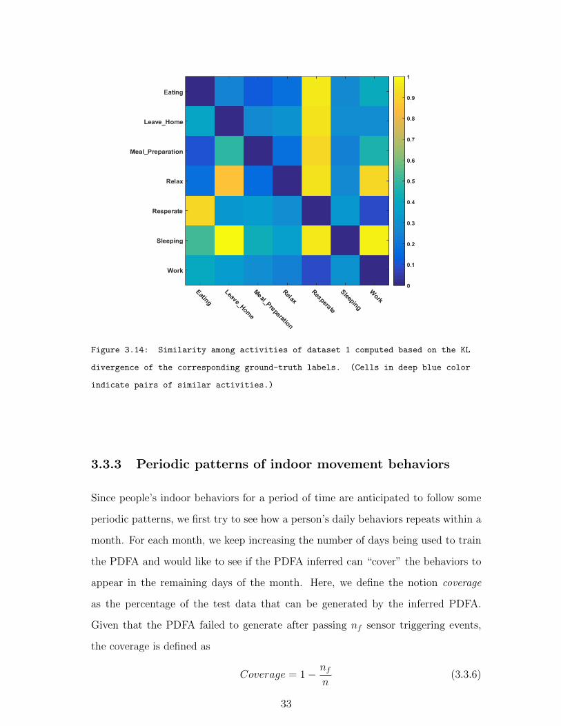
Figure 3.14: Similarity among activities of dataset 1 computed based on the KL

divergence of the corresponding ground-truth labels. (Cells in deep blue color

indicate pairs of similar activities.)

3.3.3 Periodic patterns of indoor movement behaviors

Since people’s indoor behaviors for a period of time are anticipated to follow some

periodic patterns, we first try to see how a person’s daily behaviors repeats within a

month. For each month, we keep increasing the number of days being used to train

the PDFA and would like to see if the PDFA inferred can “cover” the behaviors to

appear in the remaining days of the month. Here, we define the notion coverage

as the percentage of the test data that can be generated by the inferred PDFA.

Given that the PDFA failed to generate after passing nf sensor triggering events,

the coverage is defined as

Coverage = 1− nfn

(3.3.6)

33

Figure 3.15: Similarity among activities of dataset 2 computed based on the KL

divergence of the corresponding ground-truth labels. (Cells in deep blue color

indicate pairs of similar activities.)

where n is the total number of records in the testing data. According to Figure 3.16,

we found that for most of the months, after the data for around the first 7 days were

used for training the PDFA, its coverage will reach a relatively high level and then

increases slowly as more data are further used for the training.

Next, we train a PDFA for each month and test its coverage and entropy based

on the data of the current and the subsequent months. According to Figure 3.17,

we observe that the coverage value keeps at a high level and the entropy value

fluctuates around 0.55. For example, the coverage and entropy values of the PDFA

trained based on December’s data and tested on itself would be 99.27% and 0.577

respectively. As the coverage and the entropy values do not allow us to compare

the identified subflows obtained based on the data of different months, we adopt the

similarity measure proposed in [3] and weighted it by RFBLMs.

We plot the similarity matrix between the sets of subflows of every two consec-

utive months as shown in Figure 3.18 to Figure 3.21. We can observe that some

34

Figure 3.16: The coverage of the PDFA trained based on training data of

different days.

common behaviors whose patterns remain more or less the same for a number of

months.

Figure 3.17: Entropy / Coverage values of the PDFA trained from one month’s data

(row) and tested on data of subsequent months (column).

For between-week similarity, we train PDFAs using the data of the first week of

each month and test the coverage and entropy values using the data of the remaining

weeks of that month. According to Figure 3.22, we observe that the coverage value

keeps at a high level again and the entropy value fluctuates around 0.45. Also,

according to Figure 3.23 to Figure 3.26, we find that the resident exhibits different

behavior patterns when compared with those of the first week.

35

Figure 3.18: Similarity matrices of the subflows obtained from 2010-12 and

2011-01.


2011-02.

36


2011-03.


2011-04.

37

Figure 3.22: Entropy / Coverage values of the PDFA trained from one week’s data

(row) and tested on data of subsequent weeks (column)

3.4 Summary

In this chapter, an unsupervised learning methodology is proposed to detect behav-

ioral patterns for activity identification. Our experimental results show that the

subflows obtained by applying a weighted kernel k-means to the proposed behavior-

aware mobility flow graph can identify more activity-specific behavioral patterns

than the existing frequent pattern clustering approach.

38

Figure 3.23: Similarity matrices of the subflows obtained from week1 and week1.


39



40

Chapter 4

Daily routine pattern discovery

via matrix factorization

4.1 Introduction

After detecting the subflows as activities as presented in Chapter 3, we tag each

sensor triggering event in the trajectory data with an activity label as detected and

then carry out the daily routine discovery task. A matrix with each column being

a sequence of daily activity labels ordered by the time within a day is formed. To

carry out daily routine analysis based on the acquired sequences of nominal data, the

conventional way [14] is to decompose each sequence of nominal data (labels) into

multiple sequences of binary data (one for each label) so that the existing matrix

factorization techniques can (at least) be applicable. However, such a practice will

multiply the size of the data, causing the tractability issue. In addition, the observed

labels are often correlated due to, for example, their spatial or behavioral closeness.

How to leverage the label correlation for factorizing multiple binary matrices is not

obvious, and thus often ignored. In the literature, most of the recently proposed

matrix factorization techniques are mostly dealing with matrices with real values,

with few exceptions including [47] [55].

In this chapter, we propose to factorize the nominal data matrix directly in this

41

chapter. On one hand, we avoid multiplying the size of the data. Also, we want to

capture the correlation of the activities, which is hard to be done after converting

it into multiple binary matrices. To achieve that, we assume that the similarity

of detected subflows can be estimated. We embed the discrete labels (or nominal

values) onto a d-dimensional continuous space. Then, a hierarchical probabilistic

model is proposed for the factorization, which is important as the activity labels

identified for the sensor triggering events are noisy. To carry out the model inference,

Gibbs sampling is adopted.

In the experiment, we benchmark the performance of the proposed methodol-

ogy with a number of matrix factorization techniques with highly promising results

obtained in terms of the accuracy of extracting basis vectors of nominal values as

daily activity routines using both synthetic and benchmarking data sets.

The remaining chapter is organized as follows. Section 4.2 describes the proba-

bilistic nominal matrix factorization model and its inference. Section 4.3 gives the

experimental results on a synthetic data set and a real smart home data set. Section

4.4 concludes the chapter.

4.2 Bayesian nominal matrix factorization for min-

ing daily routine patterns

A daily routine refers to a sequential pattern of activities that a person follows

within a day. To discover daily routines, we first make use of the identified activity

subflows and detect their occurrence in the data. The data DM×N is then converted

to traces of occurrence of t distinct activity labels in L = (L1, ..., Lt). We denote the

converted data as DM×NA where each column corresponds to a sequence of subflow

labels for one particular day. To do the conversion, for each column, we first find

the states corresponding to the location of the first sensor triggering event. Then,

states which can generate the longest sub-sequence based on the transition function δ

would have their subflow labels assigned to the sensor triggering events. We continue

42

this process until every record in DM×N is assigned with a subflow label. We notice

that this label assignment process can occasionally end up with occasional transient

jumps between two activity subflows due to the relatively strong assumption of hard-

partitioning for the subflow identification. We eliminate these transient jumps by

prohibiting jumps if they are shorter than one minute.

After that, each element in DA will take one of the labels in L as its value,

forming a nominal matrix. We assume that DA could have noise and missing labels

as discussed before. Thus, a true label in DA could be replaced by another one.

We further assume that the noise is not uniformly distributed over all the possible

labels but follows a distribution so that those more similar to the true one will have

a higher probability to be the replacement. The research problem here is how to

factorize the nominal matrix DM×NA into K(<< min(M,N)) basis vectors (or daily

routines) UK×M with each element of the vectors corresponding to one of the labels

in L as its value, so that matrix DA can be “well” reconstructed by combining the

basis vectors via a coefficient matrix VK×N .

4.2.1 Probabilistic nominal matrix factorization

As presented in Chapter 2, there exist a lot of algorithms for matrix factorization

[69, 41, 70]. However, work on factorizing matrices with nominal values is rare.

While one can just convert each nominal label to a numerical value and then factorize

the matrix, this is invalid as the multiplication and addition operations on labels

are undefined. With the assumption that the similarity among the labels is known

or can be estimated, we can embed the labels onto a d-dimensional continuous

vector space so that at least some ordering of the labels can be recovered. The

value of d needed is to be set so that the similarity relations of the labels can

be preserved. A higher value of d can keep the similarity information better in

general. With the embedding performed, we can replace all the value of labels

in the nominal matrix DA by the corresponding vectors in the embedding space

and factorize it. The problem becomes similar to the ordinal matrix factorization

43

problem where solutions exist. Our ultimate goal is to come up with a factorization

which can ensure that (i) the basis vectors obtained are robust to noise caused by

the imperfect activity identification step and that (ii) each row of the matrix DA

can be well-represented by a small number of basis vectors as sparse as possible for

enhancing the interpretability of basis vectors. The former suggests the use of a

probabilistic model and compute the factorization by arg maxU,V p(DA|U, V ). The

latter suggests that special attention is needed to handle how the basis vectors of the

continuous values should be converted back to the labels with the interpretability

considered. We propose a probabilistic nominal matrix factorization with a Bayesian

Lasso adopted. The flowchart is illustrated in Figure 4.1.

Figure 4.1: The proposed Probabilistic Nominal Matrix Factorization for daily

routine discovery.

4.2.2 Label embedding

To embed the labels onto a vector space, we start with the inferred mobility flow

graph and shrink the nodes in each activity subflow to from a meta-node. The set

of meta-nodes will give a new graph A′ where the nodes are corresponding to the t

subflows (Q := Q1, Q2, ..., Qt) and the edges corresponding to links among the sub-

flows which are weighted by their frequencies. We apply the node2vec algorithm [26]

to embed the t distinct labels onto a d-dimensional continuous space. The resulting

embeddings of the labels can encapsulate local and global structural relationships

among the nodes (for our case the similarity of the labels) as far as possible. It then

gives a matrix µ := [µL1 ; ...;µLt ] of size t× d, where µLi : Qi → Rd.

Then, we replace each element in DA by the corresponding d-dimensional vector

µ(m,n), resulting in a new matrix Dµ = µ(m,n) ∈ Rd with each element being a

44

vector as visualized in Figure 4.1. By further unfolding Dµ to [Dµ1 ;Dµ2 ; ...;Dµd ], a

matrix Dunfold of dimension M × d×N will be resulted. This unfolding step allows

most of the existing matrix related techniques to be applicable again. However,

it also implies that the d dimensions of the vector representation are considered

independently during the factorization. In general, it is not straightforward to ensure

that the basis vectors obtained by the factorization can be “folded” back to give a

valid label representation.

4.2.3 An extended hierarchical model

Figure 4.2: The graphical model for factorization (daily routine discovery).

We use a hierarchical model for the factorization. By assuming that the d dimen-

45

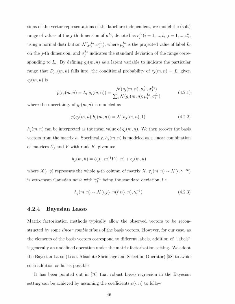
sions of the vector representations of the label are independent, we model the (soft)

range of values of the j-th dimension of µLi , denoted as rLij (i = 1, ..., t, j = 1, ..., d),

using a normal distribution N (µLij , σ

Lij ), where µLi

j is the projected value of label Li

on the j-th dimension, and σLij indicates the standard deviation of the range corre-

sponding to Li. By defining gj(m,n) as a latent variable to indicate the particular

range that Dµj(m,n) falls into, the conditional probability of rj(m,n) = Li given

gj(m,n) is

p(rj(m,n) = Li|gj(m,n)) =N (gj(m,n);µLi

j , σLij )∑

iN (gj(m,n);µLij , σ

Lij )

(4.2.1)

where the uncertainty of gj(m,n) is modeled as

p(gj(m,n)|hj(m,n)) = N (hj(m,n), 1). (4.2.2)

hj(m,n) can be interpreted as the mean value of gj(m,n). We then recover the basis

vectors from the matrix h. Specifically, hj(m,n) is modeled as a linear combination

of matrices Uj and V with rank K, given as:

hj(m,n) = Uj(·,m)ᵀV (·, n) + εj(m,n)

where X(·, y) represents the whole y-th column of matrix X, εj(m,n) ∼ N (′, γ−∞)

is zero-mean Gaussian noise with γ−1j being the standard deviation, i.e.

hj(m,n) ∼ N (uj(·,m)ᵀv(·, n), γ−1j ). (4.2.3)

4.2.4 Bayesian Lasso

Matrix factorization methods typically allow the observed vectors to be recon-

structed by some linear combinations of the basis vectors. However, for our case, as

the elements of the basis vectors correspond to different labels, addition of “labels”

is generally an undefined operation under the matrix factorization setting. We adopt

the Bayesian Lasso (Least Absolute Shrinkage and Selection Operator) [58] to avoid

such addition as far as possible.

It has been pointed out in [76] that robust Lasso regression in the Bayesian

setting can be achieved by assuming the coefficients v(·, n) to follow

46

p(v(·, n)|σ2) =k∏i=1

λ

2√σ2

exp(−λ |v(·, ni)|√σ2

).

We adopt this to achieve a sparse structure of the coefficient matrix. According to

[76, 58], this conditional Laplace prior is equivalent to integrating out a hierarchical

model for vn with addition variables τ 21 , τ

22 , ..., τ

2k , where vn is modeled as a zero-mean

Gaussian with a diagonal covariance matrix scaled by σ and τ , given as

p(v(·, n)|σ2, τ 21 , τ

22 , ..., τ

2k ) ∼ N (0, σ2Dτ )

where

Dτ = diag(τ 21 , τ

22 , ..., τ

2k )

τ 21 , τ

22 , ..., τ

2k ∼

p∏j=1

λ2

2e−λ

2τ2i /2dτ 2i , τ 2

1 , τ22 , ..., τ

2k > 0

σ2 ∼ 1σ2dσ

2

with τ 21 , τ

22 , ..., τ

2k and σ2 assumed independent among them.

For modeling Uj(·,m), γ and σLij for each of the d dimensions, we simply use the

exponential conjugate families, given as:

p(uj(·,m)|µj, ψj) = N (uj(·,m);µj, ψj)

p(µj, ψj) = NW〉(µ|, ψ||µ′| , κ|, ν|, T|)

= N (µj|µ0j , (κjψj)−1)W〉ν|(ψj|Tj)

p(σLij |α

Lij , β

Lij ) = Γ(αLi

j , βLij ) ∝ γα

Lij −1 exp(−

σLij

βLij

)

p(γj|αj, βj) = Γ(αj, βj) ∝ γαj−1j exp(−γj

βj).

where

µj =κµj0 +mujκ+m

uj =1

M

∑mujm

Tj = Tj0 + Zj +κm

κ+m(µj0 − uj)(µj0 − uj)T

Zj =∑n

i=1(xji − xj)(xji − xj)T

νj = νj0 +m

κj = κj0 +m.

47

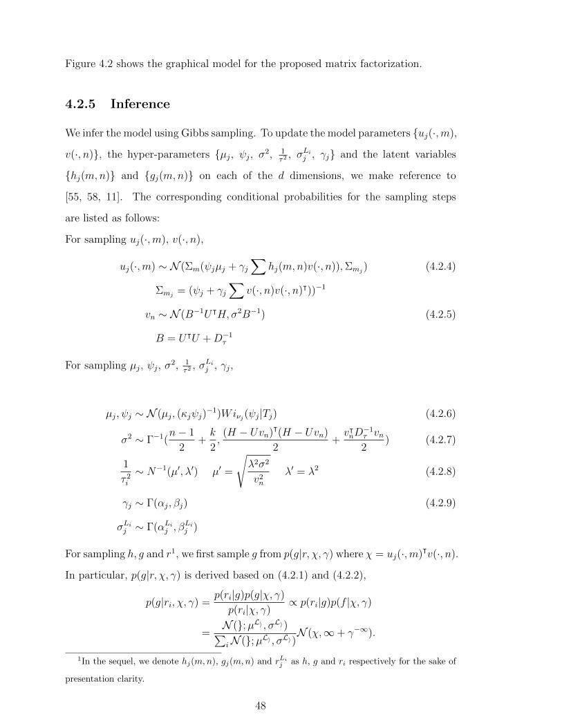
Figure 4.2 shows the graphical model for the proposed matrix factorization.

4.2.5 Inference

We infer the model using Gibbs sampling. To update the model parameters uj(·,m),

v(·, n), the hyper-parameters µj, ψj, σ2, 1τ2

, σLij , γj and the latent variables

hj(m,n) and gj(m,n) on each of the d dimensions, we make reference to

[55, 58, 11]. The corresponding conditional probabilities for the sampling steps

are listed as follows:

For sampling uj(·,m), v(·, n),

uj(·,m) ∼ N (Σm(ψjµj + γj∑

hj(m,n)v(·, n)),Σmj) (4.2.4)

Σmj= (ψj + γj

∑v(·, n)v(·, n)ᵀ))−1

vn ∼ N (B−1UᵀH, σ2B−1) (4.2.5)

B = UᵀU +D−1τ

For sampling µj, ψj, σ2, 1

τ2, σLi

j , γj,

µj, ψj ∼ N (µj, (κjψj)−1)Wiνj(ψj|Tj) (4.2.6)

σ2 ∼ Γ−1(n− 1

2+k

2,(H − Uvn)ᵀ(H − Uvn)

2+vᵀnD

−1τ vn2

) (4.2.7)

1

τ 2i

∼ N−1(µ′, λ′) µ′ =

√λ2σ2

v2n

λ′ = λ2 (4.2.8)

γj ∼ Γ(αj, βj) (4.2.9)

σLij ∼ Γ(αLi

j , βLij )

For sampling h, g and r1, we first sample g from p(g|r, χ, γ) where χ = uj(·,m)ᵀv(·, n).

In particular, p(g|r, χ, γ) is derived based on (4.2.1) and (4.2.2),

p(g|ri, χ, γ) =p(ri|g)p(g|χ, γ)

p(ri|χ, γ)∝ p(ri|g)p(f |χ, γ)

=N (;µL〉 , σL〉)∑iN (;µL〉 , σL〉)

N (χ,∞+ γ−∞).

1In the sequel, we denote hj(m,n), gj(m,n) and rLij as h, g and ri respectively for the sake of

presentation clarity.

48

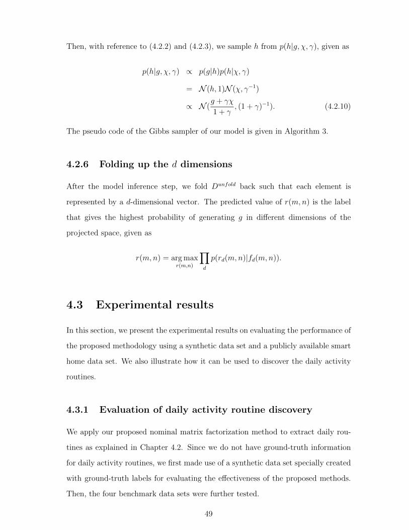
Then, with reference to (4.2.2) and (4.2.3), we sample h from p(h|g, χ, γ), given as

p(h|g, χ, γ) ∝ p(g|h)p(h|χ, γ)

= N (h, 1)N (χ, γ−1)

∝ N (g + γχ

1 + γ, (1 + γ)−1). (4.2.10)

The pseudo code of the Gibbs sampler of our model is given in Algorithm 3.

4.2.6 Folding up the d dimensions

After the model inference step, we fold Dunfold back such that each element is

represented by a d-dimensional vector. The predicted value of r(m,n) is the label

that gives the highest probability of generating g in different dimensions of the

projected space, given as

r(m,n) = arg maxr(m,n)

∏d

p(rd(m,n)|fd(m,n)).

4.3 Experimental results

In this section, we present the experimental results on evaluating the performance of

the proposed methodology using a synthetic data set and a publicly available smart

home data set. We also illustrate how it can be used to discover the daily activity

routines.

4.3.1 Evaluation of daily activity routine discovery

We apply our proposed nominal matrix factorization method to extract daily rou-

tines as explained in Chapter 4.2. Since we do not have ground-truth information

for daily activity routines, we first made use of a synthetic data set specially created

with ground-truth labels for evaluating the effectiveness of the proposed methods.

Then, the four benchmark data sets were further tested.

49

ALGORITHM 3: Gibbs sampling

Input: U, V, µ, ψ, σ,Dτ , γ, non-empty rmn

repeat

for items m = 1,...,M do

sample hmn|rmn, um, vn, γ (4.2.10);

sample um|hmn, vn, γ, µ, ψ (4.2.4);

end

for items n = 1,...,N do

sample hmn|rmn, um, vn, γ (4.2.10);

sample vn|hmn, um, γ, σ (4.2.5) ;

end

sample µ|U,ψ and ψ|U (4.2.6);

sample 1τ2|V, σ2 and σ2|V (4.2.7), (4.2.8);

sample γ|H,U, V (4.2.9);

until sufficient samples have been taken;

Evaluation metrics

Mean absolute error (MAE) is used to measure the percentage of incorrectly re-

covered labels with reference to the ground truth labels. For synthetic data, both

the ground-truth matrix and the ground-truth basis vectors are known. The mean

absolute error of recovering D (data reconstruction MAE) is defined as,

MAE =1

M ×N∑M

i=1

∑N

j=1Dist(rij, rij)

where Dist(·) is a distance function defined as Dist(rij, rij) = 0 if rij = rij or

1 otherwise. Similarly, we can also measure the basis vector reconstruction MAE.

We argue that even if the data reconstruction MAE is small, it does not necessarily

mean that the latent basis vectors can be discovered. And, if a low MAE for the

basis vectors can be obtained with respect to the ground truth, we consider the

discovery to be accurate for human interpretation.

50

Performance evaluation

We implemented the proposed method and four related matrix factorization methods

for performance comparison, including

• Ternary Matrix Factorization (TMF ) [50]: Nominal matrix is firstly trans-

formed into a binary matrix by mapping each label to a binary vector. The

binary matrix is then recursively approximated where hard constraints are

imposed to make the low rank matrices binary.

• Bayesian Non-negative Matrix Factorization (P NMF order) [70]: Labels are

ranked based on the node2vec (d = 1) results and then replaced in order by

integers.

• Probabilistic Ordinal Matrix Factorization (POMF) [55]: The labels are em-

bedded using node2vec (d = 1) to both positive and negative regions on the

real number line, with the prior on vn similar to that of um.

• Probabilistic Non-negative Ordinal Matrix Factorization with Lasso (+POMF Lasso):

The labels are embedded to only the positive real number line (d = 1) and

Lasso is applied on vn.

• Probabilistic Nominal Matrix Factorization (PNoMF): This is the method pro-

posed in this paper where the labels are embedded to only the positive side

for all the d dimensions, and the Lasso is applied on vn. Also, the noise model

for labels is considered.

Results on synthetic data

We generate synthetic data sets with eight labels A,B,C,D,E, F,G,H. We fur-

ther group the labels into subsets (A,B, C,D, E,F, G,H), where labels

within the same subset are supposed to be close to each other. Proximity infor-

mation of the labels can be expressed by a weighted adjacency matrix as shown in

Figure 4.3. We then randomly pick one label from each subset and use these four

51

labels to generate four ground-truth basis vectors. Repeating those basis vectors

gives the noise free data matrix. For evaluation, we generate three noise free data

matrices (SD1, SD2, SD3) with 384, 576, and 768 elements from basis vectors of

dimension 12, 18, and 24 respectively. We set the number of basis vectors K to 4

and check if the four ground truth basis vectors can be recovered. Also, we add

noise to the data matrices at different levels by randomly replacing labels based on

adjacency matrix to test their robustness to noise.

Figure 4.5 and 4.6 shows the experimental results based on SD3. PNoMF(2D)

outperforms significantly all the state-of-art factorization methods at all noise levels

in terms of MAE for basis vector discovery while keeping a good performance in

data reconstruction. For all the other factorization methods, even though the data

reconstruction MAE is low, the basis vector reconstruction MAE is large. That is

the discovered latent factors are inaccurate. Similar results are obtained for SD1

and SD2.

Figure 4.3: Weighted adjacency matrix of the labels for the synthetic data set.

Results on smart home data

We apply PNoMF to two real indoor trajectory data sets. In our experiment, we

set the number of basis vectors as 6 and 4 for dataset 1 and dataset 2 respectively

according to Figures 4.7 and 4.8. For dataset 1, we also split it into 5 different

52

Figure 4.4: Visualization of label embedding of synthetic data.

Figure 4.5: Basis vector reconstruction MAE of different algorithms at different

noise levels based on SD3.

53

Figure 4.6: Data reconstruction MAE of different algorithms at different noise

levels based on SD3.

subsets, covering the sensor readings collected in Dec 2010, Jan 2011, Feb 2011,

Mar 2011, and Apr 2011 for daily routine analysis per month.

As the ground-truth basis vectors are not available, we can only compare the

data reconstruction MAE. According to Tables 4.1 and 4.2, PNoMF gives the best

or close to the best result as compared to the other methods for data reconstruc-

tion. Also, the use of label embedding of a higher dimensional space will lower

the MAE which is consistent to our understanding explained earlier. As PNoMF

is designed to find highly interpretable basis vectors without sacrificing much the

matrix reconstruction accuracy, Figures 4.9 to 4.18 show the daily routines and the

corresponding coefficient matrices obtained based on the Dec, Jan, Feb, March and

April data subsets. To ease our interpretation of the daily activity routines obtained

for the five months, we put a red asterisk to the coefficient of the highest value for

each day per month. Each corresponds to the most representative daily routine for

the particular day. For example, by referring to Figure 4.9, the routine #5 can be

interpreted as having a day with eating and relaxing for most of the time with some

working hours at around 4-6pm. And according to Figure 4.10, this routine happens

54

PNoMF (1D) PNoMF (2D) PNoMF (3D) POMF +POMF Lasso P NMF order TMF

Dataset 1 0.429(0.004) 0.359(0.011) 0.304(0.005) 0.462(0.002) 0.548(0.006) 0.635(0.011) 0.307(0.002)

Dataset 2 0.580(0.006) 0.525(0.015) 0.451(0.005) 0.802(0.010) 0.794(0.009) 0.877(0.003) 0.419(0.001)

Table 4.1: Mean MAE(±SD) of smart home data.

for most of the days in Dec 2010 except for some particular days where they follow

other basis vectors with more time being spent in the kitchen at different periods of

time. Also, we compare the daily routines obtained for different months and found

that they are quite different. For example, there is quite a long period of working

time in the afternoon for the routine #5 of Dec. 2010 as compared to a much shorter

one around noon for the routine #2 of Mar. 2011. Both are the most representative

daily routines for the corresponding months. As shown in Figure 4.19 and Figure

4.20, the routine #2 happens for most of the days in dataset 2, which indicates that

the resident wakes up at around 9am, relaxes for most of the time during the day

and have a tea break at around 3pm. As discussed in [42], allowing the elderly to be

able to discuss their own daily routines and exceptions can help them reflect more

their daily activities, which in turn may provide better support to their awareness

on potential deterioration of their functional capabilities. We believe the methodol-

ogy developed in this chapter can provide more information to the elderly for more

in-depth reflection in general.

Figure 4.7: Performance of PNoMF on dataset 1 with different numbers of basis

vectors.

55

Figure 4.8: Performance of PNoMF on dataset 2 with different numbers of basis

vectors.

56

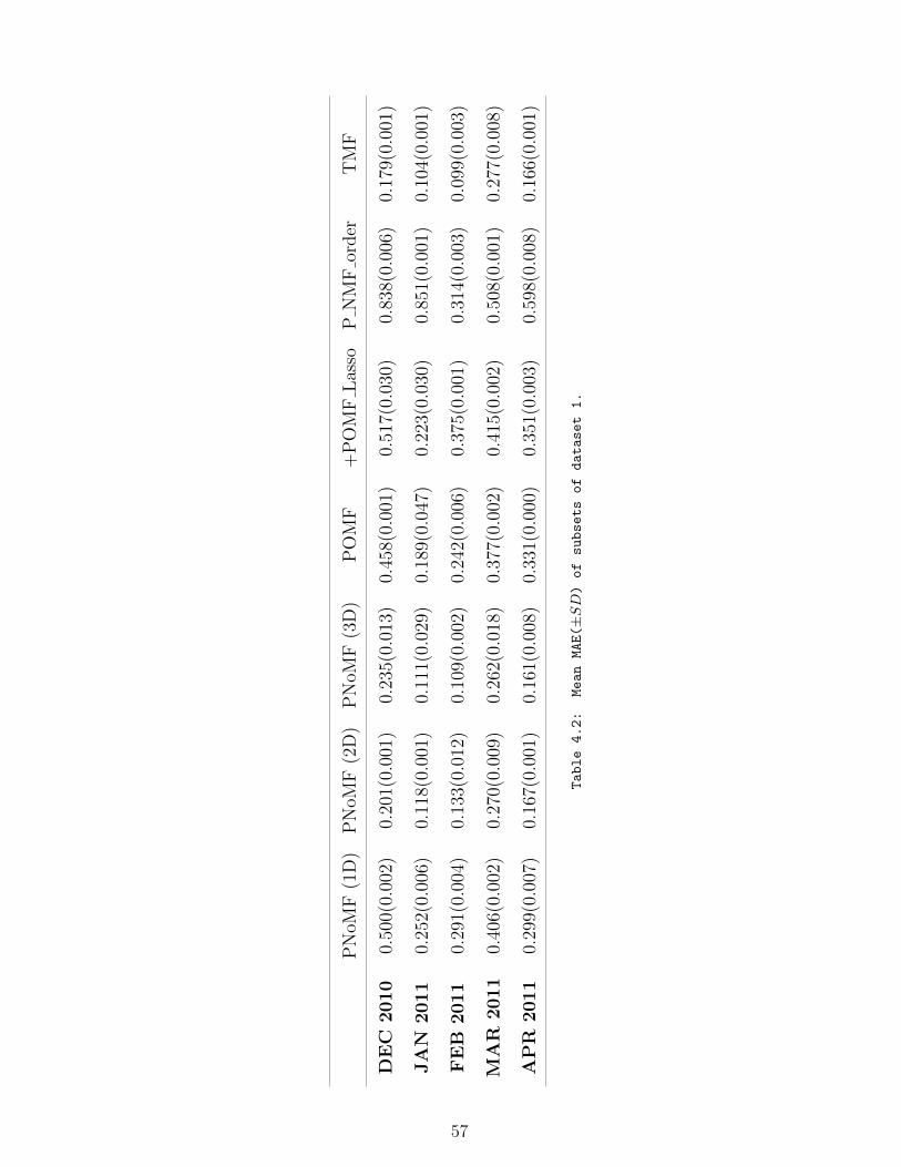
PN

oMF

(1D

)P

NoM

F(2

D)

PN

oMF

(3D

)P

OM

F+

PO

MF

Las

soP

NM

For

der

TM

F

DE

C2010

0.50

0(0.

002)

0.20

1(0.

001)

0.23

5(0.

013)

0.45

8(0.

001)

0.51

7(0.

030)

0.83

8(0.

006)

0.17

9(0.

001)

JA

N2011

0.25

2(0.

006)

0.11

8(0.

001)

0.11

1(0.

029)

0.18

9(0.

047)

0.22

3(0.

030)

0.85

1(0.

001)

0.10

4(0.

001)

FE

B2011

0.29

1(0.

004)

0.13

3(0.

012)

0.10

9(0.

002)

0.24

2(0.

006)

0.37

5(0.

001)

0.31

4(0.

003)

0.09

9(0.

003)

MA

R2011

0.40

6(0.

002)

0.27

0(0.

009)

0.26

2(0.

018)

0.37

7(0.

002)

0.41

5(0.

002)

0.50

8(0.

001)

0.27

7(0.

008)

AP

R2011

0.29

9(0.

007)

0.16

7(0.

001)

0.16

1(0.

008)

0.33

1(0.

000)

0.35

1(0.

003)

0.59

8(0.

008)

0.16

6(0.

001)

Table4.2:

MeanMAE(±SD)ofsubsetsofdataset1.

57

Figure 4.9: Daily routines (U) of DEC 2010

Figure 4.10: Coefficient matrix (V ) of DEC 2010

Figure 4.11: Daily routines (U) of JAN 2011

4.3.2 Applicability to other data sets

We compare the basis vector obtained by our proposed method with [50], using the

same voting records data set from UCI Machine learning Repository. The data set

contains voting records from the U.S House of Representatives. 435 representatives

58

Figure 4.12: Coefficient matrix (V ) of JAN 2011

Figure 4.13: Daily routines (U) of FEB 2011

Figure 4.14: Coefficient matrix (V ) of FEB 2011

from Republican Party (GOP) and Democratic Party (D) provide their opinions on

16 political issues by voting “yea”, “nay” or “unknown”. Notice that the “unknown”

opinion here does not indicate a missing value. We set these three labels to be not

similar with each other, and project the label based on their proximity onto a two

dimensional space. According to Figure 4.22, PNoMF(2D), PNoMF(3D) and TMF

have very similar performance in terms of data reconstruction MAE. Here we cannot

test the basis vector reconstruction MAE as the ground truth is not available. Still,

59

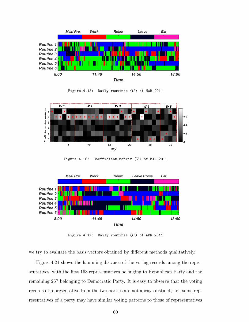
Figure 4.15: Daily routines (U) of MAR 2011

Figure 4.16: Coefficient matrix (V ) of MAR 2011

Figure 4.17: Daily routines (U) of APR 2011

we try to evaluate the basis vectors obtained by different methods qualitatively.

Figure 4.21 shows the hamming distance of the voting records among the repre-

sentatives, with the first 168 representatives belonging to Republican Party and the

remaining 267 belonging to Democratic Party. It is easy to observe that the voting

records of representative from the two parties are not always distinct, i.e., some rep-

resentatives of a party may have similar voting patterns to those of representatives

60

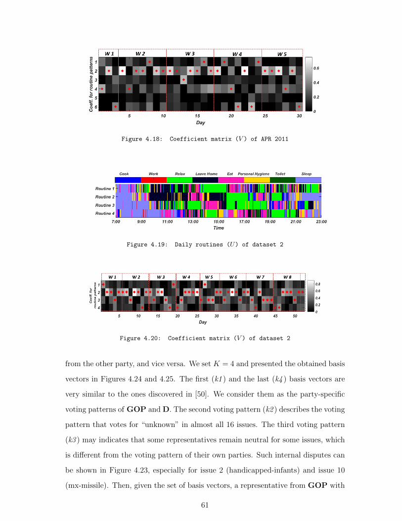
Figure 4.18: Coefficient matrix (V ) of APR 2011

Figure 4.19: Daily routines (U) of dataset 2

Figure 4.20: Coefficient matrix (V ) of dataset 2

from the other party, and vice versa. We set K = 4 and presented the obtained basis

vectors in Figures 4.24 and 4.25. The first (k1 ) and the last (k4 ) basis vectors are

very similar to the ones discovered in [50]. We consider them as the party-specific

voting patterns of GOP and D. The second voting pattern (k2 ) describes the voting

pattern that votes for “unknown” in almost all 16 issues. The third voting pattern

(k3 ) may indicates that some representatives remain neutral for some issues, which

is different from the voting pattern of their own parties. Such internal disputes can

be shown in Figure 4.23, especially for issue 2 (handicapped-infants) and issue 10

(mx-missile). Then, given the set of basis vectors, a representative from GOP with

61

the coefficients [0.72, 0.03, 0.24, 0.03] for the four basis vectors indicates that he votes

like a typical GOP representative (k1 ), but may sometimes vote for another side

(k3 ).

Figure 4.21: Hamming distance matrix of the 435 representatives.

62

Figure 4.22: Data reconstruction MAE.

63

Figure4.23:

Distributionsofvotingrecordsoftwopartiesin16politicalissues.

64

Figure4.24:

VotingpatternsU

obtainedbyTMF.

65

Figure4.25:

VotingpatternsU

obtainedbyPNoMF.

66

PNoMF(1D) PNoMF(2D) PNoMF(3D) POMF +POMF Lasso P NMF order TMF

Lenses 0.223 (0.014) 0.234 (0.020) 0.2062 (0.017) 0.388 (0.027) 0.281 (0.027) 0.285 (0.131) 0.279(0.024)

Table 4.3: Mean MAE(±SD) of the lenses data set.

Another nominal data that we can find in UCI Machine learning Repository for

our testing is the lenses data set. The data set contains 24 patients and each patient

has 4 categorical attributes, namely age, spectacle prescription, astigmatic, and tear

production rate. Each attribute has its own set of labels. There are altogether 9

labels. By allowing the possible labels of each attribute to be close and the labels not

corresponding to the same attribute farther apart, a block-diagonal matrix is used

for representing the adjacency matrix. As there are three classes in the data set, we

thus set K = 3, and then compare different methods in terms of data reconstruction

MAE. The result is shown in Table 4.3 where PNoMF(3D) gives the best result,

followed by PNoMF(1D), PNoMF(2D), and then TMF.

4.4 Summary

In this chapter, a probabilistic framework with Bayesian Lasso is proposed for nom-

inal data matrix factorization with application to smart home data mining. As

shown in our experimental results using both synthetic and real smart home data

sets, the basis vectors obtained by our proposed methodology achieve a lower data

reconstruction error and at the same time a much lower basis vector reconstruction

error as compared to a number of the state-of-the-art matrix factorization methods,

making direct interpretation of the basis vectors as daily activity routines possible.

We believe that presenting the results to the senior adults living in the smart home

will be beneficial to them to support their awareness of their daily activities, and

potential degradation.

67

Chapter 5

Discovering shift-invariant daily

routine patterns using Markov

Jump Process

5.1 Introduction

The way how a person performs daily activities within a day can varies due to

different factors which can be social [9] and environmental [29]. The occurrence of

the activities may “shift” and their durations obviously will vary. The consequence

is that even though a person follows a certain daily routine, the specific start time

and duration of different daily activities involved do vary as illustrated in Figure

5.8 which shows the plot of a raw smart home data. Without carefully taking these

variations into consideration, applying the matrix factorization methods directly, as

adopted in a number of related work, will end up with incorrect daily routines to be

extracted. The key reason is that most matrix factorization methods assume that

each column is assumed to be corresponding to the same feature. For the application

of daily routine discovery, this is essentially expecting that the same activity of a

daily routine happens at more or less the same time on different days. It is an

unrealistic assumption.

68

In this chapter, we first adopt the probabilistic nominal matrix factorization

(PNoMF) framework proposed in Chapter 4 to extract daily routines by factorizing

a sensor data matrix. We then extend it by introducing a Markov jump process

(MJP) as the prior of the daily routines. MJP is a particular continuous version

of discrete-time Markov chain where the transitions from one activity to another

are modeled as the transitions among the states of the MJP. The time interval for

each state transition is also modeled. The use of the MJP allows us to model the

variations of activity durations so that shift-invariant daily routines can be extracted.

Also, with the objective of improving the interpretability of the basis vectors, we

are inspired by the prototype-based Bayesian Case Model [38] and link up PNoMF

and MJP by obtaining the most probable data instance w.r.t. an MJP as the basis

vectors. We evaluate the proposed method using a synthetic data set and two

publicly available smart home data sets. In our experiments, we demonstrate that

the proposed method (PNoMF-MJP) can discover the ground truth basis vectors

with smaller mean absolute errors (MAE) compared with the other state-of-the-art

algorithms. Also the proposed PNoMF-MJP can predict the future activity based

on the user’s historical activities with higher accuracy.

In the followings, we first present the basic background of Markov jump process in

Section 5.2. In Section 5.3, we illustrate how a MJP can be incorporated as the prior

based on a Bayesian nominal matrix factorization framework. The experimental

results on both synthetic and real data are discussed in Section 5.4. Section 5.5

provides the concluding remark.

5.2 Markov jump process (MJP)

A family S = S(t) : t ≥ 0 of random variables S(t) : Ω→ S is called a continuous-

time stochastic process on the state space Σ, where S is the sample space. If S(t) = y,

the process is said to be in state y at time t. For some given s ∈ Ω, the S valued

set X(t, s) : t ≥ 0 is called a path of the stochastic process S associated with s.

A continuous-time stochastic process S(t) : t ≥ 0 is called a Markov process, if

69

the state space S is countable, and for any ti+1 > ti > ... > t0 the Markov property

P [S(ti+1) ∈ S|S(ti), ..., S(t0)] = P [S(ti+1) ∈ S|S(ti)] (5.2.1)

holds. If the right hand side of Eq.5.2.1 only depends on the time difference ti+1−ti,

but not on ti, the Markov process is called homogeneous. Given a homogeneous

Markov process, the function p : R+ × S × S → R+ defined by

p(t, x, y) = P [S(t) = y|S(0) = x]

is called the stochastic transition function which describes the transition probability

of moving from x to y within time t. The probability distribution

π0(x) = P [S(0) = x]

is called the initial distribution. If there is a single x ∈ S such that π0(x) = 1, then

x is called the initial state.

In the following, we focus on homogeneous Markov process. We also assume that

p(0, x, y) = δxy, where δxy = 1, if x = y and zero otherwise. This guarantees that no

transition can take place at zero time. Also the transition probabilities are assumed

continuous at t = 0: limt→0+

p(t, x, y) = δxy for every x, y ∈ S. It guarantees that the

paths of S(t) : t ≥ 0 are right continuous functions. As the state space is discrete,

for an s ∈ S and t ≥ 0, there exists ∆t > 0 so that

S(t+ ∆t, s) = S(t, s).

This fact motivates the name Markov jump process (MJP).

Assume that S(t) = s ∀t ∈ (t1, t2]|S(t1) = s describes an MJP in state s at

time t1 will remain in state s over the interval (t1, t2]. We denote such probability

by p(s, t1, t2), so that

p(s, t1, t2) = P (S(t) = s ∀t ∈ (t1, t2]|S(t1) = s).

Denoting τ(t1) as the time of the next jump after t1, we also have

p(s, t1, t2) = P (τ(t1) > t2|S(t1) = s), t2 > t1.

70

p(s, t1, t2) is monotonically non-increasing in t2 and satisfies limh→0+

p(s, t, t + h) = 1

as well as

p(s, t1, t2) = p(s, t1, t)p(s, t, t2) for t1 < t < t2.

Consequently, p has the representation

p(s, t1, t2) = exp(−∫ t2

t1

q(s, u)du)

for a nonnegative function q(s, u). We can treat the state of the MJP evolving with

time, and q(s, u) is corresponding to the rate of leaving state s at time u.

The Markov jump process will enter a new state after leaving the current state.

As shown in [21], such a probability is given as

P (u < τ(t1) ≤ v, S(τ(t1)) ∈ Σ|S(t1) = s)

= exp(−∫ u

t1

q(s, ω)dω)

(∫ v

u

exp(−∫ t

u

q(s, ω)dω)q(s, t)Pt(s, Σ)dt

)(5.2.2)

The first factor in Eq.5.2.2 is the probability of staying in state s over the interval

(t1, u]. The integral in the second factor exp(−∫ tuq(s, ω)dω)q(s, t) is the probability

for the first jump after time u to occur at time t. Specifically, exp(−∫ tuq(s, ω)dω)

describes the probability of staying in state s over the interval (u, t], while q(s, t)

models the waiting time until the jump. The distribution Pt(s, Σ) represents the

probability of jumping from state s into some measurable set Σ, conditioned on the

jump time at t. Finally, we integrate over all possible values of t in (u, v].

When the state space S of a Markov jump process is countable, it is common to

map it to the space of natural numbers, i.e. S = 1, 2, . . . , N. We can then define

a rate matrix A as follows

As,s′ =

−q(s, t) for s = s′

q(s, t)p(s, s′) for s 6= s′; s, s′ ∈ S.(5.2.3)

It is an N-by-N matrix with non-negative off diagonal elements, q(s, t) is the leaving

rate of state s and p(s, s′) is the transition probability of s and s′. Ass′ can be

interpreted as the rate of transiting from state s to state s′. The diagonal entry of

A is defined as:

Ass = −∑

s 6=s′Ass′

71

Figure 5.1: Visualization of an MJP path.

Thus, each row in the rate matrix sum to 0. |Ass| characterizes the total rate

of leaving state s, where |x| refers to the absolute value of x. The Markov jump

process can be fully characterized by the rate matrix A and the initial distribution

over states π0.

We further restrict the MJP on a finite time interval [tstart, tend]. Assume that a

particular path of the MJP jumps from one state to another at the ordered times

(t1, . . . , tn; t1 < t2 < · · · < tn−1 < tn). We define T ≡ (t0, t1, . . . , tn, tn+1) the set of

time stamps where t0 = tstart and tn+1 = tend. S is the corresponding sequence of

states, i.e. S = (s0, s1, . . . , sn, sn+1) where si = S(ti). Given the rate matrix and the

initial distribution we can sample (S, T ) by Gillespie’s algorithm [22] (Algorithm 4).

Figure 5.1 visualizes pairs (S, T ) on a MJP path.

ALGORITHM 4: Gillespie’s algorithm for sampling an MJP path on the interval

(tstart, tend)

Input: The rate matrix A and the initial distribution over states π0.

Output: An MJP path S(t) ≡ (s0, S, T ).

Draw s0 ∼ π0 to create an initial MJP. Set t0 = tstart and i = 0.

repeat

Draw z ∼ exp(|Asi |).

Increase i by 1.

Let ti = ti−1 + z.

The MJP jumps to a new state si at time ti with p(si|si−1) ∝ Asi−1si , si 6= si−1

until ti + z > tend;

72

5.3 Incorporating MJP for nominal matrix fac-

torization

We further extend the hierarchical model proposed in Chapter 4 to discover shift-

invariant daily routine patterns. To make this chapter self-contained, we restate

the key concepts. We embed the nominal labels in matrix DA onto a d-dimentional

continuous vector space by assuming that the similarity information among the

labels is known. We also assume that the d dimensions of the vector representations

of the label are independent, so we model the (soft) range of values of the j-th

dimension of µLi , denoted as rLij (i = 1, ..., t, j = 1, ..., d), using a normal distribution

N (µLij , σ

Lij ), where µLi

j is the projected value of label Li on the j-th dimension, and

σLij indicates the standard deviation of the range corresponding to Li. By defining

gj(m,n) as a latent variable to indicate the particular range that Dµj(m,n) falls

into, the conditional probability of rj(m,n) = Li given gj(m,n) is

p(rj(m,n) = Li|gj(m,n)) =N (gj(m,n);µLi

j , σLij )∑

iN (gj(m,n);µLij , σ

Lij )

where the uncertainty of gj(m,n) is modeled as

p(gj(m,n)|hj(m,n)) = N (hj(m,n), 1)

with hj(m,n) interpreted as the mean value of gj(m,n). We then recover the basis

vectors from the matrix h. Specifically, hj(m,n) is modeled as a linear combination

of matrices Uj and V with rank K, given as hj(m,n) = Uj(·,m)ᵀV (·, n) + εj(m,n)

where X(·, y) represents the whole y-th column of matrix X, εj(m,n) ∼ N (′, γ−∞)

is zero-mean Gaussian noise with γ−1j being the standard deviation, i.e.

hj(m,n) ∼ N (uj(·,m)ᵀv(·, n), γ−1j ).

We adopt the Bayesian Lasso (Least Absolute Shrinkage and Selection Operator)

[58] on v as follow to ensure the sparsity of the coefficient matrix, and thus the

interpretability of the discovered basis vectors.

p(v(·, n)|σ2, τ 21 , τ

22 , ..., τ

2k ) ∼ N (0, σ2Dτ )

73

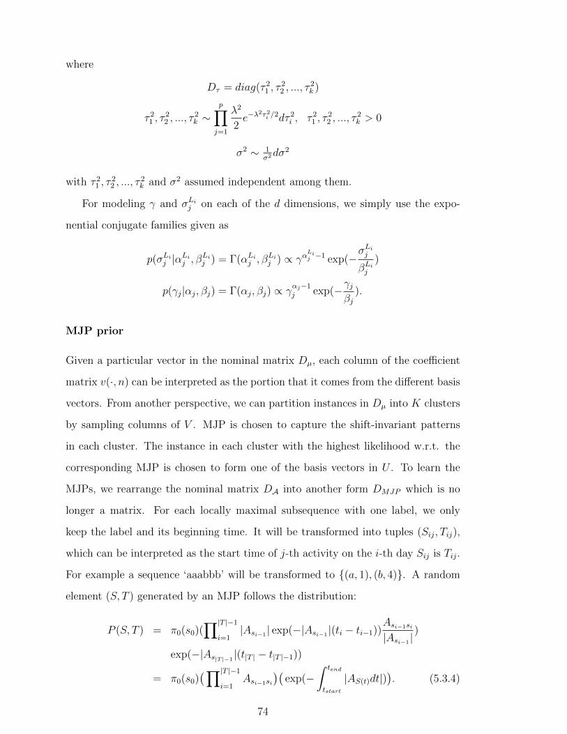
where

Dτ = diag(τ 21 , τ

22 , ..., τ

2k )

τ 21 , τ

22 , ..., τ

2k ∼

p∏j=1

λ2

2e−λ

2τ2i /2dτ 2i , τ 2

1 , τ22 , ..., τ

2k > 0

σ2 ∼ 1σ2dσ

2

with τ 21 , τ

22 , ..., τ

2k and σ2 assumed independent among them.

For modeling γ and σLij on each of the d dimensions, we simply use the expo-

nential conjugate families given as

p(σLij |α

Lij , β

Lij ) = Γ(αLi

j , βLij ) ∝ γα

Lij −1 exp(−

σLij

βLij

)

p(γj|αj, βj) = Γ(αj, βj) ∝ γαj−1j exp(−γj

βj).

MJP prior

Given a particular vector in the nominal matrix Dµ, each column of the coefficient

matrix v(·, n) can be interpreted as the portion that it comes from the different basis

vectors. From another perspective, we can partition instances in Dµ into K clusters

by sampling columns of V . MJP is chosen to capture the shift-invariant patterns

in each cluster. The instance in each cluster with the highest likelihood w.r.t. the

corresponding MJP is chosen to form one of the basis vectors in U . To learn the

MJPs, we rearrange the nominal matrix DA into another form DMJP which is no

longer a matrix. For each locally maximal subsequence with one label, we only

keep the label and its beginning time. It will be transformed into tuples (Sij, Tij),

which can be interpreted as the start time of j-th activity on the i-th day Sij is Tij.

For example a sequence ‘aaabbb’ will be transformed to (a, 1), (b, 4). A random

element (S, T ) generated by an MJP follows the distribution:

P (S, T ) = π0(s0)(∏|T |−1

i=1|Asi−1

| exp(−|Asi−1|(ti − ti−1))

Asi−1si

|Asi−1|)

exp(−|As|T |−1|(t|T | − t|T |−1))

= π0(s0)(∏|T |−1

i=1Asi−1si

)(exp(−

∫ tend

tstart

|AS(t)dt|)). (5.3.4)

74

The ith factor in the product in Eq.5.3.4 is the probability of waiting for ti − ti−1

in state si−1 (at rate Asi−1), and then transiting to state si. The last factor is

the probability of waiting for longer than t|T | − t|T |−1 in state s|T |−1, and does not

correspond to an MJP transition.

Inference

We infer the MJP via Markov chain Monte Carlo (MCMC) which iterates between

two Gibbs sampling steps: i) Sample MJP paths given current model parameters,

and ii) Update parameters given the sampled paths. For the first step, we follow the

ideas in [64], which samples a new path by running the forward-filtering backward-

sampling algorithm (FFBS) [8] on a random discretization of time. In every Gibbs

iteration, this discretization is re-sampled conditional on the old path and the current

parameters. Specifically, we sample a set of time stamps from a Poisson process with

rate Ω + Ass, where Ω > maxi(−Aii). A random discretization of time is obtained

by combining the newly sampled time stamps with the transition times of the old

path. A new path is sampled by running FFBS over these time stamps, with the

initial distribution π0 and Markov transition matrix I + 1ΩA. We can view sampling

an MJP path as sequentially sampling waiting time from an exponential density and

new states from a discrete distribution based on the current state.

For the second step, we put independent gamma priors on the diagonal elements

|Ass| which are the leaving rates of the states and put independent Dirichlet priors on

the probabilities of transitioning from one state to another. In particular, defining

ps,s′ =As,s′

|Ass| , we let:

|Ass| ∼ Gamma(α1, α2)

(ps,1, . . . , ps,s−1, ps,s+1, . . . , ps,N) ∼ Dirichlet(β).

Given a path S(t) the sufficient statistics required to calculate the posterior

distributions are the total amount of time spent in each state and the number of

transitions between each pair of states. Thus, let ns,s′ be the number of transitions

from state s to s′, ns be the number of times the MJP leaves state s, and Ts be

75

the total amount of time spent in state s. The posterior distributions for the Gibbs

sampling are

|Ass|∣∣(S, T ) ∼ Gamma(α1,s, α2,s)

(ps,1, . . . , ps,s−1, ps,s+1, . . . , ps,N)∣∣(S, T ))

∼ Dirichlet(β + (ns,1, . . . , ns,s−1, ns,s+1, . . . , ns,N)).

where α = α + ns, ns =∑

s′∈S ns,s′ and 1α2,s

= 1α2

+ 1Ts

. Other parameters are

sampled in the same way as mentioned in Section 4.2.5.

5.4 Experimental results on daily routine discov-

ering

We applied our proposed nominal matrix factorization method with Markov jump

process prior to extract daily routines based on the occurrence of the identified

subflows as explained in Section 5.3. Since we do not have ground-truth information

for daily activity routines, we first made use of a synthetic data set specially created

with ground-truth labels for evaluating the effectiveness of the proposed methods.

Then, the two real trajectory data sets were further tested.

Performance evaluation

For performance comparison, we implemented the proposed method and four related

matrix factorization methods, including

• Ternary Matrix Factorization (TMF ) [50]: Nominal matrix is firstly trans-

formed into a binary matrix by mapping each label to a binary vector. Then

this binary matrix is recursively approximated where hard constraints are im-

posed such that elements in low rank matrices should be zero or one.

• Bayesian Non-negative Matrix Factorization (P NMF order) [70]: Labels are

ranked based on the node2vec (d = 1) results and then replaced in order by

integers.

76

• Probabilistic Ordinal Matrix Factorization (POMF) [55]: The labels are em-

bedded using the node2vec (d = 1) to both positive and negative regions on

the real number line, with the prior on vn similar to that of um.

• Probabilistic Nominal Matrix Factorization (PNoMF) [43]: The labels are

embedded to only the positive side for all the d dimensions, and the Lasso

is applied on vn. Also, the labels are allowed to be replaced by other labels

based on a noise model, instead of having their corresponding range of f value

truncated.

• Probabilistic Nominal Matrix Factorization with Markov jump process prior

(PNoMF-MJP): The labels are embedded to only the positive side for all the

d dimensions, and the Lasso is applied on vn. Also, the labels are allowed to

be replaced by other labels based on a noise model, instead of having their

corresponding range of f value truncated. Basis vectors are instances from

the target matrix.

Evaluation metrics

Mean absolute error (MAE) is used to measure the percentage of incorrectly re-

covered labels with reference to the ground truth labels. For synthetic data, both

the ground-truth matrix and the ground-truth basis vectors are known. The mean

absolute error of recovering D (data reconstruction MAE) is defined as,

MAE =1

M ×N∑M

i=1

∑N

j=1Dist(rij, rij)


1 otherwise. Similarly, we can also measure the basis vector reconstruction MAE.

We argue that even if the data reconstruction MAE is small, it does not necessarily

mean that the latent basis vectors can be discovered. And, if a low MAE for the

basis vectors can be obtained with respect to the ground truth, we consider the

discovery to be accurate for human interpretation.

77

We argue that the discovered basis vectors with low MAE compare to ground

truth is accurate for human interpretation, but it is not enough. A small error rate

on predicting the test data indicates a better generalization of the obtained basis

vectors. Thus, other than measure the data reconstruction MAE and basis vector

reconstruction MAE, we measure the prediction error rate. In our experiments,

we use 90% of the data for training the daily routine patterns and the remaining

10% for testing. For each sequence in the test data, we keep the first two locally

maximal subsequence and compare different methodologies on predicting the next

locally maximal subsequence. The error rate is defined as,

Error rate =1∑Mi=1 Ni

∑M

i=1

∑Ni

j=1Dist(rij, rij)


1 otherwise. M and Ni are the number of sequences in Dtest and the number of

elements need to be predicted in i-th sequence. To calculate the error rate for

methodologies except PNoMF-MJP, we first estimate the coefficients for different

basis vectors based on the given locally maximal subsequences via non-negative

least square algorithm [5]. The linear combination of the basis vectors weighted

by the obtained coefficients gives the reconstruction of the next locally maximal

subsequence. For PNoMF-MJP, the coefficients are estimated as likelihoods of MJPs

given locally maximal subsequences by Eq.5.3.4. The prediction is computed by the

rate matrix of the MJP with the highest likelihood value.

Results on synthetic data

We generate synthetic data sets for performance evaluation with sixteen dissimilar

labels from A to P . We further assign labels into subsets (A,B, C,D, E,F,

G,H, I, J, K,L, M,N, O,P), where labels within the same subset are

close to each other. To generate data with different shift levels, we first randomly

pick one label from each subset and use these eight labels to generate four ground-

truth basis vectors. Repeating those basis vectors gives the shift free and noise free

data matrix. The shift is generated by lengthening or shortening the length of the

78

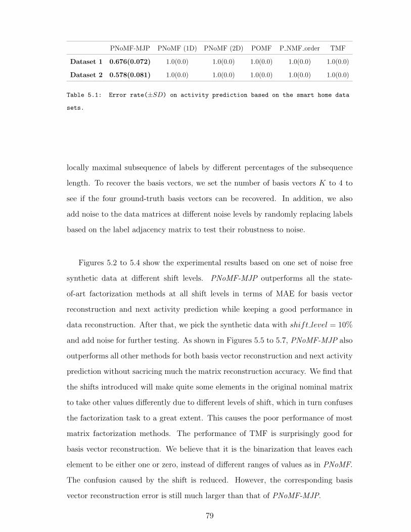
PNoMF-MJP PNoMF (1D) PNoMF (2D) POMF P NMF order TMF

Dataset 1 0.676(0.072) 1.0(0.0) 1.0(0.0) 1.0(0.0) 1.0(0.0) 1.0(0.0)

Dataset 2 0.578(0.081) 1.0(0.0) 1.0(0.0) 1.0(0.0) 1.0(0.0) 1.0(0.0)

Table 5.1: Error rate(±SD) on activity prediction based on the smart home data

sets.

locally maximal subsequence of labels by different percentages of the subsequence

length. To recover the basis vectors, we set the number of basis vectors K to 4 to

see if the four ground-truth basis vectors can be recovered. In addition, we also

add noise to the data matrices at different noise levels by randomly replacing labels

based on the label adjacency matrix to test their robustness to noise.

Figures 5.2 to 5.4 show the experimental results based on one set of noise free

synthetic data at different shift levels. PNoMF-MJP outperforms all the state-

of-art factorization methods at all shift levels in terms of MAE for basis vector

reconstruction and next activity prediction while keeping a good performance in

data reconstruction. After that, we pick the synthetic data with shift level = 10%

and add noise for further testing. As shown in Figures 5.5 to 5.7, PNoMF-MJP also

outperforms all other methods for both basis vector reconstruction and next activity

prediction without sacricing much the matrix reconstruction accuracy. We find that

the shifts introduced will make quite some elements in the original nominal matrix

to take other values differently due to different levels of shift, which in turn confuses

the factorization task to a great extent. This causes the poor performance of most

matrix factorization methods. The performance of TMF is surprisingly good for

basis vector reconstruction. We believe that it is the binarization that leaves each

element to be either one or zero, instead of different ranges of values as in PNoMF.

The confusion caused by the shift is reduced. However, the corresponding basis

vector reconstruction error is still much larger than that of PNoMF-MJP.

79

Figure 5.2: Comparison of different methodologies on basis vector reconstruction

MAE at different shift levels.

Figure 5.3: Comparison of different methodologies on matrix reconstruction MAE

at different shift levels.

80

Figure 5.4: Comparison of different methodologies on activity prediction error

rate at different shift levels.

Figure 5.5: Comparison of different methodologies on basis vector reconstruction

MAE at different noise levels.

81

Figure 5.6: Comparison of different methodologies on matrix reconstruction MAE

at different noise levels.

Figure 5.7: Comparison of different methodologies on activity prediction error

rate at different noise levels.

82

Results on Smart Home Data

We then apply the proposed nominal matrix factorization with Markov jump process

prior for daily routine discovery. In our experiment, we set the number of basis

vectors as 6 and 4 for dataset 1 and dataset 2 respectively as explained in Section

4.3. For the real world data, the ground-truth basis vectors are not available and

thus we choose to compare the MAE on data reconstruction and error rate on next

activity prediction. According to Table 5.1, PNoMF-MJP gives the best result

on activity prediction while keeping a good performance on data reconstruction

MAE as compared to the other methods. We visualize the ground-truth activities

in Figure 5.8. Figures 5.9 to 5.16 show the daily routines and the corresponding

MJPs obtained based on dataset 2. For example, by referring to Figure 5.10, the

routine can be interpreted as having a day with leaving home and relaxing activities

for most of the time with an early sleeping time at around 9:30pm. Another daily

routine as visualized in Figure 5.12 can be interpreted as relaxing for the most of the

time with waking up late and sleeping late. We can find that MJP provides a new

abstraction for visualizing daily routines where richer information can be presented.

For example, Figure 5.10 only shows two instances of one particular daily routine, it

is not easy for people to explain the underlying routine. Figure 5.9 offers us a way

to inspect the interactions among activities. We can interpret the routine as: After

cooking breakfast (‘Cook bf’) for around 16 minutes, there is a high probability to

start eating breakfast (‘Eat bf’), followed by relaxing for around 36 minutes. Such

a well summarized information about the durations of different activities and the

interactions among them cannot be revealed by only presenting the instances of basis

vectors as what all the existing methods do. We believe that this new abstraction

can better our understanding of human’s daily activity patterns.

83

Figure5.8:

Visualizationofactivitiesindataset2.

84

Figure5.9:

VisualizationofgeneratormatrixofMJPcorrespondingtodailyroutine#1.

85

Figure5.10:

Visualizationofinstancesofdailyroutine#1.

86

Figure5.11:

VisualizationofgeneratormatrixofMJPcorrespondingdailyroutine#2.

87

Figure5.12:


88

Figure5.13:


89

Figure5.14:


90

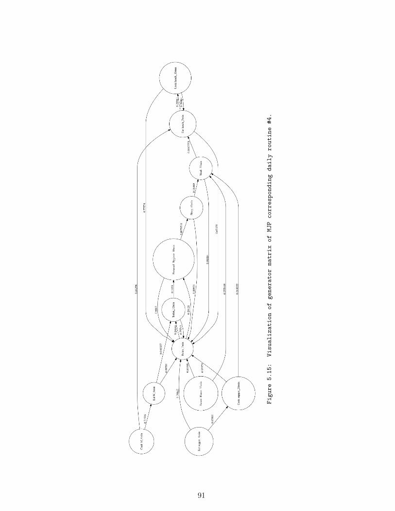
Figure5.15:


91

Figure5.16:


92

5.5 Summary

In this chapter, a probabilistic framework with Markov jump process prior and

Bayesian Lasso is proposed for shifted-invariant nominal data matrix factorization

with application to daily routine discovery. As shown in our experimental results

using both synthetic and real smart home data sets, the basis vectors obtained by our

proposed methodology achieve a much lower basis vector reconstruction error and

activity prediction error. At the same time, a much lower test data reconstruction

error as compared to a number of the state-of-the-art matrix factorization methods

can be obtained. It provides a new abstraction for visualizing daily routines. We

believe that presenting the results to the senior adults living in the smart home

will be beneficial to them to support their awareness of their daily activities, and

potential degradation.

93

Chapter 6

Conclusions

6.1 Summary of thesis

In this thesis, we focus on elderly mobility and daily routine analysis using unsu-

pervised learning methods in a smart home setting.

In Chapter 3, we presented an unsupervised learning methodology for extracting

behavioral patterns as representations of human daily activities from indoor trajec-

tory data. We make use of probabilistic finite state automaton (PDFA) with local

behavioral features to model such data. A state-merging approach is adopted for

inferring a compact PDFA where states with similar local behavioral features are

merged during the inference. The conjecture is that an activity is characterized by

a set of states (local movement patterns) where, once reached one of them, there

is a high chance of transiting and staying among the states before leaving them.

Behavioral patterns are then detected by partitioning the PDFA into subflows via

kernel k-means algorithm.

In Chapter 4, we presented a principled methodology to decompose a nominal

matrix for applications like discovery of daily routines in a smart home. To achieve

that, we assume that the similarity of detected activities can be estimated. We em-

bed the discrete labels onto a d-dimensional continuous space. Then, a hierarchical

probabilistic model with Bayesian Lasso is proposed for the factorization to ensure

the interpretability of the basis vectors. Gibbs sampling is adopted to carry out the

94

model inference.

In Chapter 5, we further extend the model proposed in Chapter 4 to discover

shift-invariant daily routine patterns. Markov jump process is introduced as prior

for basis vectors to model the variations of durations of activities. The model is also

in Bayesian framework and can be inferred via Gibbs sampling.

6.2 Contributions

Unsupervised learning methodology for activity detection is rare, especially that the

longer-range dependency of sensor triggering event is to be taken into consideration.

The proposed features in Chapter 3 are specially designed and shown particularly

effective to group triggering events exhibiting similar local movement behaviors.

Also this is the only work that model an activity as a subflow in a flow graph.

The probabilistic nominal matrix factorization framework (PNoMF) presents in

Chapter 4 is a novel extension of ordinal matrix factorization (OMF) [55] where not

only the noise model of the labels and the label similarity, but also the interpretabil-

ity of the resulting basis vectors are all considered in a unified graphical model to

achieve robust nominal matrix factorization. Other than daily routine discovery, the

proposed factorization method is also applicable to other applications as far as the

label similarity information is available.

PNoMF-MJP is the first work that introduces MJP as the prior to find shift-

invariant patterns in a matrix factorization framework. It also offers a new ab-

straction for visualizing daily routines other than simply showing the basis vectors

so that, richer information can be presented. We believe it is applicable to some

longitudinal pattern monitoring tasks in dynamic environments.

6.3 Future work

For our activity detection framework, it is noted that a number of thresholds are

needed. One possible direction is to find a generic way to determine the values

95

of these thresholds, such as the optimal number of subflows for a given PDFA,

the optimal value for checking the compatible of two candidate merging states,

etc. Another possible direction is to deal with the overlapping among subflows

instead of assuming no overlapping as in Chapter 3. Last but not least, in our work

we only consider one resident case. For the case of multiple residents, trajectory

segmentation has to be carried out before the proposed techniques can be applied.

Also, how to extend the methodology to model the interactions, if the activities are

related to interactions of more than one individual would be worth pursuing.

For our matrix factorization framework, one possible research direction is to

speed up the sampling method to improve the scalability. Another possible direc-

tion is automatic determination of the optimal number of basis vectors and the

optimal dimensions of the label embedding space. In general, it will be interest-

ing to integrate the label embedding and the matrix factorization into one unified

framework.

96

Bibliography

[1] M. J. Beal, Z. Ghahramani, and C. E. Rasmussen. The infinite hidden markov

model. In Advances in Neural Information Processing Systems, pages 577–584,

2002.

[2] R. Belohlavek and M. Krmelova. Beyond boolean matrix decompositions: To-

ward factor analysis and dimensionality reduction of ordinal data. In Proceed-

ings of IEEE 13th International Conference on Data Mining, pages 961–966.

IEEE, 2013.

[3] V. D. Blondel, A. Gajardo, M. Heymans, P. Senellart, and P. Van Dooren. A

measure of similarity between graph vertices: Applications to synonym extrac-

tion and web searching. SIAM RSeview, 46(4):647–666, 2004.

[4] O. Brdiczka, J. L. Crowley, and P. Reignier. Learning situation models in a

smart home. IEEE Transactions on Systems, Man, and Cybernetics, Part B

(Cybernetics), 39(1):56–63, 2009.

[5] R. Bro and S. De Jong. A fast non-negativity-constrained least squares algo-

rithm. Journal of Chemometrics, 11(5):393–401, 1997.

[6] D. Cai, X. He, J. Han, and T. S. Huang. Graph regularized non-negative matrix

factorization for data representation. IEEE Transactions on Pattern Analysis

and Machine Intelligence, 33(8):1548–1560, 2011.

97

[7] R. C. Carrasco and J. Oncina. Learning stochastic regular grammars by means

of a state merging method. In International Colloquium on Grammatical In-

ference, pages 139–152. Springer, 1994.

[8] C. K. Carter and R. Kohn. Markov chain monte carlo in conditionally gaussian

state space models. Biometrika, 83(3):589–601, 1996.

[9] E. Cho, S. A. Myers, and J. Leskovec. Friendship and mobility: user movement

in location-based social networks. In Proceedings of the 17th ACM SIGKDD In-

ternational Conference on Knowledge Discovery and Data Mining, pages 1082–

1090. ACM, 2011.

[10] D. J. Cook and M. Schmitter-Edgecombe. Assessing the quality of activities in

a smart environment. Methods of Information in Medicine, 48(5):480, 2009.

[11] M. H. DeGroot. Optimal Statistical Decisions, volume 82. John Wiley & Sons,

2005.

[12] I. S. Dhillon, Y. Guan, and B. Kulis. Weighted graph cuts without eigenvectors

a multilevel approach. IEEE Transactions on Pattern Analysis and Machine

Intelligence, 29(11):1944–1957, 2007.

[13] C. Doukas, I. Maglogiannis, P. Tragas, D. Liapis, and G. Yovanof. Patient fall

detection using support vector machines. In Proceedings of IFIP International

Conference on Artificial Intelligence Applications and Innovations, pages 147–

156. Springer, 2007.

[14] N. Eagle and A. S. Pentland. Eigenbehaviors: Identifying structure in routine.

Behavioral Ecology and Sociobiology, 63(7):1057–1066, 2009.

[15] M. Fanaswala and V. Krishnamurthy. Detection of anomalous trajectory pat-

terns in target tracking via stochastic context-free grammars and reciprocal

process models. IEEE Journal of Selected Topics in Signal Processing, 7(1):76–

90, 2013.

98

[16] K. Farrahi and D. Gatica-Perez. What did you do today? discovering daily

routines from large-scale mobile data. In Proceedings of the 16th ACM Inter-

national Conference on Multimedia, pages 849–852. ACM, 2008.

[17] K. Farrahi and D. Gatica-Perez. Discovering routines from large-scale human

locations using probabilistic topic models. ACM Transactions on Intelligent

Systems and Technology, 2(1):3, 2011.

[18] D. R. Ferreira and D. Gillblad. Discovering process models from unlabelled

event logs. In BPM, volume 9, pages 143–158. Springer, 2009.

[19] H. Gao, J. Tang, and H. Liu. Mobile location prediction in spatio-temporal

context. In Nokia Mobile Data Challenge Workshop, volume 41, pages 1–4,

2012.

[20] Z. Ghahramani and M. I. Jordan. Factorial hidden markov models. In Advances

in Neural Information Processing Systems, pages 472–478, 1996.

[21] I. I. Gikhman and A. V. Skorokhod. The Theory of Stochastic Processes I.

Springer, 2015.

[22] D. T. Gillespie. Exact stochastic simulation of coupled chemical reactions. The

journal of physical chemistry, 81(25):2340–2361, 1977.

[23] N. Gillis and S. A. Vavasis. Fast and robust recursive algorithmsfor separable

nonnegative matrix factorization. IEEE Transactions on Pattern Analysis and

Machine Intelligence, 36(4):698–714, 2014.

[24] A. Golightly and D. J. Wilkinson. Bayesian parameter inference for stochastic

biochemical network models using particle markov chain monte carlo. Interface

focus, 1(6):807–820, 2011.

[25] M. C. Gonzalez, C. A. Hidalgo, and A.-L. Barabasi. Understanding individual

human mobility patterns. Nature, 453(7196):779–782, June 2008.

99

[26] A. Grover and J. Leskovec. node2vec: Scalable feature learning for networks. In

Proceedings of the 22nd ACM SIGKDD International Conference on Knowledge

Discovery and Data Mining, pages 855–864. ACM, 2016.

[27] T. He, S.-H. G. Chan, and C.-F. Wong. Homemesh: a low-cost indoor wireless

mesh for home networking. IEEE Communications Magazine, 46(12), 2008.

[28] P. Hong, M. Turk, and T. S. Huang. Constructing finite state machines for

fast gesture recognition. In Proceedings of 15th International Conference on

Pattern Recognition, volume 3, pages 691–694. IEEE, 2000.

[29] T. Horanont, S. Phithakkitnukoon, T. W. Leong, Y. Sekimoto, and

R. Shibasaki. Weather effects on the patterns of people’s everyday activities: a

study using gps traces of mobile phone users. PloS One, 8(12):e81153, 2013.

[30] K. Huang, N. D. Sidiropoulos, and A. Swami. Non-negative matrix factoriza-

tion revisited: Uniqueness and algorithm for symmetric decomposition. IEEE

Transactions on Signal Processing, 62(1):211–224, 2014.

[31] C. Hug, R. Deneckere, and C. Salinesi. Map-tbs: Map process enactment traces

and analysis. In Research Challenges in Information Science (RCIS), 2012 Sixth

International Conference on, pages 1–6. IEEE, 2012.

[32] T. Hulnhagen, I. Dengler, A. Tamke, T. Dang, and G. Breuel. Maneuver recog-

nition using probabilistic finite-state machines and fuzzy logic. In Intelligent

Vehicles Symposium (IV), 2010 IEEE, pages 65–70. IEEE, 2010.

[33] A. Ihler, J. Hutchins, and P. Smyth. Learning to detect events with markov-

modulated poisson processes. ACM Transactions on Knowledge Discovery from

Data (TKDD), 1(3):13, 2007.

[34] S. Jiang, J. Ferreira, and M. C. Gonzalez. Clustering daily patterns of human

activities in the city. Data Mining and Knowledge Discovery, 25(3):478–510,

2012.

100

[35] L. Jing, P. Wang, and L. Yang. Sparse probabilistic matrix factorization by

laplace distribution for collaborative filtering. In Proceedings of the 24th Inter-

national Conference on Artificial Intelligence, pages 1771–1777, 2015.

[36] G. Khodabandelou, C. Hug, R. Deneckere, and C. Salinesi. Process mining ver-

sus intention mining. In Enterprise, Business-Process and Information Systems

Modeling, pages 466–480. Springer, 2013.

[37] G. Khodabandelou, C. Hug, R. Deneckere, and C. Salinesi. Supervised in-

tentional process models discovery using hidden markov models. In Research

Challenges in Information Science (RCIS), 2013 IEEE Seventh International

Conference on, pages 1–11. IEEE, 2013.

[38] B. Kim, R. Khanna, and O. O. Koyejo. Examples are not enough, learn to

criticize! criticism for interpretability. In Advances in Neural Information Pro-

cessing Systems, 2016.

[39] H. Kuehne, A. Arslan, and T. Serre. The language of actions: Recovering the

syntax and semantics of goal-directed human activities. In Proceedings of the

IEEE Conference on Computer Vision and Pattern Recognition, pages 780–787,

2014.

[40] J. R. Kwapisz, G. M. Weiss, and S. A. Moore. Activity recognition using

cell phone accelerometers. ACM SigKDD Explorations Newsletter, 12(2):74–

82, 2011.

[41] D. D. Lee and H. S. Seung. Learning the parts of objects by nonnegative matrix

factorization. Nature, 401:788–791, 1999.

[42] M. L. Lee and A. K. Dey. Reflecting on pills and phone use: Supporting

awareness of functional abilities for older adults. In Proceedings of the SIGCHI

Conference on Human Factors in Computing Systems, pages 2095–2104. ACM,

2011.

101

[43] C. Li, W. K. Cheung, J. Liu, and J. K. Ng. Bayesian nominal matrix factoriza-

tion for mining daily activity patterns. In Proceedings of 2016 IEEE/WIC/ACM

International Conference on Web Intelligence and Intelligent Agent Technology

(WI-IAT), pages 335–342, 2016.

[44] K. Li and Y. Fu. Prediction of human activity by discovering temporal sequence

patterns. IEEE Transactions on Pattern Analysis and Machine Intelligence,

36(8):1644–1657, 2014.

[45] Y. Li, D. Jin, Z. Wang, P. Hui, L. Zeng, and S. Chen. A markov jump pro-

cess model for urban vehicular mobility: Modeling and applications. IEEE

Transactions on Mobile Computing, 13(9):1911–1926, 2014.

[46] Z. Li, X. Wu, and H. Peng. Nonnegative matrix factorization on orthogonal

subspace. Pattern Recognition Letters, 31(9):905–911, 2010.

[47] M. M. Lin, B. Dong, and M. T. Chu. Integer matrix factorization and its

application. Technical report, 2005.

[48] Q. Lin, D. Zhang, D. Li, H. Ni, and X. Zhou. Extracting intra-and inter-

activity association patterns from daily routines of elders. In Proceedings of

International Conference on Smart Homes and Health Telematics, pages 36–

44. Springer, 2013.

[49] J.-G. Lou, Q. Fu, S. Yang, J. Li, and B. Wu. Mining program workflow from

interleaved traces. In Proceedings of the 16th ACM SIGKDD International

Conference on Knowledge Discovery and Data mining, pages 613–622. ACM,

2010.

[50] S. Maurus and C. Plant. Ternary matrix factorization. In Proceedings of IEEE

International Conference on Data Mining, pages 400–409. IEEE, 2014.

[51] R. Megret, V. Dovgalecs, H. Wannous, S. Karaman, J. Benois-Pineau,

E. El Khoury, J. Pinquier, P. Joly, R. Andre-Obrecht, Y. Gaestel, et al. The

102

immed project: wearable video monitoring of people with age dementia. In

Proceedings of the 18th ACM international conference on Multimedia, pages

1299–1302. ACM, 2010.

[52] P. Miettinen. Dynamic boolean natrix factorizations. In Proceedings of 12th

IEEE International Conference on Data Mining, pages 519–528. IEEE, 2012.

[53] K. P. Murphy and S. Russell. Dynamic bayesian networks: representation,

inference and learning. 2002.

[54] E. Nazerfard, P. Rashidi, and D. J. Cook. Discovering temporal features and

relations of activity patterns. In Proceedings of IEEE International Conference

on Data Mining Workshops, pages 1069–1075. IEEE, 2010.

[55] U. Paquet, B. Thomson, and O. Winther. A hierarchical model for ordinal

matrix factorization. Statistics and Computing, 22(4):945–957, 2012.

[56] C. Parent, S. Spaccapietra, C. Renso, G. Andrienko, N. Andrienko, V. Bogorny,

M. L. Damiani, A. Gkoulalas-Divanis, J. Macedo, N. Pelekis, et al. Semantic

trajectories modeling and analysis. ACM Computing Surveys, 45(4):42, 2013.

[57] K. Park, Y. Lin, V. Metsis, Z. Le, and F. Makedon. Abnormal human behav-

ioral pattern detection in assisted living environments. In Proceedings of the

3rd International Conference on Pervasive Technologies Related to Assistive

Environments, page 9. ACM, 2010.

[58] T. Park and G. Casella. The bayesian lasso. Journal of the American Statistical

Association, 103(482):681–686, 2008.

[59] K. Pastra and Y. Aloimonos. The minimalist grammar of action. Philo-

sophical Transactions of the Royal Society of London B: Biological Sciences,

367(1585):103–117, 2012.

103

[60] H.-K. Peng, P. Wu, J. Zhu, and J. Y. Zhang. Helix: Unsupervised grammar

induction for structured activity recognition. In Proceedings of IEEE 11th In-

ternational Conference on Data Mining, pages 1194–1199. IEEE, 2011.

[61] H. Pirsiavash and D. Ramanan. Parsing videos of actions with segmental gram-

mars. In Proceedings of the IEEE Conference on Computer Vision and Pattern

Recognition, pages 612–619, 2014.

[62] T. Prentow, A. Thom, H. Blunck, and J. Vahrenhold. Making sense of tra-

jectory data in indoor spaces. In Proceedings of the 16th IEEE International

Conference on Mobile Data Management (MDM), volume 1, pages 116–121.

IEEE, 2015.

[63] L. R. Rabiner. A tutorial on hidden markov models and selected applications

in speech recognition. Proceedings of the IEEE, 77(2):257–286, 1989.

[64] V. Rao and Y. W. Teh. Fast mcmc sampling for markov jump processes and

extensions. The Journal of Machine Learning Research, 14(1):3295–3320, 2013.

[65] P. Rashidi and D. J. Cook. Keeping the resident in the loop: Adapting the smart

home to the user. IEEE Transactions on Systems, Man, and Cybernetics-Part

A: Systems and Humans, 39(5):949–959, 2009.

[66] P. Rashidi and D. J. Cook. Mining and monitoring patterns of daily routines

for assisted living in real world settings. In Proceedings of the 1st ACM Inter-

national Health Informatics Symposium, pages 336–345. ACM, 2010.

[67] P. Rashidi, D. J. Cook, L. B. Holder, and M. Schmitter-Edgecombe. Discovering

activities to recognize and track in a smart environment. IEEE Transactions

on Knowledge and Data Engineering, 23(4):527–539, 2011.

[68] J. Saives, C. Pianon, and G. Faraut. Activity discovery and detection of be-

havioral deviations of an inhabitant from binary sensors. IEEE Transactions

on Automation Science and Engineering, 12(4):1211–1224, 2015.

104

[69] R. Salakhutdinov and A. Mnih. Probabilistic matrix factorization. In Advances

in Neural Information Processing Systems, volume 20, pages 1257–1264, 2007.

[70] M. N. Schmidt, O. Winther, and L. K. Hansen. Bayesian non-negative ma-

trix factorization. In Proceedings of International Conference on Independent

Component Analysis and Signal Separation, pages 540–547, 2009.

[71] C. M. Schneider, V. Belik, T. Couronne, Z. Smoreda, and M. C. Gonzalez. Un-

ravelling daily human mobility motifs. Journal of The Royal Society Interface,

10(84):20130246, 2013.

[72] C. Song, Z. Qu, N. Blumm, and A.-L. Barabsi. Limits of predictability in

human mobility. Science, 327(5968):1018–1021, 2010.

[73] F.-T. Sun, Y.-T. Yeh, H.-T. Cheng, C. Kuo, and M. Griss. Nonparametric

discovery of human routines from sensor data. In Proceedings of IEEE Inter-

national Conference on Pervasive Computing and Communications (PerCom),

pages 11–19. IEEE, 2014.

[74] D. Tacconi, O. Mayora, P. Lukowicz, B. Arnrich, C. Setz, G. Troster, and

C. Haring. Activity and emotion recognition to support early diagnosis of

psychiatric diseases. In Proceedings of 2nd International Conference on Perva-

sive Computing Technologies for Healthcare (Pervasive Health), pages 100–102.

IEEE, 2008.

[75] F. Thollard, P. Dupont, C. de la Higuera, et al. Probabilistic dfa inference using

kullback-leibler divergence and minimality. In Proceedings of 17th International

Conference on Machine Learning, pages 975–982, 2000.

[76] R. Tibshirani. Regression shrinkage and selection via the lasso. Journal of the

Royal Statistical Society. Series B (Methodological), pages 267–288, 1996.

[77] van der Aalst. Process Mining: Discovery - Discovery, Conformance and En-

hancement of Business Processes. Springer, 2011.

105

[78] W. M. van der Aalst. Process mining: discovering and improving spaghetti and

lasagna processes. In Computational Intelligence and Data Mining (CIDM),

2011 IEEE Symposium on, pages 1–7. IEEE, 2011.

[79] E. Vidal, F. Thollard, C. De La Higuera, F. Casacuberta, and R. C. Carrasco.

Probabilistic finite-state machines part i. IEEE Transactions on Pattern Anal-

ysis and Machine Intelligence, 27(7):1013–1025, 2005.

[80] X. Xiao, Y. Zheng, Q. Luo, and X. Xie. Inferring social ties between users

with human location history. Journal of Ambient Intelligence and Humanized

Computing, 5(1):3–19, 2014.

[81] M. Xu, J. Zhu, and B. Zhang. Nonparametric max-margin matrix factorization

for collaborative prediction. In Advances in Neural Information Processing

Systems, volume 12, pages 64–72, 2012.

[82] Z. Yan, D. Chakraborty, C. Parent, S. Spaccapietra, and K. Aberer. Semantic

trajectories: Mobility data computation and annotation. ACM Transactions

on Intelligent Systems and Technology, 4(3):49, 2013.

[83] N. J. Yuan, Y. Zheng, X. Xie, Y. Wang, K. Zheng, and H. Xiong. Discovering

urban functional zones using latent activity trajectories. IEEE Transactions on

Knowledge and Data Engineering, 27(3):712–725, 2015.

[84] T. Zhao, H. Ni, X. Zhou, L. Qiang, D. Zhang, and Z. Yu. Detecting abnormal

patterns of daily activities for the elderly living alone. In Proceedings of In-

ternational Conference on Health Information Science, pages 95–108. Springer,

2014.

[85] J. Zheng, S. Liu, and L. M. Ni. Effective routine behavior pattern discovery

from sparse mobile phone data via collaborative filtering. In Proceedings of

IEEE International Conference on Pervasive Computing and Communications,

pages 29–37, 2013.

106

[86] K. Zheng, Y. Zheng, N. J. Yuan, S. Shang, and X. Zhou. Online discovery

of gathering patterns over trajectories. IEEE Transactions on Knowledge and

Data Engineering, 26(8):1974–1988, 2014.

107

CURRICULUM VITAE

Academic qualifications of the thesis author, Mr. LI Chen:

• Received the degree of Bachelor of Engineering from Jiangxi Normal University,

July 2009.

• Received the degree of Master of Science from Hong Kong Baptist University,

November 2011.

June 2018

108

DOCTORAL THESIS Automatic extraction of behavioral ...

Documents

Transcript of DOCTORAL THESIS Automatic extraction of behavioral ...