RESEARCH ARTICLE

Do trout swim better than eels? Challenges for estimatingperformance based on the wake of self-propelled bodies

Eric D. Tytell

Received: 12 February 2007 / Revised: 16 May 2007 / Accepted: 4 June 2007 / Published online: 28 June 2007

� Springer-Verlag 2007

Abstract Engineers and biologists have long desired to

compare propulsive performance for fishes and underwater

vehicles of different sizes, shapes, and modes of propul-

sion. Ideally, such a comparison would be made on the

basis of either propulsive efficiency, total power output or

both. However, estimating the efficiency and power output

of self-propelled bodies, and particularly fishes, is meth-

odologically challenging because it requires an estimate of

thrust. For such systems traveling at a constant velocity,

thrust and drag are equal, and can rarely be separated on

the basis of flow measured in the wake. This problem is

demonstrated using flow fields from swimming American

eels, Anguilla rostrata, measured using particle image

velocimetry (PIV) and high-speed video. Eels balance

thrust and drag quite evenly, resulting in virtually no wake

momentum in the swimming (axial) direction. On average,

their wakes resemble those of self-propelled jet propulsors,

which have been studied extensively. Theoretical studies of

such wakes may provide methods for the estimation of

thrust separately from drag. These flow fields are compared

with those measured in the wakes of rainbow trout,

Oncorhynchus mykiss, and bluegill sunfish, Lepomis mac-

rochirus. In contrast to eels, these fishes produce wakes

with axial momentum. Although the net momentum flux

must be zero on average, it is neither spatially nor tem-

porally homogeneous; the heterogeneity may provide an

alternative route for estimating thrust. This review shows

examples of wakes and velocity profiles from the three

fishes, indicating challenges in estimating efficiency and

power output and suggesting several routes for further

experiments. Because these estimates will be complicated,

a much simpler method for comparing performance is

outlined, using as a point of comparison the power lost

producing the wake. This wake power, a component of the

efficiency and total power, can be estimated in a straight-

forward way from the flow fields. Although it does not

provide complete information about the performance, it

can be used to place constraints on the relative efficiency

and cost of transport for the fishes.

1 Introduction

Fishes are often assumed to be highly efficient swimmers.

After all, many species routinely swim or migrate over

very long distances, including fishes of such diverse shapes

and sizes as eels, tunas, many sharks, and river fishes like

trout (Helfman et al. 1997). Natural selection has had

hundreds of millions of years (Helfman et al. 1997) to tune

the design of these fishes. One would naturally imagine that

efficient swimming would be an important design criterion,

particularly for these migratory or long-distance swimmers.

Therefore, biologists and engineers have been eager to

examine the efficiency of undulatory swimming, with a

goal of determining the best fish body shapes and swim-

ming modes, and to extract design principles for the con-

struction of highly efficient underwater autonomous

vehicles.

This goal, however, is based on a fallacy. Natural

selection has not produced optimal swimming perfor-

mance. Selection merely results in performance that is

good enough that an animal can avoid dying or being eaten

long enough to reproduce (Garland 1998). ‘‘Good enough,’’

E. D. Tytell (&)

Department of Biology, University of Maryland,

College Park, MD 20742, USA

e-mail: tytell@umd.edu

123

Exp Fluids (2007) 43:701–712

DOI 10.1007/s00348-007-0343-x

also, is determined within a multitude of conflicting

demands. Evolutionary history, feeding, migration, and

sexual displays, among many other factors, all simulta-

neously influence an organism’s fitness. Not only this, but

the conditions under which selection happens are con-

stantly changing, as predators and prey evolve together and

the environment changes. Even though any one fish species

is not optimal (or even necessarily very good), the differ-

ences among species may provide useful hints for the

design of underwater vehicles.

However, it would be wise not to assume that fish

swimming is highly efficient—it might not be, particularly

in comparison to propeller-based propulsion at steady

speeds. For a migrating fish, an independent and possibly

more important criterion than efficiency is energy con-

sumption. The hydrodynamic energy consumption rate

Ptotal is composed of two components,

Ptotal ¼ UT þ Pwaste; ð1Þ

where UT is the useful power, the product of swimming

velocity U and the thrust force T, and Pwaste is the wasted

power. For the purposes of this review, Pwaste is assumed to

be only the power used to produce a wake (Pwake);

metabolic power wasted converting chemical energy into

mechanical energy is ignored. Propulsive efficiency, in

turn, is conventionally defined as

g ¼ UT=Ptotal: ð2Þ

Based on these definitions, Ptotal could be large, even if g is

close to one. For example, a fish with high drag might put

99% of its locomotory energy to forward propulsion, but

end up using more total energy than a very streamlined fish

that wastes 50% of its output.

Together, however, propulsive efficiency and total

energy output provide a useful way of comparing the

swimming performance of different fishes and underwater

vehicles. While natural selection cannot be said to produce

optima, different species of fishes presumably differ in

propulsive efficiency or total power consumption. In par-

ticular, one would expect migratory fishes, like trout, and

eels, to be better swimmers than fishes that generally stay

put, like bluegill sunfish—although the criteria that deter-

mine ‘‘better’’ are unknown. As an evolutionary question, it

would be interesting to examine those criteria. How does

hydrodynamic performance factor into the shape changes

over the evolutionary history of fishes? For example, trout

and eels, two very differently shaped fishes, both swim

long distances—is one body shape more efficient or more

power-conserving than the other? Or are other factors,

unrelated to swimming, more important in determining

body shape? As an engineering question, it would also be

useful to compare swimming performance among different

types of self-propelled systems. If one wanted to design a

submarine, would it be better be shaped like a trout, an eel,

or a conventional propeller-based underwater vehicle?

The recent availability of high-resolution, high-speed

particle image velocimetry (PIV; Willert and Gharib 1991)

systems has made it possible and relatively straightforward

to measure the fluid flow in a two-dimensional plane

around swimming fishes (e.g., Anderson et al. 2001; Muller

et al. 1997; Nauen and Lauder 2002a; Tytell and Lauder

2004). This measurement technique has raised the possi-

bility of estimating the thrust or drag on a swimming fish

from the flow in its wake. To date, however, such estimates

have been problematic (Schultz and Webb 2002).

In this review, the differences among wakes of several

swimming fishes are first demonstrated, using examples

from swimming eels (Tytell 2004a; Tytell and Lauder

2004), along with rainbow trout and bluegill sunfish (E. D.

Tytell, unpublished data). These differences are examined

by looking at the net momentum flux in each wake.

Because thrust is problematic to estimate in general, the

wake power is instead studied. Although it is only one

component of the total power, this review demonstrates

how it can be used to bracket the possible performance

envelopes of different fishes for future comparative studies.

1.1 Swimming modes

The fishes examined in this review span much of the range

of the standard classification of swimming modes (Breder

1926). Eels are termed anguilliform swimmers, and are

understood to undulate with about one complete wave on

their bodies, with a substantial undulation amplitude even

close to the head. Bluegill sunfish, in contrast, are termed

carangiform swimmers, and bend through about half of a

wave, which only reaches a substantial amplitude in the

posterior third of their bodies. Trout are called subca-

rangiform, which is intermediate between the eel and the

bluegill.

Additionally, the fish span a range of body shapes. Eels

are elongate, with a fairly constant oval cross-section and

no physical demarcation between the ‘‘tail’’ and ‘‘body.’’

Bluegill, in contrast, have a highly flattened body with a

fairly separate tail (caudal fin), joined by a narrow region

termed the caudal peduncle. Trout, again, are intermediate,

with a fusiform body and separate tail, but less narrowing

at the caudal peduncle than bluegill.

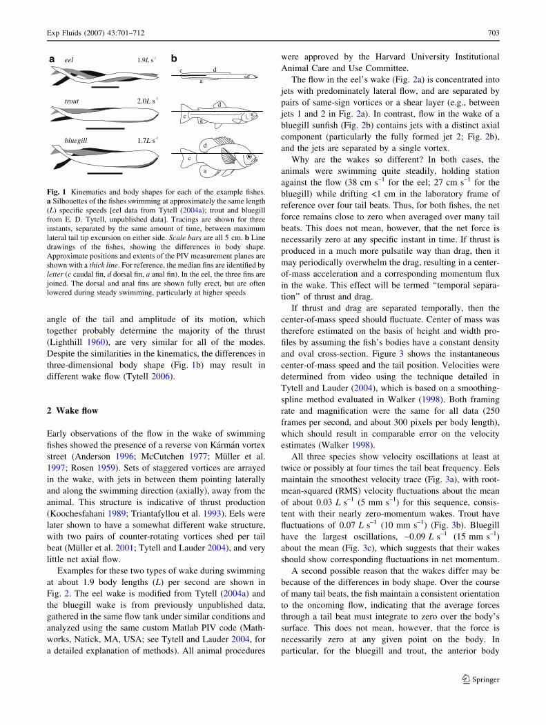
Figure 1 shows examples of the kinematics and body

shape for each fish. Although the eel moves its anterior

body more than the other fishes, all fishes have some head

motion. In fact, the modes are more similar than they are

different (Lauder and Tytell 2006). Specifically, both the

702 Exp Fluids (2007) 43:701–712

123

angle of the tail and amplitude of its motion, which

together probably determine the majority of the thrust

(Lighthill 1960), are very similar for all of the modes.

Despite the similarities in the kinematics, the differences in

three-dimensional body shape (Fig. 1b) may result in

different wake flow (Tytell 2006).

2 Wake flow

Early observations of the flow in the wake of swimming

fishes showed the presence of a reverse von Karman vortex

street (Anderson 1996; McCutchen 1977; Muller et al.

1997; Rosen 1959). Sets of staggered vortices are arrayed

in the wake, with jets in between them pointing laterally

and along the swimming direction (axially), away from the

animal. This structure is indicative of thrust production

(Koochesfahani 1989; Triantafyllou et al. 1993). Eels were

later shown to have a somewhat different wake structure,

with two pairs of counter-rotating vortices shed per tail

beat (Muller et al. 2001; Tytell and Lauder 2004), and very

little net axial flow.

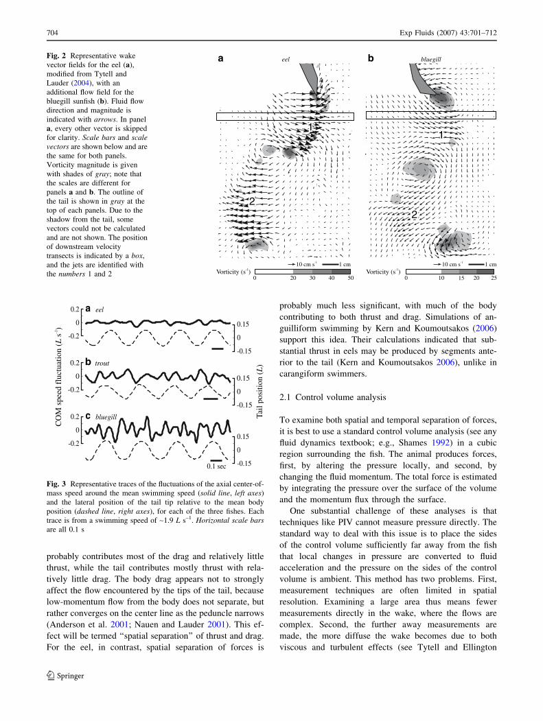
Examples for these two types of wake during swimming

at about 1.9 body lengths (L) per second are shown in

Fig. 2. The eel wake is modified from Tytell (2004a) and

the bluegill wake is from previously unpublished data,

gathered in the same flow tank under similar conditions and

analyzed using the same custom Matlab PIV code (Math-

works, Natick, MA, USA; see Tytell and Lauder 2004, for

a detailed explanation of methods). All animal procedures

were approved by the Harvard University Institutional

Animal Care and Use Committee.

The flow in the eel’s wake (Fig. 2a) is concentrated into

jets with predominately lateral flow, and are separated by

pairs of same-sign vortices or a shear layer (e.g., between

jets 1 and 2 in Fig. 2a). In contrast, flow in the wake of a

bluegill sunfish (Fig. 2b) contains jets with a distinct axial

component (particularly the fully formed jet 2; Fig. 2b),

and the jets are separated by a single vortex.

Why are the wakes so different? In both cases, the

animals were swimming quite steadily, holding station

against the flow (38 cm s–1 for the eel; 27 cm s–1 for the

bluegill) while drifting <1 cm in the laboratory frame of

reference over four tail beats. Thus, for both fishes, the net

force remains close to zero when averaged over many tail

beats. This does not mean, however, that the net force is

necessarily zero at any specific instant in time. If thrust is

produced in a much more pulsatile way than drag, then it

may periodically overwhelm the drag, resulting in a center-

of-mass acceleration and a corresponding momentum flux

in the wake. This effect will be termed ‘‘temporal separa-

tion’’ of thrust and drag.

If thrust and drag are separated temporally, then the

center-of-mass speed should fluctuate. Center of mass was

therefore estimated on the basis of height and width pro-

files by assuming the fish’s bodies have a constant density

and oval cross-section. Figure 3 shows the instantaneous

center-of-mass speed and the tail position. Velocities were

determined from video using the technique detailed in

Tytell and Lauder (2004), which is based on a smoothing-

spline method evaluated in Walker (1998). Both framing

rate and magnification were the same for all data (250

frames per second, and about 300 pixels per body length),

which should result in comparable error on the velocity

estimates (Walker 1998).

All three species show velocity oscillations at least at

twice or possibly at four times the tail beat frequency. Eels

maintain the smoothest velocity trace (Fig. 3a), with root-

mean-squared (RMS) velocity fluctuations about the mean

of about 0.03 L s–1 (5 mm s–1) for this sequence, consis-

tent with their nearly zero-momentum wakes. Trout have

fluctuations of 0.07 L s–1 (10 mm s–1) (Fig. 3b). Bluegill

have the largest oscillations, ~0.09 L s–1 (15 mm s–1)

about the mean (Fig. 3c), which suggests that their wakes

should show corresponding fluctuations in net momentum.

A second possible reason that the wakes differ may be

because of the differences in body shape. Over the course

of many tail beats, the fish maintain a consistent orientation

to the oncoming flow, indicating that the average forces

through a tail beat must integrate to zero over the body’s

surface. This does not mean, however, that the force is

necessarily zero at any given point on the body. In

particular, for the bluegill and trout, the anterior body

1.9 sL -1eel

1.7 sL -1bluegill

2.0 sL -1trout

a b

c

d

a

c

d

a

d

a

c

Fig. 1 Kinematics and body shapes for each of the example fishes.

a Silhouettes of the fishes swimming at approximately the same length

(L) specific speeds [eel data from Tytell (2004a); trout and bluegill

from E. D. Tytell, unpublished data]. Tracings are shown for three

instants, separated by the same amount of time, between maximum

lateral tail tip excursion on either side. Scale bars are all 5 cm. b Line

drawings of the fishes, showing the differences in body shape.

Approximate positions and extents of the PIV measurement planes are

shown with a thick line. For reference, the median fins are identified by

letter (c caudal fin, d dorsal fin, a anal fin). In the eel, the three fins are

joined. The dorsal and anal fins are shown fully erect, but are often

lowered during steady swimming, particularly at higher speeds

Exp Fluids (2007) 43:701–712 703

123

probably contributes most of the drag and relatively little

thrust, while the tail contributes mostly thrust with rela-

tively little drag. The body drag appears not to strongly

affect the flow encountered by the tips of the tail, because

low-momentum flow from the body does not separate, but

rather converges on the center line as the peduncle narrows

(Anderson et al. 2001; Nauen and Lauder 2001). This ef-

fect will be termed ‘‘spatial separation’’ of thrust and drag.

For the eel, in contrast, spatial separation of forces is

probably much less significant, with much of the body

contributing to both thrust and drag. Simulations of an-

guilliform swimming by Kern and Koumoutsakos (2006)

support this idea. Their calculations indicated that sub-

stantial thrust in eels may be produced by segments ante-

rior to the tail (Kern and Koumoutsakos 2006), unlike in

carangiform swimmers.

2.1 Control volume analysis

To examine both spatial and temporal separation of forces,

it is best to use a standard control volume analysis (see any

fluid dynamics textbook; e.g., Shames 1992) in a cubic

region surrounding the fish. The animal produces forces,

first, by altering the pressure locally, and second, by

changing the fluid momentum. The total force is estimated

by integrating the pressure over the surface of the volume

and the momentum flux through the surface.

One substantial challenge of these analyses is that

techniques like PIV cannot measure pressure directly. The

standard way to deal with this issue is to place the sides

of the control volume sufficiently far away from the fish

that local changes in pressure are converted to fluid

acceleration and the pressure on the sides of the control

volume is ambient. This method has two problems. First,

measurement techniques are often limited in spatial

resolution. Examining a large area thus means fewer

measurements directly in the wake, where the flows are

complex. Second, the further away measurements are

made, the more diffuse the wake becomes due to both

viscous and turbulent effects (see Tytell and Ellington

10 cm s-1 1 cm

0 20 30 40 50Vorticity (s )-1

eel bluegill

10 cm s-1 1 cmVorticity (s )-1

0 10 15 20 25

a b

1111

2222

Fig. 2 Representative wake

vector fields for the eel (a),

modified from Tytell and

Lauder (2004), with an

additional flow field for the

bluegill sunfish (b). Fluid flow

direction and magnitude is

indicated with arrows. In panel

a, every other vector is skipped

for clarity. Scale bars and scalevectors are shown below and are

the same for both panels.

Vorticity magnitude is given

with shades of gray; note that

the scales are different for

panels a and b. The outline of

the tail is shown in gray at the

top of each panels. Due to the

shadow from the tail, some

vectors could not be calculated

and are not shown. The position

of downstream velocity

transects is indicated by a box,

and the jets are identified with

the numbers 1 and 2

CO

M s

peed

flu

ctua

tion

(L s

-1)

Tail

posi

tion

()

L

eela

-0.2

0

0.2

-0.15

0

0.15

troutb

-0.2

0

0.2

-0.15

0

0.15

bluegillc

-0.2

0

0.2

-0.15

0

0.15

0.1 sec

Fig. 3 Representative traces of the fluctuations of the axial center-of-

mass speed around the mean swimming speed (solid line, left axes)

and the lateral position of the tail tip relative to the mean body

position (dashed line, right axes), for each of the three fishes. Each

trace is from a swimming speed of ~1.9 L s–1. Horizontal scale barsare all 0.1 s

704 Exp Fluids (2007) 43:701–712

123

2003, for a detailed discussion of these effects). More

precision is thus necessary for measurements in the far

wake than for those in the near wake.

However, because fishes are self-propelled, they may

not require such large control volumes. The net force is

close to zero, and so any local pressure changes will be

small and will be distributed in the wake quite rapidly.

Consider the changes in velocity shown in Fig. 3. Peak

acceleration for the bluegill is around 2,000 mm s–2, cor-

responding to a force of about 150 mN for the ~70 g fish.

Remember, this force is not thrust, but a rough estimate of

the peak net force. If all of this force is due to pressure

applied to an actuator surface swept out by the tail over a

tail beat, then the pressure change on that surface would be

well under 1% of ambient. Thus, due to the very low-net

forces on a self-propelled body, pressure changes even in

the near wake can safely be neglected.

For the control volume analysis, the remaining effect is

momentum flux through the sides of the volume. If the

sides and the top and bottom are placed parallel to the

mean flow and sufficiently far from the wake, they will

have zero flux. In the end, the only planes that matter are

the transects upstream and downstream of the fish.

Since the fluid density and mean flow speed are con-

stant, the momentum flux through these planes is propor-

tional to the average net fluid velocity added by the fish.

Transects across the wake were therefore estimated in a

5 mm thick box spanning the wake, placed 10 mm down-

stream from the average tail position (examples shown in

Fig. 2). Single transects were produced by averaging the

PIV vectors along the axial thickness of the box, which

helped to reduce noise. If necessary, transects were angled

to be perpendicular to the swimming angle of the fish to

compensate for any small angle that might have been

present. Swimming angle was <2� on average.

The net momentum flux is the difference between the

flux through the upstream and downstream planes of the

control volume. For trout and bluegill, upstream flow was

measured directly and upstream transects were estimated

analogously to the wake transects, but placed 10 mm up-

stream from the head. For eels, upstream flow could not be

measured directly, because the animals would not swim

consistently with their heads in the laser light sheet (Tytell

and Lauder 2004). Instead, the laser light sheet was posi-

tioned to view flow around the posterior two thirds of the

eels’ bodies (Fig. 1), and flow entering the control volume

was estimated from the average flow field measured

without an animal present.

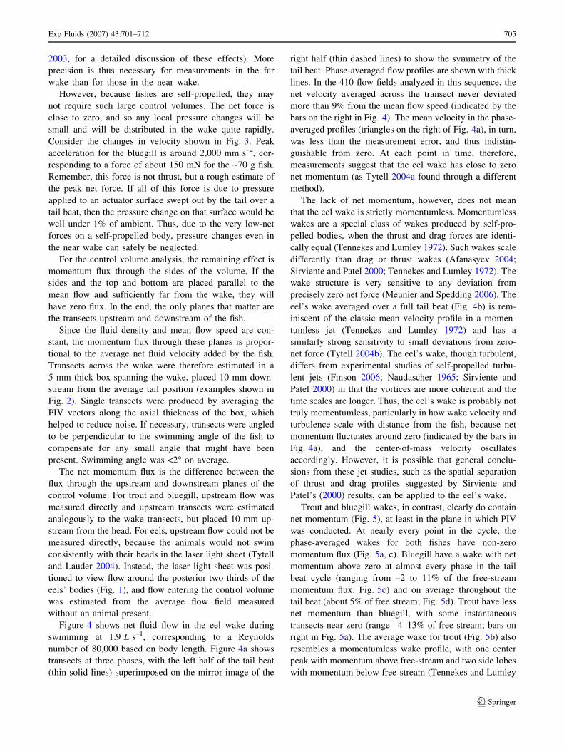
Figure 4 shows net fluid flow in the eel wake during

swimming at 1.9 L s–1, corresponding to a Reynolds

number of 80,000 based on body length. Figure 4a shows

transects at three phases, with the left half of the tail beat

(thin solid lines) superimposed on the mirror image of the

right half (thin dashed lines) to show the symmetry of the

tail beat. Phase-averaged flow profiles are shown with thick

lines. In the 410 flow fields analyzed in this sequence, the

net velocity averaged across the transect never deviated

more than 9% from the mean flow speed (indicated by the

bars on the right in Fig. 4). The mean velocity in the phase-

averaged profiles (triangles on the right of Fig. 4a), in turn,

was less than the measurement error, and thus indistin-

guishable from zero. At each point in time, therefore,

measurements suggest that the eel wake has close to zero

net momentum (as Tytell 2004a found through a different

method).

The lack of net momentum, however, does not mean

that the eel wake is strictly momentumless. Momentumless

wakes are a special class of wakes produced by self-pro-

pelled bodies, when the thrust and drag forces are identi-

cally equal (Tennekes and Lumley 1972). Such wakes scale

differently than drag or thrust wakes (Afanasyev 2004;

Sirviente and Patel 2000; Tennekes and Lumley 1972). The

wake structure is very sensitive to any deviation from

precisely zero net force (Meunier and Spedding 2006). The

eel’s wake averaged over a full tail beat (Fig. 4b) is rem-

iniscent of the classic mean velocity profile in a momen-

tumless jet (Tennekes and Lumley 1972) and has a

similarly strong sensitivity to small deviations from zero-

net force (Tytell 2004b). The eel’s wake, though turbulent,

differs from experimental studies of self-propelled turbu-

lent jets (Finson 2006; Naudascher 1965; Sirviente and

Patel 2000) in that the vortices are more coherent and the

time scales are longer. Thus, the eel’s wake is probably not

truly momentumless, particularly in how wake velocity and

turbulence scale with distance from the fish, because net

momentum fluctuates around zero (indicated by the bars in

Fig. 4a), and the center-of-mass velocity oscillates

accordingly. However, it is possible that general conclu-

sions from these jet studies, such as the spatial separation

of thrust and drag profiles suggested by Sirviente and

Patel’s (2000) results, can be applied to the eel’s wake.

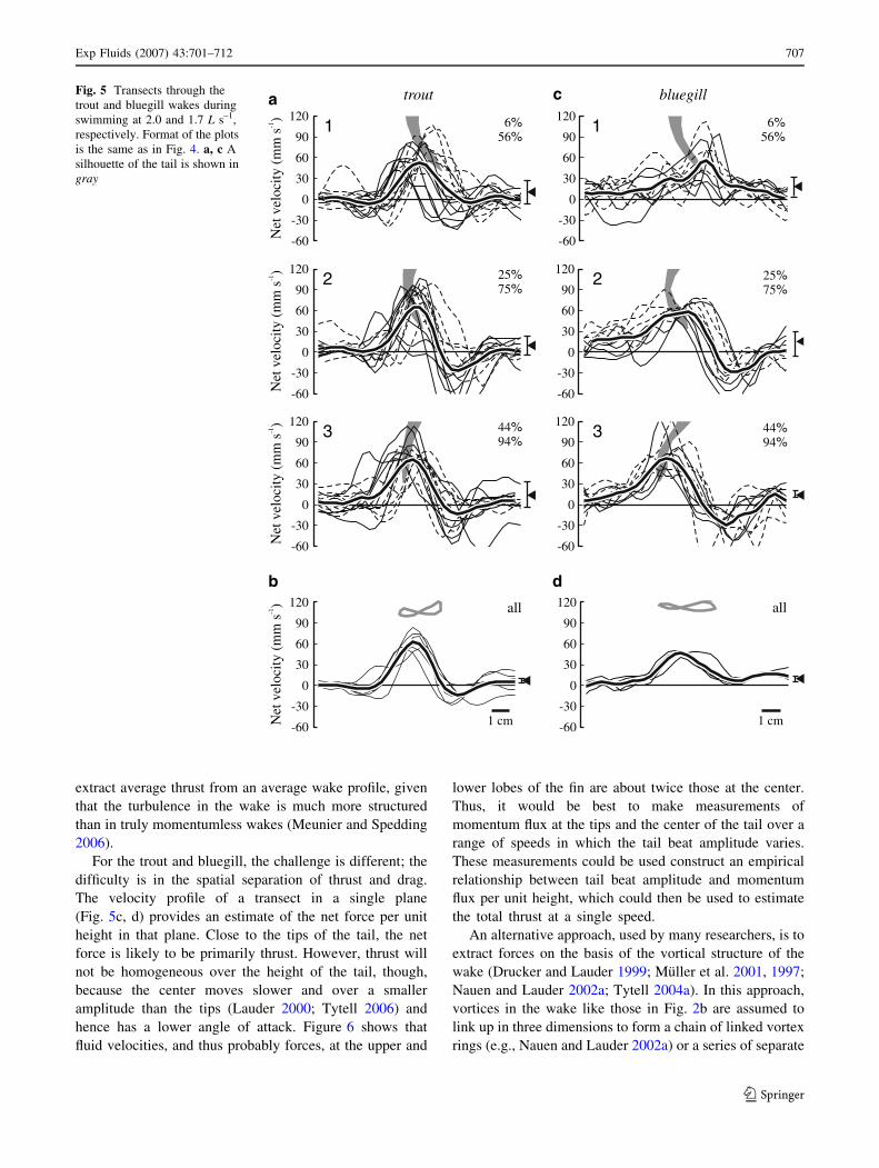
Trout and bluegill wakes, in contrast, clearly do contain

net momentum (Fig. 5), at least in the plane in which PIV

was conducted. At nearly every point in the cycle, the

phase-averaged wakes for both fishes have non-zero

momentum flux (Fig. 5a, c). Bluegill have a wake with net

momentum above zero at almost every phase in the tail

beat cycle (ranging from –2 to 11% of the free-stream

momentum flux; Fig. 5c) and on average throughout the

tail beat (about 5% of free stream; Fig. 5d). Trout have less

net momentum than bluegill, with some instantaneous

transects near zero (range –4–13% of free stream; bars on

right in Fig. 5a). The average wake for trout (Fig. 5b) also

resembles a momentumless wake profile, with one center

peak with momentum above free-stream and two side lobes

with momentum below free-stream (Tennekes and Lumley

Exp Fluids (2007) 43:701–712 705

123

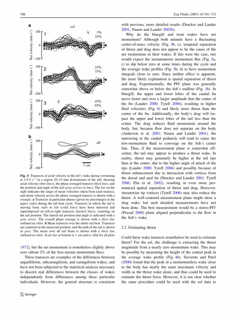
1972), but the net momentum is nonetheless slightly above

zero (about 2% of the free-stream momentum flux).

These transects are examples of the differences between

anguilliform, subcarangiform, and carangiform wakes, and

have not been subjected to the statistical analysis necessary

to discern real differences between the classes of wakes

independently from differences among these particular

individuals. However, the general structure is consistent

with previous, more detailed results (Drucker and Lauder

2001; Nauen and Lauder 2002b).

Why do the bluegill and trout wakes have net

momentum? Although both animals have a fluctuating

center-of-mass velocity (Fig. 3b, c), temporal separation

of thrust and drag does not appear to be the cause of the

net momentum in their wakes. If this were the case, one

would expect the instantaneous momentum flux (Fig. 5a,

c) to dip below zero at some times during the cycle and

the average wake profiles (Fig. 5b, d) to have momentum

integrals close to zero. Since neither effect is apparent,

the more likely explanation is spatial separation of thrust

and drag. Experimentally, the PIV plane was generally

somewhat above or below the fish’s midline (Fig. 1b). In

bluegill, the upper and lower lobes of the caudal fin

move faster and over a larger amplitude that the center of

the fin (Lauder 2000; Tytell 2006), resulting in higher

fluid velocities (Fig. 6) and likely more thrust than the

center of the fin. Additionally, the body’s drag will im-

pact the upper and lower lobes of the tail less than the

center. The drag reduces fluid momentum around the

body, but, because flow does not separate on the body

(Anderson et al. 2001; Nauen and Lauder 2001), the

narrowing at the caudal peduncle will tend to cause the

low-momentum fluid to converge on the fish’s center

line. Thus, if the measurement plane is somewhat off-

center, the tail may appear to produce a thrust wake. In

reality, thrust may genuinely be higher at the tail tips

than at the center, due to the higher angle of attack of the

tips (Lauder 2000; Tytell 2006) and possibly because of

thrust enhancement due to interaction with vortices from

the dorsal and anal fin (Drucker and Lauder 2001; Tytell

2006; Zhu et al. 2002), resulting in even more pro-

nounced spatial separation of thrust and drag. However,

streamwise tip vortices (Tytell 2006) may also reduce the

thrust. A well-centered measurement plane might show a

drag wake, but such detailed measurements have not

been done. The best measurement would be a stereo-PIV

(Prasad 2000) plane aligned perpendicular to the flow in

the fish’s wake.

2.2 Estimating thrust

Could these wake transects nonetheless be used to estimate

thrust? For the eel, the challenge is extracting the thrust

magnitude from a nearly zero momentum wake. This may

be possible by measuring the height of the central peak in

the average wake profile (Fig. 4b). Sirviente and Patel

(2000) found that the peak in a momentumless wake close

to the body has nearly the same maximum velocity and

width as the thrust wake alone, and thus could be used to

estimate the thrust force. However, it is not clear whether

the same procedure could be used with the eel data to

5%55%

Net

velo

city

(mm

s)

-1

25%75%

Net

velo

city

(mm

s)

-1

45%95%

Net

velo

city

(mm

s)

-1

1 cm

all

Net

velo

city

(mm

s)

-1eela

1

2

3

b

-100

0

100

-100

0

100

-100

0

100

-100

0

100

Fig. 4 Transects of axial velocity in the eel’s wake during swimming

at 1.9 L s–1 in a region 10–15 mm downstream of the tail, showing

axial velocity (thin lines), the phase averaged transect (thick line), and

the position and angle of the tail (gray arrows or line). The bar on the

right indicates the range of mean velocities taken from each transect,

and mean velocity across the phase averaged transect is shown with a

triangle. a Transects at particular phases (given by percentages in the

upper right) during the tail beat cycle. Transects in which the tail is

moving from right to left (solid lines) have been mirrored and

superimposed on left-to-right transects (dashed lines), centering on

the tail position. The lateral tail position and angle is indicated with a

gray arrow. The overall phase average is shown with a thick lineoutlined in white. b Mean transects over the entire tail beat. Transects

are centered on the mean tail position, and the path of the tail is shown

in gray. The mean over all tail beats is shown with a thick lineoutlined in white. Scale bar at bottom is 1 cm and is valid for all plots

706 Exp Fluids (2007) 43:701–712

123

extract average thrust from an average wake profile, given

that the turbulence in the wake is much more structured

than in truly momentumless wakes (Meunier and Spedding

2006).

For the trout and bluegill, the challenge is different; the

difficulty is in the spatial separation of thrust and drag.

The velocity profile of a transect in a single plane

(Fig. 5c, d) provides an estimate of the net force per unit

height in that plane. Close to the tips of the tail, the net

force is likely to be primarily thrust. However, thrust will

not be homogeneous over the height of the tail, though,

because the center moves slower and over a smaller

amplitude than the tips (Lauder 2000; Tytell 2006) and

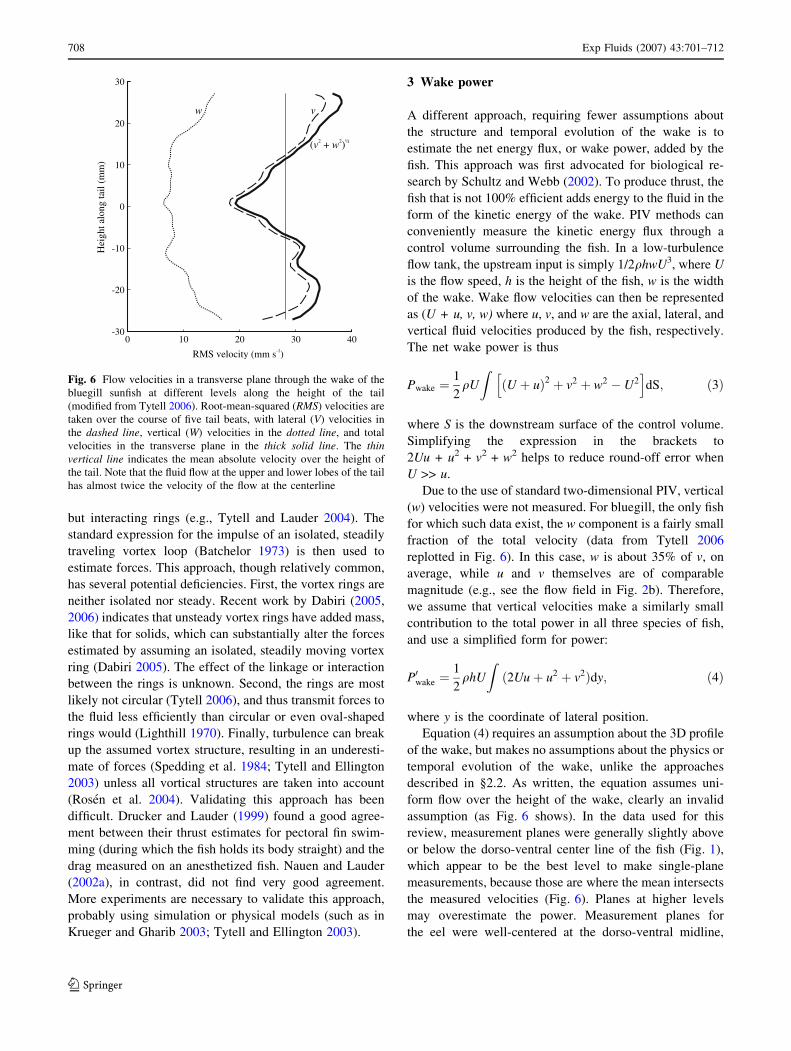
hence has a lower angle of attack. Figure 6 shows that

fluid velocities, and thus probably forces, at the upper and

lower lobes of the fin are about twice those at the center.

Thus, it would be best to make measurements of

momentum flux at the tips and the center of the tail over a

range of speeds in which the tail beat amplitude varies.

These measurements could be used construct an empirical

relationship between tail beat amplitude and momentum

flux per unit height, which could then be used to estimate

the total thrust at a single speed.

An alternative approach, used by many researchers, is to

extract forces on the basis of the vortical structure of the

wake (Drucker and Lauder 1999; Muller et al. 2001, 1997;

Nauen and Lauder 2002a; Tytell 2004a). In this approach,

vortices in the wake like those in Fig. 2b are assumed to

link up in three dimensions to form a chain of linked vortex

rings (e.g., Nauen and Lauder 2002a) or a series of separate

-60

-30

0

30

60

90

120 6%56%

Net

velo

city

(mm

s)

-125%75%

-60

-30

0

30

60

90

120N

etve

loci

ty(m

ms

)-1

44%94%

-60

-30

0

30

60

90

120

Net

velo

city

(mm

s)

-1

1 cm-60

-30

0

30

60

90

120 all

Net

velo

city

(mm

s)

-1

trout

6%56%

-60

-30

0

30

60

90

120

25%75%

-60

-30

0

30

60

90

120

44%94%

-60

-30

0

30

60

90

120

-60

-30

0

30

60

90

120 all

1 cm

bluegilla

1

2

3

c

d

1

2

3

b

Fig. 5 Transects through the

trout and bluegill wakes during

swimming at 2.0 and 1.7 L s–1,

respectively. Format of the plots

is the same as in Fig. 4. a, c A

silhouette of the tail is shown in

gray

Exp Fluids (2007) 43:701–712 707

123

but interacting rings (e.g., Tytell and Lauder 2004). The

standard expression for the impulse of an isolated, steadily

traveling vortex loop (Batchelor 1973) is then used to

estimate forces. This approach, though relatively common,

has several potential deficiencies. First, the vortex rings are

neither isolated nor steady. Recent work by Dabiri (2005,

2006) indicates that unsteady vortex rings have added mass,

like that for solids, which can substantially alter the forces

estimated by assuming an isolated, steadily moving vortex

ring (Dabiri 2005). The effect of the linkage or interaction

between the rings is unknown. Second, the rings are most

likely not circular (Tytell 2006), and thus transmit forces to

the fluid less efficiently than circular or even oval-shaped

rings would (Lighthill 1970). Finally, turbulence can break

up the assumed vortex structure, resulting in an underesti-

mate of forces (Spedding et al. 1984; Tytell and Ellington

2003) unless all vortical structures are taken into account

(Rosen et al. 2004). Validating this approach has been

difficult. Drucker and Lauder (1999) found a good agree-

ment between their thrust estimates for pectoral fin swim-

ming (during which the fish holds its body straight) and the

drag measured on an anesthetized fish. Nauen and Lauder

(2002a), in contrast, did not find very good agreement.

More experiments are necessary to validate this approach,

probably using simulation or physical models (such as in

Krueger and Gharib 2003; Tytell and Ellington 2003).

3 Wake power

A different approach, requiring fewer assumptions about

the structure and temporal evolution of the wake is to

estimate the net energy flux, or wake power, added by the

fish. This approach was first advocated for biological re-

search by Schultz and Webb (2002). To produce thrust, the

fish that is not 100% efficient adds energy to the fluid in the

form of the kinetic energy of the wake. PIV methods can

conveniently measure the kinetic energy flux through a

control volume surrounding the fish. In a low-turbulence

flow tank, the upstream input is simply 1/2qhwU3, where U

is the flow speed, h is the height of the fish, w is the width

of the wake. Wake flow velocities can then be represented

as (U + u, v, w) where u, v, and w are the axial, lateral, and

vertical fluid velocities produced by the fish, respectively.

The net wake power is thus

Pwake ¼1

2qU

ZðU þ uÞ2 þ v2 þ w2 � U2h i

dS; ð3Þ

where S is the downstream surface of the control volume.

Simplifying the expression in the brackets to

2Uu + u2 + v2 + w2 helps to reduce round-off error when

U >> u.

Due to the use of standard two-dimensional PIV, vertical

(w) velocities were not measured. For bluegill, the only fish

for which such data exist, the w component is a fairly small

fraction of the total velocity (data from Tytell 2006

replotted in Fig. 6). In this case, w is about 35% of v, on

average, while u and v themselves are of comparable

magnitude (e.g., see the flow field in Fig. 2b). Therefore,

we assume that vertical velocities make a similarly small

contribution to the total power in all three species of fish,

and use a simplified form for power:

P0wake ¼1

2qhU

Zð2Uuþ u2 þ v2Þdy; ð4Þ

where y is the coordinate of lateral position.

Equation (4) requires an assumption about the 3D profile

of the wake, but makes no assumptions about the physics or

temporal evolution of the wake, unlike the approaches

described in §2.2. As written, the equation assumes uni-

form flow over the height of the wake, clearly an invalid

assumption (as Fig. 6 shows). In the data used for this

review, measurement planes were generally slightly above

or below the dorso-ventral center line of the fish (Fig. 1),

which appear to be the best level to make single-plane

measurements, because those are where the mean intersects

the measured velocities (Fig. 6). Planes at higher levels

may overestimate the power. Measurement planes for

the eel were well-centered at the dorso-ventral midline,

0 10 20 30 40-30

-20

-10

0

10

20

30

RMS velocity (mm s )-1

Hei

ghta

long

tail

(mm

)vw

( + )v w2 2 ½

Fig. 6 Flow velocities in a transverse plane through the wake of the

bluegill sunfish at different levels along the height of the tail

(modified from Tytell 2006). Root-mean-squared (RMS) velocities are

taken over the course of five tail beats, with lateral (V) velocities in

the dashed line, vertical (W) velocities in the dotted line, and total

velocities in the transverse plane in the thick solid line. The thinvertical line indicates the mean absolute velocity over the height of

the tail. Note that the fluid flow at the upper and lower lobes of the tail

has almost twice the velocity of the flow at the centerline

708 Exp Fluids (2007) 43:701–712

123

although they did not extend all the way anteriorly to the

head (Fig. 1). Wake profiles at different levels are un-

known for eels, but with a tapered and quite flexible caudal

fin (Fig. 1b), it is likely that flow speeds will decrease away

from the midline. Thus, the values from eels are probably

also overestimates.

In all of these cases, it would be better to have parallel

planes at multiple levels to assess the contribution of spa-

tial variation in flow along the height of the fin. However,

even one plane can provide useful information, although

the data have to be regarded with appropriate caution, as

indicated above.

Data analyzed included the entire American eel

(Anguilla rostrata) data set from Tytell (2004a), consisting

of 274 steady tail beats from three eels (body lengths from

20 to 23 cm) at swimming speeds from 0.5 to 2 L s–1. Also

analyzed were unpublished data including 27 tail beats

from one trout (Oncorhynchus mykiss), body length 14 cm,

swimming at 1, 2, and 2.5 L s–1, and 31 tail beats from two

bluegill sunfish (Lepomis macrochirus), lengths 15 and

16 cm, swimming at 1.25–2 L s–1. Reynolds number ran-

ges were from 20,000 to 80,000 for the eel, 20,000 to

50,000 for the trout, and 30,000 to 50,000 for the bluegill.

To compare the fishes, the data were normalized to

produce a power coefficient CP, analogous to a drag

coefficient, by dividing by 12qSU3 (Krueger 2006; Schultz

and Webb 2002; Tytell 2004a), where S is the wetted

surface area for each species. The surface area was esti-

mated from body width and height measurements, assum-

ing an oval cross-section and including the caudal fin area.

For eels, the estimated area was 0.18 L2; for trout, 0.54 L2;

and for bluegill, 0.69 L2 (close to the values estimated by

Webb 1992). Note that this estimate does not include the

dorsal or anal fins (Fig. 1). The wetted area (i.e., twice the

lateral projected area) of these fins decreases with swim-

ming speed: for bluegill, at the lowest speeds, they make up

at most 0.10 L2 (according to measurements in Standen and

Lauder 2005), for trout they are about 0.006 L2 (Standen

and Lauder 2007), and for eels they are ~0.02 L2 (E. D.

Tytell, unpublished data).

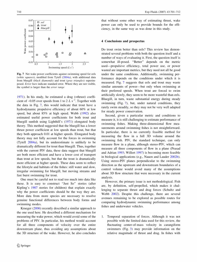
Figure 7 shows mean wake power coefficients from

eels, trout and bluegill at a range of swimming speeds. Eels

maintain about the same power coefficient, about 0.004,

over their range of swimming speeds, but with a fairly

large spread (SD = 0.002). Below speeds of 2 L s–1, both

trout and bluegill have substantially higher power coeffi-

cients than eels (trout, 0.03; bluegill, 0.04). In the one high-

speed swimming sequence from trout, the wake power

coefficient dropped to 0.007.

This review is meant to demonstrate a technique of

comparing swimming performance, and conclusions

regarding differences between species should be consid-

ered tentative. With so few data, it is not possible to per-

form the appropriate statistical analyses to distinguish real

differences among species from random variability among

individuals. Nonetheless, the data do show some interesting

trends. Bluegill sunfish waste the most energy during

steady swimming, as might be expected, because they live

in ponds or other relatively still bodies of water where they

do not typically spend much time swimming steadily

(Hartel et al. 2002). They may be better adapted to low-

speed swimming and maneuvering, in which strict power

conservation is not an important factor (Webb 2006). Trout

have comparable power coefficients to bluegill at low and

moderate speeds, but show a marked decrease in the wasted

power coefficient at the highest speed examined, possibly

reflecting their specialization for high-speed burst swim-

ming, particularly while swimming upstream in rivers (as is

known for a closely related species, Standen et al. 2004).

Eels, often considered to be inefficient (Lighthill 1970),

waste relatively much less power than bluegill or trout at

the same swimming speeds.

The wake power is only one component of the total

power (Eq. 1), but it can be used to set bounds on the useful

power and the efficiency. For example, eels are generally

thought to be less efficient than carangiform swimmers like

trout (Lighthill 1970; but see van Ginneken et al. 2005).

For the current data to be consistent with this hypothesis,

the trout must, counterintuitively, expend much more total

energy than the eel. Since it already wastes more energy,

relative to its body shape, than the eel, it must expend even

more useful energy overcoming drag, so that the wasted

portion makes up a small fraction of the total. At the same

speeds, the trout’s wake power coefficient is about eight

times larger than the eel’s; to have the same propulsive

efficiency at these speeds as the eel, its drag (=thrust)

coefficient must also be eight times larger. Thus, it seems

unlikely that trout are more efficient than eels at low

swimming speeds, which is consistent with the metabolic

data of van Ginneken et al. (2005).

In contrast, if one wanted to argue that the cost of

transport for the trout was less than that for the eel

swimming at the same speed, then the trout’s drag coeffi-

cient would have to be much less than the eel’s. In fact, if

the eel’s drag coefficient was less than the difference in the

wake power coefficients, then the trout could never have a

lower cost of transport. Of course, trout tend to swim faster

than eels, and particularly tend to swim in bursts at high

speeds, which could mean that their average cost of

transport during intermittent swimming may be lower or

equal to that of an eel swimming steadily at a low speed.

Webb has made a number of estimates of the drag and

power output of swimming fishes, using a variety of

techniques. He estimated the drag on swimming trout by

measuring the maximum sustained swimming speeds of

trout with artificially increased drag coefficients (Webb

Exp Fluids (2007) 43:701–712 709

123

1971). In his study, he estimated a drag (=thrust) coeffi-

cient of ~0.05 over speeds from 1 to 2 L s–1. Together with

the data in Fig. 7, this would indicate that trout have a

hydrodynamic propulsive efficiency of about 60% at low

speed, but about 85% at high speed. Webb (1992) also

estimated useful power coefficients for both trout and

bluegill sunfish using Lighthill’s (1971) elongated body

theory. This method suggested that the bluegill has a lower

thrust power coefficient at low speeds than trout, but that

they both approach 0.01 at higher speeds. Elongated body

theory may not fully account for the forces in swimming

(Tytell 2004a), but its underestimate is unlikely to be

dramatically different for trout than bluegill. Thus, together

with the current PIV data, these data suggest that bluegill

are both more efficient and have a lower cost of transport

than trout at low speeds, but that the trout is dramatically

more efficient at higher speeds. These data seem to reflect

the lifestyle and habitats of the fishes: still water and slow,

irregular swimming for bluegill, but moving streams and

fast burst swimming for trout.

One must be careful not to read too much into data like

these. It is easy to construct ‘‘Just So’’ stories (after

Kipling’s 1907 stories for children) that explain exactly

why the power coefficients should be the way they are.

More data from more species are necessary to resolve

genuine functional differences between body forms and

swimming modes.

Krueger (2006) recently described a similar approach to

the one used here. He described a different mechanism for

measuring the wake power, which would avoid some of the

problems of PIV. In particular, his method would account

for all three components of velocity over the entire

downstream plane, thus avoiding any assumptions about

the 3D structure of the wake. However, he also concludes

that without some other way of estimating thrust, wake

power can only be used to provide bounds for the effi-

ciency, in the same way as was done in this study.

4 Conclusions and prospectus

Do trout swim better than eels? This review has demon-

strated several problems with both the question itself and a

number of ways of evaluating it. First, the question itself is

somewhat ill-posed. ‘‘Better’’ depends on the metric

used—propulsive efficiency, total power use, or power

wasted are important metrics, but they need not all be good

under the same conditions. Additionally, swimming per-

formance depends on the conditions under which it is

measured. Fig. 7 suggests that eels and trout may waste

similar amounts of power—but only when swimming at

their preferred speeds. When trout are forced to swim

artificially slowly, they seem to be more wasteful than eels.

Bluegill, in turn, waste substantial energy during steady

swimming (Fig. 7), but, under natural conditions, they

rarely swim steadily, so they may not be very well adapted

for steady power conservation.

Second, given a particular metric and conditions to

measure it, it is still challenging to estimate performance of

swimming fishes. Making three-dimensional flow mea-

surements around swimming fishes is not straightforward.

In particular, there is no currently feasible method for

measuring the flow in a full 3D volume around the

swimming fish. PIV, the standard technique, can only

measure flow in a plane, although stereo-PIV, which can

measure all three components of flow in a plane (Prasad

and Adrian 1993; Willert 1997) is becoming more feasible

in biological applications (e.g., Nauen and Lauder 2002b).

Using stereo-PIV planes perpendicular to the swimming

direction as the upstream and downstream boundaries of a

control volume would avoid many of the assumptions

about 3D flow structure that were necessary in the current

analysis.

However, the primary issue is not methodological. Fish

are, by definition, self-propelled, which makes it chal-

lenging to separate thrust and drag forces (Schultz and

Webb 2002). Despite this challenge, there are several

avenues remaining to be explored as possible routes for

comparing hydrodynamic swimming performance among

fishes and underwater vehicles.

1. Temporal separation of forces. Although it was not

possible with the limited data used for this review, the

fluctuating center-of-mass velocity in carangiform

swimmers (Fig. 3) may provide information on the

relative magnitude of thrust and drag. In fishes with

0.5 1 1.5 2 2.5-0.01

0

0.01

0.02

0.03

0.04

0.05

0.06

0.07

Swimming speed ( s )L -1

Wak

e po

wer

coe

ffic

ient

eel

bluegilltrout

Fig. 7 Net wake power coefficients against swimming speed for eels

(white squares), modified from Tytell (2004a), with additional data

from bluegill (black diamonds) and trout (gray triangles) superim-

posed. Error bars indicate standard error. Where they are not visible,

the symbol is larger than the error range

710 Exp Fluids (2007) 43:701–712

123

relatively large fluctuations in velocity, like the blue-

gill, the thrust may temporally overwhelm the drag to

such an extent that the net force at certain phases in the

tail beat cycle is composed primarily of thrust.

2. Spatial separation of forces. Measurements of

momentum flux at the tips of the tail may provide

information on the thrust force, without much of an

effect from the drag on the fish’s body (Fig. 5d), par-

ticularly in fishes with narrow caudal peduncles like

the bluegill sunfish used as an example here, or the

mackerel (Nauen and Lauder 2002a) or tuna. Full

stereo PIV planes behind the swimming fish, perpen-

dicular to the flow, may provide the best information.

3. Zero-momentum wake profiles. For fishes like the eel,

which maintain effectively zero axial momentum in

their wakes, the velocity profile in the wake may

provide information on the thrust and drag forces

simultaneously. The near wake of a self-propelled jet

can be used to extract both the individual profiles of

thrust and drag wakes (Sirviente and Patel 2000).

Whether the time-average of a highly structured wake

from an oscillating propulsor (as in Fig. 4b) can be

used in the same way will have to be confirmed by

simulations or physical models.

4. Wake power. In the absence of effective methods to

extract thrust, the wake power (wasted power), can be

used to place bounds on the relative performance of

different fishes. Particularly if there are a priori

hypotheses about fish performance based on habitat or

lifestyle (i.e., that trout are more efficient than eels), the

wake power can be used effectively to constrain if not

disprove such hypotheses (trout would have to have a

surprisingly large drag coefficient to be more efficient

than eels, at least at swimming speeds <2 L s–1).

These methods may provide a framework for addressing

relative performance as it becomes more feasible to per-

form comparative studies of swimming in many different

fishes.

Comparative studies of the performance of many dif-

ferent fishes, examining many different performance met-

rics under many different conditions will provide the best

route to extracting design principles for undulatory swim-

ming. Only by comparing fishes with different evolutionary

histories can one begin to disentangle all the competing

adaptive pressures that were involved in producing the

body shapes and swimming modes of fishes today. Such

comparisons, while challenging, may ultimately provide

the best framework for understanding the performance of

fishes and biomimetic submarines.

Acknowledgments Many of the ideas in this review developed

from a discussion with Rajat Mittal. Data were taken with funding

from National Science Foundation grants to George V. Lauder (grant

numbers IBN9807021 and IBN0316675). Support is currently pro-

vided by the National Institutes of Health (grant number 5 F32

NS054367).

References

Afanasyev YD (2004) Wakes behind towed and self-propelled bodies:

asymptotic theory. Phys Fluids 16:3235–3238. doi:10.1063/

1.1768071

Anderson EJ, McGillis WR, Grosenbaugh MA (2001) The boundary

layer of swimming fish. J Exp Biol 204:81–102

Anderson JM (1996) Vortex control for efficient propulsion. Ph.D.

Dissertation, Dept Ocean Eng, Mass Inst Tech

Batchelor GK (1973) An introduction to fluid dynamics. Cambridge

University Press, Cambridge

Breder CM (1926) The locomotion of fishes. Zoologica 4:159–297

Dabiri JO (2005) On the estimation of swimming and flying forces

from wake measurements. J Exp Biol 208:3519–3532.

doi:10.1242/jeb.01813

Dabiri JO (2006) Note on the induced Lagrangian drift and added-

mass of a vortex. J Fluid Mech 547:105–113. doi:10.1017/

S0022112005007585

Drucker EG, Lauder GV (1999) Locomotor forces on a swimming

fish: three-dimensional vortex wake dynamics quantified using

digital particle image velocimetry. J Exp Biol 202:2393–2412

Drucker EG, Lauder GV (2001) Locomotor function of the dorsal fin

in teleost fishes: experimental analysis of wake forces in sunfish.

J Exp Biol 204:2943–2958

Finson ML (2006) Similarity behaviour of momentumless turbulent

wakes. J Fluid Mech 71:465–479

Garland T (1998) Conceptual and methodological issues in testing the

predictions of symmorphosis. In: Weibel ER, Taylor CR, Bolis L

(eds) Principles of animal design. Cambridge University Press,

Cambridge

Hartel KE, Halliwell DB, Launer AE (2002) Inland fishes of

Massachusetts. Massachusetts Audobon Society, Lincoln, MA

Helfman GS, Collette BB, Facey DE (1997) The diversity of fishes.

Blackwell Science, London

Kern S, Koumoutsakos P (2006) Simulations of optimized anguilliform

swimming. J Exp Biol 209:4841–4857. doi:10.1242/jeb.02526

Kipling R (1907) Just so stories. Doubleday, Garden City, NY

Koochesfahani MM (1989) Vortical patterns in the wake of an

oscillating airfoil. AIAA J 27:1200–1205

Krueger PS (2006) Measurement of propulsive power and evaluation of

propulsive performance from the wake of a self-propelled vehicle.

Bioinsp Biomimet 1:S49–S56. doi:10.1088/1748-3182/1/4/S07

Krueger PS, Gharib M (2003) The significance of vortex ring

formation to the impulse and thrust of a starting jet. Phys Fluids

15:1271–1281. doi:10.1063/1.1564600

Lauder GV (2000) Function of the caudal fin during locomotion in

fishes: kinematics, flow visualization, and evolutionary patterns.

Am Zool 40:101–122

Lauder GV, Tytell ED (2006) Hydrodynamics of undulatory propul-

sion. In: Shadwick RE, Lauder GV (eds) Fish biomechanics.

Academic, San Diego, pp 425–468

Lighthill J (1960) Note on the swimming of slender fish. J Fluid Mech

9:305–317

Lighthill J (1970) Aquatic animal propulsion of high hydromechan-

ical efficiency. J Fluid Mech 44:265–301

Lighthill J (1971) Large-amplitude elongated-body theory of fish

locomotion. Proc R Soc Lond B 179:125–138

McCutchen CW (1977) Froude propulsive efficiency of a small fish,

measured by wake visualisation. In: Pedley TJ (ed) Scale effects

in animal locomotion. Academic, London, pp 339–363

Exp Fluids (2007) 43:701–712 711

123

Meunier P, Spedding GR (2006) Stratified propeller wakes. J Fluid

Mech 552:229–256. doi:10.1017/S0022112006008676

Muller UK, Smit J, Stamhuis EJ, Videler JJ (2001) How the body

contributes to the wake in undulatory fish swimming: flow fields

of a swimming eel (Anguilla anguilla). J Exp Biol 204:2751–

2762

Muller UK, van den Heuvel B-LE, Stamhuis EJ, Videler JJ (1997)

Fish foot prints: morphology and energetics of the wake behind a

continuously swimming mullet (Chelon labrosus Risso). J Exp

Biol 200:2893–2906

Naudascher E (1965) Flow in the wake of self-propelled bodies and

related sources of turbulence. J Fluid Mech 22:625–656

Nauen JC, Lauder GV (2001) Locomotion in scombrid fishes:

visualization of flow around the caudal peduncle and finlets of

the chub mackerel Scomber japonicus. J Exp Biol 204:2251–2263

Nauen JC, Lauder GV (2002a) Hydrodynamics of caudal fin

locomotion by chub mackerel, Scomber japonicus (Scombridae).

J Exp Biol 205:1709–1724

Nauen JC, Lauder GV (2002b) Quantification of the wake of rainbow

trout (Oncorhynchus mykiss) using three-dimensional stereo-

scopic digital particle image velocimetry. J Exp Biol 205:3271–

3279

Prasad AK (2000) Stereoscopic particle image velocimetry. Exp

Fluids 29:107–115

Prasad AK, Adrian RJ (1993) Stereoscopic particle image velocime-

try. Exp Fluids 15:49–60

Rosen M, Spedding GR, Hedenstrom A (2004) The relationship

between wingbeat kinematics and vortex wake of a thrush

nightingale. J Exp Biol 207:4255–4268. doi:10.1242/jeb.01283

Rosen MW (1959) Waterflow about a swimming fish. US Naval

Ordnance Test Station, China Lake, CA. Tech Publ 2298, pp 1–

96

Schultz WW, Webb PW (2002) Power requirements of swimming: do

new methods resolve old questions? Integr Comp Biol 42:1018–

1025

Shames IH (1992) Mechanics of fluids, 3rd edn. McGraw-Hill, New

York

Sirviente AI, Patel VC (2000) Wake of a self-propelled body, Part 1:

momentumless wake. AIAA J 38:611–619

Spedding GR, Rayner JMV, Pennycuick CJ (1984) Momentum and

energy in the wake of a pigeon (Columba livia) in slow flight.

J Exp Biol 111:81–102

Standen EM, Hinch SG, Rand PS (2004) Influence of river speed on

path selection by migrating adult sockeye salmon (Oncorhyn-chus nerka). Can J Fish Aquat Sci 61:905–912. doi:10.1139/F04-

035

Standen EM, Lauder GV (2005) Dorsal and anal fin function in

bluegill sunfish (Lepomis macrochirus): three-dimensional kine-

matics during propulsion and maneuvering. J Exp Biol

208:2753–2763. doi:10.1242/jeb.01706

Standen EM, Lauder GV (2007) Hydrodynamic function of dorsal and

anal fins in brook trout (Salvelinus fontinalis). J Exp Biol

210:325–339. doi:10.1242/jeb.02661

Tennekes H, Lumley JL (1972) A first course in turbulence. MIT,

Cambridge, MA

Triantafyllou GS, Triantafyllou MS, Grosenbaugh MA (1993)

Optimal thrust development in oscillating foils with application

to fish propulsion. J Fluids Struct 7:205–224

Tytell ED (2004a) The hydrodynamics of eel swimming. II. Effect of

swimming speed. J Exp Biol 207:3265–3279. doi:10.1242/

jeb.01139

Tytell ED (2004b) Kinematics and hydrodynamics of linear acceler-

ation in eels, Anguilla rostrata. Proc R Soc Lond B 271:2535–

2541. doi:10.1098/rspb.2004.2901

Tytell ED (2006) Median fin function in bluegill sunfish, Lepomismacrochirus: streamwise vortex structure during steady swim-

ming. J Exp Biol 209:1516–1534. doi:10.1242/jeb.02154

Tytell ED, Ellington CP (2003) How to perform measurements in a

hovering animal’s wake: physical modelling of the vortex wake

of the hawkmoth Manduca sexta. Philos Trans R Soc Lond B

358:1559–1566. doi:10.1098/rstb.2003.1355

Tytell ED, Lauder GV (2004) The hydrodynamics of eel swimming. I.

Wake structure. J Exp Biol 207:1825–1841. doi:10.1242/

jeb.00968

van Ginneken V, Antonissen E, Muller UK, Booms R, Eding E,

Verreth J, van den Thillart G (2005) Eel migration to the

Sargasso: remarkably high swimming efficiency and low energy

costs. J Exp Biol 208:1329—1335. doi:10.1242/jeb.01524

Walker JA (1998) Estimating velocities and accelerations of animal

locomotion: a simulation experiment comparing numerical

differentiation algorithms. J Exp Biol 201:981–995

Webb PW (1971) The swimming energetics of trout. I. Thrust and

power output at cruising speeds. J Exp Biol 55:489–520

Webb PW (1992) Is the high cost of body caudal fin undulatory

swimming due to increased friction drag or inertial recoil? J Exp

Biol 162:157–166

Webb PW (2006) Stability and maneuverability. In: Shadwick RE,

Lauder GV (eds) Fish biomechanics. Academic, San Diego, pp

281–332

Willert CE (1997) Stereoscopic digital particle image velocimetry for

application in wind tunnel flows. Meas Sci Tech 8:1465–1479

Willert CE, Gharib M (1991) Digital particle image velocimetry. Exp

Fluids 10:181–193

Zhu Q, Wolfgang MJ, Yue DKP, Triantafyllou MS (2002) Three-

dimensional flow structures and vorticity control in fish-like

swimming. J Fluid Mech 468:1–28

712 Exp Fluids (2007) 43:701–712

123