Distributed micro-releases of bioterror pathogens : threat characterizations and epidemiology from...

SANDIA REPORTSAND2008-6044Unlimited ReleasePrinted October 2008

Distributed micro-releases of bioterrorpathogens: threat characterizations andepidemiology from uncertain patientobservables

J. Ray, B. M. Adams, K. D. Devine, Y. M. Marzouk, M. M. Wolf, and H. N. Najm

Prepared bySandia National LaboratoriesAlbuquerque, New Mexico 87185 and Livermore, California 94550

Sandia is a multiprogram laboratory operated by Sandia Corporation,a Lockheed Martin Company, for the United States Department of Energy’sNational Nuclear Security Administration under Contract DE-AC04-94-AL85000.

Approved for public release; further dissemination unlimited.

Issued by Sandia National Laboratories, operated for the United States Department ofEnergy by Sandia Corporation.

NOTICE: This report was prepared as an account of work sponsored by an agency ofthe United States Government. Neither the United States Government, nor any agencythereof, nor any of their employees, nor any of their contractors, subcontractors, or theiremployees, make any warranty, express or implied, or assume any legal liability or re-sponsibility for the accuracy, completeness, or usefulness of any information, appara-tus, product, or process disclosed, or represent that its use would not infringe privatelyowned rights. Reference herein to any specific commercial product, process, or serviceby trade name, trademark, manufacturer, or otherwise, does not necessarily constituteor imply its endorsement, recommendation, or favoring by the United States Govern-ment, any agency thereof, or any of their contractors or subcontractors. The views andopinions expressed herein do not necessarily state or reflect those of the United StatesGovernment, any agency thereof, or any of their contractors.

Printed in the United States of America. This report has been reproduced directly fromthe best available copy.

Available to DOE and DOE contractors fromU.S. Department of EnergyOffice of Scientific and Technical InformationP.O. Box 62Oak Ridge, TN 37831

Telephone: (865) 576-8401Facsimile: (865) 576-5728E-Mail: [email protected] ordering: http://www.doe.gov/bridge

Available to the public fromU.S. Department of CommerceNational Technical Information Service5285 Port Royal RdSpringfield, VA 22161

Telephone: (800) 553-6847Facsimile: (703) 605-6900E-Mail: [email protected] ordering: http://www.ntis.gov/ordering.htm

DEP

ARTMENT OF ENERGY

• • UN

ITED

STATES OF AM

ERIC

A

2

SAND2008-6044Unlimited Release

Printed October 2008

Distributed micro-releases of bioterrorpathogens: threat characterizations and

epidemiology from uncertain patient observables

J. Ray, B. M. Adams, K. D. Devine, Y. M. Marzouk and H. N. NajmSandia National Laboratories, P. O. Box 969, Livermore CA 94551

andMichael M. Wolf

4332 Siebel Center, MC-258, 201 N. Goodwin,University of Illinois, Urbana-Champaign

Urbana, IL 61801jairay,briadam,kddevin,ymarzou,[email protected]

[email protected]

Abstract

Terrorist attacks using an aerosolized pathogen preparation have gained credibility asa national security concern since the anthrax attacks of 2001. The ability to charac-terize the parameters of such attacks, i.e., to estimate the number of people infected,the time of infection, the average dose received, and the rate of disease spread in con-temporary American society (for contagious diseases), is important when planning amedical response. For non-contagious diseases, we address the characterization prob-lem by formulating a Bayesian inverse problem predicated on a short time-series ofdiagnosed patients exhibiting symptoms. To keep the approach relevant for responseplanning, we limit ourselves to 3–5 days of data. In computational tests performed foranthrax, we usually find these observation windows sufficient, especially if the out-break model employed in the inverse problem is accurate. For contagious diseases, weformulated a Bayesian inversion technique to infer both pathogenic transmissibilityand the social network from outbreak observations, ensuring that the two determi-nants of spreading are identified separately. We tested this technique on data collectedfrom a 1967 smallpox epidemic in Abakaliki, Nigeria. We inferred, probabilistically,different transmissibilities in the structured Abakaliki population, the social network,and the chain of transmission. Finally, we developed an individual-based epidemic

3

model to realistically simulate the spread of a rare (or eradicated) disease in a modernsociety. This model incorporates the mixing patterns observed in an (American) ur-ban setting and accepts, as model input, pathogenic transmissibilities estimated fromhistorical outbreaks that may have occurred in socio-economic environments with lit-tle resemblance to contemporary society. Techniques were also developed to simulatedisease spread on static and sampled network reductions of the dynamic social net-works originally in the individual-based model, yielding faster, though approximate,network-based epidemic models. These reduced-order models are useful in scenarioanalysis for medical response planning, as well as in computationally intensive inverseproblems.

4

Acknowledgment

This work was supported Sandia National Laboratories’ LDRD (Laboratory Directed Re-search and Development) funds, sponsored by the Computational and Information SciencesInvestment Area.

5

Contents1 Introduction . . . . . . . . . . . . . . . . . . . . . . . . . . . . . . . . . . . . . . . . . . . . . . . . . . . . . . . . . . . . . . 132 Literature review . . . . . . . . . . . . . . . . . . . . . . . . . . . . . . . . . . . . . . . . . . . . . . . . . . . . . . . . . . 17

2.1 Individual-based models of epidemics . . . . . . . . . . . . . . . . . . . . . . . . . . . . . . 172.2 Characterization of anthrax outbreaks . . . . . . . . . . . . . . . . . . . . . . . . . . . . . . 192.3 Characterization of smallpox outbreaks . . . . . . . . . . . . . . . . . . . . . . . . . . . . . 212.4 Markov Chain Monte Carlo methods . . . . . . . . . . . . . . . . . . . . . . . . . . . . . . . 22

3 Individual-based models of epidemics, including approximations. . . . . . . . . . . . . . . 253.1 Social contact networks and transmission models . . . . . . . . . . . . . . . . . . . . . 263.2 Available network data . . . . . . . . . . . . . . . . . . . . . . . . . . . . . . . . . . . . . . . . . . 273.3 Description of population sampling approaches . . . . . . . . . . . . . . . . . . . . . . 293.4 In-host pathogenesis (micro-models) . . . . . . . . . . . . . . . . . . . . . . . . . . . . . . . 303.5 Parallel implementation . . . . . . . . . . . . . . . . . . . . . . . . . . . . . . . . . . . . . . . . . 313.6 Sample simulation results . . . . . . . . . . . . . . . . . . . . . . . . . . . . . . . . . . . . . . . 32

4 Characterizing outbreaks from partial observations: the case for non-contagiousdiseases . . . . . . . . . . . . . . . . . . . . . . . . . . . . . . . . . . . . . . . . . . . . . . . . . . . . . . . . . . . . . . . . . . . 374.1 Formulation . . . . . . . . . . . . . . . . . . . . . . . . . . . . . . . . . . . . . . . . . . . . . . . . . . 384.2 Anthrax incubation models . . . . . . . . . . . . . . . . . . . . . . . . . . . . . . . . . . . . . . 394.3 Inference of attack parameters with ideal cases . . . . . . . . . . . . . . . . . . . . . . . 434.4 Inference of attack parameters under variable doses . . . . . . . . . . . . . . . . . . . 454.5 The Sverdlovsk anthrax outbreak of 1979 . . . . . . . . . . . . . . . . . . . . . . . . . . . 60

5 Characterizing outbreaks from partial observations: the case for contagious dis-eases . . . . . . . . . . . . . . . . . . . . . . . . . . . . . . . . . . . . . . . . . . . . . . . . . . . . . . . . . . . . . . . . . . . . . . 655.1 The data: the Abakaliki smallpox outbreak of 1967 . . . . . . . . . . . . . . . . . . . 665.2 Formulation of the inverse problem . . . . . . . . . . . . . . . . . . . . . . . . . . . . . . . . 675.3 Results . . . . . . . . . . . . . . . . . . . . . . . . . . . . . . . . . . . . . . . . . . . . . . . . . . . . . . 70

6 Conclusions . . . . . . . . . . . . . . . . . . . . . . . . . . . . . . . . . . . . . . . . . . . . . . . . . . . . . . . . . . . . . . 81References . . . . . . . . . . . . . . . . . . . . . . . . . . . . . . . . . . . . . . . . . . . . . . . . . . . . . . . . . . . . . . . . . . . 85

AppendixA Methodology for obtaining a dose distribution consistent with atmospheric disper-

sion over a geographically distributed population . . . . . . . . . . . . . . . . . . . . . . . . . . . . . . 93

Figures1 Parallelism: improved scalability with point-to-point communication model. 322 Spatial spread of smallpox over 21 days, full-fidelity dynamic network. . . . 333 One month smallpox SEIR data, dynamic to static network comparison. . . . 344 Six month smallpox SEIR data, dynamic to static network comparison. . . . 355 Smallpox epidemic evolution with person-to-location clustering. . . . . . . . . . 356 Smallpox epidemic spatial spread with person-to-person clustering. . . . . . . 36

6

7 The median incubation period for anthrax as a function of dose D. Thesolid line is Model A2, which assumes a dose of 2.4 spores at Sverdlovsk;the dashed line is Model D, which assumes 300 spores. The solid symbolsare median incubation periods obtained from experimental investigationsor from Sverdlovsk data. The filled circle (Sverdlovsk; Wilkening ModelA) refers to both Models A1 and A2, though only Model A2 is used inthe current study. Symbols which are not filled denote experiments wherethe population of primates was too small to draw statistically meaningfulresults. The experiments by Brachman et al. [1] are shown by vertical linesbetween symbols. In these experiments, only the lower and upper boundsof the incubation period were provided. These ranges were not used fordetermining model parameters and are only provided for reference. . . . . . . 42

8 Posterior PDFs for N (top), τ (middle), and logD (bottom) based on thetime series for Case A (left) and Case B (right), as tabulated in Table 2.Data are collected at 6-hour intervals in both cases. The correct valuesfor

�N � τ � log10 � D �� in Case A are

�102 �� 0 � 75 � 100 � ; in Case B they are�

102 �� 2 � 25 � 102 � . In both cases, PDFs are reported after 3-, 4- and 5-dayobservational periods (dotted, dashed, and solid lines respectively). . . . . . . . 47

9 Posterior PDFs for N (top), τ (middle), and logD (bottom) based on thetime series for Case C (left) and Case D (right), as tabulated in Table 2.Data are collected at 6-hour intervals in both cases. The correct valuesfor

�N � τ � log10 � D �� in Case C are

�102 �� 2 � 25 � 104 � ; in Case D they are�

104 �� 0 � 05 � 100 � . In both cases, PDFs are reported after 3-, 4- and 5-dayobservational periods (dotted, dashed, and solid lines respectively). . . . . . . . 48

10 Posterior PDFs for N (top), τ (middle), and logD (bottom) based on thetime series for Case E (left) and Case F (right), as tabulated in Table 2.Data are collected at 6-hour intervals in both cases. The correct valuesfor

�N � τ � log10 � D �� in Case E are

�104 �� 1 � 0 � 102 � ; in Case F they are�

104 �� 1 � 25 � 104 � . In both cases, PDFs are reported after 3-, 4- and 5-day observational periods (dotted, dashed, and solid lines respectively), butCase F also includes PDFs at Day 6 (solid lines with filled squares) and atDay 7 (solid lines with filled circles). . . . . . . . . . . . . . . . . . . . . . . . . . . . . . . 49

11 The joint probability density p � N � log10 � D �� obtained after 5 days of datafor Case F. We clearly see a dual characterization—a larger low-dose attackand a smaller high-dose attack. . . . . . . . . . . . . . . . . . . . . . . . . . . . . . . . . . . . 50

12 Posterior PDFs for N (top), τ (middle), and log10 D (bottom) based on thetime series for Case Ia, as tabulated in Tables 4 and 5. Lower-resolutiondata (collected in 24-hour intervals) yields the PDFs on the left, whilehigher-resolution data yields the PDFs on the right. Correct values for�

N � τ � log10 � D �� are�318 �� 1 � 5 � 3 � 46 � , where the “correct” representative

dose is taken to be log10 � D50 � . In both cases, PDFs are reported after 3-,4-, 5-, and 7-day observational periods. . . . . . . . . . . . . . . . . . . . . . . . . . . . . . 55

7

13 Posterior PDFs for N (top), τ (middle), and log10 D (bottom) based on thetime series for Case I, as tabulated in Tables 4 and 5. Lower-resolutiondata (collected in 24-hour intervals) yields the PDFs on the left, whilehigher-resolution data yields the PDFs on the right. Correct values for�



14 Posterior PDFs for N (top), τ (middle), and log10 D (bottom) based on thetime series for Case II, as tabulated in Tables 4 and 5. Lower-resolutiondata (collected in 24-hour intervals) yields the PDFs on the left, whilehigher-resolution data yields the PDFs on the right. Correct values for�



15 Posterior PDFs for N (top), τ (middle), and log10 D (bottom) based on thetime series for Case IIa, as tabulated in Tables 4 and 5. Lower-resolutiondata (collected in 24-hour intervals) yields the PDFs on the left, whilehigher-resolution data yields the PDFs on the right. Correct values for�

N � τ � log10 � D �� are�4537 �� 1 � 25 � 4 � 09 � , where the “correct” representa-

tive dose is taken to be log10 � D50 � . In both cases, PDFs are reported after3-, 4-, 5-, and 7-day observational periods. . . . . . . . . . . . . . . . . . . . . . . . . . . 58

16 Posterior PDFs for N (top), τ (middle), and log10 D (bottom) based on dailytime series for Case IIIa (left) and Case III (right). Correct values for�

N � τ � log10 � D �� are�161 �� 0 � 75 � 3 � 52 � (Case IIIa) and

�1453 �� 0 � 75 � 3 � 54 �

(Case III), where the “correct” representative dose is taken to be log10 � D50 � .In both cases, PDFs are reported after 3-, 4-, and 5-day observational peri-ods (dotted, dashed and solid lines respectively). . . . . . . . . . . . . . . . . . . . . . 61

17 Posterior PDFs for N (top), τ (middle), and log10 D (bottom) based on dailytime series for Case IV (left) and Case IVa (right). Correct values for�

N � τ � log10 � D �� are�453 �� 0 � 75 � 4 � 22 � (Case IV) and

�4453 �� 0 � 5 � 4 � 20 �

(Case IVa), where the “correct” representative dose is taken to be log10 � D50 � .In both cases, PDFs are reported after 3-, 4-, and 5-day observational peri-ods (dotted, dashed and solid lines respectively). . . . . . . . . . . . . . . . . . . . . . 62

18 PDFs of N (left) and τ (right) for the Sverdlovsk outbreak. . . . . . . . . . . . . . 64

19 Above: Samples of I10 � R10 � βin and βout for Problem I, as the MCMC chainprogressed. We see little autocorrelation and the chains are seen to be mix-ing well. Below: Scatter plot of samples of βin and βout . We see very littlecorrelation between the two. . . . . . . . . . . . . . . . . . . . . . . . . . . . . . . . . . . . . . 72

8

20 Above: PDFs for the dates of infection and removal for Cases number 5,10 and 30 for Problem I. The Cases are denoted by separate colors; plotsof removal dates contain a symbol. While the bases of the PDFs are almostas wide as those of the incubation and removal periods, the shapes of thePDFs are quite different from the skewed Γ-distributions which are used tomodel incubation and removal durations for smallpox. Below: The PDFsfor the rates of spread βin and βout developed from data collected duringthe entire epidemic (plots with symbols) and from the first 40 days of data(plots without symbols). The MAP estimate of the spread rates drawn fromthe first 40 days may be affected by measurement error in the data. . . . . . . . 73

21 The expected infection pathway � P � , drawn from data collected dur-ing the entire epidemic for Problem I. Nodes represent the 30 Cases of theoutbreak and are colored by their compound affiliations. The links in thegraphs are colored by their probability of existence – links with probabilityof 30% or higher are red while those between 10% and 30% are blue. Mostof the transmissions from the index case (Node 000) are in red, and con-nect individuals in the same compound. Infection transmissions betweenthe later Cases are almost completely in blue, indicating the reduction ofheterogeneity in the transmission mechanism as a large fraction of the pop-ulation became infected. . . . . . . . . . . . . . . . . . . . . . . . . . . . . . . . . . . . . . . . . 74

22 The expected infection pathway � P � , drawn from data collected duringthe first 40 days of the epidemic, for Problem I. Nodes represent the 30Cases of the outbreak and are colored by their compound affiliations. Thelinks in the graphs are colored by their probability of existence – links withprobability of 30% or higher are red while those between 10% and 30% areblue. Most of the transmissions from the index case (Node 000) are in red,and connect individuals in the same compound. A few red cross-compoundlinks are also evident at this point in the epidemic. . . . . . . . . . . . . . . . . . . . . 75

23 Above: PDFs for the dates of infection and removal for Case numbers 5and 10, for Problem II. The cases are denoted by separate colors; plots ofremoval dates contain a symbol. While the bases of the PDFs are almostas wide as those of the incubation and removal periods, the shapes of thePDFs are quite different from the skewed Γ-distributions which are used tomodel incubation and removal durations for smallpox. Below: The PDFsfor the rate of spread βin βout . . . . . . . . . . . . . . . . . . . . . . . . . . . . . . . . . . . 77

24 The expected infection pathway � P � , drawn from data collected duringthe first 40 days of the epidemic, for Problem II. Nodes represent the Casesof the outbreak and are colored by their compound affiliations. The links inthe graphs are colored by their probability of existence – links with prob-ability of 30% or higher are red while those between 10% and 30% areblue. Most of the transmissions from the index case (Node 000) are in red,and connect individuals in the same compound. Infection transmissionsbetween the later Cases are almost completely in blue, indicating the re-duction of heterogeneity in the transmission mechanism as a large fractionof the population became infected. . . . . . . . . . . . . . . . . . . . . . . . . . . . . . . . . 78

9

25 The expected social network � G � , drawn from data collected duringthe first 40 days, for Problem II. Nodes represent the 74 members of thepopulation and are colored by their compound affiliations. Links in thegraphs represent the cross-compound social links seen in 50% (or higher)of the samples. . . . . . . . . . . . . . . . . . . . . . . . . . . . . . . . . . . . . . . . . . . . . . . . . 79

10

Tables1 Smallpox disease periods, with duration distributions. . . . . . . . . . . . . . . . . . 312 Time series obtained from six different outbreaks, simulated with the pa-

rameters�N � τ � D � as noted at the bottom of the table. The table has been

divided into 24-hour sections, where the ni in each section are summed toproduce the low-resolution time series (24-hour resolution) used to inves-tigate the effect of temporal resolution. Time is measured in days and dosein spores. . . . . . . . . . . . . . . . . . . . . . . . . . . . . . . . . . . . . . . . . . . . . . . . . . . . . 44

3 Cases A–F; MAP estimates and 90% credibility intervals (in parentheses)for N, τ, and log10 � D � , conditioned on the high-resolution time series atDay 5. The number in the curly brackets

� � is the correct value. . . . . . . . . . 464 Time series obtained from eight simulated outbreaks with variable doses.

Cases I, Ia, II, and IIa are simulated using Wilkening’s Model A2, with theattack parameters—N, τ, and the dose distribution—indicated at the bottomof the table. Cases III, IIIa, IV and IV are simulated using Wilkening’sModel D. D is the average dose for the N infected individuals. The tablehas been divided into 24-hour sections, where the values ni in each sectioncan be summed to produce the low-resolution time series used to investigatethe effect of temporal resolution. The dose distribution is represented byits quantiles D1, D25, D50, D75, and D99; x% of the population receives adose of Dx or less. Table 5 continues the time series from Day 5 to Day 8. . 52

5 Continuation of Table 4 beyond Day 5. Time series obtained from 4 sim-ulated outbreaks with variable doses. Cases I, Ia, II, and IIa are simulatedusing Wilkening’s Model A2, with the attack parameters—N, τ, and thedose distribution—indicated at the bottom of the table. D is the averagedose for the N infected individuals. The table has been divided into 24-hoursections, where the values ni in each section can be summed to produce thelow-resolution time series used to investigate the effect of temporal reso-lution. The dose distribution is represented by its quantiles D1, D25, D50,D75, and D99; x% of the population receives a dose of Dx or less. . . . . . . . . 53

6 Cases I, Ia, II, IIa; MAP estimates and 90% credibility intervals (in paren-theses) for N, τ, and log10 � D � conditioned on data through Day 5. Correctvalues for N and τ are in

� � . The “correct” representative dose is taken tobe log10 � D50 � , also in

� � . . . . . . . . . . . . . . . . . . . . . . . . . . . . . . . . . . . . . . . . 597 Cases III, IIIa, IV, and IVa: MAP estimates and the 90% credibility inter-

vals (in parentheses) for N, τ, and log10 � D � conditioned on data throughDay 5. Correct values for N and τ are in

� � . The “correct” representativedose is taken to be log10 � D50 � , also in

� � . . . . . . . . . . . . . . . . . . . . . . . . . . . 638 Means and standard deviations of the incubation, prodromal and conta-

gious/symptomatic periods for smallpox. These were obtained from [2]. . . . 67

11

This page intentionally left blank

12

1 Introduction

The anthrax attacks of 2001 [3] are generally cited as the impetus for raising the specter ofrare pathogens as a terrorism tool. Yet pathogens have seen extensive use in war. There arerecorded accounts of malicious smallpox-infected blanket distribution during the Frenchand Indian Wars (1756–1763) and attempts to spread veterinary diseases among pack mulesand horses used in front-line positions during World War I [4]. Also, the Japanese Army,during World War II, included a unit devoted to biowarfare [5] and the Soviet Union al-legedly weaponized pathogens on an industrial scale [6]. The Sverdlovsk anthrax accident,where an aerosolized anthrax preparation was inadvertently released from a military insti-tution [7], provided one example of the potential effect of an outdoor aerosolized pathogenrelease; the “Amerithrax” attacks [3] provided a bioterrorism counterpart. Thus people’sability to weaponize pathogens and intent to use them aggressively is not in doubt.

Pathogenic preparations have both tactical and strategic uses. Large attacks with a non-contagious disease can severely degrade human population viability in a tightly circum-scribed theater of war, while a contagious disease may spread uncontrollably, seriously(and unpredictably) disrupting a nation’s operation. It has been estimated that a smallpoxattack infecting a small, but significant, fraction of a country’s population could completelyundermine its war effort–this decimation would primarily be effected by the public healthmeasures (social distancing and quarantine) required to combat spread and the requiredcare of infected people, rather than by any widespread morbidity due to the disease [4].The threat posed by weaponized pathogens should not be taken lightly.

While prevention of a bioattack against a civilian population remains the obvious preferredoption, the question of how to best mount a medical response is never far behind. Thiswas investigated first in the “Dark Winter” exercise [8] and thereafter in many TOPOFF(“Top Official”) exercises conducted by the Department of Defense. “Dark Winter,” whichinvestigated the mechanics of mounting a medical response to a smallpox attack on anAmerican city, revealed that detecting a bioattack and identifying its causative agent wereinsufficient. Logistics planning (for medical personnel and infrastructure) required knowl-edge of the number of infected individuals and the rate of disease spread. Further, thisinformation would be required quite soon after detection to mount a timely response. Sincesuch information is not readily available, any estimates provided would be “rough.”

The difficulty in deciding the response parameters has two origins. Many pathogens con-sidered for bioattack use, e.g., Bacillus anthracis, rarely cause diseases in humans andnever in epidemic numbers; hence there is no “prior art” regarding countermeasures. Oth-ers, e.g., Yersinia pestis (plague) and Variola major (smallpox) are old human scourges, butany epidemic data were collected decades ago in regions with socio-economic character-istics drastically different from those in contemporary American society, so it is not clearthat similar countermeasures would be applicable or effective today. Substantial evidenceindicates that socio-economic factors, or more specifically, social mixing patterns, play anenormous role in determining how quickly and broadly a disease spreads. For example,the basic reproductive ratio, R0, (the average number of susceptibles infected by a single

13

infectious person) for the 1972 Yugoslav smallpox outbreak was around 5.4 [9] (beforecountermeasures were introduced) and 17 within the confines of a West German hospitalduring winter [10], yet an average value of 3.0 is generally used, given the preponderance ofdata collected in rural areas of the Indian subcontinent during the 1960s and 1970s [9, 11].Therefore, while historical outbreaks may provide guidance regarding medical and publichealth responses, whole-hearted singular reliance on them would be foolhardy.

Despite the sparsity and lack of direct applicability of recorded data, the technical issuesbehind questions raised by the “Dark Winter” exercise are clear. There is a need to createmodels of rare-pathogen behavior in individuals that capture the diversity,– i.e., the stochas-tic variability,– of humans. Then, if some individuals were infected, stochasticity wouldguarantee that a small sample of those infected would develop symptoms early and bediagnosed. The problem then reduces to inferring/estimating the characteristics of the (un-seen) infected population from the small (diagnosed) sample drawn from it. This inferenceprocess is not, theoretically, far-fetched. For contagious diseases, it relies on constructingmodels that characterize pathogenic transmissibility separately from social mixing. Suchmodels, calibrated to historical outbreaks, permit the estimation of transmissibility (andthe social mixing model, though that can be discarded). This calculated transmissibility, inconjunction with a social mixing model for contemporary society, could be used to predictepidemic evolution with a reasonable degree of confidence. Finally, there is the obviousrequirement to construct a model of the social mixing observed in contemporary society,for this purpose.

These are precisely the aims of our research effort. Given the paucity of data, any estimatesdrawn will contain significant uncertainties; prudence dictates these be quantified. Thisclearly demands a statistical approach; we adopt a Bayesian approach and develop param-eter estimates as probability distribution functions. For contagious diseases, we adopt aPoisson process-based model of disease transmission and social network models of socialmixing; these allow us to directly gauge the applicability of mixing parameters that we inferfrom historical epidemic records, while cleanly separating the pathogenic transmissibilityfrom social factors of disease spread. Finally, we approach the problem of constructing anepidemic model, commensurate with contemporary American society, with an individual-based technique; this simplifies the comparison to real life for validation purposes. Whilethis approach may appear tedious and intractable, current literature offers much help.

Methodologically, the creation and “calibration” of the models present some stiff algo-rithmic issues. Individual-based urban population models can be large and unwieldy so weappeal to parallel computing. Scalable algorithms for individual-based models is an emerg-ing field; we explore and develop new techniques in this work. Markov Chain Monte Carlo(MCMC) techniques are an efficient way to solve the statistical inverse problems arisingin this context and will be adopted for the purpose; however, the high-dimensionality ofthe contagious-disease problem, especially for inference of social networks, presents novelchallenges. Our research effort therefore has both modeling and algorithmic contributionsin equal measure.

14

In the remainder of this report, we describe the inferential and modeling capabilities de-veloped and their performance with both simulated and recorded data. In Section 3 wedescribe our individual-based epidemic model and its approximations, which were devel-oped for computational celerity. In Section 4, we formulate and solve an inverse problem toestimate the characteristics of an infected population, given a small sample. In Section 5,we develop a technique that estimates both pathogenic transmissibility and a social net-work from observations of a smallpox epidemic. We conclude in Section 6 and assess theextent to which we achieved our research goals. Throughout this report, anthrax serves asa prototypical non-contagious disease; smallpox as its contagious counterpart.

15


16

2 Literature review

In this section, we survey available literature pertinent to the problems considered here.This will be done separately for the three sub-problems under investigation: the individual-based epidemic simulation, the characterization of non-communicable disease outbreaksand finally, that of communicable diseases. We finish with a short discussion of existingliterature on Markov Chain Monte Carlo methods, which are used to solve the inverseproblems arising in our work.

2.1 Individual-based models of epidemics

Epidemiologically based mathematical models and associated computer simulations arewidely used to understand historical disease outbreaks. Given sufficient characterizationsof pathogen dynamics and transmissibility, they can be used to predict the severity of fu-ture epidemics and the impact of potential interventions. Perhaps the most prolific epidemicmodels are compartmental differential equation models, which divide people into bulk cate-gories such as susceptible, infectious, and recovered (immune or dead), SIR models. Tran-sition between the compartments is then based on contact rates between susceptible andinfectious people and average recovery time. Simplifying a diverse population in this man-ner yields a system of differential equations amenable to analysis and useful for assessingkey outbreak features as a function of time. A good overview of such models, includingmathematical analysis techniques and relevance for policy making can be found in [12].

Compartmental models predict the time evolution of population fractions in various dis-ease stages, under mass-action (well-mixed population) assumptions. They can addressquestions about the rate of spread of a disease, whether it will become endemic, and howone might control seasonal or other cyclic epidemic waves. Potential enhancements to ba-sic SIR models include: adding disease progression stages (e.g., to create S-Exposed-I-Rmodels), tracking multiple cohorts of people (e.g., to add age structure or account for im-munocompromised individuals), and explicitly modeling vaccinated (people with partial orfull immunity) or quarantined groups.

A central goal of this project is to use extremely limited observations to invert epidemicmodels, characterizing outbreak sources. Most aggregate population models (stochasticODE models possibly excepted) are insufficient in this regime, where only a small fractionof the population is infected and potential transmission paths need to be analyzed to reveallikely index and secondary cases. Agent-based simulation models, with social-contact net-works and in-host pathogenesis models at their core, offer one means to predict epidemicscenarios while tracking individuals and detailed transmission paths.

A number of intermediate model types accounting for social contact structure, but shortof fully agent-based simulations, are possible. One approach involves constructing a largedifferential equation system, with one or more equations explicitly modeling each indi-

17

vidual’s disease state and coupling via a static transition matrix weighting links betweenpairs of individuals [13]. This could be viewed as analogous to electrical circuit networksimulations or a continuum model similar to the static network model presented in Sec-tion 3.1. It includes sufficient detail to study the effect of social distance between people,as represented in pairwise transmission force.

Lloyd and co-authors offer a gentle introduction to epidemic models on network topolo-gies, and analysis comparing the potential effect of local versus global mixing [14, 15].These papers bridge the gap from mass action to network-based models and illustrate chal-lenges in analyzing the effect of social structures. Many have addressed disease spreadon variously connected networks, including the authors of [16, 17, 18] and [19], someof whom use census data to inform social network construction. The importance of con-sidering contact heterogeneity is emphasized in [20], where given a particular disease’sbasic reproductive ratio R0 (a dimensionless measure often used to quantify spread in apopulation), a variety of epidemiological outcomes may be realized. Like compartmentalmodels, contact epidemiology-based models can be used to assess containment strategies(quarantine or prophylaxis) or vaccination impact. See The structure and function of com-plex networks [21] for a thorough discussion of network analysis, [22] for complex networkmetrics capturing the most salient topological features, and [23] for algorithmic generationand analysis of the social networks used in our present work.

Many of the papers cited above consider analysis of static network structures, and the cor-relation between complex network metrics and summary epidemic outcomes. We now turnto truly individual- or agent-based time-stepped simulations. They offer an alternate meansto assess disease spread in different societal structures, though have associated validationchallenges (as discussed in Section 6). These models typically have social contact networkstructure and detailed in-host pathogenesis models, but could also include agent cognitionmodels representing human behavior during an epidemic. In [24], SEIR type models areexplicitly compared to agent-based models of the same phenomena, and effect of assump-tions on network structure explored. The EpiSims model for smallpox transmission and itsassociated contact network [25] is an early example on which our simulation is based, andamong the first simulations of its scale.

Several stochastic individual-based models are presented with a strong emphasis on con-trol strategies. An age-dependent probability of transmission model is used in [26] tomodel pandemic influenza spreading among 281 million U.S. citizens. Burke et al. [27]and Longini et al. [28] also consider social structures, but use estimates of smallpox char-acteristics from a recent expert panel and, in part, calibrate smallpox models to historicaldata, before assessing vaccination strategies. Agent-based simulations can leverage sub-stantial computing power to model with extreme detail, capturing the subtle effect of socialconnectivity and performing precise scenario analysis.

18

2.2 Characterization of anthrax outbreaks

Bacillus anthracis is an aerobic Gram-positive, spore-forming nonmotile Bacillus species.The non-flagellated vegetative cell is about 1-8 µm in length and 1-1.5 µm in width. Sporesare approximately 1 µm in size and grow readily on laboratory media [29]. Anthrax sporesgerminate when situated in a media rich in amino acids, nucleotides and glucose (e.g.,blood and tissues of humans). When vegetative cells run out of nutrients, they form spores.Vegetative cells are not robust; they disappear almost completely within 24 hours of be-ing injected into water [30]. Spores, on the other hand, are hardy and can survive fordecades [31].

Inhalational anthrax follows deposition of spore-bearing particles (1-5 µm in size) in thealveolar spaces. Macrophages ingest the spores, which are mostly destroyed. The survivorsare transported via lymphatics to the mediastinal lymph nodes where germination can oc-cur up to 60 days later [32, 33]. In Sverdlovsk, cases occurred from 2 to 43 days afterexposure [7].

Few studies have used statistical methods to characterize the genesis of a partially observedepidemic. Walden & Kaplan [34] introduced a Bayesian formulation for estimating the sizeand time of a bioterror (BT) attack and tested it on a low-dose (less than ID25, the dose atwhich a person has a 25% probability of incurring the disease) anthrax release correspond-ing, approximately, to the Sverdlovsk outbreak [7] of 1979. Their formulation incorporatedan incubation period model developed by Brookmeyer et al. [35] and demonstrated the useof prior distributions on N to reduce uncertainty in the inferred characteristics. Brookmeyer& Blades [36] used a maximum likelihood approach, along with the anthrax incubationmodel in [35], to infer the size of the 2001 anthrax attacks [3] before estimating the re-duction in casualties due to the timely administration of antibiotics. Both [34] and [36]developed similar expressions for the likelihood function, i.e., the probability of observinga patient time series given an attack at time τ with N infected people. The incubation pe-riod model in [35] was not dose-dependent, and hence no doses were inferred in these twostudies.

Significantly more effort has been spent in characterizing the incubation period of inhala-tional anthrax. Most work has been experimental, with non-human primates subjected toanthrax challenges [1, 32, 37, 38, 39, 40]. Brookmeyer et al. [35], on the other hand, useddata from the Sverdlovsk outbreak to fit a log-normal distribution of incubation periodsvalid at low doses; their more recent work, based on a competing risks formulation, in-cludes dose-dependence [41]. Wilkening [42] compares four dose-dependent models forthe incubation period distribution, one of which (termed Model D) is structurally identi-cal to Brookmeyer’s [41], with updated parameters. Compared to Model D, Wilkening’sModel A2 provides slightly better agreement with the spatial and temporal distribution ofanthrax cases observed in Sverdlovsk; the median incubation period predicted by ModelD is consistently larger than that predicted by Model A2 (see Figure 7). Yet experimentalresults by Ivins et al. [40] and Brachman et al. [1] show significant departures from the re-sults of both models, especially in the 103–104 spore dose range (see Figure 7). Thus both

19

A2 and D must be considered approximate, though useful, predictive tools. In this study,we explore the impact of model error by using Model D to simulate bioterror attacks whileusing Model A2 for inference. A more detailed discussion of the anthrax incubation periodmodels is provided in Section 4.2.

The issue of dose-response functions, which indicate whether a person exposed to a numberof spores will actually contract the disease, will not be addressed in this study. We con-centrate on inferring the number of people who are actually infected, not merely exposedto the pathogen. The problem of estimating the probability of infection from D spores wasaddressed by Brookmeyer et al. [41] as well as by Glassman [43] and Druett et al. [44].Haas [45] has established that exposure to low doses can still pose a statistically significantrisk to large populations.

The BARD effort [46] also seeks to characterize a BT attack from presentation of symp-toms. It attempts to estimate the location, height, and time of an airborne anthrax release,as well as the number of spores. The observables consist of respiratory visits to emer-gency departments, as might be obtainable from syndromic surveillance systems such asRODS [47]. The model that relates these observables to outbreak characteristics includes aGaussian dispersion plume [48], Glassman’s infection relation [43], and a log-normal dis-tribution of incubation periods, with dose-dependent mean and standard deviation. How-ever, BARD’s use in an urban context is only approximate since Gaussian plumes are suitedmainly for open spaces [48].

In this study, we develop a Bayesian formulation for inferring BT attack characteristics inthe form of probability distributions for N, τ, and D, using data from the first 3–5 daysof an outbreak. We restrict ourselves to temporal analysis; that is, we do not take thelocation of diagnosed patients into consideration. All tests are performed with anthrax asthe pathogen. In this study, a hypothetical infected population receives a broad range ofdoses, commensurate with atmospheric dispersion over a 10-km � 10-km square domain.We explore how the accuracy and uncertainty of inference are affected by the size of theoutbreak, the dose received, and the frequency with which patient data is collected. In theinterest of realism, we also consider cases in which the anthrax model used to generate theobserved data (via simulated outbreaks) is different from the model used in inference. Weconclude with an application of this method to the Sverdlovsk outbreak of 1979 [7].

This study adds a new degree of realism to outbreak data and its analysis compared tothose conducted in [34, 46]. Unlike [34], we consider dose-dependent incubation periodsand populations infected by a range of doses, as might be obtained by atmospheric disper-sion, and infer a representative dose for the population. Since aerosol releases in confinedspaces can lead to high doses (comparable to or greater than ID50), the inferred dose servesas a useful indicator of the indoor versus outdoor nature of the release. Unlike [46], modeluncertainty—when the disease model used in the inference procedure is only a partially ac-curate representation of the disease’s behavior—is considered here to explore how large aninference error one might encounter under realistic conditions. Further, since our analysisis strictly temporal, we do not take into account the geographical location of patients; in amobile population, this can be a significant source of (observation) error, especially if the

20

time of infection is not known and a detailed movement schedule of the infected patients isunavailable. We also consider correlations between the inferred parameters of the attack,demonstrating realistic cases in which scarce data might support multiple characterizations.These were not explored in [34, 46].

2.3 Characterization of smallpox outbreaks

Smallpox is a highly contagious and frequently fatal disease. Its causative agent is anOrthopox virus Variola major. The best sources of epidemiological information on small-pox are [11, 49]. The disease has 12 manifestations, ranging from the uniformly fatalhemorrhagic and flat manifestation to the relatively mild “modified” manifestation [49];overall the mortality rate is approximately 30%. The disease follows a typical incubation-prodromal-contagious-removed sequence; removal by recovery bestows immunity. Thedistributions for the incubation, prodromal and contagious periods can be found in [2],where they were modeled as Γ distributions. The R0 for smallpox, a measure of the spread-ing rate in a virgin population, has been estimated to vary between 3 and 17 [9]; the upperlimit of spread was observed in a hospital in Meschede, W. Germany, in 1970 [10], wherethe contagion “leaked out” from the isolation ward with warm air into an insulated hospital(it was winter).

The threat from a release of smallpox would be of a strategic nature; apart from its highmortality rate, it spreads rather quickly. Smallpox has been used in warfare in the past (in-fected blankets were distributed to the Indians during the French and Indian Wars, 1754–1767, by the British forces in North America [4]) and it has been alleged that the SovietUnion weaponized it [6]. However, its ability to spread in a contemporary society is un-known, though attempts have been made to model it [25, 50]. These models attempt to sep-arate the effects of social mixing from pathogen characteristics, but are frequently forced touse parameters whose values are largely guessed. Thus being able to extract the pathogenictransmissibility from observations of historical epidemics, separate from the effect of socialmixing on disease spread, can be of help in informing such models. Also, given this degreeof uncertainty in crucial pathogenic and epidemiological parameters, a real-time approachto measure the instantaneous spreading rate of such an outbreak would be helpful, if only tomeasure the efficacy of epidemiological countermeasures. Thus, methods to characterizeoutbreaks of contagious diseases, from full and partial observations, can be useful.

Such efforts have already started, mostly for emerging infectious diseases. Recent stud-ies [51, 52, 53, 54] have concentrated on estimating the spread rates (R0) of various emerg-ing strains of influenza, from sparse observations; however, they have generally used con-ventional, ordinary differential equation-based SEIR models. Consequently, these studiesdo not include the effect of any structure in the population on the spread of the disease.Of late, there has been some interest in addressing problems of statistical inference, pred-icated on incomplete data, which involve stochastic epidemics in a structured population.Typically, the structure involves clustering, most commonly, a family or a household. Thein-household rate of spread is assumed to be larger than the rate at which households them-

21

selves get infected. Cauchemez et al. [55] performed such a study on the spread of in-fluenza, as observed over a period of 15 days, in Epigrippe, France. Their recent work,however, structures the population into adults and children and infers the importance ofchildren as vectors for the diseases, conditioned on Sentinel data [56]. Eichner and Di-etz [2] divided the population in the Abakaliki into 3 groups and estimated inter- and intra-group spread rates of smallpox. In both these studies, homogeneous mixing was assumedinside each group i.e., there was no notion of a social graph.

Introduction of an unobserved social graph into an inference problem renders it high-dimensional (since the social graph itself becomes a model “parameter” to be inferred)and has generally been addressed using Markov Chain Monte Carlo (MCMC). MCMChas been used to infer epidemiological models, even when social graphs were not in-volved [57, 58, 59]. Britton and O’Neill [60] investigated gastroenteritis and shigellosisoutbreaks where they explicitly introduced a social graph into a stochastic epidemic model.They assumed an SIR model and formulated a Bayesian inverse problem for the dates ofinfection and the average contagious period of the disease (assumed exponentially dis-tributed). A closed population was assumed, and a binomial graph, with an uncertainconnection probability, used to model interpersonal relations. Disease transmission overa social link was modeled as a Poisson process, whose rate was inferred as a part of thesolution. The authors formulated a Bayesian inverse problem, predicated on the removaldates of the epidemic victims, and solved it using an MCMC procedure. A mixture ofGibbs and Metropolis-Hastings updates were used to sample the high-dimensional param-eter field, which include the social graph and the infection pathway. The size of the prob-lem was generally small (10–40 patients in a population of roughly 100–200). Demirisand O’Neill [61] extended Britton and O’Neill’s approach to address two-level mixing,i.e., where the social graphs for inter-household and intra-household connections assumeddifferent contact probabilities. However, they retained the SIR model, assumed that thecontagious period was known, and modeled the social graphs as binomial graphs.

Modeling social connections with a binomial graph is rather restrictive; studies have shownthat human contacts rarely follow such a distribution [62]. Britton’s recent work has ad-dressed the generation of random graphs that follow a given degree distribution [63], butthey have not yet been incorporated into an epidemic inference problem.

2.4 Markov Chain Monte Carlo methods

We conclude our discussion of prior work with a quick review of Markov Chain MonteCarlo (MCMC) methods which we use to solve our Bayesian inverse problem. Inverseproblems are most profitably formulated in a Bayesian framework if (1) the data are di-verse and (2) the data are sparse. Diverse data, which may not be linked together via amodel in an inverse problem, can be accommodated directly via prior beliefs in a Bayesianinverse problem. Bayesian methods allow estimation of inverse problem unknowns as prob-ability density functions; this is critical when data are sparse and point estimates could beinsufficient/misleading. [64] is an excellent reference on the formulation and mathematical

22

aspects of such problems; [65] adopts a more practical approach to formulating Bayesianinverse problems. Such problems result in an expression for the joint posterior probabilitydistribution for the problem unknowns (and thus can be high-dimensional). The joint prob-ability distribution is evaluated by sampling from it, which is most efficiently done usingMCMC methods. Metropolis-Hastings samplers, which can address arbitrary posterior dis-tributions, will be used in this work; [66, 67, 68] provide an excellent and detailed treatmentof the matters, including many practical issues (e.g., “convergence” of the MCMC chain toa stationary state in a finite number of steps, for which no theoretical metric exists).

MCMC methods are not without problems; they often have difficulty sampling from mul-timodal distributions. However, “mode-hopping” MCMC methods, which directly addressthis problem, have been studied [69, 70, 71]. MCMC also have difficulty with narrow andskewed posterior distributions; these may be resolved by either transforming the unknownsyielding a better-behaved distribution (i.e., more circular) [66] or adapting the proposal dis-tribution [72], particularly when dealing with high-dimensional problems [73]. An intuitiveway to deal with higher-dimensional problems (where a single chain may have difficultyvisiting the entire space in a reasonable number of iterations) or problems where evalu-ating the posterior distribution is computationally expensive (where a single chain maynot be able to take many steps in a reasonable amount of time) is to have multiple chainsdistributed among multiple CPUs in a parallel supercomputer; Population Monte Carlomethods to do so have been investigated [74, 75].

23


24

3 Individual-based models of epidemics, includingapproximations

A detailed model for inter-person disease transmission is essential for solving inverse prob-lems to characterize outbreak source, strength, and number of people infected. It alsoenables crucial scenario analysis including potential transmission paths, effect of interven-tions such as vaccination and quarantine, and advance disaster response placement deci-sions. Detailed individual person-based models can also inform construction of aggregate(mass-action) epidemic models, such as SEIR models, potentially with structured popula-tions.

The inversion work in this project concerns source identification given extremely limitedobservations. Aggregate population models are insufficient in this regime, where the totalnumber infected is low and potential transmission paths need to be analyzed to reveal likelyindex and secondary cases. To meet these needs, we constructed a stochastic, individual-based model for disease transmission, including social contact network structure and de-tailed in-host pathogenesis models. Key features of the initial model prototype include:

� object-oriented C++ implementation;� text-based input file specifying simulation characteristics;� accepts bipartite person/location or unipartite person/person contact graph;� accepts static or dynamic (time-varying) contact graph;� capable of simulating multiple diseases simultaneously;� scales well via MPI parallelism for rapid individual scenario analysis, or can be runmassively serial for ensemble Monte Carlo analysis;� aggregates multiple events in time to coarser time scale; and� can perform reduced-order simulations using user-provided person and/or locationsamples.

In this section we describe our individual-based disease transmission model, including so-cial networks and associated transmission models, available social network data, potentialnetwork reduction approaches, and in-host pathogenesis models. We present sample simu-lation results which demonstrate bulk epidemic properties and spatial spread, including forreduced-order simulations.

25

3.1 Social contact networks and transmission models

While disease model stochasticity could derive in part from stochasticity of the social con-tact network or uncertainty of its specification, the network specification to our diseasemodel is explicit deterministic input. The specification of a social network for diseasespread may be static or dynamic, and may be bipartite (e.g., with nodes representing peo-ple and locations) or unipartite, modeling only person-to-person interactions. While anyof these combinations are feasible, those implemented in the present disease model arediscussed here.

The available transportation-based data (described in Section 3.2) include dynamic, bipar-tite graph characterizations similar to those used by Eubank et al. [25]. Graph nodes consistof people and locations, and dynamic edges connect people to locations, indicating theirtransient behavior throughout the day. In this specification, when people are collocated(same geographic coordinates and same sublocation, e.g., room within a building), there ispotential for disease transmission.

The static person-to-person networks considered consist of nodes (people) and weightededges indicating time of collocation. While weights could be specified as percent time col-located (relative to other people pairs), the data specify collocation in hours for a 24-hourperiod. The network structure is currently supplied to the disease model in augmented com-pressed sparse row (CSR) format, with a specified period (24 hours), and edge weights inhours of collocation. The static network-based disease simulation is therefore time steppedusing the 24-hour period specified for the connectivity data. Static equivalents of the dy-namic contact graphs are included in the available data sets.

We consider two models for inter-host disease transmission. The first is a physics-basedmodel, where people (and locations when considering a bipartite representation) have adisease “load” associated with each pathogen they may acquire [25]. Contagious individu-als shed pathogen, either to the location or directly to other people, at a potentially diseasestate- or covariate-dependent rate, influencing their load. Susceptible individuals absorbpathogen from the environment (at a potentially demographics-dependent rate), and up-date their load and in-host pathogenesis model accordingly, as described in Section 3.4.Load is not intended to strictly quantify the amount of disease present in an entity, butrather provides a means to model transmission and progress the relative state of diseasein an individual. In this report, the load-based model is closely associated with the dy-namic bipartite case, so individuals shed to and absorb from locations (as in the Eubanket al.“environment-mediated transmission” model), but could be generalized to the directtransmission case.

In the load transmission model, initial conditions (pathogen levels) may be specified bycontaminating locations, or directly infecting people. In contaminated locations and peo-ple who have not yet reached their infectious dose (ID), pathogen decays or grows expo-nentially at a fixed rate. This allows modeling of diseases with varying vectors, includingcontamination, and differing requirements for sustained growth or decay. A person be-

26

comes infected once they reach their assigned infectious dose.

The second transmission model is simpler, based on the probability of transmission be-tween two collocated individuals. Based on the overall probability of transmission in a24-hour period, we assume that the probability increases with time collocated, accordingto

p j 1 � exp

� � NN

∑i � 1

pi � t � wi j � (1)

where p j denotes the probability of susceptible person j being infected, given collocationwith NN neighbors over a 24-hour time period. The time-dependent pi � t � is the scaledprobability of neighbor i infecting a susceptible person and is dependent on their diseasestate and therefore simulation time t. The weight wi j indicates the time person i and j arecollocated in a 24-hour period. While this could be implemented for both the static anddynamic graph cases, we presently only consider such transmission models for the former.

Initial disease conditions (outbreaks or attacks) may affect people or locations, and maybe specified by person or location. For example, the simulation input may specify thatlocation 101 is contaminated, that all people in location 101 are directly infected, thatspecific people individuals are infected, or the location (or its occupants) corresponding toa particular individual is attacked (as in the malicious case).

3.2 Available network data

Results presented in this report use social contact network data available from the NetworkDynamics and Simulation Science Laboratory (NDSSL) of the Virginia Bioinformatics In-stitute at Virginia Tech. These synthetic data for the population of Portland, Oregon, aregenerated from detailed simulation models implemented in Simfrastructure, which aimsto simulate functioning virtual cities at the individual level [76, 77]. Simfrastructure in-cludes TRANSIMS for agent-based large-scale transit simulations [78] and EpiSims fordisease outbreak modeling [25], and is designed to create a prototypical urban populationand infrastructure and together with individuals’ movements and interaction with the in-frastructure. The most relevant features of these synthetic data include:� approximately 1.6 million people, with demographic attributes, and assignment to

households;� 243,423 geographically distinct locations that people may visit, with � x � y � coordinatepairs in meters (roughly two locations per roadway link/city block);� activity data, indicating movement of people among locations, and their purpose inoccupying a location, for a typical day (these characterize a dynamic, bipartite socialcontact graph); and

27

� a static projection of the social contact network, based on the dynamic activities, thatresults in a person-to-person social contact graph with edges weighted according totime collocated.

The populations were generated to be statistically equivalent to Portland census data atthe block level. Collocation of two individuals at a geographic location is insufficient forcontact, as a location may include multiple sublocations. For example, there may be severalhouseholds and/or work sublocations assigned to a single location.

The NDSSL released two versions of synthetic data for Portland. Initial model developmentused Data Set Version 1.0 [76], released in January 2006, but several limitations requiredmoving to Data Set Version 2.0 [77] when it was released in 2007. Potential limitationswith the Version 1.0 data include:� a total time span of approximately 30 hours, and no clear means to select a 24-hour

slice for simulation purposes;� many individuals would “disappear” for long periods of time (5–6 hours), i.e., werenot assigned to locations for these time spans, would occupy a location for potentiallyunrealistic durations (order seconds), or only have movement data for a small fractionof the 30-hour simulation period;� some overlapping people events, i.e., a person may be assigned to two distinct loca-tions at the same time, and;� lack of explicit sublocation data (as generated by the underlying EpiSims sublocationmodel).

For model prototyping and testing, most of these are not fatal limitations. However, thelack of sublocation-resolution movement data prohibited comparison between the dynamic,bipartite and static, unipartite graph models. The latter static network instances were gener-ated from social contact based on the sublocation model, which requires people to not onlyoccupy the same geographic location, but also the same sublocation. The Version 2.0 dataset explicitly included sublocation data for both person movement and household locations,enabling comparison to the static graph case.

Other minor differences between the Version 1.0 and 2.0 data sets include addition ofboolean worker information, relationship of people to household head, and number ofhousehold vehicles. Also, there are minor differences in numbering/indexing of entitiesin the data. The disease simulation can accommodated pre-processed data from either orig-inal data format.

A potential benefit of the Version 2.0 data is inclusion of several realizations of diseasespread simulated with the Epi-Fast model, including various initial conditions and simu-lated public health interventions. These could be used to to compare disease transmission

28

assumptions, with a common underlying social structure. For further details on the con-struction and characteristics of the synthetic data used, the interested reader should consultthe technical reports from NDSSL references above and references therein.

3.3 Description of population sampling approaches

The static unipartite network is one example of a surrogate for (approximation of) the fulldynamic, bipartite graph. Strategic population and/or location sampling offers another typeof surrogate or reduced-order model for the full-fidelity simulation. One model reductiontechnique involves clustering or partitioning people, based on a similarity metric, and thenselecting one or more (perhaps a percentage of) people from each cluster. The sampledrepresentatives can then be used in a disease simulation as a surrogate for the full popula-tion.

For illustration purposes, consider a simple matrix representation, with one row per loca-tion, one person per column, and non-zero entries Ci j that indicate person j visited locationi. Instead of indicators the entries could be weighted by time spent in that location over a24-hour period. The inner product of two columns C � j and C � k gives a measure of similar-ity between persons j and k in terms of locations they visited that could then be used forclustering.

We consider two specific clustering variants; the first based on person-to-location clusteringand the second on person-to-person clustering.

1. Person-to-location clustering with Zoltan: This approach clusters people who visitthe same locations, but does not represent collocation of people with respect to time.

In this variant, hypergraph coarsening [79] from the Zoltan toolkit was used to clusterthe people in the simulation. Vertices of the hypergraph represented people; hyper-edges represented locations. A hyperedge, then, consisted of all people who visiteda given location during a 24-hour period. This hypergraph representation is morecompact and retains more information than a person-to-person graph constructed byconnecting (with graph edges) all individuals who visited a location. In our coars-ening algorithm, we computed the number of locations shared by pairs of people.People who shared the most locations were considered to be most similar and, thus,were grouped together in a greedy manner. The coarsening process was terminatedwhen a coarse hypergraph of user-specified size was obtained.

This process was used to generate people samples of sizes 107,359 and 6,874 usingData Set Version 1.0. Adaptations of this process accounting for percentage of timecollocated through summary weights on hyperedges are possible, but not consideredhere.

2. Person-to-person clustering with PVXORD: This approach clusters people whoare often collocated at the same locations, or collocated for similar amounts of time.

29

In contrast to the person-to-location approaches, where the data size is M locationsby N people, this variant operates on larger N � N data, and requires examinationof time-dependent collocation data to generate the connectivity matrix. Dynamicmovement data for hour 6 only (software was limited by data size), were used toconstruct a person-to-person contact graph with edges weighted by percentage ofsimulation time individuals are truly collocated (normalized to 1.0). We used theparallel VXORD software PVXORD (Wylie, Martin, Brown) to assign people toclusters and then sample one representative person (or again a percentage of people)from each cluster. By this means a population sample of 238,370 individuals wasgenerated.

A challenge in performing this kind of network model reduction is properly scaling con-tact rates and disease properties so the reduced-order graphs are faithful to the full-fidelitysimulation; see comparative results in Section 3.6.

3.4 In-host pathogenesis (micro-models)

In-host disease progression models are based on stages and at a minimum, include thosecorresponding to an SIR model: susceptible, infectious, and recovered. The residence timesin each disease period are sampled from probability distributions, introducing a stochasticelement. Associated with each phase are indicators for whether a person is susceptible,contagious, and/or symptomatic for that phase. This could readily be extended to includeseverity of susceptibility or contagiousness dependent on a person’s disease state or evencovariate (e.g., demographic) information.

For example, for smallpox, we consider the periods with distributions specified in Ta-ble 1, similar to the original EpiSims smallpox model. Here the normal distribution isparametrized by mean and standard deviation and the uniform by its lower and upperbounds. The exposure period is of variable length, as a person remains in it until reachingtheir assigned infectious dose. At the end of the recovery period, a person could have ac-quired immunity, otherwise is dead. There is wide speculation about the pathogenesis ofsmallpox in modern society, and slightly different periods together with discrete probabil-ity distributions are reported by Longini et al. [28], with reference to consensus of a recentSmallpox Modeling Working Group working group commissioned by the United StatesDepartment of Health and Human Services.

For load-based disease models, as in [80], we assume that the human ID50 (infectiousdose, 50% probability) is 5 PFUs (plaque forming units), and that 500 PFUs provide analmost 100% probability of infection. Infectious doses for individuals in the simulation aretherefore sampled from a log-normal probability distribution with mean 18 and standarddeviation 68.

While disease stage lengths vary across individuals, the associated disease loads (with theexception of that required to enter incubation) are the same for all people. During a stage,

30

Table 1. Representative smallpox disease periods, with probability distributions for durations.

period distribution log (load threshold) notes

exposure n/aincubation normal (12.0, 2.0) 0.5prodromal constant (3.0) 2.0 symptomatic

contagious burst constant (0.5) 6.0 symptomatic, infectiouscontagious decline normal (6.5,1.0) 7.0 symptomatic, infectious

recovery uniform (6.0,12.0) 6.0

the disease load grows exponentially with (potentially negative) rate required to attain thespecified starting and ending load over the sampled period length. The in-host load modelcan therefore be represented as an ordinary differential equation

dL � t �dt a � t � L � t � (2)

with piecewise constant growth rate a � t � . While the generality of a differential equationis not necessary for the present simulation, which uses piecewise constant growth ratesover each disease stage and therefore has an explicit analytical solution, it permits thereplacement of the in-host models with more complex pathogenesis models if desired.

For the results here, we consider fixed shedding and absorption rates 1 � 0e � 4 and 5 � 0e � 3,respectively. The model also permits specifying these in a demographics- or disease state-dependent fashion. For example, data might support age-dependent transmission rates, orspecification that infected individuals are more contagious in specified time windows orgiven certain variants of a disease.

3.5 Parallel implementation

An initial implementation of load-based time stepping with the dynamic network provedcomputationally intensive (requiring over 26 CPU hours on a single 3.60-GHz Intel Xeonprocessor to simulate three weeks of disease spread). The first parallel implementationreplicated locations on all processors and partitioned people among processors. An MPIall-to-all communication pattern updated loads, where contributions to loads (load updates)were computed on all processors and then all-reduced. This approach did not scale wellwith the number of processors.

The current model incorporates a point-to-point communication model, which leveragesservices from Sandia’s Zoltan framework. [81] Along with the new parallel communica-tion model, we partitioned both locations and people among processors, reducing memory

31

2048

4096

8192

16384

32768

65536

131072

1 2 4 8 16 32 64 128 256

Tim

e fo

r Tim

este

ppin

g (s

ecs)

Number of Processors

Point-to-PointAllreduce

Figure 1. Parallelism: improved scalability with point-to-point communication model.

requirements per processor. With point-to-point communication, each processor registersneeded load updates (either local people needing off-processor location data or local lo-cations needing off-processor people data), and the Zoltan communicator orchestrates theparallel data movement when requested. For static networks a single communication ini-tialization suffices, whereas for dynamic networks the communication pattern must typi-cally be re-initialized at each time step.

Even with this additional overhead, the new parallel model scales nearly linearly up to 64processors, as shown in Figure 1. Formal profiling studies have not yet been conducted,but we conjecture that for this (relatively small) social network, communication begins todominate local processing at around 64 processors. If scalability tapered for larger datasets, load balancing via Zoltan’s hypergraph partitioning would likely help.

3.6 Sample simulation results

The section includes sample disease model results for smallpox. A preliminary plaguemodel, has been implemented, but not yet exercised.

In Figure 2 we present an example of the spatial spread of disease in Portland, Oregon,over 21 days. The initial condition (I1) exposed 1599 collocated people to 100 PFUs ofsmallpox each, 312 collocated people to 30 PFUs each, and contaminated another locationwith 1000 PFUs. Based on the dynamic load-based model, the intensity represents thedisease load at the location. The geographic spread is not simply diffuse, but indicatessocial connections are responsbile for first bringing disease to a new region. Ongoing workis exercising the model with carefully selected initial locations to assess spread across key

32

city features and natural partitions.

Figure 2. Representative spatial spread of smallpox in an urban setting over 21 days, using full-fidelity dynamic network, Data Set Version 1.0.

Comparison between the dynamic and static network approaches is shown in Figures 3and 4, with comparative SEIR data for one and six months, respectively. These results cor-respond to an initial condition affecting seven locations, with varying amounts of pathogenin the load-based case and a 95% probability of initial transmission in the direct transmis-sion case. While there are some deviations in time, the simulations agree qualitatively.The plots indicate more secondary infections in the load-based case. The parameters forthe dynamic, load-based simulation are adapted from [25] while those used in the static,simple-contact model are adapted from [28]. Given the independence of the parameters anddifferences in simulation formulations, the agreement is surprisingly good. If calibrated,this discrepancy could likely be reduced.

We present examples of model reduction for both the person-to-location (1) and person-to-person (2) sampling cases, using Data Set Version 1.0, initial condition I1. Figure 5 depictsoverall epidemic spread with the full population and with the 107,359-person sample. Theinitial outbreak wave is captured well by the reduced-order model, but the wave of sec-

33

0 10 20 301.58

1.585

1.59

1.595

1.6x 106 Susceptible

peop

le

dynamic/loadstatic/prob

0 10 20 300

0.5

1

1.5

2x 104 Exposed

0 10 20 300

500

1000

1500

2000Infectious

days

peop

le

0 10 20 300

500

1000

1500

2000Recovered

days

Figure 3. Comparison of summmary SEIR data for dynamic and static network approaches, one-month horizon, Data Set Version 2.0.

ondary infections is considerably stronger in the full population. The geographic spreadof the disease in the reduced-order case is shown in Figure 6. Qualitatively, the epidemiccharacteristics are similar, but clearly reduced-order population models must incorporatescaled rates in order to properly represent the full population. Our network sampling tech-niques are heuristic and could be improved by adding analytic rigor in the sampling processto preserve particular graph and/or simulation characteristics in the sample.

34

0 50 100 150 2000

0.5

1

1.5

2x 106 Susceptible

peop

le

dynamic/loadstatic/prob

0 50 100 150 2000

1

2

3

4

5

6x 105 Exposed

0 50 100 150 2000

0.5

1

1.5

2

2.5

3x 105 Infectious

days

peop

le

0 50 100 150 2000

5

10

15x 105 Recovered

days

Figure 4. Comparison of summmary SEIR data for dynamic and static network approaches, six-month horizon, Data Set Version 2.0.

0 10 200.85

0.9

0.95

1Susceptible

popu

latio

n fr

actio

n

0 10 200

0.05

0.1

0.15

0.2Incubating

0 10 200

2

4

6

8x 10−4 Prodromal

0 10 200

0.5

1

1.5x 10−4 Burst

days

popu

latio

n fr

actio

n

0 10 200

0.5

1x 10−3 Decline

days0 10 20

0

1

2

3

4x 10−4 Recovered

days

fullsampled

Figure 5. Smallpox epidemic: population fraction in each disease stage, comparing full-fidelitydynamic network to reduced-order network obtained via person-to-location clustering, Data SetVersion 1.0.

35

Figure 6. Representative spatial spread of smallpox in an urban setting over 21 days, usingreduced-order dynamic network based on person-to-person clustering.

36

4 Characterizing outbreaks from partial observations:the case for non-contagious diseases

Non-contagious diseases (i.e., diseases that are not spread from human to human) usuallyrefer to vector-borne diseases or zoonotics. Such diseases have been largely controlled bystandard public-health policies. However, a few of them, most famously, anthrax, havebeen weaponised – i.e., turned into a form, by industrial means, into an aerosol that can bedispersed easily and efficiently (see [82, 4] for a review of various state-sponsored programsand their vicissitudes). Outbreaks caused by their release are not expected to bear anyresemblance to commonly observed zoonotic outbreaks. In this section we identify whatsuch outbreaks of non-contagious disease may look like, what the relevant issues are andmostly, how such issues may be resolved. For the purposes of our study, we will use anthraxas the pathogen.

The release of weaponised anthrax (similar to the Amerithrax attacks [3]) will probablyoccur in a bioterrorism or biological warfare setting. The aim will be to infect a largenumber of people, N, who then would have to be cared for, thus imposing a severe costin terms of resources. From the victim’s point of view, estimating N becomes criticalfor the allocation of resources. Since the quantity of pathogen released, the time, andlocation of release may not be known, a straightforward estimation (using models of aerosoldispersion) is impossible. N, therefore, may have to be estimated by indirect means.

N individuals infected with a spectrum of doses of anthrax will come out of incubationover a period of time, leading to a time-series, ni � i 1 �� M of diagnosed people over Mdays. The time-series will provide definite proof of a biological attack and may allow oneto infer N (and secondarily, the time of release τ and a representative dose D). Further, wewill adopt a purely temporal approach which will not require the location of the diagnosedpeople at the time of infection.

In this section, we develop a Bayesian formulation for inferring BT attack characteristicsin the form of probability distributions for N, τ, and D, using data from the first 3–5 days ofan outbreak. All tests are performed with anthrax as the pathogen. Compared to [34] and[46], we introduce a new degree of realism to outbreak data and its analysis. Unlike [34],we consider dose-dependent incubation periods and populations infected by a broad rangeof doses, commensurate with atmospheric dispersion, and infer a representative dose forthe population. Since aerosol releases in confined spaces can lead to high doses (compa-rable to or greater than ID50), the inferred dose serves as a useful indicator of the indoorversus outdoor nature of the release. Unlike [46], model uncertainty—situations in whichthe disease model used in the inference procedure is not an accurate representation of thedisease’s behavior—is examined here in order to assess how large an error one might en-counter under realistic conditions. We also explore how the accuracy and uncertainty ofestimates are affected by the size of the outbreak, the dose received, and the frequencywith which patient data is collected. Further, we identify correlations between the inferredparameters of the attack, demonstrating realistic cases in which scarce data might support

37

multiple characterizations. These were not explored in [34, 46].

Since our analysis is strictly temporal, we do not rely on the geographical location of pa-tients; in a mobile population, locations can be a significant source of error, especially if thetime of infection is not known and a detailed movement schedule of the infected patients isunavailable. For example, the nighttime locations of the Sverdlovsk victims show no trend,while the daytime locations lie approximately on a straight line bearing southeast of a mil-itary facility (see [82] for a discussion; the plots of the daytime and nighttime populationsare in [83]). We conclude with an application of this method to the Sverdlovsk outbreak of1979 [7].

4.1 Formulation

We now formulate a Bayesian parameter estimation problem for the characteristics of aBT attack. Consider a time series of infected patients

�ti � ni � , i 0 �� M, where ni is the

number of people developing symptoms in the time interval � ti � 1 � ti � . For simplicity, welet the intervals be of uniform length ∆t ti � ti � 1, typically 6 or 24 hours. t0 marks thetime at which the first symptomatic patient is identified; this patient may have developedsymptoms anytime between t0 and t � 1 t0 � ∆t. M is the total length of the time series andis expected to be small, e.g., 3–5 days. We seek a probabilistic model for these observables,conditioned on an attack that infects N people at time τ with a uniform dose of D spores.By convention, we set t0 to zero, and thus τ, the time of infection, is always negative.

The dose-dependent incubation period is described by its cumulative distribution function(CDF) C � T � D � , where T , the incubation period, is the time elapsed since infection. Theprobability of an infected individual developing symptoms in the interval � ti � 1 � ti � is thus�C � ti � τ � D �� C � ti � 1 � τ � D �� . Let L ∑M

i � 0 ni be the total number of people who havedeveloped symptoms by the end of the observation period tM. Then N � L infected peopleare still asymptomatic; the probability of someone remaining asymptomatic at tM is thesurvival probability, Psurv � tM � τ � D � 1 � C � tM � τ � D � . Since the incubation times ofeach individual are conditionally independent given N, τ, D and the disease model, theprobability of the entire time series

�ti � ni � obeys a multinomial distribution with M � 2

outcomes. One outcome corresponds to remaining asymptomatic at tM; the M � 1 otherscorrespond to developing symptoms in a preceding time interval. The resulting conditionalprobability distribution is given by the following expression:

P � � ti � ni � Mi � 0 �N � τ � D � N!� N � L � !∏M

i � 0 ni!� �

Psurv � tM � τ � D �� N � L

� M

∏i � 0

� C � ti � τ � D �� C � ti � 1 � τ � D �� ni� L � N � τ � D �� (3)

38

In last line of this equation, we rewrite the probability of the observables as a likelihoodfunction L � N � τ � D � . We then use Bayes rule to obtain the posterior probability of the attackparameters:

p � N � τ � log10 � D � � � ti � ni � Mi � 0 � ∝ L � N � τ � D � πN � N � πτ � τ � πD � log10 � D �� (4)

Note that we have written the posterior density in terms of log10 � D � rather than D; this is inkeeping with [43, 42], where response to infection is generally modeled as a function of thelog-dose. Here πN , πτ, and πD are prior densities on N, τ, and log10 � D � . Presuming a lackof additional information, we use broad uniform priors on all three parameters. The jointposterior density can then be marginalized to obtain individual probability density functions(PDFs) for N, τ and log10 � D � . Integrals yielding these marginal densities are evaluatedusing the VEGAS algorithm [84], an iterative adaptive Monte Carlo method implementedin the GNU Scientific Library [85].

4.2 Anthrax incubation models

This section briefly reviews mathematical models used to predict the onset of symptomsin a person exposed instantaneously to D anthrax spores. The onset time is a randomvariable, described by its cumulative distribution function (CDF). These models are fromWilkening [42]; details of their derivation can be found in [42, 86].

The CDF for Wilkening’s Model D is given by [42, 86]

CModelD � T � D � �� T

0F � T � s;D � λ � θ � g � s � ds � (5)

which is a convolution of F � T ;D � —the probability that at least one spore out of a dose ofD spores will germinate into a vegetative anthrax cell by time t—and g � s � , which is thePDF of the time s taken, post-germination, to reach a bacterial load at which symptomsappear. F and g are defined as

F � T ;D � λ � θ � 1p 1 � exp � Dλ

λ � θQ � T �!"!#� where

Q � T � 1 � exp � � � λ � θ � T �� (6)

p 1 � exp � Dλθ � λ

! (7)

and

g � s � 1$2πσss

exp � 12

log2 � s % Ms �σ2

s!&� (8)

39

p, the probability of showing symptoms in infinite time, is also called the attack rate. Thesedistributions depend on a number of parameters:� Nthresh, a threshold bacterial load in a person that causes symptoms;� t2, the bacterial load doubling time in a given medium (e.g., mediastinal lymph nodes

where the spores germinate), which can be obtained from in vitro laboratory experi-ments;� tM, which is the time required to reach a bacterial load of Nthresh

tM tlag � t2log � 2 � Nthresh

D;� tlag, a lag time in bacterial growth experiments (typically 1 hour);� σ2

s , the variance of the log of the time required to reach the symptomatic bacterialload;� θ, the probability rate of clearance of a spore (by the immune system), specified interms of probability of clearance per spore per day;� λ, the probability rate of germination of a spore, specified in terms of probability ofgermination per spore per day.

In the present models, Ms, the median time to symptoms, is set to tM. The values ofthe parameters for Model D are θ 0 � 109 day � 1, λ 8 � 79 � 10 � 6 day � 1, tlag 1 hour,t2 2 � 07 hour, Nthresh 109 and σs 0 � 544 day � 1.

Sartwell [87] found that the incubation period for a number of diseases was log-normallydistributed, which is at odds with Eq. 5. Wilkening’s Model A2 captures this alternative byassuming a log-normal distribution,

CModelA2 � T � D � 12 ' 1 � erf ln � T % T0 �$

2S!)(*� S 0 � 804 � 0 � 079log10 � D � (9)

where T0, the median incubation time, is obtained by solving an integral equation derivedfrom Eq. 5

0 � 5 � T0

0F � T0 � s;D � λ � θ � g � s � ds �

However, in solving for t0, Wilkening used a slightly different set of parameters: θ 0 � 11 day � 1, λ 8 � 84 � 10 � 6 day � 1, tlag 1 hour, t2 2 � 06 hour, and σs 0 � 542 day � 1.

40

The reason for the slight change in parameters as well as the difference between ModelsA2 and D is discussed below.

Parameters in Eqs. 5 and 9 were obtained by fitting the models to the median incuba-tion periods observed in experiments with non-human primates (performed by Hendersonet al. [37] and Friedlander et al. [32]) and to the data from the Sverdlovsk anthrax outbreak.The average dose in the Sverdlovsk outbreak, however, had to be inferred from atmosphericdispersion models and the probability of exhibiting symptoms (in infinite time) given adose of D spores. This is the procedure adopted by Wilkening [42]. Using Glassman’smodel [43] for the probability of infection, one obtains an average dose of 2.4 spores. Al-ternatively, if one employs Eq. 7 (which is similar in form to Druett’s [44] and was used byBrookmeyer in [41]) one obtains a dose of 300 spores. Wilkening retained both possibili-ties and incorporated them into separate models. Model D is based on a dose of 300 sporesat Sverdlovsk while A2 assumes 2.4 spores.

In Figure 7, we plot the median incubation period predicted by Models A2 and D as afunction of dosage D. The dosage at Sverdlovsk, estimated as 2.4 spores (representedby � ) is used to calculate parameters for Model A2 (solid line); the alternative estimateof 300 spores (represented by a filled ∇) is used for Model D (dashed line). Studies byHenderson [37] with 2 � 1 � 105, 3 � 9 � 105 and 7 � 6 � 105 spores (represented as filled + ) andFriedlander with 3 � 5 � 105 spores (represented by filled , ) were also used to calculate theparameters of both models. Studies by Ivins et al. [40] (unfilled , ) and Gleiser et al. [39](unfilled - ) were conducted with very few primates and consequently are plotted only forreference. Primate experiments by Brachman [1] simulated the effect of prolonged regularexposure to low doses, as might be the case in a contaminated wool-sorting mill. Theprimates experienced extended periods during which they received no spores at all. Thedose was defined as the total number of spores inhaled and was generally low, between1000 and 10,000 spores. We plot the resulting ranges of incubation periods observed atvarious dosages, also for reference.

We see that the tests by Gleiser et al. and Ivins et al. agree with both models, which inturn agree with each other. However, significant differences arise when D ./ 103 spores.(Note that the vertical axis is logarithmic.) Brachman’s tests show median incubation pe-riods that are at odds with the models’ predictions; however, the mode of infection (a con-tinuous low-level infection process spread over days or months) was very different fromthe rapid (timescale of an hour) challenge one would expect in a BT attack. Both mod-els show a “kink” at D 0 103; this is because they are evaluated with a lower value ofλ (1 � 3 � 10 � 6 day � 1), corresponding to a primate ID50 of 55,000 spores, for comparisonwith primate results at the high-dose limit, while the low-dose predictions were developedwith a human ID50 of 8600 spores for comparison with Sverdlovsk data. To the best of theauthors’ knowledge, this is the sum total of experimental data obtained from anthrax chal-lenges of non-human primates where incubation times were measured. We have omitteda study by Klein et al. [88] in which an incubation period increase was observed with in-creasing doses, because only one primate was subjected to each dose, making the behaviorstatistically unreliable.

41

Dose D (spores)

Med

ian

incu

batio

npe

riod

100 101 102 103 104 105 106 107

2

4

6

8

10121416

Model A2Model DHenderson et al; J. Hyg. 54, 1956Friedlander et al; J. Infec. Dis.; 167, 1993Gleiser et al; Br. J. Exper. Pathol.; 44, 1963Ivins et al; Vaccine ; 16(11/12), 1998Sverdlovsk; Wilkening Model ASverdlovsk; Wilkening Model DBrachman et al; Bact. Rev.; 30(3), 1966; 2/28 diedBrachman et al; Bact. Rev.; 30(3), 1966; 7/31 diedBrachman et al; Bact. Rev.; 30(3), 1966; 14/32 died

Figure 7. The median incubation period for anthrax as a function of dose D. The solid line isModel A2, which assumes a dose of 2.4 spores at Sverdlovsk; the dashed line is Model D, whichassumes 300 spores. The solid symbols are median incubation periods obtained from experimentalinvestigations or from Sverdlovsk data. The filled circle (Sverdlovsk; Wilkening Model A) refersto both Models A1 and A2, though only Model A2 is used in the current study. Symbols which arenot filled denote experiments where the population of primates was too small to draw statisticallymeaningful results. The experiments by Brachman et al. [1] are shown by vertical lines betweensymbols. In these experiments, only the lower and upper bounds of the incubation period wereprovided. These ranges were not used for determining model parameters and are only provided forreference.

42

4.3 Inference of attack parameters with ideal cases

In this section we test the Bayesian estimation procedure described above. We use Wilken-ing’s Model A2, described in Section 4.2, to simulate inhalational anthrax outbreaks ofdifferent sizes. The same model is used for inference; that is, there are no systematic er-rors between the inference and data-generation models. Thus, posterior uncertainties maybe ascribed to (1) incomplete observation of the outbreak, specifically finite time resolu-tion ∆t and a short time series, and (2) the probabilistic character of disease incubation.We investigate how the quality of the inference varies with the size of the outbreak and thedose received. We also investigate whether a higher-resolution time series spanning a givenobservation period performs significantly better than a lower-resolution one.

In Table 2, we list time series at 6-hour resolution: the number of patients showing symp-toms collected over 6-hour intervals obtained from 6 simulated outbreaks, henceforth calledCases A–F. Each infected patient received an identical dose D. N indicates the number ofpeople infected and τ is the time of attack, measured in days prior to the exhibition ofsymptoms in the first diagnosed patient.

We use the procedure outlined in Section 4.1 to develop posterior PDFs for N, τ, andlog10 � D � in Cases A–F. Figs. 8, 9, and 10 plot the resulting marginal densities for

�N � τ � log10 � D ��

. These are conditioned on the 6-hour resolution time series listed in Table 2. In Table 3, wesummarize the maximum a posteriori (MAP) estimates and 90% posterior credibility in-tervals (CIs) for N, τ, and log10 � D � obtained with 5 days of data. We see that the marginalMAP estimate for N (the value of N corresponding to the peak of p � N � � ti � ni � M

i � 0 � ) isgenerally close to the correct value even with 3 days of data; increasing the length of theobservation period to 5 days usually sharpens the PDF, reflecting a reduction in uncertainty.This trend holds true for small attacks (N 102) as well as for large ones (N 104). Anexception is Case F, which will be discussed below. The time of attack τ is also identifiedquite readily, except for the small-N low-dose Case A. Larger attacks (Cases D, E, and F)have narrower PDFs for τ compared to Cases A, B, and C. Higher values of ni in Eq. 3(which generally result from large N attacks) provide structure in L and allow a more ac-curate estimation of the attack. The dose D is the most difficult parameter to infer. PDFsfor Cases A, B and C in Figs. 8 and 9 show that it is virtually impossible to estimate thedose for small (N 102) attacks; appreciable posterior probability is spread over 5 ordersof magnitude. Table 3 confirms that MAP estimates of the dose in these small attacks areincorrect. Larger attacks (N 104) yield more informative PDFs for D. Note that the sen-sitivity of C � T � D � to D is rather small for Model A2 (see the expression for S in Eq. 9),suggesting that dependence of the likelihood function on D will be weak unless ni or M islarge.

Cases D, E, and F (Figs. 9 and 10) demonstrate how early observations of an outbreak maysupport multiple hypotheses, and at times favor a “wrong” hypothesis over the correct one.For instance, Case D exhibits peaks in p � N � at N 0 4 � 103 and N 0 104. Peaks in thePDF of log10 � D � occur at 1 spore and between 104 and 105 spores. For this case, bothmarginal PDFs overwhelmingly favor a large N, low-dose attack, which is the correct char-

43

Table 2. Time series obtained from six different outbreaks, simulated with the parameters 1 N 2 τ 2 D 3as noted at the bottom of the table. The table has been divided into 24-hour sections, where the n iin each section are summed to produce the low-resolution time series (24-hour resolution) used toinvestigate the effect of temporal resolution. Time is measured in days and dose in spores.

time Case A Case B Case C Case D Case E Case F

0.00 1 1 1 1 2 10.25 0 2 2 7 13 70.50 0 1 1 12 18 240.75 1 1 1 39 39 291.00 2 2 2 50 38 601.25 0 3 3 77 64 961.50 1 2 3 77 84 1531.75 2 1 1 98 116 1642.00 1 1 2 126 130 1932.25 1 1 2 162 137 2232.50 2 3 3 146 141 2582.75 3 1 4 148 160 3023.00 2 1 3 149 190 2993.25 1 3 3 163 175 3123.50 1 1 2 181 182 3043.75 1 1 3 162 201 3354.00 2 1 2 165 200 3734.25 1 5 5 177 238 3404.50 1 4 4 169 202 3274.75 3 2 2 217 216 3325.00 1 1 1 167 217 3505.25 1 3 4 182 237 3215.50 1 1 5 163 207 316

N 100 100 100 10,000 10,000 10,000τ -0.75 -2.25 -2.25 -0.5 -1.0 -1.25D 1 100 10,000 1 100 10,000

44

acterization. A similar minor ambiguity is observed in Case E. Marginal PDFs in Case F(Figure 10) are much more strongly bimodal, however. In Figure 11 we plot the joint pos-terior density p � N � log10 � D �� to examine correlations among these parameters; it clearlyshows two distinct islands—one corresponding to a large-N low-dose attack, and the othercorresponding to a small-N high-dose attack. Up to Day 5, the data favors the wrong hy-pothesis (a larger, low-dose attack) over the correct one. Note also that the large low-doseattack corresponds to larger (i.e., later) values of τ, as evidenced by the posterior densityp � τ � for Days 3–5 (Figure 10, right column). With more data (Day 6 and 7), the correct val-ues for

�N � τ � log10 � D �� are recovered, with peaks at N 0 104, τ 04� 1 � 2, and log10 � D �50 4.

However, such a long observation period would not be relevant for consequence-planningpurposes. We stress that a Bayesian analysis is free to identify competing hypotheses, andthat the degree of belief assigned to each is determined by the data and the prior informa-tion. In a partially observed attack, the MAP estimate may be erroneous, especially if datais scarce. One possible remedy is the use of informative priors for N, τ, and/or log10 � D �instead of the broad uniform priors used here. Otherwise, natural ambiguities may remainand should be accounted for in consequence management plans based on these inferences.

Coarser time resolution (∆t 24 hours instead of 6 hours) was investigated in [86] andgenerally yielded only a mild degradation in the smoothness of the PDFs. In cases where amultimodal PDF evolves into a unimodal PDF over time (e.g., Cases D, E, and F), evolutionis more rapid when the observations are collected in 6-hour intervals.

To summarize, solution of the inference problem successfully provides N and τ for smalland large attacks. D can be estimated for large attacks. Posterior PDFs are sharper for largeattacks and for high-dose attacks. Higher temporal resolution may smoothen the PDFsslightly. When conditioning on a short time series, the Bayesian method may suggestmultiple hypotheses, supported to differing degrees by the data. In some cases, e.g., CaseF, the data might initially support the wrong hypothesis, but the correct characterization isrecovered as more data become available.

4.4 Inference of attack parameters under variable doses

In this section we conduct eight tests corresponding to more realistic conditions. In thefirst four (Cases I, Ia, II, and IIa) we relax the assumption of a constant dose D; instead,the infected people receive a range of doses commensurate with atmospheric dispersion.However, the disease is still assumed to evolve per Wilkening’s Model A2, with the samemodel providing C � T � D � to the inference procedure. In the second set of tests (Cases III,IIIa, IV, and IVa), we retain distributed doses and additionally relax the second assumption:data are generated with Model D, while the inference procedure still uses Model A2 toevaluate the incubation period distribution. This mismatch introduces a degree of realisminto the inference process since the host-pathogen interaction for humans and anthrax willseldom be characterized accurately.

In order to obtain a realistic distribution of doses in a geographically distributed population,

45

Table 3. Cases A–F; MAP estimates and 90% credibility intervals (in parentheses) for N, τ, andlog10 6 D 7 , conditioned on the high-resolution time series at Day 5. The number in the curly brackets183 is the correct value.

Case N τ log10 � D �A 70, (39.45 – 123.3) -1.75, (-2.90 – -1.04 ) 0.0, (0.18 – 4.12)�

100 � � � 0 � 75 � �0 �

B 110, (65.7 – 148.4) -2.0, (-3.1 – -1.33) 0.00, (0.14 – 3.97)�100 � � � 2 � 25 � �

2 �C 150, (88.78 – 194.7) -1.75, (-2.85 – -1.22) 0.0, (0.153 – 4.13)�

100 � � � 2 � 25 � �4 �

D 9800, (9439 – 10,350) -0.50, (-0.85 – -0.44) 0.00, (0.024 – 1.03)�10 � 000 � � � 0 � 50 � �

0 �E 10,200, (8396 – 10,890) -0.9, (-1.41 – -0.67) 1.75, (0.87– 3.23)�

10 � 000 � � � 1 � 00 � �2 �

F 18,500, (10,500 – 19,290) -0.5, (-0.99 – -0.34) 0.75, (0.16 – 3.84)�10 � 000 � � � 1 � 25 � �

4 �

46

Size of attack (N)

p(N

)

250 500 7500

0.005

0.01

0.015

0.02

Day 03Day 04Day 05

Size of attack (N)

p(N

)

250 500 7500

0.005

0.01

0.015

Day 03Day 04Day 05

Time of attack (τ)

p(τ)

-4 -3 -2 -1 00

0.2

0.4

0.6

Day 03Day 04Day 05

Time of attack (τ)

p(τ)

-4 -3 -2 -1 00

0.2

0.4

0.6

Day 03Day 04Day 05

log10(D)

p(lo

g 10(D

))

0 1 2 3 4 50

0.1

0.2

Day 03Day 04Day 05

log10(D)

p(lo

g 10(D

))

0 1 2 3 4 50

0.1

0.2

0.3

Day 03Day 04Day 05

Figure 8. Posterior PDFs for N (top), τ (middle), and logD (bottom) based on the time series forCase A (left) and Case B (right), as tabulated in Table 2. Data are collected at 6-hour intervals inboth cases. The correct values for 1 N 2 τ 2 log10 6 D 793 in Case A are 1 102 2;: 0 < 75 2 100 3 ; in Case B theyare 1 102 2;: 2 < 25 2 102 3 . In both cases, PDFs are reported after 3-, 4- and 5-day observational periods(dotted, dashed, and solid lines respectively).

47

Size of attack (N)

p(N

)

250 500 7500

0.005

0.01

0.015Day 03Day 04Day 05

Size of attack (N)

p(N

)

5000 10000 15000 200000

0.0005

0.001

0.0015

Day 03Day 04Day 05

Time of attack (τ)

p(τ)

-4 -3 -2 -1 00

0.2

0.4

0.6

Day 03Day 04Day 05

Time of attack (τ)

p(τ)

-4 -3 -2 -1 00

1

2

3

4Day 03Day 04Day 05

log10(D)

p(lo

g 10(D

))

0 1 2 3 4 50

0.1

0.2

0.3

Day 03Day 04Day 05

log10(D)

p(lo

g 10(D

))

0 1 2 3 4 50

0.5

1

1.5

2

2.5Day 03Day 04Day 05

Figure 9. Posterior PDFs for N (top), τ (middle), and logD (bottom) based on the time series forCase C (left) and Case D (right), as tabulated in Table 2. Data are collected at 6-hour intervals inboth cases. The correct values for 1 N 2 τ 2 log10 6 D 793 in Case C are 1 102 2;: 2 < 25 2 104 3 ; in Case D theyare 1 104 2;: 0 < 05 2 100 3 . In both cases, PDFs are reported after 3-, 4- and 5-day observational periods(dotted, dashed, and solid lines respectively).

48

Size of attack (N)

p(N

)

5000 10000 150000

0.0002

0.0004

0.0006

0.0008Day 03Day 04Day 05

Size of attack (N)

p(N

)

5000 10000 15000 20000 250000

0.0003

0.0006

0.0009

0.0012Day 03Day 04Day 05Day 06Day 07

Time of attack (τ)

p(τ

)

-4 -3 -2 -1 00

0.5

1

1.5

2Day 03Day 04Day 05

Time of attack (τ)

p(τ)

-4 -3 -2 -1 00

1

2

3

4

5

6Day 03Day 04Day 05Day 06Day 07

log10(D)

p(lo

g 10(D

))

0 1 2 3 4 50

0.2

0.4

0.6

Day 03Day 04Day 05

log10(D)

p(lo

g 10(D

))

0 1 2 3 4 50

1

2

3

4

5

6Day 03Day 04Day 05Day 06Day 07

Figure 10. Posterior PDFs for N (top), τ (middle), and logD (bottom) based on the time series forCase E (left) and Case F (right), as tabulated in Table 2. Data are collected at 6-hour intervals inboth cases. The correct values for 1 N 2 τ 2 log10 6 D 793 in Case E are 1 104 2;: 1 < 0 2 102 3 ; in Case F theyare 1 104 2;: 1 < 25 2 104 3 . In both cases, PDFs are reported after 3-, 4- and 5-day observational periods(dotted, dashed, and solid lines respectively), but Case F also includes PDFs at Day 6 (solid lineswith filled squares) and at Day 7 (solid lines with filled circles).

49

Size of attack (N)

log 10

(D)

5000 10000 15000 20000 250000

1

2

3

4

5

1.32E-031.19E-031.05E-039.11E-047.74E-046.37E-045.00E-043.62E-042.25E-048.82E-05

Small, high-dose attack

Large, low-dose attack

Figure 11. The joint probability density p 6 N 2 log10 6 D 7=7 obtained after 5 days of data for Case F.We clearly see a dual characterization—a larger low-dose attack and a smaller high-dose attack.

50

we first simulate an explosive point release of spores at a height of 100 meters with aGaussian plume model, thus exposing different numbers of people to varying doses asdescribed in the Appendix. We see from Figure A.1 that given a quantity of spores, thenumber of people infected depends on the total population in the domain, the orientationof the plume, and the population distribution. A release does not lead to many infectedpeople if the high concentration isopleths of the plume miss the localized regions of highpopulation density.

Tables 4 and 5 list the time series obtained from all eight cases. The time series have aresolution of 6 hours, with successive 24-hour intervals indicated in the tables. As noted inAppendix A, these cases correspond to two choices of population size (pexposed 103 forCases Ia, II, IIIa and IV; pexposed 104 for Cases I, IIa, III and IVa) combined with twochoices of plume orientation (θ 170 > for Cases I, Ia, III and IIa; θ 125 > for Cases II, IIa,IV and IVa). The latter orientation directs the plume over a more population-dense region.Tables 4 and 5 also report quantiles of the dose distribution D1 � D25 � D50 � D75, and D99. Thatis, 1% of the population receives a dose of D1 spores or less, 75% of the population receivesless than D75 spores, and D99 is near the maximum dose. In Figure A.2 (Appendix A), weplot dose distributions corresponding to the cases given in Tables 4 and 5. Note that whilethe doses may easily span two orders of magnitude, about 80% of the infected people liewithin a one-decade range of doses. We will essentially try to estimate a representativedose D for this range, by fitting the probabilistic model developed in Section 4.1, whichassumes a constant dose. This is a source of model error, adding to the uncertainty causedby incomplete observations and the inherent stochasticity of the data. This model error isnot expected to diminish with additional data, and thus one of the aims of this investigationis to quantify it.

4.4.1 Inference of attack parameters without incubation model mismatch

We begin with results from Cases Ia, I, II, and IIa—i.e., eliminating the assumption thateach infected person receives the same dose of anthrax spores, but simulating and inferringdisease progression with Wilkening’s Model A2.

Figs. 12, 13, 14, and 15 show posterior PDFs for�N � τ � log10 � D �� conditioned on the

time series in Tables 4 and 5. Table 6 reports the MAP estimates and the 90% CIs for�N � τ � log10 � D �� after 5 days of data. Since the true doses are distributed, we use the

log of the median dose, log10 � D50 � , as a reasonable value for comparison to the posteriorlog10 � D � .First consider Figs. 12 and 13, corresponding to Cases Ia and I. These attacks have similardose distributions but differ by an order of magnitude in N. In both cases, the MAP esti-mate of τ nearly coincides with the true value after only 3 days of data. In Case Ia, the MAPestimate of N deviates from the true value by approximately 20%, but the 90% CIs bracketthe correct N quite easily. In Case I, the PDF for N initially favors an inaccurate charac-terization (a peak at N 0 4000) but by Day 5, assumes a bimodal shape with a peak close

51

Table 4. Time series obtained from eight simulated outbreaks with variable doses. Cases I, Ia, II,and IIa are simulated using Wilkening’s Model A2, with the attack parameters—N, τ, and the dosedistribution—indicated at the bottom of the table. Cases III, IIIa, IV and IV are simulated usingWilkening’s Model D. D is the average dose for the N infected individuals. The table has beendivided into 24-hour sections, where the values ni in each section can be summed to produce thelow-resolution time series used to investigate the effect of temporal resolution. The dose distributionis represented by its quantiles D1, D25, D50, D75, and D99; x% of the population receives a dose ofDx or less. Table 5 continues the time series from Day 5 to Day 8.

Time (days) Case Ia Case I Case II Case IIa Case IIIa Case III Case IV Case IVa

0.0 1 3 2 5 1 1 1 30.25 2 3 2 8 1 8 5 140.50 0 6 1 8 0 20 6 360.75 4 12 5 27 1 16 13 811.00 1 14 7 46 3 9 12 771.25 2 26 12 57 2 18 14 941.50 2 28 9 85 2 28 13 1231.75 6 49 16 94 1 30 13 1322.0 6 57 9 133 2 37 17 1292.25 5 65 20 134 2 27 15 1592.50 7 68 12 139 4 41 17 1262.75 6 53 18 163 2 39 14 1493.0 11 80 15 138 3 34 9 1313.25 8 62 15 180 2 32 14 1293.50 9 89 21 140 3 25 16 1363.75 8 106 16 164 6 33 12 1004.00 17 70 20 180 4 27 14 1254.25 12 65 21 136 5 33 11 1044.50 9 87 8 147 3 33 6 1104.75 3 87 8 151 5 23 11 1065.0 6 76 7 127 6 23 15 90N 318 2989 454 4537 161 1453 453 4453τ -1.5 -1.5 -1.5 -1.25 -0.75 -0.75 -0.75 -0.5D 2912.8 2776.8 13,870.5 13,150.4 3603.5 3660.77 16,941 16,532

D1 � 10 � 2 0 � 53 0 � 65 1 � 39 1 � 32 3 � 41 2 � 65 3 � 1 3 � 0D25 � 10 � 3 1 � 23 1 � 15 3 � 96 3 � 47 1 � 99 2 � 13 9 � 8 9 � 45D50 � 10 � 4 0 � 29 0 � 26 1 � 34 1 � 24 0 � 33 0 � 35 1 � 65 1 � 57D75 � 10 � 4 0 � 41 0 � 39 1 � 91 1 � 87 0 � 48 0 � 48 2 � 09 2 � 07D99 � 10 � 4 0 � 83 0 � 87 5 � 79 5 � 91 0 � 92 0 � 95 6 � 74 6 � 52

52

Table 5. Continuation of Table 4 beyond Day 5. Time series obtained from 4 simulated outbreakswith variable doses. Cases I, Ia, II, and IIa are simulated using Wilkening’s Model A2, with theattack parameters—N, τ, and the dose distribution—indicated at the bottom of the table. D is theaverage dose for the N infected individuals. The table has been divided into 24-hour sections,where the values ni in each section can be summed to produce the low-resolution time series usedto investigate the effect of temporal resolution. The dose distribution is represented by its quantilesD1, D25, D50, D75, and D99; x% of the population receives a dose of Dx or less.

Time (days) Case Ia Case I Case II Case IIa

5.25 9 70 16 1295.50 8 91 8 1095.75 10 79 9 1476.00 9 86 12 1266.25 8 82 13 1086.50 7 55 9 1146.75 7 69 7 907.0 6 75 8 96

7.25 8 61 6 887.50 4 67 6 777.75 6 65 8 758.00 2 62 6 69

N 318 2989 454 4537τ -1.5 -1.5 -1.5 -1.25D 2912.8 2776.8 13,870.5 13,150.4

D1 � 10 � 2 0 � 53 0 � 65 1 � 39 1 � 32D25 � 10 � 3 1 � 23 1 � 15 3 � 96 3 � 47D50 � 10 � 4 0 � 29 0 � 26 1 � 34 1 � 24D75 � 10 � 4 0 � 41 0 � 39 1 � 91 1 � 87D99 � 10 � 4 0 � 83 0 � 87 5 � 79 5 � 91

53

to the correct characterization. Dose is the most difficult parameter to estimate in CaseIa—the marginal PDF of log10 � D � remains rather broad at all times. In the larger-N CaseI, however, the posterior on log10 � D � at least indicates that the attack is not a low-dose(i.e., D50 ? ID25) event. Also in Case I, conditioning on the high-resolution time-seriesprovides more structure to the PDF; the posterior densities on log10 � D � and even on τ aremore prominently bimodal, indicating that inference is inconclusive, and more observa-tions will be required to obtain a unique characterization. For reference, both Figs. 12 and13 include a further set of PDFs conditioned on data through Day 7; MAP estimates fromthese posteriors generally show even closer agreement with the true values of log10 � D50 �and N.

Inference is considerably less challenging in Cases II and IIa, corresponding to Figs. 14and 15. Because the doses are higher (D50 � ID50), the variance of the incubation perioddistribution is smaller. The time of attack τ is captured with only 3 days of data, as isa representative log10 � D � for the large N attack (Case IIa). With 5 days of data, MAPestimates for N are close to the correct values in both cases, as is the MAP estimate oflog10 D in Case II. Here, conditioning on the higher-resolution time series yielded littlegain over the lower-resolution time series. In Case II, MAP estimates of τ based on 6-hourdata are in fact inaccurate on Days 3 and 4, recovering the correct characterization after 5days of data.

In general, therefore, many of the behaviors discussed in Section 4.3 are repeated in thepresent cases. Dose D is difficult to estimate for small N attacks, while the time τ is alwayseasy to infer. We can bound the size N of the attack quite accurately for all cases. MAPestimates of N obtained from 5 days of data are always within 20% of the correct value.Further, the 90% CIs at Day 5 for N, τ, and log10 � D � almost always bracket the true attackparameters. Finer temporal resolution ∆t may better capture the evolution of the outbreak,but has a relatively minor impact on summaries of the posterior; MAP estimates obtainedfrom the low- and high-resolution time series are similar, as are the 90% CIs. Thus, whilethe errors incurred in fitting variable-dose data to a constant-dose inference model are notnegligible, the current formulation provides a reasonable and useful characterization of theBT attack.

4.4.2 Inference of variable dose attack with incubation model mismatch

We now proceed to Cases III, IIIa, IV, and IVa. As noted above, these cases introduce a sys-tematic difference between the simulated evolution of the disease in infected persons andthe model used to interpret the observed data. We simulate BT attacks using Wilkening’sModel D (i.e., sampling the incubation period distribution in Eq. 5), but infer the attackparameters using Model A2. As in Section 4.4.1, the infected population receives a distri-bution of doses (see Appendix A) but the model used in the inference process assumes aconstant dose.

Figs. 16 and 17 show posterior PDFs for�N � τ � log10 � D �� conditioned on the time series

54

Size of attack (N)

p(N

)

200 400 600 80010000

0.002

0.004

0.006

Day 03Day 04Day 05Day 07

Size of attack (N)

p(N

)

200 400 600 80010000

0.002

0.004

0.006


Time of attack (τ)

p(τ)

-4 -3 -2 -1 00

0.2

0.4

0.6

0.8

1Day 03Day 04Day 05Day 07

Time of attack (τ)

p(τ

)

-4 -3 -2 -1 00

0.2

0.4

0.6

0.8

1

1.2Day 03Day 04Day 05Day 07

log10(D)

p(lo

g 10(D

))

0 1 2 3 4 50

0.05

0.1

0.15

0.2

0.25

0.3

0.35


log10(D)

p(lo

g 10(D

))

0 1 2 3 4 50

0.05

0.1

0.15

0.2

0.25

0.3

0.35


Figure 12. Posterior PDFs for N (top), τ (middle), and log10 D (bottom) based on the time seriesfor Case Ia, as tabulated in Tables 4 and 5. Lower-resolution data (collected in 24-hour intervals)yields the PDFs on the left, while higher-resolution data yields the PDFs on the right. Correctvalues for 1 N 2 τ 2 log10 6 D 793 are 1 318 2;: 1 < 5 2 3 < 46 3 , where the “correct” representative dose is takento be log10 6 D50 7 . In both cases, PDFs are reported after 3-, 4-, 5-, and 7-day observational periods.

55

Size of attack (N)

p(N

)

102 103 1040

0.0002

0.0004

0.0006

0.0008


Size of attack (N)

p(N

)

102 103 1040

0.0003

0.0006

0.0009


Time of attack ( τ )

p(

τ)

-4 -3 -2 -1 00

0.5

1

1.5

2

2.5


Time of attack (τ)

p(τ)

-4 -3 -2 -1 00

0.5

1

1.5


log10(D)

p(lo

g 10(D

))

0 1 2 3 4 50

0.1

0.2

0.3

0.4

0.5

0.6

0.7


log10(D)

p(lo

g 10(D

))

0 1 2 3 4 50

0.1

0.2

0.3

0.4

0.5

0.6 Day 03Day 04Day 05Day 07

Figure 13. Posterior PDFs for N (top), τ (middle), and log10 D (bottom) based on the time seriesfor Case I, as tabulated in Tables 4 and 5. Lower-resolution data (collected in 24-hour intervals)yields the PDFs on the left, while higher-resolution data yields the PDFs on the right. Correctvalues for 1 N 2 τ 2 log10 6 D 793 are 1 2989 2;: 1 < 5 2 3 < 41 3 , where the “correct” representative dose is takento be log10 6 D50 7 . In both cases, PDFs are reported after 3-, 4-, 5-, and 7-day observational periods.

56

Size of attack (N)

p(N

)

102 103 1040

0.002

0.004


Size of attack (N)

p(N

)

102 103 1040

0.002

0.004


Time of attack (τ)

p(τ)

-4 -3 -2 -1 00

0.2

0.4

0.6

0.8

1

1.2

1.4


Time of attack (τ)

p(τ)

-4 -3 -2 -1 00

0.2

0.4

0.6

0.8

1

1.2

1.4

1.6


log10(D)

p(l

og10

(D)

)

0 1 2 3 4 50

0.5

1

1.5

2


log10(D)

p(lo

g 10(D

))

0 1 2 3 4 50

0.5

1

1.5

2

2.5


Figure 14. Posterior PDFs for N (top), τ (middle), and log10 D (bottom) based on the time seriesfor Case II, as tabulated in Tables 4 and 5. Lower-resolution data (collected in 24-hour intervals)yields the PDFs on the left, while higher-resolution data yields the PDFs on the right. Correctvalues for 1 N 2 τ 2 log10 6 D 793 are 1 454 2;: 1 < 5 2 4 < 13 3 , where the “correct” representative dose is takento be log10 6 D50 7 . In both cases, PDFs are reported after 3-, 4-, 5-, and 7-day observational periods.

57

Size of attack (N)

p(N

)

2000 4000 6000 80000

0.001

0.002

0.003

0.004


Size of attack (N)

p(N

)

10000 200000

0.001

0.002

0.003

0.004


Time of attack (τ)

p(τ)

-4 -3 -2 -1 00

1

2

3

4

Day 03Day 04Day 05

Time of attack (τ)

p(τ)

-4 -3 -2 -1 00

1

2

3

4


log10(D)

p(lo

g 10(D

))

0 1 2 3 4 50

1

2


log10(D)

p(l

og10

(D)

)

0 1 2 3 4 50

0.5

1

1.5

2

2.5 Day 03Day 04Day 05Day 07

Figure 15. Posterior PDFs for N (top), τ (middle), and log10 D (bottom) based on the time seriesfor Case IIa, as tabulated in Tables 4 and 5. Lower-resolution data (collected in 24-hour intervals)yields the PDFs on the left, while higher-resolution data yields the PDFs on the right. Correct valuesfor 1 N 2 τ 2 log10 6 D 793 are 1 4537 2;: 1 < 25 2 4 < 09 3 , where the “correct” representative dose is taken to belog10 6 D50 7 . In both cases, PDFs are reported after 3-, 4-, 5-, and 7-day observational periods.

58

Table 6. Cases I, Ia, II, IIa; MAP estimates and 90% credibility intervals (in parentheses) for N,τ, and log10 6 D 7 conditioned on data through Day 5. Correct values for N and τ are in 1@3 . The“correct” representative dose is taken to be log10 6 D50 7 , also in 1A3 .

Case N τ log10 � D �Ia (6-hr resolution) 400, (233.6 – 581.9) -1.5, (-2.00 – -0.795) 3.0, (0.37 – 3.99)

Ia (24-hr resolution) 400, (230.4 – 582.2) -1.5, (-2.04 – -0.78) 2.75, (0.32 – 4.00)�318 � � � 1 � 5 � �

3 � 46 �I (6-hr resolution) 4100, (2334 – 4439) -1.4, (-1.57 – -0.64) 4.00, (0.715 – 4.147)

I (24-hr resolution) 4000, (2281 – 4358) -1.4, (-1.59 – -0.70) 4.00, (0.91 – 4.173)�2989 � � � 1 � 5 � �

3 � 41 �II (6-hr resolution) 400, (305.5 – 981.6) -1.5, (-1.98 – -1.08) 4.25, (0.68 – 4.72)II (24-hr resolution) 400, (327.0 – 984.7) -1.6, (-2.10 – -1.03) 4.25, (0.36 – 4.69)�

454 � � � 1 � 5 � �4 � 13 �

IIa (6-hr resolution) 3900, (3686 – 4340) -1.3, (-1.48 – -1.14) 4.25, (4.05 – 4.72)IIa (24-hr resolution) 4000, (3709 – 4433) -1.5, (-1.55 – -1.18) 4.25, (4.04 – 4.72)�

4537 � � � 1 � 25 � �4 � 09 �

59

in Table 4. As described in the preceding section, finer resolution in the time series doesnot have a great impact on the posterior, and hence we only plot PDFs resulting fromdaily observations in each case. Several features are worth highlighting. First, the dose isidentified much more closely in Cases IV and IVa, where both N and log10 � D � are higher,than in Cases III and IIIa. Indeed, p � log10 � D �� in the low-dose small-N Case IIIa remainsbroad at all times. In Case III, after only 3 days of data, we observe a dual characterizationof the outbreak: N 0 700 and, to a larger extent, N 0 2000. However, p � N � becomesunimodal as additional data become available. In fact, PDFs for all three parameters inall four cases are unimodal by Day 5. The resulting MAP estimates and 90% CIs for�

N � τ � log10 � D �� are reported in Table 7. In contrast to Section 4.4.1, MAP estimates for Nand τ are not within 20% of the true values. With the exception of Case IIIa, N is smallerthan it should be, and in all cases τ is more negative than it should be.

A qualitative explanation for these discrepancies is advanced as follows. Since Model A2predicts shorter incubation periods than Model D (recall Figure 7), the epidemic curve assimulated with Model D will rise more slowly that predicted by Model A2. When thisdata is interpreted using Model A2, it is reasonable to expect the posterior to compensatefor the slower rise by underestimating N, i.e., by suggesting a smaller outbreak. Simulta-neous estimation of D and τ raises a few additional complications, however. Recall thatthe posterior of D is centered quite close to its true value in Cases IV and IVa, and to alesser extent in Case III. But in the likelihood function, this dose enters the wrong model.Using a “correct” dose in Model A2 is akin to using a much larger dose in Model D; bothsituations yield shorter incubation periods. Now draw a parallel with Case F in Section 4.3.There, we found that a large-dose small-N attack and a small-dose large-N attack gave riseto very similar patient data during the first five days of an outbreak. Moreover, we foundthat N and τ were positively correlated (and that both were negatively correlated with D):the small-N mode of the posterior also favored more negative τ, i.e., attacks that occurredapproximately one day earlier. The very same correlations affect inference in the presentcases. Incubation model mismatch is roughly equivalent to an overestimation of D, whichis compensated for by underestimating N and τ.

In summary, Table 7 shows that MAP estimates for N are typically within a factor of twobelow the true result and that τ is estimated roughly a day too early.

4.5 The Sverdlovsk anthrax outbreak of 1979

We now address the characterization of the Sverdlovsk anthrax outbreak. It is suspectedthat on 2 April 1979, a high-grade anthrax formulation was accidentally released from amilitary facility in Sverdlovsk (today, Yekaterinburg), Russia. The resulting outbreak lasted42 days, and patient data was collected on a daily basis [7]. Characterizing the Sverdlovskcase presents significant challenges. It corresponds to a low-dose “attack” infecting fewerthan 100 people. Wilkening [42] estimates that the average dose was either around 2–3spores, based on his Model A, or around 300 spores based on his Model D; Meselson [7]

60

Size of attack (N)

p(N

)

101 102 1030

0.0025

0.005

0.0075


Size of attack (N)

p(N

)

102 103 1040

0.0025

0.005

0.0075Day 03Day 04Day 05

Time of attack (τ)

p(τ)

-4 -3 -2 -1 00

0.2

0.4

0.6


Time of attack (τ)

p(τ)

-4 -3 -2 -1 00

0.5

1

1.5

2

Day 03Day 04Day 05

log10(D)

p(lo

g 10(D

)

0 1 2 3 4 50

0.1

0.2

0.3

Day 03Day 04Day 05

log10(D)

p(lo

g 10(D

)

0 1 2 3 4 50

0.5

1

1.5

2

2.5

3

3.5

4

4.5

Day 03Day 04Day 05

Figure 16. Posterior PDFs for N (top), τ (middle), and log10 D (bottom) based on daily time seriesfor Case IIIa (left) and Case III (right). Correct values for 1 N 2 τ 2 log10 6 D 793 are 1 161 2;: 0 < 75 2 3 < 52 3(Case IIIa) and 1 1453 2;: 0 < 75 2 3 < 54 3 (Case III), where the “correct” representative dose is taken tobe log10 6 D50 7 . In both cases, PDFs are reported after 3-, 4-, and 5-day observational periods (dotted,dashed and solid lines respectively).

61

Size of attack (N)

p(N

)

101 102 1030

0.005

0.01

0.015

Day 03Day 04Day 05

Size of attack (N)

p(N

)

7500 150000

0.002

0.004 Day 03Day 04Day 05

Time of attack(τ)

p(τ)

-4 -3 -2 -1 00

0.2

0.4

0.6

0.8

1

1.2


Time of attack (τ)

p(τ)

-4 -3 -2 -1 00

0.5

1

1.5

2

2.5

3

3.5

Day 03Day 04Day 05

log10(D)

p(l

og10

(D))

0 1 2 3 4 50

0.5

1

1.5

2


log10(D)

p(l

og10

(D))

0 1 2 3 4 50

1

2

3

4

5

6

Day 03Day 04Day 05

Figure 17. Posterior PDFs for N (top), τ (middle), and log10 D (bottom) based on daily time seriesfor Case IV (left) and Case IVa (right). Correct values for 1 N 2 τ 2 log10 6 D 793 are 1 453 2;: 0 < 75 2 4 < 22 3(Case IV) and 1 4453 2;: 0 < 5 2 4 < 20 3 (Case IVa), where the “correct” representative dose is taken to belog10 6 D50 7 . In both cases, PDFs are reported after 3-, 4-, and 5-day observational periods (dotted,dashed and solid lines respectively).

62

Table 7. Cases III, IIIa, IV, and IVa: MAP estimates and the 90% credibility intervals (in paren-theses) for N, τ, and log10 6 D 7 conditioned on data through Day 5. Correct values for N and τ are in1A3 . The “correct” representative dose is taken to be log10 6 D50 7 , also in 1B3 .

Case N τ log10 � D �IIIa (6-hr resolution) 170, (130.1 – 243.6) -1.5, (-2.3 – -0.86) 2.0, (0.23 – 3.74)IIIa (24-hr resolution 170, (125.1 – 238.8) -1.5, (-2.4 – -0.94) 2.5, (0.255 – 3.78)�

161 � � � 0 � 75 � �3 � 52 �

III (6-hr resolution) 780, (722 – 945.5) -1.7, (-2.03 – -1.42) 4.25, (4.02 – 4.723)III (24-hr resolution 760, (701 – 891.7) -1.6, (-1.91 – -1.31) 4.25, (4.04 – 4.724)�

1453 � � � 0 � 75 � �3 � 54 �

IV (6-hr resolution) 330, (297.2 – 668.6) -1.7, (-2.23 – -1.40) 4.5, (1.4 – 4.72)IV (24-hr resolution) 330, (296.3 – 705.3) -1.7, (-2.26 – -1.38) 4.5, (1.45 – 4.72)�

453 � � � 0 � 75 � �4 � 22 �

IVa (6-hr resolution) 2900, (2728 – 3056) -1.5, (-1.90 – -1.1) 4.5, (4.275 – 4.725)IVa (24-hr resolution) 2900, (2741 – 3064) -1.5, (-1.97 – -1.26) 4.5, (4.275 – 4.725)�

4453 � � � 0 � 5 � �4 � 20 �

estimates 100–2000 spores as the likely dose. The first patient presented symptoms on 4April 1979. Around 12 April, tetracycline was administered around Sverdlovsk; around 15April, people were vaccinated. These prophylactic measures probably cured a few peopleand increased the incubation period in others. Further, the available data almost certainlycontains some recording errors. Errors in the data, the effect of prophylaxis (which isnot modeled in our likelihood function), and the small size of the infected population areexpected to stress our inference process.

In Figure 18 we plot the posterior densities of N and τ based on the data in [7]. Model A2 isused for inference. After 9 days of data, the MAP estimate for N centers around 50, thoughthe earlier PDFs underestimate N. The 90% CI for N is C 41 � 15 � 66 � 49 � . In comparison, 70people are believed to have died [7, 35] and 80 are believed to have been infected [35].The time of release was easy to infer (the MAP estimate of τ is � 2, i.e., 2 April 1979); the90% CI for τ is CD� 3 � 22 �� 1 � 38 � . PDFs for the dose (omitted here) were indeterminate (the90% CI for log10 � D � spans C 0 � 18 � 3 � 5 � ); further, the average dose at Sverdlovsk is unknown.However, by 13 April (i.e., Day 9, the day of the start of the prophylaxis campaign and 2days before the vaccination campaign), our estimate for N is certainly within a factor of

63

two of the correct value, and it is clear that the outbreak will affect fewer than 200 people.However, approximately 59,000 people in the Chkalovskiy raion were impacted by themedical measures; 80% were vaccinated at least once [7].

Guillemin [82] documents the public health response undertaken by the Soviet authoritiesonce the Sverdlovsk epidemic was detected. In conjunction with the quantitative analysispresented in this section, [82] illustrates the difficulties and pitfalls faced by medical re-sponders when the origin and the extent of an epidemic are unknown. Without a modelfor inhalational anthrax, observations of symptomatic patients could not be used to prove(or disprove) any hypothesis regarding the epidemic’s genesis. Indeed, Soviet authoritiesheld that the epidemic was caused by infected meat and spent considerable effort search-ing for it. The response also prompted a significant external component, engaging manymedical personnel and officials from outside Sverdlovsk; yet by Day 4 (8 April 1979) itwas clear that the epidemic was small (Figure 18, left) and could be handled by local au-thorities. (Sverdlovsk was a military-industrial city with a population of 1.2 million [7].)Guillemin [82] also describes efforts to disinfect buildings and trees by hosing them downwith disinfectants; yet with knowledge of τ (Figure 18, right) and meteorological condi-tions, the bounds of the affected region could have been established (as Meselson did in1994 [7]) and the public health response suitably targeted. Therefore, a quantitative modeland an inferential capability could have been of assistance in 1979. The lessons are equallyapplicable in contemporary bioterror scenarios.

Size of attack (N)

p(N

)

20 40 60 80 100 120 1400

0.01

0.02

0.03

0.04

0.05Day 2Day 4Day 9

Time of attack (τ)

p(τ

)

-8 -7 -6 -5 -4 -3 -2 -1 00

0.1

0.2

0.3

0.4

0.5

0.6

0.7

Day 2Day 4Day 9

Figure 18. PDFs of N (left) and τ (right) for the Sverdlovsk outbreak.

64

5 Characterizing outbreaks from partial observations:the case for contagious diseases

In Section 4, we described how one may estimate the characteristics of an outbreak causedby a (nearly) instantaneous infection of N individuals from partial observations. While theanalysis assumed that the disease was non-contagious, the same approach could also beapplied quite easily to a contagious disease provided the incubation period of the diseasewas larger than the period of observation/data collection; in such a case, the time-serieswould consist solely of the index cases and consequently, the problem would be no differentfrom the one for non-contagious diseases.

The difference between an outbreak of a non-contagious disease and a contagious oneis, of course, the ability of the disease to spread. The spread of a disease depends onthe intrinsic transmissibility of the pathogen (for example, the common cold spreads farmore easily than tuberculosis) as well as the mixing patterns of the population that allowthe transmission of the pathogen. The mixing pattern can be enormously influential indeciding the spreading rate – smallpox epidemics have exhibited reproductive ratios R0varying between 3 and 17 [9] and consequently, when characterizing an outbreak of acontagious disease, it becomes necessary to infer both the transmissibility of the pathogenand the social mixing pattern. This is particularly true if the pathogen is an emergingone (e.g., avian flu) which may be expected to undergo evolutionary changes (affectingtransmissibility) from outbreak to outbreak, over time.

Epidemics of contagious diseases are conventionally simulated with SEIR models. Anindividual in a population is expected to be in one of the four states (Susceptible–Exposed–Infectious–Removed). Removal can mean death or recovery. The time spent by an individ-ual in the exposed and infectious states are assumed to be random variables. Often they aremodeled as exponential distributions, though realistic (observed) distributions tend to bebetter modeled with log-normal or Γ distributions. The evolution of the fractions of a pop-ulation in these categories are governed by a system of ordinary differential equations [12],where the effect of pathogenic transmissibility and mixing in a population in determiningthe spread are “lumped together” in a basic reproductive number R0. These models aregenerally applicable in large epidemics where homogeneous mixing of a population can besafely assumed. Network models (e.g., [89]; also see Section 2.3), on the other hand, con-sist of individual members of a population linked into social network which reflects theirmixing pattern; transmission occurs along the links in a probabilistic manner. Individual-based models [25] are even more detailed, involving pathogen-load dynamics inside eachindividual and transmission of the disease via contamination of shared locations.

In this section, we will formulate a statistical inverse problem to infer the transmissibility ofa pathogen as well as the mixing pattern. We will adopt a network model of the epidemic,since it is the simplest one that explicitly separates transmissibility from mixing. Thisformulation is based on the one in [60], but extends it in the following ways:

65

1. We will use SEIR models, instead of SIR.

2. We will model the disease realistically, using Γ distributions for the incubation andremoval periods (i.e., the exposed and infectious states respectively, rather than ex-ponential distributions.

3. We will incorporate a structured population.

Below, we describe the context from which the data (observations of an epidemic) wereextracted. Thereafter, we formulate the inverse problem.

5.1 The data: the Abakaliki smallpox outbreak of 1967

Between April and June, 1967, a smallpox outbreak with 32 cases occurred in the townof Abakaliki (pop. 31,200) in Nigeria [90]. Thirty of the 32 cases belonged to the FaithTabernacle Church (FTC), a religious group that refused vaccination and medical treatment.The FTC members (a total of 74) lived in 7 large “compounds,” often with many non-FTCmembers (total over 7 compounds: 92); however, social contacts between them were rare.The FTC members were closely related and visited each other; four times a week theygathered at the church. The index case (Case 0) in Abakaliki came to live in Compound 1on April 2nd, 1967; by April 5th, (Day 0) she had developed a macular rash. Thereafter,smallpox spread in Compound 1. On Day 25, a family seemingly free of smallpox movedto Compound 2, where on day 26 and 30, the children developed clinical signs of smallpox.Thereafter, smallpox spread in Compound 2. The last case occurred on June 20, Day 76.No medical interventions were instituted until Case 11; thereafter, smallpox cases weresomewhat tardily isolated at the hospital. This was the only concession FTC membersmade to the health authorities; they steadfastly refused to be vaccinated. Many of the FTCmembers were vaccinated (35 out of 74), but the smallpox cases generally were not. Onlythe dates of appearance of symptoms were recorded and the fate of the smallpox casesare unknown (no deaths were reported (!)). A tabulation of the dates of appearance ofsymptoms, as well as the possible duration of the contagious period (since we do not knowof the cases’ fates) are available in [2]. The 2 non-FTC smallpox cases were associatedwith FTC members; one (Case 20) operated a booth in the market opposite Case 1, whilethe second, Case 27, washed clothes for the people in Compound 1.

To test our technique, we will slightly idealize the problem. We will ignore the non-FTCpopulation (including the 2 cases) and treat the FTC community as a closed population.We will assume that a social network, modeled as a binomial random graph with a linkprobability of pin, exists within each compound; cross-compound social links exist, also asa binomial random graph, with a link probability of pout . The spread of infection along asocial link is modeled as a Poisson process, with rates βin � βout for in-compound and out-of-compound social links respectively. Each of 30 cases have unknown dates of infectionand removal Ii � Ri � i 1 �� 30, while their dates of exhibition of symptoms Si forms theevidence on which the inverse problem is predicated. The other (unobserved) parameters

66

Table 8. Means and standard deviations of the incubation, prodromal and contagious/symptomaticperiods for smallpox. These were obtained from [2].

Disease state Mean Std. Dev.

Incubation period, tI 11.6 1.9Prodromal period, tP 2.49 0.88Contagious period, tC 16.0 2.83

of this stochastic epidemic model are the social network G and the infection pathway P . Wemodel the behavior of smallpox as “latent” period (non-contagious), which corresponds tothe sum of the incubation and prodromal periods and the contagious period. The incubation,prodromal and contagious/symptomatic periods are assumed to be Γ distributed, with themeans and standard deviations in Table 8; these were obtained from [2].

5.2 Formulation of the inverse problem

Let I be the set of infection dates Ii for the 30 cases. Let R be the set of dates of removaland S, the dates when the cases showed symptoms (the evidence). Then, if two cases jand k were known to have a social link between them, then the likelihood that j showedsymptoms on S j, conditioned on the infection date Ik and transmission rate β jk is

L E A FE j G k F � S j � β jk � Ik � β jk exp � � β jk � Ik � S j ��where β jk βin or βout depending upon whether j and k belong to the same of differentcompound. Thus the likelihood of observing S, given the infection pathway (the directedgraph of links j H k over which the disease has been transmitted) P

L E A F � S � I �JIβ � P � ∏E j G k FLK Pexp � � β jk � Ik � S j �� (10)

where Iβ �βin � βout � and � j � k � denotes the directed link j H k.

P contains a subset of the links in G , the undirected graph of social contacts, over whichdisease transmission occurred; the other links in G did not transmit the disease. This in-cludes links � j � k � between two nodes (people) who never contracted the disease, linkswhere j M P but k is not (and thus transmission over � j � k � never occurred) and j � k M P butlink � j � k �N%M P . Given our Poisson process model of transmission over links, the probabil-ity of escaping infection, having been in contact for time τ jk, is exp � � β jkτ jk � . Thus the

67

likelihood of observing S given I � R �;Iβ � P � G is

L E B F � S � I � R �JIβ � P � G � ∏E j G k FLK G O P G j K Pexp � � β jkτ jk ��

τ jk max � min � Ik � R j �� S j � 0 � (11)

where � j � k �BM G P P are the set of links that exist in G but not in P . For j who nevercontracted the disease, I j ∞ in Eq. 11.

Let a social network G contain n �n1 � n2 �� n7 � in-compound links in the 7 compounds

and m �m1 � m2 �� m7 � out-of-compound links. Then given p �

pin � pout � , the proba-bility of observing G is

L E E F � G �p � 7

∏i � 1

pniin � 1 � pin � C E Ni FL� ni pmi Q 2

out � 1 � pout � D E Ni Gmi F (12)

where

C � Ni � Ni2

! �D � Ni � mi � Ntot � Ni � Ni � mi

2� (13)

Ni is the FTC population in Compound i and Ntot 74 is the total FTC population.

Since an infection pathway P is always contained in G , we set the probability of observingP , conditioned on G i.e L E F F � P �G � 1.

The probability of observing a set of symptom time S, conditioned on the set of infectionand removal times, is given by

L E D F � S � I � R � 30

∏i � 1

pl � Si � Ii � pR � Ri � Si � (14)

where pl � t � and the pR � t � are the PDFs of the latent and contagious periods of smallpox.

Thus the probability of observing S is

L � S � I � R �JIβ � p � P � G � L E A F L E B F L E D F L E E F � (15)

Using Bayes theorem, we can derive an expression for the joint posterior probability forI � R � Iβ � p � P � G conditioned on S is

p � I � R � Iβ � p � P � G � S � ∝ L � S � I � R � Iβ � p � P � G � πI � I � πR � R � πβ � Iβ � πp � p � (16)

68

where the various π � ��R� are PDFs representing prior beliefs regarding the various parame-ters.

Given the data (in Section 5.1), it is realistic to assume that βin S βout and pin S pout . Weexpress these relations as

βin � 1 � r � βout � r S 0 � βout S 0pout ρpin � ρ ? 1 � pin ? 1 (17)

and introduce them into Eq. 16 to derive an expression for the posterior distributionp � I � R � r� βout � pin � ρ � P � G � S � as

p � I � R � r� βout � pin � ρ � P � G �S � ∝L � S � I � R � r� βout � pin � ρ � P � G � πI � I � πR � R � πr � r � πβout � βout � πpin � pin � πρ � ρ � (18)

We employ uniform distributions for all the priors. Incubation periods I are believed tolie uniformly between 0 and 30 days, while the removal period R, between 0 and 40. Theprior for r is a U � 0 � 40 � , while that for βout is U � 0 � 10 � . The priors for both ρ and pin areU � 0 � 1 � .The solution to the inverse problem lies in evaluating p � I � R � r� βout � pin � ρ � P � G � S � in Eq. 18for various values of the independent variables. Given its high dimension, this is intractable;instead we draw samples from the distribution p � I � R � r� βout � pin � ρ � P � G � S � using a simpleMarkov chain Monte Carlo method and histogram them to develop PDFs for βin � βout � pinand pout .

Given our choice of priors, the posterior distribution in Eq. 18 cannot be easily expressedin terms of canonical distributions and hence we use a Metropolis-Hastings sampler. Weuse an independence sampler for the duration of incubation and removal periods as well asfor P and G , in a manner similar to [60]. We also carry out the following transformations:

ξin log � r �T� � ∞ � ξin � ∞ξout log � βout �T� � ∞ � ξin � ∞ηin logit � pin �� ∞ � ηin � ∞ηout logit � ρ �T� � ∞ � ηout � ∞

and use a normal distribution as a proposal for the remaining parameters ( Iξ � Iη). The prob-lem is thus solved using a single-component MH sampler, in terms of I � R � Iξ � Iη � P , and G ,using a combination of random-walk and independence samplers. The parameters of inter-est are subsequently reconstructed from them. Note that the priors are expressed in termsdistributions of r� βout � pin and ρ and are transformed to equivalent distributions in Iξ and Iηin the actual computations.

69

5.3 Results

The model and the inverse problem described above in Section 5.2 cannot be solved togenerate useful information, given the data in Section 5.1; there are simply too many pa-rameters/variables to be inferred from the data. However, the problem can be significantlysimplified by making a few fairly realistic assumptions. These assumptions results in dif-ferent, simpler problems which can, thereafter, be solved to extract useful information fromthe data. These simpler problems are described below.

Problem I: In this case, we simplify the problem by assuming that we have a fully con-nected population (i.e., ρ 1 � pin 1). However, in-compound and cross-compound sociallinks differ in strength and the observed differential rates of spread are accommodated byhaving two distinct spread rates i.e., βin � βout , on in-compound and cross-compound linksrespectively. This requires that we estimate r and βout from the data. Further, while thereis a unique G (given full connectivity), there may be many possible P . In this model, wewill develop estimates for I � R � βin � βout and the expected value of the disease transmissionchain � P � .

In Figure 19, above, we plot the variation of four parameters as the MCMC chain pro-gresses. The MCMC chain was run for 20,000 iterations, with a sample being saved every10 iterations. It is clear that the last 15,000 iterations (i.e., the last 1,500 saved samples)show proper mixing of the chain and that the samples can be used for drawing inferences.In Figure 19, below, we plot the samples in a βin � βout space to show the correlation struc-ture between the two spread rates – we see very little of it. In Figure 20 (above), we plot theinferred PDFs for the dates of infection and removal of 3 different Cases. While the baseof the PDFs are rather wide (10 days for the dates of infection and 15 for dates of removal),they are roughly symmetric, unlike the skewed Γ-distributions one observes for incubationand removal periods i.e., the PDFs are informative. However, both the dates of infectionand removal are largely nuisance variables and the specificity with which we can infer avalue for them is not very important. In Figure 20 (below), we plot the PDFs for both βinand βout (lines with symbols). The MAP (maximum a posteriori) estimate of βin is roughlyfour times larger than the MAP value for βout , corroborating the faster spread of smallpoxinside a compound that was qualitatively observed in the data. However, somewhat non-intuitively, the PDF for βin is much wider than that of βout – given the preponderance onin-compound transmission (as indicated by the larger MAP value of βin), one would haveexpected the credibility interval on the value of βin to be much narrower. This issue is beinginvestigated further.

In Figure 21, we plot the expected infection pathway � P � as a directed graph. The 30Cases (the nodes in the graph) are colored per their compound affiliations. The color ofthe links indicates the probability of their existence - all links with a probability of 0.3 orhigher are red and those between 0.1 and 0.3 are blue. We see a clear transmission of thedisease from the index case (Node 000) to other members of her compound (most of thelinks originating from Node 000 are red and connect to other members of her compound);further most red links exists between nodes of the same color, indicating cohabitation in

70

the same compound. Cross-compound links are generally blue, indicating less certaintyregarding their existence; however, this lack of certainty is compensated by their largernumber, which enable inter-compound transmission. Also, higher numbered nodes (whowere infected and showed symptoms later) have a larger number of blue links connectedto them (e.g., Node 000 has only one, while Node 029 has four), indicating an inabilityto “pin down” the source of their infection as well as the identity of the individuals theyinfected. This is expected – as the number of infected individuals increased and becamea substantial fraction of the total population of 74, the infection mechanism approachedthose that would be observed in a homogeneously mixed population i.e., where one has anequal probability of being infected by any contagious individual.

The results presented above were obtained with data collected during the entire 90-dayduration of the epidemic. We now consider partial observations. By Day 40 of the outbreak,the disease had spread outside Compound 1 and thus there was some (slight) evidenceof inter-compound transmission. Using the data collected by Day 40, we infer the sameparameters. In Figure 20 (below), we plot the PDFs for βin � βout so inferred using lineswithout symbols. While the widths of the PDFs are about the same, the MAP value of βinis about a third smaller, as is the MAP value for βout . The cause for this underestimationis being investigated, but may be due to errors in the data – while the epidemic started inearly April, 1967, it was reported to the WHO (which gathered the data) in the later part ofMay [90]. Further, the date of appearance of symptoms was obtained by interviewing thefamilies of the Cases rather than by any documentary proof – thus, there was ample scopefor the introduction of “measurement” errors due to faulty memories. In Figure 22, we plotthe expected infection pathway, as obtained from the first 40 days of data.

Problem II: In this case, we investigate a partially connected society. We assume, realisti-cally, that the rate of spread along a social link is the same i.e βin βout (or alternatively,r 0), and the slower spread of the disease across compounds is due to the paucity of“strong” social links across compounds. We assume that in-compound mixing is strong –we have a fully connected social network inside a compound (i.e., pin 1) and a sparsesocial network exists between individuals across compounds (i.e., ρ � 1). In this case weinfer βout and pout ρ as PDFs. We also generate samples of P as in the previous case, aswell as G . We perform the analysis with the first 40 days of data. For the purposes of theMCMC chain, the prior on ρ was U � 0 � 25 � 0 � 75 � ; this was done to rule out a fully connectedsocial network.

We performed an examination of MCMC chain, in a manner similar to Problem I, to ensurethat the chain was mixing and the samples could be used for analysis. As above, the first 500saved samples were discarded, to account for the “burn-in” period. In Figure 23 (above),we plot the PDFs for the dates of infection and recovery of Cases 5 and 10 (Case 30 hadno symptoms in the first 40 days). Comparing these PDFs with those obtained in ProblemI, we see that the shape of the PDFs is similar, and the MAP values are for Problem II areshifted to the right by about 1 day (Problem II infers that infections and removals happeneda day later, compared to Problem I). Thus the two models show very little difference inthe values of the infection and removal dates. In Figure 23 (below), we plot the PDF

71

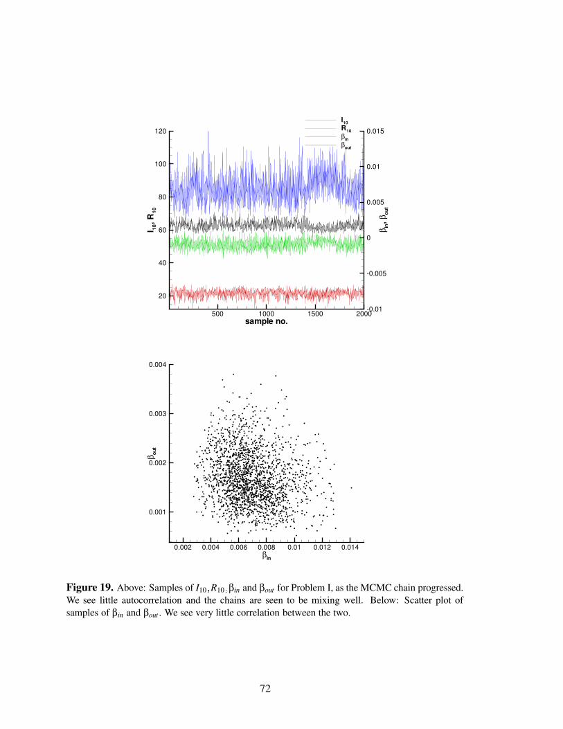
sample no.

I 10,R

10

β in,β

out

500 1000 1500 2000

20

40

60

80

100

120

-0.01

-0.005

0

0.005

0.01

0.015

I10R10βinβout

βin

β out

0.002 0.004 0.006 0.008 0.01 0.012 0.014

0.001

0.002

0.003

0.004

Figure 19. Above: Samples of I10 2 R10 2 βin and βout for Problem I, as the MCMC chain progressed.We see little autocorrelation and the chains are seen to be mixing well. Below: Scatter plot ofsamples of βin and βout . We see very little correlation between the two.

72

x (days since first symptomatic)

p(x)

20 40 60 80 100

0.05

0.1

0.15

0.2

0.25

0.3I5R5I10R10I30R30

x (days-1)

p(x)

0.002 0.004 0.006 0.008 0.01 0.012 0.014

100

200

300

400

500

600

700

β1β2β1 (40 days)β2 (40 days)

Figure 20. Above: PDFs for the dates of infection and removal for Cases number 5, 10 and 30for Problem I. The Cases are denoted by separate colors; plots of removal dates contain a symbol.While the bases of the PDFs are almost as wide as those of the incubation and removal periods,the shapes of the PDFs are quite different from the skewed Γ-distributions which are used to modelincubation and removal durations for smallpox. Below: The PDFs for the rates of spread β in andβout developed from data collected during the entire epidemic (plots with symbols) and from thefirst 40 days of data (plots without symbols). The MAP estimate of the spread rates drawn from thefirst 40 days may be affected by measurement error in the data.

73

Figure 21. The expected infection pathway U P V , drawn from data collected during the entireepidemic for Problem I. Nodes represent the 30 Cases of the outbreak and are colored by theircompound affiliations. The links in the graphs are colored by their probability of existence – linkswith probability of 30% or higher are red while those between 10% and 30% are blue. Most of thetransmissions from the index case (Node 000) are in red, and connect individuals in the same com-pound. Infection transmissions between the later Cases are almost completely in blue, indicatingthe reduction of heterogeneity in the transmission mechanism as a large fraction of the populationbecame infected.

74

Figure 22. The expected infection pathway U P V , drawn from data collected during the first 40days of the epidemic, for Problem I. Nodes represent the 30 Cases of the outbreak and are coloredby their compound affiliations. The links in the graphs are colored by their probability of existence– links with probability of 30% or higher are red while those between 10% and 30% are blue. Mostof the transmissions from the index case (Node 000) are in red, and connect individuals in the samecompound. A few red cross-compound links are also evident at this point in the epidemic.

75

for βin βout . Comparing with Figure 20 (below), we see that the width of the PDF forProblem II is similar to that for βin in Problem I, while the MAP value lies in betweenthe MAP values for βin and βout , though closer to βin if one considers the median value(3 � 37 � 10 � 3day � 1, as opposed to 4 � 76 � 10 � 3day � 1 for Problem I). This is intuitivelycorrect, since the bulk of the transmission was in-compound. In Figure 24 we plot theexpected infection pathway � P � . Comparing it to Figure 22, we see that the two arevery similar, but not identical (for example, Node 008 has four in-links in Problem II,but 3 in Problem I). Again, transmission links can be inferred with high probability onlyfor the first few Cases; the links connected to the latter Cases are generally blue. Thusthe inferences drawn by the two models are quite comparable. In Figure 25 we plot theexpected social network � G � . As in Problem I, the 74 nodes (individuals in the entirepopulation) are colored by their compound affiliations. Only cross-compound links whichhave appeared in 50% (or higher) of the samples are plotted. A subset of these links, whichwere instrumental in disease transmission, appears in Figure 24.

76

x (days since first symptomatic)

p(x)

10 20 30 40 50

0.05

0.1

0.15

0.2

I5R5I10R10

x (days-1)

p(x)

0.002 0.003 0.004 0.005 0.006 0.007

100

200

300

400

β1β2

Figure 23. Above: PDFs for the dates of infection and removal for Case numbers 5 and 10, forProblem II. The cases are denoted by separate colors; plots of removal dates contain a symbol.While the bases of the PDFs are almost as wide as those of the incubation and removal periods,the shapes of the PDFs are quite different from the skewed Γ-distributions which are used to modelincubation and removal durations for smallpox. Below: The PDFs for the rate of spread β in W βout .

77

Figure 24. The expected infection pathway U P V , drawn from data collected during the first 40days of the epidemic, for Problem II. Nodes represent the Cases of the outbreak and are coloredby their compound affiliations. The links in the graphs are colored by their probability of existence– links with probability of 30% or higher are red while those between 10% and 30% are blue.Most of the transmissions from the index case (Node 000) are in red, and connect individuals inthe same compound. Infection transmissions between the later Cases are almost completely in blue,indicating the reduction of heterogeneity in the transmission mechanism as a large fraction of thepopulation became infected.

78

Figure 25. The expected social network U G V , drawn from data collected during the first 40days, for Problem II. Nodes represent the 74 members of the population and are colored by theircompound affiliations. Links in the graphs represent the cross-compound social links seen in 50%(or higher) of the samples.

79


80

6 Conclusions

Simulations with individual-based models yield detailed predictions of where on the so-cial network disease will spread as well as the transmission chain information and struc-ture necessary to perform source inversion problems. They are potentially valid when thewell-mixed assumptions of (deterministic) differential equations are inappropriate. In Sec-tion 3 we present smallpox simulation results from our individual-based model, whichwe designed to be parallel scalable and to investigate the effect of social contact networkstructures and reduced-order modeling. A static unipartite graph formulation demonstratedcomparable performance to a more computationally costly dynamic bipartiite formulation,though with the loss of geographic location information. Static person-to-person contactgraphs with basic probability of transmission models still offer individual resolution andcontact tracing ability. Results for network sampling (model reduction) indicate that qual-itatively similar predictions are possible for both geographic spread and population countepidemic spread. However, appropriately scaling the simulation to the reduced networkremains a challenge. Our simulation demonstrates that individual-based models can scalewell in parallel, if appropriate communication patterns are used.

We favor the term “individual-based” for our models since, with the exception of choosingwhen to seek medical care or self-quarantine, disease progression is uninfluenced by au-tonomous decision, and we include no cognitive models. However, we offer some conclud-ing remarks on agent-based models in general. Agent-based models typically implementlocal learning, adaptation, and interaction rules, but can exhibit global emergent (complexadaptive) behavior. They are useful for modeling social systems and networks, traffic andtransit systems, economies and governments, supply chains and logistics, and even systemsof systems, e.g., the nuclear fuel cycle or operational fleets. Agent-based models closelyalign with structures present in these kinds of systems.

While often intuitive, agent-based models can be complex, and all but the simplest transi-tion models are challenging to analyze. Other criticisms and potential limitations include:� lack of detailed quantitative information needed to define agent behavior (especially

for human decision-making models);� stochastic nature mandates simulation ensembles to characterize outcomes instead ofsingle calculations;� computational intensity; and� they are not thought of as prescriptive models in the typical engineering sense andthere is no clear way to invert to identify parameters.

Perhaps the greatest challenge with agent-based models is performing verification and vali-dation to ensure credibility for their intended use. Verification assesses whether the “right”solution to the mathematical formulation implemented has been found. Code verification

81

can largely (though not entirely) be addressed through good software development prac-tices. Solution verification, however, presents a problem. There is no clear analog to orderof convergence or method of manufactured solutions. While not rigorous, steps toward ver-ification might include: testing network models by creating carefully structured networks,where transmission paths and incubation rates would be appropriately modeled by an ODEmodel; or testing cases where analytic or well-established solutions apply. These, however,will not exercise the full extent of an agent-based model (stochasticity, dynamic contacts,emergent behavior, etc.).

Credibility checks on models require data for both individual agent, connectivity, andsystem-level model validation. This is rare in the context of eradicated or emergent dis-eases, though there are some exceptions [91]. At least for social networks, data might begathered from studies in a controlled population, perhaps in observational studies of ru-mors or other information dissemination. Engineering hierarchical validation approachesmay offer some help. Also, methods for validating stochastic simulations are needed: onecan only examine output summary statistics or distributions, and must therefore employappropriate statistical measures.

Applications of social network-based simulations reach far beyond disease modeling; de-veloping verified and validated predictive capability is crucial. Ultimately, practitionerswill demand best-estimate predictions with quantified uncertainty, especially when modeldetails are not well known.

In Section 4 we have developed a Bayesian approach to characterize bioterror attacks froma time series of diagnosed patients. Our tests with anthrax show that an observation periodof 3–5 days may be sufficient to estimate the number of asymptomatic infected people, thetime of infection, and a representative dose, and to provide quantified uncertainty intervalsaround these estimates; in the absence of an accurate disease model, we may arrive within afactor of two of the size of the attack. The resolution of the time series of diagnosed patientshas a small impact if the disease model is accurate; otherwise, model errors dominate.

This Bayesian approach is amenable to many potential extensions and improvements. In-formative prior distributions for N and τ, drawn from syndromic surveillance data, mayincrease the efficiency of the inference process. The ability to “fuse” disparate sources ofdata via prior distributions contributes significantly to the robustness of Bayesian inferencein data-starved environments. One could also incorporate atmospheric transport processesinto the likelihood function, thus using the spatial locations of diagnosed patients to guideposterior estimates, though for urban terrains this could lead to very involved computations.Also, the present approach can immediately be applied to other noncontagious diseases, aswell as to contagious diseases with long incubation periods, such as smallpox, where sec-ondary cases do not appear in the early time series of patient data.

The Bayesian inference method developed in Section 5 is novel, in the sense that it explic-itly accounts for the role of pathogenic transmissibility and mixing in the spread of a diseaseand infers them from the data. These two variables could also be used, independently – thelink probabilities inferred in Section 5 (Case II) could easily be used in a network epidemic

82

model for any other disease (e.g., influenza). The inference of the transmissibility, β, canbe easily used to track the evolution of the transmissibility of emerging infectious diseases;in fact, such efforts have already commenced [51, 52, 53, 54]. Further, the inference ofa transmission chain can often be helpful in identifying the mechanism of transmission.For example, in-family transmission is not very strong for Ebola, since it mainly spreadsvia contaminated bodily fluids, most commonly when preparing a contaminated corpse forfinal disposal. This is generally done by the women of a village [92], leading to strongcross-family transmission. Such a mechanism would be reflected in both Iβ and � P �and would be helpful in detecting the actual mechanism. Thus, while our intention was toapply our approach to counter bioterrorism, there is little to prevent its use with emerginginfectious diseases.

The importance of quantitatively characterizing a BT attack was explicitly identified in the“Dark Winter” exercise [8]. Participants sought the ability “. . . to immediately predict thelikely size of the epidemic on the basis of the initial cases; to know how many people wereexposed.” Thus the primary utility of our inference procedure is within a response planframework. Response to a BT attack would typically involve confirmatory testing and lo-gistics (the transport of medical materials and personnel), both of which could be bettertargeted by a quantitative characterization of the attack. By placing the estimated origin ofan attack in the context of a transportation network, one could predict the location of futurepatients and guide prophylactic activities accordingly. The probabilistic characterizationsdeveloped here, along with resource hedging for risk mitigation, support a measured ap-proach to addressing BT attacks. In addition to being more sustainable, measured responsesmay introduce fewer undesirable side effects and be less susceptible to feints.

83


84

References

[1] Philip S. Brachman, Arnold F. Kaufmann, and Frederic G. Dalldorf. Industrial in-halational anthrax. Bacteriological Reviews, 30(3):646–657, 1966.

[2] Martin Eichner and Klaus Dietz. Transmission potential of smallpox: Estimates basedon detailed data from an outbreak. American Journal of Epidemiology, 158(2):110–117, 2003.

[3] John A. Jernigan et al. Bioterrorism-related innhalational anthrax: The first 10 casesreported in the United States. Emerging Infectious Diseases, 7(6):933–944, 2001.

[4] Jeanne Guillemin. Biological Weapons: From the Invention of State-Sponsored Pro-grams to Contemporary Bioterrorism. Columbia University Press, 2006.

[5] P. Williams and D. Wallace. Unit 731: Japan’s Secret Biological Warfare in WorldWar II. The Free Press, New York, 1989.

[6] Ken Alibek and Stephen Handelman. Biohazard. Delta, New York, NY, USA, 2000.

[7] Matthew Meselson, Jeanne Guillemin, Martin Hugh-Jones, Alexander Langmuir,Ilone Popova, Alexis Shelokov, and Olga Yampolskaya. The Sverdlovsk anthrax out-break of 1979. Science, 266:1202–1208, 1994.

[8] Tara O’Toole, Michael Mair, and Thomas V. Inglesby. Shining light on Dark Winter.Clinical Infectious Diseases, 34:972–983, 2002.

[9] R. Gani and S. Leach. Transmission potential of smallpox in contemporary popula-tions. Nature, 414, December 2001.

[10] P. F. Wehrle, J. Posch, K. H. Richter, and D. A. Henderson. An airborne outbreakof smallpox in a German hospital and its significance with respect to other recentoutbreaks in Europe. Bulletin of the World Health Organization, 43:669–679, 1970.

[11] F. Fenner, D. A. Henderson, I. Arita, Z. Jezek, and I. D. Ladnyi. Smallpox and ItsEradication. World Health Organization, Geneva, 1988.

[12] R. M. Anderson and R. M. May. Infectious Diseases of Humans: Dynamics andControl. Oxford University Press, New York, 1992.

[13] Henry C. Tuckwell, Laurent Toubiana, and Jean-Francois Vibert. Spatial epidemicnetwork models with viral dynamics. Physical Review E, 57(2), February 1998.

[14] A.L. Lloyd and S. Valeika. Network models in epidemiology: An overview. InB. Blasius, J. Kurths, and L. Stone, editors, Complex Population Dynamics: Nonlin-ear Modeling in Ecology, Epidemiology and Genetics. World Scientific, 2007.

[15] A.L. Lloyd, S. Valeika, and A. Cintron-Arias. Infection dynamics on small-worldnetworks. In A.B. Gumel, C. Castillo-Chavez, and D.P. Clemence, editors, Modelingthe Dynamics of Human Diseases: Emerging Paradigms and Challenges. AMS, 2006.

85

[16] R. M. May and A. L. Lloyd. Infection dynamics on scale-free networks. PhysicalReview E., 64(066112), 2001.

[17] Y. Moreno, R. Pastor-Satorras, and A. Vespignani. Epidemic outbreaks in complexheterogeneous networks. European Physics Journal B, 26:521–529, 2002.

[18] Marc Barthelemy, Alain Barrat, Romualdo Pastor-Satorras, and Alessandro Vespig-nani. Dynamical patterns of epidemic outbreaks in complex heterogeneous networks.Journal of Theoretical Biology, 235(2):275–288, July 2005.

[19] Lauren Ancel Meyers, M.E.J. Newman, and Babak Pourbohloul. Predicting epi-demics on directed contact networks. Journal of Theoretical Biology, 240(400418),2006.

[20] Lauren Ancel Meyers, Babak Pourbohloul, M.E.J. Newman, Danuta M. Skowronski,and Robert C. Brunham. Network theory and SARS: predicting outbreak diversity.Journal of Theoretical Biology, 232(7181), 2005.

[21] M. E. J. Newman. The structure and function of complex networks. SIAM Review,45(2):167–256, 2003.

[22] L. da F. Costa, F. A. Rodrigues, G. Travieso, and P. R. Villas Boas. Characterization ofcomplex networks: A survey of measurements. Advances in Physics, 56(1):167–242,2007.

[23] Stephen Eubank, V.S. Anil Kumar, Madhav V. Marathe, Aravind Srinivasany, and NanWangz. Structural and algorithmic aspects of massive social networks. In Proceedingsof the fifteenth annual ACM-SIAM symposium on discrete algorithms, pages 718–727,New Orleans, LA, 2004.

[24] Hazhir Rahmandad and John Sterman. Heterogeneity and network structure in the dy-namics of diffusion: Comparing agent-based and differential equation models. Tech-nical Report (Working Paper Series) ESD-WP-2004-05, Engineering Systems Divi-sion, Massachusetts Institute of Technology, November 2004.

[25] Stephen Eubank, Hasan Guclu, V. S. Anil Kumar, Madhav V. Marathe, Aravind Srini-vasan, Zoltan Toroczkai, and Nan Wang. Modelling disease outbreaks in realisticurban social networks. Nature, 429:180–184, 2004.

[26] Timothy C. Germann, Kai Kadau, Ira M. Longini, Jr., and Catherine A. Macken.Mitigation strategies for pandemic influenza in the United States. Proceedings of theNational Academy of Science, 103(15):5935–5940, April 2006.

[27] Donald S. Burke, Joshua M. Epstein, Derek A. T. Cummings, Jon I. Parker, Ken-neth C. Cline, Ramesh M. Singa, and Shubha Chakravarty. Individual-based com-putational modeling of smallpox epidemic control strategies. Academic EmergencyMedicine, 13:1142–1149, 2006.

86

[28] Ira M. Longini Jr., M. Elizabeth Halloran, Azhar Nizam, Yang Yang, Shufu Xu, Don-ald S. Burke, Derek A.T. Cummings, and Joshua M. Epstein. Containing a largebioterrorist smallpox attack: a computer simulation approach. International. Journalof Infectious Diseases, 11:98–108, 2007.

[29] Thomas V. Inglesby, Donald A. Henderson, John G. Barteltt, Michael S. Ascher, Ed-ward Eitzen, Arthur M. Friedlander, Jerome Hauer, Joseph McDade, Michael T. Os-terholm, Tara O’Toole, Gerald Parker, Trish M. Perl, Philip K. Russel, and KevinTomcat. Anthrax as a biological weapon – Medical and public health management.Journal of the American Medical Association., 281(18):1735–1745, 1999.

[30] R. W. Titball, P. C. Turnbull, and R. A. Hutson. The monitoring and detection of Bacil-lus anthracis in the environment. Journal of Applied Bacteriology, 70(suppl):9S–18S,1991.

[31] R. P. Williams. Bacillus anthracis and other spore forming bacilli. In A. Braude, L. E.Davis, and J. Fierer, editors, Infectious Disease and Medical Microbiology, pages270–278. W. B. Saunders Co., Philadelphia, PS, 1986.

[32] M. M. Friedlander, S. L. Welkos, M. L. Pitt, J. W. Ezzell, P. L. Worsham, K. J. Rose,B. E. Ivins, J. R. Lowe, G. B Howe, P. Mikesell, and Wade B. Lawrence. Postexposureprophylaxis against experimental inhalation anthrax. Journal of Infectious Disease,167(5):1239–1243, 1993.

[33] J. M. Ross. The pathogenesis of anthrax following the administration of spores by therespiratory route. Journal of Pathology and Bacteriology, 73:485–495, 1957.

[34] J. Walden and E. H. Kaplan. Estimating time and size of bioterror attack. EmergingInfectious Diseases, 10(7):1202–1205, 2004.

[35] R. Brookmeyer, N. Blades, M. Hugh-Jones, and D. A. Henderson. The statistical anal-ysis of truncated data: application to the Sverdlovsk anthrax outbreak. Biostatistics,2:233–247, 2001.

[36] Ron Brookmeyer and Natalie Blades. Statistical models and bioterrorism: Appli-cation to the U.S. anthrax attacks. Journal of the American Statistical Association,98(464):781–788, 2003.

[37] D. W. Henderson, S. Peacock, and F. C. Belton. Observations on the prophylaxis ofexperimental pulmonary anthrax in the monkey. Journal of Hygiene, 54:28–36, 1956.

[38] Wilhelm S. Albrink and Robert J. Goodlow. Experimental inhalational anthrax in thechimpanzee. The American Journal of Pathology, 35(5):1055–1065, 1959.

[39] C. A. Gleiser, C. C. Berdjis, H. A. Hartman, and W. S. Gochenour. Pathology ofexperimental respiratory anthrax in Macaca Mulatta. British Journal of ExperimentalPathology, 44:416–426, 1963.

87

[40] B. E. Ivins, M. L. M. Pitt, P. F. Fellows, J. W. Farchaus, G. E. Benner, D. M. Waag,S. F. Little, G. W. Anderson, P. H. Gibbs, and A. M. Friedlander. Comparative effi-cacy of experimental anthrax vaccine candidates against inhalational anthrax in rhesusmacaques. Vaccine, 16(11/12):1141–1148, 1998.

[41] R. Brookmeyer, E. Johnson, and S. Barry. Modelling the incubation period of anthrax.Statistics in Medicine, 24:531–542, 2005.

[42] D. Wilkening. Sverdlovsk revisted: Modeling human inhalational anthrax. Proceed-ings of the National Academy of Science, 103(20):7589–7594, May 2006.

[43] H. N. Glassman. Discussion on industrial inhalational anthrax. Bacteriological Re-view, 30:657–659, 1966.

[44] H. A. Druett, D. W. Henderson, L. Packman, and S. Peacock. Studies on respiratoryinfection. I.The influence of particle size on respiratory infection with anthrax spores.Journal of Hygiene, 51:359–371, 1953.

[45] C. N. Haas. On the risk of mortality to primates exposed to anthrax spores. RiskAnalysis, 22(2):189–193.

[46] W. R. Hogan, G. Cooper, G. L Wallstrom, and M. Wagner. An Improved BayesianAerosol Release Detector. Technical report, The RODS Laboratory, 550 CellomicsBuilding, 100 Technology Drive, Pittsburgh, PA 15219, 2005.

[47] Fu-chang Tsui, Jeremy U. Espino, Virginia M. Dato, Per H. Gesteland, Judith Hut-man, and Michael M. Wagner. Technical Description of RODS : A real-time publichealth surveillance system. Journal of the Americal Medical Informatics Association,10(5):399–408, 2003.

[48] D. Bruce Turner. Workbook of Atmospheric Dispersion Estimates: An Introductionto Dispersion Modeling. Lewis Publishers, CRC Press LLC, 2000 N.W. CorporateBlvd. Boca Raton, FL 33431, 1994.

[49] A. R. Rao. Smallpox. The Kothari Book Depot, Bombay, 1972.

[50] M. Elizabeth Halloran, Ira M. Longini, Azhar Nizam, and Yang Yang. Containingbioterrorist smallpox. Science, 298:1428–1432, November 2002.

[51] Luis M. A. Bettencourt and Ruy M. Ribeiro. Real-time Bayesian estimation of theepidemic potential of emerging infectious diseases. Public Library of Science – One,3(5), 2008.

[52] Gerardo Chowell, Hiroshi Nishiura, and Luis M. A. Bettencourt. Comparative estima-tion of the reproduction number for pandemic influenza from daily case notificationdata. Journal of the Royal Society – Interface, 4, 2007.

[53] Yang Yang, M. Elizabeth Halloran, Johathan D. Sugimota, and Ira M. Longini. De-tecting human-to-human transmission of avian influenza A (H5N1). Emerging Infec-tious Diseases, 13(9):1348–1353, 2007.

88

[54] Michiel van Boven, Marion Koopmans, Mirna Du Ry van Beest Holle, Adam Meijer,Don Klinkenberg, Christl A Donnelly, and Hans (J. A. P.) Heesterbeek. Detectingemerging transmissibility of avian influenza virus in human households. Public Li-brary of Science, Computational Biology, 3(7):e145, Jul 2007.

[55] S. Cauchemez amd F. Carrat, C. Viboud, A. J. Valleron, and P. Y. Boelle. A BayesianMCMC approach to study transmission of influenza: application to household longi-tudinal data. Statistics in Medicine, 23:3469–3487, 2004.

[56] Simon Cauchemez, Alain-Jacques Valleron, Pierre-Yves Boelle, Antoine Flahault,and Neill M. Ferguson. Estimating the impact of school closure on influenza trans-mission from Sentinel data. Nature, 452(10):750–755.

[57] Phillip O’Neill, David J Balding, Niels G. Becker, Mervi Eerola, and Denis Mollison.Analyses of infectious disease data from household outbreaks by MCMC methods.Applied Statistics, 49(4):517–542.

[58] P. D. O’Neill and G. O. Roberts. Bayesian inference of partially observed stochasticepidemics. Journal of the Royal Statistical Society, Series A, 162:121–129, 1999.

[59] Michael Hohle, Erik Jorgensen, and Philip D. O’Neill. Inference in disease transmis-sion experiments by using stochastic epidemic models. Journal of the Royal Statisti-cal Society: Series C (Applied Statistics), 54(2):349–366, 2005.

[60] Tom Britton and P. O’Neill. Bayesian inference for stochastic epidemics in popula-tions with random social structure. Scandinavian Journal of Statistics, 29:375–390,2002.

[61] Nikolaos Demiris and Philip D. O’Neill. Bayesian inference for stochastic multitypeepidemics in structured populations via random graphs. Journal of the Royal Statisti-cal Society: Series B (Statistical Methodology), 67(5):731–745, 2005.

[62] G. Chowell, J. M. Hyman, S. Eubank, and C. Castillo-Chavez. Scaling laws forthe movement of people between locations in a large city. Physical Review E,68(066102):1–7, 2003.

[63] Tom Britton, Maria Deijfen, and Anders Martin-Lof. Generating simple ran-dom graphs with prescribed degree distribution. Journal of Statistical Physics,124(6):1377–1397, 2006.

[64] J. Kaipio and E. Somersalo. Statistical and Computational Inverse Problems.Springer, New York, 2004.

[65] D. S. Sivia. Data Analysis: A Bayesian Tutorial. Oxford University Press, Inc, NewYork, 2004.

[66] W. R. Gilks, S. Richardson, and D. J. Spiegelhalter, editors. Markov Chain MonteCarlo in Practice. Chapman & Hall, 1996.

89

[67] C. P. Robert. Mixtures of distributions: inference and estimation. In W. R. Gilks,S. Richardson, and D. J. Spiegelhalter, editors, Markov Chain Monte Carlo in Prac-tice, chapter 24, pages 441–464. Chapman & Hall, 1996.

[68] Andrew Gelman, John B. Carlin, Hal S. Stern, and Donal B. Rubin. Bayesian DataAnalysis. Chapman & Hall / CRC Press, Boca Raton, FL, 2004.

[69] Hakon Tjelmeland and Jo Eidsvik. On the use of local optimizations withinMetropolis-Hastings updates. Journal of the Royal Statistical Society, B, 66(2):411–427, 2004.

[70] Hakon Tjelmeland and Bjorn Kare Hegstad. Mode jumping proposals in MCMC.Scandinavian Journal of Statistics, 28:201–223, 2001.

[71] Cristian Sminchisescu, Max Welling, and Geoffrey Hinton. A mode-hoppingMCMC sampler. Technical Report CSRG-478, University of Toronto, 6 King’sCollege Road, Pratt Building, Toronto, Ontario, CANADA, M5S 3G4, 2003.http://www.cs.toronto.edu/ crismin/.

[72] Heikki Haario, Eero Saksman, and Johanna Tamminen. An adaptive Metropolis al-gorithm. Bernoulli, 7(2):223–242, 2001.

[73] Heikki Haario, Eero Saksman, and Johanna Tamminen. Component-wise adaptationfor high dimensional MCMC. Computational Statistics, 20:265–273, 2005.

[74] J. A. Vrugt, H. V. Gupta, W. Bouten, and S. Sorooshian. A shuffled complex evolu-tion Metropolis algorithm for optimization and uncertainty assessment of hydrologicmodel parameters. Water Resources Research, 39(8), 2003.

[75] J. A. Vrugt, B. O. Nuallain, B. A. Robinson, Willem Bouten, Stefan C. Dekker, andPeter M. A. Sloot. Application of parallel computing to stochastic parameter estima-tion in environmental models. Computers and Geosciences, 32:1139–1155, 2006.

[76] Synthetic data products for societal infrastructures and proto-populations:Data set 1.0. Technical Report NDSSL-TR-06-006, Network Dynamicsand Simulation Science Laboratory, Virginia Polytechnic Institute and StateUniversity, 1880 Pratt Dr, Building XV, Blacksburg, VA, 24061, 2006.http://ndssl.vbi.vt.edu/Publications/ndssl-tr-06-006.pdf.

[77] Synthetic data products for societal infrastructures and proto-populations:Data set 2.0. Technical Report NDSSL-TR-07-003, Network Dynamicsand Simulation Science Laboratory, Virginia Polytechnic Institute and StateUniversity, 1880 Pratt Dr, Building XV, Blacksburg, VA, 24061, 2007.http://ndssl.vbi.vt.edu/Publications/ndssl-tr-07-003.pdf.

[78] C. Barrett, R. Beckman, K. Berkbigler, K. Bisset, B. Bush, K. Campbell, S. Eubank,K. Henson, J. Hurford, D. Kubicek, M. Marathe, P. Romero, J. Smith, L. Smith,P. Speckman, P. Stretz, G. Thayer, E. Eeckhout, and M.D. Williams. TRANSIMS:

90

Transportation analysis simulation system. Technical Report Technical Report LA-UR-00-1725, Los Alamos National Laboratory, 2001. Unclassified Report.

[79] K.D. Devine, E.G. Boman, R.T. Heaphy, R.H. Bisseling, and U.V. Catalyurek. Par-allel hypergraph partitioning for scientific computing. In Proc. of 20th InternationalParallel and Distributed Processing Symposium (IPDPS’06). IEEE, 2006.

[80] J. Ray, Y. M. Marzouk, H. N. Najm, M. Kraus, and P. Fast. A Bayesian methodfor characterizing distributed micro-releases: I. The single-source case for non-contagious diseases. SAND Report SAND2006-1491, Sandia National Laboratories,Livermore, CA 94551-0969, March 2006. Unclassified unlimited release.

[81] Erik Boman, Karen Devine, Lee Ann Fisk, Robert Heaphy, Bruce Hendrickson,Courtenay Vaughan, Umit Catalyurek, Doruk Bozdag, William Mitchell, and JamesTeresco. Zoltan 3.0: Parallel Partitioning, Load-balancing, and Data ManagementServices; User’s Guide. Sandia National Laboratories, Albuquerque, NM, 2007.Tech. Report SAND2007-4748W http://www.cs.sandia.gov/Zoltan/u html/ug.html.

[82] Jeanne Guillemin. Anthrax: The Investigation of a Deadly Outbreak. University ofCalifornia Press, 2001.

[83] Jeanne Guillemin. The political determinants of delayed diagnosis: The 1979Sverdlovsk anthrax outbreak and the 1972 Yugoslavian smallpox epidemics. InRajan Gupta and Mario R. Perez, editors, Confronting Terrorism – 2002. LosAlamos National Laboratory, March 25–29 2002. http://library.lanl.gov/cgi-bin/getdoc?event=CT2002&document=20.

[84] G. Peter Lepage. A new algorithm for adaptive multidimensional integration. Journalof Computational Physics, 27:192–203, 1978.

[85] GNU Scientific Library. http://www.gnu.org/software/gsl/.

[86] J. Ray, Y. M. Marzouk, M. Kraus, and P. Fast. A Bayesian method for characterizingdistributed micro-releases: II. Inference under model uncertainty with short time-series data. SAND Report SAND2006-7568, Sandia National Laboratories, Liver-more, CA 94551-0969, December 2006. Unclassified unlimited release.

[87] P. E. Sartwell. The distribution of incubation periods of infectious diseases. AmericanJournal of Hygiene, 51:310–318, 1950.

[88] Frederick Klein, Jerry S. Walker, David F. Fitzpatrick, Ralph E. Lincoln, Bill G.Mahlandt, William L. Jones, James P. Dobbs, and Kenneth J. Hendrix. Pathophysiol-ogy of anthrax. Journal of Infectious Diseases, 116(2):123–138, 1966.

[89] Romualdo Pastor-Satorras and Alessandro Vespignani. Epidemic spreading in scale-free networks. Physical Review Letters, 86(14):3200–3203, 2001.

[90] D. Thompson and William Foege. Faith Tabernacle smallpox epidemic. TechnicalReport WHO/SE/68.3, World Health Organization, 1968.

91

[91] Jonathan B. Tucker and Raymond A. Zilinskas. The 1971 smallpox epidemic inAralsk, Kazakhstan, and the Soviet biological warfare program. Technical ReportOccasional Paper No. 9, Center for Nonproliferation Studies, Monterey Institute ofInternational Studies, Monterey, California, 2002.

[92] G. Chowell, N. W. Hengartner, C. Castillo-Chavez, P. W. Fenimore, and J. M. Hyman.The basic reproductive number of Ebola and the effects of public health measures:The case of Congo and Uganda. Technical Report LA-UR-03-8189, Los AlamosNational Laboratory, Los Alamos, NM, 2003.

92

A Methodology for obtaining a dose distribution consis-tent with atmospheric dispersion over a geographicallydistributed population

The spatial distribution of dosages due to atmospheric release of an aerosol can be modeledusing a simple Gaussian plume model [48]. An atmospheric release typically occurs over adomain with a non-uniform population distribution; we can combine the plume model withthe population distribution to calculate the number of people exposed to a given dose. Inthis appendix, we describe a simple way to obtain such a population-dosage distribution.

We consider a square domain, L km on each side; in this study, L 10 km. The domain isdivided into N blocks per side; here N 100. Twenty five population clusters are chosenin the form of Gaussian kernels Aexp � � r2 % R2 � , where r2 � x � x0 � 2. The strength ofthe kernel A, its center x0, and its length scale R are randomly sampled from independentuniform distributions. The population density in any block, with its center at x, is a sumof the strengths of all the 25 kernels. The strengths of the kernels are scaled to obtain atotal population (in the domain) of Pdomain. The population in a given block is obtainedby multiplying the population density with the block area. This creates a geographicallydistributed population.

The number of people exposed (i.e., those who inhaled the aerosol, but may or may notdevelop symptoms) and infected (i.e., who will develop symptoms) is dependent on thelocation and size of the release and direction of the wind. We release 1013 spores at theorigin, at a height of 100 meters. A wind speed of 4 m/s and a Pasquill stability classof “B” are assumed. Pasquill stability classes indicate atmospheric stability; class B indi-cates a moderately unstable atmosphere with strong daytime insolation. Details of Pasquillstability classes and atmospheric dispersion are in [48]. In our study, wind directions aremeasured in degrees from due north; that is, a wind direction of zero degrees is a wind fromdue north, 90 degrees is a westerly wind, and a direction of 180 degrees is a wind from duesouth. The release is assumed to be an explosive point release, and the concentration of theaerosol at any point � x � y � on the ground and any time t is given by [48]:

χ � x � y � t � 2QT� 2π � 3 Q 2σx X σy X σz X exp YZ� � x [8� ut � 22σ2

x X \ exp YZ� � y []� 22σ2

y X^\ exp Y_� � H []� 22σ2

z XZ\ (19)

where � x [ � y [ � are Cartesian coordinates in a frame of reference where the x [ -axis is alignedwith the wind. σx X � σy X and σz X are coefficients dependent on x [ and on the Pasquill stabilityclass. H is the height of release and χ is the concentration of the aerosol in spores per unitvolume. u is the wind velocity. QT is the total number of spores released. The relation

93

between x [ and x is given by

xy! cos � π � θ � � sin � π � θ �

sin � π � θ � cos � π � θ � ! x [y [ !

where θ is the wind direction. Assuming a breathing rate β of 30 liters a minute, one canobtain an expression for the number of spores inhaled per unit time. Integrating to infinitetime, one obtains the total number of spores D inhaled by a person positioned at � x � y � (orat � x [ � y [ � ):

D QT β2πσx X σy X σz X exp Y � � y [ � 2

2σ2y X^\ exp Y � � H [ � 2

2σ2z X`\ � 1 � erf � x [ ��a�

The dosage assigned to a given block is decided by the location of its center. If we chooseModel A2 to simulate the BT attack, we use Glassman’s formula to model the probabilitya of showing symptoms (in infinite time) given a dosage D [43]:

a � D � 12 ' 1 � erf ln � D % D0 �

S$

2!)( (20)

where D0 8 � 600 spores and S 3 � 44. These correspond to a human ID50 of 8600 sporesand a probit slope of 0.67 [42, 43]. If Model D is chosen instead, we employ Eq. 7 todetermine the probability of infection given a dose D. Since the population in a block isknown, we can then use the probability of infection to calculate the number of people in theblock who will proceed to develop symptoms over time, per the incubation period model.

In this study, we use Pdomain 3 � 106 and two plume directions, θ 170 > and 125 > .The two releases result in, respectively, 686,068 and 1,869,741 exposed individuals, i.e.,individuals who have received a dose of one spore or more. The maximum doses observedin the two cases are 30,877 and 314,053 respectively. The dose range is divided into 100equal bins and a histogram of the number of people in each bin is developed for eachof the cases. The histogram is then normalized to obtain the “exposure” PDF, i.e, thePDF of the dose received by an individual in the exposed population. Given the largepopulation (Pdomain 3 � 106), the PDF developed from a histogram with 100 bins is quitesmooth. Note that only a fraction of the exposed population will develop symptoms, with anindividual’s probability of being infected (and subsequently developing symptoms) beinggiven by Glassman’s relation (Eq. 20) or Eq. 7.

The “exposure” PDFs developed for θ 170 > and 125 > are then used to sample from asmaller exposed population of pexposed for each of the tests. Values of pexposed and θ usedfor the different cases are in Table A.1. Each exposed individual is then allowed to becomeinfected with a dose-dependent probability. The resulting infected sub-population yieldsthe final dose distribution.

94

1

1

1

1

1

1

1

1

1

1

1

1

12

2

2

2

2

2

2 2

2

3

3

3

3

33

3

4

4

4

4

4

5

5

5

5

5

6

6

6

7

7

7

78

8

9

10

1112

13

15

x

y

2000 4000 6000 8000 10000

2000

4000

6000

8000

Level density

16 320015 300014 280013 260012 240011 220010 20009 18008 16007 14006 12005 10004 8003 6002 4001 200

x

y

2000 4000 6000 8000 10000

2000

4000

6000

8000

1

1

11 1

1

1

1

1

1

1

2

2

2 2

2

2

2

2

2

2

2

3

3

3

3

3

3

3

4

4

4

4

4

4

5

5

5

5

5

6

6

6

7

7

7

8

9

9

10

11

11 12

1314

1516

x

y

2000 4000 6000 8000 10000

2000

4000

6000

8000 Level density

16 320015 300014 280013 260012 240011 220010 20009 18008 16007 14006 12005 10004 8003 6002 4001 200

x

y

2000 4000 6000 8000 10000

2000

4000

6000

8000

Figure A.1. Dosage plumes plotted over the population distribution for θ W 170 b (left) and 125 b(right). We see on the right that the extremities of the plume extend into a high-population-densityregion. Population density is measured in number of people per square kilometer. Thus we mayexpect a substantial number of high-dosage cases, resulting in a higher average dosage D.

Table A.1. The wind direction, θ, and the size of the exposed population, pexposed, used to gen-erate the infected population in various attacks. For Cases I, Ia, II, and IIa, Eq. 20 is used for theprobability of infection, while for Cases III, IIIa, IV, and IVa, Eq. 7 is used.

pexposed 103 pexposed 104

θ 170 > Case Ia, Case IIIa Case I, Case IIIθ 125 > Case II, Case IV Case IIa, Case IVa

Dose distributions resulting from this process, for all the cases (viz. Cases Ia, I, II, IIa, IIIa,III, IVa and IV) are depicted in Figure A.2. We plot the inverse CDF of doses—i.e., theabscissa is the fraction of the infected population which receives a dose less than or equalto the ordinate. In each inset, we also plot a histogram of the dose distribution. Note thatwhile the doses may easily span two orders of magnitude, about 80% of the infected peoplelie within a one-decade range.

95

Cumulative fraction of population

log 10

(Dos

e)[s

pore

s]

0 0.2 0.4 0.6 0.8 12

2.5

3

3.5

4

Dose

Num

bero

finf

ecte

dpe

ople

0 2000 4000 6000 8000 100000

5

10

15

20

25

30

35


log 10

(Dos

e)[s

pore

s]

0 0.2 0.4 0.6 0.8 12

2.5

3

3.5

4

Dose

Num

bero

finf

ecte

dpe

ople

2000 4000 6000 8000 100000

5

10

15

20


log 10

(Dos

e)[s

pore

s]

0 0.2 0.4 0.6 0.8 12

2.5

3

3.5

4

Dose

Num

bero

finf

ecte

dpe

ople

0 5000 10000 15000 20000 250000

20

40

60

80

100

120

140

160

180

200

220


log 10

(Dos

e)[s

pore

s]

0 0.2 0.4 0.6 0.8 12

2.5

3

3.5

4

Dose

Num

bero

finf

ecte

dpe

ople

5000 10000 15000 20000 250000

20

40

60

80

100


log 10

(Dos

e)[s

pore

s]

0.2 0.4 0.6 0.8 12.5

3

3.5

4

4.5

5

Dose

Num

bero

finf

ecte

dpe

ople

50000 1000000

20

40

60

80

100

120


log 10

(Dos

e)[s

pore

s]

0 0.2 0.4 0.6 0.8 13

3.5

4

4.5

5

Dose

Num

bero

finf

ecte

dpe

ople

50000 1000000

20

40

60

80

100


log 10

(Dos

e)[s

pore

s]

0.2 0.4 0.6 0.8 12.5

3

3.5

4

4.5

5

Dose

Num

bero

finf

ecte

dpe

ople

50000 1000000

200

400

600

800

1000

1200


log 10

(Dos

e)[s

pore

s]

0 0.2 0.4 0.6 0.8 13

3.5

4

4.5

5

Dose

Num

bero

finf

ecte

dpe

ople

50000 1000000

100

200

300

400

500

600

700

Figure A.2. The inverse cumulative distribution of doses for Cases Ia, I, II, and IIa (left column)and Cases IIIa, III, IV, IVa (right column). The abscissa is the fraction of the infected populationwhich receives a dose less than or equal to the ordinate. Inset: we plot histograms containing thenumber of infected people in each dose bin. While the histograms have long tails, the bulk of thepopulation receives doses spanning one order of magnitude.

.

96

Distribution:

1 Michael M. Wolf4332 Siebel Center, MC-258201 N. GoodwinUrbana, IL 61801

1 Youssef Marzouk, 0851 MS 90561 Habib Najm, 08351 MS 90561 Brian Adams, 01411 MS 13181 Karen D. Devine, 01416 MS 13182 Jaideep Ray, 08964 MS 91591 Donna Chavez, LDRD Office, 01011 MS 0123

2 Central Technical Files 08945-1 MS 90181 Technical Library,99536 MS 0899

97

Distributed micro-releases of bioterror pathogens : threat characterizations and epidemiology from...

Documents

Transcript of Distributed micro-releases of bioterror pathogens : threat characterizations and epidemiology from...