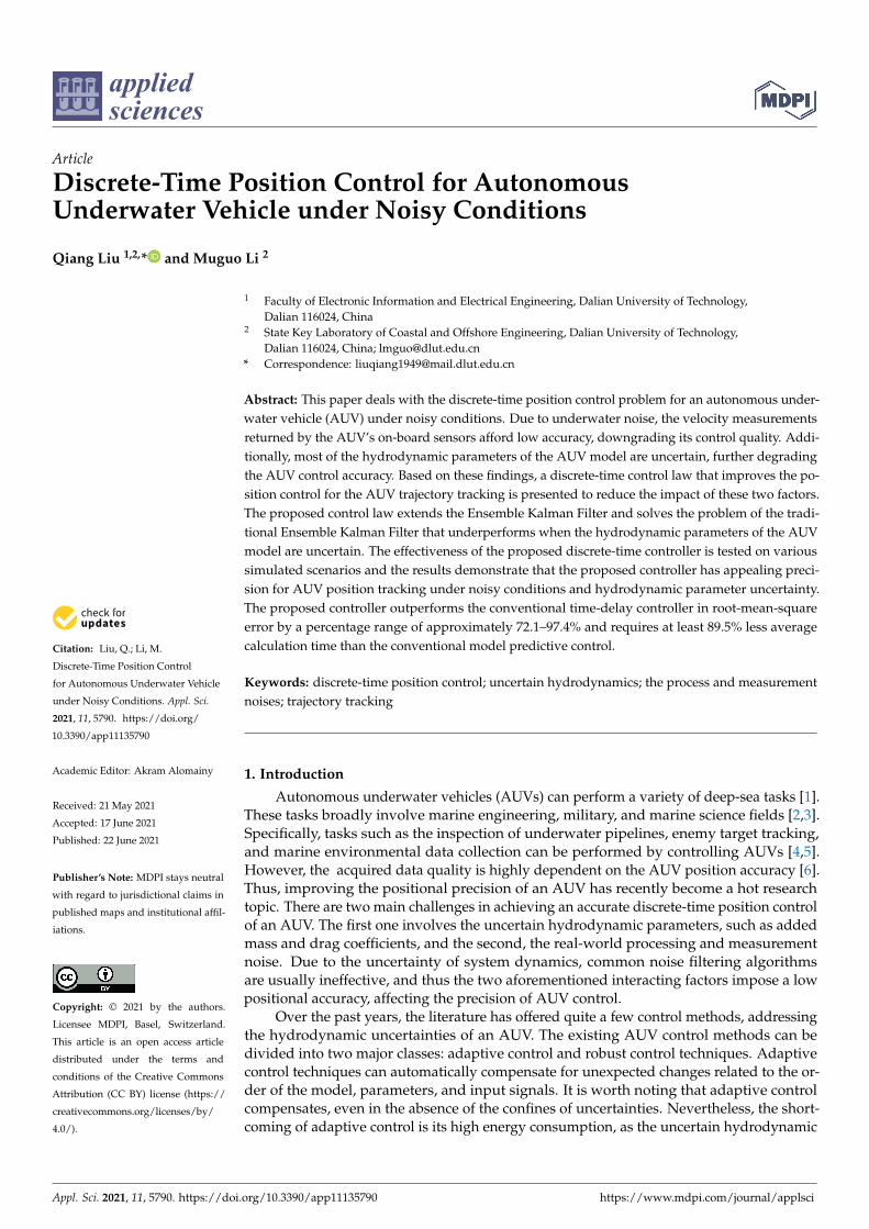
applied sciences

Article

Discrete-Time Position Control for AutonomousUnderwater Vehicle under Noisy Conditions

Qiang Liu 1,2,* and Muguo Li 2

�����������������

Citation: Liu, Q.; Li, M.

Discrete-Time Position Control

for Autonomous Underwater Vehicle

under Noisy Conditions. Appl. Sci.

2021, 11, 5790. https://doi.org/

10.3390/app11135790

Academic Editor: Akram Alomainy

Received: 21 May 2021

Accepted: 17 June 2021

Published: 22 June 2021

Publisher’s Note: MDPI stays neutral

with regard to jurisdictional claims in

published maps and institutional affil-

iations.

Copyright: © 2021 by the authors.

Licensee MDPI, Basel, Switzerland.

This article is an open access article

distributed under the terms and

conditions of the Creative Commons

Attribution (CC BY) license (https://

creativecommons.org/licenses/by/

4.0/).

1 Faculty of Electronic Information and Electrical Engineering, Dalian University of Technology,Dalian 116024, China

2 State Key Laboratory of Coastal and Offshore Engineering, Dalian University of Technology,Dalian 116024, China; lmguo@dlut.edu.cn

* Correspondence: liuqiang1949@mail.dlut.edu.cn

Abstract: This paper deals with the discrete-time position control problem for an autonomous under-water vehicle (AUV) under noisy conditions. Due to underwater noise, the velocity measurementsreturned by the AUV’s on-board sensors afford low accuracy, downgrading its control quality. Addi-tionally, most of the hydrodynamic parameters of the AUV model are uncertain, further degradingthe AUV control accuracy. Based on these findings, a discrete-time control law that improves the po-sition control for the AUV trajectory tracking is presented to reduce the impact of these two factors.The proposed control law extends the Ensemble Kalman Filter and solves the problem of the tradi-tional Ensemble Kalman Filter that underperforms when the hydrodynamic parameters of the AUVmodel are uncertain. The effectiveness of the proposed discrete-time controller is tested on varioussimulated scenarios and the results demonstrate that the proposed controller has appealing preci-sion for AUV position tracking under noisy conditions and hydrodynamic parameter uncertainty.The proposed controller outperforms the conventional time-delay controller in root-mean-squareerror by a percentage range of approximately 72.1–97.4% and requires at least 89.5% less averagecalculation time than the conventional model predictive control.

Keywords: discrete-time position control; uncertain hydrodynamics; the process and measurementnoises; trajectory tracking

1. Introduction

Autonomous underwater vehicles (AUVs) can perform a variety of deep-sea tasks [1].These tasks broadly involve marine engineering, military, and marine science fields [2,3].Specifically, tasks such as the inspection of underwater pipelines, enemy target tracking,and marine environmental data collection can be performed by controlling AUVs [4,5].However, the acquired data quality is highly dependent on the AUV position accuracy [6].Thus, improving the positional precision of an AUV has recently become a hot researchtopic. There are two main challenges in achieving an accurate discrete-time position controlof an AUV. The first one involves the uncertain hydrodynamic parameters, such as addedmass and drag coefficients, and the second, the real-world processing and measurementnoise. Due to the uncertainty of system dynamics, common noise filtering algorithmsare usually ineffective, and thus the two aforementioned interacting factors impose a lowpositional accuracy, affecting the precision of AUV control.

Over the past years, the literature has offered quite a few control methods, addressingthe hydrodynamic uncertainties of an AUV. The existing AUV control methods can bedivided into two major classes: adaptive control and robust control techniques. Adaptivecontrol techniques can automatically compensate for unexpected changes related to the or-der of the model, parameters, and input signals. It is worth noting that adaptive controlcompensates, even in the absence of the confines of uncertainties. Nevertheless, the short-coming of adaptive control is its high energy consumption, as the uncertain hydrodynamic

Appl. Sci. 2021, 11, 5790. https://doi.org/10.3390/app11135790 https://www.mdpi.com/journal/applsci

Appl. Sci. 2021, 11, 5790 2 of 19

parameters to be adapted impose great computational complexity. Given the limited energyresources of an AUV, this deficiency poses a disadvantage for AUV applications. Despitethis, adaptive control is still used with [7] a focuse on proportional integral derivative (PID)controllers for AUV. In this work, the PID control algorithm, despite being classic, is provento be quite effective for AUV control. Based on a set of saturation functions for trajectorytracking of AUV, Guerrero et al. [8] propose a nonlinear robust PID controller to cope withsystem uncertainty. In [9], the authors introduce a conventional back-stepping methodthat applies to AUV platforms for diving control. Sliding mode controllers (SMCs) [10,11]are designed for AUV control in the presence of uncertain hydrodynamics, with theiradvantage being their implementation simplicity. Based on a sliding mode control, Yan etal. [12] present a robust adaptive SMC. To track the desired path, Xiang et al. [13] proposea robust fuzzy controller for AUV that considers a massive uncertainty of the dynamics.Ref. [14] describes a novel adaptive autopilot, based on L1 adaptive control theory, thatis robust to the system uncertainties. To achieve trajectory tracking control, Londhe andPatre [15] propose a robust adaptive tracking controller for AUV.

Compared with adaptive control techniques, robust control techniques require fewercomputing resources. However, this type of control demands the knowledge of someof the hydrodynamic parameters, which are usually uncertain. To solve this parameteruncertainty problem, Kumar et al. successively design a continuous time-delay con-trol law [16] and a discrete time-delay control law [17]. Ref. [18] presents an enhancedtime-delay controller (TDC) for the position control of AUV. The enhanced TDC is compu-tationally simple and robust to unmodeled dynamics and disturbances. These time-delaycontrollers (TDCs) are designed by employing the time-delay estimator (TDE) that is capa-ble of estimating uncertain hydrodynamic parameters, using time-delayed state derivativesand control inputs [19,20]. The TDCs have two additional advantages, namely, savingcomputing resources, and having no requirements of prior information about uncertainparameters. However, it should be mentioned that all aforementioned controllers [7–18] donot consider any process and measurement noises.

Given that the Global Positioning System (GPS) navigation system does not operateunderwater, AUVs estimate their position utilizing acoustic and optical devices that areusually considered to be on-board navigation sensors [21,22]. Both these sensor types feedthe positional AUV controller with velocity information from which the traveled distanceis derived. However, especially in the deep-sea, sensor measurements are inevitablyaffected by noise, influencing the quality of the measurement data and ultimately limitingthe precision of the AUV controller. Moreover, the mathematical model of AUV imposessome process noise. Thus, the process and measurement noises incommode the designof a motion AUV controller. To deal with these noises, several estimation approaches havebeen made. Ermayanti et al. [23] present a Fuzzy Kalman Filter (FKF) to estimate the AUVposition, while [24] propose an Ensemble Kalman Filter (EnKF). Compared with FKF,EnKF manages a more accurate position estimation, and additionally, the computationalcomplexity of EnKF is less than that of FKF, saving energy for the AUV platforms evaluatedhere. Fan et al. [25] introduce a comprehensive scheme that combines a Kalman filter-type navigation for both the cross-track and heading control of AUV. However, currentestimation methods become invalid if any uncertain hydrodynamic parameters exist.Yan et al. [26] utilize an advanced control strategy, i.e., the model predictive control (MPC),to improve the trajectory tracking stability of an AUV under external disturbances andnoise. Yang et al. [27] propose a high aiming precision method for the unmanned combat airvehicle (UCAV) under the MPC framework. These MPC algorithms can bring a satisfactorycontrol precision. However, exploiting MPC imposes a sizable computational complexityand energy consumption during the mission. In [28], the deterministic artificial intelligence(D.A.I.) is used to eliminate the motion trajectory tracking error for unmanned underwatervehicles in continuous time. However, the performance of D.A.I. is severely degradedby the discretization implementation [29].

Appl. Sci. 2021, 11, 5790 3 of 19

In practice, AUV is commonly driven by a propulsion system and controlled by an on-board computer. Given that the computer only processes discrete digital signals, the goal isto design a discrete-time controller. Hence, in this work, the discrete-time position controlfor AUV under noisy conditions is studied and a discrete-time control law for trajectorytracking is proposed. The contributions of this paper are as follows:

1. A control law, which is a modified algorithm based on the EnKF that first introducesthe TDE into the EnKF.

2. An AUV positional control method that solves the problem of uncertainty in the hy-drodynamics parameters, where the traditional EnKF underperforms.

3. Since the proposed solution utilizes the TDE algorithm, it does not need any infor-mation about the bounds of uncertain terms of the system hydrodynamics, exceptthe rigid body inertia matrix parameter.

4. Several Matlab/Simulink simulations are performed and the result demonstratesthat the proposed discrete-time control law attains better position control precision,compared to the existing control laws, for trajectory tracking. The scenarios includevarious noise conditions, where the precision of the proposed control law in trajectorytracking is verified and the presented technique is also tested on several samplingtimes or ensembles. Finally, under the same noise conditions, the performanceof the proposed discrete-time control law is tested against that of the conventionallinear controller, TDC, and MPC controller.

The rest of this paper is organized into four parts as follows. Section 2 introducesthe AUV model architecture, while in Section 3 a stability analysis of the proposed discrete-time controller is presented. Additionally, the steps to implement the proposed modifiedEnKF algorithm are expressed. Finally, Section 4 presents the simulation results, andSection 5 concludes this work.

2. System Model Building

To describe the motion of the AUV in three-dimensional (3D) space, two coordinatesystems are usually required (Figure 1). The first one involves the earth-fixed frame {E},while the other one is the body-fixed frame {B}. Specifically, in Figure 1a, the positionand orientation of the AUV can be defined by the earth-fixed frame, while in Figure1b, the body-fixed frame as a moving coordinate system describes the AUV velocity andacceleration. Since an AUV motion involves of six degrees of freedom (6-DoF), its dynamicscan be written as follows [30]:

Mv + C(v)v + D(v)v + g(η) = τ (1)

Reference [30] also describes the the kinematics of AUV as:

η = J(η)v (2)

In Equation (1), M = MRB + MA, where M represents the inertia matrix, and MRBand MA denote the rigid body mass matrix and the added mass matrix, respectively.C(v) denotes the Coriolis and the centripetal matrix of the rigid body (CRB) with addedmass (CA). Therefore, C(v) = CRB(v) + CA(v). D(v) represents the matrix, includingthe linear and the quadratic drag. Vector g(η) denotes the restoring force and moment.v = [u v w p q r]T , [u v w]T are the linear velocities and [ p q r]T are the angularvelocities. τ represents the control input, which includes the forces and moments. InEquation (2), η = [x y z φ θ ψ]T . Considering frame {E}, x, y, and z describe the positionof AUV for surge, sway, and heave, respectively. Likewise, φ, θ, and ψ represent the Eulerangles for roll, pith and yaw, respectively. The non-singular J(η) denotes the kinematictransformation matrix from the frame {B} to frame {E}.

Appl. Sci. 2021, 11, 5790 4 of 19

°

z,

y,θ

x,ф

(the center of earth)

(The geographic south)

(The geographic south)

(a)

u

(surge)

p

(roll)

r

(yaw)

v

(sway)

q

(pitch)

w

(heave)

(b)

Figure 1. AUV 3D position tracking reference frames: (a) earth-fixed frame and (b) body-fixed frame.

In this paper, the following assumptions are made, considering the study of the discrete-time position control for AUV:

• The AUV is regarded as a rigid body.• The vehicle is symmetric, and thus MRB and MA are positive definite.• During the controller design, all AUV model parameters are unknown, except from MRB.• Given that most AUVs are designed with pitch and roll stability, in the model, the pitch

and roll motion are neglected.• The motions of surge, sway, and heave are considered and studied. Given that r(t)' 0

and ψ(t) ' ψc, with |ψc| < π/2.

By neglecting the pitch and roll motions, the AUV model can be simplified anddegraded from a 6-DoF problem to a 4-DoF. Thus, the resulting 4-DoF of hydrodynamicand kinematic equations is used [31]:

M =

mu 0 0 00 mv 0 00 0 mw 00 0 0 Ir

(3)

C(v(t)) =

0 0 0 −muv(t)0 0 0 mvu(t)0 0 0 0

muv(t) −mvu(t) 0 Ir

(4)

Appl. Sci. 2021, 11, 5790 5 of 19

D(v(t)) =

ku + ku|u||u(t)| 0

0 kv + kv|v||v(t)|0 00 0

0 00 0

kw + kw|w||w(t)| 00 kr + kr|r||r(t)|

(5)

g(η(t)) = [0 0 −W(t) 0]T (6)

τ(t) = [Fu(t) Fv(t) Fw(t) Tr(t)] (7)

J(η(t)) =

cos(ψc) − sin(ψc) 0 0sin(ψc) cos(ψc) 0 0

0 0 1 00 0 0 1

(8)

3. Discrete-Time Controller Design in Trajectory Tracking

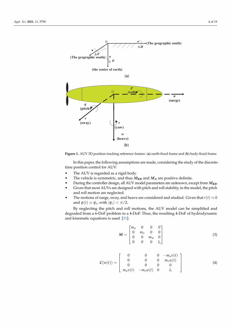
In this section, the design of the proposed discrete-time controller for AUV positionalcontrol in trajectory tracking noisy conditions is presented.

The control objective is to design a discrete-time control law, where the AUV canfollow the reference trajectory as the time increases. The schematic diagram of the proposedcontroller is shown in Figure 2. The symbols used throughout this paper are presentedin Table 1.

Linear discrete

time controllerKinematics

The modified algorithm

+

-Real system

+

+

Sensors

The proposed discrete-time controller

Measuremet

noise

vτ η

η(k)^

ηd(k) Zero-order

holder

τ(k) ηe(k) ( )

~ ηd

DynamicsProcess noise

Figure 2. Schematic diagram of the proposed discrete-time position control for trajectory tracking.

Appl. Sci. 2021, 11, 5790 6 of 19

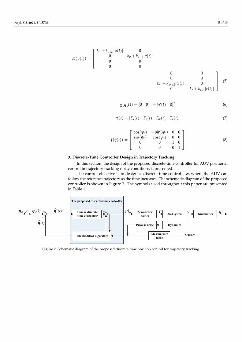
Table 1. The nomenclature.

Symbol Description Unit

T The sampling time sη(k) The real position at time kT mηr(k) The reference position at time kT m

η(k) The estimated position generated by proposedmodified algorithm at time kT m

ηe(k) The estimated position error at time kT,ηe(k) = ηr(k)− η(k) m

η(k) The position error at time kT,η(k) = ηr(k)− η(k) m

v(k) The real velocity at time kT m/svr(k) The reference velocity at time kT m/s

v(k) The estimated velocity generated by proposedmodified algorithm at time kT m/s

ve(k) The estimated velocity error at time kT,ve(k) = vr(k)− v(k) m/s

v(k) The velocity error at time kT,v(k) = vr(k)− v(k) m/s

3.1. Discrete-Time Control Law

For a continuous system, as a rule, there are two methods to design a discrete-timecontroller, either by discretizing an analog controller, or by building a discrete-time modelof a continuous system and subsequently deriving the discrete-time controller. The differencebetween these two methods is that the first one uses the derivative of the system state in thecontrol law. However, the system state is obtained through sensors that are affected by the noise,and thus, if the control law contains the derivative of the state of the system, it will increasethe influence of the noise factor. Therefore, the second method is adopted in this work.

Hence, Equation (1) can be rewritten as follows:

MRBv + MAv + C(v)v + D(v)v + g(η) = τ (9)

let f (t) = C(v)v + D(v)v + g(η), and one can obtain:

MRBv(t) + MAv(t) + f (t) = τ(t) (10)

In Equation (10), f (t) and MA are assumed to be unknown. In other words, onlythe parameter MRB is known.

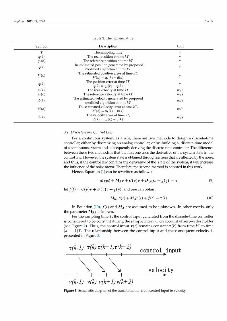
For the sampling time T, the control input generated from the discrete-time controlleris considered to be constant during the sample interval, on account of zero-order holder(see Figure 2). Thus, the control input τ(t) remains constant τ(k) from time kT to time(k + 1)T. The relationship between the control input and the consequent velocity ispresented in Figure 3.

Appl. Sci. 2021, 1, 0 6 of 21

Table 1. The nomenclature.

Symbol Description Unit

T The sampling time sη(k) The real position at time kT mηr(k) The reference position at time kT m

η(k) The estimated position generated by proposedmodified algorithm at time kT m

ηe(k) The estimated position error at time kT,ηe(k) = ηr(k)− η(k) m

η(k) The position error at time kT,η(k) = ηr(k)− η(k) m

v(k) The real velocity at time kT m/svr(k) The reference velocity at time kT m/s

v(k) The estimated velocity generated by proposedmodified algorithm at time kT m/s

ve(k) The estimated velocity error at time kT,ve(k) = vr(k)− v(k) m/s

v(k) The velocity error at time kT,v(k) = vr(k)− v(k) m/s

For a continuous system, as a rule, there are two methods to design a discrete-timecontroller, either by discretizing an analog controller, or by building a discrete-time modelof a continuous system and subsequently deriving the discrete-time controller. The differencebetween these two methods is that the first one uses the derivative of the system state in thecontrol law. However, the system state is obtained through sensors that are affected by the noise,and thus, if the control law contains the derivative of the state of the system, it will increasethe influence of the noise factor. Therefore, the second method is adopted in this work.

Hence, Equation (1) can be rewritten as follows:

MRBv + MAv + C(v)v + D(v)v + g(η) = τ (9)

let f (t) = C(v)v + D(v)v + g(η), and one can obtain:

MRBv(t) + MAv(t) + f (t) = τ(t) (10)

In Equation (10), f (t) and MA are assumed to be unknown. In other words, onlythe parameter MRB is known.

For the sampling time T, the control input generated from the discrete-time controlleris considered to be constant during the sample interval, on account of zero-order holder(see Figure 2). Thus, the control input τ(t) remains constant τ(k) from time kT to time(k + 1)T. The relationship between the control input and the consequent velocity ispresented in Figure 3.

τ(k-1) τ(k) τ(k+1) τ(k+2)

v(k-1) v(k) v(k+1)v(k+2)

Figure 3. Schematic diagram of the transformation from control input to velocity.Figure 3. Schematic diagram of the transformation from control input to velocity.

Appl. Sci. 2021, 11, 5790 7 of 19

By integrating Equation (10) concerning the time over the sample interval,

MRB(v(k + 1)− v(k)) + H(k) = Tτ(k) (11)

where

H(k) = MA(v(k + 1)− v(k)) +∫ kT+T

kTf (ξ)dξ (12)

with H(k) representing the entire uncertainty of the AUV hydrodynamics. Accordingto [17], Equation (11) is considered to be an accurate discrete-time model of the continuoussystem of Equation (10). From Equation (11), one can write the following:

v(k + 1) = M−1RB(Tτ(k)− H(k)) + v(k) (13)

The control law is given as follows:

τ(k) = T−1(MRB(u(k)− v(k)) + H(k)) (14)

where

u(k) = J−1(ηr(k + 1) + KPηe(k) + KD ˙ηe(k)) (15)

with KP and KD being the proportional gain matrix and the derivativegain matrix, respectively.

In Equation (14), H(k) denotes an estimate of H(k) by TDE. Hence, H(k) can beexpressed as follows:

H(k) = H(k− 1) (16)

From Equation (11), one can write the following:

H(k− 1) = Tτ(k− 1)−MRB(v(k)− v(k− 1))

= H(k) (17)

Because v(k) and v(k − 1) in Equation (17) are not available, they can be replacedby the estimate v(k) and v(k− 1). Finally, by substituting H(k) into Equation (14), the sum-mative control law is obtained:

τ(k) = T−1MRB(u(k)− 2v(k) + v(k− 1)) + τ(k− 1) (18)

3.2. Stability Analysis

By combining Equation (11) with Equation (14),

H(k)− H(k) = MRB(u(k)− v(k)− v(k + 1) + v(k)) (19)

u(k) is substituted into Equation (19) and one can obtain the following:

M−1RB(H(k)−H(k))=J−1(ηr(k+1)+KPηe(k)+KD ˙ηe(k))

− v(k + 1) + v(k)− v(k) (20)

One can write from Equation (2) the following:v(k + 1) = J−1η(k + 1)v(k) = J−1η(k)v(k) = J−1 ˙η(k)

(21)

Appl. Sci. 2021, 11, 5790 8 of 19

Combining Equation (20) with Equation (21) yields the following:

J−1(ηr(k+1)− η(k + 1)+KPηe(k)+KD ˙ηe(k))

=M−1RB(H(k)−H(k))+ J−1(η(k)− ˙η(k)) (22)

Let e(k) = η(k)− η(k). It is assumed that e(k) and e(k) are all bounded. One can writethe following:

ηe(k) = ηr(k)− η(k) = η(k)− e(k) (23)

From Equations (22) and (23) one can write the following:

J−1(˙η(k+1)+KP(η(k)− e(k))+KD( ˙η(k)− e(k)))

=M−1RB(H(k)−H(k))− J−1e(k) (24)

Equation (24) can be rewritten as follows:

˙η(k+1)+KPη(k)+KD ˙η(k) = JM−1RB(H(k)−H(k))

+ KPe(k) + KD e(k) + e(k) (25)

ε(k) is defined as follows:

ε(k) = M−1RB(H(k)− H(k)) (26)

Equation (26) shows that ε(k) can be considered to represent the approximate error inthe estimate H(k) by TDE.

Equation (25) can be simplified by using the forward difference approximation. Thesimplified equation becomes the following:

η(k+2) + (KD − I)η(k+1) + (KP − KD)η(k)

= −T Jε(t) + KPe(k) + (KD + I)e(k) (27)

If (−T Jε(k) + KPe(k) + (KD + I)e(k)) is bounded, then the Bounded Input BoundedOutput (BIBO) stability of the presented control law can be proved. Here, KPe(k) + (KD +I)e(k) is bounded and the boundedness of ε(k) will be shown as follows.

From Equations (11), (14) and (26) one can write the following:

ε(k) = v(k + 1)− u(k)− v(k) + v(k) (28)

let H1(k) =∫ kT+T

kT f (ξ)dξ and one can obtain:

H(k) = H1(k) + MA(v(k + 1)− v(k)) (29)

By using Equations (11) and (29) one can write the following:

M(v(k + 1)− v(k)) + H1(k) = Tτ(k) (30)

From Equation (28) one can write the following:

Mε(k) = Mv(k + 1)−Mu(k)−Mv(k) + Mv(k)

= Tτ(k)− H1(k)−Mu(k) + Mv(k) (31)

Substituting τ(k) into the above equation, we get the following:

Mε(k) =(MRB −M)u(k) + (M −MRB)v(k)

+ H(k)− H1(k) (32)

Appl. Sci. 2021, 11, 5790 9 of 19

Substituting H(k) into Equation (32), we get the following:

Mε(k) =(MRB −M)u(k) + (M −MRB)v(k)

+ Tτ(k− 1)−MRB(v(k)− v(k− 1))− H1(k) (33)

Using Equation (30) one can write the following:

Tτ(k− 1) = M(v(k)− v(k− 1)) + H1(k− 1) (34)

Substituting Equation (34) into Equation (33), we get the following:

Mε(k) =−MAu(k) + MAv(k)

+MA(v(k)− v(k− 1)) + H1(k− 1)− H1(k) (35)

From Equation (28), one can obtain the following:

v(k)− v(k− 1) = ε(k− 1) + u(k− 1)− v(k− 1) (36)

Substituting Equation (36) into Equation (35), we get the following:

ε(k) = Aε(k− 1) + B1 + B2 (37)

where

A = M−1MA (38)

B1 = M−1MA(u(k− 1)− u(k) + v(k)− v(k− 1)) (39)

B2 = M−1(H1(k− 1)− H1(k)) (40)

Here, B1 and B1 are considered to be the bounded disturbance. According to [17],it is already proven that the eigenvalues of A lie within the unit disc. Therefore, ε(k) isbounded and the BIBO stability of the presented control law is proved.

3.3. The Modified Algorithm Based on EnKF

This subsection introduces the proposed algorithm, relying on a modified EnKF,which involves a TDE scheme canceling the uncertain terms of the state space form. Itshould be noted that the proposed strategy combining the EnKF with TDE offers overallrobustness against large noise levels and great system parameter uncertainties. TDE is used,as it requires only the MRB parameter to be known. This is important, as the remainingparameters, such as C(v), D(v), and g(η), are usually unknown in practical applications;thus, exploiting TDE the proposed method affords broadening the uncertainty boundsof the involved parameters. The motivations for using the EnKF over the Extended KalmanFilter (EKF) counterpart are that the EnKF is a Kalman Filter variant appropriate for largescale-problems as the one investigated in this paper, and is more accurate and efficient thanEKF, even for relatively low ensembles, i.e., N > 50 [32–34].

According to the separation principle, the optimal control and state estimation prob-lems can be decoupled in some situations. Given that the process and the observationnoise are Gaussian, the optimal solution can be separated into a Kalman Filter and a linearquadratic regulator, known as linear–quadratic Gaussian control. In this work, EnKFis a linear variant of the Kalman Filter, and thus, TDE can be considered to be a linearestimation (or optimal control) [35]. Therefore, the separation principle is still availablefor the designed controller.

Appl. Sci. 2021, 11, 5790 10 of 19

Hence, for the proposed controller, the state space form becomes the following:

v(k)=v(k−1)+M−1RB(H(k−1)−H(k−1))−v(k−1)

+ J−1(ηr(k) + KPηe(k− 1) + KD ˙ηe(k− 1)) (41)

where H(k) contains all the uncertain terms. The process noise is not contained in Equation (41),and therefore, the uncorrelated process noise ς(k) and the measurement noise ζ(k) are addedinto the Equation (41):

v(k)=v(k−1)+M−1RB(H(k−1)−H(k−1))−v(k−1)

+ J−1(ηr(k) + KPηe(k− 1) + KD ˙ηe(k− 1))

+ ς(k− 1) (42)

The observation equation is as follows:

Z(k) = Hov(k) + ζ(k) (43)

where Ho is the observation operator. The ς(k) and ζ(k) are random Gaussian noise withmean 0. Their covariance matrix is Q and R, respectively.

The modified algorithm based on the EnKF [24] becomes the following:

1. Setting the initial estimated velocity v(0) = 0.2. By using the state space form, the N-ensemble for variable state is presented as

follows:

v−i (k)=v(k− 1)+(

M−1RB(H(k− 1)− H(k− 1))

)+J−1(ηr(k)+KPηe(k− 1)+KD ˙ηe(k− 1))

+ ςi(k− 1) (44)

where i counts from 1 to N, N is the number of variable state ensemble members, andςi(k) ∼ N(0, Q(k)) (i = 1, . . . , N) is the ensemble of the process noise.The uncertain terms H(k) can be eliminated by using TDE. When T is set small enoughclose to zero, H(k− 1)− H(k− 1) ≈ 0. Therefore, Equation (44) is simplified to thefollowing:

v−i (k) =v(k− 1)+ ςi(k− 1)

+J−1(ηr(k)+KPηe(k−1)+KD ˙ηe(k−1)) (45)

Let v−(k) = ∑Ni=1 v−i (k), which denotes the mean of v−i (k + 1). Then, the error

covariance is obtained as follows:

P−(k)=1

N − 1

N

∑i=1

(v−i (k)− v−(k))

× (v−i (k)− v−(k))T

3. The N-ensemble for measurement data is presented as follows:

Zi(k) = Hov(k) + ζ i(k) (46)

where ζ i(k) ∼ N(0, R(k)) (i = 1, . . . , N) is the measurement noise ensemble. TheKalman gain is set as follows:

Kg(k−1)=P−(k)HoT(

HoP−(k)HoT+R(k−1)

)−1

Appl. Sci. 2021, 11, 5790 11 of 19

and thus the estimation is expressed as follows:

vi(k) =v−i (k) + Kg(k− 1)(Zi(k)− Hov−i (k))

The mean of the estimation is the following:

v(k) =N

∑i=1

vi(k) (47)

4. The estimated velocity v(k) can be transformed into the estimated position η(k)by using the kinematics from Equation (21). Finally, the control input τ(k) is obtainedby substituting v(k) and η(k) .

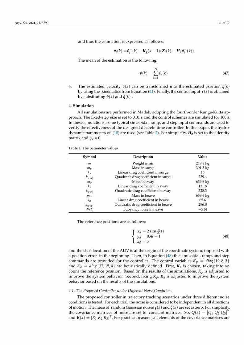
4. Simulation

All simulations are performed in Matlab, adopting the fourth-order Runge-Kutta ap-proach. The fixed-step size is set to 0.01 s and the control schemes are simulated for 100 s.In these simulations, some typical sinusoidal, ramp, and step input commands are used toverify the effectiveness of the designed discrete-time controller. In this paper, the hydro-dynamic parameters of [18] are used (see Table 2). For simplicity, Ho is set to the identitymatrix and ψc = 0.

Table 2. The parameter values.

Symbol Description Value

m Weight in air 219.8 kgmu Mass in surge 391.5 kgku Linear drag coefficient in surge 16

ku|u| Quadratic drag coefficient in surge 229.4mv Mass in sway 639.6 kgkv Linear drag coefficient in sway 131.8

kv|v| Quadratic drag coefficient in sway 328.3mw Mass in heave 639.6 kgkw Linear drag coefficient in heave 65.6

kw|w| Quadratic drag coefficient in heave 296.8W(t) Buoyancy force in heave −5 N

The reference positions are as follows:xd = 2 sin( π

20 t)yd = 0.4t + 1zd = 5

(48)

and the start location of the AUV is at the origin of the coordinate system, imposed witha position error in the beginning. Then, in Equation (48) the sinusoidal, ramp, and stepcommands are provided for the controller. The control variables Kp = diag{19, 8, 3}and Kd = diag{37, 15, 4} are heuristically defined. First, Kp is chosen, taking into ac-count the reference position. Based on the results of the simulations, Kp is adjusted toimprove the system behavior. Second, fixing Kp, Kd is adjusted to improve the systembehavior based on the results of the simulations.

4.1. The Proposed Controller under Different Noise Conditions

The proposed controller in trajectory tracking scenarios under three different noiseconditions is tested. For each trial, the noise is considered to be independent in all directionsof motion. The mean of random Gaussian noises ς(k) and ζ(k) are set as zero. For simplicity,the covariance matrices of noise are set to constant matrices. So, Q(k) = [Q1 Q2 Q3]

T

and R(k) = [R1 R2 R3]T . For practical reasons, all elements of the covariance matrices are

Appl. Sci. 2021, 11, 5790 12 of 19

assumed to be less than or equal to 1. For the sake of the trials, three cases are randomlygenerated as follows:

Case 1 : Q(k) =

0.160.040.09

R(k) =

0.640.04

1

Case 2 : Q(k) =

0.041

0.81

R(k) =

0.251

0.04

Case 3 : Q(k) =

0.010.360.49

R(k) =

0.091

0.81

Let the ensemble size N = 100 and the sampling time T = 0.01 s. The proposed

controller is tested for cases 1–3 as presented above. The reference positions and the actualtracked positions for cases 1–3 are presented in Figures 4–6. All figures highlight thatthe AUV effectively follows the desired positions with high precision in surge, sway, andheave. Hence, it is verified that the proposed controller is effective in position trackingfor AUV under various noise conditions.

Appl. Sci. 2021, 11, 5790 13 of 19Appl. Sci. 2021, 1, 0 13 of 21

−3

−2

−1

0

1

2

0

10

20

30

40

50

0

1

2

3

4

5

6

Start location

x(m)y(m)

z(m

)

Reference position

The proposed controller with N=100

(a)

0 20 40 60 80 100

−2−1

012

Time(s)

x(m

)

Reference positon in surgeThe proposed controller with N=100

0 20 40 60 80 1000

20

40

60

80

Time(s)

y(m

)

Reference positon in swayThe proposed controller with N=100

0 20 40 60 80 100−5

0

5

10

15

Time(s)

z(m

)

Reference positon in heaveThe proposed controller with N=100

(b)

Figure 4. AUV position tracking for noise case 1 (T = 0.01 s and N = 100): (a) 3D position trackingand (b) tracking in surge, sway, and heave.

Figure 4. AUV position tracking for noise case 3 (T = 0.01 s and N = 100): (a) 3D position trackingand (b) tracking in surge, sway, and heave.

4.2. The Proposed Controller Utilizing Different Sampling Times

It is well known that different sampling times have a great impact on the performanceof position tracking. For this trial, N is set to 100 and case 1 is chosen as the noise condition.Then, the proposed controller is tested for different sampling times T, i.e., 0.01 s, 0.02 s,0.05 s, and 0.1 s. Figure 5 presents the 3D position tracking for the corresponding samplingtime T. The latter figure highlights that the position tracking degrades as the sampling time

Appl. Sci. 2021, 11, 5790 14 of 19

increases. This happens not only because of the discrete-time controller, but also becauseof TDE. Accordingly, when the sampling time increases, H(k) is not approximately equalto H(k).

−4

−2

0

2

0

20

40

600

1

2

3

4

5

6

Start location

x(m)y(m)

z(m

)

Reference position

The proposed controller with T=0.01s

(a)

−2

0

2

4

0

20

40

600

1

2

3

4

5

6

x(m)

Start location

y(m)

z(m

)

Reference position

The proposed controller with T=0.02s

(b)

−5

0

5

0

20

40

600

2

4

6

8

Start location

x(m)y(m)

z(m

)

Reference position

The proposed controller with T=0.05s

(c)

−5

0

5

0

20

40

600

2

4

6

8

Start location

x(m)y(m)

z(m

)

Reference position

The proposed controller with T=0.1s

(d)

Figure 5. AUV 3D position tracking for noise case 1 under various sampling times (N = 100): (a) T = 0.01 s, (b) T = 0.02 s,(c) T = 0.05 s, and (d) T = 0.1 s.

4.3. The Proposed Controller Utilizing Different Ensembles

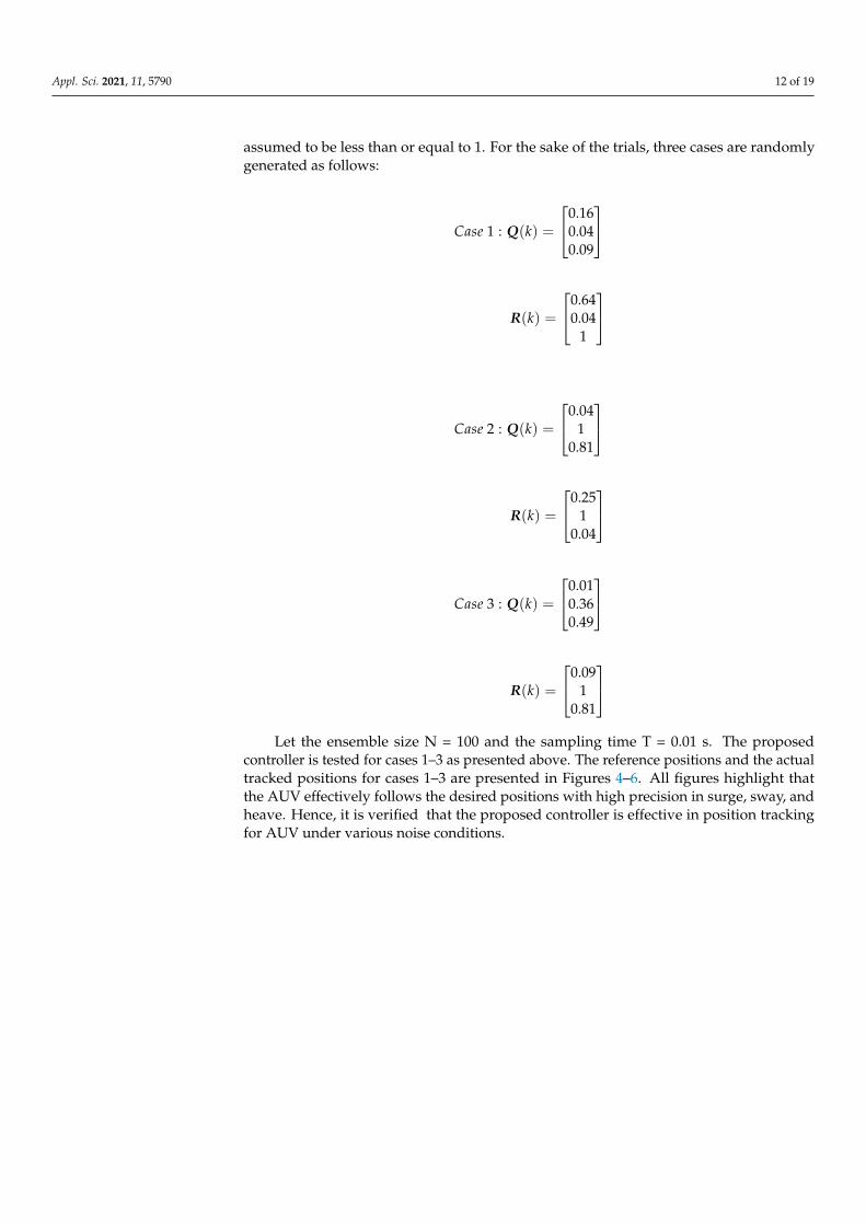
In this trial, T is set to 0.01s and the proposed method is tested for ensembles equalto 50, 100, and 200. Figure 6 presents the related results and demonstrates that in allcases, the AUV tracks the reference positions effectively. Additionally, this trial highlightsthe position tracking precision of the proposed technique in terms of root-mean-square

Appl. Sci. 2021, 11, 5790 15 of 19

(RMS) errors of the AUV position at a steady state. The corresponding results over the threenoise cases examined and for all ensembles are presented in Table 3. From the latter table,it can be concluded that there is no mathematical relationship between the RMS errors andensemble size, and that a larger ensemble size increases the computational requirements.Table 4 shows the computational time under different noise conditions for ensemblesequal to 50, 100, and 200. The computational time increases with the ensemble size. Thus,choosing a small ensemble size affords saving the AUV’s energy that, in any case, is limited.

−5

0

5

0

20

40

600

2

4

6

Start location

x(m)y(m)

z(m

)

Reference position

The proposed controller with N=50

The proposed controller with N=100

The proposed controller with N=200

(a)

−5

0

5

0

50

1000

2

4

6

Start location

x(m)y(m)

z(m

)

Reference position

The proposed controller with N=50

The proposed controller with N=100

The proposed controller with N=200

(b)

−5

0

5

0

50

0

2

4

6

Start location

x(m)y(m)

z(m

)

Reference position

The proposed controller with N=50

The proposed controller with N=100

The proposed controller with N=200

(c)

Figure 6. AUV 3D position tracking under various ensemble (N) sizes and noise levels (T = 0.01 s):(a) noise case 1, (b) noise case 2, and (c) noise case 3.

Table 3. RMS errors (m) at steady state, using the proposed controller under various ensemble sizes (T = 0.01 s).

Ensemble (N)Case 1 Case 2 Case 3

RMS(ex) RMS(ey) RMS(ez) RMS(ex) RMS(ey) RMS(ez) RMS(ex) RMS(ey) RMS(ez)

50 0.0522 0.0990 0.0443 0.0488 0.0931 0.0497 0.0323 0.0831 0.0443100 0.0477 0.0919 0.0442 0.0546 0.0902 0.0442 0.0238 0.0713 0.0443200 0.0873 0.0996 0.0441 0.0698 0.0926 0.0442 0.0300 0.0764 0.0441

Table 4. Computational time of the proposed modified EnKF algorithm (T = 0.01 s).

Ensemble (N)Time (s)

Case 1 Case 2 Case 3

50 3.73 3.84 3.71100 4.31 4.40 4.28200 5.48 5.52 5.42

4.4. Evaluating Current Controllers under Various Noise Conditions

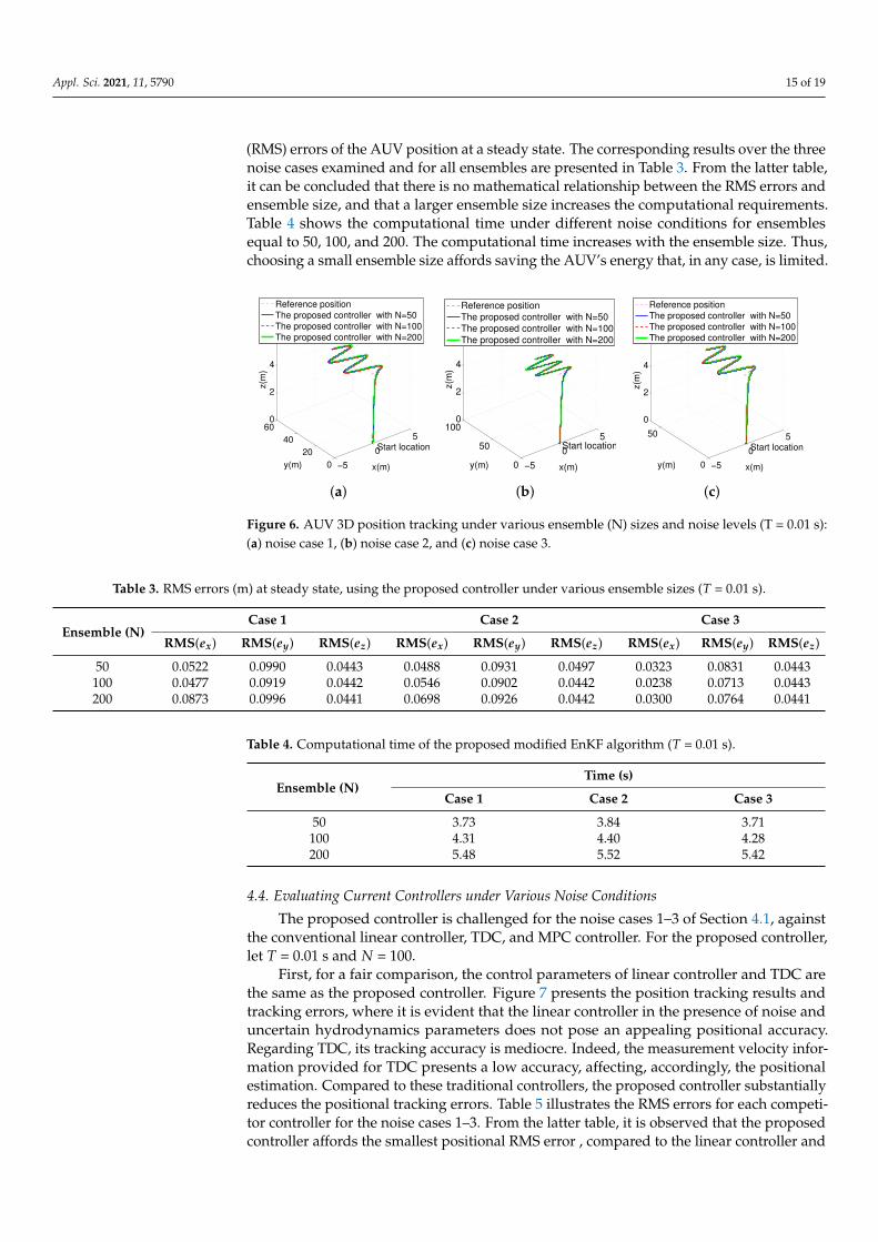
The proposed controller is challenged for the noise cases 1–3 of Section 4.1, againstthe conventional linear controller, TDC, and MPC controller. For the proposed controller,let T = 0.01 s and N = 100.

First, for a fair comparison, the control parameters of linear controller and TDC arethe same as the proposed controller. Figure 7 presents the position tracking results andtracking errors, where it is evident that the linear controller in the presence of noise anduncertain hydrodynamics parameters does not pose an appealing positional accuracy.Regarding TDC, its tracking accuracy is mediocre. Indeed, the measurement velocity infor-mation provided for TDC presents a low accuracy, affecting, accordingly, the positionalestimation. Compared to these traditional controllers, the proposed controller substantiallyreduces the positional tracking errors. Table 5 illustrates the RMS errors for each competi-tor controller for the noise cases 1–3. From the latter table, it is observed that the proposedcontroller affords the smallest positional RMS error , compared to the linear controller and

Appl. Sci. 2021, 11, 5790 16 of 19

TDC. In particular, the linear controller performs poorly, while the proposed controlleroutperforms the conventional TDC in RMS error by a percentage range of approximately72.1–97.4%.

−50

5

0

500

5

10

15

x(m)

Start location

y(m)

z(m

)

Reference position

The proposed controller with N=100

TDC

linear controller

0 20 40 60 80 100−2−1

012

Time(s)

xe(m

)

0 20 40 60 80 100−18−13

−8−3

2

Time(s)

ye(m

)

0 20 40 60 80 100−10

−505

Time(s)

ze(m

)

(a)

−50

5

0

500

5

10

15

x(m)

Start location

y(m)

z(m

)

Reference position

The proposed controller with N=100

TDC

linear controller

0 20 40 60 80 100−2−1

012

Time(s)

xe(m

)

0 20 40 60 80 100−18−13

−8−3

2

Time(s)

ye(m

)

0 20 40 60 80 100−10

−505

Time(s)

ze(m

)

(b)

−50

5

0

500

5

10

15

x(m)

Start location

y(m)

z(m

)

Reference position

The proposed controller with N=100

TDC

linear controller

0 20 40 60 80 100−2−1

012

Time(s)

xe(m

)

0 20 40 60 80 100−18−13

−8−3

2

Times(s)

ye(m

)0 20 40 60 80 100

−10−5

05

Time(s)z

e(m

)

(c)

Figure 7. AUV 3D position tracking and tracking errors for various controllers under different noise conditions (T = 0.01 s):(a) noise case 1, (b) noise case 2, and (c) noise case 3.

Table 5. RMS errors (m) for various controllers.

ControllerCase 1 Case 2 Case 3

RMS(ex) RMS(ey) RMS(ez) RMS(ex) RMS(ey) RMS(ez) RMS(ex) RMS(ey) RMS(ez)

Linear controller 1.0787 9.1009 \ 1.0828 9.2346 \ 1.0765 9.1327 \TDC 0.1902 1.1115 0.8273 0.1958 1.2472 0.8433 0.0329 2.7515 0.8618

The proposed controllerwith N = 100 (T = 0.01 s) 0.0477 0.0919 0.0442 0.0546 0.0902 0.0442 0.0238 0.0713 0.0443

Then, the proposed controller is compared against an advanced control strategy, i.e.,MPC. Running a MPC solver in MATLAB is a huge computational burden for computer,and thus MPC is simulated only for 80 s. Given that the proposed MPC for AUV for trajec-tory tracking in [26] applies to this work, this method is compared against the proposedone. Table 6 presents the MPC parameters. The type of MPC algorithm is State FeedbackPredictive Control (SFPC), and the cost function is defined as follows:

J(k) = ‖Y(k)−Yd(k)‖2Qc

+ ‖4U(k)‖2Rc

where ‖x‖2A = xT Ax; Y(k) and Yd(k) denote the predicted position and the desired position,

respectively. 4U(k) is the control input increment.Figure 8 presents the 3D position tracking results under various noise conditions,

and Table 7 illustrates the RMS errors at a steady state for the MPC controller and theproposed controller. It indicates that the MPC controller and the proposed controller bothprecisely track the truth positions. Given that the suggested method meets the requirementof high tracking accuracy, the performance of the calculation time is examined, in particular.Table 8 presents the average calculation time of the MPC controller and that of the proposed

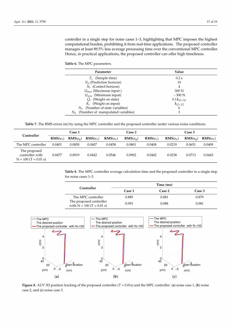
Appl. Sci. 2021, 11, 5790 17 of 19

controller in a single step for noise cases 1–3, highlighting that MPC imposes the highestcomputational burden, prohibiting it from real-time applications. The proposed controllermanages at least 89.5% less average processing time over the conventional MPC controller.Hence, in practical applications, the proposed controller can offer high timeliness.

Table 6. The MPC parameters.

Parameter Value

Ts (Sample time) 0.2 sNp (Prediction horizon) 10

Nc (Control horizon) 4Umax (Maximum input ) 300 NUmin (Minimum input) −300 N

Qc (Weight on state) 0.1I10×10Rc (Weight on input) I12×12

Nx (Number of state variables) 6Nu (Number of manipulated variables) 3

Table 7. The RMS errors (m) by using the MPC controller and the proposed controller under various noise conditions.

ControllerCase 1 Case 2 Case 3

RMS(ex) RMS(ey) RMS(ez) RMS(ex) RMS(ey) RMS(ez) RMS(ex) RMS(ey) RMS(ez)

The MPC controller 0.0401 0.0850 0.0407 0.0458 0.0801 0.0408 0.0219 0.0651 0.0409

The proposedcontroller with

N = 100 (T = 0.01 s)0.0477 0.0919 0.0442 0.0546 0.0902 0.0442 0.0238 0.0713 0.0443

Table 8. The MPC controller average calculation time and the proposed controller in a single stepfor noise cases 1–3.

ControllerTime (ms)

Case 1 Case 2 Case 3

The MPC controller 0.889 0.881 0.879The proposed controllerwith N = 100 (T = 0.01 s) 0.093 0.088 0.081

−50

5

0

20

400

2

4

6

x(m)

Start location

y(m)

z(m

)

The MPC

The desired position

The proposed controller with N=100

(a)

−50

5

0

20

400

2

4

6

x(m)

Start location

y(m)

z(m

)

The MPC

The desired position

The proposed controller with N=100

(b)

−50

5

0

20

400

2

4

6

x(m)

Start location

y(m)

z(m

)

The MPC

The desired position

The proposed controller with N=100

(c)

Figure 8. AUV 3D position tracking of the proposed controller (T = 0.01s) and the MPC controller: (a) noise case 1, (b) noisecase 2, and (c) noise case 3.

Appl. Sci. 2021, 11, 5790 18 of 19

Finally, it is worth noting that the proposed controller is tested only against open-source controllers, namely the conventional linear controller, TDC, and MPC controller,because re-implementing current controllers might lead to a non-optimized solution thatinevitably would underestimate the capabilities of the original method.

5. Conclusions

In this paper, a discrete-time position controller that is suitable for AUVs is devel-oped. The proposed method considers noise and uncertain hydrodynamic parameters and,additionally, all the system parameters to be unknown, except from the rigid body iner-tia matrix, which is the norm for practical applications. The suggested technique modifiesthe Ensemble Kalman Filter accordingly to afford accurate positional estimation of an AUVunder noisy conditions and major system uncertainties. The contribution of this paper isessential, as, compared to the traditional Ensemble Kalman Filter algorithm, the proposedone is more robust and effective for AUVs.

The effectiveness of the proposed modified Ensemble Kalman Filter method on quitea few simulated scenarios involving various nuisances and parameter setups is demon-strated. Indeed, the results of simulations highlight that the proposed discrete-timecontroller achieves the precise positional control for an AUV in the presence of both noiseand uncertain hydrodynamics. By comparing the root-mean-square errors of the pro-posed controller against the conventional linear controller and time-delay controller, it canbe found that the proposed discrete-time controller affords the most accurate positionaltracking. In particular, the proposed controller outperforms the conventional time-delaycontroller in root-mean-square error by a percentage range of approximately 72.1–97.4%.Moreover, compared to the model predictive control, the proposed controller takes atleast 89.5% less average calculation time. Thus, the proposed controller has the advan-tages of high tracking accuracy and high timeliness. Future research shall investigatethe effectiveness of the proposed controller under rapidly changing system disturbances.

Author Contributions: Conceptualization, Q.L. and M.L.; Methodology, Q.L.; Software, Q.L.; Writ-ing–original draft, Q.L.; Writing—review and editing, M.L. Both authors have read and agreed to thepublished version of the manuscript.

Funding: This research received no external funding.

Institutional Review Board Statement: Not applicable.

Informed Consent Statement: Not applicable.

Data Availability Statement: The data presented in this study are available on request from thecorresponding author. The data are not publicly available due to privacy constraints..

Conflicts of Interest: The authors declare no conflict of interest.

References1. Cui, R.; Ge, S.S.; How, B.V.E.; Choo, Y.S. Leader–follower formation control of underactuated autonomous underwater vehicles.

Ocean Eng. 2010, 37, 1491–1502. [CrossRef]2. Wang, T.; Zhao, Q.; Yang, C. Visual navigation and docking for a planar type AUV docking and charging system. Ocean Eng.

2021, 224, 108744. [CrossRef]3. Borlaug, I.L.G.; Pettersen, K.Y.; Gravdahl, J.T. Comparison of two second-order sliding mode control algorithms for an articulated

intervention AUV: Theory and experimental results. Ocean Eng. 2021, 222, 108480. [CrossRef]4. Ma, X.; Yanli, C.; Bai, G.; Liu, J. Multi-AUV Collaborative Operation Based on Time-Varying Navigation Map and Dynamic Grid

Model. IEEE Access 2020, 8, 159424–159439. [CrossRef]5. Liu, F.; Shen, Y.; He, B.; Wan, J.; Wang, D.; Yin, Q.; Qin, P. 3DOF Adaptive Line-Of-Sight Based Proportional Guidance Law

for Path Following of AUV in the Presence of Ocean Currents. Appl. Sci. 2019, 9, 3518. [CrossRef]6. Paull, L.; Saeedi, S.; Seto, M.; Li, H. AUV navigation and localization: A review. IEEE J. Ocean. Eng. 2013, 39, 131–149. [CrossRef]7. Jalving, B. The NDRE-AUV flight control system. IEEE J. Ocean. Eng. 1994, 19, 497–501. [CrossRef]8. Guerrero, J.; Torres, J.; Creuze, V.; Chemori, A.; Campos, E. Saturation based nonlinear PID control for underwater vehicles:

Design, stability analysis and experiments. Mechatronics 2019, 61, 96–105. [CrossRef]

Appl. Sci. 2021, 11, 5790 19 of 19

9. Li, J.H.; Lee, P.M. Design of an adaptive nonlinear controller for depth control of an autonomous underwater vehicle. Ocean Eng.2005, 32, 2165–2181. [CrossRef]

10. Joe, H.; Kim, M.; Yu, S.C. Second-order sliding-mode controller for autonomous underwater vehicle in the presence of unknowndisturbances. Nonlinear Dyn. 2014, 78, 183–196. [CrossRef]

11. Kim, M.; Joe, H.; Kim, J.; Yu, S.C. Integral sliding mode controller for precise manoeuvring of autonomous underwater vehiclein the presence of unknown environmental disturbances. Int. J. Control 2015, 88, 2055–2065. [CrossRef]

12. Yan, Z.; Wang, M.; Xu, J. Robust adaptive sliding mode control of underactuated autonomous underwater vehicles with uncertaindynamics. Ocean Eng. 2019, 173, 802–809. [CrossRef]

13. Xiang, X.; Yu, C.; Zhang, Q. Robust fuzzy 3D path following for autonomous underwater vehicle subject to uncertainties.Comput. Oper. Res. 2017, 84, 165–177. [CrossRef]

14. Lee, K.W.; Singh, S.N. Multi-input submarine control via L1 adaptive feedback despite uncertainties. J. Syst. Control Eng. 2014,228, 330–347.

15. Londhe, P.; Patre, B. Adaptive fuzzy sliding mode control for robust trajectory tracking control of an autonomous underwatervehicle. Intell. Serv. Robot. 2019, 12, 87–102. [CrossRef]

16. Kumar, R.P.; Dasgupta, A.; Kumar, C. Robust trajectory control of underwater vehicles using time delay control law. Ocean Eng.2007, 34, 842–849. [CrossRef]

17. Kumar, R.P.; Kumar, C.; Sen, D.; Dasgupta, A. Discrete time-delay control of an autonomous underwater vehicle: Theory andexperimental results. Ocean Eng. 2009, 36, 74–81. [CrossRef]

18. Kim, J.; Joe, H.; Yu, S.c.; Lee, J.S.; Kim, M. Time-delay controller design for position control of autonomous underwater vehicleunder disturbances. IEEE Trans. Ind. Electron. 2016, 63, 1052–1061. [CrossRef]

19. Hsia, T.C.; Gao, L. Robot manipulator control using decentralized linear time-invariant time-delayed joint controllers. In Proceed-ings of the IEEE International Conference on Robotics and Automation, Cincinnati, OH, USA, 13–18 May 1990; pp. 2070–2075.

20. Youcef-Toumi, K.; Ito, O. A time delay controller for systems with unknown dynamics. In Proceedings of the 1988 AmericanControl Conference, Atlanta, GA, USA, 15–17 June 1988; pp. 904–913.

21. Xu, C.; Xu, C.; Wu, C.; Qu, D.; Liu, J.; Wang, Y.; Shao, G. A novel self-adapting filter based navigation algorithm for autonomousunderwater vehicles. Ocean Eng. 2019, 187, 106146. [CrossRef]

22. Wu, Y.; Ta, X.; Xiao, R.; Wei, Y.; An, D.; Li, D. Survey of underwater robot positioning navigation. Appl. Ocean Res. 2019,90, 101845. [CrossRef]

23. Ermayanti, Z.; Apriliani, E.; Nurhadi, H.; Herlambang, T. Estimate and control position autonomous underwater vehicle based ondetermined trajectory using fuzzy Kalman filter method. In Proceedings of the IEEE 2015 International Conference on AdvancedMechatronics, Intelligent Manufacture, and Industrial Automation (ICAMIMIA), Surabaya, Indonesia, 15–17 October 2015;pp. 156–161.

24. Apriliani, E.; Nurhadi, H. Ensemble and Fuzzy Kalman Filter for position estimation of an autonomous underwater vehiclebased on dynamical system of AUV motion. Expert Syst. Appl. 2017, 68, 29–35.

25. Fan, S.; Li, B.; Xu, W.; Xu, Y. Impact of current disturbances on AUV docking: Model-based motion prediction and counteringapproaches. IEEE J. Ocean. Eng. 2017, 43, 888–904. [CrossRef]

26. Yan, Z.; Gong, P.; Zhang, W.; Wu, W. Model predictive control of autonomous underwater vehicles for trajectory tracking withexternal disturbances. Ocean Eng. 2020, 217, 107884. [CrossRef]

27. Yang, Z.; Sun, Z.; Piao, H.; Zhao, Y.; Zhou, D.; Kong, W.; Zhang, K. An Autonomous Attack Guidance Method with High AimingPrecision for UCAV Based on Adaptive Fuzzy Control under Model Predictive Control Framework. Appl. Sci. 2020, 10, 5677.[CrossRef]

28. Sands, T. Development of Deterministic Artificial Intelligence for Unmanned Underwater Vehicles (UUV). J. Mar. Sci. Eng.2020, 8, 578. [CrossRef]

29. Shah, R.; Sands, T. Comparing Methods of DC Motor Control for UUVs. Appl. Sci. 2021, 11, 4972. [CrossRef]30. Fossen, T.I. Guidance and Control of Ocean Vehicles; John Wiley & Sons Inc: Hoboken, NJ, USA, 1994.31. Caccia, M.; Veruggio, G. Guidance and control of a reconfigurable unmanned underwater vehicle. Control Eng. Pract. 2000, 8,

21–37. [CrossRef]32. Hommels, A.; Murakami, A.; Nishimura, S.I. A comparison of the ensemble Kalman filter with the unscented Kalman filter:

application to the construction of a road embankment. Geotechniek 2009, 13, 52.33. Kondo, K.; Tanaka, H. Comparison of the extended Kalman filter and the ensemble Kalman filter using the barotropic general

circulation model. J. Meteorol. Soc. Jpn. Ser. II 2009, 87, 347–359. [CrossRef]34. Reichle, R.H.; Walker, J.P.; Koster, R.D.; Houser, P.R. Extended versus ensemble Kalman filtering for land data assimilation.

J. Hydrometeorol. 2002, 3, 728–740. [CrossRef]35. Song, X.; Yan, X.; Li, X. Survey of duality between linear quadratic regulation and linear estimation problems for discrete-time

systems. Adv. Differ. Equat. 2019, 2019, 1–19. [CrossRef]