An Experimental Evaluation of Various Sampling Path Strategies for an Autonomous Underwater Vehicle

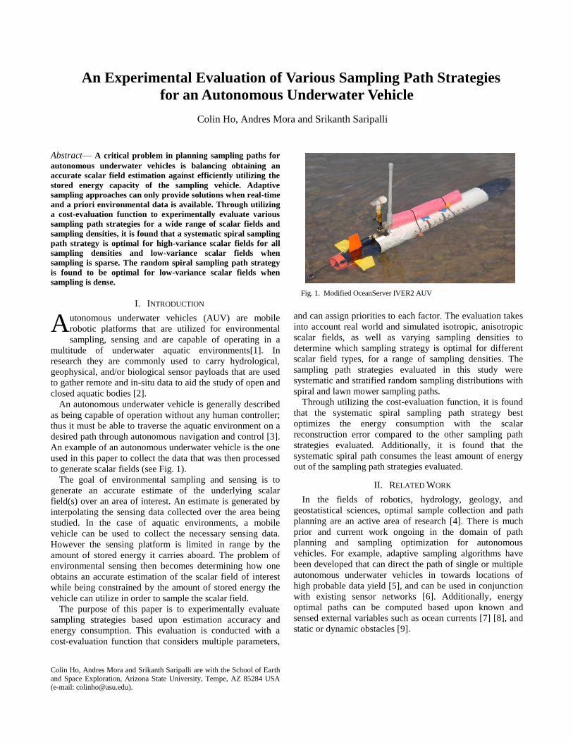
Fig. 1. Modified OceanServer IVER2 AUV

Abstract— A critical problem in planning sampling paths for

autonomous underwater vehicles is balancing obtaining an

accurate scalar field estimation against efficiently utilizing the

stored energy capacity of the sampling vehicle. Adaptive

sampling approaches can only provide solutions when real-time

and a priori environmental data is available. Through utilizing

a cost-evaluation function to experimentally evaluate various

sampling path strategies for a wide range of scalar fields and

sampling densities, it is found that a systematic spiral sampling

path strategy is optimal for high-variance scalar fields for all

sampling densities and low-variance scalar fields when

sampling is sparse. The random spiral sampling path strategy

is found to be optimal for low-variance scalar fields when

sampling is dense.

I. INTRODUCTION

utonomous underwater vehicles (AUV) are mobile

robotic platforms that are utilized for environmental

sampling, sensing and are capable of operating in a

multitude of underwater aquatic environments[1]. In

research they are commonly used to carry hydrological,

geophysical, and/or biological sensor payloads that are used

to gather remote and in-situ data to aid the study of open and

closed aquatic bodies [2].

An autonomous underwater vehicle is generally described

as being capable of operation without any human controller;

thus it must be able to traverse the aquatic environment on a

desired path through autonomous navigation and control [3].

An example of an autonomous underwater vehicle is the one

used in this paper to collect the data that was then processed

to generate scalar fields (see Fig. 1).

The goal of environmental sampling and sensing is to

generate an accurate estimate of the underlying scalar

field(s) over an area of interest. An estimate is generated by

interpolating the sensing data collected over the area being

studied. In the case of aquatic environments, a mobile

vehicle can be used to collect the necessary sensing data.

However the sensing platform is limited in range by the

amount of stored energy it carries aboard. The problem of

environmental sensing then becomes determining how one

obtains an accurate estimation of the scalar field of interest

while being constrained by the amount of stored energy the

vehicle can utilize in order to sample the scalar field.

The purpose of this paper is to experimentally evaluate

sampling strategies based upon estimation accuracy and

energy consumption. This evaluation is conducted with a

cost-evaluation function that considers multiple parameters,

Colin Ho, Andres Mora and Srikanth Saripalli are with the School of Earth

and Space Exploration, Arizona State University, Tempe, AZ 85284 USA (e-mail: [email protected]).

and can assign priorities to each factor. The evaluation takes

into account real world and simulated isotropic, anisotropic

scalar fields, as well as varying sampling densities to

determine which sampling strategy is optimal for different

scalar field types, for a range of sampling densities. The

sampling path strategies evaluated in this study were

systematic and stratified random sampling distributions with

spiral and lawn mower sampling paths.

Through utilizing the cost-evaluation function, it is found

that the systematic spiral sampling path strategy best

optimizes the energy consumption with the scalar

reconstruction error compared to the other sampling path

strategies evaluated. Additionally, it is found that the

systematic spiral path consumes the least amount of energy

out of the sampling path strategies evaluated.

II. RELATED WORK

In the fields of robotics, hydrology, geology, and

geostatistical sciences, optimal sample collection and path

planning are an active area of research [4]. There is much

prior and current work ongoing in the domain of path

planning and sampling optimization for autonomous

vehicles. For example, adaptive sampling algorithms have

been developed that can direct the path of single or multiple

autonomous underwater vehicles in towards locations of

high probable data yield [5], and can be used in conjunction

with existing sensor networks [6]. Additionally, energy

optimal paths can be computed based upon known and

sensed external variables such as ocean currents [7] [8], and

static or dynamic obstacles [9].

An Experimental Evaluation of Various Sampling Path Strategies

for an Autonomous Underwater Vehicle

Colin Ho, Andres Mora and Srikanth Saripalli

A

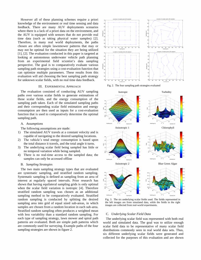
Fig. 2. The four sampling path strategies evaluated

30 35 40 45 50 55 60 65 70 75 8030

35

40

45

50

55

60

65

70Locations of sample points (30 samples)

Easting [m]

Nort

hin

g [

m]

30 35 40 45 50 55 60 65 70 75 8030

35

40

45

50

55

60

65


Easting [m]

Nort

hin

g [

m]

30 35 40 45 50 55 60 65 70 75 8030

35

40

45

50

55

60

65


Easting [m]

Nort

hin

g [

m]

30 35 40 45 50 55 60 65 70 75 8030

35

40

45

50

55

60

65


Easting [m]

Nort

hin

g [

m]

Isotropic Turbidity

Anisotropic 1 Chlorophyll

Anisotropic 2 Blue Green Algae

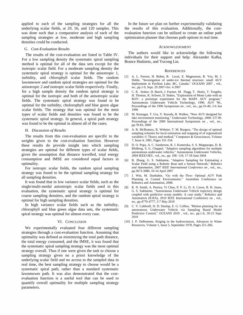
Fig. 3. The six underlying scalar fields used. The fields represented in the left images are from simulated data, while the fields in the right images are collected from real-world experiments.

0

20

40

60

0

20

40

6020

22

24

26

28

30

Easting (m)

Isotropic simulated field

Northing (m)

Units

21

22

23

24

25

26

27

28

29

30

0

20

40

60

0

20

40

60-1

0

1

2

3

4

Easting (m)

True simulated field

Northing (m)

Units

0

0.5

1

1.5

2

2.5

3

0

20

40

60

0

20

40

6020

22

24

26

28

Easting (m)

Anisotropic 1 simulated field

Northing (m)

Units

21

22

23

24

25

26

27

0

20

40

60

0

20

40

60-1

-0.5

0

0.5

1

1.5

Easting (m)Northing (m)

Units

-0.6

-0.4

-0.2

0

0.2

0.4

0.6

0.8

1

0

20

40

60

0

20

40

6050

52

54

56

58

60

Easting (m)

Anisotropic 2 simulated field

Northing (m)

Units

52

53

54

55

56

57

58

59

0

20

40

60

0

20

40

6030.6

30.8

31

31.2

31.4

31.6

Easting (m)Northing (m)

Units

30.7

30.8

30.9

31

31.1

31.2

31.3

31.4

31.5

However all of these planning schemes require a priori

knowledge of the environment or real time sensing and data

feedback. There are many AUV deployments scenarios

where there is a lack of a priori data on the environment, and

the AUV is equipped with sensors that do not provide real

time data (such as taking physical water samples) [2].

Therefore, in many real world deployments, the paths

chosen are often simple lawnmower patterns that may or

may not be optimal for the situation they are being utilized

[1], [2]. The evaluation conducted in this paper is targeted at

looking at autonomous underwater vehicle path planning

from an experimental field scientist’s data sampling

perspective. The goal is to comparatively evaluate various

sampling path strategies using a cost-evaluation function that

can optimize multiple parameters. These results from this

evaluation will aid choosing the best sampling path strategy

for unknown scalar fields, with no real time data feedback.

III. EXPERIMENTAL APPROACH

The evaluation consisted of conducting AUV sampling

paths over various scalar fields to generate estimations of

those scalar fields, and the energy consumption of the

sampling path taken. Each of the simulated sampling paths

and their corresponding scalar field estimation and energy

consumption are then used as inputs for a cost-evaluation

function that is used to comparatively determine the optimal

sampling path.

A. Assumptions

The following assumptions are made:

1) The simulated AUV travels at a constant velocity and is

capable of navigating to the desired sampling locations.

2) The vehicle’s total energy consumption is based upon

the total distance it travels, and the total angle it turns.

3) The underlying scalar field being sampled has little or

no temporal variation while being sampled.

4) There is no real-time access to the sampled data; the

samples can only be accessed offline

B. Sampling Strategies

The two main sampling strategy types that are evaluated

are systematic sampling, and stratified random sampling.

Systematic sampling is defined as sampling from an area of

interest at regularly spaced intervals. Prior research has

shown that having equilateral sampling grids is only optimal

when the scalar field variation is isotropic [4]. Therefore

stratified random sampling was chosen as an additional

sampling method to be comparatively evaluated. Stratified

random sampling is conducted by splitting the desired

sampling area into grid of equal sized sub-areas, in which

samples are chosen from a random location in each sub-area.

Stratified random sampling often produces a weighted mean

with less variability than a standard random sampling. For

each type of sampling strategy, lawn mower and spiral path

patterns are evaluated. Both are simple path patterns which

are commonly used for surveying. Example paths of the four

sampling strategies are shown in figure 2.

C. Underlying Scalar Field Data

The underlying scalar field was represented with both real

world and simulated data. The goal was to utilize enough

scalar field data to be representative of many scalar field

distributions commonly seen in real world data sets. Thus,

six different underlying scalar fields were generated and

collected for the purposes of this evaluation and are shown

in Fig. 3. The data sets derived from real world data

consisted of a turbidity data set representing multi-modal

data, a chlorophyll data set representing high anisotropy and

variance, and a blue green algae cell count data set

representing moderate anisotropy data with a high degree of

spatial variance. The first simulated data set was a linearly

varying distribution representing isotropic data. The second

simulated data set was a normal distribution that represented

moderately anisotropic data. The third and final simulated

data set was a bi-modal normal distribution that represented

moderate-variance anisotropic data.

IV. EVALUATION METHODS

A. Estimation Evaluation

Once a sampling path has been generated, it is then used

to sample the underlying scalar field. With those samples, an

estimation of the underlying scalar field is generated through

ordinary Kriging. Kriging is a form of linear least squares

estimation that interpolates the value of a location upon a

scalar field from known values at nearby locations, which in

this case are the sampled locations [10].Ordinary Kriging is

a specific type of Kriging that assumes that the experimental

variogram can be constructed, and that the mean of the

scalar field being estimated is unknown but constant. Z

represents the underlying scalar field, thus the Kriging

estimation of the scalar field at any location is the weighted

average of observed values. This is represented through the

following equation.

. (1)

The estimation variance of z(xo) is given by

(2)

where is the variogram of xi and x0. The weights

wi(x) are chosen such that they fulfill the unbiasedness

condition (they all sum to 1), and also minimize the

estimation variance. Thus, the weights are determined

through the equation

(3)

where is the Lagrance parameter associated with the

minimization.

Once the Kriging estimation was generated, it accuracy is

evaluated through the computation of its integrated mean

square error (IMSE) with respect to the underlying scalar

field.

B. Energy Consumption Evaluation

The energy consumed by the vehicle travelling along the

sampling path was computed through the use of a simple

energy consumption model. The model has two input

parameters; the distance travelled, and the total angle turned.

Since it is assumed that the vehicle is travelling straight at a

constant velocity, it is extrapolated that the vehicle

consumes its stored energy at a constant rate. An

autonomous underwater vehicle may also experience in

increase in energy consumption while turning. This

additional increase may be nominal or significant, depending

on the design of the vehicle. Therefore the model takes the

additional energy consumption while turning into

consideration through the use of a constant multiplier for the

total turn angle. The energy consumption equation is

modeled through the following equation.

(4)

For this equation, d and θ respectively represent the total

distance of the sampling path, and the cumulative turn angle.

The constant kθ is a constant multiplier that represents the

increase in energy consumption while turning for a vehicle.

This weight is better understood through the following

relation.

. (5)

This relation defined as such; for each right angle turn

taken, an additional energy penalty of travelling a straight

distance dt is added.

C. Cost-Evaluation Function

The cost-evaluation function is a general evaluation

method that allows for quantitative comparative analysis for

multiple input parameters. It normalizes and then assigns

each input parameter a weight, allowing for the function to

prioritize each parameter in respect to one another. These

weights must all sum to one. In the case of this evaluation,

we are investigating which sampling strategy is optimal for

both estimation error and energy consumption. Therefore the

parameters that were selected to be inputs for the cost-

evaluation function were the total distance travelled d, the

total energy consumed E, and the IMSE for the specific

sampling path taken ε. Our proposed cost-evaluation

function is as follows,

(6)

where Wd, WE, and Wε, are the weighted factors that

provide specific priorities between the total distance

travelled, the total energy consumed, and the IMSE for the

sampling path taken. , , and are normalization

factors assigned constant values to normalize each of their

corresponding parameters and eliminate their dimensions.

V. EXPERIMENTAL RESULTS AND DISCUSSION

A. Underlying Scalar Field Data Generation

The six different scalar fields used in this evaluation were

either generated from simulated equations, or from a real

world dataset. The isotropic scalar field used for this

evaluation was generated by the following equation.

(7)

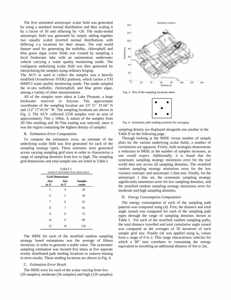
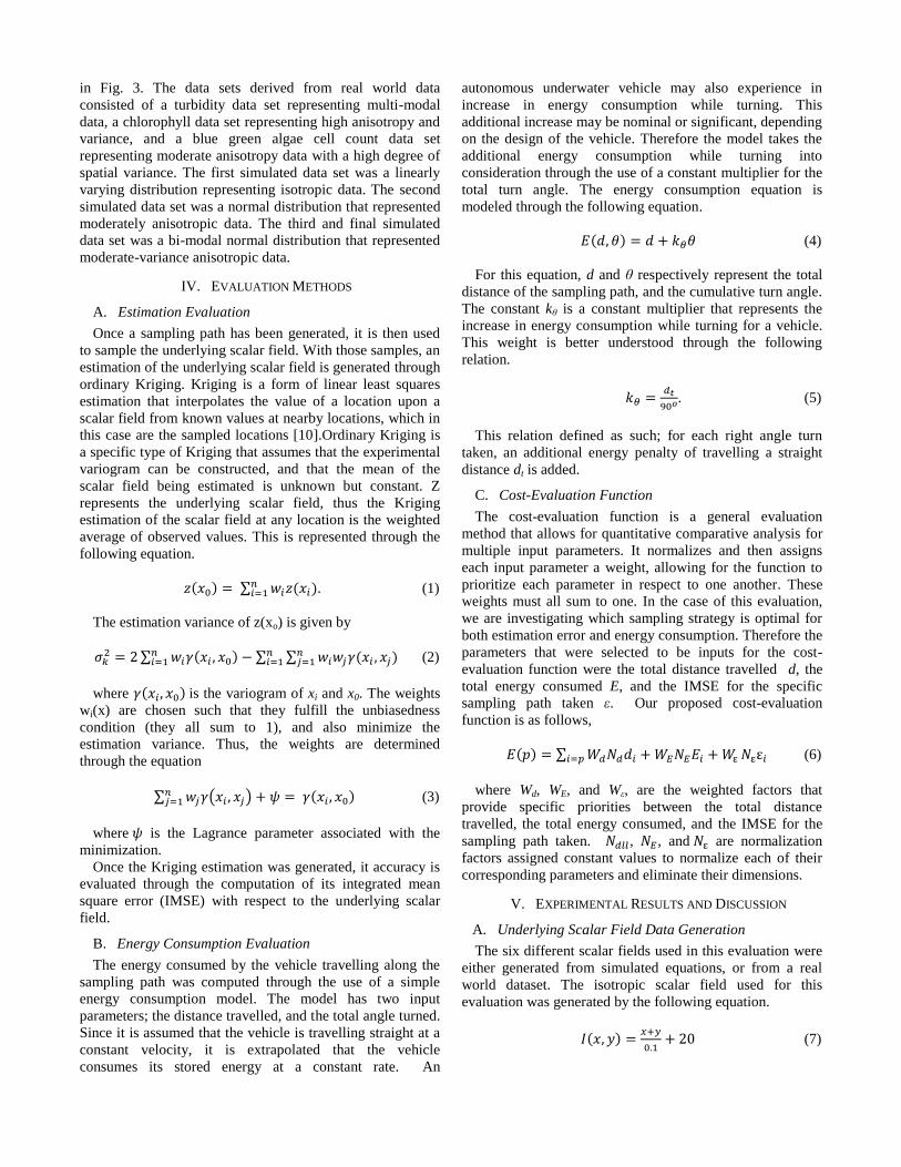
Fig. 3. Plot of the sampling locations taken

0 20 40 60 80 100 120 1400

20

40

60

80

100

120

140

Easting (m)

Nort

hin

g (

m)

Sampling Locations

Fig. 4. Systematic path seeding positions for averaging

The first simulated anisotropic scalar field was generated

by using a standard normal distribution and then scaling it

by a factor of 50 and offseting by +20. The multi-modal

anisotropic field was generated by simply adding together

two equally scaled inverted normal distributions with

differing x-y locations for their means. The real world

dataset used for generating the turbidity, chlorophyll and

blue green algae scalar fields was created by sampling a

local freshwater lake with an autonomous underwater

vehicle carrying a water quality monitoring sonde. The

contiguous underlying scalar field was then generated by

interpolating the samples using ordinary kriging.

The AUV to used to collect the samples was a heavily

modified OceanServer IVER2 platform, which carries a YSI

6600V2 water quality monitoring sonde. The sonde sampled

the in-situ turbidity, cholorophyll, and blue green algae,

among a variety of other measurements.

All of the samples were taken at Lake Pleasant, a large

freshwater reservoir in Arizona. The approximate

coordinates of the sampling location are 33o 51’ 55.66” N

and 112o 17’45.01” W. The sampling locations are shown in

Fig. 3. The AUV collected 2258 samples over an area of

approximately 70m x 100m. A subset of the samples from

30-70m northing and 30-70m easting was selected, since it

was the region containing the highest density of samples.

B. Estimation Error Computation

To compute the estimation error, an estimate of the

underlying scalar field was first generated for each of the

sampling strategy types. These estimates were generated

across varying sampling grid sizes in order to characterize a

range of sampling densities from low to high. The sampling

grid dimensions and total sample size are listed in Table I.

TABLE I.

SAMPLE DISTRIBUTION GRID SIZES

Grid Dimensions

Sample

count

Size

in X

Size

in Y

5 4 20

6 5 30

7 6 42

8 7 56

9 8 72

10 9 90

12 10 120

The IMSE for each of the stratified random sampling

strategy based estimations was the average of fifteen

iterations, in order to generate a stable value. The systematic

sampling estimation was iterated five times at five separate

evenly distributed path seeding locations to remove biasing

in error results. These seeding locations are shown in Fig. 4.

C. Estimation Error Result

The IMSE error for each of the scalar varying from low

(20 samples), moderate (56 samples) and high (120 samples)

sampling density are displayed alongside one another in the

Table II on the following page.

Through looking at the IMSE versus number of sample

plots for the various underlying scalar fields, a number of

correlations are apparent. Firstly, both strategies demonstrate

a reduction in IMSE as the number of samples increases, as

one would expect. Additionally, it is found that the

systematic sampling strategy minimizes error for the real

world data sets across all sampling densities. The stratified

random sampling strategy minimizes error for the low

variance isotropic and anisotropic 2 data sets. Finally, for the

anisotropic 1 data set, the systematic sampling strategy

significantly minimizes error for low sampling densities, and

the stratified random sampling strategy minimizes error for

moderate and high sampling densities.

D. Energy Consumption Computation

The energy consumption of each of the sampling path

patterns was computed using (4). First, the distance and total

angle turned was computed for each of the sampling path

types through the range of sampling densities shown in

Table I. For each of the stratified random sampling paths,

the total distance travelled and total cumulative angle turned

was computed as the averages of 50 iterations of each

sample grid size. Finally (4) was applied using kθ values

from a range of 0 to 2. This range characterizes vehicles for

which a 90o turn correlates to consuming the energy

equivalent to travelling an additional distance of 0m to 2m.

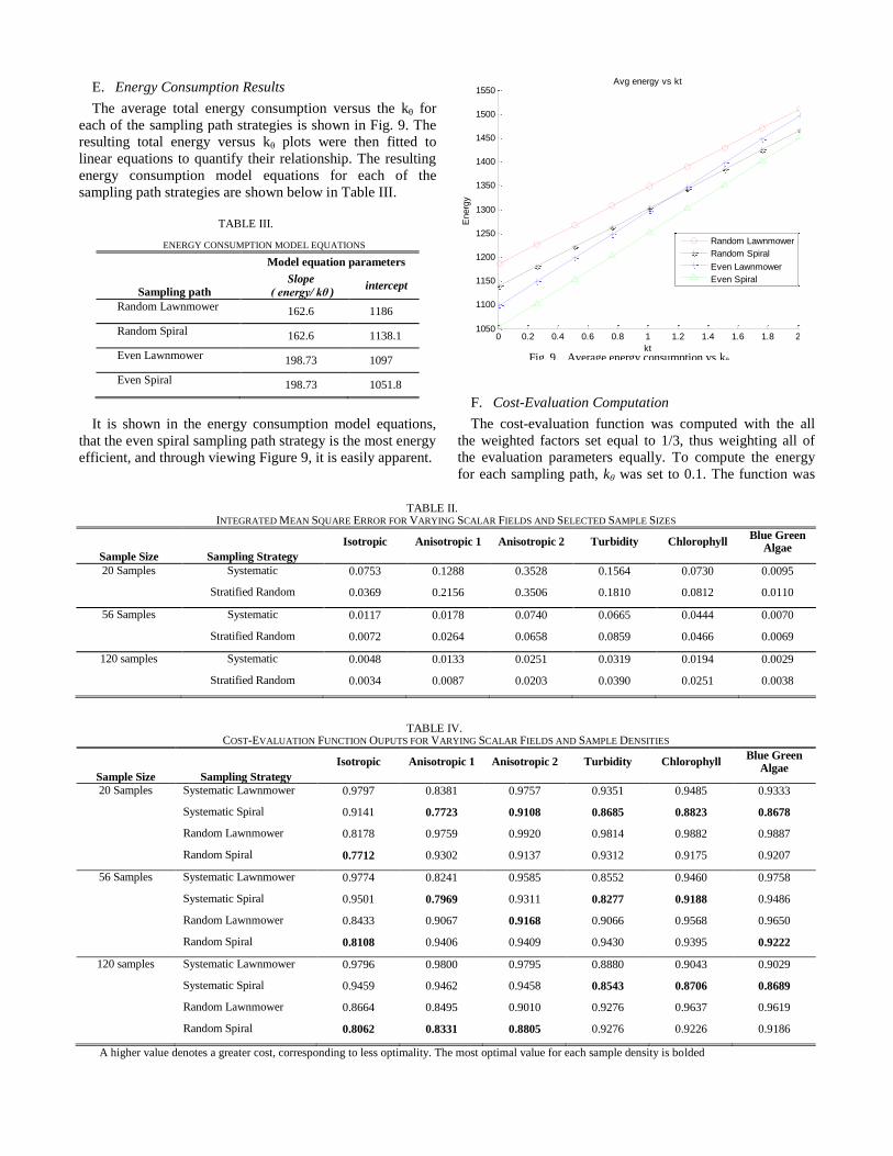
TABLE II. INTEGRATED MEAN SQUARE ERROR FOR VARYING SCALAR FIELDS AND SELECTED SAMPLE SIZES

Sample Size Sampling Strategy

Isotropic Anisotropic 1 Anisotropic 2 Turbidity Chlorophyll Blue Green

Algae

20 Samples Systematic 0.0753 0.1288 0.3528 0.1564 0.0730 0.0095

Stratified Random 0.0369 0.2156 0.3506 0.1810 0.0812 0.0110

56 Samples Systematic 0.0117 0.0178 0.0740 0.0665 0.0444 0.0070


120 samples Systematic 0.0048 0.0133 0.0251 0.0319 0.0194 0.0029


TABLE IV. COST-EVALUATION FUNCTION OUPUTS FOR VARYING SCALAR FIELDS AND SAMPLE DENSITIES

Sample Size Sampling Strategy

Isotropic Anisotropic 1 Anisotropic 2 Turbidity Chlorophyll Blue Green

Algae

20 Samples Systematic Lawnmower 0.9797 0.8381 0.9757 0.9351 0.9485 0.9333

Systematic Spiral 0.9141 0.7723 0.9108 0.8685 0.8823 0.8678

Random Lawnmower 0.8178 0.9759 0.9920 0.9814 0.9882 0.9887

Random Spiral 0.7712 0.9302 0.9137 0.9312 0.9175 0.9207

56 Samples Systematic Lawnmower 0.9774 0.8241 0.9585 0.8552 0.9460 0.9758



Random Spiral 0.8108 0.9406 0.9409 0.9430 0.9395 0.9222

120 samples Systematic Lawnmower 0.9796 0.9800 0.9795 0.8880 0.9043 0.9029



Random Spiral 0.8062 0.8331 0.8805 0.9276 0.9226 0.9186

A higher value denotes a greater cost, corresponding to less optimality. The most optimal value for each sample density is bolded

Fig. 9. Average energy consumption vs kθ

0 0.2 0.4 0.6 0.8 1 1.2 1.4 1.6 1.8 21050

1100

1150

1200

1250

1300

1350

1400

1450

1500

1550Avg energy vs kt

kt

Energ

y

Random Lawnmower

Random Spiral

Even Lawnmower

Even Spiral

E. Energy Consumption Results

The average total energy consumption versus the kθ for

each of the sampling path strategies is shown in Fig. 9. The

resulting total energy versus kθ plots were then fitted to

linear equations to quantify their relationship. The resulting

energy consumption model equations for each of the

sampling path strategies are shown below in Table III.

TABLE III.

ENERGY CONSUMPTION MODEL EQUATIONS

Sampling path

Model equation parameters

Slope

( energy/ kθ ) intercept

Random Lawnmower 162.6 1186

Random Spiral 162.6 1138.1

Even Lawnmower 198.73 1097

Even Spiral 198.73 1051.8

It is shown in the energy consumption model equations,

that the even spiral sampling path strategy is the most energy

efficient, and through viewing Figure 9, it is easily apparent.

F. Cost-Evaluation Computation

The cost-evaluation function was computed with the all

the weighted factors set equal to 1/3, thus weighting all of

the evaluation parameters equally. To compute the energy

for each sampling path, kθ was set to 0.1. The function was

applied to each of the sampling strategies for all the

underlying scalar fields, at 20, 56, and 120 samples. This

was done such that a comparative analysis of each of the

sampling strategies at low, moderate and high sampling

densities could be conducted.

G. Cost-Evaluation Results

The results of the cost-evaluation are listed in Table IV.

For a low sampling density the systematic spiral sampling

method is optimal for all of the data sets except for the

isotropic scalar field. For a moderate sampling density the

systematic spiral strategy is optimal for the anisotropic 1,

turbidity, and chlorophyll scalar fields. The random

lawnmower and random spiral strategies are optimal for the

anisotropic 2 and isotropic scalar fields respectively. Finally,

for a high sample density the random spiral strategy is

optimal for the isotropic and both of the anisotropic scalar

fields. The systematic spiral strategy was found to be

optimal for the turbidity, cholorophyll and blue green algae

scalar fields. The strategy that was optimal for the most

types of scalar fields and densities was found to be the

systematic spiral strategy. In general, a spiral path strategy

was found to be the optimal in almost all of the cases.

H. Discussion of Results

The results from this cost-evaluation are specific to the

weights given to the cost-evaluation function. However

these results do provide insight into which sampling

strategies are optimal for different types of scalar fields,

given the assumption that distance travelled, total energy

consumption and IMSE are considered equal factors in

optimality.

For isotropic scalar fields, the random spiral sampling

strategy was found to be the optimal sampling strategy for

all sampling densities.

It was found that in low variance scalar fields, such as the

single/multi-modal anisotropic scalar fields used in this

evaluation, the systematic spiral strategy is optimal for

coarse sampling densities, and the random spiral strategy is

optimal for high sampling densities.

In high variance scalar fields such as the turbidity,

chlorophyll and blue green algae data sets, the systematic

spiral strategy was optimal for almost every case.

VI. CONCLUSION

We experimentally evaluated four different sampling

strategies through a cost-evaluation function. Assuming that

optimality was defined as minimizing the total path distance,

the total energy consumed, and the IMSE, it was found that

the systematic spiral sampling strategy was the most optimal

strategy overall. Thus if one were given the task to choose a

sampling strategy given no a priori knowledge of the

underlying scalar field and no access to the sampled data in

real time, the best sampling strategy to choose would be a

systematic spiral path, rather than a standard systematic

lawnmower path. It was also demonstrated that the cost-

evaluation function is a useful tool that can be used to

quantify overall optimality for multiple sampling strategy

parameters.

In the future we plan on further experimentally validating

the results of this evaluation. Additionally, the cost-

evaluation function can be utilized to create an online path

optimization planner that chooses path options in real time.

ACKNOWLEDGMENT

The authors would like to acknowledge the following individuals for their support and help: Alexander Kafka, Brance Hudzietz, and Yucong Lin.

REFERENCES

[1] A. L. Forrest, H. Bohm, B. Laval, E. Magnusson, R. Yeo, M. J. Doble, "Investigation of under-ice thermal structure: small AUV deployment in Pavilion Lake, BC, Canada," OCEANS 2007 , vol., no., pp.1-9, Sept. 29 2007-Oct. 4 2007

[2] C. R . Stoker, D. Barch, J. Farmer, M. Flagg, T. Healy, T. Tengdin, H. Thomas, K. Schwer, D. Stakes, "Exploration of Mono Lake with an ROV: a prototype experiment for the MAPS AUV program," Autonomous Underwater Vehicle Technology, 1996. AUV '96., Proceedings of the 1996 Symposium on , vol., no., pp.33-40, 2-6 Jun 1996

[3] M. Kumagai, T. Ura, Y. Kuroda, R. Walker, "New AUV designed for lake environment monitoring," Underwater Technology, 2000. UT 00. Proceedings of the 2000 International Symposium on , vol., no., pp.78-83, 2000

[4] A. B. McBratney, R. Webster, T. M. Burgess, “The design of optimal sampling schemes for local estimation and mapping of of regionalized variables--I: Theory and method,” Computers & Geosciences, Volume 7, Issue 4, 1981, Pages 331-334.

[5] D. O. Popa, A. C. Sanderson, R. J. Komerska, S. S. Mupparapu, D. R. Blidberg, S. G. Chappel, "Adaptive sampling algorithms for multiple autonomous underwater vehicles," Autonomous Underwater Vehicles, 2004 IEEE/OES , vol., no., pp. 108- 118, 17-18 June 2004

[6] B. Zhang, G. S. Sukhatme, "Adaptive Sampling for Estimating a Scalar Field using a Robotic Boat and a Sensor Network," Robotics and Automation, 2007 IEEE International Conference on , vol., no., pp.3673-3680, 10-14 April 2007

[7] J. Witt, M. Dunbabin, “Go with the Flow: Optimal AUV Path Planning in Coastal Environments,” Australian Conference on Robotics and Automation, 2008.

[8] R. N. Smith, A. Pereira, Yi Chao, P. P. Li, D. A. Caron, B. H. Jones, G. S. Sukhatme, "Autonomous Underwater Vehicle trajectory design coupled with predictive ocean models: A case study," Robotics and Automation (ICRA), 2010 IEEE International Conference on , vol., no., pp.4770-4777, 3-7 May 2010

[9] C. V. Caldwell, D. D. Dunlap, E. G. Collins, "Motion planning for an autonomous Underwater Vehicle via Sampling Based Model Predictive Control," OCEANS 2010 , vol., no., pp.1-6, 20-23 Sept. 2010

[10] J. P. Delhomme, Kriging in the hydrosciences, Advances in Water Resources, Volume 1, Issue 5, September 1978, Pages 251-266.

An Experimental Evaluation of Various Sampling Path Strategies for an Autonomous Underwater Vehicle

Documents

Transcript of An Experimental Evaluation of Various Sampling Path Strategies for an Autonomous Underwater Vehicle