Acoustic inversion with self noise of an autonomous underwater vehicle to measure sound speed in...
7
Acoustic Inversion with Self Noise of an Autonomous Underwater Vehicle to Measure Sound Speed in Marine Sediments A. Vincent van Leijen 1 [email protected] Leon J.M. Rothkrantz 2,3 [email protected] Frans C. A. Groen 4 [email protected] 1 Force Vision, Defence Materiel Organisation, P.O.Box 10.000, 1780 AC, Den Helder, The Netherlands 2 MMI group, Delft University of Technology, Mekelweg 4, 2628 CD, Delft, The Netherlands 3 Sensor Systems Department, Netherlands Defence Academy, Nieuwe Diep 8, 1781 AC, Den Helder, The Netherlands 4 FNWI, University of Amsterdam, Science Park 107, 1098 XG, Amsterdam, The Netherlands Abstract – This work reports on an experiment from the Maritime Rapid Environmental Assessment sea trials in 2007, where autonomous underwater vehicles were de- ployed for environmental assessment. Even though these underwater vehicles are very quiet platforms, this work in- vestigates the potential of vehicle self noise for geoacoustic inversion purposes. It is shown that sound speed in marine sediments has been found by a short range inversion from vehicle self noise that was recorded with a sparse vertical re- ceiver array. With the demonstrated inversion method, large areas can be segmented into range-independent patches that can each be characterized by separate inversions. Keywords: Environmental monitoring, sonar, geoacoustic inversion, autonomous underwater vehicles. 1 Introduction Various military and civilian activities at sea have a connec- tion with marine sediments. For Anti-Submarine Warfare (ASW) and Mine Counter Measures (MCM), the sonar per- formance is strongly affected by the acoustic properties of the sea bottom. The sediment type influences the underwater visibility for divers and also indicates the likelihood of burial of mines, pipes and other objects. From a civilian point of view, the continental shelf is being surveyed for petrol, gas, minerals and other natural resources. A worldwide network of pipes and cables supports the internet and the transport of natural resources and information. These networks on the sea floor require inspection, maintenance and repair. All this human activity depends on adequate sensing of the underwater domain. Today’s marine survey deals with high resolution bathymetry from multi beam echo sounders, and extensive acoustic imaging that is provided by side scan sonar. Autonomous underwater vehicles (AUV’s) are pro- grammed to do the job and carry these sensors to remote environments. AUV’s are true underwater robots that can access locations where human divers cannot go, because of dangerous underwater currents or great depths. As a first step to assess what is in the seabottom, this work studies the potential of autonomous underwater vehicles to measure acoustic properties of the sea bottom. The method to do so is geoacoustic inversion. This techique aims to find parameters such as density and sound speed, by analysis of bottom reflected sound. In stead of using sonar transmis- sions, shipping sounds can be used as sound sources of op- portunity [1]. In this case, the sound source is the machin- ery noise of the underwater vehicle itself. Recordings of a REMUS AUV were made during the Maritime Rapid Envi- ronmental Assessment sea trials of 2007 (MREA07). It was anticipated that the weak source level of an AUV might limit its potential for geoacoustic inversion. But as it turned out, low frequencies from a REMUS signature can still be strong enough to find the sound speed of marine sediment. 2 Inversion with AUV self noise Scientific experiments with geoacoustic inversion tradition- ally depend on a controlled source geometry and a verti- cal or horizontal receiver array [2]. Experiments with con- trolled sound sources have been carried out for broad band and narrow band transmissions while the reception is usu- ally done with a vertical array [3]. In an attempt to exploit sound sources of uncontrolled nature a variety of low and mid-frequency (0.1 kHz – 6 kHz) sources of opportunity has been investigated such as ambient noise [4], different kinds of sea life [5, 6], aircraft propellers [7], shipping [8, 9, 10] and even land vehicles [11]. This current experimental work demonstrates how acoustic properties of the seabed are in- verted from AUV self noise. During the MREA07 sea trials, two REMUS AUV’s [12, 13] have been observed to radi- ate several low frequency tones in a broad band of 0.8 kHz - 1.4 kHz while the vehicles were deployed to run bathy- metrical surveys in a shallow water area. Underwater sound was received with a sparse vertical array from a small boat at anchor. The method described here does not rely on high power sonar transmissions and has a limited environmental im- pact. Like other sound source of opportunity concepts, the use of AUV’s has potential for military applications, such as discrete sea bottom characterization in support of ASW or MCM operations. A civil application is environmental 12th International Conference on Information Fusion Seattle, WA, USA, July 6-9, 2009 978-0-9824438-0-4 ©2009 ISIF 41
Transcript of Acoustic inversion with self noise of an autonomous underwater vehicle to measure sound speed in...
Acoustic Inversion with Self Noise of an Autonomous Underwater
Vehicle to Measure Sound Speed in Marine Sediments
A. Vincent van Leijen1
Leon J.M. Rothkrantz2,3
Frans C. A. Groen4
1Force Vision, Defence Materiel Organisation, P.O.Box 10.000, 1780 AC, Den Helder, The Netherlands2MMI group, Delft University of Technology, Mekelweg 4, 2628 CD, Delft, The Netherlands
3Sensor Systems Department, Netherlands Defence Academy, Nieuwe Diep 8, 1781 AC, Den Helder, The Netherlands4FNWI, University of Amsterdam, Science Park 107, 1098 XG, Amsterdam, The Netherlands
Abstract – This work reports on an experiment from the
Maritime Rapid Environmental Assessment sea trials in
2007, where autonomous underwater vehicles were de-
ployed for environmental assessment. Even though these
underwater vehicles are very quiet platforms, this work in-
vestigates the potential of vehicle self noise for geoacoustic
inversion purposes. It is shown that sound speed in marine
sediments has been found by a short range inversion from
vehicle self noise that was recorded with a sparse vertical re-
ceiver array. With the demonstrated inversion method, large
areas can be segmented into range-independent patches that
can each be characterized by separate inversions.
Keywords: Environmental monitoring, sonar, geoacoustic
inversion, autonomous underwater vehicles.
1 IntroductionVarious military and civilian activities at sea have a connec-
tion with marine sediments. For Anti-Submarine Warfare
(ASW) and Mine Counter Measures (MCM), the sonar per-
formance is strongly affected by the acoustic properties of
the sea bottom. The sediment type influences the underwater
visibility for divers and also indicates the likelihood of burial
of mines, pipes and other objects. From a civilian point of
view, the continental shelf is being surveyed for petrol, gas,
minerals and other natural resources. A worldwide network
of pipes and cables supports the internet and the transport of
natural resources and information. These networks on the
sea floor require inspection, maintenance and repair.
All this human activity depends on adequate sensing of
the underwater domain. Today’s marine survey deals with
high resolution bathymetry from multi beam echo sounders,
and extensive acoustic imaging that is provided by side scan
sonar. Autonomous underwater vehicles (AUV’s) are pro-
grammed to do the job and carry these sensors to remote
environments. AUV’s are true underwater robots that can
access locations where human divers cannot go, because of
dangerous underwater currents or great depths.
As a first step to assess what is in the seabottom, this work
studies the potential of autonomous underwater vehicles to
measure acoustic properties of the sea bottom. The method
to do so is geoacoustic inversion. This techique aims to find
parameters such as density and sound speed, by analysis of
bottom reflected sound. In stead of using sonar transmis-
sions, shipping sounds can be used as sound sources of op-
portunity [1]. In this case, the sound source is the machin-
ery noise of the underwater vehicle itself. Recordings of a
REMUS AUV were made during the Maritime Rapid Envi-
ronmental Assessment sea trials of 2007 (MREA07). It was
anticipated that the weak source level of an AUV might limit
its potential for geoacoustic inversion. But as it turned out,
low frequencies from a REMUS signature can still be strong
enough to find the sound speed of marine sediment.
2 Inversion with AUV self noise
Scientific experiments with geoacoustic inversion tradition-
ally depend on a controlled source geometry and a verti-
cal or horizontal receiver array [2]. Experiments with con-
trolled sound sources have been carried out for broad band
and narrow band transmissions while the reception is usu-
ally done with a vertical array [3]. In an attempt to exploit
sound sources of uncontrolled nature a variety of low and
mid-frequency (0.1 kHz – 6 kHz) sources of opportunity has
been investigated such as ambient noise [4], different kinds
of sea life [5, 6], aircraft propellers [7], shipping [8, 9, 10]
and even land vehicles [11]. This current experimental work
demonstrates how acoustic properties of the seabed are in-
verted from AUV self noise. During the MREA07 sea trials,
two REMUS AUV’s [12, 13] have been observed to radi-
ate several low frequency tones in a broad band of 0.8 kHz
- 1.4 kHz while the vehicles were deployed to run bathy-
metrical surveys in a shallow water area. Underwater sound
was received with a sparse vertical array from a small boat
at anchor.
The method described here does not rely on high power
sonar transmissions and has a limited environmental im-
pact. Like other sound source of opportunity concepts, the
use of AUV’s has potential for military applications, such
as discrete sea bottom characterization in support of ASW
or MCM operations. A civil application is environmental
12th International Conference on Information FusionSeattle, WA, USA, July 6-9, 2009
978-0-9824438-0-4 ©2009 ISIF 41

monitoring of areas such as sensitive ecosystems or marine
wildlife habitats.
The wider application of geoacoustic inversion with AUV
self noise, is to divide a survey area in many segments. Each
part can then be characterized with a range-independent in-
version and the result is a gridded map with variations in
marine sediments.
3 Concept of inversion with self noiseSelf noise of ships has been used before for inversion pur-
poses [8, 9, 10]. In these cases receptions were made with
many hydrophones, such as 32 or more, mostly configured
in a horizontal array and at a long distance from the noise
source. Previous work on geoacoustic inversion with ship
noise [1] investigated the use of narrowband tones and short
range receptions. The movement of the ship was used to col-
lect a series of independent observations. Acoustic data was
recorded with a sparse vertical array of four hydrophones
that spanned the water column. The result was a local range-
independent environmental model. The current work fol-
lows the same approach, by receiving noise of an underwater
vehicle at short range and on a light sparse array in a vertical
configuration.
3.1 Error function
Acoustic inversion methods are ment to derive a geometric
or environmental model from observed underwater sound.
In an iterative process, numerous replica models are con-
structed and evaluated. Inversion is a search for the best
model and therefore the acoustic impact of replica models
needs to be compared with the observed data.
The observed signatures from ships that are used here are
narrowband tones. For reception on hydrophone n, with
n ∈ {1, ..., NS}, the received signature component of a ship
can be noted as dn,f . Each tone is characterized by its fre-
quency f (in Hz) and can be modelled in the frequency do-
main as a vector wf with entries for the NS hydrophone
depths. Replica data wf is calculated with a propagation
code and a model vector m that holds geoacoustic parame-
ters such as sediment density and sound speed. A common
method to match observed data dn,f with the replica vector
wf (m), is to use a normalized Bartlett processor of the form
[2, 14]
Bf (m) =
[
w†f (m)R̂fwf (m)
tr[R̂f ] ‖wf (m)‖2
]
, (1)
where † denotes the conjugate transpose operator, m is the
model vector to be optimized and R̂f are the cross-spectral
density matrices defined as
R̂f =1
NS
NS∑
n=1
dn,fd†n,f . (2)
By definition 0 ≤ Bf (m) ≤ 1 and a perfect match between
observed data and replica data is found when Bf (m) ≡ 1.
Geometric and geoacoustic parameters can be estimated by
maximizing Eq. 1. To minimize the mismatch over NF fre-
quencies, an error function can take form
E(m) =1
NF
NF∑
f=1
1 − Bf (m) (3)
or more general for receptions at NR ranges
E(m) =1
NF NR
NF∑
f=1
NR∑
r=1
1 − Bf,r(m) . (4)
3.2 Movement of the sound source
For fixed source-receiver geometries, observations dn,f
are usually obtained from Fourier transformed receptions,
where the integration time τB is reciprocal to the bandwidth
B of the transmitted signal. For a moving sound source of
the size of an AUV it is favorable to keep the distance trav-
eled small in comparison with wavelength. For a maximum
ships displacement of λ/4, the integration time τv can be
chosen to depend on ships speed v as
τv =c
4vf(5)
with v and c in m/s and f in Hz. Typical ship noise contains
low frequency narrowband components with f < 2 kHz.
For v = 9.7 m/s (5 kts) and c = 1500 m/s it follows that
B < 52 Hz. The smallest integration time can been chosen
as
τ = min(τB , τv). (6)
The movement of the ship is further used to collect a series
of independent observations. Based on the principle of reci-
procity of source and receiver [15], and the assumption of a
range-independent environment, the source can be modeled
at a fixed position while the receptions are taken to vary in
distance to the source. As a result, the observations at NR
different source-receiver ranges can be regarded as incoher-
ent observations from a 2D-array with a horizontal aperture
of NR groups of vertical hydrophone arrays.
4 AUV experimentsAutonomous vehicles are cooperative platforms that run
programmed tracks and submerge to desired depths. De-
ployment is mainly limited by bad weather or water condi-
tions, like swell or high sea states and the presence of fish-
ing nets. Most AUV’s are well equipped to sample the wa-
ter column. Normal operation of a REMUS AUV results
in temperature and salinity data of the water column and a
bathymetric chart of the surveyed area. Both types of data
are input to the inversion process. In this work self noise is
received at a fixed position but autonomous vehicles are also
capable of towing their own receiving sensors [16, 17].
5 ObservationsOn the morning of April 29th, 2007, two REMUS AUV’s
were deployed in a shallow water area nearby the medieval
42

Figure 1: Geometry for the experiments on April 29th 2007,
south east of the Island of Elba. Depth contour lines are
in meters; the first AUV track is based on the 33 m depth
contour line.
sea village of Castiglione della Pescaia, Italy. The experi-
mental geometry and historical bathymetry [18] are shown
in Fig. 1. Both vehicles ran along the tracks in an area of
0.1 km by 2 km that was selected to overlay and be in line
with the 33 m depth contour line. Markers indicate positions
of the sparse vertical line array (SVLA), CTD sampling of
Fig. 2, seismic bottom profile of Fig. 3 and the side scan
sonar (SSS) image of Fig. 4. Experiments were conducted
in very calm waters, sea state 2 or less, and under a par-
tial cover of clouds. In the water column, the ambient noise
was highly fluctuating due to the presence of many coastal
vessels, mainly recreational boats. Before and during the
experiments no fishing activities had been observed.
5.1 Water column and SVP
Part of the MREA07 sea trials was an extensive sampling of
the water column by measuring conductivity, temperature
and depth (CTD) for the purpose of oceanographic model-
ing and forecasting. As such and with the deployment of the
AUV’s and two small motor boats, a CTD measurement was
taken in the middle of the designated area. The sound veloc-
ity profile in Fig. 2 is obtained according to the method of
Medwin [19]. The profile reveals a strong negative gradient
below depths of 10 m.
5.2 Bottom: bathymetry and seismic profiling
An area with a water depth of ≈33 m was selected for the
initial experiments and the AUV’s were programmed to run
at 3 m above the sea bed and in straight lines parallel with
1512 1514 1516 1518 1520
0
5
10
15
20
25
30
c (m/s)
de
pth
(m
)
Figure 2: Sound-speed profile for position 42o44.802′N,
010o49.800′E at 08:45:50 UTC, 29-04-2007.
the bottom contour lines. Depths along the first leg are con-
firmed with ADCP data and found to be between 32 m and
33 m.
The area selection was also based on a seismic survey that
was run on April 24th with an EdgeTech X-Star sub-bottom
profiling system, provided and operated by TNO. The bot-
tom profile in Fig. 3 is for a segment perpendicular to the
AUV lines. At a water depth of 33 m layers of sediment are
observed with strongest reflections at 8 m and 10 m in the
sea bed.
ping numbers
de
pth
(m
)
200 400 600 800 1000
10
20
30
40
50
60
70
80
90
Figure 3: Seismic profiling between positions 42o44.196′N,
010o49.392′E and 42o45.192′N, 010o50.436′E.
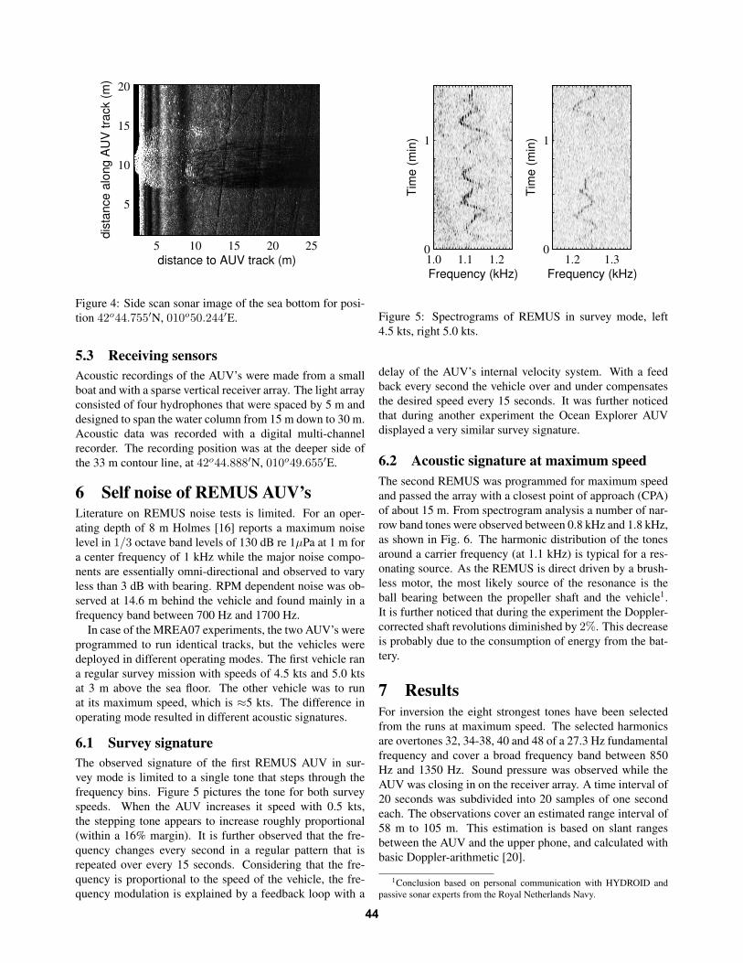
During the self noise inversion experiments the REMUS
vehicles operated their 900 kHz side scan sonars (SSS). The
acoustic image in Fig. 4 shows a school of small fish and
their shadows on the sea floor. Fishery with trawling nets
has left traces on the bottom which is a strong indication for
a sandy sediment.
43
distance to AUV track (m)
dis
tan
ce
alo
ng
AU
V t
rack (
m)
252015105
5
10
15
20
Figure 4: Side scan sonar image of the sea bottom for posi-
tion 42o44.755′N, 010o50.244′E.
5.3 Receiving sensors
Acoustic recordings of the AUV’s were made from a small
boat and with a sparse vertical receiver array. The light array
consisted of four hydrophones that were spaced by 5 m and
designed to span the water column from 15 m down to 30 m.
Acoustic data was recorded with a digital multi-channel
recorder. The recording position was at the deeper side of
the 33 m contour line, at 42o44.888′N, 010o49.655′E.
6 Self noise of REMUS AUV’sLiterature on REMUS noise tests is limited. For an oper-
ating depth of 8 m Holmes [16] reports a maximum noise
level in 1/3 octave band levels of 130 dB re 1µPa at 1 m for
a center frequency of 1 kHz while the major noise compo-
nents are essentially omni-directional and observed to vary
less than 3 dB with bearing. RPM dependent noise was ob-
served at 14.6 m behind the vehicle and found mainly in a
frequency band between 700 Hz and 1700 Hz.
In case of the MREA07 experiments, the two AUV’s were
programmed to run identical tracks, but the vehicles were
deployed in different operating modes. The first vehicle ran
a regular survey mission with speeds of 4.5 kts and 5.0 kts
at 3 m above the sea floor. The other vehicle was to run
at its maximum speed, which is ≈5 kts. The difference in
operating mode resulted in different acoustic signatures.
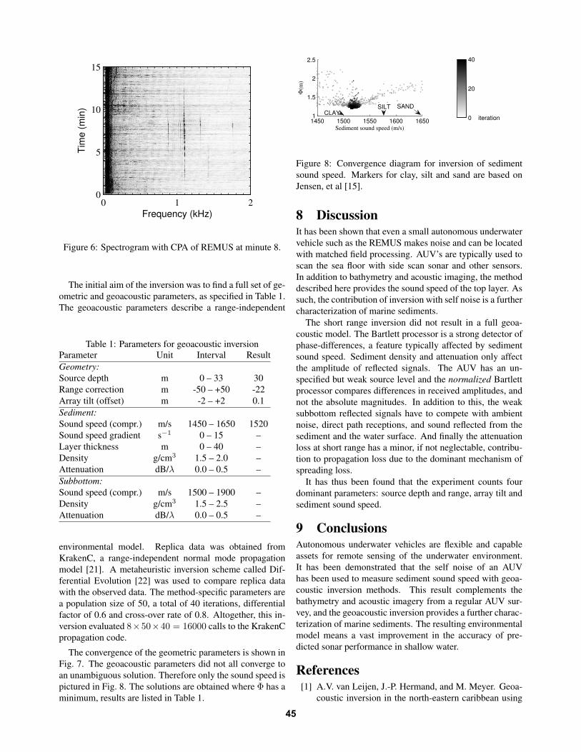
6.1 Survey signature
The observed signature of the first REMUS AUV in sur-
vey mode is limited to a single tone that steps through the
frequency bins. Figure 5 pictures the tone for both survey
speeds. When the AUV increases it speed with 0.5 kts,
the stepping tone appears to increase roughly proportional
(within a 16% margin). It is further observed that the fre-
quency changes every second in a regular pattern that is
repeated over every 15 seconds. Considering that the fre-
quency is proportional to the speed of the vehicle, the fre-
quency modulation is explained by a feedback loop with a
Frequency (kHz)
Tim
e (
min
)
1.0 1.1 1.2
1
0
Frequency (kHz)
Tim
e (
min
)
1.2 1.3
1
0
Figure 5: Spectrograms of REMUS in survey mode, left
4.5 kts, right 5.0 kts.
delay of the AUV’s internal velocity system. With a feed
back every second the vehicle over and under compensates
the desired speed every 15 seconds. It was further noticed
that during another experiment the Ocean Explorer AUV
displayed a very similar survey signature.
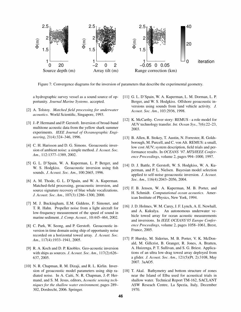
6.2 Acoustic signature at maximum speed
The second REMUS was programmed for maximum speed
and passed the array with a closest point of approach (CPA)
of about 15 m. From spectrogram analysis a number of nar-
row band tones were observed between 0.8 kHz and 1.8 kHz,
as shown in Fig. 6. The harmonic distribution of the tones
around a carrier frequency (at 1.1 kHz) is typical for a res-
onating source. As the REMUS is direct driven by a brush-
less motor, the most likely source of the resonance is the
ball bearing between the propeller shaft and the vehicle1.
It is further noticed that during the experiment the Doppler-
corrected shaft revolutions diminished by 2%. This decrease
is probably due to the consumption of energy from the bat-
tery.
7 Results
For inversion the eight strongest tones have been selected
from the runs at maximum speed. The selected harmonics
are overtones 32, 34-38, 40 and 48 of a 27.3 Hz fundamental
frequency and cover a broad frequency band between 850
Hz and 1350 Hz. Sound pressure was observed while the
AUV was closing in on the receiver array. A time interval of
20 seconds was subdivided into 20 samples of one second
each. The observations cover an estimated range interval of
58 m to 105 m. This estimation is based on slant ranges
between the AUV and the upper phone, and calculated with
basic Doppler-arithmetic [20].
1Conclusion based on personal communication with HYDROID and
passive sonar experts from the Royal Netherlands Navy.
44
Frequency (kHz)
Tim
e (
min
)
0 1 2
15
10
5
0
Figure 6: Spectrogram with CPA of REMUS at minute 8.
The initial aim of the inversion was to find a full set of ge-
ometric and geoacoustic parameters, as specified in Table 1.
The geoacoustic parameters describe a range-independent
Table 1: Parameters for geoacoustic inversion
Parameter Unit Interval Result
Geometry:
Source depth m 0 – 33 30
Range correction m -50 – +50 -22
Array tilt (offset) m -2 – +2 0.1
Sediment:
Sound speed (compr.) m/s 1450 – 1650 1520
Sound speed gradient s−1 0 – 15 –
Layer thickness m 0 – 40 –
Density g/cm3 1.5 – 2.0 –
Attenuation dB/λ 0.0 – 0.5 –
Subbottom:
Sound speed (compr.) m/s 1500 – 1900 –
Density g/cm3 1.5 – 2.5 –
Attenuation dB/λ 0.0 – 0.5 –
environmental model. Replica data was obtained from
KrakenC, a range-independent normal mode propagation
model [21]. A metaheuristic inversion scheme called Dif-
ferential Evolution [22] was used to compare replica data
with the observed data. The method-specific parameters are
a population size of 50, a total of 40 iterations, differential
factor of 0.6 and cross-over rate of 0.8. Altogether, this in-
version evaluated 8×50×40 = 16000 calls to the KrakenC
propagation code.
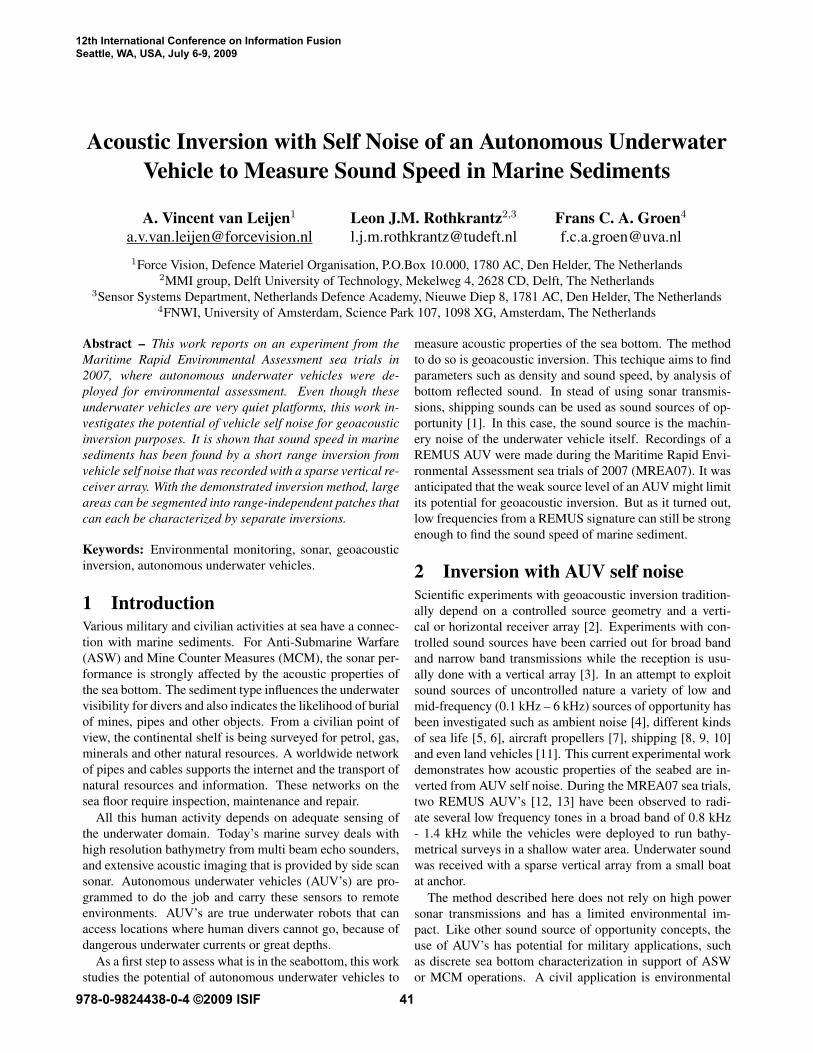
The convergence of the geometric parameters is shown in
Fig. 7. The geoacoustic parameters did not all converge to
an unambiguous solution. Therefore only the sound speed is
pictured in Fig. 8. The solutions are obtained where Φ has a
minimum, results are listed in Table 1.
1450 1500 1550 1600 16501
1.5
2
2.5
Sediment sound speed (m/s)
Φ(m
)
0 0
0 iteration
20
40
SANDSILTCLAY
Figure 8: Convergence diagram for inversion of sediment
sound speed. Markers for clay, silt and sand are based on
Jensen, et al [15].
8 DiscussionIt has been shown that even a small autonomous underwater
vehicle such as the REMUS makes noise and can be located
with matched field processing. AUV’s are typically used to
scan the sea floor with side scan sonar and other sensors.
In addition to bathymetry and acoustic imaging, the method
described here provides the sound speed of the top layer. As
such, the contribution of inversion with self noise is a further
characterization of marine sediments.
The short range inversion did not result in a full geoa-
coustic model. The Bartlett processor is a strong detector of
phase-differences, a feature typically affected by sediment
sound speed. Sediment density and attenuation only affect
the amplitude of reflected signals. The AUV has an un-
specified but weak source level and the normalized Bartlett
processor compares differences in received amplitudes, and
not the absolute magnitudes. In addition to this, the weak
subbottom reflected signals have to compete with ambient
noise, direct path receptions, and sound reflected from the
sediment and the water surface. And finally the attenuation
loss at short range has a minor, if not neglectable, contribu-
tion to propagation loss due to the dominant mechanism of
spreading loss.
It has thus been found that the experiment counts four
dominant parameters: source depth and range, array tilt and
sediment sound speed.
9 ConclusionsAutonomous underwater vehicles are flexible and capable
assets for remote sensing of the underwater environment.
It has been demonstrated that the self noise of an AUV
has been used to measure sediment sound speed with geoa-
coustic inversion methods. This result complements the
bathymetry and acoustic imagery from a regular AUV sur-
vey, and the geoacoustic inversion provides a further charac-
terization of marine sediments. The resulting environmental
model means a vast improvement in the accuracy of pre-
dicted sonar performance in shallow water.
References[1] A.V. van Leijen, J.-P. Hermand, and M. Meyer. Geoa-
coustic inversion in the north-eastern caribbean using
45
0 201
1.5
2
2.5
Source depth (m)
Φ(m
)
−0.05 0 0.051
1.5
2
2.5
Range correction (km)
Φ(m
)
−2 0 21
1.5
2
2.5
Array tilt (m)
Φ(m
)
0 iteration
20
40
Figure 7: Convergence diagrams for the inversion of parameters that describe the experimental geometry.
a hydrographic survey vessel as a sound source of op-
portunity. Journal Marine Systems. accepted.
[2] A. Tolstoy. Matched field processing for underwater
acoustics. World Scientific, Singapore, 1993.
[3] J.-P. Hermand and P. Gerstoft. Inversion of broad-band
multitone acoustic data from the yellow shark summer
experiments. IEEE Journal of Oceanographic Engi-
neering, 21(4):324–346, 1996.
[4] C. H. Harisson and D. G. Simons. Geoacoustic inver-
sion of ambient noise: a simple method. J. Acoust. Soc.
Am., 112:1377–1389, 2002.
[5] G. L. D’Spain, W. A. Kuperman, L. P. Berger, and
W. S. Hodgkiss. Geoacoustic inversion using fish
sounds. J. Acoust. Soc. Am., 100:2665, 1996.
[6] A. M. Thode, G. L. D’Spain, and W. A. Kuperman.
Matched-field processing, geoacoustic inversion, and
source signature recovery of blue whale vocalizations.
J. Acoust. Soc. Am., 107(3):1286–1300, 2000.
[7] M. J. Buckingham, E.M. Giddens, F. Simonet, and
T. R. Hahn. Propeller noise from a light aircraft for
low-frequency measurement of the speed of sound in
marine sediment. J. Comp. Acoust., 10:445–464, 2002.
[8] C. Park, W. Seong, and P. Gerstoft. Geoacoustic in-
version in time domain using ship of opportunity noise
recorded on a horizontal towed array. J. Acoust. Soc.
Am., 117(4):1933–1941, 2005.
[9] R. A. Koch and D. P. Knobles. Geo-acoustic inversion
with ships as sources. J. Acoust. Soc. Am., 117(2):626–
637, 2005.
[10] N. R. Chapman, R. M. Dizaji, and R. L. Kirlin. Inver-
sion of geoacoustic model parameters using ship ra-
diated noise. In A. Caiti, N. R. Chapman, J.-P. Her-
mand, and S. M. Jesus, editors, Acoustic sensing tech-
niques for the shallow water environment, pages 289–
302, Dordrecht, 2006. Springer.
[11] G. L. D’Spain, W. A. Kuperman, L. M. Dorman, L. P.
Berger, and W. S. Hodgkiss. Offshore geoacoustic in-
versions using sounds from land vehicle activity. J.
Acoust. Soc. Am., 103:2936, 1998.
[12] K. McCarthy. Cover story: REMUS - a role model for
AUV technology transfer. Int. Ocean Sys., 7(6):22–23,
2003.
[13] B. Allen, R. Stokey, T. Austin, N. Forrester, R. Golds-
borough, M. Purcell, and C. von Alt. REMUS: a small,
low cost AUV; system description, field trials and per-
formance results. In OCEANS ’97. MTS/IEEE Confer-
ence Proceedings, volume 2, pages 994–1000, 1997.
[14] D. J. Battle, P. Gerstoft, W. S. Hodgkiss, W. A. Ku-
perman, and P. L. Nielsen. Bayesian model selection
applied to self-noise geoacoustic inversion. J. Acoust.
Soc. Am., 116(4):2043–2056, 2004.
[15] F. B. Jensen, W. A. Kuperman, M. B. Porter, and
H. Schmidt. Computational ocean acoustics. Amer-
ican Institute of Physics, New York, 1994.
[16] J. D. Holmes, W. M. Carey, J. F. Lynch, A. E. Newhall,
and A. Kukulya. An autonomous underwater ve-
hicle towed array for ocean acoustic measurements
and inversions. In IEEE OCEANS’05 Europe Confer-
ence Proceedings, volume 2, pages 1058–1061, Brest,
France, 2005.
[17] P. Hursky, M. Siderius, M. B. Porter, V. K. McDon-
ald, M. Gillcrist, B. Granger, R. Jones, A. Bratten,
A. Huizenga, P. T. Sullivan, and S. G. Briest. Applica-
tions of an ultra low-drag towed array deployed from
a glider. J. Acoust. Soc. Am., 121(5)(Pt. 2):3108, May
2007. 3aAO5.
[18] T. Akal. Bathymetry and bottom structure of zones
near the Island of Elba used for acoustical trials in
shallow water. Technical Report TM-162, SACLANT
ASW Reseach Centre, La Spezia, Italy, December
1970.
46

[19] H. Medwin. Speed of sound in water: A simple equa-
tion for realistic parameters. J. Acoust. Soc. Am.,
58:1318–1319, 1975.
[20] X. Lurton. An introduction to underwater acoustics:
principles and applications. Springer-Praxis, Chich-
ester, 2002.
[21] M. Porter. The kraken normal mode program. Tech-
nical Report SACLANT-SM-245, NATO SACLANT
Undersea Research Centre, La Spezia, 1991.
[22] Rainer Storn and Kenneth Price. Differential evolution
- a simple and efficient adaptive scheme for global op-
timization over continuous spaces. Technical Report
TR-95-012, Berkeley, CA, March 1995.
47