
An Efficient Method for Testing Autonomous Driving Software ...
163
TECHNISCHE UNIVERSIT ¨ AT M ¨ UNCHEN Lehrstuhl f¨ ur Echtzeitsysteme und Robotik An Efficient Method for Testing Autonomous Driving Software against Nondeterministic Influences Pascal Marcel Minnerup Vollst¨ andiger Abdruck der von der Fakult¨ at f¨ ur Informatik der Technischen Universit¨ at M¨ unchen zur Erlangung des akademischen Grades eines Doktors der Naturwissenschaften (Dr. rer. nat.) genehmigten Dissertation. Vorsitzender: Prof. Alfons Kemper, Ph.D. Pr¨ ufer der Dissertation: 1. Prof. Dr.-Ing. habil. Alois Knoll 2. Prof. Dr.-Ing. Ren C. Luo Die Dissertation wurde am 09.05.2017 bei der Technischen Universit¨ at M¨ unchen eingereicht und durch die Fakult¨ at f¨ ur Informatik am 13.09.2017 angenommen.
-
Upload
khangminh22 -
Category
Documents
-
view
2 -
download
0
Transcript of An Efficient Method for Testing Autonomous Driving Software ...

TECHNISCHE UNIVERSITAT MUNCHENLehrstuhl fur Echtzeitsysteme und Robotik
An Efficient Method for TestingAutonomous Driving Software
against Nondeterministic Influences
Pascal Marcel Minnerup
Vollstandiger Abdruck der von der Fakultat fur Informatik der Technischen
Universitat Munchen zur Erlangung des akademischen Grades eines
Doktors der Naturwissenschaften (Dr. rer. nat.)
genehmigten Dissertation.
Vorsitzender: Prof. Alfons Kemper, Ph.D.
Prufer der Dissertation: 1. Prof. Dr.-Ing. habil. Alois Knoll
2. Prof. Dr.-Ing. Ren C. Luo
Die Dissertation wurde am 09.05.2017 bei der Technischen Universitat Munchen
eingereicht und durch die Fakultat fur Informatik am 13.09.2017 angenommen.


Acknowledgements
First of all, I would like to thank Prof. Dr. Alois Knoll for offering the opportunity to work on this
fascinating and challenging topic, as well as for his encouragement and support. Many thanks
also go to Prof. Dr. Ren C. Luo for his valuable inputs and suggestions. I would also like to
thank Prof. Dr. Bernd Radig for his last-minute commitment in my Rigorosum and Prof. Alfons
Kemper, Ph.D. for chairing the defense. Moreover, I would like to thank Dr. Markus Rickert for
his great support in mentoring my research efforts. Special thanks go to Dominik Bauch, Julian
Bernhard, Martin Buchel, Dr. Chao Chen, Klemens Esterle, Patrick Hart, Gereon Hinz, Tobias
Kessler, David Lenz and all other colleagues and students who supported me during my time at
fortiss. Finally, I would like to thank my wife, my parents, my siblings, my parents-in-law and
my friends for proof reading and for the constant support while working on the thesis.


Fur Katta


Abstract
Autonomous driving planning and control functions have to ensure reliable execution in all
situations for which they can be activated. The reliability is challenged by the large number
of scenarios, by nondeterministic behavior of traffic participants and by inaccurate sensors and
actuators. All three conditions can be controlled and reproduced in a simulation environment.
Additionally, the simulation environment can execute the same planning and control code as the
real vehicle and thus include all implemented improvements. However, it remains a challenge
to cover combinations of the conditions above efficiently. This thesis presents a new method
that directly tests the implementation of the planning system and efficiently provokes undesired
behavior. The method maps the states of the tested system to a discrete state space. Similar
to model checking, it covers all reachable states in this space. In contrast to traditional model
checking, state transitions are performed by dynamically executing the actual implementation
of the checked system. Furthermore, each analysis step increases the density of the state space
and reduces the discretization error. Reaching different states requires branching the execution
of the simulation at intermediate points. For this purpose, the state of the entire software
system is stored. This allows restoring and continuing from it with different influences of the
nondeterministic parts. Omitting states that are similar to already analyzed states reduces the
complexity of the search. This way, the method finds undesired behaviors more efficiently than
state of the art methods dealing with nondeterminism by random execution. The approach is
shown to be applicable to planning and control software used in the automotive industry. It can
be integrated into the automotive pre-development process supporting iterations of tests and
software improvements.

Inhaltsangabe
Planungs- und Regelungsfunktionen fur das autonome Fahren mussen eine zuverlassige
Ausfuhrung in allen Situationen sicherstellen, in denen sie aktiviert werden konnen. Die
Zuverlassigkeit kann beeintrachtigt werden durch die große Zahl unterschiedlicher Szenarien,
durch nichtdeterministisches Verhalten von Verkehrsteilnehmern und durch Sensor- und
Aktorungenauigkeiten. Alle drei Einflussfaktoren konnen in einer Simulationsumgebung
kontrolliert und reproduziert werden. Außerdem kann die Simulationsumgebung dieselbe
Planungs- und Regelungssoftware wie das echte Fahrzeug ausfuhren und dementsprechend
alle implementierten Verbesserungen testen. Allerdings bleibt es eine Herausforderung, auch
Kombinationen dieser Einflussfaktoren effizient zu testen. Die vorliegende Arbeit stellt eine
neue Methode vor, die die Implementierung des Planungssystems direkt testet und die effizient
ungewolltes Verhalten provoziert. Die Methode bildet die Zustande des zu testenden Systems
auf einen diskreten Zustandsraum ab. Analog zum Model-Checking deckt sie alle Zustande
in diesem abstrakten Zustandsraum ab. Im Gegensatz zu traditionellem Model-Checking
werden Zustandsubergange durch die dynamische Ausfuhrung der Softwareimplementierung
des zu testenden Systems umgesetzt. Außerdem wird der diskrete Zustandsraum mit jedem
Schritt dichter, so dass Diskretisierungsfehler reduziert werden. Um unterschiedliche Zustande
zu erreichen ist es notig, die Ausfuhrung an Zwischenpunkten verzweigen zu lassen. Zu
diesem Zweck wird der Zustand des gesamten Softwaresystems gespeichert. Dadurch kann
dieser Zustand geladen werden und die Ausfuhrung mit unterschiedlichem Einfluss der
nichtdeterministischen Bestandteile wiederholt werden. Indem Zustande ausgelassen werden,
die ahnlich zu bereits analysierten Zustanden sind, wird die Komplexitat der Suche reduziert.
Auf diese Weise findet die prasentierte Methode ungewolltes Verhalten effizienter als aktuelle
Methoden, die auf zufallige Ausfuhrung setzen, um unterschiedliche Verhalten zu produzieren.
Es wird gezeigt, dass der Ansatz auf Planungs- und Regelungssoftware in der Automobilindustrie
anwendbar ist. Er kann in den Vorentwicklungsprozess integriert werden, um eine iterative
Entwicklung aus Tests und Softwareverbesserungen zu unterstutzen.

Contents
1 Introduction 1
1.1 Importance of Systematic Testing . . . . . . . . . . . . . . . . . . . . . . . . . . . 2
1.2 Software Development Process . . . . . . . . . . . . . . . . . . . . . . . . . . . . 4
1.3 Contributions and Structure . . . . . . . . . . . . . . . . . . . . . . . . . . . . . . 5
2 State of the Art for Testing Autonomous Driving Systems 6
2.1 Planning and Control Algorithms . . . . . . . . . . . . . . . . . . . . . . . . . . . 6
2.2 Formal Verification of Planning Concepts . . . . . . . . . . . . . . . . . . . . . . 8
2.3 Testing in a Simulation Environment . . . . . . . . . . . . . . . . . . . . . . . . . 9
2.3.1 Realistic Models for Simulation . . . . . . . . . . . . . . . . . . . . . . . . 10
2.3.2 Simulation with Driver Interaction . . . . . . . . . . . . . . . . . . . . . . 11
2.4 Simulation with a Set of Possible Events . . . . . . . . . . . . . . . . . . . . . . . 12
2.5 Testing in the Physical World . . . . . . . . . . . . . . . . . . . . . . . . . . . . . 13
2.6 Sources for Test Scenarios . . . . . . . . . . . . . . . . . . . . . . . . . . . . . . . 14
3 Modeling the Environment of an Autonomous Vehicle 16
3.1 Representing Physical Vehicle Scenarios in a Simulation Environment . . . . . . 16
3.1.1 Modelling the Physical World . . . . . . . . . . . . . . . . . . . . . . . . . 17
3.1.2 Modeling the Simulation System . . . . . . . . . . . . . . . . . . . . . . . 18
3.1.3 Correspondence between the Physical World and the Simulation . . . . . 20
3.2 Vehicle and Environment Model . . . . . . . . . . . . . . . . . . . . . . . . . . . 22
3.3 Modelling Inaccurate Sensors and Actuators . . . . . . . . . . . . . . . . . . . . . 23
3.3.1 Precision, Recall and Efficiency . . . . . . . . . . . . . . . . . . . . . . . . 24
3.3.2 Actuator Inaccuracies . . . . . . . . . . . . . . . . . . . . . . . . . . . . . 26
3.3.3 Positioning Inaccuracies . . . . . . . . . . . . . . . . . . . . . . . . . . . . 31
3.3.4 Mapping Inaccuracies . . . . . . . . . . . . . . . . . . . . . . . . . . . . . 33
3.3.5 Model Inaccuracies and Scenario Specific Nondeterminism . . . . . . . . . 36
3.4 Determining Inaccuracy Boundaries . . . . . . . . . . . . . . . . . . . . . . . . . 37
3.5 Finding Undesired Behaviors . . . . . . . . . . . . . . . . . . . . . . . . . . . . . 39
3.5.1 Definition of Undesired Behavior . . . . . . . . . . . . . . . . . . . . . . . 39
3.5.2 Problem Definition . . . . . . . . . . . . . . . . . . . . . . . . . . . . . . . 40
4 An Efficient Approach for Testing with Inaccuracies and Nondeterminism 41
4.1 A Concept for Efficiently Covering the State Space . . . . . . . . . . . . . . . . . 41
4.1.1 Basic Concepts . . . . . . . . . . . . . . . . . . . . . . . . . . . . . . . . . 42

CONTENTS
4.1.2 Reducing the Complexity . . . . . . . . . . . . . . . . . . . . . . . . . . . 42
4.1.3 Loading and Saving the State of a Software Component . . . . . . . . . . 46
4.2 Optimizing the Search Efficiency . . . . . . . . . . . . . . . . . . . . . . . . . . . 48
4.2.1 Expanding the Most Novel State . . . . . . . . . . . . . . . . . . . . . . . 48
4.2.2 Prioritizing Unexpanded States . . . . . . . . . . . . . . . . . . . . . . . . 50
4.2.3 Generalization of the Grid Concept . . . . . . . . . . . . . . . . . . . . . . 51
4.3 Determining Scenarios to be Tested . . . . . . . . . . . . . . . . . . . . . . . . . . 52
4.3.1 Sources for Collecting Scenarios . . . . . . . . . . . . . . . . . . . . . . . . 53
4.3.2 Recording and Restoring Scenarios . . . . . . . . . . . . . . . . . . . . . . 54
4.3.3 Identifying Relevant Situations . . . . . . . . . . . . . . . . . . . . . . . . 56
4.3.4 Analyzing Recorded Scenarios . . . . . . . . . . . . . . . . . . . . . . . . . 56
4.3.5 Distributing Analysis Results . . . . . . . . . . . . . . . . . . . . . . . . . 57
4.4 Searching for Temporal Behavior Patterns . . . . . . . . . . . . . . . . . . . . . . 58
4.4.1 Combining STARVEC and Computation Tree Logic . . . . . . . . . . . . 59
4.4.2 Fast Pattern Search Based on Simple Automata . . . . . . . . . . . . . . 61
4.4.3 Comparing Pattern State Machines and Computation Tree Logic . . . . . 62
4.5 Interaction with Traffic Participants . . . . . . . . . . . . . . . . . . . . . . . . . 64
4.5.1 Modeling Traffic Participants . . . . . . . . . . . . . . . . . . . . . . . . . 64
4.5.2 Identifying Self-Caused Accidents . . . . . . . . . . . . . . . . . . . . . . . 65
5 A Framework for Testing Automotive Planning and Control Components 69
5.1 Software Architecture . . . . . . . . . . . . . . . . . . . . . . . . . . . . . . . . . 69
5.2 Integration into the Development Process . . . . . . . . . . . . . . . . . . . . . . 71
5.2.1 Benefit from Detected Weaknesses . . . . . . . . . . . . . . . . . . . . . . 73
5.2.2 Inaccuracies as Base for Developer Discussions . . . . . . . . . . . . . . . 73
5.3 Using Serialized Software Components for Debugging . . . . . . . . . . . . . . . . 75
5.3.1 Triggering Serialization . . . . . . . . . . . . . . . . . . . . . . . . . . . . 78
5.3.2 Simulation Environment for Reproducing Faults . . . . . . . . . . . . . . 78
5.3.3 Application to an Industrial Project . . . . . . . . . . . . . . . . . . . . . 79
5.4 Towards Self-Aware Autonomous Vehicles . . . . . . . . . . . . . . . . . . . . . . 82
5.4.1 Learning for Planning and Control Systems . . . . . . . . . . . . . . . . . 83
5.4.2 Learning for Simulation Environments . . . . . . . . . . . . . . . . . . . . 84
5.4.3 Applying STARVEC to Learned Systems . . . . . . . . . . . . . . . . . . 84
6 Evaluation 86
6.1 Test Setup . . . . . . . . . . . . . . . . . . . . . . . . . . . . . . . . . . . . . . . . 86
6.1.1 System under Test . . . . . . . . . . . . . . . . . . . . . . . . . . . . . . . 86
6.1.2 Alternative Methods for Testing against Nondeterminism . . . . . . . . . 88
6.1.3 Evaluation Scenarios . . . . . . . . . . . . . . . . . . . . . . . . . . . . . . 91
6.2 Performance of the STARVEC Algorithm . . . . . . . . . . . . . . . . . . . . . . 95
6.2.1 Comparison of Alternative Test Methods . . . . . . . . . . . . . . . . . . 95
6.2.2 Detected Combinations of Inaccuracies . . . . . . . . . . . . . . . . . . . . 101
6.2.3 Worst-Case Performance of the Monte Carlo Algorithm . . . . . . . . . . 103
6.2.4 Comparison between STARVEC and RRT . . . . . . . . . . . . . . . . . . 105
6.3 Scenarios with additional Patterns of Inaccuracy . . . . . . . . . . . . . . . . . . 106
6.3.1 Scenarios with Errors of the Environment Sensors . . . . . . . . . . . . . 106

CONTENTS
6.3.2 Scenarios with Traffic Participants . . . . . . . . . . . . . . . . . . . . . . 1086.4 Summary of the Evaluation . . . . . . . . . . . . . . . . . . . . . . . . . . . . . . 109
7 Future Work 1117.1 Extending the Application of the STARVEC Algorithm . . . . . . . . . . . . . . 1117.2 Application to Online Validation of Learned Planning and Control Systems . . . 1127.3 Combining RRT and Novelty Based Exploration . . . . . . . . . . . . . . . . . . 1147.4 Testing High Speed Scenarios . . . . . . . . . . . . . . . . . . . . . . . . . . . . . 1147.5 Testing the Interaction with Many Traffic Participants . . . . . . . . . . . . . . . 117
8 Conclusion 120
Appendices 122
A NuSMV base model 123
B Plots of Collisions in the Analyzed Scenarios 125
List of figures 137
Abbreviations 139
List of tables 140
References 151


Chapter 1
Introduction
Autonomous driving is one of the most revolutionary techniques that will be developed in
the near future. It is expected to increase road safety, redesign urban areas and push new
industry branches. According to the WHO (World Health Organization), there have been 1.25
million traffic deaths in 2013 and 3% of the world’s GDP (Gross Domestic Product) [1], [2]
has been spent on the consequences of traffic accidents. In the USA (United States of America)
alone, $212 billion are lost every year [3]. By using autonomous driving, car manufacturers
aim to prevent all “traffic fatalities” [4]. Furthermore, autonomous driving might reduce the
need for parking space in urban areas by more than 5.7 billion square meters [3] allowing the
redistribution of the space to bicycle lanes, parks or new housing. It also makes areas that are less
accessible by current public transport systems more attractive and reduces housing costs in city
centers [5]. By improving traffic flow [6], autonomous driving can reduce congestion and thereby
improve the accessibility of some areas. Autonomous driving can deliver an increase in safety,
efficiency, comfort, social inclusion and accessibility of city centers [7]. The new mobility gained
by autonomous driving will push business models like car sharing and peer-to-peer rentals. For
example, logistic companies cut down their costs [3]. This way, transporting products that are
currently not shipped because of cost and delays might become profitable. Overall, autonomous
driving promises large benefits to customers and financial gains to service providers.
Because of these benefits, automotive companies are developing increasingly capable driver
assistance systems that will ultimately lead to fully autonomous driving [8]. As the complexity
of driver assistance systems increases, so does the necessary effort for testing and evaluation
[9]. Each function has to work for a billion hours without severe accidents [10], which makes
exhaustive physical vehicle tests for validation economically infeasible. Instead, engineers can
test autonomous driving functions in a simulation. Unfortunately, simulated tests do no exhibit
the same behavior as physical tests, due to inaccurate models and environmental uncertainty
[11]. The inaccuracy includes the behavior of the sensors and actuators that are not performing
equally to their ideal models. This difference is called the “reality gap” [12]. Furthermore, traffic
1

2 CHAPTER 1. INTRODUCTION
participants have a large set of possible motions, which lead to different interactions with the
autonomous vehicle. In the physical world, this leads to faults but in simulation, these faults
do not appear. For these reasons, thorough and economically feasible testing requires new test
methods [13]. A recent example of a fault occurring only in reality is the Google self-driving
car colliding with a bus, even though the sensors did detect the bus and the actuators would
have been capable of decelerating the vehicle in time [14]. The issue occurred only in a specific
constellation of traffic behavior and ego vehicle motion that the Google engineers did not test
in simulation.
1.1 Importance of Systematic Testing
There are several development steps for performing simulated tests in the automotive industry.
Early tests are performed as SIL (Software In the Loop)-tests. SIL-tests represent the
environment of the tested software as a software simulation. This allows early dynamic testing of
the software component [15]. HIL (Hardware In the Loop)-tests add more realism by executing
parts of the system on real hardware.
Systematic testing of autonomous vehicles has to cope with several challenges as illustrated in
Figure 1.1. It can be performed in simulation or in the physical world. In order to perform
these tests in simulation, engineers have to determine the right scenarios to be tested. These
scenarios have to include particularly dangerous situations in order to have meaningful test
results. However, the dangerous situations cannot be determined in advance. The difficulty of
the simulation (top right step in Figure 1.1) is that it has to mirror the possible behaviors of
the real world. Otherwise, it would miss many of the weaknesses of the planning and control
software. The alternative to simulation are physical tests (bottom left step). Physical tests offer
the advantage that the real world is full of testing scenarios and engineers can use the actual
vehicle instead of creating models. The disadvantage is that the tests are resource intensive.
Testing in simulation helps to prepare physical tests and remove as many defects as possible
before testing physically. If either simulation or physical tests uncover a fault, engineers have
to resolve that fault. Often, the cause of the fault is not obvious, in particular if the test driver
and the development engineer are different persons. In these cases, the development engineers
can only access the stored log information and the fault description of the test driver. Using this
information, they need to reproduce the fault in a simulation environment. For faults detected in
simulation, this step consumes relatively little time while faults detected in physical test-drives
are more difficult to reproduce. A fix for a detected fault can affect the autonomous vehicle’s
behavior in previously tested situations as well (bottom arrow in Figure 1.1). Repeating all
previous physical tests is very costly. Therefore, it is again valuable to obtain as much information
in simulation as possible.

1.1. IMPORTANCE OF SYSTEMATIC TESTING 3
Lane width
Find relevant simulation scenarios
Lane width Lane width
Lane width Lane width
Lane width Lane width
Lane width Lane width
Physically test a large set of scenarios
Test in simulation
Reproduce and fix detectedfaults in simulation
Lane width
Scenarios
Detected faults
Detectedfaults
Fixes can affect already tested scenarios
Figure 1.1: Challenges of testing in simulation or the physical world. Testing in simulation requires determiningrelevant dangerous scenarios to be tested. Testing in the physical world is resource intensive and may have to berepeated if a defect is found.
In summary, testing systematically is important for limiting the costs of assessing autonomous
driving systems. Major challenges for testing planning and control systems are:
• The relevant scenarios to be tested in simulation need to be determined.
• Some faults seldom occur in physical test-drives and never in imperfect simulation
environments. They require many driven test kilometers.
• Faults need to be reproduced in order to resolve them.
• Fixes of faults can necessitate the repetition of expensive tests.
The approach presented in this thesis addresses these challenges.

4 CHAPTER 1. INTRODUCTION
Research
Pre-development
Serial development
Hea
vy w
eigh
t
pro
cess
es
Nu
mb
ero
f
rem
ain
ing
erro
rs
Figure 1.2: Coming closer to the serial production, the software development processes become more heavyweightand tolerate fewer defects remaining in the system.
1.2 Software Development Process
The development of new automotive features starts with researching the technical possibilities
and ends with a serial product. Along this path, the development process becomes more
heavyweight and tolerates fewer errors remaining in the system as depicted in Figure 1.2. The
first two steps are research and pre-development. Both share the goal to determine whether a
technical function can be realized. The main difference is that while pre-development focuses
“on contemporary vehicle deployment” [16], research can target applications in the more distant
future. For this reason, research results need to be less robust. They mainly need to work for a
small set of demonstration scenarios, proving the feasibility of the general approach.
Pre-development also targets later application, but work in a larger set of scenarios. The goal of
pre-development is to survey the core requirements and evaluate the possible technical realization
for serial production [17]. This includes determining the limitations of the developed approach
and building demonstrators that are sufficiently robust for conducting user studies. For these
purposes, engineers have to test a subset of the physical scenarios mentioned in Section 1.1 in
reality and in simulation.
Serial development has to produce systems that are very unlikely to fail even if executed
for a much longer time than the total test time. For this part of the development process,
engineers need methods that identify seldom-occurring corner cases. Thus, they have to test the
autonomous driving system systematically both in the physical world and in simulation.

1.3. CONTRIBUTIONS AND STRUCTURE 5
1.3 Contributions and Structure
This thesis focuses on efficiently testing variations of scenarios that involve inaccurate sensor
measurements and actuator responses as well as nondeterministic behavior of traffic participants
in a simulation environment. It presents a new concept that combines directly testing the
implementation of the planning system with the goal of covering reachable states, which
corresponds to model checking. This way, it can support the development of autonomous driving
systems.
Chapter 2 summarizes and discusses the state of the art for ensuring the correctness of
autonomous driving systems. These methods include design considerations, tests in simulation
and tests in the physical world.
Modeling the physical part of an autonomous driving system is discussed in Chapter 3. It models
the environment, the vehicle and the inaccuracies such that events in the physical world can
be reproduced in simulation. Nondeterminism allows achieving this with incomplete models.
The chapter ends with the representation of an undesired behavior that should be found in the
simulation system.
Finding these behaviors is the focus of Chapter 4. It first presents a new concept for efficiently
searching for these undesired behaviors. Next, it explains methods for optimizing the speed
within the presented concepts. The resulting function is applied to scenarios that can be derived
as described in Section 4.3. Section 4.4 describes how complex patterns of undesired behaviors
can be represented for the algorithm described above. Additionally, the scenarios can contain
dynamic traffic participants modeled in Section 4.5.
Chapter 5 describes the framework that integrates the methods described in Chapter 4. It starts
with the architecture of the involved software components. Next, the integration of the framework
into development processes and the use for debugging purposes are described. Finally, the path
towards application in learning systems is presented.
The methods and concepts developed in the main part of the thesis are evaluated in Chapter
6. It compares the STARVEC (Systematic Testing of Autonomous Road Vehicles against Error
Combinations) approach to several other algorithms in different scenarios.
Chapter 7 discusses how future research projects can continue the work described in this thesis.
Finally, the results are summarized in Chapter 8.

Chapter 2
State of the Art for Testing
Autonomous Driving Systems
Achieving safe and correct autonomous driving systems is targeted from multiple perspectives.
The first approach is to design planning and control functions such that they can cope with all
situations. Several such methods are described in Section 2.1. However, the simplifications of
these methods applied for gaining efficiency can lead to undesired behavior in some situations.
Therefore, some researchers try to prove their planning principle to work in all situations as
explained in Section 2.2. This section also explains some weaknesses due to which the proofs do
not replace tests. Section 2.3 describes approaches for testing in a simulation environment. For a
good coverage, the simulation needs to consider nondeterministic events as explained in Section
2.4. Such events are automatically included in real world tests, which are discussed in Section
2.5. The disadvantage of such tests is a worse cost efficiency. Instead, Section 2.6 explains how
to use the real world as a source for test scenarios in simulation.
2.1 Planning and Control Algorithms
The first step for achieving safe autonomous driving is to design the planning and control
methods such that they do not cause collisions with obstacles. Figure 2.1 shows some basic
approaches for collision avoidance. Figure 2.1(a) depicts the most common approach. A shape
around the vehicle (light green rounded rectangles) is checked against collisions with obstacles
(dark green box) for any predicted position along the planned path. The shape is the vehicle
shape enlarged by some safety margin or, alternatively, the shape of the obstacle is enlarged. The
distance may depend on the type of the obstacle [18]. This collision check is used in combination
with path or trajectory planning methods like [19]–[23]. An overview of planning methods is
presented in [24]. The challenge is to choose a safety margin that allows the planning component
6

2.1. PLANNING AND CONTROL ALGORITHMS 7
(a) Safety distance (b) Growing safety distance
(c) Potential fields (d) Planning with uncertainty
Figure 2.1: Different methods for avoiding a collision with an obstacle caused by sensor and actuator errors.Methods based only on safety distances are vulnerable to noisy inputs. Lower safety distances for near positionscan lead to unnecessary closely approaching the obstacle. Potential fields are complex to parameterize correctlyand planning with uncertainty requires high computation power.
to find a comfortable path but prevents collisions caused by sensor or actuator inaccuracies. This
distance can be chosen based on test experience. The red rounded rectangle in Figure 2.1(a)
depicts another disadvantage of this method: On the shortest path computed in the planning
operations, the safety margin touches the obstacle. Any controller or measurement error can lead
to the safety margin colliding with the obstacle. If the vehicle searches another path starting
at this colliding position, the planning system fails. Increasing or reducing the safety distance
does not solve the problem, because on the shortest path the safety margin always touches the
evaded obstacle.
Werling [25] addresses this problem by starting with no safety margin and enlarging it over time
or driven distance as depicted in Figure 2.1(b). This approach enforces plans that keep a safety
distance in the future, but leaves the start position valid, even if sensor noise lets an obstacle
suddenly appear closer. Figure 2.1(b) also illustrates a disadvantage: The planned trajectory for
the near future can make the vehicle approach the obstacle without need. This is depicted by the
second safety shape, which touches the obstacle although it is smaller than the corresponding
safety shape in Figure 2.1(a). A good parametrization has to ensure that the reduced safety
distance is still large enough and grows fast enough to accommodate sensor inaccuracies. This
increases the challenge to find the right safety distances mentioned above. Furthermore, users
can perceive the trajectory as unnecessarily dangerous.
A classical approach for avoiding the perceived risk is to penalize closeness to obstacles [26].
This penalty creates potential fields around static obstacles [27] as depicted in Figure 2.1(c).
The planning algorithm tries to avoid the areas with high penalty depicted by the red gradient.

8 CHAPTER 2. STATE OF THE ART
The approach can also be applied to dynamic obstacles [28]. One disadvantage is that potential
fields can push the vehicle away from its goal [29] and completely block narrow passages [30]. This
problem can be solved by adjusting the potential fields in these regions [31]. Another challenge
is that the potential fields only penalize but do not forbid getting close to an obstacle. Hence,
engineers have to choose the right parameters for preventing collisions even more carefully than
for safety margins.
Some planning concepts address this challenge by incorporating uncertainty as depicted Figure
2.1(d). They consider the position of static obstacles as uncertain (transparent copies of green
box), which can result in the collision being already inevitable [32] when the correct position
is measured. A state from which a collision is inevitable is called “inevitable collision state”
[33]. Robots avoiding these “inevitable collision states” remain safe even if obstacles appear
suddenly. Patil et. al. [34] consider motion uncertainty and extend their work with a version
optimized for higher state dimensions [35]. Lenz et. al. [36] simultaneously take into account
sensor and actuator inaccuracies maximizing the probability of collision freedom. Uncertainty
of traffic participants can also be regarded while planning [37]. One disadvantage of doing so is
the need of high computation power. In order to reduce the computation time, researchers use
simplified abstractions of the vehicle and the environment. Thus, these functions also have to
be configured with sufficient safety margins in order to achieve collision freedom. These safety
margins need to be tested in simulation and physical test-drives.
In summary, all methods described above require additional mechanisms for actually ensuring
collision freedom for a specific vehicle and parametrization.
2.2 Formal Verification of Planning Concepts
Formal verification is one mechanism aiming to ensure collision freedom for planning and control
systems. Carreno et. al. [38] regard a collision-avoidance system for airplanes on two parallel
runways. The authors verify that the collision warning system issues a warning no later than four
seconds before the collision occurs. For the verification, they use PVS (Prototype Verification
System) [39] to model both the warning system and the allowed trajectories. For autonomous
driving, there is a large number of different scenarios. Therefore, Althoff uses reachability analysis
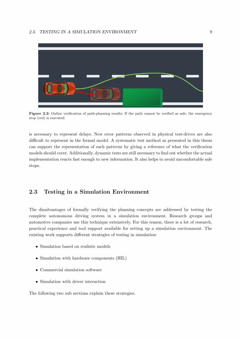
[40]–[42] to verify the planned path online in any current situation as depicted in Figure 2.2. The
green path is the path to be verified for collision freedom under all expected inaccuracies. If the
analysis cannot verify it to be safe, the autonomous vehicle follows the red path to a previously
verified safe stop. The verification uses a simplified model of the vehicle that the authors validate
by comparing it to a more complex model in simulation. One disadvantage of verification is that
it limits the types of sensor and actuator errors to be modeled. For example, delays are difficult
to represent. Errors are often modeled as a linear function of the current state of the vehicle.
Delays are either not linear, or not a function of the current state. Therefore, further effort
2.3. TESTING IN A SIMULATION ENVIRONMENT 9
Figure 2.2: Online verification of path-planning results: If the path cannot be verified as safe, the emergencystop (red) is executed.
is necessary to represent delays. New error patterns observed in physical test-drives are also
difficult to represent in the formal model. A systematic test method as presented in this thesis
can support the representation of such patterns by giving a reference of what the verification
models should cover. Additionally, dynamic tests are still necessary to find out whether the actual
implementation reacts fast enough to new information. It also helps to avoid uncomfortable safe
stops.
2.3 Testing in a Simulation Environment
The disadvantages of formally verifying the planning concepts are addressed by testing the
complete autonomous driving system in a simulation environment. Research groups and
automotive companies use this technique extensively. For this reason, there is a lot of research,
practical experience and tool support available for setting up a simulation environment. The
existing work supports different strategies of testing in simulation:
• Simulation based on realistic models
• Simulation with hardware components (HIL)
• Commercial simulation software
• Simulation with driver interaction
The following two sub sections explain these strategies.

10 CHAPTER 2. STATE OF THE ART
Simulation Models
Perception
sensor models
Vehicle dynamics
Road surface
Wind
Traffic
model
Obstacle model
Localization
sensor models
Figure 2.3: Models involved in an autonomous driving simulation: There are localization and mapping sensormodels including obstacle models, vehicle dynamic models including the effect of the road surface and wind, andmodels of traffic participants.
2.3.1 Realistic Models for Simulation
Simulation cannot be identical to the execution in a physical environment: There is always a
gap between those two–the reality gap [43]. A simulation without a reality gap requires perfect
models. Figure 2.3 shows the models that are involved in an autonomous driving simulation.
Sensor models specify how the vehicle perceives its environment. The main sensors are for
mapping the environment and localizing the car. Ultrasonic sensors, laser scanners, radars and
cameras are the major contributors for mapping algorithms. On the one hand, models of these
sensors help to increase the mapping performance [44], [45]. On the other hand, ultrasonic
sensor models [46]–[48] and camera models [49] are used to test autonomous vehicles. Global
Navigation Satellite Systems (GNSS) [50], [51], environment features detected by camera [52],
[53] and odometry [54] are the basis of localization concepts. Each concept has different error
characteristics that have to be modeled. Additionally, vehicle dynamic and actuator models like
Vedyna [55] precisely model the behavior of the vehicle depending on the road model [56]. Some
researchers also learn models during the execution of the autonomous system [57], [58] in order
to improve the decision-making performance. The models can also include environment events
like wind coming from the side (large blue arrow in Figure 2.3). Finally, the traffic interacting
with the autonomous vehicle can be simulated using traffic simulation engines like Sumo [59].
One limiting factor of tests in simulation environments is computation power. For this reason,
research groups try to accelerate the simulation by parallelizing simulation flows [60] and
reducing the complexity of the simulation that consists of many parts [48], [61].
Mature vehicle simulations can reduce development cost. For this reason, several commercial
simulation software systems are available. Examples are Virtual Test Drive of Vires1 presented
1http://www.vires.com/docs/VIRES_VTD_Details_201403.pdf

2.3. TESTING IN A SIMULATION ENVIRONMENT 11
in [62], the Pre-Crash Scenario Analyzer (PRESCAN)2 from Tass International presented in [63]
and CarMaker of IPG Automotive3. Research teams are also working on integrating existing
simulation components into a larger framework [64].
Hardware in the Loop (HIL) tests can further reduce the reality gap by using physical hardware
for parts of the simulation. In this setup, parts of the system are included as real hardware. This
can include electronic control units to run the software, and parts of the actuators and sensors.
For example, the HIL tests can use the physical camera in combination with a computer screen
[65] instead of a camera model. As an alternative, the VEHIL setup [66]–[68] models traffic
participants as physical elements by using a base moving at the relative speed of the vehicle.
This way, it can integrate physical radar sensors and laser scanners into the HIL setup.
2.3.2 Simulation with Driver Interaction
The HIL setup does not include a physical representation of the human sitting in the car. In the
physical world, the human influences the system by interacting with its interface or intervening
in critical situations. For the autonomous driving system, this adds additional nondeterminism.
Driving simulators add this missing human element. Sensors and software systems require only a
simulation of aspects they need for their core function. In contrast, a human behaves differently
if the simulation does not feel real. Thus, a driving simulator has to recreate the physical world
as realistically as possible. This includes vision, acoustics, the cabin interior and inertial effects
of the vehicle movements. The latter aspect is the most challenging one. A widespread version of
driving simulators mimic vehicle dynamics by moving a cabin, the driver sits in. A hexapod can
rotate this cabin and simulate accelerations [69], [70]. Additional rails in one [71], [72] or two
[73], [74] directions simulate long motions potentially with high acceleration in those directions.
A cost and space efficient alternative to hexapod systems is using a robot arm [75].
Instead of using an indoor device, the Vehicle in the Loop (VIL) concept [76]–[78] uses physically
moving vehicles and simulates the driver’s vision. The vehicles move on a testing ground without
obstacles. Inside the car, the passenger does not see the exterior, but a simulation. The virtual
car moves in this simulation, interacts with traffic participants and encounters dangerous events
while the physical car safely moves in an empty plane producing the same inertial effects. This
setup is also used for testing autonomous driving systems without driver interaction in a realistic
but safe environment [79].
The mechanisms described in the previous sub sections are not sufficient for generating the same
behavior as in physical tests. In particular, they do not consider nondeterminism of sensors,
actuators and traffic. Instead, they can be used as a basis to improve the simulation for the
approach presented in this thesis.
2https://www.tassinternational.com/prescan3http://ipg.de/de/simulationsolutions/carmaker/

12 CHAPTER 2. STATE OF THE ART
Effectivity of the test method
Sym
bo
lic
exec
uti
on
Ran
do
m t
esti
ng
Co
mp
lex
ity o
f th
e S
UT
Mo
del
chec
kin
g
wit
h d
ynam
ic a
nal
ysi
s
ST
AR
VE
C
Syst
emat
ic r
and
om
test
ing
Figure 2.4: Classification of test methods according to the maximal possible complexity of the SUT and theeffectivity in finding faults. Random testing can be applied to complex systems but misses many faults, whereassymbolic execution is limited to less complex systems but finds a large portion of existing faults.
2.4 Simulation with a Set of Possible Events
From the perspective of the planning and control algorithm in an autonomous vehicle, the
vehicle and its environment behave nondeterministically. Nondeterministic input is a well-studied
problem in software engineering. Typically, the nondeterminism is the input of a user or
another system. Robust and secure applications have to ensure their functionality for arbitrary
input. Symbolic execution is a successful approach for finding defects like access violations in
software systems. The concept replaces real values of inputs and variables by symbols and
branch conditions by constraints [80]. This way, it can execute a range of possible input values
at once. A constraint solver generates actual inputs leading to a software error. Researchers
have successfully applied symbolic execution to basic libraries of operating systems [80] and
to generating exploits [81]. However, it suffers from the path explosion problem and generates
constraints that can become hard to solve [82]. This makes it difficult to apply it to complex
programs. For the programs analyzed by symbolic execution, the input is usually limited to a
small size, which reduces the analysis computation requirements.
Figure 2.4 classifies test methods according of the maximal possible complexity of the SUT
(System Under Test) and the effectivity of the test method in finding faults. This plot classifies
symbolic execution as effective in finding faults. It does not reach the maximal effectivity because
only restricted input spaces are checked. The low value in the vertical axis indicates that it can
handle only a limited complexity of the tested software.
In order to cover problems that are more complex, the authors of [83] combine model checking
with dynamic analysis. Similarly to the approach presented in this thesis, they use both sound
and unsound abstractions for the decision whether the analysis has already visited a state. If
the analysis has visited a state that is mapped to the same abstraction, it also considers the
regarded state as visited. This allows model checkers to test complex software efficiently. Figure
2.4 lists the approach further to the left, as it might overlook some bugs due to the unsound
abstractions. The unsound abstractions trade some effectivity for the ability to cope with higher

2.5. TESTING IN THE PHYSICAL WORLD 13
complexity. Model checking can also be used to ensure that a test method reaches high coverage
according to some metrics. Some research teams [84], [85] generate test cases based on Linear
Temporal Logic and model checking.
Collisions caused by planning and control software are still too complex for the abstractions
mentioned above. Therefore, a typical approach in the automotive industry is to add random
noise to sensor measurements. Testing tools like Exact [86], or Time Partition Testing (TPT) of
PikeTec [87] support simulation with such noise. Frameworks like Open Robinos [88] can also add
noise. Random testing is applicable to programs of any complexity and is thus listed with a high
value in the vertical axis in Figure 2.4. The disadvantage is that they only test a very small subset
of possible inputs and are hence not as effective in finding bugs as symbolic execution. In order to
use this subset efficiently, researchers try to create a noise distribution that is close to reality [89],
[90]. The authors of [91], [92] apply randomized algorithms for validating the collision probability
of an Adaptive Cruise Controller in a simulation environment. Using Chernoff bounds, they
estimate the number of experiments necessary for a predefined accuracy and reliability. They
increase the efficiency by applying importance sampling: Prior known successful or failing tests
are not executed. In Figure 2.4 this systematic random testing is listed as more effective than
classic random testing. It achieves effectivity by the assumption that it already knows some
successful test results, which reduces the maximal complexity of the system it can analyze.
In [93], the impact of sensor noise on driver assistance functions is explored using a novelty
search [94]. They apply periodic or constant noise patterns and evaluate the results focusing
on creating as different results as possible. As they do not compare intermediate states, their
method only finds constant noise patterns leading to undesired behavior. That is, the deviation
between ideal and simulated sensor measurements remains constant. In contrast, the STARVEC
algorithm presented in this thesis finds scenarios in which fluctuating error patterns are worse
than constant patterns, as shown in Chapter 6. In Figure 2.4 the approach of [93] would be close
to systematic random tests.
For actual automotive software further assumptions are applicable that fill the gap between
systematic random testing and model checking. The authors of [95] use rapidly exploring random
trees in order to determine the worst-case performance of a control component in the presence
of disturbances to state variables. The approach works for a controller with a very limited set
of state variables. This thesis extends a similar approach to more complex systems and error
patterns.
2.5 Testing in the Physical World
In addition to virtual testing, physical tests are necessary to validate autonomous driving
systems. Typically, professional test drivers or automated test systems4 execute defined scenarios
4ATG, Automated Testing Ground: https://youtu.be/8czFgk26qZ8

14 CHAPTER 2. STATE OF THE ART
either on a dedicated testing ground like AstaZero [96] or on public roads [97]. Engineers have
to reproduce the faults occurring during these physical tests in order to understand and repair
the causative defect.
Reproducing faults is also a challenge for the teams that participated in the DARPA Urban
Challenge [98] and implement autonomous vehicles. They deal with faults by recording
communication data when it occurs and replay the data in order reproduce it. Two of the eleven
finalist teams explicitly describe how they reproduce failures [99], [100] and seven mention that
they are able to record and playback communication data [101]–[107] most likely also used for
reproducing faults. The remaining two teams do not explain how they deal with such problems
[108], [109].
However, these logs can become very large and are not always sufficient for reproducing failures
due to nondeterminism and missing initialization sequences. Some research groups reduce the
size and the time necessary for replaying the communication logs by removing or shortening
unnecessary parts [110], [111]. Instead of using communication signal logs, the input arguments
of single functions are stored by [112]. If a fault occurs within this function, the authors can
quickly replayed it with little effect of nondeterminism. Instead of a communication log, [113] uses
general log messages emitted at any position in the code in order to reproduce the execution
path leading to the fault. [114] automatically enhances log outputs in order to increase the
performance of this method. If no logs are available, program crash dumps can guide randomized
testing [115] trying to reproduce the fault. However, these methods do not robustly reproduce
any faulty behavior caused by the complex inputs of planning and control systems. Section 5.3
shows how fault reproduction can be performed more robustly for automotive applications.
2.6 Sources for Test Scenarios
Both simulated and physical tests require defined test scenarios, which are extracted from
• requirement documents,
• problem understanding for creating parameterizable scenarios or
• gathered data.
Requirement documents are the first source for defining test scenarios. They should list the
different types of scenarios to be expected. For each of these scenario types, there should be a
test case either derived manually or supported by systematic specifications [116].
In addition to requirement documents, autonomous driving engineers understand the potential
scenarios the function should support. By using this understanding, they can create test scenarios
that cover as many relevant cases as possible. The authors of [117], [118] present a method for
generating test cases for a parking system by evaluating the results of each test run. Using

2.6. SOURCES FOR TEST SCENARIOS 15
a heuristic, they try to push the test executions toward collisions by altering the starting
conditions, for example the shape of obstacles.
The third source of relevant scenarios is gathered data. Accident databases like the German
GIDAS (German In-Depth Accident Study) database [119] provide such data. These databases
contain information about the accident causes, which has been gathered by specialized teams
after severe accidents. Other countries maintain similar databases. The efforts of [120] harmonizes
these databases. As it contains particularly dangerous and difficult scenarios, the data from these
accident databases is relevant for test cases. The authors of [121], [122] reproduce these scenarios
and the street geometries of the accident in a simulation environment. The reconstruction can be
enhanced by using three-dimensional geographic data for modeling the terrain characteristics.
The reproduced scenarios are used to evaluate the expected performance of new driver assistance
functions with additional sensors [123].
Alternatively, engineers can extract the data from physical test-drives. Wachenfeld et. al [124]
propose to equip consumer vehicles with the necessary sensor and computing power to gather
real world scenarios and perform short simulation sequences. As the scenarios are extracted
from the real world, they have the same random distribution as in the real world. In frequently
started short simulation sequences, an ADAS (Advanced Driver Assistance System) can take
over control of the simulated vehicle. The shortness of the simulation increases the realism. If
the ADAS causes a collision in the simulation, engineers can address the problem. The physical
vehicle remains safe because a human controls it.
Scenario generation can also be supported by using laser scanners as a reference sensor system
for recording real world scenarios [125] or running simulations parallel to actual task executions
in order to detect faults [12]. Finally, there are public databases for relevant scenarios like
Kitti for vision benchmarks [126] or the Next Generation Simulation Program [127] for traffic
scenarios. This thesis contributes to the state of the art by proposing a method for collecting
scenarios of almost-accidents during any physical vehicle drive. These almost-accidents only
remained collision free, because the sensor and actuator inaccuracies did not affect the vehicle
more strongly than they did.
Chapter 3
Modeling the Environment of an
Autonomous Vehicle
The algorithm presented in this thesis searches for undesired behavior of an autonomous driving
system in a simulation environment. For this purpose, it must be possible to produce the
undesired behavior in a simulation environment. This chapter investigates how to design a
simulation environment that supports the generation of physically possible behavior. First,
Section 3.1 describes how a simulation environment can represent physical scenarios. It divides
the simulation into an ideal behavior and separately handled inaccuracy models. Section
3.2 discusses modeling the ideal behavior. The description of inaccuracy models that enable
the simulation environment to approximate physical behaviors follow in Section 3.3. These
inaccuracy models have to be configured based on data from physical vehicles described in
Section 3.4. Using the simulation, engineers can search for undesired behaviors as defined in
Section 3.5.
3.1 Representing Physical Vehicle Scenarios in a Simulation
Environment
The first step to simulate undesired behavior that is possible in reality is to ensure a
correspondence between simulation and the physical world. The design of the simulation
environment has to ensure this correspondence. This section starts with describing the physical
world as a mathematical set of states and a transition function in Section 3.1.1. Section 3.1.2
describes the simulation system the same way. Finally, Section 3.1.3 investigates how these two
systems relate to each other.
16

3.1. REPRESENTING PHYSICAL VEHICLE SCENARIOS 17
QSE : Simulation properties:shape of the street, surfaceproperties, vehicle position
QS : Planned path, internalrepresentation of theenvironment
Qsimulation states = QSE ×QS
Sim
ula
tion
QPE : Configuration of everyatom in the environment
QS : Planned path, internalrepresentation of theenvironment
Qphysical states = QPE ×QS
Phy
isca
lw
orld
Figure 3.1: States in the physical world and states in the simulation world consist of the vehicle software stateplus the state of the remaining world or the remaining simulation.
3.1.1 Modelling the Physical World
From a mathematical perspective, the state of the physical world is an element of the set of all
possible physical states Qphysical states. The behavior of the physical world can be regarded as
a function Fphysical world that determines the state of the world after a specified time t ∈ R+
has passed. If the physical world is known perfectly, this function can be approximated as
deterministic.
Fphysical world : Qphysical states × R+ → Qphysical states (3.1)
As the focus of this thesis lies on representing the behavior of a vehicle, it is reasonable to divide
the physical states into the states of the software system QS and the states of the physical
environment QPE :
Qphysical states = QPE ×QS (3.2)
This partition is also depicted in Figure 3.1. The state of the software system QS consists
of all information stored by the software. This includes the path it plans to follow and the
internal representation of the environment. The state of the physical environment QPE contains

18 CHAPTER 3. MODELING THE ENVIRONMENT
everything else, including the configuration of every atom in the environment. As explained in
the next section, the simulation environment can be split up similarly.
The software system consists of runnable entities, each of which has a cycle time. The runnable
entity reads its input, performs computations and writes its result to the output ports after
its cycle time has passed. Computations taking longer than the specified cycle time either
are handled inside the runnable entity by storing intermediate values as an internal state or
represent a software fault. This kind of fault can be detected by timing analysis tools and is
not considered in this thesis. Most computations finish before the cycle time ends. Idle waiting
time can extend these computations to take exactly as long as the cycle time. The remaining
case are computations taking exactly as long as their allotted cycle time. Because of the discrete
cycle times of the runnable entities, a time discrete finite state machine can represent the whole
system:
∆physical world(spw) := (FS(spw), FPE(spw))
spw := (xPE , xS)
FS(spw) := FS(xS , y(xPE))
FPE(spw) := FPE(xPE , u(xS)) (3.3)
where ∆physical world is the transition relation. spw is the state of the physical world, which
consists of the state of the physical environment xPE and the state of the vehicle software xS .
FS is the transition function of the software system, which depends on the current state of the
vehicle software and the perception y(xPE) of the environment state xPE . FPE is the transition
function of the environment that depends on the current actions u(xS) of the software system
and the current state of the environment. The state of the environment xPE may contain the
history of previous actions that affect the environment with some delay. The following sections
use this representation to compare the transitions in the physical world to the transitions in a
simulation system.
3.1.2 Modeling the Simulation System
The equivalent system can be defined for a simulation system by a set of simulation states
Qsimulation states = QSE ×QS (3.4)
where QSE is the set of states of the SE (Simulation Environment) and QS is the set of
software states as defined in the previous section. Similar to Equation 3.3, the transition function

3.1. REPRESENTING PHYSICAL VEHICLE SCENARIOS 19
∆sim world of the simulation system can be represented as:
∆sim world(ssw, e) := (FS(ssw, e), FSE(ssw, e))
ssw := (xSE , xS)
FS(ssw, e) := FS(xS , ysim(xSE , e))
FSE(ssw, e) := FSE(xSE , u(xS), e) (3.5)
where ssw is the state of the simulated world, e is an event, FSE is the transition function
of the simulation environment, xSE is the state of the simulation environment and ysim is the
simulated perception. As before, the software system is represented by its transition function
FS , its state xS and its currently performed action u(xS).
In contrast to the function representing the physical environment, Equation 3.1.2 explicitly
includes events e that occur during a simulation step. These events represent nondeterministic
behavior of the vehicle and the environment. Such nondeterministic events exist, because the
simulation system does not model the physical world perfectly. Not modeled parts are assumed
nondeterministic.
The transition function of the software FS is the same as for the physical world. The perception
y of the physical state xPE is replaced by the simulated perception ysim of the simulated world,
which depends on the current event e. Similar to the transition function FPE of the physical
environment, the transition function FSE of the simulation environment depends on the current
state xSE and the current input u. Additionally, it depends on the nondeterministic event e.
Equation 3.6 splits the transition function FSE into the ideal behavior as described in Section
3.2 and deviations to the ideal model as described in Section 3.3. The split version of FSE is:
FSE(xSE , u, e) = FSE,ideal(Ex(xSE , e), Eu(u, xSE , e), u) (3.6)
where FSE,ideal is the ideal behavior of the vehicle according to the vehicle model described in
Section 3.2. Additionally to the current state and the applied action, it depends on the requested
actions because the simulation state is modeled to contain a history of requests. Ex is the error
applied directly to the simulation state as defined in Section 3.3.5 and Eu is the error applied
to the input values as defined in Section 3.3.2. Eu may depend on the current simulation state
including the history of previously applied actions.
Similarly, ysim can be split into an ideal perception model ysim,ideal and deviations to the model:
ysim(xSE , e) = Ey(ysim,ideal(xSE), e) (3.7)
where Ey is the inaccurate perception defined in Sections 3.3.3 and 3.3.4.

20 CHAPTER 3. MODELING THE ENVIRONMENT
FSE,ideal and ysim,ideal can be computed by existing simulation tools like the ones mentioned in
Section 2.3. The approach presented in this thesis makes no assumptions about the complexity
of the simulation tool, i.e. it can be arbitrarily complex.
3.1.3 Correspondence between the Physical World and the Simulation
The goal of the simulation is to model the physical environment. Hence, every state spw in the
physical world has a representation ssw in the simulated world:
ssw = Rphys→sim(spw) (3.8)
The ability to represent a physical state in a simulation environment does not imply the ability to
represent a behavior. A behavior can be described as a sequence of states (spw,0, spw,1, ..., spw,n).
This sequence can be mapped to a sequence of simulation states based on Equation 3.8. A
simulation execution also visits a set of simulation states. In theory, a simulation execution
that visits exactly the mapped states might exist. In practice, this is usually impossible for two
reasons: Firstly, the simulation might run in an incompatible frequency. Secondly, numerical
errors lead to slight deviations even if the simulation is almost perfect. Instead, the simulation
can approximate a physical behavior by executing an approximated sequence. Each state of the
approximated sequence has to be similar to a state of the physical sequence that is mapped
using Equation 3.8.
Figure 3.2 visualizes the approximation. The upper part of the image represents the physical
execution. It corresponds to the execution in the simulation environment in the lower part of
the image. The small blue circles represent states in the physical and the simulated world. The
physical states have a representation in the simulation environment represented by the vertical
lines. However, these states are not identical to the states of the simulation sequence. Therefore,
the represented physical states are mapped to the closest simulated state indicated by horizontal
lines. Multiple physical states can be mapped to one simulation state. In Figure 3.2, spw,5 and
spw,6 are mapped to ssw,6. Some simulation states can have no physical state mapped to them,
as ssw,5 in Figure 3.2. If the distance to the closest simulation state indicated by the horizontal
lines is short enough, the simulation sequence approximates the physical sequence.
This can also be formally measured: A sequence of n states observed in the physical vehicle
(spw,0, spw,1, ..., spw,n) (small circles in the upper image) can be approximated in the simulation
environment according to a distance metric
µdistance : Qsimulation states ×Qsimulation states → R+0 (3.9)

3.1. REPRESENTING PHYSICAL VEHICLE SCENARIOS 21
ssw,0 ssw,1 ssw,2
ssw,3
ssw,4 ssw,5ssw,6
Simulation
spw,0 spw,1spw,2
spw,3spw,4 spw,5
spw,6
Phyiscalworld
< α
Figure 3.2: Representation of a physically driven sequence (upper part) in a simulation environment (lowerpart). Each physical state can be represented in the simulation (vertical lines) and is mapped to a simulated state(horizontal lines). The distance between the representation and the mapped state should be small (“< α”).
and an accuracy α ∈ R (vertical lines) if the following conditions apply: Firstly, there is a
sequence of m simulation states (ssw,0, ssw,1, ..., ssw,m) and m simulation events (e0, e1, ..., em)
and a monotonous function fmapping : N0 → N0. Secondly, this sequence can be executed in the
simulation system:
∀i ∈ {0, 1, ...,m− 1} : ssw,i+1 = ∆sim world(ssw,i, ei) (3.10)
Thirdly, each state of the physical sequence is approximated by a state of the simulation sequence:
∀i ∈ {0, 1, ..., n} : µdistance
(Rphys→sim(spw,n), ssw,fmapping(n)
)≤ α (3.11)
The approximation error α and the mapping function fmapping are intended to compensate
discretization effects but not significant deviations like model inaccuracies. This notion of
approximation implies that an abstract error in the simulation environment can approximate a
different error occurring in the physical world. For example, the physical vehicle accelerates
with a delay of 0.1 s. In this example, the simulation environment does not model delays,
but only offsets of up to 0.1 m s−2. However, this simulation environment might still be able
to approximate physical vehicle sequences using the acceleration offsets. Section 3.3.2 further
discusses this flexibility.

22 CHAPTER 3. MODELING THE ENVIRONMENT
The whole simulation environment has a high recall if it can approximate all sequences observed
on a physical vehicle as further discussed in Section 3.3.1.
A simulation sequence is physically possible if there is a corresponding sequence of states
(spw,0, spw,1, ..., spw,n) that can be observed in the physical world. The simulation sequence has
to approximate the representation of the sequence of physical states according to Equation 3.8.
In practice, it is usually impossible to replay a sequence observed in a simulation environment
in the physical world. Instead, software engineers can argue based on experience and for a single
example whether it is reasonable to assume that a simulation sequence is physically possible.
Physically impossible sequences are a result of imprecise error models. Modeling extreme
inaccuracies as events makes it simpler to create a simulation environment that can represent all
sequences executed by a physical vehicle. However, this simulation environment will produce
many sequences that are not physically possible. Such sequences are only a problem if a
conclusion is based on these sequences. The approach presented in this thesis produces example
sequences for detected undesired behaviors. Engineers can use these sequences to discuss for a
single example whether it is physically possible. If the sequence is physically impossible, the
simulation system can be refined to avoid such sequences while remaining able to represent all
sequences observed in the physical vehicle. This is more efficient than eliminating all physically
impossible sequences from the simulation system.
To summarize, the simulation environment should be able to approximate all physical behavior
sequences. This can be ensured by designing the inaccuracies to the environment perception, the
actions on the environment and the simulation state itself accordingly. Inaccuracies leading to
physically impossible behaviors are only a problem if these behaviors are relevant. In this case,
the inaccuracy models have to be adapted accordingly. An example definition of a simulation
that can approximate physical behaviors is listed at the end of Section 3.3.2.
3.2 Vehicle and Environment Model
As explained in the previous section, the simulation environment is divided into a deterministic
simulation and some nondeterministic error events. This section discusses the deterministic
simulation. The simplest simulation environment that is able to represent all physical behavior
patterns contains only a single simulation state. All physical states are mapped to this state.
Hence, all physical state sequences can be mapped to sequences in the simulation. However, such
a simulation would also be able to represent relevant but impossible physical sequences. For this
reason, the simulation should at least model the basic geometry and dynamics of the vehicle.
The standard tool for modeling a vehicle used for static planning algorithms is the simple
single-track model [128]:
3.3. MODELLING INACCURATE SENSORS AND ACTUATORS 23
xyθ
=
v · cos(θ)v · sin(θ)
v · tan(Ψ)/L
(3.12)
where x and y are the position, θ is the orientation, v is the speed, Ψ is the steering angle and
L is the distance between the axles of the vehicle.
For low speed scenarios, the simple single-track model performs already similar to the actual
vehicle if all actuators perform ideally. As the evaluations in this thesis are performed on low
speed scenarios, they are based on a similar single-track model. As discussed in the previous
section, this model is still able to represent all physical scenarios including high-speed scenarios
if the inaccuracy models are designed accordingly. Section 3.3 describes these models. Similarly
to the very simple model described at the beginning of this section, the simple single-track model
can be insufficient for some applications. It can create deviations between simulation and reality
that result in collisions in simulation and that are therefore relevant. However, these collisions
are not physically possible. Thus, a suitable model for the scenarios to be tested must be chosen.
For example, the simulation approaches described in Section 2.3.1 can be used for modeling the
vehicle accurately. Furthermore, car manufacturers have developed their own models, which
are particularly accurate for the properties important for specific development projects. Any of
these simulation environments can be used together with the STARVEC framework presented
in this thesis. The simulation environment is only required to be able to transmit its current
vehicle state and allow setting the current vehicle state. Attaching any simulation environment
is possible, because the concept directly executes the simulation without interfering with the
actual model computations. The proposed error models only adjust the inputs and the outputs
of the simulation tool.
3.3 Modelling Inaccurate Sensors and Actuators
The previous section introduced nondeterminism for closing the reality gap between simulation
and the real world. Figure 3.3 illustrates some sources of nondeterminism. The nondeterminism
covers
• inaccuracies of sensors and actuators,
• deviations between the used simulation model and an ideal model,
• variations to the scenario like different ground or changing wind conditions and
• additional nondeterministic events as described in Section 4.5.
The corresponding nondeterministic models are described in the following. First, Section 3.3.1
introduces the concept of precision, recall and efficiency advocating to aim for high recall.

24 CHAPTER 3. MODELING THE ENVIRONMENT
Inaccuratelocalization
Inaccuratevehicle model
Inaccurateactuators
Inaccurateenvironment map
Figure 3.3: Sensors, actuators and the vehicle model are inaccurate.
The following sub sections describe the different kinds of inaccuracies. They cover actuator
inaccuracies in Section 3.3.2, positioning inaccuracies in Section 3.3.3, mapping inaccuracies in
Section 3.3.4 and model inaccuracies in Section 3.3.5.
3.3.1 Precision, Recall and Efficiency
The sensor and actuator inaccuracy models must represent the reality as well as possible. The
models receive parts of the simulation state as input and compute possible behaviors as output.
As these models include nondeterminism, multiple resulting patterns are possible. For example,
a gas pedal model receives the current acceleration command as input and generates possible
resulting vehicle velocities as output. The quality of the model can be represented based on
three metrics: The model should achieve high
• recall,
• precision, and
• efficiency.
Recall is the “proportion of all the relevant documents in the collection that are in the result
set” [129]. In the context of this section, the result set is the set of generated behaviors and the
relevant set is the set of physically possible behaviors. Hence, high recall means that actions that
can be observed of physical sub systems can also be generated by their simulated counterpart.
The gas pedal model mentioned above has a high recall if the observed velocities in the physical
world are included in the model output. A trivial gas pedal model achieving 100% recall emits
the full velocity range as output. If the whole simulation has a high recall, undesired behaviors
that can occur in reality can also be reproduced in simulation. Precision is the “proportion of
documents in the result set that are actually relevant” [129]. In the context of this section,

3.3. MODELLING INACCURATE SENSORS AND ACTUATORS 25
Physically possible paths
Possible in Simulation
(a) High recall, low precision
Possible in Simulation
Physically possible paths
(b) High precision, low recall
Figure 3.4: Recall vs. precision: Figure 3.4(a) shows that low precision can lead to accidents that are predictedbut physically impossible. Figure 3.4(b) depicts a physically possible unintended lane departure that the simulationdoes not predict.
high precision means that the inaccuracy model does not allow more deviation from the ideal
behavior than the physical world does. A gas pedal model allowing exactly one resulting velocity
for any requested acceleration achieves high precision.
Figure 3.4 illustrates the effects of precision and recall. The green and orange shapes depict the
area that the red ego vehicle might cover in the future. Both shapes are broader than the vehicle,
because sensor and actuator inaccuracies can lead to different behaviors covering different areas.
The green shape contains all physically possible paths that a perfect simulation would predict.
The orange shape depicts the behaviors predicted by the imperfect simulation. Figure 3.4(a)
shows the effect of high recall, but low precision. The simulation (orange shape) predicts all
behavior patterns that are possible in the physical world (green shape). However, the simulation
additionally predicts patterns that are not physically possible including a frontal collision with
the approaching truck. A test method using this simulation would falsely classify the autonomous
driving system as unsafe. In contrast, Figure 3.4(b) depicts a simulation that achieves high
precision by assuming ideal behavior of sensors and actuators. This simulation correctly predicts

26 CHAPTER 3. MODELING THE ENVIRONMENT
that no collision with the truck is possible, but fails to predict than an unintended lane departure
is possible. A test method that uses this simulation cannot find any errors of the autonomous
driving system, although an error is possible.
The third metric is efficiency. Efficiency includes test computation efficiency and model validation
efficiency. Test computation efficiency means that the model enables the test algorithm to be
efficient. The test method presented in this thesis is more efficient if the model output is described
by few parameters. For example, the acceleration inaccuracy can be modeled to result in a range
between a minimal and a maximal possible acceleration, which corresponds to a single parameter
to be varied. Other test methods may have other requirements for the models. Hence, the test
computation efficiency depends on the used testing concept. The second part of efficiency is
model validation efficiency. High model validation efficiency means that only a low amount
of physical vehicle drive data is necessary for determining inaccuracy boundaries. Section 3.4
explains this process. A model that computes the output based on the input plus a value between
a minimal and a maximal offset can be validated efficiently. Each data point of a physical
test-drive directly contributes to all model parameters: the minimal and the maximal offset.
A model containing many special cases cannot be validated efficiently. Each data point of a
physical test-drive only contributes to the currently active special case. This requires a large
amount of data in order to have sufficient information for each model parameter.
The first goal of creating a model is to achieve high recall. This corresponds to the concept
of over-approximation often used for verification [130]. If the test algorithm then classifies the
autonomous driving system as safe, the precision of the model is sufficient. If it finds weaknesses
that seem physically impossible, engineers should increase the precision, possibly at the cost of
efficiency.
3.3.2 Actuator Inaccuracies
The main vehicle actuators are the acceleration (gas pedal, brake) and the steering (steering
wheel) actuators. Hence, the action u(xS) in Equation 3.1.2 can be written as:
u(t) := u(xS(t)) =
(a(t)
Ψ(t)
)(3.13)
where xS(t) is the state of the software at time t, a(t) is the requested acceleration at time t,
Ψ(t) is the requested steering angle. A more precise model might include additional actuators
like light switches or gear selection.

3.3. MODELLING INACCURATE SENSORS AND ACTUATORS 27
The first input is the acceleration. Figure 3.51 shows some of the factors influencing the performed
acceleration. Each of these factors can have a complex influence on the actually performed
acceleration as expressed in Equations 3.14-3.17.
aact(t) = Fwheel(ftorque(t), spw,t) (3.14)
ftorque(t) = Fmotor,brake(ccommands(t), smotor(t)) (3.15)
ccommands(t) = FECU (ftorque,desired(t), sECU (t)) (3.16)
ftorque,desired(t) = Facccontr(ades(t), sacccontr(t)) (3.17)
The actually performed acceleration aact(t) depends on the road conditions, the state of the
wheels, the dynamic state of the vehicle and many other influences. Equation 3.14 summarizes
that as a function Fwheel of the applied torque ftorque(t) and the state of the physical world spw,t.
In exceptional cases, the acceleration may have no direct correlation to the applied torque. Such
cases can be modeled separately. For normal operation, Equation 3.18 simplifies the complex
correlations to a nondeterministic function Fwheel. It implements a factor between a minimum
cw,min and a maximum cw,max, an offset between −ow and ow and a delay ∆tw to the ideal
translation of torque to acceleration. However, neither the maximal factors, nor the maximal
offset or the delay is known.
Fwheel(ftorque(t)) ∈ [cw,min; cw,max] ∗ Fw,ideal(ftorque(t−∆tw)) + [−ow; ow] (3.18)
The state of the motor itself is complex, too. It consists of the state of the throttle, the state
of the cylinders, of the direct injection motors, the emission control systems and other factors
summarized as smotor(t) in Equation 3.15. The ECU (Engine Control Unit) controls these states
and the behavior of the motor by commands ccommands. The state of the motor and the commands
of the ECU define the resulting torque by some unknown function Fmotor,brake as described in
Equation 3.15.
The ECU defines these commands by its implementation FECU . Additionally to implementing
the desired torque ftorque,desired, it aims at smoothing the vehicle motion, reducing emissions,
extending the motor life and several other goals influencing its internal state sECU (t) in Equation
3.16. The smoothing mechanisms lead to inertia effects and the torque not being implemented at
the requested time. However, the engine controllers are designed to converge towards the desired
torque. That is, after some time ∆tECU ∈ [∆tECU,min,∆tECU,max] (with a constant request) the
1Public domain icons from https://commons.wikimedia.org/wiki: Digifant.jpg, Servofreno seccionado.jpg,Throttle body.jpg, and Sparkplug.jpg

28 CHAPTER 3. MODELING THE ENVIRONMENT
Planningand controlsoftware
Accelerationcontroller
Enginecontrol unit
Brakebooster
ThrottleSpark plugOther enginecomponents
Wheel forces
Desiredacceleration
Desiredtorque
Motor actuatorcommands
Brakeforce
Resulting torque
Figure 3.5: Components influencing the performed acceleration: the acceleration controller converts the desiredacceleration to a desired torque, which it passes to the engine and the brake control units. These units generatecommands for their hardware components leading to a resulting torque and a resulting acceleration.

3.3. MODELLING INACCURATE SENSORS AND ACTUATORS 29
engine performs a torque that differs from the desired torque by less than some offset oECU :
FECU = ftorque,desired(t− [∆tECU,min,∆tECU,max]) + [−oECU ; oECU ] (3.19)
The offset and the delay depend on the implementation of the ECU and the performance of the
physical translations and are hence not known.
Finally, some current serial production cars have an additional acceleration controller. It
computes the desired torque ftorque,desired(t) based on the desired acceleration ades(t) and its
internal state sacccontr as listed in Equation 3.17. As for the engine control unit, this controller
aims at multiple goals including smooth behavior of the vehicle. It is also designed to converge
towards the requested acceleration. Hence, after some time with a constant desired acceleration,
the performed and the desired acceleration are similar:
aact(t) ∈ [amin(t); amax(t)]
amin(t) = mintref∈[t−dmax;t](ades(tref))− omax
amax(t) = maxtref∈[t−dmax;t](ades(tref)) + omax (3.20)
aact(t) is the performed acceleration at time t, amin and amax are the minimal and the maximal
acceleration possible due to the nondeterminism. dmax is the maximal delay and omax is the
maximal offset between the requested and the performed acceleration.
The acceleration controller does not converge for accelerations that are requested for a very
short period of time. If the acceleration requests alternates between a very low and a very
high value, the performed acceleration is somewhere in between, but gets neither near the low,
nor the high request. This behavior is also included in the approximating equation 3.20. The
original Equations 3.14-3.17 are very complex, and contain many unknown values. Therefore, it
is reasonable to directly estimate the few parameters of the approximated equation instead of
the many parameters of the original equations. Due to the non-determinism, the behavior of the
complex original equations is included in the approximated equations.
A more radical approximation would model only offsets to the desired acceleration instead of
offsets plus delays:
aact(t) ∈ [ades(t)− omax; ades(t) + omax] (3.21)
With omax being the maximal allowed offset to the steering angle. This model is still able
to perform all behaviors possible by Equations 3.14-3.17. In a project connected to this thesis,
physical vehicle tests were performed. In these tests, a strong influence of delays to the performed

30 CHAPTER 3. MODELING THE ENVIRONMENT
t[s]
a(t)
0.5 1 1.5 2
0.5
1requested
observed
Delay
Offset
Figure 3.6: Effect of offsets and delays to the observed output. For rapidly changing inputs, the delay is thedominating pattern, for almost constant inputs, the offset dominates.
accelerations could be observed. Figure 3.6 illustrates the different effects of delay and offset to
the performed acceleration. The depicted maximal offset is as low as 0.05 m s−2, but there
is a constant delay of 0.2 s. Modeling this delay as offset results in a maximal offset of about
0.5m s−2, which is reached at t = 0.25s. This means a very low precision of the model. Therefore,
the suggested model for acceleration inaccuracies consists of an offset interval and an interval
between zero and the maximal acceleration delay dmax as shown in Equation 3.20.
This model allows efficient testing as the output can be described by a single parameter that
defines which acceleration between the minimum and the maximum is executed. Small variations
of these parameters lead to small changes of the vehicle behavior. The model also allows efficient
model validation as it includes no special cases. Special cases can be necessary for some situations.
For example, some vehicles show higher offsets when starting from zero velocity. Additionally,
quick changes to the acceleration request can lead to overshoots in the performed acceleration
[131]. Modeling such special cases increases the precision of the model at the cost of efficiency
as proposed at the end of Section 3.3.1.
Section 3.1.3 demands that there is a correspondence between the physical world and the
simulation. For a behavior in the real world, there should be a representation in the simulation
such that Equation 3.11 holds. If we regard an example in which only acceleration errors are
relevant, the inaccuracy model defined in this section fulfills this demand with:
• µdistance(s1, s2) is the Euclidean distance between the vehicle centers of states s1 and s2.
• The simulation states consist of the vehicle position, velocity and acceleration.
• Rphys→sim maps these continuous physical values to the nearest floating point numbers.
• The discretization is chosen to be α/2.

3.3. MODELLING INACCURATE SENSORS AND ACTUATORS 31
With these definitions, the simulation can approximate any acceleration behavior of the physical
world if the maximal acceleration offsets and delays are sufficiently high.
The combination of offset and delay can also model other temporal effects like inertia effects.
The steering inaccuracy is very similar to the acceleration inaccuracy with a different relation
between offset and delay.
In summary the inaccurate action Eu in 3.6 can be described as:
Eu(u, xSE , e) :=
(aact(t)
Ψact(t)
)(3.22)
Where aact(t) is the performed acceleration defined in Equation 3.20. The actual value is chosen
as defined by the current nondeterministic event e. Analogously, Ψact(t) is the performed steering
angle.
3.3.3 Positioning Inaccuracies
Autonomous vehicles use two different systems for estimating the position and the motion of
the vehicle: vehicle odometry and external position information. The vehicle odometry uses
wheel motion and inertia measurement sensors for estimating the relative motion of the vehicle.
Its accuracy decreases with the distance traveled due to undetected drifts and slips [129].
Therefore, a second system measures globally correct positions. This system can be based on a
Global Navigation Satellite System [50], artificial or natural landmarks [52] or other concepts.
The estimations of the system can jump, because of the incorporation of new information like
another satellite or a detected landmark. Autonomous planning and control systems can access
information from both systems.
Figure 3.7 shows exaggerated inaccuracies of these two positioning systems. The upper image
(Figure 3.7(a)) shows inaccuracies of the global positioning system. The deviation drifts away
from the true position, but every time the positioning system detects a new landmark or satellite,
it jumps back to the approximated true position. Some localization systems avoid these jumps
by replacing them with slow drifts back to the true position. The lower image (Figure 3.7(b))
shows inaccuracies of the odometry. The position estimations are smooth, but the deviation to
the true position has no upper limit.
The model for global position inaccuracies used in this thesis is a drift of the position and the
orientation of the vehicle. For example, the estimated x position xestimated(t) is computed as:

32 CHAPTER 3. MODELING THE ENVIRONMENTGlobal Positioning Inaccuracies
Driven path
Estimated path
(a) Global positioning inaccuracy
EML Inaccuracies
Driven path
Estimated path
(b) Inaccuracy of the odometry
Figure 3.7: Inaccuracies of positioning sensors. The top image shows typical global positioning inaccuraciesincluding jumps. The lower image shows inaccuracies of the odometry without jumps but high final inaccuracies.
xestimated(t) = xreal(t) + xoffset(t)
xoffset(t) =
{xnew, if new position is measured
xoffset(t−∆t) + xdrift(t), else
xdrift(t) ∈ [xdrift,min;xdrift,max]
xnew ∈ [xnew,min;xnew,max] (3.23)
where xreal(t) is the actual x position of the vehicle and xoffset(t) is the measurement offset to
the real x position. xnew is the measurement error after reading new positioning data. It can be
wrong by a value between a minimum xnew,min and a maximum xnew,max. In the experiments in
Section 6, this interval is modeled to be empty. xdrift is the velocity at which the measured x
position may deviate from the real x position and can be between a minimum xdrift,min and a
maximum xdrift,max. Additionally, the absolute offset is limited to a maximal value.
The inaccuracy of the odometry is similar without the option to jump back to a new measured
value. The odometry model has been implemented together with delays and inaccuracies of the
velocity measurement in [131] and is tested in the evaluation chapter.

3.3. MODELLING INACCURATE SENSORS AND ACTUATORS 33
Mapping Error
2
3
1
Figure 3.8: Inaccuracies of ultra sonic sensors. The upper left green box is detected at an inaccurate positiondue to ambiguous measured maxima (1). The red box is not detected due to insufficient sensor range (2). Thebottom green box is out of the sensor range (3) but leads to a not existing obstacle (blue box) being identified.
3.3.4 Mapping Inaccuracies
Autonomous vehicles perceive their environment based on various sensors including radar,
ultrasonic, laser scanners and centrally stored maps.
Ultra sonic sensors generate acoustic signals that are reflected by obstacles in the environment.
Figure 3.8 depicts three sources of errors of ultrasonic sensors: inaccurate measurements, sensor
capability limits and wrong signal assignment. They are related to effects visible in the raw
sensor signals depicted in Figure 3.9.
The first error source is inaccurate measurements. As depicted in Figure 3.9 the regarded signal
does not instantaneously change from zero to maximum. Additionally, sensor noise surrounds
the increase. Therefore, the return time of the acoustic signal cannot be determined precisely.
This leads to obstacles being detected at positions that deviate from reality. Accordingly, in
Figure 3.8 the detected obstacle (red line) of the top left sensor (cone 1) does not exactly match
the perimeter of the corresponding real obstacle (green box).
The second error source are sensor capability limits. One such limit is the minimal and maximal
sensor range. Ultrasonic sensors cannot detect obstacles closer than some minimum because the
emitted signal blinds the sensors for some time as depicted in Figure 3.9. Moreover, they cannot
detect obstacles that are further away than some maximum, because the reflected signals get
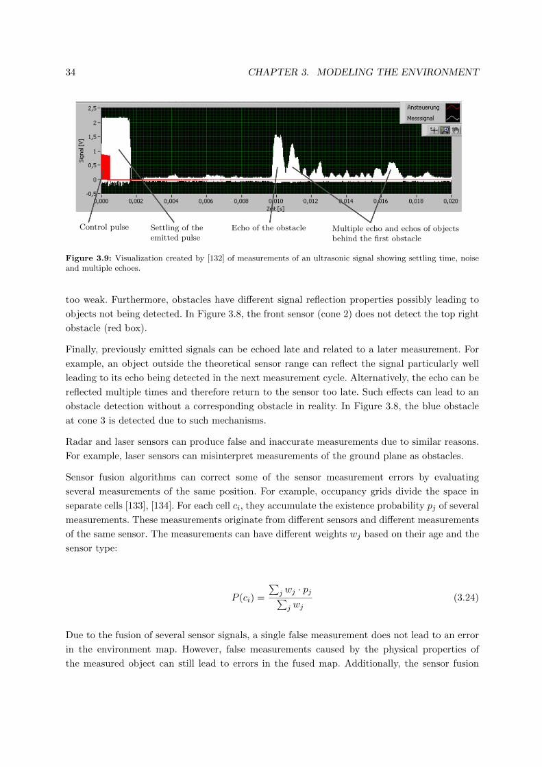
34 CHAPTER 3. MODELING THE ENVIRONMENT
Control pulse Settling of theemitted pulse
Echo of the obstacle Multiple echo and echos of objectsbehind the first obstacle
Figure 3.9: Visualization created by [132] of measurements of an ultrasonic signal showing settling time, noiseand multiple echoes.
too weak. Furthermore, obstacles have different signal reflection properties possibly leading to
objects not being detected. In Figure 3.8, the front sensor (cone 2) does not detect the top right
obstacle (red box).
Finally, previously emitted signals can be echoed late and related to a later measurement. For
example, an object outside the theoretical sensor range can reflect the signal particularly well
leading to its echo being detected in the next measurement cycle. Alternatively, the echo can be
reflected multiple times and therefore return to the sensor too late. Such effects can lead to an
obstacle detection without a corresponding obstacle in reality. In Figure 3.8, the blue obstacle
at cone 3 is detected due to such mechanisms.
Radar and laser sensors can produce false and inaccurate measurements due to similar reasons.
For example, laser sensors can misinterpret measurements of the ground plane as obstacles.
Sensor fusion algorithms can correct some of the sensor measurement errors by evaluating
several measurements of the same position. For example, occupancy grids divide the space in
separate cells [133], [134]. For each cell ci, they accumulate the existence probability pj of several
measurements. These measurements originate from different sensors and different measurements
of the same sensor. The measurements can have different weights wj based on their age and the
sensor type:
P (ci) =
∑j wj · pj∑j wj
(3.24)
Due to the fusion of several sensor signals, a single false measurement does not lead to an error
in the environment map. However, false measurements caused by the physical properties of
the measured object can still lead to errors in the fused map. Additionally, the sensor fusion

3.3. MODELLING INACCURATE SENSORS AND ACTUATORS 35
Mapping Error
12 3
Figure 3.10: Mapping error caused by a positioning error: Measurement 1 correctly identifies an obstacle.Measurement 3 correctly identifies free space. The wrong estimation of the vehicle position leads to measurement3 being interpreted as cone 2. As a result, the obstacle is considered not to exist anymore.
Obstacleatwrongposition
Ghostobstacle
Not yetdetectedobstacle
Figure 3.11: Inaccuracies of the environment map include obstacles detected at the wrong position, not detectedobstacles and detected but not existing obstacles.
algorithm depends on a correct estimation of the vehicle motion. Figure 3.10 depicts a scenario
in which correct sensor measurements but false ego position estimations lead to mapping errors:
First, measurement 1 correctly identifies an obstacle. Next, measurement 3 correctly identifies
free space. The wrong estimation of the vehicle position leads to the assumption that the cone
of measurement 3 is actually at position 2. Hence, the position at which the obstacle has been
identified is measured to be empty. As a result, the sensor fusion algorithm either classifies the
obstacle as a measurement error, or as not existing anymore.
In total, the fused map data contains inaccuracies that are similar to the inaccuracies of the
single sensors. Figure 3.11 shows possible inaccuracies of the environment map at this abstraction
level. The transparent blue boxes are measured obstacles, the red and the green boxes are real
obstacles. The left blue box represents a measured obstacle that does not physically exist.
It makes the vehicle execute an unnecessary evasive maneuver. The right blue box is the
inaccurately measured representation of the physical green obstacle. Engineers have to consider
such offsets when choosing the safety distances of the planning algorithm. Finally, the red

36 CHAPTER 3. MODELING THE ENVIRONMENT
obstacle is not detected at all in the current time step. The later it is detected, the higher
the risk of a collision.
Some of these inaccuracies have been implemented for the STARVEC algorithm in the Master
Thesis [131]. Inaccurate position measurements can be represented by adding offsets to the
positions of measured obstacles. Obstacles that are measured but do not exist can be represented
by adding obstacles to the measurements. However, this only tests some positions for ghost
obstacles, rather than all possible positions. Not detected obstacles are removed from the fused
map. The not detected obstacles can be a pre-defined set of potentially not detected obstacles
or a rule, for example a maximal sight radius. In Chapter 6, inaccuracies corresponding to not
detected obstacles and inaccuracies corresponding to displaced obstacles are evaluated. Figure
3.11 only includes inaccuracies of the static environment map. Dynamic obstacles are dealt with
in Section 4.5.
Together, the positioning inaccuracies described in Section 3.3.3 and the mapping inaccuracies
described in this section form the inaccurate environment perception ysim(xSE , e) defined in
Equation 3.7.
3.3.5 Model Inaccuracies and Scenario Specific Nondeterminism
Additionally, to the sensor and actuator inaccuracies listed above, the model of the vehicle itself
is not perfect. The deviation from the physical vehicle can also be modeled as nondeterminism.
Instead of changing the sensor measurements or actuator behavior this nondeterminism directly
changes the state of the vehicle. The same concept of precision and recall discussed for sensor
and actuator inaccuracies also applies to model errors: If the model of the vehicle is very
inaccurate–for example it only models driving straight ahead–very high model inaccuracies have
to be assumed. The result is to falsely classify the autonomous driving system as unsafe. Model
uncertainty also covers variations to street surface conditions.
Model inaccuracies also cover deviations between a model designed for low speed motions and
a vehicle driving fast. For low speed motions, the single-track model is very accurate. For
high-speed scenarios, the vehicle may for example drift laterally. Using an inaccurate model
leads to high inaccuracy boundaries as described in Section 3.4. High inaccuracy boundaries
lead to collisions being predicted in simulation that are not actually physically possible. In such
cases, the developers have to switch to a more complex model that more adequately represents
the vehicle behavior. If the high inaccuracy boundaries do not lead to undesired behavior, it is
not necessary to improve the model. Hence, the boundary at which it is necessary to switch to
models that are more complex depends on the use cases of the developed software system.
Finally, there can be scenario specific nondeterminism. The example of traffic participants is
discussed in Section 4.5. Other examples would be sensor failures, or driver interventions for
which the performance of the planning system is tested.
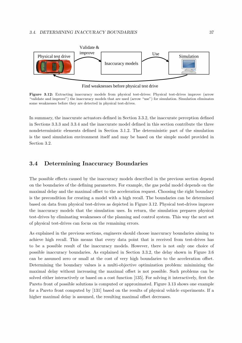
3.4. DETERMINING INACCURACY BOUNDARIES 37
Physical test drive
Inaccuracy models
Simulation
Validate &
improve Use
Find weaknesses before physical test drive
Figure 3.12: Extracting inaccuracy models from physical test-drives: Physical test-drives improve (arrow“validate and improve”) the inaccuracy models that are used (arrow “use”) for simulation. Simulation eliminatessome weaknesses before they are detected in physical test-drives.
In summary, the inaccurate actuators defined in Section 3.3.2, the inaccurate perception defined
in Sections 3.3.3 and 3.3.4 and the inaccurate model defined in this section contribute the three
nondeterministic elements defined in Section 3.1.2. The deterministic part of the simulation
is the used simulation environment itself and may be based on the simple model provided in
Section 3.2.
3.4 Determining Inaccuracy Boundaries
The possible effects caused by the inaccuracy models described in the previous section depend
on the boundaries of the defining parameters. For example, the gas pedal model depends on the
maximal delay and the maximal offset to the acceleration request. Choosing the right boundary
is the precondition for creating a model with a high recall. The boundaries can be determined
based on data from physical test-drives as depicted in Figure 3.12. Physical test-drives improve
the inaccuracy models that the simulation uses. In return, the simulation prepares physical
test-drives by eliminating weaknesses of the planning and control system. This way the next set
of physical test-drives can focus on the remaining errors.
As explained in the previous sections, engineers should choose inaccuracy boundaries aiming to
achieve high recall. This means that every data point that is received from test-drives has
to be a possible result of the inaccuracy models. However, there is not only one choice of
possible inaccuracy boundaries. As explained in Section 3.3.2, the delay shown in Figure 3.6
can be assumed zero or small at the cost of very high boundaries to the acceleration offset.
Determining the boundary values is a multi-objective optimization problem: minimizing the
maximal delay without increasing the maximal offset is not possible. Such problems can be
solved either interactively or based on a cost function [135]. For solving it interactively, first the
Pareto front of possible solutions is computed or approximated. Figure 3.13 shows one example
for a Pareto front computed by [131] based on the results of physical vehicle experiments. If a
higher maximal delay is assumed, the resulting maximal offset decreases.

38 CHAPTER 3. MODELING THE ENVIRONMENT
0 0.1 0.2 0.3 0.4 0.5 0.6 0.7 0.8 0.9 1
-0.8
-0.6
-0.4
-0.2
0
0.2
0.4
0.6
0.8
Delay [s]
Acc
lera
tion
Off
set
[ms−
2]
-1
offset for error model 1offset for error model 2
Figure 3.13: Pareto front of possible offset and delay parameters extracted from physical vehicle drive data by[131]. By assuming a high delay, lower maximal offsets can be concluded. The experiment was conducted withtwo different error models.
Among the solutions of the Pareto front, the software engineer chooses the best solution. As all
solutions maximize the recall, the best solution is the one that also maximizes the precision.
That means the best solution leads to as few as possible different behaviors of the vehicle
in the simulation environment. For determining the best solution based on a cost function,
engineers have to assign weights for boundary changes to each parameter. Using these weights,
the optimization algorithm can automatically choose the best result from the Pareto front.
Instead of weights, the cost function can also be based on metrics estimating the precision
resulting of the boundary values.
If the computed boundaries result in very imprecise inaccuracy models, the inaccuracy model
might not be complex enough. In this case, the complexity of the model has to be increased.
For the acceleration error, the added complexity can be to distinguish a special situation
for stopped vehicles as explained in Section 3.3.2. Too many special situations can result in
overfitting the model to the available data. The more special situations are distinguished, the
more data is necessary for deriving the inaccuracy boundaries. One method for reducing the
effect of overfitting is to add error margins to the inaccuracy boundaries. This error margin can
be proportional to the statistically computed standard deviation of the average of computed
boundaries. A larger data set that is relevant for the regarded boundary reduces this standard
deviation. This way, the recall is increased and more data increases not only the recall but also
the precision.
Engineers can apply the optimization approach for determining the actuator and position sensor
inaccuracy boundaries. For the offsets in the mapping errors and the distance for which it can
happen that obstacles are not be detected, they can apply a similar method. For the Tesla

3.5. FINDING UNDESIRED BEHAVIORS 39
Autopilot, systematically gathering this data might have resulted in an error model stating that
a relevant obstacle is sometimes detected only in the very last moment. Such an error model
can trivially lead to a collision that the STARVEC framework would also detect. This could
demonstrate the need to improve the sensor fusion system, which might have prevented the
fatal Tesla accident [136]. In addition to not detected obstacles, there can be measured but not
existing obstacles. The positioning of such ghost obstacles can either be included in the scenario
description or be performed randomly.
3.5 Finding Undesired Behaviors
The simulation including models for sensor and actuator inaccuracies can generate different
behaviors of the vehicle. This is the precondition for finding undesired behavior. This section
starts with a definition of undesired behaviors in Section 3.5.1. It concludes with the definition of
the problem in Section 3.5.2 that is addressed by the approaches presented in the next chapter.
The relevant question is whether there is an undesired behavior among the set of possible
behaviors generated by the simulation.
3.5.1 Definition of Undesired Behavior
First, undesired behavior has to be defined. The most common undesired behavior searched
for are collisions with some static or dynamic obstacle. However, the car manufacturer might
consider many other behaviors undesired. For example, it can consider uncomfortable or
non-elegant behavior as described in Section 4.4 undesired. For the purpose of an automatic
analysis, the system analyst has to formally specify what behavior they consider undesired.
In mathematical terms, this specification is a function:
fundesired physical behavior : (Qphysical states)n → B (3.25)
where Qphysical states is the set of all possible physical states as defined in Section 3.1.1. The
function fundesired physical behavior states whether a given sequence of n physical states shows
an undesired behavior. For analysis purposes, it is reasonable to define this function in the
simulation state space:
fundesired simulation behavior : (Qsimulation states)n → B (3.26)
Using the function Rphys→sim defined in Section 3.1.3 this function can also be applied to
sequences of physical states.
40 CHAPTER 3. MODELING THE ENVIRONMENT
The undesired behavior of colliding with an obstacle mentioned above can be identified by
deciding for a single state whether it is undesired. This kind of undesired behavior can be
defined as a function:
fundesired simulation state : Qsimulation states → B (3.27)
A simulation sequence is undesired if it contains an undesired state.
In the concept presented in this thesis, the undesired behavior can be represented as a software
component taking any information available in the simulation as input and triggering an event if
it detects an undesired state. The concept considrers such a component as part of the simulation
environment maintaining an internal state. Additionally, Section 4.4 describes a method for
specifying fundesired simulation behavior in CTL (Computation Tree Logic).
3.5.2 Problem Definition
The goal of this thesis is to efficiently determine if an autonomous driving system can show
undesired behavior in the physical world. On the one hand, this requires modeling the behavior
of the vehicle such that all physical behaviors can be represented and the precision is maximized.
The previous sections addressed this task. On the other hand, this requires using this model for
efficiently finding undesired behaviors in a simulation environment.
Using the definitions of Sections 3.1 and 3.5.1, the algorithm solving the latter step can be
specified as:
Algorithm Find undesired behavior
Input: ssw,init, Eevents,∆sim world, fundesired simulation behavior
Output: For each detected undesired behavior: sequence of events (e1, e2, ..., en) resulting
in the undesired behavior
where ssw,init is the initial state of the simulated world and Eevents is the set of all possible
events. ∆sim world is the transition function defined in Section 3.1.2 that determines the next
resulting state for a given current state and an active event. fundesired simulation behavior is the
specification of the undesired behavior defined in Section 3.5.1. The output consists of the events
e1, e2, ..., en ∈ Eevents. The corresponding states can be computed based on ∆sim world.
As the simulation is specified to be executed in discrete time steps (compare Section 3.1.1),
the number of possible behaviors with a limited maximal length is finite. However, it grows
exponentially with the length of the simulation: In each simulation step, any of the n := |Eevents|possible events can be applied. After m steps, there are nm possible behaviors.

Chapter 4
An Efficient Approach for Testing
with Inaccuracies and
Nondeterminism
This chapter presents several aspects of a new concept for efficiently searching the space of
possible behaviors for undesired behaviors. First, the basic concept is described and motivated
in Section 4.1. Next, it is extended to perform more efficiently in most scenarios in Section 4.2.
Using a system that is based on the created method, scenarios from real world test-drives are
imported and analyzed as described in Section 4.3. In both, real world scenarios and simulation
scenarios, complex temporal behaviors can be searched for as described in Section 4.4. Finally,
Section 4.5 applies the presented concepts to the interaction with traffic participants.
4.1 A Concept for Efficiently Covering the State Space
This section presents the primary concept of the STARVEC algorithm. Some of the findings in
this section have already been published in [137]. It starts with the basic concepts of testing
the implemented software and covering the geometric state space in Section 4.1.1. Next, Section
4.1.2 explains how storing simulation states and uniformly covering the reachable state space
reduces the complexity of the task. Finally, Section 4.1.3 explains how the simulation state of
the whole planning and control system can be stored and loaded.
41

42 CHAPTER 4. TESTING WITH INACCURACIES AND NONDETERMINISM
4.1.1 Basic Concepts
The concept presented in this section is based on two ideas:
1. Planning and control algorithms are quickly adapted to new problems. Therefore, the
implemented code rather than an abstract concept should be tested.
2. Planning and controlling of a vehicle is a geometrical problem, thus geometrically similar
positions typically lead to similar behavior.
The first idea is to execute the implemented software directly. During the development of
an autonomous driving system, many small problems occur and have to be resolved. For
example, in an industrial project connected to this thesis, the team working on the planning
and control software implemented special strategies for some special cases. One example of
such a strategy applies if the computed trajectory needs to be adapted due to controller
errors while following a very sharp curve. These special cases quickly lead to deviations
between a simplifying abstraction designed to increase computation efficiency and the actual
implementation. Additionally, designing good abstractions often requires more time than the
implementation itself. For these reasons, abstractions should be developed as soon as the actual
concept is stable for a long period. Software updates can challenge this stability even after
serial production has started. Furthermore, testing the implemented code also allows using any
implementations of sensor and actuator deviations. Many abstraction concepts require these
deviations to depend only on the current state of the vehicle or some helper variables. Deviations
that depend on the history of states–like delays–are difficult to represent. The concept presented
in this thesis allows implementing errors like the delays described in Chapter 3.3.
The second idea is that autonomous planning and control tasks are geometrical problems for
which similar positions lead to similar behavior. In particular, this is true for reactive high
frequency controllers that compute their behavior based on the planned and the current position.
Planning components can compute a different path for slightly different positions. However, this
is usually only true for one direction. That is, if two points A and B are geometrically close to
each other, a vehicle at a Point C between A and B will probably behave similar to being at A
or similar to being at B.
4.1.2 Reducing the Complexity
The sensor and actuators are modeled to be nondeterministic as described in Section 3.2. In
theory, the behavior can change at any time leading to an infinite set of possible behaviors. For
this reason, the time and the error models are sampled, such that there is a finite set of d error
characteristics that can change after a finite amount of time tstep. If there are d different error
characteristics, and the simulated scenario takes up to l · tstep seconds, there are up to dl possible

4.1. A CONCEPT FOR EFFICIENTLY COVERING THE STATE SPACE 43
Figure 4.1: Example of (coarse) geometric discretization. The top red cone and the state after executing theyellow path are in the same grid cell and considered similar.
different states this time. Executing all of them requires a simulation time of:
tsimulation,full = O(dl)
(4.1)
The simulation time grows exponentially with the duration of the test sequence.
The algorithm searches for undesired behaviors like collisions or uncomfortable driving. These are
externally visible geometric behaviors. There are exponentially many possible paths, but large
sub sets of them are geometrically almost identical. For these almost identical paths, different
future behavior is mostly due to sensor and actuator inaccuracies rather than different planning
results. Groce and Joshi [83] have regarded a similar problem trying to cover different behaviors
related to memory accesses. They applied “sound and unsound abstractions” [83] considering
paths only as different if they perform different memory accesses. This way, they are able to
achieve a good coverage of different behaviors connected to memory access. The same approach
can be transferred to autonomous driving systems by considering states only as different if they
are geometrically different according to some geometric grid as depicted in Figure 4.1. If the
test process encounters any state that it has already visited according to this metric, it does
not continue the simulation. This means, it does not add the state to the queue of states that it
plans to expand further.
Figure 4.2 depicts a schema of the resulting execution rule. It starts by storing the current
simulation state (Top left box). At this point, storing a state means to store the applied sensor
and actuator inaccuracies in order to be able to reproduce the state. Accordingly, restoring in
the next step means to apply the stored sensor and actuator inaccuracies until the analysis
reaches the stored state. Later in this section, this is replaced by actually storing the state
itself. For the restored state, an error type is applied that has not been applied yet (“Apply

44 CHAPTER 4. TESTING WITH INACCURACIES AND NONDETERMINISM
Store and load state Run simulation for tstep seconds
Start
Store and enqueue state if not terminal and grid cell is empty
Restore top state from queue
Pop state from queue
Apply next error type
All errors
applied?
Run simulation for t_base_cycle seconds
Compare to undesired state patterns
tstep simulated?
yes
Finishedstore and load
no
Start
Finish
Figure 4.2: Overview of the STARVEC algorithm for finding error pattern combinations leading to undesiredstates. Loading states and applying new inaccuracy patterns alternates with executing a short part of thesimulation sequence.

4.1. A CONCEPT FOR EFFICIENTLY COVERING THE STATE SPACE 45
next error type”). If all error types have been applied to this state, it is removed from the state
queue, else it remains in the queue in order to be restored again. Next, the test supervisor starts
with the restored state and the applied error pattern to execute the simulation environment for
tstep. During that time, the simulation is continuously checked for collisions or other undesired
behaviors.
This approach reduces the complexity of the testing task. A typical scenario includes moving
from one position to another. If no sensor and actuator inaccuracies occur, the vehicle will
execute one path that will be referred to as reference path. Sensor and actuator inaccuracies
lead to deviations from the reference path by a limited range. For example, they can result
in controller errors by some decimeters, but typically not multiple meters. This limited range
combined with a finite grid density leads to a finite amount of possible states around each point
of the reference path. If K is the maximal number of grid borders in one dimension for one
position along the ideal reference path and Ndimensions is the number of observed geometric
dimensions, this leads to KNdimensions possible states for each point along the reference path.
Executing a single simulation step for all possible states at one point of the reference path with
all error characteristics requires d ·KNdimensions execution steps. Additionally, the path leading
to these nodes has to be executed, requiring between one and l steps depending on the distance
to the scenario start. This process has to be repeated for each of the l points along the reference
path resulting in a complexity of
tsimulation,grid = O(KNdimensions · d · l2
)(4.2)
K and Ndimensions do not depend on the length of the scenario. Hence, the abstraction reduces
the complexity from exponential in l (compare Equation 4.1) to quadratic in l.
This complexity can be further reduced by storing and reloading the state of the whole simulation
including the planning and control software. The technical details of storing and loading states
are explained in the next section. Using this capability, reaching any of the final states requires
only reaching the predecessor states plus d simulation steps for each final state, which are up
to KNdimensions. The same applies for the predecessor states regarding their predecessors. This
process has to be repeated up to l times until the initial states are reached. Thus, the complexity
is reduced to linear in l:
tsimulation,grid = O(KNdimensions · d · l
)(4.3)
In practice, finding undesired behavior typically does not require the worst-case execution time.
Hence, the observed computation speed gains are lower than theoretically possible. However,
the experiments in [137] show that a significant speed up is reached for relevant scenarios.

46 CHAPTER 4. TESTING WITH INACCURACIES AND NONDETERMINISM
4.1.3 Loading and Saving the State of a Software Component
The presented algorithm must be able to store and load the state of the simulation environment
including the planning and control system. It can do this based on a serialization library.
For example, Sumaray and Makki [138] compare “XML, JSON, Thrift, and ProtoBuf”. For
serializing (storing) the state of a whole software component, the storing code must require
as little implementation overhead, as possible. C++ libraries for XML (Extensible Markup
Language) and JSON (JavaScript Object Notation) need explicit implementation of each value
to be stored including referenced classes and cannot cope with private data members. ProfoBuf
additionally requires writing a specification file for the serialized data. In contrast, Boost
Serialization1 serializes referenced classes identically to basic data types. Boost Serialization
copes with calling the right serialization function of referenced classes and ensures serializing
multiply referenced classes only once. It can also access private data members.
For this purpose, the software developer needs to enhance the classes with two lines of code
for declaring the serialization function and registering the class. The actual serialization code is
stored in a separate source file. It mainly contains a list of the members of each class embedded
into the boost serialization syntax. The library supports different serialization formats including
XML and a compressed binary format. The implementation created for this thesis stores the
serialized states to the hard drive instead of keeping it in the main memory. This way, the size of
the main memory does not limit the execution. Furthermore, the state of the whole test system
can be loaded after terminating the process and potentially changing the source code of the test
component.
It has been demonstrated that it is feasible to implement and maintain the code for serialization
of a complex software project. The demonstrated example is the planning and control framework
developed during this dissertation. The computational overhead for loading and saving states
is small compared to the time necessary for the actual simulation. In order to minimize the
storage requirements, the serialized data is compressed using the ZLib standard [139]. Figure
4.3 compares the overhead caused by the test supervisor algorithm and the actual simulation
time. The overhead consists of the time necessary for loading and saving states, evaluating
whether a state shows undesired behavior and choosing which state to expand next. In total,
the computation time used for the actual simulation is significantly higher than the time used
for overhead. Optimizing the storing procedures can further reduce the overhead. In addition
to the computation time, the testing framework requires 23 kB per stored state on average. It
stores one state per simulated second.
Another precondition of using the presented test supervisor is the ability to run the simulation
for a specified time. That means there has to be a scheduler component that can trigger the
execution of both the simulation environment and the planning and control components. In
1www.boost.org/libs/serialization/doc/

4.1. A CONCEPT FOR EFFICIENTLY COVERING THE STATE SPACE 47
0 50 100 150 200 250 300 350 400 450 500 550 600 650
Simulation
Overhead
Computation time [s]
Figure 4.3: Comparison of the computation time used for simulation vs. overhead of the presented testingalgorithm: The simulation time dominates the total computation time.
Rea
d 1
Write Output Read Input Cycle
Wri
te 1
Wri
te 2
Wri
te 3
Rea
d 2
Rea
d 3
Cyc
le 1
Cyc
le 2
Cyc
le 3
Time
Figure 4.4: Serial execution of software components: In each step, components 1, 2 and 3 are executed serially.
order to create deterministic results, it should also trigger the data transmission between the
tested components. Figure 4.4 shows the execution model applied in the implementations for
this thesis. In each simulation cycle, the current time is increased and the active components are
determined. A component is active if the current simulated time is a multiple of the component’s
cycle time. In the example, components one, two and three are active. First, all components
write their current output, that is the output that has been computed in the previous cycle.
This corresponds to each component requiring its full cycle time for its computation. Next, each
components reads its input data and finally, each component performs its main computations in
its periodically called cycle method. These strict execution orders enforce the same deterministic
behavior even if the simulation is executed faster than in real time.
In order to speed up the computation, the execution of the read, write and execute methods
can be performed in parallel, as depicted in Figure 4.5. If separate simulated clocks are used for
each component, the cycle execution of a component may take longer than one cycle time of
component with the highest frequency. The execution may take until the component is triggered
to write its output data. The long execution time does not change the behavior of the complete
system. This way, several cycles of a high frequency component like a controller can be executed
during the computation time of a low frequency component like a planner.

48 CHAPTER 4. TESTING WITH INACCURACIES AND NONDETERMINISM
Write Output Read Input Cycle
Write 1
Write 2
Write 3
Read 1
Read 2
Read 3
Cycle 1
Cycle 2
Cycle 3
Time
Figure 4.5: Parallel execution of software components: In each step, components 1, 2 and 3 are executed inparallel.
The execution model leads to some data being transmitted but not read yet in each point in
time. Therefore, the buffered data has to be serialized in addition to the actual state of the
software components.
In summary, the proposed method reduces the complexity for finding undesired behaviors caused
by sensor and actuator inaccuracies from exponential in the length of the simulation l to linear.
It accomplishes this by discretizing the space of geometric states and exploiting the ability to
save and load states.
4.2 Optimizing the Search Efficiency
The method described in the previous section reduces the worst-case complexity for finding
undesired behaviors. However, it requires specifying the size of the grid and takes the worst-case
execution time even for finding undesired behaviors that occur often.
Thus, the method is extended by two concepts:
• Replacing the geometric discretization grid by novelty search
• Choosing the applied error characteristic randomly until all characteristics have been
applied
These concepts are presented in Sections 4.2.1 and 4.2.2. Section 4.2.3 extends the pure geometric
grid to a grid containing arbitrary user defined states. Some concepts of the described test
method have been introduced in [140] as the STARVEC algorithm.
4.2.1 Expanding the Most Novel State
The first concept mentioned in the introduction to this section is novelty search. Instead of
ignoring states that are in a grid cell in which another state has already been expanded, all states

4.2. OPTIMIZING THE SEARCH EFFICIENCY 49
are kept in a priority queue waiting for expansion. Figure 4.6 shows an exemplary situation.
State 1 has been expanded 7 times resulting in states 2-8. States 6 and 8 have already been
2 3 4 5
7
1
86
Figure 4.6: Example set of expanded (green) and not expanded (white) states. Node 7 has the highest distanceto any neighbor. Node 2 has the highest distance to the nearest expanded neighbor.
expanded, too. The resulting priority queue is depicted in Figure 4.7. The priority of each state
State 2: 4.0
State 3: 3.0
State 7: 2.1
State 4: 2.0
State 5: 1.0
Figure 4.7: Priority queue of the STARVEC algorithm. The priorities correspond to the distances to the nearestexpanded neighbor in Figure 4.6.
is proportional to the distance to the next fully expanded state. The distance is the Euclidean
distance in a state space that corresponds to the grid introduced in Section 4.1.2: The state
space contains one dimension for each regarded state variable. In Figure 4.7, State 2 has the
highest priority, as its nearest expanded state (State 6) has a distance of 4.0. For the distance
computation, only expanded states rather than all reached states are considered. This aims to
distribute the expanded states in the state space evenly. Considering all reached states would
result in expanding State 7 leaving the left half of the state space without expanded states.
The exact formula for computing the priority p(s) is shown in the following equation
(Equation 4.4):
p(s) = mins′∈Qexplored states(dist(s, s′)
)(4.4)

50 CHAPTER 4. TESTING WITH INACCURACIES AND NONDETERMINISM
where Qexplored states is the set of the already explored simulation states and dist(s, s′) is the
Euclidean distance between states s and s’ in the space of the grid introduced in Section 4.1.2.
The termmins′∈Qexplored states(dist(s, s′)) is approximated using the library FLANN (Fast Library
for Approximate Nearest Neighbors) [141].
At all times, the highest priority in the queue is the largest distance from any not expanded
state to its neighboring state. One could fit a grid-like structure to the state space with each cell
having a radius lower than this distance. Each cell containing a state also contains at least one
expanded state. This way, the advantages of the grid-based approach described in the previous
section still apply. However, this virtual grid becomes continuously denser, resulting in a fast
and increasingly dense coverage of the state space. The concept is similar to the concept of RRT
(Rapidly-exploring Random Tree)[142]. For this task, Novelty Search performs better than RRT,
because most states in the state space are not reachable by only altering error characteristics.
This significantly slows down an RRT based approach as discussed in the evaluation in Chapter
6.
4.2.2 Prioritizing Unexpanded States
The second concept mentioned in the introduction to this section is to randomly choose from
the error characteristics planned to be applied. Each error characteristic is a combination of
configurations of the error models as described in Section 3.3. In some situations, only a few
of the error models significantly influence the behavior of the vehicle. In these cases, a limited
number of randomly chosen successors is likely to contain all configuration combinations of
these few error models. The limitation to the number of chosen successors reduces the negative
impact of error models with little influence. This speeds up the search process if large sets of
error characteristics are defined.
The successor limitation is reflected in the priority formula shown in Equation 4.5.
p(s) = w(s) · dmod(s) (4.5)
where w(s) is the weight of a state and dmod(s) is the modified distance to its nearest expanded
neighbor. As the successor limitation leads to states not being fully expanded, the distance to
the nearest expanded neighbor is replaced by a radius. Within this radius, the total number of
expansion has to exceed a threshold:
dmod(s) = min({r ∈ R+|
(Σ{s′∈Qexplored states|dist(s,s′)<r}nsucc(s)
)> nthreshold
})(4.6)

4.2. OPTIMIZING THE SEARCH EFFICIENCY 51
en
Figure 4.8: Planning concept that uses the green path as reference. If the controller error en is too high, theplanner computes a trajectory (blue path) that smoothly returns to the reference path.
where Qexplored states is the set of already explored simulation states, nsucc(s) is the number of
successor states of state s and nthreshold is the number of expansions that needs to be exceeded
within the computed radius.
The weight is computed as:
w(s) = (wsuccessor · nsucc(s) + 1)−1 (4.7)
where wsuccessor is a weight factor penalizing the number of successors.
4.2.3 Generalization of the Grid Concept
The previous sections focus on improving the efficiency. This section additionally increases the
applicability of the concept by allowing custom state dimensions. The basic concept described
in Section 4.1 projects the state of the vehicle to a geometric grid. This grid includes external
features like the position, orientation, acceleration or velocity of the vehicle. In addition to
these external features, the future trajectory of the vehicle depends on the internal state of the
planning algorithm.
One planning concept is to first create a collision free path and use a controller to follow
the initially planned path. In this case, the state of the planning component mainly consists
of constant parts like the initially planned path and externally visible parts like the current
environment map and the perceived vehicle state. In this case, the grid that consists of dimensions
that correspond to physical states is a good abstraction of the simulation state.
Another planning concept is depicted in Figure 4.8. The planning and control system follows
an initially planned reference path (green path), but some sections of the path are adapted
continuously. For example, [25] continuously adapts the velocity, reacts to new obstacles and
high controller deviations. The resulting trajectory (blue path in Figure 4.8) in each adaptation
depends on the start position of the replanning procedure. This start position is not necessarily
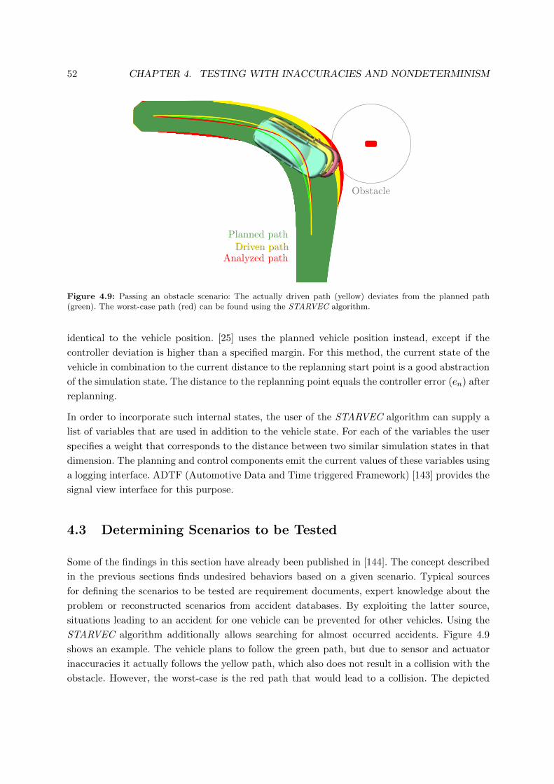
52 CHAPTER 4. TESTING WITH INACCURACIES AND NONDETERMINISM
Planned pathDriven pathDriven path
Analyzed path
Obstacle
Figure 4.9: Passing an obstacle scenario: The actually driven path (yellow) deviates from the planned path(green). The worst-case path (red) can be found using the STARVEC algorithm.
identical to the vehicle position. [25] uses the planned vehicle position instead, except if the
controller deviation is higher than a specified margin. For this method, the current state of the
vehicle in combination to the current distance to the replanning start point is a good abstraction
of the simulation state. The distance to the replanning point equals the controller error (en) after
replanning.
In order to incorporate such internal states, the user of the STARVEC algorithm can supply a
list of variables that are used in addition to the vehicle state. For each of the variables the user
specifies a weight that corresponds to the distance between two similar simulation states in that
dimension. The planning and control components emit the current values of these variables using
a logging interface. ADTF (Automotive Data and Time triggered Framework) [143] provides the
signal view interface for this purpose.
4.3 Determining Scenarios to be Tested
Some of the findings in this section have already been published in [144]. The concept described
in the previous sections finds undesired behaviors based on a given scenario. Typical sources
for defining the scenarios to be tested are requirement documents, expert knowledge about the
problem or reconstructed scenarios from accident databases. By exploiting the latter source,
situations leading to an accident for one vehicle can be prevented for other vehicles. Using the
STARVEC algorithm additionally allows searching for almost occurred accidents. Figure 4.9
shows an example. The vehicle plans to follow the green path, but due to sensor and actuator
inaccuracies it actually follows the yellow path, which also does not result in a collision with the
obstacle. However, the worst-case is the red path that would lead to a collision. The depicted

4.3. DETERMINING SCENARIOS TO BE TESTED 53
obstacle can be either some static obstacle like a crash barrier or it can be a pedestrian who has
an area of motion uncertainty around it. Such almost occurred accidents are more likely than
actual accidents. Therefore, a system that can identify almost occurred accidents and helps
repairing the causative defect can substantially reduce the number of accidents that are due to
conceptual weaknesses.
First, Section 4.3.1 describes the situations in which scenarios can be stored for further analysis.
Next, Section 4.3.2 discusses the equipment and techniques used for storing scenarios. Section
4.3.3 investigates how the available scenarios can be filtered for relevant situations. These relevant
situations are analyzed as described in Section 4.3.4. Finally, Section 4.3.5 explains how to
distribute the results of the analysis to the vehicle fleet.
4.3.1 Sources for Collecting Scenarios
There are various situations in different levels of the development process of autonomous vehicles
providing scenarios worth further analysis. Scenario data can be collected from:
• test-drives executed by developers
• test-drives according to requirement specifications
• drives performed in a prototype testing program, and
• regular usage by customers
Developers regularly drive the experimental vehicle in order to test the functions they are
currently working on. These test-drives are usually less systematic than independent vehicle
tests but they are based on knowledge and experience that is not necessarily available during
requirements specification or test-drives by independent test experts. A disadvantage of this
source is that the tested autonomous driving software might still contain known defects. Such
known defects can dominate and mask conceptual weaknesses to be found by scenario analysis.
That means instead of finding the conceptual weaknesses, the scenario analysis only finds the
known defects. In this case, the analysis does not produce relevant results.
The second group of scenario sources mentioned above are test-drives based on the requirements
specification. These test-drives systematically cover the requirements and can be additionally
supported by reference sensor systems or known environment maps. This way, the recorded data
can be of high quality. Systems tested by professional test drivers contain less defects than the
experimental system described above. Consequently, many detected problems are relevant.
After professionally testing the vehicles, but before the final customers use the product, a limited
set of almost final prototypes is produced and used. These prototypes can still contain some extra
devices for gathering development data, which increases the quality of the collected data. The

54 CHAPTER 4. TESTING WITH INACCURACIES AND NONDETERMINISM
O1
Figure 4.10: Points (gray) at which the planning and control system is saved while following the path describedin Figure 4.9. The dark grey states are regarded by the analysis, as the car is close to the obstacle.
prototypes are used in a similar way as they are used by the end customers and hence create
similar data before market launch.
Finally, scenarios can be gathered anonymously during usage by the final customers. Data
collected from this source cannot prevent the distribution of faulty vehicles, but it can help
eliminating defects before they lead to undesired behavior experienced by a customer. For
example, they can include the almost-accidents described at the beginning of this section and
help resolving their cause. Customer vehicles do not contain reference sensors, which reduces
the quality of collected data, but they produce the largest amount of data.
4.3.2 Recording and Restoring Scenarios
During the drives used for data collection described in the previous section, the state of the
vehicle and its environment is stored periodically. Figure 4.10 shows markers for each position
at which the state is saved while executing the motion described in Figure 4.9.
Figure 4.11 illustrates how the scenarios are stored and loaded. Storing the state of the planning
and control software is based on the same techniques as used for the STARVEC algorithm
described in Section 4.1.3. This is depicted by the boxes of the Planning and Control system as
input (bottom right green box) and output (top right red box) of the Scenario Extractor. The
only difference are connections to the execution environment: The system clock is replaced by a
simulated clock with the same time stamp.
In contrast, the Simulation Environment (top left box) has to be recreated based on the Perceived
Environment (bottom left box). Depending on the available sensors, different information sources
can be used. For some test-drives, Ground Truth data is available. For example, if the test-drive
is executed on a test track, the exact position of the road and all obstacles might have been
measured in advance. On public roads, 3D-geodata [145] from high definition maps might exist
that includes the environment geometry. If no ground truth data is available or the data is not
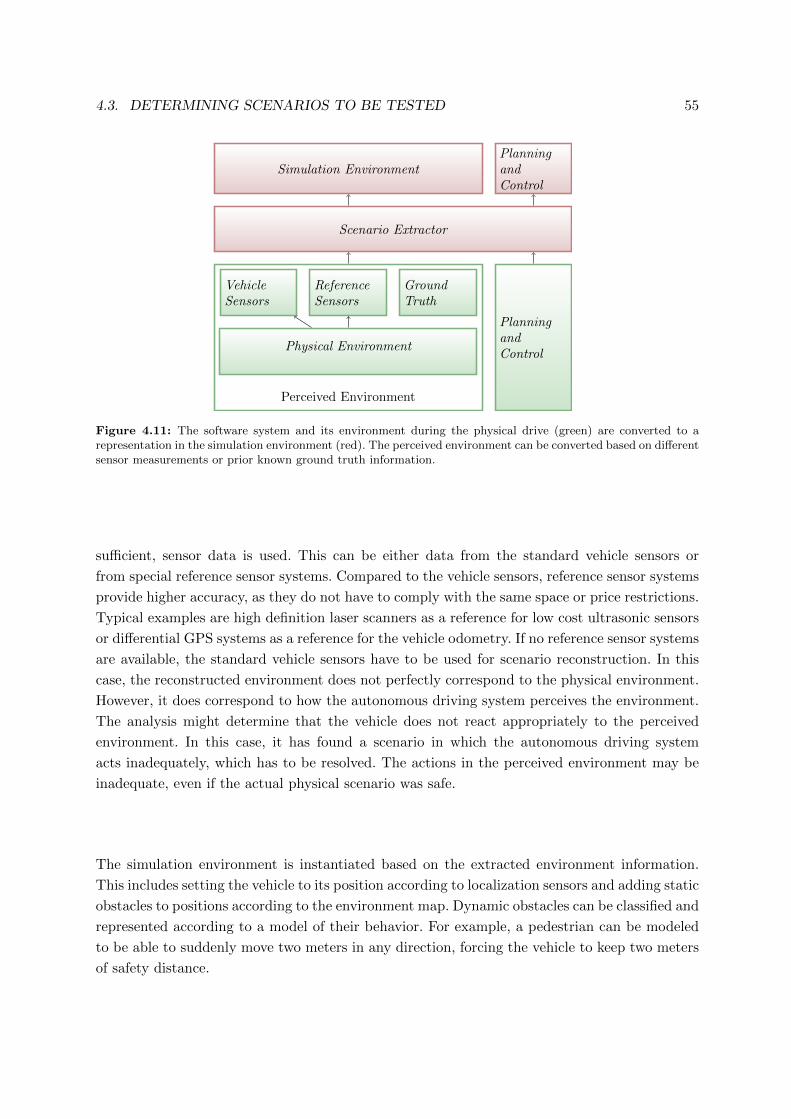
4.3. DETERMINING SCENARIOS TO BE TESTED 55
VehicleSensors
ReferenceSensors
GroundTruth
Physical Environment
Perceived Environment
PlanningandControl
Scenario Extractor
PlanningandControl
Simulation Environment
Figure 4.11: The software system and its environment during the physical drive (green) are converted to arepresentation in the simulation environment (red). The perceived environment can be converted based on differentsensor measurements or prior known ground truth information.
sufficient, sensor data is used. This can be either data from the standard vehicle sensors or
from special reference sensor systems. Compared to the vehicle sensors, reference sensor systems
provide higher accuracy, as they do not have to comply with the same space or price restrictions.
Typical examples are high definition laser scanners as a reference for low cost ultrasonic sensors
or differential GPS systems as a reference for the vehicle odometry. If no reference sensor systems
are available, the standard vehicle sensors have to be used for scenario reconstruction. In this
case, the reconstructed environment does not perfectly correspond to the physical environment.
However, it does correspond to how the autonomous driving system perceives the environment.
The analysis might determine that the vehicle does not react appropriately to the perceived
environment. In this case, it has found a scenario in which the autonomous driving system
acts inadequately, which has to be resolved. The actions in the perceived environment may be
inadequate, even if the actual physical scenario was safe.
The simulation environment is instantiated based on the extracted environment information.
This includes setting the vehicle to its position according to localization sensors and adding static
obstacles to positions according to the environment map. Dynamic obstacles can be classified and
represented according to a model of their behavior. For example, a pedestrian can be modeled
to be able to suddenly move two meters in any direction, forcing the vehicle to keep two meters
of safety distance.

56 CHAPTER 4. TESTING WITH INACCURACIES AND NONDETERMINISM
4.3.3 Identifying Relevant Situations
The computation time of the STARVEC algorithm is linear to the duration of the scenario. This
makes it possible to analyze all recorded data in full length provided sufficient computation
power per driven distance. However, this is not necessary as most situations have small collision
risk. If all static obstacles are several meters away and the vehicle drives slowly, sensor and
actuator inaccuracies in the past cannot lead to a collision, either. This makes it reasonable
to limit further analysis to situations that appear to have a high collision risk. For example
situations, in which an obstacle is very close to the vehicle. Limiting analyzed scenarios to these
situations reduces the necessary computation power per driven distance as well as the amount
of data that needs to be stored and transmitted. The latter factor is a limitation for consumer
vehicles, for which the data needs to be transmitted using mobile network connections.
The focus of this thesis lies on inaccuracies of sensors and actuators rather than on complete
sensor failures. However, for identifying relevant scenarios on consumer vehicles, failing sensors
are another factor. Data from these scenarios can be used to analyze whether the fail-safe concept
could have led to a collision. Another factor for identifying relevant scenarios is unexpected
behavior of traffic participants. The presented concept can be applied to determine whether the
situation was still safe. For test-drives of autonomous driving systems on public roads, the test
driver sometimes has to intervene in order to prevent an accident. From September 2014 until
November 2015, Mercedes-Benz reported 967 [146], Volkswagen reported 85 [147] and Bosch
reported 625 [148] interventions during test-drives in California. Such interventions can also be
used as a trigger for later analysis trying to determine whether the intervention prevented a
possible accident. Google [149] uses a similar approach for filtering the disengagements reported
to the traffic agency. By applying the STARVEC algorithm, the post analysis can find situations
that are more dangerous among these disengagements.
4.3.4 Analyzing Recorded Scenarios
The restored simulation states are considered as part of a search tree as the one created by the
STARVEC framework described in Section 4.1. Each state is assigned to its physical predecessor
as a successor in the search tree and added to the queue of not expanded states. If a trigger
is used for identifying relevant scenarios, only states some seconds before and after the trigger
are added to the queue of not expanded states. In this case, the analysis is also limited to this
period. Any simulation state of which the time stamp is higher than the end of the time frame
is no further expanded. If the analysis finds an undesired behavior, the sequence leading to that
behavior starts with a physical state and continues with simulated states.

4.3. DETERMINING SCENARIOS TO BE TESTED 57
4.3.5 Distributing Analysis Results
An undesired behavior found by the STARVEC analysis is due either to incorrect models or
a weakness of the planning and control system. In the first case, the detected sequence is
an example that can be used for investigating possible model improvements. As discussed in
Section 3.4, it might be possible to create a more complex model that does not exhibit the
actions leading to the detected undesired behavior. For example, the behavior of the model in
special situations like accelerating from zero velocity can be implemented. This requires sufficient
physical test-drive data showing the behavior of the vehicle in that special case.
The second case is a weakness of the planning and control system. The consequences of this
weakness depend on the source of the scenario. If the source was an early test-drive, developers
need to regard the scenario and eliminate potential errors. If the source is a vehicle owned by a
customer, a quick reaction is necessary. Possible reactions are
• adapting parameters of the vehicle software,
• deactivating the executed function at one geographic position, or
• globally deactivating the executed function.
The reaction to adapt parameters is reasonable if the undesired behavior is a collision due
to unexpectedly high controller deviations. In this case, the safety distance parameters can
be increased covering these deviations. The parameter adjustment can be performed either
manually or automatically. After adjusting the parameters, all other known scenarios should be
reanalyzed. The disadvantage of increasing safety distances is that this can decrease the overall
function performance. For example, a parking assistant would require larger parking lots. The
parameter adjustment can also be a temporary solution until the planning and control software
is conceptually improved and able to cope with lower safety distances.
Another possible reaction is to deactivate or constrain the corresponding function for a specific
geographic position. For example, if the controller deviations are due to bad road conditions,
other vehicles can be warned to drive more carefully at one specific bend. This way, the analysis
does not only evaluate autonomous vehicles, but also the environment and the infrastructure.
Finally, if the analysis uncovers a safety risk that cannot be resolved by applying the reactions
listed above, the function can be deactivated globally. If this happens, the responsible engineers
have to work on a solution that enables the autonomous driving system to cope with that
situation in order to reactivate the function quickly.

58 CHAPTER 4. TESTING WITH INACCURACIES AND NONDETERMINISM
0.5 1 1.5 2
0.2
0.4
0.6
0.8
time [s]
velocity
[ms−
2]
(a) Example velocity plot
CTL: ¬EF(v > 0.3∧E[v > 0 U v = 0∧E[v ≥ 0 U v > 0.05]])
(b) CTL formula
p0 p1 p2 p3v > 0.3 v = 0 v > 0.05
v > 0 0 ≤ v ≤ 0.05
v < 0
(c) Pattern state machine
Figure 4.12: Stopping before the goal position and restarting in the same direction expressed as a state machine,an example velocity plot and a Computation Tree Logic formula.
4.4 Searching for Temporal Behavior Patterns
Some of the findings in this section have already been published in [150]. The simplest undesired
behavior that can be searched for are collisions. Behaviors that are more complex can cover a
time span rather than a single point in time. For example, a car might drive slalom or repeatedly
start and stop needlessly. These patterns cannot be detected by comparing a single state to a
specification of undesired states. Instead, a sequence of states can be compared to a specification
of undesired sequences.
Figure 4.12 shows different representations of the same undesired behavior of starting and
stopping without need. The first representation is not formal, but a plot of the velocity signal
that an engineer recognizes as an example of this pattern. The second representation is CTL,
which is typically used for model checking. The goal of model checking is to determine whether
“a given automaton satisfies a given temporal formula” [151]. It is performed by several freely
available tools like NuSMV (New Symbolic Model Verifier) [152]. Using these tools requires only

4.4. SEARCHING FOR TEMPORAL BEHAVIOR PATTERNS 59
connecting the STARVEC algorithm with model checking tools as described in Section 4.4.1.
An alternative to these tools is the problem specific implementation of Breadth First Search
described in Section 4.4.2. It uses the third representation shown in Figure 4.12(c).
4.4.1 Combining STARVEC and Computation Tree Logic
The system for which temporal logic specifications should be checked consists of the planning
component, the deterministic part of the environment and the nondeterministic events. The
typical model checking approach starts with creating a model of each component. Next, this
model is represented in a model checking tool like NuSMV. Using this representation, the tool
applies the specification to the model. As stated in Section 4.1.1, the goal is to check the actual
implementation of the planning component. However, the whole software code of the planning
component is too complex for automatically generating a model of the source code for which a
model checker can produce results in reasonable time. Instead, the STARVEC algorithm creates
a search tree connecting possible reachable states. This tree can be regarded as a model of the
possible behavior of the planning software. As explained in Section 4.2, not expanded states are
considered to be similar to their nearest expanded neighbor states. If an expanded state and
all its neighboring not expanded states are treated as a single state, the search tree becomes a
general graph. The transition guards of this graph are the active nondeterministic environment
events leading from the source of a transition to its target state. This graph can be converted
to a NuSMV compatible representation.
Listing 4.1 shows the structure of such a transition table. It computes a new value for the macro
NEXT STATE ID. First, it checks whether the variable sub step is below NUM SUB STEPS.
As the environment event changes only after a specified time, for example one second, several
simulation steps have to be completed before reaching a new state. These sub steps have to
be represented in the NuSMV model, as the undesired behavior might happen in one of these
steps. Therefore, the counter sub step counts from 0 to NUM SUB STEPS and restarts with
0. The state id can only change after executing NUM SUB STEPS sub steps. If the state id
changes, the new state is determined based on the current state (state id) and the currently
active environment event (error number). Some environment events lead to the same target
state, because not expanded states are represented by their nearest expanded neighbor. Some
states lead to the special state TERMINAL STATE. The simulation is not continued at these
states, because either an undesired behavior is detected, or a simulation end condition is reached.
This transition table is one central element for combining NuSMV with STARVEC. It is
generated based on the STARVEC search graph. In addition to the transition table, a property
table is necessary. It lists for the combination of each defined property with each state, sub
step and environment event whether this property is true or false. As NuSMV cannot access the
simulation states directly, it depends on these properties being defined and extracted. The syntax
of the property tables is similar to the transition table shown above. The extracted properties

60 CHAPTER 4. TESTING WITH INACCURACIES AND NONDETERMINISM
Listing 4.1: NuSMV transition table: the id of the next state is computed based on the current state and thenumber of the current error pattern. The active state only changes if sub step equals NUM SUB STEPS.
1 NEXT_STATE_ID :=
2 case
3 sub_step < NUM_SUB_STEPS - 1 : state_id;
4 sub_step = NUM_SUB_STEPS - 1 :
5 case
6 state_id = 0 :
7 case
8 error_number = 0 : 1;
9 error_number = 1 : 1;
10 error_number = 2 : 1;
11 error_number = 3 : 1;
12 esac;
13 [...]
14 state_id = 1051 :
15 case
16 error_number = 0 : 998;
17 error_number = 1 : 566;
18 error_number = 2 : 571;
19 error_number = 3 : 571;
20 esac;
21 state_id = 1052 : TERMINAL_STATE;
22 [...]
23 esac;
24 esac;
can be used in CTL and LTL (Linear Temporal Logic) formulas for specifying undesired behavior
(bottom right box in Figure 4.13).
Additionally, a NuSMV base model is required. The base model combines the transition table,
the property table and the temporal logic specification. It is constant for all search graphs and
is shown in Listing A.1 in the appendix. The main parts of it are a definition of the NuSMV
state variables and state transitions.
Both the transition table and the property table can become very large. In the worst-case, the
property table can contain one line for each combination of state, sub step, environment event
and defined property. The transition table can contain one line for each combination of state
and environment event. Three measures are applied to reduce the number of lines:
1. If all successors of a state are identical, the inner case clause (line 8-11 in 4.1) is omitted.
2. All states preceding a special state are integrated into a single case using the NuSMV set
construct: state id in {2, 3, 4, 6}.
3. The set constructs are shortened by combining directly succeeding ids: state id in {2..4, 6}.
Together, these measures reduce the size of the transition table by about 70%. Similar reductions
can be applied to the property table.

4.4. SEARCHING FOR TEMPORAL BEHAVIOR PATTERNS 61
STARVEC Search Graph
TransitionGeneratorProperties
NuSMV base modelNuSMV State Transitions
and Property TablesLTL/CTL formulas
NuSMV
Figure 4.13: Steps for generating a NuSMV model from test data: The STARVEC search graph is converted toNuSMV transition and property tables. These tables are the basis for checking CTL formulas.
Using the resulting optimized transition table, NuSMV can search for patterns like the formula
shown in Figure 4.12(b). NuSMV is a tool for proving properties of a model like the one
described by the transition table created in this section. If the Boolean formula describing the
property is not satisfied, NuSMV generates a counter example. For the present application, the
counter example is one instance of the undesired behavior of the autonomous driving system.
Accordingly, the property to be proven is that the system cannot exhibit the undesired behavior.
Therefore, the CTL formula in Figure 4.12(b) starts with the negation operator “¬” followed
by a specification of the behavior. EF (Exists Finally) means that there exists a path for which
eventually some property is fulfilled. In this case, the property is the occurrence of the undesired
behavior starting with the velocity being larger than 0.3m s−1. The remaining operators are EU
(Exists Until) operators. They state that there exists a path for which a property holds until
another property holds. First, the velocity is positive until it is zero. At this point, it stays larger
or equal to zero until it is larger than 0.05 m s−1.
In summary, CTL can be used for specifying temporal patterns of undesired behavior. The
model generated by the STARVEC analysis can be converted to a representation that NuSMV
can check against such a specification.
4.4.2 Fast Pattern Search Based on Simple Automata
An alternative is to define the pattern of an undesired behavior as a deterministic automaton.
The transitions of the automaton are guarded by logic conditions on some variables. These
variables are a subset of the ones tracked in the checked model. If the accepting state of that
automaton is reached, it means that the behavior has occurred. BFS (Breadth First Search)
can determine if this state is reachable within the checked model. The checked model is the
combination of the automaton above and the model used for extracting the NuSMV transition
tables.

62 CHAPTER 4. TESTING WITH INACCURACIES AND NONDETERMINISM
STARVEC Search Graph Pattern Automaton
BFS
Figure 4.14: Steps for generating the input of the Breadth First Search (BFS): It directly uses the STARVECsearch graph.
Breadth first search means that “the root node is expanded first, then all the successors of the
root node are expanded next, then their successors, and so on” [129]. In contrast, DFS (Depth
First Search) “always expands the deepest node in the current fringe of the search tree” [129].
BFS is superior to DFS in this context, as it provides the shortest path to an occurrence of the
pattern, which is easier to understand.
Figure 4.14 illustrates that generating the inputs for the BFS is simpler than for NuSMV, because
BFS can directly access the states in the STARVEC search graph. The only inputs are the
STARVEC search graph and the pattern automaton. Property tables as described for the NuSMV
model are not necessary, because the pattern automaton can contain guards directly pointing
to state variables. For both the NuSMV model generation and the pattern state machine, it
is necessary to list all variables that can be used for properties or guards before executing the
STARVEC algorithm. The analysis then stores the values of these variables in each simulation
step. In the worst-case, the BFS visits every combination of model state and pattern state once.
Thus, its run time is linear to the size of the combined state machine.
An example for a pattern automaton is shown in Figure 4.12. The pattern can be initialized at
any point during the simulation, hence p0 is always reachable. First, the pattern searches for
a velocity larger than 0.3 m s−1. This triggers the transition from state p0 to state p1. If the
velocity is lower than zero at any point during the pattern comparison, the pattern state is reset
to p0. The transition from p1 to p2 is triggered when the velocity is zero. Finally, the velocity
needs to be larger than 0.05 m s−1 in order to reach the terminal state p3. Reaching p3 means
the specified pattern is detected.
4.4.3 Comparing Pattern State Machines and Computation Tree Logic
Using Computation Tree Logic for specifying undesired behaviors has two advantages over BFS:
• CTL has the higher expression power
• CTL is a standard language that many experts are able to use.
The first advantage is the expression power. A possible undesired behavior pattern might
constrain all possible future scenarios. For example, an emergency brake system should be
activated if the collision is inevitable for any actions of the involved vehicles. A false positive is

4.4. SEARCHING FOR TEMPORAL BEHAVIOR PATTERNS 63
1 1.5 2 2.5 3 3.5 4 4.5 5 5.5 6 6.5 7 7.5
50
100
150
200
*1000 STARVEC states
t computation[s]
NuSMVBFS
Figure 4.15: Comparison of BFS and NuSMV computation times: NuSMV is very slow for large state numbers.
the system first being activated but no collision follows. This could be expressed by both CTL
and the pattern state machine. A false negative is if the system is not activated but for all possible
future states, a collision occurs. As the pattern state machine determines for a single execution
whether the pattern occurred, the false negative cannot be expressed using the pattern state
machine. CTL can demand properties for all possible future scenarios, enabling it to express
false negatives.
The second advantage of CTL are the available experts. The language is taught at universities
and applied by many research groups. The involved experts are both trained to express problems
in CTL and to use available tools like NuSMV. In contrast, using the problem specific pattern
state machine requires the engineers to get familiar with it. However, it is easy enough for most
temporal logic experts to familiarize themselves quickly.
The advantage of the pattern state machine is the computation time. As depicted in Figure 4.15
the NuSMV computation time for detecting a simple pattern increases rapidly with the number
of STARVEC states to be covered. For 7500 states, it requires 213s, whereas BFS requires only
0.86s. For searching in 350.000 states, the BFS requires 77 seconds, which is still feasible.
Both, the BFS based method and NuSMV emit a state trace with the corresponding environment
events resulting in the detected behavior. The BFS based method is integrated into the
STARVEC framework such that this behavior can be replayed by clicking the corresponding
button. Instead of sequentially loading the explored states of the state trace, the simulation is
rerun with the detected environment events leading to the behavior. This way, a debugging tool
can be attached to the simulation allowing more thorough analysis of the interaction of planning
components and the environment. For the NuSMV based method, the emitted environment

64 CHAPTER 4. TESTING WITH INACCURACIES AND NONDETERMINISM
events can also be entered into the simulation environment allowing replaying the detected
behavior.
In summary, CTL beats the BFS based method concerning expression power. Most relevant
behavior patterns can be expressed by both formalisms, but some corner cases can be expressed in
CTL, but not using the pattern state machines. However, the BFS based method is significantly
faster than the method based on analyzing CTL in NuSMV, making it the better choice for
applications that do not require the corner cases. All cases that were relevant in the development
of the planning and control system referred to in this thesis could be expressed using the BFS
based approach.
4.5 Interaction with Traffic Participants
One of the most complex challenges for autonomous driving is the interaction with other
traffic participants. They can show a large number of possible behavior patterns for which
the vehicle concept and implementation has to ensure safe operation. This makes it difficult
to test interacting autonomous driving systems. Errors related to a complex chain of events,
which were not discovered in prior simulations, recently led to one of Google’s self-driving cars
bumping into the side of a bus at two miles per hour.
Section 4.5.1 describes how to model the behavior of the traffic participant as nondeterminism,
for producing such complex events in a simulation environment. It concludes by describing
how STARVEC uses this model for generating undesired behavior like collisions. Section 4.5.2
describes how to identify the collisions that are caused by the ego vehicle.
4.5.1 Modeling Traffic Participants
In Chapter 3, the STARVEC algorithm is used for handling sensor and actuator inaccuracies
affecting the vehicle nondeterministically. Traffic participants also have multiple options in each
moment. Therefore, they can be modeled similarly to sensor and actuator inaccuracies.
In the scenarios regarded in this thesis, the opposing vehicle follows a lane that the ego vehicle
wants to cross or merge into. Figure 4.16 visualizes that within this lane, the opposing vehicle can
drive either fast, or slowly. It can drive at a constant speed, repeatedly change its velocity or slow
down to a full stop due to various reasons. These reasons do not need to be known for modeling
the traffic motion, because they are modeled as nondeterminism. In the STARVEC framework,
the nondeterministic behavior can change after a fixed time interval. For each time interval,
the opposing vehicle can accelerate, decelerate or keep its velocity. Combinations of these three
motion primitives lead to different motions including the options depicted in Figure 4.16. The
whole range of motions is allowed. The model does not include behavior rules like maintaining a

4.5. INTERACTION WITH TRAFFIC PARTICIPANTS 65
Figure 4.16: Examples of different possible speed profiles resulting in different behavior of the complete system:The vehicle can repeatedly change its velocity (top), drive with a constant velocity (middle) or decelerate to afull stop (bottom). Many other combinations are possible.
minimum distance or driving carefully. Such rules might prevent behavior patterns in simulation
that do occur in reality.
The resulting behavior includes patterns that seem to be intentionally aggressive. A physical
driver might have various reasons for such behavior. Therefore, the autonomous vehicle should
ensure that for any behavior leading to a collision the behavior of the opposing vehicle was
not acceptable and the collision was directly caused by this behavior. Instead of removing
unacceptable behavior from the model of the opposing vehicle, the resulting collisions should be
filtered for those caused by the ego vehicle. This approach avoids removing some unanticipated
but acceptable behavior from the traffic participant model. For example, the traffic participant
might overtake with little safety distance.
Based on the traffic participant model the STARVEC algorithm searches for different behaviors
of the system the same way it does with sensor and actuator inaccuracies. In each step, a
different pattern of traffic participant behavior can be selected. The resulting configurations are
compared to the specifications of undesired behavior. If an undesired pattern is detected, it can
be replayed and analyzed.
4.5.2 Identifying Self-Caused Accidents
In a static environment, the ego vehicle must prevent all collisions. In contrast, traffic participants
might steer their car directly into the ego vehicle and make it impossible to prevent the collision.
The task of a test method is to find collisions and decide whether they should have been prevented
by the ego vehicle.
Figure 4.17 shows some example situations of a collision between an autonomous vehicle (red,
ego vehicle) and a traffic participant (blue truck). The first sub figure (Figure 4.17(a)) depicts

66 CHAPTER 4. TESTING WITH INACCURACIES AND NONDETERMINISM
(a) Inevitable side collision (b) Inevitable frontal collision
(c) Evade by emergency braking (d) Evade by comfortable braking
(e) Evade by not accelerating
Figure 4.17: Different constellations of a collision between the ego vehicle and a truck. If the ego vehicle crashedinto the truck, the truck could not have prevented the collision. If the ego vehicle enters the lane far in front ofthe truck, the truck is responsible for preventing collisions with the ego vehicle.

4.5. INTERACTION WITH TRAFFIC PARTICIPANTS 67
the ego vehicle steering into the side of the truck. The truck can only prevent this situation by
not approaching the ego vehicle too closely. As the truck has the right of way, the blame for the
collision can be assigned to the ego vehicle. In the second situation (Figure 4.17(b)), the truck
drives into the ego vehicle. The truck has the right of way and does not need to assume that the
ego vehicle will block its way. Therefore, the collision is also the fault of the ego vehicle. In the
third situation (Figure 4.17(c)), the truck could avoid the collision by executing an emergency
brake maneuver. The fault of the following collision can mostly be assigned to the ego vehicle,
as it may not force the truck to perform such a maneuver. The truck can be partially blamed
for the collision if it does not brake. The collision following the fourth situation (Figure 4.17(d))
should be avoided by both traffic participants. The ego vehicle should not force the truck to
brake immediately, but the truck has to avoid a collision by braking. Finally, a collision following
the fifth situation (Figure 4.17(e)) is the fault of the truck. The truck only hits the ego vehicle
if it accelerates although the ego vehicle is in front of it.
The first kind of situation can be identified by checking whether the accident would occur if
the ego vehicle had stopped just before the collision. If stopping can prevent the collision and
the truck has the right of way, the collision is most likely the fault of the ego vehicle. The same
applies if the right of way is not clear, for example in unstructured environments. The ego vehicle
should follow a driving strategy such that it does not actively drive into another vehicle. If all
vehicles ensured that they are only involved in collisions that cannot be prevented by stopping,
there will not be any collision. Therefore, it has to be determined whether an accident would
have occurred if the ego vehicle stopped. This decision can be made by moving the virtual
representation of the ego vehicle to the previous position and repeating the collision check. For
the scenarios regarded in the evaluation (Section 6.3.2), it is sufficient to check, which vehicle
reached a critical position first.
Situations b-d ((Figures 4.17(b)-4.17(d)) can be recognized based on the concept presented in
Section 4.4. The temporal sequence to search for would be
• the ego vehicle first merges into the lane of the truck,
• then collides, while
• the safety distance between the two vehicles is at no point in time sufficient and
• after a short reaction time, the pursuant vehicle decelerated constantly.
The last step of the sequence depends on the situation to search for. For situation b, the
deceleration would be an emergency brake maneuver that is not sufficient. In situation c,
comfortably braking and in situation d constant velocity are not sufficient for avoiding the
collision.
Detecting situation e requires searching for any collision. However, avoiding this collision results
in overly conservative driving of the ego vehicle. In most merge situations, it would not be able

68 CHAPTER 4. TESTING WITH INACCURACIES AND NONDETERMINISM
Figure 4.18: Collision of the ego vehicle in an intersection. The truck has the right of way. Hence, the collisionis the fault of the ego vehicle.
to squeeze in between two other vehicles. Accepting situation d (Figure 4.17(d)) might also be
considered necessary for avoiding overly conservative driving.
The collision pattern to search for depends on the tested scenario. Figure 4.18 shows a collision
between the ego vehicle and a truck having the right of way. In this scenario, a collision as in
situation e can be avoided without driving overly conservative: The truck may be expected to
accelerate comfortably. It is still not necessary to cope with the truck accelerating at its physical
limit.
In summary, determining that a collision is the fault of the ego vehicle is possible for some
scenarios based on the STARVEC algorithm. For other scenarios, collisions that are mainly the
fault of the opposing traffic participant have to be accepted in order to avoid overly conservative
driving.

Chapter 5
A Framework for Testing
Automotive Planning and Control
Components
Based on the description of the STARVEC approach in Chapter 4, this chapter explains how the
test framework can be integrated into a software architecture. First, Section 5.1 describes the
implemented architecture of the STARVEC framework including the interaction with inaccuracy
models and simulation components. Next, Section 5.2 explains how the benefit of the STARVEC
approach can be maximized in the development process. As an additional advantage, Section
5.3 shows how the concept of loading and saving states introduced in Section 4.1.3 increases the
efficiency of debugging. Finally, Section 5.4 outlines how the STARVEC algorithm can be used
for online testing of self-evolving autonomous driving systems.
5.1 Software Architecture
Figure 5.1 shows the simulation architecture of the presented testing framework. As described in
Section 4.1.3, the STARVEC framework can trigger all components involved in the simulation.
For this purpose, the components are expected to implement the TriggerableFilter interface
that requests the implementation of five functions: The three scheduling functions described in
Section 4.1.3, plus the load and the save function described in Section 4.1.3. The interface
is implemented by every planning component and simulation component. The simulation
environment can consist of separate components for the vehicle dynamics, environment mapping
and other systems interacting with the planning and control software. Additionally, there can be
components that introduce inaccuracies into the system. For example, a component defining the
acceleration inaccuracy described in Section 3.3.2 can expect the currently requested acceleration
69

70 CHAPTER 5. A FRAMEWORK FOR TESTING PLANNING COMPONENTS
-triggerable_filters : TriggerableFilter
Starvec
+triggerCycle()
+ReadInput()
+WriteOutput()
+SaveState()
+LoadState()
-clock : SimulatedClock
TriggerableFilter
PlanningComponent1 PlanningComponent2 PlanningComponent3
SimulationComponent1 SimulationComponent2 InaccuracySimulation1
SimulatedClock
Figure 5.1: Architecture of STARVEC and the simulation environment. Each component implements thetriggerable filter interface and registers with the STARVEC system.

5.2. INTEGRATION INTO THE DEVELOPMENT PROCESS 71
+triggerCycle()
+ReadInput()
+WriteOutput()
+SaveState()
+LoadState()
-clock : SimulatedClock
TriggerableFilter
SimulationWrapper
+setState()
+getState()
+Synchronize()
ThirdPartySimulation
Figure 5.2: Instead of directly implementing the triggerable filter interface, a third party component can beconnected to a wrapper filter implementing the interface. The communication between the wrapper and the thirdparty component follows the specification of the third party component.
of the controller as input and emit an inaccurate acceleration to be performed by a simulation
environment.
For some components, it is impossible to let them directly implement the TriggerableFilter -
interface. An example of such a component is a third party simulation software with defined
interfaces. In this case, a wrapper component connects the simulation and the STARVEC
framework. Figure 5.2 shows such a wrapper. It implements the same TriggerableFilter interface
as the other components, but instead of directly performing the corresponding actions, it
forwards them to the third party simulation. If it is requested to store its state, it reads the
current state of the simulation and returns the representation requested by STARVEC. The
third party simulation might use a different concept for synchronizing with other components.
This concept is also translated by the wrapper component.
The internal structure of the STARVEC framework is depicted in Figure 5.3. It shows the major
structural parts of the implementation with some names changed for easier understanding.
The StarvecBase mediates between the STARVEC algorithm, the middleware and the GUI
(Graphical User Interface). The actual test concept is implemented in the class StarvecAlgorithm.
It administrates the search tree and tells the scheduler to trigger the simulation and planning
components for loading or saving states. For the decision, which state is loaded next, the
STARVEC algorithm asks its OpenQueue which state to load. The implementation of this queue
defines the test concept that is running as used in Chapter 6. The RandomQueue always returns
the last stored state, which corresponds to not using the load and save state functionality. Parallel
to the core concept implementation, there is a GUI component that displays information about
the current execution state from the StarvecBase and can trigger methods in the framework.
5.2 Integration into the Development Process
Developers should apply the STARVEC system in parallel to the main development process. A
set of test scenarios can be included in a continuous integration process or executed as regression
tests at each milestone. This section first describes how developers should deal with detected

72 CHAPTER 5. A FRAMEWORK FOR TESTING PLANNING COMPONENTS
StarvecBase
StarvecAlgorithm
OpenQueue Scheduler
TriggerableFilter
1
StarvecQueue StarvecRRTQueue
RandomQueueGridQueue
GUI
SearchTree
1
Figure 5.3: Internal architecture of the STARVEC system: The major components are the algorithm core(“StarvecAlgorithm”), the queue of states to be expanded (“OpenQueue”), the tree containing all explored states(“SearchTree”) and the “Scheduler” communicating with the simulation components.

5.2. INTEGRATION INTO THE DEVELOPMENT PROCESS 73
faults in order to benefit from that information. Next, the role of modeling inaccuracies and
applying the STARVEC concept for discussing the consequences of faults is sketched.
5.2.1 Benefit from Detected Weaknesses
If the test method finds undesired states like a collision, the software engineer has the following
options:
1. improve the planning and control system,
2. increase the safety distances, or
3. verify that such a combination of errors is impossible and change the error model.
The first solution means to handle the undesired case inside the planning function itself, which is
the preferred solution. The second solution–increasing the safety distance–can solve the problem
in one scenario, but it will prevent the system from working in other scenarios. Finally, if it can
be verified that the combination of errors leading to the undesired state is physically not possible,
the error model can be changed accordingly. For example, the software engineer might conclude
that at low speeds the steering angle offset is lower than at a higher speed. The disadvantage is
that adding such exceptions would add parameters to the error model. As explained in Section
3.3.1, this would make testing and model validation less efficient.
5.2.2 Inaccuracies as Base for Developer Discussions
A fault in a physical test-drive is often a consequence of inaccuracies in localization, mapping,
vehicle actuators and imperfect control. Improving any of these components improves the
performance of the vehicle. However, the effect of improvements in one component to the
behavior of the system is often difficult to estimate. For example, there is no simple correlation
between localization inaccuracies and resulting controller deviations.
Figure 5.4 shows an informal process of coping with faults occurring in a physical test-drive.
It starts with the fault. This can either be a safety relevant error of the autonomous driving
system, or a weakness like some function not being completed successfully. If the fault is related
to controller deviations, any of the reasons listed above can be the primary cause. Therefore,
the first step is to analyze the signal traces logging the performance of the involved components
(second box). Based on this analysis, a counter measure has to be found. A typical counter
measure is the adaptation of the component that performed worse than expected. The assignment
which component is considered responsible is based on discussions and experience of previous
faults. Political considerations can also be involved. Next, the assigned team tries to improve
the performance of its components accordingly. If it is successful, the fault can be considered
solved. Else, the discussion is repeated and the problem is reassigned to either the same or a

74 CHAPTER 5. A FRAMEWORK FOR TESTING PLANNING COMPONENTS
Fault or weakness
occuring during
physical test drive
Analyze recorded
signal traces
Assign according
to experience and
discussion
Improve sensor
fusion performance
Improve actuator
performance
Improve planning
performance
Success?no yes
Not to be solved
Finish
Figure 5.4: Coping with faults and weaknesses in the development process: The fault needs to be analyzed andassigned to the team developing one of the software components. In some cases, there are several options whichcomponent to adjust in order to fix the fault.

5.3. USING SERIALIZED SOFTWARE COMPONENTS FOR DEBUGGING 75
different team. It can also be considered as unsolvable with the available sensors and actuators.
For example, a narrow passage can be considered as impassable.
This informal process includes no documentation about expected inaccuracies and no analysis
of the consequences to other scenarios. The decision which component should be considered
responsible can be wrong. In addition, it gives little information about whether a better sensor
would improve the performance. Modeling sensor and actuator inaccuracies and using the
STARVEC algorithm can improve the discussion as depicted in Figure 5.5. The green boxes can
be enhanced by the STARVEC framework. First, the decision which component is responsible
for an occurred fault can be based on a comparison with sensor and actuator models. If the
sensor or actuator performance is worse than the models predict, the assumption is that the
corresponding component can improve the performance for that situation. If this is impossible,
the models have to be changed accordingly. This affects further tests of other scenarios and
serves as a documentation of sensor and actuator performance. The changed models might also
lead to predicted faults in other scenarios that have not yet been observed in physical test-drives.
If the inaccuracies are within the limits of the models, it should be possible to reproduce the
fault using the STARVEC system. In this case, the scenario is added to the regression test set
and the performance of the planning and control components is improved for this scenario. If
it cannot be improved, the requirements to the sensor and actuator components are increased
or the scenario is considered as not to be solved. A result of this process are valuable sensor
and actuator inaccuracy models and a test set of difficult planning and control situations. Based
on these artifacts, decisions about replacing, up- or down- grading sensors or actuators can be
made and a first evaluation of new planning and control components can be executed fast.
5.3 Using Serialized Software Components for Debugging
The content of this section is based on the paper published in [153]. As mentioned in Section
4.1, the regarded approach requires being able to save and load the state of the planning and
control system. Apart from allowing efficient testing using the STARVEC algorithm, this also
supports debugging efforts. If a fault occurs during the development process of an autonomous
vehicle, the reason of this error is often not immediately clear. Figure 5.6 illustrates the effect
of a fault occurring in different steps of the development process. In order to understand and fix
the corresponding defect, the fault needs to be reproduced in a simulation environment. If the
fault occurs while executing a unit test it can be reproduced and fixed quickly. A fault during a
full simulation or a physical test-drive can be more difficult to reproduce.
The typical approaches for reproducing a fault are based either on manual experiments or
on signal traces. Both methods are often not sufficient for reproducing the objected behavior.
Manual experiments cannot create the exact same situation that led to the behavior in the
vehicle. However, some faults only occur in very special situations and are therefore difficult to

76 CHAPTER 5. A FRAMEWORK FOR TESTING PLANNING COMPONENTS
Fault or weakness
occuring during
physical test drive
Analyze recorded
signal traces
Compare inaccuracies to
models
Sensor performance
worse than model:
Improve sensor
fusion performance
Actuator
performance worse
than model:
Improve actuator
performance
Can be reproduced
using STARVEC:
Add scenario to
regression test set
Success?no yes
Not to be solved
Finish
Improve planning
performance
Adjust sensor and
actuator models
Figure 5.5: Coping with fault and weaknesses in the development process supported by STARVEC : Thenegotiated allowed inaccuracies created by each component are integrated into the inaccuracy models. This makesdecisions more explicit.

5.3. USING SERIALIZED SOFTWARE COMPONENTS FOR DEBUGGING 77
Unit test for single function
System test in a simulation
environment
Physical test drives
Simple reproduction and
analysis of failures
Sometimes difficult
reproduction and analysis
of failures
Labor intensive
reproduction and analysis
of failures
Figure 5.6: Reproducing faults in the development process: Faults detected in unit tests require little effort,while reproducing faults detected in physical test-drives are labor intensive.
reproduce manually on a workstation. The second typical approach is based on signal traces.
On the one hand, they can be used to replay many computation sequences. On the other hand,
they require signal data starting with the initialization of the involved component until the
manifestation of the fault. This requires a large amount of data for long test-drives. Moreover,
it takes much time to replay the whole signal trace. Without the start of the signal data, the
regarded component might be in a different state and thus not show the observed behavior.
Furthermore, nondeterminism can change the behavior of the component. The nondeterminism
is either wanted like in randomized algorithms or unintended like in race conditions. This
nondeterminism can happen at any time between initialization and fault manifestation and
prevent the fault from being reproduced.
Exploiting the save and load operations that are also used by STARVEC can solve these
problems. The approach deserializes the state of the planning and control system that was
serialized just before the fault occurred. This way, it can execute the cycle showing the faulty
behavior again with a debugger attached to it. Based on this approach, the software engineers
can quickly find and fix the underlying defect. Moreover, they can test the corrected software by
executing the computation cycle. For achieving this goal, serialization has to be triggered in the
right moment as described in Section 5.3.1 and an environment for deserialization as described
in Section 5.3.2 has to be available. Based on these prerequisites, the method can be applied
efficiently as described in the case study in Section 5.3.3.

78 CHAPTER 5. A FRAMEWORK FOR TESTING PLANNING COMPONENTS
5.3.1 Triggering Serialization
The ideal moment for serialization is just before the interesting event occurs. Three mechanisms
can be applied for approximating this ideal:
• manual trigger for serialization,
• serialization each time, an error message is logged
• serialization before each cycle
The manual trigger can be used to store a state that a test driver considers worth further
analysis. For example, the car might refuse to continue driving without an apparent reason.
If the system recognizes that something does not work, the logged error message can be used
as a trigger, instead. This is particularly useful to find an example of an already known error
pattern. For example, situations in which the planning component is unable to find a path. In
practice, serialization is performed just before the cycle is executed, which approximates the
ideal mentioned above. If no error occurs in the cycle, the serialized data is discarded. This way
the exact situation in which the error occurs can be repeated. Finally, serialization in each cycle
means that the serialized data is never discarded. This setting allows tracing back a faulty system
state to the point in time in which it became faulty. This setting produces a larger amount of
data but still less than a signal trace.
In any of the three triggers for serialization, some engineers notice that some behavior of the
vehicle needs further investigation and file a ticket in a bug tracking system. To this ticket, they
attach the corresponding serialized software components.
5.3.2 Simulation Environment for Reproducing Faults
In addition to the planning components serialized before a fault occurs there needs to be an
environment for deserializing the component and reproducing the fault. This can be either a
stand-alone environment supporting only the interfaces of one software component or a closed
loop simulation of the planning components and the components interacting with it.
In the project supporting this thesis, mainly a stand-alone environment is used. A screenshot
of this environment is depicted in Figure 5.7. In this application, the software engineer can
control the planning component based on a GUI. The user interface contains a visualization of
the planning results. This visualization is integrated in a more general visualization concept:
Each component developed by the planning and control team has access to a logging and
visualization interface. It uses this interface for publishing information about its computation
states. In the stand-alone environment, this interface is implemented to forward the visualization
to the depicted GUI. The GUI also allows controlling the inputs of the planning and control

5.3. USING SERIALIZED SOFTWARE COMPONENTS FOR DEBUGGING 79
Figure 5.7: Deserialized planner in a stand-alone environment: The main area visualizes the planned path andthe current position known by the planner.
component precisely. These inputs include triggering the execution of another cycle and setting
the time of the simulated clock.
Loading a state of the planning and control system can also increase the accessibility of debug
information. Typically, engineers use release builds for executing planning and control systems on
the real car. In contrast, the stand-alone execution environment can deserialize the same planning
system using a debug build. This way, standard debugging software can step through each line of
code of the planning and control system. If an error message indicates the problem that should
be further analyzed, tracing it down to the source code is very simple. The software engineer
only adds a break point to the line of code emitting the error message. When the debugger hits
the break point, the software engineer analyzes the state of the software component.
Some cases require executing the particular situation in a full simulation. This is performed by
reproducing the situation as described in Section 4.3.
5.3.3 Application to an Industrial Project
The approach presented in the previous sections has been applied to an industrial software
project. This Section summarizes the process and the results of an example application for
tracing back a software fault to a defect and fixing the defect. Figures 5.7-5.11 visualize the
single steps.
The technique was useful in a situation in which the vehicle drove less smoothly than usually.
In this situation, the integration team collects the log files created by the planning and control

80 CHAPTER 5. A FRAMEWORK FOR TESTING PLANNING COMPONENTS
16:29:25.376
0
0.51
time
acce
lera
tion
[m
/s2]
Acceleration PlannerAcceleration Measured
Figure 5.8: The planner assumed the wrong current acceleration: At the marked point in time, the planned andthe measured acceleration should be identical.
Figure 5.9: The log message of the planning component confirms the wrong acceleration assumption (red circle).
system. They attach these log files to a ticket for the team responsible for the planning and
control components asking for analysis.
First, the planning and control team identifies the objected driving situation in the recorded
acceleration data. This data is part of the log files and depicted in Figure 5.8. It contains the
measured acceleration and the acceleration computed by the planning component. The team
knows that at the time marked in Figure 5.8, these two acceleration values are supposed to
be approximately equal. However, the values differ significantly which means that the planning
component computes and emits the wrong acceleration.
Next, the planning and control team analyzes the log messages created by the planning
component at the regarded time. Figure 5.9 shows the log message indicating that the planning
and control component assumed a wrong initial acceleration.
Hence, the planning and control team loads the state of their component that was serialized
before the faulty log message was created. In this case, a stand-alone environment is sufficient
for reproducing the fault. This environment is depicted in Figure 5.7. The main part of the
stand-alone environment contains an illustration of the current position, the current reference
path and the currently planned trajectory. For this particular loaded state, the illustration does
not depict any wrong behavior.

5.3. USING SERIALIZED SOFTWARE COMPONENTS FOR DEBUGGING 81
Figure 5.10: The stand-alone environment allows re-running the cycle using a debug build of the planner basedon the serialized state. A standard debugging tool allows quickly finding the line of code and variable valuesleading to a bad acceleration interpolation.
Figure 5.11: After fixing the corresponding function, the serialized situation can be repeated with a differentversion of the planner showing that the problem does not occur anymore.
Instead, the planning and control team uses a debugging tool to execute the planning cycle step
by step. This way, they finally execute the lines of code depicted in Figure 5.10. These lines
of code include the function “interpolateState” which does not return the correct result in this
context. The context assumes that the interpolated value is between the two input values. The
input values are 0.18 and −0.07, but the interpolated value is 0.46.
Instead of an interpolation, the regarded line of code performed an extrapolation. The problem
is fixed by limiting the results to the interval between the two input values.
Finally, the improved software component is tested by executing the same serialized state with
the new version of the planning system. Figure 5.11 shows that the interpolation function now
correctly returns 0.18 which is in the interval of the two input values.
The regarded solution to a software defect is an example how loading and saving states improves
the development process. It starts with a vague observation of the vehicle acting uncomfortably
82 CHAPTER 5. A FRAMEWORK FOR TESTING PLANNING COMPONENTS
and traces it to the incorrect implementation of an interpolation function in the source code.
For preventing further problems, a unit test is added testing the regarded part of the planning
component.
In the described example, a signal trace is less useful than the serialized software components:
• It would require significantly more time until the planning component reaches the exact
same state as in the vehicle.
• The error was strongly related to the timing of the components: A few milliseconds
difference let the problem disappear.
• A signal trace would have been very large and might not have been transferred over the
internet.
The signal trace would also be larger than the serialized software components. The ADTF signal
traces of a seven-minute simulation require 812 MB compared to 10 MB for the serialized states
of the regarded planning and control system.
In summary, loading and saving states does not only allow efficient testing, but also efficient
reproduction of faults. The proposed method has been implemented and successfully used in a
software project.
5.4 Towards Self-Aware Autonomous Vehicles
In the book chapter [154], Winfield suggests to make robots self-aware by equipping them
with a “What-If”-engine. This engine is basically an internal simulation of the robot and its
environment and needs to be “controlled by the same Robot Controller as the real robot”.
It enables the robot to predict the consequences of its actions, even if the robot model, the
environment simulation and the robot controller have evolved by Machine Learning and the robot
has not been designed for the current situation. Winfield argues that this ability corresponds
to a limited version of self-awareness and enables the robot to behave ethically. Whether this
ability can be called self-awareness is controversial, but it can help a robot to cope with new
situations.
The same principle can be transferred to autonomous driving as depicted in Figure 5.12. It
is divided into the STARVEC algorithm (right box), the planning and control system to be
tested (top left box) and the simulation environment for this system (bottom left box). Both
interacting components: the planning and control system and the simulation environment can
be based on learning mechanisms. This section first investigates how the planning system and
each of the three depicted simulation components can be supported by learning techniques in sub
sections 5.4.1 and 5.4.2. Next, Section 5.4.3 addresses some challenges of applying the STARVEC
algorithm to such systems.

5.4. TOWARDS SELF-AWARE AUTONOMOUS VEHICLES 83
Learnedenvironment
model
Learnedrobot model
Learnedaccuracybounds
Learned simulation environment events
Learned planning and control algorithm
Searchforfaults
STARVECalgorithm
Actuators Sensors
Figure 5.12: Testing learned algorithms online: All simulation elements and the planning and control algorithmscan be based on learned information. STARVEC tests the behavior of the components rather than the internalstructure and is therefore also applicable to learned components.
5.4.1 Learning for Planning and Control Systems
Several recent scientific works have investigated how to teach a robotic system to perform
autonomous driving planning and control tasks based on machine learning. The developers of
[155] enhance a full size road vehicle by a camera system and computer controlled steering and
acceleration. They teach the system the correspondence between video images and the steering
behavior of a human driver. Based on this learned knowledge, the vehicle is able to follow a road
in some demonstrated scenarios. Similarly, the authors of [156] teach a model vehicle to make
steering decisions based on video images. The focus of the paper is to create a system that works
without lane markings and on unpaved roads.
These research projects are two recent examples of machine learning algorithms used for solving
planning and control problems. The input of both systems differs from the input assumed
in Section 3.3.4. The learning systems use raw video images, while the planning and control
system referred to in this thesis relies on preprocessed information: the position and state of the
vehicle and an environment obstacle map. The preprocessed information is more abstract, i.e. it
contains less data. This simplifies the simulation of such a system. In contrast, simulating video
images is more complex. This can be addressed by increasing the similarity between simulation
and reality as described in Section 2.3. For classic autonomous driving systems, developers
might know which part of the simulation needs to be particularly accurate. For example, a
pedestrian intention recognition system might require seeing the movements of arms and legs
but ignore facial expressions. Machine learning systems do not tell which part of a video image
they are actually using. This makes the development of sufficiently accurate simulation systems
significantly more difficult. An alternative approach is to also learn the correct simulation as
described in Section 5.4.2.
84 CHAPTER 5. A FRAMEWORK FOR TESTING PLANNING COMPONENTS
Another alternative is to apply the machine learning system to the same abstract preprocessed
information that the classical planning approach uses. This way it can be tested using the same
simulation and the same error models as the classical planning approach.
5.4.2 Learning for Simulation Environments
As sketched in Figure 5.12, the simulation environment can also be learned based on gathered
data.
The first part of the simulation to be learned is the model of the environment. For example, the
authors of [157] create a machine learning algorithm that predicts how the video input of the
vehicle evolves over time. It includes the video representation of other vehicles moving around
the ego car.
The second box depicted in Figure 5.12 is learning the model of the own vehicle. One example
of such a learning technique is presented in [57]: The software automatically learns the actuator
capabilities of the robot. It does so by optimizing a set of internal models to fit to the behavior
of the robot and by performing actions that distinguish candidate models. Analogously, an
autonomous vehicle might for example learn that it always slightly drifts towards one side in
some situations. The resulting model can be used by the simulation and hence by the STARVEC
algorithm.
The third box in Figure 5.12 refers to automatically learning accuracy bounds of sensors and
actuators. For example, the acceleration actuator might perform the requested acceleration with
some maximal offset as described in Section 3.3.2. A process of determining the accuracy bounds
is described in Section 3.4.
5.4.3 Applying STARVEC to Learned Systems
The STARVEC concept is applicable to such learned environments as it has only few
requirements to the involved components. As Winfield points out, the simulation might fail
“to (virtually) collide with an object” [154] and hence incorrectly classify a motion as safe.
This challenge can be reduced by applying the STARVEC method as it detects also collisions
caused by inaccuracies and nondeterminism. Currently, most research solutions for improving
planning and control performance by machine learning directly apply the results to the robot
and ensure safety only by human supervision. Systematically testing the behavior of the resulting
planning and control component is a first step for increasing the safety of the approach. If the
accuracy bounds of the sensor and actuator model is automatically determined, the robot can
also reproduce observed undesired behavior in simulation. It used either almost correct sensor
and actuator models or less correct ones. If it uses correct models, it is able to reproduce the
behavior using the STARVEC algorithm and some starting situation as described in Section 4.3.

5.4. TOWARDS SELF-AWARE AUTONOMOUS VEHICLES 85
If it uses incorrect models, experiencing the undesired behavior makes it update the accuracy
bounds also allowing it to reproduce the behavior.
The main challenge of applying the STARVEC system is its dependency on high computation
power. Basically, it can be used for two use cases:
1. Assessing the safety of a maneuver before executing it
2. Testing the safety of a new set of machine learned parameters before applying them
The first use case requires fast execution of the STARVEC process. This either requires very high
available computation power inside the vehicle. It has to be strong enough to execute several
thousands of instances of the planning and control component and the environment simulation
in parallel. This is technologically not possible, yet. The alternative is a high bandwidth and low
latency connection to a high performance computer. With the introduction of the successors of
LTE (Long Term Evolution), the fifth generation mobile network (5G) [158], such connections
are possible.
The second use case is to validate evolutionary changes made by machine learning over night
before applying these changes to the control system. For this use case, STARVEC has less strict
time requirements but needs more total computation time. This can be solved either by a very
powerful computer in the vehicle or by a standard mobile connection to a high performance
computer.

Chapter 6
Evaluation
The STARVEC concept has been evaluated in multiple scenarios and compared to several
state of the art algorithms. Section 6.1 describes these scenarios and the competing methods.
Next, Section 6.2 shows that STARVEC performs better than the competing test functions
in the evaluated scenarios. Section 6.3 extends the evaluation to more patterns of inaccuracy
and additional nondeterministic events. Additionally to the evaluations in this Chapter, [159]
successfully applies the STARVEC algorithm to compare the performance of a new uncertainty
based control concept to a state of the art algorithm.
6.1 Test Setup
The test setup consists of the compared search algorithms, the planning and control component
they are applied to and the scenarios in which they are evaluated. First, Section 6.1.1 describes
the planning and control system and its major configuration parameters. Next, Section 6.1.2
presents the search algorithms that are extracted from related research and compared to the
STARVEC approach. Finally, the scenarios in which the planning and control system is tested
are defined in Section 6.1.3.
6.1.1 System under Test
The system under test is a planning and control system that consists of a static path planner
(pp) based on the concept of [19] and a trajectory planner (tp) based on the work of [25]. It is
an adapted version of the system presented in [160]. The static path planner creates curvature
continuous paths from a start configuration to a goal configuration that do not collide with any
static obstacle. The path planner collision check can be configured by a lateral (spp,lat) and a
longitudinal (spp,long) safety distance that enlarge a shape around the vehicle. This shape may
86

6.1. TEST SETUP 87
Figure 6.1: Safety margins used in the collision-avoidance system: The truck is predicted to stop (blue, yellowand red arrows) but driving constant velocity is checked additionally (dark blue arrows). The geometric safetymargin (green rectangle) would collide with the latter prediction of the truck.
not collide with a static obstacle. The created paths are passed to the trajectory planner that
reacts to local changes of the environment and unpredicted errors.
The trajectory planner predicts the future motions of all traffic participants and computes an ego
vehicle trajectory that does not collide with any obstacle or traffic participant at the predicted
positions. Two kinds of safety margins have been added as depicted in Figure 6.1:
• a geometric safety margin and
• a behavioral safety margin
The geometric safety margin corresponds to the collision checking-concept of the path planner. It
is implemented by enlarging the vehicle shape by configurable safety distances (green rounded
rectangle): A lateral (stp,lat) and a longitudinal (stp,long) safety distance. The purpose of the
geometric safety distance is to compensate actuator and location sensor inaccuracies.
The behavioral safety margin should compensate wrong behavior predictions about traffic
participants. For each traffic participant, a virtual duplicate with an increased acceleration
is considered. The light blue, yellow and red arrows in Figure 6.1 represent the predicted
deceleration of the truck. The dark blue arrows are the virtual duplicate that is not decelerating.
This is meant to avoid collisions due to traffic participants changing their behavior to stronger
accelerations. Both safety margins can be configured and are heuristic methods and no proofs
for preventing collisions. If the ego car is not moving, the situation depicted in Figure 6.1 would
be considered as colliding: The geometric safety margin (green rounded rectangle) collides with
the behavioral safety margin (dark blue arrows) of the truck.
For the purpose of evaluation, some unsafe behavior optimizations have been added. If the traffic
participant is predicted to collide despite the ego vehicle not moving, the traffic participant is
assumed to stop. This way it will accelerate in front of the truck instead of blocking its way until

88 CHAPTER 6. EVALUATION
the truck actually stops. This behavior is similar to what the software of the Google Car assumed
according to [14]. However, this collision check does not use the actual vehicle shape, but adds
a safety distance sassume stop similar to the safety margins described above. This behavior also
corresponds to the software of the Google Car before the reported accident [14]. It can lead to
situations in which the traffic participant behaves exactly as predicted but only collides because
the ego vehicle starts moving. A good test method should find these situations. STARVEC does
find such situations as demonstrated in Section 6.3.2.
The behavioral safety margins are used for the collision checks of the trajectory planner. In order
to define the actual trajectory, the system under test applies the two level concept described
in [25]. It consists of a trajectory planner and a low-level controller. The input of the two level
system is a reference path. This reference path is computed once by the path-planning component
and is constant during the execution. The trajectory planner follows the reference path, but is
allowed to deviate in order to evade obstacles or to correct controller errors smoothly. This
deviation is performed in the frenet frame: All states are represented as a longitudinal position
on the reference path and a lateral deviation from the reference path. In this representation,
the trajectory planner finds a trajectory that minimizes the jerk in equation 6.1 relative to the
reference path.
J =
∫ τ
0
1
2u2(t)dt+ cgoal (6.1)
J is the computed cost for a trajectory. u is the control input that corresponds to the acceleration
and steering of the vehicle and is expressed as the applied jerk. cgoal is the additional cost for
deviations of the goal position to the reference path. As described above, such deviations occur
due to static obstacles or high controller deviations. The cost term 6.1 is applied to both: the
longitudinal and lateral motions of the vehicle. Werling has proven that the optimal solution for
this minimization problem is a polynomial [25].
The result of the minimization is a trajectory, which is passed to the low-level controller. The
stability of this controller has been proven asymptotically stable [25]. However, the proof does
not include actuator errors as defined in this thesis.
6.1.2 Alternative Methods for Testing against Nondeterminism
The system under test presented in the previous section is evaluated against STARVEC and
several competing concepts that are based on related work. For comparison, the competing
methods are implemented inside the STARVEC framework as depicted in Figure 6.2. It
corresponds to the schema depicted in Figure 4.2. One difference is the choice of the state
to be expanded next, which degenerates to always the already active state. This way the whole

6.1. TEST SETUP 89
Run simulation for tstep secondsStore and load state
Apply next error type
Run simulation for
t_base_cycle seconds
Compare to undesired
state patterns
tstep simulated?
Start
Finish
Start
Pop state from
queue
Apply alternate
error type
Is initial state?
no
Finished
store and load
yes
Algorithm?
Periodic
Apply constant
error type
Constant
Apply random
error type
Random
Store and enqueue state if not
terminal state
Restore top state from queue
Figure 6.2: Implementation of existing test methods based on the schema depicted in Figure 4.2: The competingalgorithms only differ in a custom method for choosing the next error type to be applied.

90 CHAPTER 6. EVALUATION
simulation sequence is executed in a row instead of splitting it into small pieces as for the
STARVEC approach. If the current simulation sequence has finished, the initial state is chosen
instead, which means a new simulation sequence is started. For this reason, the initial state
always remains in the stack of states to be expanded (box “Is initial state?”). The choice of
the inaccuracy pattern to be expanded next depends on the used method (compare box “Apply
next error type”). Three concepts have been implemented for comparison:
• a Monte Carlo method,
• periodic inaccuracies, and
• constant inaccuracies.
The Monte Carlo based method corresponds to the state of the art in the industry as described
in Section 2.4. Random noise is added to the sensor outputs and actuator inputs that are
modeled as inaccurate. For the inaccuracy models described in Section 3.3, this means the
applied inaccuracy pattern is chosen at random. Typically, the inaccuracy varies with a high
frequency, which corresponds to a low step time tstep in Figure 4.2. Two versions of the Monte
Carlo algorithm are implemented: one with a high frequency and one with the same frequency
with which the STARVEC process varies the inaccuracy. As the following sections show, the low
frequency version performs better in finding collisions than the high frequency version. Therefore,
in this evaluation chapter, the high frequency version is referred to as Monte Carlo HF (Monte
Carlo with High Frequency), the low frequency version just as “Monte Carlo”.
The second and third competing method are periodic and constant inaccuracies. Ramirez et.
al. [93] have applied such patterns in order to find latent behavior resulting of inaccuracies.
Constant patterns means that in every step the same inaccuracy is chosen, except for the initial
step in which a random inaccuracy is chosen. The corresponding box “Apply constant error
type” in Figure 6.2 does nothing if the current state is not the initial state. If the current state
is the initial state, it chooses a new random inaccuracy that remains constant during the new
simulation sequence. This corresponds to the Monte Carlo Method with an infinite step time.
In contrast, for the periodic pattern, two combinations of inaccuracies are chosen at random at
the beginning. These combinations alternate in each step (box “Apply alternate error type”).
In addition to the traditional test methods, a method sharing most of the source code with
the STARVEC framework and differing only in the choice of the next node to be expanded has
been implemented. The node choice is based on the RRT [142] algorithm that is widely used
for solving planning problems [161]–[163]. In each step, RRT generates a random point in the
configuration space for choosing the node to be expanded. Next, it expands the state that is
closest to this random point. This strategy aims at quickly covering the configuration space. As
explained in Section 6.2.4, this strategy has a different effect for testing, as most areas of the
configuration space are not reachable. Section 6.2.4 also presents a modified version of the RRT
that is more efficient for testing, which is referred to as “Optimized RRT”.
6.1. TEST SETUP 91
In total, STARVEC is evaluated against five methods:
• Monte Carlo
• Monte Carlo HF
• Periodic Noise
• Constant Noise
• RRT
• Optimized RRT
Each concept is applied to the four parking scenarios and five lane following scenarios described
in the next section.
6.1.3 Evaluation Scenarios
The STARVEC method has been evaluated with several static obstacle scenarios and some
scenarios with traffic participants. Static scenarios can be categorized into those with and
without direction change. Scenarios with direction change are mainly parking scenarios discussed
later in this section. Scenarios without direction change typically involve following some kind of
reference path. Figure 6.3 shows five examples, each representing a category of static scenarios
without direction change.
The first example (Figure 6.3(a)) depicts the task of following a narrow lane with static obstacles
to the left and to the right. By adjusting the lane width of the scenario, it corresponds to following
any straight public street, parking garage transit lane or other straight path. The obstacles could
be the border of a bridge, some flowerbeds or the walls of a narrow alley. The scenario can be
varied by changing the width of the lane. For the experiments in this evaluation, the lane is
0.3 m wider than the safety shape of the path planner. Hence, an experiment with a higher
safety distance also tests a wider lane.
The task changes if the lane is not straight, but follows a curve or corner as depicted in Figure
6.3(d). Such settings are common in public parking garages or in front of a private garage next to
a house. As for the narrow lane, the width of the curve can be adjusted. It is three meters larger
than the width of the path planner safety shape. The vehicle still drives close to the borders as
it turns around the corner.
It also makes a difference if the narrow part only starts after the curve (Figure 6.3(c)) like at the
entrance of a garden or an alley. For the evaluation in this chapter, the width of the target lane
is set to the width of the safety shape plus 1.8 m. This width still represents a narrow target,
but allows the path planner to find a path without direction change into the target lane.

92 CHAPTER 6. EVALUATION
Lane width
(a) Narrow lane
Lanewidth
(b) Narrow barrier
Lane width
(c) Turn into narrow alley
Lane width
(d) Narrow curve
(e) Evading an obstacle
Figure 6.3: Static scenarios without direction change: Many static real world scenarios are similar to one of thedepicted situations. Therefore, these scenarios are chosen as a test set for evaluating the competing algorithms.
In some scenarios, the narrow part is very short, for example at barriers or at a historic city
gate. This situation is depicted in Figure 6.3(b) and is configured with a width identical to the
path planner safety shape.
Finally, the lane might be narrow only at one side as depicted in Figure 6.3(e). The obstacle
corresponds to a car parked at the side of the street or a construction site forcing the ego vehicle
to evade with sufficient safety distance. For this scenario, the exact position of the obstacle
makes a significant difference, as it only leads to an offset of the evasion path. It is configured
such that the middle of the front of the vehicle would collide with one corner of the obstacle.
Parking scenarios mainly vary in the parking orientation, the available space and additional
obstacles distributed in that space. Figure 6.4 shows four such scenarios. The width of the
parking lots is set to equal the size of the path planner safety distance.
Although there is an infinite amount of static scenarios, many of them are similar to the scenarios
listed above. For this reason, these scenarios are used as a test set for evaluating the performance
of the STARVEC system.

6.1. TEST SETUP 93
(a) Cross parking (b) Parallel parking
(c) Skewed parking (d) Forward parking
Figure 6.4: Parking scenarios with different orientations of the parking lot: The width of the parking lot is asnarrow as the planning and control system accepts.

94 CHAPTER 6. EVALUATION
As described above, each of the scenarios can be configured by some parameters determining
the available space. Additionally, the safety distances of the planning and control algorithm can
be adjusted. It should be adjusted such that none of the following three descriptions applies:
• If the safety distances are high but there is little available space, the vehicle does not start
to move at all.
• If the safety distances and the available space are both too large, there is never a collision.
• If they are both too small, there is almost always a collision.
The comparison between STARVEC and the competing methods is only conclusive if collisions
occur seldom. For this case, the competing algorithms show different performance.
As described in Section 2.1, safety distances compensate deviations resulting of inaccuracies in
combination with the planned path. The necessary safety distance depends on the scenario. For
the development of autonomous driving systems, it needs to be set to the maximal necessary
distance over all scenarios. For this evaluation, the safety distance (compare Section 6.1.1) is
determined separately for each scenario. It is set to a just too small value that can lead to a
collision. This way, each scenario is valuable for the comparison of the alternative test methods.
In order to define the tested safety distance a set of preparing experiments is performed for each
scenario. The set of experiments starts with the safety distances listed in Equation 6.2.
stp,lon = 0.05 m
stp,lat = 0.00 m
spp,lon = stp,lon + 0.05 m
spp,lat = stp,lat + 0.05 m (6.2)
In each step, the STARVEC framework is executed three times. If it needs more than 5, 000
simulated seconds on average to find a collision, the used set of safety distances is stored and the
preparatory experiments sequence is finished. If it finds a collision in less than 5, 000 simulated
seconds on average, the safety distances are increased and the next step of the experiment
sequence is started. After each step, the safety distances are increased by 0.05 m each. In some
cases, one step results in a collision in less than 5, 000 simulation seconds while the following
step leads to no collisions within 30, 000 simulation seconds. In these cases, a safety distance
between these two steps is chosen by searching with smaller increments. For the parallel parking
scenario these smaller increments also do not lead to a seldom collision. Instead, the offset
between longitudinal and lateral safety distances is increased to 0.1 m. This way, instead of a
little complex longitudinal collision a more complex lateral collision occurs.
For the barrier and the narrow target lane scenario, the lateral path-planning safety distance
spp,lat was set to stp,lat + 0.2 m in order to create a scenario with the target number of necessary
simulation seconds. As result, the safety distances listed in Table 6.1 are used for the evaluations.

6.2. PERFORMANCE OF THE STARVEC ALGORITHM 95
Table 6.1: Safety distances applied as a result of the preparatory experiments.
Scenario stp,lon stp,lat spp,lon spp,lat
Cross parking 0.37 0.32 0.42 0.37Parallel parking 0.19 0.09 0.24 0.14Skewed parking 0.25 0.2 0.3 0.25Forward parking 0.24 0.19 0.29 0.24Narrow lane 0.12 0.07 0.17 0.12Barrier 0.09 0.04 0.14 0.24Narrow target lane 0.161 0.111 0.211 0.311Narrow curve 0.21 0.16 0.26 0.21Obstacle 0.15 0.1 0.20 0.15Ghost obstacle 0.35 0.3 0.40 0.35
Using these preparatory experiments, the resulting absolute number of simulated seconds
required by STARVEC only demonstrates that the concept is applicable. The most valuable
result of the evaluation experiments is the relative performance of the STARVEC framework
and the alternative test methods.
In addition to the static scenarios, some scenarios with dynamic traffic participants are evaluated.
These scenarios are described in Section 6.3.2.
6.2 Performance of the STARVEC Algorithm
Based on the scenarios described in Section 6.1.3, STARVEC is evaluated against the concepts
described in Section 6.1.2. First, Section 6.2.1 describes the direct execution in the reference
scenarios. Next, Section 6.2.2 discusses some detected examples of undesired behaviors. Section
6.2.3 compares the performance of the Monte Carlo and the STARVEC algorithm in a scenario
with scalable complexity. In this scenario, it demonstrates the different orders of run time
complexity of the two test principles. Finally, the STARVEC approach is compared to two
versions of the RRT method in more detail.
The results show that STARVEC performs significantly better than the competing test methods.
The difference increases with higher complexity of the detected inaccuracy patterns.
6.2.1 Comparison of Alternative Test Methods
Tables 6.2 and 6.3 show the performance of the involved test concepts. Each value in these
tables is the average number of seconds in simulation time in 10 experiments until the listed test
function finds a collision state in the listed scenario. For some scenarios, some test functions do
not find a collision within one million simulated seconds. This is indicated by the term “> 1.0M”.

96 CHAPTER 6. EVALUATION
Table 6.2: Average simulation time until the first collision state is detected for the scenarios listedin Section 6.1.3. > 1M indicates that no collision is found within 1 M (Million) seconds in simulationtime.
Algorithm STARVEC Monte Carlo Monte Carlo HF Constant Periodic
Cross parking 5,245 > 1.0M > 1.0M > 1.0M > 1.0MParallel parking 9,088 769,203 > 1.0M 1,867 > 1.0MSkewed parking 11,522 > 1.0M > 1.0M > 1.0M > 1.0MForward parking 13,299 > 1.0M > 1.0M 94,637 > 1.0MNarrow lane 5,988 65,516 > 1.0M > 1.0M > 1.0MBarrier 6,502 25,024 > 1.0M > 1.0M > 1.0MNarrow target lane 34,162 > 1.0M 233,858 > 1.0M > 1.0MNarrow curve 2,059 8,067 > 1.0M 249,333 > 1.0MObstacle 10,384 > 1.0M 49,276 30,276 314,827Ghost obstacle 16,369 > 1.0M > 1.0M > 1.0M > 1.0M
Table 6.3: Average simulation time until the first collision state is detected for the scenarios listed inSection 6.1.3.
Algorithm STARVEC Optimized RRT RRT
Cross parking 5,245 20,612 48,313Parallel parking 9,088 6,485 21,669Skewed parking 11,522 36,067 76,040Forward parking 13,299 51,746 222,522Narrow lane 5,988 > 0.9M > 1.0MBarrier 6,502 31,510 19,416Narrow target lane 32,030 > 1.0M > 0.6MNarrow curve 2,059 109,733 111,316Obstacle 10,384 17,186 38,004Ghost obstacle 16,369 27,680 55,341
6.2. PERFORMANCE OF THE STARVEC ALGORITHM 97
In this case, the corresponding one million states are executed only once. More precisely a set
of experiments with a total of one million simulated seconds is executed. The Monte Carlo, the
constant and the periodic algorithm consist of repeating the same test sequence many times.
Thus, there is no difference between running several experiments with a low number of simulated
seconds or a single experiment with a large number of simulated seconds. The two RRT versions
continuously build up a search tree. Therefore, the number of required simulation states of two
failing experiments cannot be added. It is possible that the RRT does not find a collision when
executed a thousand times with a limit of a hundred simulation seconds. In the same scenario,
the RRT might find a collision when executed a single time with a limit of 100, 000 simulation
seconds. For this reason, the RRT experiments are only aborted after one million simulation
seconds and repeated ten times. If none of the experiments leads to a detected collision, this is
indicated by “> 1.0M”. If some of the experiments lead to a detected collision, the lower bound
for the actual average is computed, for example “> 0.6M”.
Figures 6.5 and 6.6 illustrate the same values as tables 6.2 and 6.3. The visible part of the
columns is limited to a maximum of 100, 000 states. The visual comparison allows making the
observations described in the following paragraphs.
The STARVEC approach finds a collision in all tested scenarios. As explained in Section 6.1.3, the
most interesting part about the experiments is the relative performance of STARVEC compared
to the competing methods.
For most scenarios, the test function based on constant inaccuracies does not find a collision
within 100,000 simulated seconds. However, there are three exceptions: evading an obstacle,
forward parking and parallel parking. For the obstacle scenario, it is about as fast and for the
parallel parking scenario, it is faster than STARVEC. Although the constant inaccuracy principle
performs well for a few scenarios, the overall performance of it is bad. It can only cope with
scenarios in which this specific class of inaccuracy pattern combinations can lead to a collision.
For these scenarios, it can be relatively fast, as it is not distracted by alternative inaccuracy
patterns to be tested.
The test system based on periodically changing inaccuracies needs more than 100, 000 simulation
seconds to find a collision in each of the compared scenarios. On the one hand, the additional
degree of freedom added by alternating patterns makes it slower in detecting the collisions caused
by constant inaccuracies. For the obstacle scenario in which the constant inaccuracy approach
is fast, the periodic inaccuracy method is significantly slower but does find a collision in less
than one million states. On the other hand, it misses many possible collisions that are caused
by non-alternating inaccuracy patterns.
In some scenarios, the Monte Carlo approach is better suited for detecting collision states because
it does not constrain the class of possible inaccuracy pattern combinations. The result can be
regarded in the scenario comparison. In three of the compared scenarios, the low frequency
Monte Carlo algorithm is able to find a sequence of inaccuracies leading to a collision within

98 CHAPTER 6. EVALUATION
0 0.1 0.2 0.3 0.4 0.5 0.6 0.7 0.8 0.9 1
·105
Crossparking
Parallelparking
Skewedparking
Forwardparking
Average simulation time for finding a collision [s]
Periodic Constant Monte Carlo HF Monte CarloRRT Optimized RRT STARVEC
Figure 6.5: Comparison of the performance of different algorithms in a set of parking scenarios. Constantinaccuracies lead to an undesired behavior for parallel parking and forward parking. No other undesired behaviorsare found for random, constant or periodic inaccuracies. The STARVEC approach performs better than bothversions of RRT.

6.2. PERFORMANCE OF THE STARVEC ALGORITHM 99
0 0.1 0.2 0.3 0.4 0.5 0.6 0.7 0.8 0.9 1
·105
Narrowlane
Barrier
Turn intonarrow lane
Narrowcurve
Obstacle
Ghostobstacle
Average simulation time for finding a collision [s]
Periodic Constant Monte Carlo HF Monte CarloRRT Optimized RRT STARVEC
Figure 6.6: Comparison of the performance of different algorithms in a set of lane following scenarios. Constantinaccuracies lead to an undesired behavior for obstacle evasion but fail in the other scenarios. Periodic inaccuraciesdo not find a collision within less than 100,000 states in all six scenarios. Random inaccuracies and RRT aresuccessful in some scenarios but slower than the STARVEC algorithm. STARVEC finds undesired behaviors inall examples.
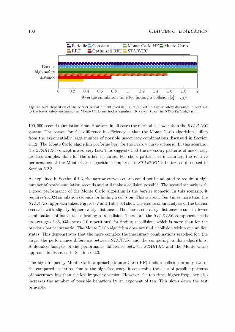
100 CHAPTER 6. EVALUATION
0 0.2 0.4 0.6 0.8 1 1.2 1.4 1.6 1.8 2
·105
Barrierhigh safety
distance
Average simulation time for finding a collision [s]
Periodic Constant Monte Carlo HF Monte CarloRRT Optimized RRT STARVEC
Figure 6.7: Repetition of the barrier scenario mentioned in Figure 6.5 with a higher safety distance: In contrastto the lower safety distance, the Monte Carlo method is significantly slower than the STARVEC algorithm.
100, 000 seconds simulation time. However, in all cases the method is slower than the STARVEC
system. The reason for this difference in efficiency is that the Monte Carlo algorithm suffers
from the exponentially large number of possible inaccuracy combinations discussed in Section
4.1.2. The Monte Carlo algorithm performs best for the narrow curve scenario. In this scenario,
the STARVEC concept is also very fast. This suggests that the necessary patterns of inaccuracy
are less complex than for the other scenarios. For short patterns of inaccuracy, the relative
performance of the Monte Carlo algorithm compared to STARVEC is better, as discussed in
Section 6.2.3.
As explained in Section 6.1.3, the narrow curve scenario could not be adapted to require a high
number of tested simulation seconds and still make a collision possible. The second scenario with
a good performance of the Monte Carlo algorithm is the barrier scenario. In this scenario, it
requires 25, 024 simulation seconds for finding a collision. This is about four times more than the
STARVEC approach takes. Figure 6.7 and Table 6.4 show the results of an analysis of the barrier
scenario with slightly higher safety distances. The increased safety distances result in fewer
combinations of inaccuracies leading to a collision. Therefore, the STARVEC component needs
an average of 36, 033 states (10 repetitions) for finding a collision, which is more than for the
previous barrier scenario. The Monte Carlo algorithm does not find a collision within one million
states. This demonstrates that the more complex the inaccuracy combinations searched for, the
larger the performance difference between STARVEC and the competing random algorithms.
A detailed analysis of the performance difference between STARVEC and the Monte Carlo
approach is discussed in Section 6.2.3.
The high frequency Monte Carlo approach (Monte Carlo HF) finds a collision in only two of
the compared scenarios. Due to the high frequency, it constrains the class of possible patterns
of inaccuracy less than the low frequency version. However, the ten times higher frequency also
increases the number of possible behaviors by an exponent of ten. This slows down the test
principle.
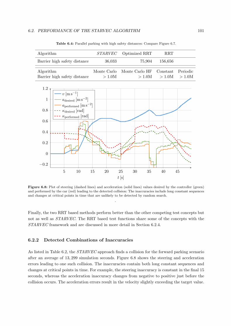
6.2. PERFORMANCE OF THE STARVEC ALGORITHM 101
Table 6.4: Parallel parking with high safety distances: Compare Figure 6.7.
Algorithm STARVEC Optimized RRT RRT
Barrier high safety distance 36,033 75,904 156,656
Algorithm Monte Carlo Monte Carlo HF Constant PeriodicBarrier high safety distance > 1.0M > 1.0M > 1.0M > 1.0M
5 10 15 20 25 30 35 40 45
−0.2
0
0.2
0.4
0.6
0.8
1
1.2
t [s]
v [m s−1]
adesired [m s−2]
aperformed [m s−2]
κdesired [rad]
κperformed [rad]
Figure 6.8: Plot of steering (dashed lines) and acceleration (solid lines) values desired by the controller (green)and performed by the car (red) leading to the detected collision: The inaccuracies include long constant sequencesand changes at critical points in time that are unlikely to be detected by random search.
.
Finally, the two RRT based methods perform better than the other competing test concepts but
not as well as STARVEC. The RRT based test functions share some of the concepts with the
STARVEC framework and are discussed in more detail in Section 6.2.4.
6.2.2 Detected Combinations of Inaccuracies
As listed in Table 6.2, the STARVEC approach finds a collision for the forward parking scenario
after an average of 13, 299 simulation seconds. Figure 6.8 shows the steering and acceleration
errors leading to one such collision. The inaccuracies contain both long constant sequences and
changes at critical points in time. For example, the steering inaccuracy is constant in the final 15
seconds, whereas the acceleration inaccuracy changes from negative to positive just before the
collision occurs. The acceleration errors result in the velocity slightly exceeding the target value.

102 CHAPTER 6. EVALUATION
Figure 6.9: Results of STARVEC (top) and Monte Carlo (bottom) algorithm: The latter covers noticeably lessarea (blue path lines) and is less likely to find collisions.
This intensifies the effect of the steering inaccuracies leading to the collision. The illustrated
pattern of inaccuracies also shows why the competing test principles perform worse in this
scenario. Constant inaccuracies do not change at all and hence do not change at critical points
in time. Periodic inaccuracies are unlikely to change at the critical point in time. For this reason,
the method based on periodic inaccuracies does not find any collision. The method based on
constant inaccuracies finds a different collision after a long simulation time.
The Monte Carlo algorithm also does not find a collision in this scenario. The reason for the
performance difference to the STARVEC approach is illustrated in Figure 6.9. It compares the
performance of the two test methods in the parallel parking scenario in the first 10, 000 simulation
seconds. The blue lines represent driven trajectories of the vehicle during the simulation. They
visualize that the STARVEC system covers significantly more area than the Monte Carlo
algorithm. This correlates to the ability of both test principles to find undesired behaviors
like collisions.
Figures B.1-B.10 in Appendix B show the motions and the controller states for one example
of each of the remaining scenarios. In most cases, the combination of lateral and longitudinal
controller errors at an effective point in time leads to the collision.
Apart from searching for collision states, the presented test functions can also search for
temporal behavior patterns as described in Section 4.4. As depicted in Figure 6.10, applying the
STARVEC and the Monte Carlo algorithm to the suggested double stop pattern reveals a similar
performance difference. The higher the velocity of the second motion in the pattern searched
for, the less often it occurs and the more complex are the necessary inaccuracy patterns. As
the complexity of the inaccuracy pattern increases, so does the number of necessary simulation

6.2. PERFORMANCE OF THE STARVEC ALGORITHM 103
0.19 0.19 0.2 0.2 0.21 0.21 0.22 0.22 0.23 0.23
2
4
6
·104
velocity of second motion [m s−2]
simulatedtime[s]
Monte CarloSTARVEC
Figure 6.10: Simulated seconds of Monte Carlo vs. STARVEC algorithm until double stop pattern is found.
seconds for both algorithms to find them. However, for the Monte Carlo algorithm it increases
significantly faster than for the STARVEC approach. The difference between both test functions
is investigated in the next section.
6.2.3 Worst-Case Performance of the Monte Carlo Algorithm
As described in Section 4.1.2, there is an exponential number of possible behaviors that can be
generated based on sensor and actuator inaccuracies. This makes the Monte Carlo algorithm
often fail to find an undesired behavior within reasonable time. If the undesired behavior depends
only on very few random choices, the Monte Carlo algorithm performs well. Scenarios can be
adapted by changing some scenario parameters. However, for most scenarios, it is difficult to
scale the number of random choices that influence whether the undesired behavior is performed.
In these cases, the Monte Carlo algorithm either finds an undesired behavior quickly or does not
find any undesired behavior depending on the chosen scenario parameters. Therefore, a scenario
is needed that can be scaled. The scenario depicted in Figure 6.11 helps to demonstrate the
difference between the STARVEC approach and the Monte Carlo algorithm. Its main component
is a long corridor consisting of a variable number of barriers and a following obstacle that is
not detected by the ego vehicle. The ego vehicle only collides with the not detected obstacle at
the end of the corridor if it does not get stuck on the path. As the corridor is very narrow, it is
likely to get stuck at each barrier. The more repetitions of the barrier, the smaller the share of
behaviors that result in hitting the obstacle.

104 CHAPTER 6. EVALUATION
Notdetectedobstacle
n repetitions
Figure 6.11: n repetitions of a barrier situation: The ego vehicle only collides with the not detected obstacle atthe end of the corridor if it does not get stuck on the path.
10 20 30 40 50 60 70 80 90
1
2
3
·104
Explored distance [m]
Sim
ulation
time[s]
STARVECMonte Carlo
Figure 6.12: Comparison of the STARVEC and the Monte Carlo algorithm in the scenario depicted in Figure6.11: After 20 meters, the Monte Carlo algorithm is slower than STARVEC and quickly exceeds 100.000 simulatedseconds.
Figure 6.12 shows the relation between length of the corridor and the necessary simulation time
of the STARVEC and the Monte Carlo algorithm. It plots the number of simulated seconds
necessary to reach a distance in the narrow barrier corridor on average of ten repetitions. In the
first 20 meters, the Monte Carlo algorithm is faster than the STARVEC system. Afterward, it
grows quickly and exceeds 100.000 simulated seconds for covering less than 30 m. In contrast,
the number of necessary simulated seconds for the STARVEC method grows almost linearly.
These results confirm the time complexity of the involved test functions computed in Section
4.1.2. The Monte Carlo algorithm randomly picks any of the exponentially many behaviors.
Thus, the necessary simulation time grows with the number of possible behaviors and hence
with the distance to cover. In contrast, the STARVEC approach uniformly covers the available
space, which grows only linearly with the distance to cover.

6.2. PERFORMANCE OF THE STARVEC ALGORITHM 105
Cross Parking
4
5
1
2
3
6
Most novel state
4
1
2
3
6
5
(a) RRT vs. STARVEC
Cross Parking
4
5
1
2
3
6
Most novel state
4
1
2
3
6
5
(b) Optimized RRT
Figure 6.13: Comparison of RRT, STARVEC and a modified version of RRT: RRT focuses on states at theborder of the set of explored states, whereas STARVEC explores the “most novel state”. The modified version ofRRT explores more states in the center of the set of explored states.
6.2.4 Comparison between STARVEC and RRT
Two of the compared test methods are based on the RRT concept. Similarly to the STARVEC
approach, the RRT principle aims to cover the state space quickly by evenly distributing the
nodes that are expanded. The even distribution is reached by randomly picking states in the
configuration space and expanding the nearest explored node. However, for testing against
inaccuracies this does not lead to an even distribution as illustrated in Figure 6.13(a). The
inaccuracies do not fully control the motion of the vehicle, but only influence it. Different
inaccuracies lead to different trajectories driven by the vehicle. Some of these trajectories are
illustrated by the green lines. The blue circles represent states along these trajectories that have
been stored as described in Section 4.1. The RRT algorithm tries to cover the remaining area by
randomly picking states in the configuration space. These states are depicted by the triangles
1-6. As the inaccuracies do not fully control the vehicle, the resulting trajectories still move
along the planned trajectory instead of towards the sampled random states. The lines from the
triangles to the explored states (blue circles) indicate which state is chosen to be expanded next
according to the RRT concept. Almost all chosen states are at the border of the explored space
of reachable states, because sampling a random node in the middle of the reachable state space
occurs seldom. States at the start and the end of the trajectory are sampled particularly often.
In contrast, STARVEC picks the state that is farthest away from all already expanded states.
In Figure 6.13 this is labeled as the “most novel state”. The result is that the RRT algorithm
106 CHAPTER 6. EVALUATION
performs significantly worse than the STARVEC system in the evaluated scenarios (compare
Figures 6.5 and 6.6). Most undesired behaviors occur at the border of the reachable state space.
However, some states at the border of the set of reachable states can only be reached by traversing
intermediate states that are not at the border of this state space. These intermediate states are
disregarded by the RRT concept.
The RRT concept is faster than the STARVEC approach in finding the final seconds before an
undesired behavior occurs because it is biased to extreme states. The STARVEC test supervisor
does not expand the extreme states if a very similar state has already been expanded. This
makes the test method slower in this part of the search.
Therefore, an optimized version of the RRT is created for comparison. The sampling strategy of
the optimized RRT concept is limited to an area around already explored states as depicted in
Figure 6.13(b). The new test method only samples states with a distance of less than a threshold
to already explored states. If a state with a higher distance is sampled, a new random sample is
created. The allowed area is depicted as a yellow shape surrounding the explored trajectories. The
modification makes it more likely to sample states in the middle of the reachable state space. The
strategy corresponds to increasing the sampling density in narrow passages as used by many
RRT based planning techniques like [164]. The resulting test function performs significantly
better than the basic RRT method as shown in Figures 6.5 and 6.6. The test function is labeled
as “Optimized RRT”. It is faster than the original RRT approach in most scenarios. In one
case, it performs better than the STARVEC principle while the STARVEC system dominates
the other scenarios. Section 7.3 discusses potential benefits of creating a combined version of
STARVEC and RRT.
6.3 Scenarios with additional Patterns of Inaccuracy
In addition to the scenarios with actuator inaccuracies evaluated in Section 6.2.1, further
inaccuracy models have been developed and evaluated. Section 6.3.1 discusses experiments with
a large set of sensor inaccuracies in addition to the actuator inaccuracies. Section 6.3.2 evaluates
the nondeterministic models of traffic participants introduced in Section 4.5.
6.3.1 Scenarios with Errors of the Environment Sensors
In the scenarios evaluated in this section, three kinds of inaccuracy models are added. They
affect the odometry-based localization, the global localization and the environment mapping
sensors. The corresponding inaccuracy models are described in Sections 3.3.3 and 3.3.4. For the
odometry-based localization and environment map errors, an implementation created in [131] is
applied. The odometry localization errors in that work have been developed based on a global
localization error implementation created in the present thesis.

6.3. SCENARIOS WITH ADDITIONAL PATTERNS OF INACCURACY 107
0 0.2 0.4 0.6 0.8 1 1.2 1.4 1.6 1.8 2
·105
Crossparking
Narrowcurve
Narrowlane
Average simulation time for finding a collision [s]
Periodic Constant Monte Carlo HF Monte CarloRRT Optimized RRT STARVEC
Figure 6.14: Comparison of the test competing principles with a large set of sensor and actuator inaccuraciesin a parking and two lane following scenarios. STARVEC outperforms the competing test methods.
Figure 6.14 shows the results of the application of the competing algorithms to three scenarios
with these inaccuracy patterns. The scenarios correspond to those used in Section 6.2.1. The
only difference is that the safety distances of the planning component have been adjusted to
the additional inaccuracy models as described in Section 6.1.3. The maximum of the bars in
Figure 6.14 is 200, 000 instead of 100, 000 in order to account for the higher number of possible
inaccuracy patterns in each step.
The experiments show that STARVEC performs significantly better than the Monte Carlo
methods in all three examples. In two cases the constant inaccuracy patterns perform similar to
STARVEC while they do not find the collision in the cross parking scenario. This corresponds to
the results in Section 6.2.1 where the constant inaccuracy algorithm performs well in some cases
but does not find the collision in the other scenarios. As in Section 6.2.1, the periodic inaccuracy
approach eventually finds a collision in the scenario in which the constant inaccuracy method
is very fast. It does not find an undesired behavior in the other two scenarios. Finally, the RRT
based systems perform better than Monte Carlo, but worse than STARVEC.
All in all, the experiments in this Section show that the STARVEC approach can cope with a
high number of simultaneously active inaccuracy patterns. For such scenarios, the STARVEC
system requires more simulation seconds for reliably testing a planning and control system.
Existing test methods are less efficient in finding undesired behaviors for these cases.

108 CHAPTER 6. EVALUATION
Figure 6.15: Collision of the ego vehicle with a long truck during the attempt to merge into the line of traffic ofthe truck.
6.3.2 Scenarios with Traffic Participants
In addition to the static scenarios, the presented concept has been tested in two scenarios
involving the interaction with traffic participants:
1. a scenario involving merging into another lane with traffic coming from behind and
2. an intersection scenario with traffic coming from the side.
In both scenarios, the opposing traffic participant has the right of way. The first scenario is
depicted in Figure 6.15 and is similar to the situation that lead to the accident caused by
a Google autonomous driving prototype [165]. At the beginning, the autonomous vehicle is
commanded to merge into the left part of the lane because the right part is obstructed by some
obstacle. In this case, the obstacles are a pile of sand bags. A truck is approaching from behind
and the ego vehicle has to decide whether it can complete the merge before the truck arrives. In
the second scenario (Figure 4.18), the ego vehicle wants to cross a street on which the arriving
truck has the right of way. The truck is modeled as described in Section 4.5.1 and the ego vehicle
collision-avoidance system includes the weaknesses described in Section 6.1.1.
STARVEC and the Monte Carlo algorithm are applied to these scenarios trying to find collisions
that are the fault of the ego vehicle. Figure 6.16 compares the performance of the two test
functions. The smaller the assumed safety distance described in Section 6.1.1, the more difficult
it is to find the collision. This assumed safety distance decreases towards the right part of Figure
6.16. The comparison shows that the required simulation time grows faster for the Monte Carlo
algorithm than for the STARVEC approach. Moreover, the STARVEC method is also more
efficient regarding the absolute numbers.

6.4. SUMMARY OF THE EVALUATION 109
0.2 0.1 0.02
1
2
3
·105
0.6
Assumed truck safety distance [m]
Sim
ulatedtime[s]
Monte CarloSTARVEC
Figure 6.16: Simulated seconds of Monte Carlo vs. STARVEC algorithm until a clearly assignable collisionis found. Smaller assumed safety distances make both concepts take longer to find the collision. STARVECoutperforms the Monte Carlo method.
The sequences leading to a collision can be relatively complex as shown in Figure 6.17. It depicts
one behavior detected by the STARVEC system. First, the truck decelerates and is predicted
to stop soon. Therefore, the ego vehicle starts driving towards the lane (Figure 6.17(a)). Next,
the truck accelerates again and the ego vehicle brakes in order to prevent a collision (Figure
6.17(b)). When the truck repeats braking, the ego vehicle reacts by accelerating (Figure 6.17(c))
but does not reach the initially intended speed. Thus, it has to halt when it realizes that the
truck does not stop (Figure 6.17(d)). However, it reaches standstill only just soon enough, but
falsely assumes that the truck will not be able to pass anymore. It concludes that the truck will
stop, too. Consequently, it starts driving. This leads to the collision depicted in Figure 6.15.
All in all, the experiments demonstrate that the STARVEC approach can be efficiently applied to
scenarios containing the interaction with traffic participants. As for the scenarios in the previous
sections, STARVEC analyzed these scenarios significantly more efficiently than the Monte Carlo
approach.
6.4 Summary of the Evaluation
In summary, the evaluation shows that the STARVEC system outperforms existing methods
for finding undesired behaviors caused by nondeterministic events. The performance difference
has been demonstrated in scenarios with and without direction changes. Moreover, the
demonstration contains scenarios with few and with many nondeterministic events including
scenarios with traffic participants. In some scenarios the exponential worst-case complexity of
the Monte Carlo approach can be observed while STARVEC solves these scenarios in linear time.

110 CHAPTER 6. EVALUATION
(a) Truck decelerates (b) Truck accelerates
(c) Truck decelerates (d) Truck accelerates
Figure 6.17: The red vehicle tries to merge back (black curve) into the main lane avoiding a collision of its safetydistance (green perimeter) with the predicted positions of the truck (orange lines). The truck switches betweendeceleration and acceleration ultimately leading to the collision in Figure 6.15.

Chapter 7
Future Work
The work in this thesis presents a method for testing autonomous driving systems more efficiently
than previous approaches. In order to exploit the potential of this new concept fully, further
research is necessary. This chapter outlines several research projects that would extend the
benefit on the STARVEC framework. First, Section 7.1 suggests extending the application to
mature autonomous driving systems in order to get a bigger amount of experimental results.
Next, Section 7.2 describes how an online learning system can be designed and tested using the
STARVEC method. Section 7.3 advocates combining the STARVEC and the RRT approach in
order to increase testing efficiency further. Another research project is to apply the STARVEC
approach to high-speed scenarios outlined in Section 7.4. Finally, the interaction with a large
number of traffic participants is one of the major challenges for both development and testing
of autonomous driving systems as addressed in Section 7.5.
7.1 Extending the Application of the STARVEC Algorithm
The STARVEC concept has been implemented and evaluated against the combination of several
scenarios, a planning and control system and a set of models of sensor and actuator inaccuracies.
All three aspects should be extended in future research.
The tested scenarios include the set of scenarios listed in Section 6.1.3. While this is a reasonable
set for evaluating the performance of the test function, requirement specifications list many
more special cases in which a planning and control system has to function. A comprehensive
analysis includes all of the scenarios specified in the requirement documents. Furthermore, it
includes some scenarios as described in Section 4.3. Such an analysis can demonstrate both: the
applicability of STARVEC and the performance of the tested planning and control system.
Sections 3.3 and 3.4 provide sensor and actuator error models that cover major kinds of
inaccuracies. Additionally, a method is described for finding the necessary parameters that
111

112 CHAPTER 7. FUTURE WORK
Starvec + Deep Learning Project
Creation of a deeplearning autonomous
driving system
Over nightvalidation of the
system
On-Demand validation bases on powerful processors
On-Demand validation based on datacenter and high-
bandwidth
Additional learnedvehicle and
environment model
Figure 7.1: The first step of the proposed research effort is the development of a self-learning autonomous drivingsystem. Using this system, four paths of research can be followed.
make the models useful. Vehicles involved in research projects accompanying this thesis, often
displayed quite large offsets and delays between requested and performed actions. Partially this
is due to the development of the actuator software not being finished. Some of the deficiencies
will remain after optimization of the actuator software. For example, actuators can be inaccurate
when starting the vehicle or rapidly changing the requests. Therefore, a valuable research project
would be to use a vehicle with optimized actuators and create inaccuracy models including all
vehicle specific deficiencies.
7.2 Application to Online Validation of Learned Planning and
Control Systems
Section 5.4 describes how the STARVEC approach can be used for validating a planning
and control system that is adapted by machine learning mechanisms. A research project can
implement a system that continuously improves its planning performance using deep learning.
As this planning and control component changes its behavior with each additional piece of
information, the prior executed tests are not sufficient for attesting the safety of the system.
The STARVEC concept can improve the safety by evaluating either a specific scenario or a set
of scenarios before applying changes over night.
Figure 7.1 shows a possible setup of a research project. The research project starts with the
creation of a continuously learning autonomous driving system. Such a system can be based on
existing works of [155], [156]. However, these demonstrations do not consider reliability issues,
yet. The general idea of these methods is to learn the behavior of human drivers without explicitly
punishing collisions. With enough data, the system will not create collisions, because humans
avoid collisions, too. The STARVEC algorithm would detect the rare cases of collisions and
reject most versions of the learned system.
Therefore, the learning system needs to be extended by an additional collision-avoidance
mechanism. This can be a simulation environment that is used as supplementary data source

7.2. TEST ONLINE VALIDATIONOF LEARNED PLANNING AND CONTROL SYSTEMS113
rewarding collision preventing systems. In a further step, this simulation can be based on the
STARVEC algorithm as described in [140]. This would lead to detecting more possible collisions
and hence a stronger reward for collision preventing systems.
Based on this learning system, Figure 7.1 depicts four lines of research that are worth
investigating:
1. Validation of the autonomous driving system in the vehicle over night,
2. on-demand validation based on powerful computation resources,
3. on-demand validation based on a data center and a high communication bandwidth and
4. validation of the autonomous driving system with learned environment and vehicle models.
The first research path is to validate the autonomous driving system over night. During the
day, the system collects data but does not use it for changing its behavior, yet. As soon as the
vehicle is parked, the changes are applied to a virtual duplicate of the vehicle. The STARVEC
algorithm tests this duplicate in various test scenarios trying to find situations and environment
events in which the system would create a collision. The changes are only applied if STARVEC
does not find any safety issues. If the car is started before the tests are completed, the changes
are not applied.
In this path of development, several research questions need to be answered:
• How many scenarios need to be tested in order reach sufficient confidence in the reliability
of the system?
• Can the learning system recognize if it encounters a situation that is not similar to one of
the tested scenarios?
• How should the system cope with failing tests? If the tests fail once, they may be likely to
fail again in the next night.
The second path of research is the on-demand validation based on powerful computation
resources. For example, the learning system is queried to park into a very narrow parking
lot. Before starting the parking motion, the scenario is tested in simulation using the
STARVEC algorithm. This requires a very large number of processor cores–probably more than
1000–available in the vehicle. The research project may assume the availability of such resources
in the future. This leaves some research questions still to be answered:
• How can the execution of the STARVEC algorithm be parallelized on a large number of
processor cores?
• How should the vehicle behave if the system is not considered safe for this motion?
For massively parallelizing the STARVEC algorithm there needs to be an analysis master that
manages the queue of simulation states. Instead of choosing a single state to be executed next,
114 CHAPTER 7. FUTURE WORK
it picks one or more states for each processing core. The processing cores execute the simulation
starting with the input state. This leads to a new state, which they report to the analysis master
who adds the state to the search queue.
The availability of more than 1000 processor cores becomes more realistic in a data center, which
is the third research path. Additionally to the research questions for a local execution of the
STARVEC algorithm, this requires reasoning about the communication:
• Can all necessary data of the current scenario be transmitted to the datacenter sufficiently
fast?
• Does the data center need a remote copy of the currently active autonomous driving
software of each vehicle?
Finally, a fourth path of research investigates learning vehicle and environment models, too. The
models have to interact with the STARVEC framework in order to reach maximal efficiency.
All in all, the described efforts would generate an insight into how self-learning autonomous
driving systems can be continuously tested in order to increase their reliability.
7.3 Combining RRT and Novelty Based Exploration
The evaluation in Chapter 6 shows that the STARVEC system performs better than the
implemented approaches based on an RRT algorithm. However, as explained in Section 6.2.4,
the RRT based approach has advantages in finding the final seconds leading to an undesired
behavior. The implemented modification of the RRT principle does not close the gap between
the RRT based approach and the STARVEC method. Instead, a combination of both ideas
might lead to a better performance in particular when applied to very complex scenarios like
those proposed in Section 7.5. A simple combination of both algorithms would alternate between
the RRT approach and the STARVEC approach for choosing the next node to be expanded.
Alternatively, the priority of each state in the priority queue introduced in Section 4.2 could be
adapted. The priority could be based on a combination of the distances to the nearest expanded
node and to a random node. On the one hand, this would still lead to novel nodes being expanded.
On the other hand, nodes at the border of the reachable state space would be expanded sooner.
7.4 Testing High Speed Scenarios
A promising application for the STARVEC approach are high-speed scenarios like highway
driving or platooning. The goal of platooning is to reduce fuel consumption and improve traffic
flow by reducing the distance between succeeding vehicles. Figure 7.2 sketches a platooning
scenario. The vehicles try to keep a safety distance as between the red vehicle and the second

7.4. TESTING HIGH SPEED SCENARIOS 115Platooning
Safety distance
Reduced safety distance
due to inclination
Figure 7.2: Sketch of a platooning scenario. The vehicles try to keep a safety distance as between the red vehicleand the second truck. The first truck slows down because of the inclination leading to a temporarily reducedsafety distance between the two trucks.
truck. The first truck slows down because of the inclination. This leads to a temporarily reduced
safety distance between the two trucks. At this moment, the first truck might be forced to
perform an emergency brake action due to an unexpected event happening in front of him. The
second truck has to be able to brake despite of the reduced safety distance and possibly other
negative current conditions. In addition, the red vehicle also needs to brake fast enough.
On the one hand, this has to be ensured by applying a well-constructed control mechanism. On
the other hand, the actual implementation and an accurate vehicle model may lead to states
not predicted by the simplified models used for the concept design. Instead, the STARVEC
concept can be applied to determine whether the safety distances and braking concepts applied
in different situations are sufficient for ensuring the platoon’s safety.
Figure 7.3 sketches a project consisting of five research tasks to be addressed. The first task is
to implement a platooning system based on existing work for example of [166] or [167]. This has
to include the controller for the good cases, i.e. cases in which no seldom disturbances occur.
Additionally, there need to be functions dealing with emergencies. If the vehicle leading the
platoon has to perform an emergency brake action, there needs to be a strategy minimizing
or preventing damage to the following vehicles. The capability of handling such situations
determines how close the vehicle can approach during normal operation. The closer the vehicles
can approach, the more fuel they are saving. The STARVEC framework can then be applied
to the implemented platooning control system in order to find weaknesses in its emergency
handling.
The implementation of the platooning controller is sufficient for first experiments about the
applicability of the STARVEC concept to the platooning problem. For more comprehensive
experiments with the platooning technology, it is necessary to implement further platooning
or high-speed scenario specific environment events. One such event is the change of the road
inclination described in the first paragraph of this section. Another important event is a late

116 CHAPTER 7. FUTURE WORK
Platooning System Environment events Adjustments to the
STARVEC algorithm
Standard ACC High speed merge
maneuvers
• Good case
controller
• Emergency
maneuvers
• Change of road
inclination
• Late detected
static obstacle
• Changed road
friction
• Wind
• Instable
communication
• Relative
positions and
velocities
• Analyze
efficiency
• Sudden lane
change of vehicle
in front
• Nondeterministic
behavior of
involved vehicles
• Limited length of
own lane
Figure 7.3: Five parallel research tasks for analyzing high-speed scenarios.
detected static obstacle in front of the leading vehicle. This obstacle might trigger the emergency
brake maneuver mentioned in the first paragraph of this section. Furthermore, the road friction
might change at an unfavorable point in time. This affects the emergency brake maneuver.
If the road friction is low during the whole scenario, the platooning control system might
adapt by increasing the safety distances. A low road friction occurring shortly before the
emergency braking starts can have more severe effects. The fourth event listed in Figure 7.3
is wind influencing the controller behavior. It can lead to some deviations from the planned
vehicle trajectory that can accumulate with other effects in an emergency brake maneuver.
Finally, communication problems are a major factor for platooning systems. These problems
include communication delays, or temporarily or permanently lost connections to platooning
participants. The platooning system has to cope with the deficiencies and continue safe operation.
As for the other tested events, communication problems occurring in a favorable moment can
be handled differently to those affecting emergency maneuvers.
The third research task to be investigated are adjustments to the STARVEC algorithm. The
STARVEC concept is designed to support different kinds of autonomous driving systems.
However, the experiments in this thesis focus on low speed scenarios. For gaining efficiency
in high-speed scenarios, some properties of them can be exploited. One such property is low
relative velocities. The velocity of the rear vehicles typically only deviates by less than one
meter per second from the velocity of the leading vehicle. Instead of using the absolute position
and velocity of the involved vehicles for the state abstraction introduced in Section 4.1, these
relative values can be used. This can reduce the size of the explored state space.
The results of the first three development lanes cover efficient tests of a platooning system. The
insights gained in these efforts can be extended to other high-speed scenarios. One such scenario
involves a standard ACC (Adaptive Cruise Control) system. Such systems can be tested against
a vehicle cutting into the ego vehicle’s lane at a close distance. This behavior can occur in
unfavorable moments like when the car is currently accelerating.

7.5. TESTING THE INTERACTION WITH MANY TRAFFIC PARTICIPANTS 117
Figure 7.4: The ego vehicle (red) wants to merge into the left lane between the two other cars. The lane of theego vehicle ends after a limited distance.
Finally, the insights can be applied to high-speed merge maneuvers as listed in Figure 7.3
and illustrated in Figure 7.4. As regarded in Section 4.5, the traffic participants can behave
nondeterministically. The merging controller has to ensure safe operation as long as the behavior
of the other vehicles is acceptable. The maneuver can become more difficult due to the events
listed in the previous paragraphs. Additionally, the system has to cope with situations in which
the own lane ends.
In summary, the research efforts described in this section improve testing of autonomous systems
in high-speed scenarios by applying the STARVEC concept to them.
7.5 Testing the Interaction with Many Traffic Participants
Another direction of future research are scenarios with many traffic participants. The basis for
this has been presented in Section 4.5. It demonstrates tests of the planning and control system
in the presence of a traffic participant behaving nondeterministically. Figure 7.5 shows a more
complex traffic situation. It depicts a large number of traffic participants simultaneously using a
roundabout. Each traffic participant has many options for his future trajectory. The vehicles can
change lanes, turn into the roundabout exit, accelerate, decelerate and do many more things.
The ego vehicle has to find a plan that does not cause a collision for any behavior of the traffic
participants.
Three main challenges have to be addressed for testing such a scenario with the STARVEC
framework:
1. efficiently modeling other traffic participants
2. exploring adaptations to the STARVEC algorithm core, and
3. identifying who is responsible for which collision.

118 CHAPTER 7. FUTURE WORK
Figure 7.5: A complex roundabout with many traffic participants. Each traffic participant has many options forhis future trajectory. The ego vehicle must not cause an accident for any behavior of other traffic participants.
The large number of traffic participants has to be modeled such that the possible behaviors
are well covered and the analysis remains efficient. First, this requires implementing a small
set of atomic actions that cover the behaviors of the vehicle similar to the set in Section 4.5.
Additionally to the challenges solved in this thesis, the total number of different actions possible
by the large number of traffic participants is significantly higher. In order to keep the simulation
efficient several abstractions of the vehicle actions are reasonable. Three possible abstractions
are:
1. Adapting the set of possible actions based on the distance of a car to the ego vehicle,
2. limiting nondeterminism to vehicles relevant in the near future and
3. modeling the behavior of car convoys instead of single cars.
The first abstraction means that cars with a high distance to the ego vehicle are modeled with
less possible actions. For example, the actions can be limited to only acceleration and lane
changes without lateral deviations within a lane. Instead of modeling acceleration, the vehicles
can also be limited to a small set of possible target velocities. The second abstraction implies
that some cars in the scene behave deterministically, because they only slightly influence the ego
vehicle. For example, the vehicles at the top right corner will not get close to the ego vehicle soon.
Their presence is important as they might affect the chosen future path, but small deviations
of their behavior does not influence the current plan. Finally, convoys of cars can be modeled

7.5. TESTING THE INTERACTION WITH MANY TRAFFIC PARTICIPANTS 119
together instead of modeling the behavior of every single car. This limits the range of possible
resulting behavior patterns only slightly but increases the efficiency of the analysis. The convoy
can perform the same actions as a single vehicle plus it can dissolve or merge with another
convoy or vehicle. All three abstractions limit the set of possible behavior patterns of the full
system. It has to be researched whether these limitations significantly influence the analysis
results. Furthermore, additional abstractions can be developed and compared.
The second research challenge are adaptations to the STARVEC algorithm. Two reasonable
adaptations are a comparison of different search techniques and changing the abstraction of
traffic states. One possible search technique to investigate is the combination of STARVEC
and RRT suggested in Section 7.3. The abstraction of traffic states can exploit the different
consequences of deviations of the ego position and deviations of the traffic participants’ positions.
The position of traffic participants can be mapped to a coarser grid. Additionally, it can be
defined as a position on a lane and the distance to this position.
Finally, the third research challenge copes with identifying those collisions that are actually
caused by the ego vehicle. As described in Section 4.5, temporal behavior patterns can support
this filtering. However, the situations possible in the sketched roundabout are more complex and
require research for defining the temporal logic behavior patterns.
All in all, interaction with many traffic participants is one of the major challenges of autonomous
driving. A system for efficiently testing these interactions can speed up the development and
evaluation of new concepts addressing this challenge.

Chapter 8
Conclusion
In this thesis, a new method for testing autonomous driving planning and control software
against nondeterminism resulting from sensor and actuator inaccuracies or behavior of traffic
participants is presented. It searches for behaviors that can be specified either based on a single
state like collisions or based on a time sequence like repeated stops during a parking maneuver.
The approach exploits the geometric nature of these behaviors in order to reduce the complexity
of their detection. A comparison shows that it is significantly more efficient than a classical Monte
Carlo algorithm. Based on the approach, scenarios from physical test-drives can be analyzed
finding almost-accidents that could have been accidents but have not been. If a fault actually
occurs in a test-drive, parts of the method can be reused for robust reproduction of the fault in
a simulation environment. The concept has been implemented as a prototype and tested with
an autonomous driving system created for an industrial partner.
It can be applied to autonomous driving projects by implementing load and store operations for
the involved software components. In future projects the system can be optimized for execution
on high performance computers. This makes it applicable to testing a large set of scenarios
simultaneously. Furthermore, additional research is necessary for creating the most valid and
efficient sensor and actuator inaccuracy models. It also seems promising to apply it to high-speed
scenarios like platooning or highway driving. Finally, scenarios with many traffic participants
can be tested by the concept.
120


Appendices
122

Appendix A
NuSMV base model
Listing A.1: NuSMV transition table for one state
1 MODULE main
2 DEFINE
3 <NuSMV -tables > -- Has to be replaced by the tables generated from
4 -- the STARVEC search graph
56 ------------------------------------------------------------------
7 --------------------- Special States -----------------------------
8 ------------------------------------------------------------------
9 INVALID := FALSE;
10 NO_STATE := MAX_STATE_ID + 1; -- The successor state of not
11 -- expanded states
12 TERMINAL_STATE := MAX_STATE_ID + 2; -- The successor state of all
13 -- terminal states
14 -- Replaces not expanded successor states if, similar states are
15 -- not included in the behavior pattern searched for
16 SIMILAR_STATE := MAX_STATE_ID + 3;
17 --
18 --
19 --
2021 VAR
22 state_id : 0 .. SIMILAR_STATE; -- The STARVEC node id. Each state
23 -- corresponds to one simulated
24 -- second
25 sub_step : 0 .. 99; -- The base simulation steps. Each base step
26 -- corresponds to 0.01 simulated seconds
27 error_number : 0..3; -- The currently active error pattern number.
28 -- It can only change when the STARVEC
29 -- state_id changes
3031 IVAR
32 next_error_number : 0..3;
3334 ASSIGN
3536 next(state_id) := NEXT_STATE_ID; -- NEXT_STATE_ID is a table
123

124 APPENDIX A. NUSMV BASE MODEL
37 -- generated from the STARVEC
38 -- search graph
394041 next(sub_step) :=
42 case
43 sub_step = 99 : 0;
44 TRUE : sub_step + 1;
45 esac;
4647 -- The active error number can only change when the STARVEC
48 -- state_id changes
49 next(error_number) :=
50 case
51 sub_step = 99 : next_error_number;
52 TRUE : error_number;
53 esac;
5455 -- The initial error_number is a free variable
56 INIT state_id = 0 & sub_step = 0;
5758 -- Model plausibility check: Special state NO_STATE is not
59 -- reachable
60 INVARSPEC state_id != NO_STATE;
6162 DEFINE
6364 -- Example pattern to be checked: Double forward pattern. G0-G3
65 -- are property tables generated from the STARVEC search graph:
66 -- G0: velocity >0.3
67 -- G1: velocity =0
68 -- G2: velocity >-0.05
69 -- G3: velocity >0.3
70 SPEC !EF(G0 & E[G2 U G1 & E[G2 U G3 & state_id < NO_STATE ]]);
7172 -- The NuSMV output can be very long. The following regex can be
73 -- used for search+replace by "" in order to get only STARVEC
74 -- state changes
75 --( sub_step = \d+| -> (Input|State): \d+\.\d+ <-
76 --| NEXT_STATE_ID = \d+)\r\n

Appendix B
Plots of Collisions in the AnalyzedScenarios
Figures B.1-B.10 show examples of detected collisions for each of the scenarios compared in
Section 6.2.1. For each displayed pair, the left Figure shows the path leading to the detected
collision. The right Figure shows controller states in the final about 10 seconds before the collision
occurs. In these plots, σtra is the steering angle planned by the trajectory planner, σdes is the
steering angle desired by the controller and σact is the actually performed steering angle. en is
the lateral position error of the controller and eψ is the orientation error of the controller.
−5 0 5 10
−10
0
(a) Driven path
26 28 30 32 34
−0.2
0
0.2
t [s]
σdes [rad] σact [rad]
σtra [rad] en [m]
eψ [rad]
(b) Controller states in the final seconds
Figure B.1: Collision detected in the “turn into narrow lane” scenario: The controller fails to follow the finalcurve to the right: The planned curvature σtra and the performed curvature σact deviate in the final second. Thisleads to a growing orientation error eψ that adds up with an already present high position error en.
125

126 APPENDIX B. PLOTS OF COLLISIONS IN THE ANALYZED SCENARIOS
−5 0 5 10
−10
−5
0
(a) Driven path
15 20 25
−0.4
−0.2
0
0.2
0.4
t [s]
σdes [rad] σact [rad]
σtra [rad] en [m]
eψ [rad] et [m]
(b) Controller states in the final seconds
Figure B.2: Collision detected in the “narrow curve” scenario: The trajectory planner plans to change thesteering angle σtra too fast for the controller to compensate current errors. This leads to an orientation error eψthat makes the vehicle touch the obstacle and is not compensated by the small position error.
0 10 20 30−4−2024
(a) Driven path
10 15 20 25
−0.4
−0.2
0
0.2
0.4
t [s]
σdes [rad] σact [rad]
σtra [rad] en [m]
eψ [rad]
(b) Controller states in the final seconds
Figure B.3: Collision detected in the “obstacle” scenario: The controller perceives changes of the trajectory planas non-continuous σtra values due to inaccurate predictions of the planner. This adds up with the inaccuratesteering to a high position error en exactly when the vehicle passes the obstacle.

127
−6−5−4−3
−30
−20
−10
0
(a) Driven path
20 22 24 26 28−0.2
−0.1
0
0.1
0.2
t [s]
σdes [rad] σact [rad]
σtra [rad] en [m]
eψ [rad]
(b) Controller states in the final seconds
Figure B.4: Collision detected in the “narrow lane” scenario: The trajectory planner defines slight S-shapedcurves for compensating controller errors. One of these curves leads to the trajectory planning safety distancetouching an obstacle. Additionally the controller fails to follow the curves exactly leading to a collision.
0 10 20 30
−101
(a) Driven path
22 24 26 28 30
−0.2
0
0.2
t [s]
σdes [rad] σact [rad]
σtra [rad] en [m]
eψ [rad]
(b) Controller states in the final seconds
Figure B.5: Collision detected in the “narrow barrier” scenario: In this scenario, the safety distances are setto very small values. Some seconds before the collision the controller error are small enough for the trajectoryplanner to compensate and big enough for the safety distance to touch the obstacle. Therefore, the vehicle triesto pass the barrier despite of the controller errors. At the barrier, inaccurate steering leads to a position errorthat is as large as the safety distance.

128 APPENDIX B. PLOTS OF COLLISIONS IN THE ANALYZED SCENARIOS
0 10 20−2
0
2
4
(a) Driven path
10 12 14 16 18
−0.1
0
0.1
0.2
t [s]
σdes [rad] σact [rad]
σtra [rad] en [m]
eψ [rad] et [m]
(b) Controller states in the final seconds
Figure B.6: Collision detected in the “ghost obstacle” scenario: Inaccurate actuators lead to a longitudinalcontroller error et that adds up with an orientation error and leads to a collision.
−10 −5 0 5
−5
0
5
(a) Driven path
30 35 40−0.4
−0.2
0
0.2
0.4
t [s]
σdes [rad] σact [rad]
σtra [rad] en [m]
eψ [rad] et [m]
(b) Controller states in the final seconds
Figure B.7: Collision detected in the “forward parking” scenario: Inaccurate acceleration in the 40th secondleads to a high longitudinal error et during a sharp curve. This leads to a lateral error en that the controller doesnot compensate fast enough. Additionally, the trajectory planning safety distance already touches the obstacledue to a previous lateral error in the 34th second.

129
−5 0
−5
0
5
(a) Driven path
35 40
−0.4
−0.2
0
t [s]
σdes [rad] σact [rad]
σtra [rad] en [m]
eψ [rad] et [m]
(b) Controller states in the final seconds
Figure B.8: Collision detected in the “skewed parking” scenario: Inaccurate steering leads to an orientation erroreψ in the 42nd second. It adds up with an already present lateral error en leading to a collision.
−10 −5 0−4
−2
0
(a) Driven path
0 5 10 15−0.4
−0.2
0
0.2
0.4
t [s]
σdes [rad] σact [rad]
σtra [rad] en [m]
eψ [rad] et [m]
(b) Controller states in the final seconds
Figure B.9: Collision detected in the “parallel parking” scenario: High longitudinal errors et lead to lateral errorsen due to a sharp curve. This leads to a collision with the side wall.

−5 0
−5
0
5
(a) Driven path
35 40
−0.4
−0.2
0
0.2
t [s]
σdes [rad] σact [rad]
σtra [rad] en [m]
eψ [rad] et [m]
(b) Controller states in the final seconds
Figure B.10: Collision detected in the “cross parking” scenario: High longitudinal errors et lead to lateral errorsen due to a sharp curve. In the 44th second, steering inaccuracy leads to an orientation error eψ that adds upwith the lateral error en leading to a collision.

List of Figures
1.1 Challenges of testing in simulation or the physical world. Testing in simulation
requires determining relevant dangerous scenarios to be tested. Testing in the
physical world is resource intensive and may have to be repeated if a defect is
found. . . . . . . . . . . . . . . . . . . . . . . . . . . . . . . . . . . . . . . . . . . 3
1.2 Coming closer to the serial production, the software development processes
become more heavyweight and tolerate fewer defects remaining in the system. . . 4
2.1 Different methods for avoiding a collision with an obstacle caused by sensor and
actuator errors. Methods based only on safety distances are vulnerable to noisy
inputs. Lower safety distances for near positions can lead to unnecessary closely
approaching the obstacle. Potential fields are complex to parameterize correctly
and planning with uncertainty requires high computation power. . . . . . . . . . 7
2.2 Online verification of path-planning results: If the path cannot be verified as safe,
the emergency stop (red) is executed. . . . . . . . . . . . . . . . . . . . . . . . . . 9
2.3 Models involved in an autonomous driving simulation: There are localization
and mapping sensor models including obstacle models, vehicle dynamic models
including the effect of the road surface and wind, and models of traffic participants. 10
2.4 Classification of test methods according to the maximal possible complexity of
the SUT and the effectivity in finding faults. Random testing can be applied to
complex systems but misses many faults, whereas symbolic execution is limited
to less complex systems but finds a large portion of existing faults. . . . . . . . . 12
3.1 States in the physical world and states in the simulation world consist of the
vehicle software state plus the state of the remaining world or the remaining
simulation. . . . . . . . . . . . . . . . . . . . . . . . . . . . . . . . . . . . . . . . 17
3.2 Representation of a physically driven sequence (upper part) in a simulation
environment (lower part). Each physical state can be represented in the simulation
(vertical lines) and is mapped to a simulated state (horizontal lines). The distance
between the representation and the mapped state should be small (“< α”). . . . 21
3.3 Sensors, actuators and the vehicle model are inaccurate. . . . . . . . . . . . . . . 24
3.4 Recall vs. precision: Figure 3.4(a) shows that low precision can lead to accidents
that are predicted but physically impossible. Figure 3.4(b) depicts a physically
possible unintended lane departure that the simulation does not predict. . . . . . 25
131

132 LIST OF FIGURES
3.5 Components influencing the performed acceleration: the acceleration controller
converts the desired acceleration to a desired torque, which it passes to the engine
and the brake control units. These units generate commands for their hardware
components leading to a resulting torque and a resulting acceleration. . . . . . . 28
3.6 Effect of offsets and delays to the observed output. For rapidly changing inputs,
the delay is the dominating pattern, for almost constant inputs, the offset dominates. 30
3.7 Inaccuracies of positioning sensors. The top image shows typical global positioning
inaccuracies including jumps. The lower image shows inaccuracies of the odometry
without jumps but high final inaccuracies. . . . . . . . . . . . . . . . . . . . . . . 32
3.8 Inaccuracies of ultra sonic sensors. The upper left green box is detected at an
inaccurate position due to ambiguous measured maxima (1). The red box is not
detected due to insufficient sensor range (2). The bottom green box is out of the
sensor range (3) but leads to a not existing obstacle (blue box) being identified. . 33
3.9 Visualization created by [132] of measurements of an ultrasonic signal showing
settling time, noise and multiple echoes. . . . . . . . . . . . . . . . . . . . . . . . 34
3.10 Mapping error caused by a positioning error: Measurement 1 correctly identifies
an obstacle. Measurement 3 correctly identifies free space. The wrong estimation
of the vehicle position leads to measurement 3 being interpreted as cone 2. As a
result, the obstacle is considered not to exist anymore. . . . . . . . . . . . . . . . 35
3.11 Inaccuracies of the environment map include obstacles detected at the wrong
position, not detected obstacles and detected but not existing obstacles. . . . . . 35
3.12 Extracting inaccuracy models from physical test-drives: Physical test-drives
improve (arrow “validate and improve”) the inaccuracy models that are used
(arrow “use”) for simulation. Simulation eliminates some weaknesses before they
are detected in physical test-drives. . . . . . . . . . . . . . . . . . . . . . . . . . . 37
3.13 Pareto front of possible offset and delay parameters extracted from physical
vehicle drive data by [131]. By assuming a high delay, lower maximal offsets
can be concluded. The experiment was conducted with two different error models. 38
4.1 Example of (coarse) geometric discretization. The top red cone and the state after
executing the yellow path are in the same grid cell and considered similar. . . . . 43
4.2 Overview of the STARVEC algorithm for finding error pattern combinations
leading to undesired states. Loading states and applying new inaccuracy patterns
alternates with executing a short part of the simulation sequence. . . . . . . . . . 44
4.3 Comparison of the computation time used for simulation vs. overhead of the
presented testing algorithm: The simulation time dominates the total computation
time. . . . . . . . . . . . . . . . . . . . . . . . . . . . . . . . . . . . . . . . . . . . 47
4.4 Serial execution of software components: In each step, components 1, 2 and 3 are
executed serially. . . . . . . . . . . . . . . . . . . . . . . . . . . . . . . . . . . . . 47
4.5 Parallel execution of software components: In each step, components 1, 2 and 3
are executed in parallel. . . . . . . . . . . . . . . . . . . . . . . . . . . . . . . . . 48
4.6 Example set of expanded (green) and not expanded (white) states. Node 7 has the
highest distance to any neighbor. Node 2 has the highest distance to the nearest
expanded neighbor. . . . . . . . . . . . . . . . . . . . . . . . . . . . . . . . . . . . 49

LIST OF FIGURES 133
4.7 Priority queue of the STARVEC algorithm. The priorities correspond to the
distances to the nearest expanded neighbor in Figure 4.6. . . . . . . . . . . . . . 49
4.8 Planning concept that uses the green path as reference. If the controller error enis too high, the planner computes a trajectory (blue path) that smoothly returns
to the reference path. . . . . . . . . . . . . . . . . . . . . . . . . . . . . . . . . . 51
4.9 Passing an obstacle scenario: The actually driven path (yellow) deviates from
the planned path (green). The worst-case path (red) can be found using the
STARVEC algorithm. . . . . . . . . . . . . . . . . . . . . . . . . . . . . . . . . . 52
4.10 Points (gray) at which the planning and control system is saved while following the
path described in Figure 4.9. The dark grey states are regarded by the analysis,
as the car is close to the obstacle. . . . . . . . . . . . . . . . . . . . . . . . . . . . 54
4.11 The software system and its environment during the physical drive (green) are
converted to a representation in the simulation environment (red). The perceived
environment can be converted based on different sensor measurements or prior
known ground truth information. . . . . . . . . . . . . . . . . . . . . . . . . . . . 55
4.12 Stopping before the goal position and restarting in the same direction expressed
as a state machine, an example velocity plot and a Computation Tree Logic formula. 58
4.13 Steps for generating a NuSMV model from test data: The STARVEC search graph
is converted to NuSMV transition and property tables. These tables are the basis
for checking CTL formulas. . . . . . . . . . . . . . . . . . . . . . . . . . . . . . . 61
4.14 Steps for generating the input of the Breadth First Search (BFS): It directly uses
the STARVEC search graph. . . . . . . . . . . . . . . . . . . . . . . . . . . . . . 62
4.15 Comparison of BFS and NuSMV computation times: NuSMV is very slow for
large state numbers. . . . . . . . . . . . . . . . . . . . . . . . . . . . . . . . . . . 63
4.16 Examples of different possible speed profiles resulting in different behavior of the
complete system: The vehicle can repeatedly change its velocity (top), drive with
a constant velocity (middle) or decelerate to a full stop (bottom). Many other
combinations are possible. . . . . . . . . . . . . . . . . . . . . . . . . . . . . . . . 65
4.17 Different constellations of a collision between the ego vehicle and a truck. If the
ego vehicle crashed into the truck, the truck could not have prevented the collision.
If the ego vehicle enters the lane far in front of the truck, the truck is responsible
for preventing collisions with the ego vehicle. . . . . . . . . . . . . . . . . . . . . 66
4.18 Collision of the ego vehicle in an intersection. The truck has the right of way.
Hence, the collision is the fault of the ego vehicle. . . . . . . . . . . . . . . . . . . 68
5.1 Architecture of STARVEC and the simulation environment. Each component
implements the triggerable filter interface and registers with the STARVEC system. 70
5.2 Instead of directly implementing the triggerable filter interface, a third party
component can be connected to a wrapper filter implementing the interface. The
communication between the wrapper and the third party component follows the
specification of the third party component. . . . . . . . . . . . . . . . . . . . . . 71

134 LIST OF FIGURES
5.3 Internal architecture of the STARVEC system: The major components are
the algorithm core (“StarvecAlgorithm”), the queue of states to be expanded
(“OpenQueue”), the tree containing all explored states (“SearchTree”) and the
“Scheduler” communicating with the simulation components. . . . . . . . . . . . 72
5.4 Coping with faults and weaknesses in the development process: The fault needs to
be analyzed and assigned to the team developing one of the software components.
In some cases, there are several options which component to adjust in order to
fix the fault. . . . . . . . . . . . . . . . . . . . . . . . . . . . . . . . . . . . . . . . 74
5.5 Coping with fault and weaknesses in the development process supported by
STARVEC : The negotiated allowed inaccuracies created by each component are
integrated into the inaccuracy models. This makes decisions more explicit. . . . . 76
5.6 Reproducing faults in the development process: Faults detected in unit tests
require little effort, while reproducing faults detected in physical test-drives are
labor intensive. . . . . . . . . . . . . . . . . . . . . . . . . . . . . . . . . . . . . . 77
5.7 Deserialized planner in a stand-alone environment: The main area visualizes the
planned path and the current position known by the planner. . . . . . . . . . . . 79
5.8 The planner assumed the wrong current acceleration: At the marked point in
time, the planned and the measured acceleration should be identical. . . . . . . . 80
5.9 The log message of the planning component confirms the wrong acceleration
assumption (red circle). . . . . . . . . . . . . . . . . . . . . . . . . . . . . . . . . 80
5.10 The stand-alone environment allows re-running the cycle using a debug build
of the planner based on the serialized state. A standard debugging tool allows
quickly finding the line of code and variable values leading to a bad acceleration
interpolation. . . . . . . . . . . . . . . . . . . . . . . . . . . . . . . . . . . . . . . 81
5.11 After fixing the corresponding function, the serialized situation can be repeated
with a different version of the planner showing that the problem does not occur
anymore. . . . . . . . . . . . . . . . . . . . . . . . . . . . . . . . . . . . . . . . . 81
5.12 Testing learned algorithms online: All simulation elements and the planning and
control algorithms can be based on learned information. STARVEC tests the
behavior of the components rather than the internal structure and is therefore
also applicable to learned components. . . . . . . . . . . . . . . . . . . . . . . . . 83
6.1 Safety margins used in the collision-avoidance system: The truck is predicted
to stop (blue, yellow and red arrows) but driving constant velocity is checked
additionally (dark blue arrows). The geometric safety margin (green rectangle)
would collide with the latter prediction of the truck. . . . . . . . . . . . . . . . . 87
6.2 Implementation of existing test methods based on the schema depicted in Figure
4.2: The competing algorithms only differ in a custom method for choosing the
next error type to be applied. . . . . . . . . . . . . . . . . . . . . . . . . . . . . . 89
6.3 Static scenarios without direction change: Many static real world scenarios are
similar to one of the depicted situations. Therefore, these scenarios are chosen as
a test set for evaluating the competing algorithms. . . . . . . . . . . . . . . . . . 92
6.4 Parking scenarios with different orientations of the parking lot: The width of the
parking lot is as narrow as the planning and control system accepts. . . . . . . . 93

LIST OF FIGURES 135
6.5 Comparison of the performance of different algorithms in a set of parking
scenarios. Constant inaccuracies lead to an undesired behavior for parallel parking
and forward parking. No other undesired behaviors are found for random, constant
or periodic inaccuracies. The STARVEC approach performs better than both
versions of RRT. . . . . . . . . . . . . . . . . . . . . . . . . . . . . . . . . . . . . 98
6.6 Comparison of the performance of different algorithms in a set of lane following
scenarios. Constant inaccuracies lead to an undesired behavior for obstacle evasion
but fail in the other scenarios. Periodic inaccuracies do not find a collision within
less than 100,000 states in all six scenarios. Random inaccuracies and RRT are
successful in some scenarios but slower than the STARVEC algorithm. STARVEC
finds undesired behaviors in all examples. . . . . . . . . . . . . . . . . . . . . . . 99
6.7 Repetition of the barrier scenario mentioned in Figure 6.5 with a higher safety
distance: In contrast to the lower safety distance, the Monte Carlo method is
significantly slower than the STARVEC algorithm. . . . . . . . . . . . . . . . . . 100
6.8 Plot of steering (dashed lines) and acceleration (solid lines) values desired by the
controller (green) and performed by the car (red) leading to the detected collision:
The inaccuracies include long constant sequences and changes at critical points
in time that are unlikely to be detected by random search. . . . . . . . . . . . . . 101
6.9 Results of STARVEC (top) and Monte Carlo (bottom) algorithm: The latter
covers noticeably less area (blue path lines) and is less likely to find collisions. . . 102
6.10 Simulated seconds of Monte Carlo vs. STARVEC algorithm until double stop
pattern is found. . . . . . . . . . . . . . . . . . . . . . . . . . . . . . . . . . . . . 103
6.11 n repetitions of a barrier situation: The ego vehicle only collides with the not
detected obstacle at the end of the corridor if it does not get stuck on the path. . 104
6.12 Comparison of the STARVEC and the Monte Carlo algorithm in the scenario
depicted in Figure 6.11: After 20 meters, the Monte Carlo algorithm is slower
than STARVEC and quickly exceeds 100.000 simulated seconds. . . . . . . . . . . 104
6.13 Comparison of RRT, STARVEC and a modified version of RRT: RRT focuses on
states at the border of the set of explored states, whereas STARVEC explores
the “most novel state”. The modified version of RRT explores more states in the
center of the set of explored states. . . . . . . . . . . . . . . . . . . . . . . . . . . 105
6.14 Comparison of the test competing principles with a large set of sensor and actuator
inaccuracies in a parking and two lane following scenarios. STARVEC outperforms
the competing test methods. . . . . . . . . . . . . . . . . . . . . . . . . . . . . . . 107
6.15 Collision of the ego vehicle with a long truck during the attempt to merge into
the line of traffic of the truck. . . . . . . . . . . . . . . . . . . . . . . . . . . . . . 108
6.16 Simulated seconds of Monte Carlo vs. STARVEC algorithm until a clearly
assignable collision is found. Smaller assumed safety distances make both concepts
take longer to find the collision. STARVEC outperforms the Monte Carlo method. 109
6.17 The red vehicle tries to merge back (black curve) into the main lane avoiding a
collision of its safety distance (green perimeter) with the predicted positions of
the truck (orange lines). The truck switches between deceleration and acceleration
ultimately leading to the collision in Figure 6.15. . . . . . . . . . . . . . . . . . . 110

136 LIST OF FIGURES
7.1 The first step of the proposed research effort is the development of a self-learning
autonomous driving system. Using this system, four paths of research can be
followed. . . . . . . . . . . . . . . . . . . . . . . . . . . . . . . . . . . . . . . . . . 112
7.2 Sketch of a platooning scenario. The vehicles try to keep a safety distance as
between the red vehicle and the second truck. The first truck slows down because
of the inclination leading to a temporarily reduced safety distance between the
two trucks. . . . . . . . . . . . . . . . . . . . . . . . . . . . . . . . . . . . . . . . 115
7.3 Five parallel research tasks for analyzing high-speed scenarios. . . . . . . . . . . 116
7.4 The ego vehicle (red) wants to merge into the left lane between the two other
cars. The lane of the ego vehicle ends after a limited distance. . . . . . . . . . . . 117
7.5 A complex roundabout with many traffic participants. Each traffic participant
has many options for his future trajectory. The ego vehicle must not cause an
accident for any behavior of other traffic participants. . . . . . . . . . . . . . . . 118
B.1 Collision detected in the “turn into narrow lane” scenario: The controller fails to
follow the final curve to the right: The planned curvature σtra and the performed
curvature σact deviate in the final second. This leads to a growing orientation
error eψ that adds up with an already present high position error en. . . . . . . 125
B.2 Collision detected in the “narrow curve” scenario: The trajectory planner plans
to change the steering angle σtra too fast for the controller to compensate current
errors. This leads to an orientation error eψ that makes the vehicle touch the
obstacle and is not compensated by the small position error. . . . . . . . . . . . . 126
B.3 Collision detected in the “obstacle” scenario: The controller perceives changes of
the trajectory plan as non-continuous σtra values due to inaccurate predictions of
the planner. This adds up with the inaccurate steering to a high position error enexactly when the vehicle passes the obstacle. . . . . . . . . . . . . . . . . . . . . 126
B.4 Collision detected in the “narrow lane” scenario: The trajectory planner defines
slight S-shaped curves for compensating controller errors. One of these curves
leads to the trajectory planning safety distance touching an obstacle. Additionally
the controller fails to follow the curves exactly leading to a collision. . . . . . . . 127
B.5 Collision detected in the “narrow barrier” scenario: In this scenario, the safety
distances are set to very small values. Some seconds before the collision the
controller error are small enough for the trajectory planner to compensate and
big enough for the safety distance to touch the obstacle. Therefore, the vehicle
tries to pass the barrier despite of the controller errors. At the barrier, inaccurate
steering leads to a position error that is as large as the safety distance. . . . . . . 127
B.6 Collision detected in the “ghost obstacle” scenario: Inaccurate actuators lead to
a longitudinal controller error et that adds up with an orientation error and leads
to a collision. . . . . . . . . . . . . . . . . . . . . . . . . . . . . . . . . . . . . . . 128
B.7 Collision detected in the “forward parking” scenario: Inaccurate acceleration in
the 40th second leads to a high longitudinal error et during a sharp curve. This
leads to a lateral error en that the controller does not compensate fast enough.
Additionally, the trajectory planning safety distance already touches the obstacle
due to a previous lateral error in the 34th second. . . . . . . . . . . . . . . . . . 128

LIST OF FIGURES 137
B.8 Collision detected in the “skewed parking” scenario: Inaccurate steering leads to
an orientation error eψ in the 42nd second. It adds up with an already present
lateral error en leading to a collision. . . . . . . . . . . . . . . . . . . . . . . . . . 129
B.9 Collision detected in the “parallel parking” scenario: High longitudinal errors etlead to lateral errors en due to a sharp curve. This leads to a collision with the
side wall. . . . . . . . . . . . . . . . . . . . . . . . . . . . . . . . . . . . . . . . . 129
B.10 Collision detected in the “cross parking” scenario: High longitudinal errors et lead
to lateral errors en due to a sharp curve. In the 44th second, steering inaccuracy
leads to an orientation error eψ that adds up with the lateral error en leading to
a collision. . . . . . . . . . . . . . . . . . . . . . . . . . . . . . . . . . . . . . . . . 130

Abbreviations
ACC Adaptive Cruise Control 117
ADAS Advanced Driver Assistance System 15
ADTF Automotive Data and Time triggered Framework 52, 83
BFS Breadth First Search 62–64
CTL Computation Tree Logic 40, 58, 61–64, 134
DFS Depth First Search 62
ECU Engine Control Unit 27
FLANN Fast Library for Approximate Nearest Neighbors 50
GDP Gross Domestic Product 1
GIDAS German In-Depth Accident Study 15
GUI Graphical User Interface 72, 79
HIL Hardware In the Loop 2, 9, 11
JSON JavaScript Object Notation 46
LTE Long Term Evolution 86
LTL Linear Temporal Logic 61
M Million 96–98, 102, 141
Monte Carlo HF Monte Carlo with High Frequency 91, 92, 97, 101, 102
NuSMV New Symbolic Model Verifier 58, 61–64, 134
138

Abbreviations 139
PVS Prototype Verification System 8
RRT Rapidly-exploring Random Tree 50, 91, 92, 96, 98–100, 102, 106–108, 112, 115, 120, 136
SE Simulation Environment 18
SIL Software In the Loop 2
STARVEC Systematic Testing of Autonomous Road Vehicles against Error Combinations 5,
23, 36, 39, 41, 44, 48, 49, 52, 54, 56, 57, 59, 61–66, 68, 70–74, 76, 78, 83–87, 89, 91–93,
95–110, 112–118, 120, 133–136
SUT System Under Test 12, 132
USA United States of America 1
WHO World Health Organization 1
XML Extensible Markup Language 46

List of Tables
6.1 Safety distances applied as a result of the preparatory experiments. . . . . . . . . 95
6.2 Average simulation time until the first collision state is detected for the scenarios
listed in Section 6.1.3. > 1M indicates that no collision is found within 1 M
seconds in simulation time. . . . . . . . . . . . . . . . . . . . . . . . . . . . . . . 96
6.3 Average simulation time until the first collision state is detected for the scenarios
listed in Section 6.1.3. . . . . . . . . . . . . . . . . . . . . . . . . . . . . . . . . . 96
6.4 Parallel parking with high safety distances: Compare Figure 6.7. . . . . . . . . . 101
140

Bibliography
[1] T. Toroyan, M. M. Peden, and K. Iaych, “Global status on road report 2015,”Management of Noncommunicable Diseases, Disability, Violence and Injury Prevention(NVI), Geneva, Switzerland, Tech. Rep., 2015, p. 150.
[2] M. Peden, T. Toroyan, E. Krug, et al., “The Status of Global Road Safety: The Agenda forSustainable Development encourages urgent action,” Journal of the Australasian Collegeof Road Safety, vol. 27, no. 2, pp. 37–39, 2016.
[3] M. D. W. Bertoncello, “Automotive Software Engineering: Grundlagen, Prozesse,Methoden und Werkzeuge effizient einsetzen,” McKinsey Quarterly, 2015.
[4] S. Elfstrom, Volvo Car Group initiates world unique Swedish pilot project with self-drivingcars on public roads, Gothenburg, Sweden, 2013.
[5] Y. Freemark, “Will autonomous cars change the role and value of public transportation?”The Transport Politic, pp. 1–9, 2015.
[6] G. R. Campos, P. Falcone, and J. Sjoberg, “Traffic safety at intersections: a priority basedapproach for cooperative collision avoidance,” in 3rd International Symposium on FutureActive Safety Technology Towards zero traffic accidents (FAST-zero), Goteborg, Sweden,2015.
[7] ERTRAC Task Force Connectivity and Automated Driving, “Automated DrivingRoadmap,” ERTRAC, Brussels, Belgium, Tech. Rep., 2015.
[8] K. Bengler, K. Dietmayer, B. Farber, et al., “Three Decades of Driver Assistance Systems:Review and Future Perspectives,” IEEE Intelligent Transportation Systems Magazine,vol. 6, no. 4, pp. 6–22, Jan. 2014.
[9] J. E. Stellet, M. R. Zofka, J. Schumacher, et al., “Testing of advanced driver assistancetowards automated driving: A survey and taxonomy on existing approaches and openquestions,” in 18th IEEE International Conference on Intelligent Transportation Systems(ITSC), 2015.
[10] M. Fausten, M. Helmle, and F. von Zeppelin, “Absicherung von FAS und AD Systemen,”in Fahrerassistenz und Aktive Sicherheit, Essen: Klaffke, Werner, 2015, pp. 219–229.
[11] A. J. Ramirez, A. C. Jensen, and B. H. C. Cheng, “A taxonomy of uncertaintyfor dynamically adaptive systems,” in 7th ICSE Workshop on Software Engineeringfor Adaptive and Self-Managing Systems (SEAMS), Zurich, Switzerland, Jun. 2012,pp. 99–108.
[12] A. G. Millard, J. Timmis, and A. F. Winfield, “Run-time detection of faults inautonomous mobile robots based on the comparison of simulated and real robotbehaviour,” in IEEE/RSJ International Conference on Intelligent Robots and Systems(IROS), Chicago, USA: IEEE, Sep. 2014, pp. 3720–3725.
141

142 BIBLIOGRAPHY
[13] A. Cacilo, S. Schmidt, P. Wittlinger, et al., “Hochautomatisiertes Fahren Auf Autobahnen– Industriepolitische Schlussfolgerungen,” Fraunhofer-Institut fur Arbeitswirtschaft undOrganisation IAO, Tech. Rep., 2015.
[14] C. Urmson, Google Self-Driving Car Project - SXSW Interactive, 2016.[15] J. Schauffele and T. Zurawka, Automotive Software Engineering, 5th ed. Wiesbaden:
Springer Fachmedien, 2013, p. 346. arXiv: arXiv:1011.1669v3.[16] K. Stapel, E. Knauss, and C. Allmann, “Lightweight Process Documentation: Just
Enough Structure in Automotive Pre-development,” Software Process Improvement,vol. 16, pp. 142–151, 2008.
[17] C. Allmann, “Requirements Engineering in der automotive Entwicklung – Von der Ideebis zum Produkt,” Softwaretechnik-Trends, p. 2, 2009.
[18] J. Schroder, “Adaptive Verhaltensentscheidung und Bahnplanung fur kognitiveAutomobile,” PhD thesis, Universitat Karlsruhe (TH), 2009. arXiv: arXiv:1011.1669v3.
[19] T. Fraichard and A. Scheuer, “From Reeds and Shepp’s to Continuous-Curvature Paths,”IEEE Transactions on Robotics, vol. 20, no. 6, pp. 1025–1035, Dec. 2004.
[20] U. Schwesinger, M. Rufli, P. Furgale, et al., “A sampling-based partial motion planningframework for system-compliant navigation along a reference path,” in IEEE IntelligentVehicles Symposium (IV), Gold Coast, Australia: IEEE, 2013, pp. 391–396.
[21] J. Ziegler, P. Bender, T. Dang, et al., “Trajectory planning for Bertha — A local,continuous method,” in IEEE Intelligent Vehicles Symposium (IV), Dearborn, USA:IEEE, 2014, pp. 450–457.
[22] X. Li, Z. Sun, D. Cao, et al., “Real-time trajectory planning for autonomous urbandriving: Framework, algorithms, and verifications,” IEEE/ASME Transactions onMechatronics, vol. 21, no. 2, pp. 740–753, 2016.
[23] U. Schwesinger, M. Burki, J. Timpner, et al., “Automated Valet Parking and Charging fore-Mobility—Results of the V-Charge Project,” in IEEE Intelligent Vehicles Symposium(IV), Gothenburg, Sweden: IEEE, 2016.
[24] B. Paden, M. Cap, S. Z. Yong, et al., “A Survey of Motion Planning and ControlTechniques for Self-driving Urban Vehicles,” arXiv preprint, pp. 1–27, 2016. arXiv: 1604.07446.
[25] M. Werling, “Ein neues Konzept fur die Trajektoriengenerierung und -stabilisierung inzeitkritischen Verkehrsszenarien,” PhD thesis, Karlsruher Institut fur Technologie, 2010.
[26] A. R. Willms and S. X. Yang, “Real-time robot path planning via a distance-propagatingdynamic system with obstacle clearance,” IEEE Transactions on Systems, Man, andCybernetics, Part B: Cybernetics, vol. 38, no. 3, pp. 884–893, 2008.
[27] O. Khatib, “Real-time obstacle avoidance for manipulators and mobile robots,”International Journal of Robotics Research, pp. 500–505, 1985.
[28] S. Ge and Y. Cui, “Dynamic motion planning for mobile robots using potential fieldmethod,” Autonomous Robots, vol. 13, no. 3, pp. 207–222, 2002.
[29] R. Tilove, “Local obstacle avoidance for mobile robots based on the method ofartificialpotentials,” in IEEE International Conference on Robotics and Automation (ICRA),Cincinnati, USA: IEEE, 1990.
[30] Y. Koren, S. Member, J. Borenstein, et al., “Potential Field Methods and Their InherentLimitations for Mobile Robot Navigation,” in IEEE International Conference on Roboticsand Automation (ICRA), Sacramento, USA: IEEE, 1991, pp. 1398–1404.

BIBLIOGRAPHY 143
[31] D. Dolgov, S. Thrun, M. Montemerlo, et al., “Practical Search Techniques in PathPlanning for Autonomous Driving,” in First International Symposium on SearchTechniques in Artificial Intelligence and Robotics (STAIR-08), Chicago, USA, 2008.
[32] T. Fraichard, H. Asama, I. Collision, et al., “Inevitable Collision States . A Step TowardsSafer Robots?” In IEEE-RSJ International Conference on Intelligent Robots and Systems(IROS), Las Vegas, USA, 2003.
[33] S. Petti and T. Fraichard, “Safe Motion Planning in Dynamic Environments,”in IEEE/RSJ International Conference on Intelligent Robots and Systems (IROS),Edmonton, Canada, 2005.
[34] S. Patil, Y. Duan, J. Schulman, et al., “Gaussian belief space planning with discontinuitiesin sensing domains,” in IEEE International Conference on Robotics and Automation(ICRA), Hong Kong, China: IEEE, 2014, pp. 6483–6490.
[35] S. Patil, G. Kahn, M. Laskey, et al., “Scaling up Gaussian belief space planning throughcovariance-free trajectory optimization and automatic differentiation,” Springer Tractsin Advanced Robotics, vol. 107, pp. 515–533, 2015.
[36] D. Lenz, M. Rickert, and A. Knoll, “Heuristic search in belief space for motion planningunder uncertainties,” in IEEE/RSJ International Conference on Intelligent Robots andSystems (IROS), Hamburg, Germany, 2015.
[37] E. Galceran, A. G. Cunningham, R. M. Eustice, et al., “Multipolicy Decision-Makingfor Autonomous Driving via Changepoint-based Behavior Prediction,” Robotics: Scienceand Systems, 2015.
[38] C. Munoz and V. Carreno, “Aircraft Trajectory Modeling and Alerting AlgorithmVerification,” in The 13th International Conference on Theorem Proving in HigherOrder Logics, ser. Lecture Notes in Computer Science, Portland, USA: Springer BerlinHeidelberg, Jan. 2000, pp. 90–105.
[39] S. Owre, J. M. Rushby, and N. Shankar, “PVS: a prototype verification system,” in11th International Conference on Automated Deduction, Saratoga Springs, USA, 1992,pp. 748–752.
[40] M. Althoff, “Reachability Analysis and its Application to the Safety Assessment ofAutonomous Cars,” PhD thesis, Technische Universitat Munchen, Munich, Feb. 2010,p. 221.
[41] M. Althoff and J. M. Dolan, “Online verification of automated road vehicles usingreachability analysis,” IEEE Transactions on Robotics, vol. 30, no. 4, pp. 903–918, 2014.
[42] M. Althoff, “An Introduction to CORA 2015 ( Tool Presentation ),” in Proc. of theWorkshop on Applied Verification for Continuous and Hybrid Systems, vol. 2015, Seattle,2015, pp. 1–28. arXiv: 05218657199780521865715.
[43] N. Jakobi, P. Husbands, and I. Harvey, “Noise and the Reality Gab: The Use of Simulationin Evolutionary Robotics,” Lecture Notes in Computer Science, vol. 929, pp. 704–720,1995.
[44] S. Thrun, “Learning Occupancy Grid Maps With Forward Sensor Models,” AutonomousRobots, no. 1998, pp. 1–28, 2003.
[45] P. Lohmann, A. Koch, and M. Schaeffer, “Approaches to the filtering of laser scannerdata,” International Archives of Photogrammetry and Remote Sensing, vol. 33, no. B3/1;PART 3, pp. 540–547, 2000.

144 BIBLIOGRAPHY
[46] E. Roth, T. Dirndorfer, and K. von Neumann-Cosel, “Analyse und Validierungvorausschauender Sensormodelle in einer integrierten Fahrzeug-und Umfeldsimulation,”VDI-Berichte, 2010.
[47] E. Roth, T. J. Dirndorfer, A. Knoll, et al., “Analysis and Validation of Perception SensorModels in an Integrated Vehicle and Environment Simulation,” in 22nd InternationalTechnical Conference on the Enhanced Safety of Vehicles (ESV), Washington, DC, USA,2011.
[48] F. Netter, F. Gauterin, and B. Butterer, “Real-data validation of simulation models in afunction-based modular framework,” in Sixth IEEE International Conference on SoftwareTesting, Verification and Validation (ICST), Luxembourg, 2013, pp. 41–47.
[49] D. Gruyer, M. Grapinet, and P. De Souza, “Modeling and validation of a new genericvirtual optical sensor for ADAS prototyping,” in IEEE Intelligent Vehicles Symposium(IV), Alcala de Henares, Spain: IEEE, 2012, pp. 969–974.
[50] N. Viandier, D. Nahimana, J. Marais, et al., “Gnss performance enhancement in urbanenvironment based on pseudo-range error model,” in IEEE/ION Position, Location andNavigation Symposium (PLANS), Monterey, USA, 2008, pp. 377–382.
[51] L. Wang, P. D. Groves, and M. K. Ziebart, “GNSS shadow matching: Improving urbanpositioning accuracy using a 3D city model with optimized visibility scoring scheme,”Navigation, Journal of the Institute of Navigation, vol. 60, no. 3, pp. 195–207, 2013.
[52] J. Ziegler, H. Lategahn, M. Schreiber, et al., “Video based localization for BERTHA,” inIEEE Intelligent Vehicles Symposium (IV), Dearborn, USA: IEEE, 2014, pp. 1231–1238.
[53] S. Houben, M. Neuhausen, M. Michael, et al., “Park marking-based vehicleself-localization with a fisheye topview system,” Journal of Real-Time Image Processing,pp. 1–16, Sep. 2015.
[54] M. Baer, M. E. Bouzouraa, C. Demiral, et al., “Egomaster: A central ego motionestimation for driver assist systems,” in IEEE International Conference on Control andAutomation (ICCA), Christchurch, New Zealand, 2009, pp. 1708–1715.
[55] T. Seibert and G. Rill, “Fahrkomfortberechnungen unter einbeziehung dermotorschwingungen,” VDI-Berichte, 1998.
[56] G. Rill, “Vehicle Dynamics,” Lecture Notes - Fachhochschule Regensburg, no. October,2006.
[57] J. C. Bongard, “Accelerating self-modeling in cooperative robot teams,” IEEETransactions on Evolutionary Computation, vol. 13, no. 2, pp. 321–332, 2009.
[58] P. O’Dowd, A. F. Winfield, and M. Studley, “The distributed co-evolution of an embodiedsimulator and controller for swarm robot behaviours,” in IEEE/RSJ InternationalConference on Intelligent Robots and Systems (IROS), San Francisco, USA, Sep. 2011.
[59] D. Krajzewicz and G. Hertkorn, “SUMO (Simulation of Urban MObility) An open-sourcetraffic simulation,” in 4th Middle East Symposium on Simulation and Modelling(MESM20002), Sharjah, UAE, 2002, pp. 63–68.
[60] S. H. A. Niaki and I. Sander, “An automated parallel simulation flow for heterogeneousembedded systems,” in Conference on Design, Automation and Test in Europe (DATE),ser. DATE ’13, Grenoble, France: EDA Consortium, 2013, pp. 27–30.
[61] F. Netter, “Komplexitatsadaption integrierter Gesamtfahrzeugsimulationen,” PhD thesis,Karlsruher Institut fur Technologie (KIT), 2015.
[62] K. von Neumann-Cosel, “Virtual Test Drive,” PhD thesis, Technische UniversitatMunchen, 2014.

BIBLIOGRAPHY 145
[63] O. Gietelink, K. Labibes, D. Verburg, et al., “Pre-crash system validation with PRESCANand VEHIL,” in IEEE Intelligent Vehicles Symposium (IV), Parma, Italy: IEEE, 2004,pp. 913–918.
[64] M. R. Zofka, S. Klemm, F. Kuhnt, et al., “Testing and Validating High Level Componentsfor Automated Driving : Simulation Framework for Traffic Scenarios,” in IEEE IntelligentVehicles Symposium (IV), Gothenburg, Sweden: IEEE, 2016.
[65] M. Nentwig and M. Stamminger, “Hardware-in-the-loop testing of computer vision baseddriver assistance systems,” in IEEE Intelligent Vehicles Symposium (IV), Baden-Baden,Germany: IEEE, 2011, pp. 339–344.
[66] L. Verhoeff, D. Verburg, H. Lupker, et al., “VEHIL: a full-scale test methodology forintelligent transport systems, vehicles and subsystems,” in IEEE Intelligent VehiclesSymposium (IV), Dearborn, USA: IEEE, 2000, pp. 369–375.
[67] D. J. Verburg, A. C. van der Knaap, and J. Ploeg, “VEHIL - Developing and TestingIntelligent Vehicles,” in IEEE Intelligent Vehicles Symposium (IV), Versailles, France:IEEE, 2002.
[68] O. Gietelink, J. Ploeg, B. De Schutter, et al., “Development of advanced driver assistancesystems with vehicle hardware-in-the-loop simulations,” International Journal of VehicleSystem Dynamics, vol. 44, no. 7, pp. 569–590, 2006.
[69] V. Schill, T. Schulz, A. Kemeny, et al., “Renewal of the Renault Ultimate Simulator,” inDriving simulation conference, Paris, France, 2012.
[70] K. Stahl and K.-D. Leimbach, “Vehicle dynamics simulation by using hardware in theloop techniques,” in 17th International IEEE Conference on Intelligent TransportationSystems (ITSC), IEEE, Oct. 2014, pp. 520–524.
[71] E. Zeeb, “Daimlers new full-scale, high-dynamic driving simulator - a technical overview,”in Driving Simulation Conference, Paris, France, 2010, pp. 157–165.
[72] H. Lin, X. Wang, Z. Wu, et al., “Tongji University Advanced Driving Behavior and TrafficSafety Research Simulator (TUDS simulator),” in Driving Simulation Conference, Paris,France, 2012.
[73] J. Jansson, J. Sandin, B. Augusto, et al., “Design and performance of the VTI Sim IV,”in Driving simulation conference, Paris, France, 2014.
[74] Y. Yasuno, E. Kitahara, T. Takeuchi, et al., “Nissan’s New High Performance DrivingSimulator for Vehicle Dynamics Performance & Man-Machine Interface Studies,” inDriving simulation conference, Paris, France, 2014, pp. 30–33.
[75] M. Kleer, O. Hermanns, K. Dreßler, et al., “Driving simulations for commercial vehicles-A technical overview of a robot based approach,” in Driving simulation conference, Paris,France, 2012, pp. 1–8.
[76] H. Winner, S. Hakuli, and G. Wolf, “Handbuch Fahrerassistenzsysteme,” Vieweg+Teubner Verlag,, p. 719, 2009.
[77] I. Karl, G. Berg, F. Ruger, et al., “Driving Behavior and Simulator Sickness While Drivingthe Vehicle in the Loop: Validation of Longitudinal Driving Behavior,” IEEE IntelligentTransportation Systems Magazine, vol. 5, no. 1, pp. 42–57, 2013.
[78] G. Berg, “Das Vehicle in the Loop - Ein Werkzeug fur die Entwicklung und Evaluation vonsicherheitskritischen Fahrerassistenzsystemen,” PhD thesis, Universitat der BundeswehrMunchen, 2014.
146 BIBLIOGRAPHY
[79] G. Schildbach and F. Borrelli, “A Dynamic Programming Approach for NonholonomicVehicle Maneuvering in Tight Environments,” in IEEE Intelligent Vehicles Symposium(IV), Gothenburg, Sweden: IEEE, 2016, pp. 1–6.
[80] C. Cadar, D. Dunbar, and D. R. Engler, “KLEE: Unassisted and Automatic Generationof High-Coverage Tests for Complex Systems Programs,” in 8th USENIX conference onOperating systems design and implementation, San Diego, USA, 2008, pp. 209–224.
[81] M. Stephen, “Automatic Exploit Generation (AEG),” Communications of the ACM,vol. 47.2, 2014.
[82] B. Y. C. Cadar and K. Sen, “Symbolic Execution for Software Testing: Three DecadesLater,” Communications of the ACM, vol. 56, no. 2, pp. 1–8, 2013.
[83] A. Groce and R. Joshi, “Extending model checking with dynamic analysis,” in LectureNotes in Computer Science, vol. 4905 LNCS, Springer Berlin Heidelberg, Jan. 2008,pp. 142–156.
[84] G. Fraser, F. Wotawa, and P. E. Ammann, “Testing with model checkers: a survey,”Software Testing, Verification and Reliability, vol. 19, no. 3, pp. 215–261, Sep. 2009.
[85] O. Sokolsky, “Specification-based testing with linear temporal logic,” in IEEEInternational Conference on Information Reuse and Integration (IRI), Las Vegas, USA:IEEE, 2004, pp. 493–498.
[86] AEV, “Exact 3.0,” Audi Electronic Venture, Tech. Rep., 2012.[87] E. Bringmann, “Besonderheiten beim Test automobiler Steuerungs- und
Regelungssysteme,” Softwaretechnik-Trends, 2008.[88] Elektrobit, “Open robinos specification,” Elektrobit Automotive GmbH, Tech. Rep.,
2016, pp. 1–42.[89] T. Dirndorfer and M. Botsch, “Model-Based Analysis of Sensor-Noise in Predictive
Passive Safety Algorithms,” in 22nd International Technical Conference on the EnhancedSafety of Vehicles (ESV), Washington, DC, USA, 2011.
[90] D. Gruyer, S. Pechberti, and S. Glaser, “Development of Full Speed Range ACC withSiVIC, a virtual platform for ADAS Prototyping, test and evaluation,” in IEEE IntelligentVehicles Symposium (IV), Gold Coast, Australia: IEEE, 2013, pp. 100–105.
[91] O. Gietelink, B. De Schutter, and M. Verhaegen, “A Probabilistic Approach for Validationof Advanced Driver Assistance Systems,” Transportation Research Record: Journal of theTransportation Research Board, vol. 1910, pp. 20–28, Jan. 2005.
[92] O. Gietelink, “Design and validation of advanced driver assistance systems,” PhD thesis,Technische Universiteit Delft, 2007.
[93] A. J. Ramirez, A. C. Jensen, B. H. C. Cheng, et al., “Automatically exploring howuncertainty impacts behavior of dynamically adaptive systems,” in 26th IEEE/ACMInternational Conference on Automated Software Engineering (ASE), ser. ASE ’11,Washington, DC, USA: IEEE Computer Society, 2011, pp. 568–571.
[94] J. Lehman and K. Stanley, “Exploiting Open-Endedness to Solve Problems Through theSearch for Novelty.,” Artificial Life, vol. XI, 2008.
[95] D. Hes, M. Althoff, and T. Sattel, “Comparison of trajectory tracking controllersfor emergency situations,” in IEEE Intelligent Vehicles Symposium (IV), Gold Coast,Australia: IEEE, 2013, pp. 163–170.
[96] J. Jacobson, P. Janevik, and P. Wallin, “Challenges in creating AstaZero , the activesafety test area,” Transport Research Arena, vol. 46, no. 0, 2014.

BIBLIOGRAPHY 147
[97] A. Dobrindt, “Innovationscharta ”Digitales Testfeld Autobahn” auf der BundesautobahnA9,” Bundesministerium fur Verkehr und digitale Infrastruktur, Berlin, Germany, Tech.Rep., 2015.
[98] DARPA, “Urban Challenge,” Defense Advanced Research Projects Agency, Tech. Rep.,2007.
[99] A. Bacha, C. Bauman, R. Faruque, et al., “Odin: Team VictorTango’s entry in theDARPA Urban Challenge,” Journal of Field Robotics, vol. 25, no. 8, pp. 467–492, 2008.
[100] B. J. Patz, Y. Papelis, R. Pillat, et al., “A practical approach to robotic design for theDARPA Urban Challenge,” Journal of Field Robotics, vol. 25, no. 8, pp. 528–566, 2008.
[101] Y.-L. Chen, V. Sundareswaran, C. Anderson, et al., “TerraMaxTM: Team Oshkosh urbanrobot,” Journal of Field Robotics, vol. 25, no. 10, pp. 841–860, Oct. 2008.
[102] J. R. McBride, J. C. Ivan, D. S. Rhode, et al., “A perspective on emerging automotivesafety applications, derived from lessons learned through participation in the DARPAGrand Challenges,” Journal of Field Robotics, vol. 25, no. 10, pp. 808–840, Oct. 2008.
[103] F. W. Rauskolb, K. Berger, C. Lipski, et al., “Caroline: An autonomously driving vehiclefor urban environments,” Journal of Field Robotics, vol. 25, no. 9, pp. 674–724, Sep. 2008.
[104] J. Bohren, T. Foote, J. Keller, et al., “Little Ben: The Ben Franklin Racing Team’sentry in the 2007 DARPA Urban Challenge,” Journal of Field Robotics, vol. 25, no. 9,pp. 598–614, Sep. 2008.
[105] J. Leonard, J. How, and S. Teller, “A perception-driven autonomous urban vehicle,”Journal of Field Robotics, vol. 25, no. 9, 2008.
[106] I. Miller, M. Campbell, D. Huttenlocher, et al., “Team Cornell’s Skynet: Robustperception and planning in an urban environment,” Journal of Field Robotics, vol. 25,no. 8, pp. 493–527, 2008.
[107] C. Urmson, J. Anhalt, D. Bagnell, et al., “Autonomous driving in urban environments:Boss and the Urban Challenge,” Journal of Field Robotics, vol. 25, no. 8, pp. 425–466,2008.
[108] M. Montemerlo, J. Becker, and S. Bhat, “Junior: the stanford entry in the urbanchallenge,” Journal of Field Robotics, vol. 25, no. 9, 2008.
[109] S. Kammel, J. Ziegler, B. Pitzer, et al., “Team AnnieWAY’s autonomous system for the2007 DARPA Urban Challenge,” Journal of Field Robotics, vol. 25, no. 9, pp. 615–639,2008.
[110] J. Clause and A. Orso, “A Technique for Enabling and Supporting Debugging ofField Failures,” in 29th International Conference on Software Engineering (ICSE’07),Minneapolis, USA: IEEE, May 2007, pp. 261–270.
[111] C. Zamfir, G. Altekar, and I. Stoica, “Automating the debugging of datacenterapplications with ADDA,” in 43rd Annual IEEE/IFIP International Conference onDependable Systems and Networks (DSN), Budapest, Hungary: IEEE, Jun. 2013,pp. 1–12.
[112] S. Artzi, S. Kim, and M. D. Ernst, “ReCrash:Making Software Failures Reproducibleby Preserving Object States Shay,” in European Conference on Object-OrientedProgramming, ser. Lecture Notes in Computer Science, Berlin, Heidelberg: Springer, 2008.
[113] D. Yuan, H. Mai, W. Xiong, et al., “SherLog: Error Diagnosis by Connecting Clues fromRun-time Logs,” ACM SIGPLAN Notices, vol. 45, no. 3, p. 143, Mar. 2010.

148 BIBLIOGRAPHY
[114] D. Yuan, J. Zheng, S. Park, et al., “Improving Software Diagnosability via LogEnhancement,” ACM Transactions on Computer Systems, vol. 30, no. 1, pp. 1–28, Feb.2012.
[115] J. Roßler, “From software failure to explanation,” PhD thesis, Universitat des Saarlandes,Aug. 2013.
[116] J. Bach, S. Otten, and E. Sax, “Model based scenario specification for developmentand test of automated driving functions,” in IEEE Intelligent Vehicles Symposium (IV),Gothenburg, Sweden: IEEE, 2016, pp. 1149–1155.
[117] O. Buhler and J. Wegener, “Automatic testing of an autonomous parking system usingevolutionary computation,” Society of Automotive Engineers Inc., pp. 115–122, 2004.
[118] J. Wegener and O. Buhler, “Evaluation of different fitness functions for the evolutionarytesting of an autonomous parking system,” in Genetic and Evolutionary ComputationGecco 2004, vol. 3103, 2004, pp. 1400–1412.
[119] D. Otte, C. Krettek, H. Brunner, et al., “Scientific approach and methodology of a newin-depth investigation study in germany called gidas,” in 18th Technical Conference onthe Enhanced Safety of Vehicles, Nagoya, Japan, 2003.
[120] D. Ockel, J. Bakker, and R. Schoeneburg, “An initiative towards a simplified internationalin-depth accident database,” Berichte der Bundesanstalt fuer Strassenwesen, 2013.
[121] C. Erbsmehl and L. Hannawald, “Simulation realer Unfalleinlaufszenarien der GermanIn-Depth Accident Study (GIDAS),” VDI-Berichte, 2008.
[122] D. P. Wood and S. O’Riordain, “Monte Carlo Simulation Methods Applied to AccidentReconstruction and Avoidance Analysis,” SAE Technical Paper, Tech. Rep., Mar. 1994.
[123] C. Erbsmehl, “Simulation of real crashes as a method for estimating the potential benefitsof advanced safety technologies,” in 21st Conference on the Enhanced Safety of Vehicles,Stuttgart, Germany, 2009.
[124] W. Wachenfeld and H. Winner, “Virtual Assessment of Automation in Field OperationA New Runtime Validation Method,” in 10. Workshop Fahrerassistenzsysteme, Walting,Germany, 2015, pp. 161–170.
[125] U. Lages, M. Spencer, and R. Katz, “Automatic scenario generation based on laserscannerreference data and advanced offline processing,” in IEEE Intelligent Vehicles SymposiumWorkshops (IV Workshops), Gold Coast, Australia: IEEE, Jun. 2013, pp. 146–148.
[126] A. Geiger, P. Lenz, and R. Urtasun, “Are we ready for autonomous driving? TheKITTI vision benchmark suite,” in IEEE Conference on Computer Vision and PatternRecognition (CVPR), Providence, USA: IEEE, Jun. 2012, pp. 3354–3361.
[127] V. Alexiadis, J. Colyar, J. Halkias, et al., “The next generation simulation program,”ITE Journal (Institute of Transportation Engineers), vol. 74, no. 8, pp. 22–26, 2004.
[128] P. Riekert and T. E. Schunck, “Zur Fahrmechanik des gummibereiften Kraftfahrzeugs,”Ingenieur-Archiv, vol. 12, no. 1, p. 70, 1941.
[129] S. Russell, P. Norvig, J. Canny, et al., Artificial intelligence: a modern approach. UpperSaddle River: Pearson Education, Inc., 2003.
[130] C.-H. Cheng, M. Rickert, C. Buckl, et al., “Toward the Design of Robotic Softwarewith Verifiable Safety,” in 33rd Annual IEEE International Computer Software andApplications Conference, vol. 1, Seattle, USA, 2009, pp. 622–623.
[131] Y. Yu, “Development and Evaluation of Realistic Fault Models Based on Data of RealVehicles,” Technical University of Munich, 2016.

BIBLIOGRAPHY 149
[132] TU Dresden, “Ultraschall Laufzeitverfahren zur Distanzmessung,” Dresden, Tech. Rep.,2013.
[133] T. Kubertschak, M. Maehlisch, and H.-J. Wuensche, “Towards a unified architecture formapping static environments,” in 17th International Conference on Information Fusion(FUSION), Salamanca, Spain, 2014, pp. 1–8.
[134] T. Kubertschak and M. Maehlisch, “Fusion Routine Independent Implementation ofAdvanced Driver Assistance Systems with Polygonal Environment Models,” in 19thInternational Conference on Information Fusion (FUSION), Heidelberg, Germany, 2016.
[135] K. Deb, “Multi-objective optimization using evolutionary algorithms: an introduction,”Multi-objective evolutionary optimisation for product design and manufacturing, pp. 1–24,2011.
[136] S. Thielman, Fatal crash prompts federal investigation of Tesla self-driving cars, NewYork, USA, Jul. 2016.
[137] P. Minnerup and A. Knoll, “Testing autonomous driving systems against sensor andactuator error combinations,” in IEEE Intelligent Vehicles Symposium (IV), Dearborn,USA: IEEE, 2014.
[138] A. Sumaray and S. K. Makki, “A comparison of data serialization formats for optimalefficiency on a mobile platform,” in Proceedings of the 6th International Conference onUbiquitous Information Management and Communication - ICUIMC ’12, New York, NewYork, USA: ACM Press, Feb. 2012, p. 1.
[139] P. Deutsch and J.-L. Gailly, “ZLIB Compressed Data Format Speci cation version 3.3,”Aladdin Enterprises, Tech. Rep., 1996, pp. 1–10.
[140] P. Minnerup and A. Knoll, “Testing Automated Vehicles against Actuator Inaccuraciesin a Large State Space,” in 9th IFAC Symposium on Intelligent Autonomous Vehicles,Leipzig, Germany, 2016.
[141] M. Muja and D. G. Lowe, “Fast approximate nearest neighbors with automatic algorithmconfiguration,” in International Conference on Computer Vision Theory and Applications(VISAPP), Lisboa, Portugal, 2009, pp. 331–340.
[142] S. M. Lavalle, “Rapidly-Exploring Random Trees: A New Tool for Path Planning,”Computer Science Dept., Iowa State University, Tech. Rep., 1998.
[143] Elektrobit, “EB Assist ADTF 2.13.3 User Manual,” Elektrobit Group Plc., Erlangen,Tech. Rep., 2016. arXiv: arXiv:1011.1669v3.
[144] P. Minnerup, T. Kessler, and A. Knoll, “Collecting Simulation Scenarios byAnalyzing Physical Test Drives,” in 18th International IEEE Conference on IntelligentTransportation Systems (ITSC), Las Palmas de Gran Canaria, 2015, pp. 2915–2920.
[145] B. Bartels, C. Erbsmehl, and L. Hannawald, “Reconstruction of accidents based on3D-geodata,” Berichte der Bundesanstalt fuer Strassenwesen, 2013.
[146] H. Kraft, “Mercedes-Benz Disengagment Report,” California Department of MotorVehicles, Sacramento, USA, Tech. Rep., 2015.
[147] C. L. Winterman, “Volkswagen Group of America, Inc.’s Disengagement Reports,”California Department of Motor Vehicles, Sacramento, USA, Tech. Rep., 2015.
[148] J. Becker, “Annual Report of Autonomous Mode Disengagements,” CaliforniaDepartment of Motor Vehicles, Sacramento, USA, Tech. Rep., 2015.
[149] Google, “Google Self-Driving Car Testing Report on Disengagements of AutonomousMode,” California Department of Motor Vehicles, Sacramento, USA, Tech. Rep., 2015.

150 BIBLIOGRAPHY
[150] P. Minnerup and A. Knoll, “Temporal Logic for finding Undesired Behaviors ofAutonomous Vehicles in a State Space Explored by Dynamic Analysis,” in IEEEIntelligent Vehicles Symposium (IV), Gothenburg, Sweden: IEEE, 2016.
[151] B. Berard, M. Bidoit, A. Finkel, et al., Systems and software verification: model-checkingtechniques and tools. Springer-Verlag Berlin Heidelberg, 2003, pp. 39–40.
[152] A. Cimatti, E. Clarke, E. Giunchiglia, et al., “NuSMV 2: An OpenSource Tool forSymbolic Model Checking,” in Computer Aided Verification, ser. Lecture Notes inComputer Science, Springer Berlin Heidelberg, Jan. 2002, pp. 359–364.
[153] P. Minnerup, D. Lenz, T. Kessler, et al., “Debugging Autonomous Driving Systems UsingSerialized Software Components,” in 9th IFAC Symposium on Intelligent AutonomousVehicles, Leipzig, Germany, 2016.
[154] A. F. Winfield, “Robots with internal models: A route to self-aware and hence saferrobots,” The Computer After Me: Awareness And Self-Awareness In Autonomic Systems,pp. 237–252, 2014.
[155] A. Vance, The First Person to Hack the iPhone Built a Self-Driving Car. In His Garage,2015.
[156] M. Felsberg, A. Robinson, and K. Ofj, “Visual Autonomous Road Following by SymbioticOnline Learning,” in IEEE Intelligent Vehicles Symposium (IV), Gothenburg, Sweden:IEEE, 2016.
[157] E. Santana and G. Hotz, “Learning a Driving Simulator,” pp. 1–8, 2016. arXiv: 1608.01230.
[158] R. El Hattachi and J. Erfanian, “5G White Paper,” Next Generation Mobile NetworksAlliance, Tech. Rep., 2015, pp. 1–125.
[159] T. Kessler, P. Minnerup, and A. Knoll, “Systematically Comparing Control Approaches inthe Presence of Actuator Errors,” in IEEE Intelligent Vehicles Symposium (IV), RedondoBeach, USA, 2017.
[160] D. Lenz, P. Minnerup, C. Chen, et al., “Mehrstufiges Planungskonzept fuerpilotierte Parkhausfunktionen,” in 30. VDI/VW-Gemeinschaftstagung ”Fahrerassistenzund Integrierte Sicherheit 2014”, Wolfsburg, Germany, 2014.
[161] C.-b. Moon and W. Chung, “Kinodynamic Planner Dual-Tree RRT (DT-RRT) forTwo-Wheeled Mobile Robots Using the Rapidly Exploring Random Tree,” IEEETransactions on Industrial Electronics, vol. 62, no. 2, pp. 1080–1090, 2015.
[162] J. Nieto, E. Slawinski, V. Mut, et al., “Online path planning based on rapidly-exploringrandom trees,” Proceedings of the IEEE International Conference on IndustrialTechnology, vol. 1109, pp. 1451–1456, 2010.
[163] K. Solovey, O. Salzman, and D. Halperin, “Finding a needle in an exponential haystack:Discrete RRT for exploration of implicit roadmaps in multi-robot motion planning,”in Springer Tracts in Advanced Robotics, 255827, vol. 107, 2015, pp. 591–607. arXiv:1305.2889.
[164] L. Zhang and D. Manocha, “An efficient retraction-based RRT planner,” in IEEEInternational Conference on Robotics and Automation (ICRA), Pasadena, USA: IEEE,2008, pp. 3743–3750.
[165] Google, “Google Self-Driving Car Project Monthly Report,” Google Self-Driving CarProject, Tech. Rep. February, 2016.

BIBLIOGRAPHY 151
[166] M. Fusco, E. Semsar-Kazerooni, J. Ploeg, et al., “Vehicular platooning: Multi-LayerConsensus Seeking,” in IEEE Intelligent Vehicles Symposium (IV), Gothenburg, Sweden:IEEE, 2016, pp. 382–387.
[167] M. Di Bernardo, A. Salvi, and S. Santini, “Distributed consensus strategy for platooningof vehicles in the presence of time-varying heterogeneous communication delays,” IEEETransactions on Intelligent Transportation Systems, vol. 16, no. 1, pp. 102–112, 2015.