Discrete time model of a multi-cell dc/dc converter: Non linear approach

Mathematics and Computers in Simulation 71 (2006) 310–319

Discrete time model of a multi-cell dc/dc converter:Non linear approach

Bruno Robert a,∗, Abdelali El Aroudi b

a Universite de Reims Champagne-Ardenne, UFR-Sciences, CReSTIC-DeCom, Moulin de la Housse, BP 1039, Cedex 2, Reims, Franceb Universitat Rovira i Virgili, DEEEA, Campus Sescelades, 43700 Tarragona, Spain

Available online 2 May 2006

Abstract

By using a non linear discrete time model, this paper shows how to predict bifurcations in a two cells chopper and analyses theroad to chaos. Equilibrium points and their stability are investigated in an analogical way to determine the nature of the bifurcations.The global behaviour is studied by using bifurcation diagrams showing collisions between fixed points and borderlines. The bordercollision bifurcations have their origin in the saturations of the PWM modulator.© 2006 IMACS. Published by Elsevier B.V. All rights reserved.

Keywords: Multi-cell; Converter; Bifurcation; Chaos; Modelling

1. Introduction

For all industrial fields, power electronics converters play an essential role as well as variable speed drives or aspower sources or for cleaning a power network. To meet the new needs, the structures of the converters evolve in orderto reduce the stress of the components and to push back the operation limits to higher voltage or current levels. Agrowing activity currently relates to the multi-cell converters.

Multi-cell converters are developed to avoid or reduce the consequences of switches defects. Thus, they increasethe reliability of the equipment. The multi-cell converters applications include the speed variation for medium andhigh voltage motors, the dynamic restoration of voltage and the harmonics filtering. Equipped with an appropriatecontrol, these converters are well adapted to the conditioning of the renewable energy sources issued for example fromwindmills. Moreover, thanks to their modular structure, they can be associated very easily [2,3,5,10].

During last years, it has been observed that most static converters exhibit strange non linear phenomena. Apart fromtheir normal operating mode, the multi-cell converters can also present sub-harmonic modes and sometimes chaoticbehaviours. However, the linear average models do not make it possible to predict the bifurcation phenomena, thesub-harmonic oscillations, the chaos or the presence of multiple attractors. By nature, this type of model masks theessential non linearities of the real system by considering its average state on an operating period or by linearizing itsdynamics around an operating point [1,11]. To analyze, to predict and control these strange behaviours, it is necessaryto have non linear discrete time models [4,8,9].

∗ Corresponding author.E-mail addresses: [email protected] (B. Robert), [email protected] (A. El Aroudi).

0378-4754/$32.00 © 2006 IMACS. Published by Elsevier B.V. All rights reserved.doi:10.1016/j.matcom.2006.02.022

mailto:[email protected]

mailto:[email protected]

dx.doi.org/10.1016/j.matcom.2006.02.022

B. Robert, A. El Aroudi / Mathematics and Computers in Simulation 71 (2006) 310–319 311

Fig. 1. Structure of a two cells chopper.

2. The converter

Fig. 1 shows the studied converter. It is based on a buck chopper modified in order to allow a higher input voltageby using two serial switches (transistors or diodes). A flying capacitor balances the switch voltages. Fig. 2 depicts thelinear controller which drives the PWM modulator in order to control the output current and to stabilize the capacitorvoltage near E/2. It is worth to note that the duty cycles d1 of u1 and d2 of u2 are defined with the off state. In normaloperating mode, d1 and d2 lie between 0 and 0.5, if Ir > E/2R. During each period, the operating cycle is then split intofour intervals as shown on Fig. 3.

Interval 1: u1 = 0, u2 = 1.The capacitor is discharged through the inductive load.

Interval 2: u1 = 1, u2 = 1.The inductor is charged and the capacitor remains stable.

Interval 3: u1 = 1, u2 = 0.The capacitor is charged through the inductive load.

Inerval 4: The topology is the same as the one of interval 2 but the duration can be different.

3. Modellization

3.1. Open loop operation

The model is built in a dimensionless state space. The state vector is denoted X = [i v]t . Voltages are scaled with theinput voltage E and currents are scaled with the maximal current E/R. The time is scaled with the switching periodT. The dynamic of each interval k ∈ {1, 2, 3, 4} is described by a linear differential system with constant coefficients:X = AkX+ Bk. The open loop model is obtained by integrating, in an analogical way, and by stacking up the solutions

Fig. 2. Voltage and current controls of the converter.

312 B. Robert, A. El Aroudi / Mathematics and Computers in Simulation 71 (2006) 310–319

Fig. 3. Normal running mode: (a) waveforms and (b) cycle.

at switching instants:

xn+1 = ϕ(d1, d2) · xn + ψ(d1, d2).

Let be ϕk(t) = eAkt and ψk(t) = [I2 − eAkt]X∞k, X∞k denoting the asymptotic state on the interval, then:

ϕ(d1, d2) = ϕ4

(1

2− d2

)· ϕ3(d2) · ϕ2

(1

2− d1

)· ϕ1(d1),

ψ(d1, d2) = ϕ4

(1

2− d2

)· ϕ3(d2) · ϕ2

(1

2− d1

)· ψ1(d1) . . .+ ϕ4

(1

2− d2

)· ϕ3(d2) · ψ2

(1

2− d1

). . .

+ϕ4

(1

2− d2

)· ψ3

(1

2− d1

)+ ψ4(d1)


ψ(d1, d2) = ϕ4

(1

2− d2

)· ϕ3(d2) · ϕ2

(1

2− d1

)· ψ1(d1) · · · + ϕ4

(1

2− d2

)· ϕ3(d2) · ψ2

(1

2− d1

)· · ·

+ϕ4

(1

2− d2

)· ψ3

(1

2− d1

)+ ψ4(d1).

Let be δL = RT/L � 1 and δC = T/RC � 1 in order to reduce the ripple current in the load and the ripple voltage onthe capacitor. Then the model can be linearized to obtain a simplified two-dimensional map:

Xn+1 =[

1 − δL (d1 − d2)δL(d2 − d1)δC 1

]Xn +

(δL(1 − d1)

0

).

3.2. Control

A PWM modulator drives the switches. A basic solution consists in comparing a modulating signal with the controlsignal. To avoid chattering, the PWM output is usually latched until the end of the period. Our modulator is differentof the previous one. Indeed, the load current and the capacitor voltage are sampled at the beginning of the period andused to evaluate the current error εi = in − Ir and the voltage error εv = vn − 0.5, where Ir and 0.5 are the current andvoltage references. The controller computes the control law inferred from Ref. [7] to determine the duty cycles d1 andd2 to be applied to u1 and u2. It is worth to note that d1 �= d2:

d1/2(Xn) = ki · εi ± kv · εv,

where ki > 0 and kv > 0 are the current and voltage gains, respectively. Then the closed loop model is given as atwo-dimensional non linear map:

Xn+1 =[

1 − δL(1 + ki) 2δLkv(vn − 1)

−2δCkv(vn − 0.5) 1

]Xn . . .+

⎛⎝ δL

(1 + kiIr + kv

2

)0

⎞⎠ . (1)

3.3. Equilibrium point

The normal periodic running mode of the whole converter-control corresponds to the equilibrium point of the firstorder map (1) given by the solution of X∗

n+1 = X∗n. This point is denoted X∗

1:

⎛⎝ δL

(1 + kiIr + kv

2

)0

⎞⎠ =

[δL(1 + ki) −2δLkv(vn − 1)

2δCkv(vn − 0.5) 0

]X∗

1.

It follows: X∗1 = [i∗1, v∗1]t =

[1+kiIr1+ki ,

12

]t.

We label i, the static error with respect to the reference: i = i∗1 − Ir = (1 − Ir)/(1 + ki). We notice thatthere is a monotonically decreasing function of ki, a classical result for a proportional corrector. Therefore:limki→∞

i∗1 = I+r .

The Jacobian matrix of the map (1) is given as following:

J(X) =[

1 − δL(1 + ki) 2δLkv(2vn − 1)

−2δCkv(vn − 0.5) −2δCkvin + 1

]


Evaluated at the equilibrium point X∗1, J is diagonal. Assuming that kv < 1/(δC), | − 2δCkvi∗1 + 1| < 1 whatever i∗1

is. This fact leads to the Floaquet’s characteristic multiplier of i∗1. The stability condition is then:

|1 − δL(1 + ki)| < 1

ki > 0

}⇒ 0 < ki <

2

δL− 1.

We note ki1 the stability limit of

X∗1 : ki1 = 2L− 1. (2)

4. Global behaviour

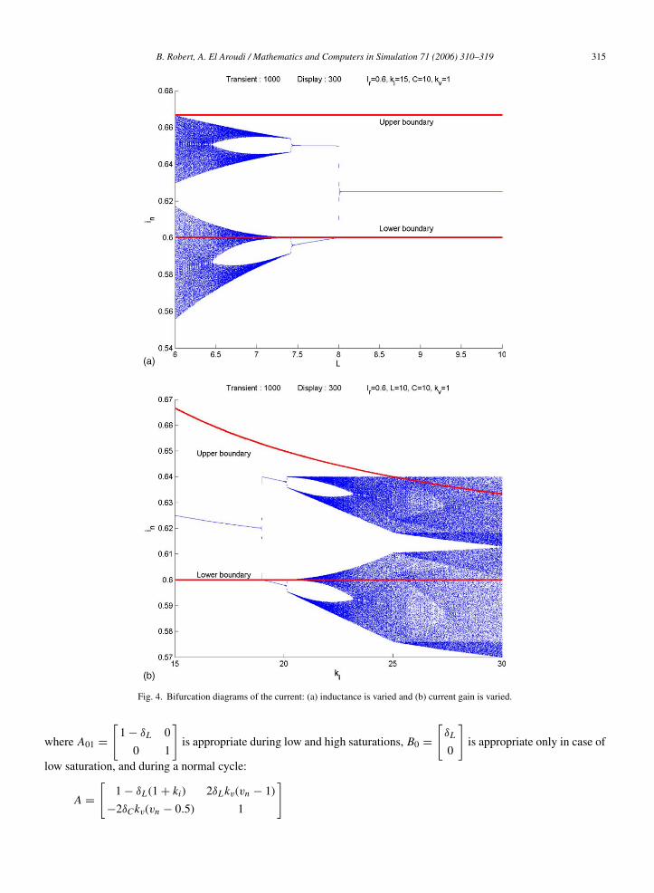
The bifurcation diagrams of Fig. 4 give an account of the global behaviour of the converter when the inductance ofthe inductor or the current gain is varied. The current reference is fixed to Ir = 0.6 and the voltage gain kv = 1. Rememberthat we use a dimensionless model. Then the nominal values are:

E = 1, R = 1, L = 10, C = 40, F = 1 then δL = 0.1, δC = 0.1.

The first diagram is computed with a constant current gain ki = 15 and the inductance is varied. On the right side,the converter has a fundamental (T = 1) periodic running mode. This is the most important one from an engineeringpoint of view. The fixed point is indeed independent of L. However, below the stability limit (2), i.e. L = 8, a stable twoperiodic running mode appears. The sampled current alternates at each period. By reducing some more the inductance,a new running mode appears. The current alternates inside four chaotic strips.

The second diagram is computed with a constant inductance L = 10 and the current gain is varied. On the left side,the normal fixed point is moving towards the reference when the gain growths. Over the stability limit (ki = 19), aperiod doubling appears and then a chaotic running mode.

It is worth to note that these diagrams deal with non standard bifurcations as flip or Neimark–Sacker bifurcations.There is no period doubling series or other usual way to chaos but only one period doubling and a sudden bifurcationto chaos. The next section set out to show that these bifurcations are about border collision phenomena [6].

5. Piecewise model

In this section, the model is improved in order to take into account the natural saturations of the duty cycle of thePWM modulator: d1/2 ∈ [0, 1]. This approach is essential to explain the uncommon way to chaos observed on thebifurcation diagrams.

Due to the PWM duty cycle saturations, two borderlines split the state plane into three regions. In each of them, theconverter is modelled by a specific map. Then the global model, including the PWM saturations is a piecewise modelin the state plane.

At first, we consider the low saturation. In that case, the sampled current is small enough so that both switchesremain closed over the whole period: u1 = 1, u2 = 1 and d1 = d2 = 0. This defines the lower boundary: εi = 0 ⇒ in = Ir.The second case is reached when the current is high enough so that both switches are opened u1 = 0, u2 = 0. This newtopology appears also inside a normal running mode when Ir < (1/2) without change the model (1). Here, due to thehigh saturation, both switches remains opened during the whole period: d1 = d2 = 1. This leads to the upper boundary:εi = (1/ki) ⇒ in = Ir + (1/ki). Therefore, the piecewise model is given as it follows:

Xn+1 = F (Xn) =

⎧⎪⎪⎨⎪⎪⎩F1(Xn) = A01Xn + B0 if in ≤ Ir

F2(Xn) = AXn + B if Ir ≤ in ≤ Ir + 1

ki

F3(Xn) = A01Xn else


Fig. 4. Bifurcation diagrams of the current: (a) inductance is varied and (b) current gain is varied.

where A01 =[

1 − δL 0

0 1

]is appropriate during low and high saturations, B0 =

[δL

0

]is appropriate only in case of

low saturation, and during a normal cycle:

A =[

1 − δL(1 + ki) 2δLkv(vn − 1)

−2δCkv(vn − 0.5) 1

]


B =⎛⎝ δL

(1 + kiIr + kv

2

)0

⎞⎠ .

By using this new model, we are able to study the conditions of existence of the fixed point X∗1. Indeed, we showed

in Section 3.3 that ∀ki > 0, i∗1(ki) > Ir. Moreover, it is easy to verify that ∀ki > 0, i∗1(ki) < Ir + (1/ki). Then the fixedpoint locus is located between the two boundaries. We conclude that the fixed point X∗

1 exists in the interval [0 ∞[and is stable in the interval [0 ki1[ .

6. 2T periodic mode

This section show that a 2T-periodic mode settles down after the destabilization of X∗1. It is characterized by the

two fixed points of the map Xn+2 = F2 ◦ F1(Xn). Here after, F21 denotes the composition F2 ◦ F1:

Xn+2 = F21(Xn) = A21Xn + B21, (3)

where:

A21 =[

(1 − δL(1 + ki))(1 − δL) 2δLkv(vn − 1)

(−2δCkv(vn − 0.5))(1 − δL) 1

]

B21 = δL

⎡⎣2 + ki(Ir − δL) − δL + kv

2−2δCkv(vn − 0.5)

⎤⎦

The first equilibrium point, denotedX∗2, of the second order map (3) is given by the solution of F21(X∗

2) = X∗2. This

point is:

X∗2 = [i∗2, v∗2]t =

[ki(Ir − δL) + 2 − δL

ki(1 − δL) + 2 − δL,

1

2

]tThe second one is:

F1(X∗2) =

[kiIr(1 − δL) + 2 − δL

ki(1 − δL) + 2 − δL,

1

2

]t.

At the bifurcation point:⎧⎪⎪⎪⎪⎨⎪⎪⎪⎪⎩X∗

2 =[Ir,

1

2

]t

F1(X∗2) =

[Ir(2 − 3δL + δ2

L) + 2δL − δ2L

2 − δL,

1

2

]t

Conventionally, F1(i∗2) denotes [1, 0] · F1(X∗2). If Ir < 1, then i∗2 < F1(i∗2). Thus this bifurcation is always discontin-

uous. Therefore, it is a non standard bifurcation. It can be understood by the following way. At the bifurcation point ki1,the fixed point X∗

1 loses its stability, the characteristic multiplier crossing −1. Then the orbit alternates two divergingvalues until one of them collides one of the two boundaries. Then the second order fixed point spring up.

The study of the conditions of existence of X∗2 and F1(X∗

2) confirms this analysis. They are three:

• i∗2 < Ir is true if ki > ki1.• F1(i∗2) > Ir is always true.• F1(i∗2) < Ir + 1/ki. If Ir > (1/2 − δL), this condition is always true since ki > 0. Else, the condition is

ki < (2 − δL)/(Ir(1 − δL)).


Fig. 5. Existence of X∗2.

By combining the conditions, the existence of X∗2 is depicted on Fig. 5.

Below the limit value Ir = (1 − δL)/(2 − δL), another second order fixed point X∗∗2 appears as the solution of F2 ◦

F3(X∗∗2 ) = X∗∗

2 and can be studied following the same method.The Jacobian matrix of the map (3) is given as following:

J(X) =[

1 − δL(1 + ki) 2δLkv(2vn − 1)

−2δCkv(vn − 0.5)(1 − δL) 2δLδCkv(in − 1) + 1 − 2δCkv

]

Evaluated at the equilibrium pointX∗2, J is a diagonal matrix. Assuming that kv < (1/(δC(1 + δL)) then |2δLδCkv(i∗2 −

1) + 1 − 2δCkv| < 1 whatever i∗2 is. This fact leads to the Floaquet’s characteristic multiplier of i∗2. The stabilitycondition is then:

|(1 − δL(1 + ki))(1 − δL)| < 1

ki > ki1

}⇒ ki1 < ki <

1 + (1 − δL)2

δL(1 − δL).

We note ki2 the stability limit of X∗2: ki2 = (L2 + (L − 1)2/(L − 1).

We conclude that the fixed point X∗2 collides with the boundary exactly when the fixed point X∗

1 loses its stability.X∗

2 exists in the interval [ki1 ∞[ and is stable in the interval [ki1 ki2 [.

7. Four chaotic intervals

This section show that new 4T-periodic fixed points appear after destabilization of X∗2 and that they are unstable

on all domain of existence. The bifurcation diagram depicted in Fig. 4b illustrates that. The appearance, beyond ki2,of these new unstable fixed points, generates a chaotic behaviour. Iterates are divided on four dense intervals that wecall 1–4, in the increasing order of the values of iterates belonging to these intervals (see Fig. 4). The four intervalsare alternatively visited in the following order: 1–3–2–4. This can be observed during the simulation by considering apoint of 1 and its next successive iterates. The lower boundary divides the interval 2 in two sub-intervals. Dependingon the position of the iterate in this interval, below or above Ir, the fourth order map has two distinct forms:

Xn+4 ={F2121 = F2 ◦ F1 ◦ F2 ◦ F1(Xn) if in+2 < Ir

F2221 = F2 ◦ F2 ◦ F2 ◦ F1(Xn) if in+2 > Ir

Concerning the fixed point of F2121 and its stability, the results are identical to the ones of F21. Indeed, Xn+4 =F2121(Xn, ki) = F2

21(Xn, ki) and then the fourth order fixed point X∗4(ki) = X∗

2(ki) and ki > k2i ⇒ X∗4 is unstable.


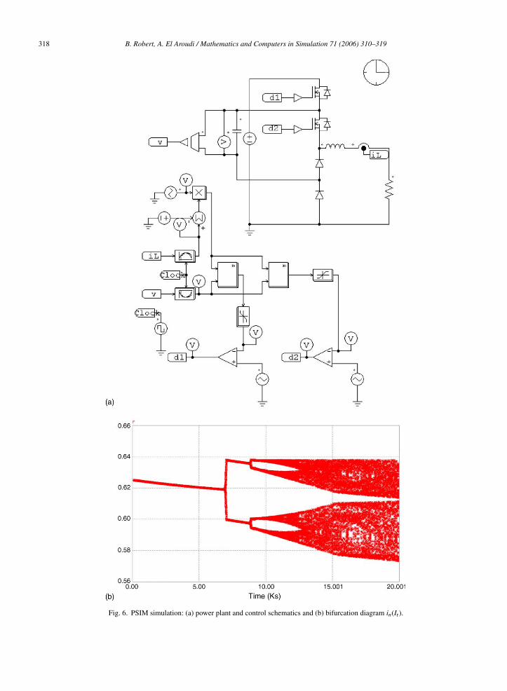
Fig. 6. PSIM simulation: (a) power plant and control schematics and (b) bifurcation diagram in(Ir).


A precise study of the second form, Xn+4 = F2221(Xn, ki), allows to conclude that at the point ki = ki2, the secondorder fixed point X∗

2 becomes unstable and a new unstable fixed point X∗4 appears. It is always unstable. We are in

the presence of a bifurcation from a 2T-periodic solution to a chaotic solution on four intervals and this bifurcation isdiscontinuous.

8. Simulations

By using the previous numerical value E = 1, R = 1, L = 10, C = 40, F = 1, δL = 0.1 and δC = 0.1, we determine thevalidity conditions of the study: Ir > 0.474 and kv < 9.09. The bifurcation points are: ki1 = 19 and ki2 = 20, 11.

Fig. 6 presents a numerical simulation computed by the PSIM® software. The control parameters are: Ir = 0.6, kv = 1and the current gain sweeps slowly the interval [15,30] with a saw tooth modulation of 2 × 104 fundamental periods.The diagram fits the theoretical one computed by Matlab® on Fig. 4b. The bifurcation points are took down at: ki1 = 20.1and ki2 = 21.5. Owing to the linearization of the exponential matrices during the modellization process, they are notexactly equal to the previous values but remain very closed.

9. Conclusions

The distinctive feature of this study lies in the investigation of the map’s properties allowing for the analyticaldetermination of the fixed points, their domains of stability, and of the bifurcation points. More precisely, we showedthat some of these bifurcations are discontinuous. The analysis is performed while keeping in mind the current andvoltage controller’s tuning and the influence of the current reference. In this particular setting, we showed that, owingto the discrete time digital controller all the bifurcations are Border Collision Bifurcations. We think that this type ofcontroller simplifies the non linear behaviours and the method can help to understand how the constants of the systeminfluence its dynamics. This method will also allow us to study the consequences of the motion of the boundaries underthe effect of a variable reference, sinusoidal for example, as it is often the case.

References

[1] S. Banerjee, G.C. Verghese, Nonlinear Phenomena in Power Electronics, Attractors, Bifurcations and Nonlinear Control, IEEE Press, NewYork, April 2001.

[2] J. Chiasson, L. Tolbert, K. McKenzie, D. Zhong, Harmonic elimination in multilevel converters, in: Proceedings of IASTED’03, 2003, pp.284–289.

[3] C. Franco Hernandez, T. Luis Moran, C. Jose Espinoza, R. Juan Dixon, A generalized control scheme for active front-end multilevel converters,in: Proceedings of IECON, 2001, pp. 915–920.

[4] Circuits and Systems I: Fundamental Theory and Applications, IEEE Transactions on, vol. 50, issue 8, 2003, pp. 1125–1129 (see also Circuitsand Systems I: Regular Papers, IEEE Transactions on).

[5] T. Meynard, M. Fadel, N. Aouda, Modeling of multilevel converters, IEEE Trans. Ind. Electron. 44 (3) (1997) 356–364.[6] H.E. Nusse, J.A. Yorke, Border-collision bifurcations for piecewise smooth one-dimensional maps, Int. J. Bifurcat. Chaos 5 (1995) 189–207.[7] D. Pinon, M. Fadel, T. Meynard, Sliding mode controls for a two-cell chopper, in: Proceedings of EPE, 1999, CD-ROM.[8] B. Robert, H.H.C. Iu, M. Feki, Adaptive time-delayed feedback for chaos control in a PWM single phase inverter, J. Circuits Syst. Comput. 13

(3) (2004) 519–534.[9] B. Robert, C. Robert, Border collision bifurcations in a one-dimensional piecewise smooth map for a PWM current-programmed H-bridge

inverter, Int. J. Control 75 (16/17) (2002) 1356–1367.[10] J. Rodrigez, et al., High-Voltage Multilevel Converter with Regeneration Capability, IEEE Trans. Ind. Electron. 49 (4) (2002) 839–846.[11] C.K. Tse, Complex Behavior of Switching Power Converters, CRC Press, Boca Raton, USA, 2003, ISBN 0-849-31862-9.

Discrete time model of a multi-cell dc/dc converter: Non linear approach

Documents

Transcript of Discrete time model of a multi-cell dc/dc converter: Non linear approach