1

Diese Arbeit wurde am DLR Institut für Solarforschung vorgelegt The present work was submitted to the DLR - Institute of Solar Research Thermochemischer Schwefelkreisprozess zur Langzeitspeicherung von konzentrierter solarthermischer Energie: Prozessimplementierung eines partikelbeheiztem Reaktorkonzeptes und techno-ökonomische Optimierung Thermochemical sulphur cycle for long-term storage of concentrated solar thermal energy: Process implementation of a particle heated reactor concept and techno-economic optimization Masterarbeit Master’s thesis Von / presented by: Julian Josef Belina Martikelnummer/ Student ID no.: 370169 Betreuer / Supervisor: M.Sc Andreas Rosenstiel Prüfer / Examiner: Univ.-Prof. Dr. -Ing. Robert Pitz-Paal DLR - Institut für Solarforschung, Lehrstuhl für Solartechnik DLR - Institute of Solar Research, chair of solar research Rheinisch-Westfälische Technische Hochschule Aachen Aachen 07.01.2021

Zentrales Prüfungsamt/Central Examination Office

Eidesstattliche Versicherung Statutory Declaration in Lieu of an Oath

___________________________ ___________________________

Name, Vorname/Last Name, First Name Matrikelnummer (freiwillige Angabe) Matriculation No. (optional)

Ich versichere hiermit an Eides Statt, dass ich die vorliegende Arbeit/Bachelorarbeit/

Masterarbeit* mit dem Titel I hereby declare in lieu of an oath that I have completed the present paper/Bachelor thesis/Master thesis* entitled

__________________________________________________________________________

__________________________________________________________________________

__________________________________________________________________________

selbstständig und ohne unzulässige fremde Hilfe (insbes. akademisches Ghostwriting)

erbracht habe. Ich habe keine anderen als die angegebenen Quellen und Hilfsmittel benutzt.

Für den Fall, dass die Arbeit zusätzlich auf einem Datenträger eingereicht wird, erkläre ich,

dass die schriftliche und die elektronische Form vollständig übereinstimmen. Die Arbeit hat in

gleicher oder ähnlicher Form noch keiner Prüfungsbehörde vorgelegen. independently and without illegitimate assistance from third parties (such as academic ghostwriters). I have used no other than

the specified sources and aids. In case that the thesis is additionally submitted in an electronic format, I declare that the written

and electronic versions are fully identical. The thesis has not been submitted to any examination body in this, or similar, form.

___________________________ ___________________________

Ort, Datum/City, Date Unterschrift/Signature

*Nichtzutreffendes bitte streichen

*Please delete as appropriate

Belehrung: Official Notification:

§ 156 StGB: Falsche Versicherung an Eides Statt

Wer vor einer zur Abnahme einer Versicherung an Eides Statt zuständigen Behörde eine solche Versicherung

falsch abgibt oder unter Berufung auf eine solche Versicherung falsch aussagt, wird mit Freiheitsstrafe bis zu drei

Jahren oder mit Geldstrafe bestraft.

Para. 156 StGB (German Criminal Code): False Statutory Declarations

Whoever before a public authority competent to administer statutory declarations falsely makes such a declaration or falsely

testifies while referring to such a declaration shall be liable to imprisonment not exceeding three years or a fine. § 161 StGB: Fahrlässiger Falscheid; fahrlässige falsche Versicherung an Eides Statt

(1) Wenn eine der in den §§ 154 bis 156 bezeichneten Handlungen aus Fahrlässigkeit begangen worden ist, so

tritt Freiheitsstrafe bis zu einem Jahr oder Geldstrafe ein.

(2) Straflosigkeit tritt ein, wenn der Täter die falsche Angabe rechtzeitig berichtigt. Die Vorschriften des § 158

Abs. 2 und 3 gelten entsprechend.

Para. 161 StGB (German Criminal Code): False Statutory Declarations Due to Negligence

(1) If a person commits one of the offences listed in sections 154 through 156 negligently the penalty shall be imprisonment not exceeding one year or a fine. (2) The offender shall be exempt from liability if he or she corrects their false testimony in time. The provisions of section 158 (2) and (3) shall apply accordingly.

Die vorstehende Belehrung habe ich zur Kenntnis genommen: I have read and understood the above official notification:

___________________________ ___________________________

Ort, Datum/City, Date Unterschrift/Signature

3

I. Abstract (English) The solid sulphur cycle process utilizes elemental sulphur as a thermochemical energy storage medium for concentrated solar thermal energy. The produced sulphur can be transported to a different location to produce electricity from thermal energy released in a chemical process. In this thesis a process was designed which also includes sulphuric acid recycling. A detailed simulation model of a novel particle heated reactor concept was developed. It is used for a numerical techno-economic optimization based on an Aspen Plus process simulation. Im-provements in reactor design were derived from the simulation model. The techno-economic optimum was found for a large reactor that converts a large share (98.65 %) of the educt SO3. An optimal thermal energy supply temperature close to 1000 °C was determined. This is the maximum output temperature of the concentrated solar thermal energy system. Particle temperature at the outlet of the reactor was at the design maximum. Reactor performance was improved by increasing its heat transfer capabilities. It was achieved by decreasing the tube distance in the reactor and increasing the fluid velocity. The result of the techno-economic analysis shows that the optimized process is not economi-cally feasible under the assumed boundary conditions. The main cost factor is the transporta-tion of diluted sulphuric acid for recycling between both locations of the process. High revenues are created by the recycling process of sulphuric acid. Should the sulphuric acid recycling prices increase from 50 €/t to 96.21 €/t the process will become economically feasible. A high conversion of the SO3 decomposition reaction is important for an economic process design. An increased maximum concentrated solar thermal energy system output temperature would increase the economic performance. Higher temperature differences between particles are desirable if the reactor can withstand them. Further energy integration might yield and economically feasible process. The high spent acid treatment revenues and transportation costs show the potential for on-site sulphuric acid recycling powered by concentrated solar thermal energy.

4

II. Abstract (German) Der feste Schwefel Kreislaufprozess verwendet elementaren Schwefel als thermochemisches Speichermedium für konzentrierte solarthermische Energie. Der produzierte Schwefel kann zu einem anderen Standort transportiert werden, um dort Elektrizität aus der thermischen Energie eines chemischen Prozesses zu erzeugen. In dieser Arbeit wurde in den Kreislaufprozess Schwefelsäurerecycling integriert. Es wurde ein detailliertes Simulationsmodel eines neuen partikelbeheizten Reaktorkonzeptes entwickelt. Dieses wurde für eine techno-ökonomische Optimierung auf Basis einer Aspen Plus Prozesssimulation verwendet. Verbesserungen des Reaktordesigns wurden vom Simulationsmodell abgeleitet. Das techno-ökonomische Optimum wurde für einen großen Reaktor gefunden, der einen Großteilteil (98,65 %) des SO3 umsetzt. Die optimale thermische Energiebereitstellungstempe-ratur liegt nahe 1000 °C. Dies ist die maximale Ausgangstemperatur des konzentrierten solar-thermischen Energiesystems. Die optimale Partikelausgangstemperatur des Reaktors ist an der Auslegungsobergrenze. Die Reaktorleistung wurde durch eine Erhöhung der Wärmetrans-portleistungsfähigkeit verbessert. Dies wurde durch die Reduzierung des Rohrabstandes und die Erhöhung der Fluidgeschwindigkeit erreicht. Das Ergebnis der techno-ökonomischen Analyse zeigt, dass der Hauptkostenfaktor die Trans-portkosten von verdünnter Schwefelsäure zum Recycling zwischen den beiden Prozessstand-orten ist. Durch die Aufbereitung der Schwefelsäure werden hohe Einnahmen erzeugt. Sollte sich der Aufbereitungspreis der Schwefelsäure von 50 €/t auf 96,21 €/t erhöhen, wird der Pro-zess wirtschaftlich tragbar. Ein hoher Umsatz der SO3 Zersetzungsreaktion ist wichtig für einen wirtschaftlich rentablen Prozess. Eine höhere Partikelausgangstemperatur des konzentrierten solarthermischen Ener-giesystems würde die Rentabilität des Prozesses verbessern. Eine weitere Verbesserung kann mit einer höheren Temperaturdifferenzen zwischen Partikeln und dem Fluid im Reaktor erzielt werden. Weitere Energieintegration könnte den Prozess wirtschaftlich tragbar machen. Die hohen Einnahmen aus dem Abfallsäureaufbereitung und die Transportkosten zeigen, dass es vor Ort Potential für einen Schwefelsäure Recyclingprozess gibt, der mit konzentrierter so-larthermischer Energie betrieben wird.

5

III. Table of Contents

I. ABSTRACT (ENGLISH) 3

II. ABSTRACT (GERMAN) 4

III. TABLE OF CONTENTS 5

IV. LIST OF FIGURES 6

V. LIST OF TABLES 7

VI. ABBREVIATIONS 8

1 INTRODUCTION 9

2 THEORETICAL BACKGROUND 11

2.1 CONCENTRATED SOLAR POWER (CSP) SYSTEMS AND CONCENTRATED SOLAR THERMAL ENERGY SYSTEMS (CSTES) 11 2.2 COMPUTER-AIDED CHEMICAL PROCESS DESIGN AND SIMULATION 16 2.3 ECONOMIC EVALUATION OF CHEMICAL PLANTS 19

2.3.1 Net present worth 𝑊𝑁𝑃 19 2.3.2 Cost of manufacturing (COM) and revenues 20 2.3.3 Total plant investment costs 22

3 PRIOR RESEARCH AND SUBJECT OF RESEARCH 26

3.1 PRIOR RESEARCH 26 3.2 SUBJECT OF RESEARCH 30

4 MODELLING OF PARTICLE HEATED 𝐇𝟐𝐒𝐎𝟒 SPLITTING REACTOR 32

4.1 IMPLEMENTATION AND SOLUTION OF THE REACTOR MODEL 34 4.2 HEAT TRANSFER MODEL 35

4.2.1 Heat exchange surface calculation 36 4.2.2 Complete heat transfer coefficient 𝛼𝑡𝑜𝑡𝑎𝑙 36 4.2.3 Shell side heat transfer coefficient 37 4.2.4 Composite tube resistance 39 4.2.5 Fluid side thermal resistance 40

4.3 REACTION MODEL 41 4.3.1 Equilibrium between 𝑆𝑂3 and 𝑆𝑂2 41 4.3.2 Selection of reaction kinetic for 𝐹𝑒2𝑂3 coated silicon carbide foams 42 4.3.3 Stable region of 𝐹𝑒2𝑂3 catalysts 44

4.4 THERMODYNAMIC MODEL 45 4.4.1 Sulphuric acid thermodynamic model 45 4.4.2 Validation of vapour liquid equilibrium 46 4.4.3 Particle Enthalpy 47

4.5 RESULTS OF THE REACTOR MODEL AND COMPARISON THE EXPERIMENTAL REACTOR 48 4.5.1 Heat transfer model 49 4.5.2 Experimental reactor 52

5 PROCESS SIMULATION AND OPTIMIZATION 53

5.1 CONCEPT OF THE SOLID SULPHUR CYCLE 54 5.1.1 Presentation of the solid sulphur cycle and its performance indicators 54 5.1.2 Optimization potential of design variables 56 5.1.3 Calculation of the net present worth 57 5.1.4 Titan dioxide production 58

5.2 SECTIONS OF THE PROCESS 58 5.2.1 Implementation of the simulation 58 5.2.2 Concentrated solar thermal energy system (CSTES) 58

6

5.2.3 𝐻2𝑆𝑂4 splitting reactor 63 5.2.4 𝑆𝑂2 separation 64 5.2.5 Disproportionation 65 5.2.6 𝐻2𝑆𝑂4 concentration 66 5.2.7 𝐻2𝑆𝑂4 production plant 68

6 RESULTS AND DISCUSSION OF OPTIMIZATION AND ECONOMIC EVALUATION 68

6.1 RESULTS 68 6.1.1 Economic and CSTES results 69 6.1.2 Process results 73

6.2 DISCUSSION 77

7 SUMMARY AND CONCLUSION 80

8 OUTLOOK 82

APPENDIX A ECONOMICS 83

8.1 INVESTMENT COST PARAMETERS 83 8.2 PRESSURE FACTORS 83 8.3 MATERIAL AND MODULE FACTORS 83 8.4 FACTORS FOR PRESSURE VESSELS 84

APPENDIX B PROPERTIES 85

8.5 HEAT CAPACITIES 85 8.5.1 Particle heat capacity 85 8.5.2 Air 85

8.6 THERMAL CONDUCTIVITY 86 8.6.1 Air 86 8.6.2 Bauxite Bulk conductivity 86 8.6.3 Tube conductivity 87

8.7 PARTICLE PROPERTIES 87

9 PUBLICATION BIBLIOGRAPHY 87

IV. List of figures FIGURE 1: DEPICTION OF THE SOLID SULPHUR CYCLE. 10 FIGURE 2: TYPES OF SOLAR RECEIVERS (BUCK AND SCHWARZBÖZL 2018, P. 695). 11 FIGURE 3: CONCENTRATED SOLAR POWER SYSTEM (BUCK AND SCHWARZBÖZL 2018, P. 697). 12 FIGURE 4: CONCENTRATED SOLAR THERMAL ENERGY SYSTEM (CSTES) USING A SOLAR TOWER AS CONCENTRATING SYSTEM. (EBERT

7/6/2017, P. 4) 13 FIGURE 5: IMAGE OF A HELIOSTAT IN A HELIOSTAT FIELD (BUCK AND SCHWARZBÖZL 2018, P. 700). 14 FIGURE 6: FALLING FILM PARTICLE RECEIVER(LEFT) AND CENTRIFUGAL PARTICLE RECEIVER (RIGHT) (BUCK AND SCHWARZBÖZL 2018,

P. 729). 14 FIGURE 7: DEPICTION OF CENTREC® (EBERT ET AL. 2019, P. 2). 15 FIGURE 8: BELT BUCKET ELEVATOR PARTICLE TRANSPORT SYSTEM (EBERT ET AL. 2019, P. 7). 15 FIGURE 9: STRUCTURE OF A PROCESS SIMULATOR. (HAYDARY 2018, P. 9) 16 FIGURE 10: THERMAL ENERGY STORAGE PRINCIPLES (KERSKES 2016, P. 346). 26 FIGURE 11: DEPICTION OF COMPLETE SOLID SULPHUR CYCLE (THOMEY ET AL. 2018, P. 13). 27 FIGURE 12: VOLUMETRIC TWO CHAMBER REACTOR AND RECEIVER COMBINATION FOR H2SO4 EVAPORATION AND SO3

DECOMPOSITION (WONG 2014, P. 16). 28 FIGURE 13: BAYONET REACTOR (M.B. GORENSEK 2009, P. 30). 29 FIGURE 14: DIRECT CONTACT SO3 DECOMPOSITION REACTOR AND H2SO4 EVAPORATOR FROM PEGASUS PROJECT (THOMEY ET AL.,

P. 1). 29 FIGURE 15: DEPICTION OF THE INDIRECT HEATED COMBINED H2SO4 EVAPORATOR AND SO3 DECOMPOSITION REACTOR (AGRAFIOTIS

ET AL. 2020, P. 3) 30 FIGURE 16: DEPICTION OF PROCESS INVESTIGATED IN THIS THESIS. 31

7

FIGURE 17: DEPICTION OF SINGLE TUBE REACTOR MODEL OF THE H2SO4 SPLITTING REACTOR (OWN DEPICTION). 33 FIGURE 18: DEPICTION OF THE ASPEN PLUS MODEL FOR THE H2SO4 EVAPORATOR AND SO3 DECOMPOSITION REACTOR SECTION. 34 FIGURE 19: EQUILIBRIUM DEGREE OF DISSOCIATION Α𝑆𝑂3 FOR SO3 DECOMPOSITION REACTION IN DEPENDENCE OF VARIOUS

PRESSURES FOR 90 WT% SULPHURIC ACID. 42 FIGURE 20: VISUAL COMPARISON OF FE2O3 COATED FOAMS ON THE LEFT (OLIVEIRA 9/14/2020B) AND FE2O3 COATED

HONEYCOMB FRAGMENTS ON THE RIGHT (GIACONIA ET AL. 2011, P. 6499). 43 FIGURE 21: MINIMUM TEMPERATURE OF STABLE FE2O3 IN DEPENDENCE OF SO3 PARTIAL PRESSURE. 45 FIGURE 22: BOILING AND DEW CURVE AT VARYING MASS CONCENTRATIONS AT A PRESSURE OF 1 BAR. 46 FIGURE 23: BOILING AND DEW CURVE AT VARYING MASS CONCENTRATIONS AT A PRESSURE OF 10 BAR. 47 FIGURE 24: BOILING AND DEW CURVE AT VARYING MASS CONCENTRATIONS AT A PRESSURE OF 15 BAR. 47 FIGURE 25: ENTHALPY STORED AS SENSIBLE HEAT IN PARTICLES AT DIFFERENT HOT PARTICLE INLET TEMPERATURES AND COLD PARTICLE

OUTLET TEMPERATURES. 48 FIGURE 26: MASS BASED ENTHALPY REQUIRED TO DECOMPOSE 70 WT% SULPHURIC ACID. 49 FIGURE 27: PARTICLE HEAT TRANSFER COEFFICIENT AT VARIOUS TEMPERATURES IN DEPENDENCE OF THE BULK WIDTH. 49 FIGURE 28: COMPLETE HEAT TRANSFER COEFFICIENT FOR DECOMPOSITION AND REQUIRED SECTION LENGTH TO MAINTAIN A WHSV OF

2 FOR VARYING FLUID FLOW. 50 FIGURE 29: COMPLETE HEAT TRANSFER COEFFICIENT AND REQUIRED SECTION LENGTH FOR THE SUPERHEATING SECTION FOR VARYING

FLUID FLOW. 51 FIGURE 30: COMPLETE HEAT TRANSFER COEFFICIENT AND REQUIRED SECTION LENGTH TO FOR THE PREHEATING SECTION FOR VARYING

FLUID FLOW. 51 FIGURE 31: COMPLETE HEAT TRANSFER COEFFICIENT AND REQUIRED SECTION LENGTH TO FOR THE VAPORIZATION SECTION FOR VARYING

FLUID FLOW. 52 FIGURE 32: DEPICTION OF THE INDIRECT HEATED EXPERIMENTAL COMBINED H2SO4 EVAPORATOR AND SO3 DECOMPOSITION

REACTOR. 53 FIGURE 33: DEPICTION OF THE SIMULATION, ECONOMIC EVALUATION AND TECHNO-ECONOMIC OPTIMIZATION OF THE SOLID SULPHUR

CYCLE. 55 FIGURE 34: DEPICTION OF SO2 SEPARATION HIERARCHY IN ASPEN PLUS. 65 FIGURE 35: DEPICTION OF THE DISPROPORTIONATION SECTION HIERARCHY IN THE ASPEN PLUS SIMULATION. 66 FIGURE 36: CONTENT OF THE ACTUAL 𝐻2𝑆𝑂4 CONCENTRATION SECTION. 67 FIGURE 37: CONTENT OF THE 𝐻2𝑆𝑂4 CONCENTRATION SECTION DURING OPTIMIZATION. 67 FIGURE 38: NET PRESENT WORTH, GRASS ROOT COSTS AND ANNUAL CASH FLOW OF THE SOLID SULPHUR CYCLE WHICH IS DESIGNED FOR

THE 20 MW CENTREC®. ADDITIONALLY, THE REQUIRED ANNUAL CASH FLOW TO REACH A NET PRESENT WORT OF 0 IS SHOWN. 69

FIGURE 39: ITEMIZED DEPICTION OF THE ANNUAL CASH FLOW OF THE SOLID SULPHUR CYCLE. 70 FIGURE 40: INVESTMENT COSTS OF THE SECTIONS OF THE SOLID SULPHUR CYCLE. 71 FIGURE 41: INVESTMENT COST OF THE CSTES COMPONENTS. 71 FIGURE 42: CSTES SYSTEM COST IN MILLION € FOR A 20 MW CENTREC® (LEFT) AND 40 MW CENTREC® (RIGHT) DESIGN IN

DEPENDENCE OF THE PARTICLE OUTLET TEMPERATURE. 72 FIGURE 43: THERMAL RECEIVER EFFICIENCY 𝜂𝑟𝑒𝑐𝑒𝑖𝑣𝑒𝑟 AND SOLAR RADIATION TO ABSORBED THERMAL ENERGY EFFICIENCY

𝜂𝑠𝑜𝑙𝑎𝑟, 𝑡ℎ𝑒𝑟𝑚𝑎𝑙 IN DEPENDENCE OR PARTICLE RECEIVER OUTLET TEMPERATURE °C FOR A 20 MW AND 40 MW CENTREC®. 72

FIGURE 44 RESULTS OF THE OPTIMIZATION OF THE COMPLETE SOLID SULPHUR CYCLE. RESULTS ARE SHOWN IN GREEN AND LOSSES IN

RED. (OWN DEPICTION) 73 FIGURE 45: SECTION OF THE COMPLETE H2SO4 SPLITTING REACTOR IN THE 20 MW SOLID SULPHUR CYCLE. (OWN DEPICTION) 75 FIGURE 46: DEPICTION OF A SINGLE TUBE OF THE H2SO4 SPLITTING REACTOR IN THE 20 MW SOLID SULPHUR CYCLE. (OWN DEPICTION)

76

V. List of Tables TABLE 1: SUMMARIZED PARAMETERS FOR DIRECT MANUFACTURING COSTS 21 TABLE 2: SUMMARIZED PARAMETERS FOR FIXED MANUFACTURING COSTS. 22 TABLE 3: SUMMARIZED PARAMETERS FOR GENERAL EXPENSES OF MANUFACTURING COSTS. 22 TABLE 4: SUMMARY OF TOTAL DIRECT MANUFACTURING COSTS. 22 TABLE 5: DEFINITION OF REACTOR STAGES IN DEPENDENCE OF FLUID AGGREGATE STATES. 35 TABLE 6: PARTICLE CONTACT HEAT TRANSFER COEFFICIENT PARAMETERS 38 TABLE 7: WALL TO PARTICLE HEAT TRANSFER PARAMETERS 38 TABLE 8: RADIATION HEAT TRANSFER COEFFICIENTS. 39

8

TABLE 9: COMPARISON OF FE2O3 COATED FOAM CATALYST AND FE2O3 COATED HONEYCOMBS FROM. 42 TABLE 10: REACTION RATES CALCULATED BY (VAN DER MERWE 2014, P. 77) FROM EXPERIMENTAL RESULTS OBTAINED BY GIACONIA

(GIACONIA ET AL. 2011, P. 6504). 43 TABLE 11: DIMENSION OF EXPERIMENTAL H2SO4 EVAPORATOR AND SO3 DECOMPOSITION REACTOR (THANDA 11/10/2020). 53 TABLE 12: INTRODUCTION OF PROCESS EFFICIENCIES AND RATIOS. 56 TABLE 13: FLOW SPECIFIC COSTS FOR ANNUAL CASH FLOW CALCULATIONS. 57 TABLE 14: NUMBER OF FLUID PROCESS STEPS FOR OPERATOR NUMBER ESTIMATION. 58 TABLE 15: CENTREC® DIMENSION FOR 40 MW THERMAL RATING. 59 TABLE 16: PARAMETERS FOR EQUATION EQ. 5.6 AND EQ. 5.5. 60 TABLE 17: PARAMETERS FOR COST CALCULATION OF VERTICAL TRANSPORT SYSTEM 62 TABLE 18: VARIABLES TO DETERMINE INVESTMENT COST CALCULATION. 64 TABLE 19: REACTION CONDITIONS IN DISPROPORTIONATION REACTORS. 65 TABLE 20: INTRODUCTION OF PROCESS EFFICIENCIES AND RATIOS. 73 TABLE 21: PARAMETERS FOR 𝐶𝑃0 CALCULATION USING EQ. 2.17 (TURTON 2012, PP. 988–990) . 83 TABLE 22: PRESSURE FACTORS FOR BARE MODULE CALCULATIONS 1 (TURTON 2012, P. 1006). 83 TABLE 23: MATERIAL FACTORS AND MODULE FACTOR CONSTANTS (TURTON 2012, PP. 1009–1014). 84 TABLE 24: COEFFICIENTS FOR BASIC COSTS OF PRESSURES VESSELS (BIEGLER ET AL. 1997, P. 134). 84 TABLE 25: MODULE FACTOR FOR PRESSURE VESSELS (BIEGLER ET AL. 1997, P. 134). 84 TABLE 26: PRESSURE FACTOR FOR PRESSURE VESSELS (BIEGLER ET AL. 1997, P. 113). 84 TABLE 27: PARAMETERS FOR PARTICLE HEAT CAPACITY EQUATIONS. 85

VI. Abbreviations

CEPCI Chemical Engineering Plant Cost Index COBYLA Constrainted Optimization By Linear Approximations COM Cost of manufacturing CSP Concentrated Solar Power CSTES Concentrated solar thermal energy system DNI Direct normal irradiation FCI Fixed capital investment HTM Heat transfer medium HyS Hybrid sulphur cycle PTFE Polytetrafluoroethylene PV Photovoltaic SiC Silicon Carbide TCS Thermochemical energy storage TES Thermal energy storage WHSV Weight Hourly Space Velocity

9

1 Introduction To limit global warming to 1.5°C with no or limited overshoot, anthropogenic CO2 emissions need to decline by about 45 % from 2010 levels by 2030 and to net zero by 2050 (Masson-Delmotte et al. 2018). Photovoltaic (PV) and wind power are currently capable to reduce the fossil fuel usage. To replace dispatchable fossil-fuel based electricity generation capacities considerable electricity storage capacities would be required. Calm, dull winter days with high power demand present the most critical scenario for PV and wind power supply. (Wirth 2020, p. 53) Concentrated Solar Power (CSP) systems are an interesting alternative because thermal stor-ages can be integrated easily and are cheaper than battery storages. Due to the dispatchability they have potential to provide energy grid stability services (Mehos et al. 2016, p. 6). Two tank molten salt thermal storage systems which are currently employed in CSP systems cost 35 $/kWh and 80 $/kWh. New storage technologies like encapsulated phase change material system could reduce the cost to 20 $/kWh (Jacob et al. 2017, p. 5). Whereas installation cost for the two main flow battery technologies vanadium redox flow and zinc bromine flow were between 315 $/kWh and 1680 $/kWh in 2016 and are expected to come down to between 108 $/kWh and 576 $/kWh (International Renewable Energy Agency, p. 19). A disadvantage of CSP systems is that they can only utilize direct radiation which makes them a technology which is suitable for locations with high direct normal irradiation (DNI) of over 2000 $/kWh. Examples for these regions are Chile, South Africa, Australia and other regions in the worlds sunbelt. (Buck and Schwarzbözl 2018, p. 694) To store large quantities of energy and even compensate seasonal changes of energy demand and load profiles thermochemical storages are a promising technology (Hussain 2011, p. 2). Cost of thermal storages limit CSP system operation from thermal storage capacity to approx-imately 15 hours (Prieto et al. 2016, p. 909). Whereas thermochemical storages are suitable for long term storage of energy because they have nearly no energy loss over time (Prieto et al. 2016, p. 909). Their volumetric energy densities can be much higher than the volumetric energy density of latent thermal energy storages (TES) and sensible TES. The volumetric en-ergy densities ratios of thermochemical energy storages to TES can reach values between 1 and 10 for latent TES and 2.5 to 15 for sensible (TES) (Hussain 2011, p. 4). Thermochemical storages store thermal energy in the form of chemical bonds of molecules using reversible reactions. This thermal energy can be provided by concentrated solar energy systems (Kerskes 2016, p. 345). However all concepts for thermochemical storage concepts are still in development at this point. (Buck and Schwarzbözl 2018, p. 729) This thesis evaluates the economic performance of the so-called Solid Sulphur Cycle (Sattler et al. 2017, p. 33) which is shown in Figure 1. It is currently investigated in the two DLR projects BaSiS (Bedarfsgerechte Solarstromproduktion mittels Schwefelspeichertechnologie) (Thomey 2020) and PEGASUS ("Renewable PowEr Generation by Solar PArticle Receiver Driven SUl-phur Storage Cycle") (Overbeck et al. 2018).

10

Figure 1: Depiction of the solid sulphur cycle.

The cycle consists of the following steps (Sattler et al. 2017, p. 33):

• Sulphuric acid (H2SO4) splitting to sulphur dioxide (SO2) is the main energy demanding step in the process. Thermal energy is supplied by a concentrated solar energy system at high temperatures between 973 K - 1073 K.

• SO2 is converted to elemental sulphur which is the chemical storage medium of this cycle in the disproportionation step.

• Sulphur (S) is converted to H2SO4 and the energy released by the reaction is converted to electricity.

Sulphur is an interesting energy storage medium due to its high energy density, low specific density, low cost and the option to store and transport solid sulphur at ambient conditions. Combustion of sulphur produces heat at temperatures above 1500 K which makes it suitable for high efficiency electricity production using a gas turbine (Sattler et al. 2017, pp. 33–34). Transportation of sulphur allows to locate the energy demanding part of the process to a region with a high DNI and move the electricity production to a region of electricity demand. Sulphur and sulphuric acid are important bulk chemicals. The production of H2SO4 from S is exothermic and the generated heat is already used to produce electricity using a steam turbine. Thus, there are good options to integrate the solid sulphur cycle in already existing H2SO4 production

plants (Thomey et al., p. 1). Decomposition of H2SO4 is also a common recycling method (Müller 2012b, p. 142). Integration of H2SO4 recycling into the solid sulphur cycle has been

investigated in a previous techno-economic study. It offers the advantage to further reduce CO2 emissions by substitution of conventional recycling processes (Rosenstiel 2018, p. 2). This approach is also chosen for the process investigated in this thesis. To supply heat at a sufficiently high temperature level to split H2SO4 to SO2 molten salts cannot be used because they can only operate at temperatures up to 565°C. Solid particles can be used as a heat transfer medium (HTM) temperature up to at least 1000°C (Buck and Schwarzbözl 2018, p. 708). But handling of solid particles as HTM requires novel process equipment such as a solar particle receiver and particle heat exchangers. (Buck and Schwarzbözl 2018, p. 728) Emphasis of the process simulation lays on the particle heated H2SO4 splitting reactor which

is currently investigated in experiments in the BaSiS project. Decomposition of H2SO4 is a common feature of all so-called sulphur cycles (Sattler et al. 2017, p. 31) which makes the reactor relevant to all. An example for these cycles is the hybrid sulphur cycle (HyS) which produces hydrogen. (Sattler et al. 2017, pp. 32–35) To evaluate techno-economic performance of the solid sulphur cycle a model of the H2SO4 splitting reactor is developed. This model is implemented using the process simulation

11

software Aspen Plus. The simulation is complemented by various automation procedures which are conducted using the Python programming language. The reactor model is integrated into an Aspen simulation of a part of the solid sulphur cycle. The sulphuric acid production of the solid sulphur cycle is not modelled in detail. Results from a previous techno-economic study are used to evaluate the complete process. Simulation’s emphasis lays on the sulphuric acid decomposition whereas other parts of the process are simulated using simplifications. Numerical techno-economic optimization is used to find the best design parameter combina-tion of a process which represents the analysis of an infinite number of process alternatives. For this method an objective function is defined which describes the economic performance in dependence of the process variables with respect to process constraints. These constraints describe for example material limitations and other design constrictions. This function is then numerically optimized to find an optimum of the economic objective function (Pintarič and Kravanja 2006, p. 4224). The result of the economic performance evaluation of the process allows to determine whether the process design is economically acceptable (Pintarič and Kravanja 2006, p. 4223) and to compare it to other thermochemical energy storage (TCS) pro-cess designs.

2 Theoretical background This chapter presents the theoretical background for this thesis. First concentrated solar power systems and concentrated solar thermal energy systems are presented in section 2.1. In sec-tion 2.2 the procedure and methods of computer-aided chemical process design are pre-sented. In last section 2.3 the method for economic evaluation of a chemical process is pre-sented.

2.1 Concentrated solar power (CSP) systems and concentrated solar ther-mal energy systems (CSTES)

This section introduces concentrated solar power (CSP) systems and concentrated solar ther-mal energy systems (CSTES). CSP systems concentrate solar energy to provide thermal en-ergy or electricity (Estela and SolarPACES 2009, p. 7). Some sources use the term CSP sys-tems solely for systems that provide electricity (Buck and Schwarzbözl 2018, p. 694). In this thesis the term CSTES will only be used for systems that provide thermal energy to distinguish them from systems that produce electricity directly. CSP systems utilize solar irradiation to heat a heat transfer medium of a thermal power cycle which converts the thermal energy to electricity. Concentrated solar thermal systems rely on the same principle but miss the last conversion step to electricity. There are two concentration principles: line focusing and point focusing systems. Line focus systems can reach concentra-tion levels up to 100 while point focus systems can reach concentration levels up to 1000. Examples for line focusing and point focusing systems are given in Figure 2. (Buck and Schwarzbözl 2018, p. 694)

Figure 2: Types of solar receivers (Buck and Schwarzbözl 2018, p. 695).

12

Parabolic trough (first from the right) and linear Fresnel plants (first from the left) are line fo-cusing systems. Solar tower (second from the left) and parabolic dish (second from the right) systems are representatives of point focusing systems. Due to the higher concentration levels in point focusing systems higher operating temperatures can be reached. Typical point focus-ing systems can reach 500 °C - 1000 °C while line focussing systems have operating temper-atures of 400 °C - 550 °C. (Buck and Schwarzbözl 2018, p. 695) Many CSP systems can easily integrate thermal storages which is a major advantage over photovoltaic systems which require expensive electrical storages like batteries to store energy. Integration of energy storage in CSP systems enables them to supply dispatchable energy. This makes them an enabling technology for integration of higher shares of fluctuating energy sources. Unlike photovoltaic systems CSP systems can only utilize direct solar radiation. Thus, they are most attractive in regions with high direct insolation levels. (Buck and Schwarzbözl 2018, p. 695) In this thesis a high temperature process is discussed and thus the following chapter concen-trates on point focusing systems. In particular tower systems will be discussed because ther-mal storage integration in parabolic dish systems is difficult. This is important for continuous operation of chemical processes. Also, parabolic dish systems are limited in their maximum size. An example for CSP solar tower system is depicted in Figure 3 and a CSTES is shown in Figure 4. (Buck and Schwarzbözl 2018, p. 696)

Figure 3: Concentrated solar power system (Buck and Schwarzbözl 2018, p. 697).

13

Figure 4: Concentrated solar thermal energy system (CSTES) using a solar tower as concen-

trating system. (Ebert 7/6/2017, p. 4) Both consist of the following equipment types (Buck and Schwarzbözl 2018, p. 697):

• Heliostat field • Receiver • Tower • Thermal energy storage (optional)

In both systems incoming solar irradiation is concentrated on a focal point on a solar tower using a heliostat field. A solar receiver is located at the focal point where the incoming solar irradiation is absorbed by the heat transfer medium (HTM) and converted into thermal energy. The hot HTM can be stored in a hot storage until the heat is required by the industrial process or for electricity production in a power cycle. After the heat of the HTM has been transferred to the process it can be either stored in a cold storage or it is reheated again directly. The major difference between both systems is the power block which is employed in the CSP system while all other component types are the same. A power block is usually a conventional Rankine cycle. (Buck and Schwarzbözl 2018, pp. 697–698) Hereinafter, the individual component types of CSP systems and CSTES that were introduced before are described in detail. Also, specific equipment is introduced that is part of the solid sulphur cycle investigated in this thesis. A heliostat field is a huge number of individually tracked mirrors which are called heliostats. An example of a single heliostat is depicted in Figure 5. They are tracked in two axes to concen-trate incoming solar irradiation 𝑃𝑠𝑜𝑙𝑎𝑟 on a common focal point in the solar tower. In this process several losses occur which depend on the single heliostat and the exact field layout. They can all be summarized using the field efficiency 𝜂𝑓𝑖𝑒𝑙𝑑 which is defined as the ratio of the incoming

solar radiation 𝑃𝑠𝑜𝑙𝑎𝑟 to the solar radiation which reaches the focal point 𝑃𝑖𝑛𝑡 according to eq.

2.1. The incoming solar radiation 𝑃𝑠𝑜𝑙𝑎𝑟 can be calculated from the direct normal irradiation (DNI), the number of individual heliostats 𝑛ℎ𝑒𝑙 and the reflection area of the individual heliostats

𝐴𝐻𝑒𝑙. The losses are caused by off-axis reflection which decreases the effective mirror area proportional to the cosine of the incidence angle 𝜂𝑐𝑜𝑠, blocking and shadowing in the heliostat field 𝜂𝑏&𝑠, incomplete reflection 𝜂𝑟𝑒𝑓𝑙, atmospheric attenuation 𝜂𝑎𝑡𝑚, and interception 𝜂𝑖𝑛𝑡.

(Buck and Schwarzbözl 2018, p. 712)

𝜂𝑓𝑖𝑒𝑙𝑑 = 𝑃𝑖𝑛𝑡

𝑃𝑠𝑜𝑙𝑎𝑟=

𝑃𝑖𝑛𝑡

𝑛ℎ𝑒𝑙∗𝐴𝐻𝑒𝑙∗𝐷𝑁𝐼= 𝜂𝑐𝑜𝑠 ∗ 𝜂𝑏&𝑠 ∗ 𝜂𝑟𝑒𝑓𝑙 ∗ 𝜂𝑎𝑡𝑚 ∗ 𝜂𝑖𝑛𝑡 eq. 2.1

particle receiver

vertical transportsystem

hot storage

heat to process

cold storageheliostat field

14

Figure 5: Image of a heliostat in a heliostat field (Buck and Schwarzbözl 2018, p. 700).

At the focal point of the heliostat field a receiver is located where solar radiation is absorbed and converted to thermal energy which is then transferred to a heat transfer medium (HTM). Current systems use water or molten salts as HTM which allow operation temperatures up to about 550 °C. Receivers are often metallic tubes which are irradiated from the outside with HTM flowing inside the tubes. (Buck and Schwarzbözl 2018, pp. 697–698) Due to the high temperatures required in the process investigated in this thesis conventional HTM cannot be used. Particles have some interesting characteristics. They can be used as HTM over a wide temperature operation range up to over 1000 °C and have a high volumetric energy density. This makes them an interesting choice for high temperature applications. The wide temperature range offers potential for a techno-economic optimization between heat ex-changer size, storage size and receiver efficiency. Particles used as a HTM require new equip-ment such as the receiver concepts shown in Figure 6. (Buck and Schwarzbözl 2018, p. 728)

Figure 6: Falling film particle receiver(left) and centrifugal particle receiver (right) (Buck and

Schwarzbözl 2018, p. 729). Both of the concepts shown are so-called direct absorption concepts because the dark parti-cles are irradiated directly. On the left side of Figure 6 a falling film receiver is shown which relies on free falling particles. On the right side a concept with a rotating cavity is shown (Buck

and Schwarzbözl 2018, p. 728). Energy losses in the receiver ��𝑙𝑜𝑠𝑠 occur due to incomplete

absorption of solar radiation 𝜂𝑎𝑏𝑠, thermal radiation ��𝑙𝑜𝑠𝑠,𝑟𝑎𝑑 and convective losses (Buck and

15

Schwarzbözl 2018, p. 713). The corresponding receiver efficiency 𝜂𝑟𝑒𝑐𝑒𝑖𝑣𝑒𝑟 is generally defined

as the ratio of the absorbed thermal energy 𝑃𝑡ℎ and the intercepted solar irradiation 𝑃𝑖𝑛𝑡 ac-cording to eq. 2.2.

𝜂𝑟𝑒𝑐𝑒𝑖𝑣𝑒𝑟 = 𝑃𝑡ℎ𝑃𝑖𝑛𝑡

=��𝑎𝑏𝑠 − ��𝑙𝑜𝑠𝑠

𝑃𝑖𝑛𝑡= 𝜂𝑎𝑏𝑠 −

��𝑙𝑜𝑠𝑠,𝑟𝑎𝑑 − ��𝑙𝑜𝑠𝑠,𝑐𝑜𝑛𝑣𝑃𝑖𝑛𝑡

eq. 2.2

In this thesis a rotating cavity absorber that is distributed under the name CentRec® is chosen as particle receiver which is shown in more detail in Figure 7. Particles that enter the cylinder at the top are driven radially to the outside of the rotating cylinder barrel by centrifugal force. Due to the inclination the particles are driven downwards to the outlet of the cylinder at the bottom. Adjustment of the rotation speed allows to control the residence time of particles in the cylinder and thus the outlet temperature. Thus, the particle temperature can be hold constant even if the radiation is fluctuating. Not all incoming radiation is converted into usable thermal energy. Hot particles are collected at the collector ring and fall down into the hot particle stor-age (Ebert et al. 2019, p. 2). Cold particles are transported to the CentRec® using a belt bucket particle transport system which is shown in Figure 8. (Ebert et al. 2019, p. 6)

Figure 7: Depiction of CentRec® (Ebert et al. 2019, p. 2).

Figure 8: Belt bucket elevator particle transport system (Ebert et al. 2019, p. 7).

16

Efficiency of a complete CSP system 𝜂𝑡𝑜𝑡𝑎𝑙 is defined in eq. 2.3. It describes the ratio of the

output power of electricity 𝑃𝑒𝑙 and the power of the incoming solar radiation 𝑃𝑠𝑜𝑙𝑎𝑟. It can be calculated from the efficiencies of the individual equipment blocks heliostat field 𝜂𝑓𝑖𝑒𝑙𝑑, receiver

𝜂𝑟𝑒𝑐 and the power block 𝜂𝑝𝑏. (Buck and Schwarzbözl 2018, p. 712)

𝜂𝑡𝑜𝑡𝑎𝑙 = 𝑃𝑒𝑙𝑃𝑠𝑜𝑙𝑎𝑟

= 𝜂𝑓𝑖𝑒𝑙𝑑 ∗ 𝜂𝑟𝑒𝑐 ∗ 𝜂𝑝𝑏 eq. 2.3

The power block efficiency 𝜂𝑝𝑏 is defined as the ratio of the thermal power that is provided to

the process to the electricity output 𝑃𝑒𝑙. It depends in particular on the temperature level at

which 𝑃𝑡ℎ is provided and the overall process configuration. (Buck and Schwarzbözl 2018, p. 713)

𝜂𝑝𝑏 = 𝑃𝑒𝑙𝑃𝑡ℎ

eq. 2.4

2.2 Computer-aided chemical process design and simulation This section explains what chemical process design and process simulators are. Then the most important elements of the process simulator used in this thesis are presented. And lastly important methods and tools for the process design are presented. Chemical process design and process simulators Chemical process design is the procedure of selection of a series of process steps and their integration to form a complete manufacturing system for chemicals (Smith 2005, Preface). The procedure can be aided by a process simulator software. "A process simulator is software used for the modelling of the behavior of a chemical process in steady state, by means of the deter-mination of pressures, temperatures, and flows." It allows to (Chaves et al. 2016, p. 2): • “Predict the behavior of a process” • “Analyze in a simultaneous way different cases, changing the values of main operating vari-ables” • “Optimize the operating conditions of new or existing plants” • “Track a chemical plant during its whole useful life, in order to foresee extensions or process improvements” The structure of a process simulator is depicted in Figure 9.

Figure 9: Structure of a process simulator. (Haydary 2018, p. 9)

Tasks of the structure elements are (Haydary 2018, p. 9):

• Flowsheet topology o Determination of the sequence of individual unit operation modules o Initialization of process inputs o Identification of recycle loops and tear streams o Convergence of energy and mass balances on the flowsheet level

17

• Unit operation models o Calculation of required results for individual unit operation such as heat ex-

changers, reactors and pumps using a set of equations which are specific to each type of unit operation

o Return the results to the flowsheet topology

• Physical property models o Solving thermodynamic models for thermodynamic properties such as

▪ Enthalpy ▪ Entropy ▪ Phase equilibria

o Thermodynamic properties are provided to unit operation models and the flow-sheet topology directly

Unit operations in Aspen Plus used in this thesis The following unit operations are used in the simulation and information is retrieved from the Aspen Plus help:

• RPlug o Is a rigorous model for plug flow reactors. o Assumes perfect mixing in radial direction and no mixing in axial direction. o Can only model kinetic reactions. o Can be heated using thermal fluids in counter-current and co-current configu-

rations.

• RStoic o Is a simplified model that calculates output stream compositions in dependence

of user provided conversions and stoichiometries.

• Heater o Sets the thermodynamic condition of an output stream and calculates heat re-

quirements of the stream. o Can model

▪ Heaters ▪ Coolers ▪ Valves ▪ Pumps (without required work input) ▪ Compressors (without required work input)

• HeatX o Rigorous heat exchanger model which including the following heat exchanger

types: ▪ Counter-current and co-current ▪ Segmental baffle TEMA E, F, G, H, J and X shells ▪ Rod baffle TEMA E and F shells ▪ Bare and low-finned tubes

o Can perform: ▪ Design calculations ▪ Mechanical vibration analysis ▪ Simplified heat and material balance calculations

• Sep o Models a simplified stream split based on user provided split factors for each

component.

• Pump o Models a pump or turbine for single phase liquids.

• Compressor o Models

▪ Polytropic centrifugal compressors ▪ Polytropic positive displacement compressors ▪ Isentropic compressors

18

o Can handle single-phase, two-phase and three-phase fluids.

• Flash o Models flashes, evaporators, knock-out drums and other single stage separa-

tors. o Performs vapour-liquid or vapour-liquid-liquid equilibrium calculations for spec-

ified stream outlet conditions.

• Mixer o Combines multiple input streams into a single output stream.

• FSplit o Combines multiple input streams or uses a single input stream to divide it into

two or more output streams with the same outlet conditions. Methods for computer-aided process design Methods that were used to aid the process design are presented here. Methods are either provided by Aspen Plus or integrated into the Aspen Plus simulation using Python automation procedures. Automation of Aspen Plus using Python or other external software is not officially supported thus no official documentation is available. Aspen Plus can be controlled automatically via the Component Object Model (COM) interface which is also called ActiveX automation. To prevent confusion with the cost of manufacturing (COM) which is presented later the term ActiveX will be used instead. The automation can be conducted using any programming language that can interact via ActiveX automation. In this thesis Python is used as a programming language which can interact with Aspen Plus using the win32com package (pywin32 2020). The interaction is mainly based on automatically writ-ing values into the simulation, starting the simulation and retrieving values from the simulation for further processing. Inofficial tutorials for basic commands such as retrieving values and starting the simulation via ActiveX automation are available online (Kitchin 2013). Through automated interaction with the process simulators various tasks can be conducted such as:

• Solution of implicit equations which depend on simulation inputs and simulation results.

• Customized design specs for improved automated error handling.

• Post simulation evaluation of simulation results like the calculation of the net present worth.

• Numerical optimization of design variables using an objective function which is subject to numerous constraints.

Supplemental calculations such as the heat transfer model in section 4.2 can depend on sim-ulation inputs and outputs and are thus implicitly formulated. Sets of implicit calculations can be solved by providing initial guesses for the simulation results. Solution of the of equations can then be provided to Aspen Plus simulation. Then the simulation can be run and the results are reused to solve the set of equations until convergence is reached. A design specification is a tool in Aspen Plus that automatically adjusts a design variable so that the value of a target variable matches a user specified target value (Aspen Technology, Inc. 1999, pp. 99–100). In this thesis design specifications are implemented using ActiveX au-tomation even though design specs are available as Aspen Plus tools. This has the advantage that not converged solutions can be detected easily. Also, convergence issues can be detected more easily during simulation runtime to save simulation calculation time. Complex calculations such as the determination of the net present worth can be done auto-matically after each relevant simulation run. Relevant variables are retrieved automatically and stored for further processing. Stored values are used to calculate desired performance indica-tors such as the net present worth.

19

Numerical techno-economic optimization aims to find a set of design variables d that results in the best economic performance of the variant investigated. Mathematically the problem can be described according to eq. 2.5 (Pintarič and Kravanja 2006, p. 4228). Here the net present worth WNP is chosen as an objective function f(y, x, d) to be maximized which is calculated according to section 2.3.1. It evaluates the investment costs and time depended cash flows simultaneously. Thus, the solution is a compromise between a low investment project with high profitability and small cash flows and high investment projects with high cashflows and low profitability. (Pintarič and Kravanja 2006, p. 4228)

𝑚𝑎𝑥𝑦,𝑥,𝑑 f(y, x, d)

Subject to

h(y, x, d) = 0 g(y, x, d) ≤ 0

x, d ∈ R, y ∈ {0,1}𝑚

eq. 2.5

The equality constraints h(y, x, d) and inequality constraints g(y, x, d) are used to model process and design constraints. Detailed discussion of the constraints used is presented in chapter 5. Continuous variables and integer variables are referred to as x and y respective. To solve the optimization problem formulated in eq. 2.5 an optimization algorithm is required. No information about the problem structure is available via ActiveX automation. Thus, the al-gorithm needs to handle a so-called Black Box Optimization which does not require any infor-mation about the derivation of the objective function. A suitable algorithm for that kind of prob-lem is “Constrained Optimization By Linear Approximations” (COBYLA) algorithm. It works by constructing polynomial approximations of the objective function and the constraints at the vertices of the simplices of the optimization design variables. A simplex is the convex hull of n+1 points the number of optimization variables n (Powell.M.J.D. 2007, p. 3). A Python imple-mentation provided by the package Scipy has been used to conduct the optimization (Virtanen et al. 2020). The algorithm is only suitable to continuous variables. To apply it to integer varia-bles, intermediate and final results were rounded to integers. A numerical optimization tool is also provided by Aspen Plus. It has the downside that the objective function is limited to 255 characters. Three optimization algorithms are provided which are called sequential quadratic programming (SQP), COMPLEX and Bound Optimiza-tion By Quadratic Approximation (BOBYQA). Especially the limitation in characters is a prob-lem when the economic performance of a complete process is evaluated. Furthermore, no discrete variables such as the number of reactor tubes can be handled.

2.3 Economic evaluation of chemical plants This section presents the measure used to evaluate the overall economic performance of the process in section 2.3.1, the procedure to estimate the direct manufacturing cost of the chem-ical plant in 2.3.2 and the method evaluate its investment cost in section 2.3.3. When prices were supplied in $ average $ to € conversion rate 1.1313 for 2020 was used for conversion (exchangerates.org.uk 2020).

2.3.1 Net present worth 𝐖𝐍𝐏 As measure for economic performance the net present worth WNP is chosen. It is a criterion for economic performance that accounts for investment cost and cashflows simultaneously. Thus, it suitable to a apply it to a single objective optimization which is presented in section 2.2. Applying investment cost centred criteria like the maximization of the internal rate of return or the minimization of the payback time favour low investment solutions with small cash flows

20

and high profitability. Whereas the minimization of the total annual cost or maximization of the profit favour high investment cost solution with high cashflows and low profitability. Maximiza-tion for WNP yields a design which is a compromise between profitability and a high profit. (Pintarič and Kravanja 2006, p. 4224) The criterion for the simplification of that investment costs occur only at the beginning of the time period investigated it can be calculated according to Eq. 2.6 .

WNP = −I + FC (1 + rd)

tl − 1

rd(1 + rd)tl

Eq. 2.6

In Eq. 2.6 WNP refers to the net present worth, 𝐼 represents the total capital investment, FC is

the annual cash flow, 𝑟𝑑 to the discount rate and 𝑡𝑙 to the project lifetime. Annual cash flows are the sum of positive and negative cash flows of the project such as revenues and operating costs. With a discount rate equal to the minimum acceptable rate of return rMARR is the recom-mended criterion for the design of process flow sheets. (Pintarič and Kravanja 2006, p. 4223)

2.3.2 Cost of manufacturing (COM) and revenues Revenues can be calculated from the product streams of the simulation and the weight specific revenues associated (Pintarič and Kravanja 2006, p. 4223). Cost of manufacturing (COM) con-sists of all costs associated with the production in a chemical plant and can be separated in the following categories according to (Turton 2012, p. 243) : FCI = fixed capital investment

1. Direct manufacturing costs 2. Fixed manufacturing costs 3. General expenses

A method to estimate these costs is provided. The following costs are required to apply the method:

• Fixed capital investment FCI (𝐶𝑇𝑀 or 𝐶𝐺𝑅) o Calculation procedure is presented in section 2.3.3

• Cost of operating labour 𝐶𝑂𝐿 • Cost of utilities

• Cost of waste treatment 𝐶𝑊𝑇

• Cost raw materials 𝐶𝑅𝑀

Operating Labour This calculation of this section is based on equation and assumptions from (Turton 2012, pp. 247–248). Cost for operating labour is calculated by eq. 2.7 using the total number of op-erators required for 24 h operation at 356 days a year 𝑁𝑂𝐿,24ℎ,𝑦𝑒𝑎𝑟 and an average operator

wage in the gulf coast region 𝑐𝑤𝑎𝑔𝑒 in 2010 is assumed. It was provided to be 28.64 $/h which

sums up to 59,580 $/year or 52,665.0756 $/year. A chemical plant operator earns 66,000 MAD/year (Salaryexplorer) which corresponds to 15,340.71 €/year.

𝐶𝑂𝐿 = 𝑁𝑂𝐿,24ℎ,𝑦𝑒𝑎𝑟 ∗ 𝑐𝑤𝑎𝑔𝑒 eq. 2.7

𝑁𝑂𝐿,24ℎ,𝑦𝑒𝑎𝑟 can be calculated from the number of simultaneously required operators N𝑂𝐿 ac-

cording to eq. 2.8. The correlation is based on the following assumptions: A single operator works 49 weeks a year and has five eight-hour shifts a week which sums up to 245 shifts per operator per year. For 24-hour operation at 365 days a year 1095 shifts are required per N𝑂𝐿 which is approximately 4.5. This number represents operating labour but does not include any support or supervisory staff.

21

𝑁𝑂𝐿,24ℎ,𝑦𝑒𝑎𝑟 = N𝑂𝐿 ∗ 4.5 eq. 2.8

N𝑂𝐿 is calculated according to eq. 4.9. P is the number of particulate processing steps like

transportation distribution and particulate size control, and particulate removal. 𝑁𝑁𝑃 is the num-ber of nonparticulate processing steps like compressors, towers, reactors, heaters and heat exchanger. The equation is derived from a process with two particulate processes and should not be used for processes with more particulate steps. Pumps and vessels are specifically excluded.

N𝑂𝐿 = [6.29 + 31.7𝑃2 + 0.23𝑁𝑁𝑃]

0.5 eq. 2.9

The annual amount of operation and maintenance costs typically lies in a range of 1 % – 2 % of the total capital investment. (Buck and Schwarzbözl 2018, p. 714) Labour cost for solar equipment is neglected because the minimum maintenance cost for other equipment is as-sumed to be 2% of the capital investment according to section 2.3.3 which is already included for the solar concentrated solar thermal energy system. Direct manufacturing costs The direct manufacturing costs consist of the following single costs (Turton 2012, p. 245):

• Raw materials 𝐶𝑅𝑀

• Waste treatment 𝐶𝑊𝑇

• Utilities 𝐶𝑈𝑇

• Operating labour 𝐶𝑂𝐿 o 𝑎𝑂𝐿=1

• Direct supervisory and clerical labour 𝐶𝑆𝐶𝐿= 𝑎𝑆𝐶𝐿 ∗ 𝐶𝑂𝐿 o 𝑎𝑆𝐶𝐿 is in the range of 0.1 - 0.25

• Maintenance and repairs 𝐶𝑀𝑅= 𝑎𝑀𝑅 *FCI o 𝑎𝑀𝑅 is in the range of 0.02 - 0.1

• Operating supplies 𝐶𝑂𝑆 = 𝑎𝑂𝑆*FCI o 𝑎𝑂𝑆 is in the range of 0.009 o Contains cost for support of daily operation that are not considered raw materi-

als like chart paper, lubricants, miscellaneous chemicals, filters and protecting clothing.

• Laboratory charges 𝐶𝐿𝐶 = 𝑎𝐶𝐿 ∗ 𝐶𝑂𝐿 o 𝑎𝐶𝐿 is in the range of 0.1 - 0.2

• Patents and royalties 𝐶𝑃𝑇= 𝑎𝑃𝑇*COM o 𝑎𝑃𝑇 is in the range of 0 - 0.06

The sum of all direct manufacturing costs can be calculated by equation eq. 2.10 which sums all single coefficients to 𝑎𝑑𝑖𝑟,𝑂𝐿, 𝑎𝑑𝑖𝑟,𝐹𝐶𝐼 and 𝑎𝑑𝑖𝑟,𝐶𝑂𝑀.

𝐶𝐷𝑀𝐶 = = 𝐶𝑅𝑀 + 𝐶𝑊𝑇 + 𝐶𝑈𝑇 + 𝑎𝑑𝑖𝑟,𝑂𝐿𝐶𝑂𝐿 + 𝑎𝑑𝑖𝑟,𝐹𝐶𝐼FCI + 𝑎𝑑𝑖𝑟,𝐶𝑂𝑀COM eq. 2.10

Table 1: Summarized parameters for direct manufacturing costs

Parameter 𝑎𝑑𝑖𝑟,𝑂𝐿 𝑎𝑑𝑖𝑟,𝐹𝐶𝐼 𝑎𝑑𝑖𝑟,𝐶𝑂𝑀.

Parameter range 1.2 - 1.45 0.029 - 0.109 0 - 0.06

Fixed manufacturing costs

Fixed manufacturing costs consist of the following single costs (Turton 2012, p. 246):

• Depreciation 𝐶𝐷𝐸𝑃

• Is neglected because it is already considered using WNP as a profitability measure

• Local taxes and insurance 𝐶𝑡𝑎𝑥,𝑖𝑛𝑠 = 𝑎𝑡𝑎𝑥,𝑖𝑛𝑠 ∗ FCI

• 𝑎𝑡𝑎𝑥,𝑖𝑛𝑠 is in the range of 0.01 - 0.05

22

• Plant overhead costs 𝐶𝑂𝑉𝐸𝑅 = 𝑎𝑂𝑉𝐸𝑅,𝑂𝐿*𝐶𝑂𝐿 +𝑎𝑂𝑉𝐸𝑅,𝐹𝐶𝐼*FCI

• Includes costs associated with auxiliary operations for the process like fire protec-tion, payroll, accounting services and medical services.

• 𝑎𝑂𝑉𝐸𝑅,𝑂𝐿 = 0.5 – 0.7 and 𝑎𝑂𝑉𝐸𝑅,𝐹𝐶𝐼= 0.036

These estimations add up to 𝐶𝐹𝑀𝐶 according to eq. 2.11 𝐶𝐹𝑀𝐶 = 𝑎𝑓𝑖𝑥,𝑂𝐿*𝐶𝑂𝐿 + 𝑎𝑓𝑖𝑥,𝐹𝐶𝐼*FCI eq. 2.11

Table 2: Summarized parameters for fixed manufacturing costs.

Parameter 𝑎𝑓𝑖𝑥,𝑂𝐿 𝑎𝑓𝑖𝑥,𝐹𝐶𝐼

Parameter range 0.5-0.7 0.05 - 0.086

General expenses The administration costs consist can be divided and estimated as follows (Turton 2012, p. 246):

1. Administration costs 𝐶𝐴𝐷𝑀= 𝑎𝐴𝐷𝑀,𝑂𝐿 ∗ 𝐶𝑂𝑙 + 𝑎𝐴𝐷𝑀,𝐹𝐶𝐼 ∗ 𝐹𝐶𝐼 o 𝑎𝐴𝐷𝑀,𝑂𝐿 = 0.177 and 𝑎𝐴𝐷𝑀,𝐹𝐶𝐼= 0.009

2. Distribution and selling costs 𝐶𝐷&𝑆=𝑎𝐷&𝑆*COM

o 𝑎𝐷&𝑆 is in the range of 0.02 - 0.2 o This cost includes costs for marketing, sales salaries and other miscellaneous

costs. 3. Research and development 𝐶𝑅&𝐷=𝑎𝑅&𝐷*COM

o 𝑎𝑅&𝐷= 0 - 0.05

𝐶𝐺𝐸 = = 𝑎𝐺𝐸𝑁,𝑂𝐿 𝐶𝑂𝐿+ 𝑎𝐺𝐸𝑁,𝐹𝐶𝐼FCI + (𝑎𝐺𝐸𝑁,𝐶𝑂𝑀)*COM eq. 2.12

Table 3: Summarized parameters for general expenses of manufacturing costs.

Parameter 𝑎𝑑𝑖𝑟,𝑂𝐿 𝑎𝑑𝑖𝑟,𝐹𝐶𝐼 𝑎𝑑𝑖𝑟,𝐶𝑂𝑀.

Parameter range 0.177 0.009 0.02 - 0.25

Total cost of manufacturing Total cost of manufacturing can be calculated as the sum total direct manufacturing costs, fixed costs and general manufacturing expenses. This equation is implicit towards COM and has the form of eq. 2.14.

𝐶𝑂𝑀 = 𝐶𝐷𝑀𝐶 + 𝐶𝐹𝑀𝐶 + 𝐶𝐺𝐸

eq. 2.13

𝐶𝑂𝑀 =𝐶𝑅𝑀 + 𝐶𝑊𝑇 + 𝐶𝑈𝑇 + 𝐶𝑈𝑇 + 𝑎𝑂𝐿,𝑡𝑜𝑡𝑎𝑙𝐶𝑂𝐿 + 𝑎𝐹𝐶𝐼,𝑡𝑜𝑡𝑎𝑙FCI

𝑎𝐶𝑂𝑀,𝑡𝑜𝑡𝑎𝑙

eq. 2.14

The coefficients are sums of the coefficients of the preceding sections.

• 𝑎𝐶𝑂𝑀,𝑡𝑜𝑡𝑎𝑙 = 1 − 𝑎𝑑𝑖𝑟,𝐶𝑂𝑀 − 𝑎𝑔𝑒𝑛,𝐶𝑂𝑀

• 𝑎𝑂𝐿,𝑡𝑜𝑡𝑎𝑙 = 𝑎𝑑𝑖𝑟,𝑂𝐿 + 𝑎𝑓𝑖𝑥,𝑂𝐿 + 𝑎𝑔𝑒𝑛,𝑂𝐿

• 𝑎𝐹𝐶𝐼,𝑡𝑜𝑡𝑎𝑙 = 𝑎𝑑𝑖𝑟,𝐹𝐶𝐼 + 𝑎𝑓𝑖𝑥,𝑂𝐿 + 𝑎𝑔𝑒𝑛,𝑂𝐿

Table 4: Summary of total direct manufacturing costs.

Parameter 𝑎𝑡𝑜𝑡𝑎𝑙,𝑂𝐿 𝑎𝑡𝑜𝑡𝑎𝑙,𝐹𝐶𝐼 𝑎𝑡𝑜𝑡𝑎𝑙,𝐶𝑂𝑀.

Parameter range 1.877 – 2.327 0.084 - 0.204 0.02- 0.31

2.3.3 Total plant investment costs The total investment costs of a chemical plants consist of various single costs which can be categorized as follows according to (Turton 2012, p. 214):

• Direct project expenses o Equipment cost free on board 𝐶𝑃

23

▪ Is the cost of the equipment at the manufacturers site. o Materials required for installation 𝐶𝑀

▪ Cost of additional materials for equipment installation such as piping and instrumentation.

o Labour cost to install equipment and material 𝐶𝐿 • Indirect project expenses

o Freight, insurance and taxes 𝐶𝐹𝐼𝑇

o Construction overhead 𝐶𝑂 o Contractor engineering expenses 𝐶𝐸

• Contingency and fee o Contingency 𝐶𝑐𝑜𝑛𝑡 o Contractor fee 𝐶𝐹𝑒

• Auxiliary and facilities o Site development 𝐶𝑆𝑖𝑡𝑒 o Auxiliary buildings 𝐶𝐴𝑢𝑥 o Off-sites and utilities 𝐶𝑂𝑓𝑓

Direct and indirect expenses are calculated as the sum of the Bare Module factors 𝐶𝐵𝑀. Cal-culation procedure of 𝐶𝐵𝑀 is shown in the following section. The cost contingency, fee and

Auxiliary cost are estimated by the calculation total module costs 𝐶𝑇𝑀 and grass root costs 𝐶𝐺𝑅. Calculation procedure for bare module costs 𝐶𝐵𝑀 Category 1 and 2 are calculated for each process equipment and summed afterwards to get the complete category 1 and 2 costs of the plant. The bare module costs 𝐶𝐵𝑀 are calculated in the following steps which are based on chapter 7 of (Turton 2012, p. 230):

1. Calculation of purchase equipment cost at manufactures site at standard conditions 𝐶𝑃0

in the year of purchase. o Standard conditions are at ambient pressure and made of carbon steel

2. Bare module costs 𝐶𝐵𝑀 are calculated by multiplying 𝐶𝑃0 with the bare module factor

𝐹𝐵𝑀. It can be calculated in various ways which depend on the process equipment.

o 𝐹𝐵𝑀 can be calculated in multiple steps

1. 𝐶𝑃0 is multiplied with the bare module factor at ambient conditions 𝐹𝐵𝑀

0

2. Pressure factor is calculated 𝐹𝑝

3. Material factor 𝐹𝑚 is calculated

4. All previous factors are combined to 𝐹𝐵𝑀 according to equation eq. 2.15 o Depending on the type of equipment some or all of the steps can be combined

in a single equation or value

3. Calculation of Bare module costs 𝐶𝐵𝑀0 multiplication of 𝐶𝑃

0with bare module factors 𝐹𝐵𝑀0 .

4. Update the cost for the current year using the Chemical Engineering Plant Cost Index (CEPCI) index (Turton 2012, p. 230)

𝐶𝐵𝑀 = 𝐶𝑃0𝐹𝐵𝑀 eq. 2.15

Basic cost calculation 𝑪𝑷𝟎

The basic costs are calculated according to equation eq. 4.13 which originates from eq. 4.12 (Turton 2012, p. 987).

𝑙𝑜𝑔10(𝐶𝑃0) = 𝐾1 + 𝐾2 ∗ 𝑙𝑜𝑔10(𝐴) + 𝐾3 ∗ (𝑙𝑜𝑔10(𝐴))

2

eq. 2.16

𝐶𝑃0 = 10𝐾1+𝐾2∗𝑙𝑜𝑔10(𝐴)+𝐾3∗(𝑙𝑜𝑔10(𝐴))

2

eq. 2.17

24

𝐴 is the capacity or size parameter for the equipment (Turton 2012, p. 987). 𝐾1, 𝐾2 and 𝐾3 are regressed parameters for different equipment types. Parameters for equipment used in the process are provided in Table 21 in section 8.1. The cost data used for regression was ob-tained from different manufactures and the R-Books software marketed by Richardson Engi-neering Services. (Turton 2012, p. 218)

Bare module base case 𝐶𝐵𝑀0

The bare module factor at ambient pressures for equipment made of a standard material in the

basic year 𝐹𝐵𝑀0 is calculated according to eq. 2.18. (Turton 2012, p. 217).

𝐹𝐵𝑀0 = [1 + 𝛼𝐿 + 𝛼𝐹𝐼𝑇 + 𝛼𝐿 ∗ 𝛼0 + 𝛼𝐸] ∗ [1 + 𝛼𝑀]

eq. 2.18

It accounts for the following costs of direct and indirect cost 𝐶𝑖 by applying the respective factor 𝛼𝑖 to eq. 2.18.

• Labour cost 𝐶𝐿

• Freight, insurance and taxes 𝐶𝐹𝐼𝑇

• Construction overhead 𝐶𝑂

• Contractor engineering expenses 𝐶𝐸

• Materials required for installation 𝐶𝑀

𝐶𝐵𝑀;0 = 𝐶𝑃

0 ∗ 𝐹𝐵𝑀0

eq. 2.19

Pressure factor 𝑭𝒑

Due to higher operating pressures equipment might need an increased wall thickness. To ac-count for different equipment thickness a pressure factor 𝐹𝑝 is used for additional costs corre-

lated. (Turton 2012, p. 220) For most equipment types 𝐹𝑝 can be calculated according to eq.

2.21 which is derived from eq. 2.20 (Turton 2012, p. 1005).

𝑙𝑜𝑔10(𝐹𝑝) = 𝐶1 + 𝐶2 ∗ 𝑙𝑜𝑔10(𝑃) + 𝐶3 ∗ (𝑙𝑜𝑔10(𝑃))2

eq. 2.20

𝐹𝑝 = 10𝐶1+𝐶2∗𝑙𝑜𝑔10(𝑃)+𝐶3∗((𝑙𝑜𝑔10(𝑃))

2

eq. 2.21

Material factor 𝐹𝑚 The material factor 𝐹𝑚 accounts cost associated with equipment materials other than carbon steel. It is not simply ratio of relative cost of the material of interest to carbon steel. It is rather proportional to equipment size which is proportional to equipment weight. As a simplification it is assumed to be proportional to the pressure factor (Turton 2012, p. 228). They are provided in tables for several materials and equipment types (Turton 2012, p. 1009). Materials factors used in this thesis are listed in Table 23. Bare module costs 𝑪𝑩𝑴 Bare module costs account for all direct and indirect project cost at the basic year of purchase. They are calculated according to eq. 4.13. which includes a correction factor to account for increased instrumentation cost 𝑓𝑃&𝐼 of modern chemical plants since the Guthrie method has

been published first. 𝐵1= 𝐹𝐵𝑀0 − 1 − 𝑓𝑃&𝐼 and 𝐵2=(1 + 𝑓𝑃&𝐼) are introduced and provided in ta-

bles for some equipment types. (Turton 2012, p. 230)

𝐶𝐵𝑀 = 𝐶𝑃0 [𝐹𝑃𝐹𝑀(1 + 𝑓𝑃&𝐼) + 𝐹𝐵𝑀

0 − 1 − 𝑓𝑃&𝐼] = 𝐶𝑃0[𝐵1 + 𝐵2𝐹𝑃𝐹𝑀] = 𝐶𝑃

0𝐹𝐵𝑀 eq. 2.22

Besides the cost presented in the preceding sections 𝐶𝐵𝑀 includes the installation cost of the equipment 𝐶𝑖𝑛𝑠𝑡𝑎𝑙𝑙𝑎𝑡𝑖𝑜𝑛 according to eq. 2.23. It also includes an increased installation cost for equipment with materials other than carbon steel and higher pressures to eq. 2.24

25

𝐶𝑖𝑛𝑠𝑡𝑎𝑙𝑙𝑎𝑡𝑖𝑜𝑛 = 𝐶𝑃0(𝐹𝐵𝑀

0 − 1)

eq. 2.23

𝐶𝑒𝑞𝑢𝑖𝑝𝑚𝑒𝑛𝑡 𝑢𝑝𝑑𝑎𝑡𝑒 = 𝐶𝑃0(𝐹𝑃𝐹𝑀 − 1)𝑓𝑃&𝐼

eq. 2.24

Update cost by Chemical Engineering Plant Cost Index (CEPCI) After 𝐶𝐵𝑀 has been calculated the cost needs to be adjusted for inflation using Chemical En-gineering Plant Cost Index (CEPCI) 𝐼𝐶𝐸𝑃𝐶𝐼 according to eq. 2.25. “The purchased costs for these types of equipment were obtained in 2003, but the costs given here have been normal-ized to 2001” (Turton 2012, p. 987). Thus the 𝐼𝐶𝐸𝑃𝐶𝐼,2019= 607.5 (Jenkins 2020) and 𝐼𝐶𝐸𝑃𝐶𝐼,2001=

397 for the period of May to September in 2001 (Turton 2012, p. 987) are used for inflation adjustment.

𝐶𝐵𝑀,2019 = 𝐶𝐵𝑀,2001 ∗607.5

397= 𝐶𝐵𝑀,2001 ∗

𝐼𝐶𝐸𝑃𝐶𝐼,2019𝐼𝐶𝐸𝑃𝐶𝐼,2001

eq. 2.25

Total module costs 𝑪𝑻𝑴 and grass root costs 𝑪𝑮𝑹 The total module cost 𝐶𝑇𝑀 is calculated by multiplication of the bare module costs 𝐶𝐵𝑀,𝑖 with

cost factors for contingency 𝐹𝑐𝑜𝑛𝑡𝑖𝑔𝑒𝑛𝑐𝑦 and fees 𝐹𝑓𝑒𝑒 which is shown in eq. 2.26. (Turton 2012,

p. 232)

𝐶𝑇𝑀 = (𝐹𝑐𝑜𝑛𝑡𝑖𝑔𝑒𝑛𝑐𝑦 + 𝐹𝑓𝑒𝑒) ∑ 𝐶𝐵𝑀,𝑖

𝑛𝑚𝑜𝑑𝑢𝑙𝑒𝑠

𝑖

= 1.18 ∑ 𝐶𝐵𝑀,𝑖

𝑛𝑚𝑜𝑑𝑢𝑙𝑒𝑠

𝑖

eq. 2.26

Grass Root costs 𝐶𝐺𝑅 include the costs of section 4 and are calculated by eq. 2.27. The auxil-iary factor 𝐹𝑎𝑢𝑥𝑖𝑙𝑙𝑎𝑟𝑦 is multiplied by the bare module costs at base conditions (ambient pres-

sure and carbon steel as material) 𝐶𝐵𝑀,𝑖0 which is added to the total module cost to obtain the

grass root costs. 𝐹𝑎𝑢𝑥𝑖𝑙𝑙𝑎𝑟𝑦 varies greatly from 0.2 to greater than 1. In this thesis the minimum

value of 0.2 has been used. (Turton 2012, p. 232) The cost for the share of the sulphuric acid plant is neglected in the calculation of the grass root cost because the auxiliary costs are al-ready considered in the investment cost of the previous economic study.

𝐶𝐺𝑅 = 𝐶𝑇𝑀 + (𝐹𝑎𝑢𝑥𝑖𝑙𝑖𝑎𝑟𝑦) ∑ 𝐶𝐵𝑀,𝑖0

𝑛𝑚𝑜𝑑𝑢𝑙𝑒𝑠

𝑖

eq. 2.27

Pressure vessel For the cost calculation of a pressure vessel a correlation from a different source is used due to a simpler calculation procedure. eq. 2.18 gives the basic cost pressure vessels. (Biegler et al. 1997, p. 134)

𝐶 = 𝐶0 ∗ [𝐿

𝐿0]𝛼

[𝐷

𝐷0]𝛽

eq. 2.28

The bare module cost are calculated according to eq. 2.29 (Biegler et al. 1997, p. 113) . The coefficients are supplied in 8.4. The chemical plant index in 1968 is 𝐼𝐶𝐸𝑃𝐶𝐼,1968 = 115 (Biegler

et al. 1997, p. 133).

𝐶𝐵𝑀 = 𝐶 ∗ (𝐹𝑚𝑎𝑡𝑒𝑟𝑖𝑎𝑙 ∗ 𝐹𝑃) + 𝐹𝑚𝑜𝑑𝑢𝑙𝑒 − 1) ∗𝐼𝐶𝐸𝑃𝐶𝐼,2019𝐼𝐶𝐸𝑃𝐶𝐼,1968

eq. 2.29

As a material factor 𝐹𝑚𝑎𝑡𝑒𝑟𝑖𝑎𝑙 = 4.23 has been chosen which corresponds to cladding with the most expensive material available in the source titanium. Vessels are assumed to have a length to diameter ratio of 4.

26

3 Prior research and subject of research This chapter describes prior research related to the solid sulphur cycle and the objective of this thesis. In section 3.1 thermal storages are introduced, sulphur cycles in general, the solid sul-phur cycle in particular and H2SO4 splitting reactors which are integrated in sulphur cycles generally. In the following section 3.2 the solid sulphur cycle which is investigated in this thesis is presented. Also, the subject of research is narrowed down.

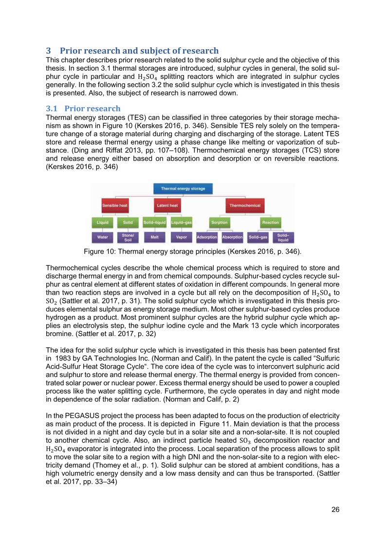
3.1 Prior research Thermal energy storages (TES) can be classified in three categories by their storage mecha-nism as shown in Figure 10 (Kerskes 2016, p. 346). Sensible TES rely solely on the tempera-ture change of a storage material during charging and discharging of the storage. Latent TES store and release thermal energy using a phase change like melting or vaporization of sub-stance. (Ding and Riffat 2013, pp. 107–108). Thermochemical energy storages (TCS) store and release energy either based on absorption and desorption or on reversible reactions. (Kerskes 2016, p. 346)

Figure 10: Thermal energy storage principles (Kerskes 2016, p. 346).

Thermochemical cycles describe the whole chemical process which is required to store and discharge thermal energy in and from chemical compounds. Sulphur-based cycles recycle sul-phur as central element at different states of oxidation in different compounds. In general more than two reaction steps are involved in a cycle but all rely on the decomposition of H2SO4 to SO2 (Sattler et al. 2017, p. 31). The solid sulphur cycle which is investigated in this thesis pro-duces elemental sulphur as energy storage medium. Most other sulphur-based cycles produce hydrogen as a product. Most prominent sulphur cycles are the hybrid sulphur cycle which ap-plies an electrolysis step, the sulphur iodine cycle and the Mark 13 cycle which incorporates bromine. (Sattler et al. 2017, p. 32) The idea for the solid sulphur cycle which is investigated in this thesis has been patented first in 1983 by GA Technologies Inc. (Norman and Calif). In the patent the cycle is called “Sulfuric Acid-Sulfur Heat Storage Cycle“. The core idea of the cycle was to interconvert sulphuric acid and sulphur to store and release thermal energy. The thermal energy is provided from concen-trated solar power or nuclear power. Excess thermal energy should be used to power a coupled process like the water splitting cycle. Furthermore, the cycle operates in day and night mode in dependence of the solar radiation. (Norman and Calif, p. 2) In the PEGASUS project the process has been adapted to focus on the production of electricity as main product of the process. It is depicted in Figure 11. Main deviation is that the process is not divided in a night and day cycle but in a solar site and a non-solar-site. It is not coupled to another chemical cycle. Also, an indirect particle heated SO3 decomposition reactor and

H2SO4 evaporator is integrated into the process. Local separation of the process allows to split to move the solar site to a region with a high DNI and the non-solar-site to a region with elec-tricity demand (Thomey et al., p. 1). Solid sulphur can be stored at ambient conditions, has a high volumetric energy density and a low mass density and can thus be transported. (Sattler et al. 2017, pp. 33–34)

27

Figure 11: Depiction of complete solid sulphur cycle (Thomey et al. 2018, p. 13).

In the following, the solid sulphur cycle in Figure 11 is presented. In the first step solar energy is used to heat particles using a heliostat field and a solar particle receiver. Heat of the particles is transferred to the combination of H2SO4 evaporator and SO3 decomposition reactor where reactions in eq. 3.1 (Holleman et al. 1985, p. 507), eq. 3.2 (Holleman et al. 1985, p. 498) occur. H2SO4 → SO3 + H2O ΔH298= 176.6.0

𝑘𝐽

𝑚𝑜𝑙 eq. 3.1

SO3 → SO2 + O2 ΔH298= 99.0 𝑘𝐽

𝑚𝑜𝑙 eq. 3.2

Cold particles are then reheated and reintroduced to the process. In the gas separation H2O,

SO2 and O2 are separated. H2O and SO2 are then transferred to the disproportionation reactor where the disproportionation reaction presented in eq. 3.3 (Norman and Calif, p. 2) occurs. 2H2O+ 3SO2 → 2H2SO4 + S ΔH298 = -260.42

𝑘𝐽

𝑚𝑜𝑙 eq. 3.3

Diluted sulphuric acid as a side product of the disproportionation step is concentrated and recycled. Surplus water is stored to be used as educt for the disproportionation reaction. Ele-mental sulphur from the disproportionation step is transported to the non-solar site where it is burned in sulphur burner according to eq. 3.4 (Holleman et al. 1985, p. 498). S + O2 → SO2 ΔH298= 297.0

𝑘𝐽

𝑚𝑜𝑙 eq. 3.4

Energy from the hot gases is converted to electrical energy in a combination of a gas turbine and a generator. SO2 reacts to SO3 in the contact process according to eq. 3.5 (Holleman et al. 1985, p. 498). Heat released during the reaction is used to produce steam which powers a steam turbine for additional electricity production.

28

2SO2 + O2 → SO3 ΔH298= -99.0 𝑘𝐽

𝑚𝑜𝑙 eq. 3.5

SO3 produced is converted to high concentrated sulphuric acid in an absorber according to eq. 3.6 (Holleman et al. 1985, p. 507). SO3 + H2O → H2SO4 ΔH298= -176.6.0

𝑘𝐽

𝑚𝑜𝑙 eq. 3.6

As mentioned earlier in this section splitting of H2SO4 to SO2 plays a role in all sulphur cycles. Various reactor concepts to perform the splitting reaction using solar energy have already been developed. A volumetric receiver reactor is shown in Figure 12, a bayonet reactor is shown Figure 13 and a direct contact reactor is shown in Figure 14. The volumetric reactor receiver consists of two chambers one for sulphuric acid decomposition and one for SO3 decomposition respective which is shown Figure 12. It has a potentially high thermal efficiency. On the other hand the operating pressure is limited due to the window in a reactor (Wong 2014, p. 15). Furthermore, it is not possible to operate continuously because it is directly coupled to incoming radiation without storage possibilities.

Figure 12: Volumetric two chamber reactor and receiver combination for H2SO4 evaporation

and SO3 decomposition (Wong 2014, p. 16). To decouple the reactor from direct radiation indirect heated reactors can be used. An example for indirect heated reactors is the bayonet reactor which can be heated by a heat transfer medium (HTM). It consists in its simplest form of one closed ended tube co-axially aligned with an open-ended tube to form two concentric flow paths. Heat is supplied by the HTM to the outer tube from the outside while heat is recovered from the inner tube. H2SO4 is fed at the open end to the outer tube where it is vaporized before passing through an annular catalyst bed (M.B. Gorensek 2009, p. 30). Advantages of the bayonet design are the internal heat re-cuperation and low fabrication cost. (M.B. Gorensek 2009, p. 31)

29

Figure 13: Bayonet reactor (M.B. Gorensek 2009, p. 30).

Indirect heat transfer reduces the thermal efficiency due to additional thermal resistance be-tween the heat transfer medium and the reaction fluid. A direct contact reactor is shown in Figure 14 which removes the heat transfer resistance between the HTM and the reaction fluid. It was suggested in an early stage of the PEGASUS project (Thomey et al., p. 1). Hot catalytic particles enter the reactor at the top of the reactor and move downward driven by gravity. Liquid sulphuric acid enters at the bottom of the reactor in counter flow to the particles and evaporates in tubes. The incoming vapour comes in direct contact with the hot catalytic particles where the SO3 decomposition reaction takes place. A surplus of hot catalytic particles can be stored to enable continuous operation in low radiation phases. Particles are heated in a separate particle receiver such as the centrifugal particle receiver CentRec®. In the direct contact zone a high heat transfer between particles and fluid can be reached. Due to the direct contact the streams cannot be adjusted freely because particles could be carried out of the reactor or enter the evaporation tubes.

Figure 14: Direct contact SO3 decomposition reactor and H2SO4 evaporator from PEGASUS

project (Thomey et al., p. 1). To choose the catalyst independently from the particles which are used as heat transfer me-dium an indirect heated concept as shown in Figure 15 can be used. This design also has the advantages that fluid and particle flows can be adjusted freely and high reactor pressures can be realised. Hot bauxite particles enter the shell on the top side of the heat exchanger and are driven downwards by gravity. Liquid H2SO4 enters the tubes at the bottom into the preheating and evaporation part. After vaporizing and superheating they reach the Fe2O3 catalyst foam in

30

the reactor zone. During evaporation and superheating reaction eq. 3.1 occurs. In the reactor zone SO3 decomposition according to eq. 3.2 occurs subsequently. This concept has been developed in the PEGASUS project and tested experimentally parallel to this thesis.

Figure 15: Depiction of the indirect heated combined H2SO4 evaporator and SO3 decomposi-

tion reactor (Agrafiotis et al. 2020, p. 3)

3.2 Subject of research This thesis evaluates the economic performance of a version of the solid sulphur cycle which has been proposed in the PEGASUS project. Basis for the economic evaluation is a simulation which is conducted using the process simulator Aspen Plus. It complemented by other com-puter-aided process design methods presented in section 2.2. The most important method used in the process design of this thesis is the numerical techno-economic optimization. The economic evaluation of the process is conducted according to the method described in section 2.3. Emphasis of the modelling and simulation effort lays on the SO3 decomposition reaction

and evaporation of H2SO4. It is the main energy demanding step of the solid sulphur cycle and all other sulphur cycles. It is thus expected to have a strong influence on the overall process perfomance. In particular the influence of the reactor size and particle outlet temperature of the CSTES towards the net present worth will be investigated. Parallel to this thesis, a new experimental reactor and evaporator concept is built in the PEGASUS and BASIS project. This reactor concept is chosen for the simulation and its performance is analysed. The experimental reactor is modelled in a rigorous simulation approach to describe the behaviour more accu-rately. The concept for the process investigated in this thesis is depicted in Figure 16. It is very similar to the concept of the solid sulphur cycle proposed in the PEGASUS project shown in Figure 11. The most important difference is the integration of sulphuric acid recycling in the cycle. High concentrated sulphuric acid is sold to an external process and treated afterwards. So excess thermal energy of the process can be utilized. The sulphuric acid production and elec-tricity production on the non-solar site are not simulated in this thesis. Results of the non-solar site required to evaluate the complete process are instead used from a previous techno-eco-nomic study (Rosenstiel 2018).

31

Figure 16: Depiction of process investigated in this thesis.

Spent acid from titan dioxide TiO2 production plants has been selected as recycling stream. Titan dioxide is produced in large quantities which allows to design a process which stores and transports considerable amounts of energy. TiO2 production capacities in Germany in 2001 using the sulphate process were 322,000 t/a (Federal Environmental Agency 2001, p. 1) and 2.767 million t/a world-wide in 2008 (Auer et al. 2012, p. 258). Integrating sulphuric acid recy-cling into the process has also been investigated in a previous study (Rosenstiel 2018) which inspired this process design choice. The integration has the following advantages and disadvantages:

• Advantages o More fossil fuels can be substituted because the conventional H2SO4 recycling

process is powered by fossil fuels. o Additional revenue is created for the treatment of the spent sulphuric acid. o Excess heat of the cycle is utilized.

• Disadvantages o Increased transportation cost due to additional mass of the diluted acid o Additional engineering efforts for separation of impurities

In this thesis a strongly simplified recycling process is simulated. Only the excess water of the diluted sulphuric acid without impurities is considered to estimate the potential of the integra-tion of sulphuric acid recycling into the process. Numerical techno-economic optimization is used to investigate the influence of mainly two de-sign variables for the net present worth of the process. The reactor size and the particle inlet temperature to the decomposition section. The design variables investigated have

Decomposition

DisproportionationAcid

concentration

Elemental

sulphur

SO2, H2O,

H2SO4

Heat transfer particles

Concentrated

H2SO4

Hot particle

storageCold particle

storage

Heliostats & Solar

thermal receiver

Sulphuric acid

production

Titan dioxide

production

𝑆𝑂2 separation

Electricity

O2

H2SO470 wt%

H2SO465 wt%

H2SO4 22 wt%

Titan dioxide

Solar

radiation

SO2, SO3,H2O, O2

H2O

Solar site

Non-solar

site

CSTES

External

process

32

contradicting influences towards the net present worth. A large H2SO4 splitting reactor size increases the conversion which is desirable because it reduces the recycle fluid flow. Thus, it increases the amount of energy stored in chemical bonds. A small reactor is desirable because it reduces the investment costs. A high particle inlet temperature in the reactor is desirable because it increases the reaction rate, shifts the equilibrium to the product side and reduces the required thermal storage size of the CSTES. But a high particle inlet temperature increases thermal losses in the CSTES. Numerical techno-economic optimization for the net present worth quantifies the effects. It shows if the effects are in balance at some point or if one effect dominates another completely. The reactor model and the model implementation in the simu-lation is described in chapter 4. The simulation of the complete process is presented in chapter 5 and the corresponding results are presented in chapter 6.

4 Modelling of particle heated 𝐇𝟐𝐒𝐎𝟒 splitting reactor This chapter presents the simulation model developed for the H2SO4 evaporator and SO3 de-

composition reactor concept shown in Figure 15. The combination of H2SO4 evaporator and SO3 decomposition reactor will be called H2SO4 splitting reactor in this thesis. In the following the reactor and the model structure are presented. The reactor consists of multiple tubes which are located in a shell as it can be seen in Figure 15. Fluid enters at the bottom in the tubes and moves upwards to the catalyst. First H2SO4 reacts to H2O and 𝑆O3 according to eq. 3.1 during and after evaporation. Afterwards 𝑆O3 reacts

to 𝑆O2 according to eq. 3.2 at elevated temperatures in contact with the catalyst. Particles enter on the top of the shell and move downward driven by gravity. While moving down heat is transferred from the particles to the fluid. Goal of the simulation of the H2SO4 splitting reactor is the calculation of the reached conversion

rate of the SO3 decomposition reaction. It depends on the reactor size and different particle inlet temperatures, particle mass flows, fluid inlet temperatures, fluid mass flows and fluid pres-sures. The size of the reactor is determined by the tube lengths, tube diameter, number of tubes and the catalyst mass in the reactor. The reactor is modelled as parallel connected single composite tubes which are individually surrounded by a particle bulk. A model of a single tube is split lengthwise into four modelling sections as it can be seen on the left side of Figure 17. The first three sections (preheating, vaporization and superheating) are based on the different fluid aggregate states which strongly influence the heat transfer. The fourth section is determined by the presence of the catalyst for the SO3 decomposition reaction in eq. 3.2. Particle flow and fluid are shared evenly between all of them. This approach allows simple adjustment of reactor capacity in the process by in-creasing and decreasing the number of tubes.

33

Figure 17: Depiction of single tube reactor model of the H2SO4 splitting reactor (own

depiction).

Decomposition

Superheating

Vaporisation

Preheating

Particle bulk

𝑏𝑢𝑙𝑘

𝑐𝑜𝑛𝑡𝑎𝑐𝑡

Stainles steel

tube 𝑆𝑆

Silicon carbide

tube 𝑆𝑖𝐶

Catalyst

Vapour 𝑔𝑎𝑠

Liquid 𝑙𝑖𝑞𝑢𝑖𝑑

𝑣𝑎𝑝𝑜𝑟𝑖𝑠𝑎𝑡𝑖𝑜𝑛

34

The required size of the reactor mainly depends on the required residence time of the SO3 decomposition reaction. The amount of heat which needs to be transferred to reach a sufficient conversion influences the reactor size as well. The correlation between the size of the reactor and the transferred heat is described by the heat transfer model in section 4.2. Correlations between thermodynamic properties such as temperature, density and pressure of the fluid and the particles are described in the section 4.4. The reaction equilibrium and the reaction kinetic which determine the required residence time in the SO3 decomposition reactor are described in section 4.3. The decomposition of H2SO4 is assumed to be very fast and thus only controlled by heat transfer. The conversion is calculated from an equilibrium equation which is part of the thermodynamic model in section 4.4. Implementation and solution of the reactor model is pre-sented in section 4.1.

4.1 Implementation and solution of the reactor model The model for H2SO4 splitting reactor is implemented using a combination of Aspen Plus unit operation blocks and Python modules. Aspen Plus unit operation blocks are shown in Figure 18. They are located inside of an Aspen Plus hierarchy block to allow easy integration into a process. Each of the sections (preheating, vaporization, and superheating) are modelled by two heater blocks respectively. The decomposition section is modelled as a RPlug reactor. The required reaction kinetic and reaction equilibrium for the RPlug model are presented in section 4.3

Figure 18: Depiction of the Aspen Plus model for the H2SO4 evaporator and SO3 decomposi-

tion reactor section. The fluid side Heater blocks are used to set the respective fluid state reached which is required for the applicability of the heat transfer model. Particle side Heater blocks are used to transfer the required amount of heat from the particles to the fluid to reach the desired thermodynamic fluid state. This implementation allows physically infeasible solutions which is advantageous for flowsheet evaluation automation. An erroneous calculation can be detected from the simu-lation result and noted as constraint violation consequently. An example for an erroneous cal-culation is heat that is transferred from a lower temperature to a higher temperature. Thereby expensive numerical solution attempts for infeasible solutions can be avoided and the problem can be clearly located. When the optimization algorithm tries an input parameter combination which leads to an unphysical solution a penalty is added to objective function and the next input parameter combination will yield a feasible solution again.

35

The solving procedure is different for the first three sections of the reactor compared to the decomposition section. 𝑡𝑜𝑡𝑎𝑙,𝑝𝑟𝑒ℎ𝑒𝑎𝑡𝑖𝑛𝑔, 𝑡𝑜𝑡𝑎𝑙,𝑣𝑎𝑝𝑜𝑟𝑖𝑧𝑎𝑡𝑖𝑜𝑛 and 𝑡𝑜𝑡𝑎𝑙,𝑠𝑢𝑝𝑒𝑟ℎ𝑒𝑎𝑡𝑖𝑛𝑔 are used to cal-

culate the required size of the respective section after the simulation has run. The amount of heat transferred in each section depends on the fluid state described in Table 5. The section size calculation is described in section 4.2.1. SO3 decomposition is modelled using a RPlug block which is configured as counter-current thermal fluid and a multitube reactor so that the reactor size can be increased by adding more tubes to it. The RPlug block requires a heat transfer coefficient to calculate the heat exchange, a reaction kinetic and a reaction equilibrium to determine the conversion reached. In the de-composition section 𝑡𝑜𝑡𝑎𝑙,𝑑𝑒𝑐𝑜𝑚𝑝𝑜𝑠𝑖𝑡𝑖𝑜𝑛 depends on the conversion reached, outlet tempera-

ture, fluid mass flow and stream composition and vice versa. Some of these quantities are note available prior to the simulation run. Thus, an initial guess is provided for an iterative solution using Python and Aspen Plus. Besides the initial guess for 𝑡𝑜𝑡𝑎𝑙,𝑑𝑒𝑐𝑜𝑚𝑝𝑜𝑠𝑖𝑡𝑖𝑜𝑛 the inner tube

diameter, tube length, number of tubes and catalyst mass is provided to Aspen Plus prior to the simulation run. The results from the simulation are read from Aspen Plus via ActiveX using Python. These are used to recalculate 𝑡𝑜𝑡𝑎𝑙,𝑑𝑒𝑐𝑜𝑚𝑝𝑜𝑠𝑖𝑡𝑖𝑜𝑛 and to provide the result again to the

simulation which run again. These steps are repeated until convergence is reached. As stop-ping criteria 𝑑𝑒𝑐𝑜𝑚𝑝𝑜𝑠𝑖𝑡𝑖𝑜𝑛,𝑛𝑒𝑤 − 𝑑𝑒𝑐𝑜𝑚𝑝𝑜𝑠𝑖𝑡𝑖𝑜𝑛,𝑜𝑙𝑑 < 0.01 is used.

Another problem in the initialization of the RPlug block is that particle stream and the fluid stream need to be fully specified at reactor inlet. Thus, the particle inlet temperature cannot bet used as a design variable directly. It can only be adjusted indirectly by changing particle outlet temperature of the reactor. The calculator blocks PREPROP, VAPPROP, SUPPROP, PARTPRES and DECOPRES are used to retrieve physical properties of the corresponding streams for evaluation in Python.

4.2 Heat transfer model This section describes the heat transfer model used to simulate the SO3 particle heated de-

composition reactor and H2SO4 evaporator. For each section of the reactor which is shown on the left side of Figure 17 a complete heat transfer coefficient 𝑡𝑜𝑡𝑎𝑙 is calculated. Each 𝑡𝑜𝑡𝑎𝑙 characterizes the heat transfer from the particle bulk to the fluid in the tube in the respective section. They are called 𝑡𝑜𝑡𝑎𝑙,𝑝𝑟𝑒ℎ𝑒𝑎𝑡𝑖𝑛𝑔, 𝑡𝑜𝑡𝑎𝑙,𝑣𝑎𝑝𝑜𝑟𝑖𝑧𝑎𝑡𝑖𝑜𝑛, 𝑡𝑜𝑡𝑎𝑙,𝑠𝑢𝑝𝑒𝑟ℎ𝑒𝑎𝑡𝑖𝑛𝑔 and

𝑡𝑜𝑡𝑎𝑙,𝑑𝑒𝑐𝑜𝑚𝑝𝑜𝑠𝑖𝑡𝑖𝑜𝑛 from bottom to top.

In each section several thermal resistances occur between the particle bulk and the fluid which can be seen in the top view of Figure 17. They are used to calculate 𝑡𝑜𝑡𝑎𝑙 for the respective

stage and the detailed calculation procedure of 𝑡𝑜𝑡𝑎𝑙 is described in section 4.2.2 to 4.2.5. An important simplification in the model the neglected influence of the foam for the heat transfer. From experimental experience it is known that the overall heat transfer is increased by foams added to the tubes but it has not been quantified so far (Oliveira 9/14/2020a). Thus, calculation of the heat transfer coefficient is a conservative estimate. The first three sections are separated by the respective state of the fluid at the inlet and outlet of the stage during heating which is shown in Table 5. The heat transfer coefficient for the decomposition section is calculated separately because it needs to be supplied prior to the simulation run.

Table 5: Definition of reactor stages in dependence of fluid aggregate states.

Stage Preheating Vaporization Superheating

Inlet fluid temperature

Design variable or result from preceding acid concentration

Saturated liquid temperature

Saturated vapour tem-perature

Outlet fluid temperature

Saturated liquid temperature Saturated vapour temperature

Design variable

36

Most of the properties which are required for the heat transfer calculations are temperature dependent. The average section temperature of the fluid or particles are used to determine the value which is recommended in the VDI heat atlas. (Stephan et al. 2019, p. 840) Unless stated otherwise physical properties were used from the Aspen Plus simulation. The heat transfer modelling approach presented here is based on the simulation of the moving bed sulphuric acid evaporator in chapter 7 of (Thanda 2018, pp. 19–32).

4.2.1 Heat exchange surface calculation This section describes the calculation of the heat exchange area A which is required for cost estimation of heat exchangers. The heat exchanger surface is calculated according to the log-arithmic mean temperature difference method (LMTD). The main equation for counterflow heat exchanger which are applied in this thesis is shown in eq. 4.1. Q is the transferred heat, 𝑡𝑜𝑡𝑎𝑙

the overall heat exchange coefficient, A the heat exchange surface, Δ𝑇2 and Δ𝑇1 are the tem-perature differences between the hot and the cold fluid at the inlet and outlet of the heat ex-changer (Bergman and Lavine 2017, p. 714). 𝑡𝑜𝑡𝑎𝑙 depends on temperature depended prop-erties and the tube geometry. Thus, an iterative solution is required to determine A which is conducted using Python modules.

Q = 𝑡𝑜𝑡𝑎𝑙 ∗ A ∗Δ𝑇2 − Δ𝑇1

ln (Δ𝑇2Δ𝑇1

)

eq. 4.1

4.2.2 Complete heat transfer coefficient 𝛂𝒕𝒐𝒕𝒂𝒍 The overall heat transfer value of a tube in the decomposer and evaporator combination is calculated from several single thermal resistances 𝑅𝑗 which can be modelled as a series of

single thermal resistances as presented in eq. 4.2 (Stephan et al. 2019, p. 92).

𝑅𝑡𝑜𝑡𝑎𝑙 = ∑𝑅𝑗𝑗

eq. 4.2

The correlation between the overall heat transfer value 𝑡𝑜𝑡𝑎𝑙, A and the 𝑅𝑡𝑜𝑡𝑎𝑙 seen in eq. 4.3 and eq. 4.4.

R = Δ𝑇

��

eq. 4.3

In (Stephan et al. 2019, p. 92) 𝑡𝑜𝑡𝑎𝑙 is referred to as k and in Aspen Plus it is referred to as U which all represent the same coefficient. It is important to note that the total heat exchanger surface 𝐴𝑡𝑜𝑡𝑎𝑙 can be defined at arbitrary radial positions in a cylinder with a thickness. In this case the surface at the inner tube diameter will be chosen because the Aspen Plus RPlug reactor can only be defined using inner tube diameters.

k = 𝑡𝑜𝑡𝑎𝑙 = 1

𝑅𝑡𝑜𝑡𝑎𝑙𝐴

eq. 4.4

The single heat resistances which occur from the particle bed on the outside of the tube to the fluid in the center of the tube are depicted on the right side of Figure 17. They are summarized in eq. 4.5. The influence of the foams in the middle of the tubes which are included in the experimental reactor are neglected.

𝑅𝑡𝑜𝑡𝑎𝑙 = 𝑅𝑏𝑢𝑙𝑘,𝑟𝑒𝑠𝑖𝑠𝑡𝑎𝑛𝑐𝑒 + 𝑅𝑐𝑜𝑛𝑡𝑎𝑐𝑡,𝑟𝑒𝑠𝑖𝑠𝑡𝑎𝑛𝑐𝑒 + 𝑅𝑆𝑆 316𝑇𝑖 + 𝑅𝑆𝑖𝐶 + 𝑅𝑓𝑙𝑢𝑖𝑑 eq. 4.5

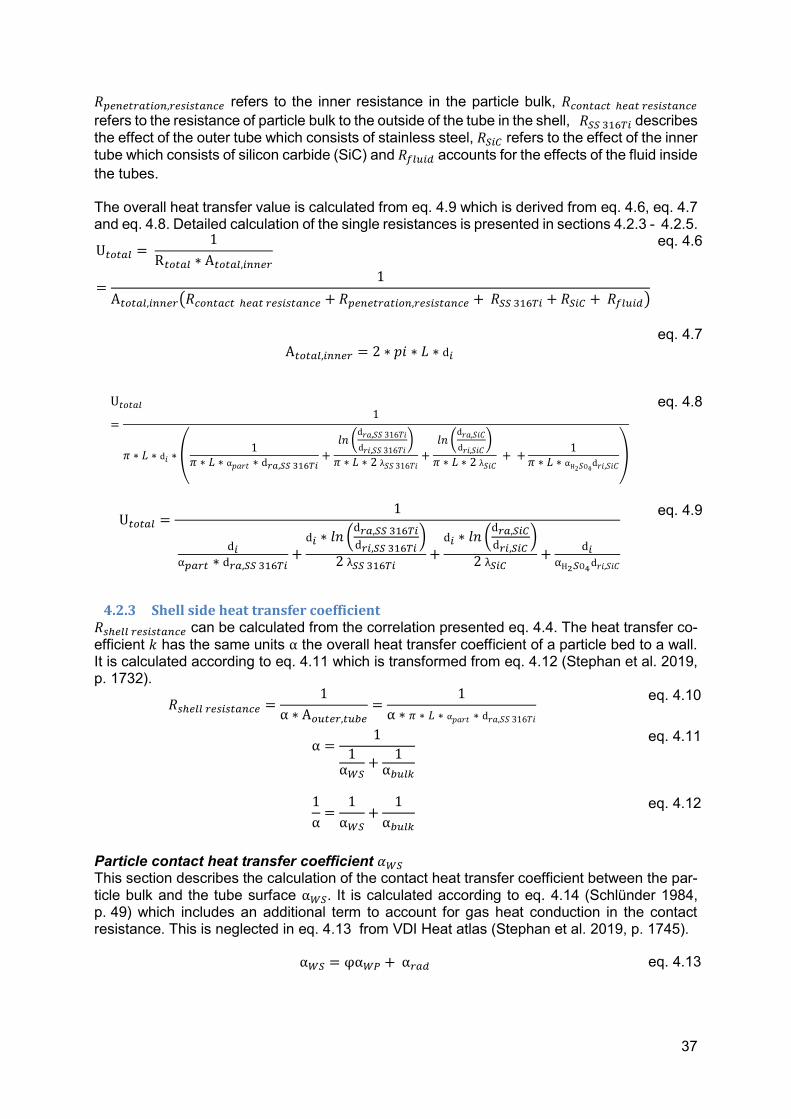
37

𝑅𝑝𝑒𝑛𝑒𝑡𝑟𝑎𝑡𝑖𝑜𝑛,𝑟𝑒𝑠𝑖𝑠𝑡𝑎𝑛𝑐𝑒 refers to the inner resistance in the particle bulk, 𝑅𝑐𝑜𝑛𝑡𝑎𝑐𝑡 ℎ𝑒𝑎𝑡 𝑟𝑒𝑠𝑖𝑠𝑡𝑎𝑛𝑐𝑒

refers to the resistance of particle bulk to the outside of the tube in the shell, 𝑅𝑆𝑆 316𝑇𝑖 describes the effect of the outer tube which consists of stainless steel, 𝑅𝑆𝑖𝐶 refers to the effect of the inner

tube which consists of silicon carbide (SiC) and 𝑅𝑓𝑙𝑢𝑖𝑑 accounts for the effects of the fluid inside

the tubes. The overall heat transfer value is calculated from eq. 4.9 which is derived from eq. 4.6, eq. 4.7 and eq. 4.8. Detailed calculation of the single resistances is presented in sections 4.2.3 - 4.2.5.

U𝑡𝑜𝑡𝑎𝑙 =

1

R𝑡𝑜𝑡𝑎𝑙 ∗ A𝑡𝑜𝑡𝑎𝑙,𝑖𝑛𝑛𝑒𝑟

=1

A𝑡𝑜𝑡𝑎𝑙,𝑖𝑛𝑛𝑒𝑟(𝑅𝑐𝑜𝑛𝑡𝑎𝑐𝑡 ℎ𝑒𝑎𝑡 𝑟𝑒𝑠𝑖𝑠𝑡𝑎𝑛𝑐𝑒 + 𝑅𝑝𝑒𝑛𝑒𝑡𝑟𝑎𝑡𝑖𝑜𝑛,𝑟𝑒𝑠𝑖𝑠𝑡𝑎𝑛𝑐𝑒 + 𝑅𝑆𝑆 316𝑇𝑖 + 𝑅𝑆𝑖𝐶 + 𝑅𝑓𝑙𝑢𝑖𝑑)

eq. 4.6

A𝑡𝑜𝑡𝑎𝑙,𝑖𝑛𝑛𝑒𝑟 = 2 ∗ 𝑝𝑖 ∗ 𝐿 ∗ d𝑖

eq. 4.7

U𝑡𝑜𝑡𝑎𝑙

=1

𝜋 ∗ 𝐿 ∗ d𝑖 ∗ (1

𝜋 ∗ 𝐿 ∗ 𝑝𝑎𝑟𝑡 ∗ d𝑟𝑎,𝑆𝑆 316𝑇𝑖+

𝑙𝑛 (d𝑟𝑎,𝑆𝑆 316𝑇𝑖

d𝑟𝑖,𝑆𝑆 316𝑇𝑖)

𝜋 ∗ 𝐿 ∗ 2 λ𝑆𝑆 316𝑇𝑖+

𝑙𝑛 (d𝑟𝑎,𝑆𝑖𝐶

d𝑟𝑖,𝑆𝑖𝐶)

𝜋 ∗ 𝐿 ∗ 2 λ𝑆𝑖𝐶 + +

1𝜋 ∗ 𝐿 ∗ H2𝑆O4d𝑟𝑖,𝑆𝑖𝐶

)

eq. 4.8

U𝑡𝑜𝑡𝑎𝑙 =1

d𝑖

𝑝𝑎𝑟𝑡 ∗ d𝑟𝑎,𝑆𝑆 316𝑇𝑖+d𝑖 ∗ 𝑙𝑛 (

d𝑟𝑎,𝑆𝑆 316𝑇𝑖d𝑟𝑖,𝑆𝑆 316𝑇𝑖

)

2 λ𝑆𝑆 316𝑇𝑖+d𝑖 ∗ 𝑙𝑛 (

d𝑟𝑎,𝑆𝑖𝐶d𝑟𝑖,𝑆𝑖𝐶

)

2 λ𝑆𝑖𝐶+

d𝑖 H2𝑆O4d𝑟𝑖,𝑆𝑖𝐶

eq. 4.9

4.2.3 Shell side heat transfer coefficient 𝑅𝑠ℎ𝑒𝑙𝑙 𝑟𝑒𝑠𝑖𝑠𝑡𝑎𝑛𝑐𝑒 can be calculated from the correlation presented eq. 4.4. The heat transfer co-

efficient 𝑘 has the same units the overall heat transfer coefficient of a particle bed to a wall. It is calculated according to eq. 4.11 which is transformed from eq. 4.12 (Stephan et al. 2019, p. 1732).

𝑅𝑠ℎ𝑒𝑙𝑙 𝑟𝑒𝑠𝑖𝑠𝑡𝑎𝑛𝑐𝑒 =1

∗ A𝑜𝑢𝑡𝑒𝑟,𝑡𝑢𝑏𝑒=

1

∗ 𝜋 ∗ 𝐿 ∗ 𝑝𝑎𝑟𝑡 ∗ d𝑟𝑎,𝑆𝑆 316𝑇𝑖

eq. 4.10

=1

1 𝑊𝑆

+1

𝑏𝑢𝑙𝑘

eq. 4.11

1

=

1

𝑊𝑆+

1

𝑏𝑢𝑙𝑘

eq. 4.12

Particle contact heat transfer coefficient 𝛼𝑊𝑆 This section describes the calculation of the contact heat transfer coefficient between the par-ticle bulk and the tube surface 𝑊𝑆. It is calculated according to eq. 4.14 (Schlünder 1984, p. 49) which includes an additional term to account for gas heat conduction in the contact resistance. This is neglected in eq. 4.13 from VDI Heat atlas (Stephan et al. 2019, p. 1745).

𝑊𝑆 = φ 𝑊𝑃 + 𝑟𝑎𝑑

eq. 4.13

38

𝑊𝑆 = φ 𝑊𝑃 + (1 − φ)

2λ𝑔d𝑝

√2 +2(𝑙0 + δ)

d𝑝

+ 𝑟𝑎𝑑

eq. 4.14

Table 6: Particle contact heat transfer coefficient parameters

Symbol φ λ𝑔 d𝑝 𝛿

Description surface cover-age factor

thermal conduc-tivity of the in-terstitial gas

mean particle diameter

surface rough-ness of the par-

ticle

Value applied 0.8 From Appendix B

0.001 m 2.5 µm from Ap-pendix B

Wall to particle heat transfer coefficient 𝛼𝑊𝑃

Wall to particle heat transfer coefficient 𝑊𝑃 is calculated according to eq. 4.15 (Stephan et al.

2019, p. 1745)

𝑊𝑃 =

4λ𝑔

𝑑[(1 +

2(𝑙 + δ)

𝑑) 𝑙𝑛 (1 +

𝑑

2(𝑙 + δ)) − 1]

eq. 4.15

The modified mean free path of particles l0 is calculated according to eq. 4.16 (Stephan et al. 2019, p. 1745):

l0 = 22 − γ

γ√2𝜋𝑅𝑇

𝑀

λ𝑔

𝑝 (2𝑐𝑝,𝑔 −𝑅𝑀)

eq. 4.16

Accommodation factor γ is calculated according to eq. 4.17 which is transformed from eq. 4.18 (Stephan et al. 2019, p. 1746). C = 2.8 is which is the value for air (Stephan et al. 2019, p. 1746).

γ = 1

1 + 100.6−

(1000𝑇

+1)

𝐶

eq. 4.17

log(1

γ− 1) = 0.6 -

(1000

𝑇)+1

C

eq. 4.18

Table 7: Wall to particle heat transfer parameters

Symbol 𝑀 R c𝑝,𝑔

Description Molar mass of interstitial gas Universal gas constant

specific heat capacity of the interstitial gas

Value applied 0.02986 𝑘𝑔

𝑚𝑜𝑙 8.314

𝐽

𝑚𝑜𝑙𝐾 From Appendix B

Radiation heat transfer coefficient 𝜶𝒓𝒂𝒅 The radiation coefficient is calculated according to eq. 4.19 and eq. 4.20. (Stephan et al. 2019, p. 1745)

𝑟𝑎𝑑 = 4 ∗ 𝐶𝑤,𝑏𝑒𝑑𝑇3 eq. 4.19

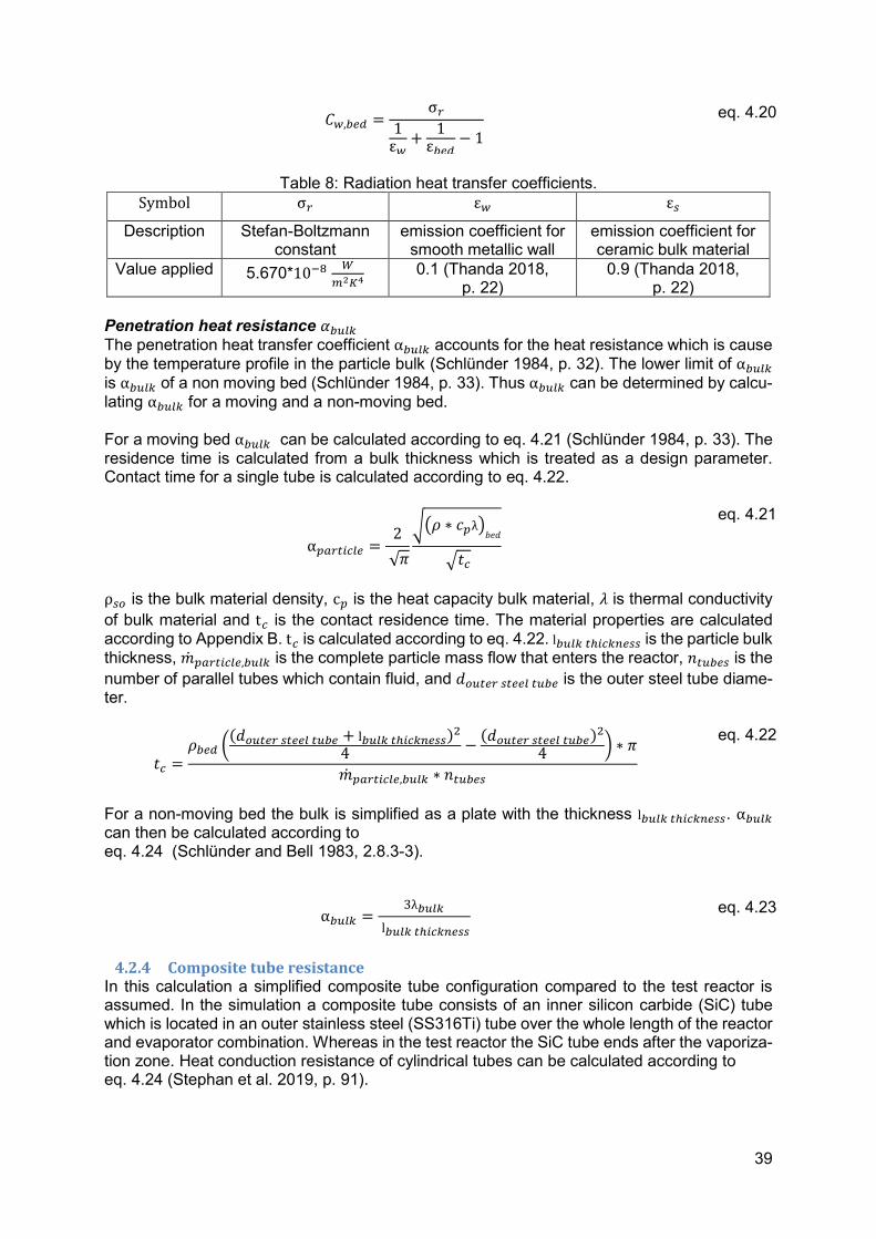
39

𝐶𝑤,𝑏𝑒𝑑 =σ𝑟

1ε𝑤+

1ε𝑏𝑒𝑑

− 1 eq. 4.20

Table 8: Radiation heat transfer coefficients.

Symbol σ𝑟 ε𝑤 ε𝑠

Description Stefan-Boltzmann constant

emission coefficient for smooth metallic wall

emission coefficient for ceramic bulk material

Value applied 5.670*10−8 𝑊

𝑚2𝐾4 0.1 (Thanda 2018,

p. 22) 0.9 (Thanda 2018,

p. 22)

Penetration heat resistance 𝛼𝑏𝑢𝑙𝑘

The penetration heat transfer coefficient 𝑏𝑢𝑙𝑘 accounts for the heat resistance which is cause by the temperature profile in the particle bulk (Schlünder 1984, p. 32). The lower limit of 𝑏𝑢𝑙𝑘

is 𝑏𝑢𝑙𝑘 of a non moving bed (Schlünder 1984, p. 33). Thus 𝑏𝑢𝑙𝑘 can be determined by calcu-lating 𝑏𝑢𝑙𝑘 for a moving and a non-moving bed. For a moving bed 𝑏𝑢𝑙𝑘 can be calculated according to eq. 4.21 (Schlünder 1984, p. 33). The residence time is calculated from a bulk thickness which is treated as a design parameter. Contact time for a single tube is calculated according to eq. 4.22.

𝑝𝑎𝑟𝑡𝑖𝑐𝑙𝑒 =2

√𝜋

√(𝜌 ∗ 𝑐𝑝λ)𝑏𝑒𝑑

√𝑡𝑐

eq. 4.21

ρ𝑠𝑜 is the bulk material density, c𝑝 is the heat capacity bulk material, 𝜆 is thermal conductivity

of bulk material and t𝑐 is the contact residence time. The material properties are calculated according to Appendix B. t𝑐 is calculated according to eq. 4.22. l𝑏𝑢𝑙𝑘 𝑡ℎ𝑖𝑐𝑘𝑛𝑒𝑠𝑠 is the particle bulk thickness, ��𝑝𝑎𝑟𝑡𝑖𝑐𝑙𝑒,𝑏𝑢𝑙𝑘 is the complete particle mass flow that enters the reactor, 𝑛𝑡𝑢𝑏𝑒𝑠 is the

number of parallel tubes which contain fluid, and 𝑑𝑜𝑢𝑡𝑒𝑟 𝑠𝑡𝑒𝑒𝑙 𝑡𝑢𝑏𝑒 is the outer steel tube diame-ter.

𝑡𝑐 =𝜌𝑏𝑒𝑑 (

(𝑑𝑜𝑢𝑡𝑒𝑟 𝑠𝑡𝑒𝑒𝑙 𝑡𝑢𝑏𝑒 + l𝑏𝑢𝑙𝑘 𝑡ℎ𝑖𝑐𝑘𝑛𝑒𝑠𝑠)2

4−(𝑑𝑜𝑢𝑡𝑒𝑟 𝑠𝑡𝑒𝑒𝑙 𝑡𝑢𝑏𝑒)

2

4) ∗ 𝜋

��𝑝𝑎𝑟𝑡𝑖𝑐𝑙𝑒,𝑏𝑢𝑙𝑘 ∗ 𝑛𝑡𝑢𝑏𝑒𝑠

eq. 4.22

For a non-moving bed the bulk is simplified as a plate with the thickness l𝑏𝑢𝑙𝑘 𝑡ℎ𝑖𝑐𝑘𝑛𝑒𝑠𝑠. 𝑏𝑢𝑙𝑘 can then be calculated according to eq. 4.24 (Schlünder and Bell 1983, 2.8.3-3).

𝑏𝑢𝑙𝑘 =3λ𝑏𝑢𝑙𝑘

l𝑏𝑢𝑙𝑘 𝑡ℎ𝑖𝑐𝑘𝑛𝑒𝑠𝑠

eq. 4.23

4.2.4 Composite tube resistance In this calculation a simplified composite tube configuration compared to the test reactor is assumed. In the simulation a composite tube consists of an inner silicon carbide (SiC) tube which is located in an outer stainless steel (SS316Ti) tube over the whole length of the reactor and evaporator combination. Whereas in the test reactor the SiC tube ends after the vaporiza-tion zone. Heat conduction resistance of cylindrical tubes can be calculated according to eq. 4.24 (Stephan et al. 2019, p. 91).

40

𝑅𝑐𝑜𝑛𝑑𝑢𝑐𝑡𝑖𝑜𝑛,𝑐𝑦𝑐𝑙𝑖𝑛𝑑𝑒𝑟 =

𝑙𝑛 (r𝑎r𝑖)

𝜋 ∗ 𝐿 ∗ 2 ∗ λ=

𝑙𝑛 (d𝑎d𝑖)

𝜋 ∗ 𝐿 ∗ 2 ∗ λ

eq. 4.24

Their respective thermal resistance is calculated by eq. 4.25 and eq. 4.26. Outer diameters are calculated from the inner tube diameter d𝑟𝑖,𝑆𝑖𝐶 and the corresponding wall and gap thick-

nesses. The thicknesses t𝑆𝑖𝐶 = 4 𝑚𝑚 and t𝑆𝑆 316𝑇𝑖 = 3 𝑚𝑚 are assumed to be the same as in the evaporation zone (Thanda 11/10/2020).

𝑅𝑆𝑆 316𝑇𝑖 =

𝑙𝑛 (d𝑟𝑎,𝑆𝑆 316𝑇𝑖d𝑟𝑖,𝑆𝑆 316𝑇𝑖

)

𝜋 ∗ 𝐿 ∗ 2 λ𝑆𝑆 316𝑇𝑖

eq. 4.25

𝑅𝑆𝑖𝐶 =

𝑙𝑛 (d𝑟𝑎,𝑆𝑖𝐶d𝑟𝑖,𝑆𝑖𝐶

)

𝜋 ∗ 𝐿 ∗ 2 λ𝑆𝑖𝐶

eq. 4.26

4.2.5 Fluid side thermal resistance This section describes the calculation of the thermal resistance of the fluid inside the tubes. The resistance can be calculated according to eq. 4.27 (Stephan et al. 2019, p. 91).

𝑅𝑐𝑜𝑛𝑣 =1

𝑓𝑙𝑢𝑖𝑑 ∗ A

eq. 4.27

Convective heat transfer coefficient 𝑓𝑙𝑢𝑖𝑑 can be calculated by eq. 4.29 which is transposed

from eq. 4.28 (Stephan et al. 2019, p. 840). Heat transfer of mixtures can be calculated using the correlations for pure components with properties of the mixtures (Stephan et al. 2019,

p. 1110). λ 𝑊

𝑚𝐾 is the fluid conductivity and 𝑑𝑖 𝑚 the hydraulic diameter which in this case is the

inner diameter of the tube.

Nu = 𝑓𝑙𝑢𝑖𝑑 ∗ 𝑑𝑖

λ𝑓𝑙𝑢𝑖𝑑

eq. 4.28

𝑓𝑙𝑢𝑖𝑑 = Nu ∗ λ𝑓𝑙𝑢𝑖𝑑

𝑑𝑖

eq. 4.29

The Nusselt number can be calculated from two different correlation depending on the fluid flow regime. For Re > 2300 the flow is considered to be turbulent and is calculated according to eq. 4.30 and eq. 4.31. For Re < 2300 the flow is considered to be laminar and is calculated according to eq. 4.32. For both equations hydrodynamically developed flows are assumed. (Stephan et al. 2019, p. 1033)

Nu𝑡𝑢𝑟𝑏𝑢𝑙𝑒𝑛𝑡 =

ξ8(Re − 1000) ∗ Pr

1 + 12,7 √ξ8 ∗ (Pr

23 − 1)

eq. 4.30

ξ = (1.82 ∗ 𝑙𝑜𝑔10(𝑅𝑒) − 1.64)−2 eq. 4.31

𝜂𝑓𝑙𝑢𝑖𝑑 𝑃𝑎

𝑠 is the dynamic viscosity and 𝜌𝑓𝑙𝑢𝑖𝑑

𝑘𝑔

𝑚3 the fluid density. In the laminar flow regime a

Nusselt correlation is provided in eq. 4.32 assuming hydrodynamic developed flows. (Stephan et al. 2019, p. 1033)

Nu𝑙𝑎𝑚 = √4.363 + 1.3023 ∗ 𝑅𝑒 ∗ 𝑃𝑟 ∗𝑑

𝑧

3

eq. 4.32

41

The Reynolds number is calculated according to eq. 4.33 (Stephan et al. 2019, p. 840) and the Prandtl number can be calculated according to eq. 4.34 (Stephan et al. 2019, p. 78). For short tubes and Reynolds numbers in the range of 2300 < Re < 4000 it is possible that a higher Nusselt number is calculated for the laminar case than for the turbulent. In such a case the higher value has to be applied. (Stephan et al. 2019, p. 1032)

Re =𝑣𝑓𝑙𝑢𝑖𝑑𝑑𝑖𝜌𝑓𝑙𝑢𝑖𝑑

𝜂

eq. 4.33

Pr = 𝜂𝑓𝑙𝑢𝑖𝑑𝜌𝑓𝑙𝑢𝑖𝑑𝑐𝑝,𝑓𝑙𝑢𝑖𝑑

λ𝑓𝑙𝑢𝑖𝑑

eq. 4.34

The average fluid velocity 𝑣𝑓𝑙𝑢𝑖𝑑 𝑚

𝑠 in a single tube is calculated according to eq. 4.35 from total

fluid mass flow ��𝑓𝑙𝑢𝑖𝑑 entering the reactor and the number of tubes 𝑛𝑡𝑢𝑏𝑒𝑠 in which the flow is

separated.

𝑣𝑓𝑙𝑢𝑖𝑑 = ��𝑓𝑙𝑢𝑖𝑑

ρ𝑓𝑙𝑢𝑖𝑑∗ 𝑛𝑡𝑢𝑏𝑒𝑠 eq. 4.35

Vaporization Because the heat transfer coefficient during vaporization is assumed to several magnitudes higher than the heat transfer coefficient on the shell side the fluid heat transfer coefficient is neglected in the vaporization zone. This simplification is based on the investigation by (Thanda 2018, p. 67) and qualitative comparison of vaporization heat transfer coefficients in vertical tubes during vaporization, preheating and superheating (Steiner and Taborek 1992, p. 48).

4.3 Reaction model This section describes the model of the SO3 reaction which is presented in eq. 4.36 which has

an reaction enthalpy of 99 𝑘𝑗

𝑚𝑜𝑙 (Müller 2012b, p. 150).

SO3 → SO2 + O2 eq. 4.36

Most important characteristics of the reaction are the equilibrium which is presented in section 4.3.1, the reaction kinetic. It mainly describes the influence of the residence time and temper-ature on the conversion reached in the reactor presented in section 4.3.2 . The minimum re-actor temperature to prevent poisoning of the catalyst is presented in section 4.3.3.

4.3.1 Equilibrium between 𝐒𝐎𝟑 and 𝐒𝐎𝟐 An equation for the calculation of the equilibrium constant 𝐾𝑝,𝑆𝑂3 of the SO3 decomposition

reaction is presented in eq. 4.37 (Ishikawa 1982, p. 238)

𝑙𝑜𝑔(𝐾𝑝,𝑆𝑂3) = 8.8557 −5465.5

𝑇− 1.21572 ∗ log (𝑇)

eq. 4.37

To use the equation in an Aspen Plus simulation it needs to be converted as shown in:

𝑙𝑛(𝐾𝑝,𝑆𝑂3) = −6.761541126 −−9191.919961

𝑇+ 2.2188 ∗ ln(𝑇) + 0 ∗ 𝑇

eq. 4.38

To check the validity of the equation experimental values for the degree of dissociation 𝑆𝑂3

(Fedders et al., p. 169) have been plotted against simulation results produced in Aspen Plus using eq. 4.38. The degree of dissociation is defined according to eq. 4.39 in which 𝑃𝑆𝑂2 and

𝑃𝑆𝑂3corespond to the partial pressure of SO3 and SO2 respectively. The results are shown in

Figure 19.

42

𝑆𝑂3 =𝑃𝑆𝑂2

𝑃𝑆𝑂3 + 𝑃𝑆𝑂2

eq. 4.39

Figure 19: Equilibrium degree of dissociation 𝑆𝑂3 for SO3 decomposition reaction in depend-

ence of various pressures for 90 wt% sulphuric acid. The experimental data has been obtained for 90 wt% sulphuric acid and for pressures in the range of 1 to 40 bar. It can be seen that 𝑆𝑂3 increases with temperature and decreases with

pressure. This is in accordance with the le Chatelier's principle which predicts a shift to the reaction side with fewer molecules and an increase in conversion with rising temperatures for endothermic reactions (Pfennig 2004, pp. 305–307). Furthermore, the simulation results show an acceptable agreement with the experimental data. The data has been produced using a RPlug reactor with a large residence time and a constant reactor temperature. The 90 wt% sulphuric acid has been fully converted to H2O and SO3 be-fore the SO3 decomposition reaction occurs.

4.3.2 Selection of reaction kinetic for 𝐅𝐞𝟐𝐎𝟑 coated silicon carbide foams This section describes the kinetic used for the Fe2O3 coated silicon carbide foams and how it

was selected. At the end there is a brief presentation of the intrinsic reaction rate of Fe2O3 and why it cannot be applied in an industrial reactor. The foams are used to catalyse the SO3 decomposition reaction presented in eq. 3.2. No kinetic equation has been published that describes the kinetic behaviour the coated foams. Therefore, the available of the Fe2O3 coated foam has been compared to other Fe2O3 based catalyst. The comparison to the catalyst with the kinetic chosen is summarized in Table 9. Both catalysts which are shown in Figure 20 have a rather coarse structures which is the basis for the selec-tion of the kinetic. Missing data is marked with an “-“ symbol.

Table 9: Comparison of Fe2O3 coated foam catalyst and Fe2O3 coated honeycombs from.

Catalyst Iron loading

Catalyst bulk

density 𝑘𝑔

𝑚3

Apparent Iron bulk

density 𝑘𝑔

𝑚3

Mass specific surface

Tested pressure range bar

Kinetic equation available

43

Honeycomb Fragments

18.5 wt%

- - - 1 - 4 ✓

Fe2O3 coated foams

37.5 wt% 738.349 201.3945 - - -

Figure 20: Visual comparison of Fe2O3 coated foams on the left (Oliveira 9/14/2020b) and

Fe2O3 coated honeycomb fragments on the right (Giaconia et al. 2011, p. 6499). The results obtained in the experiments were fitted into an equation presented in eq. 4.40 which was solved for the conversion of an isothermal plug flow reactor directly. Even though typical Arrhenius parameters 𝐴 and 𝐸𝐴 were used during the fitting, they cannot be used to model the reaction rate in Aspen Plus. The equation depends on the weight hourly space ve-locity (WHSV), the conversion X, and the reaction temperature T. Aspen Plus reactors require an equation that models the reaction rate directly using the Arrhenius approach in eq. 4.22 for example.

−ln (1 − 𝑋) =𝐴 ∗ 𝑒−

𝐸𝐴𝑅∗𝑇

𝑊𝐻𝑆𝑉

eq. 4.40

r = 𝐴 ∗ 𝑒−𝐸𝐴𝑅∗𝑇

eq. 4.41

The results of the experiments using the Fe2O3 coated honeycomb fragments (Giaconia et al. 2011, p. 6504) were further analysed in another publication. In the publication reaction rates have been calculated for several temperatures based on the pure Fe2O3 of the coated catalysts (van der Merwe 2014, p. 77). These reaction constants are presented in Table 10. They are fitted for an Arrhenius approach presented in eq. 4.41

Table 10: Reaction rates calculated by (van der Merwe 2014, p. 77) from experimental re-

sults obtained by Giaconia (Giaconia et al. 2011, p. 6504).

Reaction rate 𝑚3

𝑘𝑔𝑐𝑎𝑡∗ℎ𝑟

17 30 45

Temperature K 1048 1073 1098

This resulted in an activation energy 𝐸𝐴 = 3.4252 ∗ 1010

𝐽

𝑘𝑚𝑜𝑙 and a prexponential factor A of

186476.768 𝑘𝑚𝑜𝑙

𝑘𝑔𝑐𝑎𝑡∗ℎ𝑟 in eq. 4.41. This reaction kinetic is based on pure Fe2O3 catalyst mass

𝑘𝑔𝑐𝑎𝑡. To simulate the behaviour of a reactor completely filled with the Fe2O3 coated foams it is necessary to calculate the pure Fe2O3 mass 𝑚𝐹𝑒2𝑂3 in this reactor. This can be done using

the bulk density of pure Fe2O3 𝜌𝐹𝑒2𝑂3,pure of the catalyst and the reactor volume 𝑉𝑟𝑒𝑎𝑐𝑡𝑜𝑟 ac-

cording to eq. 4.42. This approach is used to calculate 𝑚𝐹𝑒2𝑂3 in the RPlug reactor of the 𝑆𝑂3

decomposition reaction section.

44

𝑚𝐹𝑒2𝑂3 = 𝜌𝐹𝑒2𝑂3,pure ∗ 𝑉𝑟𝑒𝑎𝑐𝑡𝑜𝑟

eq. 4.42

It can be calculated from the catalyst production loading data according to eq. 4.43 (Thanda 8/28/2020)

𝜌𝐹𝑒2𝑂3,pure =𝑚𝐹𝑒2𝑂3

𝑉𝑓𝑜𝑎𝑚= 𝜋 ∗

𝑑𝑓𝑜𝑎𝑚

2

2

∗ 𝑙𝑓𝑜𝑎𝑚 = 201.3945 𝑘𝑔

𝑚3

eq. 4.43

A single foam has a length of 𝑙𝑓𝑜𝑎𝑚 = 40 mm and a diameter of 𝑑𝑓𝑜𝑎𝑚= 25 mm. (Mannheim

2020, pp. 46–47) A single foam has a total weight of 𝑚𝑡𝑜𝑡𝑎𝑙 10.5431 g and contains 𝑚𝐹𝑒2𝑂3

3.9544 g of pure Fe2O3. From 𝑚𝑡𝑜𝑡𝑎𝑙 the complete catalyst bulk density 𝜌𝐹𝑒2𝑂3,complete can be

calculated according to eq. 4.44. It is used to determine the price of the catalyst and to calculate the weight hourly space velocity (WHSV) according to eq. 4.45.

𝜌𝐹𝑒2𝑂3,complete =𝑚𝑐𝑜𝑚𝑝𝑙𝑒𝑡𝑒

𝑉𝑓𝑜𝑎𝑚= 𝜋 ∗

𝑑𝑓𝑜𝑎𝑚

2

2

∗ 𝑙𝑓𝑜𝑎𝑚 = 738.3493 𝑘𝑔

𝑚3

eq. 4.44

𝑊𝐻𝑆𝑉 =𝑚𝐻2𝑆𝑂4,𝑙𝑖𝑞𝑢𝑖𝑑

𝑘𝑔ℎ

𝑚𝑐𝑎𝑡𝑎𝑙𝑦𝑠𝑡 𝑘𝑔

eq. 4.45

Even though no kinetic equation which describes reaction kinetic of Fe2O3 coated foams is available a detailed study which investigated the intrinsic reaction rate of the Fe2O3 catalyst

has been conducted. In the corresponding experiments very fine pure Fe2O3 powder with par-ticle sizes of 40 +-14 µm with a purity of 99.99 % has been used. (van der Merwe 2014, p. 50) Due to the high specific surface of particles with a small diameter no transport limitations occur in the experiments and the intrinsic reaction rate can be observed directly. Particles with a diameter this small are not suitable for an industrial reactor because the pressure drop would increase strongly which can be seen in eq. 4.4. (Pesic et al. 2015, p. 4)

−ΔP

𝐻= 150 ∗

(1 − )2

3∗𝑑𝑝2 ∗ 𝑈 + 1.75 ∗

(1 − ) ∗𝑓

3 ∗ 𝑑𝑝∗ 𝑈2

eq. 4.46

The equation describes the pressure drop ΔP over a particle bed and the particle diameter 𝑑𝑝is

in the denominator of both terms in the equation. Decreasing the particle size thus increases the pressure drop. Van Merwe suggests a subsequent investigation to study the influence of the particle size and thus the influence of the transport limitations on the reaction rate. This could be the basis for detailed economic study which analysis the performance of the Fe2O3 catalyst. Results could be used to compare the performance to other catalyst such as platinum group catalysts. (van der Merwe 2014, p. 50)

4.3.3 Stable region of 𝐅𝐞𝟐𝐎𝟑 catalysts Fe2O3 and SO3 form Fe2(SO4)3 at sufficiently high SO3 partial pressures and low temperatures. This makes the Fe2O3 unavailable to the SO3 decomposition reaction and thus decreases its

catalytic activity (Brown et al. 1986, p. 174). For α- Fe2O3 the minimum required partial pres-sure of 𝑃𝑆𝑂3can be calculated to form stable Fe2(SO4)3 from eq. 4.47 (Halstead and Laxton

1974). It has been reformulated in eq. 4.48 to calculate the minimum reactor temperature at which the Fe2O3 remains stable. The results are shown in Figure 21.

45

Figure 21: Minimum temperature of stable Fe2O3 in dependence of SO3 partial pressure.

𝑙𝑜𝑔10(𝑃𝑆𝑂3) = 14.18 −0.95

𝑇∗ 104

eq. 4.47

𝑇 = −0.95 ∗ 104

(𝑙𝑜𝑔10(𝑃𝑆𝑂3) − 14.18)

eq. 4.48

4.4 Thermodynamic model H2SO4 and SO3 decomposition are the main energy consuming steps in this thermodynamic cycle. Thus, a proper model for the thermodynamic properties is required to simulate the pro-cess behaviour.

4.4.1 Sulphuric acid thermodynamic model In this thesis the electrolyte NRTL model proposed by (Que et al. 2011, p. 963) has been used as a thermodynamic model. It is validated for a temperature range between 273 K and 773 K over the complete concentration range from pure water, to pure sulphuric acid to pure SO3 (Que et al. 2011, p. 963). The most important properties of the H2SO4, H2O and SO3 system are the enthalpies at various thermodynamic states of mixed system and the vapour-liquid equilibrium. The evaporation of H2SO4 and the decomposition of SO3 are the main energy demanding steps in the process. Thus, the correct simulation of the values is in particular interest of this thesis. For the complete decomposition of 1 t H2SO4 in a 70 wt% sulphuric acid solution the enthalpy

requirement is reported to be 6.4106*106 kJ/t (Müller 2012a, p. 95). This value corresponds to 1

0.7 t of complete 70 wt% sulphuric acid solution. The Simulation predicts a required enthalpy of

6.3045 𝑘𝐽

𝑡 which is in good agreement with the value reported.

The vapour-liquid equilibrium is important to the separation of H2SO4 by flash distillation and to represent the temperature profile of the reactor correctly. Vapour-liquid equilibria determine concentrations that can be reached in a separation step. If an azeotrope is calculated wrongly a simulation might design separation process that is physically infeasible or vice versa. The

46

temperature profile of the reactor is important to correctly represent the amount of heat trans-ferred at certain temperature. This influences the reactor size because the heat transfer coef-ficients vary with temperatures and fluid aggregate states. Furthermore the thermodynamic models incorporates the complex solution chemistry that oc-curs in the system of H2SO4, H2O and SO3 which shown in eq. 4.49 to eq. 4.53 (Que et al. 2011,

p. 964) . For this thesis especially eq. 4.52 is of interest because it converts H2SO4 to SO3 which is subsequently converted to SO2. It is still important to activate the solution chemistry in Aspen Plus in order calculate thermodynamic properties of interest. Many of the model parameters have been refitted to give accurate results at the concentration predicted by the solution chem-istry. Thus, using only the apparent concentrations of H2SO4 and H2O might lead to wrong results.

H2SO4 + H2O ↔ HSO4− + H3O

+ eq. 4.49

HSO4− + H2O ↔ SO4

− +H3O+ eq. 4.50

H3O+ + H2O ↔ +H5O2

+ eq. 4.51

SO3 + H2O ↔ H2SO4 eq. 4.52

SO3 + H2SO4 ↔ H2S2O7 eq. 4.53

4.4.2 Validation of vapour liquid equilibrium This section shows the vapour-liquid equilibria at 1 bar in Figure 22, 10 bar in Figure 23 and at 15 bar in Figure 24. The results are compared with experimental data from (Hartmann, pp. 82–106), (Gmitro and Vermeulen 1963, p. 742) and (Green and Perry 2007, pp. 2–87) as it can be seen in the graphs. Very good agreement between experimental data and simulation is reached at 1 bar. With increasing pressure, the error increases between simulation data and experimental data but the trend of the experimental data is still matched.

Figure 22: Boiling and dew curve at varying mass concentrations at a pressure of 1 bar.

47

Figure 23: Boiling and dew curve at varying mass concentrations at a pressure of 10 bar.

Figure 24: Boiling and dew curve at varying mass concentrations at a pressure of 15 bar.

4.4.3 Particle Enthalpy The particle enthalpies are calculated using the heat capacity equation presented in section 8.5.1. They are implemented into the Aspen Plus simulation according to the procedure pre-sented in the same section. Figure 25 shows how much enthalpy can be stored and recovered as sensible heat by heating and cooling 1 kg of bauxite particles. Hot particle temperature in °C is varied on the x-axis and cold particle temperature is varied as parameter of different

curves which can be seen in the legend. The graph shows that between 1.05 MJ

𝑘𝑔 and 0.57

MJ

𝑘𝑔

of enthalpy can be stored in the particles depending on the hot and cold temperature.

48

Figure 25: Enthalpy stored as sensible heat in particles at different hot particle inlet tempera-

tures and cold particle outlet temperatures.

4.5 Results of the reactor model and comparison the experimental reactor This section first discusses the energy requirement of the H2SO4 splitting reaction and the re-sulting ratios for fluid and particle mass flows. Results of the heat transfer model and the re-quired reactor size for various fluid mass flows are discussed. In section 4.5.2 a comparison of the model to the experimental reactor that is build in the PEGASUS project is presented. Figure 26 shows the required enthalpy to decompose 70 wt% H2SO4 at various constant reactor temperatures and different reactor inlet temperatures. It can be seen that they range

from 3.8 𝑀𝐽

𝑘𝑔 to 4.5

𝑀𝐽

𝑘𝑔 for the temperature interval investigated. From the enthalpy which is

stored as latent from section 4.4.3 the particle to fluid mass flow ratio is calculated. It lays

between Rmax =4.5

0.57= 7.895

𝑘𝑔𝐵𝑎𝑢𝑥𝑖𝑡𝑒

𝑘𝑔𝐻2𝑆𝑂4 and Rmin =

3.7

1.05= 3.524

𝑘𝑔𝐵𝑎𝑢𝑥𝑖𝑡𝑒

𝑘𝑔𝐻2𝑆𝑂4.

49

Figure 26: Mass based enthalpy required to decompose 70 wt% sulphuric acid.

4.5.1 Heat transfer model The two main process variables which influence the heat transfer coefficient in a particle heat exchanger or particle heated reactor are the particle bulk width and fluid velocity. The influence of the particle bulk width is shown in Figure 27. The figure shows a steep increase heat transfer with a decreasing bulk width. No experimental data is available that tested the minimum tube clearance for undisturbed flow in vertical tube particle heat exchangers. Instead reported tube distance which was used for horizontal tube heat exchanger has been used to calculate the bulk thickness 𝑙𝑏𝑢𝑙𝑘 according to eq. 4.54 (Baumann and Zunft 2014, p. 4).

𝑙𝑏𝑢𝑙𝑘 =𝑠ℎ − 𝑑02

=37 𝑚𝑚 − 26.9 𝑚𝑚

2= 5.05 𝑚𝑚

eq. 4.54

Figure 27: Particle heat transfer coefficient at various temperatures in dependence of the

bulk width.

50

To show the influence of an increasing fluid velocity on the heat transfer coefficient and reactor size a simulation of a reactor with 6 tubes has been conducted with increasing mass flow. The mass flow has been increased and the WHSV has been hold constant by increasing the reactor section size and catalyst mass according to section 4.3.2. The bulk width has been set to the minimum tube clearance of 5 mm. The results for the decomposition section can be seen in Figure 28. The heat transfer coefficient increases with the mass flow. The lengths of the sec-tions show a steep increase with the mass flow. A reduction in diameter increases the heat transfer strongly but also increases the required section length to a great extent. A high reactor length is problematic because the reactor has to be erected vertically due to the gravity driven particle flow. A cost estimation for a reactor with a great height is a big deviation of standard equipment and thus difficult and time-consuming to conduct.

Figure 28: Complete heat transfer coefficient for decomposition and required section length

to maintain a WHSV of 2 for varying fluid flow. The superheating and preheating section in Figure 29 and Figure 30 show an increasing heat transfer coefficient for a rising fluid mass flow with a moderate increase in section length. The preheating section is in general much shorter due to the higher heat transfer coefficient and the smaller amount of energy which needs to be transferred due to the smaller temperature range between inlet and outlet. The preheating section shows a slightly decreased section length for an increased tube diameter which is caused by the additional heat transfer area per section length. The superheater shows a remarkable behaviour. An increase in tube diameter leads to an increased section length which is caused by the strong reduction in the heat trans-fer coefficient.

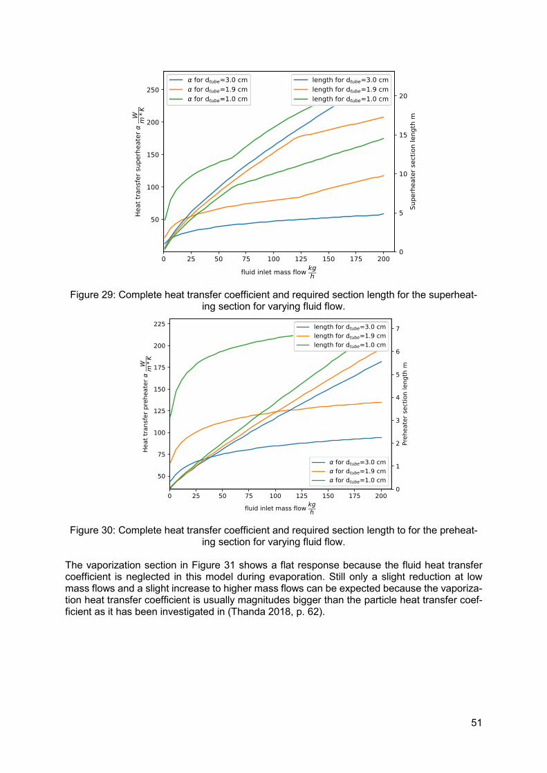
51

Figure 29: Complete heat transfer coefficient and required section length for the superheat-

ing section for varying fluid flow.

Figure 30: Complete heat transfer coefficient and required section length to for the preheat-

ing section for varying fluid flow. The vaporization section in Figure 31 shows a flat response because the fluid heat transfer coefficient is neglected in this model during evaporation. Still only a slight reduction at low mass flows and a slight increase to higher mass flows can be expected because the vaporiza-tion heat transfer coefficient is usually magnitudes bigger than the particle heat transfer coef-ficient as it has been investigated in (Thanda 2018, p. 62).

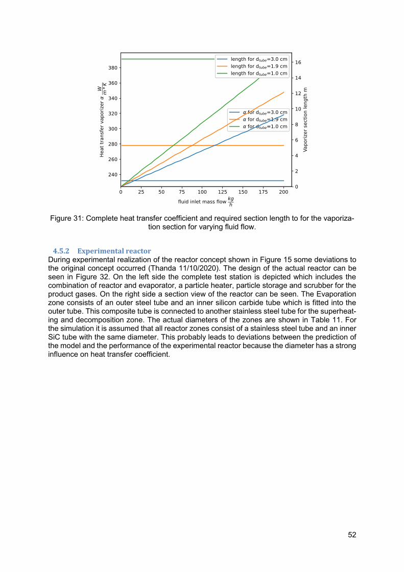
52

Figure 31: Complete heat transfer coefficient and required section length to for the vaporiza-

tion section for varying fluid flow.

4.5.2 Experimental reactor During experimental realization of the reactor concept shown in Figure 15 some deviations to the original concept occurred (Thanda 11/10/2020). The design of the actual reactor can be seen in Figure 32. On the left side the complete test station is depicted which includes the combination of reactor and evaporator, a particle heater, particle storage and scrubber for the product gases. On the right side a section view of the reactor can be seen. The Evaporation zone consists of an outer steel tube and an inner silicon carbide tube which is fitted into the outer tube. This composite tube is connected to another stainless steel tube for the superheat-ing and decomposition zone. The actual diameters of the zones are shown in Table 11. For the simulation it is assumed that all reactor zones consist of a stainless steel tube and an inner SiC tube with the same diameter. This probably leads to deviations between the prediction of the model and the performance of the experimental reactor because the diameter has a strong influence on heat transfer coefficient.

53

Figure 32: Depiction of the indirect heated experimental combined H2SO4 evaporator and SO3

decomposition reactor.

Table 11: Dimension of experimental H2SO4 evaporator and SO3 decomposition reactor (Thanda 11/10/2020).

Preheating and evaporation Superheating and decomposition

Zones Inner di-ameter

Outer di-ameter

Tube thickness

Inner di-ameter

Outer di-ameter

Tube thick-ness

Stainless steel tube

32 mm 28 mm 2 mm 32 mm 26 mm 3 mm

SiC Tube 18 mm 26 mm 4 mm - - -

5 Process simulation and optimization This chapter describes the simulation, evaluation and optimization of the solid sulphur cycle. The simulation is conducted using an Aspen Plus simulation. Main results of interest of the simulation are the energetic process efficiencies, stream mass flows and other process varia-bles which are required to evaluate the process economics according to section 2.3. The sim-ulation and evaluation are the basis for a numerical techno-economic optimization. Objective function of the optimization is the net present worth WNP of the complete process for four design variables which are presented in the first section of this chapter. The techno-economic optimi-zation is conducted using the programming language Python which interacts with the Aspen Plus simulation via ActiveX automation. Python is also used to conduct additional automation procedures. Basics for the procedures are explained in section 2.2 and more specifics are presented later in this chapter. Furthermore, the reactor model presented in chapter 4 is inte-grated into the simulation of the complete process. In particular the reactor size determined by the number of reactor tubes, the spent sulphuric acid mass flow, particle mass flow and reactor temperature will be investigated as design var-iables. Changes in design variables have highly interlinked direct and indirect influences on the process variables and the WNP which are discussed in this chapter. Emphasis of the

SO2

O2

SO3

H2O

54

modelling effort lays on the H2SO4 evaporator and SO3 decomposition reactor of the process. It is the main endothermic process step of the solid sulphur cycle.

5.1 Concept of the solid sulphur cycle This section first presents the top layer of the solid sulphur cycle simulation model, explains optimization objective and then describes simulation approach.

5.1.1 Presentation of the solid sulphur cycle and its performance indicators Figure 33 shows the top hierarchy of the model of the solid sulphur cycle which is integrated into an automatic economic evaluation, and techno-economic optimization. Hierarchies of the process sections are depicted in the center of Figure 33. The concentrated solar thermal en-ergy system (CSTES) provides the thermal energy for solar site of the solid sulphur cycle. Particles are used as a heat transfer medium to supply thermal energy to the H2SO4 splitting

reactor in the decomposition section (SO3SCALE). It contains the H2SO4 splitting reactor model from chapter 4 which converts H2SO4 to SO2. The product gases are used to provide

thermal power to sulphuric acid concentration section (ACICONC). In the SO2 separation sec-tion (SO2SEPA) the O2 is separated from the SO2, H2SO4 and H2O. Latter ones are transferred to the disproportionation section (DISPROP) where SO2 and H2O are converted to S and H2SO4. Sulphur is separated from the diluted sulphuric acid and transported to the sulphuric acid pro-duction plant. There sulphur is converted to sulphuric acid which is sold to the titan dioxide production again. Heat released during the production of sulphuric acid is used to produce electricity in the non-solar site. Spent sulphuric acid from the titan dioxide production is trans-ported to the solar site and concentrated with the diluted sulphuric acid from the disproportion-ation section.

55

Figure 33: Depiction of the simulation, economic evaluation and techno-economic optimiza-

tion of the solid sulphur cycle. The performance of the process can be measured from an energetic and an economic point of view. Process economics can be measured by the net present worth of the process. Whereas the energetic evaluation can be conducted using thermal efficiencies. Net present worth is the difference between the investment cost and all futures cash flows during the project time which are corrected for inflation. The detailed calculation procedure is presented in section 2.3.1. More details to the assumptions made and boundary conditions chosen for the net present wort calculation are presented in section 5.1.3.

Table 12 shows the energetic efficiencies and ratios in dependence for two different energy inputs. Solar as an energetic input means the total incoming solar radiation and thermal pro-cess power is the thermal energy that is available to the process at the decomposition. Energy stored in the sulphur depends on the amount of heat that is utilized from the conversion of sulphur to sulphuric acid. There are three different exothermic steps in the conversion from sulphur to sulphuric acid which are shown in eq. 5.1, eq. 5.2 (Holleman et al. 1985, p. 498) and eq. 5.3 (Holleman et al. 1985, p. 507). Heat from the reaction enthalpy in eq. 5.3 cannot be recuperated in all sulphuric acid production plant designs. Therefore, two efficiencies are calculated. ηsolar,S,cont and ηthermal,S,cont assume that heat from eq. 5.3 is not recuperated.

ηsolar,S,abs and ηthermal,S,abs assumes that heat from eq. 5.3 is recuperated.

S + O2 → SO2 ΔH= 297.0

𝑘𝐽

𝑚𝑜𝑙 eq. 5.1

Economic evaluation

Optimization

CSTES Heat transfer

model

Sulphuric acid

productionTitan dioxide

production

Concentrated

sulphuric acid

Cold

particles

Sulphur

Hot

particles

Spent

sulphuric acidSolar site

Non-solar

site

56

2SO2 +O2 → SO3 ΔH= 99.0 𝑘𝐽

𝑚𝑜𝑙 eq. 5.2

SO3 +H2O → 2H2SO4 ΔH= 176.6.0 𝑘𝐽

𝑚𝑜𝑙 eq. 5.3

Rsolar,H2SO4,spent and Rthermal,H2SO4,spent are ratios which show how much sulphuric acid can

be treated per amount of energy input. ηsolar,electricity and ηthermal,electricity are the efficiencies

for electrical energy produced in the sulphuric acid production for their respective energy input.

Table 12: Introduction of process efficiencies and ratios.

Energy input location

Sulphur contact Sulphur ab-sorption

Spent sulphuric

acid 𝑘𝑔

𝑀𝐽

Electricity

Solar

ηsolar,S,cont ηsolar,S,abs Rsolar,H2SO4,spent ηsolar,electricity

Thermal pro-cess power

ηthermal,S,cont ηthermal,S,abs Rthermal,H2SO4,spent ηthermal,electricity

5.1.2 Optimization potential of design variables The techno-economic optimization varies the design variable with the goal to maximize the net present worth WNP. Design variables investigated are the spent acid mass flow ��𝑠𝑝𝑒𝑛𝑡,𝑎𝑐𝑖𝑑 from

the titan dioxide production, the number of tubes 𝑛𝑡𝑢𝑏𝑒𝑠 of the H2SO4 splitting reactor, the par-ticle mass flow that is circulated between the CSTES and H2SO4 splitting reactor and particle

inlet temperature to the H2SO4 splitting reactor. In the following the influences of the design variables towards the WNP are discussed. On the one hand increasing spent acid mass flow ��𝑠𝑝𝑒𝑛𝑡,𝑎𝑐𝑖𝑑 increases H2SO4 available for

splitting which increases the potential revenues of the process. On the other hand an increase in ��𝑠𝑝𝑒𝑛𝑡,𝑎𝑐𝑖𝑑 decreases the residence time in the reactor which decreases the conversion. The

decrease in conversion leads to a higher fluid mass flow ��𝑓𝑙𝑢𝑖𝑑,𝑟𝑒𝑎𝑐𝑡𝑜𝑟 in the H2SO4 splitting

reactor. An increase in number of tubes 𝑛𝑡𝑢𝑏𝑒𝑠 increases the investment costs but also increases the conversion reached in decomposition of SO3. An increased conversion leads to a higher amount of thermal energy converted to solid sulphur which increases the process efficiencies like ηsolar,S and ηthermal,electricity. The optimization will yield a compromise between the in-

creased investment costs of a big reactor and increased annual cash flow due to the increased conversion. The optimum of the reactor design depends on specific reactor size costs. A lower size specific-reactor cost will shift the optimum to a bigger reactor and vice versa. The particle mass flow ��𝑝𝑎𝑟𝑡𝑖𝑐𝑙𝑒 needs to be adjusted to account for the varying demand in

thermal energy with varying fluid mass flow ��𝑓𝑙𝑢𝑖𝑑,𝑟𝑒𝑎𝑐𝑡𝑜𝑟 in the H2SO4 splitting reactor and

varying conversions reached. The particle temperature has conflicting effects on the net pre-sent worth. An increase in 𝑇𝑝𝑎𝑟𝑡𝑖𝑐𝑙𝑒,𝑖𝑛 leads to higher thermal losses in the thermal receiver,

and thus higher investment cost for the heliostat field to supply a sufficient amount of thermal energy. An increase in 𝑇𝑝𝑎𝑟𝑡𝑖𝑐𝑙𝑒,𝑖𝑛 reduces the storage size because the mass specific thermal

energy stored in the particles is increased. It is also favourable for the SO3 decomposition because the reaction is endothermic. This causes the reaction equilibrium to shift to the side of the products and to increase the reaction rate which increases the conversion reached.

57

5.1.3 Calculation of the net present worth This section introduces assumptions made and boundary conditions chosen for the calculation of the net present worth of the solid sulphur cycle. To calculate the net present worth of the process the annual cash flow and the investment costs of the process are required. Calculation of the investment cost is conducted according to the method presented in section 2.3. Which individual equations were used for the calculations of individual equipment is presented in the section 5.2 of this chapter. To calculate the annual cashflow stream specific prices and reve-nues are required which are summarized in Table 13. The simulation has been conducted assuming a best-case scenario with the highest revenues and lowest cost of the range pre-sented here and in the economic section 2.3.

Table 13: Flow specific costs for annual cash flow calculations.

Stream specific revenues and prices

Diluted sul-phuric acid treatment revenue

Concentrated sulphuric

acid revenue

Diluted sul-phuric acid

transportation costs by ship

Sulphur trans-portation cost

by ship

Electricity cost

Electricity revenue

50 €

𝑡 60 - 80

€

𝑡 39.78 - 46.41

€

𝑡 26.52 - 30.94

€

𝑡 0.0354 -

0.1326 €

𝑘𝑊ℎ

0.067 €

𝑘𝑊ℎ

Stream specific prices were obtained from industry experts which are involved in sulphuric acid recycling. The diluted sulphuric acid stream revenue of 50 €/t is paid for the stream connecting the titan dioxide production and acid concentration. It was obtained from an industry expert in the titan dioxide production industry. Additionally, costs need to be considered for the trans-portation of sulphur and sulphuric acid by ship between the solar site and non-solar site of the process. Sulphur transportation costs via ship range from 30 - 35 $/t (Argus Sulphur 2020) for various different routes such as Middle East – EC India or Baltic – Brazil. The price of sulphuric acid transportation is assumed to be 1.5 times higher (Kürten 11/6/2020). The transport cost for sulphur and sulphuric acid are simply added to the cost of manufacturing because it is an expense which is not considered in the cost estimation method. As electricity revenue 0.0670 €/kWh has been assumed based on the average production cost including a margin for the producer and retail in 2018 for private household contracts (Bundesnetzagentur und Bundeskartellamt 2018). Electricity prices for industrial customers range from 0.04 - 0.15 $/kWh (DACE price booklet 2020, p. 175). Further economic findings were made which are not used in the simulation but might be inter-esting for further research in sulphuric acid recycling and handling. For sulphuric acid with organic impurities an average treatment price of about 120 €/t can be assumed (Kürten 10/31/2020). Spent sulphuric acid is not publicly available on the market. Due to individual contracts and variations in spent sulphuric acid compositions a wide range of treatment prices between 0 €/t - 500 €/t are possible. Furthermore, prices for transportation of sulphuric acid in a train are 40 €/t. On the trains sulphuric acid is transported in tanks which contain 50 - 60 tonnes of sulphuric acid. Transportation cost depends strongly on the initiation of the transport rather than on the actual distance transported. A possible transportation distance ranges from an imaginary middle point in Germany to the border of Germany. (Kürten 9/1/2020) Cost of operating labour is 𝐶𝑂𝐿 is estimated according to section 2.3.2 which requires the num-

ber of fluid process steps and particle process steps 𝑛particle. The fluid steps are presented in

Table 14. The number of particulate steps in eq. 2.9 is assumed to be zero even though parti-cles are handled in the process. This assumption has been made it is expected that the pro-cess can be highly automated. Whereas the equation predicts a high required workforce for

58

particle handling. This estimation results in 3 simultaneous operators and 14 in total for 24-hour operation over a complete year.

Table 14: Number of fluid process steps for operator number estimation.

𝑛heat exchanger 𝑛reactor 𝑛collumn 𝑛compressor 𝑛𝑡𝑜𝑡𝑎𝑙,𝑓𝑙𝑢𝑖𝑑

5 4 1 1 10

5.1.4 Titan dioxide production The titan dioxide production is treated as external process and is not modelled in this thesis. It is assumed that the spent sulphuric acid contains only 22 wt% H2SO4 and 78 wt% H2O which are typical values for spent acid from titan dioxide production (Müller 2012b, p. 187). Other impurities are neglected. Spent sulphuric acid of the TiO2 dioxide production contains about 4.5 % FeSO4, 5.4 % of other metal sulphate salts and 22 wt% H2SO4 (Müller 2012b, p. 187). In the conventional recycling

process it is separated by concentrating the spent acid mixture to a concentration of H2SO4 70 wt% at which the minimum salt solubility is reached. (Müller 2012b, p. 188) The acid is subsequently cooled, minerals are crystalized and subsequently filtered from the stream re-sulting in a nearly salt-free sulphuric acid (Federal Environmental Agency 2001, p. 7). Even though the impurities are not modelled the acid concentration to 70 wt% is included. This is the main energy demanding step in the concentration.

5.2 Sections of the process This section explains how the complete simulation, economic evaluation and techno-economic optimization are implemented. Thereupon, detailed modelling assumptions of the individual sections are presented.

5.2.1 Implementation of the simulation Figure 33 shows which part of the solid sulphur cycle is modelled using Aspen Plus and which is modelled using Python modules. Sections labelled with a Python symbol are modelled in a Python module. Most other Aspen Plus symbols represent Aspen Plus hierarchies. The 4 As-pen Plus hierarchies are the decomposition (SO3SCALE), SO2 separation (SO2SEPA), dis-proportionation (DISPROP) and acid concentration blocks (ACICONC). The optimized design variables of the process are the spent acid mass flow ��𝑠𝑝𝑒𝑛𝑡,𝑎𝑐𝑖𝑑 (SPENDACI), the particle

mass flow ��𝑝𝑎𝑟𝑡𝑖𝑐𝑙𝑒 (hot particles and cold particles), the particle inlet temperature 𝑇𝑝𝑎𝑟𝑡𝑖𝑐𝑙𝑒,𝑖𝑛

(hot particles), and the number of tubes 𝑛𝑡𝑢𝑏𝑒𝑠 in the H2SO4 splitting reactor (SO3SCALE). Titan dioxide production is treated as an external process which is not simulated either. It is assumed that an arbitrary amount of spent acid can be provided. It is also assumed that an arbitrary amount of concentrated sulphuric acid can be sold to the titan dioxide production. Economic evaluation and techno-economic optimization are conducted using Python which communicates via ActiveX with the Aspen Plus simulation. Furthermore, the heat transfer model and the H2SO4 splitting reactor are solved iteratively via ActiveX. Also, two design specs are solved simultaneously while the heat transfer model is solved. The design specs which are introduced in 2.2 are discussed in more detail the following sections.

5.2.2 Concentrated solar thermal energy system (CSTES) This section describes the simulation approach for CSTES. The main variables of interest are thermal power provided, the particle mass flow, the hot particle temperature which is available to the process and the cost of the system. The thermal power provided is assumed to be constant which is discussed more detail later. The particle mass flow and the particle

59

temperature are varied directly in Aspen Plus and the corresponding system costs are evalu-ated in Python modules after a simulation run. The system modelled consists of the following equipment:

• Heliostat field

• Solar tower

• Particle receiver

• Particle transport system

• Particle storage

It is assumed that the CentRec® cannot be scaled continuously without considerable effort. Thus, a predesigned CentRec® with 40 MW and 20 MW thermal output are chosen for two different investigations. Other components of the CSTES and the available thermal process power are calculated from this design point. It is assumed that the CSTES are located In Ouarzazate, Morocco. This is important because the available radiation strongly influences the system size and performance. It can be charac-terized using the direct normal irradiation (DNI) (Buck and Schwarzbözl 2018, p. 693). Values

have been obtained for the coordinates 30.93ｰN -6.90ｰE 1140mNN from Meteonorm 6.1

maps. CentRec® size and cost The cost of CentRec® can be calculated according to eq. 5.4. Dcyl is the diameter of the cylin-

drical chamber of the CentRec®, Dap is the diameter of the aperture of the system Lcyl is the

length of the cylinder in the system. (Frantz et al., p. 57) The cost include 20 % transport and installation costs, 10 % manufacturing costs and 30 % profit for the supplier of the CentRec® (Frantz et al., p. 57). Thus, the results of eq. 5.4 can be considered as bare module cost.

𝐶𝑟 =∗ {932503 ∗ (Dcyl + 0.2

5.5)2

∗Lcyl

7.9+ 1000 ∗ 𝜋 ∗ ((Dcyl + 0.2)

2− Dap

2 )}

∗ (1 + 0.2 + 0.1) ∗ (1 + 0.3)

eq. 5.4

For a design of 40 MW CentRec® an aperture surface of 30 𝑚2 has been proposed using internal information from DLR (Giuliano, Frantz 2017). To calculate a suitable Dcyl, Lcyl and

Dap the results from an optimization for the levelized cost of heat from Pegasus project have

been used. The optimization for levelized cost of heat has been conducted for a 20 MW Cen-

tRec®. Best results were obtained for Dap = 3.17 𝑚, Dcyl

Dap = 1.3 and

Lcyl

Dap = 3.25 (Frantz et al.,

p. 59). The ratios from the optimization and the aperture surface provided are used to deter-mine the size of the 40 MW CentRec® which is shown in Table 15.

Table 15: CentRec® dimension for 40 MW thermal rating.

Variable name Dap 𝑚 Dcyl 𝑚 Lcyl 𝑚

Value 6.180

8.035

20.086

Required incoming solar radiation and available process energy The absorbed thermal power of the CentRec® 𝑃𝑟,𝑎𝑏𝑠 is used to calculate the required incoming

solar radiation to the complete heliostat field 𝑃𝑠𝑜𝑙𝑎𝑟 which is required to calculate required he-liostat field size. In a first step the incoming radiation to the CentRec® 𝑃𝑟,𝑖𝑛𝑡 is calculated ac-

cording to eq. 5.5 which is derived from eq. 5.6 (Buck and Giuliano 2019, p. 5). It already considers the thermal losses in the CentRec®. The corresponding parameters and variables

60

are shown in Table 16. 𝑃𝑟,𝑖𝑛𝑡 is the incoming power to the receiver and 𝑃𝑟,𝑎𝑏𝑠 is the absorbed

thermal power.

𝑃𝑟,𝑖𝑛𝑡 =𝑃𝑟,𝑎𝑏𝑠 + Ɛ ∗ δ ∗ 𝐴𝑎𝑝 ∗ 𝑇𝑟,𝑒𝑥

4 + ℎ ∗ 𝐴𝑎𝑝 ∗ (𝑇𝑟,𝑒𝑥 − 𝑇𝑎𝑚𝑏)

𝛼

eq. 5.5

𝑃𝑟,𝑎𝑏𝑠 = 𝛼 ∗ 𝑃𝑟,𝑖𝑛𝑡 − Ɛ ∗ δ ∗ 𝐴𝑎𝑝𝑇𝑟,𝑒𝑥4 − ℎ ∗ 𝐴𝑎𝑝(𝑇𝑟,𝑒𝑥 − 𝑇𝑎𝑚𝑏) eq. 5.6

Table 16: Parameters for equation eq. 5.6 and eq. 5.5.

Effective solar ab-sorptivity

Effective thermal

emissivity

Stefan–Boltzmann constant

Convective heat loss coefficient

Aperture surface

Receiver exit temperature

Ambient tempera-

ture

𝛼 Ɛ δ ℎ 𝐴𝑎𝑝 𝑇𝑟,𝑒𝑥 𝑇𝑎𝑚𝑏

0.95 0.9 5.670374419*

10−8 𝑊

𝑚2𝐾4

30 𝑊

𝑚2𝑘 𝑚2 𝐾 300 K

In a second step the solar radiation losses in the heliostat field are considered from eq. 5.7 which is derived from eq. 2.1. In this thesis heliostat field efficiency ηfield = 56.93 % is used for both the 20 MW design and the 40 MW design. The value was determined in a previously conducted techno-economic evaluation which employed a 40 MW CentRec®. (Rosenstiel 2018, p. 78)

𝑃𝑠𝑜𝑙𝑎𝑟 = 𝐴𝑓𝑖𝑒𝑙𝑑 ∗ 𝐷𝑁𝐼 = 𝜂𝑓𝑖𝑒𝑙𝑑 ∗ 𝑃𝑟,𝑖𝑛𝑡 eq. 5.7

To calculate the thermal energy that is continuously available to the process 𝑃𝑝𝑟𝑜𝑐𝑒𝑠𝑠. DNI val-

ues have with an hourly resolution for Ouarzazate, Morocco from Meteonorm 6.1 maps have been analysed. The average DNI during sun hours over the complete year has been calculated by summarising all DNI values and dividing them by the number of hours with non-zero radia-

tion which results in a value of DNI = 638.6786 𝑊

𝑚2. Furthermore, the average time per day with

non-zero radiation has been calculated to be ℎ𝑟𝑎𝑑𝑖𝑎𝑡𝑖𝑜𝑛 = 10.7975 ℎ hours of sun per day on average over the complete year. The process energy which will be continuously available for the process per hour 𝐸𝑝𝑟𝑜𝑐𝑒𝑠𝑠 MWh is calculated according to eq. 5.9

𝑃𝑝𝑟𝑜𝑐𝑒𝑠𝑠 = 𝑃𝑑𝑒𝑠𝑖𝑔𝑛,40𝑀𝑊

𝑀𝑊 ∗ℎ𝑟𝑎𝑑𝑖𝑎𝑡𝑖𝑜𝑛

ℎ24ℎ

= 17.996 𝑀𝑊

eq. 5.8

𝑃𝑝𝑟𝑜𝑐𝑒𝑠𝑠 =

𝑃𝑑𝑒𝑠𝑖𝑔𝑛,20𝑀𝑊𝑀𝑊 ∗

ℎ𝑟𝑎𝑑𝑖𝑎𝑡𝑖𝑜𝑛ℎ

24ℎ

= 8.998 𝑀𝑊

eq. 5.9

Heliostat Field The required heliostat field surface can be calculated using the required incoming radiation to the CentRec® from eq. 5.10.

𝐴𝑓𝑖𝑒𝑙𝑑 =𝑃𝑟,𝑖𝑛𝑡

𝐷𝑁𝐼 ∗ η𝑓𝑖𝑒𝑙𝑑

eq. 5.10

The cost of the heliostat field is calculated according to eq. 5.11 (Frantz et al., p. 58).

61

𝐶𝑓𝑖𝑒𝑙𝑑 = 𝐴𝑓 ∗ 𝐶𝑠,𝑝𝑓

eq. 5.11

𝐶𝑠,𝑝𝑓 is the surface specific cost of an installed heliostat field and assumed to be 100 €/𝑚2

(Buck and Giuliano 2019). Solar Tower The cost of the solar tower Ct is mainly determined by its height. A tower height from Ht =120 𝑚 for a 40 MW CentRec® design from a previous techno-economic study is used in this thesis (Rosenstiel 2018, p. 78). For a 20 MW design a tower height of 71.4 m is assumed from an optimisation levelized cost of thermal energy of a 20 MW system (Frantz et al., p. 59). 𝐶𝑡 is calculated according to eq. 5.12 (Frantz et al., p. 58).

𝐶𝑡 = 161.7565 ∗ 𝐻𝑡1.9274 eq. 5.12

Storage System The main design variable of the storage is the maximum required energy to be stored 𝑒𝑠𝑡. It is determined by the process power demand 𝑃𝑝𝑟𝑜𝑐𝑒𝑠𝑠 and the required hours of full load operation

from storage ℎ𝑟𝑒𝑞. ℎ𝑟𝑒𝑞 is calculated from the hours with no radiation per day and is rounded

up to 14 hours. The required energy storage capacity is calculated from thermal power that is continuously provided to the process 𝑃𝑝𝑟𝑜𝑐𝑒𝑠𝑠 according to eq. 5.13.

𝑒𝑠𝑡 =𝑃𝑝𝑟𝑜𝑐𝑒𝑠𝑠

𝑀𝑊∗ℎ𝑟𝑒𝑞

ℎ

eq. 5.13

The cost of the particle storage system is determined by the cost of particles and the cost of the storage containments. Particle costs are calculated according to equation eq. 5.14 (Frantz et al., p. 55). 𝑚𝑝𝑎𝑡𝑖𝑐𝑙𝑒 is multiplied by the factor 1.1 to account for additional required particles

in transport systems. 𝑐𝑠𝑝,𝑝𝑎𝑟𝑡 is the mass specific particle price and assumed to cost 1 €/kg

(Buck and Giuliano 2019, p. 3).

𝑐𝑝𝑎𝑟𝑡 = 1.1 ∗ 𝑚𝑝𝑎𝑡𝑖𝑐𝑙𝑒 ∗ 𝑐𝑠𝑝,𝑝𝑎𝑟𝑡

eq. 5.14

The required particle mass is calculated from the required energy according to eq. 5.15 (Frantz et al., p. 55). The equation is solved using the integrate function from the Python Scipy library (Virtanen et al. 2020).

𝑚𝑠𝑡 =𝑒𝑠𝑡

∫ 𝑐𝑝𝑎𝑟𝑡𝑖𝑐𝑙𝑒𝑑𝑇𝑇𝑟,𝑒𝑥𝑇𝑟,𝑖𝑛

eq. 5.15

The storage system consists of a particle tank for the hot and cold particles each. The cost of the particle containments Cstc is determined by the surface of the respective containment and the particle temperature in the containment which influences the insulation cost. It can be cal-culated according to eq. 5.16 (Frantz et al., p. 56).

Cstc = Astc ∗ Ca,sp,is(Tr,ex) + Astc ∗ Ca,sp,is(Tr,in)

eq. 5.16

Ca,sp,is is the area specific surface cost of the containment which is calculated according to eq.

2.17. fins is the insulation cost share and is assumed to be 0.3. Storage temperature 𝑇𝑠𝑡 has the unit °C. (Frantz et al., p. 55)

𝐶𝑎,𝑠𝑝,𝑖𝑠 = 1000 ∗ (1 + 𝑓𝑖𝑛𝑠 ∗ 𝑇𝑠𝑡 − 600

400)

eq. 5.17

62

The required containment surface 𝐴𝑠𝑡𝑐 is calculated from the cylinder diameter 𝑑𝑐𝑦𝑙𝑖𝑛𝑑𝑒𝑟 of the

containment according to eq. 5.18. The cylinder height has been assumed to be 2 ∗ 𝑑𝑐𝑦𝑙𝑖𝑛𝑑𝑒𝑟 =

ℎ𝑐𝑦𝑙𝑖𝑛𝑑𝑒𝑟 because the cost equation was derived using this ratio (Frantz et al., p. 55). eq. 5.18

is derived from the equation of the surface of a shown eq. 5.19.

𝐴𝑐𝑦𝑙𝑖𝑛𝑑𝑒𝑟 = 2 ∗ (𝜋 ∗𝑑𝑐𝑦𝑙𝑖𝑛𝑑𝑒𝑟2

4) + 𝜋 ∗ 𝑑𝑐𝑦𝑙𝑖𝑛𝑑𝑒𝑟

2 ∗ 2 = 𝜋 ∗ 𝑑𝑐𝑦𝑙𝑖𝑛𝑑𝑒𝑟2 ∗ 2.5

eq. 5.18

𝐴𝑐𝑦𝑙𝑖𝑛𝑑𝑒𝑟 = 2 ∗ (𝜋 ∗𝑑𝑐𝑦𝑙𝑖𝑛𝑑𝑒𝑟2

4) + 𝜋 ∗ 𝑑𝑐𝑦𝑙𝑖𝑛𝑑𝑒𝑟 ∗ ℎ𝑐𝑦𝑙𝑖𝑛𝑑𝑒𝑟

eq. 5.19

The required diameter dcylinder is calculated from the required particle mass according to eq.

5.20. Previous equation is derived from the volume balance of the cylindrical containment and the particles shown in eq. 5.21. The bulk particle density 𝜌𝑝𝑎𝑟𝑡𝑖𝑐𝑙𝑒,𝑏𝑢𝑙𝑘 is used to corelated the

cylinder Volume 𝑉𝑐𝑦𝑙𝑖𝑛𝑑𝑒𝑟 to the particle mass 𝑚𝑝𝑎𝑟𝑡𝑖𝑐𝑙𝑒 stored in the in the cylinder.

𝑑𝑐𝑦𝑙𝑖𝑛𝑑𝑒𝑟 = √𝑉𝑐𝑦𝑙𝑖𝑛𝑑𝑒𝑟 ∗ 2

𝜋

3

= √𝑚𝑝𝑎𝑟𝑡𝑖𝑐𝑙𝑒 ∗ 2

𝜋𝜌𝑝𝑎𝑟𝑡𝑖𝑐𝑙𝑒,𝑏𝑢𝑙𝑘

3

eq. 5.20

𝑉𝑐𝑦𝑙𝑖𝑛𝑑𝑒𝑟 = 𝜋 ∗𝑑𝑐𝑦𝑙𝑖𝑛𝑑𝑒𝑟2

4∗ ℎ𝑐𝑦𝑙𝑖𝑛𝑑𝑒𝑟 = 𝜋 ∗

𝑑𝑐𝑦𝑙𝑖𝑛𝑑𝑒𝑟2

4∗ 2 ∗ 𝑑𝑐𝑦𝑙𝑖𝑛𝑑𝑒𝑟 =

𝜋∗𝑑𝑐𝑦𝑙𝑖𝑛𝑑𝑒𝑟3

2

eq. 5.21

Vertical Transport System The cost of the vertical transport system is calculated according to eq. 5.22 (Frantz et al., p. 58). The corresponding parameters are given in Table 17.

𝑐𝑡𝑟 = 425000 {1 + 𝑘𝑇 (𝑇𝑙 − 𝑇𝑙,0𝑇𝑙,0

)} ∗ {1 + 𝑘𝑚 (�� − ��0

��0)} ∗ {1 + 𝑘𝐻 (

𝐻𝑙 −𝐻𝑙,𝑜𝐻𝑙,𝑜

)}

eq. 5.22

Table 17: Parameters for cost calculation of vertical transport system

Variable name

Temperature scaling fac-tor

Mass flow scaling factor

Lift height scaling factor

Reference design tem-perature

Reference design mass flow

Reference design height

symbol 𝑘𝑇 𝑘𝑚 𝑘ℎ 𝑇𝑙,0 ��0 𝐻𝑙,𝑜

Value 0.1 0.5 0.2 600 °C 997 kg/s 70 m

Source (Frantz et al., p. 58)

(Frantz et al., p. 58)

(Frantz et al., p. 58)

(Repole and Jeter, p. 2)

(Repole and Jeter, p. 5)

(Repole and Jeter, p. 2)

The reference design parameters were not clearly stated in the final report and thus were extracted from cited paper. It remains unclear if the receiver (138 m) or lift height (70 m) was considered as reference design height (Repole and Jeter, p. 2). In this thesis it is assumed to be 70 m. The power provided by the CSTES to the process 𝑃𝑝𝑟𝑜𝑐𝑒𝑠𝑠,𝑚𝑎𝑥 is integrated into the simulation

as a constraint according to eq. 5.23. 𝑃𝑝𝑟𝑜𝑐𝑒𝑠𝑠,𝑚𝑎𝑥 is compared to the actual power transferred

to the process from the particles 𝑃𝑝𝑟𝑜𝑐𝑒𝑠𝑠,𝑢𝑠𝑒𝑑. 𝑃𝑝𝑟𝑜𝑐𝑒𝑠𝑠,𝑢𝑠𝑒𝑑 is calculated from the simulation

results by subtraction of energy flow of the 𝑃𝑝𝑎𝑟𝑡𝑖𝑐𝑙𝑒𝑠,𝑖𝑛𝑙𝑒𝑡 at the reactor inlet and energy flow of

the particles at the reactor outlet 𝑃𝑝𝑎𝑟𝑡𝑖𝑐𝑙𝑒,𝑜𝑢𝑡𝑙𝑒𝑡.

g(x) ≤ 𝑃𝑝𝑟𝑜𝑐𝑒𝑠𝑠,𝑚𝑎𝑥 − 𝑃𝑝𝑟𝑜𝑐𝑒𝑠𝑠,𝑢𝑠𝑒𝑑

eq. 5.23

63

Furthermore, the maximum particle temperature that the CentRec® can provide is also imple-mented using the constraint eq. 5.24. The actual particle temperature at the inlet is a result of the simulation and cannot be directly provided as an input which is further elaborated in the following section 5.2.3.

g(x) ≤ 𝑇𝑝𝑎𝑟𝑡𝑖𝑐𝑙𝑒,𝑖𝑛𝑙𝑒𝑡,𝑚𝑎𝑥 − 𝑇𝑝𝑎𝑟𝑡𝑖𝑐𝑙𝑒𝑠,𝑖𝑛𝑙𝑒𝑡

eq. 5.24

5.2.3 𝐇𝟐𝐒𝐎𝟒 splitting reactor This section describes the simulation approach of the H2SO4 evaporator and SO3 decomposer used in this the simulation of the simulation of the solar site of the solid sulphur cycle. There-fore, the hierarchy block presented in Figure 18 is coupled with Python according to the pro-cedure described in chapter 4. This block is then connected to the acid concentration and SO2 separation as it can be seen in Figure 33. Due to the integration into a recycling loop, additional dependencies occur between reactor variables and design variables. A decrease in conversion increases the fluid mass flow be-cause more educt is recycled. A decrease in conversion has conflicting dependencies for the energy requirement of the reactor. An increase in conversion requires more energy because the SO3 reaction is endothermic but the recycle mass flow decreases at the same time which decreases the energy requirement for stream heating. Thus, it depends on the start conversion if more or less energy is required to operate the reactor. Furthermore, the energy supply is subject to strong constraints which allows only a small win-dow of operability. Particle inlet temperature is limited to 1000°C which is the maximum state of the art particle outlet temperature that the CSTES can supply. Also, the particle outlet mass flow should have a maximum temperature of 200°C when leaving the H2SO4 splitting reactor to prevent damage at the Polytetrafluoroethylene (PTFE) tubes at the inlet. To reduce interdependence of the design concerning the constraints the variables are not op-timized directly. Instead particle mass flow to fluid mass flow ratio Rparticle,fluid is introduced. A

change in the fluid mass flow now increases the particle mass proportional and prevents that particle mass flow and fluid mass flow need to be changed alternately which causes conver-gence issues during the optimization. Furthermore, WHSV to Rparticle,fluid ratio

RWHSV,Rparticle,fluid is introduced to account for the change in energy requirement with changing

conversion. Evaluation of optimization results in which the direction of heat transfer is violated are pre-vented by inequality constraints according to eq. 5.25. This has the advantage that design parameter combinations which yield unphysical solutions can still be handled automatically. Using a HeatX block instead will yield simulation errors with a behaviour difficult to predict. If the constraint is violated heat exchange area calculation is skipped to prevent an infeasible solution attempt.

g(x) ≤ 𝑇ℎ𝑜𝑡 − 𝑇𝑐𝑜𝑙𝑑 − 𝑇𝑚𝑖𝑛𝑖𝑚𝑢𝑚 𝑎𝑝𝑝𝑟𝑜𝑎𝑐ℎ

eq. 5.25

Constraint in eq. 5.26 is used to prevent poisoning the catalyst according to section 4.3.3.

g(x) ≤ 𝑇𝑟𝑒𝑎𝑐𝑡𝑜𝑟,𝑚𝑖𝑛 − 𝑇𝑐𝑎𝑡𝑎𝑙𝑦𝑠𝑡,𝑚𝑖𝑛(𝑃𝑆𝑂3)

eq. 5.26

Constraint eq. 5.27 with 𝑇𝑝𝑎𝑟𝑡𝑖𝑐𝑙𝑒 𝐶𝑒𝑛𝑡𝑅𝑒𝑐 ,𝑚𝑎𝑥 = 1000 °C limits the maximum particle temperature

to the maximum temperature particle outlet temperature of the CentRec®.

64

g(x) ≤ 𝑇𝑝𝑎𝑟𝑡𝑖𝑐𝑙𝑒 𝐶𝑒𝑛𝑡𝑅𝑒𝑐 ,𝑚𝑎𝑥 − 𝑇𝑝𝑎𝑟𝑡𝑖𝑐𝑙𝑒 ,𝑟𝑒𝑎𝑡𝑜𝑟 𝑖𝑛𝑙𝑒𝑡

eq. 5.27

The maximum particle outlet temperature of the preheating section should not be higher than 𝑇𝑝𝑎𝑟𝑡𝑖𝑐𝑙𝑒 ,𝑒𝑣𝑎𝑝𝑜𝑟𝑎𝑡𝑜𝑟 𝑚𝑎𝑥 = 200°𝐶 to prevent damage at the inlet tubes. Such a solution is pre-

vented by the constraint in eq. 5.28.

g(x) ≤ 𝑇𝑝𝑎𝑟𝑡𝑖𝑐𝑙𝑒 ,𝑒𝑣𝑎𝑝𝑜𝑟𝑎𝑡𝑜𝑟 𝑚𝑎𝑥 − 𝑇𝑝𝑎𝑟𝑡𝑖𝑐𝑙𝑒,𝑒𝑣𝑎𝑝𝑜𝑟𝑎𝑡𝑜𝑟 𝑜𝑢𝑡 eq. 5.28

The size of the reactor and heating section is determined by the tube diameter 𝑑𝑡𝑢𝑏𝑒,𝑟𝑒𝑎𝑐𝑡𝑜𝑟, number of tubes 𝑛𝑡𝑢𝑏𝑒𝑠 and the length of the complete reactor section 𝑙𝑡𝑜𝑡𝑎𝑙. 𝑙𝑡𝑜𝑡𝑎𝑙 is determined

from the length of the single sections. The section of the reactor length 𝑙𝑟𝑒𝑎𝑐𝑡𝑜𝑟, number of tubes and inner tube diameter are supplied as design variables. The catalyst mass is calcu-lated from the decomposition section volume using the bulk density of the catalyst. The lengths of the other sections are calculated from the heat transfer coefficients of the respective section using the LMTD method described in section 4.2.1.

Table 18: Variables to determine investment cost calculation.

Variable name

Reactor length

Preheater length

Vapor-izer

length

Super-heater length

Number of reac-tor tubes

Tube di-ameter

Catalyst mass

Symbol lreactor lpreheater lvaporizer lsuperheater ntubes dtube,reactor mcatalyst

Variable type

design process process process design design process

Because the H2SO4 evaporation and decomposition section is a novel design there is no cost correlation available in literature. Thus, cost estimation of equipment with a similar shape is applied. According to (Woods 2007, p. 421) the cost of a nonadiabatic multitube fixed bed catalyst reactor can be estimated by calculating the cost of a fixed tube heat exchanger. Thus, a correlation for fixed tube heat exchanger is used which is valid for a heat exchange surface

from 10 𝑚2 to 1000 𝑚2. Parameters for eq. 2.17 are given in section 8.1. The cost of the reactor is estimated using the heat exchange surface 𝐴ℎ𝑥 which is calculated by eq. 5.29. The costs are calculated using the procedure presented in section 2.3. The corre-sponding parameters determined by the variables in Table 18.

Ahx = ntubes ∗ dtube,inner,reactor ∗ ltotal

eq. 5.29

No material factors for silicon carbide are available. Thus, material factors nickel alloys have been used because they are rather expensive and suitable for sulphuric acid to some extent (Turton 2012, p. 227). The catalyst cost are assumed to be 8.839 €/kg of true catalyst which is the highest value for silica or alumina doped catalysts. (Ulrich and Vasudevan 2003, p. 398)

5.2.4 𝐒𝐎𝟐 separation SO2 separation can be conducted using either a condensation process or an absorption pro-cess. In the condensation process the pressure of a SO2 containing stream is increased or the

temperature is lowered or a combination of both is applied. After condensation of SO2 the liquid phase can be removed from the remaining gas phase. In the absorption process SO2 is ab-

sorbed in a liquid such as water or alkaline solutions. In a second step SO2 is desorbed and a high purity SO2 gas is obtained (Müller 2012a, pp. 108–112). To model one of these processes suitable thermodynamic model is required to calculate the corresponding solubilities and heat requirements.

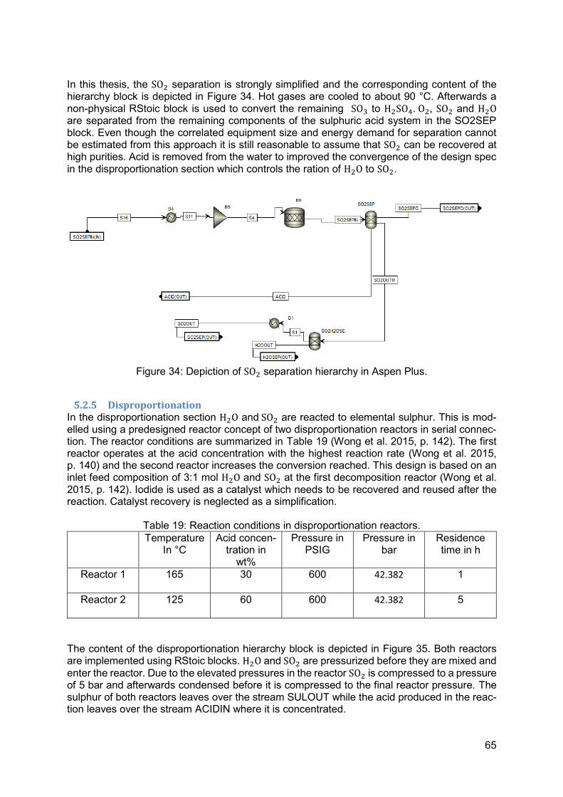
65

In this thesis, the SO2 separation is strongly simplified and the corresponding content of the hierarchy block is depicted in Figure 34. Hot gases are cooled to about 90 °C. Afterwards a non-physical RStoic block is used to convert the remaining SO3 to H2SO4. O2, SO2 and H2O are separated from the remaining components of the sulphuric acid system in the SO2SEP block. Even though the correlated equipment size and energy demand for separation cannot be estimated from this approach it is still reasonable to assume that SO2 can be recovered at high purities. Acid is removed from the water to improved the convergence of the design spec in the disproportionation section which controls the ration of H2O to SO2.

Figure 34: Depiction of SO2 separation hierarchy in Aspen Plus.

5.2.5 Disproportionation In the disproportionation section H2O and SO2 are reacted to elemental sulphur. This is mod-elled using a predesigned reactor concept of two disproportionation reactors in serial connec-tion. The reactor conditions are summarized in Table 19 (Wong et al. 2015, p. 142). The first reactor operates at the acid concentration with the highest reaction rate (Wong et al. 2015, p. 140) and the second reactor increases the conversion reached. This design is based on an inlet feed composition of 3:1 mol H2O and SO2 at the first decomposition reactor (Wong et al. 2015, p. 142). Iodide is used as a catalyst which needs to be recovered and reused after the reaction. Catalyst recovery is neglected as a simplification.

Table 19: Reaction conditions in disproportionation reactors.

Temperature In °C

Acid concen-tration in

wt%

Pressure in PSIG

Pressure in bar

Residence time in h

Reactor 1 165 30 600 42.382

1

Reactor 2 125 60 600 42.382

5

The content of the disproportionation hierarchy block is depicted in Figure 35. Both reactors are implemented using RStoic blocks. H2O and SO2 are pressurized before they are mixed and

enter the reactor. Due to the elevated pressures in the reactor SO2 is compressed to a pressure of 5 bar and afterwards condensed before it is compressed to the final reactor pressure. The sulphur of both reactors leaves over the stream SULOUT while the acid produced in the reac-tion leaves over the stream ACIDIN where it is concentrated.

66

To maintain the composition over varying conversions in the H2SO4 splitting reactor a Python

design spec has been implemented. It checks whether the H2O and SO2 ratio is bigger or smaller than 3. For ratios larger than 3 water is removed in the H2OSEPBL over the stream H2OOUT and the added water H2OADJIN is set to 0. If the ratio is smaller than three water is added in the H2OADJIN stream and no water is removed in H2OSEPBL. A Python design spec has been used because Aspen Plus design spec lacks the proper option implement con-ditions on the design spec. Thus, it is not possible to address different blocks or streams at different conditions. This is required when the water should be removed or added depending on the stream composition before the disproportionation reactor. Additional water required is available from the acid concentration hierarchy which is not connected to improve the conver-gence of the flowsheet.

Figure 35: Depiction of the disproportionation section hierarchy in the Aspen Plus simulation. Investment costs for the components were calculated using the procedure presented in section 2.3. Disproportionation reactors were estimated as jacketed agitated reactors using the reactor module factor. The compressor was estimated as a stainless steel rotary compressor and the pumps are assumed to be nickel alloy centrifugal pumps. Parameters for cost equation and bare module factors are presented in Appendix A.

5.2.6 𝐇𝟐𝐒𝐎𝟒 concentration This section simulates the concentration of H2SO4 to 70 wt% before it enters H2SO4 splitting reactor. A multi effect evaporation is modelled to reduce heat requirement of the separation process which is shown in Figure 36. The temperature is adjusted before each stage using the HeatX blocks. Pressure is reduced before each stage using the valves VALV1, VALV2 and VALV3. After the concentration the pressure is increased to the required pressure in the H2SO4 splitting reactor. The RStoic block is non-physical and only used to check the apparent sul-phuric acid concentration after the concentration stage.

67

Figure 36: Content of the actual 𝐻2𝑆𝑂4 concentration section.

During the optimization a simplified hierarchy block was used which is shown in Figure 37. It is based on a single flash which increases the heat requirement but allows to adjust the H2SO4 concentration over wider range of inlet acid concentrations using a single design spec. The design spec adjusts the vapour fraction in the flash and heater block so that acid outlet con-centration is maintained at 70 wt% for varying acid inlet concentrations.

Figure 37: Content of the 𝐻2𝑆𝑂4 concentration section during optimization.

Flash vessels are sized using eq. 5.30. V is the volume of the vessel, 𝐹𝐿 is the liquid outlet stream, ρ𝑙 is the liquid density and 𝜏 is the residence time. Residence time is assumed to be 5 minutes as suggested in the source. The equation is multiplied by two to account for extra space for the vapour. Cost of the flash vessel can be estimated as a pressure vessel (Biegler et al. 1997, p. 112). Cost for the pressure vessels were calculated according to section 2.3 assuming length to diameter ratio of 4 and a material factor for cladded titanium which is the most expensive cladding material provided. The pump has been assumed to be centrifugal pump that is made of a nickel alloy.

𝑉 = 2 ∗𝐹𝐿 ∗ 𝜏

ρ𝑙

eq. 5.30

𝑉 = 𝐿 ∗𝐷2

4∗ 𝜋 = 𝐷 ∗

𝐿

𝐷

𝐷2

4∗ 𝜋 = 𝐷3 ∗ 𝜋

eq. 5.31

For the heat transfer from hot decomposition gases a heat transfer coefficient of 40 𝐵𝑡𝑢

°𝐹∗𝑓𝑡2∗ℎ =

40 *5.6783 = 226.132 𝑊

𝑚2𝐾 has bee assumed which is the lowest value for an air to water heat

exchanger. As heat transfer value of 250 𝐵𝑡𝑢

°𝐹∗𝑓𝑡2∗ℎ = 250 *5.6783 = 1419.575

𝑊

𝑚2𝐾 has been used

which is the lowest value for condensing steam and water (Green and Perry 2007, pp. 11–25).

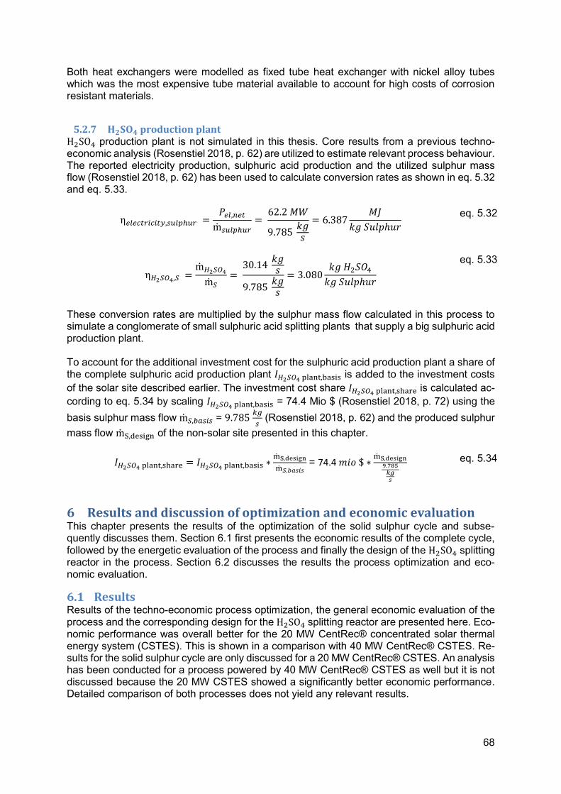
68

Both heat exchangers were modelled as fixed tube heat exchanger with nickel alloy tubes which was the most expensive tube material available to account for high costs of corrosion resistant materials.

5.2.7 𝐇𝟐𝐒𝐎𝟒 production plant H2SO4 production plant is not simulated in this thesis. Core results from a previous techno-economic analysis (Rosenstiel 2018, p. 62) are utilized to estimate relevant process behaviour. The reported electricity production, sulphuric acid production and the utilized sulphur mass flow (Rosenstiel 2018, p. 62) has been used to calculate conversion rates as shown in eq. 5.32 and eq. 5.33.

η𝑒𝑙𝑒𝑐𝑡𝑟𝑖𝑐𝑖𝑡𝑦,𝑠𝑢𝑙𝑝ℎ𝑢𝑟 =𝑃𝑒𝑙,𝑛𝑒𝑡m𝑠𝑢𝑙𝑝ℎ𝑢𝑟

= 62.2 𝑀𝑊

9.785 𝑘𝑔𝑠

= 6.387𝑀𝐽

𝑘𝑔 𝑆𝑢𝑙𝑝ℎ𝑢𝑟

eq. 5.32

η𝐻2𝑆𝑂4,𝑆 =m𝐻2𝑆𝑂4

m𝑆= 30.14

𝑘𝑔𝑠

9.785 𝑘𝑔𝑠

= 3.080𝑘𝑔 𝐻2𝑆𝑂4𝑘𝑔 𝑆𝑢𝑙𝑝ℎ𝑢𝑟

eq. 5.33

These conversion rates are multiplied by the sulphur mass flow calculated in this process to simulate a conglomerate of small sulphuric acid splitting plants that supply a big sulphuric acid production plant. To account for the additional investment cost for the sulphuric acid production plant a share of the complete sulphuric acid production plant 𝐼𝐻2𝑆𝑂4 plant,basis is added to the investment costs

of the solar site described earlier. The investment cost share 𝐼𝐻2𝑆𝑂4 plant,share is calculated ac-

cording to eq. 5.34 by scaling 𝐼𝐻2𝑆𝑂4 plant,basis = 74.4 Mio $ (Rosenstiel 2018, p. 72) using the

basis sulphur mass flow m𝑆,𝑏𝑎𝑠𝑖𝑠 = 9.785 𝑘𝑔

𝑠 (Rosenstiel 2018, p. 62) and the produced sulphur

mass flow mS,design of the non-solar site presented in this chapter.

𝐼𝐻2𝑆𝑂4 plant,share = 𝐼𝐻2𝑆𝑂4 plant,basis ∗mS,design

m𝑆,𝑏𝑎𝑠𝑖𝑠 = 74.4 𝑚𝑖𝑜 $ ∗

mS,design

9.785𝑘𝑔𝑠

eq. 5.34

6 Results and discussion of optimization and economic evaluation This chapter presents the results of the optimization of the solid sulphur cycle and subse-quently discusses them. Section 6.1 first presents the economic results of the complete cycle, followed by the energetic evaluation of the process and finally the design of the H2SO4 splitting reactor in the process. Section 6.2 discusses the results the process optimization and eco-nomic evaluation.

6.1 Results Results of the techno-economic process optimization, the general economic evaluation of the process and the corresponding design for the H2SO4 splitting reactor are presented here. Eco-nomic performance was overall better for the 20 MW CentRec® concentrated solar thermal energy system (CSTES). This is shown in a comparison with 40 MW CentRec® CSTES. Re-sults for the solid sulphur cycle are only discussed for a 20 MW CentRec® CSTES. An analysis has been conducted for a process powered by 40 MW CentRec® CSTES as well but it is not discussed because the 20 MW CSTES showed a significantly better economic performance. Detailed comparison of both processes does not yield any relevant results.

69

6.1.1 Economic and CSTES results Figure 38 shows the net present worth of the complete solid sulphur cycle. Additionally, it shows the grass root cost and annual cash flow which were used to calculate the net present worth. Lastly, the required annual cash flow for an economically feasible process is shown. It can be seen that the net present worth calculated for the process is -16.2228 million € and clearly negative. Due to the low annual cash flow and high investment costs the process is not economically feasible as presented. A net present worth of 0 would indicate an economically feasible process. WNP is equal to 0 when an annual cashflow of 2.099 million € is generated. Annual cashflow of the current process is 0.194 million €. A main costs factor is the transpor-tation of sulphuric acid and sulphur between the solar and non-solar site by ship. To be exact the transportation cost for the spent sulphuric acid is the main cost which can be seen in Figure 39. Without the transportation costs the net present worth would increase to 8.18 million €.

Figure 38: Net present worth, grass root costs and annual cash flow of the solid sulphur cycle

which is designed for the 20 MW CentRec®. Additionally, the required annual cash flow to reach a net present wort of 0 is shown.

In Figure 39 revenues, costs the annual cash flow of the process are itemised. It can be seen that a considerable revenue is generated but also high costs are associated. An interesting point is that the highest share of the revenue is created from the spent acid treatment. The process would be economically feasible if the electricity price would be increased to 0.281 €/kWh from the 0.067 €/kWh assumed. When the other prices are kept constant the spent acid revenue needs to be increased to 77.72 €/t from 50 €/t to yield an economically feasible pro-cess. Applying the same procedure to the concentrated acid price a concentrated sulphuric acid price increase from 80 €/t to 205.15 €/t would be required.

70

Figure 39: Itemized depiction of the annual cash flow of the solid sulphur cycle.

The highest investment costs are associated with CSTES which can be seen in Figure 40. The cost of the H2SO4 splitting reactor and the share for the sulphuric acid production plant are approximately the same. Still each costs approximately 10% of the total investment cost com-pared to about 70% for the CSTES. The major share of the cost of the CSTES is associated with the heliostat field which can be seen in Figure 41.

71

Figure 40: Investment costs of the sections of the solid sulphur cycle.

Figure 41: Investment cost of the CSTES components.

All previous results are based on a CSTES designed for a 20 MW CentRec®. In the following the investment costs for two CSTES are analysed. Figure 42 shows investment costs of a CSTES which has been designed for a 20 MW CentRec® on the left side and respectively for a 40 MW CentRec® on the right side. The particle outlet temperature has been varied as the main influence factor for the investment cost. Particle mass flow has been varied to supply a

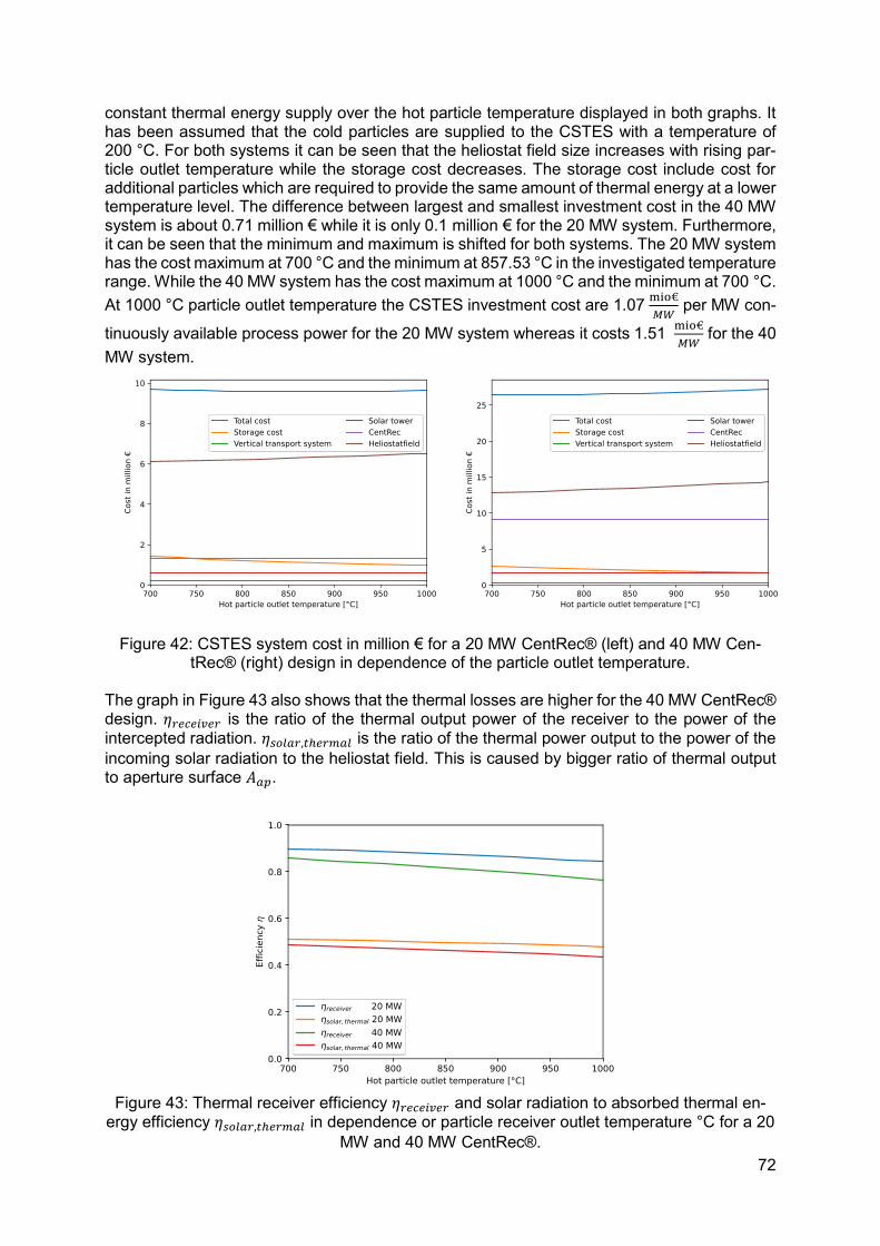
72

constant thermal energy supply over the hot particle temperature displayed in both graphs. It has been assumed that the cold particles are supplied to the CSTES with a temperature of 200 °C. For both systems it can be seen that the heliostat field size increases with rising par-ticle outlet temperature while the storage cost decreases. The storage cost include cost for additional particles which are required to provide the same amount of thermal energy at a lower temperature level. The difference between largest and smallest investment cost in the 40 MW system is about 0.71 million € while it is only 0.1 million € for the 20 MW system. Furthermore, it can be seen that the minimum and maximum is shifted for both systems. The 20 MW system has the cost maximum at 700 °C and the minimum at 857.53 °C in the investigated temperature range. While the 40 MW system has the cost maximum at 1000 °C and the minimum at 700 °C.

At 1000 °C particle outlet temperature the CSTES investment cost are 1.07 mio€

𝑀𝑊 per MW con-

tinuously available process power for the 20 MW system whereas it costs 1.51 mio€

𝑀𝑊 for the 40

MW system.

Figure 42: CSTES system cost in million € for a 20 MW CentRec® (left) and 40 MW Cen-tRec® (right) design in dependence of the particle outlet temperature.

The graph in Figure 43 also shows that the thermal losses are higher for the 40 MW CentRec® design. 𝜂𝑟𝑒𝑐𝑒𝑖𝑣𝑒𝑟 is the ratio of the thermal output power of the receiver to the power of the

intercepted radiation. 𝜂𝑠𝑜𝑙𝑎𝑟,𝑡ℎ𝑒𝑟𝑚𝑎𝑙 is the ratio of the thermal power output to the power of the

incoming solar radiation to the heliostat field. This is caused by bigger ratio of thermal output to aperture surface 𝐴𝑎𝑝.

Figure 43: Thermal receiver efficiency 𝜂𝑟𝑒𝑐𝑒𝑖𝑣𝑒𝑟 and solar radiation to absorbed thermal en-

ergy efficiency 𝜂𝑠𝑜𝑙𝑎𝑟,𝑡ℎ𝑒𝑟𝑚𝑎𝑙 in dependence or particle receiver outlet temperature °C for a 20

MW and 40 MW CentRec®.

73

6.1.2 Process results This section presents the technical results of the optimization. First the results of the complete flow sheet are presented which are followed by the results of the H2SO4 splitting reactor. The results of the optimization of the complete process are shown in Figure 44.

Figure 44 Results of the optimization of the complete solid sulphur cycle. Results are shown

in green and losses in red. (Own depiction) The optimization converged to a solution close to the maximum process power that the CSTES can supply. This indicates that at least a local optimum has been found. From an energetic point of view the process can be evaluated by the indicators presented in Table 20. It can be seen that 11.1% of the thermal energy input in the process is converted to electricity. When comparing this value to other energy storing processes it needs to be considered that addi-tional energy is required to concentrate the spent sulphuric acid. The thermal efficiencies from solar to thermal process power can be converted using the thermal efficiency of the CSTES which is ηsolar,receiver= 0.4801. It is calculated by multiplication from the heliostat field efficiency

which is assumed to be ηfield = 0.5693 and the thermal receiver efficiency ηreceiver = 0.8433.

Table 20: Introduction of process efficiencies and ratios.

Energy input location

Sulphur contact Sulphur ab-sorption

Spent sulphuric

acid treated 𝑘𝑔

𝑀𝐽

Electricity

Solar

0.1034 0.1495 0.1163 0.0531

Thermal pro-cess power

0.2151 0.3111 0.2422 0.111

Decomposition

DisproportionationAcid

concentration

Elemental

sulphur

Hot particle

storageCold particle

storage

Heliostats & Solar

thermal receiver

Sulphuric acid

production

Titan dioxide

production

𝑆𝑂2 separation

Electricity

O2

Titan dioxide

H2O

Solar site

Non-solar

site

CSTES

External

process

Input 8.9 MW

Input 18.74 MW

0.1567 𝑘𝑔

𝑠

H2SO4 22 wt%

2.18 𝑘𝑔

𝑠

Concentrated

H2SO40.483

𝑘𝑔

𝑠 𝜂𝑡ℎ𝑒𝑟𝑚𝑎𝑙,𝐻2𝑆𝑂4,𝑐𝑜𝑛

11.1

𝜂𝑠𝑜𝑙𝑎𝑟,𝑡ℎ𝑒𝑟𝑚𝑎𝑙 48.28 Loss 2.4 MW Loss 0.36 MW

Particles

9.35 𝑘𝑔

𝑠

74

A complete energy analysis is not possible based on the results because the SO2 separation is not modelled physically. Still two main points of energy loss can be identified from the 8.998 MW continuously supplied to the process by the CSTES:

• Thermal losses of acid concentration o 2.4 MW or 26.67 % of the thermal energy supplied to the process

• Disproportionation o 0.36 MW or 4.1 % of the thermal energy supplied to the process

Most of the thermal heat lost is at a comparably low temperature level between 70 and 170 °C. The results for the complete H2SO4 splitting reactor are shown in Figure 45. It only shows a section of the complete reactor. According to the economic function that is used to estimate the costs the reactor it needs to be splitted into at least two reactors due the upper validity

boundary condition of 1000 m2. It can be seen that the particle inlet and outlet temperature are very close to the maximum boundaries provided at 1000 °C and 200 °C respectively. Further-more, it can be seen that the fluid outlet temperature is close to the particle inlet temperature. The solution converged to a weight hourly space velocity (WHSV) of 2.018 and a conversion of 98.65 % which is close to equilibrium. The particle inlet temperature is 999.92 °C which is close to the maximum CentRec® particle outlet temperature of 1000 °C. The deviation is probably caused by a loose convergence cri-terium to save computation time. Total spent acid mass flow and particle mass flow converged to a solution that utilizes nearly all energy supplied to the process. The particle mass flow to fluid mass flow ratio 4.288 which is in the valid range presented in the section 4.5.

75

Figure 45: Section of the complete H2SO4 splitting reactor in the 20 MW solid sulphur cycle.

(Own depiction) Figure 46 shows that the biggest tube section is the decomposition section followed by the superheating section. The lowest heat transfer coefficient is in the superheating section but it is only slightly bigger than in the decomposition section. The complete reactor tube length is 7.35 m. The superheater fluid outlet temperature has been set to 800 °C.

𝑛𝑡𝑢𝑏𝑒𝑠=3922

𝑙𝑡𝑢𝑏𝑒 =7.35 m

m𝑝𝑎𝑟𝑡𝑖𝑐𝑙𝑒,𝑡𝑜𝑡𝑎𝑙 = 33.64𝑡

ℎ

m𝑓𝑙𝑢𝑖𝑑,𝑡𝑜𝑡𝑎𝑙= 7.47𝑡

ℎ

𝑚𝑐𝑎𝑡𝑎𝑙𝑦𝑠𝑡,𝑡𝑜𝑡𝑎𝑙= 3.7 𝑡

𝑇𝑝𝑎𝑟𝑡𝑖𝑐𝑙𝑒,𝑜𝑢𝑡 =

199.96 °C𝑇𝑓𝑙𝑢𝑖𝑑,𝑖𝑛 = 77.28 °C

𝑇𝑓𝑙𝑢𝑖𝑑,𝑜𝑢𝑡 = 988.32 °C

𝑇𝑝𝑎𝑟𝑡𝑖𝑐𝑙𝑒,𝑖𝑛 = 999.33 °C

76

Figure 46: Depiction of a single tube of the H2SO4 splitting reactor in the 20 MW solid sulphur

cycle. (Own depiction)

l 𝑑𝑒𝑐𝑜𝑚𝑝𝑜𝑠𝑖𝑡𝑖𝑜𝑛=4.5𝑚

l 𝑠𝑢𝑝𝑒𝑟ℎ𝑒𝑎𝑡𝑖𝑛𝑔=2.28 𝑚

l 𝑣𝑎𝑝𝑜𝑟𝑖𝑠𝑎𝑡𝑖𝑜𝑛=0.41 [𝑚]

l 𝑝𝑟𝑒ℎ𝑒𝑎𝑡𝑖𝑛𝑔

=0.16 𝑚

𝑑𝑒𝑐𝑜𝑚𝑝𝑜𝑠𝑖𝑡𝑖𝑜𝑛 = 50.1W

m2

𝑠𝑢𝑝𝑒𝑟ℎ𝑒𝑎𝑡𝑖𝑛𝑔 = 44.23W

m2

𝑣𝑎𝑝𝑜𝑟𝑖𝑠𝑎𝑡𝑖𝑜𝑛 = 286.11W

m2

𝑝𝑟𝑒ℎ𝑒𝑎𝑡𝑖𝑛𝑔 = 96.29𝑊

𝑚2𝐾

l 𝑡𝑢𝑏𝑒=7.35 𝑚

𝑑𝑖𝑛𝑛𝑒𝑟 = 0.019 𝑚

t𝑆𝑖𝑐,𝑡𝑢𝑏𝑒 = 0.005𝑚

t𝑆𝑆,𝑡𝑢𝑏𝑒 = 0.002 𝑚

t𝑏𝑢𝑙𝑘 = 0.005𝑚

77

6.2 Discussion This section discusses the results of the techno-economic optimization and evaluation pre-sented in section 6.1 as well as findings about the reactor in general from section 4.5. First economic results are discussed, thereupon the findings about the concentrated solar thermal energy system. Economics modelling efforts and optimization potentials Even though the process is not economically feasible with the assumptions made it shows that the process might be economically feasible in the sulphuric acid recycling prices range re-ported. An increase in sulphuric acid treatment revenue from 50 €/t to 96.21 €/t would yield an economic feasible process. This value is in the range of 120 €/t revenue suggested by an industrial expert. It was also shown that the transportation of the spent sulphuric acid is a main cost factor. Removing the transport costs would increase net present worth from -16.228 mil-

lion € to 8.18 million €. This corresponds to an economically feasible process. Neglecting the transportation costs would invalidate some of the assumptions. It still shows potential of on-site sulphuric acid recycling and can be used to motivate a study for a sulphuric acid recycling plant powered by a concentrated solar thermal energy system. The analysis showed a low sensibility of the net present worth towards the electricity price and the concentrated sulphuric acid price. The electricity price should be increased to 0.281 €/kWh from 0.067 €/kWh which corresponds to a ratio of 4.194. Concentrated acid price would be required to increase to 205.15 €/t from 80 €/t corresponding to a ratio of 2.56. These ratios are high compared to the increased ratio of 1.924 for the spent sulphuric acid treatment. This is caused by the high cost of the spent sulphuric handling. Moving highly concentrated sulphuric acid instead reduces the mass which needs to be transported and energy required to concen-trate sulphuric acid. This can be used to increase the sensibility of the net present worth to-wards the electricity price and concentrated sulphuric acid price. When evaluating these results, it needs to be considered that major simplifications have been made and the results can only be treated as preliminary. The first major simplifications are the ideally modelled SO2 separation and the neglected flue gas cleaning to reduce modelling ef-forts. Subsequently the corresponding capital and heat requirements of the sections could not be calculated. The influence of impurities on the process was also not modelled. Impurities might block the catalyst in the H2SO4 splitting reactors when they cannot be removed to a sufficient extent before entering the reactor. If the purification is not possible another option is to enhance the maximum particle outlet temperature of the CentRec® and to remove the cat-alyst. A further option could be to utilize another reactor concept like a moving bed reactor which could prevent the blocking. In lack of a suitable kinetic equation for Fe2O3 coated foams a kinetic for a different Fe2O3 based catalyst has been used. Pressure drop has been neglected and the reactor pressure has been arbitrarily set to 1 bar which is in the valid range of the kinetic equation used. No cost correlations were available for particle heated H2SO4 splitting reactor. Also, no material factors

for silicon carbide was available for the cost correlations used to estimate the cost of the H2SO4 splitting reactor. Other expensive materials were used instead. Silicon carbide is an expensive material and cost increases are possible. The sulphuric acid production has not been modelled at all and should be integrated in a complete study to investigate possible optimization potential and influence of impurities. It should also be noted that there are still many optimization potentials available for the pro-cess. The heat of the H2SO4 splitting reactor product gases could recuperated using a particle heated bayonet reactor. The reaction conditions in the disproportionation section can be opti-mized for the net present worth of the process. More heat could be recuperated using mem-brane evaporation to concentrate the sulphuric acid. It allows to use thermal energy in a low

78

temperature range between 40 °C – 80 °C. It is also interesting to the recycling processes to separate impurities from the sulphuric acid (Kesieme et al. 2012, p. 624). Possible heat source for the membrane evaporation are disproportionation reaction and the H2SO4 splitting reactor

product gases. H2SO4 inlet concentration to the H2SO4 splitting reactor could be increased. Depending on the quality of the cleaned H2SO4 splitting reactor product gases the oxygen could be sold as a product. CSTES The investment cost of the concentrated solar thermal energy system have been evaluated in dependence of the particle outlet temperature of the CentRec®. The thermal energy output of the CentRec® has been held constant by adjusting the particle mass flow and heliostat field size. Increasing the particle temperature increases the thermal losses but also decreases the required particle mass to store the same amount of thermal energy. Increased thermal losses increase the required heliostat field size but decrease the required storage size and particle mass. The influence of the additional thermal losses can be seen by the decrease in thermal receiver efficiency ηreceiver with rising particle receiver outlet temperature in Figure 43. Subsequently the ηsolar,thermal decreases with the solar radiation in the same manner. It was found that a

20 MW CentRec® CSTES has always lower specific thermal supply costs then a 40 MW Cen-tRec® system. This is caused by the increased thermal losses in the bigger CentRec® system and the investment cost increase which is disproportional to the absorbed thermal power in-crease. The aperture ratio is 3.8 while the supplied thermal ratio is only doubled. This also explains the difference in investment cost per available thermal process power. These findings might not reflect the reality correctly because a constant DNI during sun hours was assumed. Fluctuations in radiation might have a stronger influence on the thermal losses than predicted by this calculation. To show if a 20 MW CentRec® system is superior to a 40 MW CentRec® system in a big scale plant, the cost for the particle distribution system needs to be considered. The optimization for the particle inlet temperature yields a solution close to the maximum par-ticle temperature of 1000 °C that the CSTES can deliver. A small deviation of about 0.1 °C to 1000 °C is caused by a loose convergence constraint due to high computational costs of the simulation. The result is in accordance with the findings about the temperature dependence of the investment cost of the CSTES model. It showed only small changes in investment costs with changing particle outlet temperature because two conflicting effects are nearly evening out their influence. On the on hand an increase in particle temperature increases the thermal losses in the system but decreases the required storage size. On the other hand, a higher particle inlet temperature increases in the SO3 decomposition reactor increases the reaction rate. It also shifts the equilibrium to the product side and thus the results are reasonable. Reactor The optimization yielded a relatively large reactor size which consists of 3922 tubes. Each one is 7.35 m long and has an inner diameter of 19 mm. This big reactor size causes a high con-version of 98.65 % of the SO3 decomposition reaction which is close to equilibrium. Although the reactor is quite large, its share is only 9.64 % of the total equipment cost, compared to 71.6 % for the CSTES energy provision. The high conversion increases the process efficiency because it decreases the recycled fluid mass. Still the conversion is below equilibrium conver-sion because the increase in investment cost for a larger reactor is not in proportion to the benefit of an increased conversion. Close to the equilibrium the reaction rate gets smaller. This decreases the proportionality between the reactor investment costs and the increase in reve-nues due to a higher process efficiency. It should be considered that the cost correlation might not capture the real cost of the novel equipment and that increased reactor costs might shift the optimum reactor size and

79

conversion to a lower value. Another restriction of the results is that the kinetic is not validated for Fe2O3 coated foams. A numerical optimization of the reactor design variables is not useful with the cost correlation used. The cost correlation employed is solely based on the heat exchange surface area. Influ-ences of different combinations of the inner tube diameter, tube length, number of tubes and the fluid mass flow are neglected. Instead the reactor has been designed for an increased heat transfer coefficient. The reactor height is directly coupled to the tube length. Particles are driven by gravity and thus the reactor needs to be erected vertically. Therefore, the tube length is limited by the maximum reactor height. In section 4.5 possibilities were presented to increase the heat transfer of the reactor. The first possibility is to decrease the particle bulk width which can be seen in Figure 27. It has been set to 5 mm which is the lowest value which has been reported for a particle heated horizontal tube heat exchanger. It still should be validated until which particle bulk width the predicted increase in heat transfer coefficient holds. The particle contact time is much longer in the de-sign presented than in the heat exchanger reported. Thus, it should be tested if the small bulk width causes blocking or other particle flow problems. The second possibility is to increase the heat transfer is to increase the fluid velocity by. This can be done by increasing the fluid mass flow. To maintain a sufficient residence time in the tube the length of the sections needs to be increased. From the point of view of the heat trans-fer model only the tube length is a limitation for heat transfer. In order to design a reactor which is similar to a standard heat exchanger the design variables have been chosen so that the complete tube length is below 10 m. The complete reactor length could not be supplied to the reactor simulation model as a design variable directly. Instead a decomposition section length, number of tubes and the inner tube diameter must be supplied. Decomposition reactor length has been set to 4.5 m so that the complete result is sufficiently below 10 m. Decreasing the inner tube diameter increases the heat transfer coefficient in all sections as it can be seen in section 4.5. Towards the section length there are conflicting influences. In the decomposition section, vaporization section and preheating section the section length in-creases with decreasing diameter. In the superheating section the effect is reversed. This has different reasons. In the decomposition section the volume needs to be hold constant to main-tain the residence time and weight hourly space velocity (WHSV). Thus, the length needs to increase when inner tube diameter is decreased. In the other sections the heat transferred per heat exchange area is increased. But more heat needs to be transferred due to the increased fluid mass flow. In the preheating and vaporization section the second effect dominates the first effect. In the superheating section the ratio is reversed. As a compromise between both effects an inner tube diameter of 19 mm has been chosen. The small tube diameter requires a high number of tubes in the reactor. These results might deviate from experiments with experimental reactor of the PEGAUS pro-ject because the influence of foams is neglected. It is known from experimental experience that the overall heat transfer of the fluid is increased by the foams (Oliveira 9/14/2020a). Still the effect has not been quantified so far. In Figure 43 it can be seen that the decomposition zone is about half of the length of the complete reactor. The second biggest section is the superheating section. Both together cause 92.24 % of the reactor heat exchange area or volume. The size of the superheating section is mainly caused by the heat transfer coefficient which is low compared to the preheating and superheating section. In the decomposition section the required size is mainly caused by the low weight hourly space velocity (WHSV) and the required reactor volume. The fluid outlet temperature is close to the particle inlet temperature which indicates that the heat transfer is

80

not a limiting issue in the reaction zone of the current reactor. Thus, the reactor performance could be increased by increasing the gas heat transfer coefficient. The decomposition section could profit from an increase in tube diameter to decrease the section length. An option to enhance the heat transfer further would be to use multiple particle heated cross flow reactors. These can be located next to each other and can be connected in series on the fluid side. This increase the fluid tube length and allows to increase fluid velocity. Also, the average heat transfer temperature difference would increase which decreases the required reactor size. It should be noted that no pressure drop was considered in the evaluation which needs to considered when higher velocities are reached. Thus, suitable correlation for the fluid velocity dependent pressure drop in foams is required. Another interesting investigation would be the the kinetic behaviour of Fe2O3 coated foams in dependence of different catalyst loads, bulk densities and pressures. This would require a suitable kinetic which describes the effects of these design variables towards the pressure drop and reaction rate.

7 Summary and Conclusion The process concept of the solid sulphur cycle process presented in the PEGASUS project has been adapted to integrate sulphuric acid recycling. A model for a novel particle heated H2SO4 splitting reactor has been developed and implemented into an Aspen simulation. A model-based analysis was used to propose improvements for the reactor concepts. The reac-tor model has been integrated into a simulation of the adapted solid sulphur cycle. Both simu-lations are supplemented by Python automation procedures for various purposes. Simplifica-tions have been made in the simulation of the process to reduce modelling efforts. The simu-lation was used to conduct a techno-economic optimization of the complete process for four design variables. Results of the optimization are analysed to show potential of the solid sulphur cycle. Two concentrated solar thermal energy systems have been investigated for the invest-ment cost in dependence of the supplied temperature. The net present worth of the solid sulphur cycle investigated in this thesis is -16.2228 million €. Thus, the process is not economically feasible as presented. Integration of sulphuric acid re-cycling offers additional revenues for treatment of spent sulphuric acid which make up a main share of the revenues of this process. Furthermore, additional CO2 emissions can be prevented when conventional fossil-fuel based recycling processes are replaced. A main cost factor is the transportation of spent sulphuric acid from the non-solar site of the process to the solar site. Compared to the solid sulphur cycle without sulphuric acid recycling the effect is intensi-fied. Due to the additional mass of water in spent acid approximately 4.5 times more mass needs to be transported compared to pure sulphuric acid. Still the revenue for treatment of sulphuric acid outweighs the transportation costs. The analysis of the transport costs shows potential for on-site CSTES powered sulphuric acid recycling processes. It needs to be noticed that the purification of spent sulphuric acid from titan dioxide and SO2 separation is strongly simplified. The results only show potential for the recycling process. The spent sulphuric acid prices were estimated by two industry experts. They showed a strong variation in composition and treatment revenue from 0 €/t to 500 €/t. In particular spent acid treatment prices of 50 €/t were estimated for sulphuric acid recycling in titan dioxide production. 120 €/t were estimated for conventional hydron carbon contaminated acids. An analysis of the process economics showed that an increase from 50 €/t acid treatment revenue to 96.21 €/t would yield an economically feasible process. A change in treated sulphuric acid might yield and economically feasible process. Further modelling efforts are required to substantiate the findings.

81

The techno-economic optimization has been conducted in dependence of four design varia-bles. H2SO4 splitting reactor size has been investigated in terms of tube numbers, the treated acid mass flow provided to the process, the particle mass flow that provides thermal energy to the process and the inlet temperature of the particle mass flow to the process. An economic optimum was found for a big H2SO4 splitting reactor which yielded a high conver-sion 98.65 % which is close to equilibrium. The number of tubes converged to 3922 with a total length of 7.3 m each. Inner tube diameter has been set to 19 mm. H2SO4 splitting reactor cost are still only 9.64 % of the complete equipment cost. These costs are low compared to the investment cost for the concentrated solar thermal energy system (CSTES) which make up 72 % of the total equipment cost. Thus, a big reactor size which increases the cash flow is reasonable. Still the optimum reactor size yielded a conversion below the equilibrium conver-sion. This shows that optimum reactor size is a function of the volume specific reactor costs. More expensive reactors will yield an economic optimum at lower conversions. It should be noted that no kinetic equation is available for Fe2O3 coated foams. Validity of the kinetic still needs to be shown by experiments. Economic optimum particle inlet temperature was found to be 1000 °C which is the maximum temperature that the CSTES can provide. The effects of an increased reaction rate of the SO3 decomposition reaction, the equilibrium shift towards the products and the decreased thermal storage size outweigh the increased thermal losses due to increased particle outlet tempera-ture. Still it should be noted that a constant DNI during daytime was assumed in the simulation. Radiation fluctuations over a real day might change the results. Particle mass flow and fluid mass flow have been included in the optimization to scale the process to the maximum fluid mass flow and energy mass flow. The process design treats 2.18 kg/s of spent sulphuric acid, circulates 9.35 kg/s of particles as heat transfer medium and provides 1 MW of electricity. The total investment cost is 17.88 million €. Two improvements for the indirect particle heated H2SO4 splitting reactor have been proposed. A reduction of particle bulk thickness to 5 mm has been used in the process simulation which showed great improvement in heat transfer. No experimental data for vertical tube heat ex-changer was available. Thus, results should be compared to future experiments to validate the simulation results. Increasing the fluid velocity increases the heat transfer in the reactor. This effect is in conflict with reactor height which increases the equipment costs at some point. Increase in velocity also increases the pressure drop. This should be considered when the economically optimum length of the reactor is determined. Two CSTES for 20 MW CentRec® and 40 MW CentRec® have been investigated. Results showed that the investment cost per thermal power supplied to the process were always cheaper in the 20 MW system. This was caused by the aperture size ratio of the 40 MW system and the 20 MW system which is 3.8. Whereas the thermal output is only doubled. The in-creased ration of aperture surface to thermal power supplied increases the CentRec® invest-ment cost and thermal losses as well. At 1000 °C particle outlet temperature the continuously available process power costs 1.07 million €/MW for the 20 MW system whereas it costs 1.51 million €/MW for the 40 MW system. A constant DNI during the day has been assumed and the influence of radiations fluctuations should be investigated.

82

8 Outlook Even though no economically feasible process could be designed in this thesis there are still optimization potentials available to improve the process efficiency and economic performance which should be investigated. On-site sulphuric acid recycling is an economically interesting process in which CSTES could replace fossil fuels. Incorporation of optimization potentials might yield an economically feasible pure solid sulphur cycle. This would be advantageous because it could be scaled independently from the sulphuric acid recycling requirements. The model for the H2SO4 splitting reactor can be used for other sulphur cycles as well after valida-tion has been conducted. Further optimization potentials to increase the economic performance of the solid sulphur cycle are:

• Heat of SO3 reaction product gasses could be recuperated using a particle-heated bay-onet reactor.

• Low-temperature heat of the process could be used to concentrate sulphuric acid by membrane evaporation. Heat from sources with temperature as low as 40 °C - 80 °C could be used. Membranes also have interesting properties for purification of impuri-ties (Kesieme et al. 2012, p. 624). The disproportionation reaction and SO3 reactor product gasses are possible heat sources.

• Depending on the quality of SO2 separation gasses oxygen could be sold as a product. The disproportionation reactors could be numerically optimized for net present worth instead of using predesigned reactor.

• The disproportionation could be modelled in dependence of varying residence time, temperature, pressure and catalyst mass to include these variables as design varia-bles in a techno-economic optimization.

Further efforts are required to substantiate findings made in this thesis:

• A kinetic for Fe2O3 coated needs to be developed to investigate the full potential of the catalyst. It should include pressure dependencies as well as variations in catalyst load-ing and geometry.

• A detailed simulation of the sulphuric acid production plant should be included into the techno-economic optimization so that their mutual influence of both processes investi-gated when impurities are modelled as well.

• A more detailed investigation which simulates the purification process in higher detail could substantiate the findings made.

• Further efforts need to be made model the SO2 separation which is strongly simplified in this. A challenge in the modelling efforts is to find a thermodynamic model that de-scribes H2SO4 splitting section, SO2 separation, disproportionation and H2SO4 concen-tration adequately or to use several models parallel. The thermodynamic employed in this thesis relies on parameters regressed specifically for its application. This might cause problems when parameters are share among thermodynamic models.

• Purification of the sulphuric acid needs to be modelled more detail.

83

Appendix A Economics

8.1 Investment cost parameters

Table 21: Parameters for 𝐶𝑃0 calculation using eq. 2.17 (Turton 2012, pp. 988–990) .

Equipment type

K1 K2 K3 Capacity units of pa-rameter A

Min size Max size

Jacketed agitated re-actor

4.1052 0.5320 -0.0005 𝑚3 0.1 35

Rotary com-pressor

5.0355 -1.8002 0.8253 kW 18 950

Pumps cen-trifugal

3.3892 0.0536 0.1538 kW 1 300

Fixed tube heat ex-changer

4.3247 -0.3030 0.1634 𝑚2 10 1000

8.2 Pressure factors Table 22: Pressure factors for bare module calculations 1 (Turton 2012, p. 1006).

Equipment type C1 C2 C3 Pressure Unit

Min size Max size

Bayonet, fixed tube sheet, floating head, kettle reboiler and U tube (Pressure on tube only)

0 0 0 Bar gauge 0 5

Bayonet, fixed tube sheet, floating head, kettle reboiler and U tube (Pressure on tube only)

-0.00164

-0.00627 0.0123 Bar gauge 5 140

Compressors

0 0 0 Bar gauge

Centrifugal pumps 0 0 0 Bar gauge 0 10

Centrifugal pumps -0.3935 0.3957 -0.00226 Bar gauge 10 100

𝐹𝑝 = 10𝐶1+𝐶2∗𝑙𝑜𝑔10(𝑃)+𝐶3∗((𝑙𝑜𝑔10(𝑃))

2

Eq. 8.1

8.3 Material and module factors

84

Table 23: Material factors and Module factor constants (Turton 2012, pp. 1009–1014).

Equipment type

Heat exchanger fixed tube

(nickel tube and CS shell)

Pump cen-trifugal

(Nickle al-loy)

Reactors Centrifugal blower or compressor (Ni alloy)

B1 1.63 1.89 1.89

B2

1.66 1.35 1.35

𝐹𝑀 2.6 4.4 11.4

𝐹𝐵,𝑀 4

8.4 Factors for pressure vessels

Table 24: Coefficients for basic costs of pressures vessels (Biegler et al. 1997, p. 134).

Equipment 𝐶0 $ 𝐿0 ft

Application range L ft

𝐷0 ft Application range D ft

𝛼 𝛽

Vertical fabrica-tion

1000 4 4-100 3 1-10 0.81 1.05

Horizontal fab-rication

690 4 4-100 2*103 -2 ∗104

1-10 0.78 0.98

Table 25: Module factor for pressure vessels (Biegler et al. 1997, p. 134). Equipment MF2 MF4 MF6 MF8 MF10

Vertical fabrication 4.23 4.12 4.07 4.06 4.02

Horizontal fabrication 3.18 3.06 3.01 2.99 2.96

Application range for base cost in $

<200,000 200,000 –

400,000

400,000 –

600,000

600,000 –

800,000

800,000 – 1,000,000

Table 26: Pressure factor for pressure vessels (Biegler et al. 1997, p. 113).

Pres-sure

range Psig

<50 50-100

100-200

200-300

300-400

400-500

500-600

600-700

700-800

800-900

900-1000

Pres-sure fac-

tor

1 1.05 1.15 1.2 1.35 1.45 1.6 1.8 1.9 2.3 2.5

The material factor for cladded titanium is 4.23 (Biegler et al. 1997, p. 113).

85

Appendix B Properties For practical appliance of temperature dependent heat transfer parameters it is recommended

to use the average value of the inlet and outlet conditions ϑ𝑚 = ϑ𝑖𝑛𝑙𝑒𝑡 + ϑ𝑜𝑢𝑡𝑙𝑒𝑡

2 .(Stephan et al.

2019, p. 840)

8.5 Heat capacities This section presents heat capacity values and correlations used for calculation or validation of Aspen parameters.

8.5.1 Particle heat capacity The bauxite particle heat capacity is relevant to determine the amount of energy supplied by the particles which varies with temperature. Internal measurements were made at DLR to de-termine the temperature dependent heat capacity. The data was fitted to a quatric polynomial and a valid range from 0 °C to 1200 °C was stated. (Reichart 2014, p. 24)

𝐶𝑝,𝑝𝑎𝑟𝑡𝐽

𝑘𝑔 ∗ 𝐾= 3.663 ∗ 10−10 ∗ 𝑇4 − 5.6345 ∗ 10−7 ∗ 𝑇3 − 4.6662 ∗ 10−4 ∗ 𝑇2

+ 1.1323 ∗ 𝑇 + 789.55

Eq. 8.2

Aspen provides the DIPPR (Design Institute for Physical properties) equation number 100 which is shown in Eq. 8.3 and is also a quatric polynomal. Parameter 𝑪𝟔 correspods to the low temperature limit and 𝑪𝟕 to the high temperature limit of validity (Aspen Technology 2016, p. 279) Parameters can only be entered for the mole specific heat capacity. Thus, parameters were transformed using the molecular weight provided by the APV100.Solids databank

101.96128 𝒈

𝒎𝒐𝒍 .

𝐶𝑝,𝑝𝑎𝑟𝑡𝐽

𝑚𝑜𝑙 ∗ 𝐾= +𝐶1 + 𝐶2 ∗ 𝑇 + 𝐶3 ∗ 𝑇

2 + 𝐶4 ∗ 𝑇3 + 𝐶5 ∗ 𝑇

4 Eq. 8.3

Table 27: Parameters for particle heat capacity equations.

𝐶1 𝐽

kg∗𝐾 𝐶2

𝐽

kg∗𝐾2 𝐶3

𝐽

kg∗𝐾3 𝐶4

𝐽

kg∗𝐾4 𝐶5

𝐽

kg∗𝐾5 𝐶6 °C 𝐶7 °C

789.55 1.1323 -4.6662 ∗10−4

-5.6345 ∗10−7

3.663∗ 10−10

273.15 1473.15

80.50352862 0.115450757

-4.75772E-05

-5.74501E-08

3.70425E-11 0 1200

The transformed parameters must be entered to CPDSDIP. Furthermore, the parameter C5 of the parameter set THRSTW for Al2O3 must be set to 100 to utilize Eq. 8.3 for calculation of the solid heat capacity of the component. To calculate enthalpy differences at different tempera-tures states it is necessary to adjust the input parameters to Kelvin.

𝐶𝑝,𝑝𝑎𝑟𝑡𝐽

𝑘𝑔 ∗ 𝐾= 3.663 ∗ 10−10 ∗ (𝑇 + 273.15)4 − 5.6345 ∗ 10−7 ∗ (𝑇 + 273.15)3

− 4.6662 ∗ 10−4 ∗ (𝑇 + 273.15)2 + 1.1323 ∗ (𝑇 + 273.15) + 789.55

Eq. 8.4

8.5.2 Air

86

The dry air heat capacity 𝑐𝑝, 𝑎𝑖𝑟 is calculated according to eq. 8.5 and eq. 8.6 which is appli-

cable in the range of 175 to 800 K. 𝑅𝐴 𝐽

𝑘𝑔𝐾= 287.05

𝐽

𝑘𝑔𝐾 is the mass specific gas constant for

dry air (Dixon 1996, p. 504)

𝑐𝑝,𝑎𝑖𝑟𝐽

𝑘𝑔𝐾= 𝑐𝑣,𝑎𝑖𝑟 + 𝑅𝐴

eq. 8.5

𝑐𝑣,𝑎𝑖𝑟 𝐽

𝑘𝑔𝐾= 717.8 + 0.07075 ∗ ( 𝑇𝐾 − 300) + 261,25 ∗ 10

−6 ∗ (( 𝑇𝐾 − 300))2

eq. 8.6

8.6 Thermal conductivity This section shows different thermal conductivities used which were not obtained from the Aspen Plus simulation.

8.6.1 Air The thermal air conductivity is calculated according to eq. 8.7. It is valid in a range of 100 – 1000K and temperature 𝑇𝐾 has to be provided using Kelvin. (Dixon 1996, p. 504) If values for temperatures higher than 1000 K are required the value for 1000 K is used.

𝜆𝑎𝑖𝑟 𝑊

𝑚 ∗ 𝐾= ∗

2.636 ∗ 10−3 ∗ 𝑇𝐾1.5

𝑇𝐾 + 2.45 ∗ 10(−12𝑇𝐾

)

eq. 8.7

8.6.2 Bauxite Bulk conductivity The bulk conductivity 𝜆𝑏𝑒𝑑 is based in the model of Zehner, Bauer and Schlünder (Stephan et al. 2019, p. 1836). It is calculated according to equations eq. 8.8, eq. 8.9, eq. 8.10 and eq. 8.11. The interstitial gas is assumed to be air and 𝜆𝑓 is used from eq. 8.6, and 𝐶𝑓 from eq. 8.5.

C =2.8 is which is a constant which should be applied for air as interstitial gas (Stephan et al. 2019, p. 1746). The porosity 𝜓 is assumed to be 0,48, the emissivity 𝜖 to 0,8 and the particle

conductivity 𝜆𝐺 to 2 𝑊

𝑚𝐾. (Mevißen, p. 29)

𝜆𝑏𝑒𝑑 = 𝑘𝑏𝑒𝑑 ∗ 𝜆𝑓

eq. 8.8

𝑘𝑏𝑒𝑑 = (1 − √1 − 𝜓 ) ∗ 𝜓 ∗ [(𝜓 − 1 + 𝑘𝐺−1)−1 + 𝑘𝑟𝑎𝑑]

+√1 − 𝜓 ∗ [𝜑𝑘𝑝 + (1 − 𝜑)𝑘𝑐]

with

𝑘𝑐 =2

𝑁{𝐵(𝑘𝑝 + 𝑘𝑟𝑎𝑑 − 1)

𝑁2𝑘𝐺𝑘𝑝𝑙𝑛

𝑘𝑝 + 𝑘𝑟𝑎𝑑

𝐵[𝑘𝐺 + (1 − 𝑘𝐺)(𝑘𝑝 + 𝑘𝑟𝑎𝑑)]

+𝐵 + 1

2𝐵[𝑘𝑟𝑎𝑑𝑘𝐺

− 𝐵 (1 +1 − 𝑘𝐺𝑘𝐺

𝑘𝑟𝑎𝑑)] −𝐵 − 1

𝑁𝑘𝐺},

𝑁 =1

𝑘𝐺(1 +

𝑘𝑟𝑎𝑑 − 𝐵𝑘𝐺𝑘𝑝

) − 𝐵 (1

𝑘𝐺− 1)(1 +

𝑘𝑟𝑎𝑑𝑘𝑝

),

𝐵 = 𝐶𝑓 [1 − 𝜓

𝜓]

109𝑓(𝜁),

𝑘𝑟𝑎𝑑 =𝜆𝑟𝑎𝑑

𝜆𝑓=

4𝜎

(2𝜖) − 1

𝑇3𝑑

𝜆𝑓,

and

𝑘𝐺 =𝜆𝐺

𝜆𝑓= [1 + (

𝑙

𝑑)]−1.

eq. 8.9

87

𝑙0 = 2 ∗2 − 𝑦

𝑦∗ √

2𝜋𝑅𝑇

𝑀𝑓∗

𝜆𝑓

𝑝(2𝑐𝑝,𝑓 −𝑅𝑀𝑓)

eq. 8.10

𝑙𝑔 (1

𝑦− 1) = 0.6 −

(1000𝐾𝑇

) + 1

𝐶

eq. 8.11

8.6.3 Tube conductivity The thermal conductivity of silicon carbide is calculated according eq. 8.12 which is valid in the range between 300-1800 K. (Karditsas and Baptiste 1995)

𝜆𝑓 𝑊

𝑚 ∗ 𝐾= 1299 − 3.9407 ∗ 𝑇 + 4.8745 ∗ 10−3 ∗ 𝑇2 − 2.6974 ∗ 10−6 ∗ 𝑇3 + 5.4787

∗ 10−10 ∗ 𝑇4

eq. 8.12

Thermal conductivity of stainless steel is assumed to be 19 𝑊

𝑚∗𝐾.(Thanda 2018, p. 46)

8.7 Particle properties The particles are assumed have a diameter 𝑑𝑝𝑎𝑟𝑡 = 0.001 𝑚 and a bulk density of ρ𝑝𝑎𝑟𝑡𝑖𝑐𝑙𝑒 =

2004 𝑘𝑔

𝑚3 (Saint-Gobain 2013, p. 3). The surface roughness is assume to be δ = 2.5 μm which

is the value suggested for aluminum silicate (Stephan et al. 2019, p. 1746).

9 Publication bibliography Agrafiotis, Christos; Thomey, Dennis; Oliveira, Lamark de; Overbeck, Nicolas; Thanda, Vamshi Krishna; Roeb, Martin; Sattler, Christian (2020): Solar energy conversion and storage through sulphur-based thermochemical cy-cles implemented on centrifugal particle receivers. In : SOLARPACES 2019: International Conference on Concen-trating Solar Power and Chemical Energy Systems. SOLARPACES 2019: International Conference on Concentrat-ing Solar Power and Chemical Energy Systems. Daegu, South Korea, 1–4 October 2019: AIP Publishing (AIP Conference Proceedings), p. 170001.

Argus Sulphur (2020): Executive summary.

Aspen Technology (2016): Aspen Physical Property Models. Version Number: V9.

Aspen Technology, Inc. (Ed.) (1999): Aspen Plus V10 User Guide. Available online at https://user.eng.umd.edu/~nsw/chbe446/AspenPlusV10UserGuide2.pdf.

Auer, Gerhard; Woditsch, Peter; Westerhaus, Axel; Kischkewitz, Jürgen; Griebler, Wolf-Dieter; Liedekerke, Marcel de (2012): Pigments, Inorganic, 2. White Pigments. In : Ullmann's Encyclopedia of Industrial Chemistry. Weinheim, Germany: Wiley-VCH Verlag GmbH & Co. KGaA.

Baumann, Torsten; Zunft, Stefan (2014): Experimental Investigation on a Moving Bed Heat Exchanger used for discharge of a particle-based TES for CSP. In : Eurotherm Seminar #99 - Advances in Themal Energy Storage. Eurotherm Seminar #99. Lleida, Spanien, 28.05.-30.05.2014. Available online at https://elib.dlr.de/89232/.

Bergman, Theodore L.; Lavine, Adrienne S. (2017): Fundamentals of heat and mass transfer. Eighth edition. Ho-boken, NJ, ©2017: John Wiley & Sons.

Biegler, Lorenz T.; Grossmann, Ignacio E.; Westerberg, Arthur W. (1997): Systematic methods of chemical process design. Upper Saddle River, NJ: Prentice-Hall (Prentice-Hall international series in the physical and chemical engi-neering sciences).

Brown, Lloyd Chauncey; Trester, Paul; Besenbruch, Gottfried (1986): High-Pressure Catalytic Metal Reactor in a Simulated Solar Central Receiver. General Atomics.

Buck, Reiner; Giuliano, Stefano (2019): Solar tower system temperature range optimization for reduced LCOE. In : SOLARPACES 2018: International Conference on Concentrating Solar Power and Chemical Energy Systems. SO-LARPACES 2018: International Conference on Concentrating Solar Power and Chemical Energy Systems. Casa-blanca, Morocco, 2–5 October 2018: AIP Publishing (AIP Conference Proceedings), pp. 0–8.

Buck, Reiner; Schwarzbözl, Peter (2018): 4.17 Solar Tower Systems. In : Comprehensive Energy Systems: Else-vier, pp. 692–732.

Bundesnetzagentur und Bundeskartellamt (2018): Über alle Tarife mengengewichteter Elektriztätspreis für Haushaltskunden für den Abnahmefall 4,500 kWh im Jahr. Available online at

88

https://www.bmwi.de/Redaktion/DE/Downloads/I/Infografiken/infografik-Tarife-mengengewichteter-elektri-zitaetspreis-fuer-haushaltskunden.pdf?__blob=publicationFile&v=10.

Chaves, Iván Darío Gil; López, Javier Ricardo Guevara; Zapata, José Luis García; Robayo, Alexander Leguizamón; Niño, Gerardo Rodríguez (2016): Process Simulation in Chemical Engineering. In Iván Darío Gil Chaves, Javier Ricardo Guevara López, José Luis García Zapata, Alexander Leguizamón Robayo, Gerardo Rodríguez Niño (Eds.): Process Analysis and Simulation in Chemical Engineering. Cham: Springer International Publishing, pp. 1–51.

DACE price booklet. Cost information for estimation and comparison (2020). Edition 34.

Ding, Yate; Riffat, S. B. (2013): Thermochemical energy storage technologies for building applications: a state-of-the-art review. In Int. J. Low-Carbon Tech. 8 (2), pp. 106–116. DOI: 10.1093/ijlct/cts004.

Dixon, John C. (1996): Tires, suspension and handling. 2nd ed. London, Warrendale, Pa.: Arnold; Society of Auto-motive Engineers.

Ebert, Miriam (2017): CentRec Zentrifugal-Partikelreceiver: Vom Labor bis Zum Technikumsmaßstab. Sonnenkol-loquium 2017. Köln, 7/6/2017.

Ebert, Miriam; Amsbeck, Lars; Rheinländer, Jens; Schlögl-Knothe, Bärbel; Schmitz, Stefan; Sibum, Marcel et al. (2019): Operational experience of a centrifugal particle receiver prototype. In : SOLARPACES 2018: International Conference on Concentrating Solar Power and Chemical Energy Systems. SOLARPACES 2018: International Con-ference on Concentrating Solar Power and Chemical Energy Systems. Casablanca, Morocco, 2–5 October 2018: AIP Publishing (AIP Conference Proceedings), p. 30018.

Estela; SolarPACES (Eds.) (2009): Concentrating Solar Power Global Outlook 09. Why Renewable Energy is hot. Available online at http://www.solarpaces.org/wp-content/uploads/concentrating-solar-power-2009.pdf.

exchangerates.org.uk (2020). Available online at https://www.exchangerates.org.uk/EUR-USD-spot-exchange-rates-history-2020.html.

Fedders, H.; Hammeke, K.; Savvidis, E.; Dahl, R.; Hoffmann, H.: EXPERIMENTELLE UNTERSUCHUNGEN ZUR KINETIK DER SO3-SPALTUNG BEI HÖHEREN DRÜCKEN UND THERMODYNAMISCHE BERECHNUNG VON SPALTREAKTOREN : Bericht. Available online at https://op.europa.eu/en/publication-detail/-/publication/43f28db9-f188-40e7-ab50-db54f7789ce0.

Federal Environmental Agency (2001): Large Volume Solid Inorganic Chemicals. German Notes on BAT for the production of. Available online at https://www.umweltbundesamt.de/sites/default/files/medien/publika-tion/long/3226.pdf, checked on 9/29/2020.

Frantz, Cathy; Ebert, Miriam; Amsbeck, Lars; Buck, Reiner: Design and cost study of improved scaled-up receiver version based on simulation results.

Giaconia, Alberto; Sau, Salvatore; Felici, Claudio; Tarquini, Pietro; Karagiannakis, George; Pagkoura, Chrysoula et al. (2011): Hydrogen production via sulfur-based thermochemical cycles: Part 2: Performance evaluation of Fe2O3-based catalysts for the sulfuric acid decomposition step. In International Journal of Hydrogen Energy 36 (11), pp. 6496–6509. DOI: 10.1016/j.ijhydene.2011.02.137.

Giuliano; Frantz (2017): Internal information in the PEGASUS project on CentRec design specification to Andreas Rosenstiel, 2017.

Gmitro, John Irving; Vermeulen, Theodore (1963): Vapor-Liquid Equilibria for Aqueous Sulfuric Acid.

Green, Don W.; Perry, Robert H. (2007): Perry's Chemical Engineers' Handbook (8th Edition). 8th ed. Blacklick, USA: McGraw-Hill Professional Publishing.

Halstead, W. David; Laxton, James W. (1974): Equilibria in the Fe2(SO4)3/Fe2O3/SO3 system. In J. Chem. Soc., Faraday Trans. 1 70 (0), p. 807. DOI: 10.1039/f19747000807.

Hartmann, H.: Thermochemische Wasserstoffproduktion, Trennverfahren Teil 1 : Verdampfungsgleichgewichte des Systems H2O/H2SO4 Teil 2 : Die Bestimmung der gas- und flüssigkeitsseitigen Stoffübergangskoeffizienten sowie der Gleichgewichtslöslichkeit für das System SO2/O2-H2O : ABSCHLUSSBERICHT. Available online at https://op.europa.eu/en/publication-detail/-/publication/5c151083-5551-4ae9-ba9d-e774cc2cfe11.

Haydary, Juma (2018): Chemical Process Design and Simulation. Newark: American Institute of Chemical Engi-neers. Available online at https://ebookcentral.proquest.com/lib/gbv/detail.action?docID=5615552.

Holleman, A. F.; Wiberg, Egon; Nils, Wiberg (1985): Kapitel XIV. Die Gruppe der Chalkogene. In A. F. Holleman, Egon Wiberg, Wiberg Nils (Eds.): Lehrbuch der anorganischen Chemie: De Gruyter, pp. 449–536.

Hussain, Sahil (2011): A Critical Review of Thermochemical Energy Storage Systems. In The Open Renewable Energy Journal 4. Available online at https://benthamopen.com/contents/pdf/TOREJ/TOREJ-4-42.pdf, checked on 6/30/2020.

International Renewable Energy Agency: Electricity storage and renewables: Costs and markets to 2030.

89

Ishikawa, H. (1982): Catalyzed thermal decompositon of H2SO4 and production of HBr by the reaction of SO2 with Br2 and H2O. In International Journal of Hydrogen Energy 7 (3), pp. 237–246. DOI: 10.1016/0360-3199(82)90087-8.

Jacob, Rhys; Saman, Wasim; Bruno, Frank (2017): Capital cost expenditure of high temperature latent and sensible thermal energy storage systems. In. SOLARPACES 2016: International Conference on Concentrating Solar Power and Chemical Energy Systems. Abu Dhabi, United Arab Emirates, 11–14 October 2016: Author(s) (AIP Conference Proceedings), p. 80012.

Jenkins, Scott (2020): 2019 Chemical Engineering Plant Cost Index Annual Average. In Chemical Engineering, 3/20/2020. Available online at https://www.chemengonline.com/2019-chemical-engineering-plant-cost-index-an-nual-average/, checked on 9/16/2020.

Karditsas, Panayiotis J.; Baptiste, Marc-Jean (1995): Thermal and structural properties of fusion related materials. (UKAEA-FUS--294). Available online at http://www-ferp.ucsd.edu/LIB/PROPS/PANOS/.

Kerskes, Henner (2016): Thermochemical Energy Storage. In : Storing Energy: Elsevier, pp. 345–372.

Kesieme, Uchenna K.; Milne, Nicholas; Aral, Hal; Cheng, Chu Yong; Duke, Mikel (2012): Novel application of mem-brane distillation for acid and water recovery from mining waste waters. In C. D. McCullough, M. A. Lund, L. Wyse (Eds.): International Mine Water Association Symposium. 2012: Bunbury, Western Australia proceedings. [Perth, Western Australia]: Mine and Water Environment Research Centre, pp. 624–630.

Kitchin, John (2013): Running Aspen via Python. Available online at https://kitch-ingroup.cheme.cmu.edu/blog/2013/06/14/Running-Aspen-via-Python/.

Kürten, Martin (2020): Transport cost of sulphuric acid and sulphuric acid treatment revenues. E-Mail to Julian Belina, 9/1/2020.

Kürten, Martin (2020): Presentation of the Grillo AG. Online presentation to Julian Belina, 10/31/2020.

Kürten, Martin (11/6/2020): Shipping prices of sulphur and sulphuric acid.

M.B. Gorensek, W. SummerA. (2009): HYBRID SULFUR PROCESS REFERENCE DESIGN AND COST ANALY-SIS.

Mannheim, Anne (2020): Assembly and initial operation of a particle heated lab reactor for the decomposition of sulphuric acid. Master Thesis.

Masson-Delmotte, V.;. Zhai, P.; Pörtner, H.-O.; Roberts, D.; Skea, J.; Shkula, P. R. et al. (2018): Global warming of 1.5°C. An IPCC Special Report on the impacts of global warming of 1.5°C above pre-industrial levels and related global greenhouse gas emission pathways, in the context of strengthening the global response to the threat of climate change, sustainable development, and efforts to eradicate poverty. Edited by IPCC. Available online at https://www.ipcc.ch/site/assets/uploads/sites/2/2019/06/SR15_Full_Report_High_Res.pdf.

Mehos, Mark; Turchi, Craig; Jorgensen, Jennie; Denholm, Paul; Ho, Clifford; Armijo, Kenneth (2016): On the Path to SunShot: Advancing Concentrating Solar Power Technology, Performance, and Dispatchability. National Re-newable Energy. Available online at https://www.nrel.gov/docs/fy16osti/65688.pdf, checked on 6/30/2020.

Mevißen, Lutz Eric: Detailed engineering of a particle-heated lab-scale reactor for the decomposition of sulphuric acid. Master thesis. Beuth Hochschule für Technik Berlin, Berlin.

Müller, Hermann (2012a): Sulfur Dioxide. In : Ullmann's Encyclopedia of Industrial Chemistry. Weinheim, Germany: Wiley-VCH Verlag GmbH & Co. KGaA.

Müller, Hermann (2012b): Sulfuric Acid and Sulfur Trioxide. In : Ullmann's Encyclopedia of Industrial Chemistry. Weinheim, Germany: Wiley-VCH Verlag GmbH & Co. KGaA.

Norman, John H.; Calif, LaJolla: Sulfuric Acid-Sulfur Heat Storage Cycle. Patent no. 4,4321,734.

Oliveira, Lamark de Lamark.de-Oliveira@dlr.de (2020a): Additional catalyst information. Telephone call to Julian Belina, 9/14/2020.

Oliveira, Lamark de Lamark.de-Oliveira@dlr.de (2020b): Pictures of catalyst to Julian Belina, 9/14/2020.

Overbeck, N.; Thomey, D.; Thanda, V.; Agrafiotis, C. (2018): Storage of solar energy as elemental sulphur: Devel-opment of a reactor for sulphuric acid splitting driven by solar heated particles. Frankfurt (Annual Meeting of Pro-cessNet Expert Group on Energy Chemical Engineering). Available online at https://www.pegasus-project.eu/wp-content/uploads/2018/06/Poster_DLR_DECHEMA2018_Entwicklung-eines-mit-solar-aufgeheizten-Partikeln-be-triebenen-Schwefels%C3%A4urespaltungsreaktors.pdf, checked on 7/8/2020.

Pesic, Radojica; Kaludjerovic-Radoicic, Tatjana; Boskovic-Vragolovic, Nevenka; Arsenijevic, Zorana; Grbavcic, Zel-jko (2015): Pressure drop in packed beds of spherical particles at ambient and elevated air temperatures. In CI&CEQ 21 (3), pp. 419–427. DOI: 10.2298/CICEQ140618044P.

Pfennig, Andreas (2004): Thermodynamik der Gemische. Berlin, Heidelberg: Springer Berlin Heidelberg.

90

Pintarič, Z. Novak; Kravanja, Z. (2006): Selection of the Economic Objective Function for the Optimization of Pro-cess Flow Sheets. In Ind. Eng. Chem. Res. 45 (12), pp. 4222–4232. DOI: 10.1021/ie050496z.

Powell.M.J.D. (2007): A view of algorithms for optimization without derivatives1. Department of Applied Mathemat-ics and Theoretical Physics. Cambridge. Available online at http://www.optimization-online.org/DB_HTML/2007/06/1680.html.

Prieto, Cristina; Cooper, Patrick; Fernández, A. Inés; Cabeza, Luisaa F. (2016): Review of technology: Thermo-chemical energy storage for concentrated solar power plants. In Renewable and Sustainable Energy Reviews 60, pp. 909–929. DOI: 10.1016/j.rser.2015.12.364.

pywin32 (2020). Available online at https://github.com/mhammond/pywin32.

Que, Huiling; Song, Yuhua; Chen, Chau-Chyun (2011): Thermodynamic Modeling of the Sulfuric Acid−Water−Sul-fur Trioxide System with the Symmetric Electrolyte NRTL Model. In J. Chem. Eng. Data 56 (4), pp. 963–977. DOI: 10.1021/je100930y.

Reichart, Markus Alois (2014): Concept development and design of a direct contact heat exchanger for ceramic particles and atmospheric air. Master Thesis.

Repole, Kenzo K. D.; Jeter, Sheldon M.: Design and Analysis of a High Temperature Particulate Hoist for Proposed Particle Heating Concentrator Solar Power Systems. In : Volume 1: Biofuels.

Rosenstiel, Andreas (2018): Techno-economic study of a concentrated so- lar thermal plant with sulphur as thermo- chemical energy storage for baseload power generation and sulphuric acid recycling. Master Thesis. Technische Universität Berlin.

Saint-Gobain (Ed.) (2013): Sintered Bauxite. High Density Data Proppants Data Sheet.

Salaryexplorer: How much money does chemical plant operator make in Morocco. Available online at http://www.salaryexplorer.com/salary-survey.php?loc=146&loctype=1&job=12174&jobtype=3#:~:text=A%20per-son%20working%20as%20a,%2C%20transport%2C%20and%20other%20benefits.

Sattler, Christian; Roeb, Martin; Agrafiotis, Christos; Thomey, Dennis (2017): Solar hydrogen production via sulphur based thermochemical water-splitting. In Solar Energy 156, pp. 30–47. DOI: 10.1016/j.solener.2017.05.060.

Schlünder, E.U (1984): Heat transfer to packed and stirred beds from the surface of immersed bodies. In Chemical Engineering and Processing: Process Intensification 18 (1), pp. 31–53. DOI: 10.1016/0255-2701(84)85007-2.

Schlünder, Ernst U.; Bell, Kenneth J. (Eds.) (1983): Heat exchanger design handbook. Düsseldorf: VDI-Verl.

Smith, Robin (2005): Chemical process design and integration. Chichester, West Sussex: Wiley. Available online at http://www.loc.gov/catdir/description/wiley042/2004014695.html.

Steiner, Dieter; Taborek, Jerry (1992): Flow Boiling Heat Transfer in Vertical Tubes Correlated by an Asymptotic Model. In Heat Transfer Engineering 13 (2), pp. 43–69. DOI: 10.1080/01457639208939774.

Stephan, Peter; Kabelac, Stephan; Kind, Matthias (Eds.) (2019): VDI-Wärmeatlas. Fachlicher Träger VDI-Gesell-schaft Verfahrenstechnik und Chemieingenieurwesen. 12th ed. 2019. Berlin, Germany: Springer Vieweg (VDI Springer Reference).

Thanda, Vamshi Krishna (2018): Thermochemische Herstellung von Schwefel als solaren Brennstoff: Konstruktion und Entwicklung eines mit keramischen Partikeln beheizten Wanderbett-Wärmetauschers zur Schwe-felsäureverdampfung. Universität Duisburg Essen, Essen. German Aerospace Center (DLR).

Thanda, Vamshi Krishna (2020): Catalyst loading. E-Mail to Julian Belina, 8/28/2020.

Thanda, Vamshi Krishna (2020): Reactor size. E-mail to Julian Belina, 11/10/2020.

Thomey, Dennis (2020): DLR - Institut für Solarforschung - BaSiS. Available online at https://www.dlr.de/sf/de/desk-topdefault.aspx/tabid-9315/22259_read-53509/, updated on 8/3/2020, checked on 8/3/2020.

Thomey, Dennis; Agrafiotis, Christos; Overbeck, Nicolas; Gobereit, Birgit; Frantz, Cathy; Baumann, Torsten et al.: Bedarfsgerechte Solarstromproduktion durch Kombination von Partikeltechnologie und Schwefelspeicher-Kreis-prozess. Available online at https://www.dlr.de/sf/Portaldata/73/Resources/dokumente/soko/soko2017/DLR-Son-nenkolloquium2017_Poster_Thomey_(DLR)_Schwefelspeicher.pdf, checked on 7/8/2020.

Thomey, Dennis; Agrafiotis, Christos; Overbeck, Nicolas; Roeb, Martin; Sattler, Christian (2018): Solar sulphur – fuel for on-demand and carbon-free power production. 2nd Middle East Sulphur 2018, 2018. Available online at https://www.pegasus-project.eu/wp-content/uploads/2018/06/Thomey_et_al_2018_solar_sulphur_PEGA-SUS_Middle_East_Sulphur_pub.pdf, checked on 8/3/2020.

Turton, Richard (2012): Analysis, synthesis, and design of chemical processes. 4. ed. Upper Saddle River, NJ: Prentice Hall (Prentice Hall international series in the physical and chemical engineering sciences).

Ulrich, Gael D.; Vasudevan, Palligarnai T. (2003): Chemical engineering process design and economics. A practical guide. 2nd ed. Boca Raton, FL: CRC Press.

91

van der Merwe, Abraham Frederik (2014): Reaction kinetics of the iron-catalysed decomposition of SO3. Available online at https://pdfs.semanticscholar.org/9e32/08222d07ddc7b424f603dbf01244eda7ce97.pdf, checked on 5/28/2020.

Virtanen, Pauli; Gommers, Ralf; Oliphant, Travis E.; Haberland, Matt; Reddy, Tyler; Cournapeau, David et al. (2020): SciPy 1.0: fundamental algorithms for scientific computing in Python. In Nature methods 17 (3), pp. 261–272. DOI: 10.1038/s41592-019-0686-2.

Wirth, Harry (2020): Recent Facts about Photovoltaics in Germany. Edited by Fraunhofer ISE. Available online at https://www.ise.fraunhofer.de/content/dam/ise/en/documents/publications/studies/recent-facts-about-photovolta-ics-in-germany.pdf.

Wong, Bunsen (2014): Sulfur Based Thermochemical Heat Storage for Baseload Concentrated Solar Power Gen-eration.

Wong, Bunsen; Brown, Lloyd; Buckingham, Robert; Sweet, Wendi; Russ, B.; Gorensek, Max (2015): Sulfur dioxide disproportionation for sulfur based thermochemical energy storage. In Solar Energy 118, pp. 134–144. DOI: 10.1016/j.solener.2015.04.037.

Woods, Donald R. (2007): Rules of thumb in engineering practice. Weinheim: Wiley-VCH. Available online at http://www3.interscience.wiley.com/cgi-bin/bookhome/114262354.