J A H R E S B E R I C H T 2020 - DLR - Deutsches Zentrum für ...

STAB

J A H R E S B E R I C H T

2020

zum Band

Notes on Numerical Fluid Mechanics and

Multidisciplinary Design

- New Results in Numerical and Experimental

Fluid Mechanics XIII

„Deutsche Strömungsmechanische Arbeitsgemeinschaft, STAB“

INHALT

Seite

Mitteilungen der Geschäftsstelle 3

Zielsetzungen, chronologische Entwicklung und Organisation Gremien

4

Verfassen von „Mitteilungen“ für den nächsten Jahresbericht 11

Wissenschaftliche Zeitschriften: „CEAS Aeronautical Journal“ und „CEAS Space Journal“

13

Inhaltsverzeichnis der „Mitteilungen“ 14

Mitteilungen 20

Namensverzeichnis der Autoren und Koautoren 186

2

Mitteilungen der Geschäftsstelle

Die STAB-Jahresberichte werden normalerweise bei den alternierenden Veranstaltun-gen Symposium und Workshop als Sammlung der Kurzfassungen (Mitteilungen) der Vorträge an die Teilnehmer verteilt. Da das STAB-Symposium in diesem Jahr aufgrund der Corona-Pandemie nicht stattfindet, sondern nur der „Tagungsband“ veröffentlicht wird, erscheint der diesjährige STAB-Jahresbericht lediglich in digitaler Form.

Der Bericht enthält 83 Mitteilungen über Arbeiten aus den Projektgruppen und Fachkrei-sen der STAB. Den Mitteilungen vorangestellt ist ein Inhaltsverzeichnis (Seite 14 bis 19), das nach Projektgruppen/Fachkreisen gegliedert ist. Innerhalb der Rubriken ist al-phabetisch nach Verfassern sortiert. Die Beiträge verteilen sich (bezogen auf den Erstautor) zu 41 % auf die Hochschulen und zu 59 % auf Forschungseinrichtungen (DLR, DNW, ISL). Auf Seite 186 sind die Autoren und Koautoren dieses Berichtes auf-gelistet.

Die Jahresberichte werden nur an den tatsächlich daran interessierten Personenkreis verteilt und können zusätzlich von der Webseite (https://www.dlr.de/as/desktopdefault.aspx/tabid-128/268_read-1678/) heruntergeladen werden.

Aktualisierte Informationen über STAB finden Sie auch unter: www.dlr.de/agstab

Göttingen, im Oktober 2020

3

https://www.dlr.de/as/desktopdefault.aspx/tabid-128/268_read-1678/

http://www.dlr.de/agstab

Zielsetzungen, chronologische Entwicklung und Organisation

Die Arbeitsgemeinschaft „Strömungen mit Ablösung“ (STAB) wurde auf Initiative der Deutschen Gesellschaft für Luft- und Raumfahrt (DGLR) - Lilienthal-Oberth, e.V. - 1979 von Strömungsforschern, Aerodynamikern und Luftfahrtingenieuren aus DLR, Hoch-schule und Industrie ins Leben gerufen.

Sie entstand aus „dem gemeinschaftlichen Bestreben, die Strömungsforschung in Deutschland generell zu fördern und durch Konzentration auf ein wirtschaftlich und for-schungspolitisch zukunftsträchtiges Teilgebiet zu vertiefen“ (Auszug aus der Präambel der Verfahrensordnung der STAB).

In Zeiten knapper werdender Kassen bei gleichzeitig massiv erhöhtem Wettbewerbs-druck sind diese Ansätze notwendiger denn je. Die öffentlichen Finanziers setzen diese Kooperationsbereitschaft inzwischen aber auch voraus. Da dieser Leitgedanke der STAB dadurch inzwischen anderweitig verfolgt wird, konzentriert sie sich mehr auf fach-liche Veranstaltungen.

STAB ist als ‚Kompetenznetzwerk’ der DGLR angegliedert. Auf der DGLR-Webseite fin-det man STAB unter: http://www.dglr.de/index.php?id=2428

In der STAB sind alle wichtigen Gebiete der Strömungsmechanik - insbesondere die der Luft- und Raumfahrt - aus Grundlagenforschung, Großforschung und Industrie in Deutschland zusammengeschlossen. Bei der Gründung Ende der 70er Jahre stand die Idee dahinter, über ein hochaktuelles fachliches Thema - identifiziert wurde seinerzeit „Strömungen mit Ablösung“ - Forschungsverbünde aus der Industrie, den Hochschulen und der Großforschung zu organisieren. In den folgenden Jahren sind auch andere strömungsmechanische Fragestellungen aufgegriffen worden, womit die STAB sich in der Fachwelt einen wohlbekannten Namen erworben hat. Es sind aber nicht nur diejeni-gen angesprochen, die sich mit den traditionellen Themen der Strömungsmechanik be-schäftigen, sondern es können auch Probleme aus dem Automobilbau, der Gebäudeae-rodynamik, der Verfahrenstechnik, dem Motorenbau, usw. diskutiert werden.

Die Programmleitung hat im November 2000 entschieden, zukünftig das „AG“ im Na-men wegzulassen.

Die öffentlichkeitsrelevanten wissenschaftlichen Aktivitäten spiegeln sich in der nachfol-genden chronologischen Entwicklung wider:

DGLR-Symposium „Forschung und Entwicklung auf dem Gebiet der Strömungsmechanik und Aerody-namik in der Bundesrepublik Deutschland“

Bonn, 29.11.-01.12.1978

„Gespräch über Strömungsforschung in Deutsch-land“

Ottobrunn, 30.01.1979

„Memorandum über zukünftige nationale Zusam-menarbeit in der Strömungsforschung, insbesonde-re der Aerodynamik auf dem Gebiet der Strömun-gen mit Ablösung“

Oktober 1979

Programmpräsentation anlässlich der BDLI-Jahrestagung

Bonn, 01.07.1980

4

http://www.dglr.de/index.php?id=2428

Programm der Arbeitsgemeinschaft „Strömungen mit Ablösung“

September 1980

Programmpräsentation im Bundesministerium für Forschung und Technologie

Bonn, 19.03.1981

Konstituierung des Kuratoriums und Neuorganisati-on der Arbeitsgemeinschaft „Strömungen mit Ablö-sung" (AG STAB)

Köln-Porz, 23.02.1982

Konstituierung von Programmlei-tung/Programmausschuss

Göttingen, 24.03.1982

Erfassung STAB-relevanter Aktivitäten in der Bun-desrepublik Deutschland (Stand Mitte 1981)

April 1982

Fachtagung anlässlich der ILA '82 „Strömungen mit Ablösung“

Hannover, 19.05.1982

Neue Impulse für die Strömungsforschung- und Ae-rodynamik; Vortrag von H.-G. Knoche, DGLR-Jahrestagung

Hamburg, 01.-03.10.1984

DGLR Workshop „2D-Messtechnik“ Markdorf, 18.-19.10.1988

Symposium

1. DGLR-Fachsymposium München, 19.-20.09.1979

2. DGLR- Fachsymposium Bonn, 30.06.-01.07.1980

3. DGLR- Fachsymposium Stuttgart, 23.-25.11.1981

4. DGLR- Fachsymposium Göttingen, 10.-12.10.1983

5. DGLR- Fachsymposium München, 09.-10.10.1986

6. DGLR-Fach-Symposium Braunschweig,08.-10.11.1988

7. DGLR- Fachsymposium Aachen, 07.-09.11.1990

8. DGLR- Fachsymposium Köln-Porz, 10.-12.11.1992

9. DGLR- Fachsymposium Erlangen, 04.-07.10.1994

10. DGLR- Fachsymposium Braunschweig,11.-13.11.1996

11. DGLR- Fachsymposium Berlin, 10.-12.11.1998



14. DGLR- Fachsymposium Bremen, 16.-18.11.2004

15. DGLR- Fachsymposium Darmstadt, 29.11.-01.12.2006

16. DGLR- Fachsymposium Aachen, 03.-04.11.2008

17. DGLR- Fachsymposium Berlin, 09.-10.11.2010 5



20. DGLR- Fachsymposium Braunschweig,08.-09.11.2016

21. DGLR- Fachsymposium Darmstadt, 06.-07.11.2018

22. DGLR- Fachsymposium Aufgrund der Corona-Pandemie abgesagt

Workshop

1. STAB-Workshop Göttingen, 07.-08.03.1983

2. STAB-Workshop Köln-Porz, 18.-20.09.1984
















18. STAB-Workshop Göttingen, 07.- 08.11.2017


Ein Kurs über „Application of Particle Image Velocimetry, PIV“ findet seit 1993 regelmäßig im DLR in Göttingen statt, letztmalig am: 18. - 22.03.2019

6

Die STAB-Symposiums-Tagungsbände durchlaufen einen Begutachtungsprozess. Die Bände der letzten Jahre finden Sie hier aufgelistet.

• Notes on Numerical Fluid Mechanics, Vol. 60; Ed.: H. Körner, R. Hilbig; Vieweg, Braunschweig/Wiesbaden, 1997

• Notes on Numerical Fluid Mechanics, Vol. 72; Ed.: W. Nitsche, H.-J. Heinemann, R. Hilbig; Vieweg, Braunschweig/Wiesbaden, 1999

• Notes on Numerical Fluid Mechanics, Vol. 77; Ed.: S. Wagner, U. Rist, H.-J. Hei-nemann, R. Hilbig; Springer, Berlin Heidelberg New York, 2002

• Notes on Numerical Fluid Mechanics and Multidisciplinary Design, Vol. 87; Ed.: Chr. Breitsamter, B. Laschka, H.-J. Heinemann, R. Hilbig; Springer, Berlin Heidel-berg New York, 2004

• Notes on Numerical Fluid Mechanics and Multidisciplinary Design, Vol. 92; Ed.: H. J. Rath, C. Holze, H.-J. Heinemann, R. Henke, H. Hönlinger; Springer, Berlin Hei-delberg New York, 2006

• Notes on Numerical Fluid Mechanics and Multidisciplinary Design, Vol. 96; Ed.: C. Tropea, S. Jakirlic, H.-J. Heinemann, R. Henke, H. Hönlinger; Springer-Verlag Ber-lin Heidelberg, 2007

• Notes on Numerical Fluid Mechanics and Multidisciplinary Design, Vol. 112; Eds.: A. Dillmann, G. Heller, M. Klaas, H.-P. Kreplin, W. Nitsche, W. Schröder; Springer-Verlag Berlin Heidelberg, 2010

• Notes on Numerical Fluid Mechanics and Multidisciplinary Design, Vol. 121; Eds.: A. Dillmann, G. Heller, H.-P. Kreplin, W. Nitsche, I. Peltzer; Springer-Verlag Berlin Heidelberg, 2013

• Notes on Numerical Fluid Mechanics and Multidisciplinary Design, Vol. 124; Eds.: A. Dillmann, G. Heller, E. Krämer, H.-P. Kreplin, W. Nitsche, U. Rist; Springer-Verlag Berlin Heidelberg, 2014

• Notes on Numerical Fluid Mechanics and Multidisciplinary Design, Vol. 132; Eds.: A. Dillmann, G. Heller, E. Krämer, C. Wagner, C. Breitsamter; Springer-Verlag Berlin Heidelberg, 2016

• Notes on Numerical Fluid Mechanics and Multidisciplinary Design, Vol. 136; Eds.: A. Dillmann, G. Heller, E. Krämer, C. Wagner, S. Bansmer, R. Radespiel, R. Semaan; Springer-Verlag Berlin Heidelberg, 2018

• Notes on Numerical Fluid Mechanics and Multidisciplinary Design, Vol. 142; Eds.: A. Dillmann, G. Heller, E. Krämer, C. Wagner, C. Tropea, S. Jakirlic; Springer-Verlag Berlin Heidelberg, 2019

Vorschau:

20. STAB-Workshop November 2021

23. DGLR- Fachsymposium November 2022, Berlin

7

Programmleitung

Dipl.-Ing. R. Behr [email protected]

(Ariane Group, München) Tel.: 089 / 6000 25171

Prof. Dr. C. Breitsamter [email protected]

(Technische Universität München) Tel.: 089 / 289-16137

Prof. Dr. A. Dillmann (Sprecher) [email protected]

(DLR, Göttingen) Tel.: 0551 / 709-2177

Prof. Dr. J. Fröhlich [email protected]

(TU Dresden) Tel.: 0351 / 463 37607

Dr. R. Höld [email protected]

(MBDA Deutschland GmbH, Schrobenhausen) Tel.: 08252 / 99 8845

Dr. G. Heller (Sprecher) [email protected]

(Airbus, Bremen) Tel.: 0421 / 538-2649

Prof. Dr. E. Krämer (Sprecher) [email protected]

(Universität Stuttgart) Tel.: 0711 / 685-63401

P. Noeding [email protected]

(Airbus, Bremen) Tel.: 0421 / 539-4752

Prof. Dr. R. Radespiel [email protected]

(Technische Universität Braunschweig) Tel.: 0531 / 391-94250

Prof. Dr. C.-C. Rossow [email protected]

(DLR, Braunschweig) Tel.: 0531 / 295-2400

Prof. Dr. U. Rist [email protected]

(Universität Stuttgart) Tel.: 0711 / 685-63432

Dipl.-Ing. D. Schimke [email protected]

(Airbus, Helicopters) Tel.: 090 / 6718 511

Prof. Dr. W. Schröder [email protected]

(RWTH, Aachen) Tel.: 0241 / 80 95410

Prof. Dr. L. Tichy [email protected]

(DLR, Göttingen) Tel.: 0551 / 709-2341

8

mailto:[email protected]





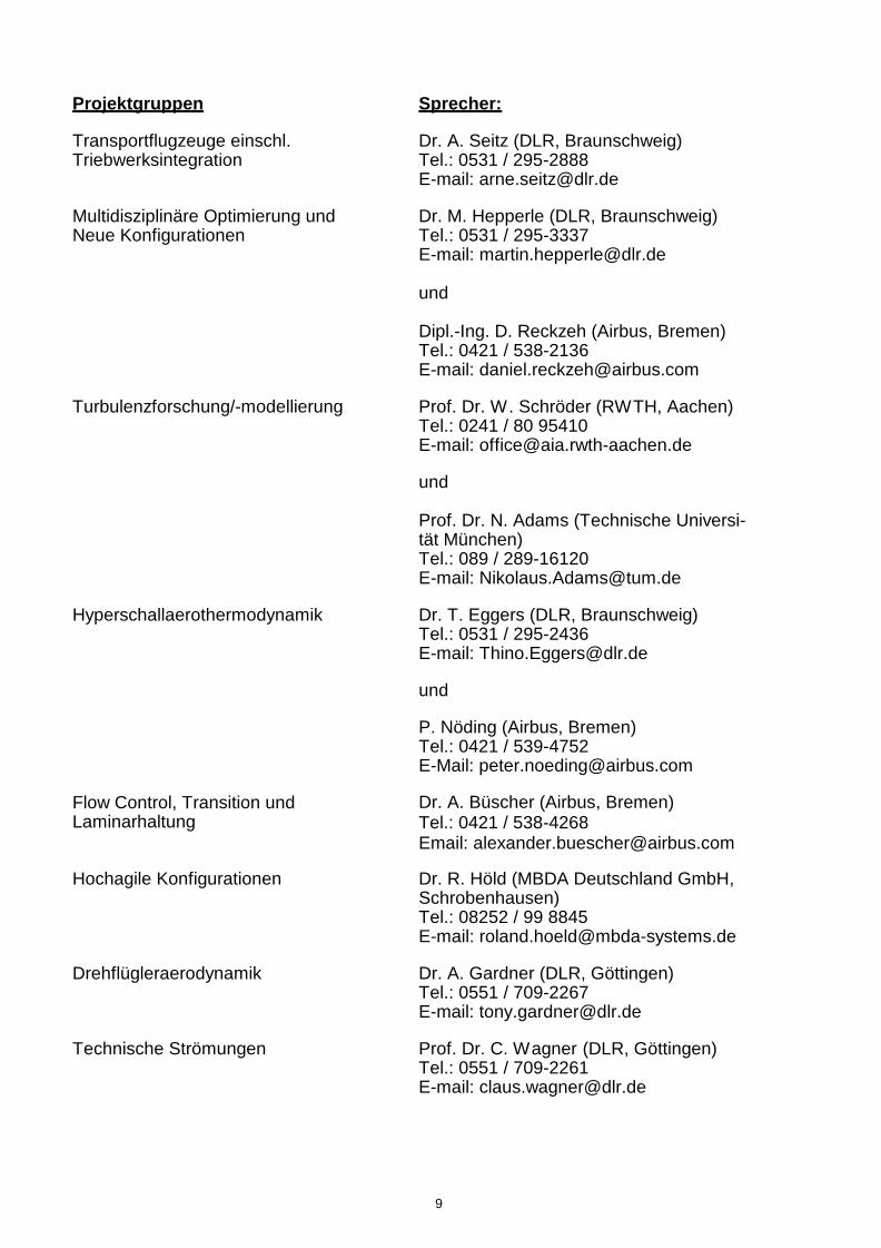
Projektgruppen Sprecher:

Transportflugzeuge einschl. Triebwerksintegration

Dr. A. Seitz (DLR, Braunschweig) Tel.: 0531 / 295-2888 E-mail: [email protected]

Multidisziplinäre Optimierung und Neue Konfigurationen

Dr. M. Hepperle (DLR, Braunschweig) Tel.: 0531 / 295-3337 E-mail: [email protected] und Dipl.-Ing. D. Reckzeh (Airbus, Bremen) Tel.: 0421 / 538-2136 E-mail: [email protected]

Turbulenzforschung/-modellierung Prof. Dr. W. Schröder (RWTH, Aachen) Tel.: 0241 / 80 95410 E-mail: [email protected]

und Prof. Dr. N. Adams (Technische Universi-tät München) Tel.: 089 / 289-16120 E-mail: [email protected]

Hyperschallaerothermodynamik Dr. T. Eggers (DLR, Braunschweig) Tel.: 0531 / 295-2436 E-mail: [email protected]

und

P. Nöding (Airbus, Bremen) Tel.: 0421 / 539-4752 E-Mail: [email protected]

Flow Control, Transition und Laminarhaltung

Dr. A. Büscher (Airbus, Bremen) Tel.: 0421 / 538-4268 Email: [email protected]

Hochagile Konfigurationen Dr. R. Höld (MBDA Deutschland GmbH, Schrobenhausen) Tel.: 08252 / 99 8845 E-mail: [email protected]

Drehflügleraerodynamik Dr. A. Gardner (DLR, Göttingen) Tel.: 0551 / 709-2267 E-mail: [email protected]

Technische Strömungen Prof. Dr. C. Wagner (DLR, Göttingen) Tel.: 0551 / 709-2261 E-mail: [email protected]

9










Fachkreise: siehe hierzu die

‚Querschnittsthemen (Q)’ der DGLR unter www.dglr.de:

Aeroelastik und Strukturdynamik Q 1.2

Prof. Dr. L. Tichy (DLR, Göttingen) Tel.: 0551 / 709-2341 E-Mail: [email protected]

Fluid- und Thermodynamik Q.2

Dr. B. Eisfeld (DLR, Braunschweig) Tel.: 0531 / 295-3305 E-mail: [email protected]

Numerische Aerodynamik Q 2.1

Dr. C. Grabe (DLR, Göttingen) Tel.: 0551 / 709-2628 E-mail: [email protected]

Experimentelle Aerodynamik Q 2.2

Prof. Dr. C. Breitsamter (Technische Univer-sität München) Tel.: 089 / 289-16137 E-mail: [email protected]

Strömungsakustik/Fluglärm Q 2.3

Prof. Dr. J. Delfs (DLR, Braunschweig) Tel.: 0531 / 295-2170 E-mail: [email protected]

Versuchsanlagen Q 2.4

Prof. Dr. G. Eitelberg (DNW, Emmeloord) Tel.: 0031 527 / 248521 E-mail: [email protected]/[email protected]

Wissenschaftlicher

Koordinator Prof. Dr. Claus Wagner (DLR Göttingen) Tel. 0551 / 709-2261 E-mail: [email protected]

Stand: Oktober 2020

10

http://www.dglr.de/




mailto:%[email protected]



Verfassen von „Mitteilungen“:

Die Anmeldungen zum STAB-Symposium bzw. STAB-Workshop werden bei der jeweiligen

Veranstaltung als Bericht/Proceedings an die Teilnehmer verteilt.

Die Mitteilung ist eine zweiseitige Kurzfassung des Beitrags, bei der nur der unten dar-

gestellte Kopf vorgegeben ist.

Mitteilung

Projektgruppe / Fachkreis:

Thema / Titel des Beitrags

Autor(en)

Institution

Adresse

E-mail

Bitte halten Sie sich bei der Anmeldung zur STAB-Veranstaltung unbedingt an die vorge-

gebenen zwei Seiten pro „Mitteilung“.

Tragen Sie bitte keine Seitenzahlen ein.

Der Druck erfolgt weiterhin ausschließlich in schwarz/weiß.

Für Rückfragen steht Ihnen die Geschäftsstelle gerne zur Verfügung:

Tel.: 0551 / 709 - 2464

Fax: 0551 / 709 - 2241

E-mail: [email protected]

Mit freundlichen Grüßen

Ihre Projektgruppenleiter/Ihre Fachkreisleiter/Ihre Geschäftsstelle

11

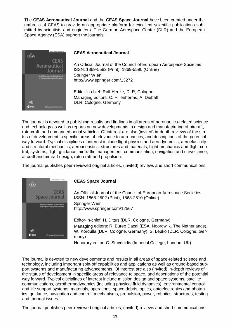
The CEAS Aeronautical Journal and the CEAS Space Journal have been created under the umbrella of CEAS to provide an appropriate platform for excellent scientific publications sub-mitted by scientists and engineers. The German Aerospace Center (DLR) and the European Space Agency (ESA) support the journals.

CEAS Aeronautical Journal

An Official Journal of the Council of European Aerospace Societies ISSN: 1869-5582 (Print), 1869-5590 (Online)

Springer Wien http://www.springer.com/13272

Editor-in-chief: Rolf Henke, DLR, Cologne

Managing editors: C. Hillenherms, A. Dieball DLR, Cologne, Germany

The journal is devoted to publishing results and findings in all areas of aeronautics-related science and technology as well as reports on new developments in design and manufacturing of aircraft, rotorcraft, and unmanned aerial vehicles. Of interest are also (invited) in-depth reviews of the sta-tus of development in specific areas of relevance to aeronautics, and descriptions of the potential way forward. Typical disciplines of interest include flight physics and aerodynamics, aeroelasticity and structural mechanics, aeroacoustics, structures and materials, flight mechanics and flight con-trol, systems, flight guidance, air traffic management, communication, navigation and surveillance, aircraft and aircraft design, rotorcraft and propulsion.

The journal publishes peer-reviewed original articles, (invited) reviews and short communications.

CEAS Space Journal

An Official Journal of the Council of European Aerospace Societies ISSN: 1868-2502 (Print), 1868-2510 (Online)

Springer Wien http://www.springer.com/12567

Editor-in-chief: H. Dittus (DLR, Cologne, Germany)

Managing editors: R. Bureo Dacal (ESA, Noordwijk, The Netherlands),

W. Kordulla (DLR, Cologne, Germany), S. Leuko (DLR, Cologne, Ger-

many)

Honorary editor: C. Stavrinidis (Imperial College, London, UK)

The journal is devoted to new developments and results in all areas of space-related science and technology, including important spin-off capabilities and applications as well as ground-based sup-port systems and manufacturing advancements. Of interest are also (invited) in-depth reviews of the status of development in specific areas of relevance to space, and descriptions of the potential way forward. Typical disciplines of interest include mission design and space systems, satellite communications, aerothermodynamics (including physical fluid dynamics), environmental control and life support systems, materials, operations, space debris, optics, optoelectronics and photon-ics, guidance, navigation and control, mechanisms, propulsion, power, robotics, structures, testing and thermal issues.

The journal publishes peer-reviewed original articles, (invited) reviews and short communications.

13

http://www.springer.com/13272




1. Projektgruppe „Transportflugzeuge einschl. Triebwerksintegration“

Seite

Ehrle Waldmann Lutz Krämer

Influence of the Wind Tunnel Model Mounting on the Wake Evolution of the Common Research Model in Post Stall

20

Müller, J. Hillebrand Lutz Krämer

Assessment of the Disturbance Velocity Approach to Determine the Gust Im-pact on Airfoils

22

Schollenberger Lutz Krämer

Comparison of different methods for the extraction of airfoil characteristics of propeller blades as input for propeller models in CFD

24

2. Projektgruppe „Multidisziplinäre Optimierung und

neue Konfigurationen“

Ilic Abu-Zurayk Schulze

Effects of different treatment of design parameters on multidisciplinary optimi-zation of transport aircraft

26

3. Projektgruppe „Turbulenzforschung/-modellierung“

Herbert Skeledzic Lienhart Ertunc

Effect of the Motion Pattern on the Turbulence Generated by an Active Grid 28

Klein, Marten Schmidt, H.

Stochastic modeling of passive scalars in turbulent channel flows 30

Korsmeier Knopp Strelets Guseva

Performance of state-of-the-art RANS models on a novel 2D turbulent waketest case producing a severe APG 32

Mäteling Klaas Schröder

A comprehensive approach to study large-scale amplitude modulation of near-wall small-scale structures in turbulent wall-bounded flows 34

Pochampalli Zhou Suarez Özkaya Gauger

Machine learning enhancement of Spalart-Allmaras Turbulence Model for airfoils 36

Weinschenk Wenzel Rist

Identification of Lagrangian Coherent Structures (LCS) in a flat-plate turbulent boundary layer with adverse pressure gradient

38

4. Projektgruppe „Hyperschallaerothermodynamik“

Franze Numerische Fehleranalyse von Modellen für hochgenaue Fluid-Struktur-Trajektorien-Kopplung

40

14

Huismannn Fechter Leicht

HyperCODA – Extension of CODA Flow Solver to Hypersonic Flows 42

Martinez Schramm Luis

Absorption Spectroscopy of NO in Hydrogen Combustion based on Hetero-dyne Techniques using Quantum Cascade Lasers

44

Martinez Schramm Schmidt, L.

Application of Ultra-Fast Internal Temperature Sensitive Paints to a Hydrogen Combustion Flow

46

Merrem Wartemann Eggers

Aerodynamic data set generation for the experimental vehicle ReFEx 48

Wartemann Konosidou Flock Merrem

Comparison of CFD simulations and TMK wind tunnel data for the DLR ReFEx flight experiment

50

5. Projektgruppe „Flow Control, Transition und Laminarhaltung“

Asaro Khalil Bauknecht

Unsteady characterization of active flow control devices for gust load allevia-tion 52

Fehrs Helm Kaiser Klimmek

Aeroelastic Behavior of a Laminar Wing in Transonic Flow 54

Franco Sumariva Theiss Hein

Influence of surface irregularities on the expected boundary-layer transition location on hybrid laminar flow control wings 56

Helm Fehrs Krimmelbein Krumbein

Transition Prediction and Analysis of the CRM-NLF wing with the DLR TAU-Code 58

Krimmelbein Krumbein

Determination of critical N-factors for the CRM-NLF wing 60

Ohno Greiner Rist

Numerical and experimental investigations of laminar separation at unsteady inflow conditions

62

Puckert Römer Scibelli Rist

Experimental investigation on roughness-induced transition under the influ-ence of freestream turbulence

64

Schrauf An estimation for the size of a suction flap for a passive HLFC system 66

Simanowitsch Theiss Hein

Receptivitiy of swept-wing boundary layers to surface roughness and inhomo-geneous suction

68

Streit Geyr von Schwep-penburg Cruz Sanchez

DLR Feasibility study of HLFC Wing Designs for S1MA Wind Tunnel Test 70

15

Tocci Franco Sumariva Hein Chauvat Hanifi

The effect of 2-D surface irregularities on laminar-turbulent transition: A com-parison of numerical methodologies 72

Ullah Lutz Krämer

Numerical Study of Dynamic 2D Bumps for Active Gust Alleviation 74

6. Projektgruppe „Hochagile Konfigurationen“

Aggarwal Hartmann Langer Leicht

Steady-state Flow Solutions for Delta Wing Configurations at High Angle of Attack using Implicit Schemes

76

Sedlacek Heckmeier Usbek Breitsamter

Analysis of Vortex Burst Phenomena on Generic Delta Wing Planforms at Subsonic Speeds 78

Voß Numerische Modellierung eines Windkanalexperiments zur Untersuchung wirbeldominierter Strömung bei mittlerem und hohem Anstellwinkel

80

7. Projektgruppe „Drehflügleraerodynamik“

Babij Müller, Martin

Aeroelastic Dynamic Stall Computations of Double-Swept Rotor Blades 82

Cerny Faust Breitsamter

Investigation of a Coaxial Propeller Configuration under Non-Axial Inflow Con-ditions

84

Debernardis Schwarz Braukmann

BOS-based three-dimensional reconstruction of rotor blade tip vortices 86

Domogalla Quantitative Detection of Vortices by Tracer Particles and Imaging Measure-ment Techniques

88

Faust Herzog Cerny Breitsamter

Systematic Analysis of a Coxial Rotor Test Bench and the Development of a Simplified Coaxial Modeling Approach

90

Gagnon Impact of Fairings on Cycloidal Rotor Aerodynamic Efficiency 92

Kostek Surmacz Rajek Goetzendorf-Grabowski

Application of fan boundary condition for modelling helicopter rotors in vertical flight 94

Kümmel Breitsamter

Bayesian Methods for Efficient Propeller Shape Optimization Applied to Airfoil Sections

96

Kunze Selection and Implementation of Approximate Boundary Layer Methods for a Fast Mid-Fidelity Aerodynamics Code for Helicopter Simulations

98

16

Lößle Kostek Schmid

Experimental measurement and calculation of a UAV rotor’s acoustic emis-sion 100

Rottmann Aerodynamic Analysis and Optimization of a Coaxial Helicopter Fuselage 102

van der Wall Effect of vortex deflection on vortex-rotor interference and rotor trim 104

Wilke Comparisons of different spatial schemes and limiters on helicopter flows 106

Yin Rossignol Experimental and numerical study on helicopter acoustic scattering 108

8. Projektgruppe „Technische Strömungen“

Bauer Müller, Max Ehrenfried Wagner, C.

On the Coverage of Dynamic Processes in Highly Separated Flows Using the Lattice Boltzmann Method 110

Birkenmaier Krenkel

Convolutional Neural Networks for Approximation of Blood Flow in Artificial Lungs

112

Brückner Westhoff Wagner, C.

Modellierung des Wärmeübergangs bei Tropfenkondensation von feuchter Luft in Mischkonvektion

114

Lange Kohl Schmeling

Experimental simulation of the human respiration system 116

Niehaus Westhoff Wagner, C.

Development of an experimental set-up to investigate heat transport in con-vective air flows with phase transition 118

Öngüner Bell Burton Henning

Experimentelle Nachbildung einer aerodynamischen Grenzschicht an Güter-zugmodellen mit passiven Strömungskontrollelementen 120

Schiepel Westhoff

Experimentelle Untersuchung des Einflusses von Zugluft auf das Komfort-empfinden in einer generischen Fahrzeugkabine

122

Weinman Wilhelmi Bell Heine Wagner, C.

An Assessment of the Aerodynamic Characterization of a Compact Car Driving behind a Heavy Vehicle using Computational Fluid Dynamics 124

Wilhelmi Jessing Bell Heine Wiedemann Wagner, A. Wagner, C.

Aerodynamic Characterisation of a Compact Car Driving Behind a Heavy Vehicle 126

9. Fachkreis „Aeroelastik und Strukturdynamik“

Bach Feldwisch

Numerical Simulation and Validation of a 2g-Turn Manoeuvre for the DLR ATRA

128

17

Bustamante López Validation of a High-Fidelity Flight Dynamics Simulation for a Longitudinal Maneuver of the DLR ATRA

130

Feldwisch Schulze

High-Fidelity Aeroelastic Loads Calculation for a Transport Aircraft Configura-tion Including Pitch and Roll Maneuvers

132

Pflüger Breitsamter

Deformation Measurements of a Full Model with Adaptive Elasto-Flexible Membrane Wings

134

Reinbold Breitsamter

Numerical investigation of flexibility effects on the aerodynamic characteristics of delta wing control surfaces

136

10.

Göing Hogrefe Lück Friedrichs

138

Olmeda Stemmer

LES of H2/N2 Transcritical Injection 140

11. Fachkreis „Numerische Aerodynamik“

Bock Towards a Galerkin-Type High-Order Panel Method for Large-Scale Loads Analyses: A 2D Prototype

142

Cormier Lutz Krämer

Numerical Investigation of the unsteady Flow Field past an Offshore Wind Turbine in Maintenance Operations

144

Genuit Keßler Krämer

A Discontinuous Galerkin Chimera Method for Unsteady Flows on Moving Grids

146

Herr Probst

Effiziente Modellierung wandnaher Turbulenz in hybriden RANS/LES Simulationen

148

Jäckel Sensitivity Analysis of Discrepancy Terms introduced in Turbulence Models using Field Inversion

150

Krzikalla Rempke Bleh Wagner, M. Gerhold

Spliss: A Sparse Linear System Solver for Transparent Integration of Emerging HPC Technologies into CFD Solvers and Applications

152

Leicht Braun Langer

Convection Treatment for RANS Turbulence Model Equations 154

Löwe 𝑝-adaptives Discontinuous-Galerkin-Verfahren in CODA 156

Rajkumar Tangermann Klein, Markus

Towards a new benchmark configuration for realistic open cavity flow simulations in fighter aircrafts

158

Satcunanathan Meinke Schröder

Numerical investigation of a porous trailing edge by a zonal RANS/LES simulation

160

Streher Heinrich

Meshing strategies for dynamical modeling of movable control surfaces: to-wards high-fidelity flight maneuver simulations

162

18

Fachkreis „Fluid- und Thermodynamik“

Validierung iterativer und numerischer Leistungsberechnungsmethoden am Beispiel eines Einwelle-Turbojet-Triebwerkes

Vogt Meinke Schröder

Wall Resolved Large-Eddy Simulation of Transonic Airfoil Flow using an Unstructured Cartesian Method

164

Wendisch Wentrup Stück

Aerodynamic shape design of a powered helicopter cell using an adjoint RANS method with actuator disk modelling

166

Zahn Breitsamter

Neuro-fuzzy based reduced-order modeling of transonic buffet on the NASA Common Research Model

168

12. Fachkreis „Experimentelle Aerodynamik“

Heckmeier Mooshofer Hopfes Breitsamter Adams

Experimental investigation of a line-cavity system equipped with fiber-optic differential pressure sensors in a shock tube 170

Meyer 2D-Flügelprofiluntersuchungen in einer offenen Messstrecke: Aufbau, Mess-technik, Windkanalkorrekturen, Validierung

172

Meyer Untersuchungen zur Wirksamkeit aufgesetzter kleiner Vorderkantenradien für die Hochauftriebsbegrenzung von Windkraft-Laminarprofilen

174

Ruhland Breitsamter

Wake Vortex Analysis on Transport Aircraft Wing featuring Dynamic Flap Motion 176

13. Fachkreis „Strömungsakustik/Fluglärm“

Franco Ewert Soni Mößner Delfs

Propeller Source Noise Model with Mean Flow Basic considerations on description 178

Schütz Foysi

Eine simultane LES-FWH Methode für die Vorhersage von Schall in Anwe-senheit von Wirbelstärke und einer Hintergrundströmung

180

Schütz Foysi

Untersuchung der Lighthill-Quell Komponenten einer Freistrahl-Tragflügel-Klappen-Konfiguration

182

Zhou Gauger Molina Alonso Michel Thiele

Jet Noise Prediction using HyKbrid RANS/LES Simulation in SU2 184

19

STAB

the investigation.influences the behavior of the separated wake. This far field effect of the sting is also part of around the model geometry. The effective Mach number at the wing is reduced and thus inflow direction.The presence of the sting causes a measurable change in the pressure field near the aircraft tail are investigated, with the goal of determining its effect on the tailplane well as of the spanwise lift distribution. The local flow effects caused by the support system the ESWIRP project [1]. The analyses comprise differences in total wing and tailplane lift as a proven approach for such conditions. The results are compared to experimental data from Hybrid RANS/LES calculations using the DDES model are used for this reason, representing the complex flow in the separated wake due to instability and breakdown of shear layers. vious work [4] showed that scale resolving simulations are necessary to accurately resolve wind tunnel and free flight configuration are quantified at an angle of attack of 𝛼 = 18°. Pre- es on the post stall regime at 𝑀∞ = 0.25 and 𝑅𝑒∞ = 11.6 · 106. The differences between

The TAU flow solver provided by DLR [3] is used for all simulations. The present work focus-

Test Case Setup and Analyses

simulations with wind tunnel data.effects provides quantitative data on expected inaccuracies involved in comparing free flight zontal tailplane at subsonic flow conditions and high angles of attack. Understanding of these the wind tunnel model affects the propagation of the wake and its interaction with the hori- still insufficiently explored. The present study deals with the question of how the mounting of the wing pressure distribution, and the local flow at the aircraft's tail, its effect in post stall is While these studies indicate an influence of the mounting on the aerodynamic coefficients, mounting include the transonic regime [2] and the linear range of the angle of attack polar [5]. model suspension system into the fuselage. Investigations of the influence of the wind tunnel the free flight configuration in the area of the rear fuselage, which is the entry point of the mized in ETW by the use of slotted walls, the wind tunnel model differs fundamentally from project [1] and simulations of the free flight configuration. While the wall influence is mini- rimental results from the European Transonic Wind tunnel (ETW) on the basis of the ESWIRP Common Research Model (CRM) in post stall regime [4]. This includes comparisons of expe- the authors' working group has already dealt with flow physics in the wake of the NASA ween wind tunnel and simulation results and increase uncertainties. Prior work carried out in support system and the tunnel walls. Such simplifications introduce inherent differences bet- Simulations aimed at free flight conditions ignore wind tunnel specific effects such as the in combination with correction factors are often used to mimic wind tunnel effects.tion of a wind tunnel experiment is taken into account. Therefore, simplifications of the setup However, the computational effort increases significantly when the full geometric configura- mental conditions in the simulation setup need to be modeled as accurately as possible. methods. In order to ensure comparability between simulation and experiment, the experi- Validation experiments are of great importance for the development of modern CFD Introduction

Pfaffenwaldring 21, 70569 Stuttgart, Germany, [email protected] of Aerodynamics and Gas Dynamics, University of Stuttgart,

Maximilian Ehrle, Andreas Waldmann, Thorsten Lutz and Ewald Krämer

Research Model in Post StallInfluence of the Wind Tunnel Model Mounting on the Wake Evolution of the Common

Projektgruppe/Fachkreis: Transportflugzeuge einschl. Triebwerksintegration

Mitteilung

20

STAB

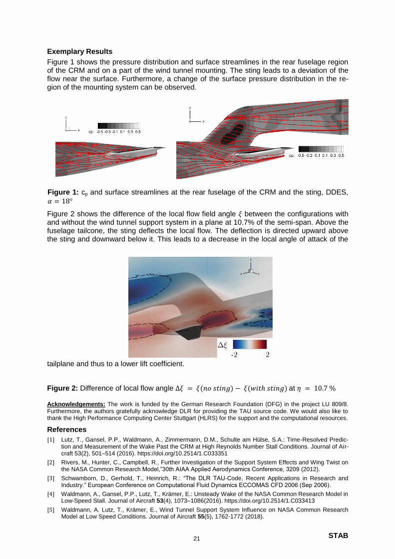
Exemplary Results

Figure 1 shows the pressure distribution and surface streamlines in the rear fuselage region of the CRM and on a part of the wind tunnel mounting. The sting leads to a deviation of the flow near the surface. Furthermore, a change of the surface pressure distribution in the re-gion of the mounting system can be observed.

Figure 1: cp and surface streamlines at the rear fuselage of the CRM and the sting, DDES,

𝛼 = 18°

Figure 2 shows the difference of the local flow field angle 𝜉 between the configurations with and without the wind tunnel support system in a plane at 10.7% of the semi-span. Above the fuselage tailcone, the sting deflects the local flow. The deflection is directed upward above the sting and downward below it. This leads to a decrease in the local angle of attack of the

tailplane and thus to a lower lift coefficient.

Figure 2: Difference of local flow angle ∆𝜉 = 𝜉(𝑛𝑜 𝑠𝑡𝑖𝑛𝑔) − 𝜉(𝑤𝑖𝑡ℎ 𝑠𝑡𝑖𝑛𝑔) at 𝜂 = 10.7 % Acknowledgements: The work is funded by the German Research Foundation (DFG) in the project LU 809/8.

Furthermore, the authors gratefully acknowledge DLR for providing the TAU source code. We would also like to thank the High Performance Computing Center Stuttgart (HLRS) for the support and the computational resources.

References

[1] Lutz, T., Gansel, P.P., Waldmann, A., Zimmermann, D.M., Schulte am Hülse, S.A.: Time-Resolved Predic-tion and Measurement of the Wake Past the CRM at High Reynolds Number Stall Conditions. Journal of Air-craft 53(2), 501–514 (2016). https://doi.org/10.2514/1.C033351

[2] Rivers, M., Hunter, C., Campbell, R., Further Investigation of the Support System Effects and Wing Twist on the NASA Common Research Model,”30th AIAA Applied Aerodynamics Conference, 3209 (2012).

[3] Schwamborn, D., Gerhold, T., Heinrich, R.: “The DLR TAU-Code, Recent Applications in Research and Industry.” European Conference on Computational Fluid Dynamics ECCOMAS CFD 2006 (Sep 2006).

[4] Waldmann, A., Gansel, P.P., Lutz, T., Krämer, E.: Unsteady Wake of the NASA Common Research Model in Low-Speed Stall. Journal of Aircraft 53(4), 1073–1086(2016). https://doi.org/10.2514/1.C033413

[5] Waldmann, A. Lutz, T., Krämer, E., Wind Tunnel Support System Influence on NASA Common Research Model at Low Speed Conditions. Journal of Aircraft 55(5), 1762-1772 (2018).

21

STAB

Mitteilung Projektgruppe/Fachkreis: Transportflugzeuge einschl. Triebwerksintegration Assessment of the Disturbance Velocity Approach to Determine the Gust Impact on

Airfoils

Jens Müller, Marco Hillebrand, Thorsten Lutz, Ewald Krämer Institute of Aerodynamics and Gas Dynamics, University of Stuttgart

Pfaffenwaldring 21, 70569 Stuttgart [email protected]

Introduction

The interaction of aircraft with atmospheric gusts leads to fluctuations of the aerodynamic forces which increase the structural loads. Hence, the effects of gust loads on aircraft have to be evaluated in the aircraft design process. In industrial application models based on linear potential flow theory like the unsteady vortex lattice or the doublet-lattice method [1] are widely used. While these methods offer a fast computation and low costs, they neglect transonic and viscous effects. Higher accuracy can be achieved when using CFD simulation. The Resolved Atmosphere Approach (RAA) [2], [3] is the most accurate method to represent atmospheric gusts in CFD simulations. Unsteady far field boundaries are used to feed the gust into the flow field. The gust is then propagated and resolved within the flow field with the impact of the aircraft on the evolution of the gust considered. Hence, all interactions between aircraft and gust can be covered, but a very fine mesh resolution is required to avoid numerical dissipation during propagation. This leads to high computational costs not feasible in industrial application. The so-called Disturbance Velocity Approach (DVA) adds the gust velocities to the flux balance by superposition. Hence, standard grid resolutions can be used which significantly reduces the computational effort. In contrast to the RAA, the DVA cannot cover the influence of the aircraft on the gust but covers the influence of the gust on the aircraft. Studies of Heinrich and Reimer [2] have shown that the DVA provides reasonable results in terms of lift for vertical gust interaction. Their simulations utilize a two dimensional wing – Horizontal Tail Plane (HTP) configuration consisting of NACA 0012 airfoils at subsonic and transonic conditions. The DVA is less accurate for gust wavelengths smaller or equal to the chord length. While their analysis involve a symmetrical two element configuration at zero angle of attack and focuses only on the lift response, the scope of the work at hand is to evaluate and identify the aerodynamic effects influencing the accuracy of the DVA in more detail. Setup

The unstructured flow solver TAU [4] developed by the German Aerospace Center (DLR) is used within this work. Two dimensional unsteady RANS simulations of an airfoil interacting

with a vertical “1-cos” gust are conducted where the vertical gust velocity 𝑤 is defined as

𝑤(𝑥) =𝐴𝑔𝑢𝑠𝑡

2[1 − cos (

2𝜋𝑥

𝜆)] with 0 ≤ 𝑥 ≤ 𝜆.

In line with [2] and [3] results of the simplified DVA are compared to RAA simulations. To avoid numerical losses during gust propagation within the RAA simulations a gust transport grid based on the Chimera technique is applied, see [2]. Gust interaction simulations for subsonic and transonic speeds are performed where a NACA 0012 airfoil is considered for the subsonic and the DLR-F15 airfoil is used for the transonic investigations. In order to identify the aerodynamic effects influencing the accuracy of the DVA, the gust wavelength 𝜆, angle of

attack 𝛼, and airfoil shape are varied. Angle of attack and shape variations are carried out for the critical gust wavelength of the DVA to be accurate. In the final manuscript selected results are presented with the focus on the aerodynamic effects influencing the accuracy of the DVA.

22

STAB

Exemplary Results

Subsonic investigations at 𝑀 = 0.25 and 𝑅𝑒 = 11.6 ∙ 106 of a NACA 0012 airfoil encountering vertical “1-cos” gusts with 𝜆/𝑐 = 1, 𝜆/𝑐 = 2 and 𝜆/𝑐 = 4 and 𝐴𝑔𝑢𝑠𝑡 = 0.1𝑢∞ at 𝛼 = 4° were

conducted. They show that lift, drag, and pitching moment coefficient of the RAA and DVA

simulations agree well for 𝜆/𝑐 = 2 and 𝜆/𝑐 = 4 with the highest deviations present in the pitching moment. 𝜆/𝑐 = 1 can be identified as the critical wavelength for the DVA to be

accurate where the 𝑐𝑙, 𝑐𝑑, and 𝑐𝑚 time histories of DVA and RAA simulation show differences to be considered. A variation of the angle of attack enables the evaluation of the influence of the flow acceleration above and the deceleration below the airfoil on the accuracy of the DVA. The differences in streamwise velocity above and below the airfoil lead to an offset in the gust position above and beneath the airfoil which can be covered by the RAA but is not taken into account when using the DVA. Additionally, an increase in angle of attack leads to higher velocity gradients at the leading edge region and a more pronounced suction peak. The time

history of the aerodynamic coefficients at 𝛼 = 0°, where the flow around the airfoil is symmetric, 𝛼 = 4°, and 𝛼 = 10° is shown in Figure 1 where 𝑡𝑟𝑒𝑓 = 𝑐/𝑢∞.

Figure 1: Time history of a NACA 0012 airfoil interacting with a vertical “1-cos” gust with critical

gust wavelength 𝜆 = 𝑐.

The results show that the agreement in maximum lift between DVA and RAA increases with increasing 𝛼 whereas 𝑐𝑑 and especially 𝑐𝑚 show significant deviations between RAA and DVA at high angles of attack. Hence, the difference in the relative gust position above and below the airfoil in the RAA simulation has no negative influence on the accuracy of the maximum lift calculated using the DVA. While the agreement in maximum 𝑐𝑚 increases at higher 𝛼,

significant deviations in the pitching moment history occur at 𝛼 = 10° especially when the gust interacts with the leading edge and when the gust is located downstream from the trailing edge. This limits the applicability of the DVA at higher angles of attack. Acknowledgment The authors gratefully acknowledge the Federal Ministry for Economic Affairs and Energy, which

funded the work presented in this report as part of the LuFo project VitAM-Turbulence.

References

[1] C. Wales, C. Valente, R. Cook, A. Gaitonde, D. Jones and J. E. Cooper, "The Future of Non-linear Modelling of aeroelastic Gust Interaction," 2018 Applied Aerodynamics Conference, 25-29 June 2018.

[2] R. Heinrich and L. Reimer, "Comparison of Different Approaches For Gust Modelling in the CFD Code TAU," International Forum on Aeroelasticity & Structural Dynamics 2013, Bristol, 24.-27. Juni 2013.

[3] R. Heinrich and L. Reimer, "Comparison of Different Approaches for Modeling of Atmospheric Efffects like Gusts and Wake-Vortices in the CFD Code TAU," International Forum on Aeroelasticity & Structural Dynamics 2017, Como, 25-28 Juni 2017.

[4] D. Schwamborn, T. Gerhold and R. Heinrich, "The DLR-TAU-Code, Recent Applications in Research and Industry," European Conference on Computational Fluid Dynamics ECCOMAS CFD, September 2006.

23

STAB

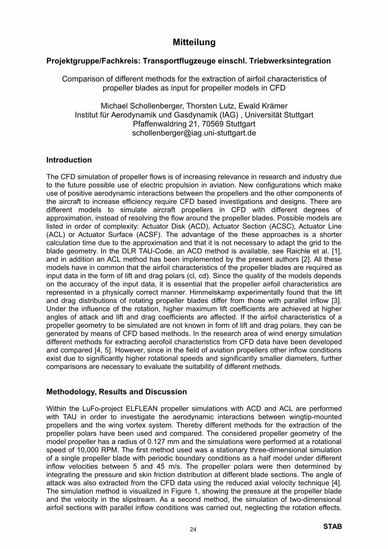
airfoil sections with parallel inflow conditions was carried out, neglecting the rotation effects.and the velocity in the slipstream. As a second method, the simulation of two-dimensional The simulation method is visualized in Figure 1, showing the pressure at the propeller blade attack was also extracted from the CFD data using the reduced axial velocity technique [4]. integrating the pressure and skin friction distribution at different blade sections. The angle of inflow velocities between 5 and 45 m/s. The propeller polars were then determined by of a single propeller blade with periodic boundary conditions as a half model under different speed of 10,000 RPM. The first method used was a stationary three-dimensional simulation model propeller has a radius of 0.127 mm and the simulations were performed at a rotational propeller polars have been used and compared. The considered propeller geometry of the propellers and the wing vortex system. Thereby different methods for the extraction of the with TAU in order to investigate the aerodynamic interactions between wingtip-mounted Within the LuFo-project ELFLEAN propeller simulations with ACD and ACL are performed

Methodology, Results and Discussion

comparisons are necessary to evaluate the suitability of different methods.exist due to significantly higher rotational speeds and significantly smaller diameters, further and compared [4, 5]. However, since in the field of aviation propellers other inflow conditions different methods for extracting aerofoil characteristics from CFD data have been developed generated by means of CFD based methods. In the research area of wind energy simulation propeller geometry to be simulated are not known in form of lift and drag polars, they can be angles of attack and lift and drag coefficients are affected. If the airfoil characteristics of a Under the influence of the rotation, higher maximum lift coefficients are achieved at higher and drag distributions of rotating propeller blades differ from those with parallel inflow [3]. represented in a physically correct manner. Himmelskamp experimentally found that the lift on the accuracy of the input data, it is essential that the propeller airfoil characteristics are input data in the form of lift and drag polars (cl, cd). Since the quality of the models depends models have in common that the airfoil characteristics of the propeller blades are required as and in addition an ACL method has been implemented by the present authors [2]. All these blade geometry. In the DLR TAU-Code, an ACD method is available, see Raichle et al. [1], calculation time due to the approximation and that it is not necessary to adapt the grid to the (ACL) or Actuator Surface (ACSF). The advantage of the these approaches is a shorter listed in order of complexity: Actuator Disk (ACD), Actuator Section (ACSC), Actuator Line approximation, instead of resolving the flow around the propeller blades. Possible models are different models to simulate aircraft propellers in CFD with different degrees of the aircraft to increase efficiency require CFD based investigations and designs. There are use of positive aerodynamic interactions between the propellers and the other components of to the future possible use of electric propulsion in aviation. New configurations which make The CFD simulation of propeller flows is of increasing relevance in research and industry due

Introduction

[email protected] Pfaffenwaldring 21, 70569 Stuttgart

Institut für Aerodynamik und Gasdynamik (IAG) , Universität StuttgartMichael Schollenberger, Thorsten Lutz, Ewald Krämer

propeller blades as input for propeller models in CFDComparison of different methods for the extraction of airfoil characteristics of

Projektgruppe/Fachkreis: Transportflugzeuge einschl. Triebwerksintegration

Mitteilung

24

The polars calculated from both methods were used for the ACL simulation and comparedwith the results of a unsteady three-dimensional fully resolved simulation of the propellergeometry with the rotation realized by the Chimera technique. With the three-dimensionalmethod a very high accuracy could be achieved. Figure 2 shows the comparison of the axialand tangential velocity, in a section x=0.15 m behind the propeller disk for the fully resolvedsimulation and the ACL with the three-dimensional based airfoil characteristics. However, thismethod requires much more effort in terms of meshing and computational time than the two-dimensional method.

In order to reduce the computational effort, a third method has the approach, to recover thelift and drag distributions from the slipstream's velocity and pressure data of one singlepropeller operating condition, taking into account a scaling of the radius to compensate forthe slipstream contraction and assuming a lift gradient of 2π. This method is especiallyintended if values from the propeller wake are already available, e.g. from experiments orexisting CFD data and has already been used in [2]. The advantage is that no exact propellergeometry and no CFD simulation is required. The final paper will compare the results of allmethods and discuss their accuracy and effort to generate input data for propeller models inCFD.

References

[1] A. Raichle, S. Melber-Wilkending, J. Himisch: A new actuator disk model for the TAUcode and application to a sailplane with a folding engine, NewResults in Numerical andExperimental Fluid Mechanics VI, 2006[2] M. Schollenberger, T. Lutz and E. Krämer: Boundary Condition Based Actuator LineModel to Simulate the Aerodynamic Interactions at Wingtip Mounted Propellers. NewResultsin Numerical and Experimental Fluid Mechanics XII, 2020[3] A. Raichle: Flusskonservative Diskretisierung des Wirkscheibenmodells als Unstetigkeits-fläche. PhD thesis, DLR, 2017[4] J. Johansen and N.N. Sørensen: Aerofoil Characteristics from 3D CFD RotorComputations, Wind Energy, 7. , 2004[5] G. Bangga: Comparison of Blade Element Method and CFD Simulations of a 10 MWWind Turbine, Fluids - Open Access Journal, 2018

STAB25

Mitteilung

Projektgruppe/Fachkreis: Multidisziplinare Optimierung und neue Konfigurationen

Effects of different treatment of design parameterson multidisciplinary optimization of transport aircraft

Caslav Ilic1,†, Mohammad Abu-Zurayk1, Matthias Schulze2

German Aerospace Center (DLR)1Institute of Aerodynamics and Flow Technology, Lilienthalplatz 7, 38108 Braunschweig

2Institute of Aeroelasticity, Bunsenstr. 10, 37073 Gottingen†Corresponding author, [email protected]

A multidisciplinary optimization (MDO) problem is given by a set of objectives, constraintsand design parameters. There exist multiple methods of solving an MDO problem, often called“formulations” or “architectures”, each with its advantages and disadvantages. Theoretically,the methods should differ only in their convergence rates, i.e. in the time needed to find thesolution. However, in a more practical setting, different methods may reach different solutions.This may happen not only due to existence of multiple local optima, but also due to noise inobjective and constraint evaluation and lack of complete derivative information. Both these traitsare often exhibited by well-established, industrial-capable disciplinary analysis and optimizationprocesses, when used as building blocks of an MDO process.

Within the DLR project VicToria, several kinds of MDO processes were developed, whichhappened to have used almost same disciplinary tools. This opens up the possibility to examineany differences in solutions that these MDO processes may deliver, for the same underlyingproblem definition and involved disciplinary tools. Two MDO processes will be used in thisstudy: an overall gradient-based process with approximate derivatives[1] (abbrev. GAD) and amixed global derivative-free/local gradient-based process[4] (abbrev. MFG).

The core of both processes is formed by two disciplinary subprocesses. The aeroelastic aero-dynamic shape analysis and optimization process[3] employs RANS equations for flow and linear-elastic FE equations for structure, with 3 degrees-of-freedom elastic trimming for steady flight,and coupled-adjoint method for computing derivatives. The loads analysis and structural op-timization process[2] employs dynamic beam model and doublet-lattice method for loads eval-uation, a shell-beam linear-elastic global FE model for gradient-based structural sizing, withconstraints of strength, buckling, and aileron reversal.

In the full paper, the two MDO processes will be firstly run with different settings of their ownoptimization parameters (such as parameter scalings), to see if different solutions are reached,and by how much. Secondly, solutions from the two MDO processes will be compared betweeneach other. Hopefully, this will shed some light on how to approach an MDO problem in a moreindustry-near setting.

At the time of this writing, a set of solutions from the MFG process is available, shown byFig. 1. Here, the goal was to optimize a twin-engine long-range airliner for minimum fuel burnover a prescribed mission. There were 2 planform design parameters (wing aspect ration, wingsweep), 126 airfoil design parameters (airfoil shape control points of 7 key section), and 392 struc-tural design parameters (thicknesses of spar, rib, and skin regions). Three optimizations wereperformed: with planform and airfoil parameters together (however in a specific global/localway), with only planform parameters at fixed airfoil shapes optimized for baseline planform,and with only planform parameters at fixed baseline airfoil shapes. In all three cases, struc-tural parameters were employed too. The latter two cases were intended as a check if sequentialglobal–local optimization (i.e. only planform—only airfoils—repeat) would be a reasonable ap-proach. It turned out that the sequential approaches get bogged down in the noise of disciplinarysubprocesses: while they change the planform parameters somewhat, the objective function (fuelburn) remains within or barely exits the noise band. This seen in the convergence rate shownby Fig. 2.

STAB26

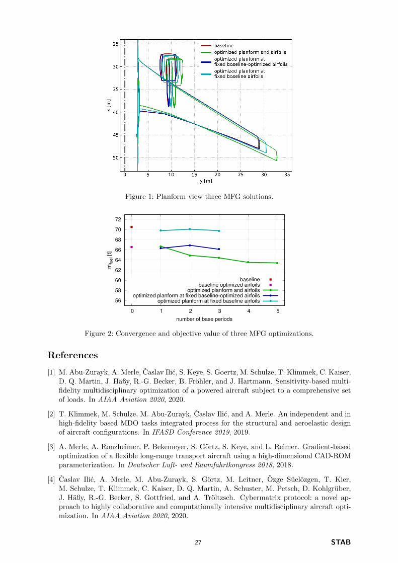
Figure 1: Planform view three MFG solutions.

56

58

60

62

64

66

68

70

72

0 1 2 3 4 5

mfu

el [

t]

number of base periods

baselinebaseline optimized airfoils

optimized planform and airfoilsoptimized planform at fixed baseline-optimized airfoils

optimized planform at fixed baseline airfoils

Figure 2: Convergence and objective value of three MFG optimizations.

References

[1] M. Abu-Zurayk, A. Merle, Caslav Ilic, S. Keye, S. Goertz, M. Schulze, T. Klimmek, C. Kaiser,D. Q. Martin, J. Haßy, R.-G. Becker, B. Frohler, and J. Hartmann. Sensitivity-based multi-fidelity multidisciplinary optimization of a powered aircraft subject to a comprehensive setof loads. In AIAA Aviation 2020, 2020.

[2] T. Klimmek, M. Schulze, M. Abu-Zurayk, Caslav Ilic, and A. Merle. An independent and inhigh-fidelity based MDO tasks integrated process for the structural and aeroelastic designof aircraft configurations. In IFASD Conference 2019, 2019.

[3] A. Merle, A. Ronzheimer, P. Bekemeyer, S. Gortz, S. Keye, and L. Reimer. Gradient-basedoptimization of a flexible long-range transport aircraft using a high-dimensional CAD-ROMparameterization. In Deutscher Luft- und Raumfahrtkongress 2018, 2018.

[4] Caslav Ilic, A. Merle, M. Abu-Zurayk, S. Gortz, M. Leitner, Ozge Suelozgen, T. Kier,M. Schulze, T. Klimmek, C. Kaiser, D. Q. Martin, A. Schuster, M. Petsch, D. Kohlgruber,J. Haßy, R.-G. Becker, S. Gottfried, and A. Troltzsch. Cybermatrix protocol: a novel ap-proach to highly collaborative and computationally intensive multidisciplinary aircraft opti-mization. In AIAA Aviation 2020, 2020.

STAB27

STAB

Mitteilung Projektgruppe/Fachkreis: Turbulenzforschung/ -modellierung

Effect of the Motion Pattern on the Turbulence Generated by an Active Grid

M. Herbert, T. Skeledzic, H. Lienhart, Ö. Ertunc Lehrstuhl für Strömungsmechanik, Friedrich-Alexander-Universität Erlangen-

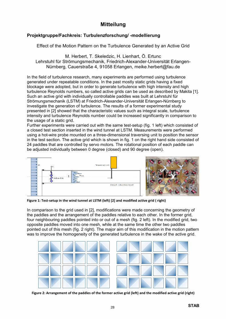
Nürnberg, Cauerstraße 4, 91058 Erlangen, [email protected] In the field of turbulence research, many experiments are performed using turbulence generated under repeatable conditions. In the past mostly static grids having a fixed blockage were adopted, but in order to generate turbulence with high intensity and high turbulence Reynolds numbers, so called active grids can be used as described by Makita [1]. Such an active grid with individually controllable paddles was built at Lehrstuhl für Strömungsmechanik (LSTM) at Friedrich-Alexander-Universität Erlangen-Nürnberg to investigate the generation of turbulence. The results of a former experimental study presented in [2] showed that the characteristic values such as integral scale, turbulence intensity and turbulence Reynolds number could be increased significantly in comparison to the usage of a static grid. Further experiments were carried out with the same test-setup (fig. 1 left) which consisted of a closed test section inserted in the wind tunnel at LSTM. Measurements were performed using a hot-wire probe mounted on a three-dimensional traversing unit to position the sensor in the test section. The active grid which is shown in fig. 1 on the right hand side consisted of 24 paddles that are controlled by servo motors. The rotational position of each paddle can be adjusted individually between 0 degree (closed) and 90 degree (open).

Figure 1: Test-setup in the wind tunnel at LSTM (left) [2] and modified active grid ( right) In comparison to the grid used in [2], modifications were made concerning the geometry of the paddles and the arrangement of the paddles relative to each other. In the former grid, four neighbouring paddles pointed into or out of a mesh (fig. 2 left). In the modified grid, two opposite paddles moved into one mesh, while at the same time the other two paddles pointed out of this mesh (fig. 2 right). The major aim of this modification in the motion pattern was to improve the homogeneity of the generated turbulence in the wake of the active grid.

Figure 2: Arrangement of the paddles of the former active grid (left) and the modified active grid (right)

28

STAB

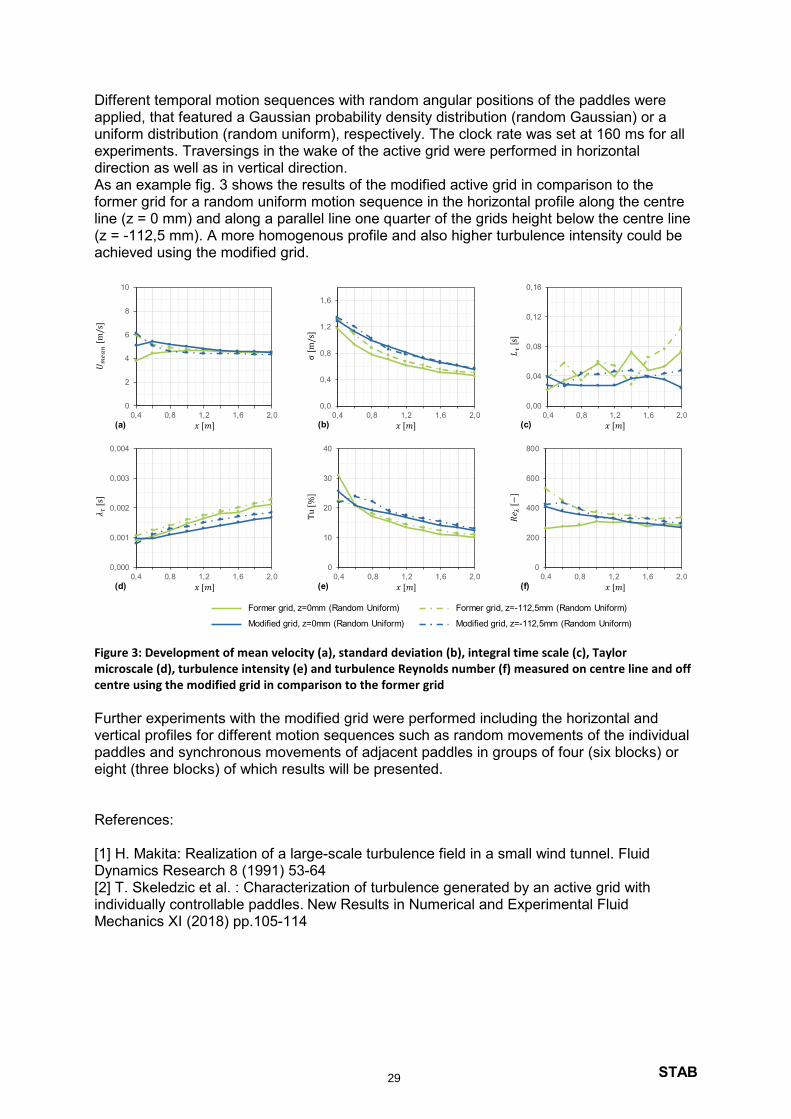
Different temporal motion sequences with random angular positions of the paddles were applied, that featured a Gaussian probability density distribution (random Gaussian) or a uniform distribution (random uniform), respectively. The clock rate was set at 160 ms for all experiments. Traversings in the wake of the active grid were performed in horizontal direction as well as in vertical direction. As an example fig. 3 shows the results of the modified active grid in comparison to the former grid for a random uniform motion sequence in the horizontal profile along the centre line (z = 0 mm) and along a parallel line one quarter of the grids height below the centre line (z = -112,5 mm). A more homogenous profile and also higher turbulence intensity could be achieved using the modified grid.

0

2

4

6

8

10

0,4 0,8 1,2 1,6 2,00,0

0,4

0,8

1,2

1,6

0,4 0,8 1,2 1,6 2,00,00

0,04

0,08

0,12

0,16

0,4 0,8 1,2 1,6 2,0

0,000

0,001

0,002

0,003

0,004

0,4 0,8 1,2 1,6 2,00

10

20

30

40

0,4 0,8 1,2 1,6 2,00

200

400

600

800

0,4 0,8 1,2 1,6 2,0

𝑥 [𝑚] 𝑥 [𝑚] 𝑥 [𝑚]

𝑥 [𝑚] 𝑥 [𝑚] 𝑥 [𝑚]

(a)

(d)

(b) (c)

(e) (f)

Former grid, z=0mm (Random Uniform)

Modified grid, z=0mm (Random Uniform)

Former grid, z=-112,5mm (Random Uniform)

Modified grid, z=-112,5mm (Random Uniform)

Figure 3: Development of mean velocity (a), standard deviation (b), integral time scale (c), Taylor microscale (d), turbulence intensity (e) and turbulence Reynolds number (f) measured on centre line and off centre using the modified grid in comparison to the former grid Further experiments with the modified grid were performed including the horizontal and vertical profiles for different motion sequences such as random movements of the individual paddles and synchronous movements of adjacent paddles in groups of four (six blocks) or eight (three blocks) of which results will be presented. References: [1] H. Makita: Realization of a large-scale turbulence field in a small wind tunnel. Fluid Dynamics Research 8 (1991) 53-64 [2] T. Skeledzic et al. : Characterization of turbulence generated by an active grid with individually controllable paddles. New Results in Numerical and Experimental Fluid Mechanics XI (2018) pp.105-114

29

Mitteilung

Projektgruppe/Fachkreis: Turbulenzforschung und -modellierung / Q2

Stochastic modeling of passive scalars in turbulent channel flows

Marten Klein* Heiko Schmidt

Lehrstuhl Numerische Strömungs- und Gasdynamik, Brandenburgische TechnischeUniversität (BTU) Cottbus-Senftenberg, Siemens-Halske-Ring 15A, D-03046 Cottbus

* Corresponding author: [email protected]

Quantitative analyses of scalar transport processes in fluid flows are relevant for many technical (like the heat transfer in cooling devices or the mixing of chemical species), environmental (like tracer and aerosol transport), and geophysical (like scalar surface fluxes in the atmospheric boundary layer) applications. Fluid flows are usually turbulent in these applications and the scalar transport is, hence, the result of turbulent (advective) stirring and molecular (diffusive) mixing processes that both act together on a range of scales. This range reaches down to the Kolmogorov and Batchelor scales that need to be resolved if a robust and accurate numerical prediction of the scalar transport is required for a given application.

In principle, direct numerical simulation (DNS) would be the ideal tool for high-fidelity scalar transport analysis and prediction. For this task, the spatial resolution can be estimated with the aid of the Kolmogorov, ηK, and Batchelor, ηB, length scales yielding grid cells as small as ηK/L ~ Re–3/4 or ηB/L ~ Sc–1/2ηK in one dimension, where Re = UL/ν denotes the Reynolds and Sc = ν /Γ the Schmidt number, ν the kinematic viscosity, Γ the scalar diffusivity, U a referencevelocity and L a reference length scale. The Bachelor length scale is more (less) restrictive than the Kolmogorov length scale when Sc > 1 (Sc < 1). A high-Sc-number scalar demands a total of O(Re9/4 Sc3/2) grid cells for a three-dimensional turbulent flow. However, even a low-Sc-number scalar is challenging, because the advecting velocity field needs to be resolved. This results in O(Re9/4) grid cells for a three-dimensional turbulent flow even when Sc << 1. For both of these cases, correspondingly high temporal resolutions are required. So, while a recent channel flow DNS without any scalars reached Re = O(105) (friction Reynolds numberReτ ≈ 5200) [1], another DNS with a passive scalar at Sc ≈ 50 remained limited to Re = O(103) (Reτ ≈ 180) [2]. In practice, Reynolds numbers may easily reach up to 106 and beyond, and Schmidt numbers may be as large as 104 [3]. DNS or high-resolution large-eddy simulation (LES) will not be feasible for this flow regime for the foreseeable future so that numerically efficient but reasonably accurate modeling strategies are required.

In the present study we numerically investigate passive scalars in fully-developed turbulent channel flows up to friction Reynolds number Reτ ≈ 5200 with Schmidt numbers (Sc) from the range 0.002 ≤ Sc ≤ 2000. For this task we apply the stochastic one-dimensional turbulence (ODT) model [4,5] in order to address both feasibility and accuracy. In ODT, a stochastic process is used to model the effects of turbulent stirring, whereas deterministic molecular diffusion is directly resolved but only for a notional line-of-sight through the turbulent flow. This line forms the ODT computational domain (the so-called “ODT line”) along which statistically representative flow profiles are numerically evolved in time. It is feasible to resolve the flow on all relevant scales even for high Schmidt and Reynolds numbers in this one-dimensional setting, but we further improve the numerical efficiency by using a fully-adaptive but conservative model implementation [6].

For stochastic channel flow simulations, we take the ODT line oriented in wall-normal direction [7,8] in order to simultaneously resolve the leading-order cross-stream passive scalar and momentum transport. ODT model parameters were calibrated for high-Re-number turbulent channel flows [1] to make sure that the momentum transport is accurately represented. The passive scalar transport is, hence, a model prediction. We compare this prediction to available channel flow reference data for moderate [2,9] and low [10,11,12]

STAB30

Schmidt numbers. We make use of ODT's predictive capabilities and keep the numerical model parameters fixed when varying both Re and Sc numbers. For large enough Reynolds number, ODT yields the well-known defect law for the boundary layer of the mean momentum and passive scalar (e.g. [2,9,10,11]). Analogous to recent reference DNS [12], we also observe that ODT exhibits a tendency towards asymptotic flow statistics, which, for the scalar, only retain a dependency on the Sc number. When the Re number is reduced, flow statistics are subject to non-universal modifications. These small-Re-number effects areless well represented within the stand-alone application of the lower-order, stochastic model.

A key advantage of the ODT model is its ability to resolve transient dynamics (e.g. [8]) and, hence, nonstationary boundary layers. Here we make use of this feature by investigating fluctuating surface scalar and momentum fluxes and their joint probability density which would otherwise only be possible with time-resolved approaches like DNS/LES (e.g. [11]). Due to the absence of closure modeling, fluctuation statistics obtained with ODT are the result of a simulation. For channel flow, we show that the model exhibits a balanced budget of the turbulence kinetic energy (TKE) and the scalar variance, respectively. In the vicinity of the wall, and further away from it in the logarithmic layer, these budgets are found in good agreement with available reference data [1,2] which indicates that both momentum and scalar transfer to the wall reasonably well captured by ODT. In fact, we have shown recently [7] that ODT predicts the Sc- and Re-number dependence of the scalar transfer coefficient, K+, consistent with reference DNS/LES, laboratory measurements, and theoretical analysis. For Sc ≥ O(100), ODT yields K+ ~ Sc–0.65, which is close to the predictionof asymptotic one-dimensional theory (K+ ~ Sc–0.67) [3], as well as DNS and laboratory measurements (K+ ~ Sc–0.70) [2,3,9].

In the contribution to STAB 2020, we will address the ODT model formulation and its application to passive scalars in turbulent channel flow. We will also address the model calibration and Re number dependence of the momentum transport in terms of first and second order velocity statistics up to Reτ ≈ 5200. After that, we will turn to passive scalars and discuss relevant first and second order turbulence statistics by comparing ODT model predictions to available reference data where possible. We will address both low (Sc < 1) and high (Sc > 1) Schmidt number regimes for various Reynolds numbers in order to relate changes in the Sc-dependence of bulk properties (like the scalar transfer coefficient) to turbulence statistics.

REFERENCES

[1] M. Lee & R. D. Moser, J. Fluid Mech. 774 (2015) 395–415. [2] F. Schwertfirm & M. Manhart, Int. J. Heat and Fluid Flow 28 (2007) 1204–1214. [3] D. A. Shaw & T. J. Hanratty, AIChE Journal 23 (1977) 28–37. [4] A. R. Kerstein, J. Fluid Mech. 392 (1999) 277–334. [5] A. R. Kerstein, W. T. Ashurst, S. Wunsch & V. Nilsen, J. Fluid Mech. 447 (2001) 85–109. [6] D. O. Lignell, A. R. Kerstein, G. Sun & E. I. Monson, Theo. Comp. Fluid Dyn. 27 (2013) 273–295. [7] M. Klein & H. Schmidt, Proc. Appl. Math. Mech. 18 (2018) e201800238. [8] M. Klein, C. Zenker & H. Schmidt, Chem. Eng. Sci. 204 (2019) 186–202. [9] Y. Hasegawa & N. Kasagi, Int. J. Heat and Fluid Flow 30 (2009) 525–533.[10] H. Kawamura, H. Abe & Y. Matsuo, Int. J. Heat Fluid Flow 20 (1999) 196–207.[11] H. Abe, H. Kawamura & Y. Matsuo, Int. J. Heat Fluid Flow 25 (2004) 404–419.[12] S. Pirozzoli, M. Bernardini & P. Orlandi, J. Fluid Mech. 788 (2016) 614–639.

STAB31

Mitteilung

Projektgruppe/Fachkreis: Turbulenzforschung/-modellierung

Performance of state-of-the-art RANS models on a novel 2D turbulent wake test case producing a severe APG

Paul Korsmeier1, Tobias Knopp1, Mjkhail Strelets2, Ekaterina Guseva2

1 DLR, Institut für Aerodynamik und Strömungstechnik Bunsenstraße 10, 37073 Göttingen, [email protected]

2 Peter the Great St. Petersburg Polytechnic University [email protected], [email protected]

A new test case of a symmetric wake at adverse pressure gradient (APG), which emulates the flow conditions over the flap of a modern high-lift system, is presented for the targeted im-provement of RANS turbulence models towards accurate maximum lift prediction. The mod-el improvements will be based on the identification of the right model term(s) which have to be modified in the future so that the modified model yields the test case data with high accuracy. For this purpose, highly resolved data from wind tunnel experiments and a complementary nu-merical experiment, see [1], were provided.

The main goal of the test case design is to produce an APG strong enough to provoke a mean flow reversal (also called „off-body separation bubble“) in the wake of a flat plate, a phe-nomenon associated with a loss in lift and observed in actual multi-element wings. The de-sign aims at a macroscopically steady flow, which was not met, for example, for the well-known experiment by Driver and Mateer, see [2].

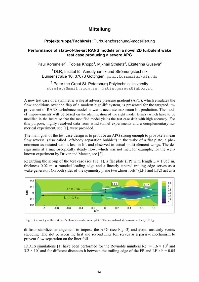
Regarding the set-up of the test case (see Fig. 1), a flat plate (FP) with length L = 1.058 m, thickness 0.02 m, a rounded leading edge and a linearly tapered trailing edge serves as a wake generator. On both sides of the symmetry plane two „liner foils“ (LF1 and LF2) act as a

diffusor-stabilizer arrangement to impose the APG (see Fig. 3) and avoid unsteady vortex shedding. The slot between the first and second liner foil serves as a passive mechanism to prevent flow separation on the liner foil.

IDDES simulations [1] have been performed for the Reynolds numbers ReL = 1.6 × 106 and 3.2 × 106 and for different distances h between the trailing edge of the FP and LF1: h = 0.05

Fig. 1: Geometry of the test case’s elements and contour plot of the normalized streamwise velocity U/Uref

32

m, 0.06 m, 0.07 m and without liner foils (ZPG). In this abstract we put the focus on the case with ReL = 1.6 × 106 and h = 0.07 m, for which the wake is at the verge of flow reversal.

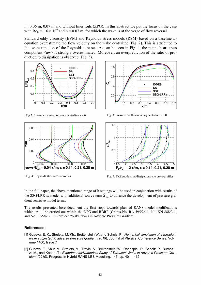
Standard eddy viscosity (EVM) and Reynolds stress models (RSM) based on a baseline -equation overestimate the flow velocity on the wake centerline (Fig. 2). This is attributed to the overestimation of the Reynolds stresses. As can be seen in Fig. 4, the main shear stress component <uw> is strongly overestimated. Moreover, an overprediction of the ratio of pro-duction to dissipation is observed (Fig. 5).

In the full paper, the above-mentioned range of h-settings will be used in conjunction with results of

the SSG/LRR- model with additional source term 4 to advance the development of pressure gra-

dient sensitive model terms.

The results presented here document the first steps towards planned RANS model modifications which are to be carried out within the DFG and RBRF (Grants No. RA 595/26-1, No. KN 888/3-1, and No. 17-58-12002) project ‘Wake flows in Adverse Pressure Gradient’.

References:

[1] Guseva, E. K., Strelets, M. Kh., Breitenstein W.,and Scholz, P.: Numerical simulation of a turbulent wake subjected to adverse pressure gradient (2019), Journal of Physics: Conference Series, Vol-ume 1400, Issue 7

[2] Guseva, E., Shur, M., Strelets, M., Travin, A., Breitenstein, W., Radespiel, R., Scholz, P., Burnaz-zi, M., and Knopp, T.: Experimental/Numerical Study of Turbulent Wake in Adverse Pressure Gra-dient (2019), Progress in Hybrid RANS-LES Modelling, 143, pp. 401 - 412

Fig. 3: Pressure coefficient along centerline z = 0

Fig. 5: TKE production/dissipation ratio cross-profiles Fig. 4: Reynolds stress cross-profiles

Fig 2: Streamwise velocity along centerline z = 0

33

STAB

Mitteilung

Projektgruppe/Fachkreis: Turbulenzforschung A comprehensive approach to study large-scale amplitude modulation of near-wall

small-scale structures in turbulent wall-bounded flows

Esther Mäteling, Michael Klaas, Wolfgang Schröder RWTH Aachen University, Institute of Aerodynamics, Wüllnerstraße 5a, 52062 Aa-

chen, [email protected]

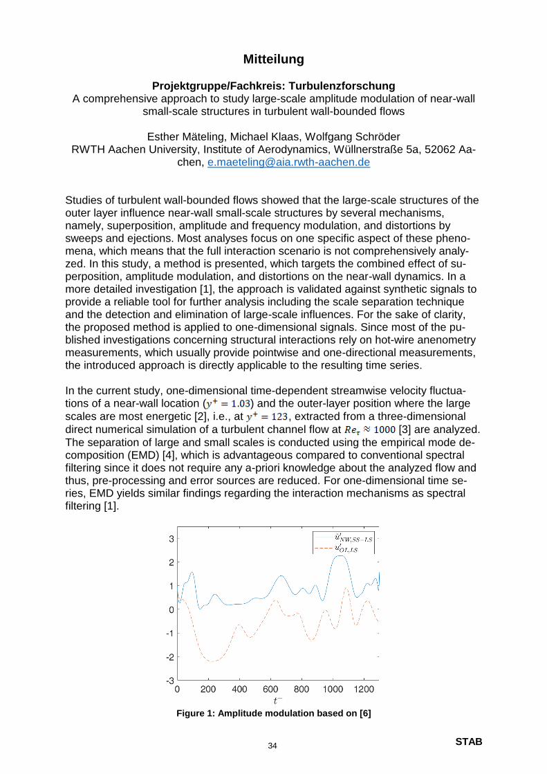
Studies of turbulent wall-bounded flows showed that the large-scale structures of the outer layer influence near-wall small-scale structures by several mechanisms, namely, superposition, amplitude and frequency modulation, and distortions by sweeps and ejections. Most analyses focus on one specific aspect of these pheno-mena, which means that the full interaction scenario is not comprehensively analy-zed. In this study, a method is presented, which targets the combined effect of su-perposition, amplitude modulation, and distortions on the near-wall dynamics. In a more detailed investigation [1], the approach is validated against synthetic signals to provide a reliable tool for further analysis including the scale separation technique and the detection and elimination of large-scale influences. For the sake of clarity, the proposed method is applied to one-dimensional signals. Since most of the pu-blished investigations concerning structural interactions rely on hot-wire anenometry measurements, which usually provide pointwise and one-directional measurements, the introduced approach is directly applicable to the resulting time series. In the current study, one-dimensional time-dependent streamwise velocity fluctua-tions of a near-wall location ( ) and the outer-layer position where the large

scales are most energetic [2], i.e., at , extracted from a three-dimensional

direct numerical simulation of a turbulent channel flow at [3] are analyzed.

The separation of large and small scales is conducted using the empirical mode de-composition (EMD) [4], which is advantageous compared to conventional spectral filtering since it does not require any a-priori knowledge about the analyzed flow and thus, pre-processing and error sources are reduced. For one-dimensional time se-ries, EMD yields similar findings regarding the interaction mechanisms as spectral filtering [1].

Figure 1: Amplitude modulation based on [6]

34


STAB

The influences of superposition and distortions manifest in an inclination angle aver-aged over all spanwise positions of , which is similar to the findings for tur-

bulent boundary layer flows from the literature [5]. For the investigation of the ampli-tude modulation a novel method is introduced. Compared to a frequently used tech-nique [6], it is superior in revealing this phenomenon due to a preceding removal of the influences of superposition and distortions. Afterwards, the near-wall and the ou-ter-layer large-scale amplitudes are determined from the analytical large-scale si-gnals, which are obtained by the Hilbert Transform. In figure 1, the near-wall large-

scale amplitude is compared to the outer-layer large scales using the

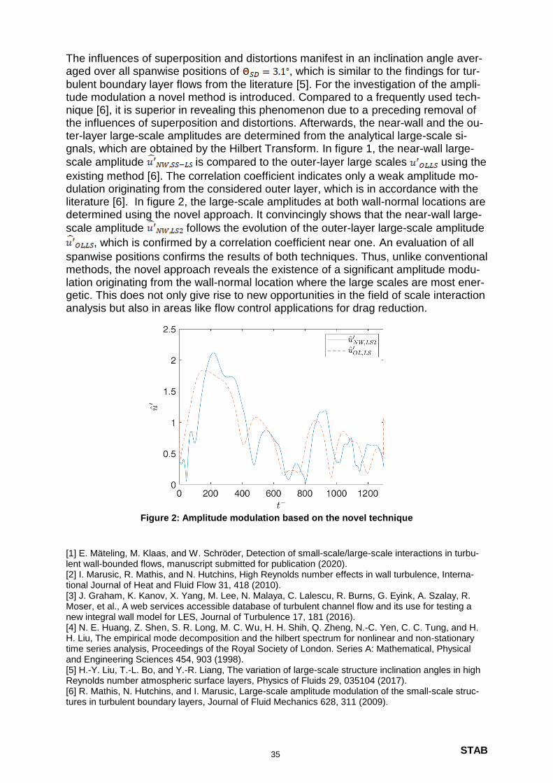
existing method [6]. The correlation coefficient indicates only a weak amplitude mo-dulation originating from the considered outer layer, which is in accordance with the literature [6]. In figure 2, the large-scale amplitudes at both wall-normal locations are determined using the novel approach. It convincingly shows that the near-wall large-

scale amplitude follows the evolution of the outer-layer large-scale amplitude

, which is confirmed by a correlation coefficient near one. An evaluation of all

spanwise positions confirms the results of both techniques. Thus, unlike conventional methods, the novel approach reveals the existence of a significant amplitude modu-lation originating from the wall-normal location where the large scales are most ener-getic. This does not only give rise to new opportunities in the field of scale interaction analysis but also in areas like flow control applications for drag reduction.

Figure 2: Amplitude modulation based on the novel technique

[1] E. Mäteling, M. Klaas, and W. Schröder, Detection of small-scale/large-scale interactions in turbu-lent wall-bounded flows, manuscript submitted for publication (2020). [2] I. Marusic, R. Mathis, and N. Hutchins, High Reynolds number effects in wall turbulence, Interna-tional Journal of Heat and Fluid Flow 31, 418 (2010). [3] J. Graham, K. Kanov, X. Yang, M. Lee, N. Malaya, C. Lalescu, R. Burns, G. Eyink, A. Szalay, R. Moser, et al., A web services accessible database of turbulent channel flow and its use for testing a new integral wall model for LES, Journal of Turbulence 17, 181 (2016). [4] N. E. Huang, Z. Shen, S. R. Long, M. C. Wu, H. H. Shih, Q. Zheng, N.-C. Yen, C. C. Tung, and H. H. Liu, The empirical mode decomposition and the hilbert spectrum for nonlinear and non-stationary time series analysis, Proceedings of the Royal Society of London. Series A: Mathematical, Physical and Engineering Sciences 454, 903 (1998). [5] H.-Y. Liu, T.-L. Bo, and Y.-R. Liang, The variation of large-scale structure inclination angles in high Reynolds number atmospheric surface layers, Physics of Fluids 29, 035104 (2017). [6] R. Mathis, N. Hutchins, and I. Marusic, Large-scale amplitude modulation of the small-scale struc-tures in turbulent boundary layers, Journal of Fluid Mechanics 628, 311 (2009).

35

STAB

Mitteilung


Machine learning enhancement of Spalart-Allmaras Turbulence Model for airfoils

Rohit Pochampalli, Beckett Y. Zhou, Guillermo Suarez, Emre Oezkaya and

Nicolas R. Gauger Chair for Scientific Computing, TU Kaiserslautern

Bldg 34, Paul-Ehrlich-Strasse, 67663 Kaiserslautern, Germany [email protected]

Introduction Reynolds averaged Navier Stokes (RANS) based turbulence models are the predominant approach to turbulence modeling, despite several shortcomings, by virtue of their low com-putational cost. These turbulence models, typically based on the Boussinesq hypothesis, are developed for specific applications and perform poorly if the flow conditions are drastically different from those for which it was calibrated, particularly with massively separated flows. On the other hand, high fidelity simulations such as direct numerical simulation (DNS) and large eddy simulation (LES) methods are computationally expensive. Hybrid approaches [1, 2] improve on the fidelity over RANS based simulations [3] typically by employing a redefinition of the length scales used in the turbulence models. The scheme presented in this work is based on the converse principle. We study if an increase in the complexity of the turbulence models could lead to better predictive accuracy. Recent years have seen a resurgence in turbulence modeling, specifically data driven ap-proaches, which utilize data from experiments or high fidelity simulations to estimate and subsequently correct functional inaccuracies [4, 5] in the models. In this paper, we consider the Spalart - Allmaras turbulence model [6], which defines a single transport equation for ed-dy turbulent viscosity and includes terms for the production, destruction and diffusion of eddy viscosity. We increase the model complexity by multiplying the production term of the model with a correction field. To estimate the correction field, we follow a framework similar to the one introduced by Duraisamy et.al [5].

Method A brief outline of the overall process follows. First, a large number of inverse problems are formulated to obtain a series of correction functions for the production term of the Spalart - Allmaras (SA) turbulence model. This correction function estimates the deficiency in the SA model for a particular test case and geometry. The data obtained from these inverse pro-blems is generalized by training a neural network to create a mapping between the mean flow variables and the inferred correction function. Subsequent to the training of the neural network, it is embedded into the CFD solver to estimate the correction field in the production term at each iteration of the iterative solver. The augmented model can then be used for new test cases. The correction function therefore forms an additional input to the ML enhanced SA model that provides a corrected eddy viscosity, which improves on the performance of the baseline SA model. The test cases considered for the preliminary results is the NACA0012 airfoil at different angles of attack, at Reynolds number 6x10

6 and Mach 0.15. The simulations are realized

using SU2 and the adjoints for the inverse problem are calculated using the discrete adjoint framework. The inverse problems for the NACA0012 case are formulated with objective function as the squared difference of the lift coefficients obtained by numerical simulation against experimental values at different angles of attack, ranging from 2 to 19 degrees. A comparison is shown in Fig. 1. The performance of the machine learning enhanced model is compared to the SA turbulence model for a subset of angles of attack for the NACA 0012

36


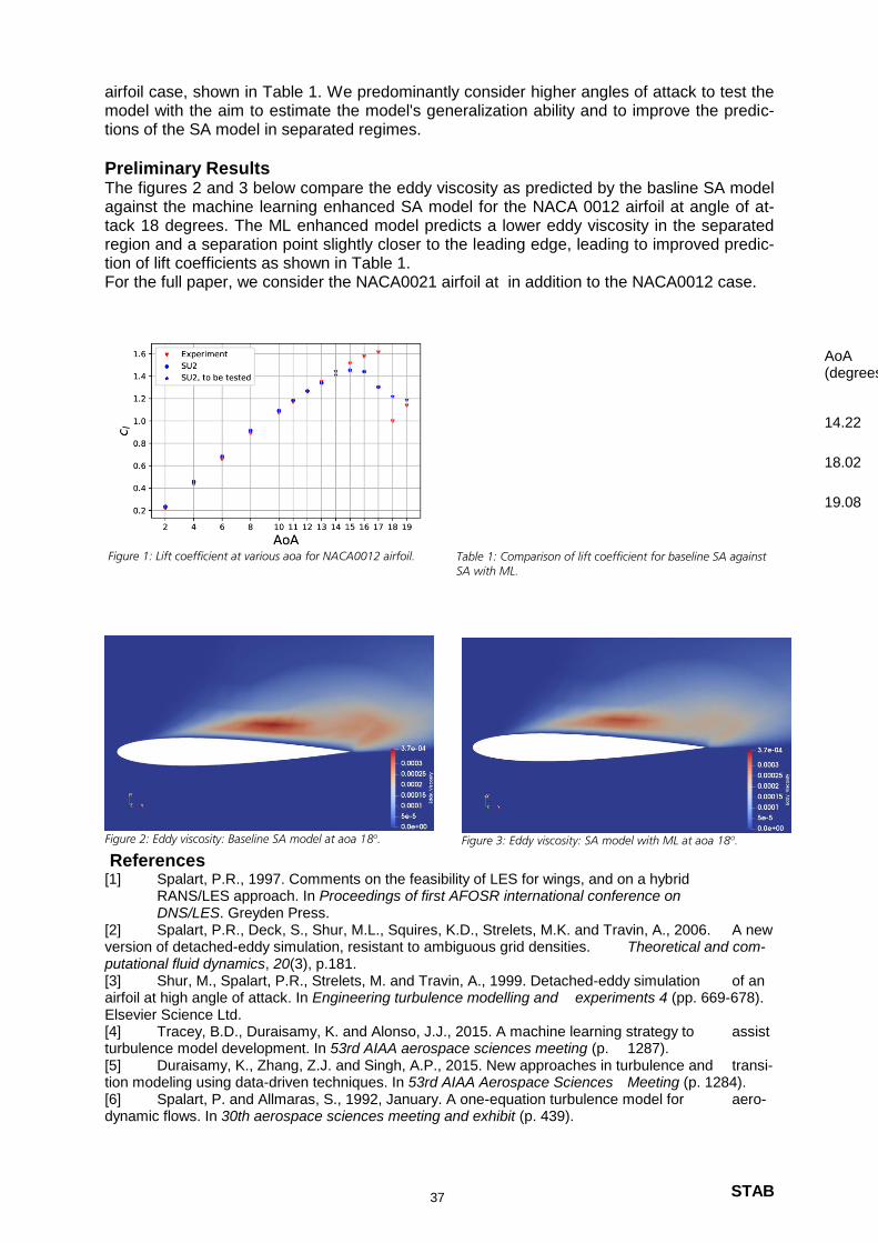
STAB

airfoil case, shown in Table 1. We predominantly consider higher angles of attack to test the model with the aim to estimate the model's generalization ability and to improve the predic-tions of the SA model in separated regimes.

Preliminary Results The figures 2 and 3 below compare the eddy viscosity as predicted by the basline SA model against the machine learning enhanced SA model for the NACA 0012 airfoil at angle of at-tack 18 degrees. The ML enhanced model predicts a lower eddy viscosity in the separated region and a separation point slightly closer to the leading edge, leading to improved predic-tion of lift coefficients as shown in Table 1. For the full paper, we consider the NACA0021 airfoil at in addition to the NACA0012 case.

AoA (degrees)

cl : Exp.

cl : Baseline SA

cl : SA with ML

14.22 1.43 1.41 1.41

18.02 0.99 1.22 1.19

19.08 1.13 1.18 1.16

Table 1: Comparison of lift coefficient for baseline SA against SA with ML.

References [1] Spalart, P.R., 1997. Comments on the feasibility of LES for wings, and on a hybrid RANS/LES approach. In Proceedings of first AFOSR international conference on DNS/LES. Greyden Press. [2] Spalart, P.R., Deck, S., Shur, M.L., Squires, K.D., Strelets, M.K. and Travin, A., 2006. A new version of detached-eddy simulation, resistant to ambiguous grid densities. Theoretical and com-putational fluid dynamics, 20(3), p.181. [3] Shur, M., Spalart, P.R., Strelets, M. and Travin, A., 1999. Detached-eddy simulation of an airfoil at high angle of attack. In Engineering turbulence modelling and experiments 4 (pp. 669-678). Elsevier Science Ltd. [4] Tracey, B.D., Duraisamy, K. and Alonso, J.J., 2015. A machine learning strategy to assist turbulence model development. In 53rd AIAA aerospace sciences meeting (p. 1287). [5] Duraisamy, K., Zhang, Z.J. and Singh, A.P., 2015. New approaches in turbulence and transi-tion modeling using data-driven techniques. In 53rd AIAA Aerospace Sciences Meeting (p. 1284). [6] Spalart, P. and Allmaras, S., 1992, January. A one-equation turbulence model for aero-dynamic flows. In 30th aerospace sciences meeting and exhibit (p. 439).

Figure 1: Lift coefficient at various aoa for NACA0012 airfoil.

Figure 2: Eddy viscosity: Baseline SA model at aoa 18o. Figure 3: Eddy viscosity: SA model with ML at aoa 18o.

37

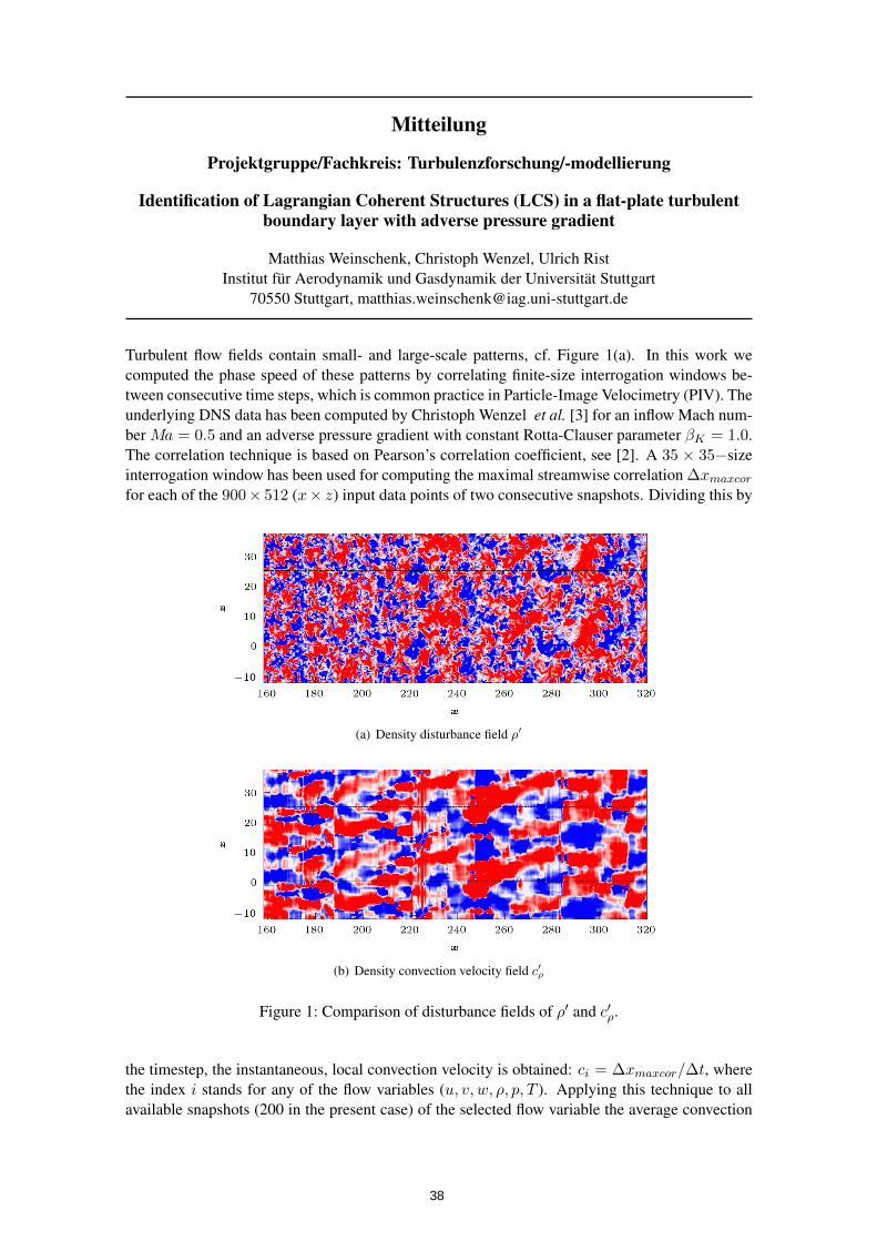
Mitteilung


Identification of Lagrangian Coherent Structures (LCS) in a flat-plate turbulentboundary layer with adverse pressure gradient

Matthias Weinschenk, Christoph Wenzel, Ulrich RistInstitut für Aerodynamik und Gasdynamik der Universität Stuttgart

70550 Stuttgart, [email protected]

Turbulent flow fields contain small- and large-scale patterns, cf. Figure 1(a). In this work wecomputed the phase speed of these patterns by correlating finite-size interrogation windows be-tween consecutive time steps, which is common practice in Particle-Image Velocimetry (PIV). Theunderlying DNS data has been computed by Christoph Wenzel et al. [3] for an inflow Mach num-ber Ma = 0.5 and an adverse pressure gradient with constant Rotta-Clauser parameter βK = 1.0.The correlation technique is based on Pearson’s correlation coefficient, see [2]. A 35 × 35−sizeinterrogation window has been used for computing the maximal streamwise correlation ∆xmaxcorfor each of the 900× 512 (x× z) input data points of two consecutive snapshots. Dividing this by

(a) Density disturbance field ρ′

(b) Density convection velocity field c′ρ

Figure 1: Comparison of disturbance fields of ρ′ and c′ρ.

the timestep, the instantaneous, local convection velocity is obtained: ci = ∆xmaxcor/∆t, wherethe index i stands for any of the flow variables (u, v, w, ρ, p, T ). Applying this technique to allavailable snapshots (200 in the present case) of the selected flow variable the average convection

38

speed ci is obtained after an additional local average in spanwise direction. Subtracting the av-erage from the instantaneous convection velocity yields high- and low-speed streaks as spatiallyconnected patterns with either positive or negative c′i = ci−ci, see Figure 1(b) showing an examplefor the outcome of this procedure applied to the density ρ′ snapshot in Figure 1(a). Interestingly,all flow variables i contain very similar patterns in their respective c′i. In addition, these patternscorrespond to the well-known high- and low-speed streaks in the streamwise velocity componentu.

Figure 2: Comparison of averaged convection velocities of all flow variables u, v, w, ρ, T, p withthe meanflow u.

Furthermore, the averaged convection velocity ci varies strongly with the wall distance and comesclose to the averaged streamwise velocity u in the logarithmic part of the mean flow profile, seegreen area in Figure 2. Obviously, all instantaneous patterns existing in this flow are bound tothe underlying material transport in streamwise direction by the streamwise velocity componentu. Only cp from the pressure p behaves different. However, this can be explained by the fact thatpressure is governed by a Poisson equation which means that it decays at a much lower rate com-pared to other variables with distance from a source. This means in the present context, that theconvection speed of the dominant structures around y+ ≈ 100 would be detectable as a pressure-wave at the wall that runs over the fluid with the speed of the coherent structures further away.The observation that all patterns (apart from pressure) travel with the local streamwise velocitymeans that these structures are bound to material, i.e., they are structures in the Lagrangian sense,presumably related to so-called Lagrangian Coherent Structures (LCS) [1].

References

[1] G Haller. Lagrangian coherent structures. Annual Review of Fluid Mechanics 2015, 47:137–162, 2015.

[2] T.D.V. Swinscow. Statistics at Square One. BMJ Publishing Group 1997, 1997.

[3] C Wenzel, B Selent, M J Kloker, and U Rist. DNS of compressible turbulent boundary layersand assessment of data/scaling-law quality. Journal of Fluid Mechanics, 842:428–468, 2018.

39

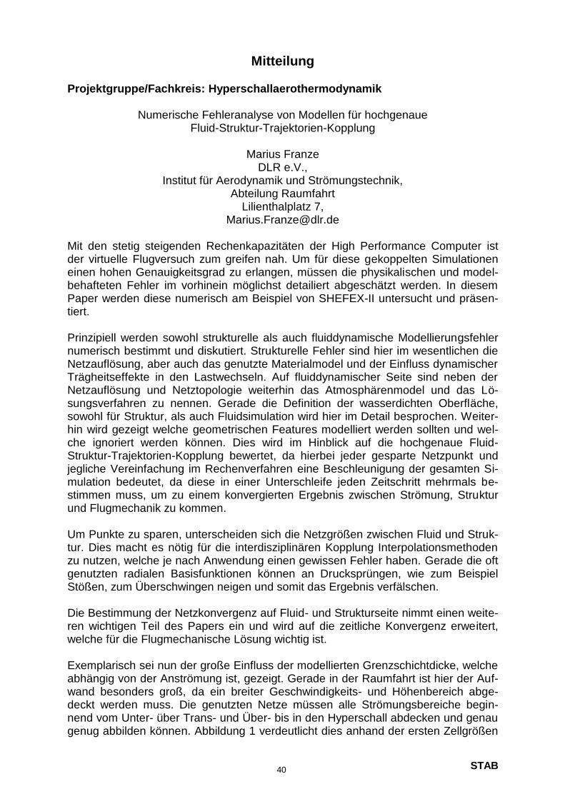
STAB

Mitteilung

Projektgruppe/Fachkreis: Hyperschallaerothermodynamik

Numerische Fehleranalyse von Modellen für hochgenaue Fluid-Struktur-Trajektorien-Kopplung

Marius Franze

DLR e.V., Institut für Aerodynamik und Strömungstechnik,

Abteilung Raumfahrt Lilienthalplatz 7,

[email protected] Mit den stetig steigenden Rechenkapazitäten der High Performance Computer ist der virtuelle Flugversuch zum greifen nah. Um für diese gekoppelten Simulationen einen hohen Genauigkeitsgrad zu erlangen, müssen die physikalischen und model-behafteten Fehler im vorhinein möglichst detailiert abgeschätzt werden. In diesem Paper werden diese numerisch am Beispiel von SHEFEX-II untersucht und präsen-tiert. Prinzipiell werden sowohl strukturelle als auch fluiddynamische Modellierungsfehler numerisch bestimmt und diskutiert. Strukturelle Fehler sind hier im wesentlichen die Netzauflösung, aber auch das genutzte Materialmodel und der Einfluss dynamischer Trägheitseffekte in den Lastwechseln. Auf fluiddynamischer Seite sind neben der Netzauflösung und Netztopologie weiterhin das Atmosphärenmodel und das Lö-sungsverfahren zu nennen. Gerade die Definition der wasserdichten Oberfläche, sowohl für Struktur, als auch Fluidsimulation wird hier im Detail besprochen. Weiter-hin wird gezeigt welche geometrischen Features modelliert werden sollten und wel-che ignoriert werden können. Dies wird im Hinblick auf die hochgenaue Fluid-Struktur-Trajektorien-Kopplung bewertet, da hierbei jeder gesparte Netzpunkt und jegliche Vereinfachung im Rechenverfahren eine Beschleunigung der gesamten Si-mulation bedeutet, da diese in einer Unterschleife jeden Zeitschritt mehrmals be-stimmen muss, um zu einem konvergierten Ergebnis zwischen Strömung, Struktur und Flugmechanik zu kommen. Um Punkte zu sparen, unterscheiden sich die Netzgrößen zwischen Fluid und Struk-tur. Dies macht es nötig für die interdisziplinären Kopplung Interpolationsmethoden zu nutzen, welche je nach Anwendung einen gewissen Fehler haben. Gerade die oft genutzten radialen Basisfunktionen können an Drucksprüngen, wie zum Beispiel Stößen, zum Überschwingen neigen und somit das Ergebnis verfälschen. Die Bestimmung der Netzkonvergenz auf Fluid- und Strukturseite nimmt einen weite-ren wichtigen Teil des Papers ein und wird auf die zeitliche Konvergenz erweitert, welche für die Flugmechanische Lösung wichtig ist. Exemplarisch sei nun der große Einfluss der modellierten Grenzschichtdicke, welche abhängig von der Anströmung ist, gezeigt. Gerade in der Raumfahrt ist hier der Auf-wand besonders groß, da ein breiter Geschwindigkeits- und Höhenbereich abge-deckt werden muss. Die genutzten Netze müssen alle Strömungsbereiche begin-nend vom Unter- über Trans- und Über- bis in den Hyperschall abdecken und genau genug abbilden können. Abbildung 1 verdeutlicht dies anhand der ersten Zellgrößen

40

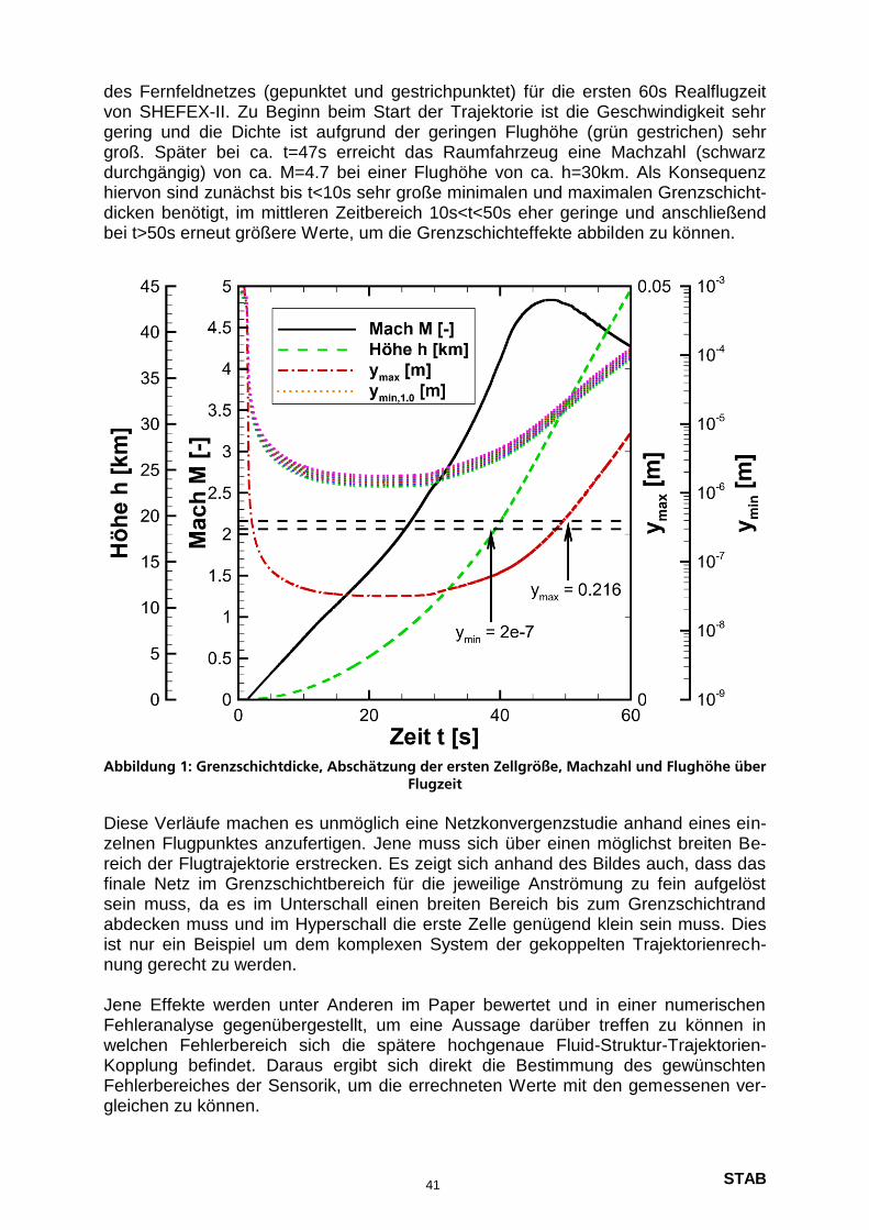
STAB

des Fernfeldnetzes (gepunktet und gestrichpunktet) für die ersten 60s Realflugzeit von SHEFEX-II. Zu Beginn beim Start der Trajektorie ist die Geschwindigkeit sehr gering und die Dichte ist aufgrund der geringen Flughöhe (grün gestrichen) sehr groß. Später bei ca. t=47s erreicht das Raumfahrzeug eine Machzahl (schwarz durchgängig) von ca. M=4.7 bei einer Flughöhe von ca. h=30km. Als Konsequenz hiervon sind zunächst bis t<10s sehr große minimalen und maximalen Grenzschicht-dicken benötigt, im mittleren Zeitbereich 10s<t<50s eher geringe und anschließend bei t>50s erneut größere Werte, um die Grenzschichteffekte abbilden zu können.

Abbildung 1: Grenzschichtdicke, Abschätzung der ersten Zellgröße, Machzahl und Flughöhe über

Flugzeit

Diese Verläufe machen es unmöglich eine Netzkonvergenzstudie anhand eines ein-zelnen Flugpunktes anzufertigen. Jene muss sich über einen möglichst breiten Be-reich der Flugtrajektorie erstrecken. Es zeigt sich anhand des Bildes auch, dass das finale Netz im Grenzschichtbereich für die jeweilige Anströmung zu fein aufgelöst sein muss, da es im Unterschall einen breiten Bereich bis zum Grenzschichtrand abdecken muss und im Hyperschall die erste Zelle genügend klein sein muss. Dies ist nur ein Beispiel um dem komplexen System der gekoppelten Trajektorienrech-nung gerecht zu werden. Jene Effekte werden unter Anderen im Paper bewertet und in einer numerischen Fehleranalyse gegenübergestellt, um eine Aussage darüber treffen zu können in welchen Fehlerbereich sich die spätere hochgenaue Fluid-Struktur-Trajektorien-Kopplung befindet. Daraus ergibt sich direkt die Bestimmung des gewünschten Fehlerbereiches der Sensorik, um die errechneten Werte mit den gemessenen ver-gleichen zu können.

41

STAB

the goal of HyperCODA is two-fold: First, extension of the equations representing

tation of the shock leads to instabilities and, in turn, an unphysical result. Therefore, entropy fix, exhibits the so-called Carbuncle phenomenon: The continuous represen- ing its default configuration of a Roe flux difference splitting including a particular as expected: A bow shock forms upstream of the cylinder. The one from CODA, us- equations for hypersonic flow conditions can prove difficult. The result from TAU is new equations to solve. As Figure 1 illustrates, even solving the steady-state Euler CODA requires extensions for high-enthalpy flows. This is not restricted to defining ous European partners, around a nucleus of ONERA, DLR and Airbus. As TAU did, has been devised and is commonly developed as the CODA CFD software by vari- retrofitting large-scale legacy code bases such as TAU, a new modular infrastructure these techniques affects basic assumptions of the software architecture. Rather than high-order discretization techniques, and multi-level parallelization. Implementing ferentiation of the whole simulation process, modularization of the implementation, tor cards. From the flow solver side, these challenges can be met with automatic di f- per socket, deep cache hierarchies with non-uniform memory access and accelera- Furthermore, the hardware has changed as well, now incorporating multiple cores leads to an ever-growing complexity of the models and the code implementing them. carried out routinely along with multi-species and multi-physics simulations. This enable gradient-based optimization, and time-resolving high-fidelity simulations are are steady-state solutions sought, nowadays their derivatives are desired as well to During the last decades, numerical simulation has changed dramatically: Not only bers, including non-ideal gas thermodynamics, gas mixtures, and chemistry.

tensions of TAU [1], HyperCODA extends CODA for applications at high Mach num- flow solver CODA (CFD for ONERA, DLR and Airbus). Similar to the spacecraft ex- This paper presents and validates HyperCODA, the hypersonics extension to the

[email protected]

Braunschweig

Institute of Aerodynamics and Flow Technology

German Aerospace Center (DLR)

Tobias Leicht

[email protected]

Göttingen

Institute of Aerodynamics and Flow Technology


Stefan Fechter

[email protected]

Dresden

Institute of Software Methods for Product Virtualization


Immo Huismann

HyperCODA – Extension of CODA Flow Solver to Hypersonic Flows


Mitteilung

42

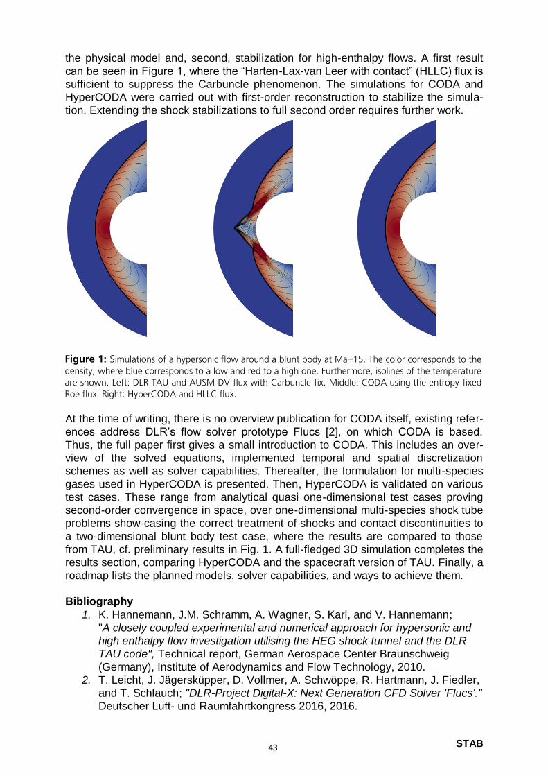
https://www.dlr.de/as/en/desktopdefault.aspx/tabid-1268/mailcontact-6046/

https://www.dlr.de/sp/en/desktopdefault.aspx/tabid-12171/mailcontact-38438/





STAB

the physical model and, second, stabilization for high-enthalpy flows. A first result

can be seen in Figure 1, where the “Harten-Lax-van Leer with contact” (HLLC) flux is

sufficient to suppress the Carbuncle phenomenon. The simulations for CODA and

HyperCODA were carried out with first-order reconstruction to stabilize the simula-

tion. Extending the shock stabilizations to full second order requires further work.

At the time of writing, there is no overview publication for CODA itself, existing refer-

ences address DLR’s flow solver prototype Flucs [2], on which CODA is based.

Thus, the full paper first gives a small introduction to CODA. This includes an over-

view of the solved equations, implemented temporal and spatial discretization

schemes as well as solver capabilities. Thereafter, the formulation for multi-species

gases used in HyperCODA is presented. Then, HyperCODA is validated on various

test cases. These range from analytical quasi one-dimensional test cases proving

second-order convergence in space, over one-dimensional multi-species shock tube

problems show-casing the correct treatment of shocks and contact discontinuities to

a two-dimensional blunt body test case, where the results are compared to those

from TAU, cf. preliminary results in Fig. 1. A full-fledged 3D simulation completes the

results section, comparing HyperCODA and the spacecraft version of TAU. Finally, a

roadmap lists the planned models, solver capabilities, and ways to achieve them.

Bibliography

1. K. Hannemann, J.M. Schramm, A. Wagner, S. Karl, and V. Hannemann;

"A closely coupled experimental and numerical approach for hypersonic and

high enthalpy flow investigation utilising the HEG shock tunnel and the DLR

TAU code", Technical report, German Aerospace Center Braunschweig

(Germany), Institute of Aerodynamics and Flow Technology, 2010.

2. T. Leicht, J. Jägersküpper, D. Vollmer, A. Schwöppe, R. Hartmann, J. Fiedler,

and T. Schlauch; "DLR-Project Digital-X: Next Generation CFD Solver 'Flucs'."

Deutscher Luft- und Raumfahrtkongress 2016, 2016.

Figure 1: Simulations of a hypersonic flow around a blunt body at Ma=15. The color corresponds to the

density, where blue corresponds to a low and red to a high one. Furthermore, isolines of the temperature are shown. Left: DLR TAU and AUSM-DV flux with Carbuncle fix. Middle: CODA using the entropy-fixed Roe flux. Right: HyperCODA and HLLC flux.

43

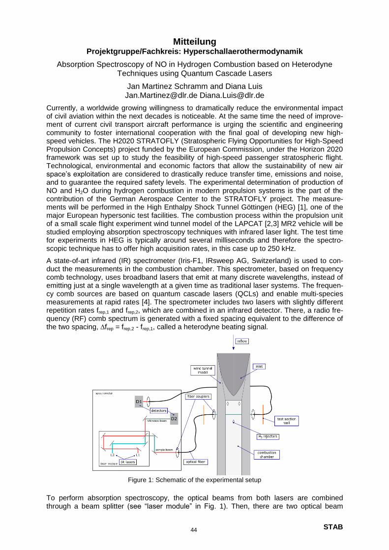
STAB

Mitteilung Projektgruppe/Fachkreis: Hyperschallaerothermodynamik

Absorption Spectroscopy of NO in Hydrogen Combustion based on Heterodyne Techniques using Quantum Cascade Lasers

Jan Martinez Schramm and Diana Luis [email protected] [email protected]

Currently, a worldwide growing willingness to dramatically reduce the environmental impact of civil aviation within the next decades is noticeable. At the same time the need of improve-ment of current civil transport aircraft performance is urging the scientific and engineering community to foster international cooperation with the final goal of developing new high-speed vehicles. The H2020 STRATOFLY (Stratospheric Flying Opportunities for High-Speed Propulsion Concepts) project funded by the European Commission, under the Horizon 2020 framework was set up to study the feasibility of high-speed passenger stratospheric flight. Technological, environmental and economic factors that allow the sustainability of new air space’s exploitation are considered to drastically reduce transfer time, emissions and noise, and to guarantee the required safety levels. The experimental determination of production of NO and H2O during hydrogen combustion in modern propulsion systems is the part of the contribution of the German Aerospace Center to the STRATOFLY project. The measure-ments will be performed in the High Enthalpy Shock Tunnel Göttingen (HEG) [1], one of the major European hypersonic test facilities. The combustion process within the propulsion unit of a small scale flight experiment wind tunnel model of the LAPCAT [2,3] MR2 vehicle will be studied employing absorption spectroscopy techniques with infrared laser light. The test time for experiments in HEG is typically around several milliseconds and therefore the spectro-scopic technique has to offer high acquisition rates, in this case up to 250 kHz.

A state-of-art infrared (IR) spectrometer (Iris-F1, IRsweep AG, Switzerland) is used to con-duct the measurements in the combustion chamber. This spectrometer, based on frequency comb technology, uses broadband lasers that emit at many discrete wavelengths, instead of emitting just at a single wavelength at a given time as traditional laser systems. The frequen-cy comb sources are based on quantum cascade lasers (QCLs) and enable multi-species measurements at rapid rates [4]. The spectrometer includes two lasers with slightly different repetition rates frep,1 and frep,2, which are combined in an infrared detector. There, a radio fre-quency (RF) comb spectrum is generated with a fixed spacing equivalent to the difference of the two spacing, ∆frep = frep,2 - frep,1, called a heterodyne beating signal.

Figure 1: Schematic of the experimental setup

To perform absorption spectroscopy, the optical beams from both lasers are combined through a beam splitter (see “laser module” in Fig. 1). Then, there are two optical beam

44

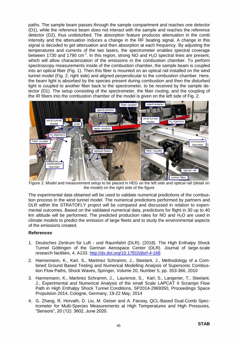
STAB

paths. The sample beam passes through the sample compartment and reaches one detector (D1), while the reference beam does not interact with the sample and reaches the reference detector (D2), thus undisturbed. The absorption feature produces attenuation in the comb intensity and the attenuation induces a change in the RF beating signal. A change in this signal is decoded to get attenuation and then absorption at each frequency. By adjusting the temperatures and currents of the two lasers, the spectrometer enables spectral coverage between 1730 and 1790 cm-1. In this region, strong NO and H2O spectral lines are present, which will allow characterization of the emissions in the combustion chamber. To perform spectroscopy measurements inside of the combustion chamber, the sample beam is coupled into an optical fiber (Fig. 1). Then this fiber is mounted on an optical rail installed on the wind tunnel model (Fig. 2, right side) and aligned perpendicular to the combustion chamber. Here, the beam light is absorbed by the species present during combustion and then the disturbed light is coupled to another fiber back to the spectrometer, to be received by the sample de-tector (D1). The setup consisting of the spectrometer, the fiber routing, and the coupling of the IR fibers into the combustion chamber of the model is given on the left side of Fig. 2.

Figure 2: Model and measurement setup to be placed in HEG on the left side and optical rail (detail on

the model) on the right side of the figure

The experimental data obtained will be used to validate numerical predictions of the combus-tion process in the wind tunnel model. The numerical predictions performed by partners and DLR within the STRATOFLY project will be compared and discussed in relation to experi-mental outcomes. Based on the validated numerical data, predictions for flight in 30 up to 40 km altitude will be performed. The predicted production rates for NO and H2O are used in climate models to predict the emission of large fleets and to study the environmental aspects of the emissions created.

References

1. Deutsches Zentrum für Luft - und Raumfahrt (DLR). (2018). The High Enthalpy Shock Tunnel Göttingen of the German Aerospace Center (DLR). Journal of large-scale research facilities, 4, A133. http://dx.doi.org/10.17815/jlsrf-4-168

2. Hannemann, K., Karl, S., Martinez Schramm, J., Steelant, J., Methodology of a Com-bined Ground Based Testing and Numerical Modelling Analysis of Supersonic Combus-tion Flow Paths, Shock Waves, Springer, Volume 20, Number 5, pp. 353-366, 2010

3. Hannemann, K., Martinez Schramm, J., Laurence, S., Karl, S., Langener, T., Steelant, J., Experimental and Numerical Analysis of the small Scale LAPCAT II Scramjet Flow Path in High Enthalpy Shock Tunnel Conditions, SP2014-2969350, Proceedings Space Propulsion 2014, Cologne, Germany, 19-22 May, 2014

4. G. Zhang, R. Horvath, D. Liu, M. Geiser and A. Farooq, QCL-Based Dual-Comb Spec-trometer for Multi-Species Measurements at High Temperatures and High Pressures, “Sensors”, 20 (12): 3602, June 2020.

45

http://dx.doi.org/10.17815/jlsrf-4-168

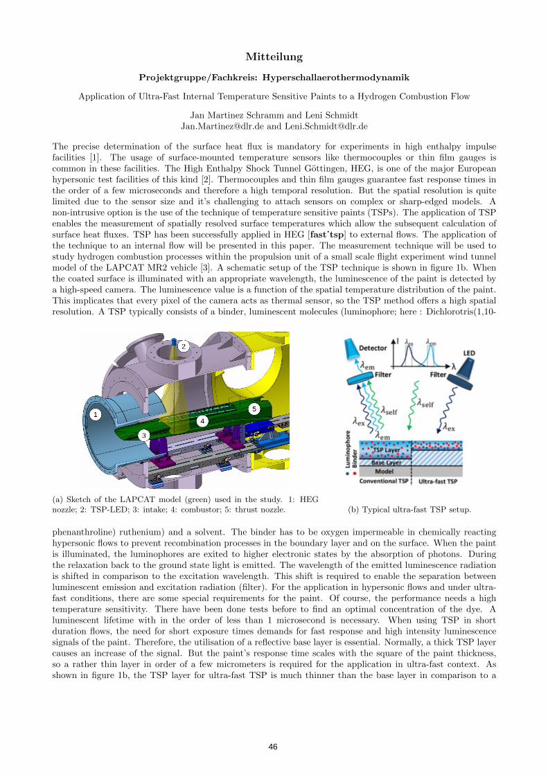
Mitteilung


Application of Ultra-Fast Internal Temperature Sensitive Paints to a Hydrogen Combustion Flow

Jan Martinez Schramm and Leni [email protected] and [email protected]

The precise determination of the surface heat flux is mandatory for experiments in high enthalpy impulsefacilities [1]. The usage of surface-mounted temperature sensors like thermocouples or thin film gauges iscommon in these facilities. The High Enthalpy Shock Tunnel Gottingen, HEG, is one of the major Europeanhypersonic test facilities of this kind [2]. Thermocouples and thin film gauges guarantee fast response times inthe order of a few microseconds and therefore a high temporal resolution. But the spatial resolution is quitelimited due to the sensor size and it’s challenging to attach sensors on complex or sharp-edged models. Anon-intrusive option is the use of the technique of temperature sensitive paints (TSPs). The application of TSPenables the measurement of spatially resolved surface temperatures which allow the subsequent calculation ofsurface heat fluxes. TSP has been successfully applied in HEG [fast˙tsp] to external flows. The application ofthe technique to an internal flow will be presented in this paper. The measurement technique will be used tostudy hydrogen combustion processes within the propulsion unit of a small scale flight experiment wind tunnelmodel of the LAPCAT MR2 vehicle [3]. A schematic setup of the TSP technique is shown in figure 1b. Whenthe coated surface is illuminated with an appropriate wavelength, the luminescence of the paint is detected bya high-speed camera. The luminescence value is a function of the spatial temperature distribution of the paint.This implicates that every pixel of the camera acts as thermal sensor, so the TSP method offers a high spatialresolution. A TSP typically consists of a binder, luminescent molecules (luminophore; here : Dichlorotris(1,10-

(a) Sketch of the LAPCAT model (green) used in the study. 1: HEGnozzle; 2: TSP-LED; 3: intake; 4: combustor; 5: thrust nozzle. (b) Typical ultra-fast TSP setup.

phenanthroline) ruthenium) and a solvent. The binder has to be oxygen impermeable in chemically reactinghypersonic flows to prevent recombination processes in the boundary layer and on the surface. When the paintis illuminated, the luminophores are exited to higher electronic states by the absorption of photons. Duringthe relaxation back to the ground state light is emitted. The wavelength of the emitted luminescence radiationis shifted in comparison to the excitation wavelength. This shift is required to enable the separation betweenluminescent emission and excitation radiation (filter). For the application in hypersonic flows and under ultra-fast conditions, there are some special requirements for the paint. Of course, the performance needs a hightemperature sensitivity. There have been done tests before to find an optimal concentration of the dye. Aluminescent lifetime with in the order of less than 1 microsecond is necessary. When using TSP in shortduration flows, the need for short exposure times demands for fast response and high intensity luminescencesignals of the paint. Therefore, the utilisation of a reflective base layer is essential. Normally, a thick TSP layercauses an increase of the signal. But the paint’s response time scales with the square of the paint thickness,so a rather thin layer in order of a few micrometers is required for the application in ultra-fast context. Asshown in figure 1b, the TSP layer for ultra-fast TSP is much thinner than the base layer in comparison to a

46

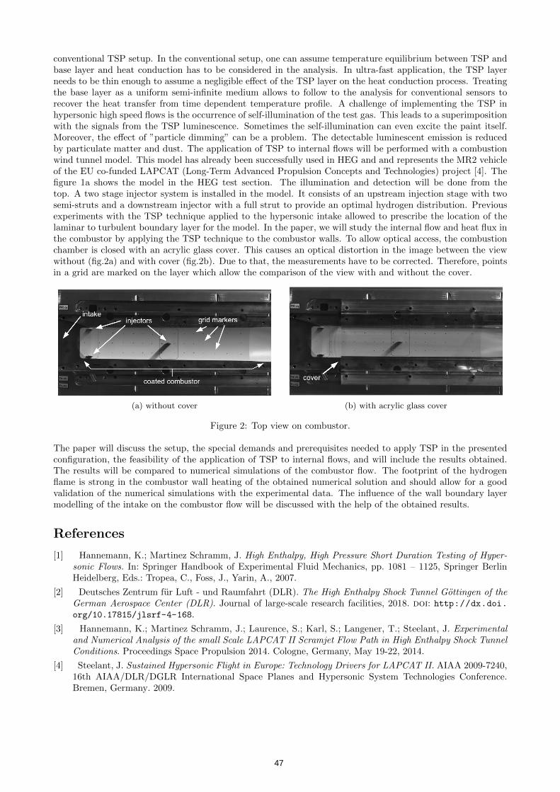
conventional TSP setup. In the conventional setup, one can assume temperature equilibrium between TSP andbase layer and heat conduction has to be considered in the analysis. In ultra-fast application, the TSP layerneeds to be thin enough to assume a negligible effect of the TSP layer on the heat conduction process. Treatingthe base layer as a uniform semi-infinite medium allows to follow to the analysis for conventional sensors torecover the heat transfer from time dependent temperature profile. A challenge of implementing the TSP inhypersonic high speed flows is the occurrence of self-illumination of the test gas. This leads to a superimpositionwith the signals from the TSP luminescence. Sometimes the self-illumination can even excite the paint itself.Moreover, the effect of ”particle dimming” can be a problem. The detectable luminescent emission is reducedby particulate matter and dust. The application of TSP to internal flows will be performed with a combustionwind tunnel model. This model has already been successfully used in HEG and and represents the MR2 vehicleof the EU co-funded LAPCAT (Long-Term Advanced Propulsion Concepts and Technologies) project [4]. Thefigure 1a shows the model in the HEG test section. The illumination and detection will be done from thetop. A two stage injector system is installed in the model. It consists of an upstream injection stage with twosemi-struts and a downstream injector with a full strut to provide an optimal hydrogen distribution. Previousexperiments with the TSP technique applied to the hypersonic intake allowed to prescribe the location of thelaminar to turbulent boundary layer for the model. In the paper, we will study the internal flow and heat flux inthe combustor by applying the TSP technique to the combustor walls. To allow optical access, the combustionchamber is closed with an acrylic glass cover. This causes an optical distortion in the image between the viewwithout (fig.2a) and with cover (fig.2b). Due to that, the measurements have to be corrected. Therefore, pointsin a grid are marked on the layer which allow the comparison of the view with and without the cover.

(a) without cover (b) with acrylic glass cover

Figure 2: Top view on combustor.

The paper will discuss the setup, the special demands and prerequisites needed to apply TSP in the presentedconfiguration, the feasibility of the application of TSP to internal flows, and will include the results obtained.The results will be compared to numerical simulations of the combustor flow. The footprint of the hydrogenflame is strong in the combustor wall heating of the obtained numerical solution and should allow for a goodvalidation of the numerical simulations with the experimental data. The influence of the wall boundary layermodelling of the intake on the combustor flow will be discussed with the help of the obtained results.

References

[1] Hannemann, K.; Martinez Schramm, J. High Enthalpy, High Pressure Short Duration Testing of Hyper-sonic Flows. In: Springer Handbook of Experimental Fluid Mechanics, pp. 1081 – 1125, Springer BerlinHeidelberg, Eds.: Tropea, C., Foss, J., Yarin, A., 2007.

[2] Deutsches Zentrum fur Luft - und Raumfahrt (DLR). The High Enthalpy Shock Tunnel Gottingen of theGerman Aerospace Center (DLR). Journal of large-scale research facilities, 2018. doi: http://dx.doi.org/10.17815/jlsrf-4-168.

[3] Hannemann, K.; Martinez Schramm, J.; Laurence, S.; Karl, S.; Langener, T.; Steelant, J. Experimentaland Numerical Analysis of the small Scale LAPCAT II Scramjet Flow Path in High Enthalpy Shock TunnelConditions. Proceedings Space Propulsion 2014. Cologne, Germany, May 19-22, 2014.

[4] Steelant, J. Sustained Hypersonic Flight in Europe: Technology Drivers for LAPCAT II. AIAA 2009-7240,16th AIAA/DLR/DGLR International Space Planes and Hypersonic System Technologies Conference.Bremen, Germany. 2009.

47

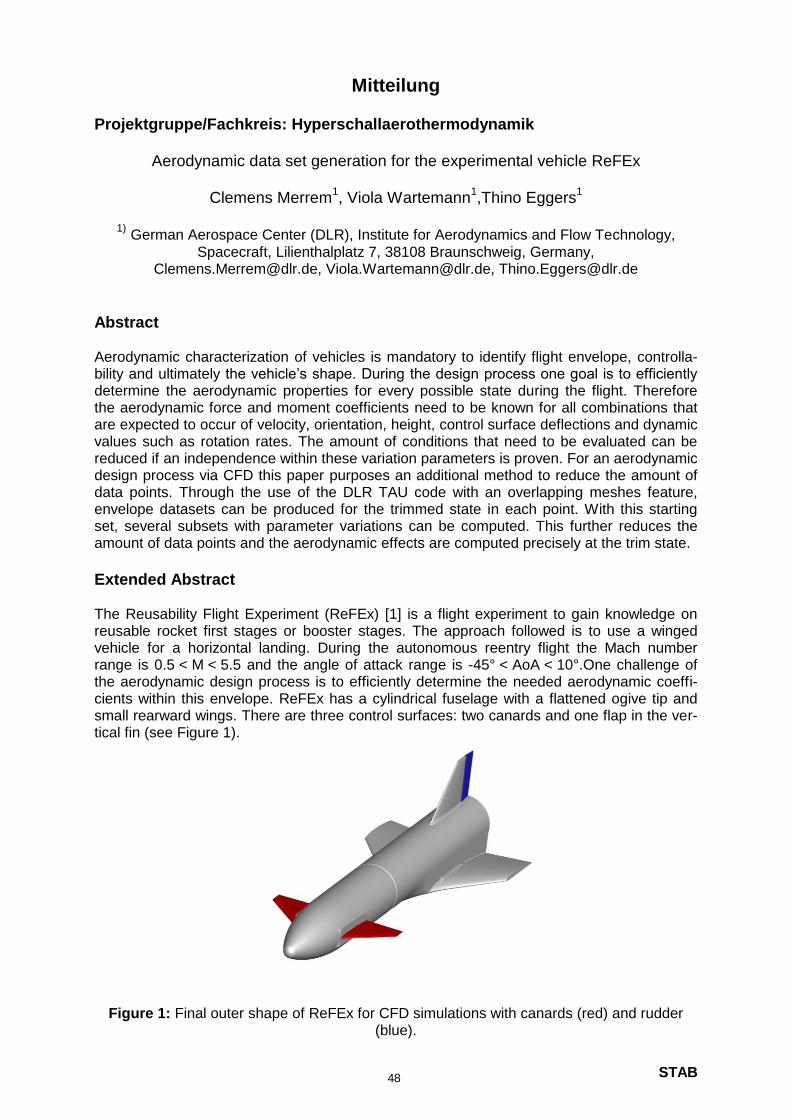
STAB

Mitteilung


Aerodynamic data set generation for the experimental vehicle ReFEx

Clemens Merrem1, Viola Wartemann

1,Thino Eggers

1

1)

German Aerospace Center (DLR), Institute for Aerodynamics and Flow Technology,

Spacecraft, Lilienthalplatz 7, 38108 Braunschweig, Germany, [email protected], [email protected], [email protected]

Abstract Aerodynamic characterization of vehicles is mandatory to identify flight envelope, controlla-bility and ultimately the vehicle’s shape. During the design process one goal is to efficiently determine the aerodynamic properties for every possible state during the flight. Therefore the aerodynamic force and moment coefficients need to be known for all combinations that are expected to occur of velocity, orientation, height, control surface deflections and dynamic values such as rotation rates. The amount of conditions that need to be evaluated can be reduced if an independence within these variation parameters is proven. For an aerodynamic design process via CFD this paper purposes an additional method to reduce the amount of data points. Through the use of the DLR TAU code with an overlapping meshes feature, envelope datasets can be produced for the trimmed state in each point. With this starting set, several subsets with parameter variations can be computed. This further reduces the amount of data points and the aerodynamic effects are computed precisely at the trim state.

Extended Abstract The Reusability Flight Experiment (ReFEx) [1] is a flight experiment to gain knowledge on reusable rocket first stages or booster stages. The approach followed is to use a winged vehicle for a horizontal landing. During the autonomous reentry flight the Mach number range is 0.5 < M < 5.5 and the angle of attack range is -45° < AoA < 10°.One challenge of the aerodynamic design process is to efficiently determine the needed aerodynamic coeffi-cients within this envelope. ReFEx has a cylindrical fuselage with a flattened ogive tip and small rearward wings. There are three control surfaces: two canards and one flap in the ver-tical fin (see Figure 1).

Figure 1: Final outer shape of ReFEx for CFD simulations with canards (red) and rudder

(blue).

48

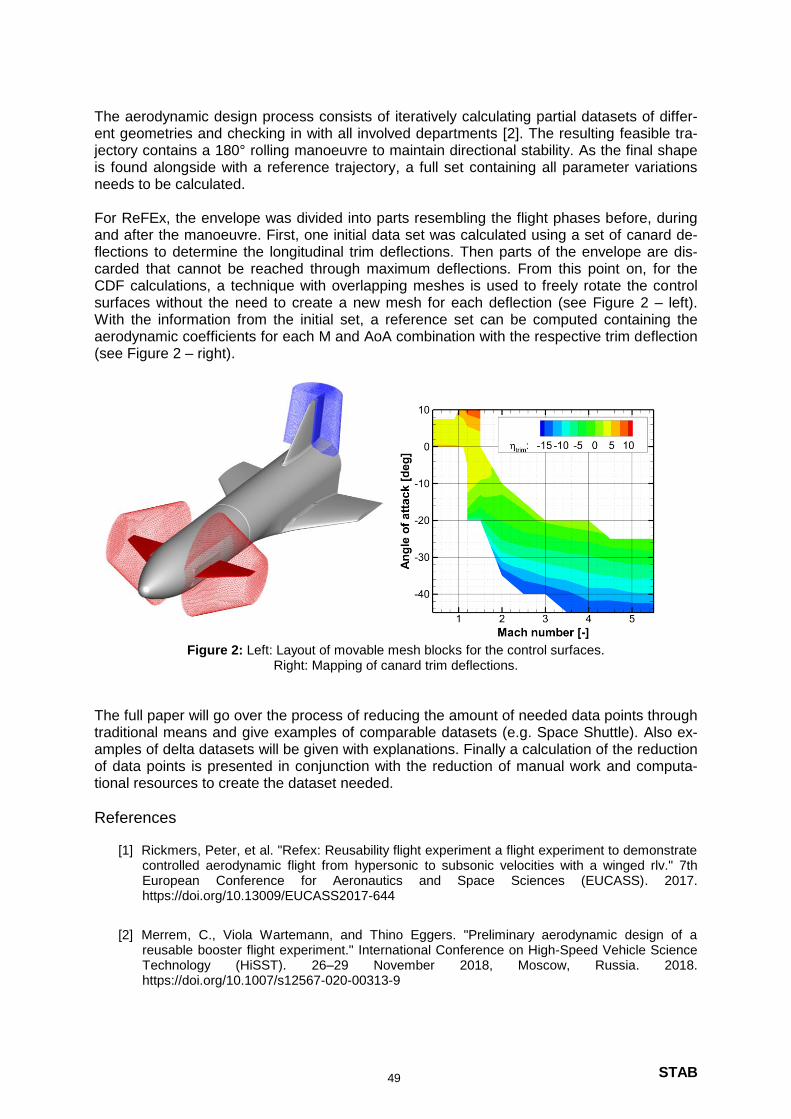
STAB

The aerodynamic design process consists of iteratively calculating partial datasets of differ-ent geometries and checking in with all involved departments [2]. The resulting feasible tra-jectory contains a 180° rolling manoeuvre to maintain directional stability. As the final shape is found alongside with a reference trajectory, a full set containing all parameter variations needs to be calculated. For ReFEx, the envelope was divided into parts resembling the flight phases before, during and after the manoeuvre. First, one initial data set was calculated using a set of canard de-flections to determine the longitudinal trim deflections. Then parts of the envelope are dis-carded that cannot be reached through maximum deflections. From this point on, for the CDF calculations, a technique with overlapping meshes is used to freely rotate the control surfaces without the need to create a new mesh for each deflection (see Figure 2 – left). With the information from the initial set, a reference set can be computed containing the aerodynamic coefficients for each M and AoA combination with the respective trim deflection (see Figure 2 – right).

Figure 2: Left: Layout of movable mesh blocks for the control surfaces.

Right: Mapping of canard trim deflections.

The full paper will go over the process of reducing the amount of needed data points through traditional means and give examples of comparable datasets (e.g. Space Shuttle). Also ex-amples of delta datasets will be given with explanations. Finally a calculation of the reduction of data points is presented in conjunction with the reduction of manual work and computa-tional resources to create the dataset needed.

References

[1] Rickmers, Peter, et al. "Refex: Reusability flight experiment a flight experiment to demonstrate controlled aerodynamic flight from hypersonic to subsonic velocities with a winged rlv." 7th European Conference for Aeronautics and Space Sciences (EUCASS). 2017. https://doi.org/10.13009/EUCASS2017-644

[2] Merrem, C., Viola Wartemann, and Thino Eggers. "Preliminary aerodynamic design of a reusable booster flight experiment." International Conference on High-Speed Vehicle Science Technology (HiSST). 26–29 November 2018, Moscow, Russia. 2018. https://doi.org/10.1007/s12567-020-00313-9

49

STAB

Mitteilung

Projektgruppe/Fachkreis: Hyperschallaerothermodynamik Comparison of CFD simulations and TMK wind tunnel data for the DLR ReFEx flight

experiment

Viola Wartemann1, Ntarinai Konosidou

1, Andreas Flock

2, Clemens Merrem

1

1) German Aerospace Center (DLR), Institute for Aerodynamics and Flow Technology, De-

partment Spacecraft, Lilienthalplatz 7, 38108 Braunschweig, Germany, [email protected], [email protected]

2) German Aerospace Center (DLR), Institute for Aerodynamics and Flow Technology, De-partment Supersonic and Hypersonic Technology, Linder Höhe, 51147 Köln, Germany, An-

[email protected]

The German Aerospace Center (DLR) is currently developing the Reusable Flight Experi-ment ReFEx as a technology demonstrator for a reusable, Vertical Take-off and Horizontal Landing (VTHL) booster stage [1]. A two-staged VSB-30 sounding rocket transports ReFEx to an altitude of about 130 km. After the separation from the carrier rocket, an autonomous re-entry is performed with a maximum Mach number of approx. 5. The first part of the follow-ing re-entry will be flown upside down at high, negative angles of attack (α), for the initial deceleration, to keep the structural and aerothermal loads within acceptable limits and to provide lateral stability. At M ≈ 1.5, a 180° roll manoeuvre will be performed to reach the nominal orientation and an angle of attack close to α = 10° for a maximum lift to drag ratio. One major task covered by the Department Spacecraft of the DLR Institute of Aerodynamics and Flow Technology in this project is the aerodynamic design of ReFEx [2]. Extensive da-tasets are needed to lay out the vehicle itself, the flight envelope for the trajectory and the control systems. The numerical generation of these aerodynamic data sets for the whole flight range are the second big task. The data bases are supported by wind tunnel experi-ments performed by the Department Supersonic and Hypersonic Technology in Cologne. Especially, the planned dynamic measurements are of interest for the comparison. The first test campaign, which is in the focus of the current paper, includes static measurements of the belly-up flight phase (M > 1.5). For the measurements the trisonic wind tunnel (TMK) is used, which is a cold flow, blow down wind tunnel. The TMK covers a broad range of Mach and Reynolds numbers and al-lows for testing at low hypersonic, supersonic, trans- and subsonic velocities. A scaled model of ReFEx was designed to fit into the TMK test section. It enables canard angles of 0°, ±5°, ±10° and ±15° and rudder deflections of 0°, 5° and 10°. For the simulations the DLR TAU code is applied. For the analysis presented in the current paper Navier-Stokes calculations were performed, using mainly the Spalart-Allamaras turbu-lence model. Beside a detailed grid study, an analysis of different turbulence models will be discussed. In the planned main chapter, the comparison will be concentrated on the calculated / meas-ured aerodynamic coefficients. The influence of the sting will be analysed as well as the Reynolds number effect. A first impression of the comparison can be seen in Figure 1, which shows an example at M = 4.5, α = 0°. To visualise the shocks within the simulations as schlieren images like in the measurements (top view of figure 1) an integration through the whole flow field is neces-sary, which will be done for the final paper. As current status, two CFD cuts are illustrated: in the middle for y = 0.0 m for the main shock at the front of the vehicle and the shock at the

50




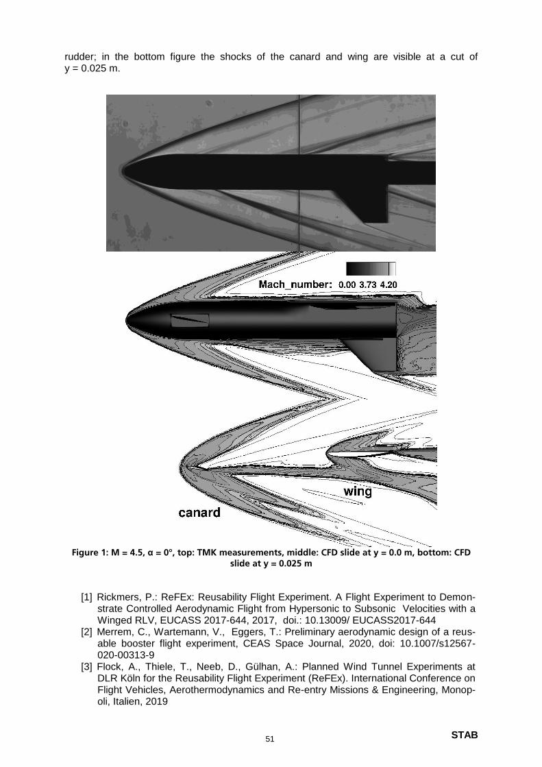
STAB

rudder; in the bottom figure the shocks of the canard and wing are visible at a cut of y = 0.025 m.

Figure 1: M = 4.5, α = 0°, top: TMK measurements, middle: CFD slide at y = 0.0 m, bottom: CFD

slide at y = 0.025 m

[1] Rickmers, P.: ReFEx: Reusability Flight Experiment. A Flight Experiment to Demon-strate Controlled Aerodynamic Flight from Hypersonic to Subsonic Velocities with a Winged RLV, EUCASS 2017-644, 2017, doi.: 10.13009/ EUCASS2017-644

[2] Merrem, C., Wartemann, V., Eggers, T.: Preliminary aerodynamic design of a reus-able booster flight experiment, CEAS Space Journal, 2020, doi: 10.1007/s12567-020-00313-9

[3] Flock, A., Thiele, T., Neeb, D., Gülhan, A.: Planned Wind Tunnel Experiments at DLR Köln for the Reusability Flight Experiment (ReFEx). International Conference on Flight Vehicles, Aerothermodynamics and Re-entry Missions & Engineering, Monop-oli, Italien, 2019

51

STAB

To fulfil the goal of a 75% CO2 reduction per passenger-kilometer of the European Aviation Roadmap described in the European Commission’s Flightpath 2050 report [1], new technol-ogies have to be identified to reduce the airplane structural weight, drag, and fuel consump-tion. Today, conventional control surfaces such as flaps or ailerons are used to reduce un-steady gust and manoeuvre loads. Further reduction in wing weight appears feasible if dedi-cated flow control devices are applied instead. A number of previous studies have investigat-ed the performance of active flow control, e.g. for fluidic and micro-mechanical flow actuators [2,3]. The most promising actuator designs for load alleviation on a passenger aircraft wing were compared in [4]. It was found that a jet perpendicular to the surface (normal jet) placed in the rear part of the suction side and a tangential jet over a Coanda surface inserted at the trailing edge (Coanda jet) are well suited for compensating typical peak loads of unsteady gusts over a range of different altitudes and flight Mach numbers.

This study focuses on investigating the suitability of different flow control devices for com-pensating a discrete vertical gust in terms of control amplitude and reaction. The gusts and the actuator response are determined using unsteady RANS simulations. To accelerate the investigation of the gust effects, an analytical model is proposed, based on a quasi-steady gust superposition on precomputed airfoil polars. The outputs of the gust simulations are airfoil peak load increments and corresponding temporal response times, which serve as target values for unsteady actuator simulations. A conventional trailing edge flap, normal jet, and Coanda jet are simulated and their control authorities and response times compared with the gust load history to identify suitable load alleviation designs for a range of gusts.

The unsteady 2D RANS simulations are conducted with the TAU code from the German Aerospace Center (DLR). The Spalart-Allmaras negative formulation with rotation and curva-ture corrections [5] is chosen as turbulence model with a 2nd order central scheme for the spatial discretization. The appropriate size of the mesh elements is identified with a mesh independence study, resulting in y+(1) ≤1 and a total number of elements of approximately 1 million, including local refinement around the actuator locations. The gust interaction with the airfoil is simulated applying the Disturbance Velocity Approach (DVA), i.e. a disturbance ve-locity due to the gust is added as source term to the Navier-Stokes equations [6]. In this analysis the airfoil is considered rigid.

The DLR-F15 supercritical airfoil in clean cruise configuration with a relative maximum thickness of 12.5% is simulated at Mach numbers M=0.37, 0.59, 0.78, corresponding to take off without high lift system, climbing at intermediate altitude, and cruise at design altitude of a medium-range airplane. Accordingly, the chord Reynolds number varies in the range of Rec=1.3 – 1.8×107. A representative cut of the 3D wing is scaled according to infinite swept wing theory to obtain representative operating conditions with a sweep angle φ=17°, short-ened chord c, reduced M, and increased angle of attack α. Based on aircraft certification requirements [7], three gust wavelengths (18 m, 116 m and 214 m) are selected and the gust amplitude is calculated as a function of altitude and air-plane properties as Vgust=10 – 16 m/s, expressed in true air speed.

An analytical approach is developed following the same logic of the DVA, i.e. the disturb-ance velocity due to the gust is vectorially added to the flight velocity V∞ to determine the change in the angle of attack along the gust. The gust-induced changes in α are used to es-

[email protected]. 37, 38108 Braunschweig, Germany

1 Institut of Fluid Mechanics, Technische Universität Braunschweig, Hermann-Blenk-

Salvatore Asaro1, Khalid Khalil1 and André Bauknecht1

for gust load alleviationUnsteady characterization of active flow control devices

Projektgruppe: Flow Control, Transition und Laminarhaltung

52

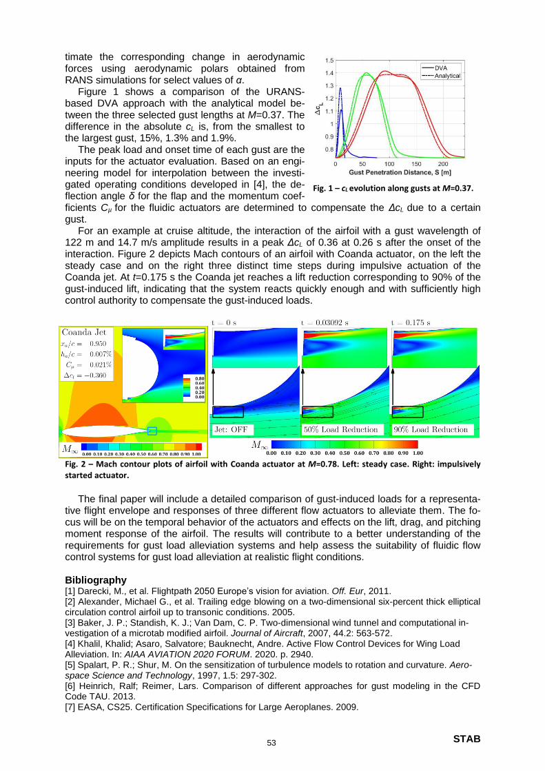
STAB

timate the corresponding change in aerodynamic forces using aerodynamic polars obtained from RANS simulations for select values of α.

Figure 1 shows a comparison of the URANS-based DVA approach with the analytical model be-tween the three selected gust lengths at M=0.37. The difference in the absolute cL is, from the smallest to the largest gust, 15%, 1.3% and 1.9%.

The peak load and onset time of each gust are the inputs for the actuator evaluation. Based on an engi-neering model for interpolation between the investi-gated operating conditions developed in [4], the de-flection angle δ for the flap and the momentum coef-ficients Cµ for the fluidic actuators are determined to compensate the ΔcL due to a certain gust.

For an example at cruise altitude, the interaction of the airfoil with a gust wavelength of 122 m and 14.7 m/s amplitude results in a peak ΔcL of 0.36 at 0.26 s after the onset of the interaction. Figure 2 depicts Mach contours of an airfoil with Coanda actuator, on the left the steady case and on the right three distinct time steps during impulsive actuation of the Coanda jet. At t=0.175 s the Coanda jet reaches a lift reduction corresponding to 90% of the gust-induced lift, indicating that the system reacts quickly enough and with sufficiently high control authority to compensate the gust-induced loads.

Fig. 2 – Mach contour plots of airfoil with Coanda actuator at M=0.78. Left: steady case. Right: impulsively started actuator.

The final paper will include a detailed comparison of gust-induced loads for a representa-

tive flight envelope and responses of three different flow actuators to alleviate them. The fo-cus will be on the temporal behavior of the actuators and effects on the lift, drag, and pitching moment response of the airfoil. The results will contribute to a better understanding of the requirements for gust load alleviation systems and help assess the suitability of fluidic flow control systems for gust load alleviation at realistic flight conditions. Bibliography [1] Darecki, M., et al. Flightpath 2050 Europe’s vision for aviation. Off. Eur, 2011. [2] Alexander, Michael G., et al. Trailing edge blowing on a two-dimensional six-percent thick elliptical circulation control airfoil up to transonic conditions. 2005. [3] Baker, J. P.; Standish, K. J.; Van Dam, C. P. Two-dimensional wind tunnel and computational in-vestigation of a microtab modified airfoil. Journal of Aircraft, 2007, 44.2: 563-572. [4] Khalil, Khalid; Asaro, Salvatore; Bauknecht, Andre. Active Flow Control Devices for Wing Load Alleviation. In: AIAA AVIATION 2020 FORUM. 2020. p. 2940. [5] Spalart, P. R.; Shur, M. On the sensitization of turbulence models to rotation and curvature. Aero-space Science and Technology, 1997, 1.5: 297-302. [6] Heinrich, Ralf; Reimer, Lars. Comparison of different approaches for gust modeling in the CFD Code TAU. 2013. [7] EASA, CS25. Certification Specifications for Large Aeroplanes. 2009.

Fig. 1 – cL evolution along gusts at M=0.37.

53

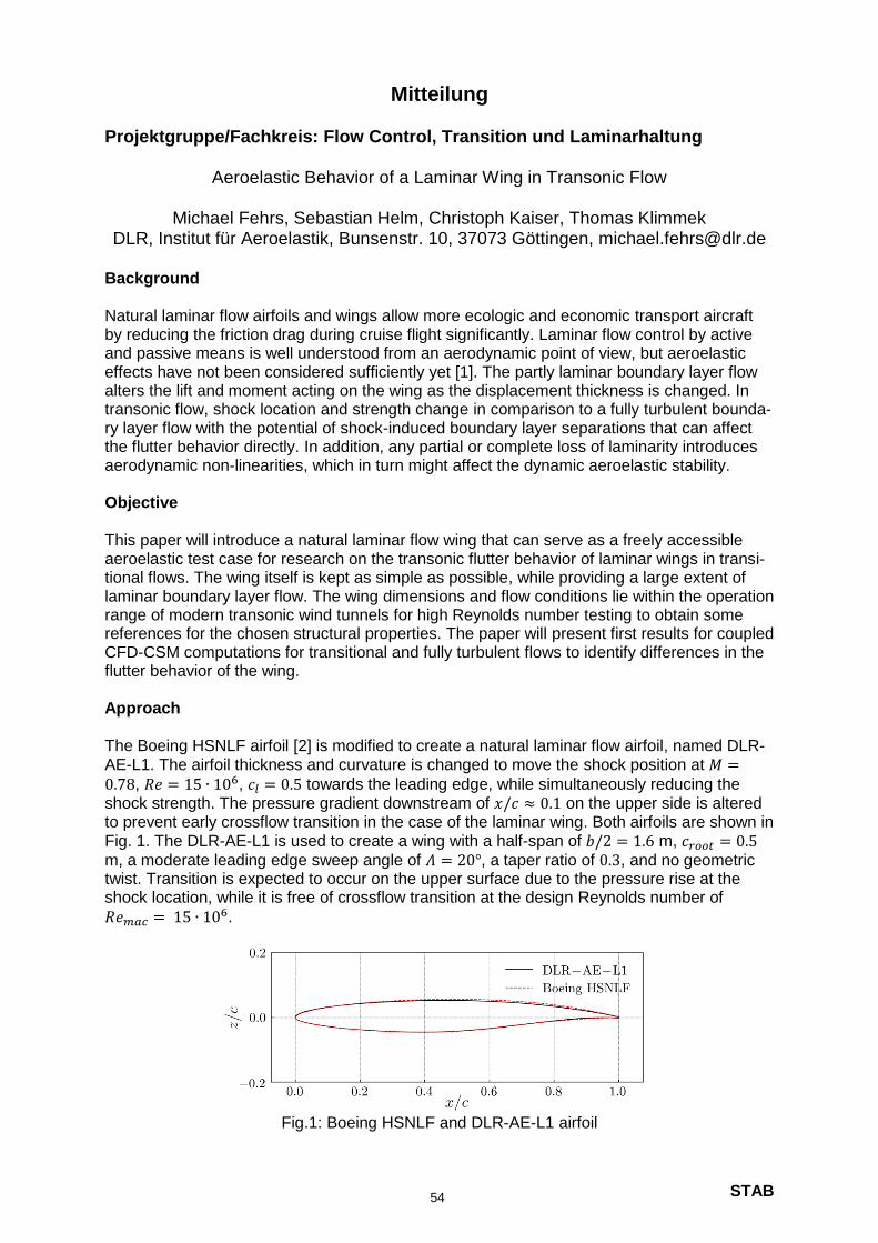
STAB

Mitteilung Projektgruppe/Fachkreis: Flow Control, Transition und Laminarhaltung

Aeroelastic Behavior of a Laminar Wing in Transonic Flow

Michael Fehrs, Sebastian Helm, Christoph Kaiser, Thomas Klimmek DLR, Institut für Aeroelastik, Bunsenstr. 10, 37073 Göttingen, [email protected]

Background Natural laminar flow airfoils and wings allow more ecologic and economic transport aircraft by reducing the friction drag during cruise flight significantly. Laminar flow control by active and passive means is well understood from an aerodynamic point of view, but aeroelastic effects have not been considered sufficiently yet [1]. The partly laminar boundary layer flow alters the lift and moment acting on the wing as the displacement thickness is changed. In transonic flow, shock location and strength change in comparison to a fully turbulent bounda-ry layer flow with the potential of shock-induced boundary layer separations that can affect the flutter behavior directly. In addition, any partial or complete loss of laminarity introduces aerodynamic non-linearities, which in turn might affect the dynamic aeroelastic stability. Objective This paper will introduce a natural laminar flow wing that can serve as a freely accessible aeroelastic test case for research on the transonic flutter behavior of laminar wings in transi-tional flows. The wing itself is kept as simple as possible, while providing a large extent of laminar boundary layer flow. The wing dimensions and flow conditions lie within the operation range of modern transonic wind tunnels for high Reynolds number testing to obtain some references for the chosen structural properties. The paper will present first results for coupled CFD-CSM computations for transitional and fully turbulent flows to identify differences in the flutter behavior of the wing. Approach The Boeing HSNLF airfoil [2] is modified to create a natural laminar flow airfoil, named DLR-AE-L1. The airfoil thickness and curvature is changed to move the shock position at 𝑀 =0.78, 𝑅𝑒 = 15 ∙ 106, 𝑐𝑙 = 0.5 towards the leading edge, while simultaneously reducing the shock strength. The pressure gradient downstream of 𝑥/𝑐 ≈ 0.1 on the upper side is altered to prevent early crossflow transition in the case of the laminar wing. Both airfoils are shown in Fig. 1. The DLR-AE-L1 is used to create a wing with a half-span of 𝑏/2 = 1.6 m, 𝑐𝑟𝑜𝑜𝑡 = 0.5

m, a moderate leading edge sweep angle of 𝛬 = 20°, a taper ratio of 0.3, and no geometric twist. Transition is expected to occur on the upper surface due to the pressure rise at the shock location, while it is free of crossflow transition at the design Reynolds number of

𝑅𝑒𝑚𝑎𝑐 = 15 ∙ 106.

Fig.1: Boeing HSNLF and DLR-AE-L1 airfoil

54

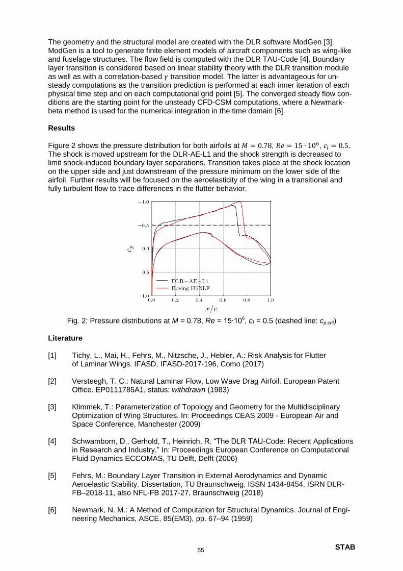
STAB

The geometry and the structural model are created with the DLR software ModGen [3]. ModGen is a tool to generate finite element models of aircraft components such as wing-like and fuselage structures. The flow field is computed with the DLR TAU-Code [4]. Boundary layer transition is considered based on linear stability theory with the DLR transition module as well as with a correlation-based 𝛾 transition model. The latter is advantageous for un-steady computations as the transition prediction is performed at each inner iteration of each physical time step and on each computational grid point [5]. The converged steady flow con-ditions are the starting point for the unsteady CFD-CSM computations, where a Newmark-beta method is used for the numerical integration in the time domain [6]. Results

Figure 2 shows the pressure distribution for both airfoils at 𝑀 = 0.78, 𝑅𝑒 = 15 ∙ 106, 𝑐𝑙 = 0.5. The shock is moved upstream for the DLR-AE-L1 and the shock strength is decreased to limit shock-induced boundary layer separations. Transition takes place at the shock location on the upper side and just downstream of the pressure minimum on the lower side of the airfoil. Further results will be focused on the aeroelasticity of the wing in a transitional and fully turbulent flow to trace differences in the flutter behavior.

Fig. 2: Pressure distributions at M = 0.78, Re = 15∙106, cl = 0.5 (dashed line: cp,crit)

Literature [1] Tichy, L., Mai, H., Fehrs, M., Nitzsche, J., Hebler, A.: Risk Analysis for Flutter

of Laminar Wings. IFASD, IFASD-2017-196, Como (2017) [2] Versteegh, T. C.: Natural Laminar Flow, Low Wave Drag Airfoil. European Patent

Office. EP0111785A1, status: withdrawn (1983)

[3] Klimmek, T.: Parameterization of Topology and Geometry for the Multidisciplinary Optimization of Wing Structures. In: Proceedings CEAS 2009 - European Air and Space Conference, Manchester (2009)

[4] Schwamborn, D., Gerhold, T., Heinrich, R. “The DLR TAU-Code: Recent Applications

in Research and Industry,” In: Proceedings European Conference on Computational Fluid Dynamics ECCOMAS, TU Delft, Delft (2006)

[5] Fehrs, M.: Boundary Layer Transition in External Aerodynamics and Dynamic

Aeroelastic Stability. Dissertation, TU Braunschweig, ISSN 1434-8454, ISRN DLR-FB–2018-11, also NFL-FB 2017-27, Braunschweig (2018)

[6] Newmark, N. M.: A Method of Computation for Structural Dynamics. Journal of Engi-

neering Mechanics, ASCE, 85(EM3), pp. 67–94 (1959)

55

STAB


Influence of surface irregularities on the expected boundary-layer transition location on hybrid laminar flow control wings

J. A. Franco Sumariva1,2, A. Theiss1, S. Hein1

1 DLR, Institut für Aerodynamik und Strömungstechnik (AS), Bunsenstraße 10, D-37073 Göttingen, Germany

2 Universidad Politécnica de Madrid (UPM),

Plaza Cardenal Cisneros 3, E-28040 Madrid, Spain

[email protected]

Introduction Hybrid laminar flow control (HLFC) wings have captured the interest of several research pro-jects, in particular the HLFC-WIN project [1], because of the potential of suction for reducing drag on commercial aircraft [2]. This reduction in drag is mainly due to the impact on laminar-turbulent transition, extending the region along the wings where the flow remains laminar. Typically, on HLFC wings, suction is applied only in the leading edge region (before the front spar). The flow suction modifies the boundary-layer (BL) profiles in such a way that the growth of flow instabilities that might trigger the above mentioned laminar-turbulent transition location, e.g. Tollmien-Schlichting (TS) waves or crossflow (CF) vortices, is delayed. Howev-er, the joint between the leading edge suction panel and the wing box may introduce surface irregularities (e.g. backward/forward-facing steps (BFS/FFS), gaps, etc.) that might enhance the spatial development of those flow instabilities and, therefore, reduce the potential benefit of the suction system [3]. For this reason, it is crucial during the design process to quantify the influence of such surface irregularities in terms of BL instability.

Methodology

The Adaptive Harmonic Linearized Navier-Stokes (AHLNS) approach [4], in combination with the Parabolized Stability equations (PSE) [5], offers the most efficient way to compute the effect of surface irregularities on the spatial development of convective instabilities, e.g. TS waves and CF vortices, in terms of n-factor curves [6]. The PSE are applied far from the lo-cation of the surface irregularity, where the streamwise variations of the base flow quantities remain small (w.r.t. wall-normal gradients). The AHLNS methodology is used in the vicinity of the irregularity, where the assumption of small variations of the streamwise variables is no longer valid. The efficiency of the AHLNS approach, in comparison with other standard methodologies as Direct Numerical simulations (DNS), lies in the “wave-like” character as-sumed for describing the convective instabilities, in a similar fashion as PSE. This assump-tion significantly reduces the number of streamwise grid points required in comparison with DNS computations [7], allowing parametric studies for transonic wings at high Reynolds numbers.

Results In the present work, we concentrate on the influence of surface irregularities on the expected BL transition location. In order to reduce the large number of parametric studies, certain quantities remain fixed, e.g. suction flow-rate distribution, Mach number, Reynolds number and streamwise location of the surface irregularity. The parametric study focuses on the type

56

STAB

of surface irregularity (gap, BFS, FFS), its height (0.2-0.8 mm) and length (1-3 mm). As an example, Figure 1-a) shows the baseflow streamwise velocity contours and sectional stream-lines for a BFS of 0.2 mm height placed at 20% chord. Although the step height is relatively small (~25% of the BL displacement thickness), the length of the recirculation area is about 7 mm. Figure 1-b) depicts the spatial evolution of a particular incoming TS wave for the same BFS, computed with AHLNS.

a) b)

Figure 1. a) Streamwise velocity contours and sectional streamlines for a BFS of 0.2 mm height placed at 20% chord in global coordinates (x,z) [axes are to scale]; b) Real part of the streamwise velocity disturbance 𝕽( 𝒎𝒂𝒙⁄ ) for an incoming TS wave of frequency f = 3141 Hz and spanwise wavenumber 𝜷 = 105 m

-1 at an

arbitrary instant of time for a BFS of 0.2 mm height placed at 20% chord in body-attached coordinates (s,y) [axes are not to scale].

Acknowledgments Authors would like to thank Martin Kruse (DLR) for providing the TAU version for the base flow computations including suction. The work described in this abstract has received funding from the Clean Sky 2 Joint Undertaking under grant agreement No. 807097, HLFC-WIN pro-ject.

References [1] HLFC-WIN project: https://www.hlfc-win.eu/ [2] Reneaux, J., Overview on drag reduction technologies for civil transport aircraft.

ECCOMAS (2004). [3] Methel, J., Forte, M., Vermeersch, O., Casalis, G., An experimental study on the effects

of two‑dimensional positive surface defects on the laminar–turbulent transition of a sucked boundary layer. Exp Fluids 60, 94 (2019).

[4] Franco Sumariva, J.A., Hein, S., Valero, E., On the influence of two-dimensional hump roughness on laminar-turbulent transition. Phys. Fluids 32, 034102 (2020).

[5] Hein, S., Bertolotti, F.P., Simen, M., Hanifi, A., Henningson, D., Linear nonlocal instability analysis - the linear NOLOT code. Internal Report No. DLR IB 223-94 A56 (1995).

[6] Arnal, D., Boundary layer transition: Predictions based on linear theory. Progress in Transition Modelling, AGARD Report No. 793 (1994).

[7] Franco, J.A., Hein, S., Adaptive Harmonic Linearized Navier-Stokes equations used for boundary-layer instability analysis in the presence of large streamwise gradients, AIAA Paper 2018-1548 (2018).

57

https://www.hlfc-win.eu/

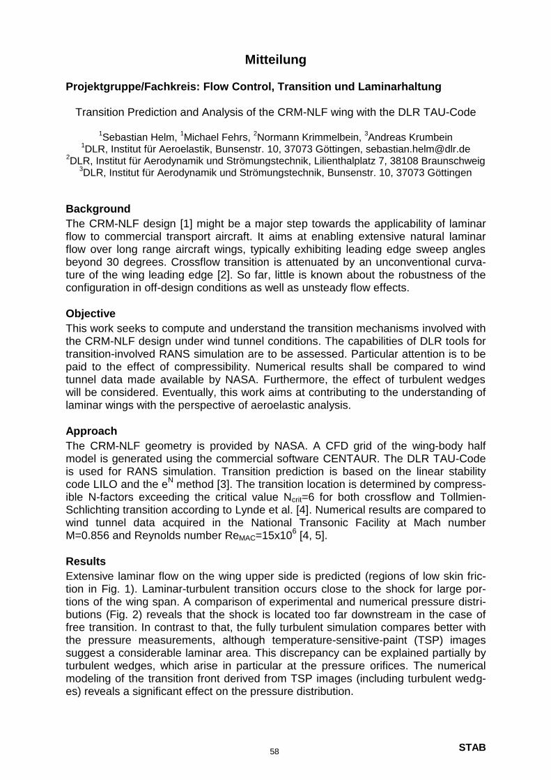
STAB

Mitteilung

Projektgruppe/Fachkreis: Flow Control, Transition und Laminarhaltung

Transition Prediction and Analysis of the CRM-NLF wing with the DLR TAU-Code

1Sebastian Helm,

1Michael Fehrs,

2Normann Krimmelbein,

3Andreas Krumbein

1DLR, Institut für Aeroelastik, Bunsenstr. 10, 37073 Göttingen, [email protected]

2DLR, Institut für Aerodynamik und Strömungstechnik, Lilienthalplatz 7, 38108 Braunschweig

3DLR, Institut für Aerodynamik und Strömungstechnik, Bunsenstr. 10, 37073 Göttingen

Background

The CRM-NLF design [1] might be a major step towards the applicability of laminar flow to commercial transport aircraft. It aims at enabling extensive natural laminar flow over long range aircraft wings, typically exhibiting leading edge sweep angles beyond 30 degrees. Crossflow transition is attenuated by an unconventional curva-ture of the wing leading edge [2]. So far, little is known about the robustness of the configuration in off-design conditions as well as unsteady flow effects.

Objective

This work seeks to compute and understand the transition mechanisms involved with the CRM-NLF design under wind tunnel conditions. The capabilities of DLR tools for transition-involved RANS simulation are to be assessed. Particular attention is to be paid to the effect of compressibility. Numerical results shall be compared to wind tunnel data made available by NASA. Furthermore, the effect of turbulent wedges will be considered. Eventually, this work aims at contributing to the understanding of laminar wings with the perspective of aeroelastic analysis.

Approach

The CRM-NLF geometry is provided by NASA. A CFD grid of the wing-body half model is generated using the commercial software CENTAUR. The DLR TAU-Code is used for RANS simulation. Transition prediction is based on the linear stability code LILO and the e

N method [3]. The transition location is determined by compress-

ible N-factors exceeding the critical value Ncrit=6 for both crossflow and Tollmien-Schlichting transition according to Lynde et al. [4]. Numerical results are compared to wind tunnel data acquired in the National Transonic Facility at Mach number M=0.856 and Reynolds number ReMAC=15x10

6 [4, 5].

Results

Extensive laminar flow on the wing upper side is predicted (regions of low skin fric-tion in Fig. 1). Laminar-turbulent transition occurs close to the shock for large por-tions of the wing span. A comparison of experimental and numerical pressure distri-butions (Fig. 2) reveals that the shock is located too far downstream in the case of free transition. In contrast to that, the fully turbulent simulation compares better with the pressure measurements, although temperature-sensitive-paint (TSP) images suggest a considerable laminar area. This discrepancy can be explained partially by turbulent wedges, which arise in particular at the pressure orifices. The numerical modeling of the transition front derived from TSP images (including turbulent wedg-es) reveals a significant effect on the pressure distribution.

58

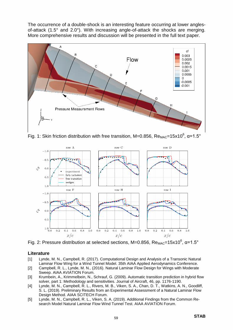
STAB

The occurrence of a double-shock is an interesting feature occurring at lower angles-of-attack (1.5° and 2.0°). With increasing angle-of-attack the shocks are merging. More comprehensive results and discussion will be presented in the full text paper.

Fig. 1: Skin friction distribution with free transition, M=0.856, ReMAC=15x10

6, α=1.5°

Fig. 2: Pressure distribution at selected sections, M=0.856, ReMAC=15x10

6, α=1.5°

Literature

[1] Lynde, M. N., Campbell, R. (2017). Computational Design and Analysis of a Transonic Natural Laminar Flow Wing for a Wind Tunnel Model. 35th AIAA Applied Aerodynamics Conference.

[2] Campbell, R. L., Lynde, M. N., (2016). Natural Laminar Flow Design for Wings with Moderate Sweep. AIAA AVIATION Forum.

[3] Krumbein, A., Krimmelbein, N., Schrauf, G. (2009). Automatic transition prediction in hybrid flow solver, part 1: Methodology and sensitivities. Journal of Aircraft, 46, pp. 1176-1190.

[4] Lynde, M. N., Campbell, R. L., Rivers, M. B., Viken, S. A., Chan, D. T., Watkins, A. N., Goodliff, S. L. (2019). Preliminary Results from an Experimental Assessment of a Natural Laminar Flow Design Method. AIAA SCITECH Forum.

[5] Lynde, M. N., Campbell, R. L., Viken, S. A. (2019). Additional Findings from the Common Re-search Model Natural Laminar Flow Wind Tunnel Test. AIAA AVIATION Forum.

59

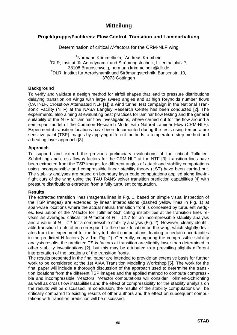
STAB

Mitteilung


Determination of critical N-factors for the CRM-NLF wing

1Normann Krimmelbein,

2Andreas Krumbein

1DLR, Institut für Aerodynamik und Strömungstechnik, Lilienthalplatz 7,

38108 Braunschweig, [email protected] 2DLR, Institut für Aerodynamik und Strömungstechnik, Bunsenstr. 10,

37073 Göttingen

Background

To verify and validate a design method for airfoil shapes that lead to pressure distributions delaying transition on wings with large sweep angles and at high Reynolds number flows (CATNLF, Crossflow Attenuated NLF [1]) a wind tunnel test campaign in the National Tran-sonic Facility (NTF) at the NASA Langley Research Center has been conducted [2]. The experiments, also aiming at evaluating best practices for laminar flow testing and the general suitability of the NTF for laminar flow investigations, where carried out for the flow around a semi-span model of the Common Research Model with Natural Laminar Flow (CRM-NLF). Experimental transition locations have been documented during the tests using temperature sensitive paint (TSP) images by applying different methods, a temperature step method and a heating layer approach [3].

Approach

To support and extend the previous preliminary evaluations of the critical Tollmien-Schlichting and cross flow N-factors for the CRM-NLF at the NTF [3], transition lines have been extracted from the TSP images for different angles of attack and stability computations using incompressible and compressible linear stability theory (LST) have been carried out. The stability analyses are based on boundary layer code computations applied along line-in-flight cuts of the wing using the TAU RANS solver transition prediction capabilities [4] with pressure distributions extracted from a fully turbulent computation.

Results The extracted transition lines (magenta lines in Fig. 1, based on simple visual inspection of the TSP images) are extended by linear interpolations (dashed yellow lines in Fig. 1) at span-wise locations where the actual natural transition front is concealed by turbulent wedg-es. Evaluation of the N-factor for Tollmien-Schlichting instabilities at the transition lines re-veals an averaged critical TS-N-factor of N = 11.7 for an incompressible stability analysis and a value of N = 4.1 for a compressible stability analysis (Fig. 2). However, clearly identifi-able transition fronts often correspond to the shock location on the wing, which slightly devi-ates from the experiment for the fully turbulent computations, leading to certain uncertainties in the predicted N-factors (y > 1m, Fig. 2). Generally, comparing the compressible stability analysis results, the predicted TS-N-factors at transition are slightly lower than determined in other stability investigations [2], but this may be attributed to a prevailing slightly different interpretation of the locations of the transition fronts. The results presented in the final paper are intended to provide an extensive basis for further work to be considered at the 1st AIAA Transition Modeling Workshop [5]. The work for the final paper will include a thorough discussion of the approach used to determine the transi-tion locations from the different TSP images and the applied method to compute compressi-ble and incompressible N-factors. N-factor computations will consider Tollmien-Schlichting as well as cross flow instabilities and the effect of compressibility for the stability analysis on the results will be discussed. In conclusion, the results of the stability computations will be critically compared to existing results of other authors and the effect on subsequent compu-tations with transition prediction will be discussed.

60

STAB

Fig. 1: CRM-NLF, TSP image, heating layer, M = 0.856, ReMAC = 15x10

6, = 2.5°

Fig. 2: CRM-NLF wing, Tollmien-Schlichting N-factors at transition

Literature

[1] Lynde, M. N., Campbell, R. L. (2017). Computational Design and Analysis of a Transonic Natural Laminar Flow Wing for a Wind Tunnel Model. AIAA-2017-3058 [2] Lynde, M. N., Campbell, R. L., Viken, S. A. (2019). Additional Findings from the Common Research Model Natural Laminar Flow Wind Tunnel Test. AIAA-2019-3292 [3] Watkins, A. N., Goodman, K. Z., Peak, S. M. (2019). Transition Detection at Cryogenic Temperatures Using a Carbon-Based Resistive Heating Layer Coupled with Temperature Sensitive Paint. AIAA-2019-2191 [4] Krumbein, A., Krimmelbein, N., Schrauf, G. (2009). Automatic transition prediction in hy-brid flow solver, part 1: Methodology and sensitivities. Journal of Aircraft, 46, pp. 1176-1190. [5] https://transitionmodeling.larc.nasa.gov/workshop_i/

61

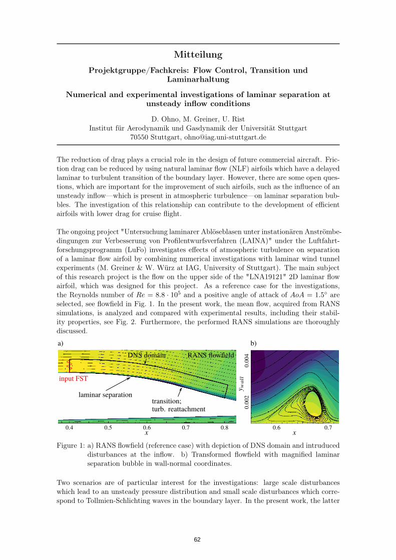
Mitteilung

Projektgruppe/Fachkreis: Flow Control, Transition undLaminarhaltung

Numerical and experimental investigations of laminar separation atunsteady inflow conditions

D. Ohno, M. Greiner, U. RistInstitut für Aerodynamik und Gasdynamik der Universität Stuttgart

70550 Stuttgart, [email protected]

The reduction of drag plays a crucial role in the design of future commercial aircraft. Fric-tion drag can be reduced by using natural laminar flow (NLF) airfoils which have a delayedlaminar to turbulent transition of the boundary layer. However, there are some open ques-tions, which are important for the improvement of such airfoils, such as the influence of anunsteady inflow—which is present in atmospheric turbulence—on laminar separation bub-bles. The investigation of this relationship can contribute to the development of efficientairfoils with lower drag for cruise flight.

The ongoing project "Untersuchung laminarer Ablöseblasen unter instationären Anströmbe-dingungen zur Verbesserung von Profilentwurfsverfahren (LAINA)" under the Luftfahrt-forschungsprogramm (LuFo) investigates effects of atmospheric turbulence on separationof a laminar flow airfoil by combining numerical investigations with laminar wind tunnelexperiments (M. Greiner & W. Würz at IAG, University of Stuttgart). The main subjectof this research project is the flow on the upper side of the "LNA19121" 2D laminar flowairfoil, which was designed for this project. As a reference case for the investigations,the Reynolds number of Re = 8.8 · 105 and a positive angle of attack of AoA = 1.5 areselected, see flowfield in Fig. 1. In the present work, the mean flow, acquired from RANSsimulations, is analyzed and compared with experimental results, including their stabil-ity properties, see Fig. 2. Furthermore, the performed RANS simulations are thoroughlydiscussed.

Figure 1: a) RANS flowfield (reference case) with depiction of DNS domain and intruduceddisturbances at the inflow. b) Transformed flowfield with magnified laminarseparation bubble in wall-normal coordinates.

Two scenarios are of particular interest for the investigations: large scale disturbanceswhich lead to an unsteady pressure distribution and small scale disturbances which corre-spond to Tollmien-Schlichting waves in the boundary layer. In the present work, the latter

62

case is investigated in direct numerical simulations (DNS) with an isotropic synthetic tur-bulent inflow following the ansatz by Jacobs & Durbin [2]. Free-stream turbulence (FST)is generated through superposition of eigenmodes associated with the continous spectrumof the underlying linear stability problem which takes the boundary layer at the inflowinto account. The method was extended for a flow over curved surfaces as well as com-pressible simulations including unsteady characteristic boundary conditions, see depictionin Fig. 1a). The numerical setup was already validated for a bypass transition scenario(Brandt et al. [1]) by the authors, see [3]. The study focuses on the impact of the turbu-lence intensity Tu on the separated flow in direct numerical simulations as well as in thewind tunnel experiments.

Figure 2: a) Stability diagram for the reference case based on numerical results; lines:n-factors. b) Experimental results: measured amplitudes of wall pressure; equiv-alent to n-factors.

References

[1] L. Brandt, P. Schlatter, and D.S. Henningson. Transition in boundary layers subjectto free-stream turbulence. Journal of Fluid Mechanics, 517:167–198, 9 2004.

[2] R.G. Jacobs and P.A. Durbin. Simulations of bypass transition. Journal of FluidMechanics, 428:185–212, 2 2001.

[3] D. Ohno, J. Romblad, and U. Rist. Laminar to turbulent transition at unsteadyinflow conditions: Direct numerical simulations with small scale free-stream turbulence.In New Results in Numerical and Experimental Fluid Mechanics XII, pages 214–224,Cham, 2020. Springer International Publishing.

63

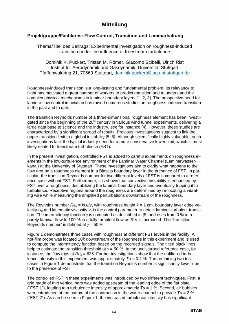
STAB


Thema/Titel des Beitrags: Experimental investigation on roughness-induced transition under the influence of freestream turbulence

Dominik K. Puckert, Tristan M. Römer, Giacomo Scibelli, Ulrich Rist

Institut für Aerodynamik und Gasdynamik, Universität Stuttgart Pfaffenwaldring 21, 70569 Stuttgart, [email protected]

Roughness-induced transition is a long-lasting and fundamental problem. Its relevance to flight has motivated a great number of workers to predict transition and to understand the complex physical mechanisms in laminar boundary layers [1, 2, 3]. The prospective need for laminar flow control in aviation has raised numerous studies on roughness-induced transition in the past and to date. The transition Reynolds number of a three-dimensional roughness element has been investi-gated since the beginning of the 20th century in various wind tunnel experiments, delivering a large data base to science and the industry, see for instance [4]. However, these studies are characterized by a significant spread of results. Previous investigations suggest to link the upper transition limit to a global instability [5, 6]. Although scientifically highly valueable, such investigations lack the typical industry need for a more conservative lower limit, which is most likely related to freestream turbulence (FST). In the present investigation, controlled FST is added to careful experiments on roughness el-ements in the low-turbulence environment of the Laminar Water Channel (Laminarwasser-kanal) at the University of Stuttgart. These investigations aim to clarify what happens to the flow around a roughness element in a Blasius boundary layer in the presence of FST. In par-ticular, the transition Reynolds number for two different levels of FST is compared to a refer-ence case without FST. Furthermore, it is shown that convective instability is enhanced by FST over a roughness, destabilizing the laminar boundary layer and eventually tripping it to turbulence. Receptive regions around the roughness are determined by re-locating a vibrat-ing wire while measuring the amplified perturbations downstream of the roughness. The Reynolds number Rek = kUe/v, with roughness height k = 1 cm, boundary layer edge ve-locity Ue and kinematic viscosity v, is the control parameter to detect laminar-turbulent transi-tion. The intermittency function γ is computed as described in [5] and rises from 0 % in a purely laminar flow to 100 % in a fully turbulent flow as Rek is increased. The “transition Reynolds number” is defined at γ = 50 %. Figure 1 demonstrates three cases with roughness at different FST levels in the facility. A hot-film probe was located 10k downstream of the roughness in this experiment and is used to compute the intermittency function based on the recorded signals. The tilted black lines help to estimate the transition threshold at γ = 50 %. In the undisturbed reference case, for instance, the flow trips at Rek = 635. Further investigations show that the unfiltered turbu-lence intensity in this experiment was approximately Tu = 0.4 %. The remaining two test cases in Figure 1 demonstrate that the transition Reynolds number is significantly lower due to the presence of FST. The controlled FST in these experiments was introduced by two different techniques. First, a grid made of thin vertical bars was added upstream of the leading edge of the flat plate (“FST-1”), leading to a turbulence intensity of approximately Tu = 1 %. Second, air bubbles were introduced at the bottom of the contraction in the water channel to provide Tu = 2 % (“FST-2”). As can be seen in Figure 1, the increased turbulence intensity has significant

64


STAB

impact on the transition location. In the full paper, this observation is investigated in more de-tail to clarify the role of freestream turbulence in roughness-induced transition.

Figure 1: Intermittency (in percent) versus Reynolds number

References: 1 L. Klanfer and P. Owen, „The effect of isolated roughness on boundary layer transition,“

RAE Tech. Memo, p. 355, 1953. 2 P. Klebanoff, W. Cleveland and K. Tidstrom, „On the evolution of a turbulent boundary

layer induced by a three-dimensional roughness element,“ J. Fluid Mech., vol. 237, pp. 101-187, 1992.

3 N. Denissen and E. White, „Secondary instability of roughness-induced transient growth,“ Phys. Fluids., vol. 25, p. 114108, 2013.

4 A. von Doenhoff and A. Braslow, „The effect of distributed surface roughness on laminar flow,“ Boundary Layer Control 2, pp. 657-681, 1961.

5 D. K. Puckert and U. Rist, „Experiments on critical Reynolds number and global insta-bility in roughness-induced laminar-turbulent transition,“ J. Fluid Mech., vol. 844, 2018.

6 M. Bucci, D. K. Puckert, C. Andriano, J.-C. Loiseau, S. Cherubini, J.-C. Robinet and U. Rist, „Roughness-induced transition by quasi-resonance of a varicose global mode,“ J. Fluid Mech., vol. 836, pp. 167-191, 2018.

65

STAB

An estimation for the size of a suction flap for a passive HLFC system

Geza Schrauf DLR, Lilienthalplatz 7, 38108 Braunschweig, [email protected]

For larger aircraft, we need hybrid laminar flow control (HLFC) to achieve laminar flow, i.e. a combination of boundary layer suction at the leading edge before the front spar and suitable profile shaping behind it. The current state of the art is to apply suction with the help of a mi-cro-perforated titanium surface. The necessary suction power to drive the HLFC system can be obtained by a fan or a compressor. If this is the case, we have an active suction system. However, we can also generate the suction power with the help of an outlet flap, as can be seen in Figures 1 and 2. Because such a system does not require a compressor, we call it a passive HLFC system. In the pre-design phase of a passive suction system, we need to know whether an envisaged location for a suction flap is suitable for its installation. The main restriction is the available space inside the wing or tail at the chosen location. For this, it is necessary to estimate the size of the suction flap. If the needed flap would be too large, we have to find a different loca-tion or modify the suction system so that it would need less power and, therefore, would re-quire a smaller flap. Navier-Stokes calculations for an outlet flap are very work-intensive: the generation of the geometry data, the computational grid, the calculation, and the evaluations often need sev-eral weeks. Thus we needed a fast method to obtain a first-order estimate of the flap size. We have developed a method that considerably speeds up the design process by avoiding unnecessary Navier-Stokes computations for inadequate locations. In this paper, we will derive a simple estimate for the size of an outlet flap and present com-parisons with TAU-calulations. Literaure: F. M. Rogallo: “Internal Flow Systems for Aircraft.” NACA Technical Report 713, 1941.


Mitteilung

66

STAB

Figure 1: Closed suction flap installed in A320 HLFC VTP.

Figure 2: Open suction flap of Figure 1 in the test rig.

67

STAB


Receptivitiy of swept-wing boundary layers to surface roughness and inhomogene-ous suction

D. Simanowitsch, A. Theiss, S. Hein

DLR – Institut für Aerodynamik und Strömungstechnik, Bunsenstraße 10, D-37073 Göttingen, Germany, [email protected]

Background and Motivation Hybrid Laminar Flow Control (HLFC) is a promising concept to reduce the fuel con-sumption of future commercial airplanes. Suction through porous surfaces is used to delay laminar-turbulent transition and thus reduce the overall skin-friction drag. In three-dimensional (3D) boundary layers, suction in the leading-edge region of the transonic swept wings is used to stabilize crossflow instabilities [1]. However, suction does not only change the stability characteristics of the boundary layer but also af-fects its receptivity, meaning the initial amplitudes of disturbances triggered by the environment. Moreover, suction through porous surfaces typically increases surface roughness and results in a non-uniform suction distribution. In N-factor based transi-tion prediction using either Linear Stability Theory (LST) or linear Parabolized Stabil-ity Equations (PSE), only the stabilization of the boundary layer by suction is covered assuming an idealized spanwise homogenous suction distribution. The additional changes in the receptivity characteristics of the boundary layer due to suction and any detrimental effects due to the porous surface, resulting e.g. in a non-uniform suc-tion distribution or increased surface roughness, therefore have to be modelled by assuming lower transition N-factors compared to the transition N-factors used for transonic swept wings without suction panels. Only few data exist in literature on the receptivity coefficients of realistic transonic swept-wing boundary layers without and with suction. Such data, together with sufficient information on the actual surface roughness and suction inhomogeneity, would allow quantifying those detrimental ef-fects on the development of stationary crossflow vortices and thus could provide some guidelines of how the corresponding transition N-factors have to be adjusted. Approach and Results In the present work, the receptivity of compressible quasi-3D boundary layers to sur-face roughness and inhomogeneous suction is studied in detail. The stability charac-teristics of the boundary layer without and with suction are analyzed by linear PSE [2]. The corresponding receptivity coefficients for surface roughness and non-uniform suction are derived from adjoint PSE computations [3]. For a given shape of the sur-face roughness or information on the non-uniformity of the suction velocity distribu-tion, the resulting amplitude of the stationary crossflow vortices generated by these surface irregularities can be computed. In the first step, the present numerical ap-proach has been verified by comparisons with suitable reference data from literature. Tempelmann [4] studied the response of a generic incompressible quasi-3D bounda-ry layer, the Falkner-Skan-Cooke (FSC) similarity solution, to a small spanwise peri-odic surface roughness. The chordwise shape of this roughness is denoted in Figure 1a as Shape 1. The amplitude of the stationary crossflow instability triggered by the roughness and its subsequent downstream growth is plotted in Figure 1b together

68

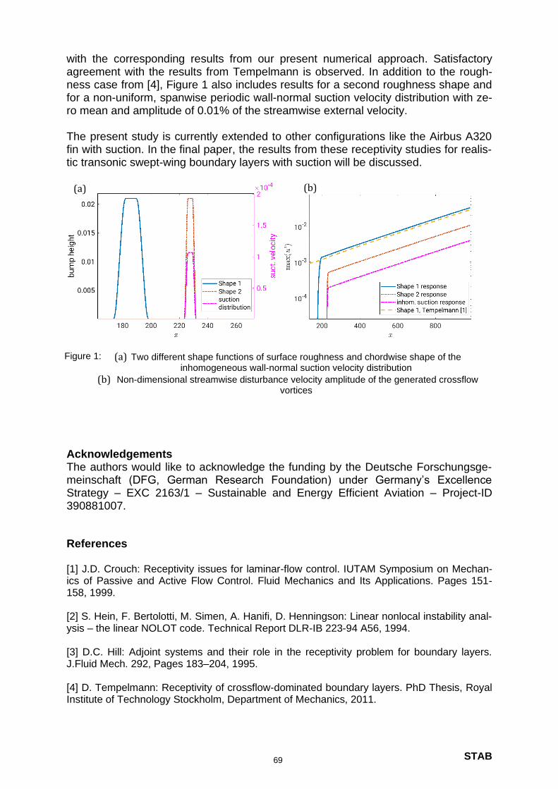
STAB

with the corresponding results from our present numerical approach. Satisfactory agreement with the results from Tempelmann is observed. In addition to the rough-ness case from [4], Figure 1 also includes results for a second roughness shape and for a non-uniform, spanwise periodic wall-normal suction velocity distribution with ze-ro mean and amplitude of 0.01% of the streamwise external velocity. The present study is currently extended to other configurations like the Airbus A320 fin with suction. In the final paper, the results from these receptivity studies for realis-tic transonic swept-wing boundary layers with suction will be discussed.

(a) Two different shape functions of surface roughness and chordwise shape of the inhomogeneous wall-normal suction velocity distribution

(b) Non-dimensional streamwise disturbance velocity amplitude of the generated crossflow vortices

Acknowledgements The authors would like to acknowledge the funding by the Deutsche Forschungsge-meinschaft (DFG, German Research Foundation) under Germany’s Excellence Strategy – EXC 2163/1 – Sustainable and Energy Efficient Aviation – Project-ID 390881007.

References [1] J.D. Crouch: Receptivity issues for laminar-flow control. IUTAM Symposium on Mechan-ics of Passive and Active Flow Control. Fluid Mechanics and Its Applications. Pages 151-158, 1999. [2] S. Hein, F. Bertolotti, M. Simen, A. Hanifi, D. Henningson: Linear nonlocal instability anal-ysis – the linear NOLOT code. Technical Report DLR-IB 223-94 A56, 1994. [3] D.C. Hill: Adjoint systems and their role in the receptivity problem for boundary layers. J.Fluid Mech. 292, Pages 183–204, 1995. [4] D. Tempelmann: Receptivity of crossflow-dominated boundary layers. PhD Thesis, Royal Institute of Technology Stockholm, Department of Mechanics, 2011.

(a)

Figure 1:

(b)

69

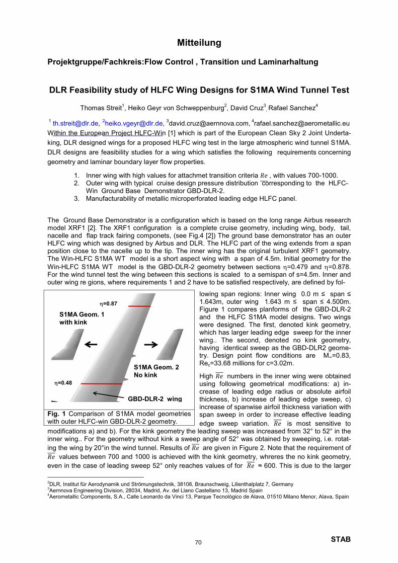
STAB

The Ground Base Demonstrator is a configuration which is based on the long range Airbus research model XRF1 [2]. The XRF1 configuration is a complete cruise geometry, including wing, body, tail, nacelle and flap track fairing componets, (see Fig.4 [2]) The ground base demonstrator has an outer HLFC wing which was designed by Airbus and DLR. The HLFC part of the wing extends from a span position close to the nacelle up to the tip. The inner wing has the original turbulent XRF1 geometry. The Win-HLFC S1MA WT model is a short aspect wing with a span of 4.5m. Initial geometry for the Win-HLFC S1MA WT model is the GBD-DLR-2 geometry between sections =0.479 and =0.878. For the wind tunnel test the wing between this sections is scaled to a semispan of s=4.5m. Inner and outer wing re gions, where requirements 1 and 2 have to be satisfied respectively, are defined by fol-

lowing span regions: Inner wing 0.0 m ≤ span ≤ 1.643m, outer wing 1.643 m ≤ span ≤ 4.500m. Figure 1 compares planforms of the GBD-DLR-2 and the HLFC S1MA model designs. Two wings were designed. The first, denoted kink geometry, which has larger leading edge sweep for the inner wing.. The second, denoted no kink geometry, having identical sweep as the GBD-DLR2 geome-try. Design point flow conditions are M∞=0.83, Rec=33.68 millions for c=3.02m. High numbers in the inner wing were obtained using following geometrical modifications: a) in-crease of leading edge radius or absolute airfoil thickness, b) increase of leading edge sweep, c) increase of spanwise airfoil thickness variation with span sweep in order to increase effective leading

edge sweep variation. is most sensitive to modifications a) and b). For the kink geometry the leading sweep was increased from 32° to 52° in the inner wing.. For the geometry without kink a sweep angle of 52° was obtained by sweeping, i.e. rotat-

ing the wing by 20°in the wind tunnel. Results of are given in Figure 2. Note that the requirement of

values between 700 and 1000 is achieved with the kink geometry, whreres the no kink geometry,

even in the case of leading sweep 52° only reaches values of for ≈ 600. This is due to the larger

2DLR, Institut für Aerodynamik und Strömungstechnik, 38108, Braunschweig, Lilienthalplatz 7, Germany 3Aernnova Engineering Division, 28034, Madrid, Av. del Llano Castellano 13, Madrid Spain 4Aerometallic Components, S.A., Calle Leonardo da Vinci 13, Parque Tecnológico de Alava, 01510 Milano Menor, Alava, Spain

Fig. 1 Comparison of S1MA model geometries with outer HLFC-win GBD-DLR-2 geometry.

S1MA Geom. 2No kink

GBD-DLR-2 wing

S1MA Geom. 1with kink

=0.87

=0.48

Manufacturability of metallic microperforated leading edge HLFC panel.3.Win Ground Base Demonstrator GBD-DLR-2.Outer wing with typical cruise design pressure distribution corresponding to the HLFC- 2.Inner wing with high values for attachmet transition criteria , with values 700-1000.1.

geometry and laminar boundary layer flow properties.

DLR designs are feasibility studies for a wing which satisfies the following requirements concerning king, DLR designed wings for a proposed HLFC wing test in the large atmospheric wind tunnel S1MA. Within the European Project HLFC-Win [1] which is part of the European Clean Sky 2 Joint Underta-

1 [email protected], 2

[email protected], [email protected], 4

[email protected]

Thomas Streit1, Heiko Geyr von Schweppenburg

2, David Cruz

3, Rafael Sanchez

4

DLR Feasibility study of HLFC Wing Designs for S1MA Wind Tunnel Test

Projektgruppe/Fachkreis:Flow Control , Transition und Laminarhaltung

Mitteilung

70

STAB

absolute leading edge radius of the kink geometry, which in part is due to airfoil sections with larger chord length. Note also that due to the proximity of the inner wing to the wind tunnel wall the effective leading sweep is less than the geometrical leading edge sweep.

Fig. 2 as function of span position Attachment transition criteria (left side), effective leading edge sweep angle (right side).

To achieve requirement 2 the 3D DLR inverse design code [3] was used using as target pressure dis-tribution the design point pressure distribution of the GBD-DLR-2 geometry. Figure 3 shows pressure distributions results for the kink geometry. For both the kink geometry and the no kink geometry the inverse design process was able to find geometries which lead to the target HLFC pressure distribu-tion in a span region 0.40 < < 0.80. Despite the wind tunnel model being a low aspect ratio wing with an inner wing having largely different pressure distributions in comparison to the GBD-DLR-2 long range configuration, it was possible to obtain an outer wing geometry with the target pressure distribu-tion. The obtained outer wing satisfies requirements regarding pressure distribution in the suction re-gion, N-factor distribution, shock position and isobar concept design. As function of angle of incidence the designed wing geometries also develop pressure distributions with characteristics similar to the GBD-DLR-2 configuration.

Fig.3 Pressure distributions for outer wing sections for kink geometry. Comparison between initial no kink pressure distribution (green line) and design results (black). The initial designs did not satisfy requirement 3. The short aspect ratio of the wind tunnel model and design requirements 2) and 3) led to a 3d geometry with non acceptable variations of thickness and twist. Therefore in a further design step wings were constructed based on a reduced number of defin-ing sections, which however still satisfied requirement 1) and 2). For the final designs for both cases, i.e. the kink and non kink geometry, Aernnova and Aerometallic Components verified that a leading edge metallic microperfurated suction panel could be manufactured. References [1] https://www.hlfc-win.eu/ [2] Pattison, J. ,Wilson, T., Herring, M.,”High Fidelity Simulation of the Folding Wing Tip for Loads Alleviation”, Interna-

tional Forum on Aerolasticity and Structural Dynamics”, 2018, St.Petersburg, Russia. [3] Streit, T. and Hoffrogge, C., “DLR transonic inverse design code, extensions and modifications to increase versatility

and robustness”, Aeronautical J, 2017, 121, (1245), pp 1733-1757, https://doi.org/10.1017/aer.2017.101

71

STAB

Mitteilung

Projektgruppe/Fachkreis: Flow Control, Transition und Laminarhaltung The effect of 2-D surface irregularities on laminar-turbulent transition: A comparison

of numerical methodologies

F. Tocci, J. A. Franco, S. Hein DLR, Institut für Aerodynamik und Strömungstechnik (AS),

Abteilung Hochgeschwindigkeitskonfigurationen, Bunsenstr.10, 37073 Göttingen [email protected]

G. Chauvat, A. Hanifi

KTH Royal Institute of Technology, Dept. of Engineering Mechanics, FLOW, SE-100 44 Stockholm, Sweden

Laminar-turbulent transition prediction is of practical interest in aircraft design since transition affects important aerodynamic quantities such as drag and heat transfer. Extended laminar flow on aerodynamic surfaces is an effective way of reducing aircraft drag. One of the major challenges for the implementation of laminar-flow surfaces is the potential for any irregularity to move transition upstream. Under low-disturbance environment, boundary-layer transition results from the growth and breakdown of different flow instabilities. In 2-D flows the scenar-io is dominated by Tollmien-Schlichting (TS) instabilities. Common wing-surface irregulari-ties, such as two-dimensional steps, gaps or waviness can alter the growth characteristics of TS waves and therefore must be taken into account at the design stage. The effect of steps, gaps and humps on the development of TS waves in an incompressible boundary layer has been investigated in [1] using direct numerical simulations (DNS). All the irregularities were found to have an overall destabilizing effect. In the present work, we com-pare those results with Local Stability Theory (LST), Parabolized Stability Equations (PSE) and Adaptive Harmonic Linearized Navier-Stokes (AHLNS) approach. In the past, LST and PSE, together with the e

N method, have been successfully applied for transition prediction in

cases without surface irregularities where the local streamwise flow gradients were small. However, the validity of the assumptions of such methods becomes questionable with the increased gradients locally induced by the surface irregularities. AHLNS removes some of the inherent limitations present in LST and PSE, and it has been already applied effectively in the presence of humps by Franco et al. [2]. Edelmann et al. [3] used LST with forward-facing steps introducing a special treatment for the region around the step and Park et al. [4] performed PSE analyses for smooth humps. To the best of the authors’ knowledge, there is no published comparison between LST, PSE, AHLNS, and DNS for the development of TS waves encountering surface irregularities. Fig. 1 shows the steady laminar base flow for one of the surface imperfections studied: a smooth hump. For this case, the comparison between LST, PSE, AHLNS, and DNS for the development of TS waves is given in Fig. 2 for a selected frequency. TS waves are destabi-lized in the decelerated region on the leeward side of the hump where they also interact with the separation bubble. A perfect agreement between DNS and AHLNS is observed. The LST and PSE results exhibit differences in the hump region, before recovering the same growth rate far downstream. Moreover, LST is already underpredicting the decay in the stable region upstream of the hump. This behaviour was also noticed for the flat plate. For the frequency considered the TS wavelength is twice the width of the hump and therefore the applicability of PSE would be dubious. The characteristic length scale of the perturbation in the streamwise direction is of the same order as the corresponding characteristic length scale of the streamwise flow variation induced by the surface irregularity. For LST the basic state is approximated as locally parallel, an assumption that does not hold, in particular in the vicinity of the hump. Under these circumstances LST should be used with caution. In the

72


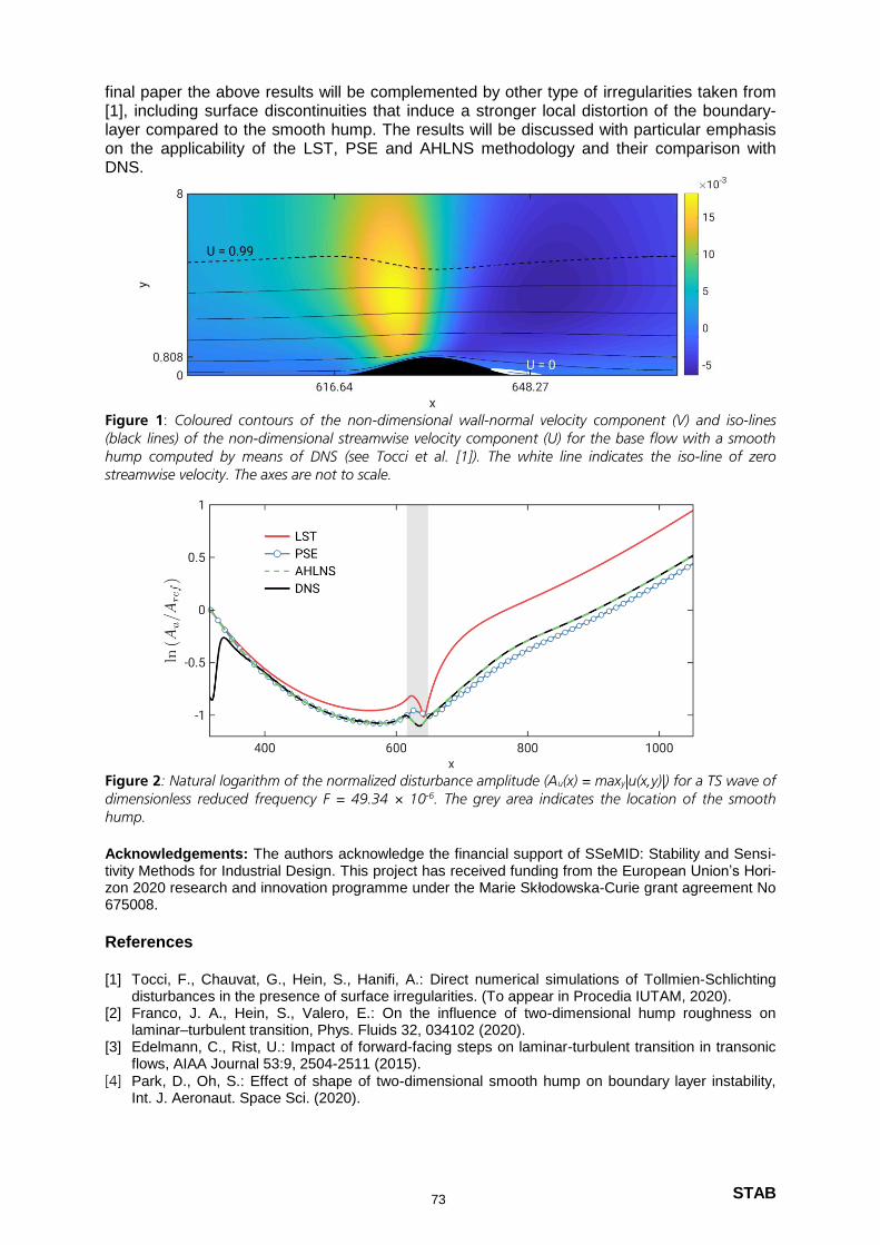
STAB

final paper the above results will be complemented by other type of irregularities taken from [1], including surface discontinuities that induce a stronger local distortion of the boundary-layer compared to the smooth hump. The results will be discussed with particular emphasis on the applicability of the LST, PSE and AHLNS methodology and their comparison with DNS.

Figure 1: Coloured contours of the non-dimensional wall-normal velocity component (V) and iso-lines (black lines) of the non-dimensional streamwise velocity component (U) for the base flow with a smooth hump computed by means of DNS (see Tocci et al. [1]). The white line indicates the iso-line of zero streamwise velocity. The axes are not to scale.

Figure 2: Natural logarithm of the normalized disturbance amplitude (Au(x) = maxy|u(x,y)|) for a TS wave of dimensionless reduced frequency F = 49.34 × 10-6. The grey area indicates the location of the smooth hump.

Acknowledgements: The authors acknowledge the financial support of SSeMID: Stability and Sensi-tivity Methods for Industrial Design. This project has received funding from the European Union’s Hori-zon 2020 research and innovation programme under the Marie Skłodowska-Curie grant agreement No 675008.

References

[1] Tocci, F., Chauvat, G., Hein, S., Hanifi, A.: Direct numerical simulations of Tollmien-Schlichting

disturbances in the presence of surface irregularities. (To appear in Procedia IUTAM, 2020). [2] Franco, J. A., Hein, S., Valero, E.: On the influence of two-dimensional hump roughness on

laminar–turbulent transition, Phys. Fluids 32, 034102 (2020). [3] Edelmann, C., Rist, U.: Impact of forward-facing steps on laminar-turbulent transition in transonic

flows, AIAA Journal 53:9, 2504-2511 (2015).

[4] Park, D., Oh, S.: Effect of shape of two-dimensional smooth hump on boundary layer instability, Int. J. Aeronaut. Space Sci. (2020).

73

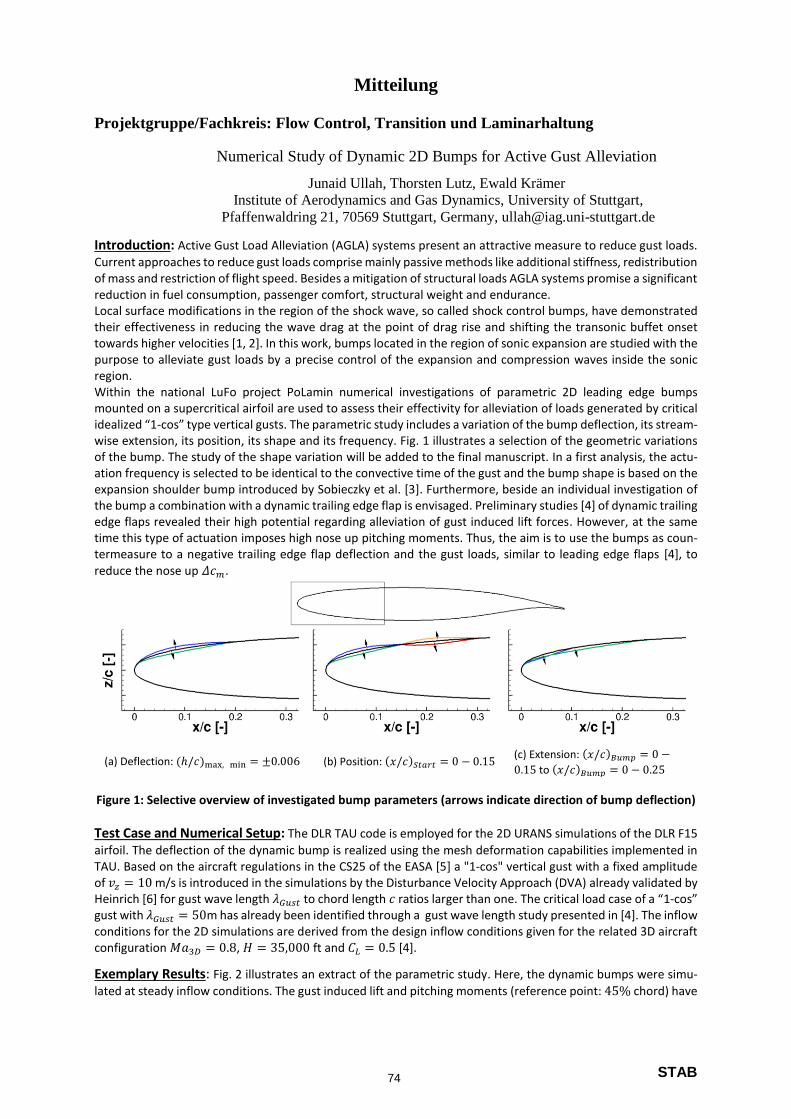
STAB

Figure 1: Selective overview of investigated bump parameters (arrows indicate direction of bump deflection)

Test Case and Numerical Setup: The DLR TAU code is employed for the 2D URANS simulations of the DLR F15

airfoil. The deflection of the dynamic bump is realized using the mesh deformation capabilities implemented in TAU. Based on the aircraft regulations in the CS25 of the EASA [5] a "1-cos" vertical gust with a fixed amplitude of 𝑣𝑧 = 10 m/s is introduced in the simulations by the Disturbance Velocity Approach (DVA) already validated by Heinrich [6] for gust wave length 𝜆𝐺𝑢𝑠𝑡 to chord length 𝑐 ratios larger than one. The critical load case of a “1-cos” gust with 𝜆𝐺𝑢𝑠𝑡 = 50m has already been identified through a gust wave length study presented in [4]. The inflow conditions for the 2D simulations are derived from the design inflow conditions given for the related 3D aircraft configuration 𝑀𝑎3𝐷 = 0.8, 𝐻 = 35,000 ft and 𝐶𝐿 = 0.5 [4].

Exemplary Results: Fig. 2 illustrates an extract of the parametric study. Here, the dynamic bumps were simu-

lated at steady inflow conditions. The gust induced lift and pitching moments (reference point: 45% chord) have

(a) Deflection: (ℎ/𝑐)max, min = ±0.006 (b) Position: (𝑥/𝑐)𝑆𝑡𝑎𝑟𝑡 = 0 − 0.15 (c) Extension: (𝑥/𝑐)𝐵𝑢𝑚𝑝 = 0 −

0.15 to (𝑥/𝑐)𝐵𝑢𝑚𝑝 = 0 − 0.25

reduce the nose up 𝛥𝑐𝑚.

termeasure to a negative trailing edge flap deflection and the gust loads, similar to leading edge flaps [4], to time this type of actuation imposes high nose up pitching moments. Thus, the aim is to use the bumps as coun- edge flaps revealed their high potential regarding alleviation of gust induced lift forces. However, at the same the bump a combination with a dynamic trailing edge flap is envisaged. Preliminary studies [4] of dynamic trailing expansion shoulder bump introduced by Sobieczky et al. [3]. Furthermore, beside an individual investigation of ation frequency is selected to be identical to the convective time of the gust and the bump shape is based on the of the bump. The study of the shape variation will be added to the final manuscript. In a first analysis, the actu- wise extension, its position, its shape and its frequency. Fig. 1 illustrates a selection of the geometric variations idealized “1-cos” type vertical gusts. The parametric study includes a variation of the bump deflection, its stream- mounted on a supercritical airfoil are used to assess their effectivity for alleviation of loads generated by critical Within the national LuFo project PoLamin numerical investigations of parametric 2D leading edge bumps region.purpose to alleviate gust loads by a precise control of the expansion and compression waves inside the sonic towards higher velocities [1, 2]. In this work, bumps located in the region of sonic expansion are studied with the their effectiveness in reducing the wave drag at the point of drag rise and shifting the transonic buffet onset Local surface modifications in the region of the shock wave, so called shock control bumps, have demonstrated reduction in fuel consumption, passenger comfort, structural weight and endurance.of mass and restriction of flight speed. Besides a mitigation of structural loads AGLA systems promise a significant Current approaches to reduce gust loads comprise mainly passive methods like additional stiffness, redistribution Introduction: Active Gust Load Alleviation (AGLA) systems present an attractive measure to reduce gust loads.

Pfaffenwaldring 21, 70569 Stuttgart, Germany, [email protected]

Institute of Aerodynamics and Gas Dynamics, University of Stuttgart,

Junaid Ullah, Thorsten Lutz, Ewald Krämer

Numerical Study of Dynamic 2D Bumps for Active Gust Alleviation


Mitteilung

74

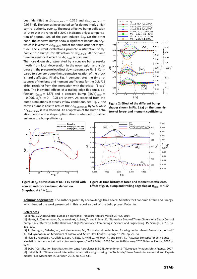
STAB

been identified as 𝛥𝑐𝑙,𝐺𝑢𝑠𝑡,𝑚𝑎𝑥 = 0.315 and 𝛥𝑐𝑚,𝐺𝑢𝑠𝑡,𝑚𝑎𝑥 =

0.038 [4]. The bumps investigated so far do not imply a high control authority over 𝑐𝑙. The most effective bump deflection of -0.6% 𝑐 in the range of 5-20% 𝑐 indicates only a compensa-tion of approx. 10% of the gust induced Δ𝑐𝑙 . On the other hand, the concave bumps show a significant impact on 𝛥𝑐𝑚, which is inverse to 𝛥𝑐𝑚,𝐺𝑢𝑠𝑡 and of the same order of magni-

tude. The current evaluations promote a utilization of dy-namic nose bumps for alleviation of 𝛥𝑐𝑚,𝐺𝑢𝑠𝑡. At the same

time no significant effect on 𝛥𝑐𝑙,𝐺𝑢𝑠𝑡 is presumed.

The nose down 𝛥𝑐𝑚 generated by a concave bump results mostly from local deceleration in the nose region and a de-crease in the pressure level just downstream, see Fig. 3. Com-pared to a convex bump the streamwise location of the shock is hardly affected. Finally, Fig. 4 demonstrates the time re-sponses of the force and moment coefficients for the DLR F15 airfoil resulting from the interaction with the critical “1-cos” gust. The individual effects of a trailing edge flap (max. de-flection 𝜂max = 4.5°) and a concave bump ((ℎ/𝑐)𝑚𝑎𝑥 =−0.006, 𝑥/𝑐. = 0 − 0.2) are shown. As expected from the bump simulations at steady inflow conditions, see Fig. 2, the convex bump is able to reduce the 𝛥𝑐𝑚,𝐺𝑢𝑠𝑡,𝑚𝑎𝑥 by 52% while

𝛥𝑐𝑙,𝐺𝑢𝑠𝑡,𝑚𝑎𝑥 is less affected. An adaptation of the bump actu-

ation period and a shape optimization is intended to further enhance the bump efficiency.

Acknowledgements: The authors gratefully acknowledge the Federal Ministry for Economic Affairs and Energy,

which funded the work presented in this report as part of the LuFo project PoLamin.

References [1] König, B., Shock Control Bumps on Transonic Transport Aircraft, Verlag Dr. Hut, 2014. [2] Mayer, R., Zimmermann, D., Wawrzinek, K., Lutz, T., and Krämer, E., “Numerical Study of Three-Dimensional Shock Control Bump Flank Effects on Buffet Behavior,” High Performance Computing in Science and Engineering 15, Springer, 2016, pp. 495–509. [3] Sobieczky, H., Geissler, W., and Hannemann, M., “Expansion shoulder bump for wing section viscous/wave drag control,” IUTAM Symposium on Mechanics of Passive and Active Flow Control, Springer, 1999, pp. 29–34. [4] Klug, L., Radespiel, R., Ullah, J., Seel, F., Lutz, T., Wild, J., Heinrich, R., and Streit, T., “Actuator concepts for active gust alleviation on transport aircraft at transonic speeds,” AIAA Scitech 2020 Forum, 6-10 January 2020 Orlando, Florida, 2020, p. 0271. [5] EASA, “Certification Specifications for Large Aeroplanes (CS-25). Amendment 3,” European Aviation Safety Agency, 2007. [6] Heinrich, R., “Simulation of interaction of aircraft and gust using the TAU-code,” New Results in Numerical and Experi-mental Fluid Mechanics IX, Springer, 2014, pp. 503–511.

Figure 3: 𝒄𝒑 distribution of DLR F15 airfoil with

convex and concave bump deflection. Snapshot at (𝒉/𝒄)𝐦𝐚𝐱

Figure 4: Time history of force and moment coefficients. Effect of gust, bump and trailing edge flap at 𝜼𝐦𝐚𝐱 = 𝟒. 𝟓°

Figure 2: Effect of the different bump shapes shown in Fig. 1 (a) on the time his-tory of force- and moment coefficients

75

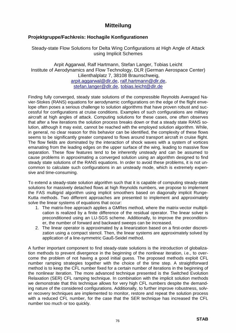
STAB

Mitteilung

Projektgruppe/Fachkreis: Hochagile Konfigurationen

Steady-state Flow Solutions for Delta Wing Configurations at High Angle of Attack

using Implicit Schemes

Arpit Aggarwal, Ralf Hartmann, Stefan Langer, Tobias Leicht Institute of Aerodynamics and Flow Technology, DLR (German Aerospace Center)

Lilienthalplatz 7, 38108 Braunschweig, [email protected], [email protected],

[email protected], [email protected]

Finding fully converged, steady state solutions of the compressible Reynolds Averaged Na-vier-Stokes (RANS) equations for aerodynamic configurations on the edge of the flight enve-lope often poses a serious challenge to solution algorithms that have proven robust and suc-cessful for configurations at cruise conditions. Examples of such configurations are military aircraft at high angles of attack. Computing solutions for these cases, one often observes that after a few iterations the solution process breaks down or that a steady state RANS so-lution, although it may exist, cannot be reached with the employed solution algorithm. While, in general, no clear reason for this behavior can be identified, the complexity of these flows seems to be significantly greater compared to flows around transport aircraft in cruise flight. The flow fields are dominated by the interaction of shock waves with a system of vortices emanating from the leading edges on the upper surface of the wing, leading to massive flow separation. These flow features tend to be inherently unsteady and can be assumed to cause problems in approximating a converged solution using an algorithm designed to find steady state solutions of the RANS equations. In order to avoid these problems, it is not un-common to calculate such configurations in an unsteady mode, which is extremely expen-sive and time-consuming. To extend a steady-state solution algorithm such that it is capable of computing steady-state solutions for massively detached flows at high Reynolds numbers, we propose to implement the FAS multigrid algorithm using implicit smoothers based on diagonally implicit Runge-Kutta methods. Two different approaches are presented to implement and approximately solve the linear systems of equations that occur:

1. The matrix-free approach applies a GMRes method, where the matrix-vector multipli-cation is realized by a finite difference of the residual operator. The linear solver is preconditioned using an LU-SGS scheme. Additionally, to improve the precondition-er, the number of forward and backward sweeps can be increased.

2. The linear operator is approximated by a linearization based on a first-order discreti-zation using a compact stencil. Then, the linear systems are approximately solved by application of a line-symmetric Gauß-Seidel method.

A further important component to find steady-state solutions is the introduction of globaliza-tion methods to prevent divergence in the beginning of the nonlinear iteration, i.e., to over-come the problem of not having a good initial guess. The proposed methods exploit CFL number ramping strategies together with the choice of the time step. A straightforward method is to keep the CFL number fixed for a certain number of iterations in the beginning of the nonlinear iteration. The more advanced technique presented is the Switched Evolution Relaxation (SER) CFL ramping technique. In combination with the implicit solution methods we demonstrate that this technique allows for very high CFL numbers despite the demand-ing nature of the considered configurations. Additionally, to further improve robustness, solv-er recovery techniques are implemented to monitor, restore and repeat the solution process with a reduced CFL number, for the case that the SER technique has increased the CFL number too much or too quickly.

76





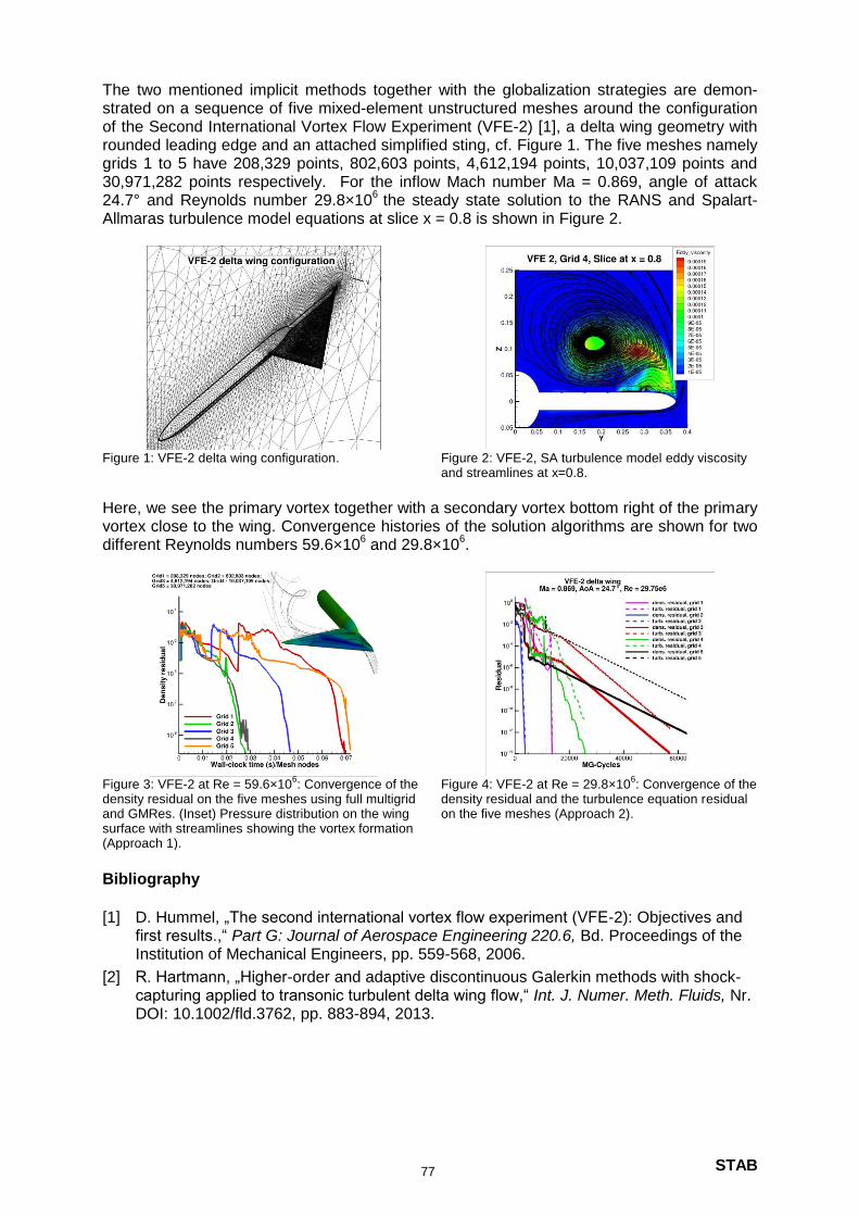
STAB

The two mentioned implicit methods together with the globalization strategies are demon-strated on a sequence of five mixed-element unstructured meshes around the configuration of the Second International Vortex Flow Experiment (VFE-2) [1], a delta wing geometry with rounded leading edge and an attached simplified sting, cf. Figure 1. The five meshes namely grids 1 to 5 have 208,329 points, 802,603 points, 4,612,194 points, 10,037,109 points and 30,971,282 points respectively. For the inflow Mach number Ma = 0.869, angle of attack 24.7° and Reynolds number 29.8×10

6 the steady state solution to the RANS and Spalart-

Allmaras turbulence model equations at slice x = 0.8 is shown in Figure 2.

Figure 1: VFE-2 delta wing configuration. Figure 2: VFE-2, SA turbulence model eddy viscosity

and streamlines at x=0.8.

Here, we see the primary vortex together with a secondary vortex bottom right of the primary vortex close to the wing. Convergence histories of the solution algorithms are shown for two different Reynolds numbers 59.6×10

6 and 29.8×10

6.

Figure 3: VFE-2 at Re = 59.6×10

6: Convergence of the

density residual on the five meshes using full multigrid and GMRes. (Inset) Pressure distribution on the wing surface with streamlines showing the vortex formation (Approach 1).

Figure 4: VFE-2 at Re = 29.8×106: Convergence of the

density residual and the turbulence equation residual on the five meshes (Approach 2).

Bibliography

[1] D. Hummel, „The second international vortex flow experiment (VFE-2): Objectives and first results.,“ Part G: Journal of Aerospace Engineering 220.6, Bd. Proceedings of the Institution of Mechanical Engineers, pp. 559-568, 2006.

[2] R. Hartmann, „Higher-order and adaptive discontinuous Galerkin methods with shock-capturing applied to transonic turbulent delta wing flow,“ Int. J. Numer. Meth. Fluids, Nr. DOI: 10.1002/fld.3762, pp. 883-894, 2013.

77

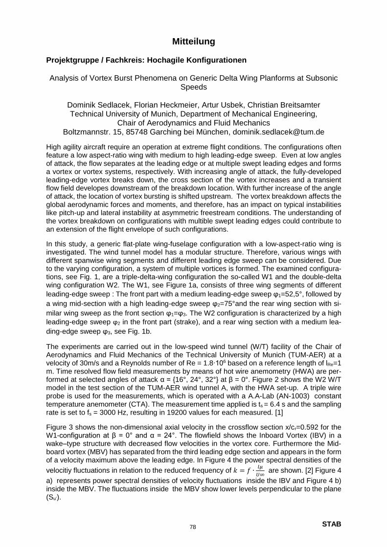
STAB

Mitteilung Projektgruppe / Fachkreis: Hochagile Konfigurationen Analysis of Vortex Burst Phenomena on Generic Delta Wing Planforms at Subsonic

Speeds

Dominik Sedlacek, Florian Heckmeier, Artur Usbek, Christian Breitsamter Technical University of Munich, Department of Mechanical Engineering,

Chair of Aerodynamics and Fluid Mechanics Boltzmannstr. 15, 85748 Garching bei München, [email protected]

High agility aircraft require an operation at extreme flight conditions. The configurations often feature a low aspect-ratio wing with medium to high leading-edge sweep. Even at low angles of attack, the flow separates at the leading edge or at multiple swept leading edges and forms a vortex or vortex systems, respectively. With increasing angle of attack, the fully-developed leading-edge vortex breaks down, the cross section of the vortex increases and a transient flow field developes downstream of the breakdown location. With further increase of the angle of attack, the location of vortex bursting is shifted upstream. The vortex breakdown affects the global aerodynamic forces and moments, and therefore, has an impact on typical instabilities like pitch-up and lateral instability at asymmetric freestream conditions. The understanding of the vortex breakdown on configurations with multible swept leading edges could contribute to an extension of the flight envelope of such configurations.

In this study, a generic flat-plate wing-fuselage configuration with a low-aspect-ratio wing is investigated. The wind tunnel model has a modular structure. Therefore, various wings with different spanwise wing segments and different leading edge sweep can be considered. Due to the varying configuration, a system of multiple vortices is formed. The examined configura-tions, see Fig. 1, are a triple-delta-wing configuration the so-called W1 and the double-delta wing configuration W2. The W1, see Figure 1a, consists of three wing segments of different

leading-edge sweep : The front part with a medium leading-edge sweep ϕ1=52,5°, followed by

a wing mid-section with a high leading-edge sweep ϕ2=75°and the rear wing section with si-

milar wing sweep as the front section ϕ1=ϕ3. The W2 configuration is characterized by a high

leading-edge sweep ϕ2 in the front part (strake), and a rear wing section with a medium lea-

ding-edge sweep ϕ3, see Fig. 1b.

The experiments are carried out in the low-speed wind tunnel (W/T) facility of the Chair of Aerodynamics and Fluid Mechanics of the Technical University of Munich (TUM-AER) at a velocity of 30m/s and a Reynolds number of Re = 1.8∙106 based on a reference length of lRe=1 m. Time resolved flow field measurements by means of hot wire anemometry (HWA) are per-formed at selected angles of attack α = 16°, 24°, 32° at β = 0°. Figure 2 shows the W2 W/T model in the test section of the TUM-AER wind tunnel A, with the HWA set-up. A triple wire probe is used for the measurements, which is operated with a A.A-Lab (AN-1003) constant temperature anemometer (CTA). The measurement time applied is ts = 6.4 s and the sampling rate is set to fs = 3000 Hz, resulting in 19200 values for each measured. [1]

Figure 3 shows the non-dimensional axial velocity in the crossflow section x/cr=0.592 for the W1-configuration at β = 0° and α = 24°. The flowfield shows the Inboard Vortex (IBV) in a wake–type structure with decreased flow velocities in the vortex core. Furthermore the Mid-board vortex (MBV) has separated from the third leading edge section and appears in the form of a velocity maximum above the leading edge. In Figure 4 the power spectral densities of the

velocitiy fluctuations in relation to the reduced frequency of 𝑘 = 𝑓 ∙𝑙𝜇

𝑈∞ are shown. [2] Figure 4

a) represents power spectral densities of velocity fluctuations inside the IBV and Figure 4 b) inside the MBV. The fluctuations inside the MBV show lower levels perpendicular to the plane (Su’).

78

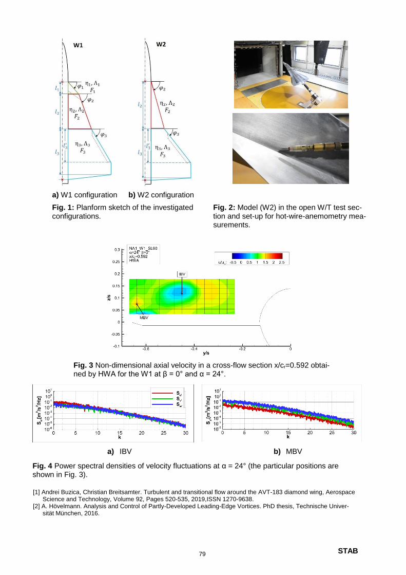
STAB

a) W1 configuration

b) W2 configuration

Fig. 1: Planform sketch of the investigated configurations.

Fig. 2: Model (W2) in the open W/T test sec-tion and set-up for hot-wire-anemometry mea-surements.

Fig. 3 Non-dimensional axial velocity in a cross-flow section x/cr=0.592 obtai-ned by HWA for the W1 at β = 0° and α = 24°.

a) IBV b) MBV

Fig. 4 Power spectral densities of velocity fluctuations at α = 24° (the particular positions are shown in Fig. 3).

[1] Andrei Buzica, Christian Breitsamter. Turbulent and transitional flow around the AVT-183 diamond wing, Aerospace Science and Technology, Volume 92, Pages 520-535, 2019,ISSN 1270-9638.

[2] A. Hövelmann. Analysis and Control of Partly-Developed Leading-Edge Vortices. PhD thesis, Technische Univer-sität München, 2016.

79

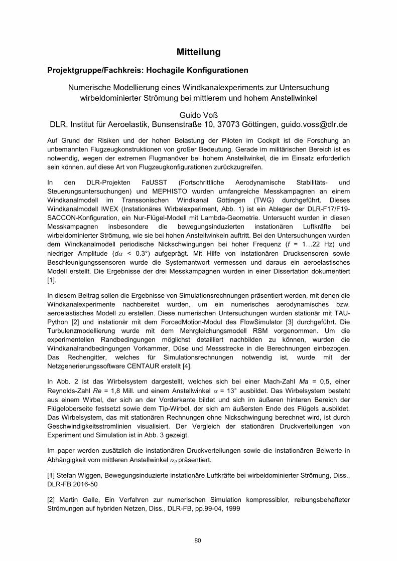
Mitteilung

Projektgruppe/Fachkreis: Hochagile Konfigurationen

Numerische Modellierung eines Windkanalexperiments zur Untersuchung

wirbeldominierter Strömung bei mittlerem und hohem Anstellwinkel

Guido Voß DLR, Institut für Aeroelastik, Bunsenstraße 10, 37073 Göttingen, [email protected]

Auf Grund der Risiken und der hohen Belastung der Piloten im Cockpit ist die Forschung an

unbemannten Flugzeugkonstruktionen von großer Bedeutung. Gerade im militärischen Bereich ist es

notwendig, wegen der extremen Flugmanöver bei hohem Anstellwinkel, die im Einsatz erforderlich

sein können, auf diese Art von Flugzeugkonfigurationen zurückzugreifen.

In den DLR-Projekten FaUSST (Fortschrittliche Aerodynamische Stabilitäts- und

Steuerungsuntersuchungen) und MEPHISTO wurden umfangreiche Messkampagnen an einem

Windkanalmodell im Transsonischen Windkanal Göttingen (TWG) durchgeführt. Dieses

Windkanalmodell IWEX (Instationäres Wirbelexperiment, Abb. 1) ist ein Ableger der DLR-F17/F19-

SACCON-Konfiguration, ein Nur-Flügel-Modell mit Lambda-Geometrie. Untersucht wurden in diesen

Messkampagnen insbesondere die bewegungsinduzierten instationären Luftkräfte bei

wirbeldominierter Strömung, wie sie bei hohen Anstellwinkeln auftritt. Bei den Untersuchungen wurden

dem Windkanalmodell periodische Nickschwingungen bei hoher Frequenz (f = 1…22 Hz) und

niedriger Amplitude (d < 0.3°) aufgeprägt. Mit Hilfe von instationären Drucksensoren sowie

Beschleunigungssensoren wurde die Systemantwort vermessen und daraus ein aeroelastisches

Modell erstellt. Die Ergebnisse der drei Messkampagnen wurden in einer Dissertation dokumentiert

[1].

In diesem Beitrag sollen die Ergebnisse von Simulationsrechnungen präsentiert werden, mit denen die

Windkanalexperimente nachbereitet wurden, um ein numerisches aerodynamisches bzw.

aeroelastisches Modell zu erstellen. Diese numerischen Untersuchungen wurden stationär mit TAU-

Python [2] und instationär mit dem ForcedMotion-Modul des FlowSimulator [3] durchgeführt. Die

Turbulenzmodellierung wurde mit dem Mehrgleichungsmodell RSM vorgenommen. Um die

experimentellen Randbedingungen möglichst detailliert nachbilden zu können, wurden die

Windkanalrandbedingungen Vorkammer, Düse und Messstrecke in die Berechnungen einbezogen.

Das Rechengitter, welches für Simulationsrechnungen notwendig ist, wurde mit der

Netzgenerierungssoftware CENTAUR erstellt [4].

In Abb. 2 ist das Wirbelsystem dargestellt, welches sich bei einer Mach-Zahl Ma = 0,5, einer

Reynolds-Zahl Re = 1,8 Mill. und einem Anstellwinkel = 13° ausbildet. Das Wirbelsystem besteht

aus einem Wirbel, der sich an der Vorderkante bildet und sich im äußeren hinteren Bereich der

Flügeloberseite festsetzt sowie dem Tip-Wirbel, der sich am äußersten Ende des Flügels ausbildet.

Das Wirbelsystem, das mit stationären Rechnungen ohne Nickschwingung berechnet wird, ist durch

Geschwindigkeitsstromlinien visualisiert. Der Vergleich der stationären Druckverteilungen von

Experiment und Simulation ist in Abb. 3 gezeigt.

Im paper werden zusätzlich die instationären Druckverteilungen sowie die instationären Beiwerte in

Abhängigkeit vom mittleren Anstellwinkel präsentiert.

[1] Stefan Wiggen, Bewegungsinduzierte instationäre Luftkräfte bei wirbeldominierter Strömung, Diss.,

DLR-FB 2016-50

[2] Martin Galle, Ein Verfahren zur numerischen Simulation kompressibler, reibungsbehafteter

Strömungen auf hybriden Netzen, Diss., DLR-FB, pp.99-04, 1999

80

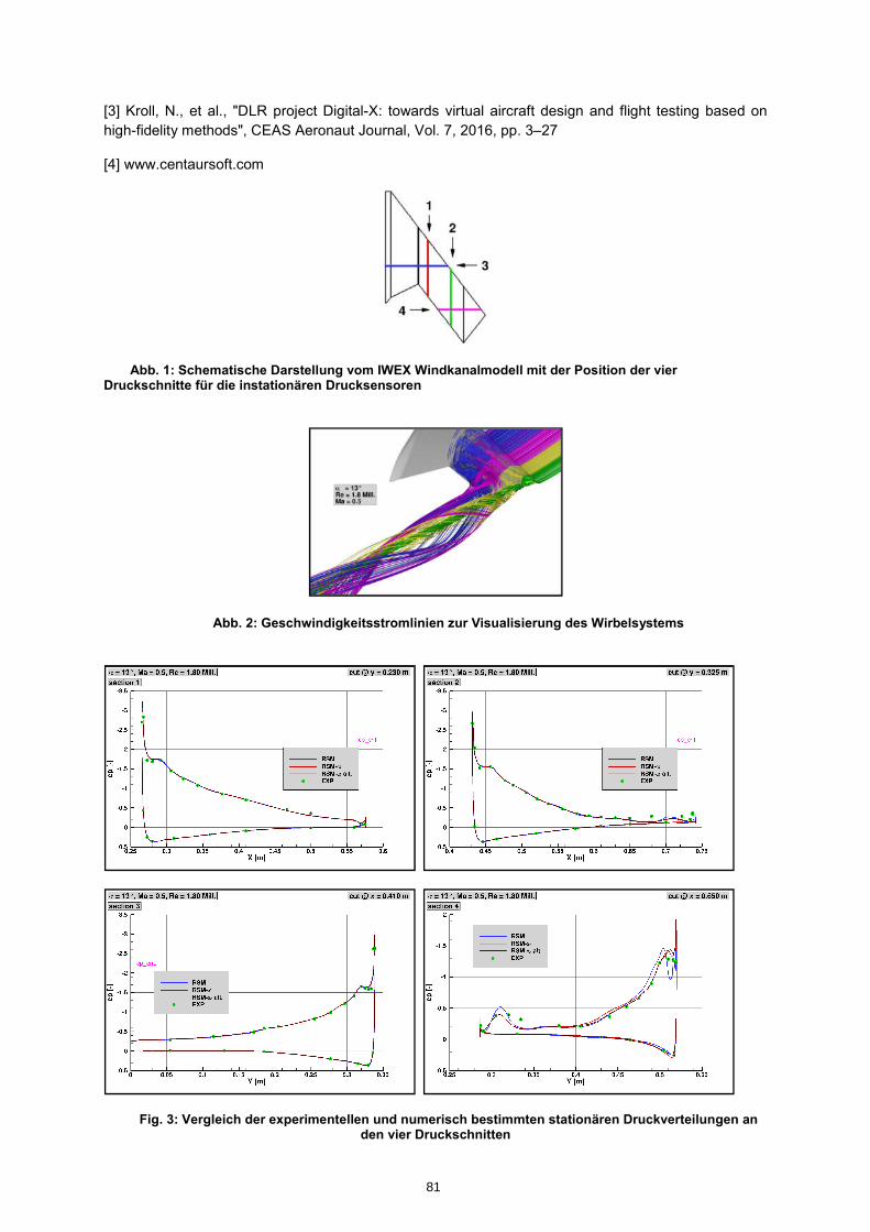
[3] Kroll, N., et al., "DLR project Digital-X: towards virtual aircraft design and flight testing based on

high-fidelity methods", CEAS Aeronaut Journal, Vol. 7, 2016, pp. 3–27

[4] www.centaursoft.com

Abb. 1: Schematische Darstellung vom IWEX Windkanalmodell mit der Position der vier Druckschnitte für die instationären Drucksensoren

Abb. 2: Geschwindigkeitsstromlinien zur Visualisierung des Wirbelsystems

Fig. 3: Vergleich der experimentellen und numerisch bestimmten stationären Druckverteilungen an den vier Druckschnitten

81

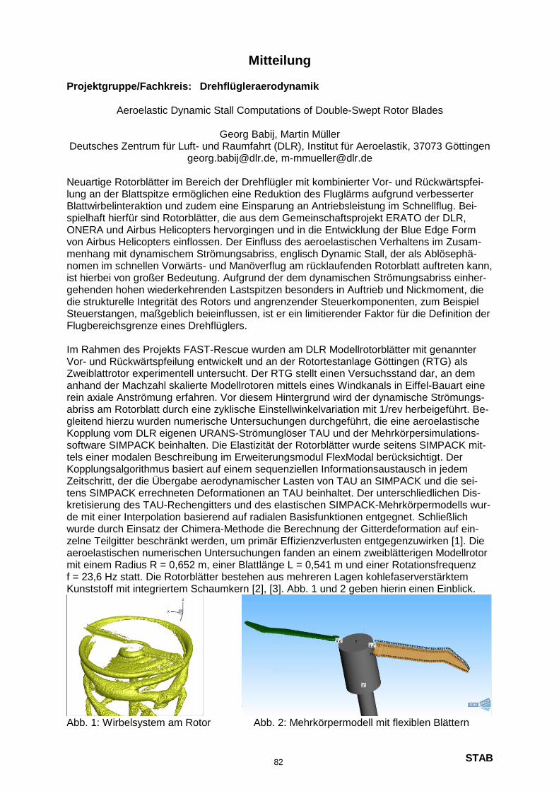
STAB

Mitteilung

Projektgruppe/Fachkreis: Drehflügleraerodynamik

Aeroelastic Dynamic Stall Computations of Double-Swept Rotor Blades

Georg Babij, Martin Müller Deutsches Zentrum für Luft- und Raumfahrt (DLR), Institut für Aeroelastik, 37073 Göttingen

[email protected], [email protected] Neuartige Rotorblätter im Bereich der Drehflügler mit kombinierter Vor- und Rückwärtspfei-lung an der Blattspitze ermöglichen eine Reduktion des Fluglärms aufgrund verbesserter Blattwirbelinteraktion und zudem eine Einsparung an Antriebsleistung im Schnellflug. Bei-spielhaft hierfür sind Rotorblätter, die aus dem Gemeinschaftsprojekt ERATO der DLR, ONERA und Airbus Helicopters hervorgingen und in die Entwicklung der Blue Edge Form von Airbus Helicopters einflossen. Der Einfluss des aeroelastischen Verhaltens im Zusam-menhang mit dynamischem Strömungsabriss, englisch Dynamic Stall, der als Ablösephä-nomen im schnellen Vorwärts- und Manöverflug am rücklaufenden Rotorblatt auftreten kann, ist hierbei von großer Bedeutung. Aufgrund der dem dynamischen Strömungsabriss einher-gehenden hohen wiederkehrenden Lastspitzen besonders in Auftrieb und Nickmoment, die die strukturelle Integrität des Rotors und angrenzender Steuerkomponenten, zum Beispiel Steuerstangen, maßgeblich beieinflussen, ist er ein limitierender Faktor für die Definition der Flugbereichsgrenze eines Drehflüglers. Im Rahmen des Projekts FAST-Rescue wurden am DLR Modellrotorblätter mit genannter Vor- und Rückwärtspfeilung entwickelt und an der Rotortestanlage Göttingen (RTG) als Zweiblattrotor experimentell untersucht. Der RTG stellt einen Versuchsstand dar, an dem anhand der Machzahl skalierte Modellrotoren mittels eines Windkanals in Eiffel-Bauart eine rein axiale Anströmung erfahren. Vor diesem Hintergrund wird der dynamische Strömungs-abriss am Rotorblatt durch eine zyklische Einstellwinkelvariation mit 1/rev herbeigeführt. Be-gleitend hierzu wurden numerische Untersuchungen durchgeführt, die eine aeroelastische Kopplung vom DLR eigenen URANS-Strömunglöser TAU und der Mehrkörpersimulations-software SIMPACK beinhalten. Die Elastizität der Rotorblätter wurde seitens SIMPACK mit-tels einer modalen Beschreibung im Erweiterungsmodul FlexModal berücksichtigt. Der Kopplungsalgorithmus basiert auf einem sequenziellen Informationsaustausch in jedem Zeitschritt, der die Übergabe aerodynamischer Lasten von TAU an SIMPACK und die sei-tens SIMPACK errechneten Deformationen an TAU beinhaltet. Der unterschliedlichen Dis-kretisierung des TAU-Rechengitters und des elastischen SIMPACK-Mehrkörpermodells wur-de mit einer Interpolation basierend auf radialen Basisfunktionen entgegnet. Schließlich wurde durch Einsatz der Chimera-Methode die Berechnung der Gitterdeformation auf ein-zelne Teilgitter beschränkt werden, um primär Effizienzverlusten entgegenzuwirken [1]. Die aeroelastischen numerischen Untersuchungen fanden an einem zweiblätterigen Modellrotor mit einem Radius R = 0,652 m, einer Blattlänge L = 0,541 m und einer Rotationsfrequenz f = 23,6 Hz statt. Die Rotorblätter bestehen aus mehreren Lagen kohlefaserverstärktem Kunststoff mit integriertem Schaumkern [2], [3]. Abb. 1 und 2 geben hierin einen Einblick.

Abb. 1: Wirbelsystem am Rotor Abb. 2: Mehrkörpermodell mit flexiblen Blättern

82

STAB

Es werden vier Testfälle vorgestellt, von denen Testfall Nr. 1 mit ausschließlich kollektivem Blatteinstellwinkel von 17 ° einen schwebeflugähnlichen Zustand eines Drehflüglers darstellt. Als Ausgangspunkt für drei weitere Testfälle werden mit ihm zuerst die aerodynamischen Blattlasten und strukturellen Deformationen an den beiden Blättern ermittelt und gezeigt, dass sie im Betrag übereinstimmen. Mittels Superposition eines zyklischen Anteils im Blatt-einstellwinkel werden Testfall Nr. 2 mit 17°+/- 8°, Nr. 3 mit 19,3° +/- 8° und Nr. 4 mit 26,3 ° +/- 6° definiert. Die Topologie des Strömungfeldes für Testfall Nr. 1 und 2 ist durch anliegende Strömung am Rotorblatt und markante Randwirbel an den Blattspitzen gekennzeichnet. Durch eine Erhöhung des maximalen Blatteinstellwinkels wird in den Testfällen Nr. 3 und 4 der dynami-sche Strömungabriss am Rotorblatt herbeigeführt. Die Topologie des Strömungsfelds bein-haltet nun ebenfalls Wirbelstrukturen, die beim Durchlaufen des maximalen Blattein-stellwinkels im Bereich der Rückwärtspfeilung ablösen, stromab fließen und das nachlaufen-de Rotorblatt beeinflussen. Die Intensität und räumliche Ausdehnung dieser Wirbelstruktu-ren im Nachlauf vergrößert sich mit zunehmenden maximalem Blatteinstellwinkel. Sie führen zu einer Interaktion beider Rotorblätter untereinander, die sich zum einen in den integralen aerodynamischen Blattlasten und zum anderen in den Blattverformungen widerspiegelt. Der Zeitverlauf für die aerodynamischen Blattlasten mit sinusähnlicher Form, der für Testfall Nr. 2 mit anliegender Strömung gegeben sind, weicht mit Einsetzen des dynamischen Strö-mungsabrisses einem periodischen Verlauf, der zunehmend höherharmonische Anteile be-inhaltet. Diesbezüglich stellen Abb. 3 und 4 den Verlauf der am Blatt senkrecht angreifenden Komponente Fn über dem Blatteinstellwinkel Θ für Testfall Nr. 2 und 4 dar. Mit zunehmender Stärke des dynamsichen Strömungsabriss, von Testfall Nr. 2 zu 4, verschwindet der ellip-senförmige Verlauf für Fn an beiden Blätter, der über der Zeit aufgetragen eine sinusähnliche Form darstellt. Des Weiteren divergieren die zugehörigen Amplituden beider Blätter vonei-nander weg, so dass ein Rotorblatt höher belastet ist als das andere. Dieser Umstand ist aufgrund der Elastizität der Rotorblätter auf leicht unterschiedliche Blatttrajektorien zurück-führen, die abschwimmende Wirbelfelder der vorlaufenden Blätter unterschiedlich durch-kreuzen.

Abb. 3: Normalkomponente Fn, Testfall Nr. 2 Abb. 4: Normalkomponente Fn, Testfall Nr. 4 Komplettiert wird die numerische Untersuchung mit einem Vergleich zu experimentellen Da-ten, die integrale aerodynamsichen Blattlasten für Testfall Nr. 2 und 3 beinhalten. Literaturangaben:

1. S.Surrey, B.Ortun, K.-V. Truong, F.Wienke. Investigation of the structural blade dynamics and aeroelastic behavior of the 7A rotor. American Helicopter Society 72nd Annual Forum, West Palm Beach, Florida, 2016

2. M.M.Mueller, T.Schwermer, H.Mai, C.Stieg. Development of an innovative double-swept rotor blade tip for the rotor test facility Goettingen. Deutscher Luft- und Raumfahrtkongress, Fried-richshafen, 2018

3. J.Arnold, S.Waitz. Using multibody dynamics for the stability assessment of a new double-swept rotor blades setup. 44th European Rotorcraft Forum, Delft, 2018

83

STAB

employing a SST turbulence model for the turbulent closure. Using the computational model, themesh approach. ANSYS Fluent is used to solve the incompressible URANS equations, manner. The computational domain was discretized using ANSYS ICEM CFD utilizing a sliding Navier-Stokes simulations are performed in order to study the flow field in a time-resolved In parallel to the experimental study, a series of corresponding unsteady Reynolds-Averaged

investigated.upstream propeller and their influence on the behavior of the downstream propeller are addition to this, the varying accelerations of the flow in axial and circumferential direction by the the individual blade tip vortices as well as their mutual interactions influencing the wake roll-up. In structures. A characteristic example is provided in Fig. 3, which illustrates by smoke visualization inflow angles. Emphasis is on identifying the interactions of the propeller wakes and the vortex Furthermore, the flow fields are captured using smoke visualization and discussed under different

single propellers under inflow angles higher than αdisc>90°.propellers decreases. The total performance diminish to a large extent in comparison to the increased axial velocity. Under high inflow angles, the difference in effective thrust between both downstream propeller due to the mutual interaction of the two propellers, especially, by the propellers and the performance of the upstream propeller is higher than the one of the As expected, the overall thrust of the coaxial propeller is lower than the one of two single

propellers (see Fig. 2).the efficiency of the coaxial configuration. The results are compared to two isolated puller Wind tunnel experiments are performed to measure the steady and transient loads, and to study

fully reversed inflow (see Fig. 1).configuration is analyzed under different inflow angles ranging from axial inflow, lateral inflow to a and puller version, diameter DP=0.45 m) propellers with an axial spacing of Δx=0.381 Dx=0.381 DP. The In this work, a coaxial configuration is investigated using a pair of commercial APC 18x8 (pusher

scale propellers.there is still a demand for the analysis of the influence of non-axial inflow conditions on small- angles. [5] Since the majority of propeller research is focusing on axial inflow conditions [6], response to their operating scope, these propellers are often subjected to a wide range of inflow propellers in order to attain higher thrust levels while maintaining a compact package. In propellers has risen significantly. Such devices are often equipped with counter-rotating coaxial In the last decades, the interest for light-weight air vehicles and UAVs equipped with small-scale

scale propellers to meet the requirements of the aircraft design. [1] [2] [3] [4]moments. Most of these analyses focused on relatively small inflow angle variations and large- characteristics of propellers revealing the existence of side-forces as well as pitching and yawing in the wind-tunnel to investigate the influence of the inflow angle on the steady and unsteady load when the propeller is operated at non-axial inflow conditions. Experiments have been performed beginning of their usage, the generation of additional loads and vibrations have been observed aircraft and more recently, flight vehicles capable of vertical take-off and landing. From the very Propellers are the classic device for producing the required thrust output for typical light-weight

[email protected] Universität München, Boltzmannstr. 15, 85748 Garching

M. Cerny, J. Faust, C. Breitsamter

Investigation of a Coaxial Propeller Configuration under Non-Axial Inflow Conditions


Mitteilung

84

vortex structures in the propeller wake, and their evolution and interaction with the propellerblades can be investigated further. For example, the deformation of the upstream propeller’sblade wake by the downstream propeller and its flow acceleration can be observed by anillustration of the normalized circumferential velocity component (see Fig. 4).

Fig. 1: Design of the coaxial configuration. Fig. 2: Normalized thrust coefficient over the inflow angle.

Fig. 3: Smoke visualization in the wind tunnel,αdisc=90°, U∞=5 m/s, n=4000 rpm.

Fig. 4: Illustration of the normalized circumfer-ential velocity component by URANS calcula-tion, αdisc=0°, U∞=10 m/s, n=4000 rpm.

The gathered data may be used to improve the aerodynamic performance of small-scale coaxialconfigurations, in especially efficiency, flight time and range. Lastly, the knowledge of thebehavior under non-axial inflow conditions may improve the maneuverability and controllabilityand therefore, increase the flight safety and comfort.

References

1 Frederick W. Lanchester: The Flying-Machine from an Engineering Standpoint, Constable & Co., Ltd., London, UK, 1917

2 R. G. Harris: Forces on a Propeller Due to Sideslip, Reports and Memoranda, British Advisory Committee for Aeronautics, Vol. 2, no. 427, 1918

3 Franz Misztal: Vorträge aus dem Gebiete der Aerodynamik und verwandter Gebiete, Springer-Verlag, Berlin, Heidelberg, 1930

4 Hermann Glauert: Aerodynamic Theory - Division L - Airplane Propellers , Julius Springer, Farnborough, UK, 1935

5 B. Theys, G. Dimitriadis, T. Andrianne, P. Hendrick, and J. De Schutter: Wind Tunnel Testing of a VTOL MAV Propeller in Tilted Operating Mode,International Conference on Unmanned Aircraft Systems (ICUAS), Orlando, Florida, USA, May27-30, 2014, pp. 1064-1072

6 Tomas Sinnige, Nando van Arnhem, Tom C. A. Stokkermans, Georg Eitelberg, and Leo L. M. Veldhuis: Wingtip-Mounted Propellers: Aerodynamic Analysis of Interaction Effects and Comparison with Conventional Layout, Journal of Aircraft, Vol. 56, no. 1, 2018

STAB85

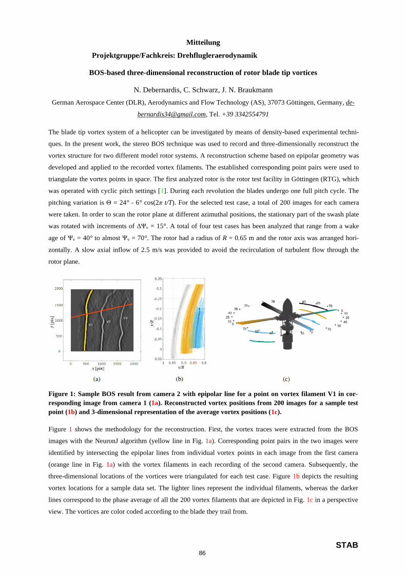
STAB

Figure 1: Sample BOS result from camera 2 with epipolar line for a point on vortex filament V1 in cor-

responding image from camera 1 (1a). Reconstructed vortex positions from 200 images for a sample test

point (1b) and 3-dimensional representation of the average vortex positions (1c).

Figure 1 shows the methodology for the reconstruction. First, the vortex traces were extracted from the BOS

images with the NeuronJ algorithm (yellow line in Fig. 1a). Corresponding point pairs in the two images were

identified by intersecting the epipolar lines from individual vortex points in each image from the first camera

(orange line in Fig. 1a) with the vortex filaments in each recording of the second camera. Subsequently, the

three-dimensional locations of the vortices were triangulated for each test case. Figure 1b depicts the resulting

vortex locations for a sample data set. The lighter lines represent the individual filaments, whereas the darker

lines correspond to the phase average of all the 200 vortex filaments that are depicted in Fig. 1c in a perspective

view. The vortices are color coded according to the blade they trail from.

rotor plane.

zontally. A slow axial inflow of 2.5 m/s was provided to avoid the recirculation of turbulent flow through the

age of Ψv = 40° to almost Ψv = 70°. The rotor had a radius of R = 0.65 m and the rotor axis was arranged hori-

was rotated with increments of ΔΨv = 15°. A total of four test cases has been analyzed that range from a wake

were taken. In order to scan the rotor plane at different azimuthal positions, the stationary part of the swash plate

pitching variation is Θ = 24° - 6° cos(2π t/T). For the selected test case, a total of 200 images for each camera

was operated with cyclic pitch settings [1]. During each revolution the blades undergo one full pitch cycle. The

triangulate the vortex points in space. The first analyzed rotor is the rotor test facility in Göttingen (RTG), which

developed and applied to the recorded vortex filaments. The established corresponding point pairs were used to

vortex structure for two different model rotor systems. A reconstruction scheme based on epipolar geometry was

ques. In the present work, the stereo BOS technique was used to record and three-dimensionally reconstruct the

The blade tip vortex system of a helicopter can be investigated by means of density-based experimental techni-

[email protected], Tel. +39 3342554791

German Aerospace Center (DLR), Aerodynamics and Flow Technology (AS), 37073 Göttingen, Germany, de-

Debernardis, C. Schwarz, J. N. BraukmannN.

BOS-based three-dimensional reconstruction of rotor blade tip vortices

Projektgruppe/Fachkreis: Drehflugleraerodynamik

Mitteilung

86

STAB

The reconstruction scheme was validated trough a comparison with vortex positions from a simultaneous PIV

measurement [1]. The results will be part of the final paper. Subsequently, the reconstruction scheme was additi-

onally applied to the wake of a free-flying model helicopter in ground effect. The model helicopter rotor con-

sisted of two (Nb = 2) untwisted, stiff, and cut-off rotor blades with a radius of R = 0.7 m, chord length of

c = 54.5 mm, and a symmetrical Joukovski 0015 airfoil.

Figure 2: BOS image showing the epipolar intersection with vortex filaments (2a). Model helicopter and

reconstructed main rotor vortex system (2b). Radius of the vortex system vs. wake age (2c).

In Fig. 2, a BOS image of the model helicopter vortex system during takeoff is depicted (see also [2]). A chal-

lenging factor for the vortex reconstruction is the small angle between vortex filaments and epipolar lines (red

and green lines), which increases the risk of identifying false point pair matches. Despite the increased complexi-

ty, it was possible to reconstruct the vortex system, which is depicted in Fig. 2b. The characteristic helical shape

of the vortex system with a decreasing diameter with wake age is visible. After a certain wake age, an expansion

of the wake can be detected as a result of the close ground. At the time of the image acquisition, the helicopter

rotor is about 1 rotor radius R above the ground as was reported in [3]. The evolution of the vortex system‘s

radius versus the wake age is better visible in Fig. 2c. After a first contraction, which reaches a value of 0.9 R at

the vortex age of 340°, the radius of the vortex system expands due to the proximity of the ground starting from

a wake age of 470° up to the maximum detectable vortex age of 650°. A similar behavior was also observed in

data from PIV measurements for the same model helicopter in ground effect [3].

In summary, the presented data demonstrates the possibility of reconstructing 3D vortex positions using a two-

camera stereo BOS system for different rotor systems and operating states. This enables the extraction of quanti-

tative data from BOS recordings, which will be investigated in more detail in the final paper and compared to

findings from corresponding PIV measurements.

References

[1] Braukmann, J. N., Wolf, C. C., Goerttler, A., and Raffel, M., “Blade Tip Vortex Characterization of a Rotor under

Cyclic Pitch Conditions Using BOS and PIV”, AIAA 2019-2325, Proceedings of the AIAA Science and Technology

Forum and Exposition, San Diego, CA, January 7–11, 2019.

[2] Bauknecht, A., Schwarz, C., Raffel, M., and Mailander, S., “Flow Measurement Techniques for Rotor Wake Cha-

racterization on Free-Flying Helicopters in Ground Effect,” AIAA 2019-2107, Proceedings of the AIAA Science and

Technology Forum and Exposition, San Diego, CA, January 6–10, 2019, DOI: 10.2514/6.2019-2107.

[3] Schwarz, C., Bauknecht, A., Mailander, S., and Raffel, M., “Wake Characterization of a Free-Flying Model He-

licopter in Ground Effect,” Journal of the American Helicopter Society, 64, 012010 (2019), DOI:

10.4050/JAHS.64.012010.

87

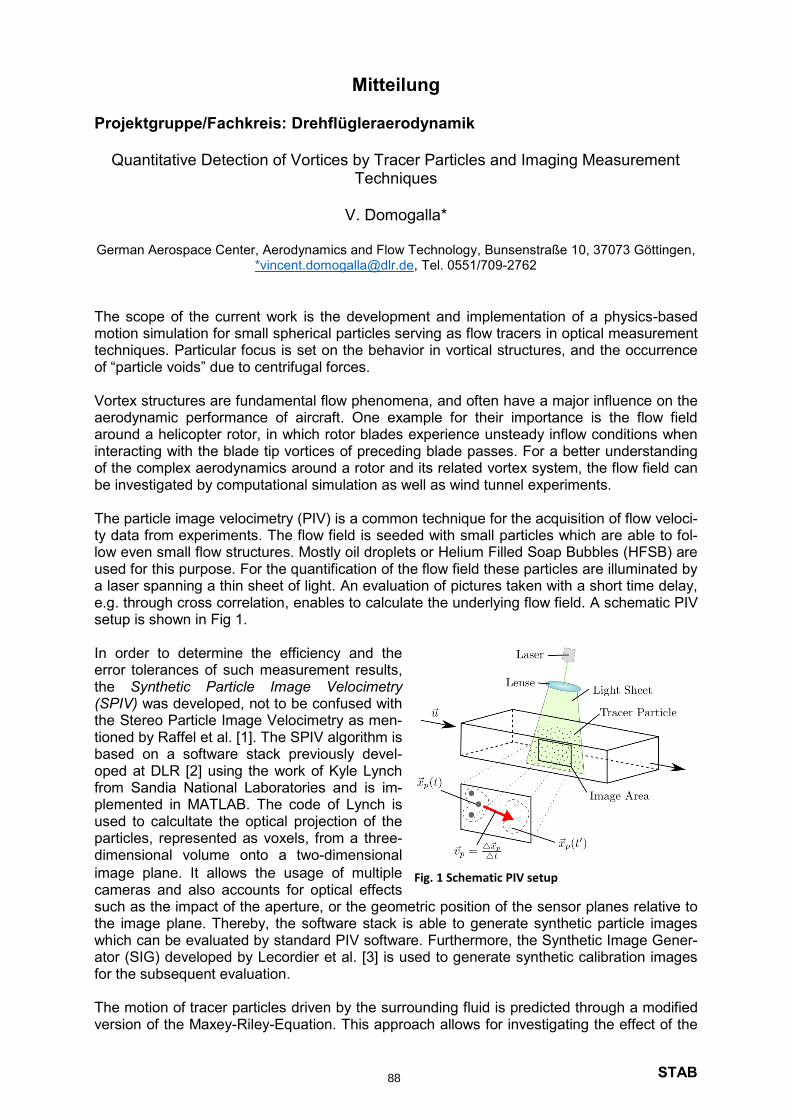
STAB

Mitteilung Projektgruppe/Fachkreis: Drehflügleraerodynamik

Quantitative Detection of Vortices by Tracer Particles and Imaging Measurement Techniques

V. Domogalla*

German Aerospace Center, Aerodynamics and Flow Technology, Bunsenstraße 10, 37073 Göttingen,

*[email protected], Tel. 0551/709-2762

The scope of the current work is the development and implementation of a physics-based motion simulation for small spherical particles serving as flow tracers in optical measurement techniques. Particular focus is set on the behavior in vortical structures, and the occurrence of “particle voids” due to centrifugal forces. Vortex structures are fundamental flow phenomena, and often have a major influence on the aerodynamic performance of aircraft. One example for their importance is the flow field around a helicopter rotor, in which rotor blades experience unsteady inflow conditions when interacting with the blade tip vortices of preceding blade passes. For a better understanding of the complex aerodynamics around a rotor and its related vortex system, the flow field can be investigated by computational simulation as well as wind tunnel experiments. The particle image velocimetry (PIV) is a common technique for the acquisition of flow veloci-ty data from experiments. The flow field is seeded with small particles which are able to fol-low even small flow structures. Mostly oil droplets or Helium Filled Soap Bubbles (HFSB) are used for this purpose. For the quantification of the flow field these particles are illuminated by a laser spanning a thin sheet of light. An evaluation of pictures taken with a short time delay, e.g. through cross correlation, enables to calculate the underlying flow field. A schematic PIV setup is shown in Fig 1. In order to determine the efficiency and the error tolerances of such measurement results, the Synthetic Particle Image Velocimetry (SPIV) was developed, not to be confused with the Stereo Particle Image Velocimetry as men-tioned by Raffel et al. [1]. The SPIV algorithm is based on a software stack previously devel-oped at DLR [2] using the work of Kyle Lynch from Sandia National Laboratories and is im-plemented in MATLAB. The code of Lynch is used to calcultate the optical projection of the particles, represented as voxels, from a three- dimensional volume onto a two-dimensional

image plane. It allows the usage of multiple cameras and also accounts for optical effects such as the impact of the aperture, or the geometric position of the sensor planes relative to the image plane. Thereby, the software stack is able to generate synthetic particle images which can be evaluated by standard PIV software. Furthermore, the Synthetic Image Gener-ator (SIG) developed by Lecordier et al. [3] is used to generate synthetic calibration images for the subsequent evaluation. The motion of tracer particles driven by the surrounding fluid is predicted through a modified version of the Maxey-Riley-Equation. This approach allows for investigating the effect of the

Fig. 1 Schematic PIV setup

88

mailto:*[email protected]

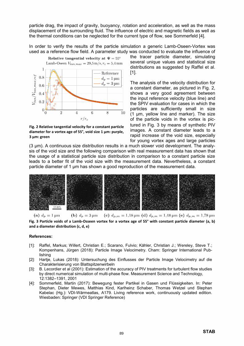
STAB

particle drag, the impact of gravity, buoyancy, rotation and acceleration, as well as the mass displacement of the surrounding fluid. The influence of electric and magnetic fields as well as the thermal conditions can be neglected for the current type of flow, see Sommerfeld [4]. In order to verify the results of the particle simulation a generic Lamb-Oseen-Vortex was used as a reference flow field. A parameter study was conducted to evaluate the influence of

the tracer particle diameter, simulating several unique values and statistical size distributions as suggested by Raffel et al. [1]. The analysis of the velocity distribution for a constant diameter, as pictured in Fig. 2, shows a very good agreement between the input reference velocity (blue line) and the SPIV evaluation for cases in which the particles are sufficiently small in size (1 µm, yellow line and marker). The size of the particle voids in the vortex is pic-

tured in Fig. 3 by means of synthetic PIV images. A constant diameter leads to a rapid increase of the void size, especially for young vortex ages and large particles

(3 µm). A continuous size distribution results in a much slower void development. The analy-sis of the void size and the following comparison with real measurement data has shown that the usage of a statistical particle size distribution in comparison to a constant particle size leads to a better fit of the void size with the measurement data. Nevertheless, a constant particle diameter of 1 μm has shown a good reproduction of the measurement data.

Fig. 3 Particle voids of a Lamb-Osseen vortex for a vortex age of 55° with constant particle diameter (a, b) and a diameter distribution (c, d, e) References:

[1]: Raffel, Markus; Willert, Christian E.; Scarano, Fulvio; Kähler, Christian J.; Wereley, Steve T.; Kompenhans, Jürgen (2018): Particle Image Velocimetry. Cham: Springer International Pub-lishing

[2]: Hartje, Lukas (2018): Untersuchung des Einflusses der Particle Image Velocimetry auf die Charakterisierung von Blattspitzenwirbeln

[3]: B. Lecordier et al (2001): Estimation of the accuracy of PIV treatments for turbulent flow studies by direct numerical simulation of multi-phase flow. Measurement Science and Technology, 12:1382–1391, 2001

[4]: Sommerfeld, Martin (2017): Bewegung fester Partikel in Gasen und Flüssigkeiten. In: Peter Stephan, Dieter Mewes, Matthias Kind, Karlheinz Schaber, Thomas Wetzel und Stephan Kabelac (Hg.): VDI-Wärmeatlas, A179. Living reference work, continuously updated edition. Wiesbaden: Springer (VDI Springer Reference)

Fig. 2 Relative tangential velocity for a constant particle diameter for a vortex age of 55°, void size 1 μm: purple, 3 μm: green

89

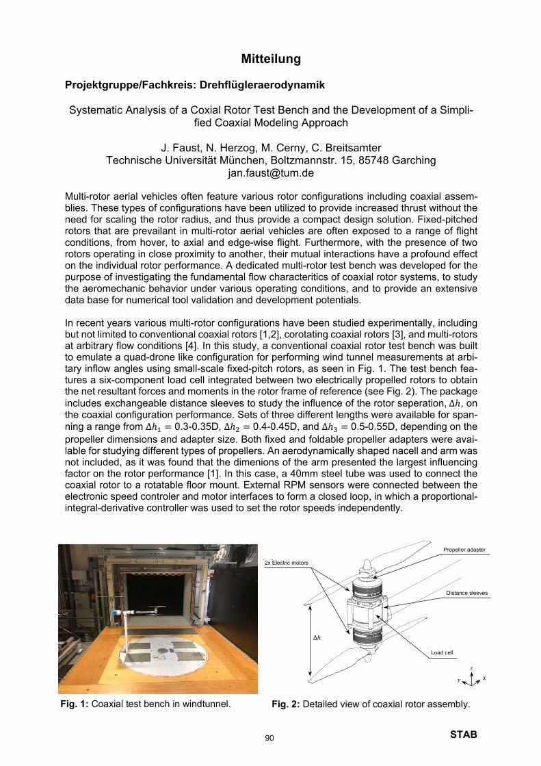
STAB

𝑥

𝑧

𝑦

Fig. 1: Coaxial test bench in windtunnel.

Δℎ

Fig. 2: Detailed view of coaxial rotor assembly.

2x Electric motors

Load cell

Distance sleeves

Propeller adapter

integral-derivative controller was used to set the rotor speeds independently.electronic speed controler and motor interfaces to form a closed loop, in which a proportional- coaxial rotor to a rotatable floor mount. External RPM sensors were connected between the factor on the rotor performance [1]. In this case, a 40mm steel tube was used to connect the not included, as it was found that the dimenions of the arm presented the largest influencing lable for studying different types of propellers. An aerodynamically shaped nacell and arm was propeller dimensions and adapter size. Both fixed and foldable propeller adapters were avai- ning a range from Δℎ! = 0.3-0.35D, Δℎ" = 0.4-0.45D, and Δℎ# = 0.5-0.55D, depending on the the coaxial configuration performance. Sets of three different lengths were available for span- includes exchangeable distance sleeves to study the influence of the rotor seperation, Δℎ, on the net resultant forces and moments in the rotor frame of reference (see Fig. 2). The package tures a six-component load cell integrated between two electrically propelled rotors to obtain tary inflow angles using small-scale fixed-pitch rotors, as seen in Fig. 1. The test bench fea- to emulate a quad-drone like configuration for performing wind tunnel measurements at arbi- at arbitrary flow conditions [4]. In this study, a conventional coaxial rotor test bench was built but not limited to conventional coaxial rotors [1,2], corotating coaxial rotors [3], and multi-rotors In recent years various multi-rotor configurations have been studied experimentally, including

data base for numerical tool validation and development potentials.the aeromechanic behavior under various operating conditions, and to provide an extensive purpose of investigating the fundamental flow characteritics of coaxial rotor systems, to study on the individual rotor performance. A dedicated multi-rotor test bench was developed for the rotors operating in close proximity to another, their mutual interactions have a profound effect conditions, from hover, to axial and edge-wise flight. Furthermore, with the presence of two rotors that are prevailant in multi-rotor aerial vehicles are often exposed to a range of flight need for scaling the rotor radius, and thus provide a compact design solution. Fixed-pitched blies. These types of configurations have been utilized to provide increased thrust without the Multi-rotor aerial vehicles often feature various rotor configurations including coaxial assem-

[email protected] Universität München, Boltzmannstr. 15, 85748 Garching

Faust, N. Herzog, M. Cerny, C. BreitsamterJ.

fied Coaxial Modeling ApproachSystematic Analysis of a Coxial Rotor Test Bench and the Development of a Simpli-


Mitteilung

90

STAB

In this study three commercial propellers were studied in axial flow conditions, namely a high-speed model aircraft APC18x8 propeller (D=457,2 mm), two- and three-bladed KDE 18,5x6,3 (D=469,9 mm) foldable propellers for quadcopter applications. A series of parameter studies were performed to characterize the coaxial rotor configurations in static thrust conditions. Iso-lated pusher and puller configurations were tested and compared with a previous single rotor test bench [5]. Following this, the influence of ground effect, rotor clearance spacing, various blade number combinations (2x2, 2x3, and 3x3) were studied at matched rotor speeds. Lastly, the influence of variable rotor speeds and yaw-torque trimming was studied by maintaining the upper rotor speed fixed and varying the bottom rotor speed, as torque-balanced rotor system were found to increase the total thrust of a quadcopter vehicle significantly [6]. Further studies could also be performed using the current test bench to operate the coaxial rotor in a corotating configuration. This could provide insights into the influence of swirl recovery, which is expected to play an important role with high disc loading [7]. Alongside the experimental study, a simplified modeling strategy was developed to predict the coaxial rotor loads using the output data from an in-house BEMT (Blade Element Momentum Theory) code and TUMRAC (TUM Rotor Aeromechanics Code), an in-house developed nu-merical lifting-line method featuring a free-wake vortex inflow model. The SIM (Synchronous Iterative Matching) methodology was developed that consists of an iterative look-up strategy, where the operating conditions experienced by one rotor are superpositioned with the resultant induced inflow velocity of the other rotor, a schematic summary is provided in Fig. 3. A preli-minary comparison between the numerical BEMT and experimental data for isolated rotor and coaxial configurations using APC18x8 rotors is shown in Fig. 4. References [1] B. Theys, G. Dimitriadis, P. Hendrick, and J. De Schutter, `Ìnfluence of propeller configuration on propulsion system efficiency of multi-rotor Unmanned Aerial Vehicles´´, 2016 International Conference on Unmanned Aircraft Systems (ICUAS), Arlington, VA, June 2016. [2] D. Shukla, and N. Komerath, ``Drone Scale Coaxial Rotor Aerodynamic Interactions Investiga-tion´´, Journal of Fluids Engineering, Vol. 141, July 2019. [3] S. Conley, and C. Russel, ``Mechanical Design of the Multirotor Test Bed´´, VFS Aerome-chanics for Advanced Vertical Flight Technical Meeting, San Jose, CA, January 2020. [4] C. Johnson, J. Sirohi, G. Jacobellis, R. Singh, and R. McDonald, `Ìnvestigation of Stacked Rotor Performance in Hover Part 1 : Experimental Measurements´´, VFS Aeromechanics for Ad-vanced Vertical Flight Technical Meeting, San Jose, CA, January 2020. [5] M. Cerny, N. Herzog, J. Faust, M. Stuhlpfarrer, and C. Breitsamter, ``Systematic Investigation of Fixed-Pitch Small-Scale Propeller Under Non-Axial Inflow Conditions´´, DLRK 2018, Frie-drichshafen, Germany, September 2018. [6] S. Yoon, W. M. Chan, and T. H. Pulliam, ``Computations of Torque-Balanced Coaxial Rotor Flows´´, AIAA SciTech 2017, Grapvine, TX, January 2017. [7] C. P. Coleman, `À Survey of Theoretical and Experimental Coaxial Rotor Aerodynamic Research´´, NASA Technical Paper 3675, Ames Research Center, Moffett Field, CA, 1997.

INPUT: Ω!, Ω" , 𝑉(#

OUTPUT: ∑ ,∑𝑀((

Ω! 𝑉(# + 𝑉( $," Ω" 𝑉(# + 𝑉( $,!

", 𝑀(( "

!, 𝑀(( !

ROTOR 1 DATABASE

ROTOR 2 DATABASE

Fig. 3: Synchronous Iterative Matching strategy.

SIM

Fig. 4: APC18x8 static thrust output.

1000 2000 3000 4000 5000 6000 7000RPM [-]

0.06

0.08

0.1

0.12

0.14

0.16

CT [-

]

EXP, isolated puller rotorEXP, isolated pusher rotorEXP, coaxial rotorBEMT, isolated rotorBEMT-SIM, coaxial rotor

91

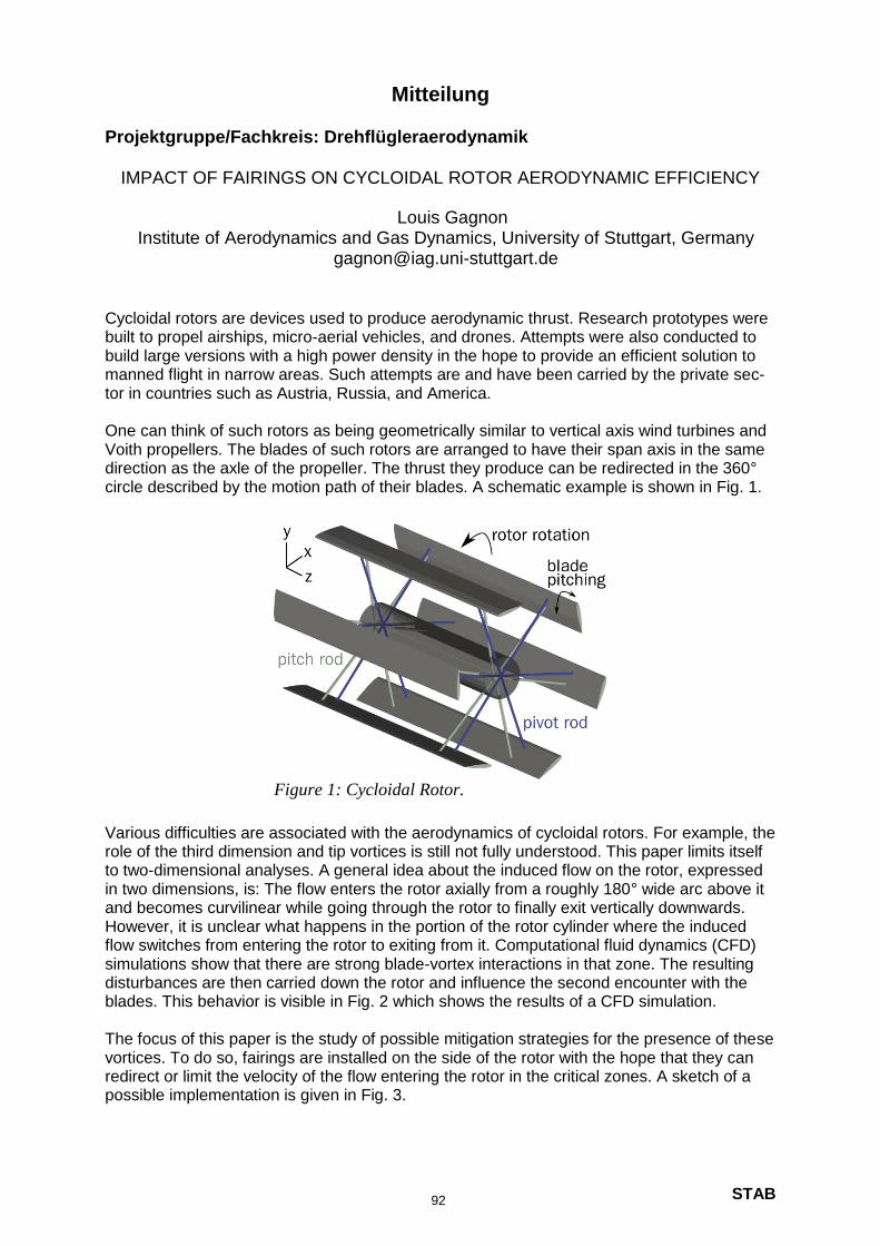
STAB

Cycloidal rotors are devices used to produce aerodynamic thrust. Research prototypes were built to propel airships, micro-aerial vehicles, and drones. Attempts were also conducted to build large versions with a high power density in the hope to provide an efficient solution to manned flight in narrow areas. Such attempts are and have been carried by the private sec-tor in countries such as Austria, Russia, and America. One can think of such rotors as being geometrically similar to vertical axis wind turbines and Voith propellers. The blades of such rotors are arranged to have their span axis in the same direction as the axle of the propeller. The thrust they produce can be redirected in the 360° circle described by the motion path of their blades. A schematic example is shown in Fig. 1.

Various difficulties are associated with the aerodynamics of cycloidal rotors. For example, the role of the third dimension and tip vortices is still not fully understood. This paper limits itself to two-dimensional analyses. A general idea about the induced flow on the rotor, expressed in two dimensions, is: The flow enters the rotor axially from a roughly 180° wide arc above it and becomes curvilinear while going through the rotor to finally exit vertically downwards. However, it is unclear what happens in the portion of the rotor cylinder where the induced flow switches from entering the rotor to exiting from it. Computational fluid dynamics (CFD) simulations show that there are strong blade-vortex interactions in that zone. The resulting disturbances are then carried down the rotor and influence the second encounter with the blades. This behavior is visible in Fig. 2 which shows the results of a CFD simulation. The focus of this paper is the study of possible mitigation strategies for the presence of these vortices. To do so, fairings are installed on the side of the rotor with the hope that they can redirect or limit the velocity of the flow entering the rotor in the critical zones. A sketch of a possible implementation is given in Fig. 3.

Figure 1: Cycloidal Rotor.

[email protected]

Institute of Aerodynamics and Gas Dynamics, University of Stuttgart, Germany Louis Gagnon

IMPACT OF FAIRINGS ON CYCLOIDAL ROTOR AERODYNAMIC EFFICIENCY


Mitteilung

92

STAB

The work is carried out with the help of a two-dimensional Unsteady Reynolds Averaged Na-vier Stokes (URANS) CFD simulation with a fully resolved boundary layer flow. The full paper covers the model details. Amongst these are the embedded interpolation interfaces for the oscillating blades and the peculiar mesh types they require. The OpenFOAM solver is relied upon and thus the specific numerical schemes and algorithms are briefly covered, along with a validation based on experimental data for an oscillating airfoil. The first testing was conducted with two fairing installations, each being centered at the hori-zontal axis. They are referred to as the large near and away small to reflect their characteris-tics. The large near is slightly wider and closer to the rotor as the away small fairing. As shown in Fig. 4, they have limited influence on the thrust generated and power consumed by the rotor.

They highlight the limited influence of the fairings on the behavior of the induced flow and the resulting vortices. The weak influence is thought to be caused by the fairings lying on the side of the rotor. There, the flow enters only very slowly into the rotor, even when no fairing is present. There, the flow is also highly disturbed, as was seen in Fig. 2.

Figure 2: Vorticity field showing the blade vortex inter-

action caused by the lateral inflow along with a zoomed

insert.

Figure 3: Faired cycloidal rotor.

Figure 4: Evolution of thrust (T), thrust angle (Ta), power consumption (P), and power load-

ing (PL) over the last quarter of revolution (revs) of the simulation and plotted along with the

mean over each revolution.

93

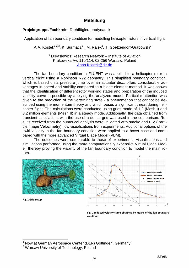
STAB

Fig. 1 Grid setup

Fig. 2 Induced velocity curve obtained by means of the fan boundary condition

2 Now at German Aerospace Center (DLR) Göttingen, Germany

3 Warsaw University of Technology, Poland

tors.el, thereby proving the viability of the fan boundary condition to model the main ro- simulations performed using the more computationally expensive Virtual Blade Mod-

The outcomes were comparable to those of experimental visualizations and pared with the more advanced Virtual Blade Model (VBM).swirl velocity in the fan boundary condition were applied to a hover case and com- cle Image Velocimetry) flow visualizations from experiments. Additional options of the sults received from the numerical analysis were validated with smoke and PIV (Parti- transient calculations with the use of a dense grid was used in the comparison. Re- 3,2 million elements (Mesh II) in a steady mode. Additionally, the data obtained from copter flight. The calculations were conducted using grids made of 1,2 (Mesh I) and scribed using the momentum theory and which poses a significant threat during heli- given to the prediction of the vortex ring state - a phenomenon that cannot be de- velocity curve is possible by applying the analyzed model. Particular attention was that the identification of different rotor working states and preparation of the induced vantages in speed and stability compared to a blade element method. It was shown which is based on a pressure jump over an actuator disc, offers considerable ad- vertical flight using a Robinson R22 geometry. This simplified boundary condition,

The fan boundary condition in FLUENT was applied to a helicopter rotor in

[email protected] Krakowska Av. 110/114, 02-256 Warsaw, Poland

1 Łukasiewicz Research Network – Institute of Aviation

A.A. Kostek1,2,3

, K. Surmacz11

, M. Rajek1, T. Goetzendorf-Grabowski

32

Application of fan boundary condition for modelling helicopter rotors in vertical flight


Mitteilung

94


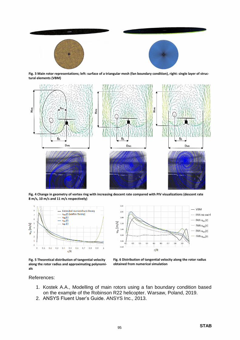
STAB

Fig. 3 Main rotor representations; left: surface of a triangular mesh (fan boundary condition), right: single layer of struc-tural elements (VBM)

Fig. 4 Change in geometry of vortex ring with increasing descent rate compared with PIV visualizations (descent rate 8 m/s, 10 m/s and 11 m/s respectively)

Fig. 5 Theoretical distribution of tangential velocity along the rotor radius and approximating polynomi-als

Fig. 6 Distribution of tangential velocity along the rotor radius obtained from numerical simulation

References:

1. Kostek A.A., Modelling of main rotors using a fan boundary condition based on the example of the Robinson R22 helicopter. Warsaw, Poland, 2019.

2. ANSYS Fluent User’s Guide. ANSYS Inc., 2013.

95

STAB


Bayesian Methods for Efficient Propeller Shape Optimization Applied to Airfoil Sections

Andreas Kümmel, Christian Breitsamter

Chair of Aerodynamics and Fluid Mechanics, Technical University of Munich, Boltzmannstr. 15, 85748 Garching bei München, [email protected]

Introduction: The upcoming trend of urban air mobility creates new points of contact between aviation and society. This results in new challenges, which directly influence the objectives for new aircraft. For example, the societal demand for emission-free, green transportation requires new developments in the field of the propulsion system, because of its decisive influence on the overall efficiency and emissions of the aircraft. Therefore, optimized propulsion systems are needed. In the case of urban air mobility, propellers are mostly used to generate the required thrust and lift. Furthermore, the aeroacoustic footprint of a propeller is determining the acceptance of new flight configurations in urban areas. Propellers pose a challenge for the optimization process due to the variety of design variables. These can be categorized in two different types: first, the shape variables, and second, the operation conditions, like rotational speed and flight velocity. Shape design variables are e.g. the chord, thickness and pitch-angle distributions and the radial airfoil sections of the propeller. Here, exemplarily only the radial airfoil sections of the propeller blade are considered. They have a significant influence on the aerodynamic efficiency of the propeller and the broadband aeroacoustic noise [1]. Method: For the propeller optimization, a Python-based fully automated optimization framework is implemented [2]. The four main modules of the framework are the airfoil parametrization, the discretization, the aerodynamic analysis, and the post-processing of the results. First, the airfoils are parametrized by means of two 4th order Bezier curves for the upper and lower side of the airfoil (see Figure 1). This allows to cover a wide range of different airfoils while keeping the number of design variables relatively low. In the following, the parametrized airfoil is passed to the mesh generation tool ANSYS ICEMCFD. Here, a block-structured grid is generated. For the aerodynamic analysis, CFD simulations with ANSYS Fluent are conducted. In the final module, the simulation results are post-processed and the objective function is returned to the optimizer. Afterwards, the optimization loop restarts with a new design point to be investigated. Optimization Problem: The variety of design variables during a propeller optimization demands for a fast and efficient optimization algorithm to reduce the number of function evaluations and optimization time. Therefore, a machine learning based Bayesian optimization (BO) algorithm is used. The BO method uses a combination of a Gaussian process (GP) to create a statistical model of the optimization problem and an acquisition function to determine where to evaluate the next sample. The BO is a global optimization method, best suitable for computational expensive black box functions, without the knowledge of derivatives and therefore, well suited for this optimization problem [3]. The radial airfoil sections are optimized regarding the aerodynamic efficiency as well as the trailing edge airfoil-self-noise. The objective function is composed of the lift-to-drag ratio 𝜀 = 𝐶𝑙/𝐶𝑑 and the sound pressure level 𝑆𝑃𝐿𝑠𝑒𝑙𝑓−𝑛𝑜𝑖𝑠𝑒. Additionally, structural constraints must

be fulfilled. The different airfoil sections have to withstand the inertial loads and the resulting stress 𝜎 evoked by the propeller rotation.

96

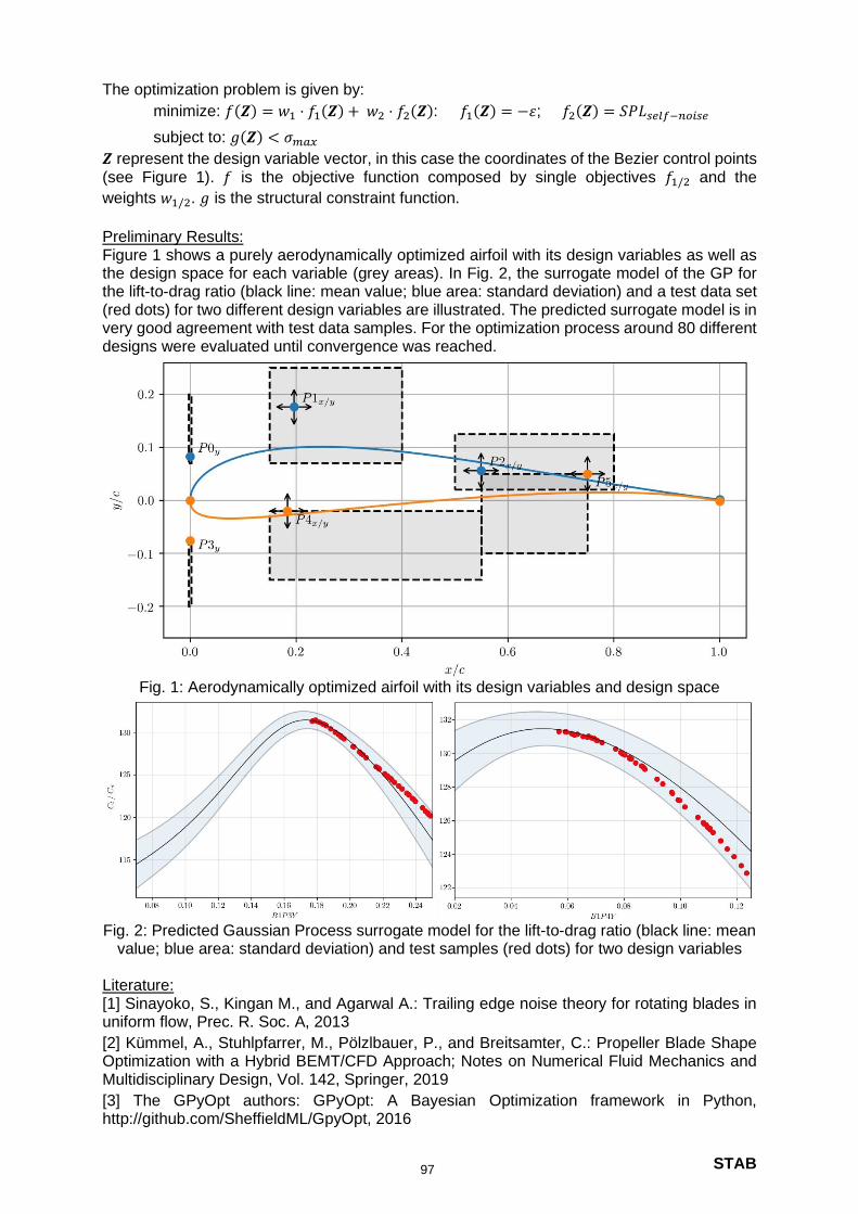
STAB

The optimization problem is given by:

minimize: 𝑓(𝒁) = 𝑤1 ⋅ 𝑓1(𝒁) + 𝑤2 ⋅ 𝑓2(𝒁): 𝑓1(𝒁) = −𝜀; 𝑓2(𝒁) = 𝑆𝑃𝐿𝑠𝑒𝑙𝑓−𝑛𝑜𝑖𝑠𝑒

subject to: 𝑔(𝒁) < 𝜎𝑚𝑎𝑥

𝒁 represent the design variable vector, in this case the coordinates of the Bezier control points (see Figure 1). 𝑓 is the objective function composed by single objectives 𝑓1/2 and the

weights 𝑤1/2. 𝑔 is the structural constraint function.

Preliminary Results: Figure 1 shows a purely aerodynamically optimized airfoil with its design variables as well as the design space for each variable (grey areas). In Fig. 2, the surrogate model of the GP for the lift-to-drag ratio (black line: mean value; blue area: standard deviation) and a test data set (red dots) for two different design variables are illustrated. The predicted surrogate model is in very good agreement with test data samples. For the optimization process around 80 different designs were evaluated until convergence was reached.

Fig. 1: Aerodynamically optimized airfoil with its design variables and design space

Fig. 2: Predicted Gaussian Process surrogate model for the lift-to-drag ratio (black line: mean

value; blue area: standard deviation) and test samples (red dots) for two design variables Literature: [1] Sinayoko, S., Kingan M., and Agarwal A.: Trailing edge noise theory for rotating blades in uniform flow, Prec. R. Soc. A, 2013

[2] Kümmel, A., Stuhlpfarrer, M., Pölzlbauer, P., and Breitsamter, C.: Propeller Blade Shape Optimization with a Hybrid BEMT/CFD Approach; Notes on Numerical Fluid Mechanics and Multidisciplinary Design, Vol. 142, Springer, 2019

[3] The GPyOpt authors: GPyOpt: A Bayesian Optimization framework in Python, http://github.com/SheffieldML/GpyOpt, 2016

97

STAB

Mitteilung


Selection and Implementation of Approximate Boundary Layer Methods for a Fast Mid-Fidelity Aerodynamics Code for Helicopter Simulations

Philipp Kunze

Deutsches Zentrum für Luft- und Raumfahrt e.V., Institut für Aerodynamik und Strömungstechnik, Lilienthalplatz 7, 38108 Braunschweig, [email protected]

With continuously increasing computing power the use of mid-fidelity methods is becoming feasible in ever earlier phases of helicopter development. One such method is DLR's Un-steady Panel Method (UPM). The free-wake method allows for capturing many interaction effects which cannot be captured by lower fidelity aerodynamics models commonly used in comprehensive rotorcraft codes. However, the potential flow method, which is used to model aerodynamic bodies in UPM, does not consider viscous effects. As these effects play an important role in many flight conditions, UPM has been extended by approximate boundary layer methods, which are able to estimate these effects. The selection and implementation process of these methods is sketched and exemplary results are presented in this paper. Two approaches were selected in order to approximately predict friction forces and flow sep-aration regions. The first approach is based on stripwise analysis using integral boundary layer methods for laminar and turbulent flow in combination with empirical transition criteria. The current implementation takes the inviscid velocity distribution as input and predicts skin friction, transition, and flow separation points. However, it is only intended for the analysis of lifting bodies (rotor blades, wings, stabilizers). For arbitrary non-lifting bodies (e.g. fuselage), a simplified approach based on local flow properties and flat plate analogy was selected. It was extended by simple flow separation criteria. The newly implemented methods were vali-dated and compared for several test cases including airfoils (e.g. Figure 1a), wings (e.g. Figure 1b), a rotor in hover (Figure 2), and two fuselage geometries (e.g. Figure 3). Both approaches showed to be robust and able to deliver good results, within the limits of the un-derlying models. The frictional forces and the transition and separation points calculated by the stripwise analysis method are in good accordance with most experiments and reference results. Additionally, the results were found to be conservative. The simplified analysis for non-lifting bodies also proved to be robust and tends to provide conservative estimates, but its accuracy lags behind the one of the stripwise analysis method.

(a) MBB VA-2 airfoil skin friction coefficient at ɑ=4.0° and Re=6x106 (sign of lower surface cf* is inverted for improved clarity)

(b) Three-dimensional tapered untwisted wing at ɑ=5.0° and Re=4x106

Figure 1: Skin friction of an airfoil and a wing calculated by the implemented integral boundary layer methods compared to experiment / reference results using XFOIL[2] / VSAERO[3]

98


STAB

(a) Contour plot of lower and upper rotor blade surface

(b) Section r/R=70% laminar/turbulent analysis results incl. transition

(c) Section r/R=70% fully turbulent analysis results

Figure 2: Skin friction coefficient on the rotor 7A in hover calculated by UPM with the implemented Eppler method compared to FLOWer[4] RANS results (θ0 = 5.97°, Matip = 0.617)

(a) Surface pressure distribution (b) Skin friction coefficient and flow separation line

Figure 3: UPM surface pressure and skin friction results of the isolated ROBIN fuselage at ɑ=0° compared to VSAERO[3]

Acknowledgment: The work described in this abstract was funded by the German Federal Ministry for Economic Affairs and Energy under grant number 20H1501B. The responsibility of this publication lies with the author

References: [1] J. Yin and S. R. Ahmed, "Helicopter MainRotor/Tail-Rotor Interaction," Journal of the American

Helicopter Society, vol. 4, pp. 293-302, 2000. [2] M. Drela, "Xfoil: An analysis and design system for low Reynolds number airfoils," in Low Reyn-

olds Number Aerodynamics, T. J. Mueller, Ed., Springer, Berlin, Heidelberg 1989, pp. 1-12. [3] J. Nathman, "VSAERO User's Manual, Version 7.02," Analytical Methods, Redmond, 2007. [4] Raddatz J., Fassbender J.K., „Block Structured Navier-Stokes Solver FLOWer,” in MEGAFLOW -

Numerical Flow Simulation for Aircraft Design. Notes on Numerical Fluid Mechanics and Multi-disciplinary Design (NNFM), vol 89. Kroll N., Fassbender J.K., Eds., Springer, Berlin, Heidelberg, 2005.

99

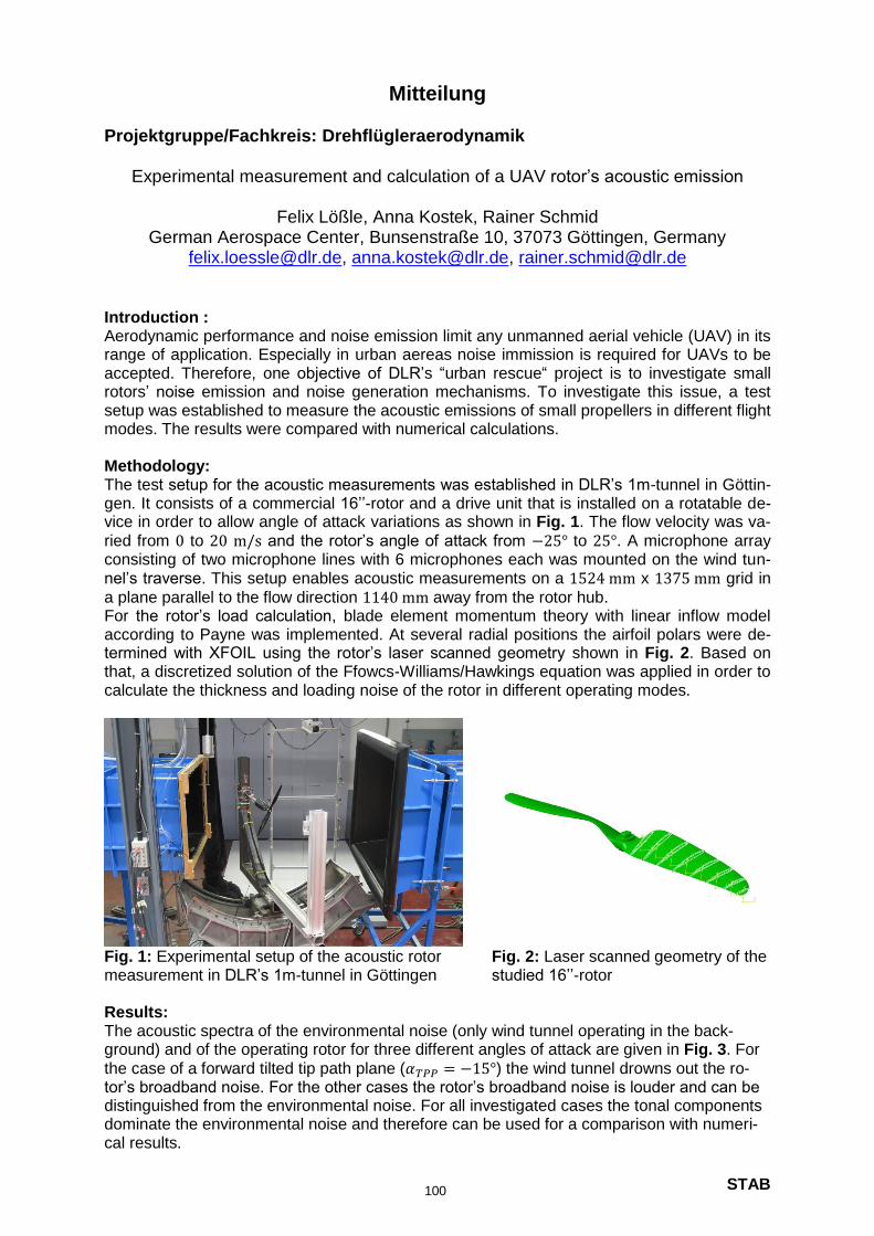
STAB


Experimental measurement and calculation of a UAV rotor’s acoustic emission

Felix Lößle, Anna Kostek, Rainer Schmid German Aerospace Center, Bunsenstraße 10, 37073 Göttingen, Germany

[email protected], [email protected], [email protected]

Introduction : Aerodynamic performance and noise emission limit any unmanned aerial vehicle (UAV) in its range of application. Especially in urban aereas noise immission is required for UAVs to be accepted. Therefore, one objective of DLR’s “urban rescue“ project is to investigate small rotors’ noise emission and noise generation mechanisms. To investigate this issue, a test setup was established to measure the acoustic emissions of small propellers in different flight modes. The results were compared with numerical calculations. Methodology: The test setup for the acoustic measurements was established in DLR’s 1m-tunnel in Göttin-gen. It consists of a commercial 16’’-rotor and a drive unit that is installed on a rotatable de-vice in order to allow angle of attack variations as shown in Fig. 1. The flow velocity was va-

ried from 0 to 20 m/s and the rotor’s angle of attack from −25° to 25°. A microphone array consisting of two microphone lines with 6 microphones each was mounted on the wind tun-nel’s traverse. This setup enables acoustic measurements on a 1524 mm x 1375 mm grid in

a plane parallel to the flow direction 1140 mm away from the rotor hub. For the rotor’s load calculation, blade element momentum theory with linear inflow model according to Payne was implemented. At several radial positions the airfoil polars were de-termined with XFOIL using the rotor’s laser scanned geometry shown in Fig. 2. Based on that, a discretized solution of the Ffowcs-Williams/Hawkings equation was applied in order to calculate the thickness and loading noise of the rotor in different operating modes.

Fig. 1: Experimental setup of the acoustic rotor measurement in DLR’s 1m-tunnel in Göttingen

Fig. 2: Laser scanned geometry of the studied 16’’-rotor

Results: The acoustic spectra of the environmental noise (only wind tunnel operating in the back-ground) and of the operating rotor for three different angles of attack are given in Fig. 3. For

the case of a forward tilted tip path plane (𝛼𝑇𝑃𝑃 = −15°) the wind tunnel drowns out the ro-tor’s broadband noise. For the other cases the rotor’s broadband noise is louder and can be distinguished from the environmental noise. For all investigated cases the tonal components dominate the environmental noise and therefore can be used for a comparison with numeri-cal results.

100




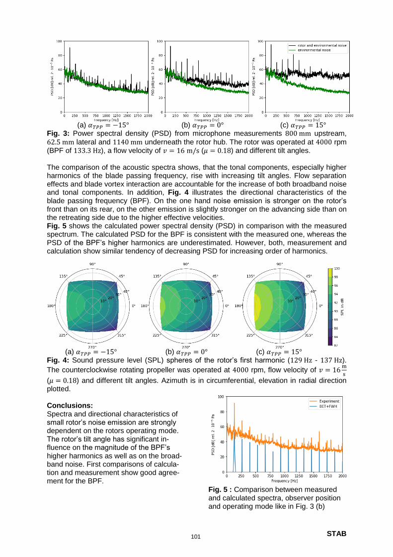
STAB

g

(a) 𝛼𝑇𝑃𝑃 = −15° (b) 𝛼𝑇𝑃𝑃 = 0° (c) 𝛼𝑇𝑃𝑃 = 15° Fig. 3: Power spectral density (PSD) from microphone measurements 800 mm upstream,

62.5 mm lateral and 1140 mm underneath the rotor hub. The rotor was operated at 4000 rpm (BPF of 133.3 Hz), a flow velocity of 𝑣 = 16 m/s (𝜇 = 0.18) and different tilt angles. The comparison of the acoustic spectra shows, that the tonal components, especially higher harmonics of the blade passing frequency, rise with increasing tilt angles. Flow separation effects and blade vortex interaction are accountable for the increase of both broadband noise and tonal components. In addition, Fig. 4 illustrates the directional characteristics of the blade passing frequency (BPF). On the one hand noise emission is stronger on the rotor’s front than on its rear, on the other emission is slightly stronger on the advancing side than on the retreating side due to the higher effective velocities. Fig. 5 shows the calculated power spectral density (PSD) in comparison with the measured spectrum. The calculated PSD for the BPF is consistent with the measured one, whereas the PSD of the BPF’s higher harmonics are underestimated. However, both, measurement and calculation show similar tendency of decreasing PSD for increasing order of harmonics.

(a) 𝛼𝑇𝑃𝑃 = −15° (b) 𝛼𝑇𝑃𝑃 = 0° (c) 𝛼𝑇𝑃𝑃 = 15° Fig. 4: Sound pressure level (SPL) spheres of the rotor’s first harmonic (129 Hz - 137 Hz).

The counterclockwise rotating propeller was operated at 4000 rpm, flow velocity of 𝑣 = 16m

s

(𝜇 = 0.18) and different tilt angles. Azimuth is in circumferential, elevation in radial direction plotted. Conclusions: Spectra and directional characteristics of small rotor’s noise emission are strongly dependent on the rotors operating mode. The rotor’s tilt angle has significant in-fluence on the magnitude of the BPF’s higher harmonics as well as on the broad-band noise. First comparisons of calcula-tion and measurement show good agree-ment for the BPF.

Fig. 5 : Comparison between measured and calculated spectra, observer position and operating mode like in Fig. 3 (b)

101

Mitteilung


Aerodynamic Analysis and Optimization of a Coaxial Helicopter Fuselage

Lukas Rottmann

Deutsches Zentrum für Luft- und Raumfahrt e.V. Braunschweig, Lilienthalplatz 7,38106 Braunschweig, [email protected]

The CoAX 2D coaxial ultralight helicopter developed by edm-aerotec had its maiden flight in 2015 [1]. As part of the national LuFo project CURoT (Coaxial Ultralight Ro-torcraft Technology), edm-aerotec invited DLR and the Technical University of Mu-nich to investigate aeromechanical and aerodynamic phenomena that occur espe-cially in coaxial helicopter configurations.The DLR Institute of Aerodynamics and Flow Technology contributed the expertise inthe field of fuselage aerodynamics and determined the potential for optimization of the existing fuselage cell. For this purpose, the DLR unstructured hybrid flow solver Tau was used [2]:

For the preliminary analysis, the fuselage was first simulated isolated from the rotor downwash. The rotor head was simulated with a simplified geome-try. In addition, all ducts in the fuselage were closed. For the cruise flight, fuselage polars with different angles of attack and yaw angles were calcu-lated.

In order to investigate the flow of the CoAX 2D more closely, the rotor down-wash in the second section was modelled using an actuator disc approach inTau [3]. The input data for the actuator disc is provided by a comprehensive-code Camrad II [4]. The model in Camrad II of the CoAX 2D was created by the Technical University of Munich [5]. Each actuator disc input corresponds to a trimmed flight condition. The flight conditions calculated in Camrad II are based on the flight tests performed by edm-aerotec [6]. During these flight tests, the deflection of the tail boom was measured by means of a strain gauge in addition. These values were used to validate the Tau results. In ad-dition to various flight speeds, climb and descent speeds were also consid-ered.

Finally, the simulations carried out in advance were analysed and evaluated. Based on the results, concepts for optimizing the fuselage were developed. In coordination with the company edm-aerotec an aerodynamic optimization of the landing gear was decided, because in the course of the airworthiness requirement LTF-ULM 2019 [7] the maximum take-off weight had to be raisedfrom 450kg to 600kg and the current landing gear had to be adapted to the higher weight. The changes to the landing gear from an aerodynamic point of view related to the shape of the landing gear. Finally, the aerodynamics of the new chassis was compared with the old configuration.

102


Figure 1 shows the complex vortex formations at the CoAX 2D fuselage exemplary for an airspeed of 32 m/s. The rotor downwash is modelled using an actuator disc.

Figure 2 shows the result of the Tau validation. Here a overall good agreement can be seen between the Tau and Camrad II compared to the flight experiments.

Figures:

References:

[1] www.edm-aerotec.de[2] D.Schwamborn, T.Gerhold, R.Heinrich“The DLR Tau-code: Recent applications in research

and industry”, European Conference on Computational Fluid Dynamics 2006[3] A.Raichle M.Stefan, J. Himisch,” A new Actuator Disk Model for the TAU Code and application

to a sailplane with a folding engine.”, STAB-Symposium 2006, 2006-11-29 - 2006-12-01, Darmstadt

[4] Comprehensive analytical model of rotorcraft aerodynamics and dynamics, www.johnson-aeronautics.com/CAMRADII.html

[5] R.Feil, D Eble and M. Hajek, "Comprehensive Analysis of a Coaxial Ultralight Rotorcraftand Validation with Full-Scale Flight-Test Data" ,Journal of the american helicopter society 63, 042004 (2018)

[6] R.Feil, M Rinker and M. Hajek, “Flight Testing of a Coaxial Ultralight Rotorcraft”,in AHS 2017.[7] Bekanntmachung von Lufttüchtigkeitsforderungen für Ultraleichthubschrauber

LTF –ULH vom 28.02.2019

Figure 1: Vorticity field from CoAX 2D at 32m/s Figure 2: Comparison of the horizontalstabiliser force between Camrad II,Tau and the flight experiment

103

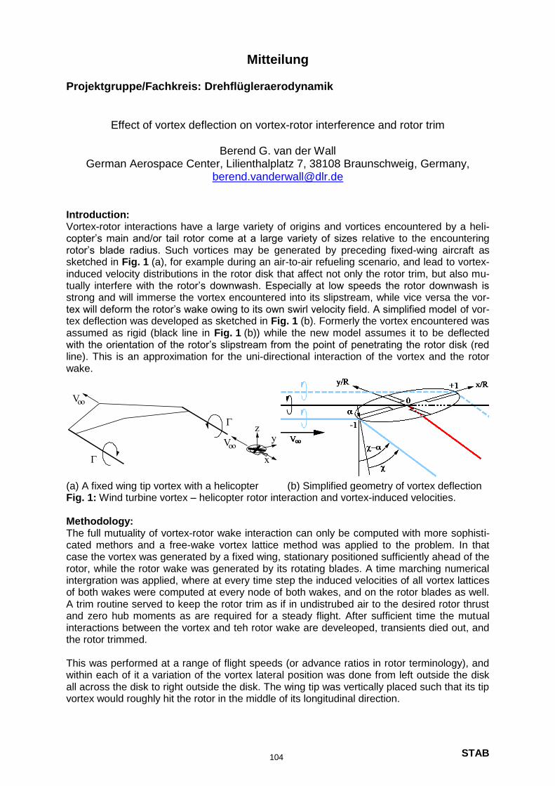
STAB


Effect of vortex deflection on vortex-rotor interference and rotor trim

Berend G. van der Wall German Aerospace Center, Lilienthalplatz 7, 38108 Braunschweig, Germany,

[email protected] Introduction: Vortex-rotor interactions have a large variety of origins and vortices encountered by a heli-copter’s main and/or tail rotor come at a large variety of sizes relative to the encountering rotor’s blade radius. Such vortices may be generated by preceding fixed-wing aircraft as sketched in Fig. 1 (a), for example during an air-to-air refueling scenario, and lead to vortex-induced velocity distributions in the rotor disk that affect not only the rotor trim, but also mu-tually interfere with the rotor’s downwash. Especially at low speeds the rotor downwash is strong and will immerse the vortex encountered into its slipstream, while vice versa the vor-tex will deform the rotor’s wake owing to its own swirl velocity field. A simplified model of vor-tex deflection was developed as sketched in Fig. 1 (b). Formerly the vortex encountered was assumed as rigid (black line in Fig. 1 (b)) while the new model assumes it to be deflected with the orientation of the rotor’s slipstream from the point of penetrating the rotor disk (red line). This is an approximation for the uni-directional interaction of the vortex and the rotor wake.

(a) A fixed wing tip vortex with a helicopter (b) Simplified geometry of vortex deflection Fig. 1: Wind turbine vortex – helicopter rotor interaction and vortex-induced velocities. Methodology: The full mutuality of vortex-rotor wake interaction can only be computed with more sophisti-cated methors and a free-wake vortex lattice method was applied to the problem. In that case the vortex was generated by a fixed wing, stationary positioned sufficiently ahead of the rotor, while the rotor wake was generated by its rotating blades. A time marching numerical intergration was applied, where at every time step the induced velocities of all vortex lattices of both wakes were computed at every node of both wakes, and on the rotor blades as well. A trim routine served to keep the rotor trim as if in undistrubed air to the desired rotor thrust and zero hub moments as are required for a steady flight. After sufficient time the mutual interactions between the vortex and teh rotor wake are develeoped, transients died out, and the rotor trimmed. This was performed at a range of flight speeds (or advance ratios in rotor terminology), and within each of it a variation of the vortex lateral position was done from left outside the disk all across the disk to right outside the disk. The wing tip was vertically placed such that its tip vortex would roughly hit the rotor in the middle of its longitudinal direction.

oV

ooV

o

z

x

y

G

G

104


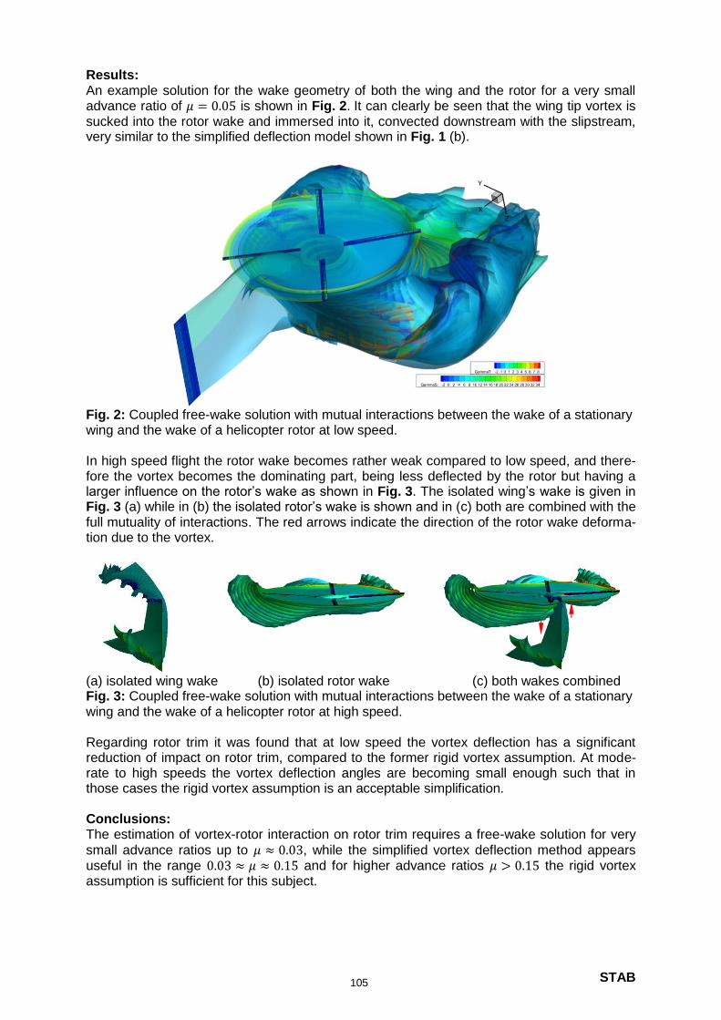
STAB

Results: An example solution for the wake geometry of both the wing and the rotor for a very small advance ratio of 𝜇 = 0.05 is shown in Fig. 2. It can clearly be seen that the wing tip vortex is sucked into the rotor wake and immersed into it, convected downstream with the slipstream, very similar to the simplified deflection model shown in Fig. 1 (b).

Fig. 2: Coupled free-wake solution with mutual interactions between the wake of a stationary wing and the wake of a helicopter rotor at low speed. In high speed flight the rotor wake becomes rather weak compared to low speed, and there-fore the vortex becomes the dominating part, being less deflected by the rotor but having a larger influence on the rotor’s wake as shown in Fig. 3. The isolated wing’s wake is given in Fig. 3 (a) while in (b) the isolated rotor’s wake is shown and in (c) both are combined with the full mutuality of interactions. The red arrows indicate the direction of the rotor wake deforma-tion due to the vortex.

(a) isolated wing wake (b) isolated rotor wake (c) both wakes combined Fig. 3: Coupled free-wake solution with mutual interactions between the wake of a stationary wing and the wake of a helicopter rotor at high speed. Regarding rotor trim it was found that at low speed the vortex deflection has a significant reduction of impact on rotor trim, compared to the former rigid vortex assumption. At mode-rate to high speeds the vortex deflection angles are becoming small enough such that in those cases the rigid vortex assumption is an acceptable simplification. Conclusions: The estimation of vortex-rotor interaction on rotor trim requires a free-wake solution for very

small advance ratios up to 𝜇 ≈ 0.03, while the simplified vortex deflection method appears useful in the range 0.03 ≈ 𝜇 ≈ 0.15 and for higher advance ratios 𝜇 > 0.15 the rigid vortex assumption is sufficient for this subject.

105

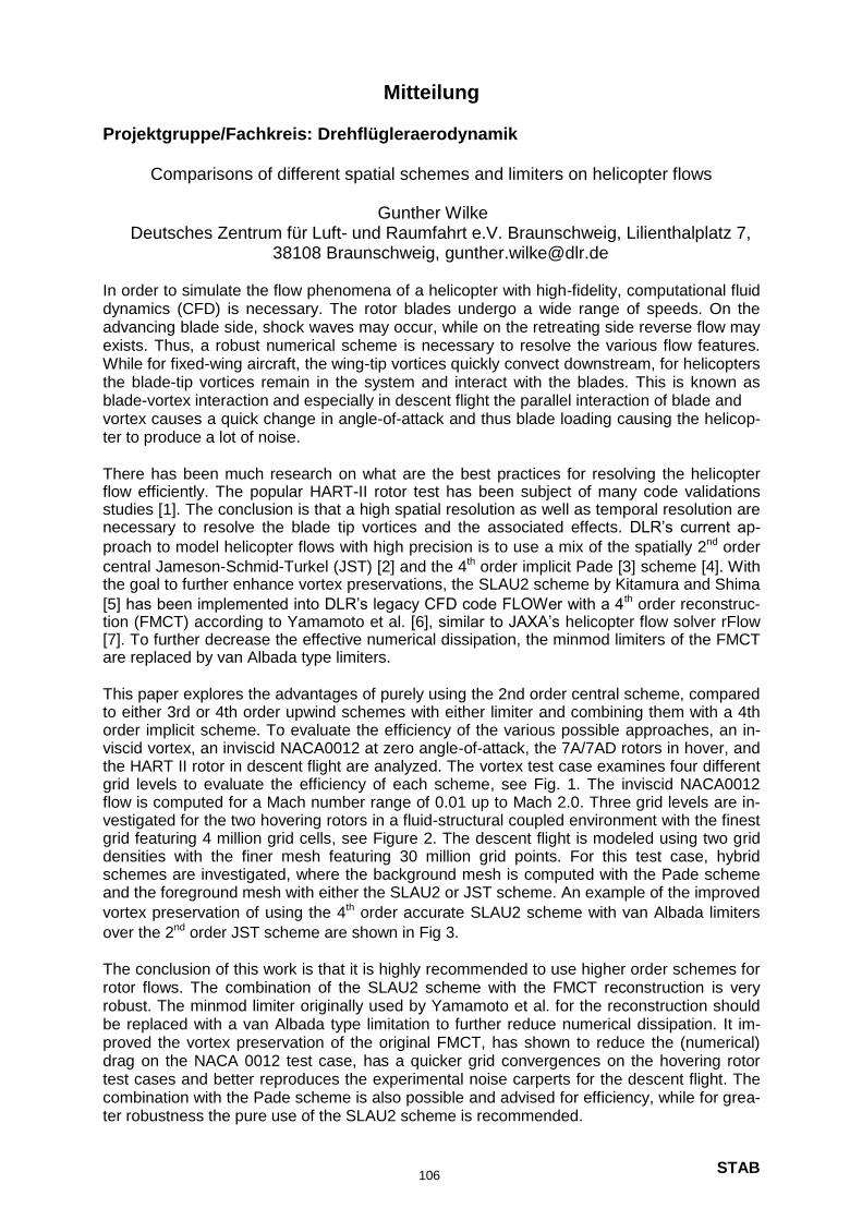
STAB

ter robustness the pure use of the SLAU2 scheme is recommended.combination with the Pade scheme is also possible and advised for efficiency, while for grea- test cases and better reproduces the experimental noise carperts for the descent flight. The drag on the NACA 0012 test case, has a quicker grid convergences on the hovering rotor proved the vortex preservation of the original FMCT, has shown to reduce the (numerical)be replaced with a van Albada type limitation to further reduce numerical dissipation. It im- robust. The minmod limiter originally used by Yamamoto et al. for the reconstruction should rotor flows. The combination of the SLAU2 scheme with the FMCT reconstruction is very The conclusion of this work is that it is highly recommended to use higher order schemes for

over the 2nd order JST scheme are shown in Fig 3.

vortex preservation of using the 4th order accurate SLAU2 scheme with van Albada limiters and the foreground mesh with either the SLAU2 or JST scheme. An example of the improved schemes are investigated, where the background mesh is computed with the Pade scheme densities with the finer mesh featuring 30 million grid points. For this test case, hybrid grid featuring 4 million grid cells, see Figure 2. The descent flight is modeled using two grid vestigated for the two hovering rotors in a fluid-structural coupled environment with the finest flow is computed for a Mach number range of 0.01 up to Mach 2.0. Three grid levels are in- grid levels to evaluate the efficiency of each scheme, see Fig. 1. The inviscid NACA0012 the HART II rotor in descent flight are analyzed. The vortex test case examines four different viscid vortex, an inviscid NACA0012 at zero angle-of-attack, the 7A/7AD rotors in hover, and order implicit scheme. To evaluate the efficiency of the various possible approaches, an in- to either 3rd or 4th order upwind schemes with either limiter and combining them with a 4th This paper explores the advantages of purely using the 2nd order central scheme, compared

are replaced by van Albada type limiters.[7]. To further decrease the effective numerical dissipation, the minmod limiters of the FMCT tion (FMCT) according to Yamamoto et al. [6], similar to JAXA’s helicopter flow solver rFlow [5] has been implemented into DLR’s legacy CFD code FLOWer with a 4th order reconstruc- the goal to further enhance vortex preservations, the SLAU2 scheme by Kitamura and Shima central Jameson-Schmid-Turkel (JST) [2] and the 4th order implicit Pade [3] scheme [4]. With proach to model helicopter flows with high precision is to use a mix of the spatially 2nd order necessary to resolve the blade tip vortices and the associated effects. DLR’s current ap- studies [1]. The conclusion is that a high spatial resolution as well as temporal resolution are flow efficiently. The popular HART-II rotor test has been subject of many code validations There has been much research on what are the best practices for resolving the helicopter

ter to produce a lot of noise.vortex causes a quick change in angle-of-attack and thus blade loading causing the helicop- blade-vortex interaction and especially in descent flight the parallel interaction of blade and the blade-tip vortices remain in the system and interact with the blades. This is known as While for fixed-wing aircraft, the wing-tip vortices quickly convect downstream, for helicopters exists. Thus, a robust numerical scheme is necessary to resolve the various flow features. advancing blade side, shock waves may occur, while on the retreating side reverse flow may dynamics (CFD) is necessary. The rotor blades undergo a wide range of speeds. On the In order to simulate the flow phenomena of a helicopter with high-fidelity, computational fluid

38108 Braunschweig, [email protected] Zentrum für Luft- und Raumfahrt e.V. Braunschweig, Lilienthalplatz 7,

Gunther Wilke

Comparisons of different spatial schemes and limiters on helicopter flows


Mitteilung

106

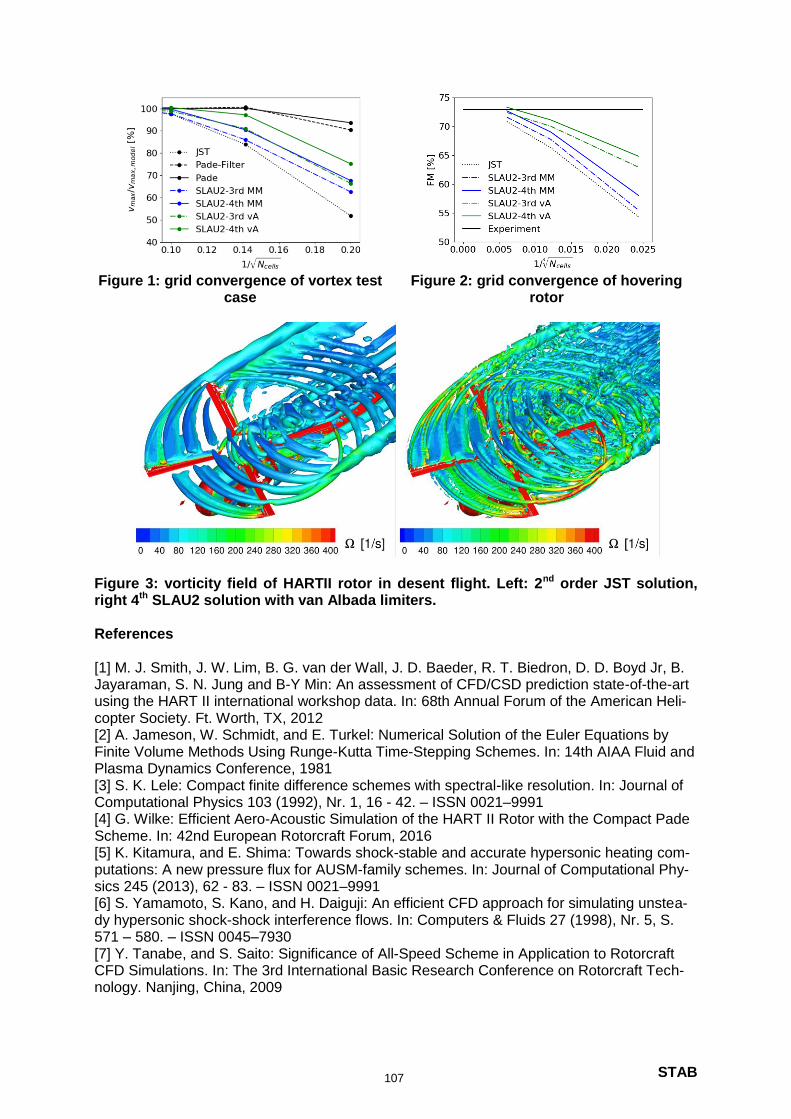
STAB

Figure 1: grid convergence of vortex test

case

Figure 2: grid convergence of hovering rotor

Figure 3: vorticity field of HARTII rotor in desent flight. Left: 2nd order JST solution, right 4th SLAU2 solution with van Albada limiters. References [1] M. J. Smith, J. W. Lim, B. G. van der Wall, J. D. Baeder, R. T. Biedron, D. D. Boyd Jr, B. Jayaraman, S. N. Jung and B-Y Min: An assessment of CFD/CSD prediction state-of-the-art using the HART II international workshop data. In: 68th Annual Forum of the American Heli-copter Society. Ft. Worth, TX, 2012 [2] A. Jameson, W. Schmidt, and E. Turkel: Numerical Solution of the Euler Equations by Finite Volume Methods Using Runge-Kutta Time-Stepping Schemes. In: 14th AIAA Fluid and Plasma Dynamics Conference, 1981 [3] S. K. Lele: Compact finite difference schemes with spectral-like resolution. In: Journal of Computational Physics 103 (1992), Nr. 1, 16 - 42. – ISSN 0021–9991 [4] G. Wilke: Efficient Aero-Acoustic Simulation of the HART II Rotor with the Compact Pade Scheme. In: 42nd European Rotorcraft Forum, 2016 [5] K. Kitamura, and E. Shima: Towards shock-stable and accurate hypersonic heating com-putations: A new pressure flux for AUSM-family schemes. In: Journal of Computational Phy-sics 245 (2013), 62 - 83. – ISSN 0021–9991 [6] S. Yamamoto, S. Kano, and H. Daiguji: An efficient CFD approach for simulating unstea-dy hypersonic shock-shock interference flows. In: Computers & Fluids 27 (1998), Nr. 5, S. 571 – 580. – ISSN 0045–7930 [7] Y. Tanabe, and S. Saito: Significance of All-Speed Scheme in Application to Rotorcraft CFD Simulations. In: The 3rd International Basic Research Conference on Rotorcraft Tech-nology. Nanjing, China, 2009

107

Mitteilung Projektgruppe/ Fachkreis

Ansprechpartner Jianping Yin, Karl-Stéphane Rossignol

Institution DLR / Institut für Aerodynamik und Strömungstechnik

Adresse Lilienthalplatz 7 Telefon: 0531 / 295-3313 38108 Braunschweig Telefax: 0531 / 295-2914 Email: [email protected],

weitere Partner Thema

Experimental and numerical study on helicopter acoustic scattering

Ausgangssituation:

With rising concern for environmental issues and increasingly stringent noise regulation, the noise has gained importance in the helicopter’s design process. Extensive work, both theoretical and experimental helped to deepen the understanding of the noise generating mechanisms. Even though the scattering of rotor generated noise by the fuselage has been recognized as having a significant influence on the noise spectra and directivity generated, the research effort towards acoustic installation effects, especially the scattering of tail rotor noise, has not been studied extensively. To further understand helicopter noise propagation the GARTEUR Action Group HC/AG-24 [1,2,3] is established. The objectives of this AG are (1) to develop and validate numerical prediction methods and (2) to generate a unique noise scattering database through wind tunnel test using generic configurations.

Ziel:

To accurately predict the effective helicopter external noise under the influence of the fuselage, advanced analysis tools that overcome the so-called free-field limitation of classical acoustic analogy methods are required. For this purpose, validations of the tools with the experiment data need to be conducted. The acoustic scattering predictions will be analyzed and compared with the test results. This paper will focus on the results from the numerical and wind tunnel activities conducted by DLR.

Lösungsweg:

The GARTEUR AG24 shielding experiments were conducted in DLR’s Acoustic Wind tunnel in Braunschweig (AWB).The scattering for generic configurations was studied using the sound generated by two monopole type point sound sources and a model tail-rotor. Figure 1 demonstrates two experiments, first using a sphere as a shielding object (left) and, second a simplified helicopter model (right). The helicopter model consists of an ellipsoid fuselage, cylindric tail boom and a simple empennage. DLR Fast Multipole Boundary Element Method (FMCAS) code which solves the exterior Helmholtz problem for the scattered pressure field is applied in numerical simulations [4,5]. The validity of the method is demonstrated by comparing the scattering by spheres with analytic solutions.

Ergebnis:

Figure 2 left shows the contour plot of the shielding factor from numerical simulations on a receiving plane (microphones) for the helicopter model. The general shielding characteristics can be observed by the higher and lower levels represented by different colors. The comparisons with the experimental results taken by a microphone array along the center line are given in Figure 2, right. The comparison shows a very good agreement in terms of

DREHFLÜGLERAERODYNAMIK

108

amplitude and phase.

.

Figure 1. Test set-up for the acoustic shielding tests in AWB using the laser sound source methodology, left: laser sound source (B,C), sphere with sting support (D) and microphone (A), right: GARTEUR Helicopter model

Figure 2. noise scattering by GARTEUR helicopter model (left: simulation; right:

comparison of noise shielding factor with simulation at y=0m and y=0.1m)

Literatur: [2] Yin, J., Rossignol, K-S., Barbarino, M., Bianco, D., Testa, C., Brouwer, H., Janssen, R., Reboul, G., Vigevano, L., Bernardini, G., Gennaretti, M., Serafini, J., Poggi, C.: GARTEUR activities on acoustical methods and experiments for studying on acoustic scattering. CEAS Aeronautical Journal, Vol 10 (2), Page 531-551, 2019 (DOI: 10.1007/s13272-018-0333-0) [3]Rossignol, K.-S., Delfs, J., Boden, F.: On the relevance of convection effects for a laser-generated sound source. 21th AIAA/CEAS Aeroacoustics Conference, AIAA 2015-3146, Dallas, 2015. [4] Lummer, M., Richtery, C., Pröber, C., Delfs, J.: Validation of a model for open rotor noise predictions and calculation of shielding effects using a fast BEM. 19th AIAA/CEAS Aeroacoustics Conference (34th AIAA Aeroacoustics Conference), 27–29 May 2013. [5] Yin, J.: Investigation of Rotor Noise Shielding Effects by the Helicopter Fuselage in Forward Flight. Journal of Aircraft, 56 (4), Page 1-12. American Institute of Aeronautics and Astronautics (AIAA), 2019 (DOI: 10.2514/1.C035009)

Weiteres Vorgehen:

In the framework of AG24, a unique noise scattering database was established, enabling the assessment, and further development, of noise scattering prediction tools capabilities.

109

Mitteilung

Projektgruppe/Fachkreis: Technische Strömungen

On the Coverage of Dynamic Processes in Highly Separated Flows Using the LatticeBoltzmann Method

Christian Bauer, Max Müller, Klaus Ehrenfried and Claus WagnerInstitut für Aerodynamik und Strömungstechnik, DLR, Bunsenstr. 10, 37073 Göttingen

[email protected]

Ground vehicles are exposed to a vast variety of unsteady aerodynamic phenomena such as gusts. This iswhy the effect of gusts has been the focus of many studies, e.g. on cars in full scale (Schroeck et al., 2011),trains in full scale (Baker et al., 2004) as well as on simplified car models in wind tunnels (Ferrand, 2014).In order to gain better insight into the flow dynamics, Hemida and Krajnovic (2010) investigated the effect ofcross winds on a generic train with different nose shapes using large-eddy simulations. Another unsteadyeffect that has recently gained interest is the multi-stability of the wake behind cars. In this context, Cadotet al. (2016) detected bi-stability in the lift forces acting on full-scale cars during wind tunnel testing. Thisbi-stability was further investigated in wind tunnel testing on simplified car models by Grandemange et al.(2013) and Pavia et al. (2018).Due to the highly transient behaviour of the flow, the existing numerical methods require revision concerningtheir capability of coping with the flow dynamics. For such investigations, the flow around a sphere is usuallychosen as a setup, as it has been in the focus of aerodynamic research since the very beginning (Prandtl,1914) and, thus, is the subject of many studies described in the literature. However, the flow around a sphereis an example of a fully separated flow, whose prediction poses a challenge to numerical investigations suchas the DES study of Constantinescu and Squires (2004). The highly instationary dynamics in the wake ofsuch a flow are described by hot-wire measurements (Achenbach, 1972) as well as by flow visualisation(Chrust et al., 2013). The latter clearly shows the development of hairpin vortices and the loss of planarsymmetry.In order to study the force answer of both the influence of incoming sinusoidal, gust-like flow patterns andwake-induced instabilities, Müller et al. (2020) introduced a test setup consisting of a sphere mounted onan internal six-component balance attached to a cross-stream rod (CSR). This setup also included a gustgenerator equipped with four wings with motor-driven carbon fibre flaps. This experiment provides informa-tion on the dynamical behaviour of a highly separated flow over a sphere at a CSR and therefore enhancesexisting comparisons between numerical and experimental investigations. The present study is intended toevaluate to what extent the dynamics of this flow can be represented by a numerical simulation.Thus, in accordance with the literature and the above-described wind tunnel tests with a sphere mountedon the CSR, numerical simulations are performed, solving the Lattice Boltzmann equation (LBE). To capturethe dynamics of the flow at Reynolds numbers as high as 3 × 105, the Lattice Boltzmann method is chosento solve the governing equations via 3DS SIMULIA PowerFLOW R©. In contrast to traditional numericalmethods in fluid mechanics not the Navier-Stokes but the Lattice Boltzmann equation (LBE) is solved inPowerFLOW R©. The LBE describes the dynamics of a particle velocity distribution function on a mesoscopicscale. Macroscopic quantities are then deducted via integration of mesoscopic variables. The discrete LBEreads

fi (x + ei∆x , t + ∆t) = fi (x, t) + Ωi (f (x, t)), i = 0, 1, ... , M, (1)

where x is the location in space, t is the location in time, fi is the particle velocity distribution function alongthe i th direction and Ωi is the collision operator representing the rate of change of fi due to collision (Chenand Doolen, 1998). Moreover, the collision term is approximated by the Bhatnagar, Gross, and Krook (BGK)model using a linear relaxation (Bhatnagar et al., 1954).Figure 1 (left) shows a snapshot of the first results of the numerical investigation at Re = 3 × 105. On theleeward side of the sphere with the CSR, the velocity magnitude is depicted as pseudo-colour plot, whereasstreamlines are represented in white. Next to the plot is an oil-film photograph reflecting the shear stresseson the sphere’s surface. Two counter-rotating vortices can be identified in addition to a region connected tothe separation — and consequently recirculation — bubble. Qualitatively, the shape of the pseudo-colourfaces matches the shape of the oil film. Note that the plot from the simulation is a snapshot, whereasoil-film visualisations have an averaging character. On the right side in figure 1, hairpin vortex sheddingat Re = 280 performed by Chrust et al. (2013) is shown for comparison. Despite the drastically differentReynolds number and test setup, a pair of counter-rotating vortices similar to the one detected with the oilfilm is observed. The similarity between first numerical results and the experiment and the agreement withthe descriptions in the literature appear to be promising, but further investigations need to be performed to

STAB110

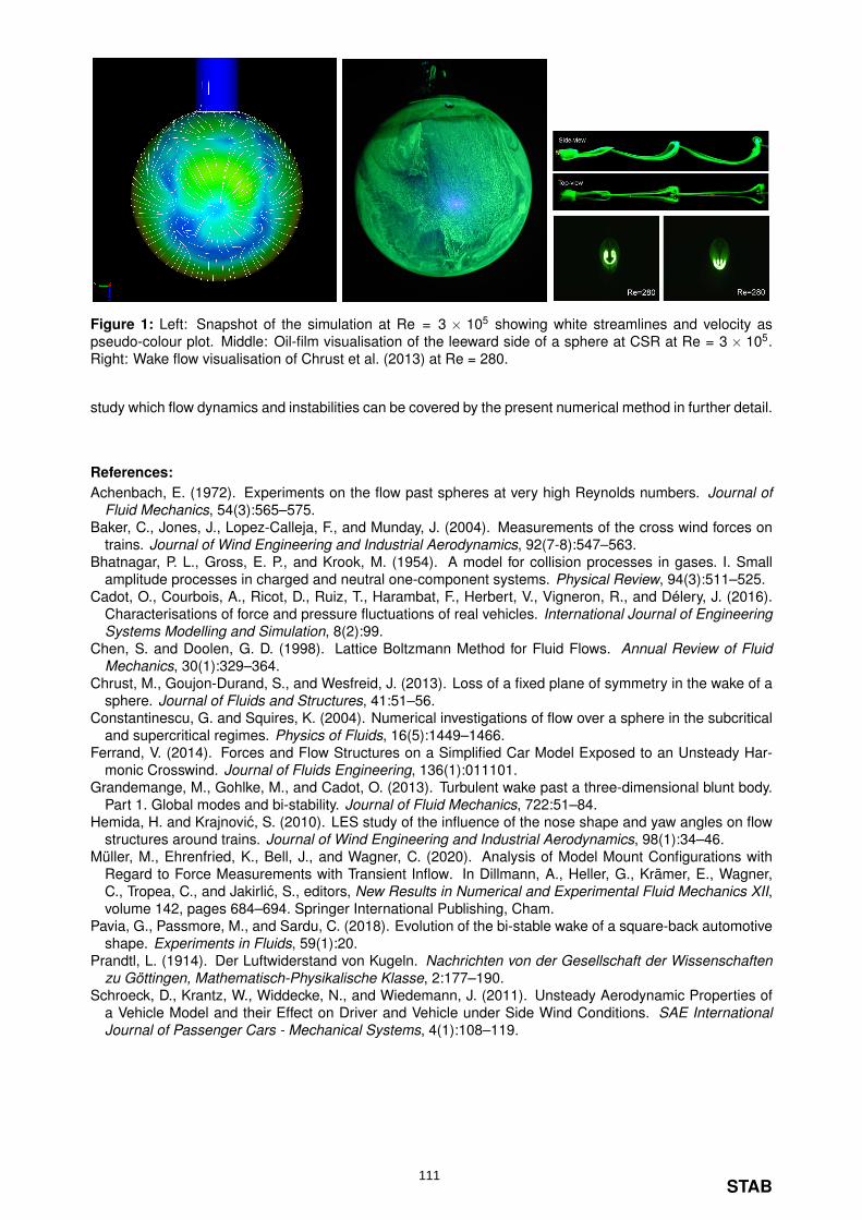
Figure 1: Left: Snapshot of the simulation at Re = 3 × 105 showing white streamlines and velocity aspseudo-colour plot. Middle: Oil-film visualisation of the leeward side of a sphere at CSR at Re = 3 × 105.Right: Wake flow visualisation of Chrust et al. (2013) at Re = 280.

study which flow dynamics and instabilities can be covered by the present numerical method in further detail.

References:Achenbach, E. (1972). Experiments on the flow past spheres at very high Reynolds numbers. Journal of

Fluid Mechanics, 54(3):565–575.Baker, C., Jones, J., Lopez-Calleja, F., and Munday, J. (2004). Measurements of the cross wind forces on

trains. Journal of Wind Engineering and Industrial Aerodynamics, 92(7-8):547–563.Bhatnagar, P. L., Gross, E. P., and Krook, M. (1954). A model for collision processes in gases. I. Small

amplitude processes in charged and neutral one-component systems. Physical Review, 94(3):511–525.Cadot, O., Courbois, A., Ricot, D., Ruiz, T., Harambat, F., Herbert, V., Vigneron, R., and Délery, J. (2016).

Characterisations of force and pressure fluctuations of real vehicles. International Journal of EngineeringSystems Modelling and Simulation, 8(2):99.

Chen, S. and Doolen, G. D. (1998). Lattice Boltzmann Method for Fluid Flows. Annual Review of FluidMechanics, 30(1):329–364.

Chrust, M., Goujon-Durand, S., and Wesfreid, J. (2013). Loss of a fixed plane of symmetry in the wake of asphere. Journal of Fluids and Structures, 41:51–56.

Constantinescu, G. and Squires, K. (2004). Numerical investigations of flow over a sphere in the subcriticaland supercritical regimes. Physics of Fluids, 16(5):1449–1466.

Ferrand, V. (2014). Forces and Flow Structures on a Simplified Car Model Exposed to an Unsteady Har-monic Crosswind. Journal of Fluids Engineering, 136(1):011101.

Grandemange, M., Gohlke, M., and Cadot, O. (2013). Turbulent wake past a three-dimensional blunt body.Part 1. Global modes and bi-stability. Journal of Fluid Mechanics, 722:51–84.

Hemida, H. and Krajnovic, S. (2010). LES study of the influence of the nose shape and yaw angles on flowstructures around trains. Journal of Wind Engineering and Industrial Aerodynamics, 98(1):34–46.

Müller, M., Ehrenfried, K., Bell, J., and Wagner, C. (2020). Analysis of Model Mount Configurations withRegard to Force Measurements with Transient Inflow. In Dillmann, A., Heller, G., Krämer, E., Wagner,C., Tropea, C., and Jakirlic, S., editors, New Results in Numerical and Experimental Fluid Mechanics XII,volume 142, pages 684–694. Springer International Publishing, Cham.

Pavia, G., Passmore, M., and Sardu, C. (2018). Evolution of the bi-stable wake of a square-back automotiveshape. Experiments in Fluids, 59(1):20.

Prandtl, L. (1914). Der Luftwiderstand von Kugeln. Nachrichten von der Gesellschaft der Wissenschaftenzu Göttingen, Mathematisch-Physikalische Klasse, 2:177–190.

Schroeck, D., Krantz, W., Widdecke, N., and Wiedemann, J. (2011). Unsteady Aerodynamic Properties ofa Vehicle Model and their Effect on Driver and Vehicle under Side Wind Conditions. SAE InternationalJournal of Passenger Cars - Mechanical Systems, 4(1):108–119.

STAB111

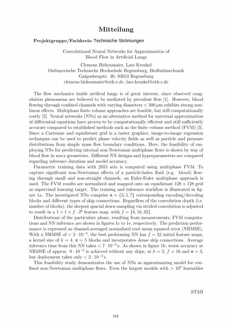
Mitteilung


Convolutional Neural Networks for Approximation ofBlood Flow in Artificial Lungs

Clemens Birkenmaier, Lars KrenkelOstbayerische Technische Hochschule Regensburg, Biofluidmechanik

Galgenbergstr. 30, 93053 [email protected], [email protected]

The flow mechanics inside artifical lungs is of great interest, since observed coag-ulation phenomena are believed to be mediated by prevalent flow [1]. However, bloodflowing through confined channels with varying diameters < 300µm exhibits strong non-linear effects. Multiphase finite volume approaches are feasible, but still computationallycostly [2]. Neural networks (NNs) as an alternative method for universal approximationof differential equations have proven to be computationally efficient and still sufficientlyaccurate compared to established methods such as the finite volume method (FVM) [3].Since a Cartesian and equidistant grid is a raster graphics, image-to-image regressiontechniques can be used to predict phase velocity fields as well as particle and pressuredistributions from simple mass flow boundary conditions. Here, the feasibility of em-ploying NNs for predicting internal non-Newtonian multiphase flows is shown by way ofblood flow in wavy geometries. Different NN designs and hyperparameters are comparedregarding inference duration and model accuracy.

Parametric training data with 2055 sets is computed using multiphase FVM. Tocapture significant non-Newtonian effects of a particle-laden fluid (e.g. blood) flow-ing through small and non-straight channels, an Euler-Euler multiphase approach isused. The FVM results are normalized and mapped onto an equidistant 128× 128 gridas supervised learning target. The training and inference workflow is illustrated in fig-ure 1a. The investigated NNs comprise n = 3, 5, 7 corresponding encoding/decodingblocks and different types of skip connections. Regardless of the convolution depth (i.e.number of blocks), the deepest spacial down-sampling via strided convolution is adjustedto result in a 1× 1× f · 2n feature map, with f = 8, 16, 32.

Distributions of the particulate phase, resulting from measurements, FVM computa-tions and NN inference are shown in figures 1c to 1e, respectively. The prediction perfor-mance is expressed as channel-averaged normalized root mean squared error (NRMSE).With a NRMSE of < 2 · 10−3, the best preforming NN has f = 32 initial feature maps,a kernel size of k = 4, n = 5 blocks and incorporates dense skip connections. Averageinference time from this NN takes < 7 · 10−3 s. As shown in figure 1b, worst accuracy atNRMSE of approx. 9 · 10−3 is achieved without any skips, at k = 2, f = 16 and n = 3,but deployment takes only < 2 · 10−3 s.

This feasibility study demonstrates the use of NNs as approximating model for con-fined non-Newtonian multiphase flows. Even the largest models with > 108 learnables

STAB

112

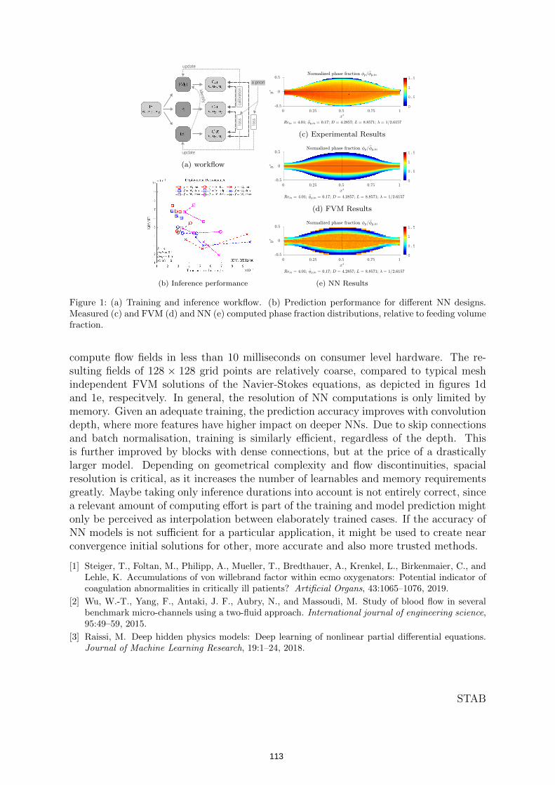
update

update

loss

calib

ratio

nlo

ss

iden

tify

a priori

(a) workflow

(b) Inference performance

0

0.5

1

1.5

(c) Experimental Results

0

0.5

1

1.5

(d) FVM Results

0

0.5

1

1.5

(e) NN Results

Figure 1: (a) Training and inference workflow. (b) Prediction performance for different NN designs.Measured (c) and FVM (d) and NN (e) computed phase fraction distributions, relative to feeding volumefraction.

compute flow fields in less than 10 milliseconds on consumer level hardware. The re-sulting fields of 128 × 128 grid points are relatively coarse, compared to typical meshindependent FVM solutions of the Navier-Stokes equations, as depicted in figures 1dand 1e, respecitvely. In general, the resolution of NN computations is only limited bymemory. Given an adequate training, the prediction accuracy improves with convolutiondepth, where more features have higher impact on deeper NNs. Due to skip connectionsand batch normalisation, training is similarly efficient, regardless of the depth. Thisis further improved by blocks with dense connections, but at the price of a drasticallylarger model. Depending on geometrical complexity and flow discontinuities, spacialresolution is critical, as it increases the number of learnables and memory requirementsgreatly. Maybe taking only inference durations into account is not entirely correct, sincea relevant amount of computing effort is part of the training and model prediction mightonly be perceived as interpolation between elaborately trained cases. If the accuracy ofNN models is not sufficient for a particular application, it might be used to create nearconvergence initial solutions for other, more accurate and also more trusted methods.

[1] Steiger, T., Foltan, M., Philipp, A., Mueller, T., Bredthauer, A., Krenkel, L., Birkenmaier, C., andLehle, K. Accumulations of von willebrand factor within ecmo oxygenators: Potential indicator ofcoagulation abnormalities in critically ill patients? Artificial Organs, 43:1065–1076, 2019.

[2] Wu, W.-T., Yang, F., Antaki, J. F., Aubry, N., and Massoudi, M. Study of blood flow in severalbenchmark micro-channels using a two-fluid approach. International journal of engineering science,95:49–59, 2015.

[3] Raissi, M. Deep hidden physics models: Deep learning of nonlinear partial differential equations.Journal of Machine Learning Research, 19:1–24, 2018.

STAB

113

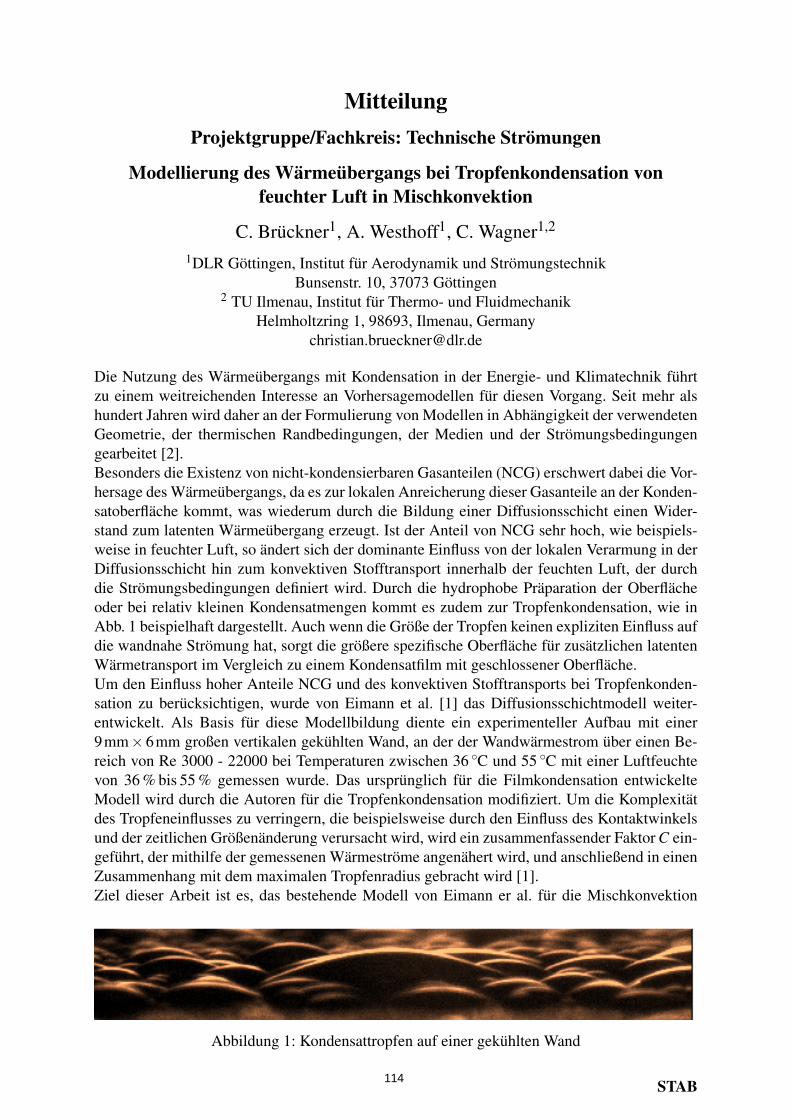
MitteilungProjektgruppe/Fachkreis: Technische Stromungen

Modellierung des Warmeubergangs bei Tropfenkondensation vonfeuchter Luft in Mischkonvektion

C. Bruckner1, A. Westhoff1, C. Wagner1,2

1DLR Gottingen, Institut fur Aerodynamik und StromungstechnikBunsenstr. 10, 37073 Gottingen

2 TU Ilmenau, Institut fur Thermo- und FluidmechanikHelmholtzring 1, 98693, Ilmenau, Germany

[email protected]

Die Nutzung des Warmeubergangs mit Kondensation in der Energie- und Klimatechnik fuhrtzu einem weitreichenden Interesse an Vorhersagemodellen fur diesen Vorgang. Seit mehr alshundert Jahren wird daher an der Formulierung von Modellen in Abhangigkeit der verwendetenGeometrie, der thermischen Randbedingungen, der Medien und der Stromungsbedingungengearbeitet [2].Besonders die Existenz von nicht-kondensierbaren Gasanteilen (NCG) erschwert dabei die Vor-hersage des Warmeubergangs, da es zur lokalen Anreicherung dieser Gasanteile an der Konden-satoberflache kommt, was wiederum durch die Bildung einer Diffusionsschicht einen Wider-stand zum latenten Warmeubergang erzeugt. Ist der Anteil von NCG sehr hoch, wie beispiels-weise in feuchter Luft, so andert sich der dominante Einfluss von der lokalen Verarmung in derDiffusionsschicht hin zum konvektiven Stofftransport innerhalb der feuchten Luft, der durchdie Stromungsbedingungen definiert wird. Durch die hydrophobe Praparation der Oberflacheoder bei relativ kleinen Kondensatmengen kommt es zudem zur Tropfenkondensation, wie inAbb. 1 beispielhaft dargestellt. Auch wenn die Große der Tropfen keinen expliziten Einfluss aufdie wandnahe Stromung hat, sorgt die großere spezifische Oberflache fur zusatzlichen latentenWarmetransport im Vergleich zu einem Kondensatfilm mit geschlossener Oberflache.Um den Einfluss hoher Anteile NCG und des konvektiven Stofftransports bei Tropfenkonden-sation zu berucksichtigen, wurde von Eimann et al. [1] das Diffusionsschichtmodell weiter-entwickelt. Als Basis fur diese Modellbildung diente ein experimenteller Aufbau mit einer9mm×6mm großen vertikalen gekuhlten Wand, an der der Wandwarmestrom uber einen Be-reich von Re 3000 - 22000 bei Temperaturen zwischen 36 C und 55 C mit einer Luftfeuchtevon 36 % bis 55 % gemessen wurde. Das ursprunglich fur die Filmkondensation entwickelteModell wird durch die Autoren fur die Tropfenkondensation modifiziert. Um die Komplexitatdes Tropfeneinflusses zu verringern, die beispielsweise durch den Einfluss des Kontaktwinkelsund der zeitlichen Großenanderung verursacht wird, wird ein zusammenfassender Faktor C ein-gefuhrt, der mithilfe der gemessenen Warmestrome angenahert wird, und anschließend in einenZusammenhang mit dem maximalen Tropfenradius gebracht wird [1].Ziel dieser Arbeit ist es, das bestehende Modell von Eimann er al. fur die Mischkonvektion

Abbildung 1: Kondensattropfen auf einer gekuhlten Wand

STAB114

und fur große Skalen anzupassen. Die experimentelle Untersuchung erfolgt mit einem verti-kal orientierten, einseitig gekuhlten Stromungskanal mit rechteckigem Querschnitt. Der Kanalhat einen Querschnitt von 50mm × 533mm und Kondensation erfolgt uber eine Lange von2,05 m [3]. Die Messungen werden in einem Bereich von Re 2000 - 8000 bei Temperaturenzwischen 25 C und 35 C mit einer Luftfeuchte von 30 % bis 50 % durchgefuhrt.

yx

Tb

Tsat = Ti

Tw

1hd

1Ch f

Tw Ti Tw

Abbildung 2: Schemader Tropfenkondensati-on

Zur grundsatzlichen Abbildung des Warmeubergangs bei der Trop-fenkondensation dient die inverse Warmewiderstandskaskade, bei derdie einzelnen Warmetransportmechanismen durch einen Widerstandausgedruckt werden. In Abb. 2 sind der Temperaturverlauf zwischender Bulk-Stromung Tb, der Kondensatoberflache Ti und der Wand Twsowie die einzelnen Warmewiderstande 1

hdund 1

Ch fschematisch dar-

gestellt. Aus der Summe der Warmewiderstande lasst sich dann derGesamtwarmeubergangskoeffizient ht bestimmen.

ht =

[1hd

+1C

1h f

]−1

(1)

Die Bestimmung der einzelnen Warmeubergangskoeffizienten h er-folgt mithilfe des experimentell gemessenen Gesamtwarmestroms qtund der Temperatur an der Kondensatoberflache Ti, mit der dieTeilwarmestrome in der lokalen Warmebilanz ermittelt werden.

qt = ht(Tb −Tw) = hd(Ti −Tw) =Ch f (Tb −Ti) (2)

Im Gegensatz zum sehr kleinen Experiment von Eimann et al. kann Tinicht als konstant uber die Kanallange angenommen werden. Die lo-kale Kondensatoberflachentemperatur Ti wird durch die Verwendungeines aquivalenten Kondensatfilms mit der aquivalenten Schichtdi-cke dd ermittelt. Die Abschatzung der aquivalenten Schichtdicke er-folgt durch optische Auswertung von mikroskopischen Aufnahmenanalog zu Abb. 1.Durch diese Ubertragung der integral bestimmten experimentellen Er-gebnisse auf die lokale Warmebilanz und durch den Vergleich mit denModellvorhersagen von Eimann et al. soll dieses Paper die Anwend-barkeit dieses Modells auf großen Skalen im untersuchten Parameter-bereich uberprufen.

Literatur:[1] Eimann, F., Zheng, S., Philipp, C., Omranpoor, A. H. und Gross, U. Dropwise condensation

of humid air - Experimental investigation and modelling of the convective heat transfer,International Journal of Heat and Mass Transfer 154, 2020

[2] Huang, J., Zhang, J. und Wang, L. Review of vapor condensation heat and mass transfer inthe presence of non-condensable gas, Applied Thermal Engineering 89, 2015, S. 469-484

[3] Brueckner, C., Bahavar, P., Westhoff, A., Wagner, C. Reynolds Number Dependency of theHeat and Mass Transfer in Mixed Convective Duct Flow with Condensation at a CooledWall, New Results in Numerical and Experimental Fluid Mechanics XII, 142, 2020 S. 523-532

[4] Tanawasa, I., Advances in Condensation Heat Transfer, Advances in Heat Transfer 21,1991, S. 55-139

STAB115

STAB

Mitteilung Projektgruppe/Fachkreis: Technische Strömung

Experimental simulation of the human respiration system

Andreas Kohl, Pascal Lange, Daniel Schmeling Deutsches Zentrum für Luft- und Raumfahrt (DLR),

Institut für Aerodynamik und Strömungstechnik Bunsenstraße 10, 37073 Göttingen, e-mail: [email protected]

Keywords: Indoor air quality, breathing thermal manikin, CO2 distribution, passenger comfort, ventilation efficiency Research and development activities in the overall context of improving indoor envi-ronmental quality (e.g. buildings, trains, cars etc.) have been in the interest of scientists and manufactures for many decades. Besides the thermal conditions, the indoor air quality affects the comfort, health and productivity of humans [1]. Modern passenger trains are already taking this aspect into account by adjusting the volume flow rate of the supplied fresh air based on interior CO2 values. The rapidly developing situation of the corona pandemic in 2020 also leads to the fact that studies regarding air quality, air pollution level and airborne transmission of infectious agents become more and more relevant. Through the interaction of different flow mechanisms caused by natural convection around the human body, the human’s expiration and the ventilation system affect the air’s enthalpy level and the chemical parameters [2]. Hence, a mobile respi-ration device for thermal manikins was developed and tested at the DLR in Göttingen in order to simulate the human respiration process. The device provides realistic breathing volume flows and frequencies and can be connected to existing thermal manikins. Thanks to an integrated system that analyzes the air and a dosing system based on local sensors and a solenoid valve, the exhaled air can be enriched with CO2 to simulate realistic CO2 emissions of a human. In this context, any gas can be added to the system, thus allowing the investigation of airborne dispersal paths and ventilation efficiencies by means of tracer gas measurement techniques.

Figure 1: Mobile respiration system. a) Front view showing the individual components. b) Installation and connection to a thermal manikin in a generic train cabin. c) Visuali-zation of exhalation process.

The device is based on two air actuators representing the lung, see Figure 1a). A step-per motor in combination with a threaded spindle and linear slides simulates the inha-lation and exhalation process. The air analysis system is integrated in the left actuator,

a) b) c)

116


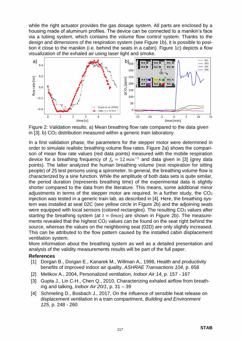
STAB

while the right actuator provides the gas dosage system. All parts are enclosed by a housing made of aluminum profiles. The device can be connected to a manikin’s face via a tubing system, which contains the volume flow control system. Thanks to the design and dimensions of the respiration system (see Figure 1b), it is possible to posi-tion it close to the manikin (i.e. behind the seats in a cabin). Figure 1c) depicts a flow visualization of the exhaled air using laser light and smoke.

Figure 2: Validation results. a) Mean breathing flow rate compared to the data given in [3]. b) CO2 distribution measured within a generic train laboratory.

In a first validation phase, the parameters for the stepper motor were determined in order to simulate realistic breathing volume flow rates. Figure 2a) shows the compari-son of mean flow rate values (red data points) measured with the mobile respiration device for a breathing frequency of 𝑓𝑏 = 12 𝑚𝑖𝑛−1 and data given in [3] (grey data points). The latter analyzed the human breathing volume (rest respiration for sitting people) of 25 test persons using a spirometer. In general, the breathing volume flow is characterized by a sine function. While the amplitude of both data sets is quite similar, the period duration (represents breathing time) of the experimental data is slightly shorter compared to the data from the literature. This means, some additional minor adjustments in terms of the stepper motor are required. In a further study, the CO2 injection was tested in a generic train lab, as described in [4]. Here, the breathing sys-tem was installed at seat 02C (see yellow circle in Figure 2b) and the adjoining seats were equipped with local sensors (colored rectangles). The resulting CO2 values after starting the breathing system (at 𝑡 = 0𝑚𝑖𝑛) are shown in Figure 2b). The measure-ments revealed that the highest CO2 values can be found on the seat right behind the source, whereas the values on the neighboring seat (02D) are only slightly increased. This can be attributed to the flow pattern caused by the installed cabin displacement ventilation system. More information about the breathing system as well as a detailed presentation and analysis of the validity measurements results will be part of the full paper.

References [1] Dorgan B., Dorgan E., Kanarek M., Willman A., 1998, Health and productivity

benefits of improved indoor air quality, ASHRAE Transactions 104, p. 658

[2] Melikov A., 2004, Personalized ventilation, Indoor Air 14, p. 157 - 167

[3] Gupta J., Lin C-H., Chen Q., 2010, Characterizing exhaled airflow from breath-ing and talking, Indoor Air 20/1, p. 31 – 39

[4] Schmeling D., Bosbach J., 2017, On the influence of sensible heat release on displacement ventilation in a train compartment, Building and Environment 125, p. 248 - 260

a) b)

117

Mitteilung

Projektgruppe/Fachkreis: Technische Stromungen

Development of an experimental set-up to investigate heat transport in convective airflows with phase transition

Konstantin Niehaus, Andreas Westhoff and Claus WagnerGerman Aerospace Center (DLR), Institute of Aerodynamics and Flow Technology, Gottingen,

Germany, [email protected]

The heat transfer in mixed convective air flows with phase transition is a phenomenon which occurs innature and a plethora of technical applications. When condensing materials form droplets, condensationleads to an increased heat transfer rate and therefore is advantageous in heat exchangers [1], whereasin other technical applications condensation is oftentimes undesirable. For instance, fogging on thewindshield or headlights of motor vehicles leads to restrictions when driving and a reduction of opticaltransparency influences road safety. In addition, a considerable amount of thermal energy is required fordefogging, which can have a negative effect on the range of electric cars [2]. The design and modificationof these components with regard to optimizing dehumidification or preventing misting is often basedon experience and intuition. Despite the enormous progress of numerical methods in recent years,there is still a lack of reliable and applicable models for the numerical simulation of condensation ingeneral, and in particular of droplet condensation on surfaces. Due to the complexity of the physicalprocesses that determine the heat transport and thus the fogging on the panes, reliable simulations areexpensive and time-consuming, and therefore not suitable for industrial applications. Thus, the objectiveof the present study is to develop a model, using dimensionless numbers, which allows the predictionof the condensation behavior on panes based on a reduced parameter space. In such a configurationthe mass transport of the vapor by phase transition, the resulting latent and the sensible heat transferare determined by the physical processes of convection and diffusion, the boundary conditions andthe material properties of the surfaces. In addition, the mass transfer of water vapor changes evenwith the smallest changes in the boundary conditions. A major challenge of this study is thereforeto design and construct an experimental setup with the appropriate measurement technology, whichmeets the requirements of ensuring defined boundary conditions, reproducibility of the experiments andmeasurement accuracy. The setup corresponds to a generic replica of a vehicle headlamp.The air flow inside automotive headlights is the result of the superposition of forced and natural convec-tion. The former is characterized by the Reynolds number Re = UL/ν and origins from ventilation holesat the rear wall of the cavity. The latter is a result of the heat emission from the internal light sourceson the headlight’s back. This can be expressed using the Grashof number Gr = L3g∆T β/ν. β, g, ν arethermal expansion coefficient, gravitational acceleration and the kinematic viscosity of the working fluidair with respect to the current laboratory condition. The characteristic velocity U is equal to the meaninlet velocity and L is a characteristic system length, i.e. the ratio between the system volume and theinlet’s cross section. ∆T is the temperature difference between the mean temperature of the heating andthe cooling plate. If the temperature of the windscreen Tc falls below the dew point Tdp, a vapor massflow Mv occurs due to phase transition. Fogging of the pane thus depends on the flow velocity U , theair temperature Ta, the pane temperature Tc, the heat emission of the lamps Ql as well as on their tem-perature Th and the dew point temperature Tdp. The challenge is to provide an experimental setup thatdoes not only exactly determine all these variables, but also controls them with high precision. For thispurpose we have designed, developed and constructed an experimental setup that meets these require-ments. The structure consists of a rectangular cavity that is heated at the rear and cooled at the front.To compensate pressure changes caused by temperature shifts, automotive headlights are designed asopen systems to allow air exchange with the engine compartment. Hence, the configuration is equippedwith an air inlet and an air outlet. This configuration maps all physical processes that determine thefogging of headlamp windshields. The dimensions of the sample are: length L = 0.5m, width W = 0.5mand height H = 0.25m. The air inlet and outlet extend over the entire cell height and have an aspectratio of 0.1. Both are aligned parallel to the sample’s side walls. A sketch of the configuration is depictedin Fig. 1. The control setup shown in Fig. 2 consists of three control loops. The first loop is connected tothe air inlet and splits up into a humidity and a temperature control cycle. The second closed loop cyclesets the temperature of the cooling plate. The transparency of the cooling plate is achieved by usingparaffin oil which flows between two parallel glass walls. The third loop controls the air temperature ofthe housing around the condensation cell. The temperature is kept at the mean cavity temperature of

STAB118

Tin

rHin

Vin

H

L

W

Tout

rHout

Vout

x

yz

Th

Tc

Fig. 1: Schematic setup of thecondensation cell: The coolingplate is colored in blue (temper-ature Tc) and the heating plateis colored in red (temperature Th).Transparent areas are kept atmean cavity temperature. Inletand outlet conditions are char-acterized by means of humidityrH, temperature Tin and volumeflow V .

housing

maincavity

air8 bar

purifiedwater rH V TM

TrHV

exhaust

T

air

paraffin oil

T

air1 bar

C1

C1

C2

C3

Fig. 2: Three loops control the inlet temperature, humidity and volume flow of the inlet (C1), the coolingplate temperature (C2) and the ambient temperature of the condensation cell (C3).

the sample to minimize heat transfer through the glass sidewalls of the volume. Optical accessibility willpave the way for the future application of measurement techniques like PIV, laser-Doppler anemometry(LDA) and methods for image-based distribution analysis of condensate, i.e. performed by Zheng etal. [3]. Kim et al. [4] studied the flow in a consumer headlight by means of stereoscopic particle imagevelocimetry (PIV). In their work they report on the superposition of thermal and forced convection andresulting three-dimensional structures. To investigate if these structures are present in the generic setupas well, we will provide results of Tomo-PIV measurements.

References

[1] E. Schmidt; W. Schurig; W. Sellschopp. Versucheuber die kondensation von wasserdampf in film- undtropfenform. Forschung im Ingenieurwesen, 1:53–63, 1930.

[2] Andreas Westhoff. Experimentelle untersuchungdes einflusses der oberflachenbeschaffenheit vonscheiben auf die kondensatbildung. Technical report,FAT, December 2017.

[3] Ferdinand; Philipp Christian; Fieback Tobias;

Gross Ulrich Zheng, Shaofei; Eimann. Modeling ofheat and mass transfer for dropwise condensation ofmoist air and the experimental validation. Interna-tional Journal of Heat and Mass Transfer, 120:879–894, 2018.

[4] Donguk; Kim Mirae; Lee Jaemyeong; Jung Ikhee;Roh Kyuchul; Kim Kyung Chun Kim, Dong; Kim. Ve-locity field measurement on natural convection insidean automotive headlamp using time-resolved stereo-scopic particle image velocimetry. International Jour-nal of Heat and Fluid Flow, 77:19–30, 2019.

STAB119

STAB

nalboden montiert, um den Einfluss der Grenzschicht auf den Boden zu minimieren.Modell sowie der Bahndamm wurden auf einer horizontalen Platte mit Abstand zum Windka- wurde ein eingleisiger Bahndamm (Single Track Ballast and Rail - STBR) verwendet. Das am Institut für Aerodynamik und Strömungstechnik am DLR Göttingen durchgeführt. Es Die Experimente wurden hauptsächlich bei U = 50 m/s im Seitenwindkanal Göttingen (SWG)

Lösungsansatz

FR8Rail II statt, das sich mit der verbesserten Effizienz von Güterzügen befasst.nen zu optimieren. Die Messungen fanden im Rahmen des EU-Projekts Shift2Rail - mische Untersuchungen zu ermöglichen, um das Containerdesign und die Ladekonfiguratio- viel längerem Modell vergleichbar ist. Ziel der Messkampagne war es, genauere aerodyna- verwendet (Abbildung 1), um eine Grenzschichtdicke zu erreichen, die mit der an einem sehr deaerodynamik [6,7] verwendet werden. Unterschiedliche Rauheitselemente wurden zugmodell im Maßstab 1:15 zum Einsatz, die typischerweise in der Umwelt- und Gebäu- men insbesondere Maßnahmen zur Grenzschichtaufdickung an einem generischen Güter- sich aus dieser Messung ergebenden Merkmale der Grenzschicht nachzubilden. Dabei ka- der vorliegenden Arbeit wurden in einem Windkanalversuch Methoden angewendet, um die len, operationellen Güterzuges mit Hilfe von Messungen an der Strecke charakterisiert [5]. In gering ist [4]. Kürzlich wurden die Merkmale der Grenzschicht im mittleren Bereich eines rea- Einfluss der Grenzschicht bei mehr als acht sich stromauf befindlichen Wagen nur noch sehr derstand eines einzelnen Containers abhängig von seiner Position im Zugverbund, wobei der dlichkeit gegenüber Grenzschichtbedingungen gezeigt. Dabei ist der aerodynamische Wi- Schienenfahrzeugen [4]. Spezifische Untersuchungen an Güterzügen haben diese Empfin- sentlichen Einfluss auf die aerodynamischen Eigenschaften (wie z.B. Luftwiderstand) von lenzintensität und Längenskalen charakterisiert werden. Diese Merkmale haben einen we- Grenzschicht. Sie wächst entlang der Zuglänge und kann durch ihre Geschwindigkeit, Turbu- Wenn sich ein Zug auf der Schienenstrecke bewegt, bildet sich auf seiner Oberfläche eine

heute angewendet wird [2,3].Interesse ist, ist die Modellierung des mittleren Bereichs des Zuges eine Methode, die bis Fällen, in denen ein Zielbereich wie das Containerdesign oder die Ladekonfiguration von perimenten zurückzuführen oder auf Beschränkungen der Ressourcen in Simulationen. In Betriebslänge zu Höhe (L/H = 250-500). Dies ist auf physikalische Beschränkungen bei Ex- Modellierung der Aerodynamik eines Güterzuges ist die Anpassung des Verhältnisses von experimentelle und numerische Methoden erforderlich. Eine erhebliche Schwierigkeit bei der Zur Verbesserung der aerodynamischen Leistung sind zuverlässige, genaue und effiziente dynamik ist ein wichtiger Aspekt für den sicheren und effizienten Betrieb von Güterzügen [1]. tainertypen und können im Durchschnitt eine Gesamtlänge von 1,6 km erreichen. Die Aero- Güterzüge fahren mit bis zu 110 km/h, befördern eine Vielzahl unterschiedlicher Frachtcon-

Problemstellung

Clayton, 3800 Victoria, Australia

2 Monash University, Department of Mechanical and Aerospace Engineering,37073 Göttingen, [email protected]

1 DLR, Institut für Aerodynamik und Strömungstechnik, Bunsenstr. 10,

Emir Öngüner1, James Bell1, David Burton2, Arne Henning1

dellen mit passiven StrömungskontrollelementenExperimentelle Nachbildung einer aerodynamischen Grenzschicht an Güterzugmo-


Mitteilung

120


STAB

Eine Reihe von Konfigurationen wurde getestet, um unterschiedliche Grenzschichtbedingun-gen zu erzeugen und schließlich die realen Bedingungen in der Praxis genauer zu modellie-ren. Die Messungen wurden mit Drucksonden auf beiden Seiten des Modells durchgeführt (Abbildung 2). Mit Hilfe der Rauheitselemente wurden die Geschwindigkeitsprofile bei x = 12H und x = 22H gemessen. Jede Konfiguration wurde in mehreren Höhen getestet. Die verschiedenen Konfigurationen erzeugen unterschiedliche Profile der Grenzschichtgeschwindigkeit und Turbulenzintensität. Dadurch bieten die Ergebnisse eine Grundlage zur Prüfung der Abhängigkeit der aerodynamischen Eigenschaften eines Contai-ners von den stromaufwärts auftretenden aerodynamischen Bedingungen.

Abbildung 1: a) Windkanalmodell im Maßstab 1:15 mit zwei Rechenpositionen, b) Modell mit unterschiedlichen

Rauheitselementen: Zaunlänge (fence): 0,2 H, Zackenlänge (spire): 1,25 H.

Abbildung 2: Positionen für Druckmessungen an der Seite des Modells mit Hilfe von Rechen: a) großes Traver-

sensystem (Länge: 800 mm), b) kleiner Rechen (Länge: 160 mm)

Quellen: 1. Shetz, J.,2001. Aerodynamics of high-speed trains. Annual Review of Fluid Mechanics 33, 371–414. 2. Östh, J. and Krajnović, S., 2014. A study of the aerodynamics of a generic container freight wagon using large-eddy simulation. Journal of Fluids and Structures, 44, 31–54. 3. Öngüner, E., Henning, A., Fey, U. and Wagner, C., 2020. Towards aerodynamically optimized freight wagons: An experimental study on container designs, Notes on Numerical Fluid Mechanics and Multidisciplinary Design 142, 437–446. 4. Cooper, K. and Campbell, W. (1981), ‘An examination of the effects of wind turbulence on the aerodynamic drag of vehicles’, Journal of Wind Engineering and Industrial Aerodynamics 9, 167– 180. 5. Bell, J., Burton, D., Thompson, M.C., The boundary layer characteristics and unsteady flow topology of full-scale operational inter-modal freight trains, under review in Journal of Wind Engineering and Industrial Aerodynamics, 2019. 6. Irwin, H., 1981. The design of spires for wind simulation. Journal of Wind Engineering and Industrial Aerodynamics 7, 361–366. 7. Counihan, J., An improved method of simulating an atmospheric boundary layer in a wind tunnel, Atmospheric Environment Pergamon Press, 1969, Vol. 3, pp. 197-214.

121

STAB

Hierfür wurde ein generisches Einpersonenfahrzeug (SPC, engl. Single Person Cabin) in einer Klimakammer mit definierten Randbedingungen aufgebaut. Abbildung 1 (A) zeigt ein

Foto der SPC mit deren Maßen. In Abbildung 1 (B) sind die zwei Lufteinlässe auf Höhe eines

Armaturenbretts mit den Volumenstrommessstrecken zu sehen. Hierbei wird sowohl der Vo-lumenstrom als auch die Luftfeuchte und Temperatur der Zuluft erfasst und geregelt. Abbil-dung 1 (C) zeigt eine Rückansicht des thermischen Menschmodells (TM) und die Lufteinläs-

se, die den Luftstrom primär auf den Brustbereich des TM lenken. Die hier verwendete Methode zur Messung des thermischen Komforts basiert auf einer Mes-sung der Oberflächentemperatur (TS) des TM mittels Infrarot(IR)-Thermometrie, die in die Äquivalenttemperatur (Teq) gemäß DIN14505 umgerechnet wird und schließlich eine Kom-fortbewertung liefert (Lange et al., 2018). Die Turbulenzintensität I der Zuluft wird auf deren Geschwindigkeitsmagnitude U normiert und beträgt ILT = 16 % und IHT = 32 % (HT). In der vorgelegten Studie wurde ein Parameterbe-reich von U = 0,25 m/s – 2,50 m/s bei einer Temperatur von jeweils T = 17, 20, 23, 26 und 29 °C untersucht. In den präsentierten Fällen waren die Zulufttemperatur und die Klimakammer-temperatur identisch, um zusätzliche thermisch induzierte Einflüsse auszuschließen. Das TM wurde mit einer konstanten Heizleistung von P = 75 W betrieben, um die typische Wärmeleis-tung eines Menschen zu simulieren. Abbildung 2 zeigt exemplarische Ergebnisse der IR-Thermometrie bei U = 1,25 m/s und T = 23 °C. Die Spalten (A), (B) and (C) zeigen TS, Teq und die thermische Komfortbewertung ge-mäß DIN14505 für ein Sommerszenario. Der Vergleich von TS (Abbildung 2 (A)) für LT und

Abbildung 1: (A) Foto der SPC mit Maßangaben in mm. (B) SPC mit Luftzuführung und Volumenstrommessstrecken. (C) Rückansicht des TMs mit Lufteinlässen.

Mitteilung


Experimentelle Untersuchung des Einflusses von Zugluft auf das Komfortempfinden in einer generischen Fahrzeugkabine

Daniel Schiepel und Andreas WesthoffDeutsches Zentrum für Luft- und Raumfahrt, Bunsenstraße 10, 37073 Göttingen,

[email protected]

Heutzutage verbringen Menschen einen erheblichen Teil ihrer Zeit in Fahrzeugen. Dabei entfällt insbesondere in den westlichen Industrienationen ein großer Anteil auf die Individu-almobilität. Die vorgelegte Studie konzentriert sich auf den thermischen Komfort in Fahrzeu-gen, der im Allgemeinen durch Temperatur, Strahlung, Luftströmung und ein individuelles Empfinden bestimmt wird. Häufig werden Standards basierend auf dem Konzept der Äquiva-lenttemperatur (Teq) gemäß DIN14505 (ENISO, 2016) verwendet, um den thermischen Kom-fort zu charakterisieren In der durchgeführten Studie wird diese Größe genutzt, um einen Schwellenwert für den thermischen Komfort bei einem Hochimpuls-Luftstrom zu ermitteln und insbesondere den Einfluss eines hohen Turbulenzgrades (HT) und eines niedrigen Tur-bulenzgrades (LT) auf das objektive Komfortempfinden zu untersuchen.

122



STAB

HT zeigt einen großen Einfluss der Turbulenzintensität auf den thermischen Komfort. Auf-grund einer reduzierten Oberflächentemperatur von 24°C ist für das HT-Szenario eine deut-lich größere Wärmeabfuhr im Brustbereich zu erkennen, verglichen mit einer Oberflächen-temperatur von 26°C beim LT-Szenario. Der gleiche Unterschied ist ebenfalls für Bauch- und Beinregionen zu erkennen und es ergibt sich eine allgemeine Temperaturreduzierung um 2 K für den HT-Fall. Das ist auf einen höheren Wärmetransport an der Oberfläche des TMs durch die höhere Turbulenzintensität der Zuluft zurückzuführen. Anhand der Oberflächen-temperatur wird für die sichtbaren Körpersegmente die Äquivalenttemperatur ermittelt. Die resultierenden Werte sind in Abbildung 2 (B) dargestellt und es sind wieder deutlich höhere Temperaturen für das LT-Szenario im Vergleich zum HT-Szenario zu erkennen. Abbildung 2 (C) zeigt das Ergebnis einer Komfortbewertung gemäß DIN14505. Hierbei bedeutet eine Bewertung von 3 „komfortabel“. Höhere Werte bedeuten „warm, aber komfortabel“ (4) bzw. „zu warm“ (5). Analog gilt dies für kleinere Werte von 2 und 1 bezüglich des Kälteempfin-dens. Das LT-Szenario führt zu einer Bewertung, die nah am komfortablen Bereich liegt, wohingegen das HT-Szenario zu vermehrten Bewertungen im Bereich „kalt“ führt. Als deut-lich beeinflusste Körperregionen lassen sich sowohl der direkte Auftreffpunkt der Zuluft, der Brustbereich, mit den angrenzenden Regionen, Bauch und Oberarme, identifizieren. Die übrigen Körperregionen wechseln das Komfortband nicht.

Abbildung 2: (A) TS des TMs, (B) ermittelte TEQ und (C) Komfortbewertung. Jeweils für LT in der oberen und HT in der unteren Zeile.

Der thermische Komfort in der SPC wurde mittels TM und IR-Thermometrie untersucht. Die Experimente umfassten den folgenden Parameterbereich: zwei Turbulenzintensitäten, ILT = 16 % und IHT = 32 %, Einströmgeschwindigkeiten, U = 0,25 m/s - 2,5 m/s, und Temperaturen, T = 17 - 29 °C. Für den untersuchten Parameterbereich ergibt sich im Fall HT im Vergleich zu LT ein erhöhter Wärmeübergang an der Oberfläche des TMs. Dies führt zu abnehmenden Äquivalenttemperaturen und damit zu einem kälteren objektiven Temperaturempfinden nach DIN14505. In naher Zukunft sollen Probandenversuche durchgeführt werden, um die objekti-ven Komfortmessungen mit dem subjektiven Empfinden zu vergleichen. This research has been funded by the Research

Association of Automotive Technology (FAT).

ENISO, D. I. (2016). Bahnanwendungen - Luftbehandlung in Schienenfahrzeugen des

Fernverkehrs - Behaglichkeitsparameter und Typprüfungen; Deutsche Fassung EN

13129:2016 . Beuth, Berlin.

Lange, P., Schmeling, D., Westhoff, A., & Bosbach, J. ( 2018). Cost-effective human comfort

manikin with realistic thermal load for studies of convection-driven ventilation

systems. Roomvent & Ventilation Konferenz, S. 367-372.

(A) (B) (C)

HT

LT

123

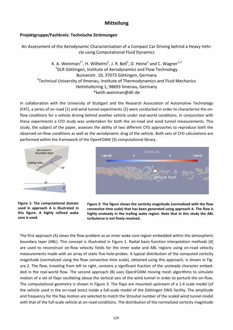
Figure 2: The figure shows the vorticity magnitude (normalized with the flow convective time scale) that has been generated using approach A. The flow is highly unsteady in the trailing wake region. Note that in this study the ABL turbulence is not finely resolved.

Figure 1: The computational domain used in approach A is illustrated in this figure. A highly refined wake core is used.

Mitteilung Projektgruppe/Fachkreis: Technische Strömungen

An Assessment of the Aerodynamic Characterization of a Compact Car Driving behind a Heavy Vehi-

cle using Computational Fluid Dynamics

K. A. Weinman1*, H. Wilhelmi1, J. R. Bell1, D. Heine1 and C. Wagner1,2 1DLR Göttingen, Institute of Aerodynamics and Flow Technology

Bunsenstr. 10, 37073 Göttingen, Germany 2Technical University of Ilmenau, Institute of Thermodynamics and Fluid Mechanics

Helmholtzring 1, 98693 Ilmenau, Germany *[email protected]

In collaboration with the University of Stuttgart and the Research Association of Automotive Technology

(FAT), a series of on-road [1] and wind tunnel experiments [2] were conducted in order to characterize the on-

flow conditions for a vehicle driving behind another vehicle under real-world conditions. In conjunction with

these experiments a CFD study was undertaken for both the on-road and wind tunnel measurements. This

study, the subject of the paper, assesses the ability of two different CFD approaches to reproduce both the

observed on-flow conditions as well as the aerodynamic drag of the vehicle. Both sets of CFD calculations are

performed within the framework of the OpenFOAM [3] computational library.

The first approach (A) views the flow problem as an inner wake core region embedded within the atmospheric

boundary layer (ABL). This concept is illustrated in Figure 1. Radial basis function interpolation methods [4]

are used to reconstruct on-flow velocity fields for the inner wake and ABL regions using on-road velocity

measurements made with an array of static five-hole-probes. A typical distribution of the computed vorticity

magnitude (normalized using the flow convective time scale), obtained using this approach, is shown in Fig-

ure 2. The flow, traveling from left to right, contains a significant fraction of the unsteady character embed-

ded in the real-world flow. The second approach (B) uses OpenFOAM moving mesh algorithms to simulate

motion of a set of flaps oscillating about the vertical axis of the wind tunnel in order to perturb the on-flow.

The computational geometry is shown in Figure 3. The flaps are mounted upstream of a 1:4 scale model (of

the vehicle used in the on-road tests) inside a full-scale model of the Göttingen SWG facility. The amplitude

and frequency for the flap motion are selected to match the Strouhal number of the scaled wind tunnel model

with that of the full-scale vehicle at on-road conditions. The distribution of the normalized vorticity magnitude

124

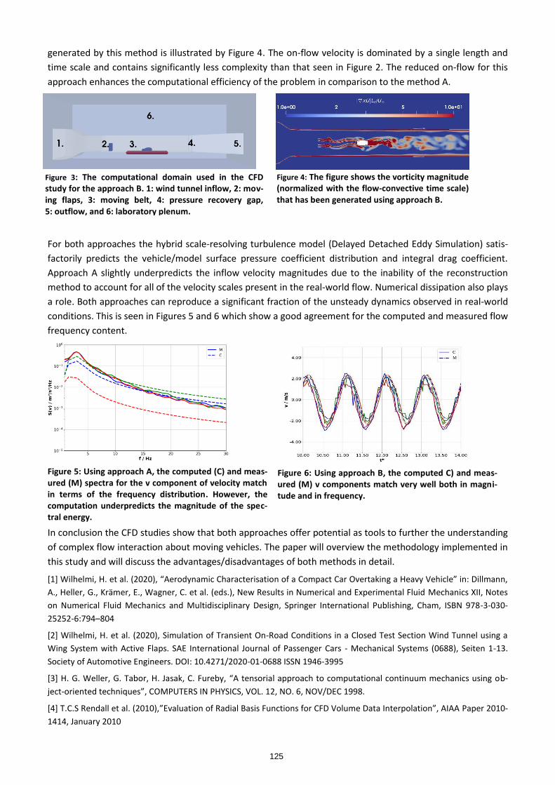
Figure 3: The computational domain used in the CFD study for the approach B. 1: wind tunnel inflow, 2: mov-ing flaps, 3: moving belt, 4: pressure recovery gap, 5: outflow, and 6: laboratory plenum.

Figure 4: The figure shows the vorticity magnitude (normalized with the flow-convective time scale) that has been generated using approach B.

generated by this method is illustrated by Figure 4. The on-flow velocity is dominated by a single length and

time scale and contains significantly less complexity than that seen in Figure 2. The reduced on-flow for this

approach enhances the computational efficiency of the problem in comparison to the method A.

For both approaches the hybrid scale-resolving turbulence model (Delayed Detached Eddy Simulation) satis-

factorily predicts the vehicle/model surface pressure coefficient distribution and integral drag coefficient.

Approach A slightly underpredicts the inflow velocity magnitudes due to the inability of the reconstruction

method to account for all of the velocity scales present in the real-world flow. Numerical dissipation also plays

a role. Both approaches can reproduce a significant fraction of the unsteady dynamics observed in real-world

conditions. This is seen in Figures 5 and 6 which show a good agreement for the computed and measured flow

frequency content.

Figure 5: Using approach A, the computed (C) and meas-ured (M) spectra for the v component of velocity match in terms of the frequency distribution. However, the computation underpredicts the magnitude of the spec-tral energy.

Figure 6: Using approach B, the computed C) and meas-ured (M) v components match very well both in magni-tude and in frequency.

In conclusion the CFD studies show that both approaches offer potential as tools to further the understanding

of complex flow interaction about moving vehicles. The paper will overview the methodology implemented in

this study and will discuss the advantages/disadvantages of both methods in detail.

[1] Wilhelmi, H. et al. (2020), “Aerodynamic Characterisation of a Compact Car Overtaking a Heavy Vehicle” in: Dillmann,

A., Heller, G., Krämer, E., Wagner, C. et al. (eds.), New Results in Numerical and Experimental Fluid Mechanics XII, Notes

on Numerical Fluid Mechanics and Multidisciplinary Design, Springer International Publishing, Cham, ISBN 978-3-030-

25252-6:794–804

[2] Wilhelmi, H. et al. (2020), Simulation of Transient On-Road Conditions in a Closed Test Section Wind Tunnel using a

Wing System with Active Flaps. SAE International Journal of Passenger Cars - Mechanical Systems (0688), Seiten 1-13.

Society of Automotive Engineers. DOI: 10.4271/2020-01-0688 ISSN 1946-3995

[3] H. G. Weller, G. Tabor, H. Jasak, C. Fureby, “A tensorial approach to computational continuum mechanics using ob-

ject-oriented techniques”, COMPUTERS IN PHYSICS, VOL. 12, NO. 6, NOV/DEC 1998.

[4] T.C.S Rendall et al. (2010),”Evaluation of Radial Basis Functions for CFD Volume Data Interpolation”, AIAA Paper 2010-

1414, January 2010

125

Mitteilung Projektgruppe/Fachkreis: Technische Strömungen

Aerodynamic Characterisation of a Compact Car Driving Behind a Heavy Vehicle

H. Wilhelmi1*, C. Jessing2, J.R. Bell1, D. Heine1, J. Wiedemann3, A. Wagner3 and C. Wagner1,4

1DLR Göttingen, Institute of Aerodynamics and Flow Technology Bunsenstr. 10, 37073 Göttingen, Germany

2University of Stuttgart, Institute of Automotive Engineering Pfaffenwaldring 12, 70569 Stuttgart, Germany

3Research Institute of Automotive Engineering and Vehicle Engines Stuttgart Pfaffenwaldring 12, 70569 Stuttgart, Germany

4Technical University of Ilmenau, Institute of Thermodynamics and Fluid Mechanics Helmholzring 1, 98693 Ilmenau, Germany

*[email protected] Aerodynamic research and development of automotive vehicles is commonly conducted in wind-

tunnel experiments and numerical simulations under idealised conditions, which are not necessarily

representative of the diverse, complex, real-world flow conditions. The work presented provides new

insight into the flow conditions and their effects on a vehicle’s unsteady aerodynamics for a typical –

particularly on the German Autobahn – real-world operating case: driving behind a heavy vehicle.

The experiments were performed under ideal conditions on a 2.9 km runway at the Fassberg airfield

next to DLR Trauen, Germany. The test track was clear of nearby infrastructure and isolated; no ve-

hicles other than the two test vehicles were present. The weather conditions were monitored during

testing and all presented results were obtained during wind conditions of less than 5 m/s.

The compact vehicle (CV) was a full-scale opera-

tional Volkswagen Golf 7 provided by

Volkswagen. The vehicle was modified to enable

the installation of measurement and data acquisi-

tion equipment. The heavy vehicle (HV) was a

Mercedes-Benz 2017 Sprinter ‘Box Body’. The

vehicle’s track-position and distance behind the

heavy vehicle were controlled during testing by

markings on the driver’s windscreen. These positions were confirmed by a camera attached to the

top of the windscreen, operating at 1 Hz. The experiments were carried out with both vehicles driving

at constant velocities of VCV = VHV = 20 - 33.3 m/s (80-120 km/h) with distances of Δx = 10 - 100 m

(see Fig.1) between the vehicles.

A 2D array consisting of 11 five-hole dynamic-pressure probes was mounted 1 m in front of the com-

pact car to measure the incoming flow properties. The array consisted of a 3 x 3 grid, with

∆y = 0.98 m and ∆z = 0.6 m spacing, starting at z = 0.5 m above the ground. Two additional five-hole

probes were included at the bottom row resulting in a finer spatial resolution of ∆y = 0.48 m. The

probes had tip diameters of 3 mm and protruded 100 mm from the 12 mm thick airfoil-shaped vertical

and horizontal beams that supported the probes and housed the pressure tubing. The probes have a

calibrated cone of acceptance of ± 50°.

The pressure was measured at 188 points on the CV’s surface. Silicone tubes of 1.5 m length and a

diameter of 1.4 mm were connected to PSI differential pressure modules. The five-hole probes used

the same pressure measurement system with identical tube dimensions in separate experiments.

Pressure was normalised as: CP = (pi−p∞)/(0.5ρVC2), where p∞ was the atmospheric pressure meas-

ured inside a reservoir located inside the vehicle, density (ρ) was determined based on the atmos-

pheric temperature, and VC was the compact car’s velocity over ground. Data was sampled at 250 Hz

Figure 1: The compact car (with probe array mounted in front) driving behind the heavy vehicle on the run-way of the Fassberg airfield.

126

and each individual measurement had – depending on the car’s velocity – a duration between 80 and

120 s.

In a first step, the change in

flow while driving behind a

leading vehicle and at different

distances was determined.

The time-varying velocity

components u, v, w were

measured by the 5 horizontal

probes at z = 0.5 m as the CV

travelled in undistributed air

(no HV), 50 m and 10 m be-

hind the HV (see Fig. 2). The

CV experiences increasing

fluctuations in all velocity

components – most significantly in the u and v components – as the vehicle drives closer to the HV.

Frequency analyses of these fluctuating velocity components have identified a dominant frequency of

~2.5 Hz, attributable to von Kármán-type vortex shedding originating from the sides of the HV. Fur-

ther analysis has also identified increasing levels of in-phase correlation in velocity fluctuation across

the width of the vehicle. The existence of a leading vehicle and the distance to it were observed to

have a clear influence on the on-flow condition that the test vehicle experiences. Furthermore, the

existence of periodic structures in the wake of the HV was identified.

To gain a first insight into the influence of the changing flow conditions on the car, transient surface

pressure values at selected

locations on the vehicle as the

CV travelled in undistributed

air (no HV), 50 m and 10 m

behind the HV are presented

in Fig. 3. Fluctuations across

the front bumper are similar to

the transient flow field meas-

ured by the probes. These

fluctuations also display signs

of correlation, but - in contrast

to the flow - the correlation is

out-of-phase across the front

bumper. The roof centreline leads to the assumption that the upstream flow has an effect that de-

creases away from the vehicle’s front. The pressure at the rear of the vehicle is largely unaffected by

the HV, as it exhibits moderate fluctuating pressure in all cases. Thus, the changed inflow conditions

have an effect on the vehicle pressure distribution. However, the strength of the change in pressure

does not only depend on the distances between the vehicles, but also on the measurement position

on the vehicle.

In conclusion, this work has proven that the flow a CV experiences while driving behind an HV has

coherent flow characteristics that are significantly different compared to undisturbed conditions. Fur-

ther, these conditions have a noticeable effect on the CV – identified here through changes in terms

of the vehicle’s transient surface pressure. These new insights can be used to improve aerodynamic

research techniques to include modelling of real-world operating conditions and to improve the de-

velopment of next-generation automotive vehicles.

Figure 2: The time-varying velocity components: u, v, w measured by the 5 horizontal probes at z = 0.5 m as the CV travelled in a. undistributed air (no HV), b. 50 m and c. 10 m behind the HV.

Figure 3: Time series of the fluctuating component of pressure at selected

locations on the vehicle, as the CV travelled in a. undistributed air (no HV), b.

50 m and c. 10 m behind the HV.

127

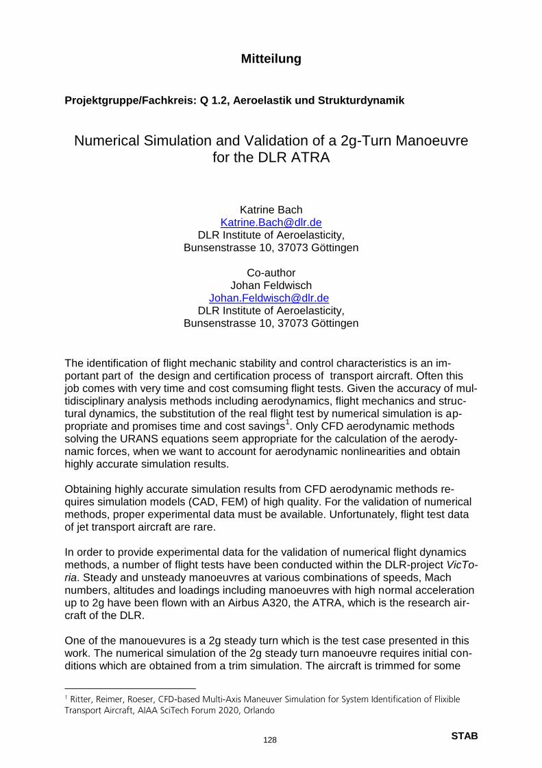
STAB

Mitteilung

Projektgruppe/Fachkreis: Q 1.2, Aeroelastik und Strukturdynamik

Numerical Simulation and Validation of a 2g-Turn Manoeuvre for the DLR ATRA

Katrine Bach [email protected]

DLR Institute of Aeroelasticity, Bunsenstrasse 10, 37073 Göttingen

Co-author

Johan Feldwisch [email protected] DLR Institute of Aeroelasticity,

Bunsenstrasse 10, 37073 Göttingen

The identification of flight mechanic stability and control characteristics is an im-portant part of the design and certification process of transport aircraft. Often this job comes with very time and cost comsuming flight tests. Given the accuracy of mul-tidisciplinary analysis methods including aerodynamics, flight mechanics and struc-tural dynamics, the substitution of the real flight test by numerical simulation is ap-propriate and promises time and cost savings

1. Only CFD aerodynamic methods

solving the URANS equations seem appropriate for the calculation of the aerody-namic forces, when we want to account for aerodynamic nonlinearities and obtain highly accurate simulation results. Obtaining highly accurate simulation results from CFD aerodynamic methods re-quires simulation models (CAD, FEM) of high quality. For the validation of numerical methods, proper experimental data must be available. Unfortunately, flight test data of jet transport aircraft are rare. In order to provide experimental data for the validation of numerical flight dynamics methods, a number of flight tests have been conducted within the DLR-project VicTo-ria. Steady and unsteady manoeuvres at various combinations of speeds, Mach numbers, altitudes and loadings including manoeuvres with high normal acceleration up to 2g have been flown with an Airbus A320, the ATRA, which is the research air-craft of the DLR. One of the manouevures is a 2g steady turn which is the test case presented in this work. The numerical simulation of the 2g steady turn manoeuvre requires initial con-ditions which are obtained from a trim simulation. The aircraft is trimmed for some

1 Ritter, Reimer, Roeser, CFD-based Multi-Axis Maneuver Simulation for System Identification of Flixible Transport Aircraft, AIAA SciTech Forum 2020, Orlando

128



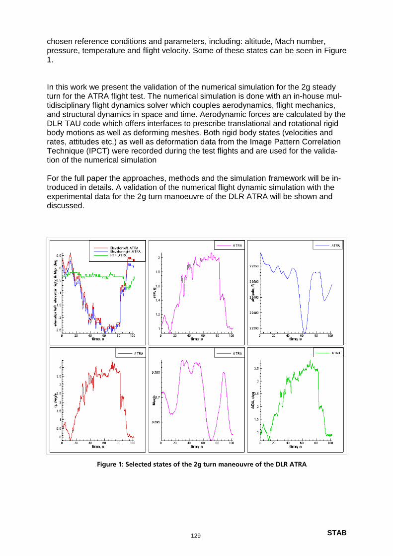
STAB

chosen reference conditions and parameters, including: altitude, Mach number, pressure, temperature and flight velocity. Some of these states can be seen in Figure 1. In this work we present the validation of the numerical simulation for the 2g steady turn for the ATRA flight test. The numerical simulation is done with an in-house mul-tidisciplinary flight dynamics solver which couples aerodynamics, flight mechanics, and structural dynamics in space and time. Aerodynamic forces are calculated by the DLR TAU code which offers interfaces to prescribe translational and rotational rigid body motions as well as deforming meshes. Both rigid body states (velocities and rates, attitudes etc.) as well as deformation data from the Image Pattern Correlation Technique (IPCT) were recorded during the test flights and are used for the valida-tion of the numerical simulation For the full paper the approaches, methods and the simulation framework will be in-troduced in details. A validation of the numerical flight dynamic simulation with the experimental data for the 2g turn manoeuvre of the DLR ATRA will be shown and discussed.

Figure 1: Selected states of the 2g turn maneouvre of the DLR ATRA

129

STAB

Mitteilung

Projektgruppe/Fachkreis: Q 1.2, Aeroelastik und Strukturdynamik Validation of a High-Fidelity Flight Dynamics Simulation for a Longitudinal Maneuver

of the DLR ATRA

Jorge Bustamante López DLR – Institute of Aeroelasticity, Bunsenstraße 10, 37073 Göttingen, Germany,

[email protected] This work presents the validation of a 2g pull up maneuver simulated using a high-fidelity approach with experimental data from real flight tests within the DLR project VicToria (Virtual Aircraft Technology Integration Platform). During the last years, several flight test campaigns of the DLR ATRA were conducted with a wide range of Mach numbers, altitudes and with various control surface inputs. One of the goals of these flight tests was to collect experi-mental data for the validaton of flight dynamic simulations. For this, the aircraft was equipped with several sensors for navigational and flight control purposes which record in-formation about flight mechanic states and control surface inputs, amongst others. Recently, maneuver flights with a newly developed deformation measurement system which tracks the time-dependent deformation of the left wing based on the Image Pattern Correlation Tech-nique (IPCT) have been conducted. The recorded data enable the comparison of time-dependent structural deformations in addition to the flight mechanic states. The numerical approach involves a multidisciplinary method, which couples aerodynamics, flight dynamics, and structural dynamics in space and time. Therefore, the governing equa-tions of motion of the free-flying flexible aircraft are derived from Lagrange’s equations of the second kind, where the mean axes conditions are applied in order to reduce the coupling between rigid body and elastic degrees of freedom. The elastic structural deformation is rep-resented by a modal approach in generalized coordinates. The aerodynamic forces are calculated by the TAU code from DLR. The discretized conser-vation equations (for mass, momentum and energy) are solved by a finite volume method, where the Spalart-Allmaras turbulence model was used. The aerodynamic forces are calcu-lated from the pressure distribution and provided at the nodes of the CFD grid (vertex-centered integration); to obtain equivalent forces on the structural nodes, a linear mapping based on an interpolation matrix is used for the (globally conservative) force transfer. For the simulation of the 2g pull-up maneuver, the time-dependent deflections of the ailer-ons, the elevator, the horizontal stabilizer and the rudder recorded during the flight test are directly prescribed for the numerical grid, the deflection is realized by grid deformation at each time step. An ALE formulation allows time-domain solutions for moving grids with rigid body and elastic motions. The thrust is also part of the experimental data set and included as an external point force acting at the location of the engines. The aircraft is modeled by a hybrid, unstructured grid, a three level v-cycle multigrid method is used to attenuate longwave interferences to improve the convergence. The simulation strategy of the maneuver consists of steady and unsteady simulations. A steady trim simulation is performed before the actual unsteady maneuver simulation in order to obtain equilibrium of loads to ensure a steady-state horizontal flight state if no control sur-face inputs were applied. The unsteady maneuver simulation is then performed in the time domain where the deflection of the control surfacesare prescribed and the coupled govern-ing equations of motion (including rigid-body and elastic degrees of freedom) are solved for each time step.

130

STAB

Figure 1 shows selected flight mechanic states and the corresponding experimental data in a frame of reference fixed to the body. The numerical methodology captures its experimental

counterpart well. Figure 2 illustrates the elastic deflections of the left wing for different load-ings as pre-dicted by the numerical simulation.

Figure 1. Validation of a numerical flight dynamic simulation with experimental data for a 2g pull-up maneuver of the DLR ATRA

Figure 2. Instantaneous deflection of the left wing for load factors of 0.5g (blue), 1g (grey) and 2,2g (red) dur-ing the pull-up maneuver

131

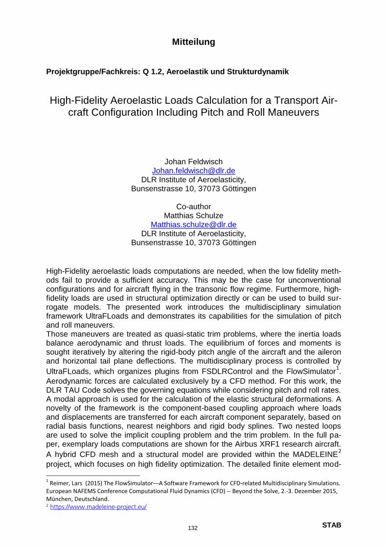
STAB

Mitteilung

Projektgruppe/Fachkreis: Q 1.2, Aeroelastik und Strukturdynamik

High-Fidelity Aeroelastic Loads Calculation for a Transport Air-craft Configuration Including Pitch and Roll Maneuvers

Johan Feldwisch [email protected]


Co-author

Matthias Schulze [email protected]


High-Fidelity aeroelastic loads computations are needed, when the low fidelity meth-ods fail to provide a sufficient accuracy. This may be the case for unconventional configurations and for aircraft flying in the transonic flow regime. Furthermore, high-fidelity loads are used in structural optimization directly or can be used to build sur-rogate models. The presented work introduces the multidisciplinary simulation framework UltraFLoads and demonstrates its capabilities for the simulation of pitch and roll maneuvers. Those maneuvers are treated as quasi-static trim problems, where the inertia loads balance aerodynamic and thrust loads. The equilibrium of forces and moments is sought iteratively by altering the rigid-body pitch angle of the aircraft and the aileron and horizontal tail plane deflections. The multidisciplinary process is controlled by

UltraFLoads, which organizes plugins from FSDLRControl and the FlowSimulator1.

Aerodynamic forces are calculated exclusively by a CFD method. For this work, the DLR TAU Code solves the governing equations while considering pitch and roll rates. A modal approach is used for the calculation of the elastic structural deformations. A novelty of the framework is the component-based coupling approach where loads and displacements are transferred for each aircraft component separately, based on radial basis functions, nearest neighbors and rigid body splines. Two nested loops are used to solve the implicit coupling problem and the trim problem. In the full pa-per, exemplary loads computations are shown for the Airbus XRF1 research aircraft.

A hybrid CFD mesh and a structural model are provided within the MADELEINE2

project, which focuses on high fidelity optimization. The detailed finite element mod-

1 Reimer, Lars (2015) The FlowSimulator---A Software Framework for CFD-related Multidisciplinary Simulations.

European NAFEMS Conference Computational Fluid Dynamics (CFD) -- Beyond the Solve, 2.-3. Dezember 2015, München, Deutschland. 2 https://www.madeleine-project.eu/

132



https://www.madeleine-project.eu/

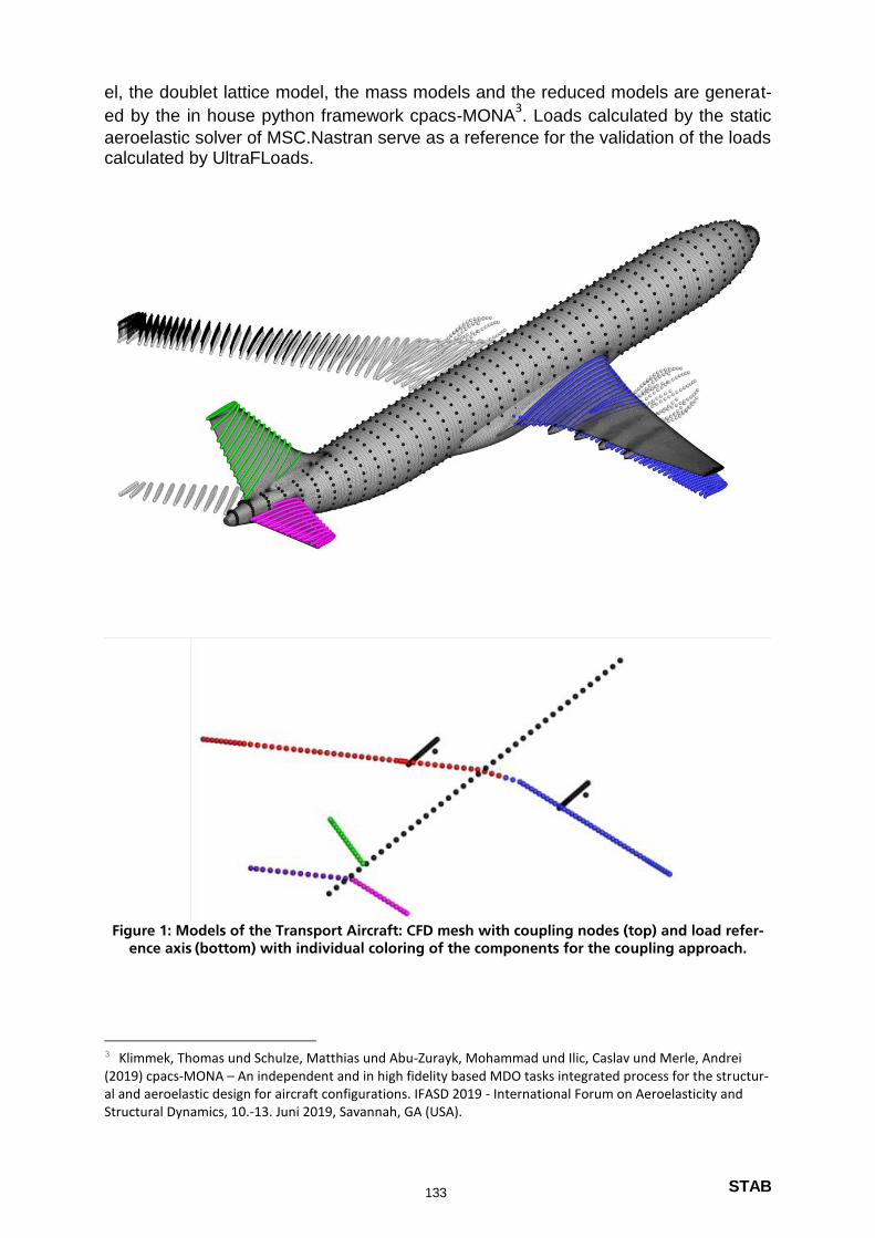
STAB

el, the doublet lattice model, the mass models and the reduced models are generat-

ed by the in house python framework cpacs-MONA3. Loads calculated by the static

aeroelastic solver of MSC.Nastran serve as a reference for the validation of the loads calculated by UltraFLoads.

Figure 1: Models of the Transport Aircraft: CFD mesh with coupling nodes (top) and load refer-

ence axis (bottom) with individual coloring of the components for the coupling approach.

3 Klimmek, Thomas und Schulze, Matthias und Abu-Zurayk, Mohammad und Ilic, Caslav und Merle, Andrei (2019) cpacs-MONA – An independent and in high fidelity based MDO tasks integrated process for the structur-al and aeroelastic design for aircraft configurations. IFASD 2019 - International Forum on Aeroelasticity and Structural Dynamics, 10.-13. Juni 2019, Savannah, GA (USA).

133

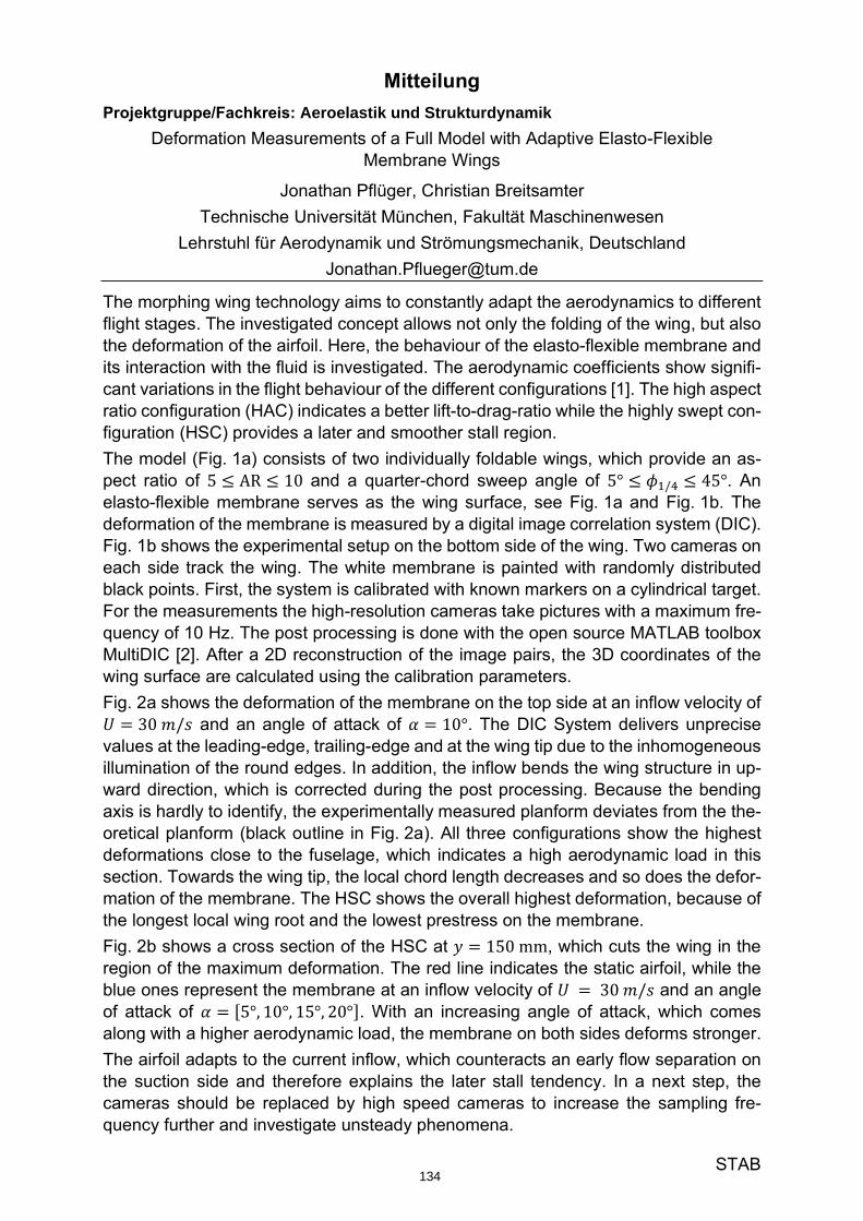
STAB

Mitteilung

Projektgruppe/Fachkreis: Aeroelastik und Strukturdynamik

Deformation Measurements of a Full Model with Adaptive Elasto-Flexible Membrane Wings

Jonathan Pflüger, Christian Breitsamter

Technische Universität München, Fakultät Maschinenwesen

Lehrstuhl für Aerodynamik und Strömungsmechanik, Deutschland

[email protected]

The morphing wing technology aims to constantly adapt the aerodynamics to different flight stages. The investigated concept allows not only the folding of the wing, but also the deformation of the airfoil. Here, the behaviour of the elasto-flexible membrane and its interaction with the fluid is investigated. The aerodynamic coefficients show signifi-cant variations in the flight behaviour of the different configurations [1]. The high aspect ratio configuration (HAC) indicates a better lift-to-drag-ratio while the highly swept con-figuration (HSC) provides a later and smoother stall region.

The model (Fig. 1a) consists of two individually foldable wings, which provide an as-pect ratio of 5 ≤ AR ≤ 10 and a quarter-chord sweep angle of 5° ≤ 𝜙 / ≤ 45°. An elasto-flexible membrane serves as the wing surface, see Fig. 1a and Fig. 1b. The deformation of the membrane is measured by a digital image correlation system (DIC). Fig. 1b shows the experimental setup on the bottom side of the wing. Two cameras on each side track the wing. The white membrane is painted with randomly distributed black points. First, the system is calibrated with known markers on a cylindrical target. For the measurements the high-resolution cameras take pictures with a maximum fre-quency of 10 Hz. The post processing is done with the open source MATLAB toolbox MultiDIC [2]. After a 2D reconstruction of the image pairs, the 3D coordinates of the wing surface are calculated using the calibration parameters.

Fig. 2a shows the deformation of the membrane on the top side at an inflow velocity of 𝑈 = 30 𝑚/𝑠 and an angle of attack of 𝛼 = 10°. The DIC System delivers unprecise values at the leading-edge, trailing-edge and at the wing tip due to the inhomogeneous illumination of the round edges. In addition, the inflow bends the wing structure in up-ward direction, which is corrected during the post processing. Because the bending axis is hardly to identify, the experimentally measured planform deviates from the the-oretical planform (black outline in Fig. 2a). All three configurations show the highest deformations close to the fuselage, which indicates a high aerodynamic load in this section. Towards the wing tip, the local chord length decreases and so does the defor-mation of the membrane. The HSC shows the overall highest deformation, because of the longest local wing root and the lowest prestress on the membrane.

Fig. 2b shows a cross section of the HSC at 𝑦 = 150 mm, which cuts the wing in the region of the maximum deformation. The red line indicates the static airfoil, while the blue ones represent the membrane at an inflow velocity of 𝑈 = 30 𝑚/𝑠 and an angle of attack of 𝛼 = [5°, 10°, 15°, 20°]. With an increasing angle of attack, which comes along with a higher aerodynamic load, the membrane on both sides deforms stronger.

The airfoil adapts to the current inflow, which counteracts an early flow separation on the suction side and therefore explains the later stall tendency. In a next step, the cameras should be replaced by high speed cameras to increase the sampling fre-quency further and investigate unsteady phenomena.

134

STAB

a) Wing with the elastic membrane, the fuselage and the air-

foil cross section (Highly Swept Configuration HSC)

b) Experimental setup for the DIC measurements on the bottom

side of the wing

Fig. 1: Membrane wing configuration and experimental setup

a) Deformation of the membrane at the top side of the wing at 𝑈 = 30𝑚/𝑠 (𝑞 = 512 𝑃𝑎) and 𝛼 = 10° for the HAC (High aspect

ratio config.), INC2 (Intermediate config. 2) and HSC (Highly swept config.), black lines: theoretical wing planform.

b) Deformation of the membrane of the HSC for different angles of attack 𝛼 = 5°, 10°, 15°, 20° at 𝑈 = 30𝑚/𝑠 and at 𝑦 = 150 𝑚𝑚

Fig. 2: Results of the deformation measurements

References

[1] Pflüger, J., and Breitsamter, C., “Experimental investigations of a full model with adaptive elasto-

flexible membrane wings,” Chinese Journal of Aeronautics, 2020. doi:

10.1016/j.cja.2020.03.037.

[2] Solav, D., Moerman, K., Jaeger, A., Genovese, K., and Hugh, H., “MultiDIC: An Open-Source

Toolbox for Multi-View 3D Digital Image Correlation,” IEEE Access; Vol. 6, 2018, pp. 30520–

30535. doi: 10.1109/ACCESS.2018.2843725.

135

STAB

Mitteilung Projektgruppe/Fachkreis: Aeroelastik und Strukturdynamik

Numerical investigation of flexibility effects on the aerodynamic characteristics of delta wing control surfaces

Christopher Reinbold, Christian Breitsamter


Introduction: A numerical method for the computation of aeroelastic simulations with moveable control sur-faces using a Chimera approach is presented. It is implemented in the multi-disciplinary simu-lation environment SimServer [1]. Here, the DLR Tau Code is utilized to solve the Reynolds-Averaged Navier-Stokes (RANS) equations and a modal solver is employed to calculate the structural displacements. The numerical approach for static aeroelastic problems is based on coupled high-fidelity computational fluid dynamics (CFD) – computational structural mechanics (CSM) simulations. Control surface regions in the CFD calculations are modeled with a Chi-mera approach for hybrid grids, in order to realistically model flap gaps and flap tip vortices. The coupling of forces and displacements between the aerodynamic and structural grid is con-ducted with an interpolation algorithm based on point-element relationships, which has been specifically developed to work with the Chimera implementation. Test case: The delta wing considered in the present work is the Model53 wing in a full-scale configuration. The Model53 is a generic semi-span cropped delta wing with a root chord length of cr = 8.4 m, a small leading-edge radius and a sweep angle of 53°. The wing is twisted by 4° and is inves-tigated with a deployed slat. Additionally, the configuration features two flaps that can be ro-tated individually around their hinge line through the Chimera boundary condition. The finite element (FE) model of the Model53 consists of 16000 triangle elements and is shown in Fig. 1. For the modeling of the ribs, spars and skin, shell elements are used which are equipped with stiffenening elements to keep buckling fields sufficiently small as well as to reduce local eigenmodes. The inner and outer flap are structurally modeled and attached to the wing with a hinge concept introduced by Maierl [2]. The structure of the wing is designed to have a wing tip deformation of approx. 0.2 m at a 9-g load. A mesh independence study for the structural grid has been performed. The CFD model and grid of the Model53 for the coarse refinement level is shown in Fig. 2. Three refinement levels of the CFD grid ranging from 4·106 to 20·106 nodes are included in the numerical investigation. Results: The influence of flexibility effects on the force and moment coefficients of the Model53 config-uration for undeflected δflap,1 = δflap,2 = 0° and deflected δflap,1 = δflap,2 = 30° control surfaces is studied. In addition, the differences between the vortex-dominated flow field of the rigid and flexible configuration are compared. The main focus of the analysis is set on the appropriate handling of control surface deflections for coupled CFD-CSM simulations. Two cases are in-vestigated: In the first case, the control surfaces are deflected for both, the CFD and the FE grid. In the second case, only the control surface of the CFD grid is deflected and the aerody-namic forces are transferred to the undeflecteed FE grid. Both cases are compared in terms of the resulting structural deformation and flow field. This investigation is particularly important if larger datasets with several control surface deflection combinations are computed, since an increase in computational efficiency and decrease in pre-processing effort can be achieved if only one FE model with undeflected control surfaces is used.

136

STAB

a) Wing structure, δflap,1 = δflap,2 = 0°. b) Wing structure, δflap,1 = δflap,2 = 30°.

c) Flap hinge concept, δflap,1 = δflap,2 = 0°. d) Flap hinge concept, δflap,1 = δflap,2 = 30°. Figure 1: FE model of the Model53 wing for various flap deflection angles δflap,1 and δflap,2.

a) Model with Chimera bocks. b) Computational grid. Figure 2: CFD model and grid of the Model53 wing. [1] U. Tremel, F. Deister, K. A. Sorensen, H. Rieger and N. P. Weatherhill, "The SimServer – a Parallel Multidisciplinary Simulation Environment", DGLS-2003-099, Munich, 2003. [2] R. Maierl, Ö. Petersson, F. Daoud and K. Bletzinger "Automatically generated aeroelastic analysis models including physics based control surface representation.", 4th Aircraft Structural Design Conference, Belfast, 2014.

137

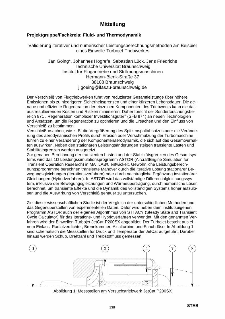
STAB

Mitteilung Projektgruppe/Fachkreis: Fluid- und Thermodynamik Validierung iterativer und numerischer Leistungsberechnungsmethoden am Beispiel

eines Einwelle-Turbojet-Triebwerkes

Jan Göing*, Johannes Hogrefe, Sebastian Lück, Jens Friedrichs Technische Universität Braunschweig

Institut für Flugantriebe und Strömungsmaschinen Hermann-Blenk-Straße 37

38108 Braunschweig [email protected]

Der Verschleiß von Flugtriebwerken führt von reduzierter Gesamtleistunge über höhere Emissionen bis zu niedrigeren Sicherheitsgrenzen und einer kürzeren Lebensdauer. Die ge-naue und effiziente Regeneration der einzelnen Komponenten des Triebwerks kann die dar-aus resultierenden Kosten und Risiken minimieren. Daher forscht der Sonderforschungsbe-reich 871 ,,Regeneration komplexer Investitionsgüter’’ (SFB 871) an neuen Technologien und Ansätzen, um die Regeneration zu optimieren und die Ursachen und den Einfluss von Verschleiß zu bestimmen. Verschleißursachen, wie z. B. die Vergrößerung des Spitzenspaltabsatzes oder die Verände-rung des aerodynamischen Profils durch Erosion oder Verschmutzung der Turbomaschine führen zu einer Veränderung der Komponentenaerodynamik, die sich auf das Gesamtverhal-ten auswirken. Neben den stationären Leistungsänderungen steigen transiente Lasten und Stabilitätsgrenzen werden ausgereizt. Zur genauen Berechnung der transienten Lasten und der Stabilitätsgrenzen des Gesamtsys-tems wird das 1D Leistungssimulationsprogramm ASTOR (AircraftEngine Simulation for Transient Operation Research) in MATLAB® entwickelt. Gewöhnliche Leistungsberech-nungsprogramme berechnen transiente Manöver durch die iterative Lösung stationärer Be-wegungsgleichungen (Iterationsverfahren) oder durch nachträgliche Ergänzung instationärer Gleichungen (Hybridverfahren). In ASTOR wird das vollständige Differentialgleichungssys-tem, inklusive der Bewegungsgleichungen und Wärmeübertragung, durch numerische Löser berechnet, um transiente Effekte und die Dynamik des vollständigen Systems höher aufzulö-sen und die Auswirkung von Verschleiß genauer zu untersuchen. Ziel dieser wissenschaftlichen Studie ist der Vergleich der unterschiedlichen Methoden und das Gegenüberstellen von experimentellen Daten. Dafür wird neben dem institutseigenen Programm ASTOR auch der eigenen Algorithmus von STTACY (Steady State and Transient Cycle Calculator) für das Iterations- und Hybridverfahren verwendet. Mit den genannten Ver-fahren wird der Einwellen-Turbojet JetCat-P200SX abgebildet. Der Turbojet besteht aus ei-nem Einlass, Radialverdichter, Brennkammer, Axialturbine und Schubdüse. In Abbildung 1 sind schematisch die Messstellen für Druck und Temperatur der JetCat aufgeführt. Darüber hinaus werden Schub, Drehzahl und Treibstofffluss gemessen.

Abbildung 1: Messstellen am Versuchstriebwerk JetCat P200SX

138

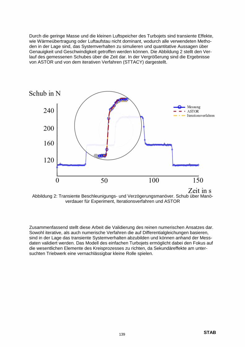
STAB

Durch die geringe Masse und die kleinen Luftspeicher des Turbojets sind transiente Effekte, wie Wärmeübertragung oder Luftaufstau nicht dominant, wodurch alle verwendeten Metho-den in der Lage sind, das Systemverhalten zu simulieren und quantitative Aussagen über Genauigkeit und Geschwindigkeit getroffen werden können. Die Abbildung 2 stellt den Ver-lauf des gemessenen Schubes über die Zeit dar. In der Vergrößerung sind die Ergebnisse von ASTOR und von dem iterativen Verfahren (STTACY) dargestellt.

Abbildung 2: Transiente Beschleunigungs- und Verzögerungsmanöver. Schub über Manö-

verdauer für Experiment, Iterationsverfahren und ASTOR Zusammenfassend stellt diese Arbeit die Validierung des reinen numerischen Ansatzes dar. Sowohl iterative, als auch numerische Verfahren die auf Differentialgleichungen basieren, sind in der Lage das transiente Systemverhalten abzubilden und können anhand der Mess-daten validiert werden. Das Modell des einfachen Turbojets ermöglicht dabei den Fokus auf die wesentlichen Elemente des Kreisprozesses zu richten, da Sekundäreffekte am unter-suchten Triebwerk eine vernachlässigbar kleine Rolle spielen.

139

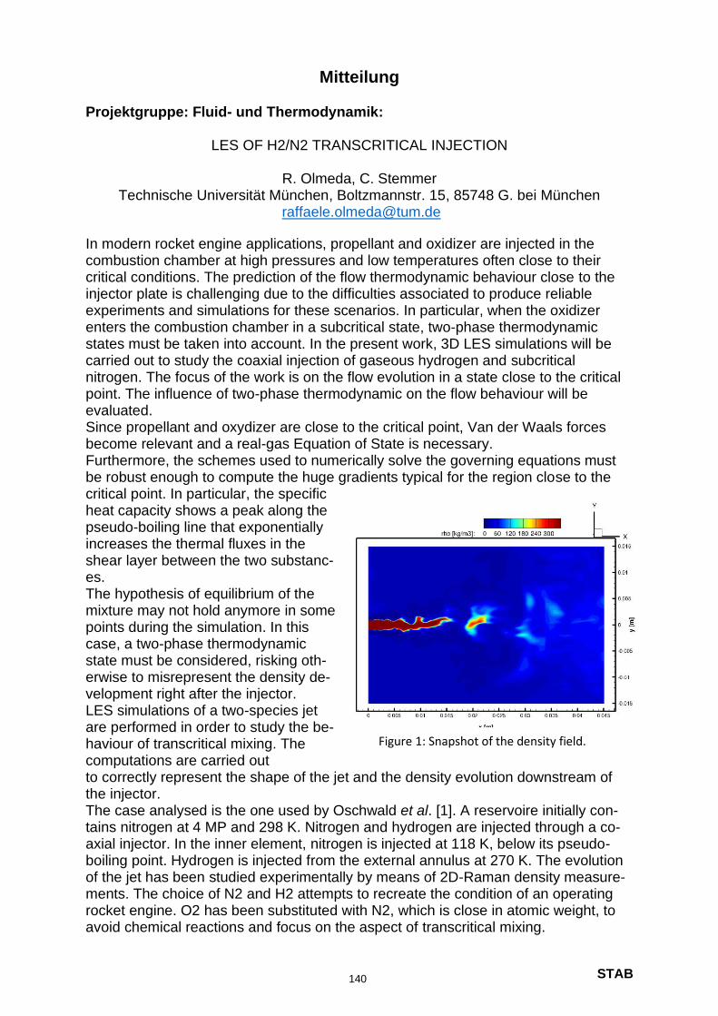
STAB

Technische Universität München, Boltzmannstr. 15, 85748 G. bei München

[email protected]

In modern rocket engine applications, propellant and oxidizer are injected in the combustion chamber at high pressures and low temperatures often close to their critical conditions. The prediction of the flow thermodynamic behaviour close to the injector plate is challenging due to the difficulties associated to produce reliable experiments and simulations for these scenarios. In particular, when the oxidizer enters the combustion chamber in a subcritical state, two-phase thermodynamic states must be taken into account. In the present work, 3D LES simulations will be carried out to study the coaxial injection of gaseous hydrogen and subcritical nitrogen. The focus of the work is on the flow evolution in a state close to the critical point. The influence of two-phase thermodynamic on the flow behaviour will be evaluated. Since propellant and oxydizer are close to the critical point, Van der Waals forces become relevant and a real-gas Equation of State is necessary. Furthermore, the schemes used to numerically solve the governing equations must be robust enough to compute the huge gradients typical for the region close to the critical point. In particular, the specific heat capacity shows a peak along the pseudo-boiling line that exponentially increases the thermal fluxes in the shear layer between the two substanc-es. The hypothesis of equilibrium of the mixture may not hold anymore in some points during the simulation. In this case, a two-phase thermodynamic state must be considered, risking oth-erwise to misrepresent the density de-velopment right after the injector. LES simulations of a two-species jet are performed in order to study the be-haviour of transcritical mixing. The computations are carried out to correctly represent the shape of the jet and the density evolution downstream of the injector. The case analysed is the one used by Oschwald et al. [1]. A reservoire initially con-tains nitrogen at 4 MP and 298 K. Nitrogen and hydrogen are injected through a co-axial injector. In the inner element, nitrogen is injected at 118 K, below its pseudo-boiling point. Hydrogen is injected from the external annulus at 270 K. The evolution of the jet has been studied experimentally by means of 2D-Raman density measure-ments. The choice of N2 and H2 attempts to recreate the condition of an operating rocket engine. O2 has been substituted with N2, which is close in atomic weight, to avoid chemical reactions and focus on the aspect of transcritical mixing.

Figure 1: Snapshot of the density field.

Olmeda, C. StemmerR.

LES OF H2/N2 TRANSCRITICAL INJECTION

Projektgruppe: Fluid- und Thermodynamik:

Mitteilung

140


STAB

Preliminary simulations are run with a splitter plate setup. A 2D mesh is expanded in the third cartesian direction with a periodic boundary condition. In a second phase, simulations are performed in a full 3D domain. LES simulations are performed with the CFD code CATUM, an in-house code devel-oped in the Chair of Aerodynamic of the Technical University of Munich [2]. It solves a finite volume form of the Navier-Stokes equations. A second-order scheme is used for the diffusive fluxes. Central difference or upwind are used for the convective flux-es depending on the local stability of the flow. The Peng-Robinson cubic equation of state is used to represent real-gas thermody-namics. It has been tested against the Soave Redlich Kwon EoS and proven to be superior for this test case. Since nitrogen is injected at a subcritical state, a two-phase subroutine is also necessary. A Vapor-Liquid Equilibrium (VLE) method is adopted in order to correctly compute the points in the two-phase region. Simulations have already been carried out with the mesh of the splitter setup. A snapshot of the partial density field can be seen in Fig. 1. The results obtained have been compared with the experimental data and plotted in Fig. 2. For the profile of nitrogen partial density in longitudinal direction, very good accuracy has already been obtained close to the injector. Going further downstream, there is a divergence from the experimental data which is expected to diminish increasing the mesh resolution and using the full 3D setup. For the profile in the radial direction instead, excellent accordance is found for r/D> 0.5. Close to the center of the injector the results are less precise. The error is most likely caused from a delayed mixing of the inner nitro-gen core with the outer hydrogen layer. Also in this case, the results are expected to improve with a finer mesh and full 3D representation, which will compute correctly the turbulent fluctuations of the jet, accelerating the mixing.

Figure 2: Nitrogen partial density profile along the central injector line (left) and in radial direction for x= 4 mm (right).

References

[1] A. Oschwald, M. Schick, M. Klar and M. Mayer, “Investigation of Coaxial LN2/GH2-Injection at supercritical Pressure by spontaneous Raman Scattering.,” in 35th AIAA/ASME/SAE/ASEE Joint Propulsion Conference and Exhibit (99-2887), Los Angeles, 1999.

[2] C. P. Egerer, S. J. Schmidt, S. Hickel and N. Adams, “Efficient implicit LES method for the simulation of turbulent cavitating flows,” Journal of Computational Physics, vol. 316, pp. 453-469, 2016, https://doi.org/10.1016/j.jcp.2016.04.021.

141

STAB

Mitteilung

Projektgruppe/Fachkreis: Numerische Aerodynamik Q 2.1

Towards a Galerkin-Type High-Order Panel Method for

Large-Scale Loads Analyses: A 2D Prototype

Karsten Bock German Aerospace Center (DLR)

Institute of Software Methods for Product Virtualization (SP), Zwickauer Straße 46, 01069 Dresden,

[email protected]

In the context of mass simulation for load analyses of aircraft, a 2D steady-state prototype was implemented to demonstrate the feasibility of high-order panel methods for aerodynamic simulations. Unlike most state-of-the-art panel methods the method presented here uses high-order singularity distributions and a Galerkin formulation. This paper describes this pro-totype implementation and demonstrates the advantages of the high-order Galerkin formula-tion over the widely employed low-order collocation-based methods. Modern aircraft design processes require a huge number of aerodynamic simulations, in par-ticular in the loads process. Although high-fidelity numerical methods such as Finite-Volume methods or Spectral-Element methods are readily available and commonly applied, these numerical methods are usually very demanding in terms of computational cost. Hence, the loads process usually refers to lower fidelity solvers to meet the requirements on simulation turnaround times. These apply flow physics models which are much simpler than the Navier-Stokes equations the high-fidelity tools are usually based on. Potential methods are one class of such methods of lower fidelity. They are based on the assumption that the flow is irrotational, which allows the introduction of a velocity potential governing the flow. Instead of solving field equations a boundary integral equation is solved on the surface of the body in the flow. Today, low-fidelity methods like the Vortex-Lattice (VLM) or Doublet-Lattice method (DLM) are commonly employed in the loads process, which both neglect the thickness of bodies. In contrast, panel methods use the actual surface of a body and, hence, are labeled as mid-fidelity tools, since they model additional effects in comparison to VLM or DLM. Therefore, the prediction accuracy of the loads process will be increased if panel methods instead of the current low-fidelity approaches are utilized. Panel methods approximate the surface of a body by a set of N surface elements, i.e. pan-els, on which a potential distribution is usually defined in terms of doublet and source singu-larities. The integral equation is then solved numerically on this approximated surface de-termining the strength of these surface singularities. In this paper, panel methods will be categorized into low- and high-order methods by the polynomial order with which these dis-tributions are defined on each panel. Low-order methods use constant source and doublet distributions, while high-order methods use linear or higher degrees. Even though high-order panel methods have been developed, e.g. [3], low-order panel methods remain very popular for two main reasons: ease of implementation and speed of computation. The main disadvantages of low-order panel methods arise from the fact that their doublet distributions feature discontinuities at the element borders. Doublet panels can be repre-sented by a combination of a vortex distribution and discrete vortices at the panel boundaries [2]. For continuous doublet distributions these boundary vortices counter each other. How-ever, the jumps present with constant doublet distributions act as vortices effectively and in-troduce spurious, non-physical velocities into the flow field. This effect decreases the accu-racy with which the boundary condition of zero panel-normal flow is fulfilled. Furthermore, the evaluation of velocities by superposition tends to be inaccurate for low-order methods on the surface itself or in the immediate vicinity of the surface. Two flow cases cannot be repre-sented by low-order panel methods due to the spurious velocities: i) supersonic flows and ii) flows with several bodies in immediate vicinity (including internal flows) [1].

142


STAB

In panel methods the discretization of the surface integral equation is most commonly achieved by enforcing the boundary condition at a set of collocation points. Due to the singu-lar nature of the fundamental solutions these collocation points cannot be located at the el-ement boundaries. Therefore, high-order collocation methods need to introduce additional equations to enforce doublet continuity. In contrast, the method presented here uses a Ga-lerkin-type approach, where the boundary conditions are enforced in an integral sense on each panel. The Galerkin approach offers a general formulation regardless of the polynomial order of the singularity distributions and, hence, lends itself to the implementation of a varia-ble order panel method. Moreover, in the easiest case of using constant singularities and one quadrature point Galerkin and collocation approach yield an equivalent equation system. Figure 1 depicts the flow fields computed by the prototype panel method with linear source and quadratic doublet distributions for 32 panels for a circle and a von Kármán airfoil. Fig-ure 2 compares the fulfillment of the zero panel-normal flow condition of low- and high-order cases for the topmost panel of the Circle. For the low-order solution this condition is violated except for the middle of the panels. Furthermore, the spurious influence of the doublet jumps at the panel ends is clearly visible in the reconstructed flow field. Using a linear doublet order instead, the boundary condition is represented more accurately and smoothly. The final pa-per will provide additional data as well as convergence studies demonstrating the capabilities and advantages of the high-order approach. Ultimately, the prototype and study presented here serve as a first step towards the development of a new 3D unsteady, high-order panel code to enable the accurate robust mass simulations for aircraft load analysis.

References:

[1] Erickson, L.L., Panel methods - An introduction, NASA Ames Research Center, NASA Ames Research Center, 1990

[2] Hess, J.L., Calculation of Potential Flow About Arbitrary Three-Dimensional Lifting Bod-ies, Defense Technical Information Center, 1972

[3] Willis, D., Peraire, J. and White, J., A Quadratic Basis Function, Quadratic Geometry, High Order Panel Method, 44th AIAA Aerospace Sciences Meeting and Exhibit, 2006

Figure 1: Streamlines calculated with the prototype 2D panel method for the flow around a circle

(left) and a von Kármán airfoil (right). Streamlines are colored by absolute value of velocity.

Figure 2: Comparison of the fulfillment of the boundary condition with low-order (left) and high-order

(right) for the two topmost panels of the circle. Streamline color shows absolute value of velocity.

143

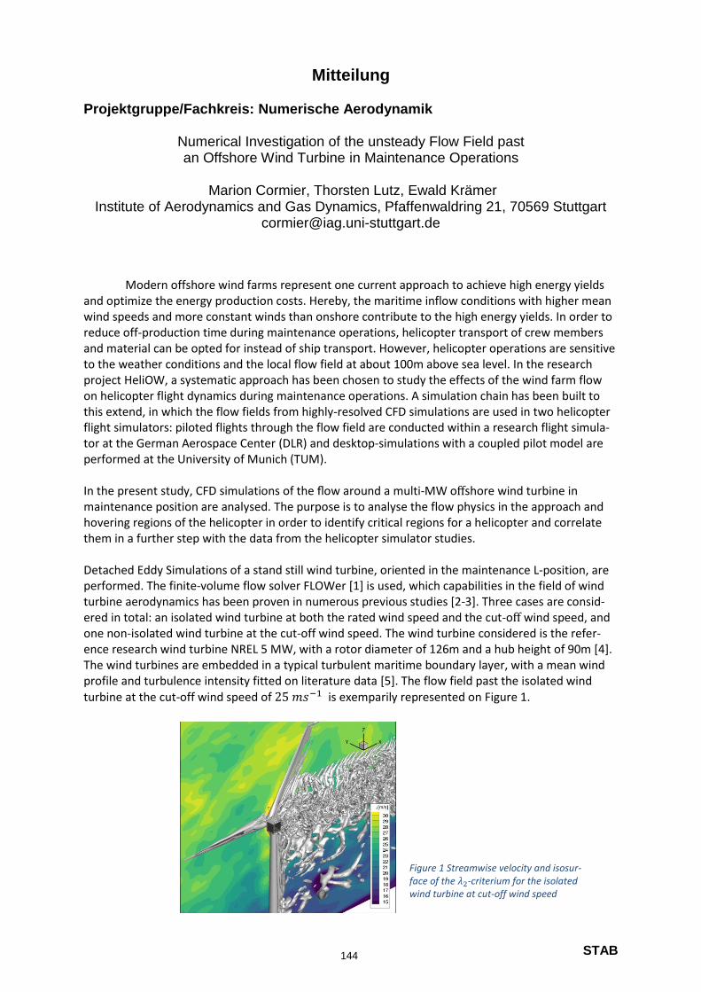
STAB

Mitteilung Projektgruppe/Fachkreis: Numerische Aerodynamik

Numerical Investigation of the unsteady Flow Field past an Offshore Wind Turbine in Maintenance Operations

Marion Cormier, Thorsten Lutz, Ewald Krämer

Institute of Aerodynamics and Gas Dynamics, Pfaffenwaldring 21, 70569 Stuttgart [email protected]

Modern offshore wind farms represent one current approach to achieve high energy yields and optimize the energy production costs. Hereby, the maritime inflow conditions with higher mean wind speeds and more constant winds than onshore contribute to the high energy yields. In order to reduce off-production time during maintenance operations, helicopter transport of crew members and material can be opted for instead of ship transport. However, helicopter operations are sensitive to the weather conditions and the local flow field at about 100m above sea level. In the research project HeliOW, a systematic approach has been chosen to study the effects of the wind farm flow on helicopter flight dynamics during maintenance operations. A simulation chain has been built to this extend, in which the flow fields from highly-resolved CFD simulations are used in two helicopter flight simulators: piloted flights through the flow field are conducted within a research flight simula-tor at the German Aerospace Center (DLR) and desktop-simulations with a coupled pilot model are performed at the University of Munich (TUM). In the present study, CFD simulations of the flow around a multi-MW offshore wind turbine in maintenance position are analysed. The purpose is to analyse the flow physics in the approach and hovering regions of the helicopter in order to identify critical regions for a helicopter and correlate them in a further step with the data from the helicopter simulator studies. Detached Eddy Simulations of a stand still wind turbine, oriented in the maintenance L-position, are performed. The finite-volume flow solver FLOWer [1] is used, which capabilities in the field of wind turbine aerodynamics has been proven in numerous previous studies [2-3]. Three cases are consid-ered in total: an isolated wind turbine at both the rated wind speed and the cut-off wind speed, and one non-isolated wind turbine at the cut-off wind speed. The wind turbine considered is the refer-ence research wind turbine NREL 5 MW, with a rotor diameter of 126m and a hub height of 90m [4]. The wind turbines are embedded in a typical turbulent maritime boundary layer, with a mean wind profile and turbulence intensity fitted on literature data [5]. The flow field past the isolated wind turbine at the cut-off wind speed of 25 𝑚𝑠−1 is exemparily represented on Figure 1.

Figure 1 Streamwise velocity and isosur-face of the 𝜆2-criterium for the isolated wind turbine at cut-off wind speed

144

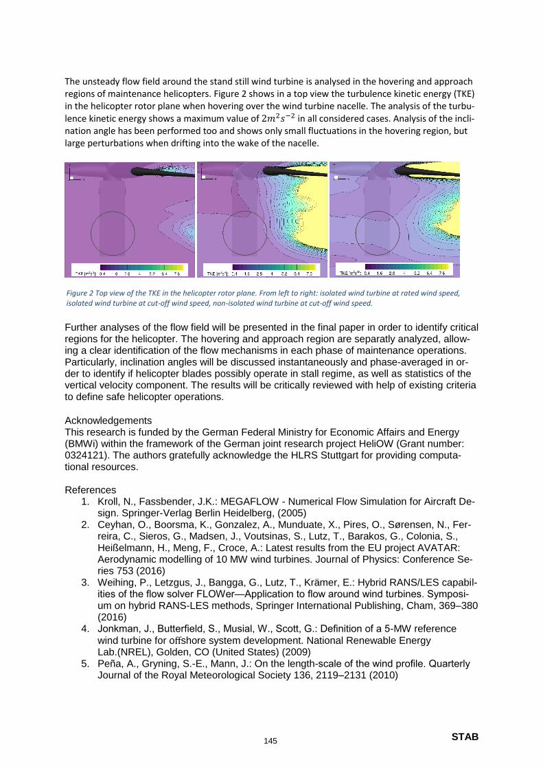
STAB

The unsteady flow field around the stand still wind turbine is analysed in the hovering and approach regions of maintenance helicopters. Figure 2 shows in a top view the turbulence kinetic energy (TKE) in the helicopter rotor plane when hovering over the wind turbine nacelle. The analysis of the turbu-lence kinetic energy shows a maximum value of 2𝑚2𝑠−2 in all considered cases. Analysis of the incli-nation angle has been performed too and shows only small fluctuations in the hovering region, but large perturbations when drifting into the wake of the nacelle.

Further analyses of the flow field will be presented in the final paper in order to identify critical regions for the helicopter. The hovering and approach region are separatly analyzed, allow-ing a clear identification of the flow mechanisms in each phase of maintenance operations. Particularly, inclination angles will be discussed instantaneously and phase-averaged in or-der to identify if helicopter blades possibly operate in stall regime, as well as statistics of the vertical velocity component. The results will be critically reviewed with help of existing criteria to define safe helicopter operations. Acknowledgements This research is funded by the German Federal Ministry for Economic Affairs and Energy (BMWi) within the framework of the German joint research project HeliOW (Grant number: 0324121). The authors gratefully acknowledge the HLRS Stuttgart for providing computa-tional resources. References

1. Kroll, N., Fassbender, J.K.: MEGAFLOW - Numerical Flow Simulation for Aircraft De-sign. Springer-Verlag Berlin Heidelberg, (2005)

2. Ceyhan, O., Boorsma, K., Gonzalez, A., Munduate, X., Pires, O., Sørensen, N., Fer-reira, C., Sieros, G., Madsen, J., Voutsinas, S., Lutz, T., Barakos, G., Colonia, S., Heißelmann, H., Meng, F., Croce, A.: Latest results from the EU project AVATAR: Aerodynamic modelling of 10 MW wind turbines. Journal of Physics: Conference Se-ries 753 (2016)

3. Weihing, P., Letzgus, J., Bangga, G., Lutz, T., Krämer, E.: Hybrid RANS/LES capabil-ities of the flow solver FLOWer—Application to flow around wind turbines. Symposi-um on hybrid RANS-LES methods, Springer International Publishing, Cham, 369–380 (2016)

4. Jonkman, J., Butterfield, S., Musial, W., Scott, G.: Definition of a 5-MW reference

wind turbine for offshore system development. National Renewable Energy Lab.(NREL), Golden, CO (United States) (2009)

5. Peña, A., Gryning, S.-E., Mann, J.: On the length-scale of the wind profile. Quarterly Journal of the Royal Meteorological Society 136, 2119–2131 (2010)

Figure 2 Top view of the TKE in the helicopter rotor plane. From left to right: isolated wind turbine at rated wind speed, isolated wind turbine at cut-off wind speed, non-isolated wind turbine at cut-off wind speed.

145

STAB

Mitteilung Projektgruppe/Fachkreis: Numerische Aerodynamik (Q 2.1)

A Discontinuous Galerkin Chimera Method for Unsteady Flows on Moving Grids

Fabian Genuit, Manuel Keßler and Ewald Krämer

Institute of Aerodynamics and Gas Dynamics, University of Stuttgart, Pfaffenwaldring 21, 70569 Stuttgart

genuit, kessler, [email protected]

Along with the still steady increase in the available computing capacity, there is also an increasing demand for Computational Fluid Dynamics (CFD) calculations of flows for larger and more complex systems in order to be able to make predictions about their properties as accurately as possible. Tra-ditional CFD solvers are often based on a Finite Volume (FV) method. However, FV solvers usually need to work on smooth and highly resolved meshes in order to produce reliable results. Furthermore, the spatial order of accuracy of the FV method stagnates at second order due to an inefficiently high par-allel communication effort in highly parallel calculations. An alternative approach should be offered by the CFD code SUNWinT (Suttgart University Numerical Wind Tunnel) developed at the Institute of Aerodynamics and Gas Dynamics (IAG) at the University of Stuttgart. The spatial discretization in SUNWinT is based on a Discontinuous Galerkin (DG) method, which is assigned to the Finite Element methods but also uses techniques of FV methods. In DG the flow solution is approximated by a polynomial approach. Theoretically, the degree 𝑝 of the polynomial is freely selectable, yielding a solution of arbitrary high order in the grid cells. Alternatively, the number of grid cells required in the discretized area can be reduced. The DG method is characterized by the requirement for the ansatz function to be continuous only within each cell, which allows a discontinu-ous solution at the cell boundaries. In order to guarantee a unique flow at the boundaries, the advec-tive flux is determined using a Riemann solver [4] known from the FV methods. The diffusive flux is treated with the so-called BR2 method [1], since it depends on the unknown state varibales and their gradients. In contrast to FV or Finite Difference methods, the solution for DG only depends on the cell itself and its direct neighbours leading to a compact stencil. Hence, the application of the method on high performance computing systems is suitable, since it is characterized by a low communication ef-fort during parallelization compared to traditional numerical methods. The aim of the SUNWinT project is the application of the DG method to complex flow problems – in this case to helicopter configurations. To this end, different numeri-cal and physical models have been implemented so far. For instance, a Chimera method was implemented by Wurst [5]. The Chimera method is an overset mesh tech-nique, requiring a computational domain that contains at least two overlapping grids, like the exemplary Chimera setup shown in Figure 1. The so-called body grid of a 2D circular cylinder (white grid lines) overlaps the back-ground grid (black grid lines). Furthermore, each cell is as-signed with a specific task. The cells colored in green are called active cells. Typically, their share is highest in a Chi-mera setup and the solution is calculated as if there was only one single grid. The hole cells (colored in blue) are located in the background grid in the area surrounding the surface of the flow body of the body grid – in this case the cylinder. In these cells the calculation of the flow solution is deactivated. The red colored cells are

Figure 1 Chimera setup of a 2D cylinder colored with the cell tasks for each one half of the grid components

146

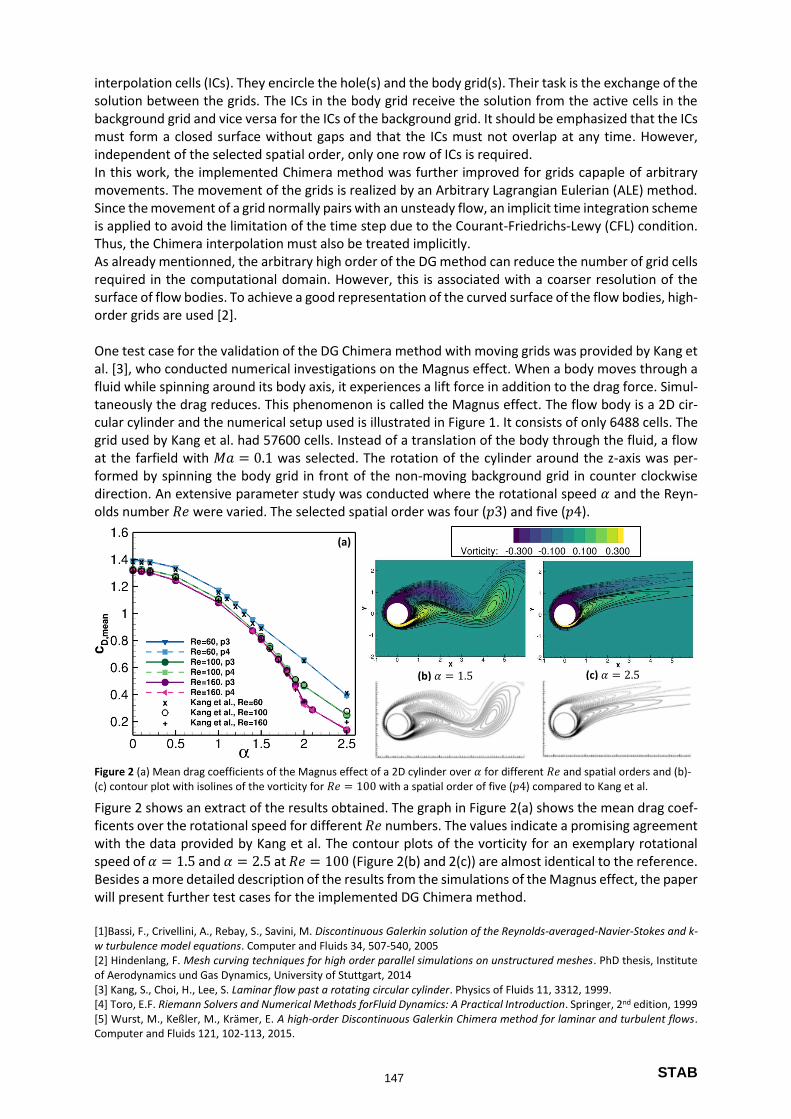
STAB

interpolation cells (ICs). They encircle the hole(s) and the body grid(s). Their task is the exchange of the solution between the grids. The ICs in the body grid receive the solution from the active cells in the background grid and vice versa for the ICs of the background grid. It should be emphasized that the ICs must form a closed surface without gaps and that the ICs must not overlap at any time. However, independent of the selected spatial order, only one row of ICs is required. In this work, the implemented Chimera method was further improved for grids capaple of arbitrary movements. The movement of the grids is realized by an Arbitrary Lagrangian Eulerian (ALE) method. Since the movement of a grid normally pairs with an unsteady flow, an implicit time integration scheme is applied to avoid the limitation of the time step due to the Courant-Friedrichs-Lewy (CFL) condition. Thus, the Chimera interpolation must also be treated implicitly. As already mentionned, the arbitrary high order of the DG method can reduce the number of grid cells required in the computational domain. However, this is associated with a coarser resolution of the surface of flow bodies. To achieve a good representation of the curved surface of the flow bodies, high-order grids are used [2]. One test case for the validation of the DG Chimera method with moving grids was provided by Kang et al. [3], who conducted numerical investigations on the Magnus effect. When a body moves through a fluid while spinning around its body axis, it experiences a lift force in addition to the drag force. Simul-taneously the drag reduces. This phenomenon is called the Magnus effect. The flow body is a 2D cir-cular cylinder and the numerical setup used is illustrated in Figure 1. It consists of only 6488 cells. The grid used by Kang et al. had 57600 cells. Instead of a translation of the body through the fluid, a flow at the farfield with 𝑀𝑎 = 0.1 was selected. The rotation of the cylinder around the z-axis was per-formed by spinning the body grid in front of the non-moving background grid in counter clockwise direction. An extensive parameter study was conducted where the rotational speed 𝛼 and the Reyn-olds number 𝑅𝑒 were varied. The selected spatial order was four (𝑝3) and five (𝑝4).

Figure 2 shows an extract of the results obtained. The graph in Figure 2(a) shows the mean drag coef-ficents over the rotational speed for different 𝑅𝑒 numbers. The values indicate a promising agreement with the data provided by Kang et al. The contour plots of the vorticity for an exemplary rotational speed of 𝛼 = 1.5 and 𝛼 = 2.5 at 𝑅𝑒 = 100 (Figure 2(b) and 2(c)) are almost identical to the reference. Besides a more detailed description of the results from the simulations of the Magnus effect, the paper will present further test cases for the implemented DG Chimera method. [1]Bassi, F., Crivellini, A., Rebay, S., Savini, M. Discontinuous Galerkin solution of the Reynolds-averaged-Navier-Stokes and k-w turbulence model equations. Computer and Fluids 34, 507-540, 2005 [2] Hindenlang, F. Mesh curving techniques for high order parallel simulations on unstructured meshes. PhD thesis, Institute of Aerodynamics und Gas Dynamics, University of Stuttgart, 2014 [3] Kang, S., Choi, H., Lee, S. Laminar flow past a rotating circular cylinder. Physics of Fluids 11, 3312, 1999. [4] Toro, E.F. Riemann Solvers and Numerical Methods forFluid Dynamics: A Practical Introduction. Springer, 2nd edition, 1999 [5] Wurst, M., Keßler, M., Krämer, E. A high-order Discontinuous Galerkin Chimera method for laminar and turbulent flows. Computer and Fluids 121, 102-113, 2015.

Figure 2 (a) Mean drag coefficients of the Magnus effect of a 2D cylinder over 𝛼 for different 𝑅𝑒 and spatial orders and (b)-(c) contour plot with isolines of the vorticity for 𝑅𝑒 = 100 with a spatial order of five (𝑝4) compared to Kang et al.

(a)

(b) 𝛼 = 1.5 (c) 𝛼 = 2.5

147

STAB

Mitteilung

Projektgruppe / Fachkreis: Numerische Aerodynamik

Effiziente Modellierung wandnaher Turbulenz in hybriden RANS/LES

Simulationen

Marius Herr, Axel Probst

DLR, Institut für Aerodynamik und Strömungstechnik

Bunsenstraße 10, 37073 Göttingen, [email protected]

Die hybride RANS/LES Methodik (HRLM) verknüpft die statistische RANS-Modellierung mit der

Large-Eddy Simulation (LES), um Strömungen der Flugzeugaerodynamik mit hoher Reynoldszahl

einem lokal skalenauflösenden Ansatz zugänglich zu machen. Die bisher in den unstrukturierten DLR-

Codes TAU (kompressibel) und THETA (inkompressibel) verwendeten Varianten der Detached-Eddy

Simulation basieren im wandnahen RANS-Bereich auf der so genannten low-Reynolds Modellierung,

die eine vollständige Auflösung der Grenzschicht bis in die viskose Unterschicht (𝑦+ ≈ 1) erfordert.

Um diese hohen Anforderungen an die wandnormale Netzauflösung zu relaxieren, wird in dieser

Arbeit die Kombination der HRLM mit analytischen Wandfunktionen nach Knopp [1] für die

turbulente Grenzschicht verfolgt. Diese stellen zwischen der normierten ersten Zellhöhe 𝑦+(1) und der

als Randbedingung vorgegebenen Wandschubspannung 𝜏𝑤 einen funktionalen Zusammenhang her, der

von der viskosen Unterschicht, über den Übergangsbereich bis in den logarithmischen Bereich gültig

ist. Die Methodik wird mit beiden Lösern TAU und THETA auf wandnormal vergröberten high-

Reynolds Netzen (𝑦+(1) ≈ 12.5 … 210) an verschiedenen kanonischen HRLM-Testfälle (periodische

Kanalströmung, rückspringende Stufe, ablösende Hügelströmung) erprobt und hinsichtlich seiner

Sensitivitäten und Potentiale für die Rechenzeitreduktion bewertet.

Vorgehen und Ergebnisse

Die Auswahl der Testfälle adressiert unterschiedliche Strömungs- und Modellierungsphänomene bei

begrenztem Rechenaufwand. So wird mit der Kanalströmung bei 𝑅𝑒𝜏 = 4200 eine wandmodellierte

LES (IDDES) einer einfachen Grenzschicht ohne Druckgradient betrachtet, während die

rückspringende Stufe und die Hügelströmung geometrie- bzw. druckinduzierte Ablösungen aufweisen,

in der die hierfür verwendete DDES vom RANS-Modus in den lokalen DES/LES Modus umschaltet.

Für alle betrachteten Testfälle werden neben den high-Reynolds Netzen mit variierenden Werten

𝑦+(1) > 1 auch die jeweiligen low-Reynolds Netze erstellt, die zur Erzeugung von numerischen

Referenzergebnissen dienen. Mit der Gegenüberstellung von TAU- und THETA-Ergebnissen werden

zudem unterschiedliche Zellmetriken am viskosen Rand betrachtet: während TAU die Wandfunktion

am oberen Rand der Primärgitterzelle auswertet, verwendet THETA einen zusätzlich eingeführten

Punkt innerhalb der Zelle, wodurch sich die effektive wandnormale Auflösung 𝑦+(1) bei ansonsten

identischem Netz erhöht. Um eine Vergleichbarkeit zwischen beiden Lösern herzustellen, beziehen

sich die 𝑦+(1)-Werte im Folgenden auf den Abstand zwischen dem Auswertepunkt und der Wand.

Abbildung 1 (links) zeigt exemplarisch einen Ausschnitt des Primärnetzes für die rückspringende

Stufe mit 𝑦+(1) = 50, wobei sich der 𝑦+(1)-Wert auf die Stelle 𝑥/ℎ = −1 bezieht. Es handelt sich

um hybride Netze mit strukturierter Vernetzung in Wandnähe und unstrukturierten Gitterzellen im

Ablösebereich der Strömung. In Abbildung 1 (rechts) sind die mittleren Wandreibungsverläufe für

eine effektive Auflösung von 𝑦+(1) = 12.5 (TAU) bzw. 13.5 (THETA) im Vergleich zu

Referenzergebnissen dargestellt. Abgesehen von einer Überschätzung der Wandreibung im

Wiederanlegebereich (10 < 𝑥/ℎ < 26) bei THETA, liegen in beiden Strömungslösern gute

Übereinstimmungen mit der low-Reynolds Rechnung vor. Die Abweichungen stromauf der Stufe (𝑥 <0) sind auf Diskretisierungsfehler der viskosen Flüsse zurückzuführen [2], die nur bei Netzen in

diesem 𝑦+(1)-Bereich beobachtet werden. Im Rahmen von Netzstudien mit systematisch vergröberten

high-Reynolds Gittern konnte gezeigt werden, dass sich für beide Löser akzeptable Übereinstimmung-

148

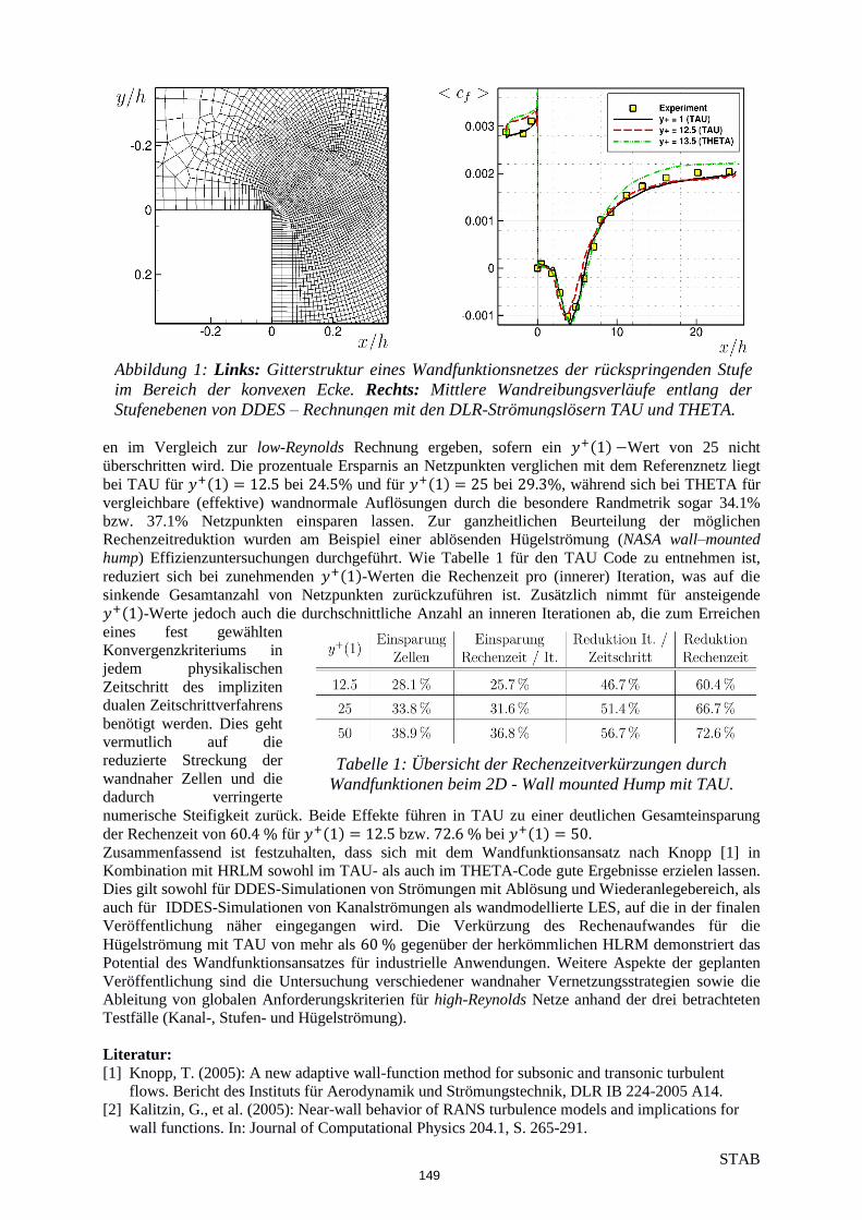
STAB

Tabelle 1: Übersicht der Rechenzeitverkürzungen durch

Wandfunktionen beim 2D - Wall mounted Hump mit TAU.

en im Vergleich zur low-Reynolds Rechnung ergeben, sofern ein 𝑦+(1) −Wert von 25 nicht

überschritten wird. Die prozentuale Ersparnis an Netzpunkten verglichen mit dem Referenznetz liegt

bei TAU für 𝑦+(1) = 12.5 bei 24.5% und für 𝑦+(1) = 25 bei 29.3%, während sich bei THETA für

vergleichbare (effektive) wandnormale Auflösungen durch die besondere Randmetrik sogar 34.1%

bzw. 37.1% Netzpunkten einsparen lassen. Zur ganzheitlichen Beurteilung der möglichen

Rechenzeitreduktion wurden am Beispiel einer ablösenden Hügelströmung (NASA wall–mounted

hump) Effizienzuntersuchungen durchgeführt. Wie Tabelle 1 für den TAU Code zu entnehmen ist,

reduziert sich bei zunehmenden 𝑦+(1)-Werten die Rechenzeit pro (innerer) Iteration, was auf die

sinkende Gesamtanzahl von Netzpunkten zurückzuführen ist. Zusätzlich nimmt für ansteigende

𝑦+(1)-Werte jedoch auch die durchschnittliche Anzahl an inneren Iterationen ab, die zum Erreichen

eines fest gewählten

Konvergenzkriteriums in

jedem physikalischen

Zeitschritt des impliziten

dualen Zeitschrittverfahrens

benötigt werden. Dies geht

vermutlich auf die

reduzierte Streckung der

wandnaher Zellen und die

dadurch verringerte

numerische Steifigkeit zurück. Beide Effekte führen in TAU zu einer deutlichen Gesamteinsparung

der Rechenzeit von 60.4 % für 𝑦+(1) = 12.5 bzw. 72.6 % bei 𝑦+(1) = 50.

Zusammenfassend ist festzuhalten, dass sich mit dem Wandfunktionsansatz nach Knopp [1] in

Kombination mit HRLM sowohl im TAU- als auch im THETA-Code gute Ergebnisse erzielen lassen.

Dies gilt sowohl für DDES-Simulationen von Strömungen mit Ablösung und Wiederanlegebereich, als

auch für IDDES-Simulationen von Kanalströmungen als wandmodellierte LES, auf die in der finalen

Veröffentlichung näher eingegangen wird. Die Verkürzung des Rechenaufwandes für die

Hügelströmung mit TAU von mehr als 60 % gegenüber der herkömmlichen HLRM demonstriert das

Potential des Wandfunktionsansatzes für industrielle Anwendungen. Weitere Aspekte der geplanten

Veröffentlichung sind die Untersuchung verschiedener wandnaher Vernetzungsstrategien sowie die

Ableitung von globalen Anforderungskriterien für high-Reynolds Netze anhand der drei betrachteten

Testfälle (Kanal-, Stufen- und Hügelströmung).

Literatur:

[1] Knopp, T. (2005): A new adaptive wall-function method for subsonic and transonic turbulent

flows. Bericht des Instituts für Aerodynamik und Strömungstechnik, DLR IB 224-2005 A14.

[2] Kalitzin, G., et al. (2005): Near-wall behavior of RANS turbulence models and implications for

wall functions. In: Journal of Computational Physics 204.1, S. 265-291.

Abbildung 1: Links: Gitterstruktur eines Wandfunktionsnetzes der rückspringenden Stufe

im Bereich der konvexen Ecke. Rechts: Mittlere Wandreibungsverläufe entlang der

Stufenebenen von DDES – Rechnungen mit den DLR-Strömungslösern TAU und THETA.

149

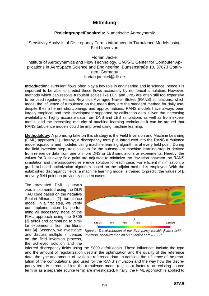
STAB

Mitteilung

Projektgruppe/Fachkreis: Numerische Aerodynamik

Sensitivity Analysis of Discrepancy Terms introduced in Turbulence Models using

Field Inversion

Florian Jäckel Institute of Aerodynamics and Flow Technology, C²A²S²E Center for Computer Ap-plications in AeroSpace Science and Engineering, Bunsenstraße 10, 37073 Göttin-

gen, Germany [email protected]

Introduction: Turbulent flows often play a key role in engineering and in science, hence it is important to be able to predict these flows accurately by numerical simulation. However, methods which can resolve turbulent scales like LES and DNS are often still too expensive to be used regularly. Hence, Reynolds-Averaged Navier Stokes (RANS) simulations, which model the influence of turbulence on the mean flow, are the standard method for daily use, despite their inherent shortcomings and approximations. RANS models have always been largely empirical and their development supported by calibration data. Given the increasing availability of highly accurate data from DNS and LES simulations as well as from experi-ments, and the increasing maturity of machine learning techniques it can be argued that RANS turbulence models could be improved using machine learning.

Methodology: A promising take on this strategy is the Field Inversion and Machine Learning (FIML) approach [1]. Hereby, a discrepancy term β is introduced into the RANS turbulence model equations and modeled using machine learning algorithms at every field point. During the field inversion step, training data for the subsequent machine learning step is derived from reference data from one or more DNS or LES simulations or experiments. Hereby, the values for β at every field point are adjusted to minimize the deviation between the RANS simulation and the associated reference solution for each case. For efficient minimization, a gradient-based optimization algorithm based on the adjoint method is employed. With the established discrepancy fields, a machine learning model is trained to predict the values of β at every field point on previously unseen cases.

The presented FIML approach was implemented using the DLR

TAU code based on the negative Spalart-Allmaras [2] turbulence model. In a first step, we verify our implementation by perfor-ming all necessary steps of the FIML approach using the S809 [3] airfoil and comparing to simi-lar experiments from the litera-ture [4]. Secondly, we investigate and discuss multiple influences on the field inversion process, the achieved solution and the inferred discrepancy fields using the S809 airfoil again. These influences include the type and the amount of regularization used in the optimization and the quality of the reference data, the type and amount of available reference data. In addition, the influence of the reso-lution of the computational grid used for the RANS simulation and the way how the discre-pancy term is introduced into the turbulence model (e.g. as a factor to an existing source term or as a separate source term) are investigated. Finally, the FIML approach is applied to

Figure 1: The distribution of the discrepancy variable β after field inversion, conducted on an S809 airfoil at α = 16.2°

150

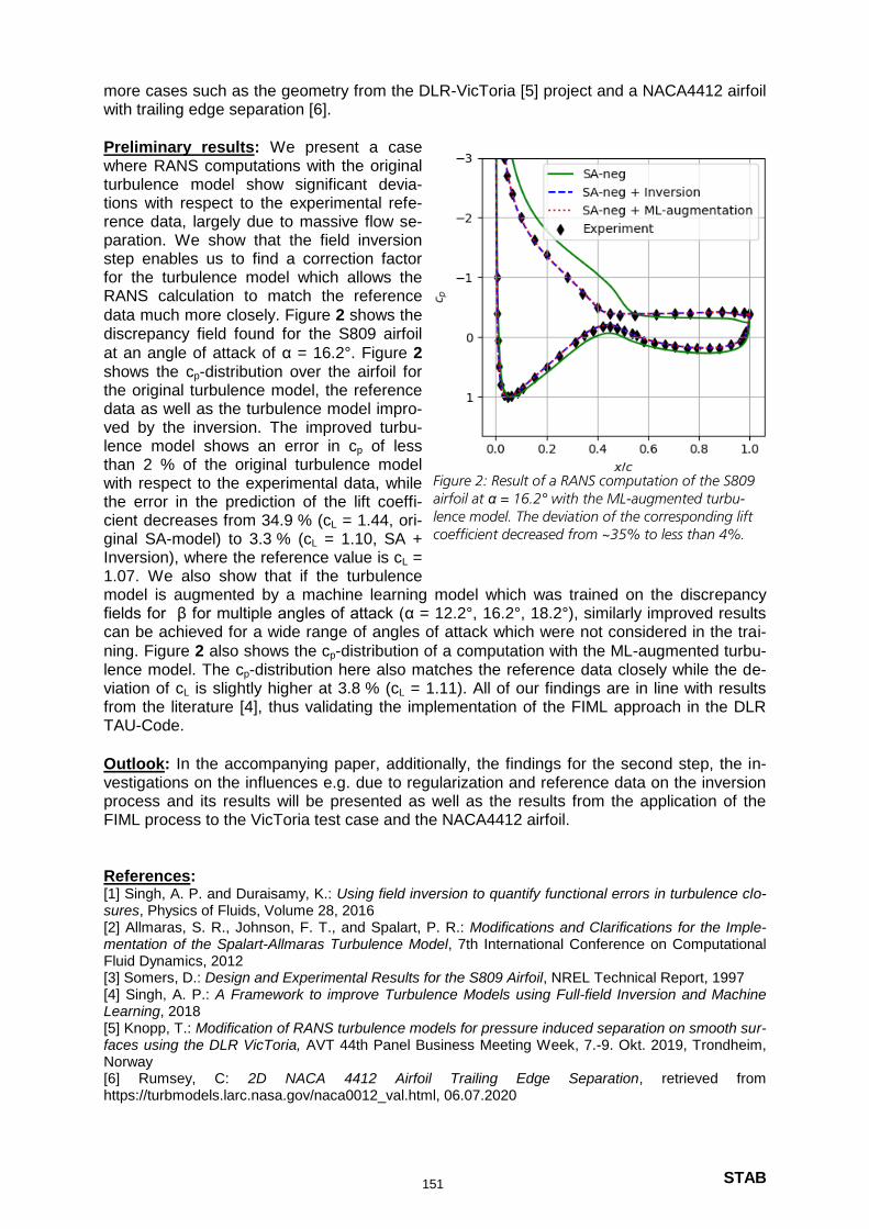
STAB

more cases such as the geometry from the DLR-VicToria [5] project and a NACA4412 airfoil with trailing edge separation [6].

Preliminary results: We present a case where RANS computations with the original turbulence model show significant devia-tions with respect to the experimental refe-rence data, largely due to massive flow se-paration. We show that the field inversion step enables us to find a correction factor for the turbulence model which allows the RANS calculation to match the reference

data much more closely. Figure 2 shows the discrepancy field found for the S809 airfoil

at an angle of attack of α = 16.2°. Figure 2 shows the cp-distribution over the airfoil for the original turbulence model, the reference data as well as the turbulence model impro-ved by the inversion. The improved turbu-lence model shows an error in cp of less than 2 % of the original turbulence model with respect to the experimental data, while the error in the prediction of the lift coeffi-cient decreases from 34.9 % (cL = 1.44, ori-ginal SA-model) to 3.3 % (cL = 1.10, SA + Inversion), where the reference value is cL = 1.07. We also show that if the turbulence model is augmented by a machine learning model which was trained on the discrepancy fields for β for multiple angles of attack (α = 12.2°, 16.2°, 18.2°), similarly improved results can be achieved for a wide range of angles of attack which were not considered in the trai-

ning. Figure 2 also shows the cp-distribution of a computation with the ML-augmented turbu-lence model. The cp-distribution here also matches the reference data closely while the de-viation of cL is slightly higher at 3.8 % (cL = 1.11). All of our findings are in line with results from the literature [4], thus validating the implementation of the FIML approach in the DLR TAU-Code.

Outlook: In the accompanying paper, additionally, the findings for the second step, the in-vestigations on the influences e.g. due to regularization and reference data on the inversion process and its results will be presented as well as the results from the application of the FIML process to the VicToria test case and the NACA4412 airfoil.

References: [1] Singh, A. P. and Duraisamy, K.: Using field inversion to quantify functional errors in turbulence clo-sures, Physics of Fluids, Volume 28, 2016 [2] Allmaras, S. R., Johnson, F. T., and Spalart, P. R.: Modifications and Clarifications for the Imple-mentation of the Spalart-Allmaras Turbulence Model, 7th International Conference on Computational Fluid Dynamics, 2012 [3] Somers, D.: Design and Experimental Results for the S809 Airfoil, NREL Technical Report, 1997 [4] Singh, A. P.: A Framework to improve Turbulence Models using Full-field Inversion and Machine Learning, 2018 [5] Knopp, T.: Modification of RANS turbulence models for pressure induced separation on smooth sur-faces using the DLR VicToria, AVT 44th Panel Business Meeting Week, 7.-9. Okt. 2019, Trondheim, Norway [6] Rumsey, C: 2D NACA 4412 Airfoil Trailing Edge Separation, retrieved from https://turbmodels.larc.nasa.gov/naca0012_val.html, 06.07.2020

Figure 2: Result of a RANS computation of the S809 airfoil at α = 16.2° with the ML-augmented turbu-lence model. The deviation of the corresponding lift coefficient decreased from ~35% to less than 4%.

151

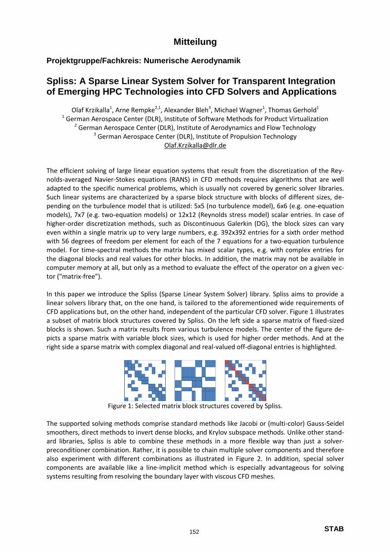
STAB


Spliss: A Sparse Linear System Solver for Transparent Integration of Emerging HPC Technologies into CFD Solvers and Applications

Olaf Krzikalla1, Arne Rempke2,1, Alexander Bleh3, Michael Wagner1, Thomas Gerhold1

1 German Aerospace Center (DLR), Institute of Software Methods for Product Virtualization 2 German Aerospace Center (DLR), Institute of Aerodynamics and Flow Technology

3 German Aerospace Center (DLR), Institute of Propulsion Technology [email protected]

The efficient solving of large linear equation systems that result from the discretization of the Rey-nolds-averaged Navier-Stokes equations (RANS) in CFD methods requires algorithms that are well adapted to the specific numerical problems, which is usually not covered by generic solver libraries. Such linear systems are characterized by a sparse block structure with blocks of different sizes, de-pending on the turbulence model that is utilized: 5x5 (no turbulence model), 6x6 (e.g. one-equation models), 7x7 (e.g. two-equation models) or 12x12 (Reynolds stress model) scalar entries. In case of higher-order discretization methods, such as Discontinuous Galerkin (DG), the block sizes can vary even within a single matrix up to very large numbers, e.g. 392x392 entries for a sixth order method with 56 degrees of freedom per element for each of the 7 equations for a two-equation turbulence model. For time-spectral methods the matrix has mixed scalar types, e.g. with complex entries for the diagonal blocks and real values for other blocks. In addition, the matrix may not be available in computer memory at all, but only as a method to evaluate the effect of the operator on a given vec-tor ("matrix-free"). In this paper we introduce the Spliss (Sparse Linear System Solver) library. Spliss aims to provide a linear solvers library that, on the one hand, is tailored to the aforementioned wide requirements of CFD applications but, on the other hand, independent of the particular CFD solver. Figure 1 illustrates a subset of matrix block structures covered by Spliss. On the left side a sparse matrix of fixed-sized blocks is shown. Such a matrix results from various turbulence models. The center of the figure de-picts a sparse matrix with variable block sizes, which is used for higher order methods. And at the right side a sparse matrix with complex diagonal and real-valued off-diagonal entries is highlighted.

Figure 1: Selected matrix block structures covered by Spliss.

The supported solving methods comprise standard methods like Jacobi or (multi-color) Gauss-Seidel smoothers, direct methods to invert dense blocks, and Krylov subspace methods. Unlike other stand-ard libraries, Spliss is able to combine these methods in a more flexible way than just a solver-preconditioner combination. Rather, it is possible to chain multiple solver components and therefore also experiment with different combinations as illustrated in Figure 2. In addition, special solver components are available like a line-implicit method which is especially advantageous for solving systems resulting from resolving the boundary layer with viscous CFD meshes.

152

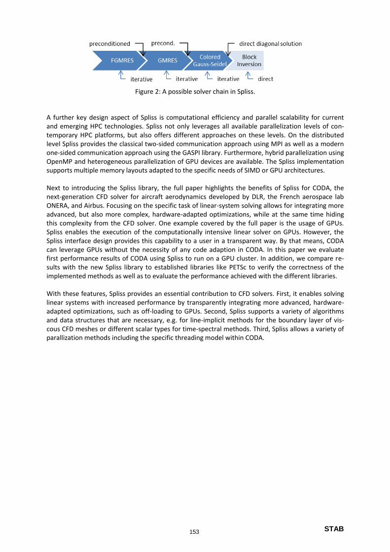
STAB

Figure 2: A possible solver chain in Spliss.

A further key design aspect of Spliss is computational efficiency and parallel scalability for current and emerging HPC technologies. Spliss not only leverages all available parallelization levels of con-temporary HPC platforms, but also offers different approaches on these levels. On the distributed level Spliss provides the classical two-sided communication approach using MPI as well as a modern one-sided communication approach using the GASPI library. Furthermore, hybrid parallelization using OpenMP and heterogeneous parallelization of GPU devices are available. The Spliss implementation supports multiple memory layouts adapted to the specific needs of SIMD or GPU architectures. Next to introducing the Spliss library, the full paper highlights the benefits of Spliss for CODA, the next-generation CFD solver for aircraft aerodynamics developed by DLR, the French aerospace lab ONERA, and Airbus. Focusing on the specific task of linear-system solving allows for integrating more advanced, but also more complex, hardware-adapted optimizations, while at the same time hiding this complexity from the CFD solver. One example covered by the full paper is the usage of GPUs. Spliss enables the execution of the computationally intensive linear solver on GPUs. However, the Spliss interface design provides this capability to a user in a transparent way. By that means, CODA can leverage GPUs without the necessity of any code adaption in CODA. In this paper we evaluate first performance results of CODA using Spliss to run on a GPU cluster. In addition, we compare re-sults with the new Spliss library to established libraries like PETSc to verify the correctness of the implemented methods as well as to evaluate the performance achieved with the different libraries. With these features, Spliss provides an essential contribution to CFD solvers. First, it enables solving linear systems with increased performance by transparently integrating more advanced, hardware-adapted optimizations, such as off-loading to GPUs. Second, Spliss supports a variety of algorithms and data structures that are necessary, e.g. for line-implicit methods for the boundary layer of vis-cous CFD meshes or different scalar types for time-spectral methods. Third, Spliss allows a variety of parallization methods including the specific threading model within CODA.

153

STAB

Mitteilung


Convection Treatment for RANS Turbulence Model Equations

Sebastian Braun, Stefan Langer, Tobias Leicht

DLR, Institute of Aerodynamics and Flow Technology

Lilienthalplatz 7, 38108 Braunschweig,


The compressible Reynolds-averaged Navier-Stokes (RANS) equations are a well-

established model for high Reynolds-number viscous flows. The Reynolds stresses – addi-

tional terms appearing in the RANS equations - can be modelled via the Boussinesq ap-

proximation in which the Reynolds stress tensor is proportional to the mean strain rate ten-

sor. The proportionality factor is known as eddy viscosity and can be modelled via partial

differential or integral equations of a transport type. Such an approach results in a system

of equations for the mean flow, coupled with another system of equations modeling the ef-

fects of turbulence.

In the context of finite-volume methods it is generally accepted that at least second order

discretization schemes should be considered for the mean flow equations due to their supe-

rior accuracy compared to first order schemes. For the turbulence model equations, the

situation is not so clear. Since the coupling of the turbulence model back into the mean flow

equations is rather weak (via the eddy viscosity and a rather small contributions of the tur-

bulent kinetic energy to the total energy conservation), one can hope for a minor effect on

the accuracy of outputs based only on the mean flow part, as local or integrated forces that

typically are of interest in aerodynamics [1]. On the other hand, converging steady-state

solutions for CFD cases based on RANS equations can be challenging, if not even impos-

sible, if the convection components in the turbulence equations are discretized with second

order, in particular when the number of degrees of freedom is systematically increased.

Even if a second order treatment might be optimal for accuracy, without robust solvability

this is not really a relevant consideration in many use cases, especially not in industrial ap-

plications.

Therefore, one of the common propositions and in fact an obvious idea is to treat the con-

vection term of the turbulence model with a first order approach only, aiming at a good

compromise between accuracy and robustness. Indeed, reducing the convection treatment

of turbulence equations to first order often has a tremendous positive effect on robustness,

so that it becomes much more feasible to obtain converged solutions. The mesh asymptotic

values of outputs are not affected, as the first order treatment leads to an overall scheme

that remains a consistent approximation of the continuous problem. However, when naively

applying this on an otherwise unmodified scheme, the adverse effect on a given mesh can

be surprisingly strong and a much higher mesh resolution is required to achieve acceptable

accuracy.

The goal of the full paper is to identify, present and discuss the main drivers, which need to

be carefully implemented when treating the convective by part by a first order discretization

only.

One major contribution for example, is the so-called entropy fix [2]. For both upwind-based

MUSCL-type schemes employing the Roe flux as well as matrix-dissipation based central

schemes, the eigenvalue decomposition of the flux linearization plays a key role. Eigenval-

ues are replaced by modified absolute values to form the Roe matrix, which scales terms

with a dissipative behavior. The modification is an ad-hoc lower limit of the absolute values

of the eigenvalues, in order to ensure non-vanishing dissipation. Typically, this entropy fix is

chosen as a fraction of the largest eigenvalue. This is an undesired ingredient, but required

as a compromise between robustness and accuracy – where higher values of the limit in-

crease dissipation, decreasing accuracy. Fortunately, for moderate values of this entropy fix

effects on the accuracy of results are relatively small for second order schemes, and values

154




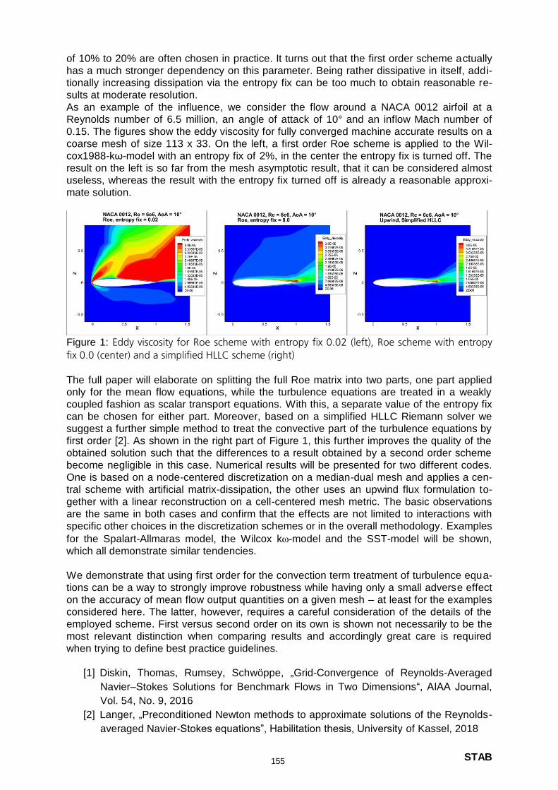
STAB

of 10% to 20% are often chosen in practice. It turns out that the first order scheme actually

has a much stronger dependency on this parameter. Being rather dissipative in itself, addi-

tionally increasing dissipation via the entropy fix can be too much to obtain reasonable re-

sults at moderate resolution.

As an example of the influence, we consider the flow around a NACA 0012 airfoil at a

Reynolds number of 6.5 million, an angle of attack of 10° and an inflow Mach number of

0.15. The figures show the eddy viscosity for fully converged machine accurate results on a

coarse mesh of size 113 x 33. On the left, a first order Roe scheme is applied to the Wil-

cox1988-kω-model with an entropy fix of 2%, in the center the entropy fix is turned off. The

result on the left is so far from the mesh asymptotic result, that it can be considered almost

useless, whereas the result with the entropy fix turned off is already a reasonable approxi-

mate solution.

Figure 1: Eddy viscosity for Roe scheme with entropy fix 0.02 (left), Roe scheme with entropy fix 0.0 (center) and a simplified HLLC scheme (right)

The full paper will elaborate on splitting the full Roe matrix into two parts, one part applied

only for the mean flow equations, while the turbulence equations are treated in a weakly

coupled fashion as scalar transport equations. With this, a separate value of the entropy fix

can be chosen for either part. Moreover, based on a simplified HLLC Riemann solver we

suggest a further simple method to treat the convective part of the turbulence equations by

first order [2]. As shown in the right part of Figure 1, this further improves the quality of the

obtained solution such that the differences to a result obtained by a second order scheme

become negligible in this case. Numerical results will be presented for two different codes.

One is based on a node-centered discretization on a median-dual mesh and applies a cen-

tral scheme with artificial matrix-dissipation, the other uses an upwind flux formulation to-

gether with a linear reconstruction on a cell-centered mesh metric. The basic observations

are the same in both cases and confirm that the effects are not limited to interactions with

specific other choices in the discretization schemes or in the overall methodology. Examples

for the Spalart-Allmaras model, the Wilcox k-model and the SST-model will be shown,

which all demonstrate similar tendencies.

We demonstrate that using first order for the convection term treatment of turbulence equa-

tions can be a way to strongly improve robustness while having only a small adverse effect

on the accuracy of mean flow output quantities on a given mesh – at least for the examples

considered here. The latter, however, requires a careful consideration of the details of the

employed scheme. First versus second order on its own is shown not necessarily to be the

most relevant distinction when comparing results and accordingly great care is required

when trying to define best practice guidelines.

[1] Diskin, Thomas, Rumsey, Schwöppe, „Grid-Convergence of Reynolds-Averaged

Navier–Stokes Solutions for Benchmark Flows in Two Dimensions“, AIAA Journal,

Vol. 54, No. 9, 2016

[2] Langer, „Preconditioned Newton methods to approximate solutions of the Reynolds-

averaged Navier-Stokes equations”, Habilitation thesis, University of Kassel, 2018

155

STAB

Mitteilung Projektgruppe/Fachkreis: Q2.1- Numerische Aerodynamik

𝑝-adaptives Discontinuous-Galerkin-Verfahren in CODA

Johannes Löwe Deutsches Zentrum für Luft- und Raumfahrt, Institut für Aerodynamik und Strömungstechnik,

Bunsenstraße 10, 37073 Göttingen, [email protected]

CODA ist eine C++-Software zur Simulation von Strömungen auf unstrukturierten Netzen auf Basis einer Finite-Volumen-Diskretisierung (FV) zweiter Ordnung sowie einer Discontinuous-Galerkin-Diskretisierung (DG) höherer Ordnung. Die Entwicklung der Software erfolgt im Rahmen einer europäischen Kooperation zusammen mit dem französischen ONERA und dem Industriepartner Airbus und basiert auf dem am DLR entwickelten Strömungslöser Flucs[1]. Im Rahmen der hier vorgestellten Arbeiten wurde das DG-Verfahren in CODA um die Fähigkeit der lokalen Ordnungsadaption erweitert. Zur Reduktion der Kosten einer Simu-

lation und zur Vereinfachung der Netzgenerierung kann damit der Polynomgrad 𝑝 der DG-Basis automatisch lokal durch Indikatoren adaptiert werden. Dadurch müssen wesentliche Merkmale der Strömung (z.B. die Lage von Wirbeln und Scherschichten) nicht vorab bekannt sein und manuell bei der Netzgenerierung und Ordnungswahl berücksichtigt werden.

Implementierung: Als Basis für die DG-Diskretisierung wird in CODA eine zelltypunabhän-

gige hierarchische Orthonormalbasis bezüglich des 𝐿2-Skalarprodukts verwendet, die aus-gehend von in den Zellmittelpunkt verschobenen Monomen durch ein modifiziertes Gram-Schmidt-Verfahren erzeugt wird. Diese Basis erlaubt auf Zellebene einen effizienten Lö-sungstransfer zwischen Diskretisierungen unterschiedlicher Ordnungen durch Abschneiden der Koeffizienten bzw. Ergänzen von Nullen. Die Verwendung einer lokal variierenden An-satzordnung verursacht höhere Kosten beim Zugriff auf die Datenstrukturen und unterschied-liche Berechnungskosten pro Zelle, die bei der Partitionierung zwecks effizienter Parallelver-arbeitung berücksichtigt werden müssen.

Indikatoren: Als Indikator für die zelllokale Adaption der Diskretisierungsordnung dient in den folgenden Beispielen der Small Scale Energy Indikator

𝜂𝐾𝑆𝑆𝐸 = ‖ 𝑝 − 𝚷𝑝−1( 𝑝)‖𝐿2(𝐾)

2,

der in jeder Zelle 𝐾 auf den Impulsvektor 𝑝 der Lösung mit Polynomgrad 𝑝 angewendet

wird[2]. Der Operator 𝚷𝑝−1 bezeichnet dabei die 𝐿2-Projektion in den Raum der Polynome

mit um eins reduziertem Polynomgrad 𝑝 − 1. Dieser Indikator lässt sich für die verwendete Orthonormalbasis sehr effizient auswerten, da lediglich die Summe der Quadrate der Koeffi-zienten von Basisfunktionen höchster Ordnung berechnet werden muss, eine zusätzliche numerische Projektion oder Integration ist nicht nötig. Für eine Erhöhung der Ordnung wer-den alle Zellen ausgewählt, deren Indikatorwert einen bestimmten Schwellwert überschreitet.

Ergebnisse: Als erster Testfall dient eine reibungsfreie Kanalströmung über einen glatten „Gaußhügel“ bei Mach 0,5 auf einem isotropen Netz mit 768 Hexaeder-Zellen. Abbildung 1 zeigt den Widerstandsbeiwert und den Entropiefehler gegenüber der Anzahl der verwende-ten Freiheitsgrade pro Variable für global und lokal variierende Ordnung von 2 bis 6. Bereits mit etwa einem Fünftel der Anzahl der Freiheitsgrade wird mit lokaler Ordnungsadaption die Genauigkeit einer Rechnung mit global 6. Ordnung erreicht. Danach stagniert der Fehler, da die Zellen mit größtem Indikatorwert bereits die maximale Ordnung (in diesem Fall 6) erreicht haben, und die Erhöhung der Ordnung in anderen Zellen nicht zur Reduktion der Fehler bei-tragen.

Als zweiter Testfall dient der Testfall C1.2 des 3. Internationalen Workshops zu High-Order CFD-Verfahren[3]. Es handelt sich um eine reibungsfreie Strömung um ein NACA0012 Profil bei Mach 0,5 und einem Anstellwinkel von 2°. Es wurde das zweitgröbste Referenznetz des Workshops genutzt, das 560 krummlinige Hexaeder-Zellen vierter Ordnung enthält.

156

STAB

Abbildung 2 (links) zeigt den berechneten Widerstandsbeiwert für Diskretisierungsordnungen von 2 bis 6. Sowohl die globale, als auch die indikatorgesteuerte lokale Erhöhung der Ord-nung zeigen monotone Konvergenz. Bei lokaler Ordnungserhöhung wird bereits mit etwa einem Drittel der Freiheitsgrade eine ähnliche Genauigkeit erreicht, wie bei Verwendung konstanter 6. Ordnung. Für den Widerstandsbeiwert in Abbildung 2 (rechts) ergibt sich nur ein geringer Vorteil der lokalen Ordnungsadaption. Ursächlich hierfür ist die stärkere Abhän-gigkeit des Auftriebsbeiwerts von der Singularität an der Hinterkante, die besser durch h-Adaption aufgelöst werden könnte.

Die Ergebnisse zeigen, dass durch lokale Ordnungsadaption auch mit einfachen und effizient auswertbaren Indikatoren eine signifikante Anzahl an Freiheitsgraden gegenüber der Ver-wendung einer hohen Ordnung im ganzen Rechengebiet eingespart werden kann.

Die Arbeiten wurden aufgrund eines Beschlusses des deutschen Bundestages durch das Bundesministerium für Wirtschaft und Energie im Rahmen des LuFo-Programms der Bun-desregierung gefördert (FKZ: 20X1704A).

[1] Leicht, Tobias und Jägersküpper, Jens und Vollmer, Daniel und Schwöppe, Axel und Hartmann, Ralf und Fiedler, Jens und Schlauch, Tobias (2016). DLR-Project Digital-X - Next Generation CFD Solver 'Flucs'. Deutscher Luft- und Raumfahrtkongress 2016, 13-15 Sep 2016, Braunschweig, Deutschland.

[2] Naddei, Fabio und de la Llave Plata, Marta und Couaillier, Vincent und Coquel, Frederic (2018). A comparison of refinement indicators for p-adaptive simulations of steady and un-steady flows using discontinuous Galerkin methods. Journal of Computational Physics. 376. 10.1016/j.jcp.2018.09.045.

[3] 3rd International Workshop on High-Order CFD Methods, Sponsored by NASA, AIAA, DLR, and ARO, January 3 – 4, 2015 at the 53rd AIAA Aerospace Science Meeting in Kis-simmee, Florida (Orlando). https://www.grc.nasa.gov/hiocfd/

Abbildung 1: Widerstandsbeiwert und Entropiefehler für den glatten Gaußhügel.

Abbildung 2: Widerstandsbeiwert und Auftriebsbeiwert für das NACA0012 Profil.

157

https://www.grc.nasa.gov/hiocfd/

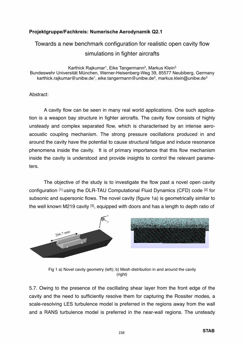
Projektgruppe/Fachkreis: Numerische Aerodynamik Q2.1

Towards a new benchmark configuration for realistic open cavity flow simulations in fighter aircrafts

Karthick Rajkumar1, Eike Tangermann2, Markus Klein3 Bundeswehr Universität München, Werner-Heisenberg-Weg 39, 85577 Neubiberg, Germany


Abstract:

A cavity flow can be seen in many real world applications. One such applica-tion is a weapon bay structure in fighter aircrafts. The cavity flow consists of highly unsteady and complex separated flow, which is characterised by an intense aero-acoustic coupling mechanism. The strong pressure oscillations produced in and around the cavity have the potential to cause structural fatigue and induce resonance phenomena inside the cavity. It is of primary importance that this flow mechanism inside the cavity is understood and provide insights to control the relevant parame-ters.

The objective of the study is to investigate the flow past a novel open cavity configuration [1] using the DLR-TAU Computational Fluid Dynamics (CFD) code [2] for subsonic and supersonic flows. The novel cavity (figure 1a) is geometrically similar to the well known M219 cavity [3], equipped with doors and has a length to depth ratio of

5.7. Owing to the presence of the oscillating shear layer from the front edge of the cavity and the need to sufficiently resolve them for capturing the Rossiter modes, a scale-resolving LES turbulence model is preferred in the regions away from the wall and a RANS turbulence model is preferred in the near-wall regions. The unsteady

STAB

Fig 1 a) Novel cavity geometry (left); b) Mesh distribution in and around the cavity (right)

266.7 mm

158



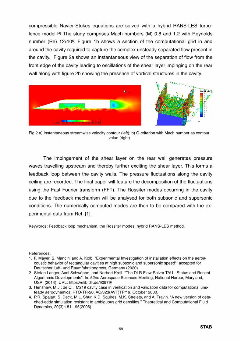
compressible Navier-Stokes equations are solved with a hybrid RANS-LES turbu-lence model [4]. The study comprises Mach numbers (M) 0.8 and 1.2 with Reynolds number (Re) 12x106. Figure 1b shows a section of the computational grid in and around the cavity required to capture the complex unsteady separated flow present in the cavity. Figure 2a shows an instantaneous view of the separation of flow from the front edge of the cavity leading to oscillations of the shear layer impinging on the rear wall along with figure 2b showing the presence of vortical structures in the cavity.

The impingement of the shear layer on the rear wall generates pressure waves travelling upstream and thereby further exciting the shear layer. This forms a feedback loop between the cavity walls. The pressure fluctuations along the cavity ceiling are recorded. The final paper will feature the decomposition of the fluctuations using the Fast Fourier transform (FFT). The Rossiter modes occurring in the cavity due to the feedback mechanism will be analysed for both subsonic and supersonic conditions. The numerically computed modes are then to be compared with the ex-perimental data from Ref. [1].

Keywords: Feedback loop mechanism, the Rossiter modes, hybrid RANS-LES method.

References:1. F. Mayer, S. Mancini and A. Kolb, "Experimental Investigation of installation effects on the aeroa-

coustic behavior of rectangular cavities at high subsonic and supersonic speed", accepted for Deutscher Luft- und Raumfahrtkongress, Germany (2020)

2. Stefan Langer, Axel Schwöppe, and Norbert Kroll. “The DLR Flow Solver TAU - Status and Recent Algorithmic Developments”. In: 52nd Aerospace Sciences Meeting, National Harbor, Maryland, USA, (2014). URL: https://elib.dlr.de/90979/

3. Henshaw, M.J.; de C., M219 cavity case in verification and validation data for computational uns-teady aerodynamics, RTO-TR-26, AC/323(AVT)TP/19, October 2000.

4. P.R. Spalart, S. Deck, M.L. Shur, K.D. Squires, M.K. Strelets, and A. Travin. “A new version of deta-ched-eddy simulation resistant to ambiguous grid densities.” Theoretical and Computational Fluid Dynamics, 20(3):181-195(2006)

STAB

Fig 2 a) Instantaneous streamwise velocity contour (left); b) Q-criterion with Mach number as contour value (right)

159

Mitteilung


Numerical investigation of a porous trailing edge by a zonal RANS/LES simulation

Sutharsan Satcunanathan1, Matthias Meinke1, Wolfgang Schröder1,2

1Institute of Aerodynamics and Chair of Fluid Mechanics, RWTH Aachen University,Wüllnerstr. 5a, 52062 Aachen, Germany

2Jülich Aachen Research Alliance, High Performance Computing, RWTH Aachen University, Seffenter Weg 23, 52074 Aachen, Germany

E-Mail: [email protected]

Experimental and numerical investigations suggest an airframe noise mitigation potential ofporous surface treatments applied to aerodynamic bodies. Acoustic prediction methodsusually require a preceding high fidelity flow simulation of the turbulent flow field as an inputof a subsquent determination of the sound field. Additionally, an overall evaluation of thenoise mitigation concept requires to take the aerodynamic penalty in terms of, e.g., the lift-to-drag ratio into account.

In most numerical approaches the porous material is treated as a homogeneous phase withspatially filtered continuously varying field variables in space and time, which are thengoverned by the volume-averaged Navier-Stokes equations. This constitutes a closureproblem, where the impact of the microscopic scales is substituted by surface filter terms,which can be determined by the Darcy-Forchheimer model [1].

In the present study a NACA 0012 airfoil with a sharp trailng edge at 3° angle-of-attack at aReynolds number based on the chord length c of Rec =1*10 and a Mach number of Ma=0.2⁶is considered. A rectangular segment made of a realistic porous material covers the last 15%of the airfoil, to allow for a redistribution of the near-wall turbulent structures before passingover the trailing edge. A spanwise extent of b=0.15c is considered, to capture the spanwisecoherence of vortical structures, which was shown to be reduced by a porous treatment. Theresults for the flow will be compared against a baseline solid airfoil.

In the present investigations the flow remains attached, such that a computationally efficientzonal approach, in which the Reynolds-averaged Navier-Stokes (RANS) equations aresolved first, followed by a large-eddy simulation (LES), is used. The LES domain is fullyembedded inside the RANS domain and starts at about 40% of the chord length and extendsup to 7c downstream of the airfoil. The overall setup is sketched in Figure 1.

STAB

Figure 1: Schematic of the RANS and LES domains around the NACA 0012 airfoil.

160

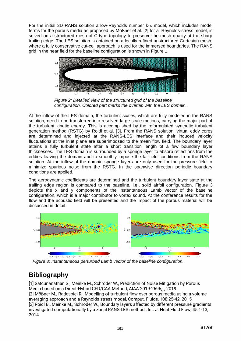
For the initial 2D RANS solution a low-Reynolds number k-ε model, which includes modelterms for the porous media as proposed by Mößner et al. [2] for a Reynolds-stress model, issolved on a structured mesh of C-type topology to preserve the mesh quality at the sharptrailing edge. The LES solution is obtained on a locally refined unstructured Cartesian mesh,where a fully conservative cut-cell approach is used for the immersed boundaries. The RANSgrid in the near field for the baseline configuration is shown in Figure 1.

At the inflow of the LES domain, the turbulent scales, which are fully modeled in the RANSsolution, need to be transferred into resolved large scale motions, carrying the major part ofthe turbulent kinetic energy. This is accomplished by the reformulated synthetic turbulentgeneration method (RSTG) by Roidl et al. [3]. From the RANS solution, virtual eddy coresare determined and injected at the RANS-LES interface and their induced velocityfluctuations at the inlet plane are superimposed to the mean flow field. The boundary layerattains a fully turbulent state after a short transition length of a few boundary layerthicknesses. The LES domain is surrounded by a sponge layer to absorb reflections from theeddies leaving the domain and to smoothly impose the far-field conditions from the RANSsolution. At the inflow of the domain sponge layers are only used for the pressure field tominimize spurious noise from the RSTG. In the spanwise direction periodic boundaryconditions are applied.

The aerodynamic coefficients are determined and the turbulent boundary layer state at thetrailing edge region is compared to the baseline, i.e., solid airfoil configuration. Figure 3depicts the x and y components of the instantaneous Lamb vector of the baselineconfiguration, which is a major contributor to vortex sound. At the conference results for theflow and the acoustic field will be presented and the impact of the porous material will bediscussed in detail.

Bibliography[1] Satcunanathan S., Meinke M., Schröder W., Prediction of Noise Mitigation by Porous Media based on a Direct-Hybrid CFD/CAA Method, AIAA 2019-2696, :, 2019[2] Mößner M., Radespiel R., Modelling of turbulent flow over porous media using a volume averaging approach and a Reynolds stress model, Comput. Fluids, 108:25-42, 2015[3] Roidl B., Meinke M., Schröder W., Boundary layers affected by different pressure gradientsinvestigated computationally by a zonal RANS-LES method., Int. J. Heat Fluid Flow, 45:1-13, 2014

STAB

Figure 3: Instantaneous perturbed Lamb vector of the baseline configuration.

Figure 2: Detailed view of the structured grid of the baseline configuration. Colored part marks the overlap with the LES domain.

161

Mitteilung

Project group / Subject group: Numerical aerodynamics

Meshing strategies for dynamical modeling of movable control surfaces: towardshigh-fidelity flight maneuver simulations

Larissa Bruna Streher, Ralf HeinrichDLR Institute for Aerodynamics and Flow Technology

Lilienthalplatz 7, 38108 Braunschweiglarissa.streher; [email protected]

The accurate prediction of the flow around a maneuvering aircraft is of majorimportance for the development of realistic digital models of aircraft, which wouldprovide a useful basis for virtual design, virtual flight testing and ultimately certifica -tion based on analysis (CbA). Although the availability of a realistic digital modelwould enable a reduction of time and costs involved in the design and certification ofan aircraft [1], as well as a reduction of the risks to aircrews during the flight testphase [2], the realization of such concept is still hampered due to technical limits inthe unsteady computations of maneuvering aircraft.

The simulation of high-fidelity flight maneuvers throughout the entire flight en-velope is especially challenging due to the deployment of control surfaces. Althoughcomputations of control surfaces with fixed deflection angles are already a standardprocedure, these are not suitable for unsteady high-fidelity simulations with varyingdeflection angles. The deflection of a control surface generates unsteady flow fea-tures that are required to analyze the dynamic stability control of an aircraft and can-not be accounted for by fixed deflection angles. Many approaches have alreadybeen developed to model dynamically moving control surfaces: mesh deformation,combination of overset meshes with rigid body rotation, combination of oversetmeshes with mesh deformation and combination of sliding interfaces with mesh de-formation (see Capsada and Heinrich [3]).

In this work, the relative body motion required for the deployment of the con-trol surfaces is carried out with two mixed approaches: combination of oversetmeshes with mesh deformation and combination of sliding interfaces with mesh de-formation. These approaches are selected since they are the only ones able to con-sider dynamically moving surfaces with a physically accurate configuration, i.e., con-sidering the gaps between the lifting and control surfaces in the span-wise direction.

The mixed approaches are based on the multi-block grid method. In the caseof one control surface, two grid blocks are required: one for the control surface andthe other for the lifting surface. The boundary solutions of the blocks are either inter-polated for the overset meshes or computed through the flux across the interface forthe sliding interface method (see Capsada and Heinrich [3]). For both approaches,the control surface is deployed through a mesh deformation algorithm based on ra-dial basis functions.

Although the combination of overset meshes with mesh deformation has beenalready successfully tested by e.g. Reimer and Heinrich [4], it was noticed that theprocess of generating valid, high-quality overset meshes is cumbersome (especiallyfor the narrow gap regions). Therefore, we have developed a software that automati-cally generates the required overlapping regions, significantly reducing the user-ef-fort needed for the mesh generation process.

Here, we show the grids for a LANN wing that result from both mixed ap-proaches to be considered. Both grids are composed of two grid blocks: one for thelifting surface and the other for the control surface. The span-wise gaps are consid-

STAB162

ered, and the control surfaces are deployed by 10 degrees through a mesh deforma-tion algorithm based on radial-basis functions. Figures 1a and 1c illustrate the meshthat uses the sliding interface method to compute the solution at the block bound-aries, whereas the mesh illustrated by Figures 1b and 1d applies the oversetmethod. The overset region was generated by the tool that we developed to extendconforming patched surfaces, reducing considerably the time needed to generate avalid overset grid.

a) Patched mesh.

b) Overset mesh.The pink and blue points are the fringe points of the wing and control surface meshblocks, respectively.

c) Block interfaces without overlapping regions forthe sliding interfaces method.

d) Block interfaces with overlapping regions for theoverset mesh.

Figure 1: Multi-block grid of a LANN wing (in pink) with a generic control surface (in blue). The controlsurface is deployed by 10 degrees.

In this work, we will further compare the combination of overset grids withmesh deformation and the combination of sliding interfaces with mesh deformationfor the dynamical deployment of control surfaces. For the generation of the oversetgrids, the implemented software that automatically generates the overlapping regionwill be used. Hence, except for the overlapping region, the meshes used for the over-set and sliding interfaces approaches are to be the same (considering conformingmeshes for zero deflection). The results will be compared with reference test casesconsisting of only one grid block. Finally, the computational time and accuracy of thesimulations will be compared, and the advantages and disadvantages of each ap-proach will be discussed.

[1] Kroll, N., Abu-Zurayk, M., Dimitrov, D., Franz, R., Führer, T., Gerhold, T., Görtz, S., Heinrich, R., Ilic,C., Jepsen, J., Jägersküpper, J., Kruse, M., Krumbein, A., Langer, S., Liu, D., Liepelt, R., Reimer, L.,Ritter, M., Schwöppe, A., Scherer, J., Spiering, F., Thormann, R., Togiti, V., Vollmer, D. And Wendisch,J.-H. "DLR project Digital-X: towards virtual aircraft design and flight testing based on high-fidelitymethods." CEAS Aeronautical Journal 7.1 (2016): pp. 3-27.

[2] Dean, J., Clifton, J., Bodkin, D., and Ratcliff, J. "High resolution CFD simulations of maneuveringaircraft using the CREATE-AV/Kestrel solver." 49th AIAA Aerospace Sciences Meeting including theNew Horizons Forum and Aerospace Exposition (2011).

[3] Capsada, L. A. and Heinrich, R. "Development of the DLR TAU code for modelling of controlsurfaces". Deutscher Luft- und Raumfahrtkongress (2018). DocumentID: 480018.

[4] Reimer, L. and Heinrich, R. "Modeling of movable control surfaces and atmospheric effects." InComputational Flight Testing. Springer, Berlin, Heidelberg. (2013): pp. 183-206.

STAB163

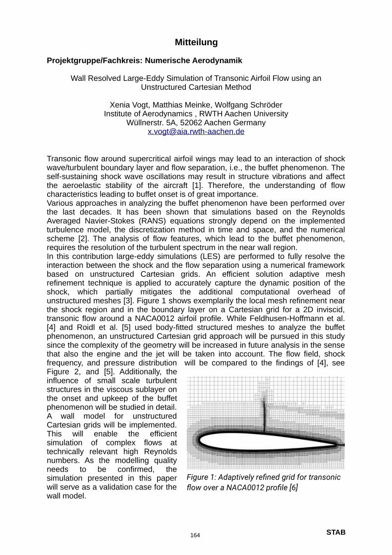
Mitteilung


Wall Resolved Large-Eddy Simulation of Transonic Airfoil Flow using anUnstructured Cartesian Method

Xenia Vogt, Matthias Meinke, Wolfgang SchröderInstitute of Aerodynamics , RWTH Aachen University

Wüllnerstr. 5A, 52062 Aachen [email protected]

Transonic flow around supercritical airfoil wings may lead to an interaction of shockwave/turbulent boundary layer and flow separation, i.e., the buffet phenomenon. Theself-sustaining shock wave oscillations may result in structure vibrations and affectthe aeroelastic stability of the aircraft [1]. Therefore, the understanding of flowcharacteristics leading to buffet onset is of great importance. Various approaches in analyzing the buffet phenomenon have been performed overthe last decades. It has been shown that simulations based on the ReynoldsAveraged Navier-Stokes (RANS) equations strongly depend on the implementedturbulence model, the discretization method in time and space, and the numericalscheme [2]. The analysis of flow features, which lead to the buffet phenomenon,requires the resolution of the turbulent spectrum in the near wall region. In this contribution large-eddy simulations (LES) are performed to fully resolve theinteraction between the shock and the flow separation using a numerical frameworkbased on unstructured Cartesian grids. An efficient solution adaptive meshrefinement technique is applied to accurately capture the dynamic position of theshock, which partially mitigates the additional computational overhead ofunstructured meshes [3]. Figure 1 shows exemplarily the local mesh refinement nearthe shock region and in the boundary layer on a Cartesian grid for a 2D inviscid,transonic flow around a NACA0012 airfoil profile. While Feldhusen-Hoffmann et al.[4] and Roidl et al. [5] used body-fitted structured meshes to analyze the buffetphenomenon, an unstructured Cartesian grid approach will be pursued in this studysince the complexity of the geometry will be increased in future analysis in the sensethat also the engine and the jet will be taken into account. The flow field, shockfrequency, and pressure distribution will be compared to the findings of [4], seeFigure 2, and [5]. Additionally, theinfluence of small scale turbulentstructures in the viscous sublayer onthe onset and upkeep of the buffetphenomenon will be studied in detail.A wall model for unstructuredCartesian grids will be implemented.This will enable the efficientsimulation of complex flows attechnically relevant high Reynoldsnumbers. As the modelling qualityneeds to be confirmed, thesimulation presented in this paperwill serve as a validation case for thewall model.

STAB

Figure 1: Adaptively refined grid for transonic flow over a NACA0012 profile [6]

164


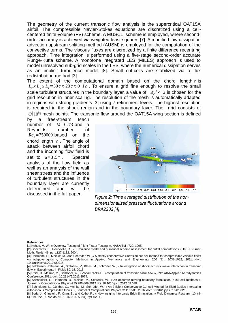
The geometry of the current transonic flow analysis is the supercritical OAT15Aairfoil. The compressible Navier-Stokes equations are discretized using a cell-centered finite-volume (FV) scheme. A MUSCL scheme is employed, where second-order accuracy is achieved via weighted least-squares [7]. A modified low-dissipationadvection upstream splitting method (AUSM) is employed for the computation of theconvective terms. The viscous fluxes are discretized by a finite difference recentringapproach. Time integration is performed using a five-stage second-order accurateRunge-Kutta scheme. A monotone integrated LES (MILES) approach is used tomodel unresolved sub-grid scales in the LES, where the numerical dissipation servesas an implicit turbulence model [8]. Small cut-cells are stabilized via a fluxredistribution method [3]. The extent of the computational domain based on the chord length c isLx x L y x Lz=30 c x 20 c x 0 . 1c . To ensure a grid fine enough to resolve the small

scale turbulent structures in the boundary layer, a value of Δy+< 2 is chosen for thegrid resolution in inner scaling. The resolution of the mesh is automatically adaptedin regions with strong gradients [3] using 7 refinement levels. The highest resolutionis required in the shock region and in the boundary layer. The grid consists ofΟ ( 108) mesh points. The transonic flow around the OAT15A wing section is definedby a free-stream Machnumber of M= 0. 73 and aReynolds number ofRec=750000 based on the

chord length c . The angle ofattack between airfoil chordand the incoming flow field isset to α=3 .5 ° . Spectralanalysis of the flow field aswell as an analysis of the wallshear stress and the influenceof turbulent structures in theboundary layer are currentlydetermined and will bediscussed in the full paper.

References[1] Kehoe, M. W., « Overview Testing of Flight Flutter Testing. », NASA TM 4720, 1995.[2] Goncalves, E., Houdeville, R., « Turbulence model and numerical scheme assessment for buffet computations », Int. J. Numer.Meth. Fluids, 46, pp. 1127-1152, 2004.[3] Hartmann, D., Meinke, M., and Schröder, W., « A strictly conservative Cartesian cut-cell method for compressible viscous flowson adaptive grids. », Computer Methods in Applied Mechanics and Engineering, 200 (9) : 1038-1052, 2011. doi :10.1016/j.cma.2010.05.015[4] Feldhusen-Hoffmann, A., Statnikov, V., Klaas, M., Schröder, W., « Investigation of shock-acoustic-wave interaction in transonicflow. », Experiments in Fluids 59, 15, 2018.[5] Roidl, B., Meinke, M., Schröder, W., « Zonal RANS-LES computation of transonic airfoil flow », 29th AIAA Applied AerodynamicsConference, 2011. doi : 10.2514/6.2011-3974. [6] Schneiders, L., Hartmann, D., Meinke, M., Schröder, W., « An accurate moving boundary formulation in cut-cell methods »,Journal of Computational Physics235:786-809,2013.doi :10.1016/j.jcp.2012.09.038.[7] Schneiders, L., Günther, C., Meinke, M., Schröder, W., « An Efficient Conservative Cut-cell Method for Rigid Bodies Interactingwith Viscous Compressible Flows. », Journal of Computational Physics 311: 62-86, 2016. doi:10.1016/j.jcp.2016.01.026.[8] Boris, J., Grinstein, F., Oran, E., and Kolbe, R., « New Insights Into Large Eddy Simulation.. » Fluid Dynamics Research 10 (4-6) : 199-228, 1992. doi :10.1016/0169-5983(92)90023-P.

STAB

Figure 2: Time averaged distribution of the non-dimensionalized pressure fluctuations around DRA2303 [4]

165

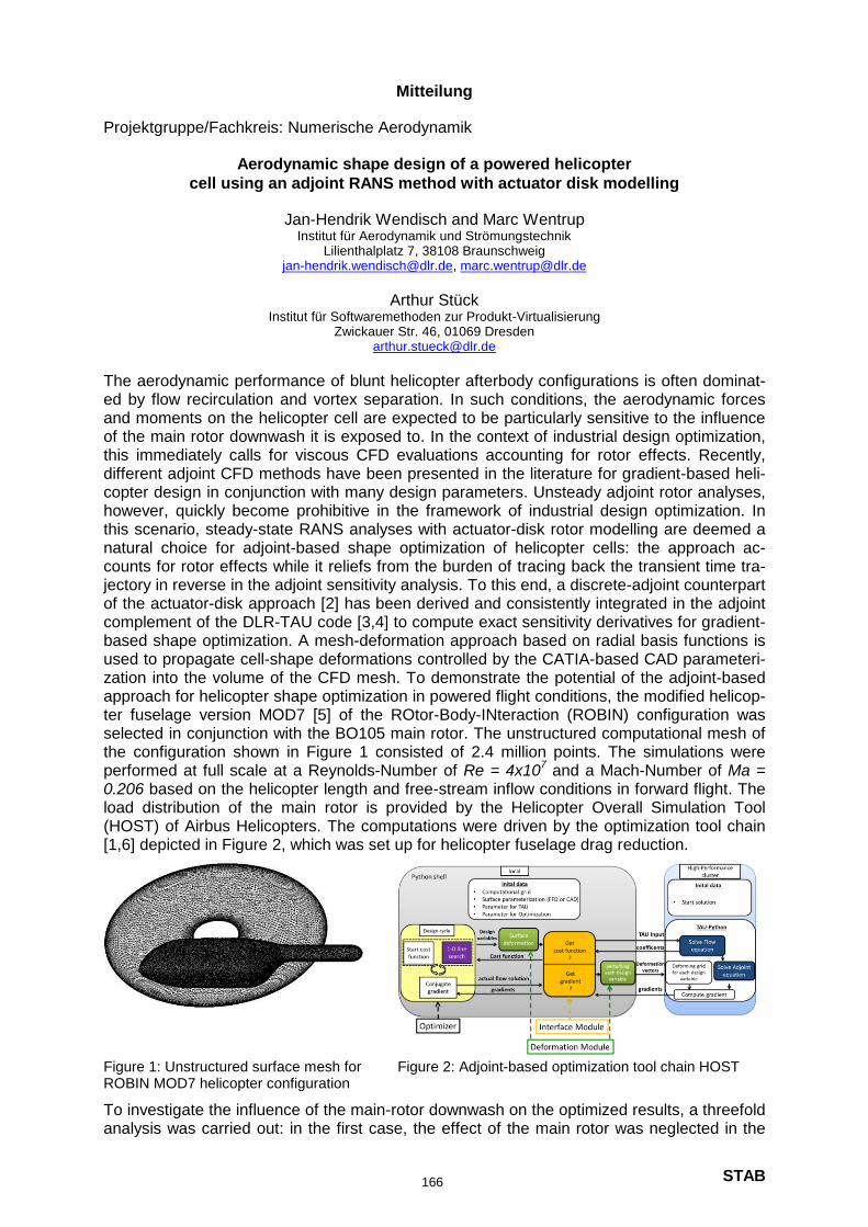
STAB

Mitteilung


Aerodynamic shape design of a powered helicopter

cell using an adjoint RANS method with actuator disk modelling

Jan-Hendrik Wendisch and Marc Wentrup Institut für Aerodynamik und Strömungstechnik

Lilienthalplatz 7, 38108 Braunschweig [email protected], [email protected]

Arthur Stück Institut für Softwaremethoden zur Produkt-Virtualisierung

Zwickauer Str. 46, 01069 Dresden [email protected]

The aerodynamic performance of blunt helicopter afterbody configurations is often dominat-ed by flow recirculation and vortex separation. In such conditions, the aerodynamic forces and moments on the helicopter cell are expected to be particularly sensitive to the influence of the main rotor downwash it is exposed to. In the context of industrial design optimization, this immediately calls for viscous CFD evaluations accounting for rotor effects. Recently, different adjoint CFD methods have been presented in the literature for gradient-based heli-copter design in conjunction with many design parameters. Unsteady adjoint rotor analyses, however, quickly become prohibitive in the framework of industrial design optimization. In this scenario, steady-state RANS analyses with actuator-disk rotor modelling are deemed a natural choice for adjoint-based shape optimization of helicopter cells: the approach ac-counts for rotor effects while it reliefs from the burden of tracing back the transient time tra-jectory in reverse in the adjoint sensitivity analysis. To this end, a discrete-adjoint counterpart of the actuator-disk approach [2] has been derived and consistently integrated in the adjoint complement of the DLR-TAU code [3,4] to compute exact sensitivity derivatives for gradient-based shape optimization. A mesh-deformation approach based on radial basis functions is used to propagate cell-shape deformations controlled by the CATIA-based CAD parameteri-zation into the volume of the CFD mesh. To demonstrate the potential of the adjoint-based approach for helicopter shape optimization in powered flight conditions, the modified helicop-ter fuselage version MOD7 [5] of the ROtor-Body-INteraction (ROBIN) configuration was selected in conjunction with the BO105 main rotor. The unstructured computational mesh of the configuration shown in Figure 1 consisted of 2.4 million points. The simulations were performed at full scale at a Reynolds-Number of Re = 4x10

7 and a Mach-Number of Ma =

0.206 based on the helicopter length and free-stream inflow conditions in forward flight. The load distribution of the main rotor is provided by the Helicopter Overall Simulation Tool (HOST) of Airbus Helicopters. The computations were driven by the optimization tool chain [1,6] depicted in Figure 2, which was set up for helicopter fuselage drag reduction.

Figure 1: Unstructured surface mesh for ROBIN MOD7 helicopter configuration

Figure 2: Adjoint-based optimization tool chain HOST

To investigate the influence of the main-rotor downwash on the optimized results, a threefold analysis was carried out: in the first case, the effect of the main rotor was neglected in the

166




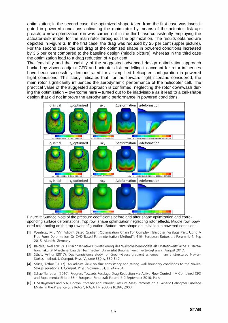
STAB

optimization; in the second case, the optimized shape taken from the first case was investi-gated in powered conditions activating the main rotor by means of the actuator-disk ap-proach; a new optimization run was carried out in the third case consistently employing the actuator-disk model for the main rotor throughout the optimization. The results obtained are depicted in Figure 3. In the first case, the drag was reduced by 25 per cent (upper picture). For the second case, the cell drag of the optimized shape in powered conditions increased by 3.5 per cent compared to the baseline design (middle picture), whereas in the third case the optimization lead to a drag reduction of 4 per cent. The feasibility and the usability of the suggested advanced design optimization approach backed by viscous adjoint CFD and actuator-disk modelling to account for rotor influences have been successfully demonstrated for a simplified helicopter configuration in powered flight conditions. This study indicates that, for the forward flight scenario considered, the main rotor significantly influences the aerodynamic performance of the helicopter cell. The practical value of the suggested approach is confirmed: neglecting the rotor downwash dur-ing the optimization – overcome here – turned out to be inadvisable as it lead to a cell-shape design that did not improve the aerodynamic performance in powered conditions.

Figure 3: Surface plots of the pressure coefficients before and after shape optimization and corre-sponding surface deformations. Top row: shape optimization neglecting rotor effects. Middle row: pow-ered rotor acting on the top-row configuration. Bottom row: shape optimization in powered conditions.

[1] Wentrup, M , “An Adjoint Based Gradient Optimization Chain For Complex Helicopter Fuselage Parts Using A Free Form Deformation Or CAD Based Parameterization Method”, 41th European Rotorcraft Forum 1.-4. Sep 2015, Munich, Germany

[2] Raichle, Axel (2017). Flusskonservative Diskretisierung des Wirkscheibenmodells als Unstetigkeitsfläche. Disserta-tion, Fakultät Maschinenbau der Technischen Universität Braunschweig, verteidigt am 7. August 2017.

[3] Stück, Arthur (2017). Dual-consistency study for Green–Gauss gradient schemes in an unstructured Navier–Stokes method. J. Comput. Phys. Volume 350, s. 530-549.

[4] Stück, Arthur (2017). An adjoint view on flux consistency and strong wall boundary conditions to the Navier-Stokes equations. J. Comput. Phys., Volume 301, s. 247-264.

[5] Schaeffler et al. (2010). Progress Towards Fuselage Drag Reduction via Active Flow Control - A Combined CFD and Experimental Effort. 36th European Rotorcraft Forum, 7-9 September 2010, Paris.

[6] E.M Raymond and S.A. Gorton, “Steady and Periodic Pressure Measurements on a Generic Helicopter Fuselage Model in the Presence of a Rotor”, NASA TM 2000-210286, 2000

167

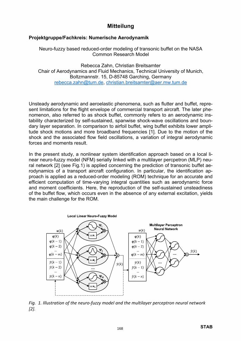
STAB


Neuro-fuzzy based reduced-order modeling of transonic buffet on the NASA Common Research Model

Rebecca Zahn, Christian Breitsamter

Chair of Aerodynamics and Fluid Mechanics, Technical University of Munich, Boltzmannstr. 15, D-85748 Garching, Germany

[email protected], [email protected] Unsteady aerodynamic and aeroelastic phenomena, such as flutter and buffet, repre-sent limitations for the flight envelope of commercial transport aircraft. The later phe-nomenon, also referred to as shock buffet, commonly refers to an aerodynamic ins-tability characterized by self-sustained, spanwise shock-wave oscillations and boun-dary layer separation. In comparison to airfoil buffet, wing buffet exhibits lower ampli-tude shock motions and more broadband frequencies [1]. Due to the motion of the shock and the associated flow field oscillations, a variation of integral aerodynamic forces and moments result. In the present study, a nonlinear system identification approach based on a local li-near neuro-fuzzy model (NFM) serially linked with a multilayer percpetron (MLP) neu-ral network [2] (see Fig.1) is applied concerning the prediction of transonic buffet ae-rodynamics of a transport aircraft configuration. In particular, the identification ap-proach is applied as a reduced-order modeling (ROM) technique for an accurate and efficient computation of time-varying integral quantities such as aerodynamic force and moment coefficients. Here, the reproduction of the self-sustained unsteadiness of the buffet flow, which occurs even in the absence of any external excitation, yields the main challenge for the ROM.

Fig. 1. Illustration of the neuro-fuzzy model and the multilayer perceptron neural network [2].

168

STAB

In order to demonstrate the performance and reliability of the ROM method for mode-ling the buffet phenomenon, the NASA Common Research Model (CRM) is investi-gated at transonic freestream conditions (Ma = 0.85, a = 5°, Re = 30 Mio.), under-going user-defined pitching motions. Therefore, unsteady Reynolds-averaged Navier-Stokes (URANS) simulations, coupled with the Spalart-Allmaras turbulence model, are performed using the DLR-TAU code. The excitation of the wing is accomplished by means of a smoothed amplitude modulated pseudo-random binary signal (SAPRBS) (see Fig.2), which allows for the representation of a wide range of ampli-tudes and frequencies.

Fig. 2. Smoothed APRBS time-series for the excitation of the pitch degree of freedom

Based on the combination of the excitation inputs and the computational fluid dyna-mics (CFD) solution, a merged data set can be obtained and employed for ROM trai-ning purposes. Therefore, 70% of the available data are randomly chosen for the training process, whereas the remaining percentage is used for the validation of the ROM. In order to eliminate statistical errors resulting from this random data segmen-tation, a Monte-Carlo based training procedure is applied [2]. Based on recent applications of the selected ROM method [2,3], a high potential for predicting the aerodynamic loads with respect to shock buffet is expected. Further, computational time and effort can be reduced by at least two orders of magnitude compared to a full-order CFD solution. [1] S. Timme. Global shock instability on NASA Common Research Model, In AIAA SciTech Forum 2019. American Institute of Aeronautics and Astronautics. Doi:10.2514/6.2019-0037 [2] M. Winter. C. Breitsamter, Nonlinear identification via connected neural networks for unsteady ae-rodynamic analysis, Aerospace Sciene and Technology, 77, pp. 802-818 (2018) [3] M. Winter. C. Breitsamter, Reduced-order modeling of transonic buffet aerodynamics, Notes on Numerical Fluid Mechanics, 142, pp. 511-520 (2020)

0 200 400 600 800 1000 1200Nondimensional Time

1.0

0.5

0.0

0.5

1.0

Exc

itat

ion

Am

plitu

de

[°]

169

STAB

Mitteilung Projektgruppe/Fachkreis: Experimentelle Aerodynamik Q 2.2

Experimental investigation of a line-cavity system equipped with fiber-optic differential pressure sensors in a shock tube

Florian Heckmeier, Niklas Mooshofer, Thomas Hopfes, Christian Breitsamter,

Nikolaus A. Adams


Introduction and Overview: The determination of the acoustic line-cavity system is crucial when operating fast-response multi-hole probes, because the pressure signal is subject to attenuation and resonance inside the line-cavity system, and therefore, could lead to distorted pressure signals. To determine the transfer function between the signal at the tip and the location of the sensor, an analytical model introduced by Bergh and Tijdeman [1] provides the basic characteristics. However, they do not account for manufacturing imperfections that cause the actual system to differ from the analytic solution. Therefore, it is essential to determine the transfer function experimentally. This has recently been done in a frequency test rig [2] by means of a speaker emitting sinusoidal signals at varying frequencies. In this study, a different method to determine the transfer function is applied. In the shock tube of the Chair of Aerodynamics and Fluid Mechanics of the Technical University of Munich (TUM-AER) [3], fiber-optic pressure sensors are mounted as the receiving unit (end of line-cavity system) and as the reference sensor. Within a system identification step, the pressure signals due to the shock are measured and set into relation as described in Paniagua [4]. In contrast to the determination in the frequency test rig, which shows bandwidth restriction due to the selected speaker, the shock should allow to also identify high frequencies. Line-cavity system:

The line-cavity system is mainly characterized by its length , its diameter , and the volume

in front of the sensor , as depicted in figure 1.

Figure 1: Sketch of the line-cavity system and its characteristic dimensions , , and

The transfer function of the linear system in the discrete -domain can be expressed by two polynomials of order :

⋅

⋅ ⋯ ⋅

1 ⋅ ⋅

⋯ ⋅ (1)

Where and are the -transformed of the time series data of the reference and the line-cavity sensor signals. After the identification of the unknown parameters in equation 1, the amplitude ratio and phase lag corresponding to the transfer function can be computed at any frequency. Hence, for following measurements, the transfer function can be applied to correct the pressures attenuated in the line-cavity system. Experimental setup: Figure 2 depicts the layout of the shock tube and connected systems for the current

experiments. The tube has an overall length of 22.5, an inner diameter of 290, and is segmented into a driver, a driven and a test section. Before experiments, a 0.2-thick PVC

170

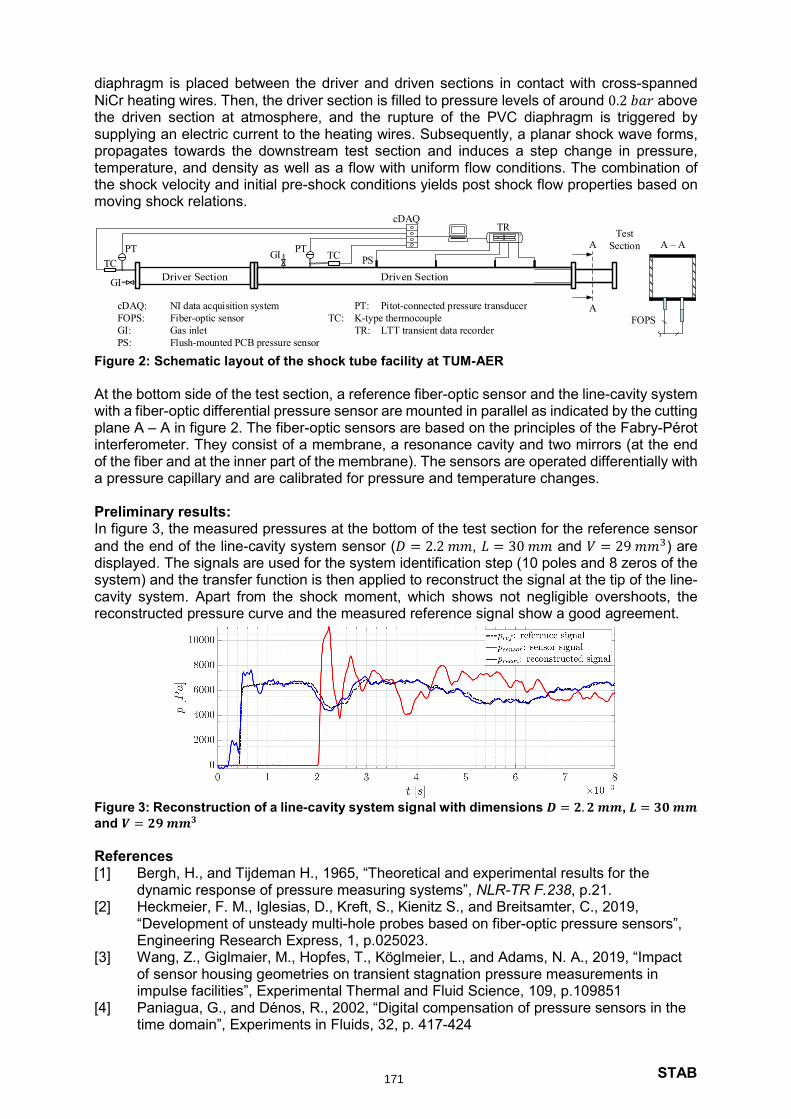
STAB

diaphragm is placed between the driver and driven sections in contact with cross-spanned

NiCr heating wires. Then, the driver section is filled to pressure levels of around 0.2! above the driven section at atmosphere, and the rupture of the PVC diaphragm is triggered by supplying an electric current to the heating wires. Subsequently, a planar shock wave forms, propagates towards the downstream test section and induces a step change in pressure, temperature, and density as well as a flow with uniform flow conditions. The combination of the shock velocity and initial pre-shock conditions yields post shock flow properties based on moving shock relations.

Figure 2: Schematic layout of the shock tube facility at TUM-AER

At the bottom side of the test section, a reference fiber-optic sensor and the line-cavity system with a fiber-optic differential pressure sensor are mounted in parallel as indicated by the cutting plane A – A in figure 2. The fiber-optic sensors are based on the principles of the Fabry-Pérot interferometer. They consist of a membrane, a resonance cavity and two mirrors (at the end of the fiber and at the inner part of the membrane). The sensors are operated differentially with a pressure capillary and are calibrated for pressure and temperature changes. Preliminary results: In figure 3, the measured pressures at the bottom of the test section for the reference sensor

and the end of the line-cavity system sensor ( 2.2, 30 and 29#) are displayed. The signals are used for the system identification step (10 poles and 8 zeros of the system) and the transfer function is then applied to reconstruct the signal at the tip of the line-cavity system. Apart from the shock moment, which shows not negligible overshoots, the reconstructed pressure curve and the measured reference signal show a good agreement.

Figure 3: Reconstruction of a line-cavity system signal with dimensions $. $%%, &'%%

and $(%%&

References [1] Bergh, H., and Tijdeman H., 1965, “Theoretical and experimental results for the

dynamic response of pressure measuring systems”, NLR-TR F.238, p.21. [2] Heckmeier, F. M., Iglesias, D., Kreft, S., Kienitz S., and Breitsamter, C., 2019,

“Development of unsteady multi-hole probes based on fiber-optic pressure sensors”, Engineering Research Express, 1, p.025023.

[3] Wang, Z., Giglmaier, M., Hopfes, T., Köglmeier, L., and Adams, N. A., 2019, “Impact of sensor housing geometries on transient stagnation pressure measurements in impulse facilities”, Experimental Thermal and Fluid Science, 109, p.109851

[4] Paniagua, G., and Dénos, R., 2002, “Digital compensation of pressure sensors in the time domain”, Experiments in Fluids, 32, p. 417-424

cDAQTR

TCTC

PT PTPS

cDAQ: NI data acquisition system PT: Pitot-connected pressure transducer

FOPS: Fiber-optic sensor TC: K-type thermocouple

GI: Gas inlet TR: LTT transient data recorder

PS: Flush-mounted PCB pressure sensor

GI

GI

Test

Section

FOPS

A

A A – A

171

STAB

Mitteilung Projektgruppe/Fachkreis: Experimentelle Aerodynamik 2D-Flügelprofiluntersuchungen in einer offenen Messstrecke: Aufbau, Messtechnik,

Windkanalkorrekturen, Validierung

Oliver Meyer Institut für Aerodynamik und Flugsimulation, Universität der Bundeswehr München, Werner-Heisenberg-Weg 39, 85577 Neubiberg, [email protected] Der Göttinger-Windkanal im Fachgebiet Strömungsmechanik der Fakultät für Maschinenbau hat eine offene Messstrecke mit den Abmessungen 0,9m x 1.2m x 2m (H x B x L) in der eine Windgeschwindigkeit von maximal 40m/s erreicht werden kann. Zu diesem Windkanal gehört eine 6-Komponenten-Überflurwaage nach dem AVA-Prinzip sowie ein Laufband für Modell-fahrzeug- oder andere bodennahe Strömungsuntersuchungen. Für die Durchführung von Flügelprofiluntersuchungen wurde zunächst die Strömungsqualität bestimmt, der axiale Druckgradient in Strömungsrichtung optimiert und ein passender Ver-suchsaufbau entwickelt [1]. Das Profil wird mit Endscheiben versehen und in der Messposition an die Windkanalwaage gehängt. Infrarot-Thermografieaufnahmen sowie Ölanstrichbilder zei-gen, dass die Endscheiben sehr gute 2D-Strömungsverhältnisse erzeugen. Der Durchmesser der Endscheiben ist so gewählt, dass er zwei Profiltiefen der verwendeten Modelle entspricht. Die verwendeten Modelle haben eine Profiltiefe von 0.35m, aus der sich eine Modellrey-

noldszahl von ca. 𝑅𝑒 = 0.8 ∙ 106 ergibt. Der Auftrieb der Profilmodelle wird mit der Windkanal-Überflurwaage gemessen und der Wi-derstand über Nachlaufmessungen ermittelt. Die Impulsverlustbestimmung im Nachlauf erfolgt über einen aerodynamisch verkleideten Pitot-Nachlaufrechen mit 106 Messstellen (Abb. 1), so dass der geometrische Anstellwinkelbereich des Modells von -20° bis 26° variiert werden kann ohne den Nachlaufrechen nachzuführen. Zusätzlich wird ein Rechen mit 20 statischen Drucksonden hinter dem Modell eingesetzt, da relativ dicht hinter dem Profil gemessen wird (Abb. 2) und mögliche statische Druckvariationen berücksichtigt werden sollten. Die Bestim-mung des Widerstandsbeiwertes erfolgt nach der von Jones beschriebenen Methode [2]. Die winkelabhängige Messgenauigkeit der Rechen wird durch Drehen der Rechen um die Hoch- und Querachse (Anstell- und Schiebewinkel) bestimmt. Dabei zeigt sich, dass der To-taldruckrechen insbesondere bei Anstellwinkelvariation in einem sehr großen Bereich wenig winkelabhängig misst und nur relativ kleine Abweichungen im gemessenen Totaldruck von z.B. 5% bei 20° Schräganströmung auftreten, s. Abb. 3. Somit kann der Messrechen auch bei großen Anstellwinkeln des Profils fest senkrecht verbaut bleiben. Die aus den Messwerten ermittelten Beiwerte ca, cw und ggf. cm, müssen nachträglich korrigiert werden. Die offene Messstrecke, jetzt seitlich zusätzlich beeinflusst durch Endscheiben, verfälscht die Modellumströmung ggü. einer freien Umströmung und damit auch die Mess-werte. Für den beschriebenen Versuchsaufbau existiert ein Messstreckeninterferenz-Kor-rekturverfahren [3], das hier ggü. dem in [1] beschriebenen Verfahren wesentlich besser passt und nun angewendet wird. Mit Hilfe der Messstrecken- und Modellgeometrie sowie dem sta-tischen Druckverlauf in der Messstrecke können mit diesem Verfahren die Messwerte erfol-greich auf 2D-Referenzwerte korrigiert werden. In dem Korrekturverfahren ist einzig die Defi-nition der Messstreckenhöhe für unseren Fall nicht näher festgelegt. Die zuvor vermessenen und hier herangezogenen inneren Grenzen des Freistrahls an der Modellposition führen schließlich zu einer erfolgreichen Korrektur der Beiwerte für verschiedene Referenzmodelle, Bsp. siehe Abb. 4. Die sichtbaren Abweichungen bei ca,max und cw resultieren u.a. aus den nicht ausreichend übereinstimmenden Reynoldszahlen von Versuchs- und Referenzwerten. Die Messtechnik kann zum einen ggü. [1] durch Verwendung und Vermessung neuer statis-cher- und Totaldruckrechen deutlich verbessert werden. Zum anderen wird eine ggü. [1] bes-ser passende und für den Versuchsfall abgestimmte Windkanalkorrektur angewendet. Beide Entwicklungen führen nun bei der Polarenermittlung von Flügelprofilen zu wesentlich besseren Ergebnissen.

172

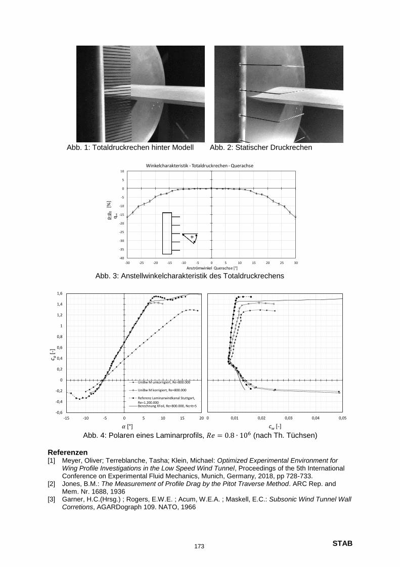
STAB

Abb. 1: Totaldruckrechen hinter Modell Abb. 2: Statischer Druckrechen

Abb. 3: Anstellwinkelcharakteristik des Totaldruckrechens

Abb. 4: Polaren eines Laminarprofils, 𝑅𝑒 = 0.8 ∙ 106 (nach Th. Tüchsen)

Referenzen [1] Meyer, Oliver; Terreblanche, Tasha; Klein, Michael: Optimized Experimental Environment for

Wing Profile Investigations in the Low Speed Wind Tunnel, Proceedings of the 5th International Conference on Experimental Fluid Mechanics, Munich, Germany, 2018, pp 728-733.

[2] Jones, B.M.: The Measurement of Profile Drag by the Pitot Traverse Method. ARC Rep. and Mem. Nr. 1688, 1936

[3] Garner, H.C.(Hrsg.) ; Rogers, E.W.E. ; Acum, W.E.A. ; Maskell, E.C.: Subsonic Wind Tunnel Wall Corretions, AGARDograph 109. NATO, 1966

-40

-35

-30

-25

-20

-15

-10

-5

0

5

10

-30 -25 -20 -15 -10 -5 0 5 10 15 20 25 30

p-p

0[%

]q∞

Anströmwinkel Querachse [°]

Winkelcharakteristik - Totaldruckrechen - Querachse

-0,6

-0,4

-0,2

0

0,2

0,4

0,6

0,8

1

1,2

1,4

1,6

-15 -10 -5 0 5 10 15 20

c a[-

]

[°]

UniBw M unkorrigiert, Re=800.000

UniBw M korrigiert, Re=800.000

Referenz Laminarwindkanal Stuttgart,Re=1.200.000Berechnung XFoil, Re=800.000, Ncrit=5

0 0,01 0,02 0,03 0,04 0,05

cw [-]

173

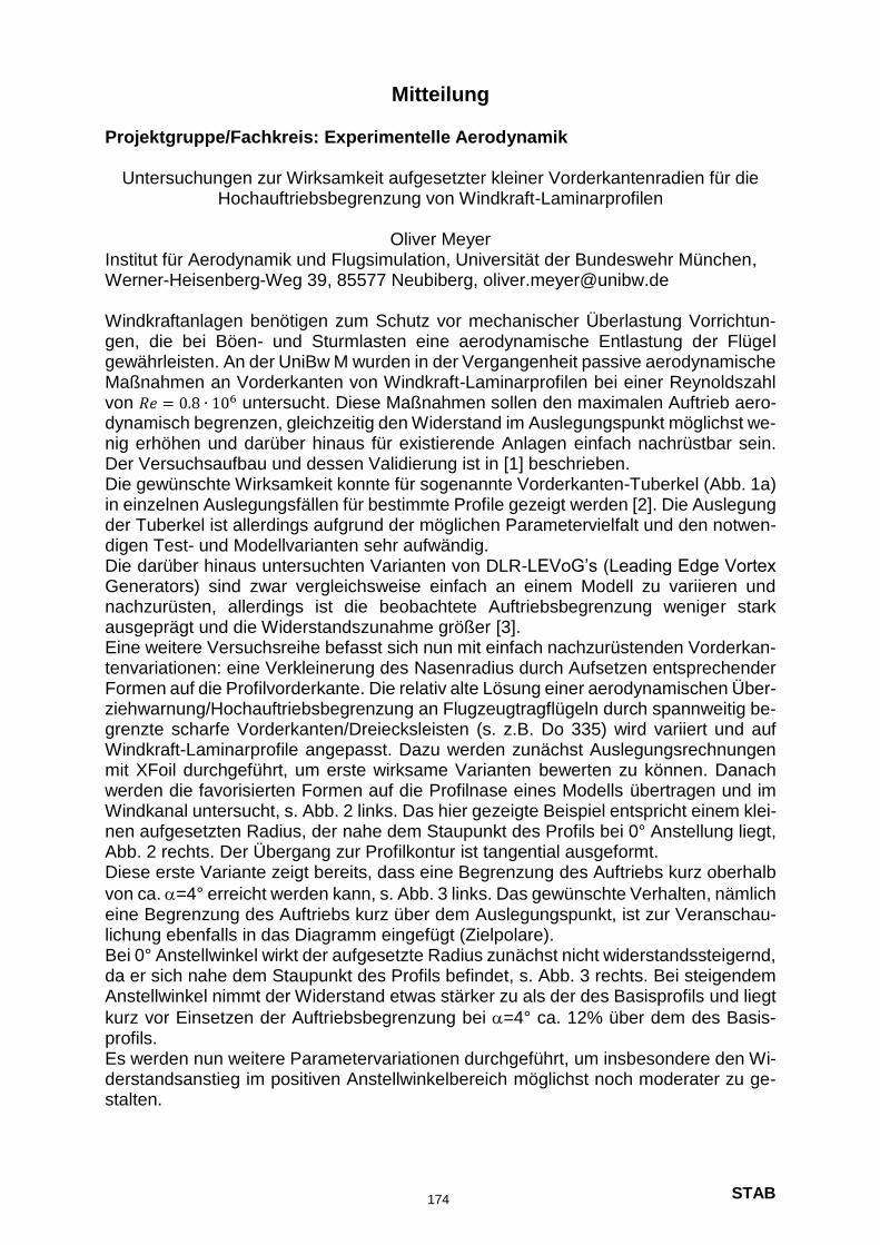
STAB

Mitteilung Projektgruppe/Fachkreis: Experimentelle Aerodynamik

Untersuchungen zur Wirksamkeit aufgesetzter kleiner Vorderkantenradien für die Hochauftriebsbegrenzung von Windkraft-Laminarprofilen

Oliver Meyer

Institut für Aerodynamik und Flugsimulation, Universität der Bundeswehr München, Werner-Heisenberg-Weg 39, 85577 Neubiberg, [email protected] Windkraftanlagen benötigen zum Schutz vor mechanischer Überlastung Vorrichtun-gen, die bei Böen- und Sturmlasten eine aerodynamische Entlastung der Flügel gewährleisten. An der UniBw M wurden in der Vergangenheit passive aerodynamische Maßnahmen an Vorderkanten von Windkraft-Laminarprofilen bei einer Reynoldszahl von 𝑅𝑒 = 0.8 ∙ 106 untersucht. Diese Maßnahmen sollen den maximalen Auftrieb aero-dynamisch begrenzen, gleichzeitig den Widerstand im Auslegungspunkt möglichst we-nig erhöhen und darüber hinaus für existierende Anlagen einfach nachrüstbar sein. Der Versuchsaufbau und dessen Validierung ist in [1] beschrieben. Die gewünschte Wirksamkeit konnte für sogenannte Vorderkanten-Tuberkel (Abb. 1a) in einzelnen Auslegungsfällen für bestimmte Profile gezeigt werden [2]. Die Auslegung der Tuberkel ist allerdings aufgrund der möglichen Parametervielfalt und den notwen-digen Test- und Modellvarianten sehr aufwändig. Die darüber hinaus untersuchten Varianten von DLR-LEVoG’s (Leading Edge Vortex Generators) sind zwar vergleichsweise einfach an einem Modell zu variieren und nachzurüsten, allerdings ist die beobachtete Auftriebsbegrenzung weniger stark ausgeprägt und die Widerstandszunahme größer [3]. Eine weitere Versuchsreihe befasst sich nun mit einfach nachzurüstenden Vorderkan-tenvariationen: eine Verkleinerung des Nasenradius durch Aufsetzen entsprechender Formen auf die Profilvorderkante. Die relativ alte Lösung einer aerodynamischen Über-ziehwarnung/Hochauftriebsbegrenzung an Flugzeugtragflügeln durch spannweitig be-grenzte scharfe Vorderkanten/Dreiecksleisten (s. z.B. Do 335) wird variiert und auf Windkraft-Laminarprofile angepasst. Dazu werden zunächst Auslegungsrechnungen mit XFoil durchgeführt, um erste wirksame Varianten bewerten zu können. Danach werden die favorisierten Formen auf die Profilnase eines Modells übertragen und im Windkanal untersucht, s. Abb. 2 links. Das hier gezeigte Beispiel entspricht einem klei-nen aufgesetzten Radius, der nahe dem Staupunkt des Profils bei 0° Anstellung liegt, Abb. 2 rechts. Der Übergang zur Profilkontur ist tangential ausgeformt. Diese erste Variante zeigt bereits, dass eine Begrenzung des Auftriebs kurz oberhalb

von ca. =4° erreicht werden kann, s. Abb. 3 links. Das gewünschte Verhalten, nämlich eine Begrenzung des Auftriebs kurz über dem Auslegungspunkt, ist zur Veranschau-lichung ebenfalls in das Diagramm eingefügt (Zielpolare). Bei 0° Anstellwinkel wirkt der aufgesetzte Radius zunächst nicht widerstandssteigernd, da er sich nahe dem Staupunkt des Profils befindet, s. Abb. 3 rechts. Bei steigendem Anstellwinkel nimmt der Widerstand etwas stärker zu als der des Basisprofils und liegt

kurz vor Einsetzen der Auftriebsbegrenzung bei =4° ca. 12% über dem des Basis-profils. Es werden nun weitere Parametervariationen durchgeführt, um insbesondere den Wi-derstandsanstieg im positiven Anstellwinkelbereich möglichst noch moderater zu ge-stalten.

174

STAB

a) Tuberkel [1] b) DLR-LEVoG’s [2] c) Variation Nasenradius

Abb. 1: Untersuchte Vorderkantenmaßnahmen

Abb. 2: links : Tragflügel mit anmodelliertem kleineren Nasenradius im Windkanal der

UniBw M, im Hintergrund Nachlaufrechen für Totaldruck und statischem Druck, rechts : Geometrie des Nasenaufsatzes an der Profilvorderkante (Prinzip)

Abb. 3 : Polaren des Basisprofils, der Zielpolare und des Basisprofils+Vorderkantenvariation

(nach Th. Tüchsen) Referenzen [1] Meyer, Oliver; Terreblanche, Tasha; Klein, Michael: Optimized Experimental Environment for

Wing Profile Investigations in the Low Speed Wind Tunnel, Proceedings of the 5th International Conference on Experimental Fluid Mechanics, Munich, Germany, 2018, pp 728-733.

[2] Terreblanche, Tasha; Meyer, Oliver; Klein, Michael: Optimization of Profile Polars for Wind Tur-bine Rotor Blades with the Use of Leading-Edge Vortex Generators, Proceedings of the 5th Inter-national Conference on Experimental Fluid Mechanics, Munich, Germany, 2018, pp 452-457.

[3] T. Terreblanche: Optimization of Profile Polars for Wind Turbine Rotor Blades with the use of Leading-Edge Vortex Generators, Master’s Thesis, TU Braunschweig, 2017

-0,6

-0,4

-0,2

0

0,2

0,4

0,6

0,8

1

1,2

1,4

1,6

-10 -5 0 5 10 15

c a [-

]

[]

Basisprofil 1

Zielpolare

VK-Radiusaufsatz 1

DesignPoint

0 0,01 0,02 0,03 0,04 0,05

cw [-]

175

STAB

Mitteilung

Projektgruppe/Fachkreis: Experimentelle Aerodynamik Q 2.2

Wake Vortex Analysis on Transport Aircraft Wing featuring Dynamic Flap Motion

Johannes Ruhland, Christian Breitsamter Lehrstuhl für Aerodynamik und Strömungsmechanik, Technische Universität Mün-

chen, Boltzmannstraße 15, 85748 Garching, [email protected] The LuFo V project BIMOD (Influencing maximum lift and wake vortex instabilities by dynam-ic flap movement), which is conducted by the Chair of Aerodynamics and Fluid Mechanics (TU Munich), the Institute of Aerospace Systems (RWTH Aachen) and the Institute of Struc-tural Mechanics (RWTH Aachen), provides a novel approach combining modern system components to achieve two different effects with one mechanism of action. On the one hand, an increase of the maximum lift is desired, on the other hand, the excitation of wake vortex instabilities to reduce the separation distances between aircraft by means of inversely oscil-lating flaps. The following investigations are limited to the aspect of wake vortex instabilities excitation. The aim is to impose a disturbance on the velocity field already in the near field of the wake vortex system [1]. The investigated geometry is a generic transport aircraft configuration based on the refer-ence geometry LR-270 (Long Range 270) configuration. The reference geometry LR-270 was created within the project BIMOD. An advanced dropped hinge flap (ADHF) System is integrated at the trailing edge and a droop nose device is located at the leading edge along the halfspan s [2] [3]. The model has three flaps. The inboard flap (IF) can be deflected stat-ically, the midboard flap (MF) and outboard flap (OF) can be operated both statically and dynamically. The spoiler deflection angle is constant. The midboard flap and outboard flap can be actuated anti-symmetrically to keep the global lift coefficient constant. The amplitude of the flap movement is determined by an excenter fixed at the motor. The frequency of the oscillation can be adjusted via the rotational speed of the motor. The wing is decoupled from the fuselage and peniche. To force turbulent boundary-layer characteristics, trip dots are installed at the leading edge of the model. This ensures the comparability of the experi-mental data to numerical results.

Figure 1: Wind tunnel model based on the geometry LR-270.

For aerodynamic force measurements and particle image velocimetry measurements (PIV), experiments are carried out in the Göttingen-type low-speed wind tunnel (W/T) A of the

176

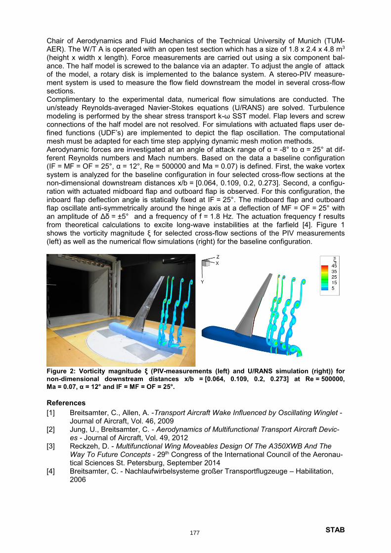
STAB

Chair of Aerodynamics and Fluid Mechanics of the Technical University of Munich (TUM-AER). The W/T A is operated with an open test section which has a size of 1.8 x 2.4 x 4.8 m3 (height x width x length). Force measurements are carried out using a six component bal-ance. The half model is screwed to the balance via an adapter. To adjust the angle of attack of the model, a rotary disk is implemented to the balance system. A stereo-PIV measure-ment system is used to measure the flow field downstream the model in several cross-flow sections. Complimentary to the experimental data, numerical flow simulations are conducted. The un/steady Reynolds-averaged Navier-Stokes equations (U/RANS) are solved. Turbulence modeling is performed by the shear stress transport k-ω SST model. Flap levers and screw connections of the half model are not resolved. For simulations with actuated flaps user de-fined functions (UDF’s) are implemented to depict the flap oscillation. The computational mesh must be adapted for each time step applying dynamic mesh motion methods. Aerodynamic forces are investigated at an angle of attack range of α = -8° to α = 25° at dif-ferent Reynolds numbers and Mach numbers. Based on the data a baseline configuration (IF = MF = OF = 25°, α = 12°, Re = 500000 and Ma = 0.07) is defined. First, the wake vortex system is analyzed for the baseline configuration in four selected cross-flow sections at the non-dimensional downstream distances x/b = [0.064, 0.109, 0.2, 0.273]. Second, a configu-ration with actuated midboard flap and outboard flap is observed. For this configuration, the inboard flap deflection angle is statically fixed at IF = 25°. The midboard flap and outboard flap oscillate anti-symmetrically around the hinge axis at a deflection of MF = OF = 25° with an amplitude of Δδ = ±5° and a frequency of f = 1.8 Hz. The actuation frequency f results from theoretical calculations to excite long-wave instabilities at the farfield [4]. Figure 1 shows the vorticity magnitude ξ for selected cross-flow sections of the PIV measurements (left) as well as the numerical flow simulations (right) for the baseline configuration.

Figure 2: Vorticity magnitude ξ (PIV-measurements (left) and U/RANS simulation (right)) for

non-dimensional downstream distances x/b = [0.064, 0.109, 0.2, 0.273] at Re = 500000,

Ma = 0.07, α = 12° and IF = MF = OF = 25°.

References

[1] Breitsamter, C., Allen, A. -Transport Aircraft Wake Influenced by Oscillating Winglet - Journal of Aircraft, Vol. 46, 2009

[2] Jung, U., Breitsamter, C. - Aerodynamics of Multifunctional Transport Aircraft Devic-es - Journal of Aircraft, Vol. 49, 2012

[3] Reckzeh, D. - Multifunctional Wing Moveables Design Of The A350XWB And The Way To Future Concepts - 29th Congress of the International Council of the Aeronau-tical Sciences St. Petersburg, September 2014

[4] Breitsamter, C. - Nachlaufwirbelsysteme großer Transportflugzeuge – Habilitation, 2006

177

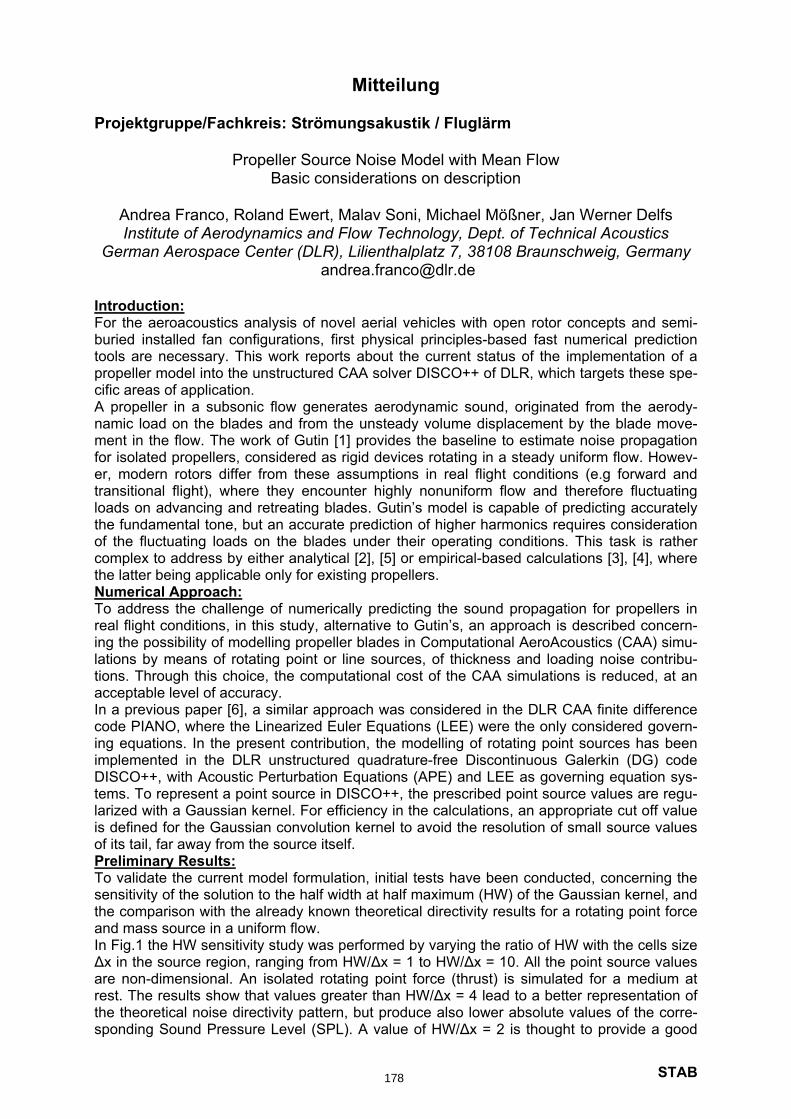
STAB

Mitteilung Projektgruppe/Fachkreis: Strömungsakustik / Fluglärm

Propeller Source Noise Model with Mean Flow Basic considerations on description

Andrea Franco, Roland Ewert, Malav Soni, Michael Mößner, Jan Werner Delfs Institute of Aerodynamics and Flow Technology, Dept. of Technical Acoustics

German Aerospace Center (DLR), Lilienthalplatz 7, 38108 Braunschweig, Germany [email protected]

Introduction: For the aeroacoustics analysis of novel aerial vehicles with open rotor concepts and semi-buried installed fan configurations, first physical principles-based fast numerical prediction tools are necessary. This work reports about the current status of the implementation of a propeller model into the unstructured CAA solver DISCO++ of DLR, which targets these spe-cific areas of application. A propeller in a subsonic flow generates aerodynamic sound, originated from the aerody-namic load on the blades and from the unsteady volume displacement by the blade move-ment in the flow. The work of Gutin [1] provides the baseline to estimate noise propagation for isolated propellers, considered as rigid devices rotating in a steady uniform flow. Howev-er, modern rotors differ from these assumptions in real flight conditions (e.g forward and transitional flight), where they encounter highly nonuniform flow and therefore fluctuating loads on advancing and retreating blades. Gutin’s model is capable of predicting accurately the fundamental tone, but an accurate prediction of higher harmonics requires consideration of the fluctuating loads on the blades under their operating conditions. This task is rather complex to address by either analytical [2], [5] or empirical-based calculations [3], [4], where the latter being applicable only for existing propellers. Numerical Approach: To address the challenge of numerically predicting the sound propagation for propellers in real flight conditions, in this study, alternative to Gutin’s, an approach is described concern-ing the possibility of modelling propeller blades in Computational AeroAcoustics (CAA) simu-lations by means of rotating point or line sources, of thickness and loading noise contribu-tions. Through this choice, the computational cost of the CAA simulations is reduced, at an acceptable level of accuracy. In a previous paper [6], a similar approach was considered in the DLR CAA finite difference code PIANO, where the Linearized Euler Equations (LEE) were the only considered govern-ing equations. In the present contribution, the modelling of rotating point sources has been implemented in the DLR unstructured quadrature-free Discontinuous Galerkin (DG) code DISCO++, with Acoustic Perturbation Equations (APE) and LEE as governing equation sys-tems. To represent a point source in DISCO++, the prescribed point source values are regu-larized with a Gaussian kernel. For efficiency in the calculations, an appropriate cut off value is defined for the Gaussian convolution kernel to avoid the resolution of small source values of its tail, far away from the source itself. Preliminary Results: To validate the current model formulation, initial tests have been conducted, concerning the sensitivity of the solution to the half width at half maximum (HW) of the Gaussian kernel, and the comparison with the already known theoretical directivity results for a rotating point force and mass source in a uniform flow. In Fig.1 the HW sensitivity study was performed by varying the ratio of HW with the cells size Δx in the source region, ranging from HW/Δx = 1 to HW/Δx = 10. All the point source values are non-dimensional. An isolated rotating point force (thrust) is simulated for a medium at rest. The results show that values greater than HW/Δx = 4 lead to a better representation of the theoretical noise directivity pattern, but produce also lower absolute values of the corre-sponding Sound Pressure Level (SPL). A value of HW/Δx = 2 is thought to provide a good

178

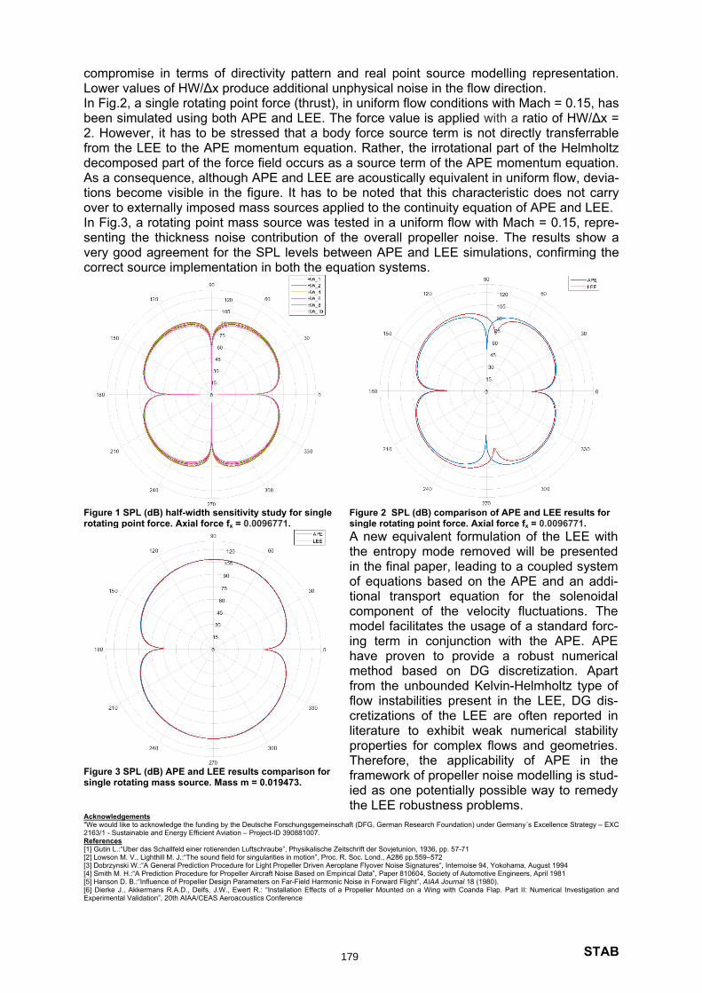
STAB

compromise in terms of directivity pattern and real point source modelling representation. Lower values of HW/Δx produce additional unphysical noise in the flow direction. In Fig.2, a single rotating point force (thrust), in uniform flow conditions with Mach = 0.15, has been simulated using both APE and LEE. The force value is applied with a ratio of HW/Δx = 2. However, it has to be stressed that a body force source term is not directly transferrable from the LEE to the APE momentum equation. Rather, the irrotational part of the Helmholtz decomposed part of the force field occurs as a source term of the APE momentum equation. As a consequence, although APE and LEE are acoustically equivalent in uniform flow, devia-tions become visible in the figure. It has to be noted that this characteristic does not carry over to externally imposed mass sources applied to the continuity equation of APE and LEE. In Fig.3, a rotating point mass source was tested in a uniform flow with Mach = 0.15, repre-senting the thickness noise contribution of the overall propeller noise. The results show a very good agreement for the SPL levels between APE and LEE simulations, confirming the correct source implementation in both the equation systems.

Acknowledgements "We would like to acknowledge the funding by the Deutsche Forschungsgemeinschaft (DFG, German Research Foundation) under Germany´s Excellence Strategy – EXC 2163/1 - Sustainable and Energy Efficient Aviation – Project-ID 390881007. References [1] Gutin L.:“Uber das Schallfeld einer rotierenden Luftschraube”, Physikalische Zeitschrift der Sovjetunion, 1936, pp. 57-71 [2] Lowson M. V., Lighthill M. J.:“The sound field for singularities in motion”, Proc. R. Soc. Lond., A286 pp.559–572 [3] Dobrzynski W.:“A General Prediction Procedure for Light Propeller Driven Aeroplane Flyover Noise Signatures“, Internoise 94, Yokohama, August 1994 [4] Smith M. H.:“A Prediction Procedure for Propeller Aircraft Noise Based on Empirical Data”, Paper 810604, Society of Automotive Engineers, April 1981 [5] Hanson D. B.:“Influence of Propeller Design Parameters on Far-Field Harmonic Noise in Forward Flight”, AIAA Journal 18 (1980). [6] Dierke J., Akkermans R.A.D., Delfs, J.W., Ewert R.: “Installation Effects of a Propeller Mounted on a Wing with Coanda Flap. Part II: Numerical Investigation and Experimental Validation”, 20th AIAA/CEAS Aeroacoustics Conference

Figure 1 SPL (dB) half-width sensitivity study for single rotating point force. Axial force fx = 0.0096771.

Figure 2 SPL (dB) comparison of APE and LEE results for single rotating point force. Axial force fx = 0.0096771.

A new equivalent formulation of the LEE with the entropy mode removed will be presented in the final paper, leading to a coupled system of equations based on the APE and an addi-tional transport equation for the solenoidal component of the velocity fluctuations. The model facilitates the usage of a standard forc-ing term in conjunction with the APE. APE have proven to provide a robust numerical method based on DG discretization. Apart from the unbounded Kelvin-Helmholtz type of flow instabilities present in the LEE, DG dis-cretizations of the LEE are often reported in literature to exhibit weak numerical stability properties for complex flows and geometries. Therefore, the applicability of APE in the framework of propeller noise modelling is stud-ied as one potentially possible way to remedy the LEE robustness problems.

Figure 3 SPL (dB) APE and LEE results comparison for single rotating mass source. Mass m = 0.019473.

179

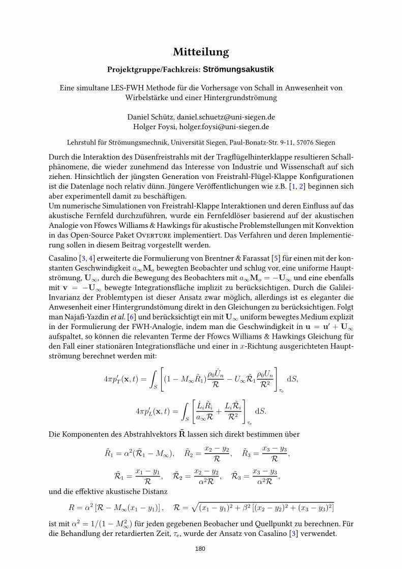
Mitteilung

Projektgruppe/Fachkreis: Strömungsakustik

Eine simultane LES-FWH Methode für die Vorhersage von Schall in Anwesenheit von

Wirbelstärke und einer Hintergrundströmung

Daniel Schütz, [email protected]

Holger Foysi, [email protected]

Lehrstuhl für Strömungsmechnik, Universität Siegen, Paul-Bonatz-Str. 9-11, 57076 Siegen

Durch die Interaktion des Düsenfreistrahls mit der Tragflügelhinterklappe resultieren Schall-

phänomene, die wieder zunehmend das Interesse von Industrie und Wissenschaft auf sich

ziehen. Hinsichtlich der jüngsten Generation von Freistrahl-Flügel-Klappe Konfigurationen

ist die Datenlage noch relativ dünn. Jüngere Veröffentlichungen wie z.B. [1, 2] beginnen sich

aber experimentell damit zu beschäftigen.

Um numerische Simulationen von Freistrahl-Klappe Interaktionen und deren Einfluss auf das

akustische Fernfeld durchzuführen, wurde ein Fernfeldlöser basierend auf der akustischen

Analogie von FfowcsWilliams &Hawkings für akustische Problemstellungenmit Konvektion

in das Open-Source Paket Overture implementiert. Das Verfahren und deren Implementie-

rung sollen in diesem Beitrag vorgestellt werden.

Casalino [3, 4] erweiterte die Formulierung von Brentner & Farassat [5] für einenmit der kon-

stanten Geschwindigkeit a∞Mo bewegten Beobachter und schlug vor, eine uniforme Haupt-

strömung, U∞, durch die Bewegung des Beobachters mit a∞Mo = −U∞ und eine ebenfalls

mit v = −U∞ bewegte Integrationsfläche implizit zu berücksichtigen. Durch die Galilei-

Invarianz der Problemtypen ist dieser Ansatz zwar möglich, allerdings ist es eleganter die

Anwesenheit einer Hintergrundstömung direkt in den Gleichungen zu berücksichtigen. Folgt

manNajafi-Yazdin et al. [6] und berücksichtigt ein mitU∞ uniform bewegtes Medium explizit

in der Formulierung der FWH-Analogie, indem man die Geschwindigkeit in u = u′ + U∞

aufspaltet, so können die relevanten Terme der Ffowcs Williams & Hawkings Gleichung für

den Fall einer stationären Integrationsfläche und einer in x-Richtung ausgerichteten Haupt-

strömung berechnet werden mit:

4πp′T (x, t) =

∫

S

[

(1−M∞R1)ρ0Un

R− U∞R1

ρ0Un

R2

]

τe

dS,

4πp′L(x, t) =

∫

S

[

LiRi

a∞R+

LiRi

R2

]

τe

dS.

Die Komponenten des Abstrahlvektors R lassen sich direkt bestimmen über

R1 = α2(R1 −M∞), R2 =x2 − y2

R, R3 =

x3 − y3R

,

R1 =x1 − y1

R, R2 =

x2 − y2α2R

, R3 =x3 − y3α2R

,

und die effektive akustische Distanz

R = α2 [R−M∞(x1 − y1)] , R =√

(x1 − y1)2 + β2 [(x2 − y2)2 + (x3 − y3)2]

ist mit α2 = 1/(1−M2

∞) für jeden gegebenen Beobacher und Quellpunkt zu berechnen. Für

die Behandlung der retardierten Zeit, τe, wurde der Ansatz von Casalino [3] verwendet.

180

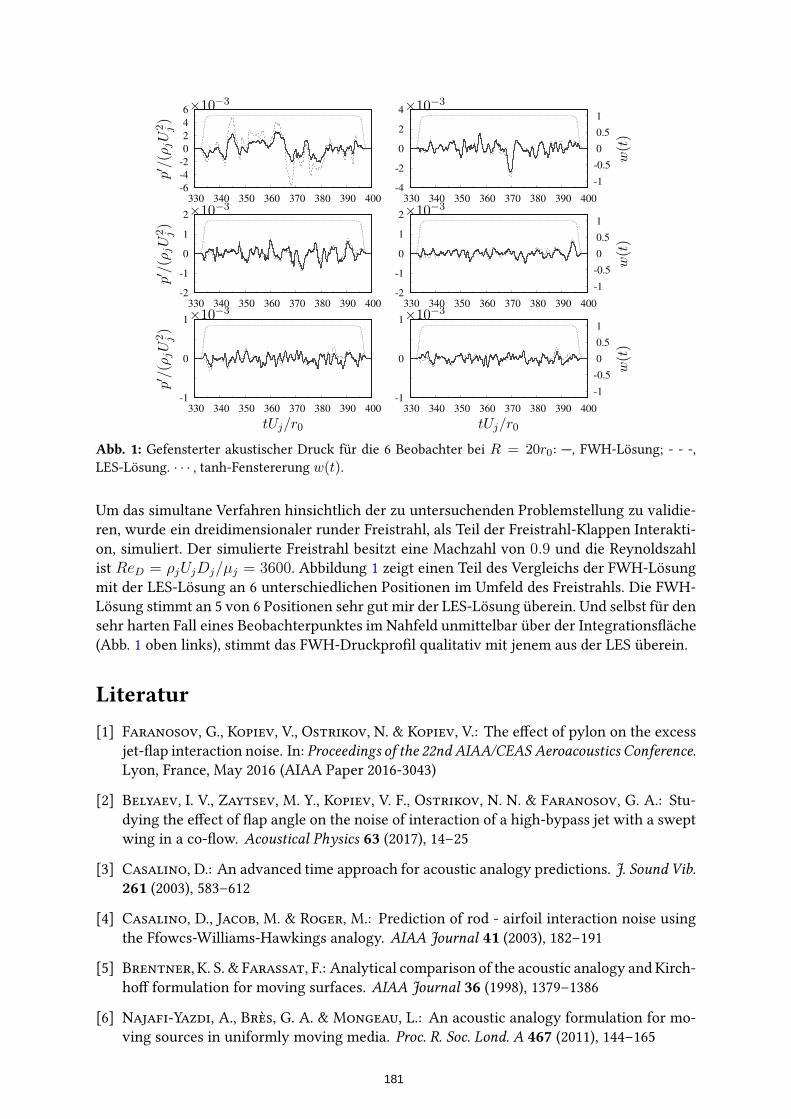
-6

-4

-2

0

2

4

6

330 340 350 360 370 380 390 400

-4

-2

0

2

4

330 340 350 360 370 380 390 400

-1

-0.5

0

0.5

1

-2

-1

0

1

2

330 340 350 360 370 380 390 400

-2

-1

0

1

2

330 340 350 360 370 380 390 400

-1

-0.5

0

0.5

1

-1

0

1

330 340 350 360 370 380 390 400

-1

0

1

330 340 350 360 370 380 390 400

-1

-0.5

0

0.5

1

p′/(ρjU

2 j)

p′/(ρjU

2 j)

p′/(ρjU

2 j)

w(t)

w(t)

w(t)

tUj/r0tUj/r0

×10−3×10−3

×10−3×10−3

×10−3×10−3

Abb. 1: Gefensterter akustischer Druck für die 6 Beobachter bei R = 20r0: —, FWH-Lösung; - - -,

LES-Lösung. · · · , tanh-Fenstererung w(t).

Um das simultane Verfahren hinsichtlich der zu untersuchenden Problemstellung zu validie-

ren, wurde ein dreidimensionaler runder Freistrahl, als Teil der Freistrahl-Klappen Interakti-

on, simuliert. Der simulierte Freistrahl besitzt eine Machzahl von 0.9 und die Reynoldszahl

ist ReD = ρjUjDj/µj = 3600. Abbildung 1 zeigt einen Teil des Vergleichs der FWH-Lösung

mit der LES-Lösung an 6 unterschiedlichen Positionen im Umfeld des Freistrahls. Die FWH-

Lösung stimmt an 5 von 6 Positionen sehr gut mir der LES-Lösung überein. Und selbst für den

sehr harten Fall eines Beobachterpunktes im Nahfeld unmittelbar über der Integrationsfläche

(Abb. 1 oben links), stimmt das FWH-Druckprofil qualitativ mit jenem aus der LES überein.

Literatur

[1] Faranosov, G., Kopiev, V., Ostrikov, N. & Kopiev, V.: The effect of pylon on the excess

jet-flap interaction noise. In: Proceedings of the 22nd AIAA/CEAS Aeroacoustics Conference.

Lyon, France, May 2016 (AIAA Paper 2016-3043)

[2] Belyaev, I. V., Zaytsev, M. Y., Kopiev, V. F., Ostrikov, N. N. & Faranosov, G. A.: Stu-

dying the effect of flap angle on the noise of interaction of a high-bypass jet with a swept

wing in a co-flow. Acoustical Physics 63 (2017), 14–25

[3] Casalino, D.: An advanced time approach for acoustic analogy predictions. J. Sound Vib.

261 (2003), 583–612

[4] Casalino, D., Jacob, M. & Roger, M.: Prediction of rod - airfoil interaction noise using

the Ffowcs-Williams-Hawkings analogy. AIAA Journal 41 (2003), 182–191

[5] Brentner, K. S. & Farassat, F.: Analytical comparison of the acoustic analogy and Kirch-

hoff formulation for moving surfaces. AIAA Journal 36 (1998), 1379–1386

[6] Najafi-Yazdi, A., Brès, G. A. & Mongeau, L.: An acoustic analogy formulation for mo-

ving sources in uniformly moving media. Proc. R. Soc. Lond. A 467 (2011), 144–165

181

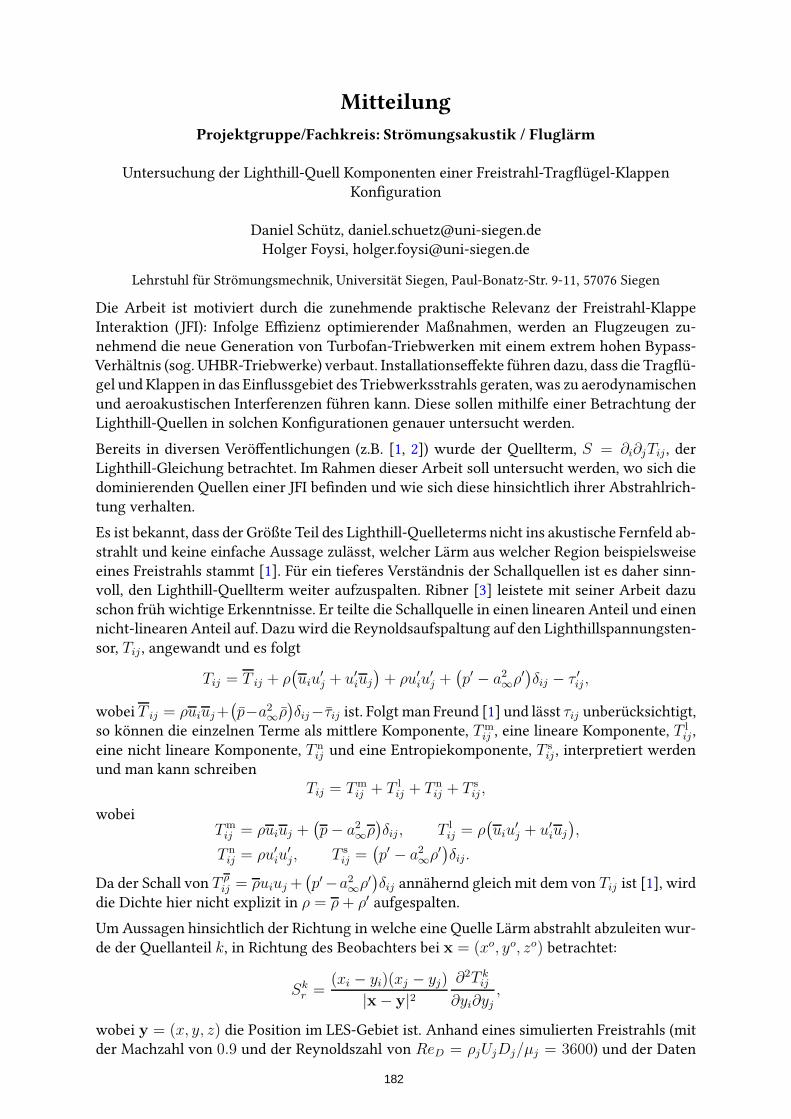
Mitteilung

Projektgruppe/Fachkreis: Strömungsakustik / Fluglärm

Untersuchung der Lighthill-Quell Komponenten einer Freistrahl-Tragflügel-Klappen

Konfiguration

Daniel Schütz, [email protected]

Holger Foysi, [email protected]

Lehrstuhl für Strömungsmechnik, Universität Siegen, Paul-Bonatz-Str. 9-11, 57076 Siegen

Die Arbeit ist motiviert durch die zunehmende praktische Relevanz der Freistrahl-Klappe

Interaktion (JFI): Infolge Effizienz optimierender Maßnahmen, werden an Flugzeugen zu-

nehmend die neue Generation von Turbofan-Triebwerken mit einem extrem hohen Bypass-

Verhältnis (sog. UHBR-Triebwerke) verbaut. Installationseffekte führen dazu, dass die Tragflü-

gel und Klappen in das Einflussgebiet des Triebwerksstrahls geraten,was zu aerodynamischen

und aeroakustischen Interferenzen führen kann. Diese sollen mithilfe einer Betrachtung der

Lighthill-Quellen in solchen Konfigurationen genauer untersucht werden.

Bereits in diversen Veröffentlichungen (z.B. [1, 2]) wurde der Quellterm, S = ∂i∂jTij , der

Lighthill-Gleichung betrachtet. Im Rahmen dieser Arbeit soll untersucht werden, wo sich die

dominierenden Quellen einer JFI befinden und wie sich diese hinsichtlich ihrer Abstrahlrich-

tung verhalten.

Es ist bekannt, dass der Größte Teil des Lighthill-Quelleterms nicht ins akustische Fernfeld ab-

strahlt und keine einfache Aussage zulässt, welcher Lärm aus welcher Region beispielsweise

eines Freistrahls stammt [1]. Für ein tieferes Verständnis der Schallquellen ist es daher sinn-

voll, den Lighthill-Quellterm weiter aufzuspalten. Ribner [3] leistete mit seiner Arbeit dazu

schon früh wichtige Erkenntnisse. Er teilte die Schallquelle in einen linearen Anteil und einen

nicht-linearen Anteil auf. Dazu wird die Reynoldsaufspaltung auf den Lighthillspannungsten-

sor, Tij , angewandt und es folgt

Tij = T ij + ρ(

uiu′

j + u′

iuj

)

+ ρu′

iu′

j +(

p′ − a2∞ρ′)

δij − τ ′ij ,

wobei T ij = ρuiuj+(

p−a2∞ρ)

δij−τij ist. Folgt man Freund [1] und lässt τij unberücksichtigt,so können die einzelnen Terme als mittlere Komponente, Tm

ij , eine lineare Komponente, T l

ij ,

eine nicht lineare Komponente, T n

ij und eine Entropiekomponente, T s

ij , interpretiert werden

und man kann schreiben

Tij = Tm

ij + T l

ij + T n

ij + T s

ij ,

wobeiTm

ij = ρuiuj +(

p− a2∞ρ)

δij , T l

ij = ρ(

uiu′

j + u′

iuj

)

,

T n

ij = ρu′

iu′

j, T s

ij =(

p′ − a2∞ρ′)

δij.

Da der Schall von T ρij = ρuiuj +

(

p′−a2∞ρ′)

δij annähernd gleich mit dem von Tij ist [1], wird

die Dichte hier nicht explizit in ρ = ρ+ ρ′ aufgespalten.

Um Aussagen hinsichtlich der Richtung in welche eine Quelle Lärm abstrahlt abzuleiten wur-

de der Quellanteil k, in Richtung des Beobachters bei x = (xo, yo, zo) betrachtet:

Skr =

(xi − yi)(xj − yj)

|x− y|2∂2T k

ij

∂yi∂yj,

wobei y = (x, y, z) die Position im LES-Gebiet ist. Anhand eines simulierten Freistrahls (mit

der Machzahl von 0.9 und der Reynoldszahl von ReD = ρjUjDj/µj = 3600) und der Daten

182

θ = 15 θ = 30 θ = 45

θ = 60 θ = 75 θ = 90

Abb. 1: Instantane Visualisierung von Sl

θ in der x-y-Ebene bei z = 0. Konturen: 8 Ebenen bei

Sr20/(ρjU

2j ) = ±0.5, 1.5, 3, 6. Positive und negative Werte sind solide bzw. gestichelt dargestellt, die

maximale Ebene ist zudem rot und die minimale blau koloriert

θ = 15 θ = 30 θ = 45

θ = 60 θ = 75 θ = 90

Abb. 2: Instantane Visualisierung von Sn

θ .

von Freund [1] und Uzun et al. [2] wurde dieses Vorgehen validiert. Abbildung1 und 2 zeigen

den linearen bzw. nicht-linearen Anteil von S abgeleitet in diverse Richtungen. Der lineare

Anteile weist im Gegensatz zum nicht-linearen Anteil eine deutliche Richtungsabhängikeit

auf. Dieses Verhalten wird durch die Untersuchungen von Freund und Uzun, neben Anderen,

bestätigt.

Ziel dieser Arbeit ist es, den oben vorgestellten Ansatz auf die in [4] vorgestellte Freistrahl-

Tragfügel-Klappen Konfigurationen anzuwenden um Rückschlüsse auf die dominanten Quel-

lanteile und ihre Abstrahlcharakteristik zu erhalten. Erste Ergebnisse dieser Untersuchung

sollen in einem ausführlicheren Artikel vorgestellt werden.

Literatur

[1] Freund, J. B.: Noise-source turbulence statistics and the noise from a Mach 0.9 jet. Phys.

Fluids 15 (2003), 1788–1799

[2] Uzun, A., S., Lyrintzis A. & Blaisdell, G. A.: Coupling of integral acoustics methods with

LES for jet noise prediction. Int. J. Aeroac. 3 (2005), 297–346

[3] Ribner, H. S.: Quadrupole correlations governing the pattern of jet noise. J. Fluid Mech.

38 (1969), 1–24

[4] Schütz, D. & Foysi, H.: Towards the Prediction of Flow and Acoustic Fields of a Jet-

Wing-Flap Configuration. In: New Results in Numerical and Experimental Fluid Mechanics

XI, Springer International Publishing, 2018, 659–669

183

Mitteilung

Projektgruppe/Fachkreis: Strömungsakustik

Jet Noise Prediction using Hybrid RANS/LES Simulation in SU2

Beckett Y. Zhou, and Nicolas R. Gauger Chair for Scientific Computing, TU Kaiserslautern

Bldg 34, Paul-Ehrlich-Strasse, 67663 Kaiserslautern, [email protected]

Eduardo S. Molina, and Juan J. Alonso Aerospace Design Laboratory, Stanford University

Stanford, CA 94305, USA

Ulf Michel and Frank Thiele CFD Software Entwicklungs- und Forschungsgesellschaft mbH

Wolzogenstrasse 4, 14163 Berlin, Germany

IntroductionNoise generated by the turbulent mixing of jets exiting the aircraft engine nozzle is asignificant contributor to the overall aircraft noise. Therefore, it is essential to understand andaccurately predict the flow of turbulent jets and the associated noise generation mechanismsin the quest to suppress jet-related aircraft noise. While it is possible to resolve the noisesource of an isolated jet using large-eddy simulations (LES), the exorbitant computationalcost associated with the turbulent boundary layer at practical Reynolds numbers makes suchmethods intractable for jet-installation noise prediction. In this paper, we present a hybridRANS/LES approach to circumvent such issue where the attached boundary layer ismodelled using RANS while the turbulence in the jet plume is resolved using LES.

MethodIn the present study, the Navier-Stokes equations are solved using the open-source SU2code [1]. The finite volume method (FVM) is applied on arbitrary unstructured meshes usinga standard edge-based data structure on a dual grid with control volumes constructed usinga median-dual, vertex-based scheme. SU2 is capable of solving unsteady problems implicitlyusing dual-time stepping, leading to second-order accuracy in both space and time. For thespatial discretization of the convective fluxes, a low-dissipation and low-dispersion skew-symmetric central scheme (LD2) is used [2]. The enhanced delayed detached-eddysimulation based on the Spalart-Allmaras turbulence model (EDDES-SA) and its variantswas implemented in SU2 by Molina [3] and has been successfully applied to predictseparated flows [4]. To mitigate the “grey area” problem characterized by slow transition fromRANS to LES mode in the initial shear-layer, a shear-layer adapted (SLA) sub-grid scalemodel [5] was implemented. For far-field noise prediction, a permeable-surface Ffowcs-Williams and Hawkings (FWH) acoustic analogy implemented by Zhou et al. [6] is used.

Preliminary ResultsIn this work, we study the turbulent flow exiting an isothermal round jet at a jet Mach numberof Mj = 0.9. The Reynolds number based on the nozzle diameter of D = 0.06223m is ReD =1.1×106. This test case was previously studied in the framework of an EU Project Go4Hybrid(G4H) and simulated with similar hybrid RANS/LES approaches employed in this work. Thetransient simulation is performed using the SU2 EDDES-SA solver on the common grid ‘G3’considered in G4H, containing 8.8 million cells. The simulation results are compared againstexperimental data from Bridges and Wernet [7]. The non-dimensional time step based on thenozzle diameter and jet axial velocity is 0.006. A total of 400 convective time units (CTU) areused to compute the turbulence statistics after an initial transient of 400 CTU. Fig. 1 reveals

STAB184


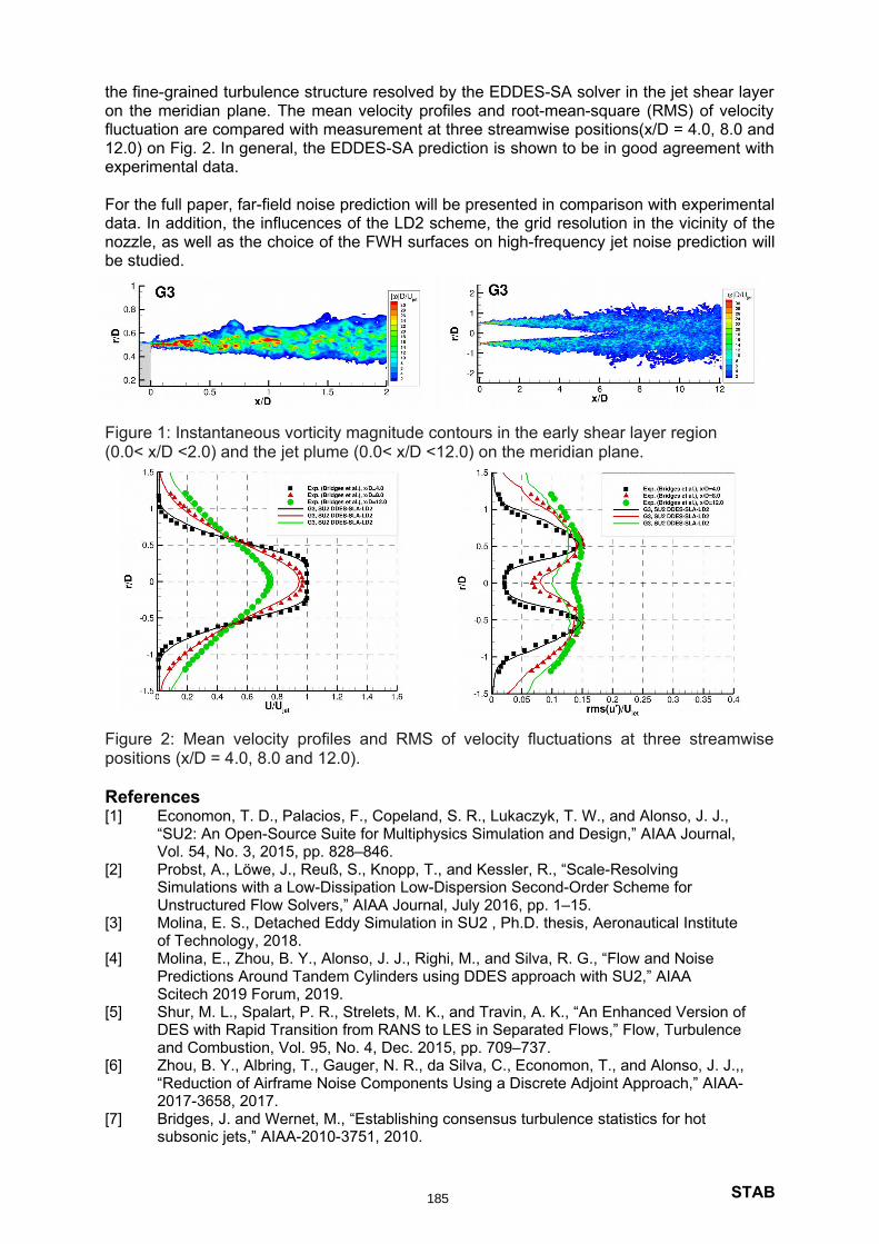
the fine-grained turbulence structure resolved by the EDDES-SA solver in the jet shear layeron the meridian plane. The mean velocity profiles and root-mean-square (RMS) of velocityfluctuation are compared with measurement at three streamwise positions(x/D = 4.0, 8.0 and12.0) on Fig. 2. In general, the EDDES-SA prediction is shown to be in good agreement withexperimental data.

For the full paper, far-field noise prediction will be presented in comparison with experimentaldata. In addition, the influcences of the LD2 scheme, the grid resolution in the vicinity of thenozzle, as well as the choice of the FWH surfaces on high-frequency jet noise prediction willbe studied.

Figure 1: Instantaneous vorticity magnitude contours in the early shear layer region (0.0< x/D <2.0) and the jet plume (0.0< x/D <12.0) on the meridian plane.

Figure 2: Mean velocity profiles and RMS of velocity fluctuations at three streamwisepositions (x/D = 4.0, 8.0 and 12.0).

References[1] Economon, T. D., Palacios, F., Copeland, S. R., Lukaczyk, T. W., and Alonso, J. J.,

“SU2: An Open-Source Suite for Multiphysics Simulation and Design,” AIAA Journal, Vol. 54, No. 3, 2015, pp. 828–846.

[2] Probst, A., Löwe, J., Reuß, S., Knopp, T., and Kessler, R., “Scale-Resolving Simulations with a Low-Dissipation Low-Dispersion Second-Order Scheme for Unstructured Flow Solvers,” AIAA Journal, July 2016, pp. 1–15.

[3] Molina, E. S., Detached Eddy Simulation in SU2 , Ph.D. thesis, Aeronautical Institute of Technology, 2018.

[4] Molina, E., Zhou, B. Y., Alonso, J. J., Righi, M., and Silva, R. G., “Flow and Noise Predictions Around Tandem Cylinders using DDES approach with SU2,” AIAA Scitech 2019 Forum, 2019.

[5] Shur, M. L., Spalart, P. R., Strelets, M. K., and Travin, A. K., “An Enhanced Version of DES with Rapid Transition from RANS to LES in Separated Flows,” Flow, Turbulence and Combustion, Vol. 95, No. 4, Dec. 2015, pp. 709–737.

[6] Zhou, B. Y., Albring, T., Gauger, N. R., da Silva, C., Economon, T., and Alonso, J. J.,, “Reduction of Airframe Noise Components Using a Discrete Adjoint Approach,” AIAA-2017-3658, 2017.

[7] Bridges, J. and Wernet, M., “Establishing consensus turbulence statistics for hot subsonic jets,” AIAA-2010-3751, 2010.

STAB185

Namensverzeichnis der Autoren und Koautoren

Autor Seite Autor Seite

Abu-Zurayk 26 Geyr von Schweppenburg 70

Adams 170 Goetzendorf-Grabowski 94

Aggarwal 76 Göing 138

Alonso 184 Greiner 62

Asaro 52 Guseva 32

Babij 82 Hanifi 72

Bach 128 Hartmann 76

Bauer 110 Heckmeier 78, 170

Bauknecht 52 Hein 56, 68, 72

Bell 120, 124, 126 Heine 124, 126

Birkenmaier 112 Heinrich 162

Bleh 152 Helm 54, 58

Bock 142 Henning 120

Braukmann 86 Herbert 28

Braun 154 Herr 148

Breitsamter 78, 84, 90, 96, 134, 136,168, 170, 176 Herzog 90

Brückner 114 Hillebrand 22

Burton 120 Hogrefe 138

Bustamante López 130 Hopfes 170

Cerny 84, 90 Huismann 42

Chauvat 72 Ilic 26

Cormier 144 Jäckel 150

Cruz 70 Jessing 126

Debernardis 86 Kaiser 54

Delfs 178 Keßler 146

Domogalla 88 Khalil 52

Eggers 48 Klaas 34

Ehrenfried 110 Klein, Markus 158

Ehrle 20 Klein, Marten 30

Ertunc 28 Klimmek 54

Ewert 178 Knopp 32

Faust 84, 90 Kohl 116

Fechter 42 Konosidou 50

Fehrs 54, 58 Korsmeier 32

Feldwisch 128, 132 Kostek 94, 100

Flock 50 Krämer 20, 22, 24, 74, 144, 146

Foysi 180, 182 Krenkel 112

Franco Sumariva 56, 72 Krimmelbein 58, 60

Franco 178 Krumbein 58, 60

Franze 40 Krzikalla 152

Friedrichs 138 Kümmel 96

Gagnon 92 Kunze 98

Gauger 36, 184 Lange 116

Genuit 146 Langer 76, 154

Gerhold 152 Leicht 42, 76, 154

186

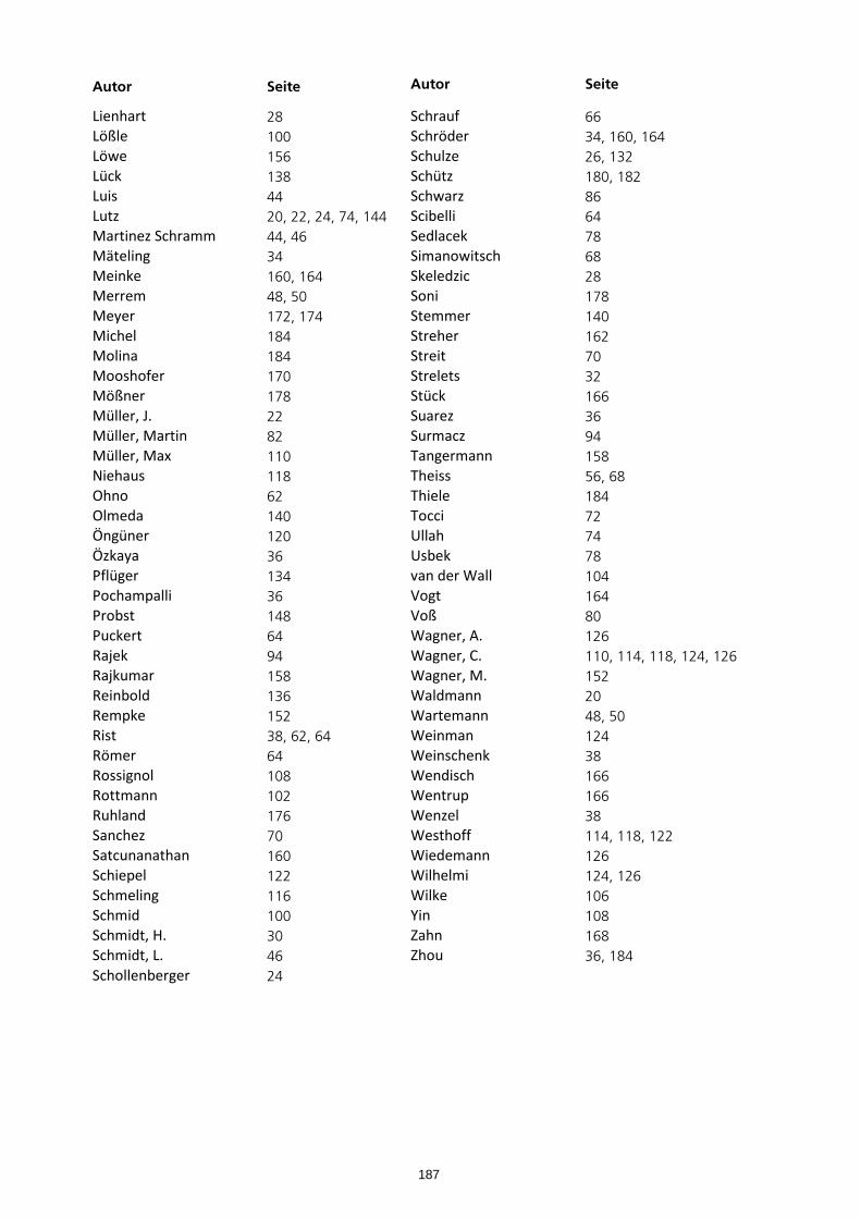
Autor Seite Autor Seite

Lienhart 28 Schrauf 66

Lößle 100 Schröder 34, 160, 164

Löwe 156 Schulze 26, 132

Lück 138 Schütz 180, 182

Luis 44 Schwarz 86

Lutz 20, 22, 24, 74, 144 Scibelli 64

Martinez Schramm 44, 46 Sedlacek 78

Mäteling 34 Simanowitsch 68

Meinke 160, 164 Skeledzic 28

Merrem 48, 50 Soni 178

Meyer 172, 174 Stemmer 140

Michel 184 Streher 162

Molina 184 Streit 70

Mooshofer 170 Strelets 32

Mößner 178 Stück 166

Müller, J. 22 Suarez 36

Müller, Martin 82 Surmacz 94

Müller, Max 110 Tangermann 158

Niehaus 118 Theiss 56, 68

Ohno 62 Thiele 184

Olmeda 140 Tocci 72

Öngüner 120 Ullah 74

Özkaya 36 Usbek 78

Pflüger 134 van der Wall 104

Pochampalli 36 Vogt 164

Probst 148 Voß 80

Puckert 64 Wagner, A. 126

Rajek 94 Wagner, C. 110, 114, 118, 124, 126

Rajkumar 158 Wagner, M. 152

Reinbold 136 Waldmann 20

Rempke 152 Wartemann 48, 50

Rist 38, 62, 64 Weinman 124

Römer 64 Weinschenk 38

Rossignol 108 Wendisch 166

Rottmann 102 Wentrup 166

Ruhland 176 Wenzel 38

Sanchez 70 Westhoff 114, 118, 122

Satcunanathan 160 Wiedemann 126

Schiepel 122 Wilhelmi 124, 126

Schmeling 116 Wilke 106

Schmid 100 Yin 108

Schmidt, H. 30 Zahn 168

Schmidt, L. 46 Zhou 36, 184

Schollenberger 24

187

J A H R E S B E R I C H T 2020 - DLR - Deutsches Zentrum für ...

Documents

Transcript of J A H R E S B E R I C H T 2020 - DLR - Deutsches Zentrum für ...