Development of a spherical motor with a 3‑DOF sensing system
194
This document is downloaded from DR‑NTU (https://dr.ntu.edu.sg) Nanyang Technological University, Singapore. Development of a spherical motor with a 3‑DOF sensing system Guo, Jinjun 2016 Guo, J. (2016). Development of a spherical motor with a 3‑DOF sensing system. Doctoral thesis, Nanyang Technological University, Singapore. https://hdl.handle.net/10356/69085 https://doi.org/10.32657/10356/69085 Downloaded on 11 Feb 2022 14:27:35 SGT
-
Upload
khangminh22 -
Category
Documents
-
view
4 -
download
0
Transcript of Development of a spherical motor with a 3‑DOF sensing system

This document is downloaded from DR‑NTU (https://dr.ntu.edu.sg)Nanyang Technological University, Singapore.
Development of a spherical motor with a 3‑DOFsensing system
Guo, Jinjun
2016
Guo, J. (2016). Development of a spherical motor with a 3‑DOF sensing system. Doctoralthesis, Nanyang Technological University, Singapore.
https://hdl.handle.net/10356/69085
https://doi.org/10.32657/10356/69085
Downloaded on 11 Feb 2022 14:27:35 SGT

1
DEVELOPMENT OF A SPHERICAL MOTOR WITH A 3-DOF
SENSING SYSTEM
GUO JINJUN
School of Mechanical & Aerospace Engineering
A dissertation submitted to Nanyang Technological University
in partial fulfilment of the requirement for the degree of
DOCTOR OF PHILOSOPHY
2016

i
ABSTRACT
The thesis proposes a new design of a spherical wheel motor (SWM) with three layers
of permanent magnets (PMs) located both inside and outside of double layers of
electrical magnets (EMs), so as to fully utilize the magnetic field generated by the EMs
and enhance the inclination torque density. The inclination torque is generally weak due
to the limited number and space for the PMs and EMs involved in inclination compared
to spinning. Finite element modeling (FEM) has been utilized for simulation, and
important design parameters are optimized to maximize the inclination torque. The
FEM modeling has been verified by experiments with discrepancy of less than 10%
achieved. The optimized design can generate strong inclination torque which can
support heavy loadings. Iron stator cores are applied in the new design to improve
magnetic torque, and the magnetic field distribution (MFD) and magnetic torque
become nonlinear due to magnetic saturation characteristics of the iron cores. Based on
the analysis of the MFD of the whole SWM applying different current inputs, the thesis
has constructed a dynamic model for SWMs with current inputs within the working
range. A multi-DOF non-contact sensing system based on magnetic sensors and neural
networks (NNs) is proposed. NNs are applied to approximate the function between
orientations and MFD. The proposed sensing system is simulated and verified by
experimental investigations. The sensing error to working range ratio is about 1.4%,
which verifies its feasibility. With the proposed SWM design with enhanced torque
capability, dynamic model and sensing system, the present findings provide strong basis
to realize an integrated system of an SWM and take it a step closer to industrial
applications.

ii
ACKNOWLEDGEMENT
First of all, I would like to express my heartfelt thanks and gratitude to my former
supervisor, Asst/P Dr. Hungsun Son, for his continuous and patient guidance, generous
help and valuable advice throughout the project. Prof. Hungsun Son is a kind,
hardworking and humorous person who is knowledgeable and always coming up with
new ideas, and I am deeply thankful for having the opportunity to work with him. Prof.
Hungsun has been back to Korea, but as the Chinese saying goes, I always respect him
as my mentor.
I am very grateful for my existing supervisors Assoc/P Ng Teng Yong and Assoc/Prof
Seet Gim Lee, Gerald. Without their guidance, I may have already given up as the way
to be a Doctor is always depressing and stressful. I will always remember Prof. Ng’s
words to persuade me not to give up in any case, and Prof. Seet’s professional guidance
on editing thesis.
I want to thank MAE staffs, thank professors who teach us in courses like Assoc/Prof
Li Hua, and professors who instruct me in confirmation report like Prof Chen I-Ming.
I also want to thank MAE technicians for their help in my research project.
I want to thank my companions in the lab, they are Mr. Xiao, Mr. You, Mr. Amit and
Ms. Wu. We always discuss problems in every aspect and share good stuffs. Thanks to
them, we have great lab environment which is beneficial for study and research.

iii
I want to express my appreciations and thanks to staffs of the Manufacturing Process
Laboratory. With the careful and patient help from Ms. Tan, Mr. Koh, Mr. Lim, Mr.
Wong and Mr. Yew, the prototype of SWM can be fabricated successfully and precisely.
I would like to thank my family, and my wife Zhang Yuting who has been with me and
support since high school and my two children Haoyi and Meiyan as my motion source.
Last but not least, I would like to thank all persons not mentioned above but who have
in one way or another, provided help throughout my research period.

iv
TABLE OF CONTENTS
ABSTRACT…………………………………………………………...………………i
ACKNOWLEDGEMENT………………………………………………...…….……i
TABLE OF CONTENTS…………………………………………………………….iv
LIST OF FIGURES…………………………………………………...…….….…..vii
LIST OF TABLES………………………………………………………………..….xi
LIST OF ABBREATIONS………………………………………………….…....…xii
LIST OF SYMBOLS……………………………………………………………….xiv
CHAPTER 1 INTRODUCTION…………………………………………………….1
1.1 Motivation ................................................................................................ .1
1.2 Background ............................................................................................... 5
1.3 Literature Review...................................................................................... 8
1.3.1 Spherical Ultrasonic Motor (SUSM) ................................................ 8
1.3.2 Designs of Spherical Electromagnetic Motors ............................... 12
1.3.3 Magnetic Field and Torque Analysis of Spherical Electromagnetic
Motors………………………………………………………………..…....16
1.3.4 Sensing System Designs for Spherical Electromagnetic Motors ... 18
1.3.5 Other Multi-DOF Actuators ............................................................ 20
1.4 Objective ................................................................................................. 22
1.5 Thesis Outline ......................................................................................... 23
CHAPTER 2 DESIGN OPTIMIZATION FOR MAXMIZING INCLINATION
TORQUE…………………………………………………………………………….26
2.1 Overview ................................................................................................. 26
2.2 Proposed Configurations of SWMs ........................................................ 28
2.3 Electromagnetic Field Fundamentals ...................................................... 30
2.4 Numerical Analysis by ANSYS .............................................................. 33
2.5 Simplified Model for Magnetic Torque .................................................. 41
2.6 Design Optimization for Enhancing Inclination Torque ......................... 46
2.7 Summary ................................................................................................. 50

v
CHAPTER 3 MAGNETIC TORQUE AND DYNAMIC MODELING ................ 52
3.1 Overview ................................................................................................. 52
3.2 Magnetic Torque Model for SWMs with Iron Cores .............................. 52
3.3 Dynamics Modeling ................................................................................ 58
3.4 Summary ................................................................................................. 62
CHAPTER 4 NEURAL NETWORK BASED ORIENTATION MEASURE
SYSTEM………………………………………………………….………..……..…63
4.1 Overview ................................................................................................. 63
4.2 Magnetic Field Distribution of a PM Based on DMP ............................ 66
4.3 Position Sensing of a Cylinder PM in 3D Based on Neural Networks ... 74
4.3.1 Introduction of Neural Networks .................................................... 74
4.3.2 Simulation of Position Sensing of 1 PM by DMP and NNs ........... 76
4.4 Simulation of Sensing System for an SWM Rotor ................................. 83
4.4.1 Preliminary Investigations of Neural Network ............................... 83
4.4.2 Sensors’ Location Optimization ..................................................... 85
4.4.3 Enlarging Training Sample to Decrease Maximum Error .............. 89
4.4.4 Effect of Structure of NNs on Sensing Performance ...................... 91
4.4.5 Investigations of Influence of Noise ............................................... 93
4.4.6 Numerical Interpolation to Reduce Measurement Workload ....... 104
4.4.7 Investigation of Computation Time .............................................. 108
4.5 Summary ............................................................................................... 110
CHAPTER 5 EXPERIMENTAL INVESTIGATIONS ........................................ 112
5.1 Overview ............................................................................................... 112
5.2 Prototype of Proposed SWM ................................................................ 112
5.3 Experimental Verifications for Torque Simulation ............................... 120
5.4 Experimental Investigations on Sensing System of SWM ................... 123
5.4.1 Experimental Setup for Position Sensing of One PM .................. 123
5.4.2 Experimental Investigation for 3-DOF Sensing System of an
SWM……………………………………………………………………..127
5.4.3 Influence of Number of Measured Components on Sensing
Performance ............................................................................................... 132

vi
5.4.4 Influence of Measuring Times on Performance ........................... 134
5.5 Summary ............................................................................................... 135
CHAPTER 6 CONCLUSION AND FUTURE WORK ........................................ 137
6.1 Accomplishments and Contributions .................................................... 137
6.1.1 Design Optimization to Enhance Inclination Torque ................... 137
6.1.2 Magnetic Torque and Dynamic Modeling .................................... 138
6.1.3 Design of a 3-DOF Non-contact Sensing System Based on MFD and
NNs……………………………………………………………………….139
6.2 Future Works ......................................................................................... 140
REFERENCE……………………………………………………………………...142
Appendix A Design Drawing of SWMs .................................................................. 152

vii
LIST OF FIGURES
Figure 1.1. Prototype of a 2-DOF Induction Motor by F.C. Williams et al. in [1]
Figure 1.2. CAD Model and Prototype of Spherical Permanent Magnet Motors in [3]
and [4]
Figure 1.3. A Contact-type Orientation Measure System Based on Optical Encoders
in [5]
Figure 1.4. Schematic of a Spherical Permanent Magnet Motor in [40]
Figure 1.5. Prototypes of Existing SUSMs
Figure 1.6. A Magnetic Sensor Based 2-DOF Sensing System in [6]
Figure 1.7. Schematic of a Spherical Permanent Magnet Motor in [45]
Figure 1.8. Stator and Rotor Packing in [41]
Figure 1.9. A Hall Effect Sensor in [4]
Figure 1.10. A Binary Spherical-Motion Encoder System
Figure 1.11. Prototype of a Spherical Motor in [101]
Figure 1.12. Schematic of a Spherical Motor Driven by Four Wires in [97]
Figure 2.1. Proposed Spherical Motor with Three Layers of PMs both Inside and
Outside of the Stator
Figure 2.2. Plain and Front Views of Existing and Proposed Configurations of
Spherical Motors
Figure 2.3. BH Curve of the Material of Ferromagnetic Stator Cores
Figure 2.4. 3D CAD model of Configuration B in ANSYS

viii
Figure 2.5. Magnetic Torque on One Pair of PMs Generated by One EM
Figure 2.6. Magnetic Torque Vs Current Density with Iron Core
Figure 2.7. Magnetic Torque on One Pair of PMs Generated by One EM with Iron
Core
Figure 2.8. Inclination Torque Calculated by SP1 and FM1
Figure 2.9. Inclination Torque Calculated by SP2 and FM2
Figure 2.10. Optimization Flowchart
Figure 2.11. Optimization Results for Configurations
Figure 3.1. Magnetic Flux Density of Ferromagnetic Stator Core with no Current
Applied
Figure 3.2. Magnetic Flux Density of Ferromagnetic Stator Core with Different
Currents Applied
Figure 3.3. B-H Curve of #20 Steel
Figure 3.4. Magnetic Torque Vs Current for SPM with Optimized Parameters
Figure 3.5. Torque Vs Separation Angle for PM and EM with Iron Core
Figure 3.6. X-Y′-Z″ Euler Angles
Figure 4.1. A Hall Effect Sensor
Figure 4.2. Flowchart of Sensing System with Hall Effect Sensors
Figure 4.3. DMP Modeling for a Cylinder PM in [52]
Figure 4.4. XOY Plane Determined by Magnetization Axis of a PM and a Sensor
Figure 4.5. Magnetic Flux Density Generated by a Cylinder PM Calculated by DMP
(R=50mm)
ix
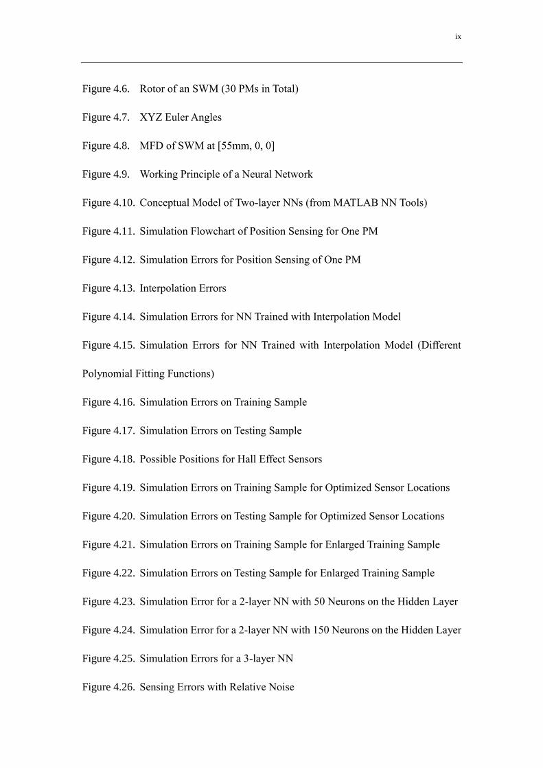
Figure 4.6. Rotor of an SWM (30 PMs in Total)
Figure 4.7. XYZ Euler Angles
Figure 4.8. MFD of SWM at [55mm, 0, 0]
Figure 4.9. Working Principle of a Neural Network
Figure 4.10. Conceptual Model of Two-layer NNs (from MATLAB NN Tools)
Figure 4.11. Simulation Flowchart of Position Sensing for One PM
Figure 4.12. Simulation Errors for Position Sensing of One PM
Figure 4.13. Interpolation Errors
Figure 4.14. Simulation Errors for NN Trained with Interpolation Model
Figure 4.15. Simulation Errors for NN Trained with Interpolation Model (Different
Polynomial Fitting Functions)
Figure 4.16. Simulation Errors on Training Sample
Figure 4.17. Simulation Errors on Testing Sample
Figure 4.18. Possible Positions for Hall Effect Sensors
Figure 4.19. Simulation Errors on Training Sample for Optimized Sensor Locations
Figure 4.20. Simulation Errors on Testing Sample for Optimized Sensor Locations
Figure 4.21. Simulation Errors on Training Sample for Enlarged Training Sample
Figure 4.22. Simulation Errors on Testing Sample for Enlarged Training Sample
Figure 4.23. Simulation Error for a 2-layer NN with 50 Neurons on the Hidden Layer
Figure 4.24. Simulation Error for a 2-layer NN with 150 Neurons on the Hidden Layer
Figure 4.25. Simulation Errors for a 3-layer NN
Figure 4.26. Sensing Errors with Relative Noise

x
Figure 4.27. Sensing Errors for a Sample with Absolute Noise
Figure 4.28. Sensing Errors with both Relative and Absolute Noise
Figure 4.29. Sensing Errors for Sensing Systems with Additional Sensors
Figure 4.30. Sensing Errors for Different Measurement Times
Figure 4.31. Interpolation Errors
Figure 4.32. Sensing Errors for Different Initial Samples before Interpolation
Figure 4.33. Computation Procedures of a Neural Network
Figure 5.1. SWM Prototypes
Figure 5.2. Copper Coil Winding Patterns
Figure 5.3. Torque Comparisons between Experiments and Simulations
Figure 5.4. Magnetic Flux Density Plot for Configuration H
Figure 5.5. Experimental Setup for Position Sensing of a PM
Figure 5.6. Position Sensing Errors for One PM in Experiments
Figure 5.7. Influence of Fluctuations of Magnetic Sensors
Figure 5.8. A Sensing System of an SWM
Figure 5.9. Voltage Output Component 1 of a Sensor
Figure 5.10. Voltage Output Component 1 after Interpolation
Figure 5.11. Measuring Error of Neural Network Based Sensing System
Figure 5.12. Sensing Errors Vs Number of Measured MFD Components
Figure 5.13. Sensing Errors Vs Measurement Times at Each Orientation

xi
LIST OF TABLES
Talbe 3.1. Design Parameters for Optimization
Talbe 3.2. Design Parameters for Optimal Model
Talbe 4.1. PM Related Parameters
Talbe 4.2. Polynomial Coefficients of MFD-Separation Angle
Talbe 4.3. RMSE of Training & Testing for MFD with Relative Noise
Talbe 4.4. RMSE of Training & Testing for MFD with Absolute Noise
Talbe 4.5. RMSEs of Training & Testing for 4, 5 and 6 Sensors
Talbe 4.6. RMSEs of Training & Testing for Multiple Measurements
Talbe 4.7. RMSEs of Training & Testing for Different Interpolation Sample
Talbe 5.1. Geometric Parameters of Spherical Wheel Motor
Talbe 5.2. Resistivity of 2 pairs of EMs (connected in series) Vs Copper Wire
Diameter
Talbe 5.3. Experimental Configurations
Talbe 5.4. Specifications of MFS-3A

xii
LIST OF ABBREATIONS
APDL ANSYS parametric design language
BP Back propagation
DC Direct current
DMP Distributed multi-pole
DOF Degree of freedoms
EM Electromagnetic magnet
EMI Electromagnetic interface
ESL Equivalent single layer
FEM Finite element modeling
FM Full model
FPGA Field-programmed gate array
GUI Graphical user interface
HPC High performance cluster
MFD Magnetic field distribution
MFDrelative noise Magnetic field distribution with relative noise
MFDabsolute noise Magnetic field distribution with absolute noise
MFDnoise Magnetic field distribution with both relative and absolute noise
MGXX, MGYY, MGZZ X, Y, Z component of coercive force
MSE Mean square error
MN Maximum negative

xiii
MP Maximum positive
MRM Multi-DOF Reconfigurable machine
NI National Instruments
NNs Neural networks
PD Proportion Differentiation
PID Proportion Integration Differentiation
PM Permanent magnet
PMSM Permanent magnet spherical motor
RMSE Root mean square error
RNN Robust neural networks
SPM Simplified model
SWM Spherical wheel motor
SUSM Spherical ultrasonic motor
THD Total harmonic distortion
VRSM Variable reluctance spherical motor

xiv
LIST OF SYMBOLS
B Magnetic flux density vector
D Displacement current density vector;
E Electric field intensity vector
ri (mm) Inner Radius
ro (mm) Outer Radius
Din (mm) Diameter of inner PM
Dout (mm) Diameter of outer PM
Dcore (mm) Diameter of EM core
Lin (mm) Length of inner PM
Lout (mm) Length of outer PM
δr(Deg) Angle between PMs in plain view
δs(Deg) Angle between EMs in plain view
Α (deg) Inclination angle of rotor from a Z-axis
Br (T) Residual Magnetism
H (Gauss) Magnetic field intensity
en Normal unit vector;
B1, B2 Magnetic flux density vector of two materials on boundary;
H1, H2 Magnetic intensity vector of two materials on boundary;
Jsurf current vector on boundary surface.
J Total current density vector

xv
Js Source current density vector
Je Induced eddy current density vector
LEM (mm) Length of EM
Tin Turns of Inner EM
Tout Turns of Outer EM
I (Amp) Current on EM
βs (Deg) Separation angle of EMs
βr (Deg) Separation angle of PMs
μ0 Space permeability
μr Relative permeability
𝜇𝑚 Permanent magnet permeability
M Relative magnetism
Scalar potential
Te Electromagnetic torque
u Currents vector
ρ Electric charge density
jk Separation angle between kth PM and jth EM
Rji+, Rji- Distance from point P to the source and sink respectively
mji Strength of the ith source or sink of jth loop

1
CHAPTER 1
INTRODUCTION
1.1 Motivation
A spherical wheel motor (SWM), unlike conventional motors of which motions are
confined along a single axis, the SWM as a form of electromagnetic motor, offers a
unique ability to control orientation of the rotor while the rotor can be continuously
spinning. There are great potential applications for SWMs in fields such as laser cutting,
robotic wrists, helicopters, omnidirectional wheels and computer vision systems.
Existing designs to realize multi-DOF motions are typically composed of plural single-
axis motors; generally equal or more motors than motion DOFs are required and
orientation control of the rotating shaft must be manipulated by an additional
transmission mechanism. These multi-axis actuators are generally bulky, slow in
dynamic response, and lack of dexterity in negotiating the orientation of the rotating
shaft. As an alternative to conventional designs, an SWM has many advantages some
of which are listed as followings:
Compact size and simple design; a spherical rotor can achieve 3-DOF motions
as a direct-drive motor without any transmission mechanism;
Isotropic motion property without any kinematic singularity in the working
range;
Quick and smooth motion control in 3-DOF.

2
Recently, two types of spherical motors differentiated by operating principles are
getting more attention, i.e. spherical ultrasonic motors (SUSMs) and SWMs based on
electromagnetic principle. The idea of SUSMs comes from the extension of the typical
single-axis ultrasonic motor which uses two natural vibrations of the stator to drive the
rotor with frictional force. An SUSM is generally compact in size, simple in structure
and able to generate high torque density. However, most SUSMs have problems such
as weak preloading force, complicated in the view of manufacturing, requiring a power
system of high voltage and frequency, which inhibit applications of such motors in
industry. Another inherent drawback is that the maximum size of an SUSM is confined
to guarantee its natural frequency ultrasonic, which causes the SUSMs not applicable
in many conditions. Compared to SUSMs, there are many benefits for SWMs inheriting
from conventional electromagnetic motors and corresponding control strategies. It can
be operated at a relatively high speed with smooth motion control. Many researchers
have been devoting to develop a compact SWM with strong output torque and high
controllability. However, these studies are still infeasible for industrial applications due
to challenges in two aspects, i.e. configuration design to improve torque capability
especially for inclination torque and design of a fast and accurate non-contact sensing
system.
An SWM consists of a number of PMs in a rotor and EMs in a stator with various
designs for a range of motion, speed and torque. The number and size of PMs and
combinations of magnetic polarities mainly affect performance with the same applied

3
current input. Since there are more PM-EM pairs involved to produce spinning torque
than inclination torque, the design is mainly concerning with how to maximize the
inclination torque with a given motor volume and a given current density limited by the
heat dissipation ability of the SWM. In particular, the inclination torque as a key
parameter should be maximized to support an external load.
The thesis has proposed a new design of SWM with PMs located both inside and
outsider of EMs, so as to fully unitize magnetic field generated by EMs and reduce
magnetic leakage. Important physical parameters affecting inclination torque have been
optimized to achieve maximum torque within a given size. Iron stator cores are utilized
to enhance magnetic torque, and effects of iron boundary of the SWM are also
investigated. There is 135% increase of torque/volume ratio of the proposed SWM
validated by experiments.
A multi-DOF sensing system is a prerequisite for development of an integrated SWM
system. Several sensing strategies based on photoelectric encoders, laser range finders,
magnetic sensors with analytical method have already been investigated by researchers.
However, above existing methods have restrictions in applications. Sensing systems
using photoelectric encoders belong to the contact type, and friction and backlash
brought by the sensing system will damage motion controllability. A non-contact
sensing system applying laser range finders is fast and accurate. However, the sensing
strategy is only applicable to SWMs with a flat bottom. Researchers use magnetic
sensors and closed-form expressions to solve the orientation from measured MFD.

4
However, due to complexity of the MFD, high-order items have to be neglected,
resulting in low accuracy.
To improve sensing performance of orientation, the thesis has designed a non-contact,
absolute, multi-DOF sensing system based on magnetic sensors, and NNs have been
applied to compute orientation from MFD. Compared to existing closed-form solutions,
NNs based computation strategy has the following advantages:
NNs computation is more accurate, since closed-form solutions have to neglect
high-order items of MFD;
Accuracy of NNs based sensing system can be easily improved by adding more
sensors or neurons;
Closed-form solutions have modeling errors, while modeling is unnecessary for the
proposed NNs based sensing system;
NNs based sensing system is more adaptive to magnetic noise and detecting error
of Hall Effect sensors.
The thesis contributes to making SWMs closer to industrial applications in mainly two
aspects, i.e. configuration design to improve torque capability and design of a sensing
system with characteristics of non-contact, fast speed (the sensing system should be fast
enough to be applied in real-time feedback control, such as 3.6 kHz for the rotor with
600r/min spinning speed, so as to sense per degree), accurate and adaptive.

5
1.2 Background
The growing demands of devices with multi-DOF motions in industry have motivated
many researchers to investigate various types of multi-DOF motors and corresponding
designs, sensing and control methods.
Research of electromagnetic multi-DOF actuators can be dated back to 1950s in [1].
F.C. Williams et al. has designed a 2-DOF induction motor. Objective of the second
DOF, which is realized by manually rotating the stator block along the stator axis, is to
adjust the spinning speed.
As the cost of high coercive rare-earth permanent magnets goes low, many researchers
have focused on PM based SWMs. Several designs have been proposed by Lee et al. in
[2, 3], and by Yan et al. in [4]. These designs can spin the rotor on a spherical bearing
as conventional electromagnetic motors, and there are multi-layer PMs and EMs to
generate the inclination torque. The PM based SWM designs share the same working
principle with difference in number and distribution of PMs and EMs.
Figure 1.1: Prototype of a 2-DOF Induction Motor by F.C. Williams et al. in [1]
6
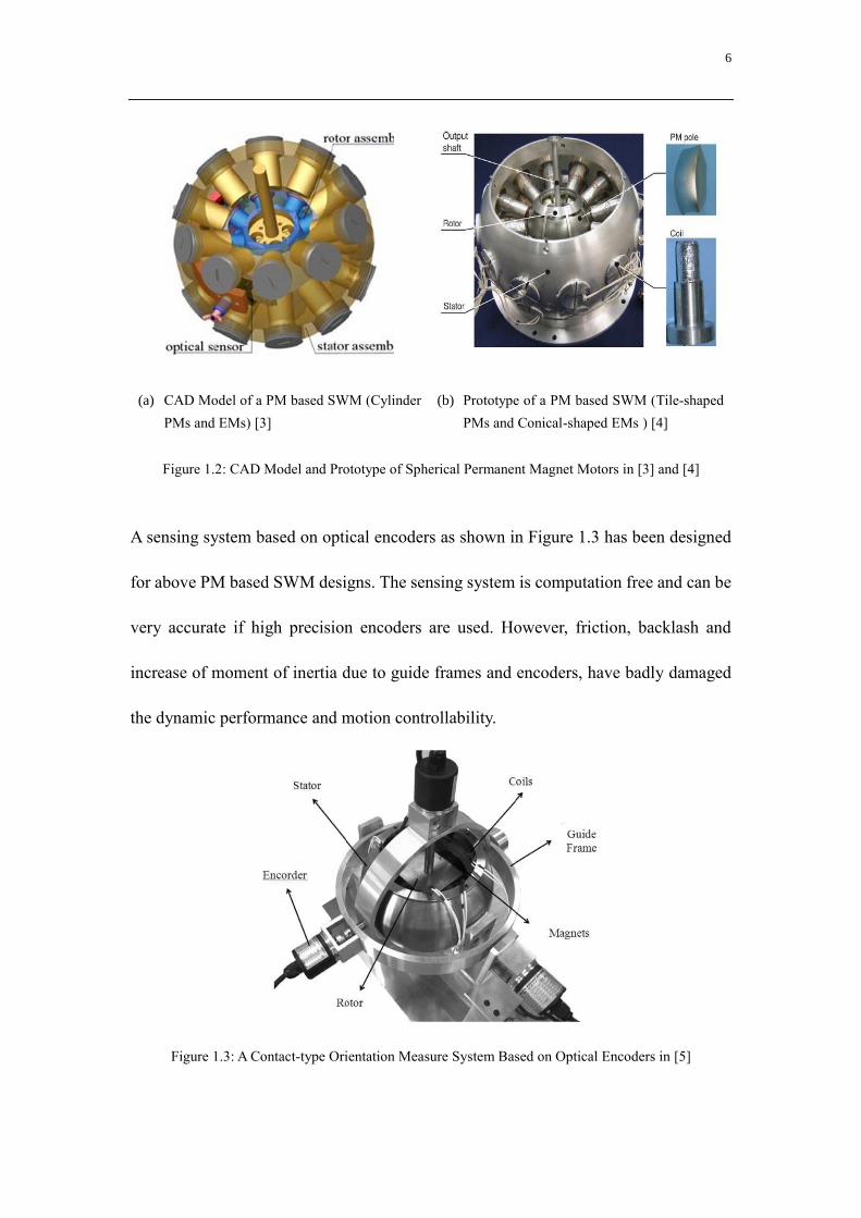
(a) CAD Model of a PM based SWM (Cylinder
PMs and EMs) [3]
(b) Prototype of a PM based SWM (Tile-shaped
PMs and Conical-shaped EMs ) [4]
Figure 1.2: CAD Model and Prototype of Spherical Permanent Magnet Motors in [3] and [4]
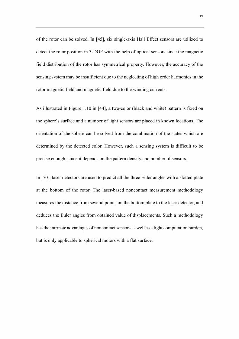
A sensing system based on optical encoders as shown in Figure 1.3 has been designed
for above PM based SWM designs. The sensing system is computation free and can be
very accurate if high precision encoders are used. However, friction, backlash and
increase of moment of inertia due to guide frames and encoders, have badly damaged
the dynamic performance and motion controllability.
Figure 1.3: A Contact-type Orientation Measure System Based on Optical Encoders in [5]

7
As shown in Figure 1.4, a magnetic sensor based 2-DOF sensing system is proposed by
Son et al. in [6]. A cylinder PM is attached on the output shaft, and four single-axis
sensors are located around the attached PM. The sensing system is able to measure 2-
DOF inclinations but not the spinning. The PM and sensors are placed far away from
the rotor PMs so MFD generated by rotor PMs can be neglected, which simplifies the
computation from MFD to orientation. However, the sensing system has the following
drawbacks:
The sensing system is 2-DOF only and spinning cannot be measured;
The sensing system is limited to be applied in SWMs with a long output shaft;
High-order items of MFD have to be neglected to obtain a closed-form solution,
which results in low accuracy.
Figure 1.4: A Magnetic Sensor Based 2-DOF Sensing System in [6]

8
1.3 Literature Review
The section offers as followings: several recent designs of SUSMs are presented first;
as to spherical electromagnetic motors, more detailed reviews of previous reported
researches are presented since our research belongs to this category. Various designs of
spherical electromagnetic motors are presented first. Secondly, different methods for
solving MFD and magnetic torque are illustrated. Thirdly, several sensing methods for
measuring orientation of the output shaft or the sphere rotor are presented and their
advantages and disadvantages are discussed. Other methods to realize multi-DOF
motions in previous reports are presented finally in the literature review.
1.3.1 Spherical Ultrasonic Motor (SUSM)
A single-DOF ultrasonic motor combines two natural vibration modes of the stator to
generate a single-DOF motion of the rotor by frictional force between the stator and the
rotor. By appropriately exciting and combining three or more natural vibration modes
of the stator of an SUSM, multi-DOF motions of the sphere rotor can be achieved. Most
spherical ultrasonic motors have prominent characteristics such as compact structure,
low weight, relatively high torque-to-volume ratio, absence of electromagnetic
radiation and high holding torque for braking without electricity. Different types of
SUSMs are proposed and studied in [7-26] and some prototypes of classic designs are
shown as in Figure 1.5.
As presented in Figure 1.5 (a), a multi-DOF ultrasonic motor with a compact plate stator
is proposed in [12] by K. Takemura et al. The motor has achieved an extremely compact

9
stator compared to previous designs. However, the difference of natural frequency of
each vibration mode caused by manufacturing tolerance and material isotropy, the small
contact area between the stator and the rotor, the weak preloading force provided by
gravity, and the nonlinear and changing dynamics during operation weaken the torque
capability and controllability of the spherical ultrasonic motor.
An SUSM with compact structure constructed of three annular stators and a spherical
rotor has been designed as presented in Figure 1.5 (b) in [16]. The maximum torque
and rotational speed of the prototype are 3.45N*mm and 65.4 rpm respectively with a
size of 26mm. However, with two pairs of guides and rotary encoders to measure the
orientation of the output shaft, the total size of the multi-DOF system is much larger
and the dynamic property is also damaged.
As shown in Figure 1.5 (c), an SUSM in [20] which has a large spherical contact surface
achieves high torque and compact structure, since contact surface is an important factor
that influences the friction force between the stator and the rotor.
As shown in Figure 1.5 (d), a multi-DOF ultrasonic motor has been used in an auditory
tele-existence robot in [13]. Several strained springs are used as a preloading
mechanism and compensation for resistance torque caused by gravity of the head.
Benefit by the sufficient preloading force provided by tensioned springs, the motor has
a potential to generate as strong as 1 N*m torque. However, the relatively large size of
the whole motor has limited its applications and the dynamic response is relatively slow.

10
Motivated by requirements of compact multi-DOF motors in minimally invasive
surgery, a long and thin bar-shaped SUSM suitable for the small work space in the
patient body has been proposed as shown in Figure 1.5 (e) as in [17]. The prototype can
generate enough torque for free space motion; however, its torque capability needs to
(a) An SUSM with a Compact Plate
stator in [12]
(d) An SUSM as Actuator of a Auditory
Tele-existence Robot Head [13]
(b) An SUSM with Compact Structure
of Three Annular Stators [16]
(c) An SUSM with a large spherical
contact surface in [20]
(e) A Long and Thin Bar-shaped SUSM
Prototype in [17]
Figure 1.5: Prototypes of Existing SUSMs

11
be improved for contact tasks such as suturing and knotting.
The SUSMs as presented above, have not been applied to actual applications due to the
following disadvantages:
It is difficult to design a preloading mechanism which can produce sufficient
normal force without any dragging force due to the spherical shape of the rotor, the
rotational torque generated by frictional force. Therefore, the friction force needs
to be improved.
Generally, the SUSM works at the natural frequency of the stator. The maximum
size of the stator is limited, since the natural frequency of the stator decreases as
the size of the stator increases. And the natural frequency must be larger than the
lower limit of ultrasonic sound, otherwise the motor will be very noisy. Since the
torque capability depends on the stator size, such problem makes the potential
maximum torque of ultrasonic motors too small for many applications.
The dynamics of SUSMs is nonlinear and changing during operation since it is
governed by friction force, which results in difficulty in control.
A high voltage (sometimes 200V peak-to-peak voltage) and frequency (higher than
20 kHz) power system is necessary for most SUSMs.
Although an SUSM itself can be very compact, the orientation sensing system is
generally large in size.

12
Other drawbacks such as very low efficiency and wear of friction have also inhibited
the SUSMs from labs to commercial usages.
1.3.2 Designs of Spherical Electromagnetic Motors
Most existing multi-DOF motors are in the type of electromagnetic motor in [1-6, 27-
96]. Although SWMs are difficult to miniaturize compared to SUSMs, they inherit
many advantages of single-axis electromagnetic motors which have been developed
maturely with a long history.
There are many different types of SWMs such as spherical induction motor, variable
reluctance spherical motor (VRSM), Direct Current (DC) servo motor, permanent
magnet spherical motor (PMSM) and so forth.
Spherical induction motor
An induction motor, also named by asynchronous motor, produces electromagnetic
torque by the interaction of rotating air-gap magnetic field and induction current on
rotor. F. C. Williams et al. in [1] have proposed the first spherical induction motor,
which could realize 2-DOF motions as shown in Figure 1.1. However, the second DOF
is achieved by manually rotating the stator block along the stator axis, and the objective
of the additional DOF is to adjust the spinning speed of the rotor.

13
Figure 1.6: A Concept Design of a 3D Induction Spherical Motor in [30]
A. Foggia et al. in [30] have presented a 3-DOF motor as in Figure 1.6, operation
principle of which is identical to the one of induction motors. The motor consists of a
moving armature of which inner surface is made of magnetic steel, with a thin layer of
copper and three fixed inductors as marked by M1, M2, and M3. By activating the three
inductors, three independent motions can be realized.
Permanent magnet spherical motor (PMSM)
Since exciting currents are not necessary for permanent magnet motors, such motors
can work with high efficiency and compact structure. The permanent magnet spherical
motor (PMSM) has attracted most researchers and many different designs emerge in
recent decades.
Lee et al. present the design concept of a spherical motor based on the variable
reluctance stepper in [31]. The spherical motor is composed of a hemispherical stator
with many electromagnets and a spherical rotor with two permanent magnets. The

14
tangential force between PMs and neighbor energized stator coils drive the rotor in 3-
DOF to minimize the magnetic reluctance. However, due to the small quantity of
permanent magnets, the torque capability of proposed design is very weak. No
prototype has been fabricated according to the design and an improved design of
variable reluctance spherical motor has been proposed and fabricated by Lee et al. in
[3] as shown in Figure 1.2 (a). Compared to previous designs, the improved design had
a more compact structure which contains more PMs and larger EMs. The torque
capability has been improved a lot due to the increase of involving PM-EM pairs;
however, the inclination torque capability is the bottleneck since there are fewer PM-
EM pairs producing inclination torque compared to the spinning torque.
A similar and further improved spherical permanent magnet motor has been proposed
by Yan el al. in [4] as shown in Figure 1.2 (b). The motor has a compact structure with
dihedral permanent magnets in rotor and conical-shaped (conical-shaped in design and
cylinder in prototype) coils in stator. Two designs differentiated by layers of magnets
(one or two layers) have been analyzed and compared. The proposed design has
improved the isotropy of the electromagnetic torque in 3-DOF, i.e. the difference
between the inclination torque and spinning torque is decreased for the proposed design
with two layers of permanent magnets in rotor.
A PMSM whose schematic is shown in Figure 1.7 has been studied by W. Wang et al.
in [45]. The motor is composed of a four-pole spherical permanent magnet rotor which
contains two pairs of parallel magnetized quarter-spheres, and four pairs of stator

15
windings. By energizing several stator winding pairs with appropriate currents, the rotor
can rotate in 3-DOF to minimize the system potential energy.
A spherical stepper motor with stator and rotor in a semi-regular packing as shown in
Figure 1.8 has been proposed by Gregory S. Chirikjian et al. The stator overlaps less
than half of the area of the rotor, leading to an advantage that such a design has large
motion range compared to previous spherical stepper motors.
Figure 1.7: Schematic of a Spherical Permanent Magnet Motor in [45]
(a) Stator (b) Rotor
Figure 1.8: Stator and Rotor Packing in [41]

16
1.3.3 Magnetic Field and Torque Analysis of Spherical Electromagnetic Motors
Recent methods about analyzing magnetic field of SWMs include mainly the
followings: theoretical analysis, distributed multi-pole (DMP) model, FE analysis and
experiments.
Theoretical analysis
In [54], the analytical expression of the magnetic field generated by rotor PMs of an air
core SWM is obtained by solving the governing equations which in this case are
Laplace’s equations. Lorentz force law is then employed to calculate the magnetic
torque. Theoretical analysis for magnetic field distribution and torque calculation
require surface and volume integrations which results in a heavy computation load and
is not suitable for online computation.
Distributed multi-pole (DMP) modeling
The DMP model proposed in [52] offers an effective closed-form solution for precise
calculation of magnetic field around a PM or an EM, and force and torque between
them. For PMSMs fabricated with non-ferromagnetic material, such method can be
easily expanded to analyze the whole PMSM under the superposition principle. The
DMP modeling inherits many advantages of previous single dipole model such as
closed-form, timesaving and visualized, is a great improvement of the previous one,
since it can account for the shape and magnetization of PMs. Moreover, compared to
single dipole models, there are no singularities in the space around PMs with DMP.

17
The magnetic field generated by a PM can be characterized by the superposition of
effects of several pairs of sources and sinks since the magnetic field satisfies the
superposition principle. The DMP modeling can obtain a pretty precise magnetic field
distribution of a PM in closed-form with only very limited pairs of sources and sinks,
which makes it suitable for online computation and real time control.
Three methods are provided to compute the magnetic torque between a PM and an EM,
i.e. by Lorentz force law with a multi-layer coil, by Lorentz force law with an equivalent
single layer (ESL) coil and by virtual displacement method with modeling the EM as a
PM which has the same geometry as the ESL.
FE analysis with ANSYS
With the rapid improvement of the computation devices and commercial FE software,
more and more researchers use the commercial software ANSYS to analyze the
magnetic field and torque. ANSYS is used in [55] to solve the spinning torque of a
permanent magnet spherical motor and presents a way to convert 3D to 2D modeling.
Other methods
The paper [64] presents a measurement-calculation approach to model the magnetic
field distribution of a PM-based SWM. With Laplace’s equations as the governing
equations, and measured data as the boundary conditions, the magnetic field
distribution is reconstructed by using software COSMOL. The main advantage of such
approach is that there is no requirements for the magnetic structure.

18
1.3.4 Sensing System Designs for Spherical Electromagnetic Motors
Unlike conventional single-axis motors whose motion is constrained along one axis,
the spherical motors have multi-DOF motions and infinite postures, so it is crucial to
find an appropriate sensing method to realize the closed-loop control. Recent sensing
systems can be characterized to contact and non-contact categories. The former one has
advantages of light computation burden, high accuracy but the sensing system will
increase mass of inertia of the rotor, bring about friction and damage the dynamic
performance of the spherical motor. More attentions have been paid to the non-contact
one employing vision or magnetic sensors.
Contact measure systems
As shown in Figure 1.3, the contact-type orientation measurement system in [5] is
realized by two guides and three optical encoders which can measure the pitch, roll and
yaw of the output shaft. Such sensing systems need almost no computation and have
very high accuracy. However, the volume and inertia of mass of the motor have been
increased a lot. And the changing dynamics due to the friction has damaged the dynamic
performance and controllability of the motor.
Non-contact sensing systems
As illustrated in Figure 1.9 in [4], the Hall Effect sensors are used to measure the
magnetic field, and by comparison with the known magnetic field distribution in 3-
DOF space which has already been obtained by DMP or theoretical analysis, the posture
19
of the rotor can be solved. In [45], six single-axis Hall Effect sensors are utilized to
detect the rotor position in 3-DOF with the help of optical sensors since the magnetic
field distribution of the rotor has symmetrical property. However, the accuracy of the
sensing system may be insufficient due to the neglecting of high order harmonics in the
rotor magnetic field and magnetic field due to the winding currents.
As illustrated in Figure 1.10 in [44], a two-color (black and white) pattern is fixed on
the sphere’s surface and a number of light sensors are placed in known locations. The
orientation of the sphere can be solved from the combination of the states which are
determined by the detected color. However, such a sensing system is difficult to be
precise enough, since it depends on the pattern density and number of sensors.
In [70], laser detectors are used to predict all the three Euler angles with a slotted plate
at the bottom of the rotor. The laser-based noncontact measurement methodology
measures the distance from several points on the bottom plate to the laser detector, and
deduces the Euler angles from obtained value of displacements. Such a methodology
has the intrinsic advantages of noncontact sensors as well as a light computation burden,
but is only applicable to spherical motors with a flat surface.

20
Figure 1.9: A Hall Effect Sensor in [4]
Figure 1.10: A Binary Spherical-Motion Encoder System: (a) Bottom of Sphere (b) Top of Sphere
(c) Stator Housing with Embedded Rings of Light Sensors (d) One of Sensor Rings [44]
1.3.5 Other Multi-DOF Actuators
Except from ultrasonic and electromagnetic designs as illustrated above, there are some
other methods to generate multi-DOF motions as in [97-103]. Some of the following

21
designs can also be characterized to electromagnetic motors; however, since their
working principles are different from driving a spherical rotor by magnetic interaction
between the rotor and stator, they are introduced separately here.
As shown in Figure 1.11, a miniature spherical motor which consists of four rods of
Galfenol (an alloy of iron and gallium, has amplified magnetostrictive effect compared
to iron), a wound coil, a rotor on the edges of the rods, and a permanent magnet under
the rotor has been proposed in [101]. The rod can be expanded or contracted when
currents are applied on wound coils. By expanding a rod and contracting the rod in the
opposite, the rotor can rotate by a tiny angle. Applying a saw tooth current which
increases gradually and falls rapidly, the rotor can be rotated. When the current is slowly
increased, the rotor rotates in accordance with the slow deformation of the rod because
of the friction; when the current falls rapidly. However, the rotor cannot follow the rapid
deformation of the rod, instead, a slippage between the rod and the rotor happens. The
rotor can be rotated continuously be repeating these operations.
Another method proposed by Hirokazu Nagasawa et al. in [97] has been illustrated in
Figure 1.12. The spherical motor is consisted of a spherical cell, a spherical concave
shell and four wires. The spherical motor manipulates the rotor in three directions
including pitch, roll and yaw by four wires. By altering lengths of the four wires with a
simple algorithm, the posture of the rotor can be controlled.

22
Figure 1.11: Prototype of a Spherical Motor in [102]
Figure 1.12: Schematic of a Spherical Motor Driven by Four Wires in [97]
1.4 Objective
The thesis research has two main objectives.
The first objective is to propose a design strategy to improve isotropic property of the
torque of the SWM by maximizing the inclination torque. There are more PMs and EMs

23
involved in creating spinning torque compared to inclination torque. However,
inclination torque is a very important performance parameter especially when the SWM
has to support an external load. The thesis has proposed a new design with PMs of the
rotor locating both inside and outside of EMs of the stator so as to fully utilize magnetic
field generated by EMs. Ferromagnetic materials are applied in the coil cores to
improve magnetic torque. Design optimization is carried out to optimize important
physical parameters and maximize the inclination torque of the SWM within a given
compact size.
The second objective is to develop an absolute 3-DOF sensing system of SWMs with
advantages of non-contact, fast response speed and high accuracy. Contact type sensors
such as one composed of three optical encoders can be fast and accurate. However, will
damage dynamic performance of the SWM seriously. The proposed sensing system
utilizes several Hall Effect sensors to measure MFD, and neural networks (NNs) to
compute orientations from MFD. It is unnecessary for the proposed sensing system to
estimate magnetic related physical parameters such as remnant magnetism or magnetic
permeability of PMs, so there is no modeling errors.
1.5 Thesis Outline
The emphasis of the research work is placed on design of configuration to enhance
torque capability, and design of a 3-DOF absolute sensing system based on magnetic
sensors and neural network algorithm. Remaining contents of the thesis are organized
as followings:

24
Chapter 2 proposes a new design of SWM with PMs located both inside and outside of
EMs, and presents a single-objective optimization process to maximize the inclination
torque with Finite Element (FE) analysis under certain constraints such as the outer
radius and current density. Since the whole SWM contains dozens of PMs and EMs, a
simplified model has been proposed to save computation load without losing accuracy.
Optimization results have verified the great improvement of proposed design in
inclination torque density.
The magnetic torque and dynamic model for SWMs with ferromagnetic stator cores are
presented in Chapter 3. Existing dynamic models about SWMs are mostly concerning
with SWMs with non-ferromagnetic materials only. For SWMs with ferromagnetic
materials, MFD and magnetic torque becomes nonlinear to current inputs, so
superposition principle is no longer applicable. The thesis has analyzed MFD of SWMs
with different input currents, and concluded that as input currents are in the working
range, magnetic torque on the rotor can be divided to two parts, i.e. a fixed part due to
ferromagnetic stator cores, and a linear part proportional to input currents. Once
magnetic torque is calculated by addition of the two parts, forward dynamic modeling-
to calculate torque by given inputs, and inverse dynamic modeling- to obtain optimal
inputs with desired torque is straightforward to build.
Chapter 4 proposes a 3-DOF sensing system based on magnetic sensors and NNs to
measure the orientation in real-time. MFD of the whole SWM is very complicated with
many PMs and EMs involved, so NNs have been used to approximate functions

25
between MFD and orientations. Optimal distribution of sensors, and important factors
affecting sensing performance are investigated in Chapter 4.
Chapter 5 presents a prototype of the proposed SWM and experimental investigations
to verify torque modeling and performance of proposed sensing system. Magnetic
torque measured in experiments is in great agreement with torque computed by FEM
modeling, which verifies our magnetic torque modeling and simplified model. For the
sensing system, ratio of sensing error to measuring range in experiments is about 1.4%.
Considering the 3% maximum error for magnetic sensors, and accuracy of reference
system, the proposed sensing system has been proven to be good in performance.
Finally in Chapter 6, a conclusion of the thesis is presented and future work to realize
an integrated system of SWM is proposed.

26
CHAPTER 2
DESIGN OPTIMIZATION FOR MAXMIZING INCLINATION
TORQUE
2.1 Overview
For multi-DOF motor designs composed of plural single-axis actuators, it is
straightforward to enhance its torque capability by improving that of each actuator.
However, for proposed PM based spherical motors in recent decades, it is still a
challenge to obtain a high torque density. Chirikjian and David [41] have proposed a
spherical motor with a stator covering only less than half of the rotor, and achieved a
very wide range of motion. However, only less than half of PMs can interact with coils
since most PMs are too far away from the coils, which greatly reduces the torque density.
Wang et al. has done design optimization to maximize the output torque. However,
there is only one parameter being optimized, i.e., the ratio of the rotor to the stator.
There are two intrinsic drawbacks to obstruct improvement of the torque density, i.e.,
the non-negligible friction torque due to direct contact of the rotor magnet with the
stator housing, and the limited number of PMs and EMs. Lee et al. [48] have proposed
a spherical motor with improved torque density due to a high-density distribution of
PMs and EMs. However, the inclination torque is weak due to a limited number of PMs
for the inclination motion compared to the spin motion. And the cylinder shape of PMs
and EMs simplifies the fabrication, but doesn’t take full advantage of the space. And
there is large magnetic flux leakage from EMs to outer space. Yan et al. [78] have

27
proposed an improved design with conical-shaped coil and magnets to enhance
utilization of space, and iron stator to reduce magnetic flux leakage, which enhance the
torque density greatly.
A spherical motor consists of a number of PMs in a rotor and EMs in a stator with
various designs for a range of motion, speed and torques. The different number of PMs
and combinations of their magnetic polarities mainly affect the performances with the
same applied current input. In particular, the inclination torque is a key performance
parameter especially when it supports an external load. To increase the inclination
torque with a certain current density input, the number and size of PMs should be
increased to maximize magnetic field interaction between PMs and EMs. However, it
is rather difficult within a limited space. Thus, recent designs are concerned with how
to maximize the inclination torque within a compact volume.
Existing designs generally use one or two layers only of PMs inside of the stator, such
designs have advantages of small moment of inertia of the rotor, but it is difficult to
obtain a high torque-to-volume ratio especially for inclination torque. The thesis has
proposed a new design of SWM with PMs located both inside and outside of the EMs
to enhance magnetic interaction between stator and rotor, and improve inclination
torque within a given spatial size. Compared to one or two layers of PMs used in the
rotor for previous designs, to improve inclination torque ability, the thesis has proposed
SWMs with three layers of PMs both inside and outside of a stator with two layers of
EMs as in Figure 2.1. Only some of the PMs and EMs are shown for a clear presentation.

28
Figure 2.1: Proposed Spherical Motor with Three Layers of PMs both Inside and Outside of the Stator
A single-objective design optimization to maximize the inclination torque within a
given spatial size is carried out for both designs with two or three layers of PMs in the
rotor, and optimization results show a great improvement of inclination torque, and a
possibility to apply such multi-DOF motors in practice engineering areas.
2.2 Proposed Configurations of SWMs
Figure 2.2(a) presents a top view of a proposed design showing magnetic polarities of
the SWM projected in the XY plane. Unlike most existing SWMs, PMs of which are
only inside of the stator (such as in Figure 2.2(b)), the proposed designs consist of PMs
at both inside and outside of the EMs with alternatively opposite polarities in radial
circularly for spinning. Similar with the spin motion, the inclination motion also
requires additional layers of pole pairs along the Z axis. The SWM can have a number
of pole layers along the Z axis as shown in Figure 2.2 (b)-(d).

29
Various designs with a different number of PMs in the rotor, but the same number of
EMs in the stator have been proposed as shown in Figure 2.2. However, the operation
principle is similar to each other although the numbers of PMs may be different; the
PM pairs are mechanically connected to the rotor and rotated together on a universal
bearing so that their magnetizations are always toward or against the center of rotation.
The spinning motion along the z-axis is analogous to a conventional stepping motor but
not for the inclination motion. The polarities of the PM pairs are alternatively opposite
to each other so that the inclination torque is controlled by the push-pull principle; if
one of PMs generates a force to push the EM, the other generates a force to pull the EM
accordingly.
Existing configuration: two layers of PMs inside of EMs
Proposed Configuration A: two layers of PMs both in and outside of EMs
Proposed Configuration B: three layers of PMs both in and outside of EMs

30
(a) Top View of a Proposed SWM (b) Existing Configuration
(c) Proposed Configuration A (d) Proposed Configuration B
Figure 2.2: Top and Front Views of Existing and a Proposed Configuration of Spherical Motor
2.3 Electromagnetic Field Fundamentals
Maxwell’s equations as followings are applied as the basis for FEM analysis of
electromagnetic field.
s e v
D D
t t
H=J+ J J J (2.1)
B
t
E=- (2.2)

31
0B= (2.3)
D= (2.4)
Where:
H: Magnetic field intensity vector;
J: Total current density vector;
Js: Source current density vector;
Je: Induced eddy current density vector;
D: Displacement current density vector;
E: Electric field intensity vector;
B: Magnetic flux density vector;
: Electric charge density.
The above Maxwell’s equations are supplemented by a constitutive equation that
describes the relationship between magnetic flux density vector and magnetic field
intensity vector
r 0
B H (2.5)

32
Where: 0 is magnetic permeability of free space with a value of -74 10 , and r
is relative permeability of the material. For air and aluminum, 1r ; for ferromagnetic
material such as iron, r depends on H instead of being a constant, generally a B-H
curve is used to describe the relationship. For permanent magnets used in the rotor, the
constitutive relation becomes
00 0B H+ Mr (2.6)
Where: 0M is remnant intrinsic magnetization vector.
In our study, the time varying effects such as eddy currents are ignored, and Maxwell’s
equations for static electromagnetic field are reduced to:
sH=J (2.7)
0B= (2.8)
For static electromagnetic field, the following boundary conditions apply on the
boundary between different materials:
1 2( ) 0e B Bn (2.9)
n 1 2 surf( - ) e H H J (2.10)
Where:
en : Normal unit vector;

33
B1, B2: Magnetic flux density vector of two materials on boundary;
H1, H2: Magnetic intensity vector of two materials on boundary;
Jsurf: current vector on boundary surface.
The primary unknowns calculated by FEM are magnetic and electric potentials, and
other electromagnetic field quantities are derived from the two potentials, such as
magnetic flux density, energy, and magnetic force.
The thesis uses ANSYS- commercial software package of FEM to do the
electromagnetic analysis and calculate the magnetic torque. Detailed procedures will
be presented in the following sections.
2.4 Numerical Analysis by ANSYS
Finite element (FE) analysis is utilized to compare the magnetic field and the torque of
different configurations. ANSYS parametric design language (APDL) is used to
simulate the electromagnetic field of the SWM, since APDL is more suitable for
parameters optimization compared to graphical user interface (GUI) and Workbench of
ANSYS. As presented in last section, the primary unknowns that ANSYS calculates are
magnetic and electric potentials, and magnetic flux density, forces, torques are derived
from the potentials, and Maxwell’s equations are used as basis for electromagnetic field
analysis. The ANSYS provides 2-D and 3-D modeling options for electromagnetic field
analysis, and 2-D model can simplify original planar or axisymmetric 3-D models to 2-

34
D models. It is much easier to generate 2-D model and more timesaving to solve.
However, in the thesis, 3-D model is selected to obtain high computation accuracy in
design optimization.
To relieve computation load, mechanical structures of stator and rotor besides PMs and
EMs are considered as made of non-ferromagnetic materials such as aluminum, and can
be modeled as part of air as they share same magnetic related material properties. Main
steps in the 3-D static electromagnetic field analysis to calculate magnetic torque on
PMs generated by EMs (direct currents applied) contains the followings:
1) Set physical environment, including element types and related KEYOPT (Key
Options) settings, material properties, real constants and so on. The settings are
according to our model type- static electromagnetic model with direct current
(DC) and ferromagnetic materials (for SWM with iron core).
2) Build the physical model including PMs, ferromagnetic core and air. Interested
regions include electromagnetic parts of the SWM and surrounding air. Volumes
representing PMs and iron cores are created first, and the air region volume is
generated by Boolean operations. EMs are modeled by primitive sources, so
actually no need to model in this step. Volumes are then meshed to generate
elements and nodes.
3) Apply boundary conditions and loads. The outer surfaces of the air volume are
meshed to INFIN47 elements, which are used to simulate the far field decay of

35
the magnetic field. Current excitations are supplied via SOURC36 elements.
SOURC36 can be treated as a “dummy” element, and current source data such
as amount of current, position and size can be specified by element real
constants. Without meshing requirements, SOURC36 simplifies the modeling
and reduces the computation time.
4) Solve the analysis.
5) Review the results and calculate the magnetic torque. There is no existing macro
in ANSYS to compute the magnetic torque, so torque of each element of the
rotor is calculated and added together to obtain the total torque.
Detailed procedures and setups of simulation with APDL in ANSYS are presented as
follows.
1) Selection of element types
Three elements are employed to analyze the electromagnetic field.
For 3-D static electromagnetic field analysis, we select element SOLID96 with eight
nodes and one degree of freedom on each node as magnetic potential. The PMs,
ferromagnetic core and air region are characterized by SOLID96.
SOURC36 which contains three nodes is a primitive (consisting of predefined
geometries) and it is applied to simulate current inputs; real constants are used to define

36
the circular shape of the coil, and amount of currents (amplitude multiply turns).
In ANSYS, generally the larger the boundary is, the better modeling accuracy will be.
However, increasing the model volume will result in more elements if element sizes
remain the same, and thus increase computation time. Boundary size is confined due to
limited computation power. INFIN47, a four-node boundary element with a magnetic
potential or temperature degree of freedom at each node, is used to model far field decay
of the magnetic field. Verified by several trials, compared to setting far field magnetic
potential to be zero, modeling with far field decay elements such as INFIN47 can
produce better results.
2) Assigning material properties
Once element types are selected, material properties need to be assigned for PMs, air
and ferromagnetic core.
It is assumed that the BH curve of the PMs is linear. The relative permeability of the
PMs is μr = 1.16, and the coercive force Hc used to define PMs in ANSYS can be
calculated by the following equation:
0/c r rH B (2.11)
There components in different directions of coercive force, named as MGXX, MGYY,
MGZZ are defined to determine the magnetization axis of PMs.

37
Figure 2.3: BH Curve of the Material of Ferromagnetic Stator Cores
For the air region, the relative permeability is 1.0.
For saturable magnetic material such as ferromagnetic core used in EMs, a BH curve
as shown in Figure 2.3 is applied to describe the relationship between magnetic flux
density and magnetic intensity. Lee et al. treat relative magnetic permeability of
ferromagnetic materials as unlimited in [31] or a large constant like 1000 in [46], and a
conclusion of linear characteristics of MFD and magnetic torque is drawn based on
such assumptions. While in practice it should be along a BH curve as shown in the
figure, the magnetic saturation happens when magnetic flux density arrives at a high
level such as 1.3T. However, the demagnetizing curve cannot be described in ANSYS,
it is regarded as coinciding the magnetizing BH curve.
3) Creating the physical model
First, PMs and ferromagnetic stator cores are geometrically modeled in the 3D space.

38
Since eddy currents are neglected in the static electromagnetic analysis, conductivity is
not considered in material properties, and materials are classified by magnetic
permeability only. Other structure components such as the rotor, stator are non-
magnetic conducting materials and their magnetic permeability is the same as air, so
can be modeled as air.
Then, a cylinder containing the whole electromagnetic components is created with
Boolean operations, so that there is no overlapping between the air and other regions.
Suppose a cylinder with diameter D and height H is just enough to covers all the
electromagnetic components; a cylinder with diameter of 2×D and height of 2×H is
created to simulate the air surrounding the electromagnetic structure, where magnetic
flux density is weaker but cannot be neglected. Larger air volume generally leads to
higher accuracy of the analysis. However, the computation load will also increase as
more elements and nodes are generated with the same meshing standard. The FEM
solution must be a good tradeoff between modeling accuracy and computation time
based on computation ability and design requirements. Magnetic field of the SWM
decays and approaches to zero in the air region, and element INFIN47 is used to
simulate the far field decay of the electromagnetic field. With application of INFIN47
elements, it is unnecessary to build a large air volume.

39
(a) Air Boundary region (b) Meshed PMs and EM
Figure 2.4: 3D CAD Model of Configuration B in ANSYS
4) Meshing with adaptive strategy
The program meshes volumes to elements and nodes, which are basic units for FEM
computation. The EM is not necessary to be meshed since it is already an element
defined by three nodes and real constants. Analysis accuracy depends mainly on two
factors- the model size and the element size. The quality of meshing significantly affects
the accuracy of the results. Generally, a model meshed with more elements leads to a
more precise calculation, while computation time is also increasing almost
proportionally until running out of the RAM (random access memory) of the PC. Thus,
the analysis requires us to employ different element sizes to mesh different parts in
order to increase accuracy within affordable computation time. The magnetic field is
strongest around the electromagnetic components, and decay radially in the air.
Obviously, PMs and ferromagnetic cores, where magnetic flux density is the strongest,
should be meshed with fine elements such as element size of 1mm. For air region, the
further the air is, the weaker the magnetic flux density is, and thus the coarser the

40
meshing should be. Moreover, we should also pay attention to the sequence of meshing
of different volumes so as to take advantage of self-adaptive meshing techniques in
ANSYS. First we mesh the outer air volume with smart meshing with the ANSYS
macro “SMRTSIZE”, which meshes the internal portion with fine elements and external
portion with coarse elements; then the PMs and the stator core are meshed with much
smaller element size; the inner air volume is meshed without assigned element size, and
they will be meshed adaptively- the closer the air is to PMs and cores, the smaller the
element size will be. Finally, the outmost surfaces are meshed with INFIN47 elements
to simulate the far field decay of electromagnetic field as the boundary conditions. The
INFIN47 is used to model magnetic flux decay in open boundary of the model, which
lowers the size requirement of the outer air.
5) Applying flags before solving the analysis
The FEM model is to calculate magnetic torque on PMs which represent the rotor. First
we group all the elements assigned with permanent magnet material properties into a
component, and then an ANSYS command macro, FMAGBC, is used to apply virtual
displacements and the Maxwell surface flag for calculating forces on the component.
6) Solve the model and compute magnetic torque
Once the model is solved, we can obtain the total force exerted on PMs (representing
the rotor). However, there is no existing macro to calculate the torque in 3D static
magnetic analysis in ANSYS. APDL are edited to calculate the cross product of the

41
force and the position vector for each node of the rotor, and cross products are then
added together to obtain the total torque on PMs.
2.5 Simplified Model for Magnetic Torque
We simulate the torque model for SWM configurations with both the air core and the
iron core. For configurations with the air core, the total torque can be obtained from the
superposition of torque on each EM-PM pair, so only one EM-PM pair in the model
needs to be simulated. The torque on one pair of PMs generated by one EM is shown
in Figure 2.5. Refer to Figure 2.2, the modeling parameters are as followings: ri= 25mm
(limited by the spherical bearing), ro=65mm (the given total size); diameter and length
of the inner PM are both 10mm, diameter and length of outer PM are 25mm and 5mm;
Inner and outer radius of the EM are 6mm and 16mm, length of the EM is 21mm,
current density is 8A/mm2 (based on heat dissipation capability); separation angle
between PMs and the EM is from 0 to 40 degrees on XOY plane. Magnetic torque
components on X and Y axis should be zero due to symmetry. However, due to the fact
that size of element cannot be infinitesimal and meshing distortion exists, there will be
nonzero torque on X and Y axis. Magnitude of torque components on X and Y axis, and
torque component on Z axis when separation angle is zero, can be used as a reference
of the computation accuracy. As presented in Figure 2.5, the average magnitude of
theoretical zero components is less than 2% of maximum magnetic torque on Z axis.
The model size and element size can be treat as a tradeoff between the computation
time and the modeling accuracy. With computed torque-separation angle curve, total

42
Figure 2.5: Magnetic Torque on One Pair of PMs Generated by One EM
magnetic torque on the rotor generated by all EMs can be calculated under the
superposition principle.
However, for configurations with stator cores made of ferromagnetic materials,
magnetic field and magnetic torque are nonlinear, and superposition principle is not
applicable. Magnetic torque generated by an EM with iron core on a pair of PMs with
different current density (same physical parameters as in last paragraph and separation
angle is ten degrees) is presented in Figure 2.6. B-H curve is used to define magnetic
permeability of the iron core, and magnetic saturation occurs with large current density
applied. The magnetic torque is nonlinear to applied currents, and there is attraction
forces between PMs and EMs with iron core even without current applied. Due to
limited heat dissipation capability, applicable maximum current density is about
8A/mm2. As shown in Figure 2.6, the torque- current density is almost along a straight
line between -8 to 8A/mm2, which indicates that for torque calculation, there is no need

43
Figure 2.6: Magnetic Torque Vs Current Density with Iron Core
to consider the saturation as long as the maximum current density is less than ±8A//mm2.
Magnetic torque on one pair of PMs generated by one EM with iron core is presented
in Figure 2.7. As shown in Figure 2.7, there is an attraction force between PMs and
EMs with iron core even no currents applied, and total magnetic torque cannot be
obtained under superposition principle. However, the whole SWM of one proposed
design contains 16 EMs and 30 pairs of PMs. Therefore it is very time consuming to
simulate the whole model for design optimization.
Figure 2.7: Magnetic Torque on One Pair of PMs Generated by One EM with Iron Core

44
In consideration of saving computation time without impairing too much modeling
accuracy, a simplified model (SPM) is proposed to alleviate the computation cost, and
the efficiency and accuracy are validated by the comparison between SPM and full
model. Prior to torque computation with SPM, it is necessary to validate torque from
the SPM against the full model (FM) for configurations with iron core. For calculation
of the inclination torque of proposed Configuration B with ferromagnetic materials in
EM cores, it is necessary to verify the following two SPMs first:
1) Torque generated by a single EM with six neighboring PMs (SPM1) and with all
PMs (FM1) are compared.
2) The other comparison is between the torque produced by two EMs with
neighboring PMs (FM2) and the sum of torques produced by each EM with
neighboring PMs (SPM2).
The simulation results in Figure 2.8 indicate that the inclination torque generated by the
SPM and FM is very close with difference less than 5%, proving that the superposition
between PMs can be applied. In addition, the SPM1 reduces computational loads; the
result from SPM1 with 463600 elements is compared to FM1 with 2078600 elements
with the same element size, and the computation times for each separation angle are
about 6.7 and 42.9 minutes respectively.
The simulation results in Figure 2.9 indicate that the inclination torque generated by an
upper and a lower EM can be calculated by addition of torque generated by each

45
separately. In the FEM mode, the initial inclination angles for upper and lower EMs are
25 and -25 degrees respectively. The results verify that total magnetic torque can be
calculated by addition of torque generated by each EM.
The comparison results indicate that torque calculated with the SPM composed of one
EM and its neighboring PMs can be expanded to analyze the whole SWM.
Figure 2.8: Inclination Torque Calculated by SP1 and FM1

46
Figure 2.9: Inclination Torque Calculated by SP2 and FM2
2.6 Design Optimization for Enhancing Inclination Torque
In FE Analysis, it is important to find an optimized mesh shape for satisfying accuracy
and computational time simultaneously. In general, smaller element size, more elements
and nodes produce more accurate results. However, the computation time is also
increasing with number of elements and nodes and a good tradeoff between
computation time and modeling accuracy must be found. Various shapes of mesh with
different element sizes are compared by the nonzero torques at zero separation angle
and computation time. Any non-zero torque at zero separation angle (PM and EM are
aligned) is considered as an error. After several trials, we set the mesh to be composed
of about 350000 tetrahedron elements for Configuration B, which takes about 10.3
minute for each computation, and confines the average errors to less than 1% of the
maximum inclination torque.

47
Design procedures for maximizing the inclination torque are shown in Figure 2.10. It
begins with defining constraints along with key design parameters and their desired
ranges in motion for orientation control. The initial constraints with design
specifications are set as following:
1) Inner radius ri and outer radius ro are initially set for all designs.
2) Air gap between a PM and EM is given since a smaller air gap is generally better
and minimizes magnetic reluctance.
3) Two EMs with an equal length but different diameters are serially connected and
become an EM to enlarge the magneto-motive force.
4) The separation angle of EMs, βs is set to avoid mechanical contacts between
neighboring EMs.
Once general constraints are pre-determined, independent and dependent design
parameters can be further classified based on their mechanical and magnetic coupling
relations. The dependent parameters (such as diameters of PMs and EMs) are designed
as large as possible as long as no mechanical contacts exist. Then, the following four
physical parameters are chosen to be independent parameters:
1) Separation angle of PMs, βr affecting the sizes of PMs;
2) Diameter of the ferromagnetic EM core, Dcore;

48
3) Lengths of inner PMs Lin, outer PMs Lout, and EMs LEM is then determined since
the size of motor is given as a constraint.
Table 2.1 Design Parameters for Optimization
Parameters Range
Inner PM length, Lin (mm) 6-12
Outer PM length, Lout (mm)
4-10
βr (deg)
26-32
Iron core diameter, Dcore(mm) 2.5-10
Figure 2.10: Optimization Flowchart

49
(a) Optimization Results of Configuration A (b) Optimizaiton Results of Configuration B
Figure 2.11: Optimization Results for Configurations
Table 2.2 Design Parameters for Optimal Model
Parameters βr (deg) Lin (mm) Lout (mm) Dcore (mm)
Configuration A 26 12 4 2.5
Configuration B 32 8 6 10
Four independent design parameters; and corresponding range are summarized in Table
2.1. Each parameter is uniformly digitized into four elements due to heavy computation
and a number of their combinations. Four parameters are first paired as two (Lin, Lout)
= ([6(initial):2(interval):12(final)] (the vector format in Matlab is used for better
illustration), [4:2:10]) and (βr, Dcore) = ([26:2:32], [2.5:2.5:10]). Then, all possible
combinations are indexed with positive integer into two axes (x, y); (Lin, Lout )=(6,4):
x=1, (6,6): x=2, …, (12,10): x=16. Similarly, (βr, Dcore) = (26, 2.5): y=1, (26, 5): y=2…
(32, 10): y=16. Thus, the total number of the index for each pair is finally 16 since each
parameter has four elements, and the total number of design variations is 1616 (=256)
accordingly.
Figure 2.11 shows the resultant torque from proposed Configuration A and B. Each

50
configuration has its own constraints. Din and Dout of Design B and C are limited mainly
by 𝛿𝑟 and 𝛽𝑟 respectively once lengths of PMs are set (they are set to be as big as
possible but avoid mechanical contact). Thus, Configuration A has 20% larger diameter
PMs than Configuration B while Configuration B has 50% more PMs, indicating
Configuration B is a more compact and efficient structure. By comparing the maximum
sum of torque, the optimized designs can be found and the parameters are given in Table
2.2. The results show that after optimization, Configuration B can generate 124% higher
inclination torque than Configuration A.
2.7 Summary
Chapter 2 presents conceptual designs of SWMs with introduction of ferromagnetic
materials in coil cores and PMs locating both inside and outside of EMs. Compared to
the number of PMs fully circulated along a spinning axis for spin motion, the number
of PMs for inclination motion is limited and thus, inclination torque is relatively weak.
To increase the inclination torque with a given current input and spatial size, the number
of PMs should be radially increased to maximize magnetic field interaction between
PMs and EMs. Two configurations with different layers of PMs located both inside and
outside the stators with ferromagnetic stator cores are proposed. A single objective
optimization for maximizing the inclination toque of both configurations is realized
with FE analysis on HPC. To relieve computation burden, simplified models are
proposed and verified. The simplified models have saved a lot of computation time
while the simulation accuracies are maintained. Optimization results have shown that

51
key geometrical parameters have significant impact on torque capabilities of the SWM.
Design optimization results have also shown that the proposed design can generate
much stronger inclination torque than existing designs and has improved isotropic
property of magnetic torques. Based on enhanced inclination torque, the proposed
SWM is able to be utilized in practice engineering applications in respect of torque
ability.

52
CHAPTER 3
MAGNETIC TORQUE AND DYNAMIC MODELING
3.1 Overview
To realize real time control, the forward model describing relationship between inputs-
currents applied on each EM and outputs- angular motions of the rotor has to be
established first. Establishment of such relationship contains two procedures, i.e.
magnetic torque modeling and dynamic modeling.
It has been a challenge to build the magnetic torque model for SWMs with
ferromagnetic materials due to nonlinearity of the complicated magnetic field. SWM
configurations without ferromagnetic materials can be regarded as a particular case of
the ones with ferromagnetic materials, and torque model of SWMs with ferromagnetic
materials can be easily extended to SWMs without ferromagnetic materials. For SWMs
without ferromagnetic materials, it is already verified by Yan et al. in [4] that the MFD
and magnetic torque is linear thus superposition principle can be applied to establish
the torque model. As to SWMs with ferromagnetic materials. However, previous
researches either used a constant as magnetic permeability of ferromagnetic materials,
or set their relative magnetic permeability as infinite, did not adopted the actual
magnetic induction curve, which is nonlinear and finite.
3.2 Magnetic Torque Model for SWMs with Iron Cores
The SPM with a constant current for SWMs with ferromagnetic stator cores has already

53
been verified in Chapter 2. For EMs with varying currents, the superposition principle
is not satisfied due to the nonlinear magnetic permeability of ferromagnetic stator cores.
However, a torque-current curve with the middle part (the applicable current range for
SWMs) approximately as a straight line has been validated with FE analysis. The torque
model of the whole SWM can be obtained from the torque-current curve and the SPM
(one EM with surrounding PMs) which has been verified in last chapter. The SPM with
optimized physical parameters obtained in Chapter 2 is used here to illustrate the
relationship between magnetic field, torque and applied currents.
Considering the problem of heat dissipation, the maximum continuous current density
applied on the coil should be less than 8A/mm2. As shown in Figure 3.1, the core is
divided into two regions: Region 1 as edges of the stator core which is closer to magnets
and its magnetic flux density is mainly influenced by neighboring magnets, and Region
2 as interior of the stator core and its magnetic flux density is influenced by PMs as
well as the coil. Comparing Figure 3.1 with Figure 3.2 (a) (b) (c) (d), we can conclude
that the maximum magnetic flux density in Region 2 is smaller than 1.5T if the current
density applied on the coil is in the range of -8 to 8A/mm2.

54
Figure 3.1: Magnetic Flux Density of Ferromagnetic Stator Core with no Current Applied
(a) Current Density= -3 A/mm2 (b) Current Density = 3 A/mm2
(c) Current Density = -8 A/mm2 (d) Current Density = 8 A/mm2

55
(e) Current= -30 A/mm2 (f) Current = 30 A/mm2
Figure 3.2: Magnetic Flux Density of Ferromagnetic Stator Core with Different Currents Applied
Figure 3.3: B-H Curve of #20 Steel
The BH curve of the ferromagnetic core as shown in Figure 3.3 can be approximately
treated as composed of two lines. So the magnetic flux density of Region 1 is varying
along Line 2, while the magnetic flux density of Region 2 is varying along Line 1.
When the current density is increased to 30 A/mm2, the magnetic flux density of Region
2 is varying along from Line 1 to Line 2. With Lorenz force law, we can assume that
the according magnetic torque-current curve is approximately along a straight line as

56
Figure 3.4: Magnetic Torque Vs Current for SPM with Optimized Parameters
the current is within the range of -2.5 to 2.5 ampere, but not anymore as the current
increases to 30 A/mm2.
The torque-current curve, as expected from the magnetic field analysis and shown in
Figure 3.4, is almost along a straight line while the current is -5 to 5 ampere (0.3mm
diameter wire is used). Two methods for computing the magnetic force in ANSYS, i.e.
virtual work and Maxwell’s equations are used, and the convergence value is as small
as 1e-8.
PMs/ EMs which have collinear axis are treated as a group, and all the 60 PMs and 16
EMs are divided to fifteen groups and eight groups respectively. Once we compute the
torque between a group of PMs and a group of EMs with ANSYS, we can obtain the
total magnetic torque of SWMs with iron stator cores by the following equation:
core current= +T T T (3.1)

57
Where Tcore indicates torque due to iron material and Tcurrent torque due to input currents,
expressed as Equations 3.2 – 3.5 respectively:
0
1 1core
( ( ) | ) 0| |
0 0
m mj k
j k
j k j k
j k
s r
jk
s rf if s r
s r
if s r
T
(3.2)
T T
current 1 2 1 2=[ ][ ] =[K K K ][I I I ]m ms sT K I (3.3)
1 0
1j
(( ( ) ( )) | ) 0| |K
0 0
mj k
j k
k j k
j k
r
jk
s rf f if s r
s r
if s r
(3.4)
8
0
( ) (i=0, 1)k
i ik
k
f c
(3.5)
rk and sj are the position vectors of the kth PM and the jth EM respectively; f0 and f1 are
torque functions between a PM pole-pair and an EM pole-pair in terms of separation
angle when input current is 0 or unit respectively as shown in Figure 3.5. f0 is fixed and
uncontrollable, and f1 - f0 can be treated as controllable unit. Noted that when the
separation angle is larger than 40 degrees, the torque between PM and EM is close to
zero. Referring to the SWM design of Son et al. in [52], the torque between a PM- and
an EM pole pair is about 0.23Nm with 4A current applied in AWG29 (American wire
gauge #29, 0.0642mm2 cross area), and there are 8 PM- and 10 EM pole pairs with a
total diameter of 76.2mm. Supposing the same current density is applied in an EM of
the

58
Figure 3.5: Torque Vs Separation Angle for PM and EM with Iron Core
proposed SWM (0.2042 mm2 cross area, 12.7A current applied), the maximum
controllable torque generated by a PM and an EM is about 2.5Nm, which is about 10.9
times of one in [52]. Considering the smaller total diameter and more PMs and EMs
(30 PM pairs and 16 EMs for proposed SWM), the torque density of the proposed SWM
is verified to be greatly improved.
3.3 Dynamics Modeling
X-Y′-Z″ Euler angles are applied to describe connection between stator coordinate
X, X'
Y
Y'
ZZ'
Y', Y"
Z'
Z"
X' X" X'" X"
Z", Z'" Y'"
Y"
Figure 3.6: X-Y′-Z″ Euler Angles

59
XYZ and rotor coordinate xyz. The rotor coordinate coincides with stator coordinate at
first as presented in Figure 2.1, and then rotate along X axis for a degree of α, and along
new Y′ axis for a degree of β, finally along latest Z″ axis for a degree of γ. The rotor
angular velocity in Euler angles is given by:
X Y Zω=αe +βe +γe (3.6)
While unit vectors of Euler angles can be expressed in rotor coordinate system in the
form of ' ''x y ze , e and e as
cos sin 0 cos 0 sin 1 0 0 1
sin cos 0 0 1 0 0 cos sin 0
0 0 1 sin 0 cos 0 sin cos 0
Xe
(3.7)
cos sin 0 cos 0 sin 0
sin cos 0 0 1 0 1
0 0 1 sin 0 cos 0
Ye
(3.8)
cos sin 0 0
sin cos 0 0
0 0 1 1
Ze
(3.9)
Then we have the angular velocity of the rotor in rotor coordinate as
ω=Kq (3.10)
Where T
q= α β γ
and

60
cos cos sin 0
cos sin cos 0
sin 0 1
K
(3.11)
According to momentum theorem of the rotor as a rigid body, assuming the gravity
center coincides with the rotor center and neglecting external torque, the dynamic
equation of the rotor in rotor coordinate is given by
eMgω+C(ω)gω=T (3.12)
Where eT is the electromagnetic torque in the rotor coordinate system, and
0 0
0 0
0 0
xx
yy
zz
I
M I
I
(3.13)
Due to rotor symmetry, we can assume that xx yyI I , and
xx
xx
xx xx
0 I I
( ) I 0 I
I I 0
z zz y
z zz x
y x
C
(3.14)
To simplify the dynamic equations with Euler angles only, angular acceleration is given
by
ω=Kq+Kq (3.15)
-sinβcosγgβ-cosβsinγgγ cosγgγ 0
K= sinβsinγgβ-cosβcosγgγ -sinγgγ 0
cosβgβ 0 0
(3.16)

61
Substituting Equation 3.10 and 3.15 into 3.12,we have
T T T T
e(K gMgK gq+(K MgK+K gCgK)gq=K T) (3.17)
Or in a simple form as
T
e[M]gq+C(q,q)=K T (3.18)
2 2cos sin 0 sin
[ ] 0 0
sin 0
xx zz zz
xx
zz zz
I I I
M I
I I
(3.19)
zz xx zz
2
xx zz zz
zz
2(I -I )sinβcosβgαgβ+I cosβgβgγ
C(q,q)= (I -I )sinβcosβgα -I cosβgαgγ
I cosβgαgβ
(3.20)
Since in the last section the electromagnetic torque is calculated in stator coordinate
system, eT is given by
cos sin 0 cos 0 sin 1 0 0
sin cos 0 0 1 0 0 cos sin
0 0 1 sin 0 cos 0 sin cos
X
e Y
Z
T
T T
T
(3.21)
Where T
X Y ZT T T is the electromagnetic torque calculated by the torque model in
stator coordinate, and we have
1 0 0
0 cos sin
sin sin cos cos cos
X
T
e Y
Z
T
K T T
T
(3.22)

62
3.4 Summary
Chapter 3 presents magnetic torque and dynamic modeling for SWMs with
ferromagnetic stator cores. Ferromagnetic cores have improved the torque capability
significantly. However, the nonlinear magnetic permeability of ferromagnetic materials
has made the superposition principle not applicable for computation of magnetic torque.
In the thesis, we analyze the MFD on ferromagnetic cores with different current inputs,
and conclude that the torque-current curve is approximately along a straight line in our
interested range, and magnetic torque on an EM can be divided to two parts due to
ferromagnetic material and current inputs respectively. Combining with the SPM
verified in Chapter 2, the total magnetic torque model of the SWM is obtained. In the
remaining part of Chapter 3, dynamic modeling is presented. With magnetic torque
model and dynamic model, the motion accelerations of the rotor under certain current
inputs and optimum current inputs for given motion accelerations can be calculated,
which lays the foundation of building an integrated closed-loop control system for an
SWM in dynamics.

63
CHAPTER 4
NEURAL NETWORK BASED ORIENTATION MEASURE
SYSTEM
4.1 Overview
Many researchers have been devoting to develop a compact, precise, high torque, and
high speed integrated system of an SWM. However, the design of sensing system is one
of the key challenges. Unlike single DOF motors, motion of which can be predicted
easily, the three rotational angles of the rotor. However, due to coupling kinematics, are
difficult to obtain in real-time. An accurate and fast speed sensing system is a
prerequisite to realize closed-loop motion control for an SWM.
Previous sensing systems of SWMs can be divided into two main groups, i.e. contact
and contact-less ones. Generally, a contact-type sensing system in [32] is realized by
two mechanical guides and three optical encoders which can measure the pitch, roll and
yaw of the output shaft. Such sensing systems have fast response without need of
computation, and can be very accurate if high performance encoders are applied.
However, the volume and inertia of mass of the motor increase a lot, and friction due
to the guides has damaged the dynamic performance and controllability of the motor.
Considering enhancing dynamic performance, a contact-less sensing system such as
one composed of magnetic sensors is preferred.
The thesis focuses on research of a sensing system for SWMs without ferromagnetic

64
materials. Verified by Wang et al. in [45], in each spinning circle, there is one-to-one
mapping between PM-based rotor orientation and the MFD, which indicates that a
unique solution of orientation always exist with measured MFD. Orientation of the
SWM can be described by three Euler angles such as ones in X-Y'-Z'' rotation order.
The chapter proposes a sensing system to obtain the three orientation angles of an SWM
based on Hall Effect sensors and neural networks. Unlike the forward modeling- to
solve MFD with given orientation, which can be solved under superposition principle
once MFD of one or one pair of PMs is computed by analysis or FEM, the inverse
modeling- to obtain three Euler angles from measured MFD is much more challenging,
and it is very difficult to acquire a closed-loop equation unless high-order terms of the
magnetic field are ignored. Neglecting high-order terms results in low accuracy, so
neural networks [105-112] which can fit any practical function have been adopted here
to approximate the relationship between inputs- measured MFD and outputs-
orientation angles.
3-axis Hall Effect sensors as presented in Figure 4.1 are applied in the sensing system.
A 3-axis Hall Effect sensor can output voltages in response to the magnetic field in 3
mutually perpendicular directions. The output voltages are proportional to magnetic
flux density components in each direction over the working range of the sensors.
As presented in Figure 4.2, the working process of the proposed sensing system is as
follows.

65
Figure 4.1: A Hall Effect Sensor
SWMMeasurement Euler Angles to
MFD
Extended
Euler Angles to
MFD
Interpolation Neural Network
MFD to Euler
Angles
Training
offline offline offline
online
Figure 4.2: Flowchart of Sensing System with Hall Effect Sensors
1) The SWM (rotor only) is equipped with encoder-based mechanical sensing system,
and the Hall Effect sensors measure the MFD of the SWM at orientations evenly
distributed in the working range.
2) The measured pairs of MFD- Euler angles are then extended by interpolation.
3) The extended MFD- Euler angles are used to train the neural network.
4) The neural network is applied to compute the Euler angles in real time.
The remainder of the chapter is organized as followings:
1) MFD generated by one PM is calculated by DMP. Compared to ANSYS or analysis,

66
DMP is able to provide a fast and closed-form solution. MFD of the SWM rotor is then
calculated by superposition of MFD of each PM in simulation with MATLAB.
2) Position sensing of one PM in 3D has been simulated with neural networks.
3) Neural networks are used to solve orientation angles from total MFD of an SWM
rotor. In the preliminary investigations, important factors of NNs affecting performance
of the sensing system are studied.
4) To model practical MFD of the SWM, magnetic noise is considered and included
in the simulation, and methods to alleviate influence of the noise are presented.
5) A large amount of MFD-orientation data is necessary to train the neural network.
However, it is too time consuming and impractical to measure this amount of data in
experiments. Numerical interpolation is used to obtain the training data from a small
number of measured data. Influence of size of initial measured data on sensing accuracy
is studied to balance measuring workload and sensing accuracy.
6) Computation time of the trained NNs is presented to verify the feasibility of the
sensing strategy to be applied in a real-time control SWM system.
4.2 Magnetic Field Distribution of a PM Based on DMP
The SWM rotor is composed of three layers of 30 (pairs) of PMs in total, to solve the
inverse modeling problem- to calculate orientation angles from measured magnetic
field, the forward modeling- to obtain MFD under given orientations, needs to build

67
first. Here we choose DMP instead of ANSYS to build the forward model due to the
following reasons:
1) DMP is closed-form with fast calculation speed.
2) DMP generates better results qualitatively. Take a cylinder PM which is magnetized
along Z axis as shown in Figure 4.3 for example, x and y component of magnetic flux
density at any point along z axis should be zero due to symmetry. However, FEM will
output nonzero results because of meshing distortions and asymmetry, while there is no
such problem with DMP.
3) MATLAB is used to carry out DMP algorithm, so the results from DMP can be
used directly in MATLAB simulation for design of the sensing system.
Figure 4.3: DMP Modeling for a Cylinder PM in [52]

68
Three assumptions are set as followings:
1) Magnetic material of PM is isotropic and the PM is axisymmetric;
2) Magnetization is along Z axis and residual magnetism is a constant;
3) Relative permeability of PM is a constant such as 1.12;
The DMP uses multiple magnetic doublets to calculate MFD of a cylinder PM as shown
in Figure 4.1, and magnetic potential due to each source or sink is given by the
following equation:
1( 1)=
4
j
mR
(4.1)
Where j equals 1 or 0 depending on source or sink, m is strength of the source or sink,
and R is distance between measured point and the source or sink. Under the
superposition principle, the potential at point P (x, y, z) can be calculated by sum of
potential due to all sources and sinks as following:
0 0
k n
P ji ji
j i
m
(4.2)
Where jim is the strength of the ith source or sink of jth loop, and ji is given by
[(1/ R ) (1/ R )] / (4 )ji ji ji (4.3)
R ji and R ji are distance from point P to the source and sink respectively as shown in

69
Figure 4.1.
Given a potential field, the magnetic field intensity H and magnetic flux density B can
be calculated by
H = - Φ (4.4)
0B= Hr (4.5)
While 0 is the permeability of free space, and r is relative permeability of PM.
Generally more pairs of sources and sinks result in higher accuracy but also increase
computation time. Values of unknown parameters such as number of loops, number of
sources and sinks in each loop, positions and strength of each source and sink, are
determined by minimizing the following error function under a certain requirement:
2
(z) (z)A
z
E dz (4.6)
(z) and AΦ (z) are magnetic potentials along the magnetization axis calculated by
DMP and analysis respectively.
As illustrated in Figure 4.4, a point sensor and magnetization axis of a PM of the SWM
rotor can define an XOY plane with rotating center of the SWM as center of the plane
and magnetization axis as X axis. Position of point P can be given by distance R and
separation angle β. When R is set to be 55mm and separation angle is from 0 to 180
degrees, the magnetic flux density components generated by a PM with parameters in

70
Table 4.1 on a sensor 55mm away from rotating point are computed by DMP as shown
in Figure 4.5. Separation angle θ= [0(initial):1(interval):179(final)], so magnetic flux
density components at 180 separation angles have been calculated. The magnetic flux
density B is expressed by polynomial as in Equation 4.7. Curve fitting by POLYFIT
functions with a least square error in MATLAB has been carried out and the polynomial
is with a degree of 12. Polynomial coefficients of Bx and By are listed in Table 4.2.
1
1 2 1
n n
n np x p x p x p
Β (4.7)
Figure 4.4: XOY Plane Determined by Magnetization Axis of a PM and a Sensor
Figure 4.5: Magnetic Flux Density Generated by a Cylinder PM Calculated by DMP (R=50mm)

71
Table 4.1 PM Related Parameters
Parameters Value
PM Diameter 13mm
PM Length 8mm
Permeability 1.12
Residual Magnetism 1.36T
Table 4.2 Polynomial Coefficients of MFD-Separation Angle
Polynomial Coefficients of Bx Polynomial Coefficients of By
P1 -1.5278e-023 P1 6.8551e-024
P2 1.7819e-020 P2 -7.0061e-021
P3 -9.1847e-018 P3 3.0160e-018
P4 2.7491e-015 P4 -6.9119e-016
P5 -5.2732e-013 P5 8.3291e-014
P6 6.7309e-011 P6 -2.7260e-012
P7 -5.7175e-009 P7 -6.6082e-010
P8 3.0948e-007 P8 1.0714e-007
P9 -9.2702e-006 P9 -7.2652e-006
P10 7.2917e-005 P10 2.2798e-004
P11 2.7025e-003 P11 -1.2608e-003
P12 6.5624e-004 P12 -6.8286e-002
P13 -1.6453e+000 P13 -3.2411e-003

72
With MFD generated by one PM, the MFD of the whole inner rotor is to be obtained
Figure 4.6. Rotor of an SWM (30 PMs in Total)
under the superposition principle, i.e. MFD of the inner rotor is sum of MFD generated
by each PM.
As shown in Figure 4.6 and Figure 2.2, initial location (without considering N or S
polarity) of each PM in stator coordinate system (coincide with rotor coordinate initially)
can be described as in Equation 4.8:
[cos(( -1) 36),sin(( -1) 36),0] ( 1, 2 ...10)
[cos(( -1) 36) cos(32),sin(( -1) 36) cos(32),sin(32)] ( 11, 12...20)
[cos(( -1) 36) cos(-32),sin(( -1) 36) cos(-32),sin(-32)] ( 21, 22 ...30)
j
j
j
P j j j
P j j j
P j j j
(4.8)
XYZ Euler angles as shown in Figure 3.6 are adopted to describe orientation of the
rotor in stator coordinate system. The rotor rotates along X axis of the stator coordinate
system for a degree of α first, and then rotates along the new Y axis for a degree of β,
and finally rotates along the new Z axis for a degree of γ. The three Euler angles α, β
and γ can define all orientations of the rotor in the working range without singularity.

73
Rotations along X, Y and Z axis are describe byα, β and γ respectively. Then relative
locations of all PMs in stator coordinate system after orientation can be illustrated by
Equation 4.9:
3 2 1( )j jP new L L L P (4.9)
Where
1
2
3
cos sin 0
sin cos 0
0 0 1
cos 0 sin
0 1 0
sin 0 cos
1 0 0
0 cos sin
0 sin cos
L
L
L
Separation angle ψ between ith sensor and jth PM can be calculated by Equation 4.10:
1cos (loc (new))ij i jp (4.10)
Where loci is direction of the ith sensor.
Magnetic flux density Bij generated by ith PM on jth sensor is expressed as in Equation
4.11.
1 1
1 2
1
1
(loc ( )) ( )( 1) ( ) ( ) ( 1) ( )
(loc ( )) ( )
if 0
( 1) ( ) ( )
if 0
i j jj j
ij ij j ij
i j j
ij
j
ij ij j
ij
P new P newPoly P new Poly
P new P new
Poly P new
B
B
(4.11)

74
Figure 4.8: MFD of SWM at [55mm, 0, 0]
The working range of the SWM is set to be -15° to 15° for α, -15° to 15° for β, and 0 to
36° for γ, since MFD is periodic every 72°, and odd-symmetric every 36° about γ for
the proposed SWM. MFD of the whole SWM at sensor [55mm, 0, 0] is presented in
Figure 4.8.
4.3 Position Sensing of a Cylinder PM in 3D Based on Neural Networks
4.3.1 Introduction of Neural Networks
Neural networks composed of simple elements (called neurons) are inspired by
biological nervous systems, and connections (weights and bias) between elements
determine function of neural networks. These connections (weights and bias) can be
trained to perform a particular function such as fitting a function, recognizing patterns,
and clustering data. As illustrated in the following figure, a neural network with initial
weight and bias values is performed to generate outputs with given inputs, then outputs

75
Neural
Networks
Inputs OutputsCompare
Adjust weights and bias
Target
Figure 4.9: Working Principle of a Neural Network
are then compared with the target, and weights and bias are adjusted according to the
difference between outputs and targets. Through repeated adjustments of weights and
bias values, the neural network with enough neurons is able to generate desired outputs
within the scope of given tolerance.
Neural networks used in the thesis is to fit the function between inputs- measured
magnetic flux densities and outputs- three Euler angles to describe the orientation. To
solve MFD from an orientation is forward modeling and is relatively straightforward
by FEM, DMP or analysis, while to solve an orientation from MFD is inverse modeling,
which is more complicated and difficult to find a closed-form solution. Fortunately,
neural networks are good at fitting functions and even a neural network with a simple
structure is able to fit any practical function as long as it contains enough neurons.
A two-layer NN in MATLAB for simulation is shown in Figure 4.10 and illustrated in
Equation 4.12.

76
Figure 4.10: Conceptual Model of Two-layer NNs (from MATLAB NN Tools)
2 2 2 1 1 1 2( ( ) )a f w f w p b b (4.12)
Where a is the output, f is transition function, w is weight matrix and b is bias matrix;
the superscripts represent the order of the layer.
4.3.2 Simulation of Position Sensing of 1 PM by DMP and NNs
Procedures of Simulation for position sensing of a PM by DMP and NNs are illustrated
in Figure 4.11. A PM is located in the center of a Cartesian coordinate system, and three
sensors are located on the X and Y axis on XOY plane. The PM is moving along X, Y
and Z axis, and NNs are used to calculate the position of the PM with measured MFD
of sensors.
To calculate the training sample, moving range of the PM is set as -10 to 10mm in x, y,
z directions, and position on each axis is stepped by 2mm such as x=[-
10(initial):2(interval):10(final)]; so there are 11*11*11=1331 positions in total in the
training sample. Since the MFD of one PM is relatively simple for neural networks,
here a two layer neural network with 50 neurons is adopted to calculate the position.
“Trainlm” training function which updates weights and bias values according to
Levenberg-Marquardt optimization has been chosen as the network training function,

77
DMP
MFD by Virtual
Sensors
Position of PM
Initial
Neural Network
Input
Output
Trained
Neural Network
Training
Accuracy Satified?
Test
No
Figure 4.11: Simulation Flowchart of Position Sensing for One PM
since it is often the fastest back-propagation algorithm in the MABLAB toolbox, and
this is also verified by several trials. During the training, Samples including 1331
positions are separated to three sets for training (80%), validation (15%) and test (5%).
The trained neural network is tested by position-MFD combinations which are not in
the training sample in case of over-defined problem, i.e. neural networks work well for
training sample but not for test sample, this happens when too many weights and bias
compared to training data size are adopted. The training sample contains positions x=[-
10(initial):2(interval):10(final)], y=[-10(initial):2(interval):10(final)],

78
Figure 4.12: Simulation Errors for Position Sensing of One PM
z=[-10(initial):2(interval):10(final)], while the test sample contains positions x=[-
9(initial):3(interval):9(final)], y=[-9(initial):3(interval):9(final)], z=[-
9(initial):3(interval):9(final)], which makes sure that most positions in the test sample
have not been used to train the neural network.
Since the position range on each axis is -10 to 10mm, while max error is less than
0.008mm, error/range ratio is about 0.04%, which verifies good performance of the
neural network and its strong ability to fit the function between MFD and positions.
However, the training sample contains 1331 positions, which are too many for practical
measurements. Two following requirements can be set to make it realistic in designing
a position sensing system of a PM:
1) Number of positions to be measured cannot be too many, and the fewer the better
to save measuring time;

79
2) Training sample must be large enough to make sure no over-defined problem, i.e.
positions of training sample must be much more than unknown weights and biases.
To satisfy both requirements: fewer measurements and sample large enough for training,
numerical interpolation is used to generate the training sample from the limited
measured data. Interpolation is from measured model (x=[-
10(initial):5(interval):10(final)] (the vector format in Matlab is used here for better
illustration), y=[-10(initial):5(interval):10(final)], z=[-10(initial):5(interval):10(final)])
to training sample (x=[-10(initial):2(interval):10(final)], y=[-
10(initial):2(interval):10(final)], z=[-10(initial):2(interval):10(final)]). Apparently,
more measured positions to be interpolated result in smaller interpolation errors, and
there is always a tradeoff between measuring times and interpolation accuracy.
(a) Interpolation Errors on the Whole Model

80
(b) Local Interpolation Error - after Magnification
Figure 4.13: Interpolation Errors
Figure 4.14 Simulation Errors for NN Trained with Interpolation Model
Numerical interpolation errors are shown as in Figure 4.13, the NN trained by

81
interpolation sample are then verified by the same test sample (without interpolation)
and position errors of the NN are shown as in Figure 4.14. For simplicity, the Figures
show one component only, while errors percentages are similar for other components
due to the same interpolation strategy. The maximum position error is about 0.1mm,
and error/range ratio is about 0.5%, which is larger than errors with original training
sample, but can still be considered as accurate position sensing.
A polynomial of degree 3 are used to curve fit MFD-position, and the polynomial
degree is chosen as 3 for the following reasons,
1) For polynomials with degrees less than 3, it is unable to fit well the complicated
MFD-position curve;
2) For polynomials with degrees larger than 3 such as 4 or more, since each axis starts
with five point only, so the polynomials may fit exactly with zero error for the 125
positions, but large errors are expected for other positions since the generalization is
not as good as polynomials with degrees of 3.
To verify the assumption, polynomials of degrees 2 or 4 are also applied to curve fit
MFD-position function and simulation results are shown in Figure 4.10. The max
position errors are 1 and 0.03mm respectively, which verifies that polynomials of
degree 3 has best performance based on given conditions.

82
(a) Simulation Errors for NN trained with Interpolation Model with Fitting Polynomial of Degree 2
(b) Simulation Errors for NN Trained with Interpolation Model with Fitting Polynomial of Degree 4
Figure 4.15 Simulation Errors for NN Trained with Interpolation Model (Different Polynomial Fitting
Functions)
Position sensing of a single cylinder PM is straightforward and can also be realized by
closed-loop equation. However, it provides a basis for investigation of designing the
sensing system for the SWM, which is presented in the following section.

83
4.4 Simulation of Sensing System for an SWM Rotor
4.4.1 Preliminary Investigations of Neural Network
Position sensing for a cylinder PM, actually can be realized by analytical closed-loop
expression since the MFD is relatively simple. However, Due to coupling between the
three Euler angles and highly complex MFD generated by dozens of PMs, it is very
challenging to find a mathematical expression to obtain Euler angles from MFD for an
SWM. Neural networks, which have been verified to be good at fitting functions, are
applied to build the complicated relationship between orientation angles and measured
MFD.
Four suppositional 3-DOF magnetic sensors are applied in the simulation, and
directional vectors of the four sensors are set as [1, 0, 0], [cos (45º), sin (45º), 0], [cos
(90º), sin (90º), 0], [cos (135º), sin (135º), 0], while all four sensors are 55mm away
from the rotating center. There are 12 measured magnetic components in total at each
orientation, and outputs are 3 Euler angles.
A Two-layer neural network are applied here to approximate the function between
orientations and MFD. The two transfer functions are shown as in Equation 4.13:
1
( 2n)
2
2(n) 1
1
(n) n
fe
f
(4.13)
Network training function TRAINLM in MATLAB is applied, so weight and bias
values are updated according to Levenberg-Marquardt optimization. One hundred

84
Figure 4.16: Simulation Errors on Training Sample
neurons are applied in the hidden layer of the neural network; among all the orientation-
MFD pairs, 85% of data is used for training, 10% is used for validation, and 5% is used
for test. The grouping of the whole training sample is to avoid over-defined problem.
The error at each orientation is defined as in Equation 4.14, where α, β, γ are calculated
results, and αd, βd and γd are desired Euler angels.
2 2 2rror= (( ) ( ) ( ) ) / 3d d dE (4.14)
The training errors of NN are shown in Figure 4.16. RMSE (Root Mean Square Error)
is 2.76×10⁻² degrees.
The trained neural network are then applied to predict orientations from test sample.
Three orientation angles of the test sample are chosen as α=[-
15(initial):.3.75(interval):15(final)], β=[-15(initial):3.75(interval):15(final)],
γ=[[0(initial):7.2(interval):36(final)]], so most orientation-MFD pairs are not used in

85
Figure 4.17: Simulation Errors on Testing Sample
training. If we get similar sensing performance for the test sample, the trained neural
network is workable without over-defined problem. Sensing error for testing
orientation-MFD pairs are as shown in Figure 4.17, and RMSE is 4.52×10⁻² degrees.
The testing error is bigger than the training error as expected, but is still in the same
order of magnitudes, which verifies that the trained NNs can be extended to the whole
working range of the SWM.
4.4.2 Sensors’ Location Optimization
In last section, directional vectors of the four sensors are set as [1, 0, 0], [cos (45º), sin
(45º), 0], [cos (90º), sin (90º), 0], [cos (135º), sin (135º), 0]. Without tilting, the MFD
is like a cosine wave every 36 degrees, and spinning angels 0, 45, 90 and 135 degrees
are evenly distributed on the cosine wave. Son et al. in [6] use four sensors with
directional vectors as [1, 0, 0], [0, 1, 0], [-1, 0, 0], [0, -1, 0]. Actually, if magnetic sensors

86
are located symmetrically in pairs, measured MFD is also odd-symmetrical, which
means the information is repetitive and the effect of two sensors is similar or same as
that of a single sensor. So in the thesis, preliminary selection of sensor locations has
already considered taking full advantage of any sensor.
The distance between a sensor and the rotating point of the SWM has small influence
on the variation trend of MFD. To avoid saturation and improve signal to noise ratio,
the distance is chosen to be 55mm to make sure that there is no magnetic saturation in
working range and the working range of selected Hall Effect sensor as ±7.3mT is fully
utilized. With a step of 15°, the possible location for sensor in spherical coordinate are
set to be [55mm, 0:15:30°, 0:15:165°]. So there are 36 candidate positions for sensors
as shown in Figure 4.18, and 4
36 58905A possible combinations. It is too time-
consuming to try all combinations and compare, hence we have applied the following
strategy to decide the locations for all sensors:
1) The first sensor is located at [55mm, 0, 0]. The distance of 55mm is chosen since
at about this distance we can take full advantage of the working range of the Hall Effect
sensors we are going to use.
2) All remaining 35 positions are used to combine with the first sensor. NNs are
trained based on the two sensors, and testing errors as illustrated in Equation 4.15 are
compared. The position generates the smallest testing error is selected to be the second
location.

87
22 2
1( ) +( ) ( )
Testing Error=
n
d d di
n
(4.15)
3) The third and fourth location are selected based on the same principle.
Four locations [55mm, 0, 0], [55mm, 0, 45°], [55mm, 0, 60°], [55mm, 0, 75°] are
selected subsequently by the above method.
Figure 4.18: Possible Positions for Hall Effect Sensors

88
Figure 4.19: Simulation Errors on Training Sample for Optimized Sensor Locations
Figure 4.20: Simulation Errors on Testing Sample for Optimized Sensor Locations

89
Sensing errors of simulation for training and testing sample are shown as in Figure 4.19
and Figure 4.20 respectively. RMSEs for training and testing are 2.01×10⁻² and
3.21×10⁻² degrees. Compared to preliminary selection of sensor locations, with the
same NN and iterations times for training, the training and testing errors are decreased
by 27.2% and 29% respectively. Since the preliminary sensor locations are settled with
consideration of obtaining more information with each sensor already, the effectiveness
of the sensor locations optimization is verified by the remarkable improvement of
performance.
4.4.3 Enlarging Training Sample to Decrease Maximum Error
As shown in Figure 4.16-4.17, 4.19-4.20 in last section, global and local maximum
errors always happen at the edge of the working range, such as α or β equals ±15º, or γ
equals 0 or 36º, at the edge of the measuring range. One solution to decrease the
maximum errors on interested working range is to enlarge the range of training sample,
so the maximum errors move to the edge of the training sample and maximum errors in
interested range become smaller.
The training sample is chosen as α= [-17(initial):.1(interval):17(final)], β= [-
17(initial):1(interval):17(final)], γ= [[-2(initial):1(interval):38(final)]], so there are
50225 orientation-MFD pairs in the training sample. The training time will increase as
larger amount of data is used. However, the training time is less important since training
it offline. The training errors and testing errors are shown as in Figure 4.21 and Figure
4.22, and testing sample is same as the one in last section.

90
Figure 4.21: Simulation Errors on Training Sample for Enlarged Training Sample
Figure 4.22: Simulation Errors on Testing Sample for Enlarged Training Sample
RMSEs for training and testing are 2.87×10⁻² and 2.89×10⁻² degrees respectively. The

91
training error with enlarged training sample is bigger than last section probably because
of different initial values. However, the testing error is smaller even with a larger
training error. And as presented in Figure 4.22, the peak errors are fewer in number and
smaller in magnitude, which verifies our strategy.
4.4.4 Effect of Structure of NNs on Sensing Performance
To investigate effect of number of layers and neurons on sensing performance, 2-layer
NNs with 50 and 150 neurons in hidden layer are applied, and sensing errors can be
compared with 4.4.2. Training error and testing errors for a NN with 50 hidden layer
neurons are presented as in Figure 4.23, and RMSEs for training and testing are 0.123
and 8.2×10⁻² degrees respectively. Training error and testing errors for a NN with 150
hidden layer neurons are presented as in Figure 4.24, and RMSEs for training and
testing are 1.24×10⁻² and 1.95×10⁻² degrees respectively. As expected, NNs with more
neurons generate more accurate results. However, the computation time also increases.
To investigate the effect of number of layers on the sensing performance, a 3-layer NN
with 30 and 36 neurons in first and second hidden layer is applied in simulation.
Number of neurons of hidden layers for the 3-layer NN is to make sure that the number
of total unknowns is the same as the one in Section 4.4.2. Sensing errors are shown as
in Figure 4.25, and RMSEs for training and testing samples are 0.0275 and 0.0195
degrees respectively, which indicate that the sensing performance of 3-layer NN is
similar to the one of 2-layer NN.

92
Figure 4.23: Simulation Error for a 2-layer NN with 50 Neurons on the Hidden Layer
Figure 4.24: Simulation Error for a 2-layer NN with 150 Neurons on the Hidden Layer

93
Figure 4.25: Simulation Errors for a 3-layer NN
4.4.5 Investigations of Influence of Noise
Relative noise
Relative magnetic field noise is defined by Equation 4.16 as following:
relative noise (1 n %)MFD MFD (4.16)
Where n is randomly distributed in the error range. For example, if up to ±3% relative
noise is added on original MFD, then n is a random value between -3 and 3. The same
2-layer NN with 100 hidden layer neurons as the one in Section 4.4.2 is applied. After
same iteration times, the results are listed in Table 4.3 and compared. As shown in the
table, the training errors increase a lot, which indicates that the inherent rules of the
MFD are damaged, and makes it more difficult for NNs to find the correct mapping.
Although sensing errors increase with relative noise, the neural network is still be able

94
to estimate reasonable orientations, which verifies the strong adaptability of the neural
network.
Table 4.3: RMSE of Training & Testing for MFD with Relative Noise
Relative Noise RMSE of Training (Degree) RMSE of Testing (Degree)
0 2.01×10⁻² 3.21×10⁻²
1% 7.19×10⁻²
0.014
0.0079
9.69×10⁻²
0.
0.0099
3% 1.39×10⁻¹
0.0197
0.0106
1.75×10⁻¹
0.0263
0.0139
5% 1.89×10⁻¹ 2.3×10⁻¹
(a) Sensing Error for Sample with 1% Relative Noise

95
(b) Sensing Errors for Sample with 3% Relative Noise
(c) Sensing Errors for Sample with 5% Relative Noise
Figure 4.26: Sensing Errors with Relative Noise

96
Absolute noise
Absolute magnetic field noise is defined by Equation 4.17 as following:
absolute noiseMFD =MFD+N (4.17)
Where N is randomly distributed in the error range. For example, if up to ±0.03mT
absolute noise is added on original MFD, then N is a random value between -0.03 and
0.03mT. Sensing RMSE of training and testing for MFD with absolute noise based on
the same NN is listed in Table 4.4, and sensing error is presented in Figure 4.27.
Table 4.4: RMSE of Training & Testing for MFD with Absolute Noise
Absolute Noise (mT)
RMSE of Training (Degree) RMSE of Testing (Degree)
0 2.01×10⁻² 3.21×10⁻²
±0.02 1.12×10⁻¹ 1.37×10⁻¹
±0.05 1.9×10⁻¹ 2.16×10⁻¹
±0.1 3.26×10⁻¹ 3.74×10⁻¹

97
(a) Sensing Errors for a Sample with 0.02mT Absolute Noise
(b) Sensing Errors for a Sample with 0.05mT Absolute Noise

98
(c) Sensing Errors for a Sample with 0.1mT Absolute Noise
Figure 4.27: Sensing Errors for a Sample with Absolute Noise
Superposition of relative and absolute noise
Figure 4.28: Sensing Errors with both Relative and Absolute Noise

99
There are both relative and absolute noises in practice; MFD with both relative and
absolute noises is given by
noise *(1 n %) NMFD MFD (4.18)
For simplicity, here only one situation, i.e. 1% relative error and 0.02mT absolute error
is imposed on original MFD. The RMSE for training sample is 1.24×10⁻¹ degrees, and
1.53×10⁻¹ for testing sample. Sensing errors of NN are as shown in Figure 4.28.
Methods to alleviate influence of noise
Since an absolute sensing system is desired in the thesis, i.e. the orientation is computed
by measured MFD components at that time only, without any historical information,
there is no way we can separate information and noise. So we have to improve
resistivity of the sensing system to noise to alleviate influence of the noise on sensing
performance. To improve noise resistivity, one method is to apply additional sensors
and the other one is to measure multiple times at each orientation. The noise is defined
as 1% relative error and 0.02 mT absolute error, and improvement of introducing
additional sensors and measuring multiple times at each orientation is studied
respectively.
Sensing errors for sensing systems with additional sensors are shown as in Figure 4.29.
The directional vector of the fifth and sixth sensors are selected as [cos (90º), sin (90º),
0], [cos (135º), sin (135º), 0]. RMSEs for sensing system with five 3-DOF sensors, are

100
9.1×10⁻² and 0.120 degrees for training and testing sample. The number of hidden layer
neurons is decreased to 84 to make sure that the same number of unknowns is applied
as in last section. RMSEs for sensing system with six 3-DOF sensors, are 7.89×10⁻² and
9.75×10⁻² degrees for training and testing sample, and number of hidden layer neurons
is decrease to 72. We can expect that the sensing errors will decrease if more sensor are
included, and computation time of the sensing system can keep the same by adjusting
number of hidden layer neurons , but hardware cost will increase.
(a) Sensing Errors for Sensing System with Five 3-D Sensors
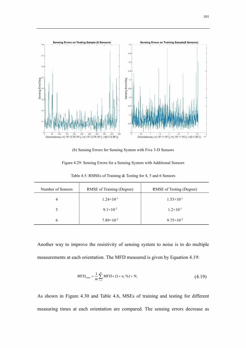
101
(b) Sensing Errors for Sensing System with Five 3-D Sensors
Figure 4.29: Sensing Errors for a Sensing System with Additional Sensors
Table 4.5: RMSEs of Training & Testing for 4, 5 and 6 Sensors
Number of Sensors RMSE of Training (Degree) RMSE of Testing (Degree)
4 1.24×10⁻¹
0.0250
1.53×10⁻¹
0.0588
0.0330
5 9.1×10⁻²
0.0152
1.2×10⁻¹
0.0362
0.0175
6 7.89×10⁻²
0.0129
9.75×10⁻²
0.0254
0.0175
Another way to improve the resistivity of sensing system to noise is to do multiple
measurements at each orientation. The MFD measured is given by Equation 4.19:
noise
1
1(1 n %) N
m
i i
i
MFD MFDm
(4.19)
As shown in Figure 4.30 and Table 4.6, MSEs of training and testing for different
measuring times at each orientation are compared. The sensing errors decrease as

102
measuring times increase, and there is remarkable improvement from one to two times,
but the improvement is very limited when measuring times increase from five to ten.
Compared to increasing number of sensors, multiple measuring has better performance
in enhancing resistivity of sensing system to noise.
(a) Sensing Errors for Two Measurement Times
(b) Sensing Errors for Five Measurement Times
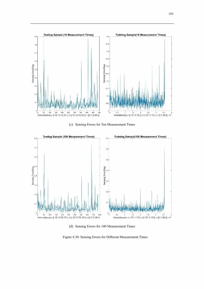
103
(c) Sensing Errors for Ten Measurement Times
(d) Sensing Errors for 100 Measurement Times
Figure 4.30: Sensing Errors for Different Measurement Times

104
Table 4.6: RMSEs of Training & Testing for Multiple Measurements
Measuring Times RMSE of Training (Degree) RMSE of Testing (Degree)
1 1.24×10⁻¹
0.0451
0.0250
1.53×10⁻¹
0.0588
0.0330
2 9.61×10⁻²
0.0088
0.0060
1.14×10⁻¹
0.0102
0.0050
5 7.98×10⁻²
0.00333
1.05×10⁻¹
0.00844
0.00400
10 6.45×10⁻²
0.0037
0.0019
8.99×10⁻²
100 4.45×10⁻²
0.0033
0.0022
6.67×10⁻²
0.0039
0.0027
4.4.6 Numerical Interpolation to Reduce Measurement Workload
Above has presented the good performance of sensing system based on neural network
and measured MFD, and training sample contains more than 3×10⁴ orientation-MFD
pairs. However, in practice, it is too time consuming to measure MFD at so many
orientations. Similar to position sensing of one PM, numerical interpolation is used to
create the training sample from fewer measurements.
Interpolation from three different initial measuring samples is executed, and
interpolation errors and sensing errors are compared. Three measuring samples are as
followings:
Initial Sample 1: α= [-15(initial):7.5(interval):15(final)], β= [-15:7.5:15], γ= [[0:9:36]],
125 orientation-MFD pairs in total;
Initial Sample 2: α= [-15(initial):6(interval):15(final)], β= [-15:6:15], γ= [[0:7.2:36]],
216 orientation-MFD pairs in total;

105
Initial Sample 3: α= [-15(initial):5(interval):15(final)], β= [-15:5:15], γ= [[0:6:36]], 343
orientation-MFD pairs in total.
The initial samples are then interpolated to interpolated sample: α= [-
15(initial):1(interval):15(final)], β= [-15:2:15], γ= [[0:1:36]], 35557 orientation-MFD
pairs in total. Noted that polynomials of degree 3, 4, and 5 are applied respectively for
sample 1, 2 and 3.
Two types of errors are compared between interpolations from different initial sample,
i.e. interpolation errors as shown in Figure 4.31 and sensing errors based on the same
neural network as shown in Figure 4.32. The sensing errors are for test sample, instead
of interpolated sample.
Figure 4.31: Interpolation Errors

106
(a) Sensing Errors for Sample 1
(b) Sensing Errors for Sample 2

107
(c) Sensing Errors for Sample 3
Figure 4.32: Sensing Errors for Different Initial Samples before Interpolation
Table 4.7: RMSEs of Training & Testing for Different Interpolation Sample
Number of Orientation-MFD Pairs
of Initial Sample
RMSE of Training
(Degree)
RMSE of Testing (Degree)
Original 2.01×10⁻²
0.0451
0.0250
3.21×10⁻²
125 2.46×10⁻²
0.0088
0.0060
7.89×10⁻¹
216 3.03×10⁻²
0.00333
3.12×10⁻¹
0.00400
343 2.09×10⁻²
0.0037
0.0019
1.66×10⁻¹
As expected, the more orientation-MFD pairs in the initial sample, the smaller errors of
interpolation and training. However, bigger initial sample also means more
measurements. So the suitable size of initial sample should be a tradeoff of accuracy

108
and measuring time requirements of sensing system.
4.4.7 Investigation of Computation Time
There are two types of computation time about neural network, i.e. training time and
running time. Training generally can be done offline, so running time to compute
orientation is more important in consideration of real-time closed-loop control.
uniformizationMFDS f1(Tansig or
Logsig)MFDS Input1Input1
f2(Purelin)Input2 Output
Figure 4.33: Computation Procedures of a Neural Network
The three types of transfer functions are defined as:
2 / 1 2* 1
1 / 1
tansig n exp n
logsig n exp n
purelin n n
(4.20)
The following factors have influence on the computation speed:
1) Size of inputs, which depends on number of sensors;
2) Structure of NN, i.e. number of layers and number of neurons on each layer;
3) Transfer functions of NN.
Computation is executed in MATLAB on a Quad-Core Laptop with 2.3 GHZ CPU

109
frequency, and computation speed based on other real-time hardware can be estimated
based on investigations of this section. Since MATLAB has strong ability in matrix
operation for its special optimization for matrix computation, while other programs may
not have, we have separated matrix operation to calculations such as additions and
multiplications.
Suppose four 3-DOF sensors are used, so there are 12 MFD inputs. First step is
normalization to transfer input values to the range of ±1. Based on MATLAB,
computation time for 12 inputs is about 2.5×10⁻⁷ second.
Refer to Equation 4.12, for a two-layer neural network with 80 neurons and 12 inputs,
there are 80×12=960 multiplications and 960+80=1040 additions before first input to
transfer functions. Computation time for 960 multiplications and 1040 additions is
about 8.7×10⁻⁶ second.
First transfer function is Tansig or Logsig, take Logsig for example, there are 80 times
of execution of Logsig function, and need about 1.9×10⁻² second. However, if we use
look up table instead of calculation, the computation time of this step can be as short as
about 6.7×10⁻⁶ second.
Then before input to transfer function 2, there are 240 multiplications and 320 additions,
which take about 2.5×10⁻⁶ second. And transfer function 2 is Purelin of three inputs, the
consuming time can be neglected.

110
So total computation time for NNs to calculate one orientation is about 1.815×10⁻⁵
second, which means a measuring rate about 55KHZ sample depends on computation
speed can be expected, which in most cases satisfies a practical SWM closed-loop
control system. However, if SWM is controlled by other hardware such as NI
controllers instead of a PC, the CPU speed may be one-tenth only of a PC, and
measuring rate decreases to about 5.5 KHZ. Then the measuring rate need to be
considered in control design in case of serious sensing delay.
4.5 Summary
The chapter has proposed a sensing system design of an SWM based on Hall Effect
sensors and neural networks. For investigation of such a sensing system, MFD of SWM
is built by DMP method to do simulation and provide useful observations.
3D position sensing of a cylinder PM is investigated first, and NNs have shown good
performance. With interpolation method to get a training sample based on fewer
measurements, the sensing system can be operated with fewer measuring times.
Preliminary investigations on NNs based sensing system of the SWM is done first, and
then the sensing system is studied to be absolute, accurate, feasible, and with fast
response. First, the spatial distribution of sensors are optimized first, and locations of
the four sensors are settled subsequently. Second, important factors about the NNs such
as layers, number of hidden layer neurons are investigated. Third, magnetic noises,
which generally exist and cannot be neglected, are considered and methods to alleviate

111
the influence are presented. Numerical interpolation is then proposed to make the
sensing system be feasible and practical by decreasing the measurement times. Finally,
the computation time and according response rate is presented. With shown
performance and estimated computation speed, the sensing system proposed in this
chapter is able to be used in real time control of an SWM.

112
CHAPTER 5
EXPERIMENTAL INVESTIGATIONS
5.1 Overview
The proposed magnetic torque modeling and sensing system need to be validated by
experimental investigations. A prototype is fabricated based on optimization results in
Chapter 2, and magnetic torque measured in experiments are compared with the one
calculated by FEM modeling. Experimental investigations about a 3-DOF positioning
system of a cylinder PM is presented first. As MFD of a single cylinder PM is much
simpler than MFD of the whole SWM, a better positioning accuracy is expected.
Experiments on proposed sensing system for the SWM are then carried out, and
strategies proposed in Chapter 4 to improve resistivity to magnetic noise, have been
verified.
5.2 Prototype of Proposed SWM
Based on the optimization results in Chapter 2, SWM prototypes are fabricated and
experimental investigations are carried out. The lengths of the PMs, separation angles
between PMs, and diameter of the stator cores are determined from design optimization.
Some parameters are predefined in design optimization such as ri (distance from inner
PM to rotating center), ro (total radius of the SWM), etc. Other parameters are
determined by maximizing the volume storing magnetic energy and minimizing the
magnetic resistance, so as to improve the torque capability. The air gap is set to be
0.5mm based on fabrication and assembly skills as a small air gap helps to improve

113
magnetic torque. With total length and lengths of inner and outer PMs, the total length
of EMs can be calculated. Each EM is separated to 2 coil with same length for
fabrication and assembly simplification. The separation angle between the 2 layers of
EMs is set as 48° to obtain the maximum diameters of the coils without mechanical
contact. The cylinder permanent magnet made of NdFeB (N52, with the available
highest residual magnetic flux density) is chosen for its high residual magnetic flux
density and high coercive force.
Some parts and experiment setups are shown in Figure 5.1 and key geometric
parameters are illustrated in Table 5.1.
For simplicity and economic considerations, #20 carbon steel is used to fabricate the
ferromagnetic stator cores, although laminated silicon steel sheets are better choice for
reducing eddy current losses and possess much higher relative magnetic permeability.
In future study, laminated silicon steel should be used to fabricate the stator cores, to
improve the magnetic permeability and reduce eddy current, which brings iron loss and
makes it difficult to compute magnetic torque.

114
(a) Bearing (b) Base (c) Bottom Plate
(d) Top Plate (e) Inner Rotor (f) Outer Rotor
(g) Stator Core (h) Stator (i) Connector
(j) NI PCI-6251 (k) Torque Measuring Setup
Figure 5.1: SWM Prototypes

115
Figure 5.2: Copper Coil Winding Patterns
Table 5.1 Geometric Parameters of Spherical Wheel Motor
Rotor and PMs Stator and EMs
ri 25° βs 24°
ro 64.9mm βr 32°
Din 13mm LEM 10.3mm
Lin 8mm Din-EM 24mm
Dout 28mm Dout-EM 32mm
Lout 6mm I ± 2.5A
Br
1.45T Dcore 10mm
βp 36°
Where:
ri: Distance from rotating center to inner surface of inside PMs;
ro: Distance from rotating center to outer surface of outside PMs;
Din, Lin: Diameter and length of the inside PMs;
Dout, Lout: Diameter and length of the outside PMs;
Din-EM: External diameter of the inside EM;
Dout-EM: External diameter of the outside EM;

116
βr: Residual magnetism of both inside and outside PMs;
βp: Separation angle between neighboring PMs on the middle layer;
βs: Separation angle between upper or lower layer EMs and middle layer PMs;
βr: Separation angle between upper or lower layer PMs and middle layer PMs;
LEM: Length of the two parts of EMs;
I: currents applied on EMs in experiments;
Dcore: Diameter of stator core.
Enameled copper wires with round section which can endure temperature as high as
180 degrees are used to wind coils. There are two considerations for determining the
diameter of copper wires, i.e. the resistance R of two pairs of EMs (an inner and outer
EM compose a pair; the two pairs are placed diagonally) which are connected in series
and activated by the same source, and the winding complexity which increases as the
diameter increases. A common commercial high-power (about 50 to 100W continuous
power) such as LM3886 from Texas Instruments can output highest power with 4 to 8
Ohm load. If the copper wires are winded ideally as presented in Figure 5.2, the space
occupancy rate SOC can be calculated by Equation 5.1. However, the SOC is calculated
in ideal condition. Based on the experience of the manufacturer, the real SOC is only
80-90% of the ideal one. The larger the diameter of copper wire, the lower the real SOC
is. Here we use 85% of the ideal SOC, which is 77.1%, for estimation of coil resistance.
2
2 2 2
1
4 90.7%, 85% 77.1%1 3 1
2 ( )4 4 8
real
DSOC SOC SOC
D D D
(5.1)
117
Where D is the diameter of the copper wires.
The resistance of a coil Rcoil with core diameter Dcore, outer diameter Dcoil, and length
Lcoil, can be calculated by Equation 5.2.
2coil 1
4
1( )
2core coil
Cu
Cu
n D DR
D
(5.2)
Where
2
(
1
4
)coil coil corereal
L D Dn SOC
D
is the number of turns.
DCu is the diameter of the copper of the wire, which is about 0.02- 0.05mm smaller than
D.
Cu is the resistivity of copper, which is 1.71×10⁻⁸ Ohm*m at 20℃. However, the
resistivity is not a constant and is dependent on the temperature as in Equation 5.3.
_ 0(1 )
CuCu t (5.3)
Where
_ 0Cu is the resistivity at 0℃, and is temperature coefficient, which is about 0.0039.
Suppose the highest working temperature for copper wire is 80℃, then the resistivity
at 80℃ is calculated to be 2.08×10⁻⁸ Ohm*m.
With external diameters of the inner coil and outer coil as presented in Table 5.1, and
Equations 5.1, 5.2 and 5.3, the resistivity and diameter of copper wire is listed in Table
5.2. For maximizing output power capability of economical amplifiers (load should be

118
less than 8 Ohm), and reducing the complexity of windings coils (smaller diameter wire
is better), the DCu and D is chosen to be 0.5mm and 0.55mm. The final coils have 370
and 225 turns, which are fewer than expected especially for the smaller coil.
Table 5.2: Resistivity of 2 pairs of EMs (connected in series) Vs Copper Wire Diameter
DCu D
n1
Turns of Inner
EM
n2
Turns of Outer
EM
R
(Temperature=20℃)
R
(Temperature=80℃)
0.2 0.225 2197 139 240.5 292.7
0.3 0.34 962 612 46.80 56.96
0.4 0.44 575 366 15.72 19.13
0.5 0.55 368 234 6.44 7.84
0.6 0.65 263 168 3.20 3.90
As illustrated in Figure 5.1 (g), the stator cores are composed of a screw and a nut, and
two parts of EMs of different diameter are connected together as shown in Figure 5.1
(h). For consideration of the strength of the structure, the plate is 1mm thick between
two parts of EMs. Since the magnetic field of the air gap between PMs and EMs is
slightly influenced by the middle turns of EMs, the losses due to the 1mm thick plate
can be neglected. And such a design solves the housing problem for stators, which
becomes more difficult since different from existing designs, there are rotors both inside
and outside of stators. Inner and outer rotors are connected by a bar as shown in Figure

119
5.1 (i) so all the PMs can rotates towards the center of the spherical rolling joint together.
The diameter of the bar is determined so that it can support the outer rotor and does not
reduce the inclination range.
A six-axis force/ torque sensor Gamma SI-130-10 as shown in Figure 5.1 (k) is mounted
on the output shaft of the motor and slides on a guide way to measure inclination torque
at different separation angles. The measure range is 130N for force and 10N*m for
torque. A data acquisition device NI PCI-6251 is used to transmit voltage information
of the torque sensor to a computer, and a calibration matrix is used to transfer voltages
to forces and torques. Take the torque on X axis as an example, since the asymmetry
from manufacturing and assembling, the actual torque can be calculated by the
following equation
'
x x zT T F L
(5.4)
Where
xT : Actual torque;
'
xT : Measured Torque;
L: Distance from the center of the spherical ball joint to the work surface of the torque
sensor.

120
5.3 Experimental Verifications for Torque Simulation
Based on the SWM prototype, inclination torques are measured and compared with
torques calculated by FEM model. The torque produced by experimental configurations
with inner PMs only or with all PMs, with aluminum or iron material for the EM core
and outer rotor as tabulated in Table 5.3 is measured and compared against simulations.
The simulation utilizes the SPM, while the experiments use all the inner PMs or inner
and outer PMs. Similar to the comparison between the SPM and FM in Chapter 2, the
resultant torque from the simulations and experiments are close to each other with
maximum discrepancy less than 10%, proving the SPM for optimization. Reasons for
the error may include that we cannot obtain exact parameter values for PMs (magnetic
permeability, coercive force, residual magnetic flux density), PMs are not fabricated
totally homogeneous, and the fabrication and assembly accuracy problem of the
measurement setup.
First, configurations D, E, F are compared with configurations A, B, C respectively.
The main difference is that configurations D, E, F have both inner rotor and outer rotor,
while configurations A, B, C have inner rotor only. The major improvement of torque-
to-volume ratio that the inclination torque produced by configurations D, E, F is more
than four times as the one produced by configurations A, B, C respectively while the
volume of configurations D, E, F has increased by less than 70%. The 135% increase
of torque density- ratio of torque to volume, argues the advantages of proposed
configuration compared to existing designs.
Similarly, configurations with ferromagnetic stator core are compared with

121
configurations with aluminum stator core. Since the magnetic torque generated by
configurations with ferromagnetic stator core is not proportional to currents, so both
positive and negative currents are imposed and compared. Considering the sum or
average of torque, ferromagnetic stator core configurations with both positive and
negative currents can produce much stronger inclination torque than aluminum core
configurations.
Finally, configurations D, E, F with aluminum outer rotor and configurations with
ferromagnetic outer rotor G, H, I are compared. With ferromagnetic boundary, the
magnetic circuit of the SWM is closed and magnetic field is mainly confined in the
SWM, and results in much less magnetic flux leakage. As shown in the Figure,
configurations G, H, I can produce torque 30% more than the one produce by
configurations D, E, F respectively. Another advantage of SWMs with ferromagnetic
boundary is that there is less undesired electromagnetic interference (EMI).
Figure 5.3: Torque Comparisons between Experiments and Simulations

122
Table 5.3: Experimental Configurations
Designs PMs (inner (I)
and/or outer (O))
EM Core (Aluminum
A; Iron I)
Current
(Amp)
Outer rotor
(None N; A; I)
A I A 2.5 N
B I I 2.5 N
C I I -2.5 N
D I and O A 2.5 A
E I and O I 2.5 A
F I and O I -2.5 A
G I and O A 2.5 I
H I and O I 2.5 I
I I and O I -2.5 I
I I and O I -2.5 I
In conclusion, SWMs with both inner rotor and outer rotor, ferromagnetic stator core
and outer rotor can produce maximum sum/ average inclination torque and less EMI.
Figure 5.4 shows magnetic flux density distribution of Configuration H. The magnetic
flux lines are along with the axis of the coil and confined within the iron boundary
(yellow in Figure 5.4). It indicates the design has less leakage of magnetic field and
magnetic flux density is strongest in iron core, which verifies the effect of iron on
enhancing magnetic interaction between the stators and the rotors. Validated by
experiments and FEM modeling, SWMs with iron core and iron boundary is to be
chosen if maximum inclination torque is the object.

123
Figure. 5.4 Magnetic Flux Density Plot for Configuration H
5.4 Experimental Investigations on Sensing System of SWM
5.4.1 Experimental Setup for Position Sensing of One PM
Position sensing of a PM which can move in three directions as shown in Figure 5.5 is
studied here for its simplicity and generality. For SWMs without ferromagnetic
materials, the sensing strategy of a PM can be extended to the whole SWM since
superposition principle can be applied. The coordinate system is defined by the mobile
platform, note that the PM is not necessarily to be in the center of the coordinate system.
Here we are going to build the forward model through interpolation from measured
magnetic flux densities, instead of analysis or DMP due to the following reasons:
1) It is difficult to measure the residual magnetism and material properties such as
actual permeability;
2) The size of Hall Effect sensors cannot be neglected, which makes it difficult to treat
actual sensors as point sensors;

124
Figure 5.5: Experimental Setup for Position Sensing of a PM
3) Environmental conditions such as magnetic noise is unable to be calculated, and
temperature, humidity … may affect performance of the sensor, let alone the sensor
itself has up to 3% error.
The mobile platform can move in 3-DOF with ranges of 20mm in two planar directions
and 10mm in vertical direction. Positioning resolution is 0.02mm in each direction.
As shown in Figure 5.5, three 3-DOF MFS-3A Hall Effect sensors are placed at [90mm,
0, 0], [0, 90mm, 0] and [-90mm, 0, 0] to measure x, y, z components of magnetic flux
densities, so nine components in total are measured.
Specifications of MFS-3A are listed in the following table. As shown in Table 5.4, max
magnetic flux density is ±7.3mT, so Hall Effect sensors cannot be put too close to the
PM in case of saturation. And also, if sensors are put too far away from the PM, the

125
measuring errors due to magnetic noise will be relatively large. The best way is to make
magnetic flux density on sensors just below the maximum measurable value. Outputs
of MFS-3A are voltages in the range of 0.5 to 4.5V while measured magnetic flux
density is in the range of ±7.3mT, and sensitivity is 280mV/mT. Magnetic flux density
is to be obtained with linear transition, and we can also use measured voltages directly
instead of transformed magnetic flux density in NNs.
Table 5.4 Specifications of MFS-3A
Parameters Value
Field Range ±7.3mT
Resolution ±10μT
Three Analog Outputs 0.5-4.5V
Sensitivity 280mV/mT
Accuracy ±3%
Frequency Response 100kHz
Size 10×13.5×12mm
Weight 2.5g
Power 36mA max at 5V
Measuring positions in experiments are chosen as x=[-
0(initial):5(interval):20mm(final)], y=[0(initial):2(interval):8mm(final)],
z=[0(initial):5(interval):20mm(final)] according to the maximum working range of the
mobile platform. And interpolation has extended the measured sample to x=[-
0(initial):1(interval):20mm(final)], y=[0(initial):1(interval):8mm(final)],

126
z=[0(initial):0.4(interval):20mm(final)], so 21×21×21=9261 positions in the
interpolated training sample. Since the voltage outputs are fluctuating due to magnetic
noise or sensor performance, we use average value of 40 measurements in each position
to eliminate the influence of fluctuation. The influence of fluctuation on position
sensing performance is presented later in this section.
The trained NN is tested by nine positions not used for interpolation in the working
range, and errors are as shown in Figure 5.6. Maximum error is about 0.2mm which is
larger than simulation in Chapter 4. The main reasons for the error include: limitations
of sensors’ performance, environmental magnetic noise, modeling error due to
interpolation, and approximation errors of the NN.
To test how much the fluctuations influence performance of the sensing system, a fixed
position has been measured 10 times and positions estimated by the same trained NN
are compared as presented in Figure 5.7. The difference between different measuring
times can be as large as 0.2mm, superposition with errors due to other factors, the total
error can be much larger than 0.2mm. And that is why we need to use average measured
value to eliminate influence of fluctuations.
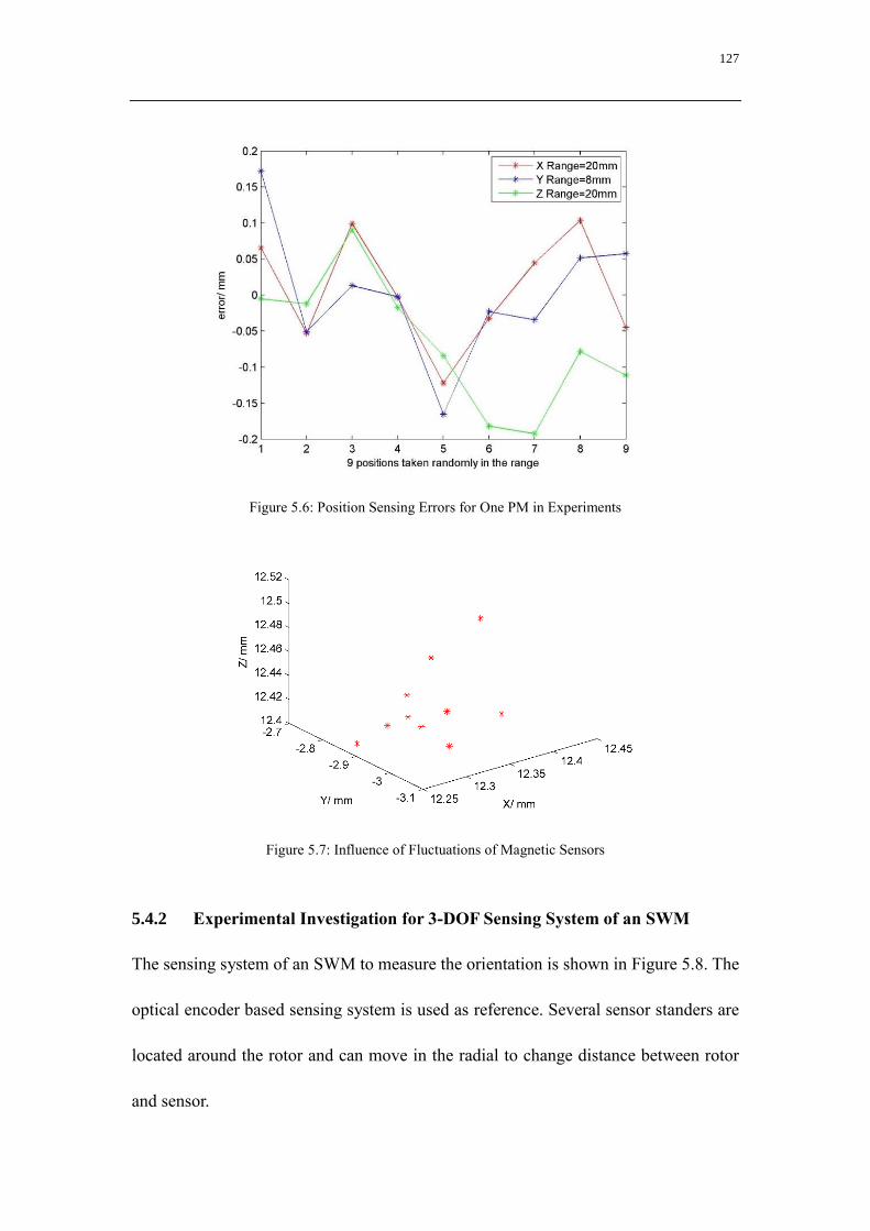
127
Figure 5.6: Position Sensing Errors for One PM in Experiments
Figure 5.7: Influence of Fluctuations of Magnetic Sensors
5.4.2 Experimental Investigation for 3-DOF Sensing System of an SWM
The sensing system of an SWM to measure the orientation is shown in Figure 5.8. The
optical encoder based sensing system is used as reference. Several sensor standers are
located around the rotor and can move in the radial to change distance between rotor
and sensor.
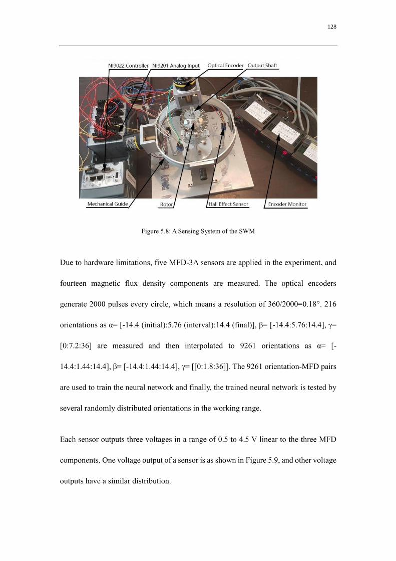
128
Figure 5.8: A Sensing System of the SWM
Due to hardware limitations, five MFD-3A sensors are applied in the experiment, and
fourteen magnetic flux density components are measured. The optical encoders
generate 2000 pulses every circle, which means a resolution of 360/2000=0.18°. 216
orientations as α= [-14.4 (initial):5.76 (interval):14.4 (final)], β= [-14.4:5.76:14.4], γ=
[0:7.2:36] are measured and then interpolated to 9261 orientations as α= [-
14.4:1.44:14.4], β= [-14.4:1.44:14.4], γ= [[0:1.8:36]]. The 9261 orientation-MFD pairs
are used to train the neural network and finally, the trained neural network is tested by
several randomly distributed orientations in the working range.
Each sensor outputs three voltages in a range of 0.5 to 4.5 V linear to the three MFD
components. One voltage output of a sensor is as shown in Figure 5.9, and other voltage
outputs have a similar distribution.
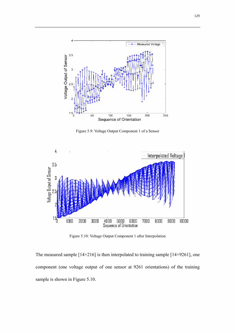
129
Figure 5.9: Voltage Output Component 1 of a Sensor
Figure 5.10: Voltage Output Component 1 after Interpolation
The measured sample [14×216] is then interpolated to training sample [14×9261], one
component (one voltage output of one sensor at 9261 orientations) of the training
sample is shown in Figure 5.10.

130
(a) Error of Two-layer NN with 30 Neurons (b) Error of Two-layer NN with 40 Neurons
(c) Error of Two-layer NN with 50 Neurons (d) Error of Two-layer NN with 60 Neurons
(e) Error of Two-layer NN with 70 Neurons (f) Error of Two-layer NN with 80 Neurons
(g) Error of Two-layer NN with 90 Neurons (h) Error of Two-layer NN with 100 Neurons
Figure. 5.11 Measuring Error of Neural Network Based Sensing System
As shown in Figure 5.11, the smallest error occurs when 80 neurons are adopted.
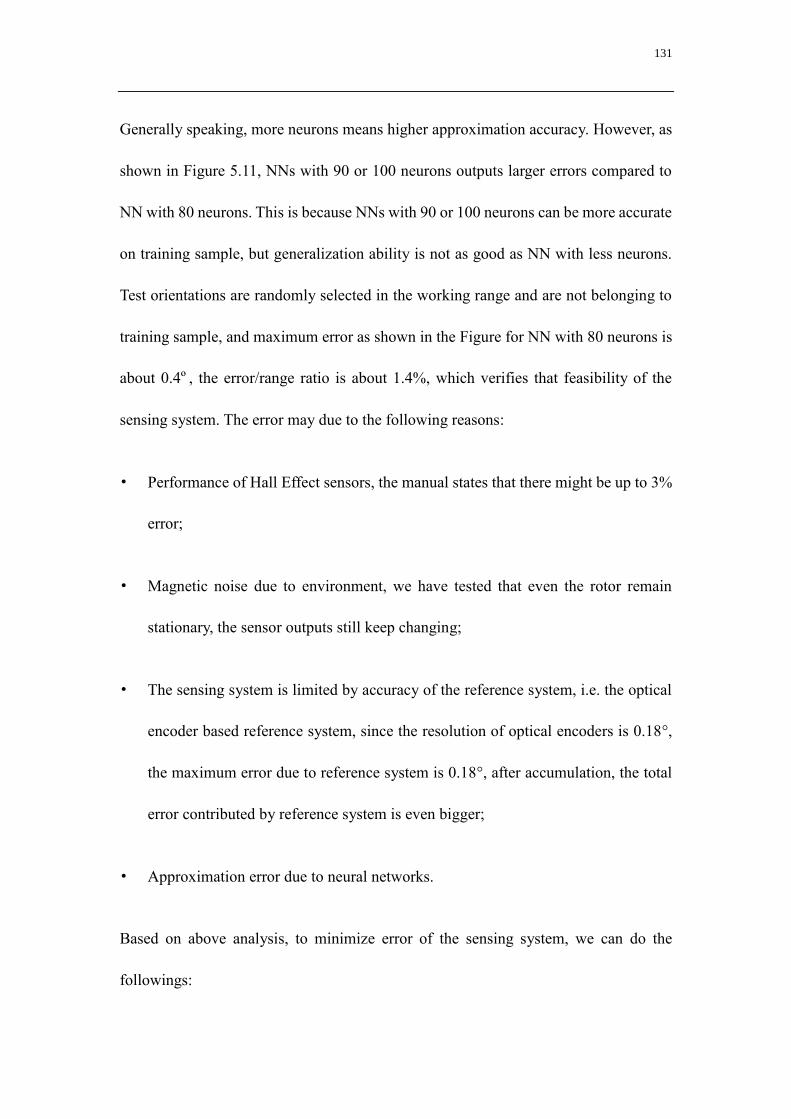
131
Generally speaking, more neurons means higher approximation accuracy. However, as
shown in Figure 5.11, NNs with 90 or 100 neurons outputs larger errors compared to
NN with 80 neurons. This is because NNs with 90 or 100 neurons can be more accurate
on training sample, but generalization ability is not as good as NN with less neurons.
Test orientations are randomly selected in the working range and are not belonging to
training sample, and maximum error as shown in the Figure for NN with 80 neurons is
about 0.4º, the error/range ratio is about 1.4%, which verifies that feasibility of the
sensing system. The error may due to the following reasons:
• Performance of Hall Effect sensors, the manual states that there might be up to 3%
error;
• Magnetic noise due to environment, we have tested that even the rotor remain
stationary, the sensor outputs still keep changing;
• The sensing system is limited by accuracy of the reference system, i.e. the optical
encoder based reference system, since the resolution of optical encoders is 0.18°,
the maximum error due to reference system is 0.18°, after accumulation, the total
error contributed by reference system is even bigger;
• Approximation error due to neural networks.
Based on above analysis, to minimize error of the sensing system, we can do the
followings:

132
• To adopt magnetic sensors with better performance such as higher stability;
• To use sensor with bigger magnetic flux density range, so noise/MFD ratio is
smaller, also can use more sensors to offset the influence of the noise ;
• To use optical encoders with higher resolution in the reference system, such as 6000
pulses per circle;
• To try NNs with more layers or neurons, and train NNs with sample with more
orientations-MFD pairs.
5.4.3 Influence of Number of Measured Components on Sensing Performance
In last sector, fourteen components are used in the sensing system, here we are to
investigate the influence of the number of measured components on sensing
performance. 7, 8 … 14 measured components are applied and the sensing errors are
compared. For time saving consideration, neural networks for all conditions are 2-layer
with 80 neurons, and maximum training times are set to be 100. As shown in Figure
5.12, more measured MFD components generally result in higher sensing accuracy,
which is reasonable since more measured components means more information, but the
improvement is not so obvious when there are more than nine measured MFD
components. So to save hardware cost, we can deduct number of measured MFD
components to 9 or 10 without reducing much accuracy.

133
(a) Sensing Errors of 7 MFD Components (b) Sensing Errors of 8 MFD Components
(c) Sensing Errors of 9 MFD Components (d) Sensing Errors of 10 MFD Components
(e) Sensing Errors of 11 MFD Components (f) Sensing Errors of 12 MFD Components
(g) Sensing Errors of 13 MFD Components (h) Sensing Errors of 14 MFD Components
Figure 5.12: Sensing Errors Vs Number of Measured MFD Components

134
5.4.4 Influence of Measuring Times on Performance
Due to magnetic noise and Hall Effect sensors’ performance, the voltage outputs are
always fluctuating. As shown in Figure 5.7, the fluctuations have influenced the
positioning accuracy seriously. To enhance performance of the sensing system, we have
used average outputs of 100 times to reduce influence of fluctuations. To investigate
how much the fluctuations affect the sensing system, we adopt average outputs of 1, 10,
20, 40, 100 times respectively and comparison is as shown in Figure 5.12. From
comparisons of sensing errors of different measuring times on each orientation, we can
conclude that more measuring times can lower the influence of fluctuations, but the
improvement becomes less obvious when measuring times at each orientation is more
than 10. The sensing error is as large as 2.4° if only one measurement is carried out at
each orientation, which verifies the necessity of multiple measurements.
In design of a practical sensing system, we need to consider requirements on sample
rate, sensing accuracy … so as to choose an appropriate times of measuring repetitions.
The comparison as shown in Figure 5.13, can be a valuable reference in future.

135
(a) One Measurements at each Orientation (b) 10 Measurements at each Orientation
(c) 20 Measurements at each Orientation (d) 40 Measurements at each Orientation
(e) 100 Measurements at each Orientation
Figure 5.13: Sensing Errors Vs Measurement Times at Each Orientation
5.5 Summary
A prototype of an SWM is fabricated based on optimization results. The SWM is
designed to be easy in fabrication and inexpensive in cost, such as the wire diameter is
chosen to be 0.5mm, so resistance of the coils is suitable for cost saving and common

136
amplifiers.
Magnetic torques of different configurations have been calculated and compared with
FEM modeling results. The great agreement between modeling and experiments has
validated the magnetic torque modeling with simplified model, and large improvement
in torque density has proven the proposed design for SWMs in enhancing inclination
torque.
Although limited by sensor specifications and accuracy of the reference measuring
system, the proposed sensing system has achieved a 1.4% ratio of error to working
range. Strategies proposed in Chapter 4 to alleviate influence of magnetic noise, have
been validated by experiments. Based on experimental verification, proposed sensing
system is feasible to be applied in an integrated SWM system with good performance.

137
CHAPTER 6
CONCLUSION AND FUTURE WORK
6.1 Accomplishments and Contributions
The thesis has presented three respects of research about an SWM, i.e. structure design
optimization to maximize the inclination torque and improve torque isotropy, magnetic
torque and dynamic modeling for SWMs with ferromagnetic stator cores, and design
of non-contact sensing system for real-time measurement of orientation in 3-DOF. The
novelties of the thesis lie mainly in 2 aspects as follows.
1. Proposal of a design optimization strategy, which including selecting key
dependent physical parameters and their ranges, and optimizing their values by the
numerical analysis method. The optimization strategy has been verified on the
proposed new design of an SWM to maximize the inclination torque capability.
2. The design of 3-DOF Hall Effect sensor based sensing system, which applies
neural networks to compute orientations from measured MFD in real-time. The
sensing system is verified to be fast and accurate by experiments, which is
important for feedback control.
6.1.1 Design Optimization to Enhance Inclination Torque
The thesis has presented a new design of an SWM with PMs both inside and outside of
the EMs, so as to improve electromagnetic torque since Electromotive Force (EMF) at

138
both sides of the coils are applied and result in less MFD leakage. Inclination torque is
generally weaker compared to spinning torque since less PM-EM pairs are involved in
inclination torque. Design optimization is then applied to obtain optimal geometrical
parameters to maximize inclination torque within a given volume. Finally, a prototype
is fabricated based on optimization results and experimental investigations are executed
to verify the simulation model.
Detailed work in structure design is listed as follows.
Two configurations with two or three layers of PMs both inside and outside of EMs,
different from previous designs with PMs only inside or outside of EMs are proposed.
APDL in ANSYS is applied to calculate the electromagnetic torque, key
geometrical parameters are selected, interpolated and compared to decide the best
combinations which can generate maximum inclination torque. Since it is unfair to
compare the two configurations with random geometrical parameters, both
configurations are optimized and then compared.
A prototype based on design optimization results is fabricated, and experiments are
carried out to verify the simulation model. The experimental results shows that there is
less than 10% discrepancy between FEM modeling and experimental measurements.
6.1.2 Magnetic Torque and Dynamic Modeling
MFD and magnetic torque of SWMs with ferromagnetic stator cores is nonlinear and

139
makes it challenging for modeling. MFD on ferromagnetic stator cores with different
applied currents is generated and analyzed by FEM, and magnetic torque model is built
based on MFD analysis and inspirations from the SPM. Although the magnetic torque
is nonlinear to current inputs, it can be divided to two parts, i.e. one fixed part due to
ferromagnetic stator cores and one part proportional to current inputs as long as the
maximum currents density is less than 8A/mm2, which is maximum current density
limited by heat dissipation. Based on the magnetic torque and dynamic model, motions
of the rotor can be anticipated with given inputs and optimal inputs can be computed
with desired motions.
6.1.3 Design of a 3-DOF Non-contact Sensing System Based on MFD and NNs
A 3-DOF, real-time and absolute sensing system based on Hall Effect sensors and NNs
is proposed and realized. Due to complicated MFD of the whole SWM, neural networks
instead of analytical expressions are applied to approximate the relationship between
MFD and orientations. Based on the fabricated prototype, the sensing system is verified
by experiments.
Detailed work in sensing system design is listed as follows.
MFD of a PM is computed by DMP, and based on superposition principle, MFD of
the whole rotor is calculated.
A solution to solve the inverse problem- to compute orientation from measured

140
MFD, based on neural networks is proposed.
Parameters affecting the sensing system are studied and methods to improve
performance of the sensing system are proposed. Practical conditions such as magnetic
noise are also considered.
Experiments are carried out to verify performance of the sensing system. Optical
encoders based measuring system is used as reference, and accuracy of proposed
sensing system is at the same level of the one of the reference system, which verifies
the performance of the proposed sensing system.
6.2 Future Works
Recommendations for future work in the area of SWMs are as followings:
Improvements on sensing system
The sensing system can still be improved in the following aspects in future work:
The thesis designs the sensing system based on SWMs with air stator cores, so
MFD generated by current inputs can be deducted under superposition principle.
However, for SWMs with ferromagnetic stator cores, nonlinearity of the MFD must be
considered, which makes design of sensing system based on magnetic field more
difficult. One important work future work is to extend the proposed sensing system to
SWMs with ferromagnetic materials.

141
The magnetic field is periodic every 72 degrees, so sensing system based on MFD
only is unable to distinguish if SWM spins 72 or more degrees. The proposed sensing
system may need an auxiliary sensing method based on design requirements.
The neural networks of the sensing system in the thesis treat the MFD- inputs of
NNs as an ordinary set of values. However, MFD of the SWM, which can be solved
analytically, possesses some intrinsic characteristics. If we can fully make use of those
characteristics, we are able to decrease the scale of the NN and improve computation
speed while accuracy is maintained.
Closed-loop controller design and realization
The magnetic torque and dynamic modeling, and proposed design of the sensing system,
have laid foundations for design of a closed-loop motion control system for SWMs.
Future work about control of SWMs are desired so as to complete an integrated SWM
system. Future work may focus on control simulations first, but the theories about the
SWM in the thesis are better to be verified by successful motion control experiments.

142
REFERENCE
1. F. C. Williams, E.R. Laithwaite and J.F. Eastham, "Development and design of spherical
induction motors," Proceedings of the IEE - Part A: Power Engineering, vol. 106(30), pp. 471-
484, 1959.
2. K. M. Lee and H. Son, "Torque Model for Design and Control of a Spherical Wheel Motor," in
Proceedings of 2005 IEEE/ASME International Conference on Advanced Intelligent
Mechatronics, Monterey, California, USA, July 2005, pp. 335–340.
3. K. M. Lee, H. Son and J. Joni, "Concept Development and Design of a Spherical Wheel Motor
(SWM). in Robotics and Automation," in Proceedings of the IEEE International Conference on
Robotics and Automation, pp. 3652-3657, Barcelona, Spain, 2005.
4. L. Yan, I. M. Chen, G. Yang and K. M. Lee, "Analytical and experimental investigation on the
magnetic field and torque of a permanent magnet spherical actuator," IEEE/ASME Transactions
on Mechatronics, 2006. 11(4): pp. 409-419.
5. D. W. Kang, W. H. Kim, S. C. Go, C. S. Jin, S. H. Won, D. H. Kon and J. Lee, "Method of
Current Compensation for Reducing Error of Holding Torque of Permanent-Magnet Spherical
Wheel Motor," IEEE Transactions on Magnetics, 2009. 45(6): p. 2819-2822.
6. H. Son and K. M. Lee, "Two-DOF magnetic orientation sensor using distributed multipole
models for spherical wheel motor," Mechatronics, pp. 156-165, 2011.
7. S. Toyama, S. Hatae and M. Nonaka, "Development of multi-degree of freedom spherical
ultrasonic motor," Fifth International Conference on Advanced Robotics, pp. 55-60, Pisa, Italy,
1991.
8. T. Shigeki, S. Shigeru, G. Zhang, M. Yasutaro and N. Kazuto, "Multi degree of freedom
spherical ultrasonic motor," IECON 20th International Conference on Industrial Electronics,
Control and Instrumentation, vol. 2, pp. 900-905, Bologna, Italy, 1994.
9. K. Takemura and T. Maeno, "Design and control of an ultrasonic motor capable of generating
multi-DOF motion,", IEEE/ASME Transactions on Mechatronics, pp. 499-506, 2001.
10. M. Aoyagi, S. P. Beeby and N.M. White, "A novel multi-degree-of-freedom thick-film
ultrasonic motor," IEEE Transactions on Ultrasonics, Ferroelectrics, and Frequency Control,
vol. 49, pp. 151-158, 2002.
11. S. Park, K. Takemura and T. Maeno, "Study on Multi-DOF Ultrasonic Actuator for
Laparoscopic Instrument," JSME International Journal Series C Mechanical Systems, Machine
Elements and Manufacturing, vol. 47(2), pp. 574-581, 2004.

143
12. K. Takemura, Ohno Y. and T. Maeno, "Design of a plate type multi-DOF ultrasonic motor and
its self-oscillation driving circuit," IEEE/ASME Transactions on Mechatronics, vol. 9(3): pp.
474-480, 2004.
13. H. Kawano, H. Ando, T. Hirahara, C. Yun and S. Ueha, "Application of a multi-DOF ultrasonic
servomotor in an auditory tele-existence robot," IEEE Transactions on Robotics, vol. 21(5), pp.
790-800, 2005.
14. C. Zhao, Z. Li, and W. Huang, "Optimal design of the stator of a three-DOF ultrasonic motor",
Sensors and Actuators A: Physical, vol. 121(2), pp. 494-499, 2005
15. Z. Li, C. Zhao, W. Huang and Z. L. Li, "Several key issues in developing of cylinder type 3-
DOF ultrasonic motor," Sensors and Actuators A: Physical, vol. 136(2), pp. 704-709, 2007.
16. T. Mashimo, K. Awaga and S. Toyama. "Development of a Spherical Ultrasonic Motor with an
Attitude Sensing System using Optical Fibers," IEEE International Conference on Robotics and
Automation, pp. 4466-4471, Roma, Italy, 2007.
17. K. Takemura, S. Park and T. Maeno, "Control of multi-dof ultrasonic actuator for dexterous
surgical instrument," Journal of Sound and Vibration, vol. 311(3–5), pp. 652-666, 2008.
18. M. Hoshina, T. Mashimo and S. Toyama. "Development of spherical ultrasonic motor as a
camera actuator for pipe inspection robot," IEEE/RSJ International Conference on Intelligent
Robots and Systems, pp. 2379-2384, St. Louis, USA, 2009.
19. T. Mashimo, S. Toyama and H. Ishida, "Design and implementation of spherical ultrasonic
motor," IEEE Transactions on Ultrasonics, Ferroelectrics, and Frequency Control, vol. 56(11),
pp. 2514-2521, 2009.
20. B. Lu, M. Aoyagi, T. Takano and H. Tamura, "Examination of Sandwich-Type Multidegree-of-
Freedom Spherical Ultrasonic Motor," Japanese Journal of Applied Physics (IPAP), vol. 49(7):
pp. 07HE24, 2010.
21. B. Lu, M. Aoyagi, T. Takano and H. Tamura, "Development of a novel rotor-embedded-type
multidegree-of-freedom spherical ultrasonic motor," ICMA International Conference on
Mechatronics and Automation, pp. 795-800, Beijing, China, 2011.
22. A. Gofukua, R. Sasakia, T. Yanob, Y. Wadaa and M. Shibatac, "Development of a two-degree-
of-freedom piezoelectric motor using single plate vibrator," in Proceedings of the Institution of
Mechanical Engineers, Part C: Journal of Mechanical Engineering Science, pp. 905–911, 2012
23. B. Lu and M. Aoyagi. "Examination of an outer-rotor-type multidegree-of-freedom spherical
ultrasonic motor," 15th International Conference on Electrical Machines and Systems, pp. 1-5,
Sapporo, Japan, 2012.

144
24. B. Li, J. Shi, G. Li and H. Li, "Design of Electromagnetic Pre-Pressure Device for 3-DOF
Spherical Ultrasonic Motor," Procedia Engineering, vol. 29, pp. 2393-2398, 2012.
25. J. Luo, C. Huang, H. Li, S. Xie and Y. Zhang, "Structural Design and Analysis of 3-DOF Bionic
Eye Based on Spherical Ultrasonic Motor," Intelligent Robotics and Applications, pp. 348-356,
Springer Berlin Heidelberg, 2012
26. M. Hoshina, T. Mashimo, N. Fukaya, O. Matsubara and S. Toyama, "Spherical ultrasonic motor
drive system for camera orientation in pipe inspection," Advanced Robotics, vol. 27(3), pp. 199-
209, 2013.
27. K. Davey and G. Vachtsevanos. "On the control of a novel spherical robotic actuator. in Decision
and Control," 25th IEEE Conference on Decision and Control, pp. 415-416, Athens, Greece,
1986.
28. K. Davey, G. Vachtsevanos and R. Powers, "The analysis of fields and torques in spherical
induction motors," IEEE Transactions on Magnetics, vol. 23(1), pp. 273-282, 1987.
29. G. Vachtsevanos, K. Davey and K. M. Lee, "Development of a novel intelligent robotic
manipulator," IEEE Control Systems Magazine, vol. 7(3), pp. 9-15, 1987.
30. A. Foggia, E. Olivier, F. Chappuis and J.C. Sabonnadiere, "A new three degrees of freedom
electromagnetic actuator," Industry Applications Society Annual Meeting, vol. 1, pp. 137-141,
1988.
31. K. M. Lee, G. Vachtsevanos and C. Kwan. "Development of a spherical stepper wrist motor,"
in Proceedings, IEEE International Conference on Robotics and Automation, vol. 1, pp. 267-
272, Philadelphia, PA, 1988.
32. K. M. Lee and C.K. Kwan, "Design concept development of a spherical stepper for robotic
applications," IEEE Transactions on Robotics and Automation, vol. 7(1), pp. 175-181, 1991
33. K. M. Lee and J. Pei, "Kinematic analysis of a three degree-of-freedom spherical wrist actuator.
in Advanced Robotics," Fifth International Conference on Robots in Unstructured
Environments, vol. 1, pp. 72-77, Pisa, Italy, 1991.
34. Lee, K.-M. and X.-a. Wang, "Dynamic Modeling and Control of a Ball-Joint-Like Variable-
Reluctance Spherical Motor," American Control Conference, Illinois, United States, 1992.
35. B. B. Bederson, R. S. Wallace and E.L. Schwartz, "Control and design of the spherical pointing
motor," in Proceedings, IEEE International Conference on Robotics and Automation, Atlanta,
GA, USA, 1993.
36. B. B. Bederson, R. S. Wallace and E.L. Schwartz, "A miniature pan-tilt actuator: the spherical

145
pointing motor," IEEE Transactions on Robotics and Automation, vol. 10(3), pp. 298-308, 1994.
37. K. M. Lee, R. B. Roth and Z. Zhou, "Dynamic Modeling and Control of a Ball-Joint-Like
Variable-Reluctance Spherical Motor," Journal of Dynamic Systems, Measurement, and Control,
vol. 118(1), pp. 29-40, 1996.
38. J. Wang, G. W. Jewell and D. Howe, "Modelling of a novel spherical permanent magnet
actuator," in Proceedings, IEEE International Conference on Robotics and Automation, vol. 2,
pp. 1190-1195, Minneapolis, MN, 1997.
39. J. Wang, G. W. Jewell and D. Howe, "Development of a novel spherical permanent magnet
actuator," in IEE Colloquium on New Topologies for Permanent Magnet Machines, no.
1997/090, June 1997, pp. 8/1–8/10.
40. J. Wang, W. Wang, G. W. Jewell and D. Howe, "A novel spherical permanent magnet actuator
with three degrees-of-freedom," IEEE Transactions on Magnetics, vol. 34(4), pp. 2078-2080,
1998.
41. G. S. Chirikjian and D. Stein, "Kinematic design and commutation of a spherical stepper motor,"
IEEE/ASME Transactions on Mechatronics, vol. 4(4), pp. 342-353, 1999.
42. D. Stein and G. S. Chirikjian, "Experiments in the commutation and motion planning of a
spherical stepper motor," in Proceedings, Design Engineering Technical Conferences and
Computers and Information in Engineering Conference, Baltimore, MD, 2000(September), pp.
1-7.
43. T. Yano and T. Suzuki, "Basic characteristics of the small spherical stepping motor," IEEE/RSJ
International Conference on Intelligent Robots and Systems, vol. 2, pp. 1980-1985, Lausanne,
Switzerland, 2002.
44. D. Stein, E.R. Scheinerman and G. S. Chirikjian, "Mathematical models of binary spherical-
motion encoders," IEEE/ASME Transactions on Mechatronics, vol. 8(2), pp. 234-244, 2003
45. W. Wang, J. Wang, G. W. Jewell and D. Howe W, "Design and control of a novel spherical
permanent magnet actuator with three degrees of freedom," IEEE/ASME Transactions on
Mechatronics, vol. 8(4), pp. 457-468, 2003.
46. K. M. Lee, J. Loni and H. Son, "Design method for prototyping a cost-effective VR spherical
motor," IEEE Conference on Robotics Automation and Mechatronics, vol. 1, pp. 542-547,
Singapore, 2004.
47. H. Li, C. Xia and T. Shi, "Spherical harmonic analysis of a- novel Halbach array PM spherical
motor," IEEE International Conference on Robotics and Biomimetics, pp. 2085-2089, Sanya,
China, 2007.

146
48. H. Son and K. M. Lee, "Distributed multi-pole model for motion simulation of PM-based
spherical motors," IEEE/ASME international conference on Advanced intelligent mechatronics,
pp. 1-6, ETH Zurich, Switzerland, 2007.
49. K. M. Lee and H. Son, "Equivalent voice-coil models for real-time computation in
electromagnetic actuation and sensor applications," IEEE/ASME international conference on
Advanced intelligent mechatronics, pp. 1-6, ETH Zurich, Switzerland, 2007.
50. P. Son, C. Xia and T. Shi, "Torque characteristic investigation of a permanent magnet spherical
motor," IEEE International Conference on Robotics and Biomimetics, pp. 2101-2105, Sanya,
China, 2007.
51. C. Xia, H. Li and T. Shi, "3-D Magnetic Field and Torque Analysis of a Novel Halbach Array
Permanent-Magnet Spherical Motor," IEEE Transactions on Magnetics, vol. 44(8), pp. 2016-
2020, 2008.
52. H. Son and K. M. Lee, "Distributed Multipole Models for Design and Control of PM Actuators
and Sensors," IEEE/ASME Transactions on Mechatronics, vol. 13(2), pp. 228-238, 2008.
53. H. Son, K. M. Lee Y. Song and J. Park, "Effects of Magnetic Conducting Boundary on Design
of Electromagnetic Actuators Using Image method," International Conference on Smart
Manufacturing Application, pp. 172-177, Gyeonggi-do, Korea, 2008.
54. L. Yan, I. M. Chen, C. K. Lim, G. Yang, W. Lin and K. M. Lee, "Design and Analysis of a
Permanent Magnet Spherical Actuator," IEEE/ASME Transactions on Mechatronics, vol. 13(2),
pp. 239-248, 2008.
55. C. Xia, P. Song, H. Li, B. Li and T. Shi, "Research on Torque Calculation Method of Permanent-
Magnet Spherical Motor Based on the Finite-Element Method," IEEE Transactions on
Magnetics, vol. 45(4), pp. 2015-2022, 2009.
56. C. K. Lim, I. M. Chen, L. Yan, G. Yang and K. M. Lee, "Electromechanical Modeling of a
Permanent-Magnet Spherical Actuator Based on Magnetic-Dipole-Moment Principle," IEEE
Transactions on Industrial Electronics, vol. 56(5), pp. 1640-1648, 2009.
57. K. M. Lee, K. Bai and J. Lim, "Dipole Models for Forward/Inverse Torque Computation of a
Spherical Motor," IEEE/ASME Transactions on Mechatronics, vol. 14(1), pp. 46-54, 2009.
58. L. Yan, I. M. Chen, C. K. Lim, G. Yang and K. M. Lee, "Empirical formulation of torque output
for spherical actuators with low-cost rotor poles, " IEEE/ASME International Conference on
Advanced Intelligent Mechatronics, pp. 1625-1630, Singapore, 2009.
59. Z. Qian, Q. Wang, L. Ju, A. Wang and J. Liu, "Torque modeling and control algorithm of a
permanent magnetic spherical motor," International Conference on Electrical Machines and

147
Systems, pp. 1-6, Tokyo, Japan, 2009.
60. Z. Li, "Robust Control of PM Spherical Stepper Motor Based on Neural Networks," IEEE
Transactions on Industrial Electronics, vol. 56(8), pp. 2945-2954, 2009.
61. C. Xia, C. Guo and T. Shi, "A Neural-Network-Identifier and Fuzzy-Controller-Based
Algorithm for Dynamic Decoupling Control of Permanent-Magnet Spherical Motor," IEEE
Transactions on Industrial Electronics, vol. 57(8), pp. 2868-2878, 2010.
62. D. W. Kang, S. H. Won and J. Lee, "Transient analysis by using current vector of three
dimensional space for multi-degree of freedom permanent-magnet motor," 14th Biennial IEEE
Conference on Electromagnetic Field Computation, pp. 1-1, IL, USA 2010.
63. H. Son and K. M. Lee, "Open-Loop Controller Design and Dynamic Characteristics of a
Spherical Wheel Motor," IEEE Transactions on Industrial Electronics, vol. 57(10), pp. 3475-
3482, 2010.
64. L. Hu, K. M. Lee and X. Fu, "A Method Based on Measured Boundary Conditions for
Reconstructing the Magnetic Field Distribution of an Electromagnetic Mechatronic System,"
IEEE/ASME Transactions on Mechatronics, vol. 15(4), pp. 595-602, 2010.
65. Q. Wang, Z. Qian and G. Li, "Vision based orientation detection method and control of a
spherical motor," 53rd IEEE International Midwest Symposium on Circuits and Systems, pp.
1145-1148, Washington, US, 2010.
66. N. Takesue, T. Ohara, R. Ishibasi, M. Hoshina, Y. Hirai, N. Fukaya, J. Arata, H. Fujimoto,"
Position control methods of spherical ultrasonic motor," IEEE/RSJ International Conference on
Intelligent Robots and Systems, pp. 3061-3066, Taipei, Taiwan, 2010.
67. Y. Tomoaki, "Simulation results of a hexahedron-octahedron based spherical stepping motor,"
Journal of Mechanical Science and Technology, vol. 24(1), pp. 33-36, 2010.
68. Bin, L., L. Gui-Dan, and L. Hong-Feng, "Magnetic Field Analysis of 3-DOF Permanent
Magnetic Spherical Motor Using Magnetic Equivalent Circuit Method," IEEE Transactions on
Magnetics, 2011. 47(8): p. 2127-2133.
69. L. Hu, K. M. Lee, J. Zou, X. Fu and H. Y. Yang, "Adaptive Measurement for Automated Field
Reconstruction and Calibration of Magnetic Systems," IEEE Transactions on Automation
Science and Engineering, vol. 8(2), pp. 327-337, 2011.
70. L. Yan, I. M. Chen, Z. Guo, Y. Lang and Y. Li, "A Three Degree-of-Freedom Optical Orientation
Measurement Method for Spherical Actuator Applications," IEEE Transactions on Automation
Science and Engineering, vol. 8(2), pp. 319-326, 2011.

148
71. F. Wu and H. Son, "Optimization of Measuring Magnetic Fields for Position and Orientation
Tracking," IEEE/ASME Transactions on Mechatronics, vol. 16(3), pp. 440-448, 2011.
72. L. Yan, I. M. Chen, C. K. Lim, G. Yang and K. M. Lee, "Design, Modeling and Experiments of
3-DOF Electromagnetic Spherical Actuators," Mechanisms and Machine Science: 4, 2011.
73. L. Yan, I. M. Chen, C. K. Lim, G. Lin, W. Lin and K. M. Lee, "Hybrid torque modeling of
spherical actuators with cylindrical-shaped magnet poles," Mechatronics, vol. 21(1) pp. 85-91,
2011.
74. K. Bai, J. Ji, K. M. Lee and S. Zhang, "A two-mode six-DOF motion system based on a ball-
joint-like spherical motor for haptic applications," Computers & Mathematics with Applications,
vol. 64(5), pp. 978-987, 2012.
75. G. Akio, S. Ryo, Y. Tomoaki, W. Yosuke and S. Mitsunobu, "Development of a spherical
stepping motor rotating around six axes," International Journal of Applied Electromagnetics &
Mechanics, vol. 39(1-4), pp. 905-911, 2012.
76. H. J. Lee, H. J. Park, G. H. Ryu, S. Y. Oh and J. Lee, "Performance Improvement of Operating
Three-Degree-of-Freedom Spherical Permanent-Magnet Motor," IEEE Transactions on
Magnetics, vol. 48(11), pp. 4654-4657, 2012.
77. L. Yan, I. M. Chen, C. K. Lim, G. Yang and K. M. Lee, "Modeling and Iron-Effect Analysis on
Magnetic Field and Torque Output of Electromagnetic Spherical Actuators With Iron Stator,"
IEEE/ASME Transactions on Mechatronics, vol. 17(6), pp. 1080-1087, 2012.
78. S. Foong, K. M. Lee and K. Bai, "Harnessing Embedded Magnetic Fields for Angular Sensing
With Nanodegree Accuracy," IEEE/ASME Transactions on Mechatronics, vol. 17(4), pp. 687-
696, 2012.
79. C. Xia, J. Xi, H. Li and T. Shi, "Design and Analysis of a Variable Arc Permanent Magnet Array
for Spherical Motor," IEEE Transactions on Magnetics, vol. 49(4), pp. 1470-1478, 2013.
80. H. Lee, H. J. Park, S. H. Won, G. H. Ryu and J. Lee, "Improvements of Performance of Multi-
DOF Spherical Motor by Double Air-gap Feature," Journal of Electrical Engineering &
Technology, vol 8(1), pp. 90-96, 2013.
81. H. J. Park, H. J. Lee, S. Y. Cho, K. D. Lee, C. Y. Park, S. H. Won and J. Lee, "A performance
study on a permanent magnet spherical motor," IEEE Transactions on Magnetics, pp. 2307-
2310, 2013.
82. J. Guo, D. H. Kim and H. Son, "Effects of Magnetic Pole Design on Orientation Torque for a
Spherical Motor," IEEE/ASME Transactions on Mechatronics, vol. 18(4), pp. 1420-1425, 2013.

149
83. H. Y. Kim, H. C. Kim and D. Gweon, "Magnetic field analysis of a VCM spherical actuator,"
Sensors and Actuators A: Physical, vol. 195, pp. 38-49, 2013.
84. K. Bai and K. M. Lee, "Magnetic field model for direct field-feedback control of a permanent
magnet spherical motor," IEEE/ASME International Conference on Advanced Intelligent
Mechatronics, pp. 768-773, Wollongong, Australia, 2013.
85. S. Maeda, K. Hirata and N. Niguchi, "Dynamic Analysis of an Independently Controllable
Electromagnetic Spherical Actuator," IEEE Transactions on Magnetics, vol. 49(5), pp. 2263-
2266, 2013.
86. M. Tsukano, Y. Sakaidani, K. Hirata, N. Niguchi, S. Maeda and A. Zaini, "Analysis of 2-Degree
of Freedom Outer Rotor Spherical Actuator Employing 3-D Finite Element Method, IEEE
Transactions on Magnetics, vol. 49(5), pp. 2233-2236, 2013.
87. B. Li, R. Yu, H. Li and G. Li, "Design Considerations of a Permanent Magnetic Spherical Motor
Using Spherical Harmonics," IEEE Transactions on Magnetics, vol. 50(8), pp. 1-9, 2014.
88. K. Bai and K. M. Lee, "Direct Field-Feedback Control of a Ball-Joint-Like Permanent-Magnet
Spherical Motor," IEEE/ASME Transactions on Mechatronics, vol. 19(3), pp. 975-986, 2014.
89. L. Edouard, J. Lozada and M. Hafez, "A curved ultrasonic actuator optimized for spherical
motors: Design and experiments," Ultrasonics, vol. 54(6), pp. 1610-1619, 2014.
90. S. Maeda, K. Hirata and N. Niguchi, "Characteristics Verification of an Independently
Controllable Electromagnetic Spherical Motor," Sensors, vol. 14(6), pp. 10072-10080, 2014.
91. L. Rossini, S. Mingard, A. Boletis, E. Forzani, E. Onillon and Y. Perriard, "Rotor Design
Optimization for a Reaction Sphere Actuator," IEEE Transactions on Industry Applications, vol.
50(3), pp. 1706-1716, 2014.
92. Y. Sakaidani, K. Hirata, N. Niguchi and S. Maeda, "Experimental Verification of Feedback
Control of a 2-DOF Spherical Actuator," IEEE Transactions on Magnetics, vol. 50(11), pp. 1-
4, 2014.
93. H. Son and K. M. Lee, "Control system design and input shape for orientation of spherical wheel
motor," Control Engineering Practice, vol. 24, pp. 120-128, 2014.
94. X. Wu, F. Guo, J. Liu, W. Chen and C. Wen, "Dynamic modelling and parameter identification
of a three-degree-of-freedom spherical actuator," Transactions of the Institute of Measurement
and Control, vol. 36(1), pp. 14-25, 2014.
95. L. Zhang, W. Chen, J. Liu, X. Wu and I. M. Chen, "Accuracy enhancement of the spherical
actuator with a two-level geometric calibration method," Chinese Journal of Aeronautics, vol.

150
27(2), pp. 328-337, 2014.
96. J. Guo, C. Bak and H. Son, "Design of a sensing system for a spherical motor based on Hall
Effect sensors and neural networks," IEEE International Conference on Advanced Intelligent
Mechatronics, pp. 1410-1414, Busan, Korea, 2015;
97. N. Hirokazu and H. Satoshi, "Development of a Spherical Motor Manipulated by Four Wires,"
in Proceedings of American Society for Precision Engineering, vol. 22, pp. 219–221, 2000.
98. C. W. Wu and C. K. Hwang, "A novel spherical wheel driven by Omni wheels," International
Conference on Machine Learning and Cybernetics, pp. 3800-3803, Kunming, China, 2008.
99. C. W. Wu, K. S. Huang, C. K. Hwang, "A novel spherical wheel driven by chains with guiding
wheels," International Conference on Machine Learning and Cybernetics, pp. 3242-3245,
Hebei, China, 2009.
100. T. Ueno, C. Saito, N. Imaizumi and T. Higuchi, "Miniature spherical motor using iron–gallium
alloy (Galfenol)," Sensors and Actuators A: Physical, vol. 154(1), pp. 92-96, 2009.
101. D. M. Ball, C. F. Lehnert and G.F. Wyeth, "A practical implementation of a continuous isotropic
spherical omnidirectional drive," IEEE International Conference on Robotics and Automation,
pp. 3775-3780, Singapore, 2010.
102. N. C. Hanumara, A. H. Slocum and T. Mitamura, "Design of a Spherically Actuated Human
Interaction Robot Head," Journal of Mechanical Design, vol. 134(5), pp. 055001-055001, 2012.
103. J. S. Oh, Y. M. Han, S. R. Lee and S. B. Choi, "A 4-DOF haptic master using ER fluid for
minimally invasive surgery system application," Smart Materials and Structures, vol. 22(4), pp.
045004, 2013.
104. E. Purwanto and S. Toyama, "Control method of a spherical ultrasonic motor," in Proceedings,
IEEE/ASME International Conference on Advanced Intelligent Mechatronics, pp. 1321-1326,
Kobe, Japan, 2003.
105. N. N. A. Charniya and S. V. Dudul, "Sensor for Classification of Material Type and Its Surface
Properties Using Radial Basis Networks," Sensors Journal, IEEE, vol. 8(12), pp. 1981-1991,
2008.
106. S. Aoyagi, T. Matsuda, Y. Ikejiri, M. Suzuki and K. Inoue, "Proposal and development of
arrayed sole sensor for legged robot and contact force detection using neural networks,"
IEEE/RSJ International Conference on Intelligent Robots and Systems, pp. 3251-3256, St. Louis,
USA, 2009.
107. H. He, Z. Zhu and E. Makinen, "A Neural Network Model to Minimize the Connected

151
Dominating Set for Self-Configuration of Wireless Sensor Networks," IEEE Transactions on
Neural Networks, vol. 20(6), pp. 973-982, 2009.
108. S. Aoyagi, T. Matsuda, T. W. Kong, T. Ishimaru, M. Suzuki and K. Inoue, "Proposal and
Development of Arrayed Sole Sensor for Legged Robot and Contact Force Detection Using
Neural Networks," Sensors Journal, IEEE, vol. 11(9), pp. 2048-2056, 2011.
109. J. C. Patra, P. K. Meher, and G. Chakraborty, "Development of Laguerre Neural-Network-Based
Intelligent Sensors for Wireless Sensor Networks," IEEE Transactions on Instrumentation and
Measurement, vol. 60(3), pp. 725-734, 2011.
110. L. Reznik, G. Von Pless and T. Al Karim, "Distributed Neural Networks for Signal Change
Detection: On the Way to Cognition in Sensor Networks," Sensors Journal, IEEE, vol. 11(3),
pp. 791-798, 2011.
111. H. Kim and S. Chang, "High-Resolution Touch Floor System Using Particle Swarm
Optimization Neural Network." Sensors Journal, IEEE, vol. 13(6), pp. 2084-2093, 2013.

152
Appendix A Design
Drawing of SWMs
The appendix presents design drawings of SWM prototype based on optimal design,
design drawings of a miniaturized SWM, and design drawings of experimental setup
for sensing system. All design drawings are final files for fabrication. For simplification,
some simple structure parts are not presented.
The 1st drawing (Page 136) is a section drawing about the whole SWM; the 2nd drawing
(Page 137) is about the inner rotor; the 3rd drawing (Page 138) is for the base to fix
SWM on the working table; the 4th drawing (Page 139) is about the spherical bearing,
which is not fabricated but bought from market; the 10th drawing (Page 145) is a
miniaturized SWM, the 11th drawing (Page 146) is about the outer rotor of the
miniaturized SWM; the 12th drawing (Page 147) is about the inner rotor of the
miniaturized SWM; the 17th drawing (Page 152) is about the reference sensing system.

153

154

155

156

157

158

159

160

161

162

163

164

165

166

167

168

169

170

171

172

173

174

175

176

177