Development of fluorescence-based point detector for biological sensing

Per Jonsson*a, Fredrik Kullandera, Melker Nordstrandb, Torbjörn Tjärnhageb, Pär Wästerbyb and Mikael Lindgrena,c

aFOI - Swedish Defence Research Agency, Sensor Technology, PO Box 1165,

SE-581 11 Linköping, Sweden bFOI - Swedish Defence Research Agency, NBC Defence, Cementv. 20, SE-901 82 Umeå, Sweden cDept. of Physics, Norwegian University of Science and Technology, NO-7491 Trondheim, Norway

ABSTRACT This paper presents the status of an ongoing development of a point detector for biological warfare agent sensing based on ultraviolet laser-induced fluorescence from single particles in air. The detector will measure the fluorescence spectra of single particles in a sheath flow air beam. The spectral detection part of the system consists of a grating and a photomultiplier tube array with 32 channels, which measure fluorescence spectra in the wavelength band from 300 nm to 650 nm. The detector is designed to measure laser induced fluorescence from single laser pulses and has been tested by measuring fluorescence from simulants of biological warfare agents in aqueous solution. The solutions were excited with laser pulses at the wavelengths of 293 nm and 337 nm. The paper also presents preliminary results on the sheath flow particle injector and time-resolved measurements of fluorescence from biological warfare agent simulants in solution. Keywords: biological agent detection, UV induced fluorescence, photomultiplier tube array, time-resolved fluorescence

1. INTRODUCTION

The interest of having the capability of detecting biological warfare agents has risen the last decade. The capability is desired not only in war situations but also to protect the civilian society from biological terrorism. In general, it is difficult to detect biological warfare agents (BWA) and the reason is mainly that already at really low doses the agents can be infective for humans. For viral hemorrhagic fevers, less than 10 organisms can cause decease and many of the most dangerous biological agents are infectious when less than 10,000 organisms or spores are inhaled [1]. It is also difficult to distinguish harmless bacteria from fatal bacteria, even genetically in some cases. There are a few methods of identifying BWA. The most mature methods are probably immunoassay-based detectors. The main drawbacks with those are that it takes several minutes from capture to identification. Another specific method is using polymerase chain reaction (PCR) of DNA followed by detection with specific gene probes. The drawbacks with this method are that real-time identification is difficult and that such a detector is sensitive to contamination during the analysis. Moreover, such biochemical methods need that special chemicals are available in order to make the analysis. To achieve an overall quick response time, many BWA detection systems are based on an initial trigger/warning detector that continuously monitor some inherent properties of the aerosol content. Should there be any sudden change in background level, they can trigger increased protection level and subsequent collection and specific analysis. These trigger detectors measures physical properties of the aerosol particles and are subjected to lower specificity and can therefore give rise to false positive alarm for natural non-pathogenic bacteria in the air. Consequently, there is a great need to measure both suitable aerosol parameters and to use good trigger algorithms. Examples of such trigger detectors are the Aerosol Size and Shape Analyzer (ASAS) system that uses the aerosol shape as one of the key parameters [2] and the Fluorescence Aerodynamic Particle Sizer (FLAPS) systems that uses particle fluorescence [3]. These detectors

* perj@foi.se, Phone +46-13-37 8578, Fax +46-13-37 8066, www.foi.se

Invited Paper

Optically Based Biological and Chemical Sensing for Defence, edited by John C. Carrano,Arturas Zukauskas, Proceedings of SPIE Vol. 5617 (SPIE, Bellingham, WA, 2004)

0277-786X/04/$15 · doi: 10.1117/12.578231

60

Downloaded From: http://proceedings.spiedigitallibrary.org/ on 11/11/2014 Terms of Use: http://spiedl.org/terms

can reach close to real-time warning, however the measurement gives a simple classification of the particles rather than identification. The route we are pursuing is based on laser induced fluorescence (LIF) with spectral resolution similar to work demonstrated in the literature [4]. This method can give a close to real-time warning and, hopefully, a higher degree of classification of the particles, with a lower degree of false positive alarms as a result. We have previously demonstrated successful experiments using multivariate data analysis (principal component analysis, PCA) of spectral fluorescence data to be able to classify different BW-simulans in field trials [5]. Furthermore, LIF can also be used in stand-off detectors, e.g. in light detection and ranging (LIDAR) systems [6]. Fluorescence-based detection of BWA relies on the fact that many biological particles inherently fluoresce when excited with UV radiation, so called endogenous fluorescence or autofluorescence. Aromatic amino acids, such as tryptophan, tyrosine and phenylalanine have a high absorption cross section at around 290 nm and they fluoresce in a band between 300 nm and 400 nm [7]. Biogenic chemicals associated with cell metabolism, such as reduced nicotinamide adenine dinucleotide (NADH) and riboflavin have their absorption cross section at around 340 nm and the resulting fluorescence peaks between 450 nm and 560 nm [7]. Preliminary spectroscopic studies and multivariate data analysis of BWA in solutions along with “realistic background chemicals” showed that an optimal way of carrying out such identification is by exciting the sample at about 290 nm and 340 nm, and use the associated fluorescence spectra up to about 650 nm for the analysis. The ultimate goal of this work is to develop a point detector for biological sensing that measures the UV induced fluorescence from single particles in air. The air is collected and prepared, e.g. particle content is concentrated and size selected. The prepared air is directed into a sheath flow air beam. The diameter of the air beam is approximately one mm and the velocity of the air is on the order of meters per seconds. The air beam is probed with a continuous wave 670 nm wavelength laser where the laser focus overlaps the air beam. When a particle is passing by the probe laser focus, the elastic scattering from the particle will trigger a detector. The trigger detector turns off the probe laser and triggers a UV laser. The UV laser emits nanosecond pulses at a wavelength of about 290 or 340 nm. The trigger detector also controls the timing of the fluorescence detector system. The spectral content of the fluorescence is analysed with a spectrometer that consists of a diffraction grating and a photomultiplier tube array with 32 channels. After the spectra are taken the particles can be routed to further analysis. In this report we present the results of an investigation of different parts in the point detector; the sheath flow air beam and the spectral fluorescence detection. The focus of the paper is on the spectral fluorescence detection part, which has been tested with simulants of BWA in aqueous solution excited with laser at the wavelengths of 293 nm and 337 nm. In addition, some results of time-resolved measurements of fluorescence will be presented. The fluorescence decay lifetime can provide additional information for discrimination between different biological molecules and is an important parameter to consider for a fully optimized detection system.

2. DETECTION SYSTEMS

2.1. Spectral detection system

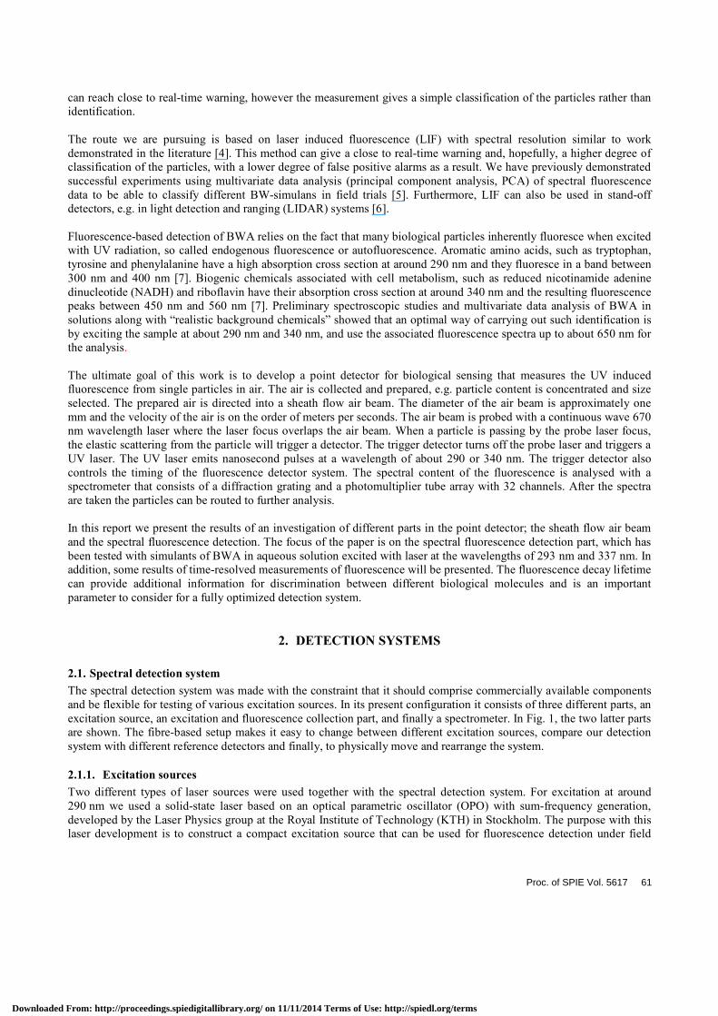
The spectral detection system was made with the constraint that it should comprise commercially available components and be flexible for testing of various excitation sources. In its present configuration it consists of three different parts, an excitation source, an excitation and fluorescence collection part, and finally a spectrometer. In Fig. 1, the two latter parts are shown. The fibre-based setup makes it easy to change between different excitation sources, compare our detection system with different reference detectors and finally, to physically move and rearrange the system.

2.1.1. Excitation sources

Two different types of laser sources were used together with the spectral detection system. For excitation at around 290 nm we used a solid-state laser based on an optical parametric oscillator (OPO) with sum-frequency generation, developed by the Laser Physics group at the Royal Institute of Technology (KTH) in Stockholm. The purpose with this laser development is to construct a compact excitation source that can be used for fluorescence detection under field

Proc. of SPIE Vol. 5617 61

Downloaded From: http://proceedings.spiedigitallibrary.org/ on 11/11/2014 Terms of Use: http://spiedl.org/terms

conditions. The wavelength of the laser was 293 nm, the maximal pulse energy was around 30 µJ, the maximal pulse repetition rate was 100 Hz and the pulse length was approximately 1 ns. The forthcoming version of this laser runs at 1 kHz. Further details on this laser can be found elsewhere in this proceeding [8]. By changing one non-linear crystal and some mirrors the OPO based laser could be made to operate at 343 nm. However, most of the experiments with excitation at around 340 nm were performed with a N2 gas laser (Oriel 79111). This laser operates at a wavelength of 337 nm, the maximal pulse energy was around 300 µJ, the maximal pulse repetition rate was 50 Hz and the pulse length was approximately 5 ns. Both lasers were coupled to the excitation and fluorescence collection module with a 10 m long fibre. The diameter of the fibre core was 1.0 mm and the numerical aperture (NA) was 0.39. Since the transmission of UV radiation in the fibre was low and since the coupling efficiency was poor only about 0.1% of the laser radiation reached the sample cell. This level of excitation was sufficient for the current fluorescence experiments, however, next step in the system optimization will be to utilise a UV fibre and improve the fibre coupling.

�������

Ocean

Optics

������ ���������

�����������

������

��������

�� ��!"�#$��%&"%���#'(&�%��)

�� ��

!��#$��%&�%���#'(&�%��)

������������*������+���,,$

������������

��+ ������������

-��� ���.�+�/�����

������+���� �!���������+)

�����������

����&�*�µ�

������+���� �!���������+)

������+�

��� �

!�0������+)

�� ��������

!"��#$��%&"%���#

'(&�%12)

3�4�����4���������,*��*

����������

Fig. 1. Schematics of the detection system.

2.1.2. Excitation and fluorescence collection optics

The excitation and fluorescence collection module is built around a sample compartment (Oriel 30750), to which four fibre optic coupled focusing probes (Oriel 77646) can be attached. In our experiments three ports where used, one for excitation and two perpendicular ports for fluorescence collection (see Fig. 1). The excitation probe focused the UV radiation into a narrow beam in the centre of the sample cell. The waist of the focus was approximately 1 mm. Two identical collection probes couple the fluorescence into fibres. The magnification of the collecting probes is unity and the NA is 0.29. One of the collecting probes was coupled to a fibre bundle (Oriel 77561), which directed the collected radiation to the spectrometer. The fibre bundle is 1 m long, has a core diameter of 1.6 mm and a NA of 0.27. The other collection probe coupled light into another fibre (Ocean Optics QP200-2-UV/VIS-BX), which was coupled to a reference spectrometer. This fibre is 2 m long, has a core diameter of 0.2 mm and a NA of 0.22. In most experiments we used coloured glass filters from Melles Griot in front of the collection probes to prevent scattered laser radiation from reaching the spectrometers. When the sample was excited with 293 nm, a WG320 filter was used and with 337 nm excitation, a GG385 filter was used.

2.1.3. Spectrometer

The spectrometer detection unit was a linear photomultiplier tube (PMT) array and a diffraction grating. We chose a PMT array because it is one of the most sensitive detectors available. The PMT array used in our spectrometer is a 32

62 Proc. of SPIE Vol. 5617

Downloaded From: http://proceedings.spiedigitallibrary.org/ on 11/11/2014 Terms of Use: http://spiedl.org/terms

channel linear PMT array (Hamamatsu H7260-4). This and similar PMT arrays are used in state-of-the-art confocal fluorescence microscopes to image pixel volumes of a few µm3. Together with the PMT array we used a spectrograph (Oriel 77442). This spectrograph has a fibre-coupled input port well suited for the fibre bundle from the collection probe and the length of the spectrum on the output port has a length comparable to the PMT array. The grating in the spectrograph has a grating density of 405 lines/mm, a blaze wavelength of 350 nm and a nominal spectral range of 285-715 nm. Normally a 280 µm slit was used at the input port of the spectrograph. For acquisition of the signal from the PMT array, a commercial readout module (Hamamatsu C8678) was used. The readout module can be either externally triggered or set to operate with an internal fast trigger circuitry allowing for charge collection using integrating capacitors. The capacitance used is C=33 pF and the integration time is fixed to 1 µs. The voltages captured by the sample and hold circuits relate to the charge by U=Q/C and represent the charge collected during the 1 µs. The commercial readout module is not fully flexible for this application, therefore we are also developing a new PMT array readout module. This circuit is tailored to the specific need with a built in pulse integration function, 9 channel sample and hold circuits and laser timing and triggering functions. It also has a high voltage unit to feed the PMT array. The unit is connected to a data acquisition card in a 2.8 GHz PC. All functions can be controlled either by on-board potentiometers or through computer control. To read the sampled voltages on the different channels and to control the high voltage and the different functions we have developed a LabView application. The present system can acquire up to 2000 spectra/s and continuously store the data to the computer hard drive.

2.1.4. Reference detectors

To qualitatively compare the results obtained with the spectral detector system we used different reference detectors. To compare the spectral information we used a fibre-coupled spectrometer (Ocean Optics USB-2000). The detector in the spectrometer is a 2048-element linear silicon CCD. The grove density of the grating is 600 lines/mm, a blaze wavelength of 400 nm and a nominal spectral range of 250-800 nm. The spectral resolution with the fibre used was approximately 5 nm. Two other detectors were used to measure the total energy. A universal radiometer (Laser Probe Rm-6600A) with a silicon energy probe (Laser Probe RjP-465) was used to measure the laser output and the excitation energy emerging out from the excitation probe. A mini PMT (Hamamatsu H5783-01) was used to measure the energy out from the collection fibres as a reference to the spectrometer values. Unfortunately, due to non-overlapping dynamic ranges these detectors were not mutually calibrated nor were they recently calibrated against any traceable instrument. Nonetheless, they provided information on relative energy levels and the mini PMT values can be used for mutual calibration of the spectrometers.

2.1.5. Collection efficiency

Consider the output voltage spectrum, U(λ), generated by the PMT array readout module upon a trigger. We assume that the conditions are such that U(λ) behaves as a linear function of the emitted fluorescence energy EF(λ). Then we can write

)()()( λλλ FEHU = . (1)

In our current detection system the transfer function H(λ) is given by

)()()()()( 9 λληλληλ STTTTH specfibfiltaqlc= . (2)

If the fluorescence radiation is isotropic the collection probe efficiency, ηc, becomes equal to the solid angle fraction of 4π opened up by the collection probe. Hence,

)2(sin 2 ac =η , (3)

Proc. of SPIE Vol. 5617 63

Downloaded From: http://proceedings.spiedigitallibrary.org/ on 11/11/2014 Terms of Use: http://spiedl.org/terms

where 2a is the acceptance cone angle of the collection probe. As stated above the collection probe focuses the light onto the fibre bundle tip with a magnification of unity. Thus, when the numerical aperture, NA, of the collection fibre bundle sets the limit, as is our case, the acceptance cone angle is found by a=arcsin(NA). Tl, Taq, Tfilt(λ) and Tfib(λ) are the transmittance for the liquid path, an air to quartz boundary, the colour filter and the fibre, respectively. ηspec is the spectrometer efficiency including the slit transmittance and the grating efficiency and S(λ) is the overall sensitivity of the PMT receiver in units of V/J. S(λ) is dependent on the adjustable PMT high voltage level. Fig. 2 shows the transfer function, H(λ), with and without the two colour filters that were used, calculated for a PMT high voltage (HV) of -800 V (gain=1.4×106). The spectral characteristics, apart from the colour filter edges, come mainly from the spectrometer grating efficiency and the PMT cathode radiant sensitivity. The NA of the fibre is 0.27 yielding ηc=0.02. Tl,=1 and Taq,=0.96 is assumed (yields Taq

9 = 0.69) and the slit transmittance was found to be 0.25. For the other parameters the manufacturers specifications have been used. The accumulated transmission factor at the peak wavelength in the fluorescence collection amounts to approximately 8×10-4 of which a factor of 0.02 is due to the collection probe efficiency, 0.34 is due to the transmittance of the optics and 0.13 is due to the spectrometer efficiency.

250 300 350 400 450 500 550 600 650 700 750 800

0,0

0,5

1,0

1,5

2,0

2,5

H(λ

) (

J/V

)

Transfer function

Wavelength (nm)

Unfiltered WG320 GG385

x1012

250 300 350 400 450 500 550 600 650 700 750 80010

-19

10-18

10-17

10-16

10-15

10-14

10-13

Detection threshold

No

ise e

quiv

alen

t en

erg

y (J

)

Wavelength (nm)

Unfiltered WG320 GG385 At PMT array

Fig. 2. Transfer functions and detection thresholds calculated according to Eq. (2). The coloured glass filters denoted WG320 and

GG385 were used with the excitation at 293 and 337 nm, respectively, unless otherwise stated. The PMT gain was set to 1.4×106

(PMT HV -800 V). The detection thresholds are extrapolated functions obtained with a readout noise level of 2 mV.

2.1.6. Detection limit

The noise for the C8678 PMT readout module is specified in units of charge and the equivalent RMS voltage noise level is sU=2 mV with the PMT HV being -800V. We have measured the voltage noise when the spectrometer shutter was closed. It was found to be approximately sU= 0.8 mV, well below the specified level. This specified value is used to find a noise equivalent level for the fluorescence energy taken at the fluorescing entity and at the detector. We see that the noise level at the PMT array element can be compared to single photon energies. The energy of a photon at 300 nm is E=6.6×10-19 J and at 600 nm E=3.3×10-19 J. The threshold level for the fluorescence emission per wavelength bin, EF(λ), is ranging from 1500 to 10000 photons between 300 and 600 nm. It is possible that an increased PMT gain (another factor of three) can raise the detection threshold. However, extraneous noise from the PMT is likely to become dominant and it might not improve the signal to noise ratio. This remains to be tested.

2.1.7. Fluorescence cross section

The fluorescence energy spectrum as defined in Eq. (1) is related to the excitation energy by the fluorescence cross section. Restricting to situations where the level of irradiation is sufficiently low that non-linear effects can be neglected and that no appreciable depletion of the number of molecules in the ground state is produced we have

64 Proc. of SPIE Vol. 5617

Downloaded From: http://proceedings.spiedigitallibrary.org/ on 11/11/2014 Terms of Use: http://spiedl.org/terms

∫∆+

∆−

≅2/

2/

')'()()(λλ

λλ

λλλσλ dLA

EnE F

LF

exc

excF (4)

following the nomenclature in Ref. [9]. A more accurate expression than this is generally not required for this purpose. We assume here that only one species contributes to the fluorescence signal. Eexc represents the total energy of the excitation light pulse, approximated to be flowing with uniform spatial distribution through a constant beam cross section denoted Aexc, n represents the number of fluorescing entities (cluster of spores, spores, cells or molecules depending on species) within the probe volume, V, cut out by the intersection of the excitation beam and the field of view of the collection probe. σF(λL) represents the spectrally integrated fluorescence cross section attributed with one entity and provides a direct relationship between the irradiance and the total emitted fluorescence power from one entity. LF(λ)dλ represents the fraction of the scattered radiation that falls into the wavelength interval (λ ,λ+dλ) where LF(λ) is the normalized fluorescence spectrum associated with the species. Finally, ∆λ is the spectrometer channel bandwidth. Accordingly, the total fluorescence energy emitted per pulse is

)(, LF

exc

exctotF

A

EnE λσ≅ . (5)

The probe volume V is well approximated by a cylinder of a height equalling the core diameter of the collection fibre bundle and an end cap area Aexc when Aexc is smaller than the cross sectional area, Ac, of the collection probe field of view. Since the magnification of the excitation probe is approximately 1.3, Aexc is slightly larger than the fibre core cross section 0.8 mm2. Then, the probe volume becomes approximately 1 mm3 or 1 µl. For aqueous solutions n=NV where N is the number density of the entity. When we treat the sheet flow air beam the aim is to detect single particles for which n=1 if a particle (possibly clusters of spores) is the entity being connected to the fluorescence cross section.

2.2. Particle injector

The detection system will also be tested together with a sheath flow air beam particle injector, which we have already developed. The purpose of the aerosol injector is to direct the aerosol to a millimetre sized measuring volume and to avoid particles from adhering on optical parts. An open ended quartz cuvette is connected to an aerosol injector. The measuring volume is in the middle of the cuvette. The injector consists of two concentric tubes. A narrow tube, with inner diameter of 1 mm and an outer diameter of 2 mm, is situated inside a wide tube. It ends about 11 mm from the end of the outer tube. The outer tube is turned from alumina. It has an inner diameter of 10 mm at the top and shrinks gradually to 8 mm where the inner tube ends. The narrowing outer tube prevents the aerosol flow from widening at the end of the inner tube. The end of the outer tube is milled to fit the quartz cuvette. Grease is used to seal the connection. A Teflon cap ends the external tube at the top. The inner tube is continuing through a hole in the cap. There is a connection to the cap through which HEPA filtered air is supplied. The aerosol is injected through the inner tube. A gas pump is connected to the rear end of the flow cell and the filtered air flow may be regulated to enable a similar flow through the tubes. We have tested the flow cell separately. The total air flow was varied between 1.4 l/min and 2.3 l/min. The mean velocity of the air through the injector is between 0.5 m/s and 0.9 m/s, calculated by the ratio of the air flow to the cross sectional area. If it is a laminar flow through the injector, the maximum velocity in the middle of the tube is 1.5 times larger than the mean velocity. The tests showed that the injector produced a one millimetre wide aerosol beam two centimetres away from the nozzle tip.

2.3. Time-resolved detector

Time-resolved fluorescence decays were recorded using an IBH 5000 U fluorescence lifetime spectrometer system with 1 nm resolved excitation and emission monochromators (5000M). The system was equipped with a TBX-04 picosecond photon detection module. UV-pulses were transferred to the IBH spectrometer using a custom-made fibre to free space connector. In case of laser excitation a spectrometer port without monochromator was used and Melles Griot coloured glass filters were used to block scattered light from the excitation source (WG305 or WG320). As reference time point the residual second harmonic generation (SHG) from the laser was projected onto an IBH TBX-01 optical trigger. The fluorescence lifetime decays were measured using time-correlated single photon counting (TC-SPC) along with the IBH

Proc. of SPIE Vol. 5617 65

Downloaded From: http://proceedings.spiedigitallibrary.org/ on 11/11/2014 Terms of Use: http://spiedl.org/terms

Data Station v 2.1 software for operation of the spectrometer and deconvolution and analysis of decays. The DAQ-card settings were chosen to give a time resolution below 10 ps. For the studies of fluorescence decay time the excitation source was a Coherent Mira 900 with a femtosecond cavity in conjunction with a Coherent 9200 Pulse-Picker and an Inrad 050 SHG/THG generator. The pulses of the fundamental tone at 867 nm were 165 femtoseconds long and the THG output at 289 nm averaged to 2.4 mW at a pulse repetition frequency of 4.75 MHz. This high repetition rate and power allows for convenient and rapid detection of the fluorescence decay using the single photon counting technique. A typical decay trace of 200 µg/ml Ovalbumin takes about 1 minute to record at a 20000:1 ratio of the highest and lowest active time channel, respectively. The UV pulses along with the residual SHG used as time-reference were transferred to an IBH time resolved fluorescence spectrometer using a fibre (Thorlabs UMT-1.0). The femtosecond-laser system could be tuned into any excitation wavelength between 270 and 350 nm. However, in this work only the tryptophan excitation around 280-290 nm was examined.

2.4. Biological samples

A few simulants of biological warfare agents and references in aqueous solution were tested. Table 1 below describes the species that we have used. Table 1: Description of biological samples used in the experiments.

Abbr. Name Characteristics Comment

BG Bacillus atrophaeus

Bacterial spores Freeze dried spores. B. Anthracis simulant previously named Bacillus subtilus var. Niger, and Bacillus globigii whereby the abbreviation BG.

BT Bacillus thuringensis

Bacterial spores Freeze dried spores. Interferent simulant. Two different variants were studied. One made at FOI (BT-B) and one commercial insecticide preparation, Turex (BT-T).

EH Pantoea agglomerans

Vegetative bacterial cells

Previously named Erwinia herbicola whereby the abbreviation EH.

OA Ovalbumin Protein Toxin simulant. Was purchased from Sigma Aldrich (A5253) FL Fluorescein Dye Reference fluorophore standard; 1 µM in glycerol.

BG, BT and OA were mixed in well defined quantities while the concentrations of EH and FL were not accurately measured. Concentrations of a few hundred µg/ml and down were used. One gram of BG or BT contains approximately 1×1013 micron sized spores. But it can be assumed that only 1% of the spores are alive and contribute efficiently to the fluorescence. Hence, we use N=C [µg/ml] × 1×105/µg to obtain the number density of living spores. Both the uncertainty with regard to the fraction of living spores and how much the dead spores fluoresce are sources of error in attempting to measure fluorescence cross sections. For OA which is a molecule being dissolved in water the number density is N=C [µg/ml] × 1.33×1013/µg.

3. RESULTS AND DISCUSSION

3.1. Spectral results using the PMT spectrometer

The PMT spectrometer was calibrated with respect to the wavelength using a Xenon flashlamp and a monochromator with the spectral bandwidth of 1 nm and the wavelength precision of ± 1 nm. The result is presented in Fig. 3. For clarity, only channel 6 to 15 are presented in the graph. The results for all channels are shown in the table. Each PTM channel covers about 17 nm. Since the magnification of the Oriel spectrograph is unity, the spectrograph resolution is much better than what can be resolved with the PMT array when using the 280 µm slit. Without the slit the resolution is set by the fibre diameter (1.6 mm). In this case, a monochromatic beam smears out and hits approximately one and a half PMT channel, being 0.9 mm wide with a 0.1 mm gap between each cathode surface. All measurements were performed with the slit if nothing else is stated.

66 Proc. of SPIE Vol. 5617

Downloaded From: http://proceedings.spiedigitallibrary.org/ on 11/11/2014 Terms of Use: http://spiedl.org/terms

PMT Channel

Centre Wavelength

PMT Channel

Centre Wavelength

1 262 nm 17 534 nm 2 279 nm 18 551 nm 3 296 nm 19 568 nm 4 313 nm 20 585 nm 5 330 nm 21 602 nm 6 347 nm 22 619 nm 7 364 nm 23 636 nm 8 381 nm 24 653 nm 9 398 nm 25 670 nm

10 415 nm 26 687 nm 11 432 nm 27 704 nm 12 449 nm 28 721 nm 13 466 nm 29 738 nm 14 483 nm 30 755 nm 15 500 nm 31 772 nm

4 6 8 10 12 14 16 18 20

0,0

0,1

0,2

0,3

0,4

Sig

na

l (V

)

PMT cannel

347 nm 364 nm 381 nm 398 nm 415 nm 432 nm 449 nm 466 nm 483 nm 500 nm

16 517 nm 32 789 nm

Fig. 3. Calibration of the wavelength of the PMT spectrometer.

Fig. 4 below shows some typical spectra of the biological samples measured with the PMT spectrometer. The pulse energies at the samples were about 80 nJ and 2 µJ for the excitation wavelengths 293 nm and 337 nm, respectively. For all the samples with known concentration (BG, BT and OA), the PMT HV was set to -800 V (gain=1.4×106). For the other samples (EH and FL) the gain was lower. The small peaks at about 675 nm and 750 nm for the excitation at 293 nm and 337 nm, respectively, are due to second-order diffraction in the grating of the spectrograph. It surprised us that a spectrograph design for 285-715 nm shows second-order effects below 715 nm, but calculations shows that this is the case. The peaks at 380 nm for the samples excited at 337 nm are attributed to Raman scattering. Occasionally, similar peaks appeared at 340 nm when the samples were excited at 293 nm. It was not possible to quantify in detail the origin and nature of such scattering signals.†

250 300 350 400 450 500 550 600 650 700 750 800

0,0

0,1

0,2

0,3

0,4

0,5

0,6

0,7

0,8

0,9

1,0 Excitation 293 nm

Sig

nal

(V

)

Wavelength (nm)

BG (160 µg/ml) BT (10 µg/ml) EH (unknown) OA (48 µg/ml) FL (unknown)

250 300 350 400 450 500 550 600 650 700 750 800

0,0

0,1

0,2

0,3

0,4

0,5

0,6

0,7

0,8

0,9

1,0 Excitation 337 nm

Sig

nal

(V

)

Wavelength (nm)

BG (16 µg/ml) BT (0.2 µg/ml) EH (unknown) OA (48 µg/ml) FL (unknown)

Fig. 4. Representative fluorescence spectra for BWA simulants and dyes excited at 293 and 337 nm.

The results in Fig. 4 above show the average spectra for a measurement series. A measurement series was normally about 1 min long, so that the averages are over approximately 6,000 and 3,000 pulses for the excitation at 293 nm

† Raman scattering and similar nonlinear scattering phenomena usually require detection at high wavelength resolution and at short (instantaneous) response times. The developed detection system is clearly not suitable for such studies.

Proc. of SPIE Vol. 5617 67

Downloaded From: http://proceedings.spiedigitallibrary.org/ on 11/11/2014 Terms of Use: http://spiedl.org/terms

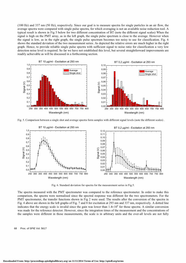
(100 Hz) and 337 nm (50 Hz), respectively. Since our goal is to measure spectra for single particles in an air flow, the average spectra were compared with single pulse spectra, for which averaging is not an available noise reduction tool. A typical result is shown in Fig 5 below for two different concentration of BT (note the different signal scales) When the signal is high on the PMT array, as in the left graph, the single pulse spectrum is close to the average. However when the signal is low, as in the right graph, the single pulse spectrum becomes too noisy to use for classification. Fig. 6 shows the standard deviation of the two measurement series. As depicted the relative errors are much higher in the right graph. Hence, to provide reliable single pulse spectra with sufficient signal to noise ratio for classification a very low detection noise level is required. So far we have not established this level, but several straightforward improvements are readily achievable as will be discussed in a forthcoming section.

250 300 350 400 450 500 550 600 650 700 750 8000,0

0,1

0,2

0,3

0,4

0,5

0,6

0,7

0,8

0,9

1,0BT 10 µg/ml - Excitation at 293 nm

Sig

na

l (V

)

Wavelength (nm)

Average Single shot

250 300 350 400 450 500 550 600 650 700 750 8000,00

0,01

0,02

0,03

0,04

0,05

0,06

0,07

0,08

0,09

0,10

BT 0,2 µg/ml - Excitation at 293 nm

Sig

na

l (V

)

Wavelength (nm)

Average Single shot

Fig. 5. Comparison between a single shot and average spectra form samples with different signal levels (note the different scales) .

250 300 350 400 450 500 550 600 650 700 750 800

0,0

0,1

0,2

0,3

0,4

0,5

0,6

0,7

0,8

0,9

1,0 BT 10 µg/ml - Excitation at 293 nm

Sig

nal

(V

)

Wavelength (nm)

250 300 350 400 450 500 550 600 650 700 750 800

0,00

0,01

0,02

0,03

0,04

0,05

0,06

0,07

0,08

0,09

0,10

0,11

0,12

BT 0,2 µg/ml - Excitation at 293 nm

Sig

nal

(V

)

Wavelength (nm)

Fig. 6. Standard deviation for spectra for the measurement series in Fig.5.

The spectra measured with the PMT spectrometer was compared to the reference spectrometer. In order to make this comparison, the spectra were normalised since the spectral response was different for the two spectrometers. For the PMT spectrometer, the transfer functions shown in Fig 2 were used. The results after the conversion of the spectra in Fig. 4 above are shown in the left graphs of Fig. 7 and 8 for excitation at 293 nm and 337 nm, respectively. A dotted line indicates that the energy scale is invalid since the gain was lower than 1.4×106 for those spectra. A similar conversion was made for the reference detector. However, since the integration times of the measurement and the concentrations of the samples were different in those measurements, the scale is in arbitrary units and the over-all levels are not fully

68 Proc. of SPIE Vol. 5617

Downloaded From: http://proceedings.spiedigitallibrary.org/ on 11/11/2014 Terms of Use: http://spiedl.org/terms

comparable with the PMT measurements. The results are presented in the graphs to the right of Fig. 7 and 8. The BG results are noisy since the fluorescence signal levels were close to the detection level of the reference detector. An artefact of the reference detector is the small peak at 500 nm, which appeared in all spectra taken with that spectrometer. Although the PMT spectrometer has considerably lower resolution the samples seem to show the same discernable characteristic spectral features.

300 350 400 450 500 550 600 6500,0

0,1

0,2

0,3

0,4

0,5

0,6

0,7

0,8x10-12 PMT spectrometer - Excitation 293 nm

En

erg

y (J

)

Wavelength (nm)

BG BT EH OA FL

300 350 400 450 500 550 600 650

0,0

0,2

0,4

0,6

0,8

1,0

Reference spectrometer - Excitation 293 nm

No

rma

lised

sp

ectr

a (

A.U

.)

Wavelength (nm)

BG BT EH OA FL

Fig. 7. Comparisons between spectra taken with the PMT and the reference spectrometers when excited at 293 nm.

350 400 450 500 550 600 650 7000,0

0,1

0,2

0,3

0,4

0,5

0,6

0,7

0,8 PMT spectrometer - Excitation 337 nm

En

erg

y (J

)

Wavelength (nm)

BG BT EH OA FL

x10-12

350 400 450 500 550 600 650 700

0,0

0,2

0,4

0,6

0,8

1,0

Reference spectrometer - Excitation 337 nm

Nor

ma

lise

d sp

ectr

a (A

.U.)

Wavelength (nm)

BG BT EH OA FL

Fig. 8. Comparisons between spectra taken with the PMT and the reference spectrometers when excited at 337 nm.

3.2. Fluorescence efficiency

The total energy per pulse was measured using the reference detectors described in Sec. 2.1.4. The radiometer was used to measure the excitation energy out from the excitation probe. The mini PMT was connected directly to the fluorescence collection fibre. The primary purpose was to compare the energy level with the PMT array values for mutual calibration. Some indicative information with regard to fluorescence efficiency was also obtained. Table 2 summarizes some measured values for BG and OA. The fluorescence from these agents was measured at both

Proc. of SPIE Vol. 5617 69

Downloaded From: http://proceedings.spiedigitallibrary.org/ on 11/11/2014 Terms of Use: http://spiedl.org/terms

wavelengths at two different concentrations. The energy as measured by the PMT array was obtained by summing up the spectral values and taking the calculated spectrometer efficiency into account. Table 2. Total fluorescence energy for BG and OA measured with a reference detector in comparison with the PMT array value.

as measured by the detectors out from fibre extrapolated flurescence from probe volume

Conc. λexc Eexc Etot PMTarray EF,tot miniPMT EF,tot PMTarray EF,tot/Eexc

[µg/ml] [nm] [nJ] n photons [fJ] [fJ] [pJ] [pJ] [e-6]

BG 160 293 80 67200 33 17 4,9 2,5 61BG 16 293 80 9600 4,8 4,0 0,7 0,6 9OA 480 293 80 768000 384 186 56 27 706OA 48 293 80 129600 64,8 40 10 5,9 119

BG 160 337 1800 504000 252 40 37 5,9 21BG 16 337 1800 72000 36 18 5,3 2,6 2,9OA 480 337 1800 180000 90 40 13 5,9 7,4OA 48 337 1800 36000 18 10 2,6 1,5 1,5

ID

E miniPMT

The excitation energy levels are much lower than the specified laser energies due to losses in the fibre connection with the laser sources as explained in Sec. 2.1.2. At this stage, the levels were sufficient. It is noted that the mini PMT values are generally about a factor of two higher than the calculated values for the PMT array which is reasonably close, although for BG a greater variation can be seen. The values extrapolated to the total fluorescence energy per pulse from the probe volume give a relation to the excitation energy. The efficiency expressed as EF,tot/Eexc shows that the fluorescence is stronger for OA than for BG with an excitation at 293 nm while BG fluoresce more efficiently than OA at 337 nm. Both species fluoresce more efficiently at 293 nm than at 337 nm, a factor of 3 for BG and almost a factor of 100 for OA. The efficiencies are generally not proportional to concentration. A factor of ten in concentration roughly yields a factor of six in fluorescence, based on the mini PMT data. Although associated with much uncertainty, Eq. (5) can be used to obtain a crude estimate of the fluorescence cross section in aqueous solutions for BG and OA. We use Aexc=1 mm2 and n=NV with V=1.6 mm3. The concentrations C=16 µg/ml for BG and C=48 µg/ml for OA correspond to the number concentrations N= 1600 mm-3 for BG (living spores) and N= 6.4×1011 mm-3 for OA molecules, according to the relations given in Sec. 2.1.7. Hence, the fluorescence cross section for BG spores are σF

BG(293) ~2.4×10-11 cm2/spore and σFBG(337) ~0.8×10-11 cm2/spore based on the

efficiencies at both number concentration levels given in Table 2. Similarly, associated with OA, dissolved in water, we arrive at fluorescence cross sections of σF

OA(293) ~75×10-20 cm2/molecule and σFOA(337) ~0.9×10-20 cm2/molecule.

3.3. Time-resolved fluorescence characterisation

After mixing samples of bacterial spores in distilled water it takes some time before they have dissolved. Some of the dissolved material precipitates and accumulates on the bottom of the fluorescence cell. By scanning the emission monochromator of the fluorescence decay time spectrometer for a constant illumination of excitation light, one obtains a “pseudo-cw” emission spectrum. Such spectra are not calibrated to the wavelength sensitivity of the PMT, however, they can aid in the selection of emission wavelength to carry out further time-resolved measurements. Emission spectra for the samples BT-T, BT-B and OA are displayed in Fig. 9. For BT-B a spectrum is shown shortly after mixing the sample (about 10 min) as well as for a considerable time after (>2 h), denoted with “i” and “f”, respectively. A clearly discernable difference between these spectra appears at 340 nm. The relative contribution from the emission at 340 nm decreases with time. Hence, the identification of solution samples must be made with care, making sure that a steady state condition is monitored. Samples of bacterial origin all showed similar behaviour with time. Clearly, in a real application, the characterization of dry particles is desired in order to identify compounds based on the fluorescence spectrum. The spectrum of OA shows its characteristic narrow peak with a maximum within the 325-350 nm band. Since this spectral portion can be associated with the heavier precipitates of the bacterial compound it can be concluded that the protein cell wall and other similar parts of the bacteria give rise to the spectral characteristic at 340 nm. In Fig. 9 all spectra have been normalized to the maximum amplitude. In addition to the above mentioned, it is noted that the absolute fluorescence contribution from BT-B in the band between 375 and 400 nm increased with time implying that the emission arises in smaller molecular fragments hidden inside the cells.

70 Proc. of SPIE Vol. 5617

Downloaded From: http://proceedings.spiedigitallibrary.org/ on 11/11/2014 Terms of Use: http://spiedl.org/terms

300 350 400 450 500 550

0,0

0,2

0,4

0,6

0,8

1,0

Em

issi

on

(a.u

.)

Wavelength (nm)

BTT OA BTBi BTBf

Fig. 9. Pseudo-cw emission spectra of some BWA simulants for this study. The sharp peak at 433 nm is due to scatter of residual SHG from the fundamental radiation (867 nm) in the partially dissolved samples BT-B sample (see main text).

BG, OA and two different preparations of BT (BT-B and BT-T) were used for measurements of the fluorescence decay time. Typically 3 mg of powder was dissolved in 6 ml of distilled water. Some measurements were carried out with more diluted solvents but essentially the same decay parameters were obtained. The data reported here are all from samples that had reached a steady state condition with the precipitate on the bottom of the sample cell. Representative fluorescence decay functions are shown in Fig. 10 for BT-T at three different wavelengths. On the logarithmic plot the decay functions are, in all cases, curved as expected from a sample with a distribution of decay times. All decay functions could be acceptably fitted, with less than 0.1% deviation, to three “free” decay times. The solid lines indicate fits to three decay time parameters with associated amplitude weight as given in Table 3. The black squares correspond to the intrinsic time response of the combined pulsed laser and PMT detector system.

0 10 20 30 40

100

101

102

103

104

Cou

nts

/chan

nel

Time (ns)

Fig. 10. Representative fluorescence decay traces for BT-T at different wavelengths (red dot: 345 nm; green circle: 385 nm; blue triangle: 490 nm). The squares represent the intrinsic time-response of the laser and detection system obtained by recording the scatter of excitation light from a solution of Ludox microspheres.

Proc. of SPIE Vol. 5617 71

Downloaded From: http://proceedings.spiedigitallibrary.org/ on 11/11/2014 Terms of Use: http://spiedl.org/terms

As seen in Table 3 and Fig. 10 the decay time increased with detection wavelength in the bacterial samples. OA did not give enough fluorescence above 425 nm indicating that the fluorescence originated from different chemical species. Indeed the time decay traces (not shown) and the associated decay parameters are similar at the same wavelength emission, also considering different species. OA was measured both using the fs-laser system and the Q-switched OPO and gave identical decay traces. The laser gave of course a considerable longer measuring time owing to the lower pulse repetition frequency (100 Hz). Tests of freshly made samples being strong scatterers showed very similar decays and associated decay time data at the various wavelengths. Conclusively, the dominating contributions in the range 340 – 490 nm are all in the range 2 – 11 ns. Hence a time-gated detection system considering only this range would be optimising the signal to noise ratio. Table 3. Summary of fluorescence decay data of some BWA simulants in distilled water.

Sample

λ = 340-350 nm Decay times [ns] (rel ampl)

λ = 380-395 nm Decay times [ns] (rel ampl)

λ = 475-490 nm Decay times [ns] (rel ampl)

BG τ1 = 5.07 (0.76) τ2 = 1.37 (0.19) τ3 = 0.17 (0.05)

τ1 = 8.97 (0.41) τ2 = 4.59 (0.55) τ3 = 0.37 (0.04)

τ1 = 11.73 (0.64) τ2 = 2.05 (0.27) τ3 = 0.22 (0.08)

BT-T τ1 = 6.91 (0.33) τ2 = 1.83 (0.51) τ3 = 0.33 (0.16)

τ1 = 7.78 (0.32) τ2 = 1.98 (0.55) τ3 = 0.29 (0.13)

τ1 = 11.20 (0.34) τ2 = 2.80 (0.54) τ3 = 0.35 (0.12)

BT-B τ1 = 5.94 (0.56) τ2 = 1.86 (0.35) τ3 = 0.27 (0.09)

τ1 = 7.74 (0.34) τ2 = 2.54 (0.55) τ3 = 0.48 (0.11)

n.d.

OA τ1 = 6.66 (0.57) τ2 = 2.44 (0.36) τ3 = 0.41 (0.07)

n.d.

n.d.

CONCLUSIONS AND FURTHER WORK A point detection system with the aim of performing “single-shot fluorescence spectroscopy” of BWA particles in air is in progress. So far our main effort has been dedicated to the development of a laser source (see separate report in this proceedings [8]) and the tests of a multi-channel spectral detection system. In addition we have carried out basic studies of spectral and temporal features of the fluorescence from BWA simulants in solution. The light source is certainly one of the most essential parts for this kind of detection system. The wavelength is critical due to excitation wavelength dependence. In the system a unique solid state OPO laser operates at a wavelength of 293 nm which is close to an optimum choice for maximum fluorescence of aromatic amino acids in BWA. It is clear that several wavelengths provide additional classification information but it remains to be found out what the optimum choices and numbers of additional wavelength are. The technology around which the laser is built can provide a variety of wavelengths and possibly to some extent tunability. The excitation energy is critical in that it determines the amount of fluorescence. The fluorescence energy will obviously not infinitely follow the excitation energy but will saturate since the number of fluorescent dye centers in the materials is limited. Moreover, a dry bacterial spore is very inhomogeneous with regard to the distribution of the fluorophores and certainly not all are in a location favourable to give strong florescence. We currently assume that a level of around 1 µJ is appropriate and sufficient in a point detector of this kind and another way of enhancing the performance is to increase the pulse repetition frequency of the laser. This is work currently underway and we expect to operate a 1 kHz OPO laser within short. The duty cycle (i.e. the on/off ratio) of the excitation pulses will certainly be a critical issue in order to optimize the performance of the final system. The PMT detector array is another crucial part. Not many detectors can compete with the performance in terms of sensitivity. We can detect optical signals, simultaneously on 32 channels, down to a single-photon level. We have obtained some results that agree well with a general view that fluorescence emission from BWA or pertinent background species is typically broadband with few narrowband features. Nonetheless, we have not established an optimum choice of spectral resolution but need to further investigate this aspect. We believe that our instrumentation can provide sufficient data to give us essential answers with regard to resolution, and we are convinced that spectral data

72 Proc. of SPIE Vol. 5617

Downloaded From: http://proceedings.spiedigitallibrary.org/ on 11/11/2014 Terms of Use: http://spiedl.org/terms

can provide more information than what is currently obtained from state-of-the-art instrumentation. By changing the grating in our spectrograph, to make use of the whole PMT array in the interesting wavelength band from 300 nm to 650 nm, we can increase the spectral resolution with a factor close to two with the current equipment. An important parameter associated with the BWA is their fluorescence cross section. The fluorescence cross section of several biological warfare aerosol simulants has been estimated in a recent work [10]. Although these values were obtained for other excitation wavelengths, 266 and 355 nm, they provide an estimate of the fluorescence emission in our case. The values were given for particles sizing approximately 1 µm and several species were investigated. The average 266 nm fluorescence cross section for bacterial spores was found to be 1.5×10-11 cm2 per spore and for Ovalbumin 3.7×10-10 cm2 per particle. Using these values a pulse energy of one µJ distributed over 1 mm2 would result in a fluorescence energy of 2×10-15 J and 5×10-14 J, respectively. If we compare these figures with our detection threshold we see that they are close to the noise equivalent level of our current system. Considering that the energy will distribute spectrally, they might even fall below the noise. It is clear that a spectrum from a single particle will become noisy and provide insufficient information under such conditions. However, as we have described our current system is far from optimized and there are order of magnitudes to gain simply by counteract basic losses in the system. Moreover BWA aerosol particles will usually consist of aggregates distributed in size between 1 and 10 µm. Larger particles will fluoresce more, at least in proportion to the effective cross sectional area and consequently be more easily classified. Nevertheless, the 1 µm sized particle must remain a goal, although challenging. Further investigations on dried samples are needed to clearly define what the limitations are for such samples. A similar route to improved performance goes via the probe volume. The probe volume (of the optics) has been set by practical considerations associated mainly with the particle injection system. We do not currently have a practical solution where the particles in the air beam can be more spatially confined. However, if that would be possible it would allow for a much more efficient optical solution which in terms of energy strongly would reduce the requirements. An early choice we made was to use simple collection probes based on lenses. The major advantage is that they allow for simple optical solutions with a variety of optical fibres. Our probes collect about 2% of the available fluorescence which is naturally an inefficiency of the system which cannot be neglected. An alternative approach commonly used in BWA point detectors is elliptical mirrors that focus the probe volume with close to unitary efficiency to a secondary focal point. It is possible to use such optics with fibres although with some reduction of the efficiency due to the limited NA of optical fibres. In any case, it might be a straightforward improvement in a later development stage beyond the scope of this work. Other system losses that we have described can be easily withdrawn by more careful design. Our investigations of the fluorescence decay functions cannot yet give a clear answer on whether or not it is possible to use the time domain information for classification. However, the time domain information may be crucial for the design of a low noise detection system capable of provide useful single particle spectra. In the near future our own designed PMT readout module will be compared with the commercially available equipment on which our spectral results were based. Resolution both in terms of “number of photon levels” and wavelength will be compared. The new OPO laser with increased pulse repetition frequency will be incorporated in our system and we will soon be moving from liquid samples to fluorescence collection from dry spores when we join our fluorescence detector with the particle injector.

ACKNOWLEDGEMENTS The authors thank Mikael Tiihonen for operating the OPO laser during the experiments and Anders Thaning for the development of the LabView application for the in-house-made PMT readout module. This work was funded by the Swedish Defence Material Administration (Contracts 255264-LB614606 and 273624-LB651760).

Proc. of SPIE Vol. 5617 73

Downloaded From: http://proceedings.spiedigitallibrary.org/ on 11/11/2014 Terms of Use: http://spiedl.org/terms

REFERENCES 1. D. R. Walt and D. R. Franz, Biological Warfare Detection, Analytical Cemistry, pp. 378 A-746 A (2000). 2. P. H. Kaye, J. E. Barton, E. Hirst and J. M. Clark, Simultaneous light scattering and intrinsic fluorescence

measurement for the classification of airborne particles, Applied Optics 39, pp. 3738-3745 (2000). 3. J. Ho, Future of biological aerosol detection, Analytica Chimica Acta 457, pp. 125–148 (2002). 4. S. C. Hill, R. G. Pinnick, S. Niles, Y.-L. Pan, S. Holler, R. K. Chang, J. Bottiger B. T. Chen, C.-S. Orr and G.

Feather, Real-time measurement of fluorescence spectra from single airborne biological particles, Field Analytical Chemistry & Technology 3, pp. 221-239 (1999).

5. T. Tjärnhage, M. Strömqvist, G. Olofsson, D. Squirrell, J. Burke, J. Ho and M. Spence Multivariate data analysis of fluorescence signals from biological aerosols, Field Analytical Chemistry & Technology 5, pp. 171-176, (2001).

6. J. R. Simard, G. Roy, P Mathieu, V. Larochelle, J. McFee, and J. Ho. Standoff Sensing of Bioaerosols Using Intensified Range-Gated Spectral Analysis of Laser-Induced Fluorescence, IEEE Transactions on geoscience and remote sensing 42 (4), 865-874, (2004).

7. J. R. Lakowicz, Principles of Fluorescence Spectroscopy, 2nd ed. (Kluwer Academic/Plenum Publisher, New York, 1999).

8. M. Tiihonen, V. Pasiskevicius, F. Laurell, and M. Lindgren, A novel UV-laser source for fluorescence excitation of proteins, [5617-42] in this proceeding.

9. R. M. Measures, Laser Remote Sensing: Fundamentals and Applications, (New York, John Wiley & Sons, 1984). 10. V. Sivaprakasam, A. L. Houston, C. Scotto, and J. D. Eversole, Multiple UV wavelength excitation and

fluorescence of bioaerosols, Optics Express 12 (19), 4457-4466, (2004).

74 Proc. of SPIE Vol. 5617

Downloaded From: http://proceedings.spiedigitallibrary.org/ on 11/11/2014 Terms of Use: http://spiedl.org/terms