Development and characterization of a membrane ... - DiVA
89
Development and characterization of a membrane-based nanocalorimeter for low temperatures Stella Tagliati Licentiate thesis in Physics Akademisk avhandling f¨ oravl¨aggande av filosofie licentiatexamen vid Stockholms universitet Department of Physics Stockholm University Stockholm, Sweden 2010
-
Upload
khangminh22 -
Category
Documents
-
view
3 -
download
0
Transcript of Development and characterization of a membrane ... - DiVA
Development and characterization of amembrane-based nanocalorimeter for
low temperatures
Stella Tagliati
Licentiate thesis in Physics
Akademisk avhandling for avlaggandeav filosofie licentiatexamen vid
Stockholms universitet
Department of PhysicsStockholm UniversityStockholm, Sweden 2010
Development and characterization of a membrane-based nanocalorimeter forlow temperaturesStella Tagliati
Licentiate thesis in PhysicsDepartment of PhysicsStockholm UniversitySweden
c© Stella Tagliati, 2010
Printed by: Universitetsservice US-AB
Abstract
A differential, membrane-based nanocalorimeter has been constructed forthermal studies of mesoscopic samples at low temperatures. The calorimeteris designed for sample masses from milligram to sub-microgram and a temper-ature range from room temperature to the sub-Kelvin region. In particular,it finds applications in the study of phase transitions and phase diagramsof superconductors and magnetic systems. Effort was spent to achieve highresolution and good absolute accuracy to be able to investigate the elec-tronic contribution of the heat capacity of superconductors. The device isbased on two free-standing silicon nitride membranes that, combined withthin film heaters and temperature sensors, give a background heat capac-ity < 200 nJ/K at 300 K, decreasing to sub-nJ/K at 10 K. The device hasseveral unique features. i) In differential mode, used for small samples, thebackground at room temperature is reduced to ≈ 2 nJ/K. ii) The resistivethermometer, made of GeAu alloy, has a high sensitivity, dlnR/dlnT ≈ −1over the entire temperature range. iii) The sample is placed in direct contactwith the thermometer which is allowed to self-heat. The thermometer canthus be operated at high DC current to increase the resolution. iv) Data areacquired with a set of eight synchronized lock-in amplifiers measuring DC,1st and 2nd harmonic signals of heater powers and temperature oscillationswith combined good absolute accuracy and high resolution. The design al-lows concurrent use of AC state steady and relaxation methods for generalstudies of specific heat, latent heat and dynamic heat capacity. The proper-ties of the nanocalorimeter were studied both analytically and numericallywith excellent agreement with experimental results. The operation of the ex-perimental setup was tested with successful calibration and characterizationmeasurements which suggest promising results.
Keywords: Nanocalorimetry, specific heat, membrane-based calorimeter,AC steady state, frequency dependence, thermal link conductance, thermalrelaxation, GeAu thermometer, numerical simulations.
iii
List of appended papers
Paper I. Emerging measurement techniques for studies of mesoscopic supercon-ductorsA. Rydh, S. Tagliati, R. A. Nilsson, R. Xie, J. E. Pearson, U. Welp,W.-K. Kwok and R. Divan,Electron Transport in Nanosystems, Proceedings of the NATO Ad-vanced Research Workshop on Electron Transport in Nanosystems,Yalta, Ukraine, September 2007, J. Bonca and S. Kruchinin (eds.),NATO Science for Peace and Security Series - B: Physics and Bio-physics, Springer, Dordrecht, 117 (2008).
My contribution: Participated in discussions and evolved the idea ofthe Wheatstone bridge measurement.
Paper II. Membrane-based calorimetry for studies of sub-microgram samplesS. Tagliati, A. Rydh, R. Xie, U. Welp and W. K. Kwok,J. Phys.: Conf. Ser. 150 052256 (2009).
My contribution: Designed and fabricated the nanocalorimeter. As-sisted in assembling the measurement setup and participated in themeasurements. Made most of the figures and writing of the article.
Paper III. Time-dependent simulations of a membrane-based nanocalorimeterS. Tagliati, J. Pipping and A. Rydh,J. Phys.: Conf. Ser. 234 042036 (2010).
My contribution: Supervised the development of the simulation pro-gram. Designed and ran the simulations. Designed and fabricated thenanocalorimeter. Made all the figures and most of the writing of thearticle.
iv
v
List of main symbols
C0 heat capacity of the platform
Ce frequency dependent part of the platform heat capacity
Cs heat capacity of the sample
C = C0 + Cs total heat capacity (sample plus platform)
Ki thermal conductance between sample and platform
Ke thermal conductance between platform and thermal bath
τi = Cs
Kirelaxation time constant between sample and platform
τe = CKe
relaxation time constant between sample plus platform and thermal bath
τe,0 = C0
Kerelaxation time constant between empty platform and thermal bath
P0 power oscillation amplitude
Pdc additional DC heating on the platform
Tb temperature of the thermal bath
T0 temperature sensed on the platform
Tac,0 temperature oscillation amplitude sensed on the platform
Toff = P0+Pdc
Keaverage temperature above Tb at steady state with additional DC heating
Tdc = P0
Keaverage temperature above Tb at steady state due to the AC power
ω angular frequency of the power (and temperature) oscillation
φ phase shift between applied power and temperature response at the platform
ϕ phase shift between applied power and temperature response at the sample

vi
Contents
Abstract iii
List of appended papers iv
List of main symbols v
1 Introduction 1
1.1 Motivation . . . . . . . . . . . . . . . . . . . . . . . . . . . . . 1
1.2 Overview of calorimetric methods . . . . . . . . . . . . . . . . 2
1.3 Dynamic heat capacity . . . . . . . . . . . . . . . . . . . . . . 9
2 Analytical models 13
2.1 Model diagrams . . . . . . . . . . . . . . . . . . . . . . . . . . 13
2.2 AC steady state method . . . . . . . . . . . . . . . . . . . . . 15
2.2.1 Analysis of the calorimetric system . . . . . . . . . . . 15
2.2.2 Effect of the internal time constant . . . . . . . . . . . 18
2.2.3 1D model of the membrane . . . . . . . . . . . . . . . 23
2.2.4 2D model of the membrane . . . . . . . . . . . . . . . 26
2.2.5 Sample size effects . . . . . . . . . . . . . . . . . . . . 28
2.2.6 Differential mode . . . . . . . . . . . . . . . . . . . . . 29
2.3 Thermal relaxation method . . . . . . . . . . . . . . . . . . . 31
2.3.1 Overview . . . . . . . . . . . . . . . . . . . . . . . . . 31
3 Device fabrication 35
3.1 Layout of the device . . . . . . . . . . . . . . . . . . . . . . . 35
3.2 Fabrication . . . . . . . . . . . . . . . . . . . . . . . . . . . . 38
3.3 Detailed description of each leayer . . . . . . . . . . . . . . . . 43
3.3.1 Heaters . . . . . . . . . . . . . . . . . . . . . . . . . . 43
3.3.2 Temperature sensor . . . . . . . . . . . . . . . . . . . . 44
3.3.3 Insulation layers . . . . . . . . . . . . . . . . . . . . . . 46
3.3.4 Thermalization layer . . . . . . . . . . . . . . . . . . . 48
vii
viii CONTENTS
4 Measurements and characterization 494.1 Measurement system . . . . . . . . . . . . . . . . . . . . . . . 49
4.1.1 Cryostat overview . . . . . . . . . . . . . . . . . . . . . 494.1.2 Electronic setup . . . . . . . . . . . . . . . . . . . . . . 49
4.2 Measurement method . . . . . . . . . . . . . . . . . . . . . . . 514.2.1 Electronics overview . . . . . . . . . . . . . . . . . . . 514.2.2 AC steady state . . . . . . . . . . . . . . . . . . . . . . 53
4.3 Characterization . . . . . . . . . . . . . . . . . . . . . . . . . 554.3.1 Thermometer calibration . . . . . . . . . . . . . . . . . 554.3.2 Thermal conductance . . . . . . . . . . . . . . . . . . . 554.3.3 AC steady state . . . . . . . . . . . . . . . . . . . . . . 574.3.4 Frequency dependence . . . . . . . . . . . . . . . . . . 584.3.5 Thermal relaxation . . . . . . . . . . . . . . . . . . . . 614.3.6 Calibration verification . . . . . . . . . . . . . . . . . . 62
5 Numerical simulations 655.1 Simulation model . . . . . . . . . . . . . . . . . . . . . . . . . 655.2 Frequency dependence . . . . . . . . . . . . . . . . . . . . . . 665.3 Heater power . . . . . . . . . . . . . . . . . . . . . . . . . . . 675.4 Oscillation distributions . . . . . . . . . . . . . . . . . . . . . 67
6 Summary of attached papers 71
Acknowledgments 72
Bibliography 73
Chapter 1
Introduction
1.1 Motivation
Accurate thermodynamic measurements are essential to understand funda-mental properties of materials in various fields of physics. Examples of inter-esting applications of novel calorimetric techniques include the study of quan-tum effects and phase transitions, in superconducting [1–19] and magnetic[20–27] systems, in condensed matter at nano-scales and low temperatures,to the investigation of soft matter objects, like polymers [28–35] or biologicalsamples at room temperature and above. In condensed matter physics, themeasurement of low temperature heat capacity is central to study volumeeffects such as the superconducting state in a material. Small sample calori-metric measurements of specific heat are particularly suited for detectingphase transitions and exploring the phase diagram of superconductors [6–10]and magnetic systems [22, 23]. The electronic specific heat provides infor-mation about the nature of the superconducting state and its temperaturedependence is related to the energy gap [13, 14]. In the past two decadesvery much attention was devoted to studies of high-Tc superconductors [15–17], of the interplay between magnetism and superconductivity [23–25] and,more recently, of the pnictides superconductors [10–13]. Because calorime-try is a unique tool to characterize the presence of unknown nano-phases inmodern materials, a device with nJ/K sensitivity, such as a membrane basednanocalorimeter, represents an important tool for thermo-physical analysis.New classes of materials may be difficult to synthesize in large, crystallinesamples which are thus available just in small quantities or thin films. Thereexist many nanocalorimeters, both custom-made and commercial, for variousdifferent applications. Nevertheless, to date a nanocalorimeter with high res-olution and absolute accuracy, for low temperatures and high magnetic fieldsapplications, able to give quantitative information on the electronic contribu-tion of the heat capacity of a superconductor, has yet not been demonstrated.
1
2 CHAPTER 1. INTRODUCTION
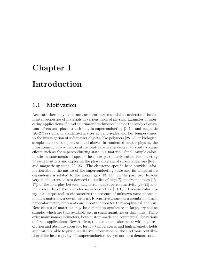
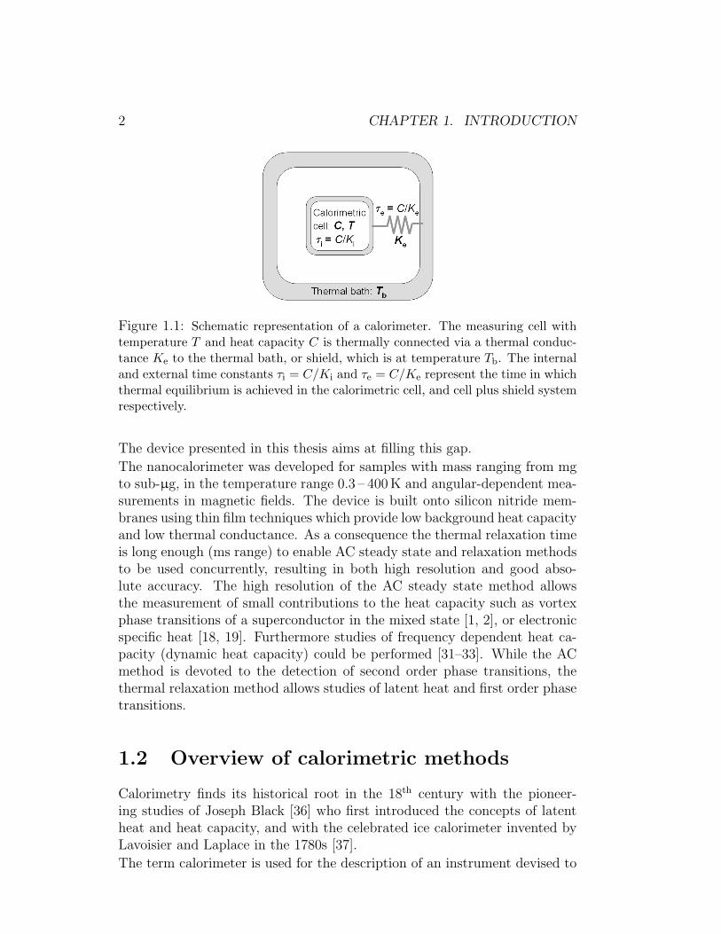
Figure 1.1: Schematic representation of a calorimeter. The measuring cell withtemperature T and heat capacity C is thermally connected via a thermal conduc-tance Ke to the thermal bath, or shield, which is at temperature Tb. The internaland external time constants τi = C/Ki and τe = C/Ke represent the time in whichthermal equilibrium is achieved in the calorimetric cell, and cell plus shield systemrespectively.
The device presented in this thesis aims at filling this gap.
The nanocalorimeter was developed for samples with mass ranging from mgto sub-µg, in the temperature range 0.3 – 400 K and angular-dependent mea-surements in magnetic fields. The device is built onto silicon nitride mem-branes using thin film techniques which provide low background heat capacityand low thermal conductance. As a consequence the thermal relaxation timeis long enough (ms range) to enable AC steady state and relaxation methodsto be used concurrently, resulting in both high resolution and good abso-lute accuracy. The high resolution of the AC steady state method allowsthe measurement of small contributions to the heat capacity such as vortexphase transitions of a superconductor in the mixed state [1, 2], or electronicspecific heat [18, 19]. Furthermore studies of frequency dependent heat ca-pacity (dynamic heat capacity) could be performed [31–33]. While the ACmethod is devoted to the detection of second order phase transitions, thethermal relaxation method allows studies of latent heat and first order phasetransitions.
1.2 Overview of calorimetric methods
Calorimetry finds its historical root in the 18th century with the pioneer-ing studies of Joseph Black [36] who first introduced the concepts of latentheat and heat capacity, and with the celebrated ice calorimeter invented byLavoisier and Laplace in the 1780s [37].
The term calorimeter is used for the description of an instrument devised to
1.2. OVERVIEW OF CALORIMETRIC METHODS 3
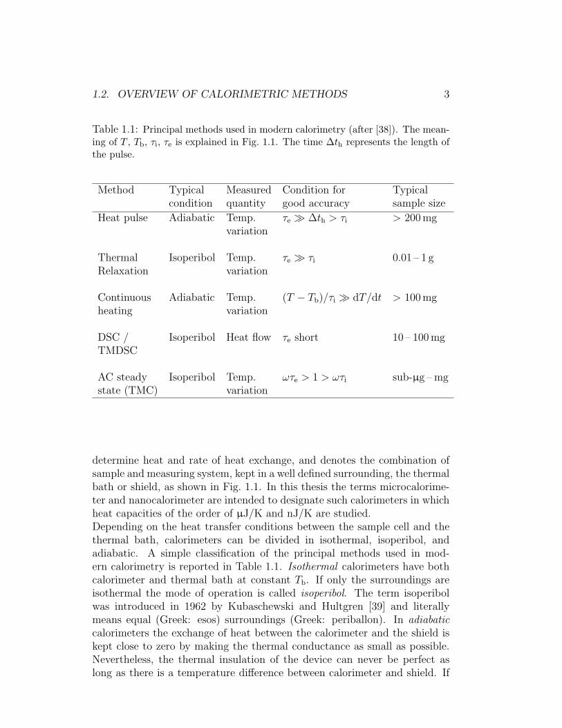
Table 1.1: Principal methods used in modern calorimetry (after [38]). The mean-ing of T , Tb, τi, τe is explained in Fig. 1.1. The time ∆th represents the length ofthe pulse.
Method Typical Measured Condition for Typicalcondition quantity good accuracy sample size
Heat pulse Adiabatic Temp. τe ∆th > τi > 200 mgvariation
Thermal Isoperibol Temp. τe τi 0.01 – 1 gRelaxation variation
Continuous Adiabatic Temp. (T − Tb)/τi dT/dt > 100 mgheating variation
DSC / Isoperibol Heat flow τe short 10 – 100 mgTMDSC
AC steady Isoperibol Temp. ωτe > 1 > ωτi sub-µg – mgstate (TMC) variation
determine heat and rate of heat exchange, and denotes the combination ofsample and measuring system, kept in a well defined surrounding, the thermalbath or shield, as shown in Fig. 1.1. In this thesis the terms microcalorime-ter and nanocalorimeter are intended to designate such calorimeters in whichheat capacities of the order of µJ/K and nJ/K are studied.Depending on the heat transfer conditions between the sample cell and thethermal bath, calorimeters can be divided in isothermal, isoperibol, andadiabatic. A simple classification of the principal methods used in mod-ern calorimetry is reported in Table 1.1. Isothermal calorimeters have bothcalorimeter and thermal bath at constant Tb. If only the surroundings areisothermal the mode of operation is called isoperibol. The term isoperibolwas introduced in 1962 by Kubaschewski and Hultgren [39] and literallymeans equal (Greek: esos) surroundings (Greek: periballon). In adiabaticcalorimeters the exchange of heat between the calorimeter and the shield iskept close to zero by making the thermal conductance as small as possible.Nevertheless, the thermal insulation of the device can never be perfect aslong as there is a temperature difference between calorimeter and shield. If
4 CHAPTER 1. INTRODUCTION
the temperature of the shield is made to vary and follow the temperatureof the internally heated calorimeter, there will be no heat flux by radiationor conduction along the supporting elements. This heat compensation be-comes particularly important above 100 K, when the radiation heat transferis not negligible anymore. When the adiabatic conditions are fulfilled, theelectrically measured heat input into the calorimeter, Q, coupled with themeasurement of the sample temperature change, ∆T , allows direct measure-ment of the heat capacity of calorimeter plus sample C = Q/∆T .The first adiabatic calorimeter was described in 1910 by Nernst [40], whorecognized the necessity of thermal insulation, in particular for low temper-ature measurements. On cooling from room temperature to liquid heliumtemperatures, the specific heat of a substance decreases by several orders ofmagnitude, and becomes vanishingly small at absolute zero. Accurate mea-surements of low temperature heat capacities become thus more and moredifficult because small heat fluxes from the surroundings can lead to signifi-cant errors. Nernst used the heat-pulse method which is realized by heatingHeat pulsethe sample for a finite time ∆th and measuring the temperature increment∆T . This method is the direct transposition of the thermodynamic definitionof heat capacity:
C = lim∆T→0
Q
∆T(1.1)
where Q is the heat supplied to the sample and calorimeter in form of apulse. A full measuring cycle is schematically shown in Fig. 1.2. The idealcase, in which fully adiabatic conditions are accomplished and the fore- andafter-heating lines are isothermal (Fig. 1.2a), can be realized only for sampleswith large heat capacity, i.e., mass m > 100 mg and T > 100 K [41].The classical adiabatic calorimeter of Nernst has been an excellent tool fordetermination of specific heats for more than five decades. The need forexcellent thermal insulation and minimization of stray heat leaks led to thedevelopment of several other calorimetric techniques, especially suited for themeasurement of small samples. As a result of this ever-lasting development,the nomenclature in calorimetry is still lacking a standardized definition, andno univocal classification of calorimeters can be found yet [42, 43].Adiabatic conditions become more and more difficult to be fulfilled when thetemperature and dimensions of the sample decrease. Semi-adiabatic condi-tions are met for samples with masses between 10 mg and 1 g [41]: the heatlosses are no longer negligible resulting in a small drift in the temperature(Fig. 1.2b). The thermal insulation of the sample can never be perfect as longas there is a temperature difference between the calorimeter and the shieldand continuous heat-loss corrections have to be made [44]. Non-adiabatic orisoperibol conditions exist when the measured heat capacities are so smallthat the thermal conductance along the electrical measuring lines cause the
1.2. OVERVIEW OF CALORIMETRIC METHODS 5
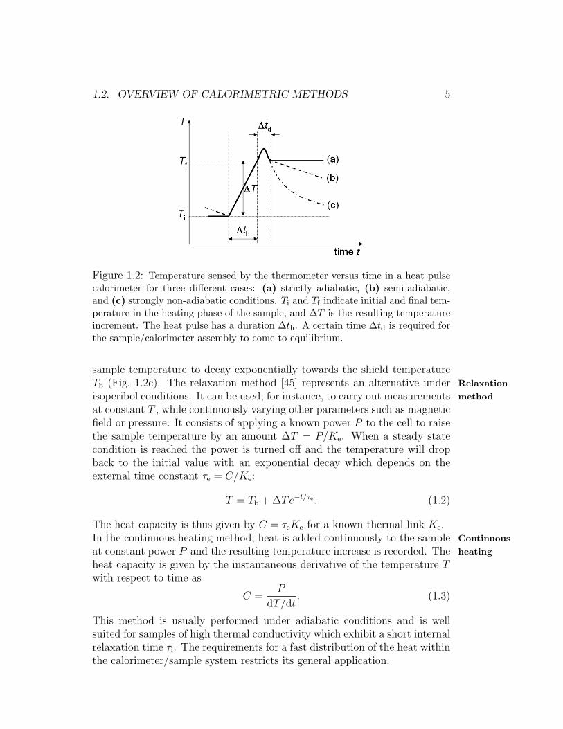
Figure 1.2: Temperature sensed by the thermometer versus time in a heat pulsecalorimeter for three different cases: (a) strictly adiabatic, (b) semi-adiabatic,and (c) strongly non-adiabatic conditions. Ti and Tf indicate initial and final tem-perature in the heating phase of the sample, and ∆T is the resulting temperatureincrement. The heat pulse has a duration ∆th. A certain time ∆td is required forthe sample/calorimeter assembly to come to equilibrium.
sample temperature to decay exponentially towards the shield temperatureTb (Fig. 1.2c). The relaxation method [45] represents an alternative under Relaxation
methodisoperibol conditions. It can be used, for instance, to carry out measurementsat constant T , while continuously varying other parameters such as magneticfield or pressure. It consists of applying a known power P to the cell to raisethe sample temperature by an amount ∆T = P/Ke. When a steady statecondition is reached the power is turned off and the temperature will dropback to the initial value with an exponential decay which depends on theexternal time constant τe = C/Ke:
T = Tb + ∆Te−t/τe . (1.2)
The heat capacity is thus given by C = τeKe for a known thermal link Ke.In the continuous heating method, heat is added continuously to the sample Continuous
heatingat constant power P and the resulting temperature increase is recorded. Theheat capacity is given by the instantaneous derivative of the temperature Twith respect to time as
C =P
dT/dt. (1.3)
This method is usually performed under adiabatic conditions and is wellsuited for samples of high thermal conductivity which exhibit a short internalrelaxation time τi. The requirements for a fast distribution of the heat withinthe calorimeter/sample system restricts its general application.
6 CHAPTER 1. INTRODUCTION
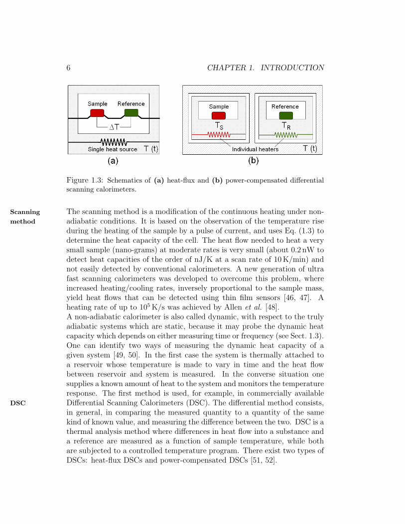
Figure 1.3: Schematics of (a) heat-flux and (b) power-compensated differentialscanning calorimeters.
The scanning method is a modification of the continuous heating under non-Scanningmethod adiabatic conditions. It is based on the observation of the temperature rise
during the heating of the sample by a pulse of current, and uses Eq. (1.3) todetermine the heat capacity of the cell. The heat flow needed to heat a verysmall sample (nano-grams) at moderate rates is very small (about 0.2 nW todetect heat capacities of the order of nJ/K at a scan rate of 10 K/min) andnot easily detected by conventional calorimeters. A new generation of ultrafast scanning calorimeters was developed to overcome this problem, whereincreased heating/cooling rates, inversely proportional to the sample mass,yield heat flows that can be detected using thin film sensors [46, 47]. Aheating rate of up to 105 K/s was achieved by Allen et al. [48].A non-adiabatic calorimeter is also called dynamic, with respect to the trulyadiabatic systems which are static, because it may probe the dynamic heatcapacity which depends on either measuring time or frequency (see Sect. 1.3).One can identify two ways of measuring the dynamic heat capacity of agiven system [49, 50]. In the first case the system is thermally attached toa reservoir whose temperature is made to vary in time and the heat flowbetween reservoir and system is measured. In the converse situation onesupplies a known amount of heat to the system and monitors the temperatureresponse. The first method is used, for example, in commercially availableDifferential Scanning Calorimeters (DSC). The differential method consists,DSCin general, in comparing the measured quantity to a quantity of the samekind of known value, and measuring the difference between the two. DSC is athermal analysis method where differences in heat flow into a substance anda reference are measured as a function of sample temperature, while bothare subjected to a controlled temperature program. There exist two types ofDSCs: heat-flux DSCs and power-compensated DSCs [51, 52].
1.2. OVERVIEW OF CALORIMETRIC METHODS 7
In the heat-flux DSC (Fig. 1.3a) a well defined exchange of the heat to be Heat-flux DSCmeasured with the environment takes place via a specific heat conductionpath with given thermal resistances. The sample and reference are connectedby a low resistance heat flow path (isothermal conditions), and the assemblyis enclosed in a single furnace which is heated with a linear heating rate
T = Tb + βt, (1.4)
where Tb is the initial temperature and β = dT/dt is the known heatingrate. For an ideally symmetrical arrangement the same heat flows to sampleand reference sides and the differential temperature ∆T is zero. When aphase transition occurs a ∆T signal arises proportional to the difference ofthe heat flow rates to sample and reference. The heat flow rate is propor-tional to ∆T through a temperature dependent proportionality factor E(T )which is related the geometry and the materials of construction of the deviceas Q = E(T )∆T . The heat capacity is given by C = Q/β.In the power-compensated DSC (Fig. 1.3b) the heat to be measured is com- Power-
compensatedDSC
pensated by increasing or decreasing an adjustable Joule heat. The measur-ing system consists of two identical furnaces, embedded in a large temperature-controlled heat sink. The temperatures of the sample and reference are con-trolled independently and are made identical by varying the power input tothe two furnaces; the energy required to do this is a measure of the heatcapacity changes in the sample relative to the reference. Finally, there existhybrid versions which combine advantages of both pure heat-flux and power-compensated DSCs resulting in better resolution and faster response time.Besides the classical operation mode where the heating rate is constant, one TMDSCcan drive the device with a variable change of the heating rate. In commer-cially available Temperature Modulated Differential Scanning Calorimeters(TMDSC) [53], a periodic variation is superimposed to the conventional tem-perature program so that
T = Tb + βt+ A sinωt, (1.5)
where A and ω are the amplitude and frequency of the modulation, andone measures the oscillating heat flow from the reservoir to the cell. Thistechnique adds the frequency dependence information to the heat capac-ity measurement. The DSC technique allows, in general, studying samplesdown to about 10 mg; when the sample size decreases, higher scan rates arerequired to maintain quasi-adiabatic conditions leading to lower temperatureand energy resolution.The requirement for heat capacity measurements on specimens with smaller TMCmasses has led to the development of a number of Temperature ModulationCalorimetry (TMC) techniques [54, 55]. Modulation techniques for studying
8 CHAPTER 1. INTRODUCTION
thermodynamic properties consist in periodically modulating the power thatheats the sample to create temperature oscillations around a mean tempera-ture. The amplitude of these oscillations is related to the thermal propertiesof the sensor and sample. There is a major difference between TMDSC andTMC. The former is a development of differential scanning calorimeter andas such it measures heat flow to the sample when heating the shield, while thelatter measures temperature variation of the sample when heating directlyon it.The first measurement of specific heat using the modulation method was3ω methodperformed by Corbino in 1910/11 [56]. He used the resistance of electricallyconducting samples to determine the temperature oscillations with a methodknown as third-harmonic (3ω) method. In this kind of experiment the samemetal resistor element is used as both heater and thermometer. The heater,with resistance R, is driven by a current at frequency ω which results in apower of double the frequency:
I(t) = I0 cosωt, (1.6a)
P (t) = P0(1 + cos 2ωt), (1.6b)
where P0 = I20R/2. The power causes diffusive thermal waves which perturb
the sensor resistance at a frequency 2ω:
R(t) = R0[1 + αδT cos(2ωt+ φ)], (1.7)
where α ≡ (1/R)(dR/dT ) is the temperature coefficient, and φ is the phaseshift of the temperature oscillation δT with respect to the power oscillation.The combined effect of driving current and resistance oscillations gives avoltage across the resistor in the form:
V (t) = I(t)R(t) = I0R0 cosωt+I0R0
2αδT cos(ωt+φ)+
I0R0
2αδT cos(3ωt+φ).
(1.8)The first term is the normal AC voltage at the drive frequency, while thesecond and third terms, which derive from mixing the current and resistanceoscillations, are dependent on the δT . The temperature oscillation ampli-tude, in turn, is related to the sample heat capacity [57].The 3ω technique was historically developed in the works of Rosenthal [58]who used a bridge technique to cancel out the much larger first harmonic,Smith et al. who measured the frequency dependent heat capacity of ger-manium [59], and, more recently, by Birge and Nagel who showed the spec-troscopic capability of this method [60, 61]. The third harmonic signal isnowadays detected using lock-in amplifiers, which give much higher preci-sion with respect to the older techniques which consisted, for example, indetecting the third harmonic output signal by means of a selective amplifierand an oscilloscope.
1.3. DYNAMIC HEAT CAPACITY 9
The use of a lock-in amplifier was introduced in the milestone paper written AC steadystate methodby Sullivan and Seidel in 1968 [62] which paved the way to the application
of modulation calorimetry to low temperature phenomena. They called theirmethod AC steady state and this term is now generally accepted. In theoriginal work the heater was driven by an AC current given by Eq. (1.6a) andthe voltage variation was synchronously detected across a separate resistancethermometer through which a dc current was maintained. When steady stateconditions occur, the temperature oscillation is related to the heat capacityof the sample plus addenda (heater and thermometer) by
δT =P0
Cω. (1.9)
Nowadays there exist many modifications of the temperature modulatedmethod. They differ in the ways of modulating the heating power (by anelectric current, with laser irradiation [63], induction heating [64], Peltierheating [65]), and by the methods of detecting the temperature oscillations(by the resistance of the sample or radiation from it, by the use of thermo-couples, resistance thermometers, or pyroelectric sensors).It should be noted that the AC calorimetry has typically poor performancesin detecting first order phase transitions and the results are essentially dif-ferent from the results of DSC [66] or those of adiabatic calorimetry. Theexclusion of the latent heat from the AC signal could be attributed to thedelay of the phase transition and thus, complete exclusion occurs only in caseof large frequency ω. If ω is much smaller than the rate of the phase transi-tion, the system is almost in equilibrium and the results of AC calorimetrycontain a large contribution of the latent heat [67]. A qualitative signal canalways be appreciated in the abrupt shift of the phase φ when two coexistingphases are present.
1.3 Dynamic heat capacity
In temperature modulated calorimetry, like for example the AC or 3ω method,one measures the response of a sample to a heat input which oscillates witha certain frequency ω. In TMDSC one measures the heat flow to the samplenecessary to keep up with a prescribed periodic temperature variation. Thesecalorimeters work in the frequency domain and the time scale of the measure-ment is set by the inverse of the frequency ω. The time scale of measurementis the smallest characteristic time interval during which a physical propertyof a system is recorded without any specific averaging [68]. An adiabaticcalorimeter works in the time domain: the temperature change of the sampleis followed as a function of time. In a time domain calorimeter the measuredthermodynamic quantities are time-averaged or, in other words, static. On
10 CHAPTER 1. INTRODUCTION
the other side, in a frequency domain calorimeter the heat capacity is con-sidered a dynamic quantity because its value does depend on the measuringtime scale, i.e., on the driving frequency. Suppose that a system contains aslow kinetic process which relaxes with a characteristic time constant τ , suchas structural change or chemical reaction. If heat is supplied in a shortertime interval than the kinetic relaxation time constant of this internal degreeof freedom, this degree will not contribute totally to the equilibrium value ofthe measured heat capacity under the time scale of observation. The mea-sured heat capacity C(ω) is thus a non-equilibrium quantity which varies intime and becomes a complex number. The complex heat capacity is defined,in analogy with the complex permittivity, as [69]:
C∗ = C ′ − iC ′′ = C∞ +C0 − C∞1 + iωτ
, (1.10)
where
C ′ = C∞ +C0 − C∞1 + (ωτ)2
(1.11)
is the real component, indicating the storage of the energy in the sample,and
C ′′ =(C0 − C∞)ωτ
1 + (ωτ)2(1.12)
is the imaginary part related to the energy loss. The real part C ′ has twoasymptotic limits: C∞, at ω → ∞, is the heat capacity related to the in-finitely fast degree of freedom as compared to the frequency, like the vibra-tional modes of the phonon bath, and C0, at ω → 0, is the static term,i.e., the total contribution at equilibrium of all the degrees of freedom of thesample.It has been derived elsewhere [33, 50] that for a typical AC experiment, thereal and imaginary part of the complex heat capacity are given by:
C ′ = − P0
ωδTsinφ, (1.13)
C ′′ =P0
ωδTcosφ− Ke
ω(1.14)
where P0 is the power oscillation amplitude at frequency ω, δT is the inducedtemperature modulation, φ is the phase lag between power and temperatureoscillations, and Ke is the thermal conductance between the calorimetriccell plus sample and the thermal bath. In the derivation of Eqs. (1.13) and(1.14) it was assumed to use frequencies low enough to neglect the internalrelaxation time constant τi between sample and calorimetric cell and within
1.3. DYNAMIC HEAT CAPACITY 11
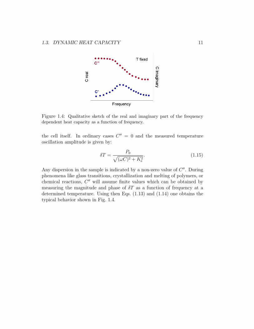
Figure 1.4: Qualitative sketch of the real and imaginary part of the frequencydependent heat capacity as a function of frequency.
the cell itself. In ordinary cases C ′′ = 0 and the measured temperatureoscillation amplitude is given by:
δT =P0√
(ωC)2 +K2e
. (1.15)
Any dispersion in the sample is indicated by a non-zero value of C ′′. Duringphenomena like glass transitions, crystallization and melting of polymers, orchemical reactions, C ′′ will assume finite values which can be obtained bymeasuring the magnitude and phase of δT as a function of frequency at adetermined temperature. Using then Eqs. (1.13) and (1.14) one obtains thetypical behavior shown in Fig. 1.4.

12 CHAPTER 1. INTRODUCTION
Chapter 2
Analytical models
2.1 Model diagrams
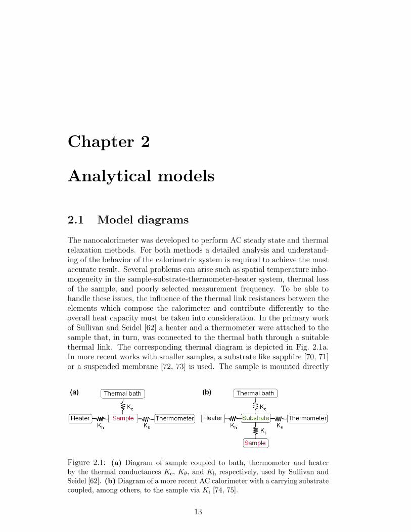
The nanocalorimeter was developed to perform AC steady state and thermalrelaxation methods. For both methods a detailed analysis and understand-ing of the behavior of the calorimetric system is required to achieve the mostaccurate result. Several problems can arise such as spatial temperature inho-mogeneity in the sample-substrate-thermometer-heater system, thermal lossof the sample, and poorly selected measurement frequency. To be able tohandle these issues, the influence of the thermal link resistances between theelements which compose the calorimeter and contribute differently to theoverall heat capacity must be taken into consideration. In the primary workof Sullivan and Seidel [62] a heater and a thermometer were attached to thesample that, in turn, was connected to the thermal bath through a suitablethermal link. The corresponding thermal diagram is depicted in Fig. 2.1a.In more recent works with smaller samples, a substrate like sapphire [70, 71]or a suspended membrane [72, 73] is used. The sample is mounted directly
Figure 2.1: (a) Diagram of sample coupled to bath, thermometer and heaterby the thermal conductances Ke, Kθ, and Kh respectively, used by Sullivan andSeidel [62]. (b) Diagram of a more recent AC calorimeter with a carrying substratecoupled, among others, to the sample via Ki [74, 75].
13
14 CHAPTER 2. ANALYTICAL MODELS
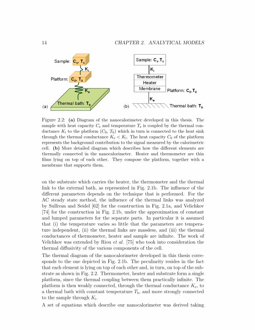
Figure 2.2: (a) Diagram of the nanocalorimeter developed in this thesis. Thesample with heat capacity Cs and temperature Ts is coupled by the thermal con-ductance Ki to the platform (C0, T0) which in turn is connected to the heat sinkthrough the thermal conductance Ke < Ki. The heat capacity C0 of the platformrepresents the background contribution to the signal measured by the calorimetriccell. (b) More detailed diagram which describes how the different elements arethermally connected in the nanocalorimeter. Heater and thermometer are thinfilms lying on top of each other. They compose the platform, together with amembrane that supports them.
on the substrate which carries the heater, the thermometer and the thermallink to the external bath, as represented in Fig. 2.1b. The influence of thedifferent parameters depends on the technique that is performed. For theAC steady state method, the influence of the thermal links was analyzedby Sullivan and Seidel [62] for the construction in Fig. 2.1a, and Velichkov[74] for the construction in Fig. 2.1b, under the approximation of constantand lumped parameters for the separate parts. In particular it is assumedthat (i) the temperature varies so little that the parameters are tempera-ture independent, (ii) the thermal links are massless, and (iii) the thermalconductances of thermometer, heater and sample are infinite. The work ofVelichkov was extended by Riou et al. [75] who took into consideration thethermal diffusivity of the various components of the cell.
The thermal diagram of the nanocalorimeter developed in this thesis corre-sponds to the one depicted in Fig. 2.1b. The peculiarity resides in the factthat each element is lying on top of each other and, in turn, on top of the sub-strate as shown in Fig. 2.2. Thermometer, heater and substrate form a singleplatform, since the thermal coupling between them practically infinite. Theplatform is then weakly connected, through the thermal conductance Ke, toa thermal bath with constant temperature Tb, and more strongly connectedto the sample through Ki.
A set of equations which describe our nanocalorimeter was derived taking
2.2. AC STEADY STATE METHOD 15
into account the different thermal links and the influence of the selectedfrequency. This derivation helped in understanding the properties of oursystem. The theoretical results have been confirmed by comparison withexperimental data, and with previous works.
2.2 AC steady state method
2.2.1 Analysis of the calorimetric system
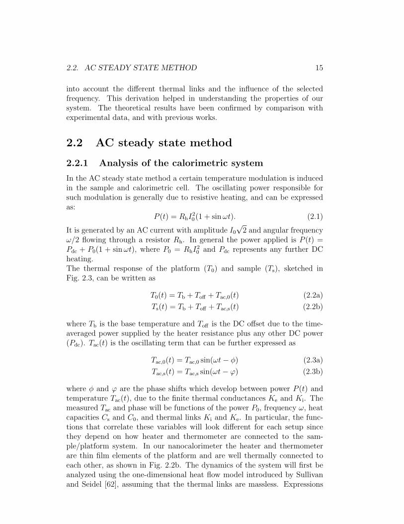
In the AC steady state method a certain temperature modulation is inducedin the sample and calorimetric cell. The oscillating power responsible forsuch modulation is generally due to resistive heating, and can be expressedas:
P (t) = RhI20 (1 + sinωt). (2.1)
It is generated by an AC current with amplitude I0
√2 and angular frequency
ω/2 flowing through a resistor Rh. In general the power applied is P (t) =Pdc + P0(1 + sinωt), where P0 = RhI
20 and Pdc represents any further DC
heating.The thermal response of the platform (T0) and sample (Ts), sketched inFig. 2.3, can be written as
T0(t) = Tb + Toff + Tac,0(t) (2.2a)
Ts(t) = Tb + Toff + Tac,s(t) (2.2b)
where Tb is the base temperature and Toff is the DC offset due to the time-averaged power supplied by the heater resistance plus any other DC power(Pdc). Tac(t) is the oscillating term that can be further expressed as
Tac,0(t) = Tac,0 sin(ωt− φ) (2.3a)
Tac,s(t) = Tac,s sin(ωt− ϕ) (2.3b)
where φ and ϕ are the phase shifts which develop between power P (t) andtemperature Tac(t), due to the finite thermal conductances Ke and Ki. Themeasured Tac and phase will be functions of the power P0, frequency ω, heatcapacities Cs and C0, and thermal links Ki and Ke. In particular, the func-tions that correlate these variables will look different for each setup sincethey depend on how heater and thermometer are connected to the sam-ple/platform system. In our nanocalorimeter the heater and thermometerare thin film elements of the platform and are well thermally connected toeach other, as shown in Fig. 2.2b. The dynamics of the system will first beanalyzed using the one-dimensional heat flow model introduced by Sullivanand Seidel [62], assuming that the thermal links are massless. Expressions
16 CHAPTER 2. ANALYTICAL MODELS
Figure 2.3: Oscillating heating power (top) which gives rise to a stationary statewhere a temperature amplitudes Tac oscillates around an offset value Toff + Tb
(bottom).
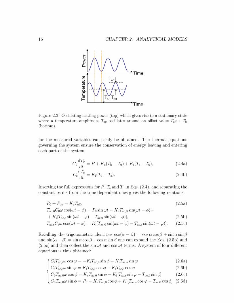
for the measured variables can easily be obtained. The thermal equationsgoverning the system ensure the conservation of energy leaving and enteringeach part of the system:
C0dT0
dt= P +Ke(Tb − T0) +Ki(Ts − T0), (2.4a)
CsdTs
dt= Ki(T0 − Ts). (2.4b)
Inserting the full expressions for P , Ts and T0 in Eqs. (2.4), and separating theconstant terms from the time dependent ones gives the following relations:
P0 + Pdc = KeToff , (2.5a)
Tac,0C0ω cos(ωt− φ) = P0 sinωt−KeTac,0 sin(ωt− φ)+
+Ki[Tac,s sin(ωt− ϕ)− Tac,0 sin(ωt− φ)], (2.5b)
Tac,sCsω cos(ωt− ϕ) = Ki[Tac,0 sin(ωt− φ)− Tac,s sin(ωt− ϕ)]. (2.5c)
Recalling the trigonometric identities cos(α − β) = cosα cos β + sinα sin βand sin(α−β) = sinα cos β− cosα sin β one can expand the Eqs. (2.5b) and(2.5c) and then collect the sinωt and cosωt terms. A system of four differentequations is thus obtained:
CsTac,sω cosϕ = −KiTac,0 sinφ+KiTac,s sinϕ (2.6a)
CsTac,sω sinϕ = KiTac,0 cosφ−KiTac,s cosϕ (2.6b)
C0Tac,0ω cosφ = KeTac,0 sinφ−Ki[Tac,s sinϕ− Tac,0 sinφ] (2.6c)
C0Tac,0ω sinφ = P0 −KeTac,0 cosφ+Ki[Tac,s cosϕ− Tac,0 cosφ] (2.6d)
2.2. AC STEADY STATE METHOD 17
The experimentally measured values are just Tac,0 and φ since the thermome-ter is part of the platform:
Tac,0 = P0
√K2
i + C2s ω
2
2C2sKeKiω2 +K2
e (K2i + C2
s ω2) + ω2K2
i (C0 + Cs)2 + ω4C2sC
20
,
(2.7a)
tanφ =ω[CsK
2i + C0(K2
i + C2s ω
2)]
C2sKiω2 +Ke(K2
i + C2s ω
2). (2.7b)
Define the total heat capacity C = C0 + Cs, and the external and internaltime constants τe = C/Ke and τi = Cs/Ki. The external time constantcharacterizes the thermal relaxation between the platform plus sample andthe surroundings. The internal time constant determines instead the timeneeded for the system to homogenize to inside temperature: it could belimited either by poor thermal conductance between sample and platform,or within the sample itself. With these definitions, Eqs. (2.7a) and (2.7b)can be rewritten as
Tac,0 =P0
ωC
[1 +
1
(ωτe)2−(
1− C20
C2
)g + 2
τi
τe
(1− C0
C
)f
]−1/2
, (2.8a)
tanφ =ω(C0 + Cs f)
Ke +Ki g. (2.8b)
where
g =(ωτi)
2
1 + (ωτi)2, (2.9a)
f =1
1 + (ωτi)2= 1− g. (2.9b)
The limiting values of these functions are f = 1 and g = 0 when ω → 0, andf = 0 and g = 1 when ω →∞.Equation (2.8a) can be written in the compact form
Tac,0 =P0√
(ωC)2 +K2, (2.10)
where
C2
= C20g + C2f. (2.11)
and
K2
= K2e
(1 + 2
Ki
Ke
g
). (2.12)
18 CHAPTER 2. ANALYTICAL MODELS
The effective heat capacity C reduces to C0 either when Cs = 0 or at high fre-quencies. At low frequencies it coincides with C0 +Cs. The effective thermalconductance K coincides with Ke at low frequencies and, for a reasonableratio of internal and external thermal conductances, it deviates up to somepercent in the high frequency range.Manipulating Eqs. (2.8a) and (2.8b), the expression for the heat capacity Ccan be derived:
C =P0
Tac,0ω
τe
τi + τe
(sinφ+ ωτi cosφ). (2.13)
In the particular case where Cs = 0 (empty cell): C = C0, and Eqs. (2.8a),(2.8b) and (2.13) become
Tac,0 =P0
ωC0
[1 +
1
(ωτe,0)2
]−1/2
, (2.14a)
tanφ = ωτe,0, (2.14b)
C0 =P0
ωTac,0
sinφ. (2.14c)
The time constant τe,0 = C0/Ke characterizes the thermal relaxation of theplatform itself.
2.2.2 Effect of the internal time constant
The relaxation time τi limits the accuracy of the measurement and a correctchoice of the working frequency minimizes its effect. The frequency of thetemperature oscillation should satisfy the following inequalites: ωτi 1 ≤ωτe. When the condition ωτe 1 is satisfied, the sample-platform systemheats up in a shorter time compared to the relaxation time to the thermalbath (adiabatic criterion, in a calorimetric sense and not in a thermodynamicsense). The condition ωτi 1 is necessary to achieve good temperaturehomogeneity within the sample-platform system (quasi-static criterion).Consider what happens in the limiting cases. For very low ω, the temperatureLimiting case:
low ω oscillation amplitude and phase become respectively:
limω→0
Tac,0 =P0
Ke
(2.15)
andlimω→0
tanφ = ωτe. (2.16)
In this limit the adiabatic criterion fails and the system composed by plat-form plus sample has time to relax towards the thermal bath. The phase ap-proaches zero meaning that heater power and temperature oscillations havetime to synchronize.
2.2. AC STEADY STATE METHOD 19
For very high ω the quasi-static criterion is not satisfied. The sample is Limiting case:high ωthermally disconnected from the platform, and just the heat capacity of the
platform C0 is probed. Equation (2.8a) for Tac, transforms into Eq. (2.14a),and Eq. (2.8b) becomes
tanφ ≈ ωC0
Ki +Ke
. (2.17)
The tangent of the phase tends to ∞, i.e., the temperature oscillation signalhas a phase π/2 with respect to the power input meaning that the systemhas no time to relax towards the thermal bath. The high frequency regime iscalled quasi-adiabatic because there is a negligible AC heat loss during onetemperature cycle although a DC heat flow is always present. The tempera-ture amplitude decreases when increasing the frequency and it reaches a pointwhere the resolution degrades considerably. Higher powers must thus be ap-plied to maintain the measured Tac at a certain minimum value, resulting inincreased Toff . This is an obstacle when one aims to work in the sub-Kelvinregion since self-heating would not allow to reach the lowest temperatures.In practice, it is useful to use simplified formulas such as Simplified rela-
tions: accuracy
C ≈ P0
ωTac,0
, (2.18)
or
C ≈ P0
ωTac,0
sinφ ≈ P0
ωTac,0
[1 +
1
(ωτe)2
]−1/2
. (2.19)
Equation (2.19) can be transformed into
C ≈ P0
ωTac,0
√1−
(Tac,0
Tdc
)2
(2.20)
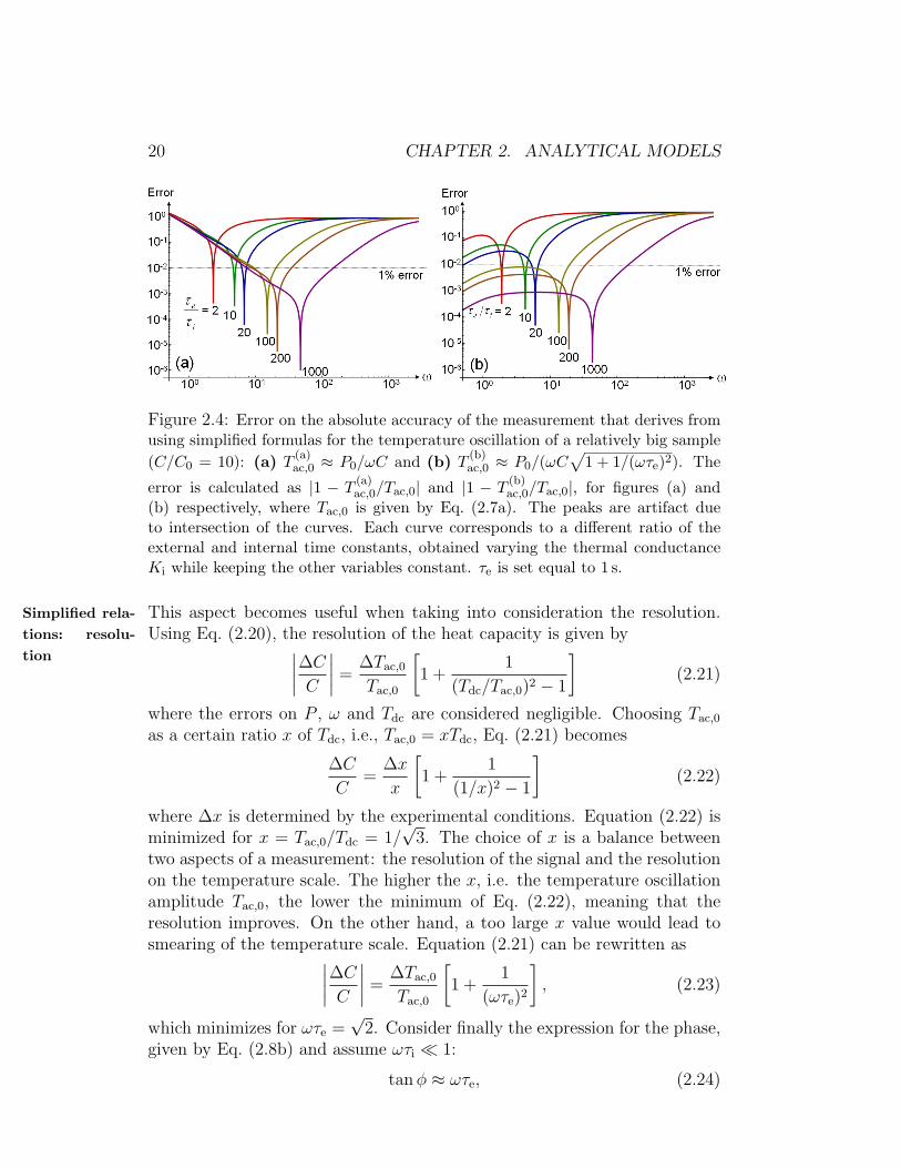
where Tdc = P0/Ke. From Fig. 2.4 it is clear that the higher the ratiobetween external and internal time constants, the wider the interval of fre-quencies that ensure a certain accuracy. The internal time constant increaseseither when the sample has a very high heat capacity, Cs, or when the ther-mal link between sample and platform, Ki, is poor. This suggests that whenmeasuring samples with Cs ≈ C0, the best accuracy can be achieved usinghighly thermally conducting substances to increase the thermal connectionto the platform. If τe ≈ τi, in order to use the simplified relations over a widetemperature range without deviating too much from the true heat capacityvalue, the frequency at which the heaters are driven needs to be continuouslyadjusted. On the other hand, when τi and τe differ of at least two orders ofmagnitude from each other, Eq. (2.19) gives a certain freedom in the choiceof the working frequency still ensuring an error level below 1%.
20 CHAPTER 2. ANALYTICAL MODELS
Figure 2.4: Error on the absolute accuracy of the measurement that derives fromusing simplified formulas for the temperature oscillation of a relatively big sample(C/C0 = 10): (a) T (a)
ac,0 ≈ P0/ωC and (b) T (b)ac,0 ≈ P0/(ωC
√1 + 1/(ωτe)2). The
error is calculated as |1 − T(a)ac,0/Tac,0| and |1 − T
(b)ac,0/Tac,0|, for figures (a) and
(b) respectively, where Tac,0 is given by Eq. (2.7a). The peaks are artifact dueto intersection of the curves. Each curve corresponds to a different ratio of theexternal and internal time constants, obtained varying the thermal conductanceKi while keeping the other variables constant. τe is set equal to 1 s.
This aspect becomes useful when taking into consideration the resolution.Simplified rela-tions: resolu-tion
Using Eq. (2.20), the resolution of the heat capacity is given by∣∣∣∣∆CC∣∣∣∣ =
∆Tac,0
Tac,0
[1 +
1
(Tdc/Tac,0)2 − 1
](2.21)
where the errors on P , ω and Tdc are considered negligible. Choosing Tac,0
as a certain ratio x of Tdc, i.e., Tac,0 = xTdc, Eq. (2.21) becomes
∆C
C=
∆x
x
[1 +
1
(1/x)2 − 1
](2.22)
where ∆x is determined by the experimental conditions. Equation (2.22) isminimized for x = Tac,0/Tdc = 1/
√3. The choice of x is a balance between
two aspects of a measurement: the resolution of the signal and the resolutionon the temperature scale. The higher the x, i.e. the temperature oscillationamplitude Tac,0, the lower the minimum of Eq. (2.22), meaning that theresolution improves. On the other hand, a too large x value would lead tosmearing of the temperature scale. Equation (2.21) can be rewritten as∣∣∣∣∆CC
∣∣∣∣ =∆Tac,0
Tac,0
[1 +
1
(ωτe)2
], (2.23)
which minimizes for ωτe =√
2. Consider finally the expression for the phase,given by Eq. (2.8b) and assume ωτi 1:
tanφ ≈ ωτe, (2.24)
2.2. AC STEADY STATE METHOD 21
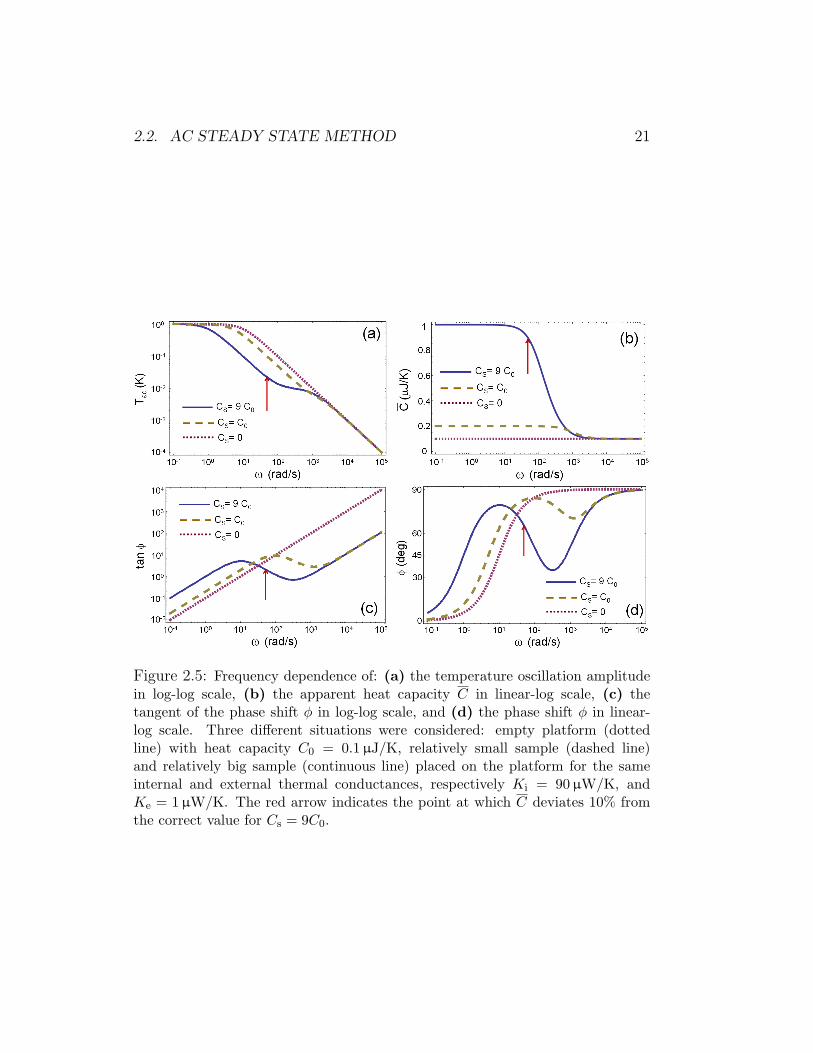
Figure 2.5: Frequency dependence of: (a) the temperature oscillation amplitudein log-log scale, (b) the apparent heat capacity C in linear-log scale, (c) thetangent of the phase shift φ in log-log scale, and (d) the phase shift φ in linear-log scale. Three different situations were considered: empty platform (dottedline) with heat capacity C0 = 0.1 µJ/K, relatively small sample (dashed line)and relatively big sample (continuous line) placed on the platform for the sameinternal and external thermal conductances, respectively Ki = 90 µW/K, andKe = 1 µW/K. The red arrow indicates the point at which C deviates 10% fromthe correct value for Cs = 9C0.
22 CHAPTER 2. ANALYTICAL MODELS
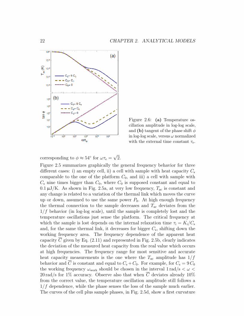
Figure 2.6: (a) Temperature os-cillation amplitude in log-log scale,and (b) tangent of the phase shift φin log-log scale, versus ω normalizedwith the external time constant τe.
corresponding to φ ≈ 54 for ωτe =√
2.
Figure 2.5 summarizes graphically the general frequency behavior for threedifferent cases: i) an empty cell, ii) a cell with sample with heat capacity Cs
comparable to the one of the platform C0, and iii) a cell with sample withCs nine times bigger than C0, where C0 is supposed constant and equal to0.1 µJ/K. As shown in Fig. 2.5a, at very low frequency, Tac is constant andany change is related to a variation of the thermal link which moves the curveup or down, assumed to use the same power P0. At high enough frequencythe thermal connection to the sample decreases and Tac deviates from the1/f behavior (in log-log scale), until the sample is completely lost and thetemperature oscillations just sense the platform. The critical frequency atwhich the sample is lost depends on the internal relaxation time τi = Ki/Cs
and, for the same thermal link, it decreases for bigger Cs, shifting down theworking frequency area. The frequency dependence of the apparent heatcapacity C given by Eq. (2.11) and represented in Fig. 2.5b, clearly indicatesthe deviation of the measured heat capacity from the real value which occursat high frequencies. The frequency range for most sensitive and accurateheat capacity measurements is the one where the Tac amplitude has 1/fbehavior and C is constant and equal to Cs +C0. For example, for Cs = 9C0
the working frequency ωwork should be chosen in the interval 1 rad/s < ω <20 rad/s for 1% accuracy. Observe also that when C deviates already 10%from the correct value, the temperature oscillation amplitude still follows a1/f dependence, while the phase senses the loss of the sample much earlier.The curves of the cell plus sample phases, in Fig. 2.5d, show a first curvature
2.2. AC STEADY STATE METHOD 23
which starts at relatively low frequncies and a dip related to the thermaldetachment of the sample which lags behind the temperature oscillations ofthe platform.The correct ωwork depends on the requirements for the specific measurement:the absolute accuracy, the resolution of the measured signal, the resolutionon the temperature scale (how smeared is the signal), and the temperaturerange. The phase is a very sensitive indicator of the actual working conditionsand it could be used to determine ωwork. The ideal condition is obtainedworking in the frequency range where the tangent of the phase shows a perfectlinear frequency dependence in log-log scale. There are two such ranges, butthe sample is sensed just in the one at lower ω. This concept becomesclear when Tac and tanφ are plotted versus the normalized frequency usingthe time constant τe (Fig. 2.6). As long as the sample curves overlap theplatform curve (dotted line), the relaxation time constant between sampleand platform is negligible.
2.2.3 1D model of the membrane
Until now the heat capacity of the platform has been considered to be lo-calized in one point. In reality, the extent of platform, leads of thermome-ter and heater, and thermal link components should be taken into account.The temperature oscillations spread in the metal leads of thermometer andheater, and in the platform (SiN membrane) over a distance of the order ofa frequency dependent thermal length
`th(ω) =
√2D
ω(2.25)
where D = κ/ρcp is the diffusivity, with κ, ρ and cp, being the thermal con-ductivity, volume density and specific heat respectively. This effect becomesmore and more negligible when the size of the sample increases, but mustbe taken into account when samples with heat capacity Cs comparable to C0
are studied. This diffusion practically results in an additional contribution tothe addenda heat capacity that can be written as C0 = Cc+Ce(ω), where Cc
is the constant part in direct contact with the heater, and Ce(ω) = Cwp(ω)is an effective heat capacity of the support as a function of frequency, andp(ω) is some frequency-dependent function. In order to derive the func-tional form of the frequency dependent heat capacity we first use a simplifiedone-dimensional case. Given a uniform wire of length L, the profile of theoscillating part of the temperature along the x-axis can be derived by solvingthe heat equation
∂T
∂t= D
∂2T
∂x2. (2.26)
24 CHAPTER 2. ANALYTICAL MODELS
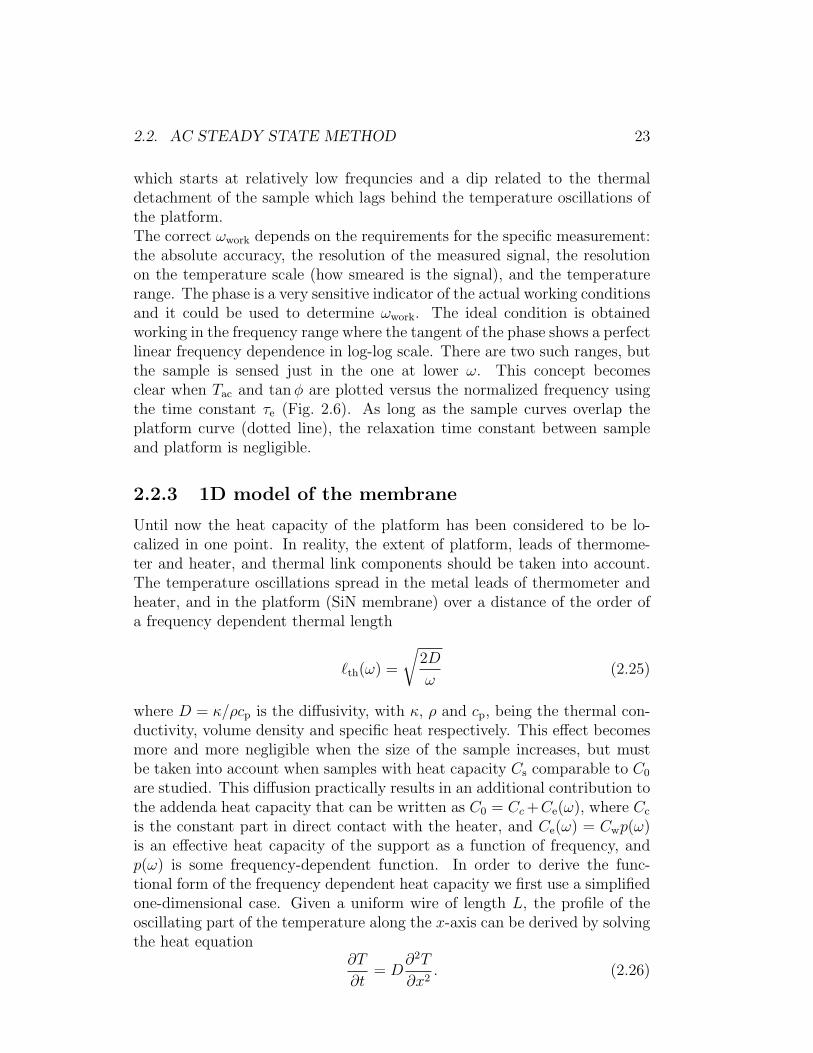
Figure 2.7: Qualitative behavior of the frequency dependent heat capacity andthermal conductances derived in Eqs. (2.37) and (2.38). At high frequencies bothbehaviors are well approximated by the respective limiting forms. The parametersCw and τw where arbitrarily chosen equal to 3 nJ/K and 0.1 s respectively.
In our specific case, Eq. (2.26) has to satisfy the following boundary condi-tions:
T (0, t) = Tac,0 sinωt+ T1,
T (L, t) = T2 (2.27)
where one end (x = 0) is at temperature T1 and subjected to a power
P (t) = P0 sin(ωt+ φ), (2.28)
and thus is periodically oscillating with amplitude Tac,0, while the other endis at a constant temperature T2. Solving the time-independent problem thefollowing temperature profile is obtained:
Tdc(x) = T1 +x
L(T2 − T1). (2.29)
The time-dependent temperature profile along the wire at steady-state isfound by means of the Laplace transforms:
Tac(x, t) = Tac,0
=
sinh[√
−iωD
(x− L)]
sinh[√
iωDL]e−iωt
∣∣∣sinh
(√iωDL)∣∣∣2 . (2.30)
The solution to the full problem is the sum of the time-dependent and time-independent contributions:
T (x, t) = Tac(x, t) + Tdc(x). (2.31)
Consider the time-dependent solution and solve the Fourier law of heat trans-fer with P (t) given by Eq. (2.28) and Tac(x, t) by Eq. (2.30),
P (t) = −LKw
[dTac(x, t)
dx
]x=0
, (2.32)
2.2. AC STEADY STATE METHOD 25
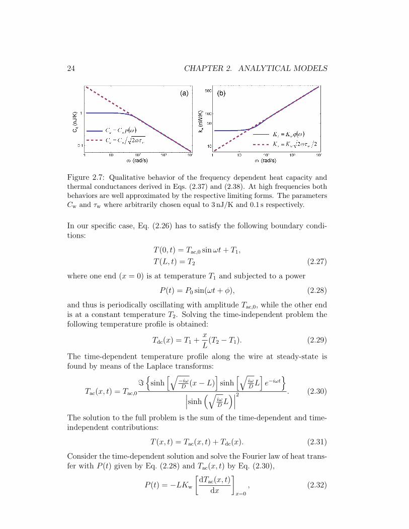
Figure 2.8: Behavior of the frequency dependent heat capacity when there existsa constant term Cc 6= 0. Cw = 3 nJ/K, τw = 0.1 s, and Cc = Cw/10 arbitrarilychosen.
where Kw is the thermal conductance in the wire. The expression for thepower amplitude that generates the temperature oscillation at x = 0 becomes
P0 = Tac,0ωCw√2ωτw
sinh√
2ωτw − sin√
2ωτw
cosh√
2ωτw − cos√
2ωτw
1
sinφ(2.33)
where the diffusivity D was substituted by L2Kw/Cw and the parameterτw = Cw/Kw was introduced. Note that the factor α =
√2ωτw = 2L/`th
where the thermal length is given by Eq. (2.25). The frequency dependenceof the phase φ is also obtained:
tanφ =sinhα− sinα
sinhα + sinα. (2.34)
The experimentally measured power amplitude P0, temperature amplitudeTac,0, phase φ and angular frequency ω are related to each other by thefollowing equations:
C0 =P0
ωTac,0
sinφ (2.35a)
Ke =P0
Tac,0
cosφ (2.35b)
Or, alternatevily: Tac,0 =
P0√(ωC0)2 +K2
e
(2.36a)
tanφ =ωC0
Ke
(2.36b)
26 CHAPTER 2. ANALYTICAL MODELS
Both the heat capacity Ce and thermal conductance Ke are frequency depen-dent and they can be written as Ce = Cwp(ω) and Ke = Kwq(ω). Solvingeither of the two systems for Ce and Ke gives the following functional forms:
p(ω) =1
α
sinhα− sinα
coshα− cosα(2.37)
and
q(ω) =α
2
sinhα + sinα
coshα− cosα. (2.38)
Consider the limits for
ω → 0 : Ce =Cw
3, Ke = Kw, (2.39)
and
ω →∞ : Ce =Cw
α,Ke = Kw
α
2. (2.40)
The same heat capacity frequency dependence was derived by Greene et al.[76] for the case of a sample suspended by wire thermocouples.In a more realistic case there exists a constant heat capacity Cc which shouldbe taken into account. Equation (2.32) transforms into
P (t) = −LKw
[dTac(x, t)
dx
]x=0
+ Cc
[dTac(x, t)
dt
]x=0
, (2.41)
and the power and tangent of the phase modify as
P0 = ωTac,0
(Cc +
Cw
α
sinhα− sinα
coshα− cosα
)1
sinφ, (2.42)
and
tanφ =Cc
Cwα
coshα− cosα
sinhα + sinα+
sinhα− sinα
sinhα + sinα. (2.43)
The heat capacity C0 = Cc +Cwp(ω) and thermal conductance Ke = Kwq(ω)conserve the same frequency dependence, and Eqs. (2.37) and (2.38) are stillvalid.
2.2.4 2D model of the membrane
In case of a two-dimensional platform, as in our specific case where the sampleis supported by a SiN membrane, the heat equation should be expressed inpolar coordinates. Equation (2.26) is transformed as
∂T
∂t= D
1
ρ
∂
∂ρ
(ρ∂T
∂ρ
). (2.44)
2.2. AC STEADY STATE METHOD 27
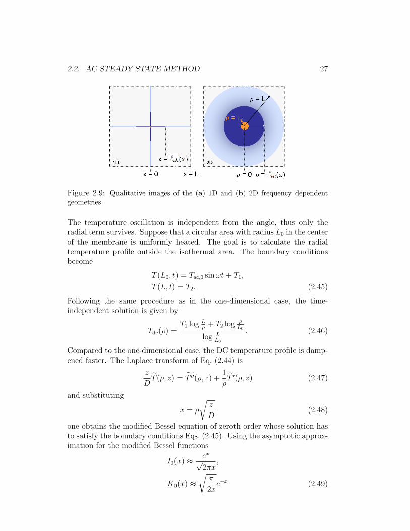
Figure 2.9: Qualitative images of the (a) 1D and (b) 2D frequency dependentgeometries.
The temperature oscillation is independent from the angle, thus only theradial term survives. Suppose that a circular area with radius L0 in the centerof the membrane is uniformly heated. The goal is to calculate the radialtemperature profile outside the isothermal area. The boundary conditionsbecome
T (L0, t) = Tac,0 sinωt+ T1,
T (L, t) = T2. (2.45)
Following the same procedure as in the one-dimensional case, the time-independent solution is given by
Tdc(ρ) =T1 log L
ρ+ T2 log ρ
L0
log LL0
. (2.46)
Compared to the one-dimensional case, the DC temperature profile is damp-ened faster. The Laplace transform of Eq. (2.44) is
z
DT (ρ, z) = T ′′(ρ, z) +
1
ρT ′(ρ, z) (2.47)
and substituting
x = ρ
√z
D(2.48)
one obtains the modified Bessel equation of zeroth order whose solution hasto satisfy the boundary conditions Eqs. (2.45). Using the asymptotic approx-imation for the modified Bessel functions
I0(x) ≈ ex√2πx
,
K0(x) ≈√
π
2xe−x (2.49)
28 CHAPTER 2. ANALYTICAL MODELS
valid for x > 0, one can finally write the steady state radial temperatureprofile:
Tac(ρ, t) = Tac,0
√L0
ρ
=
sinh[√
−iωD
(ρ− L)]
sinh[√
iωD
(L− L0)]e−iωt
∣∣∣sinh
[√iωD
(L− L0)]∣∣∣2 .
(2.50)The solution to the full problem is the sum of two contributions:
T (ρ, t) = Tac(ρ, t) + Tdc(ρ). (2.51)
Equation (2.50) differs from Eq. (2.30) by a multiplying factor√L0/ρ. This
means that, in the radial situation, the amplitude of the temperature oscil-lation is dampened faster.
The power amplitude P0 and tanφ that are obtained by solving the Fourierheat equation in ρ = L0 differ from Eqs. (2.42) and (2.43) in the argument ofthe hyperbolic and trigonometric functions which is multiplied by (L−L0)/L,and for the presence of an additive factor deriving from
√L0/ρ of Eq. (2.50).
The models given by Eqs. (2.35) and (2.36) are still valid. The participatingheat capacity and thermal conductance are both constant at low frequency,and at high frequency the heat capacity still goes as 1/
√ω and the thermal
conductance as√ω. Since there is no major difference in the frequency
dependence of the 2D heat capacity and thermal conductance compared tothe 1D model, it is enough to use Eqs. (2.37) and (2.38) for fitting purposes. Adetailed quantitative study of the two-dimensional model is still in progress.
2.2.5 Sample size effects
In a material with diffusivity D the amplitude of a thermal oscillation isdampened out on a frequency dependent length scale `th(ω) given by Eq. (2.25).It is generally required that the thermal diffusion length is much larger thanthe sample thickness, to reach a uniform temperature at a given frequency.Note that the magnitude of `th depends not only on the frequency but alsoon the thermo-physical properties of the sample, since D = κ/ρcp. For in-stance, the diffusivity of gold can be easily calculated: DAu ≈ 1.28·10−4 m2/swhich gives `th,Au(ω) ≈ 15/
√ωmm. Through the diffusivity, one can esti-
mate the sample time constant τs, which gives the time scale at which atemperature wave front reaches the extremity of the sample. It has beencalculated for a slab of thickness L, heated uniformly on one side, and isgiven by τs = L2/(
√90D) [62].
2.2. AC STEADY STATE METHOD 29
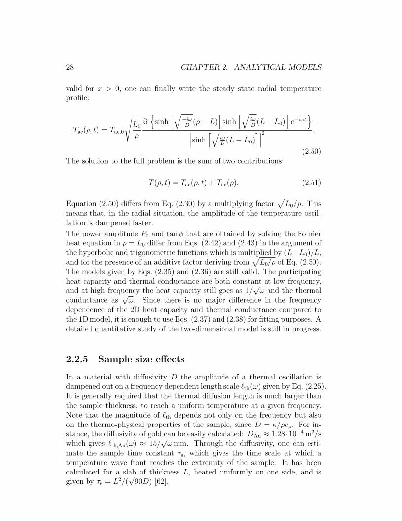
Figure 2.10: Differential scheme where one calorimetric cell hosts the sample whilethe other acts as reference.
2.2.6 Differential mode
In the differential scheme two calorimetric cells are used, as illustrated inFig. 2.10. One with the sample material on it and the other with or withouta reference sample. To practically perform differential measurements thesame power PS = PR = P0 is applied to sample and reference side, and theresulting temperature difference Tdiff is recorded. The heat capacity of thereference side Cr+0 is given by Eq. (2.19):
Cr+0 =P0
Tac,rωsinφr. (2.52)
The subscript r+0, added for clarity reasons, corresponds to the sum of areference sample and platform. Supposing to work in the optimal frequencyrange, i. e., ω such that ωτi 1, and τi τe, the sample side heat capacityis also given by Eq. (2.19),
Cs+0 =P0
Tac,0ωsinφ0. (2.53)
The subscript s+0 corresponds to the sum of the sample and platform. Theheat capacity sensed by the differential signal is the difference between theheat capacity of sample and reference sides:
Cdiff = Cs+0 − Cr+0 =P0
Tac,0Tac,rω(Tac,r sinφ0 − Tac,0 sinφr) (2.54)
Using the simplified Eq. (2.24), which is allowed when working in the optimalfrequency range, we have Tac,r = P0/Ke cosφr and Tac,0 = P0/Ke cosφ0.Using the definition of Tdc, Eq. (2.54) becomes
Cdiff =P0Tdc
ωTac,0Tac,r
(cosφr sinφ0 − sinφr cosφ0). (2.55)
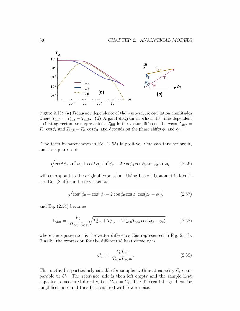
30 CHAPTER 2. ANALYTICAL MODELS
Figure 2.11: (a) Frequency dependence of the temperature oscillation amplitudeswhere Tdiff = Tac,r − Tac,0. (b) Argand diagram in which the time dependentoscillating vectors are represented. Tdiff is the vector difference between Tac,r =Tdc cosφr and Tac,0 = Tdc cosφ0, and depends on the phase shifts φr and φ0.
The term in parentheses in Eq. (2.55) is positive. One can thus square it,and its square root√
cos2 φr sin2 φ0 + cos2 φ0 sin2 φr − 2 cosφ0 cosφr sinφ0 sinφr (2.56)
will correspond to the original expression. Using basic trigonometric identi-ties Eq. (2.56) can be rewritten as√
cos2 φ0 + cos2 φr − 2 cosφ0 cosφr cos(φ0 − φr), (2.57)
and Eq. (2.54) becomes
Cdiff =P0
ωTac,0Tac,r
√T 2
ac,0 + T 2ac,r − 2Tac,0Tac,r cos(φ0 − φr), (2.58)
where the square root is the vector difference Tdiff represented in Fig. 2.11b.Finally, the expression for the differential heat capacity is
Cdiff =P0Tdiff
Tac,0Tac,rω. (2.59)
This method is particularly suitable for samples with heat capacity Cs com-parable to C0. The reference side is then left empty and the sample heatcapacity is measured directly, i.e., Cdiff = Cs. The differential signal can beamplified more and thus be measured with lower noise.
2.3. THERMAL RELAXATION METHOD 31
2.3 Thermal relaxation method
2.3.1 Overview
The thermal relaxation method was introduced by Bachmann et al. [45] in1972. It consists of applying a known power to the heater to raise the sampletemperature an amount ∆T above the frame temperature Tb. When a steadystate condition is reached the heater power is turned off and the temperaturewill drop back to Tb. Both temperature raise (TR) and fall (TF) are governedby an exponential law, which depends on the external time constant of thesystem:
TR(t) = Tb + ∆T (1− e−t/τe,R), (2.60a)
TF(t) = Tb + ∆Te−t/τe,F . (2.60b)
If the heat capacity and other material parameters can be assumed constantwithin ∆T , the raise and fall time constants, respectively τe,R and τe,F, shouldcoincide. The sample and platform are connected to each other and to thethermal bath as shown in Fig. 2.2. Equations (2.60) are valid if the thermalconductance of the heat leak Ke is small compared to that between sampleand platform Ki. When this condition is no longer met, both the external andinternal time constants, τe and τi, should be included in the equations. Thisproblem, known as lumped effect, has been addressed and solved by Shep-herd in 1985 [77], and Brando in 2009 [78], for systems thermally describedby Eqs. (2.4), under the assumption that the thermal contact between thesample and the platform is good but not ideal (finite values of Ki), while theinternal thermal conductivity of both the platform and sample are consideredinfinite. If at time t = 0, the applied power P (t) = P0 is turned to zero, theplatform temperature decay can be represented by a curve consisting of thesum of two exponentials with different time constants τ1 and τ2:
T0(t) = Tb + ∆T (a1e−t/τ1 + a2e
−t/τ2) (2.61)
where
a1 =τe − τ2
τ1 − τ2
, a2 =τ1 − τe
τ1 − τ2
(2.62)
and a1 + a2 = 1.The time constants τ1 and τ2 are given by (after [77])
τ1 =τe + τi
2
[1 +
√1− 4τiτe,0
(τe + τi)2
], (2.63a)
τ2 =τe + τi
2
[1−
√1− 4τiτe,0
(τe + τi)2
], (2.63b)
32 CHAPTER 2. ANALYTICAL MODELS
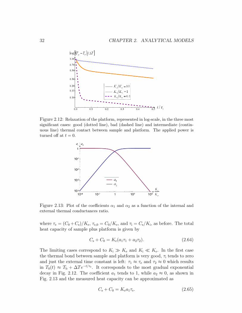
Figure 2.12: Relaxation of the platform, represented in log-scale, in the three mostsignificant cases: good (dotted line), bad (dashed line) and intermediate (contin-uous line) thermal contact between sample and platform. The applied power isturned off at t = 0.
Figure 2.13: Plot of the coefficients α1 and α2 as a function of the internal andexternal thermal conductances ratio.
where τe = (C0 +Cs)/Ke, τe,0 = C0/Ke, and τi = Cs/Ki, as before. The totalheat capacity of sample plus platform is given by
Cs + C0 = Ke(a1τ1 + a2τ2). (2.64)
The limiting cases correspond to Ki Ke and Ki Ke. In the first casethe thermal bond between sample and platform is very good, τi tends to zeroand just the external time constant is left: τ1 ≈ τe and τ2 ≈ 0 which resultsin T0(t) ≈ Tb + ∆Te−t/τe . It corresponds to the most gradual exponentialdecay in Fig. 2.12. The coefficient a1 tends to 1, while a2 ≈ 0, as shown inFig. 2.13 and the measured heat capacity can be approximated as
Cs + C0 = Kea1τe. (2.65)
2.3. THERMAL RELAXATION METHOD 33
If instead the thermal bond between sample and platform is poor, the systembehaves as if the sample was not there and the only time constant left is τe,0:τ1 ≈ ∞ and τ2 ≈ τe,0 which results in T0(t) ≈ Tb + ∆Te−t/τe,0 (steepestexponential decay in Fig. 2.12). The coefficient a2 tends to 1 and a1 ≈ 0(Fig. 2.13), and the measured heat capacity is approximated as
C0 = Kea1τe,0. (2.66)

34 CHAPTER 2. ANALYTICAL MODELS
Chapter 3
Device fabrication
3.1 Layout of the device
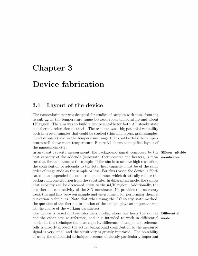
The nanocalorimeter was designed for studies of samples with mass from mgto sub-µg in the temperature range between room temperature and about1 K region. The aim was to build a device suitable for both AC steady stateand thermal relaxation methods. The result shows a big potential versatilityboth in type of samples that could be studied (thin film layers, grain samples,liquid droplets) and in the temperature range that could extend to temper-atures well above room temperature. Figure 3.1 shows a simplified layout ofthe nanocalorimeter.
In any heat capacity measurement, the background signal, composed by the Silicon nitridemembranesheat capacity of the addenda (substrate, thermometer and heater), is mea-
sured at the same time as the sample. If the aim is to achieve high resolution,the contribution of addenda to the total heat capacity must be of the sameorder of magnitude as the sample or less. For this reason the device is fabri-cated onto suspended silicon nitride membranes which drastically reduce thebackground contribution from the substrate. In differential mode, the sampleheat capacity can be decreased down to the nJ/K region. Additionally, thelow thermal conductivity of the SiN membrane [79] provides the necessaryweak thermal link between sample and environment for performing thermalrelaxation techniques. Note that when using the AC steady state method,the question of the thermal insulation of the sample plays an important rolefor the choice of the working parameters.
The device is based on two calorimetric cells, where one hosts the sample Differentialmodeand the other acts as reference, and it is intended to work in differential
mode. In this technique the heat capacity difference of sample and referencecells is directly probed; the actual background contribution to the measuredsignal is very small and the sensitivity is greatly improved. The possibilityof using the differential technique becomes obviously particularly important
35
36 CHAPTER 3. DEVICE FABRICATION
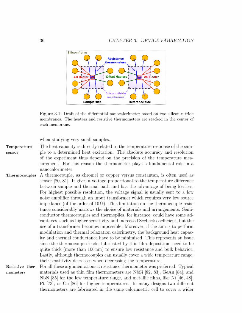
Figure 3.1: Draft of the differential nanocalorimeter based on two silicon nitridemembranes. The heaters and resistive thermometers are stacked in the center ofeach membrane.
when studying very small samples.
The heat capacity is directly related to the temperature response of the sam-Temperaturesensor ple to a determined heat excitation. The absolute accuracy and resolution
of the experiment thus depend on the precision of the temperature mea-surement. For this reason the thermometer plays a fundamental role in ananocalorimeter.A thermocouple, as chromel or copper versus constantan, is often used asThermocouplessensor [80, 81]. It gives a voltage proportional to the temperature differencebetween sample and thermal bath and has the advantage of being lossless.For highest possible resolution, the voltage signal is usually sent to a lownoise amplifier through an input transformer which requires very low sourceimpedance (of the order of 10 Ω). This limitation on the thermocouple resis-tance considerably narrows the choice of materials and arrangements. Semi-conductor thermocouples and thermopiles, for instance, could have some ad-vantages, such as higher sensitivity and increased Seebeck coefficient, but theuse of a transformer becomes impossible. Moreover, if the aim is to performmodulation and thermal relaxation calorimetry, the background heat capac-ity and thermal conductance have to be minimized. This represents an issuesince the thermocouple leads, fabricated by thin film deposition, need to bequite thick (more than 100 nm) to ensure low resistance and bulk behavior.Lastly, although thermocouples can usually cover a wide temperature range,their sensitivity decreases when decreasing the temperature.For all these argumentations a resistance thermometer was preferred. TypicalResistive ther-
mometers materials used as thin film thermometers are NbSi [82, 83], GeAu [84], andNbN [85] for the low temperature range, and metallic films, like Ni [46, 48],Pt [73], or Cu [86] for higher temperatures. In many designs two differentthermometers are fabricated in the same calorimetric cell to cover a wider
3.1. LAYOUT OF THE DEVICE 37
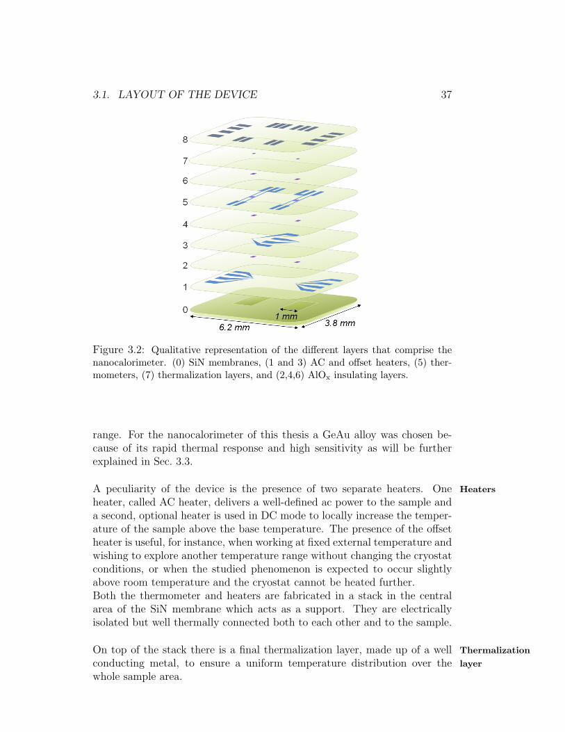
Figure 3.2: Qualitative representation of the different layers that comprise thenanocalorimeter. (0) SiN membranes, (1 and 3) AC and offset heaters, (5) ther-mometers, (7) thermalization layers, and (2,4,6) AlOx insulating layers.
range. For the nanocalorimeter of this thesis a GeAu alloy was chosen be-cause of its rapid thermal response and high sensitivity as will be furtherexplained in Sec. 3.3.
A peculiarity of the device is the presence of two separate heaters. One Heatersheater, called AC heater, delivers a well-defined ac power to the sample anda second, optional heater is used in DC mode to locally increase the temper-ature of the sample above the base temperature. The presence of the offsetheater is useful, for instance, when working at fixed external temperature andwishing to explore another temperature range without changing the cryostatconditions, or when the studied phenomenon is expected to occur slightlyabove room temperature and the cryostat cannot be heated further.Both the thermometer and heaters are fabricated in a stack in the centralarea of the SiN membrane which acts as a support. They are electricallyisolated but well thermally connected both to each other and to the sample.
On top of the stack there is a final thermalization layer, made up of a well Thermalizationlayerconducting metal, to ensure a uniform temperature distribution over the
whole sample area.
38 CHAPTER 3. DEVICE FABRICATION
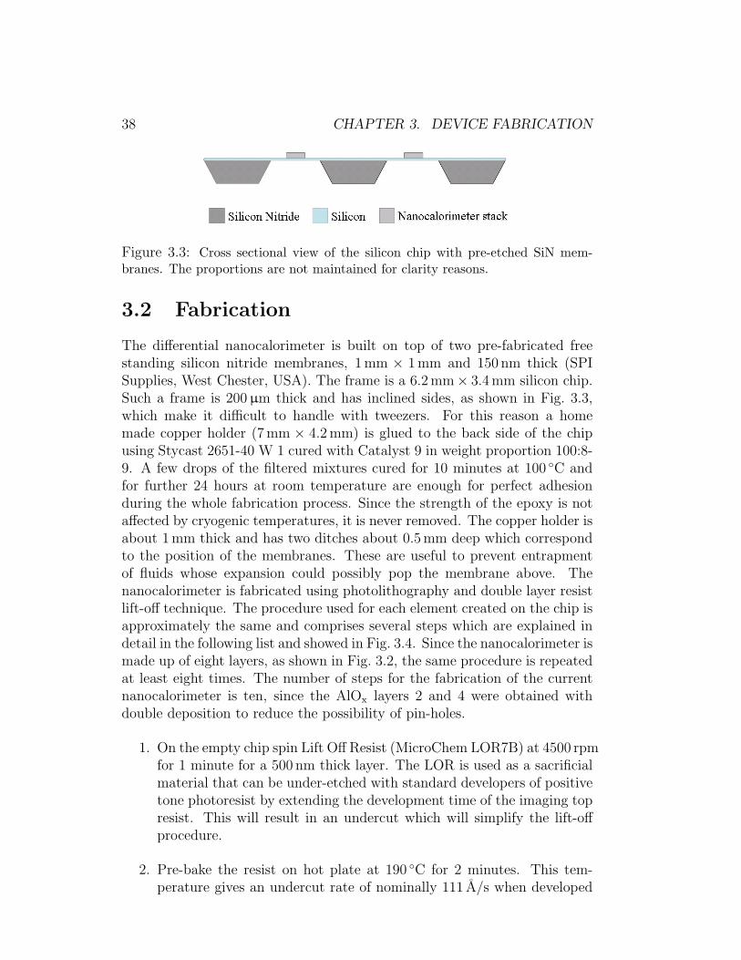
Figure 3.3: Cross sectional view of the silicon chip with pre-etched SiN mem-branes. The proportions are not maintained for clarity reasons.
3.2 Fabrication
The differential nanocalorimeter is built on top of two pre-fabricated freestanding silicon nitride membranes, 1 mm × 1 mm and 150 nm thick (SPISupplies, West Chester, USA). The frame is a 6.2 mm× 3.4 mm silicon chip.Such a frame is 200 µm thick and has inclined sides, as shown in Fig. 3.3,which make it difficult to handle with tweezers. For this reason a homemade copper holder (7 mm × 4.2 mm) is glued to the back side of the chipusing Stycast 2651-40 W 1 cured with Catalyst 9 in weight proportion 100:8-9. A few drops of the filtered mixtures cured for 10 minutes at 100 C andfor further 24 hours at room temperature are enough for perfect adhesionduring the whole fabrication process. Since the strength of the epoxy is notaffected by cryogenic temperatures, it is never removed. The copper holder isabout 1 mm thick and has two ditches about 0.5 mm deep which correspondto the position of the membranes. These are useful to prevent entrapmentof fluids whose expansion could possibly pop the membrane above. Thenanocalorimeter is fabricated using photolithography and double layer resistlift-off technique. The procedure used for each element created on the chip isapproximately the same and comprises several steps which are explained indetail in the following list and showed in Fig. 3.4. Since the nanocalorimeter ismade up of eight layers, as shown in Fig. 3.2, the same procedure is repeatedat least eight times. The number of steps for the fabrication of the currentnanocalorimeter is ten, since the AlOx layers 2 and 4 were obtained withdouble deposition to reduce the possibility of pin-holes.
1. On the empty chip spin Lift Off Resist (MicroChem LOR7B) at 4500 rpmfor 1 minute for a 500 nm thick layer. The LOR is used as a sacrificialmaterial that can be under-etched with standard developers of positivetone photoresist by extending the development time of the imaging topresist. This will result in an undercut which will simplify the lift-offprocedure.
2. Pre-bake the resist on hot plate at 190 C for 2 minutes. This tem-perature gives an undercut rate of nominally 111 A/s when developed
3.2. FABRICATION 39
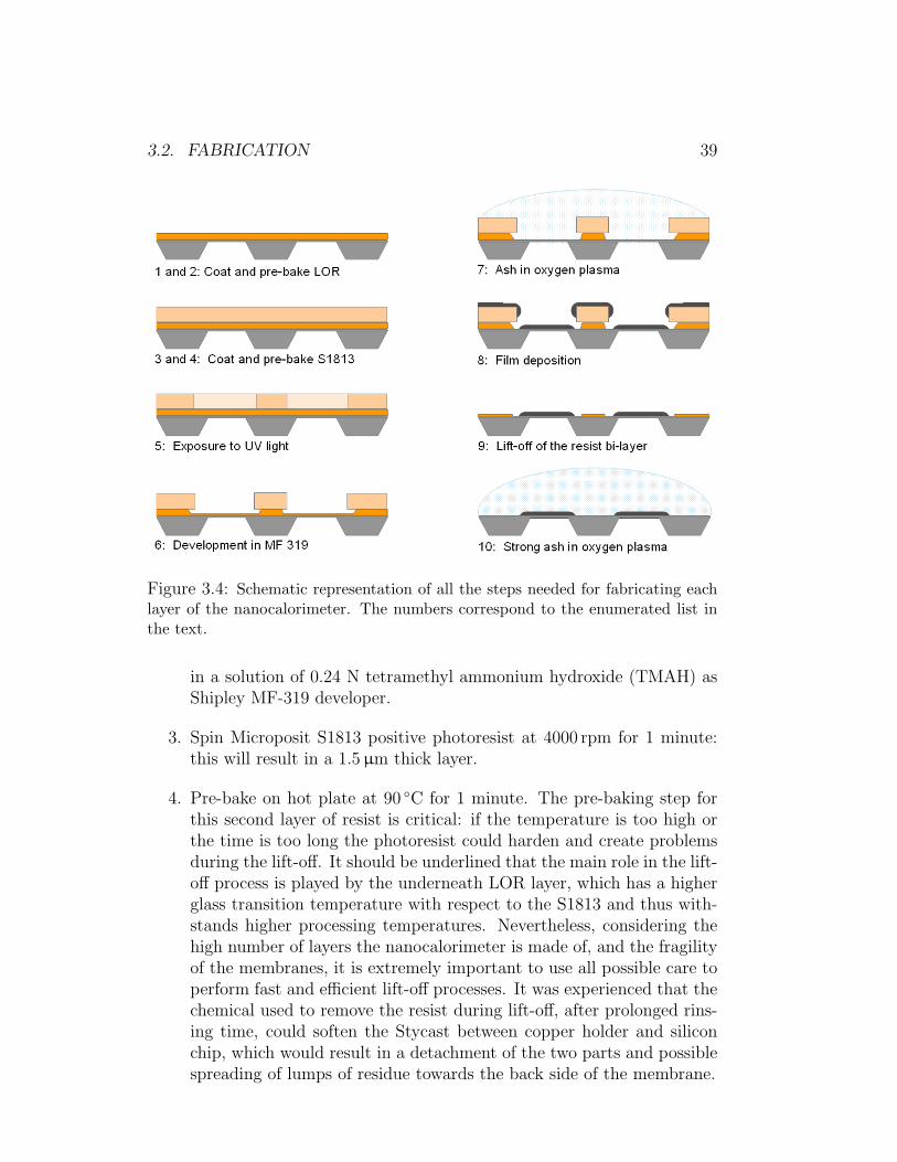
Figure 3.4: Schematic representation of all the steps needed for fabricating eachlayer of the nanocalorimeter. The numbers correspond to the enumerated list inthe text.
in a solution of 0.24 N tetramethyl ammonium hydroxide (TMAH) asShipley MF-319 developer.
3. Spin Microposit S1813 positive photoresist at 4000 rpm for 1 minute:this will result in a 1.5 µm thick layer.
4. Pre-bake on hot plate at 90 C for 1 minute. The pre-baking step forthis second layer of resist is critical: if the temperature is too high orthe time is too long the photoresist could harden and create problemsduring the lift-off. It should be underlined that the main role in the lift-off process is played by the underneath LOR layer, which has a higherglass transition temperature with respect to the S1813 and thus with-stands higher processing temperatures. Nevertheless, considering thehigh number of layers the nanocalorimeter is made of, and the fragilityof the membranes, it is extremely important to use all possible care toperform fast and efficient lift-off processes. It was experienced that thechemical used to remove the resist during lift-off, after prolonged rins-ing time, could soften the Stycast between copper holder and siliconchip, which would result in a detachment of the two parts and possiblespreading of lumps of residue towards the back side of the membrane.
40 CHAPTER 3. DEVICE FABRICATION
5. UV light exposure using a projection printing system to transfer thewanted pattern from a chromium-quartz glass photomask to the resist.
6. Development of the exposed pattern: rinse in Shipley MF-319 developerfor about 50 s and remove the chemical with deionized water. Theundercut should be at least 1 µm. It is a good rule to check the resultunder an optical microscope furnished with yellow light in order notto unintentionally expose the resist. In this way, if the undercut is notgood enough, it is possible to further develop the resist.
7. It could happen that the areas where the photoresist was developed arenot completely clean and a very thin film of polymer with a thicknessof the order of nm adherent to the substrate and invisible to the eyes,could still be present. Reactive Ion Etching (RIE) plasma with oxygenis utilized in order to oxidize (ash) photoresist and facilitate its removal.The parameters used are: 10 W RF (Radio Frequency) bias, 50 W ICP(Inductively Coupled Plasma), O2 at 20 sccm flow rate, at a pressureof 100 mTorr for an etching rate of about 0.6 nm/s and 0.5 nm/s for theLOR7B and S1813 respectively. The typical etching time is about 5minutes. The RF electromagnetic field is kept low so that the impingingions are not too energetic. When the impinging ions are too energetic,the energy transferred to the resist could hard-bake it. The relativelylow RF power is inductively coupled (ICP) in order to increase thedensity of ions and still have a high etch rate.
8. Film deposition. The materials constituting each layer are depositedeither with electron beam evaporation or sputtering. For the materialsdeposited through e-beam evaporation one needs to keep under con-trol power used and deposition time in order to limit the heating ofthe substrate. The main reasons for the substrate heating is the ther-mal radiation emitted by the glowing crucible and filament, and thecondensation energy of the particles. In the plasma sputtering, it wasexperienced that 100 W RF power is about the upper limit above whichthe particles become too energetic. The temperature sensor, made ofGeAu, is the only film deposited with RF sputtering technique. Anargon plasma is kept at the stable pressure of 3 mTorr and 25 sccm flowrate, and using 90 W RF power a rate of 6.6 A/s is obtained. One prac-tical issue regarding the clamping of the chips to the sample holder ofthe sputtering machine was overcome using crystal bond which is solidat room temperature and melts at about 100 C.
9. Lift off in a bath of Microposit Remover 1165 warmed up to 60 C andrinse in DI water to remove completely the chemical. The lift-off step is
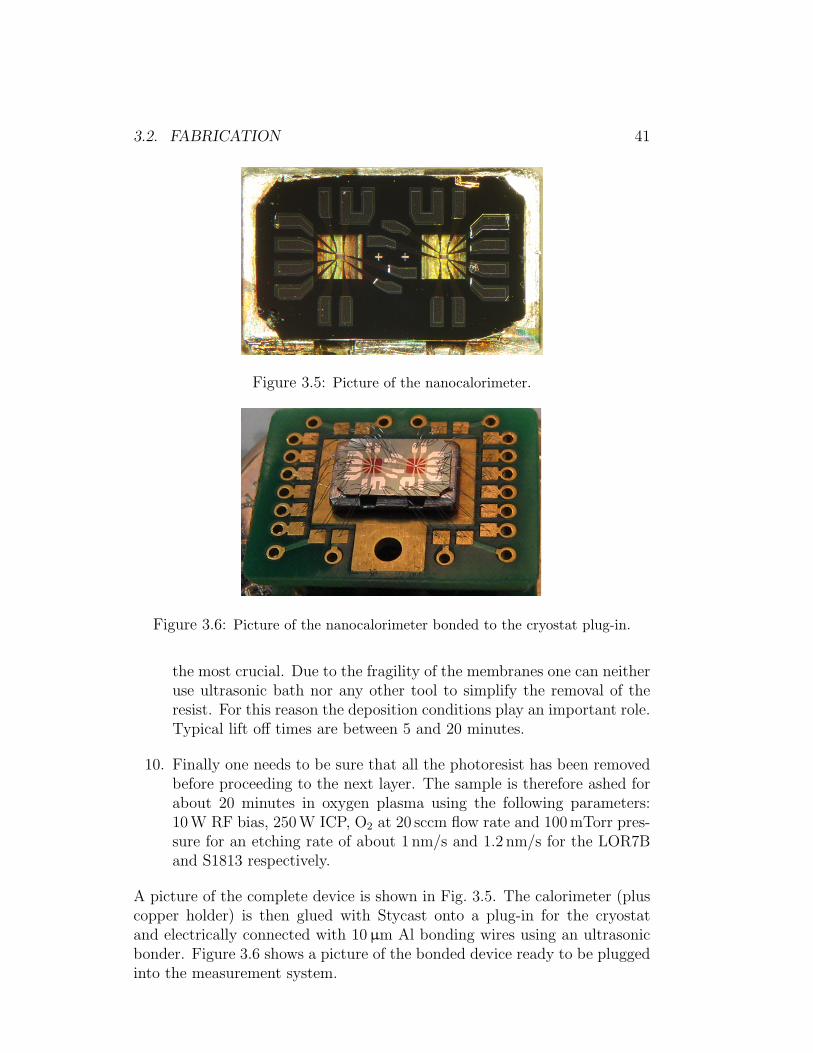
3.2. FABRICATION 41
Figure 3.5: Picture of the nanocalorimeter.
Figure 3.6: Picture of the nanocalorimeter bonded to the cryostat plug-in.
the most crucial. Due to the fragility of the membranes one can neitheruse ultrasonic bath nor any other tool to simplify the removal of theresist. For this reason the deposition conditions play an important role.Typical lift off times are between 5 and 20 minutes.
10. Finally one needs to be sure that all the photoresist has been removedbefore proceeding to the next layer. The sample is therefore ashed forabout 20 minutes in oxygen plasma using the following parameters:10 W RF bias, 250 W ICP, O2 at 20 sccm flow rate and 100 mTorr pres-sure for an etching rate of about 1 nm/s and 1.2 nm/s for the LOR7Band S1813 respectively.
A picture of the complete device is shown in Fig. 3.5. The calorimeter (pluscopper holder) is then glued with Stycast onto a plug-in for the cryostatand electrically connected with 10 µm Al bonding wires using an ultrasonicbonder. Figure 3.6 shows a picture of the bonded device ready to be pluggedinto the measurement system.
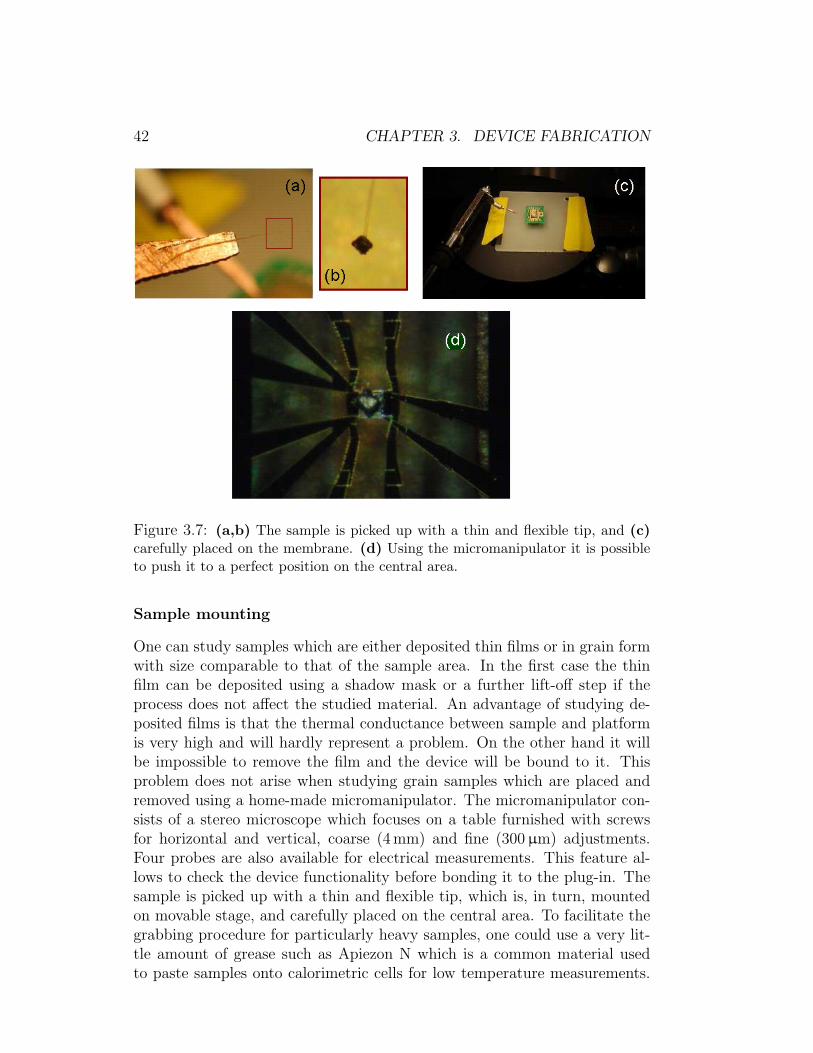
42 CHAPTER 3. DEVICE FABRICATION
Figure 3.7: (a,b) The sample is picked up with a thin and flexible tip, and (c)carefully placed on the membrane. (d) Using the micromanipulator it is possibleto push it to a perfect position on the central area.
Sample mounting
One can study samples which are either deposited thin films or in grain formwith size comparable to that of the sample area. In the first case the thinfilm can be deposited using a shadow mask or a further lift-off step if theprocess does not affect the studied material. An advantage of studying de-posited films is that the thermal conductance between sample and platformis very high and will hardly represent a problem. On the other hand it willbe impossible to remove the film and the device will be bound to it. Thisproblem does not arise when studying grain samples which are placed andremoved using a home-made micromanipulator. The micromanipulator con-sists of a stereo microscope which focuses on a table furnished with screwsfor horizontal and vertical, coarse (4 mm) and fine (300 µm) adjustments.Four probes are also available for electrical measurements. This feature al-lows to check the device functionality before bonding it to the plug-in. Thesample is picked up with a thin and flexible tip, which is, in turn, mountedon movable stage, and carefully placed on the central area. To facilitate thegrabbing procedure for particularly heavy samples, one could use a very lit-tle amount of grease such as Apiezon N which is a common material usedto paste samples onto calorimetric cells for low temperature measurements.
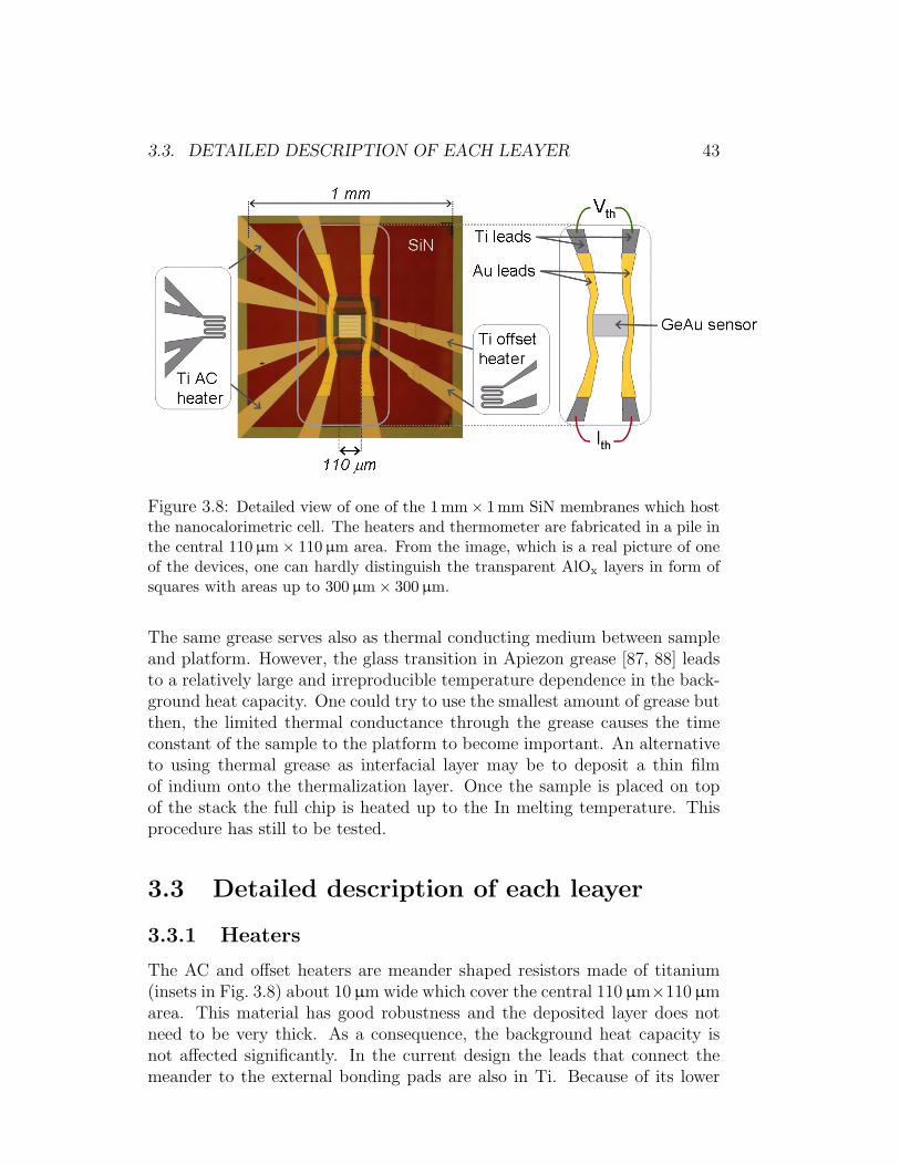
3.3. DETAILED DESCRIPTION OF EACH LEAYER 43
Figure 3.8: Detailed view of one of the 1 mm× 1 mm SiN membranes which hostthe nanocalorimetric cell. The heaters and thermometer are fabricated in a pile inthe central 110 µm× 110 µm area. From the image, which is a real picture of oneof the devices, one can hardly distinguish the transparent AlOx layers in form ofsquares with areas up to 300 µm× 300 µm.
The same grease serves also as thermal conducting medium between sampleand platform. However, the glass transition in Apiezon grease [87, 88] leadsto a relatively large and irreproducible temperature dependence in the back-ground heat capacity. One could try to use the smallest amount of grease butthen, the limited thermal conductance through the grease causes the timeconstant of the sample to the platform to become important. An alternativeto using thermal grease as interfacial layer may be to deposit a thin filmof indium onto the thermalization layer. Once the sample is placed on topof the stack the full chip is heated up to the In melting temperature. Thisprocedure has still to be tested.
3.3 Detailed description of each leayer
3.3.1 Heaters
The AC and offset heaters are meander shaped resistors made of titanium(insets in Fig. 3.8) about 10 µm wide which cover the central 110 µm×110 µmarea. This material has good robustness and the deposited layer does notneed to be very thick. As a consequence, the background heat capacity isnot affected significantly. In the current design the leads that connect themeander to the external bonding pads are also in Ti. Because of its lower
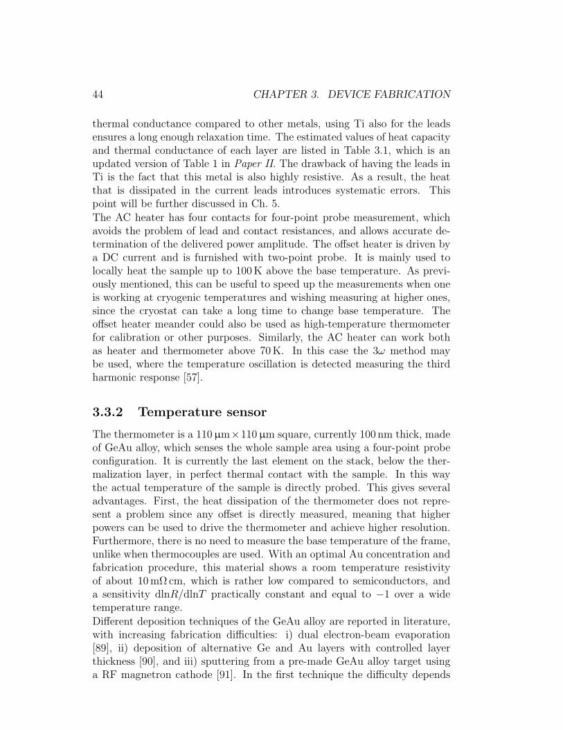
44 CHAPTER 3. DEVICE FABRICATION
thermal conductance compared to other metals, using Ti also for the leadsensures a long enough relaxation time. The estimated values of heat capacityand thermal conductance of each layer are listed in Table 3.1, which is anupdated version of Table 1 in Paper II. The drawback of having the leads inTi is the fact that this metal is also highly resistive. As a result, the heatthat is dissipated in the current leads introduces systematic errors. Thispoint will be further discussed in Ch. 5.
The AC heater has four contacts for four-point probe measurement, whichavoids the problem of lead and contact resistances, and allows accurate de-termination of the delivered power amplitude. The offset heater is driven bya DC current and is furnished with two-point probe. It is mainly used tolocally heat the sample up to 100 K above the base temperature. As previ-ously mentioned, this can be useful to speed up the measurements when oneis working at cryogenic temperatures and wishing measuring at higher ones,since the cryostat can take a long time to change base temperature. Theoffset heater meander could also be used as high-temperature thermometerfor calibration or other purposes. Similarly, the AC heater can work bothas heater and thermometer above 70 K. In this case the 3ω method maybe used, where the temperature oscillation is detected measuring the thirdharmonic response [57].
3.3.2 Temperature sensor
The thermometer is a 110 µm×110 µm square, currently 100 nm thick, madeof GeAu alloy, which senses the whole sample area using a four-point probeconfiguration. It is currently the last element on the stack, below the ther-malization layer, in perfect thermal contact with the sample. In this waythe actual temperature of the sample is directly probed. This gives severaladvantages. First, the heat dissipation of the thermometer does not repre-sent a problem since any offset is directly measured, meaning that higherpowers can be used to drive the thermometer and achieve higher resolution.Furthermore, there is no need to measure the base temperature of the frame,unlike when thermocouples are used. With an optimal Au concentration andfabrication procedure, this material shows a room temperature resistivityof about 10 mΩ cm, which is rather low compared to semiconductors, anda sensitivity dlnR/dlnT practically constant and equal to −1 over a widetemperature range.
Different deposition techniques of the GeAu alloy are reported in literature,with increasing fabrication difficulties: i) dual electron-beam evaporation[89], ii) deposition of alternative Ge and Au layers with controlled layerthickness [90], and iii) sputtering from a pre-made GeAu alloy target usinga RF magnetron cathode [91]. In the first technique the difficulty depends
3.3. DETAILED DESCRIPTION OF EACH LEAYER 45
on the uncertainty on the Au concentration during the evaporation, due todiffering evaporation rates for Au and Ge. This problem is overcome withthe second listed technique which relies on the fact that the Au atoms diffusein Ge at and above room temperature and the diffusion depends on theAu layer thickness. The third method uses a sputtering target with a fixedAu concentration which makes the final concentration of the deposited layermuch more predictable at the expense of less freedom in the choice of therelative ratios between Ge and Au concentration. This last method was theone chosen for fabricating the temperature sensor on the nanocalorimeter.The target used is a 2 inches diameter of cast GeAu alloy with 17 at% Au.The resistivity of the GeAu alloy shows a power law temperature dependence
ρ
ρ∗=
(T
T ∗
)η, (3.1)
where η = dlnρ/dlnT is the relative sensitivity of the thermometer which, inour case, is nearly −1 over a wide temperature range, and ρ∗ and T ∗ are ex-perimentally determined constants. The power law in Eq. (3.1) is explainedin terms of hopping conductivity in disordered systems in the region of ametal insulator transition [92].The most important parameters which characterize the thermometer are thesensitivity η and the room temperature resistivity ρRT . Both parameters de-pend on Au concentration, annealing temperature and annealing duration.When the thin film is first deposited it is in its amorphous state. With-out any annealing the resistivity at low temperatures is almost temperatureindependent. The existing bond between Au and Ge are metastable withrespect to thermal annealing and makes the material very sensitive to fur-ther processing. For a certain Au concentration, there is a specific annealingtemperature at and above which a process known as metal-assisted crys-tallization takes place. It was experimentally determined that the criticaltemperature drops from 330 C to 130 C as the Au concentration increasesfrom x = 0.04 to x = 0.22 [93]. During this process the bonding between Auand Ge is weakened or broken and Ge crystallizes. Because of the low solidsolubility of Au in crystalline Ge at these temperatures, the metal atoms aresqueezed out and confined to the polycristalline Ge grain boundaries. Themass transport stops once the crystallization is finished. According to formerobservations [94], the onset temperature for metal-assisted crystallization forour case is around 135 C, above which ρRT tends to stabilize. One has to finda compromise between annealing temperature and time that gives the high-est reproducibility and stability of the sensitivity, and room temperatureresistivity. The temperature sensors fabricated in the nanocalorimeter areannealed at 190 C on hotplate for 1 hour which resulted in ρRT ≈ 9 mΩcmand η ≈ −1 in the temperature range 5 K < T < 300 K, and increasing to
46 CHAPTER 3. DEVICE FABRICATION
Figure 3.9: Experimental data which show the progressive reduction of the tunnelbarrier between Ti and GeAu after several annealing procedures. The curvaturesof the red and green curves at the lowest temperatures are due to excessive selfheating.
η ≈ −2 down to 300 mK. After several months and several cooling downsρRT and η did not show any appreciable deviations.
As shown in the rightmost inset of Fig. 3.8, the GeAu square is deposited onAu/Ti leadstop of Au leads which extend roughly 300 µm out from the center where theyconnect with the external Ti leads. The main reason for this choice is thatthe surface of titanium naturally forms a thin titanium dioxide layer when incontact with air. This oxide creates a tunnel barrier between the leads andthe thermometer causing overheating in the contact areas with consequentnon-uniform distribution of the temperature. It was experienced that anneal-ing for several hours reduces this barrier effect, as shown in Fig. 3.9. Sincethis procedure is not well controlled it was preferred to avoid any barrier.Besides the mere reason to avoid a problem, combining Au and Ti gives amore defined isothermal area as shown from simulations in Ch. 5. It shouldbe emphasized that the design of the four-point probe for the thermometer isnot as a regular one, in the sense that the current and voltage leads overlap ina contact area over the GeAu sensor. For this reason the measurement picksup the barrier effect resulting in an uncontrollable temperature dependenceof the measured resistance.
3.3.3 Insulation layers
Each metallic layer is electrically insulated by aluminum oxide. Among otheroxides it shows good electric insulator properties and not too low thermalconductance so that the heat flow between layers is not affected appreciably.Additionally it is easy and fast to deposit (rate of about 2 A/s for e-beam
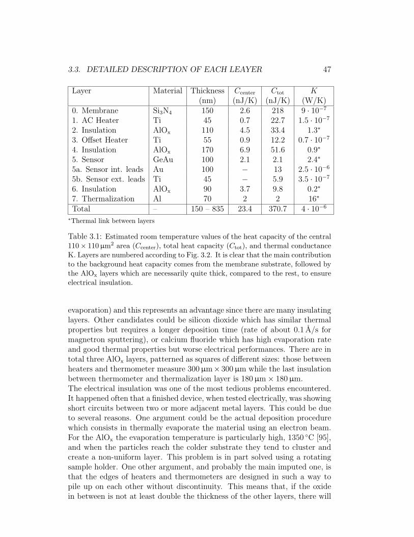
3.3. DETAILED DESCRIPTION OF EACH LEAYER 47
Layer Material Thickness Ccenter Ctot K(nm) (nJ/K) (nJ/K) (W/K)
0. Membrane Si3N4 150 2.6 218 9 · 10−7
1. AC Heater Ti 45 0.7 22.7 1.5 · 10−7
2. Insulation AlOx 110 4.5 33.4 1.3∗
3. Offset Heater Ti 55 0.9 12.2 0.7 · 10−7
4. Insulation AlOx 170 6.9 51.6 0.9∗
5. Sensor GeAu 100 2.1 2.1 2.4∗
5a. Sensor int. leads Au 100 − 13 2.5 · 10−6
5b. Sensor ext. leads Ti 45 − 5.9 3.5 · 10−7
6. Insulation AlOx 90 3.7 9.8 0.2∗
7. Thermalization Al 70 2 2 16∗
Total – 150 – 835 23.4 370.7 4 · 10−6
∗Thermal link between layers
Table 3.1: Estimated room temperature values of the heat capacity of the central110× 110 µm2 area (Ccenter), total heat capacity (Ctot), and thermal conductanceK. Layers are numbered according to Fig. 3.2. It is clear that the main contributionto the background heat capacity comes from the membrane substrate, followed bythe AlOx layers which are necessarily quite thick, compared to the rest, to ensureelectrical insulation.
evaporation) and this represents an advantage since there are many insulatinglayers. Other candidates could be silicon dioxide which has similar thermalproperties but requires a longer deposition time (rate of about 0.1 A/s formagnetron sputtering), or calcium fluoride which has high evaporation rateand good thermal properties but worse electrical performances. There are intotal three AlOx layers, patterned as squares of different sizes: those betweenheaters and thermometer measure 300 µm× 300 µm while the last insulationbetween thermometer and thermalization layer is 180 µm× 180 µm.The electrical insulation was one of the most tedious problems encountered.It happened often that a finished device, when tested electrically, was showingshort circuits between two or more adjacent metal layers. This could be dueto several reasons. One argument could be the actual deposition procedurewhich consists in thermally evaporate the material using an electron beam.For the AlOx the evaporation temperature is particularly high, 1350 C [95],and when the particles reach the colder substrate they tend to cluster andcreate a non-uniform layer. This problem is in part solved using a rotatingsample holder. One other argument, and probably the main imputed one, isthat the edges of heaters and thermometers are designed in such a way topile up on each other without discontinuity. This means that, if the oxidein between is not at least double the thickness of the other layers, there will
48 CHAPTER 3. DEVICE FABRICATION
be open paths on the sides. Until now both these problems were solved bydepositing thick layers of AlOx in two different lift-off steps. For the futurethe masks have been redesigned to reduce the probability of side pin-holes.
3.3.4 Thermalization layer
As last element of the stack, a 110 µm×110 µm of a highly conductive mate-rial is deposited. In the current devices the material chosen was aluminum,with a thickness of about 60 nm. This layer is needed to evenly distribute thetemperature over the sample area. Aluminum is a good choice only above itssuperconducting transition at 1.2 K. For lower temperatures, other materialssuch as gold, copper or silver have to be used. This may need an additionalstep in the fabrication process.
Chapter 4
Measurements andcharacterization
4.1 Measurement system
4.1.1 Cryostat overview
All the measurements were carried out using a cryogen free system based onclosed cycle refrigeration. The plug-in which hosts the sample is mounted atthe bottom of a sample holder that is inserted into the cryostat. A schematicof the system is shown in Fig. 4.1. The calorimetric measurements must bedone in vacuum since any presence of gas adds an unknown thermal linkwith a drastic decrease of the relaxation time of the device, uncertainty onthe real thermal conductance and loss of absolute accuracy as a result. Forthis reason there is an inner vacuum chamber which is connected to a turbopump. The walls of the sample holder are in contact with the chamber wallswhich, in turn, are in contact with the 4He gas. The lowest temperaturereached by the sample in vacuum is about 30 K that can be decreased toabout 2 K when exchange gas is used. When exchange gas is inserted, it isconvenient to use a nitrogen trap to avoid condensation of impurities whichwould degas at about 40-60 K disturbing the measurements. The system isalso equipped with a 17 T superconducting magnet kept at 3 K. To determinethe magnetic field a Hall probe is installed next to the sample on a stage ableto rotate 300 deg.
4.1.2 Electronic setup
In the standard measurement mode, known AC and DC currents flow throughthe heaters and thermometers. In order to reduce pick-up of electromagneticnoise, the heaters and thermometers are bonded in such a way that each
49
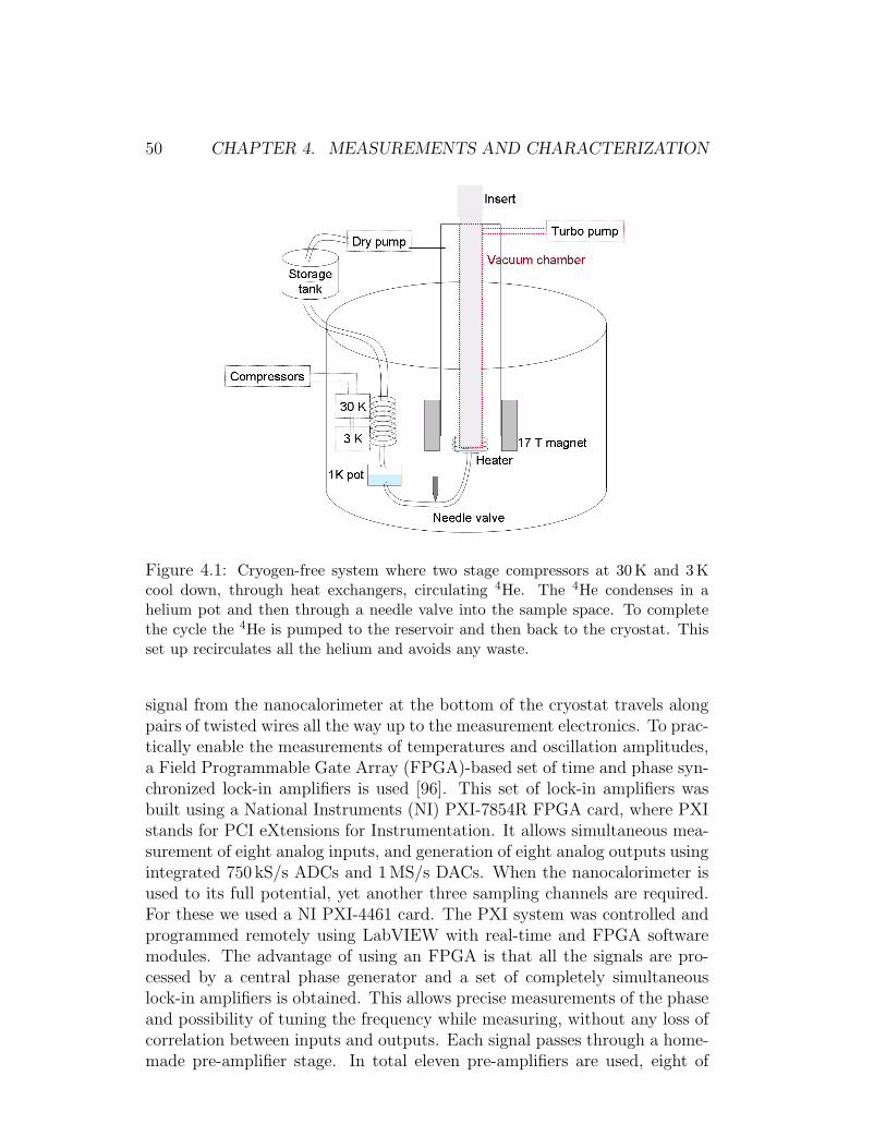
50 CHAPTER 4. MEASUREMENTS AND CHARACTERIZATION
Figure 4.1: Cryogen-free system where two stage compressors at 30 K and 3 Kcool down, through heat exchangers, circulating 4He. The 4He condenses in ahelium pot and then through a needle valve into the sample space. To completethe cycle the 4He is pumped to the reservoir and then back to the cryostat. Thisset up recirculates all the helium and avoids any waste.
signal from the nanocalorimeter at the bottom of the cryostat travels alongpairs of twisted wires all the way up to the measurement electronics. To prac-tically enable the measurements of temperatures and oscillation amplitudes,a Field Programmable Gate Array (FPGA)-based set of time and phase syn-chronized lock-in amplifiers is used [96]. This set of lock-in amplifiers wasbuilt using a National Instruments (NI) PXI-7854R FPGA card, where PXIstands for PCI eXtensions for Instrumentation. It allows simultaneous mea-surement of eight analog inputs, and generation of eight analog outputs usingintegrated 750 kS/s ADCs and 1 MS/s DACs. When the nanocalorimeter isused to its full potential, yet another three sampling channels are required.For these we used a NI PXI-4461 card. The PXI system was controlled andprogrammed remotely using LabVIEW with real-time and FPGA softwaremodules. The advantage of using an FPGA is that all the signals are pro-cessed by a central phase generator and a set of completely simultaneouslock-in amplifiers is obtained. This allows precise measurements of the phaseand possibility of tuning the frequency while measuring, without any loss ofcorrelation between inputs and outputs. Each signal passes through a home-made pre-amplifier stage. In total eleven pre-amplifiers are used, eight of
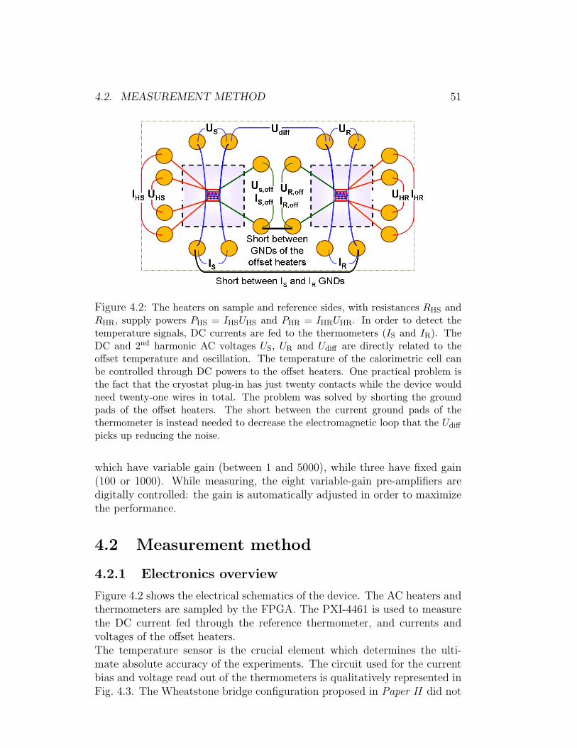
4.2. MEASUREMENT METHOD 51
Figure 4.2: The heaters on sample and reference sides, with resistances RHS andRHR, supply powers PHS = IHSUHS and PHR = IHRUHR. In order to detect thetemperature signals, DC currents are fed to the thermometers (IS and IR). TheDC and 2nd harmonic AC voltages US, UR and Udiff are directly related to theoffset temperature and oscillation. The temperature of the calorimetric cell canbe controlled through DC powers to the offset heaters. One practical problem isthe fact that the cryostat plug-in has just twenty contacts while the device wouldneed twenty-one wires in total. The problem was solved by shorting the groundpads of the offset heaters. The short between the current ground pads of thethermometer is instead needed to decrease the electromagnetic loop that the Udiff
picks up reducing the noise.
which have variable gain (between 1 and 5000), while three have fixed gain(100 or 1000). While measuring, the eight variable-gain pre-amplifiers aredigitally controlled: the gain is automatically adjusted in order to maximizethe performance.
4.2 Measurement method
4.2.1 Electronics overview
Figure 4.2 shows the electrical schematics of the device. The AC heaters andthermometers are sampled by the FPGA. The PXI-4461 is used to measurethe DC current fed through the reference thermometer, and currents andvoltages of the offset heaters.The temperature sensor is the crucial element which determines the ulti-mate absolute accuracy of the experiments. The circuit used for the currentbias and voltage read out of the thermometers is qualitatively represented inFig. 4.3. The Wheatstone bridge configuration proposed in Paper II did not
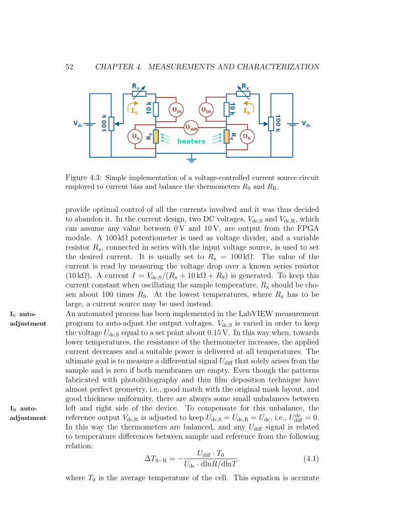
52 CHAPTER 4. MEASUREMENTS AND CHARACTERIZATION
Figure 4.3: Simple implementation of a voltage-controlled current source circuitemployed to current bias and balance the thermometers RS and RR.
provide optimal control of all the currents involved and it was thus decidedto abandon it. In the current design, two DC voltages, Vdc,S and Vdc,R, whichcan assume any value between 0 V and 10 V, are output from the FPGAmodule. A 100 kΩ potentiometer is used as voltage divider, and a variableresistor Rx, connected in series with the input voltage source, is used to setthe desired current. It is usually set to Rx = 100 kΩ. The value of thecurrent is read by measuring the voltage drop over a known series resistor(10 kΩ). A current I = Vdc,S/(Rx + 10 kΩ + RS) is generated. To keep thiscurrent constant when oscillating the sample temperature, Rx should be cho-sen about 100 times RS. At the lowest temperatures, where Rx has to belarge, a current source may be used instead.
An automated process has been implemented in the LabVIEW measurementIS auto-adjustment program to auto-adjust the output voltages. Vdc,S is varied in order to keep
the voltage Udc,S equal to a set point about 0.15 V. In this way when, towardslower temperatures, the resistance of the thermometer increases, the appliedcurrent decreases and a suitable power is delivered at all temperatures. Theultimate goal is to measure a differential signal Udiff that solely arises from thesample and is zero if both membranes are empty. Even though the patternsfabricated with photolithography and thin film deposition technique havealmost perfect geometry, i.e., good match with the original mask layout, andgood thickness uniformity, there are always some small unbalances betweenleft and right side of the device. To compensate for this unbalance, theIR auto-
adjustment reference output Vdc,R is adjusted to keep Udc,S = Udc,R = Udc, i.e., Udcdiff = 0.
In this way the thermometers are balanced, and any Udiff signal is relatedto temperature differences between sample and reference from the followingrelation:
∆TS−R = − Udiff · T0
Udc · dlnR/dlnT. (4.1)
where T0 is the average temperature of the cell. This equation is accurate
4.2. MEASUREMENT METHOD 53
as long as ∆T/T0 is small, in which case the temperature dependence of thethermometer resistance, given by Eq. (3.1), can be Taylor-expanded to firstorder:
R = R0 ·(
1 +∆T
T0
)η≈ R0 ·
(1 + η
∆T
T0
), (4.2)
where η = dlnR/dlnT is the sensitivity. For ∆T/T0 ≤ 0.1 the expansionerror is less than 1%. With this approximation, Eq. (4.1) is easily found.From Udiff = US − UR, and applying the Ohm law to US and UR,
Udiff = ISR0S ·(
1 + η∆TS
T0
)− IRR0R ·
(1 + η
∆TR
T0
), (4.3)
where T0S = T0R = T0. With the automated adjustment which keeps ISR0S =IRR0R,
Udiff = Udc,S · η∆TS −∆TR
T0
, (4.4)
where Udc,S = ISR0S.In the AC steady state method the sensitivity of the thermometer plays
a central role. In principle the higher |η|, the easier to detect small signalvariations. On the other hand, the ac signal measured at the second harmonicis assumed to be a pure sinusoid. Instead, the real form of the voltage whicharises as a consequence of the ac heating is determined by the power law ofthe resistance thermometer:
US(t) = ISR(t) = ISR0S
(1 +
Tac
T0
sin 2ωt
)η, (4.5)
and expanding up to the 2nd order the term in parenthesis
1 + ηTac
T0
sin 2ωt+1
2η(1 + η)
(Tac
T0
sin 2ωt
)2
+ o
[(Tac
T0
)3]. (4.6)
For the same oscillation amplitude to base temperature ratio, when the sensi-tivity is too high the non linear terms have stronger contributions and distortthe sinusoidal signal. This is why having η = −1, as it is for the sensor onthe calorimeter, may represent an advantage.
4.2.2 AC steady state
When the AC steady state method is performed, an AC current is appliedto the heater. The thermometer voltages US, UR and Udiff , measured at thesecond harmonic of the heater frequency, are directly related to the amplitudeof the temperature oscillations. When the same power is applied to sampleand reference sides (PS = PR), three different temperature oscillations aremeasured:
54 CHAPTER 4. MEASUREMENTS AND CHARACTERIZATION
1. the temperature oscillations of platform and sample on the sample side:
Tac,S =U2ndharm
S · TS
Udc,S · |dlnR/dlnT |, (4.7)
2. the temperature oscillations of the platform on the reference side:
Tac,R =U2ndharm
R · TR
Udc,R · |dlnR/dlnT |, (4.8)
3. and the differential temperature oscillation:
Tac,diff =U2ndharm
diff · TS
Udc,S · |dlnR/dlnT |, (4.9)
where TS and TR are the local temperatures directly probed by the GeAuthermometers, and Udc,S and Udc,R are the DC voltages measured across thethermometers. If the reference heater power is turned off, Tac,R = 0 andthe temperature oscillation amplitude of sample plus platform is measuredby the differential signal Tac,diff = Tac,S. This method is used when the heatcapacity of the sample is much bigger than the heat capacity of the platform,because in this case the correct frequency for sensing the heat capacity of thesample is too low for the empty membrane, for which the thermal link wouldactually be measured. Thus, the differential measurement (with an emptyreference) would not give accurate results. The heat capacity of the sample(or reference) side is given by
C =P
2ω · Tac
· sinφ, (4.10)
where ω is the angular frequency of the heater current and φ is the phase.The phase is a fundamental quantity that needs to be taken into account toachieve good absolute accuracy. It can be used to check that the workingfrequency is correct, i.e., τe > 1/ω > τi, in order to minimize the error. Whenthe conditions for using the differential mode are satisfied, the differentialheat capacity can be measured as:
Cdiff =P · Tac,diff
2ω · Tac,S · Tac,R
, (4.11)
where the power P and the angular frequency ω are the same on both sides.
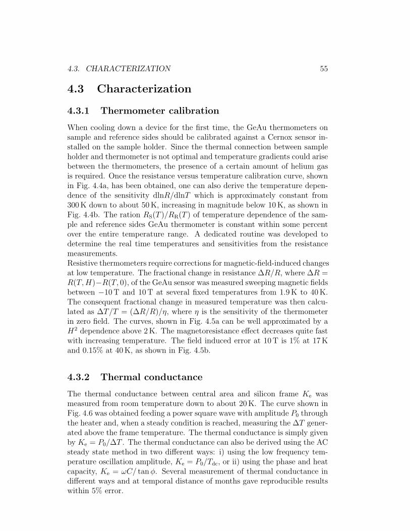
4.3. CHARACTERIZATION 55
4.3 Characterization
4.3.1 Thermometer calibration
When cooling down a device for the first time, the GeAu thermometers onsample and reference sides should be calibrated against a Cernox sensor in-stalled on the sample holder. Since the thermal connection between sampleholder and thermometer is not optimal and temperature gradients could arisebetween the thermometers, the presence of a certain amount of helium gasis required. Once the resistance versus temperature calibration curve, shownin Fig. 4.4a, has been obtained, one can also derive the temperature depen-dence of the sensitivity dlnR/dlnT which is approximately constant from300 K down to about 50 K, increasing in magnitude below 10 K, as shown inFig. 4.4b. The ration RS(T )/RR(T ) of temperature dependence of the sam-ple and reference sides GeAu thermometer is constant within some percentover the entire temperature range. A dedicated routine was developed todetermine the real time temperatures and sensitivities from the resistancemeasurements.Resistive thermometers require corrections for magnetic-field-induced changesat low temperature. The fractional change in resistance ∆R/R, where ∆R =R(T,H)−R(T, 0), of the GeAu sensor was measured sweeping magnetic fieldsbetween −10 T and 10 T at several fixed temperatures from 1.9 K to 40 K.The consequent fractional change in measured temperature was then calcu-lated as ∆T/T = (∆R/R)/η, where η is the sensitivity of the thermometerin zero field. The curves, shown in Fig. 4.5a can be well approximated by aH2 dependence above 2 K. The magnetoresistance effect decreases quite fastwith increasing temperature. The field induced error at 10 T is 1% at 17 Kand 0.15% at 40 K, as shown in Fig. 4.5b.
4.3.2 Thermal conductance
The thermal conductance between central area and silicon frame Ke wasmeasured from room temperature down to about 20 K. The curve shown inFig. 4.6 was obtained feeding a power square wave with amplitude P0 throughthe heater and, when a steady condition is reached, measuring the ∆T gener-ated above the frame temperature. The thermal conductance is simply givenby Ke = P0/∆T . The thermal conductance can also be derived using the ACsteady state method in two different ways: i) using the low frequency tem-perature oscillation amplitude, Ke = P0/Tdc, or ii) using the phase and heatcapacity, Ke = ωC/ tanφ. Several measurement of thermal conductance indifferent ways and at temporal distance of months gave reproducible resultswithin 5% error.
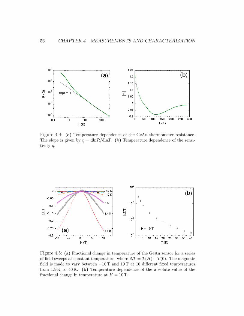
56 CHAPTER 4. MEASUREMENTS AND CHARACTERIZATION
Figure 4.4: (a) Temperature dependence of the GeAu thermometer resistance.The slope is given by η = dlnR/dlnT . (b) Temperature dependence of the sensi-tivity η.
Figure 4.5: (a) Fractional change in temperature of the GeAu sensor for a seriesof field sweeps at constant temperature, where ∆T = T (H)−T (0). The magneticfield is made to vary between −10 T and 10 T at 10 different fixed temperaturesfrom 1.9 K to 40 K. (b) Temperature dependence of the absolute value of thefractional change in temperature at H = 10 T.
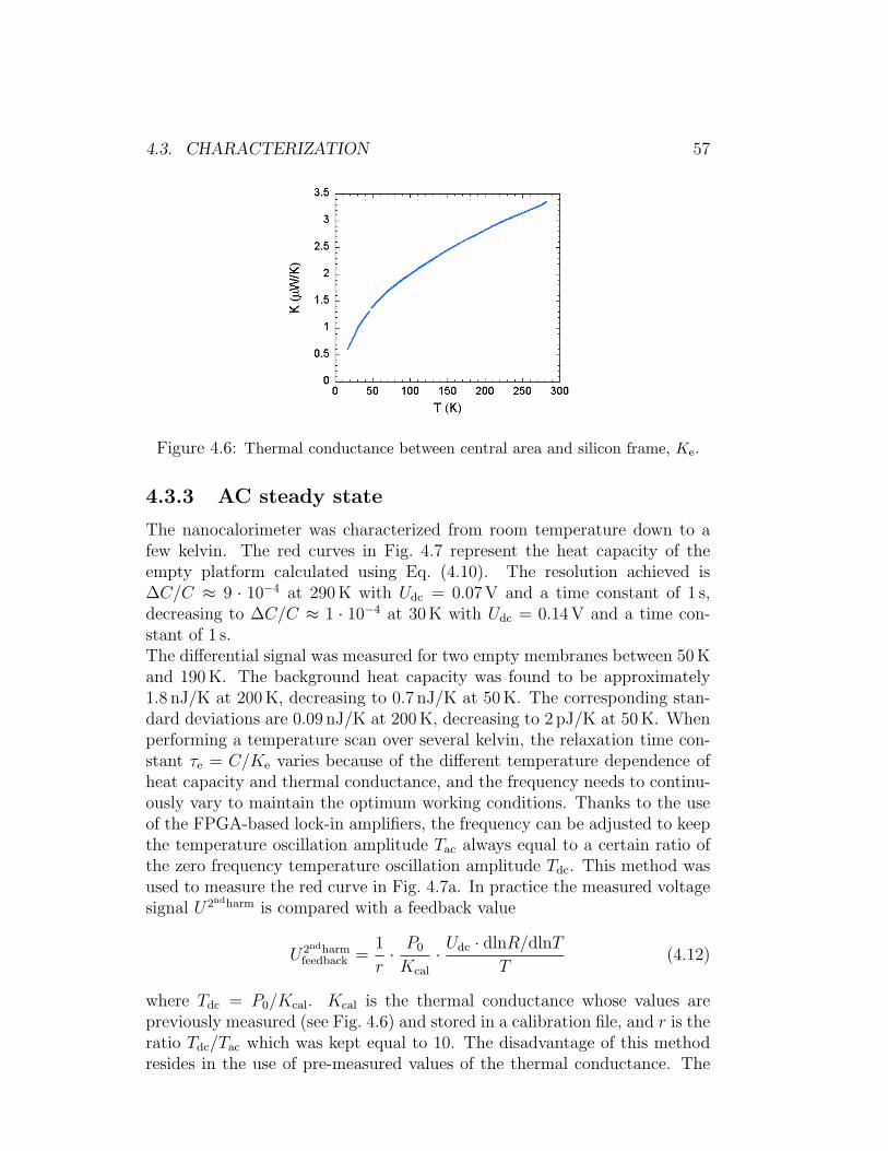
4.3. CHARACTERIZATION 57
Figure 4.6: Thermal conductance between central area and silicon frame, Ke.
4.3.3 AC steady state
The nanocalorimeter was characterized from room temperature down to afew kelvin. The red curves in Fig. 4.7 represent the heat capacity of theempty platform calculated using Eq. (4.10). The resolution achieved is∆C/C ≈ 9 · 10−4 at 290 K with Udc = 0.07 V and a time constant of 1 s,decreasing to ∆C/C ≈ 1 · 10−4 at 30 K with Udc = 0.14 V and a time con-stant of 1 s.The differential signal was measured for two empty membranes between 50 Kand 190 K. The background heat capacity was found to be approximately1.8 nJ/K at 200 K, decreasing to 0.7 nJ/K at 50 K. The corresponding stan-dard deviations are 0.09 nJ/K at 200 K, decreasing to 2 pJ/K at 50 K. Whenperforming a temperature scan over several kelvin, the relaxation time con-stant τe = C/Ke varies because of the different temperature dependence ofheat capacity and thermal conductance, and the frequency needs to continu-ously vary to maintain the optimum working conditions. Thanks to the useof the FPGA-based lock-in amplifiers, the frequency can be adjusted to keepthe temperature oscillation amplitude Tac always equal to a certain ratio ofthe zero frequency temperature oscillation amplitude Tdc. This method wasused to measure the red curve in Fig. 4.7a. In practice the measured voltagesignal U2ndharm is compared with a feedback value
U2ndharmfeedback =
1
r· P0
Kcal
· Udc · dlnR/dlnT
T(4.12)
where Tdc = P0/Kcal. Kcal is the thermal conductance whose values arepreviously measured (see Fig. 4.6) and stored in a calibration file, and r is theratio Tdc/Tac which was kept equal to 10. The disadvantage of this methodresides in the use of pre-measured values of the thermal conductance. The
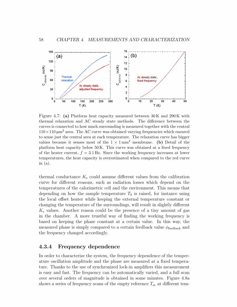
58 CHAPTER 4. MEASUREMENTS AND CHARACTERIZATION
Figure 4.7: (a) Platform heat capacity measured between 30 K and 290 K withthermal relaxation and AC steady state methods. The difference between thecurves is connected to how much surrounding is measured together with the central110×110 µm2 area. The AC curve was obtained varying frequencies which ensuredto sense just the central area at each temperature. The relaxation curve has biggervalues because it senses most of the 1 × 1 mm2 membrane. (b) Detail of theplatform heat capacity below 50 K. This curve was obtained at a fixed frequencyof the heater current, f = 3.1 Hz. Since the working frequency increases at lowertemperatures, the heat capacity is overestimated when compared to the red curvein (a).
thermal conductance Ke could assume different values from the calibrationcurve for different reasons, such as radiation losses which depend on thetemperatures of the calorimetric cell and the environment. This means thatdepending on how the sample temperature TS is raised, for instance usingthe local offset heater while keeping the external temperature constant orchanging the temperature of the surroundings, will result in slightly differentKe values. Another reason could be the presence of a tiny amount of gasin the chamber. A more trustful way of finding the working frequency isbased on keeping the phase constant at a certain value. In this way, themeasured phase is simply compared to a certain feedback value φfeedback andthe frequency changed accordingly.
4.3.4 Frequency dependence
In order to characterize the system, the frequency dependence of the temper-ature oscillation amplitude and the phase are measured at a fixed tempera-ture. Thanks to the use of synchronized lock-in amplifiers this measurementis easy and fast. The frequency can be automatically varied, and a full scanover several orders of magnitude is obtained in some minutes. Figure 4.8ashows a series of frequency scans of the empty reference Tac at different tem-
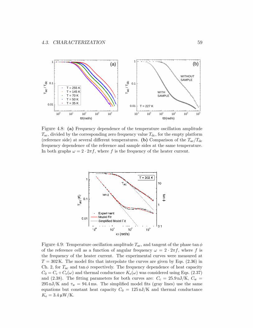
4.3. CHARACTERIZATION 59
1 0 0 1 0 1 1 0 2 1 0 3 1 0 4
0 . 0 1
0 . 1
1
T = 2 5 5 K T = 1 4 5 K T = 7 0 K T = 5 0 K T = 3 5 K
T ac /
T dc
ω ( r a d / s )
( a )
1 0 - 1 1 0 0 1 0 1 1 0 2 1 0 3 1 0 4
0 . 0 1
0 . 1
1 ( b )W I T H O U TS A M P L E
W I T H S A M P L E
T = 2 2 7 K
T ac /
T dc
ω ( r a d / s )
Figure 4.8: (a) Frequency dependence of the temperature oscillation amplitudeTac, divided by the corresponding zero frequency value Tdc, for the empty platform(reference side) at several different temperatures. (b) Comparison of the Tac/Tdc
frequency dependence of the reference and sample sides at the same temperature.In both graphs ω = 2 · 2πf , where f is the frequency of the heater current.
Figure 4.9: Temperature oscillation amplitude Tac, and tangent of the phase tanφof the reference cell as a function of angular frequency ω = 2 · 2πf , where f isthe frequency of the heater current. The experimental curves were measured atT = 302 K. The model fits that interpolate the curves are given by Eqs. (2.36) inCh. 2, for Tac and tanφ respectively. The frequency dependence of heat capacityC0 = Cc +Ce(ω) and thermal conductance Ke(ω) was considered using Eqs. (2.37)and (2.38). The fitting parameters for both curves are: Cc = 25.9 nJ/K, Cw =295 nJ/K and τw = 94.4 ms. The simplified model fits (gray lines) use the sameequations but constant heat capacity C0 = 125 nJ/K and thermal conductanceKe = 3.4 µW/K.
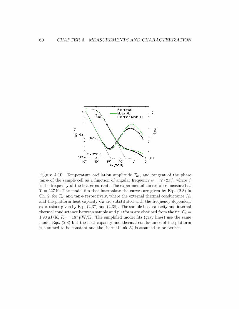
60 CHAPTER 4. MEASUREMENTS AND CHARACTERIZATION
Figure 4.10: Temperature oscillation amplitude Tac, and tangent of the phasetanφ of the sample cell as a function of angular frequency ω = 2 · 2πf , where fis the frequency of the heater current. The experimental curves were measured atT = 227 K. The model fits that interpolate the curves are given by Eqs. (2.8) inCh. 2, for Tac and tanφ respectively, where the external thermal conductance Ke
and the platform heat capacity C0 are substituted with the frequency dependentexpressions given by Eqs. (2.37) and (2.38). The sample heat capacity and internalthermal conductance between sample and platform are obtained from the fit: Cs =1.93 µJ/K, Ki = 187 µW/K. The simplified model fits (gray lines) use the samemodel Eqs. (2.8) but the heat capacity and thermal conductance of the platformis assumed to be constant and the thermal link Ki is assumed to be perfect.
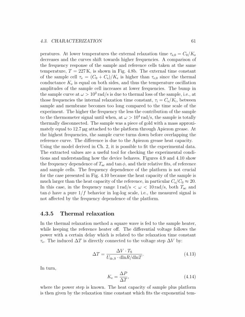
4.3. CHARACTERIZATION 61
peratures. At lower temperatures the external relaxation time τe,0 = C0/Ke
decreases and the curves shift towards higher frequencies. A comparison ofthe frequency response of the sample and reference cells taken at the sametemperature, T = 227 K, is shown in Fig. 4.8b. The external time constantof the sample cell τe = (C0 + Cs)/Ke is higher than τe,0 since the thermalconductance Ke is equal on both sides, and thus the temperature oscillationamplitudes of the sample cell increases at lower frequencies. The bump inthe sample curve at ω > 102 rad/s is due to thermal loss of the sample, i.e., atthose frequencies the internal relaxation time constant, τi = Cs/Ki, betweensample and membrane becomes too long compared to the time scale of theexperiment. The higher the frequency the less the contribution of the sampleto the thermometer signal until when, at ω > 104 rad/s, the sample is totallythermally disconnected. The sample was a piece of gold with a mass approxi-mately equal to 12.7 µg attached to the platform through Apiezon grease. Atthe highest frequencies, the sample curve turns down before overlapping thereference curve. The difference is due to the Apiezon grease heat capacity.
Using the model derived in Ch. 2, it is possible to fit the experimental data.The extracted values are a useful tool for checking the experimental condi-tions and understanding how the device behaves. Figures 4.9 and 4.10 showthe frequency dependence of Tac and tanφ, and their relative fits, of referenceand sample cells. The frequency dependence of the platform is not crucialfor the case presented in Fig. 4.10 because the heat capacity of the sample ismuch larger than the heat capacity of the reference, in particular Cs/C0 ≈ 20.In this case, in the frequency range 1 rad/s < ω < 10 rad/s, both Tac andtanφ have a pure 1/f behavior in log-log scale, i.e., the measured signal isnot affected by the frequency dependence of the platform.
4.3.5 Thermal relaxation
In the thermal relaxation method a square wave is fed to the sample heater,while keeping the reference heater off. The differential voltage follows thepower with a certain delay which is related to the relaxation time constantτe. The induced ∆T is directly connected to the voltage step ∆V by:
∆T =∆V · TS
Udc,S · dlnR/dlnT. (4.13)
In turn,
Ke =∆P
∆T, (4.14)
where the power step is known. The heat capacity of sample plus platformis then given by the relaxation time constant which fits the exponential tem-
62 CHAPTER 4. MEASUREMENTS AND CHARACTERIZATION
Figure 4.11: Relaxation technique. Temperature profiles at two different basetemperatures as response to the input power. The relaxation profiles can be fittedby a single exponential curve which gives the value of the time constant τe. Atlower temperatures the time constant is shorter and thus the raise and decay arefaster. The thermal conductance Ke can be derived by measuring ∆T .
perature decay (or raise), i.e.,
Cs + C0 = τe ·Ke. (4.15)
To practically perform this measurement, a routine was developed whichacquires the voltage pulses, fits the exponential raise and decay using anexponential function exp(t/τe), and extrapolates ∆V . In this way, usingEqs. (4.13), (4.14) and (4.15), the heat capacity and thermal conductancecan be measured as a function of temperature or magnetic field. The bluecurve in Fig. 4.7a is the heat capacity of the platform given by Eq. (4.15). Inorder to subtract the heat capacity background, two separate measurements,with and without sample, are required. The blue curve of Fig. 4.12 is obtainedby subtracting the two contributions.
4.3.6 Calibration verification
A gold sample, in grain form, with mass m = 12.7 µg, was measured from290 K down to about 10 K, and the resulting temperature dependence of theheat capacity was compared to available data, as shown in Fig. 4.12.The sample heat capacity Cs from the fits at T = 227 K shown in Fig. 4.10,is Cs = 1.93 µJ/K and is agreeing well with the heat capacity measured bothwith AC steady state and relaxation method in two separate temperaturescans.For a Au piece with mass m = 12.7 µg, the expected room temperature heat
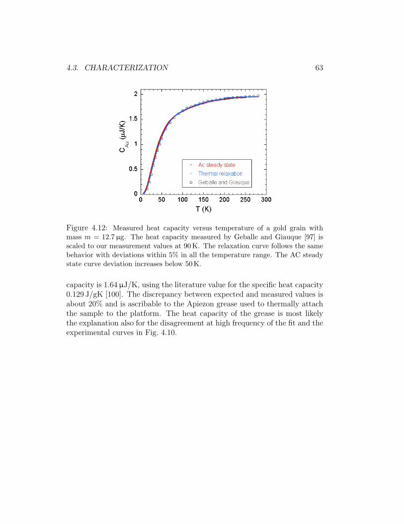
4.3. CHARACTERIZATION 63
Figure 4.12: Measured heat capacity versus temperature of a gold grain withmass m = 12.7 µg. The heat capacity measured by Geballe and Giauque [97] isscaled to our measurement values at 90 K. The relaxation curve follows the samebehavior with deviations within 5% in all the temperature range. The AC steadystate curve deviation increases below 50 K.
capacity is 1.64 µJ/K, using the literature value for the specific heat capacity0.129 J/gK [100]. The discrepancy between expected and measured values isabout 20% and is ascribable to the Apiezon grease used to thermally attachthe sample to the platform. The heat capacity of the grease is most likelythe explanation also for the disagreement at high frequency of the fit and theexperimental curves in Fig. 4.10.

64 CHAPTER 4. MEASUREMENTS AND CHARACTERIZATION
Chapter 5
Numerical simulations
5.1 Simulation model
Numerical simulations were performed with Comsol Multiphysics using theheat transfer module to describe heat flow and the AC/DC module for elec-trical properties. Since the in-plane dimensions are more than three ordersof magnitude larger than the final stack thickness, we simulated the processby a pseudo-3D model described by the heat equation [98]
C2D∂T
∂t−∇ · (κ2D∇T ) = P d+ ha(Ta − T ) + hb(Tb − T ). (5.1)
Here, C2D = ρCd where ρ (g/cm3) is the density, C (J/gK) is the specific heatand d is the layer thickness, κ2D = κd, where κ (W/cmK) is the thermal con-ductivity, P (W/cm3) is the resistive heating power density, ha,b (W/cm2K) isthe heat transfer coefficient between layers, and Ta,b are the temperatures ofneighboring layers above and below the given layer. Radiative heat transferwas neglected. The heat transfer coefficient terms in Eq. (5.1) were used toapproximate the thermal conduction perpendicular to the layers. The tem-perature differences between the layers were, however, found to be negligiblefor the studied frequency range. The parameters needed for the simulationsare C, κ and ρ for each layer and the resistivity for the layers (heater andthermometer) whose electrical behavior is involved. The resistivity of the Tiheaters was adjusted so that the numerical results agreed with the measuredelectric response. Values of specific heat and thermal conductivities wereestimated from the literature [99, 100] and Wiedemann-Franz law. To makethe external time constant coincide with experiments, the membrane specificheat had to be adjusted by 10%. The temperature offset was found to agreewell with experiments using the estimated values of thermal conductivities.The simulations presented and the experiments carried out for comparisonwere performed at a base temperature T0 = 50 K.
65
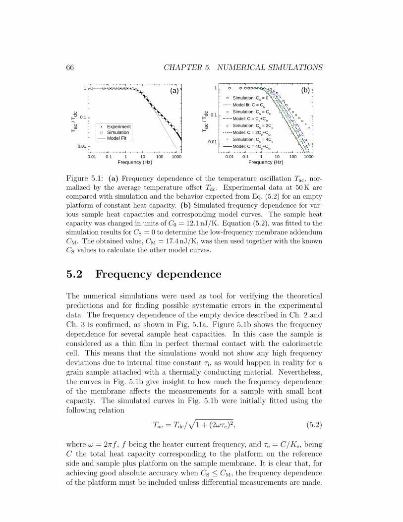
66 CHAPTER 5. NUMERICAL SIMULATIONS
0 . 0 1 0 . 1 1 1 0 1 0 0 1 0 0 00 . 0 1
0 . 1
1 ( a )
E x p e r i m e n t S i m u l a t i o n M o d e l F i t
T ac /
T dc
F r e q u e n c y ( H z )0 . 0 1 0 . 1 1 1 0 1 0 0 1 0 0 0
0 . 0 1
0 . 1
1
S i m u l a t i o n : C S = 0 M o d e l f i t : C = C M S i m u l a t i o n : C S = C 0 M o d e l : C = C 0 + C M S i m u l a t i o n : C S = 2 C 0 M o d e l : C = 2 C 0 + C M S i m u l a t i o n : C S = 4 C 0 M o d e l : C = 4 C 0 + C M
T ac /
T dc
F r e q u e n c y ( H z )
( b )
Figure 5.1: (a) Frequency dependence of the temperature oscillation Tac, nor-malized by the average temperature offset Tdc. Experimental data at 50 K arecompared with simulation and the behavior expected from Eq. (5.2) for an emptyplatform of constant heat capacity. (b) Simulated frequency dependence for var-ious sample heat capacities and corresponding model curves. The sample heatcapacity was changed in units of C0 = 12.1 nJ/K. Equation (5.2), was fitted to thesimulation results for CS = 0 to determine the low-frequency membrane addendumCM. The obtained value, CM = 17.4 nJ/K, was then used together with the knownCS values to calculate the other model curves.
5.2 Frequency dependence
The numerical simulations were used as tool for verifying the theoreticalpredictions and for finding possible systematic errors in the experimentaldata. The frequency dependence of the empty device described in Ch. 2 andCh. 3 is confirmed, as shown in Fig. 5.1a. Figure 5.1b shows the frequencydependence for several sample heat capacities. In this case the sample isconsidered as a thin film in perfect thermal contact with the calorimetriccell. This means that the simulations would not show any high frequencydeviations due to internal time constant τi, as would happen in reality for agrain sample attached with a thermally conducting material. Nevertheless,the curves in Fig. 5.1b give insight to how much the frequency dependenceof the membrane affects the measurements for a sample with small heatcapacity. The simulated curves in Fig. 5.1b were initially fitted using thefollowing relation
Tac = Tdc/√
1 + (2ωτe)2, (5.2)
where ω = 2πf , f being the heater current frequency, and τe = C/Ke, beingC the total heat capacity corresponding to the platform on the referenceside and sample plus platform on the sample membrane. It is clear that, forachieving good absolute accuracy when CS ≤ CM, the frequency dependenceof the platform must be included unless differential measurements are made.
5.3. HEATER POWER 67
5.3 Heater power
The simulations also furnished electrical information including the voltageacross the meander Vh which was current biased with a known value Ih.The power amplitude of the heater, Ph = VhIh, causing the temperatureoscillation was thus known. Using this information and the parameters foundwith the fit, Tdc and τe, the thermal conductance and finally the total heatcapacity were calculated as Ke = Ph/Tdc and C = Ke · τe, for both sampleand reference sides. Finally the heat capacity of the sample was calculatedas the difference of the heat capacities of the sample and reference sides. Itturned out that the calculated Cfit
S was always underestimated by about 15%,with respect to the true values. This is due to the dissipation in the heatercurrent leads which partly contributes to the heating but is not measuredin our four-probe configuration. The heater power should thus be correctedadding 15% of the power in the central area which roughly corresponds to75% of the power in the heater current leads. The final and more correctvalue of the platform heat capacity, CM = 17.4 nJ/K, was used together withthe known values for the different samples CS to calculate τe for each modelcurve.
5.4 Oscillation distributions
Figure 5.2 shows how the temperature oscillations distribute over the en-tire membrane for an empty device and for a thin film sample over the110 × 110 µm2. At low frequency the gradient from the central area to thethermal bath is smooth and the temperature uniformity is good within thesample area. The high conduction of the internal Au leads of the ther-mometer, however, causes the adjacent membrane areas to heat unnecessar-ily. Making the Au leads shorter would decrease this area and thus lower theover-all membrane addendum as well as increase the relaxation time constantwhen the temperature gradient becomes more uniform. At high frequencythe gradient from the central area to the thermal bath becomes steeper forboth reference and sample sides. Furthermore the temperature oscillationsare dampened faster on the sample side, as shown in Fig. 5.2d, and the oscil-lations in the current leads predominate. Since these oscillations do not reachthe thermometer sensor they are not a direct problem, but they represent apossible source of noise.The scenario depicted in Fig. 5.2 should be complemented by taking intoconsideration the heat capacity of each element which allows to study theenergy oscillations εac = C∗2DTac, where C∗2D is the composite heat capacityper surface area including all layers and sample. In Fig. 5.3, surface plotsof such energy oscillations are shown for different frequencies. To obtain a
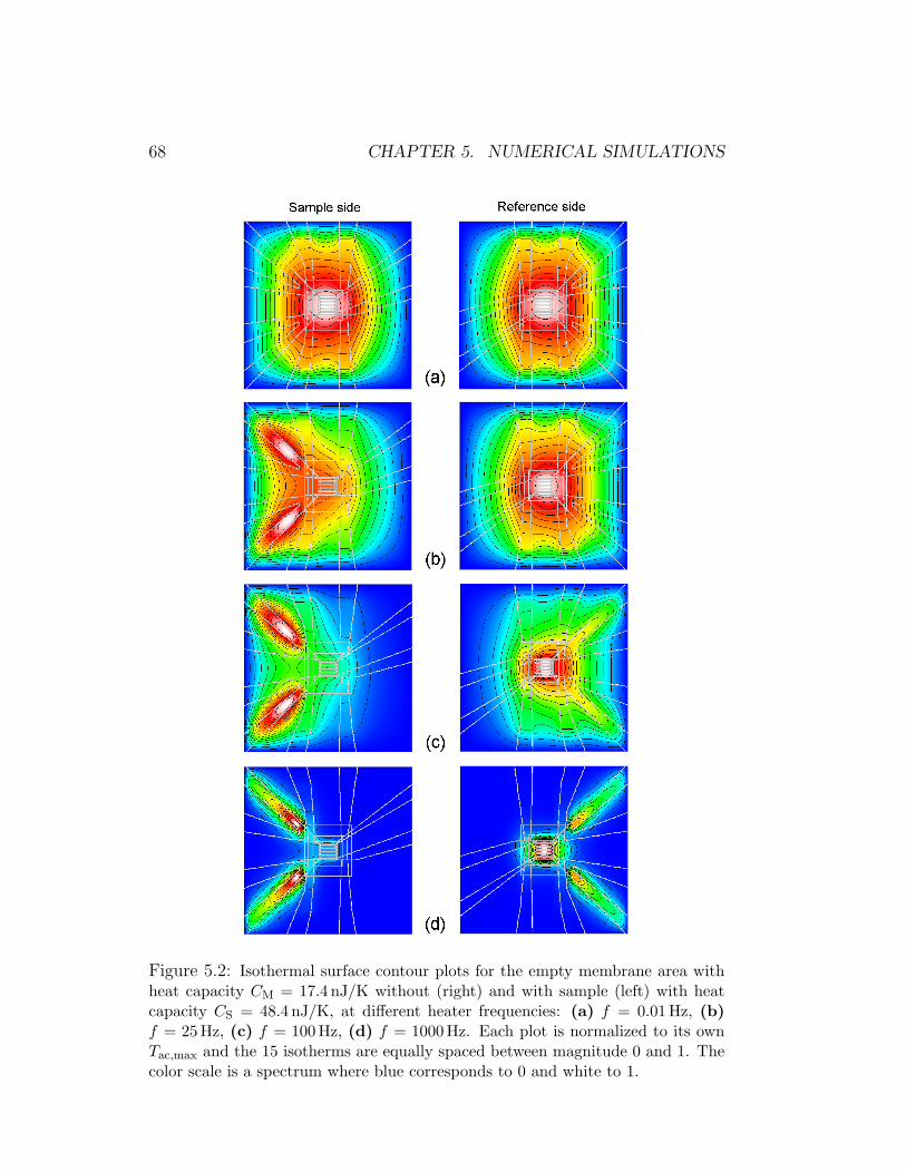
68 CHAPTER 5. NUMERICAL SIMULATIONS
Figure 5.2: Isothermal surface contour plots for the empty membrane area withheat capacity CM = 17.4 nJ/K without (right) and with sample (left) with heatcapacity CS = 48.4 nJ/K, at different heater frequencies: (a) f = 0.01 Hz, (b)f = 25 Hz, (c) f = 100 Hz, (d) f = 1000 Hz. Each plot is normalized to its ownTac,max and the 15 isotherms are equally spaced between magnitude 0 and 1. Thecolor scale is a spectrum where blue corresponds to 0 and white to 1.
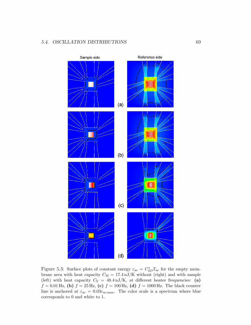
5.4. OSCILLATION DISTRIBUTIONS 69
Figure 5.3: Surface plots of constant energy εac = C∗2DTac for the empty mem-brane area with heat capacity CM = 17.4 nJ/K without (right) and with sample(left) with heat capacity CS = 48.4 nJ/K, at different heater frequencies: (a)f = 0.01 Hz, (b) f = 25 Hz, (c) f = 100 Hz, (d) f = 1000 Hz. The black counterline is anchored at εac = 0.03εac,max. The color scale is a spectrum where bluecorresponds to 0 and white to 1.
70 CHAPTER 5. NUMERICAL SIMULATIONS
more quantitative understanding of the energy distribution, the energy wasintegrated over the central 110× 110 µm2 area and compared with the energyintegrated over the total area and over the area defined by the largest AlOx
layer. In the reference side, about 87% of the energy oscillations are locatedoutside the central area at low frequencies, decreasing to 61% at f = 1000 Hz,while in the sample side the percentage is just slightly increasing from 29% to34%. The fraction of energy oscillations outside the AlOx layer at the samehigh frequency is about 20% for both sides, consistent with the contributionfrom dissipated power in the heater current leads outside the central area.The energy oscillations generated by the heater meander are thus rather wellconfined to the AlOx area at high frequencies, and separated from the energyoscillations in the heater leads, as seen in Fig. 5.3d.However, more focus should be spent on designing heater current leads withless dissipation in relation to the heater meander for better absolute accuracy.
Chapter 6
Summary of attached papers
In Paper I the basic ideas for the development of a nanocalorimeter devotedto study mesoscopic superconductors are treated. In particular, the paperfocuses on the measurement instrumentation and technique. The capabili-ties of the AC steady state method are demonstrated showing measurementsperformed with an older device which uses thermocouples as temperaturesensors. The suggested idea of using resistance thermometers derives fromthe requirements of working below 10 K, where the thermocouples loose sen-sitivity. The Wheatstone bridge configuration is proposed in order to achievethe highest possible resolution.
In Paper II the first version of our differential nanocalorimeter sensedby resistance thermometers is described. The temperature sensor is a Timeander in Wheatstone bridge configuration. The device, fabricated withmicro-lithography techniques, shows exceptional low thermal conductancewhich enables the use of the thermal relaxation method together with theAC steady state method. Both methods are demonstrated by measurementson a sub-µg sample. The lock-in amplifier idea, described in Paper I, wasdeveloped using a field-programmable gate array (FPGA) in order to be ableto simultaneously measure several signals with perfect synchronization.
In Paper III numerical simulations of the last version of the nanocalorime-ter are shown. The Ti resistance thermometer was substituted with GeAu, analloy which ensures high sensitivity down to the sub-K region. The Wheat-stone bridge configuration is abandoned in favor of a less complicated design.A second offset heater is added as an optional tool. Several automated pro-cesses have been implemented in the FPGA which allow perfect control of allthe currents delivered and of the working frequency. The frequency depen-dence of the temperature oscillation amplitude was measured and comparedwith simulated curves with excellent agreement. This study allowed a betterunderstanding of the device properties.
71
Acknowledgments
I would like to thank my supervisor Andreas Rydh not only for his scientificguidance, but also for the many fruitful discussions and opportunities hegave me to broaden my knowledge. Special thanks to Vladimir Krasnov,for his wise advices. I am grateful to all the members of the ExperimentalCondensed Matter Physics group for having always helped me whenever Ineeded, and especially to my office-mate Holger Motzkau for nice discussions.Thanks also to Daniel Oijerholm-Strom, who introduced me to the clean-room facility, for his patience and availability.I would like to thank the KTH group of Nanostructure Physics for the inter-esting conversations during our Friday seminars and the nice collaborationsin the clean-room facility. In particular I want to thank Sebastian Ander-sson and a former member Arndt von Bieren for their great help with thesputtering system without which the GeAu thermometer construction wouldhave been much more troublesome. I am grateful to the staff of AlbanovaNanoFabLab, especially Anders Liljeborg and Anders Holmberg for keepingthe lab running smoothly.I acknowledge my colleague from the atomic physics group and friend, LucaArgenti, for discussing with me parts of this thesis concerning the frequencydependence contribution of the membranes, and for his help in sorting outthe equations.Thanks so much to Michael Genkin and Katia Gallo for your friendshipand support, for the refreshing breaks we had (Micha) and still have (Ka-tia) together! Thanks to Adem Ergul and the many friends/colleagues whocontributed to create such a nice working environment!Thanks to all my friends in Italy and here in Sweden, who were always presentand made my life outside university so funny. Here I should really mentionPignun, from the italian side, who comes to visit me anytime I am back,Daniela whom I can always count on, and Filipa and Peter, on the swedishside, whose friendship I could really not do without.I thank my family in Italy for their unconditional love, in particular mybrother Marco and my mum who I missed so much and that made each ofmy returns at home a wonderful memory.Many many thanks and kisses to Tomas for all your infinite patience andlove!
72
Bibliography
[1] F. Bouquet, C. Marcenat, E. Steep, R. Calemczuk, W. K. Kwok,U. Welp, G. W. Crabtree, R. A. Fisher, N. E. Phillips and A. Schilling,An unusual phase transition to a second liquid vortex phase in the su-perconductor YBa2Cu3O7, Nature 411, 448 (2001).
[2] R. Lortz, F. Lin, N. Musolino, Y. Wang, A. Junod, B. Rosenstein andN. Toyota, Thermal fluctuations and vortex melting in the Nb3Sn super-conductor from high resolution specific heat measurements, Phys. Rev. B74, 104502 (2006).
[3] O. Bourgeois, S. E. Skipetrov, F. Ong and J. Chaussy, AttojouleCalorimetry of Mesoscopic Superconducting Loops, Phys. Rev. Lett. 94,057007 (2005).
[4] Y. Wang, R. Lortz, Y. Paderno, V. Filippov, S. Abe, U. Tutsch andA. Junod, Specific heat and magnetization of a ZrB12 single crystal:Characterization of a type-II/1 superconductor, Phys. Rev. B 72, 024548(2005).
[5] C. J. van der Beek, T. Klein, R. Brusetti, C. Marcenat, M. Wallin,S. Teitel and H. Weber, Thermodynamics of a heavy-ion-irradiated su-perconductor: The zero-field transition, Phys. Rev. B 75, 100501(R)(2007).
[6] U. Welp et al., Superconducting transition and phase diagram of single-crystal MgB2, Phys. Rev. B 67, 012505 (2003).
[7] M.-A. Measson, D. Braithwaite, J. Flouquet, G. Seyfarth, J. P. Brison,E. Lhotel, C. Paulsen, H. Sugawara and H. Sato, Superconducting phasediagram of the filled skuterrudite PrOs4Sb12, Phys. Rev. B 70, 064516(2004).
[8] R. Xie, D. Rosenmann, A. Rydh, H. Claus, G. Karapetrov, W. K. Kwokand U. Welp, Anisotropic superconducting phase diagram of C6Ca, Phys-ica C 439, 43 (2006).
73
74 BIBLIOGRAPHY
[9] C. Marcenat, S. Blanchard, J. Marcus, L. M. Paulius, C. J. van der Beek,M. Konczykowski and T. Klein, Anisotropic Enhancement of Super-conductivity in Heavy-Ion Irradiated (K,Ba)BiO3, Phys. Rev. Lett. 90,037004 (2003).
[10] U. Welp, R. Xie, A. E. Koshelev, W. K. Kwok, H. Q. Luo, Z. S. Wang,G. Mu and H. H. Wen, Anisotropic phase diagram and strong couplingeffects in Ba1−xKxFe2As2 from specific-heat measurements, Phys. Rev. B79, 094505 (2009).
[11] U. Welp, R. Xie, A. E. Koshelev, W. K. Kwok, P. Cheng, L. Fangand H.-H. Wen, Calorimetric determination of the upper critical fieldsand anisotropy of NdFeAsO1−xFx single crystals, Phys. Rev. B 78,140510(R) (2008).
[12] J. S. Kim, P. J. Hirschfeld, G. R. Stewart, S. Kasahara, T. Shibauchi,T. Terashima and Y. Matsuda, Specific heat versus field in the 30 Ksuperconductor BaFe2(As0.7P0.3)2, Phys. Rev. B 81, 214507 (2010).
[13] K. Gofryk, A. S. Sefat, M. A. McGuire, B. C . Sales, D. Mandrus,J. D. Thompson, E. D. Bauer and F. Ronning, Doping-dependentspecific heat study of the superconducting gap in Ba(Fe1−xCox)2As2,Phys. Rev. B 81, 184518 (2010).
[14] C. L. Huang, J.-Y. Lin, Y. T. Chang, C. P. Sun, H. Y. Shen, C. C. Chou,H. Berger, T. K. Lee and H. D. Yang, Experimental evidence for a two-gap structure of superconducting NbSe2: A specific-heat study in externalmagnetic fields, Phys. Rev. B 76, 212504 (2007).
[15] M. Charalambous, O. Riou, P. Gandit, B. Billon, P. Lejay, J. Chaussy,W. N. Hardy, D. A. Bonn and R. Liang, Asymmetry of Critical Expo-nents in YBa2Cu3O7−δ, Phys. Rev. Lett. 83, 2042 (1999).
[16] A. Carrington, C. Marcenat, F. Bouquet, D. Colson, A. Bertinotti,J. F. Marucco and J. Hammann, Field dependence of the specific heat ofsingle-crystal HgBa2Ca2Cu3O8−δ, Phys. Rev. B 55, R8674 (1997).
[17] A. Schilling and O. Jeandupeux, High-accuracy differential thermal anal-ysis: A tool for calorimetric investigations on small high-temperature-superconductors specimens, Phys. Rev. B 52, 9714 (1995).
[18] H. Rabani, F. Taddei, O. Bourgeois, R. Fazio and F. Giazotto, Phase-dependent electronic specific heat of mesoscopic Josephson junctions,Phys. Rev. B 78, 012503 (2008).
BIBLIOGRAPHY 75
[19] T. Park, M. B. Salamon, E. M. Choi, H. J. Kim and S.-I. Lee, Evidencefor Nodal Quasiparticles in the Nonmagnetic Superconductor YNi2B2Cvia Field-Angle-Dependent Heat Capacity, Phys. Rev. Lett. 90, 177001(2003).
[20] A. F. Lopeandıa, F. Pi and J. Rodrıguez-Viejo, Nanocalorimetricanalysis of the ferromagnetic transition in ultrathin films of nickel,Appl. Phys. Lett. 92, 122503 (2008).
[21] Y. Miyoshi, K. Morrison, J. D. Moore, A. D. Caplin and L. F. Co-hen, Heat capacity and latent heat measurements of CoMnSi using amicrocalorimeter, Rev. Sci. Instrum. 79, 074901 (2008).
[22] E. Colombier, D. Braithwaite, G. Lapertot, B. Salce and G. Knebel,High-pressure transport and microcalorimetry studies on high qualityYbCu2Si2 single crystals, Phys. Rev. B 79, 245113 (2009).
[23] G. Knebel, D. Aoki, J.-P. Brison, L. Howald, G. Lapertot, J. Pa-narin, S. Raymond and J. Flouquet, Competition and/or Coexistenceof Antiferromagnetism and Superconductivity in CeRhIn5 and CeCoIn5,Phys. Status Solidi B 247, 557 (2010).
[24] T. Park, F. Ronning, H. Q. Yuan, M. B. Salamon, R. Movshovich,J. L. Sarrao and J. D. Thompson, Hidden magnetism and quantum crit-icality in the heavy fermion superconductor CeRhIn5, Nature 440, 65(2006).
[25] D. C. Ling, C. H. Chen, Y. Y. Chen, B. C. Chang, H. C. Ku,The interplay between weak ferromagnetism and superconductivity inRuSr2EuCu2O8, Physica C 460-462, 518 (2007).
[26] Y. Matsunagaa, H. Kawaji, T. Atakeb, H. Takahashic and T. Hashimo-toa, Analysis of structural and magnetic phase transition behaviors ofLa1−xSrxCrO3 by measurement of heat capacity with thermal relaxationtechnique, Thermochim. Acta 474, 57 (2008).
[27] N. R. Pradhan, H. Duan, J. Liang and G. S. Iannacchione, Specificheat and thermal conductivity measurements for anisotropic and randommacroscopic composites of cobalt nanowires, Nanotechnology 19, 485712(2008).
[28] E. Leon-Gutierrez, G. Garcia, M. T. Clavaguera-Mora and J. Rodrıguez-Viejo, Glass transition in vapor deposited thin films of toluene, Ther-mochim. Acta 492, 51 (2009).
76 BIBLIOGRAPHY
[29] A. A. Minakov, A. W. van Herwaarden, W. Wiend, A. Wurma andC. Schick, Advanced nonadiabatic ultrafast nanocalorimetry and super-heating phenomenon in linear polymers, Thermochim. Acta 461, 96(2007).
[30] M. Y. Efremov, E. A. Olson, M. Zhang, L. H. Allen, Glass transitionof thin films of poly(2-vinyl pyridine) and poly(methyl methacrylate):nanocalorimetry measurements, Thermochim. Acta 403, 37 (2003).
[31] J.-L. Garden, J. Richard, H. Guillou and O. Bourgeois, Non-equilibriumheat capacity of polytetrafluoroethylene at room temperature, Ther-mochim. Acta 461, 122 (2007).
[32] H. Huth, L.-M. Wang, C. Schick, R. Richert, Comparing calorimetricand dielectric polarization modes in viscous 2-ethyl-1-hexanol, J. Chem.Phys. 126, 104503 (2007).
[33] D. Sharma and G. S. Iannacchione, Induced thermal dynamics in themelt of glycerol and aerosol dispersions, J. Chem. Phys. 126, 094503(2007).
[34] E. Perez-Enciso, M. A. Ramos, Low-temperature calorimetry on molec-ular glasses and crystals, Thermochim. Acta 461, 122 (2007).
[35] E. Leon-Gutierrez, G. Garcia, A. F. Lopeandıa, J. Fraxedas,M. T. Clavaguera-Mora and J. Rodrıguez-Viejo, In situ nanocalorimetryof thin glassy organic films, J. Chem. Phys. 129, 181101 (2008).
[36] J. Black, Lectures on the Elements of Chemistry, ed. J. Robison, Edin-burgh (1803).
[37] A. L. Lavoisier and P. S. Laplace, Mm. Acad. Roy. Sci., 355 (1780).
[38] E. Gmelin, Modern low temperature calorimetry, Thermochi. Acta 29,1 (1979).
[39] O. Kubaschewski and R. Hultgren, Metallurgical and Alloy Thermo-chemistry, Experimental Thermochemistry 2, ed. H. A. Skinner, NewYork, Interscience, (1962).
[40] W. Nernst, Ann. Physik 36, 395 (1911).
[41] W. Schnelle and E. Gmelin, Critical review of small sample calorimetry:improvement by auto-adaptive thermal shield control, Thermochim. Acta391, 41 (2002).
BIBLIOGRAPHY 77
[42] W. Zielenkiewicz, Towards classification of calorimeters,J. Therm. Anal. Cal. 91, 663 (2008).
[43] L. D. Hansen, Toward a standard nomenclature for calorimetry, Ther-mochim. Acta 371, 19 (2001).
[44] H. Wilhelm, T. Luhmann, T. Rus and F. Steglich, A compensated heat-pulse calorimeter for low temperatures, Rev. Sci. Instrum. 75, 2700(2004).
[45] R. Bachmann et al., Heat Capacity Measurements on Small Samples atLow Temperatures, Rev. Sci. Instrum. 43, 205 (1972).
[46] S. L. Lai, G. Ramanath, P. Infante, Z. Ma and L. Allen, High-speed (104 C/s) scanning microcalorimetry with monolayer sensitivity(J/m2), Appl. Phys. Lett. 67, 1229 (1995).
[47] S. A. Adamovsky, A. A. Minakov and C. Schick, Scanning mi-crocalorimetry at high cooling rate, Thermochim. Acta 3403, 55 (2003).
[48] M. Y. Efremov, E. A. Olson, M. Zhang, F. Schiettekatte, Z. Zhang andL. Allen, Ultrasensitive, fast, thin-film differential scanning calorimeter,Rev. Sci. Instrum. 75, 179 (2004) .
[49] Y. H. Jeong, Modern calorimetry: going beyond tradition, Ther-mochim. Acta 377, 1 (2001).
[50] Y. H. Jeong, Progress in experimental techniques for dynamic calorime-try , Thermochim. Acta 304, 67 (1997).
[51] G. W. H. Hohne, W. F. Hemminger and H.-J. Flammersheim, Differen-tial Scanning Calorimetry, Springer-Verlag Berlin Heidelberg, (2003).
[52] B. Wunderlich, Thermal Analysis of Polymeric Materials, Springer-Verlag Berlin Heidelberg, (2005).
[53] M. Reading, B. Hahn and B. Crow, US patent 5224775, (1993).
[54] E. Gmelin, Classical temperature-modulated calorimetry: A review,Thermochim. Acta 304, 1 (1997).
[55] Y. Kraftmakher, Modulation calorimetry and related techniques, PhysicsReports 356, 1 (2002).
[56] O. M. Corbino, Phys. Z. 12 (1911) 292.
78 BIBLIOGRAPHY
[57] N. Birge and S. Nagel, Wide-frequency specific-heat spectrometer, Rev.Sci. Intrum. 58, 1464 (1987).
[58] L. A. Rosenthal, Thermal Response of Bridge Wires used in Electroex-plosive Devices, Rev. Sci. Instrum. 32, 1033 (1961).
[59] R. C. Smith, High-Temperature Specific Heat of Germanium,J. Appl. Phys. 37, 4860 (1966).
[60] N. Birge and S. Nagel, Specific-Heat Spectroscopy of the Glass Transi-tion, Phys. Rev. Lett. 61, 341 (1985).
[61] N. Birge, P. Dixon and N. Menon, Specific heat spectroscopy: Origins,status and applications of the 3ω method, Thermochim. Acta 304, 51(1997).
[62] P. F. Sullivan and G. Seidel, Steady-State, ac-Temperature Calorimetry,Phys. Rev. 173, 679 (1968).
[63] M. J. Marone and J. E. Payne, An ac microcalorimeter employing adiode laser as a heater, Rev. Sci. Instrum. 68, 4516 (1997).
[64] R. K. Wunderlich, H.-J. Fecht and R. Willnecker, Power mod-ulation technique for noncontact high-temperature calorimetry,Appl. Phys. Lett. 62, 3111 (1993).
[65] Y. J. Yun, D. H. Jung, I. K. Moon and Y. H. Jeong, Peltier tip calorime-ter, Rev. Sci. Instrum. 77, 064901 (2006).
[66] E. Chateau, J.-L. Garden, O. Buourgeois and J. Chaussy, Physicalkinetics and thermodynamics of phase transitions probed by dynamicnanocalorimetry, Appl. Phys. Lett. 86, 151913 (2005).
[67] Y. Saruyama, Ac calorimetry at the first order transition point,J. Therm. Anal. 38, 1827 (1992).
[68] J.-L. Garden and J. Richard, Entropy production in ac-calorimetry,Thermochim. Acta 461, 57 (2007).
[69] J.-L. Garden, Simple derivation of the frequency dependent complex heatcapacity, Thermochim. Acta 460, 85 (2007).
[70] G. R. Stewart, Measurement of low-temperature specific heat,Rev. Sci. Instrum. 54, 1 (1983).
BIBLIOGRAPHY 79
[71] S. G. Doettinger-Zech, M. Uhl, D. L. Sisson and A. Kapitulnik Simplemicrocalorimeter for measuring microgram samples at low temperatures,Rev. Sci. Instrum. 72, 2398 (2001).
[72] J.-L. Garden, H. Guillou, A. F. Lopeandia, J. Richard, J.-S. Heron,G. M. Souche, F. R. Ong, B. Vianay, O. Bourgeois, Thermodynamicsof small systems by nanocalorimetry: From physical to biological nano-objects, Thermochim. Acta 492, 16 (2009).
[73] D. W. Denlinger et al., Thin film microcalorimeter for heat capacitymeasurements from 1.5 to 800K, Rev. Sci. Instrum. 65, 946 (1994).
[74] I. V. Velichkov, On the problem of thermal link resistances in a.c.calorimetry, Cryogenics 32, 285 (1992).
[75] O. Riou, J. F. Durastanti and Y. Sfaxi, Determination of properfrequency range for accurate heat capacity measurement by AC mi-crocalorimeter, Superlattices and Microstructure 35, 353 (2004).
[76] R. L. Greene, C. N. King, R. B. Zubeck and J. J. Hauser, Specific Heatof Granular Aluminum Films, Phys. Rev. B 6, 3297 (1972).
[77] J. P. Shepherd, Analysis of the lumped τ2 effect in relaxation calorimetry,Rev. Sci. Instrum. 56, 273 (1985).
[78] M. Brando, Development of a relaxation calorimeter for temperaturesbetween 0.05 and 4 K, Rev. Sci. Instrum. 80, 095112 (2009).
[79] B. L. Zink and F. Hellman, Specific heat and thermal conductivity oflow-stress amorphous Si-N membranes, Solid State Commun. 129, 199(2004).
[80] A. Rydh, Calorimetry of Sub-Microgram Grains, Encyclopedia of Ma-terials: Science and Technology, ed. K. H. J. Buschow, M. C. Flemings,R. W. Cahn, P. Veyssire, E. J. Kramer and S. Mahajan (Oxford: Else-vier Ltd) (2006).
[81] J. E. Graebner, Modulated-bath calorimetry, Rev. Sci. Instrum. 60, 1123(1989).
[82] B. Revaz, B. L. Zink and F. Hellman, Si-N membrane-based mi-crocalorimetry: Heat capacity and thermal conductivity of thin films,Thermochim. Acta 432, 158 (2005).
[83] D. R. Queen and F. Hellman, Thin film nanocalorimeter for heat capacitymeasurements of 30 nm films, Rev. Sci. Instrum. 80, 063901 (2009).
80 BIBLIOGRAPHY
[84] W. C. Fon, K. C. Schwab, J. M. Worlock and M. L. Roukes, Nanoscale,Phonon-Coupled Calorimetry with Sub-Attojoule/Kelvin Resolution,Nano Lett. 5, 1968 (2005).
[85] F. Fominaya, T. Fournier, P. Gandit and J. Chaussy, Nanocalorimeterfor high resolution measurements of low temperature heat capacities ofthin films and single crystals, Rev. Sci. Instrum. 68, 4191 (1997).
[86] O. Riou, P. Grandit, M. Charalambous and J. Chaussy, A very sensi-tive microcalorimetry technique for masuring specific heat of µg singlecrystals, Rev. Sci. Instrum. 68, 1501 (1997).
[87] C. A. Swenson, Specific heat (Cp) of Apiezon N grease (1 to 108 K)and calorimetry: Cp of copper below 30 K, Rev. Sci. Instrum. 70, 2728(1999).
[88] W. Schnelle, J. Engelhardt and E. Gmelin, Specific heat capacity ofApiezon N high vacuum grease and of Duran borosilicate glass, Cryo-genics 39, 271 (1999).
[89] M. Osofsky, H. Tardy, M. LaMadrid and J. M. Mochel, dc conductivity ofstrong and weak electron spin-orbit scattering materials near the metal-insulator transition, Phys. Rev. B 32, 2101 (1985).
[90] D.-M. Zhu and F. Lin, Fabrication of Ge-Au film thermometers usinginterfacial atomic diffusion, Rev. Sci. Instrum. 64, 2624 (1993).
[91] O. Bethoux, R. Brusetti, J. C. Lasjaunias and S. Sahling, Au-Ge filmsthermometers for temperature range 30 mK-300 K, Cryogenics 35, 447(1995).
[92] B. W. Dodson, W. L. McMillan, J. M. Mochel and R. C. Dynes,Metal-Insulator Transition in Disordered Germanium-Gold Alloys,Phys. Rev. Lett. 46, 46 (1981).
[93] Z. Tan, S . M. Heald, M. Ropposch, C. E. Bouldin and J. C. Woicik,Gold-induced germanium crystallization, Phys. Rev. B 46, 9505 (1992).
[94] N. A. Fortune, M. J. Graf and K. Murata, Physical dependence of thesensitivity and room-temperature stability of AuxGe1−x thin film resis-tive thermometers on annealing conditions, Rev. Sci. Instrum. 69, 133(1998).
[95] M. Ohring, Materials Science of Thin Films, 2nd edition, AcademicPress (2002).
BIBLIOGRAPHY 81
[96] R. Nilsson, FPGA-based lock-in amplifer with frequency feedback formicrocalorimetry, Master Thesis, Stockholm University, unpublished(2007).
[97] T. H. Geballe and W. F. Giauque, The Heat Capacity and Entropy ofGold from 15 to 300 K, J. Am. Chem. Soc. 74, 2368 (1952).
[98] Comsol Multiphysics 3.4, Heat Transfer Module User’s Guide, COMSOLAB, Stockholm (2007).
[99] B. Revaz, B. L. Zink, D. O’Neil, L. Hull and F. Hellman, Numericalsimulation of the heat transfer in amorphous silicon nitride membrane-based microcalorimeters, Rev. Sci. Instrum. 74, 4389 (2003).
[100] CRC Handbook of Chemistry and Physics, 88th edition, ed. D. R. Lide,Taylor and Francis, London.