LICENTIATE THESIS - DIVA

LICENTIATE THESIS 1991:06 L

Department of Applied Mathematics . luleei University of Technology S-951 87 Luleå, Sweden

PREDATOR-PREY SYSTEMS

AND APPLICATIONS

TORSTEN LINDSTRÖM

TEKNISKA HÖGSKOLAN I LULEÅ

LULEÅ UNIVERSITY OF TECHNOLOGY

epiani, ce < e c

,c) r x m

1,..

0- Iniotev'°

/4/10e9P

delleD

PREDATOR-PREY SYSTEMS AND

APPLICATIONS

Torsten Lindstrom

Depa.rLmeuL of Applied !Vlathernatics Uuiversity of Lulca.

S-95187 Lulca, Sweden

T. Lindström Predator-Prey Systems and Applications. Luleå Univer-sity of Technology, Department of Applied Mathematics, Licentiate Thesis 1991:06 L

Abstract Two-dimensional systems of ordinary differential equations are analyzed qualitatively in this thesis. The systems describe predator-prey in-teraction. The results are applied to the subarctic microtine rodent cycle problem. A partial answer to this difficult question is obtained. Microtine rodent cycles seem to be rare in more southern, not subarctic regions, because of generalist predation. To obtain this result we use the quite natural assump-tion that small rodents are not the main nutrient of generalist predators. We give examples showing that if the small rodents are the main nutrient of the generalist predators, then multiple equilibria and multiple limit cycles may occur as the generalist predator density increases.

The used model is compared to related predator-prey models. Some com-parison results are presented, and moreover, the uniqueness of a limit cycle of a related model is proved in a special case.

Subject Classifications: AMS 34C05, 92A17

Key Words: Predator-Prey system, Limit Cycle, Hopf-bifurcation, Spe-cialist predator, Generalist predator.

ISSN 0280-8242

Luleå University of Technology Department of Applied Mathematics S-95187 Luleå, Sweden

PREFACE 3

Preface This work has been carried out at the Department of Applied Mathematics, University of Luleå. I wish to thank the institution and its personnel for an active and inspiring atmosphere.

I should like to express my deep gratitude to prof. Mats Gyllenberg for giving the applied problems and for his advice and constant support. I am also grateful to Dr. Gunnar Söderbacka for introducing me to the field of dynamical systems.

I am also thankful for valuable discussions with Timo Eirola, Ilkka Han-ski, Hans Heesterbeek, Göran Högnäs, Birger Hörnfeldt, Anders Lagerkvist, Jacqueline McGlade, Simona Muratori, Ingemar Näsell, David Rand, Paavo Salminen, Jan Sundqvist, Vyatsheslav Vinogradov and John Wyller.

Luleå 19. 3. 1991 Torsten Lindström

Contents

1

2

Introduction

1.1 Predator-Prey systems

1.2 The generalized Lotka-Volterra system

1.3 A more realistic predator-prey model

1.4 Applications to the subarctic microtine rodent cycle

Qualitative analysis of a predator-prey system with limit cy-cles

7 8

10 11 12

14 2.1 Introduction 14 2.2 The model 16 2.3 Equilibria and their stability 18 2.4 Absence of limit cycles 19 2.5 Position of limit cycles 21 2.6 Qualitative behavior of limit cycles as the density of generalist

predators varies 22 2.7 Construction of multiple limit cycles 26 2.8 Construction of complicated global bifurcations 28 2.9 Remarks about a related predator-prey model 29

2.9.1 Definition and fundamental properties 29 2.9.2 Comparison of our predator-prey system with a system

of Huang-type 32

3 A generalized uniqueness theorem for limit cycles in a predator-prey system 34 3.1 Introduction 31 3.2 The case a --_,. 0 35 3.3 The general case 40

4 Summary 42

5

Chapter 1

Introduction

In theoretical ecology differential equations are used to model dynamics of different species when generations overlap and the population sizes are suf-ficiently large. The variables model the population densities (sizes) and the parameters (functions) model different properties of the species and the sur-rounding environment.

In a qualitative analysis we examine the long-run behavior of a given dynamical system. The result of this analysis can then be applied to predict under what conditions some species of a given ecology become extinct or survive, and under what kind of coexistence they live.

In technical applications like food-chains in biological sewage treatment plants it is important to choose the environmental conditions and the proper-ties of the species in order to get a sewage treatment which is easy to control automatically. That is, whenever possible, we try to choose the conditions in order to get equilibrium coexistence. This implies that a whole machinery of tools from the theory of linear dynamical systems and automatic control will apply locally even to ecosystems containing several interacting species. The main mathematical difficulty has in this context been to extend the results into infinitely many dimensions. In part, this has been successfully done (See eg. [28] and [30]). Of course, concerning technical applications, also technical problems will arise and these problems should not be neglected.

Concerning natural dynamical systems, we should take serious risks if we started to choose the conditions in order to get simple dynamics. We have to face real nonlinear dynamics like cycles and chaos whenever they are present in the beginning. To avoid environmental damage due to pollution or other effects, we want to keep the dynamics of natural ecosystems unaffected and put up pollution limits so that radical changes in long-run behavior (catastrophes) do not occur. Thus the main advantages with the results from qualitative analysis of differential equations will become present in this

7

8 CHAPTER 1. INTRODUCTION

context. A qualitative analysis of a natural ecosystem can for example be used to provide answers to questions as:

(i) May species become extinct without any apparent reason?

(ii) What kind of perturbations may cause catastrophes?

(iii) Are there important unknown factors which control the dynamics of natural ecosystems?

Of course, a qualitative examination will only provide a qualitative answer, if any. The key of understanding the complex nature will be to isolate the most important factors in order to keep the dimension of the system under consideration low. This will, at least, provide some kind of answer when we try to understand the complex nature.

The present thesis deals with two-dimensional systems of ordinary dif-ferential equations. A well-known theory called Poincare-Bendixson theory exists for these systems. This theory excludes essentially more complicated long-run behavior than cycles.

However, Poincare-Bendixson theory does not give tools to investigate two-dimensional dynamical systems of differential equations completely. For example: Limit cycles may be established by Poincare-Bendixson theory, but problems concerned with uniqueness of limit cycles can be solved without very difficult estimations only for artificially constructed examples. In most cases, also standard application of Poincare-Bendixson theory requires special constructions, and hence, special properties arising from the system under consideration ought to be used.

1.1 Predator-Prey systems In the sequel we shall restrict ourselves to predator-prey systems. That is, we have an ecological system which consists of two species, a prey and its predator. It may be the most simple example of a food-chain. A predator-prey system is usually expected to look like

h(s) — x f (s, x)

= (m f (s, x) — d)x (1.1.1)

The prey- and the predator density are denoted by s and x, respectively. The death rate of the prey is given by d. The most important quantities in a predator-prey system are the prey growth rate function (in the model (1.1.1) called h(s)) and the functional response (in the model (1.1.1) called f (s, x)).

The prey growth function is assumed to be a function of the preys only if the predators influence the prey population only by predation. This function

1.1.1. PREDATOR-PREY SYSTEMS 9

Label Formula

Remarks as k ks/(s ± a) k[l — exp(—cs)] k[l — exp(—csx l-b)] ks2/(s2 + b) k[1— exp(—cs2 x1-b)] k(s/x)/((s/x) a)

unsaturated (Lotka-Volterra) constant attack rate Holling type II, "invertebrate" (Holling) Honing type II, "invertebrate" (Ivlev) Holling type II, "invertebrate" (Watt) Holling type III, "vertebrate" lolling type III, "vertebrate" (Watt) Holling type II, ratio-dependent form

Table 1.1: Different functional responses (main part from May [27])

is usually assumed to be logistic. It will be positive in some interval ]0, K[ and negative elsewhere. The positive constant K is called the environmental carrying capacity and gives the maximal prey population in a given environ-ment. Another important quantity is the intrinsic growth rate which, up to a constant, gives the maximal momentary growth rate of the prey. If the prey growth rate is logistic, we have

h(s) = rs(1 — s/K) (1.1.2)

where r is the intrinsic growth rate and the maximal momentary growth rate is given by rK/4.

The functional response f(s, x) (or trophic function) describes the pre-dation process. Its presence in both equations describes the fact that prey biomass is converted to predator biomass with some conversion efficiency m. Many different expressions have been used as functional responses, and some of them are listed in Table 1.1. In most of the cases functions of prey only are used.

In general, for a fixed predator density, the functional response is a strictly increasing function with upper bound. The half-saturation of the predator is the prey density where the value of the functional response is half of its least upper bound. For example, if

f (s) =

(1.1.3) s + a

the half-saturation is given by a. We start by considering the systems corresponding to no carrying capac-

ity, that is unbounded prey growth. This case is described by generalized Lotka-Volterra models. In section 1.3 we consider a model with carrying capacity, but with a functional response which only depends on the prey density. An application is considered in section 1.4


1.2 The generalized Lotka-Volterra system

In the original Lotka-Volterra system it was assumed that the amount of nutrient consumed by predators is directly proportional to predator-prey en-counters, the prey growth is exponential in absence of predators and that the predator density decline exponentially in absence of prey (cf. [7] and [11]). That is

s(x* — x)

x(s s*). (1.2.1)

We generalize (1.2.1) to the following generalized Lotka-Volterra model

h = f(s)(x* — z(x))

p(x)0(s). (1.2.2)

This model contains the model (1.2.1). We shall assume that the system (1.2.2) satisfies the following general conditions.

(L—I) All the functions f, 7r, p and tk are continuously differentiable of any required order (At least C1 ).

(L—II) The function e is increasing and has a unique zero at s*.

(L—III) The functions f, ir, p are increasing and have unique zeros at zero.

We can obtain a first integral of the system (1.2.2) by separation of variables je. we look for a function of the form

H(s, x) = F(s)+ G(x) (1.2.3)

and require that the total time derivative with respect to the solutions of (1.2.2) is zero. Thus

dF. dG ds s+ dx x dF dG ds f(s)(x* 7(x)) 71P(x)0(s)

and LI = 0 provided

dF f (s) dG p(x) -= constant

ds tb(s) dx r(x) — x*

Putting the constant equal to one we get

dF e(s) dG r(x) — x* ds f(s) dx p(x)

1.1.3. A MORE REALISTIC PREDATOR-PREY MODEL 11

and hence

H(s, x) = ,b(s)

ds' -I- z(x') — x* dx'

o As') j0 P(x0

That is, every solution of the generalized Lotka-Volterra system is a closed orbit (except the axis and the equilibria).

Although it is possible to obtain a first integral of the generalized Lotka-Volterra system, the system has too many shortcomings. The main one is the lack of a carrying capacity for the prey. The generalized Lotka-Volterra system is also structurally unstable and hence the topological properties of the phase-portrait may change dramatically if it is subject to an arbitrarily small perturbation.

Although structurally unstable systems play an essential role in physics where their properties are used to derive important conservation laws, cor-responding systems have no direct importance in biology. However, their indirect importance is clear because more realistic, not well-known ecological systems may be compared to well-known different generalized Lotka-Volterra systems, and hence we may use the solutions of these systems to obtain im-portant properties of the long-run behavior of the solutions of more realistic predator-prey models.

1.3 A more realistic predator-prey model

If we assume an environmental carrying capacity we obtain the following generalization of (1.2.2)

h = f(s)(F(s) — ir(x))

th = P(x)Cs) (1.3.1)

where (s — K)F(s) < 0. The constant K is the environmental carrying capacity. We note that the system

= h(s) — x f (s)

= x(rnf(s) — d) (1.3.2)

belongs to this class. The model (1.3.1) has at most three equilibrial the origin (saddle), (K, 0)

(saddle in case of an interior equilibrium) and an interior equilibrium (s*, x*) whose stability depends on the sign of F' (s* ). This is the so-called Rosen-zweig-MacArthur graphical criterion [32].

11n section 2.9 we consider a similar model which may have more than three equilibria but there we do not assume (L-II).


A criterion for global stability of the interior fixed point (s*, x*) may be obtained when using the first integral

H(s, x) = 0 ik(s')

ds' + 1, As') p(x1)

of the generalized Lotka-Volterra system

= f (s)(F(s*) — ir(x))

= p(x)0(s). (1.3.3)

as a Lyapunov-function. One obtains

fi = t,b(s)(F(s) — F(s*)) (1.3.4)

thus showing that the equilibrium (st, x*) is globally asymptotically stable when F(s) is strictly decreasing. Other criterions can sometimes be derived using integration over closed loops over H (chapter 3). A more difficult question, the uniqueness of the limit cycle in a system of type (1.3.1) is also considered in chapter 3.

1.4 Applications to the subarctic microtine rodent cycle

Small rodents as voles and lemmings show quite regular fluctuations in their population densities. The peak densities are of order hundreds to thousands times greater than the corresponding low-density phases (cf. [33]). The period of the cycles is of order 3-5 years.

Although these cycles have been observed since 1920 no satisfactory ex-planation of the phenomenon has been given. Chitty [4] proposed that the cycles arose because of genetic variations. The small rodents were of worse genetic quality during the peak years and this caused the rapid density de-clines. On the other hand, the small rodents were of better genetic quality during low-density phases. This is the so called Chitty hypothesis.

The Chitty hypothesis can not explain the geographic pattern in the ob-servations (cf. [10]). Multiannual cycles are observed only in the boreal subarctic areas. In the southern regions the observed cyclicity is caused by seasonality. The geographical pattern is explained with different kind of predation, specialist predation and generalist predation. The generalist pre-dation in the south will have a stabilizing effect on the population densities (chapter 2).

May [27] proposed that the vole cycles may be generated by logistic growth with time-lag according to the model

= rN (t)(1 — N(t —T)/ (1.4.1)

I.L4. APPLICATIONS TO THE SUBARCTIC MICROTINE... 13

where N is the rodent population and T is the time-lag. This hypothesis was supported by Hörnfeldt [13] but, as already pointed out by Stenseth [33], there still lacks a mechanistic explanation of how such a time-lag would ensue.

Interaction with food plants has been another possible explanation of the vole cycles. The vole-densities are expected to follow fluctuations, flowering cycles, of their food plants. It is accepted that this hypothesis may describe nonsynchronous cycles but it can not describe synchronous cycles where dif-ferent vole species with different food habits vary synchronously cf. [10].

Predator-prey interaction can give rise to cycles, but very few subarctic small rodent cycles are believed to be pure predator-prey cycles. Predator-prey interaction is in general expected to be only a part of the explanation (cf. [10]) of the subarctic small rodent cycle, and the question of what causes the small rodent cycles is still open after approximately 70 years of observa-tions. We expect that the problem can be solved with a predator-prey model containing other effects than pure predation.

The main problems can be posed in the following way:

We do not know the main reason behind the cycles, and hence we do not know which effects the model has to take into account.

(ii) It will not be enough to study the solutions of the model close to equilibria. Cycles and possible chaotic phenomena have to be studied. This implies that we have to keep the dimension of the model low and neglect many, possibly, important factors.

We propose that low-dimensional models have to be used until we have a reasonable explanation for the subarctic small rodent cycle. It is enough to analyze these models in a rough and qualitative way. The next step consists of an analysis of more complicated models, for the purpose of investigating whether they produce the correct periods and variations in the rodent density or not.

(i)

Chapter 2

Qualitative analysis of a predator-prey system with limit cycles

2.1 Introduction

Fairly regular multiannual microtine rodent cycles are observed in boreal Fennoscandia. In the southern parts of Fennoscandia these multiannual cycles are not observed. The quite regular cycles in boreal Fennoscandia have been the object of extensive research, and a number of attempts have been made to explain the cycles, see [10], [13], [21], [27], [33].

May [27] suggested that the delay-differential equation

= rN(1)(1— N(t—T)1K) (2.1.1)

may describe the above mentioned phenomenon. Here N is the small rodent population, T is a time-lag and K is the environmental carrying capacity. Furthermore he showed that a time lag of about 8-9 months could generate a 3-4 year cycle. It is an interesting fact that the time between the summers in the boreal regions is approximately 8-9 months but this does still not explain how such a time-lag would ensue.

Hörnfeldt [13] studied other species interacting with the rodent cycle, in particular Tengmalm's owl, an avian vole-eating predator. Several mecha-nisms which could generate the time-lag in the model (2.1.1) were also pro-posed in [13]. Among them are predator-based, food-based and disease-based mechanisms. However, none of these hypotheses have yet been supported by enough data.

14

rs(1 — s/K) cx

= qx(1—

YS2

S al (2.1.2)

and

rs(1 — s/K) cx

qx(1— x/-ys)

s2

s at Y S2 b2

2.2.1. INTRODUCTION 15

Some attempts have also been made to explain why the cycles are not observed in the southern parts of Fennoscandia, see e.g. [9], [10]. One expla-nation is that the small rodent populations are exposed to different kinds of predation in different parts of Fennoscandia. Hanski et. al. [9] proposed the models

(2.1.3)

to explain the geographic variations. Here s is the small rodent density, x the specialist predator density and y is the generalist predator density. Note that y is not a dynamical variable but only a parameter. The growth rate of the prey is logistic with carrying capacity K and intrinsic growth rate r. The functional response (trophic function) of the specialist predators is lolling II (Michaelis-Menten kinetics) with half-saturation a l and the functional re-sponse of the generalist predators is Honing III with half-saturation 1672 , cf. [27]. The models (2.1.2) and (2.1.3) contain two kinds of predation, specialist predation and generalist predation and the environmental carrying capacity for the specialist predator is directly proportional to the prey density, cf. [26], [29].

Hanski et. al. [9] also showed by simulation techniques that generalist predation is likely to be the main stabilizing factor in the south. In the models (2.1.2) and (2.1.3) it is assumed that the microtine rodent cycles are pure predator-prey prey cycles, not cycles generated by a time-lag as in the model (2.1.1), which cause the specialist predators to follow the cycle, cf. [13].

Models like (2.1.2) and (2.1.3) are predator-prey models. Predator-prey models have together with their higher dimensional generalizations (compe-tition models, food chains and cooperation models) attracted quite much mathematical interest during the last decades (especially competition mod-els) see e.g. [5], [6], [14], [15], [20], [23].

Although the higher dimensional models seem to have attracted more at-tention mainly due to their rich variety of phenomena (chaos, complicated bifurcations and so on) there are still unsolved two-dimensional problems. For example there are still only a few quite rough methods of general valid-ity when one starts to investigate the simplest nonlinear phenomenon, limit cycles, cf. [37].

16 CHAPTER 2. QUALITATIVE ANALYSIS OF A...

The models (2.1.2) and (2.1.3) differ from the mathematically most well-known predator-prey systems in the quite special predator equation. Usually the predator growth equation is of the form

= (rn d)x, s + a

i. e. biomass is transferred from the prey population to the predator popula-tion. However, recent research indicates that the functional responses can not be considered as functions of prey only and a ratio-dependent functional re-sponse is often a much better approximation of reality [1]. The predator-prey models (2.1.2) and (2.1.3) are supposed to be more close to ratio-dependent models.

In this chapter we shall give a qualitative analysis of a single predator-prey model containing the models (2.1.2) and (2.1.3) as special cases. We shall analyze the number and stability of the equilibria and, existence and location of limit cycles. The main mathematical methods are Dulac- (cf. [37]) and Lyapunovfunctions, the Hopf-bifurcation stability formula (cf. [8]) and the theory of general rotated vector fields (cf. [37]). The results are summarized at the end of the thesis.

2.2 The model

We generalize the models introduced in [9] to the following

= h(s) — x f(s) — y fg (s)

= xg(x/s). (2.2.1)

This model contains the models (2.1.2) and (2.1.3) as two important special cases. We shall analyze the model (2.2.1) qualitatively under the following general conditions:

(A—I) All the functions h, f, f g and /9 are continuously differentiable of any required order (At least C1).

(A—II) The function ii satisfies h(s) > 0 if 0 < s < K and h(s) < 0 if S < 0 or s > K.

(A—III) The functions f and fg are increasing and have unique zeros at s = 0.

(A—Iv) The function t2 is decreasing and satisfies 19(1) > 0 if 0 < t < and 19(1) <0 if t >

2.2.2. THE MODEL 17

The system (2.2.1) may be written in the following form

= f(s)(Fy (s)— x)

= x19(xls)

(2.2.2)

which is more suitable for two dimensional phase-plane analysis. The function Fy(s) is defined by

h(s) — y f g (s) Fy (s)=-

(2.2.3) f(s)

We shall also need a function G(s) defined by

G(s) = f9(s) (2.2.4)

f(s)

Remark 2.2.1 Most of the analysis in this chapter is with small modifica-tions also valid for the more general predator-prey system

f(s)(Fy (s)— 71-(x))

th = p(x)19(xls)

(2.2.5)

where 7r and p are supposed to be increasing functions with unique zeros at zero. Note, however, that especially the proof of Theorem 2.6.4 does not (at least not immediately) carry over.

Theorem 2.2.2 Assume (A-I)-(A-IV). If s(0)> 0, x(0) > 0 and

lim Fy(s) > 0 (2.2.6)

then the solutions s(t) and x(t) of (2.2.2) remain positive and bounded.

Proof (a). Assume first lim3_,0 Fy (s) = co. The solutions will never cross the x-axis because we have .4 > 0 close to the x-axis. Hence s(t) > 0. The s-axis consists of different trajectories of the system, and hence, we have x(t) > 0 by uniqueness of solutions. Observe that when limt _o 19(0 = oo it is possible that the s-axis does not consist of different trajectories, but this causes no problems because then the vectorfield crosses the s-axis inwards. (b). Assume now Fy (s)= Fy(0) < oo. Put

= infIFy(s)IFy (s) > s.s}

-= {(s,x)10 <S <x/ x > x}.

We introduce the Lyapunov level curves

V (s , x) dx t9(_x_I s')

ds' + fx — x

lx,. As') (2.2.7)


in the region A and note that

= '19(/s)(Fy (s) — x)— 19(x I s)(— x) =

t9( .1s)(Fy (s)— x) — 19(1.$)(— x) -I-

19(1_1 s)(— x) — 19(x I s)4_— x) =

s)(Fy (s) —) + (1.9(1 s) — 19(x I s))(x_ — x) 5 0,

whenever (s, x) E A. That is, wherever the trajectory starts or enters the region A it cannot pass the x-axis at the boundary of A. The rest of the proof of positivity is analogous to part (a). (c). To prove dissipativity we note that all solutions will enter the rectangular region determined by 0 < s < K and 0 < x < Kit. 0.

Remark 2.2.3 The condition (2.2.6) states that generalist predators hunt alternative prey when the prey population is sufficiently small.

2.3 Equilibria and their stability

In this section we shall do some local equilibria analysis. We have equilibria at the solutions of the equations

h(s) — y f g (s) = 0

x = 0 (2.3.1)

and

=- KS

Fy (s) = KS. (2.3.2)

Equilibria lying in the interior of R2+ are called interior equilibria. Since an infinite number of fixed points in a dissipative system can be removed by an arbitrary small perturbation we can assume that the number of fixed points is finite and introduce the following notation.

Notation 2.3.1 We denote the solutions of h(s)— yfg (s) = 0 in descending order by K1, K2, K3,...,Kn.

Notation 2.3.2 We denote the solutions of (2.3.2) in descending order by (st, xi), (4,4),...,(s,x„*). If the solution of (2.3.2) is unique we shall de-note it by (s* x*).

The equilibria at (0, Ki) are saddles if F;(Ki) < 0 and unstable nodes if F(K) < 0. We shall treat the origin as a saddle when lim3_0 Fy (s) > 0. The following theorem characterizes the interior equilibria.

2.2.4. ABSENCE OF LIMIT CYCLES 19

Theorem 2.3.3 Assume (A-I)-(A-IV). (a) If Fyi(si)— K < 0 then the equilibrium at (xi, si) is not a saddle. On the other hand, if Fy' (si) — K > 0 then the equilibrium at (xi, si) is a saddle. (b) If the equilibrium at (xi, s) is not a saddle then the expression

f(si)Fy' (si) + cz9/(i) (2.3.3)

determine the stability of the equilibria as follows: If f(si)n(si) stY(s) < 0 then (xi , si) is asymptotically stable and if

f(si)Fy' (si) -F tar (s) > 0 then (xi` , si) is unstable.

Proof Calculation of the Jacobian matrix at (xi, si) gives

J(s:, f(s)F(s) s191a(s) )

and, consequently, the eigenvalues are

1 A± i[f(s:)F;(s:)+ K191(K)±

(2.3.4)

Kt91(h-,))2 — 4f(s7)191(s)K(F‘(.9:) — s,)] (2.3.5)

0. From (2.3.2) and Theorem 2.3.3 we get the following corollaries:

Corollary 2.3.4 Assume (A-I)-(A-IV). If F(s) < s, s > 0 then the system (2.2.2) has a unique equilibrium in R2+ which cannot be a saddle.

Corollary 2.3.5 Assume (A-I)-(A-IV). If Fy' (s) < , s > 0 then all

unstable interior equilibria of the system (2.2.2) are saddles.

2.4 Absence of limit cycles

In this section we investigate the global stability of equilibria. Similar prob-lems have been considered in [22] and [24].

Theorem 2.4.1 Assume (A-I)-(A-IV). If

f(s)F(s)d- —xs

t91—xs

) < 0

in a simply connected region, then the system (2.2.2) has no limit cycle lying competely in this region.


Proof We use the Dulac function

1 B(s, x) = x f (s)

and get the required condition.

Corollary 2.4.2 Assume (A-I)-(A-IV). If

inftER+ —119'(1) Fy (s) < f(s)

then the system (2.2.2) has no limit cycle.

(2.4.1)

(2.4.2)

We shall derive functions and construct sets with respect to different vector fields later on. In order to indicate the underlying vectorfield the functions and sets are given subscripts referring to the formula in which the vectorfield is defined. We introduce the following notation.

Notation 2.4.3 Let (VF) be the vectorfield defined by

= f (s, x)

g(s, x) (VF)

and let H (s , x) be a C1 -function. We denote the total time derivative of H(s, x) with respect to the vector field (VF) by 11(vF).

Notation 2.4.4 Let (VF) be the vectorfield defined as above and let AcR2 . We use the notation A(vF) to point out that the set A is constructed with respect to the vectorfield (VF)

Theorem 2.4.5 Assume (A-I)-(A-IV). Suppose that (2.2.2) has a unique interior equilibrium, (s* ,x*). If

(Fy (s)— Fy(s*))(s — s*) < 0

in some simply connected region, then the system (2.2.2) has no limit cycle lying completely in this region.

Proof We introduce the Lyapunov-function

V (s, x) d(x* I s')

ds' Ix x' —

f. f(s') (2.4.3)

2.2.5. POSITION OF LIMIT CYCLES 21

and get

1.42.2.2)

t9(x* Is)(Fy (s)— x) — t9(x I s)(Fy (s*)— x)

i9(x* Is)(Fy (s)— x) — i9(x* Is)(Fy (s*)— x) +

19(x* I s)(Fy (s*) — x) — 19(x I s)(Fy (s*)— x)

19(x* Is)(Fy (s)— Fy(s*)) (9(x* /s) — 19(x Is))(x* — x) 0.

LI.

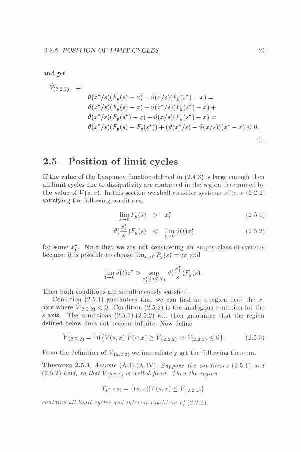
2.5 Position of limit cycles

If the value of the Lyapunov function defined in (2.4.3) is large enough then all limit cycles due to dissipativity are contained in the region determined by the value of V(s, x). In this section we shall consider systems of type (2.2.2) satisfying the following conditions.

lim Fy(s) > x: (2,5.1) 3—o

)Fy (s) < lim t9(t)x7 (2.5.2)

for some x:. Note that we are not considering an empty class of systems because it is possible to choose lims__, () Fy(s) = co and

xl` lim 19(1)x* > sup

s

Then both conditions are simultaneously satisfied. Condition (2.5.1) guarantees that we can find an c-region near the x-

axis where 1.7(2.2.2) < 0. Condition (2.5.2) is the analogous condition for the s-axis. The conditions (2.5.1)-(2.5.2) will then guarantee that the region defined below does not become infinite. Now define

-= inf{V(s, x)IV(s, x) V(2.2.2) V(2.2.2) fq• (2.5.3)

From the definition of V(2.2.2) we immediately get the following theorem.

Theorem 2.5.1 Assume (A-I)-(A-IV). Suppose the conditions (2.5.1) and (2.5.2) hold, so that V(2.2.2) is well-defined. Then. the region

V(2.2.2) -= f(s, 41V(S, <V(222)}

contains all limit cycles and interior equilibria of (2.2.2).


Lemma 2.5.2 The rectangular region

D(2.2.2) -= {(S, X)I0 < S < R1,O < S < KiK}

contains all limit cycles and interior equilibria of (2.2.2).

Remark 2.5.3 Observe that it is necessary to use Notation 2.4.4 in Lemma 2.5.2 because Ki is dependent of the system (2.2.2).

Corollary 2.5.4 The intersection v(2.2.2) n v(2.2.2) contains all limit cycles and interior equilibria of (2.2.2).

In some cases of practical importance we may have some problems when we try to use Theorem 2.5.1. For example in the model (2.1.2) the condition (2.5.1) will not be satisfied, and hence, the region V(2.2.2) will be infinite except for parameter values already guaranteeing absence of limit cycles. We remark that this difficulty can be eliminated by assuming that the functional response

f (s) s + a (2.5.4)

is an approximation of the more general functional response

s2 f(s) 82 -I- as + b

for a small b. An example is illustrated in figure 1 If we assume that the hunting efficiency of the generalist predators is low

compared to the hunting efficiency of the specialist predators at low prey-densities we have that

lim G(s) 0 (2.5.6)

Under this condition the functional response (2.5.5) will give rise to a system of type (2.2.2) which satisfies the condition (2.5.1) for all y when h(s) s(1— sIK) because then lim80 Fy (s) = co for all y > 0.

2.6 Qualitative behavior of limit cycles as the density of generalist predators varies

In this section we shall understand the qualitative behavior of the limit cy-cles as the density of the generalist predators is varied. The region Do 2 2) (Lemma 2.5.2) will in general shrink because Fy (s) < F 0 (s) when y > yo . This does not, however, exclude more and more complicated behavior as shown by the following example.

(2.5.5)

G(s)= (2.6.1) s2 b2

This corresponds to the situation in model (2.1.3). Suppose nb2 << a l . We have

Example 2.6.1 Consider the case when

82 4_ (118

2.2.6. QUALITATIVE BEHAVIOR OF LIMIT CYCLES AS... 23

lim G(s) s—d)

= 0

G(b2lai) —1

G(n62lai ) —n

G(ai ) '2-2 —2

lim G(s) 1-.00

= —1.

This means that we may force the function Fy(s) to change arbitrarily rapidly for small s as the generalist predator density increases.

Consider the model (2.1.3). We choose the parameter values r = 1, K = 1, a 1, c = 1, 7 = 1 and b = 1/1000. When y = 0 the system has a unique equilibrium which is globally asymptotically stable according to Theorem 2.4.5. If we choose y = 2/30 we have three interior equilibria and one of these is a saddle. Note also that two equilibria along the s-axis has occurred. See figure 2 where we have sketched the isoclines for this set of parameter values in the cases y = 0 and y = 2/30. Note that the latter case does not possess limit cycles surrounding the equilibrium (4, 4) (Notation 2.3.2). This can be shown with a region of type V(2.1.3) determined by 0 < s < K3, 0 < x < K3K (recall notation 2.3.1) and Theorem 2.4.1 or 2.4.5.

For the rest of this section we restrict ourselves to the case when the half-saturation of the generalist predators is high compared to the number of small rodents, that is G'(s) > 0. We start with a quite general theorem.

Theorem 2.6.2 Define two systems according to

f(s)(Fi (s)— x)

xexls) (2.6.2)

and

-= f(s)(F2(s)— x)

xt9(xls). (2.6.3)

Assume (A-I)-(A-IV) for (2.6.2)-(2.6.3). Suppose that


(i) The conditions (2.5.1) and (2.5.2) are satisfied for (2.6.2).

(ii) (Fi(s)— F2(s))(s: — s) 5_ 0 for some i

then


(ii) The region V(2.6.2) covers completely V(2.6.3)•

Proof (i). We have

1;7(2.6.2) -

19(XVS)(F2(S) - F2(e)) (79(X7S) - t9(xls))(x* — x)-

19(x* I s)(Fi (s) — Fi (s*)) — (19(x* I s) — t9(x I s))(x* — x) =

19(x* Is)(F2(s)— Ft(s*)) 5 0,

SO

1.7(2.6.3) 5. 17(2.6.2)

and hence

{(s, x)I142.6.2)(s, x) < 0} D {(s, x)I1i(2.6.3)(s, x) 5 0}

V(2.6.2) 2 V(2.6.3)•

O. We shall need the next definition for the formulation of the next theorem.

Definition 2.6.3 Let M C R. The set {M}k is defined by the relation

(s, x) E M <=> (ks, x) E {M}k. (2.6.4)

Theorem 2.6.4 Assume (A-I)-(A-IV). Suppose that GIs) > 0, y > yo. Let (sy* ,xy*), (s 0 , x 0 ) be interior equilibria of the two systems

= f(s)(Fy0 (s)— x)

= xt9(xls), (2.6.5)

and

= f*(s)(Fy (s)— x)

= xt9(xls), (2.6.6)

respectively, satisfying s; < . If (2.5.1) and (2.5.2) are satisfied for (2.6.5)

and f*(-3#3 s) = f(s) then

2.2.6. QUALITATIVE BEHAVIOR OF LIMIT CYCLES AS... 25


(ii) The region 11)(2.6.6 ) fl v(2.6.6)},;./8; will be completely con-tained in the region v(2.6.5) n r(2.6.5)•

(iii) Put A = Is > °Ty/ 0 (s) > O. If inf sEA GIs) > 0 then there exists a y such that if y > y" then the system (2.6.6) has an equi-librium which is globally asymptotically stable.

Proof We transform the system

= f* W(FyW

; = .ii9(it/S1

(2.6.7)

by the linear transform

and arrive at

= Yo X = Yo

X-. (2.6.8)

f (s)(i: — x)

where we have used the fact that,

f * —*

S f(S) s Yo

and defined l(s) as s* s*

F (s)= 1Py(2_s). (2.6.11) s*

Now replace the systems (2.6.2) and (2.6.3) in Theorem 2.6.2 by the sys-tems (2.6.5) and (2.6.9), respectively. We have to verify the conditions (i)-(ii) of Theorem 2.6.2. The condition (i) follow because of our assumptions.

To verify condition (ii) observe that,

and

s* _ x Yo S. Sy*0 = X Ey„(s; 0 )

0 < C (s) = 1- 0 (s) — F( s) = s*

- ds ( (5) P(s)).

Y 0


To prove assertion (iii) we may note that as the density of generalist predators increases we shall sooner or later have F(s) < 0. CI.

Example 2.6.5 If we use the model (2.1.2) the condition Os) > 0 of Theo-rem 2.6.4 is satisfied. However, the condition (2.5.1) is not generally satisfied, but we have already noted that this difficulty can be removed using the more general specialist predator functional response (2.5.5) (Section 2.5).

Remark 2.6.6 Theorem 2.6.4 describes an ideal case when when the motion of the limit cycles is expected to be most regular. It states that the functions h(s), f(s) and f9 (s) in the system (2.2.1) have to follow the variation in the generalist predator density in a suitable sense. These variations are depicted in figure 3 for the system (2.1.2) with the more general functional response (2.5.5).

2.7 Construction of multiple limit cycles The Hopf-bifurcation stability formula see e.g. [8] enables us to construct multiple limit cycles in the model (2.1.3). Similar ideas have been used to construct multiple limit cycles in other systems cf. [12], [34], [36]. Our example will show that this is possible without assuming that the system (2.1.3) has several interior equilibria.

We choose the parameters involved in the model (2.1.3) so that the system undergoes a Hopf-bifurcation at the equilibrium (87, s7). The choice

f(s) = 1 (2.7.1)

fr£ = 1 (2.7.2)

/Y(K) = —1/2 (2.7.3)

F;(4) = 1/2 (2.7.4)

t9(n)(K)

7

=

=

0,

1

n > 1 (2.7.5)

(2.7.6)

will simplify our work with the coordinate transforms required for using the IIopf-bifurcation stability formula.

By (2.7.2) we have x: = s: . We move the equilibrium (sr, sr) to the origin by the affine transform

e = Ti =

and the system (2.2.2) transforms into

=f(+s)[F(+s) — ij — sfl

(2.7.7)

2.2.7. CONSTRUCTION OF MULTIPLE LIMIT CYCLES 27

= +

In order to get the standard form of (2.2.2) we choose the further transform

and obtain

U = —77

v n (2.7.9)

v + s7 = f(u + v + s7)[Fy (u + v + s7) — v — s7] — (71 + .37)19(

u + v + s7)

+ = (9 + 4)19( u + V + s7 ).

(2.7.10)

We expand all functions in Taylor series, making especially use of as-sumption (2.7.5) and get as a third order approximation of the system near

(4,4)

it = 1

(v U2 U3 U2 V F"(S7)

(7)2 (4)2 ) Y

2 (u + v)2

2 s; s

J "(4) (u3 -F u2v UV2 V3) + FY

6 I" (s7) (u + v)3 +

4

f' (s' ) 2 FY"(37)f'(SZ (u v2) + 2

(u + v)3 2

1 u2 u3 ti2 v

4 (4)2 (4)2

This expression is now in standard form. This means that we can apply the Hopf bifurcation stability formula to this expression. We get

1 a =

"(s) + 4s:(Fyil(s:))2 + ss; f"(4) +

16.se Y"7

(2.7.11)

The sign of a determines the stability of (si, s7). The formula (2.7.11) is quite complicated and we start by choosing s7 = 1,

r = K and a l n-f 0. When a l 2f 0 both derivatives of f(s) in the expression vanish and we have

(2.7.8)

(2.7.12)

Fy(s) S2

S(K s) y s2

b2 (2.7.13)


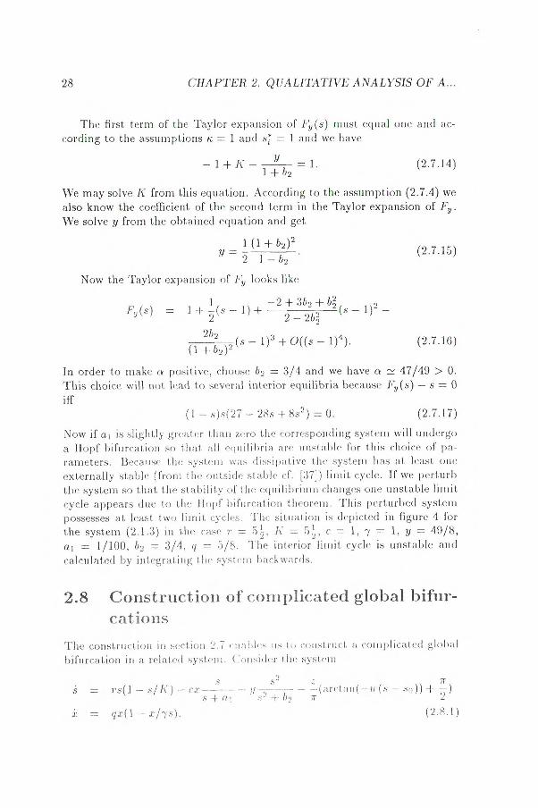
The first term of the Taylor expansion of Fy (s) must equal one and ac-cording to the assumptions ic =- 1 and si* = 1 and we have

— 1 + K Y

1b2

= 1. (2.7.14) +

We may solve K from this equation. According to the assumption (2.7.4) we also know the coefficient of the second term in the Taylor expansion of F. We solve y from the obtained equation and get

1 (1 + 62)2 y = (2.7.15)

Now the Taylor expansion of Fy looks like

Fy (6' ) =" 1 + 1(49 1) +

—2 + 362 +

(s 1)2 — 2 2 — 263

262

(1 + 62)2(s 1)3 + 0((s — 1)4). (2.7.16)

In order to make a positive, choose 62 = 3/4 and we have a 47/49 > 0. This choice will not lead to several interior equilibria because Fy (s)— s = 0

if (1— s)s(27 — 28s + 85.2 ) = 0. (2.7.17)

Now if a l is slightly greater than zero the corresponding systern will undergo

a Hopf bifurcation so that all equilibria are unstable for this choice of pa-rameters. Because the system was dissipative the system has at least one externally stable (from the outside stable cf. [37]) limit cycle. If we perturb the system so that the stability of the equilibrium changes one unstable limit cycle appears due to the Hopf bifurcation theorem. This perturbed system possesses at least two limit cycles. The situation is depicted in figure 4 for the system (2.1.3) in the case r K= c 1, 7 = 1, y = 99/8,

= 1/100, 62 = 3/4, q = 5/8. The interior limit cycle is unstable and

calculated by integrating the system backwards.

2.8 Construction of complicated global bifurcations

The construction in section 2.7 enables us to construct, a complicated global bifurcation in a related system. Consider the system

., s -.: , = rs(1 — s/ K) cx prctan(—uls — .s0 )) + —7r )

S + a l s2 + b2 71- 2

= qæ(1 — . r 17s). (2.K.1)

2.2.9. REMARKS ABOUT A RELATED PREDATOR-PREY MODEL 29

This system may be written in the usual form (2.2.2). We shall choose the parameters r = 54, K = 54, 7 = 1, c = 1, y = 49/8, a l = 1/100, b2 = 3/4, w 1500, so = 0.99, z =. 0.01 to construct complicated bifurcations with respect to the parameter q '•-• 0.682. First consider the rough view of the system (Figure 5) where we have sketched the isoclines and the unstable manifold of the saddle (K1, 0).

If we magnify the small rectangle in figure 5 we note that the system (2.8.1) has a saddle point and a couple of limit cycles surrounding it (Figure 6). If we increase the value of q the limit cycles will coalesce into each other at some value q* •

However, the bifurcation which appears as the limit cycles coalesce is not only a limit cycle bifurcation, because the stable manifolds of (4,4) (Notation 2.3.2) and the unstable manifold of (K1 ,0) (Notation 2.3.1) are involved in the bifurcation. This is illustrated in figure 7 where we have plotted successive Poincare plots of the stable and unstable manifolds in the cross-section s = 0.998 for four different values of q (horizontal axis). The x-values are plotted against the vertical axis.

When the limit cycles coalesce infinitely many saddle connection bifurcations will occur in some interval [q*, q* e]. That is, the limit cycle bifurcation-value q* is, in fact, an accumulation point of other bifurcations. The phenomenon is described in more detail in [8]. Hence the related sys-tem (2.8.1) undergoes a complicated global bifurcation scheme in the interval [q* q* + el. We note that nothing excludes this phenomenon in the predator-prey model (2.1.3), and that the numerical evidence presented here does not establish the phenomenon for the used parameter values.

2.9 Remarks about a related predator-prey model

Huang [16], [17], [18], and Huang and Merill [19] have investigated a system which is quite similar to ours. We review some results concerning these systems and present. some comparison results.

2.9.1 Definition and fundamental properties

il uang models of type

h= f(s)(Fy (s)— ir(x))

= p(x)e(s). (2.9.1)


are (especially when V(s) > 0) more well-known than our system (2.2.5). They are more close to our system than the separable system

= f(s)(Fy (4)- x) i = xt9(x: Is) (2.9.2)

corresponding to the Lyapunov-function defined in (2.4.3) and hence it may be possible to get some results about (2.2.2) comparing it to the system (2.9.1). We shall assume that the Huang-model satisfies the following general conditions:

(H-I) All the functions f, r, p and /,b are continuously differentiable of any required order (At least 0). The function Fy is continu-ously differentiable of any required order at all other points except possibly at the origin, but lim-o f(s)F(s) = 0.

(H-II) There exists a point K such that Fy(s) < 0 if s > K.

(H-III) The functions f , 7r, p are increasing and have unique zeros at zero.

Theorem 2.9.1 Assume (H-I)-(H-111). If s(0) > 0 and x(0) > 0 the solu-tions s(t) and x(t) of (2.9.1) remain positive, if moreover 1,b(s) < 0 fors < s, 0(4) = 0 and

I (s) P(x) then the system (2.9.1) is dissipative.

Remark 2.9.2 The condition (2.9.3) seems to be important only for the proof presented here, so there may be some possibilities to improve the the-orem. However, we shall mainly work with p(x) = x, and hence the theorem is enough for our purposes. We also remark that the condition 1P(s) < 0 for small s is essential for dissipativity and cannot be removed.

00 dx

Proof The axes consist of different trajectories of the system, and hence, the solutions remain positive by uniqueness of solutions. To prove dissipa-tivity, first note that all solutions will enter the infinite rectangular region 0 < s < smax, smax > K. Now introduce the Lyapunov level curves

ds dx V (s, x) =

( )3: f(s) Fi,(3:)P(x) (2.9.4)

in the infinite quadratic region s > s: , x > F(s). Now choose

I = sup 7r-l(Fy (s) e(s)) 3:‹3‹Smax

(2.9.5)

oo. (2.9.3)


and we have that 1.7 < 0 for x> i. Put

'" ds dx VO

i -{-

s: f(s) ff'y(s:) p(x)

and by (2.9.3) we may choose

(2.9.6)

dx x ma, = Ix1 — Vo).

P(x) (2.9.7)

By the Implicit function theorem the level curve V(s, x) = Vo defines a function x .= v(s) for s7 < s < smax• Now all trajectories will enter the region

= {(s, x)10 < s < s:, 0 < x < xmax} Ul(s, x)ls: < s < smax,0 < x < v(s)} •

o.

The similarities between the system (2.9.1) and generalized Lienard equa-tions;

= c,(y) — F(x)

—g(x) (2.9.8)

have been used to apply a theorem by Zhang [38] in order to prove a unique-ness of limit cycles result for the Huang model (2.9.1).

Theorem 2.9.3 (Huang, [16]) Assume (H-I)-(H-III), Suppose that (i) The function 1P is strictly increasing and has a unique zero at s* ; the function Fy(s) has a unique zero at Ki such that

(s Ki )Fy(s) < 0.

(ii) The function —F(s)f(s)

0(s) is non-decreasing for s

Then the system (2.9.1) has at most one limit cycle, and if it exists it is stable.

The fact that the system (2.9.1) has so well-known dynamics under the above conditions will be used in section 2.9,2. Note that the first condition is a condition which is expected to be valid for usual predator-prey systems of type (2.9.1), the last one is needed for the proof of the uniqueness of the limit cycle.

•


2.9.2 Comparison of our predator-prey system with a system of Huang-type

Suppose that 7.9(t) is a decreasing function defined on the entire real line. The system

f (s)(Fy (s) — x) i :----- xt9(Fy(s)Is)

(2.9.9)

is a rotation of the vectorfield (2.2.2) because

8(2.2.2) (2.2.2)

(2.9.9) (2.9.9)

Fy (s) x x f (s)(Fy (s) x)(t9(

s ) t9(7)) < 0, (2.9.10)

where .(2.2.2), i(2.2.2), .(2.9.9) and i(2.9.9) are defined by (2.2.2) and (2.9.9), respectively. The theory of general rotated vector fields (cf. [37]) gives:

Lemma 2.9.4 Assume (A-I)-(A-IV) for (2.2.2), (II-I)-(H-III) for (2.9.9) and that 19(t) is a decreasing function defined on the entire real line. Closed trajectories of the system (2.2.2) and the system (2.9.9) do not intersect. Moreover, equilibria of (2.2.2) and (2.9.9) have the same indexes.

The systems (2.2.2) and (2.9.9) are dissipative according to Theorem 2.2.2 and Theorem 2.9.1, respectively. When we combine dissipativity of the sys-tems (2.2.2) and (2.9.9) with the theory of general rotated vector fields we get:

Theorem 2.9.5 Assume (A-I)-(A-IV) for (2.2.2), (H-I)-(II-III), (2.9.3) for (2.9.9) and that 19(1) is a decreasing function defined on the entire real line. If lim3 .o Fy (s) > 0, the vectorfield (2.2.2) has no limit cycles surrounding all limit cycles and interior equilibria of (2.9.9)

Proof First note that none of the equilibria along the s-axis of the system (2.9.9) are stable. If the system (2.2.2) does not have a limit cycle the theorem holds, ie assume the existence of at least one limit cycle in the systern (2.2.2). The region between the boundary of 'R. (definition in the proof of Theorem 2.9.1) and the outermost limit cycle of (2.2.2) forms a trapping region for the system (2.9.9), and hence the existence of a limit cycle or an interior equilibrium outside the outermost limit cycle of (2.2.2) is established by the Poincar-Bendixson theorem.

We can also apply Theorem 2.9.3 to show uniqueness of limit cycles of (2.9.9) if the following conditions hold (s > 0):

Ft(s) < Fy(s)Is (2.9.11)


Fy(s)(s — 5_ 0 (2.9.12)

d F(8 )) < 0 s s*. (2.9.13)

s s

The condition (2.9.11) implies that the function Ip(s) = 19(4(s)/ s) is strictly increasing. This case is the most investigated case, because this is ecologically the most interesting. There are, however, some works about other cases (cf. [34]). If the system satisfies the condition (2.9.11) we also have by Corollary 2.3.4 and Lemma 2.9.4 that the systems (2.2.2) and (2.9.9) have a unique equilibrium which cannot be a saddle. From the above uniqueness assumptions we get the following corollary.

Corollary 2.9.6 Assume (A-I)-(A-IV) for (2.2.2), (H4)-(H-III) for (2.9.9) and that 19(t) is a decreasing function defined on the entire real line. If the conditions (2.9.11)-(2.9.13) are satisfied for the system (2.9.9), then all limit cycles of (2.2.2) are contained in the unique limit cycle of (2.9.9)

As a final remark we also note that the motion of the limit cycles in the Huang-model can be followed quite easily in certain situations.

Two Huang systems with different F:s are rotated with respect to each other if e(s) is a strictly increasing function with a unique zero at s = .5* and (TVs) — F2(s))(s — st)> 0 because

= p(x)f (s)0(s)(Fi (s) — F2(s)) 0.

(2.9.14) Moreover, if these functions satisfy the uniqueness conditions in Theorem 2.9.3 for both systems, then we know by the theory of general rotated vector fields (cf. [37]), that the unique limit cycle of system corresponding to F2 will be contained in the unique limit cycle in the system corresponding to F1.

f(s)(F1 (s) lr(x)) P(x)0(s) f(s)(F2(s) z(x)) P(x)e(s)

Chapter 3

A generalized uniqueness theorem for limit cycles in a predator-prey system

3.1 Introduction In this chapter we consider the following predator-prey system

(in f (s) — d)x ,

—a f (s)x + [3h(s),

where

f (s) =- 52 + as + h(s) = s(1 — s)

s2

(3.1.1)

and in, d, a, [3, a, b are positive parameters and x, s > 0. The cases b = 0 and a = 0 have been considered in [3] and [35], respec-

tively. We rewrite the system (3.1.1) using a new parametrization of time given by dr = dt I f (s) and arrive into

i =

—x F(s) (3.1.2)

where

So(s) /3 2

34

3.3.2. THE CASE a 0 35

F(s) r (1 s)(s2 + as b) .

and A+ , p, r> 0 and A_ <0. The Lyapunov-function defined by

u — F(A) du W (s, x) 92(u)du I

JF(A) U

with derivative W = ,o(s)(F(s) — F(A)) (3.1.3)

is an essential part of the proofs in [3] and [35].

Lemma 3.1.1 (a) The solutions s(t) and x(t) of (3.1.1) and (3.1.2) remain positive and bounded. (b) If A.4_ op, 1[ then the critical point (0, 1) is globally asymptotically stable. (c) If Ä+ ejo, 1[ and F(s) decreases the critical point A = (F(A+ ), A+) is globally asymptotically stable.

Proof The case (b) is simple. To get (a) we apply theorem 2.9.1 and for (c) consider (3.1.3) by standard Lyapunov methods.

Lemma 3.1.2 If a > 1 or b > (1 — a)3/27 then F(s) decreases, otherwise F(s) has one minimum point, sie, and one maximum point .92*. Moreover, we have

0 < si* < (1 — a)/3 < s2* < (1 — a)/2.

Proof The properties of Fi(s) lead to a direct proof. D.

From now on we can make the assumptions a < 1 and b < (1-27a)3 , and return for a while to the case a =-- 0.

3.2 The case a = 0

The essential parts of the proof proceed in a way analogous to the proof in [35] and a brief summary of it will be recalled here. Note that the proof of theorem 3.2.6 can be simplified a lot if we apply theorem 2.9.3 and is included here mainly for historical reasons. A proof based on theorem 2.9.3 is given in section 3.3.

Lemma 3.2.1 Suppose A+ Elsi*,s21. Then R(s) = F'(s)b,o(s) decreases in )0 , Alj and Pt+ , 1[.

36 CHAPTER 3. A GENERALIZED UNIQUENESS THEOREM...

Proof We have

R' = r 2s

P (52 Ä )2 ( s3 + 3)2+s + b — A+).

Because F'(A) > 0 = —24 + — b> 0 we get

—83 + 3A2+s + b — A2+

< —s3 + 3A2+s — 2A3+

< —(s — 14.)2(s + 24) <0

Lemma 3.2.2 Suppose (1). b > 0, (2). g(y) E C3[—b,b] ,

(3). 9(0) = 9'(0) = 0, (4). g"(0) > 0, (5). gm(y) > 0, Vy E [—b, 6],

(6)- 9(91) = 9(92)- Then

(1). 91+ P2 < 0, (2). gi (yi) + gi (y2) > 0.

Proof Assume y2 < 0 < yi and put a(y) = g'(y), tk(y) = —g'(—y). We may assume that we have y* such that 0(y*) = so(yl ) otherwise the lemma will follow immediately. We have

Y1 „ 1 , 2.

(p(t)dt < —2

yiSo(Yi ) < —2 Y OlY < 0(t)dt

Because yi f I2

c,o(t)dt lb(t)dt Jo

we get yi < —y2 < y*, and hence, tP( — Y2) < e(y*) = (p(yi). The lemma follows. O.

Let F be a nontrivial closed orbit of system (3.1.2). Let st and sh he the minimum and maximum s-values of F, respectively and xl and xh the minimum and maximum x-values of F, respectively.

3.3.2. THE CASE a = 0 37

Definition 3.2.3 (a). Define z1 and z2

= )t]

Z2 = [Xj, Xh] sh]

such that the condition (x, zi(x)) E F is satisfied for x E [xi, xh], i = 1, 2. (b). Moreover, let G(x)= F(z2(x))— F(zi (x)).

Lemma 3.2.4 (a). Suppose A 0:1,1E\ [si*, s21. Then G(x) 0 if x E]xl,xid• (b). Suppose A asi*, s2*[. Then there exist two points 01,02 so that

Moreover

< 01 < 02 < Xh,

GOO= G(02) = 0,

G(x) > 0 if x Elxi,01[U]02,xh[,

G(x) < 0 if x E]01,02[.

(3.2.1)

(3.2.2)

(3.2.3)

(3.2.4)

< F(z1(01)) = F(z2(02)), (3.2.5)

02 > F(Z1(02)) = F(z2(02 ))• (3.2.6)

Proof It is obvious that G(xi) = G(xh ) = 0 and if x is sufficiently close to xi or æh we get G(x) > 0 if .\ Elsi*, s2*[ and G(x) < 0 if .\ e]0, 1R[si*, 82*1.

Suppose GM= 0. We have

G' 8 =

F(z1(0)) — rr(z2(0)) F1(zi(0))] = () I. (p(x2(64)) (P(z1(0))

F(z1(61)) — L.

rR(z2(0)) H(zi(0)1 • 0 (3.2.7)

(a). Suppose C > F(zi(0)) and A+ > s2*. Put g(x) = —F(s .521 + F(s2*). By lemma 3.2.2 we get f"(z2(0)) + Flzi(9)) < 0 and 19,(zi (0))J > hP(z2(0))1, and C(0) > 0. In the case A+ < 81*, see the proof of theorem 3.3.1.

(b). If the derivative of the Lyapunov-function (3.1.3) is integrated around any nontrivial closed orbit F of (3.1.2) we have

Th 0 = Iii/di = F (z)

F() dx =

z2) G(x) dx

Jr Fi(s)ds

Jr x, x f zi(x) J3 X

(3.2.8)


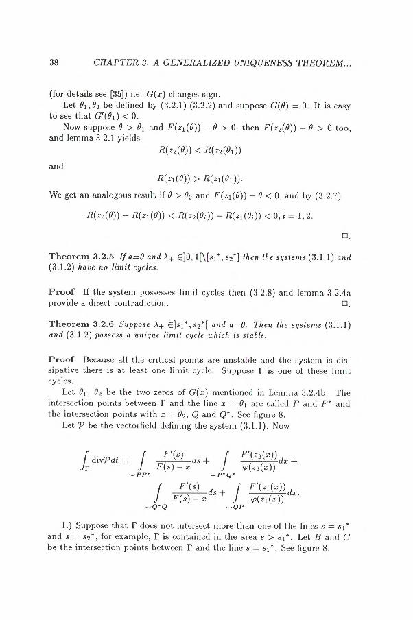
(for details see [35]) i.e. G(x) changes sign. Let 91,02 be defined by (3.2.1)-(3.2.2) and suppose G(0) = 0. It is easy

to see that G101 ) < 0. Now suppose 0 > 01 and F(zi (0)) — 0 > 0, then F(z2(0)) — 0 > 0 too,

and lemma 3.2.1 yields R(z2(0)) < R(z2(01))

and

R(zi(0)) > R(zi(01))»

We get an analogous result if 0 > 02 and F(zi (0)) — 0 < 0, and by (3.2.7)

R(z2(0)) — R(zi (0)) < R(z2(0 )) — R(zi (0i)) < 0, i .= 1,2.

3.

Theorem 3.2.5 If a=0 and Ä4. E]0,1[Msi*, .8 21 then the systems (3.1.1) and (3.1.2) have no limit cycles.

Proof If the system possesses limit cycles then (3.2.8) and lemma 3.2.4a provide a direct contradiction. O.

Theorem 3.2.6 Suppose A+ asi*, s2*[ and a=0. Then the systems (3.1.1) and (3.1.2) possess a unique limit cycle which is stable.

Proof Because all the critical points are unstable and the system is dis-sipative there is at least one limit cycle. Suppose F is one of these limit cycles.

Let 01 , 02 be the two zeros of G(x) mentioned in Lemma 3.2.4b. The intersection points between F and the line x =- 01 are called P and P* and the intersection points with x = 92, Q and Qt. See figure 8.

Let P be the vectorfield defining the system (3.1.1). Now

divPdt = F'(s) ds

Fl.z2(x)) d

J so(z2(x)) x F(s) — x '-PP. --P•Q•

f F) F(:

(s) x

ds F<;((zzii((xx))))dx

1.) Suppose that F does not intersect more than one of the lines s = s i * and s = 82*, for example, F is contained in the area s > si * . Let B and C be the intersection points between F and the line s = .8 1 *. See figure 8.

Jr

3.3.2. THE CASE a r, 0 39

The first term can be written as

[F(E1) 1 1

JF(P) F — xl(F) F — x2(F))dF

where xi(F) < x 2(F) by lemma 3.2.4b. In a similar manner it can be shown that the third term is below zero.

The sum of the second and the fourth term is

02

dx [R(zi(x))— R(z2(x))1—.

del X

When F(sp)> F(sQ), z2(x)> sp. and zi (x) < sp from which it follows

R(z2(x)) — R(zi (x)) < R(sp.) — R(sp) 5 0

by (3.2.7) and Lemma 3.2.4b. The case r E Isis < s2*} can be considered in a similar manner. 2.) Suppose I' intersects s = $j* and s =-. 82* . Suppose PP* intersects s = Si* and s = 82*. (No problems will occur

with the first term if PP* intersects only one of the lines s = si* and s = 82*). Then it is possible to determine a point L e r satisfying

F(SL) = F(s) F (sp)

X L < xp.

The integral f Fi(s)

ds F(s)— x

—PL can be rewritten as

1F(3L) 1

j«,,• ) ( F — X2(F) F — xi(F) )dF

where x i (F(s)) > x 2(F(s)) if s [s1*,E s2 ]. In a similar manner we obtain

P(s) F(s) — x

ds <0

and the value of the third term is below zero. Now let Bi and Ci be the intersection points between P and the line

s = 81*. Define B2 and C2 in a similar way as in figure 9. Put .A equal to the area between the lines s = 81* and s = s2* .


i) Suppose P, P* , Q , Q* E AC. It is easy to show that the second and the fourth term are both negative.

ii) Suppose two of the points either P,Q or P* , Q* are contained in A. We can apply the technique introduced in 1.).

iii) Suppose one of the points, for example, P is contained in A as in figure 9. Then it is possible to determine a point Bi* and we can apply the proof in 1.) to the arcs H I P and P*Bi* and apply 2.i) to the arcs s.--,Bi*Q* and

iv) Suppose two of the points either P,Q* or P* ,Q, belongs to A. We can determine two points Bi* and C2* or B2* and Ci*, resectively, and carry out a proof analogous to the proof of 2.iii). O.

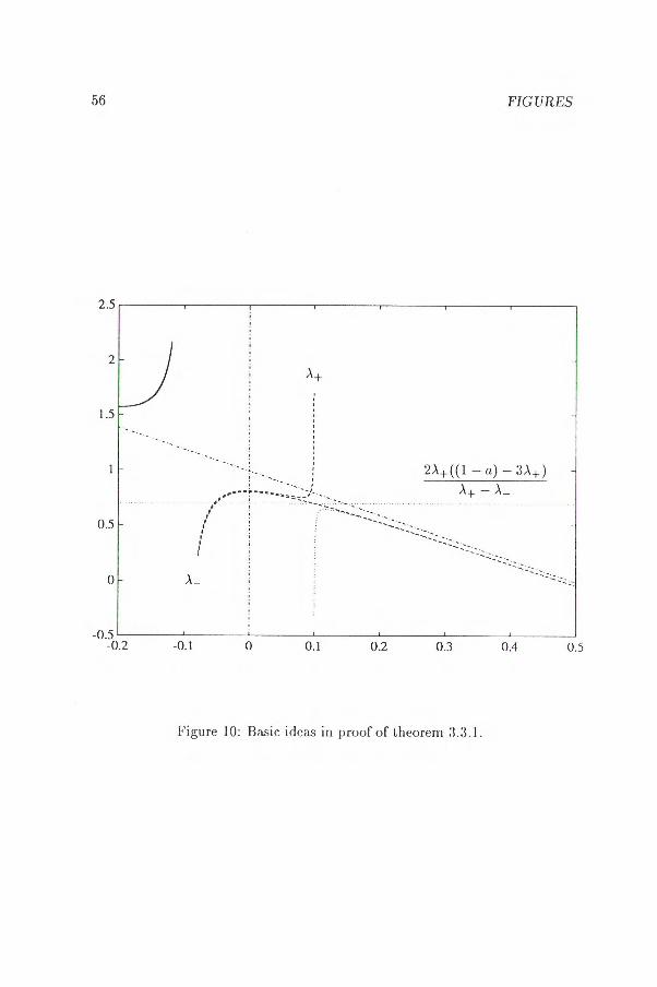
3.3 The general case Theorem 3.3.1 The systems (3.1.1) and (3.1.2) have no limit cycles if

A+ e10, s21.

Proof Only the case A+ E10, s1*[ requires some comments, and even in this case it remains to prove that

see figure 10. Put

R(si ) > R(s2), Vsi s2, si E)0, X+[, S2 EPt+, 1{,

K = 2A+ ((1 — a) — 34)

A+ —

and Ao = A+ + A_. We shall show that R(si) > K > R(s2)• Since the denominator changes sign in A+ this is equivalent to

(2A+ — A0)(-2s3 + (1— a)s2 —b)-2A+(s2 — Aos A+ A_)((1 — a) — 3A+ ) < 0

Define F(s) = —2s3 + (1 — a)s2 — b

then the inequality above can (after some technical considerations) be written in the form

(s—A+ )2[2(A0 -24)s—(242 -4A+Aol-A0(1—a))1+(2A+ —A0 )F*1 (A+ ) <0.

Because A0 <(1 - a)/2 we have

2A2+ — 4A+A0 — A0(1 — a) > 0

3.3.3. THE GENERAL CASE 41

and A o — 2A+ <0.

n.

Theorem 3.3.2 Suppose A+ Elsi*, 82*[. Then the systems (3.1.1) and (3.1.2) possess a unique limit cycle which is stable.

Proof Note that

aR(s) = F1(s)f(s)

, "Sb(s)

and hence, by theorem 2.9.3 we have to prove lemma 3.2.1, ie R(s) decreases in ]0, A+[ and ]A+ , 1[.

For basic constructions, see figure 11. We have

(s) = R(s)

(13 r)(s A+)2 (s — --)2

where

R(s) = 2s(—s3 + 342s — 42(1 — a) b) ±

Ä0 (4s3 — 6A..E.s2 — (1 — a)s2 -I- 2)+ (1 — a)s — b).

Now R.(4) = (Ao — 24)n(4)

= —2n(4)

n(4) = —124(4 — )o ) — 2(1 — a).

The second derivative of R(s) is a parabola with maximum in A0 /2 and we can conclude that R.(x) is concave, decreasing and negative for s> A+ .

Suppose R(s) > 0 for some s E [0, 4]. Because R.(0) = —bAo, R.(s) > 0 for some maximum point in ]0, 4[. That maximum has to be in a region where R1,:(s) < 0. Since e(s) > 0 at most in one region around 4/2 we can have R',:(s) < 0 only in two regions of type [4, A+] or [0, s'2] where s'2 > A0/2 > But in the first case we have

R(s) < .1r.()+)(s — A+ ) + R.(4) < 0, s > max(Ao /2, sc.).

Similarly, in the second case, we have R(s) < 0, s < min(A0 /2, s'2) if R':(s) < 0 in [0, s'2] and we have a contradiction. 0.

Remark 3.3.3 Conditions for at least two limit cycles have been given in [34]. To obtain this result a < 0 is allowed, but a2 < 4b. This will imply a non-monotonic functional response.

Chapter 4

Summary

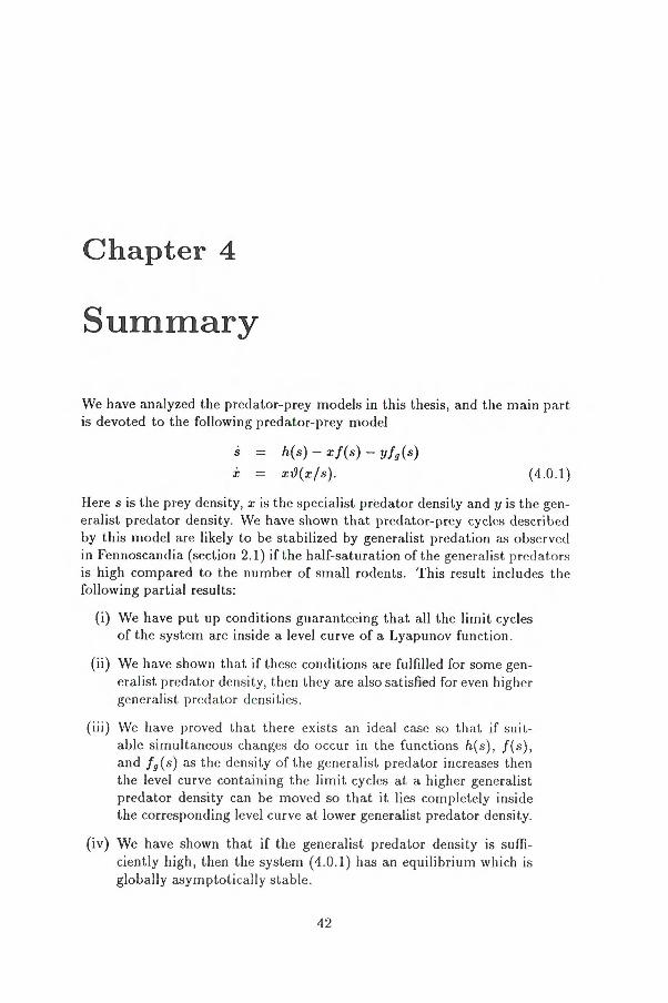
We have analyzed the predator-prey models in this thesis, and the main part is devoted to the following predator-prey model

h(s) — x f(s) — yfg (s)

xt9(x/s). (4.0.1)

Here s is the prey density, x is the specialist predator density and y is the gen-eralist predator density. We have shown that predator-prey cycles described by this model are likely to be stabilized by generalist predation as observed in Fennoscandia (section 2.1) if the half-saturation of the generalist predators is high compared to the number of small rodents. This result includes the following partial results:

(i) We have put up conditions guaranteeing that all the limit cycles of the system are inside a level curve of a Lyapunov function.

(ii) We have shown that if these conditions are fulfilled for some gen-eralist predator density, then they are also satisfied for even higher generalist predator densities.

(iii) We have proved that there exists an ideal case so that if suit-able simultaneous changes do occur in the functions h(s), f(s), and f9 (s) as the density of the generalist predator increases then the level curve containing the limit cycles at a higher generalist predator density can be moved so that it lies completely inside the corresponding level curve at lower generalist predator density.

(iv) We have shown that if the generalist predator density is suffi-ciently high, then the system (4.0.1) has an equilibrium which is globally asymptotically stable.

42

43

We have given examples showing that if the half-saturation of the gen-eralist predators is not high compared to the number of small rodents, then multiple equilibria and multiple limit cycles may occur as the density of generalist predators increases. Complicated global bifurcations may also be constructed in related systems.

We have compared our system to a more well-known class of predator-prey systems, the Huang models (section 2.9). The most important result of this comparison is that the outermost limit cycle of a special Huang model will contain all the limit cycles of our model. Uniqueness of limit cycles have also been proved for the Huang model in a special case.

Bibliography

[1] Roger Arditi, Lev R. Ginzburg. Coupling in predator-prey dynamics: Ratio dependence. J. Theor. Biol., 139:311-326, 1989.

[2] A. ,71. Ea3LIKHII. MATeMaTIPieCKaS1 6H04)143HKa 53asimo,qett cuspoumx nonpummtt. Hapca, Moncsa, 1985.

[ 3] Cheng Kuo-Shung. Uniqueness of a limit cycle for a predator-prey sys-tem. SIAM Journal on Mathematical Analysis, 12(4):541-548, 1981.

[4] D. Chitty. The natural selection of self-regulatory behaviour in animal populations. Proc. Ecol. Soc. Austr., 2:51-78, 1967.

[ 5] M. Farkas, H. I. Freedman. Stability conditions for two-predators one prey systems. Acta Appl. Math., 14(1-2):3-10, 1989.

[6] M. Farkas, H. I. Freedman. The stable coexistence of competing species on a renewable resource. J. Math. Anal. Appl., 138:461-472, 1989.

[ 7] H. I. Freedman. Deterministic Mathematical Models in Population Ecol-ogy. Marcel Dekker, inc, 270 Madison Avenue, New York, New York 10016, 1980.

[8] John Guckenheimer, Philip Holmes. Nonlinear Oscillations, Dynami-cal Systems, and Bifurcations of Vector Fields. Applied Mathematical Series. Springer-Verlag, New York, 1983.

[ 9] Ilkka Hanski, Lennart Hansson, Heikki Henttonen. Specialist predators, generalist predators and the microtine rodent cycle. Journal of Animal Ecology, 60, 1991.

[10] Lennart Hansson, Heikki Henttonen. Rodent dynamics as community processes. Trends in Ecology and Evolution, 3:195-200, 1988.

[11] Morris W. Hirsch, Stephen Smale. Differential Equations, Dynamical Systems, and Linear Algebra. Pure and Applied Mathematics. Academic Press, New York, 1974.

44

BIBLIOGRAPHY 45

[12] Josef Hofbauer, Joseph W.-H. So. Multiple limit cycles for predator-prey models. Mathematical Biosciences, 99:71-75, 1990.

[13] Birger Hörnfeldt. Cycles of voles, predator, and alternative prey in boreal Sweden. PhD thesis, University of Umeå, Sweden, 1991.

[14] S. B. Hsu, S. P. Hubell, Paul Waltman. A mathematical theory for single-nutrient competition in continuos cultures of micro-organisms. SIAM J. Appl. Math., 32(2):366-382, March 1977.

[15] S. B. Hsu, S. P. Hubell, Paul Waltman. Competing predators. SIAM J. Appl. Math., 35(4):617-625, December 1978.

[16] Huang Xun-Cheng. Uniqueness of limit cycles of generalized Lienard systems and predator-prey systems. Journal of Physics A, Mathematics and General, 21:L685—L691, 1988.

[17] Huang Xun-Cheng. Existence of more limit cycles in general predator-prey models. Journal of Physics A, Mathematics and General, 22:L61—L66, 1989.

[18] Huang Xun-Cheng. Relative positions of limit cycles in a Kolmogorov-type system. Journal of Physics A, Mathematics and General, 22:L317—L322, 1989.

[19] Huang Xun-Cheng, Stephen J. Merill. Conditions for uniqueness of limit cycles in general predator-prey systems. Mathematical Biosciences, 96:47-60, 1989.

[20] James P. Keener. Oscillatory coexistence in the chemostat. SIAM J. Appl. Math., 43(5):1005-1018, October 1983.

[21] C. J. Krebs, J. H. Myers. Population cycles in small mammals. Advances in Ecological Research, 8:268-400, 1974.

[22] Y. Kuang. Global stability of Gause-type predator-prey systems. J. Math. Biol., 28:463-474, 1990.

[23] Yang Kuang. Limit cycles in a chemostat related model. SIAM J. Appl. Math., 49(6):1759-1767, December 1989.

[24] Loiu Lii-Perng, Cheng Kuo-Shung. Global stability of a predator-prey system. J. Math. Biol., 26:65-71, 1988.

[25] Loiu Lii-Perng, Cheng Kuo-Shung. On the uniqueness of a limit cycle for a predator-prey system. SIAM Journal on Mathematical Analysis, 19(4):867-878, 1988.

46 BIBLIOGRAPHY

[26] R,. M. May. Complexity and Stability in Model Ecosystems. Princeton University Press, Princeton, 1973.

[27] R. M. May, editor. Theoretical Ecology: Principles and Applications. Blackwell Scientific Publications, 1976. (Second edition 1981).

[28] Johan Metz, Odo Diekmann. The Dynamics of Physiologically Struc-tured Populations. Springer-Verlag, Berlin, Heidelberg, 1986.

[29] J. D. Murray. Mathematical Biology. Springer-Verlag, New York, 1989.

[30] A. Pazy. Semigroups of Linear Operators and Applications to Partial Differential Equations. Springer-Verlag, New York, 1983.

[31] R. Reissig, G. Sansone, R,. Conti. Qualitative Theorie Nichtlinearer Dif-ferentialgleichungen. Editioni Cremonese, 1963.

[32] M. L. Rosenzweig, R. H. MacArthur. Graphical representation and sta-bility conditions of predator-prey interactions. The American Naturalist, XCVII:209-223, july-august 1963.

[33] N. C. Stenseth. Mathematical models of microtine cycles: Models and the real world. Acta Zool. Fennica, 173:7-12, 1985.

[34] B. B. Blmorpa,aon. ripe,ReJ11.11Ide EVAKJIbI cmcTemia inammoencT-nrotimx nonyn.snviti (Limit cycles of interacting populations systems). Becminc Hemturpacxoro YmthepcwreTa, Cep. 1, 2(8):13-17, 1990.

[35] B. B. BimorpaAon, A. B. OcHnon. 0 npeiLenwii,rx gmcnax °Anon pAymepxon ckicTemm. (Uniqueness of a limit cycle in a two-dimensional system). gen. B BI/IEHT14, 1160-B87, 1987.

[36] Dariusz M. Wrzosek. Limit cycles in predator-prey models. Mathematical Biosciences, 98:1-12, 1990.

[37] Ye Yan-Qian et al. Theory of Limit Cycles. American Mathematical Society, second edition, 1986.

[38] Zhang Zhi-Fen. Proof of the uniqueness theorem of limit cycles of gen-eralized Lienard equations. Applicable Analysis, 23:63-76, 1986.

V(2.1.2)

FIGURES

47

1.2

0.2 0.4 0.6 0.8 1 1.2 1.4 1.6 1.8 2

Figure 1: The regions V(2 2) and D(2 1 2) for a system of type (2.1.2) with the more general functional response (2.5.5) r 1, K =- 1, c = 1, y = 1, y = 0, q -= 1/5, al =- 0.015, b1 =-• 0.005

1

0.8

0.6

0.4

0.2

oo

48 FIGURES

0 0.1 0.2 0.3 0.4 0.5 0.6 0.7 0.8 0.9

Figure 2: Isoclines for the system (2.1.3) for the parameter values r = 1, K= 1, c = c = 17= 1 and b = 1/1000 for y = 0 and y 2/30

1

0.8

0.6

0.4

0.2

0

-0.2

0.5 1

0.5

0.4

0.3

0.2

0.1

0o

0.1

oo 05

0.3

0.2 fg(s)

FIGURES

49

Figure 3: Simultaneous changes of the functions f(s), h(s), f 9 (s) in the model (2.2.1) for the ideal case described by Theorem 2.6.4 together with the changes in the isoclines for y = 0 (solid), y 0.4 (dashed), 0.8 (dashdotted), 1.2 (dotted). The system corresponding to y = 0 is (2.1.2) with the more general functional response (2.5.5) and r 1, K = 1, c ---,- 1, 7 = 1, a l 0.015, b l 7=- 0.005

50 FIGURES

Figure 4: Multiple limit cycles for the system (2.1.3) in the case r =7_ K = 5 , c = 1, 7 = 1, y = 49/8, a l = 1/100, b2 = 3/4, q = 5/8

-

_

_

FIGURES 51

Oo 0.5 1 1.5 2 2.5 3 3.5 4

Figure 5: Rough view of the system (2.8.1) in the case r = 5 --, K = 5.--,

c = 1, 7 -= 1, y = 49/8, a l = 1/100, b2 -= 3/4, q = 1/1.465, so = 0.99, w = 1500, z = 0.01

4

3.5

3

2.5

2

1.5

1

0.5

52 FIGURES

1.03

1.02

1.01

1

0.99

0.98

0.97

0.96

0.95 0.95

0.96

0.97

0.98

0.99

1

1.01

1.02

1.03

Figure 6: Multiple limit cycles outside a saddle in the system (2.8.1) in the case r = 5, K = g, c = 1, -y = 1, y =. 49/8, a l = 1/100, b2 = 3/4, q = 1/1.465, 80 = 0.99, w =- 1500, z = 0.01

FIG URES 53

1.0080

1.0075

1.0070

1.0065

1.0060

1.0055

1.0050

1.0045

1.0040

1.0035

1/17 (K , o )

147; ( ,

wis (s; x;

-V-

1.0030 0.6805 0.6810 0.6815 0.6820 0.6825 0.6830 0.6835

Figure 7: Successive PoincaK-plots of the stable manifolds of (4,4) and the unstable manifold of K, 0) in the cross-section s = 0.998 against the parameter value of q (horizontal axis) and the value of x (vertical axis) for the system (2.8.1) in the case r = 5, K = 5-›, c = 1, -y 1, y -= 49/8, a l = 1/100, b2 -= 3/4, so = 0.99, w = 1500, z = 0.01

A -

•

- 01 02

Q*

`. C

54 FIGURES

oo

0.2 0.4 0.6 0.8 1 1.2 1.4 16

Figure 8: Case 1

1.2

0.8

0.6

0.4

0.2

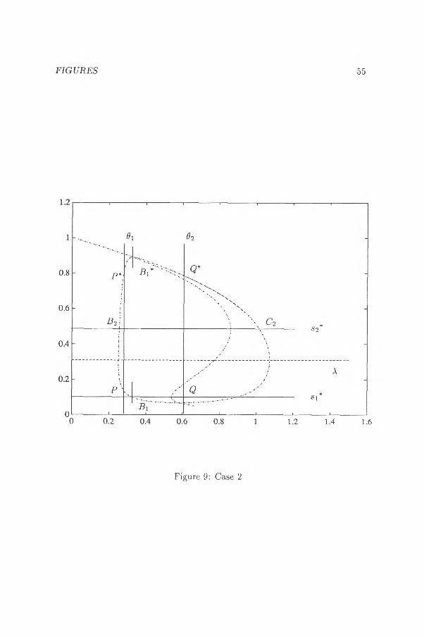
FIG URES 55

1.2

1

0.8

0.6

0.4

02

B2 ; ‘,, C2 $9*

0.2

oo 0.2

0.4

0.6

0.8

1

1.2

1.4

16

Figure 9: Case 2

56 FIGURES

2.5

2

1.5

1

0.5

0

-0.5 -0.2 -0.1

0

0.1

0.2

0.3

0.4

05

Figure 10: Basic ideas in proof of theorem 3.3.1.

FIGURES

57

x10-3 0.5

0

-0.5

-1.5

-2

-2.5

-3

-3.50

0.05 0.1 0.15 0.2 0.25 0.3 0.35 04

Figure 11: Basic ideas in proof of theorem 3.3.2.

ISSN 0280-8242 HÖGSKOLANS TRYCKERI LULEÅ

LICENTIATE THESIS - DIVA

Documents

Transcript of LICENTIATE THESIS - DIVA