Reactive Async - DIVA

IN DEGREE PROJECT COMPUTER SCIENCE AND ENGINEERING,SECOND CYCLE, 30 CREDITS

, STOCKHOLM SWEDEN 2016

Reactive AsyncSafety and efficiency of new abstractions for reactive, asynchronous programming

SIMON GERIES

KTH ROYAL INSTITUTE OF TECHNOLOGYSCHOOL OF COMPUTER SCIENCE AND COMMUNICATION

Reactive Async

Safety and efficiency of new abstractions for reactive, asynchronous programming

SIMON GERIES

Master’s Thesis at CSCSupervisor: Philipp HallerExaminer: Mads Dam

Course: DA222X

AbstractFutures and Promises have become an essential part ofasynchronous programming. However, they have importantlimitations, allowing at most one result and no support forcyclic dependencies, instead resulting in deadlocks.

Reactive Async is a prototype of an event-basedasynchronous parallel programming model that extendsthe functionality of Futures and Promises, supportingrefinement of results according to an application-specificlattice. Furthermore, it allows for completion of cyclicdependencies through quiescence detection of a threadpool.

The thesis demonstrates the practical applicability ofReactive Async by applying the model to a large staticanalysis framework, OPAL. Benchmarks comparing Reac-tive Async with Futures and Promises show an efficiencytrade-off for the flexibility of using the model.

Referat

Reaktiv Asynkronicitet - Säkerhet och effektivitetav nya abstraktioner för reaktiv, asynkron pro-grammering

Futures och Promises har blivit en viktig del avasynkron programmering. Men de har viktiga begränsning-ar, bland annat att tillåta högst ett resultat skrivas ochinget stöd för cykliska beroenden, som istället resulterar ibaklås.

Reactive Async är en prototyp av en händelsebaseradasynkron parallell programmeringsmodell som utökar funk-tionaliteten hos Futures och Promises, för att stödja föräd-ling av resultat enligt en applikation specifik lattice. Dess-utom möjliggör modellen slutförandet av cykliska beroen-den genom att upptäcka när en tråd pool ej har några oav-slutade uppgifter.

Masteruppsatsen visar att Reactive Async är praktisktillämpbar genom att applicera modellen på ett stort ram-verk för statiska analyser. Prestandatester som jämför Re-active Async med Futures och Promises visar att flexibi-liteten av modellen kompromissas med effektiviteten vidanvändning.

Contents

1 Introduction 11.1 Background . . . . . . . . . . . . . . . . . . . . . . . . . . . . . . . . 21.2 Goal . . . . . . . . . . . . . . . . . . . . . . . . . . . . . . . . . . . . 31.3 Why Reactive Async? . . . . . . . . . . . . . . . . . . . . . . . . . . 41.4 Scala syntax . . . . . . . . . . . . . . . . . . . . . . . . . . . . . . . . 41.5 Ethics . . . . . . . . . . . . . . . . . . . . . . . . . . . . . . . . . . . 51.6 Outline . . . . . . . . . . . . . . . . . . . . . . . . . . . . . . . . . . 5

2 Programming with Reactive Async 72.1 Write operations . . . . . . . . . . . . . . . . . . . . . . . . . . . . . 102.2 Dependencies . . . . . . . . . . . . . . . . . . . . . . . . . . . . . . . 112.3 Callbacks . . . . . . . . . . . . . . . . . . . . . . . . . . . . . . . . . 132.4 Thread pool and quiescence . . . . . . . . . . . . . . . . . . . . . . . 14

3 Implementation 173.1 Cell . . . . . . . . . . . . . . . . . . . . . . . . . . . . . . . . . . . . 17

3.1.1 Callbacks . . . . . . . . . . . . . . . . . . . . . . . . . . . . . 183.1.2 Dependencies . . . . . . . . . . . . . . . . . . . . . . . . . . . 193.1.3 State . . . . . . . . . . . . . . . . . . . . . . . . . . . . . . . . 22

3.2 HandlerPool . . . . . . . . . . . . . . . . . . . . . . . . . . . . . . . . 23

4 Case study 274.1 Purity analysis . . . . . . . . . . . . . . . . . . . . . . . . . . . . . . 274.2 Immutability analysis . . . . . . . . . . . . . . . . . . . . . . . . . . 294.3 Results . . . . . . . . . . . . . . . . . . . . . . . . . . . . . . . . . . . 34

5 Performance evaluation 375.1 Static analyses . . . . . . . . . . . . . . . . . . . . . . . . . . . . . . 375.2 Micro Benchmarks . . . . . . . . . . . . . . . . . . . . . . . . . . . . 38

6 Related Work 436.1 FlowPools . . . . . . . . . . . . . . . . . . . . . . . . . . . . . . . . . 436.2 Habanero-Scala . . . . . . . . . . . . . . . . . . . . . . . . . . . . . . 436.3 LVars . . . . . . . . . . . . . . . . . . . . . . . . . . . . . . . . . . . 44

7 Conclusion and future work 45

Bibliography 47

Chapter 1

Introduction

No more can we rely on achieving faster running programs by increasing the process-ing power of a computer. Most devices are being shipped with multiple processingcores making parallelism and distribution the way to increase performance. Byusing multi-threaded programming, one can utilize all cores in order to make anapplication or system run faster. However, building such systems is not always atrivial task to apprehend due to common hazards encountered in parallel program-ming like race conditions and deadlocks. Because of multiple threads running inparallel on different cores, the order in which threads will finish depends on theprocess scheduler. This can lead to some hard-to-reproduce bugs, putting a lot ofresponsibility on the programmer to consider these things. Moreover, maintainingsoftware systems is costly for companies and organizations. By reducing the like-lihood of introducing bugs in a program, companies can reallocate their resourcesto develop the system, instead of having a high focus on bug hunting, reducing themaintenance cost. Reducing the amount of bugs also adds to the safety aspect of aprogram, making it harder to use applications used in the society in an unintendedway by exploiting bugs. This increases the need to find new abstractions to threadhandling, that can reduce, or even remove the possibilities of a programmer writingan application with incorrect behavior due to the concurrency.

In this thesis, a prototype of a new parallel programming model called ReactiveAsync is introduced. It is implemented using the Scala programming language andis inspired by the LVars deterministic-by-construction parallel programming model[12]. Moreover, the model is an extension of the functionality provided by Futures[6] and Promises [14], where it maintains the expressivity of the Scala versions [5].

A case study was made showing that applying Reactive Async to a Scala-basedstatic analysis from the OPAL static analysis framework [3] could reduce the codesize significantly, while still performing slightly better. However, when compar-ing Reactive Async to Futures and Promises in Scala, by applying similar oper-ations we can observe a significant performance loss due to the additional over-head. Finally, in terms of memory usage, Futures and Promises are significantlymore light weight compared to Reactive Async.

1

CHAPTER 1. INTRODUCTION

1.1 Background

One risk factor when developing multi-threaded applications is mutability, which isa key concept in object-oriented (OO) and imperative languages such as Java, C++and C#. Mutating a shared variable, that is, a variable that can be accessed bymultiple threads at the same time, has to be done in a mutual exclusive fashion. Byusing mutual exclusion with locks, one can prevent unexpected interleaving threadscausing bugs, at the cost of the parallelism of an application. Therefore, one strivesto achieve an asynchronous parallel programming model, that is, a lock-free modelcontaining no thread-blocking parts in the code.

Sometimes, limitations can be a good thing, such as forcing or encouraging aprogrammer to use immutable data [10]. Another limitation used by pure data-parallel languages is to force concurrent tasks to independently produce new results[9]. Though these strategies are mostly adopted by functional languages, an in-creasing number of OO and imperative languages are blending the two paradigmstogether, such as Java 8 and Scala, giving languages some benefits of both worlds.

Although shared variables potentially introduce problems, some algorithms aremore naturally written using shared variables. In those cases, one can use atomicoperations such as compare-and-swap (CAS), which guarantees variable changes tobe done by one thread at a time. CAS operations usually take two parameters,the expected current value in a variable and the new value that is to be set. If thecurrent value matches the value in the variable, it replaces the current value withthe new, otherwise it fails to set the new value and returns false.

However, using CAS operations does not guarantee determinism in a concurrentprogram. Threads may still be scheduled to execute in different orders at differentruns of an application. Guaranteed determinism, that is, an execution succeedsevery run with the same result is a rarely pursued goal in concurrent programmingdue to the difficulty of achieving it. Instead, deterministic parallel programmingmodels, such as the LVars model [11], and deterministic data structures, such asFlowPools [17], use a quasi-deterministic definition which states: If an executionfails for some execution schedule, then it fails for any execution schedule, other-wise it always terminates with the same final result.

There are many programming models that use more event-based approaches[12, 15, 5] to communicate results in different forms. One event-based approach isto allow attaching defined callback functions to a construct, that are triggered andrun asynchronously once some intermediate or final result has been computed [12].Another is to allow subscription and notification communication, where a dependentprocess running on a thread can subscribe to a process of another thread. When aresult is received, a notification message is sent to all subscribers [15].

Using event-based approaches based on callback functions can have multipleadvantages. Utilizing such a model encourages running task-unique threads, whichmakes it safe to run asynchronously. Although chopping a program into threadsthat are task-unique is not always possible, an event-based approach raises theabstraction level, making it more explicit what each task depends on.

2

1.2. GOAL

Some of the most commonly used models are Futures [6] and Promises [14].In Scala, a future is a reference to a future value and a promise is a one timewritable placeholder for a value. The result of a future can be determined by anasynchronously running function. These models are event-based, where one candefine callback functions to run once a future or promise has a result. However,Futures and Promises have some limitations, such as allowing at most one write.Consider a case where a value is being computed, and at one point in the compu-tation, we have a preliminary result we want to write. Later in the computation,we achieve a new better result we want to update previous result with. Refiningresults in such a way is not possible with Futures and Promises because of the onetime writable limitation. One possible workaround for this is to create an arrayof futures, where each future can hold an intermediate result. Though this soundsfeasible, the amount of intermediate results needed is not always possible to deter-mine beforehand. Another limitation is that futures do not support resolving cyclicdependencies, where such dependencies result in a deadlock.

It is very important that program executions are efficient on modern multi-core processors. Today, the energy consumption of data centers has been shownto have an environmental impact [4]. Therefore, it is essential that one utilizesthe capacities of data centers in the most efficient way possible. Given this, itis important to evaluate performance and efficiency of the implementation of Re-active Async, which is done in chapter 5.

1.2 Goal

The aim of this thesis is to implement a prototype parallel programming model,namely Reactive Async, where the objective of the model is to be an extensionof Futures and Promises, both in functionality and expressivity. For the extendedfunctionality, it should support dependency handling, allowing for cyclic dependencyresolution. Also, it should support refinement of results. The implementation ofthe model is to include the following key properties:

• Performance. Reactive Async should have reasonable performance, com-pared to Futures and Promises for small tasks, measured in execution time.

• Determinism. Reactive Async should include some determinism propertiesby limiting write operations to be monotonic (see chapter 2). However, noclaims are made that the model itself is deterministic.

• Practicality. Reactive Async should be applicable to real scenarios and tasks.Also, it should be applicable to large applications and heavy use of the model.

3

CHAPTER 1. INTRODUCTION

1.3 Why Reactive Async?There are already many existing usable parallel programming model and all havetheir advantages and disadvantages. A model usually tries to tackle some specificproblem or use case which eases the process of creating a concurrent application. Inaddition some try to reduce the possibility of common concurrent hazards occurring.All this while still keeping good performance. Reactive Async also attempts to tacklethese issues. The following shows what characterizes Reactive Async.

An asynchronous model Reactive Async is an asynchronous parallelprogramming model, that is, it is completely lock-free. This means, thereis no thread-blocking used in the model to synchronize two threads, whichdoes not reduce parallelism of the model. Instead, Reactive Async usesCAS operations when a state changes.

Builds on Futures and Promises Because Futures and Promises are alreadywidely used and effective, Reactive Async builds on that functionality. By preserv-ing many of the key features in Futures and Promises, one can use Reactive Asyncthe same way as one would use Futures and Promises.

Has internal dependency control Concurrent programming has many usecases where one threads result depends on some result of another computing thread(section 4.1 and 4.2 show two implemented examples). An example of this is anapplication applying the Producer and Consumer concurrency model, where sev-eral threads produce data and other threads uses, or consumes, that data in someway. Dependency handling is supported in Reactive Async in the form of events toease the use of thread dependencies and still keep the model asynchronous. More-over, the dependency handling allows for detection of cyclic dependencies, whichis used for preventing deadlocks or incomplete results.

Refinement of results Futures and Promises only allow writing one time, whichcan be a troublesome limitation for some use cases. Refinement of results is sup-ported in Reactive Async, by allowing shared variables to be updated with somelimitation, which is explained in chapter 2 (see section 4.2 for use cases).

Determinism properties Reactive Async contains some determinism propertiesby allowing for monotonic updates through lattice-based operations (see chapter 2).

1.4 Scala syntaxThe following gives a brief description of how the Scala syntax is used in this thesis,in order to make it more understandable for readers not familiar with the syntax.

4

1.5. ETHICS

val defines a final value

var defines a variable

def defines a method

Unit void

trait similar to Java interface

object defines a new singleton object

sealed trait used as enums

case object used as enum values

Finally, a method with the name apply is different from normal methods,and is easier described with an example:

object Print {def apply(s: String) = println(s)

}

Print("Hello")

The Print("Hello") will invoke the apply method in the object Printwith the parameter "Hello".

1.5 EthicsEthical considerations do not apply to this project, since no experiments involv-ing humans or animals were performed.

1.6 OutlineThe next chapter describes the properties of Reactive Async and how it works from aprogrammer’s perspective. Chapter 3 goes into implementation details of the model.Chapter 4 talks about how Reactive Async was used to implement two Scala-basedstatic analyses from the OPAL static analysis framework [3]. Chapter 5 showsperformance results for the static analyses implemented using Reactive Async, andmicro benchmarks, comparing Reactive Async to Futures and Promises. Chapter6 compares Reactive Async with existing parallel programming models and datastructures, showing the similarities and differences between them. Finally, chapter7 concludes and points in which direction the model needs to move next.

5

Chapter 2

Programming with Reactive Async

Reactive Async is a prototype implementation of an event-based asynchronous par-allel programming model that can be used to create multi-threaded applications.The model can be decomposed into five parts: Cell, CellCompleter,HandlerPool, Key and Lattice.

A cell is a shared memory location, that is, an object that can be accessed andwritten to by several threads at the same time. It is also a placeholder for some value,meaning it contains some value similar to how a future contains a value. Writing toa cell is done by using a cell completer, similar to how a promise is used for writingto a future. However, the write operations are limited to being monotonic, wherethe writes are defined by an application-specific lattice. Furthermore, a cell can becompleted, meaning permanently locking a cell from further changes.

A lattice is a partially ordered set, that is, a set where each element is rankedby some order. For example, a natural number lattice can be defined, where ev-ery element is a natural number, and the order of the elements are defined by themagnitude of their number (as shown in figure 2.1). Another example, is a setlattice, where every element is a set, and the order of each element is defined bythe set inclusion. Every two elements in a lattice have a unique least upper bound,or join. In Reactive Async, the lattice is represented as the trait Lattice[V],where V is the type of the value in a cell.

trait Lattice[V] {def join(current: V, next: V): Vdef empty: V

}

A Lattice[V] is required to define a join operation and some empty element.join takes two elements and returns their least upper bound, and empty de-fines the smallest element of the lattice.

Example 2.1.class NaturalNumberLattice extends Lattice[Int] {override def join(current: Int, next: Int): Int = {if(current < next) nextelse current

7

CHAPTER 2. PROGRAMMING WITH REACTIVE ASYNC

}override def empty: Int = 0

}

Example 2.2.class SetLattice[V] extends Lattice[Set[V]] {

override def join(current: Set[V], next: Set[V]): Set[V] = {current union next

}override def empty: Set[V] = Set()

}

Example 2.1 and 2.2 shows implementations of the natural number lattice andthe set lattice. For the natural number lattice, the join of two numbers is themaximum. Given an instance val nnl = new NaturalNumberLattice,an example of the join operation is nnl.join(2, 5) = 5. The element withthe lowest order in the natural numbers lattice is 0. For the set lattice, thejoin of two sets is defined by the union of the two sets. Given an instanceval sl = new SetLattice[Int], an example of the join operation issl.join(Set(1, 2), Set(2, 3)) = Set(1, 2, 3). The element withthe lowest order in the set lattice is an empty set.

Figure 2.1: Shows a natural number lattice order, where the element with the lowestorder is the bottom element, and the one with the highest order is >.

Tying together Cell with Lattice, the empty element is the initial value ofthe cell and join is used when writing to a cell. A write does not actually inferwriting some specific value, instead, it means writing the least upper bound of thecurrent value of the cell and the new value. More formally:

Definition 2.3. A write to a cell with some value next, implies writing the resultvalue of lattice.join(current, next), where lattice is an instance of asubclass to Lattice[V] and current is the current value in a cell.

8

If we take an example of a cell that uses the set lattice, containing thecurrent value Set(2, 3), then writing Set(2, 4) to that cell, it willactually result in receiving Set(2, 3, 4).

The purpose of using a lattice to limit writes to a cell is to reducethe risk of introducing non-determinism to an application. Moreover, insome cases it could also help by explicitly showing non-determinism in anapplication by throwing an exception.

For example, if we have a lattice that allows for a one time write to a cell(see section 4.1 for an example of such a lattice), it would explicitly show bythrowing a LatticeViolationException if an application was to write twicewith two different values to the same cell.

trait Key[V] {val lattice: Lattice[V]

...}

What lattice a cell receives is determined by the key the cell receives when created(as shown in example 2.4). Key[V] requires all subclasses to hold some instanceof type Lattice[V], that is used to assign a cell’s initial value and determineshow the monotonic write operations should work for a cell by using join. For theNaturalNumberLattice, the key looks like the following:

object NaturalNumberKey extends Key[Int] {val lattice = new NaturalNumberLattice

...}

There are two different CellCompleters in Reactive Async, a traitCellCompleter[K <: Key[V], V] and a singleton object CellCompleter.The trait is used for describing the API of a cell completer, taking two type parame-ters, a subtype of Key[V], and a value type. The singleton object CellCompleteris a factory object used to create both a cell completer and a cell. A cell completerworks as a placeholder for the cell it created and is used to operate on that cell.

Example 2.4.val pool = new HandlerPoolval cellCompleter =

CellCompleter[NaturalNumberKey.type, Int](pool, NaturalNumberKey)val cell = cellCompleter.cell

Example 2.4 describes how to create a cell completer and a cell that are restrictedto the natural number lattice. As shown, CellCompleter takes two parameters,a key object, which has the same type as specified in the type parameter, and aHandlerPool object. HandlerPool is explained in section 2.4.

9


2.1 Write operationsA cell completer is used to directly apply a write to the cell it is holding.There are two methods supported for this:

def putNext(x: V): Unitdef putFinal(x: V): Unit

• putNext(x)

– Incomplete cells. When writing to an incomplete cell, putNext(x)writes some value x.

– Complete cells. When writing to a completed cell, the result ofputNext(x) depends on what the result of the join is. The oper-ation fails, that is, throws an exception if join(current, x) !=current, otherwise nothing happens, that is, if join(current, x)== current.

• putFinal(x)

– Incomplete cells. When writing to an incomplete cell, putFinal(x)first writes x if it is an element with a higher order than the current value,or if the two values are equal, then finishes by completing the cell. Theoperation fails if the current value in the cell is a higher order elementthan x.

– Complete cells. When writing to a completed cell, if current != x,then putFinal(x) fails, otherwise nothing happens.

If there are many threads performing a putNext on one cell at the same time,the cell will always result in the same value, due to each write being a lattice join op-eration. For example, for the natural numbers lattice, it is the element with the high-est number. However, if a thread performs cc.putNext(5) for a cell completercc and some other thread performs a cc.putFinal(3), then the execution willalways fail, no matter which threads succeeds in writing first. This is because, either

1. cc.putNext(5) writes to a complete cell containing the value 32. or cc.putFinal(3) writes to an incomplete cell containing the value 5

which according to the explanations above results in failing.However, if cc.putNext(1) is performed by a thread and cc.putFinal(2)

is performed on another thread, it will always result in a completed cell with thevalue 2. Finally, if you have many threads performing a putFinal on one cell at thesame where one of the elements written is different from the others, then the execu-tion always fails, because of the case when performing putFinal on a complete cell.

This explains the determinism properties achieved by having monotonic writeoperations. It also shows that there can be no contention when completing a cellthat can affect the determinism property.

10

2.2. DEPENDENCIES

2.2 DependenciesDependency handling is provided in Cell, where one can explicitly specify that theresult of a cell depends on the result of another cell. Explicit dependency assignmentis mainly used so Reactive Async can keep track of all the dependencies, in orderto later find the cyclic dependencies and resolve them.

Definition 2.5. If cell A depends on cell B, then A is referred to as the dependent,B as the dependee, and the relationship expressed as A dep B.

There are two types of dependencies that can be assigned by invoking thefollowing two methods of the dependent:

def whenNext(dependee: Cell[K, V],predicate: V => WhenNextPredicate,shortcutValue: Option[V]): Unit

def whenComplete(dependee: Cell[K, V],predicate: V => Boolean,shortcutValue: Option[V]): Unit

These two methods cause a callback function to be triggered that can write to thedependent cell when the dependee is written to with a new value. However, thiswill be referred to as a dependency being triggered.

The parameters of the method are the following:

– dependee, which is the dependee cell– predicate, which is a function– shortcutValue, which is the new value to possibly be written to the de-

pendent cell

The predicate function determines if the shortcutValue is written to thedependent cell once the dependency is triggered. Finally, the shortcutValueis an Option,1 which can be defined as Some(v), where the value v is writtento the dependent cell. It can also be defined as None, implying that the valuewritten to the dependent cell is the same value as the new value that was writtento the dependee that triggered the dependency.

That means, if the dependee is written to with value 3, triggering the depen-dency, then the dependent is also written to with value 3. Whenever a depen-dency is assigned, a callback function is created that evaluates the predicate andapplies the changes accordingly. This callback is executed asynchronously when-ever the dependency is triggered. The dependency relationship between two cellsis removed once the dependee is completed. However, what triggers the depen-dency, hinges on the dependency operation.

The whenNext dependency is triggered either when the dependee valuechanges, when it is completed or if the dependee is already completed whenthe dependency is being assigned. Each time the dependency is triggered, the

1http://www.scala-lang.org/api/2.11.8/#scala.Option

11


predicate is evaluated with the written value (the join of the current andnew value). The return type of the predicate is WhenNextPredicate,which is a sealed trait with three case objects extending it. The returned resultdetermines outcome of a triggered whenNext dependency.

DoNothing indicates that nothing happens to the dependent cell.

DoPutNext indicates that the dependency triggers a putNext operation withthe shortcutValue.

DoPutFinal indicates that the dependency triggers a putFinal operation withthe shortcutValue.

Example 2.6.cell1.whenNext(cell2, (x: Int) =>x match {

case 1 => DoPutNextcase 2 => DoPutFinalcase _ => DoNothing

},Some(3))

Example 2.6 shows cell1 assigning a whenNext dependency on cell2, whereif cell2 receives a new value 1, then putNext(3) is performed on cell1.If cell2 receives a new value 2, then putFinal(3) is performed on cell1.Otherwise no changes are made to cell1.

Example 2.7.cell1.whenNext(cell2, (x: Int) =>x match {

case 1 => DoPutNextcase 2 => DoPutFinalcase _ => DoNothing

},None)

Example 2.7 is similar to example 2.6. The difference is that in example 2.6 al-ways write 3 to the dependent, whereas in example 2.7, whatever the writtenvalue to the dependee is the same value written to the dependent. For exam-ple, if cell2 receives a new value 1, then putNext(1) is performed on cell1.If cell2 receives a new value 2, then putFinal(2) is performed on cell1.Otherwise no changes are made to cell1.

The whenComplete dependency is triggered either when the dependee is beingcompleted or if the dependee is already completed when the dependency is assigned.Similar to whenNext, the predicate is evaluated with the written value, but hasa return type Boolean that can only conclude the following:

false indicates that nothing happens to the dependent cell.

12

2.3. CALLBACKS

true indicates that the dependency triggers a putFinal operation with theshortcutValue.

Example 2.8.cell1.whenComplete(cell2, (x: Int) => x == 1, Some(3))

Example 2.8 shows cell1 assigning a whenComplete dependency on cell2,where if cell2 is completed a new value 1, then putFinal(3) is performed oncell1. Otherwise no changes are made to cell1.

It is possible to have both a whenNext and a whenComplete dependencyon the same dependee cell, from the same dependent cell. In this scenario, ev-erything works as previously explained, except that completing the dependee cellonly triggers the whenComplete dependency.

2.3 Callbacks

Similar to Futures and Promises, one can assign callback functions on a cell thatare run asynchronously once triggered. There are two types of callback functions:

def onNext[U](callback: Try[V] => U): Unitdef onComplete[U](callback: Try[V] => U): Unit

onNext The callback function is triggered whenever a cell receives a newintermediate value or is completed if there are no onCompletecallback functions is assigned to the same cell.

onComplete The callback function is triggered once a cell is completed.

Both onNext and onComplete take a function with a parameter of type Try[V]and returns some value of type U. A Try[V] object can either contain Success(v),where v is a succeeded value of type V, or Failure(e), where e is an exception.

Example 2.9.cell1.onNext {

case Success(v) => println("This is my intermediate result: " + v)case Failure(e) => println("Error: " + e)

}cell1.putNext(4)

Example 2.9 shows how to assign an onNext callback to cell1, which is triggeredby the putNext operation on cell1. If it is a successfully written intermediatevalue 4, the callback prints it, otherwise printing the exception. However, one hasto be careful how they are placed due to the asynchronous execution so they canfinish in time before an application is terminated.

13


2.4 Thread pool and quiescenceReactive Async has its own thread handling interface, which is provided by theHandlerPool. When creating an instance of a HandlerPool, one can specifythe number of threads the pool should contain. A pool is used to assign some giventask to be executed on it by calling execute with some given function. Creatinga cell completer requires a pool to be given, which is used to execute the call-back functions asynchronously as tasks on the same pool. Further, HandlerPoolsupports detection of quiescence in a thread pool.

Definition 2.10. A pool is quiescent when there are no unfinished submitted taskscurrently queued or running on it.

This is useful due to two cases where a pool can finish all task executions andbecome quiescent, but still have incomplete cells.

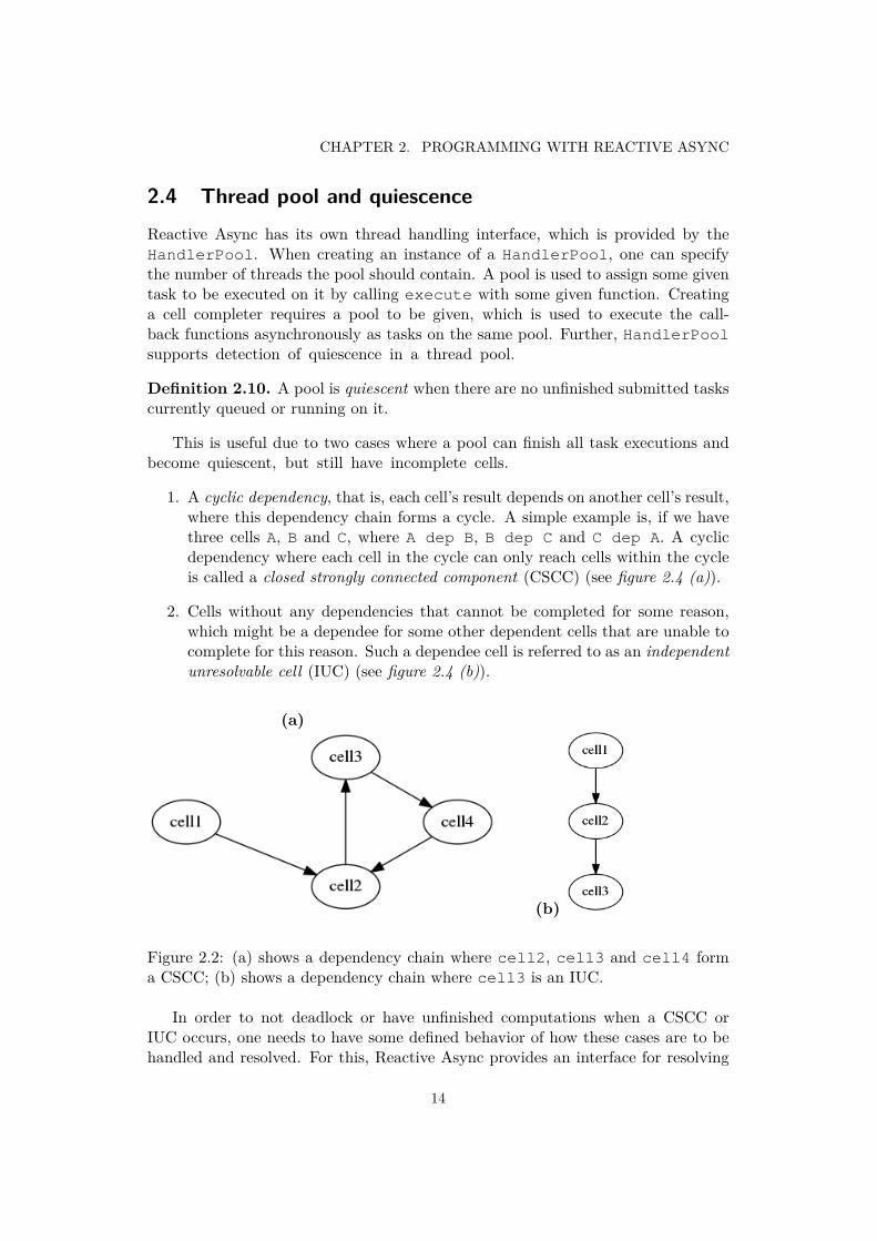
1. A cyclic dependency, that is, each cell’s result depends on another cell’s result,where this dependency chain forms a cycle. A simple example is, if we havethree cells A, B and C, where A dep B, B dep C and C dep A. A cyclicdependency where each cell in the cycle can only reach cells within the cycleis called a closed strongly connected component (CSCC) (see figure 2.4 (a)).

2. Cells without any dependencies that cannot be completed for some reason,which might be a dependee for some other dependent cells that are unable tocomplete for this reason. Such a dependee cell is referred to as an independentunresolvable cell (IUC) (see figure 2.4 (b)).

(a)

(b)

Figure 2.2: (a) shows a dependency chain where cell2, cell3 and cell4 forma CSCC; (b) shows a dependency chain where cell3 is an IUC.

In order to not deadlock or have unfinished computations when a CSCC orIUC occurs, one needs to have some defined behavior of how these cases are to behandled and resolved. For this, Reactive Async provides an interface for resolving

14

2.4. THREAD POOL AND QUIESCENCE

those cells. This is where Key[V] plays a role. Apart from holding an instance ofa lattice used by a cell, Key[V] requires defining two methods:

trait Key[V] {...

def resolve[K <: Key[V]](cells: Seq[Cell[K, V]]): Seq[(Cell[K, V], V)]def default[K <: Key[V]](cells: Seq[Cell[K, V]]): Seq[(Cell[K, V], V)]

}

resolve A method that takes a list of cells, where the dependencies of the cellsforms a CSCC, and returns a list of tuples (cell, value), wherethe first element is a cell, and the second element is the value that cellis to be completed with.

default A method that takes a list of incomplete cells that do not constructa CSCC and returns a list of tuples (cell, value), where the firstelement is a cell, and the second element is the value that cell is to becompleted with.

These methods are invoked by a method called quiescentResolveCell providedin HandlerPool. This method returns a future that can be used to place a barrier,preventing an application to terminate before all results are computed.

Example 2.11.val pool = new HandlerPool(4)pool.execute(() => someHeavyTask())val future = pool.quiescentResolveCellAwait.ready(future, 15.minutes)

Example 2.11 starts by creating a thread pool with 4 threads. Then submits atask to the thread pool which is executed when there is a free thread in the threadpool. The current thread continues and invokes quiescentResolveCell whichreturns a future. The future is used to create a barrier using Await.ready, wherethe current thread waits until all submitted tasks are finished executing or when15 minutes have passed. When all submitted tasks are finished, the pool becomesquiescent. Then quiescentResolveCell resolves all incomplete cells accordingto the resolve and default methods, and finally completes the future, whichconsequently lowers the barrier so the current blocked thread can proceed.

The quiescentResolveCell first finds all CSCCs by using an algorithmprovided by OPAL, a static analysis framework, and then invokes resolve foreach CSCC, with the incomplete cells forming that CSCC. Then finally, defaultis invoked with the rest of the cells, that are incomplete due to some IUCs.

To see two complete static analysis implementations using Reactive Async, go tochapter 4.

15

Chapter 3

Implementation

Reactive Async is a prototype implementation of an event-based asynchronous pro-gramming model implement in Scala. The implementation provides an API us-able for developing concurrent applications using refinable shared variables, ac-cording to an application-specific lattice.

The two major components in Reactive Async, a cell and a thread pool. Acell is represented using two different interface types, where the different interfacetypes are used for reading and writing to a cell. These types are also generic intwo different parts, the value the cell contain and the key which determines thelattice, the resolution of cyclic dependencies and provides default values. The res-olution of a cell ends in a callback function being executed by the HandlerPool,which registers tasks for each execution.

3.1 Cell

The interface type used for reading from a cell is Cell[K, V] and for writingto a cell is CellCompleter[K, V]. However, this CellCompleter[K, V]should not be confused with the factory singleton object CellCompleter,which is used for creating a cell. The following code shows the factorysingleton object CellCompleter.

object CellCompleter {def apply[K <: Key[V], V](pool: HandlerPool, key: K):

CellCompleter[K, V] = {val impl = new CellImpl[K, V](pool, key)pool.register(impl)impl

}}

It creates an object of CellImpl[K, V] which is a class that implements thefunctionality of both Cell[K, V] and CellCompleter[K, V], where K isthe key type and V is the value type. It takes a HandlerPool parameter thatdetermines which pool the cell registers to, which is then used for executing

17

CHAPTER 3. IMPLEMENTATION

the callback functions assigned to the created cell. Then it registers the cell tothe pool and finally returns the CellImpl[K, V] object, which is returnedas the type CellCompleter[K, V]. The Cell[K, V] object is contained inthe CellCompleter[K, V] object, which you can see in example 2.4. TheCellCompleter[K, V] object is used to perform putNext and putFinaloperations on a cell, while the Cell[K, V] object is used for assigning callbacksand dependencies. A cell contains the following information:

• A value: The value the cell holds• Callbacks: The functions that are to be executed when this cell is written to• Dependencies: Which cells this cell depends on

The type of the value a cell holds is determined by the type parameter V, whichis specified at the creation of a cell and a cell completer.

3.1.1 CallbacksCallbacks are separated into two categories:

1. NextCallback2. CompleteCallback

These two sorts of callbacks are represented as classes that contain the necessaryinformation about the callbacks. Both work almost identically, the difference is thatNextCallback is used for onNext typed callbacks, that is, when a cell receivesa new intermediate value, while CompleteCallback is used for onCompletetyped callbacks, that is, when a cell completes.

Objects of NextCallback are created either by assigning onNext callbacksor whenNext dependencies. Similarly, all objects of CompleteCallback are cre-ated either by assigning onComplete callbacks or whenComplete dependencies.Furthermore, all callback objects are stored in the cell that triggers them. Howeverything works for the dependencies is explained in section 3.1.2.

Both NextCallback and CompleteCallback take the following informationas parameters:

– A HandlerPool providing the threads to execute callbacks on– A callback function to execute when triggered– A source cell, that is, the cell used to create the callback

A callback function contained in a NextCallback object will be referred to as aNextCallback, whereas a callback function contained in a CompleteCallbackobject will be referred to as a CompleteCallback.

def onNext[U](callback: Try[V] => U): Unit = {val newNextCallback =

new NextCallback[K, V](pool, callback, this)dispatchOrAddNextCallback(newNextCallback)

}

18

3.1. CELL

def onComplete[U](callback: Try[V] => U): Unit = {val newCompleteCallback =

new CompleteCallback[K, V](pool, callback, this)dispatchOrAddCompleteCallback(newCompleteCallback)

}

The code above shows the implementation of onNext and onComplete, wherethey create a new object of NextCallback and CompleteCallback respectively.The pool the objects take is the same pool assigned to the cell, while the source cellfor onNext and onComplete assignments is the same cell executing the function.

Example 3.1.c.onNext {

case Success(v) => println("Value: " + v)case Failure(e) => println("Error: " + e)

}

Take example 3.1 for instance, where the cell c is calling the onNext method.The new NextCallback object created in onNext takes the same poolthat was assigned to c when it was created, where c is the source cell dueto it being the cell used to create the callback. Finally, when creating acallback, it is either executed instantly or stored in the cell that the callbackwas assigned to. This is determined by the dispatchOrAddNextCallbackand dispatchOrAddCompleteCallback, where if the callback is assignedto an already complete cell, then the callback is triggered instantly withthe value the cell was completed with, otherwise the callback is stored. Inexample 3.1, the callback is stored in c. How they determine if a cell iscompleted or not, is explained in section 3.1.3.

The NextCallbacks that are executed in a cell c differs for a putNext anda putFinal operation performed on c.

putNext All NextCallbacks are executed if putNext causes a value changein c

putFinal A NextCallback nc is executed if there exists no CompleteCallbacksin c that have the same source cell as nc

The CompleteCallbacks in c are executed once a putFinal operation is per-formed on c.

The only callbacks that can be removed are callbacks assigned by whenNextand whenComplete dependencies, which is explained in the following section.

3.1.2 DependenciesSimilar to callbacks, the dependencies are also separated into two categories:

1. NextDependency

19


2. CompleteDependency

These two are represented as classes that contain the necessary informationabout the dependencies. NextDependency and CompleteDependencytake the following information as parameters:

– The dependee cell– A predicate to be evaluated– A shortcut value– The dependent cell completer

For each whenNext assignment, a new object of NextDependency is created andstored in the dependent cell, where all the parameters specified in the whenNextcall are transferred to the new instance of NextDependency.

def whenNext(dependee: Cell[K, V],predicate: V => WhenNextPredicate,shortcutValue: Option[V]): Unit = {

...val newDep = new NextDependency(dependee,

predicate, shortcutValue, this)...dependee.addNextCallback(newDep, this)...

}def addNextCallback[U](callback: Try[V] => U,

source: Cell[K, V]): Unit = {

val newNextCallback = new NextCallback[K, V](pool, callback, source)dispatchOrAddNextCallback(newNextCallback)

}

The code shows the important parts of the whenNext implementation. It startsby creating a new NextDependency, where this is the dependent cell com-pleter, then later calls a method addNextCallback using the dependee, whichcreates a new NextCallback. As explained, all callbacks are stored in the cellsthat trigger them. In the case of a dependency, the cell that is to trigger thecallback is the dependee, that is why addNextCallback is called using the de-pendee. The addNextCallback takes two parameters, the callback function andthe source cell. It may seem that addNextCallback is taking the newDep ob-ject, but it is actually taking the apply method defined in NextDependencyas the callback function, which is explained later in this section. The source cellfor the dependency cases is always the dependent cell. The addNextCallbackthen creates a new NextCallback object which takes the same pool that was as-signed for the cell, the callback function and the source cell. Then finally calls thedispatchOrAddNextCallback method similar to the onNext method.

Everything explained about the whenNext implementation, and howNextDependency and NextCallback are used works almost identical with

20

3.1. CELL

the whenComplete implementation. The difference is that whenCompleteuses CompleteDependencys apply method as a callback function, which iscreated as a new CompleteCallback instead. Also the apply method inCompleteDependency differs from the one in NextDependency.

def apply(x: Try[V]): Unit

In general, for both NextDependency and CompleteDependency, the applymethod takes the newly written value that triggered the callbacks as an objectof type Try[V]. If the apply parameter x contains Failure(e), then nothinghappens, otherwise, if x contains Success(v), then predicate is evaluated withthe value v. The differences between the apply method in NextDependency andthe one in CompleteDependency are the following:

1. The predicate is handled differently due to the differences in the returnvalue.

2. The removal of the dependency objects stored in the dependent cell needs tobe handled differently.

In the case of a NextDependency nd, if nd is triggered due to a completingdependee cell, then the apply method in nd removes all NextDependencys fromthe dependent cell that have a matching dependee cell to nd. Whereas in the caseof CompleteDependency, it depends on if predicate returns true or false:

false The apply will removes both all the NextDependency objects and theCompleteDependency objects in the dependent cell that have matchingdependee cells as the triggered CompleteDependency callback.

true Implies that the dependent cell is also completed, and therefore there is noneed to remove any dependencies.

As for removal of NextCallbacks and CompleteCallbacks created by de-pendency assignments, they are removed when the dependent cell is completed,that is, when putFinal is performed on the dependent cell.

Lets consider a complete scenario where every step of creating, storing andremoving callback objects and dependency objects is described:

val pool = new HandlerPoolval completer1 =

CellCompleter[NaturalNumberKey.type, Int](pool, NaturalNumberKey)val completer2 =

CellCompleter[NaturalNumberKey.type, Int](pool, NaturalNumberKey)val cell1 = completer1.cellval cell2 = completer2.cell

cell1.whenNext(cell2, (x: Int) =>x match {case 2 => DoPutNextcase _ => DoNothing

},

21


Some(4))

completer1.putFinal(1)completer2.putNext(2)

The code shows how cell1 adds a whenNext dependency on cell2,where if cell2 receives a new value 2, then putNext(4) is performed oncell1. A NextDependency object created with whenNext and stored incell1, while the NextCallback object created is stored in cell2. Thencompleter1 completes cell1 with value 1 by calling putFinal, triggeringthe dependency callback in cell2. The callback completes by removing theNextDependency object in cell1. Finally, putFinal ends by removingthe callback from cell2. When putNext(2) is executed, no callbacks areexecuted, because cell2 does not contain one anymore.

3.1.3 StateEverything in a cell that can be changed by the public API asynchronouslyare shared variables, which are the cell value, the NextDependency andCompleteDependency objects, and the NextCallback and CompleteCallbackobjects. The cell’s state changes when one of these shared variables are changed,which is done whenever the following operations are used:

– putNext, updates a cell– putFinal, completes a cell– whenNext, assigns an update dependency– whenComplete, assigns a complete dependency– onNext, adds an update callback– onComplete, adds a complete callback

In order to ensure that a state change is atomic, all shared variables for a cellare clustered and contained in a single state object, which is an instance of theclass State. In State, all dependencies and callbacks are contained as hashmaps. The callbacks are separated into two maps, where source cell is the key,and maps to a list of NextCallback or CompleteCallback objects as values.The dependencies are also separated into two maps, where the dependee cell is thekey, and maps to a list of NextDependency or CompleteDependency objects.This ensures fast look ups and removals no matter how many dependencies orcallbacks there are. Furthermore, the state is an AtomicReference,1 and ismanipulated using a CAS operation. When a state is changed, the following stepsare used to ensure the change is made atomically:

1. Read the current state2. Create a new state object that contains the change in the state3. Executes compareAndSet(currentState, newState)

1https://docs.oracle.com/javase/8/docs/api/java/util/concurrent/atomic/AtomicReference.html

22

3.2. HANDLERPOOL

4. If the CAS operation fails, then go to step 1

By using this approach to change the state of the cell, the efficiency of the model canbe affected when there is contention for changing the state of a cell, that is, whenseveral threads uses the operations mentioned above on the same cell at the sametime. Because this was not observed, there is nothing currently implemented to easeon the contention if it occurs. However, if this was to be an issue in the future, onecould solve the contention problems with exponential backoff. This means, one canease on the contention by making the thread wait for a short time before retryingto update the state again, where each retry increases the waiting time.

When a cell is incomplete, the state object is of type State, which contains allinformation explained previously. However, when a cell is completed, the state ob-ject type changes to Try[V]. This is how dispatchOrAddCompleteCallbackand dispatchOrAddNextCallback knows if a cell is completed or not, by look-ing at the type of the state object in a cell. When the cell receives type Try[V],then no more state changes can be applied to a cell.

Recall that Try[V] only can contain a value of type V. When a cell’s stateswitches to type Try[V], it only contains the value it was completed with,and consequently looses all information about the dependencies and callbacks.Therefore there is no need to remove any dependencies or callbacks that areattached to a cell when it has been completed.

3.2 HandlerPoolThe HandlerPool has two roles, it is a thread pool used to execute tasks asyn-chronously on, which can be user specified tasks or callbacks. Furthermore, itmonitors the resolution status of a set of cells. The HandlerPool is imple-mented using a ForkJoinPool [13], a thread pool containing an amount of alivethreads which one can execute tasks on.

Monitoring of cells Whenever a cell is created, it is registered to theHandlerPool, by adding it to a hash map of incomplete cells. When a cell iscompleted, it is deregistered from the HandlerPool, that is, it is removed fromthe hash map of incomplete cells. Due to it being resolved and there is no need tomonitor the resolution status of the cell anymore. Registering and deregisteringcells can be done asynchronously, therefore the hash map is represented as anAtomicReference, where changes are made using the same steps as explained insection 3.1.3. Also, similar to cell state changes, performance can be affected by con-tention when many threads are registering and deregistering cells at the same time.The implementation does not include a way to ease on the contention if it occurs.

Quiescence The HandlerPool as mentioned in section 2.4 can detect if thepool becomes quiescent. This is done by tracking the amount of unfinished submit-ted tasks, that is, the amount of functions that are executed or queued to be executed

23


using the execute method provided in the HandlerPool. Whenever executeis called with some function, a counter is increased, registering the new submittedtask to the pool. When a task is finished executing, the counter is decreased, dereg-istering the task from the pool. A pool becomes quiescent when this counter reacheszero, which causes all onQuiescent callbacks to be executed asynchronously. AnonQuiescent callback is the product of a quiescentResolveCell call, whichcreates and assign an onQuiescent callback function to the pool. This call-back is later executed once the pool becomes quiescent. Because both the taskcounter and the onQuiescent callbacks are both strictly correlated to the qui-escence of a pool, these are contained in a state object, similar to the state ofa cell. This state object is an instance of the class PoolState, which is repre-sented as a AtomicReference due to it being changeable asynchronously. Thepool state changes are made using the same steps as mentioned in section 3.1.3.Contention could be a factor for decreasing the performance if many threads aresubmitting tasks, while many tasks are being finished. The implementation doesnot include a way to ease on the contention if it occurs.

Resolution of incomplete cells When the pool becomes quiescent, and thereare still incomplete cells, a resolution process starts, which is defined by theresolve and default method. These are executed when the onQuiescentcallback function created and assigned by quiescentResolveCell is executed.

def quiescentResolveCell[K <: Key[V], V]: Future[Boolean] = {val p = Promise[Boolean]this.onQuiescent { () =>

// Find a l l cSCCsval incompleteCells = ...val cSCCs =

closedSCCs(incompleteCells,(cell: Cell[K, V]) => cell.totalCellDependencies)

cSCCs.foreach(cSCC => resolveCycle(cSCC))

// Finds the r e s t o f the unreso lved c e l l sval rest = ...resolveDefault(rest)

p.success(true)}p.future

}

The quiescentResolveCell method first creates a promise of type Boolean,then creates the onQuiescent callback, and finally returns the future of thepromise. The created onQuiescent callback first finds all CSCCs formed by theincomplete cells by using closedSCCs provided by the OPAL framework. Thenfor each CSCC, the onQuiescent callback calls the methods resolveCycle.

def resolveCycle[K <: Key[V], V](CSCC: Seq[Cell[K, V]]): Unit = {val key = CSCC.head.keyval result = key.resolve(CSCC)

24

3.2. HANDLERPOOL

for((c, v) <- result) c.resolveWithValue(v)}

The resolveCycle takes a list of cells which form the CSCC, then extractsthe key of a cell and invokes its resolve method with the CSCC. Theresolve method returns a list of tuples (cell, value), where cell is to becompleted with value. Finally, resolveCycle iterates through the tuplesand calls resolveWithValue(v), a method that performs putFinal(v)on the cell that is calling the method.

def resolveDefault[K <: Key[V], V](cells: Seq[Cell[K, V]]): Unit = {val key = cells.head.keyval result = key.default(cells)

for((c, v) <- result) c.resolveWithValue(v)}

Once done with the cycle resolving, quiescentResolveCell finds the restof the incomplete cells, then invokes resolveDefault with those cells. TheresolveDefault method is identical to resolveCycle, except that it invokesthe default method with the rest of the incomplete cells.

The last thing the onQuiescent callback in the quiescentResolveCelldoes is completing the future with the value true, that was returned byquiescentResolveCell. This gives the ability to create a barrier untilthe onQuiescent callback is finished.

25

Chapter 4

Case study

The OPAL [3] static analysis framework implements many different forms of con-currently executed analyses for Java Bytecode. In order to show the practical appli-cability of Reactive Async, two analyses from the OPAL framework have been reim-plemented using the model, namely a purity analysis and an immutability analysis.

This chapter gives some insight on determining the purity of a method and theimmutability of a class. An explanation of how the analyses work, what approachwas used to implement the analyses, and then how they actually are implementedusing Reactive Async. The final section reports on the experience of applying Re-active Async to these analyses, and shows what the differences are between theOPAL implementations and the Reactive Async implementations. Finally, end-ing with some results showing that applying Reactive Async to an OPAL analysisimplementation could reduce the code size significantly. This is shown for the im-mutability analysis, where using Reactive Async bisects the code size.

4.1 Purity analysisPurity analysis is about determining if a method is pure or impure. A method iscalled a pure method if all the following statements hold:

– The method body does not contain an instruction that reads from or writesto a mutable field.

– All invoked methods are pure.

If one of these statements does not hold, then consequently, a method is called animpure method. That means, a pure method is a method that given the same input,always produces the same output, whereas an impure method might not.

Example 4.1.class Demo {val finalField = 0var mutableField = 0

27

CHAPTER 4. CASE STUDY

def pure(): Int = finalField + 5

def impure(): Int = mutableField + finalField}

Example 4.1 shows that pure is a pure method, due to only read-ing from an immutable value, whereas impure is an impure method, dueto reading from a mutable field.

sealed trait Puritycase object UnknownPurity extends Puritycase object Pure extends Puritycase object Impure extends Purity

Each method is represented as a cell that holds the Purity value of the method,which can be either UnknownPurity, Pure or Impure.

class PurityLattice extends Lattice[Purity] {override def join(current: Purity, next: Purity): Purity = {

if(current == UnknownPurity) nextelse if(current == next) currentelse throw LatticeViolationException(current, next)

}

override def empty: Purity = UnknownPurity}

Figure 4.1: Purity lattice.

The purity lattice allows for a one time write to a cell, where UnknownPurity hasthe lowest order and is the initial value of a cell, as defined by empty and shownin figure 4.1. If join(Pure, Impure) ever occurs, then the method throwsa LatticeViolationException, which only happens if a cell contains Pureand then receives Impure, or vice versa.

An analysis for each method is executed on a thread pool asynchronously todetermine the purity of each method. For each executed analysis, all Java Bytecodeinstructions in the body of the method being analyzed are read. If an instructionis encountered that causes the method to be impure, then the cell completer per-forms a putFinal(Impure) on that method’s cell. If the analysis for a method

28

4.2. IMMUTABILITY ANALYSIS

encounters a method invocation, the cell adds a whenComplete dependency onthe other cell which represents the invoked method.

invokerCell.whenComplete(invokedMethodCell,(x: Purity) => x == Impure,Some(Impure))

The dependency implies that, if the dependee is completed with the valueImpure, then the dependent cell, that is, the invoker, is also com-pleted with the value Impure.

object PurityKey extends Key[Purity] {val lattice = new PurityLattice

def resolve[K <: Key[Purity]](cells: Seq[Cell[K, Purity]]):Seq[(Cell[K, Purity], Purity)] = {

cells.map(cell => (cell, Pure))}def default[K <: Key[Purity]](cells: Seq[Cell[K, Purity]]):

Seq[(Cell[K, Purity], Purity)] = {

cells.map(cell => (cell, Pure))}

}

When the pool become quiescent and there are still incomplete cells left formingCSCCs or are IUC, then no impurity was found for the methods, meaning, the cellscould not be resolved to Impure. Consequently, all incomplete cells must representpure methods, and thereby receive the value Pure according to the PurityKey’sresolve and default methods shown above.

4.2 Immutability analysis

Immutability analysis is a more advanced and larger analysis. It is about deter-mining the immutability of a class, that is, if a class is immutable, conditionallyimmutable or mutable. Furthermore, the immutability of a class is built on twodifferent immutabilities: object immutability and type immutability. A class thathas object immutability value mutable, is referred to as MutableObject and aclass that has type immutability value mutable is referred to as MutableType.The same pattern is used in referring to all the possible immutability combinations.

Object immutability is determined by the immutability of the fields in aclass. If some field in a class or in its superclasses is mutable, that meansthe class is a MutableObject. For ConditionallyImmutableObject,consider a field that is an immutable reference, but what it holds is mutable.An example of this would be an immutable list, containing objects that canchange state. If there exists such a field in a class or its superclasses, then theclass is a ConditionallyImmutableObject. Finally, if a class is neither

29


found to be a MutableObject, nor a ConditionallyImmutableObject,then consequently it is an ImmutableObject.

Type Immutability of a class is restricted to the type immutability of itssubclasses. If no subclasses exist for a class, then the type immutability ofthat class is restricted to the object immutability of that class. For exam-ple, if a class has no subclasses, and the object immutability of that classis MutableObject, then the type immutability is MutableType for thatclass. If there are subclasses to a class, where some are ImmutableTypeand some are ConditionallyImmutableType, then the class is aConditionallyImmutableType.

Example 4.2.class A (val i: Int) // ImmutableObject // ImmutableTypeclass X (val i: Int) // ImmutableObject // MutableTypeclass Y (var j: Int) extends X(j) // MutableObject // MutableTypeclass Z { // Condit ional lyImmutab leObject // Conditional lyImmutableType

val x: X = new X(10)}

Example 4.2 shows four different classes with different immutability proper-ties. The first class A is an ImmutableObject due to it only having immutablefield references, where the fields are references to objects that also are immutable.Due to A not having any subclasses, the type immutability is restricted to theobject immutability, therefore the class is a ImmutableType. However, if welook at Y, the class is a MutableObject, because it has a mutable field refer-ence. Because there are no subclasses to Y, the type immutability is restricted tothe object immutability of the class, which is why the class is a MutableType.X is a ImmutableObject due to the same reason class A is. However, X is aMutableType because there exists a subclass, namely Y, that is a MutableType.Finally, Z is a ConditionallyImmutableObject because it has an immutablefield reference, but what it refers to is a MutableType. Because Z has no sub-classes, the type immutability is restricted to the object immutability of the class,which is why the class is a ConditionallyImmutableType.

sealed trait Immutabilitycase object Mutable extends Immutabilitycase object ConditionallyImmutable extends Immutabilitycase object Immutable extends Immutability

Each class has one cell representing the object immutability, and one repre-senting the type immutability of that class. However, both object immutabilityand type immutability use Immutability values, that is, either containingImmutable, ConditionallyImmutable or Mutable. If a cell representinga class’s object immutability contains Immutable, then that is considered asImmutableObject. The same goes for the cells representing a class’s typeimmutability, only that it is considered as ImmutableType.

30


The approach for the implementation was to consider all classes beingImmutableObjects and ImmutableTypes, until some information proves itto be some other higher order element according to the lattice.

class ImmutabilityLattice extends Lattice[Immutability] {override def join(current: Immutability,

next: Immutability): Immutability = {if (<=(next, current)) currentelse next

}

def <=(lhs: Immutability, rhs: Immutability): Boolean = {lhs == rhs || lhs == Immutable ||(lhs == ConditionallyImmutable && rhs != Immutable)

}

override def empty: Immutability = Immutable}

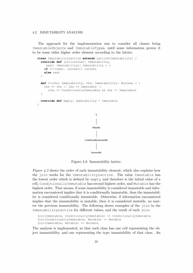
Figure 4.2: Immutability lattice.

Figure 4.2 shows the order of each immutability element, which also explains howthe join works for the ImmutabilityLattice. The value Immutable hasthe lowest order which is defined by empty and therefore is the initial value of acell, ConditionallyImmutable has second highest order, and Mutable has thehighest order. That means, if some immutability is considered immutable and infor-mation encountered implies that it is conditionally immutable, then the immutabil-ity is considered conditionally immutable. Otherwise, if information encounteredimplies that the immutability is mutable, then it is considered mutable, no mat-ter the previous immutability. The following shows examples of the join in theImmutabilityLattice for different values, and the result of each join:

join(Immutable, ConditionallyImmutable) == ConditionallyImmutablejoin(ConditionallyImmutable, Mutable) == Mutablejoin(Immutable, Mutable) == Mutable

The analysis is implemented, so that each class has one cell representing the ob-ject immutability, and one representing the type immutability of that class. An

31


analysis for each immutability is executed on a pool, where the object immutabilitycells are determined with the following cases. A cell always holds the initial valueImmutableObject, and will stay as that way if all the following statements hold:

– All fields are immutable– All field types are ImmutableType– All superclasses are ImmutableObject

A cell is evaluated to ConditionallyImmutableObject if at least oneof the following statements hold:

– All fields are immutable and there exists a field with type immutabilityConditionallyImmutableType or MutableType

– There exists a superclass with the strongest object immutabilityConditionallyImmutableObject

To evaluate the first statement, the implementation utilizes the following whenNextdependency:

cellCompleter.cell.whenNext(fieldTypeCell, (x Immutability) =>x match {

case Mutable | ConditionallyImmutable => DoPutNextcase Immutable => DoNothing

},Some(ConditionallyImmutable))

All dependencies on superclasses for all object immutabilities are evaluatedusing the same whenNext dependency:

cellCompleter.cell.whenNext(superClassCell, (x: Immutability) =>x match {

case Immutable => DoNothingcase Mutable => DoPutFinalcase ConditionallyImmutable => DoPutNext

},None)

A cell is evaluated to MutableObject if at least one of the following statementsholds:

– There exists a mutable field.– There exists a superclass that is mutable object.

If a class is found mutable, the cell is completed with that value. This is due tothe design of the lattice. Once a cell achieves the value mutable, no other valuecan be achieved, hence ensuring it is the final result.

The type immutability for a class is determined, depending on if there are anysubclasses or not. Both cases are applied using whenNext dependencies. A cellrepresenting a class with no subclasses is evaluated using the following dependency:

cellCompleter.cell.whenNext(objectImmutabilityCell, (x: Immutability) =>x match {

32



},None)

All cells representing a class with at least one subclass are evaluated using thefollowing dependency for each subclass:

cellCompleter.cell.whenNext(subclassCell, (x: Immutability) =>x match {


},None)

There are some cases where subclasses, superclasses or field types are not reachablefor the analysis. In those cases, the analysis is implemented to be conservative bycompleting cells with the value mutable to stay on the safe side for incomplete code.

Once the pool becomes quiescent, and there are still incomplete cells left, thenthey are either conditionally immutable or immutable. This is due to the imple-mentation design of the analysis, where all cells found mutable are completed. Allincomplete cells with a current value conditionally immutable cannot have anotherresult, because it is the highest order of the lattice, excluding mutable. However,for cells that are immutable, consider the case where a cell represents a superclassAnimal of some other cell that represents a class Dog, where both cells contain thevalue ImmutableObject. Lets say the Animal cell receives an intermediate resultConditionallyImmutableObject, before a whenNext dependency Dog depAnimal is assigned. If no further changes are made and the pool becomes quiescent,then the value in Dog is still ImmutableObject, when it should be evaluated toConditionallyImmutableObject. This shows that some cells with value im-mutable should be conditionally immutable when the pool becomes quiescent.

object ImmutabilityKey extends Key[Immutability] {val lattice = new ImmutabilityLattice

def resolve[K <: Key[Immutability]](cells: Seq[Cell[K, Immutability]]):Seq[(Cell[K, Immutability], Immutability)] = Seq()

def default[K <: Key[Immutability]](cells: Seq[Cell[K, Immutability]]):Seq[(Cell[K, Immutability], Immutability)] = {

val conditionallyImmutableCells =cells.filter(_.getResult() == ConditionallyImmutable)

if(conditionallyImmutableCells.nonEmpty)conditionallyImmutableCells.map(cell =>

(cell, ConditionallyImmutable))elsecells.map(cell => (cell, Immutable))

33


}}

With this information, all cells containing conditionally immutable can safely becompleted with that value, as shown in default, where it finds all cells containingthe value ConditionallyImmutable, and return them with that value to becompleted. The completion triggers all dependencies, where a dependent cell withvalue immutable receives conditionally immutable, according to the dependency.This occurs both for cells included in a CSCC and those components caused byIUC, and therefore there is no need to handle cycles as specific cases. That iswhy only the default method is needed for this analysis. However, cells that arechanged through the dependencies are never completed, due to the return valueof the predicate being DoPutNext for all conditionally immutable triggereddependencies. Therefore, default has to be executed a second time when thepool once again becomes quiescent. Now after the second time, all cells containingconditionally immutable are completed with no dependencies triggered. Finally,default is executed a third time once the pool becomes quiescent again, where allincomplete cells left contains value immutable, therefore are completed with thatvalue, as shown in the else-statement in the default method.

4.3 Results

The analyses were used to analyze the ’rt.jar’ file in JDK 7, which consists of 797packages, 163268 methods, 4596481 instructions, 77128 fields and 18591 class files.

Purity analysis The OPAL implementation and the Reactive Async implemen-tation of the purity analysis are very similar, where the main difference is howthe dependencies are handled. In the Reactive Async implementation, it is byassigning a whenComplete dependency, where the result can either be Pure orImpure, no intermediate results. Whereas in the OPAL implementation, it ispossible to receive intermediate results ConditionallyPure or MaybePure,before finalizing the results. The purity analysis implemented in OPAL is roughly180 lines of code (LOC), not counting comments and imports. The ReactiveAsync implementation is roughly 170 LOC, including the PurityKey andPurityLattice, not counting comments and imports.

Immutability analysis The Reactive Async implementation and the OPAL im-plementation of the immutability analysis are also somewhat similar. The maindifferences are how the dependencies are handled, where in Reactive Async imple-mentation, all four dependencies are whenNext dependencies. Otherwise, whereexplicit checks that cause intermediate or final results are in the OPAL implemen-tation, the same explicit checks are done in the Reactive Async implementation,using putNext for intermediate results and putFinal for final results.

34

4.3. RESULTS

The determinism properties in Reactive Async helped when bugs were acciden-tally introduced. For example, in some cases, the exception outputs in ReactiveAsync helped nailing down the cause of non-determinism by showing that someoperation is trying to add new information to a completed cell. The correctnessof the implementation was determined by using small case scenarios, were the re-sult of each class is known. Also, the results received from using the analysison a larger class file base, such as the JDK, was compared to the results of theOPAL implementation of the analysis to determine the correctness. When theReactive Async implementation was considered complete, the results still differedfrom the OPAL implementation. Consequently, by adding additional small sce-nario tests to determine the problem, it ended up revealing a bug in the OPALimplementation, causing the difference in the result.

The OPAL implementation of the immutability analysis is roughly 720 LOC, notcounting comments and imports. The Reactive Async implementation is roughly330 LOC, including the ImmutabilityKey and ImmutabilityLattice,not counting comments and imports.

35

Chapter 5

Performance evaluation

In this chapter, a comparison is made between the Reactive Async versionsof the static analyses and the OPAL versions to show the differences in ex-ecution time. Moreover, performance evaluations are made in the form ofmicro benchmarks. In these benchmarks Reactive Async is compared to Fu-tures and Promises to show the overhead difference in execution time, andalso show some of the strengths of the model.

The analyses and benchmarks were run on a HP EliteBook Folio 9470m with adual core Intel Core i7-3687U 2.1GHz with 8 GB memory and 4 MB L3 cache, run-ning the Linux distribution Elementary OS 0.3.2 Freya with kernel version 3.19.0-59-generic x86_64 (64 bit). It uses Scala version 2.11.8 and SBT version 0.13.11,where the JVM heap memory was set to 4 GB for every execution.

5.1 Static analysesEach analysis was executed on a new instance of the JVM. Both the purity analysisand the immutability analysis were executed on the ’rt.jar’ from the JDK, whichconsists of 797 packages, 163268 methods, 4596481 instructions, 77128 fields and18591 classes. The results show the average execution time of 9 runs for bothimplementations and is split up into three parts:

1. The average execution time for setting up everything before the analysis. Forexample, in the case of Reactive Async, that is creating all cells.

2. The average execution time for the analyses.

3. The average execution time of the overall execution. This does not add ad-ditional information, only sums the execution time of the setup and analysis,that is, part 1 and part 2.

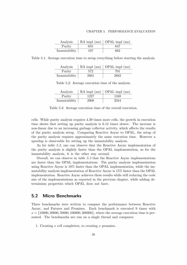
Table 5.1 shows that the immutability analysis setup is faster than the purityanalysis setup with Reactive Async, due to requiring less cells being created. Thepurity analysis require 163268 cells, while the immutability analysis requires 37182

37

CHAPTER 5. PERFORMANCE EVALUATION

Analysis RA impl (ms) OPAL impl (ms)Purity 655 647

Immutability 107 662

Table 5.1: Average execution time to setup everything before starting the analysis.



Table 5.2: Average execution time of the analysis.



Table 5.3: Average execution time of the overall execution.

cells. While purity analysis requires 4.39 times more cells, the growth in executiontime shows that setting up purity analysis is 6.12 times slower. The increase isnon-linear due to an increasing garbage collector activity, which affects the resultsof the purity analysis setup. Comparing Reactive Async to OPAL, the setup ofthe purity analysis requires approximately the same execution time. However aspeedup is observable for setting up the immutability analysis.

As for table 5.2, one can observe that the Reactive Async implementation ofthe purity analysis is slightly faster than the OPAL implementation, as for theimmutability analysis, it is the other way around.

Overall, we can observe in table 5.3 that the Reactive Async implementationsare faster than the OPAL implementations. The purity analysis implementationusing Reactive Async is 10% faster than the OPAL implementation, while the im-mutability analysis implementation of Reactive Async is 15% faster than the OPALimplementation. Reactive Async achieves these results while still reducing the codesize of the implementations as reported in the previous chapter, while adding de-terminism properties which OPAL does not have.

5.2 Micro Benchmarks

Three benchmarks were written to compare the performance between ReactiveAsync, and Futures and Promises. Each benchmark is executed 9 times withx = {10000, 20000, 50000, 100000, 200000}, where the average execution time is pre-sented. The benchmarks are run on a single thread and compares:

1. Creating x cell completers, to creating x promises.

38

5.2. MICRO BENCHMARKS

2. Creating x cell completers and completing x cells, to creating x promises andcompleting x futures.

3. Creating a cell completer and refining the value in a cell x times using theNaturalNumberLattice, to refining a result with promises x times wherex are completed with values 1 to x and then appended to a list.

The benchmarks were written using ScalaMeter [16] and executed on the sameinstance of the JVM. Before executing the benchmarks, some warm up executionswere performed until consistent results were achieved according to ScalaMeter.

Figure 5.1: Execution time of creating x cell completers, compared to creating xpromises.

The results in figure 5.1 and 5.2 show that the creating and completing cellsis significantly slower than promises, due to each created and completed cell hasto be registered to and deregistered from the HandlerPool, where each regis-tration requires the cell to be hashed. Moreover, the results shown are for a sin-gle thread execution, while creating and completing cells concurrently needs tobe done atomically, which will add additional contention on the HandlerPool.This is not an issue for promises, due to the creation and completion process ofeach promise is totally independent. In theory, adding more threads would implya bigger difference in the execution time between creating and completing cellscompared to creating and completing promises.

The growing execution time shown in figure 5.1 and 5.2 for creating and com-pleting cells is non-linear. This is due to the increasing garbage collector activitywhich was observed when exceeding 100000 cells on the machine used for these per-formance tests. This is also why the performance tests are not applied on largerx values. The overhead needed for creating and completing cells are only made by

39

CHAPTER 5. PERFORMANCE EVALUATION

Figure 5.2: Execution time of creating x cell completers and completing x cells,compared to creating x promises and completing x futures.

constant operations. Therefore the actual creation and completion process shouldnot cause the non-linear increase in execution time.

However, as for refinement of values shown in figure 5.3, the execution time ofReactive Async and Futures and Promises are similar.

40

5.2. MICRO BENCHMARKS

Figure 5.3: Execution time of creating a cell completer and refining the value ina cell x times using the NaturalNumberLattice, compared to refining a resultwith promises x times where x are completed with values 1 to x and then appendedto a list.

41

Chapter 6

Related Work

This chapter shows some models that are similar to Reactive Async andexplains the similarities and differences.

6.1 FlowPools

FlowPools [17] is a deterministic, lock-free and composable data structure, whichprovides an abstraction for multisets. It is similar to Reactive Async in that cellvalues depend on the lattice, by only allowing to add information to a cell andnot remove any. Whereas in FlowPools elements can be appended but not re-moved. Further, the lattice-based data structure generalizes what a cell can containcompared to the FlowPool data structure. FlowPools have a seal operation thatpreserves determinism by requiring the expected size of the multiset to be passedas an argument. If this size is exceeded by a program, an exception is thrown.The problem with this approach is that, the size is not always known in advance,making it hard to know dynamically. By using putFinal, one can ensure atwhat point no further information should be added.

6.2 Habanero-Scala

Habanero-Scala (HS) [8] is a library extension of Scala and supports a hybrid pro-gramming model, combining the Async/Finish Model (AFM) [2] and the ActorModel (AM) [1, 7] (two previously developed models). It is a generic task parallelprogramming model which is similar to the Reactive Async model. In HS, tasksare created using the async keyword, working as fork points, while the ReactiveAsync model uses HandlerPool that similarly acts as a fork point when using theexecute keyword. But HS has some blocking synchronization mechanisms such asthe finish keyword, which create a barrier until all child tasks that the finishembodies are finished. In Reactive Async, the quiescentResolveCell returnsa future, that can be used to create a barrier. Because futures are Awaitable,

43

CHAPTER 6. RELATED WORK

one can use Await.ready(future, duration), that waits until future iscompleted, or when the time specified by duration expires.

6.3 LVarsAs mentioned, the Reactive Async programming model is inspired by theLVars deterministic-by-construction parallel programming model [12], which isimplemented in Haskell. It offers a shared state programming model by using aconstruct the paper refers to as LVars, which is similar to Cell. By allowingthe LVars to take the least upper bound of the old and new values with respectto the lattice, it guarantees determinism, but with a limited interface. Similarto putFinal, the LVars model allows to freeze an LVar after a write, to ensurethat no further values can be added to the LVar.

The model is event-driven in that it allows event handlers to be attached toLVars by using the addHandler function. addHandler takes an LVar which theevent is attached to, the values that triggers the event, and a callback functionwhich is executed when the event is triggered. An event is triggered once the LVarreceives a value that is at the same point or higher than the current value accordingto the lattice order, and if the received value matches some value that triggers theevent. The difference between addHandler and whenComplete or whenNextis that whenComplete and whenNext assign dependencies on other cells and aretriggered when the dependee cell receives a new value. The addHandler doesnot assign a dependency on another LVar, but on some specified threshold valuesbeing exceeded by the LVar holding the callback. Also, if an LVar already containsa value that exceeds some of the specified threshold values when the callback isassigned, then the callback is executed instantly for each threshold value exceeded.When using whenNext and whenComplete, a callback for the dependency is onlyexecuted instantly if a dependency is assigned to an already completed cell.

Attaching a callback to an LVar using addHandler could however apply a de-pendency relationship between two LVars. Lets say we have two LVars, lvar1and lvar2. Attaching a callback to lvar1 that can cause a change to lvar2,would implicate a dependency relationship where lvar2 depends on some thresh-old values being exceeded by lvar1. However, there is no way to detect if suchdependencies are cyclic and no support for resolving them.

It would be possible to add an addHandler operation to Reactive Async, byadding value based callbacks that are triggered and executed whenever putNextor putFinal are used. Though this would probably need additional overhead, andbe carefully tailored with whenNext dependencies, not to cause deadlocks.

LVars are quasi-deterministic, whereas no proofs have been presented showingReactive Async is. However, the use of monotonic refinements with lattices isa step towards making the model deterministic.

Finally, quiescence detection is possible through Handler Pools in theLVars model, similar to Reactive Async.

44

Chapter 7

Conclusion and future work

This thesis has shown how Reactive Async, an event-based asynchronous paral-lel programming model, can extend the functionality and expressivity of Futuresand Promises, apply dependency handling, and allow for refinement of resultswhile adding some determinism properties. Two static analyses were reimple-mented using Reactive Async, showing that the model is both practically appli-cable and can be used for large scale applications. The results of the implementa-tions show that Reactive Async adds flexibility and facilitates the expressivity ofdependencies and refinement, reduces the code size significantly, while still main-taining a faster overall execution time.

As expected, the flexibility of Reactive Async comes at the cost of efficiencycompared to Futures and Promises. The simplicity of Futures and Promisesallows for less memory usage and overhead at creation and completion, whereaseach cell created and completed has to be registered to and deregisteredfrom the HandlerPool. Moreover, the garbage collector activity increasedwhen creating over 100000 cells on the machine used for the performancetests. However, Reactive Async allows for an easier way to apply refinement,while maintaining the same execution time.

Next step would be to tweak Reactive Async in different ways to optimize theperformance. The implementation should be further extended, by applying meth-ods to ease on possible contention, which can be done as discussed using exponentialbackoff. If possible, reducing the memory cost of storing a cell would both increasethe performance of the model and make it more applicable for applications requir-ing an extreme amount of cells. Furthermore, in order to reduce the debuggingrequired, the model has to be made deterministic. Because Reactive Async uses thesame model for refinements as LVars [12], then only using that part of the modelshould be deterministic. However, the difference is the dependency handling Reac-tive Async, which has to be included in the evaluation of the models determinismand tweaked in order to maintain the determinism.

45

CHAPTER 7. CONCLUSION AND FUTURE WORK

Acknowledgments I would like to thank Michael Eichberg for the sup-port and insights when developing the model. Also I want to thank mysupervisor Philipp Haller for supporting and giving feedback throughoutthe whole process of this thesis.

46

Bibliography

[1] Gul A. Agha. ACTORS - a model of concurrent computation in distributedsystems. MIT Press, 1990.

[2] Philippe Charles, Christian Grothoff, Vijay A. Saraswat, Christopher Donawa,Allan Kielstra, Kemal Ebcioglu, Christoph von Praun, and Vivek Sarkar. X10:an object-oriented approach to non-uniform cluster computing. In Proceedingsof the 20th Annual ACM SIGPLAN Conference on Object-Oriented Program-ming, Systems, Languages, and Applications, OOPSLA 2005, October 16-20,2005, San Diego, CA, USA, pages 519–538. ACM, 2005.

[3] Michael Eichberg and Ben Hermann. A software product line for static analyses:the OPAL framework. In Proceedings of the 3rd ACM SIGPLAN InternationalWorkshop on the State of the Art in Java Program Analysis, pages 1–6. ACM,2014.

[4] Peter Xiang Gao, Andrew R Curtis, Bernard Wong, and Srinivasan Keshav.It’s not easy being green. ACM SIGCOMM Computer Communication Review,42(4):211–222, 2012.

[5] Philipp Haller, Aleksandar Prokopec, Heather Miller, Viktor Klang, RolandKuhn, and Vojin Jovanovic. Futures and promises. http://docs.scala-lang.org/overviews/core/futures.html, 2012. Accessed: 2016-04-02.

[6] Robert H. Halstead, Jr. Multilisp: A language for concurrent symbolic compu-tation. ACM Transactions on Programming Languages and Systems, 7(4):501–538, October 1985.

[7] Carl Hewitt. Viewing control structures as patterns of passing messages. Ar-tificial intelligence, 8(3):323–364, 1977.

[8] Shams Imam and Vivek Sarkar. Habanero-Scala: Async-Finish Programmingin Scala. In The Third Scala Workshop (Scala Days 2012), 2012.

[9] Simon L. Peyton Jones, Roman Leshchinskiy, Gabriele Keller, and ManuelM. T. Chakravarty. Harnessing the multicores: Nested data parallelism inhaskell. In IARCS Annual Conference on Foundations of Software Technol-ogy and Theoretical Computer Science, FSTTCS 2008, December 9-11, 2008,

47

BIBLIOGRAPHY

Bangalore, India, pages 383–414. Schloss Dagstuhl - Leibniz-Zentrum fuer In-formatik, 2008.

[10] Robert L. Bocchino Jr., Vikram S. Adve, Danny Dig, Sarita V. Adve, StephenHeumann, Rakesh Komuravelli, Jeffrey Overbey, Patrick Simmons, HyojinSung, and Mohsen Vakilian. A type and effect system for deterministic par-allel java. In Proceedings of the 24th Annual ACM SIGPLAN Conference onObject-Oriented Programming, Systems, Languages, and Applications, OOP-SLA 2009, October 25-29, 2009, Orlando, Florida, USA, pages 97–116. ACM,2009.

[11] Lindsey Kuper and Ryan R Newton. LVars: lattice-based data structures fordeterministic parallelism. In Proceedings of the 2nd ACM SIGPLAN workshopon Functional high-performance computing, pages 71–84. ACM, 2013.

[12] Lindsey Kuper, Aaron Turon, Neelakantan R. Krishnaswami, and Ryan R.Newton. Freeze after writing: quasi-deterministic parallel programming withLVars. In The 41st Annual ACM SIGPLAN-SIGACT Symposium on Principlesof Programming Languages, POPL ’14, San Diego, CA, USA, January 20-21,2014, pages 257–270. ACM, 2014.

[13] Doug Lea. A Java fork/join framework. In Java Grande, pages 36–43, 2000.

[14] Barbara Liskov and Liuba Shrira. Promises: Linguistic support for efficientasynchronous procedure calls in distributed systems. In Richard L. Wexelblat,editor, PLDI, pages 260–267. ACM, 1988.

[15] Mark S. Miller, Eric Dean Tribble, and Jonathan S. Shapiro. Concurrencyamong strangers. In Trustworthy Global Computing, International Symposium,TGC 2005, Edinburgh, UK, April 7-9, 2005, Revised Selected Papers, pages195–229. Springer, 2005.

[16] Aleksandar Prokopec. ScalaMeter. http://axel22.github.com/scalameter, 2014.

[17] Aleksandar Prokopec, Heather Miller, Tobias Schlatter, Philipp Haller, andMartin Odersky. Flowpools: A lock-free deterministic concurrent dataflowabstraction. In Hironori Kasahara and Keiji Kimura, editors, LCPC, volume7760 of Lecture Notes in Computer Science, pages 158–173. Springer, 2012.

48

www.kth.se

Reactive Async - DIVA

Documents

Transcript of Reactive Async - DIVA