
Determination of Kinetic Parameters of the Thermal ...
259
Determination of Kinetic Parameters of the Thermal Dissociation of Methane Von der Fakultät für Maschinenwesen der Rheinisch-Westfälischen Technischen Hochschule Aachen zur Erlangung des akademischen Grades eines Doktors der Ingenieurwissenschaften genehmigte Dissertation vorgelegt von Michael Wullenkord Berichter: Univ.-Prof. Dr.-Ing. Robert Pitz-Paal Direktor Dr. Gilles Flamant Tag der mündlichen Prüfung: 08.04.2011 Diese Dissertation ist auf den Internetseiten der Hochschulbibliothek online verfügbar.
-
Upload
khangminh22 -
Category
Documents
-
view
1 -
download
0
Transcript of Determination of Kinetic Parameters of the Thermal ...

Determination of Kinetic Parameters of the Thermal Dissociation of Methane
Von der Fakultät für Maschinenwesen der Rheinisch-Westfälischen Technischen Hochschule Aachen zur Erlangung des akademischen Grades
eines Doktors der Ingenieurwissenschaften genehmigte Dissertation
vorgelegt von
Michael Wullenkord
Berichter: Univ.-Prof. Dr.-Ing. Robert Pitz-Paal Direktor Dr. Gilles Flamant Tag der mündlichen Prüfung: 08.04.2011
Diese Dissertation ist auf den Internetseiten der Hochschulbibliothek online verfügbar.

ii

Acknowledgments
iii
Acknowledgments
This work was compiled at the Institute of Technical Thermodynamics (Solar Research) of the
German Aerospace Center in Cologne in the context of the European project SOLHYCARB. I
would like to thank the European Commission for co-funding this project in the sixth framework
program (SES6 019770).
I would also like to thank Prof. Dr. Robert Pitz-Paal (First Examiner), head of Solar Research,
for supervising this work, for critical discussions, and for meaningful suggestions as well as Dr.
Gilles Flamant (Second Examiner), Director of PROMES-CNRS, for coordinating SOLHYCARB
and allowing inspiring conversation.
I am grateful for the motivating working atmosphere offered by colleagues of Solar Research.
Especially the guidance and support provided by Dr. Karl-Heinz Funken and Dr. Christian
Sattler is highly acknowledged. I appreciate that Peter Rietbrock and Lamark de Oliveira have
assisted me with their comprehensive competence in laboratory issues. I gladly honor the
helpful discussions with Nicole Janotte concerning the expression of uncertainty and the
companionship of Dr. Martina Neises who has shared office with me for several years. I would
like to thank the SOLHYCARB group for successful team work and particularly Dr. Eusebiu
Grivei for BET measurements and useful comments. I esteem the important laboratory work of
Elena Albermann, Beatrice Förster as well as Tom Maibauer and their contributions to the
project. I am indebted to Janine Schneider for manufacturing perfect thermocouples, which
functioned much longer than any bought devices, as well as to Claus-Jürgen Kröder for
calibrating them and providing advice.
This thesis would not have been possible without the grand encouragement that has been given
by my family and especially by my wife Nathalie Wullenkord who has had to demonstrate much
patience during the last years.

iv

Contents
v
Contents
List of Figures........................................................................................................................... vii
List of Tables ........................................................................................................................... xiii
Abstract..................................................................................................................................... xv
1 Introduction......................................................................................................................... 1
2 Fundamental terms and issues......................................................................................... 4 2.1 Conversion, yield and further basic figures .................................................................. 4 2.2 Reaction kinetics .......................................................................................................... 7 2.3 Uncertainty in measurement......................................................................................... 9 2.4 Uncertainty and correlation of model parameters....................................................... 11
3 Thermal splitting of methane .......................................................................................... 14 3.1 Basics ......................................................................................................................... 14 3.2 Applications with CO2-free heat supply ...................................................................... 15 3.3 Thermodynamics ........................................................................................................ 16 3.4 Kinetics ....................................................................................................................... 19
3.4.1 Kinetic experiments without seeding .................................................................. 20 3.4.2 Kinetic experiments in presence of carbon based catalysts ............................... 24 3.4.3 Kinetic experiments concerning the pyrolysis of C2-hydrocarbons..................... 26
4 Experimental ..................................................................................................................... 27 4.1 Experimental setup..................................................................................................... 27
4.1.1 Mass flow controllers .......................................................................................... 30 4.1.2 Gas chromatograph ............................................................................................ 32 4.1.3 Pressure transmitters.......................................................................................... 39
4.2 Reaction conditions .................................................................................................... 40 4.3 Procedure ................................................................................................................... 42
4.3.1 Calibration of mass flow controllers .................................................................... 45 4.3.2 Calibration of the gas chromatograph................................................................. 47 4.3.3 Molar fractions in the product gas....................................................................... 50
4.4 General results ........................................................................................................... 55 4.4.1 General results of experiments with argon as dilution gas ................................. 55 4.4.2 General results of experiments with helium as dilution gas................................ 63
4.5 Measurement of temperature ..................................................................................... 68 4.6 Additional experiments ............................................................................................... 75
4.6.1 Repeatability of results ....................................................................................... 77 4.6.2 Location and character of generated carbon ...................................................... 79 4.6.3 Balances of H- and C-atoms............................................................................... 82
4.7 Experiments with added C-particles ........................................................................... 85
5 Kinetic evaluation............................................................................................................. 90 5.1 Interpretation of measured temperatures ................................................................... 90
5.1.1 Material properties of AL23 and used gases ...................................................... 91 5.1.2 Convective heat transfer..................................................................................... 93 5.1.3 Radiative heat transfer........................................................................................ 99 5.1.4 Comparison of heat transfer coefficients and consequences ........................... 101
5.2 Diffusion.................................................................................................................... 105 5.2.1 Axial diffusion.................................................................................................... 106 5.2.2 Radial diffusion ................................................................................................. 107
5.3 Flow model ............................................................................................................... 113 5.3.1 Flow conditions at the inlet of the reactor ......................................................... 113 5.3.2 Flow conditions inside the reactor .................................................................... 121
5.3.2.1 Temperature distribution............................................................................... 124

Contents
vi
5.3.2.2 Flow lines and nested tube reactors..............................................................126 5.3.2.3 Pressure distribution......................................................................................129
5.4 Kinetic model.............................................................................................................131 5.5 Procedure..................................................................................................................133
5.5.1 Reactor model: Plug flow reactor ......................................................................138 5.5.2 Reactor model: Nested tube reactors................................................................139 5.5.3 Reactor model: Nested tube reactors with ideal radial diffusion .......................141
5.6 Kinetic parameters and further results ......................................................................142 5.7 Discussion.................................................................................................................155
6 Summary and Outlook....................................................................................................158
7 References.......................................................................................................................163
8 Nomenclature ..................................................................................................................177
Appendix..................................................................................................................................188 List of Figures of Appendix ...................................................................................................188 List of Tables of Appendix.....................................................................................................191 Appendix A: Thermodynamics ..............................................................................................194 Appendix B: Gas chromatograph..........................................................................................196 Appendix C: Reaction conditions and experimental results..................................................207 Appendix D: Fluid material properties and diffusion .............................................................223 Appendix E: Calculations with ANSYS .................................................................................226 Appendix F: Calculations with COMSOL Multiphysics..........................................................232 Appendix G: Optimization tool and results of kinetic evaluation ...........................................235

List of Figures
vii
List of Figures
Figure 3-1: General situation of a reactor for the thermal splitting of methane with methane (CH4) as well as the dilution gas (DG) at the inlet of the reactor and additional reaction products at the outlet of the reactor, which are particulate carbon (“C”), hydrogen (H2), ethane (C2H6), ethene (C2H4), and ethyne (C2H2) as well as further hydrocarbons (CmHn).................................................................................................................. 15
Figure 3-2: Equilibrium compositions at 1 bar as a function of the temperature (based on an initial amount of 1 kmol methane) .................................................................................... 18
Figure 3-3: Amount of substance of the main components of the equilibrium composition as a function of the temperature and the pressure (based on an initial amount of 1 kmol methane)........................................................................................................ 19
Figure 4-1: Sketch of the experimental setup for the kinetic analysis of the thermal decomposition of methane ......................................................................................................... 28
Figure 4-2: Picture of the experimental setup with some main components as well as additional parts like two and three way cocks (numbers in red) and connections...................... 29
Figure 4-3: Basic dimensions and axial positions of the experimental setup for the kinetic analysis of the thermal decomposition of methane in mm .............................................. 30
Figure 4-4: Configuration of gas chromatograph........................................................................ 32
Figure 4-5: Examples for GC calibration curves: the molar fraction of hydrogen detected by the HID (a) and the molar fraction of methane detected by the TCD (b) as a function of the normal peak area............................................................................................. 35
Figure 4-6: Maximum relative positive deviation of GC measurements for ethyne: measured, extended and estimated levels (OM = order of magnitude) ..................................... 38
Figure 4-7: Measurement chain of the measurement of pressures............................................ 39
Figure 4-8: Illustration of the definition of calibration curves of the GC...................................... 50
Figure 4-9: Illustration of the utilization of calibration curves of the GC which exemplarily refer to the situation before the experiments........................................................... 51
Figure 4-10: Illustration of the definition and the utilization of GC calibration curves for C2-hydrocarbons which exemplarily refer to the situation before the experiments (molar fractions smaller than the lowest molar fractions employed for the determination of calibration curves). ..................................................................................................................... 55
Figure 4-11: Conversion of methane as a function of the residence time, the nominal furnace temperature, and the initial molar fraction of methane. Dilution gas: argon. Indicators of uncertainty refer to maximum uncertainty for the residence time and to standard uncertainty for the conversion. .................................................................................... 56
Figure 4-12: Yield of hydrogen as a function of the residence time, the nominal furnace temperature, and the initial molar fraction of methane. Dilution gas: argon. Indicators of uncertainty refer to maximum uncertainty for the residence time and to standard uncertainty for the yield. ............................................................................................................. 57
Figure 4-13: Yield of ethane as a function of the residence time, the nominal furnace temperature, and the initial molar fraction of methane. Dilution gas: argon. Indicators of uncertainty refer to maximum uncertainty for the residence time and to standard uncertainty for the yield. ............................................................................................................. 57
Figure 4-14: Yield of ethene as a function of the residence time, the nominal furnace temperature, and the initial molar fraction of methane. Dilution gas: argon. Indicators of uncertainty refer to maximum uncertainty for the residence time and to standard uncertainty for the yield. ............................................................................................................. 58

List of Figures
viii
Figure 4-15: Yield of ethyne as a function of the residence time, the nominal furnace temperature, and the initial molar fraction of methane. Dilution gas: argon. Indicators of uncertainty refer to maximum uncertainty for the residence time and to standard uncertainty for the yield...............................................................................................................59
Figure 4-16: Conversion of methane as well as yields of hydrogen, ethane, ethene, and ethyne as a function of the residence time for 1300 °C nominal furnace temperature of and 10 % initial molar fraction of methane. Dilution gas: argon..................................................60
Figure 4-17: Balance of hydrogen atoms as a function of the residence time, the nominal furnace temperature, and the initial molar fraction of methane. Dilution gas: argon...........................................................................................................................................61
Figure 4-18: Relative difference between approximated (as 1 minus the sum of molar fractions of considered species except for argon) and measured molar fractions of argon in the product gas as a function of the residence time, the nominal furnace temperature and the initial molar fraction of methane.................................................................62
Figure 4-19: Yield of C2-hydrocarbons related to the yield of hydrogen as a function of the residence time, the initial molar fraction of methane, and the nominal furnace temperature. Dilution gas: argon.................................................................................................63
Figure 4-20: Conversion of methane as a function of the residence time, the nominal furnace temperature, and the initial molar fraction of methane. Dilution gas: helium. Indicators of uncertainty refer to maximum uncertainty for the residence time and to standard uncertainty for the conversion......................................................................................65
Figure 4-21: Yield of hydrogen as a function of the residence time, the nominal furnace temperature, and the initial molar fraction of methane. Dilution gas: helium. Indicators of uncertainty refer to maximum uncertainty for the residence time and to standard uncertainty for the yield...............................................................................................................65
Figure 4-22: Yield of ethane as a function of the residence time, the nominal furnace temperature, and the initial molar fraction of methane. Dilution gas: helium. Indicators of uncertainty refer to maximum uncertainty for the residence time and to standard uncertainty for the yield...............................................................................................................66
Figure 4-23: Yield of ethene as a function of the residence time, the nominal furnace temperature, and the initial molar fraction of methane. Dilution gas: helium. Indicators of uncertainty refer to maximum uncertainty for the residence time and to standard uncertainty for the yield...............................................................................................................66
Figure 4-24: Yield of ethyne as a function of the residence time, the nominal furnace temperature, and the initial molar fraction of methane. Dilution gas: helium. Indicators of uncertainty refer to maximum uncertainty for the residence time and to standard uncertainty for the yield...............................................................................................................67
Figure 4-25: Balance of hydrogen atoms as a function of the residence time, the nominal furnace temperature, and the initial molar fraction of methane. Dilution gas: helium. ........................................................................................................................................67
Figure 4-26: Assembly of the self-made thermocouple employed for temperature measurement inside the tube reactor (dimensions in mm) .........................................................68
Figure 4-27: Start position, end position, and length of a measured temperature profile (dimensions in mm).....................................................................................................................69
Figure 4-28: Profiles of minimum and maximum temperatures (1400 °C nominal furnace temperature and 2600 sccm nominal standard volume flow of Ar, average pressure at the reactor inlet: 1.031 bar, average pressure at the reactor outlet: 1.014 bar)....................................................................................................................................70
Figure 4-29: Measurement chain of the measurement of temperatures.....................................71

List of Figures
ix
Figure 4-30: Determined temperature profiles for the thermocouple in wall position (WP) and in center position (CP) (1400 °C nominal furnace temperature and 2600 sccm nominal standard volume flow of Ar, average pressure at reactor inlet: 1.031 bar, average pressure at reactor outlet: 1.014 bar, indicators of uncertainty refer to maximum uncertainty) ............................................................................................................ 74
Figure 4-31: Profiles of determined temperature profiles for the thermocouple in wall position (WP) and in center position (CP) (1600 °C nominal furnace temperature and 9800 sccm nominal standard volume flow of Ar, average pressure in above reactor: 1.039 bar, average pressure below reactor: 1.006 bar, indicators of uncertainty refer to maximum uncertainty) ................................................................................................................ 75
Figure 4-32: Examples for samples from the filter gained in experiments with argon as dilution gas: 1400 - 2600 - 10 (a) and 1300 - 650 - 5 (b) (Reaction condition: nominal furnace temperature in °C - nominal total standard volume flow in sccm - nominal initial molar fraction of methane in %) ................................................................................................. 79
Figure 4-33: Examples for samples from the reactor gained in experiments with argon as dilution gas: 1400 - 2600 - 5 (a), 1600 - 2000 - 5 (b), 1500 - 2800 - 5 (c), and 1300 - 1300 - 5 (d) (Reaction condition: nominal furnace temperature in °C - nominal total standard volume flow in sccm - nominal initial molar fraction of methane in %) ........................ 80
Figure 4-34: Specific surface area of carbon samples collected from the reactor ..................... 81
Figure 4-35: Specific surface area of carbon samples collected from the filter .......................... 81
Figure 4-36: Fractions of H- and C-atoms situated in particular species as a function of the experimental conditions (nominal furnace temperature in °C - total standard volume flow in sccm - initial molar fraction of methane in %) ................................................................. 85
Figure 4-37: General configuration of the seeding apparatus .................................................... 86
Figure 4-38: Calibration of the seeding apparatus and determination of maximum, nominal, and minimum mass flow of Super P depending on the number of revolutions of the dosing element ................................................................................................................. 86
Figure 4-39: Conversion of methane and yield of hydrogen as well as of ethane, ethene, and ethyne as a function of the applied mass flow of Super P related to values determined without seeding. Indicators of uncertainty refer to the average maximum uncertainty concerning the mass flow and to typical standard uncertainty concerning relative conversion and yields. Nominal furnace temperature: 1400 °C, nominal total standard volume flow: 3800 sccm, nominal molar fraction of methane in argon: 5 %, pressure between 1.012 bar and 1.031 bar. .............................................................................. 88
Figure 5-1: Illustration of heat transfers contributing to the temperature measured with the thermocouple........................................................................................................................ 90
Figure 5-2: Approximation of the thermal conductivity of AL23 for temperatures between 0 °C and 1600 °C employing various information ........................................................ 92
Figure 5-3: Approximation of the emissivity of AL23 for temperatures between 0 °C and 1600 °C employing various information...................................................................................... 93
Figure 5-4: Convective heat transfer coefficients for two temperatures of the tip of the thermocouple (800 °C and 1600 °C) as a function of the temperature difference between the thermocouple and the reactor wall as well as of the standard volume flow of argon. Material properties of argon were calculated for the arithmetic mean of the temperature of the thermocouple and the reactor wall and exemplarily for the maximum (max) and minimum (min) temperature of considered combinations. Standard pressure.......... 98
Figure 5-5: Convective heat transfer coefficients for two temperatures of the tip of the thermocouple (900 °C and 1500 °C) as a function of the temperature difference between the thermocouple and the reactor wall as well as of the standard volume flow

List of Figures
x
of helium. Material properties of helium were calculated for the arithmetic mean of the temperature of the thermocouple and the reactor wall. Standard pressure. ...............................99
Figure 5-6: Radiative heat transfer coefficients for two temperatures of the tip of the thermocouple (800 °C and 1600 °C) as a function of the temperature difference between the thermocouple and the reactor ..............................................................................101
Figure 5-7: Ratio of convective heat transfer coefficient to radiative heat transfer coefficient for different combinations of temperature of the thermocouple (TC) and temperature of the reactor wall as a function of the standard volume flow of argon or helium. Material properties of argon and helium were calculated for the arithmetic mean of the temperature of the thermocouple and the reactor wall. Standard pressure. ...................102
Figure 5-8: Geometrical situation of the thermocouple in center position (a) and in wall position (b) inside the reactor (sectional view). The color illustrates the temperature distribution in front of the thermocouple near the inlet of the reactor (red = hot, blue = cold). ..............................................................................................................................102
Figure 5-9: Péclet number for different standard volume flows of argon and helium through the tube reactor based on the nominal furnace temperature and standard pressure ....................................................................................................................................107
Figure 5-10: Geometric situation in the context of radial diffusion ............................................109
Figure 5-11: Diffusive quotient regarding methane as a function of the residence time, the nominal furnace temperature, the initial molar fraction of methane, and the dilution gas ............................................................................................................................................111
Figure 5-12: Diffusive quotient regarding hydrogen as a function of the residence time, the nominal furnace temperature, the initial molar fraction of methane, and the dilution gas ............................................................................................................................................112
Figure 5-13: Geometry upstream the inlet of the reactor (entrance region). Dimensions and axial positions in mm unless otherwise stated. ..................................................................113
Figure 5-14: Basics concerning the ANSYS 12 model of the entrance region as well as positions of Line X and Line Z on the reactor inlet face ............................................................117
Figure 5-15: Results of flow simulations with ANSYS 12 – Velocity in Y-direction (normal to face) at the reactor inlet for a standard volume flow of 700 sccm Ar .......................118
Figure 5-16: Results of ANSYS 12 calculations for the velocity in Y-direction (normal to face) along Line X and Line Z at the reactor inlet compared to an ideally laminar velocity profile. Corresponding conditions: 700 sccm Ar and 1400 °C nominal furnace temperature...............................................................................................................................118
Figure 5-17: Results of ANSYS 12 calculations for the velocity in Y-direction (normal to face) along Line X and Line Z at the reactor inlet compared to an ideally laminar velocity profile. Corresponding conditions: 2600 sccm Ar and 1400 °C nominal furnace temperature...............................................................................................................................119
Figure 5-18: Results of ANSYS 12 calculations for the velocity in Y-direction (normal to face) along Line X and Line Z at the reactor inlet compared to an ideally laminar velocity profile. Corresponding conditions: 9800 sccm Ar and 1600 °C nominal furnace temperature...............................................................................................................................120
Figure 5-19: Geometry of the reactor model in COMSOL Multiphysics with the reactor wall, the fluid region, and the thermocouple (TC) along with basic settings. Level of mesh refinement: 3. ..................................................................................................................121
Figure 5-20: Results of COMSOL Multiphysics calculations based on a simplified temperature profile for the wall of the reactor concerning the temperature distribution in the reactor, in the wall of the reactor as well as in the thermocouple for different sets of nominal furnace temperature and standard volume flow: 1200 °C - 95 sccm Ar (a),
List of Figures
xi
1400 °C - 2600 sccm Ar (b), 1600 °C - 9800 sccm Ar (c), and 1400 °C - 3800 sccm He (d) ............................................................................................................................................. 124
Figure 5-21: Results of COMSOL Multiphysics calculations based on a simplified temperature profile for the wall of the reactor concerning the temperature evaluation in the center of region A and along the wall of the thermocouple in region B compared to measurement with a thermocouple in wall and center position for different sets of nominal furnace temperature and standard volume flow: 1200 °C - 95 sccm Ar (a), 1400 °C - 2600 sccm Ar (b), 1600 °C - 9800 sccm Ar (c), and 1400 °C - 3800 sccm He (d) ............................................................................................................................................. 125
Figure 5-22: Results of COMSOL Multiphysics calculations based on a simplified temperature profile for the wall of the reactor concerning flow lines for different sets of nominal furnace temperature and standard volume flow: 1200 °C - 95 sccm Ar (a), 1400 °C - 2600 sccm Ar (b), 1600 °C - 9800 sccm Ar (c), and 1400 °C - 3800 sccm He (d) ............................................................................................................................................. 126
Figure 5-23: Illustration of the reactor divided into nested tube reactors (NTR)....................... 127
Figure 5-24: Results of COMSOL Multiphysics calculations based on a simplified temperature profile for the wall of the reactor concerning flow lines for 1600 °C nominal furnace temperature and 9800 sccm argon with indication of virtual nested tube reactors (NTR).......................................................................................................................... 128
Figure 5-25: Results of COMSOL Multiphysics calculations based on a simplified temperature profile for the wall of the reactor concerning the fraction of the molar flow at the inlet of the reactor in particular nested tube reactors in region B 5 mm downstream the tip of the thermocouple as a function of the molar flow of argon (a) and helium (b) at the reactor inlet.................................................................................................... 129
Figure 5-26: Results of COMSOL Multiphysics calculations based on a simplified temperature profile for the wall of the reactor concerning pressure distribution inside the reactor for different sets of nominal furnace temperature and standard volume flow: 1200 °C - 95 sccm Ar (a), 1400 °C - 2600 sccm Ar (b), 1600 °C - 9800 sccm Ar (c), and 1400 °C - 3800 sccm He (d)..................................................................................................... 130
Figure 5-27: Results of COMSOL Multiphysics calculations based on a simplified temperature profile for the wall of the reactor concerning the pressure evaluation along average radii in region A and region B compared to experimental pressure differences between the inlet and the outlet of the reactor for different sets of nominal furnace temperature and standard volume flow .................................................................................... 131
Figure 5-28: General configuration of a volume element of the reactor with ingoing and outgoing molar flows ................................................................................................................ 133
Figure 5-29: Illustration of a plug flow model applied to the tube reactor with thermocouple (TC) ................................................................................................................... 138
Figure 5-30: Illustration of a nested tube reactor model applied to the tube reactor with thermocouple (TC) ................................................................................................................... 139
Figure 5-31: Illustration of reaction steps and diffusion steps for reactor models based on nested tube reactors with (NTR + D) and without ideal radial diffusion (NTR).................... 141
Figure 5-32: Model error related to the model error for best fit kinetic parameters as a function of kinetic parameters related to the best fit kinetic parameters (reactor model 5 NTR)...................................................................................................................................... 147
Figure 5-33: Comparison of experimentally determined conversion of methane (as a function of the residence time and the nominal furnace temperature) with calculated values employing reactor model 5 NTR and respective best fit kinetic parameters. 5 % initial molar fraction of methane in argon. Indicators of uncertainty refer to maximum uncertainty (black: used for kinetic evaluation, gray: not used for kinetic evaluation). ............. 148

List of Figures
xii
Figure 5-34: Comparison of experimentally determined yield of hydrogen (as a function of the residence time and the nominal furnace temperature) with calculated values employing reactor model 5 NTR and respective best fit kinetic parameters. 5 % initial molar fraction of methane in argon. Indicators of uncertainty refer to maximum uncertainty (black: used for kinetic evaluation, gray: not used for kinetic evaluation)...............149
Figure 5-35: Comparison of experimentally determined yield of ethane (as a function of the residence time and the nominal furnace temperature) with calculated values employing reactor model 5 NTR and respective best fit kinetic parameters. 5 % initial molar fraction of methane in argon. Indicators of uncertainty refer to maximum uncertainty (black: used for kinetic evaluation, gray: not used for kinetic evaluation)...............149
Figure 5-36: Comparison of experimentally determined yield of ethene (as a function of the residence time and the nominal furnace temperature) with calculated values employing reactor model 5 NTR and respective best fit kinetic parameters. 5 % initial molar fraction of methane in argon. Indicators of uncertainty refer to maximum uncertainty (black: used for kinetic evaluation, gray: not used for kinetic evaluation)...............150
Figure 5-37: Comparison of experimentally determined yield of ethyne (as a function of the residence time and the nominal furnace temperature) with calculated values employing reactor model 5 NTR and respective best fit kinetic parameters. 5 % initial molar fraction of methane in argon. Indicators of uncertainty refer to maximum uncertainty (black: used for kinetic evaluation, gray: not used for kinetic evaluation)...............150
Figure 5-38: Comparison of experimentally determined conversion of methane (as a function of the residence time, the nominal furnace temperature, and the initial molar fraction of methane) with calculated values employing reactor model 5 NTR and respective best fit kinetic parameters. Dilution gas: helium. Indicators of uncertainty refer to maximum uncertainty. ..................................................................................................151
Figure 5-39: Comparison of experimentally determined yield of hydrogen (as a function of the residence time, the nominal furnace temperature, and the initial molar fraction of methane) with calculated values employing reactor model 5 NTR and respective best fit kinetic parameters. Dilution gas: helium. Indicators of uncertainty refer to maximum uncertainty. ...............................................................................................................................152
Figure 5-40: Comparison of experimentally determined yield of ethane (as a function of the residence time, the nominal furnace temperature, and the initial molar fraction of methane) with calculated values employing reactor model 5 NTR and respective best fit kinetic parameters. Dilution gas: helium. Indicators of uncertainty refer to maximum uncertainty. ...............................................................................................................................152
Figure 5-41: Comparison of experimentally determined yield of ethene (as a function of the residence time, the nominal furnace temperature, and the initial molar fraction of methane) with calculated values employing reactor model 5 NTR and respective best fit kinetic parameters. Dilution gas: helium. Indicators of uncertainty refer to maximum uncertainty. ...............................................................................................................................153
Figure 5-42: Comparison of experimentally determined yield of ethyne (as a function of the residence time, the nominal furnace temperature, and the initial molar fraction of methane) with calculated values employing reactor model 5 NTR and respective best fit kinetic parameters. Dilution gas: helium. Indicators of uncertainty refer to maximum uncertainty. ...............................................................................................................................153
List of Tables
xiii
List of Tables
Table 3-1: Kinetic experiments concerning the thermal decomposition of methane and determined kinetic parameters ................................................................................................... 21
Table 3-2: Kinetic experiments concerning the thermal decomposition of methane and determined kinetic parameters employing simplified kinetic models.......................................... 23
Table 3-3: Kinetic experiments concerning the thermal decomposition of methane in the presence of carbon based catalysts and determined kinetic parameters ............................ 25
Table 3-4: Kinetic experiments concerning the thermal decomposition of C2-hydrocarbons and determined kinetic parameters ..................................................................... 26
Table 4-1: Information about used mass flow controllers and gases (GCF = Gas Correction Factor) ...................................................................................................................... 31
Table 4-2: Basic information about the gas chromatograph....................................................... 33
Table 4-3: Employed detectors and calibration curves for the measurement of molar fractions of the main sample components.................................................................................. 34
Table 4-4: Extreme values for standard deviations, maximum positive deviations, and maximum negative deviations relative to mean normal peak areas determined in GC measurements for different gases and molar fractions .............................................................. 37
Table 4-5: Information about pressure transmitters and the subsequent measurement chain........................................................................................................................................... 40
Table 4-6: Reaction conditions covered in experiments with argon as dilution gas ................... 41
Table 4-7: Reaction conditions covered in experiments with helium as dilution gas.................. 42
Table 4-8: Changes of pressures at reactor inlet and reactor outlet as well as change of temperature at position 320 mm during operation of the vacuum pump of the GC.................... 44
Table 4-9: Stated, projected, and estimated accuracy of the volume flow calibration unit ......... 45
Table 4-10: Information about ready-to-use test gases employed for GC calibration ................ 48
Table 4-11: Determined ratios of normal peak areas corresponding to different molar fractions of C2-hydrocarbons. Extended values are based on experimental results, but comprise a safety factor of 1.1 (maximum) and 0.9 (minimum). ................................................ 49
Table 4-12: Information about thermocouples and the subsequent measurement chain .......... 72
Table 4-13: Conditions covered in the second experimental campaign with argon as dilution gas ................................................................................................................................. 76
Table 4-14: Conditions covered in the second experimental campaign with helium as dilution gas ................................................................................................................................. 77
Table 4-15: Differences between values for the conversion of methane as well as the yields of hydrogen, ethane, ethene, and ethyne gained in the second campaign and average values regarding the first and second campaign with argon as dilution gas related to respective standard uncertainties determined in the first campaign. (Reaction condition: nominal furnace temperature in °C - nominal total standard volume flow in sccm - nominal initial molar fraction of methane in %) ............................................................... 78
Table 4-16: Differences of values for the conversion of methane as well as the yields of hydrogen, ethane, ethene, and ethyne gained in the first and second experimental campaign with helium as dilution gas related to respective standard uncertainties. (Reaction condition: nominal furnace temperature in °C - nominal total standard volume flow in sccm - nominal initial molar fraction of methane in %).................................................... 78
Table 5-1: Stated thermal conductivity and emissivity of AL23 produced by FRIATEC............. 91

List of Tables
xiv
Table 5-2: Review of temperature profiles gained with argon regarding the existence of moderate radial temperature gradients in the relevant region of reactor ..................................104
Table 5-3: Review of temperature profiles gained with helium regarding the existence of moderate radial temperature gradients in relevant region of reactor ....................................105
Table 5-4: Diffusion volume of various species used for the method of Fuller .........................109
Table 5-5: Reynolds numbers at the inlet of the reactor and corresponding entry lengths for argon .......................................................................................................................115
Table 5-6: Reynolds numbers at the inlet of the reactor and corresponding entry lengths for helium......................................................................................................................115
Table 5-7: Initial parameter sets for the optimization process along with lower bounds (LB) and upper bounds (UB) of the parameters........................................................................137
Table 5-8: Comparison of best fit kinetic parameters and achieved agreement between experiments and optimization procedure for different reactor models: plug flow reactor (PFR), 5 nested tube reactors (5 NTR), 5 nested tube reactors with ideal radial diffusion (5 NTR + D), 10 nested tube reactors (10 NTR), and 10 nested tube reactors with ideal radial diffusion (10 NTR + D) ....................................................................................143
Table 5-9: Information about differences between quantities calculated with reactor model 5 NTR employing best fit kinetic parameters and experimentally determined quantities...................................................................................................................................144
Table 5-10: Comparison of best fit kinetic parameters and achieved agreement between experiments and optimization procedure for the reactor model based on 5 nested tube reactors (5 NTR) considering sets of nominal, minimum, and maximum temperatures and pressures .....................................................................................................146
Table 5-11: Averaged maximum radial differences of molar fractions in the heated region of the reactor for results associated with reactor model 5 NTR and respective best fit kinetic parameters .........................................................................................................147
Table 5-12: Standard uncertainties of best fit kinetic parameters for model 5 NTR..................154
Table 5-13: Matrix of correlation coefficients calculated based on the best fit kinetic parameters for model 5 NTR. Blocks colored in orange indicate the correlation of kinetic parameters describing the same reaction......................................................................155

Abstract
xv
Abstract
The solar thermal decomposition of methane could be an economically and ecologically
beneficial process to produce hydrogen and particulate carbon. Aiming at the determination of
general kinetic laws and parameters the thermal dissociation of methane was examined
employing an alumina tubular reactor situated in an electric tube furnace. Nominal furnace
temperatures in the range between 1200 °C and 1600 °C were set. Gas mixtures containing
argon or helium as dilution gas and methane with a molar fraction between 2 % and 10 % were
introduced into the reactor at an absolute pressure around 1 bar. The residence times ranged
from 0.0115 s to 1.47 s. Temperature profiles along the reactor were measured with a
thermocouple type S. Experimental results concerning the conversion of methane practically
cover the full range from minor to total progress. Hydrogen was the main product of the
decomposition. However, significant amounts of ethane, ethene, and especially ethyne formed
part of the product flow. Seeding with carbon black featuring a specific surface similar to
generated particles result in a significant increase of both, conversion of methane and yield of
hydrogen.
The laminar flow conditions at the inlet of and inside the reactor were assessed by means of
simulations employing ANSYS and COMSOL Multiphysics. Diverse reactor models based on
nested tube reactors were employed. The models either disregarded radial diffusion or implied
ideal radial diffusion. A simplified kinetic model which takes the considered species into account
and respects forward dehydrogenation reactions was engaged. Kinetic parameters were varied
in order to minimize the model errors. Best agreement between the calculations and
experimental findings was achieved for a reactor model featuring five nested tube reactors and
neglecting radial diffusion. The respective decay of methane is characterized by a reaction
order regarding methane of 1.283 and an activation energy of 510.1 kJ/mol. Low standard
uncertainties of estimated parameter values were derived from the covariance matrix. Except
for quantities associated with the same reaction, parameters showed only marginal correlation.
Radial diffusion was found to be a key phenomenon difficult to assess properly. The probable
presence of not considered high molecular intermediates and differing properties of generated
carbon have been identified as limiting issues concerning a comprehensive kinetic approach
including heterogeneous effects.

xvi
1 Introduction
1
1 Introduction
Energy systems have to be transformed substantially in order to preserve Earth and to allow
subsequent generations to benefit from our planet equitably. Today processes involved in the
provision of energy are mainly based on the combustion of fossil energy carriers or on nuclear
fission and thus not compatible with the idea of sustainability. Fossil and fissionable feedstocks
are finite and their mining involves a grave interference of landscape and healthiness. The
products of their use are either relevant for the greenhouse effect (especially carbon dioxide –
CO2) or radioactive what directly leads to the question how to dispose them reasonably. An
unrestricted discharge of CO2 to the atmosphere is not acceptable any more. According to the
IPCC1, respective emissions have to be reduced significantly in the near future in order to avoid
the risk of an incalculable climate change combined with numerous threats to mankind and
ecosystems.2
A possible resort is the establishment of the hydrogen society in which hydrogen (H2) plays the
key role as energy carrier. Hydrogen represents the ultimate species of the transition from solid
energy carriers with a high C/H-ratio (such as coal) via liquid energy carriers with moderate C/H-
ratio (such as oil) to gaseous energy carriers with low C/H-ratio (such as methane). The usage
of hydrogen in highly efficient fuel cells or internal combustion engines features a reaction with
oxygen to water and does practically not involve any emissions of harmful substances or
matters with relevance for climate change.3 Since hydrogen is a secondary energy carrier, it has
to be produced before being applied. Consequently, the application of hydrogen can only be as
clean as the method of its production. Nowadays the most important processes for the
production of hydrogen are steam reforming of methane and naphtha (38 %), partial oxidation of
heavy fuel oil (24 %), reforming of benzine (H2 as byproduct, 18 %), and coal gasification (H2 as
byproduct, 10 %), whereas minor fractions are allotted to the ethylene production and other
chemical industries as well as to the chloralkali electrolysis.4 In their current configuration they
cause massive emissions of CO2 and are thus not suitable for a carbon neutral hydrogen
system. Either the aforementioned processes have to be modified that way that CO2-drawbacks
are avoided (e. g. CCS5, renewable energy and feedstocks) or alternative, environmentally
acceptable methods have to be employed. Amongst others potential processes could be the
electrolysis of water, water splitting (in thermochemical cycles or photobiological), reforming and
1 Intergovernmental Panel on Climate Change 2 cp. [IPCC, 2007] 3 cp. [Ausubel, 2000], [Hefner, 2002], [Dunn, 2002], [Muradov, 2005 a], [Marbán, 2007] 4 cp. [Geitmann, 2002], p. 27, providing data from DWV 5 carbon capture and storage

1 Introduction
2
gasification of biomass, fermentation of biomass (thermophilic or photo fermentation) and
cracking of hydrocarbons (thermal or in thermal plasma).6
Concentrating solar power (CSP) offers the greatest potential for electricity production in the
EUMENA7 region taking renewable sources into account.8 Consequently, the employment of
solar power is also particularly interesting for the production of hydrogen and has been
discussed intensively.9 The solar thermal dissociation of methane, which is the main component
of natural gas (and biogas) still featuring great resources10, could be an ecologically and
economically beneficial method of hydrogen generation representing an intermediate step from
fossil fuel based to entirely regenerative hydrogen production. The heat input needed for the
cracking reactions is here provided by solar radiation. Since oxygen is not included in the
decomposition process, the formation of CO2 is avoided. The final products of the thermal
dissociation of methane are hydrogen and solid carbon. This allows the storage of a part of the
introduced solar energy in an advantageous energy carrier. Depending on its quality generated
carbon could be sold as an industrial commodity or landfilled without difficulty. As a result the
process does not involve drawbacks of CO2-emissions although the fossil (if not from biogas)
energy carrier methane is engaged.11 The recently completed European project SOLHYCARB
has been concerned with the solar thermal dissociation of methane.12
For a proper design and cost-efficient construction of suitable solar operated plants it is
essential to know about the kinetics of the cracking reactions. Although the kinetics of the
thermal dissociation of methane has been considered for several decades, comprehensive
information has not been reported in literature yet. Published kinetic parameters cover a wide
range of values. They are partly associated with special types of reactors or determined based
on vague reaction conditions, e. g. concerning reaction temperatures as well as diffusive
effects, and therefore refuse a universal character. Moreover, the uncertainty of estimated
values is often unclear. As a consequence the application of such kinetic findings to arbitrary
systems involves an unknown ambiguity. The aim of this work was the determination of general
kinetic parameters for the thermal decomposition of methane employing a tubular reactor and a
practically assessable kinetic model based on net forward reactions. Reaction conditions should
be investigated in detail in order to allow a reliable approximation of the circumstances of the
reactions. Special attention should be turned on the uncertainty in measurement and related
6 see e. g. [Steinberg, 1989], [Geitmann, 2002], p. 27 et seqq., [Stolten, 2010], p. 169 et seqq. 7 Europe, Middle East, North Africa 8 cp. [DLR, 2005], p. 56 9 see e. g. [Steinfeld, 2001], [Hirsch, 2001], [Fletcher, 2001], [Kodama, 2003], [Steinfeld, 2004], [Steinfeld, 2005], [Zedtwitz, 2006], [Muradov, 2008], [Ozalp, 2009], [Pregger, 2009] 10 resources of non-conventional natural gas equivalent to 103364 EJ estimated for 2008, cp. [Rempel, 2009], p. 11 11 cp. [Spath, 2003] 12 cp. [Flamant, 2007] (description of SOLHYCARB)

1 Introduction
3
propagation in the kinetic evaluation. A suitable test facility had to be developed and assembled
before experiments could be carried out. Appropriate simulation tools had to be identified and
utilized with the purpose of clarification of flow characteristics and finally of definition of an
accurate reactor model for the kinetic evaluation.
After introducing some basic terms related to data preparation, reaction kinetics, and
uncertainty in measurement as well as of model parameters in Chapter 2, general information
about the thermal splitting of methane including an overview about the state of kinetic research
is provided in Chapter 3. The experimental setup, procedures and results are presented in
Chapter 4, whereas the kinetic evaluation, which features the creation of a realistic reactor
model and the application of a simplified kinetic model taking the main components of the
product flow into account, is described in Chapter 5. Findings are summarized and an outlook is
given in Chapter 6.

2 Fundamental terms and issues
4
2 Fundamental terms and issues
This chapter provides the explanation of fundamental terms important for following
considerations as well as data preparation. Furthermore, the expressions of uncertainty in
measurement and of model parameters being part of this work are illustrated.
2.1 Conversion, yield and further basic figures
An ideal gas follows the ideal gas law which is usually written as
TnVp , Equation 1
where is the universal gas constant, p and T stand for the absolute pressure and the
temperature, respectively, while n represents the amount of substance and V is the related
volume. Consequently, conditions in a flow system, comprising a volume flow V and a flow of
amount of substance n , change in compliance with
TnVp . Equation 2
The standard volume flow NV corresponding to a certain flow of amount of substance n refers
to standard conditions, defined by the standard temperature NT and the standard pressure Np ,
and arises from
N
NN p
TnV
. Equation 3
The total initial standard volume flow of a gas mixture, containing methane and an inert dilution
gas (DG), entering a reactor tot,0N,V can be calculated employing the initial standard volume flow
of methane ,0CHN, 4V and the initial standard volume flow of the dilution gas DG,0N,V by

2 Fundamental terms and issues
5
,0CHN,DG,0N,tot,0N, 4VVV . Equation 4
The initial molar fraction of methane ,0CH4x can be determined via
tot,0N,
,0CHN,,0CH
4
4 V
Vx
. Equation 5
Respecting Equation 3 the molar flow of methane at the inlet of a reactor ,0CH4n arises from
N
N,0CHN,,0CH 44 T
pVn
. Equation 6
Given that the dilution gas is an inert gas, it does not serve as a reactant. Then the molar flow of
the dilution gas DGn equals the molar flow of the dilution gas at the outlet of the reactor PDG,n
and the molar flow of the dilution gas at the inlet of the reactor DG,0n :
N
NDG,0N,DG,0PDG,DG T
pVnnn
. Equation 7
Employing the molar fraction of the dilution gas in the product gas PDG,x the molar flow of the
product gas gP,tot,n can be calculated using
PDG,
DGgP,tot, x
nn
Equation 8
and moreover the molar flows of other gaseous species i of the product flow by

2 Fundamental terms and issues
6
...,HC,HC,HC,H,CH 22426224gP,tot,P,P, inxn ii . Equation 9
With ,0CH4n and P,CH4
n , the molar flow of methane at the outlet of the reactor, the conversion of
methane 4CHX
,0CH
P,CH,0CHCH
4
44
4 n
nnX
Equation 10
can be determined, while the yield of hydrogen 2HY arises from
,0CH
P,HH
4
2
2 2
1
n
nY
Equation 11
considering the overall decomposition reaction13 and employing P,H2n , the molar flow of
hydrogen at the outlet of the reactor. Introducing the formal reaction equations yielding in C2-
hydrocarbons
(g)H(g)HC(g)CH2 2624 ,
(g)H2(g)HC(g)CH2 2424 , and
(g)H3(g)HC(g)CH2 2224
the yields of the different C2-hydrocarbons 62HCY ,
42HCY , and 22HCY
13 see Chapter 3.1

2 Fundamental terms and issues
7
224262,0CH
P, HC,HC,HC24
in
nY i
i
Equation 12
can be determined. The factors qiF ,P, occurring in Equation 11 (0.5) and Equation 12 (2),
respectively, result from the ratio of the absolute values of the stoichiometric coefficients of
methane q,CH4 and the considered product qi ,P, concerning reaction q :
qi
q
qiF,P,
,CH
,P,4
. Equation 13
Finally the yield of C2-hydrocarbons HCC2Y arises from
2242622 HCHCHCHCC YYYY . Equation 14
2.2 Reaction kinetics
Reaction kinetics deals with the analysis of the reaction rate and the dependencies on the
influencing factors, which are
the reaction temperature RT ,
the concentration of different reactants i ic ,
the total pressure Rp , at which the reaction proceeds, and
catalysts as well as the amount of reaction sites on surfaces.
The concentration of component i ic can be calculated by

2 Fundamental terms and issues
8
V
n
V
nc ii
i
, Equation 15
where in is the amount of substance i in a certain volume V , while for a flow system the
consideration of the molar flow of component i in in the volume flow V is more suitable.
In homogeneous reactions only substances with the same state of aggregation are involved,
whereas heterogeneous reactions comprise at least two states of aggregation. The equivalent
reaction rate of a homogeneous reaction homr is defined as
i
ii
i
r
t
n
Vr
hom,
homhom d
d1
, Equation 16
where i is the stoichiometric coefficient of component i , in is the amount of substance of
component i , t is the time, and V is the considered volume. Directly connected to homr is
ir ,hom , the reaction rate of the homogeneous reaction regarding component i . Contrariwise, the
equivalent reaction rate of a heterogeneous reaction hetr refers to a relevant surface S
i
ii
i
r
t
n
Sr
surface,het,
hetsurfacehet, d
d1
, Equation 17
or a relevant mass m
i
ii
i
r
t
n
mr
mass,het,
hetmasshet, d
d1
, Equation 18
with the reaction rates of the heterogeneous reaction regarding component i ir surface,het, and
ir mass,het, . For a homogeneous reaction a common approach to analyze the relation between the
reaction rate and the influencing factors is that the reaction rate equals a product of two terms,
the first only depending on the temperature and the second only depending on the
concentrations of the reactants:

2 Fundamental terms and issues
9
)()( icfTkr .14 Equation 19
While the first term )(Tk is called rate constant and depends on the temperature T following
an Arrhenius law in accordance with
T
E
ekTk
a
0)( Equation 20
the second term )( icf is often assumed to be an exponential function appropriate to
i
mii
iccf )( . Equation 21
Here three important parameters, the kinetic parameters, can be identified: the pre-exponential
factor 0k , the activation energy aE , and the reaction order regarding component i im . Strictly
speaking, the pre-exponential factor itself is a function of the temperature. It may be
proportional to the temperature to the power of 0.5 following collision theory or proportional to
the temperature to the power of another exponent resulting from transition state theory.
However, this dependency of the pre-exponential factor on the temperature is usually weak
compared to the dependency of the exponential term of Equation 20.15 Thus, the pre-
exponential factor is considered as a constant. Usually for a heterogeneous reaction the relation
between the reaction rate and the influencing factors is more complex, especially when the
second phase does not have constant properties.
2.3 Uncertainty in measurement
In this work special attention was turned to the assessment of uncertainty of determined figures,
such as conversions, yields, and temperatures. Two different expressions of uncertainty can be
found. The first one is the maximum (positive and negative) uncertainty, whereas the second
one results from an attempt to state the standard uncertainty according to GUM16. Diverse types
of evaluation of standard uncertainty have to be distinguished: the Type A evaluation of
uncertainty, a “method of evaluation of uncertainty by statistical analysis of series of
14 cp. [Hagen, 2004], p. 31 et seqq. 15 cp. [Chorkendorff, 2003], p. 36, p. 100 et seqq., p. 108 et seqq., [Ebbing, 2005], p. 581 et seqq. 16 Guide to the expression of uncertainty in measurement, see [ISO, 2008]

2 Fundamental terms and issues
10
observations”, and the Type B evaluation of uncertainty, a “method of evaluation of uncertainty
by means other than the statistical analysis of series of observations”.17
In this work mainly the Type B evaluation of uncertainty was employed. Usually manufacturers
of used measuring devices state uncertainty of a measured value x by upper and lower limits
a and a , respectively. Consequently, the maximum positive uncertainty of x )(max xu arises
from
xaxu )(max Equation 22
and the maximum negative uncertainty of x )(max xu from
xaxu )(max . Equation 23
In absence of further information, the assumption of a rectangular probability distribution is
admissible. If not otherwise stated, a symmetric situation corresponding to
aax 5.0 Equation 24
was postulated in agreement to the specification of used instruments. Employing a , the half
width of the interval defined by a and a , calculated from
aaa 5.0 Equation 25
the standard uncertainty of x )(xu can be calculated by
17 cp. [ISO, 2008], p. 3

2 Fundamental terms and issues
11
3)(
axu .18 Equation 26
The maximum positive and negative uncertainty of a quantity y being a function of N other
quantities ix congruent to
)...,,,( 21 Nxxxfy Equation 27
arises from severest combinations of values of influencing quantities in the range of their limits
given by maximum uncertainties. Contrariwise, the combined standard uncertainty of y )(c yu
can be estimated from
N
ii
i
xux
fyu
1
2
2
c )()( .19 Equation 28
To simplify matters, the index c is eliminated in the following and )()( c yuyu is called the
standard uncertainty of y .
2.4 Uncertainty and correlation of model parameters
Given a situation of multidimensional Chi-Square fitting involving a nonlinear model following
),( ψxiyy , Equation 29
where ix is a vector of variables defining condition i influencing the function y , the merit
function to be minimized is
18 cp. [ISO, 2008], p. 11 et seqq. 19 cp. [ISO, 2008], p. 18 et seq. Assumptions: input quantities are uncorrelated and nonlinearity of the considered function is not significant (higher-order terms neglected).

2 Fundamental terms and issues
12
pointsdata
1
2
2 ),(N
i i
ii yy
ψx
, Equation 30
with ψ accounting for the set of model parameters to be varied and i characterizing the
standard deviation of iy . The covariance matrix of ψ )(ψCov provides information about the
standard uncertainty of estimated parameters (square root of diagonal elements) and
covariance between components of ψ . )(ψCov can be assessed via
1)( αψCov , Equation 31
where the components of matrix α are defined by
l
i
k
iN
i ikl
yyα
),(),(1points data
12
ψxψx .20 Equation 32
If
i
iii
yyy
),(~ ψx
, Equation 33
it is obvious that
k
i
ik
i yy
),(1~ ψx
Equation 34
and consequently
20 cp. [Press, 2007], p. 788 et seqq. (in particular p. 790, p. 798, p. 800 et seq.)
2 Fundamental terms and issues
13
points data
1
~~N
i l
i
k
ikl
yyα
. Equation 35
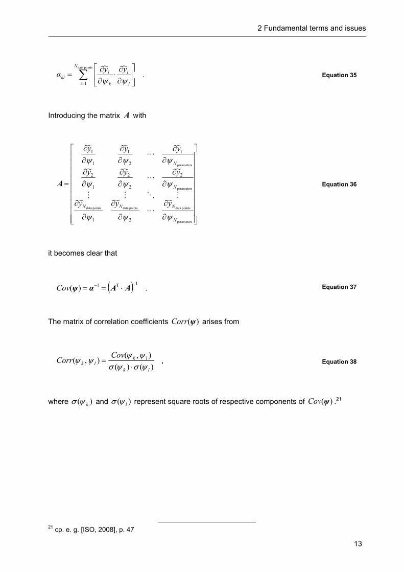
Introducing the matrix A with
parameters
points datapoints datapoints data
parameters
parameters
~~~
~~~
~~~
21
2
2
2
1
2
1
2
1
1
1
N
NNN
N
N
yyy
yyy
yyy
A Equation 36
it becomes clear that
1T1)( AAαψCov . Equation 37
The matrix of correlation coefficients )(ψCorr arises from
)()(
),(),(
lk
lklk
CovCorr
, Equation 38
where )( k and )( l represent square roots of respective components of )(ψCov .21
21 cp. e. g. [ISO, 2008], p. 47

3 Thermal splitting of methane
14
3 Thermal splitting of methane
In Chapter 3.1 basics about the thermal splitting of methane that are important for general
understanding are given, before the current extent of CO2-free applications is presented in
Chapter 3.2. Thermodynamic considerations and calculations can be found in Chapter 3.3,
whereas Chapter 3.4 provides information about the state of research concerning the kinetics of
the thermal decomposition of methane.
3.1 Basics
The overall reaction of the thermal decomposition of methane, which needs an energy input to
proceed respecting the positive standard reaction enthalpy, can be written as
(g)H2(s)C""(g)CH 24 mol
kJ8.740
R H
and summarizes numerous elementary reactions included in a complex reaction mechanism.
An accepted sequence of cracking reactions finally forming molecular hydrogen and particulate
carbon (“C”) is the stepwise dehydrogenation considering the intermediates ethane (C2H6),
ethene (C2H4), and ethyne (C2H2):
C""2......HCHCHCCH2 2222 H22
H42
H62
H4 22
The formation of methyl radicals (CH3) according to
HCHCH 34
was proven to be the initial and rate determining step of the dissociation of methane, whereas
the formation of methylene radicals (CH2) was rejected.23 Reactions of ethene may beside the
formation of ethyne also lead to the formation of propene and subsequently of propadiene and
1-butene, whereas methylation of ethyne could explain the occurrence of propyne.24 Models for
the reaction mechanism of the thermal dissociation of methane with different levels of
sophistication – partly respecting high molecular hydrocarbons such as benzene and polycyclic
aromatic hydrocarbons (PAHs) – have been suggested and applied.25
22 cp. [Khan, 1970] and [Back, 1983], p. 2 23 cp. [Back, 1983], p. 5, p. 12 et seq. 24 cp. [Billaud, 1989] 25 see. e. g. [Sundaram, 1977 a], [Sundaram, 1977 b], [Sundaram, 1978], [Roscoe, 1985], [Stewart, 1989], [Grenda, 2003], [Matheu, 2003]; including benzene: see e. g. [Billaud, 1992], [Guerét, 1994],

3 Thermal splitting of methane
15
The general situation of a reactor with entering gases and additional leaving reaction products is
shown in Figure 3-1. Cracking reactions inside the reactor consume the provided heat and lead
to the formation of the final products as well as of C2-hydrocarbons and of not further specified
hydrocarbons (CmHn).
Figure 3-1: General situation of a reactor for the thermal splitting of methane with methane (CH4) as well as the dilution gas (DG) at the inlet of the reactor and additional reaction products at the outlet of the reactor, which are particulate carbon (“C”), hydrogen (H2), ethane (C2H6), ethene (C2H4), and ethyne (C2H2) as well as further hydrocarbons (CmHn).
3.2 Applications with CO2-free heat supply
The thermal dissociation of methane offers the possibility of simultaneous CO2-emission free
production of hydrogen and carbon when the heat necessary to run the cracking reactions is
provided without the release of CO2. A possibility of CO2-free heat supply – however, up to now
without practical demonstration – is the combustion of a part of the produced hydrogen
introduced by Kreysa as “The Carbon Moratorium”.26 Another option is the use of concentrated
solar radiation. Several solar operated reactors in laboratory and prototype scales have already
been constructed and tested. Concepts of indirect heating have to be distinguished from those
of direct solar irradiation of the reactants. Steinfeld produced filamentous carbon and hydrogen
in a small scale solar irradiated reactor implying a fluidized bed of Ni catalyst and Al2O3 grains.27
Weimer and Dahl reported the construction and operation of a fluid-wall aerosol flow reactor
irradiated with concentrated solar power at maximum levels of 10 kW.28 Tornado flow conditions
were simulated and applied to a reactor, which was operated with a solar radiation input in the
range of 2 kW and allowed a volumetric absorption of solar radiation as soon as the first carbon
particles were formed. Additionally, Kogan introduced an apparatus for seeding targeting an
increase of radiative heat transfer into the gas/particle-mixture.29 A reactor configuration in the
[Olsvik, 1994], [Olsvik, 1995], [Holmen, 1995], [Tynnukov, 2002]; including PAHs: see e. g. [Lucas, 1990], [Dean, 1990], [Richter, 2000], [Younessi-Sinaki, 2009]
26 see [Kreysa, 2009] (extended and translated version of [Kreysa, 2008]) 27 see [Steinfeld, 1997] 28 see [Weimer, 2001], [Dahl, 2001], [Dahl, 2002], [Dahl, 2004] 29 see [Kogan, 2003], [Kogan, 2004], [Kogan, 2005], [Kogan, 2007]

3 Thermal splitting of methane
16
5 kW class based on a particle laden vortex flow acting as a volumetric absorber was presented
and examined with respect to the radiative heat transfer by Hirsch. Trommer investigated
respective kinetics, whereas Maag carried out further experiments after modifying the reactor.30
Abanades conducted experiments with a 1 kW reactor that featured different graphite nozzles
which absorbed solar radiation and lead heat energy into the passing flow of reactants.31 A
reactor in the 10 kW scale consisting of four units of concentric graphite tubes situated in a
graphite cavity was presented and examined by Abanades and Rodat.32 Seven straight and
horizontally oriented graphite tubes placed in a graphite cavity form the key parts of a reactor
working at an extended nominal power level of 50 kW.33 The latter configuration represents the
most advanced solar operated reactor for the thermal decomposition of methane demonstrated
up to now. Its construction and operation was one of the final objectives of the European project
SOLHYCARB.
3.3 Thermodynamics
Materials conversion can be interpreted as a balancing process which dissipates the differences
of driving potentials and finally leads to the mechanical, thermal, material, and chemical
equilibrium. Temperature and pressure represent the reference for the thermal and mechanical
potential, respectively. The material equilibrium and chemical equilibrium are related to the
chemical potential. The material equilibrium is reached as soon as the chemical potential of
component i i is equal in all involved phases. i is defined as the partial derivative of the
Gibbs energy with respect to the amount of substance of component i at constant temperature,
pressure, and amounts of substance of components other that i :
ijnpTii n
G
,,
.34 Equation 39
The free enthalpy of reaction RG arises from
30 see [Hirsch, 2004 a], [Hirsch, 2004 b], [Trommer, 2004], [Maag, 2009] 31 see [Abanades, 2005], [Abanades, 2006], [Abanades, 2007] 32 see [Abanades, 2009], [Rodat, 2009], [Rodat, 2010 b] 33 see [Rodat, 2010 a] 34 cp. [Lucas, 2008], p. 431 et seqq.

3 Thermal splitting of methane
17
i
iiG R , Equation 40
where i is the stoichiometric coefficient of component i . Introducing the standard free
enthalpy of reaction 0RG with
i
iiG 00R Equation 41
and the activity of component i ia , it can be shown that
i
iiaTGG ln0
RR . Equation 42
Regarding a heterogeneous equilibrium involving a gaseous phase treated as an ideal gas
mixture as well as a solid phase containing pure substances, the activity of a component i in
the ideal gas phase igia can be calculated employing the partial pressure ip and the standard
reference pressure 0p following
0ig
p
pa i
i , Equation 43
whereas sia , the activity of a pure solid component i , can be treated as a constant according to
1s ia . Equation 44
The chemical equilibrium is characterized by 0R G .35
Equilibrium compositions were calculated for different temperatures and pressures employing
HSC 536. The program routines determine stable compositions of chosen species using the
35 cp. [Atkins, 2010], p. 190, p. 214 et seqq. and [Weingärtner, 2003], p. 155 et seqq.

3 Thermal splitting of methane
18
“Gibbs energy minimization method”. Gaseous species comprising methane, hydrogen, all
hydrocarbons with up to 8 carbon atoms available in the HSC 5 database, and selected higher
hydrocarbons, especially polycyclic aromatic hydrocarbons (PAHs)37, as well as solid carbon
were considered. A complete table of respected species can be found in Appendix A. Figure 3-2
represents the amounts of substances in the equilibrium at 1 bar higher than 1 * 10-8 kmol
based on an initial amount of methane of 1 kmol. Small amounts of the C2-hydrocarbons
ethane, ethene, and ethyne as well as of propadiene, 1-propyne, butadiyne, and 1-heptene can
be found in the equilibrium composition, but practically only hydrogen, carbon, and methane are
the relevant species at temperatures up to 1700 °C. At 783 °C still 10 % of the initial amount of
methane remains unconverted, whereas at 1114 °C the equilibrium is almost completely shifted
to the side of products.
100 300 500 700 900 1100 1300 1500 170010-8
10-7
10-6
10-5
10-4
10-3
10-2
10-1
100
101
Am
ount
of s
ubst
ance
in k
mol
Temperature in °C
hydrogen ethane methane 1-heptene carbon butadiyne ethyne 1-propyne ethene propadiene
Figure 3-2: Equilibrium compositions at 1 bar as a function of the temperature (based on an initial amount of 1 kmol methane)
Ideally, two moles of hydrogen are formed per mole of methane. Consequently, according to the
principle of Le Chatelier and Braun an increase of pressure results in a shift of the equilibrium to
the side of methane as can be seen in Figure 3-3. Complete figures for 0.5 bar and 2 bar
corresponding to Figure 3-2 can be found in Appendix A.
36 HSC Chemistry 5: Calculation of Equilibrium Composition v. 5.0 (Outokumpu Research Oy, 2002). 37 The thermal decomposition of methane involves the presence of PAHs, e. g. naphthalene and benzo[a]pyrene, cp. e. g. [Hu, 2003]. Albermann presented a comprehensive review of literature as well as own experimental results in [Albermann, 2007]. Most of identified PAHs are part of the HSC 5 database and were respected for equilibrium calculations.

3 Thermal splitting of methane
19
100 300 500 700 900 1100 1300 1500 17000.0
0.5
1.0
1.5
2.0
0.5 bar1 bar2 bar
Am
oun
t of s
ubst
ance
in k
mol
Temperature in °C
hydrogen methane carbon
Figure 3-3: Amount of substance of the main components of the equilibrium composition as a function of the temperature and the pressure (based on an initial amount of 1 kmol methane)
3.4 Kinetics
The thermal splitting of hydrocarbons has been a frequently addressed topic in research for
more than a hundred years. For instance, the French chemist M. Berthelot presented some
basic findings in the second half of the 19th century.38 The thermal decomposition of methane
has been investigated employing different ways to heat up the reactants. Very common is the
heat supply via hot reactor walls influencing the temperature of the reactants by convection and
in presence of absorbers also by radiation. As presented in Chapter 3.2 the direct solar
irradiation of particles in contact to the reactants is possible too. Moreover, high temperature of
reactants can be achieved by compression in shock tubes. In addition, applications employing
thermal plasma, microwaves, and molten metal baths can be found.39 However, the latter
applications form part of special fields and are excluded from subsequent considerations.
Kinetic experiments have been carried out under various conditions differing for instance in
temperature and pressure. Furthermore, experiments conducted in presence of catalysts other
than those formed by the reaction itself have to be distinguished from experiments carried out
without the employment of additional substances. Influences of carbon based catalysts as well
as of metal based catalysts were examined. Abbas has recently presented a respective review
38 see e. g. [Berthelot, 1866] 39 see e. g. [Fincke, 2002], [Fulcheri, 2002] (thermal plasma); [Tanashev, 1998] (microwaves); [Serban, 2003] (molten metal)

3 Thermal splitting of methane
20
article.40 Although the present work principally deals with the simplest reaction system, which
corresponds to the situation without any added catalyst, the consideration of literature providing
information about reaction rates found for the presence of carbon material is useful, since
findings could help to understand the influence of formed carbon particles on the reaction rates.
Contrariwise, metal based catalysts may involve additional effects and are consequently
excluded in the following.
According to the general information provided in Chapter 3.1, many species are involved in the
thermal dissociation of methane. However, on the path from the reactant methane to the final
products hydrogen and carbon, C2-hydrocarbons feature particular importance as intermediates
and byproducts with significant fractions in the product flow. The reliability of kinetic data
derived from experiments respecting the individual species as reactants is not guaranteed when
transferred to reactions as intermediates, since alternative reaction mechanism could become
relevant. Nevertheless, some examples are presented in Chapter 3.4.3.
3.4.1 Kinetic experiments without seeding
Kinetic experiments concerning the thermal decomposition of methane were carried out in
shock tubes, in tube reactors and in static systems. In spite of the long-lasting consideration
there exists a remarkable lack of clarity regarding involved reactions, kinetics and mechanisms.
Scientists reported numerous – and partly inconsistent – observations in these fields along with
approaches to explain them. Most researchers agree that ethane is the primary product of the
decomposition followed by ethene and ethyne. Controversial results concerning the pressure
dependence of the dissociation41, the relevance of surface effects42, and the influence of
decomposition products such as hydrogen43, ethane, and ethyne44 were reported. Palmer
observed induction, acceleration, and deceleration periods and suggested that shock tube
experiments refer to conditions before acceleration.45 Comprehensive overviews about
respective up-to-date information were compiled in 1970 by Khan and Crynes46, in 1983 by
Back and Back47, and in 1989 by Billaud, Baronnet et al.48 Table 3-1 provides information about
40 see [Abbas, 2010 a] 41 cp. [Hartig, 1971] (“pressure dependence of k“) and [Napier, 1972] (“results were not sensitive to pressure“) 42 cp. [Shantarovich, 1962] (“The relationship R ~ s/v […] and […] indicate that cracking is a heterogeneous reaction.“) and [Palmer, 1968] (“the rate is not appreciably affected by the S/V ratio“) 43 cp. [Kevorkian, 1960] (“homogeneous reaction is not hydrogen inhibited“) and [Kassel, 1932] (“rate […] very greatly retarded by hydrogen“) 44 cp. [Eisenberg, 1967] (”rate is accelerated by ethane”), [Gordon, 1948] (“acetylene was a catalyst for the decomposition of methane”), and [Skinner, 1959] (“methane decomposition is not much affected by the presence of the decomposition products”) 45 cp. [Palmer, 1968] 46 see [Khan, 1970] 47 see [Back, 1983] 48 see [Billaud, 1989]

3 Thermal splitting of methane
21
the scope of applied reaction conditions and determined kinetic parameters along with utilized
temperature measurement techniques.
Table 3-1: Kinetic experiments concerning the thermal decomposition of methane and determined kinetic parameters
Reference / reactor / dilution gas Temperature in °C / measurement technique
Pressure in bar / residence time in ms Initial molar fraction of methane in % / conversion in %
Reaction
mol
kJinaE
)1(
30 m
mol
s
1login)log(
m
k
inm
[Kassel, 1932] / quartz vessel / - 700 °C – 850 °C / Pt-Pt/Rh TC (outer contact)
0.017 – 0.51 / up to 40 min 100 / a few
CH4 → products 332.4
12 1
[Skinner, 1959] / shock tube / Ar 1157 – 1512 / calculation
5.1 / < 15 12 (and 1) / < 10
CH4 → products 422.9 14.71
1
[Glick, 1959] / shock tube / He and Ar 1227 – 2627 / calculation
not specified (n. s.) / several ms 10 / 0 – 100
CH4 → products 355.9 12.96
1
[Kevorkian, 1960] / shock tube / Ar 1383 – 1692 / calculation
3.4 – 12.0 / 1.4 – 2.4 2 and 10 / 7.6 – 86.2
CH4 → products 389.4 14.12
1
[Shantarovich, 1962] / porcelain tube / He 1293 – 1373 / n. s.
0.023 – 0.027 / 5 – 42 1.2 – 20 / 0.12 – 1.02
CH4 → products 376.8 11.60
1
[Kozlov, 1962] / shock tube / Ar 1397 – 1777 / calculation
2.0 – 8.1 / n. s. 2 and 5 / n. s.
CH4 → products 381.0 13.65
1 (based on own data and other works)
[Palmer, 1963] / annular reactor / He 890 – 1078 / n. s.
n. s. / n. s. n. s. (variation by factor 20) / n. s.
CH4 → products 422.9 14.1
1
[Palmer, 1968] / porcelain tube / He 1050 – 1250 / Pt-Pt/10Rh TC moved through reactor
0.99 / 100 – 900 1 – 20 / up to 85
CH4 → products 431.2 14.6
1 (based on own data and other works)
CH4 (+ Ar) → CH3 + H (+ Ar) [Hartig, 1971] / shock tube / Ar
1577 – 2227 / calculation 5.1 – 222.9 / less than Kozlov, Kevorkian, and Skinner
0.2 – 1 / n. s.
368.4 11.30
2 (low pressure limit)
435.4 15.10
1 (high pressure limit)
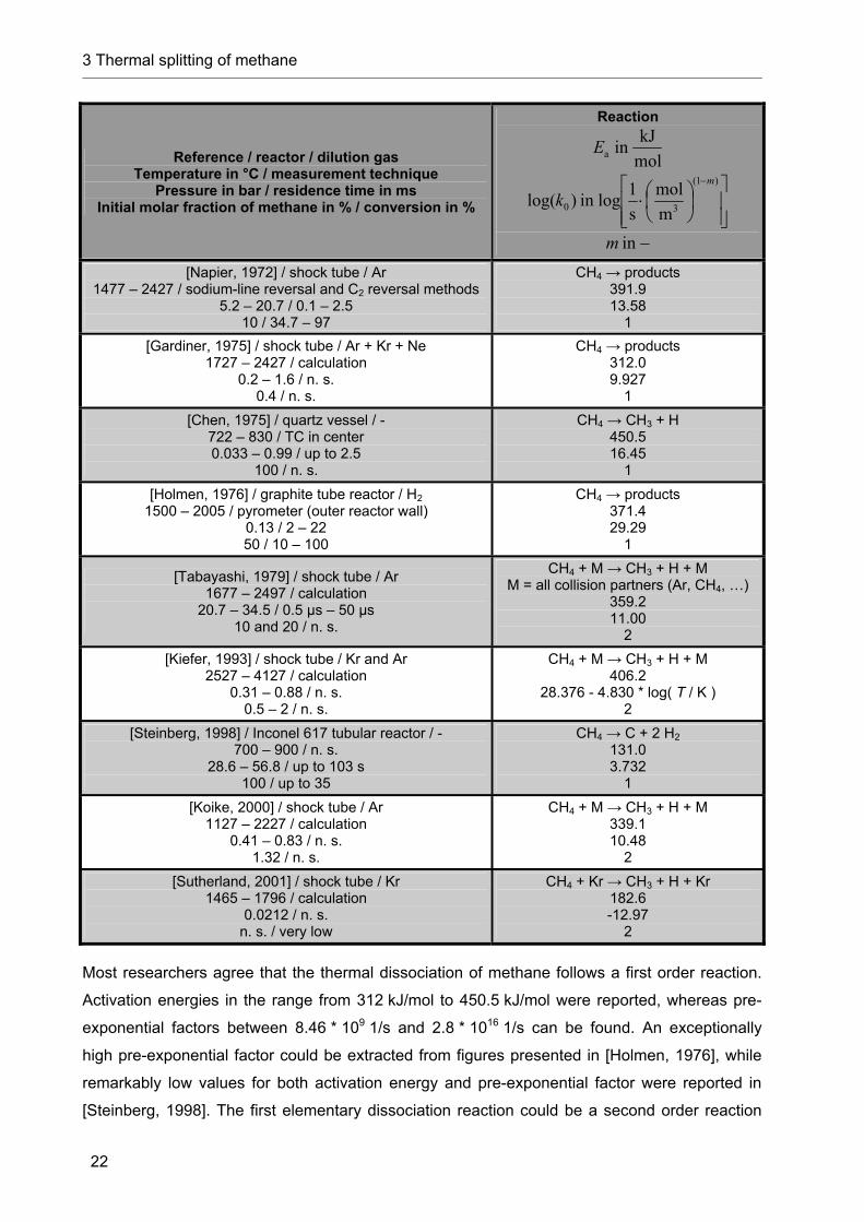
3 Thermal splitting of methane
22
Reference / reactor / dilution gas Temperature in °C / measurement technique
Pressure in bar / residence time in ms Initial molar fraction of methane in % / conversion in %
Reaction
mol
kJinaE
)1(
30 m
mol
s
1login)log(
m
k
inm
[Napier, 1972] / shock tube / Ar 1477 – 2427 / sodium-line reversal and C2 reversal methods
5.2 – 20.7 / 0.1 – 2.5 10 / 34.7 – 97
CH4 → products 391.9 13.58
1
[Gardiner, 1975] / shock tube / Ar + Kr + Ne 1727 – 2427 / calculation
0.2 – 1.6 / n. s. 0.4 / n. s.
CH4 → products 312.0 9.927
1
[Chen, 1975] / quartz vessel / - 722 – 830 / TC in center 0.033 – 0.99 / up to 2.5
100 / n. s.
CH4 → CH3 + H 450.5 16.45
1
[Holmen, 1976] / graphite tube reactor / H2 1500 – 2005 / pyrometer (outer reactor wall)
0.13 / 2 – 22 50 / 10 – 100
CH4 → products 371.4 29.29
1
[Tabayashi, 1979] / shock tube / Ar 1677 – 2497 / calculation
20.7 – 34.5 / 0.5 µs – 50 µs 10 and 20 / n. s.
CH4 + M → CH3 + H + M M = all collision partners (Ar, CH4, …)
359.2 11.00
2
[Kiefer, 1993] / shock tube / Kr and Ar 2527 – 4127 / calculation
0.31 – 0.88 / n. s. 0.5 – 2 / n. s.
CH4 + M → CH3 + H + M 406.2
28.376 - 4.830 * log( T / K ) 2
[Steinberg, 1998] / Inconel 617 tubular reactor / - 700 – 900 / n. s.
28.6 – 56.8 / up to 103 s 100 / up to 35
CH4 → C + 2 H2 131.0 3.732
1
[Koike, 2000] / shock tube / Ar 1127 – 2227 / calculation
0.41 – 0.83 / n. s. 1.32 / n. s.
CH4 + M → CH3 + H + M 339.1 10.48
2
[Sutherland, 2001] / shock tube / Kr 1465 – 1796 / calculation
0.0212 / n. s. n. s. / very low
CH4 + Kr → CH3 + H + Kr 182.6 -12.97
2
Most researchers agree that the thermal dissociation of methane follows a first order reaction.
Activation energies in the range from 312 kJ/mol to 450.5 kJ/mol were reported, whereas pre-
exponential factors between 8.46 * 109 1/s and 2.8 * 1016 1/s can be found. An exceptionally
high pre-exponential factor could be extracted from figures presented in [Holmen, 1976], while
remarkably low values for both activation energy and pre-exponential factor were reported in
[Steinberg, 1998]. The first elementary dissociation reaction could be a second order reaction

3 Thermal splitting of methane
23
involving present collision partners. Respective results differ in part significantly as can be
obtained from the table. Simplified kinetic models taking C2-hydrocarbons into account were
applied by Happel and Kramer as well as by Schulz, Klotz et al. Results of data fitting are
provided in Table 3-2. Happel and Kramer suggested the consideration of three reactions and
chose first and second order approaches in order to assess their rates, whereas Schulz, Klotz
et al. considered five second order reactions – amongst them four forward reactions as well as
one backward reaction which takes possible methane formation from the products into account.
Table 3-2: Kinetic experiments concerning the thermal decomposition of methane and determined kinetic parameters employing simplified kinetic models
Reference / reactor / dilution gas Temperature in °C / measurement technique
Pressure in bar / residence time in ms Initial molar fraction of methane in % / conversion in %
Reaction
mol
kJinaE
unitsvariousin)log( 0k
inm
CH4 → C + 2 H2 1 67.83
4.392 log[mol/(s m3 bar)] 1
CH4 → 1/2 C2H2 + 3/2 H2 2 361.9
13.50 log[mol/(s m3 bar)] 1
[Happel, 1967] / annular alumina reactor / H2 1074 – 1783 / Pt-Pt/10Rh TC (center) + pyrometer (outer wall)
0.092 – 0.94 / less than 1 21.5 – 100 / 38.4 – 100
(parameters fitted to data)
4
1,a
4 CH1,01,CH pekr T
E
4
2,a
4 CH2,02,CH pekr T
E
2
22
3,a
22
H3
2HC
3,03,HC ~1 pk
pekr T
E
C2H2 → 2 C + H2 3 74.11
6.329 log[mol/(s m3 bar2)] 2
( 3
~k = 1.515 / bar)
CH4 + M → 1/2 C2H6 + H2 + M 130
5.500 log[m3/(s mol)] 2
C2H6 + M → C2H4 + H2 + M 283
11.36 log[m3/(s mol)] 2
C2H4 + M → C2H2 + H2 + M 172.3
7.450 log[m3/(s mol)] 2
C2H2 + M → 2 C + H2 + M 17.2
1.660 log[m3/(s mol)] 2
[Schulz, 1985] / shock tube / Ar 1507 – 2257 / calculation
2.6 / 0.5 – 4 2 / 30 – 100
(parameters fitted to data)
P + M → CH4 + M
(44 CH0,CHP ccc )
38.3 1.800 log[m3/(s mol)]
2
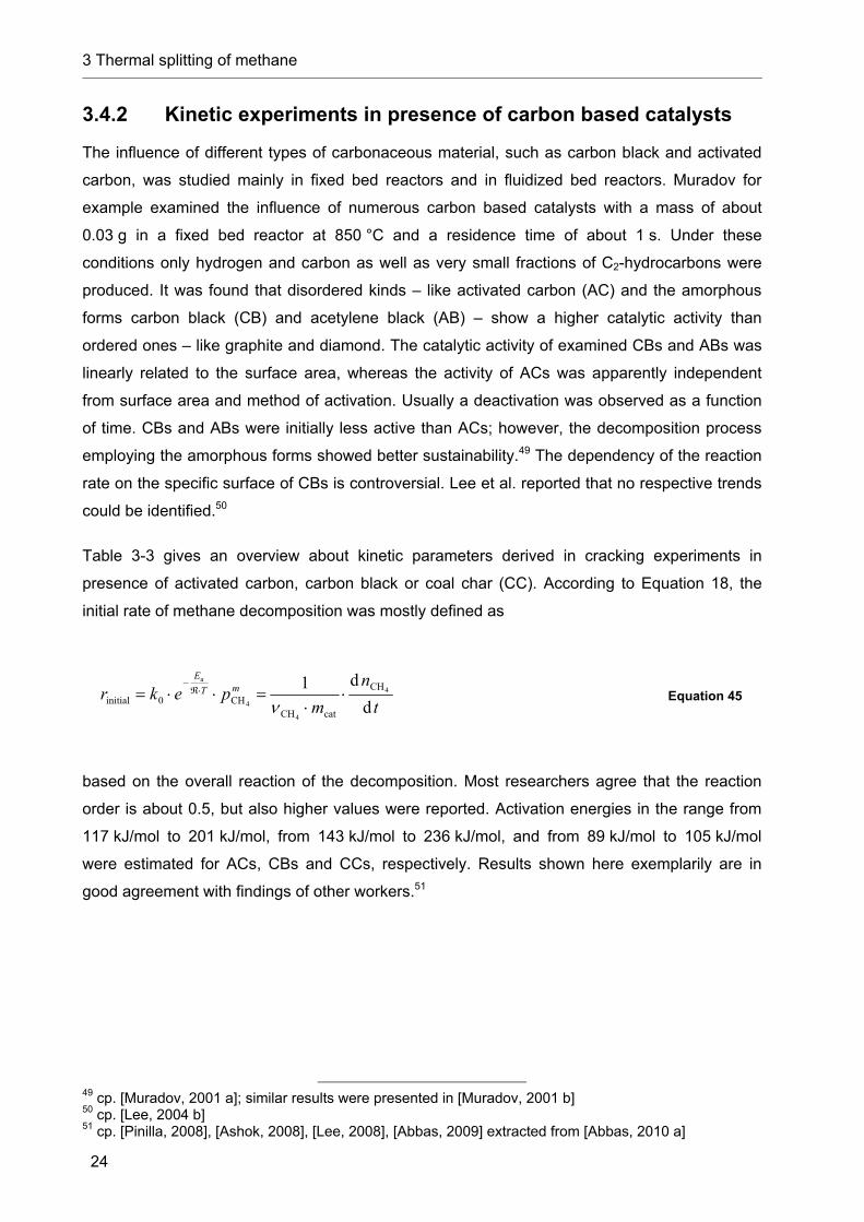
3 Thermal splitting of methane
24
3.4.2 Kinetic experiments in presence of carbon based catalysts
The influence of different types of carbonaceous material, such as carbon black and activated
carbon, was studied mainly in fixed bed reactors and in fluidized bed reactors. Muradov for
example examined the influence of numerous carbon based catalysts with a mass of about
0.03 g in a fixed bed reactor at 850 °C and a residence time of about 1 s. Under these
conditions only hydrogen and carbon as well as very small fractions of C2-hydrocarbons were
produced. It was found that disordered kinds – like activated carbon (AC) and the amorphous
forms carbon black (CB) and acetylene black (AB) – show a higher catalytic activity than
ordered ones – like graphite and diamond. The catalytic activity of examined CBs and ABs was
linearly related to the surface area, whereas the activity of ACs was apparently independent
from surface area and method of activation. Usually a deactivation was observed as a function
of time. CBs and ABs were initially less active than ACs; however, the decomposition process
employing the amorphous forms showed better sustainability.49 The dependency of the reaction
rate on the specific surface of CBs is controversial. Lee et al. reported that no respective trends
could be identified.50
Table 3-3 gives an overview about kinetic parameters derived in cracking experiments in
presence of activated carbon, carbon black or coal char (CC). According to Equation 18, the
initial rate of methane decomposition was mostly defined as
t
n
mpekr mT
E
d
d14
4
4
aCH
catCHCH0initial
Equation 45
based on the overall reaction of the decomposition. Most researchers agree that the reaction
order is about 0.5, but also higher values were reported. Activation energies in the range from
117 kJ/mol to 201 kJ/mol, from 143 kJ/mol to 236 kJ/mol, and from 89 kJ/mol to 105 kJ/mol
were estimated for ACs, CBs and CCs, respectively. Results shown here exemplarily are in
good agreement with findings of other workers.51
49 cp. [Muradov, 2001 a]; similar results were presented in [Muradov, 2001 b] 50 cp. [Lee, 2004 b] 51 cp. [Pinilla, 2008], [Ashok, 2008], [Lee, 2008], [Abbas, 2009] extracted from [Abbas, 2010 a]

3 Thermal splitting of methane
25
Table 3-3: Kinetic experiments concerning the thermal decomposition of methane in the presence of carbon based catalysts and determined kinetic parameters
Reference / reactor / dilution gas Temperature in °C / measurement technique
Pressure in bar / residence time in s / catalyst mass in gInitial molar fraction of methane in % / conversion in %
Catalysts / specific surface in m2/g
mol
kJinaE
m
kbargmin
mmollogin)log(
cat0
inm
[Kim, 2004] / fixed bed quartz tube reactor / Ar 750 – 900 / TC
n. s. / 0.6 / 0.2 – 0.8 up to 100 / up to 15
AC / 725, 912, 966 (725, 912) 194, 186, 198
n. s. ~ 0.5 (0.51, 0.49)
[Lee, 2004 a] / fluidized bed quartz tube reactor / - 700 – 900 / TC in middle of bed
n. s. / n. s. / 20 100 / up to 45
AC / 966 138.9 (MFR) – 147.4 (PFR) 13.54 (MFR) – 14.28 (PFR)
~ 0.5
[Lee, 2004 b] / fixed bed quartz tube reactor / Ar 750 – 1050 / TC 1.01 / n. s. / 0.1
up to 100 / up to 70
CB / 79, 1475 183, 143
7.920, 6.401 ~ 1 (0.919, 0.984)
[Trommer, 2004] / vortex flow reactor / Ar 627 – 800 / TC type K up to 1.1 / 9 / 1.9 g/min
15 / up to 46
AC / 900 147 (PFR) – 162 (MFR)
6.029 (PFR) log(1/s) – 6.877 (MFR) log(1/s)1
AC / 650 – 3370 (650) 160 – 201
n. s. ~ 0.5 (0.6)
[Muradov, 2005 b] / quartz microreactor with fixed bed / - 850 / TC type K
1.01 / 0.1 / 0.03 – 0.1 100 / n. s. (20 – 70)
CB / 25 – 1500 (1500) 205 – 236
n. s. ~ 0.5 (0.5)
[Bai, 2005] / fixed bed quartz tube reactor / N2 750 – 900 / n. s.
1.01 / n. s. / 1 up to 100 / up to 35
AC / n. s., 783, 735, 738 116.9, 133.6, 140.0, 184.9
n. s. 0.5
[Bai, 2006] / fixed bed quartz tube reactor / N2 750 – 900 / n. s.
1.01 / n. s. / 1 up to 100 / up to 35
CC / 22, 41, 127 (22, 127) 105, 98, 89
n. s. ~ 0.5 (0.54, 0.52)
[Jung, 2007] / fluidized bed quartz tube reactor / - 800 – 925 / TC in middle of bed
1.01 / n. s. / 20 100 / up to 50
AC / n. s. 140 n. s. n. s.
[Abbas, 2010 b] / fixed bed stainless steel tube reactor / - 775 – 850 / TC type K
1.01 / 2 – 12.2 / 20 – 120 100 / 24.2 – 68.6
AC / n. s. 163
7.409 log[dm6/(gcat mol min)] 2

3 Thermal splitting of methane
26
3.4.3 Kinetic experiments concerning the pyrolysis of C2-hydrocarbons
Table 3-4 shows some examples for works dealing with the thermal dissociation of C2-
hydrocarbons. Orders of initial stage or overall reactions were found to equal one or two. By
trend, the activation energy increases with the number of H-atoms in the reactant.
Table 3-4: Kinetic experiments concerning the thermal decomposition of C2-hydrocarbons and determined kinetic parameters
Reference / reactor / dilution gas Temperature in °C / measurement technique
Pressure in bar / residence time in ms Initial molar fraction of reactant in % / conversion in %
Reaction
mol
kJinaE
)1(
30 m
mol
s
1login)log(
m
k
inm
C2H6 → C2H4 + H2 334.9 16.65
1 (based on own data and other works)
[Kozlov, 1962] / shock tube / Ar 887 – 1307 / calculation
2.03 – 6.08 / 0.8 1 and 5 / 2 – 90
C2H6 → C2H4 + H2 288.9
14 1
(based on own data and other works)
[Hidaka, 1985] / shock tube / Ar 927 – 1427 / calculation
1.72 – 2.53 / n. s. 1 – 5 / n. s.
C2H6 → 2 CH3 334.9 14.85
1
[Kozlov, 1962] / shock tube / Ar 977 – 1577 / calculation
2.03 – 6.08 / n. s. 1 and 5 / whole range
C2H4 → C2H2 + H2 167.5 8.410
1
[Pilla, 2010] / shock tube / Ar 1117 – 1597 / calculation
2.23 – 3.14 / 1 1 / n. s.
C2H4 → C2H2 + H2 227.0 8.740
2
C2H2 → 2 C + H2 125.6 6.230
1 (suggested for high temperatures)
[Kozlov, 1962] / shock tube / Ar 1327 – 2227 / calculation
4.05 / 0.8 1 and 5 / up to 98
C2H2 → 2 C + H2 167.5 7.330
2 (suggested for low temperatures)
[Wu, 1987] / shock tube / Ne + Ar 1627 – 2227 / calculation
0.3 – 0.56 / up to 0.75 1 – 6.2 / n. s.
2 C2H2 → C4H3 + H 186.3 7.301
2

4 Experimental
27
4 Experimental
In order to investigate the kinetics of the thermal dissociation of methane, numerous
experiments were accomplished based on a wide range of reaction conditions. The feed flow
contained methane as well as an inert dilution gas, which allowed studying the influence of
methane concentration at a constant pressure level and damped the temperature change due to
reaction. Furthermore, the risk of clogging was decreased. After presenting the experimental
setup, the covered reaction conditions are introduced before the adopted procedure of the
experiments is explained. General results based on the conversion of methane and the yields of
considered products are shown subsequently.52 The next chapter deals with the measurement
of the temperature, one of the main influencing factors of reaction rates. At last additional
experiments, which were carried out in order to gain further knowledge about the repeatability of
results, location and character of formed carbon, balances of H- and C-atoms, as well as the
influences of added carbon particles, are respected.53
4.1 Experimental setup
The kinetic experiments were carried out employing an aluminum oxide tube reactor54 with an
inner/outer diameter of 8/12 mm situated in a tube furnace55 as can be seen in Figure 4-1. This
tube furnace contains molybdenum disilicide (MoSi2) heating elements which allow the provision
of heat at temperatures up to 1800 °C. The inlet gas composed of methane and a dilution gas,
either argon (Ar) or helium (He), was prepared by mass flow controllers56. Depending on the
conditions inside the reactor cracking reactions proceeded generating the desired products
hydrogen (H2) and carbon (C) as well as intermediates. The composition of the product gas was
analyzed by a gas chromatograph (GC)57 respecting argon, methane, hydrogen, and C2-
hydrocarbons. There were two particle filters which guaranteed a high efficiency of filtration: the
main filter and the GC filter with a nominal pore diameter of 1 µm and 0.5 µm, respectively.58
The main filter removed particles from the product flow before it left the systems toward the flue,
whereas the GC filter removed particles from the sample flow toward the GC. A two filter
configuration permits the usage of large filter elements in the main filter going hand in hand with
an increase of operating time due to a lower risk of clogging without drawbacks for the GC
52 Brief descriptions of the experimental setup as well as preliminary experimental results can be found in [Wullenkord, 2008], [Wullenkord, 2009 a], [Wullenkord, 2009 b], and [Wullenkord, 2010 a].
53 Respective results were partly presented in [Wullenkord, 2010 a] and [Wullenkord, 2010 b]. 54 Manufacturer: FRIATEC AG, Mannheim, Germany. 55 Manufacturer: Gero Hochtemperaturöfen GmbH & Co. KG, Neuhausen, Germany. Type HTRV 40-250-18 SO. 56 Manufacturer: MKS Instruments Deutschland GmbH, München, Germany. 57 Manufacturer / provider: SRI Instruments Inc., Las Vegas, NV, USA. Schambeck SFD GmbH, Bad Honnef, Germany. Type SRI Multiple Gas Analyzer #2 8610C. 58 Manufacturer / provider: CONTEC GmbH, Bad Honnef, Germany (filter body AVPP20 with filter element AX1-20) and B.E.S.T. Fluidsysteme GmbH, Kaarst, Germany (Swagelok).
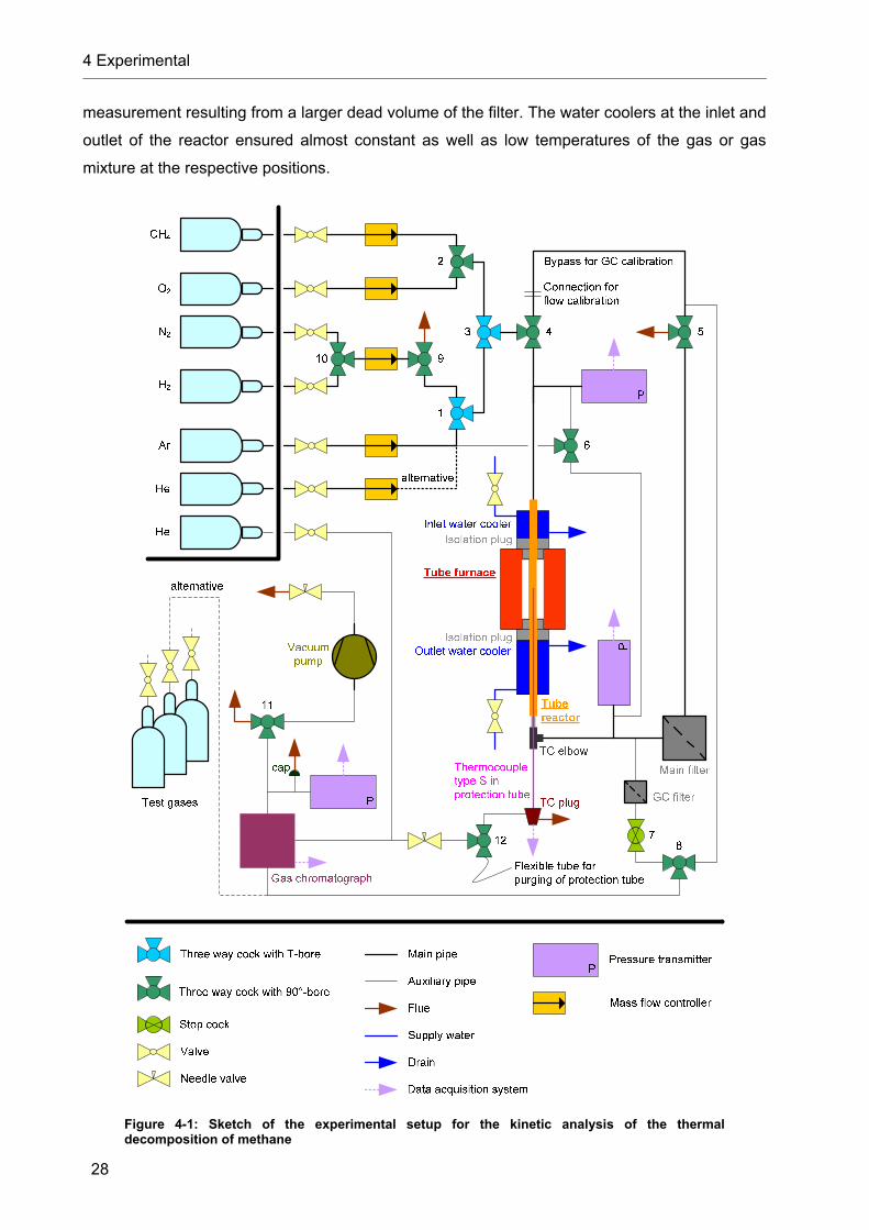
4 Experimental
28
measurement resulting from a larger dead volume of the filter. The water coolers at the inlet and
outlet of the reactor ensured almost constant as well as low temperatures of the gas or gas
mixture at the respective positions.
Figure 4-1: Sketch of the experimental setup for the kinetic analysis of the thermal decomposition of methane

4 Experimental
29
The measurement of axial temperature profiles inside the tube reactor took place using a self-
made thermocouple type S59 described in detail later (see Chapter 4.5). Finally, the pressure
was measured at both sides of the reactor tube.60 All metal parts were grounded. Figure 4-2
shows a picture of the experimental setup including stop cock and three way cocks61 as well as
fittings and connections62.
Figure 4-2: Picture of the experimental setup with some main components as well as additional parts like two and three way cocks (numbers in red) and connections
The diameters of the reactor tube and the protection tube of the thermocouple have a maximum
uncertainty of +/- 5 %, which means that the tolerance for the inner diameter of the reactor
equals 0.4 mm, whereas the outer diameter of the protection tube may vary by 0.2 mm.63
Different dimensions as well as axial positions of the experimental setup relevant for illustration
and later calculations are shown in Figure 4-3. In the following the position - 213 mm, which
59 Provider of thermo wires: E&S METRONIC Meß- und Regeltechnik GmbH, Werne, Germany. 60 Manufacturer of pressure transmitters: WIKA Alexander Wiegand GmbH & Co. KG, Klingenberg, Germany. 61 Manufacturer / provider: EM-TECHNIK GmbH, Maxdorf, Germany. B.E.S.T. Fluidsysteme GmbH, Kaarst, Germany (Swagelok). 62 Manufacturer / provider: B.E.S.T. Fluidsysteme GmbH, Kaarst, Germany (Swagelok). PTS MARQUARDT GmbH Automatisierungstechnik, Pulheim, Germany (Legris). 63 cp. [FRIATEC, 2003], p. 14
tube furnace
inlet pressure sensor
outlet water cooler
outlet pressure sensor
three way cock (8)
connection for flow
calibration
bypass for GC-
calibration
TC elbow stop cock (7)
4
5
32 1
12
6

4 Experimental
30
corresponds to the upper edge of the inlet water cooler, accounts for the inlet of the reactor. The
heated length of the tube furnace equals 250 mm. The manufacturer states that the temperature
homogeneity inside the work tube reaches +/- 10 K in 50 % of the heated length.64
Figure 4-3: Basic dimensions and axial positions of the experimental setup for the kinetic analysis of the thermal decomposition of methane in mm
Some components of the experimental setup will be described in detail in the following
chapters.
4.1.1 Mass flow controllers
For the preparation of gas mixtures, either as inlet gas or calibration gas for the gas
chromatograph, mass flow controllers (MFCs) manufactured by MKS were employed. Table 4-1
provides information about the MFCs implemented in the experimental setup and used gases.
64 [Gero, 2006]

4 Experimental
31
Table 4-1: Information about used mass flow controllers and gases (GCF = Gas Correction Factor)
Gas65 Quality Purity
Type of MFC (produced) Nominal range and gas Range for selected gas (GCF)
Accuracy Repeatability
1179 (2003) 500 sccm N2 685.0 sccm Ar (1.37)
1.0 % of FS (full scale) +/- 0.2 % of FS → +/- 1.37 sccm
1259 (1999) 2000 sccm N2 2740 sccm Ar (1.37)
0.8 % of FS n. s. (not specified)
1179 (2007) 15 SLM CO2 approximated by 20 SLM N2 (due to control unit) 27.40 SLM Ar (1.37, originally 1.986)
0.5 % of reading + 0.2 % of FS +/- 0.2 % of FS → +/- 0.0548 SLM
Ar 4.8 99.998 %
1179 (2007) 20 SLM N2 27.40 SLM Ar (1.37)
0.5 % of reading + 0.2 % of FS +/- 0.2 % of FS → +/- 0.0548 SLM
1179 (2007) 10 sccm CH4 10.00 sccm (1.00)
0.5 % of reading + 0.2 % of FS +/- 0.2 % of FS → +/- 0.02 sccm
1259 (1996) 100 sccm N2 72.00 sccm (0.72)
0.8 % of FS n. s.
CH4 4.5 99.995 %
1259 (1996) 500 sccm N2 360.0 sccm (0.72)
0.8 % of FS n. s.
1179 (2003) 500 sccm N2 725.0 sccm (1.45)
1.0 % of FS +/- 0.2 % of FS → +/- 1.45 sccm
1259 (1999) 2000 sccm N2 2900 sccm (1.45)
0.8 % of FS n. s.
He 5.0 99.999 %
1179 (2007) 20 SLM N2 29.00 SLM (1.45)
0.5 % of reading + 0.2 % of FS +/- 0.2 % of FS → +/- 0.058 SLM
O2 2.5 99.5 %
1259 (1998) 50 sccm N2 50.00 sccm (1.00)
0.8 % of FS n. s.
H2 5.0 99.999 %
1179 (2007) 10 sccm H2 10.00 sccm (1.00)
0.5 % of reading + 0.2 % of FS +/- 0.2 % of FS → +/- 0.02 sccm
N2 2.8 99.8 %
1179 (2007) 10 sccm H2 10.00 sccm (1.00)
0.5 % of reading + 0.2 % of FS +/- 0.2 % of FS → +/- 0.02 sccm
all Multigas Controller 647BE (1996)
+/- 1 digit
The measurement technique of the MFCs is based on the temperature rise of part of the
controlled gas flow with known heat capacity resulting from the import of a certain amount of
65 Provider: Praxair Deutschland GmbH, Hürth, Germany.

4 Experimental
32
heat energy.66 Since a high purity of used gases was requested, any uncertainties related to
respective impurities were neglected.
4.1.2 Gas chromatograph
A gas chromatograph equipped with a thermal conductivity detector (TCD) and a helium
ionization detector (HID) was used for the analysis of the composition of the product gas. The
TCD shows good performance for high molar fractions up to 100 %. It was used for the
evaluation of molar fractions of argon and methane (with molar fractions above 0.8 %).
Contrariwise, the HID provides high functionality for low concentrations and for hydrogen.
Hydrogen could hardly be detected with the TCD because hydrogen has quite similar thermal
conductivity characteristics compared to the carrier gas helium. Two packed columns were
utilized for the separation of the sample components: a molecular sieve column (MS) for
hydrogen, argon, and methane as well as a HayeSep A column for the C2-hydrocarbons and
higher hydrocarbons. Figure 4-4 shows the setup of the GC.
Figure 4-4: Configuration of gas chromatograph
Basic information about the GC and its periphery can be found in Table 4-2. Additional
information about the adjusted parameters of the GC as well as examples for chromatograms of
the product gas are provided in Appendix B.
66 Further information may be found on http://www.mksinst.com.
TCD
HID
valve oven
valve (10 ports) column
oven
HayeSep A
GC pressure sensor
MS 13X
three way cock: 11
IN OUT
access for test gases (alternative)
loop

4 Experimental
33
Table 4-2: Basic information about the gas chromatograph
Detectors Helium ionization detector (HID) Thermal conductivity detector (TCD)
Sample loops 2 x 1 ml
Packed columns Molecular sieve MS 13X, length: 6’ HayeSep A, length: 3 m
Load and inject device Automated gas sample valve with 10 ports
Sample carrier gas
Operating gas of HID and TCD
Helium 5.0 (purity: 99.999 %, further purification by moisture trap67 → hydrocarbon trap68 → oxygen trap69, overpressure at GC inlet: 4 bar)
Length of HID electric arc 0.8 mm … 0.9 mm
Special features of HID enhanced collector electrode inert glass tube inserted in metal tube between
electric arc and collector electrode
Power supply Variable transformer: 230 V (+/- 5 %)70
Gas samples were fed into the loops either by underpressure at the sample outlet (vacuum
pump) or by overpressure at the sample inlet (pressurized test gases). According to the ideal
gas law, the amount of injected substance loopn depends on the conditions inside the loop
before injection following
loop
looplooploop T
Vpn
. Equation 46
Since the loop’s volume loopV and loopT keep constant (the loops are situated in the tempered
valve oven), loopn is only a function of the pressure inside the loop before injection loopp , which
depends on the ambient pressure and the pressure inside the reactor. It was measured by a
pressure transmitter at the sample outlet of the GC.
Actually, the area of a peak peak,iA is a function of the amount of substance of the particular
component i approaching the detector detector,in , which equals the amount of substance of the
particular component i inside the loop loop,in arising from
67 Manufacturer: Restek GmbH, Bad Homburg, Germany. 68 Manufacturer: SGE Europe Ltd., Kiln Farm Milton Keynes, United Kingdom. 69 Manufacturer: see above 70 Manufacturer: BLOCK Transformatoren-Elektronik GmbH, Verden, Germany. Type: BR2200.

4 Experimental
34
looploop,loop, nxn ii , Equation 47
with the molar fraction of component i in the loop loop,ix , because there is no reduction of the
amount of substance between the loops and the detectors concerning the considered species.
The aim of GC measurement is the analysis of the composition of the sample in terms of molar
fractions loop,ix . Considering a sample with a molar fraction of component i loop,ix different
pressures inside the loop result in different peak areas peak,iA , since loopn depends on loopp . In
order to compensate this effect and allow comparability of different measurements, a normal
peak area Npeak,,iA was calculated by
loop
Npeak,Npeak,, p
pAA ii , Equation 48
assuming that peak,iA is proportional to loop,in . Npeak,,iA corresponds to the theoretic peak area
resulting from loop,ix at standard pressure Np . Although linear relationships could not be verified
generally, loop,ix can be well approximated as a function of Npeak,,iA . An overview about
components, the measurement of their molar fractions, and determined calibration curves is
given in Table 4-3.
Table 4-3: Employed detectors and calibration curves for the measurement of molar fractions of the main sample components
Component HID TCD Calibration curve
H2 2nd order polynomial
CH4 %)8.0(4CH x %)8.0(
4CH x 2nd order polynomial (HID), line (TCD)
Ar line
C2H6 2nd order polynomial
C2H4 2nd order polynomial
C2H2 2nd order polynomial

4 Experimental
35
As can be seen in Table 4-3, calibration curves do not have a uniform shape. Linear fit functions
as well as 2nd order polynomials can be found. Figure 4-5 (a) and (b) show examples of
calibration curves for hydrogen and methane. Approaches for the curves are valid for a wide
range of molar fractions covering more than one order of magnitude. Further examples for
calibration curves can be found in Appendix B.
0 1000 2000 3000 4000 5000 6000 70000
3
6
9
12
15
Mol
ar fr
actio
n in
%
Normal peak area in mV s
0 50 100 150 200 250 3000
2
4
6
8
10
12
Mol
ar fr
actio
n in
%
Normal peak area in mV s
Figure 4-5: Examples for GC calibration curves: the molar fraction of hydrogen detected by the HID (a) and the molar fraction of methane detected by the TCD (b) as a function of the normal peak area
The needle valve downstream the vacuum pump of the GC was installed in order to allow the
adjustment of the sample volume flow. Preliminary tests showed that practically complete
purging of the GC inlet pipes could be achieved with about 60 s operating time of the vacuum
pump at about 50 ml/min. For this volume flow the difference of the pressure at the GC sample
outlet at the end of and during the operation of the vacuum pump lies in the range of 35 mbar.
An increase of the vacuum pump volume flow due to a decrease of the flow resistance in the
needle valve downstream the vacuum pump causes a higher pressure difference (about
75 mbar at 100 ml/min and about 180 mbar at 200 ml/min). Tests were carried out in order to
check whether measurement results are affected by the sample volume flow e. g. due to a
possibly favored transport of hydrogen. An influence of the pressure difference on the
measurement result exceeding the uncertainty of GC measurement and of composition of the
test gas mixture could not be observed.
In order to quantify the uncertainty of GC measurements, test gases were injected in the GC
repeatedly. Different numbers of runs iN were performed respecting component i in the
considered test gas. For every session )( Npeak,,rel iAs , the experimental standard deviation of j
normal peak areas Npeak,,iA relative to the mean Npeak,,iA , calculated by
H2: 2nd order polynomial CH4: line
(a) (b)

4 Experimental
36
iN
jji
ii A
NA
1N,peak,,Npeak,,
1 , Equation 49
was determined according to
1
1)( 1
2
Npeak,,N,peak,,
Npeak,,Npeak,,rel
i
N
jiji
ii N
AA
AAs
i
. Equation 50
Additionally, maximum positive deviations relative to the mean maxrel,s were calculated
employing
Npeak,,
Npeak,,N,peak,,
Npeak,,maxrel,
max)(
i
ijij
i A
AAAs
Equation 51
and similarly maximum negative deviations relative to the mean maxrel,s following
Npeak,,
Npeak,,N,peak,,
Npeak,,maxrel,
min)(
i
ijij
i A
AAAs
. Equation 52
Depending on the test day determined values for the standard deviation, maximum positive
deviation, and maximum negative deviation relative to the mean differ in part significantly.
Extreme deviations observed in practice are summarized in Table 4-4 for considered gases and
molar fractions. Maximum positive and negative deviations do not always show symmetric
behavior. Compared to hydrogen and methane somewhat higher deviations have to be reported
for the C2-hydrocarbons. Greatest deviations could be found for ethyne, mainly resulting from
drifting during the particular test day. Complete information respecting results of particular test
days is provided in Appendix B.
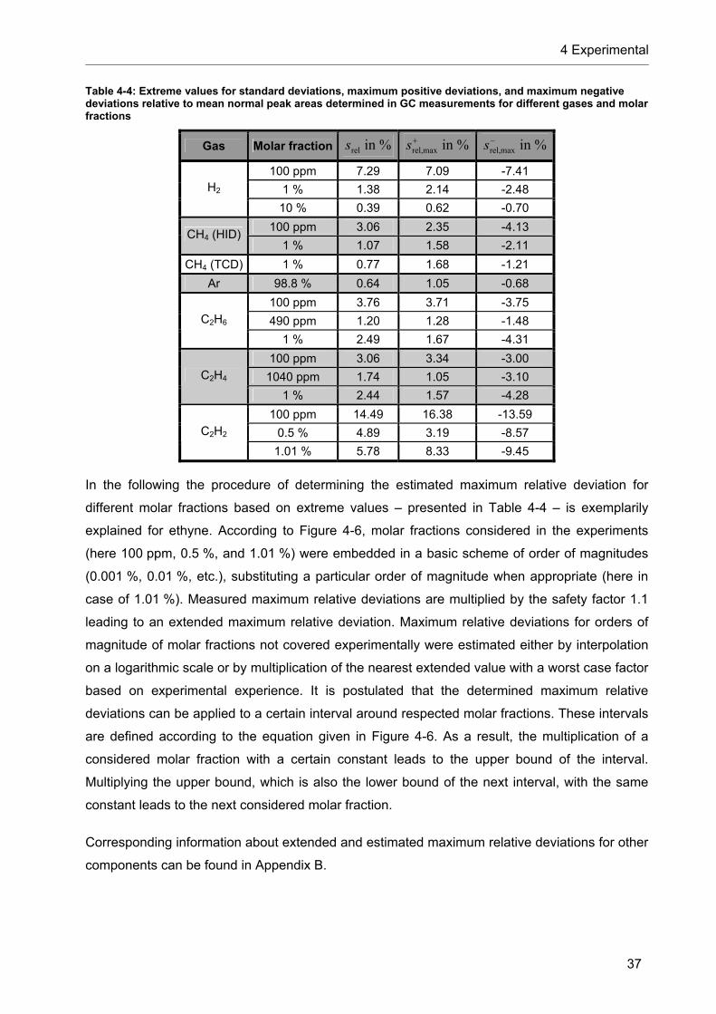
4 Experimental
37
Table 4-4: Extreme values for standard deviations, maximum positive deviations, and maximum negative deviations relative to mean normal peak areas determined in GC measurements for different gases and molar fractions
Gas Molar fraction %inrels %inmaxrel,s %inmaxrel,
s
100 ppm 7.29 7.09 -7.41
1 % 1.38 2.14 -2.48 H2
10 % 0.39 0.62 -0.70
100 ppm 3.06 2.35 -4.13 CH4 (HID)
1 % 1.07 1.58 -2.11
CH4 (TCD) 1 % 0.77 1.68 -1.21
Ar 98.8 % 0.64 1.05 -0.68
100 ppm 3.76 3.71 -3.75
490 ppm 1.20 1.28 -1.48 C2H6
1 % 2.49 1.67 -4.31
100 ppm 3.06 3.34 -3.00
1040 ppm 1.74 1.05 -3.10 C2H4
1 % 2.44 1.57 -4.28
100 ppm 14.49 16.38 -13.59
0.5 % 4.89 3.19 -8.57 C2H2
1.01 % 5.78 8.33 -9.45
In the following the procedure of determining the estimated maximum relative deviation for
different molar fractions based on extreme values – presented in Table 4-4 – is exemplarily
explained for ethyne. According to Figure 4-6, molar fractions considered in the experiments
(here 100 ppm, 0.5 %, and 1.01 %) were embedded in a basic scheme of order of magnitudes
(0.001 %, 0.01 %, etc.), substituting a particular order of magnitude when appropriate (here in
case of 1.01 %). Measured maximum relative deviations are multiplied by the safety factor 1.1
leading to an extended maximum relative deviation. Maximum relative deviations for orders of
magnitude of molar fractions not covered experimentally were estimated either by interpolation
on a logarithmic scale or by multiplication of the nearest extended value with a worst case factor
based on experimental experience. It is postulated that the determined maximum relative
deviations can be applied to a certain interval around respected molar fractions. These intervals
are defined according to the equation given in Figure 4-6. As a result, the multiplication of a
considered molar fraction with a certain constant leads to the upper bound of the interval.
Multiplying the upper bound, which is also the lower bound of the next interval, with the same
constant leads to the next considered molar fraction.
Corresponding information about extended and estimated maximum relative deviations for other
components can be found in Appendix B.

4 Experimental
38
1E-4 1E-3 0.01 0.1 1 100
5
10
15
20
170
180
190
value for OM 1 substituted by measured value for 1.01
assumed
xj, upper = xj + 1, lower = xjhh(hxj + 1/xj )0.5
j : number of intervalxj : reference value for interval
xj, lower : lower bound of interval j
xj, upper : upper bound of interval j
o
oo
o
0 ...
Max
imu
m r
elat
ive
dev
iatio
n in
%
Molar fraction in %
measured extended estimated
o basic (OM) / o substituting o additional
x 1.1
o
interpolated on logarithmic scale
xj, lower xj xj, upper
x 10
Figure 4-6: Maximum relative positive deviation of GC measurements for ethyne: measured, extended and estimated levels (OM = order of magnitude)
Be it that a certain normal peak area Npeak,,iA was determined for the component i of a gas
mixture. If no further data is available, Npeak,,iA is the best estimate for subsequent calculations.
However, the measured value could just lie on the upper or lower bound of the interval of
possible values around the theoretical average of a collectivity of not executed measurements.
It is consequently admissible to calculate the extreme values maxN,peak,,iA and minN,peak,,iA , the
limits of an interval, in which the theoretical average should be found with a probability of
practically 100 %, according to
1maxrel,
Npeak,,maxN,peak,,
s
AA i
i Equation 53
and

4 Experimental
39
1maxrel,
Npeak,,minN,peak,,
s
AA i
i . Equation 54
4.1.3 Pressure transmitters
Pressures at the inlet and the outlet of the reactor as well as at the sample outlet of the GC
were determined by pressure transmitters manufactured by WIKA. The measurement chain is
shown in Figure 4-7.
Figure 4-7: Measurement chain of the measurement of pressures
Depending on the pressure affecting the membrane of the pressure transmitter, an electric
current is available at the signal output. Via a resistor the electric current was converted into a
voltage signal which was interpreted by further components of the data acquisition system71.
Information about the employed pressure transmitters, the subsequent measurement chain, and
estimated maximum as well as standard uncertainties is provided in Table 4-5.
71 Manufacturer / provider: Advantech Co., Ltd., Milpitas, USA and National Instruments Germany GmbH, München, Germany.
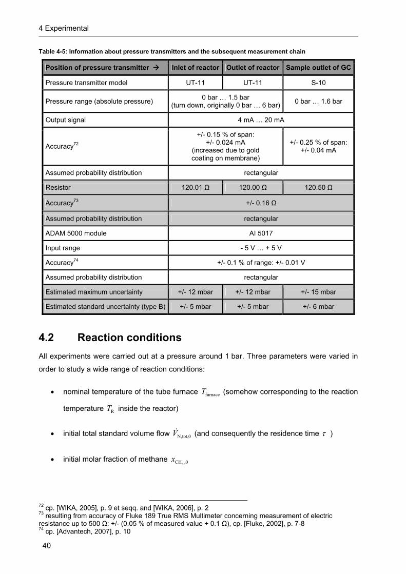
4 Experimental
40
Table 4-5: Information about pressure transmitters and the subsequent measurement chain
Position of pressure transmitter Inlet of reactor Outlet of reactor Sample outlet of GC
Pressure transmitter model UT-11 UT-11 S-10
Pressure range (absolute pressure) 0 bar … 1.5 bar
(turn down, originally 0 bar … 6 bar)0 bar … 1.6 bar
Output signal 4 mA … 20 mA
Accuracy72
+/- 0.15 % of span: +/- 0.024 mA
(increased due to gold coating on membrane)
+/- 0.25 % of span: +/- 0.04 mA
Assumed probability distribution rectangular
Resistor 120.01 Ω 120.00 Ω 120.50 Ω
Accuracy73 +/- 0.16 Ω
Assumed probability distribution rectangular
ADAM 5000 module AI 5017
Input range - 5 V … + 5 V
Accuracy74 +/- 0.1 % of range: +/- 0.01 V
Assumed probability distribution rectangular
Estimated maximum uncertainty +/- 12 mbar +/- 12 mbar +/- 15 mbar
Estimated standard uncertainty (type B) +/- 5 mbar +/- 5 mbar +/- 6 mbar
4.2 Reaction conditions
All experiments were carried out at a pressure around 1 bar. Three parameters were varied in
order to study a wide range of reaction conditions:
nominal temperature of the tube furnace furnaceT (somehow corresponding to the reaction
temperature RT inside the reactor)
initial total standard volume flow tot,0N,V (and consequently the residence time )
initial molar fraction of methane ,0CH4x
72 cp. [WIKA, 2005], p. 9 et seqq. and [WIKA, 2006], p. 2 73 resulting from accuracy of Fluke 189 True RMS Multimeter concerning measurement of electric resistance up to 500 Ω: +/- (0.05 % of measured value + 0.1 Ω), cp. [Fluke, 2002], p. 7-8 74 cp. [Advantech, 2007], p. 10

4 Experimental
41
Experiments with argon as the diluent have been carried out at five levels of nominal
temperature of the tube furnace: 1200 °C, 1300 °C, 1400 °C, 1500 °C, and 1600 °C. For every
nominal furnace temperature five (in case of 1600 °C four) residence times were applied. Each
set of nominal furnace temperature and residence time comprises three (in one case four) initial
molar fractions of methane, regularly in the range between 2 % and 10 %. An overview of the
reaction conditions finally covered in the experiments using argon as the dilution gas is given in
Table 4-6.
Table 4-6: Reaction conditions covered in experiments with argon as dilution gas
Ar Level of
/furnaceT -set Cinfurnace T sccmintot,0N,V sin %in,0CH4x
1 95 1.46 2, 5, 10
2 200 0.696 2, 5, 10
3 350 0.396 2, 5, 10
4 685 0.203 2, 5, 10
5
1200
2000 0.0697 2, 5, 10, 20
6 340 0.378 2, 5, 10
7 650 0.200 2, 5, 10
8 1300 0.100 2, 5, 10
9 2600 0.0501 2, 5, 10
10
1300
4800 0.0275 2, 5, 10
11 700 0.174 2, 5, 10
12 1400 0.0885 2, 5, 10
13 2600 0.0487 2, 5, 10
14 3800 0.0324 2, 5, 10
15
1400
6500 0.0198 2, 5, 7.1
16 1600 0.0707 2, 5, 10
17 2800 0.0415 2, 5, 10
18 4600 0.0256 2, 5, 10
19 7200 0.0162 2, 5, 6.3
20
1500
9800 0.0119 2, 3.1, 5
21 2000 0.0547 2, 5, 10
22 3350 0.0335 2, 5, 10
23 6500 0.0176 2, 5, 7.1
24
1600
9800 0.0115 2, 3, 5
Moreover, a reduced number of experiments with helium as diluent were executed. Here only
three nominal furnace temperatures were considered, namely 1300 °C, 1400 °C, and 1500 °C,
applying one or three residence times, respectively. As also done in experiments with argon as

4 Experimental
42
dilution gas, the initial molar fraction of methane was varied between 2 % and 10 %. A
corresponding summary can be found in Table 4-7.
Table 4-7: Reaction conditions covered in experiments with helium as dilution gas
He Level of
/furnaceT -set Cinfurnace T sccmintot,0N,V sin %in,0CH4x
25 1300 3800 0.0344 2, 5, 10
26 2800 0.0443 2, 5, 10
27 3800 0.0328 2, 5, 10
28
1400
6500 0.0190 2, 5, 7.1
29 1500 3800 0.0303 2, 5, 10
The residence time in the reactor – introduced before – is defined as
inletR,
N
N
furnacetot,0N,
heated2
iR,
reference
heated 4
p
p
T
TV
ld
V
V
. Equation 55
heatedV is the volume in the reactor that is actively heated by the tube furnace and which can be
calculated employing the inner diameter of the tube reactor iR,d and the heated length of the
tube furnace heatedl . referenceV is a reference volume flow depending on the initial total standard
volume flow tot,0N,V , the nominal furnace temperature furnaceT , and the average pressure at the
inlet of the reactor inletR,p , calculated as the mean of the pressures at the inlet of the reactor at
the start and the end of the GC-procedure. NT represents the standard temperature, whereas
Np stands for the standard pressure.
4.3 Procedure
At the beginning of each test day the mass flow controllers were calibrated with respect to
standard volume flows needed later on during the calibration of the GC and the cracking
experiments employing a primary flow calibrator75. By now, the tube furnace should have
reached the nominal furnace temperature, because a timer was set which allowed a controlled
start of the heating process taking into account that the heating rate must not exceed 300 K/h
75 Manufacturer: Bios International Corporation, Butler, USA. DCL-L and DCL-H in combination with DCNS.
4 Experimental
43
due to material restrictions. Subsequently, the GC was calibrated with gas mixtures
characterized by different molar fractions of hydrogen and / or methane in argon or helium
(cock 4 and cock 5 opened toward bypass). Usually a 3-point-calibration was achieved for
hydrogen and methane, whereas the number of molar fractions of argon varied depending on
the number of gas mixtures used for the GC calibration concerning hydrogen and methane. The
GC could not be calibrated with respect to helium as explained before.
As soon as the calibration of the GC, employing gas mixtures produced by mass flow
controllers, was finished, the pressure transmitters at the inlet and outlet of the reactor were
purged for several minutes with a pure flow of dilution gas (cock 1 and 4 closed, cock 5
connecting reactor outlet and flue, cock 6 opened leading dilution gas in respective direction).
Then the standard volume flow of dilution gas through the reactor was increased successively
ensuring that maximum temperature changes inside the reactor did not reach a critical extend
taking the mechanical and thermal properties of the reactor material into account. Finally the
total standard volume flow of the particular experiment was attained. In order to avoid a
contamination of the dilution gas with methane before a thermal equilibrium inside the reactor
was accomplished, cock 2 remained closed and cock 3 only connected the pipes coming from
cock 1 with the reactor. However, for standard volume flows above 2000 sccm cock 3 was
brought in central position connecting all ways after the final total standard volume flow was
reached in order to prevent a shock pressure afterwards, when cock 3 would have to be turned
to allow methane feed. The volume between cock 2 and 3 filled with methane is negligibly low
compared to the volume flow of dilution gas passing cock 3. While a thermal equilibrium inside
the reactor was approached – this usually took about an hour – the GC was calibrated with at
least one ready-to-use test gas containing the C2-hydrocarbons ethane, ethene, and ethyne. It
was assumed that the temperatures inside the reactor could be considered to be constant,
when the temperature at position 320 mm measured by the thermocouple reached constant
levels. Some minutes after a steady temperature at position 320 mm was observed, cock 2 was
opened toward methane and the respective mass flow controller was actuated to introduce the
required standard volume flow of methane. Simultaneously, the standard volume flow of the
dilution gas was reduced guaranteeing a stable residence time and finally resulting in the
projected molar fraction of methane at the inlet of the reactor. After introducing methane, a
temperature variation could be noted. The temperature change never exceeded 31.3 K and
averaged 10.5 K, comprising absolute values of temperature drops up to 4.9 K which occurred
in few cases. The establishment of a constant temperature at position 320 mm after the addition
of methane took a different amount of time depending on the reaction conditions. In most cases
three to five minutes were needed, whereas this period of time exceptionally lasted up to
29 minutes. The GCs measurement was started as soon as the criterion of a constant
temperature at position 320 mm was satisfied. Reference experiments were executed providing

4 Experimental
44
different periods of time between the initialization of the methane flow and the activation of the
GC vacuum pump. It was found that the dependencies of the measurement results on the
duration of methane flow until starting the GC-procedure were negligible within a certain interval
of time around the moment the temperature at position 320 mm reached a constant level. As a
consequence this moment provides a representative experimental situation. It guarantees that
transient conditions directly after applying methane were not considered as well as conditions
later on, when the deposition of carbon could have affected the reaction conditions.
The temperature at position at 320 mm could change during the operation of the vacuum pump
responsible for the sample transport into the loops of the GC due to the progress of the
reactions and the formation as well as deposition of carbon. However, temperatures and
pressures did not change significantly as can be seen in Table 4-8. Thus, the reaction
conditions were constant during the sample collection.
Table 4-8: Changes of pressures at reactor inlet and reactor outlet as well as change of temperature at position 320 mm during operation of the vacuum pump of the GC
Change inletR,p outletR,p mmR,320T
average absolute 0.48 mbar 0.16 mbar 0.32 K
maximum positive 7 mbar 1 mbar 5.0 K
maximum negative 1 mbar 1 mbar 0.9 K
As soon as the sample collection procedure of the GC was finished, the methane flow was
stopped, while the flow of the dilution gas was increased again in order to apply a practically
constant standard volume flow at the inlet of the reactor. The dilution gas purged the reactor
assuring that only traces of methane and reaction products remained in the system. After a few
minutes between 5 sccm and 40 sccm oxygen (O2) were added to the dilution gas by adjusting
cock 2, while the standard volume flow of dilution gas was reduced slightly keeping the total
standard volume flow constant. The oxygen reacted with carbon depositions inside the reactor
when temperatures were high enough. A temperature increase at position 320 mm could
usually be observed after a certain period of time depending on the amount of carbon deposit
and the standard volume flow of oxygen indicating that the flame front caused by the
endothermic reaction approached the tip of the thermocouple. Some minutes later, when also
the region below the tip of the thermocouple was sufficiently treated with oxygen, the oxygen
flow was stopped and the flow of dilution gas adapted to the required residence time. By doing
so, the setup was prepared for the next run. Usually all three initial molar fractions of methane,
which had to be applied for one set of nominal furnace temperature and residence time
according to the schemes given in Table 4-6 and Table 4-7, were considered during one test
day – partly more than one time.

4 Experimental
45
After the last run was performed ending with the final burning off, the temperature of the furnace
was reduced with a cooling rate of 450 K/h. While the standard volume flow through the reactor
was reduced gradually, the GC was calibrated a second time with respect to C2-hydrocarbons
using ready-to-use test gases. Afterwards, a second calibration of the GC with respect to
methane and hydrogen took place employing gas mixtures prepared with the mass flow
controllers, as done previous to the cracking experiments. A test day closed with the
programming of the controller of the tube furnace ensuring a proper progress of heating at the
beginning of the next day and the initialization of the GC column bake-out procedure.
In the following chapters the calibration of mass flow controller, the calibration of the GC, and
the determination of molar fractions in the product gas are explained in detail.
4.3.1 Calibration of mass flow controllers
Mass flow controllers were employed in order to produce GC calibration gas mixtures as well as
inlet gas mixtures for the cracking experiments. The calibration of the MFCs took place with a
volume flow calibration unit comprising a device, which measured the actual volume flow (DCL-
L and DCL-H), as well as a device, which measured the temperature and the absolute pressure
of the flow and finally calculated the standard volume flow passing the calibration unit.
Respective nominal values at the MKS control unit were adjusted that way that DC,N,iV , the
output value for the standard volume flow of gas i of the flow calibration unit, equaled the
required value. The measurement of the standard volume flow employing the calibration unit
involves a certain uncertainty depending on the level of measured volume flow. Respective
information can be extracted from Table 4-9.
Table 4-9: Stated, projected, and estimated accuracy of the volume flow calibration unit
Volume flow as percentage of lower limit of optimal flow range
< 10 % < 20 % < 30 % < 40 % < 50 % < 60 % < 80 % < 100 %
Volume flow within optimal flow range
5.8 % 3.0 % 2.1 % 1.7 % 1.4 % 1.3 % 1.1 % 1 % 1.0 %
8.12 % 4.20 % 2.94 % 2.38 % 1.96 % 1.82 % 1.54 % 1.40 % 1.4 %
Projected accuracy of DCL-L and DCL-H given in [Bios, 2006] Accuracy of DCL-L and DCL-H stated in [ANALYT, 2006], p. 4, leakage neglected Accuracy of DCL-L and DCL-H in combination with DCNS stated in [ANALYT, 2006], p. 13 and [Bios, 2009] Estimated accuracy of DCL-L and DCL-H in combination with DCNS employing rule of proportion regarding stated and projected accuracies Optimum flow range: DCL-L → 10 ml/min – 500 ml/min, DCL-H → 500 ml/min – 30 l/min Operation temperature between 20 °C and 30 °C

4 Experimental
46
,0N,iV , the standard volume flow of gas i leaving the respective mass flow controller, might have
changed during the calibration and experiment because of imprecise repeatability. Therefore
,0N,iV arises from
ityrepeatabilMKS,,N,DC,N,,0N, iii VVV Equation 56
featuring ityrepeatabilMKS,,N,iV , a repeatability term nominally set to 0 but contributing to the
uncertainty of ,0N,iV according to Table 4-1. For mass flow controllers, whose repeatability is not
provided, the repeatability was approximated by the accuracy, which is definitely a worst case
examination.
The nominal molar fraction of component i in a gas mixture used for calibration of the GC
produced by mass flow controllers MFC,ix arises from
ii
ii V
Vx
,0N,
,0N,MFC,
. Equation 57
Due to incomplete mixing of the gaseous components and purging of the bypass pipes, the
effective molar fraction of component i GC,ix could differ slightly from MFC,ix . Experimental
experience led to an approach following
bypass,MFC,GC, iii xxx , Equation 58
where bypass,ix nominally equaled 0 but contributed to the uncertainty of GC,ix with the extremes
following
MFC,bypass,maxbypass,, iii xbx Equation 59
and

4 Experimental
47
MFC,bypass,minbypass,, iii xbx , Equation 60
with a component specific uncertainty factor bypass,ib . It was found that %5.0bypass,CH4b and
%15.0bypassAr, b reasonably cover the maximum range of uncertainty and assumed that
bypass,CHbypass,H 42bb . It was postulated that the standard uncertainty of DC,N,iV , ityrepeatabilMKS,,N,iV ,
and bypass,ix can be estimated based on a rectangular probability function.
4.3.2 Calibration of the gas chromatograph
Usually three different molar fractions of methane and hydrogen were applied for the
determination of respective calibration curves of the GC. In few cases the pre- or post-
experimental GC calibration only comprehended two normal peak areas. Then, based on the
complete set of normal peak areas N,1peak,,iA , N,2peak,,iA , and N,3peak,,iA as well as the incomplete
set N,1peak,,ˆ
iA and N,2peak,,ˆ
iA , the missing normal peak area N,3peak,,ˆ
iA was estimated by
3N,peak,,
2N,peak,,
2N,peak,,3N,peak,,
1N,peak,,
1N,peak,,3N,peak,,
ˆˆ5.0ˆ
ii
ii
i
ii A
A
AA
A
AA Equation 61
with the extremes
max,3N,peak,,
min,2N,peak,,
max,2N,peak,,max,3N,peak,,
min,1N,peak,,
max,1N,peak,,max,3N,peak,,
ˆˆ5.0ˆ
ii
ii
i
ii A
A
AA
A
AA Equation 62
and
min,3N,peak,,
max,2N,peak,,
min,2N,peak,,min,3N,peak,,
max,1N,peak,,
min,1N,peak,,min,3N,peak,,
ˆˆ5.0ˆ
ii
ii
i
ii A
A
AA
A
AA . Equation 63
Concerning the C2-hydrocarbons four ready-to-use test gases with three different levels of molar
fractions had been used for the calibration of the GC as can be seen in Table 4-10. Test gas 1

4 Experimental
48
was not only used for the GC calibration with respect to C2-hydrocarbons but also with respect
to argon. Taking into account that C2H6, C2H4, C2H2, and Ar with stated qualities of 2.0, 2.5, 2.6,
and 4.8, respectively, were used for the production of the test gas, it can be shown that the
molar fraction of argon in test gas 1 1 gastest Ar,x equals approximately 98.834 %76 with conceivable
extreme values %98.860max1, gastest Ar, x and %98.809min1, gastest Ar, x .
Table 4-10: Information about ready-to-use test gases employed for GC calibration
Test gas 4CHx
62HCx 42HCx
22HCx2Hx Accuracy
Balance / further components
Notes
1 - 490 ppm
1040 ppm
1.01 %
- +/- 2
% Ar /
- 77
2 1 %
1 %
1 %
0.5 %
- +/- 5
% N2 /
CO, CO2 78
3 100 ppm
100 ppm
- - - +/- 2
% He /
C3H8, n-C4H10, i-C4H10 79
4 100 ppm
100 ppm
100 ppm
100 ppm
100ppm
+/- 10 %
N2 / O2, CO, CO2
see testgas 1
In order to reduce the duration of the calibration of the GC, in most cases only one or two test
gases, mainly including test gas 1, were applied. However, in any case the determination of an
appropriate calibration curve based on three nodes was possible, since the ratios of normal
peak areas showed quite constant behavior allowing the calculation of the missing normal peak
areas. An overview about respective ratios is provided in Table 4-11 along with determined
average values, observed standard deviation, and extreme values.
For example the missing normal peak areas ppmN,100peak,,HC 22A and % N,0.5peak,,HC 22
A could be
determined employing the measured normal peak area for 1.01 % C2H2 %N,1.01peak,,HC 22A following
average%N,1.01peak,,HC
ppmN,100peak,,HC%N,1.01peak,,HCppmN,100peak,,HC
22
22
2222
A
AAA Equation 64
and
76 Assumption: present value of molar fraction of the respective C2-hydrocarbon in the raw gas lies in the center of the interval of possible molar fraction according to the quality of the raw gas. Impurities of Ar 4.8 were neglected. 77 Manufacturer: Westfalen AG, Münster, Germany. Customer-specific test gas. 78 Manufacturer: SIGMA-ALDRICH Chemie GmbH, Taufkirchen, Germany. Fluka 68811. 79 Manufacturer: Linde AG, Pullach, Germany. Test gas in Minican.

4 Experimental
49
average%N,1.01peak,,HC
% N,0.5peak,,HC%N,1.01peak,,HC% N,0.5peak,,HC
22
22
2222
A
AAA , Equation 65
respectively. The maximum and minimum values of missing normal peak areas were
determined employing extended maximum and minimum ratios.
Table 4-11: Determined ratios of normal peak areas corresponding to different molar fractions of C2-hydrocarbons. Extended values are based on experimental results, but comprise a safety factor of 1.1 (maximum) and 0.9 (minimum).
Ratio Average # Particular
ratios Standard deviation
related to average in %Extended maximum
Extendedminimum
ppmN,490peak,,HC
ppmN,100peak,,HC
62
62
A
A 0.2233 13 5.65 0.2705 0.1834
%N,1peak,,HC
ppmN,100peak,,HC
62
62
A
A 0.01787 9 6.76 0.02294 0.01526
ppmN,490peak,,HC
%,1Npeak,,HC
62
662
A
A 12.45 27 5.05 14.60 9.018
ppmN,1040peak,,HC
ppmN,100peak,,HC
42
42
A
A0.1200 8 6.96 0.1470 0.09990
%N,1peak,,HC
ppmN,100peak,,HC
42
42
A
A0.01845 5 4.57 0.02186 0.01589
ppmN,1040peak,,HC
%N,1peak,,HC
42
42
A
A6.437 27 3.40 7.413 5.109
%N,1.01peak,,HC
ppmN,100peak,,HC
22
22
A
A0.01044 8 18.96 0.01565 0.007423
%N,0.5peak,,HC
ppmN,100peak,,HC
22
22
A
A0.02013 5 26.79 0.03083 0.01380
%N,1.01peak,,HC
% N,0.5peak,,HC
22
22
A
A 0.5185 27 3.06 0.5958 0.4219
When two test gases were applied and consequently two normal peak areas were available for
every C2-hydrocarbon, the missing normal peak areas were calculated as the arithmetic mean
of values resulting from the measured peak areas and ratios given in Table 4-11. Moreover, the
respective greatest and lowest values based on extended maximum and minimum ratios were
considered. Figure 4-8 illustrates the determination of a nominal calibration curve resulting from

4 Experimental
50
a number (usually three) of pairs of known molar fractions GC,ix and normal peak areas Npeak,,iA .
Additionally, an upper and a lower calibration curve were determined employing extreme values
according to the diagram.
Figure 4-8: Illustration of the definition of calibration curves of the GC
4.3.3 Molar fractions in the product gas
The GC was calibrated at the beginning and the end of every test day in order to minimize the
influence of possible changes of the GC characteristics during the experimental period on the
results of the measurement. The timing of each test day started with the injection of the first
calibration sample. All other injections related to this reference point of time. The time beforeGC,,it ,
corresponding to the calibration of the GC before the cracking experiments with respect to
component i , was defined as the average of times for all particular injections contributing to the
respective calibration curve. Compatibly, afterGC,,it refers to the average of times for all GC
calibration injections associated with component i , that started after the termination of the last
cracking experiment of the considered test day. The molar fraction of component i in the
product gas at the outlet of the reactor P,ix injected at the time GC,it was calculated by linear
interpolation respecting the molar fractions beforeP,,ix and afterP,,ix determined based on calibration
curves referring to the situation before and after the cracking experiments following

4 Experimental
51
beforeGC,,GC,beforeGC,,afterGC,,
beforeP,,afterP,,beforeP,,P, ii
ii
iiii tt
tt
xxxx
. Equation 66
Figure 4-9 illustrates the evaluation of a measured normal peak area of species i regarding
experiment k using calibration curves defined for the situation before the experiments.
Figure 4-9: Illustration of the utilization of calibration curves of the GC which exemplarily refer to the situation before the experiments.
The maximum uncertainty of the measurement of time only accounts for approximately 6 s and
was therefore neglected. Consequently, the extreme values for P,ix were determined according
to
beforeGC,,GC,beforeGC,,afterGC,,
maxbefore,P,,maxafter,P,,maxbefore,P,,maxP,, ii
ii
iiii tt
tt
xxxx
Equation 67
and

4 Experimental
52
beforeGC,,GC,beforeGC,,afterGC,,
minbefore,P,,minafter,P,,minbefore,P,,minP,, ii
ii
iiii tt
tt
xxxx
, Equation 68
calculating max,P,, kix – the maximum possible molar fraction of component i in the product gas
regarding experiment k – by evaluating the maximum normal peak area max,N,peak,, kiA employing
the upper calibration curve and min,P,, kix – the minimum possible molar fraction of component i
in the product gas regarding experiment k – by evaluating the minimum normal peak area
min,N,peak,, kiA employing the lower calibration curve.
When a reaction condition was applied more than one time, meaning that several experiments
could be carried out at a particular test day with marginally different conditions regarding total
standard volume flow and composition at the inlet of the reactor as well as measured pressures
at the inlet and the outlet of the reactor, average values of determined molar fractions and
pressures were used for further calculations. In these cases the minimum of calculated
maximum molar fractions of component i was considered as the maximum possible molar
fraction respecting the average and the maximum of calculated minimum molar fractions of
component i was considered as the minimum possible molar fraction respecting the average.
The maximum positive uncertainty of the molar fraction of component i in the product gas
arises from the difference of the determined maximum value and the nominal value following
P,maxP,,P,max )( iii xxxu , Equation 69
whereas the respective maximum negative uncertainty arises from
P,minP,,P,max )( iii xxxu . Equation 70
In addition to the declaration of the maximum uncertainties of molar fractions in the product gas,
the determination of a standard uncertainty was attempted. Therefore firstly an average
maximum uncertainty )( P,max ixu was calculated employing

4 Experimental
53
)()(5.0)( P,maxP,maxP,max iii xuxuxu , Equation 71
which is a reasonable measure of the maximum uncertainty because usually
)()( P,maxP,max ii xuxu . Equation 72
On average )( P,max ixu and )( P,max ixu differ from )( P,max ixu about 4.2 % for hydrogen, 4.3 %
for methane, 30.5 % for ethane, 15.1 % for ethene, 18.2 % for ethyne, and 6.1 % for argon.
The interval defined by the bounds )( P,maxP, ii xux and )( P,maxP, ii xux practically covers the
region of 100 % probability. Assuming that the probability function regarding P,ix resemble a
normal distribution and that the interval [ )(),( P,maxP,P,maxP, iiii xuxxux ] corresponds to the
confidence interval of 99 %, the standard uncertainty of P,ix can be calculated from
p
ii k
xuxu
)()( P,max
P, , Equation 73
with the coverage factor 576.2pk .80 The assumption of a normal distribution of probability, in
particular in contrast to a rectangular distribution, is admissible, since
maximum and minimum normal peak areas used for calibration and for the
determination of a corresponding molar fraction using the calibration curves were
calculated presuming extreme deviations, which is a worst case estimation. Usually
considerably smaller deviations could be reported.
maximum uncertainties of molar fractions employed for the definition of calibration
curves were calculated based on severest combinations of contributing uncertainties.
Standard uncertainties calculated postulating rectangular probability distributions of
contributing uncertainties are remarkably lower than the maximum uncertainties.
Although rectangular probability distributions were considered for all input parameters,
80 cp. [ISO, 2008], p. 70
4 Experimental
54
the probability distribution of the molar fraction as the output parameter likely
approaches a normal distribution following the Central Limit Theorem.81
though theoretically possible, the combination of extreme normal peak areas and
extreme molar fractions postulated for the determination of upper and lower calibration
curves is improbable.
The confidence interval of practically 100 % was substituted by a confidence interval of 99 %,
because levels of confidence higher than 99 % are practically unlikely to attain.82
The calibration curves did not cover the experimental findings in few cases, meaning that the
respective calculated molar fraction of component i of the product gas P,ix determined
employing the calibration curves lies above the greatest ( GC,3,ix ) or below the smallest ( GC,1,ix )
molar fraction used for GC calibration. If GC,3,P, 15.1 ii xx and GC,1,P, 85.0 ii xx the regular
procedure explained above was applied, whereas for other cases nominal, maximum, and
minimum values were recalculated taking appropriate experimental observations into account.
A deviant recalculation was carried out for calculated molar fractions of C2-hydrocarbons below
100 ppm ( 224262GC,1, HC,HC,HCppm100 ixi ). Here a linear approach for the calibration
curves was employed as can be seen in Figure 4-10.
81 cp. [ISO, 2008], p. 71 et seq. 82 cp. [ISO, 2008], p. 70

4 Experimental
55
Figure 4-10: Illustration of the definition and the utilization of GC calibration curves for C2-hydrocarbons which exemplarily refer to the situation before the experiments (molar fractions smaller than the lowest molar fractions employed for the determination of calibration curves).
4.4 General results
The following chapters provide general results of the executed experiments with argon and
helium as dilution gas, respectively. Experimental findings are mostly provided in terms of
conversion of methane and yield of hydrogen as well as of the C2-hydrocarbons. Usually
numerous graphs are shown in a particular diagram along with estimated standard uncertainties
in order to allow a rough overview of results and trends. More detailed information can be found
in Appendix C.
4.4.1 General results of experiments with argon as dilution gas
Experimental results concerning the conversion of methane practically cover the whole range
between marginal and full advance. As can be seen in Figure 4-11 the conversion of methane
clearly increases with residence time and nominal furnace temperature, which somehow
corresponds to temperatures inside the reactor. A maximum conversion of 99.8 % was
achieved at 1600 °C nominal furnace temperature and a residence time of 0.0547 s, whereas a
minimum value of 1.20 % was obtained at 1300 °C and 0.0275 s, in both cases based on 2 %
initial molar fraction of methane. The initial molar fraction of methane moderately influences the
conversion of methane determined for 1200 °C nominal furnace temperature and medium
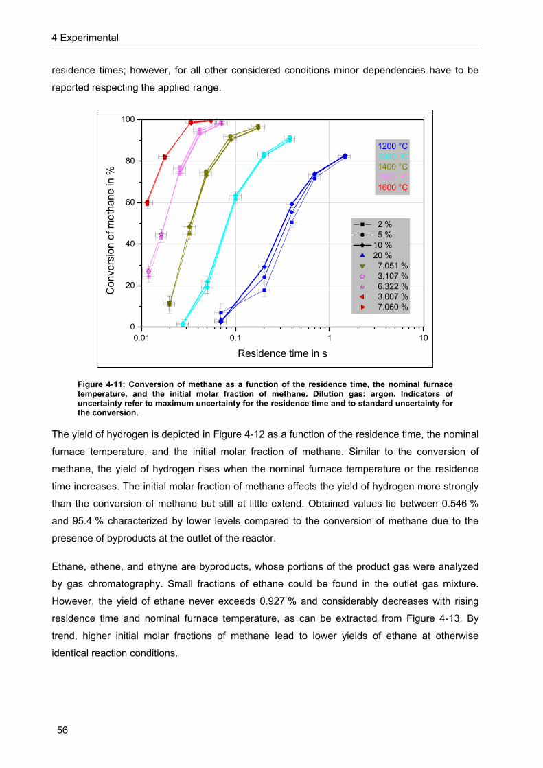
4 Experimental
56
residence times; however, for all other considered conditions minor dependencies have to be
reported respecting the applied range.
0.01 0.1 1 100
20
40
60
80
100C
onve
rsio
n of
me
than
e in
%
Residence time in s
2 % 5 % 10 % 20 % 7.051 % 3.107 % 6.322 % 3.007 % 7.060 %
1200 °C1300 °C1400 °C1500 °C1600 °C
Figure 4-11: Conversion of methane as a function of the residence time, the nominal furnace temperature, and the initial molar fraction of methane. Dilution gas: argon. Indicators of uncertainty refer to maximum uncertainty for the residence time and to standard uncertainty for the conversion.
The yield of hydrogen is depicted in Figure 4-12 as a function of the residence time, the nominal
furnace temperature, and the initial molar fraction of methane. Similar to the conversion of
methane, the yield of hydrogen rises when the nominal furnace temperature or the residence
time increases. The initial molar fraction of methane affects the yield of hydrogen more strongly
than the conversion of methane but still at little extend. Obtained values lie between 0.546 %
and 95.4 % characterized by lower levels compared to the conversion of methane due to the
presence of byproducts at the outlet of the reactor.
Ethane, ethene, and ethyne are byproducts, whose portions of the product gas were analyzed
by gas chromatography. Small fractions of ethane could be found in the outlet gas mixture.
However, the yield of ethane never exceeds 0.927 % and considerably decreases with rising
residence time and nominal furnace temperature, as can be extracted from Figure 4-13. By
trend, higher initial molar fractions of methane lead to lower yields of ethane at otherwise
identical reaction conditions.

4 Experimental
57
0.01 0.1 1 100
20
40
60
80
100
Yie
ld o
f hyd
roge
n in
%
Residence time in s
2 % 5 % 10 % 20 % 7.051 % 3.107 % 6.322 % 3.007 % 7.060 %
1200 °C1300 °C1400 °C1500 °C1600 °C
Figure 4-12: Yield of hydrogen as a function of the residence time, the nominal furnace temperature, and the initial molar fraction of methane. Dilution gas: argon. Indicators of uncertainty refer to maximum uncertainty for the residence time and to standard uncertainty for the yield.
0.01 0.1 1 100.0
0.2
0.4
0.6
0.8
1.0
Yie
ld o
f eth
ane
in %
Residence time in s
2 % 5 % 10 % 20 % 7.051 % 3.107 % 6.322 % 3.007 % 7.060 %
1200 °C1300 °C1400 °C1500 °C1600 °C
Figure 4-13: Yield of ethane as a function of the residence time, the nominal furnace temperature, and the initial molar fraction of methane. Dilution gas: argon. Indicators of uncertainty refer to maximum uncertainty for the residence time and to standard uncertainty for the yield.

4 Experimental
58
A maximum yield of 4.71 % ethene was achieved at 1300 °C nominal furnace temperature and
2 % initial molar fraction of methane. Explicit dependencies of the yield of ethene on the
residence time, the initial molar fraction of methane, and the nominal furnace temperature can
not be identified as becomes clear in Figure 4-14. The graphs for 1200 °C, 1300 °C, and partly
1400 °C indicate that a local maximum may exist at moderate residence times and that values
may stabilize at increased residence times, reaching higher levels when higher initial molar
fractions of methane were applied. A local maximum is probably not shown by graphs for higher
nominal furnace temperatures, because the applied residence times might not be low enough to
reach that region.
0.01 0.1 1 100
1
2
3
4
5
Yie
ld o
f eth
ene
in %
Residence time in s
2 % 5 % 10 % 20 % 7.051 % 3.107 % 6.322 % 3.007 % 7.060 %
1200 °C1300 °C1400 °C1500 °C1600 °C
Figure 4-14: Yield of ethene as a function of the residence time, the nominal furnace temperature, and the initial molar fraction of methane. Dilution gas: argon. Indicators of uncertainty refer to maximum uncertainty for the residence time and to standard uncertainty for the yield.
Figure 4-15 depicts the yield of ethyne, which is by far the most important byproduct. After
passing the initial stage of the splitting reactions at low residence times the yield of ethyne
approaches remarkable high levels up to 59.5 %. Mostly also here a maximum is reached at
moderate residence times. However, due to the slight slope of the graphs in the region right-
hand the maximum, large amounts of ethyne form part of the product gas even at high
residence times. Usually the yield of ethyne decreases with rising initial molar fraction of
methane, presumably due to a better promotion of the final steps of the splitting reactions
resulting from an increased probability of collision and somewhat higher concentrations of
generated carbon providing reactive sites.

4 Experimental
59
0.01 0.1 1 100
10
20
30
40
50
60
70
Yie
ld o
f eth
yne
in %
Residence time in s
2 % 5 % 10 % 20 % 7.051 % 3.107 % 6.322 % 3.007 % 7.060 %
1200 °C1300 °C1400 °C1500 °C1600 °C
Figure 4-15: Yield of ethyne as a function of the residence time, the nominal furnace temperature, and the initial molar fraction of methane. Dilution gas: argon. Indicators of uncertainty refer to maximum uncertainty for the residence time and to standard uncertainty for the yield.
The conversion of methane and the yields of considered species are shown together in Figure
4-16 exemplarily for 1300 °C nominal furnace temperature and 10 % initial molar fraction of
methane. Similar to results based on other reaction conditions, methane starts to decompose as
soon as the residence time is high enough while hydrogen and C2-hydrocarbons are generated.
For lowest residence times the yield of ethane is higher than the yield of ethyne. The shapes of
the graphs propose that the yield of ethane also exceeds the yield of ethene for residence times
lower than the residence times considered here, suggesting that ethane is one of the first
intermediates of a complex decomposition mechanism. While ethane disappears very fast, the
yields of ethene and ethyne first reach a maximum and then fall slightly with residence time.
Quite low levels of yield of ethene can be reported. Contrariwise, residence times considered in
this work are not high enough for even nearly total conversion of ethyne. Accordingly,
considerable fractions of hydrogen and carbon atoms form part of an intermediate, not of the
final and desired products. In order to increase the amount of hydrogen and particulate carbon
in the product flow, clearly longer residence times should be taken into consideration.

4 Experimental
60
0.01 0.1 110-3
10-2
10-1
100
101
102
Con
vers
ion
and
yiel
d in
%
Residence time in s
methane hydrogen ethyne ethene ethane
Figure 4-16: Conversion of methane as well as yields of hydrogen, ethane, ethene, and ethyne as a function of the residence time for 1300 °C nominal furnace temperature of and 10 % initial molar fraction of methane. Dilution gas: argon.
The fraction of recovered hydrogen atoms in the considered species relH,n arising from
,0CH
,0CHP,HCP,HCP,HCP,HP,CH
H,0
H,0PH,relH,
4
422426224
4
424624
n
nnnnnn
n
nnn
Equation 74
is a measure of the balance of H-atoms. Ideal agreement between ingoing and outgoing molar
flows of H-atoms would lead to 0relH, n . In opposition to the ideal case, determined values
are distributed within an interval defined by the limits - 5.7 % and + 6.9 % as can be seen in
Figure 4-17. Since a source of hydrogen atoms inside the reactor is rejected, positive values are
a result of the uncertainty of initial molar flows of argon and methane. Moreover, perfect
agreement lies in range of every determined value, when uncertainties are taken into account.
Consequently, it becomes clear that the respected species are the most important carriers of H-
atoms in the product flow and that the H-balance is practically satisfied.
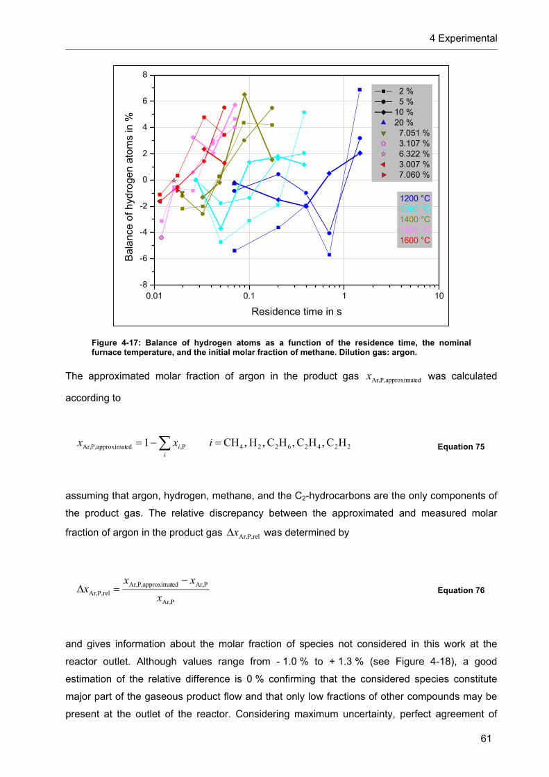
4 Experimental
61
0.01 0.1 1 10-8
-6
-4
-2
0
2
4
6
8
Bal
anc
e o
f hyd
roge
n a
tom
s in
%
Residence time in s
2 % 5 % 10 % 20 % 7.051 % 3.107 % 6.322 % 3.007 % 7.060 %
1200 °C1300 °C1400 °C1500 °C1600 °C
Figure 4-17: Balance of hydrogen atoms as a function of the residence time, the nominal furnace temperature, and the initial molar fraction of methane. Dilution gas: argon.
The approximated molar fraction of argon in the product gas edapproximatP,Ar,x was calculated
according to
22426224P,edapproximatP,Ar, HC ,HC ,HC ,H ,CH 1 i
i ixx Equation 75
assuming that argon, hydrogen, methane, and the C2-hydrocarbons are the only components of
the product gas. The relative discrepancy between the approximated and measured molar
fraction of argon in the product gas relP,Ar,x was determined by
PAr,
PAr,edapproximatP,Ar,relP,Ar, x
xxx
Equation 76
and gives information about the molar fraction of species not considered in this work at the
reactor outlet. Although values range from - 1.0 % to + 1.3 % (see Figure 4-18), a good
estimation of the relative difference is 0 % confirming that the considered species constitute
major part of the gaseous product flow and that only low fractions of other compounds may be
present at the outlet of the reactor. Considering maximum uncertainty, perfect agreement of

4 Experimental
62
approximated and measured molar fraction of argon in the product gas is possible for every
reaction condition.
0.01 0.1 1 10-1.0
-0.5
0.0
0.5
1.0
1.5x
Ar,
P,r
el in
%
Residence time in s
2 % 5 % 10 % 20 % 7.051 % 3.107 % 6.322 % 3.007 % 7.060 %
1200 °C1300 °C1400 °C1500 °C1600 °C
Figure 4-18: Relative difference between approximated (as 1 minus the sum of molar fractions of considered species except for argon) and measured molar fractions of argon in the product gas as a function of the residence time, the nominal furnace temperature and the initial molar fraction of methane.
A measure of cleanliness of the product flow is given by rel,HHC,-C 22Y , the yield of C2-
hydrocarbons HC-C2Y related to the yield of hydrogen
2HY , following
2
2
22
H
HC-Crel,HHC,-C Y
YY . Equation 77
The related yield decreases with residence time, nominal furnace temperature, and initial molar
fraction of methane as can be extracted from Figure 4-19. As a result high temperatures, a high
initial fraction of methane, and a sufficiently high residence time should be ensured in order to
generate a product flow dominated by the desired products, hydrogen as well as carbon, and
only marginally contaminated by intermediates.

4 Experimental
63
0.01 0.1 1 100.0
0.5
1.0
1.5
2.0
Yie
ld o
f C2-h
ydro
carb
ons
/ yie
ld o
f hyd
roge
n in
-
Residence time in s
2 % 5 % 10 % 20 % 7.051 % 3.107 % 6.322 % 3.007 % 7.060 %
1200 °C1300 °C1400 °C1500 °C1600 °C
Figure 4-19: Yield of C2-hydrocarbons related to the yield of hydrogen as a function of the residence time, the initial molar fraction of methane, and the nominal furnace temperature. Dilution gas: argon.
4.4.2 General results of experiments with helium as dilution gas
The measurement of the molar fraction of helium in the product gas was not possible, since
helium was used as the GC’s carrier gas. Presuming that neither argon nor helium undergo a
reaction, but only influence the reaction conditions, the good agreement between PAr,x and
edapproximatP,Ar,x stated in Chapter 4.4.1 allows the conclusion that the molar fraction of helium in
the product gas PHe,x can be estimated well according to
edapproximatP,He,PHe, xx , Equation 78
with
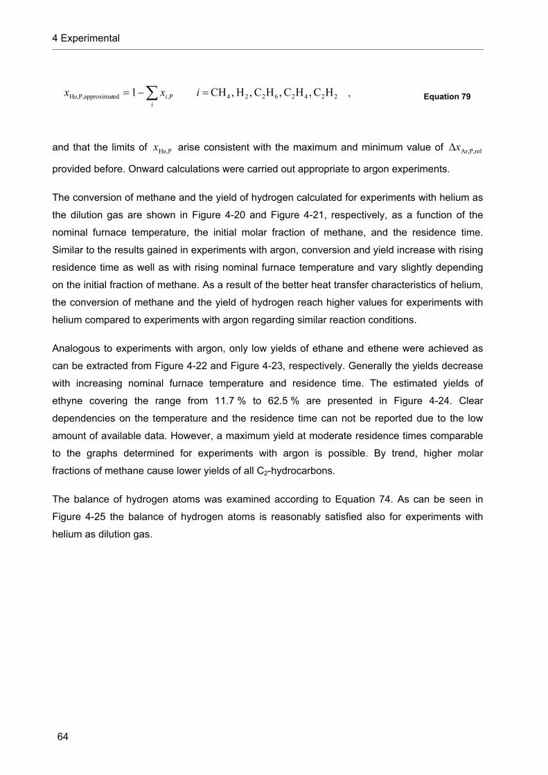
4 Experimental
64
22426224P,edapproximatP,He, HC ,HC ,HC ,H ,CH 1 i
i ixx , Equation 79
and that the limits of PHe,x arise consistent with the maximum and minimum value of relP,Ar,x
provided before. Onward calculations were carried out appropriate to argon experiments.
The conversion of methane and the yield of hydrogen calculated for experiments with helium as
the dilution gas are shown in Figure 4-20 and Figure 4-21, respectively, as a function of the
nominal furnace temperature, the initial molar fraction of methane, and the residence time.
Similar to the results gained in experiments with argon, conversion and yield increase with rising
residence time as well as with rising nominal furnace temperature and vary slightly depending
on the initial fraction of methane. As a result of the better heat transfer characteristics of helium,
the conversion of methane and the yield of hydrogen reach higher values for experiments with
helium compared to experiments with argon regarding similar reaction conditions.
Analogous to experiments with argon, only low yields of ethane and ethene were achieved as
can be extracted from Figure 4-22 and Figure 4-23, respectively. Generally the yields decrease
with increasing nominal furnace temperature and residence time. The estimated yields of
ethyne covering the range from 11.7 % to 62.5 % are presented in Figure 4-24. Clear
dependencies on the temperature and the residence time can not be reported due to the low
amount of available data. However, a maximum yield at moderate residence times comparable
to the graphs determined for experiments with argon is possible. By trend, higher molar
fractions of methane cause lower yields of all C2-hydrocarbons.
The balance of hydrogen atoms was examined according to Equation 74. As can be seen in
Figure 4-25 the balance of hydrogen atoms is reasonably satisfied also for experiments with
helium as dilution gas.
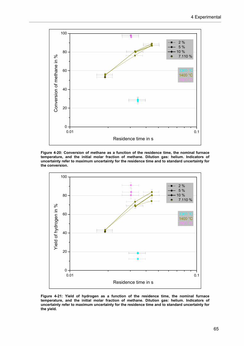
4 Experimental
65
0.010
20
40
60
80
100
Con
vers
ion
of m
eth
ane
in %
Residence time in s
2 % 5 % 10 % 7.110 %
1300 °C1400 °C1500 °C
0.1
Figure 4-20: Conversion of methane as a function of the residence time, the nominal furnace temperature, and the initial molar fraction of methane. Dilution gas: helium. Indicators of uncertainty refer to maximum uncertainty for the residence time and to standard uncertainty for the conversion.
0.010
20
40
60
80
100
Yie
ld o
f hyd
roge
n in
%
Residence time in s
2 % 5 % 10 % 7.110 %
1300 °C1400 °C1500 °C
0.1
Figure 4-21: Yield of hydrogen as a function of the residence time, the nominal furnace temperature, and the initial molar fraction of methane. Dilution gas: helium. Indicators of uncertainty refer to maximum uncertainty for the residence time and to standard uncertainty for the yield.

4 Experimental
66
0.010.0
0.2
0.4
0.6
0.8
Yie
ld o
f eth
ane
in %
Residence time in s
2 % 5 % 10 % 7.110 %
1300 °C1400 °C1500 °C
0.1
Figure 4-22: Yield of ethane as a function of the residence time, the nominal furnace temperature, and the initial molar fraction of methane. Dilution gas: helium. Indicators of uncertainty refer to maximum uncertainty for the residence time and to standard uncertainty for the yield.
0.010
1
2
3
4
5
6
Yie
ld o
f eth
ene
in %
Residence time in s
2 % 5 % 10 % 7.110 %
1300 °C1400 °C1500 °C
0.1
Figure 4-23: Yield of ethene as a function of the residence time, the nominal furnace temperature, and the initial molar fraction of methane. Dilution gas: helium. Indicators of uncertainty refer to maximum uncertainty for the residence time and to standard uncertainty for the yield.

4 Experimental
67
0.010
10
20
30
40
50
60
70
Yie
ld o
f eth
yne
in %
Residence time in s
2 % 5 % 10 % 7.110 %
1300 °C1400 °C1500 °C
0.1
Figure 4-24: Yield of ethyne as a function of the residence time, the nominal furnace temperature, and the initial molar fraction of methane. Dilution gas: helium. Indicators of uncertainty refer to maximum uncertainty for the residence time and to standard uncertainty for the yield.
0.01-10
-8
-6
-4
-2
0
2
4
6
8
10
Ba
lanc
e o
f hyd
rog
en a
tom
s in
%
Residence time in s
2 % 5 % 10 % 7.110 %
1300 °C1400 °C1500 °C
0.1
Figure 4-25: Balance of hydrogen atoms as a function of the residence time, the nominal furnace temperature, and the initial molar fraction of methane. Dilution gas: helium.
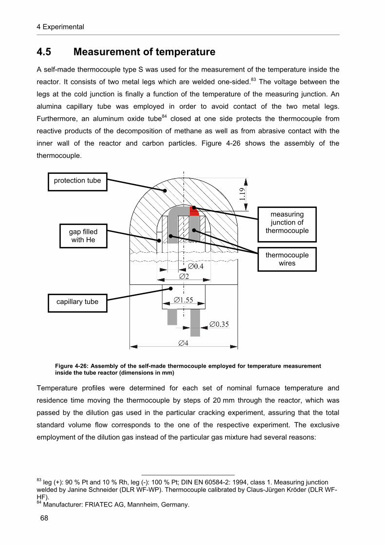
4 Experimental
68
4.5 Measurement of temperature
A self-made thermocouple type S was used for the measurement of the temperature inside the
reactor. It consists of two metal legs which are welded one-sided.83 The voltage between the
legs at the cold junction is finally a function of the temperature of the measuring junction. An
alumina capillary tube was employed in order to avoid contact of the two metal legs.
Furthermore, an aluminum oxide tube84 closed at one side protects the thermocouple from
reactive products of the decomposition of methane as well as from abrasive contact with the
inner wall of the reactor and carbon particles. Figure 4-26 shows the assembly of the
thermocouple.
Figure 4-26: Assembly of the self-made thermocouple employed for temperature measurement inside the tube reactor (dimensions in mm)
Temperature profiles were determined for each set of nominal furnace temperature and
residence time moving the thermocouple by steps of 20 mm through the reactor, which was
passed by the dilution gas used in the particular cracking experiment, assuring that the total
standard volume flow corresponds to the one of the respective experiment. The exclusive
employment of the dilution gas instead of the particular gas mixture had several reasons:
83 leg (+): 90 % Pt and 10 % Rh, leg (-): 100 % Pt; DIN EN 60584-2: 1994, class 1. Measuring junction welded by Janine Schneider (DLR WF-WP). Thermocouple calibrated by Claus-Jürgen Kröder (DLR WF-HF). 84 Manufacturer: FRIATEC AG, Mannheim, Germany.
protection tube
capillary tube
thermocouple wires
measuring junction of
thermocouple gap filled with He

4 Experimental
69
The determination of temperature profiles often took more than two hours. Usually
clogging would have occurred during that time.
The deposition of generated carbon particles would have changed the optical properties
of the thermocouple and finally influenced the temperature measurement.
The temperature changes at position 320 mm after adding methane in a cracking
experiment were moderate, suggesting that temperature profiles gained for the dilution
gas flow are very similar to temperature profiles developed in the cracking experiments.
This was confirmed by further observations at other positions in the reactor during
reference experiments. Thus, the sole consideration of temperature profiles for a pure
dilution gas flow offered a reasonable possibility of reduction of experimental time.
The measurement of temperature profiles started at position 320 mm and ended at the highest
possible position of the thermocouple, which is position 0 mm, leading to temperature profiles
with a length of 320 mm. All positions refer to the highest position of the inner wall of the
protection tube, 1 mm (the wall-thickness of the protection tube) away from the tip of the
thermocouple and approximately corresponding to the position of the measuring junction. By
inclining the thermocouple, a maximum and a minimum temperature, which differ in part
significantly, could be quantified at every axial position. An illustrating sketch is shown in Figure
4-27.
Figure 4-27: Start position, end position, and length of a measured temperature profile (dimensions in mm)
Additionally, the outer wall temperatures at the entrance of the reactor, matching the upper
edge of the inlet water cooler, and at the outlet of the reactor, matching the lower edge of the
outlet water cooler, were measured using a thermocouple type K. It is assumed that the
temperatures inside the reactor are similar to those of the outer wall at the entrance and the

4 Experimental
70
outlet of the reactor. The axial temperature drop at these positions was estimated using
experimental experience and measurements. In order to approximate the temperature profile
between the measured temperature profile mostly within the heated region of the reactor and
the temperatures at the inlet and the outlet of the reactor, respectively, a 3rd order polynomial fit
was used. Therefore 2 to 4 certain high temperatures nearest to the inlet or the outlet were
employed beside the temperatures at the inlet and outlet. At very low flow rates the 3rd order
polynomial fit might lead to higher temperatures for the profile of minimum temperatures
compared to the profile of maximum temperatures at the entrance of the reactor. In these
cases, however, the temperatures only differ not more than 3 K and an average value is used
for both profiles. This procedure results in a quite reasonable shape for the overall temperature
profile starting at the inlet and ending at the outlet of the reactor. In very few cases the
temperature profiles were smoothed at certain positions by calculating plausible temperatures
based on the collectivity of measured temperatures. Figure 4-28 gives an example of
temperature profiles determined following the aforementioned procedure.
-240 -160 -80 0 80 160 240 320 400 480 560 6400
200
400
600
800
1000
1200
1400
1600
Tem
pera
ture
in °
C
Axial position in reactor in mm
maximum measured 3rd order polynomial fit
minimum measured 3rd order polynomial fit smoothed
switching point
Figure 4-28: Profiles of minimum and maximum temperatures (1400 °C nominal furnace temperature and 2600 sccm nominal standard volume flow of Ar, average pressure at the reactor inlet: 1.031 bar, average pressure at the reactor outlet: 1.014 bar)
Considering the idea of a real externally heated tube reactor, one realizes that there is not only
an axial temperature profile but also a radial temperature profile. Near the inlet of the reactor the
wall of the reactor is hotter than the fluid passing it, whereas at the outlet of the reactor the
situation is contradictory. At a certain axial position, at the here called switching point, the
temperatures of wall and center of the reactor should be practically identically. Temperatures of

4 Experimental
71
the maximum temperature profile are consequently assigned to the temperatures measured by
the thermocouple in wall position and temperatures of the minimum temperature profile are
assigned to the temperatures measured by the thermocouple in center position between the
inlet of the reactor and the switching point. Downstream the switching point temperatures are
allocated the other way round.
The measurement chain concerning the measurement of the temperature is shown in Figure
4-29. Similar to the measurement chain of the pressure, the output signal of the measuring
device was interpreted by the data acquisition system. However, a transformation of the signal
in the data acquisition system was not required.
Figure 4-29: Measurement chain of the measurement of temperatures
The positioning of the thermocouple was done manually, resulting in a particular uncertainty
regarding the axial position. Since the contact between wall and thermocouple guarantees a
high level of accuracy concerning the positioning of the thermocouple in wall position,
uncertainty of radial positioning only has to be considered for the center position. Moreover, the
elements of the measurement chain contribute to the overall uncertainty. Respective information
is summarized in Table 4-12.
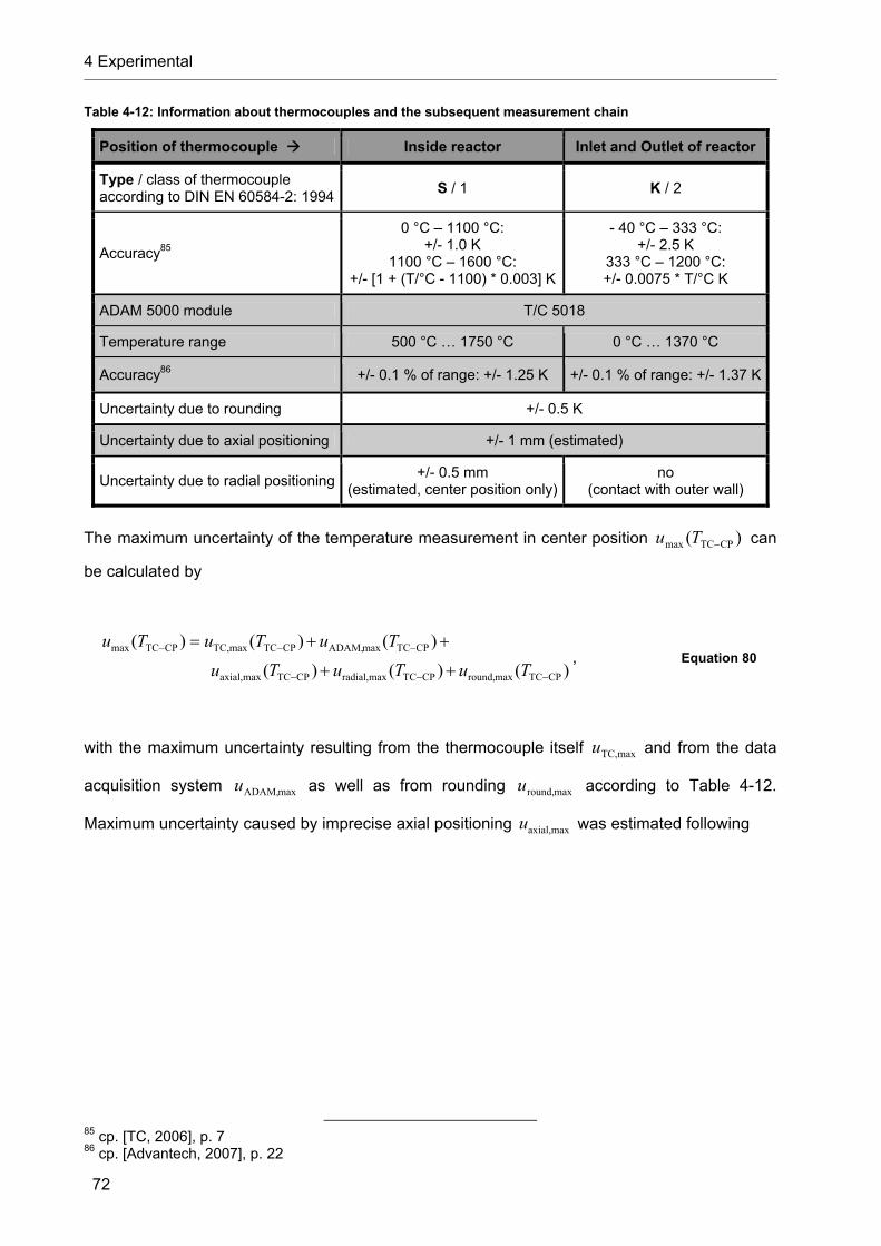
4 Experimental
72
Table 4-12: Information about thermocouples and the subsequent measurement chain
Position of thermocouple Inside reactor Inlet and Outlet of reactor
Type / class of thermocouple according to DIN EN 60584-2: 1994
S / 1 K / 2
Accuracy85
0 °C – 1100 °C: +/- 1.0 K
1100 °C – 1600 °C: +/- [1 + (T/°C - 1100) * 0.003] K
- 40 °C – 333 °C: +/- 2.5 K
333 °C – 1200 °C: +/- 0.0075 * T/°C K
ADAM 5000 module T/C 5018
Temperature range 500 °C … 1750 °C 0 °C … 1370 °C
Accuracy86 +/- 0.1 % of range: +/- 1.25 K +/- 0.1 % of range: +/- 1.37 K
Uncertainty due to rounding +/- 0.5 K
Uncertainty due to axial positioning +/- 1 mm (estimated)
Uncertainty due to radial positioning +/- 0.5 mm
(estimated, center position only)no
(contact with outer wall)
The maximum uncertainty of the temperature measurement in center position )( CPTCmax Tu can
be calculated by
)()()(
)()()(
CPTCmaxround,CPTCmax,radialCPTCmax,axial
CPTCmaxADAM,CPTCmaxTC,CPTCmax
TuTuTu
TuTuTu, Equation 80
with the maximum uncertainty resulting from the thermocouple itself maxTC,u and from the data
acquisition system maxADAM,u as well as from rounding maxround,u according to Table 4-12.
Maximum uncertainty caused by imprecise axial positioning max,axialu was estimated following
85 cp. [TC, 2006], p. 7 86 cp. [Advantech, 2007], p. 22
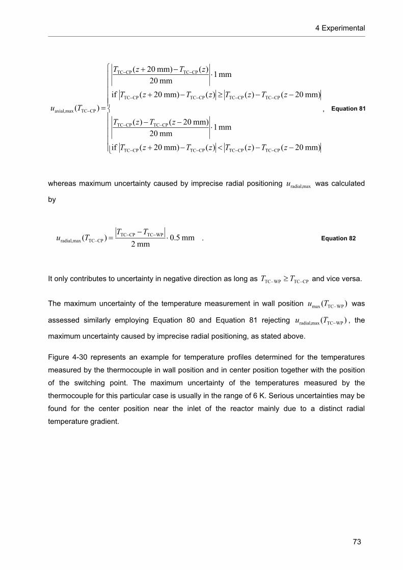
4 Experimental
73
mm)20()()(mm)20( if
mm1mm20
mm)20()(
mm)20()()(mm)20( if
mm1mm20
)(mm)20(
)(
CPTCCPTCCPTCCPTC
CPTCCPTC
CPTCCPTCCPTCCPTC
CPTCCPTC
CPTCmax,axial
zTzTzTzT
zTzT
zTzTzTzT
zTzT
Tu , Equation 81
whereas maximum uncertainty caused by imprecise radial positioning maxradial,u was calculated
by
mm5.0mm2
)( WPTCCPTCCPTCmax,radial
TTTu . Equation 82
It only contributes to uncertainty in negative direction as long as CPTCWPTC TT and vice versa.
The maximum uncertainty of the temperature measurement in wall position )( WPTCmax Tu was
assessed similarly employing Equation 80 and Equation 81 rejecting )( WPTCmaxradial, Tu , the
maximum uncertainty caused by imprecise radial positioning, as stated above.
Figure 4-30 represents an example for temperature profiles determined for the temperatures
measured by the thermocouple in wall position and in center position together with the position
of the switching point. The maximum uncertainty of the temperatures measured by the
thermocouple for this particular case is usually in the range of 6 K. Serious uncertainties may be
found for the center position near the inlet of the reactor mainly due to a distinct radial
temperature gradient.

4 Experimental
74
-240 -160 -80 0 80 160 240 320 400 480 560 6400
200
400
600
800
1000
1200
1400
1600
Tem
pera
ture
in °
C
Axial position in reactor in mm
wall position measured 3rd order polynomial fit
center position measured 3rd order polynomial fit smoothed
switching point
Figure 4-30: Determined temperature profiles for the thermocouple in wall position (WP) and in center position (CP) (1400 °C nominal furnace temperature and 2600 sccm nominal standard volume flow of Ar, average pressure at reactor inlet: 1.031 bar, average pressure at reactor outlet: 1.014 bar, indicators of uncertainty refer to maximum uncertainty)
An example for temperature profiles at conditions with higher nominal furnace temperature and
standard volume flow is shown in Figure 4-31. A maximum temperature of 1424 °C was
measured, which differs significantly from the nominal furnace temperature of 1600 °C. Either
the flow was high enough to cool the wall down to temperatures dramatically lower than the
furnace temperature or due to the geometrical situation and the high radial temperature gradient
it was not possible to measure adequate temperatures near the wall. Remarkable radial
temperature differences are also the reason for comparatively high uncertainty of the
temperature measured in the center position. The switching point is not reached in the region
where temperatures were determined but downstream the lowest position of the thermocouple.

4 Experimental
75
-240 -160 -80 0 80 160 240 320 400 480 560 6400
200
400
600
800
1000
1200
1400
1600
Tem
pera
ture
in °
C
Axial position in reactor in mm
wall position measured 3rd order polynomial fit
center position measured 3rd order polynomial fit smoothed
switching point
Figure 4-31: Profiles of determined temperature profiles for the thermocouple in wall position (WP) and in center position (CP) (1600 °C nominal furnace temperature and 9800 sccm nominal standard volume flow of Ar, average pressure in above reactor: 1.039 bar, average pressure below reactor: 1.006 bar, indicators of uncertainty refer to maximum uncertainty)
All determined temperature profiles related to the thermocouple in wall position and in center
position for argon as well as for helium as the dilution gas can be found in Appendix C.
4.6 Additional experiments
Additional experiments were carried out in order to learn about the reliability of experimental
results and to gain further information about the situation inside the reactor. Therefore selected
reaction conditions were considered again in a second experimental campaign.87 A second filter
featuring a PTFE filter element with a nominal pore diameter of 2 µm was implemented in
parallel position to the original one. By adjusting a three way cock with 90°-bore connected
downstream to both filters and a pipe toward the flue, it was possible to chose the path of the
particle laden product flow. As before, a pure flow of dilution gas with the same total standard
volume flow than the mixture of dilution gas and methane considered later on was fed to the
reactor until temperatures at position 320 mm inside the reactor reached constant levels. Then
methane was introduced to the system, while the standard volume flow of the dilution gas was
reduced simultaneously. A sample of product gas was extracted by vacuum pump of the GC as
soon as the temperature at position 320 mm did not change any more. When the sample
extraction was finished the abovementioned three way cock was switched over in order to lead
to product flow through the second filter (sample filter). This way it could be guaranteed that no
87 The second experimental campaign forms part of a student research paper, see [Maibauer, 2010].

4 Experimental
76
particles formed during the first minutes after methane addition reached the second filter.
Particles formed in this phase, in which temperatures in the reactor still approach a situation of
thermal equilibrium, likely differ from particles formed later under more or less constant
conditions. In order to allow the analysis of hydrocarbons higher than the C2-hydrocarbons, the
GC was not stopped after ethyne was detected but was in operation for an extended period of
time of 45 min. Targeting constant reaction conditions the experiment was stopped as soon as
the pressure rose more than 10 mbar compared to the initial conditions or the temperature rose
for more that 1 % of the initial temperature at position 320 mm in K. When neither the pressure
related nor the temperature related stop criterion was fulfilled, the experiment was brought to an
end after about 60 min. Then the particles present in the sample filter were removed. Carbon
deposition between the outlet of the reactor and the filter were negligible. However, a significant
amount of carbonaceous material could be removed from the inside of the reactor during the
cleaning procedure employing a metal wire, which was moved through the reactor with utmost
care. The wire was introduced in the gap between the thermocouple and the TC elbow after
removing respective sealing nuts, when the temperature of the tube furnace reached values
below 700 °C. Both, the carbon sample from the filter and from the reactor were prepared for a
further analysis, namely the determination of the BET specific surface. An overview about
reaction conditions covered in the second campaign with argon and helium as dilution gas is
provided in Table 4-13 and Table 4-14, respectively.
Table 4-13: Conditions covered in the second experimental campaign with argon as dilution gas
Cinfurnace T sccmintot,0N,V %in,0CH4x Corresponding /furnaceT -set
200 5 2 1200
685 5 4
650 5 7
1300 5 8 1300
2600 5 9
1400 5 12
2600 2, 5, 10 13 1400
3800 5 14
1600 5 16 1500
2800 5 17
2000 5 21 1600
3350 5 22
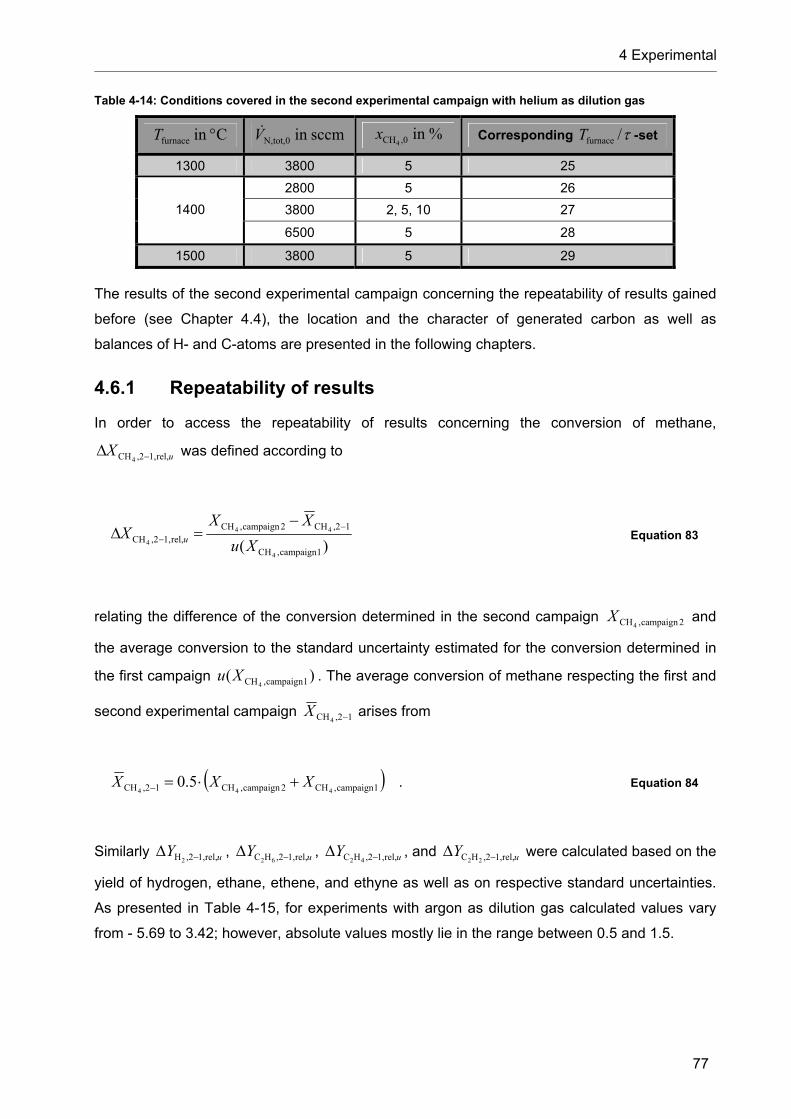
4 Experimental
77
Table 4-14: Conditions covered in the second experimental campaign with helium as dilution gas
Cinfurnace T sccmintot,0N,V %in,0CH4x Corresponding /furnaceT -set
1300 3800 5 25
2800 5 26
3800 2, 5, 10 27 1400
6500 5 28
1500 3800 5 29
The results of the second experimental campaign concerning the repeatability of results gained
before (see Chapter 4.4), the location and the character of generated carbon as well as
balances of H- and C-atoms are presented in the following chapters.
4.6.1 Repeatability of results
In order to access the repeatability of results concerning the conversion of methane,
uX rel,1,,2CH4 was defined according to
)( 1campaign ,CH
1,2CH2campaign ,CHrel,1,,2CH
4
44
4 Xu
XXX u
Equation 83
relating the difference of the conversion determined in the second campaign 2campaign ,CH4X and
the average conversion to the standard uncertainty estimated for the conversion determined in
the first campaign )( 1campaign ,CH4Xu . The average conversion of methane respecting the first and
second experimental campaign 1,2CH4 X arises from
1campaign ,CH2campaign ,CH1,2CH 4445.0 XXX . Equation 84
Similarly uY rel,1,,2H2 , uY rel,1,,2HC 62 , uY rel,1,,2HC 42 , and uY rel,1,,2HC 22 were calculated based on the
yield of hydrogen, ethane, ethene, and ethyne as well as on respective standard uncertainties.
As presented in Table 4-15, for experiments with argon as dilution gas calculated values vary
from - 5.69 to 3.42; however, absolute values mostly lie in the range between 0.5 and 1.5.

4 Experimental
78
Table 4-15: Differences between values for the conversion of methane as well as the yields of hydrogen, ethane, ethene, and ethyne gained in the second campaign and average values regarding the first and second campaign with argon as dilution gas related to respective standard uncertainties determined in the first campaign. (Reaction condition: nominal furnace temperature in °C - nominal total standard volume flow in sccm - nominal initial molar fraction of methane in %)
Reaction condition -in
rel,1,,2CH4 uX
-in
rel,1,,2H2 uY
-in
rel,1,,2HC 62 uY
-in
rel,1,,2HC 42 uY
-in
rel,1,,2HC 22 uY
1200 - 200 - 5 -0.20 2.70 -0.36 -1.77 -0.47
1200 - 685 - 5 1.23 2.80 -1.02 -1.73 -0.03
1300 - 650 - 5 0.68 1.06 -0.56 -0.26 -0.61
1300 - 1300 - 5 0.19 0.87 -0.13 -3.57 -0.73
1300 - 2600 - 5 0.32 1.97 -0.04 -5.69 -0.66
1400 - 1400 - 5 -0.07 -0.34 -1.34 1.13 0.93
1400 - 2600 - 2 0.43 0.37 -1.14 -0.62 -0.39
1400 - 2600 - 5 0.16 0.04 -0.29 0.35 0.15
1400 - 2600 - 10 0.85 0.69 0.08 -0.26 -2.14
1400 - 3800 - 5 0.40 2.06 -0.29 -1.50 -0.47
1500 - 1600 - 5 0.76 0.36 0 / 0 -0.20 -0.76
1500 - 2800 - 5 0.98 0.81 0 / 0 -0.65 -1.30
1600 - 2000 - 5 3.12 0.21 0 / 0 -1.26 -1.85
1600 - 3350 - 5 3.42 1.45 0 / 0 -1.50 -2.30
Somewhat lower differences related to the estimated standard uncertainty were calculated for
experiments with helium as dilution gas as can be seen in Table 4-16. Values range from - 1.01
to 2.49, whereas absolute values mostly lie between 0.4 and 0.7.
Table 4-16: Differences of values for the conversion of methane as well as the yields of hydrogen, ethane, ethene, and ethyne gained in the first and second experimental campaign with helium as dilution gas related to respective standard uncertainties. (Reaction condition: nominal furnace temperature in °C - nominal total standard volume flow in sccm - nominal initial molar fraction of methane in %)
Reaction condition -in
rel,1,,2CH4 uX
-in
rel,1,,2H2 uY
-in
rel,1,,2HC 62 uY
-in
rel,1,,2HC 42 uY
-in
rel,1,,2HC 22 uY
1300 - 3800 - 5 0.32 2.49 -0.51 -0.14 0.74
1400 - 2800 - 5 0.21 0.29 0.54 0.43 0.43
1400 - 3800 - 2 1.72 0.26 0.49 -0.67 -0.48
1400 - 3800 - 5 1.03 0.49 0.63 -0.20 -0.67
1400 - 3800 - 10 0.01 -0.01 0.03 0.00 -0.39
1400 - 6500 - 5 0.36 0.85 -0.08 -1.01 -0.21
1500 - 3800 - 5 0.13 0.15 0 / 0 0.69 -0.76
Since the difference between values gained in the two campaigns and the average value
usually lies in range of the standard uncertainty, a quite good repeatability of results can be

4 Experimental
79
deduced – in particular when taking into account that a simplified method of evaluation based
on a two point calibration of the GC with respect to hydrogen and methane was adopted for the
second campaign and that the second campaign was managed only with a pre-experimental
calibration of the GC with respect to hydrogen, methane, and argon.
4.6.2 Location and character of generated carbon
As stated before, carbon deposit was not only found in the sample filter but also in the reactor.
The weight of samples varied between 1 mg and 378 mg depending on the location of
deposition, the reaction conditions, and the duration of the experiment. The samples from the
filter showed a more or less uniform constitution, which could differ in general structure,
macroscopic size of agglomerates, density, color, and odor depending on the reaction
conditions. Respective examples are provided in Figure 4-32.
Figure 4-32: Examples for samples from the filter gained in experiments with argon as dilution gas: 1400 - 2600 - 10 (a) and 1300 - 650 - 5 (b) (Reaction condition: nominal furnace temperature in °C - nominal total standard volume flow in sccm - nominal initial molar fraction of methane in %)
As can be seen in Figure 4-32 (a), the samples may show a slightly brownish color indicating
the presence of high molecular hydrocarbons. Mostly the samples from the reactor contained
beside the particulate fraction a fraction of pyrocarbon which is a graphitic silvery deposition.
The shape of the pyrocarbon fragments suggests its formation and deposition on the inner wall
of the reactor. Some examples for carbon samples from the reactor are shown in Figure 4-33.
Pyrocarbon volume fractions up to 100 % could be determined for samples from the reactor.
However, an obvious dependency of the volume fraction of pyrocarbon in the samples from the
reactor on the reaction conditions could not be found.
(a) (b)

4 Experimental
80
Figure 4-33: Examples for samples from the reactor gained in experiments with argon as dilution gas: 1400 - 2600 - 5 (a), 1600 - 2000 - 5 (b), 1500 - 2800 - 5 (c), and 1300 - 1300 - 5 (d) (Reaction condition: nominal furnace temperature in °C - nominal total standard volume flow in sccm - nominal initial molar fraction of methane in %)
The BET specific surfaces of the particulate fraction of every sample providing the required
mass of about 20 mg were determined with a maximum uncertainty in the range of 0.5 m2/g.88
As can be seen in Figure 4-34, the values for the BET specific surface of samples from the
reactor vary between 6.9 m2/g and 56.4 m2/g concerning experiments with argon as dilution gas
and between 42.6 m2/g and 94.7 m2/g concerning experiments with helium as dilution gas. Most
values can be found in the range from little less than 40 m2/g to 60 m2/g. Although great effort
was made to entirely separate the pyrocarbon fraction from the particulate fraction, analyzed
particulate sample may still have been contaminated with pyrocarbon to a certain extend, which
is especially likely for measured BET values below 20 m2/g. Contrariwise, samples from the
filter are characterized by somewhat higher BET specific surfaces in the range from 22.3 m2/g
88 Measurements carried out by Dr. Eusebiu Grivei, TIMCAL, Willebroek, Belgium. 10 min preheating at 200 °C in nitrogen atmosphere.
(a) (b)
(c) (d)

4 Experimental
81
and 139.1 m2/g for experiments with argon as dilution gas and from 56.2 m2/g to 66.4 m2/g for
experiments with helium as dilution gas, as can be extracted from Figure 4-35.
0.01 0.1 10
20
40
60
80
100B
ET
spe
cific
sur
face
in
m2 /g
Residence time in s
2 % - Ar 5 % - Ar 5 % - He 10 % - Ar 10 % - He
1300 °C1400 °C1500 °C1600 °C
Figure 4-34: Specific surface area of carbon samples collected from the reactor
0.01 0.1 10
20
40
60
80
100
120
140
160
BE
T s
peci
fic s
urfa
ce i
n m
2/g
Residence time in s
5 % - Ar 5 % - He 10 % - Ar 10 % - He
1300 °C1400 °C1500 °C1600 °C
Figure 4-35: Specific surface area of carbon samples collected from the filter

4 Experimental
82
The BET specific surface of samples from the filter are mostly higher compared to those from
the reactor, probably due to the fact that smaller particles – corresponding to high specific
surfaces – are more likely able to pass the reactor and finally to reach the filter. The present
extend of data does not allow a comprehensive analysis of the dependencies of the BET
specific surface on the reaction conditions. However, it becomes clear that the BET specific
surfaces do not attain more or less constant values but differ in part significantly.
4.6.3 Balances of H- and C-atoms
As presented before, the balance of H-atoms based on the considered H-containing species,
which are methane, hydrogen, ethane, ethene, and ethyne, is practically satisfied for the whole
range of experimental conditions. With the knowledge about the mass of carbon deposition in
the experimental system, specifically in the reactor itself and the filter, formed during particular
experiments, it was possible to assess the balance of C-atoms as well. The calculative fraction
of H-atoms in component i of the product gas P,in Hˆ ix arises from
22426224,0CH
P,in HP,in H HC,HC,HC,H,CH
4ˆ
4
i
n
nfx ii
i
Equation 85
with if in H giving information about the number of H-atoms in one molecule of species i . The
calculative fraction of H-atoms situated in other (not considered) species Pothers,in Hx was
determined by
22426224P,in HPothers,in H HC,HC,HC,H,CHˆ%100ˆ ixxi
i . Equation 86
If 0ˆ Pothers,in H x , the fraction of H-atoms situated in other (not considered) species Pothers,in Hx
was set to 0 and the fraction of H-atoms in component i of the product gas P,in H ix was
calculated by

4 Experimental
83
22426224P,in H
P,in HP,in H HC,HC,HC,H,CHˆ
%100ˆ
i
xxx
ii
ii , Equation 87
else Pothers,in HPothers,in H xx and P,in HP,in H ˆ ii xx .
Similarly P,in C ix , the fraction of C-atoms situated in component i of the product gas, was
determined by
2242624,0CH
P,in CP,in C HC,HC,HC,CH
14
i
n
nfx ii
i
Equation 88
with if in C giving information about the number of C-atoms in one molecule of species i . Beside
gaseous products also solid products carry C-atoms, namely the carbon deposit in the reactor
as well as the carbon deposit in the sample filter. The average molar deposition flow in the
reactor reactorin Cn was estimated by
Creactor,CH
reactorin Creactorin C
4Mt
mn
Equation 89
employing the mass of carbon deposition inside the reactor reactorin Cm , the period between the
initialization and the termination of the methane flow reactor,CH4t , and the molecular weight of
carbon CM . Accordingly, the average molar deposition flow in the sample filter filterin Cn was
calculated by
Cfilter,CH
filterin Cfilterin C
4Mt
mn
Equation 90
employing the mass of carbon deposition in the sample filter filterin Cm and the period between
switching over of the three way cock to the sample filter and the termination of the methane flow
filter,CH4t .

4 Experimental
84
With reactorin Cn and filterin Cn the fractions of C-atoms situated in the carbon deposition in the
reactor Preactor,in Cin Cx and in the filter Pfilter,in Cin Cx could be calculated following
filterin C reactor,in C1 ,0CH
in CP,in C
4
i
n
nfx ii
i
. Equation 91
Since a deposition of pure carbon has been considered, 1filterin Cin Creactorin Cin C ff .
The fraction of C-atoms situated in other (not considered) species Pothers,in Cx was determined by
filterin Creactor,in C,HC,HC,HC,CH
%100
2242624
P,in CPothers,in C
i
xxi
i
. Equation 92
Figure 4-36 represents the fractions of H- and C-atoms in particular species respecting the
experimental conditions listed in Table 4-13 and Table 4-14. In accordance with results
presented in Chapter 4.4, the hydrogen balance is practically satisfied resulting in a marginal
fraction of H-atoms in other (not considered) species. Contrariwise, remarkable amounts of C-
atoms form part of other species leading to high fractions of C-atoms in other species up to
48.3 % and about 28.5 % on average. This indicates the presence of further C-rich species in
the product flow. Small molar fractions of the C3-hydrocarbons propene (C3H6), propyne (C3H4),
and probably propadiene (C3H4) were detected but with a molar fraction far below an order of
magnitude, which could possibly explain a high value of Pothers,in Cx , namely in the order of
magnitude of ethane regarding propene and in the order of magnitude of ethene regarding
propyne and propadiene. Low amounts of high molecular byproducts, in particular hydrocarbons
with a high C/H-ratio, could better justify the practically perfect H-balance on the one hand and
the significant disagreement of the C-balance on the other hand. Suggested by the partly
colored appearance and strong-smelling characteristics of the samples, polycyclic aromatic
hydrocarbons (PAH), such as naphthalene (C10H8)89, could have been generated. The formation
of PAHs involved in the thermal splitting of methane has already been reported.90
89 identified by Albermann in former experiments, cp. [Albermann, 2007], and confirmed by [Muradov, 2010] 90 cp. e. g. [Hu, 2003]

4 Experimental
85
0 10 20 30 40 50 60 70 80 90 100
heliu
m
1200 - 200 - 5
1200 - 685 - 5
AA1300 - 650 - 5
1300 - 1300 - 5
1300 - 2600 - 5
AA1400 - 1400 - 5
1400 - 2600 - 2
1400 - 2600 - 5
1400 - 2600 - 10
1400 - 3800 - 5
AA1500 - 1600 - 5
1500 - 2800 - 5
AA1600 - 2000 - 5
1600 - 3350 - 5
AAAA1300 - 3800 - 5
AA1400 - 2800 - 5
1400 - 3800 - 2
1400 - 3800 - 5
1400 - 3800 - 10
1400 - 6500 - 5
AA1500 - 3800 - 5
Fraction of H-atoms in particular species in %
methane ethane ethene ethyne hydrogen others
argo
n
0 10 20 30 40 50 60 70 80 90 100
argo
nh
eliu
m
Fraction of C-atoms in particular species in %
methane ethane ethene ethyne C in reactor C in filter others
Figure 4-36: Fractions of H- and C-atoms situated in particular species as a function of the experimental conditions (nominal furnace temperature in °C - total standard volume flow in sccm - initial molar fraction of methane in %)
4.7 Experiments with added C-particles
In order to investigate heterogeneous effects caused by carbon particles, experiments were
carried out employing an apparatus which allows seeding of the inlet gas.91 An overview about
the general configuration of the seeding apparatus is provided in Figure 4-37. It features a
rotating dosing as well as a rotating dispersing element, which permits the continuous
generation of gas/particle-flow made of the inlet substances argon and carbon particles.
Super P, a conductive carbon black with a typical BET specific surface of 62 m2/g and a nominal
particle size of 40 nm, was used as seeding material.92 Depending on the number of revolution
of the rotating dosing element different mass flows of particles were realized. The mass flow of
the particles was determined employing the mass of particles found in a filter downstream the
seeding apparatus and the respective duration of operation. It was found that a total standard
volume flow of about 3610 sccm Ar allows almost complete discharge of dispersed particles
91 Construction, design, qualification, optimization, and control of the apparatus forms part of a student research project and a diploma thesis, see [Förster, 2009]. 92 produced by TIMCAL, Willebroek, Belgium, cp. [TIMCAL, 2007]

4 Experimental
86
from the seeding apparatus. The longer the operation time the higher the mass of particles in
the filter. The prototype offers roughly linear characteristics a can be seen in Figure 4-38.
Figure 4-37: General configuration of the seeding apparatus
0 5 10 15 20 250.0
0.6
1.2
1.8nominal standard volume flow: 3610 sccm Arpressure: approximately standard pressuretemperature: approximately 20 °C
3.00 1/min 3.70
3.14 g/h 2.59
1.50 1/min 2.36
1.88 g/h 1.40
6.00 1/min 5.80
5.24 g/h 4.68
Mas
s g
ain
of p
artic
les
in fi
lter
in g
Duration of operation in min
0.75 1/min 2.10 1.62 g/h 1.15
Number of revolutions maximum mass flow nominal mass flow minimum mass flow
Figure 4-38: Calibration of the seeding apparatus and determination of maximum, nominal, and minimum mass flow of Super P depending on the number of revolutions of the dosing element
carbon particles
Ar + carbon particles Ar seeding
apparatus
rotating dosing element
rotating dispersing element

4 Experimental
87
Resulting from the small amounts of the seeding material, the maximum uncertainty of the
measurement of the particle mass inside the filter or rather the mass gain of the particles inside
the filter is relatively high (approximately 0.1 g). However, general trends can be identified. The
determined mass flow increases, when the number of revolution of the dosing element
increases. Maximum, nominal, and minimum mass flows were determined employing a fitting
line through the origin respecting maximum, nominal, and minimum values, respectively, as is
illustrated in Figure 4-38, exemplarily for a number of revolutions of 6 1/min. Here the
uncertainty of the duration of operation, which was not higher than 2 s, was neglected.
/furnaceT -set 14 with 5 % initial molar fraction of methane was chosen as the reference
condition, because achieved conversion of methane and yield of hydrogen lie below 50 % and
offer potential for enhancement. Although the corresponding total standard volume flow equals
3800 sccm, a standard volume flow of approximately 3610 sccm was applied to the seeding
apparatus, because only argon entered the disperser and 190 sccm methane were added
downstream in order to provide a mixture with 5 % molar fraction of methane in the gas phase
at the inlet of the reactor. The addition of Super P results in a considerable increase of the
conversion of methane and of the yield of hydrogen as can be extracted from Figure 4-39. More
precisely, with the maximum mass flow of 5.24 g/h Super P through the reactor it was possible
to increase the conversion of methane and the yield of hydrogen by 18 % and 33 %,
respectively. Contrariwise, the yield of ethyne shows only a weak dependency on the mass flow
of carbon particles, while the yields of the other C2-hydrocarbons ethane and ethene decrease
with rising mass flow of Super P – however, at comparatively low levels. Seeding obviously
affects the cracking reactions, promoting the generation of the favored product hydrogen. The
related yields of hydrogen and C2-hydrocarbons rose from 1.38 to an averaged value of 1.81,
when the particle mass flow reached its maximum. Thus, the addition of carbon black to the flow
entering the reactor leads to a higher cleanliness of the product flow.

4 Experimental
88
0 1 2 3 4 5 60.0
0.2
0.4
0.6
0.8
1.0
1.2
1.4
Fit function: 2nd order polynomial with fixed offset
+ 4 %
- 25 %
- 40 %
+ 18 %
+ 33 %
Rel
ativ
e co
nver
sion
and
yie
lds
in -
Mass flow of Super P in g/h
methane: related to 48.2 % conversion hydrogen: related to 38.0 % yield ethane: related to 0.165 % yield ethene: related to 2.86 % yield ethyne: related to 24.4 % yield
Figure 4-39: Conversion of methane and yield of hydrogen as well as of ethane, ethene, and ethyne as a function of the applied mass flow of Super P related to values determined without seeding. Indicators of uncertainty refer to the average maximum uncertainty concerning the mass flow and to typical standard uncertainty concerning relative conversion and yields. Nominal furnace temperature: 1400 °C, nominal total standard volume flow: 3800 sccm, nominal molar fraction of methane in argon: 5 %, pressure between 1.012 bar and 1.031 bar.
Seeding changes the reaction conditions inside the reactor in different ways. On the one hand
the particles provide additional sites for heterogeneous reactions, whereas on the other hand
the heat transfer between the reactor wall and the fluid is enhanced due to radiative effects.
With the current configuration it was not possible to isolate these two effects, but it is admissible
to state that the change of the conversion and yields is not only a result of a better heat transfer.
This is because an unusual change of the temperature at the position 320 mm could not be
detected after adding carbon particles, which could be expected for an extremely improved heat
input in the fluid. An extinction of radiation in the visible regime by optical observation through
the transparent glass tube at the outlet of the seeding apparatus with an inner diameter
(corresponding to the maximum optical length) of 4 mm was not or only marginally noticeable
although the absorption coefficient of carbon can be approximated by one. Since the inner
diameter of the reactor equals 8 mm, the extinction in the reactor is higher than the extinction in
the glass tube under the same circumstances. However, the consequences of a higher optical
path are compensated by the increased volume flow in the reactor and the resulting lower
concentration of carbon in the gas/particle-mixture, indicating that the extinction in the reactor
should have the same order of magnitude than the extinction in the glass tube – also for
radiation with other wavelengths, because the absorption coefficient does not exceed one.

4 Experimental
89
The theoretical mass flow of generated carbon for the reference condition without seeding
equals approximately 1.27 g/h. However, the examination of the carbon balance shows that the
fraction of C-atoms in other (not considered) compounds of the product flow equals about 20 %
resulting in a basically negligible mass flow of generated carbon. Consequently, the major part
of carbon material inside the reactor originates from the seeding material and not from
generated carbon. The surface provided by added particles in the heated region of the reactor
RP,Super S can be roughly estimated following
PSuper PSuper BET,RP,Super msS Equation 93
employing the BET specific surface of Super P PSuper BET,s , the mass flow of Super P dispersed
by the seeding apparatus PSuper m , and the average residence time according to Equation 55.
Thus, with /gm62 2PSuper BET, s , s0329.0 , and the maximum applied particle mass flow
g/h24.5maxP,Super m the maximum particle based surface area in the reactor can be calculated
to 0.0030 m2. The geometrical inner surface of the heated region of the reactor nominally equals
0.0063 m2 and therefore has the same order of magnitude. Therefore the reactor surface
probably promotes heterogeneous reactions.
The BET specific surface of carbon deposit recovered from the reactor and the sample filter is
usually comparable to (or even higher than) figures of Super P, suggesting that also generated
particles represent favored reaction sites and support heterogeneous paths of the reactions.

5 Kinetic evaluation
90
5 Kinetic evaluation
For the kinetic evaluation of the experiments it was necessary to estimate realistic reactions
conditions for all locations inside the reactor, in particular with respect to the reaction
temperature, and to set up a suitable flow model as well as a kinetic model, which covers the
dominating reactions.93
5.1 Interpretation of measured temperatures
The temperature on the surface of the protection tube of the thermocouple was a result of the
convective heat transfer between the fluid and the protection tube as well as of the radiative
heat transfer between reactor wall and the surface of the protection tube as is illustrated in
Figure 5-1.
Figure 5-1: Illustration of heat transfers contributing to the temperature measured with the thermocouple
Respecting the diameters of the protection tube as well as of the inserted capillary tube and
employing trigonometry, it can be shown that the distance between the contact line and the tip
of the protection tube theoretically equals 1.368 mm. Thus, the distance between the center of
the welded part of the thermocouple and the tip of the protection tube accounts for
93 Some basic considerations can be found in [Wullenkord, 2010 b].
RADIATIVE HEAT
TRANSFER
CONVECTIVE HEAT
TRANSFER
reactor wall
protection tube of thermocouple

5 Kinetic evaluation
91
approximately 1.19 mm corresponding to the dimensions provided in Figure 4-26. It was
postulated that HTl , the length of the heat transfer region relevant for the measurement of the
temperature, equals 2.38 mm, which is double of the aforementioned distance allowing a
symmetric consideration of the heat transfer with respect to the center of the measuring
junction.
Motivated by the low wall-thickness of the protection tube of the thermocouple (1 mm) and the
helium filling, it was assumed that the upper part of the thermocouple corresponding to HTl and
including the measuring junction attained a uniform temperature. The thermal conductivity of
FRIATEC’s AL23, which is the material of the reactor and the protection tube of the
thermocouple, lies in the range of 5 W/(m K) at 1000 °C. The material properties of AL23
provided by the manufacturer are content of Table 5-1.94
Table 5-1: Stated thermal conductivity and emissivity of AL23 produced by FRIATEC
Cin T Km
Win in
100 30 -
1000 5 0.21
Since the amount of known data is very rare, but material properties had to be applied for
subsequent calculation within a wide range of temperatures, other sources had to be used in
order to estimate reasonable dependencies of the material properties on the temperature. The
following chapter deals with material properties. Then the convective and radiative heat
transfers are examined in detail before consequences are derived.
5.1.1 Material properties of AL23 and used gases
The software EES provides a database for the thermal conductivity of alumina (polycrystalline)
in the temperature range between 300 K and 1000 K.95 Additional data for corundum, containing
99 % alumina, can be found in [VDI, 2006]96 regarding the temperature range between 400 °C
and 1200 °C. The approximation of the temperature depending function of the thermal
conductivity of AL23 according to Figure 5-2 comprises the following steps:
determination of a fit function for the collective of values of the thermal conductivity
comprising data from EES (for temperatures up to 726.85 °C corresponding to 1000 K)
and [VDI, 2006] (for temperatures above 726.85 °C)
94 see [FRIATEC, 2003] 95 EES: Engineering Equation Solver V8.412-3D (2009). Database provides data from [Incropera, 1996] and [Touloukian, 1972]. 96 p. Deb 3

5 Kinetic evaluation
92
calculation of the ratio between values given by [FRIATEC, 2003] and the fit function
determination of ratios for other temperatures by linear interpolation employing the
above mentioned ratios with the constraint, that the value should be higher than 1
calculation of values of the thermal conductivity employing the fit function and the ratios
evaluated for certain temperatures
determination of a 3rd order polynomial fit function for the values
0 400 800 1200 16000
10
20
30
40
[FRIATEC, 2003] AL23 [VDI, 2006] corundum, 99 % Al
2O
3
[EES, 2009] Al2O
3, polycrystalline
[EES, 2009] + [VDI, 2006] AL23 approximated Fit: 3rd order polynomial Fit: 3rd order polynomial
The
rmal
co
nduc
tivity
in W
/(m
K)
Temperature in °C
y = -1.59744E-08 x3 + 5.97017E-05 x2 - 7.58800E-02 x + 3.70701E+01
Figure 5-2: Approximation of the thermal conductivity of AL23 for temperatures between 0 °C and 1600 °C employing various information
The fit function for the thermal conductivity leads to a relative error of 0.21 % and - 1.65 %
concerning the given values for 100 °C and 1000 °C, respectively. The values found in [EES,
2009] do not match those from [VDI, 2006] for low temperatures. However, the shapes of the
curves suggest that latter values represent a limit at higher temperatures, which is also
admissible for the first case.
Concerning the emissivity of AL23 the data sheet only provides one value, namely the
emissivity for 1000 °C (see Table 5-1). Values found in [VDI, 2006]97 for the emissivity of
alumina indicate a linear decrease with the temperature. Applying a linear fit function, a
potential value for 1000 °C equals 0.533, what is about 2.54 times higher than the given value
from the data sheet. Assuming that a linear decrease is admissible for AL23 and that the above
97 p. Ka 5

5 Kinetic evaluation
93
mentioned discrepancy factor is also valid for other temperatures, the emissivity of AL23 was
approximated for a wider temperature range consistent with Figure 5-3.
0 400 800 1200 16000.0
0.2
0.4
0.6
0.8
1.0
[FRIATEC, 2003] AL23 [VDI, 2006] Al
2O
3
Fit: line AL23 approximated Fit: line
Em
issi
vity
in -
Temperature in °C
y = -1.57152E-04 x + 3.67152E-01
Figure 5-3: Approximation of the emissivity of AL23 for temperatures between 0 °C and 1600 °C employing various information
Material properties of used gases, specifically material properties of argon and helium, were
mostly extracted from [VDI, 2006] and are summarized in Appendix D.
5.1.2 Convective heat transfer
A convective heat transfer took place between the protection tube of the thermocouple and the
fluid passing it. The heat flux density on the wall of the thermocouple due to convection convTC,q
can be calculated by
fluidwallTC,convconvTC, TTq , Equation 94
where conv is the local convective heat transfer coefficient, wallTC,T represents the temperature
of the wall of the protection tube of the thermocouple and considering an internal flow fluidT
stands for the adiabatic mixing temperature of the fluid at the respective axial position.98
98 cp. [Baehr, 2006], p. 11 et seqq.
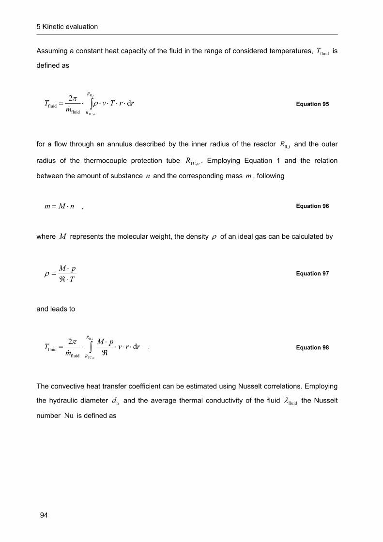
5 Kinetic evaluation
94
Assuming a constant heat capacity of the fluid in the range of considered temperatures, fluidT is
defined as
iR,
oTC,
d2
fluidfluid
R
R
rrTvm
T
Equation 95
for a flow through an annulus described by the inner radius of the reactor iR,R and the outer
radius of the thermocouple protection tube oTC,R . Employing Equation 1 and the relation
between the amount of substance n and the corresponding mass m , following
nMm , Equation 96
where M represents the molecular weight, the density of an ideal gas can be calculated by
T
pM
Equation 97
and leads to
R,i
oTC,
d2
fluidfluid
R
R
rrvpM
mT
. Equation 98
The convective heat transfer coefficient can be estimated using Nusselt correlations. Employing
the hydraulic diameter hd and the average thermal conductivity of the fluid fluid the Nusselt
number Nu is defined as

5 Kinetic evaluation
95
fluid
hconvNu
d . Equation 99
The thermal conductivity should be evaluated for an average temperature of the fluid regarding
the temperatures at the inlet and at the outlet of the considered part of the reactor.99
To estimate the order of magnitude of conv , the convective heat transfer in a concentric annular
gap had to be examined. Ways to handle the problem can be found in [VDI, 2006]100; however,
the provided equations are based on further constraints. Firstly only a constant wall temperature
is considered. The part of interest of the thermocouple’s protection tube is its tip featuring a
short length. It is admissible to consider this part to be isothermal. Secondly one has to decide,
which of the following cases matches best to the considered problem:
heat transfer at inner pipe, outer pipe isolated
heat transfer at outer pipe, inner pipe isolated
heat transfer at inner and outer pipe, wall temperatures identical
Since predominantly the heat transfer at the inner pipe affects the temperature measurement,
the first situation was chosen for further calculations. Furthermore, in absence of additional
knowledge about the velocity profile in an annulus featuring complex heat transfer processes
properties of the fluid at a certain axial position were determined for
wallTC,wallR,fluid 5.0 TTT , Equation 100
the arithmetic mean of the wall temperatures of the reactor and the thermocouple.
Generally a flow can be characterized by the Reynolds number Re , which is defined as
99 cp. [VDI, 2006], p. Gb 1 100 p. Gb 1 et seqq.

5 Kinetic evaluation
96
vd
hRe , Equation 101
where is the density, v is the average velocity of the flow, stands for the dynamic
viscosity, and hd for the hydraulic diameter.
The average velocity v arises from
A
Vv
, Equation 102
based on the volume flow V and the cross sectional area A , through which V passes.
Following [VDI, 2006]101 the hydraulic diameter hd can be calculated with the above mentioned
cross sectional area A and the wetted perimeter of the cross section wP :
wh
4
P
Ad
. Equation 103
For an annular gap, in the present case defined by the outer diameter of the protection tube of
the thermocouple oTC,d and the inner diameter of the reactor iR,d , it can be shown that
oTC,iR,h ddd . Equation 104
The Reynolds number never exceeds a value of 2300, which represents the reference value for
the transition from laminar to turbulent flow. Flows characterized by Reynolds numbers below
2300 are certainly laminar flows.102 Regarding a laminar flow in a region where temperature and
velocity profiles develop coevally, the average Nusselt number aveNu can be estimated by
101 p. LAB 4 102 cp. [VDI, 2006], p. Ga 1

5 Kinetic evaluation
97
3 33
32
31ave NuNuNuNu , Equation 105
where 1Nu refers to the Nusselt number regarding a fully developed flow, concerning both,
temperature and velocity, and arises from
8.0
iR,
oTC,1 2.166.3 Nu
d
d , Equation 106
where 2Nu refers to the Nusselt number characterizing a thermally undeveloped flow with fully
developed velocity profile and arises from
3
1
HT
h
5.0
iR,
oTC,2 PrRe14.01615.1 Nu
l
d
d
d , Equation 107
and where 3Nu arises from
2
1
HT
h6
1
3 PrRePr221
2 Nu
l
d .103 Equation 108
1Nu and 2Nu are functions of the ratio of the outer diameter of the protection tube of the
thermocouple oTC,d and the inner diameter of the reactor iR,d . Further dependencies exist on
the Reynolds number Re , the Prandtl number Pr , and the considered length of the heat
transfer region HTl . The Prandtl number is a function of properties of the fluid, namely the
dynamic viscosity , the thermal conductivity , and the specific heat capacity at constant
pressure pc , following
103 cp. [VDI, 2006], p. Gb 1 et seqq. Information from [Stephan, 1962] and [Martin, 1990] is provided.

5 Kinetic evaluation
98
pPr
c . Equation 109
The standard volume flow was varied in the range from 95 sccm to 9800 sccm, when argon was
used as dilution gas, and in the range from 2800 sccm and 6500 sccm, when helium was used
as dilution gas. For the subsequent calculations the pressure was approximated by the standard
pressure Np , since the aim of the calculations is just an estimation of the order of magnitude of
the convective heat transfer coefficient.
Figure 5-4 shows the convective heat transfer coefficient corresponding to the average Nusselt
number aveNu for different temperatures of the thermocouple and the reactor wall as well as for
different standard volume flows of argon. Properties of the fluid, which are respected for the
calculation of Nusselt numbers, were determined for an average temperature regarding the
temperature of the thermocouple and the reactor wall.
-800 -600 -400 -200 0 200 400 600 8000
50
100
150
200
250
300
Temperature of TC: 1600 °C
Con
vect
ive
hea
t tra
nsf
er c
oeffi
cien
t in
W/(
m2 K
)
Temperature difference between TC and reactor wall in K
9800 sccm
2600 sccm
95 sccm
Temperature of TC: 800 °C
maxmax
min
min
Figure 5-4: Convective heat transfer coefficients for two temperatures of the tip of the thermocouple (800 °C and 1600 °C) as a function of the temperature difference between the thermocouple and the reactor wall as well as of the standard volume flow of argon. Material properties of argon were calculated for the arithmetic mean of the temperature of the thermocouple and the reactor wall and exemplarily for the maximum (max) and minimum (min) temperature of considered combinations. Standard pressure.
Slightly different values can be found if not the average, but respective maximum or minimum
temperatures are employed as also shown in the figure. However, values of the heat transfer

5 Kinetic evaluation
99
coefficient calculated for extreme temperatures do not extend the range of values calculated for
average temperatures. The convective heat transfer coefficient strongly depends on the
standard volume flow, whereas the influence of temperatures is moderate. Maximum heat
transfer coefficients concerning the experiments with argon as the diluent can be found at a
level of 300 W/(m2 K).
Due to the high thermal conductivity of helium, the convective heat transfer coefficient is
characterized by higher values compared to calculations with argon as can be seen in Figure
5-5. Here values up to 1100 W/(m2 K) can be expected.
-600 -400 -200 0 200 400 6000
200
400
600
800
1000
1200
Temperature of TC: 1500 °C
Con
vect
ive
hea
t tra
nsf
er c
oeffi
cien
t in
W/(
m2 K
)
Temperature difference between TC and reactor wall in K
Temperature of TC: 900 °C
6500 sccm
3800 sccm
2800 sccm
Figure 5-5: Convective heat transfer coefficients for two temperatures of the tip of the thermocouple (900 °C and 1500 °C) as a function of the temperature difference between the thermocouple and the reactor wall as well as of the standard volume flow of helium. Material properties of helium were calculated for the arithmetic mean of the temperature of the thermocouple and the reactor wall. Standard pressure.
5.1.3 Radiative heat transfer
A radiative heat transfer occurred between the wall of the thermocouple and the inner wall of
the reactor. The heat flux density on the wall of the thermocouple due to radiation radTC,q ,
corresponding to the net radiative exchange between the surfaces of the thermocouple and the
wall of the reactor, can be calculated by

5 Kinetic evaluation
100
wallR,wallTC,radradTC, TTq , Equation 110
where rad is the radiative heat transfer coefficient, wallTC,T represents the temperature of the
wall of the protection tube of the thermocouple and wallR,T stands for the temperature of the
inner wall of the reactor.
The radiative heat transfer coefficient arises from
wallR,wallTC,
4wallR,
4wallTC,RTC,
rad TT
TTC
, Equation 111
employing RTC,C , a function comprising the optical and geometrical figures following
TCR,RTC,RTC
RTC,RTCRTC, 111
C , Equation 112
with the Stefan-Boltzmann constant , the emissivity of the thermocouple TC , the emissivity of
the reactor R as well as the view factors RTC, and TCR, .104
The view factor 1,2 is defined as the fraction of radiation emitted by surface 1 which is captured
by surface 2 .105 Since the surface of the reactor wall is much larger than the surface at the tip
of the thermocouple and 1RTC, , which means that approximately all radiation leaving the tip
of the thermocouple is intercepted by the surface of the reactor wall, the reciprocity relation for
view factors leads to 0TCR, . Consequently, Equation 112 can be simplified and
104 cp. [VDI, 2006], p. A 6, p. Ka 7 105 cp. [Incropera, 2002], p. 790

5 Kinetic evaluation
101
RTCRTC, C . Equation 113
Radiative heat transfer coefficients calculated for two temperatures of the thermocouple and
arising from the temperature difference for various temperatures of the reactor wall are
presented in Figure 5-6 based on an emissivity function according to Figure 5-3. As can be
extracted from the diagram, the radiative heat transfer coefficient lies in the range between
16 W/(m2 K) and 23 W/(m2 K).
-800 -600 -400 -200 0 200 400 600 8000
5
10
15
20
25
30
Temperature of TC: 1600 °C
Rad
iativ
e he
at tr
ansf
er c
oef
ficie
nt in
W/(
m2 K
)
Temperature difference between TC and reactor wall in K
Temperature of TC: 800 °C
Figure 5-6: Radiative heat transfer coefficients for two temperatures of the tip of the thermocouple (800 °C and 1600 °C) as a function of the temperature difference between the thermocouple and the reactor
5.1.4 Comparison of heat transfer coefficients and consequences
The convective heat transfer coefficient reaches – partly an order of magnitude – higher values
than the radiative heat transfer coefficient for all considered combinations as can be seen in
Figure 5-7, where the ratio of convective to radiative heat transfer coefficient is depicted. A
minimum ratio of about 4, determined for 95 sccm Ar, shows that the heat transfer between the
reactor wall as well as the fluid to the thermocouple is dominated by convection. Thus, the
measured temperature is predominantly a result of the convective heat transfer between the
thermocouple and the surrounding fluid.

5 Kinetic evaluation
102
0 2000 4000 6000 8000 10000 120001
10
100
Temperature of reactor wall
1500 °C / (1500 - 10-6) °C900 °C / (900 + 10-6) °C900 °C / 1500 °C
Ar
co
nv /
rad
in -
Standard volume flow in sccm
He
1600 °C / (1600 - 10-6) °C800 °C / (800 + 10-6) °C800 °C / 1600 °C
Temperature of TC
Figure 5-7: Ratio of convective heat transfer coefficient to radiative heat transfer coefficient for different combinations of temperature of the thermocouple (TC) and temperature of the reactor wall as a function of the standard volume flow of argon or helium. Material properties of argon and helium were calculated for the arithmetic mean of the temperature of the thermocouple and the reactor wall. Standard pressure.
However, with the current configuration it was not possible to measure the temperature at a
certain point inside the reactor, since the thermocouple covered around 25 % of the cross
sectional area of the reactor and consequently the tip of the thermocouple attained a somehow
averaged temperature of the fluid in contact. The geometrical situation is illustrated in Figure
5-8.
Figure 5-8: Geometrical situation of the thermocouple in center position (a) and in wall position (b) inside the reactor (sectional view). The color illustrates the temperature distribution in front of the thermocouple near the inlet of the reactor (red = hot, blue = cold).
reactor
(a) (b)
inner wall of reactor
contour of TC near tip
measuring junction

5 Kinetic evaluation
103
As a result, only reaction conditions characterized by a moderate radial temperature gradient in
the relevant region of the reactor should be considered for the kinetic evaluation, meaning the
determination of kinetic parameters. A moderate radial temperature gradient assures that the
temperatures of the fluid near the thermocouple, which could influence the temperature
measurement, do not differ considerably. Consequently, at axial position z the temperature in
the center of the reactor, where the radial position accounts for 0, )(C zT can be well
approximated by the temperature of the thermocouple in center position )(CPTC zT :
)()0,()( CPTCC zTrzTzT . Equation 114
Moreover, the temperature of the thermocouple in wall position )(WPTC zT is a good estimation
of the temperature of the wall of the reactor, where the radial position accounts for the inner
radius of the reactor iR,R , )(W zT and the temperature of the fluid next to it:
)(),()( WPTCiR,W zTRrzTzT . Equation 115
The latter supposition is fortified by the fact that radiative heat transport supported the
measurement of the wall temperature. Furthermore, contact between the reactor wall and the tip
of the thermocouple in wall position allowed a certain conductive heat transfer.
It is assumed that a moderate radial temperature gradient at position z is fulfilled, when
2
K)(K)(05.0K)()( CPTCWPTC
CPTCWPTC
zTzTzTzT
. Equation 116
The region of the reactor between 0z , corresponding to the upper edge of the heated region
of the tube furnace, and mm320z , corresponding to the position of the tip of the
thermocouple during the cracking experiments, was covered by temperature measurement.
Maximum temperatures and by far most of temperatures higher than 75 % of the maximum
temperature of the considered temperature profile on a K-scale can be found within the
aforementioned limits. This region was considered as the relevant region. It comprises 17
positions, since a step size of 20 mm was chosen for the temperature measurement. The
temperature profiles determined with the thermocouple for different sets of nominal furnace

5 Kinetic evaluation
104
temperature and residence time were examined with respect to the radial temperature
gradients. Table 5-2 gives an overview about the percentage of positions with moderate radial
temperature gradients inside the relevant region according to the abovementioned definition
regarding temperature profiles gained with argon. It was assumed that a percentage higher than
75 % is acceptable and that respective sets of /furnaceT could be employed for the kinetic
evaluation, whereas other conditions – eight respecting argon – should be rejected for the
evaluation step, due to an increased uncertainty of temperatures resulting from the lower
percentage of valid positions.
Table 5-2: Review of temperature profiles gained with argon regarding the existence of moderate radial temperature gradients in the relevant region of reactor
/furnaceT -set Cinfurnace T Level of
sccminArN,V
Percentage of positions with moderate radial
temperature gradients inside relevant region in %
1 95 100 (17 / 17)
2 200 100 (17 / 17)
3 350 100 (17 / 17)
4 685 100 (17 / 17)
5
1200
2000 88.2 (15 / 17)
6 340 100 (17 / 17)
7 650 100 (17 / 17)
8 1300 100 (17 / 17)
9 2600 76.5 (13 / 17)
10
1300
4800 64.7 (11 / 17)
11 700 100 (17 / 17)
12 1400 100 (17 / 17)
13 2600 82.4 (14 / 17)
14 3800 64.7 (11 / 17)
15
1400
6500 29.4 (5 / 17)
16 1600 100 (17 / 17)
17 2800 82.4 (14 / 17)
18 4600 58.8 (10 / 17)
19 7200 29.4 (5 / 17)
20
1500
9800 0 (0 / 17)
21 2000 100 (17 / 17)
22 3350 76.5 (13 / 17)
23 6500 47.1 (8 / 17)
24
1600
9800 5.9 (1 / 17)
< 75 % 75 % – 99.9 % 100 %
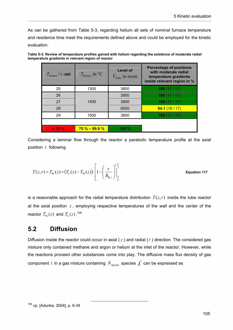
5 Kinetic evaluation
105
As can be gathered from Table 5-3, regarding helium all sets of nominal furnace temperature
and residence time meet the requirements defined above and could be employed for the kinetic
evaluation.
Table 5-3: Review of temperature profiles gained with helium regarding the existence of moderate radial temperature gradients in relevant region of reactor
/furnaceT -set Cinfurnace T Level of
sccminHeN,V
Percentage of positions with moderate radial
temperature gradients inside relevant region in %
25 1300 3800 100 (17 / 17)
26 2800 100 (17 / 17)
27 3800 100 (17 / 17)
28
1400
6500 94.1 (16 / 17)
29 1500 3800 100 (17 / 17)
< 75 % 75 % – 99.9 % 100 %
Considering a laminar flow through the reactor a parabolic temperature profile at the axial
position z following
2
iR,WCW 1)()()(),(
R
rzTzTzTrzT Equation 117
is a reasonable approach for the radial temperature distribution ),( rzT inside the tube reactor
at the axial position z , employing respective temperatures of the wall and the center of the
reactor )(W zT and )(C zT .106
5.2 Diffusion
Diffusion inside the reactor could occur in axial ( z ) and radial ( r ) direction. The considered gas
mixture only contained methane and argon or helium at the inlet of the reactor. However, while
the reactions proceed other substances come into play. The diffusive mass flux density of gas
component i in a gas mixture containing speciesN species *ij can be expressed as
106 cp. [Adunka, 2004], p. 6-34

5 Kinetic evaluation
106
kki
N
ikk
kii xD
M
MM
,1
2mix
mix* ˆ
species
j , Equation 118
if the average velocity of the mass of a volume element is chosen as the reference. Employed
are the density of the gas mixture mix , the molecular weight of the considered component i
iM , of other components k kM , and of the gas mixture mixM as well as the gradient of the
molar fraction of component k kx . In contrast to the simple formulation of the equation, the
diffusion coefficients kiD ,ˆ for gas mixtures comprising more than two species are often
unknown.107
5.2.1 Axial diffusion
Figure 5-9 represents the Péclet number Pe , calculable by
PrRePe , Equation 119
as a function of the standard volume flow and the nominal furnace temperature evaluated for
standard pressure being a good approximation of pressures observed during the experiments.
Axial diffusion is negligible for most reaction conditions, since the Péclet numbers usually
exceed a value of 10, which is a reasonable limit for the exclusion of any influences of
downstream conditions on the conditions at a certain axial position.108 However, reaction
conditions based on the two lowest standard volume flows of argon at 1200 °C nominal furnace
temperature (95 sccm and 200 sccm) undercut the limit of 10, suggesting the disregard of
concerned reaction conditions in subsequent kinetic calculations.
107 cp. [Baehr, 2006], p. 79 (information from [Sherwood, 1975]), p. 248 et seqq. and [VDI, 2006], p. Da 29 108 cp. [Patankar, 1980], p. 102

5 Kinetic evaluation
107
0 2000 4000 6000 8000 100001
10
100
1000
Péc
let n
umbe
r in
-
Standard volume flow in sccm
argon helium
1200 °C1300 °C1400 °C1500 °C1600 °C
Figure 5-9: Péclet number for different standard volume flows of argon and helium through the tube reactor based on the nominal furnace temperature and standard pressure
5.2.2 Radial diffusion
Diffusive radial molar flows were calculated for each considered product component i , rejecting
all other components of the gas mixture except for the dilution gas (DG), in order to assess the
relevance of radial diffusive effects. Although strictly speaking these values are only valid for
respective binary mixtures, they should lead to a reliable estimation of the order of magnitude of
diffusive flows, because in any case the dilution gas forms by far the main fraction of considered
gas mixtures. Molar fractions of argon below 80 % were only observed in one case, at reaction
conditions based on 20 % initial molar fraction of methane. Corresponding to Fick’s Law of
Diffusion radial,ij , the diffusive molar flux density in radial direction concerning component i in a
binary gas mixture containing component i and the dilution gas (DG) relative to the average
radial molar velocity ( 0 for laminar flow) can be calculated by

5 Kinetic evaluation
108
r
xDcj i
ii d
dDG,radial, , Equation 120
where c represents the concentration and DG,iD the binary diffusion coefficient.109 According to
the ideal gas law110, the concentration c arises from
T
pc
, Equation 121
with the absolute pressure p , the universal gas constant , and the temperature T . Binary
diffusion coefficients kiD , also depend on the temperature T as well as on the pressure p and
can be approximated by
s
m10
2bar
g/molg/molK00143.0
24
2
,d,d
1175.1
,3
13
1
-
ki
ki
ki
VVp
MMT
D Equation 122
for low pressures employing the diffusion volume dV (method of Fuller).111 The diffusion volume
for different species is provided explicitly for simple molecules like helium, argon, and hydrogen,
whereas values for more complex molecules like methane and the C2-hydrocarbons have to be
calculated from contributions of different atoms forming the molecule. Respective values are
provided in Table 5-4.
Resulting from Equation 121 and Equation 122 DG,iDc is independent from the pressure and
proportional to 0.75T . The diffusive flux density reaches its maximum at the highest temperature,
which can be approximated by the nominal furnace temperature furnaceT .
109 cp. [Baehr, 2006], p. 79 and [Incropera, 2002], p. 862 et seq. 110 see Equation 1 111 cp. [VDI, 2006], p. Da 27 et seq.

5 Kinetic evaluation
109
Table 5-4: Diffusion volume of various species used for the method of Fuller
Species indV
argon 16.2
helium 2.67
hydrogen 6.12
methane 25.14 (= 1 * 15.9 + 4 * 2.31)
ethane 45.66 (= 2 * 15.9 + 6 * 2.31)
ethene 41.04 (= 2 * 15.9 + 4 * 2.31)
ethyne 36.42 (= 2 * 15.9 + 2 * 2.31)
A general measure of the relevance of radial diffusive effects may be the here introduced
diffusive quotient iQ radial,D, , representing the ratio of the molar flux of component i penetrating
the cross section of the reactor )(zni to the estimated characteristic radial molar diffusive flux of
component i through a certain diffusion face DA evaluated at the axial position z )(D zn ,i :
Dradial,Dradial,D,
)(
)(
)(
Aj
zn
zn
znQ
i
i
,i
ii
. Equation 123
A characteristic diffusion face DA was defined by m002.0D R , which is half of the inner radius
of the reactor ( m004.0iR, R ), and m001.0z , being a reasonable increment for kinetic
calculations as described later in Chapter 5.5. A respective illustration can be found in Figure
5-10.
Figure 5-10: Geometric situation in the context of radial diffusion

5 Kinetic evaluation
110
Since
)()()()()( gtot, znzxznzxzn ij
jii , Equation 124
employing the average molar fraction of component i at the axial position z )(zxi , and
,0CHDG,0tot,g,0CHDG,0 442 nnnnn , Equation 125
because a maximum molar flow in the gas phase is achieved for total conversion of methane to
hydrogen and carbon, )(gtot, zn can be approximated by
,0CHDG,0gtot, 4)( nnzn , Equation 126
with a maximum uncertainty of
,0CH
,0CHDG,0
,0CH
,0CHDG,0
,0CHDG,0,0CHDG,0
4
4
4
4
442
xnn
n
nn
nnnn
. Equation 127
Thus, the maximum uncertainty implied by the aforementioned approximation of )(gtot, zn is
usually below 10 %.
Applying Equation 120, Equation 124 as well as Equation 126 in Equation 123 and substituting
finite differences for the derivative of ix with respect to r , iQ radial,D, can be assessed via

5 Kinetic evaluation
111
DDG,
,0CHDG,0radial,D,
4
Ar
xDc
nnxQ
ii
ii
.
Equation 128
It is assumed that the consideration of iR,Rr and iiii xrxRrxx )0()( iR, lead to
reasonable and roughly characteristic values for iQ radial,D, , whose calculation then could be
simplified to
iR,
DDG,
,0CHDG,0radial,D,
4
R
ADc
nnQ
i
i
,
Equation 129
evaluating DG,iDc for the nominal furnace temperature furnaceT and the pressure at the inlet of
the reactor. 4radial,CHD,Q is depicted in Figure 5-11 as a function of the residence time, the
nominal furnace temperature, the initial molar fraction of methane, and the dilution gas.
0.01 0.1 1 101
10
100
1000
QD
,rad
ial r
ega
rdin
g m
eth
ane
in -
Residence time in s
2 % 5 % 10 % 20 % 7.051 % 3.107 % 6.322 % 3.007 % 7.060 % 7.110 %
1200 °C1300 °C1400 °C1500 °C1600 °C
He
Ar
Figure 5-11: Diffusive quotient regarding methane as a function of the residence time, the nominal furnace temperature, the initial molar fraction of methane, and the dilution gas
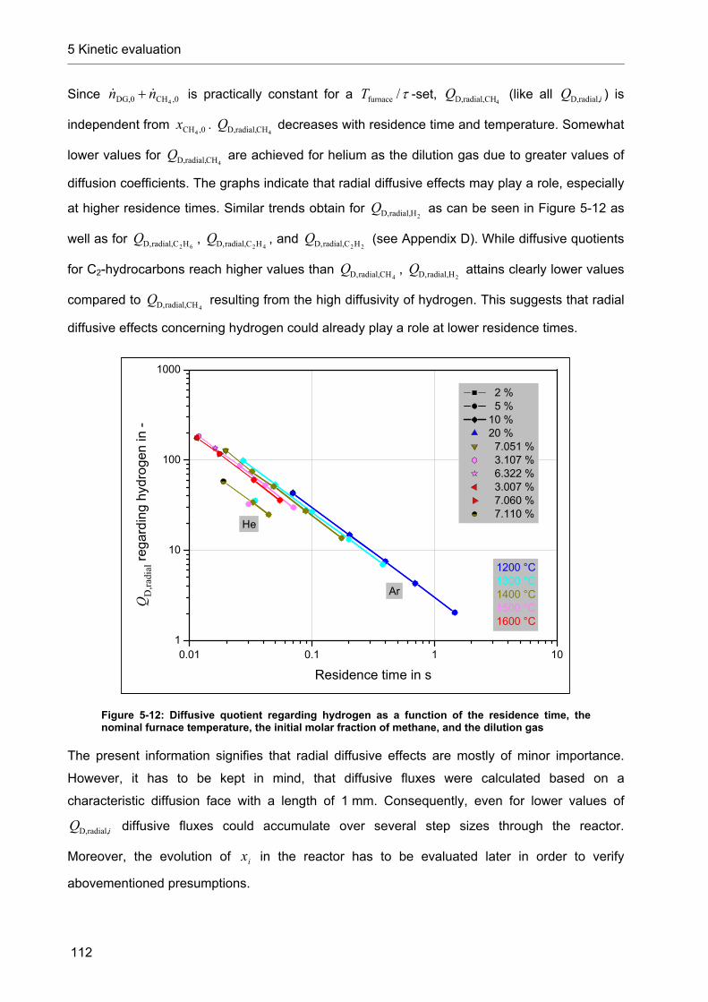
5 Kinetic evaluation
112
Since ,0CHDG,0 4nn is practically constant for a /furnaceT -set,
4radial,CHD,Q (like all iQ radial,D, ) is
independent from ,0CH4x .
4CHradial,D,Q decreases with residence time and temperature. Somewhat
lower values for 4CHradial,D,Q are achieved for helium as the dilution gas due to greater values of
diffusion coefficients. The graphs indicate that radial diffusive effects may play a role, especially
at higher residence times. Similar trends obtain for 2Hradial,D,Q as can be seen in Figure 5-12 as
well as for 62HCradial,D,Q ,
42HCradial,D,Q , and 22HCradial,D,Q (see Appendix D). While diffusive quotients
for C2-hydrocarbons reach higher values than 4CHradial,D,Q ,
2Hradial,D,Q attains clearly lower values
compared to 4CHradial,D,Q resulting from the high diffusivity of hydrogen. This suggests that radial
diffusive effects concerning hydrogen could already play a role at lower residence times.
0.01 0.1 1 101
10
100
1000
QD
,rad
ial r
egar
ding
hyd
roge
n in
-
Residence time in s
2 % 5 % 10 % 20 % 7.051 % 3.107 % 6.322 % 3.007 % 7.060 % 7.110 %
1200 °C1300 °C1400 °C1500 °C1600 °C
He
Ar
Figure 5-12: Diffusive quotient regarding hydrogen as a function of the residence time, the nominal furnace temperature, the initial molar fraction of methane, and the dilution gas
The present information signifies that radial diffusive effects are mostly of minor importance.
However, it has to be kept in mind, that diffusive fluxes were calculated based on a
characteristic diffusion face with a length of 1 mm. Consequently, even for lower values of
iQ radial,D, diffusive fluxes could accumulate over several step sizes through the reactor.
Moreover, the evolution of ix in the reactor has to be evaluated later in order to verify
abovementioned presumptions.
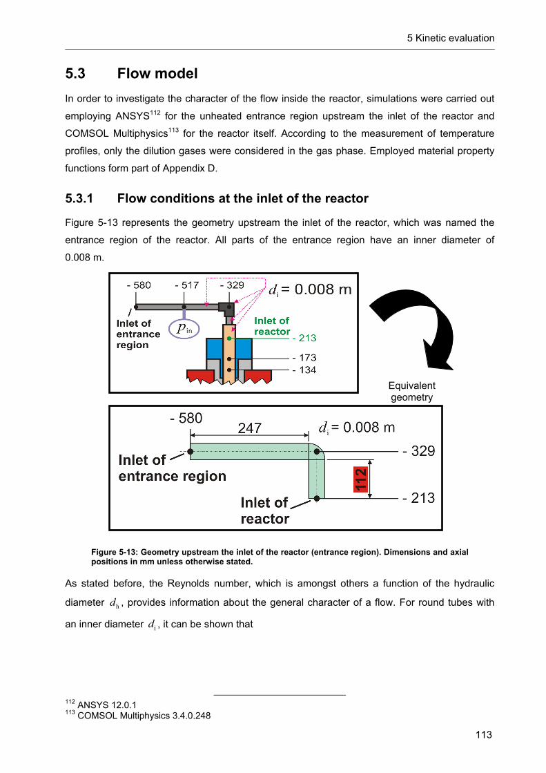
5 Kinetic evaluation
113
5.3 Flow model
In order to investigate the character of the flow inside the reactor, simulations were carried out
employing ANSYS112 for the unheated entrance region upstream the inlet of the reactor and
COMSOL Multiphysics113 for the reactor itself. According to the measurement of temperature
profiles, only the dilution gases were considered in the gas phase. Employed material property
functions form part of Appendix D.
5.3.1 Flow conditions at the inlet of the reactor
Figure 5-13 represents the geometry upstream the inlet of the reactor, which was named the
entrance region of the reactor. All parts of the entrance region have an inner diameter of
0.008 m.
Figure 5-13: Geometry upstream the inlet of the reactor (entrance region). Dimensions and axial positions in mm unless otherwise stated.
As stated before, the Reynolds number, which is amongst others a function of the hydraulic
diameter hd , provides information about the general character of a flow. For round tubes with
an inner diameter id , it can be shown that
112 ANSYS 12.0.1 113 COMSOL Multiphysics 3.4.0.248
Equivalent geometry
5 Kinetic evaluation
114
ih dd . Equation 130
Reynolds numbers calculated for the conditions in the entrance region are lower than 2300 and
denote that a laminar flow has to be considered in the entrance region (like also in the
reactor).114 The entry length el complies with the length of the region downstream an elbow or a
vessel outlet, where the velocity profile of a flow has not developed entirely yet and can be
estimated by
ilame Re dbl , Equation 131
with 06.0lam b .115 Table 5-5 provides information about the Reynolds number in the entrance
region and at the inlet of the reactor as well as the corresponding entry length regarding argon.
The entry length lies in the range between 0.0097 m and 0.9983 m.
Respective information about the entry lengths to be taken into account for helium is given in
Table 5-6. It can be seen that a significantly shorter distance is necessary in order to achieve a
developed flow. Values for the entry length are clearly below 0.08 m.
114 cp. Chapter 5.1.2 115 cp. [Munson, 2002], p. 448 and [Schröder, 2000], p. 148. Other value: 0.056, cp. [Baehr, 2006], p. 374.

5 Kinetic evaluation
115
Table 5-5: Reynolds numbers at the inlet of the reactor and corresponding entry lengths for argon
/furnaceT -set Cinfurnace T sccmintot,0N,V Re minel
1 95 20 0.0097
2 200 42 0.0204
3 350 69 0.0333
4 685 145 0.0697
5
1200
2000 424 0.2036
6 340 71 0.0343
7 650 138 0.0661
8 1300 276 0.1324
9 2600 531 0.2548
10
1300
4800 937 0.4496
11 700 136 0.0654
12 1400 297 0.1424
13 2600 552 0.2649
14 3800 805 0.3862
15
1400
6500 1378 0.6616
16 1600 318 0.1529
17 2800 560 0.2689
18 4600 929 0.4460
19 7200 1462 0.7016
20
1500
9800 1997 0.9587
21 2000 393 0.1888
22 3350 710 0.3408
23 6500 1377 0.6608
24
1600
9800 2080 0.9983
Table 5-6: Reynolds numbers at the inlet of the reactor and corresponding entry lengths for helium
/furnaceT -set Cinfurnace T sccmintot,0N,V Re minel
25 1300 3800 88 0.0422
26 2800 64 0.0310
27 3800 89 0.0428
28
1400
6500 153 0.0734
29 1500 3800 88 0.0422
As can be seen in Figure 5-13, the length of the straight part of constant inner diameter above
the inlet of the reactor equals 112 mm. As a consequence, a fully developed laminar velocity
profile cannot be guaranteed for all experimental conditions leading to an entry length longer
than 112 mm. Consulting Table 5-5, it becomes clear that applied experimental conditions

5 Kinetic evaluation
116
based on argon standard volume flows above 700 sccm lead to an entry length longer than the
provided vertical way within the entrance region. Contrariwise, 112 mm are long enough to
ensure a fully developed velocity profile for all applied experimental conditions regarding helium,
due to the low Reynolds numbers. An ideal, fully developed laminar velocity profile )(rv follows
2
i
12)(R
rvrv ,116 Equation 132
with the inner radius of the considered tubular part iR and the average velocity according to
Equation 102 evaluated for the conditions at the inlet of the reactor defined by the temperature
inletR,T and the pressure inletR,p .
In order to provide appropriate information about the flow conditions at the inlet of the reactor for
argon standard volume flows above 700 sccm and to know how much the actual velocity profile
differs from the ideal one, the flow through the entrance region was simulated with ANSYS.
Information about the geometry of the ANSYS model of the entrance region as well as about the
mesh of the reactor inlet face is provided in Figure 5-14. Velocities along two lines on the
reactor inlet face perpendicular to the axis of the reactor and to each other, namely Line X and
Line Z, were evaluated. Both lines have a length of 8 mm corresponding to the diameter of the
reactor. A position on Line X and Line Z relative to the center position is indicated by LineX and
LineZ , respectively. Further information about the configuration of the ANSYS models can be
found in Appendix E.
116 cp. [Baehr, 2006], p. 376

5 Kinetic evaluation
117
Figure 5-14: Basics concerning the ANSYS 12 model of the entrance region as well as positions of Line X and Line Z on the reactor inlet face
Figure 5-15 shows the result of the flow simulation with ANSYS 12 concerning the velocity
component v in Y-direction, which is the direction normal to the reactor inlet face, for /furnaceT -
set 11 based on a standard volume flow of 700 sccm Ar. Velocities u and w at the reactor inlet
in X- and Z-direction, respectively, are usually significantly lower than the velocity in Y-direction
and are not considered in the following.
The velocity v (multiplied by - 1 in order to provide positive values) along Line X and Line Z is
represented in Figure 5-16 together with the fully developed laminar velocity profile for
/furnaceT -set 11 (700 sccm Ar). As indicated by Equation 131, the length between the elbow of
the entrance region and the inlet of the reactor is adequately long resulting in an almost
completely mature velocity profile. Velocities along Line X and Line Z are practically equal to
each other and velocities in Y-direction for an ideally laminar profile.
Inlet of entrance region
FLOW
F L O W
Mesh of reactor inlet face / outlet face of entrance region
Line X
Line Z
0.004 m
0.004 m- 0.004 m
- 0.004 m
(0, 0)
ΔXLine
ΔZLine

5 Kinetic evaluation
118
Figure 5-15: Results of flow simulations with ANSYS 12 – Velocity in Y-direction (normal to face) at the reactor inlet for a standard volume flow of 700 sccm Ar
-0.004 -0.003 -0.002 -0.001 0.000 0.001 0.002 0.003 0.0040.0
0.1
0.2
0.3
0.4
0.5
0.6
Ve
loci
ty v
in m
/s
XLine and ZLine in m
Ideally laminar Line X Line Z
Figure 5-16: Results of ANSYS 12 calculations for the velocity in Y-direction (normal to face) along Line X and Line Z at the reactor inlet compared to an ideally laminar velocity profile. Corresponding conditions: 700 sccm Ar and 1400 °C nominal furnace temperature.

5 Kinetic evaluation
119
As expected, a higher volume flow in the entrance region causes a worse congruence of the
ideally laminar profile and the of velocity profiles along Line X and Line Z. Figure 5-17
expresses the simulation output for /furnaceT -set 13 (1400 °C, 2600 sccm Ar).
-0.004 -0.003 -0.002 -0.001 0.000 0.001 0.002 0.003 0.0040.0
0.5
1.0
1.5
2.0
Ve
loci
ty v
in m
/s
XLine and YLine in m
Ideally laminar Line X Line Z Averaged profile Fit: 6th order polynomial
Figure 5-17: Results of ANSYS 12 calculations for the velocity in Y-direction (normal to face) along Line X and Line Z at the reactor inlet compared to an ideally laminar velocity profile. Corresponding conditions: 2600 sccm Ar and 1400 °C nominal furnace temperature.
In order to provide plausible information about the velocity distribution at the inlet of the reactor
for subsequent 2D-simulations with COMSOL Multiphysics, velocity profiles determined by
ANSYS had to be transformed into a reasonably averaged velocity profile. This was attempted
by firstly computing an average value for every distance from the center point on Line X and
Line Z following
)()(5.0)()( LineLineLineX LineLineX Line XvXvXvXv Equation 133
as well as
)()(5.0)()( LineLineLine ZLineLine ZLine ZvZvZvZv , Equation 134
and secondly by averaging the so determined velocity profiles by
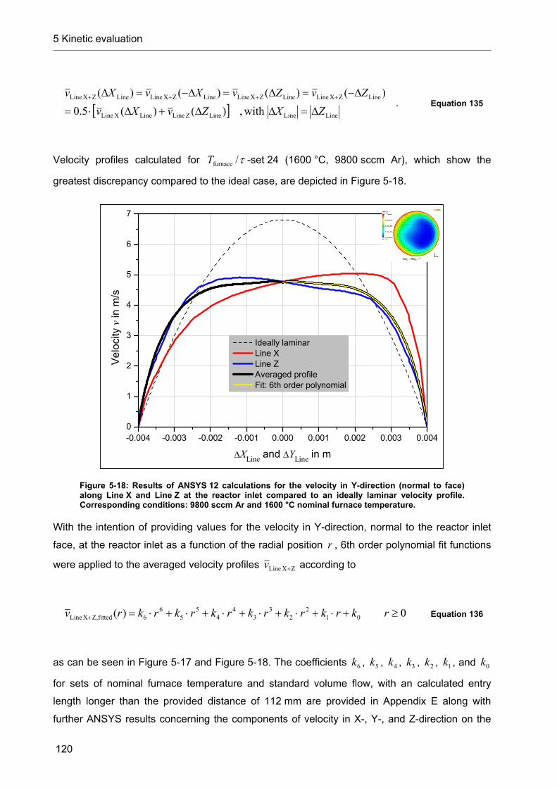
5 Kinetic evaluation
120
LineLineLine ZLineLineX Line
LineZX LineLineZX LineLineZX LineLineZX Line
with,)()(5.0
)()()()(
ZXZvXv
ZvZvXvXv
. Equation 135
Velocity profiles calculated for /furnaceT -set 24 (1600 °C, 9800 sccm Ar), which show the
greatest discrepancy compared to the ideal case, are depicted in Figure 5-18.
-0.004 -0.003 -0.002 -0.001 0.000 0.001 0.002 0.003 0.0040
1
2
3
4
5
6
7
Ve
loci
ty v
in m
/s
XLine and YLine in m
Ideally laminar Line X Line Z Averaged profile Fit: 6th order polynomial
Figure 5-18: Results of ANSYS 12 calculations for the velocity in Y-direction (normal to face) along Line X and Line Z at the reactor inlet compared to an ideally laminar velocity profile. Corresponding conditions: 9800 sccm Ar and 1600 °C nominal furnace temperature.
With the intention of providing values for the velocity in Y-direction, normal to the reactor inlet
face, at the reactor inlet as a function of the radial position r , 6th order polynomial fit functions
were applied to the averaged velocity profiles ZX Line v according to
0)( 012
23
34
45
56
6fitted,ZX Line rkrkrkrkrkrkrkrv Equation 136
as can be seen in Figure 5-17 and Figure 5-18. The coefficients 6k , 5k , 4k , 3k , 2k , 1k , and 0k
for sets of nominal furnace temperature and standard volume flow, with an calculated entry
length longer than the provided distance of 112 mm are provided in Appendix E along with
further ANSYS results concerning the components of velocity in X-, Y-, and Z-direction on the
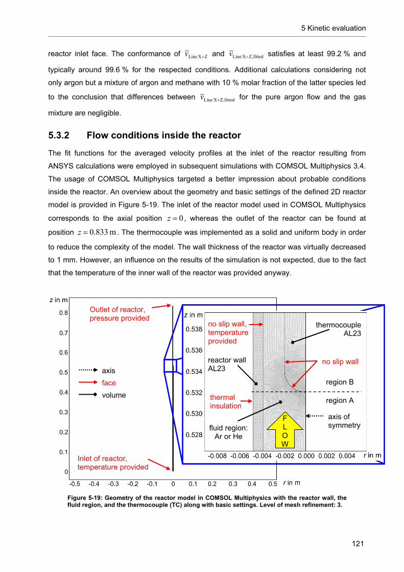
5 Kinetic evaluation
121
reactor inlet face. The conformance of ZX Line v and fitted,ZX Line v satisfies at least 99.2 % and
typically around 99.6 % for the respected conditions. Additional calculations considering not
only argon but a mixture of argon and methane with 10 % molar fraction of the latter species led
to the conclusion that differences between fitted,ZX Line v for the pure argon flow and the gas
mixture are negligible.
5.3.2 Flow conditions inside the reactor
The fit functions for the averaged velocity profiles at the inlet of the reactor resulting from
ANSYS calculations were employed in subsequent simulations with COMSOL Multiphysics 3.4.
The usage of COMSOL Multiphysics targeted a better impression about probable conditions
inside the reactor. An overview about the geometry and basic settings of the defined 2D reactor
model is provided in Figure 5-19. The inlet of the reactor model used in COMSOL Multiphysics
corresponds to the axial position 0z , whereas the outlet of the reactor can be found at
position m833.0z . The thermocouple was implemented as a solid and uniform body in order
to reduce the complexity of the model. The wall thickness of the reactor was virtually decreased
to 1 mm. However, an influence on the results of the simulation is not expected, due to the fact
that the temperature of the inner wall of the reactor was provided anyway.
Figure 5-19: Geometry of the reactor model in COMSOL Multiphysics with the reactor wall, the fluid region, and the thermocouple (TC) along with basic settings. Level of mesh refinement: 3.
F L O W
Inlet of reactor, temperature provided
Outlet of reactor, pressure provided
reactor wall AL23
thermocouple AL23
fluid region: Ar or He
region B
region A
no slip wall, temperature provided
no slip wall
axis of symmetry
thermal insulation
face
volume
axis

5 Kinetic evaluation
122
The conditions in the reactor were simulated based on the weakly compressible Navier-Stokes
mode concerning the flow as well as on convection and conduction concerning the heat
transfer. The weakly compressible Navier-Stokes mode comprises the fully compressible
composition of the equation of continuity as well as the equations of momentum and is
applicable for Mach numbers below 0.3. The Mach number is defined as
sound
Mav
v , Equation 137
with the velocity v and the velocity of sound soundv , which for an ideal gas arises from
TRvsound , Equation 138
employing the specific gas constant R , the temperature T , and the specific heat ratio .117
The specific gas constant R is connected to the universal gas constant by
MR
, Equation 139
where M represents the molecular weight of the considered gas, while the specific heat ratio
is defined as
v
p
c
c .118 Equation 140
Furthermore, the difference between the specific heat capacity at constant pressure pc and the
specific heat capacity at constant volume vc results in the specific gas constant R :
117 cp. [Munson, 2002], p. 686 et seqq. 118 cp. [Munson, 2002], p. 680 et seqq.

5 Kinetic evaluation
123
Rcc vp . Equation 141
It can be shown, that a maximum Mach number around 0.03 for experiments with argon can be
expected, whereas lower Mach numbers in the range of 0.006 represent the upper limit for
experiments with helium. Consequently, the weakly compressible Navier-Stokes mode is
applicable.
In absence of definite information about the wall temperatures of the reactor, especially in the
part above the heated region of the reactor, simplified temperature profiles for the wall were
applied for the calculations with COMSOL Multiphysics. These simplified wall temperature
profiles were defined by
the nominal furnace temperature within the heated length of the reactor
( m463.0m213.0 z , corresponding to position 0 mm… 250 mm),
the measured temperature at the inlet of the reactor ( 0z , corresponding to position
- 213 mm),
the measured temperature at the outlet of the reactor ( m833.0z , corresponding to
position 620 mm), and
linear interpolation for positions in between.
Preliminary calculations employing the established equations for the pressure drop in a laminar
pipe flow indicated that the difference between the pressure at the inlet of the reactor and the
outlet of the reactor should be marginal for the considered conditions.119 Higher measured
pressure differences might have been a result of carbon deposit in region B as explained in
Chapter 5.3.2.3. Therefore it is admissible to state that the pressure measured at the inlet of the
reactor is relevant for the major part of the reactor. Thus, the pressure at the outlet of the
reactor was set to the pressure measured at the reactor inlet.
The mesh was refined until the output of the simulations was independent from the level of
refinement. The independence was achieved for level 3 of mesh refinement corresponding to
187189 nodes and 366912 elements. The reactor wall and the thermocouple were modeled
according to material properties presented in Chapter 5.1.1. However, the significance of AL23
properties on the results of the calculation is marginal. Although high temperatures – existent in
119 Respective equations can e. g. be found in [VDI, 2006], p. Lab 1 et seqq.
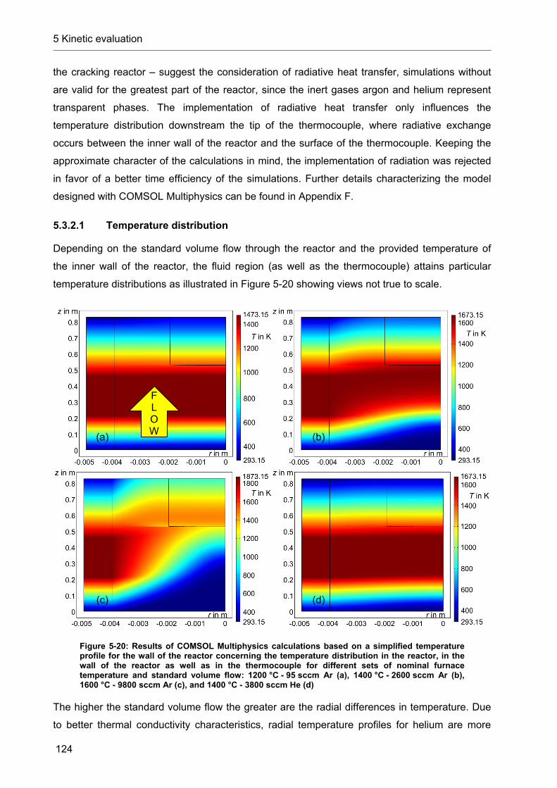
5 Kinetic evaluation
124
the cracking reactor – suggest the consideration of radiative heat transfer, simulations without
are valid for the greatest part of the reactor, since the inert gases argon and helium represent
transparent phases. The implementation of radiative heat transfer only influences the
temperature distribution downstream the tip of the thermocouple, where radiative exchange
occurs between the inner wall of the reactor and the surface of the thermocouple. Keeping the
approximate character of the calculations in mind, the implementation of radiation was rejected
in favor of a better time efficiency of the simulations. Further details characterizing the model
designed with COMSOL Multiphysics can be found in Appendix F.
5.3.2.1 Temperature distribution
Depending on the standard volume flow through the reactor and the provided temperature of
the inner wall of the reactor, the fluid region (as well as the thermocouple) attains particular
temperature distributions as illustrated in Figure 5-20 showing views not true to scale.
Figure 5-20: Results of COMSOL Multiphysics calculations based on a simplified temperature profile for the wall of the reactor concerning the temperature distribution in the reactor, in the wall of the reactor as well as in the thermocouple for different sets of nominal furnace temperature and standard volume flow: 1200 °C - 95 sccm Ar (a), 1400 °C - 2600 sccm Ar (b), 1600 °C - 9800 sccm Ar (c), and 1400 °C - 3800 sccm He (d)
The higher the standard volume flow the greater are the radial differences in temperature. Due
to better thermal conductivity characteristics, radial temperature profiles for helium are more
(a) (b)
(c) (d)
F L O W

5 Kinetic evaluation
125
even than for argon. Figure 5-21 shows the results of COMSOL Multiphysics calculations
concerning the center temperature ( 0r ) in region A as well as the temperature along the wall
of the thermocouple ( m002.0r ) in region B compared to the temperature profiles determined
by thermocouple measurements for selected sets of nominal furnace temperature and standard
volume flow. Corresponding to Figure 5-20 the difference between the temperature in the center
of the reactor and the applied temperature of the wall increases when the standard volume flow
increases.
0.0 0.1 0.2 0.3 0.4 0.5 0.6 0.7 0.8 0.90
200
400
600
800
1000
1200
1400region B
Tem
pera
ture
in °
C
Axial position in reactor in m
Wall, applied TC in wall position TC in center position r = 0.000 m, COMSOL, A r = 0.002 m, COMSOL, B
region A
iden
tical
0.0 0.1 0.2 0.3 0.4 0.5 0.6 0.7 0.8 0.90
200
400
600
800
1000
1200
1400
1600region B
Tem
pera
ture
in °
C
Axial position in reactor in m
Wall, applied TC in wall position TC in center position r = 0.000 m, COMSOL, A r = 0.002 m, COMSOL, B
region A
0.0 0.1 0.2 0.3 0.4 0.5 0.6 0.7 0.8 0.90
200
400
600
800
1000
1200
1400
1600
1800region B
Tem
pera
ture
in °
C
Axial position in reactor in m
Wall, applied TC in wall position TC in center position r = 0.000 m, COMSOL, A r = 0.002 m, COMSOL, B
region A
0.0 0.1 0.2 0.3 0.4 0.5 0.6 0.7 0.8 0.90
200
400
600
800
1000
1200
1400
1600region B
Tem
pera
ture
in °
C
Axial position in reactor in m
Wall, applied TC in wall position TC in center position r = 0.000 m, COMSOL, A r = 0.002 m, COMSOL, B
region A
Figure 5-21: Results of COMSOL Multiphysics calculations based on a simplified temperature profile for the wall of the reactor concerning the temperature evaluation in the center of region A and along the wall of the thermocouple in region B compared to measurement with a thermocouple in wall and center position for different sets of nominal furnace temperature and standard volume flow: 1200 °C - 95 sccm Ar (a), 1400 °C - 2600 sccm Ar (b), 1600 °C - 9800 sccm Ar (c), and 1400 °C - 3800 sccm He (d)
Although calculated and real values of temperature in the center of the reactor may differ in
detail, for instance due to the simplified applied wall temperature, the shape of the graphs
suggests that it is applicable to interpret the measured temperatures of the thermocouple in wall
and center position as a somehow averaged temperature of the fluid in contact.120
120 cp. Chapter 5.1.4
(a) (b)
(c) (d)

5 Kinetic evaluation
126
Consequently, basic characteristics of the results of the flow simulations should be transferable
to the real situation.
5.3.2.2 Flow lines and nested tube reactors
In every case, flow lines show a certain kind of order more or less matching the ideal laminar
flow conditions, which would be represented by flow lines parallel to the rotation axis of the
reactor characterized by 0r . The flow lines for helium and for low standard volume flows of
argon show good parallelism. However, the higher the standard volume flow the worse is the
congruence with the ideally laminar situation. Further figures of flow lines can be found in
Appendix F.
Figure 5-22: Results of COMSOL Multiphysics calculations based on a simplified temperature profile for the wall of the reactor concerning flow lines for different sets of nominal furnace temperature and standard volume flow: 1200 °C - 95 sccm Ar (a), 1400 °C - 2600 sccm Ar (b), 1600 °C - 9800 sccm Ar (c), and 1400 °C - 3800 sccm He (d)
A plug flow reactor model considers a turbulent flow and consequently an equal residence time
of every volume element entering the reactor. Contrariwise, a laminar flow features different
residence times depending on the radial position. The radial position of a volume element being
part of an ideally laminar flow keeps constant on its way through the reactor. In order to reflect
(a)
(c)
(b)
(d)
F L O W
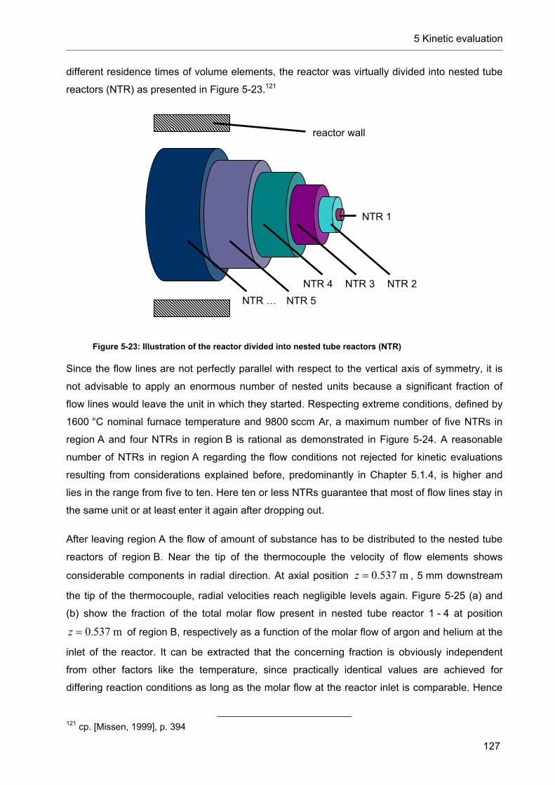
5 Kinetic evaluation
127
different residence times of volume elements, the reactor was virtually divided into nested tube
reactors (NTR) as presented in Figure 5-23.121
Figure 5-23: Illustration of the reactor divided into nested tube reactors (NTR)
Since the flow lines are not perfectly parallel with respect to the vertical axis of symmetry, it is
not advisable to apply an enormous number of nested units because a significant fraction of
flow lines would leave the unit in which they started. Respecting extreme conditions, defined by
1600 °C nominal furnace temperature and 9800 sccm Ar, a maximum number of five NTRs in
region A and four NTRs in region B is rational as demonstrated in Figure 5-24. A reasonable
number of NTRs in region A regarding the flow conditions not rejected for kinetic evaluations
resulting from considerations explained before, predominantly in Chapter 5.1.4, is higher and
lies in the range from five to ten. Here ten or less NTRs guarantee that most of flow lines stay in
the same unit or at least enter it again after dropping out.
After leaving region A the flow of amount of substance has to be distributed to the nested tube
reactors of region B. Near the tip of the thermocouple the velocity of flow elements shows
considerable components in radial direction. At axial position m537.0z , 5 mm downstream
the tip of the thermocouple, radial velocities reach negligible levels again. Figure 5-25 (a) and
(b) show the fraction of the total molar flow present in nested tube reactor 1 - 4 at position
m537.0z of region B, respectively as a function of the molar flow of argon and helium at the
inlet of the reactor. It can be extracted that the concerning fraction is obviously independent
from other factors like the temperature, since practically identical values are achieved for
differing reaction conditions as long as the molar flow at the reactor inlet is comparable. Hence
121 cp. [Missen, 1999], p. 394
NTR 1
NTR 2 NTR 3 NTR 4
NTR 5 NTR …
reactor wall

5 Kinetic evaluation
128
the aforementioned neglect of radiative heat transfer, which essentially influences the
temperatures at the thermocouple, can be justified.
Figure 5-24: Results of COMSOL Multiphysics calculations based on a simplified temperature profile for the wall of the reactor concerning flow lines for 1600 °C nominal furnace temperature and 9800 sccm argon with indication of virtual nested tube reactors (NTR)
Resulting from the high dilution, the total molar flow through the reactor varies only slightly,
namely at most by ,0CHDG,0,0CH 44nnx as already stated in Chapter 5.2.2, with the progress of
the reaction and, consequently, with the axial position in the reactor. Accordingly, the molar flow
passing from region A to region B roughly matches the molar flow at the reactor inlet. Thus, it is
admissible to distribute the total molar flow at the border between region A and region B to the
particular virtual nested tube reactors of region B consistent with the polynomial fit functions
introduced in Figure 5-25. Respective values for the coefficients 3k , 2k , 1k , and 0k of the fit
functions can be found in Appendix F.
region A
region B
NTR 5 4 3 2 1
NTR 4 3 2 1

5 Kinetic evaluation
129
0.000 0.002 0.004 0.006 0.0080.0
0.1
0.2
0.3
0.4
Fit function: y = k3 x3 + k
2 x2 + k
1 x + k
0.
Fra
ctio
n of
tota
l mol
ar fl
ow in
-
Molar flow at inlet of reactor in mol/s
NTR 1 NTR 2 NTR 3 NTR 4
..
0.000 0.002 0.004 0.006 0.0080.0
0.1
0.2
0.3
0.4
Fit function: y = k2 x2 + k
1 x + k
0
Fra
ctio
n of
tot
al m
olar
flo
w in
-
Molar flow at inlet of reactor in mol/s
NTR 1 NTR 2 NTR 3 NTR 4
..
Figure 5-25: Results of COMSOL Multiphysics calculations based on a simplified temperature profile for the wall of the reactor concerning the fraction of the molar flow at the inlet of the reactor in particular nested tube reactors in region B 5 mm downstream the tip of the thermocouple as a function of the molar flow of argon (a) and helium (b) at the reactor inlet
5.3.2.3 Pressure distribution
Figure 5-26 gives information about the pressure distribution inside the reactor for different sets
of nominal furnace temperature and standard volume flow. As one could have expected, radial
pressure differences are negligible. Contrariwise, a moderate pressure drop in axial direction
has to be reported.
The development of the pressure along lines of constant radius in region A ( m002.0r ) and
region B ( m003.0r ) extracted from information provided in Figure 5-26 is represented in
Figure 5-27. The COMSOL Multiphysics calculations show that the main pressure drop occurs
in region B, where part of the cross section of the reactor is blocked by the thermocouple, and
thereby confirm results of preliminary calculations referred to before.122 However, in most cases
experimentally determined pressure drops are somewhat higher than the calculated ones as
can be seen in Figure 5-27 exemplarily for the considered sets of nominal furnace temperature
and standard volume flow. This is probably due to the deposit of generated carbon in the gap
between thermocouple and reactor wall at locations where temperatures are not high enough to
remove carbon deposit by burning.
122 see beginning of Chapter 5.3.2
(a) (b)

5 Kinetic evaluation
130
Figure 5-26: Results of COMSOL Multiphysics calculations based on a simplified temperature profile for the wall of the reactor concerning pressure distribution inside the reactor for different sets of nominal furnace temperature and standard volume flow: 1200 °C - 95 sccm Ar (a), 1400 °C - 2600 sccm Ar (b), 1600 °C - 9800 sccm Ar (c), and 1400 °C - 3800 sccm He (d)
(a)
(c)
(b)
(d)
F L O W

5 Kinetic evaluation
131
0.0 0.1 0.2 0.3 0.4 0.5 0.6 0.7 0.8 0.90
5
10
15
20
25
30
35
region B: r = 0.003 m
p(z
= 0
) -
p(z)
in m
bar
Axial position in reactor in m
1200 °C - 95 sccm Ar, region A 1200 °C - 95 sccm Ar, region B 1200 °C - 95 sccm Ar, experiment 1400 °C - 2600 sccm Ar, region A 1400 °C - 2600 sccm Ar, region B 1400 °C - 2600 sccm Ar, experiment 1600 °C - 9800 sccm Ar, region A 1600 °C - 9800 sccm Ar, region B 1600 °C - 9800 sccm Ar, experiment 1400 °C - 3800 sccm He, region A 1400 °C - 3800 sccm He, region B 1400 °C - 3800 sccm He, experiment
region A: values for r = 0.002 m
Figure 5-27: Results of COMSOL Multiphysics calculations based on a simplified temperature profile for the wall of the reactor concerning the pressure evaluation along average radii in region A and region B compared to experimental pressure differences between the inlet and the outlet of the reactor for different sets of nominal furnace temperature and standard volume flow
Employing the present information, it is applicable to consider the pressure above the
thermocouple as a constant, whereas a linear pressure drop is assumed for region B, where the
thermocouple blocks the center of the reactor. Taking relevant axial locations into account, the
pressure p can be formulated as a function of the axial position z according to
mm728mm1 if
mm1mm1mm728
mm1 if
)(
TC
TCTC
inletR,outletR,inletR,
TCinletR,
zz
zzz
ppp
zzp
zp , Equation 142
with mm320TC z .
5.4 Kinetic model
As stated above, the predominant species involved in the thermal dissociation of methane are –
beside methane and the desired products hydrogen and carbon – the C2-hydrocarbons ethane,

5 Kinetic evaluation
132
ethene, and ethyne. Consequently, the applied kinetic model comprises the dehydrogenation
reactions starting with methane, forming the C2-intermediates, and finally generating hydrogen
and carbon:
2 CH4 (g) → C2H6 (g) + H2 (g) 1
C2H6 (g) → C2H4 (g) + H2 (g) 2
C2H4 (g) → C2H2 (g) + H2 (g) 3
C2H2 (g) → 2 “C” (s) + H2 (g) 4
Numerous other species are involved in the cracking reactions; however, since the balance of
hydrogen atoms is generally more or less satisfied, only low amounts of other (not considered)
species could be found in the product flow. The partly remarkable disagreement concerning the
balance of carbon atoms suggests that low fractions of further species with high C/H-ratio were
implicated. Without the consideration of further species, the amount of substance of formed
carbon is considerably overestimated.123 The reactions involved in the thermal dissociation of
methane proceed in the gaseous phase (homogeneous character) and presumably on the
surface of generated particles as well as on the wall of the reactor (heterogeneous character).124
The extent of present experimental data prohibits a kinetic approach, which differentiates
between homogeneous and heterogeneous reactions, because
the amount of generated carbon is not exactly predictable due to the presence of not
considered C-rich species.
two types of generated carbon have to be distinguished: pyrocarbon and particulate
carbon, whose functional dependencies of formation on the reaction conditions are not
clear.
knowledge about functional dependencies of the BET surface of generated particulate
carbon on the reaction conditions remains incomplete.
understanding of the fraction of generated carbon which does not pass the reactor but
forms deposit inside is fragmentary.
information about favored locations of carbon deposit in the reactor is not concrete.
123 cp. Chapter 4.4 and Chapter 4.6.3 124 cp. Chapter 4.7

5 Kinetic evaluation
133
Hence a certain reaction rate is interpreted as a combined result of homogeneous and
heterogeneous effects. The reaction rate qr of every considered reaction q is a function of the
reaction conditions, in particular of the temperature T and the respective concentration of the
reactant of reaction q qcreactant, . It is defined in accordance with Equation 19, Equation 20, and
Equation 21 by
q
qm
qT
E
qq cekr reactant,,0
a,
, Equation 143
employing – respectively for reaction q – the activation energy aE , the reaction order m , and
the pre-exponential factor 0k .
5.5 Procedure
Different reactor models have been applied for the kinetic evaluation. In accordance with the
findings concerning the flow conditions inside the reactor, a model based on nested tube
reactors (NTR) was introduced.125 Since the relevance of radial diffusion could not be estimated
sufficiently, two contrary cases were considered.126 On the one hand respective effects were
entirely neglected, whereas on the other hand ideal radial diffusion (D) was presumed.
Furthermore, a plug flow model (PFR) was applied as a reference model.
For any model the volume of the reactor had to be divided into volume elements. Figure 5-28
shows an illustration of one of these volume elements RV along with entering and leaving
molar flows.
Figure 5-28: General configuration of a volume element of the reactor with ingoing and outgoing molar flows
125 cp. Chapter 5.3 126 cp. Chapter 5.2.2

5 Kinetic evaluation
134
Depending on the reaction conditions, dominated by the reaction temperature RT and pressure
Rp , as well as on the kinetic parameters, the reaction rates of the considered reactions 1r , 2r ,
3r , and 4r can be calculated employing Equation 143. In conformity with Equation 16 and the
reaction scheme presented above, the molar flows leaving the particular volume element RV
arise from
R,1CH1entering,CHleaving,CH 444Vrnn Equation 144
for methane, from
R,2HC2R,1HC1entering,HCleaving,HC 62626262VrVrnn Equation 145
for ethane, from
R,3HC3R,2HC2entering,HCleaving,HC 42424242VrVrnn Equation 146
for ethene, from
R,4HC4R,3HC3entering,HCleaving,HC 22222222VrVrnn Equation 147
for ethyne, from
R,4H4R,3H3
R,2H2R,1H1entering,Hleaving,H
22
2222
VrVr
VrVrnn
Equation 148
for hydrogen, and from

5 Kinetic evaluation
135
R,4C""4entering,C""leaving,C"" Vrnn Equation 149
for carbon occupying qi , the stoichiometric coefficient of species i concerning reaction q . The
molar flow of the dilution gas keeps constant, since the inert dilution gas refuses to undergo any
reaction.
The concentration of species i ic , input factor for the calculation of the reaction rate, was
calculated following Equation 15, respecting the molar flows of gaseous species for the
estimation of the volume flow according to the ideal gas law following
22426224
entering,R
R
HC,HC,HC,H,CHDG,
j
np
Tn
V
nc
jj
iii
, Equation 150
where the pressure was calculated depending on the considered axial position.127 A limitation of
the sink terms guaranteed that the sink term of species i (corresponding to the source term of
species j formed by the reaction, which consumes species i ) never exceeded the actual
entering flow of species i . The molar flows leaving a particular volume element serve as the
entering flows of the subsequent volume element. Finally, the calculated molar flows at the
outlet of the reactor calculatedP,,CH4n , calculatedP,,H2
n , calculatedP,,HC 62n , calculatedP,,HC 42
n , and calculatedP,,HC 22n are
employed in order to estimate the calculated conversion of methane and the calculated yields of
hydrogen, ethane, ethene, and ethyne based on the respective initial molar flow of methane
,0CH4n .
An optimization tool was used to find kinetic parameters, which allow best agreement between
calculated values and experimental results.128 Following Chi-Square fitting the model error
2tot,E , which is the quantity to be minimized, was defined as
127 cp. Chapter 5.3.2.3, particularly Equation 142 128 Optimization tool: Optimization Toolbox 4.0 embedded in MATLAB Version 7.6.0.324 (R2008a), Solver: “lsnonlin“ (Nonlinear least squares), algorithm based on the interior-reflective Newton method. For further information see Appendix G.

5 Kinetic evaluation
136
2HC,
2HC,
2HC,
2H,
2CH,
2tot, 22426224 EEEEEE Equation 151
featuring
sexperiment
4
44
sexperiment
441
2
,CH
,CHcalculated,,CH
1
2,CH
2CH, )(
N
k k
kkN
kk Xu
XXEE Equation 152
and
22426221
2
,
,calculated,,
1
2,
2, HC,HC,HC,H
)(
sexperimentsexperiment
j
Yu
YYEE
N
k kj
kjkjN
kkjj Equation 153
based on sexperimentN experimental conditions considered for the kinetic evaluation.129 The
equations show that the difference between the calculated and measured conversion or yields
for experimental condition k was related to the estimated standard uncertainty of respective
experimental results. The yield of ethane and ethyne partly attained quite low values. In order
not to overvalue the respective contributions to 2, jE , a limit of marginal extend LMEY was
introduced and set to 0.001, for both ethane and ethyne. If the experimental value of the yield
lies below this limit, two cases were distinguished:
)(:2Case
0:1Case
HC,HC)001.0(
LME,
LME,calculated,,,LME,calculated,,
,LME,calculated,,
2262LME,,
j
jkjkjjkj
kjjkj
jkj
Yu
YYEYY
EYY
jYY
, Equation 154
where the standard uncertainties )( LME, jYu were estimated taking appropriate data into account.
It was found that )(62HCLME,Yu and )(
22HCLME,Yu can be approximated by 0.00027 and 0.0045,
respectively, considering the relevant range close to LMEY . The total number of reaction
129 cp. [Press, 2007], p. 778 et seqq. and Chapter 2.4

5 Kinetic evaluation
137
conditions experimentally covered accounts for 88 (73 with Ar and 15 with He)130; however, due
to the constrictions related to axial diffusion and the radial temperature gradient the number of
experimental conditions employed for the kinetic evaluation was reduced to 57 (42 with Ar and
15 with He).131
Independent from the reactor model the axial step size through the reactor z was set to 1 mm,
which features a reasonable compromise between accuracy and speed of computation.
Reference calculations with an axial step size of 0.1 mm indicated that only marginal variations
of 2tot,E should be expected, if step sizes smaller than 1 mm were applied. Different initial
parameter sets (IPSs) covering a wide range of potential values have been applied in order to
increase the probability of the identification of the global minimum instead of a local one.
Respective initial parameters are summarized in Table 5-7.
Table 5-7: Initial parameter sets for the optimization process along with lower bounds (LB) and upper bounds (UB) of the parameters
Initial Parameter Set (IPS) Parameter
1 2 3 4 5 6 7 8 9 10 11 12 LB UB
a,1E 381.0 381.0 381.0 381.0 571.5 190.5 571.5 190.5 571.5 190.5 571.5 190.5 0 700
)log( 1,0k 13.65 13.65 13.65 13.65 20.48 6.825 20.48 6.825 6.825 20.48 6.825 20.48 0.5 25
1m 1 1 1 1 1.5 0.5 1.5 0.5 1 1 1 1 0.25 3
a,2E 334.9 289.0 334.9 289.0 502.4 167.5 433.5 144.5 502.4 167.5 433.5 144.5 0 700
)log( 2,0k 16.65 14.00 16.65 14.00 24.98 8.325 21.00 7.000 8.325 24.98 7.000 21.00 0.5 25
2m 1 1 1 1 1.5 0.5 1.5 0.5 1 1 1 1 0.25 3
a,3E 167.0 167.0 167.0 167.0 250.5 83.50 250.5 83.50 250.5 83.50 250.5 83.50 0 700
)log( 3,0k 8.410 8.410 8.410 8.410 12.62 4.205 12.62 4.205 4.205 12.62 4.205 12.62 0.5 25
3m 1 1 1 1 1.5 0.5 1.5 0.5 1 1 1 1 0.25 3
a,4E 167.5 167.5 125.6 125.6 251.3 83.75 188.4 62.80 251.3 83.75 188.4 62.80 0 700
)log( 4,0k 10.33 10.33 6.23 6.23 15.50 5.165 9.345 3.115 5.165 15.50 3.115 9.345 0.5 25
4m 2 2 1 1 3 1 1.5 0.5 2 2 1 1 0.25 3
mol
kJinaE ,
)1(
30 m
mol
s
1in
m
k
, inm
IPSs 1-4 feature values on the basis of [Kozlov, 1962] IPS 1 combines maximum values, IPS 4 combines minimum values IPS 5 = IPS 1 * 1.5, IPS 6 = IPS 1 * 0.5, IPS 7 = IPS 4 * 1.5, IPS 8 = IPS 4 * 0.5
IPSs 9-12 are based on crosswise multiplication of aE and )log( 0k of IPSs 1 and 4 by 1.5 and 0.5
130 cp. Chapter 4.2 131 cp. Chapter 5.1.4 and Chapter 5.2.1

5 Kinetic evaluation
138
The common logarithm of the pre-exponential factor was altered by the optimization tool instead
of the pre-exponential factor itself with the purpose of dealing with values, which have a
somehow comparable order of magnitude.
Temperatures of the wall and the center of the reactor at axial position z , )(W zT and )(C zT ,
respectively, were determined by linear interpolation employing the sets of measured
temperatures. The following chapters provide further details about the applied reactor models.
5.5.1 Reactor model: Plug flow reactor
A common plug flow model (PFR) served as a reference model considering only an axial
division of the reactor into volume elements as is illustrated in Figure 5-29.
Figure 5-29: Illustration of a plug flow model applied to the tube reactor with thermocouple (TC)
The relevant reaction temperature at axial position z )(R zT was estimated by area-related
averaging of a parabolic temperature profile132 defined by the temperature of the center of the
reactor )(C zT and the temperature at the wall of the reactor )(W zT leading to
)()(5.0)()( CWCR zTzTzTzT . Equation 155
In region B, starting at position 319 mm, the size of the axial volume element is reduced due to
the presence of the thermocouple.
132 see Equation 117

5 Kinetic evaluation
139
5.5.2 Reactor model: Nested tube reactors
In order to approximate the laminar flow conditions inside the reactor and to consider radial
temperature differences, a more complex reactor model based on nested tube reactors (NTR)
was suggested above.133 Thereby the reactor with inner radius iR,R was divided into NTRN
nested tube reactors with uniform thickness r arising from
NTR
iR,
N
Rr . Equation 156
The outer radius o,jr and inner radius i,jr of NTR j meet
i,o, jjj rrrr Equation 157
and can consequently be calculated respecting 0i,1 r . An illustration of the reactor model is
provided in Figure 5-30.
Figure 5-30: Illustration of a nested tube reactor model applied to the tube reactor with thermocouple (TC)
133 see Chapter 5.3.2.2

5 Kinetic evaluation
140
At the inlet of the reactor the total volume flow had to be distributed to NTRN nested tube
reactors. 0,jV , the volume flow entering nested tube reactor j with the inner radius i,jr and the
outer radius o,jr , was determined by
rrrvAvVj
j
r
rA
j ˆdˆ2)ˆ(do,
i,
0, , Equation 158
employing the velocity profile )(rv according to Equation 132 if a fully developed laminar
velocity profile can be expected or according to Equation 136 if not. Since the conditions for the
ANSYS simulations and the real conditions for the cracking experiment differ slightly, a
correction factor was used being multiplied with each 0,jV assuring that the sum of all 0,jV
equals the total volume flow at the inlet of the reactor for the particular experiment. Respective
molar flows of dilution gas and methane at the inlet of nested tube reactor j , jnDG, and jn ,CH4 ,
were obtained using the ideal gas law and the initial molar fraction of methane.134 The nested
units were regarded separately meaning that no interaction takes place between each other and
molecules either present at the inlet of the reactor or formed by reactions in a particular NTR
stay inside. )(NTRR, zT j , the temperature in NTR j at the axial position z , was approximated by
evaluating the presumed parabolic temperature profile at the mean radius jr arising from
i,o,5.0 jjj rrr Equation 159
employing the respective outer radius o,jr and inner radius i,jr .
The calculated total molar flow at position 319 mm, which corresponds to the tip of the
thermocouple, was distributed to the four nested tube reactors downstream, that is region B, in
accordance with respective COMSOL Multiphysics simulation results presented before.135 In
region B )( NTRR, zT j , the relevant temperature in NTR j at axial position z , was approximated
by linear interpolation following
134 see Equation 2 and Equation 5 135 cp. Chapter 5.3.2.2

5 Kinetic evaluation
141
oTC,oTC,iR,
CWC NTRR,
)()()()( Rr
RR
zTzTzTzT jj
Equation 160
with the outer radius of the thermocouple oTC,R . In region B m002.0oTC,i1, Rr .
Two different numbers of NTR in region A were considered consistent with reasonable limits
stated in Chapter 5.3.2.2, namely 5NTR N (5 NTR) and 10NTR N (10 NTR).
5.5.3 Reactor model: Nested tube reactors with ideal radial diffusion
The reactor model based on nested tube reactors with ideal radial diffusion comprises all
features of the NTR model. However, an ideal radial diffusion step was attached to every
reaction step as illustrated in Figure 5-31. Following Equation 120, ideal radial diffusion means
that radial differences of molar fractions degrade attaining a value of 0.
Figure 5-31: Illustration of reaction steps and diffusion steps for reactor models based on nested tube reactors with (NTR + D) and without ideal radial diffusion (NTR)
Hence the average molar fractions of all components i of the flow after the reaction step was
calculated from
z z + Δz z – Δz
STEP
REACTI ON
STEP
DI FFUSI ON
STEP
D I F F U S I O N
NTR + D
S T E P
REACTI ON
STEP
R E A C T I O N
S T E P
D I F F U S I O N
NTR

5 Kinetic evaluation
142
22426224
1reactionafter ,,
1reactionafter ,,
reactionafter HC,HC,HC,H,CHDG,)(
)(
)(NTR
NTR
kzn
zn
zx
k
N
jjk
N
jji
i,
. Equation 161
The molar flows after diffusion were determined under the assumption that the total molar flow
of gaseous components in the considered NTRs do not change as a result of the diffusion step.
Consequently, )(, zzn ji , the molar flow of component i in NTR j entering a volume
element at axial position zz , arises from
22426224
reactionafter ,,reactionafter diffusionafter ,,,
HC,HC,HC,H,CHDG,
)()()()(
k
znzxznzznk
jki,jiji . Equation 162
5.6 Kinetic parameters and further results
Best fit kinetic parameters determined by the optimization tool are presented for the applied
reactor models in Table 5-8 along with the respective values for 2tot,E , the quantity, which was
minimized, as well as its constituents 2CH, 4E , 2
H, 2E , 2HC, 62E , 2
HC, 42E , and 2HC, 22E . As can be
seen, the reactor model based on five nested tube reactors (5 NTR) lead to best agreement
between experimental results and simulation resulting in 178092tot, E . However, the
optimization tool was capable of identifying best fit kinetic parameters, which lead to
comparable 2tot,E for all models. The results for five nested tube reactors with ideal radial
diffusion (5 NTR + D) are very similar to those of the plug flow model (PFR) concerning both,
the kinetic parameters and the achieved error of the model. The extension of the number of
NTR from five to ten (10 NTR and 10 NTR + D) leads to almost identical results compared to
the models based on five nested tube reactors. In the following, model 5 NTR which achieved
the lowest value for 2tot,E is analyzed more in detail.

5 Kinetic evaluation
143
Table 5-8: Comparison of best fit kinetic parameters and achieved agreement between experiments and optimization procedure for different reactor models: plug flow reactor (PFR), 5 nested tube reactors (5 NTR), 5 nested tube reactors with ideal radial diffusion (5 NTR + D), 10 nested tube reactors (10 NTR), and 10 nested tube reactors with ideal radial diffusion (10 NTR + D)
Reactor model PFR 5 NTR 5 NTR + D 10 NTR 10 NTR + D
a,1E 499.4 510.1 499.5 510.3 499.5
)log( 1,0k 17.37 17.77 17.37 17.79 17.37
Best fit kinetic
parameters of reaction
1 1m 1.331 1.283 1.329 1.286 1.328
a,2E 418.2 433.9 418.2 433.3 418.8
)log( 2,0k 17.12 17.75 17.13 17.74 17.15
Best fit kinetic
parameters of reaction
2 2m 1.044 1.049 1.046 1.050 1.044
a,3E 343.1 374.7 343.9 373.8 344.1
)log( 3,0k 14.29 15.36 14.31 15.34 14.31
Best fit kinetic
parameters of reaction
3 3m 1.333 1.301 1.328 1.303 1.327
a,4E 13.25 29.01 13.10 29.04 13.08
)log( 4,0k 2.282 2.657 2.273 2.704 2.272
Best fit kinetic
parameters of reaction
4 4m 1.966 1.599 1.965 1.638 1.964
2CH, 4E 7470 7700 7508 7689 7509
2H, 2E 1706 1688 1719 1752 1717
2HC, 62E 323 306 309 310 300
2HC, 42E 7570 6618 7550 6661 7577
2HC, 22E 1239 1498 1245 1426 1247
Selection of experiments
for kinetic evaluation: 42 x Ar and
15 x He 2
tot,E
quantity to be minimized
18308 17809 18331 17838 18349
mol
kJinaE ,
)1(
30 m
mol
s
1in
m
k
, inm
The number of degrees of freedom of a model freedom of degreesN arises from the difference of the
number of data points points dataN and the number of adjustable parameters parametersN according
to
parameterspoints datafreedom of degrees NNN . Equation 163
Since 57 reaction conditions were employed for the kinetic evaluation and each reaction
condition provides a result concerning 4CHX ,
2HY , 62HCY ,
42HCY , and 22HCY , the number of data

5 Kinetic evaluation
144
points finally adds up to 285. On the other hand there are three kinetic parameters for each of
the four considered reactions. Consequently, 12parameters N and 273freedom of degrees N . A fairly
good fit is typically characterized by freedom of degrees2
tot, NE . Contrariwise, the best present model
features freedom of degrees2
tot, 17809 NE , indicating either an improper estimation of standard
uncertainties or a weakness of the model itself.136 This issue will be discussed later.
Table 5-9 gives information about the differences between calculated (reactor model 5 NTR with
best fit kinetic parameters leading to 178092tot, E ) and experimentally determined values for
4CHX , 2HY ,
62HCY , 42HCY , and
22HCY . On average the absolute differences here equal 0.0657 and
0.0602 regarding the conversion of methane and the yield of hydrogen, respectively,
corresponding to an average relative difference of about 14.5 %. Higher relative differences
have to be reported pertaining to the yields of C2-hydrocarbons. However, the yields of ethane
and ethene, calculated and measured, are mostly much lower than the other considered
quantities. Generally about two thirds of the derived differences are smaller than the relevant
average value.
Table 5-9: Information about differences between quantities calculated with reactor model 5 NTR employing best fit kinetic parameters and experimentally determined quantities
Absolute differences Absolute differences
relative to experimental results (data not used if experimental result = 0)Quantity
Average in - Fraction of values smaller
than average in % Average in -
Fraction of values smaller than average in %
4CHX 0.0657 70.2 0.143 71.9
2HY 0.0602 66.7 0.146 71.9
62HCY 0.000664 64.9 2.86 78.9
42HCY 0.00575 61.4 0.538 52.6
22HCY 0.0806 59.6 0.473 70.2
136 cp. [Press, 2007], p. 778 et seqq.

5 Kinetic evaluation
145
The uncertainty of molar flows at the inlet and the outlet of the reactor were respected by the
estimation of the uncertainty of the conversion of methane and the yields of hydrogen as well as
of the C2-hydrocarbons, which form part of the error of the model and thus of the quantity, which
was minimized by the optimization tool. Beside the mentioned figures also temperatures and
pressures inside the reactor, being input information of the kinetic evaluation, are affected by
uncertainty. In order to assess the relevance of these uncertainties, two further sets of
temperature and pressure were investigated for the best model 5 NTR. The first extreme of
conditions inside the reactor was determined by combination of minimum temperatures and
pressures ( minmin , pT ), calculated by means of maximum negative uncertainty. Minimum
temperatures and pressures generally cause a decrease of reaction rates. Contrariwise, the
second extreme is related to maximum reaction rates based on maximum temperatures and
pressures ( maxmax , pT ) arising from respective maximum positive uncertainty. As can be seen in
Table 5-10, good agreement between the results determined for nominal and extreme
conditions concerning temperature and pressure inside the reactor has to be reported. Found
best fit kinetic parameters and model errors for the extreme conditions practically conform to
figures for nominal conditions. A somehow lower 2tot,E was achieved for the set of minimum
temperatures and pressures. The good agreement indicates that the uncertainty of measured
temperatures and pressures is low enough for a definite determination of kinetic parameters.
Different IPSs usually resulted in practically identical best fit kinetic parameter values and
consequently to practically identical model errors indicating that global minima were found.
However, in some cases IPS 9, 10, 11, or 12, which are based on opposed modification of the
activation energies and the common logarithms of the pre-exponential factors,137 led to local
minima featuring clearly higher values of 2tot,E compared to the best fit situation: IPS 9 for PFR,
IPSs 10-12 for 5 NTR, 5 NTR + D, 10 NTR, IPSs 9 and 11 for 10 NTR + D, IPSs 10 and 12 for
5 NTR employing minimum temperatures and pressures, and IPS 11 for 5 NTR employing
maximum temperatures and pressures.
137 cp. Table 5-7

5 Kinetic evaluation
146
Table 5-10: Comparison of best fit kinetic parameters and achieved agreement between experiments and optimization procedure for the reactor model based on 5 nested tube reactors (5 NTR) considering sets of nominal, minimum, and maximum temperatures and pressures
Reactor model 5 NTR 5 NTR
( minmin , pT )
5 NTR
( maxmax , pT )
a,1E 510.1 508.0 511.1
)log( 1,0k 17.77 17.77 17.76
Best fit kinetic
parameters of reaction
1 1m 1.283 1.304 1.280
a,2E 433.9 431.8 435.3
)log( 2,0k 17.75 17.75 17.75
Best fit kinetic
parameters of reaction
2 2m 1.049 1.055 1.048
a,3E 374.7 371.9 375.6
)log( 3,0k 15.36 15.34 15.35
Best fit kinetic
parameters of reaction
3 3m 1.301 1.316 1.299
a,4E 29.01 29.63 29.22
)log( 4,0k 2.657 2.687 2.650
Best fit kinetic
parameters of reaction
4 4m 1.599 1.593 1.596
2CH, 4E 7700 7442 7635
2H, 2E 1688 1638 1684
2HC, 62E 306 300 320
2HC, 42E 6618 6654 6681
2HC, 22E 1498 1501 1537
Selection of experiments
for kinetic evaluation: 42 x Ar and
15 x He 2
tot,E
quantity to be minimized
17809 17534 17857
mol
kJinaE ,
)1(
30 m
mol
s
1in
m
k
, inm
Figure 5-32 gives information about the relative change of the model error of 5 NTR, when a
particular kinetic parameter was varied keeping the other kinetic parameters constant. Within
the considered limits of variation the model error increases most with the change of activation
energies and common logarithms of reaction 1, reaction 2, and reaction 3, whereas the
kinetic parameters of reaction 4 and the reaction orders of all reactions influence the model
error only marginally. The clear dependence of the model error 2tot,E on aE and )log( 0k can be
explained by exponential expressions. By trend, kinetic parameters of the first reactions show
greater influence than the ones of subsequent reactions, because the latter reactions are
affected by products of the first reactions.

5 Kinetic evaluation
147
0.9 1.0 1.11
10
100
1000
E 2
tot /
E 2
totb
est f
it in
-
Kinetic parameter / best fit kinetic parameter in -
Reaction 1Reaction 2Reaction 3Reaction 4
Ea
log(k0)
m
Figure 5-32: Model error related to the model error for best fit kinetic parameters as a function of kinetic parameters related to the best fit kinetic parameters (reactor model 5 NTR)
An analysis of molar fractions in the considered nested tube reactors at a function of the axial
position calculated employing the reactor model 5 NTR and respective best fit kinetic
parameters indicates that the assumption )()( zxzx ii – made in Chapter 5.2.2 in order to
assess radial diffusive effects – is in fact a realistic one, at least regarding the order of
magnitude. Confirming values for the maximum radial difference of molar fractions related to the
mean, averaged for the heated region of the reactor and for all experiments used for the kinetic
evaluation, are provided in Table 5-11 along with standard deviation of values resulting from the
particular reaction conditions. The greatest averaged value was calculated for ethyne and
approaches 2.6.
Table 5-11: Averaged maximum radial differences of molar fractions in the heated region of the reactor for results associated with reactor model 5 NTR and respective best fit kinetic parameters
Species i
inmin,max,
zi
ii
x
xx
averaged for the heated region of the reactor averaged for all experiments used for the kinetic evaluation
Standard deviation
concerning the experiments
in -
methane 0.93 0.70
hydrogen 1.86 1.20
ethane 1.22 0.72
ethene 1.90 1.10
ethyne 2.59 1.76

5 Kinetic evaluation
148
Subsequently conversions and yields associated with results gained with reactor model 5 NTR
and respective best fit kinetic parameters are exemplarily compared to experimental findings
expanding the general information given in Table 5-9. Beside reaction conditions characterized
by 5 % methane (molar fraction) in argon, all reaction conditions dealing with helium as dilution
gas are considered. Further comparative diagrams can be found in Appendix G.
Figure 5-33, Figure 5-34, Figure 5-35, Figure 5-36, and Figure 5-37 represent corresponding
graphs concerning the conversion of methane, the yield of hydrogen, the yield of ethane, the
yield of ethene, and the yield of ethyne, respectively, considering argon as dilution gas.
According to the achieved model error ( 178092tot, E ) and Table 5-9, more or less clear
disagreement of experimentally determined and calculated values has to be reported. However,
the graphs often show qualitative consistence and calculated values mostly lie within or at least
close to the range, which is defined by maximum experimental uncertainty. This observation
applies to both, reaction conditions used and not used for the kinetic evaluation.
0.01 0.1 1 100
20
40
60
80
100
Con
vers
ion
of m
eth
ane
in %
Residence time in s
measured calculated
1200 °C1300 °C1400 °C1500 °C1600 °C
Figure 5-33: Comparison of experimentally determined conversion of methane (as a function of the residence time and the nominal furnace temperature) with calculated values employing reactor model 5 NTR and respective best fit kinetic parameters. 5 % initial molar fraction of methane in argon. Indicators of uncertainty refer to maximum uncertainty (black: used for kinetic evaluation, gray: not used for kinetic evaluation).

5 Kinetic evaluation
149
0.01 0.1 1 100
20
40
60
80
100
Yie
ld o
f hyd
roge
n in
%
Residence time in s
measured calculated
1200 °C1300 °C1400 °C1500 °C1600 °C
Figure 5-34: Comparison of experimentally determined yield of hydrogen (as a function of the residence time and the nominal furnace temperature) with calculated values employing reactor model 5 NTR and respective best fit kinetic parameters. 5 % initial molar fraction of methane in argon. Indicators of uncertainty refer to maximum uncertainty (black: used for kinetic evaluation, gray: not used for kinetic evaluation).
0.01 0.1 1 100.0
0.2
0.4
0.6
0.8
Yie
ld o
f eth
ane
in %
Residence time in s
measured calculated
1200 °C1300 °C1400 °C1500 °C1600 °C
Figure 5-35: Comparison of experimentally determined yield of ethane (as a function of the residence time and the nominal furnace temperature) with calculated values employing reactor model 5 NTR and respective best fit kinetic parameters. 5 % initial molar fraction of methane in argon. Indicators of uncertainty refer to maximum uncertainty (black: used for kinetic evaluation, gray: not used for kinetic evaluation).

5 Kinetic evaluation
150
0.01 0.1 1 100
1
2
3
4
5
Yie
ld o
f eth
ene
in %
Residence time in s
measured calculated
1200 °C1300 °C1400 °C1500 °C1600 °C
Figure 5-36: Comparison of experimentally determined yield of ethene (as a function of the residence time and the nominal furnace temperature) with calculated values employing reactor model 5 NTR and respective best fit kinetic parameters. 5 % initial molar fraction of methane in argon. Indicators of uncertainty refer to maximum uncertainty (black: used for kinetic evaluation, gray: not used for kinetic evaluation).
0.01 0.1 1 100
20
40
60
80
Yie
ld o
f eth
yne
in %
Residence time in s
measured calculated
1200 °C1300 °C1400 °C1500 °C1600 °C
Figure 5-37: Comparison of experimentally determined yield of ethyne (as a function of the residence time and the nominal furnace temperature) with calculated values employing reactor model 5 NTR and respective best fit kinetic parameters. 5 % initial molar fraction of methane in argon. Indicators of uncertainty refer to maximum uncertainty (black: used for kinetic evaluation, gray: not used for kinetic evaluation).
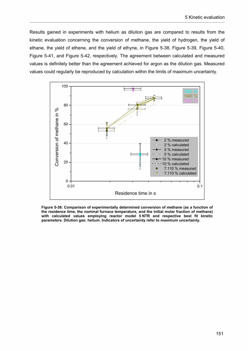
5 Kinetic evaluation
151
Results gained in experiments with helium as dilution gas are compared to results from the
kinetic evaluation concerning the conversion of methane, the yield of hydrogen, the yield of
ethane, the yield of ethene, and the yield of ethyne, in Figure 5-38, Figure 5-39, Figure 5-40,
Figure 5-41, and Figure 5-42, respectively. The agreement between calculated and measured
values is definitely better than the agreement achieved for argon as the dilution gas. Measured
values could regularly be reproduced by calculation within the limits of maximum uncertainty.
0.010
20
40
60
80
100
Con
vers
ion
of m
eth
ane
in %
Residence time in s
2 % measured 2 % calculated 5 % measured 5 % calculated 10 % measured 10 % calculated 7.110 % measured 7.110 % calculated
1300 °C1400 °C1500 °C
0.1
Figure 5-38: Comparison of experimentally determined conversion of methane (as a function of the residence time, the nominal furnace temperature, and the initial molar fraction of methane) with calculated values employing reactor model 5 NTR and respective best fit kinetic parameters. Dilution gas: helium. Indicators of uncertainty refer to maximum uncertainty.

5 Kinetic evaluation
152
0.010
20
40
60
80
100
Yie
ld o
f hyd
roge
n in
%
Residence time in s
2 % measured 2 % calculated 5 % measured 5 % calculated 10 % measured 10 % calculated 7.110 % measured 7.110 % calculated
1300 °C1400 °C1500 °C
0.1
Figure 5-39: Comparison of experimentally determined yield of hydrogen (as a function of the residence time, the nominal furnace temperature, and the initial molar fraction of methane) with calculated values employing reactor model 5 NTR and respective best fit kinetic parameters. Dilution gas: helium. Indicators of uncertainty refer to maximum uncertainty.
0.010.0
0.4
0.8
1.2
Yie
ld o
f eth
ane
in %
Residence time in s
2 % measured 2 % calculated 5 % measured 5 % calculated 10 % measured 10 % calculated 7.110 % measured 7.110 % calculated
1300 °C1400 °C1500 °C
0.1
Figure 5-40: Comparison of experimentally determined yield of ethane (as a function of the residence time, the nominal furnace temperature, and the initial molar fraction of methane) with calculated values employing reactor model 5 NTR and respective best fit kinetic parameters. Dilution gas: helium. Indicators of uncertainty refer to maximum uncertainty.

5 Kinetic evaluation
153
0.010
2
4
6
8
Yie
ld o
f eth
ene
in %
Residence time in s
2 % measured 2 % calculated 5 % measured 5 % calculated 10 % measured 10 % calculated 7.110 % measured 7.110 % calculated
1300 °C1400 °C1500 °C
0.1
Figure 5-41: Comparison of experimentally determined yield of ethene (as a function of the residence time, the nominal furnace temperature, and the initial molar fraction of methane) with calculated values employing reactor model 5 NTR and respective best fit kinetic parameters. Dilution gas: helium. Indicators of uncertainty refer to maximum uncertainty.
0.010
20
40
60
80
100
Yie
ld o
f eth
yne
in %
Residence time in s
2 % measured 2 % calculated 5 % measured 5 % calculated 10 % measured 10 % calculated 7.110 % measured 7.110 % calculated
1300 °C1400 °C1500 °C
0.1
Figure 5-42: Comparison of experimentally determined yield of ethyne (as a function of the residence time, the nominal furnace temperature, and the initial molar fraction of methane) with calculated values employing reactor model 5 NTR and respective best fit kinetic parameters. Dilution gas: helium. Indicators of uncertainty refer to maximum uncertainty.
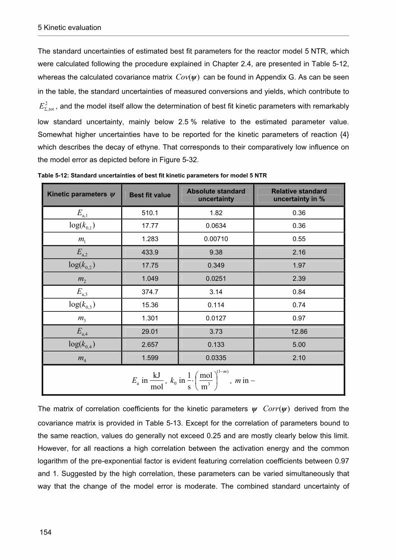
5 Kinetic evaluation
154
The standard uncertainties of estimated best fit parameters for the reactor model 5 NTR, which
were calculated following the procedure explained in Chapter 2.4, are presented in Table 5-12,
whereas the calculated covariance matrix )(ψCov can be found in Appendix G. As can be seen
in the table, the standard uncertainties of measured conversions and yields, which contribute to
2tot,E , and the model itself allow the determination of best fit kinetic parameters with remarkably
low standard uncertainty, mainly below 2.5 % relative to the estimated parameter value.
Somewhat higher uncertainties have to be reported for the kinetic parameters of reaction 4
which describes the decay of ethyne. That corresponds to their comparatively low influence on
the model error as depicted before in Figure 5-32.
Table 5-12: Standard uncertainties of best fit kinetic parameters for model 5 NTR
Kinetic parameters ψ Best fit value Absolute standard
uncertainty Relative standard uncertainty in %
a,1E 510.1 1.82 0.36
)log( 1,0k 17.77 0.0634 0.36
1m 1.283 0.00710 0.55
a,2E 433.9 9.38 2.16
)log( 2,0k 17.75 0.349 1.97
2m 1.049 0.0251 2.39
a,3E 374.7 3.14 0.84
)log( 3,0k 15.36 0.114 0.74
3m 1.301 0.0127 0.97
a,4E 29.01 3.73 12.86
)log( 4,0k 2.657 0.133 5.00
4m 1.599 0.0335 2.10
mol
kJinaE ,
)1(
30 m
mol
s
1in
m
k
, inm
The matrix of correlation coefficients for the kinetic parameters ψ )(ψCorr derived from the
covariance matrix is provided in Table 5-13. Except for the correlation of parameters bound to
the same reaction, values do generally not exceed 0.25 and are mostly clearly below this limit.
However, for all reactions a high correlation between the activation energy and the common
logarithm of the pre-exponential factor is evident featuring correlation coefficients between 0.97
and 1. Suggested by the high correlation, these parameters can be varied simultaneously that
way that the change of the model error is moderate. The combined standard uncertainty of

5 Kinetic evaluation
155
quantities derived from parameters with high correlation increases due to the fact that
covariances have to be taken into account.138
Table 5-13: Matrix of correlation coefficients calculated based on the best fit kinetic parameters for model 5 NTR. Blocks colored in orange indicate the correlation of kinetic parameters describing the same reaction.
)(ψCorr 1 2 3 4 5 6 7 8 9 10 11 12 Related to
1 1.00 1.00 0.63 0.01 0.02 0.08 0.10 0.14 0.24 -0.02 0.00 0.09 a,1E
2 1.00 1.00 0.68 0.01 0.02 0.09 0.08 0.12 0.25 -0.02 0.00 0.09 )log( 1,0k
3 0.63 0.68 1.00 -0.01 0.01 0.12 -0.10 -0.04 0.25 -0.01 -0.01 0.01 1m
4 0.01 0.01 -0.01 1.00 0.98 0.07 0.01 -0.02 -0.06 0.00 0.00 0.01 a,2E
5 0.02 0.02 0.01 0.98 1.00 0.28 0.01 -0.03 -0.06 0.00 0.00 0.01 )log( 2,0k
6 0.08 0.09 0.12 0.07 0.28 1.00 -0.03 -0.03 0.01 0.00 0.00 0.00 2m
7 0.10 0.08 -0.10 0.01 0.01 -0.03 1.00 0.97 0.09 0.00 0.02 0.09 a,3E
8 0.14 0.12 -0.04 -0.02 -0.03 -0.03 0.97 1.00 0.34 0.00 0.02 0.09 )log( 3,0k
9 0.24 0.25 0.25 -0.06 -0.06 0.01 0.09 0.34 1.00 -0.01 0.00 0.03 3m
10 -0.02 -0.02 -0.01 0.00 0.00 0.00 0.00 0.00 -0.01 1.00 0.97 -0.29 a,4E
11 0.00 0.00 -0.01 0.00 0.00 0.00 0.02 0.02 0.00 0.97 1.00 -0.06 )log( 4,0k
12 0.09 0.09 0.01 0.01 0.01 0.00 0.09 0.09 0.03 -0.29 -0.06 1.00 4m
mol
kJinaE ,
)1(
30 m
mol
s
1in
m
k
, inm
5.7 Discussion
Best fit values for the kinetic parameters were determined employing an optimization tool by
minimizing the model error. Regarding the particular models seriously different applied initial
parameter sets usually lead to practically identical best fit values for the kinetic parameters and
consequently to same values of the minimum model error. Thus, a global character of the
determined minimum model errors is indicated. The lowest value for the model error could be
located for the reactor model based on five nested tube reactors without the consideration of
radial diffusion (5 NTR). The corresponding model based on ten nested tube reactors features
virtually equal agreement and best fit kinetic parameters suggesting that the laminar flow
characteristics are respected sufficiently well by employing five nested tube reactors. The same
conclusion can be drawn by comparing the reactor models involving ideal radial diffusion. For
models respecting radial diffusion, minimum model errors only about 2.9 % higher than those of
138 cp. [ISO, 2008], p. 21
5 Kinetic evaluation
156
the models disregarding radial diffusion could be achieved. Thus, it is indicated that the limiting
conditions concerning radial diffusion are capable of reflecting the real conditions inside the
reactor more or less comparably well, or in other words, that the real conditions can be found
somewhere between the extreme effects. However, in spite of the principal difference of the
models, there exists remarkable conformity of derived best fit values of the kinetic parameters.
Except for parameters of reaction 4, best fit values corresponding to models with ideal radial
diffusion do not differ more than 8.2 % and mainly not more than 3.6 % from values
corresponding to models without radial diffusion. This could signify a rudimentarily universal
character of the determined parameter values. The gained best fit parameter values and the
achieved model error as well as its components are practically identical for the plug flow model
and for the models based on nested tube reactors featuring ideal radial diffusion. Obviously, the
latter models basically approach plug flow conditions. This proposes that the approximation of
laminar flow does not offer any advantage, when perfect radial diffusion is assumed, and that a
more sophisticated consideration of radial diffusion is advisable. It is admissible to state that
reaction temperatures were considered reasonably, since reaction conditions with doubtful
temperature distribution were excluded from the kinetic evaluation. Taking the residual
uncertainty of temperatures as well as the uncertainty of pressures inside the reactors into
account, additional optimization runs were performed based on the best present model 5 NTR.
The resulting best fit parameter values conform to values determined for the sets of nominal
temperature and pressure. Thus, the accuracy of temperatures and pressures is high enough to
definitely calculate best fit parameter values. Furthermore, a distinct finding concerning the
determined parameter values is indicated by quite low standard uncertainties derived from the
covariance matrix. Except for the correlation between the activation energy and the common
logarithm of the pre-exponential factor related to the same reaction the correlation between the
kinetic parameters is usually negligible. In spite of the relatively high model error, reactor model
5 NTR is capable of reflecting general tendencies and orders of magnitude of methane
conversion as well as of yields of hydrogen, ethane, ethene, and ethyne. When maximum
uncertainty is taken into account, calculated values are often in reach of results of both,
experiments with argon and helium as dilution gas.
In literature the integers 1 and 2 are suggested as reaction orders of the thermal decomposition
of methane as well as the thermal decomposition of C2-hydrocarbons without presence of
additional material as presented in Chapter 3.4. Contrariwise, parameter fitting to model 5 NTR
led to values between 1 and 2, namely 1.283, 1.049, 1.301, and 1.599 for reaction 1, 2, 3,
and 4, respectively. The fractional nature of derived parameters is not a general sign of poor
quality but confirms the summarizing character of net reactions and possibly reveals limitations
of a simplified kinetic approach considering a wide range of reaction conditions. The calculated
activation energy of reaction 1 lies beyond the scope of activation energies reported in

5 Kinetic evaluation
157
literature. However, also the pre-exponential factor is somewhat higher and accounts for a
partial compensation. The activation energies of the other decomposition reactions follow the
vague trend depending on the number of H-atoms as indicated by literature values exposed in
Chapter 3.4.3. Activation energies of the thermal decomposition of ethyne reported in literature
are much higher than the determined value of 29.01 kJ/mol suggesting some principal
differences of mechanisms relevant for the direct pyrolysis of ethyne on the one hand and for
the decomposition of ethyne in presence of unconverted methane and other reaction products
on the other hand. The best fit parameter set of reaction 4 is somehow similar to the
parameters reported in [Schulz, 1985], where parameters were also fitted to data gained in
experiments investigating the thermal decomposition of methane. When results of this work are
compared to findings presented in literature, is has to be taken into account that reaction
temperatures employed there for further calculations often have an approximate nature due to
imprecise measurement techniques (e. g. pyrometer measurements concerning the outer wall,
calculation from shock speed, thermocouple measurements at particular locations), which of
course imply an uncertainty of stated parameter values. Furthermore, uncertainties may result
from assumed ideal flow conditions, which could be doubtful as shown in this work.
Experiments under seeding conditions showed that carbon black, featuring a specific surface
similar to the particle samples extracted from the reactor and the filter, has great potential to
enhance heterogeneous reactions. Thus, a respective activity of generated particulate carbon is
indicated. Consequently, the relatively high model error is probably partly attributed to the
simplified kinetic model, which does not distinguish between homogeneous effects and
heterogeneous effects. However, the assessment of surface area provided by generated
particles is complicated by the presence of not considered species, which hold significant
fractions of C-atoms, and by uncertainties related to the characteristics of formed carbon as well
as the locations of carbon deposition.

6 Summary and Outlook
158
6 Summary and Outlook
The kinetics of the thermal decomposition of methane was investigated using an alumina
tubular reactor with an inner diameter of 8 mm heated by a vertical electric tube furnace.
Experiments at absolute pressures around 1 bar were carried out using argon and helium as
dilution gases. The initial molar fraction of methane was varied between 2 % and 10 %. Nominal
furnace temperatures ranged from 1200 °C to 1600 °C. Initial total standard volume flows,
varied from 95 sccm to 9800 sccm, led to residence times between 0.0115 s and 1.47 s.
Depending on the reaction conditions, conversions of methane between 1.20 % and 99.8 %
were achieved, whereas the yields of hydrogen lay in the range from 0.546 % to 95.4 %.
Similarly to the yield of hydrogen, the conversion of methane increases with residence time and
temperature, while the initial molar fraction of methane has minor influence. Beside hydrogen
and carbon, the intermediates ethane, ethene, and ethyne could be found at the outlet of the
reactor featuring maximum yields of 0.927 %, 5.63 %, and 62.5 %, respectively. The detected
species form major part of the gaseous product flow and the hydrogen balance is practically
satisfied for every reaction condition. Graphs confirm that ethane is the first formed C2-
hydrocarbon followed by ethene and ethyne. The yield of C2-hydrocarbons related to the yield of
hydrogen generally decreases when the temperature, the residence time, and / or the initial
molar fraction of methane increase. In order to achieve product flows predominantly containing
hydrogen and carbon, reaction conditions characterized by low dilution of methane, high
reaction temperatures, and high residence times should be applied.
Additional experiments attested good repeatability of results. Furthermore, the collection of
carbon samples from the reactor and the downstream filter allowed the assessment of the
balance of carbon atoms, which showed disagreement up to 48.3 % and about 28.5 % on
average. Low molar fractions of the C3-hydrocarbons propene, propyne, and most likely
propadiene were detected, but determined molar fractions lay far below an order of magnitude
which could possibly account for the disagreement of the carbon balance, namely in the order of
magnitude of ethane regarding propene and in the order of magnitude of ethene regarding
propyne and propadiene. This leads to the conclusion that small amounts of not considered
high molecular substances with a low H/C-ratio were probably present in the product flow.
Usually more carbon could be found in the reactor than in the filter. The BET specific surface of
carbon samples from the reactor ranged from 6.9 m2/g to 94.7 m2/g, whereas BET specific
surfaces of samples from the filter were somewhat higher and ranged from 22.3 m2/g to
139.1 m2/g. The samples from the reactor not only contained particulate carbon but also up to
100 % volume fraction of pyrocarbon formed at the inner wall of the reactor. A clear
dependency of the sample constitution on the reaction conditions could not be extracted.

6 Summary and Outlook
159
A novel apparatus was employed in order to add Super P, a carbon black with a typical BET
specific surface of 62 m2/g, to the gaseous flow at the inlet of the reactor and to examine the
reactions under seeding conditions. By inserting a mass flow of 5.24 g/h Super P through the
reactor, the conversion of methane and the yield of hydrogen could be increased by 18 % and
33 %, respectively, compared to the reference conditions without seeding defined by 1400 °C
nominal furnace temperature, 3800 sccm total standard volume flow at the inlet of the reactor,
and 5 % initial molar fraction of methane in argon. Simultaneously the yield of hydrogen related
to the yield of C2-hydrocarbons rose from 1.38 to an averaged value of 1.81, indicating that
seeding offers the possibility to enhance reaction rates and to raise the cleanliness of the
product flow as also reported in literature. Since the specific surface of Super P is similar to the
specific surface of extracted particle samples, rate increasing influence of generated particles is
suggested. The geometrical inner surface of the heated region of the reactor lay in the same
order of magnitude as the surface provided by added particles. It could consequently have
offered reaction sites as well and could thereby have enhanced heterogeneous reactions.
Temperature profiles inside the reactor were determined for every set of nominal furnace
temperature and total standard volume flow with a self-made thermocouple type S shielded by
an alumina protection tube. Instead of gas mixtures containing methane, pure flows of the
respective dilution gas were employed. At every considered axial position a maximum and a
minimum temperature could be measured by inclining the thermocouple. The higher the total
standard volume flow the greater was the measured radial temperature difference reaching
maximum levels of about 400 K. Helium caused clearly lower radial temperature differences
than argon resulting from better heat transfer characteristics. The temperature measurement
was influenced by convection and radiation. A comparison of respective heat transfer
coefficients showed that the temperature measurement was dominated by the convective heat
transfer. The geometrical situation disallowed a reasonable association of measured
temperatures and temperatures of the fluid at the wall and in the center of the reactor for every
case. Provided that a moderate radial temperature gradient could be expected, such an
alignment was executed. Experimental results were respected in the kinetic evaluation, only if
they were gained for conditions which ensure that at least 75 % of the considered positions in
the relevant region of the reactor show a moderate radial temperature gradient.
Axial diffusion could generally be neglected as was shown by Péclet number considerations.
Though two sets of nominal furnace temperature and residence time, which could involve
significant axial diffusion, were excluded from the kinetic evaluation. Calculations concerning
radial diffusion indicate that respective effects are mostly of minor importance. Nonetheless,
radial diffusion may become more relevant the higher the residence time is – possibly reaching
noteworthy levels especially regarding hydrogen.

6 Summary and Outlook
160
The flow through the entrance region and the reactor was generally laminar. However, it was
shown that a fully developed laminar velocity profile could not be expected at the inlet of the
reactor for every considered reaction condition. Simulations with ANSYS allowed assessing the
velocity profiles at the inlet of the reactor, which more or less differ from the ideal case
predominantly depending on the applied volume flow. Subsequent simulations with COMSOL
Multiphysics were carried out in order to develop a general idea of the flow characteristics inside
the reactor providing simplified temperature profiles of the wall. Even though not perfectly
parallel to each other and to the axis of symmetry of the reactor, in all cases flow lines clearly
show a general order which reflects the laminar characteristics of the flow. It was confirmed that
the main pressure drop occurred in the lower part of the reactor, where the center was occupied
by the thermocouple.
The shape of flow lines calculated with COMSOL Multiphysics led to the establishment of a
reactor model based on virtual nested tube reactors. Five different reactor models were applied.
Based on five and ten nested tube reactors four different models were created by implementing
ideal radial diffusion on the one hand and by entire disregard of radial diffusion on the other
hand. Furthermore, a plug flow model served as a reference case. A simplified kinetic model
comprising the net dehydrogenation reactions of methane and the intermediates ethane,
ethene, and ethyne according to
2 CH4 (g) → C2H6 (g) + H2 (g) 1
C2H6 (g) → C2H4 (g) + H2 (g) 2
C2H4 (g) → C2H2 (g) + H2 (g) 3
C2H2 (g) → 2 “C” (s) + H2 (g) 4
with the rate of reaction q defined as
q
qm
qT
E
qq cekr reactant,,0
a,
was considered. Resulting from the lack of information related to the formation and deposition of
carbon it was refused to differentiate between homogeneous and heterogeneous reactions.
Employing an optimization tool, best fit values for the kinetic parameters – the activation energy
aE , the common logarithm of the pre-exponential factor )log( 0k , and the reaction order m – for
all four reactions were determined by minimizing the model error following Chi-Square fitting.

6 Summary and Outlook
161
The model error was a function of the differences between experimentally assessed and
calculated conversions and yields as well as of estimated standard uncertainties of measured
values. Best agreement between experimental results and calculations, respecting 42 reaction
conditions with argon as diluent and 15 reaction conditions with helium as diluent, could be
achieved with the reactor model based on five nested tube reactors when the radial diffusion
was neglected. Respective values for kinetic parameters and standard uncertainties derived
from the covariance matrix are:
00710.0283.1,m
mol
s
1log0634.077.17)log(,
mol
kJ82.11.510 1
)1(
31,01a,
1
mkEm
0251.0049.1,m
mol
s
1log349.075.17)log(,
mol
kJ38.99.433 2
)1(
32,02a,
2
mkEm
0127.0301.1,m
mol
s
1log114.036.15)log(,
mol
kJ14.37.374 3
)1(
33,03a,
3
mkEm
0335.0599.1,m
mol
s
1log133.0657.2)log(,
mol
kJ73.301.29 4
)1(
34,04a,
4
mkEm
The correlation of parameters not associated with the same reaction is generally low. However,
for all reactions a high correlation between the activation energy and the common logarithm of
the pre-exponential factor was revealed featuring correlation coefficients close to 1. Therefore,
also covariances have to be taken into account for the determination of uncertainty of quantities
derived from the kinetic parameters. Very similar best fit kinetic parameters were found for
extreme values of temperatures and pressures, which represent input data for the kinetic
calculations. Moreover, best fit kinetic parameters for the other considered reactor models as
well as resulting model errors are somehow comparable with the results for the reactor model
based on five nested tube reactors without radial diffusion, indicating a rudimentarily universal
character of the determined values of the kinetic parameters. This work provides a
comprehensive and traceable analysis of uncertainty in all relevant fields of the kinetic
evaluation. The uncertainty in measurement and its propagation were respected. Finally the
standard uncertainty as well as the correlation of derived kinetic parameters was declared, what
can be rarely found in respective literature.
The given values for the kinetic parameters lead to a minimum model error, but the model error
remains relatively high. Great effort was made to estimate representative standard uncertainties

6 Summary and Outlook
162
of experimental findings. Furthermore, only reaction conditions were considered which feature a
reasonable assessment of the temperature distribution. Consequently, the model error is
basically attributed to an imprecise model. On average the differences between calculated and
experimentally determined values for the conversion of methane, the yield of hydrogen, the
yield of ethane, the yield of ethene, and the yield of ethyne equal 0.0657, 0.0602, 0.000664,
0.00575, and 0.0806, respectively. Mean differences related to experimental results lie in the
fair region of 14.5 % for the conversion of methane and the yield of hydrogen, but show clearly
higher values regarding the yields of ethane, ethene, and ethyne: 286 %, 53.8 %, and 47.3 %.
However, especially concerning ethane and ethene the latter differences appear to be less
radical when the lower level of measured values is taken into account. Moreover, general trends
are respected and calculated values for the conversion of methane as well as the yields of
hydrogen and C2-hydrocarbons are often in reach of maximum uncertainty of experimental
results.
Two potentially problematic fields could be identified regarding the discrepancy of the models.
The considered models either assume ideal radial diffusion or totally neglect respective effects.
The real conditions might have featured diffusive characteristics, which cannot globally be
described by these extreme cases. In principle, this problem may be solved with extensive work
of implementation, which goes beyond the scope of this work. In addition, the kinetic model
ignores any heterogeneous effects either on the wall of the reactor or on the surface of formed
carbon. An appropriate assessment of provided surfaces is complicated in several respects. It
was shown that a remarkable fraction of C-atoms formed part of not considered species.
Consequently, the amount of generated carbon is overestimated as long as other relevant
species are not respected. Important (intermediate) species could be benzene and particular
PAHs. The formed carbon refuses uniform characteristics regarding the principal constitution
(particulate carbon vs. pyrocarbon) and specific surfaces. In absence of suitable information, a
possibility to practically include heterogeneous effects in a model could be a modification of the
activation energy that way that this parameter is not constant but a function of an accessible
dimension, such as the concentration of formed carbon. However, significant fraction of formed
carbon does not keep a dispersed state in the flow but forms deposit on the wall and there
alters surface related properties. Before heterogeneous reactions on the wall and on the surface
of generated particles can be implemented accurately, further research has to be done in order
to understand the dependencies of carbon formation and locations of deposition on the reaction
conditions. As long as fundamental information about related mechanisms is not available, the
transfer of kinetic laws to arbitrary specifications of reactors and reaction conditions implies an
uncertainty difficult to assess.

7 References
163
7 References
[Abanades, 2005] S. Abanades and G. Flamant (2005). "Production of hydrogen by thermal methane splitting in a nozzle-type laboratory-scale reactor." International Journal of Hydrogen Energy 30: 843-853.
[Abanades, 2006] S. Abanades and G. Flamant (2006). "Solar hydrogen production from the thermal splitting of methane in a high temperature solar chemical reactor." Solar Energy 80(10): 1321-1332.
[Abanades, 2007] S. Abanades and G. Flamant (2007). "Experimental study and modeling of a high-temperature solar chemical reactor for hydrogen production from methane cracking." International Journal of Hydrogen Energy 32: 1508-1515.
[Abanades, 2009] S. Abanades, S. Tescari, et al. (2009). "Natural gas pyrolysis in double-walled reactor tubes using thermal plasma or concentrated solar radiation as external heating source." Journal of Natural Gas Chemistry 18(1): 1-8.
[Abbas, 2009] H. F. Abbas and W. M. A. Wan Daud (2009). "Thermocatalytic decomposition of methane using palm shell based activated carbon: Kinetic and deactivation studies." Fuel Processing Technology 90(9): 1167-1174.
[Abbas, 2010 a] H. F. Abbas and W. M. A. Wan Daud (2010). "Hydrogen production by methane decomposition: A review." International Journal of Hydrogen Energy 35(3): 1160-1190.
[Abbas, 2010 b] H. F. Abbas and W. M. A. W. Daud (2010). "Hydrogen production by thermocatalytic decomposition of methane using a fixed bed activated carbon in a pilot scale unit: Apparent kinetic, deactivation and diffusional limitation studies." International Journal of Hydrogen Energy 35(22): 12268-12276.
[Adunka, 2004] F. Adunka (2004). Handbuch der Wärmeverbrauchsmessung. Grundlagen. Methoden. Probleme. Essen, Vulkan.
[Advantech, 2007] Advantech Co., Ltd. (2007). ADAM-5000 Series. I/O Module. User's Manual. 2.2 rd Edition. Milpitas, Advantech Co., Ltd.
[Albermann, 2007] E. Albermann (2007). Identifizierung und quantitative Analyse der bei der thermischen Dissoziation von Methan gebildeten Nebenprodukte. Köln, Universität zu Köln. (Diploma thesis at the DLR, Institute of

7 References
164
Technical Thermodynamics, Solar Research, Köln)
[ANALYT, 2006] ANALYT-MTC Messtechnik GmbH & Co. KG (2006). Bedienungsanleitung DC-Lite. Müllheim, ANALYT-MTC Messtechnik GmbH & Co. KG.
[Ashok, 2008] J. Ashok, S. N. Kumar, et al. (2008). "COx free hydrogen by methane decomposition over activated carbons." Catalysis Communications 9(1): 164-169.
[Atkins, 2010] P. Atkins and J. de Paula (2010). Atkins' Physical Chemistry. 9. ed. Oxford, Oxford University Press.
[Ausubel, 2000] J. H. Ausubel (2000). "Where is energy going?" The Industrial Physicist 6(1): 16-19.
[Back, 1983] M. H. Back and R. A. Back (1983). Thermal Decomposition and Reactions of Methane. In: Pyrolysis. Theory and Industrial Practice. L. F. Albright, B. L. Crynes, and W. H. Corcoran. New York, Academic Press, Inc.: 1-24.
[Baehr, 2006] H. D. Baehr and K. Stephan (2006). Wärme- und Stoffübertragung. 5. ed. Berlin, Springer.
[Bai, 2005] Z. Bai, H. Chen, et al. (2005). "Catalytic decomposition of methane over activated carbon." Journal of Analytical and Applied Pyrolysis 73(2): 335-341.
[Bai, 2006] Z. Bai, H. Chen, et al. (2006). "Hydrogen production by methane decomposition over coal char." International Journal of Hydrogen Energy 31: 899-905.
[Berthelot, 1866] M. Berthelot (1866). "Ueber die Einwirkung der Hitze auf einige Kohlenwasserstoffe." Justus Liebigs Annalen der Chemie 139(3): 272-282.
[Billaud, 1989] F. Billaud, F. Baronnet, et al. (1989). "Thermal decomposition of methane. Bibliographic study and proposal of a mechanism." Revue de l'Institut français du pétrole 44(6): 813-823.
[Billaud, 1992] F. Billaud, C. Gueret, et al. (1992). "Thermal decomposition of pure methane at 1263 K. Experiments and mechanistic modelling." Thermochimica Acta 211: 303-322.
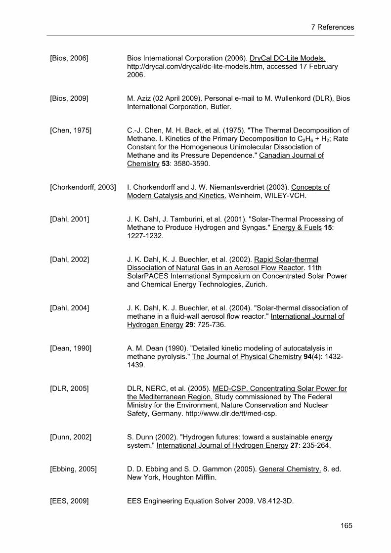
7 References
165
[Bios, 2006] Bios International Corporation (2006). DryCal DC-Lite Models. http://drycal.com/drycal/dc-lite-models.htm, accessed 17 February 2006.
[Bios, 2009] M. Aziz (02 April 2009). Personal e-mail to M. Wullenkord (DLR), Bios International Corporation, Butler.
[Chen, 1975] C.-J. Chen, M. H. Back, et al. (1975). "The Thermal Decomposition of Methane. I. Kinetics of the Primary Decomposition to C2H6 + H2; Rate Constant for the Homogeneous Unimolecular Dissociation of Methane and its Pressure Dependence." Canadian Journal of Chemistry 53: 3580-3590.
[Chorkendorff, 2003] I. Chorkendorff and J. W. Niemantsverdriet (2003). Concepts of Modern Catalysis and Kinetics. Weinheim, WILEY-VCH.
[Dahl, 2001] J. K. Dahl, J. Tamburini, et al. (2001). "Solar-Thermal Processing of Methane to Produce Hydrogen and Syngas." Energy & Fuels 15: 1227-1232.
[Dahl, 2002] J. K. Dahl, K. J. Buechler, et al. (2002). Rapid Solar-thermal Dissociation of Natural Gas in an Aerosol Flow Reactor. 11th SolarPACES International Symposium on Concentrated Solar Power and Chemical Energy Technologies, Zurich.
[Dahl, 2004] J. K. Dahl, K. J. Buechler, et al. (2004). "Solar-thermal dissociation of methane in a fluid-wall aerosol flow reactor." International Journal of Hydrogen Energy 29: 725-736.
[Dean, 1990] A. M. Dean (1990). "Detailed kinetic modeling of autocatalysis in methane pyrolysis." The Journal of Physical Chemistry 94(4): 1432-1439.
[DLR, 2005] DLR, NERC, et al. (2005). MED-CSP. Concentrating Solar Power for the Mediterranean Region. Study commissioned by The Federal Ministry for the Environment, Nature Conservation and Nuclear Safety, Germany. http://www.dlr.de/tt/med-csp.
[Dunn, 2002] S. Dunn (2002). "Hydrogen futures: toward a sustainable energy system." International Journal of Hydrogen Energy 27: 235-264.
[Ebbing, 2005] D. D. Ebbing and S. D. Gammon (2005). General Chemistry. 8. ed. New York, Houghton Mifflin.
[EES, 2009] EES Engineering Equation Solver 2009. V8.412-3D.

7 References
166
[Eisenberg, 1967] B. Eisenberg and H. Bliss (1967). "Kinetics of Methane Pyrolysis." Chemical Engineering Progress Symposium Series 63(72): 3-17.
[Fincke, 2002] J. R. Fincke, R. P. Anderson, et al. (2002). "Plasma Pyrolysis of Methane to Hyrogen and Carbon Black." Industrial and Engineering Chemistry Research 41(6): 1425-1435.
[Flamant, 2007] G. Flamant (2007). SOLHYCARB: Hydrogen and carbon nanomaterials from solar energy without CO2 emission. The Parliament Magazine. 238: 68.
[Fletcher, 2001] E. A. Fletcher (2001). "Solarthermal Processing: A Review." Journal of Solar Energy Engineering 123: 63-74.
[Fluke, 2002] Fluke Corporation (2002). Model 187 & 189. True RMS Multimeter. Bedienungs-Handbuch. Rev. 2, Everett, Fluke Corporation.
[Förster, 2009] B. Förster (2009). Qualifizierung, Optimierung und Steuerung einer Baugruppe zum Dispergieren von Carbon Black in einem Gasstrom. Berlin, Beuth Hochschule für Technik. (Diploma thesis at the DLR, Institute of Technical Thermodynamics, Solar Research, Köln)
[FRIATEC, 2003] FRIATEC AG (2003). DEGUSSIT. Delivery Programme Oxide Ceramics: Tubes, rods, laboratory ware and insulating powders. Mannheim, FRIATEC AG. (Brochure 977a)
[Fulcheri, 2002] L. Fulcheri, N. Probst, et al. (2002). "Plasma processing: a step towards the production of new grades of carbon black." Carbon 40: 169-176.
[Gardiner, 1975] W. C. Gardiner Jr., J. H. Owen, et al. (1975). "Rate and mechanism of methane pyrolysis from 2000° to 2700°K." Symposium (International) on Combustion 15(1): 857-868.
[Geitmann, 2002] S. Geitmann (2002). Wasserstoff & Brennstoffzellen. Die Technik von morgen! Berlin, Hydrogeit.
[Gero, 2006] S. Becht (10 October 2006). Personal e-mail to M. Wullenkord (DLR), Gero Hochtemperaturöfen GmbH & Co. KG, Neuhausen.
[Glick, 1959] H. S. Glick (1959). "Shock tube studies of reaction kinetics of aliphatic hydrocarbons." Symposium (International) on Combustion 7: 98-107.
[Gordon, 1948] A. S. Gordon (1948). "Pyrolysis of Methane Flowing Through a

7 References
167
Porcelain Tube in the Region 1000°." Journal of the American Chemical Society 70: 395-401.
[Grenda, 2003] J. M. Grenda, I. P. Androulakis, et al. (2003). "Application of Computational Kinetic Mechanism Generation to Model the Autocatalytic Pyrolysis of Methane." Industrial & Engineering Chemistry Research 42(5): 1000-1010.
[Guerét, 1994] C. Guerét and F. Billaud (1994). "Thermal coupling of methane: influence of hydrogen at 1330°C. Experimental and Simulated Results." Journal of Analytical and Applied Pyrolysis 29: 183-205.
[Hagen, 2004] J. Hagen (2004). Chemiereaktoren. Auslegung und Simulation. Weinheim, WILEY-VCH.
[Happel, 1967] J. Happel and L. Kramer (1967). "Acetylene and hydrogen from the pyrolysis of methane." Journal of Industrial and Engineering Chemistry 59(1): 39-50.
[Hartig, 1971] R. Hartig, J. Troe, et al. (1971). "Thermal decomposition of methane behind reflected shock waves." Symposium (International) on Combustion 13(1): 147-154.
[Hefner, 2002] R. A. Hefner III (2002). "The age of energy gases." International Journal of Hydrogen Energy 27(1): 1-9.
[Hidaka, 1985] Y. Hidaka, S. Shiba, et al. (1985). "Thermal decomposition of ethane in shock waves." International Journal of Chemical Kinetics 17(4): 441-453.
[Hirsch, 2001] D. Hirsch, M. Epstein, et al. (2001). "The solar thermal decarbonization of natural gas." International Journal of Hydrogen Energy 26: 1023-1033.
[Hirsch, 2004 a] D. Hirsch and A. Steinfeld (2004). "Solar hydrogen production by thermal decomposition of natural gas using a vortex-flow reactor." International Journal of Hydrogen Energy 29: 47-55.
[Hirsch, 2004 b] D. Hirsch and A. Steinfeld (2004). "Radiative transfer in a solar chemical reactor for the co-production of hydrogen and carbon by thermal decomposition of methane." Chemical Engineering Science 59: 5771-5778.
[Holmen, 1976] A. Holmen, O. A. Rokstad, et al. (1976). "High-Temperature Pyrolysis of Hydrocarbons. 1. Methane to Acetylene." Industrial & Engineering

7 References
168
Chemistry Process Design and Development 15(3): 439-444.
[Holmen, 1995] A. Holmen, O. Olsvik, et al. (1995). "Pyrolysis of natural gas: chemistry and process concepts." Fuel Processing Technology 42: 249-267.
[Hu, 2003] Z. J. Hu and K. J. Hüttinger (2003). "Influence of the surface area/volume ratio on the chemistry of carbon deposition from methane." Carbon 41(8): 1501-1508.
[Incropera, 1996] F. P. Incropera and D. P. DeWitt (1996). Introduction To Heat Transfer. 3. ed. New York, John Wiley & Sons.
[Incropera, 2002] F. P. Incropera and D. P. DeWitt (2002). Fundamentals of Heat and Mass Transfer. 5. ed. New York, John Wiley & Sons.
[IPCC, 2007] IPCC (2007). Climate Change 2007: Mitigation. Contribution of Working Group III to the Fourth Assessment Report of the Intergovernmental Panel on Climate Change. B. Metz, O. R. Davidson, P. R. Bosch, R. Dave, and L. A. Meyer. Cambridge and New York, Cambridge University Press.
[ISO, 2008] ISO (2008). ISO/IEC Guide 98-3:2008(E). Uncertainty of measurement – Part 3: Guide to the expression of uncertainty in measurement (GUM:1995). Geneva, International Organization for Standardization.
[Jung, 2007] J. Jung, W. Nam, et al. (2007). "Hydrogen production by catalytic decomposition of methane over carbon catalysts in a fluidized bed." Korean Journal of Chemical Engineering 24(4): 674-678.
[Kassel, 1932] L. S. Kassel (1932). "The thermal decomposition of methane." Journal of the American Chemical Society 54: 3949-3962.
[Kevorkian, 1960] V. Kevorkian, C. E. Heath, et al. (1960). "The decompostion of methane in shock waves." The Journal of Physical Chemistry 64(8): 964-968.
[Khan, 1970] M. S. Khan and B. L. Crynes (1970). "Survey of Recent Methane Pyrolysis Literature." Industrial and Engineering Chemistry 62(10): 54-59.
[Kiefer, 1993] J. H. Kiefer and S. S. Kumaran (1993). "Rate of CH4 Dissociation over 2800-4300 K: The Low-Pressure-Limit Rate Constant." The Journal of Physical Chemistry 97(2): 414-420.
7 References
169
[Kim, 2004] M. H. Kim, E. K. Lee, et al. (2004). "Hydrogen production by catalytic decomposition of methane over activated carbons: kinetic study." International Journal of Hydrogen Energy 29: 187-193.
[Kodama, 2003] T. Kodama (2003). "High-temperature solar chemistry for converting solar heat to chemical fuels." Progress in Energy and Combustion Science 29(6): 567-597.
[Kogan, 2003] M. Kogan and A. Kogan (2003). "Production of hydrogen and carbon by solar thermal methane splitting. I. The unseeded reactor." International Journal of Hydrogen Energy 28(11): 1187-1198.
[Kogan, 2004] A. Kogan, M. Kogan, et al. (2004). "Production of hydrogen and carbon by solar thermal methane splitting. II. Room temperature simulation tests of seeded solar reactor." International Journal of Hydrogen Energy 29: 1227-1236.
[Kogan, 2005] A. Kogan, M. Kogan, et al. (2005). "Production of hydrogen and carbon by solar thermal methane splitting. III. Fluidization, entrainment and seeding powder particles into a volumetric solar receiver." International Journal of Hydrogen Energy 30: 35-43.
[Kogan, 2007] A. Kogan, M. Israeli, et al. (2007). "Production of hydrogen and carbon by solar thermal methane splitting. IV. Preliminary simulation of a confined tornado flow configuration by computational fluid dynamics." International Journal of Hydrogen Energy 32(18): 4800-4810.
[Koike, 2000] T. Koike, M. Kudo, et al. (2000). "Rate Constants of CH4 + M=CH3 + H + M and CH3OH + M=CH3 + OH + M over 1400-2500 K." International Journal of Chemical Kinetics 32(1): 1-6.
[Kozlov, 1962] G. I. Kozlov and V. G. Knorre (1962). "Single-pulse Shock Tube Studies on the Kinetics of the Thermal Decomposition of Methane." Combust. Flame 6: 253-263.
[Kreysa, 2008] G. Kreysa (2008). "Methan - Chance für eine klimaverträgliche Energieversorgung." Chemie Ingenieur Technik 80(7): 901-908.
[Kreysa, 2009] G. Kreysa (2009). "Climate Protection by an Alternative Use of Methane–The Carbon Moratorium." ChemSusChem 2(1): 49-55.
[Lee, 2004 a] K. K. Lee, G. Y. Han, et al. (2004). "Thermocatalytic hydrogen production from the methane in a fluidized bed with activated carbon catalyst." Catalysis Today 93-95: 81-86.

7 References
170
[Lee, 2004 b] K. L. Lee, S. Y. Lee, et al. (2004). "Catalytic decomposition of methane over carbon blacks for CO2-free hydrogen production." Carbon 42: 2641-2648.
[Lee, 2008] S. Y. Lee, B. H. Ryu, et al. (2008). "Catalytic characteristics of specialty carbon blacks in decomposition of methane for hydrogen production." Carbon 46(14): 1978-1986.
[Lucas, 1990] P. Lucas and A. Marchand (1990). "Pyrolytic carbon deposition from methane: An analytical approach to the chemical process." Carbon 28(1): 207-219.
[Lucas, 2008] K. Lucas (2008). Thermodynamik. Die Grundgesetze der Energie- und Stoffumwandlungen. 7. ed. Berlin, Springer.
[Maag, 2009] G. Maag, G. Zanganeh, et al. (2009). "Solar thermal cracking of methane in a particle-flow reactor for the co-production of hydrogen and carbon." International Journal of Hydrogen Energy 34(18): 7676-7685.
[Maibauer, 2010] T. Maibauer (2010). Vorbereitung, Durchführung und Auswertung von reaktionskinetischen Experimenten im Umfeld der solarthermischen Spaltung von Methan zur Wasserstofferzeugung. Aachen, RWTH Aachen. (Student research project at the DLR, Institute of Technical Thermodynamics, Solar Research, Köln)
[Marbán, 2007] G. Marbán and T. Valdés-Solís (2007). "Towards the hydrogen economy?" International Journal of Hydrogen Energy 32(12): 1625-1637.
[Martin, 1990] H. Martin (1990). Vorlesung Wärmeübertragung II. Karlsruhe, Universität Karlsruhe (TU).
[Matheu, 2003] D. M. Matheu, A. M. Dean, et al. (2003). "Mechanism Generation with Integrated Pressure Dependence: A New Model for Methane Pyrolysis." The Journal of Physical Chemistry A 107(41): 8552-8565.
[Missen, 1999] R. W. Missen, C. A. Mims, et al. (1999). Introduction to chemical reaction engineering and kinetics. New York, John Wiley & Sons.
[Mortimer, 1996] C. E. Mortimer (1996). Chemie. Das Basiswissen der Chemie. 6. ed. Stuttgart, Georg Thieme.
[Munson, 2002] B. R. Munson, D. F. Young, et al. (2002). Fundamentals of Fluid Mechanics. 4. ed. New York, John Wiley & Sons.
7 References
171
[Muradov, 2001 a] N. Z. Muradov (2001). "Catalysis of methane decomposition over elemental carbon." Catalysis Communications 2: 89-94.
[Muradov, 2001 b] N. Z. Muradov (2001). "Hydrogen via methane decomposition: an application for decarbonization of fossil fuel." International Journal of Hydrogen Energy 26: 1165-1175.
[Muradov, 2005 a] N. Z. Muradov and T. N. Veziroglu (2005). "From hydrocarbon to hydrogen-carbon to hydrogen economy." International Journal of Hydrogen Energy 30: 225-237.
[Muradov, 2005 b] N. Z. Muradov, F. Smith, et al. (2005). "Catalytic activity of carbons for methane decomposition reaction." Catalysis Today 102-103: 225-233.
[Muradov, 2008] N. Z. Muradov and T. N. Veziroglu (2008). ""Green" path from fossil-based to hydrogen economy: An overview of carbon-neutral technologies." International Journal of Hydrogen Energy 33(23): 6804-6839.
[Muradov, 2010] N. Z. Muradov (19 May 2010). Comment at 18th World Hydrogen Energy Conference 2010 (WHEC 2010), Essen.
[Napier, 1972] D. H. Napier and N. Subrahmanyam (1972). "Pyrolysis of Methane in a Single Pulse Shock Tube." Journal of Applied Chemistry & Biotechnology 22: 303-317.
[Olsvik, 1994] O. Olsvik and F. Billaud (1994). "Thermal coupling of methane. A comparison between kinetic model data and experimental data." Thermochimica Acta 232: 155-169.
[Olsvik, 1995] O. Olsvik, O. A. Rokstad, et al. (1995). "Pyrolysis of Methane in the Presence of Hydrogen." Chemical Engineering & Technology 18: 349-358.
[Ozalp, 2009] N. Ozalp, A. Kogan, et al. (2009). "Solar decomposition of fossil fuels as an option for sustainability." International Journal of Hydrogen Energy 34: 710-720.
[Palmer, 1963] H. B. Palmer and T. J. Hirt (1963). "The activation energy for the pyrolysis of methane." Journal of Physical Chemistry 67: 709-711.
[Palmer, 1968] H. B. Palmer, J. Lahaye, et al. (1968). "On the Kinetics and Mechanism of the Thermal Decomposition of Methane in a Flow System." The Journal of Physical Chemistry 72: 348-353.
7 References
172
[Patankar, 1980] S. V. Patankar (1980). Numerical Heat Transfer and Fluid Flow. Washington, Hemisphere.
[Pilla, 2010] G. L. Pilla, D. F. Davidson, et al. "Shock tube/laser absorption measurements of ethylene time-histories during ethylene and n-heptane pyrolysis." Proceedings of the Combustion Institute In Press, Corrected Proof.
[Pinilla, 2008] J. L. Pinilla, I. Suelves, et al. (2008). "Kinetic study of the thermal decomposition of methane using carbonaceous catalysts." Chemical Engineering Journal 138(1-3): 301-306.
[Pregger, 2009] T. Pregger, D. Graf, et al. (2009). "Prospects of solar thermal hydrogen production processes." International Journal of Hydrogen Energy 34(10): 4256-4267.
[Press, 2007] W. H. Press, S. A. Teukolsky, et al. (2007). Numerical Recipes. The Art of Scientific Computing. 3. ed. Cambridge, Cambridge University Press.
[Rempel, 2009] H. Rempel, S. Schmidt, et al. (2009). Reserven, Ressourcen und Verfügbarkeit von Energierohstoffen - Kurzstudie 2009 -. Hannover, Bundesanstalt für Geowissenschaften und Rohstoffe.
[Richter, 2000] H. Richter and J. B. Howard (2000). "Formation of polycyclic aromatic hydrocarbons and their growth to soot–a review of chemical reaction pathways." Progress in Energy and Combustion Science 26(4-6): 565-608.
[Rodat, 2009] S. Rodat, S. Abanades, et al. (2009). "Hydrogen production from solar thermal dissociation of natural gas: development of a 10 kW solar chemical reactor prototype." Solar Energy 83(9): 1599-1610.
[Rodat, 2010 a] S. Rodat, S. Abanades, et al. (2010). "A pilot-scale solar reactor for the production of hydrogen and carbon black from methane splitting." International Journal of Hydrogen Energy 35(15): 7748-7758.
[Rodat, 2010 b] S. Rodat, S. Abanades, et al. "Co-production of hydrogen and carbon black from solar thermal methane splitting in a tubular reactor prototype." Solar Energy In Press, Corrected Proof.
[Roscoe, 1985] J. M. Roscoe and M. J. Thompson (1985). "Thermal decomposition of methane: Autocatalysis." International Journal of Chemical Kinetics 17(9): 967-990.

7 References
173
[Schröder, 2000] W. Schröder (2000). Fluidmechanik. 2. ed. Mainz, Wissenschaftsverlag.
[Schulz, 1985] G. Schulz, H.-D. Klotz, et al. (1985). "Reaktionsmodell zur Bruttokinetik der Pyrolyse von Methan im Stoßwellenrohr bei Temperaturen von 1800 K bis 2500 K." Zeitschrift für Chemie 25(3): 88-92.
[Serban, 2003] M. Serban, M. A. Lewis, et al. (2003). "Hydrogen Production by Direct Contact Pyrolysis of Natural Gas." Energy & Fuels 17(3): 705-713.
[Shantarovich, 1962] P. S. Shantarovich and B. V. Pavlov (1962). "Thermal cracking of methane." International Chemical Engineering 2(3): 415-418.
[Sherwood, 1975] T. K. Sherwood, R. L. Pigford, et al. (1975). Mass Transfer. New York, McGraw-Hill.
[Skinner, 1959] G. B. Skinner and R. A. Ruehrwein (1959). "Shock tube studies on the pyrolysis and oxidation of methane." The Journal of Physical Chemistry 63: 1736-1742.
[Spath, 2003] P. L. Spath and W. A. Amos (2003). "Using a Concentrating Solar Reactor to Produce Hydrogen and Carbon Black via Thermal Decomposition of Natural Gas: Feasibility and Ecomomics." Journal of Solar Energy Engineering 125: 159-164.
[Steinberg, 1989] M. Steinberg and H. S. Cheng (1989). "Modern and prospective technologies for hydrogen production from fossil fuels." International Journal of Hydrogen Energy 14(11): 797-820.
[Steinberg, 1998] M. Steinberg (1998). "Production of hydrogen and methanol from natural gas with reduced CO2 emission." International Journal of Hydrogen Energy 26(6): 419-425.
[Steinfeld, 1997] A. Steinfeld, V. Kirillov, et al. (1997). "Production of filamentous carbon and hydrogen by solarthermal catalytic cracking of methane." Chemical Engineeing Science 52(20): 3599-3603.
[Steinfeld, 2001] A. Steinfeld and R. Palumbo (2001). Solar Thermochemical Process Technology. Encyclopedia of Physical Science and Technology. R. A. Meyers. New York, Academic Press. 15: 237-256.
[Steinfeld, 2004] A. Steinfeld and A. Meier (2004). Solar Fuels and Materials. Encyclopedia of Energy. C. J. Cleveland. New York, Elsevier. 5: 623-637.
7 References
174
[Steinfeld, 2005] A. Steinfeld (2005). "Solar thermochemical production of hydrogen–a review." Solar Energy 78(5): 603-615.
[Stephan, 1962] K. Stephan (1962). "Wärmeübergang bei turbulenter und laminarer Strömung in Ringspalten." Chemie Ingenieur Technik 34: 207-212.
[Stewart, 1989] P. H. Stewart, G. P. Smith, et al. (1989). "The pressure and temperature dependence of methane decomposition." International Journal of Chemical Kinetics 21(10): 923-945.
[Stolten, 2010] D. Stolten, Ed. (2010). Hydrogen and Fuel Cells: Fundamentals, Technologies and Applications. Weinheim, WILEY-VCH.
[Stroppe, 2008] H. Stroppe (2008). Physik für Studierende der Natur- und Ingenieurwissenschaften. 14. ed. München, Hanser.
[Sundaram, 1977 a] K. M. Sundaram and G. F. Froment (1977). "Modeling of thermal cracking kinetics–I : Thermal cracking of ethane, propane and their mixtures." Chemical Engineering Science 32(6): 601-608.
[Sundaram, 1977 b] K. M. Sundaram and G. F. Froment (1977). "Modeling of thermal cracking kinetics–II : Cracking of iso-butane, of n-butane and of mixtures ethane–propane–n-butane." Chemical Engineering Science 32(6): 609-617.
[Sundaram, 1978] K. M. Sundaram and G. F. Froment (1978). "Modeling of Thermal Cracking Kinetics. 3. Radical Mechanisms for the Pyrolysis of Simple Paraffins, Olefins, and Their Mixtures." Industrial & Engineering Chemistry Fundamentals 17(3): 174-182.
[Sutherland, 2001] J. W. Sutherland, M.-C. Su, et al. (2001). "Rate Constants for H + CH4, CH3 + H2, and CH4 Dissociation at High Temperature." International Journal of Chemical Kinetics 33(11): 669-684.
[Tabayashi, 1979] K. Tabayashi and S. H. Bauer (1979). "The Early Stages of Pyrolysis and Oxidation of Methane." Combustion and Flame 34: 63-83.
[Tanashev, 1998] Y. Y. Tanashev, V. I. Fedoseev, et al. (1998). "Methane processing under microwave radiation: Recent findings and problems." Catalysis Today 42(3): 333-336.
[TC, 2006] TC Meß- und Regeltechnik GmbH (2006). Handbuch zur Temperaturmessung mit Thermoelementen und Widerstandsthermometern. Mönchengladbach, TC Meß- und Regeltechnik GmbH.

7 References
175
[TIMCAL, 2007] TIMCAL Ltd. (2007).Technical Data Sheet. Super P. Conductive Carbon Black. Version 03/07. Bodio, TIMCAL Ltd.
[Touloukian, 1972] Y. S. Touloukian and C. Y. Ho, Eds. (1972). Thermophysical Properties of Matter. Vol. 1-13. New York, Plenum Press.
[Trommer, 2004] D. Trommer, D. Hirsch, et al. (2004). "Kinetic investigation of the thermal decomposition of CH4 by direct irradiation of a vortex-flow laden with carbon particles." International Journal of Hydrogen Energy 29: 627-633.
[Tynnukov, 2002] Y. G. Tynnukov, M. V. Genkin, et al. (2002). "Modeling of Methane Pyrolysis Reactors." Petroleum Chemistry 42(2): 85-92.
[VDI, 2006] VDI-Gesellschaft Verfahrenstechnik und Chemieingenieurwesen, Ed. (2006). VDI-Wärmeatlas. 10. ed. Berlin, Springer.
[Weimer, 2001] A. W. Weimer, J. K. Dahl, et al. (2001). Thermal dissociation of methane using a solar coupled aerosol flow reactor. 2001 U.S. DOE Hydrogen Program Review, Baltimore.
[Weingärtner, 2003] H. Weingärtner (2003). Chemische Thermodynamik. Einführung für Chemiker und Chemieingenieure. Stuttgart, Teubner.
[WIKA, 2005] WIKA Alexander Wiegand GmbH & Co. KG (2005). Universal-Drucktransmitter. UniTrans. Betriebsanleitung. Klingenberg, WIKA Alexander Wiegand GmbH & Co. KG.
[WIKA, 2006] WIKA Alexander Wiegand GmbH & Co. KG (2006). Elektronische Druckmesstechnik. Druckmessumformer für allgemeine Anwendungen. Typ S-10, Standardausführung. Typ S-11, frontbündige Membrane. Datenblatt PE 81.01. Klingenberg, WIKA Alexander Wiegand GmbH & Co. KG.
[Wu, 1987] C. H. Wu, H. J. Singh, et al. (1987). "Pyrolysis of acetylene behind reflected shock waves." International Journal of Chemical Kinetics 19(11): 975-996.
[Wullenkord, 2008] M. Wullenkord, K.-H. Funken, et al. (2008). Wasserstofferzeugung durch die solarthermische Spaltung von Methan - Untersuchungen zur Reaktionskinetik. 11. Kölner Sonnenkolloquium. Solare Turmkraftwerke. Potential und Technologie, Köln, DLR.
[Wullenkord, 2009 a] M. Wullenkord, K.-H. Funken, et al. (2009). Reaktionskinetische Untersuchungen zur thermischen Spaltung von Methan. 12. Kölner
7 References
176
Sonnenkolloquium. Qualifizierung von Komponenten solarthermischer Kraftwerke, Köln, DLR.
[Wullenkord, 2009 b] M. Wullenkord, K.-H. Funken, et al. (2009). "Kinetische Untersuchungen zur thermischen Spaltung von Methan." Chemie Ingenieur Technik 81(8): 1036.
[Wullenkord, 2010 a] M. Wullenkord, T. Maibauer, et al. (2010). Neue Untersuchungen zur thermischen Spaltung von Methan. 13. Kölner Sonnenkolloquium. Strom aus der Wüste, Köln, DLR.
[Wullenkord, 2010 b] M. Wullenkord, K.-H. Funken, et al. (2010). Hydrogen Production by Thermal Cracking of Methane – Investigation of Reaction Conditions. 18th World Hydrogen Energy Conference 2010 – WHEC 2010, Essen. [Schriften des Forschungszentrums Jülich, Energy & Environment 78(3)]
[Younessi-Sinaki, 2009]
M. Younessi-Sinaki, E. A. Matida, et al. (2009). "Kinetic model of homogeneous thermal decomposition of methane and ethane." International Journal of Hydrogen Energy 34(9): 3710-3716.
[Zedtwitz, 2006] P. v. Zedtwitz, J. Petrasch, et al. (2006). "Hydrogen production via the solar thermal decarbonization of fossil fuels." Solar Energy 80: 1333-1337.

8 Nomenclature
177
8 Nomenclature
Formula symbols
A matrix consisting of partial derivatives various
A cross sectional area, face m2
peakA peak area of GC measurement mV s
a activity -
a half width of an interval various
a upper limit for a measured value various
a lower limit for a measured value various
b uncertainty factor %
lamb factor for a laminar flow -
RTC,C factor comprising emissivity and geometry of thermocouple and reactor
W / (m2 K4)
c concentration mol / m3
pc specific heat capacity at constant pressure J / (kg K)
vc specific heat capacity at constant volume J / (kg K)
D diffusion coefficient in a binary gas mixture m2 / s
D diffusion coefficient in a gas mixture with more than two species
m2 / s
d diameter m
hd hydraulic diameter m
E error -
aE activation energy kJ / mol
F factor, ratio of stoichiometric coefficients -
f factor regarding number of certain atoms in a molecule -

8 Nomenclature
178
G Gibbs energy (free enthalpy) J
I electric current A
j diffusive molar flux related to the average molar velocity mol / (s m2)
*j diffusive mass flux related to the average mass velocity kg / (s m2)
k coefficient of a polynomial fit function various
k rate constant (mol / m3)(1-Σmi) / s and others
pk coverage factor -
0k pre-exponential factor (mol / m3)(1-Σmi) / s and others
l length m
el entry length m
M molecular weight g / mol
Ma Mach number -
m mass kg
m reaction order -
im reaction order regarding component i -
m mass flow kg / s or g / h
N total number (e. g. of runs, of species in a gas mixture) -
Nu Nusselt number -
n amount of substance mol
n molar flow mol / s
n average molar flow mol / s
Pe Péclet number -
Pr Prandtl number -
wP wetted perimeter m
p pressure bar
p average pressure bar

8 Nomenclature
179
Np standard pressure (1.01325) bar
DQ diffusive quotient -
q heat flux density W / m2
universal gas constant (8.314472, see [Stroppe, 2008]) J / (mol K)
R specific gas constant J / (kg K)
R radius m
Re Reynolds number -
r reaction rate (equivalent ~) mol / (s m3) or mol / (s m2) or mol / (s kg)
r radial position, radius m or mm
r radial position, radius m or mm
r mean radius m or mm
S surface m2
s specific surface m2 / g
rels relative standard deviation %
maxrel,s maximum relative deviation %
T temperature K or °C
NT standard temperature (273.15) K
t time min or s
U voltage V
U voltage V
u velocity component in X-direction (ANSYS) m / s
u standard uncertainty various
maxu maximum uncertainty various
maxu average maximum uncertainty various
V volume m3
dV diffusion volume -

8 Nomenclature
180
V volume flow m3 / s
NV standard volume flow (referring to NT and Np ) sccm
v velocity / velocity component in Y-direction (ANSYS) m / s
v average velocity m / s
w velocity component in Z-direction (ANSYS) m / s
X conversion % or -
X average conversion % or -
ix vector of variables defining a condition i various
x molar fraction % or -
x measured value various
x molar fraction % or -
x average molar fraction % or -
Y yield % or -
y quantity, which is a function of other quantities various
iy part of data point, observation related to condition i various
iy~ discrepancy between observation and model related to condition i relative to the standard deviation of the observation
-
z axial position m or mm
α matrix used to determine a covariance matrix various
heat transfer coefficient W / (m2 K)
kl component of matrix α in row k and column l various
2 merit function to be minimized (Chi-Square fitting) -
RG free enthalpy of reaction J
0RH standard reaction enthalpy J
LineX position on Line X relative to the center position m
uX rel,1,,2CH4 difference of conversions of methane related to -

8 Nomenclature
181
standard uncertainty respecting experimental campaign 1 and 2
uY rel,1,,2HC 22 difference of yields of ethyne related to standard uncertainty respecting experimental campaign 1 and 2
-
uY rel,1,,2HC 42 difference of yields of ethene related to standard uncertainty respecting experimental campaign 1 and 2
-
uY rel,1,,2HC 62 difference of yields of ethane related to standard uncertainty respecting experimental campaign 1 and 2
-
uY rel,1,,2H2 difference of yields of hydrogen related to standard uncertainty respecting experimental campaign 1 and 2
-
LineZ position on Line Z relative to the center position m
emissivity -
view factor -
dynamic viscosity N s / m2
specific heat ratio -
thermal conductivity W / (m K)
average thermal conductivity W / (m K)
chemical potential J / mol
kinematic viscosity m2 / s
stoichiometric coefficient -
density kg / m3
Stefan-Boltzmann constant (5.67040 10-8, see [Baehr, 2006] )
W / (m2 K4)
standard deviation various
residence time s
average residence time s
ψ vector of model parameters various
ψ model parameter various
)(Corr matrix of correlation coefficients
)(Cov covariance matrix

8 Nomenclature
182
f general function
nabla operator, gradient
Indices and subscripts
AL23 alumina, material manufactured by FRIATEC
Ar argon
ave average
C carbon
4CH methane
CP center position
22HC ethyne
42HC ethene
62HC ethane
HCC2- C2-hydrocarbons
c combined
cat catalyst
cond conductive
conv convective
D diffusive
DG dilution gas
eq equivalent
g gaseous
H hydrogen
He helium
HT heat transfer

8 Nomenclature
183
2H hydrogen
h hydrodynamic
het heterogeneous
hom homogeneous
i inner
i component i of a gas mixture
i condition i
ig ideal gas
j run j of a collectivity of experimental runs
j interval j of a collectivity of intervals defined by molar fractions
j species j
j nested tube reactor j
k component k of a gas mixture
k experiment k
k row of a matrix
k model parameter k
LME limit of marginal extend
l column of a matrix
l model parameter l
MFC mass flow controller
max maximum
min minimum
mix mixture
N at standard conditions ( NN , pT )
N total number
o outer
P product
PT protection tube

8 Nomenclature
184
q reaction q
R reaction
R reactor
R resistor
rad radiative
rel relative, related
s solid
T transpose (of matrix)
TC thermocouple
tot total
WP wall position
0 initial conditions
0 at standard / reference condition
1 inverse (of matrix)
positive
negative
Abbreviations and chemical nomenclature
AB acetylene black
AC activated carbon
32OAl alumina
Ar argon
ave average
BET Brunauer, Emmett and Teller (specific surface)
8 Nomenclature
185
C"" particulate carbon
CB carbon black
CC coal char
CCS carbon capture and storage
2CH methylene radical
3CH methyl radical
4CH methane
CO carbon monoxide
2CO carbon dioxide
CSP concentrating solar power
nmHC hydrocarbons (not further specified)
22HC ethyne
42HC ethene
62HC ethane
HCC2- C2-hydrocarbons
43HC propyne or propadiene
63HC propene
83HC propane
34HC unsaturated hydrocarbon radical featuring 4 C-atoms and 3 H-atoms
810HC naphthalene
c combined
cat catalyst
D diffusion
DG dilution gas
DLR Deutsches Zentrum für Luft- und Raumfahrt e.V. (German Aerospace Center)

8 Nomenclature
186
DWV Deutscher Wasserstoff- und Brennstoffzellen-Verband e.V. (German Hydrogen and Fuel Cell Association)
EUMENA Europe, Middle East, North Africa
g.e. for example
seq.et et sequens
seqq.et et sequentes
FS full scale
GC gas chromatograph
GCF gas correction factor
GUM Guide to the expression of uncertainty in measurement
H hydrogen atom
He helium
HID helium ionization detector
2H hydrogen
OH2 water
IPCC Intergovernmental Panel on Climate Change
IPS initial parameter set
104HC-i isobutane
Kr krypton
LB lower bounds
M collision partner
MFC mass flow controller
MFR mixed flow reactor
2MoSi molybdenum disilicide
MS molecular sieve
max maximum
min minimum
Ne neon

8 Nomenclature
187
NTR nested tube reactor(s)
Ni nickel
2N nitrogen
s.n. not specified
104HC-n unbranched butane
OM order of magnitude
2O oxygen
P product species
PAH polycyclic aromatic hydrocarbon
PFR plug flow reactor
PTFE polytetrafluoroethylene
Pt platinum
Rh rhodium
SLM standard liter per minute (referring to NT and Np )
SOLHYCARB
Hydrogen from solar thermal energy: high temperature solar chemical reactor for co-production of hydrogen and carbon black from natural gas cracking (European project)
sccm standard cubic centimeters per minute (referring to NT and Np )
TCD thermal conductivity detector
UB upper bounds
X direction of a Cartesian coordinate system
Y direction of a Cartesian coordinate system
Z direction of a Cartesian coordinate system

Appendix
188
Appendix
List of Figures of Appendix Figure of Appendix 1: Equilibrium compositions at 0.5 bar as a function of the temperature (based on an initial amount of 1 kmol methane)...................................................195
Figure of Appendix 2: Equilibrium compositions at 2 bar as a function of the temperature (based on an initial amount of 1 kmol methane)...................................................195
Figure of Appendix 3: Valve in “Load” position and “Inject” position.........................................196
Figure of Appendix 4: Temperature program and event program for the measurement procedure..................................................................................................................................197
Figure of Appendix 5: Temperature program and event program for the column bake-out procedure............................................................................................................................197
Figure of Appendix 6: Example for a chromatogram of the product gas respecting signals of the HID. Hydrocarbons with a molecular weight higher than the C2-hydrocarbons were not considered...........................................................................................198
Figure of Appendix 7: Example for a chromatogram of the product gas respecting signals of the TCD. Hydrocarbons with a molecular weight higher than the C2-hydrocarbons were not considered...........................................................................................198
Figure of Appendix 8: Example for a GC calibration curve: methane detected by the HID (2nd order polynomial).......................................................................................................199
Figure of Appendix 9: Example for GC calibration curves: C2-hydrocarbons detected by the HID (2nd order polynomial).................................................................................................199
Figure of Appendix 10: Example a GC calibration curve: argon detected by the TCD (line) ..........................................................................................................................................200
Figure of Appendix 11: Diffusive quotient regarding ethane as a function of the residence time, the nominal furnace temperature, the initial molar fraction of methane, and the dilution gas...................................................................................................................224
Figure of Appendix 12: Diffusive quotient regarding ethene as a function of the residence time, the nominal furnace temperature, the initial molar fraction of methane, and the dilution gas...................................................................................................................224
Figure of Appendix 13: Diffusive quotient regarding ethyne as a function of the residence time, the nominal furnace temperature, the initial molar fraction of methane, and the dilution gas...................................................................................................................225
Figure of Appendix 14: Results of flow simulations with ANSYS 12 – Velocity in X-direction (parallel to face) at the reactor inlet for a standard volume flow of 700 sccm Ar........227
Figure of Appendix 15: Results of flow simulations with ANSYS 12 – Velocity in Z-direction (parallel to face) at the reactor inlet for a standard volume flow of 700 sccm Ar........227
Figure of Appendix 16: Results of flow simulations with ANSYS 12 – Velocity in X-direction (parallel to face) at the reactor inlet for a standard volume flow of 2600 sccm Ar ..............................................................................................................................................228
Figure of Appendix 17: Results of flow simulations with ANSYS 12 – Velocity in Y-direction (normal to face) at the reactor inlet for a standard volume flow of 2600 sccm Ar ..............................................................................................................................................228

Appendix
189
Figure of Appendix 18: Results of flow simulations with ANSYS 12 – Velocity in Z-direction (parallel to face) at the reactor inlet for a standard volume flow of 2600 sccm Ar.............................................................................................................................................. 229
Figure of Appendix 19: Results of flow simulations with ANSYS 12 – Velocity in X-direction (parallel to face) at the reactor inlet for a standard volume flow of 9800 sccm Ar.............................................................................................................................................. 229
Figure of Appendix 20: Results of flow simulations with ANSYS 12 – Velocity in Y-direction (normal to face) at the reactor inlet for a standard volume flow of 9800 sccm Ar.............................................................................................................................................. 230
Figure of Appendix 21: Results of flow simulations with ANSYS 12 – Velocity in Z-direction (parallel to face) at the reactor inlet for a standard volume flow of 9800 sccm Ar.............................................................................................................................................. 230
Figure of Appendix 22: Results of COMSOL Multiphysics calculations based on a simplified temperature profile for the wall of the reactor concerning flow lines for different standard volume flows of argon and a nominal furnace temperature of 1200 °C: 95 sccm (a), 200 sccm (b), 350 sccm (c), 685 sccm (d), and 2000 sccm (e)............ 233
Figure of Appendix 23: Results of COMSOL Multiphysics calculations based on a simplified temperature profile for the wall of the reactor concerning flow lines for different standard volume flows of argon and a nominal furnace temperature of 1300 °C: 340 sccm (a), 650 sccm (b), 1300 sccm (c), 2600 sccm (d), and 4800 sccm (e) ............................................................................................................................................. 233
Figure of Appendix 24: Results of COMSOL Multiphysics calculations based on a simplified temperature profile for the wall of the reactor concerning flow lines for different standard volume flows of argon and a nominal furnace temperature of 1400 °C: 700 sccm (a), 1400 sccm (b), 2600 sccm (c), 3800 sccm (d), and 6500 sccm (e) ............................................................................................................................................. 233
Figure of Appendix 25: Results of COMSOL Multiphysics calculations based on a simplified temperature profile for the wall of the reactor concerning flow lines for different standard volume flows of argon and a nominal furnace temperature of 1500 °C: 1600 sccm (a), 2800 sccm (b), 4600 sccm (c), 7200 sccm (d), and 9800 sccm (e) ............................................................................................................................................. 233
Figure of Appendix 26: Results of COMSOL Multiphysics calculations based on a simplified temperature profile for the wall of the reactor concerning flow lines for different standard volume flows of argon and a nominal furnace temperature of 1600 °C: 2000 sccm (a), 3350 sccm (b), 6500 sccm (c), 9800 sccm (d) ................................. 234
Figure of Appendix 27: Results of COMSOL Multiphysics calculations based on a simplified temperature profile for the wall of the reactor concerning flow lines for different sets of standard volume flow of helium and nominal furnace temperature: 1300 °C - 3800 sccm (a), 1400 °C - 2800 sccm (b), 1400 °C - 3800 sccm (c), 1400 °C - 6500 sccm (d), and 1500 °C - 3800 sccm (e)........................................................................... 234
Figure of Appendix 28: Comparison of experimentally determined conversion of methane (as a function of the residence time and the nominal furnace temperature) with calculated values employing reactor model 5 NTR and respective best fit kinetic parameters. 2 % initial molar fraction of methane in argon. Indicators of uncertainty refer to maximum uncertainty (black: used for kinetic evaluation, gray: not used for kinetic evaluation)..................................................................................................................... 235
Figure of Appendix 29: Comparison of experimentally determined conversion of methane (as a function of the residence time and the nominal furnace temperature) with calculated values employing reactor model 5 NTR and respective best fit kinetic parameters. 10 % initial molar fraction of methane in argon. Indicators of uncertainty
Appendix
190
refer to maximum uncertainty (black: used for kinetic evaluation, gray: not used for kinetic evaluation). ....................................................................................................................236
Figure of Appendix 30: Comparison of experimentally determined conversion of methane (as a function of the residence time and the nominal furnace temperature) with calculated values employing reactor model 5 NTR and respective best fit kinetic parameters. Diverse initial molar fractions of methane in argon. Indicators of uncertainty refer to maximum uncertainty (black: used for kinetic evaluation, gray: not used for kinetic evaluation). ......................................................................................................236
Figure of Appendix 31: Comparison of experimentally determined yield of hydrogen (as a function of the residence time and the nominal furnace temperature) with calculated values employing reactor model 5 NTR and respective best fit kinetic parameters. 2 % initial molar fraction of methane in argon. Indicators of uncertainty refer to maximum uncertainty (black: used for kinetic evaluation, gray: not used for kinetic evaluation)...............237
Figure of Appendix 32: Comparison of experimentally determined yield of hydrogen (as a function of the residence time and the nominal furnace temperature) with calculated values employing reactor model 5 NTR and respective best fit kinetic parameters. 10 % initial molar fraction of methane in argon. Indicators of uncertainty refer to maximum uncertainty (black: used for kinetic evaluation, gray: not used for kinetic evaluation)...............237
Figure of Appendix 33: Comparison of experimentally determined yield of hydrogen (as a function of the residence time and the nominal furnace temperature) with calculated values employing reactor model 5 NTR and respective best fit kinetic parameters. Diverse initial molar fractions of methane in argon. Indicators of uncertainty refer to maximum uncertainty (black: used for kinetic evaluation, gray: not used for kinetic evaluation). ...............................................................................................................................238
Figure of Appendix 34: Comparison of experimentally determined yield of ethane (as a function of the residence time and the nominal furnace temperature) with calculated values employing reactor model 5 NTR and respective best fit kinetic parameters. 2 % initial molar fraction of methane in argon. Indicators of uncertainty refer to maximum uncertainty (black: used for kinetic evaluation, gray: not used for kinetic evaluation)...............238
Figure of Appendix 35: Comparison of experimentally determined yield of ethane (as a function of the residence time and the nominal furnace temperature) with calculated values employing reactor model 5 NTR and respective best fit kinetic parameters. 10 % initial molar fraction of methane in argon. Indicators of uncertainty refer to maximum uncertainty (black: used for kinetic evaluation, gray: not used for kinetic evaluation)...............239
Figure of Appendix 36: Comparison of experimentally determined yield of ethane (as a function of the residence time and the nominal furnace temperature) with calculated values employing reactor model 5 NTR and respective best fit kinetic parameters. Diverse initial molar fractions of methane in argon. Indicators of uncertainty refer to maximum uncertainty (black: used for kinetic evaluation, gray: not used for kinetic evaluation). ...............................................................................................................................239
Figure of Appendix 37: Comparison of experimentally determined yield of ethene (as a function of the residence time and the nominal furnace temperature) with calculated values employing reactor model 5 NTR and respective best fit kinetic parameters. 2 % initial molar fraction of methane in argon. Indicators of uncertainty refer to maximum uncertainty (black: used for kinetic evaluation, gray: not used for kinetic evaluation)...............240
Figure of Appendix 38: Comparison of experimentally determined yield of ethene (as a function of the residence time and the nominal furnace temperature) with calculated values employing reactor model 5 NTR and respective best fit kinetic parameters. 10 % initial molar fraction of methane in argon. Indicators of uncertainty refer to maximum uncertainty (black: used for kinetic evaluation, gray: not used for kinetic evaluation)...............240

Appendix
191
Figure of Appendix 39: Comparison of experimentally determined yield of ethene (as a function of the residence time and the nominal furnace temperature) with calculated values employing reactor model 5 NTR and respective best fit kinetic parameters. Diverse initial molar fractions of methane in argon. Indicators of uncertainty refer to maximum uncertainty (black: used for kinetic evaluation, gray: not used for kinetic evaluation)................................................................................................................................ 241
Figure of Appendix 40: Comparison of experimentally determined yield of ethyne (as a function of the residence time and the nominal furnace temperature) with calculated values employing reactor model 5 NTR and respective best fit kinetic parameters. 2 % initial molar fraction of methane in argon. Indicators of uncertainty refer to maximum uncertainty (black: used for kinetic evaluation, gray: not used for kinetic evaluation). ............. 241
Figure of Appendix 41: Comparison of experimentally determined yield of ethyne (as a function of the residence time and the nominal furnace temperature) with calculated values employing reactor model 5 NTR and respective best fit kinetic parameters. 10 % initial molar fraction of methane in argon. Indicators of uncertainty refer to maximum uncertainty (black: used for kinetic evaluation, gray: not used for kinetic evaluation). ............. 242
Figure of Appendix 42: Comparison of experimentally determined yield of ethyne (as a function of the residence time and the nominal furnace temperature) with calculated values employing reactor model 5 NTR and respective best fit kinetic parameters. Diverse initial molar fractions of methane in argon. Indicators of uncertainty refer to maximum uncertainty (black: used for kinetic evaluation, gray: not used for kinetic evaluation)................................................................................................................................ 242
List of Tables of Appendix Table of Appendix 1: Species considered for calculations of equilibrium compositions. Species in gray form significant part of composition at equilibrium.......................................... 194
Table of Appendix 2: Parameters of gas chromatograph and their set points ......................... 196
Table of Appendix 3: Standard deviations, maximum positive deviations, and maximum negative deviations relative to mean peak areas determined in GC measurements (HID) for different molar fractions of hydrogen (extreme values in red) ................................... 200
Table of Appendix 4: Standard deviations, maximum positive deviations, and maximum negative deviations relative to mean peak areas determined in GC measurements (HID and TCD) for different molar fractions of methane (extreme values in red) ............................. 201
Table of Appendix 5: Standard deviations, maximum positive deviations, and maximum negative deviations relative to mean peak areas determined in GC measurements (TCD) for different molar fractions of argon (extreme values in red)........................................ 201
Table of Appendix 6: Standard deviations, maximum positive deviations, and maximum negative deviations relative to mean peak areas determined in GC measurements (HID) for different molar fractions of ethane (extreme values in red) ....................................... 202
Table of Appendix 7: Standard deviations, maximum positive deviations, and maximum negative deviations relative to mean peak areas determined in GC measurements (HID) for different molar fractions of ethene (extreme values in red) ....................................... 202
Table of Appendix 8: Standard deviations, maximum positive deviations, and maximum negative deviations relative to mean peak areas determined in GC measurements (HID) for different molar fractions of ethyne (extreme values in red) ....................................... 203
Table of Appendix 9: Maximum relative deviation of GC measurements for hydrogen (HID)......................................................................................................................................... 203

Appendix
192
Table of Appendix 10: Maximum relative deviation of GC measurements for methane (HID) .........................................................................................................................................204
Table of Appendix 11: Maximum relative deviation of GC measurements for methane (TCD) ........................................................................................................................................204
Table of Appendix 12: Maximum relative deviation of GC measurements for argon (TCD) ........................................................................................................................................205
Table of Appendix 13: Maximum relative deviation of GC measurements for ethane (HID) .........................................................................................................................................205
Table of Appendix 14: Maximum relative deviation of GC measurements for ethene (HID) .........................................................................................................................................206
Table of Appendix 15: Maximum relative deviation of GC measurements for ethyne (HID) .........................................................................................................................................206
Table of Appendix 16: Various information about reaction conditions for with argon as dilution gas and nominal furnace temperatures of 1200 °C and 1300 °C (nominal furnace temperature in °C - nominal total standard volume flow in sccm - nominal initial molar fraction of methane in %) I ..............................................................................................207
Table of Appendix 17: Various information about reaction conditions for with argon as dilution gas and nominal furnace temperatures of 1400 °C, 1500 °C, and 1600 °C (nominal furnace temperature in °C - nominal total standard volume flow in sccm - nominal initial molar fraction of methane in %) I .......................................................................208
Table of Appendix 18: Various information about reaction conditions for with argon as dilution gas and nominal furnace temperatures of 1200 °C and 1300 °C (nominal furnace temperature in °C - nominal total standard volume flow in sccm - nominal initial molar fraction of methane in %) II .............................................................................................209
Table of Appendix 19: Various information about reaction conditions for with argon as dilution gas and nominal furnace temperatures of 1400 °C, 1500 °C, and 1600 °C (nominal furnace temperature in °C - nominal total standard volume flow in sccm - nominal initial molar fraction of methane in %) II ......................................................................210
Table of Appendix 20: Conversion of methane as well as yields of hydrogen and ethyne along with respective maximum and standard uncertainties for experiments with argon as dilution gas and nominal furnace temperatures of 1200 °C and 1300 °C ............................211
Table of Appendix 21: Yields of ethane and ethene along with respective maximum and standard uncertainties for experiments with argon as dilution gas and nominal furnace temperatures of 1200 °C and 1300 °C......................................................................................212
Table of Appendix 22: Conversion of methane as well as yields of hydrogen and ethyne along with respective maximum and standard uncertainties for experiments with argon as dilution gas and nominal furnace temperatures of 1400 °C, 1500 °C, and 1600 °C ............213
Table of Appendix 23: Yields of ethane and ethene along with respective maximum and standard uncertainties for experiments with argon as dilution gas and nominal furnace temperatures of 1400 °C, 1500 °C, and 1600 °C......................................................................214
Table of Appendix 24: Various information about reaction conditions for with helium as dilution gas (nominal furnace temperature in °C - nominal total standard volume flow in sccm - nominal initial molar fraction of methane in %) I............................................................215
Table of Appendix 25: Various information about reaction conditions for with helium as dilution gas (nominal furnace temperature in °C - nominal total standard volume flow in sccm - nominal initial molar fraction of methane in %) II...........................................................215

Appendix
193
Table of Appendix 26: Conversion of methane as well as yields of hydrogen and ethyne along with respective maximum and standard uncertainties for experiments with helium as dilution gas .......................................................................................................................... 216
Table of Appendix 27: Yields of ethane and ethene along with respective maximum and standard uncertainties for experiments with helium as dilution gas ......................................... 216
Table of Appendix 28: Profiles of temperatures related to the thermocouple in wall position (WP) and center position (CP) for a nominal furnace temperature of 1200 °C determined in experiments with argon as dilution gas ............................................................. 217
Table of Appendix 29: Profiles of temperatures related to the thermocouple in wall position (WP) and center position (CP) for a nominal furnace temperature of 1300 °C determined in experiments with argon as dilution gas ............................................................. 218
Table of Appendix 30: Profiles of temperatures related to the thermocouple in wall position (WP) and center position (CP) for a nominal furnace temperature of 1400 °C determined in experiments with argon as dilution gas ............................................................. 219
Table of Appendix 31: Profiles of temperatures related to the thermocouple in wall position (WP) and center position (CP) for a nominal furnace temperature of 1500 °C determined in experiments with argon as dilution gas ............................................................. 220
Table of Appendix 32: Profiles of temperatures related to the thermocouple in wall position (WP) and center position (CP) for a nominal furnace temperature of 1600 °C determined in experiments with argon as dilution gas ............................................................. 221
Table of Appendix 33: Profiles of temperatures related to the thermocouple in wall position (WP) and center position (CP) determined in experiments with helium as dilution gas ............................................................................................................................... 222
Table of Appendix 34: Material properties of argon partly as a function of the temperature .............................................................................................................................. 223
Table of Appendix 35: Material properties of helium partly as a function of the temperature .............................................................................................................................. 223
Table of Appendix 36: Information about general settings for the calculations with ANSYS 12 ................................................................................................................................ 226
Table of Appendix 37: Coefficients of the polynomial fit function for the approximation of averaged velocity profiles at the inlet of the reactor. ............................................................ 231
Table of Appendix 38: Information about general settings for the calculations with COMSOL Multiphysics ............................................................................................................. 232
Table of Appendix 39: Coefficients of the polynomial fit function for the approximation of fractions of the molar flow at the inlet of the reactor present 5 mm downstream the tip of the thermocouple in particular nested tube reactors (NTR) of region B. ......................... 234
Table of Appendix 40: Information about the optimization tool used for the determination of kinetic parameters ......................................................................................... 235
Table of Appendix 41: Covariance matrix calculated based on the best fit kinetic parameters for model 5 NTR.................................................................................................... 243

Appendix
194
Appendix A: Thermodynamics Table of Appendix 1: Species considered for calculations of equilibrium compositions. Species in gray form significant part of composition at equilibrium.
CH
4(g)
C5H
8(C
PEg)
C6H
10(3
Hg)
C7H
14(C
12D
MC
Pg)
C7H
12(1
4DM
CPg
)C
8H16
(T3E
2Hg)
C8H
16(C
1E3M
CPg
)C
8H16
(1E2
MC
Pg)
C8H
10(O
XYg)
C20
H12
(BjA
Ag)
C2H
6(g)
C5H
8(C
13Pg
)C
6H10
(33D
M1B
g)C
7H14
(5M
1Hg)
C7H
12(1
3DM
CPg
)C
8H16
(T35
DM
2Hg)
C8H
16(C
14D
g)C
8H16
(1E1
MC
Pg)
C8H
10(M
XYg)
C22
H14
(Dah
BAg)
C2H
4(g)
C5H
8(3M
12Bg
)C
6H10
(2H
g)C
7H14
(44D
M2P
g)C
7H12
(12D
MC
Pg)
C8H
16(T
34D
M3H
g)C
8H16
(C13
Dg)
C8H
16(1
1DM
CH
g)C
8H10
(EE1
357O
Tg)
C22
H14
(DBA
acg)
C2H
2(g)
C5H
8(31
MBY
g)C
6H10
(24T
HD
g)C
7H14
(41M
EXg)
C7H
10(2
NO
Bg)
C8H
16(T
34D
M2H
g)C
8H16
(C12
DM
CH
g)C
8H16
(112
TMC
Pg)
C8H
10(E
BZg)
C22
H12
(Bgh
iPg)
H2(
g)C
5H8(
2PYg
)C
6H10
(24H
XDg)
C7H
14(3
THPg
)C
7H10
(13C
Hg)
C8H
16(T
344T
M2P
g)C
8H16
(6M
1Hg)
C8H
14(E
X2M
BC22
1Hg)
C8H
9(4M
PMg)
C22
H12
(DBd
efm
noC
g)
C3H
8(PP
Eg)
C5H
8(2M
13Bg
)C
6H10
(23D
MBg
)C
7H14
(3R
S4D
M1P
g)C
7H8(
TLU
g)C
8H16
(T2O
g)C
8H16
(5R
SM1H
g)C
8H14
(E2M
BC22
1Hg)
C8H
9(4E
Pg)
C22
H12
(I123
cdFg
)
C3H
6(PP
Yg)
C5H
8(23
Pg)
C6H
10(1
MC
Pg)
C7H
14(3
E2Pg
)C
7H8(
BC22
1H25
Dg)
C8H
16(T
2M3H
g)C
8H16
(55D
M1H
g)C
8H14
(CYE
g)C
8H9(
3MPM
g)C
24H
12(C
g)
C3H
6(C
PAg)
C5H
8(1P
Yg)
C6H
10(1
HEg
)C
7H14
(33D
M1P
g)C
7H8(
135C
g)C
8H16
(T25
DM
3Hg)
C8H
16(4
RSM
1Hg)
C8H
14(6
M3H
g)C
8H9(
35D
MPg
)C
26H
14(B
aAg)
C3H
4(PP
Yg)
C5H
8(14
Pg)
C6H
10(1
5HEX
g)C
7H14
(31M
EXg)
C7H
7(PM
g)C
8H16
(T23
DM
3Hg)
C8H
16(4
RS5
DM
1Hg)
C8H
14(6
M2H
g)C
8H9(
34D
MPg
)C
26H
14(B
bAg)
C3H
4(AL
Eg)
C5H
8(12
Pg)
C6H
10(1
4HEX
g)C
7H14
(31E
TPg)
C8H
18(O
CTg
)C
8H16
(T22
DM
3Hg)
C8H
16(4
E1H
g)C
8H14
(6M
1Hg)
C8H
9(2P
Eg)
C26
H14
(BeA
g)
C3H
4(C
Pg)
C5H
6(21
3MBY
g)C
6H8(
Z135
Hg)
C7H
14(2
THPg
)C
8H18
(4M
Hg)
C8H
16(T
1E3M
CPg
)C
8H16
(44D
M1H
g)C
8H14
(5R
SM3H
g)C
8H9(
2MPM
g)C
26H
14(D
Bagh
iPg)
C4H
10(N
BAg)
C5H
6(13
PNYg
)C
6H8(
MEC
Yg)
C7H
14(2
M2H
g)C
8H18
(3R
S4R
SDM
Hg)
C8H
16(T
14D
g)C
8H16
(3R
SM1H
g)C
8H14
(5R
SM2H
g)C
8H9(
25D
MPg
)C
26H
14(D
Bbgh
iPg)
C4H
10(2
MPg
)C
5H6(
13C
Pg)
C6H
8(EQ
135H
g)C
7H14
(2E3
M1P
g)C
8H18
(3M
Hg)
C8H
16(T
13D
g)C
8H16
(3R
SE4M
1Pg)
C8H
14(5
RSM
1Hg)
C8H
9(24
DM
Pg)
C26
H14
(DBc
d,lm
Pg)
C4H
8(T2
Bg)
C6H
14(H
XAg)
C6H
8(E1
35H
g)C
7H14
(24D
M2P
g)C
8H18
(3EH
g)C
8H16
(T12
Dg)
C8H
16(3
RSE
1Hg)
C8H
14(5
5DM
2Hg)
C8H
9(23
DM
Pg)
C26
H14
(DBe
ghiP
g)
C4H
8(M
CPg
)C
6H14
(3M
Pg)
C6H
8(14
CH
g)C
7H14
(24D
M1P
g)C
8H18
(3E3
Mg)
C8H
16(P
CPg
)C
8H16
(3R
S5D
M1H
g)C
8H14
(55D
M1H
g)C
8H9(
1PEg
)C
26H
14(N
1234
ghiP
g)
C4H
8(C
BAg)
C6H
14(2
MPg
)C
6H8(
13C
Hg)
C7H
14(2
3RSD
M1P
g)C
8H18
(3E2
Mg)
C8H
16(IP
Cg)
C8H
16(3
RS4
RSD
M1H
g)C
8H14
(4R
SM2H
g)C
8H8(
STYg
)C
26H
14(N
812b
cdPg
)
C4H
8(C
2Bg)
C6H
14(2
3DM
Bg)
C6H
6(BZ
Eg)
C7H
14(2
3DM
2Pg)
C8H
18(3
4Dg)
C8H
16(E
CH
g)C
8H16
(3R
S44T
M1P
g)C
8H14
(4R
SM1H
g)C
8H8(
CO
Tg)
C26
H14
(Rg)
C4H
8(2M
Pg)
C6H
14(2
2DM
Bg)
C7H
16(H
TAg)
C7H
14(2
33T1
Bg)
C8H
18(3
3Dg)
C8H
16(C
YAg)
C8H
16(3
M2I
P4Bg
)C
8H14
(4R
S5D
M2H
g)C
8H6(
EYBg
)C
28H
16(H
Zg)
C4H
8(1B
Tg)
C6H
12(T
4M2P
g)C
7H16
(3M
Hg)
C7H
14(2
1ETP
g)C
8H18
(2M
Hg)
C8H
16(C
T124
TMC
Pg)
C8H
16(3
E3M
1Pg)
C8H
14(4
RS5
DM
1Hg)
C8H
2(13
57O
Tg)
C30
H16
(Tg)
C4H
6(M
CPg
)C
6H12
(T2H
g)C
7H16
(3EP
g)C
7H14
(1H
Eg)
C8H
18(2
5Dg)
C8H
16(C
C12
4TM
CPg
)C
8H16
(3E3
Hg)
C8H
14(4
Og)
C9H
8(IN
Dg)
C32
H14
(Og)
C4H
6(C
Bg)
C6H
12(M
CPg
)C
7H16
(33D
MPg
)C
7H14
(13T
DC
g)C
8H18
(24D
g)C
8H16
(CC
123T
MC
Pg)
C8H
16(3
E2M
2Pg)
C8H
14(4
E2H
g)C
10H
8(N
PHg)
C34
H16
(DBc
dpqB
Ag)
C4H
6(2B
Yg)
C6H
12(C
HAg
)C
7H16
(2M
Hg)
C7H
14(1
3DM
Clg
)C
8H18
(23D
g)C
8H16
(C6M
3Hg)
C8H
16(3
E2M
1Pg)
C8H
14(4
E1H
g)C
11H
10(1
MN
g)C
36H
16(B
aOg)
C4H
6(1M
CPg
)C
6H12
(C4M
2Pg)
C7H
16(2
4DM
Pg)
C7H
14(1
1DM
CPg
)C
8H18
(234
Tg)
C8H
16(C
6M2H
g)C
8H16
(33D
M1H
g)C
8H14
(44D
M2H
g)C
11H
10(2
MN
g)C
38H
16(D
Bbce
fOg)
C4H
6(1B
Yg)
C6H
12(C
3M2P
g)C
7H16
(23D
MPg
)C
7H12
(CYP
g)C
8H18
(233
Tg)
C8H
16(C
5RSM
3Hg)
C8H
16(3
34TM
1Pg)
C8H
14(4
4DM
1Hg)
C12
H10
(BPH
g)C
40H
16(B
bcN
2187
stuv
Og)
C4H
6(13
Bg)
C6H
12(C
3Hg)
C7H
16(2
2DM
Pg)
C7H
12(B
C22
1Hg)
C8H
18(2
2Dg)
C8H
16(C
5RSM
2Hg)
C8H
16(2
P1Pg
)C
8H14
(3R
SM1H
g)C
12H
10(A
Ng)
C40
H16
(C26
Ag)
C4H
6(12
Bg)
C6H
12(C
2Hg)
C7H
16(2
23TM
Bg)
C7H
12(5
M2H
g)C
8H18
(224
Tg)
C8H
16(C
55D
M2H
g)C
8H16
(2M
3MH
g)C
8H14
(3R
SE4M
1Pg)
C12
H8(
ANPH
g)C
40H
16(C
26PA
g)
C4H
4(1B
3Yg)
C6H
12(4
M1P
g)C
7H14
(T4R
SM2H
g)C
7H12
(5M
1Hg)
C8H
18(2
23Tg
)C
8H16
(C4R
SM2H
g)C
8H16
(2M
2Hg)
C8H
14(3
RSE
1Hg)
C13
H10
(Fg)
C42
H16
(CPg
)
C4H
4(13
CBg
)C
6H12
(3TH
Xg)
C7H
14(T
44D
M2P
g)C
7H12
(4R
SM2H
g)C
8H18
(223
3TM
Bg)
C8H
16(C
4RS5
DM
2Hg)
C8H
16(2
M1H
g)C
8H14
(3R
S5D
M1H
g)C
14H
10(A
g)C
54H
18(C
Cg)
C4H
2(BD
Yg)
C6H
12(3
3D1B
g)C
7H14
(T3M
3Hg)
C7H
12(4
RSM
1Hg)
C8H
16(c
14D
CH
g)C
8H16
(C4O
g)C
8H16
(2E4
M1P
g)C
8H14
(3R
S4R
SDM
1Hg)
C14
H10
(PAg
)C
66H
20(C
Vg)
C5H
12(P
ENg)
C6H
12(3
2MTP
g)C
7H14
(T3M
2Hg)
C7H
12(4
4DM
2Pg)
C8H
16(T
T124
TMC
Pg)
C8H
16(C
4E2H
g)C
8H16
(2E3
RSM
1Pg)
C8H
14(3
RS4
4TM
1Pg)
C15
H10
(45M
PHEg
)C
80H
22(2
CPg
)
C5H
12(2
MBg
)C
6H12
(32M
PCg)
C7H
14(T
34D
M2P
g)C
7H12
(44D
M1P
g)C
8H16
(TT1
23TM
CPg
)C
8H16
(C44
DM
2Hg)
C8H
16(2
E33D
M1B
g)C
8H14
(3O
g)C
16H
10(P
g)C
96H
24(2
CC
g)
C5H
12(2
2Dg)
C6H
12(3
1MEP
g)C
7H14
(T2M
3Hg)
C7H
12(3
RSM
1Hg)
C8H
16(T
6M3H
g)C
8H16
(C3O
g)C
8H16
(2E1
Hg)
C8H
14(3
E3M
1Pg)
C16
H10
(FLU
g)C
(g)
C5H
10(T
2Pg)
C6H
12(2
M2P
g)C
7H14
(T12
DM
CPg
)C
7H12
(3R
S4D
M1P
g)C
8H16
(T6M
2Hg)
C8H
16(C
3M3H
g)C
8H16
(25D
M2H
g)C
8H14
(33D
M1H
g)C
17H
12(1
7HC
PaPH
Eg)
C2(
g)
C5H
10(C
PAg)
C6H
12(2
M1P
g)C
7H14
(MC
Hg)
C7H
12(3
Hg)
C8H
16(T
5RSM
3Hg)
C8H
16(C
3M2H
g)C
8H16
(25D
M1H
g)C
8H14
(334
TM1P
g)C
17H
12(1
HC
PbAg
)C
3(g)
C5H
10(C
2Pg)
C6H
12(2
E1Bg
)C
7H14
(EC
Pg)
C7H
12(3
E1Pg
)C
8H16
(T5R
SM2H
g)C
8H16
(C3E
4M2P
g)C
8H16
(24R
SDM
2Hg)
C8H
14(2
Og)
C17
H12
(1H
CPl
PHEg
)C
4(g)
C5H
10(3
M1B
g)C
6H12
(23D
2Bg)
C7H
14(C
HAg
)C
7H12
(35t
tDM
CPg
)C
8H16
(T55
DM
2Hg)
C8H
16(C
3E2H
g)C
8H16
(24R
SDM
1Hg)
C8H
14(2
M3H
g)C
18H
12(C
g)C
5(g)
C5H
10(2
M2B
g)C
6H12
(23D
1Bg)
C7H
14(C
4RSM
2Hg)
C7H
12(3
5ccD
MC
Pg)
C8H
16(T
4RSM
2Hg)
C8H
16(C
35D
M2H
g)C
8H16
(244
TM2P
g)C
8H14
(25D
M3H
g)C
18H
12(B
Ag)
C60
(g)
C5H
10(2
M1B
g)C
6H12
(1H
Eg)
C7H
14(C
44D
M2P
g)C
7H12
(34t
tDM
CPg
)C
8H16
(T4R
S5D
M2H
g)C
8H16
(C34
RSD
M2H
g)C
8H16
(244
TM1P
g)C
8H14
(22D
M3H
g)C
18H
10(B
ghiF
g)
C5H
10(1
PEg)
C6H
10(M
CPg
)C
7H14
(C3M
3Hg)
C7H
12(3
4ccD
MC
Pg)
C8H
16(T
4Og)
C8H
16(C
34D
M3H
g)C
8H16
(23R
SDM
1Hg)
C8H
14(1
OC
g)C
18H
10(C
PcdP
YRg)
C5H
10(1
2DM
CPt
g)C
6H10
(CH
Eg)
C7H
14(C
3M2H
g)C
7H12
(33D
MC
Pg)
C8H
16(T
4E2H
g)C
8H16
(C34
4TM
2Pg)
C8H
16(2
3RS4
TM1P
g)C
8H12
(CC
15C
Og)
C20
H14
(Cg)
C5H
10(1
2DM
CPc
g)C
6H10
(4M
CPg
)C
7H14
(C3H
g)C
7H12
(33D
M1P
g)C
8H16
(T44
DM
2Hg)
C8H
16(C
2Og)
C8H
16(2
3DM
2Hg)
C8H
12(C
C13
CO
g)C
20H
14(T
g)
C5H
10(1
1DM
CPg
)C
6H10
(4M
2Pg)
C7H
14(C
34D
M2P
g)C
7H12
(2M
3Hg)
C8H
16(T
3Og)
C8H
16(C
2M3H
g)C
8H16
(23D
M1H
g)C
8H12
(15C
Og)
C20
H12
(BaP
g)
C5H
8(t1
3PD
Eg)
C6H
10(4
M1P
g)C
7H14
(C2M
3Hg)
C7H
12(2
Hg)
C8H
16(T
3M3H
g)C
8H16
(C25
DM
3Hg)
C8H
16(2
34TM
2Pg)
C8H
12(1
3CO
g)C
20H
12(B
ePg)
C5H
8(SP
Eg)
C6H
10(3
RSM
1Pg)
C7H
14(C
2Hg)
C7H
12(1
Hg)
C8H
16(T
3M2H
g)C
8H16
(C23
DM
3Hg)
C8H
16(2
33TM
1Pg)
C8H
10(Z
Z135
7OTg
)C
20H
12(B
kFg)
C
C5H
8(M
CBg
)C
6H10
(3M
CPg
)C
7H14
(C13
DM
CPg
)C
7H12
(15D
MC
Pg)
C8H
16(T
3E4M
2Pg)
C8H
16(C
22D
M3H
g)C
8H16
(1O
Cg)
C8H
10(P
XYg)
C20
H12
(Pg)
Solid
spe
cies
:
Gas
eous
spe
cies
:
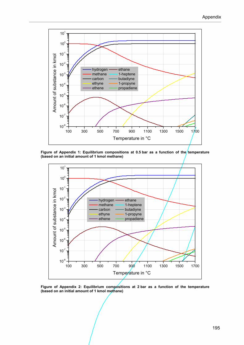
Appendix
195
100 300 500 700 900 1100 1300 1500 170010-8
10-7
10-6
10-5
10-4
10-3
10-2
10-1
100
101
Am
oun
t of s
ubst
ance
in k
mol
Temperature in °C
hydrogen ethane methane 1-heptene carbon butadiyne ethyne 1-propyne ethene propadiene
Figure of Appendix 1: Equilibrium compositions at 0.5 bar as a function of the temperature (based on an initial amount of 1 kmol methane)
100 300 500 700 900 1100 1300 1500 170010-8
10-7
10-6
10-5
10-4
10-3
10-2
10-1
100
101
Am
ount
of s
ubs
tanc
e in
km
ol
Temperature in °C
hydrogen ethane methane 1-heptene carbon butadiyne ethyne 1-propyne ethene propadiene
Figure of Appendix 2: Equilibrium compositions at 2 bar as a function of the temperature (based on an initial amount of 1 kmol methane)

Appendix
196
Appendix B: Gas chromatograph
Table of Appendix 2: Parameters of gas chromatograph and their set points
Parameter Set point Actual
Pressure of Carrier #1 21 psi 21 psi
Pressure of Carrier #2 21 psi 21 psi
Pressure of HID make up gas 21 psi 20 psi
Ion Current of HID 120 mA 120 mA
Temperature of valve 60 °C 67 °C
Temperature of HID (labeled as Detector 1) 200 °C 205 °C
Temperature of TCD 251 °C 257 °C
Sensitivity of HID medium gain
Sensitivity of TCD high gain
Figure of Appendix 3: Valve in “Load” position and “Inject” position

Appendix
197
0 5 10 150
20
40
60
80
100
Te
mpe
ratu
re o
f col
um
n ov
en in
°C
Time in min
Initial cond.: vacuum pump off, carrier #1 on, carrier #2 on, valve in "Load" position
Time in min Event0 vacuum pump on1 vacuum pump off1.2 carrier #2 off,
zero signal1.25 valve in "Inject" position5 carrier #1 off,
carrier #2 on12.82 carrier #1 on,
valve in "Load" position
20 K/min
Figure of Appendix 4: Temperature program and event program for the measurement procedure
0 50 100 150 200 250 3000
50
100
150
200
Te
mpe
ratu
re o
f col
um
n ov
en in
°C
Time in min
Initial cond.: vacuum pump off, carrier #1 on, carrier #2 on, valve in "Load" position
Time in min Event0 - 273.5 no events
20 K/min
Figure of Appendix 5: Temperature program and event program for the column bake-out procedure
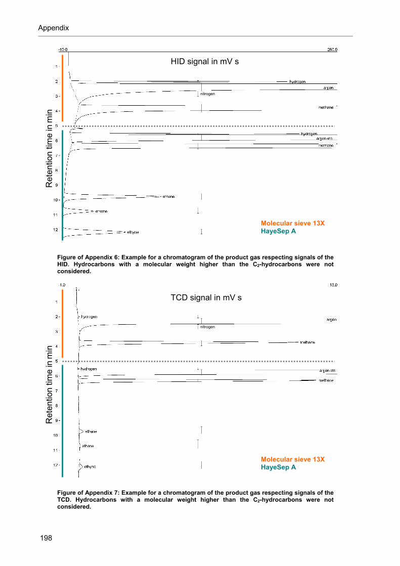
Appendix
198
Figure of Appendix 6: Example for a chromatogram of the product gas respecting signals of the HID. Hydrocarbons with a molecular weight higher than the C2-hydrocarbons were not considered.
Figure of Appendix 7: Example for a chromatogram of the product gas respecting signals of the TCD. Hydrocarbons with a molecular weight higher than the C2-hydrocarbons were not considered.
min
intim
eR
eten
tion
min
intim
eR
eten
tion
Molecular sieve 13X HayeSep A
nitrogen
nitrogen
Molecular sieve 13X HayeSep A
HID signal in mV s
TCD signal in mV s

Appendix
199
0 2000 4000 6000 80000.0
0.2
0.4
0.6
0.8
1.0
1.2
Mo
lar
fra
ctio
n in
%
Normal peak area in mV s
Figure of Appendix 8: Example for a GC calibration curve: methane detected by the HID (2nd order polynomial)
0 3000 6000 9000 12000 15000 180000.0
0.2
0.4
0.6
0.8
1.0
1.2
ethyne ethene
Mol
ar
frac
tion
in %
Normal peak area in mV s
ethane
Figure of Appendix 9: Example for GC calibration curves: C2-hydrocarbons detected by the HID (2nd order polynomial)

Appendix
200
2500 2750 3000 3250 350080
85
90
95
100
Mo
lar
fra
ctio
n in
%
Normal peak area in mV s
Figure of Appendix 10: Example a GC calibration curve: argon detected by the TCD (line)
Table of Appendix 3: Standard deviations, maximum positive deviations, and maximum negative deviations relative to mean peak areas determined in GC measurements (HID) for different molar fractions of hydrogen (extreme values in red)
Molar fraction
# Runs day 1 # Runs day 2
... %inrels %inmaxrel,
s %inmaxrel,s
100 ppm 4 3 4
1.47 0.29 7.29
1.53 0.17 7.09
-2.00 -0.33 -7.41
1 %
6 48 48 9
1.38 1.05 0.61 0.82
1.48 2.14 1.39 1.63
-1.80 -2.48 -1.29 -0.74
10 % 19 0.39 0.62 -0.70

Appendix
201
Table of Appendix 4: Standard deviations, maximum positive deviations, and maximum negative deviations relative to mean peak areas determined in GC measurements (HID and TCD) for different molar fractions of methane (extreme values in red)
Detector Molar
fraction
# Runs day 1# Runs day 2
... %inrels %inmaxrel,
s %inmaxrel,s
100 ppm 4 3 4
0.74 0.56 3.06
1.02 0.49 2.35
-0.75 -0.62 -4.13
HID
1 %
9 22 14 14 14 6
0.28 0.28 0.34 1.07 0.84 0.23
0.40 0.77 0.51 1.11 1.58 0.30
-0.51 -0.34 -0.63 -2.11 -1.15 -0.29
TCD 1 %
9 22 14 14 5
0.77 0.53 0.62 0.67 0.68
1.68 0.85 1.05 0.99 0.90
-0.92 -1.21 -0.93 -1.09 -0.58
Table of Appendix 5: Standard deviations, maximum positive deviations, and maximum negative deviations relative to mean peak areas determined in GC measurements (TCD) for different molar fractions of argon (extreme values in red)
Molar fraction
# Runs day 1# Runs day 2
... %inrels %inmaxrel,
s %inmaxrel,s
98.8 %
8 5 5 5 5 5
0.25 0.39 0.59 0.45 0.64 0.43
0.29 0.34 0.73 0.61 1.05 0.75
-0.39 -0.53 -0.57 -0.50 -0.68 -0.35

Appendix
202
Table of Appendix 6: Standard deviations, maximum positive deviations, and maximum negative deviations relative to mean peak areas determined in GC measurements (HID) for different molar fractions of ethane (extreme values in red)
Molar fraction
# Runs day 1 # Runs day 2
... %inrels %inmaxrel,
s %inmaxrel,s
100 ppm 4 3 4
3.76 1.63 0.39
3.71 1.45 0.48
-3.75 -1.77 -0.45
490 ppm
14 8 5 5 5 5 5
0.52 0.64 0.54 0.81 0.53 1.20 0.44
0.87 0.84 0.54 1.03 0.78 1.28 0.37
-1.21 -0.59 -0.60 -0.69 -0.50 -1.48 -0.62
1 % 5 4 9
2.49 0.44 0.56
1.67 0.57 0.74
-4.31 -0.35 -1.11
Table of Appendix 7: Standard deviations, maximum positive deviations, and maximum negative deviations relative to mean peak areas determined in GC measurements (HID) for different molar fractions of ethene (extreme values in red)
Molar fraction
# Runs day 1 # Runs day 2
... %inrels %inmaxrel,
s %inmaxrel,s
100 ppm 4 3 4
3.06 1.35 1.38
3.34 1.53 1.03
-3.00 -1.04 -1.95
1040 ppm
14 8 5 5 5 5 5
1.04 0.44 0.65 0.77 0.53 1.74 0.41
1.05 0.53 0.70 0.91 0.73 1.02 0.41
-2.30 -0.51 -0.73 -0.61 -0.52 -3.10 -0.52
1 % 5 4 9
2.44 0.16 0.82
1.57 0.20 1.33
-4.28 -0.20 -1.39

Appendix
203
Table of Appendix 8: Standard deviations, maximum positive deviations, and maximum negative deviations relative to mean peak areas determined in GC measurements (HID) for different molar fractions of ethyne (extreme values in red)
Molar fraction
# Runs day 1# Runs day 2
... %inrels %inmaxrel,
s %inmaxrel,s
100 ppm 4 3 4
4.86 1.87
14.49
5.27 2.09
16.38
-4.66 -1.52
-13.59
0.5 % 5 4 9
4.89 0.51 2.91
3.19 0.67 3.08
-8.57 -0.49 -4.13
1.01 %
14 8 5 5 5 5 5
4.31 3.87 1.57 3.79 2.88 5.06 5.78
5.07 3.99 1.84 4.54 2.65 6.80 8.33
-9.45 -7.80 -2.25 -5.93 -3.89 -5.11 -7.11
Table of Appendix 9: Maximum relative deviation of GC measurements for hydrogen (HID)
H2 HID Molar fraction in %
maximum relative deviation measured and extended (safety factor) estimated (assumed worst case factor)
basic / substituting additional
lower bound of interval
upper bound of interval POSITIVE NEGATIVE
0.001 0 0.00316 78.0 (10) -81.5 (10)
0.01 0.00316 0.0316 7.09
7.80 (1.1) -7.41
-8.15 (1.1)
0.1 0.0316 0.316 5.08 -5.44
1 0.316 3.16 2.14
2.35 (1.1) -2.48
-2.73 (1.1)
10 3.16 31.6 0.622
0.684 (1.1) -0.697
-0.767 (1.1)
minimum molar fraction applied or determined in experiments: 0.01 % maximum molar fraction applied or determined in experiments: 17.0 %

Appendix
204
Table of Appendix 10: Maximum relative deviation of GC measurements for methane (HID)
CH4 HID Molar fraction in %
maximum relative deviation measured and extended (safety factor) estimated (assumed worst case factor)
basic / substituting additional
lower bound of interval
upper bound of interval POSITIVE NEGATIVE
0.001 0 0.00316 25.9 (10) -45.4 (10)
0.01 0.00316 0.0316 2.35
2.59 (1.1) -4.13
-4.54 (1.1)
0.1 0.0316 0.316 2.16 -3.43
1 0.316 3.16 1.58
1.74 (1.1) -2.11
-2.32 (1.1)
10 3.16 31.6 8.69 (5) -11.6 (5)
minimum molar fraction applied or determined in experiments: 0.00152 % maximum molar fraction applied or determined in experiments: 3.37 % molar fractions > 1 % rarely employed
Table of Appendix 11: Maximum relative deviation of GC measurements for methane (TCD)
CH4 TCD Molar fraction in %
maximum relative deviation measured and extended (safety factor) estimated (assumed worst case factor)
basic / substituting additional
lower bound of interval
upper bound of interval POSITIVE NEGATIVE
0.1 0.0316 0.316 9.24 (5) -6.66 (5)
1 0.316 3.16 1.68
1.85 (1.1) -1.21
-1.33 (1.1)
10 3.16 31.6 1.85 (1) -1.33 (1)
minimum molar fraction applied or determined in experiments: 0.105 % maximum molar fraction applied or determined in experiments: 20.0 % molar fractions < 0.6 % rarely employed

Appendix
205
Table of Appendix 12: Maximum relative deviation of GC measurements for argon (TCD)
Ar TCD Molar fraction in %
maximum relative deviation measured and extended (safety factor) estimated (assumed worst case factor)
basic / substituting additional
lower bound of interval
upper bound of interval POSITIVE NEGATIVE
98.8 31.4 100 1.05
1.16 (1.1) -0.679
-0.747 (1.1)
minimum molar fraction applied or determined in experiments: 78.8 % maximum molar fraction applied or determined in experiments: 100 %
Table of Appendix 13: Maximum relative deviation of GC measurements for ethane (HID)
C2H6 HID Molar fraction in %
maximum relative deviation measured and extended (safety factor) estimated (assumed worst case factor)
basic / substituting additional
lower bound of interval
upper bound of interval POSITIVE NEGATIVE
0.001 0 0.00316 40.8 (10) -41.3 (10)
0.01 0.00316 0.0221 3.71
4.08 (1.1) -3.75
-4.13 (1.1)
0.049 0.0221 0.0700 1.28
1.41 (1.1) -1.48
-1.63 (1.1)
0.1 0.0700 0.316 1.51 -2.36
1 0.316 3.16 1.67
1.84 (1.1) -4.31
-4.74 (1.1)
minimum molar fraction applied or determined in experiments: 0.0000206 % maximum molar fraction applied or determined in experiments: 1 %

Appendix
206
Table of Appendix 14: Maximum relative deviation of GC measurements for ethene (HID)
C2H4 HID Molar fraction in %
maximum relative deviation measured and extended (safety factor) estimated (assumed worst case factor)
basic / substituting additional
lower bound of interval
upper bound of interval POSITIVE NEGATIVE
0.001 0 0.00316 36.7 (10) -33.0 (10)
0.01 0.00316 0.0322 3.34
3.67 (1.1) -3.00
-3.30 (1.1)
0.104 0.0322 0.322 1.05
1.16 (1.1) -3.10
-3.41 (1.1)
1 0.322 3.16 1.57
1.73 (1.1) -4.28
-4.71 (1.1)
minimum molar fraction applied or determined in experiments: 0.00159 % maximum molar fraction applied or determined in experiments: 1.00 %
Table of Appendix 15: Maximum relative deviation of GC measurements for ethyne (HID)
C2H2 HID Molar fraction in %
maximum relative deviation measured and extended (safety factor) estimated (assumed worst case factor)
basic / substituting additional
lower bound of interval
upper bound of interval POSITIVE NEGATIVE
0.001 0 0.00316 180 (10) -97.2 (6.5)
0.01 0.00316 0.0316 16.4
18.0 (1.1) -13.6
-15.0 (1.1)
0.1 0.0316 0.224 9.49 -11.7
0.5 0.224 0.711 3.19
3.51 (1.1) -8.57
-9.43 (1.1)
1.01 0.711 3.18 8.33
9.16 (1.1) -9.45
-10.4 (1.1)
minimum molar fraction applied or determined in experiments: 0.000150 % maximum molar fraction applied or determined in experiments: 1.99 %

Appendix
207
Appendix C: Reaction conditions and experimental results
Table of Appendix 16: Various information about reaction conditions for with argon as dilution gas and nominal furnace temperatures of 1200 °C and 1300 °C (nominal furnace temperature in °C - nominal total standard volume flow in sccm - nominal initial molar fraction of methane in %) I
Set sccminAr,0N,V sccmin,0CHN, 4V sccmintot,0N,V %in,0CH4
x
1200 - 95 - 2 93.06 1.1 2.7 1.898 0.0 0.1 94.96 1.999
1200 - 95 - 5 90.10 1.1 2.6 4.735 0.1 0.1 94.84 4.993
1200 - 95 - 10 85.51 1.1 2.6 9.513 0.1 0.2 95.02 10.01
1200 - 200 - 2 195.5 1.8 4.1 4.027 0.1 0.1 199.5 2.018
1200 - 200 - 5 189.8 1.7 4.0 10.03 0.1 0.2 199.8 5.019
1200 - 200 - 10 179.9 1.7 3.9 19.95 0.4 0.9 199.9 9.982
1200 - 350 - 2 343.7 2.9 6.2 7.060 0.1 0.1 350.8 2.013
1200 - 350 - 5 333.3 2.8 6.0 17.54 0.4 0.8 350.8 4.999
1200 - 350 - 10 313.9 2.7 5.8 35.13 0.4 1.1 349.0 10.07
1200 - 685 - 2 671.2 5.5 10.8 13.50 0.3 0.8 684.7 1.972
1200 - 685 - 5 650.4 5.3 10.5 34.19 0.4 1.1 684.6 4.994
1200 - 685 - 10 616.4 5.0 10.0 69.09 0.6 1.5 685.5 10.08
1200 - 2000 - 2 1959 20.3 49.3 39.94 0.5 1.1 1999 1.998
1200 - 2000 - 5 1905 19.9 48.6 100.2 1.8 4.3 2005 4.997
1200 - 2000 - 10 1804 19.3 47.2 200.1 2.3 5.7 2004 9.985
1200 - 2000 - 20 1600 18.1 44.3 400.1 3.8 9.1 2000 20.00
1300 - 340 - 2 332.9 2.8 6.0 6.717 0.3 0.7 339.6 1.978
1300 - 340 - 5 323.1 2.7 5.9 16.98 0.4 0.8 340.1 4.993
1300 - 340 - 10 306.5 2.6 5.7 33.89 0.4 1.1 340.4 9.956
1300 - 650 - 2 637.0 5.2 10.3 12.91 0.3 0.8 649.9 1.986
1300 - 650 - 5 616.9 5.0 10.0 32.58 0.4 1.0 649.5 5.016
1300 - 650 - 10 584.3 4.8 9.6 64.91 0.6 1.5 649.2 10.00
1300 - 1300 - 2 1276 16.3 39.8 26.06 0.4 0.9 1302 2.001
1300 - 1300 - 5 1236 16.1 39.2 65.05 0.6 1.5 1301 5.000
1300 - 1300 - 10 1172 15.8 38.3 130.1 2.0 4.7 1302 9.992
1300 - 2600 - 2 2549 24.2 57.6 51.64 0.5 1.3 2601 1.986
1300 - 2600 - 5 2470 23.6 56.5 129.3 2.0 4.7 2599 4.974
1300 - 2600 - 10 2340 22.8 54.7 259.4 2.7 6.5 2599 9.979
1300 - 4800 - 2 4695 49.4 120.5 95.96 1.8 4.2 4791 2.003
1300 - 4800 - 5 4556 48.6 118.6 239.6 2.6 6.2 4796 4.996
1300 - 4800 - 10 4345 47.3 115.6 460.6 4.2 9.9 4806 9.585
standard uncertainty / maximum uncertainty

Appendix
208
Table of Appendix 17: Various information about reaction conditions for with argon as dilution gas and nominal furnace temperatures of 1400 °C, 1500 °C, and 1600 °C (nominal furnace temperature in °C - nominal total standard volume flow in sccm - nominal initial molar fraction of methane in %) I
Set sccminAr,0N,V sccmin,0CHN, 4V sccmintot,0N,V %in,0CH4
x
1400 - 700 - 2 686.0 13.8 31.5 14.02 0.4 0.8 700.0 2.003
1400 - 700 - 5 665.2 13.8 31.2 35.03 0.4 1.1 700.2 5.003
1400 - 700 - 10 629.5 13.6 30.7 69.95 0.7 1.6 699.5 10.00
1400 - 1400 - 2 1373 16.8 41.1 27.83 0.4 1.0 1401 1.987
1400 - 1400 - 5 1330 16.6 40.5 69.90 0.7 1.6 1400 4.993
1400 - 1400 - 10 1258 16.2 39.5 140.0 2.0 4.8 1398 10.01
1400 - 2600 - 2 2549 24.2 57.6 51.67 0.5 1.3 2601 1.987
1400 - 2600 - 5 2471 23.6 56.5 129.8 2.0 4.7 2601 4.991
1400 - 2600 - 10 2340 22.8 54.7 260.5 2.7 6.5 2601 10.02
1400 - 3800 - 2 3718 43.6 106.9 76.15 1.8 3.9 3794 2.007
1400 - 3800 - 5 3615 43.1 105.4 190.4 2.3 5.5 3805 5.003
1400 - 3800 - 10 3427 42.1 102.8 380.2 3.5 8.2 3807 9.986
1400 - 6500 - 2 6362 60.4 143.9 129.5 2.0 4.7 6492 1.995
1400 - 6500 - 5 6168 59.0 141.2 324.6 3.1 7.4 6493 5.000
1400 - 6500 - 7.1 6044 58.2 139.4 458.5 4.2 9.9 6503 7.051
1500 - 1600 - 2 1566 17.9 43.8 31.99 0.4 1.0 1598 2.002
1500 - 1600 - 5 1522 17.6 43.2 80.00 1.8 4.0 1602 4.994
1500 - 1600 - 10 1433 17.2 42.0 159.9 2.1 5.1 1593 10.04
1500 - 2800 - 2 2743 25.9 61.7 55.64 0.6 1.4 2799 1.988
1500 - 2800 - 5 2665 25.0 59.2 140.0 2.0 4.8 2805 4.991
1500 - 2800 - 10 2522 24.0 57.2 280.5 2.8 6.8 2803 10.01
1500 - 4600 - 2 4504 48.2 117.9 91.98 1.8 4.2 4596 2.001
1500 - 4600 - 5 4369 47.4 116.0 229.7 2.5 6.1 4599 4.995
1500 - 4600 - 10 4166 46.2 113.1 430.9 4.0 9.5 4597 9.374
1500 - 7200 - 2 7056 65.2 153.6 144.0 2.0 4.9 7200 2.000
1500 - 7200 - 5 6824 63.6 150.3 360.0 3.4 7.9 7184 5.011
1500 - 7200 - 6.3 6735 63.0 149.1 454.5 4.2 9.8 7190 6.322
1500 - 9800 - 2 9600 83.8 189.2 196.6 2.3 5.6 9797 2.007
1500 - 9800 - 3.1 9490 83.0 187.7 304.3 3.0 7.1 9794 3.107
1500 - 9800 - 5 9350 81.9 185.7 464.7 4.3 10.0 9815 4.735
1600 - 2000 - 2 1960 20.3 49.4 40.01 0.5 1.1 2000 2.000
1600 - 2000 - 5 1903 19.9 48.6 99.91 1.8 4.3 2003 4.988
1600 - 2000 - 10 1800 19.3 47.1 200.8 2.3 5.7 2001 10.04
1600 - 3350 - 2 3285 29.8 69.3 66.76 0.6 1.5 3352 1.992
1600 - 3350 - 5 3189 29.1 67.9 167.5 2.1 5.2 3357 4.990
1600 - 3350 - 10 3020 27.9 65.6 334.7 3.2 7.6 3355 9.977
1600 - 6500 - 2 6367 60.4 143.9 129.9 2.0 4.7 6497 1.999
1600 - 6500 - 5 6180 59.1 141.3 326.3 3.1 7.4 6506 5.015
1600 - 6500 - 7.1 6045 58.2 139.4 459.2 4.2 9.9 6504 7.060
1600 - 9800 - 2 9576 83.6 188.9 195.8 2.3 5.6 9772 2.004
1600 - 9800 - 3 9486 82.9 187.6 294.1 2.9 7.0 9780 3.007
1600 - 9800 - 5 9339 81.8 185.5 460.7 4.2 9.9 9800 4.701
standard uncertainty / maximum uncertainty

Appendix
209
Table of Appendix 18: Various information about reaction conditions for with argon as dilution gas and nominal furnace temperatures of 1200 °C and 1300 °C (nominal furnace temperature in °C - nominal total standard volume flow in sccm - nominal initial molar fraction of methane in %) II
barinnletiR,p barinoutletR,pSet
start end start end
sin # Runs
1200 - 95 - 2 1.006 1.006 0.999 0.999 1.46 0.218 1
1200 - 95 - 5 1.005 1.005 0.998 0.997 1.46 0.218 1
1200 - 95 - 10 1.009 1.009 0.999 0.999 1.47 0.218 1
1200 - 200 - 2 1.008 1.008 1.009 1.009 0.697 0.0974 2
1200 - 200 - 5 1.008 1.008 1.009 1.009 0.696 0.0971 2
1200 - 200 - 10 1.008 1.008 1.009 1.009 0.696 0.0993 1
1200 - 350 - 2 1.006 1.006 1.008 1.008 0.396 0.0539 2
1200 - 350 - 5 1.006 1.006 1.008 1.008 0.396 0.0546 2
1200 - 350 - 10 1.006 1.006 1.007 1.007 0.398 0.0549 1
1200 - 685 - 2 1.006 1.007 1.006 1.007 0.203 0.0273 1
1200 - 685 - 5 1.006 1.007 1.006 1.007 0.203 0.0273 2
1200 - 685 - 10 1.006 1.007 1.006 1.007 0.203 0.0273 1
1200 - 2000 - 2 1.012 1.012 1.013 1.013 0.0699 0.0101 1
1200 - 2000 - 5 1.012 1.012 1.013 1.013 0.0696 0.0102 2
1200 - 2000 - 10 1.012 1.012 1.013 1.013 0.0697 0.0102 1
1200 - 2000 - 20 1.012 1.012 1.013 1.013 0.0698 0.0102 1
1300 - 340 - 2 0.995 0.995 0.996 0.996 0.379 0.0523 1
1300 - 340 - 5 0.994 0.994 0.996 0.996 0.378 0.0522 2
1300 - 340 - 10 0.994 0.994 0.996 0.996 0.377 0.0522 1
1300 - 650 - 2 1.004 1.005 1.004 1.005 0.200 0.0270 1
1300 - 650 - 5 1.005 1.005 1.005 1.005 0.200 0.0270 2
1300 - 650 - 10 1.005 1.005 1.005 1.005 0.200 0.0270 1
1300 - 1300 - 2 1.012 1.011 1.013 1.013 0.100 0.0152 1
1300 - 1300 - 5 1.011 1.011 1.012 1.013 0.100 0.0152 2
1300 - 1300 - 10 1.011 1.011 1.012 1.013 0.100 0.0154 1
1300 - 2600 - 2 1.009 1.009 1.007 1.007 0.0501 0.00709 1
1300 - 2600 - 5 1.009 1.009 1.008 1.008 0.0502 0.00715 2
1300 - 2600 - 10 1.009 1.009 1.008 1.008 0.0502 0.00715 2
1300 - 4800 - 2 1.020 1.020 1.019 1.019 0.0275 0.00400 2
1300 - 4800 - 5 1.020 1.020 1.018 1.019 0.0275 0.00399 2
1300 - 4800 - 10 1.020 1.020 1.018 1.019 0.0274 0.00399 1
maximum uncertainty

Appendix
210
Table of Appendix 19: Various information about reaction conditions for with argon as dilution gas and nominal furnace temperatures of 1400 °C, 1500 °C, and 1600 °C (nominal furnace temperature in °C - nominal total standard volume flow in sccm - nominal initial molar fraction of methane in %) II
barininletR,p barinR,outletpSet
start end start end
sin # Runs
1400 - 700 - 2 1.003 1.003 1.005 1.005 0.174 0.0295 1
1400 - 700 - 5 1.003 1.003 1.005 1.005 0.174 0.0295 2
1400 - 700 - 10 1.003 1.003 1.005 1.005 0.174 0.0296 1
1400 - 1400 - 2 1.011 1.012 1.004 1.004 0.0877 0.0132 2
1400 - 1400 - 5 1.021 1.021 1.010 1.010 0.0886 0.0133 1
1400 - 1400 - 10 1.026 1.030 1.010 1.010 0.0893 0.0136 2
1400 - 2600 - 2 1.031 1.031 1.025 1.025 0.0482 0.00680 1
1400 - 2600 - 5 1.048 1.048 1.030 1.030 0.0490 0.00695 1
1400 - 2600 - 10 1.045 1.046 1.028 1.028 0.0488 0.00694 1
1400 - 3800 - 2 1.013 1.013 1.012 1.012 0.0324 0.00484 1
1400 - 3800 - 5 1.013 1.013 1.012 1.013 0.0323 0.00482 2
1400 - 3800 - 10 1.013 1.014 1.012 1.012 0.0323 0.00482 1
1400 - 6500 - 2 1.058 1.058 1.050 1.050 0.0198 0.00279 1
1400 - 6500 - 5 1.057 1.057 1.049 1.049 0.0198 0.00279 2
1400 - 6500 - 7.1 1.057 1.057 1.049 1.049 0.0197 0.00279 1
1500 - 1600 - 2 0.985 0.985 0.984 0.984 0.0707 0.0105 2
1500 - 1600 - 5 0.984 0.984 0.984 0.984 0.0704 0.0106 1
1500 - 1600 - 10 0.985 0.985 0.984 0.984 0.0709 0.0106 1
1500 - 2800 - 2 1.010 1.010 1.006 1.006 0.0414 0.00585 1
1500 - 2800 - 5 1.011 1.011 1.005 1.005 0.0413 0.00585 1
1500 - 2800 - 10 1.017 1.024 1.005 1.005 0.0417 0.00591 1
1500 - 4600 - 2 1.025 1.025 1.024 1.024 0.0256 0.00373 1
1500 - 4600 - 5 1.027 1.027 1.024 1.024 0.0256 0.00373 2
1500 - 4600 - 10 1.028 1.028 1.024 1.024 0.0256 0.00374 1
1500 - 7200 - 2 1.016 1.016 1.011 1.011 0.0162 0.00227 2
1500 - 7200 - 5 1.016 1.016 1.011 1.011 0.0162 0.00228 2
1500 - 7200 - 6.3 1.015 1.016 1.010 1.010 0.0162 0.00228 1
1500 - 9800 - 2 1.018 1.017 1.005 1.005 0.0119 0.00164 3
1500 - 9800 - 3.1 1.016 1.017 1.004 1.004 0.0119 0.00164 1
1500 - 9800 - 5 1.016 1.016 1.004 1.004 0.0119 0.00164 1
1600 - 2000 - 2 1.008 1.008 1.008 1.008 0.0547 0.00790 2
1600 - 2000 - 5 1.008 1.008 1.009 1.009 0.0546 0.00797 1
1600 - 2000 - 10 1.009 1.009 1.009 1.009 0.0547 0.00798 1
1600 - 3350 - 2 1.034 1.034 1.032 1.032 0.0335 0.00467 1
1600 - 3350 - 5 1.035 1.035 1.032 1.032 0.0335 0.00469 2
1600 - 3350 - 10 1.036 1.037 1.032 1.032 0.0335 0.00470 1
1600 - 6500 - 2 1.052 1.052 1.044 1.044 0.0176 0.00248 2
1600 - 6500 - 5 1.054 1.055 1.044 1.044 0.0176 0.00248 2
1600 - 6500 - 7.1 1.055 1.057 1.044 1.044 0.0176 0.00249 1
1600 - 9800 - 2 1.033 1.033 1.022 1.022 0.0115 0.00158 1
1600 - 9800 - 3 1.033 1.033 1.023 1.023 0.0115 0.00158 2
1600 - 9800 - 5 1.034 1.035 1.023 1.023 0.0115 0.00158 1
maximum uncertainty

Appendix
211
Table of Appendix 20: Conversion of methane as well as yields of hydrogen and ethyne along with respective maximum and standard uncertainties for experiments with argon as dilution gas and nominal furnace temperatures of 1200 °C and 1300 °C
Set %in4CHX %in
2HY %in22HCY
1200 - 95 - 2 81.81 0.9693 3.551 -4.467 82.05 3.381 15.84 -13.64 24.08 1.504 6.448 -5.455
1200 - 95 - 5 82.70 0.6514 2.574 -3.015 80.63 2.555 12.46 -10.61 16.44 1.159 4.774 -3.591
1200 - 95 - 10 82.74 0.6057 2.437 -2.842 80.21 2.887 13.60 -11.39 12.08 1.011 4.199 -2.802
1200 - 200 - 2 71.68 1.213 4.378 -5.287 58.16 2.089 9.496 -7.981 28.10 2.921 11.54 -7.476
1200 - 200 - 5 73.46 0.8297 3.217 -3.712 63.64 1.074 5.223 -4.912 18.78 1.596 5.807 -4.580
1200 - 200 - 10 73.92 0.9432 3.891 -4.682 69.72 2.659 13.06 -10.78 13.90 1.324 5.712 -3.632
1200 - 350 - 2 50.39 2.280 7.617 -8.927 41.55 1.738 6.938 -5.977 22.71 2.127 8.874 -4.607
1200 - 350 - 5 55.39 2.112 7.754 -9.445 48.66 1.584 7.599 -6.431 18.73 1.773 7.784 -4.535
1200 - 350 - 10 59.38 1.787 6.668 -7.980 52.67 1.699 8.302 -7.004 14.36 1.283 5.275 -3.513
1200 - 685 - 2 17.87 3.211 12.17 -14.76 9.316 1.572 5.332 -4.456 10.45 1.900 8.082 -3.907
1200 - 685 - 5 24.09 2.542 10.03 -11.82 19.88 0.9276 3.957 -3.284 11.22 1.468 6.223 -3.049
1200 - 685 - 10 29.15 2.451 9.403 -11.05 23.38 0.7941 3.550 -3.107 10.67 1.231 4.979 -2.818
1200 - 2000 - 2 7.044 4.379 15.94 -7.044 0.8381 0.06438 0.2514 -0.1993 0.09395 0.8529 4.671 -0.07012
1200 - 2000 - 5 2.734 3.728 15.07 -2.734 1.003 0.06605 0.2809 -0.2221 0.2320 0.03713 0.1448 -0.09034
1200 - 2000 - 10 2.523 3.544 14.39 -2.523 1.346 0.08716 0.3628 -0.2862 0.4195 0.08027 0.3248 -0.1652
1200 - 2000 - 20 3.577 3.414 14.05 -3.577 2.196 0.1345 0.5468 -0.4735 0.7550 0.1337 0.5645 -0.2660
1300 - 340 - 2 91.67 0.6194 1.977 -2.747 87.19 4.872 12.81 -15.07 37.08 3.729 16.71 -10.90
1300 - 340 - 5 91.18 0.4318 1.589 -1.956 85.95 2.896 14.05 -11.79 26.06 2.191 9.337 -6.405
1300 - 340 - 10 89.96 0.4264 1.617 -1.955 85.10 3.087 14.86 -12.29 19.47 1.847 7.032 -5.477
1300 - 650 - 2 83.54 1.366 4.468 -5.339 72.29 3.156 14.43 -11.69 36.06 4.889 21.63 -10.86
1300 - 650 - 5 83.45 0.8142 2.869 -3.446 78.05 2.581 12.18 -10.29 25.65 2.409 10.13 -6.009
1300 - 650 - 10 82.45 0.6171 2.400 -2.811 77.95 2.790 12.76 -10.69 21.39 1.812 6.120 -5.954
1300 - 1300 - 2 61.63 2.148 7.603 -9.561 48.18 1.897 9.194 -7.647 36.76 4.877 21.28 -10.88
1300 - 1300 - 5 63.55 1.639 6.125 -7.269 54.29 1.652 8.180 -7.035 27.50 2.731 11.31 -7.049
1300 - 1300 - 10 63.15 1.704 6.701 -8.193 58.03 2.119 10.88 -9.014 21.80 1.816 6.755 -6.473
1300 - 2600 - 2 19.05 2.603 10.40 -12.22 9.418 1.574 4.993 -4.378 8.064 0.7638 2.404 -2.544
1300 - 2600 - 5 19.23 2.803 11.45 -13.61 13.02 0.5577 2.539 -2.140 8.659 0.6402 2.259 -2.308
1300 - 2600 - 10 22.10 2.579 10.49 -12.28 14.54 0.4611 2.220 -1.906 8.219 0.5504 2.164 -1.787
1300 - 4800 - 2 1.196 2.680 8.978 -1.196 0.5461 0.03740 0.1575 -0.1218 0.01521 0.1667 0.9270 -0.01226
1300 - 4800 - 5 1.401 1.498 5.407 -1.401 0.6944 0.04302 0.1740 -0.1391 0.09628 0.03771 0.1913 -0.02746
1300 - 4800 - 10 1.744 1.287 4.565 -1.744 0.9496 0.06674 0.2667 -0.2065 0.1515 0.03804 0.1405 -0.08064
standard uncertainty / maximum uncertainty
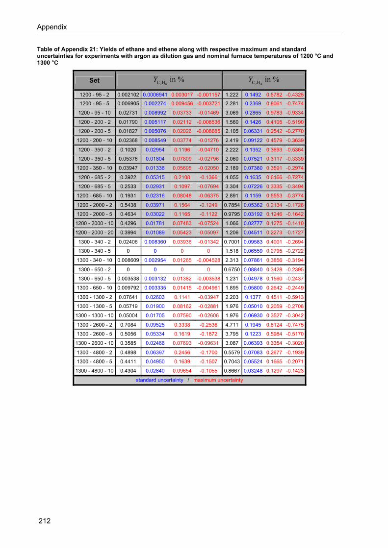
Appendix
212
Table of Appendix 21: Yields of ethane and ethene along with respective maximum and standard uncertainties for experiments with argon as dilution gas and nominal furnace temperatures of 1200 °C and 1300 °C
Set %in62HCY %in
42HCY
1200 - 95 - 2 0.002102 0.0006941 0.003017 -0.001157 1.222 0.1492 0.5782 -0.4325
1200 - 95 - 5 0.006905 0.002274 0.009456 -0.003721 2.281 0.2369 0.8061 -0.7474
1200 - 95 - 10 0.02731 0.008992 0.03733 -0.01469 3.069 0.2865 0.9783 -0.9334
1200 - 200 - 2 0.01790 0.005117 0.02112 -0.008536 1.560 0.1426 0.4105 -0.5190
1200 - 200 - 5 0.01827 0.005076 0.02026 -0.008685 2.105 0.06331 0.2542 -0.2770
1200 - 200 - 10 0.02368 0.008549 0.03774 -0.01276 2.419 0.09122 0.4579 -0.3639
1200 - 350 - 2 0.1020 0.02954 0.1196 -0.04710 2.222 0.1352 0.3693 -0.5364
1200 - 350 - 5 0.05376 0.01804 0.07809 -0.02796 2.060 0.07521 0.3117 -0.3339
1200 - 350 - 10 0.03947 0.01336 0.05695 -0.02050 2.189 0.07380 0.3591 -0.2974
1200 - 685 - 2 0.3922 0.05315 0.2108 -0.1366 4.055 0.1635 0.6166 -0.7274
1200 - 685 - 5 0.2533 0.02931 0.1097 -0.07694 3.304 0.07226 0.3335 -0.3494
1200 - 685 - 10 0.1931 0.02316 0.08048 -0.06375 2.891 0.1159 0.5553 -0.3774
1200 - 2000 - 2 0.5438 0.03971 0.1564 -0.1249 0.7854 0.05362 0.2134 -0.1728
1200 - 2000 - 5 0.4634 0.03022 0.1165 -0.1122 0.9795 0.03192 0.1246 -0.1642
1200 - 2000 - 10 0.4296 0.01781 0.07483 -0.07524 1.066 0.02777 0.1275 -0.1410
1200 - 2000 - 20 0.3994 0.01089 0.05423 -0.05097 1.206 0.04511 0.2273 -0.1727
1300 - 340 - 2 0.02406 0.008360 0.03936 -0.01342 0.7001 0.09583 0.4001 -0.2694
1300 - 340 - 5 0 0 0 0 1.518 0.06559 0.2795 -0.2722
1300 - 340 - 10 0.008609 0.002954 0.01265 -0.004528 2.313 0.07861 0.3856 -0.3194
1300 - 650 - 2 0 0 0 0 0.6750 0.08840 0.3428 -0.2395
1300 - 650 - 5 0.003538 0.003132 0.01382 -0.003538 1.231 0.04978 0.1560 -0.2437
1300 - 650 - 10 0.009792 0.003335 0.01415 -0.004961 1.895 0.05800 0.2642 -0.2449
1300 - 1300 - 2 0.07641 0.02603 0.1141 -0.03947 2.203 0.1377 0.4511 -0.5913
1300 - 1300 - 5 0.05719 0.01900 0.08162 -0.02881 1.976 0.05010 0.2059 -0.2708
1300 - 1300 - 10 0.05004 0.01705 0.07590 -0.02606 1.976 0.06930 0.3527 -0.3042
1300 - 2600 - 2 0.7084 0.09525 0.3338 -0.2536 4.711 0.1945 0.8124 -0.7475
1300 - 2600 - 5 0.5056 0.05334 0.1619 -0.1872 3.795 0.1223 0.5984 -0.5170
1300 - 2600 - 10 0.3585 0.02466 0.07693 -0.09631 3.087 0.06393 0.3354 -0.3020
1300 - 4800 - 2 0.4898 0.06397 0.2456 -0.1700 0.5579 0.07083 0.2677 -0.1939
1300 - 4800 - 5 0.4411 0.04950 0.1639 -0.1507 0.7043 0.05524 0.1665 -0.2071
1300 - 4800 - 10 0.4304 0.02840 0.09654 -0.1055 0.8667 0.03248 0.1297 -0.1423
standard uncertainty / maximum uncertainty

Appendix
213
Table of Appendix 22: Conversion of methane as well as yields of hydrogen and ethyne along with respective maximum and standard uncertainties for experiments with argon as dilution gas and nominal furnace temperatures of 1400 °C, 1500 °C, and 1600 °C
Set %in4CHX %in
2HY %in22HCY
1400 - 700 - 2 97.14 0.1821 0.6575 -0.8572 89.17 3.785 10.83 -15.54 47.54 4.285 19.69 -13.07
1400 - 700 - 5 96.55 0.1960 0.7136 -0.8869 92.55 3.295 7.451 -13.89 35.40 3.222 12.70 -10.42
1400 - 700 - 10 95.89 0.2149 0.8147 -0.9734 89.18 3.576 10.82 -14.53 29.23 1.791 7.687 -6.547
1400 - 1400 - 2 91.98 0.5799 2.016 -2.243 86.01 2.499 12.72 -11.27 40.63 2.718 11.63 -8.904
1400 - 1400 - 5 92.20 0.3351 1.265 -1.516 86.68 2.807 13.32 -11.71 32.54 3.839 14.73 -10.13
1400 - 1400 - 10 90.38 0.3799 1.563 -1.915 85.92 3.199 14.08 -13.42 40.68 2.322 10.17 -8.720
1400 - 2600 - 2 74.57 1.027 3.847 -4.573 62.52 2.572 11.29 -9.667 46.41 3.484 14.09 -10.14
1400 - 2600 - 5 75.02 1.027 3.969 -4.836 66.42 2.120 10.10 -9.393 33.08 3.798 15.28 -9.856
1400 - 2600 - 10 73.14 0.8804 3.667 -4.323 63.04 2.183 10.61 -8.865 36.51 2.131 8.647 -7.525
1400 - 3800 - 2 44.92 2.566 9.912 -12.21 33.96 1.575 7.448 -6.134 26.99 2.686 11.69 -7.503
1400 - 3800 - 5 48.22 2.176 8.500 -10.11 37.96 1.175 5.965 -5.091 24.44 2.141 8.957 -6.047
1400 - 3800 - 10 48.43 2.216 8.511 -10.16 40.66 1.323 6.575 -5.581 20.37 1.851 6.908 -5.780
1400 - 6500 - 2 10.72 3.852 14.63 -10.72 5.622 0.3513 1.466 -1.174 2.780 0.4776 1.628 -1.286
1400 - 6500 - 5 11.24 3.319 12.78 -11.24 7.030 0.2444 1.120 -0.9666 4.199 0.5705 2.237 -1.316
1400 - 6500 - 7.1 11.97 3.258 12.66 -11.97 7.972 0.3576 1.560 -1.288 4.704 0.6589 2.605 -1.499
1500 - 1600 - 2 99.06 0.03339 0.1393 -0.1558 90.83 2.326 9.171 -10.36 50.93 3.998 16.28 -12.05
1500 - 1600 - 5 98.35 0.1295 0.4164 -0.5492 91.24 3.471 8.757 -13.63 43.12 4.422 18.86 -12.31
1500 - 1600 - 10 97.81 0.1718 0.5196 -0.7160 92.98 3.453 7.016 -12.94 39.79 2.338 10.15 -7.955
1500 - 2800 - 2 95.41 0.3640 1.152 -1.306 83.40 2.212 10.88 -9.481 59.53 5.671 22.59 -14.66
1500 - 2800 - 5 94.43 0.2947 1.038 -1.284 84.89 2.847 13.97 -11.74 48.13 4.356 16.23 -13.57
1500 - 2800 - 10 93.32 0.2765 1.060 -1.253 85.04 3.055 14.56 -12.18 39.32 2.395 11.66 -6.487
1500 - 4600 - 2 77.00 1.220 3.988 -6.030 63.66 2.637 12.57 -10.41 48.05 3.867 16.13 -12.06
1500 - 4600 - 5 76.16 0.9083 3.571 -4.217 66.06 1.982 9.855 -8.465 40.57 4.016 15.71 -11.09
1500 - 4600 - 10 74.26 1.055 4.046 -4.834 67.89 2.313 11.20 -9.445 35.87 2.090 8.449 -7.358
1500 - 7200 - 2 43.19 2.250 8.638 -10.17 33.95 1.074 5.193 -4.405 25.72 1.686 6.410 -5.782
1500 - 7200 - 5 44.95 2.380 8.706 -10.27 36.86 1.309 5.882 -5.188 22.96 1.803 7.108 -5.233
1500 - 7200 - 6.3 44.59 2.523 9.127 -10.89 37.49 1.281 5.915 -5.173 21.98 1.773 7.164 -5.015
1500 - 9800 - 2 24.57 2.966 10.99 -13.11 16.47 0.6877 2.994 -2.495 9.381 1.633 7.651 -2.320
1500 - 9800 - 3.1 26.69 2.986 10.94 -12.91 17.39 0.7358 3.163 -2.649 10.41 1.896 8.345 -3.073
1500 - 9800 - 5 27.66 2.978 10.84 -12.80 18.58 0.7994 3.423 -2.846 10.49 1.645 7.865 -2.274
1600 - 2000 - 2 99.83 0.008091 0.02845 -0.03537 92.32 2.367 7.679 -10.48 43.43 3.356 13.01 -10.27
1600 - 2000 - 5 99.60 0.02220 0.07924 -0.1001 95.35 3.422 4.648 -14.17 38.23 3.740 15.29 -10.86
1600 - 2000 - 10 99.33 0.03315 0.1224 -0.1491 91.43 3.325 8.566 -13.58 35.17 2.068 8.630 -7.406
1600 - 3350 - 2 99.07 0.07378 0.2319 -0.2636 89.40 2.366 10.60 -9.969 57.31 4.428 17.24 -12.82
1600 - 3350 - 5 98.74 0.05770 0.2113 -0.2563 87.97 2.876 12.03 -11.83 47.97 4.758 18.88 -12.95
1600 - 3350 - 10 98.40 0.08117 0.2846 -0.3522 89.30 3.213 10.70 -12.75 44.23 2.576 10.36 -9.031
1600 - 6500 - 2 81.45 0.7573 2.918 -3.465 68.29 2.759 12.54 -10.77 52.48 5.810 24.72 -13.81
1600 - 6500 - 5 82.21 0.6971 2.550 -3.252 69.83 1.825 9.193 -7.976 45.72 3.391 10.97 -12.37
1600 - 6500 - 7.1 82.18 0.6914 2.506 -3.287 69.98 2.231 10.72 -9.090 43.86 2.538 9.995 -8.812
1600 - 9800 - 2 59.29 2.017 7.080 -8.598 47.85 1.993 8.740 -7.543 36.36 3.667 15.29 -8.967
1600 - 9800 - 3 60.05 1.858 6.565 -7.909 48.56 1.795 8.182 -6.804 35.22 3.389 13.87 -8.471
1600 - 9800 - 5 60.33 1.807 6.464 -7.656 49.63 1.399 6.796 -5.848 32.32 3.298 12.41 -8.945
standard uncertainty / maximum uncertainty

Appendix
214
Table of Appendix 23: Yields of ethane and ethene along with respective maximum and standard uncertainties for experiments with argon as dilution gas and nominal furnace temperatures of 1400 °C, 1500 °C, and 1600 °C
Set %in62HCY %in
42HCY
1400 - 700 - 2 0 0 0 0 0.5509 0.07239 0.2976 -0.2061
1400 - 700 - 5 0 0 0 0 1.254 0.06496 0.2511 -0.2844
1400 - 700 - 10 0 0 0 0 1.885 0.07017 0.3366 -0.2986
1400 - 1400 - 2 0.003151 0.002818 0.01267 -0.003151 0.3387 0.03696 0.1402 -0.1074
1400 - 1400 - 5 0.007131 0.002657 0.00977 -0.005311 0.7959 0.09221 0.3175 -0.2765
1400 - 1400 - 10 0.003977 0.001208 0.00516 -0.002086 1.585 0.1595 0.5790 -0.5276
1400 - 2600 - 2 0.1376 0.04532 0.1862 -0.07365 1.232 0.1476 0.5206 -0.4106
1400 - 2600 - 5 0.02749 0.006741 0.02920 -0.01136 1.144 0.1294 0.4440 -0.4030
1400 - 2600 - 10 0.02853 0.009400 0.03920 -0.01536 1.518 0.1538 0.5256 -0.4911
1400 - 3800 - 2 0.2660 0.07736 0.3459 -0.1262 3.967 0.1605 0.7386 -0.6822
1400 - 3800 - 5 0.1649 0.01776 0.07427 -0.04513 2.857 0.08801 0.4134 -0.4106
1400 - 3800 - 10 0.1384 0.01586 0.06179 -0.04250 2.519 0.09055 0.4541 -0.3552
1400 - 6500 - 2 0.9270 0.04428 0.1973 -0.1617 3.031 0.1666 0.5934 -0.6853
1400 - 6500 - 5 0.6821 0.02523 0.1068 -0.1036 2.867 0.07627 0.3423 -0.3607
1400 - 6500 - 7.1 0.6089 0.02132 0.09258 -0.08971 2.785 0.08949 0.4232 -0.3661
1500 - 1600 - 2 0.003479 0.002441 0.01016 -0.003479 0.2810 0.07570 0.3099 -0.1369
1500 - 1600 - 5 0 0 0 0 0.6696 0.07387 0.2746 -0.2313
1500 - 1600 - 10 0.001202 0.0002669 0.001182 -0.0004535 1.211 0.07445 0.3128 -0.2554
1500 - 2800 - 2 0 0 0 0 0.2670 0.07388 0.2920 -0.1338
1500 - 2800 - 5 0 0 0 0 0.5788 0.06182 0.1852 -0.2175
1500 - 2800 - 10 0.002498 0.0008504 0.003635 -0.001291 1.039 0.03545 0.1485 -0.1637
1500 - 4600 - 2 0.04934 0.01690 0.07327 -0.02672 0.9479 0.1177 0.4334 -0.3426
1500 - 4600 - 5 0.02691 0.009111 0.03837 -0.01430 1.046 0.07002 0.2431 -0.2609
1500 - 4600 - 10 0.02510 0.008578 0.03624 -0.01341 1.275 0.04965 0.2237 -0.2001
1500 - 7200 - 2 0.3427 0.04281 0.1519 -0.1193 4.032 0.1805 0.7601 -0.6905
1500 - 7200 - 5 0.2117 0.03001 0.1057 -0.07852 2.943 0.1001 0.4556 -0.4024
1500 - 7200 - 6.3 0.1984 0.02815 0.09983 -0.07388 2.806 0.09371 0.4372 -0.3801
1500 - 9800 - 2 0.8078 0.1046 0.3865 -0.2635 4.036 0.1247 0.4585 -0.6152
1500 - 9800 - 3.1 0.6309 0.07450 0.2569 -0.2083 3.656 0.1038 0.4171 -0.4985
1500 - 9800 - 5 0.5169 0.05458 0.1695 -0.1747 3.315 0.09535 0.4182 -0.4217
1600 - 2000 - 2 0 0 0 0 0.1753 0.04303 0.1682 -0.08384
1600 - 2000 - 5 0 0 0 0 0.4195 0.05258 0.1898 -0.1564
1600 - 2000 - 10 0 0 0 0 0.7946 0.03957 0.1671 -0.1546
1600 - 3350 - 2 0 0 0 0 0.2050 0.05686 0.2249 -0.1021
1600 - 3350 - 5 0 0 0 0 0.4260 0.05043 0.1781 -0.1457
1600 - 3350 - 10 0 0 0 0 0.7928 0.03918 0.1607 -0.1478
1600 - 6500 - 2 0.02206 0.006038 0.02497 -0.01060 0.7013 0.06283 0.2632 -0.1698
1600 - 6500 - 5 0.01513 0.002919 0.01243 -0.005170 0.7764 0.04094 0.1414 -0.1660
1600 - 6500 - 7.1 0.02524 0.007794 0.03309 -0.01203 0.8567 0.03464 0.1136 -0.1665
1600 - 9800 - 2 0.2088 0.06091 0.2583 -0.09609 2.138 0.1158 0.4077 -0.4603
1600 - 9800 - 3 0.1473 0.04467 0.1919 -0.06619 1.915 0.08474 0.2941 -0.3666
1600 - 9800 - 5 0.1188 0.03763 0.1589 -0.05736 1.794 0.05966 0.2427 -0.2657
standard uncertainty / maximum uncertainty

Appendix
215
Table of Appendix 24: Various information about reaction conditions for with helium as dilution gas (nominal furnace temperature in °C - nominal total standard volume flow in sccm - nominal initial molar fraction of methane in %) I
Set sccminHe,0N,V sccmin,0CHN, 4V sccmintot,0N,V %in,0CH4
x
1300 - 3800 - 2 3726 45.0 110.2 75.98 1.8 3.9 3802 1.998
1300 - 3800 - 5 3612 44.4 108.6 188.8 2.3 5.5 3801 4.967
1300 - 3800 - 10 3428 43.5 106.0 379.1 3.5 8.2 3807 9.958
1400 - 2800 - 2 2742 25.9 61.6 55.97 0.6 1.4 2798 2.000
1400 - 2800 - 5 2656 25.3 60.4 139.9 2.0 4.8 2796 5.004
1400 - 2800 - 10 2516 24.4 58.4 280.3 2.8 6.8 2796 10.02
1400 - 3800 - 2 3720 45.0 110.1 76.00 0.7 1.6 3796 2.002
1400 - 3800 - 5 3605 44.4 108.5 190.1 2.3 5.5 3795 5.009
1400 - 3800 - 10 3414 43.4 105.8 379.9 3.5 8.2 3794 10.01
1400 - 6500 - 2 6365 61.4 147.1 129.8 2.0 4.7 6495 1.999
1400 - 6500 - 5 6167 60.1 144.3 325.3 3.1 7.4 6492 5.011
1400 - 6500 - 7.1 6044 59.2 142.6 462.6 4.2 9.9 6507 7.110
1500 - 3800 - 2 3724 45.0 110.1 75.86 1.8 3.9 3800 1.996
1500 - 3800 - 5 3619 44.5 108.7 190.3 2.3 5.5 3809 4.996
1500 - 3800 - 10 3429 43.5 106.0 379.9 3.5 8.2 3809 9.974
standard uncertainty / maximum uncertainty
Table of Appendix 25: Various information about reaction conditions for with helium as dilution gas (nominal furnace temperature in °C - nominal total standard volume flow in sccm - nominal initial molar fraction of methane in %) II
barinnletiR,p barinR,outletpSet
start end start end
sin # Runs
1300 - 3800 - 2 1.011 1.011 1.012 1.011 0.0344 0.00516 1
1300 - 3800 - 5 1.011 1.012 1.011 1.012 0.0344 0.00516 1
1300 - 3800 - 10 1.012 1.012 1.011 1.011 0.0343 0.00515 3
1400 - 2800 - 2 1.016 1.016 1.008 1.008 0.0441 0.00623 1
1400 - 2800 - 5 1.019 1.021 1.007 1.007 0.0443 0.00630 1
1400 - 2800 - 10 1.019 1.022 1.017 1.017 0.0443 0.00630 1
1400 - 3800 - 2 1.020 1.020 1.011 1.011 0.0326 0.00487 1
1400 - 3800 - 5 1.021 1.022 1.011 1.011 0.0327 0.00490 1
1400 - 3800 - 10 1.025 1.032 1.020 1.020 0.0329 0.00494 1
1400 - 6500 - 2 1.015 1.015 1.012 1.012 0.0190 0.00270 2
1400 - 6500 - 5 1.014 1.014 1.012 1.012 0.0190 0.00270 1
1400 - 6500 - 7.1 1.014 1.014 1.011 1.011 0.0189 0.00269 1
1500 - 3800 - 2 1.004 1.004 1.003 1.004 0.0303 0.00455 1
1500 - 3800 - 5 1.005 1.007 1.004 1.004 0.0303 0.00454 1
1500 - 3800 - 10 1.008 1.014 1.004 1.004 0.0304 0.00457 1
maximum uncertainty

Appendix
216
Table of Appendix 26: Conversion of methane as well as yields of hydrogen and ethyne along with respective maximum and standard uncertainties for experiments with helium as dilution gas
Set %in4CHX %in
2HY %in22HCY
1300 - 3800 - 2 27.66 3.305 12.36 -15.12 12.32 1.587 7.041 -3.550 11.94 1.532 6.067 -4.040
1300 - 3800 - 5 28.66 2.920 10.88 -12.89 18.35 0.8927 3.797 -3.124 13.04 1.398 5.659 -3.435
1300 - 3800 - 10 29.27 2.939 10.21 -11.89 18.70 0.7316 2.984 -2.580 11.65 1.146 4.508 -2.839
1400 - 2800 - 2 87.70 0.9724 3.001 -3.366 74.14 2.914 12.10 -10.46 57.62 4.837 18.93 -12.64
1400 - 2800 - 5 88.99 0.5118 1.801 -2.172 83.86 2.660 12.46 -10.53 26.58 2.396 9.766 -6.225
1400 - 2800 - 10 86.88 0.4214 1.605 -1.890 80.41 2.666 11.82 -10.08 27.41 1.570 5.860 -5.223
1400 - 3800 - 2 76.28 1.882 5.872 -6.619 69.57 3.073 12.75 -10.75 58.58 5.830 22.45 -14.94
1400 - 3800 - 5 80.83 0.6809 2.654 -3.125 73.41 2.577 12.89 -9.194 40.84 5.313 20.47 -12.92
1400 - 3800 - 10 80.12 0.9446 3.252 -3.900 68.67 2.379 10.63 -9.061 28.05 1.624 6.188 -5.469
1400 - 6500 - 2 56.21 1.635 6.168 -7.357 43.32 1.898 8.262 -6.779 37.22 2.768 10.43 -8.727
1400 - 6500 - 5 55.31 1.882 6.583 -7.756 43.03 1.484 6.343 -5.613 32.67 3.220 11.62 -8.727
1400 - 6500 - 7.1 53.11 2.015 6.971 -8.200 41.28 1.313 5.711 -5.048 30.27 3.210 11.90 -8.119
1500 - 3800 - 2 98.09 0.1449 0.4613 -0.6041 80.45 3.722 16.87 -13.97 62.50 5.733 24.63 -15.98
1500 - 3800 - 5 97.60 0.1843 0.5617 -0.7102 91.10 2.903 8.896 -11.66 31.61 3.193 11.93 -8.922
1500 - 3800 - 10 96.15 0.2983 0.8543 -1.028 83.84 3.824 13.00 -10.96 37.08 2.410 8.144 -7.226
standard uncertainty / maximum uncertainty
Table of Appendix 27: Yields of ethane and ethene along with respective maximum and standard uncertainties for experiments with helium as dilution gas
Set %in62HCY %in
42HCY
1300 - 3800 - 2 0.6523 0.09196 0.3531 -0.2425 5.627 0.2265 0.9929 -0.9298
1300 - 3800 - 5 0.4182 0.05071 0.1705 -0.1483 4.267 0.1423 0.6731 -0.5588
1300 - 3800 - 10 0.3475 0.02663 0.08381 -0.09158 3.583 0.1575 0.7060 -0.4738
1400 - 2800 - 2 0.006659 0.002191 0.008834 -0.003525 0.5848 0.06730 0.2349 -0.1800
1400 - 2800 - 5 0.003452 0.001137 0.004670 -0.001844 0.6314 0.07455 0.2553 -0.2138
1400 - 2800 - 10 0.006802 0.002430 0.01001 -0.003667 1.172 0.04527 0.1889 -0.1664
1400 - 3800 - 2 0.02281 0.007510 0.03050 -0.01212 0.8611 0.0996 0.3526 -0.2677
1400 - 3800 - 5 0.01514 0.004985 0.02053 -0.008105 0.9308 0.1064 0.3549 -0.3201
1400 - 3800 - 10 0.02167 0.007374 0.03103 -0.01094 1.192 0.03440 0.1345 -0.1623
1400 - 6500 - 2 0.1663 0.05841 0.2456 -0.08926 3.324 0.1746 0.6862 -0.6263
1400 - 6500 - 5 0.1450 0.02173 0.07465 -0.05463 2.843 0.09745 0.4158 -0.3706
1400 - 6500 - 7.1 0.1493 0.02249 0.07703 -0.05632 2.846 0.08876 0.3893 -0.3425
1500 - 3800 - 2 0 0 0 0 0.2893 0.08084 0.3377 -0.1474
1500 - 3800 - 5 0 0 0 0 0.3583 0.04527 0.1627 -0.1214
1500 - 3800 - 10 0.0006207 0.0002132 0.0008924 -0.0003158 0.8666 0.03964 0.1089 -0.1365
standard uncertainty / maximum uncertainty

Appendix
217
Table of Appendix 28: Profiles of temperatures related to the thermocouple in wall position (WP) and center position (CP) for a nominal furnace temperature of 1200 °C determined in experiments with argon as dilution gas
sccm
sccm
bar
bar
620 40 5 40 5 40 5 40 5 26 5 26 5 40 5 40 5 40 5 40 5
600 53 53 47 47 36 36 52 52 56 58580 73 73 57 57 53 54 72 73 86 90560 102 102 71 71 77 80 100 101 126 133540 137 137 91 91 108 113 135 137 176 187520 180 180 116 116 147 153 177 179 234 250500 230 230 147 147 192 200 226 228 299 319480 285 285 186 186 244 254 281 284 370 394460 347 347 232 232 303 314 341 346 446 474440 414 414 287 287 368 381 408 413 524 556420 485 485 352 352 440 453 480 486 604 638400 562 562 426 426 518 531 557 564 684 721380 643 643 512 512 602 615 639 647 764 801360 728 728 609 609 692 704 726 733 841 878340 816 816 718 718 788 797 817 824 915 950320 907 7 907 7 840 10 840 10 889 8 896 10 911 8 919 10 981 6 1014 14
300 1001 7 1001 7 976 10 976 10 996 8 999 9 1009 8 1017 10 1048 6 1072 12
280 1066 6 1066 6 1054 7 1054 7 1063 6 1064 6 1076 6 1082 8 1101 5 1120 10
260 1123 6 1123 6 1115 6 1116 6 1122 6 1123 6 1128 5 1131 6 1145 5 1154 7
240 1167 5 1167 5 1161 5 1162 5 1166 5 1168 6 1169 5 1171 5 1178 5 1181 5
220 1189 4 1189 4 1186 4 1187 5 1190 4 1190 4 1191 4 1192 4 1194 4 1194 4
200 1202 4 1202 4 1200 4 1200 4 1204 4 1204 4 1204 4 1205 4 1203 4 1200 4
180 1209 3 1209 3 1208 3 1208 3 1211 3 1211 3 1211 3 1212 4 1206 3 1202 4
160 1213 3 1213 3 1212 3 1212 3 1215 3 1215 3 1215 3 1215 3 1206 3 1199 5
140 1215 3 1215 3 1215 3 1214 3 1217 3 1216 3 1217 3 1217 3 1202 3 1190 7
120 1215 3 1215 3 1214 3 1214 3 1217 3 1216 3 1216 3 1216 3 1195 4 1177 8
100 1213 3 1213 3 1212 3 1212 3 1214 3 1214 3 1213 3 1213 3 1184 4 1158 11
80 1208 3 1208 3 1208 3 1208 3 1210 3 1209 4 1207 4 1206 4 1169 4 1135 13
60 1200 4 1200 4 1200 4 1200 4 1202 4 1201 4 1197 4 1195 5 1145 4 110640 1186 4 1186 4 1186 4 1186 4 1186 4 1185 5 1179 4 1175 5 1116 1054 21
20 1162 5 1162 5 1161 5 1160 5 1160 5 1157 6 1150 5 1145 7 1068 6 9910 1124 6 1124 6 1118 7 1118 7 1116 6 1112 7 1103 7 1095 9 1001 7 913 30
-20 1053 1053 1044 1044 1042 1038 1026 1016 909 818-40 955 955 945 945 945 940 926 915 805 718-60 837 837 827 827 830 826 809 798 693 613-80 707 707 697 697 705 701 680 671 577 507-100 571 571 562 562 574 571 548 540 460 403-120 436 436 429 429 445 442 417 411 349 305-140 308 308 303 303 324 322 295 290 246 216-160 196 196 192 192 216 215 187 184 157 140-180 105 105 103 103 129 128 100 99 86 79-200 42 42 42 42 68 67 41 41 38 37-213 20 6 20 6 20 6 20 6 45 6 45 6 20 6 20 6 20 6 20 6
1.003
1.009
94.86
95
349.2
350
1.005
1.015
200.1
200
1.014
3rd order polynomial fitmeasured
switching point
maximum uncertainty in K
1.000
1.0121.012
684.7
685
1.009
1.024
2001
2000
smoothed CinWPT C T CinCPT C T
nominalAr,N ,V
actualAr,N ,V
inletR,p
outletR,p
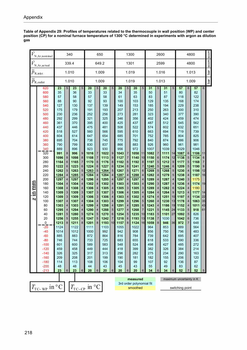
Appendix
218
Table of Appendix 29: Profiles of temperatures related to the thermocouple in wall position (WP) and center position (CP) for a nominal furnace temperature of 1300 °C determined in experiments with argon as dilution gas
sccm
sccm
bar
bar
620 23 5 23 5 20 5 20 5 20 5 20 5 31 5 31 5 57 6 57 6
600 35 36 33 33 34 35 50 51 80 82580 57 58 57 58 61 63 83 87 118 122560 88 90 92 93 100 103 129 135 168 174540 127 130 137 139 149 153 185 194 229 238520 175 179 191 193 207 213 250 263 300 310500 230 236 252 256 273 281 323 340 377 390480 292 299 321 325 346 356 402 424 459 474460 361 370 395 400 425 437 487 512 545 562440 437 446 475 481 508 522 574 602 632 651420 518 527 560 566 595 610 663 694 719 739400 604 614 647 654 685 701 752 785 804 825380 695 704 738 745 775 792 840 874 886 906360 790 799 830 837 866 883 926 960 961 981340 889 896 923 930 956 972 1007 1039 1029 1046320 991 8 996 9 1016 7 1022 9 1043 7 1058 11 1082 7 1111 14 1087 6 1106 11
300 1096 8 1098 8 1108 7 1113 9 1127 7 1140 10 1150 6 1174 12 1138 5 1134 6
280 1164 6 1165 7 1170 6 1176 8 1182 6 1192 8 1197 5 1212 9 1177 5 1168 7
260 1222 6 1223 6 1224 6 1227 6 1234 6 1241 7 1240 5 1246 6 1209 5 1190 9
240 1262 5 1263 5 1263 5 1264 5 1267 5 1271 6 1269 5 1268 5 1230 4 1198 12
220 1284 4 1285 5 1284 4 1284 4 1287 4 1288 4 1282 4 1279 5 1238 4 1187 16
200 1297 4 1297 4 1296 4 1295 4 1297 4 1297 4 1289 4 1287 4 1240 3 1175180 1304 4 1304 4 1302 4 1302 4 1303 4 1303 4 1290 3 1287 4 1236 4 1174 19
160 1308 4 1308 4 1306 4 1305 4 1305 3 1305 3 1289 4 1282 6 1224 4 1180140 1309 3 1309 3 1307 3 1307 3 1306 4 1305 4 1284 4 1264 9 1213 4 1177 14
120 1309 3 1309 3 1306 3 1306 4 1303 4 1302 4 1274 4 1251 10 1197 4 1134 22
100 1307 4 1307 4 1304 4 1303 4 1299 4 1296 5 1260 4 1230 13 1178 4 1063 35
80 1303 4 1303 4 1299 4 1298 4 1291 4 1285 6 1243 4 1186 19 1152 4 1011 43
60 1295 4 1294 4 1290 4 1288 5 1277 4 1268 7 1221 5 1145 24 1133 5 918 61
40 1281 5 1280 5 1274 5 1270 6 1254 5 1235 10 1183 5 1101 27 1092 5 82620 1256 5 1255 6 1247 5 1242 7 1218 6 1193 13 1138 7 1030 1042 6 7360 1213 8 1211 8 1201 8 1193 10 1157 8 1124 16 1059 8 946 36 972 7 648
-20 1124 1122 1111 1103 1055 1022 964 853 889 564-40 1014 1012 1000 992 942 908 856 750 796 483-60 885 883 872 864 816 784 739 642 695 407-80 746 744 733 725 683 655 618 533 590 336-100 601 600 589 583 548 524 498 427 485 272-120 459 458 449 444 418 399 382 326 384 214-140 326 325 317 313 296 282 275 234 290 163-160 209 208 201 199 190 181 182 155 206 120-180 114 113 108 106 104 99 107 92 136 87-200 48 48 44 43 45 43 55 49 83 62-213 23 6 23 6 20 6 20 6 20 6 20 6 34 6 34 6 52 7 52 5
340 650 1300 2600 4800
339.4 649.2 1301 2599 4800
1.010 1.009 1.019 1.016 1.013
1.010 1.009 1.019 1.013 1.009
measured maximum uncertainty in K
3rd order polynomial fitsmoothed switching point CinWPTC T CinCPTC T
nominalAr,N ,V
actualAr,N ,V
inletR,p
outletR,p

Appendix
219
Table of Appendix 30: Profiles of temperatures related to the thermocouple in wall position (WP) and center position (CP) for a nominal furnace temperature of 1400 °C determined in experiments with argon as dilution gas
sccm
sccm
bar
bar
620 27 5 27 5 60 6 60 6 60 6 60 6 60 6 60 6 60 6 60 6
600 43 43 83 83 84 86 86 89 85 87580 75 76 120 121 123 127 127 133 126 130560 121 122 169 172 174 182 181 191 180 187540 178 180 230 235 237 249 248 261 247 256520 245 248 300 306 310 325 324 341 322 335500 321 325 378 386 390 409 408 429 406 421480 404 409 462 472 477 500 497 523 495 512460 492 499 550 562 568 594 591 620 587 606440 584 592 642 655 661 691 687 719 680 700420 679 687 735 749 756 788 783 817 773 791400 774 783 827 843 849 883 877 912 863 879380 868 877 918 934 940 974 967 1002 948 960360 960 969 1005 1021 1027 1060 1051 1086 1027 1032340 1048 1056 1087 1103 1108 1139 1128 1160 1096 1092320 1125 7 1132 9 1162 7 1177 10 1181 7 1210 14 1198 7 1227 14 1155 6 1142 9
300 1211 7 1218 9 1230 7 1243 10 1245 6 1265 11 1250 6 1270 10 1198 5 1165 12
280 1271 6 1275 7 1286 6 1296 8 1294 6 1307 9 1292 5 1299 7 1230 5 1185 15
260 1325 6 1326 6 1332 6 1339 7 1337 6 1342 6 1323 5 1327 6 1261 5 1191 21
240 1360 5 1362 6 1366 5 1370 6 1365 5 1365 5 1338 5 1350 8 1280 4 1208 22
220 1380 5 1380 4 1383 4 1384 5 1379 4 1377 5 1360 5 1358 4 1284 4 1196200 1391 4 1391 4 1393 4 1393 4 1386 4 1379 5 1362 4 1353 7 1283 3 1171 32
180 1398 4 1397 4 1398 4 1398 4 1388 4 1376 7 1359 4 1333 1284 4 1148 38
160 1401 4 1401 4 1401 4 1400 4 1386 4 1374 7 1351 4 1304 17 1276 1 1121 44
140 1402 4 1402 4 1401 4 1400 4 1382 4 1369 7 1337 4 1275 20 1262 4 1072120 1402 4 1402 4 1399 4 1397 4 1374 4 1358 9 1323 4 1247 24 1248 4 1017 63
100 1400 4 1399 4 1394 4 1392 5 1364 5 1334 1303 4 1210 28 1232 5 97180 1395 4 1394 4 1385 4 1378 6 1342 5 1298 17 1281 5 1176 32 1195 5 923 74
60 1387 4 1386 5 1371 5 1359 8 1320 5 1252 23 1253 5 1115 40 1159 5 859 81
40 1370 5 1368 6 1348 5 1330 10 1293 6 1209 1215 6 1054 47 1113 6 805 83
20 1344 6 1339 7 1311 6 1287 13 1243 7 1144 32 1158 7 981 52 1039 7 731 84
0 1299 7 1293 9 1251 8 1216 17 1175 8 1052 39 1086 8 876 61 953 8 656 81
-20 1218 1211 1152 1107 1068 951 982 768 855 578-40 1108 1101 1032 986 950 836 869 659 749 499-60 977 971 897 852 820 715 748 552 638 420-80 831 826 751 712 684 591 622 448 526 344-100 680 675 602 570 548 468 497 351 417 271-120 529 525 457 433 416 352 376 262 314 205-140 386 384 322 306 294 247 266 183 221 145-160 259 258 204 196 188 156 170 117 141 95-180 155 155 109 107 102 84 94 66 78 56-200 82 82 45 45 43 36 41 32 35 30-213 54 7 54 7 20 6 20 6 20 6 20 6 20 6 20 5 20 6 20 5
3rd order polynomial fitsmoothed switching point
6501
measured maximum uncertainty in K
1.007 1.000 1.014 1.002 1.036
1.005 1.012 1.031
3800 6500
701.3 1399.0
700 1400 2600
2603 3795
1.024 1.065
CinWPTC T CinCPTC T
nominalAr,N ,V
actualAr,N ,V
inletR,p
outletR,p

Appendix
220
Table of Appendix 31: Profiles of temperatures related to the thermocouple in wall position (WP) and center position (CP) for a nominal furnace temperature of 1500 °C determined in experiments with argon as dilution gas
sccm
sccm
bar
bar
620 24 5 24 6 30 6 30 6 37 6 37 6 66 6 66 6 94 6 94 6
600 45 47 54 55 63 63 96 97 126 127580 84 88 95 99 107 107 143 143 171 177560 139 145 153 160 166 167 203 205 227 239540 207 215 224 236 239 240 275 279 294 312520 286 297 307 323 323 325 356 363 368 393500 375 389 399 419 416 418 445 454 450 480480 471 487 498 523 516 519 539 550 536 570460 573 591 602 631 620 624 637 649 625 659440 677 698 708 741 726 731 736 748 715 747420 783 805 816 851 832 837 835 845 804 830400 888 911 921 958 936 942 931 938 892 905380 990 1013 1023 1061 1036 1041 1022 1024 975 970360 1087 1110 1118 1156 1128 1134 1106 1101 1053 1022340 1177 1198 1206 1240 1212 1218 1181 1167 1123 1060320 1257 7 1278 13 1286 7 1316 15 1288 7 1292 8 1251 7 1223 13 1188 1079 31
300 1331 7 1340 9 1346 6 1371 13 1341 6 1348 8 1291 5 1245 16 1230 5 1078 42
280 1383 6 1394 9 1392 6 1405 9 1383 6 1381 6 1326 5 1274 18 1266 1094260 1427 6 1429 6 1433 6 1437 6 1417 5 1415 6 1355 5 1281 23 1296 5 1111 50
240 1462 6 1463 6 1461 5 1462 5 1440 5 1429 7 1373 4 1301 22 1321 1101220 1479 5 1479 5 1475 5 1475 5 1449 4 1444 6 1385 4 1288 1335 4 1088 65
200 1489 4 1488 5 1482 4 1478 5 1452 4 1441 7 1384 4 1267 35 1337 1084180 1494 4 1493 4 1484 4 1482 5 1451 4 1433 9 1384 4 1226 45 1325 5 1099 60
160 1496 4 1496 4 1484 4 1477 6 1447 5 1421 12 1372 5 1174 55 1303 1084140 1497 4 1495 5 1480 4 1469 8 1432 4 1379 19 1348 1126 1284 4 1056120 1495 4 1492 5 1473 5 1450 11 1424 4 1335 28 1323 5 1081 66 1267 1017100 1491 4 1486 6 1458 5 1426 13 1410 5 1288 37 1306 4 1035 1251 4 967 77
80 1483 5 1475 7 1442 5 1392 18 1384 5 1226 46 1289 4 989 80 1232 90560 1469 5 1454 9 1421 5 1351 24 1359 5 1176 53 1267 5 946 1211 4 838 100
40 1448 5 1431 10 1389 6 1298 1320 6 1093 1230 6 891 91 1188 5 76720 1417 7 1389 14 1344 7 1222 38 1265 7 1005 1177 6 825 1139 7 6930 1355 9 1315 19 1282 8 1127 1196 9 909 1107 8 751 1065 617
-20 1254 1203 1179 1017 1085 807 1005 670 972 541-40 1130 1077 1058 896 966 702 893 586 864 466-60 987 936 922 769 837 596 773 500 747 393-80 833 787 776 640 702 493 648 415 625 324-100 674 637 628 513 567 394 522 333 503 259-120 519 491 483 393 437 302 402 257 386 199-140 374 355 348 283 316 219 291 188 277 147-160 246 236 230 189 210 148 193 128 183 103-180 143 139 134 113 125 93 114 81 106 68-200 72 72 67 61 64 54 59 48 54 43-213 44 7 44 7 42 6 42 6 38 6 38 6 36 6 36 5 34 6 34 5
1600 2800 4600 7200 9800
1600 2800 4597 7194 9780
0.984 1.004 1.016 1.011 1.027
0.984 0.996 1.012 1.002 1.009
measured maximum uncertainty in K
3rd order polynomial fitsmoothed switching point CinWPTC T CinCPTC T
nominalAr,N,V
actualAr,N,V
inletR,p
outletR,p

Appendix
221
Table of Appendix 32: Profiles of temperatures related to the thermocouple in wall position (WP) and center position (CP) for a nominal furnace temperature of 1600 °C determined in experiments with argon as dilution gas
sccm
sccm
bar
bar
620 27 6 27 6 80 6 80 6 80 6 80 6 140 6 140 6
600 53 55 113 114 112 113 178 180580 97 102 162 165 162 165 228 237560 159 167 227 233 228 234 290 308540 235 246 305 313 308 317 363 391520 323 338 394 405 399 411 443 482500 422 439 492 506 499 513 529 579480 528 549 596 613 604 621 620 678460 640 663 704 724 713 732 714 777440 755 780 814 837 824 843 808 873420 870 896 924 949 932 952 902 963400 983 1010 1032 1058 1037 1055 993 1044380 1092 1120 1135 1161 1136 1150 1079 1113360 1195 1222 1231 1256 1225 1234 1158 1168340 1289 1313 1317 1341 1303 1304 1230 1205320 1373 8 1398 14 1397 8 1418 13 1370 7 1361 9 1295 7 1221 22
300 1441 7 1455 10 1453 7 1470 11 1411 6 1387 11 1338 6 1214 34
280 1488 6 1496 8 1494 6 1503 8 1446 6 1408 14 1373 5 1214 44
260 1531 6 1537 8 1536 6 1533 6 1477 5 1422 18 1400 5 1240 44
240 1562 6 1562 5 1559 5 1556 6 1499 5 1441 19 1424 5 1247 48
220 1578 5 1577 5 1571 5 1565 6 1506 4 1427 25 1422 4 1259 45
200 1587 5 1586 5 1575 4 1563 7 1505 4 1450 19 1418 4 1238 49
180 1591 4 1591 4 1577 4 1562 8 1499 5 1427 25 1411 4 1228160 1594 4 1593 5 1574 4 1554 10 1484 5 1369 35 1400 4 1209 53
140 1593 4 1592 5 1568 5 1546 10 1471 5 1316 45 1392 5 1160 63
120 1591 4 1586 6 1556 5 1538 10 1453 5 1262 54 1373 5 1123 68
100 1587 5 1579 7 1543 5 1518 12 1437 5 1193 68 1362 4 107780 1578 5 1566 8 1530 5 1476 20 1411 5 1111 82 1348 5 1016 90
60 1563 5 1544 10 1507 6 1419 30 1381 5 1042 92 1326 5 935 105
40 1543 6 1523 11 1466 6 1332 42 1343 5 947 1288 6 85020 1508 7 1474 17 1418 7 1238 54 1310 7 855 1238 7630 1444 9 1383 1346 10 1129 63 1242 759 1158 8 674
-20 1336 1268 1221 1003 1144 663 1051 586-40 1203 1132 1088 873 1024 568 932 499-60 1052 982 940 740 889 475 802 415-80 888 825 786 608 744 386 668 336-100 720 666 630 480 596 303 533 262-120 555 512 479 360 451 227 404 196-140 401 370 340 252 318 161 285 138-160 265 245 218 160 200 105 182 90-180 155 145 119 88 107 61 99 53-200 79 76 50 39 43 32 42 28-213 50 7 50 6 20 7 20 6 20 6 20 5 20 6 20 5
2000 3350 6500 9800
2006 3349 6493 9810
1.008 1.041 1.066 1.039
1.007 1.024 1.036 1.006
measured maximum uncertainty in K
3rd order polynomial fitsmoothed switching point CinWPTC T CinCPTC T
nominalAr,N,V
actualAr,N,V
inletR,p
outletR,p

Appendix
222
Table of Appendix 33: Profiles of temperatures related to the thermocouple in wall position (WP) and center position (CP) determined in experiments with helium as dilution gas
°Csc
cmsc
cmba
rba
r
620 24 5 24 5 23 5 23 6 20 5 20 6 37 6 37 6 23 6 23 6
600 45 45 45 46 42 43 64 64 49 51580 80 81 83 85 80 82 106 107 92 95560 129 131 136 138 134 136 164 165 151 156540 190 192 200 204 200 204 234 236 224 230520 260 263 276 281 278 283 315 318 309 316500 338 342 360 366 364 370 404 408 403 412480 423 428 450 458 457 465 500 504 504 514460 512 517 546 555 555 564 599 604 610 621440 604 610 644 654 656 666 701 707 719 730420 696 704 744 754 758 768 803 809 828 840400 788 796 842 853 857 869 902 909 935 947380 877 886 937 949 954 965 997 1004 1038 1050360 962 971 1028 1039 1045 1056 1085 1092 1134 1146340 1040 1050 1112 1122 1128 1139 1165 1172 1222 1233320 1113 6 1123 9 1190 7 1200 9 1205 7 1215 9 1239 7 1246 9 1303 7 1316 11
300 1169 6 1179 8 1250 6 1256 8 1263 6 1272 8 1286 6 1292 7 1360 6 1364 7
280 1216 5 1225 8 1300 6 1305 7 1307 6 1312 7 1324 5 1328 6 1405 6 1409 7
260 1257 5 1267 8 1344 6 1346 6 1348 6 1352 7 1358 5 1363 7 1445 6 1449 7
240 1282 5 1284 5 1371 5 1374 6 1374 5 1376 5 1380 5 1381 5 1471 5 1472 5
220 1296 4 1297 4 1387 4 1387 4 1389 4 1389 4 1391 4 1392 4 1485 5 1485 5
200 1303 4 1304 4 1396 4 1396 4 1397 4 1397 4 1397 4 1397 4 1493 4 1492 5
180 1307 4 1308 4 1401 4 1400 4 1401 4 1401 4 1399 4 1399 4 1497 4 1496 4
160 1309 3 1309 3 1403 4 1402 4 1403 4 1402 4 1398 4 1398 4 1498 4 1498 4
140 1308 4 1308 4 1403 4 1403 4 1402 4 1402 4 1394 4 1392 5 1498 4 1498 4
120 1305 4 1305 4 1402 4 1401 4 1400 4 1400 4 1386 4 1383 5 1497 4 1496 4
100 1299 4 1298 4 1398 4 1398 4 1395 4 1394 4 1372 5 1365 7 1492 4 1491 5
80 1286 4 1283 5 1392 4 1390 5 1386 4 1383 5 1347 6 1332 10 1485 5 1483 5
60 1268 5 1261 7 1380 5 1378 5 1371 5 1366 7 1305 7 1272 15 1470 5 1466 6
40 1233 6 1222 10 1359 5 1353 7 1338 6 1329 9 1242 7 1194 20 1444 6 1435 9
20 1174 7 1147 14 1321 7 1307 10 1288 8 1265 13 1159 9 1093 26 1395 7 1383 11
0 1091 8 1064 15 1250 8 1236 12 1201 1176 1042 9 965 28 1320 9 1301 14
-20 992 962 1145 1129 1095 1068 937 850 1205 1186-40 879 849 1024 1008 973 945 818 731 1076 1057-60 758 730 891 875 840 814 695 614 934 916-80 634 608 749 736 702 679 572 501 784 768-100 510 488 606 595 564 544 454 395 633 619-120 391 374 467 458 431 415 343 298 486 475-140 282 270 338 331 308 296 243 212 350 341-160 188 180 224 220 201 193 157 139 231 225-180 112 108 132 130 115 111 91 83 134 131-200 59 58 67 67 56 54 46 45 67 65-213 40 6 40 6 41 6 41 6 33 6 33 6 32 5 32 5 39 7 39 6
1300 1400 1400 1400 1500
3807 2798 3800 6499 3800
1.026 1.021 1.022 1.024 0.997
1.025 1.019 1.019 1.019 0.994
measured maximum uncertainty in K
3rd order polynomial fitsmoothed switching point
3800 2800 3800 6500 3800
CinWPTC T CinCPTC T
inletR,p
outletR,p
furn aceT
nominalHe,N,V
actualHe,N,V
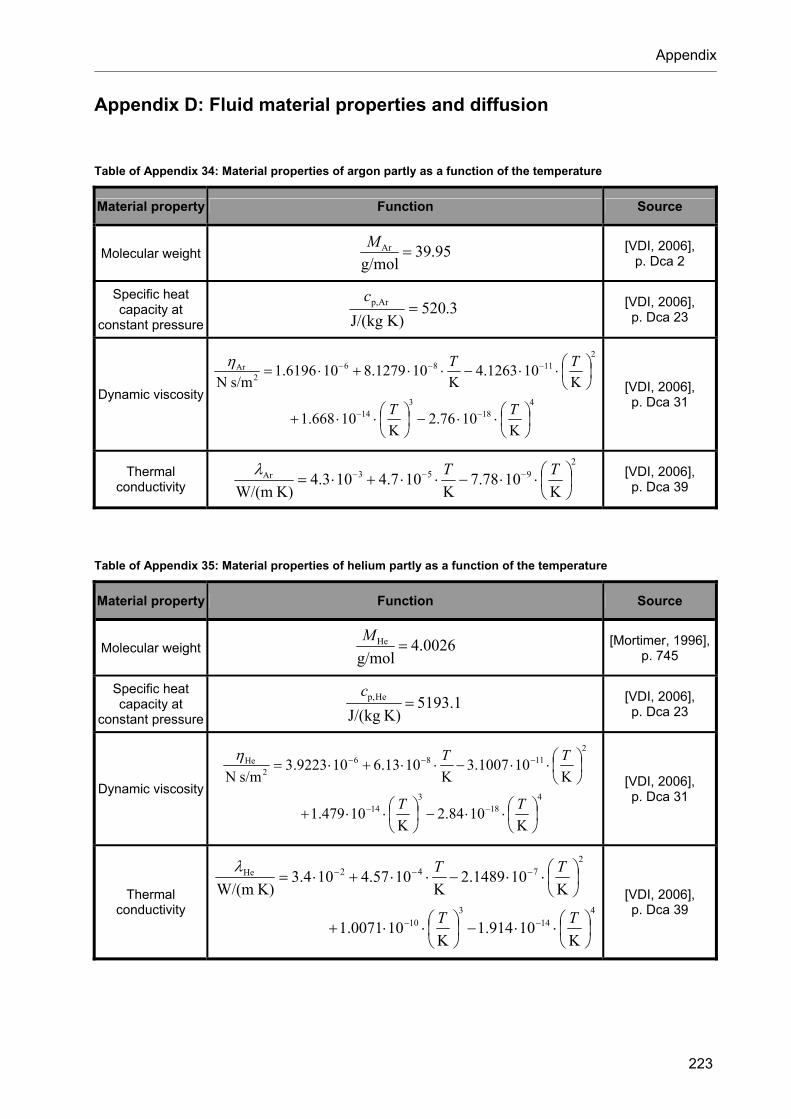
Appendix
223
Appendix D: Fluid material properties and diffusion
Table of Appendix 34: Material properties of argon partly as a function of the temperature
Material property Function Source
Molecular weight 95.39g/mol
Ar M
[VDI, 2006], p. Dca 2
Specific heat capacity at
constant pressure 3.520
K)J/(kgArp,
c [VDI, 2006],
p. Dca 23
Dynamic viscosity 4
813
41
21186
2Ar
K1076.2
K10668.1
K101263.4
K101279.8106196.1
s/mN
TT
TT
[VDI, 2006], p. Dca 31
Thermal conductivity
2953Ar
K1078.7
K107.4103.4
K)W/(m
TT
[VDI, 2006], p. Dca 39
Table of Appendix 35: Material properties of helium partly as a function of the temperature
Material property Function Source
Molecular weight 4.0026g/mol
He M
[Mortimer, 1996], p. 745
Specific heat capacity at
constant pressure 5193.1
K)J/(kgHep,
c [VDI, 2006],
p. Dca 23
Dynamic viscosity 4
813
41
21186
2He
K1084.2
K10479.1
K101007.3
K1013.6109223.3
s/mN
TT
TT
[VDI, 2006], p. Dca 31
Thermal conductivity 4
413
01
2742He
K10914.1
K100071.1
K101489.2
K1057.4104.3
K)W/(m
TT
TT
[VDI, 2006], p. Dca 39

Appendix
224
0.01 0.1 1 1010
100
1000Q
D,r
adia
l reg
ard
ing
eth
ane
in -
Residence time in s
2 % 5 % 10 % 20 % 7.051 % 3.107 % 6.322 % 3.007 % 7.060 % 7.110 %
1200 °C1300 °C1400 °C1500 °C1600 °C
He
Ar
Figure of Appendix 11: Diffusive quotient regarding ethane as a function of the residence time, the nominal furnace temperature, the initial molar fraction of methane, and the dilution gas
0.01 0.1 1 1010
100
1000
QD
,rad
ial r
ega
rdin
g e
then
e in
-
Residence time in s
2 % 5 % 10 % 20 % 7.051 % 3.107 % 6.322 % 3.007 % 7.060 % 7.110 %
1200 °C1300 °C1400 °C1500 °C1600 °C
He
Ar
Figure of Appendix 12: Diffusive quotient regarding ethene as a function of the residence time, the nominal furnace temperature, the initial molar fraction of methane, and the dilution gas

Appendix
225
0.01 0.1 1 1010
100
1000
QD
,rad
ial r
ega
rdin
g et
hyn
e in
-
Residence time in s
2 % 5 % 10 % 20 % 7.051 % 3.107 % 6.322 % 3.007 % 7.060 % 7.110 %
1200 °C1300 °C1400 °C1500 °C1600 °C
He
Ar
Figure of Appendix 13: Diffusive quotient regarding ethyne as a function of the residence time, the nominal furnace temperature, the initial molar fraction of methane, and the dilution gas

Appendix
226
Appendix E: Calculations with ANSYS
Table of Appendix 36: Information about general settings for the calculations with ANSYS 12
Mesh information
Physical preference Mesh method
CFD Automatic (Patch conforming / Sweeping)
Settings Maximum Body Size Inflation Maximum Layers Transition Growth rate Inflation Algorithm
4E-04 m 2 Smooth, Transition ratio 0.272 1.2 Pre
Statistics Nodes Elements
403715 1667453
Domain physics
Type Fluid
Material Fluid definition Morphology
Argon Material Library, user defined for reference conditions, pure substance, calorically perfect ideal gas Continuous Fluid
Setting Buoyancy Model Domain Motion Reference Pressure Heat Transfer Model Fluid Temperature Turbulence Model
Non Buoyant Stationary Reactor inlet pressure Isothermal Reactor inlet temperature Laminar
Boundary physics
Inlet face (of entrance region) Flow Regime Mass And Momentum Normal Speed
Subsonic Normal Speed average speed
Outlet face (of entrance region) Flow Regime Mass And Momentum Relative Pressure
Subsonic Static Pressure 0 bar
Walls (of entrance region) Mass And Momentum
No Slip Wall
Solver control
Basic settings Advection Scheme Convergence control Timescale Control Length Scale Option Timescale Factor Convergence Criteria Residual type Residual target Conservation target
High Resolution Auto timescale Aggressive 1.0 RMS 1E-06 1E-04
Equation Class Settings Continuity, Momentum
Advanced options Global Dynamic Model Control
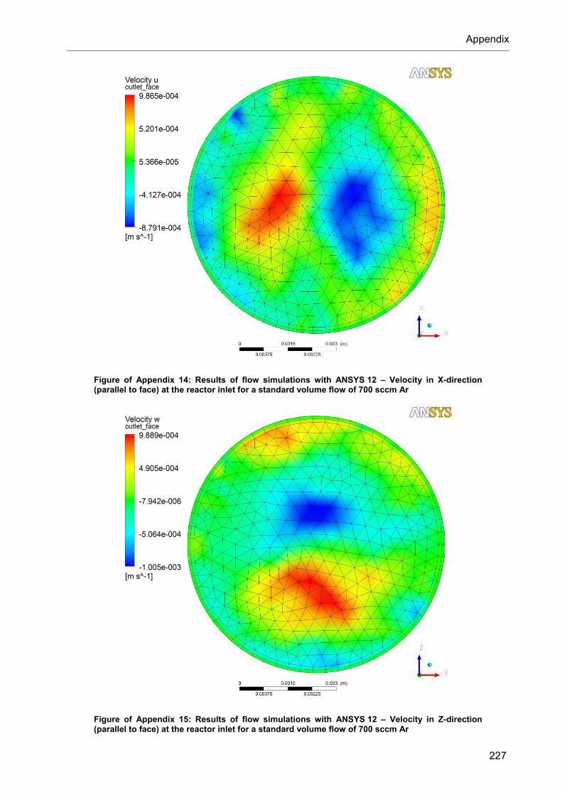
Appendix
227
Figure of Appendix 14: Results of flow simulations with ANSYS 12 – Velocity in X-direction (parallel to face) at the reactor inlet for a standard volume flow of 700 sccm Ar
Figure of Appendix 15: Results of flow simulations with ANSYS 12 – Velocity in Z-direction (parallel to face) at the reactor inlet for a standard volume flow of 700 sccm Ar

Appendix
228
Figure of Appendix 16: Results of flow simulations with ANSYS 12 – Velocity in X-direction (parallel to face) at the reactor inlet for a standard volume flow of 2600 sccm Ar
Figure of Appendix 17: Results of flow simulations with ANSYS 12 – Velocity in Y-direction (normal to face) at the reactor inlet for a standard volume flow of 2600 sccm Ar
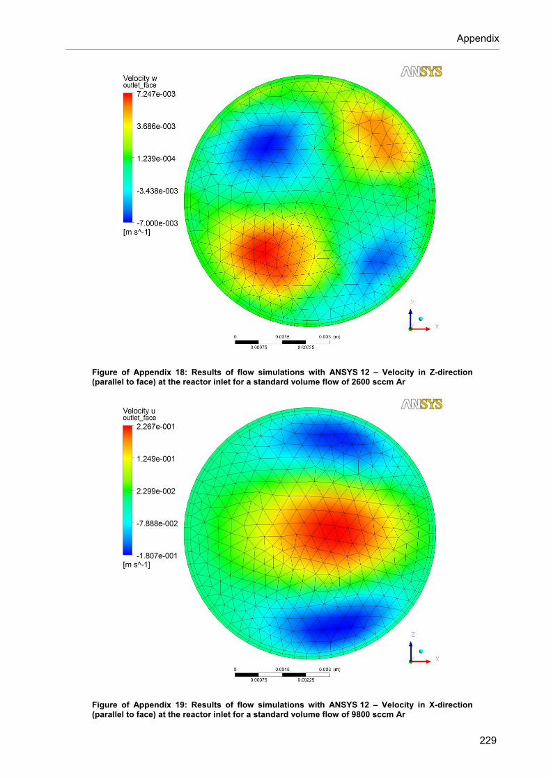
Appendix
229
Figure of Appendix 18: Results of flow simulations with ANSYS 12 – Velocity in Z-direction (parallel to face) at the reactor inlet for a standard volume flow of 2600 sccm Ar
Figure of Appendix 19: Results of flow simulations with ANSYS 12 – Velocity in X-direction (parallel to face) at the reactor inlet for a standard volume flow of 9800 sccm Ar

Appendix
230
Figure of Appendix 20: Results of flow simulations with ANSYS 12 – Velocity in Y-direction (normal to face) at the reactor inlet for a standard volume flow of 9800 sccm Ar
Figure of Appendix 21: Results of flow simulations with ANSYS 12 – Velocity in Z-direction (parallel to face) at the reactor inlet for a standard volume flow of 9800 sccm Ar

Appendix
231
Table of Appendix 37: Coefficients of the polynomial fit function for the approximation of averaged velocity profiles at the inlet of the reactor.
/furnaceT )mm/(sin iik
- set 6k 5k 4k 3k 2k 1k 0k
5 -1.46961E+15 1.76766E+13 -7.44044E+10 1.18131E+08 -1.23928E+05 3.42689E+01 1.26064E+00
8 -4.40221E+14 4.83776E+12 -1.61002E+10 7.58349E+06 -2.40424E+04 6.62798E+00 8.48611E-01
9 -2.37714E+15 2.97222E+13 -1.33812E+11 2.43183E+08 -2.47299E+05 6.87565E+01 1.68981E+00
10 -3.42516E+15 4.61344E+13 -2.36305E+11 5.05774E+08 -5.46973E+05 1.62766E+02 3.05639E+00
12 -5.53268E+14 6.19635E+12 -2.18588E+10 1.70492E+07 -3.25138E+04 9.05793E+00 9.15241E-01
13 -2.25989E+15 2.84492E+13 -1.29427E+11 2.39223E+08 -2.43357E+05 6.77897E+01 1.58450E+00
14 -2.79340E+15 3.72920E+13 -1.85612E+11 3.84844E+08 -4.06780E+05 1.17127E+02 2.20985E+00
15 -3.81975E+15 4.52614E+13 -2.21302E+11 4.70673E+08 -5.04308E+05 1.60090E+02 3.30858E+00
16 -8.18284E+14 9.31907E+12 -3.45001E+10 3.53003E+07 -5.18058E+04 1.44728E+01 1.15986E+00
17 -2.68651E+15 3.39121E+13 -1.54905E+11 2.88083E+08 -2.93237E+05 8.17667E+01 1.87827E+00
18 -3.15818E+15 4.25351E+13 -2.17571E+11 4.64999E+08 -5.02286E+05 1.49323E+02 2.79716E+00
19 -5.07327E+15 5.85432E+13 -2.79832E+11 5.88089E+08 -6.20250E+05 1.97535E+02 4.02807E+00
20 -1.16594E+16 1.23838E+14 -5.35837E+11 1.06155E+09 -1.00631E+06 3.28436E+02 5.05363E+00
21 -1.49427E+15 1.77358E+13 -7.26584E+10 1.07640E+08 -1.17152E+05 3.25357E+01 1.42472E+00
22 -2.67737E+15 3.51676E+13 -1.70303E+11 3.42289E+08 -3.55471E+05 1.00493E+02 1.95438E+00
23 -3.77435E+15 4.48292E+13 -2.19843E+11 4.68526E+08 -5.02414E+05 1.59972E+02 3.29918E+00
24 -1.17506E+16 1.24183E+14 -5.33103E+11 1.05118E+09 -9.86948E+05 3.22354E+02 4.74821E+00

Appendix
232
Appendix F: Calculations with COMSOL Multiphysics
Table of Appendix 38: Information about general settings for the calculations with COMSOL Multiphysics
Basics
Geometry 2D, axial symmetry
Modus of application Fluid flow Standard type of element Type of analysis Model of turbulence Heat transfer Standard type of element Type of analysis Model of turbulence
Weakly compressible Navier-Stokes Lagrange - P2 P1 Stationary None General heat transfer with disabled radiative heat transfer Lagrange - P2 J1 Stationary None
Mesh information
Settings Predefined mesh size Method of refinement Level of refinement
Normal Regular 3
Statistics Nodes Elements Degrees of freedom
187189 366912 (triangular) 1690584
Domain condition
Fluid Material Density Heat transfer
Argon or helium (user defined material properties) Function of temperature and pressure Convection
Reactor wall and thermocouple Material Density Specific heat capacity at constant pressure Heat transfer
AL23 3825 kg/m3 900 J/(kg K) Conduction
Boundary conditions
Inlet face of fluid domain
Velocity profile provided Temperature provided
Outlet face of fluid domain
Pressure provided Convective flux
Inner face of reactor wall
No-slip wall Temperature provided
Outer face of thermocouple
No-slip wall Temperature linked to temperature variable
Other faces
No-slip wall Thermal insulation
Solver control
Type of analysis Linear solver of equations Convergence Criteria Relative accuracy Newton damping
Stationary Direct (UMFPACK) 1E-06 activated

Appendix
233
Figure of Appendix 22: Results of COMSOL Multiphysics calculations based on a simplified temperature profile for the wall of the reactor concerning flow lines for different standard volume flows of argon and a nominal furnace temperature of 1200 °C: 95 sccm (a), 200 sccm (b), 350 sccm (c), 685 sccm (d), and 2000 sccm (e)
Figure of Appendix 23: Results of COMSOL Multiphysics calculations based on a simplified temperature profile for the wall of the reactor concerning flow lines for different standard volume flows of argon and a nominal furnace temperature of 1300 °C: 340 sccm (a), 650 sccm (b), 1300 sccm (c), 2600 sccm (d), and 4800 sccm (e)
Figure of Appendix 24: Results of COMSOL Multiphysics calculations based on a simplified temperature profile for the wall of the reactor concerning flow lines for different standard volume flows of argon and a nominal furnace temperature of 1400 °C: 700 sccm (a), 1400 sccm (b), 2600 sccm (c), 3800 sccm (d), and 6500 sccm (e)
Figure of Appendix 25: Results of COMSOL Multiphysics calculations based on a simplified temperature profile for the wall of the reactor concerning flow lines for different standard volume flows of argon and a nominal furnace temperature of 1500 °C: 1600 sccm (a), 2800 sccm (b), 4600 sccm (c), 7200 sccm (d), and 9800 sccm (e)
(a) (b) (c) (d) (e)
(a) (b) (c) (d) (e)
(a) (b) (c) (d) (e)
(a) (b) (c) (d) (e)

Appendix
234
Figure of Appendix 26: Results of COMSOL Multiphysics calculations based on a simplified temperature profile for the wall of the reactor concerning flow lines for different standard volume flows of argon and a nominal furnace temperature of 1600 °C: 2000 sccm (a), 3350 sccm (b), 6500 sccm (c), 9800 sccm (d)
Figure of Appendix 27: Results of COMSOL Multiphysics calculations based on a simplified temperature profile for the wall of the reactor concerning flow lines for different sets of standard volume flow of helium and nominal furnace temperature: 1300 °C - 3800 sccm (a), 1400 °C - 2800 sccm (b), 1400 °C - 3800 sccm (c), 1400 °C - 6500 sccm (d), and 1500 °C - 3800 sccm (e)
Table of Appendix 39: Coefficients of the polynomial fit function for the approximation of fractions of the molar flow at the inlet of the reactor present 5 mm downstream the tip of the thermocouple in particular nested tube reactors (NTR) of region B.
iik s/mol)(in
Gas NTR
3k 2k 1k 0k
1 -2.0556E+05 3.7537E+03 -1.1197E+01 1.3511E-01
2 -3.5574E+05 4.6347E+03 -1.3581E+01 3.2845E-01
3 3.1172E+05 -4.4580E+03 1.0098E+01 3.6014E-01 Ar
4 2.4958E+05 -3.9304E+03 1.4679E+01 1.7630E-01
1 - -9.7174E+01 -2.4543E-01 1.3266E-01
2 - -1.2551E+02 -3.8322E-01 3.2631E-01
3 - 8.9136E+01 1.6390E-01 3.6212E-01 He
4 - 1.3355E+02 4.6474E-01 1.7891E-01
(a) (b) (c) (d)
(a) (b) (c) (d) (e)

Appendix
235
Appendix G: Optimization tool and results of kinetic evaluation
Table of Appendix 40: Information about the optimization tool used for the determination of kinetic parameters
Optimization tool Solver Algorithm Algorithm settings Subproblem algorithm
Optimization Toolbox 4.0 embedded in MATLAB Version 7.6.0.324 (R2008a) “lsnonlin“ (Nonlinear least squares) Large scale Cholesky factorization
Stopping criteria X tolerance Function tolerance
1E-06 (default) 1E-06 (default)
Approximated derivates Finite differences Minimum perturbation Maximum perturbation
1E-08 (default) 0.1 (default)
0.01 0.1 1 100
20
40
60
80
100
Con
vers
ion
of m
eth
ane
in %
Residence time in s
measured calculated
1200 °C1300 °C1400 °C1500 °C1600 °C
Figure of Appendix 28: Comparison of experimentally determined conversion of methane (as a function of the residence time and the nominal furnace temperature) with calculated values employing reactor model 5 NTR and respective best fit kinetic parameters. 2 % initial molar fraction of methane in argon. Indicators of uncertainty refer to maximum uncertainty (black: used for kinetic evaluation, gray: not used for kinetic evaluation).

Appendix
236
0.01 0.1 1 100
20
40
60
80
100
Con
vers
ion
of m
eth
ane
in %
Residence time in s
measured calculated
1200 °C1300 °C1400 °C1500 °C1600 °C
Figure of Appendix 29: Comparison of experimentally determined conversion of methane (as a function of the residence time and the nominal furnace temperature) with calculated values employing reactor model 5 NTR and respective best fit kinetic parameters. 10 % initial molar fraction of methane in argon. Indicators of uncertainty refer to maximum uncertainty (black: used for kinetic evaluation, gray: not used for kinetic evaluation).
0.01 0.1 10
20
40
60
80
100
Con
vers
ion
of m
eth
ane
in %
Residence time in s
20 % measured 20 % calculated 7.051 % measured 7.051 % calculated 3.107 % measured 3.107 % calculated 6.322 % measured 6.322 % calculated 3.007 % measured 3.007 % calculated 7.060 % measured 7.060 % calculated
1200 °C1300 °C1400 °C1500 °C1600 °C
Figure of Appendix 30: Comparison of experimentally determined conversion of methane (as a function of the residence time and the nominal furnace temperature) with calculated values employing reactor model 5 NTR and respective best fit kinetic parameters. Diverse initial molar fractions of methane in argon. Indicators of uncertainty refer to maximum uncertainty (black: used for kinetic evaluation, gray: not used for kinetic evaluation).

Appendix
237
0.01 0.1 1 100
20
40
60
80
100
Yie
ld o
f hyd
roge
n in
%
Residence time in s
measured calculated
1200 °C1300 °C1400 °C1500 °C1600 °C
Figure of Appendix 31: Comparison of experimentally determined yield of hydrogen (as a function of the residence time and the nominal furnace temperature) with calculated values employing reactor model 5 NTR and respective best fit kinetic parameters. 2 % initial molar fraction of methane in argon. Indicators of uncertainty refer to maximum uncertainty (black: used for kinetic evaluation, gray: not used for kinetic evaluation).
0.01 0.1 1 100
20
40
60
80
100
Yie
ld o
f hyd
roge
n in
%
Residence time in s
measured calculated
1200 °C1300 °C1400 °C1500 °C1600 °C
Figure of Appendix 32: Comparison of experimentally determined yield of hydrogen (as a function of the residence time and the nominal furnace temperature) with calculated values employing reactor model 5 NTR and respective best fit kinetic parameters. 10 % initial molar fraction of methane in argon. Indicators of uncertainty refer to maximum uncertainty (black: used for kinetic evaluation, gray: not used for kinetic evaluation).
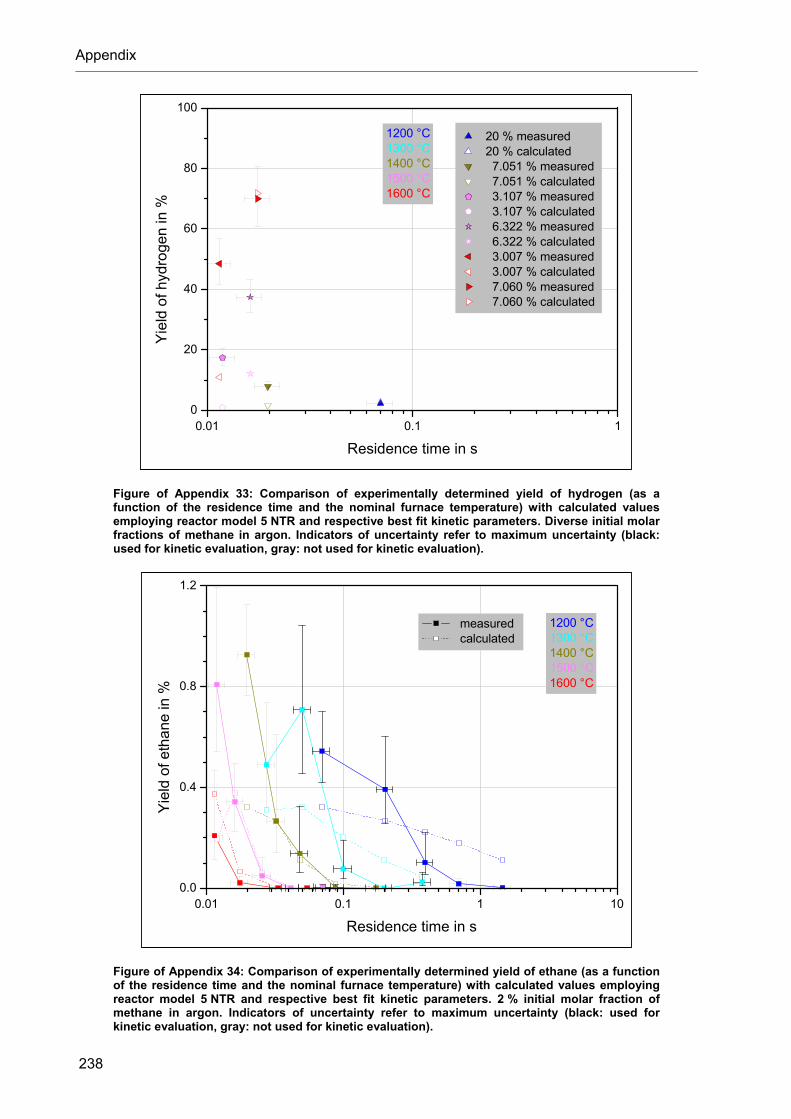
Appendix
238
0.01 0.1 10
20
40
60
80
100
Yie
ld o
f hyd
roge
n in
%
Residence time in s
20 % measured 20 % calculated 7.051 % measured 7.051 % calculated 3.107 % measured 3.107 % calculated 6.322 % measured 6.322 % calculated 3.007 % measured 3.007 % calculated 7.060 % measured 7.060 % calculated
1200 °C1300 °C1400 °C1500 °C1600 °C
Figure of Appendix 33: Comparison of experimentally determined yield of hydrogen (as a function of the residence time and the nominal furnace temperature) with calculated values employing reactor model 5 NTR and respective best fit kinetic parameters. Diverse initial molar fractions of methane in argon. Indicators of uncertainty refer to maximum uncertainty (black: used for kinetic evaluation, gray: not used for kinetic evaluation).
0.01 0.1 1 100.0
0.4
0.8
1.2
Yie
ld o
f eth
ane
in %
Residence time in s
measured calculated
1200 °C1300 °C1400 °C1500 °C1600 °C
Figure of Appendix 34: Comparison of experimentally determined yield of ethane (as a function of the residence time and the nominal furnace temperature) with calculated values employing reactor model 5 NTR and respective best fit kinetic parameters. 2 % initial molar fraction of methane in argon. Indicators of uncertainty refer to maximum uncertainty (black: used for kinetic evaluation, gray: not used for kinetic evaluation).

Appendix
239
0.01 0.1 1 100.0
0.2
0.4
0.6
Yie
ld o
f eth
ane
in %
Residence time in s
measured calculated
1200 °C1300 °C1400 °C1500 °C1600 °C
Figure of Appendix 35: Comparison of experimentally determined yield of ethane (as a function of the residence time and the nominal furnace temperature) with calculated values employing reactor model 5 NTR and respective best fit kinetic parameters. 10 % initial molar fraction of methane in argon. Indicators of uncertainty refer to maximum uncertainty (black: used for kinetic evaluation, gray: not used for kinetic evaluation).
0.01 0.1 10.0
0.2
0.4
0.6
0.8
1.0
Yie
ld o
f eth
ane
in %
Residence time in s
20 % measured 20 % calculated 7.051 % measured 7.051 % calculated 3.107 % measured 3.107 % calculated 6.322 % measured 6.322 % calculated 3.007 % measured 3.007 % calculated 7.060 % measured 7.060 % calculated
1200 °C1300 °C1400 °C1500 °C1600 °C
Figure of Appendix 36: Comparison of experimentally determined yield of ethane (as a function of the residence time and the nominal furnace temperature) with calculated values employing reactor model 5 NTR and respective best fit kinetic parameters. Diverse initial molar fractions of methane in argon. Indicators of uncertainty refer to maximum uncertainty (black: used for kinetic evaluation, gray: not used for kinetic evaluation).

Appendix
240
0.01 0.1 1 100
1
2
3
4
5
6
Yie
ld o
f eth
ene
in %
Residence time in s
measured calculated
1200 °C1300 °C1400 °C1500 °C1600 °C
Figure of Appendix 37: Comparison of experimentally determined yield of ethene (as a function of the residence time and the nominal furnace temperature) with calculated values employing reactor model 5 NTR and respective best fit kinetic parameters. 2 % initial molar fraction of methane in argon. Indicators of uncertainty refer to maximum uncertainty (black: used for kinetic evaluation, gray: not used for kinetic evaluation).
0.01 0.1 1 100
1
2
3
4
5
Yie
ld o
f eth
ene
in %
Residence time in s
measured calculated
1200 °C1300 °C1400 °C1500 °C1600 °C
Figure of Appendix 38: Comparison of experimentally determined yield of ethene (as a function of the residence time and the nominal furnace temperature) with calculated values employing reactor model 5 NTR and respective best fit kinetic parameters. 10 % initial molar fraction of methane in argon. Indicators of uncertainty refer to maximum uncertainty (black: used for kinetic evaluation, gray: not used for kinetic evaluation).

Appendix
241
0.01 0.1 10
1
2
3
4
5
Yie
ld o
f eth
ene
in %
Residence time in s
20 % measured 20 % calculated 7.051 % measured 7.051 % calculated 3.107 % measured 3.107 % calculated 6.322 % measured 6.322 % calculated 3.007 % measured 3.007 % calculated 7.060 % measured 7.060 % calculated
1200 °C1300 °C1400 °C1500 °C1600 °C
Figure of Appendix 39: Comparison of experimentally determined yield of ethene (as a function of the residence time and the nominal furnace temperature) with calculated values employing reactor model 5 NTR and respective best fit kinetic parameters. Diverse initial molar fractions of methane in argon. Indicators of uncertainty refer to maximum uncertainty (black: used for kinetic evaluation, gray: not used for kinetic evaluation).
0.01 0.1 1 100
20
40
60
80
100
Yie
ld o
f eth
yne
in %
Residence time in s
measured calculated
1200 °C1300 °C1400 °C1500 °C1600 °C
Figure of Appendix 40: Comparison of experimentally determined yield of ethyne (as a function of the residence time and the nominal furnace temperature) with calculated values employing reactor model 5 NTR and respective best fit kinetic parameters. 2 % initial molar fraction of methane in argon. Indicators of uncertainty refer to maximum uncertainty (black: used for kinetic evaluation, gray: not used for kinetic evaluation).

Appendix
242
0.01 0.1 1 100
20
40
60
Yie
ld o
f eth
yne
in %
Residence time in s
measured calculated
1200 °C1300 °C1400 °C1500 °C1600 °C
Figure of Appendix 41: Comparison of experimentally determined yield of ethyne (as a function of the residence time and the nominal furnace temperature) with calculated values employing reactor model 5 NTR and respective best fit kinetic parameters. 10 % initial molar fraction of methane in argon. Indicators of uncertainty refer to maximum uncertainty (black: used for kinetic evaluation, gray: not used for kinetic evaluation).
0.01 0.1 10
20
40
60
80
Yie
ld o
f eth
yne
in %
Residence time in s
20 % measured 20 % calculated 7.051 % measured 7.051 % calculated 3.107 % measured 3.107 % calculated 6.322 % measured 6.322 % calculated 3.007 % measured 3.007 % calculated 7.060 % measured 7.060 % calculated
1200 °C1300 °C1400 °C1500 °C1600 °C
Figure of Appendix 42: Comparison of experimentally determined yield of ethyne (as a function of the residence time and the nominal furnace temperature) with calculated values employing reactor model 5 NTR and respective best fit kinetic parameters. Diverse initial molar fractions of methane in argon. Indicators of uncertainty refer to maximum uncertainty (black: used for kinetic evaluation, gray: not used for kinetic evaluation).

Appendix
243
Table of Appendix 41: Covariance matrix calculated based on the best fit kinetic parameters for model 5 NTR
)(ψCov 1 2 3 4 5 6 7 8 9 10 11 12 Related to
1 3.29 E+00
1.15 E-01
8.14 E-03
1.43 E-01
1.27 E-02
3.86 E-03
5.56 E-01
2.86 E-02
5.57 E-03
-1.39E-01
-2.94 E-04
5.61 E-03 a,1E
2 1.15 E-01
4.02 E-03
3.05 E-04
4.05 E-03
4.45 E-04
1.45 E-04
1.53 E-02
8.82 E-04
2.03 E-04
-4.92E-03
-2.38 E-05
1.83 E-04
)log( 1,0k
3 8.14 E-03
3.05 E-04
5.05 E-05
-7.35 E-04
2.97 E-05
2.10 E-05
-2.34E-03
-3.47E-05
2.24 E-05
-3.60E-04
-1.13 E-05
2.46 E-06 1m
4 1.43 E-01
4.05 E-03
-7.35 E-04
8.79 E+01
3.20 E+00
1.57 E-02
4.36 E-01
-2.21E-02
-7.54E-03
1.22 E-03
3.77 E-03
4.04 E-03 a,2E
5 1.27 E-02
4.45 E-04
2.97 E-05
3.20 E+00
1.22 E-01
2.42 E-03
5.52 E-03
-1.15E-03
-2.70E-04
-7.56E-04
9.96 E-05
1.38 E-04
)log( 2,0k
6 3.86 E-03
1.45 E-04
2.10 E-05
1.57 E-02
2.42 E-03
6.30 E-04
-2.41E-03
-8.36E-05
2.19 E-06
-3.05E-04
-8.13 E-06
3.59 E-06 2m
7 5.56 E-01
1.53 E-02
-2.34 E-03
4.36 E-01
5.52 E-03
-2.41E-03
9.88 E+00
3.45 E-01
3.66 E-03
3.61 E-02
9.32 E-03
9.36 E-03 a,3E
8 2.86 E-02
8.82 E-04
-3.47 E-05
-2.21 E-02
-1.15 E-03
-8.36E-05
3.45 E-01
1.29 E-02
4.85 E-04
2.20 E-04
2.97 E-04
3.39 E-04
)log( 3,0k
9 5.57 E-03
2.03 E-04
2.24 E-05
-7.54 E-03
-2.70 E-04
2.19 E-06
3.66 E-03
4.85 E-04
1.61 E-04
-4.70E-04
-5.23 E-06
1.40 E-05 3m
10 -1.39 E-01
-4.92 E-03
-3.60 E-04
1.22 E-03
-7.56 E-04
-3.05E-04
3.61 E-02
2.20 E-04
-4.70E-04
1.39 E+01
4.81 E-01
-3.68 E-02 a,4E
11 -2.94 E-04
-2.38 E-05
-1.13 E-05
3.77 E-03
9.96 E-05
-8.13E-06
9.32 E-03
2.97 E-04
-5.23E-06
4.81 E-01
1.77 E-02
-2.82 E-04
)log( 4,0k
12 5.61 E-03
1.83 E-04
2.46 E-06
4.04 E-03
1.38 E-04
3.59 E-06
9.36 E-03
3.39 E-04
1.40 E-05
-3.68E-02
-2.82 E-04
1.12 E-03 4m
mol
kJinaE ,
)1(
30 m
mol
s
1in
m
k
, inm