Theoretical Determination of NMR Parameters of Metabolites ...
229
HAL Id: tel-00670018 https://tel.archives-ouvertes.fr/tel-00670018v1 Submitted on 14 Feb 2012 (v1), last revised 11 Oct 2012 (v2) HAL is a multi-disciplinary open access archive for the deposit and dissemination of sci- entific research documents, whether they are pub- lished or not. The documents may come from teaching and research institutions in France or abroad, or from public or private research centers. L’archive ouverte pluridisciplinaire HAL, est destinée au dépôt et à la diffusion de documents scientifiques de niveau recherche, publiés ou non, émanant des établissements d’enseignement et de recherche français ou étrangers, des laboratoires publics ou privés. Theoretical Determination of NMR Parameters of Metabolites and Proteins Zeinab Atieh To cite this version: Zeinab Atieh. Theoretical Determination of NMR Parameters of Metabolites and Proteins. Chemical Physics [physics.chem-ph]. Université Claude Bernard - Lyon I, 2011. English. tel-00670018v1
-
Upload
khangminh22 -
Category
Documents
-
view
3 -
download
0
Transcript of Theoretical Determination of NMR Parameters of Metabolites ...

HAL Id: tel-00670018https://tel.archives-ouvertes.fr/tel-00670018v1
Submitted on 14 Feb 2012 (v1), last revised 11 Oct 2012 (v2)
HAL is a multi-disciplinary open accessarchive for the deposit and dissemination of sci-entific research documents, whether they are pub-lished or not. The documents may come fromteaching and research institutions in France orabroad, or from public or private research centers.
L’archive ouverte pluridisciplinaire HAL, estdestinée au dépôt et à la diffusion de documentsscientifiques de niveau recherche, publiés ou non,émanant des établissements d’enseignement et derecherche français ou étrangers, des laboratoirespublics ou privés.
Theoretical Determination of NMR Parameters ofMetabolites and Proteins
Zeinab Atieh
To cite this version:Zeinab Atieh. Theoretical Determination of NMR Parameters of Metabolites and Proteins. ChemicalPhysics [physics.chem-ph]. Université Claude Bernard - Lyon I, 2011. English. �tel-00670018v1�

N° of order 185-2011 Year 2011
THESIS OF THE UNIVERSITE OF LYON
Delivered by
L‟UNIVERSITE CLAUDE BERNARD LYON 1
ECOLE DOCTORALE
PHYSIQUE ET ASTROPHYSIQUE DE LYON
to obtain
PHD DEGREE
(Decree of 7 August 2006)
PHD defense on 17 October 2011
by
Zeinab ATIEH
TITLE :
Theoretical Determination of NMR Parameters of
Metabolites and Proteins
JURY :
M. Dirk VAN ORMONDT, reporter
M. Claude LESECH, reporter
M. Dominique SUGNY
M. Abdul-Rahman ALLOUCHE, director of thesis
Mme Monique Frecon, co-director of thesis
Mme Danielle GRAVERON-DEMILLY


UNIVERSITE CLAUDE BERNARD - LYON 1
Président de l’Université
Vice-président du Conseil d‟Administration
Vice-président du Conseil des Etudes et de la Vie Universitaire
Vice-président du Conseil Scientifique
Secrétaire Général
M. A. Bonmartin
M. le Professeur G. Annat
M. le Professeur D. Simon
M. le Professeur J-F. Mornex
M. G. Gay
COMPOSANTES SANTE
Faculté de Médecine Lyon Est – Claude Bernard
Faculté de Médecine et de Maïeutique Lyon Sud – Charles Mérieux
UFR d‟Odontologie
Institut des Sciences Pharmaceutiques et Biologiques
Institut des Sciences et Techniques de la Réadaptation
Département de formation et Centre de Recherche en Biologie
Humaine
Directeur : M. le Professeur J. Etienne
Directeur : M. le Professeur F-N. Gilly
Directeur : M. le Professeur D. Bourgeois
Directeur : M. le Professeur F. Locher
Directeur : M. le Professeur Y. Matillon
Directeur : M. le Professeur P. Farge
COMPOSANTES ET DEPARTEMENTS DE SCIENCES ET TECHNOLOGIE
Faculté des Sciences et Technologies
Département Biologie
Département Chimie Biochimie
Département GEP
Département Informatique
Département Mathématiques
Département Mécanique
Département Physique
Département Sciences de la Terre
UFR Sciences et Techniques des Activités Physiques et Sportives
Observatoire de Lyon
Ecole Polytechnique Universitaire de Lyon 1
Ecole Supérieure de Chimie Physique Electronique
Institut Universitaire de Technologie de Lyon 1
Institut de Science Financière et d'Assurances
Institut Universitaire de Formation des Maîtres
Directeur : M. le Professeur F. Gieres
Directeur : M. le Professeur F. Fleury
Directeur : Mme le Professeur H. Parrot
Directeur : M. N. Siauve
Directeur : M. le Professeur S. Akkouche
Directeur : M. le Professeur A. Goldman
Directeur : M. le Professeur H. Ben Hadid
Directeur : Mme S. Fleck
Directeur : Mme le Professeur I. Daniel
Directeur : M. C. Collignon
Directeur : M. B. Guiderdoni
Directeur : M. P. Fournier
Directeur : M. G. Pignault
Directeur : M. le Professeur C. Coulet
Directeur : M. le Professeur J-C. Augros
Directeur : M. R. Bernard


Table of contents
i
Table of contents
Introduction .............................................................................................................................. 1
Chapter 1: Quantum chemical calculations of static NMR parameters ............................. 5
I NMR parameters: concept and theory ................................................................................ 6
I.1 Parameters of NMR spectrum ..................................................................................... 6
I.1.1 Signal position - chemical shift ................................................................................ 6
I.1.2 The hyper fine structure of the NMR signal - indirect spin-spin interaction ........... 9
I.2 Calculation of NMR parameters ................................................................................ 10
I.2.1 Chemical shift ..................................................................................................... 10
I.2.2 Indirect spin-spin coupling constant J ................................................................... 21
I.3 Simulation of the NMR spectrum starting from its parameters σ and J .................... 26
II Density functional theory DFT ......................................................................................... 29
II.1 Theory of the density matrix ..................................................................................... 30
II.2 The Hohenberg-Kohn theorems ................................................................................ 33
II.3 Theory of Kohn and Sham ......................................................................................... 34
II.4 Exchange correlation functionals .............................................................................. 38
II.4.1 Local density approximation .............................................................................. 38
II.4.2 Generalized gradient approximation .................................................................. 39
II.4.3 Hybrid functionals .............................................................................................. 40
III Basis sets ........................................................................................................................... 41
III.1 Extended basis sets .................................................................................................... 42
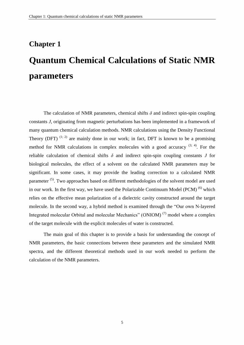
III.1.1 Double-zeta basis sets ........................................................................................ 43
III.1.2 Split valence basis sets ....................................................................................... 43
III.1.3 Polarization functions ......................................................................................... 43
III.1.4 Diffuse functions ................................................................................................ 44
III.2 The basis sets used in the present work ..................................................................... 44
III.2.1 Pople‟s basis sets ................................................................................................ 44
III.2.2 Polarization consistent basis sets ........................................................................ 45
III.2.3 Polarization consistent basis sets for J-couplings .............................................. 45

Table of contents
ii
IV Semi-empirical methods ................................................................................................... 46
V Polarizable continuum model PCM .................................................................................. 48
VI ONIOM model .................................................................................................................. 53
VI.1 Molecular mechanics ................................................................................................. 56
References ................................................................................................................................ 57
Chapter 2: Dynamical effects on NMR parameters ............................................................ 61
I Molecular dynamics .......................................................................................................... 62
I.1 Born-Oppenheimer molecular dynamics ................................................................... 62
I.2 Equations of motion of nuclei ................................................................................... 66
I.2.1 Time integration –Velocity Verlet method ............................................................ 67
I.3 Thermostat ................................................................................................................. 69
II Atom-centered density matrix propagation dynamics method ADMP ............................. 71
II.1 Scalar-mass ADMP ................................................................................................... 71
II.2 Constraints for the scalar-mass ADMP ..................................................................... 76
II.3 Mass-tensor ADMP ................................................................................................... 78
II.4 Constraints for the mass-matrix ADMP .................................................................... 80
III Vibrational corrections to NMR parameters - perturbation theory ................................... 82
III.1 Zero-point vibrational contributions .......................................................................... 82
III.2 Temperature effects ................................................................................................... 86
References ................................................................................................................................ 89
Chapter 3: Application on metabolites: results ................................................................... 91
A: Choice of a Strategy .......................................................................................................... 91
I NMR parameters ............................................................................................................... 92
I.1 Chemical shifts .......................................................................................................... 92
I.2 Indirect spin-spin coupling constants ........................................................................ 94
II Effects of functionals and basis sets - choice of a theoretical level of calculation ........... 96
II.1 Effects of functionals and basis sets: putrescine, as an example ............................... 97
II.2 Effects of functionals and basis sets: sarcosine, as an example .............................. 111
III Effects of isomers on NMR parameters .......................................................................... 116
III.1 Calculation of averaged chemical shifts: putrescine, as an example ....................... 119
III.2 Calculation of averaged indirect nuclear spin-spin coupling constants: putrescine, as
an example .......................................................................................................................... 124

Table of contents
iii
IV Vibrational effects on NMR parameters ......................................................................... 127
IV.1 Vibrational effects on chemical shifts: sarcosine, as an example ............................ 127
IV.1.1 Vibrational effects via classical mechanics - ADMP simulations ................... 127
IV.1.2 Vibrational effects via quantum mechanics ..................................................... 135
IV.2 Vibrational effects on spin-spin coupling constants: serine, as an example ........... 141
V Solvent effects on NMR parameters via ONIOM method .............................................. 148
VI Effects studied on NMR parameters ............................................................................... 151
References .............................................................................................................................. 152
B: Results in the form of published papers ........................................................................ 155
DFT calculations of isomer effects upon NMR spin-Hamiltonian parameters of prostate
polyamines ............................................................................................................................. 157
DFT calculations of 1H chemical shifts, simulated and experimental NMR spectra for
sarcosine ................................................................................................................................. 163
Solvent, isomers, and vibrational effects in DFT calculations for the NMR spin-Hamiltonian
parameters of alanine ............................................................................................................. 169
DFT calculations for the NMR spin-Hamiltonian parameters for serine ............................... 173
C: Synthesis of results .......................................................................................................... 179
References .............................................................................................................................. 183
Chapter 4: Model to predict NMR chemical shifts for biological molecules .................. 185
I Description of the model ................................................................................................. 186
II Illustrative results and discussion ................................................................................... 189
References .............................................................................................................................. 197
Conclusion and perspectives ............................................................................................... 199
Appendix A ........................................................................................................................... 203
Appendix B ............................................................................................................................ 205


Dedications
I would like to acknowledge that during this work, I was directed by Dr. Abdul-Rahman
ALLOUCHE. I thank him deeply for his guidance and patience.
I would also like to thank Dr. Monique AUBERT-FRÉCON for her support and assistance.
Dr. AUBERT-FRÉCON helped me, with patience, through her very contribution to the field
of theoretical study.
I thank the members of the jury because they have agreed to read my work and criticize it.
Besides, I thank all the members of our team.
I would like to dedicate this Doctoral dissertation to my parents who always encouraged
and supported me.
Finally, I would like to thank my husband, Dr. Mahdi, for his support and encouragement.
I couldn’t have completed this effort without his assistance, tolerance, and enthusiasm.


Introduction
1
Introduction
Nuclear magnetic resonance NMR was first described and measured in molecular
beams by Isidor Rabi in 1938, and in 1944 Rabi was awarded the Nobel Prize in physics for
his invention of the atomic and molecular beam magnetic resonance method of observing
atomic spectra.
Later, Felix Bloch and Edward Purcell noticed that magnetic nuclei, like 1H, could
absorb radio frequency (RF) energy when placed in a magnetic field of a strength specific to
the identity of the nuclei. When this absorption occurs, the nucleus is described as being in
resonance. Different atomic nuclei within a molecule resonate at different frequencies for the
same magnetic field strength. With this discovery, NMR was born and soon became an
important analytical method in the study of the composition of chemical compounds. For this
discovery, Bloch and Purcell were awarded the Nobel Prize in physics in 1952.
In 1991, Richard Ernst got the Nobel Prize in Chemistry for his contributions to the
development of the methodology of high resolution nuclear magnetic resonance (NMR)
spectroscopy. Later, Kurt Wüthrich was awarded the Nobel Prize in Chemistry in 2002 for his
development of nuclear magnetic resonance spectroscopy for determining the three-
dimensional structure of biological macromolecules in solution. One year later, in 2003, Paul
C. Lauterbur and Peter Mansfield got the Nobel Prize in Medicine for their discoveries
concerning magnetic resonance imaging (MRI).
After these discoveries, NMR became the premier organic spectroscopy available to
chemists to determine the detailed chemical structure of the chemicals they were synthesizing.
Besides, a well-known technique of NMR technology has been the Magnetic Resonance
Imaging (MRI), which is utilized extensively in the medical radiology field to obtain image
slices of soft tissues in the human body, offering by that a powerful new probe of the body's
internal anatomy and function. Magnetic resonance spectroscopy (MRS) complements MRI
as a non-invasive means for the characterization of tissue. While MRI uses the signal from
hydrogen protons from water to form anatomic images, MRS uses the signals from nuclei of
chemical molecules to determine the concentration of metabolites which are bio-markers of

Introduction
2
diseases in the tissue examined. Usually, in vivo MRS is used for detecting and quantifying
metabolites.
In MRS, the analysis of signals obtained from patients and based on a database of
prior knowledge about MRS-signals of metabolites is now very popular. The NMR related
database contains either the signals or the spectra of metabolites. The latter can be measured
in vitro or simulated from quantum mechanics. In the case of simulated database one needs
two types of spin-Hamiltonian parameters: chemical shifts δ and indirect spin-spin coupling
constants J, which characterize an MRS-signal. The parameters δ and J may be obtained from
two ways: (1) in vitro measurements of metabolite in solution, from which the determination
of chemical shifts is easy however the determination of spin-spin coupling constants is hard
and becomes impossible in the cases of complex multiplets, and (2) computer simulations
which are based on quantum chemistry calculations for the spin-Hamiltonian parameters and
are feasible for not too large molecules.
The present work aims to calculate, using the density functional theory, reliable 1H
NMR parameters of seven metabolites (putrescine, spermidine, spermine, acetate, sarcosine,
alanine, and serine). The three polyamines (putrescine, spermidine, spermine) and sarcosine
are considered as biomarkers of prostate cancer. While the concentrations of polyamines have
been shown to decrease in the presence of prostate cancer, the concentration of sarcosine has
been revealed to highly increase during prostate cancer progression and it can be detected in
urine. On the other hand, the three metabolites acetate, serine and alanine are biomarkers of
brain illnesses. The increased concentration of acetate allows the primary identification of
brain cancer.
Usually, NMR spectrum obtained for a tissue in the human body is very complex since
it corresponds to a large number of metabolites with overlapping NMR spectra. Thus, in order
to distinguish the presence or absence of a specific metabolite, its resonance peaks are
determined through simulation from NMR parameters and then they are used within
quantitation processes. One aim of this work is to simulate, for several metabolites of interest,
reliable theoretical NMR spectra.
In order to obtain NMR spectra in agreement with experiment, the present work tends
to study the effects of inclusion of isomer contributions from conformers of higher energy, in
the calculation of NMR parameters for metabolites. Besides, it aims to understand molecular
vibration and its effects on the calculated NMR parameters. Moreover, solvent effects are

Introduction
3
planned to be studied explicitly with water molecules around the metabolite and implicitly
using a continuum model.
The calculation of NMR parameters using quantum chemistry methods is feasible for
relatively small molecules, especially if the effects of solvent, isomers, and vibration are taken
into account. Unfortunately, high accuracy calculations are limited by the high computational
costs for many systems of interest (proteins, DNA, RNA ...) making large size molecules out
of reach of traditional quantum chemistry approaches. An alternative would be a model that
allows the predictions of parameters.
The second part of this work shall be devoted to put forward a model that allows the
prediction of chemical shifts of biological molecules. It must be general in the sense that it is
able to predict the chemical shifts for many types of nuclei (H, C, N) and for any biological
molecule (metabolites, proteins, DNA, RNA, ...) being small or large.
The present work is divided into four chapters, two of which present the theoretical
methods used in this work while the other two show the obtained results. The first chapter is
devoted to present the quantum chemical methods used in the calculation of NMR parameters
for motionless molecules while the second chapter presents the methods used to calculate the
dynamical effects on NMR parameters. The third chapter shows the results obtained for
metabolites, and the fourth chapter presents the model that allows the prediction of chemical
shifts for any biological molecule, including proteins.
In the first chapter, we shall present the concept of NMR parameters: chemical shifts
and indirect spin-spin coupling constants, derive their theoretical expressions, and show how
to simulate an NMR spectrum starting from its parameters. Then, we will shortly describe the
Density Functional Theory (DFT) chosen for the calculation of NMR parameters of
metabolites. After that, we will present the general basis sets and shed the light on those used
in the present work. This shall be followed by a rapid presentation of semi-empirical methods
that served in the calculation of some effects on the NMR parameters. The first chapter will
terminate by the two methods used for adding solvent, which are the Polarizable Continuum
Model (PCM) and Our own N-layered Integrated molecular Orbital and molecular Mechanics
(ONIOM) method.
The second chapter will differ from the first one in the sense that it will treat the
methods used to calculate the dynamical effects on NMR parameters. First, we shall present
Born-Oppenheimer molecular dynamics method used in the determination of conformers for a

Introduction
4
certain molecular geometry. A description of Berendsen thermostat, used in conserving a
constant temperature during molecular dynamics, will be given. This shall be followed by the
two methods used to study the molecular vibration which are Atom-centered density matrix
propagation dynamics method (ADMP), and the perturbative method.
The third chapter, divided into three parts A, B, and C, will display the results related
to metabolites. Part A will allow the choice of reliable methods to be used in the calculation
of NMR parameters for metabolites: theoretical method with DFT approach (functional/basis
set), and methods of calculation of different effects on NMR parameters (isomers, vibration,
and solvent). Part B will present the full results in a selection of our published papers. In part
C, a synthesis of all the results obtained for metabolites will be presented. It must be noted
that results given in part B will be complementary to results of part A, where in part A the
strategies of calculation shall be determined and in part B, results for metabolites using the
chosen strategies shall be displayed.
The fourth chapter will present a new model that we have developed, BioShift, which
can be used to predict chemical shifts for biological molecules (proteins, DNA, RNA,
polyamines). It shall be tested for proteins and compared to well-known models especially
designed for the prediction of chemical shifts of proteins. Bioshift will be also tested for small
molecules.
The present work terminates by a general conclusion and some perspectives that open
up new prospects in the calculation of NMR parameters.
Chapter 1: Quantum chemical calculations of static NMR parameters
5
Chapter 1
Quantum Chemical Calculations of Static NMR
parameters
The calculation of NMR parameters, chemical shifts δ and indirect spin-spin coupling
constants J, originating from magnetic perturbations has been implemented in a framework of
many quantum chemical calculation methods. NMR calculations using the Density Functional
Theory (DFT) (1; 2)
are mainly done in our work; in fact, DFT is known to be a promising
method for NMR calculations in complex molecules with a good accuracy (3; 4)
. For the
reliable calculation of chemical shifts δ and indirect spin-spin coupling constants J for
biological molecules, the effect of a solvent on the calculated NMR parameters may be
significant. In some cases, it may provide the leading correction to a calculated NMR
parameter (5)
. Two approaches based on different methodologies of the solvent model are used
in our work. In the first way, we have used the Polarizable Continuum Model (PCM) (6)
which
relies on the effective mean polarization of a dielectric cavity constructed around the target
molecule. In the second way, a hybrid method is examined through the “Our own N-layered
Integrated molecular Orbital and molecular Mechanics” (ONIOM) (7)
model where a complex
of the target molecule with the explicit molecules of water is constructed.
The main goal of this chapter is to provide a basis for understanding the concept of
NMR parameters, the basic connections between these parameters and the simulated NMR
spectra, and the different theoretical methods used in our work needed to perform the
calculation of the NMR parameters.

Chapter 1: Quantum chemical calculations of static NMR parameters
6
I NMR parameters: concept and theory
I.1 Parameters of NMR spectrum
Nuclear magnetic resonance spectroscopy provides detailed information on the
structure and dynamics of molecules through NMR spectra. In general, a NMR spectrum is
characterized by: i) a number of distinct signals, ii) hyperfine structure of individual signals,
iii) a signal intensity and line-width. Here, we are going to discuss the first two properties
while the third is out of our interest.
I.1.1 Signal position - chemical shift
A nucleus K of spin and gyromagnetic ratio is characterized by a magnetic
moment
(1.1)
where is the reduced Plank‟s constant. In the presence of an external magnetic field ,
nucleus K possesses an energy given by
(1.2)
In the case of a molecule placed in a magnetic field, electrons respond by creating
their own magnetic field proportional to . In other words, the electronic cloud around
nucleus K creates an induced magnetic field proportional to the electronic current (Biot
et Savart law (8; 9)
) which is, in turn, proportional to the external field.
(1.3)

Chapter 1: Quantum chemical calculations of static NMR parameters
7
where is the chemical shielding tensor of nucleus K. Note that is not necessarily
parallel or anti-parallel to . The induced field of electrons deshields the external magnetic
field and the effective magnetic field at the nucleus K differs from the applied field. The total
magnetic field at the nucleus K is
(1.4)
And hence the total energy becomes
(1.5)
The same nuclei in the molecule can in principle experience different effective magnetic
fields as a result of diverse chemical and structural environment.
The NMR spectrum is a record of the emission of electromagnetic radiation by a
nucleus at a given frequency of radiation. The signal position due to the radiation of nucleus K
with spin is defined by the resonance frequency (called the Larmor frequency), which
can be related to the magnetic field as
(1.6)
In the present work, we have studied the isotropic chemical shieldings of spin ½
nuclei, where an isotropic chemical shielding is calculated by averaging the trace of the
corresponding shielding tensor (equation (1.7)). Then, the Larmor frequency emitted by the
nucleus K of spin can be expressed in terms of the chemical shielding of the nucleus
K as in equation (1.8).
(1.7)
(1.8)

Chapter 1: Quantum chemical calculations of static NMR parameters
8
Equation (1.8) outlines the connection between chemical shieldings and experimental
NMR spectra. However, from an experimental point of view, the frequency axis in NMR
spectroscopy is a substantial problem because as can be seen from the above equation, the
resonance frequency depends on the magnitude of the magnetic field. Not only the resonance
frequencies acquired at different magnetic fields have to be scaled, but also the absolute
frequency scale (~106 Hz) is not appropriate for reporting NMR spectra. To solve these
problems at once, a relative scale was introduced and is called the chemical shift δ. The
chemical shift can be calculated for any nucleus according to equation (1.9).
(1.9)
In equation (1.9), is the resonance frequency of nucleus K for which the
chemical shift is to be calculated and is the resonance frequency of a given nucleus in a
standard substance. Usually, relative shifts for protons are calculated with respect to the
reference compound tetramethylsilane TMS which is chosen for chemical shift calculations in
the present work.
The chemical shift is usually expressed as the difference between chemical shieldings
of the reference nucleus and nucleus K (equation (1.10))
(1.10)
In equation (1.10), the assumption has been made, being ~10-5
. Chemical
shieldings and shifts are usually scaled with „ppm‟ (parts per million).

Chapter 1: Quantum chemical calculations of static NMR parameters
9
I.1.2 The hyper fine structure of the NMR signal - indirect spin-spin
interaction
By the hyperfine structure of a NMR signal, it is meant the fine splitting of resonance
peaks as a result of nuclear spin-spin interaction. There are two mechanisms: indirect and
direct spin-spin interaction. However, in isotropic solutions, rotational Brownian diffusion
averages the inter-nuclear direct spin-spin interactions to zero. In other words, in isotropic
solutions, these interactions do not affect the hyperfine structure of NMR signals. Thus, we
limit our study to indirect spin-spin interactions between nuclei.
The indirect spin-spin coupling (scalar coupling or J-coupling) is the effect of mutual
interaction between two nuclear spins mediated by electrons polarized by the nuclear
magnetic moments. Thus, indirect spin-spin couplings propagate along the chemical bonds;
however, their magnitude reduces dramatically as the number of bonds separating the nuclei
increases. The indirect spin-spin couplings depend on the local distribution of electrons in the
vicinity of the coupled nuclei; specific change of the electronic environment is reflected by a
change in J value. The J-coupling constant is a consequence of the nuclear magnetic moments
and is, therefore, independent of the external magnetic field. J-couplings are exhibited in
NMR spectra as the splitting of resonance lines of the coupled nuclei (see figure (1.1)).
Besides, J-coupling constants are scaled in Hz and their values can be either positive or
negative.
(i) (ii)
Figure 1.1: (i) resonance due to the emission of nuclei K & L with zero J-coupling, (ii) with non-zero J-coupling
Each NMR signal can be characterized, besides its position and hyperfine structure, by
its intensity and half-width. Both intensity and half-width are related to the relaxation

Chapter 1: Quantum chemical calculations of static NMR parameters
10
phenomena of nuclei; however, they were not studied here thoroughly.
I.2 Calculation of NMR parameters
As it was explained earlier, there are two types of NMR parameters that can be
calculated by quantum chemical methods and can be correlated with the signal position and
the hyperfine structure of a NMR spectrum: chemical shieldings and indirect spin-spin
coupling constants. Both parameters are second order molecular properties i.e. second order
partial derivatives of the energy.
NMR constants σ and J are tensors represented by matrices. Calculations
provide values for the six components of each tensor (six components instead of nine because
of symmetry). Besides, in isotropic solutions, an isotropic NMR parameter is calculated from
the trace of its corresponding tensor.
(1.11)
In the present work, we have considered isotropic values for and J represented by and J
respectively.
I.2.1 Chemical shift
I.2.1.1 GIAO method
It is known that when a system is placed in an external magnetic field, the canonical
momentum is replaced by the mechanical momentum in the quantum mechanical
equations for electrons, where is the fine structure constant, and is the vector
potential. Thus, for a hydrogen atom placed in a magnetic field , the electronic Hamiltonian
is given by

Chapter 1: Quantum chemical calculations of static NMR parameters
11
(1.12)
where is the electrostatic potential energy at position . The vector potential consists
of the external potential due to and the potential due to the magnetic moment of
nucleus K placed at position. . Note that the Hamiltonian is expressed in atomic units, in
which all the equations of section I.2.1.1 shall be given. Inserting in equation
(1.12), we obtain the corresponding Hamiltonian.
(1.13)
(1.14)
The homogenous magnetic field represented by the potential vector is clearly
independent of the gauge origin since . Thus, there is no unique choice of for
a given magnetic field . However, we would expect that values of observable quantities
(such as σ) do not depend on the chosen origin. This is true only in the limit case of exact
wavefunction. For the approximate solution of the electronic problem, the calculated
observable would be dependent on the choice of (10)
. This is a major problem for quantum
chemistry. The origin of this problem is due to the finite basis set representation used for
molecular orbitals. For atoms, there is no problem in using finite basis as long as the basis are
eigenfunctions of the angular momentum .
The Gauge origin problem in a molecule can be surmounted by using more than one
gauge origin for the external magnetic field. This is known as the local or distributed gauge
origins, which ensures a good description of magnetic interactions. The idea of distributed
origins can be achieved by introducing a gauge transformation of the wavefunction

Chapter 1: Quantum chemical calculations of static NMR parameters
12
(1.15)
where N is the number of electrons and is the number of fragments in a given system. The
gauge factor which is given by
(1.16)
shifts the gauge origin of a one electron wave function from to the gauge origin . is
the projector on the one electron subspace and on the local fragment A. Note that the above
transformation indeed defines a valid gauge transformation leaving for the exact
solution of the Schrödinger equation all physical observables invariant. This concept has first
been applied in the so-called GIAO method (Gauge Including Atomic Orbitals) (11; 12)
where to
each atomic orbital an individual gauge origin is associated.
Thus, the GIAO approach is based on choosing local gauge origins for atomic
orbitals . In addition, it is convenient to attach the additional phase factors to the atomic
orbitals instead of attaching them to the Hamiltonian. That means, the new AO that are called
gauge including atomic orbitals or London orbitals are field dependent, and they are given by
(1.17)
where denotes the usual field-independent atomic orbitals centered at and
represents the electron coordinates.

Chapter 1: Quantum chemical calculations of static NMR parameters
13
I.2.1.2 Shielding tensor calculation
We recall that when a magnetic field is applied to a molecule containing a magnetic
nucleus K with magnetic moment , its ground state energy changes due to the interaction
of the induced electronic currents with the nuclear magnetic moment and with the applied
field. For weak static perturbations, the molecular electronic energy , can be
expanded in a Taylor series around the unperturbed energy value. In this expansion, the term
bilinear in and will be exactly equal to the change in the nuclear Zeeman energy
resulting from interaction with the surrounding electrons. Therefore, the
Taylor coefficient given by a second derivative of the molecular electronic energy ,
with respect to the field strength and the nuclear magnetic moment can be identified with the
nuclear shielding tensor .
(1.18)
Equation (1.18) represents the good starting point for the evaluation of the components of the
chemical shielding tensor at the GIAO-DFT level which is mainly used in the present work.
The molecular electronic energy can be expressed as
(1.19)
(1.20)
where is the density matrix, is the one-electron Hamiltonian given previously in equation
(1.12), is the exchange-correlation energy in the framework of DFT method, is the one-
electron Kohn-Sham operator, and is the exchange-correlation piece of (for more

Chapter 1: Quantum chemical calculations of static NMR parameters
14
information about Kohn-Sham DFT see section II). The matrix elements of are given
by
(1.21)
where is the antisymmetrized two-electron integral over the atomic orbitals .
For Pure DFT methods, represents the Coulomb electrostatic energy while for hybrid
methods, it includes a coefficient for the Hartree-Fock exchange .
(1.22)
The coefficient is zero for pure DFT and non-zero for hybrid methods.
Now, using equation (1.18), the elements of the shielding tensor of nucleus K can be
derived from equation (1.19) with the help of the interchange theorem of perturbation theory
(13; 14).
(1.23)
In equation (1.23), are the elements of the one-electron Hamiltonian matrix and are
the elements of the density matrix in the atomic orbital representation. Then,
(1.24)
(1.25)
The density matrix of a closed shell molecule can be given in terms of the coefficients of the
expansion of the molecular orbitals in terms of the atomic orbitals .

Chapter 1: Quantum chemical calculations of static NMR parameters
15
(1.26)
Then,
(1.27)
To calculate the shielding tensor elements, the derivatives of the Hamiltonian are
needed. The Hamiltonian of equation (1.12) can be reformulated by inserting the explicit
form of the vector potential (equations (1.13) and (1.14)) and thus, the first and second
derivatives of (
and
) can be expressed in the atomic units as
(1.28)
(1.29)
where is the position of the electron, is the position of nucleus K, is the fine
structure constant, and is the Dirac delta function.
Equation (1.29) is true for field-independent basis functions; however, in the GIAO
approach, the basis functions are field dependent (see equation (1.17)) and thus, the derivation
with respect to includes additional terms.
(1.30)

Chapter 1: Quantum chemical calculations of static NMR parameters
16
Now, inserting equations (1.28) and (1.29) in (1.30), the expression of
can be obtained
which, if multiplied by , generates the first term of the chemical shielding (see equation
(1.23).
The second term of the nuclear magnetic shielding requires, in addition to the
derivative of the one-electron Hamiltonian given in equation (1.28), the derivative of the
density matrix with respect to the magnetic field.
(1.31)
The two terms
and
are easily obtained through the explicit
dependence of the atomic orbitals of the GIAO approach on the magnetic field (equation
(1.17)); however, the term
is obtained via the solution of the coupled-perturbed (CP)
equations (15; 16)
for which a brief description will be given in the part I.2.1.3.
I.2.1.3 Coupled perturbed equations
For a perturbed system, the expansion of the one-electron Hamiltonian and the
density matrix can be expressed as
(1.32)
(1.33)
where and are the unperturbed Hamiltonian and density matrix respectively, and
represents the external perturbation which is the magnetic field in the present case. The
perturbed density matrix obeys the two conditions:

Chapter 1: Quantum chemical calculations of static NMR parameters
17
(1.34)
(1.35)
where has been already defined in equation (1.20). In the first condition (equation
(1.34)) the density matrix commutes with , while in the second (equation (1.33)) it is
considered to be idempotent (17)
. These two conditions are sufficient and necessary to solve
for the perturbed density matrix. The change in cause a change in which can be also
expressed as a perturbation series.
(1.36)
where (1.37)
Inserting equations (1.33) and (1.36) into (1.34) and separating the orders, one obtains the
zeroth and first order equations.
(1.38)
(1.39)
Besides, inserting equation (1.33) in (1.35) and separating the orders, one finds by equating
the zeroth and first orders
(1.40)
(1.41)
Now, we define the projection operators and for the subspaces spanned by the
occupied orbitals and the ( ) empty orbitals respectively.
(1.42)
(1.43)

Chapter 1: Quantum chemical calculations of static NMR parameters
18
Using the projection operators, any matrix can be resolved into the sum of four
projected parts ( ). Then, an equation is equivalent to the four
equations .
Projecting equation (1.41) and taking into account the projection operator properties
( and for ), one finds that the (11) and (22) components of the first-
order change must vanish while the (12) and (21) components are Hermitian conjugate. Then,
can be expressed as
(1.44)
To determine
, we use the projection of equation (1.39).
(1.45)
Equation (1.45) can be rewritten as
(1.46)
Starting with
in the right hand side, the solution of
can be calculated iteratively
where its formal solution can be expressed as
(1.47)
However, from equation (1.37),
depends on
thus, the equation (1.47) has to be
solved iteratively till convergence.
may be determined more conveniently in terms of the
eigenvectors of ; this may be done (17)
by writing in terms of its eigenvalues and the
projection operators of the eigenvectors.

Chapter 1: Quantum chemical calculations of static NMR parameters
19
(1.48)
where is the projection operator for the eigenvector . In addition, the projection
operators and can be expressed as and
. Now, taking
advantage of the fact that , equation (1.47) can be rewritten as
(1.49)
This expression is a geometric series with respect to ; it converges to give the form
(1.50)
Once
is obtained, can be easily calculated from equation (1.44).
(1.51)
In our calculations of chemical shielding tensor, we were in need for the derivative of
the density matrix with respect to the magnetic field (
) which is represented by in the
coupled perturbed equations while stands for
.

Chapter 1: Quantum chemical calculations of static NMR parameters
20
Usually, the orthonormality of the molecular orbitals is considered as an additional
constraint added directly to the electronic energy. Then, the equation (1.19) can be rewritten
in a more convenient way as
(1.52)
where is demonstrated to be a diagonal matrix whose diagonal elements are the orbital
energies (18)
, and is the overlap matrix given by
(1.53)
As a result, the constraint term added in equation (1.52) gives a new expression for
.
(1.54)
and
are given by
(1.55)
(1.56)

Chapter 1: Quantum chemical calculations of static NMR parameters
21
(1.57)
(1.58)
Note that equation (1.54) must be solved iteratively because
and
depend on each other.
I.2.2 Indirect spin-spin coupling constant J
Consider a molecular system, where the nuclear magnetic moments are given by .
It is evident that electrons will interact with the nuclear magnetic moments. These interactions
are tiny relative to the electrostatic interactions between the electrons and nuclei and are
therefore adequately described by perturbation theory. For closed-shell molecules, there is no
first order change in the electronic energy. To second order, the change is described in terms
of the reduced indirect spin-spin coupling tensor KPQ.
(1.59)
where denotes the collection of all magnetic moments in the molecule. Therefore, the
KPQ tensor (describing the coupling between nuclei P and Q) is simply given by
(1.60)
The spectroscopically observed indirect NMR spin-spin coupling tensor JPQ is

Chapter 1: Quantum chemical calculations of static NMR parameters
22
proportional to the reduced tensor KPQ. JPQ is also calculated as the mixed second order
partial derivative of the total electronic energy E with respect to the nuclear magnetic
moments and of the coupled nuclei P and Q.
(1.61)
where h is plank‟s constant, and are the gyromagnetic rations of P and Q. The
corresponding scalar spin-spin coupling constant is one third of the trace of this tensor i.e. the
average of the diagonal elements of .
As a result of the magnetic hyperfine coupling of the nuclear spin to the orbital motion
of the electrons and to the spin of the electrons, four additional terms must be added to the
Hamiltonian.
(1.62)
First, the spin-orbit SO coupling represents the interaction between the nuclear
magnetic moments and the orbital magnetic moments of electrons. There are two spin-orbit
operators: the diamagnetic SO (DSO) operator and the paramagnetic SO (PSO) operator.
Next, the interaction between nuclear and electronic spin magnetic moments leads to
the Fermi contact (FC) term and the spin-dipole (SD) term. While the FC operator represents
the interaction at the position of the nucleus, the SD operator represents the interaction at a
distance.
The expression of given in the equation (1.62) can be rewritten in such a way that
the nuclear magnetic moments are shown explicitly.
(1.63)
The factor of i has been introduced to make the operator real. However, can be expressed

Chapter 1: Quantum chemical calculations of static NMR parameters
23
in terms of one-particle operators , , , and .
(1.64)
Note that is a tensor while the three operators , , and are vectors. These
four operators are given, in the atomic units, by
(1.65)
(1.66)
(1.67)
(1.68)
where I is unit matrix, is the fine structure constant, is the
relative position with respect to the nucleus P, is the electron spin, and is the Dirac
delta function. Similarity, the isotropic reduced coupling constant can be decomposed into
four components related to the four coupling mechanisms (19)
.
(1.69)
(1.70)
(1.71)
(1.72)

Chapter 1: Quantum chemical calculations of static NMR parameters
24
(1.73)
where is the ground-state wavefunction for while is the perturbed
wavefunction by the magnetic moment of nucleus Q (X stands for PSO, FC, or SD), and is
the density of the unperturbed state.
For the calculation of using the density functional theory (see part II), equation
(1.60) is a good starting point. The magnetic field generating from the magnetic moments of
nuclei leads to four additional terms in the DFT energy corresponding to the four additional
terms in the Hamiltonian of equation (1.62), which can be expressed in terms of one-particle
operators (equations (1.65) – (1.68)).
(1.74)
(1.75)
(1.76)
(1.77)
(1.78)
where is the spin-orbital defined by with denoting the space orbital and
denoting the two dimensional spinor. Now, evaluating the energy derivative of equation
(1.60) for the DFT energy, the contributions to the isotropic reduced coupling constant can be
given by
(1.79)

Chapter 1: Quantum chemical calculations of static NMR parameters
25
(1.80)
(1.81)
(1.82)
where represents the ground-state spin-orbitals for while
represents the
perturbed spin-orbitals by the magnetic moment of nucleus Q. The first order spin-orbitals are
given, using the standard perturbation theory, by
(1.83)
where the sum runs over virtual orbitals, X stands for PSO, FC, or SD, and are the
unperturbed energies corresponding to the spin-orbitals and
respectively, and is
the first-order-term of the perturbed Kohn-Sham (KS) (see part II.3) operator which is solved
iteratively.
(1.84)
Indirect scalar spin-spin coupling constants are often dominated by the FC
contributions. However, all four contributions to the spin-spin coupling constants should be
considered in any attempt to have a quantitative accuracy; the PSO, DSO and SD
contributions may often be small but can rarely be neglected.

Chapter 1: Quantum chemical calculations of static NMR parameters
26
I.3 Simulation of the NMR spectrum starting from its
parameters σ and J
In all our work, we have studied proton NMR spectra, which is the application of nuclear
magnetic resonance with respect to hydrogen. Here, we will discuss the simulation of proton
NMR spectra starting from known parameters. Once σ and J are calculated for a given
molecule, we can simulate the NMR spectrum. This allows the comparison with experimental
spectrum as well as the analysis of the NMR spectra obtained from patients using a basis of
metabolites.
A proton is a charged particle of spin it generates a magnetic moment along its
axis of rotation. The magnitude of the magnetic moment in any given direction has two equal,
but opposite, observable values ( and – ) that correspond to the spin quantum
numbers. Thus, if a proton is found in a magnetic field along z-direction, it can be regarded as
to line up with the field ( ) or against the field ( ). The magnetic moment of
a proton cannot be detected experimentally unless the proton is placed in an external magnetic
field; we recall that the energy of the nucleus in this case is given by
(1.85)
and the Hamiltonian can be written in the form (20)
(1.86)
The notation represents the up and down spins and B is the strength of the field at the
nucleus. It is good to introduce at this point suitable wave functions to describe the magnetic
states of individual nuclei (protons). The spin wavefunction is assigned to the nucleus with
and the wavefunction to the nucleus with . Taking the shielding tensor
into account would just require the replacement of the magnetic field by its new value
where is the applied magnetic field; then, for example, the energy
corresponding to the wavefunction becomes .

Chapter 1: Quantum chemical calculations of static NMR parameters
27
For a molecule having many protons, it is more convenient to analyze the over-all
energy levels of the molecule. If we have N protons and each proton has two magnetic states,
possible combinations of the spin quantum numbers are found. The Hamiltonian
describing this system can be given by
(1.87)
where is the hamiltonian due to the shielding at nucleus k (equation (1.86)) and is the
spin-spin interaction operator between nuclei and . The spin-spin Hamiltonian has the form
(1.88)
where is the coupling spin-spin constant, and is a permutation operator that
interchanges possible pairs of the specified index numbers of the nuclei in product wave
functions.
The total wave function, describing the group of N protons, cannot be expressed as the
product of the individual wave functions of nuclei when these nuclei are identical. It is
impossible to designate which members of equivalent nuclei have and which
members have . This problem is solved by forming wavefunctions as a combination
of equivalent states.
For example, for a two nucleus molecule, four possible wavefunctions describing the
nuclei 1 & 2 are possible
(1.89)

Chapter 1: Quantum chemical calculations of static NMR parameters
28
The problem lies in states and which are equivalent. We cannot differentiate which
nucleus has a spin up and which one has a spin down. This problem is solved by introducing
the mixed total wavefunction
(1.90)
where and are the mixing coefficients. The energy of this state is given by
(1.91)
Two mixed states must replace the equivalent states and . These states are determined
once the coefficients a and b are known. This is done using the variational method where the
maximum and minimum values for are calculated. In other words, and values are
obtained by solving and . This gives
(1.92)
Non trivial solutions for and (
) can be obtained by equating to zero the following
determinant
(1.93)
which leads to two values for . Inserting these values in equation (1.92) and taking in
consideration the normalization condition which forces that , one obtains the
eigenvector . Simplifying calculations, the energies of the four states can be all gathered in
a single determinant.

Chapter 1: Quantum chemical calculations of static NMR parameters
29
(1.94)
This can be generalized to N proton molecule with
(1.95)
Note that the matrix is symmetric and that = number of possible states.
Diagonalizing this matrix leads to the energy values and eigenvectors. Once the energies are
determined, we can calculate the energies of emission i.e. the difference in E between states
where the transition is allowed. Let be the sum of of the N protons. An allowed transition
between two states requires that changes by one unit ( ). Proceeding in that way,
the NMR spectrum for the molecule under study can be obtained.
II Density functional theory DFT
In the present work, the theoretical calculation of NMR parameters, accomplished
with the help of the equations given in section I, is done using the density functional theory
that showed, in the last few years, a remarkable success in the calculation of NMR parameters
(4) .
Density Functional Theory (DFT) is a theoretical method that derives properties of the
molecule based on a determination of the electron density of the molecule. There are roughly
three categories of density functional methods: (i) Local density approximation (LDA) which
assume that the density of the molecule is uniform throughout the molecule (21; 22)
, (ii)
Gradient corrected (GC) methods which account on the non-uniformity of the electron
density (23)
, (iii) Hybrid methods which attempt to incorporate some of the more useful

Chapter 1: Quantum chemical calculations of static NMR parameters
30
features from ab initio methods (specifically exchange contributions from Hartree-Fock
methods) as improvements of the functionals used in DFT, such as B3LYP (24; 25)
which is the
most commonly used functional in our computational work.
One advantage of DFT is that it is a general-purpose method, and can be applied to
most systems. DFT methods are now implemented in most popular software packages,
including Gaussian which we have used in our calculations.
On the other hand, one of the main disadvantages of DFT methods is the challenge in
determining the most appropriate functional for a particular application. In our practice, we
conclude that the B3LYP functional (together with the 6-311++G** basis set) can be
considered to be a good choice for calculating NMR parameters (see chapters IV and V).
In this section, we will describe the remarkable theorems of DFT which allow us to
find ground-state properties of a system without dealing directly with the many-electron
wavefunction .
In what follows, equations are given in atomic units ( ) such that
m and e are the electron‟s mass and charge, and a0 is Bohr‟s radius. We will deal with a
system of N electrons moving in a static potential, and adopt a conventional normalization in
which .
II.1 Theory of the density matrix
For a system of N electrons, the electronic wavefunction depends on 4N parameters; in
fact, to each electron there correspond four parameters (three due to its position and one due
to its spin). To simplify the notations, spin variable will not be explicitly indicated in this
section and the electronic wavefunction will be written as .
The electronic Hamiltonian describing the system is given by
(1.96)

Chapter 1: Quantum chemical calculations of static NMR parameters
31
In equation (1.96), riA is the distance between i-th electron and A, rij is the distance between
the i-th electron and the j-th electron, and ZA is the mass of nucleus A. Thus, T represents the
kinetic energy of electrons, Vext denotes the external potential on electrons due to the nuclei,
and Vee represents the electron-electron interactions. Thus, the electronic energy E calculated
from the Hamiltonian given in equation (1.96) depends on 4N parameters as a result of its
relation with the wavefunction.
(1.97)
The theory of the density matrix (26)
was elaborated to simplify the general expression
of the energy through reducing the number of variables. The density matrix for a system of N
particles is defined as the product of the wavefunction with its complex conjugate and it is
given by
(1.98)
Besides, the reduced density matrix of order p ( which describes the density of the
N particles taken in groups of p particles is defined as
(1.99)
where the binomial coefficient is the number of ways of choosing p particles from N,
taking the indistinguishable arrangements into consideration. Thus, the density matrix reduced
to one particle (1-RDM) is
(1.100)
If 1-RDM is restricted to its diagonal, we obtain the electronic density of one particle in the
element of volume (equation (1.100)).

Chapter 1: Quantum chemical calculations of static NMR parameters
32
(1.101)
The reduced density matrix to two particles (2-RDM) restricted to its diagonal gives the
density of electron 1 in the element of volume and the density of electron 2 in the element
of volume .
(1.102)
Implementing 1-RDM and 2-RDM in the general definition of the electronic energy (equation
(1.97)), Hohenberg and Kohn (27)
were able to express the energy as a functional of the
electronic density.
(1.103)
(1.104)
We conclude that the diagonal elements of the first and second order density matrices
(1-RDM and 2-RDM) completely determine the total energy. This appears to vastly simplify
the task in hand. Thus, the solution of the full Schrödinger equation for is not required to
find the total energy, and it is sufficient to determine and . By that, the problem in a
space of 3N coordinates has been reduced to a problem in a 6 dimensional space.
Approaches based on the direct minimization of suffer from the specific
problem that the density matrices must be constructible from an antisymmetric wavefunction
This constraint is non-trivial and it is currently an unsolved problem (28)
. In view of this,
we conclude that equation (1.104) does not lead immediately to a reliable method for
computing the total energy without calculating the many body wavefunction.

Chapter 1: Quantum chemical calculations of static NMR parameters
33
The observation which underpins density functional theory is that we do not even
require to find ; the ground state energy is completely determined by the diagonal
elements of the first order density matrix.
II.2 The Hohenberg-Kohn theorems
DFT was not put on a firm theoretical footing until the two theorems of Hohenberg-
Kohn (H-K) (27).
The first theorem demonstrates the existence of one-to-one mapping between the
ground state electronic density and the ground state wavefunction of a many-particle
system, and that all ground state properties can be expressed as a functional of this density.
Besides, it can be shown that there exists one external potential Vext which generates this
electronic density.
(1.105)
In equation (1.105), we denote by E0 the ground state energy, T the kinetic energy, and Eee the
interelectronic energy. The two terms T and Eee form the functional of Hohenberg and Kohn
FHK. This functional is universal for all systems having N electrons although its analytical
global expression is not known yet. While the kinetic energy expression T remains an
unsolved problem, the electron-electron term Eee is decomposed into two contributions: the
classic term (Coulombic repulsion) and the quantum term (exchange-correlation interaction).
The second H-K theorem proves that the ground state density minimizes the total
electronic energy of the system. In other words, the ground state energy can be calculated
using the variational principle applied to the energy with respect to the electronic density.
(1.106)
Traditional methods in electronic structure theory, in particular Hartree-Fock theory,

Chapter 1: Quantum chemical calculations of static NMR parameters
34
are based on the complicated many-electron wave function. The main objective of the density
functional theory is to replace the many-body electronic wave function by the electronic
density as the basic quantity. DFT exploits the advantages of the density which is a simple
quantity to deal with.
II.3 Theory of Kohn and Sham
To apply the DFT formalism one obviously needs good approximations for the
functional . For example, obtaining an expression for the kinetic energy of
interacting electrons in terms of the charge density is a hard problem. This yields some
difficulties in calculating the ground state energy. In 1965, Kohn and Sham (K-S) (29; 26)
proposed a new method to calculate the ground state electronic energy. Within the framework
of Kohn-Sham, the problem of interacting electrons situated in a static external potential Vext
is reduced to a problem of non-interacting electrons moving in an effective potential Vs. In
other words, a fake system which is composed of N non-interacting fermions is constructed;
in which its density and total energy are the same as the real system. One main advantage of
this scheme is that it allows a straightforward determination of a large part of the kinetic
energy in a simple way. Another advantage, from a more physical point of view, is that it
provides an exact one-particle picture of interacting electronic systems. This then provides a
rigorous basis for the one-particle arguments used in solid state physics and chemistry to
explain and predict certain features of chemical bonding.
Figure 1.2: a cartoon representing the relationship between the real many body system (left hand side) and the
non-interacting system of Kohn-Sham Density Functional Theory (right hand side)

Chapter 1: Quantum chemical calculations of static NMR parameters
35
We introduce a non-interacting N-particle system with ground state density ρ and
external potential Vs. The ground state is a Slater determinant (30)
of N orbitals satisfying
the equation
(1.107)
If we apply the first theorem of Hohenberg-Kohn to this non-interacting system, we
find that there is, at most, one external potential Vs which generates ρ, and for a given ground
state density ρ, all the properties of the system can be determined. This is in particular true for
the kinetic energy Ts[ρ] and the total energy E[ρ] which are given by
(1.108)
(1.109)
On the other hand, we recall that for the real system, the operators and are
universal for all systems, while the external potential is system dependent. Vext is
generated by the system‟s nuclei which are considered to be fixed according to the Born-
Oppenheimer approximation (31)
, and the energy associated with the real system is
(1.110)
Defining J[ρ] as the classic Coulombic interaction between electrons, it can be written as
(1.111)
where is the non-classical energy composed of the exchange energy, the

Chapter 1: Quantum chemical calculations of static NMR parameters
36
Coulomb correlation, and correlation of self-interaction. Then, the energy of the real system
(equation (1.110)) can be expressed as the sum of two terms: the analytically calculable part
and the exchange correlation part.
(1.112)
where the exchange correlation energy is given by
(1.113)
Thus, the exact energy of the real system can be finally written under the form
(1.114)
Since an analogue is considered between the fake and the real systems, their densities
and energies are identical. Hence, the expression of the energy of the fake system (equation
(1.109)) can be implemented in equation (1.114).
(1.115)
Applying, to equation (1.115), the variational principle with respect to the electronic density,
one finds
(1.116)
(1.117)

Chapter 1: Quantum chemical calculations of static NMR parameters
37
Once the expression of is determined (equation (1.117)), Kohn-Sham equations
(equation (1.107)) can be solved where their solutions, i.e. the different orbitals , satisfy the
two conditions
(1.118)
The obtained orbitals, which are solutions to the KS operator F, can produce the electronic
density of the system. However, the obtained value of results in a new value of (
depends on ). And, for a new , Kohn-Sham equations need to be solved again giving new
orbitals , which ends up with a new value of .
The problem of solving Kohn-Sham equations has to be done in a Self-Consistent
Field SCF i.e. iterative way. Usually, one starts with an initial guess for , then calculates
the corresponding and solves the Kohn-Sham equations for . From these, one calculates a
new density and starts again. This procedure is then repeated until convergence is reached and
the ground state density is calculated. From the calculated value of , the ground state energy
of the molecular system can be easily computed (equation (1.114)).
Kohn-Sham molecular orbitals are usually expanded as a linear combination of atomic
orbitals (LCAO) (32)
.
(1.119)
The coefficients are the weights of the contributions of the atomic orbitals to the
orbitals . The atomic basis function are one-electron functions centered on nuclei of the
component atoms of the molecule. The atomic orbitals used are typically those of hydrogen-
like atoms since these are known analytically i.e. Slater-type orbitals but other choices are
possible like Gaussian functions from standard basis sets. Thus, we conclude that the
appropriate choice of the basis sets is very important in solving Kohn-Sham equations and
thus, in calculating the different molecular properties, the chemical shieldings and J-couplings
in our case. Section III shall be devoted to describe the basis sets used in the present work.

Chapter 1: Quantum chemical calculations of static NMR parameters
38
II.4 Exchange correlation functionals
We recall that the exchange-correlation energy contains Fermi correlation between
electrons of the same spin, the correlation of self-interaction, Coulomb correlation between
electrons of opposite spin and the difference in the kinetic energy between the fake and the
real system (equation (1.113)). However, the exchange-correlation energy is conventionally
split into two parts: the exchange part and the correlation part.
(1.120)
The major problem with DFT is that the exact functionals for exchange and correlation
are not known. In fact, Vs cannot be calculated if Vxc is not known (equation (1.117)) which
prevents solving the Kohn-Sham equations.
Over the years, many approximate exchange-correlation functionals have been
developed and tested. In the absence of a single, universal function, some of these are better
suited than others in calculating certain physical quantities. We shall here describe the main
classes of exchange-correlation functionals, discussing briefly the functionals used in the
present work (PBE, OPBE, B3LYP, and PBE0). Three approximations of the exchange-
correlation energy are described: (i) the local density approximation, (ii) the generalized
gradient approximation, and (iii) the hybrid approximation.
II.4.1 Local density approximation
The most famous approximation of Exc is the local density approximation (LDA) (21; 22)
which is the simplest approximation for the exchange-correlation energy. One advantage of
this approximation is that it makes the system easier to solve (or more precisely, require less
computation). In LDA, the exchange-correlation energy of an electronic system is constructed
by assuming that the exchange-correlation energy per electron at a point in the electron gas,
, is equal to the exchange-correlation energy per electron in a homogeneous electron
gas that has the same electron density at the point . Then, LDA is local in the sense that the

Chapter 1: Quantum chemical calculations of static NMR parameters
39
electron exchange-correlation energy at any point in space is a function of the electron density
at that point only.
(1.121)
LDA has been very successful in solid state physics but less so in chemistry, being less
accurate than ab initio wavefunction theory. The LDA exchange-correlation functional is
usually constructed by combining the Dirac-Slater exchange functional
(33; 34) with the
Vosko-Wilk-Nusair correlation functional
(35) (SVWN functional), a parameterization
based on accurate simulations of the uniform electron gas (36)
.
The local spin-density approximation (LSDA) (37)
is a generalization of the LDA to
include the electron spin.
(1.122)
II.4.2 Generalized gradient approximation
The LDA uses the exchange-correlation energy for the uniform electron gas at every
point in the system regardless of the homogeneity of the real density. For nonuniform
densities, the exchange-correlation energy can deviate significantly from the uniform result.
This deviation can be expressed in terms of the gradient and higher spatial derivatives of the
total density. The generalized gradient approximation (GGA) (23)
uses the gradient of the
density to correct for this deviation. Thus, GGA is local but it takes into account, in addition
to the density, the gradient of this density at the same coordinate.
(1.123)
With the emergence of GGA and the development of gradient-corrected exchange-
correlation functionals, Kohn-Sham theory became competitive with the wavefunction theory.
A commonly used GGA exchange correlation functional is the Perdew-Burke-Enzerhof

Chapter 1: Quantum chemical calculations of static NMR parameters
40
(PBE) functional (23; 38)
. PBE is based on the properties of the slowly varying electron gas.
Another known functional is the OPBE which is the result of combining the newly developed
exchange functional OPTX (39; 40)
with PBE.
II.4.3 Hybrid functionals
Hybrid functionals incorporate a portion of exact exchange from Hartree-Fock theory
together with exchange and correlation from other sources (such as LDA or GGA). The
Hartree-Fock exchange energy is calculated as, for a N electron molecule
(1.124)
The popular B3LYP functional is mainly used in the present work for the calculation
of NMR parameters for different metabolites and it is given by
(1.125)
where , , and are three empirical parameters determined by
fitting the predicted values to a set of atomization energies, ionization potentials, proton
affinities, and total atomic energies; the local density approximation to the exchange-
correlation energy is given by
;
is the Becke 88
(41) exchange functional and
is the LYP (Lee, Yang, Parr) (42; 43)
correlation functional.
Another well-known hybrid functional is the PBE0 (44; 45)
(sometimes called
PBE1PBE) which is a non-empirical functional based on PBE with 25% of the exact
exchange.

Chapter 1: Quantum chemical calculations of static NMR parameters
41
III Basis sets
From section II, we found that one important task in performing electronic structure
calculations is the choice of the exchange-correlation functional. Another important task is the
choice of a basis set for expanding the molecular orbitals (here Kohn-Sham orbitals). A large
basis set is expected to provide accurate results but also requires a large computational cost. A
small basis set, on the other hand, is computationally efficient but introduces inaccuracies in
the results. It is therefore desirable to have a sequence of basis sets such that the accuracy can
be controlled and at the same time being as compact as possible. In our study, we have tested
three groups of basis sets in order to choose the most appropriate in calculating NMR
parameters. In this part, we will present these types of basis sets having the notations X-YZG,
pc-n, and pcJ-n.
Basis sets were first developed by Slater. The expression of Slater Type Orbitals
(STO) (46)
given in its Cartesian form is
(1.126)
where N is the normalization constant, is the orbital exponent which accounts for how
diffuse (large) the orbital is, and x, y, and z are the Cartesian coordinates.. The quantities m, n,
and o are integers such that m + n + o = l, the atomic orbital quantum number. When m + n +
o = 0, then STO is a s-type Gaussian function; when m + n + o = 1, then STO is a p-type
orbital; and when m + n + o = 2, the STO is a d-type Orbital. Molecular calculations using
STO‟s can be very tedious due to the evaluation of two-electron multicenter molecular
integrals involving more than two atoms.
An alternative to STO is the Gaussian Type Orbital (GTO) given by
(1.127)

Chapter 1: Quantum chemical calculations of static NMR parameters
42
where α is the orbital exponent and m + n + o = l, the atomic orbital quantum number. When
m + n + o = 0, then GTO is said to be a s-type Gaussian function; when m + n + o = 1, then
GTO is a p-type Gaussian; and when m + n + o = 2, then GTO is a d-type Gaussian.
Notice that the difference between the STO and GTO is in the exponential part. The
product of two GTOs is another GTO and by that, calculations of the needed integrals become
analytical, which represents a huge practical advantage as compared to STOs. However, some
accuracy is lost by using GTOs so that a significantly larger number of GTOs than STOs is
necessary to achieve a similar accuracy. Typically one STO should be replaced by at least
three GTOs, this corresponds to a STO-3G basis set. To bypass this disadvantage i.e to
reduce the number of primitive Gaussians to be fully treated, contracted Gaussian functions
(that still approximate Slater-type orbitals) can be constructed as linear combinations of
primitive Gaussian functions with different values of α.
(1.128)
The values of the contraction coefficients dwi and the orbital exponent α are obtained by fitting
a contracted Gaussian function to a STO or by finding the contracted Gaussian functions that
minimize the self-consistent-field energies of atoms.
III.1 Extended basis sets
The minimal basis set is the minimum number of basis functions needed to describe
the ground state of atoms in a molecule ex: The minimal basis for C atom (1s2, 2s
2, 2p
2)
contains 5 basis functions:1s, 2s, 2px, 2py, 2pz.. Beyond the minimum number of basis
functions required to describe each atom, extra basis functions, if added, introduce the
extended basis sets. There are different types of extended basis sets: multiple-zeta (double,
triple, etc), split-valence, including polarization and/or diffuse functions.
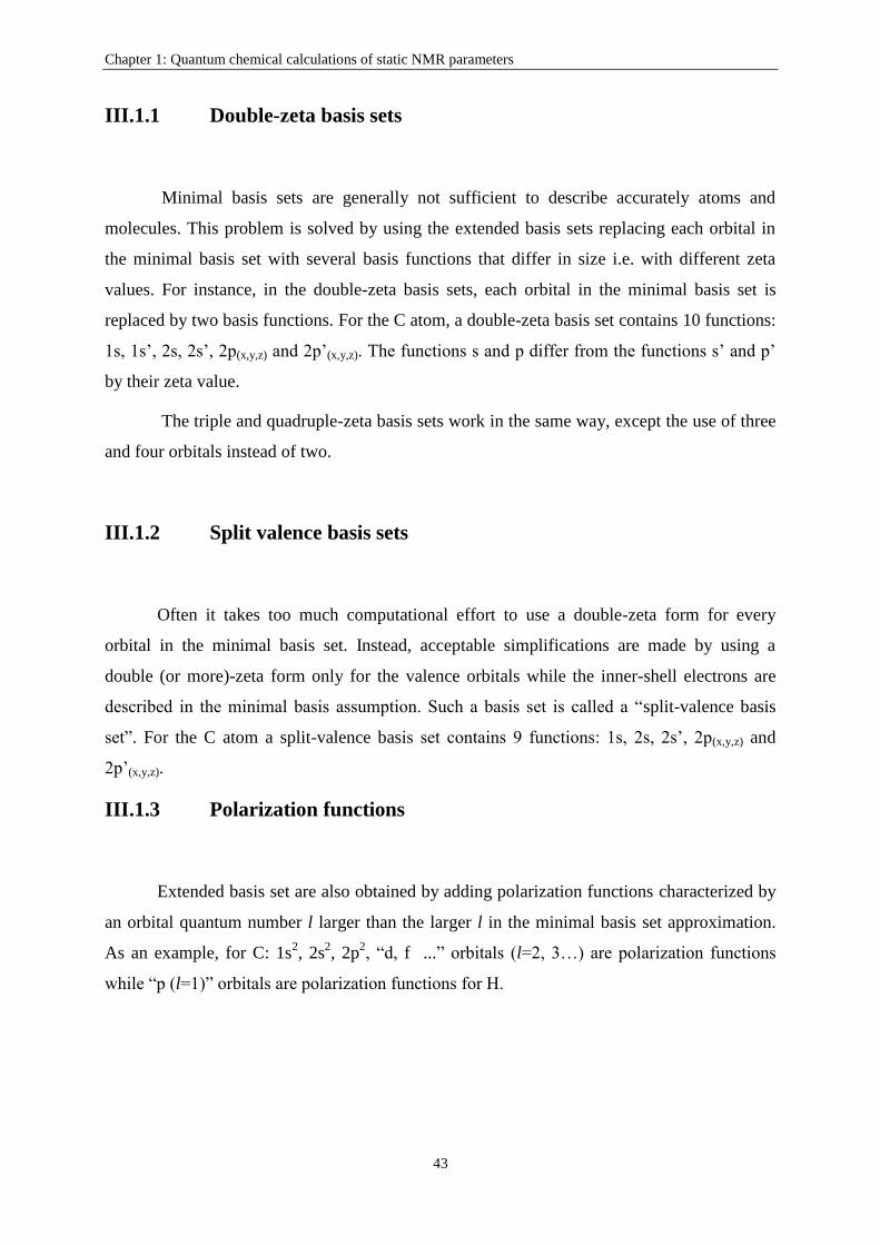
Chapter 1: Quantum chemical calculations of static NMR parameters
43
III.1.1 Double-zeta basis sets
Minimal basis sets are generally not sufficient to describe accurately atoms and
molecules. This problem is solved by using the extended basis sets replacing each orbital in
the minimal basis set with several basis functions that differ in size i.e. with different zeta
values. For instance, in the double-zeta basis sets, each orbital in the minimal basis set is
replaced by two basis functions. For the C atom, a double-zeta basis set contains 10 functions:
1s, 1s‟, 2s, 2s‟, 2p(x,y,z) and 2p‟(x,y,z). The functions s and p differ from the functions s‟ and p‟
by their zeta value.
The triple and quadruple-zeta basis sets work in the same way, except the use of three
and four orbitals instead of two.
III.1.2 Split valence basis sets
Often it takes too much computational effort to use a double-zeta form for every
orbital in the minimal basis set. Instead, acceptable simplifications are made by using a
double (or more)-zeta form only for the valence orbitals while the inner-shell electrons are
described in the minimal basis assumption. Such a basis set is called a “split-valence basis
set”. For the C atom a split-valence basis set contains 9 functions: 1s, 2s, 2s‟, 2p(x,y,z) and
2p‟(x,y,z).
III.1.3 Polarization functions
Extended basis set are also obtained by adding polarization functions characterized by
an orbital quantum number l larger than the larger l in the minimal basis set approximation.
As an example, for C: 1s2, 2s
2, 2p
2, “d, f ...” orbitals (l=2, 3…) are polarization functions
while “p (l=1)” orbitals are polarization functions for H.

Chapter 1: Quantum chemical calculations of static NMR parameters
44
III.1.4 Diffuse functions
The loosely bond electrons in an atom are sometimes important in calculating some
quantities. To treat correctly this long-range area, very important for instance for van der
Waals systems or anions, computations can use added diffuse functions i.e. functions with
very small exponents.
III.2 The basis sets used in the present work
III.2.1 Pople’s basis sets
The notation for the split-valence basis sets arising from the group of John Pople (47)
is
typically X-YZG in which G indicates that Gaussian functions are used. In this case, the core
orbitals are composed of X primitive Gaussian functions. Besides, the valence orbitals are
composed of two basis functions; the first one is composed of a linear combination of Y
primitive Gaussian functions, and the other is composed of a linear combination of Z
primitive Gaussian functions. However, the valence orbitals can be represented by more than
two basis functions, so that the notation becomes X-YZU…G.
For example, the 6-311G basis set has one contracted Gaussian function that is a linear
combination of six primitive Gaussian functions for each inner-shell atomic orbital and three
basis functions, one contracted Gaussian function that is a linear combination of three
primitive Gaussians and two primitive Gaussian functions, for each valence orbital.
In standard notations of atomic basis sets, one asterisk (*) at the end of the name of a
Pople‟s basis set denotes that polarization has been taken into account in the 'p' orbitals by
adding a 'd' orbital. Two asterisks (**) means that polarization has been taken into account for
the 's' orbitals too by adding a 'p'. Besides, diffuse basis sets are represented by the '+' signs.
One '+' means that we are accounting for the diffuse 'p' orbitals, while '++' signals that we are
accounting for both 'p' and 's' diffuse orbitals.
Several Pople‟s basis sets were used and tested in NMR calculations in the present
work some of which are 6-311+G**, 6-311++G**, 6-311++G(2d,2p), and 6-
311++G(3df,3pd). The notation (2d,2p) in the basis set 6-311++G(2d,2p) means that

Chapter 1: Quantum chemical calculations of static NMR parameters
45
polarization has been taken into account for the 'p' orbitals by adding two 'd' orbitals, and for
the 's' orbitals by adding two 'p' orbitals. Besides, the notation (3df,3pd) in the basis set 6-
311++G(3df,3pd) means that polarization has been taken into account for the 'p' orbitals by
adding three 'd' orbitals and one 'f' orbital, and for the 's' orbitals by adding three 'p' orbitals
and one 'd' orbital.
III.2.2 Polarization consistent basis sets
Some of the most widely used basis sets are those developed by Dunning and
coworkers (48; 49)
, since they are designed to converge systematically to the complete-basis-set
(CBS) limit. However, these correlation-consistent polarized (cc-p) basis sets were developed
for wavefunction based methods including electron correlation. These basis sets have the
notation (cc-pVXZ) where X stands for D,T,Q,5,6,... (D=double, T=triples, etc.), Z means
zeta, and V indicates valence basis sets. In analogy with cc-pVXZ basis sets and for
independent particle models, such as DFT, the polarization consistent basis sets (50; 51)
(pc-n)
were developed to provide a fast and controlled convergence towards CBS. In pc-n basis sets,
n indicates the level of polarization beyond the atomic system i.e. pc-0 is unpolarized, pc-1 is
of double zeta quality with a single polarization function, pc-2 is of triple zeta quality with d-
and f-type polarizations, etc.
Both (cc-pVXZ) and (pc-n) have been constructed using energetic criteria such that
the functions contributing similar amounts of energy are included at the same stage. Besides,
both are able to optimize polarization exponents for systems and augment with full set of
diffuse functions and also with tight functions (pcJ-n) (52)
. In our work, we have tested pc-n
basis set for n=0, 1, 2, 3.
III.2.3 Polarization consistent basis sets for J-couplings
After developing the basis sets (pc-n), it was found that the basis set convergence for
calculating nuclear spin-spin couplings can be improved by adding a single p-type function
with a large exponent (tight function) and allowing for a slight decontraction of the p-

Chapter 1: Quantum chemical calculations of static NMR parameters
46
functions. This resulted in the (pcJ-n) basis sets (polarization consistent basis sets for the
calculation of J-couplings). In our work, we have tested pcJ-n basis set for n=0, 1, 2, 3.
IV Semi-empirical methods
Semi-empirical calculations are set up with the same general structure as Hartree-Fock
HF calculations based on a wavefunction formulism. Within this framework, certain pieces of
information are approximated or completely omitted in the semi-empirical approach. Usually,
the core electrons are not included in the calculation and only a minimal basis set is used.
Also, some of the two-electron integrals are omitted and a large number of multicenter
integrals in the electronic repulsion term are neglected. In order to correct for the errors
introduced by omitting part of the calculation, the method is parameterized. Often, these
parameters replace some of integrals that are excluded. Parameters to estimate the omitted
values are obtained by fitting the results to experimental data or ab initio calculations
The good side of semi-empirical calculations is that they are much faster than the ab
initio calculations while the bad side lies in the results that can be sometimes erratic. If the
molecule under study is similar to molecules in the data base used to parameterize the
method, then the results may be very good; if not, the answers may be poor.
Modern semi-empirical models are based on the Neglect of Diatomic Differential
Overlap (NDDO) (53)
method in which the overlap matrix is replaced by the unit matrix
( with the j-th basis vector). This allows one to replace the Hartree-Fock
equation with a simpler equation . Approximations are also made
when evaluating one- and two-electron integrals. Semi-empirical models based on NDDO
differ by these approximations and by the parametrization philosophy.
The Modified Neglect of Diatomic Overlap (MNDO (54)
) method is the oldest NDDO-
based model that parameterizes one-center two-electron integrals based on spectroscopic data
for isolated atoms, and evaluates other two-electron integrals using the idea of multipole-
multipole interactions from classical electrostatics. The main advantage of MNDO over
earlier methods was that the values of the parameters were optimized to reproduce molecular
rather than atomic properties. When it first appeared, MNDO was immediately popular

Chapter 1: Quantum chemical calculations of static NMR parameters
47
because of its increased accuracy but afterwards, various limitations were found, such as the
inability to describe the hydrogen bond.
In 1985, an attempt, AM1 (Austin Model 1 (55)
) was made to improve MNDO by
adding a stabilizing Gaussian function to the core-core interaction to represent the hydrogen
bond. The modification resulted in non-physical attractive forces that mimic van der Waals
interactions.
In the next years, improvements led to the PM3 (Parametric Method 3 (56)
) method
where various changes to the original set of approximations used in MNDO were proposed.
PM3 uses a Hamiltonian that is very similar to the AM1 Hamiltonian, but the
parameterization strategy is different. While AM1 is parameterized largely based on small
number of atomic data, PM3 is parameterized to produce a large number of molecular
properties.
The previous semi-empirical methods tried to improve NDDO through the
modification of approximations and the extension to specific elements. Then came the PM6
(parametric method 6 (57)
) method that was set for three reasons: (i) to investigate the
incorporation of some of the reported modifications to the core-core approximations into the
NDDO methodology, (ii) to carry out an optimization of all main group elements (with
emphasis on compounds of interest in biochemistry), and (iii) to extend the methodology by
performing a restricted optimization of parameters for transition metals. Because of its
construction and parameterization for more than 80 elements, PM6 method was found to be
superior to other similar methods; in particular, PM6 corrects major errors in AM1 and PM3
calculations.
Semi-empirical methods allow treating quantum systems with a relatively large size in
a rather cheap way. Then, these methods can be used for studies requiring the repetition of
many quantum computations.

Chapter 1: Quantum chemical calculations of static NMR parameters
48
V Polarizable continuum model PCM
In vitro experimental spectra are often taken for molecules in solution (D2O), and then
any comparison between experimental and theoretical spectra requires that solvent effects be
taken into account in the theoretical study. For that, solvent effects on NMR parameters are
studied in the present work using two methods: an explicit method and an implicit one. In the
explicit method, solvent molecules surrounding the target molecule are considered during
calculation while in the implicit model, solvent molecules are replaced by their charges and
the interaction between the target molecule and these charges is considered. This section shall
be devoted to discuss the implicit model.
Since the number of solvent molecules that needs to be considered to adequately
represent the solvent is very large, this difficulty can be overcome by treating the surrounding
medium (or solvent) as a continuum having an effective dielectric constant while the solute
is treated quantum mechanically. One method that uses this technic is called the Polarizable
Continuum Model (PCM) (58; 59; 60)
that seems to be very effective in studying solvent effects.
Figure 1.3: schematic representation of PCM model
A molecule M in a solution can be seen as if placed in a cavity surrounded by a
polarizable dielectric medium. The electrostatic potential of the whole system (molecule +
medium) is the sum of electrostatic potential generated by the charge distribution of the
molecule and the reaction potential generated by the polarization of the dielectric
medium

Chapter 1: Quantum chemical calculations of static NMR parameters
49
(1.129)
where the molecular charge distribution contains both the electronic density (given as
in Kohn-Sham equations) and the nuclear distribution .
(1.130)
The general equation of Poisson which is given by
(1.131)
can be divided into two parts corresponding to inside and outside the cavity.
(1.132)
(1.133)
Using boundary conditions on the cavity surface, one finds
(1.134)
(1.135)
where is the out-ward pointing vector perpendicular to the cavity surface. The first
condition (equation (1.134)) expresses the continuity of the potential across the surface while
the second condition (equation (1.135)) involves the discontinuity of the component of the
field that is perpendicular to the cavity surface. Equation (1.135) can be rewritten as

Chapter 1: Quantum chemical calculations of static NMR parameters
50
(1.136)
This difference between the normal components of electric fields at the boarder inside
and outside the cavity, allows introducing an auxiliary quantity which is the surface charge
distribution spread on the cavity surface (C). The symbol denotes the position variable
and it is used to emphasize that this charge distribution is limited to (C). This approach of
solvation methods is called the Apparent Surface Charge method (ASC). In such method, the
potential due to the solvent is defined as
(1.137)
In the ASC approach, the source of the solute potential is reduced to a charge
distribution limited to a closed surface. This simplifies the electrostatic problem with respect
to other formulations in which the whole dielectric medium is considered as the source of the
reaction potential. Despite this remarkable simplification, the challenge remains in the
integration of over a surface of complex shape. The solution lies in the discretization of
the integral into a finite number of elements.
The cavity surface (C) is approximated in terms of a set of finite elements (called
tesserae) small enough to consider almost constant within each tessera. With
completely defined point by point, it is possible to define a point charge, , at the position
in the area such that . Then, equation (1.137) becomes
(1.138)
Once the point charges on the surface (C) are defined, the potential can be easily obtained.
In what follows, we shall not make use of the point charges but we will use instead the
original ones in terms of .
The electric medium is characterized by a polarization function proportional to the

Chapter 1: Quantum chemical calculations of static NMR parameters
51
external field; however, it can be given by the gradient of the potential vector .
(1.139)
Besides, the charge density is related to the normal component of the electric polarization
and it is given by
(1.140)
Now, substituting equation (1.135) in equation (1.140), one finds the expression of the surface
charge density in terms of internal potential
(1.141)
with
(1.142)
The calculation of can be done in an iterative way. For a given electronic
density , we start with a value of which gives a value of (equation (1.137)) which is
in turn inserted in equation (1.141) to give another new value of . This is repeated until
convergence for is obtained.
For the molecular system with electronic density , PCM model introduces the
interaction between ρ and (noted ). This interaction energy is added to the unperturbed
energy to form the total electronic energy of the molecule.
(1.143)

Chapter 1: Quantum chemical calculations of static NMR parameters
52
where is the unperturbed electronic energy given in equation (1.114). This introduces to
the Kohn-Sham equations a new term added to the external potential such that
(1.144)
Note that the added term is σ dependent. The problem of solving the Kohn-Sham equation has
now to be done in a self-consistent way taking into consideration the new perturbation
resulting from the solvent effect. The converged σ obtained from the iteration of equation
(1.141) is inserted into equation (1.144) which leads to a new electronic density ρ. The new
value of ρ is reinserted in equation (1.141) and iterations continue until convergence is
achieved.
Figure 1.4: the solvent excluding surface used in the calculation of electrostatic energy using PCM model
Energy terms are calculated using the solute cavity obtained as a set of interlocking
van der Waals spheres centered at the atomic positions. These spheres are located on the
heavy (that is non-hydrogen) elements only. In our calculations, we have used the United
Atomic Topology Model (UA0) (61)
which is applied using the atomic radii of the Universal
Force Field (UFF) (62)
. In this model, the electrostatic energy is calculated using the
solvent excluding surface which is an approximate surface found by multiplying the radii by a
constant factor (in general 1.1). Basically, this leads to obtain proper radii for each non-
hydrogen atom.
Solvent accessible surface
Solvent excluded surface
Solvent
molecules
Solvent excluded surface
Solvent accessible surface

Chapter 1: Quantum chemical calculations of static NMR parameters
53
VI ONIOM model
In the explicit method of solvation, solvent molecules surrounding the target molecule
are taken explicitly into account during calculations which means dealing with large-size
systems. Unfortunately, for these large-size molecular systems, high accuracy calculation
levels are limited by the high computational costs.
One way to overcome these limitations is hybrid methods which allow the
combination of two or more computational techniques in one calculation making it possible to
investigate large systems with high precision. The region of the system of interest is treated
with an accurate method while the remainder of the system is treated at a lower level. The
advantages of such methods is that they allow the combination of an accurate quantum-
mechanical description with the low computational cost of classical mechanics, provide a
realistic description for the site of interest, and permit a detailed analysis of the role of the
environment.
Here, we are going to focus on Gaussian's hybrid method called ONIOM (Our own N-
layered Integrated molecular Orbital and molecular Mechanics (63; 64)
). It is a general method
that can combine any number of molecular orbital methods (quantum mechanics QM (65)
) as
well as molecular mechanics (MM (66)
) methods (MM will be discussed later).
In ONIOM calculations, the molecular system under investigation is usually divided into
two or three regions that are treated at different levels of accuracy:
1. The higher layer is the smallest one, and it is treated with the most accurate method. This
layer is also called Model System (MS).
2. The low layer consists of the entire molecule. This layer is usually treated with an inexpensive
level of calculation (MM, semi-empirical method ..)
3. The Middle layer which is only present in a 3-layer ONIOM model. It is treated with a
method that is intermediate in accuracy between the high level method and the low level
method.
The entire molecule is referred to as the Real System (R). In the present work, the 2-layer
ONIOM method is used.

Chapter 1: Quantum chemical calculations of static NMR parameters
54
Figure 1.5: 2-layer assignment. The different visualizations (wire-frame and ball-stick) correspond to the low
and high layers respectively.
Figure 1.6: The Real and Model Systems
The ONIOM method works by approximating the energy of the Real System as a
combination of the energies computed by less computationally expensive means. In a two-
layer ONIOM calculation, the energy is computed as the energy of the Model System adding
two types of corrections:
1. due to the size difference between the model system and the real system
2. due to the high accuracy method used for the model system
(1.145)
The Real system contains all the atoms and is calculated only with the low accuracy
+

Chapter 1: Quantum chemical calculations of static NMR parameters
55
method. The Model System contains the part of the system that is treated at the high accuracy
method. Both low and high accuracy calculations need to be carried out for the Model system.
Note that in the ONIOM expression, all three sub-calculations are on complete systems.
Besides, when there is a bonded interaction between the two regions, the model system
includes a hydrogen link atom to saturate the open valence.
If a Quantum Mechanics method is combined with Molecular Mechanics, calculations
are referred to as QM:MM (64)
calculations. When the ONIOM (QM:MM) scheme is applied
using equation (1.145), the interaction between the two regions is included via MM
calculations and therefore follows the mechanical or classical embedding formalism. This
includes the electrostatic interaction which is evaluated as the interaction of the MM partial
charges with partial (point) charges assigned to the atoms in the QM region.
However, ONIOM calculations can optionally take advantage of electronic embedding
which enables both steric and electrostatic properties of the entire molecule to be taken into
account. In this technique, the charge distribution of the MM region interacts with the actual
charge distribution of the QM region; the partial charges from the MM region are included in
the QM Hamiltonian, which provides a more accurate description of the electrostatic
interaction and allows the wave function to respond to the charge distribution of the MM
region.
The most important consideration when planning an ONIOM study is the selection of
the various layers used in calculation. The general principle to keep in mind is that the model
system contains the chemically active portion. Besides, bond breaking or formation should
not take place within the MM region and atoms linked by double or triple bonds should be
placed within the same ONIOM region. Moreover, to be completely safe, the model system
must be extended three bonds from any connectivity change. This last advice ensures that
ONIOM energy remains continuous despite the changes in the connectivity during the
reaction.
In fact, standard MM methods cannot handle bond breaking and forming, and a
discontinuity in the potential function is observed. Thus, in QM:MM calculations, for the
ONIOM surface to be continuous during a chemical reaction, the MM contribution to the
energy must be continuous. The MM contribution is defined as the S-value where the ONIOM
energy can be written as

Chapter 1: Quantum chemical calculations of static NMR parameters
56
(1.146)
(1.147)
The S-value describes the contribution from the MM region, which includes both the energy
of the MM region as well as the interaction between the QM region and the MM region.
VI.1 Molecular mechanics
Molecular mechanics (MM (66)
) allows the calculation of structural and
thermodynamic properties of molecular systems composed of thousands of atoms. In MM
calculations, electrons are not treated explicitly as in quantum mechanics; atoms are
represented by charged masses related to each other by means of springs. Unlike in QM
calculations where the energy is found by solving Schrodinger equation, in MM calculations
the energy of molecular systems is described by empirical functions. The parameters of these
empirical functions, which are usually derived from experiments or precise quantum-chemical
calculations, form a force field. An example of a typical force field, Amber field (67)
, is of the
form
(1.148)
The first three terms describe the bonded interactions, formed by all the bonds, angles,
and dihedrals that are present in the system. The number of bonded terms scales linearly with
the size of the system. The last term describes the non-bonded interaction between each pair
of atoms in the system. The van der Waals interaction
and the Coulomb
interaction are scaled by the factors and
respectively. The number of
non-bonded terms scales quadratically with the size of the system.

Chapter 1: Quantum chemical calculations of static NMR parameters
57
References
1. Density Functional Theory. R. Dreizler, and E. Gross. 1995, Plenum Press, New York.
2. A Chemist's Guide to Density Functional Theory. W. Koch, and M. C. Hothausen. 2002, Wiley-
VCH, Weinheim.
3. Theoretical Chemistry Accounts. A. Bagno, and G. Saielli. 2006, Theor. Chem. Acc., Vol. 117, p.
603.
4. Calculation of NMR and EPR Parameters: Theory And Applications. M. Kaupp, M. Buhl, and V.
G. Malkin. 2004, Wiley-VCH.
5. A theoretical study of the NMR spin-spin coupling constants. J. Autschbach, and B. Le Guennic.
2003, J. Am. Chem. Soc., Vol. 125, p. 13585.
6. Quantum mechanical continuum solvation models. J. Tomasi, B. Mennucci, and R. Cammi. 2005,
Chem. Rev., Vol. 105, p. 2999.
7. Combining quantum mechanics methods with molecular mechanics methods in ONIOM. T. Vreven,
K. S. Byun, I. Komaromi, S. Dapprich, J. A. Montgomery, K. Morokuma, and M. J. Frisch.
2006, Chem. Theory and Comput., Vol. 2, p. 815.
8. Classical electrodynamics. J.D.Jackson. 1999, Wiley, New York. 0-471-30932-X.
9. Lehrbuch der theoretischen physik. L.D. Landau, and E.M. Lifschitz. 1981, Akademie-Verlag,
Berlin, p. 120.
10. Ab initio calculations of molecular properties. W.Kutzelnigg. 1989, J. Mol. Struct.Theochem,
Vol. 202, p. 11.
11. Théorie quantique des courants interatomiques dans les combinaisons aromatiques. F.London.
1937, J. Phys. Radium, Vol. 8, p. 397.
12. Efficient Implementation of the Gauge-Independent Atomic Orbital Method for NMR Chemical
Shift Calculations. K. Wolinski, J. F. Hinton, and P. Pulay. 1990, J. Am. Chem. Soc., Vol. 112, p.
8251.
13. Methods of molecular quantum mechanics. R.McWeeny. 1989, Academic Press, New York.
14. The variation method in quantum chemistry. S.T.Epstein. 1974, Academic Press, New York.
15. Advanced quantum chemistry. H.F.Hameka. 1963, Addision-Wesley, New York, p. 162.
16. Self-consistent Perturbation Theory of Diamagnetism. I. A Gauge-Invariant LCAO (Linear
Combination of Atomic Orbitals) Method for NMR Chemical Shifts. R.Ditchfield. 1974, R. Mol.
Phys., Vol. 27, p. 789.
17. Perturbation Theory for the Fock-Dirac Density Matrix. R.McWeeny. 1962, Phys. Rev, Vol. 126,
p. 1028.

Chapter 1: Quantum chemical calculations of static NMR parameters
58
18. Modern Quantum Chemistry. A. Szabo, and N. S. Ostlund. 1989, Mc Graw-Hill, New York.
19. Electron Coupled Interactions between Nuclear Spins in Molecules. N.F.Ramsey. 1953, Phys.
Rev., Vol. 91, p. 303.
20. Valence. C.A.Coulson. 1952, Oxford University Press, London.
21. Density functional theory of atoms and molecules. R. G. Parr, and W. Yang. 1994, Oxford
University Press. ISBN 978-0-19-509276-9.
22. Note on exchange phenomena in the thomas-fermi atom. Dirac. 1930, Proc. Cambridge Phil. Roy.
Soc, Vol. 26, p. 376.
23. Generalized gradient approximation made simple. J. P. Perdew, K. Burke, and M. Ernzerhof.
1996, Phys. Rev. Lett., Vol. 77, p. 3865.
24. Development of the Colle-Salvetti correlation-energy formula into a functional of the electron
density. C. Lee, W. Yang, and R. G. Parr. 1988, Phys. Rev. B, Vol. 37, p. 785.
25. A new mixing of Hartree–Fock and local density‐functional theories. A.D.Becke. 1993, J. Chem.
Phys., Vol. 98, p. 5648.
26. Density functional theory of atoms and molecules. R. G. Parr, and W. Yang. 1989, Oxford
University Press, New York.
27. Inhomogeneous Electron Gas. P. Hohenberg, and W. Kohn. 1964, Phys. Rev., Vol. 136, p.
B864.
28. Density Matrices and Density Functionals. V. H. Smith, and E. Erdahl. 1987, Reidel, Dordrecht.
29. Self-Consistent Equations Including Exchange and Correlation Effects. W. Kohn, and L. J.
Sham. 1965, Phys.Rev. A, Vol. 101, p. A1133.
30. The theory of complex spectra. Slater, J. 1929, Physical Review, Vol. 34, p. 2.
31. M. Born, and J. R. Oppenheimer. 1927, Ann. Phys., Vol. 84, p. 457.
32. Inorganic Chemistry: Principles of Structure and Reactivity. J.Huheey. 1972, Harper & Row.
33. P.A.Dirac. 1930, Proc. Cambridge Philos. Soc., Vol. 26, p. 376.
34. A Simplification of the Hartree-Fock Method. J.C.Slater. 1951, Phys. Rev., Vol. 81, p. 385.
35. Accurate spin-dependent electron liquid correlation energies for local spin density calculations: a
critical analysis. S. H. Vosko, L.Wilk, and M. Nusair. 1980, Can. J. Phys., Vol. 58, p. 1200.
36. Ground State of the Electron Gas by a Stochastic Method. D. M. Ceperley, and B. J. Alder.
1980, Phys. Rev. Lett., Vol. 45, p. 566.
37. Spin-Density Gradient Expansion for the Kinetic Energy. G. L. Oliver, and J. P. Perdew. 1982,
Phys. Rev. A, Vol. 20, p. 397.
38. Errata: Generalized gradient approximation made simple. J. P. Perdew, K. Burke, and M.
Ernzerhof. 1997, Phys. Rev. Lett., Vol. 78, p. 1396.

Chapter 1: Quantum chemical calculations of static NMR parameters
59
39. Left-right correlation energy. N. C. Cohen, and A. J. Handy. 2001, Mol. Phys., Vol. 99, p. 403.
40. Assessment of a new local exchange functional OPTX. W. M. Hoe, A. Cohen, and N. C. Handy.
2001, Chem. Phys. Lett., Vol. 341, p. 319.
41. Density-functional exchange-energy approximation with correct asymptotic-behavior. A.D.Becke.
1988, Phys. Rev. A, Vol. 38, p. 3098.
42. Development of the Colle-Salvetti correlation-energy formula into a functional of the electron
density. C. Lee, W. Yang, and R. G. Parr. 1988, Phys. Rev. B, Vol. 37, p. 785.
43. Results obtained with the correlation-energy density functionals of Becke and Lee, Yang and Parr.
B. Miehlich, A. Savin, H. Stoll, and H. Preuss. 1989, Chem. Phys. Lett., Vol. 157, p. 200.
44. Toward reliable density functional methods without adjustable parameters: The PBE0 model. C.
Barone, and V. Adamo. 1999, J. Chem. Phys., Vol. 110, p. 6158.
45. Atoms, molecules, solids, and surfaces: Applications of the generalized gradient approximation for
exchange and correlation. J. P. Perdew, J. A. Chevary, S. H. Vosko, K. A. Jackson, M. R.
Pederson, D. J. Singh, and C. Fiolhais. 1992, Phys. Rev. B, Vol. 46, p. 6671.
46. Atomic Shielding Constants. J.C.Slater. 1930, Phys. Rev., Vol. 36, p. 57.
47. The performance of the Becke—Lee—Yang—Parr (B—LYP) density functional theory with various
basis sets. Peter M. W. Gill, Benny G. Johnson, and John A. Pople. 1992, Chem. Phys. Lett., Vol.
197, p. 499.
48. Gaussian basis sets for use in correlated molecular calculations. I. The atoms boron through neon
and hydrogen. T.H.Dunning. 1989, J. Chem. Phys., Vol. 90, p. 1007.
49. Gaussian basis sets for use in correlated molecular calculations. V. Core‐valence basis sets for
boron through neon. D. E. Woon, and T. H. Dunning. 1995, J. Chem. Phys., Vol. 103, p. 4572.
50. Polarization consistent basis sets: principles. F.Jensen. 2001, J. Chem. Phys., Vol. 115, p. 9113.
51. Erratum: ―Polarization consistent basis sets: Principles‖. F.Jensen. 2002, J. Chem. Phys., Vol.
116, p. 3502.
52. The basis set convergence of spin−spin coupling constants calculated by density functional
methods. F.Jensen. 2006, J. Chem. Theo. Comp., Vol. 2, p. 1360.
53. Approximate Molecular Orbital Theory. J. Pople, and D. Beveridge. 1970, McGraw-Hill.
54. Ground states of molecules. 38. The MNDO method. Approximations and parameters. M. J. S.
Dewar, and W. Thiel. 1977, Journal of the American Chemical Society, Vol. 99, p. 4899.
55. Development and use of quantum mechanical molecular models. 76. AM1: a new general purpose
quantum mechanical molecular model. M. J. S. Dewar, E. G. Zoebisch, E. F. Healy, and J. J. P.
Stewart. 1985, Journal of the American Chemical Society, Vol. 107, p. 3902.
56. Optimization of Parameters for Semi-Empirical Methods I-Method. J.J.P.Stewart. 1989, J.
Comput. Chem., Vol. 10, p. 209.

Chapter 1: Quantum chemical calculations of static NMR parameters
60
57. Optimization of parameters for semiempirical methods V: Modification of NDDO approximations
and application to 70 elements. J.J.P.Stewart. 2007, J. Mol. Model., Vol. 13, p. 1173.
58. Quantum mechanical continuum solvation models. J. Tomasi, B. Mennucci, and R. Cammi.
2005, Chem. Rev., Vol. 105, p. 2999.
59. Electrostatic interaction of a solute with a continuum. A direct utilizaion of AB initio molecular
potentials for the prevision of solvent effects. S. Miertus, E. Scrocco, and J. Tomasi. 1981, Chem.
Phys., Vol. 55, p. 117.
60. Analytical Second Derivatives of the Free Energy in Solution by Polarizable Continuum models.
M. Cossi, and V. Barone. 1998, J. Chem. Phys., Vol. 109, p. 6246.
61. A new definition of cavities for the computation of solvation free energies by the polarizable
continuum model. V. Barone, M. Cossi, and J. Tomasi. 1997, J. Chem. Phys., Vol. 107, p. 3210.
62. Excited states and solvatochromic shifts within a nonequilibrium solvation approach: A new
formulation of the integral equation formalism method at the self-consistent field, configuration
interaction, and multiconfiguration self-consistent field level. B. Mennucci, R. Cammi, and J.
Tomasi. 1998, J. Chem. Phys., Vol. 109, p. 2798.
63. A new ONIOM implementation in Gaussian98. Part I. The calculation of energies, gradients,
vibrational frequencies and electric field derivatives. S. Dapprich, I. Komaromi, K.S. Byun, K.
Morokuma, and M.J. Frisch. 1999, Journal of Molecular Structure THEOCHEM, Vol. 461, p. 1.
64. Hybrid Methods: ONIOM(QM:MM) and QM/MM. T. Vreven, and K. Morokuma. 2006, Annual
Reports in Computational Chemistry, Vol. 2, p. 35.
65. Introduction to Quantum Mechanics. Griffiths, and J. David. 2004, Prentice Hall. ISBN 0-13-
111892-7.
66. Molecular Mechanics. N. L. Allinger, and U. Burkert. 1982, An American Chemical Society
Publication. ISBN 0-8412-0885-9.
67. A Second Generation Force Field for the Simulation of Proteins, Nucleic Acids, and Organic
Molecules. W. D. Cornell, P. Cieplak, C. I. Bayly, I. R. Gould, K. M. Jr. Merz, D. M. Ferguson,
D. C. Spellmeyer, T. Fox, J. W. Caldwell, and P. A. Kollman. 1995, J. Am. Chem. Soc., Vol. 117,
p. 5179.

Chapter 2: Dynamical effects on NMR parameters
61
Chapter 2
Dynamical Effects on NMR Parameters
For the reliable calculation of NMR parameters, we have taken into account, in
addition to solvent effects, the effects of isomers and vibration.
The effect of isomers originates from the fact that at ambient temperature, not only
ground-state molecules may be present but also excited molecules of higher energy. Here, we
are interested in the stable spatial isomers. The presence of isomers at ambient temperature
affects the experimental NMR spectra. Thus, isomer effects must be taken into account in the
theoretical calculation of NMR parameters to ensure a fair comparison between experimental
and simulated spectra. The conformation research for isomers is done using Born-
Oppenheimer molecular dynamics (1)
(MD) simulations where the potential energy of atoms is
calculated semi-empirically based on the PM6 method. Isomer effects are calculated in the
present work assuming a Boltzmann distribution. The averaged NMR parameter ( or ) is
calculated as an average of the NMR parameter of the various isomers weighted by
Boltzmann factor.
The vibrational effects on the NMR parameters are the result of the molecular
vibration which is available even at a temperature of zero absolute. NMR parameters often
show a strong dependence on the molecular geometry, and studies have demonstrated that the
effects of molecular motion may change NMR properties by more than 10% (2)
. In the present
work, vibrational effects are calculated using two approaches based on different
methodologies. In the first way, the atom-centered density matrix propagation (ADMP (3; 4; 5)
)
method is used. In the second way, vibrational effects are calculated quantum-mechanically
through a perturbative method (6)
that we have implemented in Gaussian (7)
.
This chapter is devoted to describe the three main methods: MD, ADMP, and the
perturbative method for vibrational corrections to NMR parameters.

Chapter 2: Dynamical effects on NMR parameters
62
I Molecular dynamics
One of the principle tools in the theoretical study of biological molecules is the
method of molecular dynamics (MD) simulation. This computational method calculates the
time dependent behavior of a molecular system. MD simulations provide detailed information
on the conformational changes of many molecules of interest, and thus, they have been used
in the present work to search for isomers.
I.1 Born-Oppenheimer molecular dynamics
The Schrödinger equation is usually so complex that it can be solved only for a few
simple cases. Therefore, to describe the dynamics of molecular systems, approximation
procedures are used to simplify the problem; one of these approximations is that of Born-
Oppenheimer. The idea is to split the Schrödinger equation, which describes the state of both
the electrons and nuclei, into two coupled equations. The influence of the electrons on the
motion of nuclei is then described by an effective potential which results from the solution of
the electronic Schrödinger equation. As a further approximation, the nuclei move according to
the classical Newton‟s equations using effective potentials which result from quantum
mechanical computations or empirical potentials.
Starting from the non-relativistic time-dependent Schrödinger equation of a molecular
system,
(2.1)
we express the total wavefunction as a function of electronic degrees of freedom ,
nuclear degrees of freedom , and time . The total molecular Hamiltonian is the sum of
kinetic energy of the atomic nuclei, kinetic energy of the electrons, interelectronic repulsion,
electronic – nuclear attraction, and internuclear repulsion

Chapter 2: Dynamical effects on NMR parameters
63
(2.2)
where is the electronic Hamiltonian. Clearly, an exact solution of equation (2.1) is not
possible and approximations must be made.
To derive the Born-Oppenheimer approximation, one uses the fact that the difference
in masses between electrons and atomic nuclei is large. Due to this difference, the ratio of the
velocity of a nucleus to the velocity of an electron is in general smaller than 10-2
.
Therefore, one assumes that the electrons adapt instantaneously to the changed nuclear
configuration and always occupy the ground-state of that nuclear configuration. This can be
exploited by assuming
(2.3)
where represents the nuclear wavefunctions, and denotes the
electronic wavefunctions which are solutions to the electronic Schrodinger equation (2.4) with
the orthonormality condition satisfying .
(2.4)
Now, inserting equation (2.3) into the time-dependent Schrödinger equation (2.1) with
the Hamiltonian operator (2.2), followed by multiplication from the left by and
integration over the electronic coordinates, this leads to a set of coupled differential equations.

Chapter 2: Dynamical effects on NMR parameters
64
(2.5)
with
(2.6)
The non-adiabatic coupling terms contribute very little to the energy, which can be
demonstrated using the time-independent perturbation theory (8)
. In the case that all coupling
operators are negligible, the set of differential equations (2.5) becomes uncoupled
(2.7)
where each electronic eigenvalue will give rise to an electronic surface, and these surfaces
are known as Born-Oppenheimer surfaces. On each Born-Oppenheimer surface, the nuclear
eigenvalue problem can be solved, which yields a set of levels (rotational and vibrational) in
the nuclear motion.
However, as a next step, the nuclear wave function will be approximated by
classical point particles. For this, we first write the wave function in terms of an amplitude
factor and a phase which are both considered to be real.
(2.8)
We can substitute (2.8) into the equation of nuclei (2.7) and then, separate the real and
imaginary parts. This leads to the coupled system of equations

Chapter 2: Dynamical effects on NMR parameters
65
(2.9)
(2.10)
The equation of (2.9) contains one term that depends on , a contribution that vanishes if
the classical limit is taken as .
(2.11)
The resulting equation (2.11) is now isomorphic to equations of motion in the Hamilton-
Jacobi formulation of classical mechanics
(2.12)
with the classical Hamilton function
(2.13)
where one puts being the conjugated moment of . Newton‟s
equations of motion associated to equation (2.12) are then
(2.14)

Chapter 2: Dynamical effects on NMR parameters
66
The nuclei move now according to the laws of classical mechanics in an effective potential
given by the electrons. It results from an averaging over the degrees of freedom of the
electrons, weighted by , where the nuclear coordinates are kept constant at their current
positions .
For the electronic ground state, the Born-Oppenheimer molecular dynamics is given
by the equations
(2.15)
(2.16)
.
In the Born-Oppenheimer method, the computation of the electron structure is reduced
to the solution of the stationary Schrödinger equation, which then is used to compute the
forces acting at that time on the nuclei so that the nuclei can be moved according to the laws
of classical molecular dynamics. The time-dependency of the state of the electrons is here
exclusively a consequence of the classical motion of the nuclei. In addition, for the Born-
Oppenheimer dynamics, a minimization is needed in every time step according to equation
(2.15).
I.2 Equations of motion of nuclei
As it was stated earlier in section I.1, the classical equations of motion are used to
describe the trajectories of nuclei in the Born-Oppenheimer approximation. Thus, in order to
find the nuclear trajectories, one needs to solve Newton‟s equations of motion (2.14) which
can be reformulated as
(2.17)

Chapter 2: Dynamical effects on NMR parameters
67
Note that, from equation (2.17), the force on nucleus K depends on the position
vectors of other nuclei . Indeed, the equations of motion of a system of a large
number of particles are not too easy to solve because the equation for one particle is coupled
to the other equations. These equations of motion cannot be solved exactly for a number of
particles larger than 2, but they can be solved numerically without too much difficulty.
I.2.1 Time integration –Velocity Verlet method
The time integration algorithm is the basis of MD simulations, and it is required to
integrate the equations of motion of particles and follow their trajectories. In the time
integration algorithm, the time is divided into small steps . The time step must be chosen
small enough to avoid discretization errors i.e. smaller than the fastest vibrational frequency
in the system.
Knowing the positions and their time derivatives for the particles at time t, one can
find the same quantities at a later time . By iterating the procedure, the time evolution
of the system can be followed for long times.
One popular integration method for MD calculations is the Velocity Verlet algorithm
(9). Usually, for a particle in motion, the position and the velocity are approximated by a
Taylor series expansion. At time t, the particle is characterized by , , and . The
speed at a mid-interval at can be expressed as
(2.18)
From the mid-interval velocity (2.18), one can easily obtain the position at
(2.19)
Then, from the calculated position (2.19), one can calculate the acceleration at time .

Chapter 2: Dynamical effects on NMR parameters
68
(2.20)
Usually, the evaluation of forces is the most time-consuming component of an MD
calculation. Now, using the results of equations (2.18) and (2.20), the velocity at time
can be calculated as
(2.21)
Eliminating the half step, the Velocity Verlet algorithm can be shortened to three steps
instead of four. Given , , and at time , one first calculates from
equation (2.22) which results from combining equations (2.18) and (2.19) (Taylor‟s expansion
to the third order).
(2.22)
Next, can be derived from using equation (2.20). At last, one
calculates using equation (2.23) which comes from the combination of equations
(2.18) and (2.21).
(2.23)
After one iteration, we obtain the position, the velocity and the acceleration of the
particle at time . Taking advantage of these quantities at , we can easily calculate
the same quantities at . The same process if continued, allows the evaluation of , ,
and at where n is an integer. Simulation time can be elongated as much as needed.
One advantages of this method is that it conserves the energy of the system; another
advantage is that it requires only a small memory since it needs to store only information from
one time step.

Chapter 2: Dynamical effects on NMR parameters
69
I.3 Thermostat
To control the temperature in MD simulations, one can use thermostats. In the present
work, we have used the Berendsen thermostat (10)
that is based on the idea of a weak coupling
between the system under study and an external heat bath of temperature T0. In this
thermostat, the velocities are scaled at each step and the rate of temperature change is given
by
(2.24)
where is the coupling constant, is the temperature of the system at time , and is the
target temperature. Equation (2.24) implies that if , the temperature will increase, but if
, the heat will be removed. Let the velocities be rescaled as . Then the change
in kinetic energy upon rescaling is
(2.25)
According to the equipartition theorem, each independent degree of freedom should
possess kinetic energy where is the Boltzmann constant. Thus, the kinetic energy
of the system of particles can be expressed as
(2.26)
Inserting (2.26) in (2.25), the change in kinetic energy can be related to the temperature as
(2.27)

Chapter 2: Dynamical effects on NMR parameters
70
Equation (2.27) can be converted to express temperature change as
(2.28)
Approximating with in (2.24), and inserting from (2.28) in equation (2.24),
we get
(2.29)
which gives the relation between scaling factor , the time step and the coupling constant
(the time interval between heat exchanges with the bath). The usual compromise value for is
0.4 ps, which results in modest temperature fluctuations. The Berendsen thermostat does not
strictly fix the temperature, but leads to exponential relaxation of instantaneous temperatures
to the target one. Also from physical viewpoint the coupling to heat bath can be viewed as
addition of a friction term – to the Newton equations of motion, where
.
This results in the modified equation of motion for particle
(2.30)
Thus, the Berendsen thermostat tries to correct deviations of the actual temperature
form the prescribed one by multiplying the velocities by a certain factor . This method of
temperature controlling allows for fluctuations of the temperature, thereby not fixing it to a
constant value; however, in each integration step it is insured that the is corrected to a value
more close to .

Chapter 2: Dynamical effects on NMR parameters
71
II Atom-centered density matrix propagation dynamics
method ADMP
Unlike Born-Oppenheimer MD, in an extended Lagrangian MD the electronic degrees
of freedom are not iterated to converge at each step, but are instead treated as fictitious
dynamical variables and propagated along with the nuclear degrees of freedom. The resultant
energy surface remains close to a converged adiabatic electronic surface.
Hence, the Lagrangian equations of motion for the nuclei are extended by adding the
electronic degrees of freedom and giving them a fictitious mass and kinetic energy. With an
appropriate choice of fictitious mass, the molecular dynamics can be calculated efficiently and
accurately.
The atom-centered density matrix propagation (ADMP (3; 4; 5)
) is an extended
Lagrangian molecular dynamics method that treats the individual elements of the reduced
one-particle density matrix as dynamic electronic variables, and employs atom-centered
Gaussian basis functions which are especially suited to deal effectively with general
molecular systems.
II.1 Scalar-mass ADMP
An extended Lagrangian (11)
describing the combined nuclear-density matrix system,
in an orthonormal basis, can be defined as
(2.31)
where , , and are the nuclear masses, positions, and velocities respectively. The density
matrix, density matrix velocity, and the fictitious mass of the density matrix elements are ,
, and , respectively. In equation (2.31), is a scalar, and generalizing it to a matrix will be
considered forward. The Lagrangian constraint matrix conserves two conditions: (1) the

Chapter 2: Dynamical effects on NMR parameters
72
idempotency of the one-particle density matrix ( ), and (2) the electron number
( ).
Using the stationary action principle of classical mechanics (12)
, the Euler-Lagrange
equations of motion for the density matrix and the nuclei can be derived from the Lagrangian
equation (2.31).
(2.32)
(2.33)
Equation (2.32) represents the dynamics of the one-electron density matrix, while
equation (2.33) represents the dynamics of the nuclei. Thus, these equations are used (13)
to
propagate the combined nuclear-density matrix system. Using the velocity Verlet algorithm,
the propagation of the density matrix at the time step i is given by
(2.34)
(2.35)
(2.36)
The equations for propagation of the density matrix are simplest in an orthonormal
basis. However, for Gaussian basis functions, which are not orthogonal, it is recommended
that they are transformed to an orthonormal basis using where is the density
matrix in the orthonormal basis, is the density matrix in the non-orthogonal Gaussian basis,
and is the transformation matrix. The overlap matrix for the non-orthogonal Gaussian basis
is given by .
Since Gaussian basis sets are atom-centered, it is important to note that the
transformation matrix is time dependent. The relation between the non-orthogonal and the
orthonormal basis is different at each time .

Chapter 2: Dynamical effects on NMR parameters
73
The non-orthogonal Gaussian basis is used only to calculate the energy and its
two derivatives and which appear in the equations of motion. For
single particle methods (DFT method in our work), the energy is calculated using the
McWeeny purification transformation which defines the purified density as
(14). Thus, the energy expression is given by
(2.37)
Here, is the one-electron matrix, and is the Coulomb potential for DFT
calculations, both in the non-orthogonal Gaussian basis. However, and represent, in
the orthogonal basis, the one- and two-electron matrices respectively. The relation between
and is , and between and is
. The term is the
exchange-correlation functional and is the nuclear repulsion energy.
The derivative of the energy with respect to the density matrix ( ) is
obtained by using the expression of McWeeny purified density (13)
in equation (2.37).
(2.38)
(2.39)
where F is the Kohn-Sham operator for DFT calculations in the orthonormal basis.
The derivative of the energy with respect to the nuclear coordinates ( ) is an
important term in ADMP. It is obtained by differentiating equation (2.37) (3)
.

Chapter 2: Dynamical effects on NMR parameters
74
(2.40)
where
because is not a function of , and similarly for . In equation (2.40), the
derivatives in the orthonormal basis depend on the derivatives in the non-orthogonal basis in
addition to the transformation matrix .
(2.41)
where is obtained by differentiating .
The derivative of the density matrix in the non-orthogonal basis is given by
(2.42)
where , because is only a function of and not of . Now, inserting
equation (2.41) and (2.42) into (2.40), the derivative of the energy with respect to the nuclei
becomes

Chapter 2: Dynamical effects on NMR parameters
75
(2.43)
Again, the Kohn-Sham operator in the non-orthogonal basis set is related to the operator
in the orthonormal basis by .
For an idempotent density matrix, the derivative of the energy with respect to the
nuclear coordinates in the non-orthogonal basis simplified to
(2.44)
where which is obtained by
differentiating . For the case where the Kohn-Sham operator and the density
matrices commute, the last term on the right hand side of equation (2.44) is zero which yields
the Born-Oppenheimer expression of the energy derivative. For converged SCF calculations,
it is the Born-Oppenheimer expression that is commonly used.

Chapter 2: Dynamical effects on NMR parameters
76
II.2 Constraints for the scalar-mass ADMP
The Lagrangian constraint matrix for the time step i ( ) is chosen to satisfy the two
conditions
(2.45)
(2.46)
While the first constraint conserves the number of electrons, the second constraint represents
the idempotency of the density matrix.
For an idempotent density matrix ,
must tend to zero
(equation (2.46)). Thus, one can solve for by a simple iterative procedure that minimizes
. Starting with
(2.47)
which is obtained from equation (2.34) by choosing , the idempotency of is
improved iteratively using
(2.48)
(2.49)
where the iteration converges rapidly and is stopped when
; being the size of the involved matrices. Note that the above algorithm comprises
only the occupied-occupied and virtual-virtual blocks of since the occupied-virtual
blocks of the constraint term are zero i.e.
where .

Chapter 2: Dynamical effects on NMR parameters
77
To determine the Lagrangian multiplier , not only is needed to satisfy the
idempotency condition, but also . Thus, one uses the first-order time derivative of the
idempotency condition (equation (2.46)) which gives a relation between the final density
matrix velocity and the density matrix .
(2.50)
This can be solved exactly to give
(2.51)
with
(2.52)
It must be noted that the iterative scheme corresponds to starting with . However, this
is not the only possible choice. A better choice is obtained from the second-order derivative of
for more accuracy.
From the equation of motion (2.32), one can obtain
(2.53)
And from the second-order time derivative of the idempotency constraint (equation (2.46)),
one finds
(2.54)

Chapter 2: Dynamical effects on NMR parameters
78
Now, with the help of the projection operators and and their properties ( ,
, and ), equations (2.53) and (2.54) can be projected to give
(2.55)
(2.56)
From equations (2.55) and (2.56), one finds
(2.57)
which is an expression for , more accurate to start with, and can be used as an initial guess
for the iterative scheme.
II.3 Mass-tensor ADMP
Consider a partitioning of the matrix into the four blocks , ,
, and . Projecting equation (2.34), we obtain
(2.58)
(2.59)
(2.60)

Chapter 2: Dynamical effects on NMR parameters
79
where , by definition, since all matrices are real symmetric.
from equation (2.38) and
from equation (2.50).
From equations (2.58) and (2.60), it is seen that the Lagrangian constraint matrix
affects the occupied-occupied and virtual-virtual blocks of the density matrix, but not the
occupied-virtual blocks (equation (2.59)). The occupied-virtual blocks are, however, governed
by the fictitious density velocity (which may be arbitrary) and the force on the density matrix.
To control this arbitrariness, a mass weighting scheme is introduced by generalizing the
fictitious mass to a matrix of masses . Another reason for this generalization is that the
density matrix elements for the core orbitals of an atom change more slowly than for the
valence orbitals since the core is more tightly bound to the nucleus. Hence, it is useful to have
a larger mass for the core orbitals and a smaller mass for the valence orbitals.
If the mass-weighted density velocity is defined as , the generalized
Lagrangian becomes
(2.61)
And the Lagrange equation for the density matrix is given by
(2.62)
The fictitious mass matrix is assumed to be independent of ; then, equation (2.62) can be
integrated to give
(2.63)
(2.64)

Chapter 2: Dynamical effects on NMR parameters
80
(2.65)
Unlike the quantity
for the scalar mass case, the
corresponding quantity for the mass-matrix case is
(2.66)
for . As a result, mass-weighting allows for the idempotency force
to affect the occupied-virtual blocks of the density matrix.
(2.67)
(2.68)
(2.69)
II.4 Constraints for the mass-matrix ADMP
As in the scalar-mass ADMP, an initial guess for and corresponds to
choosing . Thus, the equation of motion of (2.63) becomes
(2.70)

Chapter 2: Dynamical effects on NMR parameters
81
From equation (2.63), it is noted that the constraint term has the form , where the
matrix has only occupied-occupied and virtual-virtual blocks. In analogy with the scalar
mass case, one may iterate
(2.71)
where
. As in the scalar mass case,
the iterative scheme converges rapidly and it is stopped when
, where is the size of the involved matrices.
To obtain , it is necessary to satisfy the time derivative of the idempotency
condition (equation (2.50)). This is done by solving iteratively using the equation of motion of
that corresponds to choosing .
(2.72)
And iterating
(2.73)
where and =d .
This iteration converges rapidly and is stopped when
.
A higher order, initial guess for an idempotent may be obtained by using the fact
that is already satisfied by the use of equations (2.72) and
(2.73), for the previous time step . Since a solution to requires having an approximation
to see (equation (2.65)), this approximation may be used in generating an initial guess for
. Thus, using equations (2.63), (2.64), and (2.65) one obtains
(2.74)

Chapter 2: Dynamical effects on NMR parameters
82
which is a higher order initial guess for and may be used in conjunction with the iterative
scheme described in equation (2.71).
It must be noted that the ADMP method is already implemented in Gaussian contrary
to the perturbative method described in section III. In the present work, we have transformed
the perturbative method into a program which was implemented in Gaussian for an easy and
quick usage.
III Vibrational corrections to NMR parameters -
perturbation theory
Since NMR parameters depend on the molecular geometry, the molecular vibration
may result in an important effect on the NMR parameters. The effects of motion of the
nuclear framework cannot be ignored when comparing with experimental observations, and
vibrational effects must be taken into account in the calculation of NMR parameters. In this
section, vibrational effects are calculated using the second-order perturbation theory. We first
discuss the calculation of zero-point vibrational effects, and then temperature effects.
III.1 Zero-point vibrational contributions
Molecules are known to move even at 0 K, leading to what is commonly referred to as
zero-point vibrational corrections (ZPVC) to molecular properties.
The unperturbed ground-state nuclear Hamiltonian is usually chosen to be the
harmonic oscillator Hamiltonian (15)
(2.75)

Chapter 2: Dynamical effects on NMR parameters
83
where is the normal coordinate with a harmonic frequency , and is the momentum
operator for the same normal coordinate.
The unperturbed ground-state nuclear wavefunction is given as a product of the
harmonic oscillator wavefunctions
(2.76)
where
is the th excited harmonic-oscillator state of the th vibrational normal mode.
The unharmonicity of the potential energy surface is treated as perturbations to the
harmonic oscillator Hamiltonian. The nth order Hamiltonian in the perturbation expansion is
given as
(2.77)
(2.78)
where is the derivative of the electronic energy with respect to the normal coordinates
at some reference geometry taken usually to be the equilibrium geometry. It
must be noted that, is the gradient of the electronic energy with respect to the normal
coordinate ( for an equilibrium geometry); , which is the second derivative of the
electronic energy, is square the harmonic frequency of the normal mode since
.
The first-order perturbed wavefunction contains only contributions from single and
triple excitations (16; 17)
(2.79)

Chapter 2: Dynamical effects on NMR parameters
84
where , for example, has been obtained from by exciting the th, th, and
th modes to the th, mth, and oth harmonic oscillator states respectively. The coefficients ,
,
, and are given by
(17)
(2.80)
(2.81)
(2.82)
(2.83)
Let us calculate the zero-point vibrational correction of the chemical shielding under
consideration in the present work. The chemical shielding can be written as a Taylor series in
normal coordinates, in analogy with the vibrational force field, around some reference
geometry taken to be the equilibrium geometry
(2.84)
Besides, the averaged value of the nuclear shielding can be expanded in a perturbation
expansion due to the perturbed nuclear wavefunction . We may write
(2.85)
where is the th order contribution to the vibrationally averaged shielding tensor. For
the unperturbed contribution, the only non-vanishing terms are those of even order (16)

Chapter 2: Dynamical effects on NMR parameters
85
(2.86)
where for the first two contributions
(2.87)
(2.88)
The contributions to first order contain only terms of odd orders (16)
(2.89)
where for the first two contributions
(2.90)
(2.91)
Most calculations include only the three terms ,
, and
because they were shown to account for more than 90% of the vibrational
contribution to the shielding constants in four diatomic molecules (18)
. Thus,

Chapter 2: Dynamical effects on NMR parameters
86
(2.92)
And then, the expression of the averaged chemical shielding around the equilibrium geometry
can be reduced to
(2.93)
Similarly, the ZPVC to spin-spin coupling constants can be calculated using the equation
(2.94)
III.2 Temperature effects
Temperature has also an effect on the vibrational motion of the nuclear framework,
and hence on NMR parameters. The effect of temperature is usually less important than
ZPVC; however, it has to be computed for a more complete comparison with experimental
results. The observed temperature changes are primarily due to two effects: (1) the
populations of higher vibrational states, and (2) centrifugal distortions.
Equation (2.88) and (2.90) for calculating ZPVC to the NMR properties can be
extended to the vibrational average of a molecular property in an arbitrary vibrational state
described by the vibrational quantum number (19)
(2.95)
(2.96)

Chapter 2: Dynamical effects on NMR parameters
87
In order to estimate the temperature dependence of the molecular property, we assume
that the populations of the excited states are determined by a Boltzmann distribution. By
averaging over all possible vibrational states using a Boltzmann weighting of the population
of the excited states, the vibrationally averaged molecular properties at thermal equilibrium
may be calculated as (19; 20)
(2.97)
(2.98)
where
(2.99)
The population of higher rotational states does not in itself change the value of the
NMR properties since there is no dependence of the calculated properties on the rotational
state. However, the coupling of the rotational and vibrational motion in what is reffered to as
centrifugal distortions, that is, the elongation of bonds as the rotational state of the molecule
increases, give important contributions to the temperature corrections.
In evaluating the centrifugal distortions, it is customary to assume that the spacings of
the rotational energy levels are much smaller than , allowing for the use of the law of
equipartitioning of the energy, leading to the following contribution to the temperature
corrections due to centrifugal distortions
(2.100)
where is the moment of inertia tensor at the equilibrium geometry, and is the
coefficient of expansion of in normal coordinates .

Chapter 2: Dynamical effects on NMR parameters
88
Thus, the temperature dependent averaged chemical shielding and spin-spin coupling
constant around the equilibrium geometry can be expressed as
(2.101)
(2.102)

Chapter 2: Dynamical effects on NMR parameters
89
References
1. Zur Quantentheorie der Molekeln. R. Oppenheimer, and M. Born. 1927, Ann. Phys., Vol. 84, p.
457.
2. Vibrational corrections to indirect nuclear spin–spin coupling constants calculated by density-
functional theory. T. A. Ruden, O. B. Lutnaes, T. Helgaker , and K. Ruud. 2003, J. Chem. Phys.,
Vol. 118, p. 9572.
3. Ab initio molecular dynamics: Propagating the density matrix with Gaussian orbitals. H. B.
Schlegel, J. M. Millam, S. S. Iyengar, G. A. Voth, A. D. Daniels, G. E. Scuseria, and M. J. Frisch.
2001, J. Chem. Phys., Vol. 114, p. 9758.
4. Ab initio molecular dynamics: Propagating the density matrix with Gaussian orbitals. II.
Generalizations based on mass-weighting, idempotency, energy conservation and choice od initial
conditions. S. S. Iyengar, H. B. Schlegel, J. M. Millam, G. A. Voth, G. E. Scuseria, and M. J.
Frisch. 2001, J. Chem. Phys., Vol. 115, p. 10291.
5. Ab initio molecular dynamics: Propagating the density matrix with Gaussian orbitals. III.
Comparison with Born-Oppenheimer dynamics. H. B. Schlegel, S. S. Iyengar, W. Li, J. M. Millam,
G. A. Voth, G. E. Scuseria, and M. J. Frish. 2002, J. Chem. Phys., Vol. 117, p. 8694.
6. Calculation of NMR and EPR parameters: Theory and application. M. Kaupp, M. Buhl, and V. G.
Malkin. 2004, Wiley-vch.
7. Gaussian 03, Revision C.02, Gaussian, Inc., Wallingford CT. M. J. Frisch, and al. 2004.
8. Quantum Physics. S.Gasiorowicz. 1974, John Wiley & Sons, New York.
9. Computer "Experiments" on Classical Fluids. I. Thermodynamical Properties of Lennard-Jones
Molecules. L.Verlet. 1967, Phys. Rev., Vol. 159, p. 98.
10. Molecular dynamics with coupling to an external bath. H. J. C. Berendsen, J. P. M. Postma, W.
F. van Gunsteren, A. DiNola, and J. R. Haak. 1984, J. Chem. Phys., Vol. 81, p. 3684.
11. Molecular dynamics simulations at constant pressure and/or temperature. H.C.Andersen. 1980, J.
Chem. Phys., Vol. 72, p. 2384.
12. Classical mechanics. H.Goldstein. 1980, Addison-Wesley Press, Cambridge.
13. Ab initio molecular dynamics: propagating the density matrix with gaussian orbitals. H. B.
Schlegel, J. M. Millam, S. S. Iyengar, G. A. Voth, A. D. Daniels, G. E. Scuseria, and M. J. Frisch.
2001, J. Chem. Phys., Vol. 114, p. 9758.
14. R.McWeeny. 1960, Rev. Mod. Phys., Vol. 32, p. 335.
15. Molecular Vibrations. E. B. Wilson Jr, J. C. Decius, P. C. Cross. 1955, MCGraw-Hill,
NewYork.

Chapter 2: Dynamical effects on NMR parameters
90
16. Nuclear Corrections to Electronic Expectation Values: Zero‐Point Vibrational Effects in the Water
Molecule. C. W. Kern, and R. L. Matcha. 1968, J. Chem. Phys., Vol. 49, p. 2081.
17. Calculation of the vibrational wave function of polyatomic molecules. P. -O. Åstrand, K. Ruud,
and P. R. Taylor. 2000, J. Chem. Phys., Vol. 112, p. 2655.
18. K. Ruud, P. -O. Astrand, P. R. Taylor. 2003, Int. J. Comput. Methods. Sci Eng., Vol. 3, p. 7.
19. Effect of vibration and rotation on the internuclear distance. M. Toyama, T. Oka, and Y.
Morino. 1964, Journal of Molecular Spectroscopy, Vol. 13, p. 193.
20. Temperature dependences of J(C,H) and J(C,D) in 13CH4 and some of its deuterated isotopomers.
B. Bennett, W. T. Raynes, and C. W. Anderson. 1989, Spectrochimica Acta Part A: Molecular
Spectroscopy, Vol. 45, p. 821.

Chapter 3: Application on metabolites: results Choice of a Strategy
91
Chapter 3
Application on Metabolites: Results
This chapter presents our results on the 1H NMR parameters for seven metabolites:
involved in prostate (putrescine, spermidine, spermine, and sarcosine), or in brain (acetate,
alanine, and serine). It is divided into three parts. In part A, our calculations are illustrated for
four metabolites (putrescine, sarcosine, serine, and acetate) chosen as representatives of the
seven ones. In part B, the full results are presented in a selection of our published papers. In
part C, a synthesis of all the results obtained for metabolites is presented in conclusion.
A: Choice of a Strategy
NMR chemical shifts and spin-spin coupling constants can be obtained from quantum
chemical calculations for relatively small molecules. In the present work, we have calculated
the proton chemical shifts and the indirect spin-spin coupling constants for seven metabolites:
putrescine, spermidine, spermine, acetate, sarcosine, alanine, and serine. With the aim to
produce reliable theoretical values of NMR parameters for the analysis of experimental data
from magnetic resonance spectroscopy (MRS), three effects on NMR parameters are taken
into consideration: solvent, isomers, and vibration.
In this chapter, we determine the different methods to be used in the calculation of
NMR parameters. In a first step, we choose the theoretical level of calculation inside the DFT
approach (functional and basis set). This type of study is presented here in details for two of
the investigated metabolites: putrescine and sarcosine, chosen as examples.
Then, the effects of isomers, taken into account using Boltzmann distribution, are
determined through three consecutive steps that will be explained thoroughly for putrescine,
taken as an example.

Chapter 3: Application on metabolites: results Choice of a Strategy
92
After that, vibrational effects are calculated using different methods (ADMP, quantum
mechanics using CFOUR (1)
, our method) to choose the most suitable one. The effects of
vibration on chemical shieldings are studied for sarcosine chosen as an example, while the
effects on spin-spin coupling constants are evaluated for serine.
Besides, we describe our attempts to calculate solvent effects using ONIOM method
that is compared to the well-known solvent model PCM, for which acetate molecule is taken
as an example.
I NMR parameters
In this section, we show the results of calculation of NMR parameters for ground-state
putrescine, chosen as an example. The aim of this section is to illustrate the different concepts
of NMR parameters and their related numerical values.
To determine the lowest-energy structure of putrescine, we start from its chemical
formula (C4H12N2) from which many arbitrary structures can be proposed. Using molecular
dynamics (MD) simulation, many initial geometries can be selected; once they are optimized,
one can find the most stable geometry i.e. having the lowest energy, with the condition that
the harmonic frequencies of atoms are all real. Molecular dynamics simulation is performed
using the graphical interface Gabedit (2)
and the semi-empirical method PM6. All calculations
are performed using Gaussian03 (3)
.
I.1 Chemical shifts
For the calculation of the chemical shifts of protons bond to carbons of putrescine, we
choose the Tetramethylsilane (TMS) molecule [(CH3)4Si] as a reference. The chemical shift
of a certain proton of putrescine is calculated by subtracting its isotropic chemical shielding
from the isotropic chemical shielding of the protons of TMS ( ).
(3.1)

Chapter 3: Application on metabolites: results Choice of a Strategy
93
It is important to note that, both putrescine and TMS are optimized and their isotropic
chemical shieldings are evaluated, at the same theoretical level. The isotropic chemical
shieldings are calculated using the GIAO approach (see chapter 1 – section I.2.1).
Some groups of protons display quite close calculated values, indicating similarities
in conformation and intermolecular interactions for these protons. Usually, geometrical
optimizations are done at 0 K for motionless molecules which results sometimes in different
values of for protons in the same methylene group. This problem is circumvented by
averaging the chemical shifts of protons in the same methylene group because these protons
have the same chemical environment as a result of the vibration and rotation of atoms in a
molecule. It must be noted that only protons attached to carbon atoms are being studied; the
other protons, as well as the other nuclei with , are outside the range of study.
The values of and for ground-state putrescine (figure (3.1)) calculated for its eight
protons attached to carbon atoms, at the level B3LYP/6-311+G** are displayed in table (3.1)
in units of ppm. is calculated at the same theoretical level and found to be 31.982 ppm.
Figure 3.1: ground-state geometry for isolated putrescine, calculated at the B3LYP/6-311+G** level (nitrogen
in blue, carbon in grey, and hydrogen in white)
Number of H (ppm)
1 29.383 2.599
2 29.383 2.599
15 30.851 1.131
16 30.851 1.131
3 30.851 1.131
4 30.851 1.131
17 29.383 2.599
18 29.383 2.599
Table 3.1: and results for isolated ground-state putrescine calculated at the level B3LYP/6-311+G**

Chapter 3: Application on metabolites: results Choice of a Strategy
94
From table (3.1), one can easily remark that for putrescine there are two values of
and hence for . Then, protons of putrescine can be gathered in two groups; each group has a
value and it contains protons with similar chemical environment and similar atomic
neighbours. We call the shift corresponding to protons of group A (3, 4, 15, 16) - see figure
(3.1) for labelled protons, and the shift corresponding to protons of group B (1, 2, 17, 18).
The same sort of study is done for the other metabolites, where for spermine there
exist four groups of protons, for spermine four groups, for sarcosine two groups, for acetate
one group, for alanine two groups, and for serine three groups. A detailed presentation of the
chemical shifts of these metabolites will be given in the part B.
I.2 Indirect spin-spin coupling constants
The spin-spin coupling constants (between protons i and j) calculated for the eight
protons of ground-state putrescine, at the level B3LYP/ 6-311+G** are given in the table (3.2)
in Hz.
H number 1 2 15 16 3 4 17 18
1 0.000
2 -12.965 0.000
15 3.9530 10.332 0.000
16 10.332 3.953 -11.039 0.000
3 0.060 -0.260 3.422 11.140 0.000
4 -0.260 0.060 11.140 3.423 -11.039 0.000
17 -0.046 0.059 0.060 -0.260 3.953 10.332 0.000
18 0.059 -0.046 -0.260 0.060 10.332 3.953 -12.965 0.000
Table 3.2: J-couplings for isolated ground-state putrescine at the level B3LYP/6-311+G** before
symmetrisation
The interactions between protons belonging to two neighbour methylene groups must

Chapter 3: Application on metabolites: results Choice of a Strategy
95
give four equal values of spin-spin coupling constants because protons of the same methylene
are equivalent. For example, protons 1 and 2 are equivalent and on the other hand protons 15
and 16 are also equivalent; for the interaction between these two couples (1 & 2) and (15 &
16), their spin-spin coupling constants must be equal i.e. J1,15 = J1,16 = J2,15 = J2,16 =
J(1,2)x(15,16) . However, this is not the case for the calculated J-couplings appearing in table (3.2)
which is a result of calculations for geometries optimized at 0 K. To solve this problem, we
symmetrise the J-values where necessary, in particular, to obtain J3,15 = J4,15 = J3,16 = J4,16 =
J(3,4)x(15,16) and J3,17 =J4,17 =J3,18 =J4,18 = J(3,4)x(17,18) in addition to J(1,2)x(15,16). The symmetrised
J-couplings are given in table (3.3).
H number 1 2 15 16 3 4 17 18
1 0.000
2 -12.965 0.000
15 7.173 7.173 0.000
16 7.173 7.173 -11.039 0.000
3 0.060 -0.260 7.281 7.281 0.0000
4 -0.260 0.060 7.281 7.281 -11.039 0.0000
17 -0.046 0.059 0.060 -0.260 7.143 7.143 0.0000
18 0.059 -0.046 -0.260 0.060 7.143 7.143 -12.965 0.0000
Table 3.3: J-couplings for isolated ground-state putrescine at the level B3LYP/6-311+G** after symmetrisation
Note that the interactions between protons of neighbour methylene groups, which are
the symmetrised spin-spin coupling constants, have large values in comparison with other
spin-spin couplings. Moreover, the interactions between the protons of the same methylene
group (J1,2, J15,16, J3,4, J17,18) have large negative values, but they have no effect on the
simulated spectrum (two identical protons with the same chemical shift and a common
coupling constant behave as a single proton and absorb energy at a single frequency
independent of their spin-spin coupling constant ). The other interactions with small values of
(< 0.3 Hz) can be neglected.
Hence, the interactions between protons attached to neighbour carbon atoms are the

Chapter 3: Application on metabolites: results Choice of a Strategy
96
important interactions which play the main role in determining the profile of an NMR
spectrum. For putrescine, three main values of spin-spin coupling constants determine its
NMR spectrum and they are J(1,2)x(15,16), J(3,4)x(15,16), and J(3,4)x(17,18) which are calculated at the
level B3LYP/6-311+G** and found to be 7.173, 7.281, and 7.143 Hz respectively. Due to the
symmetrical form of putrescine, we can take J(1,2)x(15,16) = J(3,4)x(17,18) and by that, the number
of main spin-spin coupling constants for putrescine decreases from three to two.
The same sort of study is done for the other metabolites, where for spermine there
exist five main J-coupling values, for spermine four values, for alanine one value, and for
serine three values, while no main J-coupling values exist for sarcosine and acetate. A detailed
explanation of the spin-spin coupling constants of these metabolites will be given in the part
B.
II Effects of functionals and basis sets - choice of a
theoretical level of calculation
The three polyamines putrescine, spermine, and spermidine, are of the same type; i.e. a
chain of methyl groups and amines. If a certain theoretical level of calculation is suitable for
one of them, it shall be suitable for the two others. It is reasonable to choose putrescine, which
has the smallest size, to be the molecule under test in order to investigate various theoretical
levels of calculation. This intends to find the best functional and basis set giving the best
theoretical results for both types of NMR parameters.
The four metabolites, sarcosine, acetate, alanine, and serine, are of similar types where
all of them terminate by a hydroxyl group and are formed of the same type of atoms (H, N, O,
C). For this group, we choose sarcosine to be the molecule under study in order to determine
the suitable functional and basis set.

Chapter 3: Application on metabolites: results Choice of a Strategy
97
II.1 Effects of functionals and basis sets: putrescine, as an
example
To study the effects of functionals and basis sets on the calculated NMR parameters of
putrescine, we test three functionals B3LYP, PBE, and OPBE in combination with twelve
basis sets (6-311+G**,6-311++G**, 6-311++G(2d,2p), 6-311++G(3df,3pd), pc0, pc1, pc2,
pc3,pcJ0, pcJ1, pcJ2, pcJ3). The basis sets can be divided into three groups; the first is the
Pople‟s group that includes (6-311+G**,6-311++G**, 6-311++G(2d,2p), 6-
311++G(3df,3pd)); the second is the polarisable consistent group that contains (pc0, pc1, pc2,
pc3); the third is the polarisable consistent group for J-couplings which includes (pcJ0, pcJ1,
pcJ2, pcJ3). It must be noted that in each group the basis sets are arranged according to their
size from the smallest to the largest. At each theoretical level of calculation, optimizations for
putrescine and TMS molecules are necessary before the calculation of NMR parameters.
Here, we study the effects of functionals and basis sets on the calculated chemical
shifts of ground-state putrescine. In tables (3.4) and (3.5), we display, for isolated and
solvated putrescine, the calculated chemical shieldings in addition to the chemical shielding of
TMS and the resulting chemical shifts. Solvent effects are introduced using the PCM model.
Isolated Putrescine
B3LYP Functional
Basis set (ppm) (ppm) (ppm) = - = -
6-311+G** 31.982 30.851 29.339 1.131 2.599
6-311++G** 31.970 30.844 29.400 1.127 2.571
6-311++G(2d,2p) 31.814 30.642 29.229 1.172 2.585
6-311++G(3df,3 d) 31.679 30.506 29.098 1.173 2.581
pc0 32.605 31.568 29.817 1.038 2.789
pc1 31.519 30.250 29.127 1.268 2.392
pc2 31.779 30.548 29.193 1.232 2.586
pc3 32.949 30.351 29.006 2.598 3.943

Chapter 3: Application on metabolites: results Choice of a Strategy
98
pcJ0 32.997 31.898 30.177 1.099 2.820
pcJ1 31.791 30.734 29.199 1.058 2.592
pcJ2 31.711 30.529 29.107 1.183 2.604
pcJ3 31.665 30.478 29.063 1.187 2.602
PBE Functional
Basis set (ppm) (ppm) (ppm) = - = -
6-311+G** 31.771 30.363 28.875 1.408 2.897
6-311++G** 31.500 30.358 28.891 1.142 2.610
6-311++G(2d,2p) 31.353 30.146 28.712 1.207 2.641
6-311++G(3df,3 d) 31.218 30.008 28.583 1.210 2.634
pc0 32.098 31.067 29.248 1.032 2.850
pc1 31.123 30.169 28.612 0.954 2.511
pc2 31.261 30.076 28.632 1.185 2.630
pc3 31.177 29.986 28.554 1.191 2.623
pcJ0 32.439 31.386 29.598 1.053 2.841
pcJ1 31.361 30.268 28.710 1.093 2.651
pcJ2 31.128 30.030 28.593 1.098 2.535
pcJ3 31.168 29.977 28.546 1.191 2.622
OPBE Functional
Basis set (ppm) (ppm) (ppm) = - = -
6-311+G** 31.875 30.526 29.052 1.349 2.822
6-311++G** 31.587 30.525 29.067 1.063 2.520
6-311++G(2d,2p) 31.470 30.320 28.896 1.150 2.574
6-311++G(3df,3pd) 31.330 30.195 28.782 1.1350 2.548
pc0 32.319 31.307 29.514 1.012 2.805
pc1 31.403 30.488 28.936 0.916 2.467
pc2 31.379 30.233 28.814 1.147 2.565
pc3 31.293 30.158 28.731 1.135 2.562

Chapter 3: Application on metabolites: results Choice of a Strategy
99
pcJ0 32.566 31.539 29.791 1.027 2.776
pcJ1 31.479 30.440 28.921 1.040 2.558
pcJ2 31.317 30.176 28.759 1.141 2.558
pcJ3 31.287 30.171 28.739 1.117 2.548
Table 3.4: evolution with the basis set size of isotropic shieldings and chemical shifts for the protons of isolated
putrescine for three functionals
Solvated Putrescine
B3LYP Functional
Basis set (ppm) (ppm) (ppm) = - = -
6-311+G** 31.982 30.714 29.364 1.268 2.618
6-311++G** 31.970 30.707 29.377 1.264 2.593
6-311++G(2d,2p) 31.81 0.531 29.212 1.283 2.602
6-311++G(3df,3pd) 31.679 30.408 29.085 1.271 2.593
pc0 32.605 31.492 29.882 1.113 2.723
pc1 31.519 30.157 29.144 1.361 2.374
pc2 31.779 30.426 29.180 1.353 2.600
pc3 32.949 30.255 28.993 2.694 3.956
pcJ0 32.997 31.824 30.241 1.173 2.756
pcJ1 31.791 30.608 29.208 1.183 2.583
pcJ2 31.711 30.410 29.091 1.302 2.620
pcJ3 31.665 30.373 29.048 1.292 2.617
PBE Functional
Basis set (ppm) (ppm) (ppm) = - = -
6-311+G** 31.771 30.222 28.850 1.549 2.921
6-311++G** 31.500 30.216 28.862 1.284 2.639
6-311++G(2d,2p) 31.353 30.031 28.688 1.322 2.665
6-311++G(3df,3pd) 31.218 29.908 28.565 1.310 2.653

Chapter 3: Application on metabolites: results Choice of a Strategy
100
pc0 32.098 30.978 29.313 1.121 2.786
pc1 31.123 30.049 28.622 1.074 2.501
pc2 31.261 29.954 28.610 1.308 2.651
pc3 31.177 29.885 28.540 1.292 2.637
pcJ0 32.439 31.300 29.661 1.139 2.778
pcJ1 31.361 30.141 28.717 1.220 2.644
pcJ2 31.128 29.908 28.571 1.220 2.557
pcJ3 31.168 29.875 28.531 1.292 2.637
OPBE Functional
Basis set (ppm) (ppm) (ppm) = - = -
6-311+G** 31.875 30.386 29.034 1.488 2.840
6-311++G** 31.587 30.384 29.045 1.203 2.542
6-311++G(2d,2p) 31.470 30.207 28.877 1.263 2.593
6-311++G(3df,3pd) 31.330 30.099 28.775 1.231 2.555
pc0 32.319 31.200 29.574 1.120 2.745
pc1 31.403 30.363 28.946 1.040 2.457
pc2 31.379 30.112 28.799 1.268 2.580
pc3 31.293 30.057 28.722 1.236 2.570
pcJ0 32.566 31.437 29.851 1.129 2.715
pcJ1 31.479 30.314 28.934 1.165 2.545
pcJ2 31.317 30.075 28.756 1.242 2.561
pcJ3 31.287 30.067 28.730 1.220 2.557
Table 3.5: evolution with the basis set size of isotropic shieldings and chemical shifts for the protons of solvated
putrescine for three functionals
From the numerical values given in tables (3.4) and (3.5), the evolution of the
chemical shifts of putrescine with different theoretical levels of calculation cannot be easily
studied and analyzed. We plot for isolated and solvated ground-state putrescine, in figures
(3.2) and (3.3), the evolution of the chemical shifts and with basis set size for each
functional considered.

Chapter 3: Application on metabolites: results Choice of a Strategy
101
Figure 3.2: variation of calculated chemical shift with basis set size for isolated putrescine, for three
functionals
Figure 3.3: variation of calculated chemical shift with basis set size for solvated putrescine, for three
functionals
0,5
1
1,5
2
2,5
3 C
he
mic
al s
hif
t δ
(p
pm
)
Basis sets
δA/B3LYP
δB/B3LYP
δA/PBE
δB/PBE
δA/OPBE
δB/OPBE
0,5
1
1,5
2
2,5
3
Ch
em
ical
sh
ift
δ (
pp
m)
Basis sets
δA/B3LYP
δB/B3LYP
δA/PBE
δB/PBE
δA/OPBE
δB/OPBE

Chapter 3: Application on metabolites: results Choice of a Strategy
102
The graphs plotted in figures (3.2) and (3.3) show a similar general evolution of the
chemical shifts for both isolated and solvated putrescine. We choose to zoom on the
variation of the chemical shifts for solvated putrescine, which is of major interest for us, in
order to acquire a better understanding of the evolution of these chemical shifts. This is shown
in figures (3.4) and (3.5).
As for solvent, it has the same consequence on chemical shifts calculated using
different theoretical levels of calculation. The chemical shift is affected by the solvent
more than where its value increases by ~10% (~ 0.1 ppm) while the latter shows only a
change of ~2%.
Figure 3.4: variation of the chemical shift with basis set size for solvated putrescine, and three functionals
Figure 3.5: variation of the chemical shift with basis set size for solvated putrescine, and three functionals
1
1,1
1,2
1,3
1,4
1,5
1,6
Ch
em
ical
sh
ift
δA
(p
pm
)
Basis sets
B3LYP
PBE
OPBE
2,3
2,4
2,5
2,6
2,7
2,8
2,9
3
Ch
em
ical
sh
ifts
δB
(p
pm
)
Basis sets
B3LYP
PBE
OPBE

Chapter 3: Application on metabolites: results Choice of a Strategy
103
From figures (3.4) and (3.5), the Pople‟s group of basis sets in combination with the
B3LYP functional converges rapidly for the two chemical shifts of putrescine and
where this convergence starts at the basis set 6-311++G**. The Pople‟s group in combination
with the PBE functional shows a better convergence than the OPBE functional where this
convergence starts also at the basis set 6-311++G**.
The polarisable consistent group pcn converges starting from the basis set pc2 for the
two functionals PBE and OPBE, but it does not converge for B3LYP functional.
The pcJn group of basis sets converges starting from the basis set pcJ2 where this
convergence appears to be better for the B3LYP and OPBE functionals than the PBE
functional.
It is important to note that the three groups of basis sets converge to close values for
each functional; except for the pcn group with the B3LYP functional that does not converge.
To clarify, Pople‟s group and pcJn basis sets with the functional B3LYP converge to close
values. Pople‟s group, pcn, and pcJn basis sets with the functional PBE converge to close
values, and similarly for the OPBE functional. This is true for both chemical shifts and .
Thus, whatever functional used, we shall arrive always at the same converged values
of chemical shifts under the condition that the used basis set is of size equal or larger than the
basis set of threshold. For Pople‟s basis sets, 6-311++G** is the threshold, while for pcn and
pcJn basis sets, pc2 and pcJ2 are the thresholds respectively. For putrescine, the contracted
basis set sizes for 6-311++G**, pc2, and pcJ2 are 216, 348, and 594 basis functions
respectively which shows that the basis set 6-311++G** has the smallest size in addition to
being well adapted for the calculation of chemical shifts of putrescine.
A primary choice of a basis set suggests the basis 6-311++G**, while the choice of a
functional is not so evident at this point. It shall be discussed later depending on the results of
J-couplings. However, the results of the B3LYP functional in combination with Pople‟s basis
sets are attractive where the convergence seems to be fast and quasi-linear.
It is interesting to plot the evolution of the chemical shieldings and of putrescine
with Pople‟s basis sets at the level B3LYP in order to understand this convergence. The
chemical shielding of TMS is also plotted at the same level of theoretical calculation.

Chapter 3: Application on metabolites: results Choice of a Strategy
104
Figure 3.6: variation of with basis set size at B3LYP level for TMS and solvated putrescine
From figure 3.6, the chemical shieldings of TMS and putrescine do not converge;
passing from one basis set to another basis of larger size, decreases by the same amount
as and The difference between the chemical shielding of TMS ( ) and the chemical
shieldings of putrescine ( and ) is almost constant as a function of increasing size of basis
sets. This difference represents the chemical shift of putrescine ( or ). Thus, the
monotonous behavior of the chemical shieldings ( , , and ) is the reason of the quasi-
linear convergence of the chemical shifts calculated at the B3LYP level using Pople‟s basis
sets.
To proceed in choosing our theoretical level of calculation, the spin-spin coupling
constants of putrescine are calculated using the three functionals (B3LYP, PBE, and OPBE)
and the twelve basis sets (6-311+G**,6-311++G**, 6-311++G(2d,2p), 6-311++G(3df,3pd),
pc0, pc1, pc2, pc3,pcJ0, pcJ1, pcJ2, pcJ3). We keep in mind that the chosen functional and
basis set must be appropriate for the calculation of both NMR parameters ( and ) at once.
For putrescine, we are only interested in two main values of spin-spin coupling constants
(J(1,2)x(15,16), and J(3,4)x(15,16)); their values are displayed in tables (3.6) and (3.7), calculated for
isolated and solvated ground-state putrescine respectively.
29
30
31
32
33
Ch
em
ical
sh
ield
ing
σ (
pp
m)
Basis sets
σTMS (ppm)
σA (ppm)
σB (ppm)

Chapter 3: Application on metabolites: results Choice of a Strategy
105
Isolated Putrescine
B3LYP Functional
Basis set J(1,2)x(15,16) J(3,4)x(15,16)
6-311+G** 7.14 7.28
6-311++G** 7.18 7.3
6-311++G(2d,2p) 7.48 7.56
6-311++G(3df,3pd) 7.33 7.43
pc0 4.35 4.56
pc1 5.67 4.73
pc2 9.41 8.72
pc3 13.34 8.71
pcJ0 7.69 7.95
pcJ1 8.82 9.02
pcJ2 9.14 9.27
pcJ3 9.25 9.38
PBE Functional
Basis set J(1,2)x(15,16) J(3,4)x(15,16)
6-311+G** 6.7 6.86
6-311++G** 6.74 6.87
6-311++G(2d,2p) 7.03 7.13
6-311++G(3df,3pd) 6.9 7.02
pc0 3.98 4.20
pc1 5.57 5.68
pc2 7.5 7.62
pc3 8.04 8.18
pcJ0 6.96 7.23
pcJ1 8.19 8.40
pcJ2 8.49 8.64
pcJ3 8.59 8.74

Chapter 3: Application on metabolites: results Choice of a Strategy
106
OPBE Functional
Basis set J(1,2)x(15,16) J(3,4)x(15,16)
6-311+G** 6.42 6.11
6-311++G** 6.45 6.62
6-311++G(2d,2p) 6.78 6.91
6-311++G(3df,3pd) 6.56 6.71
pc0 3.88 4.13
pc1 5.52 5.64
pc2 7.15 7.31
pc3 7.57 7.74
pcJ0 6.34 6.63
pcJ1 7.76 8.01
pcJ2 8.06 8.24
pcJ3 8.13 8.31
Table 3.6: evolution with the basis set size of spin-spin coupling constants for isolated putrescine for three
functionals
Solvated Putrescine
B3LYP Functional
Basis set J(1,2)x(15,16) J(3,4)x(15,16)
6-311+G** 7.11 7.30
6-311++G** 7.14 7.32
6-311++G(2d,2p) 7.44 7.58
6-311++G(3df,3pd) 7.28 7.46
pc0 4.32 4.54
pc1 5.52 4.68
pc2 8.99 8.73
pc3 8.3 9.03
pcJ0 7.64 7.92

Chapter 3: Application on metabolites: results Choice of a Strategy
107
pcJ1 8.77 9.05
pcJ2 9.09 9.30
pcJ3 9.18 9.41
PBE Functional
Basis set J(1,2)x(15,16) J(3,4)x(15,16)
6-311+G** 6.68 6.89
6-311++G** 6.71 6.90
6-311++G(2d,2p) 7.00 7.16
6-311++G(3df,3pd) 6.86 7.05
pc0 3.96 4.19
pc1 5.52 5.70
pc2 7.47 7.65
pc3 8.00 8.21
pcJ0 6.92 7.21
pcJ1 8.15 8.44
pcJ2 8.45 8.67
pcJ3 8.55 8.78
OPBE Functional
Basis set J(1,2)x(15,16) J(3,4)x(15,16)
6-311+G** 6.41 6.65
6-311++G** 6.43 6.65
6-311++G(2d,2p) 6.75 6.95
6-311++G(3df,3pd) 6.53 6.76
pc0 3.87 4.13
pc1 5.47 5.67
pc2 7.13 7.35
pc3 7.54 7.77
pcJ0 6.32 6.62

Chapter 3: Application on metabolites: results Choice of a Strategy
108
Based on tables (3.6) and (3.7), we plotted the evolution of the spin-spin constants
J(1,2)x(15,16) and J(3,4)x(15,16) with basis size for isolated and solvated ground-state putrescine in
figures (3.7) and (3.8) respectively.
pcJ1 7.74 8.05
pcJ2 8.03 8.28
pcJ3 8.10 8.35
Table 3.7: evolution with the basis set size of spin-spin coupling constants for solvated putrescine for three
functionals
Figure 3.7: evolution of spin-spin coupling constants of isolated putrescine with basis set size using three
functionals
3
4
5
6
7
8
9
10
Spin
-sp
in c
ou
plin
g co
nst
ants
J (
Hz)
Basis sets
J(1,2)x(15,16)/B3LYP
J(3,4)x(15,16)/B3LYP
J(1,2)x(15,16)/PBE
J(3,4)x(15,16)/PBE
J(1,2)x(15,16)/OPBE
J(3,4)x(15,16)/OPBE

Chapter 3: Application on metabolites: results Choice of a Strategy
109
Solvent effects on J-couplings of putrescine, introduced through the PCM model, are
very small so that they can be neglected (< 1%) (except at the level B3LYP/pc3 where solvent
effects are not negligible; however J-couplings calculated at this theoretical level are
meaningless since they are away from being converged values). We recall that solvent effects
are much important for chemical shifts of putrescine (2% - 10%).
From figures (3.7) and (3.8), the first group of basis sets (6-311+G**, 6-311++G**, 6-
311++G(2d,2p), and 6-311++G(3df,3pd)) shows the best convergence of J-couplings where
the size of the basis set has a small effect on the calculated spin-spin coupling constants.
However, for one functional, the converged spin-spin coupling value is slightly different from
another functional. In particular, J(1,2)x(15,16) converges to ~ 7.3, ~ 6.9, ~ 6.5 Hz at the levels
B3LYP, PBE, and OPBE respectively, and J(3,4)x(15,16) converges to values ~ 7.4, ~ 7, ~ 6.7 Hz
using the functional B3LYP, PBE, and OPBE respectively.
The second group of basis sets (pc0, pc1, pc2, pc3) reveals the same behaviour of J-
couplings for the three used functionals. It starts with a relatively small value for the spin-spin
coupling constants (~ 4 Hz) using the basis pc0 increasing up to a value of ~ 8 Hz using the
basis pc3. The calculated values of spin-spin coupling constants using this group of basis sets
Figure 3.8: evolution of spin-spin coupling constants of solvated putrescine with basis set size using three
functionals
3
4
5
6
7
8
9
10 Sp
in-s
pin
co
up
ling
con
stan
ts J
(H
z)
Basis sets
J(1,2)x(15,16)/B3LYP
J(3,4)x(15,16)/B3LYP
J(1,2)x(15,16)/PBE
J(3,4)x(15,16)/PBE
J(1,2)x(15,16)/OPBE
J(3,4)x(15,16)/OPBE

Chapter 3: Application on metabolites: results Choice of a Strategy
110
do not show a real convergence.
The third group of basis sets (pcJ0, pcJ1, pcJ2, pcJ3) shows the same behaviour of J-
couplings using the three different functionals. Spin-spin coupling constants calculated with
the group pcJn of basis sets show a better convergence than those calculated with the pcn
group. Starting with a value of ~ 6 Hz obtained using the basis pcJ0, spin-spin coupling
constants increase up to a value of ~ 9 Hz using the basis pcJ3. Convergence of spin-spin
coupling values barely appears using the basis sets pcJ2 or pcJ3 which are, nevertheless, both
inappropriate for the calculation of spin-spin constants for molecules larger than putrescine
due to their large sizes.
As a conclusion, the Pople‟s group of basis sets is the most appropriate for the
calculation of spin-spin-coupling constants for putrescine. Besides, this group of basis sets is
found suitable for the calculation of values for putrescine under the condition that the used
basis set is of size equal or larger than the threshold (6-311++G**). Thus, we confirm that the
basis set 6-311++G**, which has a relatively small size and gives converged values for both
and J, is appropriate for the calculation of NMR parameters of putrescine.
To choose the functional, we had to simulate the NMR spectrum of solvated putrescine
in comparison with the experimental spectrum obtained in D2O solution.
Figure 3.9: comparison between experimental and theoretical multiplet of solvated putrescine
In figure (3.9), we zoom on a particular zone of the spectrum (the NMR spectrum of
putrescine is characterized by a triplet and a multiplet - seen later in the part C) where we

Chapter 3: Application on metabolites: results Choice of a Strategy
111
compare the experimental and theoretical multiplets of putrescine. The theoretical calculations
are done for three functionals, B3LYP, PBE, and OPBE, in combination with the chosen basis
set 6-311++G**, in comparison with the theoretical level B3LYP/pcJ3.
Figure (3.9) shows that using the basis set 6-311++G**, the functional B3LYP gives a
multiplet matching well the experiment, and by that, the calculated spin-spin coupling
constants are almost equal to the experimental values (the splitting is controlled by J-
couplings). The same result is found for the triplet where the level B3LYP/6-311++G** gives
a splitting, matching well the experiment. We conclude that the B3LYP functional is satisfying
for the calculation of spin-spin coupling constants of putrescine; not mentioning its efficacy in
calculating the chemical shifts, of course, using the 6-311++G** basis set.
Calculations from the B3LYP/6-311++G** level are seen to better reproduce the five
peaks of the multiplet than the B3LYP/pcJ3 level which does not give a correct description of
the multiplet. We recall that J-couplings of putrescine are ~ 7 Hz when calculated using the 6-
311++G** basis set while they reach ~ 9 Hz when calculated using the basis set pcJ3. This
comparison between the two basis sets 6-311++G** and pcJ3 shows that pcJ3 (and similarly
pcJ2) is less appropriate for the calculation of spin-spin constants of putrescine, not only due
to its large size but also for the calculated J-values which are far from the experiment.
As a conclusion, the B3LYP/6-311++G** is a satisfying compromise between
accuracy and costs for the calculation of NMR parameters of putrescine. Since the three
polyamines, putrescine, spermidine, and spermine, are of the same type, we can conclude that
this level of calculation is also suitable for the calculation of NMR parameters of both
spermidine and spermine.
II.2 Effects of functionals and basis sets: sarcosine, as an example
The four metabolites, sarcosine, acetate, alanine, and serine, are of similar types where
all of them terminate by a hydroxyl group and are formed of the same type of atoms (H, N, O,
C). For this group, we choose sarcosine to be the molecule under study in order to determine
the suitable functional and basis set. Since the solvated sarcosine is of major interest for us
because it allows comparison with experimental spectrum obtained in D2O, we decide to treat
directly the solvated molecule using the well-known PCM model.

Chapter 3: Application on metabolites: results Choice of a Strategy
112
To study the effect of functionals and basis sets on solvated sarcosine, we calculate the
chemical shifts using four functionals (B3LYP, PBE, OPBE, PBE0) and two basis sets 6-
311++G** and pcJ2. The two basis sets 6-311++G** and pcJ2 are chosen because they are
expected to be large enough for the calculation of chemical shifts as was found for putrescine
(pc2 is ignored and replaced by its recent version, pcJ2). Once the theoretical level, suitable
for the calculation of chemical shifts of sarcosine, is determined, the chemical shifts of the
other three metabolites can be calculated at the same level.
Despite that sarcosine and acetate have no J-couplings, yet alanine and serine have one
and three spin-spin coupling constants respectively. Only acceptable differences between the
eight theoretical levels of calculation (combination of four functionals and two basis sets) are
expected to exist for the spin-spin coupling constants, as J-couplings of putrescine, calculated
using these eight levels, range between (6.5 - 9 Hz). The difference between spin-spin
coupling constants calculated using different methods doesn‟t affect the total profile of the
spectrum because it is the chemical shift that determines the position of the main peaks. The
difference between the calculated J-couplings is only obvious through a zoom on each peak to
point out the splitting. Here, we assume that the theoretical level of calculation suitable for the
calculation of chemical shifts is also suitable for the calculation of spin-spin coupling
constants.
Figure 3.10: ground-state geometry of solvated sarcosine optimized at the B3LYP/6-311++G** level (nitrogen
in blue, carbon in grey, oxygen in red, and hydrogen in white)
As usual, we study protons attached to carbon atoms. For sarcosine, we are interested
in the two protons (1, 7) of the methylene group and the three protons (11, 12, 13) of the
methyl group (see figure 3.10). Equivalent protons belonging to the same group generate a
single chemical shift. Let be the chemical shift corresponding to the methyl protons A (11,
12, 13), while be the chemical shift corresponding to the methylene protons B (1, 7).

Chapter 3: Application on metabolites: results Choice of a Strategy
113
The chemical shieldings of ground-state solvated sarcosine as well as the chemical
shielding of TMS are calculated at the eight theoretical levels and are shown in tables (3.8)
and (3.9), in addition to the associated chemical shifts. The isotropic chemical shieldings are
calculated using the GIAO approach. For each theoretical level, TMS molecule is optimized
and the ground-state sarcosine is determined. The ground-state structure of sarcosine is found
to be dependent on the used functional.
Functional (ppm) (ppm) (ppm)
B3LYP 31.970 29.521 28.405 2.449 3.566
PBE 31.500 28.991 28.223 2.510 3.277
OPBE 31.587 29.059 28.399 2.528 3.188
PBE0 31.802 29.365 28.539 2.437 3.263
Table 3.8: evolution of and values of ground-state sarcosine with four functionals and the basis set 6-
311++G**
Functional (ppm) (ppm) (ppm)
B3LYP 31.711 29.235 28.071 2.476 3.640
PBE 31.128 28.713 27.859 2.415 3.269
OPBE 31.317 28.783 28.03 2.534 3.287
PBE0 31.560 29.090 28.185 2.470 3.375
Table 3.9: evolution of and values of ground-state sarcosine with four functionals and the basis set pcJ2
To make numerical data given in tables (3.8) and (3.9) easier to be understood and
analyzed, the chemical shifts and are plotted in figure (3.11) in comparison with the
experimental values. The experimental values of the chemical shifts can be easily acquired
from the position of peaks in an NMR spectrum. For sarcosine, the experimental NMR
spectrum, acquired in D2O solution at 300 MHz, shows two peaks from which we can deduce
two values of - and - that are equal to 2.741 and 3.615 ppm respectively. The
differences between experimental and calculated results are given in tables (3.10) and (3.11).

Chapter 3: Application on metabolites: results Choice of a Strategy
114
Figure 3.11: calculated values of solvated sarcosine with four functionals and two basis sets
Functional
-
-
B3LYP 0.29 0.05
PBE 0.23 0.34
OPBE 0.21 0.43
PBE0 0.30 0.35
Table 3.10: comparison between experimental and theoretical values of ground-state sarcosine with four
functionals and the basis set 6-311++G**
Functional
-
-
B3LYP 0.26 -0.03
PBE 0.33 0.35
OPBE 0.22 0.33
PBE0 0.27 0.24
Table 3.11: comparison between experimental and theoretical values of ground-state sarcosine with four
functionals and the basis set pcJ2
Figure (3.11) shows that for each functional, the two basis sets (6-311++G** and
pcJ2) give close values of chemical shifts with a maximum difference of 0.1 ppm. The
2,40
2,60
2,80
3,00
3,20
3,40
3,60
3,80
B3LYP PBE OPBE PBE0
Ch
em
ical
sh
ifts
of
sarc
osi
ne
(p
pm
)
functional
δA /6-311++G**
δB /6-311++G**
δA /pcJ2
δB /pcJ2
δA /exp
δB /exp

Chapter 3: Application on metabolites: results Choice of a Strategy
115
comparison with the experiment shows that the B3LYP functional gives the best values of
chemical shifts for both basis sets. Using the basis set 6-311++G**, the functionals PBE,
OPBE, and PBE0 give a maximum error of 0.34, 0.43, and 0.35 ppm respectively, in
comparison with 0.29 ppm for the B3LYP functional (see table (3.10)). Using the basis set
pcJ2, the functionals PBE, OPBE, and PBE0 give a maximum error of 0.35, 0.33, and 0.27
ppm respectively, in comparison with 0.26 ppm for the B3LYP functional (see table (3.11)).
Having determined the most appropriate functional (B3LYP) for the calculation of
chemical shifts of ground-state sarcosine, there remains the comparison between the two basis
sets 6-311++G** and pcJ2. It is clear that there are no large differences between values
calculated using the basis set 6-311++G** and the results of the basis set pcJ2 at the B3LYP
level. This means that the two levels of calculation B3LYP/6-311++G** and B3LYP/pcJ2 are
approximately of the same quality in calculating values for solvated sarcosine. However, 6-
311++G** is of smaller size than pcJ2. For sarcosine, the contracted basis set size for 6-
311++G** is 181 basis functions in comparison with 474 basis functions for pcJ2. Therefore,
it is obvious that the basis set 6-311++G** is more suitable for the calculation of values for
sarcosine due to its compromise between accuracy and computational needs.
However, one may wonder if the basis set pcJ1, belonging to the same group of pcJ2
but of smaller size, is suitable for the calculation of chemical shifts of sarcosine. To answer
this question, we have studied the convergence of the chemical shifts of solvated sarcosine
with the four basis sets (pcJ0, pcJ1, pcJ2, pcJ3) at the level B3LYP. Results are given in table
(3.12) while data are plotted in figure (3.12).
Basis set
pcJ0 2.644 3.672
pcJ1 2.450 3.487
pcJ2 2.476 3.640
pcJ3 2.449 3.651
Table 3.12: values of ground-state solvated sarcosine at the B3LYP level
Chapter 3: Application on metabolites: results Choice of a Strategy
116
Figure 3.12: evolution of values of ground-state solvated sarcosine at the B3LYP level
From figure (3.12), it is clear that the chemical shifts of sarcosine do not converge at
the level pcJ1. However, convergence starts to appear at the level pcJ2. In other words, pcJ2
is the basis set of smallest size belonging to the group pcJn and giving converging results of
.
As a result, the calculation of values for ground-state solvated sarcosine is
recommended at the level B3LYP/6-311++G** where this theoretical level of calculation can
be used also for acetate, alanine, and serine.
III Effects of isomers on NMR parameters
At ambient temperature, not only ground-state structures are present but also excited
molecules of higher energy. The presence of spatial isomers affects the experimental NMR
spectrum. Thus, isomer effects must be taken into account in the theoretical calculation of
NMR parameters to improve our results in comparison with the experiment. In the present
work, isomer effects are calculated assuming a Boltzmann distribution. For N stable isomers
2,2
2,4
2,6
2,8
3,0
3,2
3,4
3,6
3,8
pcJ0 pcJ1 pcJ2 pcJ3
Ch
em
ical
sh
ift
of
sarc
osi
ne
(p
pm
)
Basis sets
δA
δB

Chapter 3: Application on metabolites: results Choice of a Strategy
117
taken into account, the averaged NMR parameters ( and J) are calculated using the following
equation
(3.2)
where is the relative energy of the isomer i with respect to the ground-state structure, is
the Boltzmann constant, and is the temperature taken to be 300 K, close to the ambient
temperature of the experiments. The Boltzmann factor usually determines the effect
of each isomer on the averaged values; isomers with low relative energies are expected to be
very effective. The calculation of averaged NMR parameters seems easy; however, large
complexity lies in the determination of isomers whose number is expected to grow with the
size of the molecule. Besides, for a large number of determined isomers, the manual
calculation of averaged NMR parameters using equation (3.2) costs time and effort.
Our method of calculating isomer effects on NMR parameters is summarized in three
steps (see figure (3.13)). In the first step, isomers are selected using the constant energy
(NVE) Born Oppenheimer molecular dynamics with the Velocity Verlet algorithm and the
semi-empirical method PM6. The simulated time is 15 ps, and the time step is 0.5 ps. A high
temperature is chosen (ex: 5000 K for putrescine) in order to ensure a large exploration of the
potential surface energy. We select a large number (5000) of geometries during the simulation
process. The selected geometries are optimized at the PM6 level and similar geometries are
deleted. This step is performed through the graphical interface Gabedit.
In the second step, the geometries obtained from the first step are optimized at the
level B3LYP/6-31G* and then filtered using the “Geometry Filtration” program which is a
C++ program developed by us. The “Geometry Filtration” program requires two types of data
as input: (1) the geometries optimized at the level B3LYP/6-31G*, and (2) a maximum energy
value chosen large enough so that isomers with an energy higher than the maximum
energy are assumed not to affect the averaged NMR parameters. The program omits the
similar geometries and the geometries having energies higher than the demanded maximum,
arranges the remaining geometries in increasing order according to their energies, and creates
for them input Gaussian files ready to be executed. In each input Gaussian file, we demand:
(1) optimization at the level B3LYP/6-311++G**, (2) calculation of NMR parameters
(chemical shieldings and spin-spin coupling constants), and (3) calculation of harmonic

Chapter 3: Application on metabolites: results Choice of a Strategy
118
frequencies of atoms at the same theoretical level of calculation.
MD Calculation → X Geometries
↓
PM6 Optimisation of X Geometries→ Y Geometries
↓
B3LYP/6-31G* Optimization of Y Geometries
↓
Filtration of the Y Geometries by "Geometry Filtration" → Z Geometries
↓
Calculation of NMR parameters and Harmonic Frequencies
of the Z Geometries optimized at the B3LYP/6-311++G** level
↓
Calculation of Averaged NMR Parameters δ and J
by "Parameter Averaging"
Figure 3.13: scheme showing the three consecutive steps needed to calculate the averaged NMR parameters
First Step
Second Step
Third Step

Chapter 3: Application on metabolites: results Choice of a Strategy
119
In the third step, input Gaussian files obtained from the second step are executed. The
averaged NMR parameters are not calculated manually but rather using the program
"Parameter Averaging" developed by us. This program requires three types of data as input:
(1) the names of the output Gaussian files (which include values of chemical shieldings, spin-
spin couplings, energies, and atomic frequencies), (2) the chemical shielding of TMS, and (3)
the temperature taken to be 300 K. The program eliminates automatically unstable isomers
having at least one negative atomic frequency and calculates, for the remaining isomers, the
averaged NMR parameters applying equation (3.2).
It is important to note that in the second step we have used the basis set 6-31G* which
is of smaller size than 6-311++G** in order to eliminate the largest possible number of
isomers before any calculation using the larger basis set. The choice of the basis set 6-31G* is
based on a study that we have done for polyamines, in which we have found that for the two
basis sets (6-31G* and 6-311++G**) the arrangement of isomers according to their energies is
very close.
In this section, we choose solvated putrescine as an example to explain in details our
method of calculation of averaged NMR parameters.
The first step of our method resulted in fifty-five geometries for putrescine. The
second step determined forty geometries where the maximum energy was chosen to be
= 3.5 Kcal/mol. In the third step, these forty geometries were optimized at the level
B3LYP/6-311++G** where solvent effects were included at this stage using the PCM model;
NMR parameters and atomic frequencies were also calculated for solvated molecule at the
same level. For putrescine, no isomer was found unstable.
III.1 Calculation of averaged chemical shifts: putrescine, as an
example
The evolution of the averaged chemical shift values of solvated putrescine as a
function of relative energy is given in table (3.13).

Chapter 3: Application on metabolites: results Choice of a Strategy
120
Number of geometry (eV)
(ppm) (ppm)
1 0.000 1.264 2.594
2 0.013 1.289 2.289
3 0.025 1.314 2.692
4 0.026 1.316 2.690
5 0.039 1.322 2.696
6 0.039 1.330 2.704
7 0.040 1.337 2.710
8 0.042 1.343 2.703
9 0.050 1.349 2.705
10 0.051 1.356 2.705
11 0.051 1.358 2.711
12 0.053 1.360 2.714
13 0.056 1.362 2.716
14 0.058 1.367 2.715
15 0.059 1.371 2.718
16 0.061 1.376 2.722
17 0.064 1.377 2.724
18 0.065 1.379 2.723
19 0.066 1.383 2.724
20 0.073 1.386 2.724
21 0.074 1.388 2.726
22 0.079 1.390 2.726
23 0.079 1.391 2.728
24 0.080 1.393 2.728
25 0.081 1.395 2.728
26 0.086 1.397 2.729
27 0.095 1.398 2.730

Chapter 3: Application on metabolites: results Choice of a Strategy
121
28 0.101 1.399 2.730
29 0.104 1.400 2.731
30 0.132 1.400 2.731
31 0.133 1.400 2.731
32 0.133 1.401 2.731
33 0.147 1.401 2.731
34 0.147 1.401 2.732
35 0.156 1.401 2.732
36 0.158 1.401 2.732
37 0.160 1.401 2.732
38 0.163 1.401 2.732
39 0.194 1.401 2.732
40 0.224 1.401 2.732
Average 1.401 2.732
Table 3.13: evolution of the averaged chemical shifts for solvated putrescine with energy
In table (3.13), isomers are arranged according to their energies in an increasing order
where the first geometry represents the ground-state structure. The averaged chemical shift
value in the row is defined as the averaged value for the first isomers. The convergence of
the averaged chemical shifts is clear and the averaged values are different from those of the
ground-state structure. For solvated putrescine, isomer effects on and are found of order
0.14 ppm (10% of , and 5% of ). Thus, isomer effects on the chemical shifts of solvated
putrescine are important and cannot be neglected.
As a further check of our automatized approach, this procedure was repeated again
because the molecular dynamics simulations may result in different geometries for different
trajectories. Fifty eight geometries were obtained at the first step and forty geometries at the
second and the third steps for solvated putrescine. However, a very good matching between
the results of the first and the second trial was seen which proves the efficiency of our
automatized method.
The maximum energy used in the second step was chosen somehow arbitrarily

Chapter 3: Application on metabolites: results Choice of a Strategy
122
but large enough to ensure convergence of averaged values. To make sure that our choice of
the maximum energy was good, we plot in figures (3.14) and (3.15), the averaged chemical
shifts for solvated putrescine as a function of the relative energy .
Figure 3.14: evolution of the averaged chemical shift for solvated putrescine with relative energy
Figure 3.15: evolution of the averaged chemical shift for solvated putrescine with relative energy
From figures (3.14) and (3.15), and
converge as ∆E increases, and the
convergence starts to appear when reaching ∆E ~ 0.1 eV, which means that the averaged

Chapter 3: Application on metabolites: results Choice of a Strategy
123
chemical shifts of solvated putrescine are totally determined by the geometries having relative
energies smaller than 0.1 eV. We conclude that our choice of the maximum energy for
putrescine (in the second step) was large enough to include not only the effective geometries
but also a large number of ineffective ones. Moreover, the energy of convergence was found
to increase with the size of the molecule (ex: 0.15 eV for spermidine and 0.25 for spermine).
In order to check up if the level B3LYP/6-311++G** is also a good compromise for
the calculation of averaged chemical shifts as was found for the chemical shifts of ground-
state structure, the averaged chemical shifts of solvated putrescine were calculated using the
two functionals PBE and OPBE and the basis 6-311++G**. We recall that the three levels of
calculations (B3LYP/6-311++G**, PBE/6-311++G**, and OPBE/6-311++G**) were found
to be competitive in the calculation of chemical shifts of ground-state putrescine. Following
the same procedure as before, averaged chemical shifts were obtained for solvated putrescine
at the levels PBE/6-311++G** and OPBE/6-311++G** where these levels replaced the
B3LYP/6-311++G** level in the third step. Results in comparison with experimental values
are given in table (3.14).
6311++G**/B3LYP
Group
A 1.397 1.264 0.206 0.339
B 2.749 2.597 0.077 0.232
6311++G**/PBE
Group
A 1.812 1.284 -0.209 0.319
B 3.188 2.639 -0.362 0.187
6311++G**/OPBE
Group
A 1.579 1.203 0.024 0.400
B 2.950 2.542 -0.125 0.284
Table 3.14: comparison between averaged chemical shifts , chemical shifts of lowest-energy solvated
putrescine , and experimental chemical shifts

Chapter 3: Application on metabolites: results Choice of a Strategy
124
From table (3.14), a comparison between the averaged chemical shifts and the ground-
state chemical shifts shows that the two theoretical levels (B3LYP/6-311++G** and OPBE/6-
311++G**) improve the chemical shifts when taking isomer effects into account; however,
this is not the case when using the level PBE/6-311++G** where averaged chemical shifts are
farer from experiment than the ground-state chemical shifts.
Since using the PBE/6-311++G** level for calculating isomer effects is not suitable
for solvated putrescine, our choice for an appropriate level of calculation is done through a
comparison between the two levels B3LYP/6-311++G** and OPBE/6-311++G**. Despite
that the level OPBE/6-311++G** shows a small error for the averaged values in comparison
with the experiment (0.13 ppm), yet the level B3LYP/6-311++G** reproduces better the
experimental relative position of the two multiplets ( - ); not mentioning its better
averaged spin-spin coupling constants which will be discussed later in section III.2.
We choose the B3LYP/6-311++G** for the calculation of isomer effects of putrescine,
based on three facts (1) the calculated averaged chemical shifts are closer to the experiment
than the lowest-energy chemical shifts, (2) the relative position of multiplets is reproduced
well (the relative position is very important in analyzing experimental NMR spectra) and (3)
the averaged spin-spin coupling constants (see section III.2) are close to experimental values.
III.2 Calculation of averaged indirect nuclear spin-spin coupling
constants: putrescine, as an example
Using our method, we are able to calculate isomer effects on both NMR parameters:
chemical shifts and spin-spin coupling constants. Averaged spin-spin coupling constants, as
averaged chemical shifts, are calculated automatically in the third step of our automatized
method using the equation (3.2).
The evolutions of the averaged spin-spin coupling constants of solvated putrescine
(J(1,2)x(15,16) and J(3,4)x(15,16)), calculated at the level B3LYP/6-311++G**, are plotted as a
function of relative energy in figures (3.16) and (3.17). Results shown here correspond to
the averaged spin-spin coupling constants calculated for the isomers of solvated putrescine
whose energies and chemical shifts are previously given in table (3.13).

Chapter 3: Application on metabolites: results Choice of a Strategy
125
Figure 3.16: evolution of the averaged spin-spin coupling constant for solvated putrescine with
energy
Figure 3.17: evolution of the averaged spin-spin coupling constant for solvated putrescine with
energy
In figures (3.16) and (3.17), the th point (according to increasing energy scale)
represents the averaged spin-spin coupling constant of the first isomers, for isomers arranged
according to their energies. The averaged spin-spin coupling constants
and
converge to 6.55 Hz and 7 Hz respectively, at the B3LYP/6-

Chapter 3: Application on metabolites: results Choice of a Strategy
126
311++G** level. The averaged values and
decrease by 6% and 4%
respectively in comparison with J-couplings of the ground-state putrescine. The convergence
of the averaged spin-spin coupling constants starts at ~ 0.1 eV which is the energy of
convergence found previously for the averaged chemical shifts of solvated putrescine. This
indicates that our choice of isomers of putrescine is sufficient for the calculation of averaged
NMR parameters since convergence is attained by averaged chemical shifts and J-couplings.
The procedure of calculating the averaged spin-spin coupling constants using our
automatized method was repeated again since molecular dynamics simulations may give
different groups of isomers for different trajectories. Despite that, the same results were found
for the averaged spin-spin couplings of solvated putrescine. This is a powerful indication that
our method is not only good for the calculation of averaged chemical shifts but also for the
averaged spin-spin coupling constants.
As was done for the averaged chemical shifts of putrescine, we have tested the two
functional PBE and OPBE in combination with the basis set 6-311++G** for the calculation
of averaged spin-spin coupling constants for solvated putrescine. Results are then compared
with the B3LYP/6-311++G** level which is expected to be the most appropriate. Table (3.15)
gives the results of the averaged spin-spin couplings of solvated putrescine for three
theoretical levels. The two couplings
and which are expected to be
equal are calculated separately to see if this equality is well valid for averaged values.
Level of Calculation
B3LYP/6-311++G** 6.60 7 6.53 0.07
PBE/6-311++G** 6.15 6.75 5.98 0.17
OPBE/6-311++G** 6.20 6.61 6.04 0.16
Table 3.15: averaged spin-spin coupling constants for solvated putrescine calculated at three different levels
For all calculation levels used, the averaged spin-spin coupling constants are smaller
than the spin-spin coupling constants of ground-state putrescine by ~ 0.5 Hz. We have seen
earlier that the spin-spin couplings, calculated at the level B3LYP/6-311++G** for ground-
state solvated putrescine, reproduce well the experiment. Then, the averaged values of spin-
spin coupling constants calculated at the levels PBE and OPBE are relatively small, whereas

Chapter 3: Application on metabolites: results Choice of a Strategy
127
the values calculated at the level B3LYP are the closest to the experiment. So, as was
expected, the best results for the calculation of the averaged spin-spin coupling constants
occur at the level B3LYP/6-311++G**. Note that and
remain
approximately equal with a difference going from ~ 1% for B3LYP to ~ 3% for PBE and
OPBE.
IV Vibrational effects on NMR parameters
Vibrational effects are to be considered for an accurate calculation of NMR
parameters. For vibrational effects on chemical shifts, we have tried two ways (1) classical
mechanics through the usage of the ADMP method which is a classical molecular dynamics
in the sense that nuclei are moved classically, and (2) quantum mechanics. For this second
way, calculations were made through the usage of CFOUR program which allows the
calculation of vibrational effects on chemical shifts for a limited number of theoretical levels
including HF, and through the usage of our method which calculates vibrational effects semi-
numerically; however, it is more general than CFOUR in the sense that it is applicable for all
theoretical levels including the DFT one. Vibrational effects on spin-spin coupling constants
are calculated via our method.
For vibrational effects on chemical shifts, we give a detailed presentation for
sarcosine, and since sarcosine has no J-couplings that affect the NMR spectrum, we choose
serine to describe the method for calculating vibrational effects on spin-spin coupling
constants.
IV.1 Vibrational effects on chemical shifts: sarcosine, as an
example
IV.1.1 Vibrational effects via classical mechanics - ADMP simulations
Using ADMP simulations we have tried to calculate the vibrational effects by two
ways (1) at ambient temperature where the molecule is equilibrated at 300 K and then left to

Chapter 3: Application on metabolites: results Choice of a Strategy
128
propagate without constraints, and (2) giving the molecule an initial energy equal to its
vibrational energy (the sum is carried over atomic frequencies ) and then leaving it to
propagate without constraints.
While the first way is explained as a classical vibration at ambient temperature, the
second way aims to approximate the zero-point vibrational effects which are purely quantum
effects, by ADMP simulations. With ADMP simulations, we are not searching for results
competitive with quantum mechanics but we are just looking for a correct qualitative trend.
As we have said before, ADMP results are shown for sarcosine.
IV.1.1.1 ADMP at ambient temperature
To the ground-state geometry of sarcosine, perturbational calculations are studied
using ADMP simulations. Unconstrained ADMP simulations (NVE ensemble), in gas phase,
are performed, at the B3LYP/6-311++G** level, starting from the equilibrium geometry
optimized at the same level. The fictitious electron mass is fixed to 0.1 amu and a time step of
0.2 fs is used for a global simulation time of 2 ps at temperature 300 K, the first 0.5 ps of
which are taken for equilibration. The molecule is equilibrated for 0.5 ps maintaining a
temperature of 300 (±50) K, and then is propagated without constraints for 1.5 ps. Snapshots
are taken along the trajectory each 1.6 fs (hence a total of 938 snapshot). Thus, ADMP
simulations result in a series of geometries for sarcosine (938); for each geometry obtained at
a snapshot, we calculate chemical shieldings at the B3LYP/6-311++G** level, where solvent
effects, if needed, are included at this stage using PCM model. Shieldings are computed using
the GIAO formalism. All calculations are performed using the Gaussian03 program package
and the graphical interface Gabedit.
The vibrational chemical shieldings of sarcosine are calculated by averaging the
chemical shieldings calculated at the snapshots. Although the number of snapshots is quiet
large (938), averaged σ values were easily calculated by means of a program, developed by
us, that reads the chemical shieldings from output files (938) and calculates their average
according to equation (3.3)
(3.3)

Chapter 3: Application on metabolites: results Choice of a Strategy
129
where is the snapshot's number running from 1 to n = 938 and is the chemical shift
calculated at the snapshot . Results of obtained for isolated and solvated sarcosine using
ADMP simulations are displayed in table (3.16) in ppm.
Isolated sarcosine Solvated sarcosine
Group of Protons
A 29.525 29.178 -0.348 29.521 29.092 -0.429
B 28.595 28.281 -0.314 28.405 28.129 -0.276
Table 3.16: results for sarcosine at the level ADMP-B3LYP/6-311++G**
The running average of vibrational chemical shifts , that is, the average up to each
point, is found to be well converging so that the time of the simulation is considered as long
enough to achieve convergence for this system. Comparing the shielding constants computed
at the static level to that obtained when averaging on molecular dynamics snapshots,
values for both groups of protons are found to be deshielded with respect to the equilibrium
value (~1 - 1.5%). For isolated sarcosine, both chemical shifts are deshielded by the same
amount (~0.3 ppm) which is not the case for solvated sarcosine. This can be explained by the
fact that the equilibrium geometries for isolated and solvated sarcosine are different due to
solvent effects.
Not only vibrational effects on sarcosine must be taken into account, but also effects
on the reference molecule TMS. Once having calculated the vibrational chemical shieldings
for our molecule and its reference, vibrational chemical shifts can be determined. Then
after, results can be compared to experimental ones.
Hence, ADMP simulations with the same conditions (equilibration at 300 K, step size,
duration ..) are performed for the optimized TMS molecule in the gas phase. Optimization and
NMR calculations are done at the B3LYP/6-311++G** level. Results of at the dynamic
level compared to the static level are shown in table (3.17).

Chapter 3: Application on metabolites: results Choice of a Strategy
130
Comparing computed at B3LYP/6-311++G** level to that obtained when
averaging on molecular dynamics snapshots, a decrease in of order 0.3 ppm is found (~
1%). Vibration has a deshielding effect on of TMS as it was found for sarcosine. It must be
noted that only isolated TMS is considered because solvant effects on TMS are assumed to be
negligible.
Similar ADMP simulations (equilibration at 300 K, step size = 1.6 fs ..) are performed
for both sarcosine and TMS molecules at the HF/6-311++G** level. That means, equilibrium
geometries, ADMP simulations, and shielding calculations are all done at the same theoretical
level HF/6-311++G**. This calculation allows us to compare the results obtained by two
different theoretical levels used for MD simulations. Vibrational shielding values
obtained for isolated sarcosine and TMS at the ADMP-HF/6-311++G** level are displayed in
table (3.18).
Molecule Group of Protons –
Sarcosine
A 30.216 30.022 -0.195
B 29.491 29.292 -0.199
TMS A 32.441 32.270 -0.171
Table 3.18: results for sarcosine and TMS at the level HF/6-311++G** using ADMP simulations
The nuclear magnetic shieldings computed for the optimized structures (static level)
are compared to the average along ADMP trajectories. The shieldings of sarcosine and
TMS molecules are similarly affected by the vibrational effects (deshielded). A decrease in the
absolute value of is found in comparison with previous results corresponding to the hybrid
functional B3LYP ( ~ -0.3 ppm with B3LYP in comparison with ~ -0.2 ppm with HF).
Having calculated vibrational chemical shieldings for sarcosine and its reference
molecule TMS at the same level of theory, vibrational shifts (or
) can be calculated
31.970 31.664 -0.306
Table 3.17: results for sarcosine at the level ADMP-B3LYP/6-311++G**

Chapter 3: Application on metabolites: results Choice of a Strategy
131
as usual by subtracting (or
) from . Results of obtained for sarcosine at the
dynamic level are displayed in table (3.19). Computed averaged shifts are compared to their
equilibrium values.
Molecule Calculation level Group
Isolated
Sarcosine B3LYP/6-311++G**
A 29.178 -0.348 2.486 0.042
B 28.281 -0.314 3.383 0.008
Solvated
Sarcosine B3LYP/6-311++G**
29.092 -0.429 2.573 0.123
B 28.129 -0.276 3.537 -0.03
Isolated
Sarcosine HF/6-311++G**
A 30.022 -0.195 2.248 0.023
B 29.292 -0.199 2.978 0.027
Table 3.19: results for sarcosine using ADMP simulations at 300 K
Vibrational effects show a correction for the calculated 1H chemical shifts of the order
of ~0.05 - 0.1 ppm which is in agreement with previous studies (4)
. For solvated sarcosine, the
solvent plays an important role in modifying the equilibrium geometry leading to a change in
vibrational effects in comparison with the isolated molecule where the correction on chemical
shifts reaches ~0.12 ppm for the solvated molecule in comparison with ~0.04 ppm for the
isolated structure. Besides, although the vibrational effects on chemical shieldings of isolated
sarcosine show some difference using the two methods B3LYP and HF, yet the effects on
chemical shifts seem more matching.
It must be noted that for the previously done calculations using ADMP simulations,
the random number seed N was fixed arbitrarily (IOp(1/44=N)). In fact, when dealing with a
random number generator, long runs of numbers can be automatically created with good
random properties. Fixing this random number intends to control some initial conditions
(particularly the initial velocity) of the classical motion of the molecule under study. The aim
of this step is to make the comparison between the two studied functionals more reasonable.
To verify the influence of using different starting points on the molecular dynamics
trajectories, two trajectories are chosen arbitrarily just by changing the initial velocity with
which the molecule under study is assumed to start its motion. Results of obtained for

Chapter 3: Application on metabolites: results Choice of a Strategy
132
isolated sarcosine using different trajectories are shown in table (3.20), and those obtained for
TMS using also two trajectories are given in table (3.21).
Trajectory
1 29.178 28.281
2 29.011 28.33
Difference 0.167 -0.049
Table 3.20: results for isolated sarcosine at the level B3LYP/6-311++G** with different MD trajectories
Trajectory
1 31.664
2 31.647
Difference -0.017
Table 3.21: results for isolated TMS at the level B3LYP/6-311++G** with different MD trajectories
Comparing the trajectories obtained from these MD simulations, we have
demonstrated that the starting point does affect the conformational space explored by the
studied molecules. Although this effect appears to be weak for TMS which is quite
symmetrical, a relatively large correction on is imposed by the new MD trajectory (~ 0.16
ppm). It is obvious that the ADMP simulations are not very precise in calculating the
vibrational effects on molecules especially when considering only a single trajectory. A quick
solution of this problem proposes averaging over a large number of trajectories which is quiet
impossible in our case due to the large computational costs. However, thermal effects on
magnetic shieldings, evaluated from MD, should at least show the correct qualitative trend.
IV.1.1.2 ADMP simulations with an initial energy of
Gas phase, unconstrained NVE ADMP simulations were performed starting with the
equilibrium geometry of sarcosine and giving it an initial nuclear kinetic energy equal to the
zero-point vibrational energy:

Chapter 3: Application on metabolites: results Choice of a Strategy
133
(3.4)
where the sum is carried over the normal modes of the structure under study and ν is the
frequency characterizing each mode. Of course, a non-linear molecule with A atoms has 3A-6
normal modes (for sarcosine with 13 atoms, there exits 33 normal modes of vibration). These
harmonic frequencies are obtained theoretically as analytical second derivatives of energy.
The fictitious electron mass has been fixed to 0.1 amu and a time step of 0.2 fs has
been used for a global simulation time of 2 ps. Snapshots were taken along the trajectories
each 1.6 fs (hence a total of 1250 snapshot). No previous equilibration of the system was
performed; however, it was given an initial kinetic energy and left to propagate without
constraints.
Shieldings were computed using the GIAO approach. All calculations were performed
using the Gaussian03 program package and the graphical interface Gabedit.
Two calculation levels (B3LYP/6-311++G** and HF/6-311++G**) were used
throughout for structural and shielding calculations. At each time, the optimization of the
ground-state geometry used as a starting point, ADMP simulations, and shielding calculations
are all done at the same theoretical level. By that, we can compare results obtained by the two
different methods. These calculations were done not only for sarcosine, but also for the
reference molecule TMS. Zero-point vibrational shielding values obtained for isolated
sarcosine and TMS are displayed in tables (3.22) and (3.23) at the levels B3LYP/6-311++G**
and HF/6-311++G** respectively.
Molecule Group of Protons
Isolated Sarcosine
A 29.525 28.718 -0.807
B 28.595 27.943 -0.651
TMS A 31.970 31.340 -0.630
Table 3.22: results using ADMP simulations with = at the level B3LYP/6-311++G**

Chapter 3: Application on metabolites: results Choice of a Strategy
134
Molecule Group of Protons
Isolated Sarcosine
A 30.216 29.526 -0.691
B 29.491 28.950 -0.540
TMS A 32.441 31.914 -0.527
Table 3.23: results using ADMP simulations with = at the level HF/6-311++G**
The magnetic shieldings computed for the equilibrium structures are compared to
the average values. All shieldings are deshielded as a result of vibrational effects. This
deshielding (~0.6 ppm) is stronger than that obtained for structures equilibrated at 300 K
(~0.2 - 0.3 ppm). Of course, this was expected as for light nuclei, zero-point effects are larger
than the thermal effects. simulated using different functionals remains always in the same
order of magnitude.
Having calculated vibrational chemical shieldings for sarcosine and its reference
molecule TMS, vibrational shifts (or
) can be calculated. Results of obtained for
sarcosine at the dynamic level are displayed in tables (3.24) and (3.25). Computed averaged
shifts are compared to their equilibrium values.
Group of Protons
A 2.622 0.177
B 3.39 0.021
Table 3.24: results for isolated sarcosine using = at the level ADMP-B3LYP/6-311++G**
Group of Protons
A 2.388 0.163
B 2.964 0.014
Table 3.25: results for isolated sarcosine using = at the level ADMP-HF/6-311++G**
Vibrational effects show a correction for the calculated 1H chemical shifts of the order
of ~0.1 ppm. Although zero-point vibrational corrections for ( ,
, and ) are

Chapter 3: Application on metabolites: results Choice of a Strategy
135
found to be stronger that those simulated at 300 K, the total vibrational effect on chemical
shifts remains in the vicinity of 0.1 ppm. In fact, studying a pure quantum property using a
classical point of view is not easy. Based on our simulations, we can deduce that zero-point
vibrational effects are important to the extent that they can affect the magnetic shieldings of
our molecules by an order of ~ 0.6 ppm.
IV.1.2 Vibrational effects via quantum mechanics
Classical ADMP simulations do not include a full perturbative treatment of the ro-
vibrational problems; for example, coriolis couplings and the magnitude of the coupling via
cubic and quartic terms in the potential which may be eventually important for higher energy
modes are not evaluated. However, quantum mechanics can treat correctly the calculation of
ZPVC (zero-point vibrational corrections) to nuclear shieldings by approximating solutions to
the nuclear Schrodinger equation.
Vibrational effects on the chemical shifts of sarcosine were first estimated quantum
mechanically using the CFOUR program package. The optimization of the ground-state
geometry used as a starting point for simulations, as well as the perturbational calculations,
have been carried out at the HF level using the basis set 6-311++G**. Results of vibrational
corrections to static chemical shieldings of isolated sarcosine are shown in table (3.26).
Unfortunately, the CFOUR program is known to be limited to a number of methods;
DFT approach, which is our chosen method for metabolites, is not considered in CFOUR. That's
why we have limited our calculations to the HF level. Results given in table (3.26) show
corrections on static shieldings of order ~0.6 ppm which was previously expected when
Molecule Group of Protons
Sarcosine
A 30.216 29.518 -0.698
B 29.491 28.829 -0.662
Table 3.26: results for sarcosine at the level HF/6-311++G** where are the chemical shieldings
calculated at the static state

Chapter 3: Application on metabolites: results Choice of a Strategy
136
exploiting MD simulations in quantum calculations (comparison with table (3.23)). Alas, we
have not been able to calculate the ZPVC on the chemical shielding of the reference TMS
through the CFOUR package due to non-converging terms. Without the vibrational shielding of
TMS, we cannot calculate the vibrational chemical shifts of sarcosine.
Then, we have developed a specific code, which solves the quantum mechanical
correction on the chemical shift semi-numerically (see chapter 2, section III). We have
implemented the code in version of Gaussian03 at our disposal (which does not allow the
evaluation of vibrational effects upon NMR parameters).
(3.5)
The variation of normal coordinates is discretized into a step of = 0.03 ; this
allows us to estimate numerically, the first and second derivatives of the chemical shielding
(
and
). The numerical calculation of these derivatives requires calculating the
chemical shifts for the non-equilibrium geometries resulting from shifting the atomic
coordinates by an amount equal to the required step. On the other hand, the frequencies
are calculated analytically, and the third order derivatives of the electronic energy with respect
to the normal coordinates (
) are performed in Gaussian03.
This program allows not only the implementation of most theoretical methods (in
particular the B3LYP functional), but also the treatment of molecules that seemed to be non-
converging for CFOUR like TMS. Besides, our program calculates the temperature effects on
which are known to be very small at the ambient temperature in comparison with ZPVC
(see equation (2.101)). Our method has been implemented in the version of Gaussian of our
disposal.
Using our method, vibrational shieldings were calculated at the HF and B3LYP levels
in combination with the basis set 6-311++G** for isolated ground-state sarcosine and TMS to
be compared to previous results. Hereby, the total correction is the sum of zero-point
vibrational corrections ZPVC ( ) and temperature corrections TC ( ). Results of
vibrational shieldings are shown in tables (3.27) and (3.28), whereas, effects on shifts are
displayed in table (3.29).

Chapter 3: Application on metabolites: results Choice of a Strategy
137
Comparing ZPVC calculated either analytically (using the CFOUR package; see table
(3.26)) or semi-numerically (using our program; see table (3.28)) at the HF level shows an
excellent accord, which supports the correctness of our program.
A correction of order ~ 0.7 ppm is calculated on static shieldings for both used
calculation levels. Temperature corrections are relatively small; yet, they account for ~ 6% of
the total correction. Corrections of proton chemical shifts remain always in the vicinity of 0.1
ppm. Regardless of values, corrections using the two methods (HF and B3LYP)
appear to be harmonic which was also found for isolated sarcosine using (ADMP-300 K) and
(ADMP- ) simulations.
Molecule Group of Protons
Sarcosine
A 29.525 28.736 -0.789 -0.731 -0.058
B 28.595 27.880 -0.715 -0.701 -0.014
TMS A 31.970 31.300 -0.670 -0.648 -0.022
Table 3.27: results for sarcosine at the level B3LYP/6-311++G** using the home-made program
Molecule Group of Protons
Sarcosine
A 30.216 29.478 -0.738 -0.699 -0.039
B 29.491 28.821 -0.670 -0.662 -0.008
TMS 31.441 31.794 -0.647 -0.623 -0.024
Table 3.28: results for sarcosine at the level HF/6-311++G** using the home-made program
Calculation Level Group of Protons
B3LYP
A 2. 64 0.119
B 3.420 0.045
HF
A 2.316 0.091
B 2.973 0.022
Table 3.29: results using the basis set 6-311++G** and the home-made program

Chapter 3: Application on metabolites: results Choice of a Strategy
138
Since the quantum mechanical methods are the most appropriate in calculating
vibrational effects on the chemical shieldings, and since the B3LYP functional was found to
be suitable for calculating these magnetic properties, and because our home-made program
can perform this job easily, we decided to simulate, at the level B3LYP/6311++G**, the
vibrational chemical shieldings of the isomers of sarcosine which were found to be eight (for
more details, see the subchapter B). By that, we can join two important factors (isomers and
the vibration) affecting the calculated chemical shifts in order to obtain the best agreement
with experiment.
The eight isomers of isolated sarcosine were optimized at the level B3LYP/6-
311++G** and static chemical shieldings were calculated at the same level of theory. The
resulting shieldings were averaged using Boltzmann contribution according to equation (3.2).
Results of chemical shieldings of isomers as well as their relative energies are shown in
table (3.30).
To the optimized structures, vibrational corrections (ZPVC and TC at 300 K) were
calculated using our program. Results of vibrational shieldings of isomers as well as their
zero-point vibrational relative energies ( ) are shown in table (3.31).
represents the equilibrium energy of an isomer while υ represents the corresponding harmonic
Geometry (eV)
1 0.000 29.525 28.595
2 0.004 29.533 28.930
3 0.020 29.369 28.891
4 0.024 29.422 28.555
5 0.051 29.478 28.596
6 0.078 29.439 28.612
7 0.096 29.377 28.476
8 0.134 29.428 28.448
Boltzmann Average 29.485 28.749
Table 3.30: static and results for isomers of isolated sarcosine at the level B3LYP/6-311++G**

Chapter 3: Application on metabolites: results Choice of a Strategy
139
frequencies (for sarcosine the sum runs over 33 frequencies).
Thus, isomer and vibrational effects were combined by calculating the Boltzmann
average of vibrational chemical shieldings using equation (3.2). Not only isomer and
vibrational effects must be considered, but also solvent effects which play an important role in
shift determination. So, we simulated solvent effects for each isomer through PCM
model. For each isomer, optimization and calculation of static shieldings of the isolated
structure was done, followed by an optimization and calculation of static shieldings of the
solvated structure at the same level of theory (B3LYP/6-311++G**). The difference between
solvated and isolated shieldings of an isomer represents the solvent effects on this
isomer and it is displayed in table (3.32).
Geometry (eV)
1 0.000 28.736 27.883
2 0.014 28.760 28.231
3 0.015 28.701 27.790
4 0.033 28.645 28.214
5 0.050 28.704 27.864
6 0.088 28.655 27.762
7 0.071 28.712 27.843
8 0.128 28.659 27.787
Boltzmann Average 28.721 27.966
Table 3.31: vibrational and results for isomers of isolated sarcosine at the level B3LYP/6-311++G**

Chapter 3: Application on metabolites: results Choice of a Strategy
140
In order to group the three important factors (solvent, isomers, and vibration) affecting
the calculated shieldings, solvent corrections were added to vibrational shieldings
, and isomers were taken through Boltzmann contribution for the new values of
shieldings ( ). Results of vibrational shieldings with solvent effects and the
resulting average are shown in table (3.33).
Geometry
1 -0.003 -0.194
2 -0.046 -0.297
3 0.003 -0.192
4 -0.037 -0.279
5 -0.010 -0.167
6 0.167 -0.169
7 0.001 -0.209
8 0.079 -0.143
Table 3.32: solvent effects on static shieldings of sarcosine calculated at the level B3LYP/6311++G**
geometry Energy (eV)
1 0.000 28.733 27.689
2 0.014 28.715 27.916
3 0.015 28.704 27.598
4 0.033 28.608 27.935
5 0.050 28.693 27.698
6 0.088 28.822 27.593
7 0.071 28.713 27.634
8 0.128 28.739 2 644
Boltzmann Average 28.708 27.743
Table 3.33: vibrational results for sarcosine including solvent effects at the level B3LYP/6-311++G**

Chapter 3: Application on metabolites: results Choice of a Strategy
141
Transforming shieldings to shifts allows a better understanding and an easy comparison with
experimental results. Table (3.34) shows how different factors affect the simulated chemical
shifts through a comparison with experimental values.
It must be noted that to static shifts, the static TMS shielding was taken as a reference
(31.97 ppm) and to vibrational shifts (including vibrational effects), the vibrational TMS
shielding was taken as a reference (31.3 ppm).
We conclude that the three factors are important in calculating theoretical shifts. For
sarcosine, the solvent has a strong effect on the chemical shift (~ 0.2 ppm) in comparison
with a negligible effect on . The vibration corrects the shifts by ~ 0.05 ppm for and ~ 0.1
ppm for . However, isomers work on ameliorating the difference between the two shifts (~
0.1 ppm). These three effects joined together give the best agreement between theory and
experiment.
IV.2 Vibrational effects on spin-spin coupling constants: serine, as
an example
Since sarcosine has no J-couplings that affect the NMR spectrum, we choose serine to
illustrate the vibrational effects on spin-spin coupling constants via our method which was
Included Effects
Solvent 2.450 3.568 0.292 0.049
isomers 2.486 3.221 0.255 0.394
vibration 2.564 3.418 0.180 0.200
vibration+solvent 2.567 3.611 0.174 0.004
vibration+isomer 2.579 3.334 0.162 0.281
isomers+solvent 2.503 3.511 0.238 0.104
solvent+isomers+vibration 2.592 3.557 0.148 0.058
Table 3.34: effect of different factors on calculated chemical shifts of sarcosine

Chapter 3: Application on metabolites: results Choice of a Strategy
142
found suitable to calculate vibrational chemical shieldings. For serine, we are interested in
three main spin-spin coupling constants , , and (for proton numbers, see
figure (3.18)).
Figure 3.18: Lowest-energy structure of the solvated serine, optimized at the B3LYP/6-311++G** level
Our program calculates the vibrational effects on spin-spin coupling constants for an
equilibrium geometry, as it is done for the chemical shieldings, semi-numerically.
(3.6)
The calculation of (
and
) is done numerically in parallel with the numerical
calculation of the derivatives of , while
and are calculated by Gaussian03. Besides,
our program allows the calculation of the temperature effects on using equation (2.102).
Using our method, vibrational spin-spin coupling constants were calculated at the
B3LYP/6-311++G** level for isolated ground-state serine. Hereby, the total correction is
the sum of zero-point vibrational corrections ZPVC ( ) and temperature corrections TC
( ). Results of vibrational spin-spin coupling constants for isolated serine are shown in
table (3.35).

Chapter 3: Application on metabolites: results Choice of a Strategy
143
From table (3.35), vibrational corrections on static spin-spin coupling constants of
serine vary between 4% and 10%. This means that the inclusion of vibrational effects may
change the indirect spin-spin coupling constants significantly. Comparison of the ZPVCs with
the temperature effects suggests that changing the temperature from 0 to 300 K causes only a
small correction.
We decided to calculate, at the B3LYP/6-311++G** level, the vibrational spin-spin
coupling constants for the isomers of serine which were found to be thirty two (for more
details, see the subchapter B). By that, we can join two important factors (isomers and the
vibration) affecting the calculated spin-spin coupling constants in order to obtain the best
accord with experiment.
The thirty-two isomers of isolated serine were optimized at the level B3LYP/6-
311++G** and static spin-spin coupling constants were calculated at the same level of theory.
The resulting J-couplings were averaged using Boltzmann contribution according to equation
(3.2). Results of spin-spin coupling constants of isomers as well as their relative energies
are shown in table (3.36).
Protons of interaction (Hz) (Hz) – (Hz) (Hz)
13x14 4.4 4.59 0.19 0.18 0.01
12x13 8.67 9.57 0.90 1.06 -0.16
12x14 -9.15 -9.74 -0.59 -0.42 -0.17
Table 3.35: results for isolated ground-state serine at the level B3LYP/6-311++G** using the home-made
program
Geometry (eV) (Hz) (Hz) (Hz)
1 0.000 4.40 8.67 -9.15
2 0.002 2.76 1.59 -10.96
3 0.111 2.17 2.72 -11.02
4 0.037 3.62 1.14 -9.60
5 0.066 3.85 9.55 -11.42
6 0.143 3.59 8.36 -12.28

Chapter 3: Application on metabolites: results Choice of a Strategy
144
7 0.068 4.12 8.67 -9.14
8 0.147 2.99 8.98 -10.09
9 0.181 10.05 5.28 -10.43
10 0.141 2.88 2.30 -5.91
11 0.185 3.68 8.43 -10.41
12 0.207 9.34 4.71 -9.87
13 0.189 2.51 8.29 -10.28
14 0.196 9.80 4.85 -6.16
15 0.094 8.59 4.37 -10.69
16 0.126 8.14 3.85 -10.24
17 0.192 2.77 8.92 -10.26
18 0.065 2.28 1.94 -10.84
19 0.015 8.66 4.39 -9.43
20 0.226 3.53 8.49 -10.52
21 0.176 8.73 4.49 -10.37
22 0.172 9.94 4.73 -11.05
23 0.138 3.31 1.25 -11.19
24 0.135 9.44 5.22 -7.27
25 0.112 7.61 3.78 -10.65
26 0.118 2.89 0.99 -10.93
27 0.199 2.26 2.24 -7.06
28 0.161 2.19 1.06 -11.03
29 0.322 2.79 1.29 -7.36
30 0.368 2.47 1.01 -11.64
31 0.331 2.59 1.66 -10.70
32 0.394 3.75 9.92 -9.24
Boltzmann Average 4.50 4.68 -9.98
Table 3.36: static and results for isomers of isolated serine at the level B3LYP/6-311++G**

Chapter 3: Application on metabolites: results Choice of a Strategy
145
To the optimized structures, vibrational corrections (ZPVC and TC at 300 K) on spin-
spin coupling constants were calculated using our program. Due to the large computational
costs of vibrational effects (1 month for an isomer of serine), we have limited our calculations
to seventeen isomers having vibrational energies less than 0.16 eV. The remaining fifteen
isomers, having relatively large energies, have small weighting factors , so that their
effect on the calculated averaged spin-spin coupling constants is expected to be weak.
Results of vibrational spin-spin coupling constants of the seventeen isomers as well as
their zero-point vibrational relative energies ( ) are shown in table (3.37).
represents the equilibrium energy of an isomer while υ represents the harmonic frequencies of
atoms.
Geometry (eV) (Hz)
(Hz) (Hz)
1 0.000 4.59 9.57 -9.74
2 0.009 3.08 1.72 -11.63
3 0.099 3.23 2.42 -11.59
4 0.035 3.57 1.39 -10.25
5 0.074 3.92 10.31 -12.15
6 0.139 4.04 9.56 -12.73
7 0.068 4.64 9.79 -10.14
8 0.133 3.07 9.72 -10.76
10 0.128 2.87 2.38 -7.61
15 0.093 9.68 4.84 -11.15
16 0.113 9.13 4.15 -10.82
18 0.071 2.54 2.00 -11.52
19 0.032 9.67 4.62 -9.79
23 0.138 3.89 1.44 -11.51
24 0.132 10.76 5.66 -7.62
25 0.108 8.88 3.97 -11.26
26 0.120 3.20 1.10 -11.61
Boltzmann Average 4.66 5.59 -10.48
Table 3.37: vibrational and results for isomers of isolated serine at the level B3LYP/6-311++G**

Chapter 3: Application on metabolites: results Choice of a Strategy
146
Isomer and vibrational effects were combined by calculating the Boltzmann average of
vibrational spin-spin coupling constants using equation (3.2) where the result of this
combination gave 4.66, 5.59, and -10.48 Hz for
,
, and
respectively.
Not only isomer and vibrational effects must be considered, but also solvent effects.
So, we simulated solvent effects for each isomer through PCM model. For each isomer,
optimization and calculation of static spin-spin coupling constants of the isolated structure
was done, followed by an optimization and calculation of static spin-spin coupling constants
of the solvated structure at the same level of theory (B3LYP/6-311++G**). The difference
between solvated and isolated J-couplings of an isomer represents the solvent effects
on this isomer and it is displayed in table (3.38).
Geometry
1 -1.39 -0.28 -1.04
2 0.89 -0.11 -0.42
3 1.13 -0.67 0.00
4 -1.10 0.98 -1.21
5 -0.16 -0.16 0.29
6 -0.34 0.07 0.79
7 -1.10 -0.23 -1.05
8 -0.01 -0.27 -0.07
10 -0.08 0.26 -1.50
15 1.01 0.31 0.06
16 1.11 1.25 -0.24
18 0.71 0.24 -0.06
19 -0.17 -0.49 -1.19
23 0.53 -0.15 -0.50
24 0.69 0.01 -0.18
25 0.03 -0.87 -0.37
26 0.56 -0.15 -0.73
Table 3.38: solvent effects on static spin-spin coupling constants of serine calculated at the level
B3LYP/6-311++G**

Chapter 3: Application on metabolites: results Choice of a Strategy
147
In order to group the three important factors (solvent, isomers, and vibration) affecting
the calculated spin-spin coupling constants, solvent corrections were added to
vibrational J-couplings, and isomers were taken through Boltzmann contribution for the new
values of ( ). Results of vibrational spin-spin coupling constants with solvent
effects for serine and the resulting average are shown in table (3.39).
Comparing our results to the experiment, table (3.40) shows how different factors
(isomers, vibration, solvent) affect the simulated spin-spin coupling constants. The
Geometry (eV)
1 0.000 3.20 9.29 -10. 8
2 0.009 3.97 1.61 -12.05
3 0.099 4.36 1.75 -11.59
4 0.035 2.47 2.37 -11.46
5 0.074 3.76 10.15 -11.86
6 0.139 3.70 9.64 -11.93
7 0.068 3.54 9.56 -11.18
8 0.133 3.06 9.45 -10.83
10 0.128 2.79 2.63 -9.11
15 0.093 10.70 5.15 -11.09
16 0.113 10.24 5.39 -11.06
18 0.071 3.25 2.23 -11.58
19 0.032 9.49 4.14 -10.99
23 0.138 4.42 1.29 -12.01
24 0.132 11.45 5.67 -7.80
25 0.108 8.91 3.10 -11.64
26 0.120 3.75 0.95 -12.34
Boltzmann Average 4.25 5.49 -11.30
Table 3.39: vibrational results for serine including solvent effects at the level B3LYP/6-311++G**

Chapter 3: Application on metabolites: results Choice of a Strategy
148
experimental values of , , and were found to be 3.561, 5.959, and -12.254 Hz
respectively.
From table (3.40), it is clear that the case where the three effects are taken into account
at once gave the best accord with the experiment. We conclude that the three factors are
important in calculating theoretical spin-spin coupling constants, as it was found for chemical
shifts.
V Solvent effects on NMR parameters via ONIOM
method
In vitro experimental spectra are often taken for molecules in solution (D2O), and then
any comparison between experimental and theoretical spectra requires that solvent effects be
taken into account in the theoretical study.
In the explicit method of solvation, ONIOM, solvent molecules surrounding the target
molecule are taken explicitly into account during calculations. It is well established that water
molecules play an important role in the essential functions of systems and that the hydrogen
Included Effects (Hz) (Hz) (Hz)
solvent 3.11 8.39 -10.2 0.54 -2.41 -2.06
Isomers 4.50 4.68 -9.98 -0.94 1.30 -2.28
Vibration 4.59 9.57 -9.74 -1.03 -3.59 -2.52
vibration +solvent 3.20 9.29 -10.78 0.36 -3.31 -1.47
vibration +isome 4.66 5.59 -10.48 -1.10 0.39 -1.77
isomers+solvent 4.03 5.55 -10.50 -0.47 0.43 -1.75
solvent+isomer+vibration 4.25 5.50 -11.3 -0.70 0.49 -0.96
Table 3.40: effect of different factors on calculated spin-spin coupling constants of serine

Chapter 3: Application on metabolites: results Choice of a Strategy
149
bonding capability of water molecule is crucial in the interactions between solvent water
molecules and molecules under study.
Using ONIOM method, the region of the system of interest is treated with an accurate
method while the remainder of the system is treated at a lower level. In this section, we
examine the efficacity of the ONIOM (DFT:AMBER) approach in calculating the chemical
shift of solvated acetate; the acetate molecule is treated quantum mechanically by DFT (in
particular by B3LYP/6-311++G**) and water molecules are treated by AMBER molecular
mechanics. Acetate molecule was selected because it has the smallest size among our chosen
metabolites and it can be easily surrounded by water molecules. Acetate is characterized by a
single chemical shift corresponding to the protons (2, 4, and 7) and no J-couplings.
To examine the efficacity of ONIOM method in describing hydrated structures, we
hydrated our acetate molecule first by 10 H2O and then by 120 H2O molecules and examined
the stable structures. In other words, the two sets (10 H2O + acetate) and (120 H2O + acetate)
were first optimized, and then shielding calculations were done for acetate. Results of
chemical shieldings of acetate calculated using ONIOM-GIAO approach in comparison with
PCM and experiment are shown in table (3.40).
Figure 3.19: lowest-energy acetate optimized at the B3LYP/6-311++G** level (oxygen in red, carbon in grey,
and hydrogen in white)

Chapter 3: Application on metabolites: results Choice of a Strategy
150
From table (3.41), it is clear that even 120 water molecules surrounding a small
molecule like acetate described through ONIOM model are uncompetitive with PCM model.
Of course, different arrangements of H2O molecules around acetate result in different
simulated chemical shieldings even for optimized structures. Therefore, PCM model seems to
be more suitable in describing solvent effects for the 1H chemical shieldings though it is
modeled as a macroscopic continuum dielectric medium.
Overcoming the problem of different orientations of water molecules spread around
acetate, we have used the constant energy (NVE) molecular dynamics calculation and selected
100 geometries during a simulation time of 10 ps where the time step was 1 fs and the
temperature was 300 K. MD simulations were carried out starting from the optimized
structure (using molecular mechanics). The resulting chemical shielding of acetate was
Figure 3.20: acetate molecule surrounded by water molecules
Method
ONIOM (num of H2O=10) 28.94
ONIOM (num of H2O=120) 29.77
PCM 29.86
Experiment 30.04
Table 3.41: comparison of results for acetate using two methods: ONIOM and PCM

Chapter 3: Application on metabolites: results Choice of a Strategy
151
calculated using equation (3.3) (by averaging the chemical shieldings calculated for the 100
snapshots using the level ONIOM-GIAO). This procedure was repeated three times for the
acetate molecule surrounded by 180 H2O where H2O molecules were rearranged each time in
a different manner. Results of chemical shifts of acetate are shown in table (3.42).
The averaged value of MD chemical shieldings (29.540 ppm) is comparable to the
vibrational chemical shielding calculated using ADMP simulations at 300 K for solvated
acetate (29.610 ppm).
We conclude that solvent effects on chemical shieldings of 1H bond to C atoms are
better calculated via PCM model than ONIOM method. ONIOM shows many complexes in
calculating solvent effects especially for large molecules, not mentioning its computational
costs. This justifies our choice of PCM in all our calculations; nevertheless, such a conclusion
cannot be transferred without check to other nuclei.
VI studied effects on NMR parameters
In this work, three effects on NMR parameters of metabolites have been studied,
which are solvent, isomers, and vibration. The work done is summarized in the scheme of
(3.21) which shows the different methods used to investigate each effect.
Number of trial
1 29.544
2 29.386
3 29.690
Average 29,540
Table 3.42: results for acetate using MD-ONIOM
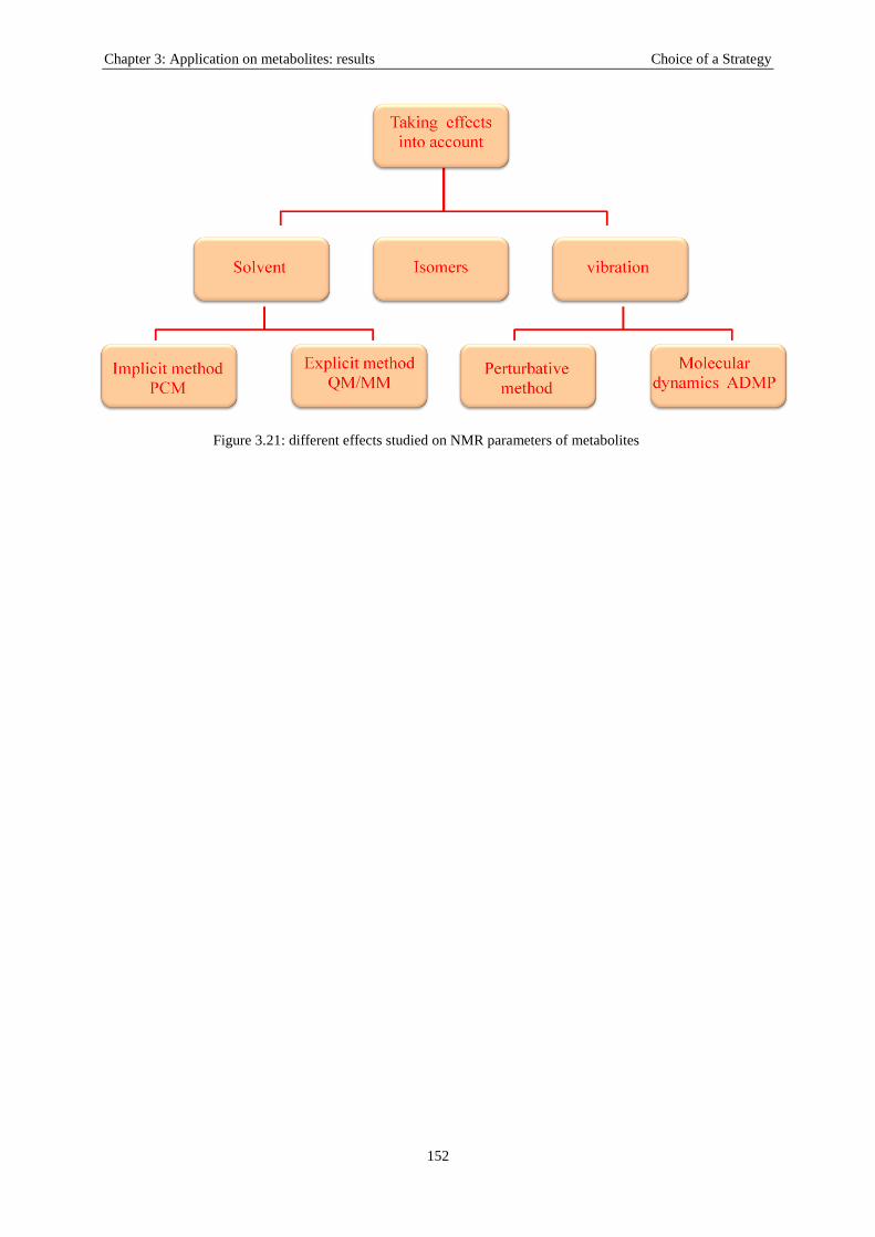
Chapter 3: Application on metabolites: results Choice of a Strategy
152
Figure 3.21: different effects studied on NMR parameters of metabolites

Chapter 3: Application on metabolites: results Choice of a Strategy
153
References
1. CFOUR, a quantum chemical program package. J.F. Stanton, and al. see <http://www.cfour.de>.
2. Gabedit—A graphical user interface for computational chemistry softwares. A.R.Allouche. 2011,
A. R. J. Comput. Chem., Vol. 32, p. 174.
3. Gaussian 03, Revision C.02. M. J. Frisch, and al. 2004, Inc., Wallingford CT.
4. Calculation of NMR and EPR parameters: Theory and application. M. Kaupp, M. Buhl, and V. G.
Malkin. 2004, Wiley-vch.

Chapter 3: Application on metabolites: results Choice of a Strategy
154

Chapter 3: Application on metabolites: results Publications
155
B: Results in the form of published papers
In part B, the full results are presented in a selection of our published papers. We
present here four papers. The first one studies isomers effects on the NMR parameters of the
three polyamines putrescine, spermidine, and spermine. The second paper presents the results
of the chemical shifts of sarcosine including the three effects: solvent, isomers, and vibration.
The third and fourth papers show the results of the three effects (solvent, isomers, and
vibration) on both types of NMR parameters (chemical shifts and spin-spin coupling
constants) for alanine and serine respectively.

Chapter 3: Application on metabolites: results Publications
156

DFT calculations of isomer effects upon NMR spin-Hamiltonian parametersof prostate polyamines
Z. Atieh, A.R. Allouche *, M. Aubert-FréconUniversité de Lyon, F-69622, Lyon, FranceUniversité Lyon 1, Villeurbanne, FranceCNRS, UMR 5579, LASIM, France
a r t i c l e i n f o
Article history:Received 8 December 2009Received in revised form 12 January 2010Accepted 12 January 2010Available online 18 January 2010
Keywords:NMR spin-Hamiltonian parametersDFT calculationsIsomer effectsProstate polyamines
a b s t r a c t
1H Nuclear Magnetic Resonance (NMR) spin-Hamiltonian parameters: chemical shifts d and spin–spincoupling constants J have been calculated using density functional theory, for the three polyamines:putrescine, spermidine and spermine present in prostate tissue. The Boltzmann weighted average ofthe chemical shifts and spin–spin coupling constants over a large number of stable conformers have beenevaluated for each molecule. The comparison of such average chemical shifts with experimental valuesshows a significant improvement from values corresponding to the lowest-energy conformers, withrms errors of 0.15 ppm for putrescine and 0.05 ppm for both spermidine and spermine. From the compar-ison between spectra simulated from calculated d and J parameters and experimental ones, the B3LYP/6-311++G�� level of theory was seen to be a good compromise between accuracy and computational costs.
� 2010 Elsevier B.V. All rights reserved.
1. Introduction
In vivo Magnetic Resonance Spectroscopy (MRS) is a non-inva-sive powerful technique for detecting and quantifying bio-markersof diseases i.e. metabolites [1]. The analysis of MRS-signals ob-tained from patients is based on a database of prior knowledgeabout MRS-signals of metabolites which are simulated quantum–mechanically with the use of the spin-Hamiltonian parameters:chemical shifts d and indirect spin–spin coupling constants J. Liter-ature values of d and J are used when available, mainly from exper-imental determinations [2]. In the present investigation we areinterested in the three polyamines: putrescine, spermidine andspermine which are metabolites of prostate tissue. Polyamine con-centrations have been shown to decrease in the presence of pros-tate cancer [3–9]. For these molecules there exist experimentalvalues of 1H chemical shifts in literature [10–12] while we knewno previous values for indirect spin–spin coupling constants.NMR chemical shifts and spin–spin constants can be obtained fromquantum chemical methods which are now well established asefficient tools for such predictions (for recent reviews see [13–15] and references therein). With the aim to supply the priorknowledge database for polyamines, we recently performed dand J calculations for the lowest-energy structure of the three poly-
amines [16,17] using the Density Functional Theory (DFT) with thehybrid exchange–correlation functional B3LYP [18,19] and the Po-ple-type [20] basis set 6-311++G��, assumed as a good cost/perfor-mance compromise. The main aim of the present paper is toevaluate in a rather systematic way, for each polyamine, the effectupon calculated chemical shifts and spin–spin coupling constants,of isomers higher in energy than the lowest-energy conformer.
The paper is organized in the following way. In Section 2 weoutline the computational approaches used. Arguments for ourchoice of a level of theory (functional/basis set) are presented inSection 3. The contribution of isomers to the calculated NMRparameters is described and discussed in Section 4 while a compar-ison of our final results with experimental data from 1H NMR spec-tra is presented in Section 5.
2. Computational approaches
For each polyamine: putrescine, spermidine and spermine,three calculation steps have been carried out (1) the determinationof stable geometries of the gas-phase and solvated species in a gi-ven range of relative energy above the lowest-energy conformer,(2) the determination of the NMR spin-Hamiltonian parameters:chemical shifts and indirect spin–spin coupling constants for eachstable structure previously determined, (3) the simulation of 1HNMR spectra from the calculated NMR spin-Hamiltonian parame-ters. In the present investigation the three solvated polyamineshave been described in the self-consistent reaction field theory
0166-1280/$ - see front matter � 2010 Elsevier B.V. All rights reserved.doi:10.1016/j.theochem.2010.01.017
* Corresponding author. Address: Université de Lyon, F-69622, Lyon, France. Tel.:+33 4 72 43 19 29; fax: +33 4 72 43 15 07.
E-mail addresses: [email protected] (Z. Atieh), [email protected] (A.R. Allouche), [email protected] (M. Aubert-Frécon).
Journal of Molecular Structure: THEOCHEM 945 (2010) 104–109
Contents lists available at ScienceDirect
Journal of Molecular Structure: THEOCHEM
journal homepage: www.elsevier .com/locate / theochem

based on the Polarisable Continuum Model (SCRF-PCM) [21,22]where water was used as solvent.
To search the stable geometries of a gas-phase or solvated poly-amine i.e. the lowest-energy structure as well as the stable isomerslying in a given relative energy range, we have proceeded as fol-lows. First we used the constant energy (NVE) molecular dynamicscalculation using the Velocity Verlet algorithm [23] with the semi-empirical PM6 potential [24] to select a reasonably large number ofinitial geometries. The simulated time was 15 ps, the time step was0.5 fs and the temperature was 5000 K. This high temperature waschosen in order to provide a large (�exhaustive) exploration of thepotential energy surface. For each polyamine considered we haveselected 5000 geometries during the simulation process. Each se-lected geometry was optimized at the PM6 level and very similarstructures were removed. Then the remaining optimized geome-tries were used as initial geometries in an optimization processusing this time the B3LYP method with the small basis set 6-31G� to calculate the potential. Very similar structures were re-moved. Furthermore only the geometries which lie in a given en-ergy gap DEmax above the lowest one (DEmax = Emax � E0 where E0
is the energy of the lowest-lying structure) were retained. Finally,the remaining structures optimized at the B3LYP/6-31G� levelwere used as initial geometries in the optimization process wherethe potential was evaluated this time at the DFT level using variousfunctionals and various basis sets larger than 6-31G�. These opti-mized structures were filtered in order to retain only those whichcorrespond to an energy minimum i.e. with no imaginary calcu-lated frequencies. We have automatized this procedure andadopted it as a good compromise between predictions accuracyand computational costs.
For a given stable geometry, the nuclear magnetic shieldingconstants r have been calculated, using the GIAO technique [25]to ensure gauge independence, for each nuclei of each gas-phaseand solvated polyamine molecule under investigation as well asfor the protons of the tetra methyl silane (TMS) molecule chosenas reference for shielding parameters. Chemical shifts for the pro-tons bound to C atoms in a polyamine, which are data directlycomparable to experimental measures, have been obtained fromd = rTMS � r. Indirect spin–spin coupling constants J have also beenevaluated for a given stable geometry. To take into account the
contribution on the calculated values of the NMR spin-Hamiltonianparameters from the structures higher in energy than the most sta-ble one, we have assumed Boltzmann distributions.
All calculations have been carried out by use of the computa-tional package Gaussian 03 [26] and the graphical interface Gabed-it [27]. Using calculated values for the chemical shifts and theindirect spin–spin constants, the NMR spectrum of each polyaminehas been simulated through a home-made code developed follow-ing the conventional way of solving the spin-Hamiltonian [28] andincluded in the graphical interface Gabedit.
3. Choice of functional and basis set
In our previous investigations [16,17] of metabolites we as-sumed, from a limited investigation involving four basis sets of Po-ple’s type, that the B3LYP/6-311++G�� level of theory is a goodcompromise between accuracy and cost. For the completeness ofpresent work, the corresponding calculated lowest-energy struc-tures are reproduced in Fig. 1. The groups of protons having thesame calculated chemical shift (noted A, B, C, D) are defined in Ta-ble 1 as well as the various spin–spin coupling constants Ja (a = A,B, C, D, E), for the three metabolites: putrescine, spermidine andspermine under investigation. In order to check further the perti-nence of our choice functional/basis set we performed calculationswith the PBE [29] and OPBE [30] functionals in combination withthe eight basis sets: pcn (n = 0.3) [31,32] and pcJn (n = 0.3) [33].
For the gas-phase putrescine, comparing the results obtainedwith the 6-311++G�� basis set (size = 324 primitive Gaussian func-tions) and with the largest one considered here i.e. the pcJ3(size = 1374), pointed out only rather small differences. For in-stance, the difference dB–dA which determines the calculated rela-tive position of the two multiplets of the NMR spectrum ofputrescine, was calculated to be 1.33 ppm at the B3LYP level withboth the 6-311++G�� and pcJ3 basis sets and 1.34 ppm at both PBEand OPBE levels with the pcJ3 basis set. For spermidine, we com-pared the da values (a = A, B, C, D) calculated at the level B3LYP/6-311++G�� (size = 531) with those obtained from the B3LYP, PBEand OPBE functionals using the pcJ2 basis set (size = 1261) whichis the largest one for which calculations were performed for theisolated molecule. The da results were seen to lie inside the disper-
Fig. 1. Lowest-energy structure for the solvated putrescine, spermidine and spermine molecules, determined at the B3LYP/6-311++G�� level of theory. N atoms in blue, Catoms in black, H atoms in grey. (For interpretation of the references to color in this figure legend, the reader is referred to the web version of this paper.)
Z. Atieh et al. / Journal of Molecular Structure: THEOCHEM 945 (2010) 104–109 105

sion range of the results obtained at the B3LYP or PBE or OPBE/pcJ2levels of theory. A similar result was obtained for the isolatedspermine when comparing the da (a = A, B, C, D) results obtainedat the B3LYP/6-311++G�� level of theory with those obtained fromthe three functionals B3LYP, PBE and OPBE using the pc2 basis set(size = 1280) which is the largest one for which calculations wereperformed for this molecule.
Contrarily to what was observed for the d calculations wherethe B3LYP/6-311++G�� results were seen to be quite close to thoseinvolving the largest basis set considered, J results were seen to besignificantly different. For putrescine, the JA,B values are �7 Hzwhen calculated using the 6-311++G�� basis set while they reach�9 Hz when calculated using the pcJ3 basis set, and this for anyof the three functionals considered in the present study. Similar re-sults were obtained for the five Ja (a = A, B, C, D, E) numerical valuesfor spermidine and the four Ja (a = A, B, C, D) numerical values forspermine (see Table 1 for the definition of A, B, C, D, E). At this stepof our theoretical investigation, we have no criterion to select thecorrect values of J and then the correct level of theory. Neverthelessthe comparison with experiment (see Section 5) will demonstratethat J values �7 Hz better reproduce experimental structures inNMR spectra.
In conclusion, our choice of the B3LYP/6-311++G�� level of the-ory appears as a reasonable compromise between accuracy andcost for the further calculations of the NMR spin-Hamiltonianparameters for a large number of isomers of the three polyamines.
4. Contribution of isomers in the calculation of NMR spin-Hamiltonian parameters
Up to now we have considered only the lowest-energy geome-try of each of the polyamines when calculating the d and J NMRparameters. In fact during the search procedure described in Sec-tion 2, we found many isomer structures at DFT/6-31G� level lyingin a given energy gap DEmax above the lowest one, that may affectthe results. The number of isomers to be taken into account growswith the size of the molecule, as expected.
For each polyamine, we first chose a value for DEmax from whichwe filtered the isomer structures obtained at the DFT/6-31G� leveli.e. only isomer structures with a relative energy <DEmax were se-lected. All these structures were re-optimized at the DFT/6-311++G�� level. Then we arranged these isomers following increas-ing relative energies. For each retained geometry (having a relativeenergy DEi, i = 0, 1, . . .., N) we calculated the chemical shifts and thespin–spin coupling constants. The contribution from the ith con-former to the averaged values of d and J is evaluated under theassumption of Boltzmann distribution:
PðiÞaveraged ¼P
j¼0;iPje�DEj=kT
Pj¼0;ie
�DEj=kT; i ¼ 0; 1; . . . N ð1Þ
where N is the number of stable structures to be taken into accountand P stands for d or J. DEj is the relative energy of the isomer j, k isthe Boltzmann constant and T is the temperature. In present workwe chose T = 300 K, close to the ambient temperature of experi-ments. Proceeding in that way allows us to point out the conver-gence of the results.
For putrescine we chose DEmax = 3.5 kcal/mol and then 44 iso-mers are to be taken into account. Averaged chemical shifts dav
A
and davB were seen to converge for DEconv = �2.3 kcal/mol. For sper-
midine we chose DEmax = 5 kcal/mol and then 230 isomers are tobe taken into account. Averaged chemical shifts dav
A ; davB , dav
X anddav
D were seen to converge for DE = DEconv = �3.5 kcal/mol. Forspermine we chose DEmax = 6.5 kcal/mol and then 300 isomersare to be taken into account. Averaged chemical shifts dav
A , davB , dav
X
and davD were seen to converge for DE = DEconv = �5.8 kcal/mol.
The evolution of the averaged chemical shifts versus the relativeenergy, using the 6-311++G�� basis set are drawn in Fig. 2 forthe spermidine chosen as example, the same evolution trendsbeing observed for the solvated putrescine and spermine. Chemicalshift results evaluated at the B3LYP/6-311++G�� level of theory,including the averaged values as well as the values for thelowest-energy structure (quoted as d0) are gathered in Table 2for the three solvated polyamines. The contributions from isomers,evaluated through the root mean square deviations rms =ffiffiffiffiffiffiffiffiffiffiffiffiffiffiffiffiffiffiffiffiffiffiffiffiffiffiPM
i¼1ðd0
i �davi Þ
2
M
qwhere M is the number of d values (M = 2 for putres-
cine, M = 4 for spermidine and spermine), are seen to be larger forputrescine (rms = 0.14 ppm) and spermidine (rms = 0.09 ppm)than for spermine (rms = 0.02 ppm). This is consistent with the factthat the energy difference between the first isomer and the lowest-energy conformer is �0.013 eV for both putrescine and spermidinewhile it is �0.1 eV for spermine.
The convergence of the J constants with the increasing values ofthe relative energy was also evidenced for the solvated putrescine,spermidine and spermine molecules. It is illustrated in Fig. 3 forthe spermidine chosen as example. Convergence is reached forthe same value of the relative energy DEconv than for chemicalshifts. Once more, contributions from isomers to the averaged val-ues of J are larger for putrescine and spermidine with rms devia-tions of 0.58 Hz than for spermine with rms = 0.23 Hz. Spin–spincoupling constants evaluated at the B3LYP/6-311++G�� level oftheory, including the averaged values (quoted as Jav) as well asthe values for the lowest-energy structure (quoted as J0) are gath-ered in Table 3 for the three solvated polyamines.
Table 1Groups of protons (labelled a = A, B, C, D) having the same chemical shifts and definition of the various Ja (a = A, B, C, D, E) spin–spin coupling constants for the three molecules:putrescine, spermidine and spermine.
Group Putrescine Spermidine SpermineProton labelsa Proton labelsa Proton labelsa
Chemical shiftsA 3, 4, 15, 16 4, 7, 12, 15 18, 20, 21, 23B 1, 2, 17, 18 18, 26 7, 9, 32, 34C 9, 14, 17, 23 10, 12, 15, 17, 24, 26, 29, 31D 2, 10, 20, 28 4, 6, 35, 37
J spin–spin coupling constantsJA J(1,2) � (15,16) � J(3,4) � (17,18)
a J(2,10) � (4,12) J(4,6) � (7,9) � J(32,34) � (35,37)
JB J(3,4) � (15,16) J(4,12) � (7,15) J(7,9) � (10,12) � J(29,31) � (32,34)
JC J(7,15) � (9,17) J(15,17) � (18,20) � J(21,23) � (24,26)
JD J(14,23) � (18,26) J(18,20) � (21,23)
JE J(18,26) � (20,28)
a The shortened notation J(i,k) � (j,l) stands for Ji,j = Ji,l = Jk,j = Jk,l. See Fig. 1 for the proton labels of the three polyamines, respectively.
106 Z. Atieh et al. / Journal of Molecular Structure: THEOCHEM 945 (2010) 104–109

5. Comparison with experiment and discussion
Experimental 1H NMR spectra were acquired at 400 MHz for thethree molecules in solution in D2O [16,17]. The 1H NMR experi-
mental spectrum of solvated putrescine displays two structures,one triplet and one multiplet. Four structures are present for boththe solvated spermidine and spermine with two overlapping mul-tiplets on the left part of the experimental spectra. The number ofobserved multiplets is in agreement with the number of calculatedchemical shifts. From experimental spectra, experimental valuesfor the various chemical shifts have been extracted and the valuesare recalled in Table 2 for the three polyamines. For the two dA anddB values of putrescine the errors (defined as the difference be-tween experimental and calculated values) are 0.34 and0.23 ppm, respectively for the calculations with the lowest-energygeometry alone with a root mean square error rms = 0.29 ppm,while these errors are significantly reduced (0.19, 0.09 ppm) withrms = 0.15 ppm by taking into account averaged contributionsfrom isomers. This agreement with experiment is quite satisfying.For the four values dA, dB, dC and dD of spermidine the errors aresmaller than for putrescine. They range from 0.06 to 0.13 ppm(rms = 0.09 ppm) for the lowest-energy structure and are reducedto 0.04–0.06 ppm (rms = 0.05 ppm) by taking into account the con-tributions from isomers providing a good agreement with experi-ment. A good agreement with experimental values is alsoobtained for the four values dA, dB, dC and dD of solvated sperminewith rms = 0.07 ppm for the lowest-energy structure andrms = 0.05 ppm when taking into account the averaged contribu-tion from the isomers. For the 10 d values of the three polyamines,
Fig. 2. Evolution versus the relative energy of isomers of the calculateddav
A ; davB ; dav
C ; davD Boltzmann weighted average chemical shift values of the solvated
spermidine evaluated at the B3LYP/6-311++G�� level of theory.
Table 2Calculated chemical shifts at the B3LYP/6-311++G�� level of theory within the SCRF-PCM model, for the three solvated polyamines: dav
a averaged values and d0a values for
the lowest-energy geometry together with dexpa experimental values (see text for the
definition of the various a = A,B,C,D 1H groups). All d values in ppm. The number N ofisomers taken into account as well as the relative energy for which convergence isreached DEconv are quoted.
Putrescine Spermidine Spermine
N 44 230 300DEconv (kcal/mol) 2.3 3.5 5.8dav
A 1.410 1.453 1.529dav
B 2.734 1.604 1.600dav
C � 2.669 2.619dav
D � 2.746 2.663
d0A
1.264a 1.387 1.509
d0B
2.594 1.584 1.594
d0C
� 2.570 2.590
d0D
� 2.627 2.634
dexpA
1.603 1.519 1.540
dexpB
2.826 1.664 1.681
dexpC
� 2.634 2.652
dexpD
� 2.686 2.705
a Previous results [16] for the d0A and d0
A of putrescine were obtained within the C-PCM [35] model.
Fig. 3. Evolution versus the relative energy of isomers of the Boltzmann weightedaverage spin–spin coupling constant values of the solvated spermidine evaluated atthe B3LYP/6-311++G�� level of theory.
Table 3Calculated indirect spin–spin coupling constants at the B3LYP/6-311++G�� level oftheory within the SCRF-PCM model, for the three solvated polyamines: JZ
av averagedvalues and JZ
0 values for the lowest-energy geometry (see text for the definition of thevarious Z = A, B, C, D, E 1H groups). All J values in Hz.
Putrescine Spermidine Spermine
JAav
6.43 6.55 7.07
JBav
6.94 7.08 7.14
JCav
– 6.99 6.86
JDav
– 6.40 7.27
JEav
– 6.51 –
JA0
7.14a 7.15 7.19
JB0
7.32 7.37 7.24
JC0
– 7.25 7.25
JD0
– 7.24 7.43
JE0
– 7.19 –
a Previous results [16] for the JA0 and JB
0 of putrescine were obtained within the C-PCM [35] model.
Z. Atieh et al. / Journal of Molecular Structure: THEOCHEM 945 (2010) 104–109 107

the rms error is 0.15 ppm for the lowest-energy structures and0.08 ppm when taking into account the isomer effects.
In order to evidence the correlation between experimental andcalculated results, we used, as often done, a linear scaling proce-dure [34] in which dcalc = a + b dexp, taking into account the 10 d val-ues for the three polyamines treated together. For the solvatedpolyamines we obtained dcalc = �0.170 + 1.025 dexp with a regres-sion coefficient R = 0.988 for the lowest-energy structures anddcalc = �0.163 + 1.054 dexp with R = 0.995 when contribution fromisomers are included. From these linear scalings, the rms devia-tions reduce from 0.15 ppm (no scaling) to 0.08 ppm for the low-est-energy structures and from 0.08 ppm to 0.06 ppm whenisomers are taken into account.
For the solvated putrescine for which the less satisfying chem-ical shift results have been obtained we have performed two morecalculations taking into account the averaged contribution fromisomers using the PBE and OPBE functionals with the 6-311++G�� basis set. Results are presented in Table 4 together withthe results previously obtained for the lowest-energy structure.When comparing with the dA and dB experimental data, the best re-sults when considering only the lowest-energy structure are ob-tained with the PBE functional with a rms error of 0.26 ppm, tobe compared to rms = 0.34 ppm for B3LYP and rms = 0.33 for OPBE.When considering the weighted contribution from the isomers, thebest results are obtained for the OPBE functional with rms =0.09 ppm to be compared to rms = 0.15 ppm for B3LYP andrms = 0.30 for PBE. Nevertheless the experimental relative positionof the two multiplets Dd = dB � dA = 1.22 ppm, is somewhat betterreproduced by B3LYP calculations (Ddav = 1.32 ppm) than PBE(Ddav = 1.38 ppm) or OPBE (Ddav = 1.37 ppm) ones.
We have not been able to extract experimental values for thespin–spin coupling constants from our in vitro 1H NMR spectra ofthe polyamines in solution in D2O, due to their complexity. Tocompare these data with experiment we have simulated the 1HNMR spectra and compare the simulated and experimental multi-plet structures so obtained. Comparative results are presented inFig. 4 for the multiplet of the solvated putrescine atd = 2.826 ppm, calculated using the JA
av and JBav values of the spin–
spin coupling constants reported in Table 4. Calculations fromthe B3LYP/6-311++G�� level are seen to better reproduce the fivepeaks of the multiplets than the PBE and OPBE ones. The multipletstructure calculated with the J values from B3LYP/pcj3 level of the-ory which were seen to be �9 Hz, is also drawn in Fig. 4. It is clearthat these values do not allow a correct description of the multi-plet. Similar comparisons were performed for each multiplet ofeach molecule, leading to similar results as those illustrated forthe putrescine multiplet.
6. Conclusion
A theoretical investigation, based on density functional meth-ods, of the d and J NMR spin-Hamiltonian parameters have beenperformed for the protons attached to the carbon atoms of thethree polyamines: putrescine, spermidine and spermine involvedin prostate tissue. From the trends of the calculated results com-pleted by the comparison with the 1H NMR experimental spectraof these molecules, we conclude that d and J values calculated atthe B3LYP/6-311++G�� level of theory reproduce quite well thecorresponding experimental data. Results are excellent for the fourchemical shifts of spermidine and spermine with rms errors of0.05 ppm when comparing with experiment. Taking into accountthe Boltzmann weighted contributions from conformers reducesthe rms errors by �40% for the spermidine and by �30% for thespermine. For the two chemical shifts of putrescine the agreementremains satisfying with a rms error of 0.15 ppm, reduced by �50%by converged isomer contributions.
Acknowledgments
This work was supported by the E.U. Marie Curie Research Net-work MRTNCT-2006-035801, 2006–2010. The authors thank the‘‘Pôle Scientifique de Modélisation Numérique (PSMN)” at Lyon,France, for generous computational facilities.
References
[1] J.F. Jansen, W.H. Backes, K. Nicolay, M.E. Kooi, Radiology 240 (2006) 318.[2] V. Govindaraju, K. Young, A.A. Maudsley, NMR Biomed. 13 (2000) 129.[3] M.A. Thomas, T. Lange, S.S. Velan, R. Nagarajan, S. Roman, A. Gomez, D.
Margolis, S. Swart, R.R. Raylman, R.F. Schulte, P. Boesiger, Magn. Reson. Mater.Phys. 21 (2008) 443.
[4] Y. Mazaheri, A. Shukla-Dave, A. Muellner, H. Hricak, Magn. Reson. Mater. Phys.21 (2008) 379.
[5] P. Swindle, S. Ramadan, P. Stanwell, S. McCredie, P. Russell, C. Mountford,Magn. Reson. Mater. Phys. 21 (2008) 423.
[6] T. Lange, R.F. Schulte, P. Boesiger, Magn. Reson. Med. 59 (2008) 966.[7] P. Younès, N. Chemla, B. Hamzé, J. Mani, J.-F. Naouri, Ann. Urol. 41 (2007) 145.[8] A. Shukla-Dave, H. Hricak, C. Moskowitz, N. Ishill, O. Akin, K. Kuroiwa, J.
Spector, M. Kumar, V.E. Reuter, J.A. Koutcher, K.L. Zakian, Radiology 245 (2007)499.
[9] M.G. Swanson, D. Vigneron, Z.L. Tabatabai, R.G. Males, L. Schmitt, P.R. Carroll,J.K. James, R.E. Hurd, J. Kurhanewicz, Magn. Reson. Med. 50 (2003) 944.
[10] E.M. Lenz, B.F. Hägele, I.D. Wilson, S.J. Simpson, Insect Biochem. Mol. Biol. 32(2001) 51.
[11] C.D. Meo, D. Capitani, L. Mannina, E. Brancaleoni, D. Galesso, G.D. Luca, V.Crescenzi, Biomacromoles 7 (2006) 1253.
[12] W. Willker, U. Flögel, D. Leibfritz, NMR Biomed. 11 (1998) 47.[13] H. Fukui, Nucl. Magn. Reson. 38 (2009) 166.[14] L.B. Casabianca, A.C. de Dios, J. Chem. Phys. 128 (2008) 052201.[15] T. Helgaker, M. Jaszunski, M. Pecul, Prog. Nucl. Magn. Reson. Spectrosc. 53
(2008) 249.[16] A.R. Allouche, D. Graveron-Demilly, F. Fauvelle, M. Aubert-Frécon, Chem. Phys.
Lett. 466 (2008) 219.[17] Z. Atieh, A.R. Allouche, F. Fauvelle, D. Graveron, M. Aubert-Frécon, Meas. Sci.
Technol. 20 (2009) 104024.[18] A.D. Becke, J. Chem. Phys. 98 (1993) 5648.[19] C. Lee, W. Yang, R.G. Parr, Phys. Rev. B 37 (1988) 785.[20] R. Krishnan, J.S. Binkley, R. Seeger, J.A. Pople, J. Chem. Phys. 72 (1980) 650.[21] S. Miertus, E. Scrocco, J. Tomasi, Chem. Phys. 55 (1981) 117.[22] V. Barone, M. Cossi, J. Tomasi, J. Chem. Phys. 107 (1997) 3210.[23] W.C. Swope, H.C. Andersen, P.H. Berens, K.R. Wilson, J. Chem. Phys. 76 (1982)
637.
Table 4Chemical shifts (ppm) for the solvated putrescine calculated at various level of theorywithin the SCRF-PCM model.
Level of theory dexpA d0
A davA dexp
B d0B dav
B
1.603 2.826B3LYP/6-311++G�� 1.264 1.410 2.594 2.734PBE/6-311++G�� 1.284 1.812 2.639 3.188OPBE/6-311++G�� 1.203 1.579 2.572 2.950
Fig. 4. Comparison with experiment of the structure of the multiplet of the solvatedputrescine (situated at d = 2.826 ppm), calculated at different levels of theory.
108 Z. Atieh et al. / Journal of Molecular Structure: THEOCHEM 945 (2010) 104–109

[24] J.J.P. Stewart, J. Mol. Model. 13 (2007) 1173.[25] J.R. Cheeseman, G.W. Trucks, T.A. Keith, M.J. Frisch, J. Chem. Phys. 104 (1996)
5497.[26] M.J. Frisch et al., Gaussian 03, Revision C.02, Gaussian, Inc., Wallingford, CT,
2004.[27] A.R. Allouche, Gabedit is a graphical user interface for various computational
chemistry packages. Available from: <http://gabedit.sf.net>.[28] J.D. Roberts, An Introduction to the Analysis of Spin–Spin Splitting in High-
Resolution Nuclear Magnetic Resonance Spectra, W.A. Benjamin, Inc., NewYork, 1961.
[29] J.P. Perdew, K. Burke, M. Ernzerhof, Phys. Rev. Lett. 77 (1996) 3865.[30] N.C. Handy, A.J. Cohen, Mol. Phys. 99 (2001) 403.[31] F. Jensen, J. Chem. Phys. 115 (2001) 9113. erratum J. Chem. Phys. 116 (2002)
3502.[32] F. Jensen, J. Chem. Phys. 116 (2002) 7372.[33] F. Jensen, J. Chem. Theory Comput. 2 (2006) 1360.[34] D.B. Chesnut, Rev. Comput. Chem. 8 (1996) 245.[35] M. Cossi, N. Rega, G. Scalmani, V. Barone, J. Comput Chem. 24 (2003)
669.
Z. Atieh et al. / Journal of Molecular Structure: THEOCHEM 945 (2010) 104–109 109

DFT calculations of 1H chemical shifts, simulated and experimental NMR spectrafor sarcosine
Z. Atieh a, A.R. Allouche a,*, A. Lazariev b, D. Van Ormondt c, D. Graveron-Demilly b, M. Aubert-Frécon a
a Université de Lyon, F-69622 Lyon, France; Université Lyon 1, Villeurbanne; CNRS, UMR 5579, LASIM, Franceb Université de Lyon, F-69622 Lyon, France; Université Lyon 1, Villeurbanne; CNRS, UMR 5220, INSERM U630, CREATIS-LRMN, Francec Applied Physics Department, Delft University of Technology, Delft, The Netherlands
a r t i c l e i n f o
Article history:Received 24 February 2010In final form 20 April 2010Available online 24 April 2010
a b s t r a c t
Chemical shifts d have been calculated for the 1H attached to carbon atoms of sarcosine. Eight levels oftheory within the DFT approach were used, mixing the four functionals B3LYP, PBE, OPBE, PBE0 andthe two basis sets 6-311++G** and pcJ2. Boltzmann weighted isomer effects have been evaluated. Bycomparison of the 1H NMR spectrum simulated from the calculated d and the experimental one thatwe acquired at 300 MHz, the B3LYP/6-311++G** calculation was seen to be a good compromise betweenaccuracy and cost. Zero-point vibrational corrections, estimated using a second-order perturbationapproach, increase the agreement with experiment.
� 2010 Elsevier B.V. All rights reserved.
1. Introduction
Sarcosine is the N-methyl derivative of glycine. It is a naturalamino-acid found in muscles and other body tissues. Very recently[1], sarcosine was identified as a differential metabolite that washighly increased during prostate cancer progression to metastasis.Sarcosine levels seemed to control the invasiveness of the cancer.This metabolite can be detected non-invasively in urine and maydistinguish between slow-growing and aggressive prostate can-cers. Changes in concentration of metabolites in body tissues couldbe detected by in vivo Magnetic Resonance Spectroscopy (MRS) [2],a non-invasive powerful technique for detecting and quantifyingbio-markers of diseases. The analysis of MRS-signals obtained frompatients is based on a database of prior knowledge about MRS-signals of metabolites which are simulated quantum–mechanicallywith the use of the spin Hamiltonian parameters: chemical shifts dand indirect spin–spin coupling constants J. Literature values ofd and J are used, when available, mainly from experimentaldetermination.
Being currently involved in calculations of NMR spin Hamilto-nian parameters for metabolites [3–5], in order to produce reliablevalues of these parameters from which NMR spectra could be sim-ulated and used further in quantitation procedures, we investi-gated sarcosine in the present study.
2. Computational approaches
For the sarcosine molecule (C3H7NO2) in gas phase and in watersolution, four calculation steps have been carried out: (1) thedetermination of stable geometries lying in a given range of rela-tive energy above the lowest one, (2) the determination of thechemical shifts for the protons attached to carbon atoms, (3) theestimation of zero-point vibrational corrections on these chemicalshifts, and (4) the simulation of the 1H NMR spectrum of the sarco-sine from the calculated 1H chemical shifts. The solvated sarcosinehas been described by the self-consistent reaction field theory(SCRF) based on the Polarisable Continuum Model (PCM) [6,7].All calculations have been carried out by use of the computationalpackage GAUSSIAN03 [8] and the graphical interface GABEDIT [9].
2.1. Conformational search
To search the lowest-energy structure of the sarcosine as wellas the stable isomers lying in a given relative energy range abovethe lowest one, we performed first a molecular dynamics calcula-tion for the gas-phase molecule (constant energy NVE, velocityVerlet algorithm [10]) with the semi-empirical PM6 potential[11], in order to select initial geometries. The simulated time was10 ps, the time step was 1.0 fs and the temperature was 5000 Kin order to provide a large exploration of the potential energy sur-face. We have selected 5000 geometries during the simulation pro-cess. Each selected geometry was further optimized at the PM6level and very similar structures were removed. Twenty-twogeometries were obtained in that way, each of them was furtherused as initial geometry in an energy minimization procedure
0009-2614/$ - see front matter � 2010 Elsevier B.V. All rights reserved.doi:10.1016/j.cplett.2010.04.054
* Corresponding author. Fax: +33 4 72 43 15 07.E-mail address: [email protected] (A.R. Allouche).
Chemical Physics Letters 492 (2010) 297–301
Contents lists available at ScienceDirect
Chemical Physics Letters
journal homepage: www.elsevier .com/ locate /cplet t

performed at the B3LYP/6-31G* level, for the solvated molecule.Very similar structures were removed and only the stable geome-tries (i.e. with no imaginary calculated frequencies) which lie in agiven energy gap of 3.5 kcal/mol above the lowest one were re-tained. At the end of the process eight geometries were obtained.Finally, these eight structures were used as initial geometries inDFT optimization calculations. Eight different levels of theory wereconsidered, using the four functionals: B3LYP [12,13], PBE [14],OPBE [15], PBE0 [16] with the two basis sets: 6-311++G** [17]and pcJ2 [18]. Note that for sarcosine the 6-311++G** basis set con-tains 181 functions while the pcJ2 basis set contains 474 functions.As an example, the lowest-energy structure of the solvated sarco-sine determined at the B3LYP/6-311++G** level of theory is dis-played in Fig. 1.
2.2. Chemical shifts calculation
For the most stable geometry of solvated sarcosine, the isotropicnuclear magnetic shielding constants r have been calculated ateach level of theory considered, using the GIAO technique [19] toensure gauge independence, for the protons attached to carbonatoms, i.e. the two protons (labelled 1, 7 in Fig. 1) of the methylenegroup and the three protons (labelled 11–13 in Fig. 1) of the methylgroup. A similar calculation was performed at the same level oftheory for the protons of the tetra methyl silane (TMS) molecule,chosen as reference for the shielding parameters, in order to obtainthe chemical shifts for the protons under consideration throughd = rTMS � r. It should be noted that, having performed calcula-tions for a motionless molecule, the numerical r values obtainedwere not exactly identical for the two 1H of the methylene groupas well as for the three 1H of the methyl group, contrarily to whatshould have been expected. This was bypassed by averaging the rvalues for the 1H of CH2 and the 1H of CH3, respectively, so thatonly two different values: dA {11, 12, 13} and dB {1, 7} wereobtained.
To take into account the contribution on the calculated values ofthe 1H chemical shifts under consideration, from the seven struc-tures higher in energy than the most stable conformer, the chem-ical shifts di
A;B were evaluated for all the isomers i. Then, theBoltzmann weighted average dav
A;B over the stable conformers wereevaluated through:
davA;B ¼
P8i¼1d
iA;B e�DEi=kT
P8i¼1e�DEi=kT
ð1Þ
where DEi is the relative electronic energy of the isomer i, k is theBoltzmann constant and T is the temperature. In the present workwe chose T = 300 K, close to the ambient temperature of theexperiments. These calculations were performed for each of theeight levels of theory considered.
Note that the calculated indirect spin–spin coupling constant Jare �0 (<0.02 Hz), apart from large negative values for the protonsof the same group.
2.3. Estimation of vibrational effects
In order to account for the correction to the nuclear magneticshielding due to the zero-point vibrational motion we used sec-ond-order perturbation theory with the sarcosine in its equilib-rium geometry as the unperturbed system. Following [20], thezero-point vibration correction (ZPVc) to the nuclear magneticshielding of a given nucleus is calculated through:
rZPVc ¼14
XK
1xK
d2rdQ2
K
� 14
XK
1x2
K
drdQK
XL
FKLL
xLð2Þ
QK is the normal coordinate K with an harmonic frequency xK , andthe cubic force constant FKLL is defined as the third derivative of theelectronic energy E with respect to the normal coordinatesQK ; QL; QL. The sums over K and L run over all the normal vibra-tional modes of the sarcosine, i.e. 33 terms are involved. The vibra-tional average of r is given by: rvib ¼ rþ rZPVc, where r is theisotropic shielding for the non-vibrating equilibrium geometry eval-uated in previous Section 2.2.
We had first to develop a specific code for the evaluation ofrZVPc through Eq. (2), that we have implemented in the versionof GAUSSIAN03 at our disposal (which does not allow the evaluationof vibrational effects upon NMR parameters). Harmonic frequen-cies and cubic force constants are evaluated through GAUSSIAN03at the equilibrium geometry. The first- and second-order deriva-tives of the nuclear shielding with respect to the normal coordi-nates are evaluated numerically with a step of 0.03 Å. In order tocheck our code we have calculated rvib;AðBÞ for the two groups ofprotons under investigation for the isolated sarcosine at the HF/6-311++G** level of theory. The values obtained were found to beidentical to those provided by the CFOUR package [21] at the samelevel of theory.
Within the B3LYP/6-311++G** level of theory, selected as a goodchoice, risol
vib;AðBÞ vibrational averages have been calculated for the Aand B group of protons of the isolated sarcosine. In order to calcu-late the dvib;AðBÞ vibrational average of the chemical shifts, thervib,TMS vibrational average was also calculated for the protons ofthe TMS. For the isolated sarcosine, calculations were performedfor ri;isol
vib;AðBÞ for each of the eight isomers previously determined.Boltzmann averaged values rav;isol
vib;AðBÞ were then evaluated througha formula similar to Eq. (1) (with r replacing d) in which the ener-gies Ei to be considered are the sum of the electronic energy deter-mined in Section 2.1 plus the vibrational part evaluated as
PK
�hxK2 .
Solvent effects upon vibrational average of chemical shieldingwere approximated from the values for the isolated molecule cor-rected by adding for each isomer i the difference between thechemical shielding evaluated for the solvated ri
solv;AðBÞ and for theisolated ri
isol;AðBÞ non-vibrating molecule
ri;solvvib;AðBÞ ¼ ri;isol
vib;AðBÞ þ Drisolv;AðBÞ
with Drisolv;AðBÞ ¼ ri
solv;AðBÞ � riisol;AðBÞ.
Boltzmann averaged values rav;solvvib;AðBÞ were then obtained in the
same way as for the isolated molecule.
3. Results
3.1. Nuclear magnetic shieldings and chemical shifts for non-vibratingmolecules
Results for rTMS, rA, rB as well as dA and dB calculated for thefour functionals and the two basis sets considered are displayed
Fig. 1. Lowest-energy structure of the solvated sarcosine, calculated at the B3LYP/6-311++G** level of theory. The numbering of atoms is quoted. C atoms in black, Nin blue, O in red and H in grey. (For interpretation of the references in color in thisfigure legend, the reader is referred to the web version of this article.)
298 Z. Atieh et al. / Chemical Physics Letters 492 (2010) 297–301

in Table 1 for the lowest-energy structure together with the davA and
davB values including isomer effects. To compare the various results
to each other we chose as criteria the root mean square deviation(rmsd) between two sets of results. First, we considered the basisset effect on the rTMS, rA and rB nuclear shielding values, for thelowest-energy structure of the solvated sarcosine. It is seen to bequite small for each of the four functionals considered. UsingpcJ2 instead of 6-311++G** basis set results in systematically smal-ler values of r either for TMS or for solvated sarcosine. The largest
rmsd value for r (rmsd ¼ffiffiffiffiffiffiffiffiffiffiffiffiffiffiffiffiffiffiffiffiffiffiffiffiffiffiffiffiffiffiffiffiffiffiffiffiffiffiffiffiffiffiffiffiðr6-311þþG�� � rpcJ2Þ2
qfor a given func-
tional) is �0.37 ppm. The largest rmsd value for d (rmsd ¼ffiffiffiffiffiffiffiffiffiffiffiffiffiffiffiffiffiffiffiffiffiffiffiffiffiffiffiffiffiffiffiffiffiffiffiffiffiffiffiffiffiffiðd6-311þþG�� � dpcJ2Þ2
qfor a given functional) is �0.13 ppm. Then,
we considered the functional effect on the various d values forthe lowest-energy structure as well as when taking the isomers
into account. The rmsd (rmsd ¼ffiffiffiffiffiffiffiffiffiffiffiffiffiffiffiffiffiffiffiffiffiffiffiffiffiffiffiP
i¼A;BðdF1
i �dF2i Þ
2
2
rwhere F1 and F2
stand for two different functionals among the four considered)are generally smaller for results including the eight isomers(rmsd < 0.18 ppm) than for the lowest-energy structure alone(rmsd < 0.27 ppm). The largest rmsd are observed for the PBE,OPBE and PBE0 compared to B3LYP, they reach 0.27 ppm. Whencomparing the results for the PBE, OPBE and PBE0 to each other,the rmsd are quite small with the largest one �0.10 ppm.
3.2. Vibrational corrections to nuclear magnetic shieldings andchemical shifts
Zero-point vibrational corrections rZPVc have been calculated atthe B3LYP/6-311++G** level of theory for the 1H of sarcosine andTMS, from which are deduced chemical shifts for the A and B groupof protons of sarcosine. Values are gathered in Table 2 togetherwith the values for the non-vibrating molecules and the Boltzmannaveraged values taking into account isomer effects. For both mole-cules in their lowest-energy geometry, zero-point vibrational
corrections decrease the 1H nuclear magnetic shieldings byamounts �0.7 ppm while the subsequent corrections on chemicalshifts are 0.08 ppm for the 1H of the methyl group (A) and0.05 ppm for the 1H of the methylene group (B). Taking into ac-count isomer effects for the vibrating gas-phase molecule increasesdA by 0.05 ppm and decreases dB by 0.08 ppm. Solvent effects areseen to be nearly negligible for dA (+0.02 ppm) while they are quitelarger for dB (+0.23 ppm).
4. Comparison with experiment and discussion
We have acquired the 1H NMR spectrum for sarcosine in solu-tion in pure D2O with TMS for chemical shift reference (0 ppm)on a 300 MHz avance 300DRX Bruker spectrometer (7 Tesla). Fromthis spectrum, which displays two singlets (consistent with indi-rect spin–spin coupling constants J calculated to be zero), we mea-sured the two chemical shifts dexp
A ¼ 2:73 ppm and dexpB ¼ 3:61 ppm,
in very good agreement with literature experimental results [22].We compare calculated values for each level of theory with the cor-
responding experimental ones. Calculated rmsd ¼
ffiffiffiffiffiffiffiffiffiffiffiffiffiffiffiffiffiffiffiffiffiffiffiffiffiffiffiffiffiPi¼A;B
dFi �dexp
ið Þ22
r,
where F is one of the functionals {B3LYP, PBE, OPBE, PBE0}, are re-corded in Table 3 for the two basis sets. The agreement with exper-iment is better when taking into account isomers effects thanwhen considering the equilibrium geometry alone at any of thelevels of theory considered. The rmsd corresponding to calcula-tions performed with the three functionals PBE, OPBE and PBE0for any of the two basis sets are larger than those correspondingto the B3LYP calculations. They range from 0.18 ppm (isomers/PBE0/pcJ2) to 0.33 ppm (equilibrium geometry/OPBE/6-311++G**and equilibrium geometry/PBE/pcJ2) while for the B3LYP calcula-tions the rmsd are in the range 0.14 ppm (isomers/B3LYP/pcJ2)–0.20 ppm (equilibrium geometry/B3LYP/6-311++G**). The bestagreement with experiment, i.e. the smallest rmsd (0.14 ppm)
Table 1Calculated nuclear magnetic shieldings and 1H dj
A;B chemical shifts (in ppm) (j = 0:lowest-structure alone; j = av: isomer effects included) for the solvated sarcosine.
Calculation rTMS rA rB d0A d0
B davA dav
B
B3LYP 31.97a 29.52 28.41 2.45 3.57 2.50 3.5131.71b 29.24 28.07 2.48 3.64 2.54 3.59
PBE 31.50a 28.99 28.22 2.51 3.28 2.54 3.3731.13b 28.71 27.86 2.42 3.27 2.42 3.37
OPBE 31.59a 29.06 28.40 2.53 3.19 2.50 3.3131.32b 28.78 28.03 2.53 3.29 2.52 3.38
PBE0 31.80a 29.37 28.54 2.44 3.26 2.45 3.4031.56b 29.09 28.19 2.47 3.38 2.51 3.48
MP2 31.90a 29.46 28.41 2.44 3.49 2.46 3.45
a 6-311++G** basis set.b pcJ2 basis set.
Table 2Vibrational average of nuclear magnetic shieldings (and chemical shifts) for the sarcosine and TMS molecules, evaluated at the B3LYP/6-311++G** level of theory. All values inppm.
Molecule Isolated molecule, lowest-energy structure Isomer and solvent effects Experiment
r0 r0ZVPc r0
vibd0
d0vib dav;isol
vib dav;solvvib
dexp
TMS 31.97 �0.65 31.32Sarcosine Aa 29.53 �0.73 28.80 2.44 2.52 2.57 2.59 2.73Sarcosine B 28.60 �0.70 27.90 3.37 3.42 3.34 3.57 3.61
The index 0 stands for the lowest-energy geometry alone.a Group A: {11, 12, 13}; group B: {1, 7}; see Fig. 1 for the 1H labelling in brackets.
Table 3Root mean square deviations (rmsd) from experimental values for the 1H chemicalshifts of solvated sarcosine evaluated at eight DFT levels of theory: functional/basisset. Results of a MP2/6-311++G** check calculation are also quoted. All values in ppm.
Calculation Basis set rmsd(d0)a rmsd(dav)b
B3LYP 6-311++G** 0.20 0.18pcJ2 0.18 0.14
PBE 6-311++G** 0.28 0.22pcJ2 0.33 0.28
OPBE 6-311++G** 0.33 0.27pcJ2 0.27 0.22
PBE0 6-311++G** 0.32 0.24pcJ2 0.25 0.18
MP2 6-311++G** 0.22 0.20
a The index 0 stands for the equilibrium geometry alone.b The index av stands for isomers.
Z. Atieh et al. / Chemical Physics Letters 492 (2010) 297–301 299

corresponds to the (isomers/B3LYP/pcJ2) calculation. Neverthelessthe rmsd (0.18 ppm) for the (isomers/B3LYP/6-311++G**) calcula-tion is also quite small. Then, taking into account the larger sizeof the pcJ2 basis set for sarcosine (474 functions) as compared tothe 6-311++G** one (181 functions) the B3LYP/6-311++G** levelof theory appears as the best compromise between cost and accu-racy, among the eight type of calculations performed in the presentstudy.
It should be noted that, sarcosine being a rather small molecule,we performed some restricted ab initio MP2 calculations using the6-311++G** basis set in order to compare with the present B3LYPcalculations. For the eight conformers previously considered, geo-metrical structures were optimized at the MP2/6-311++G** levelof theory using as initial geometries those already determined atthe B3LYP/6-311++G** one. Isotropic nuclear magnetic shieldingswere calculated for the eight isomers of sarcosine as well as forTMS. MP2 calculations were performed using the computationalpackage GAUSSIAN09 [23]. Results are quoted in Table 1 for the sol-vated sarcosine. They are seen to be quite close to the B3LYP/6-311++G** corresponding ones. The root mean square deviationsfrom experimental chemical shift values (quoted in Table 3) areonly marginally larger than those corresponding to the B3LYP/6-311++G** calculations.
For the solvated sarcosine at the B3LYP/6-311++G** level of the-ory, taking into account vibrational effects improves significantlythe agreement with experimental data as displayed in Table 2.The rmsd decreases from 0.18 ppm (isomers/non-vibrating mole-cule) to 0.10 ppm (isomers/vibrational average) which representsthe best agreement achieved by present calculations.
We have simulated the 1H NMR spectrum of sarcosine for calcu-lated values of the chemical shifts for the proton groups A and B,evaluated under various assumptions:
� isolated non-vibrating molecule in its lowest-energy structure;� solvated non-vibrating molecule in its lowest-energy structure;� Boltzmann weighted isomer effects for the solvated non-vibrat-
ing molecule;� Boltzmann weighted isomer effects for the solvated vibrating
molecule.
These simulated spectra are compared to the experimental onein Fig. 2. Solvent effects for the non-vibrating molecule are seen to
be larger for the 1H of the methylene group than for the 1H of themethyl group. Including isomer effects for the non-vibrating sol-vated molecule correct the two group of protons by similar butopposite amounts. Vibrational corrections are larger for the groupA than for the group B and provide the best agreement withexperiment.
5. Conclusion
A theoretical investigation, based on density functional meth-ods, of the chemical shifts d have been performed for the protonsattached to the carbon atoms of the sarcosine. Four functionalsand two basis sets were used in combination. By comparison withthe experimental spectra, the best result was obtained at theB3LYP/pcJ2 level of theory. Nevertheless the B3LYP/6-311++G**was seen to be the best compromise between accuracy and cost.Zero-point vibrational corrections upon nuclear magnetic shiel-dings and chemical shifts have been evaluated through a second-order perturbational approach at the B3LYP/6-311++G** level oftheory via a home-made code that we have implemented in theversion of GAUSSIAN03 at our disposal. These corrections were seento increase the agreement between simulated and experimentalNMR spectra of sarcosine.
References
[1] A. Sreekumar et al., Nature 457 (2009) 910.[2] J.F. Jansen, W.H. Backes, K. Nicolay, M.E. Kooi, Radiology 240 (2006) 318.[3] A.R. Allouche, M. Aubert-Frécon, D. Graveron-Demilly, PCCP 9 (2007) 3098.[4] A.R. Allouche, D. Graveron-Demilly, F. Fauvelle, M. Aubert-Frécon, Chem. Phys.
Lett. 466 (2008) 219.[5] Z. Atieh, A.R. Allouche, F. Fauvelle, D. Graveron, M. Aubert-Frécon, Measur. Sci.
Technol. 20 (2009) 104024.[6] S. Miertus, E. Scrocco, J. Tomasi, Chem. Phys. 55 (1981) 117.[7] V. Barone, M. Cossi, J. Tomasi, J. Chem. Phys. 107 (1997) 3210.[8] M.J. Frisch et al., GAUSSIAN03, Revision C.02, Gaussian Inc., Wallingford, CT, 2004.[9] A.R. Allouche, GABEDIT is a Graphical User Interface for Various Computational
Chemistry Packages. <http://www.gabedit.sf.net>.[10] W.C. Swope, H.C. Andersen, P.H. Berens, K.R. Wilson, J. Chem. Phys. 76 (1982)
637.[11] J.J.P. Stewart, J. Mol. Model. 13 (2007) 1173.[12] A.D. Becke, J. Chem. Phys. 98 (1993) 5648.[13] C. Lee, W. Yang, R.G. Parr, Phys. Rev. B 37 (1988) 785.[14] J.P. Perdew, K. Burke, M. Ernzerhof, Phys. Rev. Lett. 77 (1996) 3865.[15] N.C. Handy, A.J. Cohen, Mol. Phys. 99 (2001) 403.[16] C. Adamo, V. Barone, J. Chem. Phys. 110 (1999) 6158.
Fig. 2. Experimental and simulated 1H NMR spectra of sarcosine under various assumptions, within the B3LYP/6-311++G** level of theory.
300 Z. Atieh et al. / Chemical Physics Letters 492 (2010) 297–301

[17] R. Krishnan, J.S. Binkley, R. Seeger, J.A. Pople, J. Chem. Phys. 72 (1980) 650.[18] F. Jensen, J. Chem. Theor. Comput. 2 (2006) 1360.[19] J.R. Cheeseman, G.W. Trucks, T.A. Keith, M.J. Frisch, J. Chem. Phys. 104 (1996)
5497.[20] M. Kaupp, M. Buhl, V.G. Malkin, Calculation of NMR and EPR Parameters,
Wiley–VCH, 2004.
[21] J.F. Stanton et al., CFOUR, A Quantum Chemical Program Package. <http://www.cfour.de>.
[22] <http://www.hmdb.ca/labm/servlet/labm.mlims.showFile?tbl=tbl_hnmrw&id=121821893165250904>.
[23] M.J. Frisch et al., GAUSSIAN09, Revision A.02, Gaussian Inc., Wallingford, CT,2009.
Z. Atieh et al. / Chemical Physics Letters 492 (2010) 297–301 301


Solvent, isomers and vibrational effects in DFT calculations for the NMR spin-Hamiltonian
parameters of alanine Calculated NMR parameters of alanine
Zeinab Atieh, Abdul-Rahman Allouche, Monique Aubert-Frécon
Université de Lyon, Université Lyon 1, CNRS, UMR5579, LASIM
Villeurbanne, France
[email protected]; [email protected]; [email protected]
Danielle Graveron Université de Lyon
Université Lyon1, CNRS, UMR5220, INSERM U630, CREATIS-LRMN
Abstract—DFT calculations of the 1H chemical shifts and spin-spin coupling constant have been performed for the brain metabolite alanine. Contributions from solvent, isomers and zero-point vibrational corrections have been evaluated. Comparison with experiment demonstrate that all these effects are necessary to improve the agreement between calculated and experimental data.
Keywords: 1H spin Hamiltonian parameters; DFT/B3LYP calculations ; alanine.
I. INTRODUCTION
Hydrogen 1H magnetic resonance spectroscopy (MRS) enables noninvasive in vivo quantification of brain metabolites [1]. The analysis of MRS-signals obtained from patients may be performed via methods which incorporate prior knowledge, including chemical shifts, spin-spin coupling constants …, about the metabolites that contribute to the 1H NMR spectroscopic signals, recorded in a metabolite basis set. The knowledge of spin Hamiltonian parameters enables to build such a database. They may be obtained from measurements, as done for 35 brain metabolites [2], or from first principles by using quantum chemistry methods. Some years ago we undertook to calculate chemical shifts and coupling constants for metabolites. We have already investigated a brain metabolite: GABA [3] as well as prostate metabolites: polyamines [4-6] and sarcosine [7], using density functional theory (DFT) with the exchange-correlation B3LYP functional [8, 9]. In the present work, we calculate 1H spin Hamiltonian parameters for the brain metabolite alanine, including solvent, isomers and vibrational effects.
II. METHODOLOGY
A. Conformational search
In our previous work on prostate polyamines [6] we have designed an automatic process by which to obtain the stable geometrical structures for the isomers of a given molecule. This is achieved in three steps: 1) a very large number of initial geometries are selected from a molecular dynamics (MD) calculation (constant energy NVE , Verlet velocity algorithm [10], semi-empirical PM6 potential [11]), 2) each selected geometry is optimized at the PM6 level and very similar structures are removed, 3) the remaining geometries are further optimized at the DFT/B3LYP/6-31G* level and very similar geometries are removed. The remaining structures at the end of step 3 are the isomer structures under search. For the present study of alanine, the parameters of the MD calculation were the following: a simulated time of 10 ps, a time step of 1.0 fs, a temperature of 3000K and 5000 geometries were selected at this step. At the end of the search process six isomers were obtained for both isolated and solvated alanine which were then used as initial geometries in B3LYP/6-311++G** optimization calculations. This level of theory was chosen as a good compromise between accuracy and cost from our previous studies of NMR spin-Hamiltonian parameters of metabolites [5, 6]. All these calculations were performed for the gas-phase (isolated) alanine as well as for the alanine in water solution. Solvent effects were taken into account through the self-consistent reaction field theory (SCRF) based on the Polarisable Continuum Model (PCM) [12, 13]. In this approach the alanine molecule is treated quantum mechanically, while the solvent is modeled as a macroscopic continuum dielectric medium.

B. Chemical shifts and indirect spin-spin coupling constant calculation
For each of the six isomers previously determined for both the isolated and the solvated alanine molecule, the isotropic nuclear magnetic shielding constants σ have been calculated, at the B3LYP/6-311++G** level of theory, using the GIAO technique [14] to ensure gauge independence. Similar calculations were performed for the protons of the tetra methyl silane (TMS) molecule chosen as reference for shielding parameters. Chemical shifts for the protons bound to C atoms in alanine, which are data directly comparable to experimental measures, have been obtained from δ=σTMS-σ. Indirect spin-spin coupling constants J have also been evaluated.
To take into account the contribution on the calculated values of the NMR spin-Hamiltonian parameters from the structures higher in energy than the most stable one, we have assumed Boltzmann distributions so that averaged values of the parameters P (P=δ or J) could be evaluated through:
paveraged=∑
i
P i e− ∆Ei /kT
∑i
e− ∆E i /kT (1)
where ∆Ei is the relative energy of the isomer i, k is the Boltzmann constant and T is the temperature. In present work we chose T=300°K, close to the ambient temperature of experiments.
All calculations have been carried out by use of the computational package Gaussian09 [15] and the graphical interface Gabedit [16].
C. Vibrational corrections
In order to account for the correction to the NMR parameters due to the zero-point vibrational (ZPV) motion we used second-order perturbation theory [17] with the alanine in its equilibrium geometry as unperturbed system. We have developed a specific code for the evaluation of these ZPV corrections, both for nuclear magnetic shieldings and J coupling constants. This code was validated in our previous study of sarcosine [7].
III. RESULTS
The lowest-energy structure determined for the solvated alanine, chosen as example, is displayed in Fig 1 in which are quoted the label of the various 1H under investigation.
Figure 1. Lowest-energy structure of solvated alanine. N atom in blue, C atoms in black, O atoms in red and H atoms in grey.
A Chemical shifts and indirect spin-spin coupling constant for non-vibrating alanine
The protons under investigation are those attached to C atoms, they are gathered in two groups: group A {7,10,12} and group B{1}(for the 1H labels see Fig 1). The isotropic nuclear magnetic shielding σ have been calculated for the TMS as well as for the six isomers of both the isolated and the solvated alanine and the chemical shifts δA,B have been evaluated. For each isomer the indirect spin-spin coupling constants J have been evaluated. The Boltzmann averaged values δB
av and Jav have then been obtained using Eq (1). Results are compiled in Table I.
TABLE I. CALCULATED CHEMICAL SHIFTS (IN PPM) AND J COUPLING CONSTANT (IN HZ) FOR NON-VIBRATING ALANINE
Isomer i ∆E(eV) δA
i δBi Ji
Isolated 1 2 3 4 5 6 Boltzmann-averaged values
0.000 1.34 3.45 6.54 0.001 1.43 3.23 6.36 0.046 1.33 3.36 6.35 0.057 1.28 3.76 6.11 0.098 1.30 3.50 5.97 0.248 1.23 3.02 6.52 1.37 3.37 6.42
Solvated 2 1 3 4 5 6 Boltzmann-averaged values
0.000 1.44 3.50 6.51 0.124 1.37 3.60 6.58 0.161 1.36 3.44 6.42 0.162 1.40 3.77 6.17 0.194 1.41 3.53 6.04 0.236 1.31 3.40 6.47 1.44 3.51 6.51

B Vibrational corrections for chemical shifts and indirect spin-spin coupling constant
Within the B3LYP/6-311++G** level of theory, the ZPV corrections have been calculated for the A and B group of protons of the isolated alanine as well as for the TMS, in order to deduce the ZPV corrections of the chemical shifts. ZVP corrections were also evaluated for the J constant. Calculations were performed for each of the six isomers previously determined. For a given isomer i, the corrected NMR parameters are given through: Pi,vib=Pi+Pi
ZVP with P=δ or J. Boltzmann averaged values of δvib and Jvib were then evaluated through a formula similar to Eq.(1) in which the energies Ei to be considered this time are the sum of the electronic energy plus the vibrational part evaluated as
∑K
Kω
2
hwhere the ωK are harmonic frequencies evaluated for
each normal vibrational mode K (for alanine there are 33 such modes). Results are gathered in Table II.
TABLE II. CALCULATED CHEMICAL SHIFTS (IN PPM) AND J COUPLING CONSTANT (IN HZ) INCLUDING VIBRATIONAL CORRECTIONS FOR ISOLATED
ALANINE
Isomer i ∆E(eV) δi,vibA δi,vib
B Ji ,vib
Isolated 1 2 3 4 5 6 Boltzmann-averaged values
0.000 1.39 3.55 6.87 0.015 1.43 3.37 7.13 0.046 1.36 3.53 6.89 0.054 1.36 3.85 6.63 0.095 1.37 3.65 6.50 0.237 1.32 3.24 6.87 1.40 3.52 6.93
Solvent effects upon vibrational average of nuclear magnetic shieldings and coupling constant were approximated from the corresponding values σi,vib and Ji,vib for the isolated molecule. In fact a correction equal to the difference between the value evaluated for the solvated and for the isolated non-vibrating molecule was added for each isomer. For the solvated alanine this results in: δvib
A =1.44 ppm, δvibB=3.64 ppm, Jvib
=7.28 Hz for the ground-state structure alone and in the following Boltzmann-averaged NMR parameters: δav,vib
A =1.43 ppm, δav,vib
B=3.68 ppm, Jav ,vib =7.01 Hz when considering the six isomers.
C Comparison with experiment
Measurements of proton NMR chemical shifts and J coupling constant of brain metabolites among which alanine, were obtained using high-field NMR spectra in solution [2]. Experimental values are the following: δexp
A =1.4667 ppm, δexp
B=3.7746 ppm, Jexp =7.2340 Hz, to which to compare present calculated values. To quantify the differences between calculated and experimental chemical shift values, we have evaluated the root mean square (rms) deviation for the three values: δA,B and ∆(δA-δB) which measures the relative position
of the two structures. Values are gathered in Table III together with the error ∆(J) for the J coupling constant.
TABLE III. Comparison with experiment
Model rms(δ) (ppm) ∆(J) (Hz)
Lowest-energy, isolated
+ ZPV correction
Lowest-energy, solvated
+ ZPV correction
Six isomers, isolated
+ ZPV correction
Six isomers, solvated
+ ZPV correction
0.25 0.69
0.17 0.36
0.19 0.73
0.10 -0.05
0.30 0.81
0.19 0.31
0.19 0.72
0.07 0.22
Taking into account solvent effects reduce rms(δ) from 0.25 ppm to 0.19 ppm for the lowest-energy structure alone and from 0.30 ppm to 0.19 ppm when including the six isomers. Zero-point vibrational corrections reduce rms(δ) from 0.25 ppm to 0.17 ppm for the lowest-energy structure alone and from 0.30 ppm to 0.19 ppm when including the six isomers. The best agreement with experiment for the 1H chemical shift of the two groups A and B and their relative position corresponds to the calculations including solvent and vibrational effects besides contributions from the six isomers. Contrarily to what is observed for δ values, both solvent and isomer effects upon ∆(J) are seen to be small (~0.06 Hz) while ZPV corrections are the larger ones. For non-vibrating alanine, ∆J values are in the range 0.63-0.81 Hz, reduced to 0.05-0.31 with ZPVc.
These results are illustrated in Fig 2 where are drawn the 1H NMR spectra of alanine, simulated using Gabedit from the experimental and from the various calculated values of δ and J. The right part shows the relative position of the two structures: a doublet at 1.4667 ppm and a quartet at 3.7746 ppm. These two structures are enhanced in the left part.
Figure 2. 1H NMR spectra of alanine, simulated from experimental (in black) and calculated NMR parameters.
Taking into account both criteria: the position of the peaks and their pattern, the best agreement with experiment is obtained

when solvent, isomers and vibrational effects are taken into account.
IV. CONCLUSION
The chemical shift for the two groups of protons attached to carbon atoms as well as the indirect spin-spin coupling constant have been calculated for the alanine molecule at the DFT/B3LYP/6-311++G** level of theory. Solvent and isomers effects were seen to be important contributions to improve the results for the chemical shifts. These contributions are quite negligible for the coupling constant for which vibrational corrections were seen to be significant.
ACKNOWLEDGMENT
This work was supported by the EU Marie Curie Research Network MRTNCT-2006-035801, 2006-2010. The authors thank the “Pôle Scientifique de Modélisation Numérique (PSMN)” at Lyon, France, for generous computational facilities.
REFERENCES [1] J. F. A. Jansen, W. H. Backes, K. Nicolay, and M. Eline Kooi, “1H MR
spectroscopy of the brain: absolute quantification of metabolites,” Radiology, vol. 240, pp. 240-332, 2005.
[2] V. Govindaraju, K. Young, and A. A. Maudsley, “Proton NMR chemical shifts and coupling constants for brain metabolites,” NMR Biomed., vol. 13, pp. 129-153, 2000.
[3] A. R. Allouche, M. Aubert-Frécon, and D. Graveron-Demilly, “Quantum chemistry based NMR spin Hamiltonian parameters of GABA for quantitation in magnetic resonance spectroscopy,” PCCP, vol. 9, pp. 3098-3103, 2007.
[4] A. R. Allouche, D. Graveron-Demilly, F. Fauvelle, and M. Aubert-Frécon, “ Theoretical and experimental investigation of the 1H NMR
spectrum of putrescine, ” Chem. Phys. Lett., vol. 466, pp. 219-222, 2008.
[5] Z. Atieh, A. R. Allouche, D. Graveron-Demilly, F. Fauvelle, and M. Aubert-Frécon, “ Density functional theory calculations of the nuclear magnetic resonance spin-Hamiltonian parameters for two polyamines of prostate tissue : spermidine and spermine, ” Measurement Science and Technology, vol. 20, 104024, 2009.
[6] Z. Atieh, A. R. Allouche, and M. Aubert-Frécon, “ DFT calculations of isomer effects upon NMR spin-Hamiltonian parameters, ” J. Mol. Struc. THEOCHEM, vol. 945, pp. 104-109, 2010.
[7] Z. Atieh, A. R. Allouche, A. Lazariev, D. Van Ormondt, D. Graveron-Demilly, and M. Aubert-Frécon, “DFT calculations of 1H chemical shifts, simulated and experimental NMR spectra for sarcosine,” unpublished.
[8] A. D. Becke, “Density-functional thermochemistry III.The role of exact exchange,” J. Chem. Phys. Vol. 98, pp. 5648-5652, 1993.
[9] C. Lee, W. Yang, and R. G. Parr, “Development of the Colle-Salvetti correlation-energy formula into a functional of the electron density,” Phys. Rev. B., vol. 37, pp. 785-789, 1988.
[10] W. C. Swope, H. C. Andersen, P. H. Berens, and K. R. Wilson, “A computer simulation method for the calculation of equilibrium constants for the formation of physical clusters of molecules: application to small water clusters,” J. Chem. Phys., vol. 76, pp. 637-649, 1982.
[11] J. J. P. Stewart, “Optimization of parameters for semi-empirical methods V: modification of NDDO approximations and application to 70 elements,” J. Mol. Modeling, vol. 13, pp. 1173-1213, 2007.
[12] S. Miertus, E. Scrocco, and J. Tomasi, “Electrostatic interaction of a solute with a continuum. A direct utilization of ab initio molecular potentials for the prevision of solvent effects,” Chem. Phys., vol. 55, pp. 117-129, 1981.
[13] V. Barone, M. Cossi, and J. Tomasi, “A new definition of cavities for the computation of solvation free energies by the polarisable continuum model,” J. Chem. Phys., vol. 107, pp. 3210-3221, 1997.
[14] J. R. Cheeseman, G. W. Trucks, T. A. Keith, and M. J. Frisch, “A comparison of models for calculating nuclear magnetic resonance shielding tensors,” J. Chem. Phys., vol. 104, pp. 5497-5509, 1996.
[15] M. J. Frisch et al. Gaussian 09, Revision A.2, Gaussian, Inc., Wallingford CT, 2009.
[16] A. R. Allouche, Gabedit is a graphical user interface for various computational chemistry packages. It is freely available from http://gabedit.sf.net
[17] M. Kaupp, M. Buhl, and G. Malkin, Calculation of NMR and EPR parameters, Wiley-VCH, pp. 153-159, 2004.

IOP PUBLISHING MEASUREMENT SCIENCE AND TECHNOLOGY
Meas. Sci. Technol. 22 (2011) 114015 (5pp) doi:10.1088/0957-0233/22/11/114015
Density functional theory (DFT)calculations of the proton nuclearmagnetic resonance (NMR)spin-Hamiltonian parameters for serineZ Atieh1, A R Allouche1, D Graveron-Demilly2 andM Aubert-Frecon1
1 CNRS, UMR 5579, LASIM, Universite Lyon l, F-69622 Villeurbanne, France2 CNRS, UMR 5220, INSERM U630, CREATIS-LRMN, Universite Lyon l, F-69622 Villeurbanne,France
E-mail: [email protected], [email protected], [email protected] [email protected]
Received 7 December 2010, in final form 22 August 2011Published 14 October 2011Online at stacks.iop.org/MST/22/114015
Abstract1H nuclear magnetic resonance spin-Hamiltonian parameters: chemical shifts δ and indirectspin–spin coupling constants J, have been calculated for serine, a brain metabolite. Serinemolecules in the gas-phase as well as in solution in water have been investigated using densityfunctional theory. Solvent and conformer effects as well as zero-point vibrational correctionshave been taken into account. For the non-vibrating molecule, the best agreement is obtainedwhen solvent and conformer effects are included. Zero-point vibrational corrections improvethe agreement with experimental values, leading to a root mean square deviation of 0.05 ppmfor chemical shifts and 0.7 Hz for spin–spin coupling constants.
Keywords: serine, NMR parameters, DFT/B3LYP calculations, simulated NMR spectra
(Some figures in this article are in colour only in the electronic version)
1. Introduction
In vivo magnetic resonance spectroscopy (MRS) is a non-invasive powerful technique for detecting and quantifyingmetabolites which are bio-markers of diseases (for arecent review see [1]). In MRS, quantitation based ona metabolite basis set is nowadays very popular. Inthis approach, MRS signals obtained from patients areexpanded as a linear combination of the MRS signals—eitherquantum mechanically simulated or in vitro measured—of themetabolite basis set. Simulations of the basis set signals, basedon quantum chemistry, need prior knowledge of the nuclearmagnetic resonance (NMR) spin-Hamiltonian parameters:chemical shifts δ and indirect spin–spin coupling constantsJ. Literature values of δ and J are used when available, mainlyfrom experimental determinations. For instance, estimated
values from experiments of proton NMR parameters δ and J aretabulated in [2] for 35 low molecular weight brain metabolites,among which is serine.
Another way of producing the necessary input datafor computer simulations is to perform quantum chemistrycalculations of δ and J, which are feasible for these nottoo large molecules. NMR chemical shifts and spin–spincoupling constants can be obtained from quantum chemicalmethods which are now well established as efficient tools forsuch predictions (for recent reviews see [3–5] and referencestherein). Despite its potential usefulness, it appears thatthis possibility had not been considered for metabolitespreviously to our early investigations of the γ -amino butyricacid (GABA) [6].
With the aim of producing reliable theoretical values ofproton NMR parameters for the metabolite basis set, we have
0957-0233/11/114015+05$33.00 1 © 2011 IOP Publishing Ltd Printed in the UK & the USA

Meas. Sci. Technol. 22 (2011) 114015 Z Atieh et al
calculated to date the proton chemical shifts and the indirectspin–spin coupling constants and we have simulated the 1HMR spectra of six metabolites: GABA [6], putrescine (put)[7–9], spermidine (spd) [8, 9], spermine (sp) [8, 9], sarcosine(sar) [10] and alanine (ala) [11]. A similar investigation of theamino-acid serine (ser), a brain metabolite, is presented heretogether with a synthesis of our work on the seven metabolitesalready considered.
2. Summary of the computational approach
Serine has been investigated following the computationalapproach used in our previous studies of metabolites. Only themain features are reported here for completeness. Two distinctparts have to be carried out. The first part of the computationalapproach concerns the determination of all (at least expected)the stable structures (i.e. corresponding to an energy minimum)lying inside a given energy gap above the lowest-energyconformer, for the serine molecule in both the gas-phase and inwater solution. Our aim being to provide useful NMR data forfurther use in analysis of in vivo MRS spectra, it is necessaryto take solvent effects into account. Here water is used tosimulate the physiological media. Furthermore, experimentalspectra are obtained at room temperature so that they maycorrespond not only to the most stable conformer but rather toan average of different conformers.
In the course of our previous investigation of the prostatemetabolites [7–10] as well as of alanine [11], we have designeda procedure summarized in the following, to best achieve thisaim. It is based on a molecular dynamics (MD) selection of5000 initial geometries, using a temperature of 5000 K in orderto provide a large (∼exhaustive) exploration of the potentialenergy surface. These initial geometries are selected, in a firststep, from the constant energy (NVE) MD calculation usingthe Velocity Verlet algorithm [12] with the semi-empiricalPM6 potential [13]. The simulated time is 15 ps, and the timestep is 0.5 fs. In a second step, each selected geometry isoptimized at the PM6 level, using the eigenvector followingroutine [14] and very similar structures are removed. Ina third step, the remaining optimized geometries are usedas initial geometries in an optimization process using thistime the density functional theory (DFT) approach with thehybrid exchange-correlation B3LYP functional [15, 16] withthe rather small basis set of Pople’s type [17] 6-31G∗ tocalculate the energy. The B3LYP functional involves theBecke’s three-parameter exchange functional [15] togetherwith the LYP’s correlation functional [16]. Very similarstructures are removed, and only the conformers which liein a given energy gap above the lowest one are retained. Ina fourth step, each of these conformers is further optimizedat the B3LYP/6-311++G∗∗ level of theory, selected as a goodcompromise between accuracy and cost from our previousinvestigations. At the end of the procedure, these optimizedstructures are filtered in order to retain only those whichcorrespond to an energy minimum, i.e. with no imaginarycalculated frequencies.
This general conformational search procedure is availablefor both the gas-phase and the solvated species described in the
self-consistent reaction field theory based on the polarizablecontinuum model (SCRF-PCM) [18, 19] where water was usedas solvent. In this model, the solute is placed in a cavity createdby a set of overlapping spheres, surrounded by a polarizablecontinuum medium representing the solvent and characterizedby an effective dielectric constant.
The second part of the computational approach concernsthe calculation of the proton nuclear magnetic shieldings σ ,performed via the gauge-including atomic orbital (GIAO)method [20] ensuring gauge invariance, for both the metaboliteunder consideration and the tetra-methyl silane (TMS)molecule chosen as reference. The chemical shifts δ for the1H bound to the C atoms are obtained from δ = σ (1H)TMS
– σ(1H)metabolite. Indirect spin–spin coupling constants J arealso calculated. The calculations of the various σ and J areperformed for each stable conformer determined in the firstpart of the computational approach.
It should be noted that, up to now in the presentcalculations, each stable structure has been treated asmotionless. This is a crude assumption that can be correctedpartly by taking into account effects due to the vibration of themolecule. Zero-point vibrational (ZPV) corrections to NMRparameters have been taken into account. They have beenevaluated for each conformer in a second-order perturbationalapproach as described in [21] and were used previously forsarcosine [10] and alanine [11].
The effects of the various conformers upon the NMRparameters and their ZPV corrections are averaged under aBoltzmann distribution assumption.
Energy calculations as well as nuclear magnetic shieldingsand indirect spin–spin coupling constants have been calculatedusing the package Gaussian03 [22] via the easy-to-use graph-ical interface Gabedit [23]. ZPV corrections to NMR param-eters within the DFT approach have been calculated througha home-made code that we have implemented in the versionof Gaussian03 at our disposal. Using the chemical shifts andindirect spin–spin coupling constants, NMR spectra have beensimulated via Gabedit from a home-made code developed fol-lowing the conventional way of solving the time-independentSchrodinger equation with the spin-Hamiltonian [24].
3. Results
For the serine molecule in water solution the lowest-energystructure optimized at the B3LYP/6-311++G∗∗ level of theoryis displayed in figure 1 showing the numbering of the protonsunder investigation. Three distinct chemical shift values wereobtained for the three protons attached to the carbon atoms,labeled 12 and 14 (∈CH2) and 13 (∈CH) in figure 1. Threedistinct values of the indirect spin–spin coupling constantsbetween these three protons were obtained. They are labeledJ13,14, J12,13 and J12,14. Numerous stable conformers weredetermined above the lowest-energy one for both the gas-phase and the solvated molecule. For each conformer, thevalues of the three chemical shifts and spin–spin couplingconstants have been calculated. Then, contributions to theaveraged values of δ and J through the Boltzmann distributionassumption have been taken into account for conformers with
2
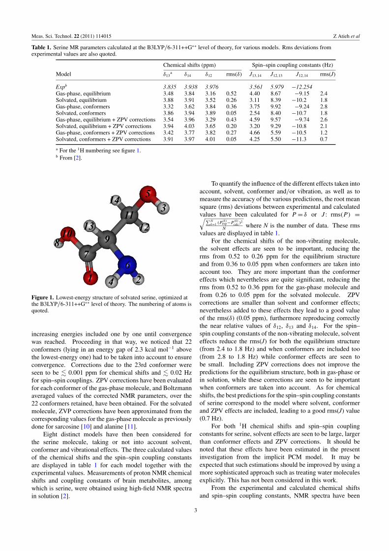
Meas. Sci. Technol. 22 (2011) 114015 Z Atieh et al
Table 1. Serine MR parameters calculated at the B3LYP/6-311++G∗∗ level of theory, for various models. Rms deviations fromexperimental values are also quoted.
Chemical shifts (ppm) Spin–spin coupling constants (Hz)
Model δ13a δ14 δ12 rms(δ) J13,14 J12,13 J12,14 rms(J)
Expb 3.835 3.938 3.976 3.561 5.979 −12.254Gas-phase, equilibrium 3.48 3.84 3.16 0.52 4.40 8.67 −9.15 2.4Solvated, equilibrium 3.88 3.91 3.52 0.26 3.11 8.39 −10.2 1.8Gas-phase, conformers 3.32 3.62 3.84 0.36 3.75 9.92 −9.24 2.8Solvated, conformers 3.86 3.94 3.89 0.05 2.54 8.40 −10.7 1.8Gas-phase, equilibrium + ZPV corrections 3.54 3.96 3.29 0.43 4.59 9.57 −9.74 2.6Solvated, equilibrium + ZPV corrections 3.94 4.03 3.65 0.20 3.20 9.29 −10.8 2.1Gas-phase, conformers + ZPV corrections 3.42 3.77 3.82 0.27 4.66 5.59 −10.5 1.2Solvated, conformers + ZPV corrections 3.91 3.97 4.01 0.05 4.25 5.50 −11.3 0.7
a For the 1H numbering see figure 1.b From [2].
Figure 1. Lowest-energy structure of solvated serine, optimized atthe B3LYP/6-311++G∗∗ level of theory. The numbering of atoms isquoted.
increasing energies included one by one until convergencewas reached. Proceeding in that way, we noticed that 22conformers (lying in an energy gap of 2.3 kcal mol−1 abovethe lowest-energy one) had to be taken into account to ensureconvergence. Corrections due to the 23rd conformer wereseen to be � 0.001 ppm for chemical shifts and � 0.02 Hzfor spin–spin couplings. ZPV corrections have been evaluatedfor each conformer of the gas-phase molecule, and Boltzmannaveraged values of the corrected NMR parameters, over the22 conformers retained, have been obtained. For the solvatedmolecule, ZVP corrections have been approximated from thecorresponding values for the gas-phase molecule as previouslydone for sarcosine [10] and alanine [11].
Eight distinct models have then been considered forthe serine molecule, taking or not into account solvent,conformer and vibrational effects. The three calculated valuesof the chemical shifts and the spin–spin coupling constantsare displayed in table 1 for each model together with theexperimental values. Measurements of proton NMR chemicalshifts and coupling constants of brain metabolites, amongwhich is serine, were obtained using high-field NMR spectrain solution [2].
To quantify the influence of the different effects taken intoaccount, solvent, conformer and/or vibration, as well as tomeasure the accuracy of the various predictions, the root meansquare (rms) deviations between experimental and calculatedvalues have been calculated for P = δ or J : rms(P ) =√∑N
k=1 (P(k)exp−P
(k)calc)
2
Nwhere N is the number of data. These rms
values are displayed in table 1.For the chemical shifts of the non-vibrating molecule,
the solvent effects are seen to be important, reducing therms from 0.52 to 0.26 ppm for the equilibrium structureand from 0.36 to 0.05 ppm when conformers are taken intoaccount too. They are more important than the conformereffects which nevertheless are quite significant, reducing therms from 0.52 to 0.36 ppm for the gas-phase molecule andfrom 0.26 to 0.05 ppm for the solvated molecule. ZPVcorrections are smaller than solvent and conformer effects;nevertheless added to these effects they lead to a good valueof the rms(δ) (0.05 ppm), furthermore reproducing correctlythe near relative values of δ12, δ13 and δ14. For the spin–spin coupling constants of the non-vibrating molecule, solventeffects reduce the rms(J) for both the equilibrium structure(from 2.4 to 1.8 Hz) and when conformers are included too(from 2.8 to 1.8 Hz) while conformer effects are seen tobe small. Including ZPV corrections does not improve thepredictions for the equilibrium structure, both in gas-phase orin solution, while these corrections are seen to be importantwhen conformers are taken into account. As for chemicalshifts, the best predictions for the spin–spin coupling constantsof serine correspond to the model where solvent, conformerand ZPV effects are included, leading to a good rms(J) value(0.7 Hz).
For both 1H chemical shifts and spin–spin couplingconstants for serine, solvent effects are seen to be large, largerthan conformer effects and ZPV corrections. It should benoted that these effects have been estimated in the presentinvestigation from the implicit PCM model. It may beexpected that such estimations should be improved by using amore sophisticated approach such as treating water moleculesexplicitly. This has not been considered in this work.
From the experimental and calculated chemical shiftsand spin–spin coupling constants, NMR spectra have been
3

Meas. Sci. Technol. 22 (2011) 114015 Z Atieh et al
Figure 2. NMR spectra of serine simulated from experimental as well as from calculated values of the NMR parameters at theB3LYP/6-311++G∗∗ level of theory, for various models.
Table 2. Comparison between experimental and calculated (B3LYP/6-311++G∗∗) MR parameters (δ in ppm, J in Hz) for the sevenmetabolites investigated.
Model Metabolite Nδ rms(δ) Metabolite NJ rms(J)
Gas-phase, equilibrium structure Gaba, put, spd, sp, sar, ala, ser 20 0.29 ala, ser 4 2.1gaba, ala, ser 8 1.2
Solvated, equilibrium structure Gaba, put, spd, sp, sar, ala, ser 20 0.18 ala, ser 4 1.6Gas-phase, conformers put, sar, ala, ser 9 0.30 ala, ser 4 2.5Solvated, conformers put, spd, sp, sar, ala, ser 17 0.11 ala, ser 4 1.6Gas-phase, equilibrium structure + ZVP corrections sar, ala, ser 7 0.31 ala, ser 4 2.3Solvated, equilibrium structure + ZVP corrections sar, ala, ser 7 0.16 ala, ser 4 1.8Gas-phase, conformers + ZVP corrections sar, ala, ser 7 0.24 ala, ser 4 1.0Solvated, conformers + ZVP corrections sar, ala, ser 7 0.07 ala, ser 4 0.6
simulated using Gabedit [23]. Some are drawn in figure 2. Itis clear that considering only the equilibrium geometry of theserine molecule, evenly in water solution, does not lead to arealistic description of the NMR spectrum simulated from theexperimental values for the δ and J parameters. Adding theeffects of solvated conformers greatly improves the agreement,the best one being displayed when ZPV corrections are addedtoo.
4. Comparison with experimental data for sevenmetabolites
Up to now we have calculated the NMR parameters of theGABA [6], alanine [11], serine, putrescine [7–9], spermidine[8, 9], spermine [8, 9] and sarcosine [10] molecules in variousmore or less sophisticated models. A synthesis of all thedata is presented in table 2. We knew experimental chemicalshifts for each molecule while, to the best of our knowledge,experimental spin–spin coupling constants are available onlyfor the three brain metabolites: GABA, alanine and serine [2].
In order to compare the experimental and calculated NMRparameters, the rms(δ) and rms(J) have been calculated andtheir values are recorded in table 2 together with the numberN of data and the list of metabolites considered.
Taking into account solvent effects greatly improves theagreement between calculated and experimental δ values;the rms values are significantly reduced for the equilibriumgeometry (from 0.29 to 0.18 ppm) as well as for conformers(from 0.30 to 0.11 ppm). The ZPV corrections are small forgas-phase as well as solvated molecules in their equilibriumgeometry. In contrast they improve the accuracy of calculatedresults when conformer effects are included, reducing the rmsfrom 0.30 to 0.24 ppm for the gas-phase molecules and from0.11 to 0.07 ppm for the solvated molecules. For chemicalshifts our best result is obtained when solvent, conformer andvibrational effects are taken into account, with a good valuefor the corresponding rms (0.07 ppm). Solvent effects are alsoimportant for the J constants, reducing the rms from 2.1 to1.6 Hz for molecules in their equilibrium structure and from2.5 to 1.6 Hz when conformer effects are included. Taking
4

Meas. Sci. Technol. 22 (2011) 114015 Z Atieh et al
into account vibrational effects improves the accuracy whenconformer effects are included too, reducing the rms from 2.5to 1.0 Hz for gas-phase molecules and from 1.6 to 0.6 Hz forsolvated molecules. Once more our best result for J values isobtained when solvent, conformer and vibrational effects aretaken into account, with a good value for the correspondingrms (0.6 Hz).
5. Conclusion
The 1H NMR spin-Hamiltonian parameters have beencalculated at the B3LYP/6-311++G∗∗/GIAO level of theoryfor the serine molecule under eight various assumptions:taking or not into account solvent, conformer and vibrationaleffects. From the comparison between these predicted valuesand the known experimental ones, it is demonstrated thatthe best agreement is obtained when solvent, conformer andvibrational corrections are taken into account, leading to goodvalues for the rms deviations for both the chemical shiftsand the spin–spin coupling constants. The same conclusionis pointed out from similar comparisons involving the sevenmetabolites investigated to date.
Our best calculated values for the various δ and Jparameters will be implemented as data in the jMRUI softwarepackage [25], a popular standard for quantitation of MRSsignals.
Acknowledgments
This work is supported by the EU Marie Curie ResearchNetwork MRTNCT-2006-035801, 2006–2010. The authorsthank the ‘Pole Scientifique de Modelisation Numerique(PSMN)’ at Lyon, France, for generous computationalfacilities. This work was granted access to the HPCresources of [CCRT/CINES/IDRIS] under the allocation20XX-c2010086341 made by GENCI (Grand EquipementNational de Calcul Intensif).
References
[1] Van der Graaf M 2010 In vivo magnetic resonancespectroscopy: basic methodology and clinical applicationsEur. Biophys. J. 39 527–40
[2] Govindaraju V, Young K and Maudsley A A 2000 ProtonNMR chemical shifts and coupling constants for brainmetabolites NMR Biomed. 13 129–53
[3] Fukui H 2009 Theoretical aspects of spin–spin couplings Nucl.Mag. Reson. 38 166–93
[4] Casabianca L B and de Dios A C 2008 Ab initio calculationsof NMR chemical shifts J. Chem. Phys. 128 052201
[5] Helgaker T, Jaszunski M and Pecul M 2008 The quantumchemical calculation of NMR indirect spin–spin couplingconstants Prog. Nucl. Magn. Reson. Spectrosc. 53 249–68
[6] Allouche A R, Aubert-Frecon M and Graveron-Demilly D2007 Quantum chemistry-based NMR spin Hamiltonianparameters of GABA for quantitation in magnetic resonancespectroscopy Phys. Chem. Chem. Phys. 9 3098–103
[7] Allouche A R, Graveron-Demilly D, Fauvelle Fand Aubert-Frecon M 2008 Theoretical and experimentalinvestigation of the 1H NMR spectra of putrescine Chem.Phys. Lett. 466 219–22
[8] Atieh Z, Allouche A R, Fauvelle F, Graveron Dand Aubert-Frecon M 2009 Density functional theory(DFT) calculations of the (NMR) nuclear magneticresonance spin-Hamiltonian parameters for two polyaminesof prostate tissue: spermidine and spermine Meas. Sci.Technol. 20 104024
[9] Atieh Z, Allouche A R and Aubert-Frecon M 2010 DFTcalculations of isomer effects upon NMR spin-Hamiltonianparameters of prostate polyamines J. Mol. Struct.THEOCHEM 945 104–9
[10] Atieh Z, Allouche A R, Lazariev A, van Ormondt D,Graveron-Demilly D and Aubert-Frecon M 2010 DFTcalculations of 1H chemical shifts, simulated andexperimental NMR spectra for sarcosine Chem. Phys. Lett.492 297–301
[11] Atieh Z, Allouche A R, Graveron-Demilly Dand Aubert-Frecon M 2010 Solvent, isomers and vibrationaleffects in DFT calculations for the NMR spin-Hamiltonianparameters of alanine Proc. 2010 IEEE Int. Workshop onImaging Systems and Techniques (IST) pp 369–72
[12] Swope W C, Andersen H C, Berens P H and Wilson K R 1982A computer simulation method for the calculation ofequilibrium constants for the formation of physical clustersof molecules: application to small water clusters J. Chem.Phys. 76 637–49
[13] Stewart J J P 2007 Optimization of parameters forsemi-empirical methods V: modification of NDDOapproximations and application to 70 elements J. Mol.Model. 13 1173–213
[14] Baker J 1986 An algorithm for the location of transition statesJ. Comp. Chem. 7 385–95
[15] Becke A D 1993 Density-functional thermochemistry: III. Therole of exact exchange J. Chem. Phys. 98 5648–52
[16] Lee C, Yang W and Parr R G 1988 Development of theColle–Salvetti correlation-energy formula into a functionalof the electron density Phys. Rev. B 37 785–9
[17] Krishnan R, Binkley J S, Seeger R and Pople J A 1980Self-consistent molecular orbital methods: XX. A basis setfor correlated wavefunctions J. Chem. Phys. 72 650–4
[18] Miertus S, Scrocco E and Tomasi J 1981 Electrostaticinteraction of a solute with a continuum. A direct utilizationof ab initio molecular potentials for the prevision of solventeffects Chem. Phys. 55 117–29
[19] Barone V, Cossi M and Tomasi J 1997 A new definition ofcavities for the computation of solvation free energies by thepolarisable continuum model J. Chem. Phys. 107 3210–21
[20] Cheeseman J R, Trucks G W, Keith T A and Frisch M J 1996A comparison of models for calculating nuclear magneticresonance shielding tensors J. Chem. Phys. 104 5497–509
[21] Kaupp M, Buhl M and Malkin V G 2004 Calculation of NMRand EPR Parameters (New York: Wiley)
[22] Frisch M J et al 2004 Gaussian 03, Revision D.02, Gaussian,Inc., Wallingford, CT
[23] Allouche A R 2011 Gabedit. A graphical user interface forcomputational chemistry softwares J. Comp. Chem.32 174–82
[24] Roberts J D 1961 An Introduction to the Analysis of Spin–SpinSplitting in High-Resolution Nuclear Magnetic ResonanceSpectra (New York: Benjamin)
[25] Stefan D et al 2009 Quantitation of magnetic resonancespectroscopy signals: the jMRUI software package Meas.Sci. Technol. 20 104035
5


Chapter 3: Application on metabolites: results Synthesis of results
179
C: Synthesis of results
In the present work, we have designed, for the calculations of the 1H NMR parameters
( and ) of metabolites, many computational methods that allows (1) the determination of all
the stable isomers of a metabolite in a given energy range above the lowest one, (2) the
calculation of the chemical shifts and the spin-spin coupling constants for the protons of
each isomer and averaging the values following a Boltzmann distribution, (3) the calculation
of zero-point vibrational corrections for these NMR parameters for the protons of each isomer
and averaging the corrected values following a Boltzmann distribution, (4) the simulation of
the corresponding MR spectrum. These computational methods are based on the DFT/B3LYP
method with the 6-311++G** basis set.
In this part C, a synthesis of the results using these computational methods is
presented for seven metabolites (Gaba (1)
, putrescine (put) (2; 3)
, spermidine (spd) (4; 3)
,
spermine (sp) (4; 3)
, sarcosine (sar) (5)
, alanine (ala) (6)
and serine (ser) (7)
), one of which (Gaba)
was studied within the group.
For each molecule, we knew experimental chemical shifts while, to the best of our
knowledge, experimental spin-spin coupling constants are available for only the three brain
metabolites: GABA, alanine and serine (8)
.
In order to compare the experimental and calculated NMR parameters, the root mean
square (rms) deviations have been calculated for the chemical shifts and spin-spin coupling
constants using equation (3.7)
(3.7)
where N is the number of data. rms values for different models of calculation are displayed in
table (3.43).

Chapter 3: Application on metabolites: results Synthesis of results
180
Eight models of calculation were done : 1: gas phase + equilibrium structure, 2:
solvated, equilibrium structure, 3 : gas phase + isomers, 4 : solvated + isomers, 5 : 1 +
vibration ; 6 : 2 + vibration ; 7 : 3 + vibration, 8 : 4 + vibration.
Results of table (3.43) are plotted in figures (3.21) and (3.22) for rms of chemical
shifts and spin-spin coupling constants respectively.
Model Metabolite Nδ Rms (δ) Metabolite NJ rms (J)
Gas-phase, equilibrium
struc ure
Gaba, put, spd,
sp, sar, ala, ser 20 0.29
ala, ser 4 2.1
gaba, ala, ser 8 1.2
Solvated, equilibrium
structure
Gaba, put, spd,
sp, sar, ala, ser 20 0.18 ala, ser 4 1.6
Gas-phase, isomers put, sar, ala,
ser 9 0.3 ala, ser 4 2.5
Solvated, isomers put, spd, sp,
sar, ala, ser 17 0.11 ala, ser 4 1.6
Gas-phase, equilibrium
structure + ZVP
corrections
sar, ala, ser 7 0.31 ala, ser 4 2.3
Solvated, equilibrium
structure + ZVP
corrections
sar, ala, ser 7 0.16 ala, ser 4 1.8
Gas-phase, isomers +
ZVP corrections sar, ala, ser 7 0.24 ala, ser 4 1.0
Solvated, isomers + ZVP
corrections sar, ala, ser 7 0.07 ala, ser 4 0.6
Table 3.43: results for acetate using MD-ONIOM

Chapter 3: Application on metabolites: results Synthesis of results
181
From table (3.42) and figure (3.21), we can note that taking into account solvent
effects greatly improves the agreement between calculated and experimental values, as
could be expected, the rms values are significantly reduced for the equilibrium geometry
(from 0.29 ppm to 0.18 ppm) as well as for isomers (from 0.30 ppm to 0.11 ppm). The zero-
point vibrational corrections are small for gas-phase as well as solvated molecules in their
equilibrium geometry. On the contrary they improve the accuracy of calculated results when
Figure 3.21: rms of the chemical shifts
Figure 3.22: rms of the spin-spin coupling constants

Chapter 3: Application on metabolites: results Synthesis of results
182
isomers effects are included, reducing the rms from 0.30 ppm to 0.24 ppm for the gas-phase
molecules and from 0.11 ppm to 0.07 ppm for the solvated molecules. For chemical shifts our
best result is obtained when solvent, isomers and vibrational effects are taken into account,
with a good value for the corresponding rms (0.07 ppm).
Solvent effects are also important for the constants, reducing the rms from 2.1 Hz to
1.6 Hz for molecules in their equilibrium structure and from 2.5 Hz to 1.6 Hz when isomers
effects are included. Taking into account vibrational effects improves the accuracy when
isomers effects are included too, reducing the rms from 2.5 Hz to 1.0 Hz for gas-phase
molecules and from 1.6 Hz to 0.6 Hz for solvated molecules. Once more our best result for
values is obtained when solvent, isomers and vibrational effects are taken into account, with a
good value for the corresponding rms (0.6 Hz).
As a conclusion, from the comparisons with experiments for the 7 metabolites under
investigation, the best agreement for the chemical shifts of the non-vibrating metabolites (with
a rms of 0.1 ppm) is obtained when taking into account the isomers effects for the solvated
species. Zero-point vibrational corrections improve this agreement, reducing the rms from 0.1
ppm to 0.07 ppm. The best agreement for the spin-spin coupling constants of the non-
vibrating metabolites (with a rms of 1.6 Hz) is obtained when taking into account the isomers
effects for the solvated species. Zero-point vibrational corrections improve this agreement,
reducing the rms from 1.6 Hz to 0.6 Hz.
These results demonstrate that the DFT/B3LYP/6-311++G** level of theory is able to
provide accurate values of 1H NMR parameters. It may be inferred that they are reliable
enough to serve as good starting values for the simulation of basis-set signals for further
quantitation methods for metabolites.

Chapter 3: Application on metabolites: results Synthesis of results
183
References
1. Quantum chemistry-based NMR spin Hamiltonian parameters of GABA for quantitation in
magnetic resonance spectroscopy. A. R. Allouche, M. Aubert-Frécon, and D. Graveron-Demilly.
2007, Phys. Chem. Chem. Phys., Vol. 9, p. 3098.
2. Theoretical and experimental investigation of the 1H NMR spectrum of putrescine. A. R. Allouche,
D. Graveron-Demilly, F. Fauvelle, and M. Aubert-Frécon. 2008, Chem. Phys. Lett., Vol. 466, p.
219.
3. DFT calculations of isomer effects upon NMR spin-Hamiltonian parameters of prostate polyamines.
Z. Atieh, A. R. Allouche, and M. Aubert-Frécon. 2010, J. Mol. Structur. THEOCHEM, Vol. 945, p.
104.
4. Density functional theory calculations of the nuclear magnetic resonance spin-Hamiltonian
parameters for two polyamines of prostate tissue: spermidine and spermine . Z. Atieh, A. R.
Allouche, F. Fauvelle, D. Graveron, and M. Aubert-Frécon. 2009, Measurement Science &
Technology, Vol. 20, p. 104024.
5. DFT calculations of 1H chemical shifts, simulated and experimental NMR spectra for sarcosine. Z.
Atieh, A. R. Allouche, A. Lazariev, D. Van Ormondt, D. Graveron-Demilly, and M. Aubert-
Frécon. 2010, Chem. Phys. Lett., Vol. 492, p. 297.
6. Solvent, isomers and vibrational effects in DFT calculations for the NMR spin-Hamiltonian
parameters of alanine. Z. Atieh, AR. Allouche, D. Graveron-Demilly, and M. Aubert-Frécon.
2010, Proceedings of the 2010 IEEE International Workshop on Imaging Systems and Technics (IST),
p. 369.
7. Density Functional Theory (DFT) calculations of the (NMR) nuclear magnetic resonance spin-
Hamiltonian parameters for serine. Z. Atieh, A. R. Allouche, D. Graveron-Demilly, and M.
Aubert-Frécon. Measurement Science & Technology.
8. Proton NMR chemical shifts and coupling constants for brain metabolites. V. Govindaraju, K.
Young, and A. A. Maudsley. 2000, NMR Biomed., Vol. 13, p. 129.

Chapter 3: Application on metabolites: results Synthesis of results
184

Chapter 4: Model to predict NMR chemical shifts for biological molecules
185
Chapter 4
Model to Predict NMR chemical shifts for
biological molecules
The NMR chemical shifts, measurable under very general conditions and with a good
accuracy are sensitive probes of chemical environment of atoms. They are particularly suited
for characterizing the structure of biological molecules. One major obstacle, however, has
been the difficulty to understand in details the complicated conformational dependencies of
the chemical shifts.
Several approaches are now available for the increasingly quantitative prediction of
chemical shifts from a 3D protein structure. SHIFTX (1)
is a widely used program, which uses
chemical shift hypersurfaces to describe the structural effects such as torsion angles, and
classical equations to calculate physical effects. Quite a similar approach is adopted in the
PRSI program (2)
. In the SPARTA program (3)
a combination of local sequence homology is
combined with dihedral angle effects. 1H chemical shifts are modeled with density functional
calculations in the SHIFTS (4)
approach, and PROSHIFT (5)
uses artificial neural networks to
predict the chemical shifts from empirical structural information. Recently, in the recent
CamShift (6)
program, the chemical shifts in proteins are calculated from inter-atomic
distances. All these approaches have been developed specifically for proteins. Abraham (7)
and his collaborators have developed a model, based on effective charges for predicting the
proton chemical shifts for organic molecules.
An alternative method of determining NMR chemical shifts is by using the ab initio
gauge-invariant atomic orbital (GIAO) method, together with the DFT method or with any
method based on wave-function (like MP2 (8)
, CCSD (9)
, …) in which the nuclear shielding
tensor is calculated. Since the protons are located on the periphery of the molecule their
chemical shifts will be more sensitive to intermolecular interactions. So the solvent effects
cannot be neglected. The experiments are usually performed at 300 K. It is therefore likely

Chapter 4: Model to predict NMR chemical shifts for biological molecules
186
that the measured spectrum is that of several isomers of the molecule. A conformational
search is then often necessary (10)
. It was also shown that the zero-point vibrational correction
is not negligible (11)
. Taking into account of all these corrections makes the calculations very
expansive for molecules of medium size and unfordable for proteins. Several recent studies
have shown that the chemical shifts calculated by averaging the values along a trajectory of
molecular dynamics can improve the quality of the predicted values (12; 13; 14)
. Having a
simple, fast and accurate model to predict chemical shifts for a given geometry is very
important to achieve this type of study.
In this chapter, we present a new model, BioShift, that can be used to predict chemical
shifts for biological molecules (proteins, DNA, RNA, polyamines ...). It is simple, fast and
involves a limited number of parameters. It is particularly adapted to be used in molecular
dynamics studies with a molecular mechanics potential. We test the model for polyamines
which are rather small molecules as well as for proteins for which a lot of NMR chemical
shifts are available. The tests show that our simple and fast model is competitive, by his
accuracy, with sophisticated models specifically developed for proteins. It was seen to be also
successful for polyamines.
I Description of the model
In the BioShift method, the chemical shift of an atom is approximated formally as a
sum of: (1) a term depending on the atom-type of (we have used Amber (15)
types in our
study), (2) bond terms, (3) angle terms, (4) dihedral terms, and (5) non-bonded terms. The
chemical shift of a given atom , of type is then modeled by:
(4.1)

Chapter 4: Model to predict NMR chemical shifts for biological molecules
187
where , , are the Amber types of atoms , and respectively. The bond term
includes the effect of all atoms making a chemical bond with
the atom . The bond term depends on the types of atoms and as well as the distance
between them.
Figure (4.1): atoms and related by a chemical bond
The angle term includes the effects of all atoms
separated from the atom by two chemical bonds where is the intermediate atom. The
angle term depends on the types of atoms , , and , as well as the distance between atoms
and .
Figure (4.2): atoms and related through an angle
The dihedral term includes the effects of
all atoms separated from the atom by three chemical bonds where atoms and are the
intermediate atoms. The dihedral term depends on the types of atoms , , , and , as well
as the distance between the atoms and .

Chapter 4: Model to predict NMR chemical shifts for biological molecules
188
Figure (4.3): atoms A and D related through a dihedral angle
The non-bonded term includes the effects of all
atoms non-bonded to the atom . The non-bonded term depends on the types of atoms
and , as well as the distance between them.
We have chosen a simple generic model form for the four functions , where is
equal to (bond), (angle), (dihedral), or (non-bonded), and taken into account the
contribution to the chemical shift of atom from one atom bonded to ( ) or
connected to through an angle ( ) or through a dihedral ( ) or non-
bonded to ( )
(4.2)
where is the distance between atoms and . The parameters depend on the types of
atoms and as well as on the connection-types ( ). The number of terms is
generally chosen to be equal to 1 or 2. For the parameters , the values +1, -3, -6 or -8 may
be used, following the connection-type ( ) as well as the atom-type.
It must be noted that, we have tried to replace the function which depends on the
distance, by other functions that depend on the angle for angle terms or on the dihedral angle
for dihedral terms; however, the function depending on the distance showed a better stability
and performance in predicting chemical shifts.
The and parameters are to be fitted by maximizing the agreement between
predicted and experimental chemical shifts for a set of biological molecules for which both
structures and chemical shifts are known experimentally. Using these fitted parameters,
chemical shifts can be predicted for other biological molecules.

Chapter 4: Model to predict NMR chemical shifts for biological molecules
189
II Illustrative results and discussion
Since NMR chemical shifts are available for a vast number of proteins, we have tested
our model for this type of molecules. For fitting the and parameters and choosing the
more appropriate values of , we used the RefDB17 database of chemical shifts and the
corresponding Protein Data Bank (PDB) structures, and we extracted the chemical shifts of
HA, HN, CA, CB, CO, and N nuclei for ten proteins (1IAR, 1BDO, 1MMS, 2IHB, 1KQR,
1QOG, 2RN2, 1MXE, 1CWC, 2J1K). We used the known chemical shifts for the first five
proteins of the precedent list to fit the parameters of our model. The other five proteins were
used for testing the accuracy of the prediction obtained from our fitted parameters.
The PDB structures do not contain the positions of the hydrogen atoms, these were
added. The positions of H atoms were optimized using the Amber force-field potential
implemented in Gabedit.
Figure (4.4): protein 1MMS after the addition of H atoms and optimizing their positions
Here, we present our results for the smallest number of parameters allowing a good
accuracy together with a comparison with the results we obtained via SHIFTX and those
published from CamShift which are two of the state-of-the-art chemical shift predictors. For
the six nuclei ( , and ) the root mean squares deviations (rmsd) between
experimental and fitted chemical shift values are displayed in tables (4.1) while rmsd values
between experimental and predicted chemical shifts are displayed in table (4.2). The
correlation coefficient R, reflecting the quality of the agreement between a certain model and
experimental data, is also quoted for the set of the 5 proteins included in the fitting process.

Chapter 4: Model to predict NMR chemical shifts for biological molecules
190
Nuclei
HA
P=20/1310/300a
HN
P=15/608/235
CA
P=35/1539/349
Fitted proteins rmsd rmsd rmsd
1IAR 129 0.26/0.23/0.21b
1 5 0.43/0.44/0.39 129 1.76/1/1.01
1BDO 86 0.31/0.28/0.24 75 0.46/0.55/0.45 79 1.71/1.01/1.31
1MMS 136 0.33/0.34/0.30 123 0.53/0.6/0.64 126 2.14/2.3/1.46
2IHB 113 0.35/0.24/0.21 108 0.57/0.54/0.49 111 1.91/1.22/1.19
1KQR 165 0.44/0.39/0.32 149 0.59/0.59/0.70 159 1.83/1.15/1.18
The set of 5 proteins
629
0.35/0.31/0.27
R=0.76/0.84c
580
0.53/0.55/0.56
R=0.63/0.64
604
1.88/1.44/1.23
R=0.91/0.95
Nuclei
CB
P=40
CO
P=22
N
P=35/1168/271
Fitted proteins Rmsd rmsd rmsd
1IAR 124 1.36/1.25/1.11 128 1.06/1.08/0.87 120 2.91/2.79/2.40
1BDO 71 1.94/1.49/1.30 - - 75 3.48/1.97/2.49
1MMS 116 2.2/3.37/1.26 126 1.78/2.29/1.18 123 3.24/3.17/3.13
2IHB 107 2.39/0.93/0.81 111 1.38/1.27/1.10 06 2.46/2.1/2.28
1KQR 149 1.96/1.38/1.28 156 1.26/1.15/1.10 148 3.47/2.93/3.23
The set of 5 proteins
567
1.99/1.56/1.15
R=0.99/0.99
521
1.39/1.51/1.07
R=0.78/0.78
572
3.14/2.72/2.79
R=0.80/0.86
Table (4.1): root mean square deviation (rmsd, in ppm) between chemical shift values from models and
experimental ones. The number of adjustable parameters (P) in each model as well as the number of chemical
shifts ( is quoted. The sign ‘-‘ means lack of experimental data for the concerned nucleus.
a the first entry corresponds to number of adjustable parameters in our model, the second one to the number of
parameters of hypersurfaces used in SHIFTX, the third one to the adjustable parameters in CamShift.
b the first entry corresponds to present results, the second one to the results we obtained using SHIFTX, the
third one to literature results from CamShift
c the first entry corresponds to present results, the second one to the results we obtained using SHIFTX

Chapter 4: Model to predict NMR chemical shifts for biological molecules
191
nuclei HA HN CA
Predicted proteins rmsd rmsd rmsd
1QOG 89 0.38 /0.37a
76 0.49/0.48 84 2.33/1.29
2RN2 169 0.37/0.30 148 0.56/0.52 122 1.87/0.82
1MXE 155 0.25/0.20 142 0.47/0.38 144 2.13/0.87
1CWC 167 0.35/0.36 156 0.73/0.65 159 2.09/1.21
2J1K 122 0.36/0.40 108 0. /0.47 106 1.61/1.17
The 10 proteins set 1331 0.35 /0.32 1210 0.55 /0.53 1219 1.95/1.27
nuclei CB CO N
Predicted proteins rmsd rmsd rmsd
1QOG 80 2.04/1.11 45 1.63/1.87 76 4.2/2.43
2RN2 - - - - 148 3.95/2.46
1MXE - - 144 1.28/0.78 144 2.52/2.09
1CWC - - 148 1.46/1.26 148 3.98/2.68
2J1K 93 2.16/1.62 91 1.25/1.12 92 3.10/3.00
The 10 proteins set 740 2.02/1.53 949 1.38/1.37 1180 3.37/2.60
Table (4.2): root mean square deviation (rmsd, in ppm) between chemical shift values from models and
experimental ones. The number of predicted chemical shifts ( ) is quoted.
a the first entry corresponds to present results, the second one to the results we obtained using SHIFTX
Chemical shift values obtained from models (BioShift and SHIFTX) are plotted
against their experimental values in figures (4.5), (4.6), (4.7), (4.8), (4.9), and (4.10) for the
six nuclei , , , , and respectively, for the five proteins: 1IAR, 1BDO,
1MMS, 2IHB, 1KQR.

Chapter 4: Model to predict NMR chemical shifts for biological molecules
192
Figure (4.5): scatter plots for the chemical shifts (in ppm) of the atoms of the set of 5 proteins: 1IAR,
1BDO, 1MMS, 2IHB, 1KQR. (Black) points for present data (correlation coefficient R=0.76), (red) points ∆
for SHIFTX data (R=0.84).
Figure (4.6): scatter plots for the chemical shifts (in ppm) of the atoms of the set of 5 proteins: 1IAR,
1BDO, 1MMS, 2IHB, 1KQR. (Black) points for present data (R=0.63), (red) points ∆ for SHIFTX data
(R=0.64).
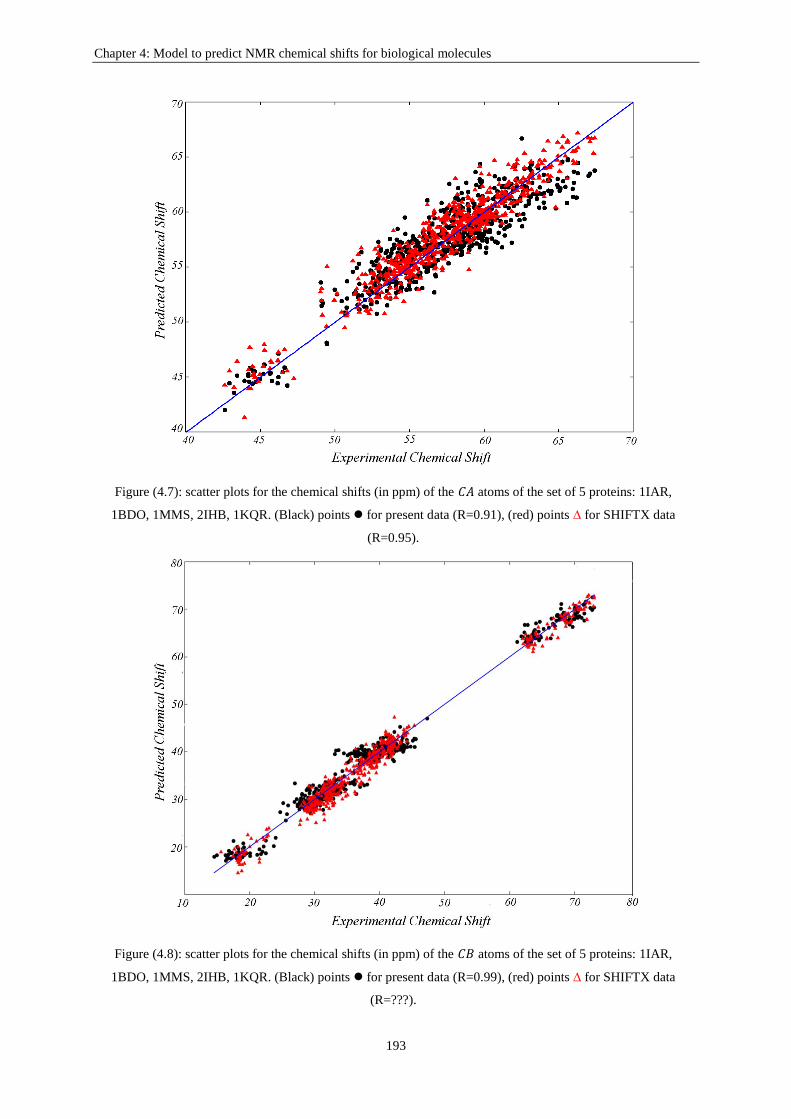
Chapter 4: Model to predict NMR chemical shifts for biological molecules
193
Figure (4.7): scatter plots for the chemical shifts (in ppm) of the atoms of the set of 5 proteins: 1IAR,
1BDO, 1MMS, 2IHB, 1KQR. (Black) points for present data (R=0.91), (red) points ∆ for SHIFTX data
(R=0.95).
Figure (4.8): scatter plots for the chemical shifts (in ppm) of the atoms of the set of 5 proteins: 1IAR,
1BDO, 1MMS, 2IHB, 1KQR. (Black) points for present data (R=0.99), (red) points ∆ for SHIFTX data
(R=???).

Chapter 4: Model to predict NMR chemical shifts for biological molecules
194
Figure (4.9): scatter plots for the chemical shifts (in ppm) of the atoms of the set of 4 proteins: 1IAR,
1MMS, 2IHB, 1KQR. (Black) points for present data (R=0.78), (red) points ∆ for SHIFTX data (R=????)
Figure (4.10): scatter plots for the chemical shifts (in ppm) of the N atoms of the set of 5 proteins: 1IAR,
1BDO, 1MMS, 2IHB, 1KQR. (Black) points for present data (R=0.80), (red) points ∆ for SHIFTX data
(R=0.86).

Chapter 4: Model to predict NMR chemical shifts for biological molecules
195
The full list of the parameters used in our model (BioShift) and their numerical values
are displayed in appendix B.
The results of table (4.1) show that, BioShift with a limited number of parameters
provide an overall similar accuracy in comparison with SHIFTX for and protons,
sligthly poorer than the results from CamShift for . With only 15 parameters (to compare
to 608 parameters in SHIFTX and 235 parameters in CamShift), BioShift reproduces the
chemical shifts for 580 protons with a root mean square deviation rmsd = 0.53 ppm (the
correlation between the experimental chemical shifts and BioShift's predictions R=0.63), to be
compared to rmsd = 0.55 ppm (R=0.64) obtained from the SHIFTX program. A similar
accuracy was obtained for 629 protons using 20 parameters (to compare to 1310
parameters in SHIFTX and 300 parameters in CamShift).
For the , , and nuclei, the fits are quite good with values of R larger than 0.8
similar to the values obtained from SHIFTX, while the rmsd are somewhat larger than both
results from SHIFTX and CamShift. The increase of the number of non-bonded parameters
(and consequently the computational time) was seen to slightly improve the predictions. For
CA, the rmsd was 1.73 ppm instead of 1.88 ppm for the 604 CA of the 5 proteins included in
the fitting process. For CB, the rmsd was 1.56 ppm instead of 1.99 ppm for the 567 CB nuclei
while for N the rmsd was 2.92 ppm instead of 3.14 ppm for the 572 N nuclei. The
discrepancies with the results from SHIFTX are lowered but remain larger than for the
protons. According to our tests, it seems that taking a function that depends on the dihedral
angle in place of a function that depends upon the distance between atoms connected through
a dihedral does not improve the accuracy of the prediction. Note that in our model, we have
used the same parameters for an atom-type in any amino acid, whereas in the model
implemented in the SHIFTX program as well as in other models such as CamShift, different
parameters are used for a given atom-type for each amino acid. Besides, it has been shown
that taking into account the fluctuation of the chemical shift of C nuclei over time improves
(about 1 ppm more accuracy) the quality of the prediction (16)
. A time averaging on the
chemical shift values, computed by our model, over conformations obtained by molecular
dynamics simulations should improve the accuracy of the present predictions.
For CO, the fits are good with a value of R = 0.78 similar to the value obtained from
SHIFTX. The rmsd for the fitted proteins is in between the rmsd values obtained from
SHIFTX and CamShift. The rmsd values are 1.39, 1.51, and 1.07 ppm using the present

Chapter 4: Model to predict NMR chemical shifts for biological molecules
196
model, SHIFTX, and CamShift for the 521 CO nuclei of the proteins included in the fitting
process.
From table (4.2), present results show also that the parameters fitted to reproduce at
the best the experimental values for the five proteins: 1IAR, 1BDO, 1MMS, 2IHB, 1KQR,
can predict with as good accuracy, the chemical shifts for the five other proteins considered:
1QOG, 2RN2, 1MXE, 1CWC, 2J1K.
As a further test of the present model, we used it to obtain the chemical shifts of the
H1 protons of the four polyamines: putrescine, spermidine, spermine, and cadaverine (a fourth
polyamine) that we have investigated from DFT calculations. Using parameters previously
fitted for proteins together with two more parameters specific to polyamines (angle term: H1
CT NT, α=35.457501, β=1; dihedral term: H1 CT NT H, α=-14.143552, β=1) the
experimental values of the chemical shifts for the 16 H1 were reproduced with a rmsd of 0.03
ppm and R=0.86, showing that the model works also for this type of molecules.
Besides, using the parameters previously fitted for proteins, we tested our model in the
prediction of H1 chemical shifts for 20 amino acids. The rmsd between predicted and
experimental values was found to be 0.3 ppm. This precision of prediction is usually
expected, and of course, better precisions can only be obtained by quantum chemistry
calculation in which the inclusion of different corrections is sometimes needed (solvent,
vibration, temperature …).
As a conclusion, we proposed the BioShift method to predict chemical shifts for
biomolecules and we applied it successfully to rather small ones (polyamines) and to proteins.
The functional form and the number of parameters of our model make the BioShift
predictions very rapid and suitable to compute chemical shift in molecular dynamics
simulations for macromolecules like proteins, DNA and RNA. This model should be
particularly useful for certification of molecular dynamics trajectories with NMR chemical
shifts using a molecular mechanic potential.

Chapter 4: Model to predict NMR chemical shifts for biological molecules
197
References
1. Rapid and accurate calculation of protein 1H, 13C and 15N chemical shifts. S. Neal, A. M. Nip, H.
Y. Zhang, and D. S. Wishart. 2003, J. Biomol. NMR, Vol. 26, p. 215.
2. Predicting 15N chemical shifts in proteins using the preceding residue-specific individual shielding
surfaces from φ, ψi−1, and χ1torsion angles. Y. J. Wang, and O. Jardetzky. 2004, J. Biomol. NMR,
Vol. 28, p. 327.
3. Protein backbone chemical shifts predicted from searching a database for torsion angle and
sequence homology. Y. Shen, and A. Bax. 2007, J. Biomol. NMR, Vol. 38, p. 289.
4. A new model for chemical shifts of amide hydrogens in proteins. S. Moon, and D. A. Case. 2007, J.
Biomol. NMR, Vol. 38, p. 139.
5. PROSHIFT: Protein chemical shift prediction using artificial neural networks. J.Meiler. 2003, J.
Biomol. NMR, Vol. 26, p. 25.
6. Fast and Accurate Predictions of Protein NMR Chemical Shifts from Interatomic Distances. K. J.
Kohlhoff, P. Robustelli,A. Cavalli, X. Salvatella, and M. Vendruscolo. 2009, J. Am. Chem. Soc.,
Vol. 131, p. 13894.
7. 1H chemical shifts in NMR: Part 23, the effect of dimethyl sulphoxide versus chloroform solvent on
1H chemical shifts. R. J. Abraham, J. J. Byrne, L. Griffiths, and M. Perez. 2006, Mag. Res.Chem.,
Vol. 44, p. 491.
8. MP2 energy evaluation by direct methods. M. Head-Gordon, J. A. Pople, and M. J. Frisch. 1988,
Chem. Phys. Lett., Vol. 153, p. 503 .
9. A full coupled‐cluster singles and doubles model: The inclusion of disconnected triples. G. D. P.,
and R. J. Bartlett. 1982, J. Chem. Phys., Vol. 76, p. 1910.
10. DFT calculations of isomer effects upon NMR spin-Hamiltonian parameters of prostate
polyamines. Z. Atieh, A. R. Allouche, and M. Aubert-Frecon. 2010, J. Mol. Struct.-THEOCHEM,
Vol. 945, p. 104.
11. DFT calculations of 1H chemical shifts, simulated and experimental NMR spectra for sarcosine.
Z. Atieh, A. R. Allouche, A. Lazariev, D. Van Ormondt ,D. Graveron-Demilly, and M. Aubert-
Frecon. 2010, Chem. Phys. Lett., Vol. 492, p. 297.
12. Certification of Molecular Dynamics Trajectories with NMR Chemical Shifts. D. Li, and R.
Brueschweiler. 2010, J. Phys. Chem. Lett., Vol. 1, p. 246.
13. Time Averaging of NMR Chemical Shifts in the MLF Peptide in the Solid State. I. De Gortari, G.
Portella, X. Salvatella, V. S. Bajaj, P. C. A. van der Wel, J. R. Yates, M. D. Segall, C. J. Pickard,
M. C. Payne, and M. Vendruscolo. 2010, J. Am. Chem. Soc., Vol. 132, p. 5993.
14. 4D prediction of protein 1H chemical shifts. J. Lehtivarjo, T. Hassinen, S. Korhonen, M.
Perakyla, and R. Laatikainen. 2009, J. Biomol. NMR, Vol. 45, p. 413.

Chapter 4: Model to predict NMR chemical shifts for biological molecules
198
15. A Second Generation Force Field for the Simulation of Proteins, Nucleic Acids, and Organic
Molecules. W. D. Cornell, P. Cieplak, C. I. Bayly, I. R. Gould, K. M. Merz, D. M. Ferguson, D. C.
Spellmeyer, T. Fox, J. W. Caldwell, and P. A. Kollman. 1995, J. Am. Chem. Soc., Vol. 117, p.
5179.
16. Time Averaging of NMR Chemical Shifts in the MLF Peptide in the Solid State. I. De Gortari, G.
Portella, X. Salvatella, V. S. Bajaj, P. C. A. van der Wel, J. R. Yates, M. D. Segall, C. J. Pickard,
M. C. Payne, and M. Vendruscolo. 2010, J. Am. Chem. Soc., Vol. 132, p. 5993.

Conclusion and perspectives
199
Conclusion and perspectives
In the first part of the present work, 1H Nuclear Magnetic Resonance (NMR) spin-
Hamiltonian parameters: chemical shifts and spin–spin coupling constants have been
calculated using the density functional theory for seven metabolites: four involved in prostate
diseases (putrescine, spermidine, spermine, and sarcosine) and three involved in brain
diseases (acetate, serine, and alanine). A theoretical investigation of the NMR parameters has
been performed for the protons attached to carbon atoms for these metabolites. Several levels
of theory within the DFT approach were used, mixing four functionals B3LYP, PBE, OPBE,
PBE0 and twelve basis sets belonging to three groups: (1) Pople’s basis sets (6-311+G**, 6-
311++G**, 6-311++G(2d,2p), 6-311++G(3df,3pd)), (2) polarisable consistent basis sets
designed for the calculation of chemical shifts (pc0, pc1, pc2, pc3), and (3) the polarisable
consistent basis sets designed for the calculation of spin-spin coupling constants (pcJ0, pcJ1,
pcJ2, pcJ3). By comparison with the experiment, we have demonstrated that the
DFT/B3LYP/6-311++G** level of theory is able to provide accurate values of 1H NMR spin-
Hamiltonian parameters. Using this level of theory, we have studied three effects on the NMR
parameters of metabolites: (1) isomers (2) vibration, and (3) solvent.
The effects on calculated chemical shifts and spin-spin coupling constants, of isomers
higher in energy than the lowest-energy conformer were taken into account. To search the
stable geometries lying in a relative energy range, we have put forward an automatized
method that can be summarized in three consecutive steps: (1) molecular dynamics
calculation using the semi-empirical PM6 potential followed by optimization at the same level
and filtration of similar geometries, (2) optimization of the remaining geometries at the level
B3LYP/6-31G* followed by filtration of similar geometries in addition to geometries having
energies higher than a chosen maximum, and (3) optimization of geometries remaining from
step two at the level B3LYP/6-311++G** followed by calculation of NMR parameters of
each isomers at the same level. The effects of isomers were taken into account through the
calculation of the averaged NMR parameter ( or ) as an average of the NMR parameter of
the various isomers weighted by Boltzmann factor. For all studied metabolites, isomer effects
were seen to reduce the differences between experimental and simulated spectra.

Conclusion and perspectives
200
The second type of studied effects has been the molecular vibration. To calculate
vibrational corrections on chemical shifts and spin-spin coupling constants, we have used
several methods like the ADMP of Gaussian and the CFOUR package; however, zero-point
vibrational corrections were better evaluated through the second order perturbational
approach at the B3LYP/6-311++G** level of theory via a home-made code that we have
implemented in the version of Gaussian03 at our disposal. The corrections due to vibration
were seen to increase the agreement between simulated and experimental NMR spectra.
For the reliable calculation of NMR parameters, the effects of a solvent, particularly
water, were studied using two approaches based on different methodologies of the solvent
model: (1) PCM method which treats the solvent as a continuum having an effective dielectric
constant, and (2) ONIOM method with which explicit solvent molecules can be considered
during calculation. The PCM model was found to be better than ONIOM in calculating
chemical shifts of protons attached to carbon atoms for the metabolites considered in the
present work.
For the calculations of the NMR parameters of metabolites, the three effects: isomers,
vibration, and solvent, were grouped together in the following way: (1) determination of all
the stable isomers of a metabolite in a given energy range above the lowest one, (2)
calculation of the chemical shifts and the spin-spin coupling constants for the protons of each
isomer, (2) calculation of the zero-point vibrational corrections for these NMR parameters of
each isomer via our method, (3) calculation of solvent corrections of each isomer as a
difference between isolated and solvated isomers, (4) averaging the corrected values of the
NMR parameters following a Boltzmann distribution. For all studied metabolites, the three
effects grouped together were seen to give the best accord with experiment. The root mean
square deviation of between calculated and experimental values decreases from 0.29 ppm
for gas-phase molecules to 0.07 ppm when the three effects are taken into account. The root
mean square deviation of decreases from 2.1 Hz for gas-phase molecules to 0.6 Hz when the
three effects are taken into account.
Despite the potential usefulness of quantum chemistry calculations, it appears that this
possibility had not been considered for determining the NMR parameters of metabolites
previously to our early investigations.
The second part of the present work was devoted to put forward a method that allows
the prediction of chemical shifts for biological molecules. We proposed the BioShift method

Conclusion and perspectives
201
which is based on the distance between atoms as well as their Amber types. As a test, we have
chosen 5 proteins to fit the parameters of our method and 5 other proteins for the prediction of
chemical shifts. Bioshift was seen to be competitive with well-known methods for chemical
shift prediction of proteins such as SHIFTX. For the set of 10 proteins, the root mean square
deviations between chemical shifts from BioShift and experiment were found to be 0.32, 0.55,
1.95, 2.02, 1.38, 3.37 ppm for (20 parameters), (15 parameters), (35 parameters),
(40 parameters), (22 parameters), and (35 parameters) respectively.
BioShift was found to be successful when applied to large molecules (proteins) as well
as small ones (polyamines). It is able to predict the chemical shifts of different types of nuclei
(hydrogen, carbon, nitrogen). The functional form and the small number of parameters of our
model make the BioShift predictions very rapid and suitable to compute chemical shifts for
macromolecules (proteins, DNA and RNA).
The present work opens the door to new domains of research. Reliable NMR
parameters calculated theoretically within the DFT approach can be obtained for various
metabolites of interest, in particular, metabolites related to cancers and illnesses. The
calculated NMR parameters would form a good basis for the analysis of in vivo NMR spectra,
which allows the identification of health problems and prescribing the correct treatment.
It is well known that the extraction of spin-spin coupling constants from experimental
NMR spectra is very hard and sometimes impossible in the case of complex multiplets. Thus,
developing a model that allows the prediction of spin-spin coupling constants would be very
useful not only for small molecules, but also for large ones where quantum chemistry
calculations require lot of time and effort.

202

203
APPENDIX A
Proteins are biochemical compounds consisting of one or more polypeptides typically
folded into a globular or fibrous form, facilitating a biological function. A polypeptide is a
single linear polymer chain of amino acids bonded together by peptide bonds between the
carboxyl and amino groups of adjacent amino acid residues.
Amino acids are molecules containing an amine group (- NH2), a carboxylic acid
group (- COOH) and a side-chain (- R) that varies between different amino acids. The key
elements of an amino acid are carbon, hydrogen, oxygen, and nitrogen.
Amino acid structure in its
unionized form
PDB types of atoms in a polypeptide (chain of amino acids);
red sticks correspond to oxygen, white ones to hydrogen, grey ones to
carbon, and blue ones to nitrogen
The alpha carbon (Cα or CA) in an amino acid refers to the first carbon that attaches to
the carboxylic group and amine group. By extension, the second carbon (belonging to the
chain - R) is the beta carbon (Hβ or HB). This nomenclature is also applied to the hydrogen
atoms attached to the carbons. A hydrogen attached to an alpha carbon is called an alpha-
hydrogen (Hα or HA); a hydrogen on the beta-carbon is a beta-hydrogen (Hβ or HB). Besides,
CO
CB
CA
HB
HA
N HN
CO CA
N
HN
HB
HB CB
CA HA
CO HN
N
HB
CB

204
the nomination CO denotes the carbon of the hydroxyl group and HN corresponds to the
hydrogen atom of the amine.
These atom types, often called PDB (Protein Data Bank) types, are used in the PBD
files to give a 3-D structural data for proteins.
In addition to PDB types, there appears in the text the usage of amber types of atoms
which are more general than PDB types. The definitions of amber types for atoms used in the
text are given in the table below.
C sp2 C carbonyl group
CA sp2 C pure aromatic (benzene)
CB sp2 aromatic C, 5&6 membered ring junction
CC sp2 aromatic C, 5 membered ring HIS
CT sp3 aliphatic C
CW sp2 aromatic 5 membered ring w/1 N-H and 1 H (HIS)
H H bonded to nitrogen atoms
HC H aliphatic bonded to C without electron withdrawing group
H1 H aliphatic bonded to C with one electron withdrawing group
HA H aromatic bonded to C without electron withdrawing groups
H4 H aromatic bonded to C with one electron withdrawing group
HO hydroxyl group
HS hydrogen bonded to sulphur
N sp2 nitrogen in amide groups
NA sp2 N in 5 membered.ring w/H atom (HIS)
O carbonyl group oxygen
OH oxygen in hydroxyl group
O2 carboxyl and phosphate group oxygen
S sulphur in disulfide linkage
SH sulphur in cystine

205
APPENDIX B
The full list of the parameters used in our model (BioShift) and their numerical values
are displayed in the following table.
Nuclei Connection-type atom-type α Β
HA angle H1 CT H1 -0.001252 1
=4.360674 H1 CT CT 0.178129 1
1.081202 1
-1.068982 1
dihedral H1 CT CT H1 0.002180 1
H1 CT CT HC 0.001545 1
H1 CT CT CA 0.095887 1
H1 CT C N -0.228869 1
H1 CT C O2 -0.107976 1
H1 CT CT C -0.060482 1
H1 CT CT CT -0.015104 1
non-bonded H1 HC -27.848934 -6
H1 H4 -34.669321 -6
H1 HO -24.785825 -6
H1 O 106.188718 -6

206
H1 O2 90.742822 -6
H1 CT 69.095932 -6
H1 C -118.150118 -6
H1 CA -114.834903 -6
HN angle H N C -3.99023 1
=8.31992 H N CT 1.67604 1
dihedral H N C O 2.28325 1
H N C CT 038737 1
H N CT CT -0.48176 1
H N CT C -0.30465 1
H N CT H1 -0.52654 1
non-bonded H H1 25.37866 -6
H HC 0.06955 -6
H CT -17.87494 -6
H C -51.49065 -6
H O 24.64331 -6
H O2 40.67695 -6
H N -65.27136 -6
CA bond CT CT -7.5010 1
=57.1789 CT H1 -29.7513 1

207
CT C 26.3300 1
CT N -10.4114 1
CT CT HC -2.1773 1
CT CT H1 -1.8889 1
CT N C 3.3544 1
CT N H 17.1286 1
CT CT CA 0.4589 1
CT C N 0.3922 1
CT C O -4.3712 1
CT CT CT -0.0808 1
CT CT C 15.9541 1
CT CT OH -0.0824 1
CT CT SH 0.0767 1
CT CT CC -0.3221 1
CT CT C* 0.6442 1
CT C O2 -1.7196 1
CT N CT -0.5063 1
dihedral CT N C CT -1.9012 1
CT C N CT -0.3581 1
CT CT CT C -0.0488 1
CT CT CT CT -0.2458 1
CT CT CT S -0.1936 1

208
CT CT C N -6.8084 1
CT CT C O -6.6614 1
CT CT SH SH -0.4644 1
CT N CT CT 18.6519 1
CT CT C O2 -6.7330 1
non-bonded CT H1 -598.2073 -6
CT CT 71.8596 -6
CT C 3901.1357 -6
CT O -1518.9212 -6
CT N 3582.3359 -6
CB bond CT CT 6.394357 1
=38.96958 CT H1 -16.281169 1
CT C 48.611209 1
CT HC -19.145002 1
CT CC -169.12476 1
CT C* -54.578441 1
CT SH 89.661579 1
CT CA 5.387395 1
CT OH 23.775073 1
CT CT HC -3.757956 1
CT CT H1 10.260945 1

209
CT C N -16.054964 1
CT C O -9.913498 1
CT CT C -2.989766 1
CT C O2 -15.224503 1
CT CT N -0.300033 1
CT OH HO -7.628854 1
CT C* CB 39.503018 1
CT CC CW 194.525548 1
CT SH HS -76.576509 1
CT CA CA 21.008331 1
CT CT S -21.094927 1
CT SH SH 5.585565 1
CT CC NA -103.774854 1
CT C* CW -11.992778 1
dihedral CT CT CT CT -0.565275 1
CT CT CT H1 -0.513591 1
CT CT C O 1.224747 1
CT CT C O2 0.645703 1
CT CT N H 5.59301 1
CT C N H -2.052032 1
CT CA CA CA -11.139753 1
CT CA CA HA -5.472510 1
CT CT CT N 11.316408 1

210
CT SH SH CT 0.835525 1
CT CT N CT -4.351534 1
CT CT S CT -0.539585 1
non-Bonded CT C 3621.223558 -6
CT O -1411.054849 -6
CO
=175.90247 bond C CT 8.432198 1
C O -5.462836 1
C O2 -1.539415 1
C N -14.437318 1
angle C CT H1 -1.083785 1
C CT CT 0.248137 1
C CT N -6.819603 1
C N H 6.073799 1
dihedral C CT CT CT 0.000012 1
C CT CT H1 -0.410838 1
C CT N C 0.396539 1
C CT N H 4.117023 1
C CT N CT 3.583480 1
C N CT CT 1.03740 1

211
C N CT H1 1.09002 1
C N CT C -0.153706 1
C CT CT C -0.303321 1
non-bonded C H1 -318.273833 -6
C HC -222.85729 -6
C CT 305.315903 -6
C N 693.117868 -6
N bond N H 4.00616 1
=119.34712 N CT 13.15210 1
N C 59.68094 1
angle N C O -12.86645 1
N C CT -18.75183 1
N CT CT 7.78220 1
N CT H1 3.49654 1
N CT C -21.59006 1
dihedral N C CT N -15.76468 -3
N C CT N -1908.1756 -6
N CT CT CT -9.04791 -3
N CT CT CT 857.69117 -6
N C CT CT 163.06129 -3

212
N C CT CT -5407.3957 -6
N CT C O 322.99561 -3
N CT C O -6019.8547 -6
N CT C N 131.01339 -3
N CT C N -3500.1412 -6
N CT CT CA 89.35759 -3
N CT CT CA -4687.6471 -6
N CT CT SH 7.51588 -3
N CT CT SH -3704.6268 -6
N CT CT OH -458.45137 -3
N CT CT OH 7634.98493 -6
N CT CT C -164.25794 -3
N CT CT C 2274.69501 -6
N CT C O2 690.17839 -3
N CT C O2 -14986.972 -6
non-bonded N H1 -558.31208 -6
N HC -734.66475 -6
N CT 3407.37310 -6
N C -719.16881 -6
N O 356.88755 -6
N O2 774.41414 -6
Model parameters for the six nuclei of amber types: and , where = 1 ∀ u, except for
dihedral terms for the nuclei for which = 2


Title: Theoretical Determination of NMR Parameters of Metabolites and Proteins
Abstract: The present work presents a theoretical study of the NMR spectra of biological molecules.
In the first part, DFT calculations of the spin-Hamiltonian NMR parameters (chemical shifts and
spin-spin coupling constants) for protons attached to carbon atoms have been performed for four
prostate metabolites: putrescine, spermidine, spermine, and sarcosine, and three brain metabolites:
acetate, alanine, and serine. A theoretical investigation, within the DFT approach, of the NMR
parameters of metabolites has shown that the B3LYP/6-311++G** level of calculation is a good
compromise between accuracy and costs. Contributions from solvent were evaluated using the PCM
model, Boltzmann weighted isomer effects were calculated, and zero-point vibrational corrections
were estimated using a second order perturbation approach. Comparison with experiment has
demonstrated that all these effects are necessary to improve the agreement between calculated and
experimental data. In the second part, we have presented a new model, BioShift, that allows the
prediction of chemical shifts of different nuclei (H, N, C…) for biological molecules (proteins, DNA,
RNA, polyamine …). It is simple, fast, and involves a limited number of parameters. Comparison
with well-known sophisticated models designed especially for the prediction of chemical shifts of
proteins showed that Bioshift is competitive with such models.
Keywords: DFT calculations, B3LYP/6-311++G**, NMR, chemical shifts, spin-spin couplings,
metabolites, conformers, molecular vibration, prediction of chemical shifts of proteins
Titre: Détermination Théorique des Paramètres RMN de Métabolites et Protéines
Résumé: Ce travail présente une étude théorique des spectres RMN de molécules biologiques. Dans
la première partie, les calculs DFT des paramètres RMN (déplacements chimiques et constantes de
couplage spin-spin) pour les protons liés à des atomes de carbone ont été réalisés pour quatre
métabolites de la prostate: la putrescine, la spermidine, la spermine, et la sarcosine, et trois
métabolites du cerveau: l'acétate, l'alanine et la sérine. Une étude théorique systématique, dans
l'approche DFT, des paramètres de RMN des métabolites a montré que la méthode B3LYP/6-
311++G** est un bon compromis entre la précision et les coûts. Les contributions du solvant ont été
évaluées en utilisant le modèle PCM, les effets des isomères, pondérés dans l’approximation de
Boltzmann, ont été pris en compte, et les corrections de vibration de point zéro ont été estimées en
utilisant une approche perturbative au second ordre. La comparaison avec l'expérience a démontré
que tous ces effets sont nécessaires pour améliorer l'accord entre les données calculées et
expérimentales, aboutissant à des résultats de grande précision. Dans la deuxième partie, nous avons
développé un nouveau modèle, BioShift, qui permet la prédiction des déplacements chimiques des
différents noyaux (H, N, C ...) pour des molécules biologiques (protéines, ADN, ARN, polyamine ...).
Il est simple, rapide, et comporte un nombre limité de paramètres. La comparaison avec des modèles
sophistiqués conçus spécialement pour la prédiction des déplacements chimiques des protéines a
montré que Bioshift est concurrentiel avec de tels modèles.
Mots-clefs: calculs DFT, B3LYP/6-311++G**, RMN, déplacement chimique, couplage spin-spin,
métabolites, conformères, vibration moléculaire, prédiction des déplacements chimique de protéines
Adresse du Laboratoire: Laboratoire de Spectrométrie Ionique et Moléculaire UMR 5579
Université Claude Bernard Lyon 1, Bâtiment Kastler, 43 Bd du 11 Novembre 1918
69622 Villeurbanne Cedex France