A genetic algorithm with decimal coding for the estimation of kinetic and energetic parameters

Ž .Chemometrics and Intelligent Laboratory Systems 50 2000 121–135www.elsevier.comrlocaterchemometrics

A genetic algorithm with decimal coding for the estimation ofkinetic and energetic parameters

L. Balland ), L. Estel, J.-M. Cosmao, N. MouhabLRCP, INSA Rouen, Place E. Blondel, B.P. 08, F-76131 Mont Saint Aignan Cedex, France

Received 15 July 1999; accepted 21 September 1999

Abstract

A hybrid estimation method is proposed to estimate simultaneously the kinetic and energetic parameters of chemicalmodels. This method combines a genetic algorithm with a local convergence method, the former generating initialisationpoints for the latter. The method is applied to a real complex chemical system: the saponification of ethyl acetate at a con-centration of 1 mol ly1. The reaction is carried out in a calorimetric reactor which determines experimental profiles of powerdelivered or absorbed by the reaction mass. A model, based on mass and energy balances in the reaction mass, including thekinetic and energetic parameters of the reaction, allows to calculate the power profile. The comparison between the experi-mental and calculated profiles gives the criterion to minimise. The parameters of the model are successfully determined. Thehybrid method determines more efficiently and more rapidly the solution of the problem than a set of several estimationswith a local convergence method. q 2000 Elsevier Science B.V. All rights reserved.

Keywords: Genetic algorithm; Kinetic parameter estimation; Saponification of ethyl acetate; Calorimetric reactor

1. Introduction

The knowledge of the thermal and kinetic be-haviour of the chemical reaction mass in an indus-trial process is essential, both during the conceptionphase and in safety studies. The modelling of chemi-cal processes needs the estimation of non measurableparameters, such as kinetic constants. The morecomplex chemical systems are, the more sophisti-cated parameter estimation tools are required.

The estimation method of kinetic and energeticparameters described here consists in carrying out the

) Corresponding author. Tel.: q33-235-5284-56; fax: q33-235-5284-52; e-mail: [email protected]

chemical reaction in a calorimetric reactor. The pro-file of power delivered or absorbed by the reactionmass is measured against the time. Taking the sameexperimental conditions, the power profile is calcu-lated off line from a mathematical model, based onmass and energy balance. This model involves thekinetic and energetic parameters which need to beevaluated. For each reaction, the parameters are en-thalpy, the kinetic constants as well as the reagentpartial orders, and occasionally, for equilibria, theequilibrium constant. This profile calculated thanks tothe model is compared to the experimental one. Thedifference between the two curves is assumed to bethe criterion to be minimised, by the means of chang-

w xing the kinetic and energetic parameters 1 .

0169-7439r00r$ - see front matter q 2000 Elsevier Science B.V. All rights reserved.Ž .PII: S0169-7439 99 00057-X

( )L. Balland et al.rChemometrics and Intelligent Laboratory Systems 50 2000 121–135122

The number of parameters to be estimated in-creases very rapidly with the complexity of thephysico-chemical model. It is necessary to use a ro-bust estimation method, allowing the whole parame-ter space to be explored in order to determine theglobal solution to the problem, and not merely a lo-cal solution. The drawback with local convergenceestimation methods is that they are only able to findthe solution in the neighbourhood of the startingpoint. So if the problem presents several local min-ima, the solution found will be the one nearest thestarting point. And a physical system only has onesolution, which is the global minimum.

Ž .Genetic Algorithms GAs are estimation methodswhich are independent of the starting point and ableto search in the entire space. They have been the sub-ject of several studies, particularly in the field of

w xchemical engineering. D.B. Hibbert 2 proposed agood overview of applications of GA in chemistry.One difficulty of these methods is that they require alarge number of estimations of the criterion.

This paper presents a hybrid method, including aGA which is combined to a local convergencemethod. The GA is used to generate suitable initiali-sation points for local convergence methods. The GAuses decimal coding to carry out cross-over and mu-tation operations.

This method was used to estimate the energeticŽ . ŽD H and kinetic pre-exponential factor, activation

.energy, order parameters of the reaction of ethyl ac-etate saponification in water–alcohol reaction massw x3 .

2. Description of the numerical method

2.1. General algorithmrprinciple

The algorithm of the method is presented in Fig.1. It includes two main steps, the first being the GAitself. The GA manages a population of individuals.Each individual corresponds to a point in the param-eter space. This point is associated with a set of val-ues for each parameter, which allows to calculate acriterion. The lower the criterion is, the better the in-dividual is.

The GA step is used for detecting parameter spacezones where the criterion is of greatest interest. The

population of individuals is split in groups. The be-longing of an individual to a group or another is de-cided according to the Euclidean distance betweenindividuals.

If the number of groups Nbgr is too high, the GAis continued until Nbgr is low enough. The limit isfixed by the user. Then, the second main step is initi-ated. It consists in initialising a local convergencemethod with the best individual from each group.

The different steps of the GA are detailed in thefollowing paragraphs.

2.2. Choice of the first generation

In the GA, the first step consists in creating thefirst generation of individuals. This can be done indifferent ways.

2.2.1. Random distributionPoints are chosen randomly in the whole research

space. This is the most common solution as it is themost straightforward to implement. However, if thenumber of points is low, the points will not be veryevenly scattered. Large zones will not be exploreddue to the concentration of points in other zones. Tohave a sufficient uniformity of distribution, it is nec-essary to increase the number of points, which willincrease the length of calculation time.

2.2.2. Regular latticeTo avoid this drawback, a simple technique con-

sists in building a regular lattice of the parameterspace, which allows all the zones of space to be in-spected. However, if one of the parameters has a shortrange, then the variations for this parameter will notgreatly influence the value of the criterion.

A limit situation appears when some of the pa-rameters are useless for the system: they do not in-fluence the value of the criterion. It is calculated forseveral sets of values of useless parameters associ-ated with unchanged values of the other parameters.This will, of course, give no new information forseeking the optimum of the criterion and will there-fore be a waste of computation time.

For example, let us consider a kinetic model withthree parameters to estimate, one of them being the

( )L. Balland et al.rChemometrics and Intelligent Laboratory Systems 50 2000 121–135 123

Fig. 1. Algorithm of the method.

enthalpy of reaction D H. Thanks to the first princi-ple of thermodynamics, its value can be estimated apriori by integrating the experimental power data, di-vided by the number of reacting moles.

Qsyn D HsHqd t . 1Ž .0

It is then possible to define a very narrow rangeof variation for this parameter. If a lattice with 10points per parameter is chosen for the three parame-ters, that makes 1000 points to calculate. However,only 100 points will have very different values of thecriterion. The 900 other points will have approxi-mately the same value of the criterion with one of the

100 first points because the only parameter whichmakes the difference is the enthalpy of reaction whichdoes not have a great influence on the value of thecriterion.

2.2.3. Uniform latticeThis drawback can be avoided thanks to a uni-

form lattice. In this lattice, it is necessary that, what-ever the parameter, one value of this parameter be met

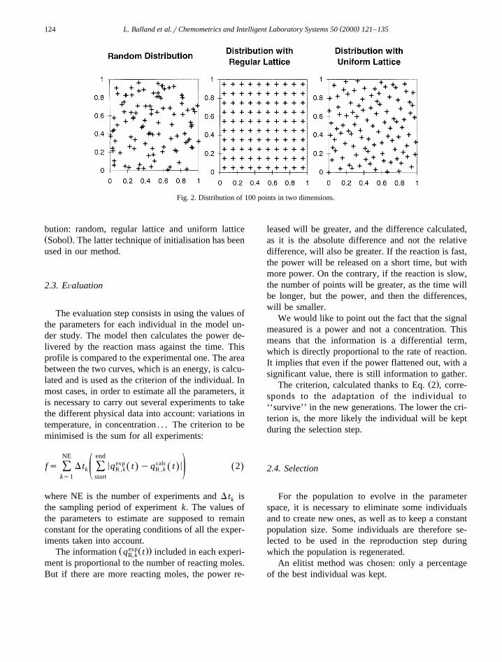
w xfor only one single point of the lattice. Sobol 4 pro-posed an algorithm to calculate the coordinates of thepoints to respect this condition. An example for thedistribution of 100 points in two dimensions is givenin Fig. 2. This figure shows the three kinds of distri-


Fig. 2. Distribution of 100 points in two dimensions.

bution: random, regular lattice and uniform latticeŽ .Sobol . The latter technique of initialisation has beenused in our method.

2.3. EÕaluation

The evaluation step consists in using the values ofthe parameters for each individual in the model un-der study. The model then calculates the power de-livered by the reaction mass against the time. Thisprofile is compared to the experimental one. The areabetween the two curves, which is an energy, is calcu-lated and is used as the criterion of the individual. Inmost cases, in order to estimate all the parameters, itis necessary to carry out several experiments to takethe different physical data into account: variations intemperature, in concentration . . . The criterion to beminimised is the sum for all experiments:

NE endexp calc< <fs D t q t yq t 2Ž . Ž . Ž .Ý Ýk R ,k R ,kž /

ks1 start

where NE is the number of experiments and D t isk

the sampling period of experiment k. The values ofthe parameters to estimate are supposed to remainconstant for the operating conditions of all the exper-iments taken into account.

Ž expŽ ..The information q t included in each experi-R, k

ment is proportional to the number of reacting moles.But if there are more reacting moles, the power re-

leased will be greater, and the difference calculated,as it is the absolute difference and not the relativedifference, will also be greater. If the reaction is fast,the power will be released on a short time, but withmore power. On the contrary, if the reaction is slow,the number of points will be greater, as the time willbe longer, but the power, and then the differences,will be smaller.

We would like to point out the fact that the signalmeasured is a power and not a concentration. Thismeans that the information is a differential term,which is directly proportional to the rate of reaction.It implies that even if the power flattened out, with asignificant value, there is still information to gather.

Ž .The criterion, calculated thanks to Eq. 2 , corre-sponds to the adaptation of the individual to‘‘survive’’ in the new generations. The lower the cri-terion is, the more likely the individual will be keptduring the selection step.

2.4. Selection

For the population to evolve in the parameterspace, it is necessary to eliminate some individualsand to create new ones, as well as to keep a constantpopulation size. Some individuals are therefore se-lected to be used in the reproduction step duringwhich the population is regenerated.

An elitist method was chosen: only a percentageof the best individual was kept.


2.5. Reproduction

2.5.1. CodingRegarding the reproduction step, a first solution

was studied, without any coding as proposed byw xBicking et al. 5 . The value of the parameters is kept

as it is, and the children are chosen randomly in thesubspace defined by two parents. This method did notgive interesting results due to the natural tendency ofthis method to create children in the middle of thespace, and then children are excluded from the bor-der. That is why a method using coded parameterswas preferred.

In most GAs, the coding of values of parametersis based on the binary representation of numbers. Forthe sake of simplicity, decimal coding was preferred.

All parameters are reduced and centred between 0Ž .and 1 cf. Section 2.7.2 . This infers that their deci-

mal value is written as: 0. xyz . . . with x, y, and zŽ .decimal characters included between ‘0’ and ‘9’ .

Number coding is done by converting their decimalvalue in an ASCII character chain, without the first 0and the decimal point. Thus 0.14016 will be coded as:‘1’, ‘4’, ‘0’, ‘1’, ‘6’. It is with this chain of charac-ters that the cross-over and mutation operations willbe carried out.

The length of the chains will state the necessaryprecision. However, it is not possible to exceed theprecision of the binary representation of the realnumbers. As the computation code is written for realnumbers in double precision, the coding chain is lim-ited to a maximum of 15 characters.

2.5.2. Cross-oÕerTwo parents are chosen randomly from among the

individuals selected. The parents’ chains are com-bined to create a new child.

The coding chains of the two parents are cut atŽ .certain points the same for both parents and the

chain segments are interchanged between the twoparents. Two new children are created. One of the twochildren is randomly chosen to complete the popula-tion.

2.5.3. MutationEach character in the coding chain has a probabil-

ity m of changing randomly. The value of m is low

Ž .few percentage and decreases linearly with thew xnumber of generations, as proposed by Hibbert 6 .

Indeed, during the first generations, the individualsare far from the solution and it is necessary to makethem evolve. On the contrary, when the number ofgenerations is higher, then the individuals are nearerfrom the solution and it is no longer necessary tomake them evolve so much.

2.6. Determination of groups

The calculation of the criterion of each individualŽ Ž ..Eq. 2 is quite long. There are a lot of points per

Ž .experiment there could be several thousands , thereŽ .could be several experiments up to 10 or more . For

complicated cases, the length of calculation time willexceed several seconds, even on fast computer. Sothere is a need in a fast converging method. The ideawas not to let the GA converge but detect before theformation of local minima. Then a local convergencemethod is much faster than GA.

To bring to the fore the creation of aggregates atthe end of a generation, the individuals selected areclassified by rising order of the criterion. The Eu-clidean distance from each individual to the best ofthem is calculated; if it is less than the distance pre-defined by the user, this individual belongs to the firstgroup, otherwise it is the first element of the secondgroup; and so on. Each group is characterised by itsbest point and its number of points. As the processgoes on, there is a progressive decrease in the num-ber of groups. According to the number of groups, theuser can decide either to create a new generation orto continue with the second main step: the local con-vergence method. The software also serves to definea minimum number of groups from which the secondmain step of computation is started automatically.This allows to compute without any intervention bythe user. Otherwise, intervention is required at the endof each generation.

As said before, the second main step of computa-tion is to start a criterion minimisation method fromthe best individual of each group. The method cho-

w xsen is Rosenbrock’s method with constraints 7 . Itthen gives as many solutions as there are groups.Different situations can then occur: either a globaloptimum clearly appears, or several optima give sim-ilar values of the criterion and the choice among them


is made by taking their physical meanings into ac-count.

2.7. Choice of parameters

To increase the efficiency of the parameter esti-mation method, it is important to choose the mostsensitive parameters possible to estimate. Bearing thisin mind, some variables may be changed.

2.7.1. Kinetic constantsAmong the parameters to estimate, the kinetic

constants are often difficult to estimate. These con-Žstants k follow an Arrhenius’ law with pre-ex-i

.ponential factor A and activation energy E :i i

yEik sA exp . 3Ž .i i ž /RTr

Ž w x w x.Several authors Chen 8 , Billardello 9 showedthe advantage of not using A and E , as parametersi i

to identify, but a function of these. Indeed, the crite-rion function should be equi-sensitive to all the pa-rameters in order to obtain an efficient minimisationmethod: partial derivatives of the criterion functionover each parameter must have approximately the

w xsame value. This is why, as proposed by Chen 8 , itis better to estimate not A directly, but its loga-i

rithm: ln A .iIf it is necessary to estimate simultaneously pre-

exponential factor A and activation energy E , it isi i

then possible to use crossed reparameterisation.w xPritchard and Bacon 10 proposed:

w s ln A yE rRTU 4Ž .i i i

c s ln E rR 5Ž .i i

where TU is a reference temperature. The parametersw xA and E become w and c . Swaels 11 notes thati i i i

w and c have no physical meanings, which makesi i

their limits and initial values difficult to choose apriori. Moreover, the exploration of the domain pre-sents a discontinuity for E sR. This is why Swaelsi

prefers to use the following reparameterisation:

Eik sA exp y 6Ž .i ,1 i ž /RT1

Eik sA exp y 7Ž .i ,2 i ž /RT2

with T and T as two reference temperatures, taken,1 2

most of the time, at the extremes of the temperaturerange corresponding to the experimental data. Thevalues of A and E are then given by the followingi i

equations:

ki ,1A s 8Ž .i Ei

exp yž /RT1

RT T1 2E s ln k y ln k . 9Ž . Ž .i i ,1 i ,2 T yT1 2

The method now consists in identifying k andi,1

k , which are the values of the kinetic constant fori,2

two temperatures. To improve the distribution of val-ues, it is possible to carry out the estimation with thelogarithm of the kinetic constants.

To show the interest of changing parameters, theresponse surface of the criterion function was repre-sented, either as a function of E and the logarithm ofA, or as a function of the kinetic constant at two dif-ferent temperatures. A simple real case was chosen,with only one reaction, the enthalpy of which was al-ready known. Figs. 3 and 4 show the difference ofprofile according to the parameters used. In Fig. 3,which represents the response surface with the loga-rithm of A and the activation energy E, the surfacepresents a deep crevasse, the bottom of which isslightly curved in the neighbourhood of the opti-mum. Conversely, in Fig. 4, which represents thesame function but with changed parameters, the sur-face presents only a well and the optimum of thefunction is therefore much easier to find. The forbid-den zone corresponds to negative values of the acti-vation energy. It is clear from these figures thatchanging parameters allows the function to be muchmore sensitive to their values, which will thus beeasier to estimate.

w xPigram et al. 12 have proposed another changingin parameters. They determine the equation of the linein the valley described in Fig. 3, and recast the ex-pression of the parameters to ensure the parameters besearched in a narrow band in the bottom of the val-ley. This method was not suitable for us as we haveno way to determine the valley in advance.


Fig. 3. Response surface of the criterion function without change of parameters.

2.7.2. NormalisationAll the parameters are systematically centred and

reduced to between 0 and 1. This technique is veryuseful for the GA.

At the end of each generation, the program com-putes the Euclidean distance between the points in theparameter space. The ranges of variation in the val-ues of the parameters have to be the same for all pa-

rameters. If all parameters vary between 0 and 1, thenthe direction does not affect the distance.

2.8. Validation

The method was validated using numerical exam-ples from the literature, such as Griewangk’s func-

w x w xtion 13 or Schwefel’s function 14 . These functions

Fig. 4. Response surface of the criterion function with change of parameters.


are known to be strongly multimodal. The estimationmethod was able not only to determine the best mini-mum, but also some of the secondary minima.

3. Application

3.1. Chemical model studied

The reaction under study is the saponification ofŽ . Ž .ethyl acetate A , by sodium hydroxide B to give

Ž . Ž .sodium acetic acid salt C and ethanol D .

AcOEtqNaqOHy™AcOyNaqqEtOH

AqB™CqD

ŽThe reaction is carried out in concentrated 1 moly1 .l hydroalcoholic mixture, in a range of tempera-

ture between 158C and 308C.To avoid equilibrium conditions, between acid–

alcohol and ester–water, the sodium hydroxide is inŽ .large excess 1.5 times more than ester , and is in the

reactor at the beginning of the reaction. With such

concentration, the ester is not rapidly soluble in wa-ter. Moreover, there is a difference in the densitiesbetween water and ester. That is the reason why ahydroalcoholic mixture is preferred: 50% in mass forethanol, 4.5% for sodium hydroxide and 45.5% forwater.

The Mettler w RC1 glass made calorimetric reac-tor presented in Fig. 5 works at atmospheric pres-sure. It is composed of a jacketed reactor with tan-gential input for the heat transfer fluid. The capacityof the reactor is 2 l. It is equipped with a Pt100 tem-perature probe, an electrical calibration heating, a

Žstirring system either anchor or turbine with four. Žbaffles and an introduction system two dosing

pumps and two balances, with measurement of the.temperature at introduction . The heating–cooling

system, which uses a single heat transfer fluid, workswithin a temperature range from y158C to q2008C.

An exploitation software solves the energetic bal-Ž .ance on the reaction mass every 2 s, thanks to Eq. 10

Ž exp.which enables the power released or absorbed qR

by the physical and chemical transformations of thereaction mass to be calculated. This balance is estab-lished with the hypotheses that the agitation is per-

Fig. 5. Diagram of the RC1 Calorimetric Reactor.


fect and that the temperature is homogeneousŽ .throughout the jacket Fig. 6 :

dTrexpq qÝ m.cp qU.A. T yTŽ . Ž .R r fd tNS

Eq n Cp T yT qq s0. 10Ž .˙ Ž .Ý j j r j lossjs1

During each experiment, which are carried out atdifferent temperatures, the calorimetric reactor isfilled with 1.5 l of the hydroalcoholic mixture. Firstof all, calibrations are carried out to calculate the

Ž .global heat transfer conductance U.A and the heatŽ .capacity of the reaction mass Ým.cp . These values

are required to calculate the experimental profile ofthe power released or absorbed by the reaction mass

Ž . Ž .with Eq. 10 . Then 88 g 1 mol of ethyl acetate isintroduced in 85 s. The reaction is supposed to befinished when no more power is measured from thereaction mass. Finally, new calibrations are carriedout to take into account the evolution of the heatconductance and the heat capacity due to the reac-tion. The measurements allow to calculate the exper-imental power profile released or absorbed by the re-

exp w xaction mass q , as explained by Balland et al. 15 .R

To determine the parameters in the whole range oftemperature, three experiments are carried out: thefirst one with a variation of temperature between 158Cand 308C during the same time as the introduction ofester; the second one by trying to maintain the tem-perature at 158C; and the third one by trying to main-tain it at 308C.

Fig. 6. Powers exchanged with the reaction mass.

The profile of power measured by the calorimetricreactor shows a small negative peak at the beginningof the introduction. This is due to an excess heat. Totake such a heat into account, a reaction for mixing� 41 is introduced in the stoichiometric model:

pure � 4A ™A 1

� 4AqB™CqD 2

� 4Reaction 1 corresponds to the dissolution of ethylacetate inserted into the reaction mass, and reaction� 42 is the chemical reaction itself.

3.2. Mass balance

In a semi-batch reactor, the instantaneous massbalance is written for an active chemical species j:

E NRdn dnj jqV n r s 11Ž .Ýr i j id t d tis1

Ž E . Ž .where dn r d t is the flow rate of introduction ofj

j, r the speed of the ith reaction, with the stoichio-i

metric coefficient n and V the volume of the reac-i, j r

tion mass.The speed of ith reaction is:

NSo i , jr sk C 12Ž .Łi i j

js1

where k is the kinetic constant, following Arrhe-iŽ .nius’ law 3 , o the order of constituent j in the re-i, j

action i and C the concentration of constituent j:j

n jC s . 13Ž .j Vr

Let us define a new variable, a normalised extentw xfor each reaction 16 :

DnŽ .j ix s ; j such as n /0 14Ž .i i , j

n ni , j 0

Ž .where n is the reference mole number and Dn the0 j i

mole number of constituent j which has reacted in theith reaction between initial and current times. Thenthe state of chemical species j is given by its molenumber:

NREn sn qn qn n x 15Ž .Ýj j j ,0 0 i , j i

is1


Table 1Range of estimation

y1Ž . Ž . Ž .Parameter k s D H o k 158C k 258C D H o o1 1 1A 2 2 2 2A 2By1 3 y1 y1 3 y1 y1 y1Ž . Ž . Ž . Ž .kJ mol m mol s m mol s kJ mol

y2 y8 y8Minimum 10 1 0.3 10 10 y60 0.3 0.3y3 y3Maximum 1 10 2.5 10 10 y40 2.5 2.5

where n is the mole number of constituent j at ini-j,0Ž .tial time. The differential of Eq. 15 leads to:

E NRdn dnj js q0qn n x 16Ž .˙Ý0 i j id t d t is1

Ž . Ž .The equality of 11 and 16 determines the produc-tion flow rate of the ith reaction:

n x sr V 17Ž .˙0 i i r

With the following definitions of dimensionlessnumbers:

nj ,0Y s 18Ž .j ,0 n0

nEj

Z s 19Ž .j n0

Ž .Eq. 12 becomes:

o i , jÝ o i , jNS NRV n ir 0x s k Y q Z q n x .˙ Ł Ýi i j ,0 j i , j iž / ž /n V0 r js1 is1

20Ž .

In our case, the number of chemical reaction isŽ .two. The system of differential Eq. 20 becomes:

o y11An0 o1Ax sk Z yx 21Ž . Ž .˙1 1 A 1ž /Vr

o qo y12 A 2 Bn0 o o2 A 2 Bx sk x yx Y yxŽ . Ž .˙2 2 1 2 B0 2ž /Vr

22Ž .

where Z is the introduction variable of ester evolv-A

ing with time:

nEA

Z s 23Ž .A n0

3.3. Energy balance

The thermal power released or absorbed by thechemical reactions is written as:

NRcalcq syV r D H 24Ž .ÝR r i i

is1

Ž . Ž .Thanks to 17 , 24 becomes:NR

calcq syn x D H 25Ž .˙ÝR 0 i iis1

In our case, each phenomenon contributes to thetotal power according to its energy and kinetics:

q calc syn x D H qx D H 26Ž .˙ ˙Ž .R 0 1 1 2 2

The temperature is supposed to be controlled. But,Ž .as the volume is quite important up to 2 l , the tem-

perature cannot be considered to strictly follow the settemperature. Therefore, the experimental evolution of

Table 2Parameters of the GA

Size of Selection Mutation Maximal number Characters per Positions ofpopulation rate rate of generations parameter cross-over

200 0.2 5% 50 10 after 1, 3, 6


Table 3Parameters of Rosenbrock’s method

Distance Limit group Precision Multiplication factor Maximum numberbetween groups number to stop for the constraints of iterations

y5 y4 40.1 3 10 10 10

the temperature must be taken into account in the ex-pression of the kinetic constants. To solve our sys-

Ž . ŽŽ .tem composed of algebraic 23 and differential 21Ž .. w xand 22 equations, the Gear’s method 17 was

adopted: an algorithm based on the DASSL programw x18 was written in Cqq.

3.4. Estimation of parameters

3.4.1. Range of searchŽ . Ž .With the system of Eqs. 21 – 23 necessary to

calculate the power released or absorbed by the reac-Ž .tion mass with Eq. 26 , nine parameters must be es-

Žtimated: the enthalpy of the two reactions D H and1. Ž .D H , the two kinetic constants k and k which2 1 2

each have two parameters according to the tempera-Ž . Žture A and E , and the three orders o , o andi i 1A 2A.o .2B

� 4The chemical equation 1 represents the mixing ofthe ester. As the range of temperature is quite nar-row, the kinetic constant k is supposed to be inde-1

pendent of temperature. So, there are only eight pa-rameters to estimate.

The parameters are estimated in the range indi-cated in Table 1.

The units of kinetic constants k and k suppose1 2

that the orders are equal to one. The kinetic constantsas well as the orders are estimated according to theirlogarithm. An additional constraint is added: the sumof the two enthalpies should be limited between y50and y40 kJ moly1.

3.4.2. Parameters of the estimation methodsThe parameters of the GA are given in Table 2.The parameters of the Rosenbrock’s method are

given in Table 3.The incertitude interval is calculated with a confi-

dence level of 99%. The amplitude of the interval forw xthe parameter u 12 is:m

ampl s var u t 27Ž .(m m b r2, syn

Žwhere t is the Student’s t-value for the 100 1br2, syn.yb confidence level and the number of data points

Ž . Ž .s minus the number of parameters to estimate ndegrees of freedom. The variance of the parameter um

is:

y12ˆ2 f u E fŽ .var u s 28Ž .m 2ž /syn Eum u

Table 4Results of the estimation before and after locally convergent method

Ž . Ž . Ž .Parameter 1st group 2675 iterations 2nd group 2015 iterations 3rd group 837 iterations

Before After Before After Before After

k 0.0139 0.0317"0.0006 0.0139 0.0123"0.0006 0.0109 0.0142"0.00021

D H 5910 6310"130 5550 6400"150 9510 7750"901

D H y48,670 y50,700"230 y48,670 y50,600"200 y50,360 y51,400"1002y5 y5 y6 y5 y5 y5Ž .k 158C 1.66=10 1.32"0.02=10 5.97=10 1.51"0.03=10 2.51=10 2.5"0.2=102y5 y5 y5 y5 y5 y5Ž .k 258C 4.49=10 2.83"0.05=10 2.01=10 3.21"0.05=10 8.76=10 5.0"0.3=102

o 1.015 1.178"0.008 1.003 1.36"0.01 1.024 1.38"0.011A

o 1.117 0.962"0.007 1.383 0.945"0.007 1.136 0.914"0.0052A

o 0.958 0.977"0.005 0.912 0.977"0.006 0.912 0.939"0.0052B

Criterion 12,400.1 3683.41 13,774.6 3590.99 13,946.8 4108.07


Fig. 7. Profiles of experimental and calculated power.

ˆŽ .where f u is the criterion at the estimated point andŽŽ 2 . Ž 2 ..y1E f r Eu is the diagonal of the inverse ofˆm u

Hessian matrix.

3.4.3. ResultsThe first step, representing the GA, stops after the

18th generation, which has detected three groups.Starting from these three points, obtained thanks to

Žthe best individual of each of the three groups given.in the columns ‘‘Before’’ of Table 4 , the local con-

vergence method ends up at the results given in thecolumns ‘‘After’’ of Table 4. The units are indicatedin Table 1.

By comparing the criterion, the second groupseems to give the best results. Fig. 7 shows the goodcorrelation between the three experiments and the

Table 5Comparison of results with literature

w x w xICT 19 Villermaux 16 Present papery1 y1 y1Cs0.01 mol l Cs0.1 mol l Cs1 mol l

y5 y5 y5Ž .k 158C 5.45=10 4.31=10 1.51=102y5 y5 y5Ž .k 258C 10.6=10 7.78=10 3.21=102


Table 6Results with the 20 best out of 100

a 1 2 3 4 5 6 7 8 9 10

Criterion before 23,022 26,500 26,716 34,917 35,417 40,127 52,213 55,303 57,666 62,650Number of iterations 385 1690 1336 393 329 318 261 3307 299 734Criterion after 13,260 4160.1 4533.9 9597.1 34,378 6555.5 35,925 3728.1 44,515 13,886

a 11 12 13 14 15 16 17 18 19 20

Criterion before 62,771 68,023 71,747 77,501 83,653 84,241 84,848 85,859 86,680 87,359Number of iterations 220 380 1133 3560 5231 1197 911 285 2711 2198Criterion after 38,851 65,764 12,813 3679.0 3968.3 4519.3 5327.5 29,954 3704.3 3633.5

model calculated with the values obtained by thesecond group.

3.5. Discussion

In literature, the kinetic experimental studies ofethyl acetate saponification are only carried out inaqueous reaction mass with low concentration. The

Žw xInternational Critical Tables 19 , Vol. 7, pp. 129–. Ž .130 give a relation log ks f T in a range of tem-10

perature between 108C and 458C for concentrationy2 y1 w xabout 10 mol l . Likewise, Villermaux 16 , for

temperatures of 268C and 328C and a concentration of0.1 mol ly1, gives the following values:

As3.05P103 m3 moly1 sy1

Es43,300 J moly1

To compare the results, Table 5 gives the valuesof the kinetic constant at 158C and 258C.

The kinetic constants calculated here are aboutthree times as small as those of literature. However,the difference between the values of literature andthose of the present study can be explained with thefollowing points.

Ø The concentrations used here are 10 to 100times higher than those of literature.

Ø The composition of the reaction mass is alsoquite different. This last point can be strengthened by

w xthe results obtained by Celdran et al. 20 . He showsin his works on the n-butyl acetate saponification thatthe proportion waterrethanol has a great influence onkinetic parameters.

Ø The orders calculated for the reactants areslightly different from 1, unlike the studies in the lit-erature where they are fixed to 1.

For all these reasons, the comparison must be lim-ited to some of idea of the value, which is respected.The experiments cannot be carried out with smallerconcentrations because the signal measured would betoo weak.

These results required 8447 estimations of the cri-terion, 5527 of them with the three local conver-gence methods, and 2920 with GA.

Furthermore, to test the efficiency of the GA, thesame calculation is again carried out by bypassing theGA. A total of 100 points are taken in the parameter

Ž .space, scattered on a uniform lattice Sobol’s type .The criterion is calculated for all the 100 points andonly the 20 best ones are kept. These numbers arechosen arbitrarily. These 20 points serve to start a lo-cal convergence method. The value of the criterionbefore and after the estimation method, as well as thenumber of iterations are given in Table 6.

Table 7Values of the 20th point

Ž . Ž .k D H D H k 158C k 258C o o o1 1 2 2 2 1A 2A 2A

y5 y50.0243"0.0007 6190"130 y50,700"100 1.03"0.02=10 2.22"0.04=10 1.21"0.01 0.96"0.01 1.01"0.01


The 20th point gives the best result which is notso far from the one previously determined as indi-cated in Table 7. The units are indicated in Table 1.

But the total number of iterations is 26,978, morethan three times as high as with the hybrid method. Itcan also be noticed that the 14th and the 19th pointsgive correct results. This fact points out the difficultyto determine the numbers of points initial and to bekept: if fewer points were kept, for instance only the10 best out of the 100 initial points, the best resultswould not have been found. If more points are kept,this will increase the calculation time.

4. Conclusion

In this article, an estimation method for kinetic andenergetic parameters is presented. The importance ofchanging parameters is underlined. This method con-siderably facilitates the search for the optimum.

The estimation method is a hybrid method, com-pleting a GA with a local convergence method. TheGA detects the most relevant zones in the parameterspace, then the local convergence method rapidly de-termines the relative minimum of the zone, and so onfor all the zones detected. So the method is able togive not just a single answer, but a set of answers.Thus the user decides, according to the physicalmeaning of the solutions, which one is the mostprobable answer to the problem.

This method is applied to a real complex case: thedetermination of kinetic and energetic parameters ofthe saponification of ethyl acetate in hydroalcoholicreaction mass with a concentration of 1 mol ly1. Thevalues of the parameters estimated allow to representall the three experiments. The hybrid estimationmethod is compared to a much more simple one,where the 20 best points out of 100 scattered in thewhole parameter space serve to initiate a local con-vergence method. This second method is dependentof the initial number of points and the number ofpoints to keep. Indeed, to avoid missing the physi-cally significant solution, the numbers of points needto be high. But this will extensively increase the cal-culation time. So this method is costly in time incomparison to the hybrid method. The latter allows to

determine more surely and more rapidly the solutionto the problem.

References

w x1 L. Balland, Contribution a l’Estimation des Parametres Cine-` ` ´´tiques et Energetiques de Systemes Chimiques en milieu Ho-´ `

mogene et Heterogene dans un Reacteur Calorimetrique.` ´ ´ ` ´ ´Thesis of the University of Rouen, France, 1997, 245 pp.

w x2 D.B. Hibbert, Genetic algorithms in chemistry, Chemomet-Ž .rics and Intelligent Laboratory Systems 19 1993 277–293.

w x3 L. Balland, J.-M. Cosmao, N. Mouhab et al., Estimation desParametres de Modeles Cinetiques par Mesure des Flux` ` ´

´d’Energie dans un Reacteur Double Enveloppe, Entropie 186´Ž .1994 25–32.

w x4 J.M. Sobol, On the systematic search in a hypercube, SIAMŽ . Ž .J. Number Anal. 16 5 1979 790–793.

w x5 F. Bicking, C. Fonteix, J.-P. Corriou, I. Marc, Global optimi-sation by artificial life: a new technique using genetic popu-

Ž . Ž .lation evolution, Operations Research 28 1 1994 23–36.w x6 D.B. Hibbert, A hybrid genetic algorithm for the estimation

of kinetic parameters, Chemometrics and Intelligent Labora-Ž .tory Systems 19 1993 319–329.

w x7 H.H. Rosenbrock, An automatic method for finding theŽ .greatest or the least value of a function, Comput. J. 3 1960

175–184.w x8 N.H. Chen, Determination of Arrhenius constants by linear

Ž . Ž .and non linear fitting, AIChE J. 38 4 1992 626–628.w x9 P. Billardello, X. Joulia, J.M. Le Lann et al., A general strat-

egy for parameter estimation in DAE Systems, Comput.Ž . Ž .Chem. Eng. 17 5–6 1993 517–525.

w x10 D.J. Pritchard, D.W. Bacon, Prospect for reducing correlationamong parameter estimates in kinetic models, Chem. Eng.

Ž .Sci. 33 1978 1539–1543.w x11 Ph. Swaels, Modelisation et Simulation Dynamique de´

Reacteurs Chimiques Discontinus. Thesis of the University of´Rouen, France, 1995, 304 pp.

w x12 P.J. Pigram, R.N. Lamb, D.B. Hibbert, R.E. Collins, Model-ing of the desorption behavior of microporous amorphous hy-

Ž .drogenated carbon films, Langmuir 10 1994 142–147.w x13 A.O. Griewangk, Generalized descent for global optimisa-

Ž .tion, J.O.T.A. 34 1981 11–39.w x14 H.P. Schwefel, Numerische Optimierung von Computer-¨

Modellen mittels der Evolutionsstrategie. InterdisciplinarySystem Research, Birkhauser, Basel, 1977, p. 26.¨

w x15 L. Balland, N. Mouhab, S. Alexandrova, J.-M. Cosmao, L.Estel, Determination of kinetic and energetic parameters ofchemical reactions in a heterogeneous liquidrliquid system,

Ž . Ž .Chem. Eng. Technol. 22 4 1999 321–329.w x16 J. Villermaux, Genie de la Reaction Chimique, Conception et´ ´

fonctionnement des Reacteurs, Technique et Documentation´Lavoisier, Paris, 1993, 448 pp.

w x17 C.W. Gear, The automatic integration of ODE, NumericalŽ . Ž .Mathematics 14 3 1971 176–179.


w x18 L. Petzold, Differentialralgebraic equations are not ODE’s,Ž . Ž .SIAM J. Sci. Stat. Comput. 3 3 1982 367–384.

w x Ž .19 E.W. Washburn Ed. , International Critical Tables of Nu-merical Data, Physics, Chemistry and Technology, Vol. 7,McGraw-Hill, New York, pp. 1926–1933.

w x20 E.W. Celdran, M.V. Ramon, P. Martinez, Influence of thepolarity of the medium on the alkaline hydrolysis of n-butyl

Ž .acetate in hydroalcoolic mixtures, Z. Naturforsch. 32a 19771496–1500.

A genetic algorithm with decimal coding for the estimation of kinetic and energetic parameters

Documents

Transcript of A genetic algorithm with decimal coding for the estimation of kinetic and energetic parameters