
detection of gas in sandstone reservoir using avo analysis in
185
DETECTION OF GAS IN SANDSTONE RESERVOIR USING AVO ANALYSIS IN PRINOS BASIN By CHOUSTOULAKIS E. EMMANOUIL SCIENTIFIC ADVISOR: PROF. VAFIDIS ANTONIOS A THESIS Submitted in partial fulfillment of the requirements for the degree of MASTER OF SCIENCE IN PETROLEUM ENGINEERING TECHNICAL UNIVERSITY OF CRETE November, 2015
-
Upload
khangminh22 -
Category
Documents
-
view
4 -
download
0
Transcript of detection of gas in sandstone reservoir using avo analysis in
DETECTION OF GAS IN SANDSTONE RESERVOIR USING AVO ANALYSIS IN
PRINOS BASIN
By
CHOUSTOULAKIS E. EMMANOUIL
SCIENTIFIC ADVISOR: PROF. VAFIDIS ANTONIOS
A THESIS
Submitted in partial fulfillment of the requirements
for the degree of
MASTER OF SCIENCE IN PETROLEUM ENGINEERING
TECHNICAL UNIVERSITY OF CRETE
November, 2015

This thesis, “DETECTION OF GAS IN SANDSTONE RESERVOIR USING AVO
ANALYSIS IN PRINOS BASIN”, is hereby approved in partial fulfillment of the
requirements for the Degree of MASTER OF SCIENCE IN PETROLEUM
ENGINEERING.
DEPARTMENT: School of Mineral Resources Engineering
Signatures:
Prof. Antonios Vafidis
(Scientific Advisor-Applied Geophysics Laboratory)
Prof. Dionissios T. Hristopulos
(Member Committee- Geostatistics Laboratory)
Prof. Nikolaos Varotsis
(Member Committee-PVT and Core Analysis Laboratory)
Date

Abstract
This thesis was focused on an integrated approach of gas detection in the sandstone reservoir of
Prinos oil field, located in the northern Aegean Sea between the island of Thasos and city of
Kavala on the mainland. The rock properties variation with depth in the study area, were inferred
from suite of quality controlled well seismic logs, while the geological structure of the model
was based on an East-West 2D geological plan of Prinos basin. Furthermore, the top layer of the
reservoir was considered to be 50% saturated with gas, so, its elastic parameters were
accordingly adjusted. The above information were given as input to a synthetic data simulator
(Applied Geophysics Laboratory of the Technical University of Crete) in order to build low
frequency synthetic seismograms. Additionally, a signal processing graphical interface was
build, in order to properly process the synthetic data before the application of the AVO analysis.
The GUI can support the whole preprocessing scheme prior to the AVO analysis, from the
commissioning of the SGY data, until the generation of the stacked and migrated sections, while
the results can be represented graphically at any point. Finally, an analytical AVO analysis flow
was adapted for the processed seismic data which successfully detected the presence of gas in
the shallow gas saturated layer. The AVO analysis flow included rock physics analysis,
intercept-gradient crossplots, far versus near stack attributes, detailed investigation of distance
to amplitude analysis and AVO inversion for the elastic parmetres of the model.

4
Acknowledgements
First and foremost, I would like to thank my supervisor, Dr. Antonis Vafidis, Professor in Applied
Geophysics Lab in Department of Mineral Resources Engineering of Technical University of
Crete whose help, guidance and supervision from preliminary to concluding levels, enabled me
to fulfill this thesis.
I also thank Dr. George Kritikakis, Lab and Teaching Staff of Applied Geophysics Laboratory
for his significant contribution and help.
I am also grateful to all my lecturers in the master of Petroleum engineering, most especially,
Prof. Nikos Pasadakis without whom this master course would have never been viable and Dr.
Vasilios Gaganis for his support, constructive feedback and communicability of knowledge. I
would always be indebted to you all.
Many thanks goes to my course mates in the Pertroleum Engineering course and especially to
my study group mates, Katerina Stathopoulou and Aggeliki Vlassopoulou for their collaboration
and support through this work.
I thank my examination committee: Professors Dionissios Christopoulos and Nikolaos Varotsis
for their time and input.
The last but the most important, I want to express my heartfelt appreciation to my parents,
Emmanouil Choustoulakis and Argiro Kalisperaki, my brothers Nikos Choustoulakis, Kyriakos
Choustoulakis, Aris Choustoulakis and my girlfriend, Marilena Anastasaki. Without your love,
support and understanding, I couldn’t be able to get my work done.

5
Table of Contents:
1. Introduction............................................................................................... 1
2. Prinos Basin .............................................................................................. 2 2.1 Geological Setting ....................................................................................... 3 2.2 Stratigraphy ................................................................................................. 4 2.3 Traps and Reservoir .................................................................................... 6 2.4 Oil generation and migration ...................................................................... 7
3. Synthetic data simulator .......................................................................... 8 3.1 Heterogeneous Approach ............................................................................ 9 3.2 Elastic wave propagation .......................................................................... 11 3.3 Accuracy, convergence and stability ......................................................... 12
4. AVO Analysis Theory ............................................................................. 16 4.1 AVO analysis principles ........................................................................... 16 4.2 Transforming From the Offset to the Angle Domain ................................ 20 4.3 Ray Tracing ............................................................................................... 22 4.4 Seismic Data Pre-Processing for AVO Analysis ...................................... 24 4.5 Far versus near-stack attributes ................................................................. 27 4.6 AVO attributes combining intercept and gradient .................................... 28 4.7 AVO Analysis Application on Gas Detection ........................................... 30 4.8 AVO Response Classification ................................................................... 35
5. Seismic Data Processing Analysis ........................................................ 38 5.1 Prinos Basin Geological Model Representation ........................................ 41 5.2 Velocity and Bulk Density Estimation ...................................................... 47 5.3 Synthetic Seismic Data Acquisition .......................................................... 54 5.4 Seismic Data Processing ........................................................................... 62
5.4.1 Preprocessing .............................................................................. 66 5.4.2 Spherical divergence correction .................................................. 70 5.4.3 Spiking and Predictive deconvolution ...................................... 71 5.4.4 FX deconvolution ..................................................................... 74 5.4.5 F-K Filtering ............................................................................. 76 5.4.6 CMP sorting ............................................................................. 78 5.4.7 Velocity Analysis ..................................................................... 79 5.4.8 NMO correction ....................................................................... 82 5.4.9 Radon Transform ...................................................................... 83 5.4.10 Stacking .................................................................................... 85 5.4.11 Post-stack Processing ............................................................... 87 5.4.12 Migration .................................................................................. 88
6 Seismic Processing Graphical Interface .............................................. 93 6.1 Plotting Different Gather Types ................................................................ 95 6.2 Signal Processing Analysis ..................................................................... 100 6.3 Stack section ........................................................................................... 106 6.4 Migration ................................................................................................. 108 6.5 Plotting tools ........................................................................................... 111
7 AVO Analysis Application ................................................................... 114 7.1 Ray tracing .............................................................................................. 114 7.2 Rock Physics of AVO ............................................................................. 118 7.3 AVO crossplot analysis ........................................................................... 120 7.4 Near Far Stack ......................................................................................... 123 7.5 PG crossplot ............................................................................................ 127 7.6 Detailed investigation of distance to amplitude analysis. ....................... 131 7.7 AVO inversion of elastic parameters ...................................................... 133
8 Summary and Conclusion ................................................................... 135

6
9 References ............................................................................................. 136
Appendix A ....................................................................................................... 140 Matlab Codes: ............................................................................................. 140
AVA inversion ................................................................................... 140 AVO classification ............................................................................. 141 Common Offset gather creation ......................................................... 144 Digitize function ................................................................................ 144 Excel creation .................................................................................... 151 Geometrical Spreading ...................................................................... 153 PG Crossplots of Synthetic Data ....................................................... 153 Raytracing Algorithm ........................................................................ 157 Record’s Length Calculation ............................................................. 159 Rock Physics ...................................................................................... 162 Spline Layers ..................................................................................... 169
Appendix B ....................................................................................................... 173 List of Figures ............................................................................................. 173
Chapter 2 ............................................................................................ 173 Chapter 3 ............................................................................................ 173 Chapter 4 ............................................................................................ 173 Chapter 5 ............................................................................................ 174 Chapter 6 ............................................................................................ 176 Chapter 7 ............................................................................................ 177
Appendix C ....................................................................................................... 179 List of Tables ............................................................................................... 179
1. Introduction
1
1. Introduction
In recent years, as the easy to find conventional hydrocarbon reserves in the earth’s crust are
being exploited, the oil industries tend to search in more difficult terrains and much deeper
waters to match the growing demand for fossil fuels. As such, exploration for oil and gas over
time has advanced from being qualitative to quantitative. Quantitative studies of the subsurface
in general and hydrocarbon fields in particular, require a lot of integrated data and analysis from
geologists, geophysicists, petrophysicists, and reservoir engineers.
Fueled by progressive technological advances and breakthroughs in the oil and gas industry,
the possible computing power has also followed suite, such, that reservoir characterization has
extended from deterministic to probabilistic. Accurate characterization requires a combination
of 3D and 4D seismic volume interpretations, seismic inversion and amplitude analyses, rock
physics and AVO (amplitude versus offset) analysis. Earlier, geophysical data were mainly
used in exploration, and to a smaller extent in the development of discoveries. In more recent
times geophysical and petrophysical data is integrated in reservoir characterization schemes,
and serves as a link between geologic reservoir properties (such as porosity, sorting, clay
content, lithology and saturation) and seismic properties (like P-wave and S-wave velocities
Vp/Vs ratio, acoustic impedance, elastic moduli, bulk density) (Avseth et al., 2010). Reservoir
characterization therefore simply refers to quantitatively assigning reservoir properties which
usually show a non-uniform and non-linear spatial distribution.
This study will focus on an integrated approach to reservoir characterization of the Prinos oil
field, located in the northern Aegean Sea, between the island of Thasos and city of Kavala on
the mainland. A suite of quality controlled well seismic logs, along with a 2D geological model
will be used to infer the rock property variations with depth in the study area. The rock
properties will then be used to build low frequency synthetic seismograms, using a synthetic
data simulator, (Applied Geophysics Laboratory of the Technical University of Crete) and later
perform AVO modeling. However, the synthetic data needs special pre-treatment prior to the
application of the AVO analysis. In order to cope with such a demanding and complex
procedure, a graphical interface is built which can undertake the whole preprocessing scheme
prior to the AVO analysis. The study begins with the geological and stratigrahical setting of
Prinos basin.

2. Prinos Basin
2
2. Prinos Basin
The Prinos basin is the only geological area in Greece, where oil and gas are being produced
for more than thirty years. Exploration for hydrocarbons in this particular offshore area has
started in the beginning of the seventies. The first seismic campaign took place in the sea of
Thrace in 1970 and the first oil discovery in Prinos basin occurred in 1973. The search for oil
in this basin is still under continuation. The taphrogenetic basin of Prinos has been widely
studied, due to its hydrocarbon reservoirs. The combined geological information, derived from
the analysis of lithological, stratigraphic and geochemical data of the basin, suggested a structural
and depositional model, strongly related to the Miocene tectonics and sedimentation [Proedrou, P.,
and Papaconstantinou, C.M., 2004].
The largest part of the basin is located offshore between the island of Thassos and the opposite
mainland to the west. Only the north-eastern portion of it lies onshore in the Delta Nestos plain
(Figure 2.1). The total area covers 800km2. The sea depth doesn't exceed fifty meters. In this
chapter the general geologic and geotectonic characteristics of Prinos basin, in the wide
geological area, are being presented.
Figure 2.1 Prinos – Kavala Basin. Prinos field, Prinos North field, Epsilon field and South Kavala gas
filed are the only productive hydrocarbon fields in Greece. The oil generation and the migration paths are
shown (improved version published after Kioumourtzi et al., 2007).
2. Prinos Basin
3
2.1 Geological Setting
Prinos - Kavala basin has been formed during Palaeogene period at the southern margin of the
Rhodope Massif, controlled by NE-SW and NW-SE faults, at the area that nowadays is
surrounded by Thassos Island and the mainland of NE Greece. It is a result of the post-alpine
tectonism that started in early to middle Miocene and led to the breaking of the Aegean plate and to
the subsidence of the pre-alpine Rhodope massive under the sea level. This gravity tectonics was
responsible for the genesis of grabens and horsts in North Aegean. The NE part of Prinos basin was
probable close by the first time of its formation, while the SW basement started to uplift by
messinian period, forming the south Kavala ridge (Figure 2.1). The basin was gradually isolated
from the open sea and changed into a lagoon. A number of gravity, often echelon, faults with NE-
SW and NW-SE direction formed the taphrogenetic basin of Prinos. Its length is approximately 38
km, from Nestos river delta in NE, to offshore south Kavala ridge in SW. Its width is approximately
20 km, from Thassos Island in SE, to the opposite mainland in NW. It is subdivided into two sub-
basins, separated by a topographic basement high, in Ammodhis area (Figure 2.1).
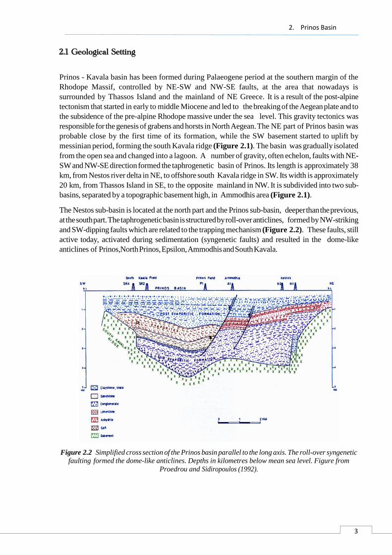
The Nestos sub-basin is located at the north part and the Prinos sub-basin, deeper than the previous,
at the south part. The taphrogenetic basin is structured by roll-over anticlines, formed by NW-striking
and SW-dipping faults which are related to the trapping mechanism (Figure 2.2). These faults, still
active today, activated during sedimentation (syngenetic faults) and resulted in the dome-like
anticlines of Prinos, North Prinos, Epsilon, Ammodhis and South Kavala.
Figure 2.2 Simplified cross section of the Prinos basin parallel to the long axis. The roll-over syngenetic
faulting formed the dome-like anticlines. Depths in kilometres below mean sea level. Figure from
Proedrou and Sidiropoulos (1992).
2. Prinos Basin
4
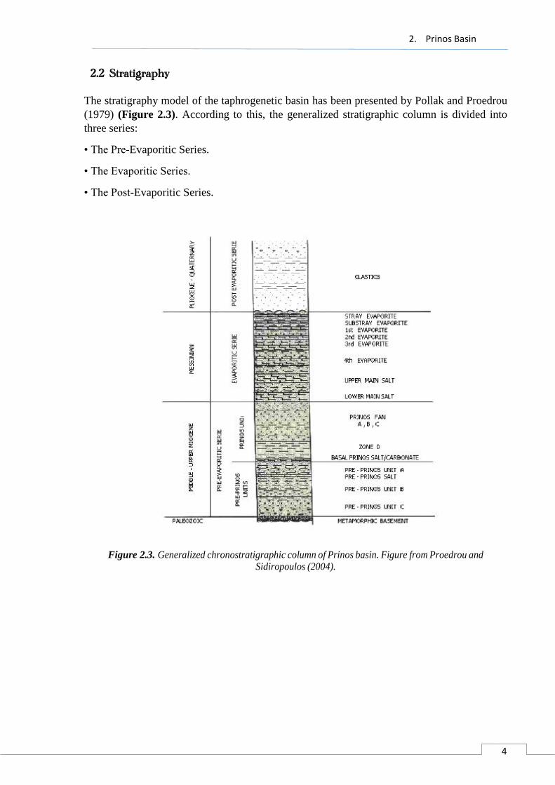
2.2 Stratigraphy
The stratigraphy model of the taphrogenetic basin has been presented by Pollak and Proedrou
(1979) (Figure 2.3). According to this, the generalized stratigraphic column is divided into
three series:
• The Pre-Evaporitic Series.
• The Evaporitic Series.
• The Post-Evaporitic Series.
Figure 2.3. Generalized chronostratigraphic column of Prinos basin. Figure from Proedrou and
Sidiropoulos (2004).
2. Prinos Basin
5
The Palaeozoic basement is composed of metamorphic rocks: gneiss, quartzite and dolomitic
marble. The Pre-Evaporitic Series, closely related to Miocene tectonics, begins with continental
deposits: conglomerates with large basement components, sandstones, feldspatic, mainly immature,
claystones and thick coal seams. These continental deposits originated from the NE and SW parts
of the basin, decrease in thickness towards the centre of the sub-basins. They are followed by
marine deposits of shales with interbedded sandstones, coarser at the periphery of the basin,
which overlay the older ones with an unconformity. Above these units, a zone of limestone,
dolomite and anhydrite layers alternated with clastics follows. Towards the centre of the basin, to
the deeper parts, the anhydrite is replaced by a few metres thick layers of salt. At the top of the Pre-
Evaporitic Series, at Prinos sub-basin, there is an extended deposition of dark gray claystone, the
zone D. It is petro-liferous and strong carbonaceous, with sandstone intercalations. The following
Prinos sub-marine fan, consists entirely of turbiditic fan deposits, which were deposited along the
downthrown side of a fault escarpment. The present facies, are representative of the turbidite
facies classification of Walker and Mutti (1973). At Nestos sub-basin, the equivalent zone is the
pro-deltaic varves (Proedrou and Papaconstantinou, 2004).
The Evaporitic Series, closely related to Messinian “Salinity Crisis” of the Mediterranean Sea (Hsu,
1972), consists of two facies, in each of the two sub-basins. In the northern one, anhydrite and
limestone layers 3-5 m thick, alternate each other and with sandstone, claystones and marls, too. The
series in the southern part, consists of 7-8 salt layers with increasing thickness towards the base of
the section, which alternate with clastics and has a total thickness up to 800 m. The salt is white,
gray, crystalline, often intercalated by anhydrite and dolomite layers (Proedrou and
Papaconstantinou, 2004). The Post-Evaporitic Series is pure clastic and marine origin, as indicated
by the presence of a great number of Pliocene foraminifere and algae. Towards the top, coarse
clastic sediments with abundant rests of molluscs point out to a deltaic, according the seismic,
prograding sequence. A transgression followed with deposition of marine clastic sediments
(Proedrou and Papaconstantinou, 2004). These three series reflect the different sedimentological
conditions of each period and generally, increase in thickness towards the centre of the sub-basins.
2. Prinos Basin
6
2.3 Traps and Reservoir
The most typical anticlines for the broad basin are the Prinos and Prinos North oil fields as
rollover anticlines in front of syngenetic northwest-southeast striking downthrown faults. To
the same case belongs the south Kavala gas field being formed as a combination of a rollover
anticline and a stratigraphic pinch-out of the south western flank against the basement (P.
Proedrou 2001). In contrast, the Ammodhis structures, as well as the Epsilon structure are
rollover anticlines surrounded by mainly down-thrown faults. Stratigraphic traps are traced
along the basin margins and mainly along the western margin, where the basin flank is dipping
gently. A peculiarity states the Kallirachi trap building up between two major down-thrown
faults in conjunction. The first fault is marginal and syngenetic with the basin formation, while
the second one as internal fault, is postdepositional. The stratigraphic horizons are dipping from
the fault conjunction to the centre of the basin (Figure 2.4).
Reservoirs are mainly sandstones and secondly siltstones, that resulted of the uppermost Miocene
depositions from deltaic, marine and turbiditic environments. The evaporites cover the whole
basin, keeping hydrocarbons below them, except from an upward movement of hydrocarbons in
South Kavala and Ammodhis fields, probable due to fault activation. Generally, porosity and
permeability is decreasing with increasing depth, due to weight overlay, clay content and
dolomitization (Proedrou and Papaconstantinou, 2004).
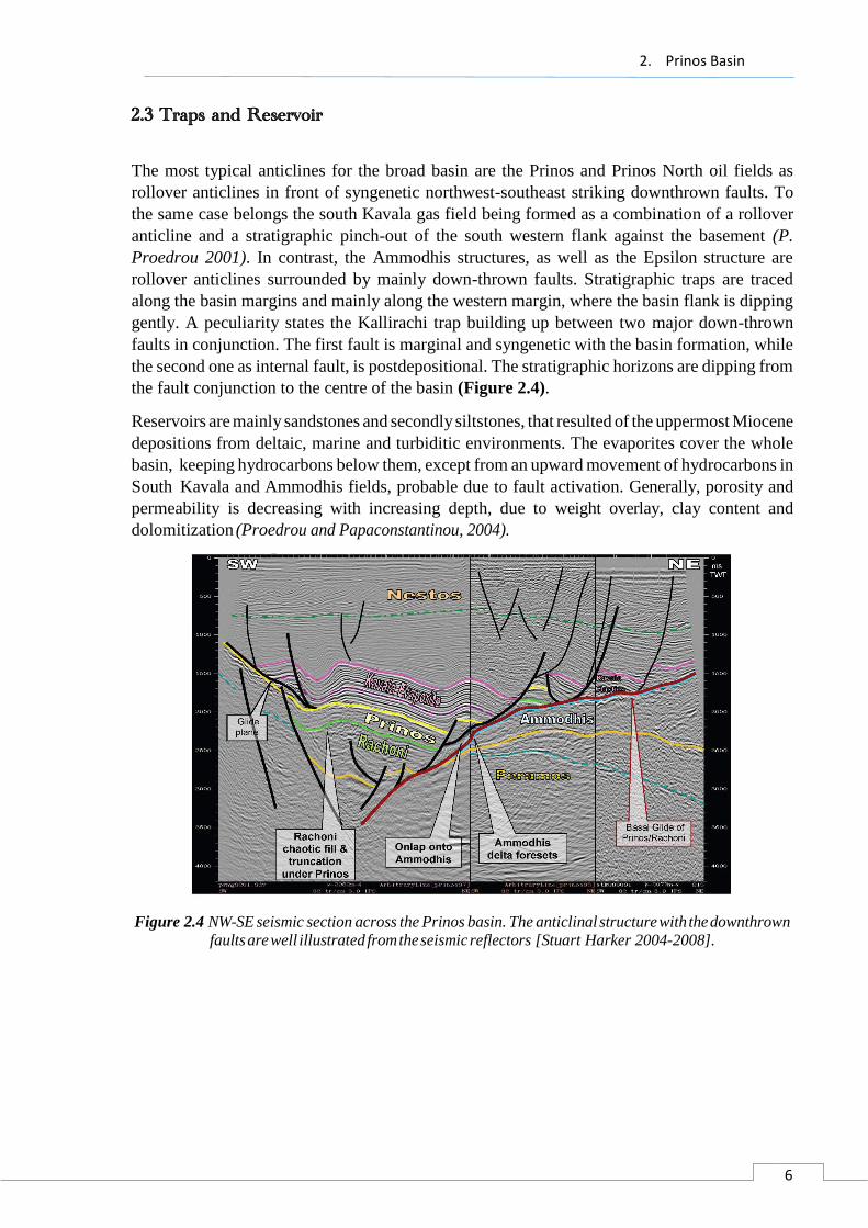
Figure 2.4 NW-SE seismic section across the Prinos basin. The anticlinal structure with the downthrown
faults are well illustrated from the seismic reflectors [Stuart Harker 2004-2008].
2. Prinos Basin
7
2.4 Oil generation and migration
Marine claystones of Middle to Upper Miocene age and messinian claystones deposited under
highly reducing conditions interrupted by hyperjaline episodes are considered to be the source
of oil in the basin. Coal deposits may have a good potential for gas generation. The oil source -
rock is characterized by a waxy sapropelic oil prone kerogen with terrestrially derived organic
matter frequently dominant. Maturity measurements show vitrinite reflectance up to 1.10 for
depths up to 3500 meters. The central part of the basin, with a depth of approximately 5500m
was never reached by drilling. Generally there is a rapid increase of thermal maturity towards
the basement throughout the basin suggesting that a heat source is originating from it
(Robertson Research INT. 1981).
According to the oil maturation plots oil reached the threshold of maturity during latest Miocene
in the deepest part of the basin. Generation continued throughout the Pliocene and recent. The
present top of the maturation window starts at depths of 2500m. The equivalent top for gas
window is at depth of 4000m (Proedrou, Sidiropoulos 1992). Only in Nestos area where the
geothermal gradient is very high the zone of peak gas generation is reached at 3500m. The
Prinos, North Prinos, Epsilon and Ammodhis oils are of the same quality. They belong to an
aromatic - asphaltic type with a sulfur content. The gases are dissolved in the wet phase and
consist from methane to pentane with H2S and CO2 in various percentages.
The sweet hydrocarbons more probably have been generated from the earlier deposited miocene
claystones in an open marine phase. This early phase produced more mature hydrocarbons
without any H2S contribution. The coal has more probably also contributed to the gas
generation. In contrast the Prinos , North Prinos, Epsilon and Ammodhis fields contain a more
immature oil with high content in H2S and CO2 that mainly was originated from the under
reducing conditions deposited claystones (Rigakis et al 2001).
Concerning the oil migration it breaks out from the deepest parts of the southern half of the
basin and spreads out radial to the periphery and to the central basin Highs where the trapping
mechanisms were present (Figure 2.4). The gas migration from the deepest part of the Nestos
subbasin is very local and due to the absence of good quality and sufficient volume reservoirs
has been dispersed.
3. Synthetic Data Simulator
8
3. Synthetic data simulator
A basic tool in exploration seismology is the synthetic seismogram which is generated by
solving an elastic wave equation. The analytical solution is not always known. Therefore,
various approximation methods have been suggested for the computation of synthetic
seismograms.
In a series method, the solution of the propagation problem is represented by an infinite
series (Asymptotic Ray Theory). The coefficients of a finite number of terms (most
often the leading term only) are then determined numerically to yield an approximation
to the true solution. One of the disadvantages of ART is that a large number of rays is
necessary to generate a synthetic seismogram.
In transform methods, if the independent variables in the wave equation are separable
by applying transforms partial differential equations can be reduced to ordinary
differential equations which can be solved analytically or numerically. Having found
the solution of the ordinary differential equations, the inverse transforms must be
evaluated.
In segmentation methods, the given interval is segmented into subintervals and the
differential equation is approximated with reference to those segments. Depending on
the size of the segments and the, approximation procedure for the solution, there are
several methods. One subgroup consists of the finite difference and finite element
methods waves.
In finite differences (FD), both the spatial and time variables are discretized by superimposing
a rectangular grid on the model. Finite difference approximations to the differential equations
that describe the wave propagation, give rise to difference equations. Numerical solutions are
obtained from the difference equations solved on the discrete grid subject to some initial
condition.
Kelly et al. (1976) pointed out that two formulations can be distinguished: The homogeneous
approach solves the wave equation in each homogeneous layer separately. Boundary conditions
must be explicitly imposed on the interfaces between different layers. The heterogeneous
formulation directly solves the wave equation for the whole model. The wave equation in this
case allows the physical properties to vary both laterally and vertically. In the heterogeneous
approach, boundary conditions are satisfied implicitly and more complicated geometries can be
accommodated with no extra effort.

3. Synthetic Data Simulator
9
3.1 Heterogeneous Approach
The heterogeneous approach has certain advantages over the homogeneous since it can be
applied to any model geometry without requiring major changes in the program code. In
approximating the second order wave equation, numerical differentiation of the elastic
parameters is necessary. Here, the equivalent first order hyperbolic system will be examined
A first order system in two dimensions can be expressed as
, , , , , ,f x zU x z t A U x z t B U x z t (3.1)
Where U is a vector function of x, z and t. In problems of seismic wave propagation, U includes
any relevant components of displacement (or their time derivatives) and stress, A, B are
matrices, containing the properties of the medium as functions of x and z, with 0 < x < Hx, 0 <
z < Hz. The symbol ∂ denotes partial derivative with respect to a spatial or temporal coordinate
s. This system is solved numerically for t>0, subject to initial conditions: U(x, z, t = 0).
A system is called hyperbolic if, for all real α, β with α2+β2=1, there exists a nonsingular
transformation matrix Q, such that
1Q A B Q D (3.2)
where D is a diagonal matrix with real elements. All of these conditions are satisfied if the
matrices A and B, are real and symmetric.
To set up the finite-difference method, two integers are selected J > 0, M > 0 and the time step
K > 0. If Hx and Hz are the endpoints of the grid and h = Hx/J = Hz/M, the mesh points (xj, zm,
tn) are defined by
xj = jh for each j = 0,1, ... J
zm = mh for each m = 0,1, ... M
tn = nk for each n = 0,1, ...
Various difference approximations for hyperbolic systems are well established and have been
applied in different fields. The best known method for first-order hyperbolic systems is the Lax-
Wendroff method (Lax and Wendroff, 1964, Mitchell, 1981) where a difference equation is
determined so that it has accuracy of second order. A Lax-Wendroff scheme for a first order
hyperbolic system in two space dimensions with the matrices of coefficients A and B varying
both in space and time given by Mitchell (1981) has been modified so that it maintains second
order accuracy where the matrices A and B depend on the space variables. The modified Lax-
Wendroff scheme is based on the Taylor expansion of U at time t+k for k>0 carried to second
order.
2
2 3
2
1, , , , ( )
2
U UU x z t k U x z t k k O k
t t
(3.3)
which becomes, after replacing the time derivatives by space derivatives from equation (3.1)
and keeping up to second order terms in k

3. Synthetic Data Simulator
10
2
, , , ,2
U U k U U U UU x z t k U x z t k A B A A B A A B
x z x x z z x z
(3.4)
A modified Lax-Wendroff scheme [Griffiths, Abramovici, 1987; Vafidis, 1988], when applied
to equation 3.4, results in:
(3.5)
where p=k/h. The differencing star of this scheme is shown in Figure 3.1. It is a nine-point
numerical scheme explicit in the vector U. Given the vector U at a given time, it is a simple
matter to compute U at any other time by the above forward time marching process.
Figure 3.1 The differencing star for the modified Lax-Wendroff scheme.
21
, , 1, , 1, , , 1 , , 1
2
, 1, , 1, , , 1 , , 1 ,
, 1, ,
2 2
4
2 24
22 2
n
j m j m j m j m j m j m j m j m j m
n
j m j m j m j m j m j m j m j m j m
j m j m j m
pU I A A A A B B B B
pA B B B B A A A U
p pA I A A
, , , 1 1,
, , 1 , , , 1, , 1
, , 1, , , 1 , 1,
2
2 2 2
2
2 2
n
j m j m j m j m
n
j m j m j m j m j m j m j m
n
j m j m j m j m j m j m j m
pB A A U
p p pB I B B A B B U
p p pA I A A B A A U
, , , 1 , 1, , , 1
2
, , , , 1, 1 1, 1 1, 1 1, 1
2 2 2
8
n
j m j m j m j m j m j m j m
n n n n
j m j m j m j m j m j m j m j m
p p pB I B B A B B U
pA B B A U U U U
3. Synthetic Data Simulator
11
3.2 Elastic wave propagation
The basic equation for two-dimensional SH-wave propagation in a heterogeneous isotropic
medium, in absence of body forces, is:
( , ) ( , , ) , ( , , ) , ( , , )u x x z zx z u x z t x z u x z t x z u x z t (3.6)
where u(x, z, t) is the displacement, μ(x, z) the shear modulus, and ρ(x, z) the density.
Instead of solving numerically the second-order hyperbolic wave equation one can use an
equivalent first-order systemcoo. In matrix form the system is:
1 1 0 0
0 0 0 0 0
0 0 0 0
0 0
0
t xy xy z xy
zy zy zy
u u up p
or t x zU A U B U (3.7)
where the dot denotes time derivative and σxy(x, z, t) , σzy (x, z, t) are the stress components.
The system in equation (3.7) can also be written in the form
1
1
0 0 1 0 0 1
0 0 1 0 0 0 0 0
0 0 0 1 0 0 0
0 0
0
t xy x xy z xy
zy zy zy
u u u
(3.8)
Now, the earth's response is resolved into components in the horizontal (x) and the vertical (z)
directions only. To calculate the elastic response of a model in rectangular (x, z) coordinates,
the corresponding first-order system was solved numerically. This system consists of the basic
equations of motion in the x- and z-direction.
( , ) ( , , ) , , , ,t x xx xzp x z u x z t x z t z x z t
( , ) w( , , ) , , , ,t x xz zzp x z x z t x z t z x z t (3.9)
and the stress-strain relations after taking the first time derivatives
, , ( , ) 2 (x,z) u( , , ) , , ,t xx x zx z t x z x z t x z w x z t
, , ( , ) , , ( , ) u( , , )t xz x zx z t x z w x z t x z x z t
, , ( , ) u( , , ) (x,z) 2 (x,z) , ,t zz x zx z t x z x z t w x z t (3.10)

3. Synthetic Data Simulator
12
where u(x, z, t) and w(x, z, t) are the displacements in the x- and z-directions, respectively, σxx,
σxz, σzz, the stress components, μ(x, z) and λ(x, z) the Lame parameters, p(x,z) the density and
the dot denotes time derivative. In this formulation there are no space derivatives of the Lame
coefficients.
Equations (3.9) and (3.10) can be written in the following matrix form
1
1
0 0 0
0 0 0
0 0 0 0
0 0 0 0
0 0 0
0
2
0
0
t xx
zz
xz
w
p
p
u
1
1
0 0 0
0 0 0
0 0 0 0
0 0 0 0
0
0
0
2
0 0
xx
zz
xz
u
w
p
p
0
z xx
zz
xz
u
w
(3.11)
One of the key factors in forward modelling is the implementation of the source. Since the
treated problems are two-dimensional, line sources were considered. To avoid the large values
of the response in the source region Alterman's and Karal's method (1968) was used. The
solution to the two-dimensional elastic or acoustic system for a homogeneous, infinitely
extended, medium with a line source, is well known. Convolving the impulse response with the
source excitation results in an integral that can be evaluated numerically. A Gaussian function
whose frequency response is practically band limited defines the source excitation.
3.3 Accuracy, convergence and stability
To guarantee that solutions to the difference equations remain bounded as the computations
proceed, and that as the grid spacing becomes smaller and smaller those solutions approach the
solution of the differential equation the accuracy the convergence and stability must be checked.
Accuracy
A criterion for the local accuracy of a finite difference formula is defined by the difference, E,
between the exact solutions of the differential, W, and the difference, U, equations at a grid
point (jh, mh, (n+1)k) as
, , ,
n n n
j m j m j mE W U (3.12)
The Taylor series of Wn is
21 3[ ]
2
n n n n
t tt
kW W kW W O k (3.13)
Replacing the time derivatives from the differential system (3.l) we get
2
1 3
2 [ ]2
n n nn n
x x z x zx z
kW W AW BW A AW BW B AW BW O
(3.14)

3. Synthetic Data Simulator
13
The Lax-Wendroff scheme (3.5) after approximating the difference operators by keeping the
leading terms only
2 2 , 2 , 2 n n n n n n
x x x z z z x x x x x xU hU U hU A A U h AU
2 2 2 , 4n n n n
z z z z z x z zxz z xB U h BU U h U
2 22 , 2n n n n
z z z x x xx x zxz zA A U h AU B B U h B U (3.15)
Gives
2 2
1
2
n n nn n
x z x xz x zx
p hU U ph AU BU A AU A BU B U
n n
xz z x z zB AU AU B BU
(3.16)
Substituting the equations (3.13) and (3.16) in equation (3.12), the truncation error is of third
order in time. Similarly, by expanding the Taylor series in the space domain, one can obtain
accuracy of the order (h2, k2) or (2, 2). The truncation error of MacCormack schemes has the
form
4 2 21
6o x x x
E k A AU kh O h O kh O k
(3.17)
Convergence
The various difference schemes are only useful for solving PDE, if they are convergent and
stable. Convergence exists if the theoretical solution to a difference equation approaches the
solution of the corresponding differential equation as the mesh is refined. The Courant-
Friedrichs-Lewy (1928) (CFL) condition must be satisfied for explicit difference replacements
to the hyperbolic differential equations for the systems to be convergent. The CFL condition
states that the domain of dependence of the difference equation must include the domain of
dependence of the differential equation. If the CFL condition is not satisfied the solution of the
difference equation is independent of the initial data of the problem which lies outside the
domain of dependence of the difference equation but lies inside the domain of dependence of
the differential equation. Alteration of this initial data modifies the solution of the differential
equation but leaves the solution of the difference equation unaltered. The domain of dependence
of a hyperbolic system can be found by the method of characteristics (Mitchell, 1981). The
domain of dependence of an explicit difference system is confined by the grid points which
influence the value of U at a certain point and depends on the mesh ratio p.
As an example the simple SH wave equation with μ(x,z)=p(x,z)= 1 will be considered. The
domains of dependence of the system (3.7) and the explicit difference system (3.5) will be
examined with respect to the Cauchy initial value problem where the initial conditions are
U (x, z, 0) = C (x, z) -∞< x, z<+∞ (3.18)
3. Synthetic Data Simulator
14
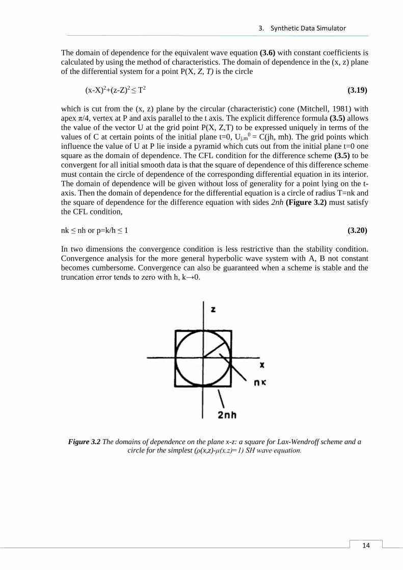
The domain of dependence for the equivalent wave equation (3.6) with constant coefficients is
calculated by using the method of characteristics. The domain of dependence in the (x, z) plane
of the differential system for a point P(X, Z, T) is the circle
(x-X)2+(z-Z)2 ≤ T2 (3.19)
which is cut from the (x, z) plane by the circular (characteristic) cone (Mitchell, 1981) with
apex π/4, vertex at P and axis parallel to the t axis. The explicit difference formula (3.5) allows
the value of the vector U at the grid point P(X, Z,T) to be expressed uniquely in terms of the
values of C at certain points of the initial plane t=0, Uj,m0 = C(jh, mh). The grid points which
influence the value of U at P lie inside a pyramid which cuts out from the initial plane t=0 one
square as the domain of dependence. The CFL condition for the difference scheme (3.5) to be
convergent for all initial smooth data is that the square of dependence of this difference scheme
must contain the circle of dependence of the corresponding differential equation in its interior.
The domain of dependence will be given without loss of generality for a point lying on the t-
axis. Then the domain of dependence for the differential equation is a circle of radius T=nk and
the square of dependence for the difference equation with sides 2nh (Figure 3.2) must satisfy
the CFL condition,
nk ≤ nh or p=k/h ≤ 1 (3.20)
In two dimensions the convergence condition is less restrictive than the stability condition.
Convergence analysis for the more general hyperbolic wave system with A, B not constant
becomes cumbersome. Convergence can also be guaranteed when a scheme is stable and the
truncation error tends to zero with h, k→0.
Figure 3.2 The domains of dependence on the plane x-z: a square for Lax-Wendroff scheme and a
circle for the simplest (ρ(x,z)-μ(x.z)=1) SH wave equation.
3. Synthetic Data Simulator
15
Stability
The problem of stability consists of finding conditions under which the difference between the
theoretical and numerical solutions of the difference equation remains bounded as time
progresses. A finite difference scheme is unstable when its error grows without a bound. The
easiest way of investigating stability is to use the Fourier series approach pioneered by von
Neumann. In this discussion boundary or initial conditions are not going to be taken into
consideration.
A stability analysis of a hyperbolic system in two space dimensions is difficult, even with A
and B constant. The stability of a difference scheme at a grid point in the field will be the same
as the stability of the corresponding difference equation where the values of the coefficients
have been 'frozen' to the values attained at that grid point. This local stability condition\ usually
a limitation on the-size of the mesh ratio p, will vary from point to point in the field and the
overall stability condition must be the largest mesh ratio which satisfies the local stability
condition at every grid point in the region. The von Neumann necessary condition for the
stability of a system requires the magnitude of the maximum eigenvalue of the amplification
matrix to be less than one. The amplification matrix for the Lax-Wendroff scheme with A, B
constant
2 2 2 11 cos 1 cosn sin sin sin sin
2G I p A AB BA n ip A n
(3.21)
is used to evaluate the eigenvalues. Lax and Wendroff( 1964) proved that if
,max ,m A B A Ba a a (3.22)
where aA, aB ae the eigenvalues of the matrices A, B respectively, then the Lax-Wendroff
scheme with A,B constant is stable if
1
2 2mp a (3.23)
For the MacCormack scheme, since the matrix A (or B) can be diagonalized, the von Neumann
condition is both necessary and sufficient for stability. If a is an eigenvalue of A the stability
condition for this scheme is given by 2
3mp a (3.24)
The MacCormack scheme stability condition is almost half as restrictive as the Lax-Wendroff.
The number of time steps required for the generation of a synthetic trace of a given duration is
therefore halved so that the method becomes less expensive.
4. AVO Analysis Theory
16
4. AVO Analysis Theory
The variation of reflection and transmission coefficients with angle of incidence (AVA) (and
corresponding increasing offset) is often referred to as offset-dependent reflectivity and is the
fundamental basis for amplitude-versus-offset (AVO) analysis. There are two kinds of AVO
phenomena according to the types of seismic data. One is P-wave AVO and the other is
multicomponent AVO corresponding to single component P-wave seismic data and
multicomponent seismic data, respectively. Today, AVO analysis is widely used in
hydrocarbon detection, lithology identification, and fluid parameter analysis, due to the fact that
seismic amplitudes at the boundaries are affected by the variations of the physical properties
just above and just below the boundaries. In recent years, a growing number of theories and
techniques in seismic data acquisition, processing, and seismic data interpretation have been
developed, updated, and employed. AVO analysis in theory and practice is becoming
increasingly attractive [Feng and Bancroft 2006].
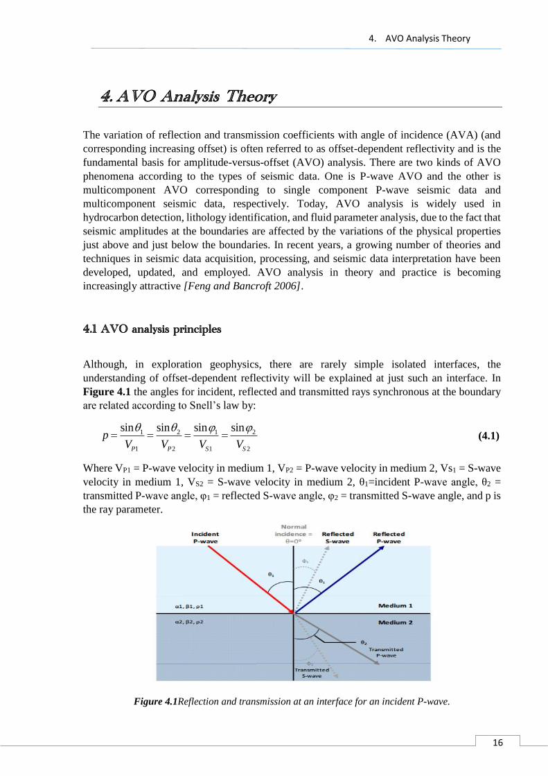
4.1 AVO analysis principles
Although, in exploration geophysics, there are rarely simple isolated interfaces, the
understanding of offset-dependent reflectivity will be explained at just such an interface. In
Figure 4.1 the angles for incident, reflected and transmitted rays synchronous at the boundary
are related according to Snell’s law by:
1 2 1 2
1 2 1 2
sin sin sin sin
P P S S
pV V V V
(4.1)
Where VP1 = P-wave velocity in medium 1, VP2 = P-wave velocity in medium 2, Vs1 = S-wave
velocity in medium 1, VS2 = S-wave velocity in medium 2, θ1=incident P-wave angle, θ2 =
transmitted P-wave angle, φ1 = reflected S-wave angle, φ2 = transmitted S-wave angle, and p is
the ray parameter.
Figure 4.1Reflection and transmission at an interface for an incident P-wave.
4. AVO Analysis Theory
17
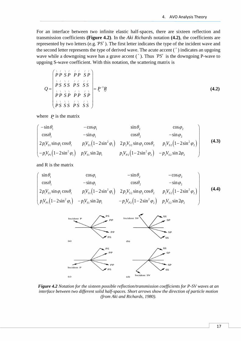
For an interface between two infinite elastic half-spaces, there are sixteen reflection and
transmission coefficients (Figure 4.2). In the Aki Richards notation (4.2), the coefficients are
represented by two letters (e.g. P̀S ). The first letter indicates the type of the incident wave and
the second letter represents the type of derived wave. The acute accent ( ) indicates an upgoing
wave while a downgoing wave has a grave accent ( ` ). Thus P̀S is the downgoing P-wave to
upgoing S-wave coefficient. With this notation, the scattering matrix is
\ / \ / / / / /
\ / \ / / / / /
1
\ \ \ \ / \ / \
\ \ \ \ / \ / \
P P S P P P S P
P S S S P S S SQ P R
P P S P P P S P
P S S S P S S S
(4.2)
where P is the matrix
1 1 2 2
1 1 2
sin cos sin cos
cos si
cos n
2
2 2
1 1 1 1 1 1 1 2 2 2 2 2 2 2
2 2
1 1 1 1 1 1 2 2 2 2 2 2
sin
2 sin cos 1 2sin 2 sin cos 1 2sin
1 2sin sin
2 1 2sin si n 2
S S S S
P S P S
pV pV p V p V
pV pV p V p V
(4.3)
and R is the matrix
1 2
2
1 2
1 1
sin cos sin cos
cos s cos in
2
2 2
1 1 1 1 1 1 1 2 2 2 2 2 2 2
2 2
1 1 1 1 1 1 2 2 2 2 2 2
sin
2 sin cos 1 2sin 2 sin cos 1 2sin
1 2sin sin 2 1 2sin s i 2 n
S S S S
P S P S
pV pV p V p V
pV pV p V p V
(4.4)
Figure 4.2 Notation for the sixteen possible reflection/transmission coefficients for P-SV waves at an
interface between two different solid half-spaces. Short arrows show the direction of particle motion
(from Aki and Richards, 1980).

4. AVO Analysis Theory
18
Koefoed (1955) first pointed out the practical possibilities of using AVO analysis as an indicator
of VP -VS variations and empirically established five rules, which were later verified by Shuey
(1985) for moderate angles of incidence:
a) When the underlying medium has the greater longitudinal [P-wave] velocity and other
relevant properties of the two strata are equal to each other, an increase of Poisson’s
ratio for the underlying medium causes an increase of the reflection coefficient at the
larger angles of incidence.
b) When, in the above case, Poisson’s ratio for the incident medium is increased, the
reflection coefficient at the larger angles of incidence is thereby decreased.
c) When, in the above case, Poisson’s ratios for both media are increased and kept equal
to each other, the reflection coefficient at the larger angles of incidence is thereby
increased.
d) The effect mentioned in (a) becomes more pronounced as the velocity contrast becomes
smaller.
e) Interchange of the incident and the underlying medium affects the shape of the curves
only slightly, at least up to values of the angle of incidence of about 30 degrees.
Bortfeld (1961) linearized the Zoeppritz equations by assuming small changes in layer
properties (Δρ/ρ, ΔVρ/Vρ, ΔVs/Vs <<1).
This approach was also followed by Richards and Frazier (1976) and Aki and Richards (1980)
who derived a form of approximation simply parameterized in terms of the changes in density,
P-wave velocity, and S-wave velocity across the interface:
2 2 2 2
2
1 1( ) 1 4 4
2 2cos ( )
ss s
s
V VR V V
V V
(4.5)
Where Δρ=ρ2-ρ1, ΔVP=VP2-VP1, ΔVS=VS2-VS1, ρ=(ρ2+ρ1)/2, VP=(VP2+VP1)/2, VS=(VS2+VS1)/2,
θ= (θ1+θ2)/2 and p is the ray parameter as defined by equation (4.1). By simplifying the
Zoeppritz equations, Shuey (1985) presented another form of the Aki and Richards (1980)
approximation,
2 2 2
2
1( ) sin tan sin
21
Po o o
P
VR R A R
V
(4.6)
Where Ro is the normal-incidence P-P reflection coefficient, Ao is given by:
1 2
2 11
o o oA B B
(4.7)
and/
/ /
P Po
P P
V VB
V V
(4.8)
Where Δσ is the average Poisson’s ratio and is defined as Δσ=σ2-σ1 and σ=(σ2+σ1)/2.
4. AVO Analysis Theory
19
With various assumptions, the (4.6) can be simplified as:
2sinpR R G (4.9)
This equation is linear if R is plotted as a function of sin2θ. Then a linear regression analysis
can be performed on the seismic amplitudes to estimate intercept, Rρ, and gradient G. Before
performing the linear regression, firstly the data should be transformed from constant offset
form to constant angle form.
The quantity Aο, given by equation (4.6), specifies the variation of R(θ) in the approximation
range 0 <θ < 30° for the case of no contrast in Poisson’s ratio. The first term gives the amplitude
at normal incidence, the second term characterizes R(θ) at intermediate angles, and the third
term describes the approach to the critical angle. The coefficients of Shuey’s approximation
form the basis of various weighted stacking procedures. Weighted stacking, here also called
Geostack (Smith and Gidlow, 1987), is a means of reducing prestack information to AVO
attribute traces versus time. This is accomplished by calculating the local angle of incidence for
each time sample, then performing regression analysis to solve for the first two or all three
coefficients of an equation of the kind:
2 2 2sin sin tanR C (4.10)
where A is the “zero-offset” stack, B is commonly referred to as the AVO “slope” or “gradient”
and the third term becomes significant in the far-offset stack. At the same time, the “fluid factor”
concept was introduced by Smith and Gidlow (1987) to highlight gas-bearing sandstones.
Hilterman (1989) derived another convenient approximation:
2 2cos 2.25 sinoR R (4.11)
Thus, at small angles Rο dominates the reflection coefficient whereas Δσ dominates at larger
angles. In this way, we can think of a near-offset stack as imaging P-wave impedance contrasts
while the far-offset stack images Poisson’s-ratio contrasts. The analysis of amplitude variation
with offset (AVO) was a significant component in the development of direct hydrocarbon
indicators (DHIs), and AVO techniques are identified by Hilterman (2001) as the second era of
amplitude interpretation, following the brightspot era.

4. AVO Analysis Theory
20
4.2 Transforming From the Offset to the Angle Domain
As mentioned on chapter 4.1, both Zoeppritz equations and Shuey’s equation are dependent
upon the angle of incidence at which the seismic ray strikes the horizon of interest. However,
the seismic data is recorded as a function of offset. While offset and angle are roughly similar,
there is a nonlinear relationship between them, which must first be accounted for in processing
and analysis schemes which require that angle be used instead of offset. This type of analysis
is termed AVA (amplitude versus angle) rather than AVO. An example of such a transform is
shown in Figure 4.3.
Figure 4.3 (a) shows AVO response and (b) shows transform of (a) in AVA (amplitude versus angle)
response [NTNU, AVO theory, 2004].
An offset gather is shown in Figure 4.3 (a), and the equivalent angle gather is shown in Figure
4.3 (b). At the top of each gather a schematic of the raypath’s geometry is shown for the
reflected events in a particular trace of each gather. As it is observed from Figure 4.3, the angle
of incidence for a constant offset trace decreases with depth, whereas the angle remains constant
with depth for a constant angle trace. The operation for computing this transform is quite
straightforward. To transform from constant offset to constant angle, the relationship between
X and θ needs to be known. For a complete solution, a full ray tracing must be done. However,
a good approximation is to use straight rays. In this case it is found that:

4. AVO Analysis Theory
21
tan2
(4.12)
Where θ=angle of incidence, X=offset and Z=depth.
If the velocity down to the layer of interest is known:
2
oV tZ
(4.13)
Where V=Velocity either RMS or Average and to= total zero-offset travel time.
Substituting equation (4.12) into (4.13) gives:
tano
X
V t
(4.14)
which gives the mapping from offset to angle. By inverting equation (4.14), the mapping from
angle to offset derives:
tanoX V t (4.15)
Equation (4.15) thus allows the mapping of the amplitudes on an offset gather to amplitudes on
an angle gather. Figure 4.4 shows a theoretical set of constant angle curves superimposed on
an offset versus time plot. As it is observed from Figure 4.4 the curves increase to larger offsets
at deeper times. This means that a constant angle seismic trace would contain amplitudes
collected from longer offset on the AVO gather as time increases.
Figure 4.4 A plot of constant angle curves superimposed on constant offset traces.
4. AVO Analysis Theory
22
4.3 Ray Tracing
The ray-tracing problem in AVO is that for a given source and receiver location, and a given
reflection layer, the raypath which connects the source and receiver should be defined, while
obeying Snell’s Law in each layer. The following derivation follows that of Dahl and Ursin
(1991). Define the ray-parameter, p, as:
1
1
sin
P
pV
(4.16)
where θ1 is the emergence angle for energy from the source and VP1 is the P-wave velocity of
the first layer. Snell’s Law indicates that for any layer:
sin i
Pi
pV
(4.17)
If the emergence angle is known, the offset, y, at which the reflected energy will come back to
the surface can be calculated:
2 2( )
1
k k
kk
D V py p
V p
(4.18)
In this equation, Dk is the thickness of the kth layer, and the sum is over all layers down to the
reflecting interface.
In the ray-tracing problem, the desired offset yd is known, it is the distance between the source
and receiver for the trace in question. The problem is to find the value of p that gives the correct
value of y in equation (4.18). Unfortunately, there is no explicit solution to this problem. The
approach used in AVO is an iterative solution, sometimes called a “shooting method”. The first
step is to make a guess at the correct value of p, say po. With this value of p, the initial value of
y can be calculated, from equation (4.18):
2 21
k k oo
kk o
D V py
V p
(4.19)
Usually, yo will not be the same as the desired value yd. The error is Δy=yd-yo.
An improved value for p is then given by:
'
o
pp p y
y
(4.20)
where ∂p/∂y is calculated from equation (4.18) as:
1
3/22 21
k k
kk o
D Vp
y V p
(4.21)

4. AVO Analysis Theory
23
The new value, p’, when used in equation (4.18) should give a value of y closer to the desired
yd than the initial guess. Ray tracing consists of continually applying equations (4.19) to (4.21)
until a “convergence condition” is reached.
The convergence condition in AVO is reached when either of the following is true:
1) The maximum number of iterations is reached. For synthetic modelling in AVO, the
maximum number of iterations is set to 100. This value should never be reached under
normal circumstances.
2) The offset error Δy becomes “small enough”. In AVO, the tolerance is set to the greater
of 1% of the desired offset or 1 distance unit. If, for example, the desired offset is 1000
m, the iterations will stop when the error is less than 10m. If the desired offset is 10m,
the iterations will stop when the error is less than 1m.
The algorithm described by equations (4.19) to (4.21) is so efficient that for the vast majority
of cases, convergence is reached in two or three iterations. Unfortunately, certain pathological
conditions can occur from time to time, which cause the algorithm to get stuck. The worst case
occurs when a single layer between the surface and the target interface has a P-wave velocity
much higher than average. In this case, the propagation angle θi in equation (4.17) is close to
90°. This also means that the ray-path is close to critical but not quite. Instability can then arise,
which causes the error, Δy, to converge very slowly. A typical cause of anomalously high
velocity layers is, in fact, errors in the log.
4. AVO Analysis Theory
24
4.4 Seismic Data Pre-Processing for AVO Analysis
AVO processing should preserve or restore relative trace amplitudes within CMP gathers.
This implies two goals:
o Reflections must be correctly positioned in the subsurface
o Data quality should be sufficient to ensure that reflection amplitudes contain
information about reflection coefficients.
Even though the unique goal in AVO processing is to preserve the true relative amplitudes,
there is no unique processing sequence. It depends on the complexity of the geology, whether
it is land or marine seismic data and whether the data will be used to extract regression-based
AVO attributes or more sophisticated elastic inversion attributes. Cambois (2001) defines AVO
processing as any processing sequence that makes the data compatible with Shuey's equation.
If that is the model used for the AVO inversion. Camhois emphasizes that this can be a very
complicated task.
Factors that change the amplitudes of seismic traces can be grouped into Earth effects,
acquisition-related effects, and noise (Dey-Sarkar and Suatek, 1993). Earth effects include i)
spherical divergence, ii) absorption, iii) transmission losses, iv) interbed multiples, v) converted
phases, vi) tuning, vii) anisotropy, and viii) structure. Acquisition-related effects include source
and receiver arrays and receiver sensitivity. Noise can be ambient or source generated,
coherent or random. Processing attempts to compensate for or remove these effects, but can
in the process change or distort relative trace amplitudes. This is an important trade-off we need
to consider in pre-processing for AVO.
a) Spiking deconvolution and wavelet processing
In AVO analysis we normally want zero-phase data. However, the original seismic pulse is
causal, usually some sort of minimum phase wavelet with noise. Deconvolution is defined as
convolving the seismic trace with an inverse filter in order to extract the impulse response from
the seismic trace. This procedure will restore high frequencies and therefore improve the
vertical resolution and recognition of events. The wavelet shape can vary vertically (with time),
laterally (spatially), and with offset. However, AVO analysis is normally carried out within a
limited time window where one can assume stationarity. Lateral changes in the wavelet shape
can be handled with surface-consistent amplitude balancing (e.g., Cambois and Magesan,
1997). Offset-dependent variations are often more complicated to correct for, and are attributed
to both offset-dependent absorption, tuning effects, and NMO stretching. NMO stretching acts
like a low-pass, mixed-phase, nonstationary filter, and the effects are very difficult to eliminate
fully (Cambois, 2001).
b) Spherical divergence correction
Spherical divergence, or geometrical spreading, causes the intensity and energy of spherical
waves to decrease inversely as the square of the distance from the source (Newman, 1973). This
technique will be further analysed in the next chapter.
4. AVO Analysis Theory
25
c) Surface-consistent amplitude balancing
Source and receiver effects as well as water depth variation can produce large deviations in
amplitude that do not correspond to target reflector properties. Commonly, statistical amplitude
balancing is carried out both for time and offset. However, this procedure can have a dramatic
effect on the AVO parameters. It easily contributes to intercept leakage and consequently
erroneous gradient estimates (Cambois, 2000). Cambois (2001) suggested modeling the
expected average amplitude variation with offset following Shuey's equation, and then using
this behaviour as a reference for the statistical amplitude balancing.
d) Multiple removal
One of the most deteriorating effects on pre-stack amplitudes is the presence of multiples. There
are several methods of filtering away multiple energy, but not all of these are adequate for AVO
pre-processing. The method known as f-k multiple filtering, done in the frequency-wavenumber
domain, is very efficient at removing multiples, but the dip in the f-k domain is very similar for
near-offset primary energy and near-offset multiple energy. Hence, primary energy can easily
be removed from near traces and not from far traces, resulting in an artificial AVO effect. More
robust demultiple techniques include linear and parabolic Radon transform multiple removal
(Hampson, 1986; Herrmann et al., 2000).
e) NMO (normal moveout) correction
A potential problem during AVO analysis is error in the velocity moveout correction. When
extracting AVO attributes, one assumes that primaries have been completely flattened to a
constant traveltime. This is rarely the case, as there will always be residual moveout. The reason
for residual moveout is almost always associated with erroneous velocity picking, and great
efforts should be put into optimizing the estimated velocity field (e.g., Adler, 1999; Le Meur
and Magneron, 2000). However, anisotropy and non-hyperbolic moveouts due to complex
overburden may also cause misalignments between near and far offsets. Ursin and Ekren (1994)
presented a method for analyzing AVO effects in the offset domain using time windows. This
technique reduces moveout errors and creates improved estimates of AVO parameters. One
should be aware of AVO anomalies with polarity shifts (class lip, see definition below) during
NMO corrections, as these can easily be misinterpreted as residual moveouts (Ratcliffe and
Adler, 2000).
f) Pre-stack migration
Pre-stack migration might be thought to be unnecessary in areas where the sedimentary section
is relatively flat, but it is an important component of all AVO processing. Pre-stack migration
should be used on data for AVO analysis whenever possible, because it will collapse the
diffractions at the target depth to be smaller than the Fresnel zone and therefore increase the
lateral resolution (Berkhout, 1985; Mosher et al., 1996). Normally, pre-stack time migration
(PSTM) is preferred to prestack depth migration (PSDM), because the former tends to preserve
amplitudes better. However, in areas with highly structured geology, PSDM will be the most
accurate tool (Cambois, 2001). An amplitude-preserving PSDM routine should then be applied
(Bleistein, 1987; Schleicher et al., 1993; Hanitzsch, 1997). Migration for AVO analysis can be

4. AVO Analysis Theory
26
implemented in many different ways. Resnick et al. (1987) and Allen and Peddy (1993) among
others have recommended Kirchhoff migration together with AVO analysis.
Below are presented three different proposed pre-processing schemes for AVO analysis of a
2D seismic line.
Yilmaz (2001)
(1) Pre-stack signal processing (source signature processing, geometric scaling, spiking
deconvolution and spectral whitening).
(2) Sort to CMP and do sparse interval velocity analysis.
(3) NMO using velocity field from step 2.
(4) Demultiple using discrete Radon transform.
(5) Sort to common-offset and do DMO correction.
(6) Zero-offset FK time migration.
(7) Sort data to common-reflection-point (CRP) and do inverse NMO using the
velocity field from step 2.
(8) Detailed velocity analysis associated with the migrated data.
(9) NMO correction using velocity field from step 8.
(10) Stack CRP gathers to obtain image of pre-stack migrated data. Remove residual multiples
revealed by the stacking.
(11) Unmigrate using same velocity field as in step 6.
(12) Post-stack spiking deconvolution.
(13) Remigrate using migration velocity field from step 8.
Ostrander (1984):
(1) Spherical-divergence correction.
(2) Exponential-gain correction.
(3) Minimum-phase spiking deconvolution.
(4) Velocity analysis.
(5) NMO correction.
(6) Trace equalization.
(7) Horizontal trace summing.
Chiburis (1984):
(1) Mild f-k multiple suppression.
(2) Spherical divergence and NMO correction.
(3) Whole-trace equalization.
(4) Flattening on a consistent reference event.
(5) Horizontal trace summing.
(6) Peak amplitude picked interactively.
(7) Smoothed least-squares curve fitting.
(8) Despiking of outliers.
(9) Results clipped and smoothed.
(10) Curve refitting.
4. AVO Analysis Theory
27
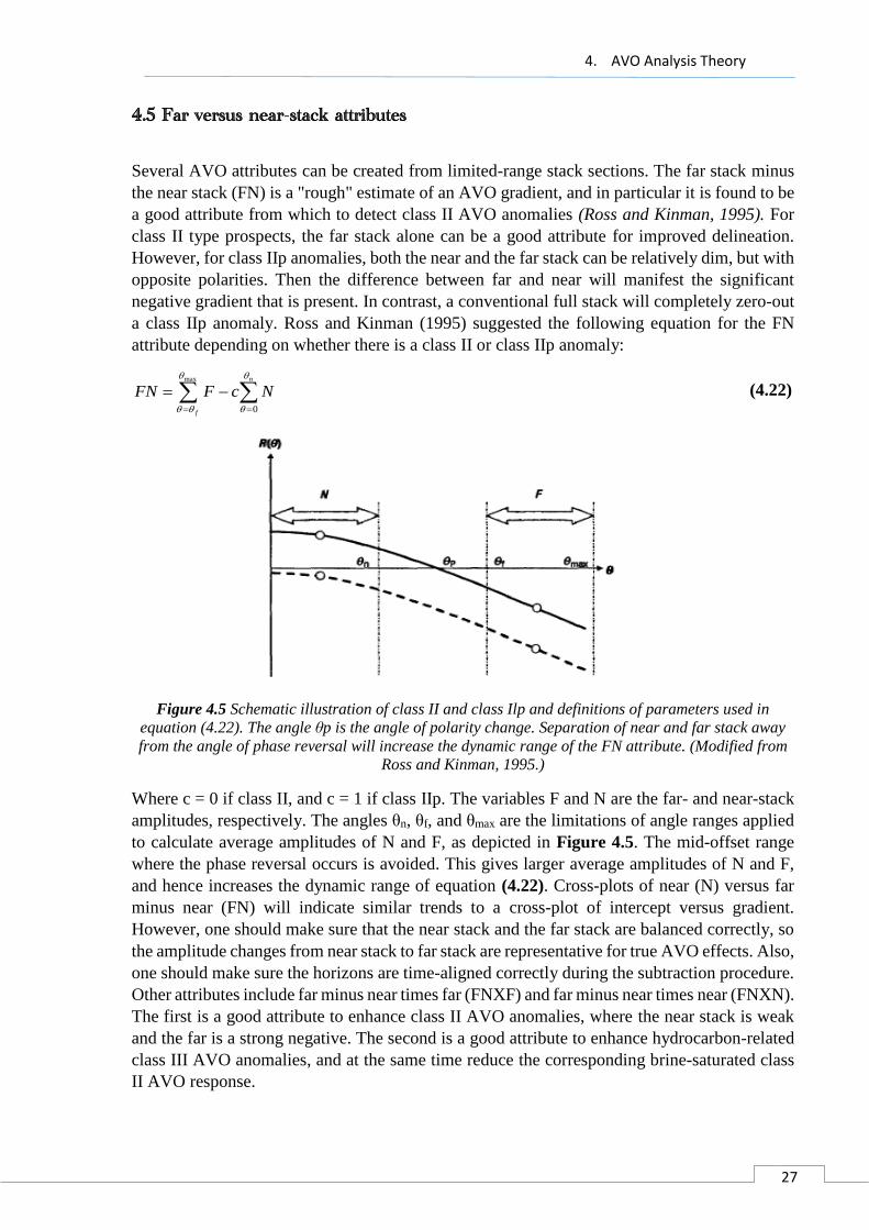
4.5 Far versus near-stack attributes
Several AVO attributes can be created from limited-range stack sections. The far stack minus
the near stack (FN) is a "rough" estimate of an AVO gradient, and in particular it is found to be
a good attribute from which to detect class II AVO anomalies (Ross and Kinman, 1995). For
class II type prospects, the far stack alone can be a good attribute for improved delineation.
However, for class IIp anomalies, both the near and the far stack can be relatively dim, but with
opposite polarities. Then the difference between far and near will manifest the significant
negative gradient that is present. In contrast, a conventional full stack will completely zero-out
a class IIp anomaly. Ross and Kinman (1995) suggested the following equation for the FN
attribute depending on whether there is a class II or class IIp anomaly:
max
0
n
f
FN F c N
(4.22)
Figure 4.5 Schematic illustration of class II and class Ilp and definitions of parameters used in
equation (4.22). The angle θp is the angle of polarity change. Separation of near and far stack away
from the angle of phase reversal will increase the dynamic range of the FN attribute. (Modified from
Ross and Kinman, 1995.)
Where c = 0 if class II, and c = 1 if class ΙΙp. The variables F and N are the far- and near-stack
amplitudes, respectively. The angles θn, θf, and θmax are the limitations of angle ranges applied
to calculate average amplitudes of N and F, as depicted in Figure 4.5. The mid-offset range
where the phase reversal occurs is avoided. This gives larger average amplitudes of N and F,
and hence increases the dynamic range of equation (4.22). Cross-plots of near (N) versus far
minus near (FN) will indicate similar trends to a cross-plot of intercept versus gradient.
However, one should make sure that the near stack and the far stack are balanced correctly, so
the amplitude changes from near stack to far stack are representative for true AVO effects. Also,
one should make sure the horizons are time-aligned correctly during the subtraction procedure.
Other attributes include far minus near times far (FNXF) and far minus near times near (FNXN).
The first is a good attribute to enhance class II AVO anomalies, where the near stack is weak
and the far is a strong negative. The second is a good attribute to enhance hydrocarbon-related
class III AVO anomalies, and at the same time reduce the corresponding brine-saturated class
II AVO response.
4. AVO Analysis Theory
28
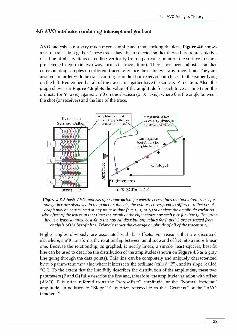
4.6 AVO attributes combining intercept and gradient
AVO analysis is not very much more complicated than stacking the data. Figure 4.6 shows
a set of traces in a gather. These traces have been selected so that they all are representative
of a line of observations extending vertically from a particular point on the surface to some
pre-selected depth (in two-way, acoustic travel time). They have been adjusted so that
corresponding samples on different traces reference the same two-way travel time. They are
arranged in order with the trace coming from the shot-receiver pair closest to the gather lying
on the left. Remember that all of the traces in a gather have the same X-Y location. Also, the
graph shown on Figure 4.6 plots the value of the amplitude for each trace at time t2 on the
ordinate (or Y- axis) against sin2θ on the abscissa (or X- axis), where θ is the angle between
the shot (or receiver) and the line of the trace.
Figure 4.6 A basic AVO analysis after appropriate geometric corrections the individual traces for
one gather are displayed in the panel on the left; the colours correspond to different reflectors. A
graph may be constructed at any point in time (e.g. t1, t2 or t3) to analyse the amplitude variation
with offset of the traces at that time; the graph at the right shows one such plot for time t2. The gray
line is a least-squares, best-fit to the natural distribution; values for P and G are extracted from
analysis of the best-fit line. Triangle shows the average amplitude of all of the traces at t2.
Higher angles obviously are associated with far offsets. For reasons that are discussed
elsewhere, sin2θ transforms the relationship between amplitude and offset into a more-linear
one. Because the relationship, as graphed, is nearly linear, a simple, least-squares, best-fit
line can be used to describe the distribution of the amplitudes (shown on Figure 4.6 as a gray
line going through the data points). This line can be completely and uniquely characterized
by two parameters: the value where it intersects the ordinate (called “P”), and its slope (called
“G”). To the extent that the line fully describes the distribution of the amplitudes, these two
parameters (P and G) fully describe the line and, therefore, the amplitude variation with offset
(AVO). P is often referred to as the “zero-offset” amplitude, or the “Normal Incident”
amplitude. In addition to “Slope,” G is often referred to as the “Gradient” or the “AVO
Gradient.”
4. AVO Analysis Theory
29
There are other pieces of information or AVO parameters which may be extracted from the
traces or from the graph of their amplitudes. Sometimes a subset of the traces such as those
reflected through a small angle (or from a short offset distance) are stacked independently of
the others and, in this case, referred to as “Nears.” Other groupings, such as those reflected
through a large angle or an intermediate angle, are called “Fars” or “Mids.” Summarizing,
the most commonly used parameters in AVO analysis are the values of Ps and Gs, which
together completely define the gathers; the stack, which averages all of the information from
the gathers; and the nears, mids and fars, which average subsets of the information in the
gathers.
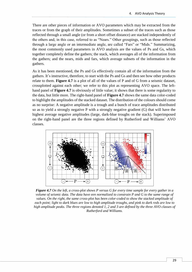
As it has been mentioned, the Ps and Gs effectively contain all of the information from the
gathers. It’s instructive, therefore, to start with the Ps and Gs and then see how other products
relate to them. Figure 4.7 is a plot of all of the values of P and of G from a seismic dataset,
crossplotted against each other; we refer to this plot as representing AVO space. The left-
hand panel of Figure 4.7 is obviously of little value; it shows that there is some regularity to
the data, but little more. The right-hand panel of Figure 4.7 shows the same data color-coded
to highlight the amplitudes of the stacked dataset. The distribution of the colours should come
as no surprise: A negative amplitude is a trough and a bunch of trace amplitudes distributed
so as to yield a strongly negative P with a strongly negative gradient (G) that will have the
highest average negative amplitudes (large, dark-blue troughs on the stack). Superimposed
on the right-hand panel are the three regions defined by Rutherford and Williams’ AVO
classes.
Figure 4.7 On the left, a cross-plot shows P versus G for every time sample for every gather in a
volume of seismic data. The data have een normalized to constrain P and G to the same range of
values. On the right, the same cross-plot has been color-coded to show the stacked amplitude of
each point; light to dark blues are low to high amplitude troughs, and pink to dark reds are low to
high amplitude peaks. The three regions denoted 1, 2 and 3 are defined by the three AVO classes of
Rutherford and Williams.

4. AVO Analysis Theory
30
4.7 AVO Analysis Application on Gas Detection
By far, gas-sand detection is the most promising application of AVO analysis. It is hoped that
the characteristically low VP/VS ratio of gas sands should allow their differentiation from other
low-impedance layers, such as coals and porous brine sands (Castagna et al., 1993). Rutherford
and Williams (1989) defined three distinct classes of gas-sand AVO anomalies. Their Class 1
occurs when the normal-incidence P-wave reflection coefficient is strongly positive and shows
a strong amplitude decrease with offset and a possible phase change at far offset (Figure 4.8).
Figure 4.8 Zoeppritz P-wave reflection coefficients for a shale/gas-sand interface for a range of R0
values. The Poisson’s ratio and density of the shale were assumed to be 0.38 and 2.4 g/cm3,
respectively. The Poisson’s ratio and density of the gas sand were assumed to be 0.15 and 2.0 g/cm3,
respectively (Rutherford and Williams, 1989).
Class 2, for small P-wave reflection coefficients, shows a very large percent change in AVO.
In this situation, if the normal-incidence reflection coefficient is slightly positive, a phase
change at near or moderate offsets will occur. Class 3 anomalies (Rutherford and Williams,
1989) have a large negative normal-incidence reflection coefficient, which becomes more
negative as offset increases (these are classical bright spots). A simple rule of thumb that
generally applies to shale over gas-sand reflections is that the reflection coefficient becomes
more negative with increasing offset (Castagna and Backus, 1993).
But on the principles of AVO crossplotting, Castagna and Swan (1997) suggest that
hydrocarbon-bearing sands overlain by shale should be classified according to their
location in the A-B plane, rather than by their normal-incidence reflection coefficient
alone. Class I sands (Castagna et al., 1997) are of higher impedance than the overlying
unit. They occur in quadrant IV of the A-B plane. The normal incidence reflection
coefficient is positive while the AVO gradient is negative. And the reflection coefficient
decreases with increasing offset. Class II sands (Castagna et al.1997) have about the
same impedance as the overlying unit. They exhibit highly variable AVO behaviour and
may occur in quadrants II, III, or IV of the A-B plane. Class III sands (Castagna and
Swan, 1997) here are of lower impedance than the overlying unit and are frequently
bright. (
Figure 4.9).
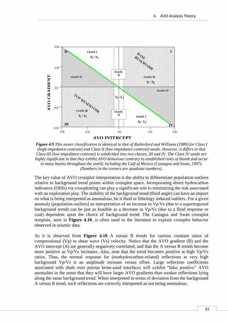
4. AVO Analysis Theory
31
Figure 4.9 This newer classification is identical to that of Rutherford and Williams (1989) for Class I
(high-impedance-contrast) and Class II (low-impedance-contrast) sands. However, it differs in that
Class III (low-impedance-contrast) is subdivided into two classes, III and IV. The Class IV sands are
highly significant in that they exhibit AVO behaviour contrary to established rules of thumb and occur
in many basins throughout the world, including the Gulf of Mexico (Castagna and Swan, 1997).
(Numbers in the corners are quadrant numbers).
The key value of AVO crossplot interpretation is the ability to differentiate population outliers
relative to background trend points within crossplot space. Incorporating direct hydrocarbon
indicators (DHIs) via crossplotting can play a significant role in minimizing the risk associated
with an exploration play. The stability of the background trend (fluid angle) can have an impact
on what is being interpreted as anomalous, be it fluid or lithology induced outliers. For a given
anomaly (population outliers) an interpretation of an increase in Vp/Vs (due to a superimposed
background trend) can be just as feasible as a decrease in Vp/Vs (due to a fluid response or
coal) dependent upon the choice of background trend. The Castagna and Swan crossplot
template, seen in Figure 4.10, is often used in the literature to explain crossplot behavior
observed in seismic data.
As it is observed from Figure 4.10 A versus B trends for various constant ratios of
compressional (Vp) to shear wave (Vs) velocity. Notice that the AVO gradient (B) and the
AVO intercept (A) are generally negatively correlated, and that the A versus B trends become
more positive as Vp/Vs increases. Also, note that the trend becomes positive at high Vp/Vs
ratios. Thus, the normal response for (nonhydrocarbon-related) reflections at very high
background Vp/Vs is an amplitude increase versus offset. Large reflection coefficients
associated with shale over porous brine-sand interfaces will exhibit “false positive” AVO
anomalies in the sense that they will have larger AVO gradients than weaker reflections lying
along the same background trend. When interpreted in terms of deviation from the background
A versus B trend, such reflections are correctly interpreted as not being anomalous.
AV
O G
RA
DIE
NT
AVO INTERCEPT
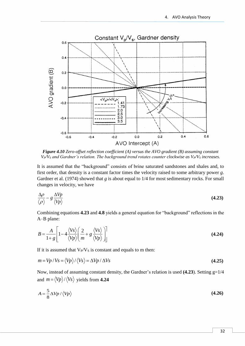
4. AVO Analysis Theory
32
Figure 4.10 Zero-offset reflection coefficient (A) versus the AVO gradient (B) assuming constant
VP/VS and Gardner’s relation. The background trend rotates counter clockwise as VP/VS increases.
It is assumed that the “background” consists of brine saturated sandstones and shales and, to
first order, that density is a constant factor times the velocity raised to some arbitrary power g.
Gardner et al. (1974) showed that g is about equal to 1/4 for most sedimentary rocks. For small
changes in velocity, we have
Vpg
Vp
(4.23)
Combining equations 4.23 and 4.8 yields a general equation for “background” reflections in the
A–B plane:
21 4
1
Vs VsAB g
g Vp m Vp
(4.24)
If it is assumed that VP/VS is constant and equals to m then:
/ / /m Vp Vs Vp Vs Vp Vs (4.25)
Now, instead of assuming constant density, the Gardner’s relation is used (4.23). Setting g=1/4
and /m Vp Vs yields from 4.24
5/
8A Vp Vp (4.26)
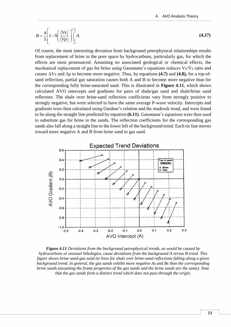
4. AVO Analysis Theory
33
2
41 9
5
VsB A
Vp
(4.27)
Of course, the most interesting deviation from background petrophysical relationships results
from replacement of brine in the pore space by hydrocarbons, particularly gas, for which the
effects are most pronounced. Assuming no associated geological or chemical effects, the
mechanical replacement of gas for brine using Gassmann’s equations reduces VP/VS ratio and
causes ΔVP and Δρ to become more negative. Thus, by equations (4.7) and (4.8), for a top-of-
sand reflection, partial gas saturation causes both A and B to become more negative than for
the corresponding fully brine-saturated sand. This is illustrated in Figure 4.11, which shows
calculated AVO intercepts and gradients for pairs of shale/gas sand and shale/brine sand
reflectors. The shale over brine-sand reflection coefficients vary from strongly positive to
strongly negative, but were selected to have the same average P-wave velocity. Intercepts and
gradients were then calculated using Gardner’s relation and the mudrock trend, and were found
to lie along the straight line predicted by equation (6.11). Gassmann’s equations were then used
to substitute gas for brine in the sands. The reflection coefficients for the corresponding gas
sands also fall along a straight line to the lower left of the background trend. Each tie line moves
toward more negative A and B from brine sand to gas sand.
Figure 4.11 Deviations from the background petrophysical trends, as would be caused by
hydrocarbons or unusual lithologies, cause deviations from the background A versus B trend. This
figure shows brine sand-gas sand tie lines for shale over brine-sand reflections falling along a given
background trend. In general, the gas sands exhibit more negative As and Bs than the corresponding
brine sands (assuming the frame properties of the gas sands and the brine sands are the same). Note
that the gas sands form a distinct trend which does not pass through the origin.
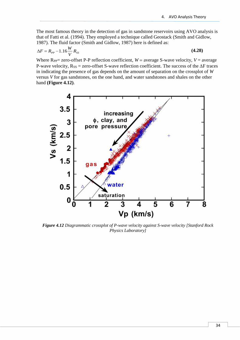
4. AVO Analysis Theory
34
The most famous theory in the detection of gas in sandstone reservoirs using AVO analysis is
that of Fatti et al. (1994). They employed a technique called Geostack (Smith and Gidlow,
1987). The fluid factor (Smith and Gidlow, 1987) here is defined as:
1.16PP SS
WF R R
V (4.28)
Where RPP= zero-offset P-P reflection coefficient, W average S-wave velocity, V = average
P-wave velocity, RSS = zero-offset S-wave reflection coefficient. The success of the F traces
in indicating the presence of gas depends on the amount of separation on the crossplot of W
versus V for gas sandstones, on the one hand, and water sandstones and shales on the other
hand (Figure 4.12).
Figure 4.12 Diagrammatic crossplot of P-wave velocity against S-wave velocity [Stanford Rock
Physics Laboratory]
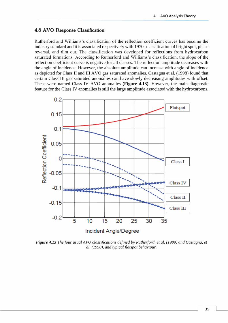
4. AVO Analysis Theory
35
4.8 AVO Response Classification
Rutherford and Williams’s classification of the reflection coefficient curves has become the
industry standard and it is associated respectively with 1970s classification of bright spot, phase
reversal, and dim out. The classification was developed for reflections from hydrocarbon
saturated formations. According to Rutherford and Williams’s classification, the slope of the
reflection coefficient curve is negative for all classes. The reflection amplitude decreases with
the angle of incidence. However, the absolute amplitude can increase with angle of incidence
as depicted for Class II and III AVO gas saturated anomalies. Castagna et al. (1998) found that
certain Class III gas saturated anomalies can have slowly decreasing amplitudes with offset.
These were named Class IV AVO anomalies (Figure 4.13). However, the main diagnostic
feature for the Class IV anomalies is still the large amplitude associated with the hydrocarbons.
Figure 4.13 The four usual AVO classifications defined by Rutherford, et al. (1989) and Castagna, et
al. (1998), and typical flatspot behaviour.
4. AVO Analysis Theory
36
A brief description of the characteristics for each AVO class is given below, while in Table 1
and Figure 4.14 their characteristics are summarized.
Class I (Dim out) anomalies have the following properties:
Amplitude decreases with increasing angle, and may reverse phase on the far angle
stack
Represents relatively hard sands with hydrocarbons.
These sands tend to plot along the background trend in intercept-gradient cross-plots
Amplitude on the full stack is smaller for the hydrocarbon zone than for an equivalent
wet saturated zone.
Wavelet character is peak-trough on near angle stack
Wavelet character may or may not be peak-trough on the far angle stack.
Class II (Phase reversal) anomalies have the following properties:
There is little indication of the gas sand on the near angle stack.
Representing transparent sands with hydrocarbons. Often shows up as dim spots or
weak negative reflectors on the seismic
The gas sand event increases amplitude with increasing angle. This attribute is more
pronounced than anticipated because of the amplitude decrease of the shaleupon-shale
reflections.
The gas sand event may or may not be evident on the full stack, depending on the far
angle amplitude contribution to the stack.
Wavelet character on the stack may or may not be trough-peak for a hydrocarbon
charged thin bed.
Wavelet character is trough-peak on the far angle stack.
Inferences about lithology are contained in the amplitude variation with incident
angle.
AVO alone, unless carefully calibrated, cannot unambiguously distinguish a clean wet
sand from a gas sand, because both have similar (increasing) behavior with offset.
Class III (Bright spot) anomalies have the following properties:
Hydrocarbon zones are bright on the stack section and on all angle limited stacks.
Represents relatively soft sands with high fluid sensitivity
The hydrocarbon reflection amplitude, with respect to the background reflection
amplitude, is constant or increases slightly with incident angle range. Even though the
amplitude of the hydrocarbon event can decrease with angle, as suggested for the
Class 4 AVO anomalies, the surrounding shale-upon-shale reflections normally
decrease in amplitude with angle at a faster rate.
Wavelet character is trough-peak on all angle stacks. This assumes that the dominant
phase of the seismic wavelet is zero and the reservoir is below tuning thickness.
Class IV anomalies have the following properties:
Mainly gas sands with low impedance
They have negative intercept but positive gradient.
The reflection coefficients decrease with increasing offset.

4. AVO Analysis Theory
37
Class Relative impedance Quadrant R(0) G AVO
product
Amplitude
Over Offset
I High-impedance sand 4th + - Negative Decreases
II No or low contrast 4th + - Negative Increases
IIp No or low contrast 3rd - - Positive Decreases
III Low impedance 3rd - - Positive Increases
IV Low impedance 2nd - + Negative Decreases
Table 1. AVO classes, after Rutherford and Williams (1989), extended by Castagna and Smith (1994),
and Ross and Kinman (1995).
Figure 4.14 Rutherford and Williams AVO classes, originally defined for gas sands (classes I, II and
III), along with the added classes IV (Castagna and Smith, 1994) and Ilp (Ross and Kinman, 1995).
Figure is adapted from Castagna et al. (1998).
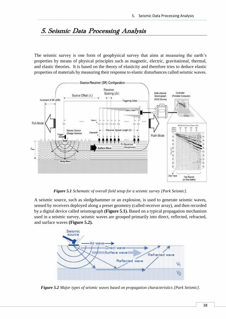
5. Seismic Data Processing Analysis
38
5. Seismic Data Processing Analysis
The seismic survey is one form of geophysical survey that aims at measuring the earth’s
properties by means of physical principles such as magnetic, electric, gravitational, thermal,
and elastic theories. It is based on the theory of elasticity and therefore tries to deduce elastic
properties of materials by measuring their response to elastic disturbances called seismic waves.
Figure 5.1 Schematic of overall field setup for a seismic survey [Park Seismic].
A seismic source, such as sledgehammer or an explosion, is used to generate seismic waves,
sensed by receivers deployed along a preset geometry (called receiver array), and then recorded
by a digital device called seismograph (Figure 5.1). Based on a typical propagation mechanism
used in a seismic survey, seismic waves are grouped primarily into direct, reflected, refracted,
and surface waves (Figure 5.2).
Figure 5.2 Major types of seismic waves based on propagation characteristics [Park Seismic].
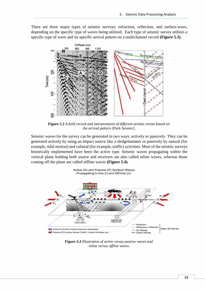
5. Seismic Data Processing Analysis
39
There are three major types of seismic surveys: refraction, reflection, and surface-wave,
depending on the specific type of waves being utilized. Each type of seismic survey utilizes a
specific type of wave and its specific arrival pattern on a multichannel record (Figure 5.3).
Figure 5.3 A field record and interpretation of different seismic events based on
the arrival pattern [Park Seismic].
Seismic waves for the survey can be generated in two ways: actively or passively. They can be
generated actively by using an impact source like a sledgehammer or passively by natural (for
example, tidal motion) and cultural (for example, traffic) activities. Most of the seismic surveys
historically implemented have been the active type. Seismic waves propagating within the
vertical plane holding both source and receivers are also called inline waves, whereas those
coming off the plane are called offline waves (Figure 5.4).
Figure 5.4 Illustration of active versus passive waves and
inline versus offline waves.
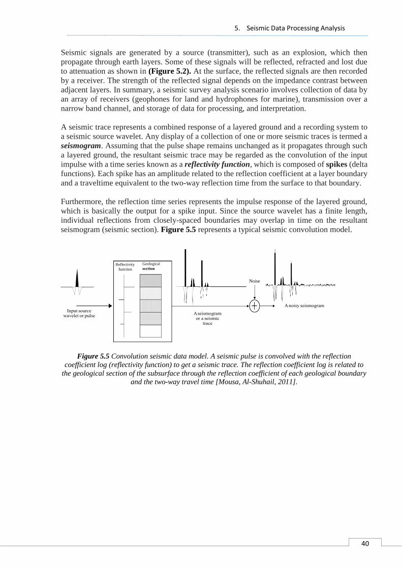
5. Seismic Data Processing Analysis
40
Seismic signals are generated by a source (transmitter), such as an explosion, which then
propagate through earth layers. Some of these signals will be reflected, refracted and lost due
to attenuation as shown in (Figure 5.2). At the surface, the reflected signals are then recorded
by a receiver. The strength of the reflected signal depends on the impedance contrast between
adjacent layers. In summary, a seismic survey analysis scenario involves collection of data by
an array of receivers (geophones for land and hydrophones for marine), transmission over a
narrow band channel, and storage of data for processing, and interpretation.
A seismic trace represents a combined response of a layered ground and a recording system to
a seismic source wavelet. Any display of a collection of one or more seismic traces is termed a
seismogram. Assuming that the pulse shape remains unchanged as it propagates through such
a layered ground, the resultant seismic trace may be regarded as the convolution of the input
impulse with a time series known as a reflectivity function, which is composed of spikes (delta
functions). Each spike has an amplitude related to the reflection coefficient at a layer boundary
and a traveltime equivalent to the two-way reflection time from the surface to that boundary.
Furthermore, the reflection time series represents the impulse response of the layered ground,
which is basically the output for a spike input. Since the source wavelet has a finite length,
individual reflections from closely-spaced boundaries may overlap in time on the resultant
seismogram (seismic section). Figure 5.5 represents a typical seismic convolution model.
Figure 5.5 Convolution seismic data model. A seismic pulse is convolved with the reflection
coefficient log (reflectivity function) to get a seismic trace. The reflection coefficient log is related to
the geological section of the subsurface through the reflection coefficient of each geological boundary
and the two-way travel time [Mousa, Al-Shuhail, 2011].
Reflectivity Geological
function
Noise

5. Seismic Data Processing Analysis
41
5.1 Prinos Basin Geological Model Representation
The synthetic dataset that will be analyzed in this thesis consists of a hypothetical two-
dimensional (2-D) land line using the geological setting of Prinos basin. The construction of
the layer’s structure below the subsurface of Prinos basin, along with the synthetic seismic
dataset were based on the synthetic data simulator algorithm that was described on chapter 3.
The whole procedure was implemented in Matlab environment and will be more explicitly
described, step by step, below.
Geological model creation
As a first step, the geological model under examination needs to be defined. In Figure 5.6 a 3-
D representation of Prinos basin, along with its stratigraphy column is presented [Michelakis
2010]. Due to the high complexity of the 3-D model, only a single plan was chosen for the
implementation of the seismic survey. Specifically, a plan of the model with East-West
orientation was extracted, as shown in Figure 5.7-Figure 5.8.
Figure 5.6 3-D geological model representation of Prinos basin [Michelakis 2010].
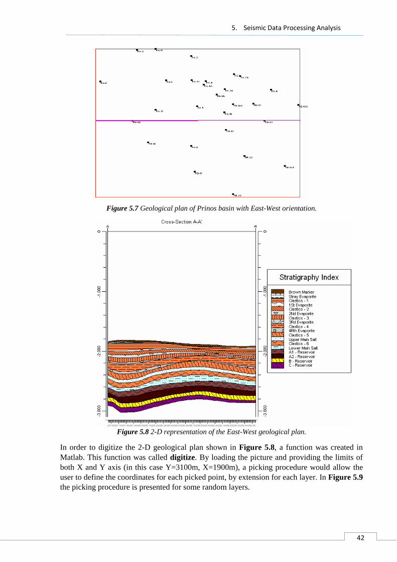
5. Seismic Data Processing Analysis
42
Figure 5.7 Geological plan of Prinos basin with East-West orientation.
Figure 5.8 2-D representation of the East-West geological plan.
In order to digitize the 2-D geological plan shown in Figure 5.8, a function was created in
Matlab. This function was called digitize. By loading the picture and providing the limits of
both X and Y axis (in this case Y=3100m, X=1900m), a picking procedure would allow the
user to define the coordinates for each picked point, by extension for each layer. In Figure 5.9
the picking procedure is presented for some random layers.

5. Seismic Data Processing Analysis
43
Figure 5.9 Picking procedure for the layers’ digitization.
After applying the picking procedure, the coordinates of each layer are interpolated using the
“spline” function with respect to the X axis, in order to smoothen the results and avoid the
randomness related to the picked values. The result for a spline interval of 5 m is presented in
Figure 5.10.
Figure 5.10 Digitized layers after applying spline procedure with spline
interval equal to 5m.

5. Seismic Data Processing Analysis
44
The layers are also presented in a more comprehensible form, using the “area” function of
Matlab (Figure 5.11).
Figure 5.11 Layer representation versus depth using the “area” function.
The geological model presented so far is still of high complexity but it can be further simplified,
since most of the top formations shown in Figure 5.11 share the same geological properties.
Specifically, the top formations are, mainly, evaporites that act as the “cap-rock” of the
reservoir with similar geophysical attributes.On the other hand, the last five layers constitute
the basic layers of the Prinos basin reservoir. As a result, the top layers were considered as one
simple layer of evaporites, the last four layers were digitized and inserted to the simulator
seperately, while the last layer was considered as the base of the reservoir. Summarizing, the
final model, as implemented in the simulator, consists of six basic formations: Evaporite
formation, Sand A1, Sand A2, Sand B, Sand C and the Base formation (Figure 5.12). The
overall evaluation of the formation of Prinos basin, as derived from a well resistivity log
analysis is presented in Table 2 [Fronimos 1998].
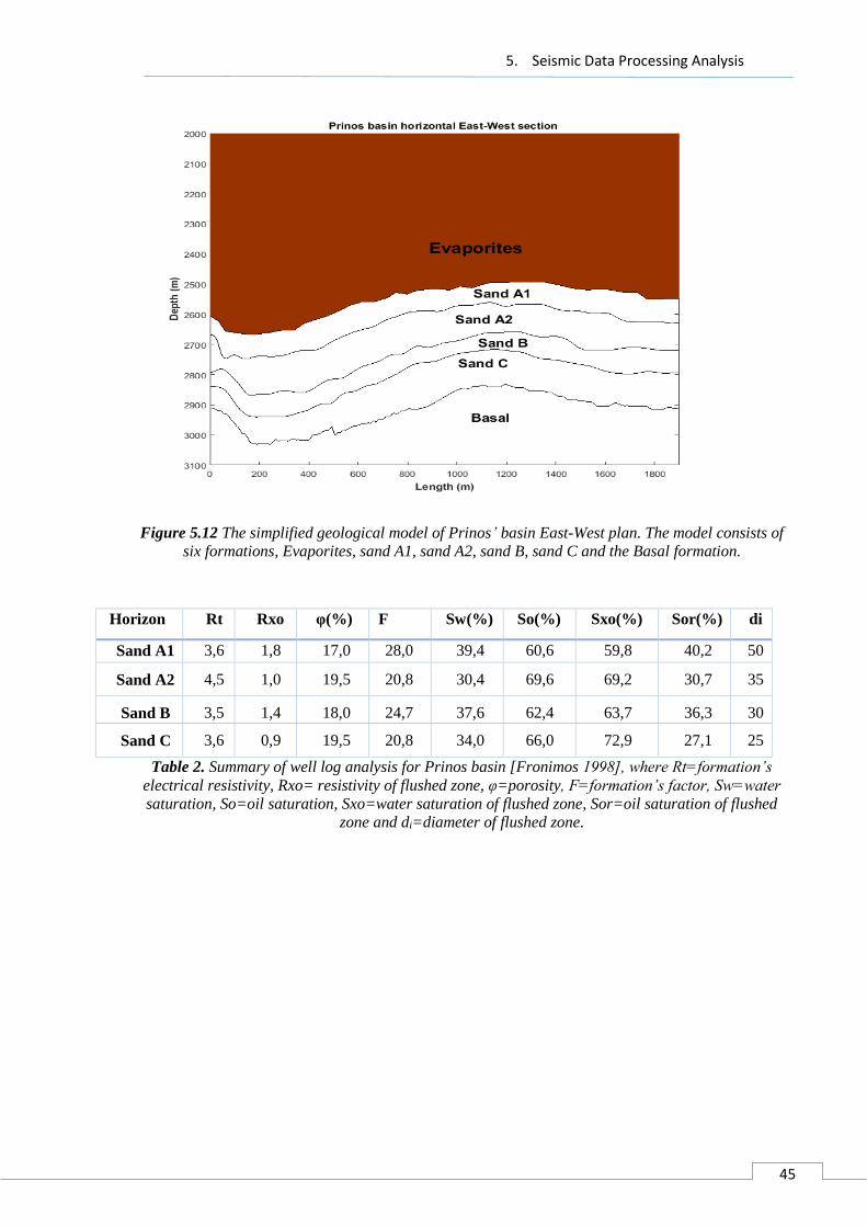
5. Seismic Data Processing Analysis
45
Figure 5.12 The simplified geological model of Prinos’ basin East-West plan. The model consists of
six formations, Evaporites, sand A1, sand A2, sand B, sand C and the Basal formation.
Horizon Rt Rxo φ(%) F Sw(%) So(%) Sxo(%) Sor(%) di
Sand A1 3,6 1,8 17,0 28,0 39,4 60,6 59,8 40,2 50
Sand A2 4,5 1,0 19,5 20,8 30,4 69,6 69,2 30,7 35
Sand B 3,5 1,4 18,0 24,7 37,6 62,4 63,7 36,3 30
Sand C 3,6 0,9 19,5 20,8 34,0 66,0 72,9 27,1 25
Table 2. Summary of well log analysis for Prinos basin [Fronimos 1998], where Rt=formation’s
electrical resistivity, Rxo= resistivity of flushed zone, φ=porosity, F=formation’s factor, Sw=water
saturation, So=oil saturation, Sxo=water saturation of flushed zone, Sor=oil saturation of flushed
zone and di=diameter of flushed zone.

5. Seismic Data Processing Analysis
46
A brief analysis of the results presented in Table 2 is carried out below:
Sand A1 displays the lowest porosity value and the lowest oil saturation value (along the other
reservoir formations), 17.0% and 60.6% respectively. At the same time, it shows the lowest
hydrocarbon mobility, indicating a formation with low permeability.Finally, the flushed zone
has the biggest diameter compared to the other formations. The above results indicate a non-
homogenous transitional formation from the cap-rock to the reservoir. This theory testifies the
decreased mobility of the hydrocarbons, the low porosity and the great infiltration zone.
Sand A2 displays the highest porosity value and at the same time the greatest oil saturation
value (along the other reservoir layers), 19.5% and 69.65% respectively. The hydrocarbon
mobility level is good enough (saturation level inside the flushed zone 30.7%) and the diameter
of the flushed zone is the greatest among the other formations. It should also be pointed out that
it shows the highest value of electrical resistivity.
Sand B displays a porosity value equals to 18.0%. The hydrocarbon saturation level (62.4%) is
the lowest among the rest of the reservoir formations. The hydrocarbon mobility is also the
lowest among the rest of the formations, while the diameter of the flushed zone is 30 in. The
above information confirms that formation Sand B is slightly more compact than Sand A2,
while this difference becomes even more pronounced when Sand B is compared to Sand C.
Sand C displays the same porosity value with Sand A2 (19,5%) and oil saturation slightly lower
(66,0% over 69,6%). The characteristic that differentiates this formation from the others, is the
very high permeability and mobility ratio of the hydrocarbons. The oil saturation inside the
infiltration zone along with the diameter of the infiltration zone are the lowest ones with values
(27.1%) and (25in) respectively.
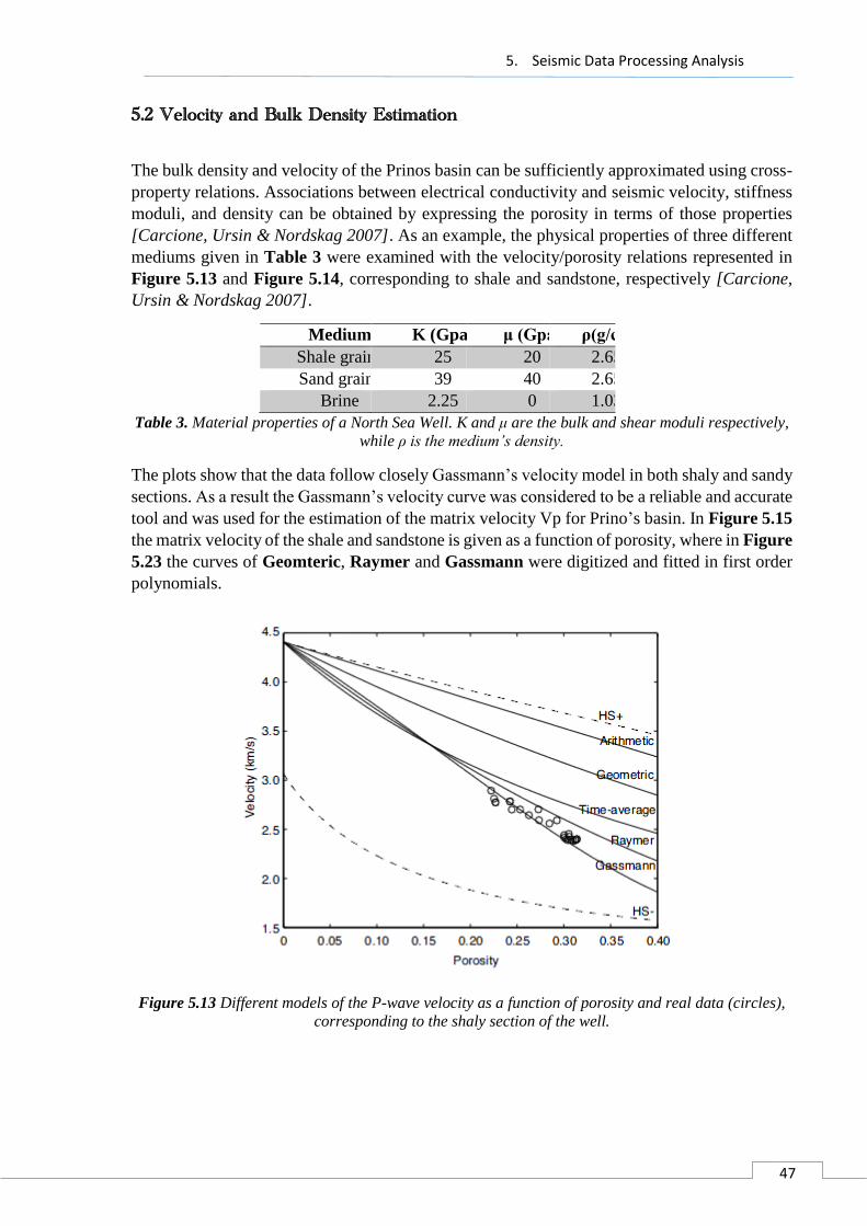
5. Seismic Data Processing Analysis
47
5.2 Velocity and Bulk Density Estimation
The bulk density and velocity of the Prinos basin can be sufficiently approximated using cross-
property relations. Associations between electrical conductivity and seismic velocity, stiffness
moduli, and density can be obtained by expressing the porosity in terms of those properties
[Carcione, Ursin & Nordskag 2007]. As an example, the physical properties of three different
mediums given in Table 3 were examined with the velocity/porosity relations represented in
Figure 5.13 and Figure 5.14, corresponding to shale and sandstone, respectively [Carcione,
Ursin & Nordskag 2007].
Medium K (Gpa) μ (Gpa) ρ(g/cc)
Shale grains 25 20 2.65
Sand grains 39 40 2.65
Brine 2.25 0 1.03
Table 3. Material properties of a North Sea Well. K and μ are the bulk and shear moduli respectively,
while ρ is the medium’s density.
The plots show that the data follow closely Gassmann’s velocity model in both shaly and sandy
sections. As a result the Gassmann’s velocity curve was considered to be a reliable and accurate
tool and was used for the estimation of the matrix velocity Vp for Prino’s basin. In Figure 5.15
the matrix velocity of the shale and sandstone is given as a function of porosity, where in Figure
5.23 the curves of Geomteric, Raymer and Gassmann were digitized and fitted in first order
polynomials.
Figure 5.13 Different models of the P-wave velocity as a function of porosity and real data (circles),
corresponding to the shaly section of the well.
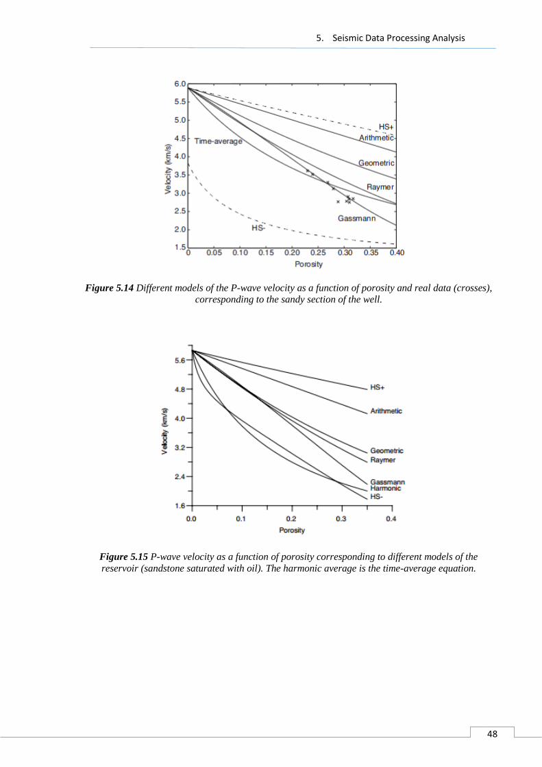
5. Seismic Data Processing Analysis
48
Figure 5.14 Different models of the P-wave velocity as a function of porosity and real data (crosses),
corresponding to the sandy section of the well.
Figure 5.15 P-wave velocity as a function of porosity corresponding to different models of the
reservoir (sandstone saturated with oil). The harmonic average is the time-average equation.
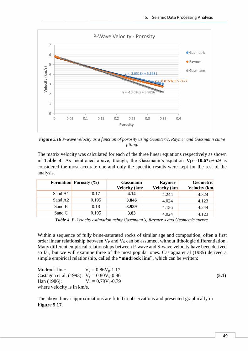
5. Seismic Data Processing Analysis
49
Figure 5.16 P-wave velocity as a function of porosity using Geomteric, Raymer and Gassmann curve
fitting.
The matrix velocity was calculated for each of the three linear equations respectively as shown
in Table 4. As mentioned above, though, the Gassmann’s equation Vp=-10.6*φ+5.9 is
considered the most accurate one and only the specific results were kept for the rest of the
analysis.
Formation Porosity (%) Gassmann
Velocity (km/s)
Raymer
Velocity (km/s)
Geometric
Velocity (km/s)
Sand A1 0.17 4.14 4.244 4.324
Sand A2 0.195 3.846 4.024 4.123
Sand B 0.18 3.989 4.156 4.244
Sand C 0.195 3.83 4.024 4.123
Table 4. P-Velocity estimation using Gassmann’s, Raymer’s and Geometric curves.
Within a sequence of fully brine-saturated rocks of similar age and composition, often a first
order linear relationship between VP and VS can be assumed, without lithologic differentiation.
Many different empirical relationships between P-wave and S-wave velocity have been derived
so far, but we will examine three of the most popular ones. Castagna et al (1985) derived a
simple empirical relationship, called the “mudrock line”, which can be written:
Mudrock line: Vs = 0.86Vp-1.17
Castagna et al. (1993): Vs = 0.80Vp-0.86 (5.1)
Han (1986): Vs = 0.79Vp-0.79
where velocity is in km/s.
The above linear approximations are fitted to observations and presented graphically in
Figure 5.17.
y = -8.0518x + 5.6931
y = -8.8159x + 5.7427
y = -10.626x + 5.9016
0
1
2
3
4
5
6
7
0 0.05 0.1 0.15 0.2 0.25 0.3 0.35 0.4
Ve
loci
ty (
km/s
)
Porosity
P-Wave Velocity - Porosity
Geometric
Raymer
Gassmann
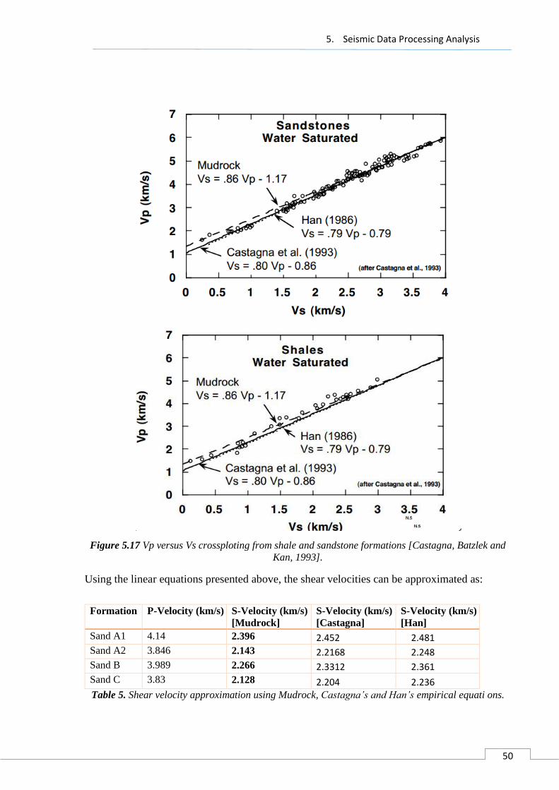
5. Seismic Data Processing Analysis
50
Figure 5.17 Vp versus Vs crossploting from shale and sandstone formations [Castagna, Batzlek and
Kan, 1993].
Using the linear equations presented above, the shear velocities can be approximated as:
Table 5. Shear velocity approximation using Mudrock, Castagna’s and Han’s empirical equati ons.
Formation P-Velocity (km/s) S-Velocity (km/s)
[Mudrock]
S-Velocity (km/s)
[Castagna]
S-Velocity (km/s)
[Han]
Sand A1 4.14 2.396 2.452 2.481 Sand A2 3.846 2.143 2.2168 2.248 Sand B 3.989 2.266 2.3312 2.361 Sand C 3.83 2.128 2.204 2.236

5. Seismic Data Processing Analysis
51
The results from the mudrock line approximation are considered more accurate, so the final
values for the shear velocity are those derived from the Lindseth approximation.
Finally, for the approximation of the medium’s density two different approaches are tested.
Gardner’s equation can approximate the density from the matrix Velocity Vp as:
b
PV (5.2)
Where ρ is the bulk density in g/cc, Vp is the P-wave velocity in ft/s, a=0.23 and b=0.25. This
empirical relationship is based on field and laboratory measurements of saturated sedimentary
rocks from a wide variety of basins and depths.
Lindseth (1979), also, proposed an empirical relation between acoustic impedance and density
which is used to extract the density from the reflectivity:
0.308 3460P PV V (5.3)
Where ρ is the bulk density in g/cc, Vp is the P-wave velocity in ft/s.
Using both equations (5.2) and (5.3) we get the following density values (Table 6):
Formation P-Velocity (ft/s) Density (g/cc) [Gardner] Density (g/cc) [Lindseth]
Sand A1 13583 2.483 2.420
Sand A2 12631 2.438 2.357
Sand B 13091 2.460 2.389
Sand C 12566 2.435 2.353
Table 6. Density estimation from P-velocity using Gardner and Lindseth approximations.
The Lindseth equation is considered more accurate, so the final values for the bulk density are
those derived from the Lindseth approximation.
All the velocity approximations used so far are accurate only for water or brine saturated sands.
However, the scope of this thesis is the detection of gas in the sandstone reservoir of Prinos. In
order to introduce gas in the synthetic data, the first layer of the reservoir is considered to be
50% gas saturated. According to Domenico (1974), only a small amount of gas in the pore space
will produce a large decrease of velocity (Figure 5.19a) and a large change in reflectivity
(Figure 5.19b). Thus, for the reservoir of Prinos with average depth ≈ 3 km, the red dashed
curve shown in Figure 5.19a, can give a good estimation of the P-wave velocity drop for a 50%
gas saturation. The curve was fitted in a 3rd order polynomial, as shown in Figure 5.19, giving
a mathematical relationship between the gas saturation and the P-wave velocity drop for our
model. Taking the above relationship one step further, the curve was plotted again, but this time
the velocity drop was expressed as a percentage ratio, as shown in Figure 5.20. Hence, judging
from Figure 5.20, for a 50% gas saturation the P-wave velocity is expected to drop about 8%.
Based on the above assumption, the P-wave velocity of the first layer of the reservoir was
reduced from 4140 m/s to 3809 m/s.

5. Seismic Data Processing Analysis
52
Figure 5.18 Effect of gas/water or oil/water saturation on velocity. Solid curves are for gas, dashed
for oil. a) P-wave velocity versus saturation and b) reflection coefficient for gas/oil sands overlain by
shale. [Sheriff and Geldart, 1995]
Figure 5.19 P-wave velocity versus gas saturation at 3050 m.
Figure 5.20 Percentage P-wave velocity drop versus gas saturation at 3050m.
y = -0.7984x3 + 1.6414x2 - 1.1198x + 2.9773
2.65
2.7
2.75
2.8
2.85
2.9
2.95
3
3.05
00.20.40.60.811.2
Ve
loci
ty (
km/s
)
Gas Saturation
y = -24.543x3 + 51.181x2 - 35.57x - 0.992
-12
-10
-8
-6
-4
-2
0
0 0.2 0.4 0.6 0.8 1 1.2
Ve
loci
ty d
rop
(%
)
Gas Saturation
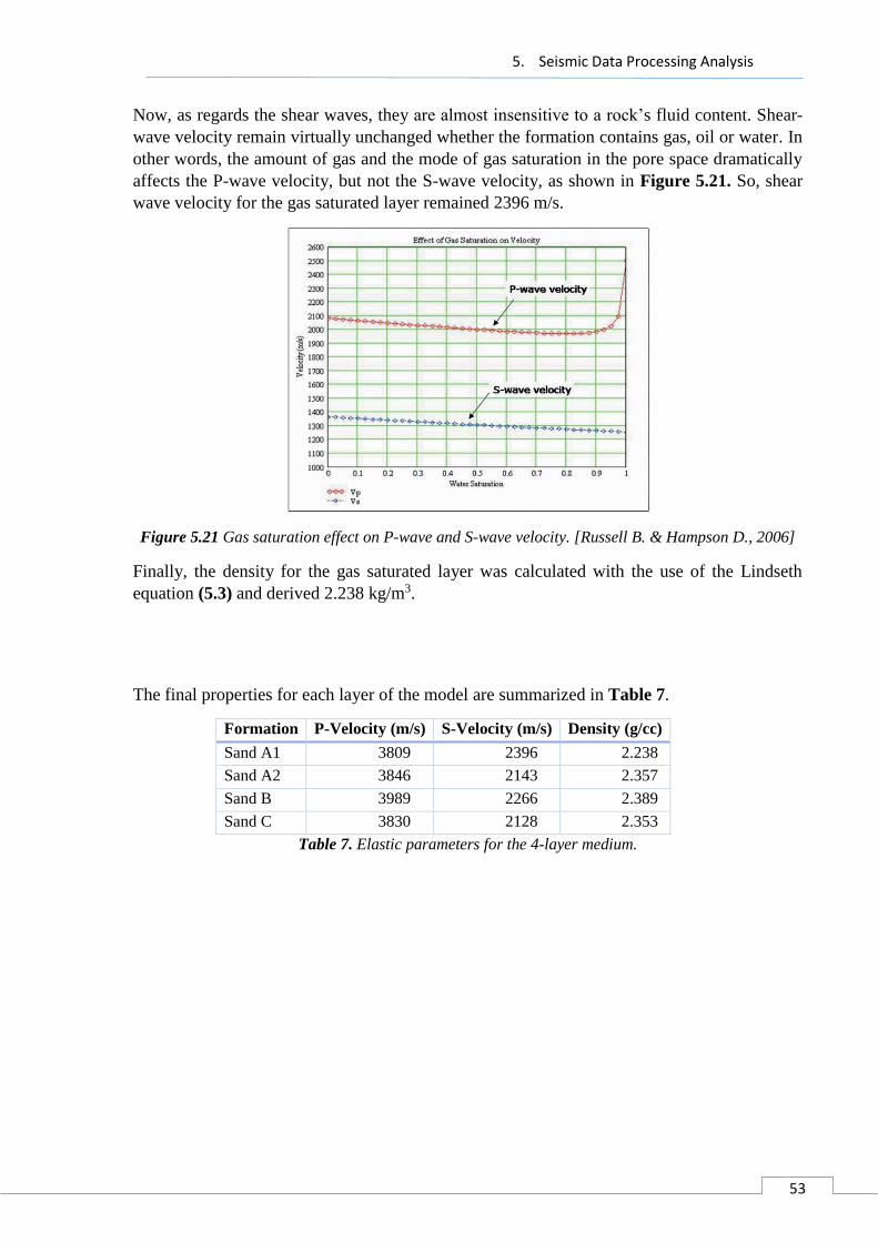
5. Seismic Data Processing Analysis
53
Now, as regards the shear waves, they are almost insensitive to a rock’s fluid content. Shear-
wave velocity remain virtually unchanged whether the formation contains gas, oil or water. In
other words, the amount of gas and the mode of gas saturation in the pore space dramatically
affects the P-wave velocity, but not the S-wave velocity, as shown in Figure 5.21. So, shear
wave velocity for the gas saturated layer remained 2396 m/s.
Figure 5.21 Gas saturation effect on P-wave and S-wave velocity. [Russell B. & Hampson D., 2006]
Finally, the density for the gas saturated layer was calculated with the use of the Lindseth
equation (5.3) and derived 2.238 kg/m3.
The final properties for each layer of the model are summarized in Table 7.
Formation P-Velocity (m/s) S-Velocity (m/s) Density (g/cc)
Sand A1 3809 2396 2.238
Sand A2 3846 2143 2.357
Sand B 3989 2266 2.389
Sand C 3830 2128 2.353
Table 7. Elastic parameters for the 4-layer medium.
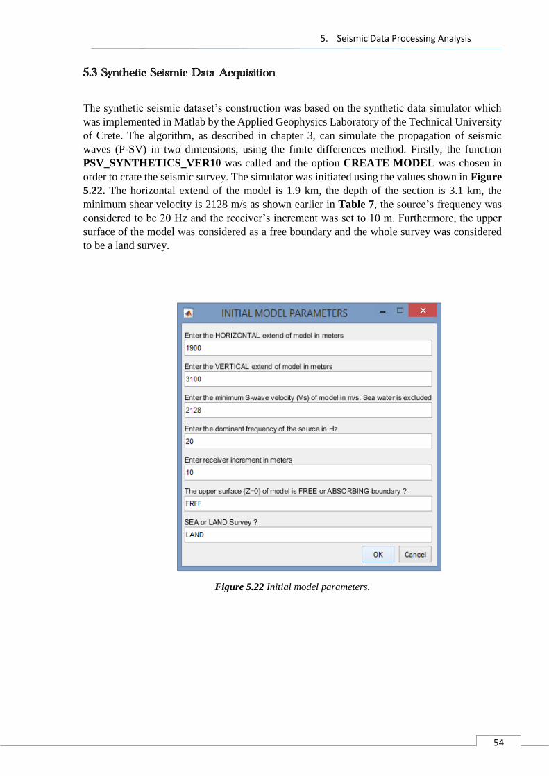
5. Seismic Data Processing Analysis
54
5.3 Synthetic Seismic Data Acquisition
The synthetic seismic dataset’s construction was based on the synthetic data simulator which
was implemented in Matlab by the Applied Geophysics Laboratory of the Technical University
of Crete. The algorithm, as described in chapter 3, can simulate the propagation of seismic
waves (P-SV) in two dimensions, using the finite differences method. Firstly, the function
PSV_SYNTHETICS_VER10 was called and the option CREATE MODEL was chosen in
order to crate the seismic survey. The simulator was initiated using the values shown in Figure
5.22. The horizontal extend of the model is 1.9 km, the depth of the section is 3.1 km, the
minimum shear velocity is 2128 m/s as shown earlier in Table 7, the source’s frequency was
considered to be 20 Hz and the receiver’s increment was set to 10 m. Furthermore, the upper
surface of the model was considered as a free boundary and the whole survey was considered
to be a land survey.
Figure 5.22 Initial model parameters.

5. Seismic Data Processing Analysis
55
In order to avoid any kind of stability or numeric dispersion errors when solving the differential
wave equation with the finite difference method, the following constraints should be applied:
For the grid’s dimensions, the following calculation took place:
min
max
21287.1
15 15 20
aDh
f
(5.4)
By taking into account the receiver’s interval, the final grid size was derived as:
10 105
10 2
7.1
xGrid
xceil ceil
Dh
(5.5)
So the final grid size is set to 5 m. It is obvious at this point that the higher the frequency
of the source, the smallest the grid size and, as a result, the higher the complexity of the
simulation would be.
For the system’s stability, the following condition should be met:
max
max
2 2
3 3
t Grida t
Grid a
(5.6)
Where amax is the maximum P-velocity 4750 m/s and Δx is the receiver’s increment 10
m, so the above condition is translated to:
42 57 10
3 4750t t s
For the numeric dispersion (the change of wave’s propagation velocity with
frequency), the following condition should be met:
min 5Grid
(5.7)
Wheremin
min
max
a
f , amin is the minimum S-velocity 2128 m/s and fmax is the dominant
frequency of the source 20Hz, so the condition is fulfilled as:
min 2128 / 2021.28 5
5Grid
As a next step, the geometry and the properties of each layer should be introduced to the
simulator. The formation above the reservoir was considered as a thick layer of evaporites with
Vp=4750 m/s, Vs=3100 m/s and ρ=2.6 g/cc which acts as a cap-rock. Below the reservoir there
is another evaporite formation with Vp=4750 m/s, Vs=2900 m/s and ρ=2.7 g/cc which acts as
the base of the reservoir. The geophysical properties of the reservoir between those two
formations were calculated in the previous chapter and are introduced to the simulator one by
one as shown in Figure 5.23.
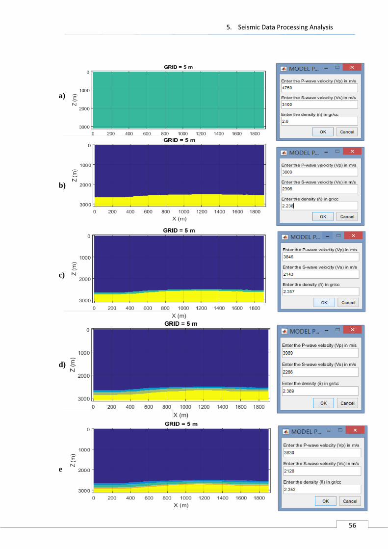
5. Seismic Data Processing Analysis
56
a)
b)
c)
d)
e)

5. Seismic Data Processing Analysis
57
f)
Figure 5.23 Representation of the layers import in the simulator. a) The background evaporite
horizon. b-e) The horizons sand A1, sand A2 , sand B and sand C respectively. f) To the bed evaporite
horizon.
The geophysical properties of the Prinos basin with respect to depth are summarized in Figure
5.24, where the Poisson’s ratio is calculated as:
2 2
2 2
0.5s p
s p
V VPR
V V
(5.8)
Figure 5.24 Vp, Vs, density and Poisson’s ratio versus depth for the Prinos basin.
After the definition of the geophysical and geological properties of the basin, the seismic
survey’s set up should be defined. The number of the shots is a crucial factor for the quality and
the duration of the seismic data acquisition. In this simulation the number of the sources was
chosen to be 48 with a 40 m interval in order to cover the whole extension of the basin (48-
1)x40=1880m. All the sources were horizontally spread and set at 3xGrid=15m below the
surface , while the first source was initiated at 10m in the horizontal plane as shown in Figure
5.25.
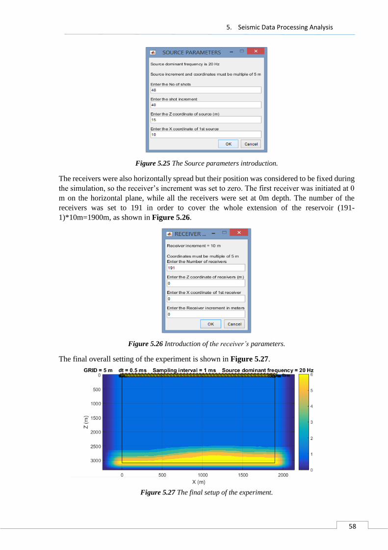
5. Seismic Data Processing Analysis
58
Figure 5.25 The Source parameters introduction.
The receivers were also horizontally spread but their position was considered to be fixed during
the simulation, so the receiver’s increment was set to zero. The first receiver was initiated at 0
m on the horizontal plane, while all the receivers were set at 0m depth. The number of the
receivers was set to 191 in order to cover the whole extension of the reservoir (191-
1)*10m=1900m, as shown in Figure 5.26.
Figure 5.26 Introduction of the receiver’s parameters.
The final overall setting of the experiment is shown in Figure 5.27.
Figure 5.27 The final setup of the experiment.
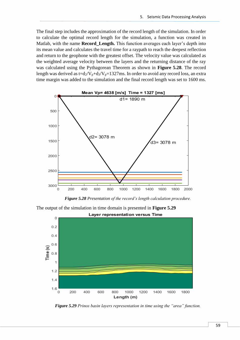
5. Seismic Data Processing Analysis
59
The final step includes the approximation of the record length of the simulation. In order
to calculate the optimal record length for the simulation, a function was created in
Matlab, with the name Record_Length. This function averages each layer’s depth into
its mean value and calculates the travel time for a raypath to reach the deepest reflection
and return to the geophone with the greatest offset. The velocity value was calculated as
the weighted average velocity between the layers and the returning distance of the ray
was calculated using the Pythagorean Theorem as shown in Figure 5.28. The record
length was derived as t=d2/Vp+d3/Vp=1327ms. In order to avoid any record loss, an extra
time margin was added to the simulation and the final record length was set to 1600 ms.
Figure 5.28 Presentation of the record’s length calculation procedure.
The output of the simulation in time domain is presented in Figure 5.29
Figure 5.29 Prinos basin layers representation in time using the “area” function.
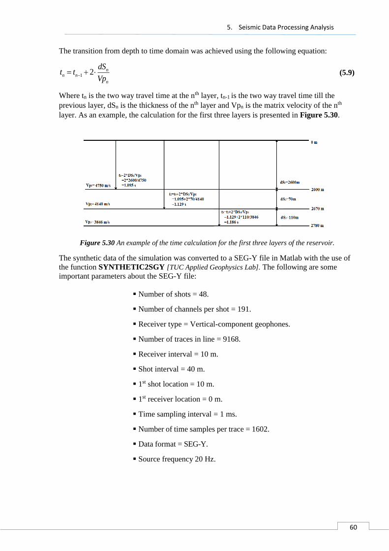
5. Seismic Data Processing Analysis
60
The transition from depth to time domain was achieved using the following equation:
1 2 nn n
n
dSt t
Vp (5.9)
Where tn is the two way travel time at the nth layer, tn-1 is the two way travel time till the
previous layer, dSn is the thickness of the nth layer and Vpn is the matrix velocity of the nth
layer. As an example, the calculation for the first three layers is presented in Figure 5.30.
Figure 5.30 An example of the time calculation for the first three layers of the reservoir.
The synthetic data of the simulation was converted to a SEG-Y file in Matlab with the use of
the function SYNTHETIC2SGY [TUC Applied Geophysics Lab]. The following are some
important parameters about the SEG-Y file:
Number of shots = 48.
Number of channels per shot = 191.
Receiver type = Vertical-component geophones.
Number of traces in line = 9168.
Receiver interval = 10 m.
Shot interval = 40 m.
1st shot location = 10 m.
1st receiver location = 0 m.
Time sampling interval = 1 ms.
Number of time samples per trace = 1602.
Data format = SEG-Y.
Source frequency 20 Hz.

5. Seismic Data Processing Analysis
61
The stacking chart plot of the synthetic data is presented in Figure 5.31. The red dots represent
the different explosions (sources) while the blue rectangles represent the receivers. As shown
in Figure 5.31, 48 different explosions took place in varying x-axis locations (40 m interval),
while the 191 receivers were recording each shot in the same fixed position. The number of
traces per line is derived 191x48=9168. The number of traces per shot equals the receivers’
number (191) and is presented graphically in Figure 5.32.
Figure 5.31 The stacking chart plot of the seismic data.
Figure 5.32 The number of traces per shot.
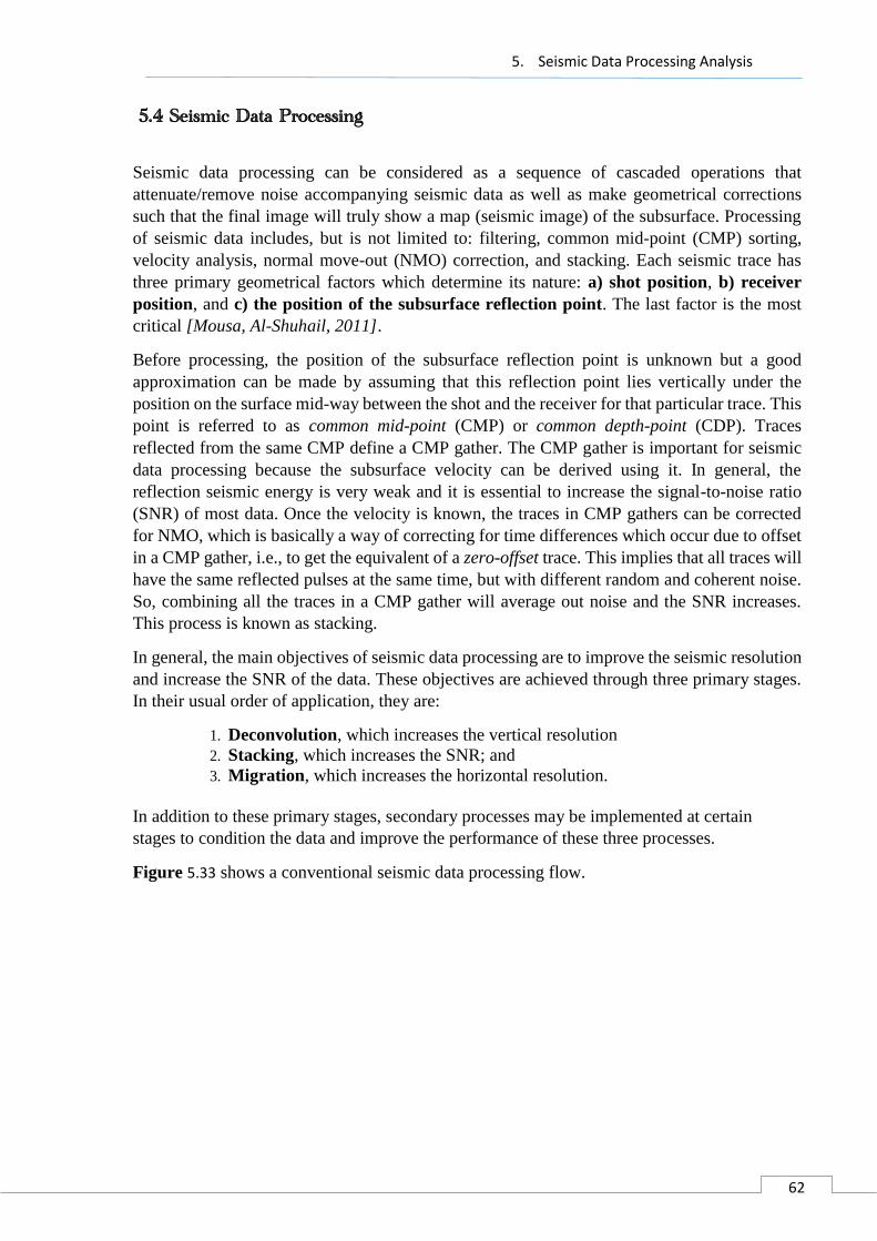
5. Seismic Data Processing Analysis
62
5.4 Seismic Data Processing
Seismic data processing can be considered as a sequence of cascaded operations that
attenuate/remove noise accompanying seismic data as well as make geometrical corrections
such that the final image will truly show a map (seismic image) of the subsurface. Processing
of seismic data includes, but is not limited to: filtering, common mid-point (CMP) sorting,
velocity analysis, normal move-out (NMO) correction, and stacking. Each seismic trace has
three primary geometrical factors which determine its nature: a) shot position, b) receiver
position, and c) the position of the subsurface reflection point. The last factor is the most
critical [Mousa, Al-Shuhail, 2011].
Before processing, the position of the subsurface reflection point is unknown but a good
approximation can be made by assuming that this reflection point lies vertically under the
position on the surface mid-way between the shot and the receiver for that particular trace. This
point is referred to as common mid-point (CMP) or common depth-point (CDP). Traces
reflected from the same CMP define a CMP gather. The CMP gather is important for seismic
data processing because the subsurface velocity can be derived using it. In general, the
reflection seismic energy is very weak and it is essential to increase the signal-to-noise ratio
(SNR) of most data. Once the velocity is known, the traces in CMP gathers can be corrected
for NMO, which is basically a way of correcting for time differences which occur due to offset
in a CMP gather, i.e., to get the equivalent of a zero-offset trace. This implies that all traces will
have the same reflected pulses at the same time, but with different random and coherent noise.
So, combining all the traces in a CMP gather will average out noise and the SNR increases.
This process is known as stacking.
In general, the main objectives of seismic data processing are to improve the seismic resolution
and increase the SNR of the data. These objectives are achieved through three primary stages.
In their usual order of application, they are:
1. Deconvolution, which increases the vertical resolution
2. Stacking, which increases the SNR; and
3. Migration, which increases the horizontal resolution.
In addition to these primary stages, secondary processes may be implemented at certain
stages to condition the data and improve the performance of these three processes.
Figure 5.33 shows a conventional seismic data processing flow.
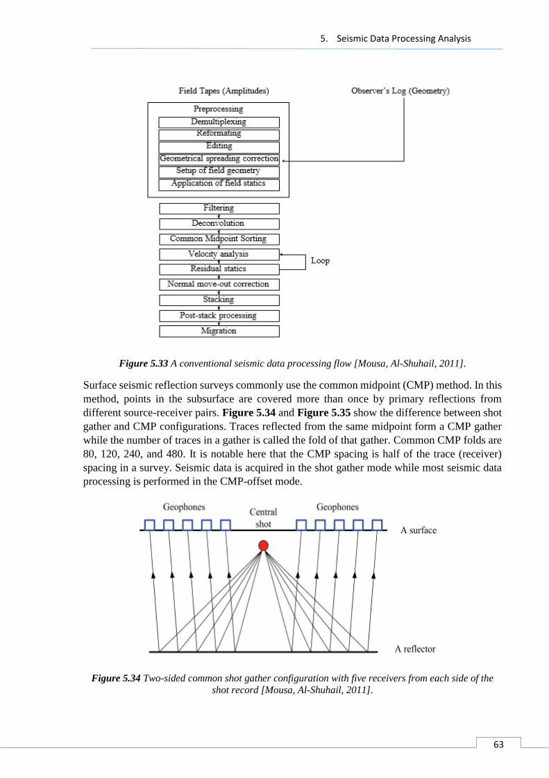
5. Seismic Data Processing Analysis
63
Figure 5.33 A conventional seismic data processing flow [Mousa, Al-Shuhail, 2011].
Surface seismic reflection surveys commonly use the common midpoint (CMP) method. In this
method, points in the subsurface are covered more than once by primary reflections from
different source-receiver pairs. Figure 5.34 and Figure 5.35 show the difference between shot
gather and CMP configurations. Traces reflected from the same midpoint form a CMP gather
while the number of traces in a gather is called the fold of that gather. Common CMP folds are
80, 120, 240, and 480. It is notable here that the CMP spacing is half of the trace (receiver)
spacing in a survey. Seismic data is acquired in the shot gather mode while most seismic data
processing is performed in the CMP-offset mode.
Figure 5.34 Two-sided common shot gather configuration with five receivers from each side of the
shot record [Mousa, Al-Shuhail, 2011].
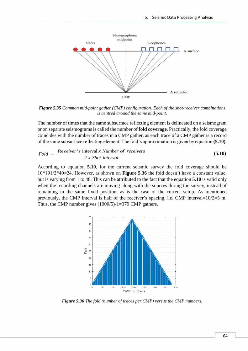
5. Seismic Data Processing Analysis
64
Figure 5.35 Common mid-point gather (CMP) configuration. Each of the shot-receiver combinations
is centred around the same mid-point.
The number of times that the same subsurface reflecting element is delineated on a seismogram
or on separate seismograms is called the number of fold coverage. Practically, the fold coverage
coincides with the number of traces in a CMP gather, as each trace of a CMP gather is a record
of the same subsurface reflecting element. The fold’s approximation is given by equation (5.10).
Re ' interval
2 i
ceiver s x Number of receiversFold
x Shot nterval (5.10)
According to equation 5.10, for the current seismic survey the fold coverage should be
10*191/2*40≈24. However, as shown on Figure 5.36 the fold doesn’t have a constant value,
but is varying from 1 to 48. This can be attributed to the fact that the equation 5.10 is valid only
when the recording channels are moving along with the sources during the survey, instead of
remaining in the same fixed position, as is the case of the current setup. As mentioned
previously, the CMP interval is half of the receiver’s spacing, i.e. CMP interval=10/2=5 m.
Thus, the CMP number gives (1900/5)-1=379 CMP gathers.
Figure 5.36 The fold (number of traces per CMP) versus the CMP numbers.

5. Seismic Data Processing Analysis
65
Before starting the processing analysis of the synthetic data, a simple demonstration of the
source’s expected waveform is presented. As stated previously, the dominant frequency of the
source is 20 Hz with sampling interval 1ms. Using the data above, along with the approximated
reflectivity series of the Prino’s subsurface (which will be further analyzed in chapter 7), a first
representation of the synthetic seismic data is given on Figure 5.37.
Figure 5.37 Representation of source wavelet, reflectivity series and their convolution in time.
In the following section, the processing steps presented in Figure 5.33 are elaborated, beginning
with the preprocessing procedure.
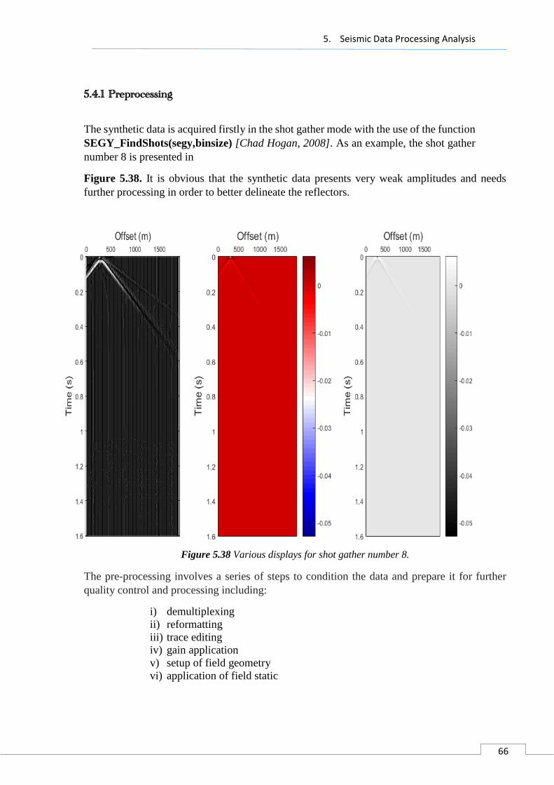
5. Seismic Data Processing Analysis
66
5.4.1 Preprocessing
The synthetic data is acquired firstly in the shot gather mode with the use of the function
SEGY_FindShots(segy,binsize) [Chad Hogan, 2008]. As an example, the shot gather
number 8 is presented in
Figure 5.38. It is obvious that the synthetic data presents very weak amplitudes and needs
further processing in order to better delineate the reflectors.
Figure 5.38 Various displays for shot gather number 8.
The pre-processing involves a series of steps to condition the data and prepare it for further
quality control and processing including:
i) demultiplexing
ii) reformatting
iii) trace editing
iv) gain application
v) setup of field geometry
vi) application of field static
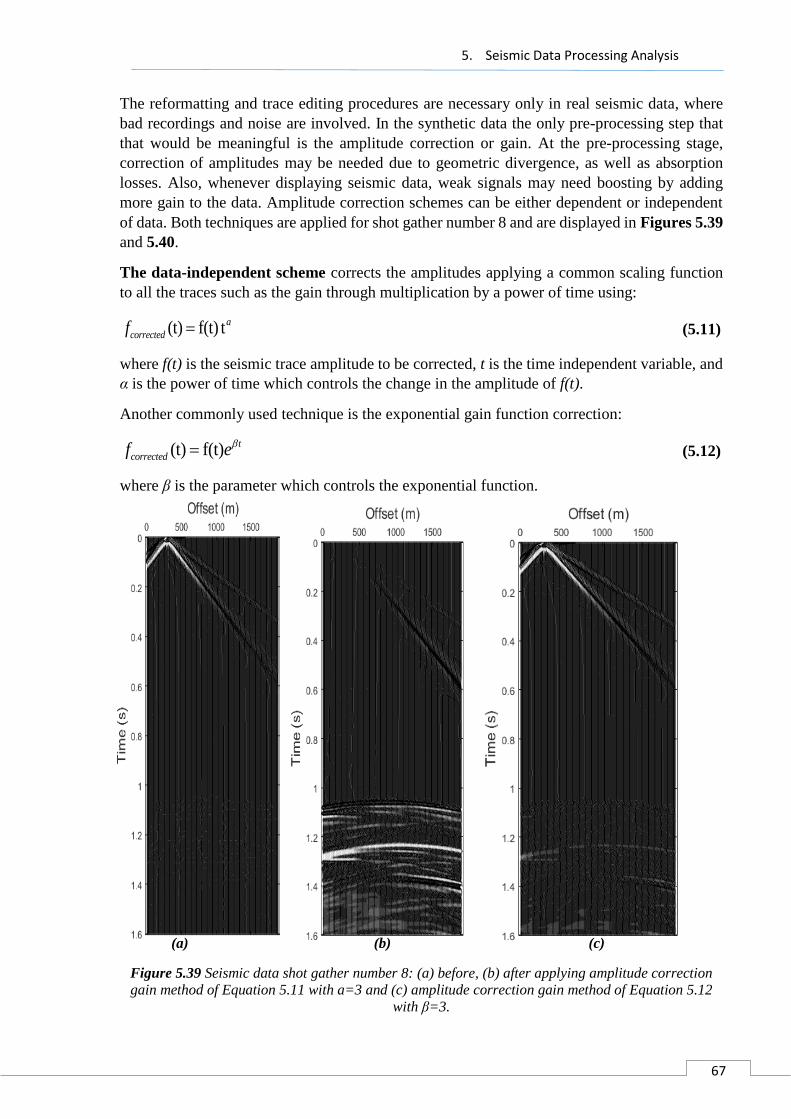
5. Seismic Data Processing Analysis
67
The reformatting and trace editing procedures are necessary only in real seismic data, where
bad recordings and noise are involved. In the synthetic data the only pre-processing step that
that would be meaningful is the amplitude correction or gain. At the pre-processing stage,
correction of amplitudes may be needed due to geometric divergence, as well as absorption
losses. Also, whenever displaying seismic data, weak signals may need boosting by adding
more gain to the data. Amplitude correction schemes can be either dependent or independent
of data. Both techniques are applied for shot gather number 8 and are displayed in Figures 5.39
and 5.40.
The data-independent scheme corrects the amplitudes applying a common scaling function
to all the traces such as the gain through multiplication by a power of time using:
(t) f(t) ta
correctedf (5.11)
where f(t) is the seismic trace amplitude to be corrected, t is the time independent variable, and
α is the power of time which controls the change in the amplitude of f(t).
Another commonly used technique is the exponential gain function correction:
(t) f(t) t
correctedf e (5.12)
where β is the parameter which controls the exponential function.
(a) (b) (c)
Figure 5.39 Seismic data shot gather number 8: (a) before, (b) after applying amplitude correction
gain method of Equation 5.11 with a=3 and (c) amplitude correction gain method of Equation 5.12
with β=3.
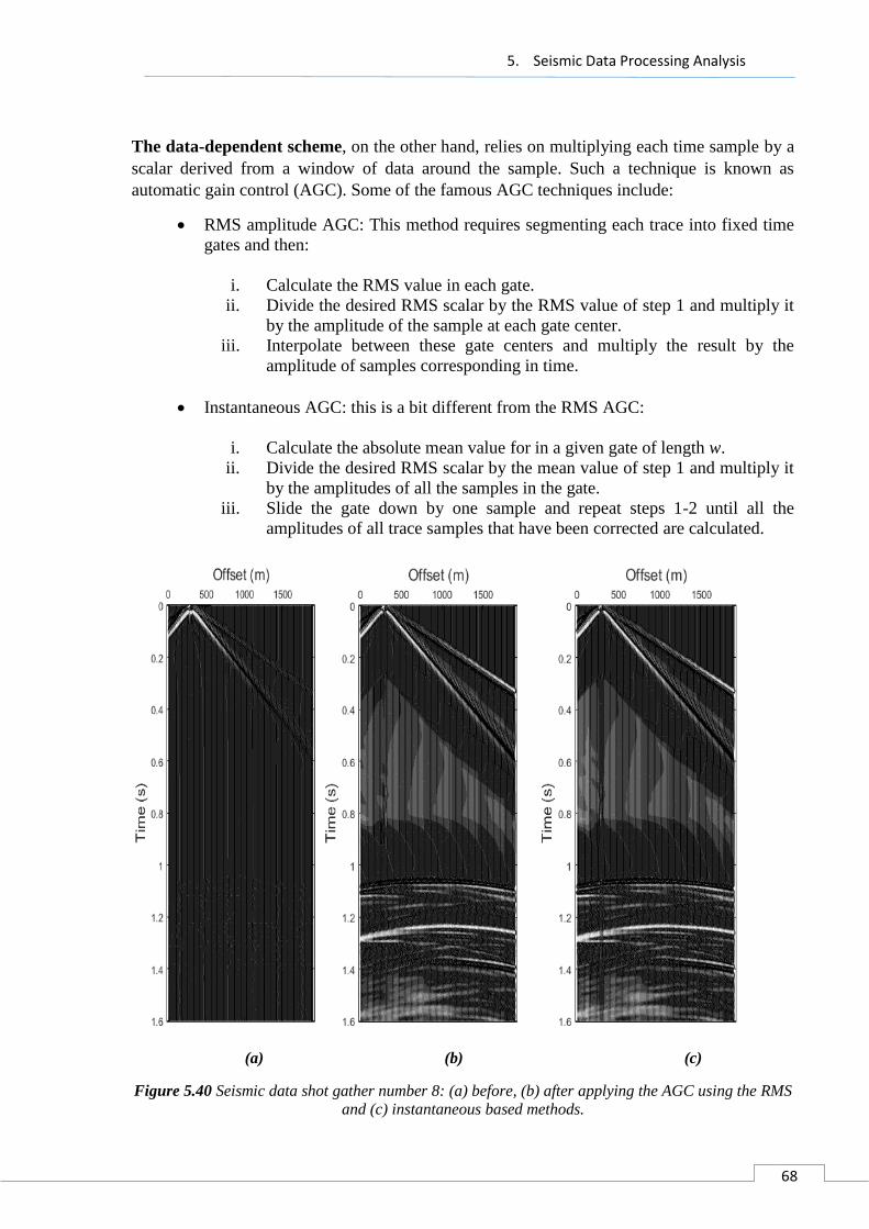
5. Seismic Data Processing Analysis
68
The data-dependent scheme, on the other hand, relies on multiplying each time sample by a
scalar derived from a window of data around the sample. Such a technique is known as
automatic gain control (AGC). Some of the famous AGC techniques include:
RMS amplitude AGC: This method requires segmenting each trace into fixed time
gates and then:
i. Calculate the RMS value in each gate.
ii. Divide the desired RMS scalar by the RMS value of step 1 and multiply it
by the amplitude of the sample at each gate center.
iii. Interpolate between these gate centers and multiply the result by the
amplitude of samples corresponding in time.
Instantaneous AGC: this is a bit different from the RMS AGC:
i. Calculate the absolute mean value for in a given gate of length w.
ii. Divide the desired RMS scalar by the mean value of step 1 and multiply it
by the amplitudes of all the samples in the gate.
iii. Slide the gate down by one sample and repeat steps 1-2 until all the
amplitudes of all trace samples that have been corrected are calculated.
(a) (b) (c)
Figure 5.40 Seismic data shot gather number 8: (a) before, (b) after applying the AGC using the RMS
and (c) instantaneous based methods.

5. Seismic Data Processing Analysis
69
In order to better understand the differences between the data-dependent and independent gain
schemes, the amplitude envelope of gain is presented in Figure 5.41, separately before and after
the application of each process.
Figure 5.41 The amplitude envelope gain in dB of the average trace for a) instantaneous ACG, b)
RMS amplitude ACG, c) power gain correction with a=3 and d) exponential gain correction with b=3.
It is obvious from Figure 5.41 that the data-dependent gain increases the amplitude of the
average trace, both in early and in late times, while in the case of the power and exponential
gains the amplitudes are increased mainly in the later times. Also, the data-dependent gain has
greater and more abrupt impact on the average trace’s amplitude. Finally, there is a difference
between the power and the exponential gain, with the latter giving a smoother and lower
amplitude boosting.
For the data independent scheme the function iac(Dshot,t,pow,T) was used, while for the time-
dependent scheme the function AGCgain(Dshot,dt,agc,T) was used. Finally, for the
amplitude’s envelope plotting the function seis_env_dB(Dshot,Dg,t) was applied.
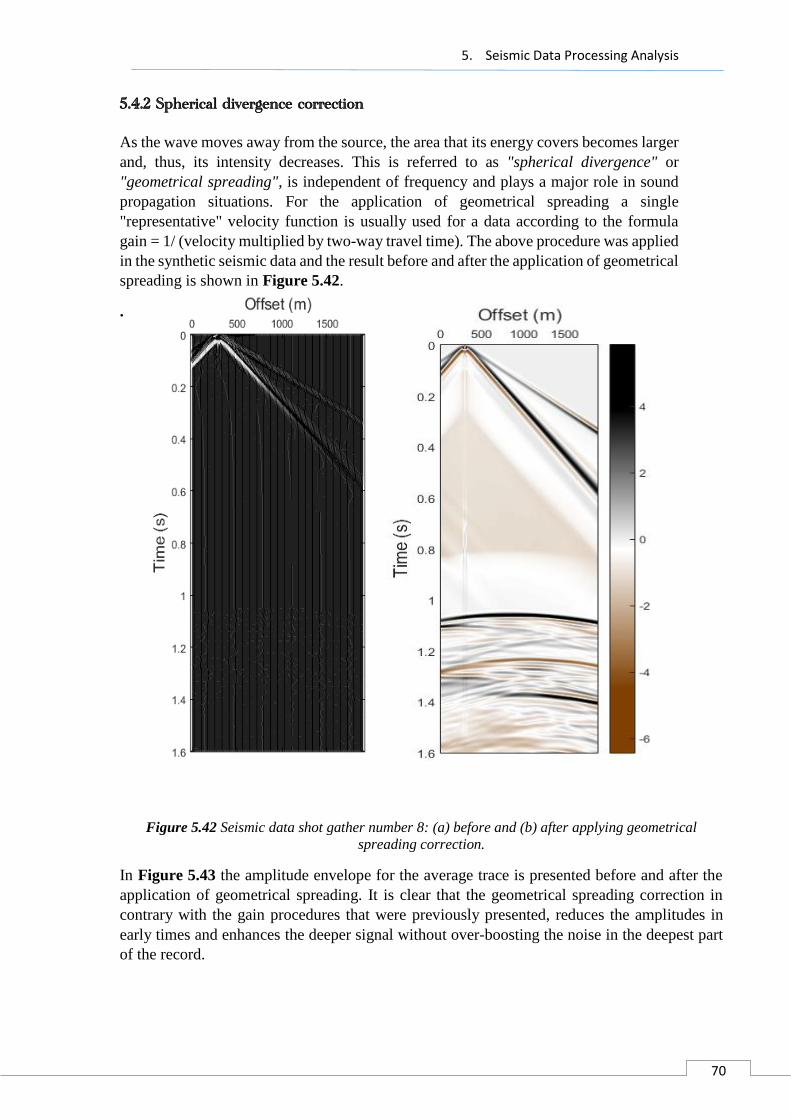
5. Seismic Data Processing Analysis
70
5.4.2 Spherical divergence correction
As the wave moves away from the source, the area that its energy covers becomes larger
and, thus, its intensity decreases. This is referred to as "spherical divergence" or
"geometrical spreading", is independent of frequency and plays a major role in sound
propagation situations. For the application of geometrical spreading a single
"representative" velocity function is usually used for a data according to the formula
gain = 1/ (velocity multiplied by two-way travel time). The above procedure was applied
in the synthetic seismic data and the result before and after the application of geometrical
spreading is shown in Figure 5.42.
.
Figure 5.42 Seismic data shot gather number 8: (a) before and (b) after applying geometrical
spreading correction.
In Figure 5.43 the amplitude envelope for the average trace is presented before and after the
application of geometrical spreading. It is clear that the geometrical spreading correction in
contrary with the gain procedures that were previously presented, reduces the amplitudes in
early times and enhances the deeper signal without over-boosting the noise in the deepest part
of the record.
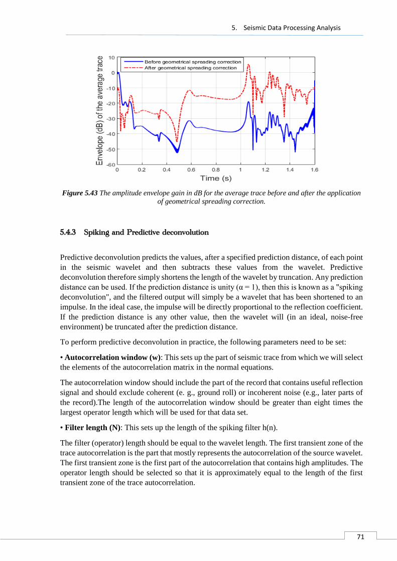
5. Seismic Data Processing Analysis
71
Figure 5.43 The amplitude envelope gain in dB for the average trace before and after the application
of geometrical spreading correction.
5.4.3 Spiking and Predictive deconvolution
Predictive deconvolution predicts the values, after a specified prediction distance, of each point
in the seismic wavelet and then subtracts these values from the wavelet. Predictive
deconvolution therefore simply shortens the length of the wavelet by truncation. Any prediction
distance can be used. If the prediction distance is unity (α = 1), then this is known as a "spiking
deconvolution", and the filtered output will simply be a wavelet that has been shortened to an
impulse. In the ideal case, the impulse will be directly proportional to the reflection coefficient.
If the prediction distance is any other value, then the wavelet will (in an ideal, noise-free
environment) be truncated after the prediction distance.
To perform predictive deconvolution in practice, the following parameters need to be set:
• Autocorrelation window (w): This sets up the part of seismic trace from which we will select
the elements of the autocorrelation matrix in the normal equations.
The autocorrelation window should include the part of the record that contains useful reflection
signal and should exclude coherent (e. g., ground roll) or incoherent noise (e.g., later parts of
the record).The length of the autocorrelation window should be greater than eight times the
largest operator length which will be used for that data set.
• Filter length (N): This sets up the length of the spiking filter h(n).
The filter (operator) length should be equal to the wavelet length. The first transient zone of the
trace autocorrelation is the part that mostly represents the autocorrelation of the source wavelet.
The first transient zone is the first part of the autocorrelation that contains high amplitudes. The
operator length should be selected so that it is approximately equal to the length of the first
transient zone of the trace autocorrelation.

5. Seismic Data Processing Analysis
72
• Percent prewhitening (ε): This sets up the amount of white random noise that needs to be
included into the autocorrelation matrix to stabilize the solution of the normal equations.
The magnitude of prewhitening is measured as a percentage of the zero-lag
autocorrelation value r(0). In practice, typically 0.1% to 0.3% prewhitening is standard
in processing. In Figure 5.44 the autocorrelogram of the shot gather number 8 is
displayed along with the output of the shot gather after applying spiking deconvolution.
The chosen value for the autoceralltion window is 0.2 s, while the prewhitening value
was set to 0.1%. It is clear that the data became spikier, something that can also be proved
by analyzing the data in the spectrum domain via the power spectral density of the
average traces as seen in Figure 5.45.
(a) (b) (c)
Figure 5.44 Shot gather 8 (a) before applying spiking deconvolution (b) its autocorrelogram for
window 0.2 s and (c) after applying spiking deconvolution.
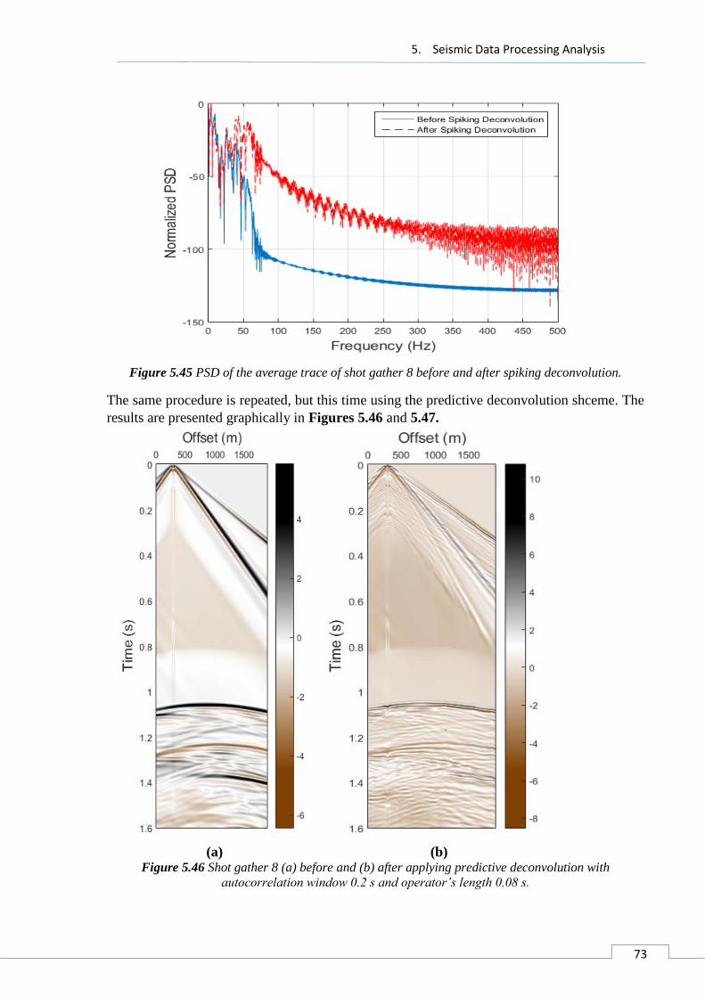
5. Seismic Data Processing Analysis
73
Figure 5.45 PSD of the average trace of shot gather 8 before and after spiking deconvolution.
The same procedure is repeated, but this time using the predictive deconvolution shceme. The
results are presented graphically in Figures 5.46 and 5.47.
(a) (b) Figure 5.46 Shot gather 8 (a) before and (b) after applying predictive deconvolution with
autocorrelation window 0.2 s and operator’s length 0.08 s.
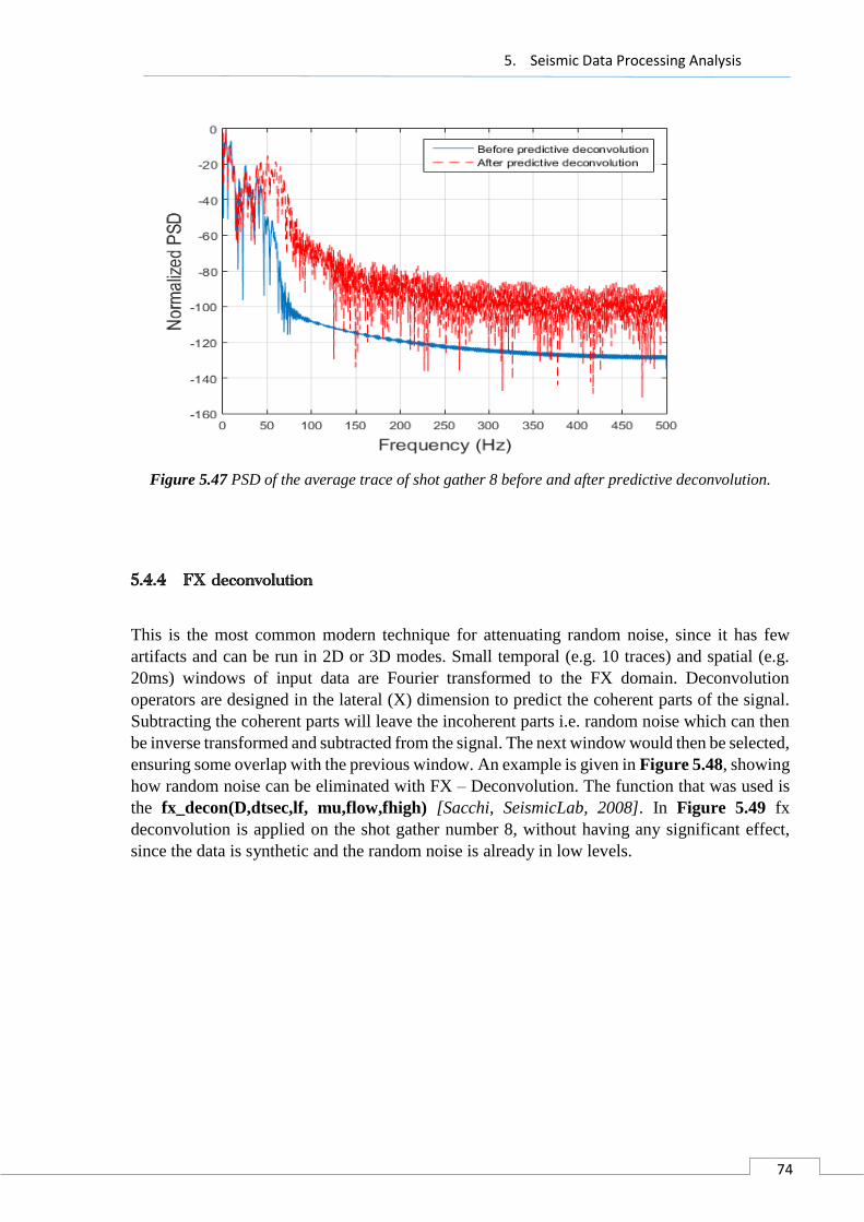
5. Seismic Data Processing Analysis
74
Figure 5.47 PSD of the average trace of shot gather 8 before and after predictive deconvolution.
5.4.4 FX deconvolution
This is the most common modern technique for attenuating random noise, since it has few
artifacts and can be run in 2D or 3D modes. Small temporal (e.g. 10 traces) and spatial (e.g.
20ms) windows of input data are Fourier transformed to the FX domain. Deconvolution
operators are designed in the lateral (X) dimension to predict the coherent parts of the signal.
Subtracting the coherent parts will leave the incoherent parts i.e. random noise which can then
be inverse transformed and subtracted from the signal. The next window would then be selected,
ensuring some overlap with the previous window. An example is given in Figure 5.48, showing
how random noise can be eliminated with FX – Deconvolution. The function that was used is
the fx_decon(D,dtsec,lf, mu,flow,fhigh) [Sacchi, SeismicLab, 2008]. In Figure 5.49 fx
deconvolution is applied on the shot gather number 8, without having any significant effect,
since the data is synthetic and the random noise is already in low levels.

5. Seismic Data Processing Analysis
75
Figure 5.48 Display of seismic data form left to right, before FX deconvolution, after FX deconvolution and
estimated noise.
(a) (b)
Figure 5.49 Shot gather number 8 (a) before and (b) after the application of fx deconvolution.
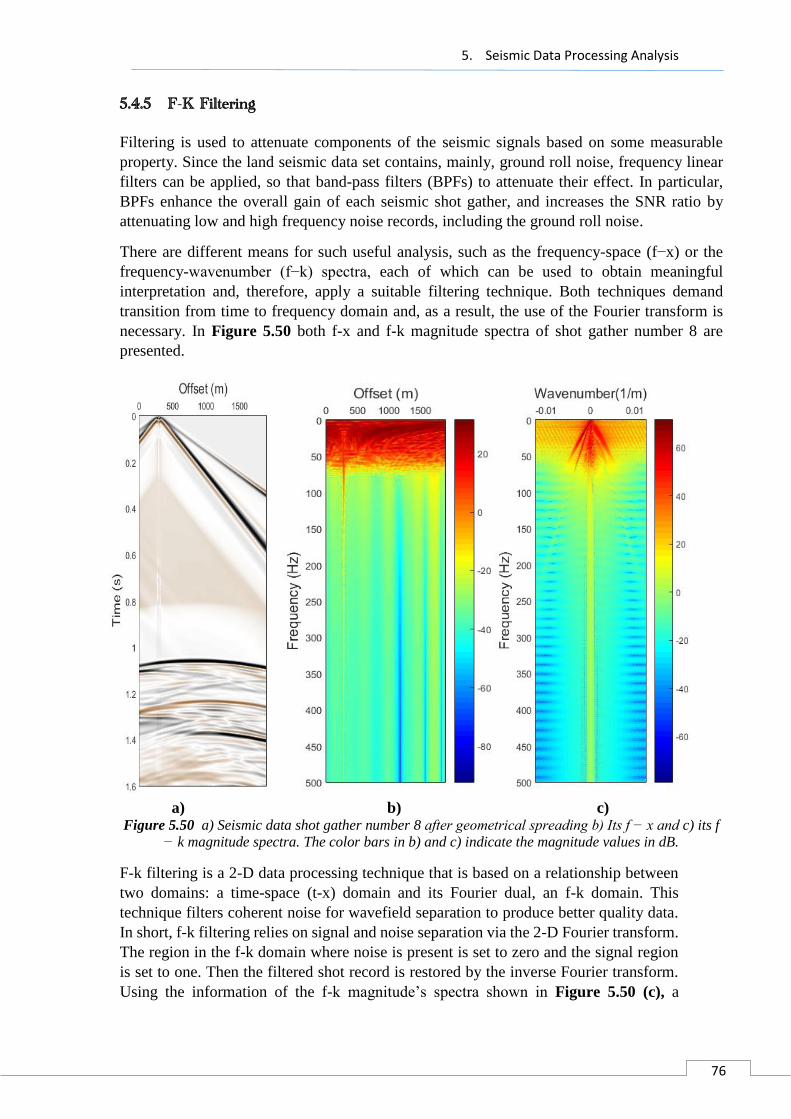
5. Seismic Data Processing Analysis
76
5.4.5 F-K Filtering
Filtering is used to attenuate components of the seismic signals based on some measurable
property. Since the land seismic data set contains, mainly, ground roll noise, frequency linear
filters can be applied, so that band-pass filters (BPFs) to attenuate their effect. In particular,
BPFs enhance the overall gain of each seismic shot gather, and increases the SNR ratio by
attenuating low and high frequency noise records, including the ground roll noise.
There are different means for such useful analysis, such as the frequency-space (f−x) or the
frequency-wavenumber (f−k) spectra, each of which can be used to obtain meaningful
interpretation and, therefore, apply a suitable filtering technique. Both techniques demand
transition from time to frequency domain and, as a result, the use of the Fourier transform is
necessary. In Figure 5.50 both f-x and f-k magnitude spectra of shot gather number 8 are
presented.
a) b) c) Figure 5.50 a) Seismic data shot gather number 8 after geometrical spreading b) Its f − x and c) its f
− k magnitude spectra. The color bars in b) and c) indicate the magnitude values in dB.
F-k filtering is a 2-D data processing technique that is based on a relationship between
two domains: a time-space (t-x) domain and its Fourier dual, an f-k domain. This
technique filters coherent noise for wavefield separation to produce better quality data.
In short, f-k filtering relies on signal and noise separation via the 2-D Fourier transform.
The region in the f-k domain where noise is present is set to zero and the signal region
is set to one. Then the filtered shot record is restored by the inverse Fourier transform.
Using the information of the f-k magnitude’s spectra shown in Figure 5.50 (c), a
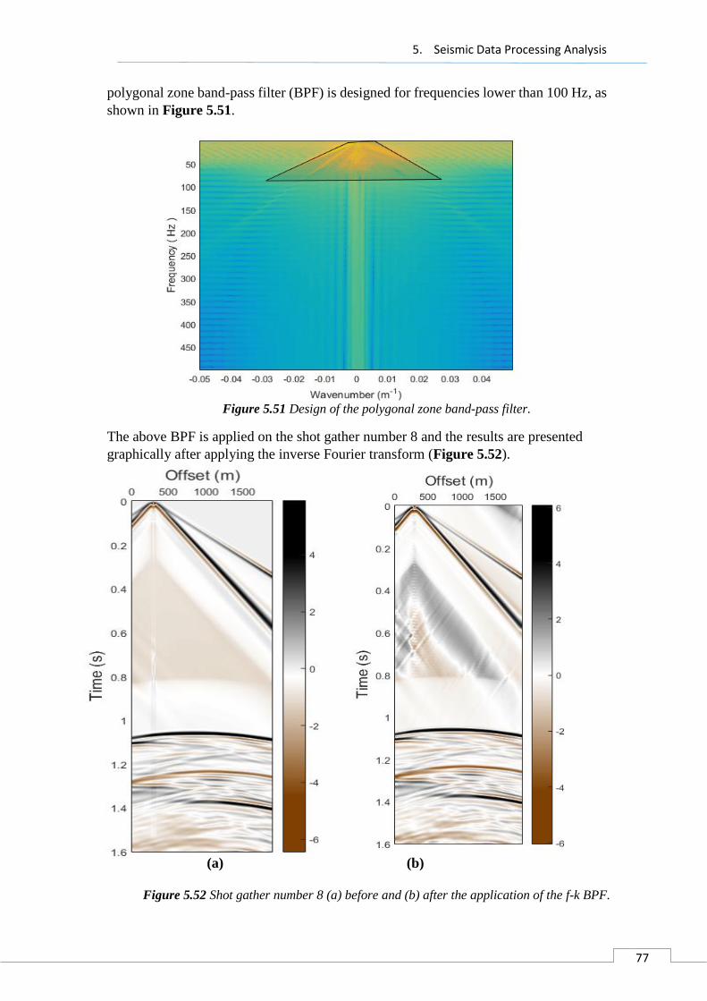
5. Seismic Data Processing Analysis
77
polygonal zone band-pass filter (BPF) is designed for frequencies lower than 100 Hz, as
shown in Figure 5.51.
Figure 5.51 Design of the polygonal zone band-pass filter.
The above BPF is applied on the shot gather number 8 and the results are presented
graphically after applying the inverse Fourier transform (Figure 5.52).
(a) (b)
Figure 5.52 Shot gather number 8 (a) before and (b) after the application of the f-k BPF.
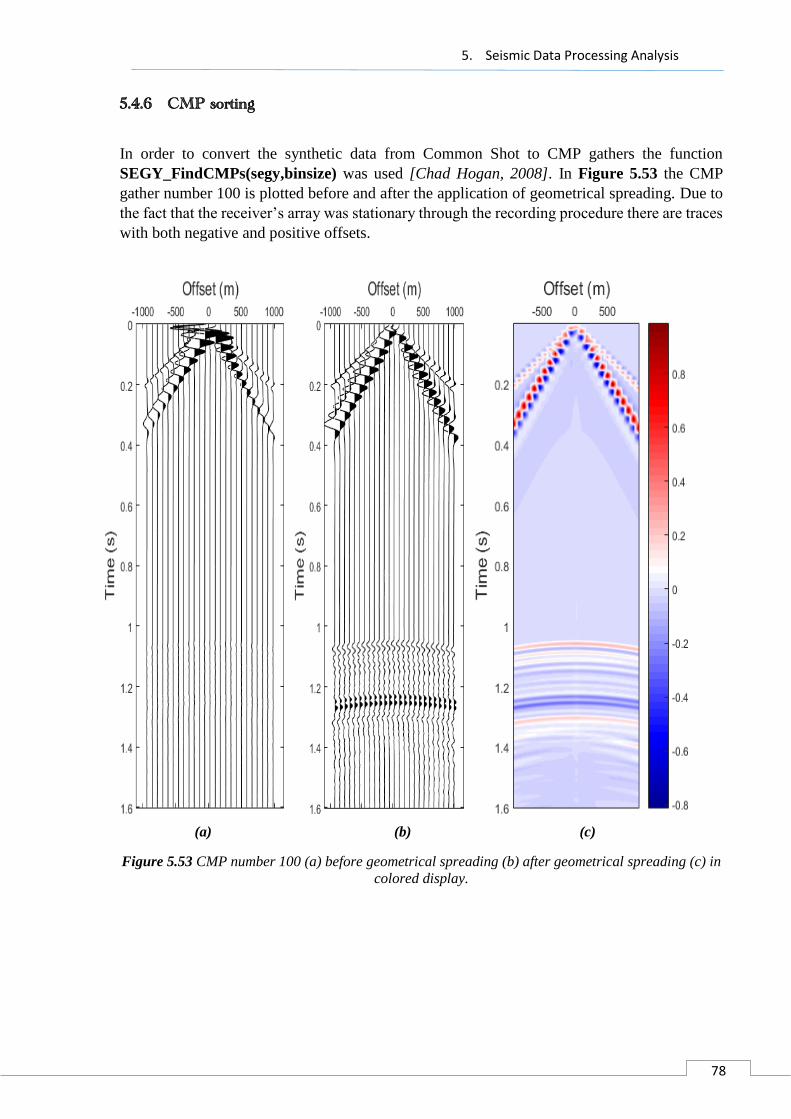
5. Seismic Data Processing Analysis
78
5.4.6 CMP sorting
In order to convert the synthetic data from Common Shot to CMP gathers the function
SEGY_FindCMPs(segy,binsize) was used [Chad Hogan, 2008]. In Figure 5.53 the CMP
gather number 100 is plotted before and after the application of geometrical spreading. Due to
the fact that the receiver’s array was stationary through the recording procedure there are traces
with both negative and positive offsets.
(a) (b) (c)
Figure 5.53 CMP number 100 (a) before geometrical spreading (b) after geometrical spreading (c) in
colored display.
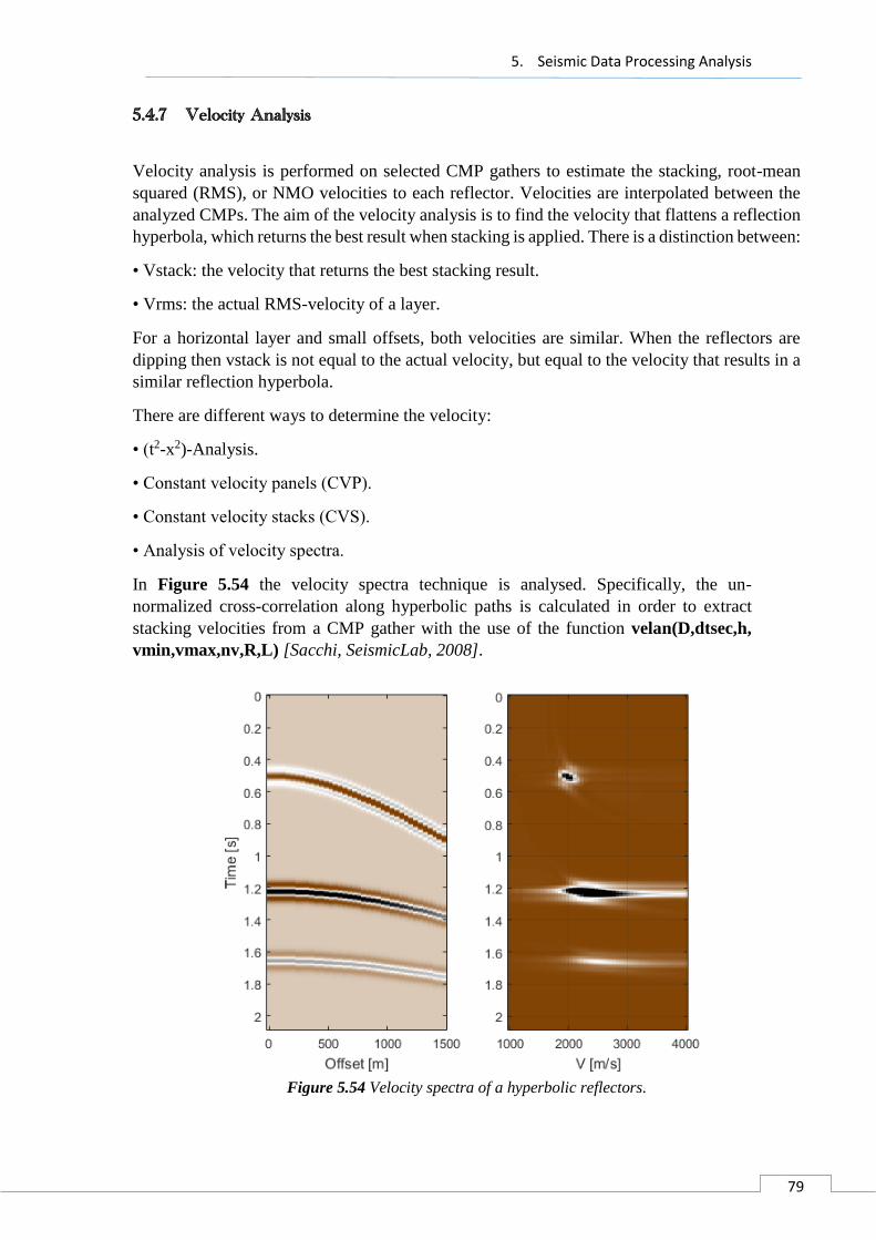
5. Seismic Data Processing Analysis
79
5.4.7 Velocity Analysis
Velocity analysis is performed on selected CMP gathers to estimate the stacking, root-mean
squared (RMS), or NMO velocities to each reflector. Velocities are interpolated between the
analyzed CMPs. The aim of the velocity analysis is to find the velocity that flattens a reflection
hyperbola, which returns the best result when stacking is applied. There is a distinction between:
• Vstack: the velocity that returns the best stacking result.
• Vrms: the actual RMS-velocity of a layer.
For a horizontal layer and small offsets, both velocities are similar. When the reflectors are
dipping then vstack is not equal to the actual velocity, but equal to the velocity that results in a
similar reflection hyperbola.
There are different ways to determine the velocity:
• (t2-x2)-Analysis.
• Constant velocity panels (CVP).
• Constant velocity stacks (CVS).
• Analysis of velocity spectra.
In Figure 5.54 the velocity spectra technique is analysed. Specifically, the un-
normalized cross-correlation along hyperbolic paths is calculated in order to extract
stacking velocities from a CMP gather with the use of the function velan(D,dtsec,h,
vmin,vmax,nv,R,L) [Sacchi, SeismicLab, 2008].
Figure 5.54 Velocity spectra of a hyperbolic reflectors.
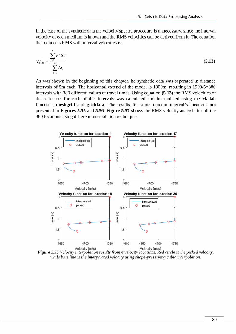
5. Seismic Data Processing Analysis
80
In the case of the synthetic data the velocity spectra procedure is unnecessary, since the interval
velocity of each medium is known and the RMS velocities can be derived from it. The equation
that connects RMS with interval velocities is:
2
2 1
1
N
i i
iRMS N
i
i
V t
V
t
(5.13)
As was shown in the beginning of this chapter, he synthetic data was separated in distance
intervals of 5m each. The horizontal extend of the model is 1900m, resulting in 1900/5=380
intervals with 380 different values of travel times. Using equation (5.13) the RMS velocities of
the reflectors for each of this intervals was calculated and interpolated using the Matlab
functions meshgrid and griddata. The results for some random interval’s locations are
presented in Figures 5.55 and 5.56. Figure 5.57 shows the RMS velocity analysis for all the
380 locations using different interpolation techniques.
Figure 5.55 Velocity interpolation results from 4 velocity locations. Red circle is the picked velocity,
while blue line is the interpolated velocity using shape-preserving cubic interpolation.

5. Seismic Data Processing Analysis
81
Figure 5.56 Comparison between interpolated vrms (blue) and block constant vint (red) on 4 velocity
analysis locations.
Figure 5.57 Interpolated vrms for all velocity analysis locations.
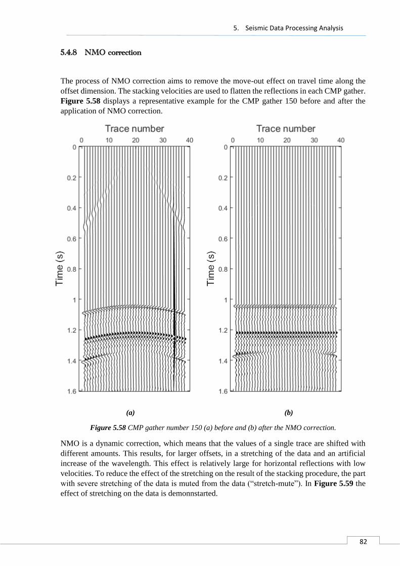
5. Seismic Data Processing Analysis
82
5.4.8 NMO correction
The process of NMO correction aims to remove the move-out effect on travel time along the
offset dimension. The stacking velocities are used to flatten the reflections in each CMP gather.
Figure 5.58 displays a representative example for the CMP gather 150 before and after the
application of NMO correction.
(a) (b)
Figure 5.58 CMP gather number 150 (a) before and (b) after the NMO correction.
NMO is a dynamic correction, which means that the values of a single trace are shifted with
different amounts. This results, for larger offsets, in a stretching of the data and an artificial
increase of the wavelength. This effect is relatively large for horizontal reflections with low
velocities. To reduce the effect of the stretching on the result of the stacking procedure, the part
with severe stretching of the data is muted from the data (“stretch-mute”). In Figure 5.59 the
effect of stretching on the data is demonnstarted.
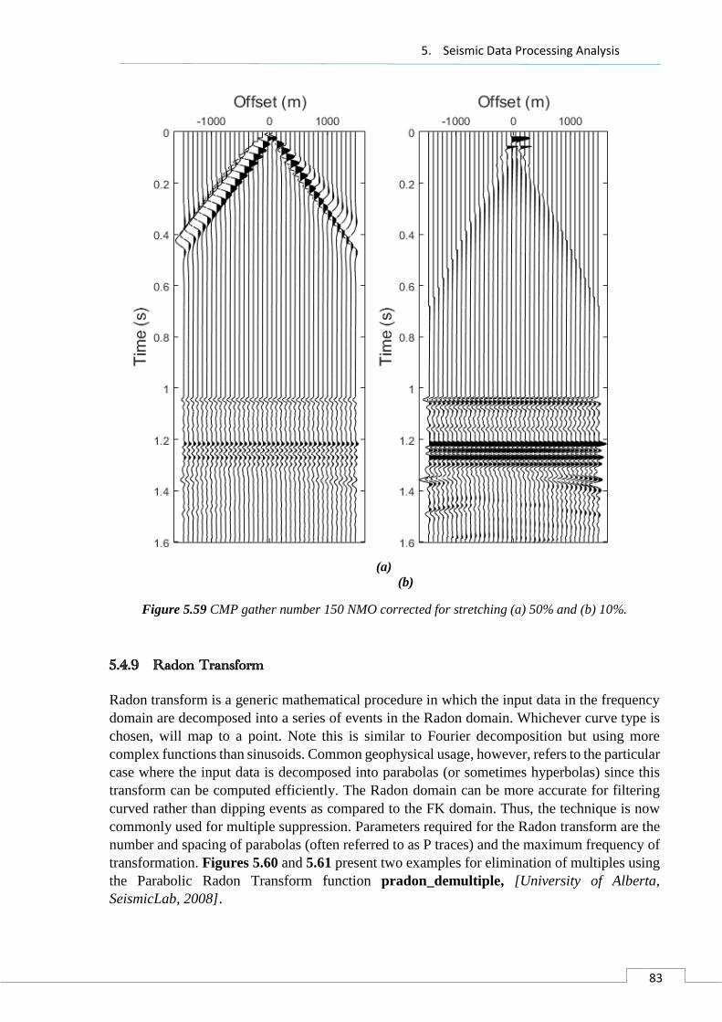
5. Seismic Data Processing Analysis
83
(a)
(b)
Figure 5.59 CMP gather number 150 NMO corrected for stretching (a) 50% and (b) 10%.
5.4.9 Radon Transform
Radon transform is a generic mathematical procedure in which the input data in the frequency
domain are decomposed into a series of events in the Radon domain. Whichever curve type is
chosen, will map to a point. Note this is similar to Fourier decomposition but using more
complex functions than sinusoids. Common geophysical usage, however, refers to the particular
case where the input data is decomposed into parabolas (or sometimes hyperbolas) since this
transform can be computed efficiently. The Radon domain can be more accurate for filtering
curved rather than dipping events as compared to the FK domain. Thus, the technique is now
commonly used for multiple suppression. Parameters required for the Radon transform are the
number and spacing of parabolas (often referred to as P traces) and the maximum frequency of
transformation. Figures 5.60 and 5.61 present two examples for elimination of multiples using
the Parabolic Radon Transform function pradon_demultiple, [University of Alberta,
SeismicLab, 2008].

5. Seismic Data Processing Analysis
84
Figure 5.60 Parabolic Radon transform used on synthetic data for the elimination of multiples.
Figure 5.61 Parabolic Radon transform used on real seismic data for the elimination of multiples.
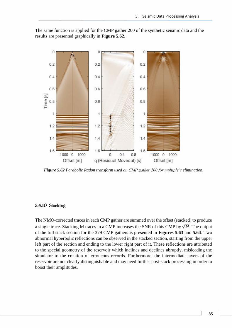
5. Seismic Data Processing Analysis
85
The same function is applied for the CMP gather 200 of the synthetic seismic data and the
results are presented graphically in Figure 5.62.
Figure 5.62 Parabolic Radon transform used on CMP gather 200 for multiple’s elimination.
5.4.10 Stacking
The NMO-corrected traces in each CMP gather are summed over the offset (stacked) to produce
a single trace. Stacking M traces in a CMP increases the SNR of this CMP by √𝑀. The output
of the full stack section for the 379 CMP gathers is presented in Figures 5.63 and 5.64. Two
abnormal hyperbolic reflections can be observed in the stacked section, starting from the upper
left part of the section and ending to the lower right part of it. These reflections are attributed
to the special geometry of the reservoir which inclines and declines abruptly, misleading the
simulator to the creation of erroneous records. Furthermore, the intermediate layers of the
reservoir are not clearly distinguishable and may need further post-stack processing in order to
boost their amplitudes.
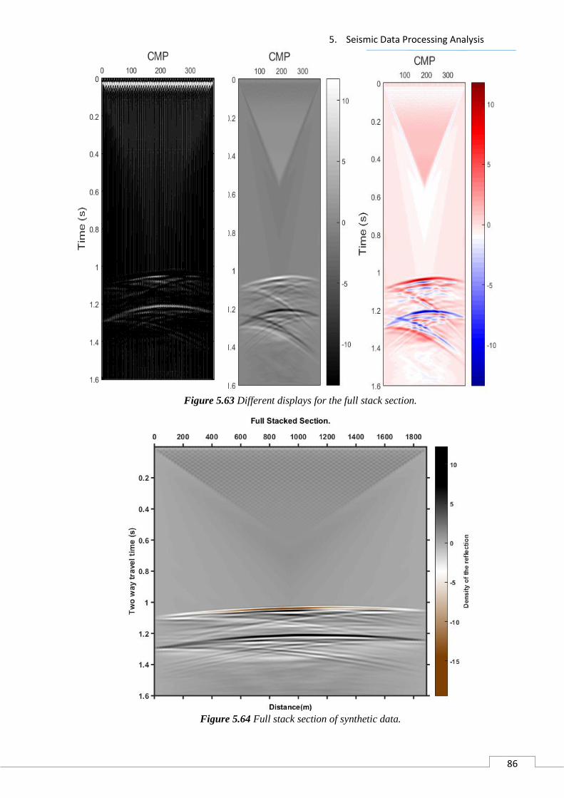
5. Seismic Data Processing Analysis
86
Figure 5.63 Different displays for the full stack section.
Figure 5.64 Full stack section of synthetic data.

5. Seismic Data Processing Analysis
87
5.4.11 Post-stack Processing
Post-stack processing includes time-variant band-pass filtering, dip filtering and other processes
to enhance the stacked section. After applying post-stack FK filtering, Radon transform and
spiking deconvolution to the seismic stacked section the intermediate reflectors were
significantly enhanced, as shown in Figure 5.65.
Figure 5.65 Full stack section of synthetic data after post-stack application of FK filtering, Radon
transform and spiking deconvolution.
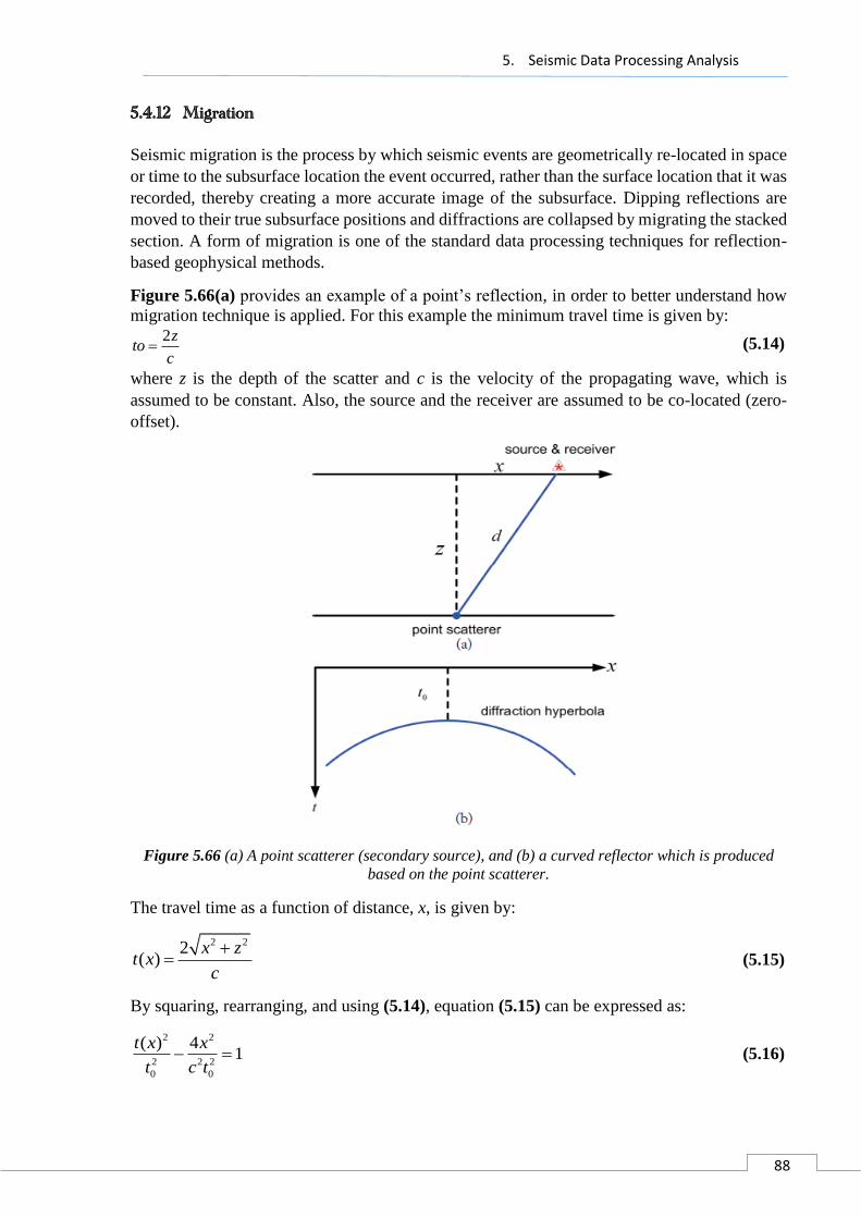
5. Seismic Data Processing Analysis
88
5.4.12 Migration
Seismic migration is the process by which seismic events are geometrically re-located in space
or time to the subsurface location the event occurred, rather than the surface location that it was
recorded, thereby creating a more accurate image of the subsurface. Dipping reflections are
moved to their true subsurface positions and diffractions are collapsed by migrating the stacked
section. A form of migration is one of the standard data processing techniques for reflection-
based geophysical methods.
Figure 5.66(a) provides an example of a point’s reflection, in order to better understand how
migration technique is applied. For this example the minimum travel time is given by: 2z
toc
(5.14)
where z is the depth of the scatter and c is the velocity of the propagating wave, which is
assumed to be constant. Also, the source and the receiver are assumed to be co-located (zero-
offset).
Figure 5.66 (a) A point scatterer (secondary source), and (b) a curved reflector which is produced
based on the point scatterer.
The travel time as a function of distance, x, is given by:
2 22( )
x zt x
c
(5.15)
By squaring, rearranging, and using (5.14), equation (5.15) can be expressed as:
2 2
2 2 2
0 0
( ) 41
t x x
t c t (5.16)
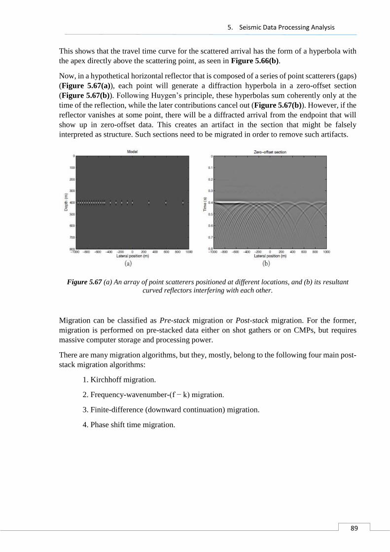
5. Seismic Data Processing Analysis
89
This shows that the travel time curve for the scattered arrival has the form of a hyperbola with
the apex directly above the scattering point, as seen in Figure 5.66(b).
Now, in a hypothetical horizontal reflector that is composed of a series of point scatterers (gaps)
(Figure 5.67(a)), each point will generate a diffraction hyperbola in a zero-offset section
(Figure 5.67(b)). Following Huygen’s principle, these hyperbolas sum coherently only at the
time of the reflection, while the later contributions cancel out (Figure 5.67(b)). However, if the
reflector vanishes at some point, there will be a diffracted arrival from the endpoint that will
show up in zero-offset data. This creates an artifact in the section that might be falsely
interpreted as structure. Such sections need to be migrated in order to remove such artifacts.
Figure 5.67 (a) An array of point scatterers positioned at different locations, and (b) its resultant
curved reflectors interfering with each other.
Migration can be classified as Pre-stack migration or Post-stack migration. For the former,
migration is performed on pre-stacked data either on shot gathers or on CMPs, but requires
massive computer storage and processing power.
There are many migration algorithms, but they, mostly, belong to the following four main post-
stack migration algorithms:
1. Kirchhoff migration.
2. Frequency-wavenumber-(f − k) migration.
3. Finite-difference (downward continuation) migration.
4. Phase shift time migration.
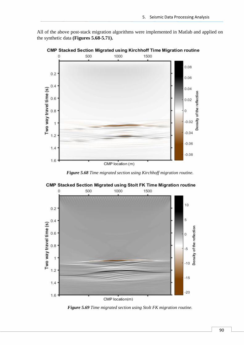
5. Seismic Data Processing Analysis
90
All of the above post-stack migration algorithms were implemented in Matlab and applied on
the synthetic data (Figures 5.68-5.71).
Figure 5.68 Time migrated section using Kirchhoff migration routine.
Figure 5.69 Time migrated section using Stolt FK migration routine.
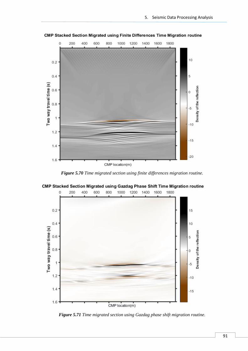
5. Seismic Data Processing Analysis
91
Figure 5.70 Time migrated section using finite differences migration routine.
Figure 5.71 Time migrated section using Gazdag phase shift migration routine.

5. Seismic Data Processing Analysis
92
In order to verify the accuracy of the migration, the Kirchhoff time migrated section is
superimposed on the reflectors (Figure 5.72) and on the rms velocity model (Figure 5.73). In
both of the cases the migrated section matches the expected values accurately enough.
Figure 5.72 Superposition of the reflectors on the migrated section.
Figure 5.73 Superposition of the interval velocity model on the migrated section.
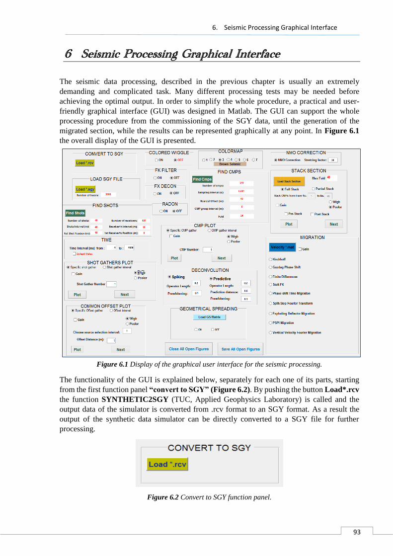
6. Seismic Processing Graphical Interface
93
6 Seismic Processing Graphical Interface
The seismic data processing, described in the previous chapter is usually an extremely
demanding and complicated task. Many different processing tests may be needed before
achieving the optimal output. In order to simplify the whole procedure, a practical and user-
friendly graphical interface (GUI) was designed in Matlab. The GUI can support the whole
processing procedure from the commissioning of the SGY data, until the generation of the
migrated section, while the results can be represented graphically at any point. In Figure 6.1
the overall display of the GUI is presented.
Figure 6.1 Display of the graphical user interface for the seismic processing.
The functionality of the GUI is explained below, separately for each one of its parts, starting
from the first function panel “convert to SGY” (Figure 6.2). By pushing the button Load*.rcv
the function SYNTHETIC2SGY (TUC, Applied Geophysics Laboratory) is called and the
output data of the simulator is converted from .rcv format to an SGY format. As a result the
output of the synthetic data simulator can be directly converted to a SGY file for further
processing.
Figure 6.2 Convert to SGY function panel.
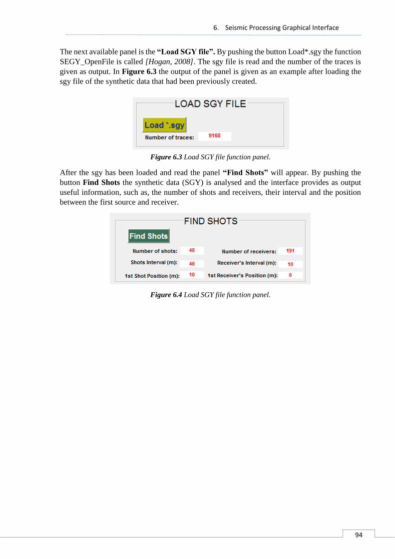
6. Seismic Processing Graphical Interface
94
The next available panel is the “Load SGY file”. By pushing the button Load*.sgy the function
SEGY_OpenFile is called [Hogan, 2008]. The sgy file is read and the number of the traces is
given as output. In Figure 6.3 the output of the panel is given as an example after loading the
sgy file of the synthetic data that had been previously created.
Figure 6.3 Load SGY file function panel.
After the sgy has been loaded and read the panel “Find Shots” will appear. By pushing the
button Find Shots the synthetic data (SGY) is analysed and the interface provides as output
useful information, such as, the number of shots and receivers, their interval and the position
between the first source and receiver.
Figure 6.4 Load SGY file function panel.
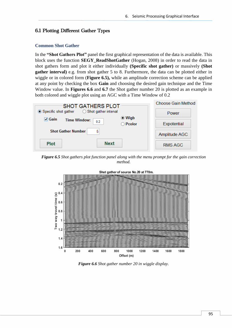
6. Seismic Processing Graphical Interface
95
6.1 Plotting Different Gather Types
Common Shot Gather
In the “Shot Gathers Plot” panel the first graphical representation of the data is available. This
block uses the function SEGY_ReadShotGather (Hogan, 2008) in order to read the data in
shot gathers form and plot it either individually (Specific shot gather) or massively (Shot
gather interval) e.g. from shot gather 5 to 8. Furthermore, the data can be plotted either in
wiggle or in colored form (Figure 6.5), while an amplitude correction scheme can be applied
at any point by checking the box Gain and choosing the desired gain technique and the Time
Window value. In Figures 6.6 and 6.7 the Shot gather number 20 is plotted as an example in
both colored and wiggle plot using an AGC with a Time Window of 0.2
Figure 6.5 Shot gathers plot function panel along with the menu prompt for the gain correction
method.
Figure 6.6 Shot gather number 20 in wiggle display.
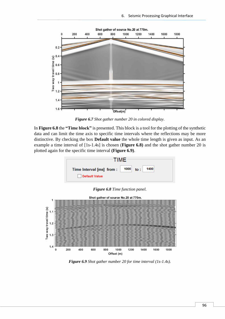
6. Seismic Processing Graphical Interface
96
Figure 6.7 Shot gather number 20 in colored display.
In Figure 6.8 the “Time block” is presented. This block is a tool for the plotting of the synthetic
data and can limit the time axis to specific time intervals where the reflections may be more
distinctive. By checking the box Default value the whole time length is given as input. As an
example a time interval of [1s-1.4s] is chosen (Figure 6.8) and the shot gather number 20 is
plotted again for the specific time interval (Figure 6.9).
Figure 6.8 Time function panel.
Figure 6.9 Shot gather number 20 for time interval (1s-1.4s).
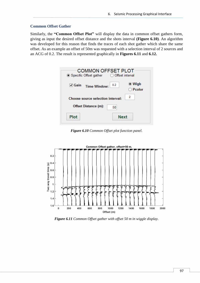
6. Seismic Processing Graphical Interface
97
Common Offset Gather
Similarly, the “Common Offset Plot” will display the data in common offset gathers form,
giving as input the desired offset distance and the shots interval (Figure 6.10). An algorithm
was developed for this reason that finds the traces of each shot gather which share the same
offset. As an example an offset of 50m was requested with a selection interval of 2 sources and
an ACG of 0.2. The result is represented graphically in Figures 6.11 and 6.12.
Figure 6.10 Common Offset plot function panel.
Figure 6.11 Common Offset gather with offset 50 m in wiggle display.
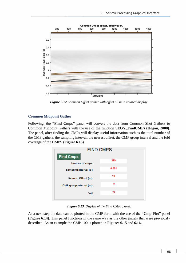
6. Seismic Processing Graphical Interface
98
Figure 6.12 Common Offset gather with offset 50 m in colored display.
Common Midpoint Gather
Following, the “Find Cmps” panel will convert the data from Common Shot Gathers to
Common Midpoint Gathers with the use of the function SEGY_FindCMPs (Hogan, 2008).
The panel, after finding the CMPs will display useful information such as the total number of
the CMP gathers, the sampling interval, the nearest offset, the CMP group interval and the fold
coverage of the CMPS (Figure 6.13).
Figure 6.13. Display of the Find CMPs panel.
As a next step the data can be plotted in the CMP form with the use of the “Cmp Plot” panel
(Figure 6.14). This panel functions in the same way as the other panels that were previously
described. As an example the CMP 100 is plotted in Figures 6.15 and 6.16.

6. Seismic Processing Graphical Interface
99
Figure 6.14 Display of the CMP Plot function panel.
Figure 6.15 Common Midpoint Gather number 100 in wiggle display.

6. Seismic Processing Graphical Interface
100
Figure 6.16 Common Midpoint Gather number 100 in colored display.
6.2 Signal Processing Analysis
The next available panels are associated with the signal processing analysis of the seismic data,
presented analytically on chapter 5. The first panel, named “FK filter” (Figure 6.17) applies
FK filtering on the data with the use of the function fk_filter (Tzanis, 2005). The function
allows the user to design a band pass filter of the data on the screen (in frequency domain) and
after applying the filter, transforms back the data to time domain with inverse Fourier transform.
An example of the FK filter application on CMP gather 100 is shown on Figures 6.18 and 6.19.
Figure 6.17 Fk filter function panel.
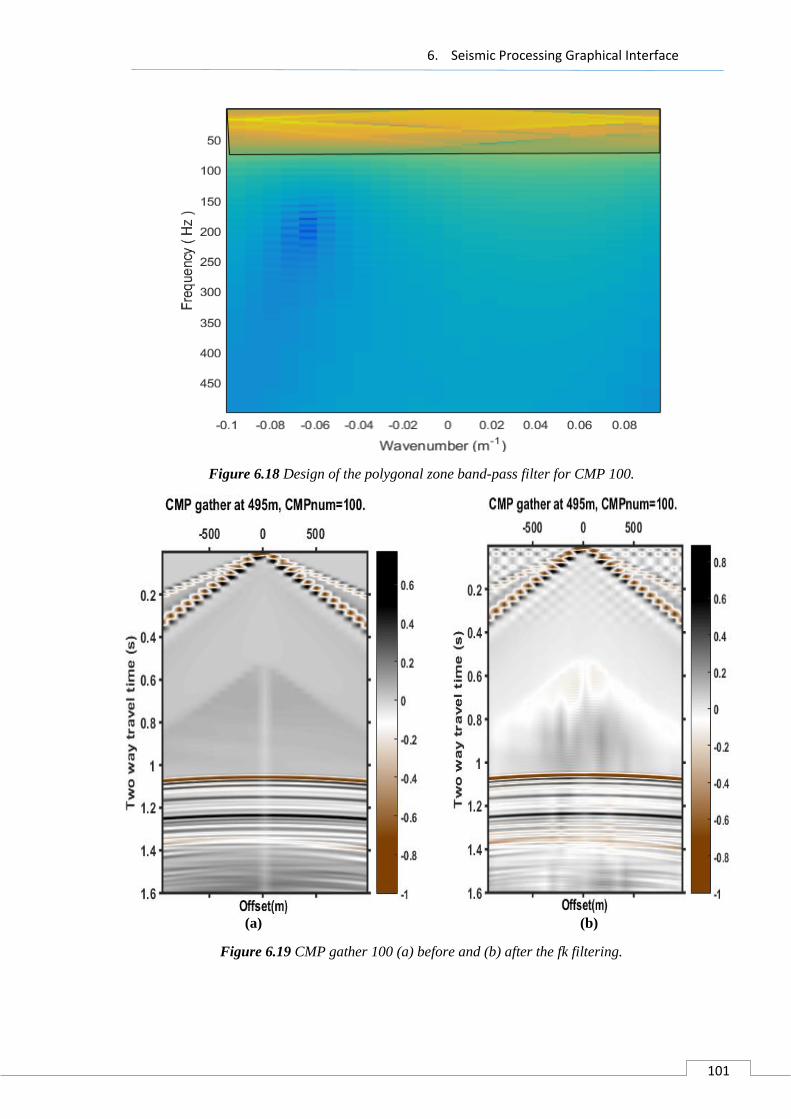
6. Seismic Processing Graphical Interface
101
Figure 6.18 Design of the polygonal zone band-pass filter for CMP 100.
(a) (b)
Figure 6.19 CMP gather 100 (a) before and (b) after the fk filtering.
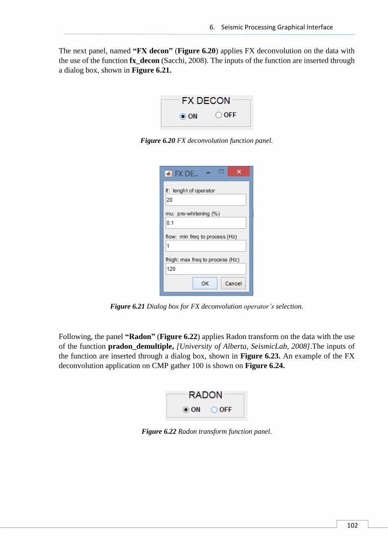
6. Seismic Processing Graphical Interface
102
The next panel, named “FX decon” (Figure 6.20) applies FX deconvolution on the data with
the use of the function fx_decon (Sacchi, 2008). The inputs of the function are inserted through
a dialog box, shown in Figure 6.21.
Figure 6.20 FX deconvolution function panel.
Figure 6.21 Dialog box for FX deconvolution operator’s selection.
Following, the panel “Radon” (Figure 6.22) applies Radon transform on the data with the use
of the function pradon_demultiple, [University of Alberta, SeismicLab, 2008].The inputs of
the function are inserted through a dialog box, shown in Figure 6.23. An example of the FX
deconvolution application on CMP gather 100 is shown on Figure 6.24.
Figure 6.22 Radon transform function panel.

6. Seismic Processing Graphical Interface
103
Figure 6.23 Dialog box for Radon transform operator’s selection.
(a) (b)
Figure 6.24 CMP gather 100 (a) before and (b) after the radon transform.
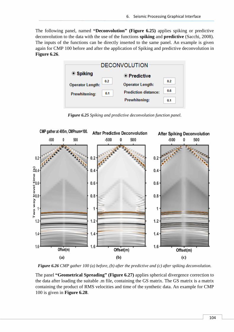
6. Seismic Processing Graphical Interface
104
The following panel, named “Deconvolution” (Figure 6.25) applies spiking or predictive
deconvolution to the data with the use of the functions spiking and predictive (Sacchi, 2008).
The inputs of the functions can be directly inserted to the same panel. An example is given
again for CMP 100 before and after the application of Spiking and predictive deconvolution in
Figure 6.26.
Figure 6.25 Spiking and predictive deconvolution function panel.
(a) (b) (c)
Figure 6.26 CMP gather 100 (a) before, (b) after the predictive and (c) after spiking deconvolution.
The panel “Geometrical Spreading” (Figure 6.27) applies spherical divergence correction to
the data after loading the suitable .m file, containing the GS matrix. The GS matrix is a matrix
containing the product of RMS velocities and time of the synthetic data. An example for CMP
100 is given in Figure 6.28.
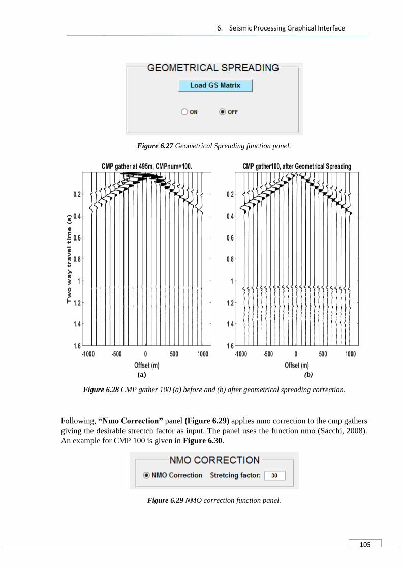
6. Seismic Processing Graphical Interface
105
Figure 6.27 Geometrical Spreading function panel.
(a) (b)
Figure 6.28 CMP gather 100 (a) before and (b) after geometrical spreading correction.
Following, “Nmo Correction” panel (Figure 6.29) applies nmo correction to the cmp gathers
giving the desirable strectch factor as input. The panel uses the function nmo (Sacchi, 2008).
An example for CMP 100 is given in Figure 6.30.
Figure 6.29 NMO correction function panel.

6. Seismic Processing Graphical Interface
106
(a) (b)
Figure 6.30 CMP gather 100 (a) before and (b) after nmo correction.
6.3 Stack section
In the “Stack Section” panel (Figure 6.31), all the CMP gathers of the model are read (or
loaded, if they have been previously read) and summed in order to create the stack section of
the model. The stack section panel gives to user the ability to apply different processing
schemes on the pre-stacked and the post-stacked data. A partial stack of the data is also available
by giving the desired initial and final traces of the cmp gather. In Figure 6.32 an example is
given for the full stack section of the model, before and after the post stack processing.
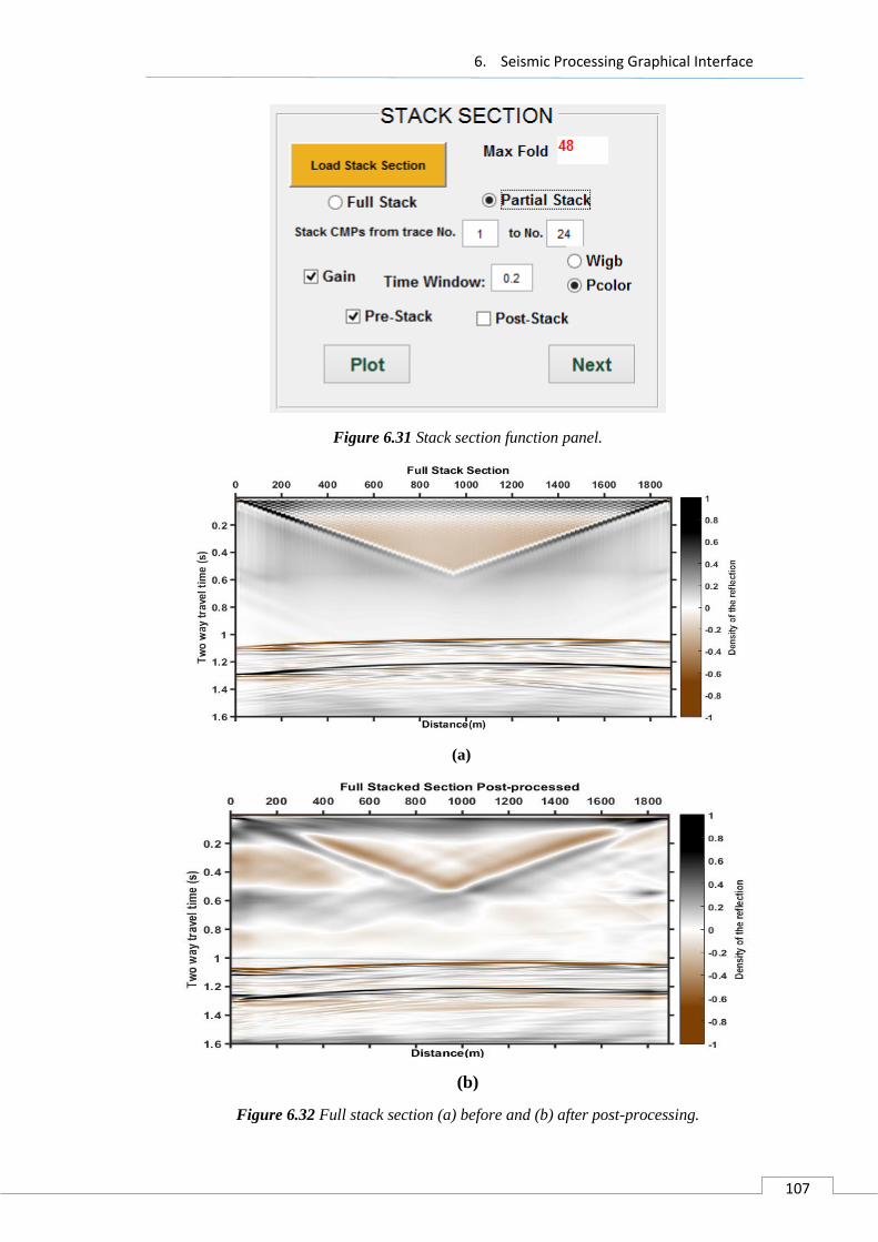
6. Seismic Processing Graphical Interface
107
Figure 6.31 Stack section function panel.
(a)
(b)
Figure 6.32 Full stack section (a) before and (b) after post-processing.
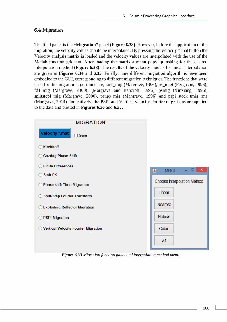
6. Seismic Processing Graphical Interface
108
6.4 Migration
The final panel is the “Migration” panel (Figure 6.33). However, before the application of the
migration, the velocity values should be interpolated. By pressing the Velocity *.mat button the
Velocity analysis matrix is loaded and the velocity values are interpolated with the use of the
Matlab function griddata. After loading the matrix a menu pops up, asking for the desired
interpolation method (Figure 6.33). The results of the velocity models for linear interpolation
are given in Figures 6.34 and 6.35. Finally, nine different migration algorithms have been
embodied to the GUI, corresponding to different migration techniques. The functions that were
used for the migration algorithms are, kirk_mig (Margrave, 1996), ps_migt (Ferguson, 1996),
fd15mig (Margrave, 2000), (Margrave and Bancroft, 1996), psmig (Xinxiang, 1996),
splitstepf_mig (Margrave, 2000), psnps_mig (Margrave, 1996) and pspi_stack_tmig_rms
(Margrave, 2014). Indicatively, the PSPI and Vertical velocity Fourier migrations are applied
to the data and plotted in Figures 6.36 and 6.37.
Figure 6.33 Migration function panel and interpolation method menu.
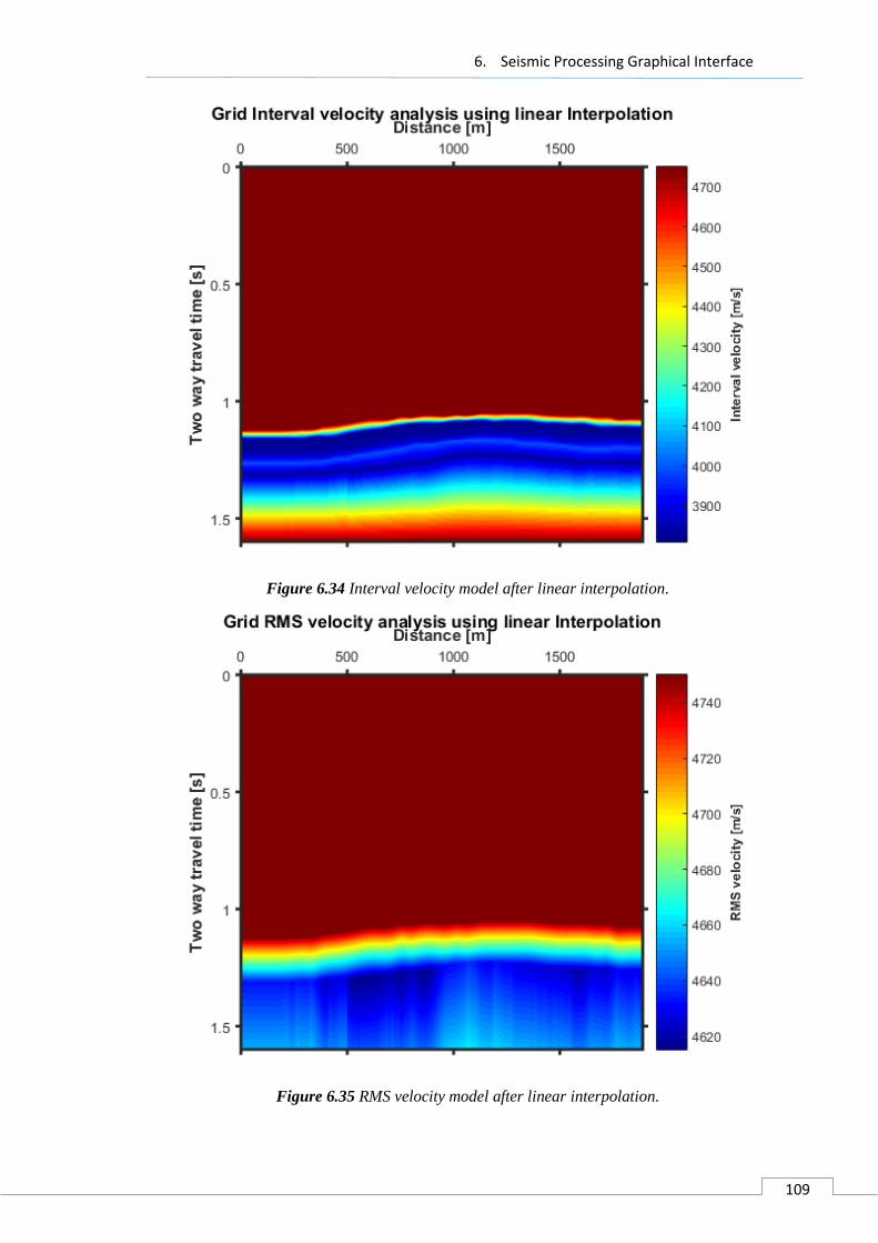
6. Seismic Processing Graphical Interface
109
Figure 6.34 Interval velocity model after linear interpolation.
Figure 6.35 RMS velocity model after linear interpolation.
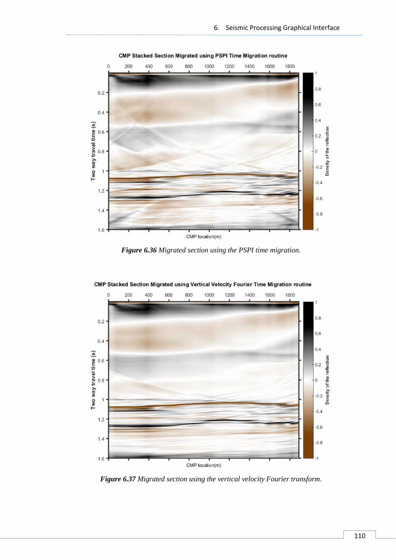
6. Seismic Processing Graphical Interface
110
Figure 6.36 Migrated section using the PSPI time migration.
Figure 6.37 Migrated section using the vertical velocity Fourier transform.

6. Seismic Processing Graphical Interface
111
6.5 Plotting tools
In this final part the different plotting features of the GUI are analysed. The “COLORED
WIGGLE” panel (Figure 6.38) allows the wiggle plots to be colorized. For the colored wiggle
the function wiggle was used (Portugal, 2012). If the colored option is chosen the wiggle plot
will be presented with blue color for the negative amplitudes and red color for the positive
amplitudes as shown in Figures 6.39 and 6.40.
Figure 6.38 Wiggle type selection panel.
(a) (b)
Figure 6.39 Wiggle plot of CMP gather 100 (a) with and (b) without colorized amplitudes.
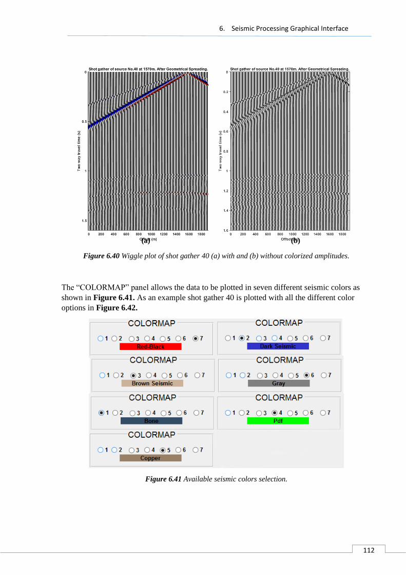
6. Seismic Processing Graphical Interface
112
(a) (b)
Figure 6.40 Wiggle plot of shot gather 40 (a) with and (b) without colorized amplitudes.
The “COLORMAP” panel allows the data to be plotted in seven different seismic colors as
shown in Figure 6.41. As an example shot gather 40 is plotted with all the different color
options in Figure 6.42.
Figure 6.41 Available seismic colors selection.
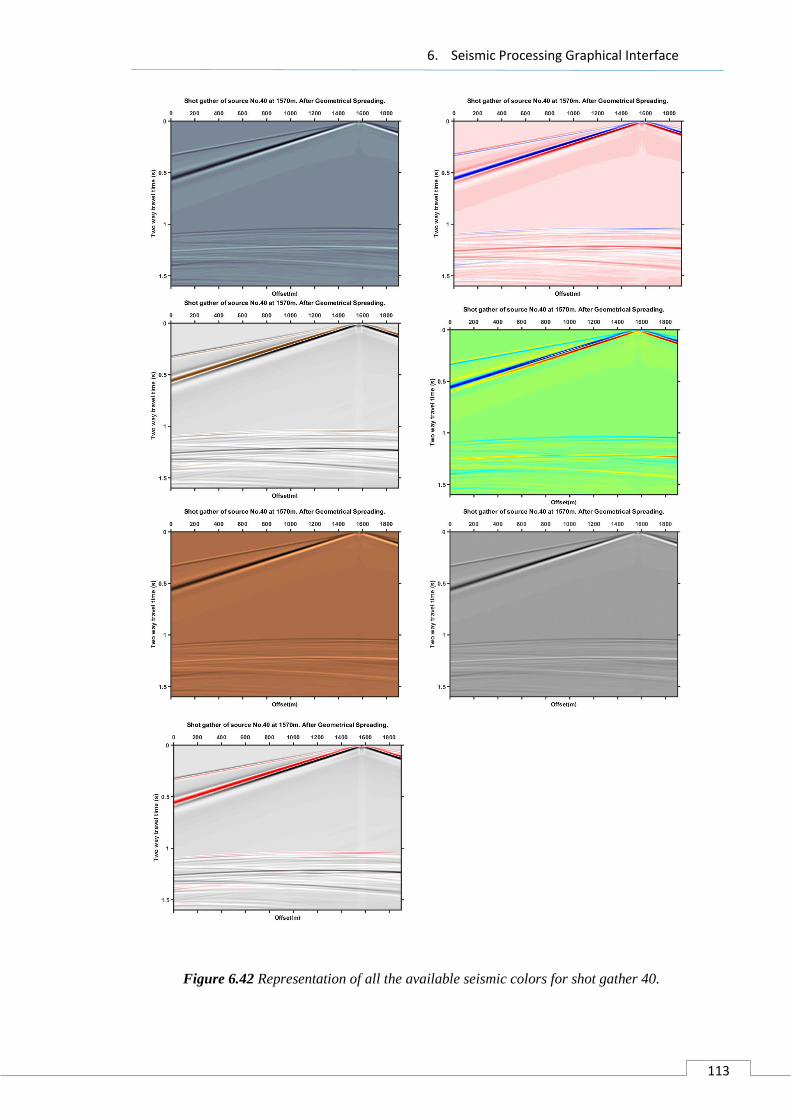
6. Seismic Processing Graphical Interface
113
Figure 6.42 Representation of all the available seismic colors for shot gather 40.
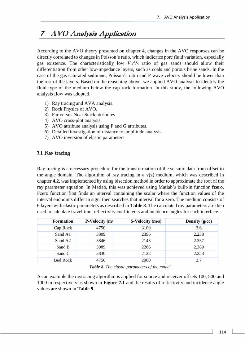
7. AVO Analysis Application
114
7 AVO Analysis Application
According to the AVO theory presented on chapter 4, changes in the AVO responses can be
directly correlated to changes in Poisson’s ratio, which indicates pore fluid variation, especially
gas existence. The characteristically low VP/VS ratio of gas sands should allow their
differentiation from other low-impedance layers, such as coals and porous brine sands. In the
case of the gas-saturated sediment, Poisson’s ratio and P-wave velocity should be lower than
the rest of the layers. Based on the reasoning above, we applied AVO analysis to identify the
fluid type of the medium below the cap rock formation. In this study, the following AVO
analysis flow was adopted.
1) Ray tracing and AVA analysis.
2) Rock Physics of AVO.
3) Far versus Near Stack attributes.
4) AVO cross-plot analysis.
5) AVO attribute analysis using P and G attributes.
6) Detailed investigation of distance to amplitude analysis.
7) AVO inversion of elastic parameters.
7.1 Ray tracing
Ray tracing is a necessary procedure for the transformation of the seismic data from offset to
the angle domain. The algorithm of ray tracing in a v(z) medium, which was described in
chapter 4.2, was implemented by using bisection method in order to approximate the root of the
ray parameter equation. In Matlab, this was achieved using Matlab’s built-in function fzero.
Fzero function first finds an interval containing the scalar where the function values of the
interval endpoints differ in sign, then searches that interval for a zero. The medium consists of
6 layers with elastic parameters as described in Table 8. The calculated ray parameters are then
used to calculate traveltime, reflectivity coefficients and incidence angles for each interface.
Formation P-Velocity (m/s) S-Velocity (m/s) Density (g/cc)
Cap Rock 4750 3100 3.6
Sand A1 3809 2396 2.238
Sand A2 3846 2143 2.357
Sand B 3989 2266 2.389
Sand C 3830 2128 2.353
Bed Rock 4750 2900 2.7
Table 8. The elastic parameters of the model.
As an example the raytracing algorithm is applied for source and receiver offsets 100, 500 and
1000 m respectively as shown in Figure 7.1 and the results of reflectivity and incidence angle
values are shown in Table 9.
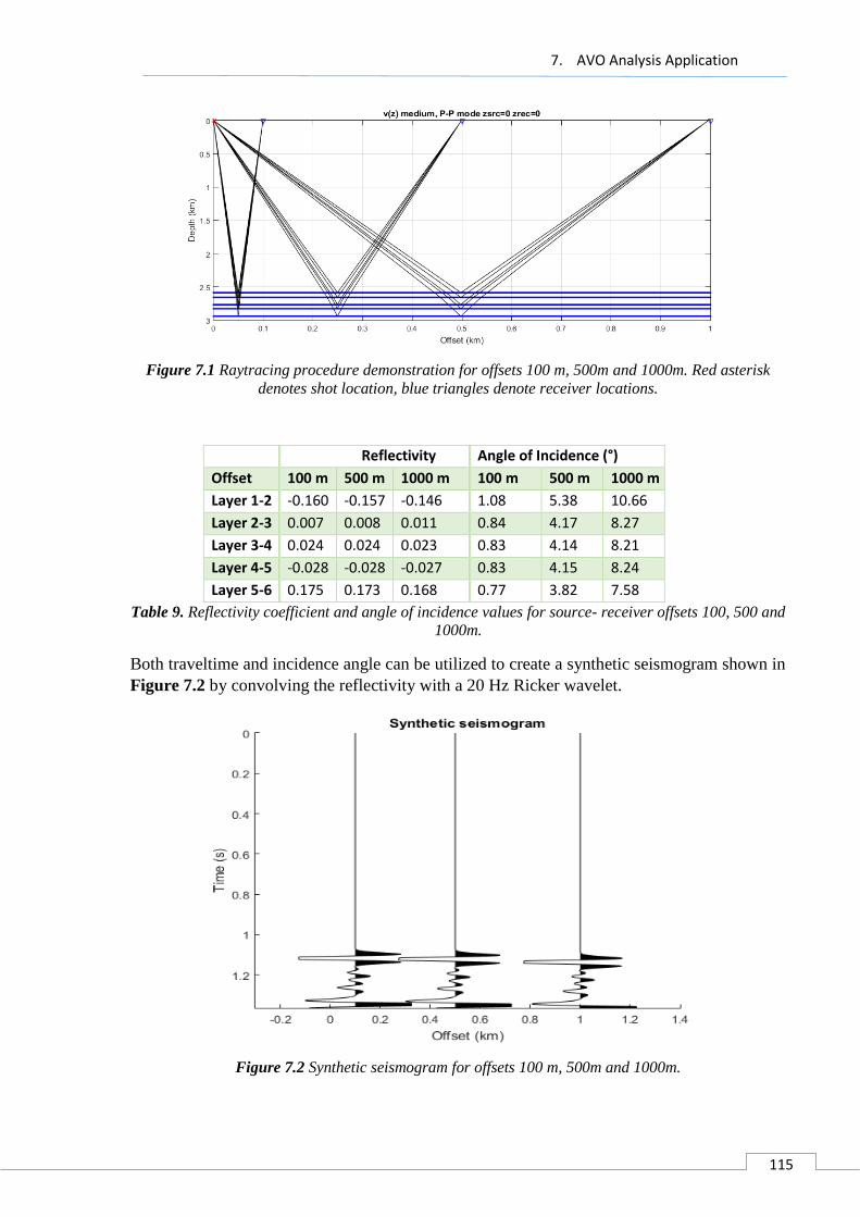
7. AVO Analysis Application
115
Figure 7.1 Raytracing procedure demonstration for offsets 100 m, 500m and 1000m. Red asterisk
denotes shot location, blue triangles denote receiver locations.
Reflectivity Angle of Incidence (°)
Offset 100 m 500 m 1000 m 100 m 500 m 1000 m
Layer 1-2 -0.160 -0.157 -0.146 1.08 5.38 10.66
Layer 2-3 0.007 0.008 0.011 0.84 4.17 8.27
Layer 3-4 0.024 0.024 0.023 0.83 4.14 8.21
Layer 4-5 -0.028 -0.028 -0.027 0.83 4.15 8.24
Layer 5-6 0.175 0.173 0.168 0.77 3.82 7.58
Table 9. Reflectivity coefficient and angle of incidence values for source- receiver offsets 100, 500 and
1000m.
Both traveltime and incidence angle can be utilized to create a synthetic seismogram shown in
Figure 7.2 by convolving the reflectivity with a 20 Hz Ricker wavelet.
Figure 7.2 Synthetic seismogram for offsets 100 m, 500m and 1000m.
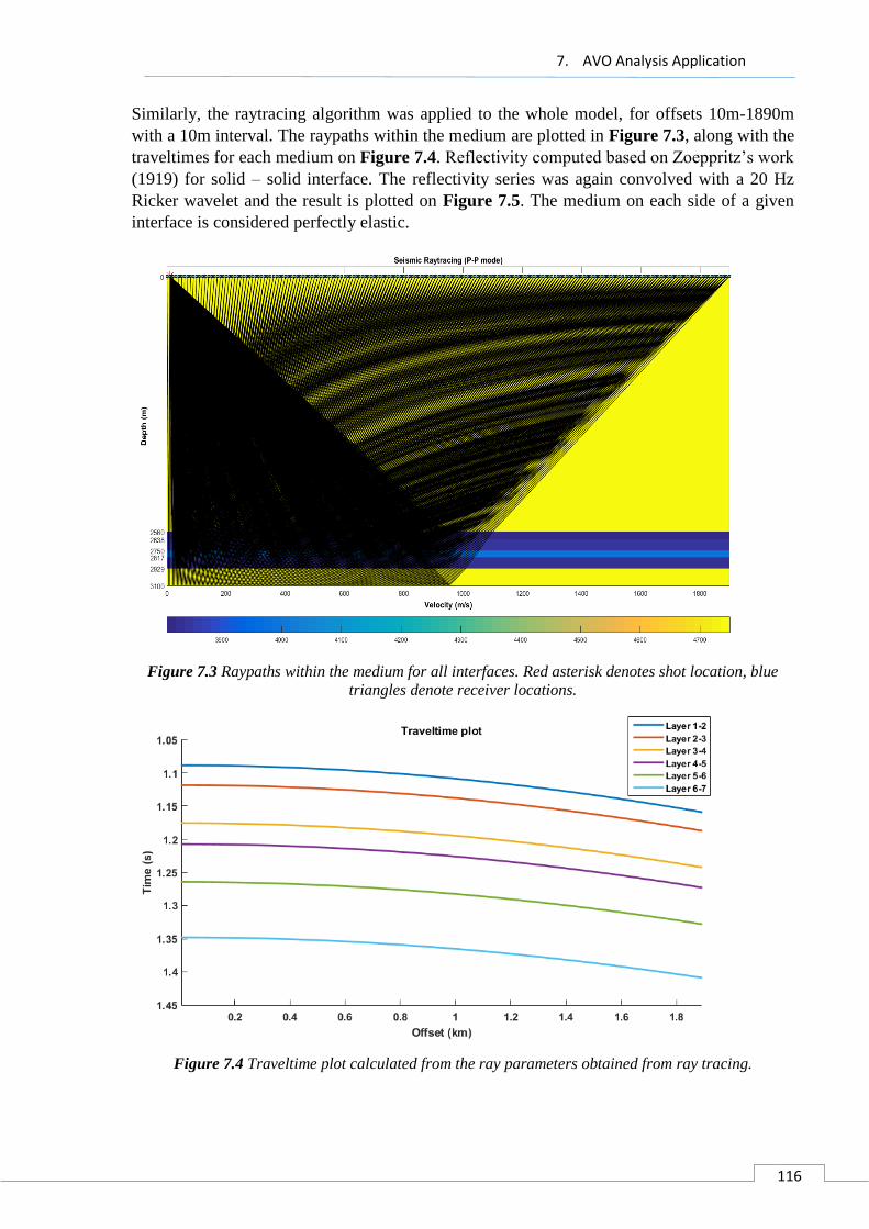
7. AVO Analysis Application
116
Similarly, the raytracing algorithm was applied to the whole model, for offsets 10m-1890m
with a 10m interval. The raypaths within the medium are plotted in Figure 7.3, along with the
traveltimes for each medium on Figure 7.4. Reflectivity computed based on Zoeppritz’s work
(1919) for solid – solid interface. The reflectivity series was again convolved with a 20 Hz
Ricker wavelet and the result is plotted on Figure 7.5. The medium on each side of a given
interface is considered perfectly elastic.
Figure 7.3 Raypaths within the medium for all interfaces. Red asterisk denotes shot location, blue
triangles denote receiver locations.
Figure 7.4 Traveltime plot calculated from the ray parameters obtained from ray tracing.

7. AVO Analysis Application
117
Figure 7.5 Synthetic seismogram created by convolving the reflectivity calculated from incidence
angle with 20 Hz Ricker wavelet.
Judging from Figure 7.5 the shallower interface between the overburden and the reservoir,
presents highly negative amplitudes, while the deeper interface presents highly positive
amplitudes. The intermediate interfaces have low amplitudes and are not easily observed. This
behaviour can be confirmed, by analysing the convolved synthetic trace, separately, for each
layer (Figure 7.6).
Figure 7.6 Reflectivity series of each layer convolved with a 20 Hz Ricker wavelet, along with the
overall synthetic trace.

7. AVO Analysis Application
118
7.2 Rock Physics of AVO
Rock Physics represents the link between geologic reservoir parameters (e.g., porosity, clay
content, sorting, lithology, saturation) and seismic properties (e.g., VP/VS, density, elastic
moduli). Rock physics models can be used to interpret observed sonic and seismic velocities in
terms of reservoir parameters. These models can also be used to estimate expected seismic
properties from observed reservoir properties in order to interpret the seismic response (AVO)
away from the well.
A typical task in a Rock Physics study is to calculate AVO attributes from the well logs and
cross-plot various attributes from selected geologic units. These cross-plots are used to:
understand how the rock properties are related
determine the rock properties in various lithologies in the area
determine the sensitivity of various attributes to fluid effects
contribute velocity constraints such as mudrock line values to AVO analysis of
seismic data.
contribute to interpretation of attribute sections
Using the function logsyn in Matlab the elastic parameters of the model were converted to
synthetic logs. Synthetic log for P sonic, S sonic, density and Poisson’s ratio were estimated as
shown in Figure 7.7.
Figure 7.7 P sonic, S Sonic, and density synthetic log from the lithology model

7. AVO Analysis Application
119
The synthetics logs were then used for the crossplots of Vp-Vs, Vp/Vs-Vp,Vp/Vs-Vs and
Vp/Vs-Poisson’s Ratio as shown in Figure 7.8.
Figure 7.8 Cross plot of physical rock properties from the lithology model.
The crossplot of Vp-Vs shows a positive indicator of gas presence, since there are data points
deviating from the mudrock line. Specifically, those data points have a trend slightly shifted
upwards of the mudrock line. This behaviour as presented in Figure 4.12 of chapter 4 is an
indicator of gas saturation. The gas presence is also confirmed by the low Vp/Vs ratios of data
points in the Vp/Vs-Vp and Vp/Vs-Vs crossplots, which are deviating from the basic trend line.
Gas
Gas
Gas

7. AVO Analysis Application
120
7.3 AVO crossplot analysis
AVO crossplots are a simple and elegant way of representing AVO data. Offset variations in
amplitude for reflecting interfaces are represented as single points on a crossplot of intercept
and gradient. The advantage of this type of plot is that a great deal of information can be
presented and trends can be observed in the data that would be impossible to see with a standard
offset (or angle) versus amplitude plot. The crossplot is an ideal way of examining differences
in AVO responses that may be related to lithologic or fluid-type variations.
Commonly used techniques for revealing these differences include color-coding samples from
the crossplot and using this as an overlay to a seismic display or creating linear combinations
of intercept (R0) and gradient (G).
Before applying the AVO crossplot analysis the reflection coeffcients of the model are
calculated using Hilterman, Shuey, Bortfeld and Aki Richard approximations with the function
ava_approximation [E. Rietsch, 2003]. The reflection coefficients are plotted against the angle
of incidence (AVA response) for the different approximations (Figure 7.9).
Figure 7.9 Refflection coefficients versus angle of incidence, using Hilterman, Shuey, Bortfeld and
Aki-Richard approximations for the five different layers of the model.
The Hilterman approximation gives more pessimistic values for the reflection coefficients,
compared to the other methods, but is considered more reliable since it takes into account the
Poisson’s ratio of each interface. Thus, the AVA response is plotted again using only the
Hilterman approximation in Figure 7.10.

7. AVO Analysis Application
121
Figure 7.10 AVA response using Hilterman approximation for the five interfaces of the model.
Comparing Figure 7.10 with the Figure 4.13 of AVO classification each medium of the model
can be categorized to an AVO class as shown in Table 10.
Medium AVO class
1: Layers 1-2 IV
2: Layers 2-3 Flatspot
3: Layers 3-4 II
4: Layers 4-5 IV
5: Layers 5-6 I Table 10. AVO classification of the model’s interfaces.
In Figure 7.11 the reflection coefficients are plotted against the square sin of the angle of
incidence, giving the same results with Figure 7.10, but in a more linear form.
Figure 7.11 Reflection coefficients versus the square sin of the angle of incidence for the five
interfaces of the model.
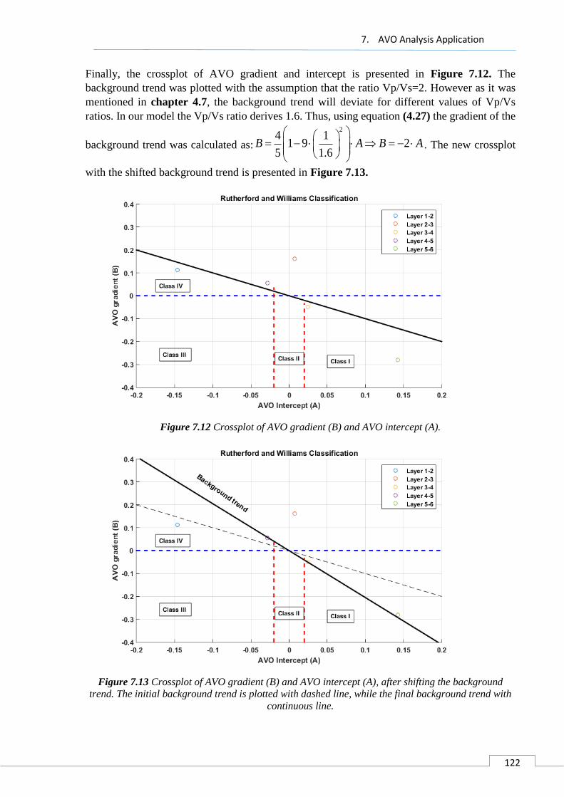
7. AVO Analysis Application
122
Finally, the crossplot of AVO gradient and intercept is presented in Figure 7.12. The
background trend was plotted with the assumption that the ratio Vp/Vs=2. However as it was
mentioned in chapter 4.7, the background trend will deviate for different values of Vp/Vs
ratios. In our model the Vp/Vs ratio derives 1.6. Thus, using equation (4.27) the gradient of the
background trend was calculated as:
24 1
1 9 25 1.6
B A B A
. The new crossplot
with the shifted background trend is presented in Figure 7.13.
Figure 7.12 Crossplot of AVO gradient (B) and AVO intercept (A).
Figure 7.13 Crossplot of AVO gradient (B) and AVO intercept (A), after shifting the background
trend. The initial background trend is plotted with dashed line, while the final background trend with
continuous line.
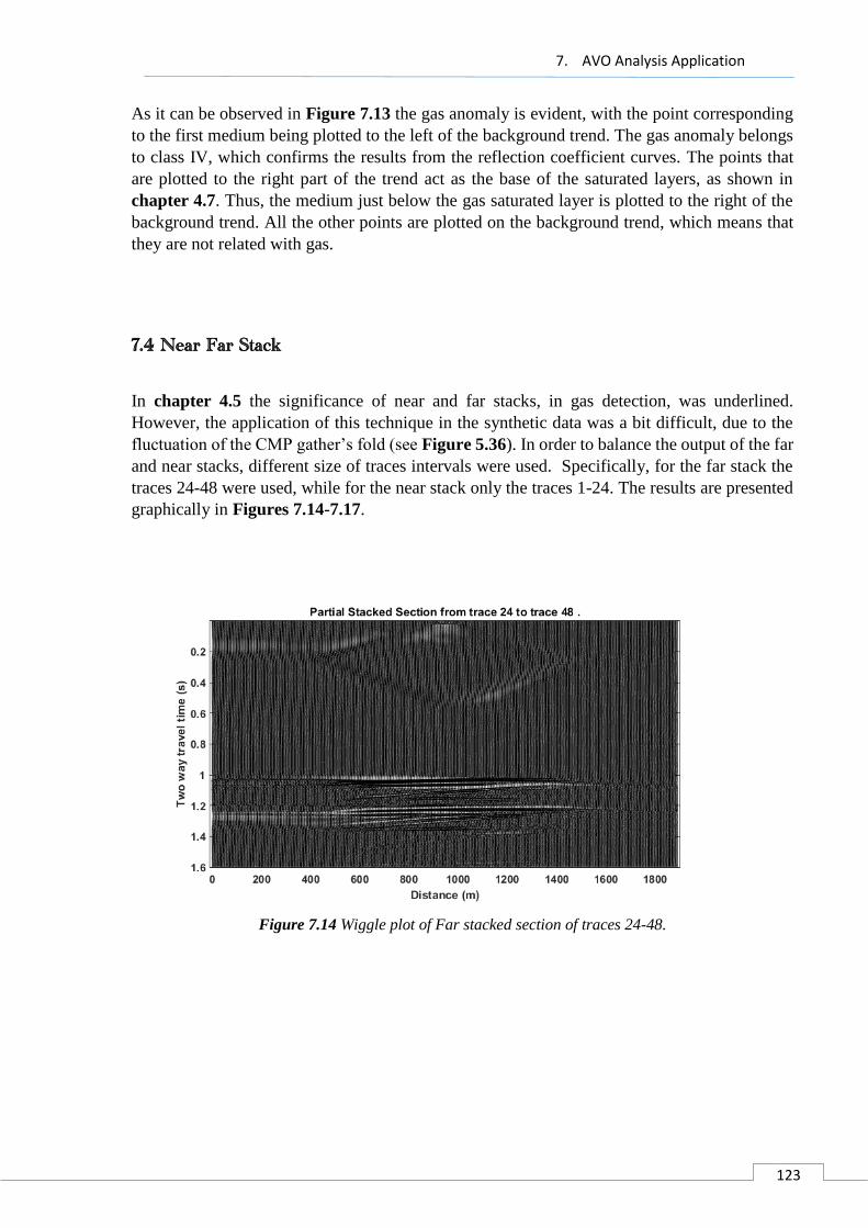
7. AVO Analysis Application
123
As it can be observed in Figure 7.13 the gas anomaly is evident, with the point corresponding
to the first medium being plotted to the left of the background trend. The gas anomaly belongs
to class IV, which confirms the results from the reflection coefficient curves. The points that
are plotted to the right part of the trend act as the base of the saturated layers, as shown in
chapter 4.7. Thus, the medium just below the gas saturated layer is plotted to the right of the
background trend. All the other points are plotted on the background trend, which means that
they are not related with gas.
7.4 Near Far Stack
In chapter 4.5 the significance of near and far stacks, in gas detection, was underlined.
However, the application of this technique in the synthetic data was a bit difficult, due to the
fluctuation of the CMP gather’s fold (see Figure 5.36). In order to balance the output of the far
and near stacks, different size of traces intervals were used. Specifically, for the far stack the
traces 24-48 were used, while for the near stack only the traces 1-24. The results are presented
graphically in Figures 7.14-7.17.
Figure 7.14 Wiggle plot of Far stacked section of traces 24-48.
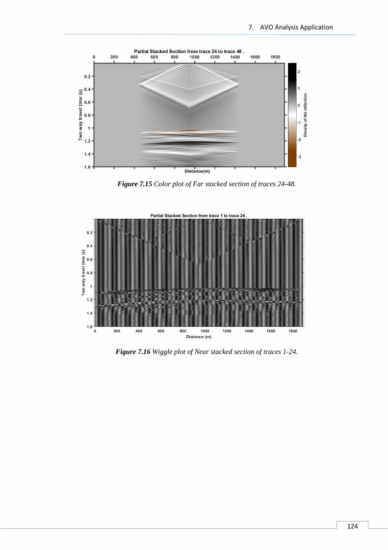
7. AVO Analysis Application
124
Figure 7.15 Color plot of Far stacked section of traces 24-48.
Figure 7.16 Wiggle plot of Near stacked section of traces 1-24.
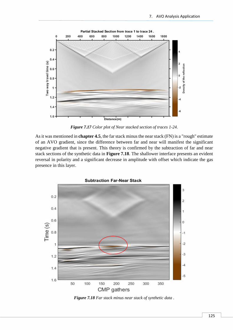
7. AVO Analysis Application
125
Figure 7.17 Color plot of Near stacked section of traces 1-24.
As it was mentioned in chapter 4.5, the far stack minus the near stack (FN) is a "rough" estimate
of an AVO gradient, since the difference between far and near will manifest the significant
negative gradient that is present. This theory is confirmed by the subtraction of far and near
stack sections of the synthetic data in Figure 7.18. The shallower interface presents an evident
reversal in polarity and a significant decrease in amplitude with offset which indicate the gas
presence in this layer.
Figure 7.18 Far stack minus near stack of synthetic data .

7. AVO Analysis Application
126
Furthermore, the crossploting of Near versus Far minus Near stack in Figure 7.19 gives almost
the same results with the gradient versus intercept crossplot. The shallower interface is plotted
on the left part of the plot, separately from the other interfaces, which again confirms the gas
presence in the specific medium.
Figure 7.19 Crossplot of Near versus Far minus Near stack.
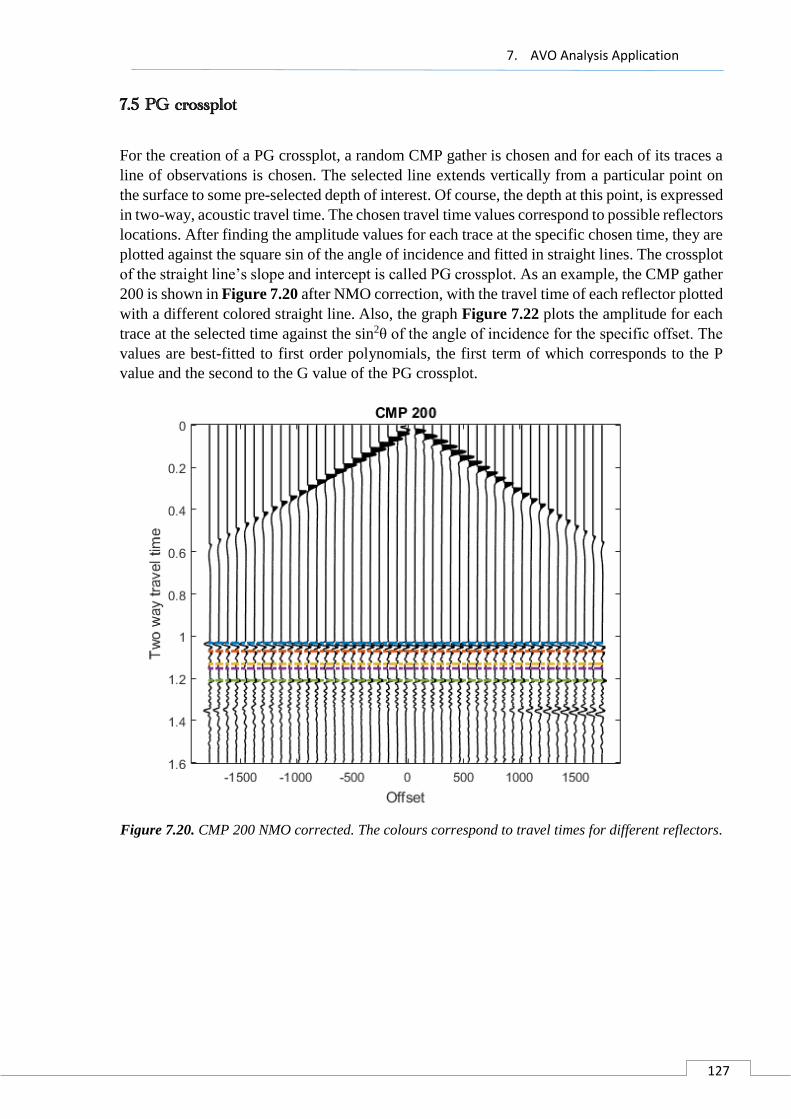
7. AVO Analysis Application
127
7.5 PG crossplot
For the creation of a PG crossplot, a random CMP gather is chosen and for each of its traces a
line of observations is chosen. The selected line extends vertically from a particular point on
the surface to some pre-selected depth of interest. Of course, the depth at this point, is expressed
in two-way, acoustic travel time. The chosen travel time values correspond to possible reflectors
locations. After finding the amplitude values for each trace at the specific chosen time, they are
plotted against the square sin of the angle of incidence and fitted in straight lines. The crossplot
of the straight line’s slope and intercept is called PG crossplot. As an example, the CMP gather
200 is shown in Figure 7.20 after NMO correction, with the travel time of each reflector plotted
with a different colored straight line. Also, the graph Figure 7.22 plots the amplitude for each
trace at the selected time against the sin2θ of the angle of incidence for the specific offset. The
values are best-fitted to first order polynomials, the first term of which corresponds to the P
value and the second to the G value of the PG crossplot.
Figure 7.20. CMP 200 NMO corrected. The colours correspond to travel times for different reflectors.
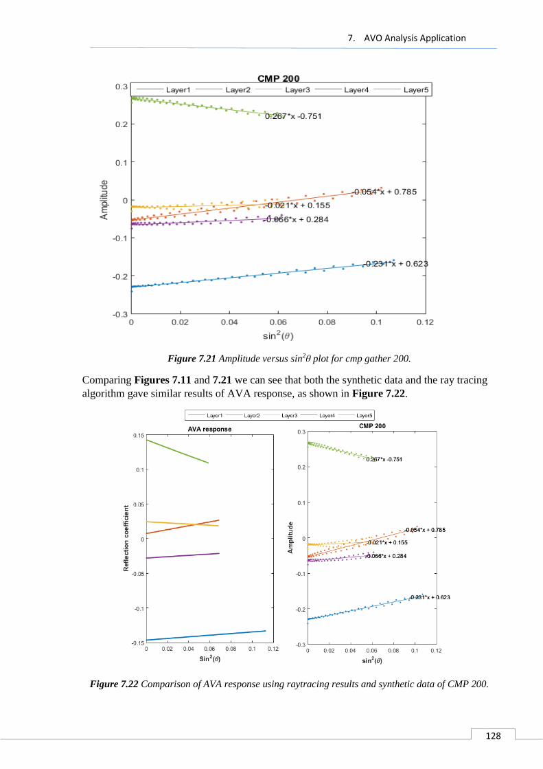
7. AVO Analysis Application
128
Figure 7.21 Amplitude versus sin2θ plot for cmp gather 200.
Comparing Figures 7.11 and 7.21 we can see that both the synthetic data and the ray tracing
algorithm gave similar results of AVA response, as shown in Figure 7.22.
Figure 7.22 Comparison of AVA response using raytracing results and synthetic data of CMP 200.
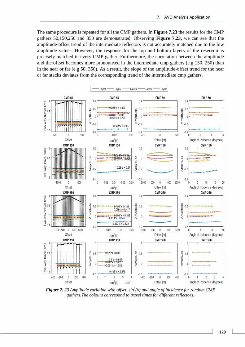
7. AVO Analysis Application
129
The same procedure is repeated for all the CMP gathers. In Figure 7.23 the results for the CMP
gathers 50,150,250 and 350 are demonstrated. Observing Figure 7.23, we can see that the
amplitude-offset trend of the intermediate reflectors is not accurately matched due to the low
amplitude values. However, the response for the top and bottom layers of the reservoir is
precisely matched in every CMP gather. Furthermore, the correlation between the amplitude
and the offset becomes more pronounced in the intermediate cmp gathers (e.g 150, 250) than
in the near or far (e.g 50, 350). As a result, the slope of the amplitude-offset trend for the near
or far stacks deviates from the corresponding trend of the intermediate cmp gathers.
Figure 7. 23 Amplitude variation with offset, sin2(θ) and angle of incidence for random CMP
gathers.The colours correspond to travel times for different reflectors.
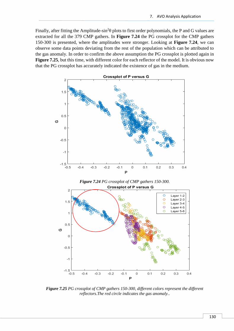
7. AVO Analysis Application
130
Finally, after fitting the Amplitude-sin2θ plots to first order polynomials, the P and G values are
extracted for all the 379 CMP gathers. In Figure 7.24 the PG crossplot for the CMP gathers
150-300 is presented, where the amplitudes were stronger. Looking at Figure 7.24, we can
observe some data points deviating from the rest of the population which can be attributed to
the gas anomaly. In order to confirm the above assumption the PG crossplot is plotted again in
Figure 7.25, but this time, with different color for each reflector of the model. It is obvious now
that the PG crossplot has accurately indicated the existence of gas in the medium.
Figure 7.24 PG crossplot of CMP gathers 150-300.
Figure 7.25 PG crossplot of CMP gathers 150-300, different colors represent the different
reflectors.The red circle indicates the gas anomaly..
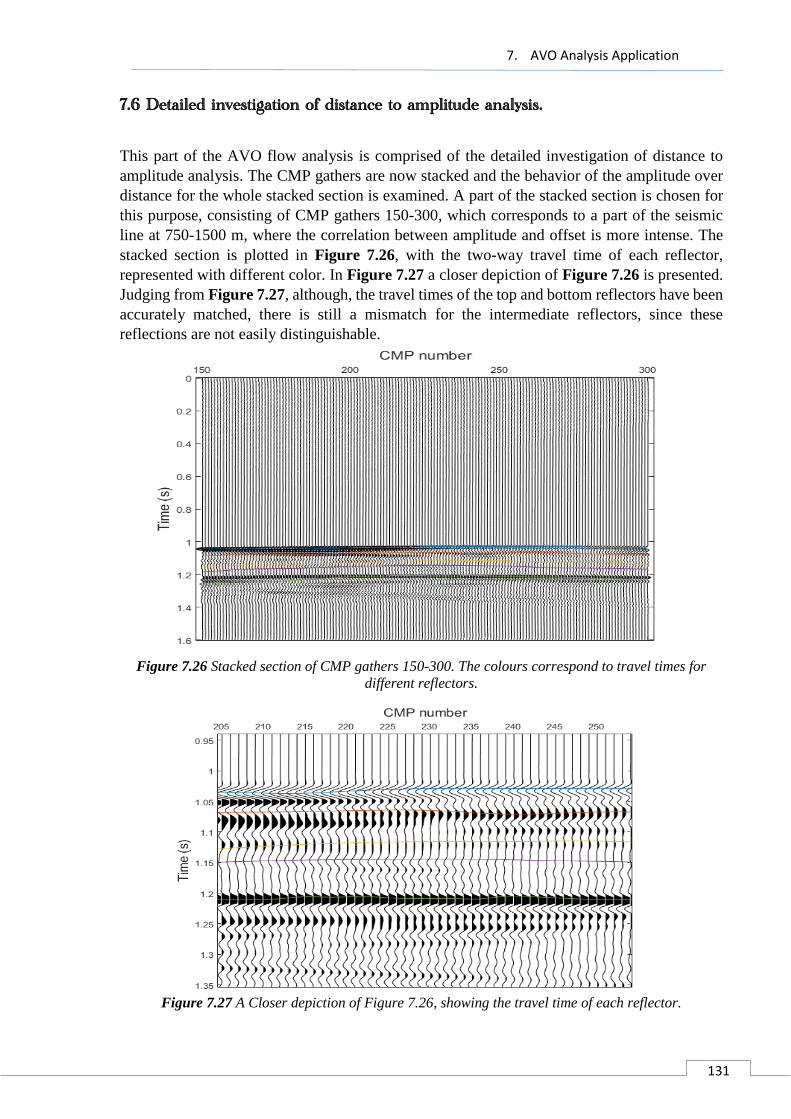
7. AVO Analysis Application
131
7.6 Detailed investigation of distance to amplitude analysis.
This part of the AVO flow analysis is comprised of the detailed investigation of distance to
amplitude analysis. The CMP gathers are now stacked and the behavior of the amplitude over
distance for the whole stacked section is examined. A part of the stacked section is chosen for
this purpose, consisting of CMP gathers 150-300, which corresponds to a part of the seismic
line at 750-1500 m, where the correlation between amplitude and offset is more intense. The
stacked section is plotted in Figure 7.26, with the two-way travel time of each reflector,
represented with different color. In Figure 7.27 a closer depiction of Figure 7.26 is presented.
Judging from Figure 7.27, although, the travel times of the top and bottom reflectors have been
accurately matched, there is still a mismatch for the intermediate reflectors, since these
reflections are not easily distinguishable.
Figure 7.26 Stacked section of CMP gathers 150-300. The colours correspond to travel times for
different reflectors.
Figure 7.27 A Closer depiction of Figure 7.26, showing the travel time of each reflector.
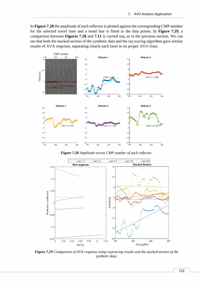
7. AVO Analysis Application
132
In Figure 7.28 the amplitude of each reflector is plotted against the corresponding CMP number
for the selected travel time and a trend line is fitted to the data points. In Figure 7.29, a
comparison between Figures 7.28 and 7.11 is carried out, as in the previous section. We can
see that both the stacked section of the synthetic data and the ray tracing algorithm gave similar
results of AVA response, separating clearly each layer to its proper AVO class.
Figure 7.28 Amplitude versus CMP number of each reflector.
Figure 7.29 Comparison of AVA response using raytracing results and the stacked section of the
synthetic data.

7. AVO Analysis Application
133
7.7 AVO inversion of elastic parameters
In the final part of the AVO flow analysis, AVO inversion is applied to the elastic parameters
of the model, using Shuey’s (1985) approximation to the exact expression of the particle
displacement reflection and transmission coefficients (the relative displacement amplitudes).
Since, we are only using 2-term approximation, which is valid only for incidence angle below
30 degree, the maximum incidence angle used in the inversion is set to 25 degree. The algorithm
of the avo inversion is given as inputs, the desired error tolerance, the angles of incidence (lower
than 25°) and the reflection coefficients of the model along with an initial assumption for the
poisson’s ratio of the upper and lower layers. A repetitive loop is then applied, where the partial
derivative of the reflection coefficient is calculated, using its Jacobian matrix with the function
derive_avo (Mudianto, 2007). Then, an increment parameter for the Poisson’s ratio is
calculated with the function marquardt (Mudianto, 2007). The function applies a least squares
inversion algorithm, using Marquardt – Levenberg optimization method (Lines and Treitel,
1984). The inverted value of the Poisson’s ratio derives as the sum of the initially assumed
value of Poisson’s ratio plus the increment parameter. The error tolerance id then checked for
every loop. Finally, knowing the inverted values of the Poisson’s ratio, the inverted values of
P-wave and S-wave velocities can be easily approximated, with the use of equations 5.1 and
5.8. Inversion result (Poisson’s ratio, P-wave velocity and S-wave velocity for each interface)
is then plotted on Figures 7.30-7.32, along with the true model.
Figure 7.30 S-wave velocity for true (red) and inverted (blue) models.

7. AVO Analysis Application
134
The matching between the true and inverted data is not pretty accurate for the P-wave and S-
wave velocities with the deviation ratio ranging from 10%-15%. Despite the deviation of the
values, the behaviour of the elastic parameters through depth is pretty similar for the true and
inverted data. Great differences are observed especially for the top and bottom formations
where the changes of the elastic parameters are more abrupt. The deviation of the true and
inverted values for the Poisson’s ratio are even higher with a deviation percentage of about
20%. These deviations can be attributed to the several assumptions and simplifications made
initially for the calculation of the model’s elastic parameters.
Figure 7.31 P-wave velocity for true (red) and inverted (blue) models.
Figure 7.32 Poisson's ratio for true (red) and inverted (blue) models.
8. Summary and Conclusion
135
8 Summary and Conclusion
This study was focused on an integrated approach of gas detection in the sandstone reservoir of
Prinos oil field, located in the northern Aegean Sea. The rock properties variation with depth in
the study area, were inferred from real well seismic logs (Fronimos, 1998). The geological
structure of the model was based on an East-West 2D geological plan of Prinos basin
(Michelakis, 2010). Furthermore, the top layer of the reservoir was considered to be 50%
saturated with gas, so, its elastic parameters were accordingly adjusted. The above information
were given as input to a synthetic data simulator (Applied Geophysics Laboratory of the
Technical University of Crete) in order to build low frequency synthetic seismograms.
Additionally, a signal processing graphical interface was build, in order to properly process the
synthetic data before the application of the AVO analysis. Finally, an analytical AVO analysis
flow was adapted for the processed seismic data which managed to successfully detect the
presence of gas in the gas saturated layer.
Despite the major limitations and simplifications that the model was based on (Gassmann fluid
replacement model, mudrock line and Lindseth density correlation), it still provides a robust
approach. The AVO signature is not dependent on the properties of the reservoir alone but also
on the overburden through which the seismic pulse propagates. As a result, fluid replacement
modeling needs to take into account not just the properties of the reservoir but the cap rock as
well. However, despite these simplistic assumptions and limitations the following conclusions
can be arrived at:
Combined with rock physical property analysis, petrophysical analysis, and geological
information, AVO modeling provides useful information in interpretation and thus
increases certainty in gas detection and reservoir characterization. It emphasizes the
influence of petrophysical rock properties on seismic rock properties.
Cross-plotting of rock properties indicate that reservoir sandstone is of high impedance
encased with in low impedance shale. Large drop in Poisson’s ratio for gas charged
reservoir sand allow utilization of AVO technique to characterize the reservoir.
The AVO anomaly in the target zone in the present case has been classified as class IV
anomaly on the basis of highly negative intercept and highly positive gradient
computed from the model.
The results taken from AVO analysis on the synthetic gathers show good correlation
with the results taken from the raytracing algorithm.
Cross-plot of Intercept versus Gradient from AVO analysis shows marked separation
of anomalous points from background trend (shale/wet sand) which has been identified
as calss IV AVO anomaly.
AVO modeling may be used as a complimentary tool with 3D seismic in reservoir
monitoring during production since the effects of changing saturation are less visible
on the stacked seismic data compared to the changes in the reflection coefficient as a
function of offset in the prestack domain
9. References
136
9 References
[1] Abdullatif, A. A. & Mousa W. A., (2011). Processing of Seismic Ref lection Data
Using MATLAB TM.
[2] Aki, K. and Richards, P. (1980). Quantitative seismology.
[3] Almutlaq, M., & Margrave, G. (2010). Tutorial: AVO inversion. Crewes.Org, 22, 1–
23.
[4] Arthur, J. M., & Lawton, D. C. (2011). Multicomponent AVO analysis of a single
thinning bed, 23(1996), 1–15.
[5] Avseth, P. (2010). Explorational Rock Physics – The Link Between Geological
Processes and Geophysical Observables. Petroleum Geoscience, pp.403-426.
[6] Avseth, P., Mukerji, T. and Mavko, G. (2005). Quantitative seismic interpretation.
Cambridge, UK: Cambridge University Press.
[7] Bagaini, C., Bunting, T., & El-emam, A. (2010). Land Seismic Techniques for High-
Quality Data, 28–39.
[8] Bhardwaj, B. M., Jambhekar, C. V, & Kandpal, M. C. (1985). Detection of gas in
sandstone reservoirs using AVO analysis in Cambay Basin.
[9] Carcione, J. M., Ursin, B. and Nordskag, J. I. (2007). Cross-property relations between
electrical conductivity and the seismic velocity of rocks.
[10] Castagna, J. P. (1985). Relationships between compressional-wave and shear-wave
velocities in clastic silicate rocks. Geophysics, 50(4), 571.
[11] Castagna, J. P., & Swan, H. W. (1997). Principles of AVO crossplotting. The Leading
Edge, 16(4), 337.
[12] Castagna, J. P., M. L. Batzle, and T. K. Kan, (1993), Rock physics – The link between
rock properties and AVO response, in J. P. Castagna and M. Backus, eds., Offset-
dependent reflectivity – Theory and practice of AVO analysis: Investigations in
Geophysics 8, 135–171.
[13] Castagna, J. P., Swan, H. W., & Foster, D. J. (1998). Framework for AVO gradient
and intercept interpretation. Geophysics, 63(3), 948.
[14] Chiburis, E., Leaney, S., Skidmore, C., Franck, C., & Mchugo, S. (1993). Hydrocarbon
detection with AVO. Oilfield Review, 5(1), 42–50.
[15] Dvorkin, J. P. (2008). Seismic Reflections of Rock Properties
9. References
137
[16] Fatti, J. L., Smith, G. C., Vail, P. J., Strauss, P. J., & Levitt, P. R. (1994). Detection of
gas in sandstone reservoirs using AVO analysis : A 3-D seismic case history using the
Geostack technique, 59(9), 1362–1376.
[17] Feng, H., & Bancroft, J. C. (2006). AVO principles, processing and inversion.
CREWES Research Report — Volume 18 (2006), 18, 1–19.
[18] Fronimos P. (1998). Examination of horizontal well’s location with the use of
geophysical loggings. Logging While Drilling.
[19] Guo, Q. (2014). Tuning, Avo, and Flat-Spot Effects in a Seismic Analysis of North
Sea.
[20] Han, D., Nur, a, & Morgani, D. (1986). De-hua Han*, A. Nur*, and Dale Morgani.
Geophysics, 51(Ii), 2093–2117.
[21] Hato, M. H., Namori, T. I., Ahar, A. B., & Atsuoka, T. M. (2004). Application of AVO
Analysis to Seismic Data for Detection of Gas below Methane Hydrate Stability Zone
in Nankai Trough Area, 54(1), 105–113.
[22] Hsu, K.J., (1972). Origin of saline giants: a critical review after the discovery of the
Mediterranean evaporite. Earth-Science Review, v. 8, pp.371-396.
[23] K. 0. Friedrichs and H. Lewy, “Uber die Eindeutigkeit und das Abhangigkeitsgebiet
der Losungen beim Anfangswertproblem hearer hyperbolischer
Differentialgleichungen,” Math. Ann. 98, 192-204 (1928).
[24] Kiomourtzi, P., Pasadakis, N. and A. Zelilidis, (2007). Geochemical Characterization
of Satellite Hydrocarbon Formations in Prinos-Kavala Basin (North Greece). Bull.
Geol. Soc. Greece, vol. XXXX, n., pp.839-850.
[25] Lee, M. W. (2015). Elastic velocities of partially gas-saturated unconsolidated
sediments Elastic velocities of partially gas-saturated unconsolidated sediments.
[26] Lines, L.R., and Treitel, (1984). A review of least-squares inversion and its application
to geophysical problems: Geophysical Prospecting, 32,159-186.
[27] Macleod, M. (n.d.). Shear Waves Shine Brightly, 2–15.
[28] Margrave, G. F. (2000). New seismic modelling facilities in Matlab. Report, 12, 1–
45.
[29] Mavko, G. The Rock Physics of AVO, Stanford Rock Physics Laboratory 302–326.
[30] Michelakis M. (2010). 3D stromatographical simulation of the Prinos basin’s
hydrocarbon reservoir.
[31] Murdianto B.S. (2007). Velocity Interpolation, Raytracing in V (z) Medium , AVO /
AVA Inversion , Acoustic Wave Finite Difference Modeling and Migration.
[32] N. Rigakis, N. Roussos, E. Kamberis, P. Proedrou. (2001). Hydrocarbon gas
9. References
138
accumulations in Greece and their origin 9 International congress of the geological
society of Greece with emphasis on the contribution of geosciences to development.
Volume XXXIV, No 3, Athens, 2001
[33] Nainggolan H. (2011). Seismic Forward Modelling for Synthetic P-P & P-S Reflection
(Reviewed and Implemented by Matlab).
[34] Nieto, C. E., & Stewart, R. R. (2001). Angle of incidence estimation for converted-
waves, 13(2).
[35] Norwegian University of Science and Technology (1999). Avo theory.
[36] P. D. Lax and B. Wendroff, “Difference schemes for hyperbolic equations with high
order accuracy,” Comm. Pure and Applied Math. 17, No. 3, 381-398 (1964).
[37] Pelletier, H. (2009). AVO Crossplotting II : Examining Vp / Vs Behavior. Frontiers
& Innovation Conference, (1998), 105–110.
[38] Pelletier, H. (2009). AVO Crossplotting II : Examining Vp / Vs Behavior. Frontiers
& Innovation Conference, (1998), 105–110.
[39] Pollak, W.H., (1979). Structural and lithological development of the Prinos-Kavala
basin, sea of Thrace, Greece.
[40] Proedrou, P., (1979). The Evaporite formation in the Nestos-Prinos graben in the
northern Aegean sea.
[41] Proedrou, P., (2001). South Kavala gas field-Taphrogenetic Prinos basin. Bull. Geol.
Soc. Greece, vol. XXXIV, n.3, pp.1221-1228.
[42] Proedrou, P., and C.M., Papaconstantinou, (2004). Prinos basin – A model for oil
exploration. Bull. Geol. Soc. Greece, vol. XXXVI, n.1, pp.327-333.
[43] Proedrou, P., and T. Sidiropoulos, (1992). Prinos field – Greece, Aegean basin,
structural traps. Treatise of petroleum Geology atlas of oil and gas fields, AAPG,
pp.275-291.
[44] Russell B. and Hampson D. (2006). The old and the new in seismic inversion.
[45] Rutherford, R., & Williamss, R. H. (1989). Amplitude-versus-offset variations in gas
sands, 54(2).
[46] Simm R., White R. and Uden R. (2000). The anatomy of AVO crossplots.
[47] Vafidis, A., Abramovici, F., and Kanasewich, E. R., (1992), Elastic wave propagation
using fully vectorized high order finite-difference algorithms: Geophysics, 57, 218-
232.
[48] Vafidis. A., Abramovici, F. and Kanasewichm E.R. (1992). Elastic wave propagation
using fully vectorised high-order finite-difference algorithms. Geophysics 57, 218-
232.
9. References
139
[49] Walker, R.G., and E. Mutti, (1973). Turbidite facies and facies associations, in G.V.
Middleton and A.H. Bouma, eds, Turbidites and deep water sedimentation: SEPM
Pacific Section Short Course, Anaheim, California, pp.119-157.
[50] Xu, Y., & Technologies, R. (n.d.). Angle-dependent amplitude and AVO / AVA
analysis with PSDM.
[51] Young, R., & LoPiccolo, R. (2005). AVO analysis demystified. Hart’s E & P, 78(10),
77–81.
[52] Zhang, H., & Brown, R. J. (2001). A review of AVO analysis. CREWES Research
Report, 13(1), 357–380.
Matlab Codes:
[53] Abdulatif A. A. and Mousa W. A., (2011)
[54] Margrave G.F, (2013), CREWES Matlab Library, http://www.crewes.org/
[55] Rietsch E. (2003). Quantitative Seismic Interpretation.
[56] Technical University of Crete. Applied Geophysics Lab.
[57] Tzanis A. National and Kapodistrian University of Athens, (2005).
[58] University of Alberta, Seismic Lab, (2008). Signal Analysis and Imaging Group.
http://www-geo.phys.ualberta.ca/saig/SeismicLab.

Appendix A
140
Appendix A
Matlab Codes:
AVA inversion
% run AVA inversion for each interface
% initial model : Poisson's ratio for upper and lower layer
% max. incidence angle is set to 25 deg. since we're using 2-term
Shuey
% approximation
pois1 = 0.4; pois2 = 0.2; thetamax = 25;
disp('Starting AVA inversion using Shuey''s (1985) approximation');
disp(sprintf('Maximum incidence angle is set to %d
degree',thetamax));
disp('==========================================================');
% stopping criteria
stop = 1e-4;
for k = 2:2:nint
ao = refl(k,1);
fprintf('Running AVA inversion for layer %d and %d\n',k,k+1);
fprintf('True parameters for these layers :\n');
fprintf('ao = %0.3f\n',ao);
fprintf('Poisson''s ratio for upper layer = %0.3f\n',pois(:,k));
fprintf('Poisson''s ratio for lower layer = %0.3f\n',pois(:,k+1));
itheta = find(theta(k,:)<=thetamax);
thetan = theta(k,1:length(itheta)); % incidence angle
Robs = refl(k,1:length(itheta))'; % observation data, from forward
modeling
poisson = [pois1 pois2];
p = [ao poisson]'; thetan = thetan';
Rcal = shuey(ao,poisson,thetan);
a = deriv_avo(ao,poisson,thetan); % jacobian matrix
beta = 1e-5; % damping factor, to prevent singular matrix
delta = marquardt(Robs,Rcal,a,p,beta); % parameter increment
p = p+delta; % update initial model
poisr(k-1) = p(2); poisr(k) = p(3);
error = sum((Robs-Rcal).^2); % sum of squared errors
% iterative computation
count=0;
while stop<error % stop iteration if error < stopping criteria
ao = p(1); poisson = [p(2) p(3)];
Rcal = shuey(ao,poisson,thetan);
a = deriv_avo(ao,poisson,thetan);
delta = marquardt(Robs,Rcal,a,p,beta);
p = p+delta;
poisr(k-1) = p(2); poisr(k) = p(3);
error = sum((Robs-Rcal).^2);
count = count+1; % update no. of iteration
end
pois1 = p(2); pois2 = p(3);
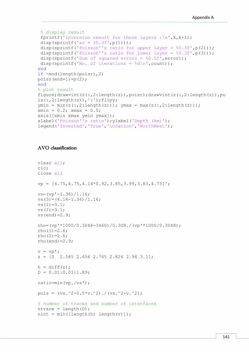
Appendix A
141
% display result
fprintf('Inversion result for these layers :\n',k,k+1);
disp(sprintf('ao = %0.3f',p(1)));
disp(sprintf('Poisson''s ratio for upper layer = %0.3f',p(2)));
disp(sprintf('Poisson''s ratio for lower layer = %0.3f',p(3)));
disp(sprintf('Sum of squared errors = %0.5f',error));
disp(sprintf('No. of iterations = %d\n',count));
end
if ~mod(length(poisr),2)
poisr(end+1)=p(2);
end
% plot result
figure;drawvint(z(:,2:length(z)),poisr);drawvint(z(:,2:length(z)),po
is(:,2:length(z)),'r');flipy;
ymin = min(z(:,2:length(z))); ymax = max(z(:,2:length(z)));
xmin = 0.2; xmax = 0.5;
axis([xmin xmax ymin ymax]);
xlabel('Poisson''s ratio');ylabel('Depth (km)');
legend('Inverted','True','Location','NorthWest');
AVO classification
clear all;
clc;
close all
vp = [4.75,4.75,4.14*0.92,3.85,3.99,3.83,4.75]';
vs=(vp'-1.36)/1.16;
vs(3)=(4.14-1.36)/1.16;
vs(1)=3.1;
vs(2)=3.1;
vs(end)=2.9;
rho=(vp'*1000/0.3048-3460)/0.308./(vp'*1000/0.3048);
rho(1)=2.6;
rho(2)=2.6;
rho(end)=2.9;
v = vp';
z = [0 2.585 2.656 2.765 2.826 2.94 3.1];
h = diff(z);
D = 0.01:0.01:1.89;
ratio=min(vp./vs');
pois = (vs.^2-0.5*v.^2)./(vs.^2-v.^2);
% number of traces and number of interfaces
ntrace = length(D);
nint = min([length(h) length(v)]);

Appendix A
142
% find ray parameters using MATLAB command : fzero
disp('Calculating ray parameters...');
figure;
for j = 1:ntrace
offset = D(j);
for i = 1:nint
hh = h(1:i);
vv = v(1:i);
er = 0.0001;
x = min(1./vv) - er;
if D(j)>0
p(i,j) = fzero('fun_ray',[-er x],[],offset,hh,vv);
else
p(i,j) = fzero('fun_ray',[er -x],[],offset,hh,vv);
end
theta(i,j) = (asin(p(i,j)*vv(i)))*180/pi;
% calculate traveltime based on ray parameters
t(i,j) = 2*sum(hh./(vv.*sqrt(1-p(i,j)^2*vv.^2)));
end
end
angles=theta;
for i=1:size(angles,2)
[refl,coeff]=ava_approximation(vp,vs',rho',angles(:,i)','two-term');
a(:,i)=refl(:,1);
b(:,i)=coeff(:,1);
c(:,i)=coeff(:,2);
end
figure;
for i=2:size(angles,1)
plot(angles(i,:),a(i,:))
hold on;
end
xmin = min(min(angles)); xmax = max(max(angles));
ymin = min(min(a)); ymax = max(max(a));
axis([xmin xmax ymin ymax]);
xlabel('Incidence angle (degree)');ylabel('Reflection coefficient');
title('AVA response');legend(...'Layer 1-2',
'Layer 1-2','Layer 2-3','Layer 3-4','Layer 4-5','Layer 5-
6');%,'Layer 6-7');
prepfig
figure;
for i=2:size(angles,1)
plot(sind(angles(i,:)).^2,a(i,:))
hold on;
end
xlabel('Sin^2(\theta)');ylabel('Reflection coefficient');

Appendix A
143
title('AVA response');legend(...'Layer 1-2',
'Layer 1-2','Layer 2-3','Layer 3-4','Layer 4-5','Layer 5-
6');%,'Layer 6-7');
prepfig
figure;
for i=2:size(b,1)
scatter(b(i,:),c(i,:));
hold on;
end
grid on;
hold on;
plot([-0.2 0.2],[0 0],'--b')
hold on;
plot([-0.02 -0.02],[-0.4 0.0342],'--r')
hold on;
plot([0.02 0.02],[-0.4 -0.0342],'--r')
hold on;
plot([-0.2,0.2],[4/5*(1-9*(1/ratio)^2)*(-0.2),4/5*(1-
9*(1/ratio)^2)*0.2],'--k')
legend('Layer 1-2','Layer 2-3','Layer 3-4','Layer 4-5','Layer 5-
6');%,'Layer 6-7');
xlabel('AVO Intercept (A)');
ylabel('AVO gradient (B)');
title('Rutherford and Williams Classification');
figure1=gcf;
h = text(-0.15,0.22, 'Background trend','FontSize',10);
set(h, 'rotation', -35)
annotation(figure1,'textbox',...
[0.49 0.2 0.09 0.04],...
'String',{'Class II'},...
'FitBoxToText','on','FontWeight','bold');
annotation(figure1,'textbox',...
[0.6 0.18 0.08 0.04],...
'String','Class I',...
'FitBoxToText','on','FontWeight','bold');
annotation(figure1,'textbox',...
[0.2 0.2 0.09 0.04],...
'String','Class III','FontWeight','bold');
annotation(figure1,'textbox',...
[0.2 0.45 0.09 0.04],...
'String','Class IV',...
'FitBoxToText','on','FontWeight','bold');
ylim([-0.4 0.4])

Appendix A
144
Common Offset gather creation
count=0;
rec=0;
dx1=dx; % Keep the coordinate of the receivers
for k=1:sourceinterval:SourceNum
count=count+1;
sx1(count)=segy.sx(k); % Keep the coordinate of the shot
idx = find( sx1(count)-dx1 == offsett ); % Keep the
indexes of the requested offfset
if ~isempty(idx)
rec=rec+1;
[h, t, shot] = SEGY_ReadShotGather(segy, k); % Read all
traces for each shot
common_offset(1:handles.max_length_def,rec)=shot(1:handles
.max_length_def,idx); % Keep the desired trace
sx2(rec)=segy.sx(k);
end
end
fprintf('\n%d Common offset gathers have been found with
offset= %d\n',rec,offsett);
Digitize function
function varargout = digitize(varargin)
global check_flag
%DIGITIZE digitize data from image.
% DIGITIZE with no input or output arguments allows the user to
% select an image file to load;only IMREAD-compatible image
% files are supported. The function then prompts the user
% to graphically identify the location of the origin and the X-
% and Y- axes of the plot. The user may then graphically select
% an arbitrary number of data points from anywhere on the image
% using the left mouse button. Data acquisition is terminated
% by clicking the RIGHT mouse button. The function then prompts
% the user to save the acquired data to file.
%
% ACQDATA = DIGITIZE with one output argument returns the X- and
% Y- values of the graphically selected data in the array ACQDATA.
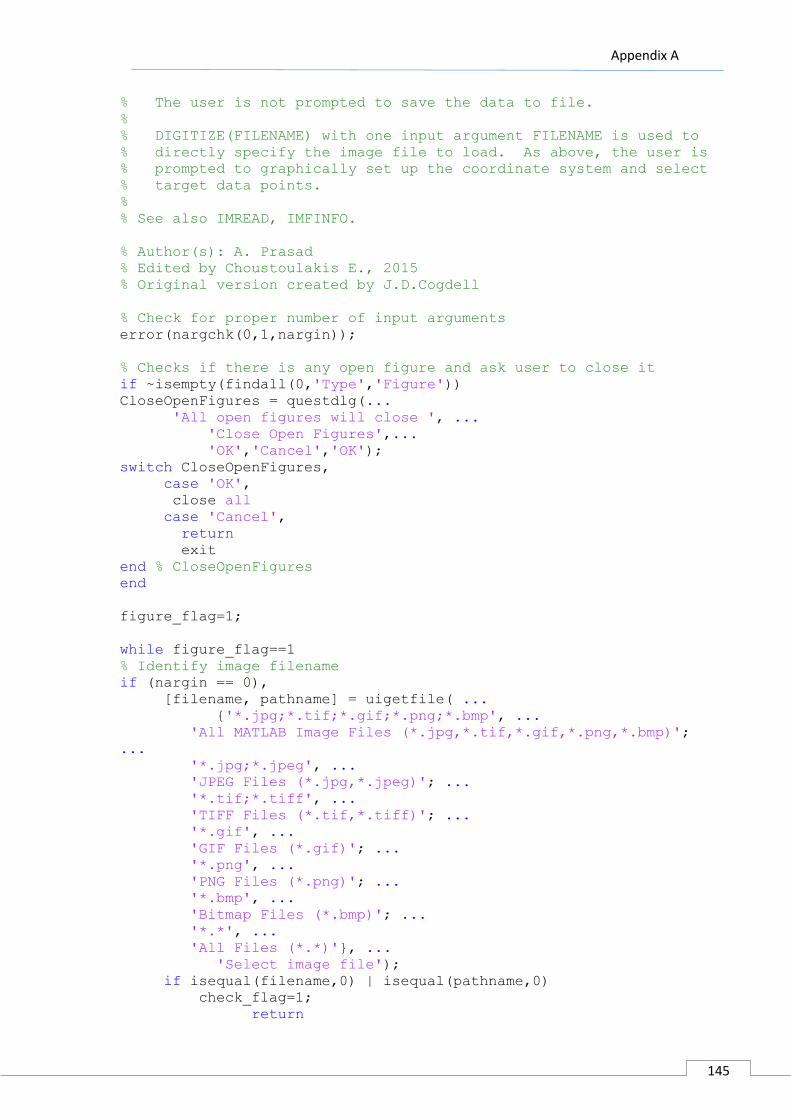
Appendix A
145
% The user is not prompted to save the data to file.
%
% DIGITIZE(FILENAME) with one input argument FILENAME is used to
% directly specify the image file to load. As above, the user is
% prompted to graphically set up the coordinate system and select
% target data points.
%
% See also IMREAD, IMFINFO.
% Author(s): A. Prasad
% Edited by Choustoulakis E., 2015
% Original version created by J.D.Cogdell
% Check for proper number of input arguments
error(nargchk(0,1,nargin));
% Checks if there is any open figure and ask user to close it
if ~isempty(findall(0,'Type','Figure'))
CloseOpenFigures = questdlg(...
'All open figures will close ', ...
'Close Open Figures',...
'OK','Cancel','OK');
switch CloseOpenFigures,
case 'OK',
close all
case 'Cancel',
return
exit
end % CloseOpenFigures
end
figure_flag=1;
while figure_flag==1
% Identify image filename
if (nargin == 0),
[filename, pathname] = uigetfile( ...
{'*.jpg;*.tif;*.gif;*.png;*.bmp', ...
'All MATLAB Image Files (*.jpg,*.tif,*.gif,*.png,*.bmp)';
...
'*.jpg;*.jpeg', ...
'JPEG Files (*.jpg,*.jpeg)'; ...
'*.tif;*.tiff', ...
'TIFF Files (*.tif,*.tiff)'; ...
'*.gif', ...
'GIF Files (*.gif)'; ...
'*.png', ...
'PNG Files (*.png)'; ...
'*.bmp', ...
'Bitmap Files (*.bmp)'; ...
'*.*', ...
'All Files (*.*)'}, ...
'Select image file');
if isequal(filename,0) | isequal(pathname,0)
check_flag=1;
return
Appendix A
146
else
check_flag=0;
imagename = fullfile(pathname, filename);
end
elseif nargin == 1,
imagename = varargin{1};
[path, file,ext] = fileparts(imagename);
filename = strcat(file,ext);
end
% Read image from target filename
pic = imread(imagename);
image(pic)
FigName = ['IMAGE: ' filename];
set(gcf,'Units', 'normalized', ...
'Position', [0 0.125 1 0.85], ...
'Name', FigName, ...
'NumberTitle', 'On', ...
'MenuBar','None')
set(gca,'Units','normalized','Position',[0 0 1 1]);
% dimensions
prompt = {'Enter the MAXIMUM X axis value',...
'Enter the MAXIMUM Z axis value'};
tit = 'X-Y';
lin = 1;
df ={'1900','3100'};
xv = inputdlg(prompt,tit,lin,df);
if isempty(xv)
figure_flag=1;
if ~isempty(findall(0,'Type','Figure'))
close(FigName)
end
else
X=str2num(xv{1});
Z=str2num(xv{2});
figure_flag=0;
end
end
% INSTRUCTIONS
msg{1}=['PICKING POINTS'];
msg{2}=['=> Press RIGHT mouse click to SELECT a
point of the figure'];
msg{3}=['=> Press LEFT mouse click to ZOOM'];

Appendix A
147
msg{4}=['=> Press DOUBLE-LEFT mouse click to
UNZOOM...'];
msg{5}=['=> Press BACKSPACE to DELETE last
point'];
msb=msgbox(msg,'Help about picking
procedure','help');
set(msb,'WindowStyle','modal');
uiwait(msb);
% Determine location of origin with mouse click
origin_flag=1;
while origin_flag==1
OriginButton = questdlg('Select the ORIGIN (Xo,Yo) of the axes with
RIGHT mouse button click', ...
'DIGITIZE: user input required', ...
'OK','Cancel','OK');
switch OriginButton,
case 'OK',
drawnow
[Xopixels,Yopixels] = ginput2(1);
h1=line(Xopixels,Yopixels,...
'Marker','o','Color','g','MarkerSize',14);
h2=line(Xopixels,Yopixels,...
'Marker','x','Color','g','MarkerSize',14);
case 'Cancel',
close(FigName)
return
end % switch OriginButton
% Prompt user for X- & Y- values at origin
prompt={'Enter the X value at the origin',...
'Enter the Y value at the origin:'};
def={'0','3100'};
dlgTitle='DIGITIZE: user input required';
lineNo=1;
answer=inputdlg(prompt,dlgTitle,lineNo,def);
if (isempty(char(answer{:})) == 1),
origin_flag=1;
set(h1,'Visible','off');
set(h2,'Visible','off');
else
OriginXYdata = str2num(char(answer{:}));
origin_flag=0;
end
end
x_flag=1;
while x_flag==1
% Define X-axis

Appendix A
148
XLimButton = questdlg(...
'Select a point on the X-axis with RIGHT mouse button click ',
...
'DIGITIZE: user input required', ...
'OK','Cancel','OK');
switch XLimButton,
case 'OK',
drawnow
[XAxisXpixels,XAxisYpixels] = ginput2(1);
h1=line(XAxisXpixels,XAxisYpixels,...
'Marker','*','Color','b','MarkerSize',14);
h2=line(XAxisXpixels,XAxisYpixels,...
'Marker','s','Color','b','MarkerSize',14);
case 'Cancel',
close(FigName)
return
end % switch XLimButton
% Prompt user for XLim value
prompt={'Enter the X value at the selected point'};
def={'1900'};
dlgTitle='DIGITIZE: user input required';
lineNo=1;
answer=inputdlg(prompt,dlgTitle,lineNo,def);
if (isempty(char(answer{:})) == 1),
x_flag=1;
set(h1,'Visible','off');
set(h2,'Visible','off');
else
x_flag=0;
XAxisXdata = str2num(char(answer{:}));
end
end
scalefactorXdata = XAxisXdata - OriginXYdata(1);
% Rotate image if necessary
% note image file line 1 is at top
th = atan((XAxisYpixels-Yopixels)/(XAxisXpixels-Xopixels));
% axis rotation matrix
rotmat = [cos(th) sin(th); -sin(th) cos(th)];
% Define Y-axis
y_flag=1;
while y_flag==1
YLimButton = questdlg(...
'Select a point on the Y-axis with RIGHT mouse button click',
...
'DIGITIZE: user input required', ...
'OK','Cancel','OK');
switch YLimButton,

Appendix A
149
case 'OK',
drawnow
[YAxisXpixels,YAxisYpixels] = ginput2(1);
h1=line(YAxisXpixels,YAxisYpixels,...
'Marker','*','Color','b','MarkerSize',14);
h2=line(YAxisXpixels,YAxisYpixels,...
'Marker','s','Color','b','MarkerSize',14);
case 'Cancel',
close(FigName)
return
end % switch YLimButton
% Prompt user for YLim value
prompt={'Enter the Y value at the selected point'};
def={'1800'};
dlgTitle='DIGITIZE: user input required';
lineNo=1;
answer=inputdlg(prompt,dlgTitle,lineNo,def);
if (isempty(char(answer{:})) == 1),
y_flag=1;
set(h1,'Visible','off');
set(h2,'Visible','off');
else
y_flag=0;
YAxisYdata = str2num(char(answer{:}));
end
end
scalefactorYdata = YAxisYdata - OriginXYdata(2);
% Complete rotation matrix definition as necessary
delxyx = rotmat*[(XAxisXpixels-Xopixels);(XAxisYpixels-Yopixels)];
delxyy = rotmat*[(YAxisXpixels-Xopixels);(YAxisYpixels-Yopixels)];
delXcal = delxyx(1);
delYcal = delxyy(2);
% Commence Data Acquisition from image
msgStr{1} = 'Click with RIGHT mouse button to ACQUIRE';
msgStr{2} = 'Click with LEFT mouse button to ZOOM IN';
msgStr{3} = 'DOUBLE Click LEFT mouse button to ZOOM OUT';
msgStr{4} = 'Press BACKSPACE to CANCEL last point';
msgStr{5} = 'Press ESC to STOP';
titleStr = 'Ready for data acquisition';
uiwait(msgbox(msgStr,titleStr,'warn','modal'));
drawnow
numberformat = '%6.2f';
nXY = [];
ng = 0;
flag=1;
counter=0;
Appendix A
150
while flag==1
counter=counter+1;
while 1,
n = 0;
col=rand(1,3);
% %%%%%%%%%%%%%% DATA ACQUISITION LOOP
%%%%%%%%%%%%%%%%%%%%%%%%%%%%%%%%%%%%%%%
while 1
[x,y, buttonNumber] = ginput2(1,'KeepZoom');
xy = rotmat*[(x-Xopixels);(y-Yopixels)];
delXpoint = xy(1);
delYpoint = xy(2);
if buttonNumber == 3
h=line(x,y,'Marker','.','Color',col,'MarkerSize',16);
x = OriginXYdata(1) +
delXpoint/delXcal*scalefactorXdata;
y = OriginXYdata(2) +
delYpoint/delYcal*scalefactorYdata;
n = n+1;
xpt(n) = x;
ypt(n) = y;
ng = ng+1;
nXY(ng,:) = [n x y];
elseif buttonNumber == 8
set(h,'Visible','off')
n=n-1;
ng=ng-1;
xpt(end)=[];
ypt(end)=[];
nXY(end,:)=[];
else
if buttonNumber ~=[1,2,3,8]
query = questdlg('STOP digitizing and save data?', ...
'DIGITIZE: confirmation', ...
'YES', 'NO', 'NO');
drawnow
switch upper(query),
case 'YES',
%disp(sprintf('\n'))
break
case 'NO',
end % switch query
end

Appendix A
151
end
end
% %%%%%%%%%%%%%% DATA ACQUISITION LOOP
%%%%%%%%%%%%%%%%%%%%%%%%%%%%%%%%%%%%%%%
cncl=0;
[writefname, writepname] = uiputfile('*.mat','Save data as');
if (writefname == 0) & (writepname == 0),
cncl=1;
end
if cncl~=1
writepfname = fullfile(writepname, writefname);
writedata = [ypt' xpt'];
writedata = writedata(writedata(:,1)>0 & writedata(:,1)<Z &
writedata(:,2)>0 & writedata(:,2)<X,:);
[z_column,Indexes]=sort(writedata(:,2));
writedata=writedata(Indexes,:);
writedata=[writedata(1,1) -5; writedata; writedata(end,1) X+5;
Z+5 X+5; Z+5 -5; writedata(1,1) -5];
eval(['Layer' num2str(counter) '= writedata']);
save(writepfname,['Layer' num2str(counter)]);
end
question = questdlg('Do you want to draw another layer ?',
...
'LAYER: drawing', ...
'YES', 'NO', 'YES');
drawnow
switch upper(question),
case 'YES',
flag=1;
break;
case 'NO',
flag=0;
break;
end % switch query
end
end
close all
end
Excel creation
% Excel Creation
ExcelButton = questdlg(...
'Do you want to create an excel velocity file?', ...
'EXCEL: Creation', ...
'OK','Cancel','OK');
Appendix A
152
switch ExcelButton,
case 'OK',
cncl=0;
[writefname, writepname] = uiputfile({'*.xlsx';'*.xls'},'Save
data as');
if (writefname == 0) & (writepname == 0),
cncl=1;
end
if cncl~=1
writepfname = fullfile(writepname, writefname);
end
fprintf('Please WAIT as the data is being saved..\n')
fprintf(['Do NOT OPEN ',writefname,' file yet..\n\n'])
wb = waitbar(0,'Initializing waitbar...');
B={'Layer','X position','Z Depth','Time [s]','Vint
[m/s]','Vrms - Time [m/s]'};
xlswrite(writepfname,B,1,'A1')
canc=0;
for l=1:length(xlength)
wbtxt{1}=['WRITING EXCEL DATA. DATA ',num2str(l),' OF
',num2str(length(xlength)),'. Please wait...'];
perc=l/length(xlength);
wb =waitbar(perc,wb,wbtxt);
if ~ishandle(wb)
canc=1;
break
end
xlswrite(writepfname,Layer_name(l),1,['A',num2str(l+1)])
xlswrite(writepfname,xlength(l),1,['B',num2str(l+1)])
xlswrite(writepfname,Depth(l),1, ['C',num2str(l+1)])
xlswrite(writepfname,time_conv(l),1, ['D',num2str(l+1)])
xlswrite(writepfname,Vint(l),1, ['E',num2str(l+1)])
xlswrite(writepfname,Vrms_time(l),1, ['F',num2str(l+1)])
fprintf([num2str(round(l/length(xlength)*100)),'%% of the data has
been saved to ',writefname,'..\n']);
end
close(wb)
if canc==1
fprintf('\nEXCEL CREATION HAS BEEN CANCELED\n');
else
fprintf('\nEXCEL CREATION HAS FINISHED\n');
fprintf(['You can now OPEN ',writefname,'\n']);
Appendix A
153
end
end
return
Geometrical Spreading
time_interval=2*Model_Parameters.dt*1000; % The sampling dt is
converted to two way travel time in seconds
k=0;
for i=1:length(x) % for all the distance intervals
for j=1:ln % for all the layers
k=k+1;
if j==1
time_new{i}=(0:time_interval:time_cmp(j,i)*1000); % the first
value of the time array will be zero and the next will be the first
value of "time_cmp"
Vrms_cmp{i}=repmat(Vrms_time(k),1,length(time_new{i})); % the
first value of the Vrms array will the Vrms of the first layer and
will be repeated for the rest of the array
elseif j==ln
new_time_array=(time_new{i}(end)+time_interval:time_interval:t_max);
% the final value of time array will be equal to the time length
Vrms_cmp{i}=[Vrms_cmp{i},
repmat(Vrms_time(k),1,length(new_time_array))];
time_new{i}=[time_new{i},new_time_array];
else
new_time_array=(time_new{i}(end)+time_interval:time_interval:time_cm
p(j,i)*1000);% the same procedure is being repeated and the new
arrays are jointed together
Vrms_cmp{i}=[Vrms_cmp{i},
repmat(Vrms_time(k),1,length(new_time_array))];
time_new{i}=[time_new{i},new_time_array];
end
end
GV{i}=time_new{i}'.*Vrms_cmp{i}'/1000; % For each distance interval
the GV value is calculated as the product of time and vrms
end
PG Crossplots of Synthetic Data
clc
clear
load CMP_correctedd
load Time_Vel_Spreading
load CMP_final_preprocessed_1_10

Appendix A
154
load CMP_partial_24_48
for i=1:size(CMP_corrected,2)
Stack(:,i)=sum(CMP_corrected{i},2);
end
col=lines(5);
off=0.021;
figure;
subplot(2,3,1)
hold on;
mwigb(Stack(:,150:300),2,(150:300),(0:0.001:1.6));
xlabel('CMP number','FontSize',14)
ylabel('Time (s)','FontSize',14)
hold on;
for i=2:6
p= polyfit((1:379),Time_Vel_Spreading{1}(i,2:end-1)-off,3);
yfit(i-1,:) = polyval(p,(1:379));
Time100=Time_Vel_Spreading{1}(i,150:300);
plot((150:300),Time100-off,'color',col(i-1,:))
hold on;
end
col=lines(5);
l=0;
for cmpcol=150:300
l=l+1;
Time=Time_Vel_Spreading{1}(:,cmpcol+2);
Vrms=Time_Vel_Spreading{2}(:,cmpcol+2);
Times=round((Time(2:end-1))*1000)';
Times=Times+1;
col=lines(length(Times));
k=0;
for i=Times
k=k+1;
amplitude(k,cmpcol)=Stack(i,cmpcol);
plot(cmpcol,amplitude(k,:),'.','color',col(k,:));
p = polyfit(x,amplitude(k,:),1);
yfit = polyval(p,x);
hold on;
ger(k)=plot(x,yfit,'color',col(k,:));
if p(1)<0
text(x(2),yfit(1),[num2str(round(p(2)*1000)/1000),'*x
',num2str(round(p(1)*1000)/1000)])
else
text(x(2),yfit(1),[num2str(round(p(2)*1000)/1000),'*x +
',num2str(round(p(1)*1000)/1000)])
end
hold on;
end
end
xlabel('CMP number');
ylabel('Amplitude');
Appendix A
155
title(['CMP ',num2str(cmpcol)]);
col={'o','.','d','s','*'};
figure;
for i=1:5
subplot(2,3,i+1)
hold on;
if i==2
q= polyfit((150:300),amplitude(i+1,150:300),1);
qfit(i,:) = polyval(q,(150:300));
hf(i)=plot((150:300),amplitude(i+1,150:300),'s','color',col(i,:
));
hold on;
plot((150:300),qfit(i,:),'-','color',col(i,:))
hold on;
elseif i==3
q= polyfit((150:300),amplitude(i-1,150:300),1);
qfit(i,:) = polyval(q,(150:300));
hf(i)=plot((150:300),amplitude(i-
1,150:300),'s','color',col(i,:));
hold on;
plot((150:300),qfit(i,:),'-','color',col(i,:))
hold on;
else
q= polyfit((150:300),amplitude(i,150:300),1);
qfit(i,:) = polyval(q,(150:300));
hf(i)=plot((150:300),amplitude(i,150:300),'s','color',col(i,:))
;
hold on;
plot((150:300),qfit(i,:),'-','color',col(i,:))
hold on;
end
text(225,-3,[num2str(round(q(1)*1000)/1000),' *x
+',num2str(round(q(2)*1000)/1000)]);
title(['Reflector ',num2str(i)]);
ylim([-20 15])
end
figure;
for i=1:5
if i==2
hold on;
q= polyfit((150:300),amplitude(i+1,150:300),1);
fre(i,1)=q(1);fre(i,2)=q(2);
qfit(i,:) = polyval(q,(150:300));
hf(i)=plot((150:300),amplitude(i+1,150:300),'o','color',col(i,:
),'MarkerSize',2);
hold on;
plot((150:300),qfit(i,:),'-','color',col(i,:),'LineWidth',0.5)
elseif i==3
hold on;
q= polyfit((150:300),amplitude(i-1,150:300),1);

Appendix A
156
fre(i,1)=q(1);fre(i,2)=q(2);
qfit(i,:) = polyval(q,(150:300));
hf(i)=plot((150:300),amplitude(i-
1,150:300),'o','color',col(i,:),'MarkerSize',2);
hold on;
plot((150:300),qfit(i,:),'-','color',col(i,:),'LineWidth',0.5)
else
hold on;
q= polyfit((150:300),amplitude(i,150:300),1);
fre(i,1)=q(1);fre(i,2)=q(2);
qfit(i,:) = polyval(q,(150:300));
hf(i)=plot((150:300),amplitude(i,150:300),'o','color',col(i,:),
'MarkerSize',2);
hold on;
plot((150:300),qfit(i,:),'-','color',col(i,:),'LineWidth',0.5)
end
end
title('Stacked Section');
xlabel('Cmp gather');
ylabel('Amplitude');
ylim([-20 15])
met=0;
for cmpcol=(150:300)
met=met+1;
Time100=Time_Vel_Spreading{1}(:,cmpcol+1);
Vrms100=Time_Vel_Spreading{2}(:,cmpcol+1);
Times=round((Time100(2:end-1)-off)*1000)';
Times=Times+1;
hh=h{cmpcol};
ind=abs(hh)/10;
idx=find(ind==0);
ind(idx)=1;
angles=theta(:,ind);
k=0;
col=lines(length(Times));
for i=Times
k=k+1;
amplitude{k}=CMP_corrected{cmpcol}(i,:);
x=sind(angles(k,:)).^2;
p = polyfit(x,amplitude{k},1);
PG(met,:)=[p(1) p(2)];
if k==1
PG1(met,:)=[p(1) p(2)];
elseif k==2
PG2(met,:)=[p(1) p(2)];
elseif k==3
PG3(met,:)=[p(1) p(2)];
elseif k==4
PG4(met,:)=[p(1) p(2)];
else
PG5(met,:)=[p(1) p(2)];
end
end
end
Appendix A
157
Raytracing Algorithm
% This script creates synthetic seismogram. Traveltimes are
calculated
% using raytracing and amplitudes are calculated using Zoeppritz's
% equation. AVA inversion is run on synthetics to get elastic
parameters
% (Poisson's ratio) using Shuey's (1985) approximation.
clc;
clear all;
close all
v = [4.75,4.75,4.14*0.92,3.85,3.99,3.83 4.75];
z = [0 2.585 2.656 2.765 2.826 2.94 3.1];
h = diff(z);
D = (0.01:0.01:1.89);
vs=(v-1.36)/1.16;
vs(3)=(4.14-1.36)/1.16;
vs(1)=3.1;
vs(2)=3.1;
vs(end)=2.9;
rho=(v*1000/0.3048-3460)/0.308./(v*1000/0.3048);
rho(1)=2.6;
rho(2)=2.6;
rho(end)=2.9;
pois = (vs.^2-0.5*v.^2)./(vs.^2-v.^2);
% number of traces and number of interfaces
ntrace = length(D);
nint = min([length(h) length(v)]);
% find ray parameters using MATLAB command : fzero
disp('Calculating ray parameters...');
for j = 1:ntrace
offset = D(j);
for i = 1:nint
hh = h(1:i);
vv = v(1:i);
er = 0.0001;
x = min(1./vv) - er;
if D(j)>0
p(i,j) = fzero('fun_ray',[-er x],[],offset,hh,vv);
else
p(i,j) = fzero('fun_ray',[er -x],[],offset,hh,vv);
end
theta(i,j) = (asin(p(i,j)*vv(i)))*180/pi;
% calculate traveltime based on ray parameters
Appendix A
158
t(i,j) = 2*sum(hh./(vv.*sqrt(1-p(i,j)^2*vv.^2)));
end
end
disp('Ray parameter calculation completed');
% plot traveltime
figure
hold on
for i = 1:nint
plot(D,t(i,:)); axis ij;
axis([min(D) max(D) 0 1.25*max(max(t))]);
title('Traveltime plot');
xlabel('Offset (km)');ylabel('Time (s)');
end
hold off
prepfig
% source and receiver depths
zsrc = z(:,1); zrec = zsrc;
figure;
col=copper(length(z)-1);
for i=2:length(z)
plot([0,1.9],[z(i),z(i)],'-','color','b','LineWidth',2)
hold on;
end
%figure;
flipy;
% trace the rays, iterate over each layer
disp('Tracing rays...');
for k = 1:length(z)
zd = z(:,k);
[t2,p2] = traceray_pp(v,z,zsrc,zrec,zd,D,10,-1,10,1,1,2);
end
title(['v(z) medium, P-P mode zsrc=' num2str(zsrc) ' zrec='
num2str(zrec)])
line(D,zrec*ones(size(D)),'color','b','linestyle','none','marker','v
')
line(0,zsrc,'color','r','linestyle','none','marker','*')
grid;xlabel('Offset (km)');ylabel('Depth (km)');
disp('Ray tracing completed');
%prepfig;
% create zeros matrix for spike's location
tmax = max(max(t)); dt = 0.001;
ta = (0:dt:tmax);
spikes = zeros(length(ta),ntrace);
% put spikes into location
Appendix A
159
disp('Creating synthetics...');
for i = 1:nint
for j = 1:ntrace
ir(i,j) = fix(t(i,j)/dt+0.1)+1;
refl(i,j) = zoeppritz(rho(:,i),v(:,i),vs(:,i),...
rho(:,i+1),v(:,i+1),vs(:,i+1),1,1,1,theta(i,j));
refl(i,j) = real(refl(i,j));
if i==2 || i==nint-1
refl(i,j)=-refl(i,j);
end
spikes(ir(i,j),j) = spikes(ir(i,j),j)+refl(i,j);
end
end
% convolve spikes with 25Hz ricker wavelet
[w,tw] = ricker(0.001,20);
for i = 1:ntrace
seis(:,i) = convz(spikes(:,i),w);
end
disp('Synthetics done');
% plot synthetics
figure;plotseis(seis,ta,D,1,2,1,1,'k');
title('Synthetic seismogram');set(gca,'xaxislocation','bottom');
xlabel('Offset (km)');ylabel('Time (s)');
%prepfig
% plot AVO response
xmin = min(min(theta)); xmax = max(max(theta));
ymin = min(min(refl)); ymax = max(max(refl));
figure;plot(theta(1,:),refl(1,:),...
theta(2,:),refl(2,:),'r',theta(3,:),...
refl(3,:),'k',theta(4,:),refl(4,:),'g',theta(5,:),refl(5,:),'c',thet
a(6,:),refl(6,:),'b');
axis([xmin xmax ymin ymax]);
xlabel('Incidence angle (degree)');ylabel('Reflection coefficient');
title('AVA response');legend('Layer 1-2',...
'Layer 2-3','Layer 3-4','Layer 4-5','Layer 5-6','Layer 6-7');
Record’s Length Calculation
k=0;
for i=1:size(Source.positions,1) % For all the shots number
for j=1:size(Receivers.positions{i},1) % Take the positions of all
the receivers at each shot
dist(j)=abs(Source.positions(i,2)-Receivers.positions{i}(j,2)); %
Save in varriable dist all the distances between each shot and
receivers
end
The varriable "dist" has length equal to the number of the
receivers,
Appendix A
160
[Dist_max(i),Rec_Ind(i)]=max(dist); % Keep the max distances between
shot and receiver for each shot in an array "Dist_max" along with
the No of the receiver "Rec_Ind"
end
[Dist_max,Sourc_Ind]=max(Dist_max); % Keep the overall max distance
between shot and receiver "Dist_max" alog with the No of the source
with the max distance
Rec_Indx=Rec_Ind(Sourc_Ind); % Pass the No of the source to the
previous Rec_Ind array in order to find the number of the receiver
with the max distance from the particular source
Sourc_dist=Source.positions(Sourc_Ind,2); % Take the ds position of
the specific source
Rec_dist=Receivers.positions{Sourc_Ind}(Rec_Indx,2); % Take the dx
position of the specific receiver
leng=length(Model_Parameters.BodyVertex); % Number of the layers
for m=1:leng % Calculate the mean value of depth for each layer
mean_z(m)=mean(Model_Parameters.BodyVertex{m}(:,1));
end
% If mn=1 the "import" menu had been chosen previously and the
values of interval velocities, max distance and max depth are stored
as Vp,X and Z
%If mn~=1 the menu cretae had been chosen previously and the same
values are stored now as Model_Parameters.Vp, X_depth and Z_depth
if mn==1
mean_z=[0 mean_z];
P_velocity=Vp;
X_length=X;
Zmax=Z;
else
mean_z=[0 mean_z];
P_velocity=Model_Parameters.Vp;
X_length=X_depth;
Zmax=Z_depth;
end
% Here the ratio of each layer is calculated compared to the rest of
the model
Layers_Volume=diff(mean_z);
for i=1:length(mean_z)-1
Z_ratio_max=mean_z(i+1); % For each iteration the max depth
increases as the ray reaches to the rest of the layers
z_ratio{i}=Layers_Volume(1:i)/Z_ratio_max;
end
Vmean=P_velocity(1:end-1)*z_ratio{end}';
Appendix A
161
% The average Interval velocity for the last layer is calculated
% Representation of record length's calculation plot
figure('color','w');
plot(Sourc_dist,0,'hr','MarkerSize',10,'MarkerFaceColor','k');
hold on;
plot(Rec_dist,0,'vk','MarkerSize',7,'MarkerFaceColor','r');
hold on;
col=lines(length(mean_z)-1);
for i=1:length(mean_z)-1
plot([0,X_length],[mean_z(i+1),mean_z(i+1)],'color',col(i,:),'LineWi
dth',2)
hold on;
end
plot([Sourc_dist,Rec_dist],[10,10],'k','LineWidth',2)
hold on;
plot([Sourc_dist,Dist_max/2],[0,mean_z(end)],'k','LineWidth',2)
hold on;
plot([Rec_dist,Dist_max/2],[0,mean_z(end)],'k','LineWidth',2)
hold on;
set(gca,'YDir','reverse');
% plot axis values
x1=Dist_max/2;
x2=Dist_max/4;
y2=mean_z(end)/2;
x3=3*Dist_max/4;
y3=mean_z(end)/2;
d1=Dist_max;
d2=round(sqrt((mean_z(end))^2+(Dist_max/2)^2));
d3=d2;
text(x1,10,['d1= ', num2str(d1),' m'], 'FontSize',
12,'color','k','VerticalAlignment','top');
if Sourc_dist-Rec_dist>0
text(x2,y2 ,['d2= ', num2str(d2),' m'], 'FontSize',
12,'color','k','HorizontalAlignment','right','VerticalAlignment','bo
ttom');
text(x3,y3,['d3= ', num2str(d3),' m'], 'FontSize',
12,'color','k','HorizontalAlignment','right','VerticalAlignment','to
p');
else
text(x2,y2 ,['d2= ', num2str(d2),' m'], 'FontSize',
12,'color','k','HorizontalAlignment','left','VerticalAlignment','bot
tom');
text(x3,y3,['d3= ', num2str(d3),' m'], 'FontSize',
12,'color','k','HorizontalAlignment','left','VerticalAlignment','top
');
end
set(gca,'YDir','reverse');
Appendix A
162
V_mean=round(Vmean);
time=round((d2/V_mean+d3/V_mean)*1000); % Time calculated using the
Vrms value
%time=round(sqrt(d2^2+d3^2+d1^2)*1000/V_mean); % Time calculated
using the Vrms value
%Rounding the time to its nearest order of magnitude
order_magnitude = floor(log(abs(time))./log(10))-1;
time_int=time;
time=round(time/10^order_magnitude)*10^order_magnitude+300;
title (['Mean Vp= ',num2str(V_mean),' [m/s]',' Time =
',num2str(time_int),' [ms]'],'FontWeight','bold');
Rock Physics
figure;
set(gcf,'color','white');
% Plot P wave velocity
subplot(1,4,1);
stairs(vp,zlayer,'LineWidth',2.5,'Color',[0.07843 0.1686
0.549]);
ylabel('Depth (m)','FontWeight','bold','Color','black');
title('V_{p} (m/s)','FontWeight','bold');
set(gca,'XMinorGrid','on','YMinorGrid','on','YDir','reverse','Y
Color','k',...
'XAxisLocation','top','XColor','k','FontWeight',...
'demi','FontAngle','italic');
ax=gca;
ax.MinorGridLineStyle='-';
ylim([2500 3100]);
% Plot S wave velocity
subplot(1,4,2);
stairs(vs,zlayer,'LineWidth',2.5,'Color',[1 0 0]);
title('V_{s} (m/s)','FontWeight','bold');
set(gca,'XMinorGrid','on','YMinorGrid','on','YDir','reverse','Y
Color','k',...
'XAxisLocation','top','XColor','k','FontWeight',...
'demi','FontAngle','italic');
ax=gca;
ax.MinorGridLineStyle='-';
ylim([2500 3100]);
% Plot Density
subplot(1,4,3);
stairs(ro,zlayer,'LineWidth',2.5,'Color',[0.07059 0.6392
0.07059]);
title('Density (kg/m^3)','FontWeight','bold');
set(gca,'XMinorGrid','on','YMinorGrid','on','YDir','reverse','Y
Color','k',...
'XAxisLocation','top','XColor','k','FontWeight',...
'demi','FontAngle','italic');
ax=gca;
ax.MinorGridLineStyle='-';

Appendix A
163
ylim([2500 3100]);
xlim([2 3]);
% Plot Poissons Ratio
subplot(1,4,4);
stairs(pois,zlayer,'LineWidth',2.5,'Color',[0.2 0.1 0.9]);
title('Poisson''s Ratio','FontWeight','bold');
set(gca,'XMinorGrid','on','YMinorGrid','on','YDir','reverse','Y
Color','k',...
'XAxisLocation','top','XColor','k','FontWeight',...
'demi','FontAngle','italic');
ax=gca;
ax.MinorGridLineStyle='-';
ylim([2500 3100]);
% Plot Geology Model
fId=figure('units','normalized','outerposition',[0 0 1
1],'color','w');
%writerObj = VideoWriter('Test.avi'); % Name it.
%writerObj.FrameRate = 20; % How many frames per second.
%open(writerObj);
%color = load('mycmap.txt');
pcolor(xx,zz,repmat(vlayer,1,nx)); shading flat; hold on
colormap(parula); colorbar ('horz');
axis([0 xmax zmin-0.03*zmax zmax])
set(gca,'YDir','reverse','XaxisLocation','bottom',....
'Ytick',zlayer,'FontWeight','demi','PlotBoxAspectRatioMode','Ma
nual',...
'PlotBoxAspectRatio',[2.4 1.2 1],'Position',[0.04 0.30 0.90
0.60]);
% Plot Source-Receiver Group
plot(xs,zs,'r*','markersize',12); hold on
plot(xr,zr,'sk','markersize',4,'markerfacecolor','c'); hold on
xlabel('Velocity (m/s)','FontWeight','bold','Color','black');
ylabel('Depth (m)','FontWeight','bold','Color','black');
figure;
for i=1:ns
tm = load(['time_shot',num2str(i),'.mat']); tt = tm.twt;
plot(xx(2:nlayer,:),tt(2:nlayer,:,i),'b.'); hold on
xlabel('Horizontal Position
(m)','FontWeight','bold','FontAngle','normal','Color','black');
ylabel('Time
(s)','FontWeight','bold','FontAngle','normal','Color','black');
title('Traveltime','FontWeight','bold');
set(gca,'Ydir','reverse');
set(gcf,'color','white');
end
% Plot Reflection Coefficient
figure;
for i=1:ns
reflz = load(['reflz_shot',num2str(i),'.mat']); reflz =
reflz.rcz;
Appendix A
164
refls = load(['refls_shot',num2str(i),'.mat']); refls =
refls.rcs;
reflt = load(['reflt_shot',num2str(i),'.mat']); reflt =
reflt.rct;
theta = load(['teta_shot',num2str(i),'.mat']); angle =
theta.angle;
%Reflection Coefficient of Zoeppritz
for j=1:nlayer
subplot(1,3,1)
plot(abs(angle(j,:,i)),reflz(j,:,i),'.'); hold on
xlabel('Incidence Angles
(degree)','FontWeight','bold','Color','black');
ylabel('Reflection
Coefficient','FontWeight','bold','Color','black');
grid on; title('Rpp
Zoeppritz','FontWeight','bold','Color','black')
set(gca,'YColor','k','XColor','k'); hold on
%Reflection Coefficient of Shuey
subplot(1,3,2)
plot(abs(angle(j,:,i)),refls(j,:,i),'.'); hold on
xlabel('Incidence Angles
(degree)','FontWeight','bold','Color','black');
grid on; title('Rpp Shuey','FontWeight','bold','Color','black')
set(gca,'YColor','k','XColor','k'); hold on
%Reflection Coefficient of Thomsen
subplot(1,3,3)
plot(abs(angle(j,:,i)),reflt(j,:,i),'.'); hold on
xlabel('Incidence Angles
(degree)','FontWeight','bold','Color','black');
grid on; title('Rpp
Thomsen','FontWeight','bold','Color','black')
set(gca,'YColor','k','XColor','k'); hold on
set(gcf,'color','white');
end
end
for i=1:ns
refls = load(['refls_shot',num2str(i),'.mat']); refls =
refls.rcs;
theta = load(['teta_shot',num2str(i),'.mat']); angle =
theta.angle;
Rt = load(['intercept_shot',num2str(i),'.mat']); Rt = Rt.AA;
Gt = load(['gradient_shot',num2str(i),'.mat']); Gt = Gt.BB;
Ro(1:nlayer,:,i) = Rt(1:nlayer,:,i);
Go(1:nlayer,:,i) = Gt(1:nlayer,:,i);
Rc(1:nlayer,:,i) = refls(1:nlayer,:,i);
inc(1:nlayer,:,i) = angle(1:nlayer,:,i);
end
Rp = reshape(Ro,nr*ns*nlayer,1);
G = reshape(Go,nr*ns*nlayer,1);
R = reshape(Rc,nr*ns*nlayer,1);
teta = reshape(inc,nr*ns*nlayer,1);
% Plot Attributes
figure;
Appendix A
165
% Rp-G Cross Plot
subplot(1,2,1)
for i=1:nlayer
plot(Ro(i,:),Go(i,:),'.','MarkerSize',10); hold on
end
%plot(R,G,'m.'); hold on
xlabel('R','FontWeight','bold','Color','black');
ylabel('G','FontWeight','bold','Color','black');
grid on; title('R-G Cross
Plot','FontWeight','bold','Color','black')
set(gca,'YColor','k','XColor','k'); hold on
legend('Layer1','Layer2','Layer3','Layer4','Layer5','Layer6','L
ayer7');
% R-sin^2(teta) Cross Plot
subplot(1,2,2)
for i=1:nlayer
plot((sin(inc(i,:)).^2),Rc(i,:),'.'); hold on
end
xlabel('sin^2(teta)','FontWeight','bold','Color','black');
ylabel('R(teta)','FontWeight','bold','Color','black');
grid on; title('R-sin^2(teta) Cross
Plot','FontWeight','bold','Color','black')
set(gca,'YColor','k','XColor','k'); hold on
set(gcf,'color','white');
legend('Layer1','Layer2','Layer3','Layer4','Layer5','Layer6','L
ayer7');
%==============================================================
==============================
% AVO Modelling
%==============================================================
==============================
fprintf('---> Starting AVO Modelling ...\n');
% Make wavelet ricker (f = 2 Hz)
dt = 0.001; f = 20;
[w,tw] = ricker(dt,f);
% Create zeros matrix for spike's location
tmax = max(tt(:));
tr = 0:dt:tmax; nt = length(tr);
t = tt(2:nlayer,:);
%t = t(:,all(~isnan(t)));
t(:,all(isnan(t)))=0;
%t(:,2)=[];
% Take reflectivity into spike location
spikes = zeros(nt,nray);
rcz = real(reflz(2:nlayer,:));
for k=1:nlayer-1
for j=1:nray-1
ir(k,j) = fix(t(k,j)/dt+0.1)+1;
spikes(ir(k,j),j) = spikes(ir(k,j),j) + rcz(k,j);
end
end
% Convolve spikes with wavelet ricker
for j=1:nray
seisz(:,j) = convz(spikes(:,j),w);
end

Appendix A
166
ampz=reshape(seisz,length(tr),nr,ns);
for i=1:ns
ampz_shot(:,:,i) = ampz(:,:,i);
save(['ampz_shot',num2str(i),'.mat'],'ampz_shot');
end
% CMP Stacked
Stacked = zeros(nt,nr);
for i=1:ns
files = load(['ampz_shot',num2str(i),'.mat']);
files = files.ampz_shot;
Stacked = Stacked + files(:,:,i);
end
% Save Seismic Data
save(['seis','.mat'],'Stacked');
% Plot AVO
figure;
wig(xr,tr,Stacked,'black'); hold on
xlabel('Offset (m)','FontWeight','bold','Color','black');
ylabel('Time (s)','FontWeight','bold','Color','black');
title('Synthetic
Seismogram','FontWeight','bold','Color','black');
axis tight
set(gca,'YColor','k','XColor','k'); hold on
set(gcf,'color','white');
fprintf(' AVO Modelling has been computed...[OK]\n');
%==============================================================
==============================
% Seismogram Synthetic
%==============================================================
==============================
% Create Smooth Synthetic Log From Elastic Data Set
[pson,sson,spson,rlog,zlog] = logsyn(vp,vs,ro,zlayer,1000);
vplog = 1.0e6./pson; vslog = 1.0e6./sson;
rholog = 0.31.*(vplog).^0.25; vpvs = vplog./vslog;
poisson = (vslog.^2-0.5*vplog.^2)./(vslog.^2-vplog.^2);
% Plot Synthetic Data Log
% Plot Rock Properties
figure;
% Cross Plot P and S wave velocity
subplot(2,2,1);
plot(vplog(800:1000),vslog(800:1000),'.','Color',[0.07843
0.1686 0.549]);
%p = polyfit(vplog(400:500),vslog(400:500),1);
%yfit = polyval(p,vplog(400:500));
hold on;
plot(vplog(800:1000),(vplog(800:1000)-1360)/1.16,'r');
%plot(vplog(400:500),yfit,'r');
%text(4400,2800,[num2str(round(p(2)*1000/1000)),'*x
+',num2str(round(p(1)*1000)/1000)])
text(4000,2800,[num2str(0.862),'*Vp -',num2str(1172.4)])
xlabel('Vp (m/s)','FontWeight','bold','Color','black');
ylabel('Vs (m/s)','FontWeight','bold','Color','black');
title('Cross Plot of Vp and
Vs','FontWeight','bold','Color','black');
Appendix A
167
set(gca,'XMinorGrid','on','YMinorGrid','on','YColor','k',...
'XAxisLocation','bottom','XColor','k',...
'FontWeight','demi','FontAngle','italic');
ax=gca;
ax.MinorGridLineStyle='-';
% Plot S Sonic Log
subplot(2,2,2);
plot(vplog(800:1000),vpvs(800:1000),'.','Color',[1 0 0]);
p = polyfit(vplog(800:1000),vpvs(800:1000),2);
yfit = polyval(p,vplog(800:1000));
hold on;
plot(vplog(800:1000),yfit,'r');
%text(4400,1.7,[num2str(round(p(2)*1000/1000)),'*Vp
+',num2str(round(p(1)*1000)/1000)])
xlabel('Vp (m/s)','FontWeight','bold','Color','black');
ylabel('Vp/Vs ratio','FontWeight','bold','Color','black');
title('Cross Plot of Vp and Vp/Vs
Ratio','FontWeight','bold','Color','black');
set(gca,'XMinorGrid','on','YMinorGrid','on','YColor','k',...
'XAxisLocation','bottom','XColor','k',...
'FontWeight',...
'demi','FontAngle','italic');
ax=gca;
ax.MinorGridLineStyle='-';
% Plot Density Log
subplot(2,2,3);
plot(vslog(800:1000),vpvs(800:1000),'.','Color',[0.07059 0.6392
0.07059]);
p = polyfit(vslog(800:1000),vpvs(800:1000),2);
yfit = polyval(p,vslog(800:1000));
hold on;
plot(vslog(800:1000),yfit,'r');
%text(2.52,1.7,[num2str(round(p(2)*1000/1000)),'*Vp
+',num2str(round(p(1)*1000)/1000)])
xlabel('Vs (m/s^2)','FontWeight','bold','Color','black');
ylabel('Vp/Vs ratio','FontWeight','bold','Color','black');
title('Cross Plot of Shear Velocity and Vp/Vs
Ratio','FontWeight','bold','Color','black');
set(gca,'XMinorGrid','on','YMinorGrid','on','YColor','k',...
'XAxisLocation','bottom','XColor','k',...
'FontWeight','demi','FontAngle','italic');
ax=gca;
ax.MinorGridLineStyle='-';
subplot(2,2,4);
plot(poisson(800:1000),vpvs(800:1000),'m.');
xlabel('Poisson Ratio','FontWeight','bold','Color','black');
ylabel('Vp/Vs ratio','FontWeight','bold','Color','black');
title('Cross Plot of Poisson''s Ratio and Vp/Vs
Ratio','FontWeight','bold','Color','black');
set(gca,'XMinorGrid','on','YMinorGrid','on','YColor','k',...
'XAxisLocation','bottom','XColor','k',...
'FontWeight','demi','FontAngle','italic');
set(gcf,'color','white');
ax=gca;
ax.MinorGridLineStyle='-';
Appendix A
168
% Integrate Depth and Velocity To Get Two-Way Time
tstart = 0; tracenum = 10;
[tz,zt] = sonic2tz(spson,zlog,-100,tstart);
tzobj = [zt tz];
vins = vplog; dens = rholog; z = zlog;
% Determine Ricker Wavelet
dt = 0.001; f = 20;
[w,tw] = ricker(dt,f);
[theo,tlog,rcs,pm,p] =
seismogram(vins,dens,z',w,tw,tzobj,0,0,1);
% Compare AVO Data Estimation
rseis = load(['seis','.mat'],'Stacked'); num = 1:191;
rseis = rseis.Stacked; seis = rseis(:,num);
[seisr,zp,dzp,tz,zt]=seis2z(seis,tr,vp,zlayer,vs,1,min(zlayer),
max(zlayer));
figure;
set(gcf,'color','white');
% Plot P Sonic Log
subplot(1,4,1);
stairs(pson,zlog,'LineWidth',1,'Color',[0.07843 0.1686 0.549]);
xlabel('P sonic (US/m)','FontWeight','bold','Color','black');
ylabel('Depth (m)','FontWeight','bold','Color','black');
set(gca,'XMinorGrid','on','YMinorGrid','on','YDir','reverse','X
Dir','reverse','YColor',...
'k','XAxisLocation','top','XColor',...
'k','FontWeight','demi','FontAngle','italic');
ax=gca;
ax.MinorGridLineStyle='-';
% Plot S Sonic Log
subplot(1,4,2);
stairs(sson,zlog,'LineWidth',1,'Color',[1 0 0]);
xlabel('S sonic (US/m)','FontWeight','bold','Color','black');
set(gca,'XMinorGrid','on','YMinorGrid','on','YDir','reverse','X
Dir','reverse','YColor','k',...
'XAxisLocation','top','XColor','k','FontWeight',...
'demi','FontAngle','italic');
ax=gca;
ax.MinorGridLineStyle='-';
% Plot Density Log
subplot(1,4,3);
stairs(rlog,zlog,'LineWidth',1,'Color',[0.07059 0.6392
0.07059]);
xlabel('Density (kg/m^3)','FontWeight','bold','Color','black');
set(gca,'XMinorGrid','on','YMinorGrid','on','YDir','reverse','Y
Color','k',...
'XAxisLocation','top','XColor','k','FontWeight',...
'demi','FontAngle','italic');
ax=gca;
ax.MinorGridLineStyle='-';
subplot(144);
stairs(poisson,zlog,'LineWidth',1,'Color',[0.07843 0.1686
0.549]);
Appendix A
169
xlabel('Poisson Ratio','FontWeight','bold','Color','black');
ylabel('Depth (m)','FontWeight','bold','Color','black');
title('Poisson Ratio','FontWeight','bold','Color','black');
set(gca,'XMinorGrid','on','YMinorGrid','on','YDir','reverse','Y
Color','k',...
'XAxisLocation','bottom','XColor','k',...
'FontWeight','demi','FontAngle','italic');
ax=gca;
ax.MinorGridLineStyle='-';
figure;
wig(1:191,zp',seisr,'blue'); hold on
xlabel('Trace Number','FontWeight','bold','Color','black');
title('AVO Estimation','FontWeight','bold','Color','black');
axis tight
set(gca,'YDir','reverse','YColor','k',...
'XAxisLocation','bottom','XColor','k',...
'FontWeight','demi','FontAngle','italic');
ax=gca;
ax.MinorGridLineStyle='-';
set(gcf,'color','white');
Spline Layers
function [] = Spline_layers
global figm fign Model_Parameters...
record_length X_length P_velocity Zmax...
depth_layer time time_layer z_ratio...
record_length_flag time_fin
record_length_flag=0;
spline_flag=1; % While spline_flag=1 the user will be asked to give
record length and spline interval
while spline_flag==1
spline_flag=0;
% Give the record length and the spline interval
prompt = {'Enter the record length (ms)' 'Enter the
SPLINE interval value'};
tit = 'RECORD LENGTH - SPLINE DEFINITION';
lin = 1;
df ={num2str(time) '50'};
xv = inputdlg(prompt,tit,lin,df);
if isempty(xv);
record_length_flag=1;
return;
else
for j=1:size(xv,2);
if isempty(xv{j});
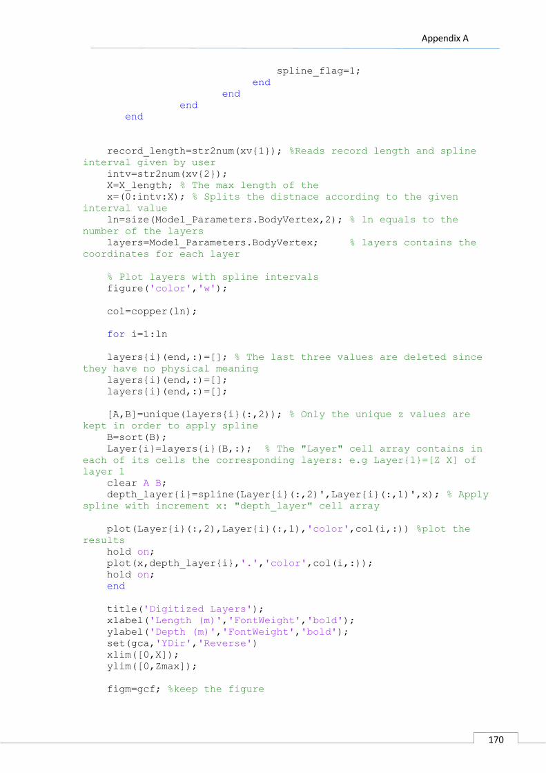
Appendix A
170
spline_flag=1;
end
end
end
end
record_length=str2num(xv{1}); %Reads record length and spline
interval given by user
intv=str2num(xv{2});
X=X_length; % The max length of the
x=(0:intv:X); % Splits the distnace according to the given
interval value
ln=size(Model_Parameters.BodyVertex,2); % ln equals to the
number of the layers
layers=Model_Parameters.BodyVertex; % layers contains the
coordinates for each layer
% Plot layers with spline intervals
figure('color','w');
col=copper(ln);
for i=1:ln
layers{i}(end,:)=[]; % The last three values are deleted since
they have no physical meaning
layers{i}(end,:)=[];
layers{i}(end,:)=[];
[A,B]=unique(layers{i}(:,2)); % Only the unique z values are
kept in order to apply spline
B=sort(B);
Layer{i}=layers{i}(B,:); % The "Layer" cell array contains in
each of its cells the corresponding layers: e.g Layer{1}=[Z X] of
layer 1
clear A B;
depth_layer{i}=spline(Layer{i}(:,2)',Layer{i}(:,1)',x); % Apply
spline with increment x: "depth_layer" cell array
plot(Layer{i}(:,2),Layer{i}(:,1),'color',col(i,:)) %plot the
results
hold on;
plot(x,depth_layer{i},'.','color',col(i,:));
hold on;
end
title('Digitized Layers');
xlabel('Length (m)','FontWeight','bold');
ylabel('Depth (m)','FontWeight','bold');
set(gca,'YDir','Reverse')
xlim([0,X]);
ylim([0,Zmax]);
figm=gcf; %keep the figure

Appendix A
171
% Load Interval velocities
vint=P_velocity; % Vint contains the interval velocities for each
layer
depths=cell2mat(depth_layer);
depths2=reshape(depths,[length(x) ln]);
depth_final=depths2';
depth_final=[zeros(1,size(depth_final,2));depth_final];
depth_diff=diff(depth_final);
for i=1:length(x)
time_jnk=2*depth_diff(:,i)./vint(1:end-1)';
time_final(:,i)=cumsum(time_jnk);
end
time_final=[zeros(1,length(x)); time_final ;
(record_length/1000)*ones(1,length(x))];
depth_final=[depth_final; Zmax*ones(1,length(x))];
figure('color','w');
for i=1:ln % for all the layers
plot(x,time_final(i+1,:),'.-','color',col(i,:));
hold on;
end
title('Digitized Layers');
xlabel('Length (m)','FontWeight','bold');
ylabel('Time (s)','FontWeight','bold');
set(gca,'YDir','Reverse')
xlim([0,X]);
ylim([0,record_length/1000]);
fign=gcf;
Z=Zmax;
t_max=record_length;
k=0;
for i=1:length(x) % For the whole length of the spline array
for j=1:ln+2 % For all the layers
k=k+1;
Vint(k)=vint(j);
Depth(k)=depth_final(j,i);
Layer_name(k)={strcat('Layer',num2str(j))};
xlength(k)=x(i);
time_conv(k)=time_final(j,i);
end
end
time_cmp=time_final;
vint_cmp=reshape(Vint,[ln+2,length(x)]);
% Calculate Vrms using Time
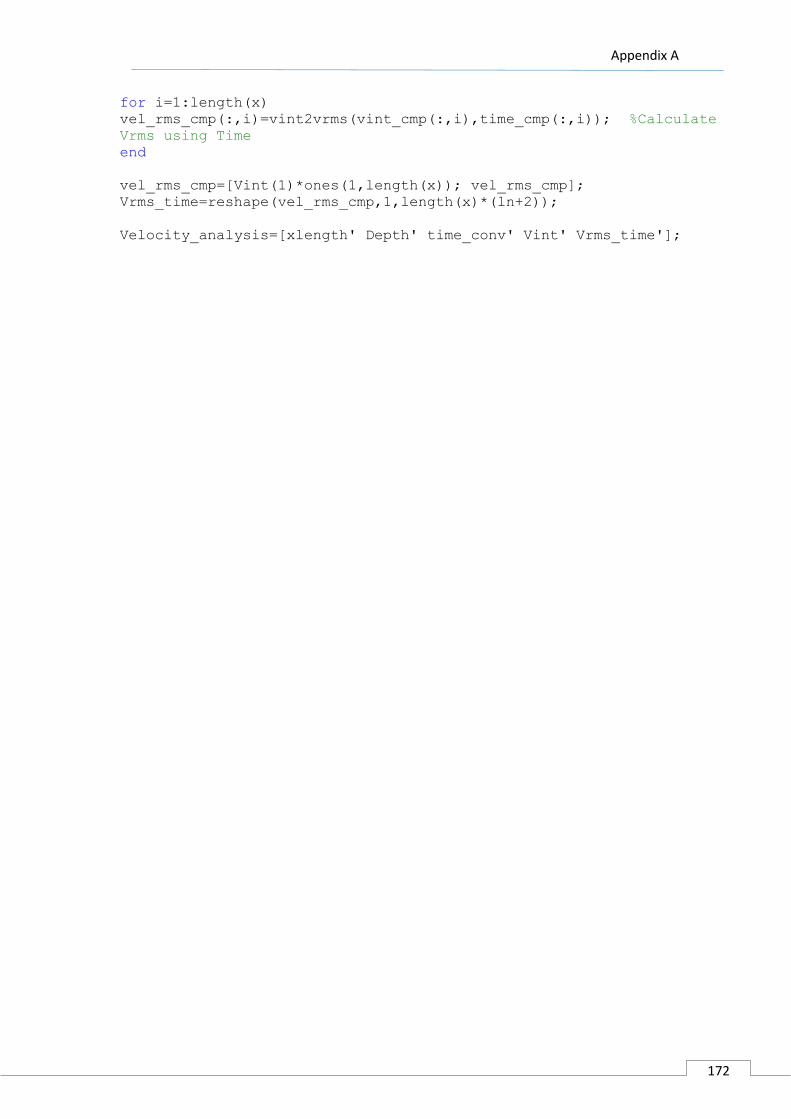
Appendix A
172
for i=1:length(x)
vel_rms_cmp(:,i)=vint2vrms(vint_cmp(:,i),time_cmp(:,i)); %Calculate
Vrms using Time
end
vel_rms_cmp=[Vint(1)*ones(1,length(x)); vel_rms_cmp];
Vrms_time=reshape(vel_rms_cmp,1,length(x)*(ln+2));
Velocity_analysis=[xlength' Depth' time_conv' Vint' Vrms_time'];
Appendix B
173
Appendix B
List of Figures
Chapter 2 Figure 2.1 Prinos – Kavala Basin. Prinos field, Prinos North field, Epsilon field and South Kavala gas filed
are the only productive hydrocarbon fields in Greece. The oil generation and the migration paths are shown
(improved version published after Kioumourtzi et al., 2007). .................................................................... 2 Figure 2.2 Simplified cross section of the Prinos basin parallel to the long axis. The roll-over syngenetic
faulting formed the dome-like anticlines. Depths in kilometres below mean sea level. Figure from
Proedrou and Sidiropoulos (1992). ............................................................................................................... 3 Figure 2.3. Generalized chronostratigraphic column of Prinos basin. Figure from Proedrou and Sidiropoulos
(2004). ......................................................................................................................................................... 4 Figure 2.4 NW-SE seismic section across the Prinos basin. The anticlinal structure with the downthrown
faults are well illustrated from the seismic reflectors [Stuart Harker 2004-2008]. ........................................ 6
Chapter 3 Figure 3.1 The differencing star for the modified Lax-Wendroff scheme. ................................................ 10 Figure 3.2 The domains of dependence on the plane x-z: a square for Lax-Wendroff scheme and a circle
for the simplest (ρ(x,z)-μ(x.z)=1) SH wave equation. ................................................................................ 14
Chapter 4 Figure 4.1Reflection and transmission at an interface for an incident P-wave. ....................................... 16 Figure 4.2 Notation for the sixteen possible reflection/transmission coefficients for P-SV waves at an
interface between two different solid half-spaces. Short arrows show the direction of particle motion
(from Aki and Richards, 1980). ................................................................................................................. 17 Figure 4.3 (a) shows AVO response and (b) shows transform of (a) in AVA (amplitude versus angle)
response [NTNU, AVO theory, 2004]. ....................................................................................................... 20 Figure 4.4 A plot of constant angle curves superimposed on constant offset traces. .............................. 21 Figure 4.5 Schematic illustration of class II and class Ilp and definitions of parameters used in equation
(4.22). The angle θp is the angle of polarity change. Separation of near and far stack away from the
angle of phase reversal will increase the dynamic range of the FN attribute. (Modified from Ross and
Kinman, 1995.) ......................................................................................................................................... 27 Figure 4.6 A basic AVO analysis after appropriate geometric corrections the individual traces for one
gather are displayed in the panel on the left; the colours correspond to different reflectors. A graph may
be constructed at any point in time (e.g. t1, t2 or t3) to analyse the amplitude variation with offset of the
traces at that time; the graph at the right shows one such plot for time t2. The gray line is a least-
squares, best-fit to the natural distribution; values for P and G are extracted from analysis of the best-fit
line. Triangle shows the average amplitude of all of the traces at t2. ...................................................... 28 Figure 4.7 On the left, a cross-plot shows P versus G for every time sample for every gather in a volume
of seismic data. The data have een normalized to constrain P and G to the same range of values. On the
right, the same cross-plot has been color-coded to show the stacked amplitude of each point; light to
dark blues are low to high amplitude troughs, and pink to dark reds are low to high amplitude peaks.
The three regions denoted 1, 2 and 3 are defined by the three AVO classes of Rutherford and Williams.
.................................................................................................................................................................. 29 Figure 4.8 Zoeppritz P-wave reflection coefficients for a shale/gas-sand interface for a range of R0
values. The Poisson’s ratio and density of the shale were assumed to be 0.38 and 2.4 g/cm3,
respectively. The Poisson’s ratio and density of the gas sand were assumed to be 0.15 and 2.0 g/cm3,
respectively (Rutherford and Williams, 1989). ......................................................................................... 30

Appendix B
174
Figure 4.9 This newer classification is identical to that of Rutherford and Williams (1989) for Class I
(high-impedance-contrast) and Class II (low-impedance-contrast) sands. However, it differs in that Class
III (low-impedance-contrast) is subdivided into two classes, III and IV. The Class IV sands are highly
significant in that they exhibit AVO behaviour contrary to established rules of thumb and occur in many
basins throughout the world, including the Gulf of Mexico (Castagna and Swan, 1997). (Numbers in the
corners are quadrant numbers). ............................................................................................................... 31 Figure 4.10 Zero-offset reflection coefficient (A) versus the AVO gradient (B) assuming constant VP/VS
and Gardner’s relation. The background trend rotates counter clockwise as VP/VS increases. ................ 32 Figure 4.11 Deviations from the background petrophysical trends, as would be caused by hydrocarbons
or unusual lithologies, cause deviations from the background A versus B trend. This figure shows brine
sand-gas sand tie lines for shale over brine-sand reflections falling along a given background trend. In
general, the gas sands exhibit more negative As and Bs than the corresponding brine sands (assuming
the frame properties of the gas sands and the brine sands are the same). Note that the gas sands form
a distinct trend which does not pass through the origin. ......................................................................... 33 Figure 4.12 Diagrammatic crossplot of P-wave velocity against S-wave velocity [Stanford Rock Physics
Laboratory] ............................................................................................................................................... 34 Figure 4.13 The four usual AVO classifications defined by Rutherford, et al. (1989) and Castagna, et al.
(1998), and typical flatspot behaviour. .................................................................................................... 35 Figure 4.14 Rutherford and Williams AVO classes, originally defined for gas sands (classes I, II and III),
along with the added classes IV (Castagna and Smith, 1994) and Ilp (Ross and Kinman, 1995). Figure is
adapted from Castagna et al. (1998). ...................................................................................................... 37
Chapter 5 Figure 5.1 Schematic of overall field setup for a seismic survey [Park Seismic]. ...................................... 38 Figure 5.2 Major types of seismic waves based on propagation characteristics [Park Seismic]. ............. 38 Figure 5.3 A field record and interpretation of different seismic events based on the arrival pattern
[Park Seismic]. .......................................................................................................................................... 39 Figure 5.4 Illustration of active versus passive waves and inline versus offline waves. .......................... 39 Figure 5.5 Convolution seismic data model. A seismic pulse is convolved with the reflection coefficient
log (reflectivity function) to get a seismic trace. The reflection coefficient log is related to the geological
section of the subsurface through the reflection coefficient of each geological boundary and the two-
way travel time [Mousa, Al-Shuhail, 2011]. ............................................................................................. 40 Figure 5.6 3-D geological model representation of Prinos basin [Michelakis 2010]. ............................... 41 Figure 5.7 Geological plan of Prinos basin with East-West orientation. .................................................. 42 Figure 5.8 2-D representation of the East-West geological plan. ............................................................ 42 Figure 5.9 Picking procedure for the layers’ digitization. ......................................................................... 43 Figure 5.10 Digitized layers after applying spline procedure with spline interval equal to 5m. ............... 43 Figure 5.11 Layer representation versus depth using the “area” function. .............................................. 44 Figure 5.12 The simplified geological model of Prinos’ basin East-West plan. The model consists of six
formations, Evaporites, sand A1, sand A2, sand B, sand C and the Basal formation. .............................. 45 Figure 5.13 Different models of the P-wave velocity as a function of porosity and real data (circles),
corresponding to the shaly section of the well. ........................................................................................ 47 Figure 5.14 Different models of the P-wave velocity as a function of porosity and real data (crosses),
corresponding to the sandy section of the well. ....................................................................................... 48 Figure 5.15 P-wave velocity as a function of porosity corresponding to different models of the reservoir
(sandstone saturated with oil). The harmonic average is the time-average equation. ............................ 48 Figure 5.16 P-wave velocity as a function of porosity using Geomteric, Raymer and Gassmann curve
fitting. ....................................................................................................................................................... 49 Figure 5.17 Vp versus Vs crossploting from shale and sandstone formations [Castagna, Batzlek and Kan,
1993]......................................................................................................................................................... 50
Appendix B
175
Figure 5.18 Effect of gas/water or oil/water saturation on velocity. Solid curves are for gas, dashed for
oil. a) P-wave velocity versus saturation and b) reflection coefficient for gas/oil sands overlain by shale.
[Sheriff and Geldart, 1995] ....................................................................................................................... 52 Figure 5.19 P-wave velocity versus gas saturation at 3050 m. ................................................................ 52 Figure 5.20 Percentage P-wave velocity drop versus gas saturation at 3050m. ...................................... 52 Figure 5.21 Gas saturation effect on P-wave and S-wave velocity. [Caldwell, Christie, Engelmark,
Kristiansen, Macleod, McHugo and Ozdemir, 1999] ................................................................................ 53 Figure 5.22 Initial model parameters. ...................................................................................................... 54 Figure 5.23 Representation of the layers import in the simulator. a) The background evaporite horizon.
b-e) The horizons sand A1, sand A2 , sand B and sand C respectively. f) To the bed evaporite horizon. . 57 Figure 5.24 Vp, Vs, density and Poisson’s ratio versus depth for the Prinos basin. .................................. 57 Figure 5.25 The Source parameters introduction. .................................................................................... 58 Figure 5.26 Introduction of the receiver’s parameters. ............................................................................ 58 Figure 5.27 The final setup of the experiment.......................................................................................... 58 Figure 5.28 Presentation of the record’s length calculation procedure. .................................................. 59 Figure 5.29 Prinos basin layers representation in time using the “area” function. .................................. 59 Figure 5.30 An example of the time calculation for the first three layers of the reservoir. ...................... 60 Figure 5.31 The stacking chart plot of the seismic data. .......................................................................... 61 Figure 5.32 The number of traces per shot. ............................................................................................. 61 Figure 5.33 A conventional seismic data processing flow [Mousa, Al-Shuhail, 2011]. ............................. 63 Figure 5.34 Two-sided common shot gather configuration with five receivers from each side of the shot
record [Mousa, Al-Shuhail, 2011]. ............................................................................................................ 63 Figure 5.35 Common mid-point gather (CMP) configuration. Each of the shot-receiver combinations is
centred around the same mid-point. ........................................................................................................ 64 Figure 5.36 The fold (number of traces per CMP) versus the CMP numbers. ........................................... 64 Figure 5.37 Representation of source wavelet, reflectivity series and their convolution in time. ............ 65 Figure 5.38 Various displays for shot gather number 8. .......................................................................... 66 Figure 5.39 Seismic data shot gather number 8: (a) before, (b) after applying amplitude correction gain
method of Equation 5.11 with a=3 and (c) amplitude correction gain method of Equation 5.12 with β=3.
.................................................................................................................................................................. 67 Figure 5.40 Seismic data shot gather number 8: (a) before, (b) after applying the AGC using the RMS
and (c) instantaneous based methods. ..................................................................................................... 68 Figure 5.41 The amplitude envelope gain in dB of the average trace for a) instantaneous ACG, b) RMS
amplitude ACG, c) power gain correction with a=3 and d) exponential gain correction with b=3. .......... 69 Figure 5.42 Seismic data shot gather number 8: (a) before and (b) after applying geometrical spreading
correction.................................................................................................................................................. 70 Figure 5.43 The amplitude envelope gain in dB for the average trace before and after the application of
geometrical spreading correction. ............................................................................................................ 71 Figure 5.44 Shot gather 8 (a) before applying spiking deconvolution (b) its autocorrelogram for window
0.2 s and (c) after applying spiking deconvolution. .................................................................................. 72 Figure 5.45 PSD of the average trace of shot gather 8 before and after spiking deconvolution. ............ 73 Figure 5.46 Shot gather 8 (a) before and (b) after applying predictive deconvolution with
autocorrelation window 0.2 s and operator’s length 0.08 s. .................................................................... 73 Figure 5.47 PSD of the average trace of shot gather 8 before and after predictive deconvolution. ........ 74 \Figure 5.48 Display of seismic data form left to right, before FX deconvolution, after FX deconvolution
and estimated noise. ................................................................................................................................ 75 Figure 5.49 Shot gather number 8 (a) before and (b) after the application of fx deconvolution. ............ 75 Figure 5.50 a) Seismic data shot gather number 8 after geometrical spreading b) Its f − x and c) its f − k
magnitude spectra. The color bars in b) and c) indicate the magnitude values in dB. ............................. 76 Figure 5.51 Design of the polygonal zone band-pass filter. ..................................................................... 77 Figure 5.52 Shot gather number 8 (a) before and (b) after the application of the f-k BPF. ..................... 77 Figure 5.53 CMP number 100 (a) before geometrical spreading (b) after geometrical spreading (c) in
colored display. ......................................................................................................................................... 78

Appendix B
176
Figure 5.54 Velocity spectra of a hyperbolic reflectors. ........................................................................... 79 Figure 5.55 Velocity interpolation results from 4 velocity locations. Red circle is the picked velocity,
while blue line is the interpolated velocity using shape-preserving cubic interpolation. ......................... 80 Figure 5.56 Comparison between interpolated vrms (blue) and block constant vint (red) on 4 velocity
analysis locations. ..................................................................................................................................... 81 Figure 5.57 Interpolated vrms for all velocity analysis locations. ............................................................ 81 Figure 5.58 CMP gather number 150 (a) before and (b) after the NMO correction. ................................ 82 Figure 5.59 CMP gather number 150 NMO corrected for stretching (a) 50% and (b) 10%. ..................... 83 Figure 5.60 Parabolic Radon transform used on synthetic data for the elimination of multiples. ........... 84 Figure 5.61 Parabolic Radon transform used on real seismic data for the elimination of multiples. ....... 84 Figure 5.62 Parabolic Radon transform used on CMP gather 200 for multiple’s elimination. ................. 85 Figure 5.63 Different displays for the full stack section. .......................................................................... 86 Figure 5.64 Full stack section of synthetic data. ...................................................................................... 86 Figure 5.65 Full stack section of synthetic data after post-stack application of FK filtering, Radon
transform and spiking deconvolution. ...................................................................................................... 87 Figure 5.66 (a) A point scatterer (secondary source), and (b) a curved reflector which is produced based
on the point scatterer. .............................................................................................................................. 88 Figure 5.67 (a) An array of point scatterers positioned at different locations, and (b) its resultant curved
reflectors interfering with each other. ...................................................................................................... 89 Figure 5.68 Time migrated section using Kirchhoff migration routine. .................................................... 90 Figure 5.69 Time migrated section using Stolt FK migration routine. ...................................................... 90 Figure 5.70 Time migrated section using finite differences migration routine. ....................................... 91 Figure 5.71 Time migrated section using Gazdag phase shift migration routine. .................................... 91 Figure 5.72 Superposition of the reflectors on the migrated section. ...................................................... 92 Figure 5.73 Superposition of the interval velocity model on the migrated section. ................................. 92
Chapter 6 Figure 6.1 Display of the graphical user interface for the seismic processing. ......................................... 93 Figure 6.2 Convert to SGY function panel. ................................................................................................ 93 Figure 6.3 Load SGY file function panel. ................................................................................................... 94 Figure 6.4 Load SGY file function panel. ................................................................................................... 94 Figure 6.5 Shot gathers plot function panel along with the menu prompt for the gain correction
method. .................................................................................................................................................... 95 Figure 6.6 Shot gather number 20 in wiggle display. ............................................................................... 95 Figure 6.7 Shot gather number 20 in colored display. .............................................................................. 96 Figure 6.8 Time function panel. ................................................................................................................ 96 Figure 6.9 Shot gather number 20 for time interval (1s-1.4s). ................................................................. 96 Figure 6.10 Common Offset plot function panel. ..................................................................................... 97 Figure 6.11 Common Offset gather with offset 50 m in wiggle display. .................................................. 97 Figure 6.12 Common Offset gather with offset 50 m in colored display. ................................................. 98 Figure 6.13. Display of the Find CMPs panel. ........................................................................................... 98 Figure 6.14 Display of the CMP Plot function panel. ................................................................................ 99 Figure 6.15 Common Midpoint Gather number 100 in wiggle display. .................................................... 99 Figure 6.16 Common Midpoint Gather number 100 in colored display. ................................................ 100 Figure 6.17 Fk filter function panel. ....................................................................................................... 100 Figure 6.18 Design of the polygonal zone band-pass filter for CMP 100. .............................................. 101 Figure 6.19 CMP gather 100 (a) before and (b) after the fk filtering. .................................................... 101 Figure 6.20 FX deconvolution function panel. ........................................................................................ 102 Figure 6.21 Dialog box for FX deconvolution operator’s selection. ........................................................ 102 Figure 6.22 Radon transform function panel. ........................................................................................ 102 Figure 6.23 Dialog box for Radon transform operator’s selection. ........................................................ 103

Appendix B
177
Figure 6.24 CMP gather 100 (a) before and (b) after the radon transform. .......................................... 103 Figure 6.22 Spiking and predictive deconvolution function panel. ......................................................... 104 Figure 6.26 CMP gather 100 (a) before, (b) after the predictive and (c) after spiking deconvolution. .. 104 Figure 6.27 Geometrical Spreading function panel. ............................................................................... 105 Figure 6.28 CMP gather 100 (a) before and (b) after geometrical spreading correction. ...................... 105 Figure 6.29 NMO correction function panel. .......................................................................................... 105 Figure 6.30 CMP gather 100 (a) before and (b) after nmo correction. .................................................. 106 Figure 6.31 Stack section function panel. ............................................................................................... 107 Figure 6.32 Full stack section (a) before and (b) after post-processing. ................................................ 107 Figure 6.33 Migration function panel and interpolation method menu. ............................................... 108 Figure 6.34 Interval velocity model after linear interpolation. ............................................................... 109 Figure 6.35 RMS velocity model after linear interpolation. .................................................................... 109 Figure 6.36 Migrated section using the PSPI time migration. ................................................................ 110 Figure 6.37 Migrated section using the vertical velocity Fourier transform. ......................................... 110 Figure 6.38 Wiggle type selection panel. ............................................................................................... 111 Figure 6.39 Wiggle plot of CMP gather 100 (a) with and (b) without colorized amplitudes. ................. 111 Figure 6.40 Wiggle plot of shot gather 40 (a) with and (b) without colorized amplitudes. ................... 112 Figure 6.41 Available seismic colors selection. ....................................................................................... 112 Figure 6.42 Representation of all the available seismic colors for shot gather 40. ................................ 113
Chapter 7 Figure 7.1 Raytracing procedure demonstration for offsets 100 m, 500m and 1000m. Red asterisk
denotes shot location, blue triangles denote receiver locations. ........................................................... 115 Figure 7.2 Synthetic seismogram for offsets 100 m, 500m and 1000m. ................................................ 115 Figure 7.3 Raypaths within the medium for all interfaces. Red asterisk denotes shot location, blue
triangles denote receiver locations. ........................................................................................................ 116 Figure 7.4 Traveltime plot calculated from the ray parameters obtained from ray tracing. ................. 116 Figure 7.5 Synthetic seismogram created by convolving the reflectivity calculated from incidence angle
with 20 Hz Ricker wavelet. ...................................................................................................................... 117 Figure 7.6 Reflectivity series of each layer convolved with a 20 Hz Ricker wavelet, along with the overall
synthetic trace. ....................................................................................................................................... 117 Figure 7.7 P sonic, S Sonic, and density synthetic log from the lithology model .................................... 118 Figure 7.8 Cross plot of physical rock properties from the lithology model. .......................................... 119 Figure 7.9 Refflection coefficients versus angle of incidence, using Hilterman, Shuey, Bortfeld and Aki-
Richard approximations for the five different layers of the model. ....................................................... 120 Figure 7.10 AVA response using Hilterman approximation for the five interfaces of the model. .......... 121 Figure 7.11 Reflection coefficients versus the square sin of the angle of incidence for the five interfaces
of the model. .......................................................................................................................................... 121 Figure 7.12 Crossplot of AVO gradient (B) and AVO intercept (A). ........................................................ 122 Figure 7.13 Crossplot of AVO gradient (B) and AVO intercept (A), after shifting the background trend.
The initial background trend is plotted with dashed line, while the final background trend with
continuous line. ...................................................................................................................................... 122 Figure 7.14 Wiggle plot of Far stacked section of traces 24-48. ............................................................ 123 Figure 7.15 Color plot of Far stacked section of traces 24-48. ............................................................... 124 Figure 7.16 Wiggle plot of Near stacked section of traces 1-24. ............................................................ 124 Figure 7.17 Color plot of Near stacked section of traces 1-24................................................................ 125 Figure 7.18 Far stack minus near stack of synthetic data . .................................................................... 125 Figure 7.19 Crossplot of Near versus Far minus Near stack. .................................................................. 126 Figure 7.20. CMP 200 NMO corrected. The colours correspond to travel times for different reflectors.
................................................................................................................................................................ 127 Figure 7.21 Amplitude versus sin2θ plot for cmp gather 200. ................................................................ 128 Figure 7.22 Comparison of AVA response using raytracing results and synthetic data of CMP 200. .... 128

Appendix B
178
Figure 7. 23 Amplitude variation with offset, sin2(θ) and angle of incidence for random CMP
gathers.The colours correspond to travel times for different reflectors. ................................................ 129 Figure 7.24 PG crossplot of CMP gathers 150-300. ................................................................................ 130 Figure 7.25 PG crossplot of CMP gathers 150-300, different colors represent the different reflectors.The
red circle indicates the gas anomaly.. .................................................................................................... 130 Figure 7.26 Stacked section of CMP gathers 150-300. The colours correspond to travel times for
different reflectors. ................................................................................................................................. 131 Figure 7.27 A Closer depiction of Figure 7.26, showing the travel time of each reflector. ..................... 131 Figure 7.28 Amplitude versus CMP number of each reflector. ............................................................... 132 Figure 7.29 Comparison of AVA response using raytracing results and the stacked section of the
synthetic data. ........................................................................................................................................ 132 Figure 7.30 S-wave velocity for true (red) and inverted (blue) models.................................................. 133 Figure 7.31 P-wave velocity for true (red) and inverted (blue) models. ................................................ 134 Figure 7.32 Poisson's ratio for true (red) and inverted (blue) models. ................................................... 134
Appendix C
179
Appendix C
List of Tables
Table 1. AVO classes, after Rutherford and Williams (1989), extended by Castagna and Smith (1994),
and Ross and Kinman (1995). ................................................................................................................... 37 Table 2. Summary of well log analysis for Prinos basin [Fronimos 1998], where Rt=formation’s electrical
resistivity, Rxo= resistivity of flushed zone, φ=porosity, F=formation’s factor, Sw=water saturation,
So=oil saturation, Sxo=water saturation of flushed zone, Sor=oil saturation of flushed zone and
di=diameter of flushed zone. .................................................................................................................... 45 Table 3. Material properties of a North Sea Well. K and μ are the bulk and shear moduli respectively,
while ρ is the medium’s density. ............................................................................................................... 47 Table 4. P-Velocity estimation using Gassmann’s, Raymer’s and Geometric curves. .............................. 49 Table 5. Shear velocity approximation using Mudrock, Castagna’s and Han’s empirical equati ons. ..... 50 Table 6. Density estimation from P-velocity using Gardner and Lindseth approximations. ..................... 51 Table 7. Elastic parameters for the 4-layer medium. ............................................................................... 53 Table 8. The elastic parameters of the model. ....................................................................................... 114 Table 9. Reflectivity coefficient and angle of incidence values for source- receiver offsets 100, 500 and
1000m. .................................................................................................................................................... 115 Table 10. AVO classification of the model’s interfaces........................................................................... 121