Electrochemical Impedance Spectroscopy Options for Proton ...
Upload
khangminh22Category
view
1download
0
AVO ANALYSIS AND IMPEDANCE INVERSION
FOR FLUID PREDICTION IN HOOVER FIELD,
GULF OF MEXICO
------------------------------------------------------------
A Thesis
Presented to
the Faculty of the Department of Earth and Atmospheric Sciences
University of Houston
-----------------------------------------
In Partial Fulfillment
of the Requirements for the Degree
Master of Science
-----------------------------------------
By
Charles Bassey Inyang
May 2009
AVO ANALYSIS AND IMPEDANCE INVERSION
FOR FLUID PREDICTION IN HOOVER FIELD,
GULF OF MEXICO
____________________________________
Charles Bassey Inyang
APPROVED:
____________________________________
Dr. John Castagna, Chairman
____________________________________
Dr. Janok Bhattacharya, Member
____________________________________
Dr. Tad Smith, Member
____________________________________
Dean, College of Natural Sciences and Mathematics
ii
Acknowledgements
My sincere gratitude goes to my adviser for his timely advice and encouragement. I
also wish to thank my committee members, Dr. Bhattacharya and Dr. Tad Smith for their
support and advice. I wish to thank Dr. Casey and administrative staff of the department for
their support. I acknowledge all students who provided assistance during this research and
preparation for defense; especially Jeremy, Jadranka, Felipe, Chirag, and Okey. I
acknowledge the management and staff of Fusion Petroleum Technologies Incorporated for
their financial, technical, and moral support. I acknowledge all Professors whose classes I
took, which enabled me to carry out this research. I also acknowledge Jay and Santos for IT
support. I thank my family for their unconditional support and encouragement. I also thank
Inyang and Eji Effiong, Emeka Onuoha, Daniel and Amaka Dei, DC SALT, my house
fellowship, RCCG dominion chapel, friends and colleagues for their support, encouragement
and prayers. For all those whose names I did not mention, it wouldn’t have been possible
without you all. Finally, I wish to thank Almighty God for life, favor, perseverance, and
success even during rough and tough times.
iii
AVO ANALYSIS AND IMPEDANCE INVERSION
FOR FLUID PREDICTION IN HOOVER FIELD,
GULF OF MEXICO (GOM)
---------------------------------------
An Abstract of a Thesis
Presented to
the Faculty of the Department of Earth and Atmospheric Sciences
University of Houston
---------------------------------------------
In Partial Fulfillment
of the Requirements for the Degree
Master of Science
--------------------------------------------
By
Charles Bassey Inyang
May 2009
iv
Abstract
The Hoover deep-water field reservoir, comprises low-impedance turbidite oil sands,
and is a bright spot which exhibits Class IV AVO characteristics. Although the AVO effect
on the hydrocarbon is minimal, conventional AVO modeling and analysis on synthetics
from logs and extracted traces from near- and far-angle stacks show that one can
discriminate oil from brine for which amplitude drops relatively faster with offset. This is
achieved by using cross plots and attributes derived from AVO intercept (A), gradient (B), or
reflection coefficients (Rp and Rs) such as scaled Poisson’s ratio, fluid factor, and sum of
reflection coefficients. Both absolute and relative impedance inversion methods, applied on
the near- and far-angle stacked volumes, also identify the hydrocarbon-saturated section of
the reservoir as a bright spot. The far-angle stack impedance volume shows a reduction in
the number of bright spots, compared to the near-angle stack. Inversion results also show
that the reservoir is not as homogenous as observed on the input seismic. There is variation
in horizontal impedance contrast between oil- and brine-saturated reservoir sands,
depending on the inversion method used. Inversions carried out with or without using an
initial model, also yield similar results. Although low impedance associated with bright
amplitudes is not an unambiguous indicator of hydrocarbon sands, AVO analysis, as well as
inversion of near- and far-stacked seismic data, offer an opportunity for additional
measurements which can be used to reduce risk.
v
Table of contents
Acknowledgements iii Abstract title page iv Abstract v Table of contents vi List of figures viii List of tables xvi
1. Introduction 1 1.1. Introduction 1 1.2. Geologic setting 2
1.2.1. Gulf of Mexico 2 1.2.2. Hoover Field 4
1.3. Data acquisition and processing 5 1.4. Software used 7 1.5. Research methodology 7
2. Three-dimensional (3D) seismic data interpretations 10
2.1. Introduction 10 2.2. Horizon interpretation 11 2.3. Seismic attributes 13
2.3.1. Time structure and contour 13 2.3.2. Amplitude extraction 14 2.3.3. Dip magnitude and azimuth 19
2.4. Time slices 20 2.5. Structural and stratigraphic interpretation 21 2.6. Amplitude analysis 22
3. Log interpretation and AVO analysis 24
3.1. Seismic to log correlation 24 3.1.1. Introduction 24 3.1.2. Synthetic seismogram generation 24 3.1.3. Correlation, wavelet extraction and phase determination
for model-based and sparse-spike inversions 26 3.1.4. Correlation and phase calibration of seismic for high-resolution
Band-limited impedance inversion 29 3.2. Well log interpretation 33
3.2.1. Gamma-ray log 36 3.2.2. Density log 36 3.2.3. Neutron 37 3.2.4. P-wave sonic 37 3.2.5. Resistivity 38 3.2.6. Density porosity (Φ) 40
vi
3.2.7. Water saturation (Sw) 40 3.3. Fluid-replacement modeling 42
3.3.1. Introduction 42 3.3.2. Fluid-substitution equations 43 3.3.3. Fluid substitution 44
3.3.3.1. Case 1: In-situ fluid (Oil) 44 3.3.3.2. Case 2: Brine 46 3.3.3.3. Case 3: Gas 46
3.3.4. Interpretation of results 48 3.3.4.1. Vp, Vs, ρ, Ksat and PR 48 3.3.4.2. Vp/Vs ratio 49 3.3.4.3. Impedance and amplitude contrasts 49
3.4. AVO modeling and analysis 52 3.4.1. Introduction 52 3.4.2. Synthetic modeling of AVO from logs 55 3.4.3. AVO gradient analysis plots/curves 57 3.4.4. AVO attributes and crossplots 60 3.4.5. AVO attributes extraction from gathers 67
4. Inversion of seismic data 71
4.1. Introduction 71 4.1.1. Benefits of impedance inversion 73
4.2. Acoustic impedance-inversion methods 74 4.2.1. Model-based inversion 74
4.2.1.1. Inversion parameters and results 77 4.2.2. Band-limited inversion 79
4.2.2.1. Inversion parameters and results 80 4.2.3. Sparse-spike inversion 81
4.2.3.1. Inversion parameters and results 81 4.2.4. High-resolution band-limited impedance inversion 85
4.2.4.1. Inversion parameters and results 86 4.3. Elastic impedance-inversion methods 88
4.3.1. High-resolution band-limited impedance inversion 88 4.4. Discussion of inversion results 90
4.4.1. Cross-sections and horizon slices 90 4.4.2. Comparison of high-resolution band-limited impedance
inversion with input seismic 99 4.5. Limitation of inversion methods 103
5. Conclusions 104
6. References 106
vii

List of figures Figure 1.1: Acoustic impedance inversion results (a) band-limited impedance and (b) quadrature. 3 Figure 1.2: Prediction map of net-oil thickness before drilling HA-3. 3 Figure 1.3: Location map of the Gulf of Mexico. 3
Figure 1.4: Map showing the location of Hoover field in the Gulf of Mexico. 4 Figure 1.5: Seismic section with log through the Hoover P1:10 reservoir horizon showing the bright spot, oil-water contact and some reservoir properties. 5 Figure 1.6: Full-stacked seismic section with frequency spectrum of 0-65 Hz and dominant frequency of about 32 Hz (bottom right). 6 Figure 1.7: Near-stacked seismic section (0o-15o) with frequency spectrum of 0-65 Hz and dominant frequency of about 32 Hz (bottom right). 6
Figure 1.8: Far-stacked seismic section (30-42o) with frequency spectrum of 0-65 Hz and dominant frequency of about 18 Hz (bottom right). 7 Figure 1.9: Research work flow. 9
Figure 2.1: Deep-water physiography. 10
Figure 2.2: Base map of survey area, showing an inline, B-A, crossline, A”-B” and location of two wells. 11 Figure 2.3: Inline view of interpreted horizons on near-stacked volume. 12 Figure 2.4: Crossline view of interpreted horizons on near-stacked volume. 13 Figure 2.5: Close-up on the near-stacked volume showing bright spot at about 4200ms. 13 Figure 2.6: Time-structure and contour map of hor_1b through the reservoir sand. 14 Figure 2.7: Minimum amplitude extraction on hor_5 showing NE-SW erosional grooves. 16 Figure 2.8: Arbitrary line A-B from figure 2.3.2 showing normal fault (red arrow) and erosional groove marks (blue arrows) due to sediment transport. 16
viii
Figure 2.9: RMS amplitude extraction on hor_4 showing NE-SW and NW-SE erosional grooves. 17 Figure 2.10: RMS amplitude extraction on hor_1b from near-stacked seismic. 17 Figure 2.11: RMS amplitude extraction on hor_1b from far-stacked seismic. 18 Figure 2.12: RMS amplitude extraction on hor_1b from full-stacked seismic. 18 Figure 2.13: Dip magnitude map of hor_1b showing dip direction of the horizon and hydrocarbon-trapping mechanism. 18 Figure 2.14: Dip azimuth map of hor_1b showing its geometry. 19 Figure 2.15: Coherence time slice at 2100ms showing NE-SW-trending deep-water channels. 20 Figure 2.16: Coherence time slice at 3400ms showing NW-SE- and NE-SW-trending grooves and mass-transport complex. 20 Figure 2.17: A/B amplitude ratio for full- (A), near- (B) and far- (C) stacks. 23
Figure 3.1: Zero-phase wavelet extracted from near-stacked seismic around well HA-1 (A) and HA-4 (B) showing time response, frequency content, and phase of wavelet. 26 Figure 3.2: Correlation of near-stacked seismic with well HA-1 using wavelet from seismic. 27 Figure 3.3: Correlation of near-stacked seismic with well HA-1 using wavelet from well. 27 Figure 3.4: Correlation of near-stacked seismic with well HA-4 using wavelet from seismic. 28 Figure 3.5: Correlation of near-stacked seismic with well HA-4 using wavelet from well. 28 Figure 3.6: Multi-well analysis for near-stacked seismic with average wavelet extracted from both wells. 29 Figure 3.7: Correlation of synthetic from well HA-1 and near-stacked seismic data with zero-phase wavelet. 30 Figure 3.8: Phase calibration of seismic, showing correlation and phase before (A) and after (B) phase calibration for a 3.7 s and 4.27 s window. 31
ix
Figure 3.9: Correlation of synthetic from well HA-1 and near-stacked seismic data with wavelet extracted from seismic after correlation. 31 Figure 3.10: Near-stacked seismic with wells HA-1 and HA-4, showing gamma-ray logs. 32 Figure 3.11: Correlation of synthetic from well HA-1 and far-stacked seismic data with zero-phase wavelet (3.2 s to 4.27 s). 32 Figure 3.12: Phase calibration of seismic using well HA-1, showing correlation and phase before (A) and after (B) phase calibration for a 3.7 s to 4.27 s window. 33 Figure 3.13: Well HA-1 logs. 34
Figure 3.14: Close-up section of Well HA-1 logs showing the reservoir interval (in black box). 34 Figure 3.15: Well HA-4 log curves. 35
Figure 3.16: Close-up section of Well HA-4 showing the reservoir interval (in black box). 35 Figures 3.17: Crossplot (left) and cross-section (right) display of density against measured depth. 39 Figures 3.18: Crossplot (left) and cross-section (right) display of density against neutron porosity. 39 Figure 3.19: In-situ logs with calculated density-porosity and water saturation for HA-1 prior to fluid substitution. 42 Figure 3.20: In-situ logs and calculated S-wave, Poisson’s ratio, and impedance logs for HA-1 prior to fluid substitution. 45 Figure 3.21: Result of fluid substitution for oil which creates a new S-wave log. 46
Figure 3.22: Results of fluid substitution for brine showing modified logs in red. 47
Figure 3.23: Results of fluid substitution for gas showing newly generated gas logs in red. 47 Figure 3.24: Close-up on the fluid substitution results showing changes in the reservoir models for oil, brine, and gas. 48
x
Figure 3.25: Crossplot (left) and cross section (right) display of density against Vp/Vs ratio. 49 Figure 3.26: Synthetics generated for oil, brine, and gas models after fluid substitution. 50 Figure 3.27: Zoeppritz P-wave reflection coefficients for a shale-gas sand interface for a range of reflection coefficients. 53 Figure 3.28: Classification of AVO response using P-wave reflection coefficient. 54 Figure 3.29: AVO intercept (A) and gradient (B) crossplot. 54 Figure 3.30: AVO behavior for gas sands. 55
Figure 3.31: (a) Brine, (b) oil, and (c) gas AVO synthetics generated from the exact Zoeppritz equations taking into account geometric spreading, and transmission losses, and (d) near-angle stacked seismic. 56 Figure 3.32: (a) Brine, (b) oil, and (c) gas AVO synthetics generated from the elastic wave equations taking into account geometric spreading, and transmission losses, and (d) near-angle stacked seismic. 56 Figure 3.33: (a) Brine, (b) oil, and (c) gas AVO synthetics generated from the exact Zoeppritz equation, ignoring transmission losses and geometric spreading, and (d) near-angle stacked seismic. 57 Figure 3.34: AVO synthetic (left) and gradient analysis plot (right) for brine-saturated reservoir sands using the exact Zoeppritz equations. 58 Figure 3.35: AVO synthetic (left) and gradient analysis plot (right) for oil-saturated reservoir sands using the exact Zoeppritz equations. 59 Figure 3.36: AVO synthetic (left) and gradient analysis plot (right) for gas-saturated reservoir sands using the exact Zoeppritz equations. 59 Figure 3.37: AVO synthetic (left) and gradient analysis plot (right) for brine-saturated reservoir sands using the elastic wave equations. 59 Figure 3.38: AVO synthetic (left) and gradient analysis plot (right) for oil-saturated reservoir sands using the elastic wave equations. 60 Figure 3.39: AVO synthetic (left) and gradient analysis plot (right) for gas-saturated reservoir sands using the elastic wave equations. 60 Figure 3.40: AVO product for brine and oil synthetics. 61
xi
Figure 3.41: AVO product for brine and gas synthetics. 61 Figure 3.42: Scaled Poisson’s ratio change for brine and oil synthetics. 61 Figure 3.43: Scaled Poisson’s ratio change for brine and gas synthetics. 62 Figure 3.44: Fluid factor for brine and oil synthetics. 62 Figure 3.45: Fluid factor for brine and gas synthetics. 63 Figure 3.46: αRp + βRs for brine and oil synthetics. 63 Figure 3.47: αRp + βRs for brine and gas synthetics. 63 Figure 3.48: αRp - βRs for brine and oil synthetics. 64 Figure 3.49: αRp - βRs for brine and gas synthetics. 64 Figure 3.50: AVO attributes crossplot for brine and oil synthetics. 65 Figure 3.51: Crossplots transferred to brine-oil synthetics cross sections. 66 Figure 3.52: AVO attributes crossplot for brine and gas synthetics. 66 Figure 3.53: Crossplots transferred to brine-gas synthetics cross sections. 66 Figure 3.54: A section showing gathers generated by extracting traces from near- and far-angle stacked seismics shown as 1 and 2 offsets respectively. 67 Figure 3.55: A close-up section of extracted traces in figure 3.54 with inserted gamma-ray log showing each pair of near and far traces. 67 Figure 3.56: Scaled Poisson’s ratio change extracted from gathers showing reservoir zone with strongest contrast, where the top of the reservoir shows a decrease as a result of the introduction of hydrocarbon. 68 Figure 3.57: Scaled Poisson’s ratio change on horizon slice through the top of the Reservoir in figure 3.56 with a 10ms window showing the hydrocarbon sands with large negative amplitude. 68 Figure 3.58: AVO intercept, (A) on gathers showing anomalously low intercept at the top of the reservoir. 69 Figure 3.59: AVO intercept on horizon slice through the top of the reservoir in figure 3.58 with a 10ms window showing the hydrocarbon sands with large negative amplitude. 69
xii
Figure 3.60: Sum of reflection coefficients, (aRp+bRs) on gathers showing reservoir zone with large contrast. 70 Figure 4.1: Comparison of AI (0°) and EI (30°) curves from a well. The EI shows anomalously low values at hydrocarbon areas. 72 Figure 4.2: Final inversion spectrum composed of the model and seismic band. 73 Figure 4.3: Input to inversion process. 75 Figure 4.4: Unfiltered initial model derived from wells HA-1 and HA-4 containing all frequencies showing gamma-ray log from HA-1. 75 Figure 4.5: Extracted average wavelet from both wells used in inversion. 76 Figure 4.6: Near-angle stacked seismic data. Inset: bottom right (band-limited frequency spectrum of input seismic lacking low frequencies). 76 Figure 4.7: Impedance inversion flowchart. 76 Figure 4.8: Filtered initial model for AI inversion, showing gamma-ray log from HA-1. 77 Figure 4.9: Model-based inversion result from sample rate of 4 ms, 15 iterations and 50 % impedance constraint. 78 Figure 4.10: Model-based post-inversion validation plot of HA-1. 78 Figure 4.11: Band-limited AI inversion flow chart. 79 Figure 4.12: Band-limited AI inversion result. 80 Figure 4.13: Band-limited AI post inversion validation plot for HA-1. 81 Figure 4.14: Sparse-spike AI inversion result at 100 % sparseness. 83 Figure 4.15: Post-inversion validation plot for HA-1 at 100 % sparseness. 83 Figure 4.16: Sparse-spike AI inversion result at 50 % sparseness. 84 Figure 4.17: Post-inversion validation plot for HA-1 at 50 % sparseness. 84 Figure 4.18: High-resolution band-limited impedance inversion work flow. 85 Figure 4.19: An example of an extracted wavelet at a location used for inversion shown in the time domain (left) and frequency domain (right). 86
xiii
Figure 4.20: Spectrally broadened reflectivity volume derived from spectral inversion of near-angle stacked seismic. 87 Figure 4.21: Inversion result from high-resolution band-limited impedance inversion of near-stack using wavelet with WL2 of 120 ms, time window of 60 ms and alpha of 0.5. 88 Figure 4.22: Far-angle stacked seismic data. 89 Figure 4.23: Spectrally broadened reflectivity volume derived from spectral inversion of far-angle stacked seismic. 89 Figure 4.24: Inversion result from band-limited inversion of far-stack using wavelet of WL2 of 120 ms, time window of 60 ms and alpha of 0.5. 90 Figure 4.25: Close up on model-based near-stack AI inversion for cross line 32730 from figure 4.9. 92 Figure 4.26: Close up on band-limited near-stack AI inversion for cross line 32730 from figure 4.12. 92 Figure 4.27: Close up on sparse-spike near-stack AI inversion for cross line 32730 from figure 4.14. 93 Figure 4.28: Close up on high-resolution band-limited near-stack impedance inversion for cross line 32730 from figure 4.21. 93 Figure 4.29: Close up on high-resolution band-limited far-stack impedance inversion for cross line 32730 from figure 4.24. 94 Figure 4.30: Horizon slice on model-based near-stack AI inversion. 94 Figure 4.31: Horizon slice on band-limited near-stack AI inversion. 95
Figure 4.32: Horizon slice on sparse-spike near-stack AI inversion. 95
Figure 4.33: Horizon slice on the high-resolution band-limited near-stack impedance inversion. 96 Figure 4.34: Horizon slice on high-resolution band-limited far-stack impedance inversion. 96 Figure 4.35: Horizon slice on high-resolution band-limited near-stack impedance inversion showing arbitrary line A-B. 97
xiv
Figure 4.36: Cross-section of high-resolution band-limited near-stack impedance inversion from arbitrary line A-B of figure 4.25 highlighting bright spots. 97 Figure 4.37: Horizon slice on high-resolution band-limited far-stack impedance inversion showing arbitrary line A-B. 98 Figure 4.38: Cross-section of high-resolution band-limited far-stack impedance inversion from arbitrary line A-B of figure 4.27 showing change in impedance of bright spots. 98 Figure 4.39: Input near-stacked seismic volume (-900 phase rotated) with black arrows indicating some areas for which resolution will improve. 99 Figure 4.40: Reflectivity volume obtained from spectral inversion of seismic volume in figure 4.39, with black arrows indicating some areas of improved resolution. 100 Figure 4.41: Band-limited impedance volume obtained from integration of reflectivity volume in figure 4.40 . 100 Figure 4.42: (A) Input seismic volume and (B) Reflectivity volume obtained from spectral inversion of seismic volume, with arrows indicating some areas of improved resolution. 101 Figure 4.43: Input seismic RMS amplitude horizon slice through the reservoir with arrows indicating some areas for which resolution will improve. 101 Figure 4.44: High-resolution band-limited impedance RMS amplitude horizon slice through the reservoir with arrows indicating some areas with improved resolution. 102 Figure 4.45: Reflectivity volume RMS amplitude horizon slice showing improved resolution of the reservoir. 102
xv

xvi
List of tables
Table 3.1: Zero-phase wavelet-extraction parameters for near-stacked seismic. 25
Table 3.2: Fluid-replacement modeling input and output parameters. 51
Table 3.3: Sensitivity of output parameters to fluid substitution. 52
Chapter 1: Introduction
1.1 Introduction
Deep-water or turbidite systems are “sediments that have been transported under
gravity-flow processes and deposited in the marine environment, beneath storm-wave base,
from the slope to the floor of the basin” (Slatt, 2006, p.339). According to Slatt,
“engineering definition of deep water refers to offshore reservoirs that have been drilled in
modern water depths more than 500 m” (p.340). It has been observed that discoveries in the
deep-water have been increasing rapidly, although it was less than 5 % of the world’s oil
production in 2007 (Weimer and Slatt, 2007). Bright spots have been recognized as potential
hydrocarbon indicators, but it has also been observed that they are not unique to
hydrocarbons, as they can also be caused by the presence of lithology such as coal, over
pressured shales, and high porosity sands (Chiburis et al., 1993; Sen, 2006). Without
consideration of the AVO response, the uncertainty of the interpretation increases. Bright
spots are common in deep-water reservoirs in the Gulf of Mexico, of which the oil-saturated
Hoover field reservoir is a typical example.
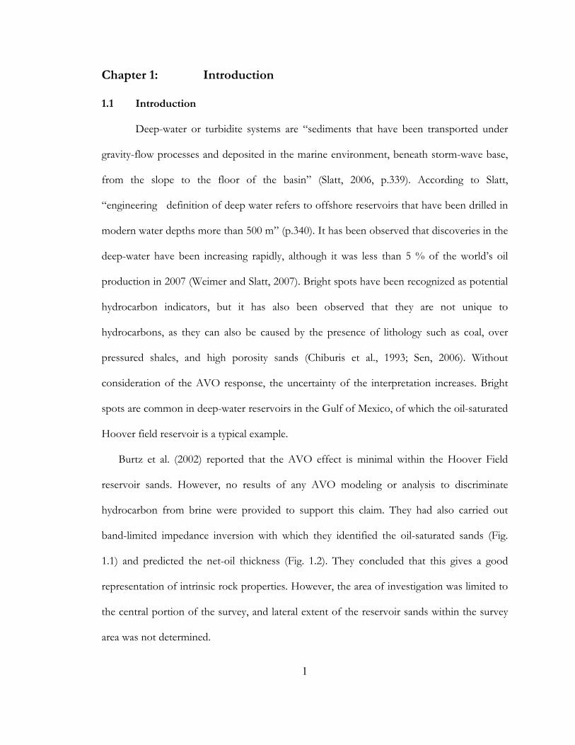
Burtz et al. (2002) reported that the AVO effect is minimal within the Hoover Field
reservoir sands. However, no results of any AVO modeling or analysis to discriminate
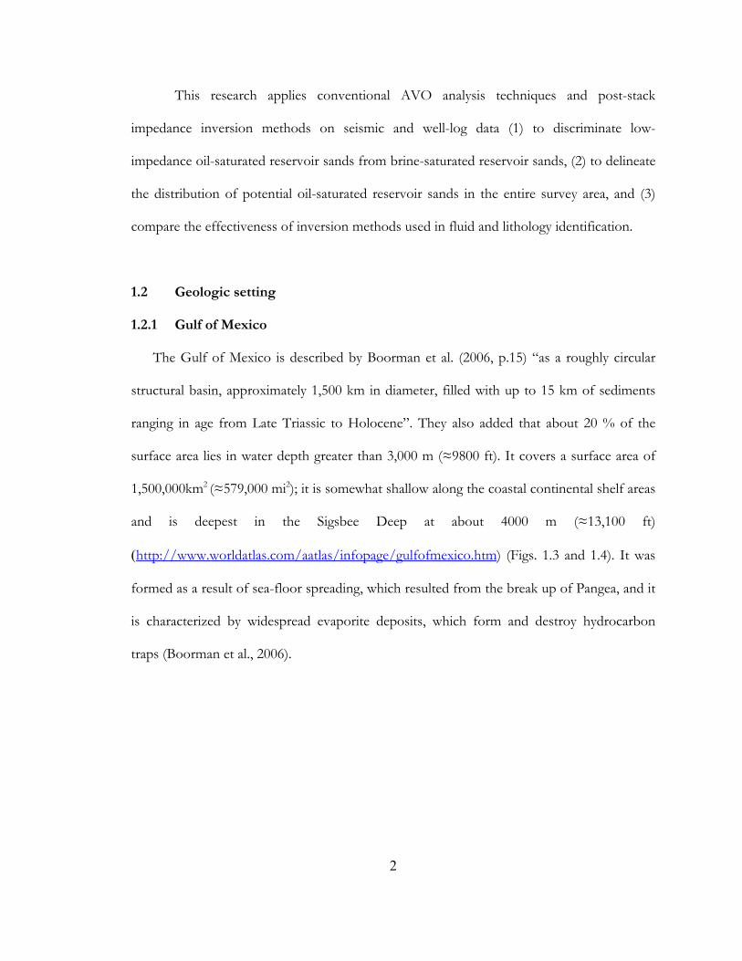
hydrocarbon from brine were provided to support this claim. They had also carried out
band-limited impedance inversion with which they identified the oil-saturated sands (Fig.
1.1) and predicted the net-oil thickness (Fig. 1.2). They concluded that this gives a good
representation of intrinsic rock properties. However, the area of investigation was limited to
the central portion of the survey, and lateral extent of the reservoir sands within the survey
area was not determined.
1
This research applies conventional AVO analysis techniques and post-stack
impedance inversion methods on seismic and well-log data (1) to discriminate low-
impedance oil-saturated reservoir sands from brine-saturated reservoir sands, (2) to delineate
the distribution of potential oil-saturated reservoir sands in the entire survey area, and (3)
compare the effectiveness of inversion methods used in fluid and lithology identification.
1.2 Geologic setting
1.2.1 Gulf of Mexico
The Gulf of Mexico is described by Boorman et al. (2006, p.15) “as a roughly circular
structural basin, approximately 1,500 km in diameter, filled with up to 15 km of sediments
ranging in age from Late Triassic to Holocene”. They also added that about 20 % of the
surface area lies in water depth greater than 3,000 m (≈9800 ft). It covers a surface area of
1,500,000km2 (≈579,000 mi2); it is somewhat shallow along the coastal continental shelf areas
and is deepest in the Sigsbee Deep at about 4000 m (≈13,100 ft)
(http://www.worldatlas.com/aatlas/infopage/gulfofmexico.htm) (Figs. 1.3 and 1.4). It was
formed as a result of sea-floor spreading, which resulted from the break up of Pangea, and it
is characterized by widespread evaporite deposits, which form and destroy hydrocarbon
traps (Boorman et al., 2006).
2
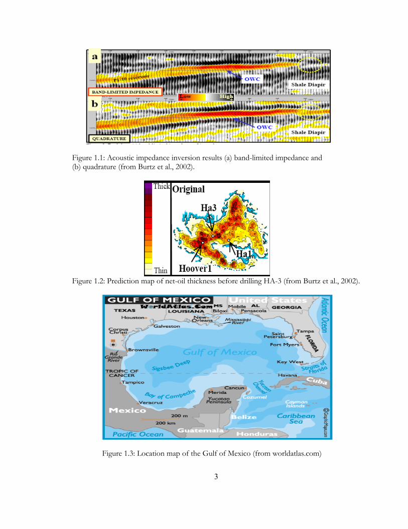
Figure 1.1: Acoustic impedance inversion results (a) band-limited impedance and (b) quadrature (from Burtz et al., 2002).
Figure 1.2: Prediction map of net-oil thickness before drilling HA-3 (from Burtz et al., 2002).
Figure 1.3: Location map of the Gulf of Mexico (from worldatlas.com)
3
1.2.2 Hoover Field
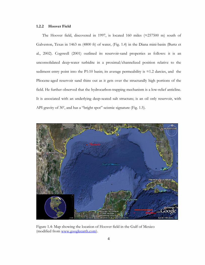
The Hoover field, discovered in 1997, is located 160 miles (≈257500 m) south of
Galveston, Texas in 1463 m (4800 ft) of water, (Fig. 1.4) in the Diana mini-basin (Burtz et
al., 2002). Cogswell (2001) outlined its reservoir-sand properties as follows: it is an
unconsolidated deep-water turbidite in a proximal/channelized position relative to the
sediment entry point into the P1:10 basin; its average permeability is ≈1.2 darcies, and the
Pliocene-aged reservoir sand thins out as it gets over the structurally high portions of the
field. He further observed that the hydrocarbon-trapping mechanism is a low-relief anticline.
It is associated with an underlying deep-seated salt structure; is an oil only reservoir, with
API gravity of 30o, and has a “bright spot” seismic signature (Fig. 1.5).
Figure 1.4: Map showing the location of Hoover field in the Gulf of Mexico (modified from www.googleearth.com).
4
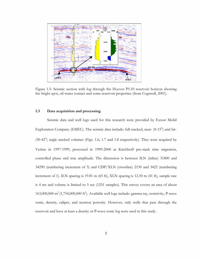
Figure 1.5: Seismic section with log through the Hoover P1:10 reservoir horizon showing the bright spot, oil-water contact and some reservoir properties (from Cogswell, 2001).
1.3 Data acquisition and processing
Seismic data and well logs used for this research were provided by Exxon Mobil
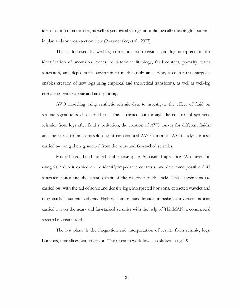
Exploration Company (EMEC). The seismic data include: full-stacked, near- (0-15o) and far-
(30-42o) angle stacked volumes (Figs. 1.6, 1.7 and 1.8 respectively). They were acquired by
Veritas in 1997-1999, processed in 1999-2000 as Kirchhoff pre-stack time migration,
controlled phase and true amplitude. The dimension is between ILN (inline) 31800 and
34290 (numbering increment of 5) and CDP/XLN (crossline) 2130 and 3422 (numbering
increment of 1). ILN spacing is 19.81 m (65 ft), XLN spacing is 12.50 m (41 ft), sample rate
is 4 ms and volume is limited to 5 sec (1251 samples). This survey covers an area of about
163,000,000 m2 (1,754,000,000 ft2). Available well logs include: gamma ray, resistivity, P-wave
sonic, density, caliper, and neutron porosity. However, only wells that pass through the
reservoir and have at least a density or P-wave sonic log were used in this study.
5
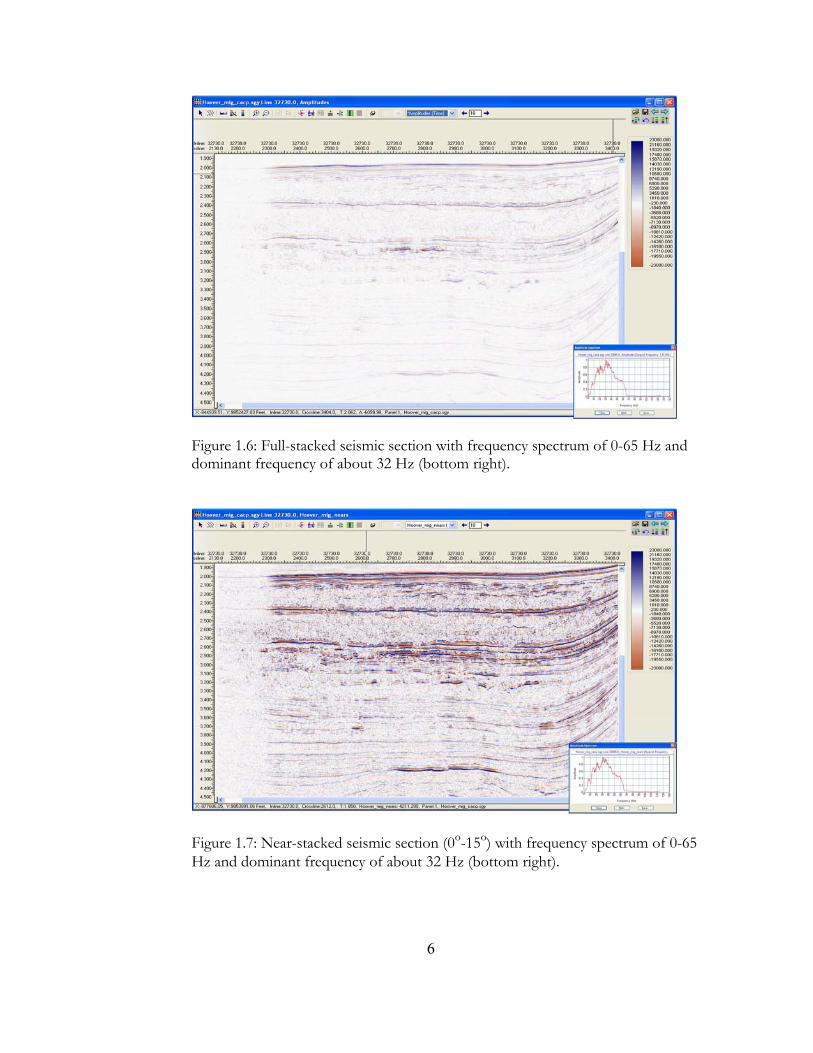
Figure 1.6: Full-stacked seismic section with frequency spectrum of 0-65 Hz and dominant frequency of about 32 Hz (bottom right).
Figure 1.7: Near-stacked seismic section (0o-15o) with frequency spectrum of 0-65 Hz and dominant frequency of about 32 Hz (bottom right).
6
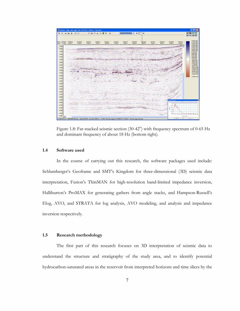
Figure 1.8: Far-stacked seismic section (30-42o) with frequency spectrum of 0-65 Hz and dominant frequency of about 18 Hz (bottom right).
1.4 Software used
In the course of carrying out this research, the software packages used include:
Schlumberger’s Geoframe and SMT’s Kingdom for three-dimensional (3D) seismic data
interpretation, Fusion’s ThinMAN for high-resolution band-limited impedance inversion,
Halliburton’s ProMAX for generating gathers from angle stacks, and Hampson-Russell’s
Elog, AVO, and STRATA for log analysis, AVO modeling, and analysis and impedance
inversion respectively.
1.5 Research methodology
The first part of this research focuses on 3D interpretation of seismic data to
understand the structure and stratigraphy of the study area, and to identify potential
hydrocarbon-saturated areas in the reservoir from interpreted horizons and time slices by the
7
identification of anomalies, as well as geologically or geomorphologically meaningful patterns
in plan and/or cross-section view (Posamentier, et al., 2007).
This is followed by well-log correlation with seismic and log interpretation for
identification of anomalous zones, to determine lithology, fluid content, porosity, water
saturation, and depositional environment in the study area. Elog, used for this purpose,
enables creation of new logs using empirical and theoretical transforms, as well as well-log
correlation with seismic and crossplotting.
AVO modeling using synthetic seismic data to investigate the effect of fluid on
seismic signature is also carried out. This is carried out through the creation of synthetic
seismics from logs after fluid substitution, the creation of AVO curves for different fluids,
and the extraction and crossplotting of conventional AVO attributes. AVO analysis is also
carried out on gathers generated from the near- and far-stacked seismics.
Model-based, band-limited and sparse-spike Acoustic Impedance (AI) inversion
using STRATA is carried out to identify impedance contrasts, and determine possible fluid
saturated zones and the lateral extent of the reservoir in the field. These inversions are
carried out with the aid of sonic and density logs, interpreted horizons, extracted wavelet and
near stacked seismic volume. High-resolution band-limited impedance inversion is also
carried out on the near- and far-stacked seismics with the help of ThinMAN, a commercial
spectral inversion tool.
The last phase is the integration and interpretation of results from seismic, logs,
horizons, time slices, and inversion. The research workflow is as shown in fig 1.9.
8
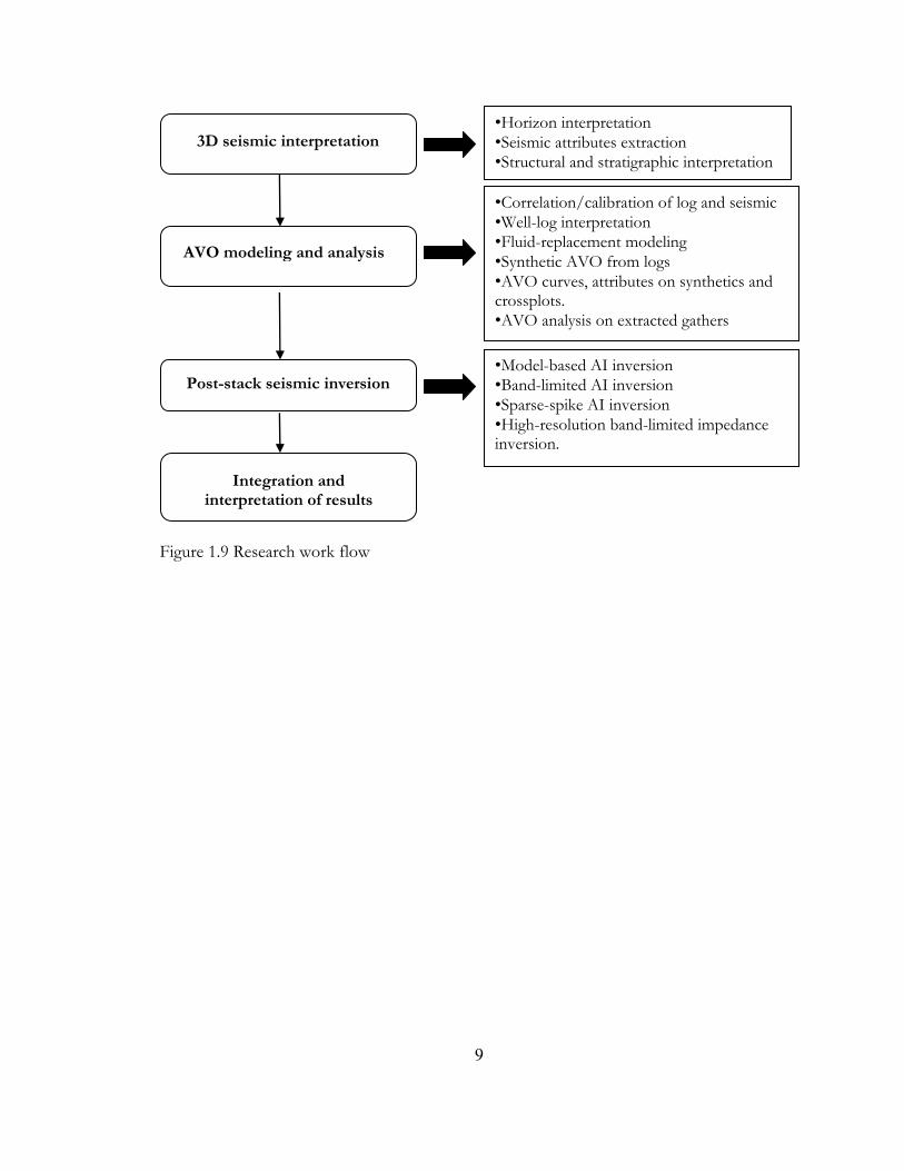
•Horizon interpretation •Seismic attributes extraction 3D seismic interpretation•Structural and stratigraphic interpretation
•Correlation/calibration of log and seismic •Well-log interpretation •Fluid-replacement modeling
AVO modeling and analysis •Synthetic AVO from logs •AVO curves, attributes on synthetics and crossplots. •AVO analysis on extracted gathers
•Model-based AI inversion •Band-limited AI inversion •Sparse-spike AI inversion •High-resolution band-limited impedance inversion.
Post-stack seismic inversion
Integration and interpretation of results
Figure 1.9 Research work flow
9
Chapter 2: Three-dimensional (3D) seismic data interpretations
2.1 Introduction
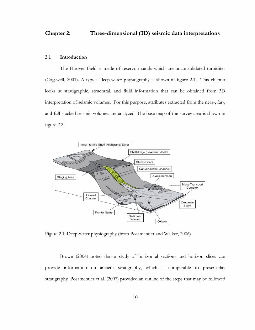
The Hoover Field is made of reservoir sands which are unconsolidated turbidites
(Cogswell, 2001). A typical deep-water physiography is shown in figure 2.1. This chapter
looks at stratigraphic, structural, and fluid information that can be obtained from 3D
interpretation of seismic volumes. For this purpose, attributes extracted from the near-, far-,
and full-stacked seismic volumes are analyzed. The base map of the survey area is shown in
figure 2.2.
Figure 2.1: Deep-water physiography (from Posamentier and Walker, 2006)
Brown (2004) noted that a study of horizontal sections and horizon slices can
provide information on ancient stratigraphy, which is comparable to present-day
stratigraphy. Posamentier et al. (2007) provided an outline of the steps that may be followed
10
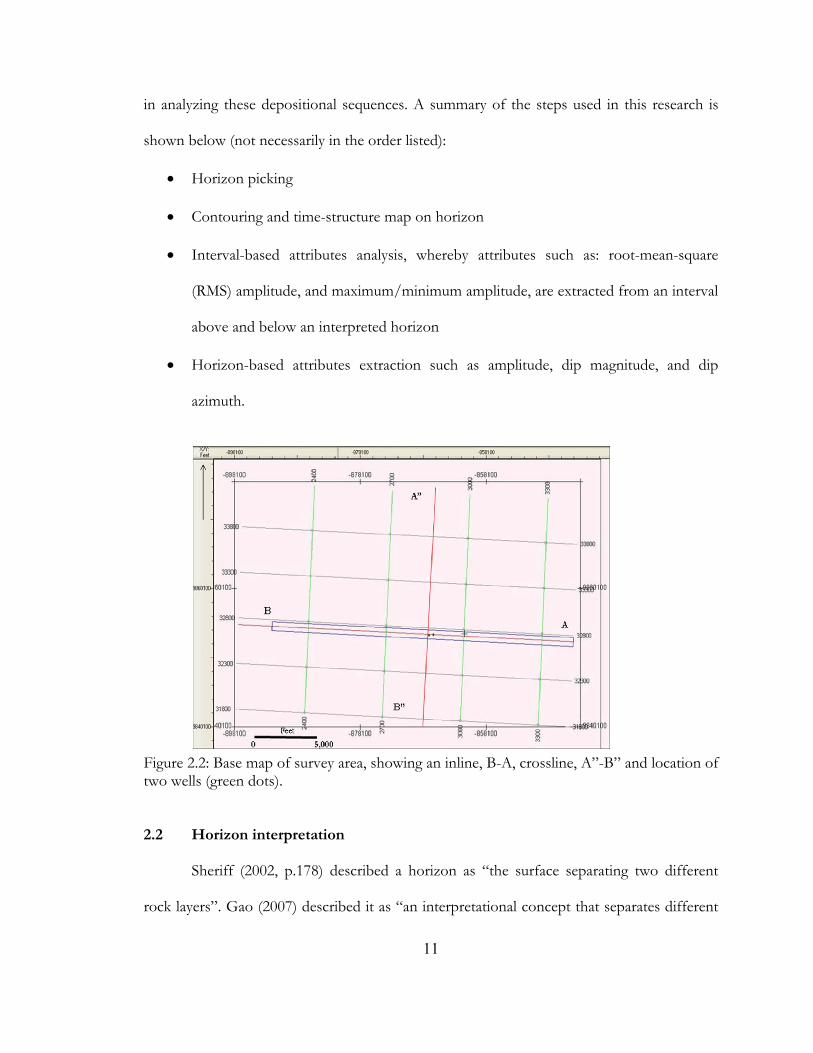
in analyzing these depositional sequences. A summary of the steps used in this research is
shown below (not necessarily in the order listed):
• Horizon picking
• Contouring and time-structure map on horizon
• Interval-based attributes analysis, whereby attributes such as: root-mean-square
(RMS) amplitude, and maximum/minimum amplitude, are extracted from an interval
above and below an interpreted horizon
• Horizon-based attributes extraction such as amplitude, dip magnitude, and dip
azimuth.
Figure 2.2: Base map of survey area, showing an inline, B-A, crossline, A”-B” and location of two wells (green dots). 2.2 Horizon interpretation
Sheriff (2002, p.178) described a horizon as “the surface separating two different
rock layers”. Gao (2007) described it as “an interpretational concept that separates different
11
geological units such as: water from shallow sediments, sedimentary rock from salt diapirs or
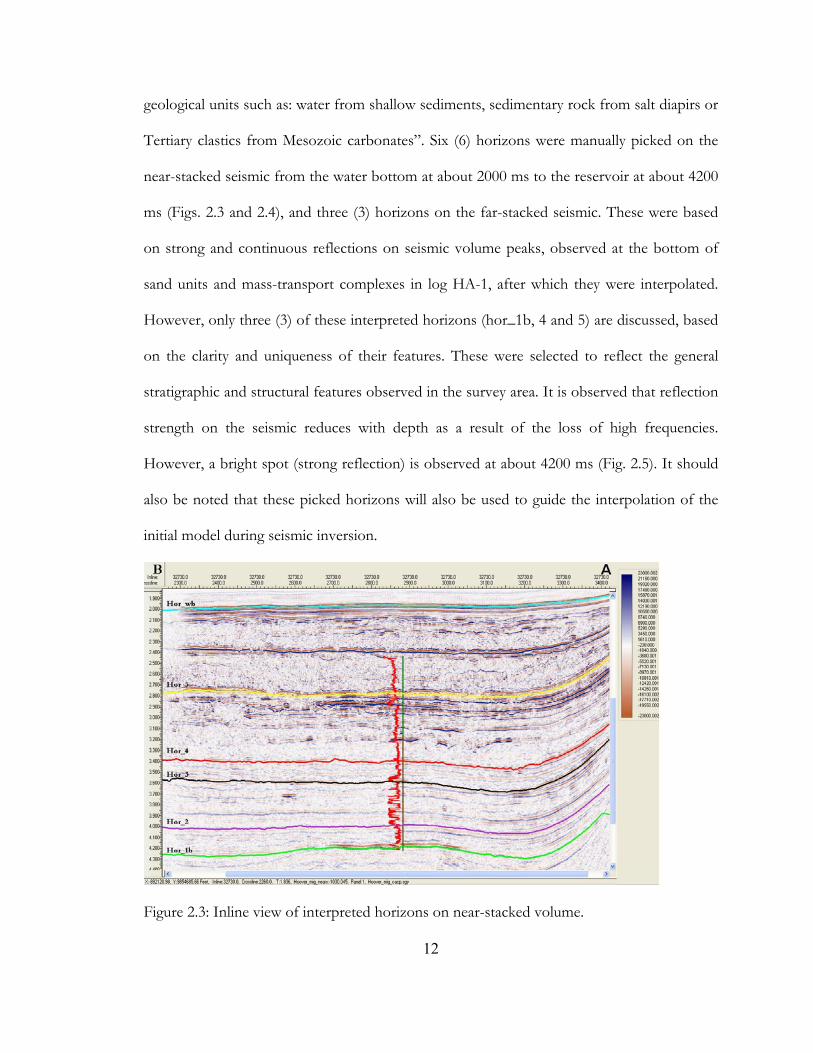
Tertiary clastics from Mesozoic carbonates”. Six (6) horizons were manually picked on the
near-stacked seismic from the water bottom at about 2000 ms to the reservoir at about 4200
ms (Figs. 2.3 and 2.4), and three (3) horizons on the far-stacked seismic. These were based
on strong and continuous reflections on seismic volume peaks, observed at the bottom of
sand units and mass-transport complexes in log HA-1, after which they were interpolated.
However, only three (3) of these interpreted horizons (hor_1b, 4 and 5) are discussed, based
on the clarity and uniqueness of their features. These were selected to reflect the general
stratigraphic and structural features observed in the survey area. It is observed that reflection
strength on the seismic reduces with depth as a result of the loss of high frequencies.
However, a bright spot (strong reflection) is observed at about 4200 ms (Fig. 2.5). It should
also be noted that these picked horizons will also be used to guide the interpolation of the
initial model during seismic inversion.
Figure 2.3: Inline view of interpreted horizons on near-stacked volume.
12
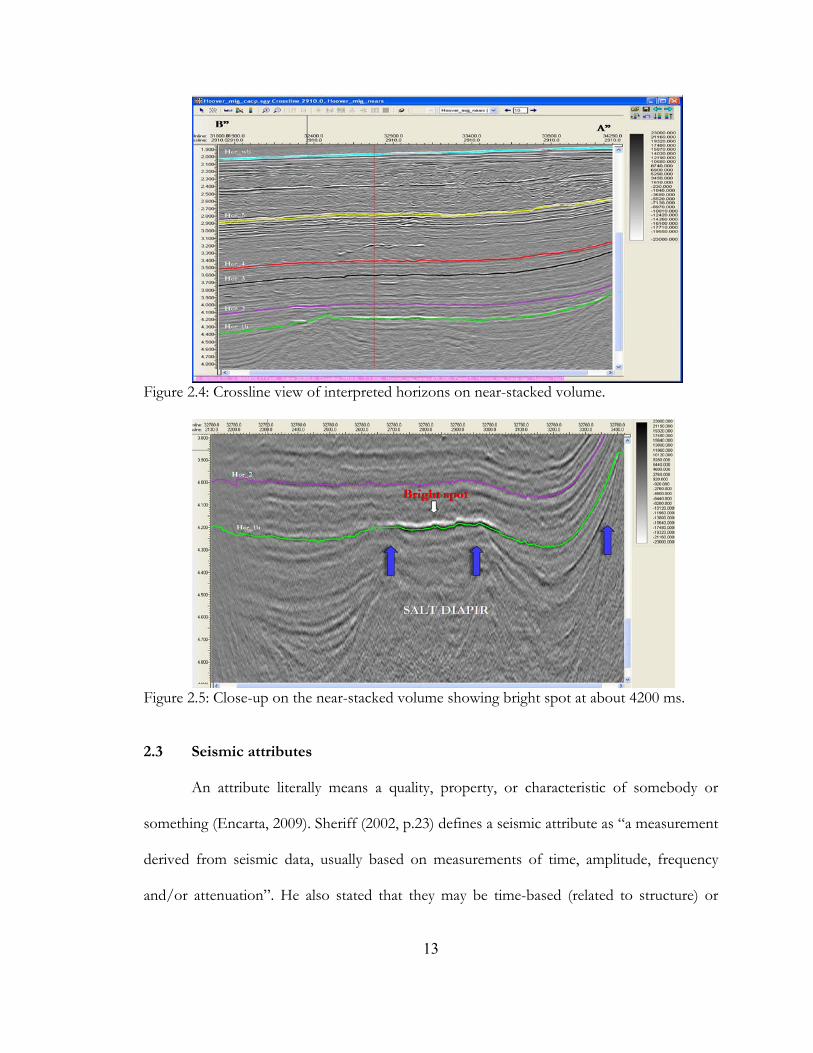
Figure 2.4: Crossline view of interpreted horizons on near-stacked volume.
Figure 2.5: Close-up on the near-stacked volume showing bright spot at about 4200 ms.
2.3 Seismic attributes
An attribute literally means a quality, property, or characteristic of somebody or
something (Encarta, 2009). Sheriff (2002, p.23) defines a seismic attribute as “a measurement
derived from seismic data, usually based on measurements of time, amplitude, frequency
and/or attenuation”. He also stated that they may be time-based (related to structure) or
13
amplitude-based (related to stratigraphy and reservoir characterization). To aid my
interpretation, I have used the following attributes: time structure, horizon amplitude (RMS),
dip, azimuth, and coherence on the picked horizons and time slices (excluding the water
bottom).
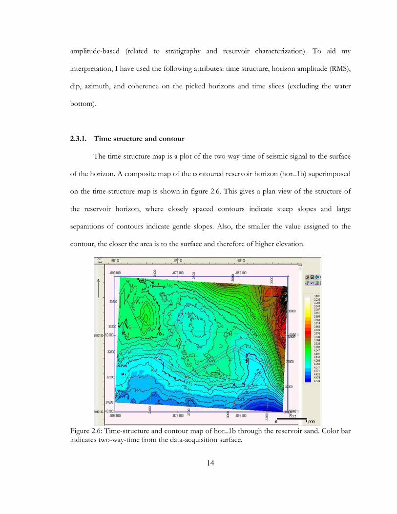
2.3.1. Time structure and contour
The time-structure map is a plot of the two-way-time of seismic signal to the surface
of the horizon. A composite map of the contoured reservoir horizon (hor_1b) superimposed
on the time-structure map is shown in figure 2.6. This gives a plan view of the structure of
the reservoir horizon, where closely spaced contours indicate steep slopes and large
separations of contours indicate gentle slopes. Also, the smaller the value assigned to the
contour, the closer the area is to the surface and therefore of higher elevation.
Figure 2.6: Time-structure and contour map of hor_1b through the reservoir sand. Color bar indicates two-way-time from the data-acquisition surface.
14
2.3.2 Amplitude extraction
Seismic amplitude variation plays a major role in identifying potential hydrocarbon
reservoirs and sediment-travel paths from source. Results of amplitudes extraction on the
interpreted horizons are as shown in figures 2.7, 2.9 and 2.10 for the near stack, figure 2.11
for the far stack and figure 2.12 for the full stack. Stratigraphic features observed are shown
and discussed below.
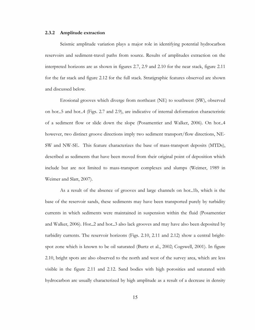
Erosional grooves which diverge from northeast (NE) to southwest (SW), observed
on hor_5 and hor_4 (Figs. 2.7 and 2.9), are indicative of internal deformation characteristic
of a sediment flow or slide down the slope (Posamentier and Walker, 2006). On hor_4
however, two distinct groove directions imply two sediment transport/flow directions, NE-
SW and NW-SE. This feature characterizes the base of mass-transport deposits (MTDs),
described as sediments that have been moved from their original point of deposition which
include but are not limited to mass-transport complexes and slumps (Weimer, 1989 in
Weimer and Slatt, 2007).
As a result of the absence of grooves and large channels on hor_1b, which is the
base of the reservoir sands, these sediments may have been transported purely by turbidity
currents in which sediments were maintained in suspension within the fluid (Posamentier
and Walker, 2006). Hor_2 and hor_3 also lack grooves and may have also been deposited by
turbidity currents. The reservoir horizons (Figs. 2.10, 2.11 and 2.12) show a central bright-
spot zone which is known to be oil saturated (Burtz et al., 2002; Cogswell, 2001). In figure
2.10, bright spots are also observed to the north and west of the survey area, which are less
visible in the figure 2.11 and 2.12. Sand bodies with high porosities and saturated with
hydrocarbon are usually characterized by high amplitude as a result of a decrease in density
15
and velocity. On the other hand, non-hydrocarbon sands, outside the bright spot, show
relatively low amplitudes.
Figure 2.7: Minimum amplitude extraction on hor_5 showing NE-SW erosional grooves. Blue arrows indicate flow direction.
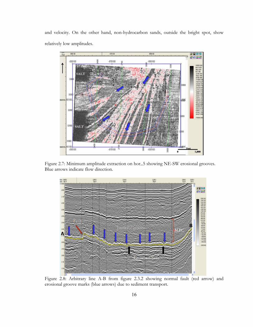
Figure 2.8: Arbitrary line A-B from figure 2.3.2 showing normal fault (red arrow) and erosional groove marks (blue arrows) due to sediment transport.
16
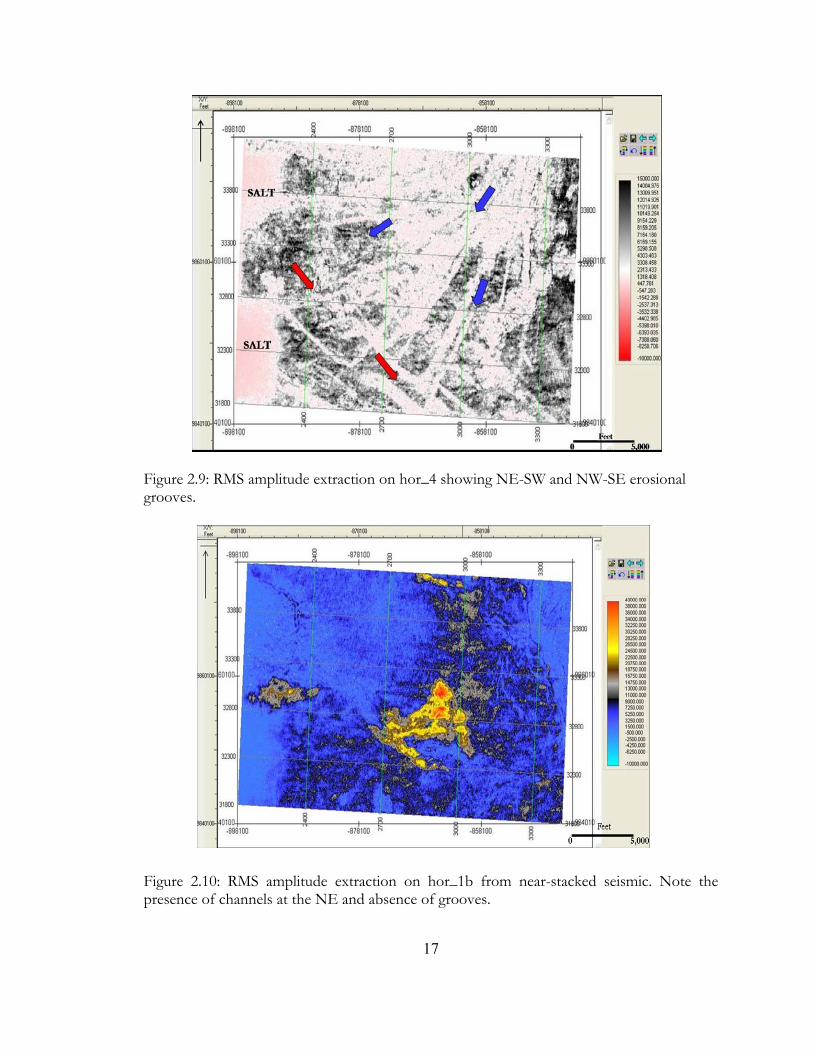
Figure 2.9: RMS amplitude extraction on hor_4 showing NE-SW and NW-SE erosional grooves.
Figure 2.10: RMS amplitude extraction on hor_1b from near-stacked seismic. Note the presence of channels at the NE and absence of grooves.
17
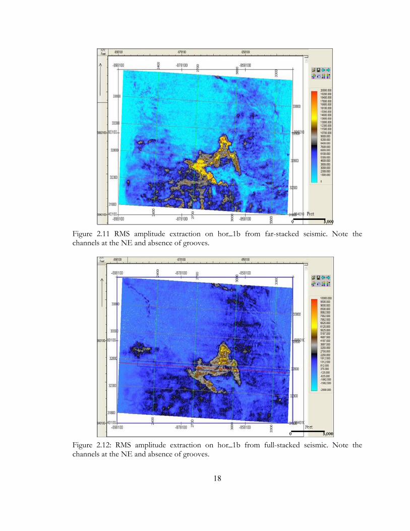
Figure 2.11 RMS amplitude extraction on hor_1b from far-stacked seismic. Note the channels at the NE and absence of grooves.
Figure 2.12: RMS amplitude extraction on hor_1b from full-stacked seismic. Note the channels at the NE and absence of grooves.
18
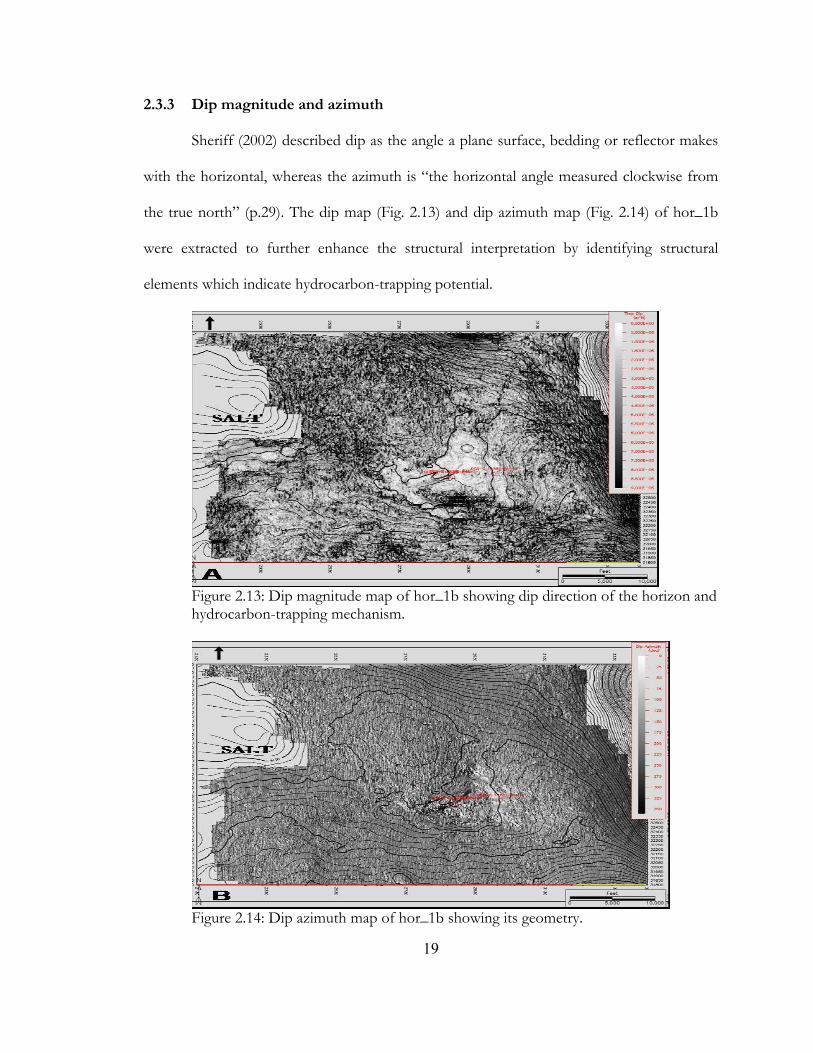
2.3.3 Dip magnitude and azimuth
Sheriff (2002) described dip as the angle a plane surface, bedding or reflector makes
with the horizontal, whereas the azimuth is “the horizontal angle measured clockwise from
the true north” (p.29). The dip map (Fig. 2.13) and dip azimuth map (Fig. 2.14) of hor_1b
were extracted to further enhance the structural interpretation by identifying structural
elements which indicate hydrocarbon-trapping potential.
Figure 2.13: Dip magnitude map of hor_1b showing dip direction of the horizon and hydrocarbon-trapping mechanism.
Figure 2.14: Dip azimuth map of hor_1b showing its geometry.
19
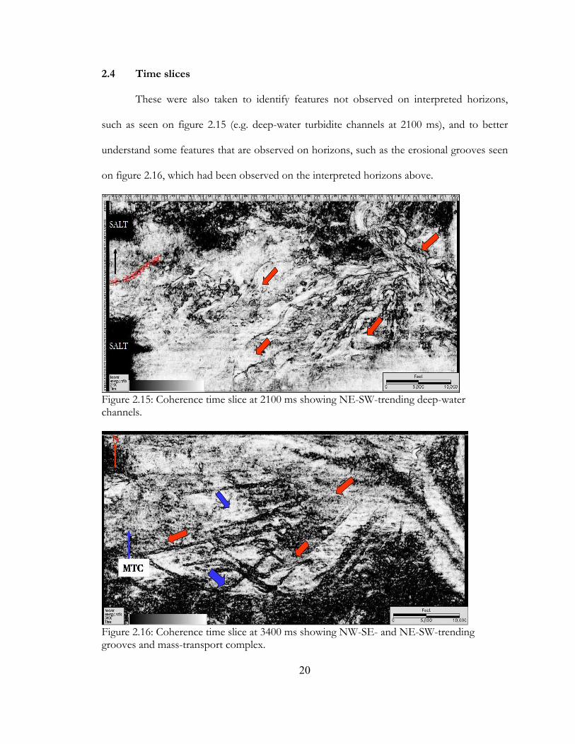
2.4 Time slices
These were also taken to identify features not observed on interpreted horizons,
such as seen on figure 2.15 (e.g. deep-water turbidite channels at 2100 ms), and to better
understand some features that are observed on horizons, such as the erosional grooves seen
on figure 2.16, which had been observed on the interpreted horizons above.
Figure 2.15: Coherence time slice at 2100 ms showing NE-SW-trending deep-water channels.
Figure 2.16: Coherence time slice at 3400 ms showing NW-SE- and NE-SW-trending grooves and mass-transport complex.
20
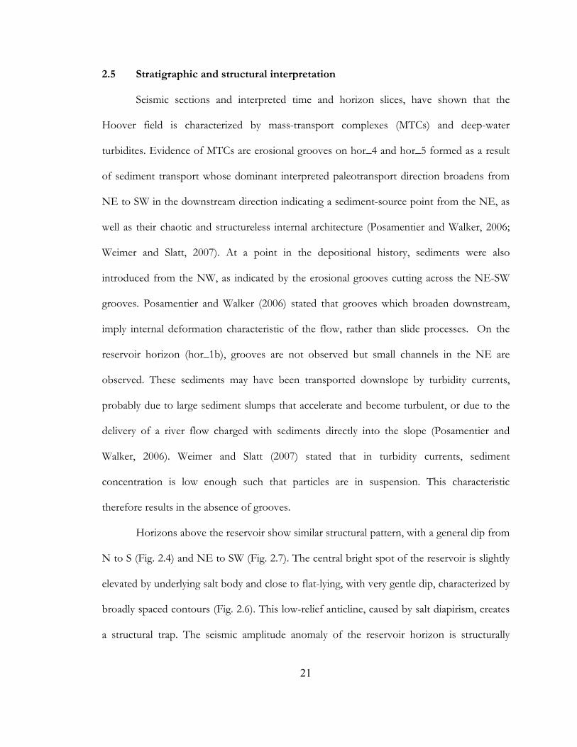
2.5 Stratigraphic and structural interpretation
Seismic sections and interpreted time and horizon slices, have shown that the
Hoover field is characterized by mass-transport complexes (MTCs) and deep-water
turbidites. Evidence of MTCs are erosional grooves on hor_4 and hor_5 formed as a result
of sediment transport whose dominant interpreted paleotransport direction broadens from
NE to SW in the downstream direction indicating a sediment-source point from the NE, as
well as their chaotic and structureless internal architecture (Posamentier and Walker, 2006;
Weimer and Slatt, 2007). At a point in the depositional history, sediments were also
introduced from the NW, as indicated by the erosional grooves cutting across the NE-SW
grooves. Posamentier and Walker (2006) stated that grooves which broaden downstream,
imply internal deformation characteristic of the flow, rather than slide processes. On the
reservoir horizon (hor_1b), grooves are not observed but small channels in the NE are
observed. These sediments may have been transported downslope by turbidity currents,
probably due to large sediment slumps that accelerate and become turbulent, or due to the
delivery of a river flow charged with sediments directly into the slope (Posamentier and
Walker, 2006). Weimer and Slatt (2007) stated that in turbidity currents, sediment
concentration is low enough such that particles are in suspension. This characteristic
therefore results in the absence of grooves.
Horizons above the reservoir show similar structural pattern, with a general dip from
N to S (Fig. 2.4) and NE to SW (Fig. 2.7). The central bright spot of the reservoir is slightly
elevated by underlying salt body and close to flat-lying, with very gentle dip, characterized by
broadly spaced contours (Fig. 2.6). This low-relief anticline, caused by salt diapirism, creates
a structural trap. The seismic amplitude anomaly of the reservoir horizon is structurally
21
consistent in that it conforms to the observed trapping structure (Brown, 2006), and shows
the probable geometry of the hydrocarbon-water contact. The NE section is bounded by a
structurally high area caused by salt withdrawal and upwelling due to sediment loading
(Weimer and Slatt, 2007).
2.6 Amplitude analysis
For a quantitative comparison of the full-, near-, and far-stacked volumes
amplitudes, they are normalized by a version of the A/B normalization technique described
by Hilterman (2001), where A is the anomaly (the reservoir horizon) and B the background
amplitude (zones away from the reservoir that are brine saturated). In this analysis, B is taken
as the interval RMS amplitudes between two horizons (hor_2 and a second horizon taken
300ms below hor_2). Based on these assumptions, it is observed that the areas away from
the bright spot have A/B ratios of between 1 and 3.5 and the bright spots have higher
amplitudes ranging between 6.5 and 10 (Fig. 2.17). This answers a question raised by Brown
(2004) on whether the amplitude anomaly is large relative to the background. The amplitude
anomaly shows an apparent Class 4 response (Castagna et al., 1998), i.e. a bright amplitude
which decreases with offset.
22
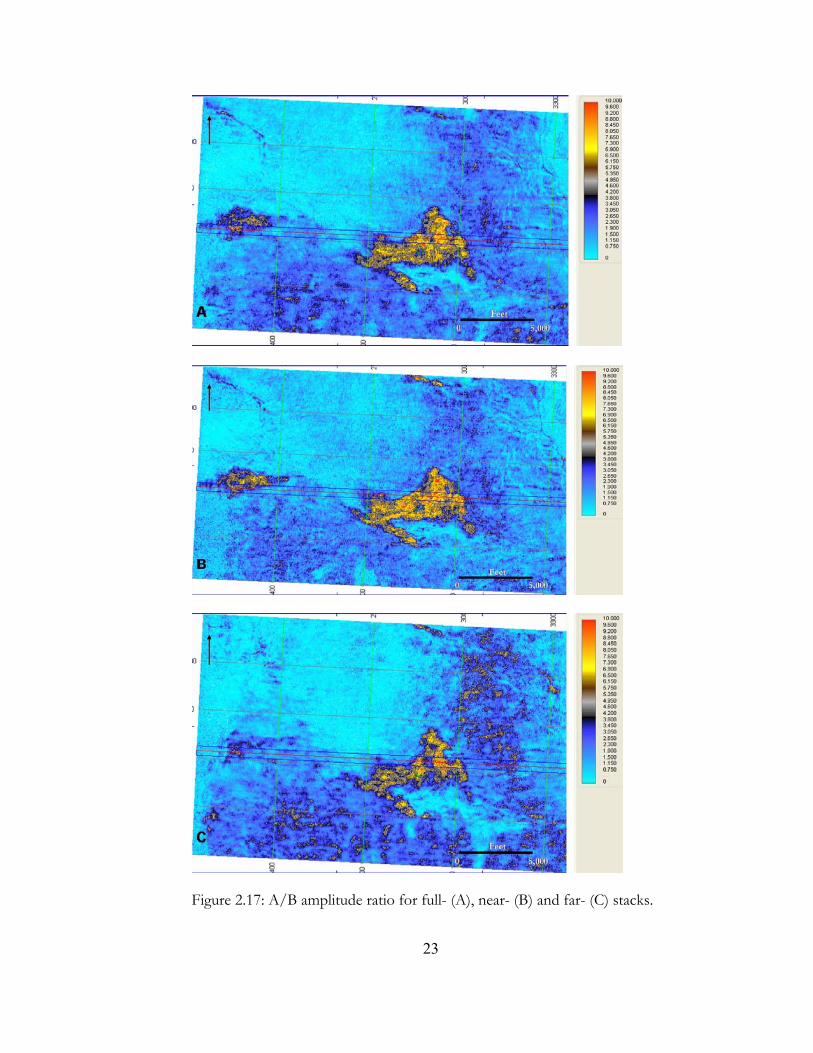
Figure 2.17: A/B amplitude ratio for full- (A), near- (B) and far- (C) stacks.
23
Chapter 3: AVO analysis from well logs
3.1 Seismic to log correlation
3.1.1 Introduction
Correlation is basically a measure of the similarity between a pair of traces. This
involves aligning the synthetic seismic generated from logs with seismic trace(s) near the well
location. In this research, correlation is carried out for near- and far-stacked seismic data
with logs in wells HA-1 and HA-4 using Hampson-Russell’s AVO and Kingdom’s SynPAK.
However, there are no deviation surveys to correct measured depths to true vertical depth.
Two methods of wavelet extraction from the seismic are used. The first involves the
extraction of wavelet after correlation, which represents the phase of the seismic and may
not be zero phase. The second involves the calibration of the seismic to zero phase after
correlation and subsequent extraction of a zero or close to zero-phase wavelet.
3.1.2 Synthetic seismogram generation (Forward modeling)
The correlation process begins with the convolution of reflectivity, r(t) derived from
density, P-wave velocity, and S-wave velocity logs with a zero-phase wavelet, w(t) extracted
from the seismic at the well location (Fig. 3.1) to generate a synthetic seismic, s(t) which is
correlated with each stacked section.
s(t) = w(t) * r(t) (1)
24
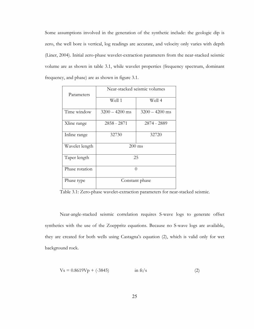
Some assumptions involved in the generation of the synthetic include: the geologic dip is
zero, the well bore is vertical, log readings are accurate, and velocity only varies with depth
(Liner, 2004). Initial zero-phase wavelet-extraction parameters from the near-stacked seismic
volume are as shown in table 3.1, while wavelet properties (frequency spectrum, dominant
frequency, and phase) are as shown in figure 3.1.
Near-stacked seismic volumes Parameters
Well 1 Well 4
Time window 3200 – 4200 ms 3200 – 4200 ms
Xline range 2858 - 2871 2874 - 2889
Inline range 32730 32720
Wavelet length 200 ms
Taper length 25
Phase rotation 0
Phase type Constant phase
Table 3.1: Zero-phase wavelet-extraction parameters for near-stacked seismic.
Near-angle-stacked seismic correlation requires S-wave logs to generate offset
synthetics with the use of the Zoeppritz equations. Because no S-wave logs are available,
they are created for both wells using Castagna’s equation (2), which is valid only for wet
background rock.
Vs = 0.8619Vp + (-3845) in ft/s (2)
25
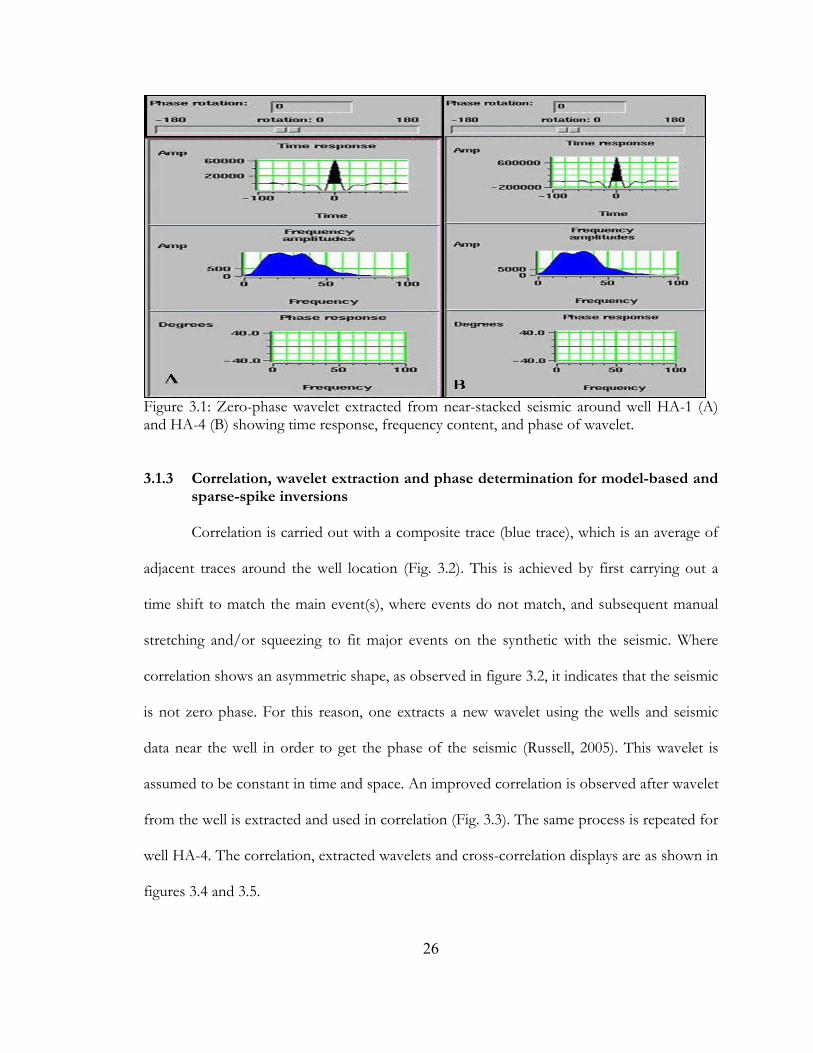
Figure 3.1: Zero-phase wavelet extracted from near-stacked seismic around well HA-1 (A) and HA-4 (B) showing time response, frequency content, and phase of wavelet.
3.1.3 Correlation, wavelet extraction and phase determination for model-based and sparse-spike inversions
Correlation is carried out with a composite trace (blue trace), which is an average of
adjacent traces around the well location (Fig. 3.2). This is achieved by first carrying out a
time shift to match the main event(s), where events do not match, and subsequent manual
stretching and/or squeezing to fit major events on the synthetic with the seismic. Where
correlation shows an asymmetric shape, as observed in figure 3.2, it indicates that the seismic
is not zero phase. For this reason, one extracts a new wavelet using the wells and seismic
data near the well in order to get the phase of the seismic (Russell, 2005). This wavelet is
assumed to be constant in time and space. An improved correlation is observed after wavelet
from the well is extracted and used in correlation (Fig. 3.3). The same process is repeated for
well HA-4. The correlation, extracted wavelets and cross-correlation displays are as shown in
figures 3.4 and 3.5.
26
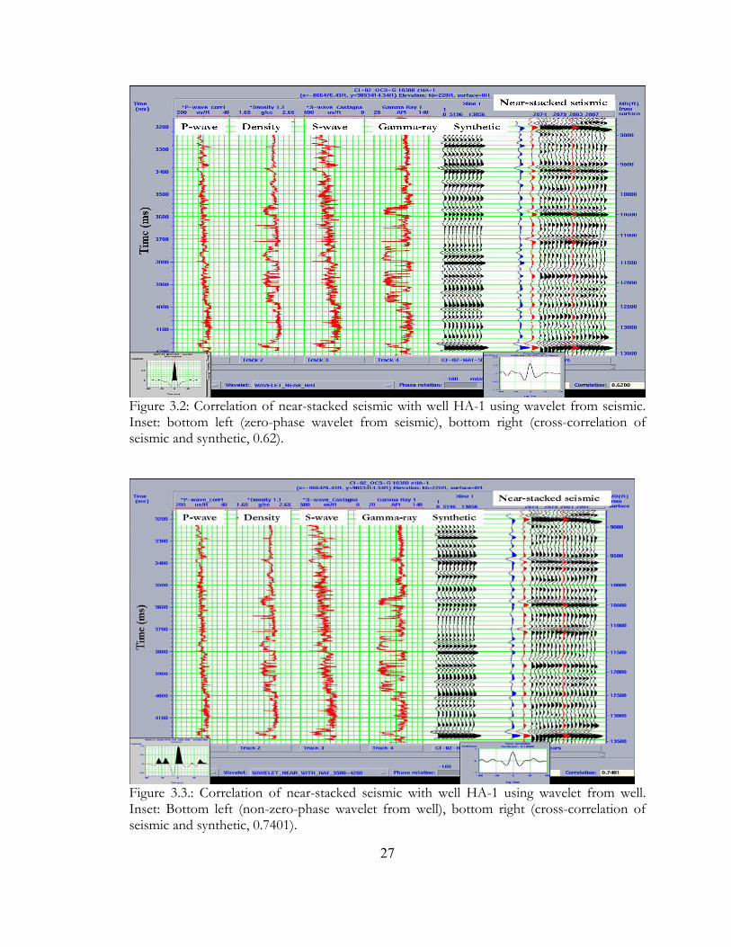
Figure 3.2: Correlation of near-stacked seismic with well HA-1 using wavelet from seismic. Inset: bottom left (zero-phase wavelet from seismic), bottom right (cross-correlation of seismic and synthetic, 0.62).
Figure 3.3.: Correlation of near-stacked seismic with well HA-1 using wavelet from well. Inset: Bottom left (non-zero-phase wavelet from well), bottom right (cross-correlation of seismic and synthetic, 0.7401).
27
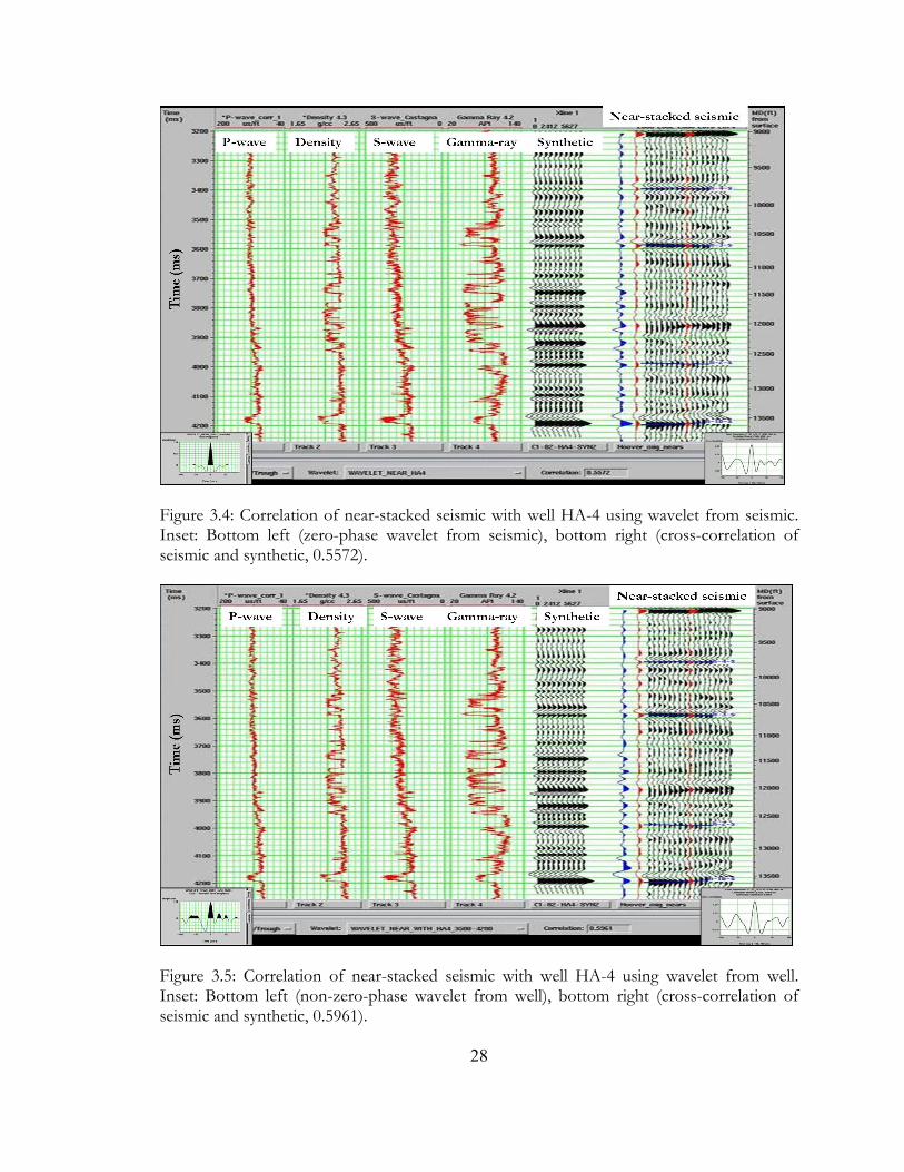
Figure 3.4: Correlation of near-stacked seismic with well HA-4 using wavelet from seismic. Inset: Bottom left (zero-phase wavelet from seismic), bottom right (cross-correlation of seismic and synthetic, 0.5572).
Figure 3.5: Correlation of near-stacked seismic with well HA-4 using wavelet from well. Inset: Bottom left (non-zero-phase wavelet from well), bottom right (cross-correlation of seismic and synthetic, 0.5961).
28
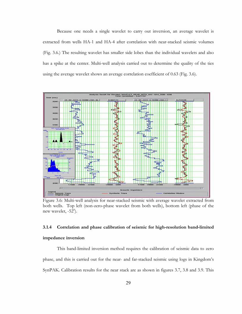
Because one needs a single wavelet to carry out inversion, an average wavelet is
extracted from wells HA-1 and HA-4 after correlation with near-stacked seismic volumes
(Fig. 3.6.) The resulting wavelet has smaller side lobes than the individual wavelets and also
has a spike at the center. Multi-well analysis carried out to determine the quality of the ties
using the average wavelet shows an average correlation coefficient of 0.63 (Fig. 3.6).
Figure 3.6: Multi-well analysis for near-stacked seismic with average wavelet extracted from both wells. Top left (non-zero-phase wavelet from both wells), bottom left (phase of the new wavelet, -520).
3.1.4 Correlation and phase calibration of seismic for high-resolution band-limited
impedance inversion
This band-limited inversion method requires the calibration of seismic data to zero
phase, and this is carried out for the near- and far-stacked seismic using logs in Kingdom’s
SynPAK. Calibration results for the near stack are as shown in figures 3.7, 3.8 and 3.9. This
29
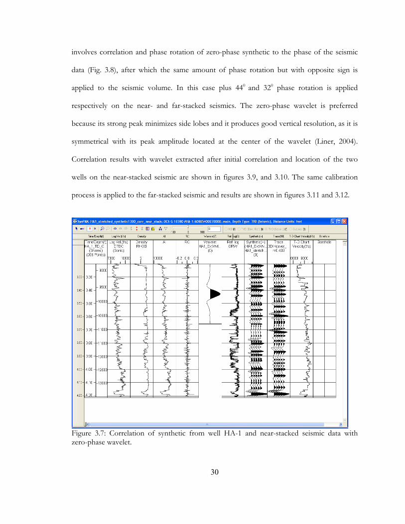
involves correlation and phase rotation of zero-phase synthetic to the phase of the seismic
data (Fig. 3.8), after which the same amount of phase rotation but with opposite sign is
applied to the seismic volume. In this case plus 440 and 320 phase rotation is applied
respectively on the near- and far-stacked seismics. The zero-phase wavelet is preferred
because its strong peak minimizes side lobes and it produces good vertical resolution, as it is
symmetrical with its peak amplitude located at the center of the wavelet (Liner, 2004).
Correlation results with wavelet extracted after initial correlation and location of the two
wells on the near-stacked seismic are shown in figures 3.9, and 3.10. The same calibration
process is applied to the far-stacked seismic and results are shown in figures 3.11 and 3.12.
Figure 3.7: Correlation of synthetic from well HA-1 and near-stacked seismic data with zero-phase wavelet.
30
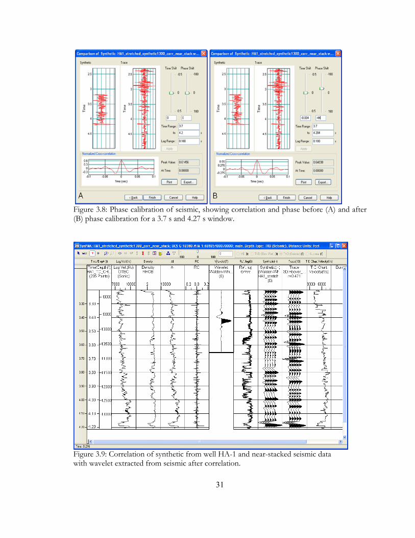
Figure 3.8: Phase calibration of seismic, showing correlation and phase before (A) and after (B) phase calibration for a 3.7 s and 4.27 s window.
Figure 3.9: Correlation of synthetic from well HA-1 and near-stacked seismic data with wavelet extracted from seismic after correlation.
31
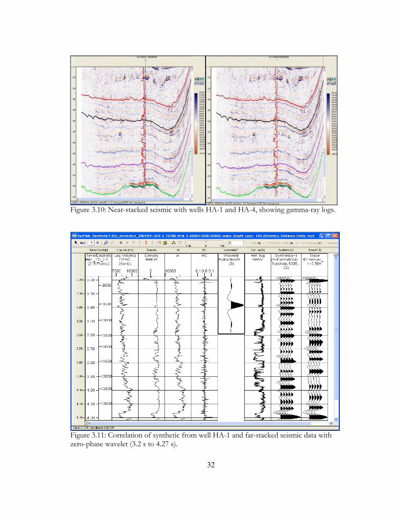
Figure 3.10: Near-stacked seismic with wells HA-1 and HA-4, showing gamma-ray logs.
Figure 3.11: Correlation of synthetic from well HA-1 and far-stacked seismic data with zero-phase wavelet (3.2 s to 4.27 s). 32
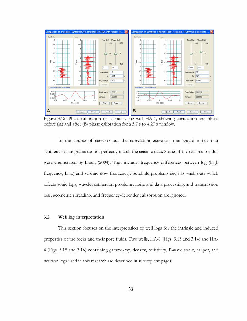
Figure 3.12: Phase calibration of seismic using well HA-1, showing correlation and phase before (A) and after (B) phase calibration for a 3.7 s to 4.27 s window.
In the course of carrying out the correlation exercises, one would notice that
synthetic seismograms do not perfectly match the seismic data. Some of the reasons for this
were enumerated by Liner, (2004). They include: frequency differences between log (high
frequency, kHz) and seismic (low frequency); borehole problems such as wash outs which
affects sonic logs; wavelet estimation problems; noise and data processing; and transmission
loss, geometric spreading, and frequency-dependent absorption are ignored.
3.2 Well log interpretation
This section focuses on the interpretation of well logs for the intrinsic and induced
properties of the rocks and their pore fluids. Two wells, HA-1 (Figs. 3.13 and 3.14) and HA-
4 (Figs. 3.15 and 3.16) containing gamma-ray, density, resistivity, P-wave sonic, caliper, and
neutron logs used in this research are described in subsequent pages.
33
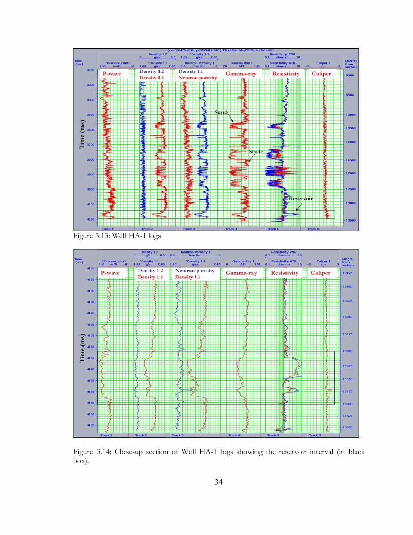
Figure 3.13: Well HA-1 logs
Figure 3.14: Close-up section of Well HA-1 logs showing the reservoir interval (in black box).
34
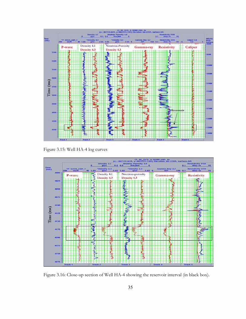
Figure 3.15: Well HA-4 log curves
Figure 3.16: Close-up section of Well HA-4 showing the reservoir interval (in black box).
35
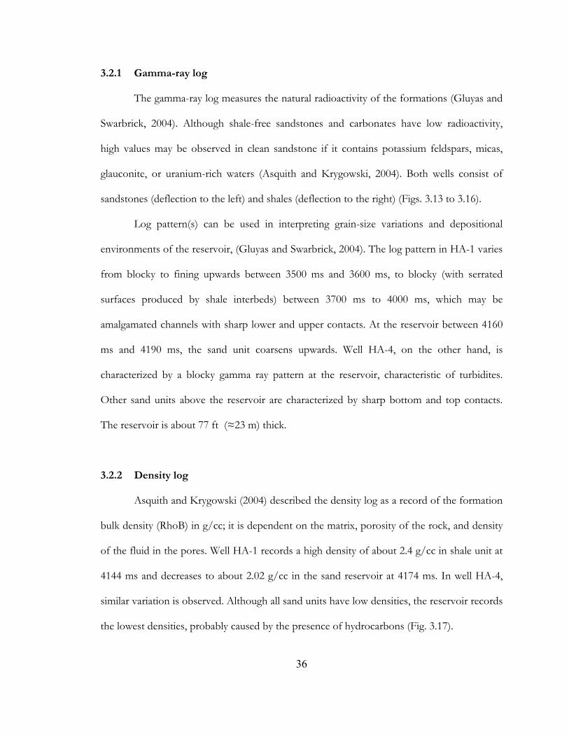
3.2.1 Gamma-ray log
The gamma-ray log measures the natural radioactivity of the formations (Gluyas and
Swarbrick, 2004). Although shale-free sandstones and carbonates have low radioactivity,
high values may be observed in clean sandstone if it contains potassium feldspars, micas,
glauconite, or uranium-rich waters (Asquith and Krygowski, 2004). Both wells consist of
sandstones (deflection to the left) and shales (deflection to the right) (Figs. 3.13 to 3.16).
Log pattern(s) can be used in interpreting grain-size variations and depositional
environments of the reservoir, (Gluyas and Swarbrick, 2004). The log pattern in HA-1 varies
from blocky to fining upwards between 3500 ms and 3600 ms, to blocky (with serrated
surfaces produced by shale interbeds) between 3700 ms to 4000 ms, which may be
amalgamated channels with sharp lower and upper contacts. At the reservoir between 4160
ms and 4190 ms, the sand unit coarsens upwards. Well HA-4, on the other hand, is
characterized by a blocky gamma ray pattern at the reservoir, characteristic of turbidites.
Other sand units above the reservoir are characterized by sharp bottom and top contacts.
The reservoir is about 77 ft (≈23 m) thick.
3.2.2 Density log
Asquith and Krygowski (2004) described the density log as a record of the formation
bulk density (RhoB) in g/cc; it is dependent on the matrix, porosity of the rock, and density
of the fluid in the pores. Well HA-1 records a high density of about 2.4 g/cc in shale unit at
4144 ms and decreases to about 2.02 g/cc in the sand reservoir at 4174 ms. In well HA-4,
similar variation is observed. Although all sand units have low densities, the reservoir records
the lowest densities, probably caused by the presence of hydrocarbons (Fig. 3.17).
36
The density-correction curve, DRho (labeled density 1.2 and 4.1), indicates the
amount of correction that has been added to the density log during processing due to
borehole effects (Asquith and Krygowski, 2004). They advised that where the correction
curve exceeds 0.20 g/cc, the density log reading should be considered suspect and possibly
invalid. In both wells, density correction values are below 0.2 g/cc.
3.2.3 Neutron log
The neutron log measures hydrogen atom concentration present in formation pores
(Gluyas and Swarbrick, 2004; Slatt, R.M., 2006). Asquith and Krygowski (2004) stated that a
low hydrogen density indicates low liquid-filled porosity. They also added that when pores
are filled with gas rather than oil or water, the reported neutron porosity is less (i.e. gas
effect) than the actual formation porosity as a result of the lower concentration of hydrogen
in gas compared to oil or water. Brine- and oil-saturated sands in both wells record about the
same amount of neutron porosity as shown in figures 3.13 to 3.16 and 3.18, making it a poor
discriminating property.
3.2.4 P-wave sonic log
The P-wave sonic log measures the transit time (Δt in μs/ft) of an acoustic
waveform between a transmitter and a receiver (Veeken, 2007). Both logs show a general
increase in velocity with depth, with a sudden decrease in the reservoir (Figs. 3.13 to 3.16).
P-wave velocity in the overlying shale ranges between 2854 m/s (9365 ft/s) and 2943 m/s
(9655 ft/s), however it drops to below 2377 m/s (7,800 ft/s) in the reservoir, probably due
37
to the presence of hydrocarbons before increasing above 2957 m/s (9,700 ft/s) in the
underlying shales.
3.2.5 Resistivity log
Resistivity is “the property of a material that resists the flow of an electric current”
(Sheriff, 2002, p.298). A brine-saturated rock is expected to have a lower resistivity than
hydrocarbon-saturated rock, as it is more conductive. Resistivity logs available in the survey
area include phase-shift-derived resistivity (PSR) and attenuation-derived resistivity (ATR).
The PSR log is equivalent to the spherically focused resistivity log on the wireline induction
tool with average depth of investigation of 75 cm whereas ATR is equivalent to the dual
induction-medium measurement with an average depth of investigation of 125 cm (Moore,
et al., 1998). In this research, they would be considered as “deep” for ATR and “shallow” for
PSR, although in the true sense of the word they are not. Drilling fluids used in HA-1 and
HA-4 are sea water and polymer respectively. Although both wells have a pay zone with
higher resistivity than the surrounding formations, this is relatively low for an oil reservoir, as
it is less than 10 ohm-m. In HA-1, resistivity increases over 100 % from 1.19 ohm-m at
about 4155 ms in the shale water-saturated unit, to approximately 3.5 ohm-m at about
4161ms in the sandstone reservoir with hydrocarbon. This decreases slowly towards the
bottom of the reservoir with a value of 1.1 ohm-m at 4186 ms at the bottom of the
reservoir. Similar readings are obtained in HA-4. At the reservoir, there is little separation
between both logs. Where there is a separation as observed in the sand units above the
reservoir in HA-1, it is as a result of invasion.
38
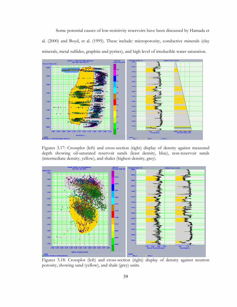
Some potential causes of low-resistivity reservoirs have been discussed by Hamada et
al. (2000) and Boyd, et al. (1995). These include: microporosity, conductive minerals (clay
minerals, metal sulfides, graphite and pyrites), and high level of irreducible water saturation.
Figures 3.17: Crossplot (left) and cross-section (right) display of density against measured depth showing oil-saturated reservoir sands (least density, blue), non-reservoir sands (intermediate density, yellow), and shales (highest density, grey).
Figures 3.18: Crossplot (left) and cross-section (right) display of density against neutron porosity, showing sand (yellow), and shale (grey) units.
39
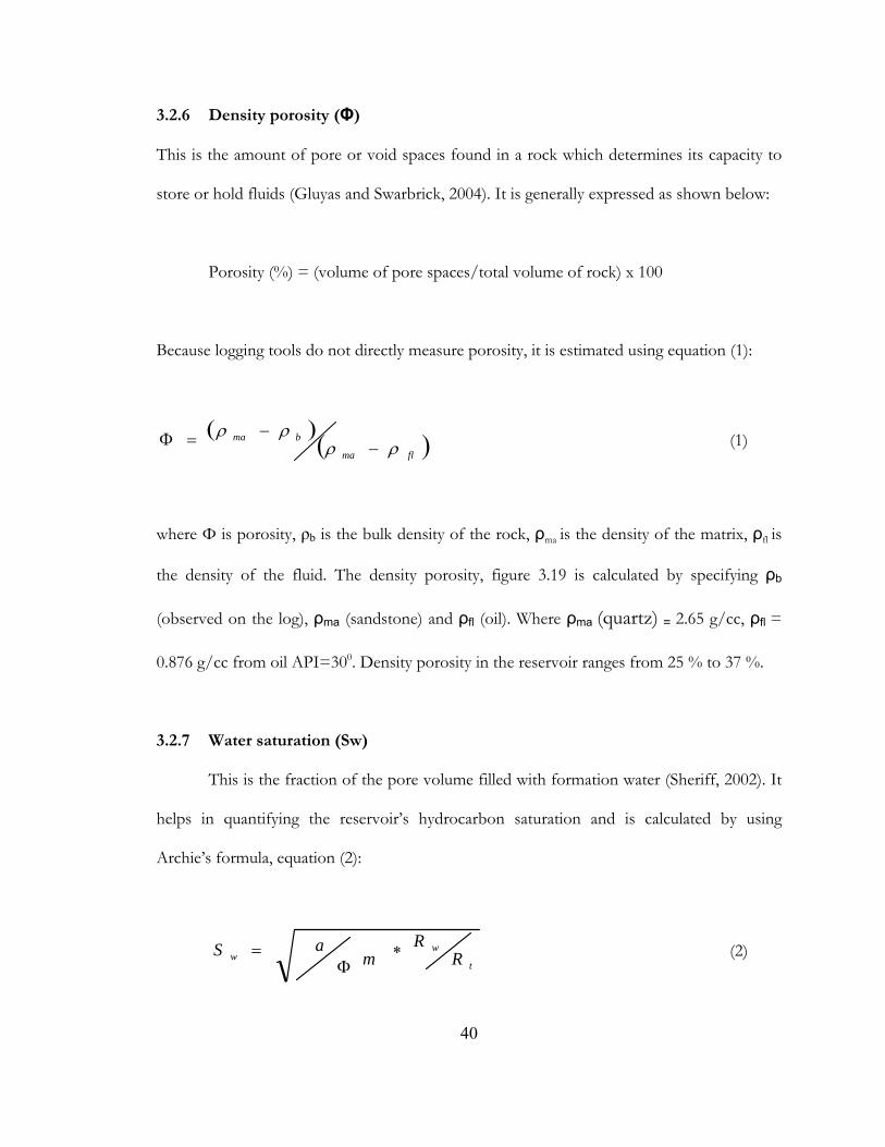
3.2.6 Density porosity (Φ)
This is the amount of pore or void spaces found in a rock which determines its capacity to
store or hold fluids (Gluyas and Swarbrick, 2004). It is generally expressed as shown below:
Porosity (%) = (volume of pore spaces/total volume of rock) x 100
Because logging tools do not directly measure porosity, it is estimated using equation (1):
)()( flma
bmaρρ
ρρ−
−=Φ (1)
where Φ is porosity, ρb is the bulk density of the rock, ρma is the density of the matrix, ρfl is
the density of the fluid. The density porosity, figure 3.19 is calculated by specifying ρb
(observed on the log), ρma (sandstone) and ρfl (oil). Where ρma (quartz) = 2.65 g/cc, ρfl =
0.876 g/cc from oil API=300. Density porosity in the reservoir ranges from 25 % to 37 %.
3.2.7 Water saturation (Sw)
This is the fraction of the pore volume filled with formation water (Sheriff, 2002). It
helps in quantifying the reservoir’s hydrocarbon saturation and is calculated by using
Archie’s formula, equation (2):
t
ww R
Rm
aS ∗Φ
= (2)
40
where a is a constant, m is cementation factor, Ф is porosity, Rw is resistivity of formation
water, and Rt is true resistivity of the formation. Selley (1985) pointed out that this method is
valid for clean, clay-free formations. Because the Hoover field’s “deep” resistivity logs
records low resistivity, a larger Sw than should be the case would be obtained from the
formula. Generally, a = 1 and m = 2; however, for unconsolidated sands (soft formations), a
= 0.62 and m=2.15 from the Humble formula (Selley, 1985). From equation (2), the only
unknown is Rw which has to be calculated from a brine-saturated portion of the log as
shown below in equation (3):
Φ⎟⎟⎠
⎞⎜⎜⎝
⎛⎥⎦⎤
⎢⎣⎡
=
21
*t
w
w
RRC
S (3)
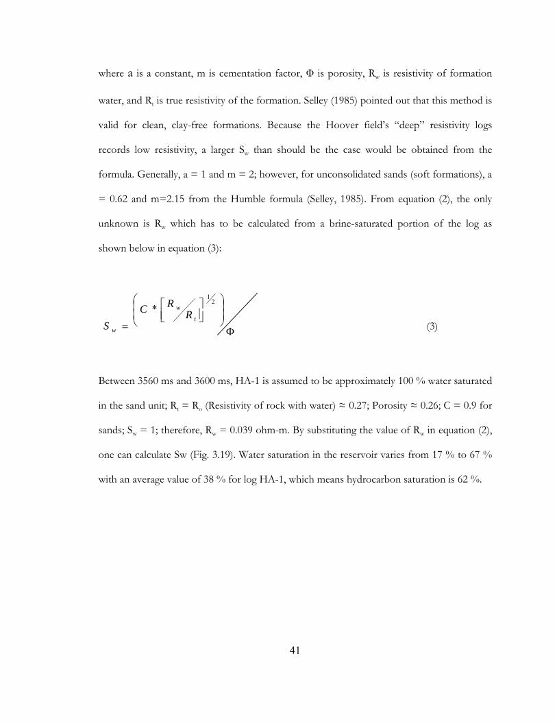
Between 3560 ms and 3600 ms, HA-1 is assumed to be approximately 100 % water saturated
in the sand unit; Rt = Ro (Resistivity of rock with water) ≈ 0.27; Porosity ≈ 0.26; C = 0.9 for
sands; Sw = 1; therefore, Rw = 0.039 ohm-m. By substituting the value of Rw in equation (2),
one can calculate Sw (Fig. 3.19). Water saturation in the reservoir varies from 17 % to 67 %
with an average value of 38 % for log HA-1, which means hydrocarbon saturation is 62 %.
41
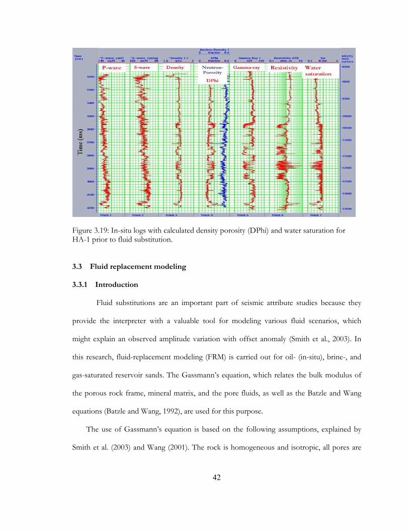
Figure 3.19: In-situ logs with calculated density porosity (DPhi) and water saturation for HA-1 prior to fluid substitution.
3.3 Fluid replacement modeling
3.3.1 Introduction
Fluid substitutions are an important part of seismic attribute studies because they
provide the interpreter with a valuable tool for modeling various fluid scenarios, which
might explain an observed amplitude variation with offset anomaly (Smith et al., 2003). In
this research, fluid-replacement modeling (FRM) is carried out for oil- (in-situ), brine-, and
gas-saturated reservoir sands. The Gassmann’s equation, which relates the bulk modulus of
the porous rock frame, mineral matrix, and the pore fluids, as well as the Batzle and Wang
equations (Batzle and Wang, 1992), are used for this purpose.
The use of Gassmann’s equation is based on the following assumptions, explained by
Smith et al. (2003) and Wang (2001). The rock is homogeneous and isotropic, all pores are
42
interconnected and communicating, pore pressure is equilibrated throughout the rock, the
pore fluid does not interact with the solid in such a way that would soften or harden the
frame, and the media is closed and no pore fluid leaves the rock volume.
3.3.2 Fluid-substitution equations
Smith et al. (2003) stated that the application of the Gassmann’s equation is a two-
part process, which involves the determination of the bulk modulus of the porous rock
frame before calculating the bulk modulus of the rock saturated with any desired fluid
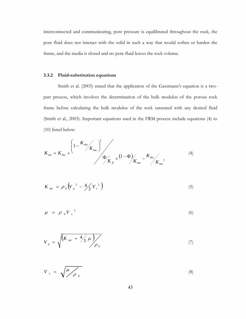
(Smith et al., 2003). Important equations used in the FRM process include equations (4) to
(10) listed below:
)(2
2
1
1
ma
dry
mafl
ma
dry
drysat
KK
KK
KK
KK−Φ−+Φ
⎜⎜⎝
⎛⎟⎠⎞−
+= (4)
)( 22
34
spbsat VVK −= ρ (5)
2sb Vρμ = (6)
)(b
satp
KV ρ
μ34+
= (7)
bsV ρ
μ= (8)
43
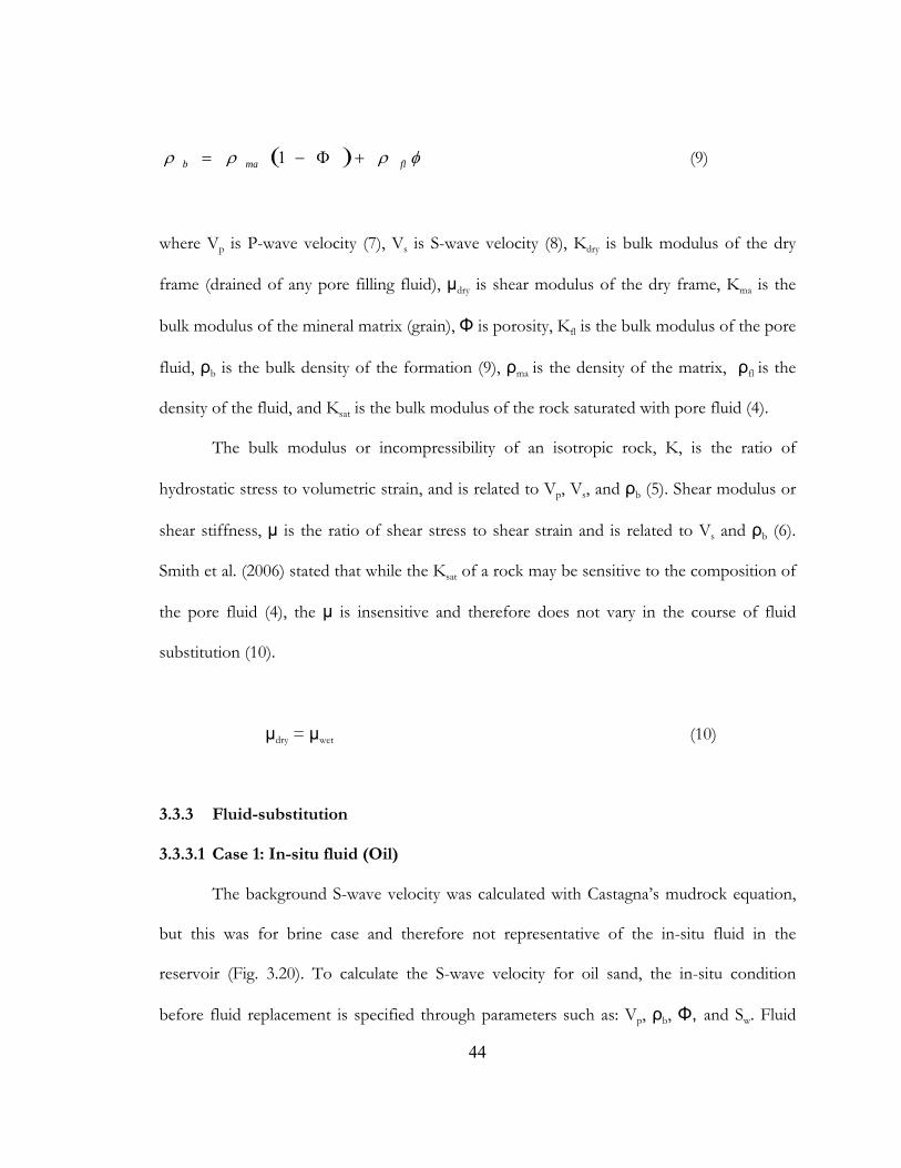
( ) φρρρ flmab +Φ−= 1 (9)
where Vp is P-wave velocity (7), Vs is S-wave velocity (8), Kdry is bulk modulus of the dry
frame (drained of any pore filling fluid), μdry is shear modulus of the dry frame, Kma is the
bulk modulus of the mineral matrix (grain), Φ is porosity, Kfl is the bulk modulus of the pore
fluid, ρb is the bulk density of the formation (9), ρma is the density of the matrix, ρfl is the
density of the fluid, and Ksat is the bulk modulus of the rock saturated with pore fluid (4).
The bulk modulus or incompressibility of an isotropic rock, K, is the ratio of
hydrostatic stress to volumetric strain, and is related to Vp, Vs, and ρb (5). Shear modulus or
shear stiffness, μ is the ratio of shear stress to shear strain and is related to Vs and ρb (6).
Smith et al. (2006) stated that while the Ksat of a rock may be sensitive to the composition of
the pore fluid (4), the μ is insensitive and therefore does not vary in the course of fluid
substitution (10).
μdry = μwet (10)
3.3.3 Fluid-substitution
3.3.3.1 Case 1: In-situ fluid (Oil)
The background S-wave velocity was calculated with Castagna’s mudrock equation,
but this was for brine case and therefore not representative of the in-situ fluid in the
reservoir (Fig. 3.20). To calculate the S-wave velocity for oil sand, the in-situ condition
before fluid replacement is specified through parameters such as: Vp, ρb, Φ, and Sw. Fluid
44
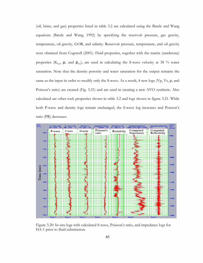
(oil, brine, and gas) properties listed in table 3.2 are calculated using the Batzle and Wang
equations (Batzle and Wang, 1992) by specifying the reservoir pressure, gas gravity,
temperature, oil gravity, GOR, and salinity. Reservoir pressure, temperature, and oil gravity
were obtained from Cogswell (2001). Fluid properties, together with the matrix (sandstone)
properties (Kma, μ, and ρma), are used in calculating the S-wave velocity at 38 % water
saturation. Note that the density porosity and water saturation for the output remains the
same as the input in order to modify only the S-wave. As a result, 4 new logs (Vp, Vs, ρ, and
Poisson’s ratio) are created (Fig. 3.21) and are used in creating a new AVO synthetic. Also
calculated are other rock properties shown in table 3.2 and logs shown in figure 3.21. While
both P-wave and density logs remain unchanged, the S-wave log increases and Poisson’s
ratio (PR) decreases.
Figure 3.20: In-situ logs with calculated S-wave, Poisson’s ratio, and impedance logs for HA-1 prior to fluid substitution.
45
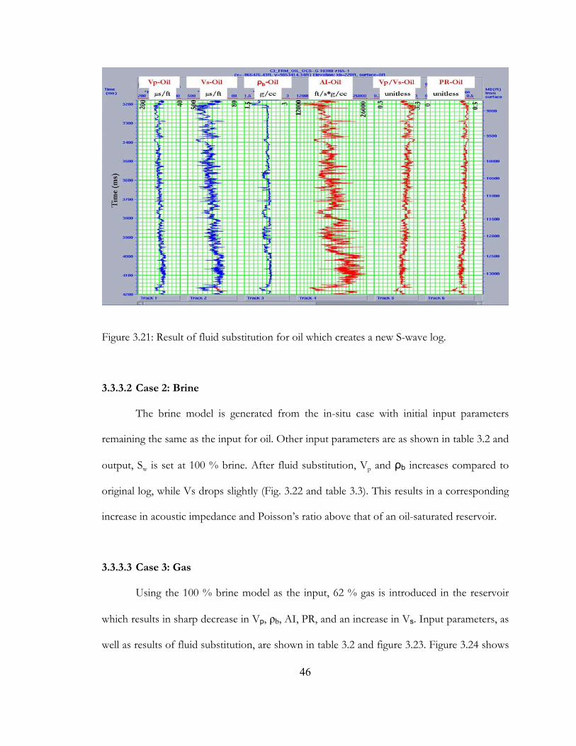
Figure 3.21: Result of fluid substitution for oil which creates a new S-wave log.
3.3.3.2 Case 2: Brine
The brine model is generated from the in-situ case with initial input parameters
remaining the same as the input for oil. Other input parameters are as shown in table 3.2 and
output, Sw is set at 100 % brine. After fluid substitution, Vp and ρb increases compared to
original log, while Vs drops slightly (Fig. 3.22 and table 3.3). This results in a corresponding
increase in acoustic impedance and Poisson’s ratio above that of an oil-saturated reservoir.
3.3.3.3 Case 3: Gas
Using the 100 % brine model as the input, 62 % gas is introduced in the reservoir
which results in sharp decrease in Vp, ρb, AI, PR, and an increase in Vs. Input parameters, as
well as results of fluid substitution, are shown in table 3.2 and figure 3.23. Figure 3.24 shows
46
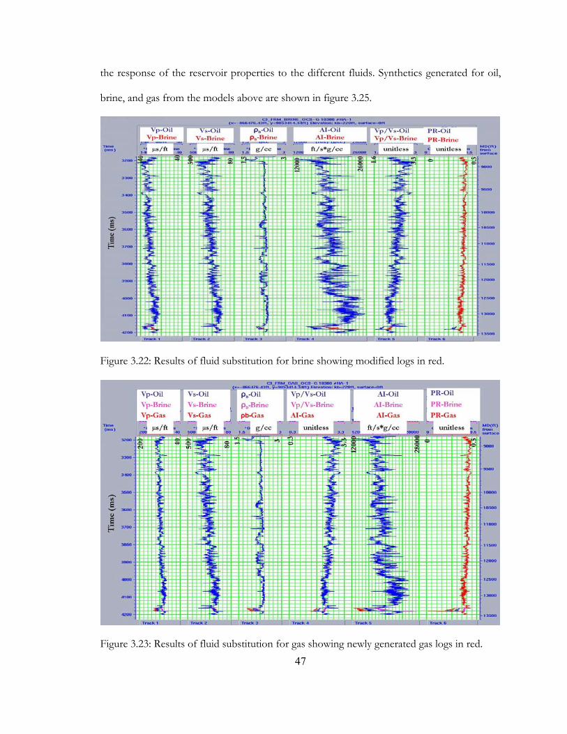
the response of the reservoir properties to the different fluids. Synthetics generated for oil,
brine, and gas from the models above are shown in figure 3.25.
Figure 3.22: Results of fluid substitution for brine showing modified logs in red.
Figure 3.23: Results of fluid substitution for gas showing newly generated gas logs in red. 47
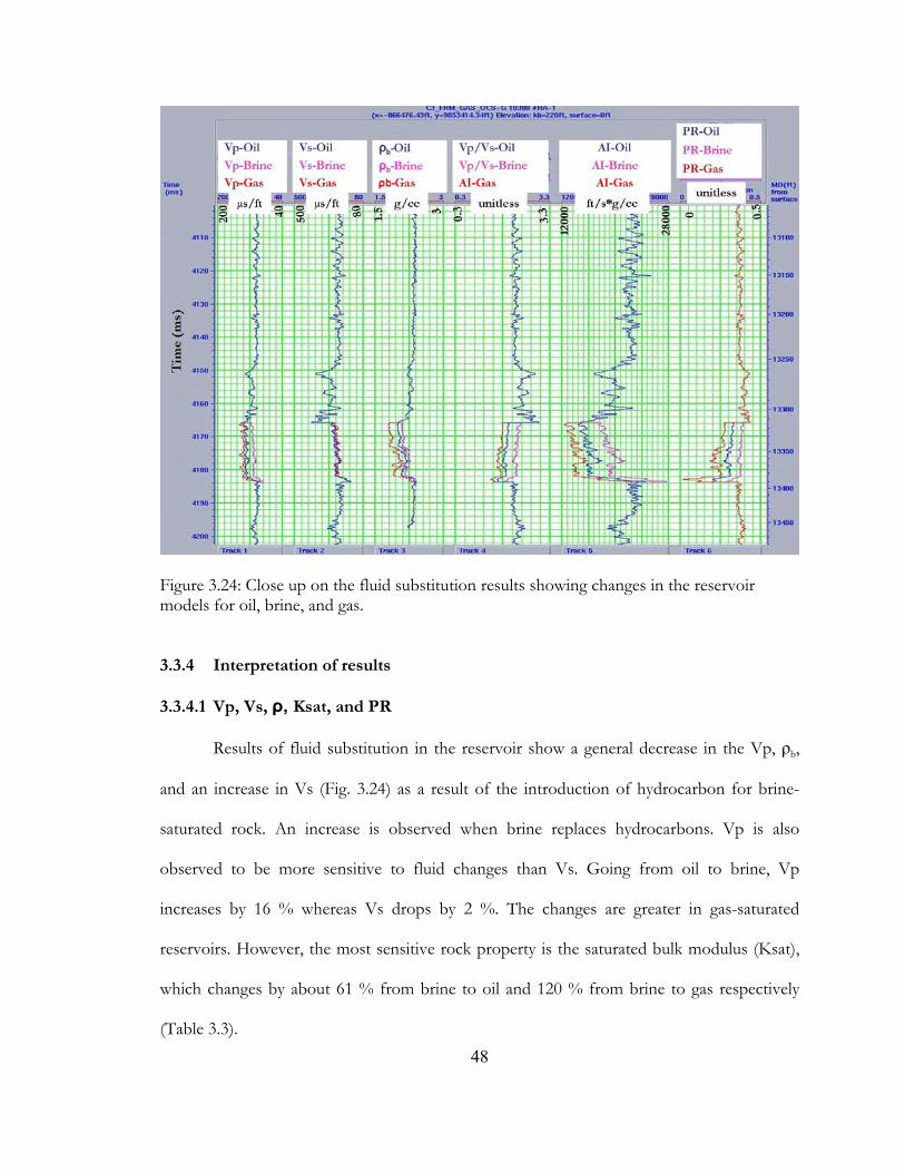
Figure 3.24: Close up on the fluid substitution results showing changes in the reservoir models for oil, brine, and gas. 3.3.4 Interpretation of results
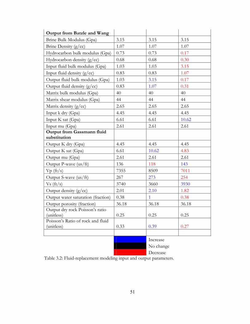
3.3.4.1 Vp, Vs, ρ, Ksat, and PR
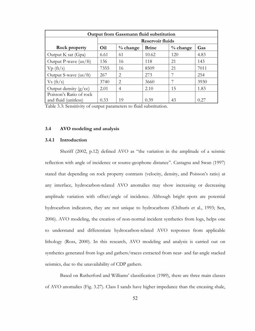
Results of fluid substitution in the reservoir show a general decrease in the Vp, ρb,
and an increase in Vs (Fig. 3.24) as a result of the introduction of hydrocarbon for brine-
saturated rock. An increase is observed when brine replaces hydrocarbons. Vp is also
observed to be more sensitive to fluid changes than Vs. Going from oil to brine, Vp
increases by 16 % whereas Vs drops by 2 %. The changes are greater in gas-saturated
reservoirs. However, the most sensitive rock property is the saturated bulk modulus (Ksat),
which changes by about 61 % from brine to oil and 120 % from brine to gas respectively
(Table 3.3). 48
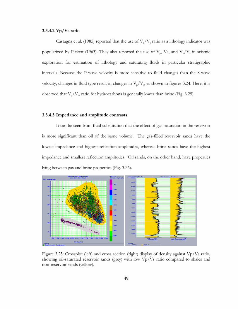
3.3.4.2 Vp/Vs ratio
Castagna et al. (1985) reported that the use of Vp/Vs ratio as a lithology indicator was
popularized by Pickett (1963). They also reported the use of Vp, Vs, and Vp/Vs in seismic
exploration for estimation of lithology and saturating fluids in particular stratigraphic
intervals. Because the P-wave velocity is more sensitive to fluid changes than the S-wave
velocity, changes in fluid type result in changes in Vp/Vs, as shown in figures 3.24. Here, it is
observed that Vp/Vs, ratio for hydrocarbons is generally lower than brine (Fig. 3.25).
3.3.4.3 Impedance and amplitude contrasts
It can be seen from fluid substitution that the effect of gas saturation in the reservoir
is more significant than oil of the same volume. The gas-filled reservoir sands have the
lowest impedance and highest reflection amplitudes, whereas brine sands have the highest
impedance and smallest reflection amplitudes. Oil sands, on the other hand, have properties
lying between gas and brine properties (Fig. 3.26).
Figure 3.25: Crossplot (left) and cross section (right) display of density against Vp/Vs ratio, showing oil-saturated reservoir sands (grey) with low Vp/Vs ratio compared to shales and non-reservoir sands (yellow).
49
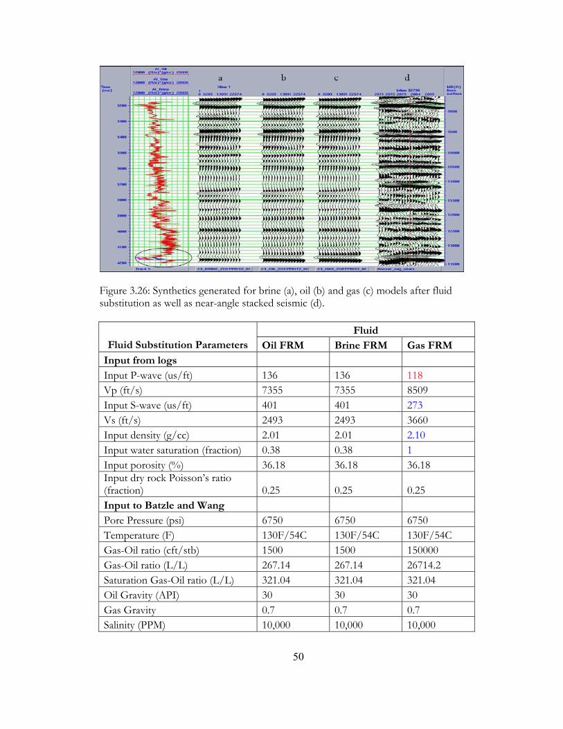
Figure 3.26: Synthetics generated for brine (a), oil (b) and gas (c) models after fluid substitution as well as near-angle stacked seismic (d).
Fluid Fluid Substitution Parameters Oil FRM Brine FRM Gas FRM
Input from logs Input P-wave (us/ft) 136 136 118 Vp (ft/s) 7355 7355 8509 Input S-wave (us/ft) 401 401 273 Vs (ft/s) 2493 2493 3660 Input density (g/cc) 2.01 2.01 2.10 Input water saturation (fraction) 0.38 0.38 1 Input porosity (%) 36.18 36.18 36.18 Input dry rock Poisson’s ratio (fraction) 0.25 0.25 0.25 Input to Batzle and Wang Pore Pressure (psi) 6750 6750 6750 Temperature (F) 130F/54C 130F/54C 130F/54C Gas-Oil ratio (cft/stb) 1500 1500 150000 Gas-Oil ratio (L/L) 267.14 267.14 26714.2 Saturation Gas-Oil ratio (L/L) 321.04 321.04 321.04 Oil Gravity (API) 30 30 30 Gas Gravity 0.7 0.7 0.7 Salinity (PPM) 10,000 10,000 10,000
50
Output from Batzle and Wang Brine Bulk Modulus (Gpa) 3.15 3.15 3.15 Brine Density (g/cc) 1.07 1.07 1.07 Hydrocarbon bulk modulus (Gpa) 0.73 0.73 0.17 Hydrocarbon density (g/cc) 0.68 0.68 0.30 Input fluid bulk modulus (Gpa) 1.03 1.03 3.15 Input fluid density (g/cc) 0.83 0.83 1.07 Output fluid bulk modulus (Gpa) 1.03 3.15 0.17 Output fluid density (g/cc) 0.83 1.07 0.31 Matrix bulk modulus (Gpa) 40 40 40 Matrix shear modulus (Gpa) 44 44 44 Matrix density (g/cc) 2.65 2.65 2.65 Input k dry (Gpa) 4.45 4.45 4.45 Input K sat (Gpa) 6.61 6.61 10.62 Input mu (Gpa) 2.61 2.61 2.61 Output from Gassmann fluid substitution Output K dry (Gpa) 4.45 4.45 4.45 Output K sat (Gpa) 6.61 10.62 4.83 Output mu (Gpa) 2.61 2.61 2.61 Output P-wave (us/ft) 136 118 143 Vp (ft/s) 7355 8509 7011 Output S-wave (us/ft) 267 273 254 Vs (ft/s) 3740 3660 3930 Output density (g/cc) 2.01 2.10 1.82 Output water saturation (fraction) 0.38 1 0.38 Output porosity (fraction) 36.18 36.18 36.18 Output dry rock Poisson’s ratio (unitless) 0.25 0.25 0.25 Poisson’s Ratio of rock and fluid (unitless) 0.33 0.39 0.27 Increase No change Decrease
Table 3.2: Fluid-replacement modeling input and output parameters.
51
Output from Gassmann fluid substitution Reservoir fluids
Rock property Oil % change Brine % change Gas Output K sat (Gpa) 6.61 61 10.62 120 4.83 Output P-wave (us/ft) 136 16 118 21 143 Vp (ft/s) 7355 16 8509 21 7011 Output S-wave (us/ft) 267 2 273 7 254 Vs (ft/s) 3740 2 3660 7 3930 Output density (g/cc) 2.01 4 2.10 15 1.83 Poisson’s Ratio of rock and fluid (unitless) 0.33 19 0.39 43 0.27
Table 3.3: Sensitivity of output parameters to fluid substitution.
3.4 AVO modeling and analysis
3.4.1 Introduction
Sheriff (2002, p.12) defined AVO as “the variation in the amplitude of a seismic
reflection with angle of incidence or source-geophone distance”. Castagna and Swan (1997)
stated that depending on rock property contrasts (velocity, density, and Poisson’s ratio) at
any interface, hydrocarbon-related AVO anomalies may show increasing or decreasing
amplitude variation with offset/angle of incidence. Although bright spots are potential
hydrocarbon indicators, they are not unique to hydrocarbons (Chiburis et al., 1993; Sen,
2006). AVO modeling, the creation of non-normal incident synthetics from logs, helps one
to understand and differentiate hydrocarbon-related AVO responses from applicable
lithology (Ross, 2000). In this research, AVO modeling and analysis is carried out on
synthetics generated from logs and gathers/traces extracted from near- and far-angle stacked
seismics, due to the unavailability of CDP gathers.
Based on Rutherford and Williams’ classification (1989), there are three main classes
of AVO anomalies (Fig. 3.27). Class I sands have higher impedance than the encasing shale,
52
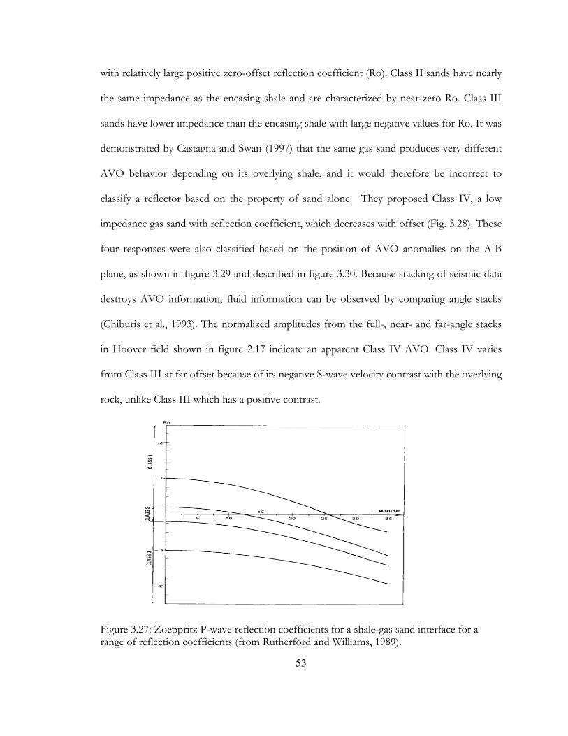
with relatively large positive zero-offset reflection coefficient (Ro). Class II sands have nearly
the same impedance as the encasing shale and are characterized by near-zero Ro. Class III
sands have lower impedance than the encasing shale with large negative values for Ro. It was
demonstrated by Castagna and Swan (1997) that the same gas sand produces very different
AVO behavior depending on its overlying shale, and it would therefore be incorrect to
classify a reflector based on the property of sand alone. They proposed Class IV, a low
impedance gas sand with reflection coefficient, which decreases with offset (Fig. 3.28). These
four responses were also classified based on the position of AVO anomalies on the A-B
plane, as shown in figure 3.29 and described in figure 3.30. Because stacking of seismic data
destroys AVO information, fluid information can be observed by comparing angle stacks
(Chiburis et al., 1993). The normalized amplitudes from the full-, near- and far-angle stacks
in Hoover field shown in figure 2.17 indicate an apparent Class IV AVO. Class IV varies
from Class III at far offset because of its negative S-wave velocity contrast with the overlying
rock, unlike Class III which has a positive contrast.
Figure 3.27: Zoeppritz P-wave reflection coefficients for a shale-gas sand interface for a range of reflection coefficients (from Rutherford and Williams, 1989).
53
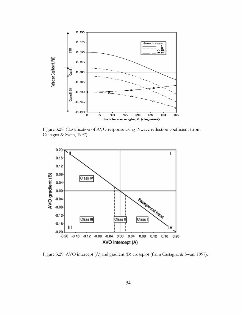
Figure 3.28: Classification of AVO response using P-wave reflection coefficient (from Castagna & Swan, 1997).
Figure 3.29: AVO intercept (A) and gradient (B) crossplot (from Castagna & Swan, 1997).
54
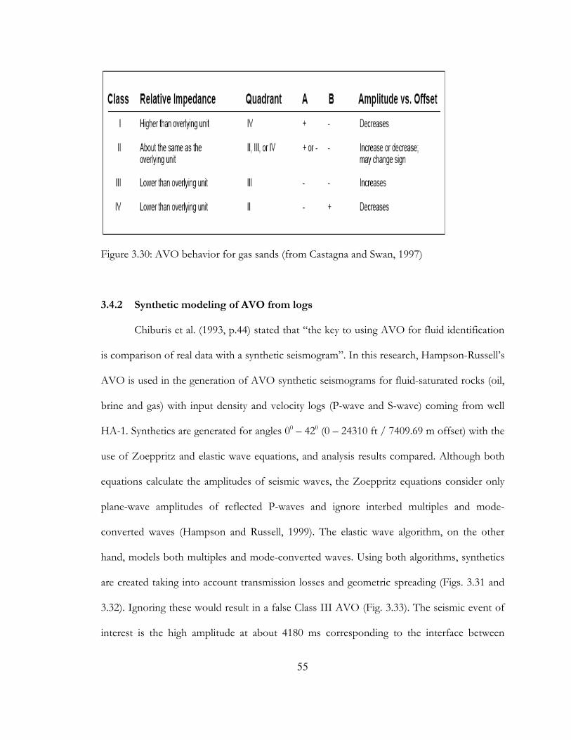
Figure 3.30: AVO behavior for gas sands (from Castagna and Swan, 1997)
3.4.2 Synthetic modeling of AVO from logs
Chiburis et al. (1993, p.44) stated that “the key to using AVO for fluid identification
is comparison of real data with a synthetic seismogram”. In this research, Hampson-Russell’s
AVO is used in the generation of AVO synthetic seismograms for fluid-saturated rocks (oil,
brine and gas) with input density and velocity logs (P-wave and S-wave) coming from well
HA-1. Synthetics are generated for angles 00 – 420 (0 – 24310 ft / 7409.69 m offset) with the
use of Zoeppritz and elastic wave equations, and analysis results compared. Although both
equations calculate the amplitudes of seismic waves, the Zoeppritz equations consider only
plane-wave amplitudes of reflected P-waves and ignore interbed multiples and mode-
converted waves (Hampson and Russell, 1999). The elastic wave algorithm, on the other
hand, models both multiples and mode-converted waves. Using both algorithms, synthetics
are created taking into account transmission losses and geometric spreading (Figs. 3.31 and
3.32). Ignoring these would result in a false Class III AVO (Fig. 3.33). The seismic event of
interest is the high amplitude at about 4180 ms corresponding to the interface between
55
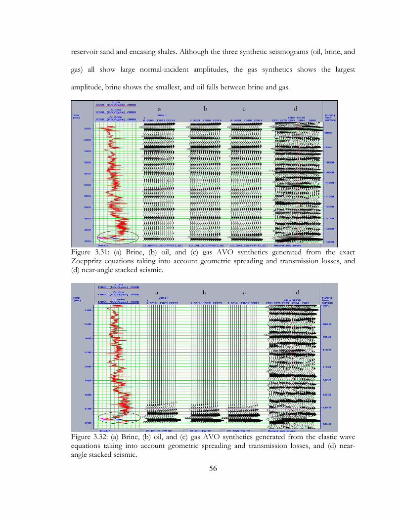
reservoir sand and encasing shales. Although the three synthetic seismograms (oil, brine, and
gas) all show large normal-incident amplitudes, the gas synthetics shows the largest
amplitude, brine shows the smallest, and oil falls between brine and gas.
Figure 3.31: (a) Brine, (b) oil, and (c) gas AVO synthetics generated from the exact Zoeppritz equations taking into account geometric spreading and transmission losses, and (d) near-angle stacked seismic.
Figure 3.32: (a) Brine, (b) oil, and (c) gas AVO synthetics generated from the elastic wave equations taking into account geometric spreading and transmission losses, and (d) near-angle stacked seismic.
56
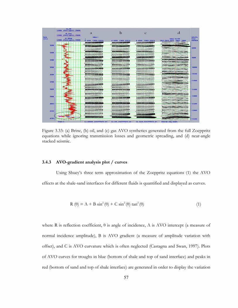
Figure 3.33: (a) Brine, (b) oil, and (c) gas AVO synthetics generated from the full Zoeppritz equations while ignoring transmission losses and geometric spreading, and (d) near-angle stacked seismic.
3.4.3 AVO-gradient analysis plot / curves
Using Shuey’s three term approximation of the Zoeppritz equations (1) the AVO
effects at the shale-sand interfaces for different fluids is quantified and displayed as curves.
R (θ) = A + B sin2 (θ) + C sin2 (θ) tan2 (θ) (1)
where R is reflection coefficient, θ is angle of incidence, A is AVO intercept (a measure of
normal incidence amplitude), B is AVO gradient (a measure of amplitude variation with
offset), and C is AVO curvature which is often neglected (Castagna and Swan, 1997). Plots
of AVO curves for troughs in blue (bottom of shale and top of sand interface) and peaks in
red (bottom of sand and top of shale interface) are generated in order to display the variation
57
in amplitudes between different fluids in reservoir sands and to compare hydrocarbon and
non-hydrocarbon-saturated sands.
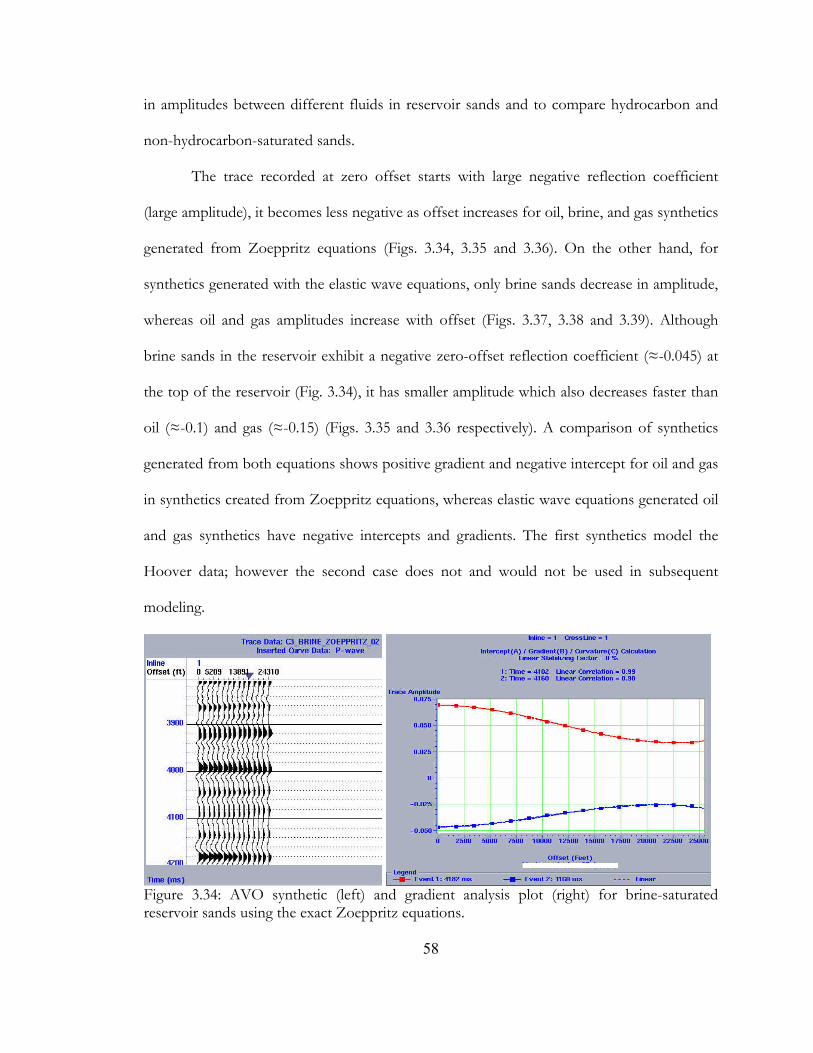
The trace recorded at zero offset starts with large negative reflection coefficient
(large amplitude), it becomes less negative as offset increases for oil, brine, and gas synthetics
generated from Zoeppritz equations (Figs. 3.34, 3.35 and 3.36). On the other hand, for
synthetics generated with the elastic wave equations, only brine sands decrease in amplitude,
whereas oil and gas amplitudes increase with offset (Figs. 3.37, 3.38 and 3.39). Although
brine sands in the reservoir exhibit a negative zero-offset reflection coefficient (≈-0.045) at
the top of the reservoir (Fig. 3.34), it has smaller amplitude which also decreases faster than
oil (≈-0.1) and gas (≈-0.15) (Figs. 3.35 and 3.36 respectively). A comparison of synthetics
generated from both equations shows positive gradient and negative intercept for oil and gas
in synthetics created from Zoeppritz equations, whereas elastic wave equations generated oil
and gas synthetics have negative intercepts and gradients. The first synthetics model the
Hoover data; however the second case does not and would not be used in subsequent
modeling.
Figure 3.34: AVO synthetic (left) and gradient analysis plot (right) for brine-saturated reservoir sands using the exact Zoeppritz equations.
58
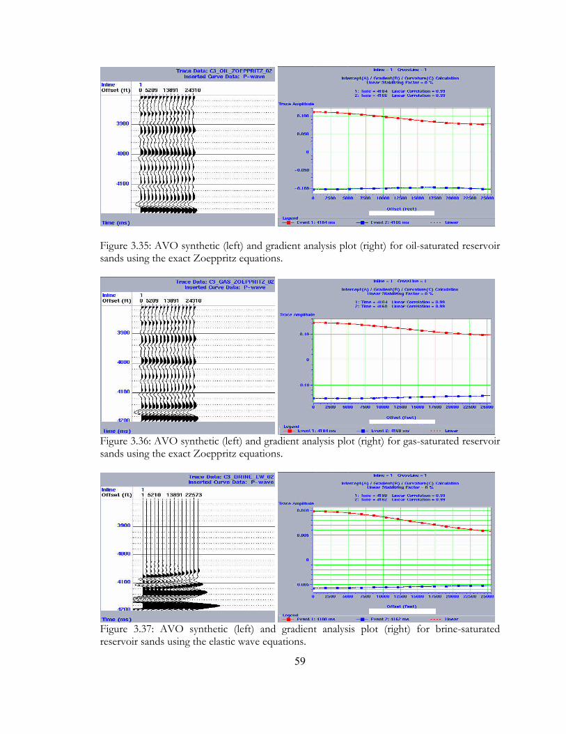
Figure 3.35: AVO synthetic (left) and gradient analysis plot (right) for oil-saturated reservoir sands using the exact Zoeppritz equations.
Figure 3.36: AVO synthetic (left) and gradient analysis plot (right) for gas-saturated reservoir sands using the exact Zoeppritz equations.
Figure 3.37: AVO synthetic (left) and gradient analysis plot (right) for brine-saturated reservoir sands using the elastic wave equations.
59
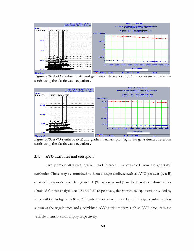
Figure 3.38: AVO synthetic (left) and gradient analysis plot (right) for oil-saturated reservoir sands using the elastic wave equations.
Figure 3.39: AVO synthetic (left) and gradient analysis plot (right) for gas-saturated reservoir sands using the elastic wave equations. 3.4.4 AVO attributes and crossplots
Two primary attributes, gradient and intercept, are extracted from the generated
synthetics. These may be combined to form a single attribute such as AVO product (A x B)
or scaled Poisson’s ratio change (αA + βB) where α and β are both scalars, whose values
obtained for this analysis are 0.5 and 0.27 respectively, determined by equations provided by
Ross, (2000). In figures 3.40 to 3.43, which compares brine-oil and brine-gas synthetics, A is
shown as the wiggle trace and a combined AVO attribute term such as AVO product is the
variable intensity color display respectively.
60
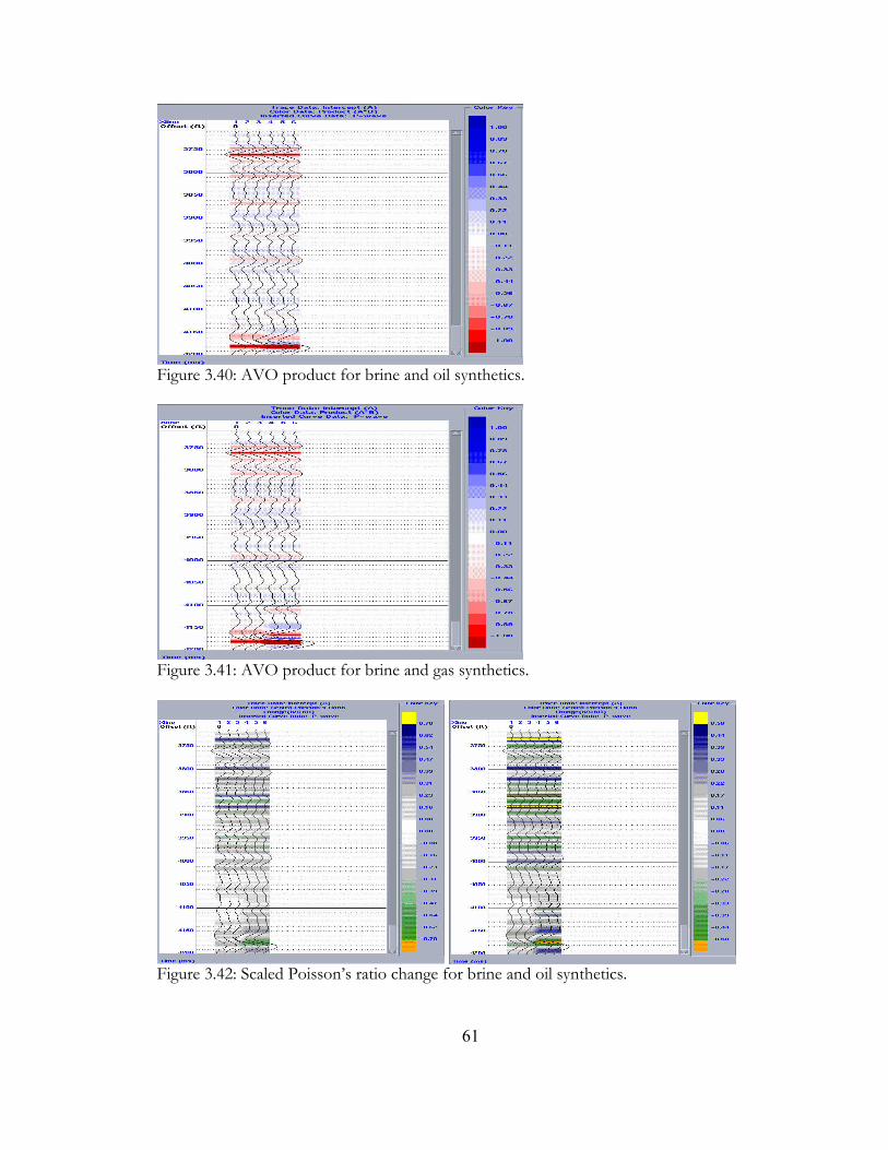
Figure 3.40: AVO product for brine and oil synthetics.
Figure 3.41: AVO product for brine and gas synthetics.
Figure 3.42: Scaled Poisson’s ratio change for brine and oil synthetics.
61
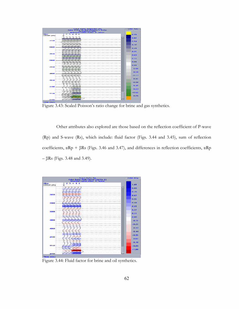
Figure 3.43: Scaled Poisson’s ratio change for brine and gas synthetics.
Other attributes also explored are those based on the reflection coefficient of P-wave
(Rp) and S-wave (Rs), which include: fluid factor (Figs. 3.44 and 3.45), sum of reflection
coefficients, αRp + βRs (Figs. 3.46 and 3.47), and differences in reflection coefficients, αRp
– βRs (Figs. 3.48 and 3.49).
Figure 3.44: Fluid factor for brine and oil synthetics.
62
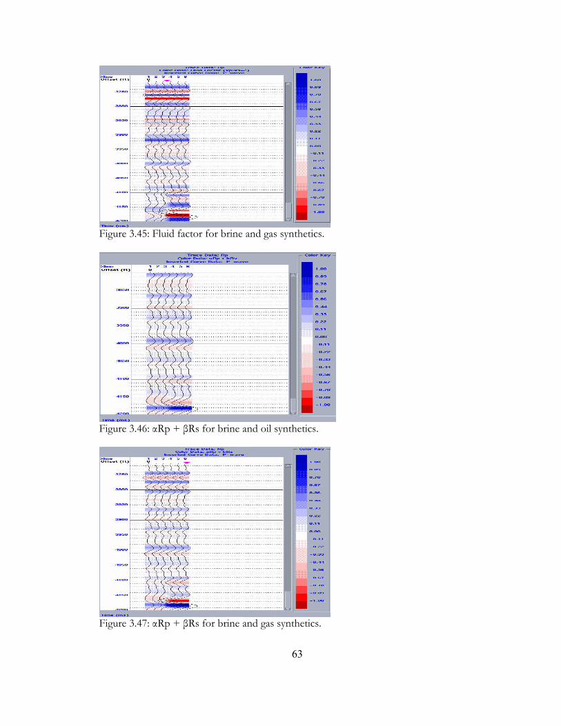
Figure 3.45: Fluid factor for brine and gas synthetics.
Figure 3.46: αRp + βRs for brine and oil synthetics.
Figure 3.47: αRp + βRs for brine and gas synthetics.
63
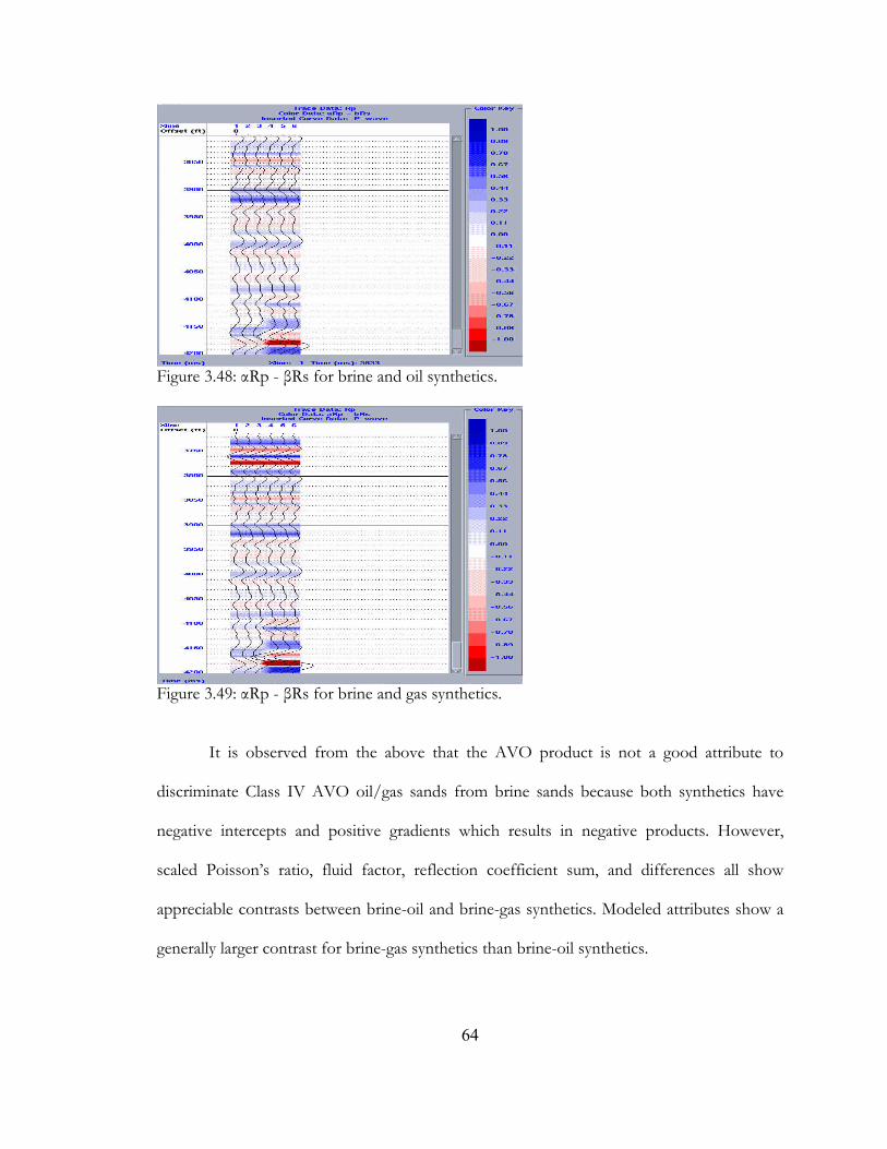
Figure 3.48: αRp - βRs for brine and oil synthetics.
Figure 3.49: αRp - βRs for brine and gas synthetics.
It is observed from the above that the AVO product is not a good attribute to
discriminate Class IV AVO oil/gas sands from brine sands because both synthetics have
negative intercepts and positive gradients which results in negative products. However,
scaled Poisson’s ratio, fluid factor, reflection coefficient sum, and differences all show
appreciable contrasts between brine-oil and brine-gas synthetics. Modeled attributes show a
generally larger contrast for brine-gas synthetics than brine-oil synthetics.
64
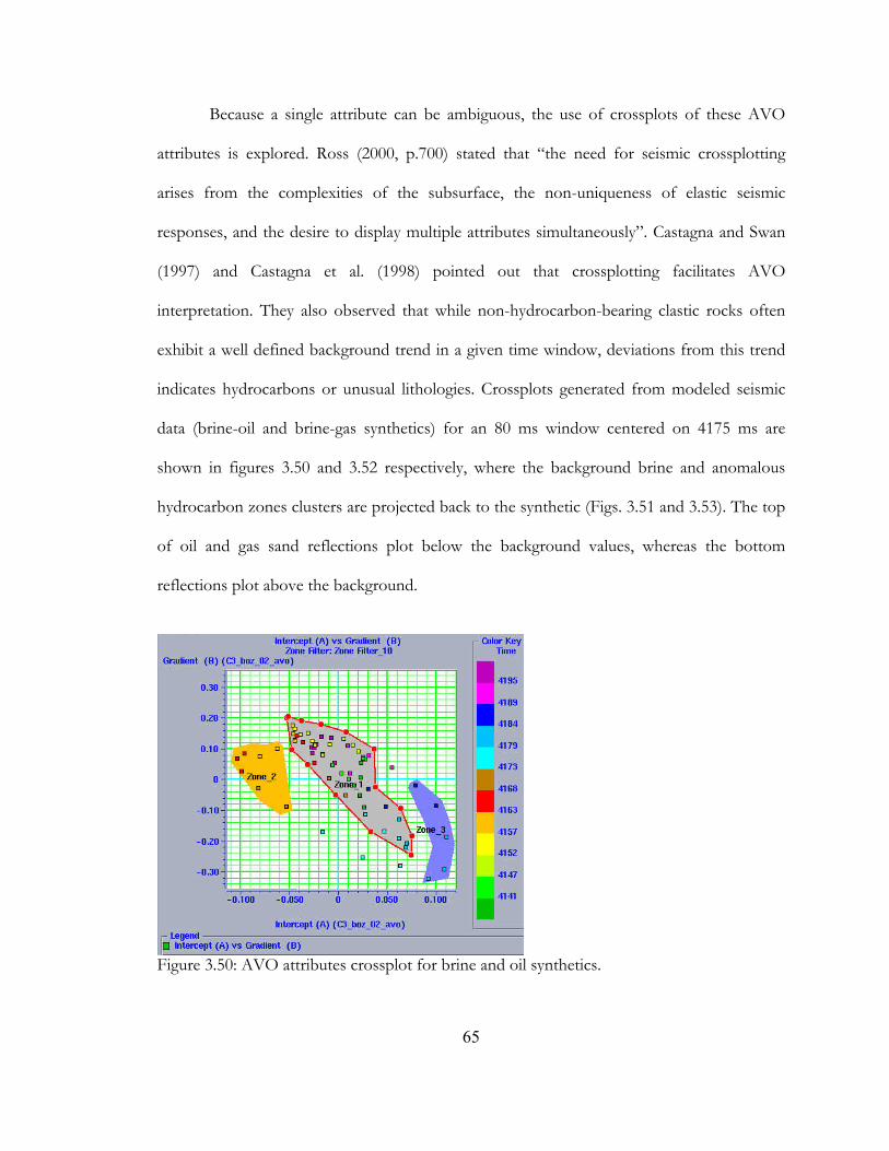
Because a single attribute can be ambiguous, the use of crossplots of these AVO
attributes is explored. Ross (2000, p.700) stated that “the need for seismic crossplotting
arises from the complexities of the subsurface, the non-uniqueness of elastic seismic
responses, and the desire to display multiple attributes simultaneously”. Castagna and Swan
(1997) and Castagna et al. (1998) pointed out that crossplotting facilitates AVO
interpretation. They also observed that while non-hydrocarbon-bearing clastic rocks often
exhibit a well defined background trend in a given time window, deviations from this trend
indicates hydrocarbons or unusual lithologies. Crossplots generated from modeled seismic
data (brine-oil and brine-gas synthetics) for an 80 ms window centered on 4175 ms are
shown in figures 3.50 and 3.52 respectively, where the background brine and anomalous
hydrocarbon zones clusters are projected back to the synthetic (Figs. 3.51 and 3.53). The top
of oil and gas sand reflections plot below the background values, whereas the bottom
reflections plot above the background.
Figure 3.50: AVO attributes crossplot for brine and oil synthetics.
65
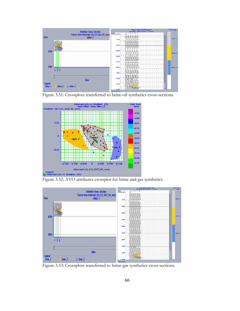
Figure 3.51: Crossplots transferred to brine-oil synthetics cross-sections.
Figure 3.52: AVO attributes crossplot for brine and gas synthetics.
Figure 3.53: Crossplots transferred to brine-gas synthetics cross-sections.
66
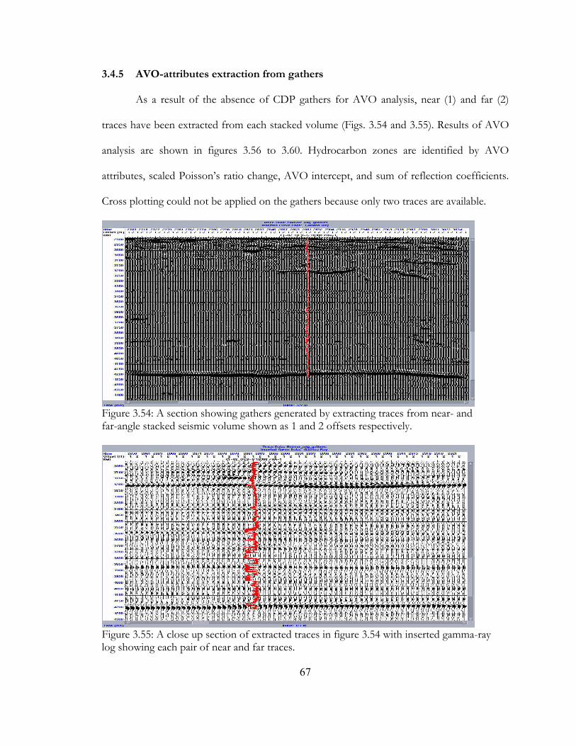
3.4.5 AVO-attributes extraction from gathers
As a result of the absence of CDP gathers for AVO analysis, near (1) and far (2)
traces have been extracted from each stacked volume (Figs. 3.54 and 3.55). Results of AVO
analysis are shown in figures 3.56 to 3.60. Hydrocarbon zones are identified by AVO
attributes, scaled Poisson’s ratio change, AVO intercept, and sum of reflection coefficients.
Cross plotting could not be applied on the gathers because only two traces are available.
Figure 3.54: A section showing gathers generated by extracting traces from near- and far-angle stacked seismic volume shown as 1 and 2 offsets respectively.
Figure 3.55: A close up section of extracted traces in figure 3.54 with inserted gamma-ray log showing each pair of near and far traces.
67
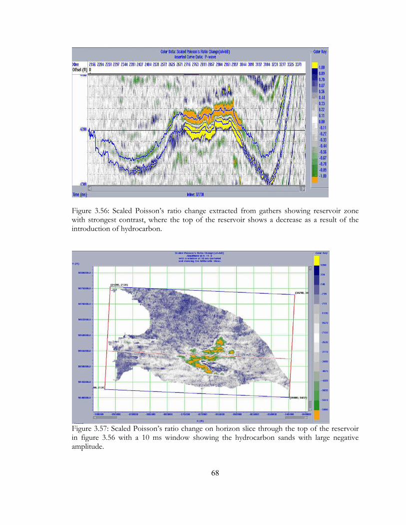
Figure 3.56: Scaled Poisson’s ratio change extracted from gathers showing reservoir zone with strongest contrast, where the top of the reservoir shows a decrease as a result of the introduction of hydrocarbon.
Figure 3.57: Scaled Poisson’s ratio change on horizon slice through the top of the reservoir in figure 3.56 with a 10 ms window showing the hydrocarbon sands with large negative amplitude.
68
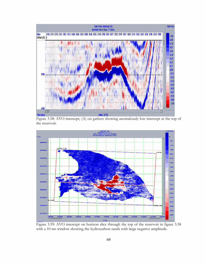
Figure 3.58: AVO intercept, (A) on gathers showing anomalously low intercept at the top of the reservoir.
Figure 3.59: AVO intercept on horizon slice through the top of the reservoir in figure 3.58 with a 10 ms window showing the hydrocarbon sands with large negative amplitude.
69
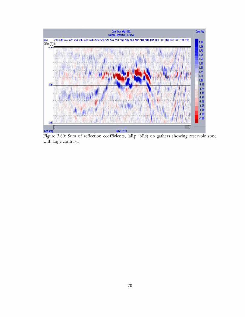
Figure 3.60: Sum of reflection coefficients, (aRp+bRs) on gathers showing reservoir zone with large contrast.
70
Chapter 4: Inversion of seismic data 4.1 Introduction
Inversion literally means to undo an operation (Veeken, 2007). Russell (2005, p.3)
defined it as “the process of extracting from the seismic data, the underlying geology which
gave rise to that seismic”. This process aims at reconstructing subsurface features
from geophysical measurements such that the model response “fits” the observation with
some measure of error (Treitel and Lines, 2001).
Acoustic Impedance (AI) is the product of density (ρ) and P-wave velocity (Vp) of a
rock, equation (1): pVAI ∗= ρ (1)
AI inversion methods transform seismic data into pseudo-acoustic impedance logs (Latimer
et al., 2003). Other than P-wave and density information, seismic data also consist of S-wave
data, but conventional seismic inversion does not account for Vp/Vs changes in AVO data
(Russell, 2005). Failure to account for these may result in inaccurate impedance estimation,
especially in reservoirs (Savic et al., 2002).
Elastic Impedance (EI) is the generalization of AI for variable incidence angles
(Connolly, 1999, p.438). Connolly added that it also enables one to calibrate and invert non-
zero-offset seismic data similar to AI inversion of zero offset data, and that it is a function of
P-wave velocity, S-wave velocity, density, and incident angle (θ), equation (2):
)sin41()sin8()sin1(
)(
222 θθθθ ρ KK
sp VVEI −−+ ∗∗= (2) where K is a constant that is taken equal to average of (Vs/Vp)2
71
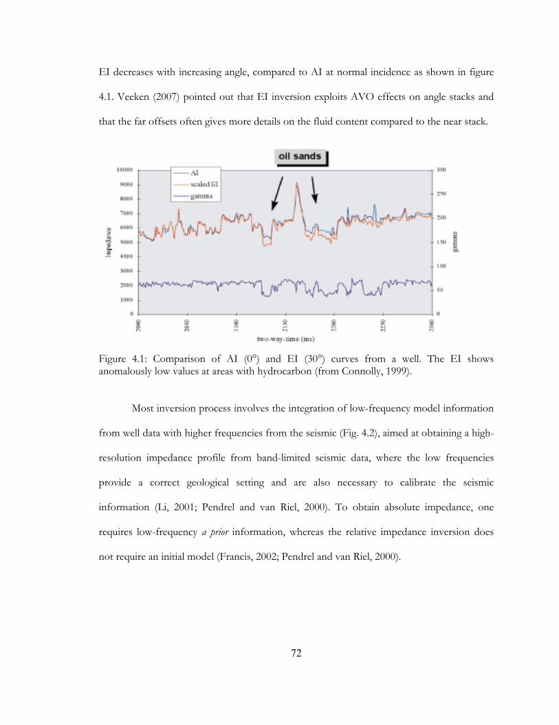
EI decreases with increasing angle, compared to AI at normal incidence as shown in figure
4.1. Veeken (2007) pointed out that EI inversion exploits AVO effects on angle stacks and
that the far offsets often gives more details on the fluid content compared to the near stack.
Figure 4.1: Comparison of AI (0°) and EI (30°) curves from a well. The EI shows anomalously low values at areas with hydrocarbon (from Connolly, 1999).
Most inversion process involves the integration of low-frequency model information
from well data with higher frequencies from the seismic (Fig. 4.2), aimed at obtaining a high-
resolution impedance profile from band-limited seismic data, where the low frequencies
provide a correct geological setting and are also necessary to calibrate the seismic
information (Li, 2001; Pendrel and van Riel, 2000). To obtain absolute impedance, one
requires low-frequency a prior information, whereas the relative impedance inversion does
not require an initial model (Francis, 2002; Pendrel and van Riel, 2000).
72
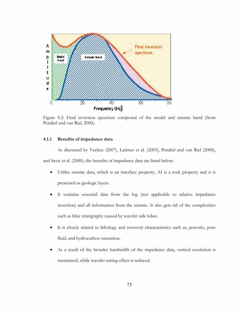
Figure 4.2: Final inversion spectrum composed of the model and seismic band (from Pendrel and van Riel, 2000). 4.1.1 Benefits of impedance data
As discussed by Veeken (2007), Latimer et al. (2003), Pendrel and van Riel (2000),
and Savic et al. (2000), the benefits of impedance data are listed below:
• Unlike seismic data, which is an interface property, AI is a rock property and it is
presented as geologic layers.
• It contains essential data from the log (not applicable to relative impedance
inversion) and all information from the seismic. It also gets rid of the complexities
such as false stratigraphy caused by wavelet side lobes.
• It is closely related to lithology and reservoir characteristics such as, porosity, pore
fluid, and hydrocarbon saturation.
• As a result of the broader bandwidth of the impedance data, vertical resolution is
maximized, while wavelet tuning effect is reduced.
73
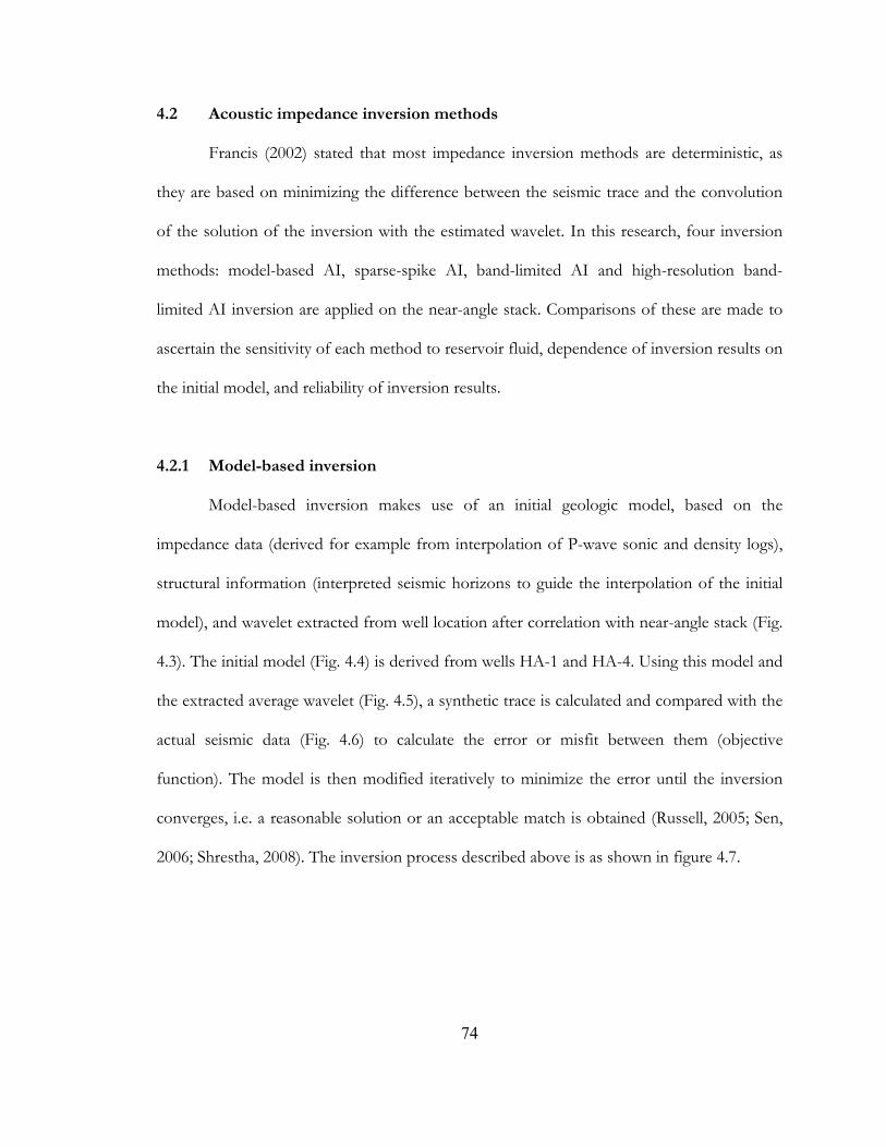
4.2 Acoustic impedance inversion methods
Francis (2002) stated that most impedance inversion methods are deterministic, as
they are based on minimizing the difference between the seismic trace and the convolution
of the solution of the inversion with the estimated wavelet. In this research, four inversion
methods: model-based AI, sparse-spike AI, band-limited AI and high-resolution band-
limited AI inversion are applied on the near-angle stack. Comparisons of these are made to
ascertain the sensitivity of each method to reservoir fluid, dependence of inversion results on
the initial model, and reliability of inversion results.
4.2.1 Model-based inversion
Model-based inversion makes use of an initial geologic model, based on the
impedance data (derived for example from interpolation of P-wave sonic and density logs),
structural information (interpreted seismic horizons to guide the interpolation of the initial
model), and wavelet extracted from well location after correlation with near-angle stack (Fig.
4.3). The initial model (Fig. 4.4) is derived from wells HA-1 and HA-4. Using this model and
the extracted average wavelet (Fig. 4.5), a synthetic trace is calculated and compared with the
actual seismic data (Fig. 4.6) to calculate the error or misfit between them (objective
function). The model is then modified iteratively to minimize the error until the inversion
converges, i.e. a reasonable solution or an acceptable match is obtained (Russell, 2005; Sen,
2006; Shrestha, 2008). The inversion process described above is as shown in figure 4.7.
74

Figure 4.3: Input to inversion process (modified from Veeken, 2007)
Figure 4.4: Unfiltered initial model derived from wells HA-1 and HA-4 containing all frequencies showing gamma-ray log from HA-1.
75
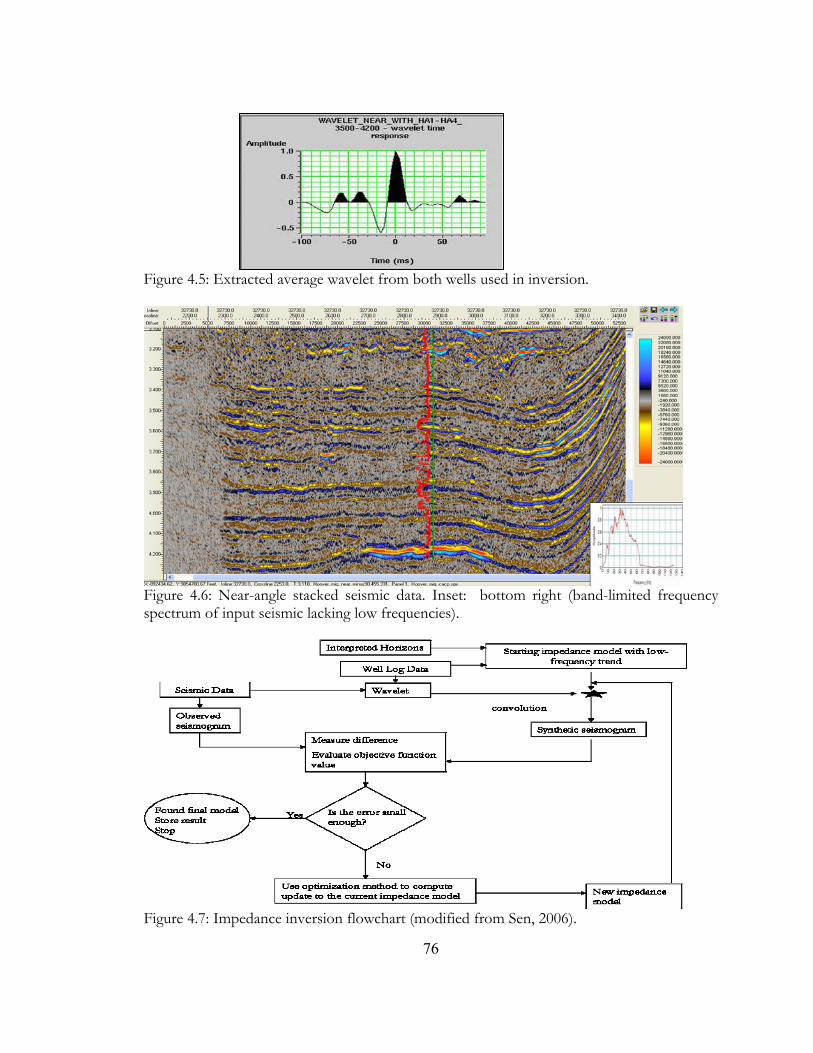
Figure 4.5: Extracted average wavelet from both wells used in inversion.
Figure 4.6: Near-angle stacked seismic data. Inset: bottom right (band-limited frequency spectrum of input seismic lacking low frequencies).
Figure 4.7: Impedance inversion flowchart (modified from Sen, 2006).
76
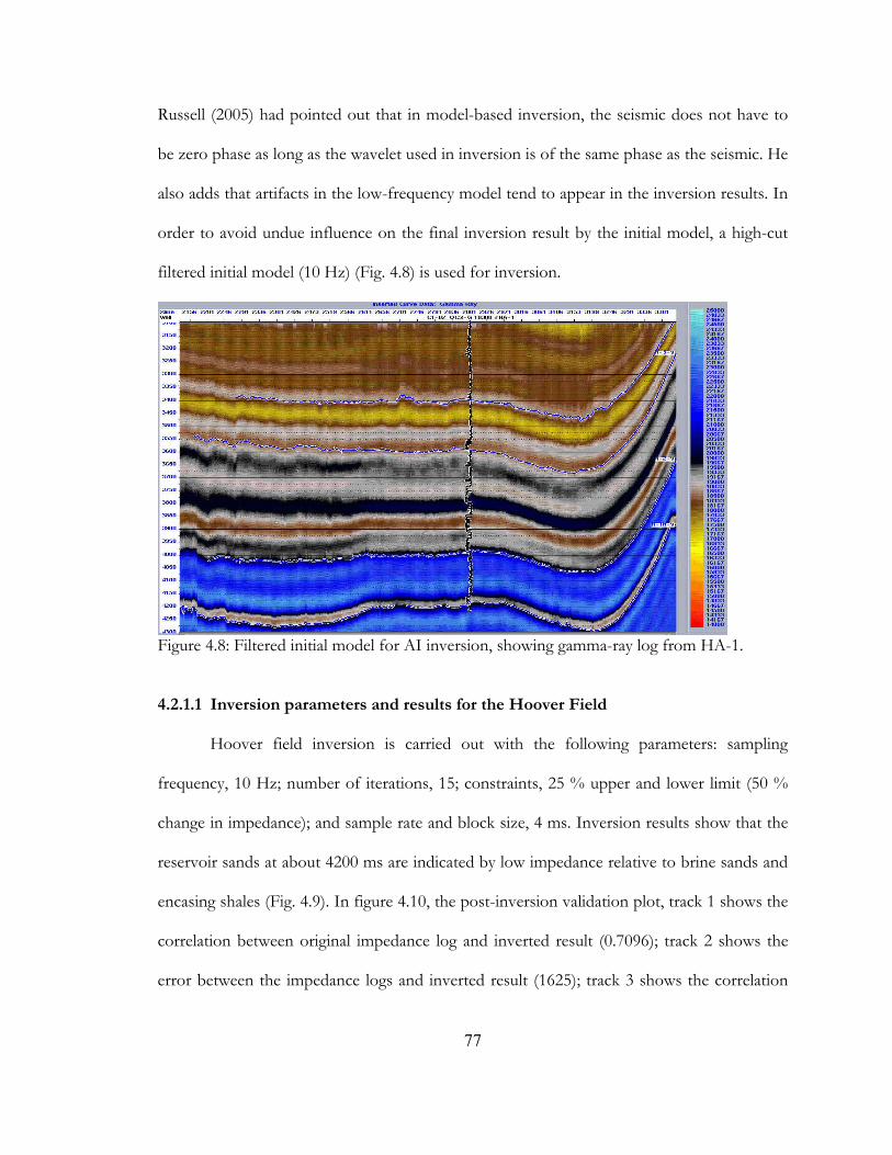
Russell (2005) had pointed out that in model-based inversion, the seismic does not have to
be zero phase as long as the wavelet used in inversion is of the same phase as the seismic. He
also adds that artifacts in the low-frequency model tend to appear in the inversion results. In
order to avoid undue influence on the final inversion result by the initial model, a high-cut
filtered initial model (10 Hz) (Fig. 4.8) is used for inversion.
Figure 4.8: Filtered initial model for AI inversion, showing gamma-ray log from HA-1. 4.2.1.1 Inversion parameters and results for the Hoover Field
Hoover field inversion is carried out with the following parameters: sampling
frequency, 10 Hz; number of iterations, 15; constraints, 25 % upper and lower limit (50 %
change in impedance); and sample rate and block size, 4 ms. Inversion results show that the
reservoir sands at about 4200 ms are indicated by low impedance relative to brine sands and
encasing shales (Fig. 4.9). In figure 4.10, the post-inversion validation plot, track 1 shows the
correlation between original impedance log and inverted result (0.7096); track 2 shows the
error between the impedance logs and inverted result (1625); track 3 shows the correlation
77
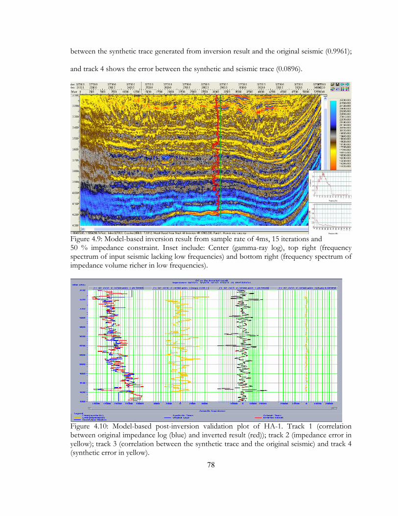
between the synthetic trace generated from inversion result and the original seismic (0.9961);
and track 4 shows the error between the synthetic and seismic trace (0.0896).
Figure 4.9: Model-based inversion result from sample rate of 4ms, 15 iterations and 50 % impedance constraint. Inset include: Center (gamma-ray log), top right (frequency spectrum of input seismic lacking low frequencies) and bottom right (frequency spectrum of impedance volume richer in low frequencies).
Figure 4.10: Model-based post-inversion validation plot of HA-1. Track 1 (correlation between original impedance log (blue) and inverted result (red)); track 2 (impedance error in yellow); track 3 (correlation between the synthetic trace and the original seismic) and track 4 (synthetic error in yellow). 78
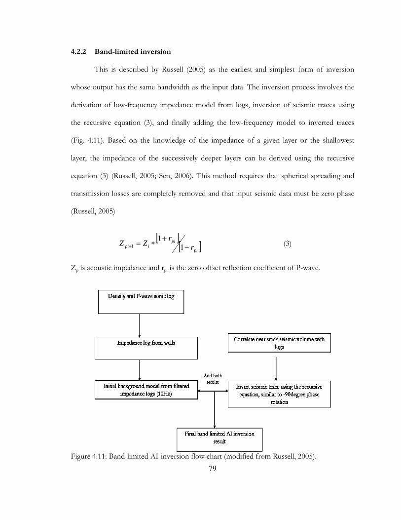
4.2.2 Band-limited inversion
This is described by Russell (2005) as the earliest and simplest form of inversion
whose output has the same bandwidth as the input data. The inversion process involves the
derivation of low-frequency impedance model from logs, inversion of seismic traces using
the recursive equation (3), and finally adding the low-frequency model to inverted traces
(Fig. 4.11). Based on the knowledge of the impedance of a given layer or the shallowest
layer, the impedance of the successively deeper layers can be derived using the recursive
equation (3) (Russell, 2005; Sen, 2006). This method requires that spherical spreading and
transmission losses are completely removed and that input seismic data must be zero phase
(Russell, 2005)
][[ ]pi
piipi r
rZZ −+
∗=+ 11
1 (3)
Zp is acoustic impedance and rpi is the zero offset reflection coefficient of P-wave.
Figure 4.11: Band-limited AI-inversion flow chart (modified from Russell, 2005). 79
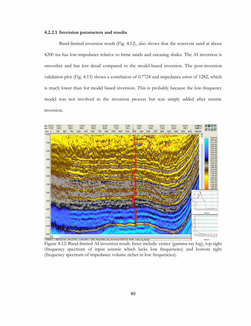
4.2.2.1 Inversion parameters and results
Band-limited inversion result (Fig. 4.12), also shows that the reservoir sand at about
4200 ms has low-impedance relative to brine sands and encasing shales. The AI inversion is
smoother and has less detail compared to the model-based inversion. The post-inversion
validation plot (Fig. 4.13) shows a correlation of 0.7724 and impedance error of 1282, which
is much lower than for model based inversion. This is probably because the low-frequency
model was not involved in the inversion process but was simply added after seismic
inversion.
Figure 4.12: Band-limited AI inversion result. Inset include: center (gamma-ray log), top right (frequency spectrum of input seismic which lacks low frequencies) and bottom right (frequency spectrum of impedance volume richer in low frequencies).
80
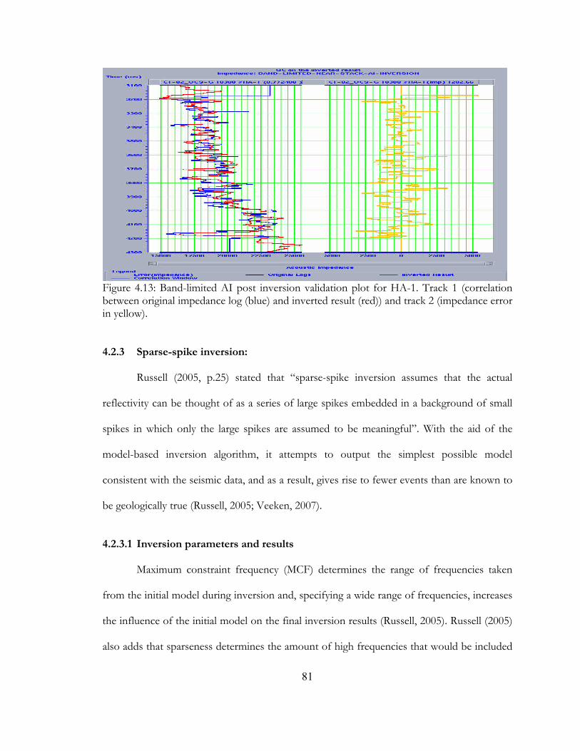
Figure 4.13: Band-limited AI post inversion validation plot for HA-1. Track 1 (correlation between original impedance log (blue) and inverted result (red)) and track 2 (impedance error in yellow). 4.2.3 Sparse-spike inversion:
Russell (2005, p.25) stated that “sparse-spike inversion assumes that the actual
reflectivity can be thought of as a series of large spikes embedded in a background of small
spikes in which only the large spikes are assumed to be meaningful”. With the aid of the
model-based inversion algorithm, it attempts to output the simplest possible model
consistent with the seismic data, and as a result, gives rise to fewer events than are known to
be geologically true (Russell, 2005; Veeken, 2007).
4.2.3.1 Inversion parameters and results
Maximum constraint frequency (MCF) determines the range of frequencies taken
from the initial model during inversion and, specifying a wide range of frequencies, increases
the influence of the initial model on the final inversion results (Russell, 2005). Russell (2005)
also adds that sparseness determines the amount of high frequencies that would be included
81
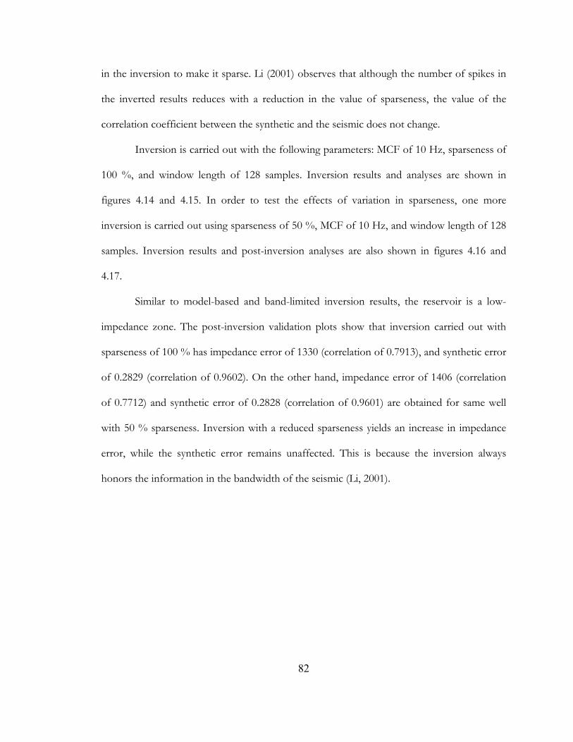
in the inversion to make it sparse. Li (2001) observes that although the number of spikes in
the inverted results reduces with a reduction in the value of sparseness, the value of the
correlation coefficient between the synthetic and the seismic does not change.
Inversion is carried out with the following parameters: MCF of 10 Hz, sparseness of
100 %, and window length of 128 samples. Inversion results and analyses are shown in
figures 4.14 and 4.15. In order to test the effects of variation in sparseness, one more
inversion is carried out using sparseness of 50 %, MCF of 10 Hz, and window length of 128
samples. Inversion results and post-inversion analyses are also shown in figures 4.16 and
4.17.
Similar to model-based and band-limited inversion results, the reservoir is a low-
impedance zone. The post-inversion validation plots show that inversion carried out with
sparseness of 100 % has impedance error of 1330 (correlation of 0.7913), and synthetic error
of 0.2829 (correlation of 0.9602). On the other hand, impedance error of 1406 (correlation
of 0.7712) and synthetic error of 0.2828 (correlation of 0.9601) are obtained for same well
with 50 % sparseness. Inversion with a reduced sparseness yields an increase in impedance
error, while the synthetic error remains unaffected. This is because the inversion always
honors the information in the bandwidth of the seismic (Li, 2001).
82
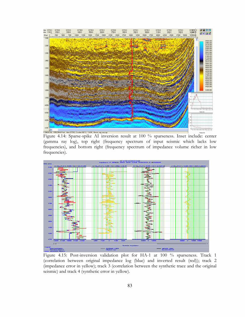
Figure 4.14: Sparse-spike AI inversion result at 100 % sparseness. Inset include: center (gamma ray log), top right (frequency spectrum of input seismic which lacks low frequencies), and bottom right (frequency spectrum of impedance volume richer in low frequencies).
Figure 4.15: Post-inversion validation plot for HA-1 at 100 % sparseness. Track 1 (correlation between original impedance log (blue) and inverted result (red)); track 2 (impedance error in yellow); track 3 (correlation between the synthetic trace and the original seismic) and track 4 (synthetic error in yellow).
83
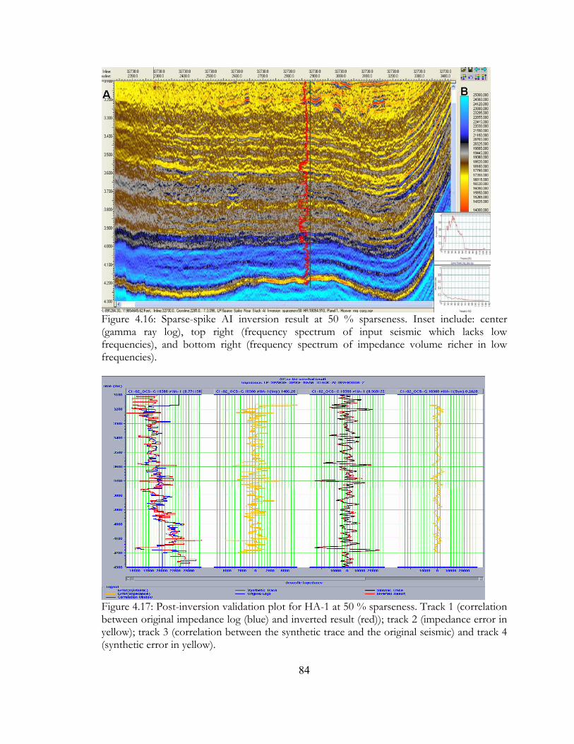
Figure 4.16: Sparse-spike AI inversion result at 50 % sparseness. Inset include: center (gamma ray log), top right (frequency spectrum of input seismic which lacks low frequencies), and bottom right (frequency spectrum of impedance volume richer in low frequencies).
Figure 4.17: Post-inversion validation plot for HA-1 at 50 % sparseness. Track 1 (correlation between original impedance log (blue) and inverted result (red)); track 2 (impedance error in yellow); track 3 (correlation between the synthetic trace and the original seismic) and track 4 (synthetic error in yellow).
84

4.2.4. High-resolution band-limited impedance inversion
This is an inversion method that involves the integration of inverted reflectivity
derived from the application of spectral decomposition on post-stack seismic data
(Portnaguine and Castagna, 2005). A commercial application of this method, ThinMAN, is
applied on both near- and far-stacked seismic volumes to get inverted impedance volumes
which show the contrast in impedance between a unit and its underlying/overlying layer (i.e.
relative impedance). This does not require an initial model or interpreted horizon(s), and it
can be performed without well calibration (Chopra et al., 2006). It also makes use of a set of
time- and space-varying wavelets, unlike the constant wavelet used in model based and
sparse-spike inversions. The inversion workflow is as shown in figure 4.18.
Figure 4.18: High-resolution band-limited impedance inversion work flow.
85

4.2.4.1 Inversion parameters and results
The inversion process starts with the calibration of seismic data to zero phase, as
discussed in section 3.1.4. Spectral inversion leads to broadening of the frequency
bandwidth, which would not be achieved if the sampling frequency is greater than the
nyquist frequency. To make room for the expected increase, the sample rate of the seismic
data is reduced from 4 ms to 1 ms, i.e. a nyquist frequency of 125 Hz to 500 Hz.
One of the factors that affects the quality of inversion is the wavelet. The more
representative the wavelet is of the seismic volume, the better the inversion results. In this
inversion, a set of time- and space-varying wavelets is extracted statistically from the seismic.
The left panel of figure 4.19, shows the time domain of an extracted wavelet with a spike
(red) and side lobes (light blue), while the right panel shows the vertical variation of
frequency at a given location.
Figure 4.19: An example of an extracted wavelet at a location used for inversion shown in the time domain (left) and frequency domain (right).
Based on the extracted zero-phase wavelet, a series of inversions is carried out to test
different regularization parameters, alpha (α), which increases/decreases the stability of the
86
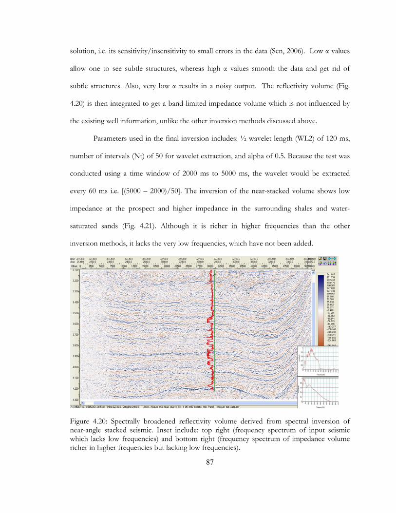
solution, i.e. its sensitivity/insensitivity to small errors in the data (Sen, 2006). Low α values
allow one to see subtle structures, whereas high α values smooth the data and get rid of
subtle structures. Also, very low α results in a noisy output. The reflectivity volume (Fig.
4.20) is then integrated to get a band-limited impedance volume which is not influenced by
the existing well information, unlike the other inversion methods discussed above.
Parameters used in the final inversion includes: ½ wavelet length (WL2) of 120 ms,
number of intervals (Nt) of 50 for wavelet extraction, and alpha of 0.5. Because the test was
conducted using a time window of 2000 ms to 5000 ms, the wavelet would be extracted
every 60 ms i.e. [(5000 – 2000)/50]. The inversion of the near-stacked volume shows low
impedance at the prospect and higher impedance in the surrounding shales and water-
saturated sands (Fig. 4.21). Although it is richer in higher frequencies than the other
inversion methods, it lacks the very low frequencies, which have not been added.
Figure 4.20: Spectrally broadened reflectivity volume derived from spectral inversion of near-angle stacked seismic. Inset include: top right (frequency spectrum of input seismic which lacks low frequencies) and bottom right (frequency spectrum of impedance volume richer in higher frequencies but lacking low frequencies).
87
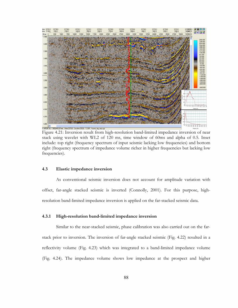
Figure 4.21: Inversion result from high-resolution band-limited impedance inversion of near stack using wavelet with WL2 of 120 ms, time window of 60ms and alpha of 0.5. Inset include: top right (frequency spectrum of input seismic lacking low frequencies) and bottom right (frequency spectrum of impedance volume richer in higher frequencies but lacking low frequencies). 4.3 Elastic impedance inversion
As conventional seismic inversion does not account for amplitude variation with
offset, far-angle stacked seismic is inverted (Connolly, 2001). For this purpose, high-
resolution band-limited impedance inversion is applied on the far-stacked seismic data.
4.3.1 High-resolution band-limited impedance inversion
Similar to the near-stacked seismic, phase calibration was also carried out on the far-
stack prior to inversion. The inversion of far-angle stacked seismic (Fig. 4.22) resulted in a
reflectivity volume (Fig. 4.23) which was integrated to a band-limited impedance volume
(Fig. 4.24). The impedance volume shows low impedance at the prospect and higher
88
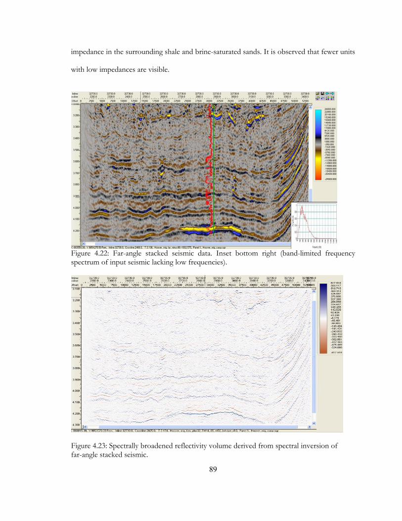
impedance in the surrounding shale and brine-saturated sands. It is observed that fewer units
with low impedances are visible.
Figure 4.22: Far-angle stacked seismic data. Inset bottom right (band-limited frequency spectrum of input seismic lacking low frequencies).
Figure 4.23: Spectrally broadened reflectivity volume derived from spectral inversion of far-angle stacked seismic.
89
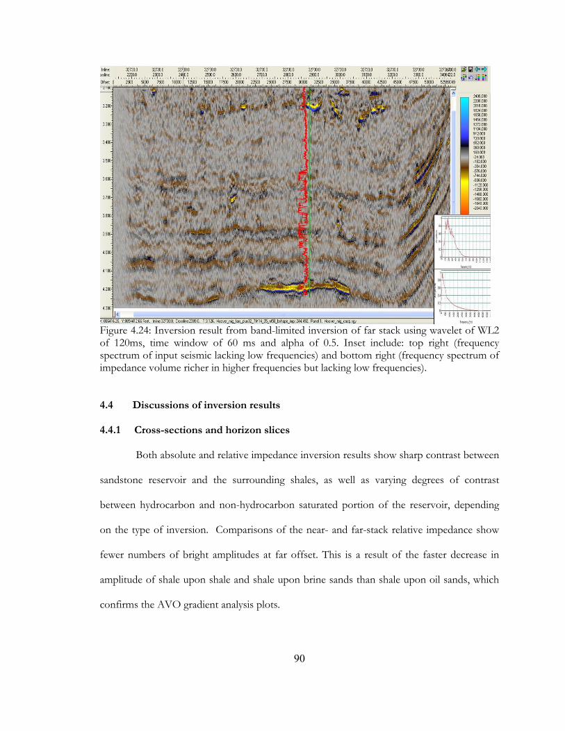
Figure 4.24: Inversion result from band-limited inversion of far stack using wavelet of WL2 of 120ms, time window of 60 ms and alpha of 0.5. Inset include: top right (frequency spectrum of input seismic lacking low frequencies) and bottom right (frequency spectrum of impedance volume richer in higher frequencies but lacking low frequencies).
4.4 Discussions of inversion results
4.4.1 Cross-sections and horizon slices
Both absolute and relative impedance inversion results show sharp contrast between
sandstone reservoir and the surrounding shales, as well as varying degrees of contrast
between hydrocarbon and non-hydrocarbon saturated portion of the reservoir, depending
on the type of inversion. Comparisons of the near- and far-stack relative impedance show
fewer numbers of bright amplitudes at far offset. This is a result of the faster decrease in
amplitude of shale upon shale and shale upon brine sands than shale upon oil sands, which
confirms the AVO gradient analysis plots.
90
The post-inversion validation plots show that the model-based AI inversion gives the
best correlation between the input-seismic and the synthetic-seismic generated after
inversion. The band-limited AI inversion gives a better correlation and smaller error between
the original log and the inverted result than the model-based case. This is probably because it
simply adds the initial model to the inverted traces. Although the sparse-spike AI inversion
shows a smaller impedance error, it has a larger synthetic error than the model-based results.
This is likely to be caused by its preference of larger spikes for geologic boundaries.
A close up on inline 32730 (Figs. 4.25, 4.26, 4.27, 4.28 and 4.29) shows the
distribution of reservoir sands as well as the hydrocarbon-saturated sands. To get a plan view
of the reservoir horizon, 30ms window on horizon slices (Figs. 4.30 to 4.34) are taken on
these cross sections. Both cross sections and horizon slices show the contrast in impedance
between the oil- and brine-saturated reservoir, as well as the heterogeneity of the reservoir,
which is more visible in figures 4.33 and 4.34. One observes that although all the inversion
methods have a good vertical impedance contrast between the reservoir sands and
surrounding shales, the same cannot be said for the horizontal contrast within the reservoir.
Sparse-spike inversion produces the least horizontal contrast in impedance. Arbitrary lines
from figures 4.35 and 4.37 and their respective cross sections (Fig. 4.36 and 4.38) reveal
bright spots away from the main prospect at the north (between crossline 2700 and 3000)
and at the west (between inline 32800 and 33300). They are brighter at the near stack and
diminish in amplitude on the far stack.
91
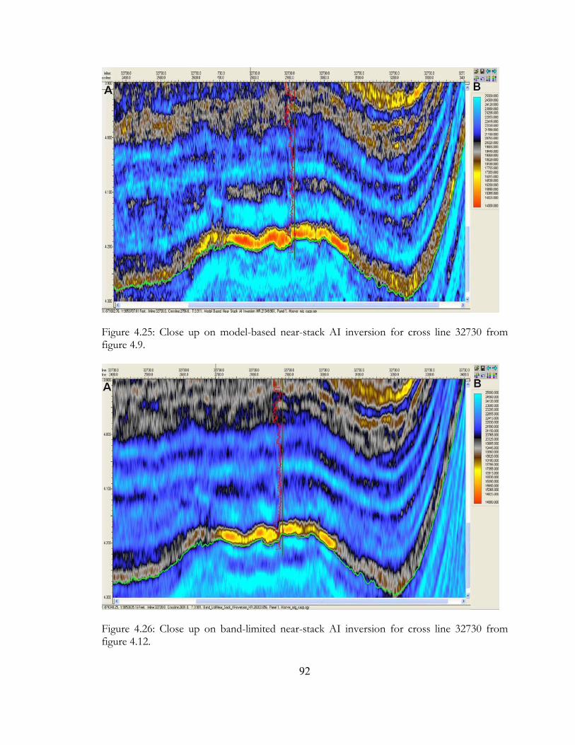
Figure 4.25: Close up on model-based near-stack AI inversion for cross line 32730 from figure 4.9.
Figure 4.26: Close up on band-limited near-stack AI inversion for cross line 32730 from figure 4.12.
92
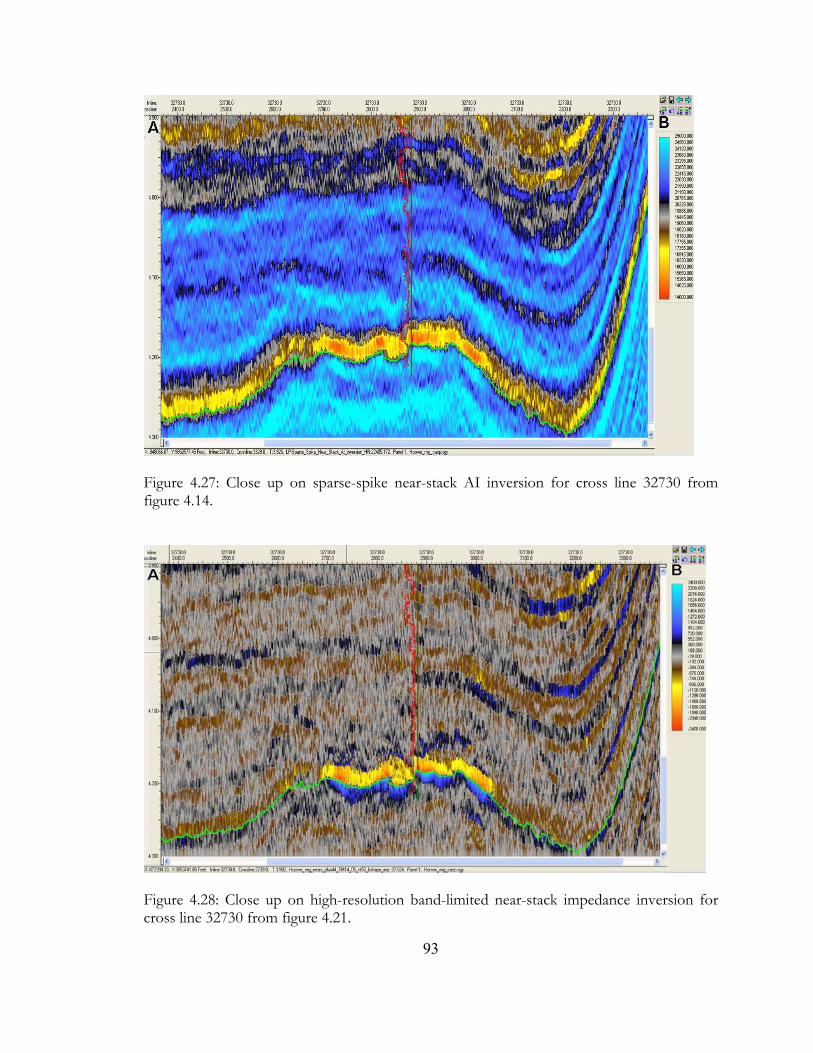
Figure 4.27: Close up on sparse-spike near-stack AI inversion for cross line 32730 from figure 4.14.
Figure 4.28: Close up on high-resolution band-limited near-stack impedance inversion for cross line 32730 from figure 4.21.
93
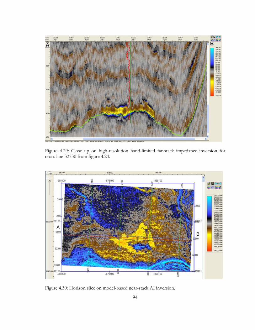
Figure 4.29: Close up on high-resolution band-limited far-stack impedance inversion for cross line 32730 from figure 4.24.
Figure 4.30: Horizon slice on model-based near-stack AI inversion.
94
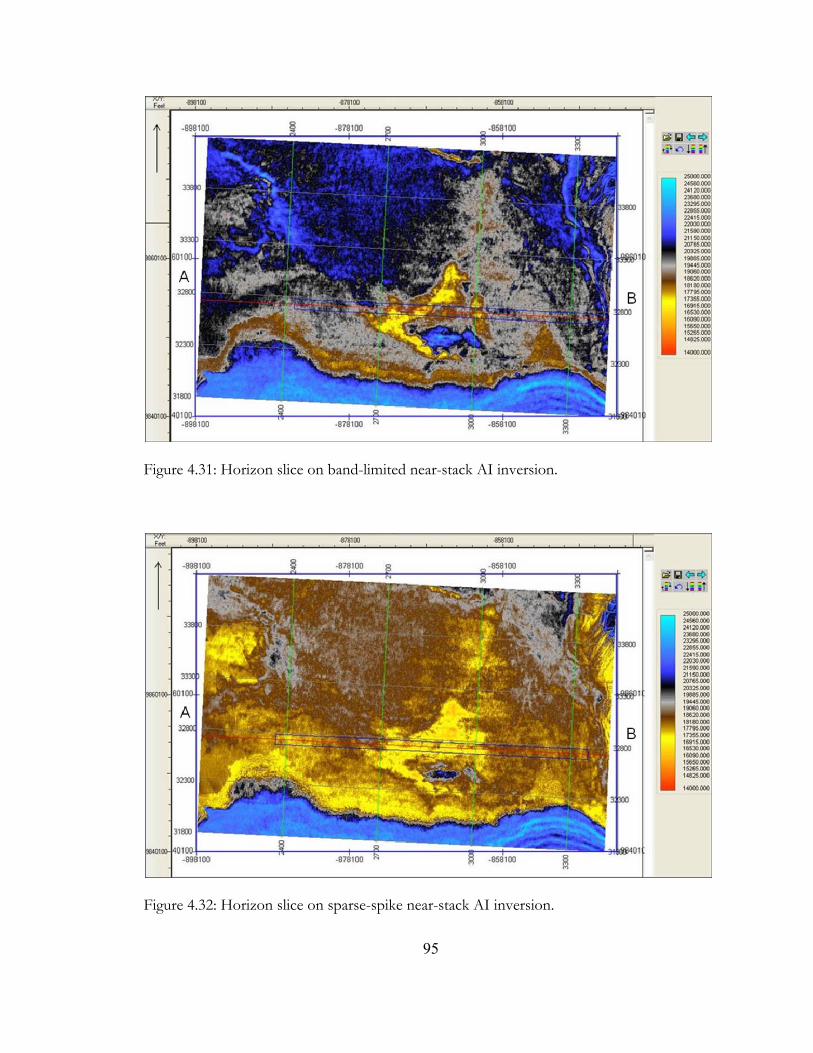
Figure 4.31: Horizon slice on band-limited near-stack AI inversion.
Figure 4.32: Horizon slice on sparse-spike near-stack AI inversion.
95
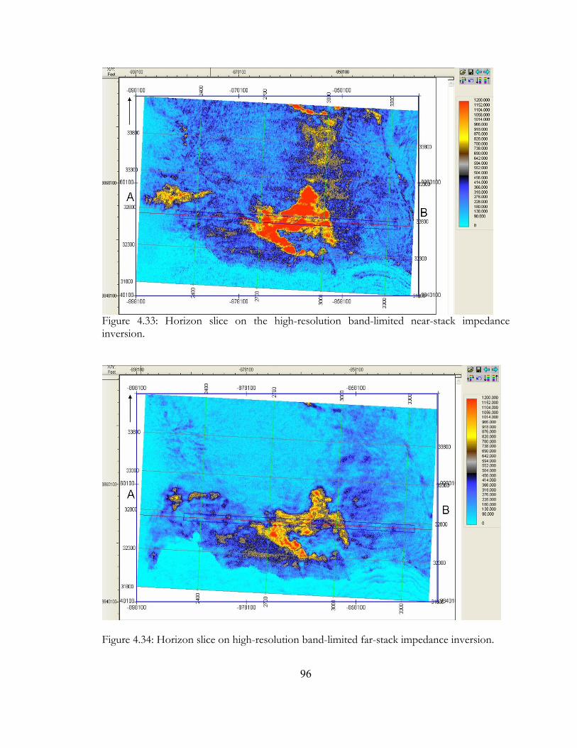
Figure 4.33: Horizon slice on the high-resolution band-limited near-stack impedance inversion.
Figure 4.34: Horizon slice on high-resolution band-limited far-stack impedance inversion.
96
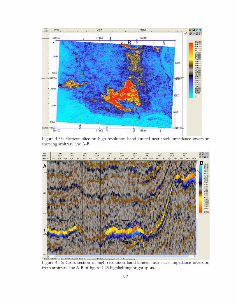
Figure 4.35: Horizon slice on high-resolution band-limited near-stack impedance inversion showing arbitrary line A-B.
Figure 4.36: Cross-section of high-resolution band-limited near-stack impedance inversion from arbitrary line A-B of figure 4.25 highlighting bright spots.
97
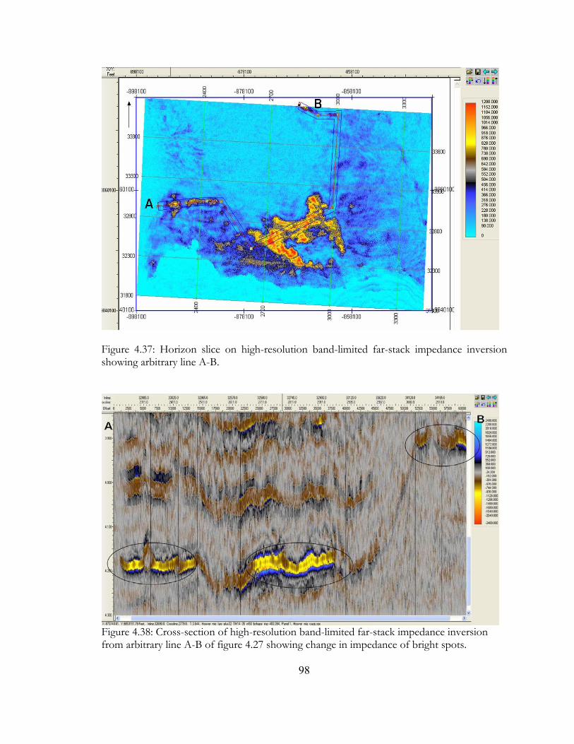
Figure 4.37: Horizon slice on high-resolution band-limited far-stack impedance inversion showing arbitrary line A-B.
Figure 4.38: Cross-section of high-resolution band-limited far-stack impedance inversion from arbitrary line A-B of figure 4.27 showing change in impedance of bright spots.
98
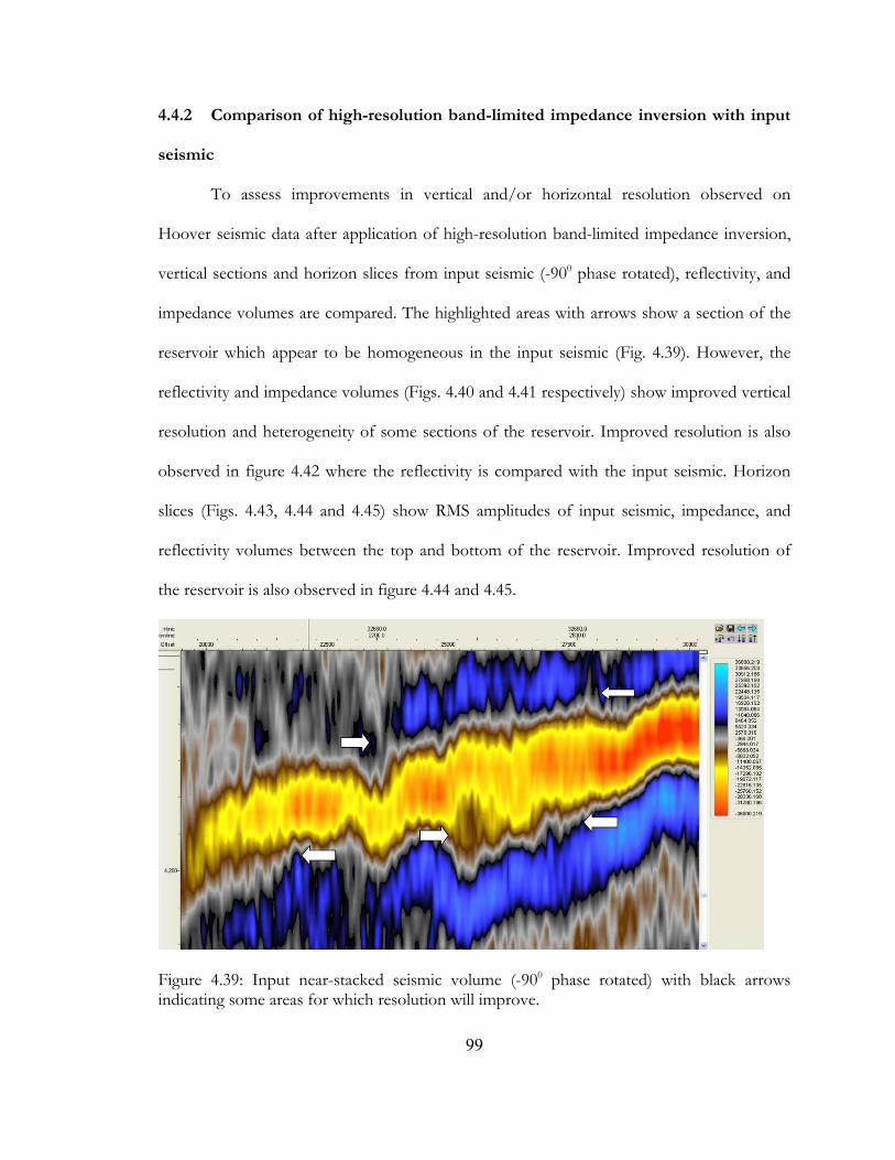
4.4.2 Comparison of high-resolution band-limited impedance inversion with input
seismic
To assess improvements in vertical and/or horizontal resolution observed on
Hoover seismic data after application of high-resolution band-limited impedance inversion,
vertical sections and horizon slices from input seismic (-900 phase rotated), reflectivity, and
impedance volumes are compared. The highlighted areas with arrows show a section of the
reservoir which appear to be homogeneous in the input seismic (Fig. 4.39). However, the
reflectivity and impedance volumes (Figs. 4.40 and 4.41 respectively) show improved vertical
resolution and heterogeneity of some sections of the reservoir. Improved resolution is also
observed in figure 4.42 where the reflectivity is compared with the input seismic. Horizon
slices (Figs. 4.43, 4.44 and 4.45) show RMS amplitudes of input seismic, impedance, and
reflectivity volumes between the top and bottom of the reservoir. Improved resolution of
the reservoir is also observed in figure 4.44 and 4.45.
Figure 4.39: Input near-stacked seismic volume (-900 phase rotated) with black arrows indicating some areas for which resolution will improve.
99
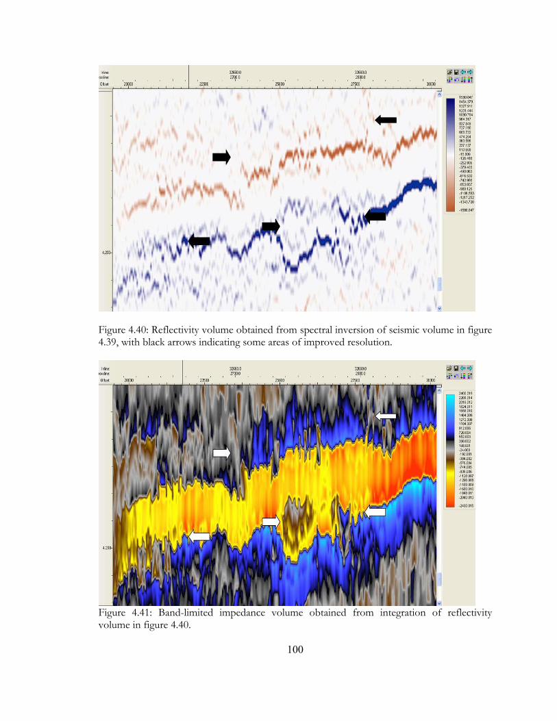
Figure 4.40: Reflectivity volume obtained from spectral inversion of seismic volume in figure 4.39, with black arrows indicating some areas of improved resolution.
Figure 4.41: Band-limited impedance volume obtained from integration of reflectivity volume in figure 4.40.
100
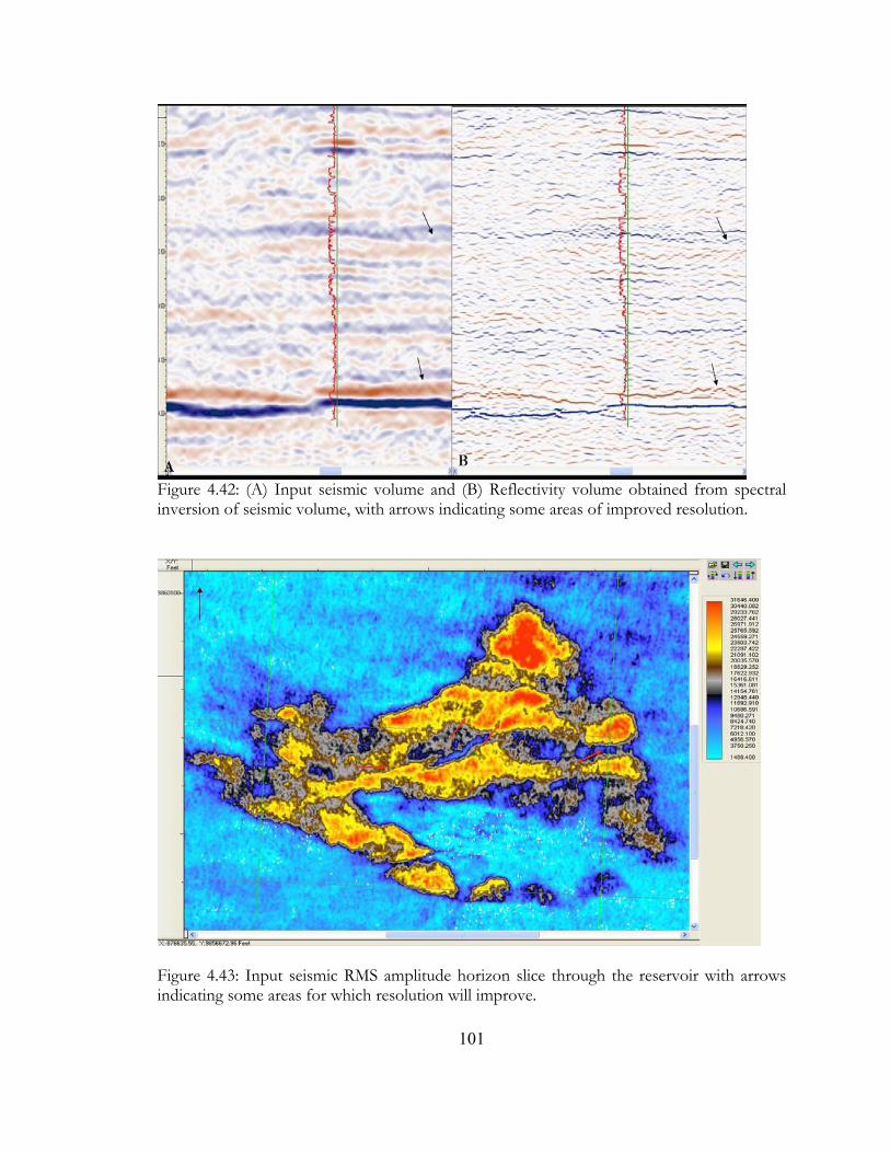
Figure 4.42: (A) Input seismic volume and (B) Reflectivity volume obtained from spectral inversion of seismic volume, with arrows indicating some areas of improved resolution.
Figure 4.43: Input seismic RMS amplitude horizon slice through the reservoir with arrows indicating some areas for which resolution will improve.
101
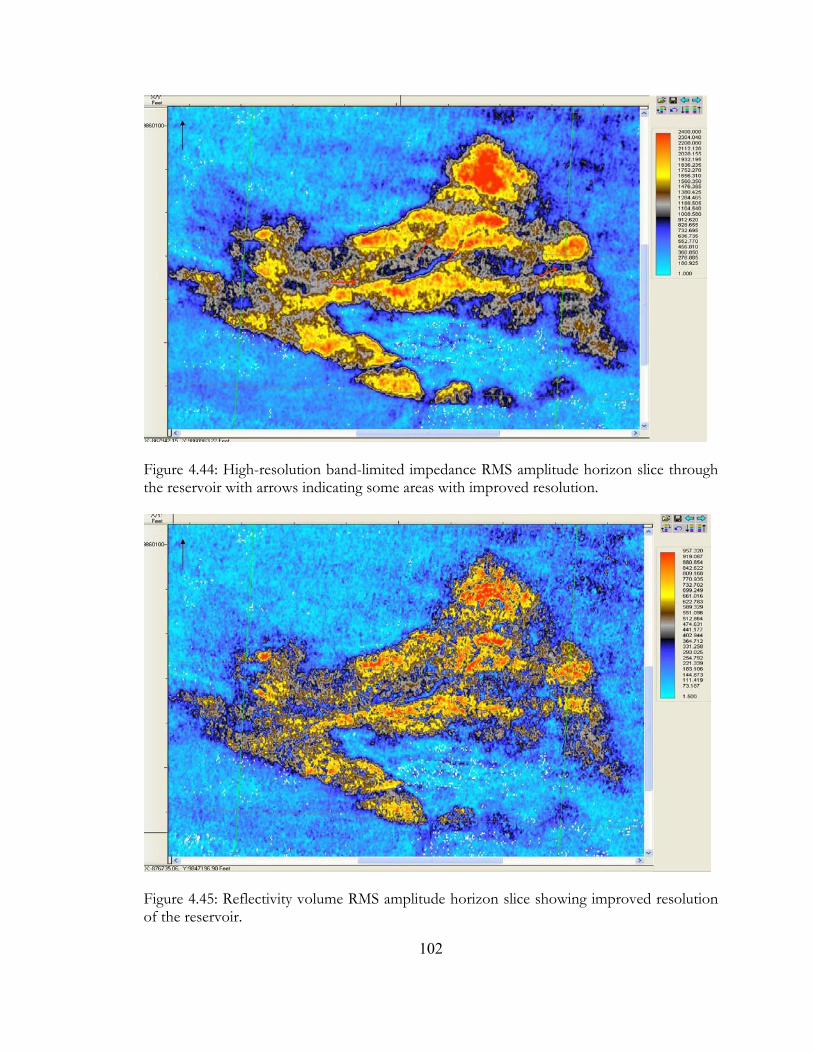
Figure 4.44: High-resolution band-limited impedance RMS amplitude horizon slice through the reservoir with arrows indicating some areas with improved resolution.
Figure 4.45: Reflectivity volume RMS amplitude horizon slice showing improved resolution of the reservoir.
102
4.5 Limitations of inversion methods
It is important to note that if the acquired data do not illuminate all sections of the
subsurface, such information may not be recovered by inversion (Treitel and Lines, 2001).
Francis (2002, p.2) also noted that “seismic inversion is an averaging process, caused both by
minimization and by bandwidth limitations”. Lastly, inversion is also known to be non-
unique, as there is more than one possible model which may fit the seismic data. However,
solutions can and have been constrained to give a more likely result.
103
Chapter 5: Conclusions
During the course of this research, Hoover field data (seismic and well logs) have
been investigated for hydrocarbons using 3D seismic attributes, conventional AVO analysis,
and post-stack impedance inversion methods.
Three-dimensional interpretations of the seismic data show that the reservoir is made
of turbidites sands and that the hydrocarbon-saturated section is a bright spot which is
slightly elevated by the underlying salt body. It also displays apparent Class IV AVO
properties. In the process of validating the presence of hydrocarbons from 3D
interpretations, some questions raised by Brown (2006) have been answered. These answers
include: (1) there is a reflection at the top and another at the bottom of the reservoir, (2) the
reflection from the reservoir is anomalous in amplitude, (3) the seismic amplitude anomaly is
structurally consistent, and (4) it is also large relative to the background values, with a ratio
of about 3:1 i.e. 300 % increase.
Logs in the survey area are made of stacked sandstone and shale sequences. The
reservoir sands, about 77 ft (≈23 m) thick, are characterized by low bulk densities, low P-
wave velocities, and relatively higher resistivities and porosities compared to the overlying
shales. The reservoir however is a low-resistivity oil reservoir with values below 10 ohm-m.
Fluid substitution, AVO modeling and analysis shows that whereas amplitude of
brine sands decreased rapidly with offset, oil- and gas-sand amplitudes on synthetics
decreased relatively slower (Figs. 3.34, 3.35 and 3.36). AVO attributes based on gradient (B),
intercept (A), and P-wave (Rp) and S-wave (Rs) reflection coefficients on synthetics and
extracted seismic traces shows that the AVO product is not good for Class IV environment
104
(Figs. 3.40 and 3.41). However, attributes such as scaled Poisson’s ratio change (Figs. 3.42,
3.43, 3.56 and 3.57), fluid factor and sum of reflection coefficients produced better results.
Although the AVO effect on oil is minimal when considered in isolation (Fig. 3.35), it is
significant when compared with brine (Fig. 3.34), such that one is able to discriminate oil
from brine in Hoover field (Figs. 3.50 and 3.51). This is because brine has a less negative
intercept compared to oil and this decreases faster with offset, unlike oil which decreases
very slowly with offset.
Both absolute and relative impedance inversion results show sharp contrast between
oil-saturated reservoir sands with the encasing shales, as well as varying degrees of contrast
between oil- and brine-saturated portions of the reservoir, depending on the inversion
method used. The far-stack high-resolution impedance inversion resulted in a smaller
number of bright amplitudes, compared to the near-stack, as a result of the faster decrease in
amplitude of shale upon shale and shale upon brine sands compared to shale upon oil-sands.
In addition to the central portion of the reservoir, low-impedance sands are also observed in
the northern and western portions of the reservoir (Figs. 4.35 to 4.38). At far offset, the
bright spot left in the reservoir is probably hydrocarbon-saturated turbidites. A comparison
of the absolute impedance inversion results shows that the model-based inversion produced
the best correlation with the synthetic generated after inversion, relative to the sparse-spike
and band-limited AI inversion. Although the high-resolution impedance inversion (Figs. 4.40
and 4.41) shows that the oil-saturated section of the reservoir is not as homogenous as
shown on the input near-stacked seismic volume (Fig. 4.39), it gives results similar to other
inversion methods carried out with an initial model, thereby increasing ones confidence on
the inversion results.
105
6. References
Asquith, G. and Krygowski, D., 2004, Basic Well Log Analysis (2nd edition), AAPG. Batzle, M., and Wang, Z., 1992, Seismic properties of pore fluids: Geophysics, Vol. 57, No. 11, 1396-1408. Boorman, C., Cowgill, M., Ginal, E., Mandley, R., Thompson, J., Roberts, G., and Archer, S., 2006, Huge potential still waiting in the Gulf of Mexico: GEO Expro Issue No. 4/5. Boyd, A., Davis, B., Flaunm, C., Klein, J., Sneider, R., Sibbit, A., and Singer, J., 1995, The lowdown on low resistivity pay: Oilfield Review, 4-18. Brown, A.R., 2004, Interpretation of Three-Dimensional Seismic Data (6th edition), AAPG Memoir 42 and SEG Investigations in Geophysics, No. 9. Burtz, O., Matteucci, G., and Meyer, W., 2002, Model-based calibration of band-limited impedance data: Hoover field, SEG International Exposition and 7th Annual Meeting. Castagna, J.P., and Swan, H.W., 1997, Principles of AVO crossplotting: The Leading Edge, Vol. 4, No. 16, 337-342. Castagna, J.P., Swan, H.W., and Foster, D. J., 1998, Framework for AVO gradient and intercept interpretation: Geophysics, Vol. 63, No. 3, 984-956. Chiburis, E., Franck, C., Leaney, S., McHugo, S., and Skidmore, C., 1993, Hydrocarbon detection from AVO: Oilfield Review, 44-50. Chopra, S., Portniaguine, O., and Castagna, J. P., 2006, Seismic resolution and thin-bed reflectivity inversion: CSEG Recorder, 19-25. Cogswell, T.L., 2001, Diana basin development – a pragmatic approach to the exploitation of two deepwater GOM fields: AAPG Annual Convention, Denver, 6 p. Connolly, P., 1999, Elastic impedance: The Leading Edge, Vol. 18, No. 4, 438 - 452.
Encarta, 2009, http://encarta.msn.com/dictionary_/attribute.html accessed 02/18/2009
Francis, A., 2002, Deterministic inversion – Over due for retirement? Petroleum exploration society of Great Britain (PETEX) 2002 Conference, 1-8. Gao, D., 2007, 3D seismic interpretation, unpublished lecture notes. Gluyas, J., and Swarbrick, R., 2004, Petroleum Geoscience, Blackwell Publishing Company, 359 p.
106
Hamada, G.M., Al-Blehed, M.S., and Al-Awad, M.N.J., 2000, Nuclear magnetic resonance log evaluation of low resistivity sandstone reservoirs by-passed by conventional logging analysis: Society of Petroleum Engineers International, SPE 64406, 1-11.
Hilterman, F., 2001, Seismic amplitude interpretation, SEG/EAGE Distinguished Instructor Short Course, Distinguished Instructor Series, No. 4.
Latimer, R., Davidson, R., and van Riel, P. 2000, An interpreter’s guide to understanding and working with seismic-derived acoustic impedance data: The Leading Edge, Vol. 19, 242-256. Li, Q., 2001, LP sparse-spike inversion, Strata technique document, Hampson-Russell software services limited, 14 p. Liner, C. L., 2004, Elements of 3D Seismology (2nd edition): PennWell Corporation, 608 p.
Moore, J.C., Klaus, A., et al., 1998, Explanatory notes: Proceedings of the oceanography drilling program, Initial reports, Vol. 171A, 11-15. Pendrel, J.V., and van Riel, P., 2000, Effect of well control on constrained sparse-spike seismic inversion. CSEG Recorder, Vol. 21, 18-28. Portniaguine, O., and Castagna, J. P., 2005, Spectral inversion: Lessons from modeling and Boonesville case study, 75th SEG Meeting, 1638-1641. Posamentier, H. W., and Walker, R.G., 2006, Deep water turbidites and submarine fans, in Facies Models Revisited, SEPM Special Publication, No. 84, 399-520. Posamentier, H. W., Davies, R. J., Cartwright, J. A., and Wood, L., 2007, Seismic geomorphology – an overview, in Posamentier, H. W., Davies, R. J., Cartwright, J. A. and Wood, L., eds., Seismic Geomorphology: Applications to Hydrocarbon Exploration and Production. Geological Society, London, Special Publications, No. 277, 1-14. Ross, C. P., 2000, Effective AVO crossplot modeling: A tutorial, Geophysics, Vol. 65, No. 3, 700-711. Russell, B., 2005, Strata workshop: Theory and exercises in seismic inversion and AVO, unpublished lecture notes.
Russell, B., and Hampson, D., 1999, AVO theory, Hampson-Russell software services limited, 69 p.
Russell, B., and Hampson, D., 2006, The old and the new in seismic inversion: CSEG Recorder, 5-11.
Rutherford, S.R., and Williams, R.H., 1989, Amplitude versus offset variations in gas sands, Geophysics, Vol. 54, No. 6, 680 - 688.
107
108
Savic, M., VerWest, B., Masters, R., Sena, A., and Gingrich, D., 2000, Elastic impedance inversion in practice: SEG Expanded Abstracts Vol. 19, 689. Selley, R., 1985, Elements of Petroleum Geology, W. H. Freeman and Company, 449 p
Sen, M. K., 2006, Seismic Inversion, Society of Petroleum Engineers, U.S.A, 120 p. Sheriff, R. E., 2002, Encyclopedic Dictionary of Applied Geophysics (4th edition), SEG, 429 p. Shrestha, R. K., 2008, Reservoir characterization of high impedance sands in the Ada field, North Louisiana, USA: GSH/SEG Spring Symposium Technical Program, 5 p. Slatt, R. M., 2006, Stratigraphic reservoir characterization for petroleum geologists, geophysicists and engineers, in Cibitt, J., ed., Handbook of Petroleum Exploration and Production, Vol. 6, 478 p. Smith, T. M., Sondergeld, C.H., and Rai, C.S., 2003, Gassmann fluid substitutions: A tutorial, Geophysics, Vol. 68, No. 2, 430-440. Treitel, S., and Lines, L., 2001, Past, present and the future of geophysical inversion-A new millennium analysis: Geophysics, Vol. 66, No. 1, 21-24. Veeken, P. C. H., 2007, Seismic stratigraphy, basin analysis and reservoir characteristics, in Helberg, K., and Treitel, S., eds., Handbook of Geophysical Exploration, Seismic Exploration Vol. 37, 509 p. Wang, Z., 2001, Fundamentals of seismic rock physics: Geophysics, Vol. 66, 398-412. Weimer, P., and Slatt, R.M., 2007, Petroleum geology of deep water settings, AAPG Studies in Geology No. 57, AAPG/Datapages Discovery Series No. 8.
http://www.worldatlas.com/aatlas/infopage/gulfofmexico.htm accessed 02/18/2009
http://earth.google.com/ accessed 04/18/2009
Copyright © 2022 FDOKUMEN