Research on Application of Six Sigma Management in Project ...
Upload
khangminh22Category
view
0download
0

DESIGN FOR SIX SIGMAIn Technology and Product Development
C. M. Creveling, J. L. Slutsky, and D. Antis, Jr.
Prentice Hall PTRUpper Saddle River, New Jerseywww.phptr.com
ProductDevelopment
Process
. . .what to do and when to do it. . .
Tools andBest
Practices
ProjectManagement
Methods

Library of Congress Cataloging-in-Publication DataCreveling, Clyde M.
Design for Six Sigma : in technology & product development / C.M. Creveling, J.L. Slutsky & D. Antis.
p. cm.Includes bibliographical references and index.ISBN 0-13-009223-11. Quality control--Statistical methods. 2. Experimental design. I. Slutsky, Jeff, 1956-
II. Antis, D. (Dave) III. Title.
TS156 .C74 2003658.5'62dc21
2002027435
Publisher: Bernard GoodwinEditorial Assistant: Michelle VincentiMarketing Manager: Dan DePasqualeManufacturing Manager: Alexis R. Heydt-LongCover Director: Jerry VottaCover Designer: Nina ScuderiArt Director: Gail Cocker-BoguszFull-Service Production Manager: Anne GarciaComposition/Production: Tiffany Kuehn, Carlisle Publishers Services
© 2003 Pearson Education, Inc.Publishing as Prentice Hall PTRUpper Saddle River, New Jersey 07458
Prentice Hall books are widely used by corporations and government agencies for training, marketing, andresale. For more information regarding corporate and government bulk discounts please contact:
Corporate and Government Sales (800) 382-3419or [email protected]
Other company and product names mentioned herein are the trademarks or registered trademarks of theirrespective owners.
All rights reserved. No part of this book may be reproduced, in any form or by any means, withoutpermission in writing from the publisher.
Printed in the United States of America
10 9 8 7 6 5 4 3 2 1
ISBN 0-13-0092231
Pearson Education LTD. Pearson Education Australia PTY, Limited Pearson Education Singapore, Pte. Ltd Pearson Education North Asia Ltd Pearson Education Canada, Ltd. Pearson Educación de Mexico, S.A. de C.V. Pearson Education Japan Pearson Education Malaysia, Pte. Ltd.

We would like to dedicate this book to our families.
For Skip CrevelingKathy and Neil Creveling
For Jeff Slutsky Ann, Alison, and Jason
For Dave AntisDenise, Aaron, Blake, Jared, and Shayla Antis
Without their patience and support, this book would have been much thinner.

This page intentionally left blank

Foreword xv
Preface xvii
Acknowledgments xxvii
PART I Introduction to Organizational Leadership, Financial Performance,and Value Management Using Design For Six Sigma 1
CHAPTER 1 The Role of Executive and Management Leadership in Design For Six Sigma 3
CHAPTER 2 Measuring Financial Results from DFSS Programs and Projects 13
CHAPTER 3 Managing Value with Design For Six Sigma 29
PART II Introduction to the Major Processes Used in Design For Six Sigma in Technology and Product Development 45
CHAPTER 4 Management of Product Development Cycle-Time 47
CHAPTER 5 Technology Development Using Design For Six Sigma 71
CHAPTER 6 Product Design Using Design For Six Sigma 111
CHAPTER 7 System Architecting, Engineering, and Integration Using Design For Six Sigma 177
PART III Introduction to the Use of Critical Parameter Management in DesignFor Six Sigma in Technology and Product Development 249
CHAPTER 8 Introduction to Critical Parameter Management 251
CHAPTER 9 The Architecture of the Critical Parameter Management Process 257
CHAPTER 10 The Process of Critical Parameter Management in Product Development 265
CHAPTER 11 The Tools and Best Practices of Critical Parameter Management 309
CHAPTER 12 Metrics for Engineering and Project Management Within CPM 321
CHAPTER 13 Data Acquisition and Database Architectures in CPM 331
v
Brief Contents
PART IV Tools and Best Practices for Invention, Innovation, and Concept Development 337
CHAPTER 14 Gathering and Processing the Voice of the Customer: CustomerInterviewing and the KJ Method 341
CHAPTER 15 Quality Function Deployment: The Houses of Quality 361
CHAPTER 16 Concept Generation and Design for x Methods 381
CHAPTER 17 The Pugh Concept Evaluation and Selection Process 399
CHAPTER 18 Modeling: Ideal/Transfer Functions, Robustness Additive Models,and the Variance Model 411
PART V Tools and Best Practices for Design Development 435
CHAPTER 19 Design Failure Modes and Effects Analysis 437
CHAPTER 20 Reliability Prediction 449
CHAPTER 21 Introduction to Descriptive Statistics 471
CHAPTER 22 Introduction to Inferential Statistics 479
CHAPTER 23 Measurement Systems Analysis 495
CHAPTER 24 Capability Studies 507
CHAPTER 25 Multi-Vari Studies 519
CHAPTER 26 Regression 529
CHAPTER 27 Design of Experiments 549
PART VI Tools and Best Practices for Optimization 569
CHAPTER 28 Taguchi Methods for Robust Design 571
CHAPTER 29 Response Surface Methods 601
CHAPTER 30 Optimization Methods 615
PART VII Tools and Best Practices for Verifying Capability 629
CHAPTER 31 Analytical Tolerance Design 631
CHAPTER 32 Empirical Tolerance Design 671
CHAPTER 33 Reliability Evaluation 687
CHAPTER 34 Statistical Process Control 707
EPILOGUE Linking Design to Operations 723
APPENDIX A Design For Six Sigma Abbreviations 729
APPENDIX B Glossary 731
INDEX 751
vi Brief Contents

Contents
Foreword xv
Preface xvii
Acknowledgments xxvii
PART I Introduction to Organizational Leadership, Financial Performance,and Value Management Using Design For Six Sigma 1
CHAPTER 1 The Role of Executive and Management Leadership in Design For Six Sigma 3Leadership Focus on Product Development as Key Business Process 3The Strategic View of Top-Line Growth 8Enabling Your Product Development Process to Have the Ability to Produce the
Right Data, Deliverables, and Measures of Risk within the Context ofYour Phase/Gate Structure 10
Executive Commitment to Driving Culture Change 11Summary 11References 12
CHAPTER 2 Measuring Financial Results from DFSS Programs and Projects 13A Case Study 13Deploying the Voice of the Customer 14DFSS Project Execution Efficiency 16Production Waste Minimization 18Pricing and Business Risk 24
CHAPTER 3 Managing Value with Design For Six Sigma 29Extracting Value 29Value as a Formula 31Measuring Value in the Marketplace 33Identifying the Purposes of Design 36Design Based on the Voice of the Customer 37Putting Concept Engineering to Work 38References 44
vii

PART II Introduction to the Major Processes Used in Design For Six Sigma in Technology and Product Development 45
CHAPTER 4 Management of Product Development Cycle-Time 47The Product Development Process Capability Index 48Product Development Process 50Project Management 58The Power of PERT Charts 60References 70
CHAPTER 5 Technology Development Using Design For Six Sigma 71The I2DOV Roadmap: Applying a Phase/Gate Approach to Technology
Development 72I2DOV and Critical Parameter Management During the Phases and Gates
of Technology Development 77I2DOV Phase 1: Invention and Innovation 78I2DOV Phase 2: Develop Technology Concept Definition, Stabilization, and
Functional Modeling 87I2DOV Phase 3: Optimization of the Robustness of the Subsystem Technologies 92I2DOV Phase 4: Certification of the Platform or Subsystem Technologies 101References 110
CHAPTER 6 Product Design Using Design For Six Sigma 111An Introduction to Phases and Gates 112Preparing for Product Commercialization 113Defining a Generic Product Commercialization Process Using CDOV
Roadmap 114The CDOV Process and Critical Parameter Management During the Phases and
Gates of Product Commercialization 117CDOV Phase 2: Subsystem Concept and Design Development 133CDOV Phase 3A: Optimizing Subsystems 150CDOV Phase 3B: System Integration 160CDOV Phase 4A: Verification of Product Design Functionality 165CDOV Phase 4B: Verification of Production 171References 176
CHAPTER 7 System Architecting, Engineering, and Integration Using Design For Six Sigma 177Phase 1: System Concept Development 179Phase 2: Subsystem, Subassembly, Component, and Manufacturing Concept
Design 196Phase 3A: Subsystem Robustness Optimization 210
viii Contents
Phase 3B: System Integration 219Phase 4A: Final Product Design Certification 231Phase 4B: Production Verification 241References 247
PART III Introduction to the Use of Critical Parameter Management in DesignFor Six Sigma in Technology and Product Development 249
CHAPTER 8 Introduction to Critical Parameter Management 251Winning Strategies 251Focus on System Performance 252Data-Driven Process 253The Best of Best Practices 256Reference 256
CHAPTER 9 The Architecture of the Critical Parameter Management Process 257Who Constructs the CPM Process? 258Timing Structure of the CPM Process: Where and When Does CPM Begin? 258What Are the Uses of CPM? 259Reference 263
CHAPTER 10 The Process of Critical Parameter Management in Product Development 265Definitions of Terms for Critical Parameter Management 268Critical Parameter Management in Technology Development and Product
Design: Phase 1 271Phase 2 in Technology Development or Product Design 276Phases 3 and 4: Stress Testing and Integration 302Capability Summaries and the Capability Growth Index 307
CHAPTER 11 The Tools and Best Practices of Critical Parameter Management 309The Rewards of Deploying Proven Tools and Best Practices 310Critical Parameter Management Best Practices for Technology
Development 312Critical Parameter Management Best Practices for Product
Commercialization 315
CHAPTER 12 Metrics for Engineering and Project Management Within CPM 321Key CPM Metrics 322Statistical Metrics of CPM 326The Capability Growth Index and the Phases and Gates of Technology
Development and Product Commercialization 329
CHAPTER 13 Data Acquisition and Database Architectures in CPM 331Instrumentation, Data Acquisition, and Analysis in CPM 331Databases: Architectures and Use in CPM 335References 336
Contents ix

PART IV Tools and Best Practices for Invention, Innovation, and ConceptDevelopment 337
CHAPTER 14 Gathering and Processing the Voice of the Customer: CustomerInterviewing and the KJ Method 341Where Am I in the Process? 341What Am I Doing in the Process? 342What Output Do I Get at the Conclusion of this Phase of the Process? 343Gathering and Processing the Voice of the Customer Process Flow
Diagram 343Verbal Descriptions of the Application of Each Block Diagram 343VOC Gathering and Processing Checklist and Scorecard 359References 360
CHAPTER 15 Quality Function Deployment: The Houses of Quality 361Where Am I in the Process? 361What Am I Doing in the Process? 362What Output Do I Get at the Conclusion of this Phase of the Process? 363QFD Process Flow Diagram 363Verbal Descriptions for the Application of Each Block Diagram 363QFD Checklist and Scorecards 377References 380
CHAPTER 16 Concept Generation and Design for x Methods 381Where Am I in the Process? 381What Am I Doing in the Process? 382What Output Do I Get at the Conclusion of this Phase of the Process? 383Concept Generation and DFx Process Flow Diagram 384Verbal Descriptions for the Application of Each Block Diagram 385Concept Generation and DFx Checklist and Scorecards 394References 397
CHAPTER 17 The Pugh Concept Evaluation and Selection Process 399Where Am I in the Process? 399What Am I Doing in the Process? 400What Output Do I Get at the Conclusion of this Phase of the Process? 401The Pugh Concept Selection Process Flow Diagram 401Verbal Descriptions for the Application of Each Block Diagram 401Pugh Concept Selection Process Checklist and Scorecard 408References 410
CHAPTER 18 Modeling: Ideal/Transfer Functions, Robustness Additive Models,and the Variance Model 411Where Am I in the Process? 411What Am I Doing in the Process? 412
x Contents
What Output Do I Get at the Conclusion of this Phase of the Process? 413Modeling Process Flow Diagram 417Verbal Descriptions for the Application of Each Block Diagram 417Modeling Checklist and Scorecard 431References 434
PART V Tools and Best Practices for Design Development 435
CHAPTER 19 Design Failure Modes and Effects Analysis 437Where Am I in the Process? 437What Am I Doing in the Process? 438What Output Do I Get at the Conclusion of this Phase of the Process? 438The DFMEA Flow Diagram 438Verbal Descriptions for the Application of Each Block Diagram 438DFMEA Checklist and Scorecard 445References 447
CHAPTER 20 Reliability Prediction 449Where Am I in the Process? 449What Am I Doing in the Process? 450What Output Do I Get at the Conclusion of this Phase of the Process? 450The Reliability Prediction Flow Diagram 450Applying Each Block Diagram Within the Reliability Prediction Process 450Reliability Prediction Checklist and Scorecard 466References 469
CHAPTER 21 Introduction to Descriptive Statistics 471Where Am I in the Process? 471What Output Do I Get from Using Descriptive Statistics? 472What Am I Doing in the Process? 472Descriptive Statistics Review and Tools 472
CHAPTER 22 Introduction to Inferential Statistics 479Where Am I in the Process? 479What Am I Doing in the Process? 480What Output Do I Get from Using Inferential Statistics? 480Inferential Statistics Review and Tools 480References 493
CHAPTER 23 Measurement Systems Analysis 495Where Am I in the Process? 495What Am I Doing in the Process? 495What Output Do I Get at the Conclusion of Measurement Systems
Analysis? 496MSA Process Flow Diagram 496
Contents xi

Verbal Descriptions for the Application of Each Block Diagram 496MSA Checklist and Scorecard 504References 505
CHAPTER 24 Capability Studies 507Where Am I in the Process? 507What Am I Doing in the Process? 507What Output Do I Get at the Conclusion of a Capability Study? 508Capability Study Process Flow Diagram 508Verbal Descriptions of the Application of Each Block Diagram 508Capability Study Checklist and Scorecard 517References 517
CHAPTER 25 Multi-Vari Studies 519Where Am I in the Process? 519What Am I Doing in the Process? 519What Output Do I Get at the Conclusion of this Phase of the Process? 520Multi-Vari Study Process Flow Diagram 520Verbal Descriptions for the Application of Each Block Diagram 521Multi-Vari Study Checklist and Scorecard 526Reference 527
CHAPTER 26 Regression 529Where Am I in the Process? 529What Am I Doing in the Process? 529What Output Do I Get at the Conclusion of this Phase of the Process? 530Regression Process Flow Diagram 530Verbal Descriptions for the Application of Each Block Diagram 530Regression Checklist and Scorecard 547References 548
CHAPTER 27 Design of Experiments 549Where Am I in the Process? 549What Am I Doing in the Process? 549What Output Do I Get at the Conclusion of this Phase of the Process? 550DOE Process Flow Diagram 550Verbal Descriptions for the Application of Each Block Diagram 550DOE Checklist and Scorecard 567Reference 568
PART VI Tools and Best Practices for Optimization 569
CHAPTER 28 Taguchi Methods for Robust Design 571Where Am I in the Process? 571What Am I Doing in the Process? 571
xii Contents

What Output Do I Get at the Conclusion of Robust Design? 572The Robust Design Process Flow Diagram 572Verbal Descriptions for the Application of Each Block Diagram 573Robust Design Checklist and Scorecard 596References 599
CHAPTER 29 Response Surface Methods 601Where Am I in the Process? 601What Am I Doing in the Process? 601What Output Do I Get at the Conclusion of RSM? 602RSM Process Flow Diagram 602Verbal Descriptions of the Application of Each Block Diagram 602RSM Checklist and Scorecard 613Reference 614
CHAPTER 30 Optimization Methods 615Where Am I in the Process? 615What Am I Doing in the Process? 615What Output Do I Get at the Conclusion of Optimization? 616Optimization Process Flow Diagram 616Verbal Descriptions of the Application of Each Block Diagram 616Optimization Checklist and Scorecard 627References 628
PART VII Tools and Best Practices for Verifying Capability 629
CHAPTER 31 Analytical Tolerance Design 631Where Am I in the Process? 631What Am I Doing in the Process? 631What Output Do I Get at the Conclusion of Analytical Tolerance
Design? 632The Analytical Tolerance Design Flow Diagram 633Verbal Descriptions for the Application of Each Block Diagram 633Analytical Tolerance Design Checklist and Scorecard 667References 669
CHAPTER 32 Empirical Tolerance Design 671Where Am I in the Process? 671What Am I Doing in the Process? 671What Output Do I Get at the Conclusion of Empirical Tolerance Design? 672The Empirical Tolerance Design Flow Diagram 672Verbal Descriptions for the Application of Each Block Diagram 672Empirical Tolerance Design Checklist and Scorecard 683Reference 685
Contents xiii
CHAPTER 33 Reliability Evaluation 687Where Am I in the Process? 687What Am I Doing in the Process? 688What Output Do I Get at the Conclusion of Reliability Evaluations? 688The Reliability Evaluation Flow Diagram 688Detailed Descriptions for the Application of Each Block Diagram 688Reliability Evaluation Checklist and Scorecard 705References 706
CHAPTER 34 Statistical Process Control 707Where Am I in the Process? 707What Am I Doing in the Process? 707What Output Do I Get at the Conclusion of SPC? 708SPC Process Flow Diagram 708Verbal Descriptions of the Application of Each Block Diagram 708SPC Checklist and Scorecard 722References 722
EPILOGUE Linking Design to Operations 723
APPENDIX A Design For Six Sigma Abbreviations 729
APPENDIX B Glossary 731
INDEX 751
xiv Contents

Foreword
Once in a while an idea evolves from merely a good concept to the inspiration for real change.The continued search for the “new, best way” can sometimes divert attention from the de-
velopment of existing ways to a higher standard. Design For Six Sigma (DFSS) is such a devel-opment. It marries the notion of doing things right the first time with the belief in the importanceof leadership in making things better.
DFSS is based on the foundation that design is a team sport in which all appropriate orga-nizational functions need to participate. Each key function needs to apply its appropriate science.The key function in product design is typically the core engineering team. In information systemsdesign it will be the core information technology team. In people systems design it will be the hu-man resources team. The “science” any of these teams deploy must revolve around a well-bal-anced portfolio of tools and best practices that will enable them to develop outstanding data andthus deliver the right results.
In our company’s experience, most of the design projects have been product related so Iwill refer to our learnings in that area—although my guess is that the lessons apply morebroadly.
Before DFSS we had a number of initiatives around new product introductions. In additionto the typical milestone monitoring process (project management within our Phase/Gate process)there was a great deal of emphasis placed in co-location and cross-functional teams. The out-comes were fairly predictable, in hindsight. While leadership around co-location shortened thelines of communication, it did little for the content or the quality of those communications. Weneeded to communicate with better data.
In this team sport of design using DFSS we would expect many functions to have impor-tant inputs to the design process—and in the case of the product design, we now expect engi-neering to apply its science with the added benefit of the right balance of DFSS tools to create op-timum solutions for our customers.
DFSS sets forth a clear expectation of leadership roles and responsibilities. This includesclear definition of expectations measures, deliverables, and support from senior management.
xv

Accountability is clarified with DFSS, enabling recognition of proper performance. We focuson all this, while applying the latest design techniques in a disciplined, preplanned sequence.
This may sound like the latest “new way” if not for the fact that it really is more like the de-velopment of the old way to a higher standard that feels a lot like the right way.
—Frank McDonaldVP and General Manager
Heavy Duty EnginesCummins, Inc.
xvi Foreword

Preface
In its simplest sense, DFSS consists of a set of needs-gathering, engineering and statistical meth-ods to be used during product development. These methods are to be imbedded within the or-
ganization’s product development process (PDP). Engineering determines the physics and tech-nology to be used to carry out the product’s functions. DFSS ensures that those functions meetthe customer’s needs and that the chosen technology will perform those functions in a robustmanner throughout the product’s life.
DFSS does not replace current engineering methods, nor does it relieve an organization ofthe need to pursue excellence in engineering and product development. DFSS adds another di-mension to product development, called Critical Parameter Management (CPM). CPM is the dis-ciplined and focused attention to the design’s functions, parameters, and responses that are criti-cal to fulfilling the customer’s needs. This focus is maintained by the development teamthroughout the product development process from needs gathering to manufacture. Manufactur-ing then continues CPM throughout production and support engineering. Like DFSS, CPM isconducted throughout and embedded within the PDP. DFSS provides most of the tools that en-able the practice of CPM. In this light, DFSS is seen to coexist with and add to the engineeringpractices that have been in use all along.
DFSS is all about preventing problems and doing the right things at the right time duringproduct development. From a management perspective, it is about designing the right cycle-timefor the proper development of new products. It helps in the process of inventing, developing, op-timizing, and transferring new technology into product design programs. It also enables the sub-sequent conceptual development, design, optimization, and verification of new products prior totheir launch into their respective markets.
The DFSS methodology is built upon a balanced portfolio of tools and best practices thatenable a product development team to develop the right data to achieve the following goals:
1. Conceive new product requirements and system architectures based upon a balance be-tween customer needs and the current state of technology that can be efficiently andeconomically commercialized.
2. Design baseline functional performance that is stable and capable of fulfilling the prod-uct requirements under nominal conditions.
xvii

3. Optimize design performance so that measured performance is robust and tunable inthe presence of realistic sources of variation that the product will experience in the de-livery, use, and service environments.
4. Verify systemwide capability (to any sigma level required, 6 or otherwise) of theproduct and its elements against all the product requirements.
DFSS is managed through an integrated set of tools that are deployed within the phases ofa product development process. It delivers qualitative and quantitative results that are summa-rized in scorecards in the context of managing critical parameters against a clear set of productrequirements based on the “voice of the customer.” In short it develops clear requirements andmeasures their fulfillment in terms of 6 standards.
A design with a critical functional response (for example, a desired pressure or an acousti-cal sound output) that can be measured and compared to upper and lower specification limits re-lating back to customer needs would look like the following figure if it had 6 sigma performance.
The dark black arrows between the control limits (UCL and LCL, known as natural toler-ances set at / 3 standard deviations of a distribution that is under statistical control) and thespecification limits (USL and LSL, known as VOC-based performance tolerances) indicates de-sign latitude that is representative of 6 sigma performance. That is to say, there are 3 standard de-viations of latitude on each side of the control limit out to the specification limit to allow for shiftsin the mean and broadening of the distribution. The customer will not feel the variability quicklyin this sense. If the product or process is adjustable, there is an opportunity to put the mean backon to the VOC-based performance target or to return the distribution to its desired width withinits natural tolerances. If the latitude is representative of a function that is not serviceable or ad-
UCLy
USLLSL LCL
12s
Cp =USL – LSL
6s= 2
6s
Performance (VOC) TolerancesNatural Tolerances
xviii Preface
justable, then the latitude is suggestive of the reliability of the function if the drift off target ordistribution broadening is measured over time. In this case, Cp (short-term distribution broaden-ing with no mean shift) and Cpk metrics (both mean shifting and distribution broadening overlong periods of time) can be clear indicators of a design’s robustness (insensitivity to sources ofvariation) over time. DFSS uses capability metrics to aid in the development of critical productfunctions throughout the phases and gates of a product development process.
Much more will be said about the metrics of DFSS in later chapters. Let’s move on to dis-cuss the higher level business issues as they relate to deploying DFSS in a company.
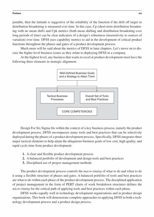
At the highest level, any business that wants to excel at product development must have thefollowing three elements in strategic alignment:
Design For Six Sigma fits within the context of a key business process, namely the productdevelopment process. DFSS encompasses many tools and best practices that can be selectivelydeployed during the phases of a product development process. Specifically, DFSS integrates threemajor tactical elements to help attain the ubiquitous business goals of low cost, high quality, andrapid cycle-time from product development:
1. A clear and flexible product development process2. A balanced portfolio of development and design tools and best practices3. Disciplined use of project management methods
The product development process controls the macro-timing of what to do and when to doit using a flexible structure of phases and gates. A balanced portfolio of tools and best practicesare what to do within each phase of the product development process. The disciplined applicationof project management in the form of PERT charts of work breakdown structures defines the micro-timing for the critical path of applying tools and best practices within each phase.
DFSS works equally well in technology development organizations and in product designorganizations. This book will demonstrate complete approaches to applying DFSS in both a tech-nology development process and a product design process.
Well-Defined Business Goalsand a Strategy to Attain Them
Tactical BusinessProcesses
Overall Set of Toolsand Best Practices
CORE COMPETENCIES
Preface xix

The metrics of DFSS break down into three categories:
1. Cycle-time (controlled by the product development process and project managementmethods)
2. Design and manufacturing process performance capability of critical-to-function pa-rameters (developed by a balanced portfolio of tools and best practices)
3. Cost of the product and the resources to develop it
DFSS is focused on CPM. This is done to identify the few variables that dominate the de-velopment of baseline performance (Yavg.), the optimization of robust performance (S/N and ),and the certification of capable performance (Cp and Cpk) of the integrated system of designedparameters. DFSS instills a system integration mind-set. It looks at all parameters—within theproduct and the processes that make it—as being important to the integrated performance of thesystem elements, but only a few are truly critical.
DFSS starts with a sound business strategy and its set of goals and, on that basis, flowsdown to the very lowest levels of the design and manufacturing process variables that deliver onthose goals. To get any structured product development process headed in the right direction,DFSS must flow in the following manner:
Define business strategy: Profit goals and growth requirements
Identify markets and market segments: Value generation and requirements
Gather long-term voice of customer and voice of technology trends
Develop product line strategy: Family plan requirements
Develop and deploy technology strategy: Technology and subsystem platformrequirements
Gather product specific VOC and VOT: New, unique, and difficult needs
Conduct KJ analysis: Structure and rank the VOC
Build system House of Quality: Translate new, unique, and difficult VOC
Document system requirements: New, unique, and difficult, and importantrequirements
Define the system functions: Functions to be developed to fulfill requirements
Generate candidate system architectures: Form and fit to fulfill requirements
Select the superior system concept: Highest in feasibility, low vulnerability
DFSS tools are then used to create a hierarchy of requirements down from the system levelto the subsystems, subassemblies, components, and manufacturing processes. Once a clear andlinked set of requirements is defined, DFSS uses CPM to measure and track the capability of theevolving set of Ys and xs that comprise the critical functional parameters governing the perform-ance of the system. At this point DFSS drives a unique synergy between engineering design prin-
xx Preface

ciples and applied statistical analysis methods. DFSS is not about statistics—it is about productdevelopment using statistically enabled engineering methods and metrics.
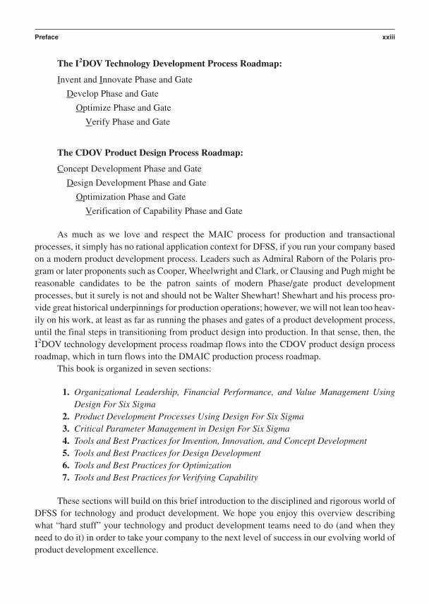
DFSS does not require product development teams to measure quality and reliability to de-velop and attain quality and reliability. Product development teams apply DFSS to analyticallymodel and empirically measure fundamental functions as embodied in the units of engineeringscalars and vectors. It is used to build math models called ideal or transfer functions [Y f(x)]between fundamental (Yresponse) response variables and fundamental (xinputs) input variables.When we measure fundamental (Yresponse) values as they respond to the settings of input (xinputs)variables, we avoid the problems that come with the discontinuities between continuous engi-neering input variables and counts of attribute quality response variables.
DFSS avoids counting failures and places the engineering team’s focus on measuring realfunctions. The resulting fundamental models can be exercised, analyzed, and verified statisticallythrough Monte Carlo simulations and the sequential design of experiments.
Defects and time-to-failure are not the main metrics of DFSS. DFSS uses continuous vari-ables that are leading indicators of impending defects and failures to measure and optimize criti-cal functional responses against assignable causes of variation in the production, delivery, and useenvironments. We need to prevent problems—not wait until they occur and then react to them.
If one seeks to reduce defects and improve reliability, avoiding attribute measures of qual-ity can accelerate the time it takes to reach these goals. You must do the hard work of measuringfunctions. As a result of this mind-set, DFSS has a heavy focus in measurement systems analysisand computer-aided data acquisition methods. The sign of a strong presence of DFSS in a com-pany is its improved capability to measure functional performance responses that its competitorsdon’t know they should be measuring and couldn’t measure even if they knew they should! Letyour competitors count defects—your future efficiencies in product development reside in meas-uring functions that let you prevent defective design performance.
DFSS requires significant investment in instrumentation and data acquisition technology.It is not uncommon to see companies that are active in DFSS obtaining significant patents for
Continuousx
Measuring
A realfunction
based onphysical law
Con
tinuo
us Y
Continuousx
A "pseudo-function"based on a subjective
judgment of quality
Defective
Acceptable
Counting
Attr
ibut
e Y
Preface xxi
their inventions and innovations in measurement systems. Counting defects is easy and cheap.Measuring functions is often difficult and expensive. If you want to prevent defects during pro-duction and use, you have to take the hard fork in the metrology road back in technology devel-opment and product design. Without this kind of data, CPM is extremely difficult.
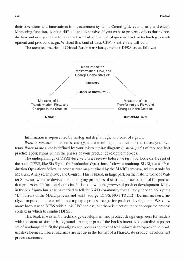
The technical metrics of Critical Parameter Management in DFSS are as follows:
Information is represented by analog and digital logic and control signals.What to measure is the mass, energy, and controlling signals within and across your sys-
tems. When to measure is defined by your micro-timing diagram (critical path) of tool and bestpractice applications within the phases of your product development process.
The underpinnings of DFSS deserve a brief review before we turn you loose on the rest ofthe book. DFSS, like Six Sigma for Production Operations, follows a roadmap. Six Sigma for Pro-duction Operations follows a process roadmap outlined by the MAIC acronym, which stands forMeasure, Analyze, Improve, and Control. This is based, in large part, on the historic work of Wal-ter Shewhart when he devised the underlying principles of statistical process control for produc-tion processes. Unfortunately this has little to do with the process of product development. Manyin the Six Sigma business have tried to tell the R&D community that all they need to do is put a“D” in front of the MAIC process and voilà! you get DFSS. NOT TRUE!!! Define, measure, an-alyze, improve, and control is not a proper process recipe for product development. We knowmany have started DFSS within this SPC context, but there is a better, more appropriate processcontext in which to conduct DFSS.
This book is written by technology development and product design engineers for readerswith the same or similar backgrounds. A major part of the book’s intent is to establish a properset of roadmaps that fit the paradigms and process context of technology development and prod-uct development. These roadmaps are set up in the format of a Phase/Gate product developmentprocess structure.
Measures of theTransformation, Flow, andChanges in the State of:
ENERGY
. . .what to measure. . .
Measures of theTransformation, Flow, andChanges in the State of:
MASS
Measures of theTransformation, Flow, andChanges in the State of:
INFORMATION
xxii Preface
The I2DOV Technology Development Process Roadmap:
Invent and Innovate Phase and Gate
Develop Phase and Gate
Optimize Phase and Gate
Verify Phase and Gate
The CDOV Product Design Process Roadmap:
Concept Development Phase and Gate
Design Development Phase and Gate
Optimization Phase and Gate
Verification of Capability Phase and Gate
As much as we love and respect the MAIC process for production and transactionalprocesses, it simply has no rational application context for DFSS, if you run your company basedon a modern product development process. Leaders such as Admiral Raborn of the Polaris pro-gram or later proponents such as Cooper, Wheelwright and Clark, or Clausing and Pugh might bereasonable candidates to be the patron saints of modern Phase/gate product developmentprocesses, but it surely is not and should not be Walter Shewhart! Shewhart and his process pro-vide great historical underpinnings for production operations; however, we will not lean too heav-ily on his work, at least as far as running the phases and gates of a product development process,until the final steps in transitioning from product design into production. In that sense, then, theI2DOV technology development process roadmap flows into the CDOV product design processroadmap, which in turn flows into the DMAIC production process roadmap.
This book is organized in seven sections:
1. Organizational Leadership, Financial Performance, and Value Management UsingDesign For Six Sigma
2. Product Development Processes Using Design For Six Sigma3. Critical Parameter Management in Design For Six Sigma4. Tools and Best Practices for Invention, Innovation, and Concept Development5. Tools and Best Practices for Design Development6. Tools and Best Practices for Optimization7. Tools and Best Practices for Verifying Capability
These sections will build on this brief introduction to the disciplined and rigorous world ofDFSS for technology and product development. We hope you enjoy this overview describingwhat “hard stuff” your technology and product development teams need to do (and when theyneed to do it) in order to take your company to the next level of success in our evolving world ofproduct development excellence.
Preface xxiii
How to Get the Most From This Book
This text on DFSS was written to serve several types of readers:
1. Executives, R&D directors and business leaders2. Program managers, project managers and design team leaders3. Technical practitioners who comprise design teams
If you are an executive, R&D director, or some other form of business leader, we wrotethe Introduction and Part I for you.
If you are a program manager, project manager, or a design team leader, we wrote Parts IIand III primarily for you.
If you are a technical practitioner who will be applying the tools of DFSS on technologyand product design programs and projects we wrote the Tool chapters in Parts IV throughVII for you.
An extensive glossary at the end of the book is intended for all readers.
Parts II through VII of this book were designed to serve as a reference to be used overand over as needed to remind and refresh the reader on what to do and when to do itduring the phases and gates of technology development and product design. These partscan be used to guide your organization to improve discipline and rigor at gate reviewsand to help redesign your product development process to include Six Sigma metrics anddeliverables.
If you want to understand any DFSS tool and its deliverables prior to a gate review, werecommend reading the appropriate tool chapter(s) prior to the gate review.
—Skip CrevelingJeff SlutskyDave Antis
xxiv Preface

Preface
xxv
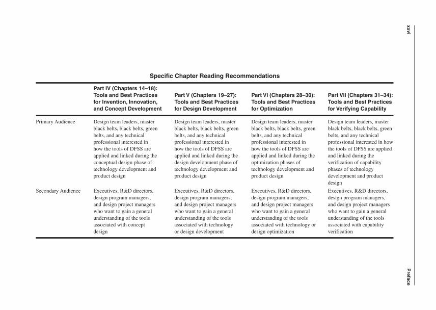
Specific Chapter Reading Recommendations
Part I (Chapters 1–3):Organizational Leadership, Part II (Chapters 4–7): Part III (Chapters 8–13):
Introduction to Design Financial Performance and Product Development Critical Parameter For Six Sigma Value Management using DFSS Processes Using DFSS Management Using DFSS
Primary Audience All readers Executives, R&D directors, Program managers, project Project Managers design team business leaders, design program managers, and design leaders, master black belts, managers, design project managers, team leaders black belts, green belts, and and design team leaders any technical professional
interested in how to managecritical requirements and thetechnical deliverables thatfulfill them during the phasesand gates of a technology andproduct design process
Secondary Audience Master black belts, black belts, Executives, R&D directors, Executives, R&D directors, green belts as well as any technical business leaders, master and design program managersprofessional interested in leadership, black belts, black belts, who want to gain a general financial performance, and the green belts and any understanding of the process management of value technical professional and tools associated with
interested in how Phase/ Critical Parameter Gate processes can be used Managementto help manage new product development in a Six Sigma context
(continued)
xxviP
reface
Specific Chapter Reading Recommendations
Part IV (Chapters 14–18):Tools and Best Practices Part V (Chapters 19–27): Part VI (Chapters 28–30): Part VII (Chapters 31–34):for Invention, Innovation, Tools and Best Practices Tools and Best Practices Tools and Best Practices and Concept Development for Design Development for Optimization for Verifying Capability
Primary Audience Design team leaders, master Design team leaders, master Design team leaders, master Design team leaders, masterblack belts, black belts, green black belts, black belts, green black belts, black belts, green black belts, black belts, greenbelts, and any technical belts, and any technical belts, and any technical belts, and any technical professional interested in professional interested in professional interested in professional interested in how how the tools of DFSS are how the tools of DFSS are how the tools of DFSS are the tools of DFSS are applied applied and linked during the applied and linked during the applied and linked during the and linked during the conceptual design phase of design development phase of optimization phases of verification of capability technology development and technology development and technology development and phases of technology product design product design product design development and product
design
Secondary Audience Executives, R&D directors, Executives, R&D directors, Executives, R&D directors, Executives, R&D directors, design program managers, design program managers, design program managers, design program managers, and design project managers and design project managers and design project managers and design project managers who want to gain a general who want to gain a general who want to gain a general who want to gain a general understanding of the tools understanding of the tools understanding of the tools understanding of the tools associated with concept associated with technology associated with technology or associated with capability design or design development design optimization verification

Acknowledgments
xxvii
The authors would like to acknowledge the role of Sigma Breakthrough Technologies, Inc. forproviding the opportunity to test and validate the Design For Six Sigma methodology docu-
mented in this book. SBTI supported the use of the methods and tools described here within awide range of companies during their corporate Six Sigma deployments. The cycles of learningwere of true benefit to the final product you see here.
There are a few leaders, colleagues, mentors, students, and friends that we would like torecognize and thank for their influence on our thinking—but more importantly, on our actions.
While the body of knowledge known as Design For Six Sigma is still evolving and form-ing, some elements are becoming accepted standards. In the area of Concept Engineering, the ef-forts of Mr. Joseph Kasabula, Dr. Don Clausing, and the late Dr. Stuart Pugh in making the toolsand best practices for managing the fuzzy front end of Product Development practical and ac-tionable is unsurpassed. Our thinking on Product Development as a process has been greatly en-hanced by the works of Dr. Don Clausing and Mr. Robert Cooper. Probably the single most im-portant person in the last two decades when it comes to defining how an engineer can properlydevelop tolerances in a Six Sigma context is our great friend Mr. Reigle Stewart. We simply havenever seen or heard a better teacher on the subject of developing tolerances for Six Sigma per-formance. We believe a major characteristic of a Six Sigma design is its “robustness” to sourcesof variation. We thank the world’s best mentors on Robust Design: Dr. Genichi Taguchi; his son,Shin Taguchi; and Dr. Madhav Phadke.
We would also like to thank Dr. Stephen Zinkgraf, CEO of Sigma Breakthrough Technolo-gies Inc., for his support. Steve’s contributions to the Six Sigma industry are vast and his influ-ence and efforts to provide us with an environment where we could build on our ability to linkSix Sigma to Product Development is gratefully acknowledged.
Thanks to all our peers and the students of DFSS who read our manuscripts and offered ad-vice. Mr. Steve Trabert (from StorageTek Corp.), Mr. David Mabee, and Mr. Joseph Szostek wereespecially helpful for their detailed review and comments on improvements.
We would also like to recognize and express our heartfelt thanks to our colleagues, Mr.Randy Perry (Chapter 2), Mr. Scott McGregor (Chapter 3), Mr. Ted Hume (Chapters 20 and 33),and Dr. Stephen Zinkgraf (Epilogue), for contributing to this text. Their work helped us round outthis comprehensive book on DFSS. Each of them added a unique perspective that we were lack-ing. Our thanks to each of you for helping us make this a better book.
Finally, we want to say thank you to the world’s most patient and long-suffering editor, Mr.Bernard Goodwin, and his staff at Prentice Hall. Thanks also to Tiffany Kuehn and her team atCarlisle Publishers Services. You all comprised an outstanding publishing team.

This page intentionally left blank

P A R T I
Introduction to OrganizationalLeadership, Financial
Performance, and ValueManagement Using Design
For Six Sigma
Chapter 1 The Role of Executive and Management Leadership in Design For SixSigma
Chapter 2 Measuring Financial Results from DFSS Programs and ProjectsChapter 3 Managing Value with Design For Six Sigma
These three topical areas are the basis on which DFSS, at the executive and managerial level,achieves success. Corporate support is not good enough. DFSS initially requires a driving impulsefrom the highest levels in a company, well beyond verbal support. It then requires an active, fre-quent, and sustaining push from the top down. Clear and measurable expectations, required deliv-erables, and strong consequences for high and low performance must be in place for DFSS to work.If you want to read how this was handled at GE, just read the chapter on Six Sigma from JackWelch’s autobiography Jack: Straight from the Gut.
The reason to do DFSS is ultimately financial. It generates shareholder value based on de-livering customer value in the marketplace. Products developed under the discipline and rigor ofa DFSS-enabled product development process will generate measurable value against quantita-tive business goals and customer requirements. DFSS helps fulfill the voice of the business by ful-filling the voice of the customer:
• DFSS satisfies the voice of the business by generating profits through new products.• It satisfies the voice of the customer by generating value through new products.• It helps organizations to meet these goals by generating a passion and discipline for
product development excellence through active, dynamic leadership.
Let’s find out how. . . .1

This page intentionally left blank

C H A P T E R 1
The Role of Executive andManagement Leadership inDesign For Six Sigma
Leadership Focus on Product Development as a Key Business Process
Let’s begin with a great example of an executive who successfully led a company into organicgrowth using Design For Six Sigma (DFSS), Jack Welch of General Electric (GE). Jack Welchtook advantage of the cost reduction approach of operational Six Sigma pioneered by Motorolaand Allied Signal, which guided GE to over $1.5 billion in savings during its third full year of de-ployment. However, Jack saw the incredible power of Six Sigma in terms of growth and realizedthat limiting it to a cost-reduction focus was short-sighted. He saw the numbers and their impactinside of GE and noticed that GE’s customers were not yet feeling the results of their Six Sigmainitiatives. Never complacent, Jack set a new goal where the customer would feel the impact ofSix Sigma as GE developed new products and services. In the end, GE became the most suc-cessful company to date to deploy the DFSS methodology, as you’ll soon see.
In 1996, GE Power Systems launched an innovation in their gas turbine design that was soreliable that 210 units were produced without a single unplanned reliability-based power outage.This put them into the enviable position of market leader at exactly the time power demand surgedin the late 1990s. Even in 2002, Power Systems is one of the most significant contributors to GE’scorporate profits, all due to a deliberate focus on product reliability and customer satisfaction. GEMedical Systems launched a CT Scanner called LightSpeed in 1998. The time for a chest scanwas reduced from 3 minutes to a mere 17 seconds. GE Medical Systems launched 22 new designsbetween 1998 and 2001 using Design For Six Sigma. Jack drove the transition from operationalSix Sigma to Design for Six Sigma as a matter of strategic intent. GE management did the mosteffective thing a company can do to move the benefits of Six Sigma upstream into their com-pany’s strategic business processes—they aligned the tools and best practices of DFSS with theirproduct development process, and they did it with rigor and discipline.
3

Welch was relentless about getting the results of Six Sigma out to the customer. This be-havior made him open enough to listen to a suggestion from GE Plastics and set the mark for anew vision for his Six Sigma investment. GE launched metrics of performance into their score-card system which were measured as the customers saw them. Armed with the customers’ view,GE has not only applied Six Sigma to their products but also to the way their business processesdeliver services to their customers. This brings us to our next major insight about properly lead-ing a company using DFSS: Creation of management scorecards that measure new product de-velopment performance data in comparison to things customers directly state they care about.
GE’s current CEO, Jeffrey Immelt, has taken this one step further, withholding a portion ofexecutive bonuses unless the executives can prove that they have added value to their customers.At GE, the Six Sigma story is still evolving. Our third major insight for managing in a DFSS con-text is that executive management will continue to drive Six Sigma into the upstream organiza-tions that do advanced platform and product planning, as well as applied research and technologydevelopment. A new form of DFSS called Technology Development For Six Sigma (TDFSS) hasemerged in the last year. This book contains the first disciplined approach to its deploymentwithin a structured Phase/Gate process context.
In contrast, consider a different company who launched Six Sigma in 1997. In the late1980s, Polaroid Corporation was considered one of most enviable companies in America. Theyhad over $600 million in cash and an excellent balance sheet. Their market share was secure andgrowth seemed to be guaranteed into the next century. Polaroid took on some debt to avoid a hos-tile takeover by Shamrock Holdings before the end of 1988. They then conducted two very ex-pensive product launches into carbon-based films for medical imaging and small-format SLRinstant cameras. Both of these initiatives failed miserably, which resulted in a change to their topleadership. With a new CEO focused exclusively on cost reduction, Polaroid initiated a Six Sigmaprogram in their operations.
Although official savings were never made public, it is believed that Polaroid Corporation(a $2 billion company at the time) saw savings in relative proportion to those posted by Motorola,Honeywell, and GE. In April of 2000, Polaroid’s former Executive Vice President of Global Op-erations told a Six Sigma team of a major appliance manufacturer that their Six Sigma cost re-duction initiative had kept them out of bankruptcy for the past 4 years. Unfortunately, in the fallof 2001, Polaroid, with over $900 million in debt, filed for Chapter 11 protection. How could acompany that embraced Six Sigma get into such a position? Primarily, they failed to take it up-stream into the most important business processes for organic growth—their technology devel-opment and product commercialization processes.
Real estate agents, insurance adjusters, and other businesses that used instant photographyfor the past 50 years had all switched to digital cameras. Polaroid saw this trend coming too late.They finally tried to enter this emerging market but failed to stand up to the marketing and designcompetition of Sony, HP, and Kodak. There is no doubt that Polaroid would have stayed alivelonger and maybe even survived with a focus on linking together key up-front Design For SixSigma elements such as market forecasting and segmentation, voice of technology evaluations
4 Chapter 1

and benchmarking, gathering and processing the voice of the customer, product platform archi-tecting, and focused technology building based on all the previously mentioned activities. Thingswould have likely been different if they had deployed these as key tools within the earliest phasesof their product development process.
One key lesson to be learned from Polaroid is the risk that accrues from focusing on inter-nal metrics and executive opinions rather than external data and customer needs. An internal fo-cus can bring short-term gains if you are lucky, but customers and technology change rapidly, asPolaroid learned too late. Just like the shift away from slide rules and typewriters, we have wit-nessed the passing of another era in technology and the company which brought it to fruition.
We are reminded of the efforts taken at Motorola to achieve the goal of Six Sigma in theirnew product introductions. In 1988 and 1989, they achieved remarkable results and saw manu-facturing labor costs reduce to almost half. Scrap was reduced by 65 percent per year, and Mo-torola immediately became more competitive in their market segment. As they moved into the1990s and attempted to achieve 5 and 6 sigma designs, they often heard the following argument,“Due to the exponential relationship of sigma scores to defects, there is not nearly as much sav-ings when improving from 5 to 6 sigma as there is when improving from 3 to 4 sigma.” They wereconvinced that they could no longer achieve the remarkable profit margin improvements of be-fore. What made this scenario worse was that their teams actually believed it.
Internal metrics, such as sigma improvement levels based upon cleaning up designs in de-fects and waste, are only half correct. Consider a company which produces paper products.Through some manufacturing and production process focused improvements, the company canreduce the scrap and the amount of paper wasted through paper breaks and reel changes. How-ever, as long as the focus is on reducing the amount of trim, the return per Six Sigma project willonly get smaller. This is because the paradigm of trim and waste reduction has been establishedas the primary goal for this product. Contrast this with a focus on product platform application inalignment with market characteristics which cause their customers to choose their products overthe competition across differentiated segments. New, breakthrough designs using different sub-strates, densities, materials, and processing technologies will largely be ignored if the cost of poorquality (COPQ) focus becomes the overriding goal for their business processes. Businessprocesses must account for both cost control as well as investment of capital to increase growth.Six Sigma has evolved to the point where its new frontiers are on the growth side. This means SixSigma has to be coupled with the business processes that govern technology development andproduct commercialization.
As consultants, we have been able to work with over 35 different companies in the de-ployment of Six Sigma. Many of these went on to deploy DFSS as a natural follow on to opera-tional Six Sigma. We have been privileged to see some companies achieve results that match orrival GE. We have seen others fail despite their best efforts. For us, one thing is very clear in thedeployment of DFSS: You must focus on acquiring true customer needs and then apply the dis-cipline of Design For Six Sigma within the phases and gates of your product development processto efficiently transform those needs into new products and services.
The Role of Executive Management Leadership in Design For Six Sigma 5

A company which we have been able to work with since 2000 is Samsung SDI. SamsungSDI produces various displays including ones for color televisions and computer monitors, STNLCD, VFD, and rechargeable batteries. Samsung SDI kicked off their Six Sigma program with avengeance in January of 2000. Within 24 months, they saw their profits more than triple to $530million USD and their sales grow from $4 billion USD to $4.4 billion USD. In December of 2000Samsung SDI was the first recipient of the annual South Korean Six Sigma Award.
SDI has deployed Six Sigma across all areas of management, one of which was their prod-uct development organization, with numerous DFSS projects focused on improving design aswell as completely new innovations. SDI led Samsung Electronics to become the largest produc-ers of televisions and flat panel display monitors in the world (Newsweek, 2002). Their flat paneldisplays for TVs and computer monitors were rated the number one value independently by twolarge electronic chains in the United States. Samsung SDI and Samsung Electronics, both asworld leading companies, have maintained a mutually supportive relationship. The two launchedan amazing string of technologies and products that are setting them up to become a powerhousemultinational company in their own right.
As Samsung SDI launched their DFSS program, they went through a rigorous process ofmatching the broad set of DFSS tools with their existing Product Development Process (PDP).As we will discuss in Chapters 5 and 6, generic product development TDFSS and DFSS roadmapshave been proven to help align companies' technology development and product design processeswith the right mix of DFSS tools and best practices. Samsung SDI fully embraced the Critical Pa-rameter Management (CPM) methodology we discuss in Chapters 8–13 to manage and balancethe voice of customer and the voice of physical law throughout their development process. Within6 months of launching DFSS, SDI had a well designed system of scorecards and tool applicationchecklists to manage risk and cycle-time from the voice of the customer through to the launch ofproducts that meet customer and business process demands. The culture of SDI embraced this dis-ciplined approach and they have realized tangible benefits in a very short period of time. Just visityour local computer and electronics stores and look for Samsung products—they are the directresult of their recent DFSS initiatives. SDI is literally putting DFSS developed products on storeshelves today and using product development methods they initiated just 2 years ago. One of themis OLED, which is recently emerging as a new type of display. As a result of a successful DFSSproject, Samsung SDI became the first company in the world to produce the 15.1" XGAAMOLED display.
The product development process should be one of the top three strategic business processissues for any executive leadership team. Even if you have excellent technological platforms andworld class sales and marketing capabilities, you must always make the management of the PDP(sometimes referred to as the product pipeline) a key part of the way you manage your business.The DFSS roadmap and tool sets presented in this text can, if followed with sincere and activeleadership discipline, help your teams design cycle-times and manage risks that consistently de-liver products and services that truly delight your customers.
You can launch a DMAIC (Define, Measure, Analyze, Improve, and Control) Six Sigmaprogram with significant initial success without much regard for your business processes.
6 Chapter 1
Chances are good that each function and operation has enough internal waste to yield numerousfinancial breakthrough projects during the first few years of a traditional Six Sigma initiative.However, achieving your top-line growth goals will be strongly improved by integrating SixSigma tool applications within the core business processes which align key customer metrics withyour flow of product offerings.
The best performance of launching products under the influence of DFSS comes from us-ing the right tools at the right time from start to finish during your Phase/Gate product develop-ment cycle. Just like Samsung SDI, you must map the generic DFSS roadmap into your specificPhase/Gate process, develop scorecards for quick and easy measurable go/no-go decisions, andrigorously manage your PDP with data from properly selected and applied tools. This brings usto our next major recommendation: Executive management cannot take a hands-off approach tothe design and structure of the product development process and the tools that are required to de-velop the data they need to manage risk and cycle-time.
We have seen some of the best-designed product development processes in the world. Manyof these processes were making almost no impact on the company’s cycle-time or commercialsuccess. The usual reason is passive indifference to actually using the Phase/Gate discipline theprocess was supposed to embody. Few teams or individuals were ever held accountable for usingspecific tools and delivering specific results. We have also seen well-designed DFSS tools inte-grated into these Phase/Gate processes with little effect on success. Again, management indiffer-ence to the process, its deliverables, and its metrics lay at the root of the anemic performance.While we can’t expect senior leadership to know all the intricacies of the DFSS tools androadmaps, we must expect regular and disciplined gate reviews with real go/kill decisions basedon business, customer, and capability metrics. The key issue for senior management is to estab-lish a disciplined product development process, require and personally participate in its use, andstructure a system of performance metrics that are routinely summarized and used to manage riskand drive growth at their operational level.
The first three parts of this book will provide an outline for a systematic approach of DFSSintegration to product development process management in your company.
Again, we admonish you to take an active role in developing and using your PDP. Hold ex-ecutives, managers, and teams accountable for the deliverables that come from proper tool uti-lization. Attend the regular gate reviews—ask yourself “When was the last time I sat in on a gatereview and got involved with the teams and shared in the positive and negative implication oftheir results ?” Demand data, reject unfounded suppositions and guessing, and require statisticalvalidation to back up the recommendations proposed at gate reviews. Make the hard decisions tokill the low probability of success projects early and manage short falls in project performance asproactively as you can. If you get involved with your PDP correctly, you will achieve PDP cycle-time reductions that are predictable and reproducible.
How is it possible to attain meaningful cycle-time reductions in your PDP if we add morecustomer needs and requirements definition tasks up front such as DFSS requires? Most commer-cialization cycle-time problems are attributed to correcting errors in judgment and problems cre-ated by undisciplined use of a limited set of tools that underdeveloped critical data. Few programs
The Role of Executive Management Leadership in Design For Six Sigma 7

are late because teams focused on preventing technical and inbound marketing problems. DFSS isabout preventing problems and providing breakthrough solutions to well-defined requirements—not about fixing problems your people created in the earlier phases. In fact, as much as two-thirdsof the cycle-time in new product development is spent correcting such problems.
There are two distinct areas that the DFSS roadmap will address, two “voices” which mustbe understood to minimize the redesign and design rework loop (build-test-fix engineering): Thevoice of the customer (VOC) and the voice of the product/process (VOP). Conducting CriticalParameter Management will remove the conditions that promote design rework.
Often a team will complete the design of an exciting new product only to hear the customersay, “That is not what I asked for.” We will spend considerable time addressing this issue in PartsIII and IV (Critical Parameter Management and Concept Development) and provide a roadmapto minimize this type of expensive commercialization error. We have seen countless new designsand concepts that no customer really wanted. The greatest opportunity to increase the efficientutilization of product development team resources is to reduce the number of projects that haveno true “voice of the customer.” In these cases, little or no data exists to back up the voice of thecorporate specialists.
The other issue is that the product itself is incompatible with its manufacturing processesand the end use operating environment. How many times have we seen a product that is patentablebut not manufacturable or fails to function as expected when the customer puts it to use? Parts Vthrough VII cover the tools within the DFSS roadmap that are designed to prevent and minimizethese kinds of problems. As an executive, you need to be in touch with these tools and how theyprovide the data you and your management teams need to manage risk.
The Strategic View of Top-Line Growth
The following list of project types illustrates the transition a business must undertake to shift frombottom-line Six Sigma operations projects to top-line DFSS projects. Type A projects give youthe most control over the market and your profit margins (assuming the customer values the newproduct), while Type D and E projects yield the lowest market control. Most DFSS programs startwith Type C through E projects and evolve to Type A and B. If your DFSS program remains fo-cused on Type D and E, you may still suffer the same fate as Polaroid and others. You can onlycut costs so much—then you have to spend money to make money.
Top-Line Growth Using Long-Term DFSS-Based Commercialization Projects
Type A Project: Initiate market share by opening new markets with new designs
(establish the price)
Type B Project: Obtain market share in new markets with an existing design
(at the current market price)
Type C Project: Improve margins and revenue growth in existing markets with a newdesign
(premium price)
8 Chapter 1

Bottom-Line Growth Using Short-Term Hybrid DFSS/Operations Six SigmaProjects
Type D Project: Decrease cost of an existing design
(hold the current price)
Type E Project: Decrease product rework and warranty costs
(reduce cost of poor quality)
GE’s former CEO, Jack Welch, stated, “You can’t manage (grow) long term if you can’t eatshort term . . . any fool can do one or the other. The test of a leader is balancing the two” (Welch,2001). While hundreds of companies will speak to their cost-reduction success using Six Sigma,only a fraction will state that it helped them achieve remarkable growth. Most of those actuallyattain growth through the additional capacity from production and transactional process im-provement projects. Very few companies have been able to use Six Sigma to develop new prod-ucts and services which “so delight the customer” that they impact the annual reports throughincreased growth and revenues. This book is about changing organizational behavior to grow thetop line.
The model for strategic business growth can be illustrated as a matrix:
The Role of Executive Management Leadership in Design For Six Sigma 9
Type D/E(lower costs)
Exi
stin
gN
ew
NewExisting
Pro
duct
Market
Type C(deliver value)
Type B(deliver value)
Type A(deliver value)
A business can eat short term with cost-reducing Type D/E projects and then grow over thelong term with value-driving Type A, B, and C DFSS-based projects and programs.
Operations (DMAIC) Six Sigma will help you solve your current problems and “eat shortterm.” DFSS will prevent many of those same problems from ever occurring again and will lever-age your resources to drive value into your future designs. If you do not develop new productsthat possess strong value in your customer’s eyes, you will indeed starve. If much of your newproduct development resources are distracted from their mission because they are constantly fix-ing poor designs that have managed to get out into the plant and into your customer’s hands, howcan you ever find the time to fulfill your business strategy?
In some of the following chapters in this text, you will begin to see the strategic layout il-lustrated in the following list, defining the context in which a business deploys DFSS to generatenew product development initiatives. It is a recipe for getting product development started right.These are the key elements that help drive value out to customers and return the required profitsto the business and its shareholders.

Define business strategy: profit goals and requirements
Identify markets and market segments: value generation and requirements
Gather long-term voice of customer and voice of technology trends
Develop product line strategy: family plan requirements
Develop/deploy technology strategy: technology and subsystem platform requirements
Gather product-specific VOC and VOT: new, unique, and difficult needs
Conduct KJ analysis: structure and rank the NUD* VOC needs
Build system House of Quality: translate NUD VOC needs
Document system requirements: create system requirements document
Define the system functions: modeling performance
Generate candidate system architectures: concept generation
Select the superior system concept: Pugh concept selection process
You can see that the strategy transitions quickly into tactical applications of specific toolsand best practices. Financial performance will flow from your core competencies found withinthis list. Fail to fund, support, and execute on any one of these line items and your company couldbe in big trouble over the long term. It may look good to take short cuts in the short term but inthe long term you will underperform. DFSS tools and best practices will greatly aid your effortsto gain significant improvements in financial performance. The gains come from your leadershipand personal, frequent, visible support of these elements of success.
Enabling Your Product Development Process to Have the Ability to Produce the Right Data, Deliverables, and Measures of Risk within the Context of Your Phase/Gate Structure
There is a fine balance that must be maintained between the following elements of a product de-velopment strategy:
1. A clear, flexible, and disciplined product development process• Most companies have a formal, documented product development process.• Most companies do not follow their own process with discipline and rigor.• The process allows for the insufficient development and documentation of the criti-
cal parameter data required to properly assess risk at a gate review.2. A broad portfolio of tools and best practices
• Most product development teams use an anemic, limited set of tools mainly due totime constraints imposed by management deadlines for technology transfer andproduct launch.
10 Chapter 1
*NUD stands for New, Unique, and Difficult
• Product development teams have widely varying views regarding what tools shouldbe deployed during product development. This causes the development of insuffi-cient data required to manage phase-by-phase risk accrual.
• Management has avoided being prescriptive in requiring specific tool use, therebyrequiring a predominantly reactive approach to risk management because they don’tget the right data at the right time.
3. A rigorous approach to project management• Projects are funded without a clear, up-front, integrated project plan that illustrates
a balanced use of tools and best practices on a phase-by-phase basis.• Project managers make up their plan as they react to problems—project plans are ar-
chitected by a reactive strategy rather than a proactive strategy.• Project tasks are not underwritten by a broad portfolio of tools and best practices, as-
suring a series of self-perpetuating build-test-fix cycles.• Project task timelines are estimated using best case deterministic projections rather
than using reasonable statistical estimates of the shortest, likeliest, and longest esti-mated task cycle-times. Critical path cycle-times need to be analyzed using MonteCarlo simulations.
Chapter 4 provides a detailed discussion of how these three items integrate to estimate, de-sign, and manage cycle-time within the context of DFSS.
Executive Commitment to Driving Culture Change
Being a proactive leader requires disciplined follow-through on product development process ex-ecution. DFSS can and will become a major source of success in your business if you spend thetime to plan a disciplined implementation within the context of a well-designed and managedproduct development process. The goal is to transition your business from short-term cost effi-ciency to sustained economic growth over the long term. To do so, you must lead your organiza-tion to deliver value to your customers by giving them what they want. Then they will happilyprovide you with what you want.
Lead boldly!
Summary
1. Six Sigma has to be coupled with the business processes that govern technology de-velopment and product commercialization.
2. Align the tools and best practices of DFSS with your product development processphases and gates.
3. Create management scorecards that measure new product development performancedata in comparison to things customers directly state they care about.
The Role of Executive Management Leadership in Design For Six Sigma 11

4. Executive management must drive Six Sigma into the upstream organizations that do advanced platform and product planning and applied research and technology development.
5. Executive management cannot take a hands-off approach to the design and structure ofthe product development process and the tools that are required to develop the datathey need to manage risk and cycle-time.
6. Establish a disciplined product development process, require and personally partici-pate in its use, and structure a system of performance metrics that are routinely sum-marized and used to manage risk and drive growth at the operational and strategiclevels.
References
Welch, J. (2001). Jack: Straight from the gut. New York: Warner Business Books.Samsung in bloom. (2002, July 15). Newsweek, 35.
12 Chapter 1

C H A P T E R 2
Measuring Financial Results from DFSS Programsand Projects
This chapter was written by Randy Perry, an expert in Six Sigma financial metricsand a former Design For Six Sigma specialist at Allied Signal Corporation.
The purpose of Six Sigma in design organizations is to allow businesses to accomplish well-defined business objectives effectively and efficiently as measured by financial results.
Specifically, Design For Six Sigma implementation can be characterized by three major goals, allof which result in improved financial performance. First, DFSS implementation allows compa-nies to better meet the needs of customers by deploying “the voice of the customer” throughoutthe phases and gates of a product design and commercialization process. Secondly, DFSSmethodology enables businesses to more efficiently execute the development and scale-up of newproducts, thus improving time-to-market and reducing development rework. Finally, DFSS al-lows companies to successfully transfer new technologies from the R&D organization to the de-sign organization. It then enables the transfer of new products from the design organization to themanufacturing organization with minimal production waste once these new products are pro-duced in a company’s manufacturing facilities. The use of Design For Six Sigma in each of theseareas can result in significant and measurable financial benefits.
A Case Study
Throughout this chapter we will consider the example of a new chemical product, which is beingcommercialized, with a projected sales price of $1.60 per pound. Since this is a new chemicalproduct without current commercial sales, the marketing group has, with 95 percent confidence,estimated that the actual sales price could be anywhere from $1.45 to $1.75 per pound. Market-ing also indicates that the customer will not accept the product with a strength of less than 88pounds per square inch (psi) or greater than 100 psi. The total operating expense for productionof the product is projected to be $1.00 per pound of product produced with an operating yield of
13

90 percent first grade product per pound of production. It is projected that 10 million pounds ofthe product will be sold next year and each succeeding year for the next 10 years. After 10 yearsit is believed that the product will no longer be viable in the marketplace.
The total investment, including technical development resources and capital equipment, isestimated at $10 million prior to any sales revenue being generated. The company’s cost of cap-ital is currently 10 percent and its tax rate 40 percent. Sales of the new product are scheduled tobegin on January 1 of next year. Today is July 1, and the R&D and marketing groups have esti-mated that the product can be ready for commercial sales from the manufacturing facility sixmonths from today. As mentioned earlier, we will refer to this case study example as we examinevarious financial aspects of the DFSS implementation process. Our intent is to build linkage be-tween DFSS tools and meaningful financial returns to the business.
Deploying the Voice of the Customer
Many new product commercialization efforts fail due to lack of early customer involvement indefining product requirements and their resulting specifications. Requirements are based on cus-tomer needs while specifications are developed during the phase of the product developmentprocess to fulfill the requirements as closely as possible through the use of design tools.
Clearly, customers buy products that can be purchased at pricing that allows them to maketheir required profits while meeting a specific functional need. Also, suppliers develop productsthat allow them to make desired profits and grow their strategic businesses. A product develop-ment process that integrates Design For Six Sigma methods addresses customer need and prod-uct value requirements in part through the execution of the Quality Function Deployment (QFD)process as shown in Figure 2–1.
Execution of Quality Function Deployment, as part of the concept engineering process,enables customers to define specific needs. These needs are then rigorously translated into func-tional requirements that the product must fulfill. Through the application of numerous DFSS toolsthe product design specifications are developed. The hierarchy of specifications defines the mea-surable design characteristics that are developed in an attempt to fulfill the product requirements.The final use of QFD is in the definition of the requirements by which the new product will bemanufactured. Failure to execute the concept engineering process—and more specifically theQFD process—effectively can result in a failed commercialization effort and significant financiallosses. Other serious consequences to the business can also occur, such as damaged customer re-lationships, loss of marketplace credibility, and the possible loss of current market share. A con-servative estimate of the cost of failure at this early stage of product development can be the lossof technology and design staff time, raw materials, operating expenses, and perhaps even wastedmajor capital investment for new production processing equipment. Should a newly developedproduct not meet customers’ needs or pricing requirements, a major investment of time andmoney may result in the generation of minimal new sales revenue.
As shown in Figure 2–2, commercialization expenses typically follow a traditional invest-ment S-curve with a small percentage of total commercialization spending occurring early andlate in the project execution process.
14 Chapter 2

FUNCTIONALPRODUCT
REQUIREMENTS
IMPORTANTDIFFICULT
NEW
IMPORTANTDIFFICULT
NEW
IMPORTANTDIFFICULT
NEW
HIGHRISK
HIGHRISK
CU
STO
ME
RN
EE
DS
FU
NC
TIO
NA
LP
RO
DU
CT
RE
QU
IRE
ME
NT
S
PR
OD
UC
TD
ES
IGN
SP
EC
IFIC
AT
ION
S
PRODUCTDESIGN
SPECIFICATIONS
PROCESSSPECIFICATIONS
ProductPlanning
ProductDesign
ProcessDesign
CUSTOMERNEEDS
PRODUCTFUNCTIONAL
REQUIREMENTS
PRODUCT DESIGNSPECIFICATIONS
PROCESSSPECIFICATIONS
Figure 2–1 Quality Function Deployment ProcessSource: Used by permission of SBTI.
0 1 2 3 4 5 6
Month
$12,000,000
$10,000,000
$8,000,000
$6,000,000
$4,000,000
$2,000,000
$0
Figure 2–2 Product Development Cost
15

Early in the commercialization effort, concepts for the new product are being formed andreviewed with customers. During this concept engineering phase, technical and marketing per-sonnel typically conduct relatively inexpensive customer interviews, benchmarking, and labora-tory bench scale trials to assess new product concept viability. Much larger expenditures occur inthe middle of the project Phase/Gate process. Soon after a concept has been selected and productand process definitions completed, capital project scoping begins, followed by costly majorequipment purchases. Capital equipment installation and checkout then begin. Once major equip-ment checkout is completed, relatively inexpensive start-up costs are then incurred. For the rea-sons described previously, determination that a new product will not be successful in themarketplace early in the development process can save a company a great deal of money. In thecase study example presented earlier, determination within the first month of the developmentprocess that our new product will not successfully meet the needs of the customer or supplier willallow our costs to be contained to less than $1 million of the total development budget of $10 mil-lion. As can be seen in Figure 2–2, the cost of killing our project increases rapidly over the next3 months to approximately $9 million! The total cost of a failed commercialization effort in ourexample could range up to $10 million with additional undefined costs for lost opportunity to de-velop other products, loss of marketplace credibility, loss of current market share, and damage tokey customer relationships. Early customer involvement and properly executed DFSS methodscan help minimize these costs and allow key development resources to be reallocated to morestrategic projects as needed.
DFSS Project Execution Efficiency
The second area of financial benefit that comes from the implementation of Design For Six Sigmaprinciples is the efficient execution of the product development process and the transitional scale-up to steady-state production of new products. Once a “system” (product, manufacturing, andsupport process) concept has been defined and agreed upon through the QFD process, numerousDFSS tools are used to identify and quantify key relationships and control variables. We call thisCritical Parameter Management (CPM). Through use of these tools, significant cost savingscan be realized by improving the product time-to-market and reducing product rework. To illus-trate these points we will return to our case study example. For example, let’s suppose thatthrough the use of DFSS tools we can reduce the time-to-market for our new product by 3 months,reducing the commercialization time from 9 months to our projected 6 months. Under this sce-nario we can use traditional financial measures of net present value (NPV) and internal rate of re-turn (IRR) to assess the value of this improved time-to-market.
Net present value is defined as the total value, in current dollars, of a series of future cashflows. In our specific case, the series of cash flows will consist of an initial expenditure of $10million in year zero (today’s dollars after investment tax credits) and the collection of net after-tax profits in years 1 through 10. The future cash flows in years 1 through 10 will be discounted
16 Chapter 2

for the time value of money using the company’s cost of capital, which has been given at 10 per-cent. In order to calculate the financial benefit associated with our expedited time-to-market wemust first estimate the after-tax profits associated with commercialization of our new product. Wewill use the following equation to calculate annual after-tax profits.
After-Tax Profit Volume (Sales Price Cost per Pound/Yield) (1 Tax Rate)
For our new product we know that the marketing group has estimated that the product willsell 10 million pounds per year for the next 10 years at a sales price of $1.60 per pound. We alsohave estimates from our development team that the production cost is estimated at $1.00 perpound of material produced and that the process should run with a 90 percent yield of first qual-ity product per pound of material produced. More realistic cases will involve a slower volumeramp-up with pricing changes being forecast throughout the product life cycle. This type of analy-sis would require a spreadsheet model using the best estimates of volume, price, yield, and pro-duction cost by period. We will continue with our simplified example for illustrative purposes.The after-tax profit for our new product can now be obtained as:
After-Tax Profit
$2.933 M/year
With knowledge of the product’s life cycle (10 years), after-tax cash flow generated fromsales of our new product, initial required investment, and the cost of capital, we can now calcu-late the net present value for our new product as:
NPV1 $8.02 M
In other words, the expected value of our new product in current dollars is expected to beapproximately $8 million if the product is commercialized on time and with all current assump-tions. A commercialization delay of 3 months, given a finite product life cycle of 10 years, willreduce the after-tax revenues generated from the product in the first year to
9/12 $2.933 M $2.2 M
(2.9333)
(1 .10)6 (2.9333)
(1 .10)7 (2.9333)
(1 .10)8 (2.9333)
(1 .10)9 (2.9333)
(1 .10)10
NPV1 10M (2.9333)
(1 .10)1 (2.9333)
(1 .10)2 (2.9333)
(1 .10)3 (2.9333)
(1 .10)4 (2.9333)
(1 .10)5
10 M lbsyear $1.60lb product $1.00lb production
.9 lbs productlb production (1 .4)
Measuring Financial Results from DFSS Programs and Projects 17
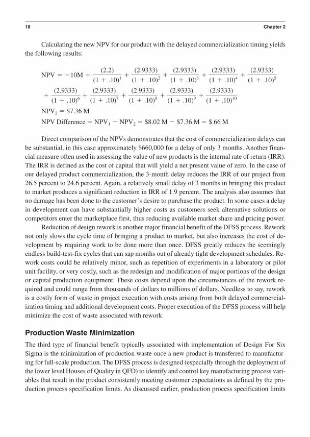
Calculating the new NPV for our product with the delayed commercialization timing yieldsthe following results:
NPV2 $7.36 M
NPV Difference NPV1 NPV2 $8.02 M $7.36 M $.66 M
Direct comparison of the NPVs demonstrates that the cost of commercialization delays canbe substantial, in this case approximately $660,000 for a delay of only 3 months. Another finan-cial measure often used in assessing the value of new products is the internal rate of return (IRR).The IRR is defined as the cost of capital that will yield a net present value of zero. In the case ofour delayed product commercialization, the 3-month delay reduces the IRR of our project from26.5 percent to 24.6 percent. Again, a relatively small delay of 3 months in bringing this productto market produces a significant reduction in IRR of 1.9 percent. The analysis also assumes thatno damage has been done to the customer’s desire to purchase the product. In some cases a delayin development can have substantially higher costs as customers seek alternative solutions orcompetitors enter the marketplace first, thus reducing available market share and pricing power.
Reduction of design rework is another major financial benefit of the DFSS process. Reworknot only slows the cycle time of bringing a product to market, but also increases the cost of de-velopment by requiring work to be done more than once. DFSS greatly reduces the seeminglyendless build-test-fix cycles that can sap months out of already tight development schedules. Re-work costs could be relatively minor, such as repetition of experiments in a laboratory or pilotunit facility, or very costly, such as the redesign and modification of major portions of the designor capital production equipment. These costs depend upon the circumstances of the rework re-quired and could range from thousands of dollars to millions of dollars. Needless to say, reworkis a costly form of waste in project execution with costs arising from both delayed commercial-ization timing and additional development costs. Proper execution of the DFSS process will helpminimize the cost of waste associated with rework.
Production Waste Minimization
The third type of financial benefit typically associated with implementation of Design For SixSigma is the minimization of production waste once a new product is transferred to manufactur-ing for full-scale production. The DFSS process is designed (especially through the deployment ofthe lower level Houses of Quality in QFD) to identify and control key manufacturing process vari-ables that result in the product consistently meeting customer expectations as defined by the pro-duction process specification limits. As discussed earlier, production process specification limits
(2.9333)
(1 .10)6 (2.9333)
(1 .10)7 (2.9333)
(1 .10)8 (2.9333)
(1 .10)9 (2.9333)
(1 .10)10
NPV 10M (2.2)
(1 .10)1 (2.9333)
(1 .10)2 (2.9333)
(1 .10)3 (2.9333)
(1 .10)4 (2.9333)
(1 .10)5
18 Chapter 2

originate from the customer. These limits must be established early in the product commercializa-tion process. DFSS strongly supports—in fact, it demands—the concurrent engineering of theproduct and its supporting network of production processes. Failure to establish production re-quirements early can result in delays in the commercialization schedule, costly rework, or transla-tion of a design into manufacturing that is not capable of meeting customer requirements.
Let’s suppose for a moment that a product and its associated manufacturing processes aredeveloped with only minimal input from the customer regarding product requirement limits. Asshown in Figure 2–3, we will assume that our best knowledge of the customer requirement is thatthe product should never have product strength of less than 65 percent or above 90 percent. Us-ing this information, the company’s R&D staff has designed a product with strength of 77.5 per-cent, halfway between what are believed to be the customer requirements. The process isdetermined to have a product strength standard deviation of 6.25 percent and so is positioned 2standard deviations from the customer specifications. Under the assumption of a normal distri-bution of product strength around the mean, we can estimate the total waste in this process as ap-proximately 4.6 percent. But what happens to this process in the long term once the process istransferred to manufacturing? Process variation is likely to be substantially higher over a periodof years than that observed in the short-term development process. Also, what happens if the cus-tomer decides to tighten the product specification limits prior to finally accepting the product?These questions represent a few of the risks associated with this product since customer specifi-cations were not specifically agreed to early in the development process and the process was notdeveloped with a reasonable view of long-term variation. We will now examine these concepts inmore detail with our case study example.
Measuring Financial Results from DFSS Programs and Projects 19
CustomerRequirement
CustomerRequirement
2.3% Waste(x > 90%)
2.3% Waste(x < 65%)
"GoodProduct"
Product Strength (%)
Average = 77.5%
60 65 70 75 80 85
2 Sigma2 Sigma
90 95
Figure 2–3 Product Strength Waste Analysis

The process for production of our new product is projected to produce a first quality yieldof 90 percent with an average strength of 94 psi based on short-term development data. Additionaldata from the R&D effort indicates that the product’s strength standard deviation in the short termis approximately 3.64 psi. Based on this information we can perform some important financialassessments for our new process. First, using the distance of the average strength from the spec-ification limits, we can calculate the sigma level of our new process. The sigma level will be de-fined as the number of standard deviations that the mean is located from the specification limits.In our case, the mean of 94 psi is located 6 psi from both the lower and upper specification lim-its. Given our estimation of the standard deviation at 3.64 psi we can see that we currently havea 1.65 sigma process. Using the standard normal curves, we can estimate the waste associatedwith this process at approximately 10 percent, 5 percent both below the lower specification andabove the upper specification limits (see Figure 2–4).
The cost associated with this short-term waste can be estimated by calculating the entitle-ment (or best possible result) of the process at 100 percent yield.
Entitlement After-Tax Profit
$3.6 M/year
We can also now calculate the entitlement net present value of our new product as:
10 M lbsyear $1.60lb product $1.00lb production
1 lbs productlb production (1 .4)
20 Chapter 2
CustomerRequirement
CustomerRequirement
5% Waste(x > 100)
5% Waste(x < 88)
"GoodProduct"
Product Strength (psi)
Average = 94
88 9086 92 94 96
1.65 Sigma1.65 Sigma
10098 102
Figure 2–4 Case Study Example–Initial Specifications
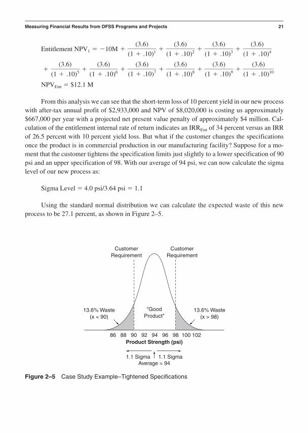
NPVEnt $12.1 M
From this analysis we can see that the short-term loss of 10 percent yield in our new processwith after-tax annual profit of $2,933,000 and NPV of $8,020,000 is costing us approximately$667,000 per year with a projected net present value penalty of approximately $4 million. Cal-culation of the entitlement internal rate of return indicates an IRREnt of 34 percent versus an IRRof 26.5 percent with 10 percent yield loss. But what if the customer changes the specificationsonce the product is in commercial production in our manufacturing facility? Suppose for a mo-ment that the customer tightens the specification limits just slightly to a lower specification of 90psi and an upper specification of 98. With our average of 94 psi, we can now calculate the sigmalevel of our new process as:
Sigma Level 4.0 psi/3.64 psi 1.1
Using the standard normal distribution we can calculate the expected waste of this newprocess to be 27.1 percent, as shown in Figure 2–5.
(3.6)
(1 .10)5 (3.6)
(1 .10)6 (3.6)
(1 .10)7 (3.6)
(1 .10)8 (3.6)
(1 .10)9 (3.6)
(1 .10)10
Entitlement NPV1 10M (3.6)
(1 .10)1 (3.6)
(1 .10)2 (3.6)
(1 .10)3 (3.6)
(1 .10)4
Measuring Financial Results from DFSS Programs and Projects 21
CustomerRequirement
CustomerRequirement
13.6% Waste(x > 98)
13.6% Waste(x < 90)
"GoodProduct"
Product Strength (psi)
Average = 94
88 9086 92 94 96
1.1 Sigma1.1 Sigma
10098 102
Figure 2–5 Case Study Example–Tightened Specifications

Also, we can calculate the after-tax profit for our product as:
$1.37 M/year
We can now calculate the net present value of our new product with the tightened processspecifications as:
NPV $1.58 M
The IRR of our new product now becomes 6.2 percent, which is below our cost of capital.The results of the customer tightening the specifications results in a new product that is no longerfinancially viable. In fact, we see that the value of the product over a 10-year life cycle is nownegative, indicating that the company will now lose money by investing in this product underthese conditions.
This analysis is the “best case” estimate of the penalty associated with production yield lossfor our new product. As mentioned earlier, long-term variation of a process in a manufacturingenvironment is generally substantially larger than the short-term variation defined in R&D. Whileeach process and product is different, conventional estimates indicate that a process can shift byas much as 1.5 standard deviations in either direction from the mean in the long term.
Let’s consider this scenario as the “worst case” financial penalty associated with translationof a process from R&D to manufacturing without testing to assess the long-term sigma of theprocess. As shown in Figure 2–6, if the process to manufacture our new product shifts down by1.5 sigma (5.46 psi), the new operating average for the process will be 88.5 psi.
This operating region is just 0.5 psi above our lower specification limit and will result in anestimated 44.5 percent waste in the long term. An estimate of the financial impact of such a shiftin the process can be calculated as follows:
After-Tax Profit
After-Tax Loss $1.21 M/year
(Notice that we take credit for a tax loss to help soothe the pain!)
10 M lbsyear $1.60lb product $1.00lb production
.555 lbs productlb production (1 .4)
(1.37)
(1 .10)6 (1.37)
(1 .10)7 (1.37)
(1 .10)8 (1.37)
(1 .10)9 (1.37)
(1 .10)10
NPV 10M (1.37)
(1 .10)1 (1.37)
(1 .10)2 (1.37)
(1 .10)3 (1.37)
(1 .10)4 (1.37)
(1 .10)5
10 M lbsyear $1.60lb product $1.00lb production
.729 lbs productlb production (1 .4)
22 Chapter 2
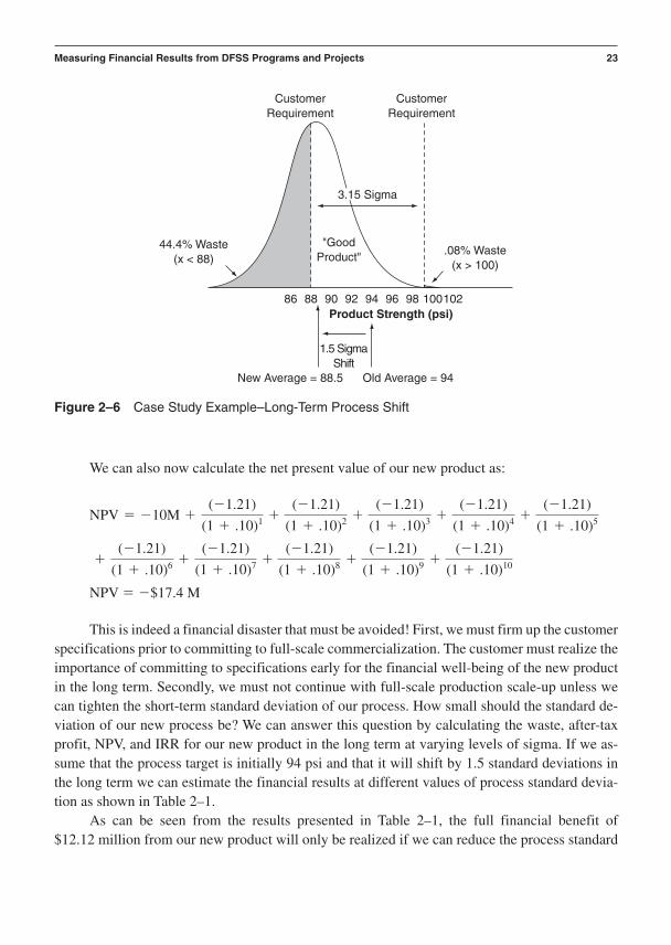
We can also now calculate the net present value of our new product as:
NPV $17.4 M
This is indeed a financial disaster that must be avoided! First, we must firm up the customerspecifications prior to committing to full-scale commercialization. The customer must realize theimportance of committing to specifications early for the financial well-being of the new productin the long term. Secondly, we must not continue with full-scale production scale-up unless wecan tighten the short-term standard deviation of our process. How small should the standard de-viation of our new process be? We can answer this question by calculating the waste, after-taxprofit, NPV, and IRR for our new product in the long term at varying levels of sigma. If we as-sume that the process target is initially 94 psi and that it will shift by 1.5 standard deviations inthe long term we can estimate the financial results at different values of process standard devia-tion as shown in Table 2–1.
As can be seen from the results presented in Table 2–1, the full financial benefit of $12.12 million from our new product will only be realized if we can reduce the process standard
(1.21)
(1 .10)6 (1.21)
(1 .10)7 (1.21)
(1 .10)8 (1.21)
(1 .10)9 (1.21)
(1 .10)10
NPV 10M (1.21)
(1 .10)1 (1.21)
(1 .10)2 (1.21)
(1 .10)3 (1.21)
(1 .10)4 (1.21)
(1 .10)5
Measuring Financial Results from DFSS Programs and Projects 23
CustomerRequirement
CustomerRequirement
.08% Waste(x > 100)
44.4% Waste(x < 88)
"GoodProduct"
Product Strength (psi)
New Average = 88.5 Old Average = 94
88 9086 92 94 96
1.5 SigmaShift
10098 102
3.15 Sigma
Figure 2–6 Case Study Example–Long-Term Process Shift
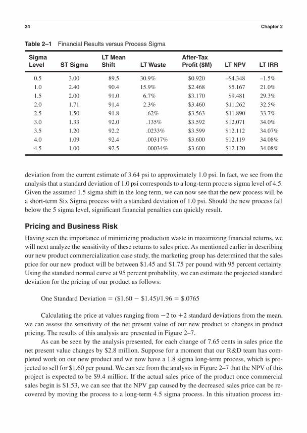
deviation from the current estimate of 3.64 psi to approximately 1.0 psi. In fact, we see from theanalysis that a standard deviation of 1.0 psi corresponds to a long-term process sigma level of 4.5.Given the assumed 1.5 sigma shift in the long term, we can now see that the new process will bea short-term Six Sigma process with a standard deviation of 1.0 psi. Should the new process fallbelow the 5 sigma level, significant financial penalties can quickly result.
Pricing and Business Risk
Having seen the importance of minimizing production waste in maximizing financial returns, wewill next analyze the sensitivity of these returns to sales price. As mentioned earlier in describingour new product commercialization case study, the marketing group has determined that the salesprice for our new product will be between $1.45 and $1.75 per pound with 95 percent certainty.Using the standard normal curve at 95 percent probability, we can estimate the projected standarddeviation for the pricing of our product as follows:
One Standard Deviation ($1.60 $1.45)/1.96 $.0765
Calculating the price at values ranging from 2 to 2 standard deviations from the mean,we can assess the sensitivity of the net present value of our new product to changes in productpricing. The results of this analysis are presented in Figure 2–7.
As can be seen by the analysis presented, for each change of 7.65 cents in sales price thenet present value changes by $2.8 million. Suppose for a moment that our R&D team has com-pleted work on our new product and we now have a 1.8 sigma long-term process, which is pro-jected to sell for $1.60 per pound. We can see from the analysis in Figure 2–7 that the NPV of thisproject is expected to be $9.4 million. If the actual sales price of the product once commercialsales begin is $1.53, we can see that the NPV gap caused by the decreased sales price can be re-covered by moving the process to a long-term 4.5 sigma process. In this situation process im-
24 Chapter 2
Table 2–1 Financial Results versus Process Sigma
Sigma LT Mean After-TaxLevel ST Sigma Shift LT Waste Profit ($M) LT NPV LT IRR
0.5 3.00 89.5 30.9% $0.920 –$4.348 –1.5%
1.0 2.40 90.4 15.9% $2.468 $5.167 21.0%
1.5 2.00 91.0 6.7% $3.170 $9.481 29.3%
2.0 1.71 91.4 2.3% $3.460 $11.262 32.5%
2.5 1.50 91.8 .62% $3.563 $11.890 33.7%
3.0 1.33 92.0 .135% $3.592 $12.071 34.0%
3.5 1.20 92.2 .0233% $3.599 $12.112 34.07%
4.0 1.09 92.4 .00317% $3.600 $12.119 34.08%
4.5 1.00 92.5 .00034% $3.600 $12.120 34.08%

provement can offset an initially overly optimistic estimate of the sales price and the project willstill bring the $9.4 million expected value. Unfortunately, process improvement cannot always beused as a means of recovering lost market value due to inaccurate estimates of selling price. Asshown in Figure 2–7, once a process reaches the 4.5 long-term sigma level, pricing impacts willdirectly influence product value with few options to mitigate these effects. For this reason, theconcept of Six Sigma Pricing is introduced. Simply put, the risk of pricing changes should be es-timated through direct dialogue with the customer. After these conversations, an assessment ofthe pricing sigma level should be made. Once the target price and sigma level are established, aproject risk analysis can be run to assess the risk of pricing changes on the potential NPV of theproject. As shown in Figures 2–8 and 2–9, production cost and sales volume also have major im-pact on the value of newly commercialized products.
In order to assess the total business risk for a newly commercialized product, estimates oftarget value and standard deviation for yield, sales price, production cost, and sales volume shouldbe established and analyzed using Monte Carlo simulation techniques. The result of such ananalysis for our case study product is shown in Figure 2–10 using the following assumptions.
Target Value Standard Deviation
Sales Price $1.60 $0.0765Sales Volume 10 M lbs/yr 1 M lbs/yr
(Note: Capped at maximum of 10M lbs/yr by capacity constraints)
Production Cost $1.00 $0.051Yield 90% 2.6%
Measuring Financial Results from DFSS Programs and Projects 25
Process Sigma Level
$18,000,000
0.5 1.5 2 2.5 3 3.5 4 4.5 5 5.5 6
Increasing Price
$13,000,000
$8,000,000
$3,000,000
($2,000,000)
($7,000,000)
($12,000,000)
$1.45$1.52$1.60$1.67$1.75
10
Figure 2–7 NPV Price Sensitivity
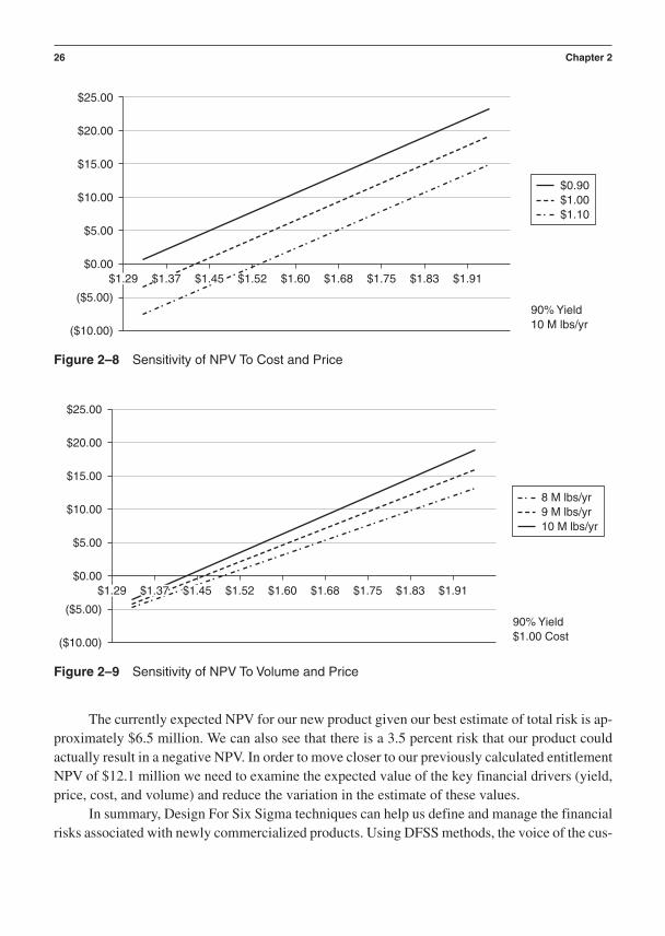
The currently expected NPV for our new product given our best estimate of total risk is ap-proximately $6.5 million. We can also see that there is a 3.5 percent risk that our product couldactually result in a negative NPV. In order to move closer to our previously calculated entitlementNPV of $12.1 million we need to examine the expected value of the key financial drivers (yield,price, cost, and volume) and reduce the variation in the estimate of these values.
In summary, Design For Six Sigma techniques can help us define and manage the financialrisks associated with newly commercialized products. Using DFSS methods, the voice of the cus-
26 Chapter 2
$25.00
$1.52 $1.60 $1.68 $1.75 $1.83 $1.91
90% Yield$1.00 Cost
$20.00
$15.00
$10.00
$0.00
$5.00
($5.00)
($10.00)
8 M lbs/yr9 M lbs/yr10 M lbs/yr
$1.29 $1.37 $1.45
Figure 2–9 Sensitivity of NPV To Volume and Price
$25.00
$1.52 $1.60 $1.68 $1.75 $1.83 $1.91
90% Yield10 M lbs/yr
$20.00
$15.00
$10.00
$0.00
$5.00
($5.00)
($10.00)
$0.90$1.00$1.10
$1.29 $1.37 $1.45
Figure 2–8 Sensitivity of NPV To Cost and Price
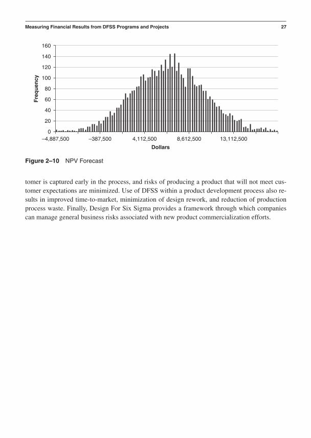
tomer is captured early in the process, and risks of producing a product that will not meet cus-tomer expectations are minimized. Use of DFSS within a product development process also re-sults in improved time-to-market, minimization of design rework, and reduction of productionprocess waste. Finally, Design For Six Sigma provides a framework through which companiescan manage general business risks associated with new product commercialization efforts.
Measuring Financial Results from DFSS Programs and Projects 27
–4,887,500 –387,500 4,112,500 8,612,500 13,112,500
Dollars
Fre
qu
ency
160
140
120
100
80
60
0
40
20
Figure 2–10 NPV Forecast

This page intentionally left blank

C H A P T E R 3
Managing Value with Design For Six Sigma
Written by Scott A. McGregor, Marketing Consultant for Design For Six Sigma andVice President of Marketing at Uniworld Consulting, Inc.
Value is a driving function of design. What an interesting concept. It seems that this would bea simple rule in the design of new features or products. In fact, it is one of the hardest rules
for a company to follow. It should be a heuristic of every organization that has product and ser-vice designs at the heart of its long-term business. Why don’t companies embrace this as an in-ternal rule? It is not because extracting value from the voice of the customer is hard or too vague.In fact, many different processes make the process efficient and productive. Good marketing per-sonnel and design personnel can extract that voice and turn it into an excellent detailed designthat speaks to customer needs with weight and priority. Companies fail to extract value as a driv-ing function for a number of reasons: time, pet projects, politics/internal culture, poor process,and budget. There are others, I’m sure, but those are the ones I see most frequently.
Extracting Value
Extracting value is not an engineering science. Extracting value is not solely a marketing science.Many marketing departments don’t even do the kind of value analysis that would position theirproducts in the market. The corporate marketing machines that do are often the winners in the mar-ket game. They dominate the market with products that win share and influence their position inthe market. At the very least, using an analytic value model will help an organization position it-self in the marketplace with metrics that go beyond share and volumes. Indeed, share is the mea-sure of market acceptance but often that measure comes late or not at all in the data we collect.
Real winners extract value measures as a means of discovering market acceptance, findgaps in the market mind-set for the offering, and lead a company to making the right decisions inmarket performance and product changes. Sometimes, measuring market perceptions of valueleads a company to engage in innovative design.
29

In recent years I have seen a number of products enter into the market where it is apparentthat value is being managed as a function of marketing and R&D departments. PRILOSEC®/LOSEC® (omeprazole), a pharmaceutical for the treatment of a number of gastrointestinal ailments, is a product with which I had extensive experience in managing customer value.Through diligent management of the value proposition, this medication went from last place inthe anti-ulcer/GERD (gastroesophageal reflux disease) market to first place. Originally marketedin the United States by Merck & Co., Inc., and Astra Merck, Inc. (currently it is owned by As-traZeneca L.P.), it is the premier product in its class and is currently the world’s most prescribedpharmaceutical product. Value became a driver for the product from the prelaunch phase of newproduct indications to postlaunch market activities. On another level, value became a driver indetermining business case decisions for budget and resource allocation at a portfolio level. I amconvinced that understanding and managing value internally and externally is the key driver fora marketing department in the success of a product.
PRILOSEC® is an example of a product being managed at all levels. Some would arguethat value management as a function of design is a waste of time, especially those who work innon-consumer products and services. Too often I have heard business managers say, “Value man-agement would be great for consumer products like toothpaste or soap, but we sell our productsto other manufacturers or to other corporate clients. Why should we do this kind of research fora business-to-business buyer?” When I first started hearing this argument, I thought it had somevalidity. Honestly, why would you commit to research and data measures on the value of prod-ucts that are often specified and constrained by other businesses? It seems it would be a wastedeffort. A beer can manufacturer will tell you, “A beer can is a beer can is a beer can!” Is there re-ally much room to extract value and design improvements to a beer can? How many changes havethere been since the pop-top opener? Some would argue that the beer and soft drink can marketis a great example of only designing to customer specifications and making sure we have enoughmargin to make a profit when it is manufactured. Having recently worked with a major manu-facturer of this kind of product, I became aware that this mentality has led the company to a farworse position than focusing on margins. It has let the customer (soft drink and beer bottlers) de-termine what their profit margins will be. They search for margin in the “down-gauging” of canthickness, thus saving them money in aluminum costs. All other improvements are in incremen-tal improvements in preventing error. They have lost control not only of the value proposition butof the internal value proposition for the product itself. The only management left to them is themanagement of margins. The profit is no longer latent in the market; now it is just extracted frominternal capability and margins. If there were a word for a product that would describe it as some-thing less than a commodity, I would use it here. However, the picture is not all bleak for the canindustry, and I will return to it later to illustrate that there is hope for the old beer can after all.
Cummins, Inc., is a premier example of a company that strives to prevent the overall com-moditization of its core product lines. You find marketing intimately tied to design and manufac-turing throughout the organization. Cummins has customers from end consumers to corporatebuyers that it strives to satisfy by meeting specifications and to delight by exceeding expectationswith novel and robust designs. One example of this is through the continued management of cus-
30 Chapter 3
tomer perceptions of value in light duty truck engines (Dodge Ram 2500-Cummins diesel trucks).Daimler-Chrysler could, with relative ease, start migrating trucks to its standard Mercedes dieselsthat have satisfied global markets for years. By all appearances, it would be a wise move to an in-ternal capability that would result in savings to the bottom line, but Cummins has created a strongerand more valued perception, in my opinion, for its product in the market and with the manufacturer.The company not only manages value with the customer base but constantly looks for new marketpositions against which to build its portfolio. It is an example of great product management at alllevels for an industrial-based product. I can only praise Cummins further for its skillful handling ofregulatory issues while managing a portfolio of value-added industrial products. Cummins is mygreatest argument against disregarding value as an industrial manufacturer for business buyers.
From PRILOSEC® to beer cans to engines, from consumer to industrial buyers, from in-novative to commodity products, value is the function that determines market acceptance and suc-cess. It must therefore be the key driver in designing products and services and their subsequentimprovements.
Value as a Formula
Yes, it’s possible to realize the concept of value as a formula. How could we express perceivedvalue to the customer as a measurable calculation? To begin, let’s start with the simplest expres-sion of value.
Value (Quality components) Price
Value is the sum of the worth of the quality relative to the price. As a rule customers alwaysbuy on value and quality. Buyers may say they buy on price, but that is a failure on the seller’sand the buyer’s part to realize the true value proposition before them. Well, now we have a for-mula for value, so how do we define quality into the formula?
Quality (Product dimensions) (Service dimensions)
In short, quality is the sum of the features and benefits of the product and of the service thatcomes with the product. Each product can be broken down into its fundamental dimensions ofquality. Garvin (1987) best outlined dimensions of quality from the customer’s point of view:
1. Performance—primary operating characteristic of a product or service2. Features—secondary characteristics of a product or service3. Reliability—frequency with which a product or service fails4. Conformance or consistency—match with specifications or standards5. Durability—product life6. Serviceability—speed, courtesy, and competence of repair7. Aesthetics—fits and finishes8. Perceived quality—reputation (pp. 49–50)
Managing Value with Design For Six Sigma 31
Dimensions of quality may change for each product line, but these eight clearly and con-cisely capture the vision of dimensional quality. Pharmaceutical companies traditionally havegone another route, using safety, tolerability, efficacy, ease of use, and price as their key five di-mensions. They have been forced to rethink that with the advent of stronger buying positions ofcustomers like health maintenance organizations and group purchasing organizations, but thevalue proposition still focuses on dimensions of quality that are important to the buyer.
Service also has dimensions of quality. Consider these 10 dimensions of service listed byBerry et al. (1985):
1. Reliability—consistency of performance2. Responsiveness—timeliness of service3. Competence—possession of required skills and knowledge4. Access—approachability and ease of contact5. Courtesy—politeness, respect, consideration, and friendliness6. Communication—listening to customers and keeping them informed in a language
they can understand7. Credibility—trustworthiness, believability, honesty8. Security—freedom from danger, risk, or doubt9. Understanding of the customer—efforts to understand the customer’s needs
10. Tangibles—physical evidence of service (pp. 45–46)
Some companies use specific dimensions of quality or service to find their place in the mar-ket. For instance, Steinway has domineered the market for high-end pianos with the elegant de-sign and substantive quality of its grand pianos. People buy them because they want the samesound and look of a piano that would be in front of a symphony. Yamaha, on the other hand, looksto provide pianos to people who want a good-sounding, affordable piano in their home. Yamahaserves more of the common buyer market. Each provides quality that more than satisfies its cus-tomer base, but each is specific to that base at the same time.
Being first in all dimensions of quality is seldom necessary. Quality Function Deploymenthelps one see this. A well-managed, well-designed product can find its place in the market by fo-cusing on some of the key dimensions and executing to them without fail. Dell™ Computers andGateway® both exemplify this. For Dell™ the dimensions have been building machines with aneye to business requirements and the service level that is required by those businesses (perfor-mance, reliability, serviceability, responsiveness, and competency of repair). Gateway® deliversa quality product for the average consumer who wants to be involved in the design of their endproduct. Gateway® delivers on similar dimensions but with different measurable components foreach of those dimensions (performance, features, reliability, responsiveness, communication, andcourtesy). Each company actively manages these dimensions and ensures the overall quality ofthe product for the consumers they understand best. The dimensions can be subtle but arenonetheless effective.
32 Chapter 3

Competing on quality can often come with some tricky mistakes. Let’s take a moment andaddress a few. First is the fundamental mistake of directly attacking the industry’s quality leader.Why would that be a mistake? Well, there are a number of reasons. The quality leader may not bethe market leader. We can’t lose sight of the fact that we are in market competition, not qualitycompetition. We are merely using quality as a weapon to change the market perceptions. The eas-iest way to change market perception is by changing price, but that is a gross error that turns amarket of quality leaders into a commodity market overnight. Another key mistake is competingon quality dimensions that are unimportant to consumers. I laughed heartily at Apple when it tooka normal Macintosh computer and put it in a colored, stylized shell. As a business user of ma-chines I found its offering inadequate to my needs and the needs of the corporation. My error wasnot seeing the quality dimensions for the market they were pursuing. For college-age studentswith computing needs, a need for style, and a need for space savings, the iMac spoke volumes tothem. That effort alone brought Apple back once again from the edges of extinction.
Other obvious mistakes include assuming reliability and conformance are less importantthan customers think they are; an ancillary error is relying on the wrong quality metric. In the1970s GM relied on its dedication to single platform quality with moderate modification to styleto sell the same general car through multiple brands. GM focused on these platforms while vir-tually ignoring dimensions such as reliability, performance, consistency, and durability. Buyerstaught Detroit a lesson by buying on the quality dimensions described in Japanese automotive of-ferings. Certainly, the cars were smaller and offered less features, but they did offer consistentquality in engine reliability, fit and finish, interiors that did not have loose screws under the car-pet, and excellent service records. Fulfilling the designs of the value formula, Japanese auto mak-ers offered their products at a price that the consumer saw as superior value.
Measuring Value in the Marketplace
We have established value, quality, price, and dimensions of quality in the value formula. Wheredo we go next? We have to operate against competitors at a level that we can quantify and at whichwe can operate. In fact, what we seek to do is to understand the value proposition in the market-place to a quantifiable level that allows us to design or innovate around it. That is the goal and theplace where the statistical metrics of Six Sigma become quite important. Next, we will treat theseconcepts abstractly and begin to move toward some measurable view of them. We will abstracteach of them to see them as relative components of the great value formula. We will now use prod-uct and service value and quality measures to guide our business and R&D decisions.
Two new questions now emerge. What do we measure and how do we use it meaningfully?I won’t attempt to answer how we get the value data—there are a number of means of obtainingmarket data, not the least of which is customer surveys. I will discuss extracting voice for a de-sign project, but time and space constraints do not allow a discussion of extracting quantifiablemarket perception data. What do we measure? We measure comparative performance against our competitors. We begin with a simple comparison of three or four simple data points. Believeit or not, a few data points tell an incredible story. A wise product manager for the world’s largest
Managing Value with Design For Six Sigma 33
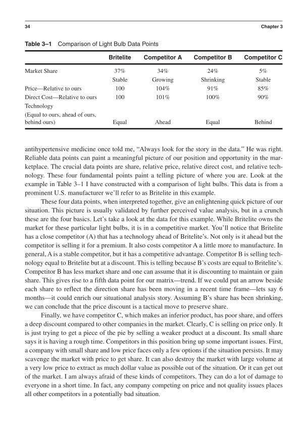
antihypertensive medicine once told me, “Always look for the story in the data.” He was right.Reliable data points can paint a meaningful picture of our position and opportunity in the mar-ketplace. The crucial data points are share, relative price, relative direct cost, and relative tech-nology. These four fundamental points paint a telling picture of where you are. Look at theexample in Table 3–1 I have constructed with a comparison of light bulbs. This data is from aprominent U.S. manufacturer we’ll refer to as Britelite in this example.
These four data points, when interpreted together, give an enlightening quick picture of oursituation. This picture is usually validated by further perceived value analysis, but in a crunchthese are the four basics. Let’s take a look at the data for this example. While Britelite owns themarket for these particular light bulbs, it is in a competitive market. You’ll notice that Britelitehas a close competitor (A) that has a technology ahead of Britelite’s. Not only is it ahead but thecompetitor is selling it for a premium. It also costs competitor A a little more to manufacture. Ingeneral, A is a stable competitor, but it has a competitive advantage. Competitor B is selling tech-nology equal to Britelite but at a discount. This is telling because B’s costs are equal to Britelite’s.Competitor B has less market share and one can assume that it is discounting to maintain or gainshare. This gives rise to a fifth data point for our matrix—trend. If we could put an arrow besideeach share to reflect the direction share has been moving in a recent time frame—lets say 6months—it could enrich our situational analysis story. Assuming B’s share has been shrinking,we can conclude that the price discount is a tactical move to preserve share.
Finally, we have competitor C, which makes an inferior product, has poor share, and offersa deep discount compared to other companies in the market. Clearly, C is selling on price only. Itis just trying to get a piece of the pie by selling a weaker product at a discount. Its small sharesays it is having a rough time. Competitors in this position bring up some important issues. First,a company with small share and low price faces only a few options if the situation persists. It mayscavenge the market with price to get share. It can also destroy the market with large volume ata very low price to extract as much dollar value as possible out of the situation. Or it can get outof the market. I am always afraid of these kinds of competitors. They can do a lot of damage toeveryone in a short time. In fact, any company competing on price and not quality issues placesall other competitors in a potentially bad situation.
34 Chapter 3
Table 3–1 Comparison of Light Bulb Data Points
Britelite Competitor A Competitor B Competitor C
Market Share 37% 34% 24% 5%
Stable Growing Shrinking Stable
Price—Relative to ours 100 104% 91% 85%
Direct Cost—Relative to ours 100 101% 100% 90%
Technology
(Equal to ours, ahead of ours, behind ours) Equal Ahead Equal Behind

We need to understand, with the data we have, the kind of market in which we are compet-ing. Are we competing on price or quality? The data points in Table 3–1 should reveal most of theanswer to us. Based on the data we have two quality competitors (Britelite and A), and we havetwo price competitors (B and C). Generally, competitors that offer a price discount of at least 10percent or more are price competitors. I consider B a price competitor because of price, shrink-ing share, and equal technology. In general, it is in a position of only playing with price. Briteliteis sustaining price on existing technology while A is selling at a premium for premium technol-ogy. We could interpret this abstracted data, once we have put it in the form of a usable ratio, tooutline our market. To do this we sum the shares of those competing on quality, and then we sumthe shares of those competing on price. These two sums will give us the ratio we seek.
Price ratio component: B C 24% 5% 29%
Quality ratio component: Britelite A 37% 34% 71%
Quality-to-Price Ratio 71:29
This may seem simple, but it is quite revealing about a market situation. In this case the datasays that the market is in a pretty good position. Most of the market is responding to quality com-petition issues and is satisfied dominantly by quality competitors. Yet, we can’t ignore that almosta full third of the market is responding to price. Markets become unstable when they compete onprice. Buyers love unstable markets because they win on the price game. As designers, manufac-turers, and marketers we should strive to maintain stable, quality, competition-based markets.When the dominant portion of the market migrates to price, the market is operating with no per-ceived difference in the products. You are playing in a commodity market.
The simple fact about commodity behavior markets is that they never deal with premiummargins in their price. Commodity market manufacturers only design to maintain or incremen-tally improve margin: A light bulb is a light bulb is a light bulb. Commodity markets never sta-bilize unless there is a leap in the quality of the product and design—and the consumer recognizesthat leap. This explains why we see new light bulb designs like “soft white,” “natural light,” andeven “true blue” lights. New designs and new and better quality offerings help to stabilize themarket by sustaining price and margin. Companies that innovate and improve the quality of theirproduct in a stable market and then sell that quality at a discount without a strategy need to firetheir marketing managers for not seeing the internal quality of their own designs.
The Japanese for years have discounted novel and improved designs for only one reason—share. One aspect of Japanese marketing philosophy is “win the war, then dominate the con-quered.” Crude and highly accurate in its description, it captures a divide-and-conquer mentality.Japanese companies only discount price to gain as much share as possible, destabilize the mar-ket, and drive away competition. Then, when the market is “conquered,” they slowly begin toraise the price and bring the margins in to a more profitable situation. Fortunately, the world doesnot always subscribe to this philosophy.
We want to strive for quality-based competition in the marketplace. This engages and enti-tles our design teams to the right balance of effort. In this context DFSS has the most to offer.
Managing Value with Design For Six Sigma 35
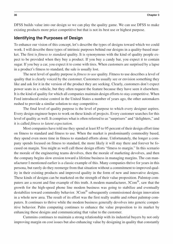
DFSS builds value into our design so we can play the quality game. We can use DFSS to makeexisting products more price competitive but that is not its best use or highest purpose.
Identifying the Purposes of Design
To enhance our vision of this concept, let’s describe the types of designs toward which we couldwork. I will describe three types of intrinsic purposes behind our designs in a quality-based mar-ket. The first is fitness to standard quality. It is synonymous with the kind of quality people ex-pect to be provided when they buy a product. If you buy a candy bar, you expect it to containsugar. If you buy a car, you expect it to come with tires. When customers are surprised by a lapsein a product’s fitness to standard, the sale is usually lost.
The next level of quality purpose is fitness to use quality. Fitness to use describes a level ofquality that is clearly voiced by the customer. Customers usually see or envision something theylike and ask for it in the version of the product they are seeking. Clearly, customers don’t expectpower seats in a vehicle, but they often request the feature because they have seen it elsewhere.It is the kind of quality for which all companies maintain design efforts to stay competitive. WhenFord introduced cruise control in the United States a number of years ago, the other automakersrushed to provide a similar solution to stay competitive.
The final level of quality purpose is the level of purpose to which every designer aspires.Every design engineer hopes to work on these kinds of projects. Every customer searches for thislevel of quality as well. It comprises what is often referred to as “surprisers” and “delighters,” andit is called fitness to latent expectation.
Most companies have told me they spend at least 85 to 95 percent of their design effort timeon fitness to standard and fitness to use. When the market is predominantly commodity based,they spend even more time in fitness to standard efforts alone. Unfortunately, the longer a com-pany spends focused on fitness to standard, the more likely it will stay there and forever be fo-cused on margin. You might as well call those design efforts “fitness to margin.” In this scenariothe morale of the engineering teams devolves, then the morale of marketing devolves, and thenthe company begins slow erosion toward a lifetime business in managing margins. The can man-ufacturer I mentioned earlier is a classic example of this. Many companies thrive for years in thispersona, but rarely do they reemerge from that situation without a commitment to improved qual-ity in their existing products and improved quality in the form of new and innovative designs.These kinds of designs can be marketed on the strength of their value proposition. Palmtop com-puters are a recent and fine example of this truth. A modem manufacturer, 3Com®, saw that thegrowth for the high-speed phone line modem business was going to stabilize and eventuallydestabilize toward commodity behavior. 3Com® subsequently commissioned design innovationin a whole new area. The result of its effort was the first really usable and robust palmtop com-puters. It continues to thrive while the modem business generally devolves into generic compet-itive behavior. Palm computing continues to enhance the value proposition to its market byenhancing these designs and communicating that value to the customer.
Cummins continues to maintain a strong relationship with its industrial buyers by not onlyimproving margin on cost issues but also enhancing value by designing in quality that constantly
36 Chapter 3

delights customers: more power, greater fuel economy, better emissions, and reduced repairs.Cummins manages its design efforts with a highly trained design team, strong R&D philosophyand testing facilities, and a constant eye to the inherent market situation.
Frank Purdue of Purdue Chicken fame created value in the market for his chicken manyyears ago by improving the quality of the chicken, meat-on-the-bone, color of the meat, and thecompany’s public image. The result was a stronger perception of quality in the customer’s mind.Purdue sold more chicken at a higher price. I always emphasize that point: More chicken at ahigher price! What is the moral of the chicken story? If Frank can do that with chicken, what canyou do with your product?
Design Based on the Voice of the Customer
The place to start is to begin a discussion on extracting the voice of the customer (VOC) and turning those needs into meaningful requirements for design. This has to be done in such a waythat we always keep the customer at the heart of the effort. If we were to ask the different de-partments of a company what was important to a new product design project, we would find theanswers are quite varied. R&D is concerned with functionality and performance; finance focuseson cost; sales is concerned with features, service, and support; and manufacturing might be overlyconcerned with the assembly of a new product. If a design team is divided on the critical issuesfor a product, how can it resolve these different opinions? Well, let’s first consider the source of these opinions. R&D staff consider functionality important because that is what they do—design functionality. Finance, by the same token, is concerned with the cost of scrap, rework, and warranty claims, and sales might be making more commission on service contracts than onthe product itself. This is just an example, but it reflects that although we like to think the com-pany is unified in design, each department is compelled by different drivers. We need a way tomanage and balance all the critical parameters that are at play. With that said, where is the cus-tomer voice?
If we heed the voice of the customer, it will serve the requirements of all the internal voicesif it is properly mined from the customer base. Those leading a design project, whether they re-alize or not, always want the best result for their project, and they want a list of design issues (re-quirements) to be weighted and prioritized. Why weighted and prioritized? Because in thebusiness of fulfilling these requirements, budget and resource constraints usually arise that forcetrade-offs and hard decisions. Constraints like time, budget, human resources, manufacturing ca-pability, and competitive pressures force the design team to focus on what is critical. We can’t doeverything, so having the design requirements placed into a weighted and prioritized list is im-perative. Customer voice should serve as a primary source of the design requirements. The vari-ous other organizations and constituencies that contribute to the design team serve as supportiveincoming voices. True, we can’t ignore the internal voice of the business, but the bigger issue iswhether we pay attention to the external customer voice in the first place.
On a tangential note, the enthusiasm for fulfilling internal departmental priorities still needs to be managed from a value and development standpoint. We can’t ignore that these inter-nal departments have relevant input and responsibility to the product whether it is in the design
Managing Value with Design For Six Sigma 37

phase or in the postlaunch phase of its life cycle. A simple, effective tool for managing these responsibilities is the What/Who Matrix. This elegant tool helps take the value criteria set forthin the value/quality analysis and internalize it by departmental responsibility. We could takeGarvin’s eight dimensions and use them as the criteria or use whatever criteria we specify. Seethe matrix in Figure 3–1 for a film manufacturer as an example.
You will note that the left-hand column of Figure 3–1 lists the quality attributes while thetop row contains the names of the internal departments responsible for the quality attribute. An Xrepresents some accountability to the issue. A box around an X shows lead responsibility for thequality attribute.
Putting Concept Engineering to Work
Once we have set value, quality, and customer voice as guideposts for our efforts, the key issueis selecting a methodology for championing these issues while pulling out the most achievable,market-attentive, and innovative designs we can. In fact, we need to ensure that we have a processthat is documented and reflects a thorough and considered approach to the market, the customer,and the goals of the company concurrently.
38 Chapter 3
Quality Attribute
Image Quality
Blemishes
Fading
Turnaround Time
Service
Availability
Reprints
Development Components Release Assembly Sales Service
A who/what matrix links key qualityattributes to the business processesthat drive performance on those attributesand shows who is the process owner.
$
Figure 3–1 Sample What/Who Matrix

The overarching process that controls this is the product development process. Within theproduct development process resides one of the greatest best practices I have ever seen in usingthe voice of the customer—concept engineering. Over the last year alone I have probably seenseveral “revolutionary” methodologies that “release innovation” and bring “excitement” to newdesigns. I hate these kinds of adjectives for design methodologies. People purporting this kind ofexcitement in training others in their “methods” are often worried about their method working inthe first place. They overhype it because they really have not seen their own process through tocompletion on anything significant. Many methodologies are empty to me for one reason only:They are centrally focused on market testing after the design is completed as evidence of consid-ering the customer. They use build-test-fix methods. In other words, presenting a model or con-cept to customers for input after initial design is the key means of extracting voice. That is notextracting voice—that is trying to get customers to buy in to an internally focused design.
I was recently presented a case study on satellite/cellular hybrid phones. As you probablyare aware, the largest company in this business went bankrupt in 1999. Its internal voice told thecompany that many business people would be thrilled to have a phone that would work anywhere.There was almost no consideration of the customer and the market in this costly project. The oldadage of a 1930s car manufacturing executive still holds true, “It is not that we build such badcars: it’s just that they are such lousy customers.” The company designed this system of satellites,phones, and beepers with the target of selling them to business users. Along the way it failed todiscover that cellular business users don’t care how their call is connected, just that it is connected.In most developed countries, cellular towers went up much easier and faster than a satellite. Thesatellite/cellular company was much more interested in putting satellites up over the United Statesthan let’s say Siberia. In fact, Siberia was where the market was—a place where phone lines don’texist and without tower-based cellular systems.
Oil fields, ocean-based oil rigs and ships, and remote locations really needed these phones.You could ask for and get $7.00 a minute for satellite calls there, but not in New York where youhad to be outside in direct sight of a satellite. Tower-based cellular airtime is less than 50 cents aminute on an expensive day. In its last days, this manufacturer starting facing comments such as,“Analysts wonder if, in its rush to get satellites in orbit, [Company X] failed to flesh out its mar-keting strategy.” In the end, the most telling comment is the one all design-based companies havefaced in their failures: “What they didn’t do was to focus on, analyze and pay attention to the mar-ket they could serve. [Company X] had a series of major (technical) accomplishments along withsome extraordinary (voice of the customer) failures” (Clarissa Bryce Christensen, space industryconsultant). Market and customer voice would have made all the difference.
This story exemplifies the need for concept engineering. What I like about this methodol-ogy is its diligence in assuring customer voice is respected at all phases and gates of the productdevelopment process. It emerged out of MIT and a consortium of Polaroid, Bose, and others inthe 1980s. Since then it has seen an evolution of changes and improvements (by the virtue of itsmission, it is ever self-improving) that have made it a robust and sound method for uncoveringdesign requirements by placing customer requirements at the heart of the effort. It incorporatesmethods that are discussed in this book, which I will only outline here.
Managing Value with Design For Six Sigma 39
Concept Engineering Methods
Preparing for customer interviews
Customer interviewing in teams
Image KJ
Requirements KJ
Requirements translation
Product-level quality function deployment (QFD)
Concept ideation
Pugh Concept Selection
Lower-level quality function deployment
Many companies use one or two of these methods, most frequently QFD and Pugh ConceptSelection. Concept engineering (CE) puts these tools into larger context in a process that is thor-ough and well thought out. In fact, it is so diligent many engineers have told me they feel it isoverkill because they already knew “most” of the information that comes from the process. Thepoint and value of CE is that it disregards nothing and assures a complete set of critical require-ments for the design project. It also assures that you use the rational, market-perceived qualitydata you’ve worked on to assess value in the marketplace. I don’t know exactly why, but designengineers, manufacturing engineers, and other R&D personnel generally resist talking to the cus-tomer. I theorize two general reasons. First is a general fear and dislike of consuming valuable“design” time in extracting this information from customers. Second is a perceived environmentin every company where someone, a leader or a dominant design team person, says, “I know whatthe customer wants. We don’t need to do all this customer-focused work because we’ve done thisso long we know what they need. Besides, I am in charge here because I already know the cus-tomer needs, and I have some new ideas that I know the customer will love.” You may find your-self nodding in agreement that this exists to some level in your company.
You can’t ignore the quality component of being diligent with your customers. This is whyCE starts with customer interviews that are not rigidly structured and tied to Likert scales. Instead,they are focused on extracting information, images of use, and emotion from the customer. Aftera complete set of customer interviews, this data can be compiled into a meaningful set of weightedcustomer issues using KJ analysis. KJ stands for Jiro Kawakita, a Japanese anthropologist whosaid that if mathematicians can treat variables data in a grouped and prioritized manner then weshould be able to do the same with attributes/language data. Some people look at the results of aKJ diagram and see an affinity diagram. In fact, it is much more than that. It is the process thatgets to the “output” that is unique and different. Space doesn’t allow a full description of theprocess here, but I will say that it is incredibly logical and intuitive, and there is never disagree-ment by the time you reach the end of a KJ. Chapter 14 will illustrate what I am talking abouthere. This structuring of VOC data is important to a team in a design project because the KJ linksthe critical customer priorities to team understanding and consensus. The beauty is that 3 months
40 Chapter 3

into the design phase if someone wants to change direction on the project, the KJ serves as thecustomer-focused guidepost that keeps the team on track.
The Image and Requirements KJ bring together images and voices of user needs that wereoffered by customers and documented by designers in their interviews. The images (context ofuse and need) are brought into the Requirements KJ as a supporting element that validates customer need. When the KJs are done, the design team then translates the customer “voiced re-quirements,” which now have weight and priority, into language and descriptions that are under-standable to the product development organization. We generally use translation worksheets thatintegrate the imaged use and need context with the stated need context. The final translation ofcritical (ranked by weight and priority) customer needs into technical requirements is done usingQuality Function Deployment.
I can’t emphasize enough the importance of keeping CE self-documenting and the data setcomplete. If a CE project is documented well, no one can approach the team and gut the effortin lieu of their “expert” opinion of what is needed without a customer-championed fight. Enoughof my plea to keep good documentation for a complete CE project. Data, real customer data, isthe key to getting it right and keeping the team focused on what is real as opposed to what isopinion.
Once customer requirements have been translated, we then can start the process of focus-ing on the critical requirements, aligning them with the value analysis that we have done earlier,and looking for comparisons against competitive quality winners in the class. To achieve this goalwe will continue our use of Quality Function Deployment (QFD). QFD is a thorough means ofaligning the measures mentioned previously and translating the requirements from “general andweighted” to “detailed and weighted” with an added analysis of the internal capability to deliver.
A good QFD application should give us a view of what we are currently capable of deliv-ering and what we need to do to fill the detailed technical requirements. See Figure 3–2 for agraphic depiction of this application.
QFD effectively brings together market data, customer input data, and internal capabilitydata to develop a workable set of detailed, critical requirements. We often limit the focus of QFDto those requirements that are new, unique, and difficult. With a workable set of detailed, criticalrequirements, we can use concept ideation as the creative means of coming up with many differ-ent kinds of designs to fulfill the requirements—both those that are routine and those that are new,unique, and difficult.
The goal of Concept Ideation is to create a rich set of creative design bases, compare themagainst the detailed requirements list, and ultimately hybridize the best elements that lie withinthem using the Pugh Process of concept selection. The graph in Figure 3–3 illustrates what weare trying to achieve in creating many useful concepts and then selecting down to the most feasi-ble one or two to take back out to our customers to see if we are on the right track.
Simply put, concept ideation entails sitting down with the requirements and creatively com-ing up with many ways of fulfilling each requirement. When you have several options for eachrequirement, you start putting them together into a concept. You do this until you have severalconcepts to benchmark against an existing best-in-class product or a previous design. With Pugh
Managing Value with Design For Six Sigma 41

Process concept selection, you whittle down (hybridize) all these innovative design concepts intothe best, and most achievable, choice. The work plan for doing this is shown with the Pugh ma-trix in Figure 3–4. You rate the ability of each concept to fulfill the detailed, critical requirementsthat came from your QFD exercise along with other important business and external require-ments. Those that fulfill those prioritized requirements best can be selected, or you could hy-bridize the concepts into a best option.
From the Pugh Process we can opt for a second round of QFD to assure that the detailed,critical customer requirements that were converted to design requirements are thoroughly trans-lated into specific design requirements embedded in the selected, superior design. The focus is onworkable requirements that the design team can understand.
42 Chapter 3
4 EngineeringCharacteristics
6 Roof Showing RelationshipsAmong Engineering Characteristics
CustomerPerceptions ofPerformance:Us C1 C2
Laboratory MeasuresOur ProductCompetitor 1Competitor 2
8 Data for Making DesignDecisions and Trade-offs
2 ImportanceRatings
1 ProductAttributes
3 PerformanceScores
5 Matrix LinkingEngineering Characteristics
to Quality Attributes
7 Scores on EngineeringLaboratory Metrics
Figure 3–2 QFD: The House of QualitySource: Used with permission from SBTI.
40
30
20
3
2
Nu
mb
er o
f C
on
cep
ts
1Time
Concept S
electionConce
ptG
ener
atio
n
Figure 3–3 Concept Engineering CycleSource: Used with permission from SBTI.

I am only briefly outlining what can be done with value analysis and CE, but I hope youcan appreciate that this is a thorough and diligent process. It really is not victim to random andcreative ideas. It is a way of capturing those ideas and finding out if they are meaningful to thevoice of the customer. In a few brief paragraphs I have outlined a way to travel down a road toproduct design requirements that are completely customer focused and driven by market per-ceived value. Recapping the highlights:
• Understanding and defining market value levers• Competitive market analysis• Measuring market-perceived quality for current situation• Defining internal quality goals
Managing Value with Design For Six Sigma 43
R A T IN G C OO D EES= Same
+ = Advantage- = Disadvantage
N A M E O FF CCOON C E P T
C o d e C o m b i n a t i o n
• Colorful
• Unique
• Novel
• Easy to manufacture
• Round top
• Easy to assemble
• Easy to distribute
• Certifiable/Repeatable
• Texas appeal
• California appeal
• Florida appeal
• U.S. appeal
• Europe appeal
• Germany appeal
• UK appeal
• Good for promotions
• Good for year round sale
• Good for seasonal sale
• 18-25 appeal
• All other ages appeal
• Adaptable to various brands
• Good for soft drinks
• Good for beer
• Shape is novel
• Volume is affected negatively
• Volume is affected positively
Sigma +'sSigma -'sSigma S's
ConceptsCurrent
Can CompetitorBest inclass
Figure 3–4 Pugh Matrix

• Designing project goals• Random customer input with focus on new design goals• Weighted customer value and product requirements• Detailed customer requirements (in customer language)• Detailed customer requirements (in design language)• General product/technical requirements• Concepts to fulfill product/technical requirements• Best concept selected• Translate specific concept product/technical requirements to detailed design
requirements
Our goal in marketing and product/service design is to bring a rational, disciplined, andthorough process to identifying market value, working toward that value as an internal qualitygoal. We seek to thoroughly extract the voice of the customer and design to that voice with weight,priority, and a commitment to both the organization and the customer in achieving a set of world-class design requirements in our quest to manage value to Six Sigma standards.
References
Berry, L. L., Zeithaml, V. A., & Parasuraman, A. (1985, May–June). Quality counts in services,too. Business Horizons, 45–46.
Garvin, D. A. (1987). Managing quality: The strategic and competitive edge. New York: Simon& Schuster.
44 Chapter 3
P A R T I I
Introduction to the MajorProcesses Used in Design For
Six Sigma in Technology andProduct Development
Chapter 4 Management of Product Development Cycle-TimeChapter 5 Technology Development Using Design For Six SigmaChapter 6 Product Design Using Design For Six SigmaChapter 7 System Architecting, Engineering, and Integration Using Design For Six
Sigma
Design For Six Sigma integrates three major elements to attain the goals of product development(low cost, high quality, and rapid cycle-time):
1. A clear and flexible product development process2. A balanced portfolio of tools and best practices3. A disciplined use of project management methods
The product development process controls the macro-timing of what to do and when to doit using a flexible structure of phases and gates. The use of project management methods controlsthe micro-timing of the application of specific tools and best practices within any given phase’scritical path.
In this section we look at how DFSS influences the process of product development in fourdiffering contexts:
1. Program and project management2. Technology development
45

3. Product design4. System architecting, engineering, and integration (within product design)
Chapter 4 explores how to develop, design, model, and simulate product developmentprocesses and project management plans that comprise the macro- and micro-timing options todevelop a product to Six Sigma cycle-time capability standards.
Chapter 5 illustrates how the phases of a technology development process are structuredrelative to deploying DFSS tools and best practices to fulfill gate deliverables.
Chapter 6 illustrates how the phases of a product design or commercialization process arestructured relative to deploying DFSS tools and best practices to fulfill gate deliverables.
Chapter 7 illustrates how to conduct system architecting, engineering, and integration us-ing the tools and best practices of DFSS in the CDOV process. Heavy emphasis is placed on thegate deliverables from deploying DFSS within a system engineering organization.
A balanced portfolio of tools and best practices is aligned to each phase of the technologydevelopment, product design, and system engineering process. The program management teamuses project management in the form of PERT charts of work breakdown structures to custom de-sign the micro-timing for the critical path of tools and best practices used to generate the deliv-erables at each gate.
These four chapters will greatly aid any company that wants to improve its current productdevelopment processes to be compatible with Six Sigma standards of excellence.
46 Part II
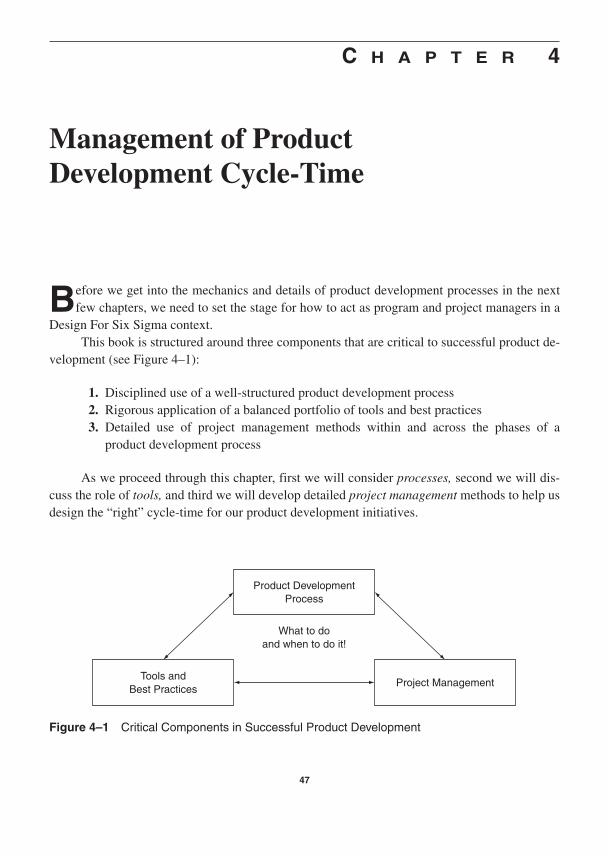
C H A P T E R 4
Management of ProductDevelopment Cycle-Time
Before we get into the mechanics and details of product development processes in the nextfew chapters, we need to set the stage for how to act as program and project managers in a
Design For Six Sigma context.This book is structured around three components that are critical to successful product de-
velopment (see Figure 4–1):
1. Disciplined use of a well-structured product development process2. Rigorous application of a balanced portfolio of tools and best practices3. Detailed use of project management methods within and across the phases of a
product development process
As we proceed through this chapter, first we will consider processes, second we will dis-cuss the role of tools, and third we will develop detailed project management methods to help usdesign the “right” cycle-time for our product development initiatives.
47
Product DevelopmentProcess
What to doand when to do it!
Tools andBest Practices
Project Management
Figure 4–1 Critical Components in Successful Product Development

The Product Development Process Capability Index
The metrics of Six Sigma can be used to improve one’s ability to manage product developmentprojects. The metric that is most associated with Six Sigma performance is the capability index:
Cp (USLLSL)/6
The capability index is quite flexible in its ability to represent the ratio of required per-formance to measured performance. We can apply this metric to the capability of a managementteam to meet its product development cycle-time goals. The Cp index can be restated for mea-suring product development process capability:
Cp (Cycle-Time Limits)/6 of Measured Cycle-Time
The upper and lower specification limits for product development cycle-time are defined as:
USL The time it takes to complete either one phase or a complete set of phases withina product development process when using a full and complete set of tools and bestpractices to fulfill the system requirements (i.e., the longest allowable cycle-time)
LSL The time it takes to complete either one phase or a complete set of phases withina product development process when using a minimum set of tools and best practices tofulfill the system requirements (i.e., the shortest allowable cycle-time)
The definition of time limits to conduct the phases of product development is consideredthe voice of the business. In that context, the USL and LSL are just like any other set of require-ments established to satisfy the voice of some constituency. The time allotment for single-phasecycle-time or complete product development process cycle-time (all eight phases in the I2DOVand CDOV processes, outlined later in this chapter) is defined by the advanced product planningteam. This team is usually made up of business leaders from inbound marketing, sales and sup-port (outbound marketing), R&D, product design, supply chain management, and manufacturingmanagement.
The cycle-time to complete a phase or the complete product development process can beboth estimated and literally measured as the product is developed. The standard deviation of cycle-time is easily calculated by performing Monte Carlo simulations on the phase-by-phase cycle-times within a program. Actually quantifying the real standard deviation of a business’sproduct development cycle-time can take years. The key is to realistically estimate task cycle-times within each phase. Every critical task can be underwritten by a tool or best practice that de-livers measurable results that fulfill specific product requirements.
The worst thing a business can do is to arbitrarily establish, or guess without data, a prod-uct launch date and then mandate that the product development community meet it. This is arecipe for the development of schedules that are simply unattainable. The amazing thing is every-body knows these schedules are unrealistic, but year in and year out this game is played. Up the
48 Chapter 4

chain of command no one is held accountable for this kind of anemic and undisciplined manage-ment behavior. The application of a Six Sigma approach to cycle-time capability measurement isa reasonable way to break this cycle of dysfunctional behavior (see Figure 4–2).
What we suggest is a disciplined, realistic, detailed estimation of task cycle-times on aphase-by-phase basis. These time estimates form a phase-by-phase project management plan,sometimes referred to as an integrated program plan. Within each phase, a critical path emerges.This critical path is a serial set of tasks that define the time it will take to complete the phase. Theapplication of Monte Carlo simulations to the critical path cycle-times allows the program man-agement team to “rehearse” the tasks within each phase under many changing time estimates. Itis easy to run thousands of practice runs through any given phase and see the resulting best, me-dian, and worst-case cycle-time projections.
When a management team says, “We don’t have time to do these estimates, we have to getthis product out the door,” you can pretty much guarantee that they will be late in delivering theproduct. They have a weak plan to get the product developed on a realistic time scale. For largeprojects, it is routine for the lateness to encompass the better part of a year! Maybe part of “get-ting the product out the door” should begin to include taking the time to properly plan the detailedtasks to do the right things at the right time in the first place. The following 9 steps illustrate a
Management of Product Development Cycle-Time 49
Current (n) ProductDevelopment Cycle-Time Performance. . .
Next (n+1) ProductDevelopment Cycle-Time Performance. . .
Next (n+2) ProductDevelopment Cycle-Time Performance. . .
Cp = 1
LSL USL
LSL USL
LSL USL
Cp << 1
Cp = 2
. . . Poor Cycle-TimePerformance
. . . Better Cycle-TimePerformance
. . . 6σ Cycle-TimePerformance
Figure 4–2 Designing Rational Product Development Cycle-Times
proven approach for designing rational product development cycle-times that can be measuredand held accountable to Six Sigma performance standards. The goal is to gain control of productdevelopment cycle-time and systematically improve it from one product to the next.
A general, 9-step process model for the disciplined management of product developmentcycle-time can be deployed as follows:
1. Build the phases and gates structure that defines your product development process(what to do at the macro level).
2. Define the full set of tools and best practices you will use to deliver the required resultsduring product development (specific tasks and deliverable results).
3. Align an appropriate (somewhere between a full set and minimum set) set of tools andbest practices within each phase of your product development process (what to do atthe micro level).
4. Estimate start and end dates for each task that is enabled by a tool or best practicewithin each phase.
5. Define who is responsible for using specific tools to deliver specific results that certifythe completion of each task within each phase.
6. Create a PERT chart of the tool-based tasks for each phase (using Microsoft® Project).7. Identify the critical path of tasks and the USL-LSL that control the cycle-time for each
phase’s PERT chart.8. Construct a Monte Carlo simulation model to calculate the earliest, median, and latest
phase completion times and Cp index created by the Critical Path tasks within eachphase (using Crystal Ball® in conjunction with Excel).
9. Create an integrated program plan by linking all the phase cycle-time estimates to-gether. Construct statistical forecasts and Cp index for the aggregated cycle-time forthe whole program (using Crystal Ball® in conjunction with Excel).
Product Development Process
1. Build the phases and gates structure that defines your product development process(what to do at the macro level).
A well-structured product development process (PDP) enables executives, program managers,project managers, and engineering team leaders to control what to do and when to do it from amacro-timing perspective. A good PDP will in large measure establish the “poise” of the organi-zation. This is particularly true when all the troubles come flowing in as a normal matter of coursein product development. Products tend to mirror the processes that develop and deliver them. Notall companies have intentionally designed product development phases. But most companieshave at least two major “phases” that they must manage:
• WAHBL phase (When All Hell Breaks Loose)• SHTF phase (S%#! Hits the Fan)
50 Chapter 4
We hope to give you some better suggestions for phase titles as we proceed.A Phase/Gate structure for conducting and completing development and design tasks en-
ables the management team to manage risk carefully in reasonable “packets” of time. Each packetof time is called a phase. A phase is made up of a rational subgroup of tasks or actions that areenabled by a specific set of tools and best practices. A reasonable number of tasks are aggregatedand conducted to deliver a predetermined set of results that move the goals of the product devel-opment program to a rational point of completion and risk assessment.
A gate covers a very short period of time, usually less than a day. The program manage-ment team assesses progress against goals, understands the current state of accumulated risk, andplans for the successful deployment of the next phase tasks and actions. The gate should beroughly broken down into 20 percent of the time used to look back at risks that have accrued andwhat is going to be done about them. Eighty percent of the time should be devoted to planning,preventing problems, and enabling the success of the next phase.
We recommend architecting a lean and flexible product development process that acts a lotlike a demand flow manufacturing process. Any size product development project or program(PDP) should be able to be taken through your phases and gates — big ones and little ones. Thephases and gates should be no more complex than your product and manufacturing process re-quirements demand — but no simpler (Einstein’s approach!). Your product development processshould be carefully architected to be lean and flexible. If it’s too lean, your customers are quitelikely to get mean so be careful. One way to know if it’s too lean is if nobody pays serious atten-tion to the gate reviews.
Another characteristic of your PDP is that it should be the key influence on how you man-age your program’s macro-timing cycle. Macro-timing is cycle-time constraint and managementacross the phases. In contrast, micro-timing is cycle-time constraint and management of the spe-cific within-phase tasks that are enabled by specific tools and best practices. Micro-timing is man-aged using the methods of project management. We will discuss those shortly.
A reasonable product development process contains two distinct processes:
1. A technology development process2. A product commercialization (design) process
The reason for two separate Phase/Gate processes is to reduce the risk associated with newtechnology development. Many companies develop new, unproven technology right in the mid-dle of a product design program. Often, the new technology is difficult to tame, and the wholecommercialization program suffers in terms of poor quality, budget overruns, and uncontrollablecycle-time. These are symptoms of poor discipline within an organization. Fortunately thesesymptoms can be mitigated, but not by measuring cost, quality, and cycle-time as primary met-rics. The chapters on Critical Parameter Management will explain what to measure to help assurethese macro-measures come out reasonably well.
The approach to technology development we have used to great benefit is to first developand certify new technologies before they are allowed into a product design program. The timing
Management of Product Development Cycle-Time 51

between technology development and product design processes can either be purely serial or setup in staggered form of parallel timing. The more you conduct Technology Development For SixSigma (TDFSS) in parallel without a fall-back design in the wings, the more risk you heap uponyour commercialization program. The phases and gates for technology development are intendedto produce essentially equivalent designs to those current designs that have experienced actualuse in the application environment by actual customers. Your technology development processhas to stand in as a reasonable surrogate of the misuse, abuse, and stresses encountered in the realworld. What can happen “out there” must be induced “in here.” Your technology developmentteams must act like customers as they stress test their new designs prior to transfer into the de-sign organization.
We will thoroughly introduce you to the four phases and gates of a TDFSS process in thenext chapter. If you are familiar with Design For Six Sigma, this is a similar process refined forthe up-stream R&D activities that are used to Invent, Innovate, Develop, Optimize, and Verifynew platforms and subsystems. We call it the I2DOV process.
The DFSS process in this text is focused on the design of new products and productionprocesses. It includes four generic phases: Concept design, Design development, Optimization,and Verify certification. We call it the CDOV process. For reference, the production operationsprocess for Six Sigma is often called MAIC, for Measure, Analyze, Improve, and Control,which is largely based on Walter Shewhart’s famous contributions to statistical process controlmethods.
We are not optometrists, but we do believe that when the I2DOV and CDOV process ele-ments are properly integrated into a product development process, they will help you see clearlyhow to develop great products with the right cycle-time and performance. The result is completeand balanced products that look and perform like the processes that created them.
Tools and Best Practices
2. Define the full set of tools and best practices you will use to deliver the requiredresults during product development (specific tasks and deliverable results).
A good portion of this text is dedicated to laying out the flow of tools and best practices used inthe TDFSS (I2DOV) and DFSS (CDOV) processes. These tools and best practices are the focusof “what to do” within each phase. The gate reviews look closely at the deliverables from eachapplication of tools and best practices. If you have an anemic set of tools and best practices thatyou are always short-circuiting because you have no time to use them properly, the following sug-gested tools and best practices will help you.
The chapters in this text offer specific suggestions for defining a full suite of tools and bestpractices. These suggested tools and best practices will go a long way in helping you determinewhere, within your design functions, you need Six Sigma performance and then how to attain itand prove it with data at a gate review. Please note that not all design functions or parameters needto be at Six Sigma levels of performance; some can be less and a few will need to be much greater.
Here is a summary list of the numerous tools and best practices you should seriously be con-sidering for application across the phases of your product development programs:
52 Chapter 4

Phase/Gate processesCustomer value and marketing segmentation analysisConcept engineeringVoice of the customer gatheringKJ (affinity diagramming) methodologyQuality Function Deployment (QFD)Houses of Quality (EQFD)Concept generation methods (TRIZ, etc.)System architectingPractical design principlesPugh concept selectionCritical Parameter ManagementProject management techniquesBasic statistical techniques
Descriptive statisticsNormal distribution parametersGraphical techniques
box plotshistogramsscatter plotstime series plotsrun chartspareto chartsinferential statisticscentral limit theoremhypothesis testingconfidence intervalssample size determination
Measurement systems analysisGage R&R and P/T studies
Design process capability analysisDesign for manufacturability and assemblyMinitab data analysis methodsFailure modes and effects analysis (FMEA)
Design failure analysisManufacturing process failure analysis
Design of experiments for empirical modeling of “ideal functions and transfer functions”Screening studies and sequential experimentationFull and fractional factorial experiments
Degrees of freedomMain effects and interaction studiesCenter points and blocking methods
Management of Product Development Cycle-Time 53
Analysis of variance (ANOVA)Simple and multiple regressionResponse surface methodsTaguchi robust design techniques
QLF and S/N metricsDesign for additivityStatic methodsDynamic methods
Tolerance designAnalytical (WC, RSS, 6s, Monte Carlo)Empirical (DOE, ANOVA, QLF, and Cp)
Reliability analysis (Prediction, HALT, HAST)Multi-vari studies (ANOVA)Statistical process control chartsManufacturing process capability analysisData transformations
Box-Cox transformation for nonnormal data
You can see that we have many tools and best practices to consider for application as weconduct our product development tasks. Each of these items is capable of delivering certain, spe-cific results. If your design needs these results to satisfy customer needs or to fulfill critical re-quirements, you must seriously consider deploying the tool or best practice. Now, we have to facethe practical fact that we have a finite amount of time to conduct product development. Only aspecific number of these tools and best practices can actually be conducted before everybody getsold and dies! You need to select a rational set of these tools and best practices and commit to ap-plying them rigorously. The key thing you will have to manage to keep your risks in balance iswhat tools and best practices you are not going to use! Choose wisely.
Aligning Tools within Phases
3. Align an appropriate (somewhere between a full set and a minimum set) set of toolsand best practices within each phase of your product development process (what to doat the micro level).
The next thing we need to do is align the appropriate tools and best practices to the appropriatephases of a product development process. We have established the I2DOV and CDOV productdevelopment processes as general models that are easy to understand and relate to your specificproduct development process vocabulary. Your words may be a bit different but everybody doessome form of conceptual design, design development, optimization, and verify certification. Mostcompanies have more than four general phases. We have laid out a sample set of tools and bestpractices in the following pages to fit within the CDOV process as an example. A full set of toolsand best practices are developed in Chapters 5 and 6. We have broken Phases 3 and 4 into two
54 Chapter 4

segments because that is typical of the way most successful companies we have seen actuallystructure their product development processes. You will see a bit of tool overlap as we progressthrough the phases.
Concept Phase (Phase 1)
Market segmentation analysis
Economic and market trend forecasting
Business case development methods
Competitive benchmarking
VOC gathering methods
KJ analysis
QFD/House of Quality – Level 1 (system level)
Concept generation techniques (TRIZ, brainstorming, brain writing)
Modular and platform design
System architecting methods
Knowledge-based engineering methods
Pugh concept evaluation and selection process
Math, graphical, and prototype modeling (for business cases and scientific andengineering analysis)
Design (Phase 2)
Competitive benchmarking
VOC gathering methods
KJ analysis
QFD/Houses of Quality – Levels 2-5 (subsystem, subassembly, component, andmanufacturing process levels)
Concept generation techniques (TRIZ, brainstorming, brain writing)
Pugh concept evaluation and selection process
Design for manufacture and assembly
Value engineering and analysis
Design failure modes and effects analysis
Measurement systems analysis
Critical parameter management
Knowledge-based engineering methods
Math modeling (business case and engineering analysis to define ideal functions andtransfer functions)
Management of Product Development Cycle-Time 55
Design of experiments (full and fractional factorial designs and sequentialexperimentation)
Descriptive and inferential statistical analysis
ANOVA data analysis
Regression and empirical modeling methods
Reliability modeling methods
Normal and accelerated life testing methods
Design capability studies
Multi-vari studies
Statistical process control (for Design Stability and Capability Studies)
Optimization (Phase 3a: Subsystem and Subassembly Robustness Optimization)
Subsystem and subassembly noise diagramming
System noise mapping
Measurement system analysis
Use of screening experiments for noise vector characterization
Analysis of means (ANOM) data analysis techniques
Analysis of variance (ANOVA) data analysis techniques
Baseline subsystem and subassembly CFR Signal-to-Noise Characterization
Taguchi’s methods for robust design
Design for additivity
Full or fractional factorial experiments for robustness characterization
Generation of the additive S/N model
Response surface methods
Design capability studies
Critical parameter management
Subsystem/subassembly/component reliability analysis
Life testing (Normal, HALT, and HAST)
Optimization (Phase 3b: System Integration and Stress Testing)
Measurement system analysis
System noise mapping
Nominal system CFR design Cp studies
Stress case system CFR design Cp studies
System-subsystem-subassembly transfer function development
56 Chapter 4

System level sensitivity analysis
Design of experiments (screening and modeling)
ANOVA
Regression
Analytical tolerance analysis
Empirical tolerance analysis
Statistical process control of design CFR performance
Reliability Assessment (normal, HALT, and HAST)
Critical Parameter Management
Verify (Phase 4a: Product Design Verification)
Measurement system analysis
System noise mapping
Analytical tolerance design
Worst case analysis
Root sum of squares analysis
Six Sigma analysis
Monte Carlo simulation
Empirical Tolerance Design
System Level sensitivity analysis
Design of experiments
ANOVA
Regression
Multi-vari studies
Design capability studies
Nominal system CFR design Cp studies
Stress case system CFR design Cp studies
Reliability assessment (Normal, HALT, and HAST)
Competitive benchmarking studies
Statistical process control of design CFR performance
Critical parameter management (with capability growth index)
Verify (Phase 4b: Production Process and Launch Verification)
Measurement system analysis
Multi-vari studies
Management of Product Development Cycle-Time 57

Design and manufacturing process capability studies
Nominal system CFR design Cp studies
Reliability assessment (Normal, HALT, and HAST)
Statistical process control of design and process CFR performance
Critical parameter management (with capability growth index)
We now have aligned numerous tools and best practices to the phases of the CDOV prod-uct development process. The phases of CDOV define the macro-timing segments that can beused to control the program’s overall cycle-time. The tools and best practices can be carefullymatched to “within-phase” actions or tasks that help fulfill specific gate requirements. How longwill it all take? Let’s begin to answer that question with the next section.
Project Management
We have established the need for the macro-timing of the phases and gates of product develop-ment. We have also illustrated the need for bringing a carefully selected set of tools and best prac-tices into that structure. It is time to constrain and manage the detailed serial and parallel flow ofspecific tasks that are enabled by these tools and best practices.
We will briefly introduce a few key principles of project management at this point. This willestablish a common vocabulary to work with as we “design” the cycle-time of our programs andprojects in a Six Sigma context. Phase timing can be structured somewhat like the various seg-ments or stages of a manufacturing process. The tools are different because the deliverables aredifferent, but using tools and best practices at the right time in the process is the same. Statisticalprocess control techniques help keep the measured output of a process, over time, on target, or atleast within reasonable boundaries (upper and lower control limits). In a similar fashion, statisti-cal analysis can be applied to the product development tasks that are tracked using project man-agement methods. If you get the sense that we are taking you into the world of capability analysisfor product development cycle-time management, you are quite right.
Too many companies manage programs to “all-success” schedules. They tend to use deter-ministic (single-point-in-time estimates) modeling of program cycle-time. This is often sterileand unrealistic. An emerging best practice is the use of an integrated, phase-by-phase projectmanagement plan. It involves the disciplined tracking of a critical path that is built up from care-fully selected, tool-based tasks that are timed using statistically based Monte Carlo simulationmodels. This is the basis for Six Sigma program management.
The statistical and probability-based methods of Six Sigma start to become important inproject and program management when we fit statistical distributions to start and end dates forwithin-phase tasks. We can use these stochastic methods to estimate and manage the start and enddates for the phases. Ultimately, we can link all the phases as probabilistic, as opposed to deter-ministic, events that can be analyzed as an integrated program plan. Integrated program plans aremade up from the project plans from each phase that are usually documented in the form of aPERT chart.
58 Chapter 4

4. Estimate start and end dates for each task that is enabled by a tool or best practicewithin each phase.
We are ready to assign cycle-time estimates to our within-phase tasks. The program or proj-ect manager can now ask his or her design teams to estimate the start and end dates for the spe-cific tool and best practice tasks that will fulfill the program’s gate deliverables. It is imperativethat the team members within the product development organization understand that they are ex-pected to use these tools and best practices and will be held personally accountable for the resultsgained from their proper and rigorous deployment.
We are now getting into the micro-mechanics of cycle-time design and management. Mostpeople don’t think about it this way, but a good project manager is really an expert in designingcycle-times. In reality, the project manager is in the profession of architecting “designer cycle-times,” crafting molding, and shaping the architecture of the cycle-time structures!
The following illustrations are examples of a template we use throughout this text to showhow specific tasks, enabled by one or more tools or best practices, can be linked in serial or par-allel networks that are referred to as a work breakdown structure. In fact, this text is loaded withthem! These form the structural basis we will use as we proceed into the design of phase-by-phasecycle-times.
Management of Product Development Cycle-Time 59
Gather the Voice of the Customer by MarketSegment
Refine and Rank the Voice of the Customer UsingKJ Analysis
Start Date: End Date: Owner:
Start Date: End Date: Owner:
Create Product or System Level House ofQuality
Start Date: End Date: Owner:
The specific tools deployed in these three tasks are:
1. Customer interviewing2. KJ analysis (affinity diagramming)3. Quality function deployment (QFD)
Specific deliverables come from using these tools:
1. Raw voice of the customer database2. Grouped and ranked VOC data in the form of an KJ (affinity) diagram3. System level House of Quality (a matrix structure diagram)

The next two chapters demonstrate, through a reasonable amount of detail, how to accountfor the major tasks in technology development and product design. Laying out the structure andflow of the major tasks that your teams will conduct during product development will leave littleto the imagination as we attempt to be good cycle-time designers and time management ac-countants. So now a project manager is not only a designer, but an architect and accountant oftime as well!
5. Define who is responsible for using specific tools to deliver specific results thatcertify the completion of each task within each phase.
Each task has a start date and end date, and now we add who specifically is responsible—personally accountable—for the delivered results from using a tool or best practice. This approachto project management during product development holds specific people accountable for specificdeliverables. If you are a manager and are uncomfortable holding people accountable for deliver-ing specific results using carefully selected tools and best practices within the agreed time alloca-tion, then this approach to product development is definitely not for you! If what we have readabout Jack Welch, former CEO and the Six Sigma czar of General Electric, is to be believed, helikely would find this level of accountability to be quite appropriate for weeding out the bottom 10percent of low performers from the product development community every year! Of course youneed to replace these people with new and capable talent so you have enough resources to applythe right number of tools and best practices rather than heaping the extra responsibility on the re-maining resources.
Many managers like to leave the decision of how results are attained up to their people. Thisis fine if the people are properly trained and enabled and actually choose to apply a balanced setof tools and best practices. It has been our experience that this almost never happens. Usually cycle-time is forced to be unrealistically tight and the teams simply revert to build-test-fix meth-ods and quickly get behind in fulfilling their desire to do things right. Their design releases getmany iterations ahead of their actual data analysis! It is rarely their fault, though. They were notgoverned by the right or reasonable expectations, so they guess and bad things start to happen.Quite frankly, it is mainly attributable to poor project management technique. Although we’venever asked him, it is a good bet that this kind of behavior would get you on Jack Welch’s “sorrybut you’ve got to go” list.
The right thing to do as a manager is to reach consensus about reasonable expectations withyour teams on the right balance of tools and best practices that absolutely must be deployed. Thengive your people the time and resources they need to use them properly. As a result, you will notneed to watch them do things over a third, fourth, or fifth time. You won’t be able to deploy allthese tools and best practices, but you can carefully choose a rational subset and then see to it thatthey get used properly.
The Power of PERT Charts
6. Create a PERT chart of the tool-based tasks for each phase (using Microsoft®
Project).
60 Chapter 4

A program or project manager can easily have each of his or her team leaders assist in the con-struction of PERT charts that act as flow diagrams to illustrate exactly what tools and best prac-tices are going to be used within each phase of technology development and product design.
You can use three major software tools to gain proficiency at project management in a SixSigma context:
1. Microsoft® Project2. Microsoft® Excel3. Decisioneering’s Crystal Ball® Monte Carlo Simulator
Tool #1 for Six Sigma Project Management: Microsoft® Project
Project management is a common topic that has been taught and practiced in industry for manyyears. The approach presented in this text is enabled by Microsoft® Project software, which iseasy to use and readily available. Microsoft® Project allows one to easily build a project time lineusing both PERT and Gantt charting methods. We recommend doing your project managementplans in PERT chart format. PERT charts are essentially serial and parallel flow charts comprisedof block diagrams such as the sample in Figure 4–3.
PERT charts are good at showing how numerous tasks are linked to one another. They arealso good at illustrating who is “on the hook” for delivering the results. When an entire phase oftasks is linked, the software can illustrate the critical path of tasks and the time required to com-plete the phase deliverables, as in Figure 4–4.
With such a diagram we can easily identify the tasks that add up to define the Critical Pathand the total cycle-time for the phase we are evaluating. You should create a PERT chart for eachphase of your technology development and product design processes. It is not uncommon for en-gineers to have personal PERT charts that essentially act as an agreement or “contract” betweenthem and their manager or team leader. These personal PERT charts get aggregated to comprisethe overall phase PERT charts. All the phase PERT charts are linked to form what is called the in-tegrated program plan (IPP).
Management of Product Development Cycle-Time 61
Figure 4–3 Sample PERT Chart Task Box
Task based on the application of a tool or best practice that has a specific deliverable.
Task Owner: Duration:
Start Date: End Date:
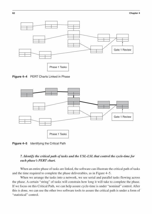
7. Identify the critical path of tasks and the USL-LSL that control the cycle-time foreach phase’s PERT chart.
When an entire phase of tasks are linked, the software can illustrate the critical path of tasksand the time required to complete the phase deliverables, as in Figure 4–5.
When we arrange the tasks into a network, we see serial and parallel tasks flowing acrossthe phase. A certain “string” of tasks will constrain how long it will take to complete the phase.If we focus on this Critical Path, we can help assure cycle-time is under “nominal” control. Afterthis is done, we can use the other two software tools to assure the critical path is under a form of“statistical” control.
62 Chapter 4
Phase 1 Tasks
Gate 1 Review
Figure 4–4 PERT Charts Linked in Phase
Phase 1 Tasks
Gate 1 Review
Figure 4–5 Identifying the Critical Path

Each phase can have specification limits defined for its allowable range of Critical Path cycle-time. The Upper and Lower Specification Limits for product development cycle-time aredefined as:
USL The time it takes to complete either one phase or a complete set of phases withina product development process when using a full and complete set of tools and bestpractices to fulfill the system requirements (i.e., the longest allowable cycle-time)
LSL The time it takes to complete either one phase or a complete set of phases withina product development process when using a minimum set of tools and best practices tofulfill the system requirements (i.e., the shortest allowable cycle-time)
Management of Product Development Cycle-Time 63
LSL USL
Phase 1: ConceptDevelopment
8. Construct a Monte Carlo simulation model to calculate the earliest, median, andlatest phase completion times and Cp index created by the Critical Path tasks withineach phase (using Crystal Ball® in conjunction with Excel).
Tool #2 for Six Sigma Project Management: Microsoft® Excel
We now take the tasks that are on the critical path and lay them out in an Excel spreadsheet thatis also linked to Crystal Ball® Monte Carlo Simulation software (www.decisioneering.com).These tasks will be evaluated mathematically by summing their individual cycle-times. The cycle-times are estimates from engineering team judgment. We will illustrate the popular trian-gular distribution approach to estimating cycle-time variation. The time estimates for each taskare assigned three possible or likely durations. One way to use this approach is to list each taskand then enter three time estimates in the Excel columns:
1. Median or Most Likely Time Duration for the task2. Minimum or Least Time Duration for the task3. Maximum or Longest Time Duration for the task
The final column contains the type of distribution we choose to represent the probabilistic,statistical, or “likely” variation that characterizes the nature of how the task duration time mightvary. See Table 4–1.
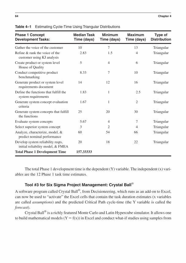
The total Phase 1 development time is the dependent (Y) variable. The independent (x) vari-ables are the 12 Phase 1 task time estimates.
Tool #3 for Six Sigma Project Management: Crystal Ball®
A software program called Crystal Ball®, from Decisioneering, which runs as an add-on to Excel,can now be used to “activate” the Excel cells that contain the task duration estimates (x variablesare called assumptions) and the predicted Critical Path cycle-time (the Y variable is called the forecast).
Crystal Ball® is a richly featured Monte Carlo and Latin Hypercube simulator. It allows oneto build mathematical models (Y f(x)) in Excel and conduct what-if studies using samples from
64 Chapter 4
Table 4–1 Estimating Cycle-Time Using Triangular Distributions
Phase 1 Concept Median Task Minimum Maximum Type of Development Tasks: Time (days) Time (days) Time (days) Distribution
Gather the voice of the customer 10 7 13 Triangular
Refine & rank the voice of the 2.83 1.5 4 Triangularcustomer using KJ analysis
Create product or system level 5 4 6 TriangularHouse of Quality
Conduct competitive product 8.33 7 10 Triangularbenchmarking
Generate product or system level 14 12 16 Triangularrequirements document
Define the functions that fulfill the 1.83 1 2.5 Triangularsystem requirements
Generate system concept evaluation 1.67 1 2 Triangularcriteria
Generate system concepts that fulfill 25 20 30 Triangularthe functions
Evaluate system concepts 5.67 4 7 Triangular
Select superior system concept 3 2 4 Triangular
Analyze, characterize, model, & 60 54 66 Triangularpredict nominal performance
Develop system reliability reqts, 20 18 22 Triangularinitial reliability model, & FMEA
Total Phase 1 Development Time 157.33333

prescribed probability distributions (in this case triangular distributions) as the assumption inputsto the model. In project management cycle-time forecasting, the models are simple summationsof the task durations that lie on the critical path.
Thus, the model for Phase 1 cycle-time is: Y Task1 Task2 Task3 . . . Task12
Each task is not treated as a deterministic event! Each is represented by the triangular distri-bution, and its value is randomly determined by Crystal Ball® for each run through the equation.
We could choose a number of distributions from inside Crystal Ball’s® Menu to represent duration time variation for each task. The normal, uniform, and triangular are the most commonoptions.
The normal distribution requires one to know the mean and standard deviation of thetask duration time. We find most teams do not usually know these parameters.
The uniform distribution basically assumes that there is an equally likely chance thatthe task duration will lie somewhere between two points in time:
The shortest likely duration
The longest likely duration
The triangular distribution, as in Figure 4–6, assumes you can estimate three separatelikelihood values for the task duration:
Median or most likely time duration for the task
Minimum or shortest likely time duration for the task
Maximum or longest likely time duration for the task
We recommend the triangular distribution because it is a conservative and reasonable esti-mator of likelihood without trying to overstretch statistical parameter assumptions. Crystal Ball®
allows you to skew your minimum and maximum duration inputs—your duration estimates donot need to be symmetrically spaced. Figure 4–6 is an example of a Crystal Ball® assumption win-dow for inputting the Phase 1 task duration estimates (symmetrically spaced) for “Gather theVoice of the Customer.”
Crystal Ball® can be set up to run through your phase tasks anywhere from 500 to many tensof thousands of practice runs. You can literally run your Phase 1 tasks through their estimated du-rations thousands of times. Recall that your forecast Y will be the total Phase 1 cycle-time. So,10,000 trips through our math model for Phase 1 looks like this as far as Crystal Ball® is concerned:
Math Version of Phase 1: Y Task1 Task2 Task3 . . . Task12
Management of Product Development Cycle-Time 65
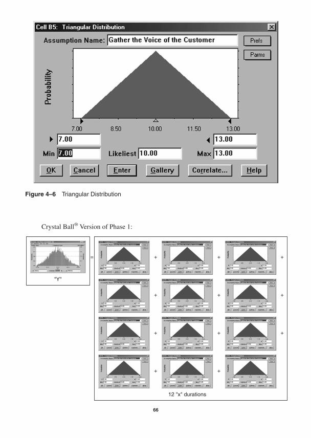
Crystal Ball® Version of Phase 1:
Figure 4–6 Triangular Distribution
"Y"
= + + +
+ + +
+ + +
+ +
12 "x" durations
66

Here we see that 10,000 random samples from 12 independent, triangular task duration dis-tributions produce a normal distribution of 10,000 Phase 1 cycle-times.
This happens because of a statistical truth called the central limit theorem. What is impor-tant is the statistical output parameters associated with the Y forecast distribution. These outputstatistics can be evaluated for several interesting characteristics:
Forecast range minimum, maximum, and width
Forecast mean, median, and standard deviation
Figure 4–7 and Figure 4–8 show an example of Crystal Ball’s® output in the form of a fre-quency chart and table of descriptive statistics for the Phase 1 cycle-time forecast.
Phase 1 cycle-time lies somewhere between the range of 143 and 170 days duration. Thereappear to be 27 days between the worst and best case cycle-time for Phase 1. The most likely cycle-time for Phase 1 is estimated to be 157 days. This is helpful information. We can rerun thismodel with various task duration estimates in any symmetrical or asymmetrical geometry wechoose. When we assign upper and lower control limits to the forecasted Phase 1 cycle-time andestimate its standard deviation, we can calculate Phase 1’s Cp index. Now, we can start talkingabout Six Sigma standards of performance in project management terms!
We can control the width of the Phase 1 cycle-time distribution and begin to minimize vari-ability in our product development process. We have just built a method to predict product de-velopment process capability.
Management of Product Development Cycle-Time 67
Figure 4–7 Frequency Chart from Crystal Ball®

The Cp index for each phase can be calculated from the Specification Limits (USL-LSL)and the estimated standard deviation from the Monte Carlo simulation (see Figure 4–9).
9. Create an integrated program plan by linking all the phase cycle-time estimatestogether. Construct statistical forecasts and Cp index for the aggregated cycle-time forthe whole program (using Crystal Ball® in conjunction with Excel).
We conclude the process for Six Sigma product development cycle-time management byrolling up the various phase cycle-times into the integrated program cycle-time. Crystal Ball®
provides the phase-by-phase forecasts needed to estimate the IPP cycle-time:
68 Chapter 4
Figure 4–8 Table of Descriptive Statistics from Crystal Ball®
Using the descriptive statistics tables from Crystal Ball® once again, we can look at therolled-up worst, best and, most likely (mean) cycle-time. The beauty of this approach is that wecan, in a few minutes, emulate our phase timing designs in any way we like. We can add or re-

move tasks, change duration estimates, and assess the outcome. A program management team caneasily sit down together, look into the future, and come up with a phase-by-phase, task-by-task,tool-by-tool plan for meeting its cost, performance, and cycle-time objectives. Choose to deploythese tools and you get this performance. Eliminate those tasks and you get these risks. Aroundand around you can go until you emerge with a balanced plan that lets you sleep at night, know-ing you cut the right corners for what you know at that time in your product development process.Later when you know more, you can add new tasks to react to an unforeseen problem. The com-mon theme in your planning for the right cycle-time should be “it’s cheaper to prevent a problemthan it is to solve one.”
The illustration in Figure 4–10 shows how the integrated program plan can be measuredagainst Six Sigma capability standards.
Product development capability performance can be tracked and, more importantly, im-proved with the Six Sigma metric in Figure 4–10 in place.
We hope this overview of using Microsoft® Project, Excel, Crystal Ball®, and product de-velopment capability growth metrics sets the stage for success as you design the right cycle-timesfor your programs and projects. These methods are easy to learn and apply. We close this chapterby reminding you all that the shortest cycle-time is not always the right cycle-time. Balance and proportion are essential to proper risk management, which is really what this is all about.Sleep well.
Management of Product Development Cycle-Time 69
LSL USL
Phase 1: ConceptDevelopment
Cp = (USL-LSL)/(6σ)
Figure 4–9 Calculating the Cp Index

References
Lowery, G., & Stover, T. S. (2001). Managing Projects with Microsoft Project 2000. New York:Wiley & Sons.
Shtub, A., Bard, A. F., & Globerson, S. (1994). Project Management: Engineering, technology,and implementation. Englewood Cliffs, NJ: Prentice Hall.
70 Chapter 4
LSL USL
Phase 1: ConceptDevelopment
Phase 1Cycle-Time
Cpphase 1
Phase 2Cycle-Time
Cpphase 2
Phase 3Cycle-Time
Cpphase 3
Phase 4Cycle-Time
Cpphase 4
LSL USL
Phase 2: DesignDevelopment
LSL USL
Phase 3: DesignOptimization
LSL USL
Phase 4: VerifyCapability
PredictedCycle-Times. . .
MeasuredCycle-Times. . .
Cp = (USL-LSL)/(T6σ)
Figure 4–10 Measuring the IPP Against Six Sigma Standards

C H A P T E R 5
Technology Development UsingDesign For Six Sigma
The development of new technology is the fuel that powers the timely delivery of new prod-ucts and new production processes. Within this portion of the total product development
process, advances in performance and quality are actually born. Any company that does not viewits R&D team as its strategic starting point for the development of quality and for laying the foun-dation for efficient cycle-time in product development is very much off base.
Product development encompasses two distinct categories in this text: the first is technol-ogy development, and the second is product design, sometimes referred to as commercialization.This text takes the position that the teams residing within research & development organizationshave the best and earliest opportunity to develop the foundations for Six Sigma performancewithin the detailed processes used to generate new and leveraged technologies. If you were to ask,“Are there Six Sigma methods that can be deployed in the day-to-day activities within an R&Dcontext?” the answer is a definitive yes! This chapter constructs an architecture for the deploy-ment of such methods in the development and transfer of new and leveraged technologies.
Industry is now beginning to recognize that technology development projects should belargely independent from product commercialization projects. This is never an easy thing to dobut if you want to minimize technical difficulties as you approach design certification and launch,this is precisely what must be done. It is risky to develop new technology within a product designproject. There are big differences in what needs to be done and known during technology devel-opment and product commercialization. Technologies that are under development are immatureand overly sensitive to sources of manufacturing, distribution, and customer use variability(“noise factors”). When they are forced into the high-pressure time line of a commercializationproject, corners get cut and sensitivities go undetected. Immature, underdeveloped technologiescan greatly slow the progress of the product due to their inability to integrate smoothly and func-tion correctly in the presence of noise factors, or any source of variation from external, unit-to-unit, or deterioration sources. In a word, they are not “certified” for safe commercial or design ap-plication. Deploying new technologies prior to their certification is analogous to launching a newproduct design that has not been made “capable” from a manufacturing and assembly perspective.To the statistician, it is similar to running a process before one has proven it to be under a state of
71
statistical control. We must quantitatively prove that a new technology is both robust and tunablebefore it can be used in a new product. By robust, we mean capable short-term performance asmeasured by Cp indices, even in the presence of noise factors. By tunable we mean capable long-term performance as measured by Cpk indices (Cpk is the measure of capability after the meanhas shifted off target by “k” standard deviations). This chapter lays a foundation for the proper de-velopment and transfer of new technologies into a product commercialization project.
Technology development and transfer must be properly controlled and managed by factsgenerated using a system integration process we call Critical Parameter Management (CPM).
CPM is fully explained and developed in a later section. The proper place to initiate CPMin a business is during advanced product planning and technology development. If CPM is prac-ticed at this earliest stage of product development, then a certified portfolio of critical functionalparameters and responses can be rapidly transferred as a “platform” into the design of families ofproducts during numerous product commercialization programs.
Critical Parameter Management is a system engineering and integration process that is usedwithin an overarching technology development and product commercialization roadmap. We willfirst look at a roadmap (I2DOV, “eye-dov”) that defines a generic technology development process,and then move on to define a similar roadmap (CDOV, pronounced “see-dov”) that defines a ra-tional set of phases and gates for a product commercialization process. These roadmaps can bestated in terms of manageable phases and gates, which are useful elements that help managementand engineering teams to conduct product development with order, discipline, and structure.
The I2DOV Roadmap: Applying a Phase/Gate Approach to Technology Development
The structured and disciplined use of phases and gates to manage product commercializationprojects has a proven track record in a large number of companies around the globe. A small butgrowing number of companies are using phases and gates within their R&D organizations to man-age the development of new and leveraged technologies prior to commercial design application.In the next two chapters we will show the linkage between the use of an overarching product de-velopment process, deployment of a full portfolio of modern tools and best practices, and a well-structured approach to project management from R&D all the way to product launch.
With this triangle of structural stability depicted in Figure 5–1, one can drive for break-throughs that deliver Six Sigma results because management, technology, and commercializationteams all know what to do and when to do it.
An Introduction to Phases and Gates
A phase is a period of time during which specific tools and best practices are used in a disciplinedmanner to deliver tangible results that fulfill a predetermined set of technology development re-quirements. We often use the term breakthrough when discussing results. What we mean by thisterm are results that are hard to get without using the kinds of tools and processes we are sug-gesting in this text. Six Sigma methods have a legacy of producing results that were elusive priorto its application.
72 Chapter 5
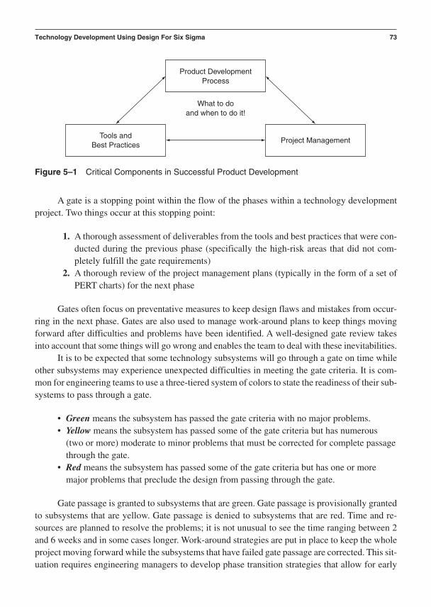
A gate is a stopping point within the flow of the phases within a technology developmentproject. Two things occur at this stopping point:
1. A thorough assessment of deliverables from the tools and best practices that were con-ducted during the previous phase (specifically the high-risk areas that did not com-pletely fulfill the gate requirements)
2. A thorough review of the project management plans (typically in the form of a set ofPERT charts) for the next phase
Gates often focus on preventative measures to keep design flaws and mistakes from occur-ring in the next phase. Gates are also used to manage work-around plans to keep things movingforward after difficulties and problems have been identified. A well-designed gate review takesinto account that some things will go wrong and enables the team to deal with these inevitabilities.
It is to be expected that some technology subsystems will go through a gate on time whileother subsystems may experience unexpected difficulties in meeting the gate criteria. It is com-mon for engineering teams to use a three-tiered system of colors to state the readiness of their sub-systems to pass through a gate.
• Green means the subsystem has passed the gate criteria with no major problems.• Yellow means the subsystem has passed some of the gate criteria but has numerous
(two or more) moderate to minor problems that must be corrected for complete passagethrough the gate.
• Red means the subsystem has passed some of the gate criteria but has one or moremajor problems that preclude the design from passing through the gate.
Gate passage is granted to subsystems that are green. Gate passage is provisionally grantedto subsystems that are yellow. Gate passage is denied to subsystems that are red. Time and re-sources are planned to resolve the problems; it is not unusual to see the time ranging between 2and 6 weeks and in some cases longer. Work-around strategies are put in place to keep the wholeproject moving forward while the subsystems that have failed gate passage are corrected. This sit-uation requires engineering managers to develop phase transition strategies that allow for early
Technology Development Using Design For Six Sigma 73
Product DevelopmentProcess
What to doand when to do it!
Tools andBest Practices
Project Management
Figure 5–1 Critical Components in Successful Product Development

and late gate passage. The ideal state is when all subsystems pass all the gate criteria at the sametime for every gate. This, of course, almost never happens. For complex projects it is foolish toexpect anything other than a series of unexpected problems. For technology managers who pre-fer a preventative approach, the second order of business in developing a Phase/Gate process isthe inclusion of a phase transition strategy that effectively deals with managing the “unexpected.”The first order of business is structuring each phase with a broad portfolio of tools and best prac-tices that help prevent unexpected design problems. This is done by focusing on the tools and bestpractices that use forward-looking metrics that measure functions (scalar and vector engineeringvariables) instead of counting quality attributes (defects and failures). The key is to prevent theneed to react to quality problems later. Quality must be designed in to the new technologies bycareful, disciplined use of the right tools and best practices that measure the right things to fulfillthis “prevent strategy” from an engineering perspective. Parts IV through VII of this text dis-cusses such tools and metrics.
Quality is certainly one of the primary requirements of a technology development project,but it is clear that the most efficient path to quality does not flow through a series of “quality met-rics.” They tend to drive “react” strategies as opposed to “prevent” strategies. We will discuss theantidote to the inefficiencies of quality metrics in the upcoming chapters on Critical ParameterManagement.
There is broad acceptance that using an overarching product development process to guidetechnology development and product commercialization is the right thing to do. What is oftenoverlooked is the value of a broad, balanced portfolio of tools and best practices that are sched-uled and conducted within each phase using the methods of Project Management.
The best way to think about establishing the architecture of any product developmentprocess is to structure it as a macro-timing diagram to constrain “what to do and when to do it”across the entire product development life cycle. With such a macro-timing diagram established,the product development management team can then conduct the phases and gates using check-lists and scorecards based on a broad portfolio of tools and best practices. The techniques of proj-ect management can then be used to construct balanced, micro-timing diagrams (often in the formof a PERT chart) that establish discipline and structure within the day-to-day use of the tools andbest practices for each person on the product development team. We recommend PERT charts be-cause they help define personal accountability for using the right tools and best practices on a day-to-day basis within the phases. They also greatly enhance the management of parallel and serialactivities, work-around strategies, and the critical path tasks that control the cycle-time of eachphase. Managing a technology development project in this manner helps assure that all the rightthings get done to balance the ever-present cost, quality, and cycle-time requirements.
Checklists
Checklists are brief summary statements of tools and best practices that are required to fulfill agate deliverable within a phase. These actions are based on work everyone must do based on abroad portfolio of tools and best practices. You know you have a good checklist when it is easyto directly relate one or more tools or best practices to each gate deliverable. Another way of rec-
74 Chapter 5

ognizing a good checklist is that it can be used to build project management PERT and Ganttcharts for day-to-day management of tool use. Tools and best practices produce deliverables thatcan be tracked on a daily, weekly, or monthly basis and can be easily reviewed using a summaryscorecard when a gate is reached. Checklists are used during project planning of tool use prior toentering the next phase. This is done to prevent problems in the next phase.
An example of a Six Sigma Tool and Best Practice Checklist follows.
Checklist of Phase 1 Tools and Best Practices:
Technology roadmapping
VOC gathering methods
KJ analysis
QFD/House of Quality—Level 1 (system level)
Patent analysis and exposure assessment
Market segmentation analysis
Economic and market trend forecasting
Business case development methods
Competitive benchmarking
Scientific exploration methods
Knowledge-based engineering methods
Math modeling (business cases, scientific, and engineering analysis)
Concept generation techniques (TRIZ, brainstorming, brain-writing)
Modular and platform design
System architecting methods
Upcoming chapters on tools have an extensive, more detailed set of checklists of step-by-step action to be done within each tool or best practice.
Scorecards
Scorecards are brief summary statements of deliverables from specific applications of tools andbest practices. They are useful to help react to problems encountered within the previous phase.
Scorecards state what deliverable is to be provided, as seen in the example in Figure 5–2. Theyshow who is specifically responsible for the deliverable so they can be held accountable for theirbehavior. The original due date for the deliverable is listed along with the actual date the deliverableis completed. The status of the deliverable in terms of completeness of fulfilling its requirements isdocumented in the Completion Status column. The actual, measured performance attained againstthe required criteria is documented in the Performance vs. Criteria column. A column for the rec-ommendation for exiting the gate is also provided in the scorecard. A final column is used to attachnotes to provide details concerning any positive or negative issues for the deliverables.
Technology Development Using Design For Six Sigma 75

Phase 1 Invention & Innovation
Completion Performance Exit Original Due Status vs. Criteria Recommendation
Date vs. Actual Red Green Red Green Red GreenDeliverable Owner Deliv. Date Yellow Yellow Yellow Notes
Market Trend Impact Analysis
Market Assessment
Market Segmentation Analysis
Market Competitive Analysis
Market Opportunity Analysis
Gap Analysis
Long Range VOC Document
Product Family Plan
Technology Response Deliverables
Technology Roadmap Document
Patent Trend Impact Analysis
Patent Position & Risk Assessment Document
System & Subsystem Technology Houses of
Quality
Technology Requirements Documents
Documented List of Functions That Fulfill the
Technology Requirements
Documented Inventions & Patent Strategy
Portfolio of Candidate Technology Concepts That
Fulfill the Functions & Requirements
Documented Critical Parameter Database &
Scorecards
Phase 2 Project Mgt. Plans
Figure 5–2 Example of a General Gate Review Scorecard
76

The scorecard helps the gatekeepers manage risk as they attempt to keep the project onschedule. They can see the critical path items and deploy the resources at their disposal to solvekey issues. The scorecard is a useful element in the process of Critical Parameter Management.The tools help identify critical parameters, and the scorecards highlight the progress in the de-velopment of the critical parameters.
No one technology development process architecture will meet the needs and priorities ofall companies. Every company must define a product development process that fits its culture,business process, and technological paradigm.
Let’s move on to review the details of the phases and gates of the I2DOV process. As wedo this, we will begin to develop the Critical Parameter Management context that is helpful in de-velopment of Six Sigma performance.
The I2DOV phases and gates structure for technology development outlined in this chapterfollows four discrete project management steps, as shown in Figure 5–3.
Beginning in Figure 5–4, we will define each of these phases and describe how they flowas part of the overarching product development process that leads to successful product launches.
I2DOV and Critical Parameter Management During the Phases and Gatesof Technology Development
Figure 5–4 illustrates the major elements for I2DOV Phase 1: Invention and Innovation basedon Market Segmentation and a Product Line Strategy.
Here we see a flow of actions that can be conducted with the help of a set of tools and bestpractices under the temporal constraint of the principles of project management. Typically a tech-nology manager constructs a PERT chart to plan the timing of these activities as they relate to useof a balanced portfolio of tools and best practices.
Technology Development Using Design For Six Sigma 77
Phase 1. I2 = Invention and Innovation
Phase 2. D = Develop
Phase 3. O = Optimize
Phase 4. V = Verify
Product #3
Product #2
Product #1
. . .then individual ProductCommercialization Projectsare conducted to fulfill aStrategic Family Plan. . .
Technology Transfer. . .
Figure 5–3 I2DOV Phases
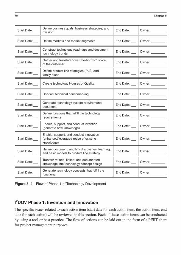
I2DOV Phase 1: Invention and Innovation
The specific issues related to each action item (start date for each action item, the action item, enddate for each action) will be reviewed in this section. Each of these action items can be conductedby using a tool or best practice. The flow of actions can be laid out in the form of a PERT chartfor project management purposes.
78 Chapter 5
Define markets and market segments
Gather and translate "over-the-horizon" voiceof the customer
Start Date: End Date: Owner:
Define business goals, business strategies, andmission
Start Date: End Date: Owner:
Start Date: End Date: Owner:
Construct technology roadmaps and documenttechnology trends
Start Date: End Date: Owner:
Define product line strategies (PLS) andfamily plans
Start Date: End Date: Owner:
Conduct technical benchmarking
Define functions that fulfill the technologyrequirements
Start Date: End Date: Owner:
Create technology Houses of QualityStart Date: End Date: Owner:
Start Date: End Date: Owner:
Generate technology system requirementsdocument
Start Date: End Date: Owner:
Enable, support, and conduct invention(generate new knowledge)
Start Date: End Date: Owner:
Enable, support, and conduct innovation(enhanced/leveraged reuse of existingknowledge)
Transfer refined, linked, and documentedknowledge into technology concept design
Start Date: End Date: Owner:
Start Date: End Date: Owner:
Refine, document, and link discoveries, learning,and basic models to product line strategy
Start Date: End Date: Owner:
Generate technology concepts that fulfill thefunctions
Start Date: End Date: Owner:
Figure 5–4 Flow of Phase 1 of Technology Development

Define Business Goals, Business Strategies, and Mission
We generally view the invention and innovation phase as the beginning of technology develop-ment. It is also the beginning of the Critical Parameter Management process. Before any tech-nology development work can begin, the foundations of the business must be well defined. Thebusinesses goals, strategy, and mission need to be clearly established. Corporate leaders mustdocument short-term and long-term business and financial targets that constitute their goals. Theymust have a documented plan that will achieve the goals. This constitutes their strategy. The lead-ers of the business must work with the board of directors to document a mission statement thatdefines their core values that provide boundaries for the businesses strategic framework and goalsetting process. Everyone must understand why the business exists.
Define Markets and Market Segments
At this step the market and technology teams discover where to gather the longer-term, “over-the-horizon” voice of the customer. Defined markets and market segments are essential to guiding theadvanced product planning team as it goes out to discover what customers need so team memberscan apply their core competencies properly. Once it is clear what market segments exist, the ad-vanced product planning team can conduct more specific market-focused voice of the customergathering activities. Technologies may be developed to apply across or within market segments. Itis important to define when technology needs are synergistic across market segments because thiswill clearly signal to the R&D leaders that a major platform opportunity exists. If a technology plat-form can be developed to serve “across market” commercialization requirements, great economiesof scale can be attained. This scenario leads to the single investment of capital that can deliverprofit from numerous family lines of products. To a lesser extent, profit amplification can occurwithin a market segment by developing a technology platform that can serve within market prod-uct family plan requirements. Market segmentation is a great help in product family planning.Without it companies don’t know when or how to divide R&D resources to help attain market shareand when to integrate resources to attain economies of scale in the use of their R&D resources.
Construct Technology Roadmaps and Document Technology Trends
Technology roadmaps are concurrently developed with the market segmentation documents.They help the business and technical leaders structure what technology development projectsshould be undertaken during the first phase of technology development.
Technology roadmaps document past and current technology patents, cost structures, per-formance, and development cycle-times. They also develop future technology forecasts withinand outside the company. A good technology roadmap will contain the following three items:
1. Historical technologies that have completed their life cycles. They should containdocumented development cycle-times, costs vs. generated revenue streams, and the de-tails of their functional performance during their life cycles.
Technology Development Using Design For Six Sigma 79

2. Current technologies that are yet to complete their life cycles. Their performance,cost, and development cycle-times should all be documented.
3. Future technologies should be scoped for estimated cost, development cycle-time,and functional performance capabilities. These projections should be based both ontechnology trend forecasting and the long-range voice of the customer assessment. La-tent customer needs are estimated within this form of documentation.
Gather and Translate “Over-the-Horizon”Voice of the Customer
The use of voice of the customer data is essential for circumspect advanced product planning.Pure invention and innovation that is not in some way linked to customer needs can produce tech-nology that is protected by a deep portfolio of uncommercializable patents. This is referred to asdesign for patentability. If your company is not careful, it can produce what is called a 6-foot-deep patent portfolio. This occurs when unbridled R&D organizations develop technology inde-pendent from the inbound marketing group and the advanced manufacturing organization. Thecompany becomes rich in patents that are incapable of being successfully transferred into revenue-bearing commercialization projects. A good question to ask about your company’s patentportfolio is, “What is the revenue bearing product hit rate based on the patent portfolio?”
It is essential that the technologists participate in gathering, ranking, and translating cus-tomer needs as part of the advanced product/technology planning process. This helps them be cir-cumspect as they seek balance between their internal inventive activities and the development oftechnologies that fulfill explicit, external market needs. However, it is entirely possible to followthe voice of the customer into a business failure (Christenson, 2000). Invention of new technolo-gies that surpass known customer needs, often called latent needs, will often play a key role innew product development.
Part of the technology development process includes the invention and discovery of uniquephenomena that may be able to be refined into a safe and mature technology independent of anyknown customer need. The focus in this case is on “the observation, identification, description,experimental investigation and theoretical explanation of natural phenomena.” This is the defini-tion of science from the American Heritage Dictionary and is largely what embodies the processof invention. The voice of the customer data may or may not play a strong role in the “discoveryof science” process. Scientists and engineers who participate in the invention process may useVOC data to guide their thinking but many do not like any constraints on their thought processes.There are really only two choices to make during technology development:
1. Recognize market needs and then drive the inventive processes so that the discoveryof physical law is directly targeted to be commercially useful according to an advancedproduct planning strategy.
2. Just invent in an unrestrained fashion and if what you come up with somehow is com-mercially useful, Bravo! You have good luck.
80 Chapter 5

Define Product Line Strategies (PLS) and Family Plans
Long-range customer needs are initially defined in broad terms and are then refined into productline technology requirements based on market segmentation. The R&D organization should helpgather and process this customer information. Once the long-range VOC data is used to definemarket segment needs, additional VOC data can be acquired to develop specific product line orfamily requirements. R&D teams use documented product line requirements as the basis for de-veloping platform technologies, system and subsystem technologies that can be used as a basisfor a family of products. The platforms are intended to fulfill the voice of the customer require-ments over a family of commercial products. Requirements for individual technologies that mayor may not support a platform are also identified and documented. Unfortunately, family planningthat is tactically fulfilled by a technology development process is largely nonexistent in manymodern companies.
Create Technology Houses of Quality
The VOC data for a specific market segment will be used to document a product line strategy anda series of embryonic family plans. The specific needs projected by the long-range VOC data andthe technology roadmaps will provide the balanced input needed to construct a series of technol-ogy Houses of Quality. The balance comes from the integration of the voice of the customer andthe voice of technology.
A technology House of Quality is created using a matrix approach while translating tech-nology needs into technology requirements. Once a group of technology requirements is definedfor a family of products, the R&D team can begin the highly technical task of defining and developing physical functions that fulfill the requirements. These physical functions lie at theheart of conceptual development of technology architectures that can ultimately become a plat-form. A technology House of Quality is the foundation upon which a platform is conceived andarchitected.
Conduct Technology Benchmarking
A major portion of a technology House of Quality is dependent upon three forms of comparativeinformation:
1. Projected customer opinions and perceptions of existing and new trends in technologythat will drive fulfillment of their needs in product performance.
2. Projected technology progressions based on current and foreseeable technological innovations. Frequently these are forecasted in the latest patents and invention disclosures.
3. Current technology benchmarking that assesses the state of the art in technology beingapplied in new products that are currently on the commercialization scene.
Technology Development Using Design For Six Sigma 81
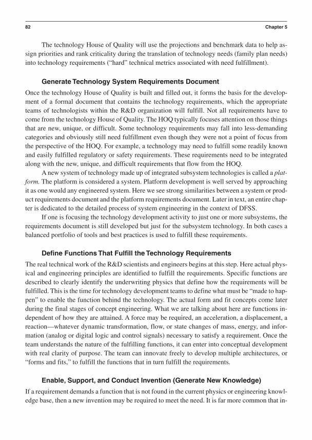
The technology House of Quality will use the projections and benchmark data to help as-sign priorities and rank criticality during the translation of technology needs (family plan needs)into technology requirements (“hard” technical metrics associated with need fulfillment).
Generate Technology System Requirements Document
Once the technology House of Quality is built and filled out, it forms the basis for the develop-ment of a formal document that contains the technology requirements, which the appropriateteams of technologists within the R&D organization will fulfill. Not all requirements have tocome from the technology House of Quality. The HOQ typically focuses attention on those thingsthat are new, unique, or difficult. Some technology requirements may fall into less-demandingcategories and obviously still need fulfillment even though they were not a point of focus fromthe perspective of the HOQ. For example, a technology may need to fulfill some readily knownand easily fulfilled regulatory or safety requirements. These requirements need to be integratedalong with the new, unique, and difficult requirements that flow from the HOQ.
A new system of technology made up of integrated subsystem technologies is called a plat-form. The platform is considered a system. Platform development is well served by approachingit as one would any engineered system. Here we see strong similarities between a system or prod-uct requirements document and the platform requirements document. Later in text, an entire chap-ter is dedicated to the detailed process of system engineering in the context of DFSS.
If one is focusing the technology development activity to just one or more subsystems, therequirements document is still developed but just for the subsystem technology. In both cases abalanced portfolio of tools and best practices is used to fulfill these requirements.
Define Functions That Fulfill the Technology Requirements
The real technical work of the R&D scientists and engineers begins at this step. Here actual phys-ical and engineering principles are identified to fulfill the requirements. Specific functions aredescribed to clearly identify the underwriting physics that define how the requirements will befulfilled. This is the time for technology development teams to define what must be “made to hap-pen” to enable the function behind the technology. The actual form and fit concepts come laterduring the final stages of concept engineering. What we are talking about here are functions in-dependent of how they are attained. A force may be required, an acceleration, a displacement, areaction—whatever dynamic transformation, flow, or state changes of mass, energy, and infor-mation (analog or digital logic and control signals) necessary to satisfy a requirement. Once theteam understands the nature of the fulfilling functions, it can enter into conceptual developmentwith real clarity of purpose. The team can innovate freely to develop multiple architectures, or“forms and fits,” to fulfill the functions that in turn fulfill the requirements.
Enable, Support, and Conduct Invention (Generate New Knowledge)
If a requirement demands a function that is not found in the current physics or engineering knowl-edge base, then a new invention may be required to meet the need. It is far more common that in-
82 Chapter 5

novation is used to integrate and extend applications of known physical principles and engineer-ing science. It is extremely important to note that the risk associated with this set of activitiesforces us to recommend that one stay clear of conducting technology development within prod-uct commercialization processes. When you get to the point of a required invention, it is likelythat developing the right function may be extremely difficult or impossible. Invention can burnup a lot of time—time you simply do not have in a product commercialization project that is tiedto a launch date. When this happens to a “design” that is really just an uncertified technology thathas been prematurely inserted into a commercialization project, the project schedule is usuallycompromised and profound implications arise for meeting the market window of the product.This form of “untamed technology” holds the impending revenues hostage! Our recommendationis not to mix uncertified technologies into your product commercialization projects.
Enable, Support, and Conduct Innovation (Enhanced/Leveraged Reuse of Existing Knowledge)
Innovation is by far the most popular form of developmental activity that characterizes R&Dprocesses as we enter the 21st century. Some call it applied research and development. The oper-ative word is applied. What that word means is that there is a preexisting technology knowledgebase available for reuse. This documented knowledge is available to be applied by either using itin a novel way or by extending or advancing the state of the art. Most baccalaureate and masterslevel engineers are trained to extend the state of the art while most doctoral level engineers andscientists are prepared to create and discover new knowledge. To some, this may not be a clearpoint of distinction, but those of us who have been in a situation where time is of the essence knowthat invention of new knowledge is simply not a timely option. We must take what is known anduse it to get the technology developed to meet the needs of our colleagues in product design.
Refine, Link, and Document Discoveries, Learning,and Basic Models to PLS
Once new knowledge and reused, but newly extended, knowledge have been developed, it istime to complete the construction of an important bridge. That bridge links what the team hasdocumented as a knowledge base to a set of well-defined application requirements related to thefamily of products that will flow from the product line strategy. This is how we integrate thepractical results being born out of the technology strategy with the product line strategy, ulti-mately fulfilling the business strategy.
The long-range voice of the customer and our benchmarked voice of technology lead us to construct a technology House of Quality that leads us to a technology requirements documentthat leads us to define technology functions that enabled the fulfillment of these diverse needs.The knowledge of “functionality fulfillment” must be held up to the product line strategy in atechnology review and answer the questions about whether and how we can get there from here. This is a test of feasibility prior to investing a lot of time and resources in concept genera-tion. The business leaders should see a rational flow of fulfillment at this point. If it is not clear,
Technology Development Using Design For Six Sigma 83

then further work needs to be done to bring all the fulfillment issues into alignment with the prod-uct line strategy.
Transfer Refined, Linked, and Documented Knowledge into Technology Concept Design
It is time to move all the knowledge forward into a format that enables the next stage of technol-ogy development known as technology concept development. The functions and requirementsmust be documented so that a rational set of concept generation, evaluation, and selection crite-ria can be rapidly developed. If there is ambiguity about what the concepts must do and fulfill,then the concepts will inevitably suffer from competitive vulnerability and will be functionallyinferior. Concept selection is yet another test of feasibility, but this time it has to do with bothfunctional and architectural potential to fulfill the technology requirements.
Generate Technology Concepts That Fulfill the Functions
The technology team now focuses the full weight of its individual and corporate developmentskill to generate candidate architectures to fulfill the functions and requirements that have beentied back to the product line strategy.
For integrated subsystems of technologies, the goal of the team is to first define a number ofcandidate system architectures, or platforms. Platforms are used to produce a number of productsfrom one investment of capital within the R&D organization. Platforms are necessary to make effi-cient use of business capital to fulfill product line strategies. It is hard to fulfill long-range businessstrategies through R&D projects that deliver one subsystem at a time for refitting onto aging prod-ucts. It is fine if a company uses a mixed technology development strategy of delivering some newsubsystems to extend existing product families while new platforms are on the way. Eventually anew platform must emerge to sustain the business as markets and technologies evolve. In some busi-ness models technology turnover is so rapid that the notion of a reusable platform does not apply.
Numerous candidate subsystem or platform concepts need to be generated. If a single con-cept dominates from one strong individual or “clique” within the R&D organization, the likeli-hood of the identifying best possible concept is not going to be attained. The entire team shouldbreak up and generate several concepts as individuals. After many concepts are generated, thenthe team convenes to evaluate and integrate the best ideas into a superior “super-concept” that islow in competitive vulnerability and high in functional feasibility. This state of superiority isachieved through consensus by the technology development team using concept selection crite-ria from the previously developed functions and requirements.
Gate 1 Readiness
At this early point in technology development a business should have a proprietary, documentedbody of science, documented customer needs for future product streams, and the embryonic tech-nical building blocks that can be developed into candidate technologies. The term fuzzy front endis appropriate to characterize the nature of this phase of technology development. We don’t have
84 Chapter 5

mature technologies yet—just the science, customer needs, and candidate concepts from whichwe hope to derive them.
With a viable cache of candidate technical knowledge and a well-planned commercial con-text in which to apply that knowledge, we approach a rational checkpoint to assess readiness tomove on into formal technology development.
Whether technology is built on completely new knowledge or integrated from existingknowledge (something we call leveraged technology), critical parameter relationships will needto be identified, stabilized, modeled, documented, desensitized to sources of variation, and in-tegrated across functional and architectural boundaries. Many of the delays that are incurred dur-ing product commercialization are due to technologies that have incomplete understanding anda lack of documentation of critical parameter relationships. As far as this text is concerned, nodifference is made between newly invented technologies or innovations that reuse existing tech-nologies. Both situations require structured, disciplined R&D teamwork to safely deliver “cer-tified” technologies to the commercialization teams. Once a certified technology is in the handsof a strong commercialization team, the team can rapidly transform it into capable designs.These issues must be foremost in the minds of the decision makers as the technology develop-ment process flows through its phases and gates.
At Gate 1 we stop and assess the candidate technologies and all the data used to arrive atthem. The tools and best practices of Phase 1 have been used, and their key results can be sum-marized in a Gate 1 scorecard (Figure 5–5). A checklist of Phase 1 tools and their deliverables canbe reviewed for completeness of results and corrective action in areas of risk. Figure 5–6 definesthe processes of I2DOV Phase 2.
General Checklist of Phase 1 Tools and Best Practices
Technology roadmapping
VOC gathering methods
KJ analysis
QFD/House of Quality—Level 1 (system level)
Patent analysis and exposure assessment
Market segmentation analysis
Economic and market trend forecasting
Business case development methods
Competitive benchmarking
Scientific exploration methods
Knowledge-based engineering methods
Math modeling (business cases, scientific and engineering analysis)
Concept generation techniques (TRIZ, brainstorming, brain-writing, etc.)
Modular and platform design
System architecting methods
Technology Development Using Design For Six Sigma 85
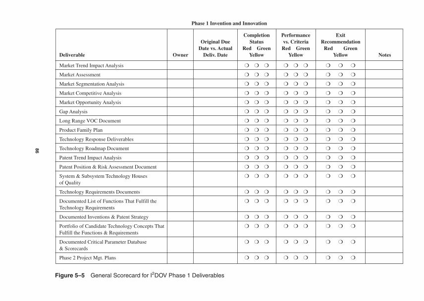
86
Phase 1 Invention and Innovation
Completion Performance Exit Original Due Status vs. Criteria Recommendation
Date vs. Actual Red Green Red Green Red GreenDeliverable Owner Deliv. Date Yellow Yellow Yellow Notes
Market Trend Impact Analysis
Market Assessment
Market Segmentation Analysis
Market Competitive Analysis
Market Opportunity Analysis
Gap Analysis
Long Range VOC Document
Product Family Plan
Technology Response Deliverables
Technology Roadmap Document
Patent Trend Impact Analysis
Patent Position & Risk Assessment Document
System & Subsystem Technology Houses
of Quality
Technology Requirements Documents
Documented List of Functions That Fulfill the
Technology Requirements
Documented Inventions & Patent Strategy
Portfolio of Candidate Technology Concepts That
Fulfill the Functions & Requirements
Documented Critical Parameter Database
& Scorecards
Phase 2 Project Mgt. Plans
Figure 5–5 General Scorecard for I2DOV Phase 1 Deliverables
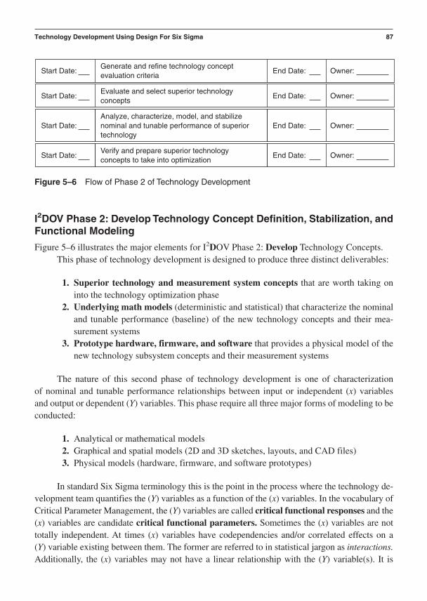
I2DOV Phase 2: Develop Technology Concept Definition, Stabilization, andFunctional Modeling
Figure 5–6 illustrates the major elements for I2DOV Phase 2: Develop Technology Concepts.This phase of technology development is designed to produce three distinct deliverables:
1. Superior technology and measurement system concepts that are worth taking oninto the technology optimization phase
2. Underlying math models (deterministic and statistical) that characterize the nominaland tunable performance (baseline) of the new technology concepts and their mea-surement systems
3. Prototype hardware, firmware, and software that provides a physical model of thenew technology subsystem concepts and their measurement systems
The nature of this second phase of technology development is one of characterization of nominal and tunable performance relationships between input or independent (x) variables and output or dependent (Y) variables. This phase require all three major forms of modeling to beconducted:
1. Analytical or mathematical models2. Graphical and spatial models (2D and 3D sketches, layouts, and CAD files)3. Physical models (hardware, firmware, and software prototypes)
In standard Six Sigma terminology this is the point in the process where the technology de-velopment team quantifies the (Y) variables as a function of the (x) variables. In the vocabulary ofCritical Parameter Management, the (Y) variables are called critical functional responses and the(x) variables are candidate critical functional parameters. Sometimes the (x) variables are not totally independent. At times (x) variables have codependencies and/or correlated effects on a (Y) variable existing between them. The former are referred to in statistical jargon as interactions.Additionally, the (x) variables may not have a linear relationship with the (Y) variable(s). It is
Technology Development Using Design For Six Sigma 87
Evaluate and select superior technologyconcepts
Verify and prepare superior technologyconcepts to take into optimization
Start Date: End Date: Owner:
Generate and refine technology conceptevaluation criteria
Start Date: End Date: Owner:
Start Date: End Date: Owner:
Analyze, characterize, model, and stabilizenominal and tunable performance of superiortechnology
Start Date: End Date: Owner:
Figure 5–6 Flow of Phase 2 of Technology Development

important to be able to quantitatively state whether the relationship is linear, nonlinear, and the ex-tent of the nonlinearity if proven to exist. Lastly, we need to know which (x) variables have an abil-ity to adjust or tune the mean value of (Y) without having a large effect on the standard deviationof the (Y) variable. The statistical variable used to quantify this relationship is the coefficient ofvariation (COV): (/ybar) 100. The COV is also the basis for an important measure of robust-ness, the signal-to-noise (S/N) ratio, during the optimization phase.
The (x) variables are often broken down into two distinct categories: control factors andnoise factors. Control factors are (x) variables that can readily be controlled and specified by thetechnology development team. Noise factors are (x) variables that are not easily controlled orspecified by the engineering team. Sometimes the (x) variables are impossible to control. Thisphase of technology development provides the first cut at distinguishing control factors fromnoise factors. The (x) factors that are found to be marginally controllable or extremely difficult orexpensive to control can be isolated for special attention. If the situation is bad enough, the tech-nology concept may need to be refined or abandoned. If the concept is found to be nominally sta-ble and tunable, the team can treat these poorly behaved control factors as noise factors duringthe optimization phase of technology development.
The multifunctional team that initiates technology concept development is typically madeup of some or all of the following personnel:
• Scientists from various technical domains• Development engineers from various technical domains• Advanced manufacturing engineers• Service specialists• Product planning and inbound marketing specialists• Supply chain development specialists• Health, safety, environmental, & regulatory specialists• Technology development partners from industry, academia, and government• Selected customers
Generate and Refine Technology Concept Evaluation Criteria
Concepts must be evaluated against a set of criteria that is directly related and traceable to thetechnology requirements. In fact, the concept evaluation criteria can literally be the technologyrequirements with little or no refinement from the statements found in the technology require-ments document. It is perfectly acceptable to develop the evaluation criteria prior to generatingthe concepts. Whether one uses the technology requirements document or the typically broaderand more detailed evaluation criteria to develop technology concepts is up to the team.
Concept evaluation criteria consist of all key requirements that must be satisfied by thetechnology concept. These criteria must comprehensively represent VOC, VOT, and productline strategy requirements. One of the reasons KJ analysis (affinity diagramming) is so impor-tant is that it helps state VOC needs and VOT issues in a hierarchy of relationships and in a rankorder of importance. This information will help the technology development team form a com-prehensive list of critical evaluation criteria. All concepts will be evaluated against a “Best-in-
88 Chapter 5

Class” benchmark datum concept. It is not uncommon for one or more of the new candidate con-cepts to bring new criteria to the forefront. This new criteria springs from innovation and new-ness embodied in the candidate concepts. Care should be taken not to miss these new criteriathat help discriminate and refine conceptual feasibility during the Pugh concept evaluationprocess.
Evaluate and Select Superior Technology Concepts
At this point the Pugh concept selection process is used to evaluate the set of candidate conceptsagainst the datum concept. The Pugh process uses an iterative converging–diverging process toevaluate concepts. The ranking of each candidate concept vs. the datum is nonnumeric and usessimple () better than the datum, () worse than the datum, or (S) same as the datum, rankingdesignations against the evaluation criteria. The iterative converging–diverging process is used toweed out weak concept elements, enabling the integration of hybrid, super-concepts from theremnants of candidates that have strong elements against the datum. Iterative “pulses” of conceptscreening and synthesis build up a small, powerful set of newly integrated hybrid concepts thattypically have the capacity to equal or surpass the datum relative to the superior fulfillment of theevaluation criteria (see Chapter 17 on the Pugh process).
Analyze, Characterize, Model, and Stabilize Nominal and TunablePerformance of Superior Technology
Once a superior concept or two have been defined from iterations through the Pugh concept se-lection process, the team is ready to conduct an extensive technical characterization. It is not abad idea to have a backup concept as a safety valve in case the superior concept possesses a fatalflaw that was missed during the Pugh process. The superior concepts are only proven to be lowin competitive vulnerability and high in technological superiority relative to the datum. They areworth the investment required to certify the new technology’s nominal and tunable performanceprior to optimization. Once in a while a superior concept passes the concept evaluation processonly to be found unusable under the deeper analytical scrutiny of this next step in the develop-ment of the technology. As you can see, Phase 2 is crucial for weeding out technologies that areoften “time bombs” when allowed to creep into a product commercialization process withoutproper development and scrutiny. Conducting failure modes and effects analysis on the superiorconcepts at this point is extremely valuable in exposing risks.
The analysis and characterization must include the development of all key Y as a function ofx relationships. As previously mentioned each relationship must be quantified in terms of nominaland tunable performance. Linear and nonlinear relationships must be defined. Interactions betweencontrol factors must be identified. If these relationships are a problem, the interactive relationshipsmust be reengineered so that the codependency between control factors will cause severe variationcontrol problems later in the product commercialization process. This reengineering to survive interactivity between control factors, called design for additivity, can first be approached in Phase2 of technology development and finalized in the Phase 3 optimization activities. In Phase 3 weadd the additional characterization of interactions between control factors and noise factors, themain focus of robust design.
Technology Development Using Design For Six Sigma 89

The most important knowledge that must come from this phase of technology development isthe quantification of the ideal/transfer functions that underwrite the basic performance of the tech-nology. In the next phase we will evaluate the controllable (x) variables that govern the performanceand adjustability of the ideal/transfer function for their robust set points in the presence of the un-controllable (x) variables known as noise factors. If we have incomplete or immature forms of the“Y is a function of x” relationships and fail in our attempt to attain robustness, we can pass along yetanother “time bomb” for our peers in product commercialization. By “time bomb” we mean a tech-nology that gets integrated into a product system and “blows up” by producing unacceptable or un-controllable performance with little or no time left to correct the problem. Technology that is poorlydeveloped and characterized is a major reason why product delivery schedules slip.
Certify and Prepare Superior Technology Concepts to Take into Optimization
It is challenging to know when a team has enough knowledge developed to state that a new tech-nology is truly ready to go forward into the optimization phase of technology development. Let’slook at a list of evidence that could convict us in a court of law of having conducted a thoroughcharacterization of a technology’s nominal and tunable performance.
1. Math models that express the “ideal function” of the technology:a. First principles math models
i. Linear approximation of Yf(x)ii. Nonlinear approximation of Yf(x)
b. Empirical math modelsi. Linear approximation of Yf(x)
ii. Interactions between control factorsiii. Nonlinear approximation of Yf(x)
2. Graphical modelsa. Geometric/spatial layout of the subsystem and platform technologiesb. Component drawings in enough detail to build prototypes
3. Physical modelsa. Prototype subsystemsb. Prototype componentsc. Measurement systems
i. Transducersii. Meters
iii. Computer-aided data acquisition boards and wiringiv. Calibration hardware, firmware, and software
4. Critical Parameter Management dataa. Mean values of all critical functional responsesb. Baseline standard deviations of all critical functional responses (without the effects
of noise factors)
90 Chapter 5
c. Cp of all critical functional responses (without the effects of noise factors)d. Coefficient of variation (COV) of all critical functional responses (without the ef-
fects of noise factors)e. List of control factors that have a statistically significant effect on the mean of all
critical functional responses, including the magnitude and directionality of thiseffect
f. List of control factors that have a statistically significant effect on the standard de-viation of all critical functional responses, including the magnitude and direction-ality of this effect (without the effects of noise factors)
g. List of control factors that have a statistically significant effect on the coefficient of variation (COV) of all critical functional responses (without the effects of noisefactors)
h. List of control factors that have statistically significant interactions with one an-other, including the magnitude and directionality of this effect
i. List of CFRs that have statistically significant interactions (correlations) with oneanother at the subsystem and system level (including the magnitude and direction-ality of this effect)
We must be able to answer a simple question: If we change this variable, what effect doesthat have on all the critical functional responses across the subsystem? We have to get this nom-inal performance knowledge first, in the absence of statistically significant noise factors. We willrefine this knowledge in Phase 3 where the major emphasis is on intentional stress testing of thebaseline subsystem technology with statistically significant noise factors. But before we can op-timize robustness of the subsystem technology, we must characterize its control factors for theirnominal contributions to “Y is a function of x” relationships.
We must be able to account for critical correlations, sensitivities, and relationships withineach new subsystem technology under nominal conditions. If we lack knowledge of these funda-mental, critical relationships, the technology is risky due to our partial characterization of its ba-sic functional performance. The development team has no business going forward until thesethings are in hand in a summary format for key business leaders and managers to assess. If theydon’t assess this evidence, they are putting the future cycle-time of the product commercializa-tion projects at risk.
Gate 2 Readiness
If technology is allowed to escape Phase 2 with anemic characterization, it is almost a sure betthat someone down the line will have to pay for the sins of omission committed here. In a veryreal sense the capital being invested in the new technology is being suboptimized. A great dealmore capital will have to be spent to make up for the incomplete investment that should haveoccurred right here. You can either pay the right amount now (yes, it always seems a high priceto pay) and get the right information to lower your risks or be “penny wise and pound fool-ish” and pay really big later when you can least afford it in both time and money! Phase 2 of
Technology Development Using Design For Six Sigma 91

technology development is truly the place to rigorously practice an old adage: Do it right thefirst time.
The following checklist outlines Phase 2 tools and best practices, while Figure 5–7 offersa Phase 2 scorecard. Then we move on to Phase 3 of I2DOV in Figure 5–8.
General Checklist of Phase 2 Tools and Best Practices
Pugh concept selection process
Knowledge-based engineering methods
Math modeling (functional engineering analysis)
Concept generation techniques (TRIZ, brainstorming, brain-writing)
Measurement system development and analysis
Hypothesis formation and testing
Descriptive and inferential statistics
Design of experiments
Regression analysis
Response surface methods
FMEA, fault tree analysis
Modular and platform design
System architecting methods
Prototyping methods (e.g., soft tooling, stereo lithography, early supplier involvement)
Cost estimating methods
Risk analysis
Critical Parameter Management
Project management methods
I2DOV Phase 3: Optimization of the Robustness of the Subsystem Technologies
Figure 5–8 illustrates the major elements for I2DOV Phase 3: Optimize subsystems.With the approval to enter the third phase of technology development, the new technologies havebeen proven to be worth the further investment required to optimize their performance. Opti-mization of a new technology focuses on two distinct activities:
1. Robustness optimization of the critical functional responses (CFRs) against a genericset of noise factors that the design will likely see in a downstream product commer-cialization application (per the deployment schedule based on the family plan strategy)
2. Certification of adjustment factors that have the capability to place the mean of thetechnology’s CFRs on to a desired target within the dynamic range specified by the ap-plication requirements from the family plan
92 Chapter 5

93
Phase 2 Develop Technology
Completion Performance Exit Original Due Status vs. Criteria Recommendation
Date vs. Actual Red Green Red Green Red GreenDeliverable Owner Deliv. Date Yellow Yellow Yellow Notes
Project Cost Magnitude Estimate
Project Type (Platform or Subsystem Technology
Development)
Documented & Verified Analytical & Empirical
Models (Ideal Functions)
Documented Empirical Data to Support the
Verification of the Analytical Models
Documented Critical Functional Responses &
Data Acquisition Means with %R&Rs & P/TRatios Certified
Documented Ideal Functions of the Superior
Technology Concepts
Documented FMEA Analysis
Documented Dynamic Adjustment Factors for
Platforms & Singular Technologies
Documented Critical Parameter Database& Scorecards
Documented Critical Parameters for
Manufacturing Process Technologies
Risk Assessments for Functions and Parameters
that are unstable or overly sensitive
Prototype Hardware, Firmware, & Software
Phase 3 Project Mgt. Plans
Figure 5–7 A General Scorecard for I2DOV Phase 2 Deliverables: Develop Technology Concepts
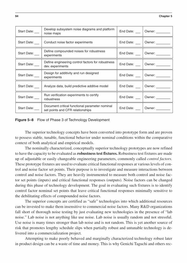
The superior technology concepts have been converted into prototype form and are provento possess stable, tunable, functional behavior under nominal conditions within the comparativecontext of both analytical and empirical models.
The nominally characterized, conceptually superior technology prototypes are now refinedto have the capacity to be evaluated as robustness test fixtures. Robustness test fixtures are madeup of adjustable or easily changeable engineering parameters, commonly called control factors.These prototype fixtures are used to evaluate critical functional responses at various levels of con-trol and noise factor set points. Their purpose is to investigate and measure interactions betweencontrol and noise factors. They are heavily instrumented to measure both control and noise fac-tor set points (inputs) and critical functional responses (outputs). Noise factors can be changedduring this phase of technology development. The goal in evaluating such fixtures is to identifycontrol factor nominal set points that leave critical functional responses minimally sensitive tothe debilitating effects of compounded noise factors.
The superior concepts are certified as “safe” technologies into which additional resourcescan be invested to make them insensitive to commercial noise factors. Many R&D organizationsfall short of thorough noise testing by just evaluating new technologies in the presence of “labnoise.” Lab noise is not anything like use noise. Lab noise is usually random and not stressful.Use noise is many times stronger than lab noise and is not random. This is yet another source ofrisk that promotes lengthy schedule slips when partially robust and untunable technology is de-livered into a commercialization project.
Attempting to make poorly behaved and marginally characterized technology robust laterin product design can be a waste of time and money. This is why Genichi Taguchi and others rec-
94 Chapter 5
Conduct noise factor experiments
Define compounded noises for robustnessexperiments
Start Date: End Date: Owner:
Develop subsystem noise diagrams and platformnoise maps
Start Date: End Date: Owner:
Start Date: End Date: Owner:
Design for additivity and run designedexperiments
Analyze data, build predictive additive model
Start Date: End Date: Owner:
Define engineering control factors for robustnessdev. experiments
Start Date: End Date: Owner:
Start Date: End Date: Owner:
Run verification experiments to certifyrobustness
Document critical functional parameter nominalset points and CFR relationships
Start Date: End Date: Owner:
Start Date: End Date: Owner:
Figure 5–8 Flow of Phase 3 of Technology Development

ommend the development of dynamic technology based on well-characterized ideal functions, aswe discussed in Phase 2. The certified math models represent the ideal functions to which Taguchiso frequently refers. As a rule, robustness optimization activities should not come before the de-velopment of some form of credible analytical model. How rigorous and detailed the modelshould be is a matter of healthy debate that is based on economics as well as the application con-text. The rule is don’t waste your time trying to make a design that is unstable under nominal con-ditions and robust under stressful conditions. Only stable, well-characterized designs are worthtaking into the robustness optimization process.
Review and Finalize CFRs for the New Subsystem Technologies
Before starting any optimization activities, the development team must have a well-defined set ofcritical functional responses. In addition, each CFR must have a measurement system definedwith its capability documented in terms of repeatability and reproducibility, known as an R&Rstudy, and precision-to-tolerance ratio, known as a P/T ratio. To produce viable results, continu-ous variables that are scalar or vector measures of functions that directly fulfill requirements mustbe used. CFRs are what we measure and make “robust” when quantifying the effects of controlfactor and noise factor interactions. We prefer not to count defects but rather to measure functionswithin and across the integrated subsystems being developed as new platform technologies. Thisassures we measure fundamental Y outputs as we change fundamental x inputs.
During optimization, we assess the efficiency of the transformation, flow, or change of state ofmass, energy, and information (logic and control signals that provide information about the flow, trans-formation, or state of the mass and energy of the subsystems). The efficiency is measured under theconditions of intentionally induced changes to both control and noise factors. To measure the flow,transformation, and state of these physical parameters we must move beyond a counting mentality toa measurement context. Counting defects and assessing time between failures, while being measuresof “quality,” are reactive metrics that are only useful after the function has deteriorated. We need tomeasure impending failure. This requires the measurement of functions in the presence of the noisefactors that cause them to deteriorate over a continuum of time. We simply cannot wait until a failureoccurs. This preventative strategy leads us to our next topic—the description of the activities that fo-cus the development team’s attention on the “physics of noise” that disrupt the flow, transformation,or state of mass, energy, and information. This is the science of reliability development. We value re-liability prediction and evaluation, but they have little to do with the actual development of reliability.
Develop Subsystem Noise Diagrams and Platform Noise Maps
Noise has been described as any source of variation that disrupts the flow, transformation, or stateof mass, energy, and information. More specifically noise factors break down into three distinctcategories:
1. External sources of variation2. Unit-to-unit sources of variation3. Deterioration sources of variation
Technology Development Using Design For Six Sigma 95

It is extremely useful to create a noise diagram that documents specific noise factors thatfall under each of the categories shown in Figure 5–9.
The cross-functional development team, and downstream advisors from design, produc-tion, service/support organizations, and selected customers must identify all the noise factors thatpotentially have a statistically significant effect on each of the subsystem critical functional re-sponses. Once a subsystem has a noise diagram constructed for each CFR, linkage can be estab-lished between each of the subsystem noise diagrams. It is important to map noise transmissionpaths within and between subsystem technologies. When two or more subsystem technologies areintegrated to form a platform or some sort of higher-level system, then we must characterize hownoise from one subsystem affects the others. We also need to characterize the flow of noise fromthe platform out to other subsystems that may connect or interact with it. You can think of an en-gine as a platform made up of various subsystems, with the platform itself assembling into a caror truck or whatever type of product is being developed. If noise transmits beyond the platformto reach a customer, service engineer, or other external constituency, we must document that po-tential negative relationship. When we account for these paths of noise transmission, we begin tounderstand how to alter the control factors to help guide the CFRs into a state of robustnessagainst the noise. Insensitivity to noise is another way of communicating the meaning of robust-ness. If you don’t have a comprehensive, systemwide noise map, composed of subsystem noise
96 Chapter 5
Unit-UnitNoise Factors:1.2.3. . . .
ExternalNoise Factors:1.2.3. . . .
OutputNoise Factors:1.2.3. . . .
DeteriorationNoise Factors:1.2.3. . . .
SubsystemTechnology
Figure 5–9 A Subsystem Noise Diagram

diagrams, how can you possibly begin the task of making a new subsystem technology or plat-form robust and know when you have finished?
Conduct Noise Factor Experiments
We just mentioned that subsystem noise diagramming and system noise mapping documents noisefactors that might be statistically significant. We can’t tell whether any one of the noise factors is sta-tistically significant (if it has an effect on the CFR that is statistically distinguishable from randomevents within a given confidence interval in the functional environment of the subsystem technologyor platform) by sitting around a table talking about them in a conference room. It is imperative thatthe development team design an experiment to quantify the magnitude and directional effect of thosenoise factors selected for experimental evaluation. Failure modes and effects analysis can be used tohelp identify and screen noise factors for inclusion in the noise experiment.
A noise experiment is usually a two-level, fractional factorial designed experiment. It canbe set up as a full or fractional factorial design. If strong interactivity is suspected then a mini-mum of a Resolution V Fractional Factorial Design is recommended. If moderate-to-low inter-activity is anticipated between the noise factors, then a Resolution III Plackett-Burman Screen-ing Experiment (an L12 array) is capable of providing a good set of data upon which to conductANOVA, an acronym for analysis of variance results. This analysis will provide the informationrequired to tell if any noise factors are statistically significant.
The subsystem prototype is set up at its baseline set point conditions and held there whilethe noise factors are exercised at their high and low set point conditions. The mean values of theCFRs are calculated. Analysis of means will provide the data to explain the magnitude and di-rectionality of each noise factor on the CFR.
Define Compounded Noises for Robustness Experiments
The results from a noise experiment provide the evidence required to go forward in defining howto properly and efficiently stress test any given subsystem technology for robustness optimiza-tion. The statistically significant noise factors can now be isolated from the rest of the noise factors—they are the only noises worth using during robustness optimization experiments. Theothers are simply not producing a significant effect on the mean value of the CFRs. Using theanalysis of means data and their main effects plots, the development team can literally see the di-rectional effect the noise factor set points have on the mean values of the CFRs. The team canquantitatively demonstrate the effect of the significant noise factors. One more piece of guess-work is removed from the technology development process!
Noise factor set points that cause the mean of a subsystem CFR to rise significantly aregrouped or compounded together to form a compound noise factor, referred to as N1. Noise fac-tor set points that cause the mean of a subsystem CFR to fall significantly are grouped or com-pounded together to form a compound noise factor referred to as N2. Both compounded noisefactors have the same set of statistically significant noise factors within them. The difference isthe specific set points (high or low) that are associated with noise factor alignment with N1 or N2(see Chapter 28 on Robust Design for examples).
Technology Development Using Design For Six Sigma 97

This noise compounding strategy facilitates the unique and efficient gathering of two datapoints (data taken for each experimental treatment combination of control factors at N1 and N2compounding levels) during the exploration of interactivity between control factors and noise fac-tors. The reason we need to be sure we have real noise factors identified is that we want to induceinteractivity between control factors and noise factors to locate robust control factor set points. Ifthe noises are not truly significant, we are not going to be exposing the control factors to anythingthat will promote the isolation of a true robust set point. Much time can be wasted testing a con-trol factor against noises that are little more than random sources of variation that are not repre-sentative of what is going on in the actual use environment. Many R&D organizations only eval-uate “nominal optimal performance” in the sterile and unrealistic environment of random andinsignificant levels of noise. Their technology is then transferred to design in a state of relativeimmaturity and sensitivity. The design teams are left to deal with the residual problems of inca-pability of performance, which is certainly a design defect! The usual response is, “That’sfunny—it worked fine in our labs.” For those on the design team it is anything but funny.
Define Engineering Control Factors for Robustness DevelopmentExperiment
We now turn our attention to the control factors that will be candidates for changes to their baselineset points to new levels that leave the CFRs in a state of reduced sensitivity to the significant, com-pounded noise factors (N1 & N2). The selection of these control factors is not a trivial event. Not allcontrol factors will help in inducing robustness. In fact only those control factors that possess inter-actions with the noise factors will have an impact in reducing sensitivity to noise (see Figure 5–10).
We begin control factor selection using the information about the ideal functions [Y = f(x)]gained during Phase 2. Any control factor that had a significant effect in the underlying functionalmodel is a candidate control factor for robustness improvement. Actually we will be looking forthree kinds of performance from the candidate control factors:
1. Control factors that have moderate to strong interactions with the compounded noisefactors are good robustizing factors (good for minimizing the standard deviation evenwith the noises freely acting in their uncontrolled fashion in the use environment).
98 Chapter 5
CF
R (
σ)
N1
Sensitive tonoise
Insensitive tonoise
N2
A2
A1
Figure 5–10 A Control Factor to Noise Factor Interaction Plot

2. Control factors that have relatively weak interactions with the compounded noise fac-tors but have strong effects on shifting the mean value of a CFR are critical adjust-ment parameters (CAPs are good for recentering the function onto a desired target,thus forcing Cpk Cp).
3. Control factors that have low interactivity with the compounded noise factors and lowshifting effect on the mean of the CFR are good economic factors (allowing one to setthem at their lowest cost set points).
Design for Additivity and Run Designed Experiment
Using the knowledge from Phase 2 function modeling, assess the nature of the interactions be-tween the control factors (CF CF interactions). Apply the rules for additivity grouping or slid-ing levels based on how energy and mass are used in the ideal function to minimize or eliminatethe disruptive effects of antisynergistic interactions (see Chapter 28 for example). The experimentmust be set up to focus on producing data that exhibits and highlights the interactivity betweenthe control factors and the compounded noise factors. Within these CF NF interactions the ro-bustness optimization potential is found.
An appropriately sized array is selected to evaluate the control factor main effects and anycontrol factor control factor interactions (usually a few two-way interactions that were statisti-cally significant in the Phase 2 analysis). The typical array will be a three-level Fractional Factor-ial format. If additivity grouping or sliding levels are used to suppress or remove the effects of CF CF interactions that are not useful, it is common to use a Resolution III design (typically an L18Plackett-Burman experimental array). If useful two-way interactions between control factors are tobe evaluated, then a Resolution V or Full Factorial design must be used (remember, a ResolutionIV design will likely confound the two-way interactions with one another, as covered in more detailin Chapter 22). Since the compound noises are exposed equally to each row from the FractionalFactorial designed experiment, the control factor treatment combinations are aligned in a Full Fac-torial exposure to the noise. A full noise factor exposure to the Fractional Factorial control factorcombinations assures that the noise was faithfully and fully delivered to (interact with) the fractionof the possible design set points you selected. Using a Fractional Factorial noise exposure strategywould understress the control factors and leave the design at risk of missing a CF NF interactionthat could be exploited on behalf of your customer’s satisfaction! For those who think Taguchimethods are optional or ineffective, you may want to rethink that position. You are probably ig-noring a whole class of interactions (CF NF) that can make a big difference for your customers.
Analyze Data, Build Predictive Additive Model
The robust design experiment will produce a rich set of data that is capable of being analyzed bytwo common statistical methods:
1. Analysis of means (ANOM)a. Provides insight on which level of each CF is best for robustness (largest S/N) or
variance minimization (smallest or 2) of the CFR
Technology Development Using Design For Six Sigma 99
b. Provides insight on which control factors have the largest effect on the mean valueof the CFR (critical adjustment parameters)
2. Analysis of variance (ANOVA)a. Provides insight on which control factors have the largest effect relative to one
another and to the error variance in the entire data set (optional for S/N metric butquite useful for variance and mean analysis).
The development team will use the control factor set points that produced maximum im-provements in CFR robustness to construct a unique math model referred to as Taguchi’s addi-tive model (see Chapter 28). It is used to predict overall robustness gain in units of the decibel.The additive model is a prediction of the expected robustness for the CFR under evaluation.
Run Verification Experiments to Certify Robustness
The optimized control factor set points must be verified in the final step of robust design. Thesame set of compounded noise factors are reused during the verification experiments. It is com-mon to run a minimum of five replicate verification tests to prove that the predicted S/N, mean,and variance values are reproducible at these new set points. Baseline set point verification testsare also commonly conducted to see if the design acts the same way that it did back in Phase 2testing prior to robustness optimization. This helps assure the development team is not missingsome additional control or noise factors that are important to the safe transfer of the technologyfor commercial application.
It is also common to verify the dynamic range of the critical adjustment parameters that af-fect the adjustment of the mean value of the CFRs. The best approach is to conduct further opti-mization of these CAPs by using regression or response surface methods.
Document Critical Functional Parameter Nominal Set Points and CFR Relationships
Once the additive model and dynamic tuning capability of the subsystem technology has beenverified, it is time to document the new set points and tuning range limits. At this point the Crit-ical Parameter Management database is updated with the results of the Phase 3 quantitative de-liverables. The traceability of critical parameter relationships will be greatly enhanced with thedata from Phase 3.
Gate 3 Readiness
Phase 3 in the technology development process is used to take technology that is safe, stable, andtunable into a state of maturity that is insensitive to noise. Gate 3 is the place for assessing theproof that the new technology is robust to a general set of noise factors that will likely be en-countered in commercial application environments. It is also the place to assess the tunability ofthe CFR to global optimum targets using one or more critical adjustment parameters (see thePhase 3 scorecard in Figure 5–11).
100 Chapter 5
Technology Development Using Design For Six Sigma 101
General Checklist of Phase 3 Tools and Best Practices
Subsystem noise diagramming
System noise mapping
Measurement system analysis
Noise experiments
Taguchi methods for robust design
Design of experiments
Analysis of means
Analysis of variance
Regression
Response surface methods
Critical parameter management
Project management methods
I2DOV Phase 4: Verification of the Platform or Subsystem Technologies
Figure 5–12 illustrates the major elements for I2DOV Phase 4: Verify Integrated System (Plat-form) or Subsystem
The final phase of technology development (Figure 5–12) is primarily focused on integrat-ing and verifying the newly robust and tunable subsystem technologies into an existing productarchitecture or into a new platform architecture. The development of subsystems and platformsis verified for commercial readiness at the Phase 4 gate. The transfer of the new technologies toproduct design is dependent on transferability criteria (technology requirements) that will be ful-filled in this final phase of technology development.
The evaluations that are conducted during this phase are stressful by nature to help assurethe technologies are mature enough to transfer. Some technologists are averse to stress testingtheir “pampered” designs because they fear that they will be rejected and will not be used in thenext new product. If these individuals succeed in protecting their designs, they place every otheremployee in the company at risk and do great disservice to the customers of the business. Mosttechnology problems show up in product design when technologies have been prematurely de-ployed in a commercialization project. They were not thoroughly stress tested for robustness (S/Nand ) and capability (mean, Cp, and Cpk). They look and work fine until they are used in a con-text where real noise factors are applied to them, intentionally or otherwise. At this point their truecharacter emerges, and all hell breaks loose! They were not completely characterized, usually tosave face, time, and money, so they were transferred at great risk. When we reactively use thechecklists and scorecards at the end of each of the four gates of technology development, we canexpect to routinely uncover the risk that is building due to anemic and incomplete characteriza-tion. Risk can be managed much more efficiently if one proactively uses the checklists and score-cards to preplan for the successful application of a balanced set of tools and best practices. If one

Phase 3 Optimize Technology
Completion Performance Exit Original Due Status vs. Criteria Recommendation
Date vs. Actual Red Green Red Green Red GreenDeliverable Owner Deliv. Date Yellow Yellow Yellow Notes
Quantification & Identification of Statistically
Significant Noise Factors
Directionality & Magnitude of the Noise Vectors
Quantification & Identification of the Baseline
(before robustness optimization) and New (afterrobustness optimization) S/N Values for the Critical Functional Responses
Identification of Control Factors That Can be
Used to Improve Robustness (includes the Additive Model Parameters That Are Criticalto Robustness
Identification & Optimization of the Control
Factors That Can be used to Adjust the Mean onto a Given Target Without Overly Compromising Robustness
Verification Results from Additive Model
Confirmation Experiments
Cp & Cpk Values for the Pre- & Post-RobustnessOptimization Critical Functional Responses
Updated Critical Parameter ManagementDatabase & Scorecards
Project Mgt. Plans for Phase 4
Figure 5–11 A General Scorecard for I2DOV Phase 3 Deliverables
102

chooses to bypass certain tools and best practices, the technology will accrue certain risks. Thegates are designed to assess the accrual of risk and to stop or alter development when the risk getstoo high.
The fourth, “integrative” phase is extremely important and the one that most companies by-pass with reckless abandon. When development teams fail to integrate their new subsystemtechnologies into an existing product or the new platform and stress test them with statisticallysignificant noise factors, they fore-go obtaining the knowledge that assures the risk of transfer-ring the new technology is acceptable. Many say, “We can’t afford to develop technology in thisrigorous fashion.” They go on to claim, “We like to integrate and test (usually with very low lev-els of statistically insignificant noise) early during product design and find out where our problems
Technology Development Using Design For Six Sigma 103
Refine and confirm "between and within"subsystem CFRs
Develop, integrate, and verify platform dataacquisition systems
Start Date: End Date: Owner:
Integrate subsystems into platform test fixturesStart Date: End Date: Owner:
Start Date: End Date: Owner:
Conduct nominal performance tests
Evaluate data against technology requirements
Start Date: End Date: Owner:
Design platform or integrated subsystemnominal performance tests
Start Date: End Date: Owner:
Start Date: End Date: Owner:
Design platform or integrated subsystem stresstests
Conduct stress tests
Start Date: End Date: Owner:
Start Date: End Date: Owner:
Refine and improve platform or integratedsubsystem performance
Rerun stress tests and perform ANOVA on datato verify reduced sensitivities
Start Date: End Date: Owner:
Perform ANOVA on data to identify sensitivitiesStart Date: End Date: Owner:
Start Date: End Date: Owner:
Conduct reliability evaluations for new subsystemtechnologies and platforms
Document CFPs and CFR relationships andverify that the technology is transferable
Start Date: End Date: Owner:
Start Date: End Date: Owner:
Figure 5–12 Flow of Phase 4 of Technology Development
are and then fix (react to) them.” This is called build-test-fix engineering and is antithetical topreventing functional performance problems. This approach assures there are problems and seekscomfort in isolating and “fixing” them—typically over and over again. It is a recipe for high war-ranty costs; late product launches; many rounds of costly post-shipping modification kits; aggra-vated, overworked service engineers; and the loss of once-loyal customers. Even worse, from astrategic perspective, is the fact that this approach ties up R&D resources and design resourceson lengthy “reliability emergency assignments” that keep them away from working on the nextdesign project that is critical to future revenue generation. Build-test-fix engineering robs the cor-poration of its future generation of value, productivity, and economic growth. All the excuses forbuild-test-fix engineering end up being the most costly and inefficient way of doing business.
Integrate Subsystems into Platform or Product Test Fixtures
The optimized subsystems are now ready to be integrated into one of two types of systems forstress testing and performance certification:
1. An existing product2. A new platform that will form the basis of many new products
When the new subsystem or subsystems have been developed for integration into an exist-ing product that is currently in the marketplace, the R&D organization must obtain a sufficientnumber of these systems for stress testing and verification of integrated performance capability.
When the new subsystems are developed for integration into a new platform, then a signif-icantly different effort must be made to integrate the subsystems into a functioning system we rec-ognize as a platform. This is harder and requires more effort because there is no existing productto be reworked to accept the new subsystems. The platform is a whole new system. It is entirelypossible that numerous existing subsystem designs will be reused and integrated into the newplatform architecture during product design.
Refine and Confirm “Between and Within” Subsystem CFRs
Prior to conducting certification tests, the development team needs to identify exactly how thecritical functional responses are going to be measured as they transmit energy, mass, and infor-mation (analog and digital logic and control signals) across subsystem boundaries. Every sub-system has an “internal or within” set of CFRs defined for it already. These were developed andmeasured in the first three phases of technology development. Now that the team integrates allthe new subsystem technologies together, it is highly likely that there will be some need to mea-sure how the CFR from one subsystem affects the mating subsystem. If one subsystem receivesmass from another subsystem, then the mass flow rate will need to be measured as a “between”subsystem CFR. If the mechanism for mass flow or transfer is through the generation of a mag-netic flux, then that would be classified as a “within” subsystem CFR. The important issue hereis for the team to be comprehensive in accounting for CFRs that measure functional interface re-
104 Chapter 5

lationships. One helpful way to approach this accounting of CFRs at integration is to write en-ergy balancing equations to account for the flow, transfer, or state of change between energy andmass across the interface boundary. These “between” subsystem CFRs may have been definedpreviously during Phase 2 and Phase 3 but not measured in the real context of an integration test.The task now becomes one of measurement system development and analysis—our next topic.
Develop, Integrate, and Verify Platform Data Acquisition Systems
A data acquisition system capable of measuring all within and between subsystem, platform, orproduct level CFRs needs to be developed, integrated, and verified at this point. These systemsinclude numerous transducers that physically measure the CFRs, wiring, interface circuit boards,computers, and software that facilitate the collection, processing, and storage of the CFR data.
The data acquisition system will need to have its repeatability, reproducibility, and precision-to-tolerance ratio evaluated to assure that the measurements are providing the level pre-cision and accuracy required to verify the performance of all the CFRs.
Design Platform or Integrated Subsystem Nominal Performance Tests
The team will need to structure a series of performance tests to evaluate the Cp and Cpk of theCFRs under nominal conditions. This test is designed to look at the performance of all of theCFRs under nonstressful conditions. It represents the best you can expect from the subsystemsand the integrated platform or product at this point in time. These tests usually include normal useconditions and scenarios. All critical-to-function parameters within the subsystem and criticalfunctional specifications at the component level are set at their nominal values. Environmentalconditions are also set at nominal or average conditions.
Conduct Nominal Performance Tests
With a comprehensive, nominal condition test plan in hand, the team can move forward and con-duct the nominal performance tests. The data acquisition system is used to collect the majority ofthe performance data from the CFRs. It is likely that some independent, special forms of metrol-ogy may be needed to measure some of the CFRs, typically at the platform or product level. Theseare often called off-line evaluations. In some cases data must be gathered on equipment in anotherlab or site equipped with special analysis equipment.
Evaluate Data Against Technology Requirements
The data is now summarized and evaluated against the technology requirements. Here we discover just how well the CFRs are performing against their targets that were established backin Phase 1. This is likely to be the best data the team is going to see because it was collected under the best or nominal conditions. With the nominal capabilities of the CFRs in hand, the team is ready to get an additional set of capability data run under the real and stressful conditionsof noise.
Technology Development Using Design For Six Sigma 105

Design Platform or Integrated Subsystem Stress Tests
The exposure of new technologies to a statistically significant set of noise factors has been discussed in the Phase 3 robustness optimization process. We return to that topic within the newcontext of the integration of the robust subsystems. To be circumspect with regard to realisticallystressing the new platform technologies or existing products that are receiving new subsystemtechnologies, the team has to expose these systems to a reasonable set of noise factors.
The typical noise factor list includes numerous sources of variation that are known to pro-voke or transmit variation within the system integration context. A designed experiment is thepreferred inspection mechanism that is capable of intentionally provoking specific levels of stresswithin the integration tests. Designed experiments help assure that thorough and properly con-trolled amounts of realistic sources of noise are intentionally introduced to the integrated subsys-tems. Without this form of designed evaluation of the various CFRs associated with the integratedsubsystems, the technology is not fully developed and cannot be safely transferred into productcommercialization.
Conduct Stress Tests
Conducting a stress test under designed experimental conditions requires a good deal of plan-ning, careful set-up procedures, and rigorous execution of the experimental data acquisitionprocess. As is always the case when measuring CFRs, the data acquisition equipment must be inexcellent condition with all instruments within calibration and measurement system analysisstandards.
Perform ANOVA on Data to Identify Sensitivities
The data set from the designed experiment can be analyzed using Analysis of Variance methods.ANOVA highlights the statistical significance of the effects of the noise factors on the variousCFRs that have been measured. It is extremely important that the team be able to document thesensitivities of each CFR to specific integration noise factors. This information is extremely valu-able to the product design engineers that will be in receipt of the transferred technologies. If theintegrated system of subsystems is too sensitive to the induced noise factors, then it may be nec-essary to return the technologies to pass through Phase 2 and 3 where the subsystems can bechanged and recharacterized for added capability and robustness.
Refine and Improve Platform or Integrated Subsystem Performance
If the integrated subsystems are shown to have sensitivities that can be de-tuned without return-ing the subsystems to Phase 2 and Phase 3, then this should be done at this point. It is not unusualto find that subsystems need to be adjusted to compensate for interface sensitivities and noisetransmission. Sometimes a noise factor can be removed or its effect minimized by some form ofnoise suppression or compensation. Typically it is possible but expensive to control some noisefactors. A common form of noise compensation is the development of feedback or feed-forward
106 Chapter 5
control systems. These add complexity and cost to the technology but there are times when thisis unavoidable.
Rerun Stress Tests and Perform ANOVA on Data to Verify Reduced Sensitivities
Once changes have been made to the subsystems and noise compensation strategies have beendeployed, the subsystems can be integrated again and a new round of stress testing can be con-ducted. The ANOVA process is conducted again and new sensitivity values can be evaluated anddocumented.
Conduct Reliability Evaluations for New Subsystems Technologies and Platforms
Each subsystem technology and integrated platform has its reliability performance evaluated atthis point (see Chapter 33).
Document CFPs and CFR Relationships and Verify That the Technology Is Transferable
The ANOVA data also holds capability (Cp) information for each CFR. This data is in the formof variances that can be derived from the mean square values within the ANOVA table by divid-ing the total mean square by the total degrees of freedom for the experiment to obtain the totalvariance for the data set. If certain noises are applied to carefully selected critical functional pa-rameters, usually as either tolerance extremes or deteriorated functional or geometric character-istics, then the sensitivities of the changes at the critical functional parameter level (x inputs) canbe directly traced to variation in the CFRs (Y outputs). This is an important final step in criticalparameter characterization within the final phase of technology development.
Gate 4 Readiness
This last phase of technology development requires additional summary analysis and informationrelated to the following topics:
• Patent stance on all new technologies• Cost estimates for the new technologies• Reliability performance estimates and forecasts (see Chapter 20)• Risk summary in terms of functional performance, competitive position,
manufacturability, serviceability, and regulatory, safety, ergonomic, and environmentalissues
Every company is different, so your specific areas of summary for technology developmentinformation transfer may contain additional items beyond this list. The scorecard in Figure 5–13covers the specific deliverables of Phase 4.
Technology Development Using Design For Six Sigma 107

Phase 4 Verify Technology
Completion Performance Exit Original Due Status vs. Criteria Recommendation
Date vs. Actual Red Green Red Green Red GreenDeliverable Owner Deliv. Date Yellow Yellow Yellow Notes
Summary of Final Technology Requirements vs.
Actual Performance Specifications Attained
Mean & Standard Deviations for each CFR
F Ratios associated with Control Noise Factor
contributions for each Subsystem and System Level CFR
Cp Values for each Subsystem and System Level CFR
Percent Contribution to Overall Variation fromCritical Noise Factors
Summary Sensitivity Analysis for All Critical
Functional Parameters Relative to their CriticalFunctional Responses
Summary Engineering Analysis Report
containing all analytical & empirical math models (including any Monte Carlo Simulations& CAE results), FMEAs, Noise Diagrams, System Noise Maps, Results from All DesignedExperiments including Robustness OptimizationActivities. This report is to contain the summaryof all knowledge to be transferred to the designengineering teams—it is their “design guide.”
108

Documented & Transferable Data AcquistionSystems
Documented Critical Parameter Database for theIntegrated Technologies
Critical Functional Responses
Critical Adjustment Parameters
Critical Functional Parameters
Critical Noise Factors
Patent Applications for New Technologies
Reliability Estimates for New Technologies
Hardware, Firmware, & Software that Embodiesthe new Subsystem or Platform Technologies
Figure 5–13 General Scorecard for I2DOV Phase 4 Deliverables
109

General Checklist of Phase 4 Tools and Best Practices
Nominal performance testing methods
Measurement system analysis
Stress testing methods using designed experiments
ANOVA data analysis
Empirical tolerance design methods
Sensitivity analysis
Reliability estimation methods
Cost estimation methods
Patent search and analysis
Cp characterization
References
Christenson, C. M. (2000). The innovator’s dilemma. New York: Harper Collins.Clausing, D. (1993). Total quality development. New York: ASME.Cooper, R. G. (2001). Winning at new products (3rd ed.). New York: Perseus.Meyer, M. H., & Lehnerd, A. P. (1997). The power of product platforms. New York: The Free
Press.Utterback, J. M. (1994). Mastering the dynamics of innovation. Boston: Harvard Press.Wheelwright, S. C. & Clark, K. B. (1992). Revolutionizing product development. New York:
The Free Press.
110 Chapter 5
C H A P T E R 6
Product Design Using Design ForSix Sigma
The use of phases and gates to manage the timing and flow of product commercialization proj-ects has shown strong results in many companies. Some skeptics contend that such ap-
proaches limit creativity, constrain the early discovery of problems, and hold back the speedylaunch of new products. We have found that companies with such spokespeople possess somecommon and repeatable traits:
1. A single personality or a small clique of insiders claims to represent the voice ofthe customer. This driving influence is used to define new product concepts and require-ments in relatively ambiguous terms that slowly enable the development team to “backthemselves into a corner” to a default system architecture and “final” product specificationsrelatively late in the product design time line.
2. A focus on the early, “speedy” integration of immature and underdeveloped sub-systems which require seemingly endless cycles of corrective action.
3. A loosely defined set of skills enabled by the undisciplined practice of a limitedportfolio of tools and best practices is centered on reacting to problems discovered (. . .ac-tually created) by trait 2.
4. A legacy of residual postlaunch problems ties up a significant portion of the company’s development and design resources, precluding it from working on the futuretechnologies and designs that will be needed to create the future revenue stream for thebusiness.
5. A “modification kit” stream contains the true optimized and final designs that senda message to the customer that “you have been our guinea pig while we finish designingthis product—after you have bought and paid for it.”
Most companies have embraced a Phase/Gate process but deploy it in a passive, undisci-plined manner. They have a reasonable process—they just don’t use it very well. They have madea small step forward but are still clinging to many of their past bad habits. Their legacy is similar
111
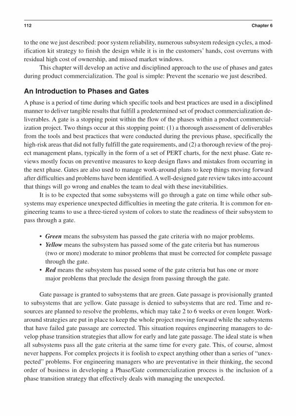
to the one we just described: poor system reliability, numerous subsystem redesign cycles, a mod-ification kit strategy to finish the design while it is in the customers’ hands, cost overruns withresidual high cost of ownership, and missed market windows.
This chapter will develop an active and disciplined approach to the use of phases and gatesduring product commercialization. The goal is simple: Prevent the scenario we just described.
An Introduction to Phases and Gates
A phase is a period of time during which specific tools and best practices are used in a disciplinedmanner to deliver tangible results that fulfill a predetermined set of product commercialization de-liverables. A gate is a stopping point within the flow of the phases within a product commercial-ization project. Two things occur at this stopping point: (1) a thorough assessment of deliverablesfrom the tools and best practices that were conducted during the previous phase, specifically thehigh-risk areas that did not fully fulfill the gate requirements, and (2) a thorough review of the proj-ect management plans, typically in the form of a set of PERT charts, for the next phase. Gate re-views mostly focus on preventive measures to keep design flaws and mistakes from occurring inthe next phase. Gates are also used to manage work-around plans to keep things moving forwardafter difficulties and problems have been identified. Awell-designed gate review takes into accountthat things will go wrong and enables the team to deal with these inevitabilities.
It is to be expected that some subsystems will go through a gate on time while other sub-systems may experience unexpected difficulties in meeting the gate criteria. It is common for en-gineering teams to use a three-tiered system of colors to state the readiness of their subsystem topass through a gate.
• Green means the subsystem has passed the gate criteria with no major problems.• Yellow means the subsystem has passed some of the gate criteria but has numerous
(two or more) moderate to minor problems that must be corrected for complete passagethrough the gate.
• Red means the subsystem has passed some of the gate criteria but has one or moremajor problems that preclude the design from passing through the gate.
Gate passage is granted to subsystems that are green. Gate passage is provisionally grantedto subsystems that are yellow. Gate passage is denied to subsystems that are red. Time and re-sources are planned to resolve the problems, which may take 2 to 6 weeks or even longer. Work-around strategies are put in place to keep the whole project moving forward while the subsystemsthat have failed gate passage are corrected. This situation requires engineering managers to de-velop phase transition strategies that allow for early and late gate passage. The ideal state is whenall subsystems pass all the gate criteria at the same time for every gate. This, of course, almostnever happens. For complex projects it is foolish to expect anything other than a series of “unex-pected” problems. For engineering managers who are preventative in their thinking, the secondorder of business in developing a Phase/Gate commercialization process is the inclusion of aphase transition strategy that effectively deals with managing the unexpected.
112 Chapter 6

The first order of business is structuring each phase with a broad portfolio of tools and bestpractices that prevent unexpected design problems. This is done by focusing on the tools and bestpractices that use forward-looking metrics that measure functions (scalar and vector engineeringvariables) instead of counting quality attributes (defects). The key is to prevent the need to reactto quality problems.
Quality must be designed in by careful, disciplined use of the right tools and best practicesthat measure the right things to enable a preventive strategy from an engineering perspective. Thelatter chapters of this text discuss such tools and metrics.
Quality is certainly one of the primary requirements of a product commercialization proj-ect, but it is now clear that the most efficient path to quality does not flow through a series of qual-ity metrics. They tend to enable “react” strategies as opposed to “prevent” strategies. We willdiscuss the antidote to the inefficiencies of quality metrics in Chapter 12.
There is near-universal acceptance that using an overarching product development processto guide technology development and product commercialization is the right thing to do. What isoften overlooked is the value of a broad portfolio of tools and best practices that are scheduledand conducted within each phase using the methods of project management (Figure 6–1).
When commercialization teams structure “what to do and when to do it” using PERT chartsunder the guiding principles of project management, engineering teams have their best chance ofmeeting cycle-time, quality, and cost goals. If the commercialization process is open to personalwhims and preferences, chaos will soon evolve and the only predictable things will becomeschedule slips, the need for design scrap and rework, and perhaps “career realignment” for theculpable engineering managers (if they are actually held accountable for their mismanagement ofthe company’s resources!).
Preparing for Product Commercialization
A few key components must be in place, in this order, before proper product commercializationcan take place:
1. Business goals defined and a strategy to meet them2. Markets and segments that will be used to fulfill the business goals
Product Design Using Design For Six Sigma 113
Product DevelopmentProcess
What to doand when to do it!
Tools andBest Practices
Project Management
Figure 6–1 Components of Successful Product Development

3. Voice of the customer and voice of technology defined based on specific market segments4. Product line strategy and family plans defined to fulfill specific market segment needs5. Technology strategy defined to fulfill product line strategy6. New platform and subsystem technologies developed and verified within their own in-
dependent technology development process (I2DOV—see Chapter 5)
With these things in place, it is much easier to see what product flow to commercialize andwhen each individual product from the family plan should be delivered to the market. This is howvalue is created for the business and its shareholders. Design For Six Sigma quantifies “top-linegrowth” financial results through its ability to enable and deliver results that fulfill the specificproduct requirements that underwrite the validity of the product’s business case.
How do we value the use of Six Sigma in product commercialization? Through the fulfill-ment of the product’s business case and the avoidance of downstream cost of poor quality. In thiscontext the Taguchi Loss Function can be helpful in quantifying the cost avoidance induced bypreventing design problems. Design For Six Sigma can also be valued through the direct cost sav-ings realized by the redesign of products and production processes that are causing warranty,scrap, and rework costs.
In terms of delivering a complete, well-integrated system, the methods of system engi-neering and integration must be in place as a governing center for the product commercializationproject (see Chapter 7 on System Engineering and Integration). The whole project must be man-aged from the technical perspective of system engineering, not from the parochial perspectivesof a loosely networked group of subsystem managers. If you are sensing a form of dictatorshipthat runs the project with a firm, disciplined hand from a project management perspective, that ismuch preferred over the “bohemian-existential” approach of poorly linked subsystem teams. A“governing legal authority” should be in place to keep personal agendas and political behaviorfrom running the show. If this is allowed to happen, it’s back to those five traits we mentioned atthe beginning of this chapter.
Defining a Generic Product Commercialization Process Using the CDOV Roadmap
We will use a generic and simple model to illustrate a Phase/Gate structure to conduct productcommercialization. The CDOV process phases we are suggesting in this text serve as guidepoststo help you align the tools and best practices of Design For Six Sigma to the actual phases in yourcompany’s commercialization process. CDOV stands for the first letters in the four phases fea-tured in Figure 6–2.
It is not uncommon to add additional subgates within each of the four phases. This is par-ticularly true of Phases 3 and 4. Phase 3 often requires subgates due to the need to first developsubsystems and then to integrate them into a system. Phase 4 requires subgates to verify the prod-uct design and then moves on to verify production ramp-up, launch, steady-state operations, andsupport processes. We will illustrate how they flow as part of the overarching product commer-cialization process that leads to successful product launches.
114 Chapter 6

The use of gates requires that the date for a gate be firmly established. The criteria for gatepassage are flexible. Thus we illustrate the nature of Phase/Gate transition as an overlapping in-terface. Some deliverables will be late while others will come in early.
The program management team can, at their discretion, allow some activities to start earlyor end late as the diagram in Figure 6–3 indicates.
We will define the general nature of each of these phases and describe the detailed stepswithin each phase. Because this book is focused on the technical development of products in thecontext of Six Sigma tools, we will not spend a lot of time on business case development andsome other details that must be included in a comprehensive product development process. Forthe sake of being circumspect in making the reader aware of these additional issues, we willbriefly illustrate what a general phase and gate should include by topical area.
Phase Topics
• Business/financial case development• Technical/design development• Manufacturing/assembly/materials management/supply chain development• Regulatory, health, safety, environmental, and legal development• Shipping/service/sales/support development
Product Design Using Design For Six Sigma 115
Phase 1. C = Concept
Phase 2. D = Design
Phase 3. O = Optimize
Phase 4. V = VerifySteady StateProduction ofEach Product
. . .the individual ProductCommercialization Project islaunched into the market tofulfill its role in fulfilling theStrategic Family Plan. . .
Production Launch. . .
Figure 6–2 CDOV Phases
ConceptDevelopment
Phase
DesignDevelopment
Phase
OptimizationPhase
VerifyCapability
Phase
Gate 4Gate 3Gate 2Gate 1
Figure 6–3 Overlaps in Phase/Gate Transmissions

We will focus most of our discussions on the technical/design development and manufacturing/assembly/materials management/supply chain development areas. It is importantto recognize though, that a broad range of Six Sigma methods can be applied across all the phasetopics listed here. That broader range includes Six Sigma methods in transactional businessprocesses, manufacturing operations processes, and service processes, all of which deploy theMAIC (Measure, Analyze, Improve and Control) roadmap.
The best way to think about establishing the architecture of any product developmentprocess is to structure it as a macro-timing diagram to constrain “what to do and when to do it”across the entire product development life cycle. With such a macro-timing diagram estab-lished, the product development management team can then conduct the phases and gates withthe help of checklists and scorecards based on a broad portfolio of tools and best practices andtheir deliverables. The techniques of project management can then be used to construct micro-timing diagrams, preferably in the form of PERT charts, that establish discipline and structurewithin the day-to-day use of the tools and best practices for each person on the product devel-opment team. We recommend PERT charts because they help define personal accountabilityfor using the right tools and best practices within the phases. They also greatly enhance themanagement of parallel and serial activities, work-around strategies, and the critical path tasksthat control the cycle-time of each phase. Managing a commercialization project in this man-ner helps assure that all the right things get done to balance the ever present cost, quality, andcycle-time requirements.
Checklists
Checklists are brief summary statements of tools and best practices that are required to fulfill agate deliverable within a phase. These are actions based on work everyone must do based on abroad portfolio of tools and best practices. You know you have a good checklist when it is easyto directly relate one or more tools or best practices to each gate deliverable. Another way of rec-ognizing a good checklist is that it can be used to build project management PERT and Ganttcharts for day-to-day management of tool use. Tools and best practices produce deliverables thatcan be tracked on a daily, weekly, or monthly basis and can be easily reviewed using a summaryscorecard when a gate is reached. Checklists are used during project planning of tool use in thecurrent phase to prevent problems in the next phase. See Figure 6–4 for an example of a tools andbest practices checklist.
Scorecards
Scorecards are summary results derived from data that was produced from the use of a full port-folio of tools and best practices within a phase. Scorecards can be developed for any level of sum-mary detail required to pass a gate. Typically senior management will see high-level scorecardsthat are simple “traffic lights” of red, yellow, or green scores. These high-level scorecards alsocontain summary statements of risks and issues. Scorecards align with checklists and containwhatever level of detail is required to prove the risks that constrain the project are being managedproperly. Scorecards are used after a phase to react to problems that occurred in the current phaseor past phases. Scorecards are used before the next phase to assure the team has the resources it
116 Chapter 6
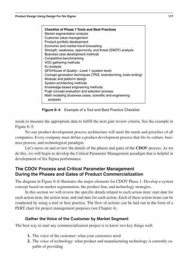
needs to measure the appropriate data to fulfill the next gate review criteria. See the example inFigure 6–5.
No one product development process architecture will meet the needs and priorities of allcompanies. Every company must define a product development process that fits its culture, busi-ness process, and technological paradigm.
Let’s move on and review the details of the phases and gates of the CDOV process. As wedo this, we will begin to develop the Critical Parameter Management paradigm that is helpful indevelopment of Six Sigma performance.
The CDOV Process and Critical Parameter Management During the Phases and Gates of Product Commercialization
The diagram in Figure 6–6 illustrates the major elements for CDOV Phase 1: Develop a systemconcept based on market segmentation, the product line, and technology strategies.
In this section we will review the specific details related to each action item: start date foreach action item, the action item, and end date for each action. Each of these action items can beconducted by using a tool or best practice. The flow of actions can be laid out in the form of aPERT chart for project management purposes (see Chapter 4).
Gather the Voice of the Customer by Market Segment
The best way to start any commercialization project is to know two key things well:
1. The voice of the customer: what your customers need2. The voice of technology: what product and manufacturing technology is currently ca-
pable of providing
Product Design Using Design For Six Sigma 117
Checklist of Phase 1 Tools and Best PracticesMarket segmentation analysisCustomer value managementProduct portfolio developmentEconomic and market trend forecastingStrength, weakness, opportunity, and threat (SWOT) analysisBusiness case development methodsCompetitive benchmarkingVOC gathering methodsKJ analysisQFD/House of Quality—Level 1 (system level)Concept generation techniques (TRIZ, brainstorming, brain-writing)Modular and platform designSystem architecting methodsKnowledge-based engineering methodsPugh concept evaluation and selection processMath modeling (business cases, scientific and engineering
analysis)
Figure 6–4 Example of a Tool and Best Practice Checklist

Phase 1 Concept Development
Original Due Completion Performance Exit Date vs. Actual Status vs. Criteria Recommendation
Deliverable Owner Deliv. Date Red Green Yellow Red Green Yellow Red Green Yellow Notes
Ranked & Documented VOC Database
System Level House of Quality
Competitive System Benchmarking Data
System Level Requirements Documents
Documented List of System Level
Functions That Fulfill the SystemRequirements
Documented Superior System Concept
Portfolio of Candidate Technologies That
Help Fulfill the System Functions & Requirements
Documented Critical Parameter Database
with estimated System CFR Interaction Transfer Functions
Documented Reliability Model and
Predicted System Reliability Performance with Gap Analysis
Estimated System Cost Projection
Phase 2 (Design Development) Project
Management Plans
Figure 6–5 Example of a General Gate Review Scorecard
118

We will lay out the importance of gathering detailed information regarding both of thesefoundational areas in the next few paragraphs. These two sources of information will form the ba-sis of what the entire product development community will “design to fulfill or surpass.” CriticalParameter Management is initiated by generating a database of ranked, prioritized, stated, and ob-served customer needs.
It is helpful to begin product design activities by asking questions like:
• What do customers specifically say they need?• What do their actions suggest they need?• What technology is being used today to meet their current needs?• What new technology (manufacturing and product design technology) is capable of
extending or improving their satisfaction with a new product?
Product Design Using Design For Six Sigma 119
Refine and rank the voice of the customer usingKJ analysis
Create product or system level House of Quality
Start Date: End Date: Owner:
Gather the voice of the customer by marketsegment
Start Date: End Date: Owner:
Start Date: End Date: Owner:
Generate product or system level requirementsdocument
Define the functions that fulfill the systemrequirements
Start Date: End Date: Owner:
Conduct competitive product benchmarkingStart Date: End Date: Owner:
Start Date: End Date: Owner:
Generate system concept evaluation criteria
Generate system concepts that fulfill thefunctions
Start Date: End Date: Owner:
Start Date: End Date: Owner:
Select superior system concept
Analyze, characterize, model, and predictnominal performance of the superior system
Start Date: End Date: Owner:
Evaluate system conceptsStart Date: End Date: Owner:
Start Date: End Date: Owner:
Develop reliability requirements, initial reliability,model, and FMEA for the system
Start Date: End Date: Owner:
Figure 6–6 Flow of Phase 1 Product Commercialization
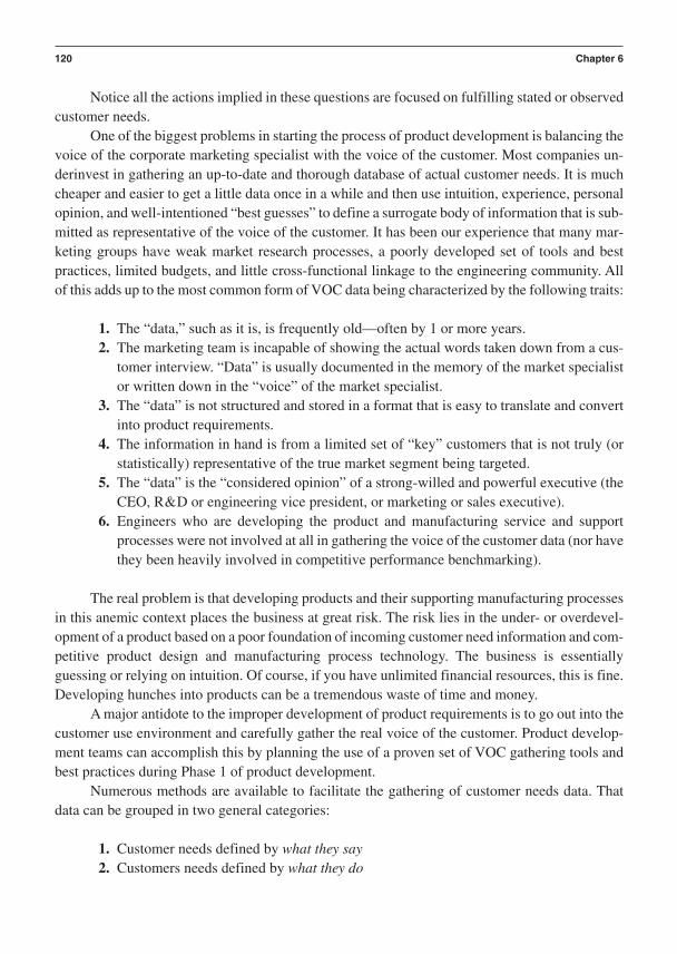
Notice all the actions implied in these questions are focused on fulfilling stated or observedcustomer needs.
One of the biggest problems in starting the process of product development is balancing thevoice of the corporate marketing specialist with the voice of the customer. Most companies un-derinvest in gathering an up-to-date and thorough database of actual customer needs. It is muchcheaper and easier to get a little data once in a while and then use intuition, experience, personalopinion, and well-intentioned “best guesses” to define a surrogate body of information that is sub-mitted as representative of the voice of the customer. It has been our experience that many mar-keting groups have weak market research processes, a poorly developed set of tools and bestpractices, limited budgets, and little cross-functional linkage to the engineering community. Allof this adds up to the most common form of VOC data being characterized by the following traits:
1. The “data,” such as it is, is frequently old—often by 1 or more years.2. The marketing team is incapable of showing the actual words taken down from a cus-
tomer interview. “Data” is usually documented in the memory of the market specialistor written down in the “voice” of the market specialist.
3. The “data” is not structured and stored in a format that is easy to translate and convertinto product requirements.
4. The information in hand is from a limited set of “key” customers that is not truly (orstatistically) representative of the true market segment being targeted.
5. The “data” is the “considered opinion” of a strong-willed and powerful executive (theCEO, R&D or engineering vice president, or marketing or sales executive).
6. Engineers who are developing the product and manufacturing service and supportprocesses were not involved at all in gathering the voice of the customer data (nor havethey been heavily involved in competitive performance benchmarking).
The real problem is that developing products and their supporting manufacturing processesin this anemic context places the business at great risk. The risk lies in the under- or overdevel-opment of a product based on a poor foundation of incoming customer need information and com-petitive product design and manufacturing process technology. The business is essentiallyguessing or relying on intuition. Of course, if you have unlimited financial resources, this is fine.Developing hunches into products can be a tremendous waste of time and money.
A major antidote to the improper development of product requirements is to go out into thecustomer use environment and carefully gather the real voice of the customer. Product develop-ment teams can accomplish this by planning the use of a proven set of VOC gathering tools andbest practices during Phase 1 of product development.
Numerous methods are available to facilitate the gathering of customer needs data. Thatdata can be grouped in two general categories:
1. Customer needs defined by what they say2. Customers needs defined by what they do
120 Chapter 6

One of the most effective methods for gathering data about stated customer needs is to forma small team of two or three people and hold a face-to-face meeting with a reasonable cross-section of customers. One person leads the discussion, one takes detailed notes or records the con-versations, and one listens and adds to the discussion to help keep a diverse and dynamic dialogin motion. This approach is characterized by an active and dynamic exchange between the cus-tomers and the interview team whom we will call the inbound marketing team. The inbound mar-keting team is typically a cross-functional group made up from a reasonable mix of the followingprofessions:
1. Market research and advanced product planning2. Technical (R&D, system or subsystem design engineers, production operations, etc.)3. Industrial design4. Service and support5. Sales6. Program management
The inbound marketing team first prepares a customer interview guide that will enable teammembers to set a specific flow of discussion in motion during the customer meeting. The inter-view guide is not a questionnaire but rather a logical “flow diagram” containing specific topicsthat are designed to stimulate free-flowing discussions about customer needs and issues that helpalign the company’s advanced product planning activities with the customers’ future needs. If aquestionnaire is all that your business needs to define future product development requirements,then phone calls, handout questionnaires, and mailing methods are much more economical. Ques-tionnaires are quite limited in the kind of detailed data that can be obtained, because you get lit-tle exchange and clarification of information to verify that what was stated was correctly received.The power of face-to-face discussions with a reasonable number of customers (current, former,and potential) is unsurpassed in assuring that you obtain many key VOC attributes based on theKANO model of customer satisfaction (see Figure 6–7):
1. Basic needs that must be in the future product2. Linear satisfiers that produce proportional satisfaction with their increased presence in
the future product3. Delighters that are often generally unknown by the customer until you stimulate some
sense of latent need that was “hidden” in the mind of the customer
The other key data that is available to the inbound marketing team is the observed behav-ior of customers in the product acquisition and use environment. These are relatively passiveevents for the inbound marketing team but obviously dynamic events on the customer’s side. Itis here that the team watches and documents customer behavior as opposed to listening to whatthey say they need. This approach has been called contextual inquiry (Clausing, 1994). This
Product Design Using Design For Six Sigma 121

method also requires careful preplanning so that meaningful vantage points and contexts for ob-servation can be arranged. The team must find a way to participate in use experiences. Obviouslynot all products are amenable to this approach, but when the product is used in an observable en-vironment, it can be quite useful in assisting in the determination of unspoken needs. In the worldof KJ analysis (our next topic), this data is profoundly useful in developing “images” of customerproblems and needs. A well-spread story tells how Honda engineers positioned themselves inparking lots and watched how people used their trunks and hatchbacks to help gather data for im-proving the next hatchback design. Eastman Kodak hands out one-time-use cameras to their em-ployees and assesses their use habits. There are many creative ways to align your teams with useexperiences. Never underestimate the knowledge you can gain by getting inside the situationalevents that are associated with the actual use of your products and processes, especially in caseswhere disruptive sources of variation, or causes of loss, are active within the use environment.
Refine and Rank the Voice of the Customer Using KJ Analysis
Once customer data is gathered in a sufficient quantity to adequately represent the scope of themarket segment, the team refines and documents the raw data by structuring it into a more use-ful form. The KJ method, named after the Japanese anthropologist Jiro Kawakita, is used toprocess the VOC data into rational groups based on common themes. It employs higher levels ofcategorizing the many details of expressed or observed/imaged need. The name affinity dia-gramming has been used to characterize this process.
KJ analysis is quite useful when you are working with nonnumerical data in verbal orworded format. The mass of VOC input can, at first glance, seem to be a jumble of multidimen-sional and multidirectional needs that is quite hard to analyze. In practical terms, KJ analysis
122 Chapter 6
Delighter. . .
. . .Basic Needs
. . .Linear Satisfier
LowFulfillment
HighFulfillment
Satisfaction
Dissatisfaction
Figure 6–7 The KANO Customer Satisfaction Model

helps make sense out of all these words, observations, and images by aligning like statements ina hierarchical format. Once the raw VOC is segmented, aligned underneath higher-level topicaldescriptors (higher levels of categorizing the many details of expressed or observed/imagedneed), and ranked under these topical descriptors, it can be loaded into the system or product levelHouse of Quality using quality function deployment techniques.
Create Product or System Level House of Quality
A process known as quality function deployment (QFD) is commonly used to help further re-fine the affinitized (or grouped by similar characteristics) VOC data. QFD uses the data, mappedusing the KJ method, to develop a clear, ranked set of product development requirements thatguide the engineering team as they seek to determine what measures of performance need to beat six Sigma levels of quality.
The QFD process produces a two-dimensional matrix called a House of Quality. The Houseof Quality, at the system level, is used to transform VOC data into technical and business per-formance requirements for the new product or process. Many teams overdo the structuring of theHouse of Quality by including too many minor details in it. The House of Quality should only bein receipt of VOC data that falls under one or more of the following categories:
1. New needs: features or performance your product has not historically delivered2. Unique needs: features or performance that are distinctive or highly desired beyond
the numerous other less-demanding needs that must be provided3. Difficult to fulfill needs: features or performance that is highly desired but is quite dif-
ficult for your business to develop and will require special efforts/investments of re-sources on your part
Cohen (1995) provides a graphical depiction of QFD, featured in Figure 6–8.Everything that is to be included in the product design requirements document is important,
but not everything is critical. The House of Quality is a tool for critical parameter identification andmanagement. It helps the development team see beyond the many important requirements to iso-late and track the few critical requirements that matter the most to successful commercialization.
Conduct Competitive Product Benchmarking
Following the voice of the customer blindly can lead to a failure in the commercialization of anew product. Let’s use an analogy to illustrate this point. When a band solicits musical requestsfrom the audience, it had better be able to play the tune! Taking requests needs to be a constrainedevent unless there is nothing you cannot do. One way to establish market segmentation or VOCconstraint is by establishing limits to whom you choose to develop and supply products. The lim-itation is usually set by your company’s capability in a given area of technology, manufacturing,outbound marketing, distribution channels, and service capability.
Within your established boundaries of limitation, which some people on a more positivenote label a participation strategy, you need to be well informed as to what your competition is
Product Design Using Design For Six Sigma 123

developing and delivering. This requires that some form of competitive benchmarking be con-ducted. Building a balanced approach to what customers say they want, what you can provide,and what your competition can provide is a reasonable way to conduct product development.
From a Six Sigma performance perspective, we need to decide what critical functional re-sponses need to be at Six Sigma quality. We must use competitive performance data to help de-fine critical functional requirements and then develop designs that can be measured with CFRs.This chain of critical requirements and their fulfilling critical responses is the essence of CriticalParameter Management and can be helpful in defining competitive options. Competitive bench-marking adds one more dimension to what candidate critical requirements and responses need tobe considered as we set up the system House of Quality. It can also be one more form of what wecall the “voice of physics” or the “voice of the process.” If a competitor is doing something new,unique, or difficult relative to what you are currently able to do, then you must seriously considerwhat you are going to do and what you are not going to do.
The House of Quality has a specific section where these trade-offs can be ranked and documented. This area of competitive vs. your performance trade-offs is often where the initialidentification of Six Sigma requirements are born. The competition is found to be good at a mea-surable function, and customers say they want more performance in this area, so we have an op-portunity to surpass the competition by taking that specific, candidate-critical function to a wholenew level—perhaps to Six Sigma functional performance or beyond. It is important to note thatnot everything needs to be at a Six Sigma level of performance. If you find a strategic functionthat is worth taking to the level of Six Sigma in terms of value to the business case and customer,you had better be able to measure it against the requirements and against your competition!
Many of the tools of Six Sigma are useful for comparative benchmarking. The followingare examples:
124 Chapter 6
System Requirements
RequirementsCorrelation Matrix
Technical Matrix
The Planning MatrixVOC
Needs
RelationshipsBetween Customer
Needs andTechnical Responses
Figure 6–8 House of Quality

1. Design and process failure modes and effects analysis2. Taguchi noise diagramming and system noise mapping3. Pugh’s concept evaluation process4. Functional flow diagramming and critical parameter mapping5. Taguchi stress testing6. Highly accelerated life tests and highly accelerated stress testing7. Multi-vari studies8. Statistical process control and capability studies (for both design functions and process
outputs)
Generate Product or System Level Requirements Document
The system House of Quality contains the information that relates and ranks the new, unique, anddifficult (NUD) VOC needs to the system level technical requirements that are to be fulfilled bythe design engineering teams. These NUD items, along with all the many other system level re-quirements, must be organized and clearly worded in the system requirements document (SRD).The SRD contains all of the product level design requirements. It is important to recognize thatthree distinct types of requirements must be developed and documented in the SRD:
1. Candidate-critical system level requirements from the system House of Quality2. Candidate-critical system level requirements that were not in the system House of
Quality because they were not new, unique, or difficult3. Noncritical but nonetheless important system requirements that must be included to
adequately complete the product level design
The system requirements document is the design guide and “bible” that the system engi-neering team, the subsystem design teams, and all other cross-functional participants in productdesign and development must seek to fulfill. If a product requirement is not covered in the SRD,it is highly likely that the omitted requirement will not be fulfilled. On the other hand, the SRDis the governing document for what does get delivered. When it is well managed, it prevents de-sign feature and function “creep.” SRDs are frequently reused and added to as a family of prod-ucts is developed as the serial flow of product line deployment is conducted.
Design Functions That Fulfill the System Requirements
Once the system requirements are clearly worded and documented, it is now time for the engi-neering teams to integrate their talents to identify what functions must be developed at the systemlevel to fulfill the system requirements. Defining these functions is the job of a cross-functionalteam of subsystem engineering team leaders, service engineers, industrial designers, system en-gineers, and other appropriate product development resources all led by the system engineeringand integration team leader. For organizations that do not have a system engineering team leader,the chief engineer or project manager often leads this effort.
System level functions are defined as physical performance variables that can be mea-sured to assess the fulfillment of the system requirements. The functions are ideally defined
Product Design Using Design For Six Sigma 125

independent of how they are accomplished. The focus is on a measurable response that can bespecified as either an engineering scalar or vector. It is important to define continuous variablesthat will be directly and fundamentally affected by the soon-to-be-defined subsystem functions.The system functions have a strong influence on the definition of the subsystem functions. Thesubsystem functions are strongly dependent on subassembly and component functions, which inturn are strongly affected by manufacturing process functions. These interconnections are de-picted in Figure 6–9.
Critical Parameter Management derives from a carefully defined architectural flow downof requirements that can be directly linked to functions that are engineered to flow up to fulfillthe requirements.
Later we will discuss a method of analytically modeling these functional hand-offs acrossthe architectural boundaries within the system. We call these analytical models ideal/transferfunctions.
The system level functions will be used to help define the many possible system architec-tures that can be configured to fulfill the functions. Here we see how customer needs drive sys-tem level technical requirements. The system level technical requirements drive the system levelengineering functions. The final linkage is how the system level engineering functions drive thedefinition of the system level architectural concepts (Figure 6–10). Once a system architecture isestimated from this perspective, the inevitable trade-offs due to subsystem, subassembly, andcomponent architectures will begin.
As you can see in Figure 6–10, the system drives the design of everything within its architecture.
Generate System Concept Evaluation Criteria
The criteria used to assess all of the candidate system concepts, against a best-in-class benchmarkdatum, must come from the system requirements and the system functions. These criteria must
126 Chapter 6
System LevelREQUIREMENTS Subsystem Level
REQUIREMENTS Subassembly LevelREQUIREMENTS Component Level
REQUIREMENTS ManufacturingProcess Level
REQUIREMENTSSystem LevelFUNCTIONS Subsystem Level
FUNCTIONS Subassembly LevelFUNCTIONS Component Level
FUNCTIONS ManufacturingProcess LevelFUNCTIONS
Figure 6–9 System Connectivity

be detailed in nature. Stating low cost as criteria is too general. One must decompose the elementsthat drive cost and state them as criteria. This rule applies to most requirements. It is OK to statea system reliability goal, but it may be better to state the more detailed criteria that lead to over-all reliability. In this context, low part count would be reasonable criteria.
The goal of concept development is to define a superior architecture that is high in feasi-bility and low in competitive vulnerability. A major mistake that many engineering teams makeis confusing feasibility and optimization. A major focus in the concept phase of the product com-mercialization process is developing the attribute known as feasibility. Feasibility is character-ized by the following traits:
1. Projected or predicted ability to fulfill a requirement2. Predicted capacity to perform, as opposed to measured capability (Cp) to perform3. Inherent robustness to customer use variation and environments4. Logical in an application context5. Likelihood or possibility of balancing requirements
Engineers are typically undertrained in the tools and best practices for developing feasibil-ity. They tend to have extensive analytical and mathematical training in developing optimality.Feasibility is measured in more generic and general terms against a broad set of system level re-quirements. Optimality is typically measured in specific engineering units against specific per-formance targets, usually at the system and subsystem level. We often find engineering teamsoverly focused on subsystem optimization much too early in the commercialization process. Thisleads to subsystems that work well as stand-alone units under nominal laboratory conditions.When these “optimized” subsystems are integrated into the system configuration, they tend tosuffer significant functional performance problems and must undergo significant redesign efforts.Once in a while, they actually must be scrapped altogether and a new subsystem concept must be
Product Design Using Design For Six Sigma 127
System Level CustomerNEEDS
Subsystem Level TechnicalREQUIREMENTS
System Level EngineeringFUNCTIONS
System Level ArchitecturalCONCEPTS
Figure 6–10 System Level Linkages

developed. In cost of poor quality terms, design, scrap, and rework costs are often found to havetheir root cause back in this concept development phase of commercialization.
Feasibility metrics are focused on requirements that are embryonic and developmental innature. Requirements will undergo some evolution and refinement as the product commercial-ization process moves forward. Optimality metrics become clear later in the CDOV process,specifically in the optimization phase (Phase 3). Many engineers become impatient, jump the gun on feasibility development, prematurely define just one vague system concept, and immedi-ately begin analytical optimization across the various subsystems. The claim is, “We are fast, weget right at the job of engineering the product.” The results of taking shortcuts like this are un-derdeveloped system architectures that are underdefined with regard to their balanced capacity tofulfill all the system requirements and functions. This being the case, you can see how a numberof subsystems can end up being poorly developed simply due to weakly defined system conceptcriteria.
Generate System Concepts That Fulfill the Functions
System architecting is a body of knowledge comprised of both science and art. System conceptsare “architected,” or structured, through a set of steps that synthesize the following items:
1. System requirements that fulfill the VOC needs2. System functions that fulfill the system requirements3. Engineering knowledge of system design, interface development, and integration4. Prior experience with system performance issues, successes, and failures
A superb reference for conducting this unique discipline is Systems Architecting, by Eber-hardt Rechtin (1990). It contains many heuristics, or “rules of thumb,” that are extremely usefulin guiding the process of defining system architectural concepts.
One of the most important aspects of developing candidate system concepts is to developmore than one. If just one system concept is developed, it is highly likely it will be lacking in itsability to possess balanced fulfillment of the system requirements. If numerous system conceptsare developed and compared to a best-in-class benchmark datum concept, using a comprehensiveset of criteria based on the system requirements and system functions, then it is much more likelythat a superior conceptual architecture can be identified. The power of this approach, known asthe Pugh concept selection and evaluation process, is in its ability to integrate the best elementsfrom numerous concepts into a “super-synthesized” superior concept.
This approach drives strong consensus around a team-developed system architecture. It isfine to have a chief system architect, but no one personality should dominate the definition of theactual system concept. It is desirable to have one person lead a disciplined process of system ar-chitectural development.
The results of the system architecting process must come from the team, but the focus onthe disciplined use of system conceptual development tools frequently comes from a strong leaderof the team. The leader should not dictate a concept but should insist on using the right tools andprocess so the team can develop the right concept.
128 Chapter 6

Evaluate System Concepts
System concepts, in the plural, are essential to the proper convergence on a single, superior sys-tem concept that will serve as the basis for all subsystem, subassembly, component, and manu-facturing process requirements. Too many products have their system defined and driven by thesubsystems. This obviously works but is a recipe for system integration nightmares. Thus, weneed to evaluate numerous system concepts.
The system concepts we evaluate are developed by individuals or small groups. If one per-son generates all the concepts, a personal bias or other form of limitation can greatly inhibit thepotential to fulfill and balance all the system requirements. You need many concepts with manyapproaches from diverse perspectives.
Each system concept is compared to the best-in-class benchmark datum using the criteria.It is typical to have between 20 and 30 criteria, depending on the nature and complexity of thesystem requirements and functions. All team members should have one or two candidate conceptsthat they have personally brought to the evaluation process. The concepts are evaluated by usingnonnumeric standards of comparison:
() is assigned to concepts that are better than the datum for a given criteria
() is assigned to concepts that are worse than the datum for a given criteria
(S) is assigned to concepts that are the same as the datum for a given criteria
These evaluation standards are efficient for the purpose of assigning value in terms of fea-sibility. If numbers are used, the evaluation can easily drift away from feasibility and become atypical engineering argument over optimal concepts.
Select Superior System Concept
The evaluation is meant to be iterative. Divergent concepts are now integrated. It is good to stepback after a first pass through the evaluation process and integrate the best features and attributes ofthe various “winning” concepts. This will generate a smaller, more potent set of synthesized con-cepts that can then go through a second round of evaluation. If one of the concepts clearly beats thedatum in the first round, it becomes the new datum. The synthesized concepts are then compared tothe new datum. Once a second round of comparisons is done, a superior concept tends to emerge.
A superior concept is defined as the one that scores highest in feasibility against the criteria—in comparison to the datum. The team should be able to clearly articulate exactly why the selectedconcept is truly superior to the others and why it is low in competitive vulnerability.
Analyze, Characterize, Model, and Predict Nominal Performance of the Superior System
With a superior concept in hand, the detailed engineering analysis at the system level can begin.It is now reasonable to invest time and resources in system modeling in depth. This is the timewhen a system level “black box network model” is formally laid out. It is where the System LevelCritical Parameter Management model is initially developed.
Product Design Using Design For Six Sigma 129
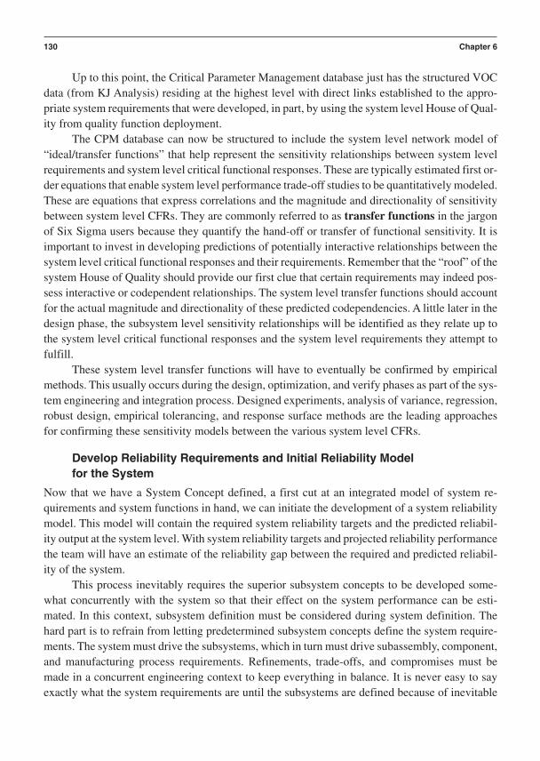
Up to this point, the Critical Parameter Management database just has the structured VOCdata (from KJ Analysis) residing at the highest level with direct links established to the appro-priate system requirements that were developed, in part, by using the system level House of Qual-ity from quality function deployment.
The CPM database can now be structured to include the system level network model of“ideal/transfer functions” that help represent the sensitivity relationships between system levelrequirements and system level critical functional responses. These are typically estimated first or-der equations that enable system level performance trade-off studies to be quantitatively modeled.These are equations that express correlations and the magnitude and directionality of sensitivitybetween system level CFRs. They are commonly referred to as transfer functions in the jargonof Six Sigma users because they quantify the hand-off or transfer of functional sensitivity. It isimportant to invest in developing predictions of potentially interactive relationships between thesystem level critical functional responses and their requirements. Remember that the “roof” of thesystem House of Quality should provide our first clue that certain requirements may indeed pos-sess interactive or codependent relationships. The system level transfer functions should accountfor the actual magnitude and directionality of these predicted codependencies. A little later in thedesign phase, the subsystem level sensitivity relationships will be identified as they relate up tothe system level critical functional responses and the system level requirements they attempt tofulfill.
These system level transfer functions will have to eventually be confirmed by empiricalmethods. This usually occurs during the design, optimization, and verify phases as part of the sys-tem engineering and integration process. Designed experiments, analysis of variance, regression,robust design, empirical tolerancing, and response surface methods are the leading approachesfor confirming these sensitivity models between the various system level CFRs.
Develop Reliability Requirements and Initial Reliability Model for the System
Now that we have a System Concept defined, a first cut at an integrated model of system re-quirements and system functions in hand, we can initiate the development of a system reliabilitymodel. This model will contain the required system reliability targets and the predicted reliabil-ity output at the system level. With system reliability targets and projected reliability performancethe team will have an estimate of the reliability gap between the required and predicted reliabil-ity of the system.
This process inevitably requires the superior subsystem concepts to be developed some-what concurrently with the system so that their effect on the system performance can be esti-mated. In this context, subsystem definition must be considered during system definition. Thehard part is to refrain from letting predetermined subsystem concepts define the system require-ments. The system must drive the subsystems, which in turn must drive subassembly, component,and manufacturing process requirements. Refinements, trade-offs, and compromises must bemade in a concurrent engineering context to keep everything in balance. It is never easy to sayexactly what the system requirements are until the subsystems are defined because of inevitable
130 Chapter 6
dependencies. The system requirements and functions change as the subsystem architectures arefirmed up. It is crucial to systems architecting and engineering goals to have a strong focus on thesystem requirements as a give-and-take process takes place between system and subsystem ar-chitecture and performance trade-offs. The key thing to remember is system requirements shouldtake precedence over and drive subsystem requirements. This rule can obviously be broken suc-cessfully, but in a DFSS context it should be done only under the constraints and insights fromthe Critical Parameter Management process.
Gate 1 Readiness
At Gate 1 we stop and assess the full set of concept development deliverables and the summarydata used to arrive at them. The tools and best practices of Phase 1 have been used, and their keyresults can be summarized in a Gate 1 scorecard (Figure 6–11). A checklist of Phase 1 tools andtheir deliverables can be reviewed for completeness of results and corrective action in areas of risk.
Prerequisite Information to Conduct Phase 1 Activities
Market segmentation analysis
Market competitive analysis
Market opportunity analysis
Market gap analysis
Product family plan
General Phase 1 Gate Review Topics
• Business/financial case development• Technical/design development• Manufacturing/assembly/materials management/supply chain development• Regulatory, health, safety, environmental, and legal development• Shipping/service/sales/support development
Checklist of Phase 1 Tools and Best Practices
Market segmentation analysis
Economic and market trend forecasting
Business case development methods
Competitive benchmarking
VOC gathering methods
KJ analysis
QFD/House of Quality—Level 1 (system level)
Concept generation techniques (TRIZ, brainstorming, brain-writing)
Modular and platform design
Product Design Using Design For Six Sigma 131

Phase 1 Concept Development
Original Due Completion Performance Exit Date vs. Actual Status vs. Criteria Recommendation
Deliverable Owner Deliv. Date Red Green Yellow Red Green Yellow Red Green Yellow Notes
Ranked & Documented VOC Database
System Level House of Quality
Competitive System Benchmarking Data
System Level Requirements Documents
Documented List of System Level
Functions That Fulfill the System Requirements
Documented Superior System Concept
Portfolio of Candidate Technologies That
Help Fulfill the System Functions & Requirements
Documented Critical Parameter Database
with estimated System CFR Interaction Transfer Functions
Documented Reliability Model and
Predicted System Reliability Performance with Gap Analysis
Estimated System Cost Projection
Phase 2 (Design Development) Project
Management Plans
Figure 6–11 A General Scorecard for CDOV Phase 1 Deliverables
132

System architecting methods
Knowledge-based engineering methods
Pugh concept evaluation and selection process
Math modeling (business cases, scientific and engineering analysis)
CDOV Phase 2: Subsystem Concept and Design Development
The diagram in Figure 6–12 illustrates the major elements for CDOV Phase 2: Develop subsys-tem concepts and designs.
Transitioning into Phase 2 of the CDOV product commercialization process requires thatthe major deliverables from the tools and best practices from Phase 1 are adequately met. It is alsopredicated on proper, advance planning for use of the design tools and best practices. This is allpart of the preventative strategy of Design For Six Sigma.
Create Subsystem Houses of Quality
It is becoming relatively common to see companies that are deploying DFSS develop a systemlevel House of Quality. Unfortunately the use of the lower level Houses of Quality tends to drop
Product Design Using Design For Six Sigma 133
Conduct subsystem benchmarking
Generate subsystem requirements documents
Start Date: End Date: Owner:
Create subsystem Houses of QualityStart Date: End Date: Owner:
Start Date: End Date: Owner:
Generate subsystem concept evaluation criteria
Generate subsystem concepts that fulfill thefunctions
Start Date: End Date: Owner:
Develop functions that fulfill the subsystemrequirements
Start Date: End Date: Owner:
Start Date: End Date: Owner:
Evaluate subsystem concepts
Select superior subsystem concepts
Start Date: End Date: Owner:
Start Date: End Date: Owner:
Develop reliability model and DFMEA for eachsubsystem
Start Date: End Date: Owner:
Analyze, characterize, model, predict, andmeasure nominal performance of superiorsubsystem (including DFMA, initial tolerances,and cost analysis)
Start Date: End Date: Owner:
Figure 6–12 Flow of Phase 2 of Product Commercialization(continued)

off precipitously after the completion of the system House of Quality. The system House of Qual-ity can and should be used to develop subsystem Houses of Quality for each subsystem within theproduct architecture. The subsystem House of Quality is extremely useful in the development ofclear, well-defined subsystem requirements documents. The subsystem requirements must alignwith and support the fulfillment of the system requirements. In the same context, the subsystemfunctions must align with and fulfill the system functions. It is our opinion that one of the weak-est links in the chain of product commercialization best practices is the cavalier approach designteams take relative to developing clear subsystem, subassembly, component, and manufacturingprocess requirements. We know from years of experience that it is quite rare to find design teamswith clear, well-documented requirements much below the system level. Things tend to get prettyundisciplined and sloppy down in the design details. This is yet another reason why most com-panies suffer from moderate to severe performance problems that require costly redesign at the
134 Chapter 6
Conduct subassembly, component, andmanufacturing process benchmarking
Generate subassembly, component, andmanufacturing process requirements documents
Start Date: End Date: Owner:
Create subassembly, component, andmanufacturing process Houses of Quality
Start Date: End Date: Owner:
Start Date: End Date: Owner:
Generate subassembly, component, andmanufacturing process evaluation criteria
Develop functions that fulfill subassembly,component, and manufacturing processrequirements
Start Date: End Date: Owner:
Develop functions that fulfill subassembly,component, and manufacturing processrequirements
Start Date: End Date: Owner:
Start Date: End Date: Owner:
Generate subassembly, component, andmanufacturing concepts that fulfill the functions
Evaluate subassembly, component, andmanufacturing process concepts
Start Date: End Date: Owner:
Start Date: End Date: Owner:
Develop reliability models and DFMEAs forreliability critical subassemblies and components
Start Date: End Date: Owner:
Select superior subassembly, component, andmanufacturing process concepts
Start Date: End Date: Owner:
Analyze, characterize, model, predict, andmeasure nominal performance of superiorsubassemblies, components, and manufacturingprocesses (including DFMA, initial tolerances,and cost analysis)
Start Date: End Date: Owner:
Figure 6–12 Continued

subsystem level. The design phase of CDOV is specifically arranged to instill much needed dis-cipline in this early but crucial area of requirements definition. It is yet another key element inCritical Parameter Management.
At a general level, the subsystem Houses of Quality (Figure 6–13) are designed to illustrateand document specific system requirements as inputs, specific fulfilling subsystem requirementsas outputs, and a variety of system-to-subsystem criticality quantification and correlation rela-tionships. They also have “rooms” that quantify competitive benchmarking relationships, bothfrom the customer’s and the engineering team’s perspective, as they align with the system andsubsystem requirements.
It bears repeating that only that which is new, unique, or difficult from the system require-ments should be brought down into the subsystem Houses of Quality.
If the subsystem Houses of Quality are not generated, it is highly likely that there will besome form of system integration problem stemming from this lack of assessment and documen-tation that must be reacted to later on in the commercialization process. It just makes good senseto apply the discipline of QFD to the system-to-subsystem requirements that are new, unique, anddifficult. Without this focus, these things may transform into that which is expensive, embarrass-ing, and treacherous. We view the construction of the subsystem Houses of Quality and the sub-system requirements documents as key steps in the DFSS strategy of design problem prevention.
Conduct Subsystem Benchmarking
When appropriate, subsystems should be benchmarked from the customer’s perspective. If theproduct design is such that the customer has no possible access to or interest in one or more ofthe subsystems, then the benchmarking activity will be solely conducted by the engineering team
Product Design Using Design For Six Sigma 135
Subsystem Requirements
SubsystemRequirements
Correlation Matrix
Technical Matrix
The Planning Matrix
Specific SystemRequirementsthat are New,
Unique, or Difficult
RelationshipsBetween System
Requirements andSubsystem Requirements
Figure 6–13 Subsystem House of Quality

from a technical perspective. If the product is serviceable or repairable, then the benchmarkingperspective of the “customer in the form of the repair technician” would be required.
A clear case where subsystem benchmarking from a customer’s perspective would be nec-essary is found in the replacement process of inkjet cartridges in a personal desktop printer. A casewhere the customer would have little role in subsystem benchmarking would be the efficiency ofa sealed cooling subsystem within a light projector used for business presentations.
Subsystem benchmarking is important because it adds information that can be used to helpestablish which subsystems possess more critical, value-adding functions from those that are ofless consequence. The customer benchmarking input helps the team identify advantages in com-petitive features. The technical benchmark data can uncover performance or architectural designinformation that can be targeted, surpassed, or exploited if a weakness is found. Benchmarkingessentially is all about exposing vulnerabilities and opportunities. The ensuing concept genera-tion, evaluation, and selection processes are all about averting, minimizing, or at least recogniz-ing competitive vulnerabilities. Sometimes it is wise to allow yourself to be equaled or surpassedby a competitor in certain areas that are not strategic to your business case. In the copier indus-try, Six Sigma quality is strategic in the area of image quality but not in cabinetry fit and finish(at least not yet). The auto industry is another matter—fit and finish of interior and exterior bodyelements is a matter for Six Sigma performance metrics.
Generate Subsystem Requirements Documents
We cannot overemphasize the importance of creating clear, well-defined subsystem requirementsdocuments. This is done by combining the subsystem House of Quality data with all the other re-quirements associated with each of the subsystems that comprise the integrated system. The sub-system Houses of Quality should not contain all the subsystem requirements. They cover justthose requirements that are new, unique, or difficult. The subsystem teams are responsible for developing designs that fulfill all of the requirements—those that are “critical” to the new, unique, and difficult requirements that have the largest impact on fulfilling the VOC needs as wellas the rest of the requirements that are of general importance. If a subsystem is being reused froma previous product, then many of the requirements are simply repeated from the last design. Asmall set of additional or “upgraded” requirements is added to the list of “reused” requirements.All requirements are important, but a few are absolutely critical in identifying the subsystem’sfunctional performance. The team may not know exactly which ones are truly critical, but it’s agood bet that many will come from the subsystem Houses of Quality.
Develop Functions That Fulfill the Subsystem Requirements
The subsystem teams need to assign a means of measuring the functions that prove that a re-quirement has been fulfilled. These functions are identified independent of the concepts that willsoon be generated to fulfill them. Once a subsystem concept is defined, the final critical func-tional responses can be identified along with their specific data acquisition methodology.
Defining a generic set of subsystem functions initiates another key element of the CriticalParameter Management process. The generic set of functions will imply a system of metrics
136 Chapter 6

within each subsystem that will eventually evolve into the hardware, firmware, and software usedto measure the nominal performance, robustness, tunability, and capability of the subsystem.
Generate Subsystem Evaluation Criteria
Concept evaluation criteria, which will be used in the Pugh concept selection process, must bebased on the subsystem requirements. It is typical for the concept criteria to be detailed in nature.The team frequently breaks general or broadly stated requirements down into two or more fo-cused or descriptive criteria statements that provide enough detail to discriminate superiority andlow vulnerability between the datum concept and the numerous candidate subsystem concepts.As was the case in system criteria generation, feasibility is what is being evaluated, not optimal-ity. The scope and depth of the criteria need to reflect this goal. It is OK to develop the evalua-tion criteria before, during, and after the concepts have been generated. In fact, it is quite commonfor criteria to be added, removed, or modified during the concept evaluation process.
Generate Subsystem Concepts That Fulfill the Functions
This step defines the “form and fit” options that can potentially fulfill the requirements and func-tions. These are commonly known as subsystem concepts. They are also referred to as candidatesubsystem architectures. As is always the case in concept development, the team needs to gener-ate numerous subsystem concepts to be compared to a best-in-class benchmark datum.
Concept generation tools range from group-based brainstorming techniques to individualmethods that help stimulate creativity in developing concepts. TRIZ is a computer-aided ap-proach to stimulating inventions and innovations. A lone innovator often uses TRIZ as he or shedevelops numerous concepts. Individuals commonly do concept generation, while concept eval-uation is done in small groups (7–10 people). It is important to set some standards for describingand illustrating the concepts. It is undesirable to have some concepts that are underdefined orpoorly illustrated while others are highly defined and clearly illustrated. It is therefore necessaryfor the team to agree to a common standard of thoroughness and completeness of concept docu-mentation. Areas to consider are as follows:
1. Textual description of the concepts2. Graphical representation of the concepts3. Mathematical equations that underwrite the basic principles of functional performance4. Physical models of the concepts
However the team chooses to document each concept, everyone must adhere to reasonablysimilar representations for the sake of fair comparisons.
Evaluate Subsystem Concepts
Each subsystem concept is compared to the best-in-class benchmark datum using the criteria. Itis typical to have between 20 and 30 criteria, depending on the nature and complexity of the
Product Design Using Design For Six Sigma 137

subsystem requirements and functions. Each team member should have one or two concepts thathe or she has personally brought to the evaluation process. The concepts are evaluated by usingnonnumeric standards of comparison:
() is assigned to concepts that are better than the datum for a given criteria
() is assigned to concepts that are worse than the datum for a given criteria
(S) is assigned to concepts that are the same as the datum for a given criteria
These evaluation standards are efficient for the purpose of assigning value in terms of fea-sibility. If numbers are used, the evaluation can easily drift away from feasibility and become atypical engineering argument over optimal concepts.
Select Superior Subsystem Concepts
The numerous, divergent subsystem concepts are compared to the datum during the first round ofevaluation. Once this is done, those subsystem concepts that score high in the comparison canhave their best attributes integrated with similar concepts. This concept synthesis process causesa convergence of criteria-fulfilling features, functions, and attributes that often enable the teamto find one or more concepts that surpass the datum. One of the superior candidate concepts isused to replace the original datum. A second round of evaluation is then conducted; comparing asmaller, more powerful group of “super-synthesized” subsystem concepts to the new datum. Oncea clearly superior subsystem concept emerges, it now is worth taking forward in the designprocess. If the concept evaluation process is bypassed, it is highly likely that the subsystem thatis taken into design will suffer from an inability to provide balanced fulfillment of the subsystemrequirements. It is easy to go with one “pet” concept to the exclusion of generating any others,but it is hard to fix its conceptual vulnerabilities later!
Analyze, Characterize, Model, Predict, and Measure Nominal Performanceof Superior Subsystems
With a superior set of subsystem concepts defined, it is now time to add a great deal of valueto them. They are worth the investment that will be made in them through the application of anumber of tools and best practices. In traditional Six Sigma methods, the Measure, Analyze,Improve, and Control (MAIC) process is applied to previously designed and stabilized pro-duction processes. In new or redesigned subsystems, the approach is different. The subsystemdesigns are not yet statistically stable “processes” in the context of Walter Shewhart’s approachto statistical process control. In fact, they are just subsystems within a system design, not pro-duction processes. The MAIC approach has its historical basis in manufacturing process con-trol charting based on the fact that a production process is in a state of “statistical control.” Thisassumes all assignable causes of variation are known and removed. It also assumes that thevariation in the function of the process is due to random, natural causes that are small in com-parison to the assignable, non-natural causes (the kind induced in a Taguchi robustness exper-iment) of variation.
138 Chapter 6

We simply don’t know enough about the subsystem parameters and measured responses tostate whether the subsystem is or is not under statistical control from a steady-state productionpoint of view. We have design and optimization work to do on the new subsystem concepts be-fore they are ready for the type of long-term capability characterization that comes from the tra-ditional MAIC process. It is possible during the design phase to generate and track short-termdesign capability performance. It is possible during the optimize and verify phases to emulatelong-term shifts by intentionally inducing special cause sources of variation using Taguchi meth-ods. In this sense, the design team can simulate Cpk data. One must recognize that this is a goodthing to do, but it is only a simulation of the actual variation to come when real production andcustomer use begins.
The MAIC process fits nicely within the verify phase of the CDOV commercializationprocess. By then the subsystem designs are mature enough to be:
1. Measured against final design requirements2. Analyzed for statistical performance in a production context3. Improved by adjusting the mean of the design critical functional responses onto the
desired target using critical adjustment parameters that were developed during the de-sign and optimization phases of CDOV
4. Controlled during the steady-state production and customer use process
Analysis, Characterization, and Modeling in the Design PhaseEach subsystem is ready to be formally analyzed, characterized, and modeled. This is done usinga blend of knowledge-based engineering tools and best practices along with the Design For SixSigma tools and best practices. The chief goals within the design phase are to analytically predictand then empirically measure the nominal or baseline performance of the superior subsystems. Itis here that the subsystem critical parameters are identified and developed. The modeling focuseson developing basic relationships called ideal/transfer functions. These linear and nonlinear sys-tems of equations are comprised of dependent design parameters, (Y) variables, and independentvariables, the subsystem (x) variables. Actually, the models also must account for the fact thatsome of the (x) variables may not be totally independent from one another in their effect on the(Y) variables. We call these codependent x-to-x variable relationships interactions. The most pop-ular method of developing these ideal/transfer functions is through the use of a blend of analyti-cal modeling methods and experimental modeling methods.
Measurement Systems in the Design PhaseProbably the most value-adding feature that Six Sigma methods bring to the design, optimization,and verify phases of product commercialization is its rigorous approach to measurement. WithinDFSS, the Critical Parameter Management approach leads one to focus on the measurement ofcritical functional responses (usually in engineering units of vectors of magnitude and direction)and critical-to-function specifications (usually in engineering units of scalars of magnitude only).We will go into great depth on these measures in the chapters on Critical Parameter Management(particularly in Chapter 12 on the metrics for CPM).
Product Design Using Design For Six Sigma 139

Before the evolving subsystems can be experimentally evaluated, they must undergo de-tailed development for data acquisition. Design For Six Sigma builds value and prevents prob-lems by measuring things that avoid the cost of poor quality (COPQ). The root causes of COPQreside in the ability of the mean and standard deviations of the critical functions to possess lowvariability while maintaining on-target performance. We would have a hard time attaining thatkind of performance by measuring defects. What is the meaning of the mean and standard devi-ation of a defect? Design teams must invest in the development and certification of measure-ment systems that provide direct measures of functional performance. We cannot afford to waituntil a failure occurs to assess design quality. We must instill discipline in our teams to avoidmeasures of attributes, yields, go-no events, defects, and any other measure of quality that is notfundamental to the flow, transformation, or state of energy and mass within the function of thedesign.
Measurement system development and analysis is a key tool in DFSS. It certifies the capa-bility of instruments that are designed to measure continuous variables that represent the functionsof the design as opposed to the more technically ambiguous measures of quality after the functionis complete. We caution against waiting to measure design performance after all the value-addingfunctions are over. When we link this function-based metrology approach to designed experimen-tation, powerful results based on functional data are delivered at the CDOV gate reviews.
Statistically designed experiments, called design of experiments (DOE), are some of themost heavily used tools from the methods of Six Sigma. An approach known as sequentialexperimentation can be used to efficiently and effectively develop critical parameter knowledgeand data:
1. Screening experiments define basic, linear, main effects between a Y variableand any number of x values. This approach usually just looks at the effects of independentx variables.
2. Main effects and interaction identification experiments define how strong themain effects and the interactions between certain main effects (xs) are on the Y variables.
3. Nonlinear effects experiments use a variety of experimental data gathering andanalysis structures to identify and quantify the strength of nonlinear effects of certain x vari-ables (second order effects and beyond as necessary).
4. Response surface experiments study relatively small numbers of xs for their op-timum set points (including the effects due to interactions and nonlinearities) for placing aY or multiple Ys onto a specific target. They can also be used to optimally reduce variabil-ity of a critical functional response in the presence of noise factors but only on a limitednumber of x parameters and noise factors.
These four general classes of designed experimentation somewhat understate the powerresident in the vast array of designed experimental methods that are available to characterize,model, and enable many forms of analysis for the basic and advanced development of any sub-system, both in terms of mean and variance performance.
140 Chapter 6
Produceability in the Design PhaseIncluded in the design characterization and analysis work is the process of designing for manu-facturability and assembleability, the development of the initial functional and assembly toler-ances that affect the output of the subsystem critical functional responses, and, of course, designcost analysis.
Even though some consideration for manufacturing and assembly is a necessity during thesubsystem concept generation process, there is always more to do as the design phase adds depthand maturity to the subsystems’ form, fit, and function. Formal application of design for manu-facturability and assembleability methods is an essential element at this point in the progressivedevelopment of each subsystem design. It is also an excellent point in the commercializationprocess to establish initial tolerances along with a detailed cost estimate for each subsystem.
Design and manufacturing tolerances are embryonic at this point in the CDOV process.They are mainly estimates. Relationships within and between subsystem functions are beingquantified and their transfer functions documented. Relationships with subsystem, subassembly,and component suppliers are also in their early stages of development. Two classes of tolerancesneed to begin to be balanced to have a chance at achieving affordable Six Sigma performance:(1) functional performance tolerances on critical functional responses within and between sub-systems and subassemblies and (2) assembly/component tolerances. One class focuses on func-tional sensitivities and the tolerances required to constrain functional variation. The other classfocuses on form and fit sensitivities and the tolerance limits that balance components and sub-assemblies as they are assembled into subsystems. Subsystem-to-system integration tolerancesalso must be projected and analyzed for “form, fit and function” at this point. Initial tolerancesfor both classes can be established using the following analytical tolerance design tools and bestpractices:
1. Worst case tolerance studies2. Root sum of squares tolerance studies3. Six Sigma tolerance studies4. Monte Carlo simulations
It is also an opportune time to begin to build a detailed database of supplier manufacturingand assembly process capabilities (Cp and Cpk) to minimize the risk of a process-to-design ca-pability mismatch. Here again we see the preventative, proactive nature of the Design For SixSigma process.
Develop Reliability Model and FMEA for Each Subsystem
The system reliability model from Phase 1 should contain an overall reliability growth factorbased on the projected reliability gap between required system reliability and the current systemreliability. It is common practice to derive a reliability allocation model from which a reliabilitybudget flows down to each major subsystem. Each subsystem needs to be analyzed for its pro-jected ability to meet the system budget. It is then possible to define a subsystem reliability gapthat must be closed for the system to meet its goals.
Product Design Using Design For Six Sigma 141

After the subsystem reliability requirements are documented, the team must embark ondefining where the reliability-critical areas reside within the subsystems. A strong method foridentifying critical reliability areas in any design is called design failure modes and effects analy-sis (DFMEA). A more rigorous form includes a probability of failure value known as criticality.Thus we see the DFMECA method includes a “probability of occurrence” term. The DFMEA datahelps the team predict the reliability of the developing subsystem. It highlights what the likelyfailure modes are and what specific effect they will have on the reliability of the subsystem andultimately on the system. DFMEA data is not only useful in defining preventative action in thedevelopment of reliability, it is extremely useful in the process of developing robustness, whichwill be discussed in the optimization phase.
It is worth stating that DFSS, in the context of the CDOV process, has an extremelyaggressive approach to developing reliability. The CDOV process contains a heavy focus onreliability requirement definition, modeling, and prediction at the front end of the process anda strong focus on assessing attained reliability at the tail end of the process. The tools and bestpractices in the design and optimize phases also do a great deal to develop and measure sur-rogate, forward-looking measures of performance that directly affect reliability (means, stan-dard deviations, signal-to-noise metrics, and CP/Cpk indices). Waiting to measure mean timeto failure and other time-based measures of failure is not an acceptable Six Sigma strategy.DFSS is not fundamentally reactive. We do everything possible at every phase in the CDOVprocess to get the most out of the DFSS tools and best practices for the sake of preventing re-liability problems.
Now, the design process steps down to the subassembly, component, and manufacturingprocess levels.
Create Subassembly, Component, and Manufacturing Process Houses of Quality
With subsystem requirements defined, the team can proceed into a “concurrent engineering”mode of design. After structuring the flow-down of the Houses of Quality, the development of subassemblies, components, and manufacturing processes can proceed in any mix of serial and parallel activities, based on tools and best practices, that make sense to the subsystem design teams. The design teams must resist short-circuiting the development of the subordinateHouses of Quality. Otherwise, these teams will be highly likely to miss something relative to what is new, unique, or difficult down in the details of the subsystem designs. The overarchingrule for conceptual development is to let the hierarchical flow-down of system-to-subsystem-to-subassembly-to-component-to-manufacturing process requirements lead to the sequencing ofconcept generation, evaluation, and selection. The design development tasks will then become aseries of trade-offs being made on a daily basis between the form, fit and functions within andbetween the hierarchy of design elements. The Critical Parameter Management process, under theleadership of the system engineering team and its process, will be your guide to balancing sensi-tivities and solving the “many-to-many” parametric problems you will encounter within andbetween the subsystems and their elements.
142 Chapter 6
Conduct Subassembly, Component, and Manufacturing ProcessBenchmarking
Now that we are getting down into the details of the subsystems and their subordinate require-ments, architectures, and functions, not every subassembly, component, or manufacturing processwill need to go through competitive or comparative benchmarking. This is a judgment call withinthe context of what is deemed critical to function and reliability for a given cost.
As part of Critical Parameter Management, the Houses of Quality and the resulting re-quirements will help make it apparent when a subassembly, component, or manufacturing processis critical enough to require the benchmarking of alternatives for your consideration. When thesubassembly or component can be effectively outsourced, then benchmarking should certainly beconsidered. Outsourcing should be done when a supplier can make designs or components betterand cheaper than you can. Many companies are reducing their vertical integration—some forgood reasons, but others are walking away from things that should remain as core competencies.Making certain critical subassemblies and components in-house is a strategic decision, whichDFSS and Critical Parameter Management can and should greatly influence. Developing specificcapability in critical manufacturing and assembly processes falls into the same scenario. Bench-marking in the context of Design For Six Sigma and Production Operations For Six Sigma willhelp focus what you choose to keep inside your company and what to safely outsource. Great careshould be exercised in the sourcing of critical-to-function or critical-to-reliability subassembliesand components.
Benchmarking is often used to help identify good ideas for how competitors develop func-tions as well as how they develop form and fit architectures that generate functions. Benchmark-ing architectures is common but we also highly recommend separating the form from the functionso your team gets a good sense for both. We have seen successful, revenue-bearing patents comefrom copying competitive functions without copying their form and fit.
Generate Subassembly, Component, and Manufacturing ProcessRequirements Documents
It is just as important to develop and fulfill a comprehensive set of requirements at this detailedlevel of design and manufacturing as it is at the system and subsystem levels. The network of crit-ical parameter relationships can get quite complex down at this level. It has been our experiencethat some design teams relax the rigor of requirement definition after the system level require-ments document is produced. Some of the biggest problems to result from this lack of follow-through on requirements definition are anemic metrics and measurement systems. Whensubassemblies, components, and manufacturing processes are undermeasured, they tend to un-derperform later in the system integration, production certification, and customer use phases ofthe product’s life cycle. The system requirements often are difficult to fulfill because the designelements that must support them are underdefined and consequently incapable of delivering theirportion of required performance. Each of these three design elements should have their require-ments documents defined from a blend of the new, unique, or difficult things that translate out oftheir respective Houses of Quality along with all other important requirements.
Product Design Using Design For Six Sigma 143

Develop Functions That Fulfill the Subassembly, Component,and Manufacturing Process Requirements
The flow of functions that are essential to the fulfillment of the hierarchy of the product’s re-quirements must be supported by these three elements of the design. Manufacturing processesprovide functions to convert mass and energy into components. The components, in turn, providean integrated set of contributions in support of subassembly and subsystem functionality.
Subassembly functions are developed based on the subassembly requirements. They, too,must indicate how the requirements will be fulfilled without specifically stating how the functionwill be accomplished. Subassemblies are typically required to create a mechanical, electrical, orchemical function based on an integrated set of components.
Components are a little different because they do not, by themselves, transform or changethe state of energy and mass. They must be integrated into a subassembly or subsystem to add upto the accomplishment of the subassembly or subsystem functions. When we discuss additivityin the robust design material, it directly relates to this notion of design elements “adding up” theircontribution to facilitate functional performance. Components tend to possess parametric char-acteristics that are best quantified under some form of specification nomenclature. This is whywe call critical functional forms, fits, and features of a component “critical-to-function specifi-cations.” These typically are documented as dimensions and surface or bulk characteristics. Astructural component may have a deflection requirement that is fulfilled through its ability to pro-vide stiffness. This does not suggest how the component will provide stiffness, just that whatevercomponent architecture is selected must be able to be measured in the units of stiffness to fulfilla deflection requirement [area moment of inertia (in.4) controlling a deflection (in.)].
Manufacturing processes create functions to make components. They control mass and en-ergy states, flows, and transformations that ultimately become components. If the functionswithin manufacturing processes are directly linked to the manufacturing process requirements,which came from component, subassembly, and subsystem requirements, we have a much betterchance of flowing functional integrity up through the system. How often do you link and relatethe functions inside your production process to the functions within your designs?
Generate Subassembly, Component, and Manufacturing Process Evaluation Criteria
Criteria to evaluate the subassembly, component, and manufacturing process concepts must bedeveloped at this point. It is not uncommon to develop the criteria during concept generation. Thesubassembly, component, and manufacturing process requirements documents are used to helpdefine the concept evaluation criteria.
Generate Subassembly, Component, and Manufacturing Process ConceptsThat Fulfill the Functions
With the detailed functions outlined, we can effectively generate the concepts for the subassem-blies, components, and manufacturing processes. This process tends to go faster than system andsubsystem concept generation, because there are fewer, less complex requirements down at this
144 Chapter 6
level. The tools and best practices to develop these concepts are linked to the physical and struc-tural nature implied in the requirements and functions. Creativity, brainstorming, knowledge-based engineering design methods, and TRIZ are a few examples of the tools used to generateconcepts at this level. The need for numerous concepts is just as important as it was with thehigher level subsystem and system concepts.
Evaluate Subassembly, Component, and Manufacturing Process Concepts
The Pugh concept evaluation and selection process is a common and popular tool used to arriveat a set of superior concepts. This approach helps prevent designs and production processes frombeing developed or selected with incomplete forethought. Many times it is tempting to just gowith one person’s “gut feel” or experience. This has proven over time to be an incomplete ap-proach to concept selection. When a cross-functional team brings its accumulated knowledge, ex-perience, and judgment to bear on a number of concepts, it is much more likely that a superiorconcept will emerge from the concept evaluation process. Integrating the best elements of nu-merous concepts into a design that is low in competitive vulnerability and high in its ability tofulfill the criteria is by far the best way to help drive the design to fulfill its requirements.
Select Superior Subassembly, Component, and Manufacturing Process Concepts
The final selection of the superior subassembly, component, and manufacturing process conceptscan often require many compromises as design functionality vs. produceability trade-offs aremade in a “concurrent engineering” context. As long as the criteria are sufficiently able to accountfor the range of requirements for these three elements, the likelihood of the most feasible designsand processes being selected is high.
Just as it is important to evaluate numerous concepts, it is equally important to be decisiveand go forward with confidence in the selected design or process. When two relatively equal con-cepts come out of the selection process, it may be wise to codevelop both concepts until a clearwinner emerges during the more formal development of the models of the concepts. Data is thetiebreaker!
Analyze, Characterize, Model, Predict, and Measure Nominal Performanceof Superior Subassemblies, Components, and Manufacturing Processes
The analysis, characterization, modeling, predicting, and measurement of the various concepts isusually developed in the following general order:
1. Math models (functional performance, tolerance stack-ups, and cost estimates)2. Geometric models (spatial form and fit and tolerance stack-ups)3. Physical models (prototypes to evaluate function and fit)
Math and geometric modeling is often performed in parallel as these models support andenable one another.
Product Design Using Design For Six Sigma 145

The most common tools from DFSS in support of this activity are:
1. Design for manufacture and design for assembly2. Measurement system analysis (design for testability)3. Designed experiments, ANOVA data analysis, and regression [deriving Y f(x)
equations]a. Ideal/transfer functions within and between subsystems and subassemblies
4. Critical Parameter Managementa. Functional flow diagramming
5. Design capability studies (baseline Cp characterization of CFRs)6. Design applications of statistical process control (nominal performance stability)7. Multi-vari studies (screening for “unknown” design influence variables)8. Value engineering and analysis (cost-to-benefit analysis and FAST diagramming)9. Analytical tolerance development and simulation (ideal/transfer functions)
A great deal of trade-off work is done in this step. Refinement of the initial concepts is donecontinuously as costs, function, and produceability requirements are initially balanced. Usuallythe designs and processes are set at the most economical level possible at this point. If basic (nom-inal) functionality, manufacturability, and assembleability (the latter two terms we often refer tojointly as produceability) are attained, we no longer refer to these elements as concepts—they arenow full-fledged designs and processes. The optimization phase of CDOV attempts to developrobustness (insensitivity to “assignable cause” sources of variation) in the designs and processeswithout significant increases in cost. The verify phase of the CDOV process may require signif-icant increases in cost to attain the proper performance and reliability requirements within thescheduled delivery time of the product to the market.
Develop Reliability Models and DFMEAs for Reliability CriticalSubassemblies and Components
Concurrent to the development of the designs and processes, the engineering team should be constructing reliability performance predictions. These predictions are used to roll up estimatedreliability performance to fulfill overall system reliability requirements. Reliability allocationsare made down to the subsystem, subassembly, and component levels within the system architecture.
As the prediction process moves forward, there are always going to be shortfalls or gaps inpredicted vs. required reliability. Design failure modes and effects analysis is a major tool usedin the earliest stages of reliability prediction and development. It identifies areas of weakness inthe designs. It also provides insight as to exactly what is likely to cause a reliability problem. IfDFMEA is done early in the design process, the team gains a strategic ability to plan and sched-ule the deployment of numerous reliability development tools and best practices to prevent reli-
146 Chapter 6

ability problems before they get embedded in the final design. A list of DFSS reliability devel-opment tools and best practices follows:
1. Employ DFMEA.2. Develop a network of ideal and transfer functions using math modeling and DOE
methods.3. Conduct sensitivity analysis on the ideal and transfer functions using Monte Carlo
simulations.4. Conduct Taguchi’s robustness optimization process on subassemblies and subsystems
prior to system integration (optimized Cp).5. Use response surface methods to identify critical adjustment parameters to adjust the
design functions onto their performance targets to maximize Cpk.6. Complete normal life testing.7. Use highly accelerated life testing (HALT).8. Use highly accelerated stress testing (HAST).
At this point in time, conducting reliability assessments on reliability-critical sub-assemblies and components is appropriate if they have already been through the supplier’s robustness optimization process. If the supplier refuses to put them through robustness opti-mization, it is highly advisable to begin life testing—yesterday. If the supplier offers no proofof confirmed robustness but says it has been done, start life testing immediately! If the sup-plier agrees to conduct robustness optimization on the subassembly or component, help thesupplier do it; then after you are sure the design has been optimized, you can conduct life test-ing procedures as necessary. It is generally a waste of time to conduct life tests on designs thatwill soon go through robustness optimization. Wait until that is done and then go forward withlife testing.
Gate 2 Readiness
At Gate 2 we stop and assess the full set of deliverables and the summary data used to arrive atthem. The tools and best practices of Phase 2 have been used and their key results can be sum-marized in a Gate 2 scorecard (Figure 6–14). A checklist of Phase 2 tools and their deliverablescan be reviewed for completeness of results and corrective action in areas of risk.
Phase 2 Gate Review Topics
• Business/financial case development• Technical/design development• Manufacturing/assembly/materials management/supply chain development• Regulatory, health, safety, environmental, and legal development• Shipping/service/sales/support development
Product Design Using Design For Six Sigma 147

Phase 2 Design Development
Original Due Completion Performance Exit Date vs. Actual Status vs. Criteria Recommendation
Deliverable Owner Deliv. Date Red Green Yellow Red Green Yellow Red Green Yellow Notes
VOC Database Linked to Subsystem,
Subassembly, Component, and Manufacturing Process Requirements
Subsystem, Subassembly, Component,
and Manufacturing Process Level Houses of Quality
Competitive Subsystem, Subassembly,
Component, and Manufacturing Process Benchmarking Data
Subsystem, Subassembly, Component,
andManufacturing Process Level Requirements Documents
Documented List of Subsystem,
Subassembly, Component, and Manufacturing Process Level Functions That Fulfill Their Respective Requirements
Documented Superior Subsystem,
Subassembly, Component, and Manufacturing Process Concepts
Portfolio of Candidate Technologies That
Help Fulfill the System Functions and Requirements
Documented Critical Parameter Database
with Estimated Subsystem and Subassembly CFR Ideal Functions
Documented Critical Parameter Database
with Estimated Subsystem and Subassembly CFR Interaction Transfer Functions (between Subsystem and Subassembly Linkage up to the System CFRs)
148

Documented Reliability Model and
Predicted System Reliability Performance with Gap Analysis
Estimated System, Subsystem,
Subassembly,Component Cost Projections
Documentation Supporting Design for
Manufacturability and Assembleability
Documented Design Failure Modes and
Effects Analysis for Subsystems, Subassemblies, Reliability Critical Components, and Manufacturing Processes
Descriptive and Inferential Statistics:
HypothesisTesting and Confidence Interval Analysis in Support of the Ideal Functions and Transfer Functions
Sequential Design of Experiments (Initial
Identification of Subsystem, Subassembly, Component, and Manufacturing Process Critical Parameters)
Analysis of Variance Methods (ANOVA)
That Underwrite Statistical Significance of Critical Parameters
Documented Cp & Cpk Values for all
Subsystem Subassembly Design CFRs
Initial Cp/Cpk Assessment for Candidate
Critical-to-Function Specifications from Manufacturing Processes from Supply Chain
Phase 3A (Optimization) Project
(Management) Plans
Figure 6–14 A General Scorecard for CDOV Phase 2 Deliverables
149

Checklist of Phase 2 Tools and Best Practices:
Competitive benchmarking
VOC gathering methods
KJ analysis
QFD/Houses of Quality—Levels 2–5 (subsystem, subassembly, component, andmanufacturing process levels)
Concept generation techniques (TRIZ, brainstorming, brain-writing)
Pugh concept evaluation and selection process
Design for manufacture and assembly
Value engineering and analysis
Design failure modes and effects analysis
Measurement systems analysis
Critical parameter management
Knowledge-based engineering methods
Math modeling (business case and engineering analysis to define ideal functions andtransfer functions)
Design of experiments (Full and Fractional Factorial designs, sequential experimentation)
Descriptive and inferential statistical analysis
ANOVA data analysis
Regression and empirical modeling methods
Reliability modeling methods
Normal and accelerated life testing methods
Design capability studies
Multi-vari studies
Statistical process control (for design stability and capability studies)
CDOV Phase 3A: Optimizing Subsystems
Phase 3 of the CDOV process covers two major parts:
• Phase 3A focuses on the robustness optimization of the individual subsystems andsubassemblies within the system.
• Phase 3B focuses on the integration of the robust subsystems, the nominalperformance evaluation, robustness optimization, and initial reliability assessment ofthe complete system.
The diagram in Figure 6–15 illustrates the major elements of Phase 3A.
150 Chapter 6

Review and Finalize the Critical Functional Responses for the Subsystemsand Subassemblies
Prior to investing a lot of time and resources in conducting the steps of robust design, it is im-portant to step back and review all of the critical functional responses for the subsystems and sub-assemblies. These direct measures of functional performance inform the teams whether theirdesigns are insensitive to sources of variation or not. Each CFR must have a capable measure-ment system that can be calibrated and certified for use during the optimization phase of the com-mercialization process. Again, we emphasize that the CFRs being measured should be continuousengineering variables. They should be scalars (magnitude of the measured variable) and vectors(magnitude and direction of the measured variable) that express the direct flow, transformation,
Product Design Using Design For Six Sigma 151
Develop subsystem noise diagrams and systemnoise map
Conduct noise factor experiments
Start Date: End Date: Owner:
Review and finalize the critical functionalresponses for the subsystems and subassemblies
Start Date: End Date: Owner:
Start Date: End Date: Owner:
Define compounded noises for robustnessexperiments
Start Date: End Date: Owner:
Define engineering control factors for robustnessoptimization experiments
Start Date: End Date: Owner:
Design for additivity and run designedexperiments or simulations
Start Date: End Date: Owner:
Analyze data, build predictive additive model
Run verification experiments to certifyrobustness
Start Date: End Date: Owner:
Start Date: End Date: Owner:
Conduct response surface experiments oncritical adjustment parameters
Start Date: End Date: Owner:
Run verification experiments to certify tunabilityand robustness parameters for subsystems andsubassemblies
Start Date: End Date: Owner:
Document critical functional parameter nominalset points, CAP and CFR relationships
Start Date: End Date: Owner:
Develop, conduct, and analyze reliability/capability evaluations for each subsystemand subassembly
Start Date: End Date: Owner:
Figure 6–15 Flow of Phase 3A of Product Commercialization
or state of mass, energy, and the controlling signals that reflect the fundamental performance ofthe designs being optimized.
Robust design is all about how the CFRs react to sources of “noise” (variation) for a givenset of control factor set points. These control factor set points will become part of the final designspecifications after optimization is complete. Their relationships to the noise factors must be eval-uated and exploited. Noise factors are expensive, difficult, or even impossible to control. Thereis a special, often ignored, class of interactions between control factors and noise factors thatshow up in the measured CFRs at the system, subsystem, and subassembly level in all products.The purpose of robust design is to investigate, quantify, and exploit these unique “control factor to noise factor” interactions. Measuring defects, yields, and go–no/go quality metrics isinappropriate for this physical, engineering context. Recall that it is quite rare to hear a lecture inphysics, chemistry, or just about any engineering topic centered on “quality” metrics—they areall focused on basic or derived units that we refer to as engineering metrics (scalars and vectors).This is how one must approach DFSS metrics for Critical Parameter Management and robust de-sign in particular.
Develop Subsystem Noise Diagrams and System Noise Map
The identification of noise factors is a key step in the optimization of any system. A noise factoris any thing that can induce variation in the functional performance of a design. The critical func-tional response is the variable used to measure the effects of noise factors. Noise factors are typ-ically broken down into three general categories:
1. External Noises—variation coming into the design from an external source2. Unit-to-unit noises—variation stemming from part-to-part, batch-to-batch, or person-
to-person sources3. Deterioration noises—variation due to wear or some other form of degraded state or
condition within the design
A noise diagram can be constructed to illustrate the noise factors that are thought to have alarge impact on the CFRs for any given subsystem or subassembly. They are most often used toaid in the structuring of two types of designed experiments:
1. Noise experiments: used to identify the magnitude and directional effect of sta-tistically significant noise factors that will later be used to induce stress in a robustness op-timization experiment
2. Robustness optimization experiments: used to investigate and quantify the in-teractions between statistically significant control factors and statistically significant noisefactors.
Statistically significant control factors, along with the interactions between other controlfactors, are identified during the design phase of the CDOV process. Statistically significant noisefactors are identified during this, the optimization phase of the CDOV process. The noise diagram(Figure 6–16) is always associated with subsystems and subassemblies, not the system.
152 Chapter 6

Noises are accounted for at the system level using a system noise map. A system noise mapillustrates the nature of how subsystems and subassemblies transfer noises across interfaceboundaries as well as how noises enter and leave the system from an external perspective. Sys-tem noise maps show all the noise diagrams as an interconnected network, so they can get quitelarge for big systems. System noise maps are used to help construct the designed experiments forthe system level stress tests, which will be discussed a little later (Phase 3B) after the subsystemsand subassemblies have been proven to be robust. System noise maps are often rather frighten-ing things to see. They show just how many noises are running around inside and outside the system—potentially playing havoc on the ability of the integrated system to fulfill its various re-quirements (Figure 6–17). Failure to construct and look at noise diagrams and system noise mapsis failure to consider the design realistically.
Product Design Using Design For Six Sigma 153
External Noise:1.2.3
Output Noise:1.2.3
Subsystem
Unit-to-Unit Noise:1.2.3
Deterioration Noise:1.2.3
Figure 6–16 Example of a Noise Diagram Template
SS#1
SS#2
SS#4
SS#3
SS#n
System BoundaryArrows Signify Transmitted Noise
Figure 6–17 Transmitted Noise Within a System Noise Map Template

Conduct Noise Factor Experiments
The subsystem and subassembly noise diagrams are now used to construct a designed experimentto test the statistical significance of the noise factors. The team simply cannot afford to be testingthe robustness of CFRs with noise factors that are indistinguishable from random events takingplace in the evaluation environment. Noise factors may seem significant in a conference room —this experiment generates the data to find out if they are actually significant. Opinions are oftenwrong about noise factors. They need to be tested to see if they are truly significant using statis-tically sound methods of data gathering and analysis.
The noise experiment is often done using a special screening experiment called a Plackett-Burman array. The data is analyzed using the analysis of variance technique. The result is knowing which noise factors are statistically significant and which are not. These tools can alsoprovide data to indicate the magnitude and directional effect of the noise factors, called a noisevector, on the mean and standard deviation of the CFRs being measured.
Define Compounded Noises for Robustness Experiments
Because robustness optimization experiments cost money, it is common to try to design them tobe as short and small as possible. One way to keep a robustness stress test economical is to com-pound or group the noise factors into logical groups of two. One grouping sets all the noise fac-tors at the set points that cause the mean of the CFR to get smaller. The other grouping takes thesame statistically significant group of noise factors and sets them up so that they drive the meanof the CRF high. This approach uniformly stresses the subsystem or subassembly by allowingevery combination of control factors to be interacted with the noise factors. This is accomplishedby exposing the treatment combinations of the control factors to the full, aggregated effects of thecompounded noise factors.
With the scenario in Figure 6–18 we have three control factors at two levels and three noisefactors at two levels. Studying every combination of the control factors and noise factors wouldrequire 64 experiments. If we compound the noise factors and stress by noise vector effect, as wehave done here, we only need 16 experiments. The key is to only use the compounded effect ofstatistically significant noise vectors.
Once the control factors have interacted with the compounded noise factors, the data is“loaded” with the information needed to isolate control factors that leave the design minimallysensitive to the noise factors.
Define Engineering Control Factors for Robustness OptimizationExperiments
Deciding which control factors to place into interaction with the statistically significant noise fac-tors is a matter of engineering science and design principles that are underwritten by the idealfunction equations developed in the design phase of the CDOV process. The logical choices arethose control factors that play a dominant role in the flow, transformation, or state of energy, mass,and controlling signals within the design.
154 Chapter 6

Design for Additivity and Run Designed Experiments
Since the Laws of Conservation of Mass and Energy are mathematically defined with additiveequations (a form of ideal function), we tend to try and match control factors and critical functionalresponses that obey these additive relationships. Setting up a robust design experiment accordingto this logic is called design for additivity. It is done to bypass unwanted control factor-to-controlfactor interactions that tend to arise from measuring quality metrics that possess discontinuousfunctions with respect to the control factors (see Chapter 28 for more details on additivity).
This is an attempt to further our effort to measure fundamental, functional relationships be-tween specifiable engineering parameters and the critical functional responses they control.Spending the time to set up a robustness experiment this way also tends to require simple exper-imental arrays because very few control factor-to-control factor interactions end up being evalu-ated in the robustness evaluations. Recall that the main focus in robust design is to study controlfactor-to-noise factor interactions.
Analyze Data, Build Predictive Additive Model
Once the designed experiment has been conducted and the CFR data collected using the certifiedmeasurement system, the signal-to-noise metrics can be calculated. Signal-to-noise transforma-tions are calculated based on the physics and design principles that underlie the design’s idealfunction. Signal-to-noise metrics are one way of looking at a summary statistic that quantifies, innumeric form, the strength of the interaction between the control and noise factors. Large differ-ences between S/N values for individual control factor set points indicate an interaction with the noise factors. This is a good thing. If a control factor has no interaction with noise factors,then robustness is impossible to improve. Gains in robustness come directly from interactions be-tween control and noise factors. The larger the S/N gain, the more insensitive the CFR becomes
Product Design Using Design For Six Sigma 155
Set Points
Low HighLow HighLow High
Control Factors:
Control Factor AControl Factor BControl Factor C
With equal exposure of each CF ateach set point to the CNFs.
Compounded Noises: Mean driven LowTemp. = 30° F
Humidity = 70%Contamination = Low
Group N1
Compounded Noises: Mean driven HighTemp. = 90° F
Humidity = 10%Contamination = High
Group N2
Figure 6–18 Grouping for Robustness Optimization Experiments
to variation—providing you set the control factor nominal value at its most robust set point andthen define the appropriate range of tolerances that help constrain the design’s robustness even inthe presence of unit-to-unit variation.
The units of the S/N metric are calculated and reported in the logarithmic unit called a deci-bel (dB). Decibel units are additive, so as we add all the individual control factor contributions torobustness, we build an equation known as the predictive additive model:
S/Npredicted S/Navg (S/NA S/Navg) (S/NB S/Navg) . . . (S/Nn S/Navg)
for n number of control factors that actually increase robustness.
Some control factors simply do not interact significantly with noise factors, so they haveno “term” to include in the predicted additive model.
Run Verification Experiments to Certify Robustness
It is good design practice to conduct an experiment to quantify the subsystem and subassemblybaseline S/N values prior to robustness optimization. That way the new, optimized S/N values canbe compared to the baseline S/N values. This helps the team recognize the amount of improve-ment gained in the optimization process. The gain in the compared S/N values is literal becausewe have transformed the CFRs from their engineering units into decibels. For every 3 dB of gainin robustness, we see the variance of the CFR drop by a factor of 2 (every 6 dB of gain is equalto lowering the standard deviation by a factor of 4). The standard deviation is lower when we ex-ploit the interactivity between certain control factors and noise factor combinations. The verifi-cation experiment provides the data to assure the team that it has correctly found an additive setof control factors that leave the CFR minimally sensitive to the noise factors.
The final “proof” of successful robustness optimization resides in the data gathered fromconfirmation tests. Verification experiments enable the team to confirm the proper control factorshave been identified, with repeatable results in the presence of the statistically significant noisefactors. The predicted S/N value must be “matched,” or repeated within a range of tolerance. Thetolerance range is calculated using one of several options and is commonly set at approximately/ 2 to 3 dB of the predicted S/N value (see Chapter 28 on robust design for the calculation ofS/N confirmation tolerance). If the predicted S/N and the verification test S/N values are repeat-able (usually three to five replicates are tested) within the tolerance zone (particularly within thelow side), the additive model is confirmed.
Conduct Response Surface Experiments on Critical Adjustment Parameters
Taguchi’s approach to robustness optimization includes a method for identifying which controlfactors have a strong effect on the mean performance of the CFR. At least two kinds of controlfactors are identified during the optimization phase:
1. Control factors that have a strong effect on robustness of the CFRs2. Control factors that have a strong effect on adjusting the mean of the CFRs
156 Chapter 6

Two or more of the control factors that have a significant ability to adjust the meanusually undergo additional testing (see Chapters 29 and 30). These parameters are candidatesfor designation as critical adjustment parameters. These parameters will be used by the assem-bly and service teams or the customer to adjust the mean of specific CFRs onto a desired target. This, of course, has significance in the long-term capability of the design’s performance.Recall that Cpk is the measure of long-term performance capability. When we use statisticalprocess control to track the CFR’s performance and we find that the mean has shifted off the target, we use the critical adjustment parameters (CAPs) to put the mean back onto thedesired target.
Response surface methods (RSM) are good at identifying and optimizing CAPs. They area special class of designed experimental methods that provide detailed information about theinput-output relationships between the mean of the CFR and a small number of critical adjust-ment parameters. Response surfaces are actually plots of experimental data that resemble thecontour maps often used by hikers. If two CAPs are being studied, the response surface will bein three dimensions and can plot the slope of adjustment sensitivity so team members can clearlysee how to precisely adjust the CAPs to put the CFR exactly where they want it. The RSMapproach can be used to adjust the standard deviation in a similar manner but is most often usedfor precision mean adjustment using two, three, or more (rarely more than six) CAPs.
Run Verification Experiments to Certify Tunability and RobustnessParameters for Subsystems and Subassemblies
Now that the control factors have been broken down into two classes, “robustizers” and “meanadjusters,” they all can be tested one last time together to prove that the subsystem or subassem-bly design is both robust and tunable. Taguchi methods have an approach to do this in one step,the dynamic method. In many cases it is enough to reach a reasonably optimum, or local optimum,design. For cases where high tuning precision is required (a global optimum is sought) then re-sponse surface methods are required. If the design loses its robustness as it is adjusted to a dif-ferent mean, the team needs to know this as early as possible. In fact, the place to assure that thisdoes not happen to be a characteristic of the design is in the technology development process.This is where Taguchi’s dynamic methods are most powerful and preventative of overly sensitivedesigns. As you can see, we prefer to have relatively high independence between control factorsthat adjust robustness and those that adjust the mean. This is why we must understand controlfactor-to-control factor interactions long before we start the optimization phase of the CDOVprocess. A team has no business conducting Taguchi methods for robust design until it has docu-mented the appropriate deliverables from the tools and best practices within the design phase.With detailed knowledge of the two classes of interactions (CFxCF interactions identified duringdesign phase and CFxNF interactions identified during optimization phase), independent opti-mization of robustness and mean performance can be efficiently completed. We believe bothTaguchi dynamic robustness evaluations and classical RSM techniques are required in theirproper sequence to do the job right. Neither is optional or a replacement for the other! If you don’tsee the wisdom in this, you need to revisit the logic of modeling and robustness in flow of the se-quential design of experiments.
Product Design Using Design For Six Sigma 157
Document Critical Functional Parameter Nominal Set Points, CAP,and CFR Relationships
With the optimization data gathered and analyzed, the team can document the results in the Crit-ical Parameter Management database. The ideal/transfer functions, now in their additive S/Nmodel form, can be updated. Additional knowledge of control factor designations can be placedin the hierarchical structure of the database for each subsystem and subassembly. The data forwhich control factors affect CFR robustness and CFR mean performance must be thoroughly doc-umented for the production and sustaining engineering community. When these communitiesneed to make decisions about cost reduction or design changes, detailed information will beavailable. Production engineering organizations are almost never given enough design informa-tion to enable the ongoing support of the design. Critical Parameter Management corrects thisproblem.
Develop, Conduct, and Analyze Reliability/Capability Evaluations for EachSubsystem and Subassembly
It is often a waste of time to conduct reliability tests on subsystems and subassemblies that havenot yet been optimized for robustness and mean performance. Prior to the gate review for the op-timization phase, the subsystems and subassemblies should be placed into appropriately designedlife testing. The life tests need not be completed prior to the Gate 3A review but they should beunderway. The data from these tests will be heavily reviewed at the Gate 3B review.
Each subsystem and subassembly should also be measured for its CFR design capabilityperformance after robustness optimization is completed. Short-term capability (Cp) evaluationand analysis should be conducted for each critical functional response. This data is to be storedin the Critical Parameter Management database for a capability growth index (see Chapter 12) re-view at the Gate 3A review.
Gate 3A Readiness
At Gate 3A we stop and assess the full set of deliverables and the summary data used to arrive atthem. The tools and best practices of Phase 3A have been used and their key results can be sum-marized in a Gate 3A scorecard (Figure 6–19). A checklist of Phase 3A tools and their deliver-ables can be reviewed for completeness of results and corrective action in areas of risk.
Phase 3A Gate Review Topics
• Business/financial case development• Technical/design development• Manufacturing/assembly/materials management/supply chain development• Regulatory, health, safety, environmental, and legal development• Shipping/service/sales/support development
158 Chapter 6

Phase 3A Optimization
Original Due Completion Performance Exit Date vs. Actual Status vs. Criteria Recommendation
Deliverable Owner Deliv. Date Red Green Yellow Red Green Yellow Red Green Yellow Notes
Verification of Robustness and Tunability
of the Subassemblies and Subsystems and Their Current Design Capability (Cp values) to Fulfill Their Respective Requirements
Subsystem and Subassembly Noise
Diagrams
System Noise Map
Complete Set of Statistically Significant
Noise Vectors
Complete Set of Pre- and Post-
Robustness Optimization Subsystem and Subassembly CFR S/N values
Confirmation of the Additive S/N Model
Complete Set of Critical Robustness
Parameters and Their Nominal Set Points
Complete Set of Critical Adjustment
Parameters (incl. Their Ideal “Tuning”Functions)
Updates to Critical Parameter Database
and Scorecards
Subsystem and Subassembly Reliability
Test Plans and Current Data/Results Summary
Phase 3B Project Management Plans
Figure 6–19 General Scorecard for CDOV Phase 3A Deliverables
159

General Checklist of Phase 3A Tools and Best Practices
Subsystem and subassembly noise diagramming
System noise mapping
Measurement system analysis
Use of screening experiments for noise vector characterization
Analysis of means (ANOM) data analysis techniques
Analysis of variance (ANOVA) data analysis techniques
Baseline subsystem and subassembly CFR signal-to-noise characterization
Taguchi’s methods for robust design
Design for additivity
Use of Full or Fractional Factorial experiments for robustness characterization
Generation of the additive S/N model
Response surface methods
Design capability studies
Critical Parameter Management
Reliability analysis
Life testing (normal, HALT, & HAST)
CDOV Phase 3B: System Integration
The diagram in Figure 6–20 illustrates the major elements in Phase 3 of the CDOV process: sys-tem integration, nominal performance evaluation, robustness optimization, and initial system re-liability assessment.
Integrate Subsystems into System Test Units
Once the subsystems and subassemblies have fulfilled their Phase 3A gate requirements, they aresafe to proceed into the Phase 3B integration phase of the CDOV process. It is extremely risky toallow nonrobust subsystems with poor adjustment capability to be integrated into the system.Many names are used to define the product as it is integrated into physical hardware, firmware,and software. Some refer to it as the system breadboard, while others call the embryonic productthe system integration fixture, test rig, or unit. Whatever you call it, it represents the first com-pletely assembled set of design elements that are attempting to fulfill the system requirements.
It is wise to conduct a fairly rigorous program of inspection on all the components that makeup the subsystems and subassemblies that are being integrated into the system. If this is not done,the system integration team has no idea what it has built. Only after testing begins will the anom-alies begin to surface. The team must prevent the whole set of errors, mistakes, and false starts thatcome with “bad parts” getting built into the integration units. It takes a great deal of time to sortthese problems out if they are buried in the system from the onset of testing. The famous quote of
160 Chapter 6
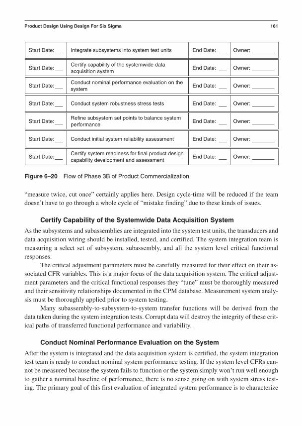
“measure twice, cut once” certainly applies here. Design cycle-time will be reduced if the teamdoesn’t have to go through a whole cycle of “mistake finding” due to these kinds of issues.
Certify Capability of the Systemwide Data Acquisition System
As the subsystems and subassemblies are integrated into the system test units, the transducers anddata acquisition wiring should be installed, tested, and certified. The system integration team ismeasuring a select set of subsystem, subassembly, and all the system level critical functional responses.
The critical adjustment parameters must be carefully measured for their effect on their as-sociated CFR variables. This is a major focus of the data acquisition system. The critical adjust-ment parameters and the critical functional responses they “tune” must be thoroughly measuredand their sensitivity relationships documented in the CPM database. Measurement system analy-sis must be thoroughly applied prior to system testing.
Many subassembly-to-subsystem-to-system transfer functions will be derived from thedata taken during the system integration tests. Corrupt data will destroy the integrity of these crit-ical paths of transferred functional performance and variability.
Conduct Nominal Performance Evaluation on the System
After the system is integrated and the data acquisition system is certified, the system integrationtest team is ready to conduct nominal system performance testing. If the system level CFRs can-not be measured because the system fails to function or the system simply won’t run well enoughto gather a nominal baseline of performance, there is no sense going on with system stress test-ing. The primary goal of this first evaluation of integrated system performance is to characterize
Product Design Using Design For Six Sigma 161
Integrate subsystems into system test units
Certify capability of the systemwide dataacquisition system
Start Date: End Date: Owner:
Start Date: End Date: Owner:
Conduct nominal performance evaluation on thesystem
Start Date: End Date: Owner:
Conduct system robustness stress testsStart Date: End Date: Owner:
Refine subsystem set points to balance systemperformance
Start Date: End Date: Owner:
Conduct initial system reliability assessment
Certify system readiness for final product designcapability development and assessment
Start Date: End Date: Owner:
Start Date: End Date: Owner:
Figure 6–20 Flow of Phase 3B of Product Commercialization
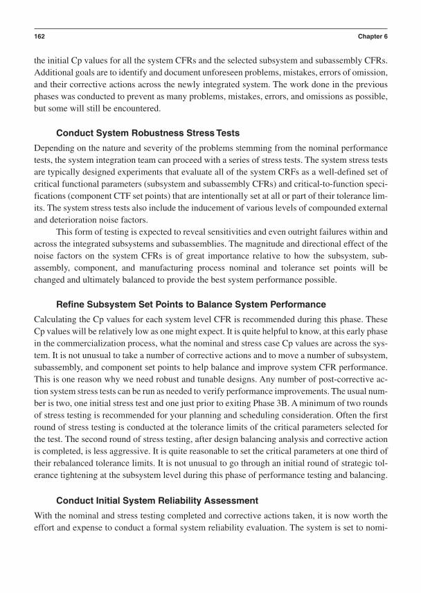
the initial Cp values for all the system CFRs and the selected subsystem and subassembly CFRs.Additional goals are to identify and document unforeseen problems, mistakes, errors of omission,and their corrective actions across the newly integrated system. The work done in the previousphases was conducted to prevent as many problems, mistakes, errors, and omissions as possible,but some will still be encountered.
Conduct System Robustness Stress Tests
Depending on the nature and severity of the problems stemming from the nominal performancetests, the system integration team can proceed with a series of stress tests. The system stress testsare typically designed experiments that evaluate all of the system CRFs as a well-defined set ofcritical functional parameters (subsystem and subassembly CFRs) and critical-to-function speci-fications (component CTF set points) that are intentionally set at all or part of their tolerance lim-its. The system stress tests also include the inducement of various levels of compounded externaland deterioration noise factors.
This form of testing is expected to reveal sensitivities and even outright failures within andacross the integrated subsystems and subassemblies. The magnitude and directional effect of thenoise factors on the system CFRs is of great importance relative to how the subsystem, sub-assembly, component, and manufacturing process nominal and tolerance set points will bechanged and ultimately balanced to provide the best system performance possible.
Refine Subsystem Set Points to Balance System Performance
Calculating the Cp values for each system level CFR is recommended during this phase. TheseCp values will be relatively low as one might expect. It is quite helpful to know, at this early phasein the commercialization process, what the nominal and stress case Cp values are across the sys-tem. It is not unusual to take a number of corrective actions and to move a number of subsystem,subassembly, and component set points to help balance and improve system CFR performance.This is one reason why we need robust and tunable designs. Any number of post-corrective ac-tion system stress tests can be run as needed to verify performance improvements. The usual num-ber is two, one initial stress test and one just prior to exiting Phase 3B. A minimum of two roundsof stress testing is recommended for your planning and scheduling consideration. Often the firstround of stress testing is conducted at the tolerance limits of the critical parameters selected forthe test. The second round of stress testing, after design balancing analysis and corrective actionis completed, is less aggressive. It is quite reasonable to set the critical parameters at one third oftheir rebalanced tolerance limits. It is not unusual to go through an initial round of strategic tol-erance tightening at the subsystem level during this phase of performance testing and balancing.
Conduct Initial System Reliability Assessment
With the nominal and stress testing completed and corrective actions taken, it is now worth theeffort and expense to conduct a formal system reliability evaluation. The system is set to nomi-
162 Chapter 6
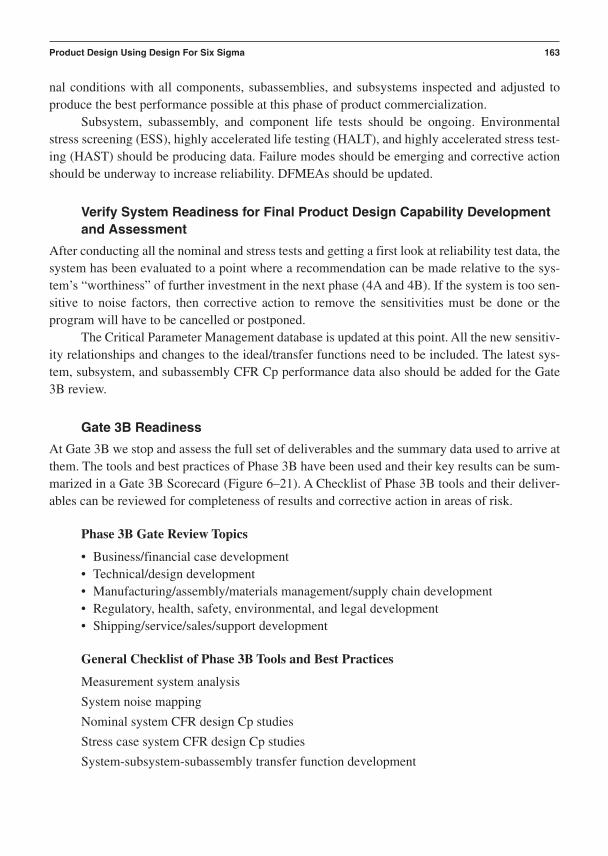
nal conditions with all components, subassemblies, and subsystems inspected and adjusted toproduce the best performance possible at this phase of product commercialization.
Subsystem, subassembly, and component life tests should be ongoing. Environmentalstress screening (ESS), highly accelerated life testing (HALT), and highly accelerated stress test-ing (HAST) should be producing data. Failure modes should be emerging and corrective actionshould be underway to increase reliability. DFMEAs should be updated.
Verify System Readiness for Final Product Design Capability Developmentand Assessment
After conducting all the nominal and stress tests and getting a first look at reliability test data, thesystem has been evaluated to a point where a recommendation can be made relative to the sys-tem’s “worthiness” of further investment in the next phase (4A and 4B). If the system is too sen-sitive to noise factors, then corrective action to remove the sensitivities must be done or theprogram will have to be cancelled or postponed.
The Critical Parameter Management database is updated at this point. All the new sensitiv-ity relationships and changes to the ideal/transfer functions need to be included. The latest sys-tem, subsystem, and subassembly CFR Cp performance data also should be added for the Gate3B review.
Gate 3B Readiness
At Gate 3B we stop and assess the full set of deliverables and the summary data used to arrive atthem. The tools and best practices of Phase 3B have been used and their key results can be sum-marized in a Gate 3B Scorecard (Figure 6–21). A Checklist of Phase 3B tools and their deliver-ables can be reviewed for completeness of results and corrective action in areas of risk.
Phase 3B Gate Review Topics
• Business/financial case development• Technical/design development• Manufacturing/assembly/materials management/supply chain development• Regulatory, health, safety, environmental, and legal development• Shipping/service/sales/support development
General Checklist of Phase 3B Tools and Best Practices
Measurement system analysis
System noise mapping
Nominal system CFR design Cp studies
Stress case system CFR design Cp studies
System-subsystem-subassembly transfer function development
Product Design Using Design For Six Sigma 163

Phase 3B Optimization
Original Due Completion Performance Exit Date vs. Actual Status vs. Criteria Recommendation
Deliverable Owner Deliv. Date Red Green Yellow Red Green Yellow Red Green Yellow Notes
System CFR Nominal Performance
Capability Indices
System CFR Stressed Performance
Capability Indices
System Sensitivity Analysis Results
System-to-Subsystem-to Subassembly
Transfer Functions
Refined Subsystem and Subassembly
Ideal Functions
System Reliability Performance
Subsystem, Subassembly, and
Component Reliability and Life Test Performance
Updated Critical Parameter Database and
Scorecards
Phase 4A Project Management Plans
Figure 6–21 General Scorecard for CDOV Phase 3B Deliverables
164

System level sensitivity analysis
Design of experiments (screening and modeling)
ANOVA
Regression
Analytical tolerance analysis
Empirical tolerance analysis
Statistical process control of design CFR performance
Reliability assessment (normal, HALT, & HAST)
Critical Parameter Management
CDOV Phase 4A: Verification of Product Design Functionality
CDOV Phase 4 covers verification of final product design, production processes, and servicecapability. CDOV Phase 4 contains two major parts:
• Phase 4A focuses on the capability of the product design functional performance.• Phase 4B focuses on the capability of production assembly and manufacturing
processes, within the business as well as the extended supply chain and serviceorganization.
The diagram in Figure 6–22 presents the major elements in Phase 4A.
Product Design Using Design For Six Sigma 165
Conduct final tolerance design on components,subassemblies, and subsystems
Place all CTF components and CFRs underSPC in supply chain and assembly operations
Start Date: End Date: Owner:
Start Date: End Date: Owner:
Build product design verification units usingproduction parts
Start Date: End Date: Owner:
Evaluate system performance under nominalconditions
Start Date: End Date: Owner:
Evaluate system performance under stressconditions
Start Date: End Date: Owner:
Complete corrective actions on problems
Evaluate system performance and reliability
Start Date: End Date: Owner:
Start Date: End Date: Owner:
Verify product design meets all requirementsStart Date: End Date: Owner:
Figure 6–22 Flow of Phase 4A of Product Commercialization
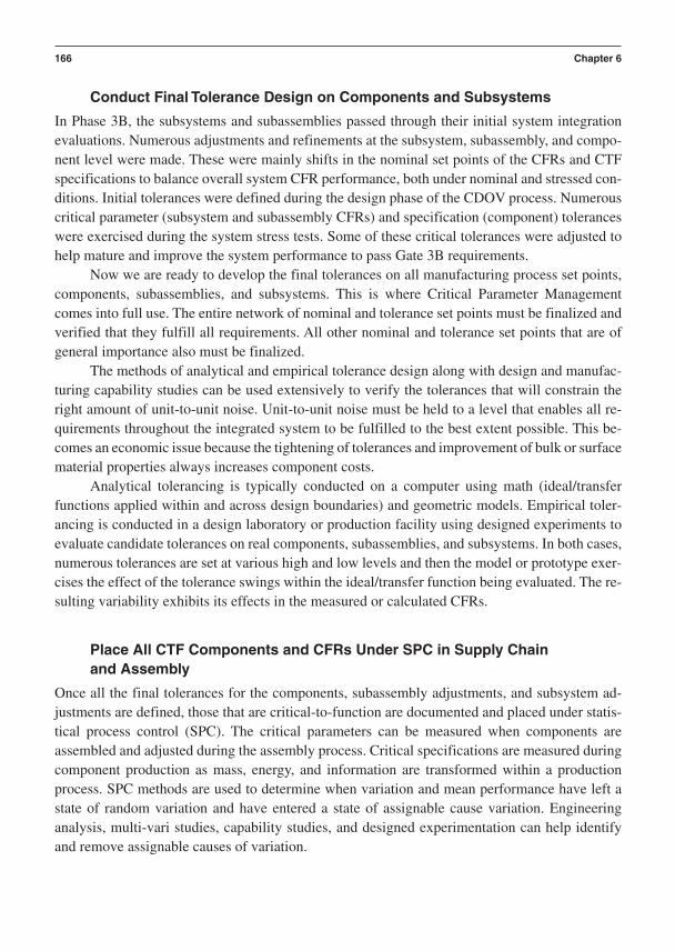
Conduct Final Tolerance Design on Components and Subsystems
In Phase 3B, the subsystems and subassemblies passed through their initial system integrationevaluations. Numerous adjustments and refinements at the subsystem, subassembly, and compo-nent level were made. These were mainly shifts in the nominal set points of the CFRs and CTFspecifications to balance overall system CFR performance, both under nominal and stressed con-ditions. Initial tolerances were defined during the design phase of the CDOV process. Numerouscritical parameter (subsystem and subassembly CFRs) and specification (component) toleranceswere exercised during the system stress tests. Some of these critical tolerances were adjusted tohelp mature and improve the system performance to pass Gate 3B requirements.
Now we are ready to develop the final tolerances on all manufacturing process set points,components, subassemblies, and subsystems. This is where Critical Parameter Managementcomes into full use. The entire network of nominal and tolerance set points must be finalized andverified that they fulfill all requirements. All other nominal and tolerance set points that are ofgeneral importance also must be finalized.
The methods of analytical and empirical tolerance design along with design and manufac-turing capability studies can be used extensively to verify the tolerances that will constrain theright amount of unit-to-unit noise. Unit-to-unit noise must be held to a level that enables all re-quirements throughout the integrated system to be fulfilled to the best extent possible. This be-comes an economic issue because the tightening of tolerances and improvement of bulk or surfacematerial properties always increases component costs.
Analytical tolerancing is typically conducted on a computer using math (ideal/transferfunctions applied within and across design boundaries) and geometric models. Empirical toler-ancing is conducted in a design laboratory or production facility using designed experiments toevaluate candidate tolerances on real components, subassemblies, and subsystems. In both cases,numerous tolerances are set at various high and low levels and then the model or prototype exer-cises the effect of the tolerance swings within the ideal/transfer function being evaluated. The re-sulting variability exhibits its effects in the measured or calculated CFRs.
Place All CTF Components and CFRs Under SPC in Supply Chain and Assembly
Once all the final tolerances for the components, subassembly adjustments, and subsystem ad-justments are defined, those that are critical-to-function are documented and placed under statis-tical process control (SPC). The critical parameters can be measured when components areassembled and adjusted during the assembly process. Critical specifications are measured duringcomponent production as mass, energy, and information are transformed within a productionprocess. SPC methods are used to determine when variation and mean performance have left astate of random variation and have entered a state of assignable cause variation. Engineeringanalysis, multi-vari studies, capability studies, and designed experimentation can help identifyand remove assignable causes of variation.
166 Chapter 6

This approach to variability reduction in the mean and standard deviation of critical pa-rameters and specifications is not cheap. That is why we use CPM. It helps the team spend moneyonly on those design and production process elements that are critical to the functional require-ments of the product.
Build Product Design Certification Units Using Production Parts
Once all the elements of the system design are toleranced and the assembly and productionprocess are under statistical control, the first sets of production parts can be ordered, inspected,and assembled. The construction of the first production systems are done by the production teamswith the design teams present to document any problems.
The list of critical functional responses that will be measured during the assembly processat the subassembly, subsystem, and system level is prepared at this point. Not all CFRs within the system that were measured during the CDOV process will continue to be measured duringsteady-state production. Only a small subset of the CFRs need to go forward as part of the man-ufacturing Critical Parameter Management program for Six Sigma. Many are measured as CTFspecifications on components out in the supply chain; a few are measured as CFRs as subassem-blies and subsystems are assembled and tested prior to integration into the final product assem-bly. The remaining CFRs are measured at the system or completed product level, usually just priorto shipping or during service processes.
Evaluate System Performance Under Nominal Conditions
Once the system is built and all CFR measurement transducers are in place, a repeat of the nom-inal system performance test can be conducted. The Cp of the system CFRs and the productionsubsystem and subassembly CFRs are measured and calculated. The aggregated effect of theseCp values is reported in a metric called the capability growth index or CGI (see Chapter 12).
Evaluate System Performance Under Stress Conditions
The new, “final” tolerances for critical-to-function components and the critical assembly and ser-vice adjustments are typically set at one third (for 3 sigma designs) to one sixth (for 6 sigma de-signs) of their limits for testing purposes. In some cases, this roughly emulates what is known instatistical tolerancing methods as a root sum of squares evaluation. It is more statistically likely thatthe variability that will actually accumulate within and across the system will not be at worst caselimits but rather some lesser amount of consumption of the tolerance limits. From experience andfrom statistical principles we have found it reasonable, over the years, to stress the performance ofthe critical response variables with components and adjustments at about one third to one sixth oftheir actual tolerances. The production CFRs are measured during these stress tests with the addedstress due to applications of external and deterioration noise factors from the system noise map.
Once again, the Cp of the system CFRs and the production subsystem and subassemblyCFRs are measured and calculated. The aggregated effect of these stressed Cp values is reported
Product Design Using Design For Six Sigma 167

in the same CGI format. The measured performance becomes the data used in documenting finalproduct design specifications that represents the teams’ best attempt to fulfill the system, subsys-tem, subassembly, and component requirements.
Complete Corrective Actions on Problems
As is always the case after nominal and stress testing, problems surface and must be corrected.The key is to prevent as many of them as possible by using the right tools and best practices atthe right time within each phase of the CDOV process. Problems at this point in the processshould be relatively minor.
Evaluate System Performance and Reliability
As you can see, this approach postpones traditional reliability assessments until corrective actionsare largely completed after nominal and stress testing is done within each major phase. There isno sense assessing reliability when you know full well you don’t have the design elements mature enough to realistically assume you are anywhere near the goal you seek to confirm. De-veloping and evaluating ideal functions, transfer functions, noise vectors, additive S/N models,tolerance sensitivity stack-up models, and capability growth models are all steady and progres-sive actions that will develop reliability. Reliability tests never grow reliability—they just tell youhow much you do or don’t have. They are important when conducted at the right time and for theright reasons. They confirm you are attaining your goals but should not be done too early. Therule to follow is: don’t consume any resources on predicting or testing reliability that really couldbe better used in the actions of developing reliability. Many of the tools and metrics of DFSS arethere because they are good at creating reliability long before you can actually measure it.
System reliability evaluations typically demonstrate the performance of the functions of thesystem in terms of mean time to failure or mean time to service. The underlying matters of im-portance in reliability testing are:
1. Time2. Failures
These are common things that customers can easily sense or measure. The product devel-opment teams must not ignore these metrics. In DFSS we must have two sets of books that arekept to track the fulfillment of all the product requirements. The book of requirements that cus-tomers worry about is typically at the system level and is rarely stated in engineering units. Tofully satisfy these quality requirements against which customers measure, we must have a set ofbooks that dig deeper, down through the hierarchy of the product and production systems archi-tectures. This “book of translated requirements” is loaded with fundamental engineering metricsthat can provide the preventative, forward-looking metrics that assure us that the functions can
168 Chapter 6

indeed be replicated, over the required lengths of time that will fulfill the VOC requirements. Ourmetrics have to be good enough to measure and make us aware of impending failures!
Verify Product Design Meets All Requirements
The ability to verify the system design requires:
1. A clear set of design requirements at the system, subsystem, subassembly, component,and manufacturing process level
2. A capable set of design performance metrics for the critical functional responses at the system, subsystem, and subassembly levels and a capable set of metrics for thecritical-to-function specifications at the component and manufacturing process level.
The construction and use of this integrated system of requirements and metrics is calledCritical Parameter Management. It will be much easier to rapidly determine the status of capa-bility to fulfill form, fit, and function requirements if a disciplined approach is taken from the firstday of the CDOV process to track these critical relationships. Critical Parameter Managementpossesses a scorecard that accumulates Cp performance growth across the subsystems and at thesystem level. This scorecard is populated with Cp values from all the subsystem critical functionalresponses and a rolled up summary capability growth value, CGI. It is somewhat analogous to“rolled throughput yield (RTY)” that is used in production operations and transactional forms ofSix Sigma. The CGI is based on CFRs while RTY is typically based on defects per million op-portunities or defects per unit. The CGI is the management team’s eyes into the “soul” of the prod-uct from a functional perspective. When the CGI scorecard is at its required level of Cp growth,the quality is inherent in the certified product design.
Gate 4A Readiness
At Gate 4A we stop and assess the full set of deliverables and the summary data used to arrive atthem. The tools and best practices of Phase 4A have been used and their key results can be sum-marized in a Gate 4A scorecard (Figure 6–23). A checklist of Phase 4A tools and their deliver-ables can be reviewed for completeness of results and corrective action in areas of risk.
Phase 4A Gate Review Topics
• Business/financial case development• Technical/design development• Manufacturing/assembly/materials management/supply chain development• Regulatory, health, safety, environmental, and legal development• Shipping/service/sales/support development
Product Design Using Design For Six Sigma 169
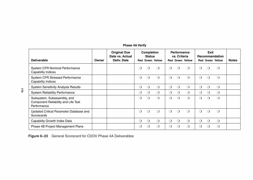
Phase 4A Verify
Original Due Completion Performance Exit Date vs. Actual Status vs. Criteria Recommendation
Deliverable Owner Deliv. Date Red Green Yellow Red Green Yellow Red Green Yellow Notes
System CFR Nominal Performance
Capability Indices
System CFR Stressed Performance
Capability Indices
System Sensitivity Analysis Results
System Reliability Performance
Subsystem, Subassembly, and
Component Reliability and Life Test Performance
Updated Critical Parameter Database and
Scorecards
Capability Growth Index Data
Phase 4B Project Management Plans
Figure 6–23 General Scorecard for CDOV Phase 4A Deliverables
170
General Checklist of Phase 4A Tools and Best Practices
Measurement system analysis
System noise mapping
Analytical tolerance design
Worst case analysis
Root sum of squares analysis
Six Sigma analysis
Monte Carlo simulation
Empirical tolerance design
System level sensitivity analysis
Design of experiments
ANOVA
Regression
Multi-vari studies
Design capability studies
Nominal system CFR design Cp studies
Stress case system CFR design Cp studies
Reliability assessment (Normal, HALT, & HAST)
Competitive benchmarking studies
Statistical process control of design CFR performance
Critical Parameter Management (with capability growth index)
CDOV Phase 4B: Verification of Production
Phase 4B of the CDOV process examines capability production, assembly, and manufacturingprocess within the business as well as the extended supply chain and service organization. Figure 6–24 covers the major elements.
Build Initial Production Units Using Inspected Production Parts
Now that the organization has completed the verification of the final product design specifica-tions, it is time to order actual production parts and build the initial production units that will bear revenue. This is not a serial process. Many parts, tools, and subassemblies will have longlead times. A good deal of judgment must be exercised to balance the risk of early order based onassumed verification versus waiting until the data is all in before ordering the “hard” tools andcomponents.
Many design organizations get their part orders way out of “phase” with their performanceand capability data. The designers keep designing before the testers finish testing! One way to
Product Design Using Design For Six Sigma 171

remedy this is to make the designer and tester the same person. At times it is good to have peo-ple so busy doing one thing they can’t get anything else done! The real problems come when thisphenomenon occurs habitually from the beginning of a new product development program. Bythe time the final production units are being built, virtually no one knows if or how well they willactually work.
The production parts need to be produced from and inspected against final, verify designspecifications. A product design specification is the actual nominal specification and tolerancethat the design can provide. The motivating forces behind the product design specifications arethe system, subsystem, subassembly, component, and manufacturing process requirements. If theparts are not inspected during this earliest production build, you run the risk of not catching anumber of human errors and mistakes that, once corrected, are likely to not be a problem everagain. If these mistake-proofing inspections do not occur, it is quite possible in any sufficientlycomplex product for these problems to go on for extended periods of time, particularly if the prob-lem is intermittent.
Assess Capability of All CFRs and CTFs in Production and Assembly Processes
A thorough assessment of the Critical Parameter Management metrics that are transferring intosteady-state production must be conducted at this point. This body of metrics is a relatively small,carefully selected group of CFRs and CTF specifications from the design CPM database. The pro-
172 Chapter 6
Build initial production units using inspectedproduction parts
Assess capability of all CFRs and CTFs inproduction and assembly processes
Start Date: End Date: Owner:
Start Date: End Date: Owner:
Assess capability of all product level andsubsystem level CFRs during assembly
Start Date: End Date: Owner:
Assess reliability of production unitsStart Date: End Date: Owner:
Verify all requirements are being met acrossassembly processes
Start Date: End Date: Owner:
Verify all requirements are being met acrossproduction processes
Verify all service requirements are being metwith service/support processes
Start Date: End Date: Owner:
Start Date: End Date: Owner:
Verify product, production, assembly, andservice/support processes are ready for launch
Start Date: End Date: Owner:
Figure 6–24 Flow of Phase 4B of Product Commercialization

duction CPM database is a scaled-down version of the design CPM database. The design CPMdatabase will be available to the production organization for the life of the product, but the spe-cific production-oriented CFRs and CTF specifications will be the leading indicators that showthat the manufacturing processes and the assembled parts coming from them are capable and un-der statistical control, assuring they are safe to use in steady-state production.
Assess Capability of All Product Level and Subsystem Level CFRs During Assembly
Within the actual product are a few CFRs that the assembly team tests as the subassemblies andsubsystems are constructed. Once these are assembled into the product, the system level CFRscan be evaluated. There is no need for additional, special, or long-term burn-in style testing whenCritical Parameter Management is systematically used across the phase and gates of the CDOVprocess.
The selection of these CFRs is somewhat analogous to the way your physician conductsyour annual physical. Neither you or your doctor can afford to test everything that is important toyour health. The few critical parameters that are the leading indicators of your health can effi-ciently and economically be evaluated. Once you pass these critical checks, out the door you go.This is essentially what must be done with products. Design in the quality, document and checkthe critical parameters, and get the product to customers so that they can be satisfied “on time”and your shareholders will see a great return on their investment in the business.
Assess Reliability of Production Units
An appropriately small number of the production units should be randomly selected for a com-plete reliability evaluation. This is done to complete the competitive benchmarking process andto assure that there are no lingering surprises in the initial production lot of system units. The datafrom this evaluation can be used as a baseline for your next product development program.
Once you are past the initial ramp-up of your production process, the data you need for re-liability should come from the base of delivered products. A strong customer service and supportprocess with a focused effort to establish data acquisition and transmission back to the design or-ganization from a few strategic customers on CFRs and general reliability is essential. This is an-other way the Critical Parameter Management process is extended out into the steady-state useenvironment.
Verify All Requirements Are Being Met Across Assembly Processes
Just as you established Critical Parameter Management metrics out into the supply chain to quan-tify the capability of incoming component CTF specifications, you should also establish a seriesof CFR and CTF specification checks as the assembly process is conducted. Here we see a por-tion of the computer-aided data acquisition systems that were used in design transferred to the as-sembly team for continued use during steady-state production.
Product Design Using Design For Six Sigma 173

Verify All Requirements Are Being Met Across Production Processes
A comprehensive roll-up of all Critical Parameter Management data in the network of productionprocesses must be gathered to demonstrate that all the critical manufacturing processes, compo-nents, assembled subassemblies, and subsystems are “on target with low variability,” or Cpkmeasured. The ultimate requirements that matter the most are at the system or completed productlevel. All system level CFRs should be found capable on a routine basis. Assignable causes ofvariation should be identified using statistical process control. They should be removed under thescrutiny and balance of the CPM database.
Verify All Service Requirements Are Being Met with Service/Support Processes
All CFRs with critical adjustment parameters that the service community will use should be cer-tified for “adjustability.” The service engineering community will then be able to play its role insustaining the Cpk values for the system and subsystem CFRs for which they are responsible.
The CPM database should be in the hands of the service engineering teams for diagnosticand maintenance purposes. One of the biggest payoffs in conducting CPM is the detailed techni-cal performance information that can be passed on to the service organization, which can readilyuse the relational ideal/transfer function information resident in the CPM database to track downroot causes of problems and take specific corrective action. This greatly increases the “fix it rightthe first time” expectation of modern customers.
Verify Product, Production, Assembly, and Service/Support Processes AreReady for Launch
As a final Gate 4B deliverable, the entire launch readiness status, based on the capabilities thatcan be tracked in the CPM database, should be prepared for review. All the capability data acrossthe organizations that are responsible for verifying launch readiness can be summarized and usedto underwrite the integrity of the decision to launch or to postpone for corrective action.
Gate 4B Readiness
At Gate 4B we stop and assess the final, full set of deliverables and the summary data used to ar-rive at them. The tools and best practices of Phase 4B have been used and their key results can besummarized in a Gate 4B scorecard (Figure 6–25). A checklist of Phase 4B tools and their deliv-erables can be reviewed for completeness of results and corrective action in areas of risk.
Phase 4B Gate Review Topics
• Business/financial case development• Technical/design development• Manufacturing/assembly/materials management/supply chain development• Regulatory, health, safety, environmental, and legal development• Shipping/service/sales/support development
174 Chapter 6

Phase 4B Verify
Original Due Completion Performance Exit Date vs. Actual Status vs. Criteria Recommendation
Deliverable Owner Deliv. Date Red Green Yellow Red Green Yellow Red Green Yellow Notes
System CFR Nominal Performance
Capability Indices
System Sensitivity Analysis Results
System Reliability Performance
Subsystem, Subassembly, and
Component Reliability and Life Test Performance
Updated Critical Parameter Database and
Scorecards
Capability Growth Index Data
Sustaining Production Engineering
Support Plans
Figure 6–25 General Scorecard for CDOV Phase 4B Deliverables
175

General Checklist of Phase 4B Tools and Best Practices
Measurement system analysis
Analytical tolerance design
Worst case analysis
Root sum of squares analysis
Six Sigma analysis
Monte Carlo simulation
Empirical tolerance design
System level sensitivity analysis
Design of experiments
ANOVA
Regression
Multi-vari studies
Design capability studies
Nominal system CFR design Cp studies
Reliability assessment (normal, HALT, & HAST)
Competitive benchmarking studies
Statistical process control of design CFR performance
Critical Parameter Management (with capability growth index)
References
Clausing, D. P. (1994). Total quality development: Improved total development process. NewYork: ASME Press.
Cohen, L. (1995). Quality function deployment: How to make QFD work for you. New York:Addison Wesley Longman.
Cooper, R. G. (2001). Winning at new products: Accelerating the process from idea to launch(3rd ed.). Reading, MA: Perseus Books.
Otto, K. N. & Wood, K. L. (2001). Product design. New Jersey: Prentice Hall.Rechtin, Eberhardt. (1990). Systems architecting: Creating and building complex systems. New
Jersey: Prentice Hall, Incorporated.Ullman, D. G. (1997). The mechanical design process. New York: McGraw-Hill.Ulrich, K. T. & Eppinger, S. D. (1995). Product design and development. New York: McGraw-
Hill.Wheelwright, S. C. & Clark, K. B. (1992). Revolutionizing product development. New York:
The Free Press.
176 Chapter 6
C H A P T E R 7
System Architecting,Engineering, and IntegrationUsing Design For Six Sigma
Virtually every product made is some form of integrated system. So is every manufacturingand assembly process. All systems are built up from the subsystems, subassemblies, and/or
components that are supplied from a network of internal and external manufacturing and assem-bly processes. Six Sigma methods are very much applicable to the development of new technol-ogy systems (commonly known as platforms), product systems, and production systems. Aspecific set of tools and best practices can be identified and applied by system architects and sys-tem integration engineers during the phases and gates of the I2DOV and CDOV product devel-opment processes. This chapter is all about “what to do and when to do it” with respect to systemarchitecting, engineering, and integration using the tools and best practices from technology de-velopment and Design For Six Sigma.
It has been our experience to find many of the companies that develop and design under theinfluence of Six Sigma methods do so largely independent of a system integration context. Mostengineering teams tend to focus their efforts on subsystem, subassembly, component, or materialdevelopment. They also tend to focus just on projects that correct, or react to, a preexisting prob-lem that will have some form of rapid and reasonably significant cost reduction. Six Sigma proj-ects have their historical roots grounded in rapid, strong financial returns. This, of course, is agreat thing, but there exists a whole class of projects that develop their economic value over thecourse of time it takes to conduct the phases and gates of a product development process. Theirfinancial value resides within the fulfillment of the new product’s business case. This approachis not driven by reaction to problems but rather the prevention of problems. The ultimate eco-nomic value resides in the development, design, and delivery of a new system!
Developing new technologies, products, and production systems takes time. The develop-ment of a new system that fulfills a complete set of requirements can return enormous financialresults. Ignoring or underinvesting in this class of applications for Six Sigma methods is starting
177

to diminish—slowly. It is time for businesses that focus on revenue growth through the develop-ment and integration of systems to improve their results with the help of Six Sigma developmentand design tools and the process of Critical Parameter Management.
Just as in the previous two chapters, we will use a flow-down of actions to illustrate the ma-jor steps one can take to conduct system architecting, system engineering, and system integrationfor Six Sigma within the CDOV Phase/Gate process. This chapter includes the start date, end date,and owner blocks in the action flow-down diagrams. We do this to remind you that all these ac-tions can and should be tracked using PERT charts for disciplined project management. The sys-tem architecting and engineering process for technology development is quite similar to the oneused in product design, so we will use the CDOV process as a general approach that can be eas-ily modified for use within the I2DOV process.
System architecting, engineering, and integration teams typically reside within the tech-nology, product, or production process development organizations. System architects are typi-cally leaders of advanced product planning teams within the product development organization.They focus on the structuring of the system elements around the functions the system must per-form to fulfill its requirements. They work with the system engineers to develop a complete setof system requirements and the network of measures that prove that the integrated subsystems,subassemblies, components, and manufacturing processes fulfill their system level requirements.System Architects are specialists who often work within a system engineering group. They guidethe initial form, fit, and function structural definition work done in the concept phase of theCDOV process. System engineers and architects work together to manage the interfaces into,across, and out of the system. In some organizations they act as surrogates for field engineering,service, support, and assembly operations during the early phase of the development process.That is to say, they build and measure the performance of the first integrated units. They trou-bleshoot and repair them during testing. They maintain configuration control and document thebill of materials and initial product role-up costs. They transfer these important functions to theproduction and production support teams gradually during the later phases of the product devel-opment process (typically during the capability verification phase of the CDOV process).
The system engineering team owns the Critical Parameter Management process. It alsoforms the leadership core of a new multifunctional product development team called the QualityCouncil. It becomes the watchdog group for the program.
The system architects help initiate CPM but due to the nature of CPM as a verification and“certification of performance” tool, its proper place of ownership is within the system engineer-ing team. The team documents all the product requirements and generates the computer-aideddatabase that tracks the complex network of requirements and fulfilling capability metrics thatverify that the system is ready for its gate reviews. The system engineering team evaluates bothnominal and stressed performance (for Cp and Cpk). These teams are the new model for whatused to be known as quality assurance groups. The old model was an organizationally indepen-dent team of inspectors who were quality conformance watchdogs. They owned nothing and werenot held responsible for delivering anything except reports of how well or badly the system per-formed. They were largely reactive and rarely preventative with regard to the development of
178 Chapter 7

product quality. The new model, as prescribed in this text, is a new team that resides within theproject or program. This team owns specific deliverables and is held directly accountable for thepreventative development of system performance in terms of both cost and quality. These systemengineers must perform their duties within the structured constraints of the CDOV process, sothey also are held accountable for cycle-time. Old-line quality assurance organizations, becausethey only focused on policing the “suspicious behaviors” of the project team, usually added to cycle-time as they held the project hostage until “they” were forced to fix the problems. Now, thesystem engineers own the problems. With such responsibility comes a driving impulse to avoidthe creation of problems in the first place. In fact, this approach encompasses specific tools andbest practices and the time and resources to assure that quality is designed into the system in theearliest phases of the project.
We advocate the dissolution of old-line QA watchdog groups. Redeploy their talent intosystem engineering and integration teams and hold them accountable for the deliverables fromthe DFSS tools and best practices. As for the “independent and objective” policing work, this canbe handled by making the system engineering manager a direct report to both the program man-ager and the corporate officer responsible for the business in which the program resides. In themajority of cases the conflict of interest is removed with this approach.
Phase 1: System Concept Development
The diagram in Figure 7–1 illustrates the major system architecting, engineering, and integrationelements for the CDOV Process Phase 1: Develop a system concept based on market segmenta-tion, the product line, and technology strategies.
The system architects and engineers participate heavily in Phase 1 inbound marketing ac-tivities. They serve in both consulting and leadership roles and provide a “feed forward” view ofwhat is likely to be coming into the next commercialization project to the system engineeringgroup. The divisional inbound marketing managers own the process and tools for voice of cus-tomer acquisition to create the database of “what is needed.” The vice president or director ofR&D owns the process and tools for voice of technology acquisition to develop the database ofwhat technologies are available or need to be developed to meet the market needs. The systemengineering manager owns the process and tools for VOC translation into system requirements,developing the CPM database to account for the hierarchy of requirements and metrics for thefulfillment of the VOC and the VOT.
The specific issues related to each Phase 1 action item (start date for each action item, theaction item, end date for each action) will be reviewed in this section. Each of these action itemscan be conducted by using a tool or best practice. The flow of actions can be laid out in the formof a PERT chart for project management purposes.
Participate in Gathering the Voice of the Customer Data
Start Date: __________ End Date: __________ Owner: __________
System Architecting, Engineering, and Integration Using Design For Six Sigma 179

180
Lead the process of refining and ranking of thevoice of the customer using KJ analysis
Integrate and align the VOC with the voice oftechnology (Needs. . .Ideas. . . Technologies =Opportunities?)**
Start Date: End Date: Owner:
Document the VOC in the Critical ParameterManagement database**
Start Date: End Date: Owner:
Participate in gathering the voice of thecustomer data
Start Date: End Date: Owner:
Conduct competitive assessments,investigations, benchmarking, and projections ofvulnerabilities**
Start Date: End Date: Owner:
Generate product or system level requirementsdocument
Start Date: End Date: Owner:
Lead the team in the definition of the functionsthat fulfill the system requirements
Start Date: End Date: Owner:
Oversee the generation of the system conceptevaluation criteria
Start Date: End Date: Owner:
Lead the team in the generation of systemconcepts that fulfill the functions
Start Date: End Date: Owner:
Lead the team in the evaluation of the systemconcepts
Start Date: End Date: Owner:
Lead the team in the selection of a superiorsystem concept
Start Date: End Date: Owner:
Develop reliability requirements, initial reliabilitymodel, and FMEA for the system
Start Date: End Date: Owner:
Calculate initial "rough order of magnitude" costestimates for the superior concept
Start Date: End Date: Owner:
Analyze, characterize, model, and predictnominal performance of the superior systemconcept
Start Date: End Date: Owner:
Identify new system and subsystem functionsthat will require new data acquisition equipment,calibration, and measurement processes
Start Date: End Date: Owner:
Work with inbound marketing team togenerate, collect, analyze, refine, and categorizenew "Blue Sky" product ideas*
Start Date: End Date: Owner:
Lead in the creation of the product or systemlevel House of Quality*
Start Date: End Date: Owner:
Start Date: End Date: Owner:
Figure 7–1 Flow of System Architecting, Engineering, and Integration Actions for Six Sigma inPhase 1 of Product Commercialization
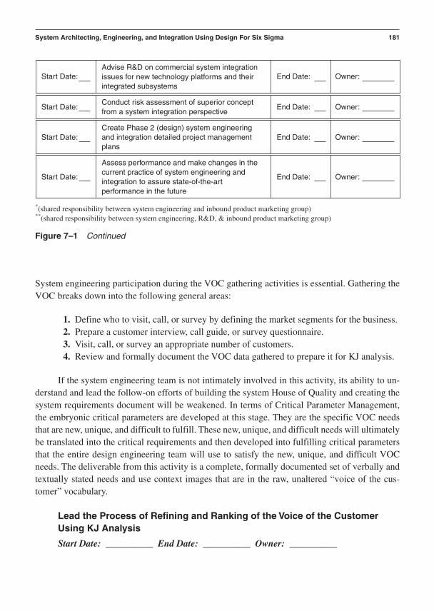
System engineering participation during the VOC gathering activities is essential. Gathering theVOC breaks down into the following general areas:
1. Define who to visit, call, or survey by defining the market segments for the business.2. Prepare a customer interview, call guide, or survey questionnaire.3. Visit, call, or survey an appropriate number of customers.4. Review and formally document the VOC data gathered to prepare it for KJ analysis.
If the system engineering team is not intimately involved in this activity, its ability to un-derstand and lead the follow-on efforts of building the system House of Quality and creating thesystem requirements document will be weakened. In terms of Critical Parameter Management,the embryonic critical parameters are developed at this stage. They are the specific VOC needsthat are new, unique, and difficult to fulfill. These new, unique, and difficult needs will ultimatelybe translated into the critical requirements and then developed into fulfilling critical parametersthat the entire design engineering team will use to satisfy the new, unique, and difficult VOCneeds. The deliverable from this activity is a complete, formally documented set of verbally andtextually stated needs and use context images that are in the raw, unaltered “voice of the cus-tomer” vocabulary.
Lead the Process of Refining and Ranking of the Voice of the CustomerUsing KJ Analysis
Start Date: __________ End Date: __________ Owner: __________
System Architecting, Engineering, and Integration Using Design For Six Sigma 181
Advise R&D on commercial system integrationissues for new technology platforms and theirintegrated subsystems
Start Date: End Date: Owner:
Conduct risk assessment of superior conceptfrom a system integration perspective
Start Date: End Date: Owner:
Create Phase 2 (design) system engineeringand integration detailed project managementplans
Start Date: End Date: Owner:
Assess performance and make changes in thecurrent practice of system engineering andintegration to assure state-of-the-artperformance in the future
Start Date: End Date: Owner:
*(shared responsibility between system engineering and inbound product marketing group)**(shared responsibility between system engineering, R&D, & inbound product marketing group)
Figure 7–1 Continued

The system architect responsible for producing the affinity diagram using KJ analysis takes a lead-ership role at this point. As the leader for this activity, the system architect must act in an unbiased,objective role as a KJ process facilitator. The multifunctional team conducting the KJ analysisshould be from inbound marketing, engineering, service, sales, production, supply chain, and pos-sibly even a few key customers. The team must process the VOC data into groups of needs thathave an “affinity” to one another. The completed KJ analysis offers a diagram of hierarchical state-ments of need. It should look like a tree structure. This diagram contains the needs that are new,unique, and difficult. Needs that are not new, unique, or difficult are still important and need to betracked to be sure their specific issue is directly covered by one or more of the system requirementsthat are soon to be documented. The primary reason we do an affinity diagram is to be sure we havecomprehensively documented the most critical needs that the customer has articulated by word,text, or observed behavior. Two levels of KJ analysis can be conducted in the following order:
1. The image KJ diagram structures and ranks “images” the interview team formed dur-ing interview sessions and through opportunities to observe the physical behaviors cus-tomers exhibit by purely observing how they use or interact with the product or processbeing evaluated for new development.
2. The requirements KJ diagram contains the combined “imaged” needs and the actualstated needs of customers. The image KJ results are used to help create the require-ments KJ diagram.
The requirements KJ is used to flow new, unique, and difficult customer needs into the sys-tem level House of Quality. The deliverable from this activity is a completed KJ diagram that con-tains the ranked and structured VOC needs (see Chapter 14 for details).
Document the VOC in the Critical Parameter Management Database
Start Date: __________ End Date: __________ Owner: __________
The system engineer responsible for the construction of the Critical Parameter Management re-lational database is now called into action. This individual enters the ranked and structured VOCdata into the CPM database. This information is structured so it can be easily linked to the spe-cific system requirements that are soon to be developed and entered in the next layer of the data-base. The Critical Parameter Management database must be a relational database so that eachcritical customer need can be linked to any and all system requirements to which it relates. Thisconnectivity is extremely important as the system architecting team attempts to fully structure asystem that can adequately balance the fulfillment of the critical customer needs.
Integrate and Align the VOC with the Voice of Technology(Needs. . .Ideas. . .Technologies Opportunities?)
Start Date: __________ End Date: __________ Owner: __________
182 Chapter 7

The system architectural team and system engineers must act as a balancing influence betweenthe desire to give customers what they ask for and what current technology can reasonably pro-vide. It is just as important for the system development teams to gather the voice of technologyas it is the voice of the customer. The system engineering team becomes the clearinghouse for theinclusion of new technologies into the concept development phase. If a new technology is to beincluded in the product architecture, the system engineering team plays a lead role is the assess-ment of its contribution to program risk.
The voice of technology includes the following information:
1. New patents in the areas to be covered by candidate designs within the new product architecture
2. Benchmarking data on the current competitive products serving the target market3. New trends in technology development related to the new product ideas4. New technologies under development from R&D that are being readied for application
The system architecting and engineering teams will need this information to properly con-duct quality function deployment. The House of Quality requires input from the voice of the cus-tomer as well as the voice of technology.
Lead in the Creation of the Product or System Level House of Quality
Start Date: __________ End Date: __________ Owner: __________
The system architecting team plays the lead role in the development and documentation of thesystem level House of Quality. The system engineering representative on the system architectingteam typically has the responsibility for documenting the system House of Quality. The multi-functional team members from the business actually conduct QFD under the guidance of an ex-perienced chief system architect.
The system House of Quality must be limited in what VOC needs are placed into it fortranslation into system requirements. Not all VOC needs are critical. Only those needs that arenew, unique, and/or difficult should be translated and ranked in the system House of Quality. Thesystem engineering team should provide assistance on what is considered new, unique, and/or dif-ficult. All other VOC needs that are old, common, and easy should be directly translated andplaced in the system requirements document. If a few of these types of needs are considered crit-ical, they should be loaded into the system House of Quality.
Conduct Competitive Assessments, Investigations, Benchmarking,and Projections of Vulnerabilities
Start Date: __________ End Date: __________ Owner: __________
System Architecting, Engineering, and Integration Using Design For Six Sigma 183
The system engineering team not only acts as the repository of customer needs and technologytrend information but also conducts qualitative and quantitative competitive product assess-ments and benchmarking tests. These may include analytical assessments, reverse engineeringand teardowns, baseline nominal and stress test evaluations, cost breakdowns, failure modes and effects analysis, life tests, service evaluations, and numerous other estimates of competitiveperformance characterizations. The system engineers provide benchmarking information to thesystem architecting team and to the subsystem teams as they begin their work in the concept de-sign phase.
Generate Product or System Level Requirements Document
Start Date: __________ End Date: __________ Owner: __________
The system architectural team will need an extremely clear and well-worded system requirementsdocument to drive the architecting process. It is risky to generate and evaluate system conceptsin the absence of a well-structured set of system requirements.
The system requirements document contains all the requirements that must be fulfilled forthe certification of the product design and its supporting hardware, software, services, and docu-mentation. The system requirements will include both the critical new, unique, and difficult re-quirements along with the old, common, and easy requirements. Typically, the old, common, andeasy requirements that are truly critical are few in number. All requirements—those that are crit-ical to functional performance and those that are considered of nominal importance—must be in-cluded in the system requirements document.
It is especially important that software requirements be clearly defined and related to hard-ware requirements. The system architectural team needs to be sure that it has adequate represen-tation from the software organization at the beginning of the conceptual design of the completesystem architecture.
Lead the Team in the Definition of the Functions That Fulfill the System Requirements
Start Date: __________ End Date: __________ Owner: __________
Once the system architecting team is in possession of the system requirements, the system engi-neering representative can lead the team through the definition of the specific functions that thesystem must perform to fulfill the requirements. The list of system functions will begin the defi-nition of the metrics for Critical Parameter Management. This activity often includes the refine-ment of functional performance targets and their units of measure. This is also the beginning ofthe definition of the requirements that will drive the development, design, and certification of asystemwide data acquisition system.
The documentation and linkage between the flow-down of needs to requirements to func-tions to concepts is essential to any Design For Six Sigma approach to product development.
184 Chapter 7
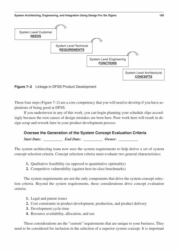
These four steps (Figure 7–2) are a core competency that you will need to develop if you have as-pirations of being good at DFSS.
If you underinvest in any of this work, you can begin planning your schedule slips accord-ingly because the root causes of design mistakes are born here. Poor work here will result in de-sign scrap and rework later in your product development process.
Oversee the Generation of the System Concept Evaluation Criteria
Start Date: __________ End Date: __________ Owner: __________
The system architecting team now uses the system requirements to help derive a set of systemconcept selection criteria. Concept selection criteria must evaluate two general characteristics:
1. Qualitative feasibility (as opposed to quantitative optimality)2. Competitive vulnerability (against best-in-class benchmarks)
The system requirements are not the only components that drive the system concept selec-tion criteria. Beyond the system requirements, these considerations drive concept evaluation criteria:
1. Legal and patent issues2. Cost constraints in product development, production, and product delivery3. Development cycle-time4. Resource availability, allocation, and use
These considerations are the “custom” requirements that are unique to your business. Theyneed to be considered for inclusion in the selection of a superior system concept. It is important
System Architecting, Engineering, and Integration Using Design For Six Sigma 185
System Level CustomerNEEDS
System Level TechnicalREQUIREMENTS
System Level EngineeringFUNCTIONS
System Level ArchitecturalCONCEPTS
Figure 7–2 Linkage in DFSS Product Development

that the architectural team initiate and lead a cross-functional effort to integrate system require-ments with software architectural constraints and capabilities. They must ensure the software andsubsystem teams are prepared to help in the generation and evaluation of system concepts asneeded.
Work with Inbound Marketing Team to Generate, Collect, Analyze, Refine,and Categorize New “Blue Sky” Product Ideas
Start Date: __________ End Date: __________ Owner: __________
There are at least two major ways to get ideas for new products:
1. Obtain new product ideas from sources outside the system architectural team.2. Generate new product ideas from within the system architecting team.
The system architectural team solicits new product ideas from any and all reasonable out-side sources. These are often referred to as blue sky ideas. This approach is democratic and allowsthe internal organization and external influences to stimulate creativity during system concept de-velopment. A tyrannical or exclusionary approach to concept development is a bad idea. Organi-zations that fear the openness of “blue sky” ideation are limiting the potential of identifyingconcepts that have superior feasibility and low competitive vulnerability. If your organization hasa few “concept tyrants,” you need a “bloodless coupe.” You cannot afford to miss a great ideafrom an individual who may be a “quiet genius.”
Lead the Team in the Generation of System Concepts That Fulfill the Functions
Start Date: __________ End Date: __________ Owner: __________
With the “blue sky” ideas in hand, the system architectural team generates a reasonable set of sys-tem concepts. A reasonable number is a relative thing. Certainly it is at least two and probablywould be better if it is six or more. The desire for numerous system concepts is justified by the factthat the team will use the best characteristics from the candidate concepts to synthesize a “super-concept,” a hybrid built upon the innovations from across the group. One idea is not enough.
One person telling everyone else the way it’s going to be is wrong. With many conceptscome many options for system integration during concept selection and evaluation.
Lead the Team in the Evaluation of the System Concepts
Start Date: __________ End Date: __________ Owner: __________
The system engineering representative takes the lead (facilitation) role in conducting the Pugh con-cept evaluation and selection process. The role includes the assurance of the following elements:
186 Chapter 7

1. A reasonable number of concepts to be evaluated2. All concepts developed and illustrated to a common, equal level of representation3. A complete set of evaluation criteria ready for use4. A best-in-class benchmark datum concept identified for the comparison process5. Adequate multifunctional team representation during the Pugh process6. The participants all trained in the use of the Pugh process
System engineers act as an unbiased facilitator. Their role is to guide the initial run-throughconcept evaluation, subsequent rationalization, and hybridization of super-concepts and the se-lection of a new datum, if required. They lead the follow-on iterations of the hybrid concept eval-uations and final selection of a superior concept relative to the final datum concept. The key is tobe able to lead the system architecting team to a consensus based upon the criteria. This is a goodpoint to remind the reader that the criteria should be representative of the voice of the customer,the voice of technology, and the voice of the business (let’s not forget the shareholders!).
Lead the Team in the Selection of a Superior System Concept
Start Date: __________ End Date: __________ Owner: __________
As the system architecting team goes through the iterative cycles of the Pugh concept selectionprocess (also called the converging-diverging process due to its iterative nature), a dominant con-cept emerges. This concept is almost never one of the original concepts. Usually it is a hybridform of two or more of the initial candidate concepts that have been synthesized.
The team needs to reach two forms of consensus:
1. The selected concept is indeed superior to the datum concept.2. The selected concept is rational and reasonable in comparison to the runner-up as they
relate to the most critical of the selection criteria (ranking of the criteria is one way tosettle this).
The second step of consensus is an important check and balance on the practicality of theoutcome. From time to time the runner-up is actually better when the team takes the time to re-flect on the top two concepts relative to the criteria that made them rank so high. Sometimes thetop two concepts are codeveloped until the data is clearly supporting one over the other in termsof maturing toward the fulfillment of the critical system requirements.
Analyze, Characterize, Model, and Predict Nominal Performance of the Superior System
Start Date: __________ End Date: __________ Owner: __________
With a superior system concept selected and documented, it is now worth the time investment toanalyze the design. The system engineers responsible for modeling system performance begin
System Architecting, Engineering, and Integration Using Design For Six Sigma 187

construction of the Critical Parameter Management database. This is done to prepare for in-depthanalysis of the system performance. At this point the system is a black box of projected outputsand yet-to-be-defined internal relationships. In Critical Parameter Management terms the systemis a collection of system level critical functional responses that need to be modeled and measuredto see if they fulfill the system requirements. The system can be modeled in three ways:
1. Analytical model of system outputs based on inputs to system performance from ex-ternal (user and environment) and internal (subsystem and subassembly) inputs
2. Graphical model of system’s external space consumption and internal space use3. Physical model of the system for functional and spatial performance characterization
These three methods of modeling characterize the estimated and actual form, fit, and func-tion of the system. One cannot do all of these modeling activities within the concept phase! Youneed to have patience and conduct the right form and degree of modeling within the appropriatephase of the CDOV process.
The following suggestions align appropriate system modeling action with the proper phasesin the CDOV process.
Phase 1 (concept design)Analytical At this point you should define the critical functional responses (Y variables)
at the system level and link them to the system requirements they fulfill. These linked relation-ships should be documented in your CPM relational database. The formal Y f(x) models for allsystem CFRs will be estimated and verified in Phase 2 (design development). This limitation isdue to the fact you have not yet defined the subsystem requirements, functions, and fulfilling ar-chitectures (form and fit). Do not be impatient. There will be plenty of time and opportunity tomodel the system level Yf(x) relationships after subsystem concept design is completed.
Graphical The system architectural (form and fit) boundaries for external space con-sumption can be graphically modeled at this point. This initial cut at an external set of spatialboundaries certainly changes but now is the time to establish a baseline external configuration.This is particularly true if the system requirements have clear space constraints. Internal spatiallayout can be estimated and allocated to each subsystem and subassembly. This will only be a pre-liminary allocation of internal space. The system engineers carefully manage the reapportionmentand balancing of system space during the subsystem concept generation and selection process.Just in case you were wondering, yes, the system engineers are the “space police.” Actually theirjurisdiction is much broader than that. They are also the “interface police” and act much like theFBI. They trace the flow of variation in functional performance and space use across interfaceboundaries. They don’t arrest and prosecute violators but they try to prevent as many violationsagainst the system requirements as possible before they occur.
Physical It is a major mistake to waste money and time prematurely slapping a systemtogether in Phase 1 to evaluate functional performance at the system level! It is fine to createspace models in prototype hardware for external and internal space allocation. If you rush off and
188 Chapter 7

integrate a system for performance and reliability evaluations this early, you have just created thefollowing situations:
1. You have rushed past proper conceptual development of subsystem requirements andsubsystem concept generation and selection (poor concept design).
2. You have prematurely integrated a pseudo-system with “designs” that are undermod-eled and uncertified for nominal baseline performance (poor nominal design).
3. The subsystems are underdefined, immature, and overly sensitive to internal (part-to-part variability and deterioration), external, and system integration noise (poor robustdesign).
You need to slow down to speed up! Slow down and let the system requirements and system architecture drive the subsystem designs as you transfer into the design phase of theCDOV product development process. You need the right cycle-time—not the shortest (rememberChapter 4!).
Phase 2 (design development)Analytical Now the system engineering team can begin to construct and validate the
numerous Y f(x) models that underwrite the critical relationships that exist between system crit-ical functional responses (Y variables) and the subsystem critical functional parameters (x vari-ables). It is typical early in the design phase to estimate the input (x) values and then predict howthey will affect the system output (Y) variables. Monte Carlo simulations are often used to do this.These are exploratory evaluations that can help begin the balancing of subsystem baseline per-formance requirements early in the program. As the subsystem architectures and prototype de-signs are developed and modeled, the system models will fill out and be much more capable ofassisting in iterative design trade-off studies.
Graphical The system space allocation model will really begin to take shape as the sub-system teams develop their architectures (form and fit relationships). Just about all of the space-balancing activity will be done in this phase of the CDOV process. The system architecture willbe adjusted and compromises will abound.
Physical The subsystems are being defined, developed, and physically prototyped atthis point. Once the subsystems have taken shape and possess stable, nominal behavior, then it isappropriate to integrate a subsystem into a “system mule” that enables the subsystem to begin tobe evaluated for integration performance. A mule is some form of designed test fixture that eitheremulates enough of the system or an old system you have commandeered for the purposes of sub-system integration simulation. A mule is representative of the future system prototype hardware.We cannot overemphasize the point that now is not the time to integrate all the nominal subsys-tem designs into the actual system prototype! We recommend limited simulation of future inte-gration hardware for the purpose of evaluating physical integration form, fit, and function for thebaseline, nominal design. The subsystems are still in a nonrobust state and are not yet worthy oftrue system integration. If you break this rule and prematurely integrate at this point, you will get
System Architecting, Engineering, and Integration Using Design For Six Sigma 189

poor performance and will have invested in data that is just going to confirm the obvious—yoursystem is not yet robust. Remain patient for one more phase.
Phase 3A (Subsystem robustness optimization)Analytical At this point in the CDOV process, the system models should be pretty ma-
ture for the Y f(x) relationships (ideal functions) that have been built on all the input criticalfunctional parameters and critical-to-function specifications. These CFP and CTF specificationsrepresent the (x) inputs from the various subsystems, subassemblies, and individual parts. MonteCarlo simulations are routinely performed to isolate system-to-subsystem and subsystem-to-subassembly-to-component sensitivity relationships that need to be “quieted” during the robust-ness activities within Phases 3A and 3B. The System Engineers expand and explore the idealfunctions within and across the system to uncover critical sensitivities. The subsystem teams canbe informed of the interface sensitivities associated with their designs so they can use Phase 3Ato “desensitize” their design not only to their own set of noise factors but also to system integra-tion noises.
Graphical The system graphical models are now in a state of high maturity. The spaceallocation models are now used to provide guidance in the iterative changes that will come frommean value changes for numerous design parameters based on robust design data.
Physical The subsystems are all going through robustness stress testing at this point in Phase 3. The mules will be used as part of the robustness evaluations. Interface noises can beemulated on the mules to identify robust set points for critical functional parameters and critical-to-function specifications on components that are estimated to affect system integration performance.
Phase 3B (system integration and stress testing)Analytical The system engineering team is now loaded with nominal set point informa-
tion that has been derived from robustness stress testing data. These robust nominal set points canbe evaluated in the sensitivity models in preparation for the design and execution of integratedsystem baseline and stress tests. The analytical models are used to help predict the many criticalsensitivity points across the integrated system. These points of sensitivity need further empiricalassessment and desensitization. Tolerance models are now developed to enable the system toler-ance allocation to begin. The subsystem teams will use this information to begin to balance theirtolerances with functional performance requirements.
Graphical The space allocation models continue to be used to provide guidance in theiterative changes that will come from mean value changes. But now the system engineers shiftover to become the “tolerance police.” System tolerance allocations are projected down to thesubsystems based on system integration stress test data. Monte Carlo simulations on geometrictolerances down through the system are now the focus.
Physical This is the moment you have been waiting for! Now is the time to build thefirst true system integration prototype. The robust subsystems now contain enough stability and
190 Chapter 7
insensitivity to noise that it is worth investing in the integration effort. The data from system in-tegration testing will now give the entire product development team the information they need tomake key performance balancing decisions. Now you should only have to “balance a few bowl-ing balls on the head of a pin” instead of many. System integration makes sense now. Three ma-jor tests are run by system engineering at this point:
1. System baseline performance and capability tests (under nominal conditions)2. System stress tests (under system stress conditions using Taguchi noise factors)3. System reliability test (under normal customer use conditions)
Phase 4A (product design verification)Analytical The system models are used to balance sensitivity and cost across the inte-
grated set of critical parameters that are now fully documented in the critical Parameter Manage-ment database. Final production and service tolerance modeling is the dominant use at this time.
Graphical System geometric tolerance allocations conclude as balance is attained downthrough the subsystems, subassembly, and components. Balance is measured through capabilityindices that are based on product design certification test data.
Physical New, “production-like beta units” or product design certification models arebuilt and evaluated for their capability in fulfilling the system requirements. The final product de-sign specifications are derived from this set of test data.
Phase 4B (production process verification)Analytical The system analytical models are used to adjust the product design specifi-
cations as necessary during production certification.
Graphical The system graphical models are used to adjust the product design specifica-tions as necessary during production certification.
Physical Production models are built and evaluated for their capability in fulfilling theproduct design specifications. The final production process specifications are derived from thisset of test data.
Identify New System and Subsystem Functions That Will Require New DataAcquisition Equipment, Calibration, and Measurement Processes
Start Date: __________ End Date: __________ Owner: __________
The definition of the system functions that fulfill the system requirements may seem like a te-dious thing to generate. They are anything but a set of tedious detail. They are essential to theproper planning and development of your data acquisition systems. The systems of transducers,meters, signal processing circuit boards, and computers will enable the collection of the data thatactually makes the Critical Parameter Management process work. It is extremely important to
System Architecting, Engineering, and Integration Using Design For Six Sigma 191
carefully plan your data acquisition system designs, calibration processes, and application meth-ods well in advance of when you have to use them. Part of the criteria for a superior system ar-chitecture is the ability to measure and verify the capability growth of all critical functionalresponses that integrate to fulfill the system requirements.
Develop Reliability Requirements, Initial Reliability Model, and FMEA for the System
Start Date: __________ End Date: __________ Owner: __________
A special effort may be warranted when your new product has new, unique, and difficult re-quirements for reliability performance. A set of specific, carefully worded reliability requirementsis the first order of action in the concept design phase. Next we identify the system functions thathave critical linkage to the system reliability requirements. This set of “Critical-to-reliability”functions must be measured both in terms of time or rate-based failure performance and function-based performance in the units of engineering scalars and vectors. We must keep two sets of“books” all the way through the CDOV phases and gates to account for all the mechanisms thatenable the growth and certification of reliability.
Book 1: Time-Based Units of Measure
• Time to failure• Rate of failure• Percent surviving per unit time
Book 2: Function-Based Performance Units of Measure
• Mean of critical-to-reliability functional response (scalar or vector)• Standard deviation of critical-to-reliability functional response (scalar or vector)• S/N improvement of critical-to-reliability functional response (scalar or vector)• Cp and Cpk of critical-to-reliability functional response (scalar or vector)
The idea here is to measure reliability directly and the ability to perform reliability criticalfunctions with increasing levels of capability (growth of Cp) even in the presence of sources ofvariation that have a history of degrading reliability. This approach lends credibility to the ideathat a robust design will help grow reliability. This is only true if the measure of robustness in-cludes data that proves insensitivity to the noise factors that typically decrease reliability.
The system engineering team is responsible for building the system reliability predictionmodel and the system failure modes and effects analysis. Initially the system reliability model willbe deterministic and based on the first estimates from the reliability block diagrams. As time goeson, in Phase 2, the model will shift to become a statistical model that is calculated using MonteCarlo simulations.
192 Chapter 7
Calculate Initial “Rough Order of Magnitude” Cost Estimates for the Superior Concept
Start Date: __________ End Date: __________ Owner: __________
The system engineering team conducts the first “rough order of magnitude” cost estimates for theconstruction of the superior product concept, represented by hardware, firmware, and softwareprototypes. These cost models will eventually evolve into the actual costs associated with the billof materials ordered to build the design certification model that is tested to produce the final prod-uct design specifications.
Advise R&D on Commercial System Integration Issues for New TechnologyPlatforms and Their Integrated Subsystems
Start Date: __________ End Date: __________ Owner: __________
R&D is often working ahead of but in parallel with the product design team. It is often develop-ing some form of new technology to transfer over to the design team, usually around the end ofPhase 1 or early in Phase 2. System engineering must be a frequent visitor to and close partner ofthe R&D teams that will transfer their work into the design community. The system engineeringpersonnel who work with R&D need to carefully communicate requirements and preventativelyreview system integration issues so that no surprises are delivered to the design team when thetechnologies are transferred.
Conduct Risk Assessment of Superior Concept from a System IntegrationPerspective
Start Date: __________ End Date: __________ Owner: __________
The system engineering team conducts a risk assessment for the system concept from a systemintegration and product design certification perspective. Any high-risk requirements are fullydiscussed and strategies put in place to deal with worst case scenarios that are likely to surfacelater in the program. These risk assessments focus on technical difficulties in terms of form, fit, and function. They also assess cost risks due to system complexity, assembleability, and serviceability. The risk assessment is underwritten by a formal system FMEA and system noisemapping.
Create Phase 2 (Design) System Engineering and Integration
Start Date: __________ End Date: __________ Owner: __________
The leader of the system engineering team creates the project management plans for the nextphase. These plans are reviewed at the Phase 1 gate review. This is a preventative assessment to
System Architecting, Engineering, and Integration Using Design For Six Sigma 193

be sure all critical tasks are identified, resources prepared, and all responsibilities and deliverablesclearly laid out. This is the point at which the system engineering team establishes the Phase 2critical path for the program from a system development perspective.
Assess Performance and Make Changes in the Current Practice of SystemEngineering and Integration to Assure State-of-the-Art Performance in theFuture
Start Date: __________ End Date: __________ Owner: __________
As a summary to Phase 1 in the CDOV process, the system engineering team should review itsperformance against its goals. The team should identify weaknesses in its ability to contribute tothe gate deliverables in the concept phase. It should also assess tool use and execution and its abil-ity to work within the multifunctional team. Future training plans can be formed and adjustmentsto the tasks and deliverables we have just discussed can be made. Gate reviews provide an ex-cellent point to gather information for continuous improvement opportunities. See the score cardfor Phase 1 in Figure 7–3.
Phase 1 Goals
Assure that customer needs are adequately translated into a clear and readable systemrequirements document.
Assure generation and selection of superior system concept.
Assure potential subsystem concept “unknowns” are at an acceptable level of risk.
Assure that Critical Parameter Management database is established.
Provide a system engineering perspective and leadership in advanced product planningactivities.
Act as a cross-functional team member primarily to R&D and inbound marketing.
Build strong awareness inside the system engineering team of incoming platform andproduct family plans.
Assist inbound marketing team in developing, evaluating, selecting, and modeling asuperior system concept for Gate 1 approval.
Checklist of Phase 1 System Engineering Tools and Best Practices
VOC gathering methods
KJ analysis/affinity diagramming
QFD: House Of Quality #1 (system or product level)
Competitive benchmarking
Reverse engineering
194 Chapter 7

System Engineering and Integration for Phase 1 Concept Development
Completion Performance Exit Original Due Status vs. Criteria Recommendation
Date vs. Actual Red Green Red Green Red GreenDeliverable Owner Deliv. Date Yellow Yellow Yellow Notes
Ranked and Documented VOC Database
System Level House of Quality
Competitive System Benchmarking Data
System Level Requirements Documents
Documented List of System Level Functions
That Fulfill the System Requirements
Documented Superior System Concept
Portfolio of Candidate Technologies That Help
Fulfill the System Functions & Requirements
Documented Critical Parameter Database
with Estimated System CFR Interaction Transfer Functions
Documented Reliability Model and Predicted
System Reliability Performance with GapAnalysis
Estimated System Cost Projection
Phase 2 (Design Development) Project
Mgt. Plans
Figure 7–3 General Score Card for CDOV Phase 1 System Engineering and Integration Deliverables
195

System architecting
Principles of modular/platform design
Knowledge-based engineering and modeling methods
Monte Carlo simulation
Concept generation methods (TRIZ, brainstorming, brain-writing)
Pugh concept evaluation and selection process
Noise diagramming and mapping
Data acquisition system design methods
Critical Parameter Management
Reliability prediction and allocation methods
Instrumentation and data acquisition system development
Cost estimating and accounting
Project management and planning methods
Phase 1 Major Deliverables
• Raw VOC data• KJ analysis results (grouped and ranked VOC data)• System level HOQ document• Superior system concept (system architectural layout, analytical models, physical
“prototype”)• System requirements document (product level requirements)• System reliability requirements and allocation model• System engineering input to the product level financial business case document• Program risk assessment document (financial, material/human resources, and technical)• Integrated program plan (IPP) . . . PERT and Gantt charts developed by the program
manager• Phase 2 system engineering project management plans (PERT and Gantt charts)
Phase 2: Subsystem, Subassembly, Component, and ManufacturingConcept Design
The diagram in Figure 7–4 illustrates the major system engineering and integration elements forCDOV Phase 2: The Design Phase of the CDOV Process. First, we will look at the unique set ofdesign actions the system engineering team takes on to help its peers in a supporting role withinthe subsystem design teams.
The system engineering team also conducts a set of actions that continue the developmentof the system as an entity unto itself. You can see from the sets of actions in Figures 7–4 and 7–5how the system engineering team has two roles: help the subsystem teams and integrate the re-sults into system deliverables.
196 Chapter 7
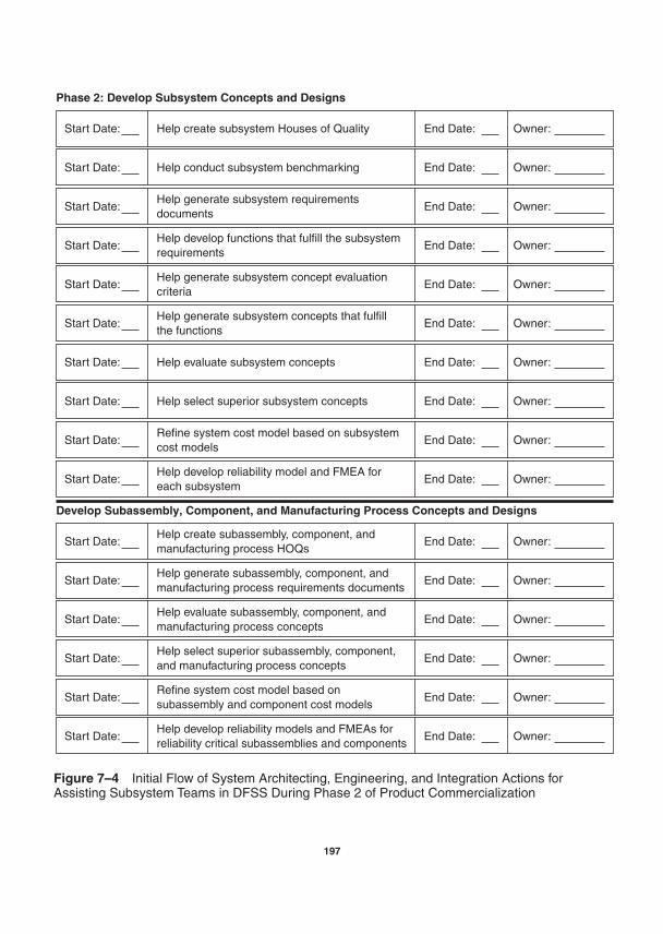
Help conduct subsystem benchmarkingStart Date: End Date: Owner:
Help generate subsystem requirementsdocuments
Start Date: End Date: Owner:
Help create subsystem Houses of QualityStart Date:
Phase 2: Develop Subsystem Concepts and Designs
Develop Subassembly, Component, and Manufacturing Process Concepts and Designs
End Date: Owner:
Help generate subsystem concept evaluationcriteria
Start Date: End Date: Owner:
Help generate subsystem concepts that fulfillthe functions
Start Date: End Date: Owner:
Help evaluate subsystem conceptsStart Date: End Date: Owner:
Help select superior subsystem conceptsStart Date: End Date: Owner:
Refine system cost model based on subsystemcost models
Start Date: End Date: Owner:
Help develop reliability model and FMEA foreach subsystem
Start Date: End Date: Owner:
Help create subassembly, component, andmanufacturing process HOQs
Start Date: End Date: Owner:
Help generate subassembly, component, andmanufacturing process requirements documents
Start Date: End Date: Owner:
Help evaluate subassembly, component, andmanufacturing process concepts
Start Date: End Date: Owner:
Help select superior subassembly, component,and manufacturing process concepts
Start Date: End Date: Owner:
Refine system cost model based on subassembly and component cost models
Start Date: End Date: Owner:
Help develop reliability models and FMEAs forreliability critical subassemblies and components
Start Date: End Date: Owner:
Help develop functions that fulfill the subsystemrequirements
Start Date: End Date: Owner:
Figure 7–4 Initial Flow of System Architecting, Engineering, and Integration Actions forAssisting Subsystem Teams in DFSS During Phase 2 of Product Commercialization
197
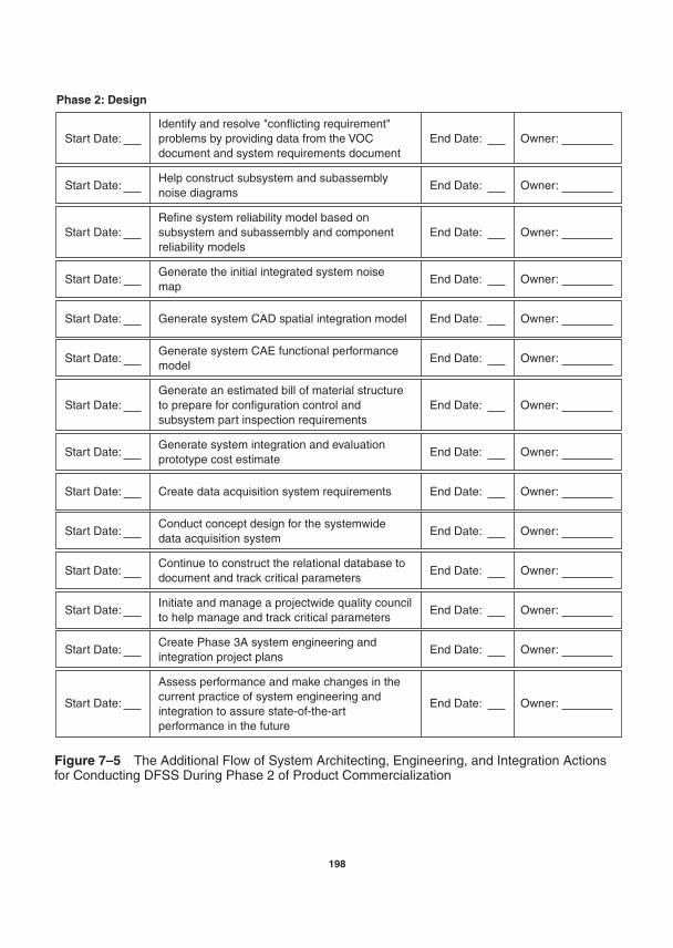
Help construct subsystem and subassemblynoise diagrams
Start Date: End Date: Owner:
Refine system reliability model based onsubsystem and subassembly and componentreliability models
Start Date: End Date: Owner:
Identify and resolve "conflicting requirement"problems by providing data from the VOCdocument and system requirements document
Start Date:
Phase 2: Design
End Date: Owner:
Generate system CAD spatial integration modelStart Date: End Date: Owner:
Generate system CAE functional performancemodel
Start Date: End Date: Owner:
Generate an estimated bill of material structureto prepare for configuration control andsubsystem part inspection requirements
Start Date: End Date: Owner:
Assess performance and make changes in thecurrent practice of system engineering andintegration to assure state-of-the-artperformance in the future
Start Date: End Date: Owner:
Generate system integration and evaluationprototype cost estimate
Start Date: End Date: Owner:
Create data acquisition system requirementsStart Date: End Date: Owner:
Conduct concept design for the systemwidedata acquisition system
Start Date: End Date: Owner:
Continue to construct the relational database todocument and track critical parameters
Start Date: End Date: Owner:
Initiate and manage a projectwide quality councilto help manage and track critical parameters
Start Date: End Date: Owner:
Create Phase 3A system engineering andintegration project plans
Start Date: End Date: Owner:
Generate the initial integrated system noisemap
Start Date: End Date: Owner:
Figure 7–5 The Additional Flow of System Architecting, Engineering, and Integration Actionsfor Conducting DFSS During Phase 2 of Product Commercialization
198
System engineers in a technology development and Design For Six Sigma context play twokey roles:
1. They work inside and between the subsystem teams to help with the tasks of sub-system development and design. In this role they fan out and “join” all the subsystem teamsto gain intimate knowledge of the critical cross-boundary interface sensitivities and sub-system performance issues. They provide system integration information and carry backsubsystem design and performance information to help plan for future system integrationtests. Their key focus is on subsystem interface geometry and functional handoffs of mass,energy, and information (digital and analog logic and control signals).
2. They work as a team of objective, independent system integrators to build, evalu-ate, and verify the complete product design. In this role they own and are responsible forthe integrated system.
We will not repeat the block diagram descriptions for the tasks that the system engineershelp conduct with their peers on the subsystem design teams. Suffice it to say that the system en-gineers work with these teams and assist them as necessary. They literally help apply the toolsand best practices of Technology and Design For Six Sigma. They should be evaluated and ratedfor their performance in this context with feedback to the system engineering manager. In thisway they can be held accountable for their contributions to preventing design problems throughthese important teamwork tasks.
The system engineers have an important preintegration function to perform during the de-sign phase of the CDOV process. Typically the system engineers divide up the subsystems be-tween themselves and lead presystem integration design review meetings. This division ofsubsystems is not done on a random basis. The subsystem interface relationships are carefullyexamined and key groups of subsystems are “owned” by each one of the system engineers. Theirjob is to make sure each of the subsystem teams are “preventatively aware” of integration issues,variation transmission sensitivities, and potential failure modes. If there is a significant issue rel-ative to system integration, it is the system engineer’s responsibility to document it and evalu-ate solutions and work with the subsystem teams involved to coordinate a resolution to theproblem. The system engineering team owns the integrated system and is responsible for its per-formance. The subsystem teams own their respective subsystems, subassemblies, components,and manufacturing/assembly process requirements. Critical Parameter Management responsi-bilities fall along these lines, but the CPM database is the responsibility of the system engineer-ing team.
The specific issues related to each Phase 2 system engineering action item (start date foreach action item, the action item, and end date for each action) will be reviewed in this section.Each of these action items can be conducted by using a tool or best practice. The flow of actionscan be laid out in the form of a PERT chart for project management purposes.
System Architecting, Engineering, and Integration Using Design For Six Sigma 199

Identify and Resolve “Conflicting Requirement” Problems by Providing Datafrom the VOC Document and System Requirements Document
Start Date: __________ End Date: __________ Owner: __________
We begin Phase 2 system engineering DFSS activities by working on clearing up any confusionor conflicts that come from the system requirements document. Two types of conflict issues gen-erally surface at the beginning of Phase 2:
1. Incomplete, poorly worded requirements (a human communication problem)2. Clearly worded requirements that are in conflict with one another (a VOC and VOT
problem)
The system engineer responsible for the Critical Parameter Management database takespossession of the ranked voice of the customer data. It is this person’s responsibility to use theVOC data to help correct poorly translated customer needs. Technical system requirements mustreflect the customer needs in technical terms. The usual problem is that the technical vocabularyof the system requirement is either too ambiguous or too prescriptive. When the system require-ment is too ambiguous, it needs to be rewritten with precise language, including units of measureand target values that everyone on the product development team can understand. When the sys-tem requirement is too prescriptive, it needs to be rewritten so that it does not imply a specific so-lution. System requirements should set a standard to be fulfilled with a unit of measure and atarget for that measure. They should not state a solution, concept, or method of fulfillment. Thatis the realm of concept generation and selection. The system requirements must be stated in sucha way that they can be used to evaluate numerous concepts or solutions. In this sense the systemrequirement implies a “function” or variable to be measured. You should be able to define manydifferent “forms and fits” of architectural concepts that fulfill the function underwritten by the vo-cabulary of the system requirement.
When two or more well-written system requirements are in conflict with one another, theproblem is much more serious. If we fulfill one system requirement, we absolutely disable ourability to fulfill another system requirement. This often happens when we have to add featuresand functions while simultaneously increasing reliability to historically unprecedented levels.About the only thing that can be done is to negotiate a balanced solution to this stand-off by go-ing back and discussing the situation with the customers. A refined and compromised VOC needwill usually result. New system requirements can then be derived from the new VOC input. Thesystem House of Quality can also be of great help in this conflict resolution process. It containsa lot of ranking information to help make the required compromises between the conflicting sys-tem requirements.
Help Construct Subsystem and Subassembly Noise Diagrams
Start Date: __________ End Date: __________ Owner: __________
200 Chapter 7

One of the most critical pieces of information that the system integration team needs to properlyevaluate the system is a clear understanding of what noises affect each of the subsystems. Thebest way for each system engineer to more fully understand the sources of variation within andbetween the subsystems they are responsible for integrating is to personally participate in the de-velopment of the subsystem noise diagrams. A noise diagram must be generated for each sub-system. The noise diagram contains the information depicted in Figure 7–6.
The outgoing sources of variation are important for proper stress test design prior to thesystem integration tests.
Generate the Initial Integrated System Noise Map
Start Date: __________ End Date: __________ Owner: __________
System noise maps can be generated by linking together all the outgoing sources of varia-tion from the subsystem noise diagrams. A good system noise map will enable the system engi-neering team to develop credible system stress tests that expose the integrated set of subsystemsto realistic forms of variation that will be encountered in the assembly, distribution, and use environment.
The system noise maps should be constructed in the design phase of the CDOV process sothey can be reviewed by all of the subsystem teams to make sure they are reasonable and com-plete. The subsystem teams can also use them to structure their subsystem robustness test plansto include integration noise and all the input noises from the noise diagram. It is not enough to
System Architecting, Engineering, and Integration Using Design For Six Sigma 201
Subsystem:
Deterioration Sourcesof Variation:-. . .-. . .-. . .
Outgoing Sourcesof Variation:-. . .-. . .-. . .
External Sourcesof Variation:-. . .-. . .-. . .
Unit-Unit Sourcesof Variation:-. . .-. . .-. . .
Figure 7–6 Subsystem Noise Diagram

just make a subsystem robust to its own internal or within subsystem noise. When businesseslaunch products (integrated systems) and they have a lot of performance and reliability problems,it is usually because these integration noises were not identified and accounted for during sub-system development and integration. Developing subsystems for robustness to both internal andintegration noise is a critical step in developing reliability into the system.
Refine System Reliability Model Based on Subsystem, Subassembly,and Component Reliability Models
Start Date: __________ End Date: __________ Owner: __________
Now that the subsystem noise diagrams, system noise map, and the system and subsystemFMEAs are in hand, refinements to the evolving reliability model can be made. It is also time toallocate reliability requirements and estimates down into the subsystems, subassemblies, andcomponents. A fairly complete reliability prediction model should be taking shape for Gate 2evaluation. Overall predicted system reliability performance will now begin to be adjusted by thenew information down at the lower levels of the system architecture.
Generate System CAD Spatial Integration Model
Start Date: __________ End Date: __________ Owner: __________
Now that the subsystems are being designed, built, and evaluated for their baseline, nominal per-formance (ideal function modeling), the system engineering team can receive the geometric CADfiles from the subsystem designers. All this form and fit information can be modeled within thesystem architecture for proper spatial relationships. Frequently “space wars” must be diplomati-cally solved and avoided. The system design leader, usually a skilled CAD operator, referees theallocation of space. A lot of analytical tolerance evaluation is conducted by the system CAD in-tegration team. It is the system engineering team’s responsibility to be the “space police.” All sub-system space use requests must go through the system CAD integration leader so that interferenceissues can be evaluated prior to approving the use of the space. The system engineers worry aboutthe functional interfaces while the system CAD integration leader worries about the form and fitinterfaces. The system CAD integration leader will make frequent visits to the system integrationmeetings to review spatial issues across and between the numerous subsystem teams.
As you can see, system integration team members are characterized by what they worryabout: across and between issues. Subsystem engineering teams tend to worry about within is-sues. The collaborative system integration meetings help assure the across, within, and betweenissues all get proper evaluation at the right time, using the right tools in the CDOV process.
Generate System CAE (Computer Aided Engineering) FunctionalPerformance Model
Start Date: __________ End Date: __________ Owner: __________
202 Chapter 7

The Critical Parameter Management database can be used to help model the functional perfor-mance of the system level critical functional responses. Each subsystem team should be devel-oping ideal/transfer function models that are expressed in terms of Y f(x) relationships. Thesemodels can be linked together and used to model system performance. The models are started us-ing models derived from “first principles.” Later, in the design phase but mostly in the optimiza-tion phase, the models are empirically developed, refined, and confirmed.
Subsystem inputs that are linked to system outputs are often referred to as transfer func-tions. Once deterministic transfer functions are developed for the critical parametric relation-ships, statistical models in the form of Monte Carlo simulations can be developed. The systemengineering team can run numerous what-if scenarios as the subsystems are changed as a resultof design development, optimization, and verify certification as prescribed in the CDOV phases.These models will be used to perform analytical tolerance design prior to system integration stresstests in Phase 3B and product certification tests in Phase 4A.
It is important that the system engineering team build these critical parameter models andremain committed to their refinement and maintenance all the way through the CDOV process.The existence and refinement of such models is a strong sign that the system engineering teamunderstands the critical parameters within the system.
Generate an Estimated Bill of Material Structure to Prepare forConfiguration Control and Subsystem Part Inspection Requirements
Start Date: __________ End Date: __________ Owner: __________
The parts, subassemblies, and subsystems that comprise the system are maturing at a high rate inthe design phase. Their physical architectures are defined and their earliest baseline set points areestablished. With this kind of information available, a preliminary part count and bill of materialcan be constructed. The system engineering team assembles the information through its systemintegration meetings with each subsystem team.
Generate System Integration and Evaluation Prototype Cost Estimate
Start Date: __________ End Date: __________ Owner: __________
The system engineering team can now bring in, from their work inside the subsystem integrationmeetings, the preliminary bill of material projections to enable the definition of a preliminary costmodel. This cost model estimates the cost of the first system to be built for Phase 3B system in-tegration tests. The model evolves with the designs and ultimately serves as the cost model forthe actual product that will be certified at Gate 4A.
Create Data Acquisition System Requirements
Start Date: __________ End Date: __________ Owner: __________
System Architecting, Engineering, and Integration Using Design For Six Sigma 203

The system interfaces are becoming clear as the subsystems and subassemblies take shape. Thetime is right to finalize a complete set of data acquisition system requirements. Each subsystemteam works with its system engineering representative to define the metrology requirements foreach of the critical functional responses they have created. The system engineering team speci-fies, purchases, and deploys a systemwide data acquisition system. Its job is to measure all sys-tem level critical functional responses and any subsystem or subassembly level critical functionalresponses that the subsystem team requests. The ability to adequately measure and document themany capability indices across the system rests at the foundation of a properly planned and de-signed data acquisition system.
Conduct Concept Design for the Systemwide Data Acquisition System
Start Date: __________ End Date: __________ Owner: __________
With a full set of data acquisition system requirements in hand, the process of designing the ac-tual system can be undertaken. The process contains the following elements:
1. Define the specific functions to be measured (targets, discrimination, and extremes ofdata ranges likely to be encountered when exploring design space using designed ex-periments).
2. Generate at least two concepts for each critical functional response being measured.3. Evaluate the concepts against a best-in-class benchmark (datum) metrology design
against the specific data acquisition requirements and criteria.4. Synthesize the best attributes from the proposed concepts and, if necessary, produce a
hybrid data acquisition concept that surpasses the datum concept.5. Develop, design, optimize, or purchase the superior concept; then verify the capability
of the data acquisition equipment.
Continue to Construct the Relational Database to Document and TrackCritical Parameters
Start Date: __________ End Date: __________ Owner: __________
The Critical Parameter Management database grows at a high rate during the design phase. Thesystem, subsystem, subassembly, and component requirements are all initially defined at thispoint. The critical functional responses for the system, subsystems, and subassemblies are gath-ered and entered into the database by the system engineering team. Every subassembly CFR islinked to its requirement and traced up to the subsystem and system level CFRs and requirementsthey help fulfill. A many-to-many relational network of measured responses and their related re-quirements will begin to be developed in the design phase. All CFRs along with their initial base-line Cp performance measures should be documented at Gate 2.
204 Chapter 7

Initiate and Manage a Projectwide Quality Council to Help Manage and Track Critical Parameters
Start Date: __________ End Date: __________ Owner: __________
A select set of engineers and professionals from the product development and operations teamsshould be formed into a Quality Council that oversees the execution of the Critical ParameterManagement process. One experienced and highly respected individual from each of the follow-ing disciplines should be a member of the Quality Council:
1. System engineering (leader of the Quality Council)2. Mechanical design engineering3. Electrical design engineering4. Software engineering5. Materials engineering6. Manufacturing engineering7. Assembly operations8. Supply chain management9. Service and product support
10. Quality assurance11. Program management
The purpose of the Quality Council is to promote and facilitate the deployment of the Criti-cal Parameter Management process. Council members make sure all the people within their sphereof influence are trained and implementing the appropriate tools and best practices of DFSS to as-sure the continual generation and updating of the Critical Parameter Management database. If anyone on the product development team has a problem or question, the Quality Council resolves theissue. Council members team up to help create solutions to exceptionally difficult metrology road-blocks. They refine and clarify definitions of requirements and critical parameter terms. The criti-cal parameter database is an intricate and complex network of requirements and parametric termsand relationships. It takes discipline and hard work to build and maintain these databases. The Qual-ity Council, under the leadership of system engineering, is responsible for helping everybody get itright. The system engineering team owns the CPM database, but the Quality Council is jointly re-sponsible for its deployment. The Quality Council files a summary report at each gate review. Thisreport informs the gate keepers of Critical Parameter Management issues, problems, and correctiveactions undertaken as well as items for resolution prior to the next phase by program management.
In summary, the members of the Quality Council are CPM troubleshooters. They try to pre-vent problems as much as possible by communicating a clear approach to CPM. The problemsthey can’t prevent they help solve. The problems they can’t solve are forwarded up the chain ofcommand in a time frame that is proportional to the nature and severity of the problem encoun-tered. They typically meet once every week or two and also on an as-needed basis.
System Architecting, Engineering, and Integration Using Design For Six Sigma 205

Create Phase 3A System Engineering and Integration Project Plans
Start Date: __________ End Date: __________ Owner: __________
The system engineering team meets to assess its required deliverables for the next phase and thenstructures detailed plans to deliver them in the allotted time. These plans are a requirement forpassage of Gate 2.
Assess Performance and Make Changes in the Current Practice of SystemEngineering and Integration to Assure State-of-the-Art Performance in the Future
Start Date: __________ End Date: __________ Owner: __________
The Team meets to assess how they performed over Phase 2. They review their use of DFSS toolsand best practices and the quality of their results. Future training plans and improvements areagreed to and included in the appropriate individuals performance plan.
In addition to the Phase 2 checklist and list of system engineering gate deliverables that fol-low, Figure 7–7 provides a Phase 2 scorecard.
Checklist of Phase 2 System Engineering and Integration Tools and Best Practices:
Competitive benchmarking (subsystem, subassembly, component)
VOC gathering methods
KJ analysis (relative to flow-down of system requirements to subsystem requirements)
QFD/Houses of Quality—Levels 2–5 (subsystem, subassembly, component, andmanufacturing process levels)
Concept generation techniques (TRIZ, brainstorming, brain-writing)
Pugh concept evaluation and selection process
Design for manufacture and assembly
Value engineering and analysis
Design failure modes and effects analysis
Measurement systems analysis
Critical parameter management
Knowledge-based engineering methods
Math modeling (engineering analysis to define ideal functions and transfer functions)
Design of experiments (Full and Fractional Factorial designs and sequentialexperimentation)
Descriptive and inferential statistical analysis
ANOVA data analysis
206 Chapter 7
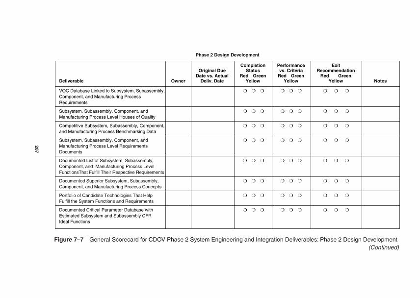
Phase 2 Design Development
Completion Performance Exit Original Due Status vs. Criteria Recommendation
Date vs. Actual Red Green Red Green Red GreenDeliverable Owner Deliv. Date Yellow Yellow Yellow Notes
VOC Database Linked to Subsystem, Subassembly,
Component, and Manufacturing Process Requirements
Subsystem, Subassembly, Component, and
Manufacturing Process Level Houses of Quality
Competitive Subsystem, Subassembly, Component,
and Manufacturing Process Benchmarking Data
Subsystem, Subassembly, Component, and
Manufacturing Process Level Requirements Documents
Documented List of Subsystem, Subassembly,
Component, and Manufacturing Process Level FunctionsThat Fulfill Their Respective Requirements
Documented Superior Subsystem, Subassembly,
Component, and Manufacturing Process Concepts
Portfolio of Candidate Technologies That Help
Fulfill the System Functions and Requirements
Documented Critical Parameter Database with
Estimated Subsystem and Subassembly CFR Ideal Functions
Figure 7–7 General Scorecard for CDOV Phase 2 System Engineering and Integration Deliverables: Phase 2 Design Development(Continued)
207

Completion Performance Exit Original Due Status vs. Criteria Recommendation
Date vs. Actual Red Green Red Green Red GreenDeliverable Owner Deliv. Date Yellow Yellow Yellow Notes
Documented Critical Parameter Database with Estimated Subsystem and Subassembly CFR Interaction Transfer Functions (Between Subsystems and Subassemblies and Linkage up to the System CFRs)
Documented Reliability Model and Predicted System Reliability Performance with Gap Analysis
Estimated System, Subsystem, Subassembly, Component Cost Projections
Documentation Supporting Design for Manufacturability and Assembleability
Documented Design Failure Modes and Effects Analysis for Subsystems, Subassemblies, Reliability Critical Components, and Manufacturing Processes
Descriptive and Inferential Statistics; Hypothesis Testing and Confidence Interval Analysis in Support of the Ideal Functions and Transfer Functions
Sequential Design of Experiments (Initial identification of Subsystems, Subassembly, Component, and Manufacturing Process Critical Parameters)
Analysis of Variance Data (ANOVA) That Underwrite Statistical Significance of Critical Parameters
Documented Cp & Cpk Values for All Subsystem and Subassembly Design CFRs
Initial Cp/Cpk Assessment for Candidate Critical- to-Function Specifications from Manufacturing Processes from Supply Chain
Phase 3A (Optimization) Project Management Plans
Figure 7–7 Continued
208

Regression and empirical modeling methods
Reliability modeling methods
Normal and accelerated life testing methods
Design capability studies
Multi-vari studies (for noise factor identification)
Statistical process control (for design stability and capability studies)
Gate 2 System Engineering Deliverables
Subsystem, subassembly, component, and manufacturing process level HOQ (assist andcreate link to system HOQ)
Subsystem, subassembly, component, and manufacturing process level requirementdocuments (assist and create links to system requirements document)
Superior subsystem, subassembly, component, and manufacturing process level concepts(assist and create links to system concept)
Software concept of operations, use cases, flow charts, block diagrams, sequence ofevents documents (assist and create links to SRD)
DFMA (assist and create links to system space allocation CAD model)
Subsystems, subassemblies, components, and manufacturing processes modeled y f(x)(assist and create links to system level CFRs in CPM database)
Subsystem DFMEAs (assist and use to refine system DFMEA)
Subsystem CFRs defined and linked to system CFRs (CPM database development)
Subsystem control factors, interactions, and linear/nonlinear model defined anddocumented in CPM database
Latest status of risks from new subsystems being transferred from R&D or being trackedfrom Phase 2 subsystem prototypes
Subsystem cost models (assist and create links to system cost model)
System noise map
System reliability model and latest subsystem allocation model
System reliability growth budget
Current bill of material structure
Status of early configuration control and problem reporting/resolution process superiordesign concept for the system level data acquisition system
Ongoing systemwide Critical Parameter Management database with inclusion ofsubsystem, subassembly, component, and manufacturing process level requirements andmeasured performance information (Cp, Cpk, etc.)
Status of Quality Council activities and agenda
Phase 3A system engineering and integration project plans and resource requirements
System Architecting, Engineering, and Integration Using Design For Six Sigma 209
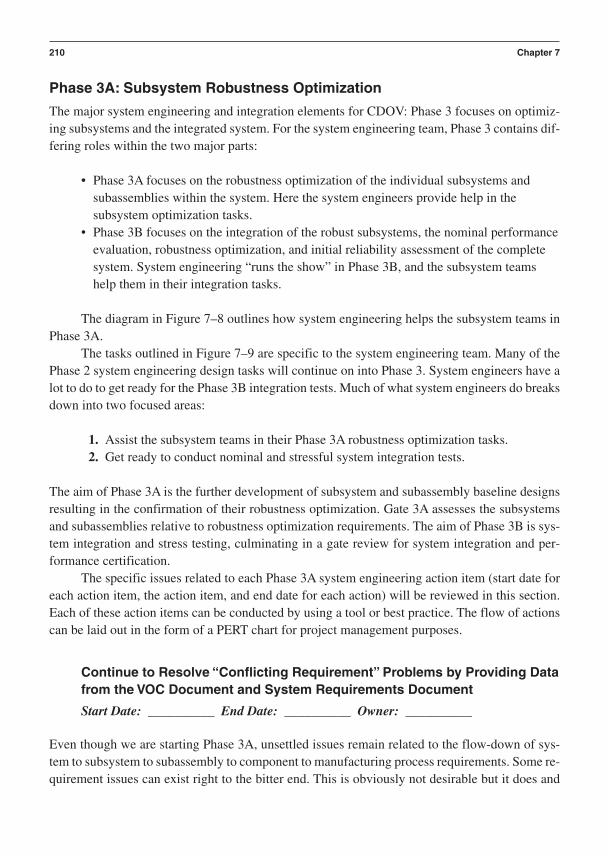
Phase 3A: Subsystem Robustness Optimization
The major system engineering and integration elements for CDOV: Phase 3 focuses on optimiz-ing subsystems and the integrated system. For the system engineering team, Phase 3 contains dif-fering roles within the two major parts:
• Phase 3A focuses on the robustness optimization of the individual subsystems andsubassemblies within the system. Here the system engineers provide help in thesubsystem optimization tasks.
• Phase 3B focuses on the integration of the robust subsystems, the nominal performanceevaluation, robustness optimization, and initial reliability assessment of the completesystem. System engineering “runs the show” in Phase 3B, and the subsystem teamshelp them in their integration tasks.
The diagram in Figure 7–8 outlines how system engineering helps the subsystem teams inPhase 3A.
The tasks outlined in Figure 7–9 are specific to the system engineering team. Many of thePhase 2 system engineering design tasks will continue on into Phase 3. System engineers have alot to do to get ready for the Phase 3B integration tests. Much of what system engineers do breaksdown into two focused areas:
1. Assist the subsystem teams in their Phase 3A robustness optimization tasks.2. Get ready to conduct nominal and stressful system integration tests.
The aim of Phase 3A is the further development of subsystem and subassembly baseline designsresulting in the confirmation of their robustness optimization. Gate 3A assesses the subsystemsand subassemblies relative to robustness optimization requirements. The aim of Phase 3B is sys-tem integration and stress testing, culminating in a gate review for system integration and per-formance certification.
The specific issues related to each Phase 3A system engineering action item (start date foreach action item, the action item, and end date for each action) will be reviewed in this section.Each of these action items can be conducted by using a tool or best practice. The flow of actionscan be laid out in the form of a PERT chart for project management purposes.
Continue to Resolve “Conflicting Requirement” Problems by Providing Datafrom the VOC Document and System Requirements Document
Start Date: __________ End Date: __________ Owner: __________
Even though we are starting Phase 3A, unsettled issues remain related to the flow-down of sys-tem to subsystem to subassembly to component to manufacturing process requirements. Some re-quirement issues can exist right to the bitter end. This is obviously not desirable but it does and
210 Chapter 7
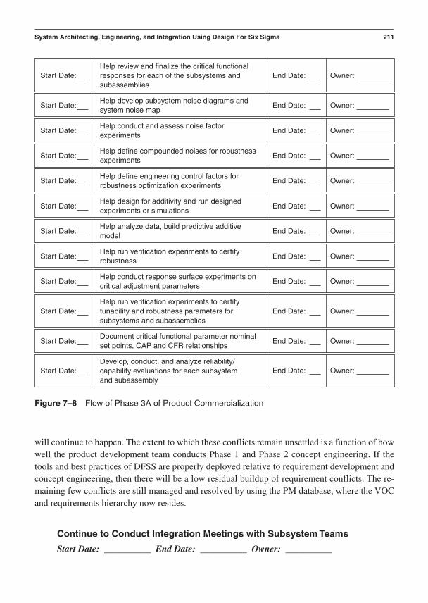
will continue to happen. The extent to which these conflicts remain unsettled is a function of howwell the product development team conducts Phase 1 and Phase 2 concept engineering. If thetools and best practices of DFSS are properly deployed relative to requirement development andconcept engineering, then there will be a low residual buildup of requirement conflicts. The re-maining few conflicts are still managed and resolved by using the PM database, where the VOCand requirements hierarchy now resides.
Continue to Conduct Integration Meetings with Subsystem Teams
Start Date: __________ End Date: __________ Owner: __________
System Architecting, Engineering, and Integration Using Design For Six Sigma 211
Help analyze data, build predictive additivemodel
Start Date: End Date: Owner:
Help run verification experiments to certifyrobustness
Start Date: End Date: Owner:
Help conduct response surface experiments oncritical adjustment parameters
Start Date: End Date: Owner:
Help run verification experiments to certifytunability and robustness parameters forsubsystems and subassemblies
Start Date: End Date: Owner:
Document critical functional parameter nominalset points, CAP and CFR relationships
Start Date: End Date: Owner:
Develop, conduct, and analyze reliability/capability evaluations for each subsystemand subassembly
Start Date: End Date: Owner:
Help review and finalize the critical functionalresponses for each of the subsystems andsubassemblies
Start Date: End Date: Owner:
Help develop subsystem noise diagrams andsystem noise map
Start Date: End Date: Owner:
Help conduct and assess noise factorexperiments
Start Date: End Date: Owner:
Help define compounded noises for robustnessexperiments
Start Date: End Date: Owner:
Help define engineering control factors forrobustness optimization experiments
Start Date: End Date: Owner:
Help design for additivity and run designedexperiments or simulations
Start Date: End Date: Owner:
Figure 7–8 Flow of Phase 3A of Product Commercialization
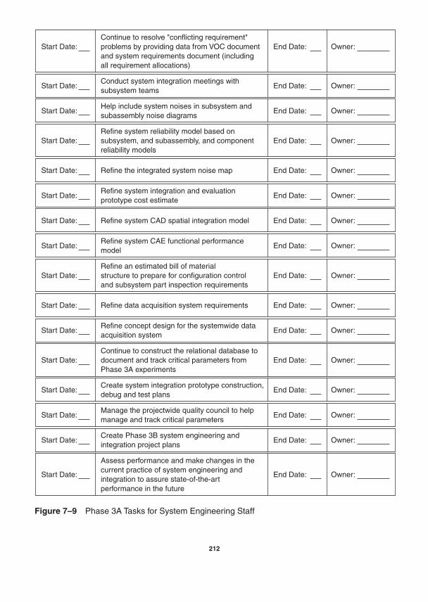
Refine system CAD spatial integration modelStart Date: End Date: Owner:
Refine system CAE functional performancemodel
Start Date: End Date: Owner:
Refine an estimated bill of material structure to prepare for configuration controland subsystem part inspection requirements
Start Date: End Date: Owner:
Create system integration prototype construction,debug and test plans
Start Date: End Date: Owner:
Manage the projectwide quality council to helpmanage and track critical parameters
Start Date: End Date: Owner:
Create Phase 3B system engineering andintegration project plans
Start Date: End Date: Owner:
Refine data acquisition system requirementsStart Date: End Date: Owner:
Refine concept design for the systemwide dataacquisition system
Start Date: End Date: Owner:
Continue to construct the relational database todocument and track critical parameters fromPhase 3A experiments
Start Date: End Date: Owner:
Assess performance and make changes in thecurrent practice of system engineering and integration to assure state-of-the-artperformance in the future
Start Date: End Date: Owner:
Continue to resolve "conflicting requirement"problems by providing data from VOC documentand system requirements document (includingall requirement allocations)
Start Date: End Date: Owner:
Conduct system integration meetings withsubsystem teams
Start Date: End Date: Owner:
Help include system noises in subsystem andsubassembly noise diagrams
Start Date: End Date: Owner:
Refine system reliability model based onsubsystem, and subassembly, and componentreliability models
Start Date: End Date: Owner:
Refine the integrated system noise mapStart Date: End Date: Owner:
Refine system integration and evaluationprototype cost estimate
Start Date: End Date: Owner:
Figure 7–9 Phase 3A Tasks for System Engineering Staff
212

The system integration meetings should be an established routine by now. The focus of thesemeetings in Phase 3A is on the development and execution of robustness optimization experi-ments. As the data comes in from the optimization experiments, the system team can update theCPM database. A pre- and post-robustness optimization Cp index for each subsystem CFR is re-quired. The purpose of subsystem robustness optimization is to minimize the subsystem CFRs tostatistically significant sources of noise. This is achieved by identifying significant interactionsbetween the subsystem’s control factors and noise factors. These unique interactions are typicallyquantified by using a series of comparisons of the signal-to-noise ratio.
Help Include System Noises in Subsystem and Subassembly Noise Diagrams
Start Date: __________ End Date: __________ Owner: __________
Each subsystem team refines and uses its respective noise diagrams to aid in the proper design ofits noise experiments and the robustness optimization experiments. The system engineers as-signed to respective subsystem teams need to be intimately involved in the robustness optimiza-tion experiments and resulting data. System engineering plays a key role in advising thesubsystem teams on integration noises that will help the subsystem become robust to these uniquenoise factors. The goal here is to get the subsystems properly stress tested so that they are fairlyeasy to integrate and evaluate in the first integrated system. If the subsystems do not include in-tegration noises in their experiments, there is a high degree of risk that the system integration testswill not go well and will likely overrun their time budget.
Refine the Integrated System Noise Map
Start Date: __________ End Date: __________ Owner: __________
The results of the subsystem and subassembly robustness evaluations may provide valuable in-formation about integration noise factors that need to be included in the system noise map. Thesystem has not been fully integrated yet but the system mules, in which the subsystems and sub-assemblies are evaluated, often yield new information about integration noise factors. Noise fac-tors that were not obvious prior to the actual experimentation may even be discovered. The systemnoise map should be updated with any new information from all iterations of the robustness op-timization experiments.
Refine System Reliability Model Based on Subsystem, Subassembly,and Component Reliability Models
Start Date: __________ End Date: __________ Owner: __________
The reliability information coming in from the various forms of subsystem, subassembly, andcomponent life tests and accelerated life tests can be used to help refine the predicted reliability
System Architecting, Engineering, and Integration Using Design For Six Sigma 213

of the system. The reliability of the newly robust subsystems and subassemblies must be evalu-ated. Robust design has a proven track record of growing reliability when the robustness stresstests include the forms of noise that deteriorate reliability. Becoming insensitive to deteriorativesources of noise typically slows the rate of failures. Care should be taken to refer back to theFMEA data to be sure the noise diagrams and the FMEAs are correlated.
Refine System Integration and Evaluation Prototype Cost Estimate
Start Date: __________ End Date: __________ Owner: __________
The subsystems are maturing in part due to the changes in certain nominal set points resultingfrom the robustness work and in part due to changes for assembleability, cost, and any number ofother requirement balancing issues. The cost estimates for the system integration prototypes canbe refined to include Phase 3A improvements. Usually robustness improvements do not have alarge impact on cost but other design changes do. Depending on the size and complexity of the system being developed, the cost to make and assemble the system prototype can be quitehigh. This may surprise managers if they are out of touch with the fact that you need to fabricateand build system prototypes that emulate the way your product will be stressed and deterioratedin the actual shipping and use environment. If you can’t afford to proactively design robustnessand durability into your product, you probably won’t gain market share or enjoy the estimatedrevenues your business case projects. And be sure to open a sizable escrow account for warrantyclaims.
It is amazing how many managers tend to think only about the lowest cost and shortest cycle-time. What DFSS and the CDOV product development process are promoting is the development of the right cost and using the appropriate cycle-time that fulfills the system requirements—nothing more and certainly nothing less!
Refine System CAD Spatial Integration Model
Start Date: __________ End Date: __________ Owner: __________
Along with the set point changes that come from the results of the robustness optimization ex-periments come the inevitable spatial form and fit changes that affect the system architecture. Thesubsystem designers need to inform the system designers of the adjustments they are planning sothey can be verified against the system space allocation model. Interferences, proximity noise in-ducement, and transmission (energy, mass, and signals where they are not supposed to be!) mustbe checked before the changes can be approved from a system performance perspective.
Refine System CAE Functional Performance Model
Start Date: __________ End Date: __________ Owner: __________
214 Chapter 7

Functions are the main focus of Critical Parameter Management in DFSS. Any changes made forrobustness optimization purposes are supposed to enhance functional integrity within and acrossthe system. Just because you have improved the robustness of a subsystem does not necessarilymean you have helped the entire system perform better. The system engineers use the systemmodel and system integration tests to help determine if changes in subsystem performance areharmonious with the maturation of system performance and the balanced fulfillment of the sys-tem requirements. Phase 3A uses the analytical and graphical models of the integrated system tocheck these issues. Phase 3B uses the physical system prototype model to evaluate the systemlevel form, fit, and functional performance issues empirically.
Refine an Estimated Bill of Material Structure to Prepare for ConfigurationControl and Subsystem Part Inspection Requirements
Start Date: __________ End Date: __________ Owner: __________
Prior to Phase 3B, the bill of material must go through one more iteration to account for the changesfrom subsystem robustness optimization. The components that are fabricated and assembled intothe system prototype model are inspected and placed under rigorous configuration control. This isdone to assure that the system integration engineers know exactly what the critical parameter val-ues at the component, subassembly, and subsystem level are prior to Phase 3B testing. If you donot inspect the critical-to-function specifications on the components prior to integration, you willexperience performance problems that will consume valuable time to hunt down. You need toknow what is being assembled into the system prototypes before you test them. History has shownconclusively that when robust subsystems and subassemblies are properly integrated, they can pro-duce remarkable system performance during the initial system evaluations in Phase 3B.
Refine Data Acquisition System Requirements
Start Date: __________ End Date: __________ Owner: __________
After the subsystem teams master the methods of measuring their subsystem critical functionalresponses in Phase 3A, all their learning and improvements can be used to help the system inte-gration team get ready to measure their CFRs during system performance evaluations in Phase3B. Many things are likely to go wrong in Phase 3A subsystem CFR measurement. The systemengineers help correct these problems and then transfer that knowledge into the planning forPhase 3B CFR measurement. It is a huge mistake for the system team to be “aloof” when the sub-system teams are setting up and taking data; team members should physically be there to learnhow to get it right when it becomes their turn to measure functional performance.
Refine Concept Design for the Systemwide Data Acquisition System
Start Date: __________ End Date: __________ Owner: __________
System Architecting, Engineering, and Integration Using Design For Six Sigma 215

The system data acquisition system architecture may need to change to accommodate changes inrequirements and additions to what the subsystem team wants measured for them in Phase 3B.
Continue to Construct the Relational Database to Document and TrackCritical Parameters from Phase 3A Experiments
Start Date: __________ End Date: __________ Owner: __________
All the results for subsystem and subassembly CFR capability growth need to be documented inthe CPM database. The signal-to-noise improvements should also be documented to help estimatethe trend in reliability growth based on increased robustness to deteriorative noise factors. TheCPM hierarchy of critical relationships down through the system should be steadily growing. Thecritical adjustment parameters that will enable Cpk values to be adjusted to equal Cp should becompletely documented for use in the Phase 3B integration and tolerance balancing evaluations.A rich set of data from the subsystem robustness and capability growth assessments should be inhand for Gate 3A review.
Manage the Projectwide Quality Council to Help Manage and Track Critical Parameters
Start Date: __________ End Date: __________ Owner: __________
The Quality Council should be actively engaged across the product development team. Councilmembers should be solving measurement system problems and clarifying Critical ParameterManagement requirements and responsibilities. They will go a long way to establishing a cultureof rigor and discipline around taking data to assess the fulfillment of requirements across andwithin the system. Without their cross-functional work, the organization will drift and fraction-ate. The result is often that the left hand doesn’t know what the right hand is doing. It also createshealthy peer pressure right where you want it—not settling for mediocre performance in gather-ing data and understanding relationships and sensitivities across the integrated system.
Create System Integration Prototype Construction, Debug and Test Plans
Start Date: __________ End Date: __________ Owner: __________
The system engineering team is heavily focused on planning system integration tests. These testplans are a required deliverable at Gate 3A. Team members are also busy making sure all the com-ponents, assembly procedures, and equipment are in place to build the system prototype models.The system data acquisition system has been purchased and is now being assembled, debugged,and assessed for measurement capability. They have communicated with the subsystem teams andmade them aware that they will require all CFT specifications to be measured on all componentsprior to integration.
216 Chapter 7

Create Phase 3B System Engineering and Integration Project Plans
Start Date: __________ End Date: __________ Owner: __________
The system engineering team meets to assess its required deliverables for the next phase (3B) andthen structures detailed plans to deliver them in the allotted time. These plans are a requirementfor passage of Gate 3A.
Assess Performance and Make Changes in the Current Practice of SystemEngineering and Integration to Assure State-of-the-Art Performance in the Future
Start Date: __________ End Date: __________ Owner: __________
The team meets to assess how it performed over Phase 3A. Team members review their use ofDFSS tools and best practices and the quality of their results. Future training plans and improve-ments are agreed to and included in the appropriate individuals’ performance plan. Figure 7–10offers a scorecard of Phase 3A gate deliverables.
Phase 3A Goals
• Help assure selection of superior subsystem concepts.• Help assure robust subsystems are ready for system integration tests.• Assure that Critical Parameter Management is established and system data acquisition
is in place.
Gate 3A System Engineering Deliverables
Subsystem HOQs (assist and create link to system HOQ)
Subsystem requirement documents (assist and create links to system requirementsdocument)
Superior subsystem concepts (assist and create links to system concept)
Software concept of operations, use cases, flow charts, block diagrams, sequence ofevents
Documents (assist and create links to SRD)
DFMA (assist and create links to system space allocation CAD model)
Subsystem’s modeled y f(x) (assist and create links to system level CFRs)
Subsystem DFMEAs (assist and use to refine system DFMEA)
Subsystem CFRs defined and linked to system CFRs
Subsystem control factors, interactions, and linear/nonlinear model defined anddocumented in CPM database
System Architecting, Engineering, and Integration Using Design For Six Sigma 217
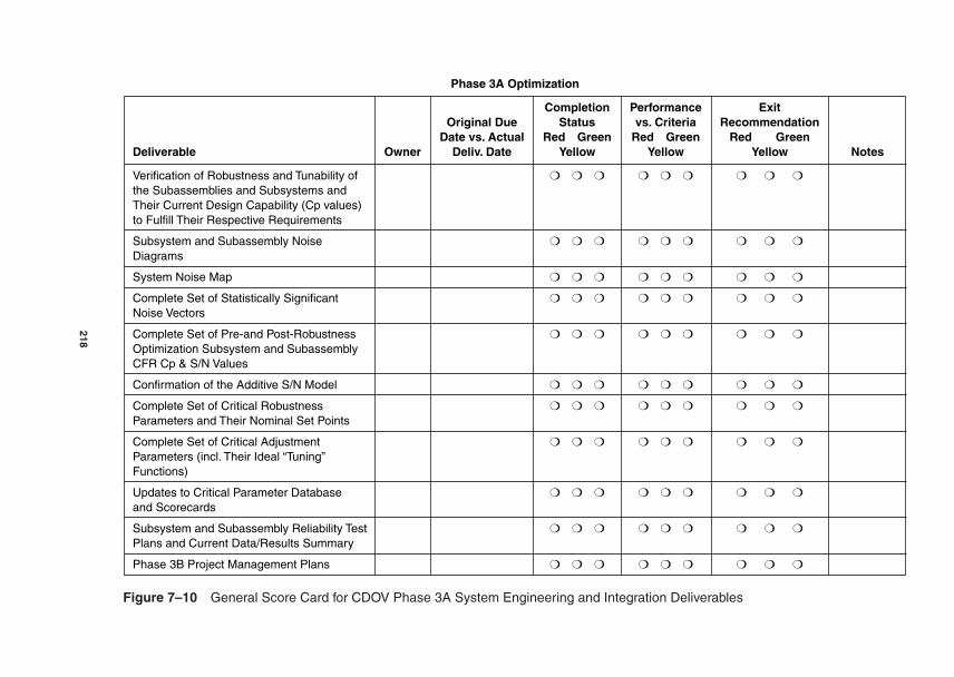
Phase 3A Optimization
Completion Performance Exit Original Due Status vs. Criteria Recommendation
Date vs. Actual Red Green Red Green Red GreenDeliverable Owner Deliv. Date Yellow Yellow Yellow Notes
Verification of Robustness and Tunability of
the Subassemblies and Subsystems and Their Current Design Capability (Cp values) to Fulfill Their Respective Requirements
Subsystem and Subassembly Noise
Diagrams
System Noise Map
Complete Set of Statistically Significant
Noise Vectors
Complete Set of Pre-and Post-Robustness
Optimization Subsystem and Subassembly CFR Cp & S/N Values
Confirmation of the Additive S/N Model
Complete Set of Critical Robustness
Parameters and Their Nominal Set Points
Complete Set of Critical Adjustment
Parameters (incl. Their Ideal “Tuning”Functions)
Updates to Critical Parameter Database
and Scorecards
Subsystem and Subassembly Reliability Test
Plans and Current Data/Results Summary
Phase 3B Project Management Plans
Figure 7–10 General Score Card for CDOV Phase 3A System Engineering and Integration Deliverables
218
Latest status of integration noise transmission (risks from new subsystems beingtransferred from R&D or being tracked from Phase 2 subsystem prototypes)
Subsystem cost models (assist and create links to system cost model)
System noise map
System reliability model and latest subsystem allocation model
System reliability growth budget
Current bill of material structure
Status of early configuration control process superior design concept for the system leveldata acquisition system
Ongoing systemwide Critical Parameter Management database with inclusion ofsubsystem requirements & performance information
Status of Quality Council activities and agenda
System level risk analysis report based on summary of system test data
Phase 3B system engineering and integration project plans and resource requirements
General Checklist of Phase 3A System Engineering and Integration Tools and Best Practices
Subsystem and subassembly noise diagramming
System noise mapping
Measurement system analysis
Use of screening experiments for noise vector characterization
Analysis of means (ANOM) data analysis techniques
Analysis of variance (ANOVA) data analysis techniques
Baseline subsystem and subassembly CFR signal-to-noise characterization
Taguchi’s methods for robust design
Design for additivity
Use of Full or Fractional Factorial experiments for robustness characterization
Generation of the additive S/N model
Response surface methods
Design capability studies
Critical Parameter Management
Reliability analysis
Life testing (normal, HALT, & HAST)
Project management and planning
Phase 3B: System Integration
The major elements of Phase 3B (see Figure 7–11) focus on system integration, nominal per-formance evaluation, robustness optimization, and initial system reliability assessment.
System Architecting, Engineering, and Integration Using Design For Six Sigma 219

Verify capability of the systemwide dataacquisition system
Start Date: End Date: Owner:
Refine and complete the system requirementsdocument
Start Date: End Date: Owner:
Conduct nominal performance evaluation on thesystem
Start Date: End Date: Owner:
Conduct system robustness stress testsStart Date: End Date: Owner:
Conduct critical life and accelerated life testsStart Date: End Date: Owner:
Document and track problem reports generatedduring tests
Start Date: End Date: Owner:
Refine subsystem set points to balance systemperformance
Start Date: End Date: Owner:
Develop and document corrective action basedon root cause analysis
Start Date: End Date: Owner:
Refine and update DFMEAs, noise diagrams,and noise maps
Start Date: End Date: Owner:
Refine and update critical parameter databaseand maps
Start Date: End Date: Owner:
Conduct initial system reliability assessment Start Date: End Date: Owner:
Refine system and subsystem reliability models,predictions and budgets
Start Date: End Date: Owner:
Define production assembly and manufacturingCPM metrics for CFRs, CAPs, CFPs, andcomponent CTF specifications
Start Date: End Date: Owner:
Assist in evaluating and documenting problemswith system assembleability, serviceability, andmaintainability
Start Date: End Date: Owner:
Assess performance and make changes in thecurrent practice of system engineering andintegration to assure state-of-the-artperformance in the future
Start Date: End Date: Owner:
Verify system readiness for final product designcapability development and assessment
Start Date: End Date: Owner:
Generate Phase 4A project management plansfor product design verification
Start Date: End Date: Owner:
Calculate design capabilities for all system andsubsystem CFRs from nominal performanceand stress tests
Start Date: End Date: Owner:
Integrate subsystems into system test unitsStart Date: End Date: Owner:
Figure 7–11 Flow of Phase 3B of Product Commercialization
The specific issues related to each Phase 3B System Engineering action item (start date for eachaction item, the action item, end date for each action) will be reviewed in this section. Each ofthese action items can be conducted by using a tool or best practice. The flow of actions can belaid out in the form of a PERT chart for project management purposes.
Integrate Subsystems into System Test Units
Start Date: __________ End Date: __________ Owner: __________
The long-awaited time to build the system integration prototype models has come. The systemengineering team oversees the physical construction of the system models. The system modelsare usually built by technicians, assemblers from the production organization, and field serviceengineers. Since this is the first time anyone has actually integrated all the subsystems, sub-assemblies, and components into a functioning system, representatives from all the organizationsthat will end up assembling and servicing the end product are included on the build team. Thisgives them an early look and feel for the product and allows them to provide assembly and ser-vice critiques that inevitably will require adjustments and changes to the system architecture. Thesooner these people get to know the system, the better they can help the design teams to iterateand optimize their designs.
Some businesses have the production organization completely conduct the first systemmodel construction. This is usually due to tight resources and a feeling that “the system belongsto production so let them build it.” The problem with this approach is that product organizationsare usually ill equipped to provide the necessary technical feedback to the design organization.The intermediary role that a small, technically focused system engineering team provides is wellsuited to managing the interfaces and documenting both functional and spatial (form and fit) is-sues encountered in the initial system build process. The system engineering team has built strongcommunication links to each of the subsystem design teams, and it is quite easy for them to pro-vide rapid and clear feedback on integration issues. The system engineering team will oversee theconstruction of all system test units through Phase 4A. At Phase 4B the production organizationtakes full ownership of the build process, and system engineering plays a supporting role.
Refine and Complete the System Requirements Document
Start Date: __________ End Date: __________ Owner: __________
A lot of learning takes place in the system integration phase. The system requirements will in-evitably undergo some changes as the entire product development team assesses the data from theconstruction and evaluation of the system integration prototype models. The goal is to freeze asmany of the system requirements as possible at the end of Phase 3B. Subsystem, subassembly,component, and manufacturing requirement balancing occur at a pretty heavy pace during thisphase. Many things come to light that were not anticipated, and many of the lower level require-ments need to be reallocated and adjusted for the sake of fulfilling the system requirements. Some
System Architecting, Engineering, and Integration Using Design For Six Sigma 221

people refer to Phases 3B and 4A as the tolerance balancing phases, “where we often have to robPeter to pay Paul.”
Verify Capability of the Systemwide Data Acquisition System
Start Date: __________ End Date: __________ Owner: __________
At the beginning of Phase 3B the system engineering team conducts measurement system analy-sis on system data acquisition to verify its capability to measure the many critical functional re-sponses across and within the subsystems. Tens or even hundreds of high- and low-speed analogand digital signals may be sampled, stored, and analyzed down through the critical parameter hi-erarchy. Many forms of measurement are required to assure that the many-to-many functional re-lationships and sensitivities are fulfilling their respective requirements.
Conduct Nominal Performance Evaluation on the System
Start Date: __________ End Date: __________ Owner: __________
The first system evaluation that is conducted is a baseline performance capability evaluation. Thistest produces critical functional response data under nominal conditions with all critical parame-ters at their nominal target set points. The test results provide Cp indices for all CFRs at the sys-tem level and the selected CFRs down at the subsystem and subassembly level that wererequested by the subsystem engineering teams.
This test is as easy as it is going to get for the newly integrated system. Just as there is nosense integrating the system until all subsystems are made robust, there is no sense running sys-tem stress tests until the system performance has been tested under stress-free, nominal condi-tions. If the system exhibits poor performance in the baseline tests, it will be a “basket case” whenthe system engineers hit it with the stressful Taguchi noise factors during the system stress tests.The Taguchi noise factors include external, unit-to-unit, and deterioration sources of variation.Don’t even think about running a system reliability test until both the baseline capability tests andthe system stress tests are completed and corrective actions implemented.
Conduct System Robustness Stress Tests
Start Date: __________ End Date: __________ Owner: __________
After the system successfully passes the required baseline evaluations, it will be set up to undergorigorous Taguchi style stress tests. Here we purposefully induce realistic stress conditions in thesystem such as:
1. External sources of variationa. Contaminationb. Temperature extremes
222 Chapter 7

c. Humidity extremesd. Vibrational extremese. Inputs of energy and/or mass to which the system is believed to be sensitive
2. Unit-to-unit sources of variationa. Part-to-partb. Consumed materials in terms of batch-to-batchc. Assembly operators (adjustment variations)d. Inputs that are commonly associated with tolerances
3. Deterioration sources of variationa. Wear of surfaces (rate based)b. Depletion of bulk properties (rate based)c. Loss of massd. Changes in physical properties due to applied loads, exposure to energy sources,
and chemical reactions over time
The system stress test can be a series of evaluations as well as a single unified “blast of re-ality.” Think of these tests in this way: Test the system as if you are the one who is going to bebuying it for your business or personal use! You are obligated to systematically stress and evalu-ate the system the way your shipping partners and customers will, so that when they get it theyare not the first to have applied such stress to the system. If you are not doing these system stresstests, you are using your customers as guinea pigs. This is no way to treat a customer you intendto keep for any length of time.
The CPM database is loaded with nominal, baseline Cp indices from the first system tests.Now we add Cp indices calculated from the CFR data under these stressful conditions. These Cpvalues will obviously be lower than the baseline values. But you need to see just how low! Someproduct development teams have established Cp 2 standards for critical functional responseswithout stress and a standard of Cp 1 with stress.
Document and Track Problem Reports Generated During Tests
Start Date: __________ End Date: __________ Owner: __________
During the baseline and stress tests, problems are encountered. Each problem should be recordedand logged into a problem reporting database. Each problem report is tracked for resolution. Theonly way to erase a problem report is to conduct corrective action and provide proof that the prob-lem has been corrected.
Calculate Design Capabilities for All System and Subsystem CFRs from Nominal Performance and Stress Tests
Start Date: __________ End Date: __________ Owner: __________
System Architecting, Engineering, and Integration Using Design For Six Sigma 223

After each system baseline and stress test, the mean and the standard deviation for each CFR can be used to calculate the Cp and Cpk values. These capability indices are the basis for SixSigma performance measurement. They also are used to update the capability growth indices for each subsystem across the system. The capability growth index is explained in Chapter 12.The capability growth index is analogous to rolled throughput yield from Operations Six Sigmamethods.
Develop and Document Corrective Action Based on Root Cause Analysis
Start Date: __________ End Date: __________ Owner: __________
The problem reports account for the things that go wrong during the system integration tests. Rootcause analysis must be conducted on each problem. Once a corrective action is defined and ap-plied, the system engineering team documents the completed problem resolution.
Refine and Update DFMEAs, Noise Diagrams, and Noise Maps
Start Date: __________ End Date: __________ Owner: __________
This disciplined effort to document and resolve problems also extends to the failure modes andeffects analysis. Any and all failures are thoroughly investigated and documented. Life testingmay be initiated on items that were not formerly identified as candidates for such evaluations. Ad-ditional engineering analysis can be conducted to identify the root cause of the failure. Failuresare always due to some form of mass and energy transformation that, over time, resulted in a fail-ure. Failure mechanisms can often be traced to a measurable parameter or response variable. Thegoal of the system and subsystem teams is to identify these variables so in the future they can bemeasured for “impending failures.” In the copier industry, where paper jams are considered fail-ures, paper position with respect to time is measured by LED and CCD sensors. In this way onecan literally see paper beginning to change position; given enough time, the paper will mistrackto a point of jamming. This is what we mean by measuring impending failures.
Conduct Critical Life and Accelerated Life Tests
Start Date: __________ End Date: __________ Owner: __________
The system engineering team is routinely conducting regular and various forms of accelerated lifetesting. Numerous items are identified for life testing by FMEA methods. As just mentioned, de-sign elements that fail during system evaluations may need to also undergo life testing now thattheir vulnerability has surfaced. These added candidates for life testing are analyzed and tested ifthe results warrant such action.
Refine Subsystem Set Points to Balance System Performance
Start Date: __________ End Date: __________ Owner: __________
224 Chapter 7

The aggregated results from system baseline and stress testing are analyzed by the system andsubsystem teams. Numerous system, subsystem, subassembly, and component set points arechanged as a result of this analysis. The goal is to balance system performance against the sys-tem requirements document. These changes take time to complete and patience needs to be exer-cised before moving on to conduct the formal system reliability tests.
Refine and Update Critical Parameter Databases and Maps
Start Date: __________ End Date: __________ Owner: __________
After the system and subsystem teams have conducted their baseline and stress tests, all CFRsand CTF specifications with their unfolding sensitivity relationships can be documented in theCritical Parameter Management database. Once again, we focus on accounting for the capabilitygrowth of the network of critical functional responses throughout the integrated system.
Any new sources of noise transmission uncovered during the system evaluations can bedocumented in the system noise map. The system noise map is usually of great interest to the as-sembly and service organizations. They use these maps in conjunction with the CPM database tohelp them in mistake proofing, problem prevention, diagnostics, and troubleshooting.
Conduct Initial System Reliability Assessment
Start Date: __________ End Date: __________ Owner: __________
Once the corrective action changes are completed and system performance is taken to a new, morebalanced level, the formal system reliability evaluations can begin. The system has evolved to alevel worth evaluating in the context of a reliability test. Formal reliability evaluations on the sys-tem are run under the following conditions:
1. Nominal customer use conditions are established and maintained during the evaluations.
2. System failures and problems are corrected as if it was a real service call.3. All components are set at their optimum, robust set points.4. All assignable causes of variability are allowed to occur naturally (without intentional
inducement) just as they would in the actual use environment.5. All system and selected subsystem and subassembly critical functional responses are
measured with the system data acquisition system after it has been checked for accu-racy and repeatability (gage R&R capabilities and P/T ratios evaluated).
The initial reliability evaluation runs until it is clear that a settled down reliability or fail-ure rate is reached. This is yet another excellent opportunity to conduct capability studies on thesystem.
The CFRs can be measured using the methods of statistical process control to establish theirCp and Cpk performance. Most engineers think SPC is only useful and applicable out in the
System Architecting, Engineering, and Integration Using Design For Six Sigma 225
supply chain where it is used during production operations. You can use SPC on subsystems start-ing in Phase 2 and continue to apply them to characterize stability of CFR performance all theway through Phases 3A, 3B, 4A, and finally 4B.
Refine System and Subsystem Reliability Models, Forecasts, and Budgets
Start Date: __________ End Date: __________ Owner: __________
We can refine the reliability prediction models and budgeted reliability allocations down throughthe system after we attain the service rate (mean time between service) and failure rate (mean timeto failure) data from the reliability evaluation. This is the system team’s first real look at objec-tive data that represents the baseline reliability of the integrated system.
It is important to note that predicting reliability does not improve reliability. It only moti-vates one to action if the prediction is quite disparate with the perceived gap in current reliabil-ity. It is a waste of precious time to run reliability tests prematurely prior to subsystem robustnessoptimization. The FMEAs, noise diagrams, and noise map all point to subsystem liabilities andrisks that must be the focus of our attention long before one should consider integrating and test-ing system reliability. Many say, “How do I know what to fix if I don’t hurry up and build a ‘sys-tem’ and test it?” Translate this as, “Let me go create a bunch of problems so I can gain comfortfrom their existence and then I can get busy fixing them.”
The DFSS approach using the CDOV process with the “vision” of Critical Parameter Man-agement strategically slows the program relative to reliability tests. This is done for the sake ofpreventing integration problems by first making the subsystems and subassemblies robust to sta-tistically significant noise factors. The noise factors are brought to our attention by conductingFMEA, noise diagramming, system noise mapping, and noise experiments in Phase 3A. You willbe able to get through system performance and reliability evaluations much quicker if you slowdown and take the time needed to develop robust subsystems in Phase 3A. If you don’t do this,you will be hurrying up early in the program only to be greatly slowed down by the vicious re-sults of all the noises to which subsystems remain sensitive after you have your disappointing re-liability test data.
Define Production, Assembly, and Manufacturing CPM Metrics for CFRs,CAPs, CFPs, and Component CTF Specifications
Start Date: __________ End Date: __________ Owner: __________
Now that you have had a full-blown data acquisition event, you can stand back with the produc-tion and service experts and ask a few key questions:
1. What few critical functional responses should we continue to measure and track as thissystem approaches production and use in the field?
2. What critical adjustment parameters are we going to measure and track in productionand service operations to keep Cpk Cp?
226 Chapter 7
3. What critical functional parameters within the subsystems should be measured aslower level CFRs during assembly and service procedures?
4. What component level critical-to-function specifications are worth tracking for Cp andCpk performance as they are produced out in the supply chain?
This information will enable the production and service organizations to begin their portionof the Critical Parameter Management process.
Assist in Evaluating and Documenting Problems with SystemAssembleability, Serviceability, & Maintainability
Start Date: __________ End Date: __________ Owner: __________
During the system builds and evaluations, many assembly, service, and maintenance issues willbecome apparent. The system engineers need to take careful notes and file rigorous problem re-ports to be sure all types of issues are documented. It is not uncommon for resource limitations toprevent assembly and service personnel to be continuously present at all times during the initialsystem evaluations. It is the system engineering team’s responsibility to act as the “eyes and ears”of these organizations until they can assume full responsibility for the system later in Phase 4B.
Verify System Readiness for Final Product Design Capability Development and Assessment
Start Date: __________ End Date: __________ Owner: __________
A thorough analysis and review of all the data from all three forms of system evaluation must beconducted prior to Gate 3B. The results are compared to the system requirements document.Many corrective actions and design improvements to balance cost and quality are under way. Arisk analysis is conducted to account for the current state of the system. If the risks are deemedmanageable, then the system engineering team can recommend passing Gate 3B. If the data and action items suggest too much risk remains, gate passage is denied and the program leadersmanage the work-around strategy to keep the program as close to the schedule as possible. Thewhole idea behind DFSS tool, CDOV discipline, and CPM data requirements is to prevent sched-ule slips.
Generate Phase 4A Project Management Plans for Product Design Certification
Start Date: __________ End Date: __________ Owner: __________
The system engineering team meets to assess its required deliverables for the next phase and thenstructures detailed plans to deliver them in the allotted time. These plans are a requirement forpassage of Gate 3B (see the scorecard in Figure 7–12).
System Architecting, Engineering, and Integration Using Design For Six Sigma 227

Phase 3B Optimization
Completion Performance Exit Original Due Status vs. Criteria Recommendation
Date vs. Actual Red Green Red Green Red GreenDeliverable Owner Deliv. Date Yellow Yellow Yellow Notes
System CFR Nominal Performance
Capability Indices
System CFR Stressed Performance
Capability Indices
System Sensitivity Analysis Results
System-to-Subsystem-to Subassembly
Transfer Functions
Refined Subsystem and Subassembly Ideal
Functions
System Reliability Performance
Subsystem, Subassembly, and Component
Reliability and Life Test Performance
Updated Critical Parameter Database and
Scorecards
Phase 4A Project Management Plans
Figure 7–12 General Score Card for CDOV Phase 3B System Engineering and Integration Deliverables
228
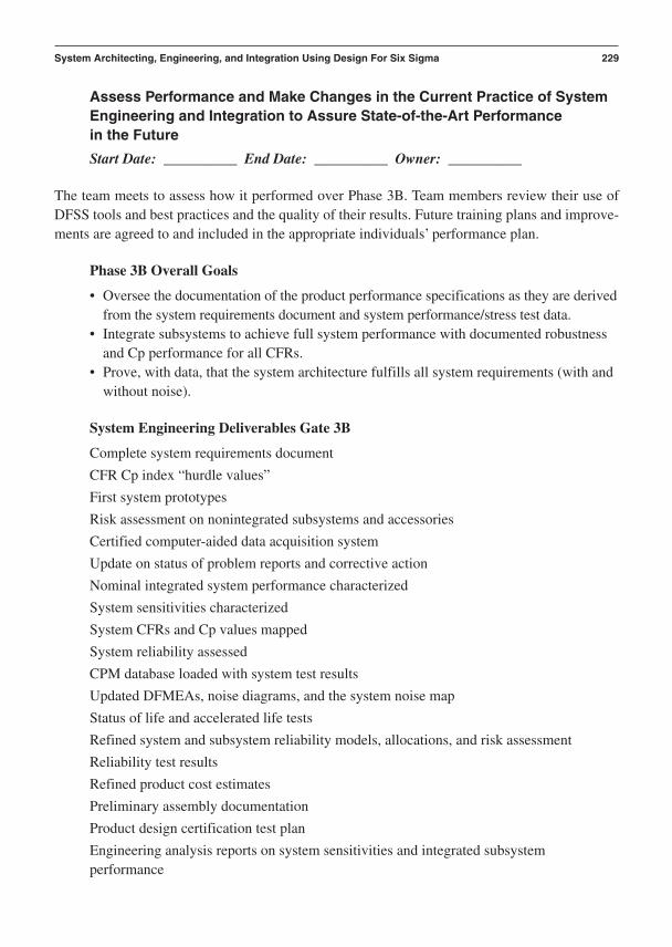
Assess Performance and Make Changes in the Current Practice of SystemEngineering and Integration to Assure State-of-the-Art Performance in the Future
Start Date: __________ End Date: __________ Owner: __________
The team meets to assess how it performed over Phase 3B. Team members review their use ofDFSS tools and best practices and the quality of their results. Future training plans and improve-ments are agreed to and included in the appropriate individuals’ performance plan.
Phase 3B Overall Goals
• Oversee the documentation of the product performance specifications as they are derivedfrom the system requirements document and system performance/stress test data.
• Integrate subsystems to achieve full system performance with documented robustnessand Cp performance for all CFRs.
• Prove, with data, that the system architecture fulfills all system requirements (with andwithout noise).
System Engineering Deliverables Gate 3B
Complete system requirements document
CFR Cp index “hurdle values”
First system prototypes
Risk assessment on nonintegrated subsystems and accessories
Certified computer-aided data acquisition system
Update on status of problem reports and corrective action
Nominal integrated system performance characterized
System sensitivities characterized
System CFRs and Cp values mapped
System reliability assessed
CPM database loaded with system test results
Updated DFMEAs, noise diagrams, and the system noise map
Status of life and accelerated life tests
Refined system and subsystem reliability models, allocations, and risk assessment
Reliability test results
Refined product cost estimates
Preliminary assembly documentation
Product design certification test plan
Engineering analysis reports on system sensitivities and integrated subsystemperformance
System Architecting, Engineering, and Integration Using Design For Six Sigma 229

Refined bill of materials
Documented system integration problem reports and corrective actions
System benchmarking test results and comparative assessment (your old product or acompetitor) and risk analysis report for product design certification
Test results for environmental, health, safety, and regulatory compliance
Final component, subsystem, and system design specifications verified
CPM database updated from product certification test results
Documented problems with system assembleability, serviceability, and maintainabilityalong with corrective actions completed
Construct, debug, deliver, and assist in testing of alpha systems
Documented results from regular and accelerated life tests
Updated DFMEAs, noise diagrams, and the system noise map from alpha systems testing
Updated Critical Parameter Management system-to-subsystem CFR maps and relationaldatabase
Preliminary service and maintenance documentation
Updated problem report and corrective action process and database
Refined bill of materials and configuration control database
System performance and integration risk assessment from all Phase 3 test data
Product performance specification document
All Phase 3 product design certification criteria met per the system requirementsdocument
Project plans for Phase 4A
Phase 3B System Engineering Tools and Best Practices
QFD
Critical Parameter Management
Capability studies
Risk analysis
Engineering analysis
Baseline, stress, and reliability performance tests
Measurement system analysis
Excel database management
Design of experiments (screening and modeling)
ANOVA
Regression
Robust design
DFMEA
230 Chapter 7

Subsystem noise diagramming
System noise mapping
Life testing
Accelerated life testing
HALT
HAST
Reliability modeling
Reliability allocation analysis
Reliability test planning
Project management
SPC
Statistical data analysis methods
Analytical tolerance design
Empirical tolerance design
Baseline performance tests
Competitive assessment
Regulatory and environmental performance test planning
Regulatory and environmental test capability studies
DFMA
Shipping performance test design
Performance, stress, and reliability testing
System–subsystem–subassembly transfer function development
System level sensitivity analysis
Health and safety testing
Risk analysis
Phase 4A: Final Product Design Certification
The major system engineering and integration elements for CDOV Phase 4 involve certification of final product design, production processes, and service capability. Phase 4 contains two major parts:
• Phase 4A focuses on the capability of the integrated system functional performance.• Phase 4B focuses on the capability of production assembly and manufacturing
processes within the business and the extended supply chain and service organization.This is also considered a part of the larger system and includes many elements thatextend beyond the system we refer to as the actual functioning product.
Figure 7–13 diagrams the major elements of Phase 4A.
System Architecting, Engineering, and Integration Using Design For Six Sigma 231

Build product design certification (alpha) unitsusing production parts
Start Date: End Date: Owner:
Evaluate system performance under nominalconditions
Start Date: End Date: Owner:
Evaluate system performance under stressconditions
Start Date: End Date: Owner:
Evaluate system capability and reliabilityperformance
Start Date: End Date: Owner:
Complete and document corrective actions onproblems
Start Date: End Date: Owner:
Generate system performance and integrationrisk assessment from all Phase 4A test data
Start Date: End Date: Owner:
Verify product design meets all requirementsStart Date: End Date: Owner:
Generate Phase 4B system engineering plansStart Date: End Date: Owner:
Convert the system requirements document intothe product performance specificationdocument
Start Date: End Date: Owner:
Assess performance and make changes in thecurrent practice of system engineering andintegration to assure state-of-the-artperformance in the future
Start Date: End Date: Owner:
Update all DFMEAs, noise diagrams, and thesystem noise map from product designcertification (alpha) systems tests
Start Date: End Date: Owner:
Develop final regulatory requirementsdocuments and conduct evaluations
Start Date: End Date: Owner:
Develop, conduct, and analyze final health,safety, and environmental tests
Start Date: End Date: Owner:
Continue to update and document the CriticalParameter Management map and relationaldatabase
Start Date: End Date: Owner:
Help all subsystem teams prepare summarycompetitive assessment documentation throughtests, literature, and field evaluations
Start Date: End Date: Owner:
Help conduct final tolerance design and costbalancing on components, subassemblies, andsubsystems (Integration)
Start Date: End Date: Owner:
Continue to conduct regular and accelerated lifetests
Start Date: End Date: Owner:
Assure all CTF components, CFRs from supplychain, and assembly operations are deliveredand set at targeted nominals
Start Date: End Date: Owner:
Figure 7–13 Flow of Phase 4A of Product Commercialization
The specific issues related to each Phase 4A system engineering action item (start date foreach action item, the action item, end date for each action) will be reviewed in this section. Eachof these action items can be conducted by using a tool or best practice. The flow of actions canbe laid out in the form of a PERT chart for project management purposes.
Help Conduct Final Tolerance Design and Cost Balancing on Components,Subassemblies, and Subsystems (Integration)
Start Date: __________ End Date: __________ Owner: __________
Just as the system engineers distributed themselves throughout the subsystem teams for the de-sign and robustness optimization activities in Phases 2 and 3, they continue in their integrationrole for tolerance and cost balancing in Phase 4A. Numerous sensitivity relationships betweenmanufacturing processes, components, subassemblies, and subsystems are fine-tuned in Phase4A. The system engineers need firsthand knowledge of these changes to be sure they account for them in their product design certification test plans. They also need to be advising and nego-tiating with the subsystem teams to be sure their changes are not compromising system perfor-mance. Balancing a subsystem’s cost and performance behavior at the expense of the systemperformance has to be carefully managed. This is the responsibility of the system engineer. Theold watchdog role of the quality assurance organization shifts to the system engineering team inthis context. The system engineers jealously guard the integrity of the system performance ful-fillment of the system requirements. Seeking balance along with compromise is a common ac-tivity during Phase 4A.
Help All Subsystem Teams Prepare Summary Competitive AssessmentDocumentation Through Tests, Literature, and Field Evaluations
Start Date: __________ End Date: __________ Owner: __________
It is common for the system engineering team to “own” the purchased competitive equipmentused for benchmarking. When competitive assessments are conducted at the system level, the sys-tem engineers run these evaluations. When competitive subsystem, subassembly, and componentperformance and architectural evaluations are conducted, they are usually performed by the re-spective subsystem teams with the assistance of their system engineering representatives. Otherforms of competitive summary assessments can be conducted as required to help provide evi-dence that the product design has reached its goals of meeting or surpassing the appropriate re-quirements and benchmarks. Because it is the system engineering team’s responsibility to provethe system is ready to pass Gate 4A requirements, team members must have time budgeted to as-sist in gathering the summary information in support of the busy subsystem teams.
Continue to Conduct Regular and Accelerated Life Tests
Start Date: __________ End Date: __________ Owner: __________
System Architecting, Engineering, and Integration Using Design For Six Sigma 233

The system engineering team continues its role of conducting the various types of life tests re-quired to verify the product design specifications. At this point, the life tests tend to become veryaggressive. Highly accelerated stress tests (HAST) and highly accelerated life tests (HALT) areappropriate.
The system is nearing a point where it is about as good as it is going to get. Now is the timeto take the system out to its real failure limits. The system and subsystem engineering teams mustknow where their critical failure limits are. This is particularly true for safety and high-cost reli-ability failure issues. Time is short in the overall program development cycle but not so short thatdesign changes can’t be made to help limit the risk of extreme failure conditions.
Assure All CTF Components and CFRs from Supply Chain and AssemblyOperations Are Delivered and Set at Targeted Nominals
Start Date: __________ End Date: __________ Owner: __________
As the system engineering team gets ready to assemble and evaluate the product design certifi-cation (alpha) units, it needs proof that all critical-to-function specifications at the componentlevel are made right on target nominal set points. The same is true for all subassembly and sub-system critical functional responses that are being delivered by the subsystem teams. It is againstall that is good and pure to permit undefined and uninspected components, subassemblies, andsubsystems to be integrated for these critical performance certification tests. This is where con-formance to specifications is extremely important. Product configuration control must be rigor-ous at this point. We recommend a few hours in a “Six Sigma pain amplification chamber” foranyone caught trying to sneak in off-nominal components through configuration control for prod-uct design certification tests. Seriously, it is unacceptable for anyone to bypass the discipline ofhaving the system “built to spec.” The whole team is charged with verifying system performanceat nominal specifications.
Build Product Design Certification (Alpha) Units Using Production Parts
Start Date: __________ End Date: __________ Owner: __________
The system engineering team oversees the physical assembly and adjustments of the components,subassemblies, and subsystems into the final product design certification units. Some people pre-fer to call these alpha test units. System engineering may have service and assembly personnelhelping to do this assembly work. The service engineers definitely conduct any service or main-tenance to these test units during the certification evaluations. All critical adjustment parametersand the CRFs they are adjusting are carefully monitored to be sure all CFR outputs are right ontarget—not just within specification limits.
Evaluate System Performance Under Nominal Conditions
Start Date: __________ End Date: __________ Owner: __________
234 Chapter 7

The product design certification units are now set up and run at their nominal set points. This isthe consummate test for everything being set at exactly what is called for in the design specifica-tions. The results of this test are compared to the system requirements. All CFRs are measuredusing the systemwide data acquisition system. All capability indices are calculated and docu-mented. This is truly a “noiseless” evaluation of the best the design can do under rigorously nom-inal conditions.
Evaluate System Performance Under Stress Conditions
Start Date: __________ End Date: __________ Owner: __________
The product design certification units are now exposed to the same variety of noises that were in-tentionally induced in Phase 3B. Sometimes the stress levels induced in Phase 3B are more ag-gressively stressful than those applied in Phase 4A. The stresses in Phase 4A certification testingmust be a reasonable mixture of stresses that are likely to happen in the normal life cycle of theproduct. Phase 3B system stress tests must be more brutal than that because you are trying to forceout the system weaknesses. Products rarely experience all noise factors occurring at high levelsof intensity over continuous operating conditions. Phase 3B stress tests are harsh and are intendedto flush out significant sensitivities and problems while time remains to correct them. Phase 4Astresses need to be metered out in more realistic doses of intensity. The mixtures of induced noisesshould mimic what your average customer group will experience in their environment and inducetheir use habits. Now, you are just seeing how far off-target your design means shift so you canemulate and document the value of Cpk for the system CFRs.
Each CFR is evaluated under these realistically stressful conditions. Their stressed (dimin-ished) Cp and Cpk indices are calculated and then compared to the unstressed Cp and Cpk in-dices. It is helpful to make these comparisons at the Gate 4A review. This gives the gate keepersa clear picture of just how capable the product is across each of the CFRs. This paints a clear SixSigma context view of the risks and accomplishments attained within the program up to this point.Credibility of certification is enhanced through the comparison of nominal and stressful data sets.
Develop Final Regulatory Requirements Documents and ConductEvaluations
Start Date: __________ End Date: __________ Owner: __________
The system engineering team has an obligation to prove that all regulatory requirements havebeen fulfilled by the final product design specifications. We call particular attention to regulatoryrequirements here because without their fulfillment you probably are prohibited by law from sell-ing the product.
This is a good place to remind the reader that requirements and specifications are often notthe same thing. We wish they were a perfect match but they frequently are not. Specifications doc-ument what the design is capable of delivering. Requirements are what we hope the design can
System Architecting, Engineering, and Integration Using Design For Six Sigma 235

fulfill. Specifications are the voice of final design and current process capability, while require-ments are jointly representing the voice of the customer and the business.
Develop, Conduct, and Analyze Final Health, Safety,and Environmental Tests
Start Date: __________ End Date: __________ Owner: __________
Health, safety, and environmental requirements should not escape the scrutiny of Six Sigma stan-dards for performance and capability. The system engineering team is responsible for evaluatingand providing certification data for these critical performance areas. There will undoubtably be a set of critical functional responses related to the requirement for health, safety, and environ-mental requirements.
Evaluate System Capability and Reliability Performance
Start Date: __________ End Date: __________ Owner: __________
The product certification tests culminate in verifying system level performance that can be mea-sured and reported in terms of Cp and Cpk. Several of the product design certification units arededicated, from the start, to run reliability certification evaluations. These evaluations are re-ported in mean time between service or mean time to failure metrics.
Complete and Document Corrective Actions on Problems
Start Date: __________ End Date: __________ Owner: __________
As is always the case for any system evaluation, there will be problems. The amount and sever-ity of problems encountered in the product design certification evaluations should be few and mi-nor, respectively. Nonetheless, any and all problems encountered during the certification testsshould be documented. Corrective actions can then be prescribed and results confirmed. All ma-jor corrective actions must be resolved to pass Gate 4A. Moderate and minor corrective actionsmay be granted provisional passage at Gate 4A, but proof of their resolution must be provided ina closely managed and tracked time frame.
Update All DFMEAs, Noise Diagrams, and the System Noise Map from Product Design Certification (Alpha) Systems Tests
Start Date: __________ End Date: __________ Owner: __________
All failure mode and effects analysis documents need to be updated after the design certificationtests are completed. New information about noise sensitivity within subsystems and across thesystem should be added to the noise diagrams and the system noise map. All significant system
236 Chapter 7
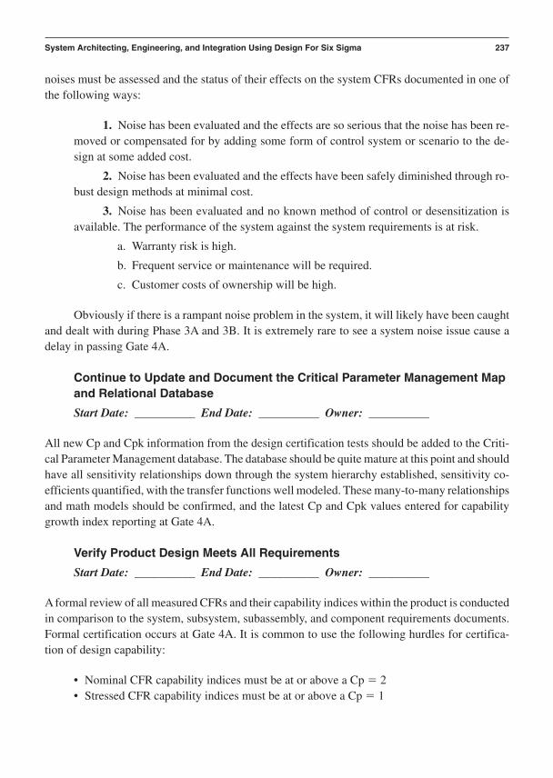
noises must be assessed and the status of their effects on the system CFRs documented in one ofthe following ways:
1. Noise has been evaluated and the effects are so serious that the noise has been re-moved or compensated for by adding some form of control system or scenario to the de-sign at some added cost.
2. Noise has been evaluated and the effects have been safely diminished through ro-bust design methods at minimal cost.
3. Noise has been evaluated and no known method of control or desensitization isavailable. The performance of the system against the system requirements is at risk.
a. Warranty risk is high.
b. Frequent service or maintenance will be required.
c. Customer costs of ownership will be high.
Obviously if there is a rampant noise problem in the system, it will likely have been caughtand dealt with during Phase 3A and 3B. It is extremely rare to see a system noise issue cause adelay in passing Gate 4A.
Continue to Update and Document the Critical Parameter Management Mapand Relational Database
Start Date: __________ End Date: __________ Owner: __________
All new Cp and Cpk information from the design certification tests should be added to the Criti-cal Parameter Management database. The database should be quite mature at this point and shouldhave all sensitivity relationships down through the system hierarchy established, sensitivity co-efficients quantified, with the transfer functions well modeled. These many-to-many relationshipsand math models should be confirmed, and the latest Cp and Cpk values entered for capabilitygrowth index reporting at Gate 4A.
Verify Product Design Meets All Requirements
Start Date: __________ End Date: __________ Owner: __________
A formal review of all measured CFRs and their capability indices within the product is conductedin comparison to the system, subsystem, subassembly, and component requirements documents.Formal certification occurs at Gate 4A. It is common to use the following hurdles for certifica-tion of design capability:
• Nominal CFR capability indices must be at or above a Cp 2• Stressed CFR capability indices must be at or above a Cp 1
System Architecting, Engineering, and Integration Using Design For Six Sigma 237

There is no hard and fast rule for what these hurdles need to be. That is up to your customerswithin the market segment you intend to serve.
Convert the System Requirements Document into the Product PerformanceSpecification Document
Start Date: __________ End Date: __________ Owner: __________
The system engineering and subsystem engineering teams must document the final design spec-ifications that completely identify all the set points for all the design parameters, those that arecritical as well as all other parameters that define the product form, fit, and function. This aggre-gated group of defining parameters is referred to as the product design specifications. The prod-uct design specifications document contains what the product development team was able todeliver as opposed to what the system requirements document asked for. Gate 4A assesseswhether these two documents are reasonably close to one another. If they are not, corrective ac-tion is definitely in order. If DFSS tools are used properly, with CPM actively tracking capabil-ity growth during the CDOV phases, the likelihood that the product design specifications will begrossly out of line with the system requirements is quite low. These specifications are used by theassembly, distribution, supply chain, service, and support organizations to build, ship, and main-tain the product over its intended life cycle.
Generate System Performance and Integration Risk Assessment from all Phase 4A Test Data
Start Date: __________ End Date: __________ Owner: __________
The system engineering team constructs a risk assessment document based on the results or thelack thereof from Phase 4A activities.
Generate Phase 4B System Engineering Plans
Start Date: __________ End Date: __________ Owner: __________
The system engineering team meets to assess required deliverables for the next phase. Teammembers create detailed plans to deliver them in the allotted time. These plans are a requirementfor passage of Gate 4A. See the scorecard in Figure 7–14.
Assess Performance and Make Changes in the Current Practice of SystemEngineering and Integration to Assure State-of-the-Art Performance in the Future
Start Date: __________ End Date: __________ Owner: __________
238 Chapter 7
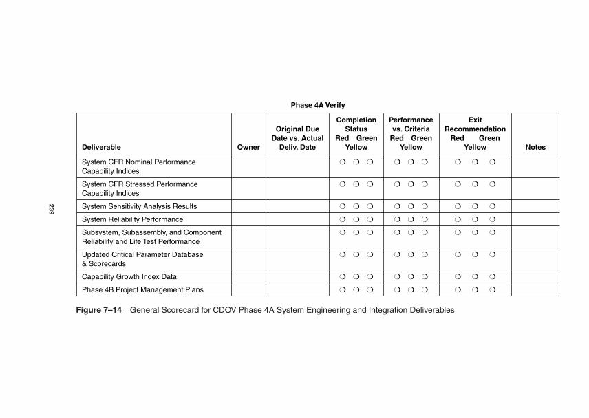
Phase 4A Verify
Completion Performance Exit Original Due Status vs. Criteria Recommendation
Date vs. Actual Red Green Red Green Red GreenDeliverable Owner Deliv. Date Yellow Yellow Yellow Notes
System CFR Nominal Performance
Capability Indices
System CFR Stressed Performance
Capability Indices
System Sensitivity Analysis Results
System Reliability Performance
Subsystem, Subassembly, and Component
Reliability and Life Test Performance
Updated Critical Parameter Database
& Scorecards
Capability Growth Index Data
Phase 4B Project Management Plans
Figure 7–14 General Scorecard for CDOV Phase 4A System Engineering and Integration Deliverables
239

The team meets to assess how it performed over Phase 4A. Team members review their use ofDFSS tools and best practices and the quality of their results. Future training plans and improve-ments are agreed to and included in the appropriate individuals’ performance plans.
Phase 4A Overall Goals
• Build and test the product design certification machines for overall productperformance and robustness validation.
• Update and evaluate production certification (pilot) machines.• Verify the product design specifications are fulfilled by measured system performance
(with and without stress).• Verify the product’s serviceability and maintainability.• Prove that the complete system is ready for production launch preparations.
General Checklist of Phase 4A System Engineering and Integration Tools and BestPractices:
Measurement system analysis
System noise mapping
Analytical tolerance design
Worst case analysis
Root sum of squares analysis
Six Sigma analysis
Monte Carlo simulation
Empirical Tolerance Design
System level sensitivity analysis
Design of Experiments
ANOVA
Regression
Multi-vari studies
Design capability studies
Nominal system CFR design Cp studies
Stress case system CFR design Cp studies
Reliability assessment (normal, HALT, & HAST)
Competitive benchmarking studies
Statistical process control of design CFR performance
Critical Parameter Management (with capability growth index)
Nominal performance and stress testing
Statistical data analysis
240 Chapter 7

Competitive benchmarking
Health, safety, regulatory, and environmental testing
Instrumentation and computer-aided data acquisition system capability (MSA)
Risk analysis
Shipping, handling, installation, safety, regulatory, and environmental testing and dataanalysis
Phase 4B: Production Verification
Phase 4B encompasses capability of production, assembly, and manufacturing processes withinthe business as well as the extended supply chain and service organization (see Figure 7–15). Sys-tem engineering begins to play a secondary role as the certification efforts fully transition over tothe production, assembly, service, support, and supply chain organizations.
The specific issues related to each Phase 4B system engineering action item (start date foreach action item, the action item, end date for each action) will be reviewed in this section. Eachof these action items can be conducted by using a tool or best practice. The flow of actions canbe laid out in the form of a PERT chart for project management purposes.
Help Build Initial Production Units Using Inspected Production Parts
Start Date: __________ End Date: __________ Owner: __________
Phase 4B ushers in a major transition for the role played by the system engineering team. This isliterally their ramp-down phase. The production, supply chain management, service, and supportorganizations take over the ownership of the system. In fact, the word system is rarely used in thislater phase of product development. The vocabulary of Phase 4B is one of product support andproduction operations. The system engineering team plays a secondary role now, providing sup-port to the new owners of the system.
Phase 4B has as one of its major goals the successful ramp-up of the production processesrequired to manufacture, assemble, evaluate, package, and distribute the product. System engi-neering had been leading the assembly and evaluation efforts in Phases 3B and 4A; now it trans-fers this responsibility. The resources in the system engineering organization act in an advisoryrole. The bill of material is transferred over to the production organization. The inspection re-quirements and process of initial production components, subassemblies, and subsystems areamong the earliest responsibilities to be transitioned. System engineering participates in the earlyproduction builds where information regarding critical adjustment parameters and their sensitiv-ity relationships with the critical functional responses are provided.
Help Conduct Shipping Tests and Packaging Assessments
Start Date: __________ End Date: __________ Owner: __________
System Architecting, Engineering, and Integration Using Design For Six Sigma 241
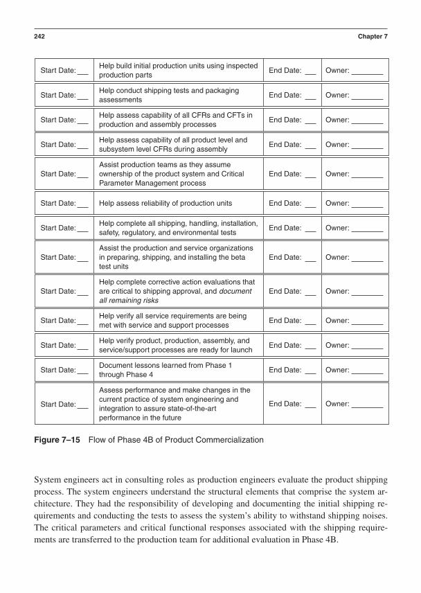
System engineers act in consulting roles as production engineers evaluate the product shippingprocess. The system engineers understand the structural elements that comprise the system ar-chitecture. They had the responsibility of developing and documenting the initial shipping re-quirements and conducting the tests to assess the system’s ability to withstand shipping noises.The critical parameters and critical functional responses associated with the shipping require-ments are transferred to the production team for additional evaluation in Phase 4B.
242 Chapter 7
Help conduct shipping tests and packagingassessments
Start Date: End Date: Owner:
Help build initial production units using inspectedproduction parts
Start Date: End Date: Owner:
Help assess capability of all CFRs and CFTs inproduction and assembly processes
Start Date: End Date: Owner:
Help assess capability of all product level andsubsystem level CFRs during assembly
Start Date: End Date: Owner:
Help complete all shipping, handling, installation,safety, regulatory, and environmental tests
Start Date: End Date: Owner:
Help verify product, production, assembly, andservice/support processes are ready for launch
Start Date: End Date: Owner:
Help verify all service requirements are beingmet with service and support processes
Start Date: End Date: Owner:
Document lessons learned from Phase 1through Phase 4
Start Date: End Date: Owner:
Assess performance and make changes in thecurrent practice of system engineering andintegration to assure state-of-the-artperformance in the future
Start Date: End Date: Owner:
Assist the production and service organizationsin preparing, shipping, and installing the betatest units
Start Date: End Date: Owner:
Assist production teams as they assumeownership of the product system and CriticalParameter Management process
Start Date: End Date: Owner:
Help assess reliability of production unitsStart Date: End Date: Owner:
Help complete corrective action evaluations thatare critical to shipping approval, and documentall remaining risks
Start Date: End Date: Owner:
Figure 7–15 Flow of Phase 4B of Product Commercialization

Help Assess the Capability of All CTFs in the Production Processes
Start Date: __________ End Date: __________ Owner: __________
The components that are produced out in the supply chain are a source of noise. The system en-gineering team transfers its knowledge of component quality issues that are still areas of risk fromthe product design certification evaluations.
Help Assess Capability of All Product Level and Subsystem Level CFRsDuring Assembly
Start Date: __________ End Date: __________ Owner: __________
Proceeding up the hierarchy of the system critical parameters, the system engineers can be help-ful in the proper measurement of the capability of the subassembly and subsystem CFRs. Theyhelp assure no errors are made as these parameters are evaluated as the production processes rampup to a steady state.
Assist Production Teams as They Assume Ownership of the ProductSystem and Its Critical Parameter Management Process
Start Date: __________ End Date: __________ Owner: __________
System Engineering plays a key role in transfer of the Critical Parameter Management processand database. A representative from the sustaining engineering team in the production organi-zation will take responsibility for the CPM tasks. The system engineer responsible for the CPMdatabase must teach and assist the appropriate personnel in the production organization as they continue to measure and track the subset of critical parameters that will be used in production.
Help Assess Reliability of Production Units
Start Date: __________ End Date: __________ Owner: __________
When the first production units roll off the assembly line, they will need to be set up and evalu-ated for reliability. This is part of the formal certification of the manufacturing, assembly, andservice processes. The system engineers created the reliability evaluation process for the productand play a key role in this Phase 4B reliability test. They have intimate knowledge of the detailsof running a disciplined reliability test and can greatly expedite the process in the production or-ganization. This responsibility is not easily thrown over the wall.
Help Complete All Shipping, Handling, Installation, Safety, Regulatory,and Environmental Tests
Start Date: __________ End Date: __________ Owner: __________
System Architecting, Engineering, and Integration Using Design For Six Sigma 243

Here, too, the system engineering team has great experience from Phase 4A testing. It has a strongexperience base from which to draw as it helps the production, distribution, and service organi-zations complete the final certification evaluations in these areas prior to shipping approval.
Assist the Production and Service Organizations in Preparing, Shipping,and Installing the Beta Test Units
Start Date: __________ End Date: __________ Owner: __________
It is common for a small number of the earliest production units to be placed into beta test sites outin the global marketplace. The system engineers often participate in site selection and installationlogistics as these units go out for early market testing. The system engineers usually partner withthe service and support organization to take critical parameter data and solve technical problems.
Help Complete Corrective Action Evaluations That Are Critical to ShippingApproval, and Document All Remaining Risks
Start Date: __________ End Date: __________ Owner: __________
The system engineers have been keeping track of the corrective action database. New issues willarise from the production process certification tests that will have their resolution back in the de-sign specifications. The system engineers can play a key role in maintaining the balance betweencosts and functional quality as the required design changes are made by the subsystem engineer-ing teams.
Help Verify All Service Requirements Are Being Met with Service and Support Processes
Start Date: __________ End Date: __________ Owner: __________
During the beta tests (or external customer evaluations), the system engineers help the service andsupport teams make changes to critical adjustment parameters as necessary. This part of the pro-duction certification process is focused on assuring that as the product requires maintenance andCFR recentering, the service procedures are clear and reliable.
Help Verify Product, Production, Assembly, and Service/Support ProcessesAre Ready for Launch
Start Date: __________ End Date: __________ Owner: __________
The experience embedded in the system engineering team is a good check and balance to judgewhether the production processes are ready and supportive of the formal product launch. It is notuncommon for members of the system engineering team to act as associate gate keepers for Gate4B. See the Scorecard in Figure 7–16.
244 Chapter 7

Phase 4B Verify
Completion Performance Exit Original Due Status vs. Criteria Recommendation
Date vs. Actual Red Green Red Green Red GreenDeliverable Owner Deliv. Date Yellow Yellow Yellow Notes
System CFR Nominal Performance
Capability Indices
System Sensitivity Analysis Results
System Reliability Performance
Subsystem, Subassembly, and Component
Reliability and Life Test Performance
Updated Critical Parameter Database and
Scorecards
Capability Growth Index Data
Sustaining Production Engineering Support
Plans
Figure 7–16 General Scorecard for CDOV Phase 4B System Engineering and Integration Deliverables
245

Assess Performance and Make Changes in the Current Practice of SystemEngineering and Integration to Assure State-of-the-Art Performance in the Future
Start Date: __________ End Date: __________ Owner: __________
The team meets to assess how it performed over Phase 4B. Team members review their use ofDFSS tools and best practices and the quality of their results. Future training plans and improve-ments are agreed to and included in the appropriate individuals’ performance plans.
Document Lessons Learned from Phase 1 Through Phase 4
Start Date: __________ End Date: __________ Owner: __________
The system engineering team meets to document all the lessons learned during all the phases.These will include the successes the team attained and the failures it created, induced, and sur-passed. This is part of the continuous improvement activity for the entire product developmentorganization.
System Engineering Deliverables Phase 4B Gate
Product installation process validated
Customer quality metrics and machine performance assessed and corrective actionidentified/resolved
Reliability data documented
Software technical documentation validated (functionality/performance)
Validation of the complete manufacturing /assembly/ supply chain process
Phase 4B Overall Goals
• Help build initial production machines with production processes and test to productionquality assurance test plans.
• Transfer CPM to production teams.• Support production and service organizations as they attain shipping approval.
General Checklist of Phase 4B System Engineering and Integration Tools and BestPractices:
Measurement system analysis
Analytical tolerance design
Worst case analysis
Root sum of squares analysis
246 Chapter 7
Six Sigma analysis
Monte Carlo simulation
Empirical tolerance design
System level sensitivity analysis
Design of experiments
ANOVA
Regression
Multi-vari studies
Design capability studies
Nominal system CFR design Cp studies
Reliability assessment (Normal, HALT, & HAST)
Competitive benchmarking studies
Statistical process control of design CFR performance
Critical Parameter Management (with capability growth index)
References
Blanchard, B. S. & Fabrycky, W. J. (1990). Systems engineering and analysis. New Jersey:Prentice Hall.
Lewis, J. W. (1994). Modeling engineering systems. Virginia: LLH Publishing.Maier, M. W. & Rechtin, E. (2000). The art of systems architecting (2nd Ed.). Boca Ratan, Fla:
CRC Press.Oliver, D. W., Kelliher, T. P. & Keegan Jr., J. G. (1997). Engineering complex systems with
objects and models. New York: McGraw-Hill.Rechtin, E. (1991). Systems architecting creating and building complex systems. New Jersey:
Prentice Hall.Shetty, D., & Kolk, R. A. (1997). Mechatronics system design. Boston, Mass: PWS Publishing Co.Stevens, R., Jackson, K., Brook, P., and Arnold, S. (1998). Systems engineering coping with
complexity. Hertfordshire: Prentice Hall Europe.
System Architecting, Engineering, and Integration Using Design For Six Sigma 247

This page intentionally left blank

P A R T I I I
Introduction to the Use ofCritical Parameter Management
in Design For Six Sigma inTechnology and Product
Development
Chapter 8 Introduction to Critical Parameter ManagementChapter 9 The Architecture of the Critical Parameter Management ProcessChapter 10 The Process of Critical Parameter Management in Product DevelopmentChapter 11 The Tools and Best Practices of Critical Parameter ManagementChapter 12 Metrics for Engineering and Project Management within CPMChapter 13 Data Acquisition and Database Architectures in CPM
Few things focus a team on the most important customer needs, product requirements, design pa-rameters, performance metrics, and deliverables for a product’s success better than Critical Para-meter Management. The notion of the existence of critical parameters and the fact that they mustbe rigorously managed is not new. What is new is the structured way in which DFSS guides theprocess of knowing what is critical, how critical parameters are measured, and how they are re-lated to one another, documented, and tracked to verify the capability of new technologies andproduct designs.
Chapter 8 is a general introduction to the topic of Critical Parameter Management. Chap-ter 9 goes deeper into the definition of CPM by discussing the architecture of the CPM process.It also establishes how CPM fits within the structure of a product development organization.Chapter 10 defines the detailed process steps of conducting CPM. It examines the timing of what
249
to do and when to do it in a Phase/Gate context. CPM scorecards are illustrated. Chapter 11 re-views the tools and best practices from DFSS that are directly applicable to CPM. The deliver-ables from the tools and best practices are also discussed.
Chapter 12 develops the metrics used within Critical Parameter Management. CPM is dataintensive. This chapter demonstrates what is measured and how CPM data is used to documentthe required performance deliverables in a gate review. Chapter 13 ends the development and dis-cussion of CPM by discussing how data acquisition systems and database architectures are usedto enable the process of CPM.
Critical Parameter Management lies at the heart of DFSS. The data from CPM actionscourses through the phases and gates of a commercialization process, enabling decisions to bemade and risks to be managed. The data it produces is the lifeblood of DFSS. Without it an or-ganization cannot keep track of the complex relationships that must be developed, designed, op-timized, balanced, and made capable as the new product evolves toward certification forproduction, servicing, maintenance, and support.
250 Part III • Introduction to the Use of Critical Parameter Management in Design For Six Sigma

C H A P T E R 8
Introduction to CriticalParameter Management
Critical Parameter Management is rapidly becoming a strategic tool for improving new prod-uct development cycle-time. It focuses multifunctional technology development and prod-
uct commercialization teams on the few things that matter the most relative to cost, quality, andtime-to-market goals. It helps unify and integrate software and hardware engineering activitiesduring the earliest phases of product development. Critical Parameter Management works wellwithin the context of fulfilling critically ranked needs defined by the voice of the customer. It alsodelivers strong results when applied to the development of unique, breakthrough technologiesthat deliver functions that were not anticipated by customers.
Critical Parameter Management enhances the discipline and structure resident within or-ganizations that are already following a formal technology development or product designprocess. Critical Parameter Management integrates technical processes, tools, and metrics thatare used to develop and transfer technology, products, and manufacturing processes for efficientcommercialization. An analogy can be used to help explain the unique nature of Critical Para-meter Management.
Winning Strategies
We will focus on product commercialization as a race to be won in this example. Picture in yourmind a racing crew from Harvard rowing a long narrow boat down the Charles River. Harvardhas invested a lot of money in the sport of rowing and has a tradition of excellence that is impor-tant to the university, its alumni, and supporters. The President of Harvard wants assurance thatthis tradition of excellence will be maintained. He cares about the quality metric of wins vs.losses, or yield if you please. But the mechanics behind a win or a loss are not a matter of qual-ity. They are a matter of physics, engineering, system integration, teamwork, and the fundamen-tal measures of system performance.
A racing crew and its equipment make up a complex system that must efficiently transformand integrate the flow of energy, mass, and information. Each rower is putting energy into the sys-tem (the boat). Each rower delivers a unique, individual contribution to the speed and direction
251

(vector) of the boat. One individual calls out a timing signal (software) to help integrate and co-ordinate the function of the rowers. The rowers must transform their potential energy into kineticenergy to transfer the mass of the boat as efficiently and harmoniously as possible. The boat ismoving in an environment that is laden with sources of uncontrollable variation (water, winddrag, and lateral forces). The boat has its own internal sources of variability as well (worn parts,oar-to-oar differences). Crew members have an interesting problem: What are the critical factorsthat create on-target functions that fulfill their objective of winning races in spite of the “noise”of uncontrollable sources of variation? This is a system integration problem.
The type of responses they measure and the tools they use to optimize their individual andsystem performance in an environment rich in sources of uncontrollable variation are crucial toreducing the time it takes to attain repeatable and durable results. The level of quality that the crewattains is by the structure of the process used to optimize its functional performance. Crew mem-bers need to structure an approach for Critical Parameter Management.
Focus on System Performance
In the context of product or process commercialization, Critical Parameter Management consid-ers the performance of the system as the highest priority. Subsystem and component performanceare important but only within the context of system optimization. They are resources to be allo-cated to fulfill system requirements and goals. Critical Parameter Management gathers, inte-grates, and documents complex networks of critical performance relationships down from thevoice of the customer to the system requirements, subsystem requirements, subassembly re-quirements, component requirements, and manufacturing process and material requirements.However, CPM goes well beyond the documentation of requirements as it also integrates andtracks what is supposed to happen vs. what is actually attained in terms of functional perfor-mance during the phases and gates of technology development and product commercializationprocesses.
Critical Parameter Management has as ultimate goals reduced time-to-market, high qualityand low cost of production and ownership. Unfortunately one cannot easily use cycle-time, qual-ity, or cost to measure the effect and efficiency of critical parameter relationships during tech-nology, product, or manufacturing process development. These are lagging indicators ofperformance. By the time these metrics are backed up with real data, it is extremely expensive totake corrective action. These metrics foster a reactive “build-test-fix” mentality within engineer-ing teams. When this mind-set governs organizational behavior, there is sure to be a need to do itover a second or third or fourth time—by design!
CPM measures the functions that are directly related to the laws of physics selected to con-trol the transformation and flow of energy, mass, and information in technology, products, andmanufacturing processes. These preventative measures are temporally efficient for the preventionof problems in cost, quality, and cycle-time. As a consequence, Critical Parameter Managementprocesses are not born out of metrics found in Total Quality Management. Critical ParameterManagement practitioners must measure functions, not quality. Metrology, in CPM, is groundedin measuring phenomena that are direct outcomes from the application of the principles of phys-
252 Chapter 8
ical law. Critical parameter metrology and data analysis is governed by the engineering scienceswith some assistance from the quality and applied statistical sciences. To be more specific, CPMperformance is based on balancing system functions under the Law of Conservation of Energyand the Law of Conservation of Mass. CPM keeps two sets of “books,” one in terms of physicsand engineering metrics (preventative metrics) and one in terms of cost, quality, and time (reac-tive business, quality, and accounting metrics). The measured performance values gathered dur-ing product and manufacturing process development are stored, maintained, processed, anddistributed as reports using a relational database, such as Access, Oracle, DOORS, the Six SigmaCockpit, and others. This quantitative, interrelational information is used to make decisions, bal-ance resources, and help manage the critical path of a product development project. In this con-text, CPM is highly supportive and synergistic with the methods of project management.
Critical Parameter Management is a process that encompasses methods and metrics con-ducted in a system engineering context. The process integrates and facilitates communication be-tween managers and technologists: scientists, engineers, technicians, designers, productionoperations personnel, and field service and support personnel. Teams that succeed at Critical Pa-rameter Management have leaders who excel at structuring and deploying engineering processmechanics, while the practitioners themselves are very good at engineering mechanics and designengineering best practices. Critical Parameter Management recognizes the value of a variety ofmetrics. There is a time and a place for measuring quality in CPM—after you’ve paid your engi-neering dues and actually have something functionally rational to measure. A dominant rule ofCPM is to refrain from measuring attribute forms of quality that are distant from the function ofthe design parameters themselves.
Early in the development process, engineering scalars and vectors are the dominant valuesto be measured and evaluated in terms of means and standard deviations. Subsystems are opti-mized by evaluating the scalars and vectors as means, standard deviations, coefficients of varia-tion, and signal-to-noise ratios. In this context they are viewed as leading indicators ofinsensitivity to noise (an uncontrollable source of variation) and reliability. Systems are balancedduring subsystem integration and refinement by measuring the scalars and vectors in terms ofshort-term design and process capability indices (Cp). Tolerances are developed within subsys-tems and components measuring functional performance through the scalar and vector means,standard deviations, and Cp and Cpk indices. During steady-state production when Cpk valuesare routinely generated and evaluated, the use of Defects Per Unit and Defects Per Million Op-portunities can legitimately be introduced to track the macro-performance of the finely tunedproduct and production process. Defect reduction and reliability improvement never come di-rectly from measuring defects and reliability but from measuring the functions that cause the de-fects and poor reliability. Keeping the mean and standard deviations of critical functions on targetlies at the heart of design defect reduction.
Data-Driven Process
Critical Parameter Management is data driven. Instrumentation, data acquisition, data analysis,and database management are some of the most important enabling best practices within CPM.
Introduction to Critical Parameter Management 253

Organizations that deploy CPM are readily identified by their investment in computer-aided dataacquisition systems linked to precision measurement instruments, efficient use of modern dataanalysis software, and the networked use of web-accessible relational databases. System per-formance knowledge is centralized, but its use is widely distributed to the cross-functional engi-neering teams across the project and extended supply chain.
Critical Parameter Management is a refinement that can be added to an existing product de-velopment process to make it better. By better we mean more structured, more disciplined, moreconcrete in quantifying the things that matter the most in satisfying the needs of the customer, thesupply chain, and the business itself—its shareholders and employees. It forces critical issues tobe covered purposefully early in a commercialization project while there is still time to preventproblems. It forces customer-focused quality, reliability, and low cost of ownership to be inher-ent in the evolving product.
Examples of key issues covered by Critical Parameter Management:
• Identification and documentation of customer needs• Prioritization of customer needs into distinct groups of critical vs. general requirements• Translation of the customer needs into technical terms that can be expressed as
functions or physical characteristics that can be measured as continuous variables(engineering scalars and vectors) for mean, standard deviation, S/N, COV, Cp and Cpkevaluation, optimization within the product and its supporting network ofmanufacturing and service processes
• Identification and documentation of critical system, subsystem, and subassemblyfunctional responses that fulfill the translated customer needs (technical requirements)
• Early identification and development of instrumentation and data acquisition systemsto measure the critical functional responses
• Generation of design concepts that embody critical functional parameters thatharmoniously control and fulfill the critical system and subsystem functions (conceptsthat are driven by measurement of functions and design for testability)
• Measurement of critical subassembly, subsystem, and system functions during theevaluation of competing design concepts (benchmarking) to see which concepts bestfulfill the documented customer needs
• Selection of a superior product concept and attendant superior subsystem concepts thatare high in inherent functional robustness and low in competitive vulnerability
• Development of a superior, integrated product and its subsystems into prototypes thatare preengineered for ease of instrumentation so optimization of S/N and Cp indicescan happen quickly (active and concurrent fulfillment of robustness and Six Sigmaquantification goals)
• Creation of a relational, hierarchical database consisting of system requirements;system, subsystem, and component critical functional responses (CFRs); and thecritical functional parameters (CFPs) that control the critical responses (including thedocumentation of CFP’s sensitivity coefficients)
254 Chapter 8

• Optimization of subsystem and subassembly critical functional responses in terms ofS/N (robustness insensitivity to noise) to identify nominal set points for component,subassembly, and subsystem critical functional parameters
• Integration of robust subsystems to define and balance system level sensitivities asmeasured by the system level critical functional responses using Cp metrics
• Definition of critical subsystem, subassembly, and component production tolerances tobalance cost and quality for design certification (Cp metrics are proactively in use onthe design and manufacturing supply chain prior to production process certification,balancing VOC with VOP)
• Transfer of metrology and data acquisition systems for manufacturing, assembly, andfield service critical functional responses for ongoing quantification of Cp and Cpkvalues (to promote on-target performance) on into steady-state production and field useof the product
CPM uses design and manufacturing process capability indices [Cp ratios of criticality(USL–LSL) to sensitivity (6)] to track the maturing ability to fulfill the system and subsystemrequirements that ultimately satisfy customer needs. As Jack Welch, former CEO of General Elec-tric, says about Six Sigma results, “If the customer can’t see and feel it . . . you haven’t got it rightyet” (Welch, 2001). Criticality has its definition rooted in the voice of the customer (targets andtolerances). Sensitivity is defined as the voice of the product and manufacturing processes (sam-ple means and standard deviations). The voice of the customer cries out its demand, “This needis critical!” into the world of product and manufacturing process development. The echo backfrom the voice of the product and manufacturing processes is frequently the disappointing re-sponse, “I’m too sensitive to sources of variation!” Superior quality is the by-product of inten-tionally developed engineering functions within products and manufacturing processes thatpossess low levels of sensitivity. Yield and part per million quality are poor and indirect measuresof sensitivity, while scalar and vector functions are continuous variables that provide measures ofprecision (variance or spread about the mean) and accuracy (mean in relation to target) needed tominimize sensitivity during development.
Critical Parameter Management uses a portfolio of best practices to reduce product andprocess sensitivity, or strength of contribution to variation, so there is wide latitude between criti-cal tolerances and actual performance distributions (measured in sample standard deviations, s). Inthe world of Six Sigma, that latitude is expressed through short-term process capabilities equal to
2 (Cp USL LSL)/6 12/6
where really stands for a sample standard deviation, s.
Critical Parameter Management makes heavy use of best practices that provide rigorousquantification of intricate relationships between control parameter (independent variables weidentify as critical functional parameters) and functional response sensitivities (dependent vari-ables we identify as critical functional responses).
Introduction to Critical Parameter Management 255

Balanced criticality and sensitivity relationships can be elusive commodities. This is espe-cially true if one poorly translates and ranks the voice of the customer and then measures qualityinstead of physical functions. When the conservative laws of physics form the basis of our engi-neering measurement process, sensitivity is easier to measure and relate to criticality. In this con-text, the signal can be separated from the noise. We can quantify which engineering parametershave a dominant contribution to robustness and which have a dominant contribution to the ad-justment of the mean. We can also quantify the percent contribution each parameter contributesto the standard deviation or mean of a critical functional response. With this information, the teamcan make enlightened technical and economic decisions up through the chain of criticality withinany engineered system, right back to the original voice of the customer. If a project team does thisacross the board, fewer design mistakes are made, fewer things have to be reevaluated, and com-mercialization cycle-time is shortened.
CPM is particularly useful in preparing for and conducting software integration and evalu-ation. It plays a key role in the rapid identification of root causes of system and subsystem levelperformance relationships and problems. It helps prevent the system integration team from wast-ing time attributing problems to software when they are actually hardware or electrical problemsand vice versa. CPM provides clear functional performance and timing paths (functional block ortree diagrams) for the software developers to follow as they generate and modify code. Softwaremodules become better defined as they relate to functional trees that exist across subsystemboundaries. CPM helps software engineers understand the system and how they need to controland time the flow of information (logic and control signals) across the integrated product. Thesystem’s transformation and flow of energy, mass, and information are balanced under this kindof discipline.
The Best of Best Practices
Critical Parameter Management helps strategic, customer-focused Six Sigma initiatives spring tolife. It provides a context to integrate numerous best practices to activate daily behaviors that gainresults quickly and efficiently as organizations and teams seek to convert their energies into cor-porate cash flow.
In summary, Critical Parameter Management clarifies the process of generating, selecting,integrating, optimizing, and balancing product and production functions within a system context.It focuses the product development team on the key transformations and flows of energy, mate-rials, and information. It amplifies time savings through rigor and discipline in what you measure,how you measure, and when you measure. World-class performance in quality, cost, and cycle-time flow from efficiencies gained in the disciplined balance of project management methods, ac-tive use of a Phase/Gate development process, and a rich and full portfolio of best practices.Critical Parameter Management thrives in such an environment.
Reference
Welch, J. F. (2001). Jack: Straight from the gut. New York: Warner Business Books.
256 Chapter 8

C H A P T E R 9
The Architecture of the CriticalParameter Management Process
Building any form of architecture requires a rational starting point. Any foundation worth itssalt comes from a sound understanding of fundamental principles and insight into basic def-
initions related to what is being built. For our purposes of defining an architecture for Critical Pa-rameter Management we provide the following definitions and underlying principles.
Architecture is defined as “a style and method of design and construction” (American Heritage Dictionary, 1975). When we say we are going to discuss the architecture of a CriticalParameter Management process, we are talking about the methodology of designing and con-structing a process to manage critical parameters across a technology and product commercial-ization process.
Critical is defined as that which is significant, influential, weighty, essential, primary, fore-most, or principal. The act of being critical is accomplished through “characterization by carefulevaluation” (American Heritage Dictionary, 1975).
For our purposes, criticality pertains to specific parameters being developed, measured, andevaluated during the phases and gates of a product development process. What is critical is de-rived from the many key deliverables that are associated with satisfying specific customer needs,business goals, governmental requirements, and societal needs. We take the time to define whatis critical versus what is of general importance and focus on those few things that matter the mostacross the spectrum.
Parameter is defined broadly in our product development context as any of the following:
• A measurable functional response that is either a continuous or discrete variable(although we prefer it to be continuous)
• A controllable engineering factor that contributes to a measurable functional response• An uncontrollable factor that contributes to a measurable functional response
Measurable functional responses are defined as dependent variables associated with a prod-uct or manufacturing, assembly, service, or maintenance process. Controllable or uncontrollable
257
factors are defined as independent variables that are associated with a product or a manufacturing,assembly, service, or maintenance process.
We use these parameters to identify and manage critical functional relationships across thecomplete product or manufacturing, assembly, service, and maintenance processes. This is whyCritical Parameter Management is considered a system engineering and integration tool.
We use the term manage to refer to a technical process associated with identifying, classi-fying, quantifying, regulating, constraining, governing, directing, controlling, influencing, dominating, guiding, steering, attenuating, balancing, overseeing, and documenting critical rela-tionships between the parameters within product development processes.
Architecting a Critical Parameter Management process is heavily governed by these defi-nitions and fundamental principles as well as the following overarching issues:
• System integration and evaluation• Phases and gates employed in product development work flow• Performance information developed through hierarchical relationships (serial and
parallel networks of causal relationships)• Traceability of ongoing measured results from maturing functional performance over
Phase/Gate time• Flexible application and reuse of the CPM process and its databases• Cross-disciplinary use of a balanced portfolio of best practices• Integrated and shared knowledge• Limited scope that accounts for the critical few vs. the common many
Who Constructs the CPM Process?
The formal architecture of Critical Parameter Management is typically developed, documented,and maintained by a system engineering team or a system engineering center of excellence. Thistype of group has the ability and responsibility to integrate and manage total system performance.A subsystem team would not have the capacity or impetus to grapple with such a global set of tasks. The elements and flow of Critical Parameter Management are constructed through a multifunctional team from various parts of a business. Members should come from marketing,advanced product planning, technology development, product design, manufacturing, safety, health, environmental, and regulatory compliance, Supply Chain Management, distribution, andservice/support organizations. The system engineering group acts in a leadership role as a unify-ing, integrating influence on the Critical Parameter Management architectural developmentprocess. The business owns the Critical Parameter Management process but the system engi-neering group acts as the steward.
Timing Structure of the CPM Process: Where and When Does CPM Begin?
Critical Parameter Management begins in an organization when the process of gathering andranking the voice of the customer is initiated. If we define the right set of customers and query
258 Chapter 9

them properly, critical needs will emerge from their “voice.” This is when criticality informationis first available for processing. Critical Parameter Management ends the day the product is dis-continued in the production and field service/support organizations. Ideally, CPM should be de-ployed within technology and platform building projects in R&D and then continued into specificproduct commercialization projects. Critical Parameter Management plays a key role in the tech-nology transfer process. It finds its most economic application when an organization developsplatforms of technology to be deployed in the generation of families of products. It greatly ac-celerates the commercialization of series of leveraged products because much of the work donein the first project is simply used over and over in the follow-on projects. Forward-looking com-panies that deploy a reuse strategy in the context of well-planned families of products gain a keyadvantage. Critical Parameter Management can be used on an individual project basis withincompanies that do not develop technology platforms. In these cases, CPM typically begins whenthe product development project is initiated.
What Are the Uses of CPM?
To gain insight into the construction of a Critical Parameter Management process, let’s look atsome of its general applications. From this pragmatic point of view we will see a rationale forhow Critical Parameter Management should be structured as form follows function.
CPM provides discipline and structure for work processes that use best practices to producecritical parameter documentation and databases during technology and product design. The crit-ical parameter documentation and databases are used by managers and engineering teams to drivepreventative planning and corrective action within the development process. CPM databases al-low comparisons to be made between requirements and actual measured performance at anylevel. The documentation and databases consist primarily of customer needs, technical require-ments, functional performance measures, and criticality-to-sensitivity relationships that cover theentire span of a platform and product family, its production processes, and service/support archi-tectures. Because Critical Parameter Management is archival in nature, it provides value in twodirections besides its immediate use in technology, product, and manufacturing process design.
The first direction is to downstream steady-state production and service/support organiza-tions. Here, key decisions on engineering changes for cost or quality are made on a continuingbasis. CPM databases can provide the information required to prevent poor engineering decisionsthat could compromise functional performance during cost reduction, material/vendor changes,or troubleshooting projects. CPM databases contain complex hierarchical relationship trees thatcan be studied during engineering change management. One can think of these trees as “smartbills of materials.” They offer detailed critical path information and relationships that providequantitative answers to questions like: If I change this nominal set point, tolerance, or material,what will happen functionally throughout the product and ultimately to the customer’s perceptionof performance, reliability, safety, and cost of use or ownership?
The second direction of value is to the upstream product planning and technology devel-opment organizations. They can use the existing CPM databases to perform what-if analysis asthey generate and evaluate new platform, product system, or subsystem concepts. CPM databases
The Architecture of the Critical Parameter Management Process 259
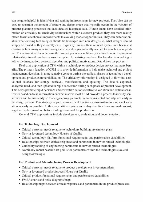
can be quite helpful in identifying and ranking improvements for new projects. They also can beused to constrain the amount of feature and design creep that typically occurs in the vacuum ofproduct planning processes that lack detailed historical data. If these teams have detailed infor-mation on criticality-to-sensitivity relationships within a current product, they can more readilymatch feasible technical improvements to evolving market opportunities. They can better ration-alize what existing technologies should be leveraged into new designs vs. what designs shouldsimply be reused as they currently exist. Typically this results in reduced cycle-times because itconstrains how many new technologies or new designs are really needed to launch a new prod-uct. The reason it works is because the product planners can literally see function vs. requirementrelationships in real numbers across the system for existing products. Far less decision making isleft to the imagination, personal agendas, and political motivations. Data drives the process.
Real-time application of CPM within a technology or product design project has many ben-efits. The primary function of CPM is to provide information to help make technical and projectmanagement decisions in a preventative context during the earliest phases of technology devel-opment and product commercialization. The criticality information is designed to flow into a re-lational database for storage, retrieval, modification, and updating. The data is captured,analyzed, used, and then updated in rapid succession during each phase of product development.This helps promote rapid decisions and corrective actions relative to variation and critical sensi-tivities based on fresh information on what matters most. CPM provides a process to identify sen-sitivities and failures early so that engineering parameters can be inspected and adjusted early inthe design process. This strategy helps to make critical functions as insensitive to sources of vari-ation as early as possible. In this way critical system and subsystem functions are made robust,together by design—long before tooling is ordered for production.
General CPM applications include development, evaluation, and documentation.
For Technology Development
• Critical customer needs relative to technology building investment plans• New or leveraged technology Houses of Quality• Critical technology platform functional requirements and performance capabilities• Relationships between critical responses and parameters in new or reused technologies• Criticality ranking of engineering parameters in new or reused technologies• Nominally robust baseline set points for parameters within the technologies (skeletal
designs/drawings)
For Product and Manufacturing Process Development
• Critical customer needs relative to product development investment plans• New or leveraged product/process Houses of Quality• Critical product functional requirements and performance capabilities• FMEA charts and noise diagrams/maps• Relationship maps between critical responses and parameters in the product/processes
260 Chapter 9

• Criticality ranking of engineering parameters in new or reused product/processes• Robust nominal and tolerance set points of all critical parameters• Design process capabilities and manufacturing process capabilities
The flow diagram in Figure 9–1 illustrates the structure of functions within Critical Para-meter Management.
The CPM flow diagram illustrates, simultaneously from left to right and top to bottom, thenature of information development and integration as a general architectural construction. Oncethe critical information structures are developed, they can be linked to define detailed criticalpaths. One can trace criticality from many perspectives or starting points up or down the productarchitecture as necessary. Not only is the CPM database capable of tracing critical paths up anddown the system architecture, it can also trace critical paths within and across subsystems. Thisdemonstrates how CPM is highly supportive of a system engineering approach to technology andproduct development. Chapter 10 will fully expand on this general model.
The horizontal and vertical critical path structures in Figure 9–1 enable the engineeringcommunity to have a global view of interactivity and sensitivity. Without this kind of multidi-mensional architecture, the engineering teams easily lose sight of what is important across im-mensely complex product functions. This is particularly true of products with hardware,electronic, and electrical functions that are controlled and sequenced through complex networksof software modules. Software engineers can preventatively structure their code when they haveaccess to critical path structures from the CPM database. This can greatly enhance coding pro-ductivity and accuracy as more and more contract software engineers are employed. It is in-evitable that contract software engineers will be constrained by their lack of experience in aparticular industry or product application. CPM provides a map for them to follow as they struc-ture their code to facilitate product functions.
System engineering groups can use CPM data to rapidly identify root causes in evaluationtests, and they can strategically induce stressful noise conditions in system robustness and toler-ance sensitivity experiments. Test planning, construction, and execution cycle-time can be greatlyreduced when clear paths of critical functions are separated from those of nominal concern.
In summary a reasonable CPM architecture must provide the following functional attributes:
• Ability to trace critical functional relationships through all levels of a technology,product, or manufacturing process
• Accessibility so these critical functional relationships can be used by managers,engineers, and technical support personnel across an entire technology developmentand product commercialization team
• Durability for reuse over many product family offerings• Flexibility so they can be used on small or large technology or product development
projects• Tunability for application across technology or product platforms
The Architecture of the Critical Parameter Management Process 261

ConstructSystem Level Houseof Quality RelatingCritical VOC Needsto Critical Technical
Requirements
Construct SubsystemLevel Houses ofQuality RelatingCritical System
Requirements toCritical Subsystem
Requirements
Construct ComponentLevel Houses ofQuality Relating
Critical SubsystemRequirements to
Critical PartRequirements
ConstructManufacturing/Assembly
Process Houses ofQuality Relating
Critical PartRequirements to
Critical Process andMaterial Requirements
Gather and IdentifyCritical Voice of theCustomer Needs
SystemRequirements
Documents
Critical Functional ResponsesIdentified During Concept Designand Optimized During SubsystemDevelopment, System Integration,
and Design Certification
Houses of Quality Generated fromCritical VOC and Technical Requirements
Using Quality Function Deployment
MeasuredSystem/Subsystem/
Part CFR Cp/CpkPerformance vs.
Final Performance
Critical Functional ParametersIdentified and Optimized During
Design and Optimize Phases(Nominal Set Points)
Critical-to-Function SpecificationsIdentified and Optimized During
Design, Optimize, and VerifyPhases
(Tolerance Set Points)
Critical Process Parameters andResponses Identified andOptimized During Design,
Optimize, and Verify Phases(Nominal/Tolerance Set Points)
System/Subsystem/Part Cp/CpkAssessment/Audit/CorrectiveAction During Steady-State
Production and Service
System Requirements toSystem CFR
Maps/Database
MeasuredSystem CFR
Cp Values
MeasuredComponent CTF
Cp Values
System CFR toSubsystem CFRMaps/Database
Subsystem CFR toSubsystem CTFMaps/Database
Component CTF toManufacturing ProcessCFR Maps/Database
MeasuredManufacturingProcess CFR
Cp Values
MeasuredSubsystem CFR
Cp Values
Convert System RequirementsDocument into Final Performance
Specifications Document
Translate CriticalVOC Needs intoCritical Technical
Requirements
SubsystemRequirements
Documents
ComponentRequirements
Documents
Manufacturing Processand Material
Requirements Documents
Figure 9–1 The Critical Parameter Management Process Flow Diagram
262

• Clarity to be understood across disciplines and organizational boundaries• Configurability for rapid conversion to new applications• Changeability for rapid addition or updating of new parameters, relationships, and data• Compatibility with the output from a broad, modern portfolio of best practices• Usability for ease of learning how to use the process, tools, and database• Capacity to fulfill the critical information management needs of a technology or
product development project
Reference
The American Heritage Dictionary of the English Language. (1975). Boston: AmericanHeritage Publishing Co. & Houghton Mifflin Co.
The Architecture of the Critical Parameter Management Process 263

This page intentionally left blank

C H A P T E R 1 0
The Process of CriticalParameter Management in Product Development
The steps of Critical Parameter Management can be mapped to a technology development orproduct commercialization process. CPM is laid out so it can account for any developing sys-
tem of many-to-many critical parametric relationships. It helps structure a “designed” flow oftools and metrics on a phase-by-phase basis to manage risk. This fact alone requires CPM to bea process. At a more detailed level, CPM helps organize the specific tasks that reside within eachdevelopment team’s project management plan (PERT chart). The more you know about con-structing project management plans within a technology development or product commercializa-tion process, the more you can apply CPM toward your Six Sigma performance goals. Mostimportantly, CPM measures the results of the Technology Development and Design For SixSigma tools that define and optimize the capability growth of all the critical functional responsesin the system.
Critical Parameter Management establishes, tracks, and manages risk based upon the fun-damental balancing model depicted in Figure 10–1.
Let’s look at the big picture of how CPM relates to the general phases and gates processesfor technology development and product commercialization. Recall that a general flow of phases
265
What is Measured?:Customer LevelSystem Level
Subsystem LevelSubassembly LevelComponent Level
Manufacturing Process Level
What is Required?:Customer LevelSystem Level
Subsystem LevelSubassembly LevelComponent Level
Manufacturing Process Level
How well do thesematch?
Figure 10–1 CPM Balancing Model

and gates for a complete product development process should look something like the diagram inFigure 10–2.
In Figure 10–3, we see a simplified, graphical model of the critical parameter flow-downthat is structured across the phases of the I2DOV or CDOV Development Processes.
Critical Parameter Management can work in the context of a technology developmentprocess just as easily as it can work within the context of a product commercialization process.Many companies fail to recognize that this kind of discipline is applicable to R&D organizations,their work processes, and best practices. R&D organizations have traditionally been slow to adoptstructured processes like CPM, often insisting that their world is one of free-flowing thought andtasks not amenable to such structure and discipline. One only need look at the number of failedcommercialization projects due to the effects from underdeveloped, uncertified technology.These immature technologies typically create insurmountable functional problems during a prod-uct commercialization program.
Relative to what CPM does and when it does it, there is not much difference between tech-nology building and commercialization cultures and processes. Both require gathering and trans-lation of customer needs into technical specifications. Both require a clear set of system,subsystem, subassembly, component, and manufacturing process level requirements. Both needto assess sensitivities of concept models and prototypes to sources of variation that affect the ro-bustness of their performance. Each must verify that the technology or design is safe to move for-ward into the commercialization or production process. CPM has the capacity to rally everyoneon the development or design team around a focused set of critical requirements and their fulfill-ing critical functional parameters and responses. These metrics help assure the tasks of technol-ogy or design development, optimization, and verification progress on a predictable schedule.
In the context of cycle-time, we like to say these Design For Six Sigma processes take theright time to conduct—not necessarily the shortest. Usually when you have the shortest cycle-
266 Chapter 10
I2
Phase1
DPhase
2
OPhase
3
VPhase
4
Technology Development
TechnologyTransfer Design
Transfer
MAICProcess
ProductionOperations
CPhase
1
DPhase
2
OPhase
3
VPhase
4
Flow of Critical Parameter Management Steps
Product Commercialization
Figure 10–2 Product Development Flow

time, you also have the maximum amount of shortcuts that actually represent the underutilizationof the tools that help prevent design problems. The right cycle-time co-opts seemingly endlessbuild-test-fix cycles that are characteristically associated with late product launches.
In a Six Sigma context, the Critical Parameter Management model relates requirements tomeasured performance using capability indices. The common symbols for capability are Cp andCpk. Requirements are expressed in terms of upper and lower specification limits. Measured per-formance is documented in terms of means and standard deviations. Figure 10–4 depicts a CPMmodel in the Six Sigma context.
Product functional performance capability and manufacturing process capability can be related and tracked across technology development and product design using the model in Figure 10–4.
The Process of Critical Parameter Management in Product Development 267
SystemRequirements
and CFRs
Subsystem/SubassemblyRequirements
and CFRs
ComponentRequirements
and CTFs
ManufacturingRequirements
and CFRs/CTFs
Figure 10–3 Critical Parameter Flow-Down Across CDOV or I2DOV Phases

Definitions of Terms for Critical Parameter Management
Six basic terms are used to define the elements of Critical Parameter Management:
1. Critical customer needs2. Critical technical requirements3. Critical functional responses4. Critical adjustment parameters5. Critical functional parameters6. Critical-to-function specifications
Critical implies that whatever is being measured and tracked is essential to fulfilling thehighest priority needs that a majority of customers have expressed.
Functional conveys that a functional variable is being measured and tracked as opposed tosome quality attribute. If the parameter is not directly measurable in units of some form of massor energy, you are not conducting true CPM. When you think of the word function, think of phys-ical performance.
Parameters can be represented as a flow-down of terms that are stored in a relational data-base, linked to one another, and evaluated in mathematical and empirical models referred to asideal/transfer functions.
CPM elements flow down the system hierarchy as displayed in Figure 10–5.The vocabulary of the flow-down of critical parameters is explained as follows.
System level critical functional responses (CFR): A continuous variable, typically eitheran engineering scalar or vector, that is a measure of a critical output from the system. Sys-tem CFRs are directly sensed by the customer and can be directly compared to the new,unique, or difficult customer needs.
System level critical adjustment parameters (CAP): A continuous variable, typically ei-ther an engineering scalar or vector, that is specifically designed to adjust a system CFR.
268 Chapter 10
What is Measured?:System CFRs (Average and σ)
Subsystem CFRs (Average and σ)Subassembly CFRs (Average and σ)Component CTFs (Average and σ)
Manufacturing Process CTFs (Average and σ)
What is Required?:Customer Needs (USL-LSL)
System Requirements (USL-LSL)Subsystem Requirements (USL-LSL)
Subassembly Requirements (USL-LSL)Component Requirements (USL-LSL)
Manufacturing Process Requirements (USL-LSL)
Cp = (USL-LSL)/6σ
Cpku = (USL-Average)/3σCpkl = (Average-LSL)/3σ
Figure 10–4 CPM Model in a Six Sigma Context

These variables are few in number and are often used by customers to adjust the mean out-put performance of the product.
Subsystem level critical functional responses (CFR): A continuous variable, typically ei-ther an engineering scalar or vector, that is a measure of a critical output from a subsystem.Subsystem CFRs are usually not directly sensed by the customer. When one or more sub-system CFRs are used as inputs to a system CFR, the name is changed to Subsystem criti-cal functional parameter (CFP). Subsystem CFRs are measured and documented for theircapability to support system CFR capability.
Subsystem level critical adjustment parameters (CAP): A continuous variable, typicallyeither an engineering scalar or vector, that is specifically designed to adjust a subsystemCFR. These variables are few in number and are sometimes available for customers to ad-just but more often are used by assembly and service organizations.
Subassembly level critical functional responses (CFR): A continuous variable, typicallyeither an engineering scalar or vector, that is a measure of a critical output from a sub-assembly. Subassembly CFRs are usually not directly sensed by the customer. When one ormore subassembly CFRs are used as inputs to a subsystem CFR, the name is changed tosubassembly critical functional parameter (CFP). Subassembly CFRs are measured anddocumented for their capability to support subsystem CFR capability.
Subassembly level critical adjustment parameters (CAP): A continuous variable, typi-cally either an engineering scalar or vector, that is specifically designed to adjust a sub-assembly CFR. These variables are also few in number and are often used by assembly andservice organizations.
Component level critical-to-function specification (CTF spec): A continuous variable,typically an engineering scalar, that is a measure of a critical component dimension or feature. It may also be a characteristic relating to a surface or bulk property of a componentor material. These CTF specifications are commonly communicated to the Supply Chain
The Process of Critical Parameter Management in Product Development 269
REQUIREMENTS
NEEDS
RESPONSES
PARAMETERS
SPECIFICATIONS
Figure 10–5 CPM Flow-Down

using “spec sheets,” CAD files, and component quality plans. They are usually measuredunder some form of variable data statistical process control as they are manufactured. Com-ponent CTF specs are designed, measured, and documented for their capability to supportsubassembly and subsystem CFR capability. This is the point where manufacturing processcapability interfaces with and transitions into product or design level performance capabil-ity. Variation in the components affect the variation in the design functions.
Manufacturing process level critical-to-function specification (CTF spec): A contin-uous variable, typically an engineering scalar or vector, that is a measure of a criticalmanufacturing process set point. These variables are literally measured on a manufactur-ing process as it produces a component or material. One major use of manufacturingprocess capability is the measurement, control, and application of these CTF variables tofulfill component requirements. The manufacturing process capability index can also beused in reference to assembly processes as well. Manufacturing process requirements(USL-LSL) establish what is required of these variables. Manufacturing CTF specs aremeasured during production to ensure that what is required of the process is being pro-vided. A manufacturing process requirement may be a pressure that is required to be at25 psi / 1 psi. The measured manufacturing process CFT spec pressure might bemeasured at 24.3 psi in the morning and 25.1 in the afternoon. The CFT spec can be com-pared to the requirement and action taken if the manufacturing process has a control prob-lem. The components are known to vary as the process pressure varies. CPM in aproduction context measures the in-process capability of the pressure. If the pressure andall other CTF specs are on target with low variability relative to the process requirements,the components need only limited measurement during production. During product de-velopment, manufacturing CTF specs are measured to document their capability to sup-port component capability.
Critical Parameter Management helps develop three specific analytical models as it seeksto quantify nominal performance in Phase 2 (ideal/transfer functions), robust performance (addi-tive models) in Phase 3, and capable performance (variance models) in Phase 4:
The Ideal/Transfer Function: Y f(xA, xB,. . . xN)
Developed in Phase 2 in I2DOV and CDOV
The Additive Model: S/nopt. S/navg. [S/nA opt. - S/navg.] . . . [S/nN opt. - S/navg.]
Developed in Phase 3 in I2DOV and 3a in CDOV
The Variance Model: 2total 2
A 2B . . . 2
N
Developed in Phase 4 in I2DOV and Phases 2, 3b, and 4a in CDOV
Without a flow-down of critical parameter relationships underwritten by each of these threemodels, you really don’t have control of your program and the data to credibly manage it in a SixSigma context.
270 Chapter 10
Critical Parameter Management in Technology Development and ProductDesign: Phase 1
The Critical Parameter Management process can be mapped against both a technology develop-ment process model (I2DOV) and a product design process model (CDOV) using the block dia-gram structures, CPM flow-down models, and scorecards offered in this chapter. The intent ofthis chapter is to provide guidance on the construction of a critical parameter database. Becausethe I2DOV and the CDOV processes both contain four phases and are focused on using relativelysimilar Six Sigma tools and best practices, we will present one CPM process that can be adaptedto either process. Figure 10–6 charts the Phase 1 process steps for system development.
The example flow-down of VOC needs shown in Figure 10–7 illustrates the highest layerin the hierarchy of critical parameters. The voice of the customer is gathered and then processedusing KJ methods. The processing includes:
1. Grouping of specific customer need statements into need categories.2. Identification and segregation of the specific VOC needs into two types:
a. Critical Needs (*): needs that are new, unique, or difficultb. Important Needs: needs that are old, common, or easy
Need categories align specific needs that are similar in nature into general categories. Needtypes separate needs into those that are termed critical and all others that are viewed as nominallyimportant. A few needs are critical, but all needs are important. CPM tracks the critical needs,technical requirements, and the design and manufacturing parameters that fulfill them. All needsmust be fulfilled to the extent that is economically feasible. Only the critical needs will be docu-mented in the critical parameter database. They will be the needs that flow into the Houses ofQuality. Only the needs that are new, unique, or difficult are worth the added expense of pro-cessing through QFD. A common mistake product development teams make is putting needs thatare old, common, or easy through QFD. There is little or no reason to do this. These needs shouldbe directly translated into technical requirements and placed into the appropriate requirementsdocument. Critical needs go through the Critical Parameter Management process, which includesa trip through the Houses of Quality (Figure 10–8). Everything else is handled through the nor-mal process of requirement documentation and certification.
The system House of Quality illustrates the linkage between the NUD VOC needs and thetranslated critical technical requirements. Notice, from the HOQ matrix in Figure 10–8, that nu-merous critical technical requirements can align with and help fulfill more than one NUD VOCneed. This is one reason why the critical parameter database needs to be set up as a relational data-base. Depending on the size of the platform or system being developed, numerous many-to-manyrelationships may need to be linked within and down through the various layers of the design’sarchitecture. This will be the case for all the lower level Houses of Quality to come.
Phase 1 delivers the first and upper-most layer of critical platform or system requirementsand their fulfilling critical functional response metrics. After Phase 1, the Critical Parameter Man-agement database will contain the general structure depicted in Figure 10–9.
The Process of Critical Parameter Management in Product Development 271

Gather and forecast customerneeds and technology/producttrends.
System DevelopmentProcess Steps
System Critical ParameterManagement Process Steps
Isolate critical customer needs that reside within thegeneral voice of the customer data and forecasted trendsin technology and competitive products.
Critical customer needs are derived from the prioritizedcategories of the voice of the customer data using theKJ method.
The critical customer needs are restated in the vocabularyof the technology or product development community andfurther ranked for importance. They are initially documentedusing the system House of Quality (using the QFD method).
Critical technology or product requirements are documentedin a relational CPM database (ACCESS/DOORS/Sigma SixCockpit). It contains an integrated structure of criticaltechnology or product requirements at the system orplatform level.
Define categories of the needsand establish them in a rankedorder of importance.
Create a platform or systemlevel technology or productrequirements documentfrom the list of technologyor product requirements.
System level critical functional responses are developedand added to CPM database. CFRs are mapped to thetechnology requirements as measurable, continuousvariables. The measured means and standard deviationsfrom these system level CFRs will be used to define thesystem level technology or product capability indices:Cpsys tech and Cpksys tech.
Platform or system level critical adjustment parameters aredeveloped and modeled to assure they have a stable andlinear relationship to the platform or system CFRs. Thisassures the technology or product is tunable.
The CAPs are linked to their CFRs in the CPM database.
Generate instrumentation and data acquisition systemarchitectures that provide a clear measurement capacityand capability for the critical functional responses for eachplatform or system concept."If you can't measure it, you can't optimize it!"
Generate numerous platformor system level technology orproduct concepts(architectures) that fulfill thesystem level functions.
Identify and characterize aset of measurable platformor system level functions thatfulfill the technology orproduct requirement.
Translate the customer needsinto system level requirements.
Gate 1: Platform or System Level Technology Invention/Innovation orProduct Concept Development
Figure 10–6 Phase 1: Platform or System Level Technology Invention/Innovation or ProductConcept Development
272

VOC NeedCategory #1
*SpecificVOC Need #1
SpecificVOC Need #2
SpecificVOC Need #n
VOC NeedCategory #2
*SpecificVOC Need #1
*SpecificVOC Need #2
SpecificVOC Need #n
VOC NeedCategory #3
SpecificVOC Need #1
*SpecificVOC Need #2
SpecificVOC Need #n
VOC NeedCategory #4
*SpecificVOC Need #1
SpecificVOC Need #2
SpecificVOC Need #n
Figure 10–7 Example of the Flow-Down of Customer Need Categorization and TypingNote: The (*) symbol indicates a need that is critical because it is new, unique, or difficult (also referred to asa NUD VOC Need).
NUD VOC Need #1
NUD VOC Need #2
NUD VOC Need #3
NUD VOC Need #n
Critical Platform or System Requirements 1-n
Figure 10–8 NUD VOC Needs-to-Platform or System Requirements HOQ
273

A more detailed view of a portion of the high-level flow-down of customer needs to systemrequirements and their measured CFRs would look like the diagram in Figure 10–10.
These parameters are documented in a relational database such as DOORS, ACCESS, orthe Six Sigma Cockpit. The development team uses this relational database to continue theprocess of building a hierarchy of critical parameter relationships between the flow-down ofneeds, requirements, critical functional requirements, critical adjustment parameters, criticalfunctional parameters, and critical-to-function specifications.
Critical Parameter Management Scorecard for System Level Performance in Phase 1
The system level CPM scorecard is typically documented as an Excel spreadsheet with the fol-lowing information placed in its columns.
Desired Performance Based on VOC and VOT
System requirement
System requirement ID number
274 Chapter 10
NUD VOC Need #1
System Requirements
Y=System CFR
System Requirements
Y=System CFR
System Requirements
Y=System CFR
NUD VOC Need #2
Figure 10–10 Flow-Down of Customer Needs to System Requirements
One-to-One, One-to-Many, and Many-to-Many Relationships
Platform or System Level: Requirements and Critical Functional Responses
Highest Level: Ranked, Detailed NUD Customer Needs
Figure 10–9 Structure of CPM Database After Phase 1

System CFR name
System CFR target
System CFR tolerances
Actual Measured Performance
Measured system CFR mean
Measured system CFR standard deviation
Measured system CFR S/N ratio
Measured system CFR CP
Measured system CFR Cpk
These items are also stored in the CPM relational database along with the related transferfunctions that link inputs from the subordinate subsystems, subassemblies, components, andmanufacturing processes that drive the measured system CFR outputs.
Since this material is just documenting what information is actually available during Phase 1, no system level measured data available is yet available. In fact, the system CFRs won’t be measured until Phases 3 and 4 during the integration evaluations. The only system in-formation available at this point is the system requirements information, as noted in the scorecardin Figure 10–11.
The Process of Critical Parameter Management in Product Development 275
Sys. Sys.Sys. Sys. Sys. Sys. Sys. CFR CFR Sys. Sys.
Sys. Reqt. CFR CFR CFR CFR Std. S/N CFR CFRReqts. # Name Target Tol. Mean Dev. Ratio Cp Cpk
Figure 10–11 Example System Level CPM Scorecard
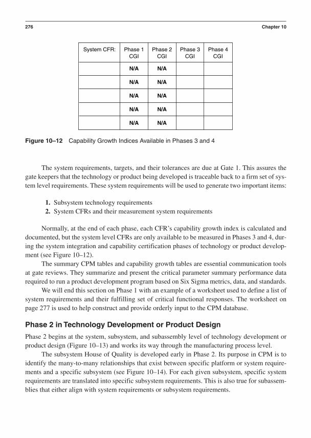
The system requirements, targets, and their tolerances are due at Gate 1. This assures thegate keepers that the technology or product being developed is traceable back to a firm set of sys-tem level requirements. These system requirements will be used to generate two important items:
1. Subsystem technology requirements2. System CFRs and their measurement system requirements
Normally, at the end of each phase, each CFR’s capability growth index is calculated anddocumented, but the system level CFRs are only available to be measured in Phases 3 and 4, dur-ing the system integration and capability certification phases of technology or product develop-ment (see Figure 10–12).
The summary CPM tables and capability growth tables are essential communication toolsat gate reviews. They summarize and present the critical parameter summary performance datarequired to run a product development program based on Six Sigma metrics, data, and standards.
We will end this section on Phase 1 with an example of a worksheet used to define a list ofsystem requirements and their fulfilling set of critical functional responses. The worksheet onpage 277 is used to help construct and provide orderly input to the CPM database.
Phase 2 in Technology Development or Product Design
Phase 2 begins at the system, subsystem, and subassembly level of technology development orproduct design (Figure 10–13) and works its way through the manufacturing process level.
The subsystem House of Quality is developed early in Phase 2. Its purpose in CPM is toidentify the many-to-many relationships that exist between specific platform or system require-ments and a specific subsystem (see Figure 10–14). For each given subsystem, specific systemrequirements are translated into specific subsystem requirements. This is also true for subassem-blies that either align with system requirements or subsystem requirements.
276 Chapter 10
System CFR: Phase 1 Phase 2 Phase 3 Phase 4CGI CGI CGI CGI
N/A N/A
N/A N/A
N/A N/A
N/A N/A
N/A N/A
Figure 10–12 Capability Growth Indices Available in Phases 3 and 4

Worksheet for Defining System Level Critical Parameters
List all system level critical requirements and the system level critical functionalresponses that fulfill each requirement:
Product/System Name: __________________________________________________
System Level Critical Requirements: System Level Critical Functional(Name and estimated nominal set point, Responses: (Name, measurement and tolerance limits) method, and units of measure)
277

Define rationalized categoriesof platform or systemrequirements and insert theminto the appropriatesubsystem/subassemblyHouses of Quality.
Subsystem/SubassemblyDevelopment/Design Process
Subsystem/Subassembly CriticalParameter Management Process
Critical platform or system requirements are linked tocritical subsystem/subassembly requirements.
Critical subsystem/subassembly requirements are derivedfrom the prioritized categories of system requirementsusing the KJ method.
For the Subsystem/Subassembly HOQs, definesubsystem/subassemblyrequirements that fulfill theincoming systemrequirements.
Subsystem/subassembly level critical functional responsesare developed and added to the CPM database. CFRs aremapped to the subsystem/subassembly requirements asmeasurable, continuous variables. The measured meansand standard deviations of these subsystem/subassemblylevel CFRs will be used to define the subsystem/subassemblylevel design capability indices: Cp and Cpk.
Subsystem/subassembly level critical adjustmentparameters are developed and modeled to assure theyhave a stable and linear relationship to thesubsystem/subassembly CFRs. This assures the technologyor design is tunable.
Generate instrumentation and data acquisition systemarchitectures that provide a clear measurement capacityand capability for the subsystem/subassembly level criticalfunctional responses for each subsystem/subassemblyconcept."If you can't measure it, you can't optimize it!"
The critical subsystem/subassembly requirements areranked relative to how well they fulfill system levelrequirements using the subsystem House of Quality (QFD).
Generate numeroussubsystem/subassemblylevel design concepts(architectures) that fulfill thesubsystem/subassemblylevel functions.
Create a subsystem/subassembly levelrequirements document fromthe list of subsystem/subassembly requirements.
Phase 2: System/Subsystem/Subassembly Level TechnologyDevelopment or Product Design
Critical subsystem/subassembly requirements aredocumented in the relational CPM database (ACCESS/DOORS/Six Sigma Cockpit). It now contains an integratedstructure of critical system-subsystem-subassemblyrequirements and CFR relationships.
Identify and characterize aset of measurable subsystem/subassembly level functionsthat fulfill subsystemrequirements.
Figure 10–13 Charting Initial Phase 2 Process Steps
278
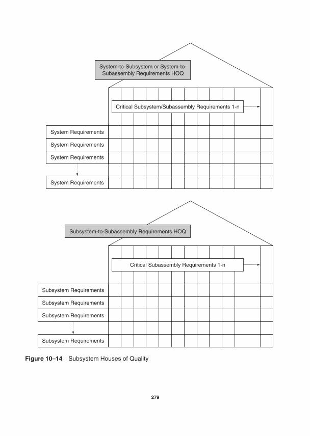
System Requirements
System-to-Subsystem or System-to-Subassembly Requirements HOQ
System Requirements
System Requirements
System Requirements
Critical Subsystem/Subassembly Requirements 1-n
Subsystem Requirements
Subsystem-to-Subassembly Requirements HOQ
Subsystem Requirements
Subsystem Requirements
Subsystem Requirements
Critical Subassembly Requirements 1-n
Figure 10–14 Subsystem Houses of Quality
279

At this point in Phase 2 the Critical Parameter Management database now contains thestructure depicted in Figure 10–15.
A detailed view of a portion of the high to middle level flow-down to subsystem require-ments and their input critical functional parameters to the system CFRs looks like the diagram inFigure 10–16.
Each system level CFR is a (Y) variable controlled by the inputs from several subsystemcritical functional parameters (x variables). The system level CFRs can have their mean outputvalue adjusted by subsystem level critical adjustment parameters. A common example of such aparameter is the steering wheel on your car. CAPs that adjust system level performance are oftenaccessible to the end user of the system. The subsystem CFPs and CAPs are the outputs from thetransformations of mass, energy, and information from within the subsystems. An output from asubsystem is an input to the system! This is an excellent illustration of how every subsystem hasa measurable and controllable output variable that can be referred to as a critical functional re-sponse with respect to the inputs to the subsystem. But as the subsystem, in turn, functions as aninput to the system, its output is now referred to as a critical functional parameter. It now flowsenergy, mass, and information into the system along with other subsystems to enable specific sys-tem level CFR performance. This subsystem-to-system input-output relationship is quantified bya term called a transfer function. Transfer functions are set up as equations and are expressed inY f(x) terms. Transfer functions are either developed from analytical engineering models or by
280 Chapter 10
One-to-One, One-to-Many, and Many-to-Many Relationships
Platform or System Level: Requirements and Critical Functional Responses
Highest Level: Ranked, Detailed NUD Customer Needs
One-to-One, One-to-Many, and Many-to-Many Relationships
Subsystem Level: Requirements and Critical Functional Responses
One-to-One, One-to-Many, and Many-to-Many Relationships
Subassembly Level: Requirements and Critical Functional Responses
Figure 10–15 Structure of CPM Database at Phase 2
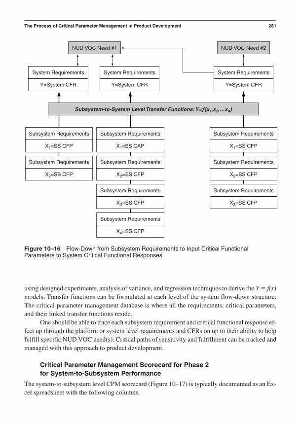
using designed experiments, analysis of variance, and regression techniques to derive the Y f(x)models. Transfer functions can be formulated at each level of the system flow-down structure.The critical parameter management database is where all the requirements, critical parameters,and their linked transfer functions reside.
One should be able to trace each subsystem requirement and critical functional response ef-fect up through the platform or system level requirements and CFRs on up to their ability to helpfulfill specific NUD VOC need(s). Critical paths of sensitivity and fulfillment can be tracked andmanaged with this approach to product development.
Critical Parameter Management Scorecard for Phase 2 for System-to-Subsystem Performance
The system-to-subsystem level CPM scorecard (Figure 10–17) is typically documented as an Ex-cel spreadsheet with the following columns.
The Process of Critical Parameter Management in Product Development 281
System Requirements
Y=System CFR
System Requirements
Y=System CFR
Subsystem Requirements
X1=SS CFP X1=SS CAP
Subsystem Requirements
Subsystem Requirements
X2=SS CFP X2=SS CFP
Subsystem Requirements
X3=SS CFP
Subsystem Requirements
X1=SS CFP
Subsystem Requirements
X2=SS CFP
Subsystem Requirements
X3=SS CFP
Subsystem Requirements
X4=SS CFP
Subsystem Requirements
Subsystem-to-System Level Transfer Functions: Y=ƒ(x1,x2,…xn)
System Requirements
Y=System CFR
NUD VOC Need #1 NUD VOC Need #2
Figure 10–16 Flow-Down from Subsystem Requirements to Input Critical FunctionalParameters to System Critical Functional Responses

Desired Performance Based on VOC and VOT
System requirement ID number
Subsystem requirement
Subsystem requirement ID number
Subsystem CFR name
Subsystem CFR target
Subsystem CFR tolerances
Actual Measured Performance
Measured subsystem CFR mean
Measured subsystem CFR standard deviation
Measured subsystem CFR S/N ratio
Measured subsystem CFR Cp
Measured subsystem CFR Cpk
Measured subsystem CFR sensitivity coefficient dY/dx
These items are also stored in the CPM relational database along with the related transferfunctions that link inputs from subsystems, subassemblies, components, and manufacturingprocesses that drive the measured system CFR outputs.
At the end of Phase 2, each subsystem level CFR’s baseline capability growth index is cal-culated and documented in a table like the one in Figure 10–18.
282 Chapter 10
Subsys. Subsys. Subsys.Sys. Subsys. Subsys. Subsys. Subsys. Subsys. CFR CFR Subsys. Subsys. SensitivityReqt. Reqt. Subsys. CFR CFR CFR CFR Std. S/N CFR CFR Coefficient
# # Reqts. Name Target Tol. Mean Dev. Ratio Cp Cpk dY/dx
Figure 10–17 Sample System-to-Subsystem Level CPM Scorecard
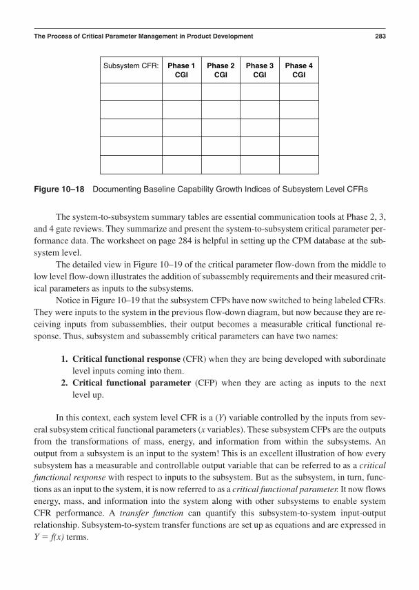
The system-to-subsystem summary tables are essential communication tools at Phase 2, 3,and 4 gate reviews. They summarize and present the system-to-subsystem critical parameter per-formance data. The worksheet on page 284 is helpful in setting up the CPM database at the sub-system level.
The detailed view in Figure 10–19 of the critical parameter flow-down from the middle tolow level flow-down illustrates the addition of subassembly requirements and their measured crit-ical parameters as inputs to the subsystems.
Notice in Figure 10–19 that the subsystem CFPs have now switched to being labeled CFRs.They were inputs to the system in the previous flow-down diagram, but now because they are re-ceiving inputs from subassemblies, their output becomes a measurable critical functional re-sponse. Thus, subsystem and subassembly critical parameters can have two names:
1. Critical functional response (CFR) when they are being developed with subordinatelevel inputs coming into them.
2. Critical functional parameter (CFP) when they are acting as inputs to the next level up.
In this context, each system level CFR is a (Y) variable controlled by the inputs from sev-eral subsystem critical functional parameters (x variables). These subsystem CFPs are the outputsfrom the transformations of mass, energy, and information from within the subsystems. An output from a subsystem is an input to the system! This is an excellent illustration of how everysubsystem has a measurable and controllable output variable that can be referred to as a criticalfunctional response with respect to inputs to the subsystem. But as the subsystem, in turn, func-tions as an input to the system, it is now referred to as a critical functional parameter. It now flowsenergy, mass, and information into the system along with other subsystems to enable system CFR performance. A transfer function can quantify this subsystem-to-system input-output relationship. Subsystem-to-system transfer functions are set up as equations and are expressed inY f(x) terms.
The Process of Critical Parameter Management in Product Development 283
Subsystem CFR: Phase 1 Phase 2 Phase 3 Phase 4CGI CGI CGI CGI
Figure 10–18 Documenting Baseline Capability Growth Indices of Subsystem Level CFRs

Worksheet for Defining Subsystem Level Critical Parameters
List all subsystem level critical requirements and the subsystem level critical functionalresponses that fulfill each requirement:
Associates System CFR
Name: _______________________________________________________________
Subsystem Level Critical Requirements: Subsystem Level Critical Functional(Name, and estimated nominal set point, Responses: (Name, measurement and tolerance limits) method, and units of measure)
284

One should be able to trace each subsystem requirement and critical functional response ef-fect up through to the platform or system level requirements and CFRs—on up to their ability tohelp fulfill specific NUD VOC need(s). Critical paths of sensitivity and requirement fulfillmentcan be tracked and managed with this approach.
The Process of Critical Parameter Management in Product Development 285
NUD VOC Need #1
System Requirements
Y=System CFR
System Requirements
Y=System CFR
Subsystem Requirements
Y1=SS CFR Y1=SS CFR
Subsystem Requirements
Subsystem Requirements
Y2=SS CFR Y2=SS CFR
Subsystem Requirements
Y3=SS CFR
Subsystem Requirements
Y1=SS CFR
Subsystem Requirements
Y2=SS CFR
Subsystem Requirements
Y3=SS CFR
Subsystem Requirements
Subsystem-to-System Level Transfer Functions: Y=ƒ(x1,x2,…xn)
SubassemblyRequirements
X1=SAssy CFP X1=SAssy CFP
SubassemblyRequirements
SubassemblyRequirements
X2=SAssy CFP
X1=SAssy CFP
SubassemblyRequirements
Subassembly-to-Subsystem Level Transfer Functions: Y=ƒ(x1,x2,…xn)
System Requirements
Y=System CFR
NUD VOC Need #2
Figure 10–19 Critical Parameter Flow-Down from the Middle to Low Level
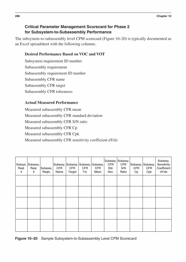
Critical Parameter Management Scorecard for Phase 2for Subsystem-to-Subassembly Performance
The subsystem-to-subassembly level CPM scorecard (Figure 10–20) is typically documented asan Excel spreadsheet with the following columns.
Desired Performance Based on VOC and VOT
Subsystem requirement ID number
Subassembly requirement
Subassembly requirement ID number
Subassembly CFR name
Subassembly CFR target
Subassembly CFR tolerances
Actual Measured Performance
Measured subassembly CFR mean
Measured subassembly CFR standard deviation
Measured subassembly CFR S/N ratio
Measured subassembly CFR Cp
Measured subassembly CFR Cpk
Measured subassembly CFR sensitivity coefficient dY/dx
286 Chapter 10
Subassy. Subassy. Subassy.Subsys. Subassy. Subassy. Subassy. Subassy. Subassy. CFR CFR Subassy. Subassy. Sensitivity
Reqt. Reqt. Subassy. CFR CFR CFR CFR Std. S/N CFR CFR Coefficient# # Reqts. Name Target Tol. Mean Dev. Ratio Cp Cpk dY/dx
Figure 10–20 Sample Subsystem-to-Subassembly Level CPM Scorecard

The Process of Critical Parameter Management in Product Development 287
These items are also stored in the CPM relational database along with the related transferfunctions that link inputs from subsystems, subassemblies, components, and manufacturingprocesses that drive the measured system CFR outputs.
At the end of Phase 2, each subassembly level CFR’s capability growth index is calculatedand documented, as in Figure 10–21.
The two summary tables in Figures 10–20 and 10–21 are essential communication tools atPhase 2, 3 and 4 gate reviews. They summarize and present the subsystem-to-subassembly criti-cal parameter performance data. The worksheet on page 288 is helpful in setting up the CPM data-base at the subassembly level.
The component Houses of Quality (Figure 10–23) are structured to establish relationshipsbetween critical subsystem and subassembly requirements and the newly defined component requirements.
Figure 10–24 offers an example of the structure for a House of Quality that links incomingcritical subassembly requirements to critical component requirements.
At this point in Phase 2 the Critical Parameter Management database now contains thestructure depicted in Figure 10–25.
Critical Parameter Management Scorecard for Phase 2for Subsystem-to-Component Performance
The subsystem-to-component level CPM scorecard (Figure 10–26) is typically documented as anExcel spreadsheet with the following columns. The process for components CPM is illustrated inFigure 10–22.
Desired Performance Based on VOC and VOT
Subsystem requirement ID number
Component requirement
Component requirement ID number
Subassembly CFR: Phase 1 Phase 2 Phase 3 Phase 4CGI CGI CGI CGI
Figure 10–21 Documenting Capability Growth Indices for Subassembly Level CFRs

Worksheet for Defining Subassembly Level Critical Parameters
List all subassembly level critical requirements and the subassembly level criticalfunctional responses that fulfill each requirement:
Associates Subsystem & CFR
Name: _______________________________________________________________
Subassembly Level Critical Requirements: Subassembly Level Critical Functional(Name, and estimated nominal set point, Responses: (Name, measurement and tolerance limits) method, and units of measure)
288

Component CTF name
Component CTF target
Component CTF tolerances
Actual Measured Performance
Measured component CTF mean
Measured component CTF standard deviation
Measured component CTF Cp
The Process of Critical Parameter Management in Product Development 289
Define rationalized categoriesof subsystem/subassemblyrequirements and insert theminto the appropriatecomponent Houses ofQuality.
Component Development/Design Process Steps
Component Critical ParameterManagement Process Steps
Critical subsystem/subassembly requirements are linked tocritical component requirements.
Critical component requirements are derived from theprioritized categories of subsystem/subassemblyrequirements using the KJ method.
For the Component HOQ,define componentrequirements that fulfill theincoming subsystem/subassembly requirements.
Component level critical-to-function specifications aredeveloped and added to CPM database. CTF specs aremapped to the component requirements as measurable,continuous variables. The measured means and standarddeviations of these component level CTF specs will beused to define the component level design capabilityindices: Cpcomp and Cpkcomp.
Generate instrumentation and data acquisition systemarchitectures that provide a clear measurement capacityand capability for the component level critical-to-functionspecs for each component concept."If you can't measure it, you can't optimize it!"
The critical component requirements are ranked relative tohow well they fulfill subsystem/subassembly levelrequirements using the component House of Quality (QFD).
Generate numerouscomponent level designconcepts (architectures) thatfulfill the component levelspecifications
Create a component levelrequirements document fromthe list of componentrequirements.
Critical component requirements are documented in therelational CPM database (ACCESS/DOORS/Six SigmaCockpit). It now contains an integrated structure of criticalsubsystem component and subassembly componentrequirements and CFR relationships.
Identify and characterize aset of measurable componentlevel specifications that fulfillcomponent requirements.
Figure 10–22 The Phase 2 Critical Parameter Management Steps for ComponentDevelopment or Design
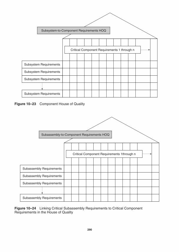
Subsystem Requirements
Subsystem-to-Component Requirements HOQ
Subsystem Requirements
Subsystem Requirements
Subsystem Requirements
Critical Component Requirements 1 through n
Figure 10–23 Component House of Quality
Subassembly Requirements
Subassembly-to-Component Requirements HOQ
Subassembly Requirements
Subassembly Requirements
Subassembly Requirements
Critical Component Requirements 1through n
Figure 10–24 Linking Critical Subassembly Requirements to Critical ComponentRequirements in the House of Quality
290

Measured component CTF Cpk
Measured component CTF sensitivity coefficient dY/dx
These items are also stored in the CPM relational database along with the related transferfunctions that link inputs from subsystems, subassemblies, components, and manufacturingprocesses that drive the measured system CFR outputs.
At the end of Phase 2, each component level CTF’s capability growth index is calculatedand documented as in Figure 10–27.
The two summary tables in Figures 10–26 and 10–27 are essential communication tools atPhase 2, 3, and 4 gate reviews. They summarize and present the subsystem-to-component criti-cal parameter performance. The worksheet on page 293 is helpful in setting up the CPM databaseat the subsystem-to-component level.
The Process of Critical Parameter Management in Product Development 291
One-to-One, One-to-Many, and Many-to-Many Relationships
Platform or System Level: Requirements and Critical Functional Responses
Highest Level: Ranked, Detailed NUD Customer Needs
One-to-One, One-to-Many, and Many-to-Many Relationships
Subsystem Level: Requirements and Critical Functional Responses
One-to-One, One-to-Many, and Many-to-Many Relationships
Subassembly Level: Requirements and Critical Functional Responses
One-to-One, One-to-Many, and Many-to-Many Relationships
Component Level: Requirements and Critical Functional Responses
Figure 10–25 Adding Component Level Requirements and CFRs to the CPM Database

Going on down to the next layer of inputs, we add the component requirements and theirmeasurable critical-to-function specifications, as they relate to the subassemblies, to our growingillustration in Figure 10–28.
Critical Parameter Management Scorecard for Phase 2 of TechnologyDevelopment for Subassembly-to-Component Performance
The subassembly-to-component level CPM scorecard (Figure 10–29) is typically documented asan Excel spreadsheet.
292 Chapter 10
Comp.Subsys. Comp. Comp. Comp. Comp. Comp. CTF Comp. Comp. Comp.
Reqt. Reqt. Comp. CTF CTF CTF CTF Std. CTF CTF CTF# # Reqts. Name Target Tol. Mean Dev. Cp Cpk dy/dx
Figure 10–26 Sample Subsystem-to-Component Level CPM Scorecard
Subsystem Related Component CTF Specification: Phase 1 Phase 2 Phase 3 Phase 4CGI CGI CGI CGI
Figure 10–27 Documenting Capability Growth Indices for Subsystem Component CTFSpecifications
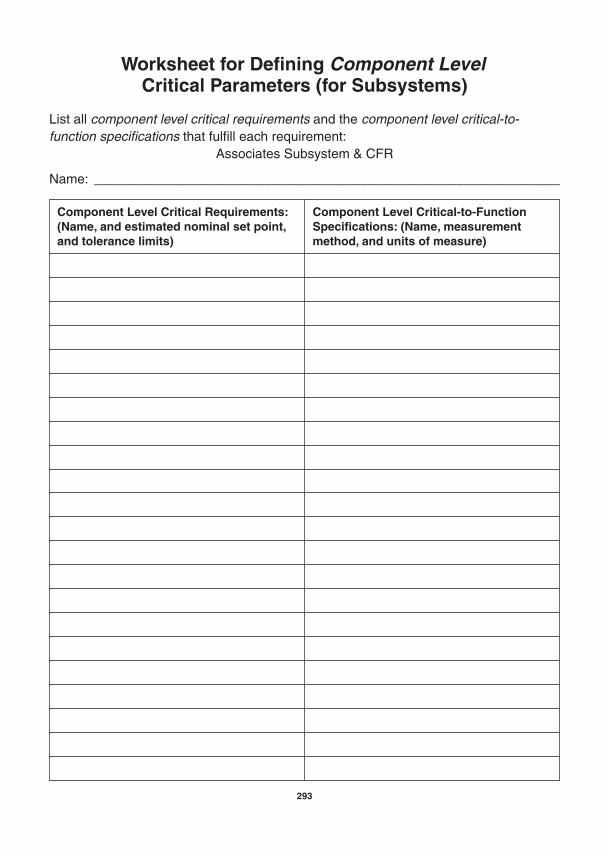
Worksheet for Defining Component Level Critical Parameters (for Subsystems)
List all component level critical requirements and the component level critical-to-function specifications that fulfill each requirement:
Associates Subsystem & CFR
Name: _______________________________________________________________
Component Level Critical Requirements: Component Level Critical-to-Function(Name, and estimated nominal set point, Specifications: (Name, measurement and tolerance limits) method, and units of measure)
293
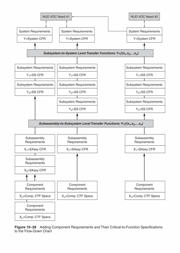
NUD VOC Need #1
System Requirements
Y=System CFR
System Requirements
Y=System CFR
Subsystem Requirements
Y1=SS CFR Y1=SS CFR
Subsystem Requirements
Subsystem Requirements
Y2=SS CFR Y2=SS CFR
Subsystem Requirements
Y3=SS CFR
Subsystem Requirements
Y1=SS CFR
Subsystem Requirements
Y2=SS CFR
Subsystem Requirements
Y3=SS CFR
Subsystem Requirements
Subsystem-to-System Level Transfer Functions: Y=ƒ(x1,x2,…xn)
SubassemblyRequirements
X1=SAssy CFR X1=SAssy CFR
SubassemblyRequirements
SubassemblyRequirements
X2=SAssy CFR
X1=SAssy CFR
SubassemblyRequirements
ComponentRequirements
ComponentRequirements
Xn=Comp. CTF Specs Xn=Comp. CTF Specs
ComponentRequirements
Xn=Comp. CTF Specs
Xn=Comp. CTF Specs
ComponentRequirements
Subassembly-to-Subsystem Level Transfer Functions: Y=ƒ(x1,x2,…xn)
System Requirements
Y=System CFR
NUD VOC Need #2
Figure 10–28 Adding Component Requirements and Their Critical-to-Function Specificationsto the Flow-Down Chart

Desired Performance Based on VOC and VOT
Subassembly requirement ID number
Component requirement
Component requirement ID number
Component CTF name
Component CTF target
Component CTF tolerances
Actual Measured Performance
Measured component CTF mean
Measured component CTF standard deviation
Measured component CTF Cp
Measured component CTF Cpk
Measured component CTF sensitivity coefficient dY/dx
These items are also stored in the CPM relational database along with the related transferfunctions that link inputs from subsystems, subassemblies, components, and manufacturingprocesses that drive the measured system CFR outputs.
At the end of Phase 2, each subassembly component level CTF specification’s capabilitygrowth index is calculated and documented as in Figure 10–30.
The Process of Critical Parameter Management in Product Development 295
Comp. Comp.Subassy. Comp. Comp. Comp. Comp. Comp. CFR CFR Comp. Comp. Comp.
Reqt. Reqt. Comp. CTF CTF CTF CTF Std. S/N CTF CTF CTF# # Reqts. Name Target Tol. Mean Dev. Ratio Cp Cpk dY/dx
Figure 10–29 Sample Subassembly-to-Component Level CPM Scorecard

The two summary tables in Figures 10–29 and 10–30 are essential communication tools atPhase 2, 3, and 4 gate reviews. They summarize and present the subassembly-to-component crit-ical parameter summary performance data. The worksheet on page 297 is helpful in setting up theCPM database at the subassembly-to-component level.
The critical parameter management database adds many new layers of structure duringPhase 2 (see Figure 10–31 on page 298). In fact, within Phase 2 the many-to-many relationshipsare first structured completely down through the system to subsystem to subassembly to compo-nent to manufacturing process architecture. There will be numerous Houses of Quality (see Fig-ure 10–32 on page 299) developed for each layer of the system’s architecture depending uponhow many subsystems, subassemblies, components, and manufacturing processes exist.
At this point in Phase 2 the Critical Parameter Management database now reflects the struc-ture depicted in Figure 10–33 on page 300.
One should be able to trace each of the manufacturing process requirements and critical-to-function specifications up to the component requirements and CFT specifications up to the sub-assembly requirements and critical functional responses. The next step is up through thesubsystem requirements and CFRs or directly up to the platform or system level requirements andCFRs, on up to the specific NUD VOC need(s) that they help fulfill. The final example of theCPM flow-down model depicts these paths (see Figure 10–34 on page 301).
Phase 2 delivers the layers of critical subsystem, subassembly, component, and manufac-turing requirements and critical parameter metrics. These are documented in the maturing rela-tional database such as DOORS, ACCESS, or the Six Sigma Cockpit. The relational database willcontinue to be used to build and manage the hierarchy of critical parameter relationships betweenthe system, subsystem, subassembly, component, and manufacturing process requirements,CFRs, CAPs, critical functional parameters, and critical-to-function component specifications.
The goals of CPM inside of Phase 2 activities are the baseline modeling and evaluation ofall subsystem, subassembly, component, and manufacturing process CFRs and CTF specs. In
296 Chapter 10
Subassembly Related Component CTF Specification: Phase 1 Phase 2 Phase 3 Phase 4CGI CGI CGI CGI
Figure 10–30 Documenting Capability Growth Indices for Subassembly Component CTFSpecifications

Worksheet for Defining Component Level Critical Parameters (for Subassemblies)
List all component level critical requirements and the component level critical-to-function specifications that fulfill each requirement:
Associates Subassembly & CFR
Name: _______________________________________________________________
Component Level Critical Requirements: Component Level Critical-to-Function(Name, and estimated nominal set point, Specifications: (Name, measurement and tolerance limits) method, and units of measure)
297
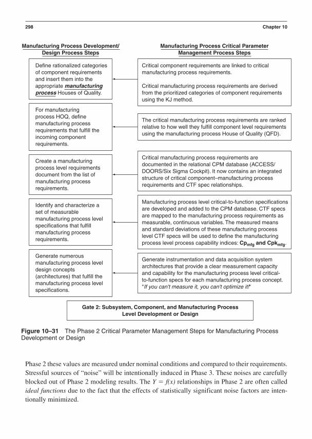
Phase 2 these values are measured under nominal conditions and compared to their requirements.Stressful sources of “noise” will be intentionally induced in Phase 3. These noises are carefullyblocked out of Phase 2 modeling results. The Y f(x) relationships in Phase 2 are often calledideal functions due to the fact that the effects of statistically significant noise factors are inten-tionally minimized.
298 Chapter 10
Define rationalized categoriesof component requirementsand insert them into theappropriate manufacturingprocess Houses of Quality.
Manufacturing Process Development/Design Process Steps
Manufacturing Process Critical ParameterManagement Process Steps
Critical component requirements are linked to criticalmanufacturing process requirements.
Critical manufacturing process requirements are derivedfrom the prioritized categories of component requirementsusing the KJ method.
For manufacturingprocess HOQ, definemanufacturing processrequirements that fulfill theincoming componentrequirements.
Manufacturing process level critical-to-function specificationsare developed and added to the CPM database. CTF specsare mapped to the manufacturing process requirements asmeasurable, continuous variables. The measured meansand standard deviations of these manufacturing processlevel CTF specs will be used to define the manufacturingprocess level process capability indices: Cpmfg and Cpkmfg.
Generate instrumentation and data acquisition systemarchitectures that provide a clear measurement capacityand capability for the manufacturing process level critical-to-function specs for each manufacturing process concept."If you can't measure it, you can't optimize it!"
The critical manufacturing process requirements are rankedrelative to how well they fulfill component level requirementsusing the manufacturing process House of Quality (QFD).
Generate numerousmanufacturing process leveldesign concepts(architectures) that fulfill themanufacturing process levelspecifications.
Create a manufacturingprocess level requirementsdocument from the list ofmanufacturing processrequirements.
Critical manufacturing process requirements aredocumented in the relational CPM database (ACCESS/DOORS/Six Sigma Cockpit). It now contains an integratedstructure of critical component–manufacturing processrequirements and CTF spec relationships.
Identify and characterize aset of measurablemanufacturing process levelspecifications that fulfillmanufacturing processrequirements.
Gate 2: Subsystem, Component, and Manufacturing ProcessLevel Development or Design
Figure 10–31 The Phase 2 Critical Parameter Management Steps for Manufacturing ProcessDevelopment or Design
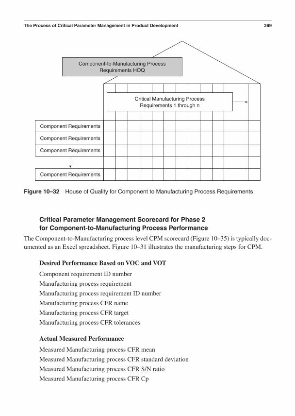
Critical Parameter Management Scorecard for Phase 2for Component-to-Manufacturing Process Performance
The Component-to-Manufacturing process level CPM scorecard (Figure 10–35) is typically doc-umented as an Excel spreadsheet. Figure 10–31 illustrates the manufacturing steps for CPM.
Desired Performance Based on VOC and VOT
Component requirement ID number
Manufacturing process requirement
Manufacturing process requirement ID number
Manufacturing process CFR name
Manufacturing process CFR target
Manufacturing process CFR tolerances
Actual Measured Performance
Measured Manufacturing process CFR mean
Measured Manufacturing process CFR standard deviation
Measured Manufacturing process CFR S/N ratio
Measured Manufacturing process CFR Cp
The Process of Critical Parameter Management in Product Development 299
Component Requirements
Component-to-Manufacturing ProcessRequirements HOQ
Component Requirements
Component Requirements
Component Requirements
Critical Manufacturing ProcessRequirements 1 through n
Figure 10–32 House of Quality for Component to Manufacturing Process Requirements
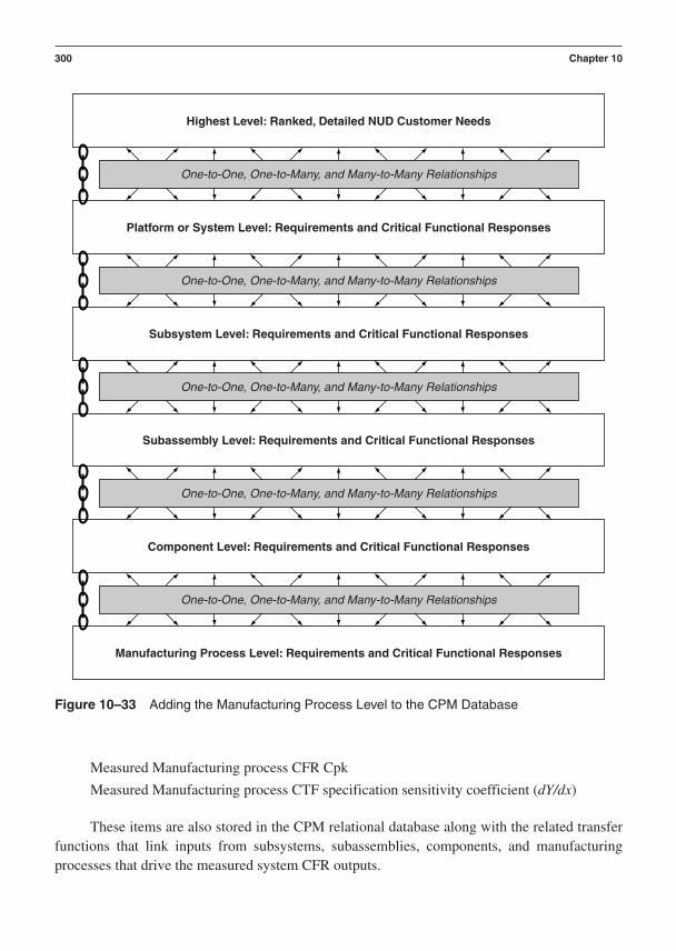
Measured Manufacturing process CFR Cpk
Measured Manufacturing process CTF specification sensitivity coefficient (dY/dx)
These items are also stored in the CPM relational database along with the related transferfunctions that link inputs from subsystems, subassemblies, components, and manufacturingprocesses that drive the measured system CFR outputs.
300 Chapter 10
One-to-One, One-to-Many, and Many-to-Many Relationships
Platform or System Level: Requirements and Critical Functional Responses
Highest Level: Ranked, Detailed NUD Customer Needs
One-to-One, One-to-Many, and Many-to-Many Relationships
Subsystem Level: Requirements and Critical Functional Responses
One-to-One, One-to-Many, and Many-to-Many Relationships
Subassembly Level: Requirements and Critical Functional Responses
One-to-One, One-to-Many, and Many-to-Many Relationships
Component Level: Requirements and Critical Functional Responses
One-to-One, One-to-Many, and Many-to-Many Relationships
Manufacturing Process Level: Requirements and Critical Functional Responses
Figure 10–33 Adding the Manufacturing Process Level to the CPM Database

NUD VOC Need #1
System Requirements
Y=System CFR
System Requirements
Y=System CFR
Subsystem Requirements
Y1=SS CFR Y1=SS CFR
Subsystem Requirements
Subsystem Requirements
Y2=SS CFR Y2=SS CFR
Subsystem Requirements
Y3=SS CFR
Subsystem Requirements
Y1=SS CFR
Subsystem Requirements
Y2=SS CFR
Subsystem Requirements
Y3=SS CFR
Subsystem Requirements
Subsystem-to-System Level Transfer Functions: Y=ƒ(x1,x2,…xn)
SubassemblyRequirements
X1=SAssy CFR X1=SAssy CFR
SubassemblyRequirements
SubassemblyRequirements
X2=SAssy CFR
X1=SAssy CFR
SubassemblyRequirements
ComponentRequirements
ComponentRequirements
X n=Comp. CTF Specs Xn=Comp. CTF Specs
ComponentRequirements
Xn=Comp. CTF Specs
Xn=Comp. CTF Specs
ComponentRequirements
Manufacturing ProcessRequirements
Xn=Mfg.. CTF Specs Xn=Mfg.. CTF Specs
Manufacturing ProcessRequirements Xn=Mfg.. CTF Specs
Manufacturing ProcessRequirements
Subassembly-to-Subsystem Level Transfer Functions: Y=ƒ(x1,x2,…xn)
System Requirements
Y=System CFR
NUD VOC Need #2
Figure 10–34 Final Phase 2 Flow-Down Chart

At the end of Phase 2, each manufacturing process level CTF specification’s capabilitygrowth index is calculated and documented, as in Figure 10–36.
The two summary tables in Figures 10–35 and 10–36 are essential communication tools atPhase 2, 3, and 4 gate reviews. They summarize and present the component-to-manufacturingprocess critical parameter summary performance data. The worksheet on page 303 is helpful insetting up the CPM database at the manufacturing process level.
Phases 3 and 4: Stress Testing and Integration
Phase 2 defines the requirements and critical metrics for all the subsystems, subassemblies, com-ponents, and manufacturing processes. The critical metrics are used in Phases 2, 3, and 4 to
302 Chapter 10
Manufacturing Process CTF: Phase 1 Phase 2 Phase 3 Phase 4CGI CGI CGI CGI
Figure 10–36 Documenting Capability Growth Indices for Manufacturing Process CTFs
Mfg. Mfg. Mfg.Comp. Mfg. Mfg. Mfg. Mfg. Mfg. CTF CTF Mfg. Mfg. CTFReqt. Reqt. Mfg. CTF CTF CTF CTF Std. S/N CTF CTF Sens.
# # Reqts. Name Target Tol. Mean Dev. Ratio Cp Cpk Coeff.
Figure 10–35 Sample Component-to-Manufacturing Process Level CPM Scorecard

Worksheet for Defining Manufacturing Process LevelCritical Parameters
List all manufacturing process level critical requirements and the manufacturingprocess level critical-to-function specifications that fulfill each requirement:
Associates Component CTF Specification
Name: _______________________________________________________________
Manufacturing Process Level Critical Manufacturing Process Level Critical-To-Requirements: (Name, and estimated Function Responses: (Name,nominal set point, and tolerance limits) measurement method, and units of
measure)
303

assess how well the evolving designs are maturing as they seek to fulfill the platform or systemlevel requirements.
In Phase 3, the subsystems, subassemblies, components, and manufacturing processes arestress tested for their ability to contribute to robustness as stand-alone units of integrated tech-nology (Figure 10–37). These stress tests include noises that are anticipated in the future Phase 4integration environment. In Phase 4, the subsystems and subassemblies are integrated into exist-ing or new platform or system structures where they will eventually reside. The Phase 4 capabil-ity, robustness, and tunability studies are conducted for baseline evaluations, robustness, andreliability stress testing at the platform or system level.
Phase 2 produced the Critical Parameter Management database flow-down structure for thenominal, baseline designs. Phase 3, the optimization phase, is focused on measuring sensitivity
304 Chapter 10
Conduct dynamic robustdesign optimization andresponse surface methods onthe superior subsystemconcept.
OptimizationProcess Steps
Critical Parameter ManagementProcess Steps
The baseline subsystem and subassembly designs arestress tested with critical noise factors using dynamicrobustness techniques. Interactions between controlfactors and noise factors are identified using changes inS/N ratios.
The instrumentation and data acquisition system is fullyconnected and used to measure the subsystem andsubassembly level CFRs.
This is done to define optimum nominal critical parameterset points that leave the subsystem and subassemblyCFRs minimally sensitive to statistically significant noisefactors.
CAP set points are optimized, using response surfacemethods to adjust the mean of the CFR on to the targetvalue for the CFR specifications in the presence of noise.
The critical parameter set points are refined and mappedto the updated, optimized subsystem and subassemblyCFRs that have previously been mapped to subsystem andsubassembly requirements.
Post-robustness and CAP optimization capability studiesare conducted. The new Cp and Cpk indices for thesubsystem and subassembly CFRs are documented inthe CPM database.
Gate 3: Subsystem and Subassembly Level Robustness Optimization
Figure 10–37 Phase 3: Subsystem and Subassembly Level Robustness Optimization

relationships between intentional changes to the established baseline critical parameters under theinfluence of intentionally induced noise factors. The following parameters are used to measurethese sensitivity relationships:
1. Critical functional responses (these are measured outputs)a. subsystem level CFRsb. Subassembly level CFRs
2. Critical parameters at the subassembly and component level as they affect the subsys-tems (these are measured and controlled inputs to a subsystem)a. Critical functional parameters (engineered vectors or scalars)b. Critical-to-function specifications (component dimension or feature, usually a
scalar)3. Critical parameters at the component level as they affect the subassemblies (these are
measured and controlled inputs to a subassembly)a. critical-to-function specifications (component dimension or feature, usually a
scalar)4. Noise factors (measured and controlled inputs to both subsystems and subassemblies)
a. External sources of variationb. Unit-to-unit sources of variationc. Deterioration sources of variation
The goals for CPM in Phase 3 are to produce the following data:
1. Incoming baseline Cp indices (from Phase 2 to Phase 3) for all subsystem and sub-assembly CFRs. These Cp values are representative of the subsystems and subassem-blies in the intentional absence of the effects of the noise factors.
2. Developing insensitivity to intentionally induced noise factors by measuring and doc-umenting the interactions between critical parameter inputs and statistically significantnoise factors. These interactions are quantified by using signal-to-noise ratio compar-isons or by generating critical parameter noise factor interaction plots.
3. Outgoing, post-robustness optimization Cp indices (from Phase 3 to Phase 4) for allsubsystem and subassembly CFRs. It is common to present two forms of Cp indices asone exits Phase 3:a. Cp indices based on the absence of induced noise factors (the best the newly opti-
mized CFRs can provide)b. Cp based on the inclusion of induced noise factors (the diminished performance of
the newly optimized CFRs)
With subsystems and subassemblies that have been optimized for robust and tunable per-formance, it is now reasonable to integrate these designs into the platform or system structure forfinal technology transfer or product design certification.
The Process of Critical Parameter Management in Product Development 305

Figure 10–38 presents a diagram of the processes of Phase 4 to verify platform or systemlevel capability.
The goals for CPM in Phase 4 are to produce the following data:
1. Incoming Cp indices (from Phase 3 to Phase 4) for all system, subsystem, and sub-assembly CFRs. These Cp values are representative of the system, subsystems, andsubassemblies after they have gone through system integration with performance ad-justed and balanced in the presence of the statistically significant noise factors. Theyestablish the capability of the product as it enters Phase 4. We need these to comparewith the final capability indices at the end of Phase 4.
2. Assess the system’s insensitivity to the transition over to production components, as-sembly, and service processes.
3. Production Cp indices (from Phase 4 to steady-state operations) for all system, sub-system, and subassembly CFRs and component and manufacturing process CTF spec-ifications. It is also common to present two forms of Cp indices as one exits Phase 4:
306 Chapter 10
Conduct certification tests onthe integrated dynamicallytunable, and robustsubsystems to prove the newplatform or system is safeand mature enough totransfer into acommercialization project orproduction.
Capability VerificationProcess Steps
Critical Parameter ManagementProcess Steps
The robust subsystem and subassembly designs areintegrated to form a functional platform or system.
The instrumentation and data acquisition system is fullyconnected and used to measure the subsystem/subassembly, and system level CFRs.
The platform or system is stress tested with critical systemlevel noises to prove that the new design CFRs are at anacceptable level of S/N performance (S/Nsys) and capabilityperformance (Cpsys and Cpksys).
Each subsystem and subassembly CFR is also evaluatedwithin the platform or system stress test to assure thecapability of each subsystem CFR is at an acceptablelevel (Cpss and Cpkss).
The platform or system level CFRs are tuned through adynamic range of test points using the CAPs in thepresence of noise to validate the robustness andtunability.
If a new subsystem is theonly focus of thedevelopment project, anexisting "system mule" mustbe used to conductcertification tests. This is doneon the integrated,dynamically tunable, androbust subsystems to provethe new subsystem is safeand mature enough to takeforward into thecommercialization project.
Gate 4: Platform or System Level Capability Verification
Figure 10–38 Phase 4: Platform or System Level Capability Verification
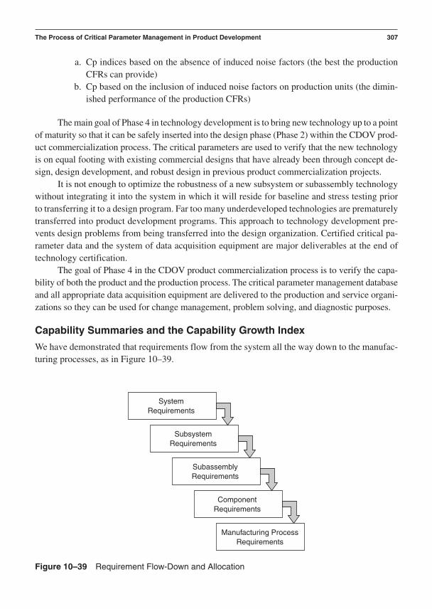
a. Cp indices based on the absence of induced noise factors (the best the productionCFRs can provide)
b. Cp based on the inclusion of induced noise factors on production units (the dimin-ished performance of the production CFRs)
The main goal of Phase 4 in technology development is to bring new technology up to a pointof maturity so that it can be safely inserted into the design phase (Phase 2) within the CDOV prod-uct commercialization process. The critical parameters are used to verify that the new technologyis on equal footing with existing commercial designs that have already been through concept de-sign, design development, and robust design in previous product commercialization projects.
It is not enough to optimize the robustness of a new subsystem or subassembly technologywithout integrating it into the system in which it will reside for baseline and stress testing priorto transferring it to a design program. Far too many underdeveloped technologies are prematurelytransferred into product development programs. This approach to technology development pre-vents design problems from being transferred into the design organization. Certified critical pa-rameter data and the system of data acquisition equipment are major deliverables at the end oftechnology certification.
The goal of Phase 4 in the CDOV product commercialization process is to verify the capa-bility of both the product and the production process. The critical parameter management databaseand all appropriate data acquisition equipment are delivered to the production and service organi-zations so they can be used for change management, problem solving, and diagnostic purposes.
Capability Summaries and the Capability Growth Index
We have demonstrated that requirements flow from the system all the way down to the manufac-turing processes, as in Figure 10–39.
The Process of Critical Parameter Management in Product Development 307
SystemRequirements
SubsystemRequirements
SubassemblyRequirements
ComponentRequirements
Manufacturing ProcessRequirements
Figure 10–39 Requirement Flow-Down and Allocation

CPM maps the variation transmission and capability flow up from the manufacturingprocesses to the system level critical functional responses (Figure 10–40).
Critical Parameter Management uses a summary statistic called the capability growth indexto demonstrate the phase-to-phase growth of the capability of the critical parameters to the gatekeepers. Critical parameter capability index status is used to help manage risk throughout thephases of the technology and product development processes. Cost and cycle-time are also im-portant and must be equally tracked and measured along the way.
The capability growth index and the other metrics of Critical Parameter Management arediscussed in the next chapter.
308 Chapter 10
System CFRPerformance
Transfer FunctionLinkage Is Used to
Track CriticalRelationships andTransmission of
Variations
Capability Flow-upof Cp and Cpk
Subsystem CFRPerformance
Subassembly CFRPerformance
Component CTFPerformance
Manufacturing Process CTFPerformance
Figure 10–40 CPM Mapping from Manufacturing Process up to System Level CriticalFunctional Responses

C H A P T E R 1 1
The Tools and Best Practices of Critical ParameterManagement
Critical Parameter Management is most effective when practiced under the discipline of abroad portfolio of Six Sigma tools and best practices. These tools and best practices focus
on the development and documentation of a systemwide network of critical functional require-ments that are fulfilled and validated by the measurement of critical functional responses andspecifications (Figure 11–1). Without this network of requirement and response relationships,critical paths cannot be clearly defined, linked, optimized, tracked, and ultimately certified.
309
ComponentRequirements
Manufacturing ProcessRequirements
What is required
CFR = critical functional responses
What is delivered
CTF Spec = critical-to-function specifications
SubassemblyRequirements
SubsystemRequirements
SystemRequirements
ComponentCTF Specs
Manufacturing ProcessCTF Specs
SubassemblyCFRs
SubsystemCFRs
SystemCFRs
Figure 11–1 Six Sigma “Network” Employed in CPM

One of the most important deliverables from CPM comes from the use of DFSS tools in thedevelopment of transfer functions. Recall that a transfer function establishes a mathematical re-lationship between a dependent (Y) variable and any number of independent (x) variables. Manytools and best practices can be deployed in the development of Six Sigma performance duringtechnology and product development. It is easy for us to define them—the challenge comes whenproject leaders try to get everyone on the development team to apply them rigorously in pursuitof the project deliverables. It is all about excellence in execution.
The term best practice is open to some debate. It has been the authors’ experience that it isrisky behavior to trust that every individual in the organization will naturally, of his or her ownaccord, do all the right things at the right times during product development. This simply does nothappen well in industry. What usually happens is an unstable process of every person doing whathe or she feels is “right” with respect to using product development tools and best practices. Thisinvariably leads to random applications of limited and varying sets of tools. The end result of suchanemic and inconsistent use of tools and best practices is mediocre quality and poor commer-cialization cycle-time. Poor product or process reliability is more often due to “death by a thou-sand cuts” than by any one glaring problem or defect in this scenario. The “cuts” come from poortool use building up negative effects day by day.
Best practices are methods that are proven to work and deliver consistent results throughrigorous application by companies that usually had no choice but to change how they conductedproduct development. If you want to find a tested set of best practices, go to companies that wereon the verge of collapse but found a set of tools that brought them back to viability.
There is a set of tools that will consistently deliver 3 sigma quality. They are easy to findand define. Companies all over the world are currently using them and getting just what theyinvested in—mediocrity. A deeper and broader set of methods that we refer to as “best prac-tices” consistently delivers 6 sigma functional quality. The companies that seem to learn thisquickly are those at the end of their line, in a crisis, and very close to going out of business. Ina word, they are motivated to apply rigor and discipline to tool use. Unfortunately, most rea-sonably healthy companies are complacent and rarely get serious about identifying and exe-cuting a modern set of best practices. No one tool or method can carry the burden of delivering6 sigma functional performance and attain cycle-time reduction within budget. However, whenproperly linked and used at the right time with discipline and rigor, there are many that will dothe job.
The Rewards of Deploying Proven Tools and Best Practices
The careful selection and integration of a group of tools and best practices within a Phase gateproduct commercialization process and detailed project management plan will outperformchaotic and random approaches to product design every time. If you buy a state-of-the art CAD(computer-aided design) system and focus on the rigorous use of the specification communica-tion language of GD&T but ignore tolerance design tools, your product will likely require re-
310 Chapter 11

work and encounter unforeseen reliability problems. If you design your technologies for nomi-nal performance and focus on “design for patentability,” you will likely experience technologytransfer problems because the technology is not robust and tunable, nor is it likely to be readilymanufacturable. Best practices create complete designs. Partial designs result from limited useof a few, favorite methods that leave critical design parameters underdeveloped. Frequently, de-velopment teams create a “new” design but don’t bother to benchmark it or stress test it alongwith a competitive design. They then have the audacity to act surprised when it is eclipsed in themarketplace where it is exposed to real sources of variability. That which is real can humble thatwhich is new!
A thorough set of best practices can be characterized by its ability to include and addressall the realities and requirements that exist within technology development, product design, man-ufacturing, delivery, service, customer use, and life-cycle environments. Probably the biggestmistake we see being made by product development managers is the underfunding of time to ex-ecute the right number of tools and best practices to fulfill their program requirements. You mayrecall we had a bit to say about that in Chapter 4.
You should select a portfolio of tools and best practices that match your company’s specificproduct development processes and goals. Every company is different, so no one company hasthe optimum recipe of best practices for anyone but themselves. Obviously the auto industry hasa great deal of commonality with respect to best practices. This is where benchmarking of bestpractices can be helpful. Some companies consider their product development process and port-folio of best practices as proprietary. This is usually vanity more than a strategic maneuver. Thevalue lies in the disciplined, active execution of the product development process and the de-ployment of a balanced set of tools and best practices that are designed to meet your objectives.The authors have seen lots of impressive product development process manuals with strong port-folios of best practices that get limited use if they are ever practiced at all. This is why your com-pany should define the critical best practices that will meet your business and customer needs andthen set out to do them better than anybody else. Having a product development process loadedwith best practices and then actually doing them well is the secret to success.
Best practices can be broken down into many categories. For our focus on Critical Para-meter Management, we will divide them into two broad areas: technology development and prod-uct commercialization. A lot of overlap and redundancy exists in the tool sets for these twoprocesses. That is to be expected if you consider technology development a means of enablingbrand new designs to catch up to the maturity of a reused or existing design that has already beenout in the marketplace. Further categorization can take place around specific types of application.For technology development and product design we will focus on four common categories:
1. Invention, innovation, and concept design2. Design development3. Optimization4. Capability verification
The Tools and Best Practices of Critical Parameter Management 311
These four general areas have previously been shown to be readily structured into specificphases for both technology and design development.
Critical Parameter Management Best Practices for TechnologyDevelopment
During technology development our focus is primarily limited to the conceptual design and pa-rameter design of new or reused subsystem technologies or an integrated group of subsystemsthat are known as platforms. The technologies being developed need to be certified for the abil-ity to merge with the rest of the design elements usually somewhere within Phase 2 of the CDOVproduct design process. We will continue our focus on phases and gates by illustrating which toolsand best practices align with the phases and gates of the I2DOV technology development process.We will also state the specific deliverable from each tool and best practice as it pertains to Criti-cal Parameter Management.
Best Practices for Conceptual Design
Phase 1: Technology Concept Invention and Innovation
Gathering and processing the voice of the customerDeliverable: Ranked and prioritized VOC data (new, unique, and difficult needs).
Quality function deployment and the Houses of QualityDeliverable: Translated VOC, NUD technology requirements, additional ranking andprioritizing in terms of customer perception, and competitive benchmarking data. Targetvalues for the technology requirements.
Competitive functional benchmarkingDeliverable: Data concerning measurable competitive product performance. This datahelps substantiate the targets set to fulfill the technology requirements.
Technology requirements generation and documentationDeliverable: Complete set of technology requirements document with target andtolerance values (including the NUD technology requirements).
Critical Parameter Management database developmentDeliverable: Initial relational database constructed and loaded with the flow-down of theNUD customer needs and the technology requirements developed to fulfill them.
Best Practices for Baseline Development
Phase 2: Technology Development
Functional analysis and functional flow diagramming (diagramming the flow,transformation and state of energy, mass, and information within the technologyconcepts)
312 Chapter 11

Deliverable: Candidate critical parameters that help begin the analytical and empiricalmodeling of the transfer functions, sometimes called ideal functions or baselineperformance models.
Analytical Math Modeling (based on first principles, typically with CAE methods)Deliverable: Initial transfer function models [Y f(x)].
Concept generation techniques (Form, fit, and function brainstorming, brain-writing,benchmarking, modeling, etc.)Deliverable: Form, fit (architectural structuring), and functional parameter definition(transfer function model) to fulfill the technology requirements.
Failure modes and effects analysis (FMEA)Deliverable: Initial assessment of the parameters that are critical to failure.
Fault tree analysis (FTA)Deliverable: Initial assessment of the flow-down of parametric failure relationshipswithin the functional architecture of the technology concepts.
Development and design of data acquisition systems (Instrumentation and measurementsystem analysis)Deliverable: Definition and capability certification of the hardware, firmware, andsoftware to be used to measure the critical functional responses and specifications foreach critical parameter.
Empirical math modeling (Inferential statistics, sequential design of experiments,ANOVA, correlation, regression, response surface methods)Deliverable: Transfer function models for critical parameters [Y f(x)].
Design for additivity and tunability (Synergistic functional interactivity of technologyelements; platform design)Deliverable: Initial assessment and quantification of the strength and directionality of allstatistically significant (control factor control factor) interactions; development andidentification of critical adjustment parameters.
Preliminary DFx analysis (Testability, modularity, manufacturability, reliability,environment, etc.)Deliverable: Identification of additional critical parameters for all performance areasrequired to meet the VOC needs.
Pugh concept evaluation and selection processDeliverable: Superior technology concepts, including their critical parameters.
Critical parameter management database developmentDeliverable: Relational database loaded with critical system, subsystem, subassembly,component, and manufacturing process parameters, their transfer functions, and theirmeasured Cp performance as they are linked to the technology requirements.
The Tools and Best Practices of Critical Parameter Management 313

Best Practices for Robustness Optimization
Phase 3: Technology Optimization
Failure modes, effects, and analysis (FMEA)Deliverable: Additional FMEA documentation data from Phase 3 robustness evaluationsand stress testing.
Fault tree analysis (FTA)Deliverable: Additional data relative to failure flow-down relationships within thearchitectures of the maturing subsystems and subassemblies.
Generic noise diagramming and platform noise mapping (Product family noises)Deliverable: Thorough documentation of the candidate noise factors for use in therobustness optimization experiments and analysis.
Development and design of data acquisition systems (Instrumentation and measurementsystem analysis)Deliverable: Additional measurement system equipment and certification data prior toPhase 3 critical parameter optimization evaluations.
Noise experimentation and noise vector characterizationDeliverable: Statistically significant noises that will be used in robustness optimizationexperiments.
Dynamic robustness optimization experiments (Continuation of sequential design ofexperiments, additive model confirmation for critical parameters that underwrite robustand tunable technologies)Deliverable: Set points for critical functional parameters (CFPs) and critical-to-functionspecifications (CTF specs) that leave the subsystem and subassembly CFRs minimallysensitive to the noise factors.
Critical Parameter Management database developmentDeliverable: Relational database loaded with Cp indices for the subsystem andsubassembly CFRs. Any new sensitivity linkage is mapped between critical parameters.Transfer functions are modified with new data.
Best Practices for Platform and Subsystem Certification
Phase 4: Technology Certification
Preliminary tolerance design and sensitivity analysisDeliverable: Tolerance models built from analytical (Worst case, RSS, and Monte Carlosimulations) and empirical (Sequential DOE-based tolerance sensitivity) studies.
System integration and platform stress testingDeliverable: CFR Cp and Cpk index data that includes the stressful effects from thestatistically significant noise factors applied during the system/platform integration tests.
314 Chapter 11

Technology capability assessment and characterization (Cp and Cpk)Deliverable: Refined CFR Cp and Cpk indices after component, subassembly, andsubsystem tolerance balancing and integration stress testing. Cp and Cpk data will bedocumented under nominal and stressful conditions for all CFRs.
Critical Parameter Management database developmentDeliverable: Relational database loaded with all critical parameter relationships andtransfer functions. The critical parameters are linked to the technology requirements tovalidate certification of the robustness and tunability of the technology.
The critical parameter database is a major part of what is transferred to the product designorganization at the end of the technology development process. The data acquisition hardware,firmware, and software are also major deliverables to the design teams. The ability to measurenew, unique, or difficult critical functional responses is a strategic advantage that can enable acommercialization team to stay on schedule as it integrates new technologies into the product de-sign architecture. It is not uncommon to see major, new patents on data acquisition designs andtechnologies as a result of CPM in R&D organizations.
Critical Parameter Management Best Practices for ProductCommercialization
The CDOV product commercialization process turns its focus on a broader set of best practices,mainly due to the fact that it must ensure that the integrated system (new technologies and reuseddesigns) is ready for steady-state production and service processes.
R&D teams tend to use a smaller set of tools and best practices than product design teams.Their job is to get the technology to a mature enough state to transfer it into product commer-cialization. The product design teams must carefully plan what tools and best practices are ap-propriate for the product they are designing. The following set of tools and best practices isessential to the successful deployment of Critical Parameter Management.
Best Practices for Concept Design for Product and Manufacturing ProcessCommercialization
Phase 1: Concept Design
Gathering and processing the voice of the customer (Customer interviewing and KJanalysis)Deliverable: Ranked and prioritized VOC data.
Quality function deployment and the Houses of QualityDeliverable: Translated VOC, NUD system requirements, and additional ranking andprioritizing in terms of customer perception and competitive benchmarking data. Targetvalues for the system requirements.
The Tools and Best Practices of Critical Parameter Management 315

Competitive functional benchmarkingDeliverable: Data concerning measurable competitive product performance. This datahelps substantiate the targets set to fulfill the system requirements.
System requirements generation and documentationDeliverable: System requirements document with target and tolerance values. Thisincludes the NUD system requirements from the House of Quality.
Critical Parameter Management database developmentDeliverable: Initial relational database constructed and loaded with NUD customer needsthat are linked to the system requirements.
Best Practices for Design Development
Phase 2: Design Development
Functional analysis and functional flow diagramming (diagramming the flow,transformation, and state of energy, mass, and information within the system, subsystem,and subassembly concepts)Deliverable: Candidate critical parameters that help begin the analytical and empiricalmodeling of the transfer functions, sometimes called ideal functions or baselineperformance models.
Analytical math modeling (based on first principles, typically with CAE methods)Deliverable: Initial transfer function models [Y f(x)]
Concept generation techniques (Form, fit, and function brainstorming, brain-writing,benchmarking, modeling, etc.)Deliverable: Form, fit (architectural structuring), and functional parameter definition(transfer function model) to fulfill the product requirements.
Failure modes and effects analysis (FMEA)Deliverable: Initial assessment of the parameters that are critical to failure.
Fault tree analysis (FTA)Deliverable: Initial assessment of the flow-down of parametric failure relationshipswithin the functional architecture of the technology concepts.
Development and design of data acquisition systems (Instrumentation and measurementsystem analysis)Deliverable: Definition of the hardware, firmware, and software to be used to measurethe critical functional responses and specifications for each critical parameter.
Empirical math modeling (inferential statistics, sequential design of experiments,ANOVA, correlation, regression, response surface methods)Deliverable: Transfer function models for critical parameters [Y f(x)].
Design for additivity and tunability (Synergistic functional interactivity of designelements; platform deployment)
316 Chapter 11

Deliverable: Initial assessment and quantification of the strength and directionality of allstatistically significant (control factor control factor) interactions. Development andidentification of critical adjustment parameters.
Preliminary DFx Analysis (Testability, modularity, manufacturability, reliability,environment, etc.)Deliverable: Identification of additional critical parameters for all performance areasrequired to meet the VOC needs.
Pugh concept evaluation and selection processDeliverable: Superior technology concepts, including their critical parameters.
Critical Parameter Management database developmentDeliverable: Relational database loaded with all critical system, subsystem, subassembly,component, and manufacturing process parameters, all transfer functions, and measuredCp performance values as they are linked to the system requirements. Baseline capabilitygrowth indices are documented for all subsystems.
Best Practices for Design Optimization
Phase 3A: Subsystem and Subassembly Robustness Optimization
Failure Modes, Effects, and Analysis (FMEA)Deliverable: Additional data from robustness stress testing that is relevant to FMEAdocumentation and failure analysis.
Fault tree analysis (FTA)Deliverable: Additional data relative to failure flow-down relationships within thematuring subsystems and subassemblies.
Specific noise diagramming and system noise mapping (Product specific noises)Deliverable: Thorough documentation of the candidate noise factors for use in therobustness optimization experiments and analysis.
Development and design of data acquisition systems (Instrumentation and measurementsystem analysis)Deliverable: Additional measurement system equipment and certification data prior toPhase 3A critical parameter evaluations.
Noise experimentation and noise vector characterizationDeliverable: Statistically significant noises that will be used in robustness optimizationexperiments.
Dynamic robustness optimization experiments [Continuation of sequential design ofexperiments: Evaluation of interactions between critical parameters (CFPs and CTFspecs) and the statistically significant noise factors, additive model confirmation forrobust and tunable subsystems and subassemblies]
The Tools and Best Practices of Critical Parameter Management 317

Deliverable: Set points for critical functional parameters (CFPs) and critical-to-functionspecifications (CTF specs) that leave the subsystem and subassembly CFRs minimallysensitive to the noise factors. Confirmation data for the additive model.
Mean optimization experiments (Continuation of sequential design of experiments:Response surface methods applied to critical adjustment parameters to place the mean ofthe CFRs on to their VOC targets)Deliverable: Set points for critical adjustment parameters (CAPs) that place the mean ofthe subsystem and subassembly CFRs on target.
Critical Parameter Management database developmentDeliverable: Relational database loaded with Cp indices for the optimized subsystem andsubassembly CFRs. Transfer functions and new sensitivity linkages are mapped betweencritical parameters. Transfer functions are modified with new data. The latest capabilitygrowth indices are documented for all subsystems.
Best Practices for System Integration and Stress Testing
Phase 3B: System Integration and Stress Testing
System integration stress testing (The integrated system is evaluated for Cp performanceunder nominal and stressful conditions)Deliverable: System, subsystem, and subassembly CFR Cp and Cpk index data thatincludes the nominal performance and the stressful effects from the statisticallysignificant noise factors applied during the system integration tests.
Product capability assessment and characterization (Cp and Cpk evaluations after thesystem, subsystems, and subassemblies have been balanced from the learning from thefirst system integration test data results)Deliverable: Refined CFR Cp and Cpk indices after component, subassembly, andsubsystem tolerance balancing and system integration stress testing. Cp and Cpk data willbe documented under nominal and stressful conditions for all CFRs.
Analytical and empirical tolerance design and sensitivity analysisDeliverable: Production tolerances (components, subassemblies, and subsystems) fromtolerance models built from analytical (Worst case, RSS, and Monte Carlo simulations)and empirical (Sequential DOE-based tolerance and /1 sensitivity) studies.
Critical Parameter Management database developmentDeliverable: Relational database loaded with all the latest critical parameterrelationships. The transfer functions are updated and linked to the product requirementsto validate the current nominal performance, robustness, and tunability of the system.Capability growth indices are documented for all subsystem and system level CFRs.
318 Chapter 11

Best Practices for Product Design Certification
Phase 4A: Product Design Certification
Final, baseline component, subsystem, and system level capability assessment andcharacterization (Cp and Cpk)Deliverable: Final product, subsystem, subassembly, component, and manufacturingprocess capability indices and capability growth indices.
Critical Parameter Management database developmentDeliverable: Relational database loaded with all the latest critical parameterrelationships. Final transfer functions are updated and linked to the product requirementsto validate certification of the nominal performance, robustness, and tunability of thecomplete product. Capability growth indices are documented for all subsystem andsystem level CFRs.
Best Practices for Production Process Certification
Phase 4B: Production Process Certification
Once the product design is certified, the ramp-up to steady-state production can be evalu-ated and certified. A smaller but powerful set of best practices are required to sustain Crit-ical Parameter Management on into production.
Transfer of data acquisition systems (Critical parameter instrumentation)Deliverable: A select group of capable and certified transducers, meters, and computer-aided data acquisition equipment to continue measuring critical parameters duringproduction.
Manufacturing process, component, subsystem, and system level product capabilityassessment and characterization (Cp and Cpk)Deliverable: Ongoing statistical process control data to measure, analyze, improve, andcontrol the capability of the critical parameters.
Critical Parameter Management database deploymentDeliverable: Relational database fully loaded with all the latest critical parameterrelationships. Final transfer functions are linked to the product and productionrequirements to validate certification of the nominal performance, robustness, andtunability of the complete product and its production processes. Final capability growthindices are documented for all subsystem and system level CFRs.
As you can see, the best practices for CPM see their heaviest use early in the product de-velopment process. The more that is understood during the development of technology, the lesstime spent developing critical parameter knowledge during product commercialization. The bestscenario is to build up a certified and reusable base of technologies, platforms, and designs that
The Tools and Best Practices of Critical Parameter Management 319

can be safely transferred and deployed into rapid commercialization projects. This approach en-ables a business strategy that is based on launching families of products.
Notice how few best practices are required once the product attains manufacturing certifi-cation and shipping approval. This is a clear sign that CPM has worked! Ideally one would liketo produce products, subsystems, and components indefinitely with no corrective action at all dur-ing steady-state production. This, of course, is not realistic.
A few disciplined companies have attained a diminished need to redesign after they havelaunched a new product into the market. The alternative is the presence of special teams of “fire-fighters” from the design organization who reside in the production organization to literally fin-ish developing the product while it is in production. These resources should be working on thenext new product—not patching up all the shortcomings of one that was supposed to be com-pleted. CPM tools and best practices go a long way in helping the product development team toget it done right the first time.
320 Chapter 11
C H A P T E R 1 2
Metrics for Engineering and Project Management Within CPM
An unfortunate mismatch exists between the metrics traditionally used by management tomeasure product development process performance and the metrics engineering teams
must use to conduct product development. Many of the current forms of product developmentmetrics are rooted in Total Quality Management and standard business performance metrics.These metrics tend to focus on financial terms such as unit manufacturing costs (UMC), qualitymeasures such as defects per million opportunities (DPMO), and time-based measures of relia-bility such as mean time to failure (MTTF). These are legitimate measures of business perfor-mance, but they are limited in scope and are lagging indicators of functional performance.Counting defects and measuring failures are considered inappropriate measures for Critical Pa-rameter Management.
Critical Parameter Management requires leading indicators that are comprehensive inscope. A comprehensive scope includes functional performance measures that can be usedthroughout the phases and gates of product development—right on into the production operationsand customer use environments. Engineering teams cannot efficiently attain on-target functionalperformance by measuring quality and reliability by reacting to such lagging indicators. Qualitymetrics such as yield (% good), percent defective, defects per million opportunities, defects perunit, go–no go attributes, and reliability metrics such as mean time between service calls andmean time to failure are all based on measuring the aftermath of physical functions that havemoved off target. The key terms in these metrics are defects, failure, and time. A positive measureof improved performance in this TQM context typically focuses around acceptability of per-formance within tolerance limits.
The dominant paradigm is acceptability, which is tolerance centric. A CPM paradigm requires reduced variability around a target-centric system that measures critical physical func-tions that lead to quality and reliability. This is why we call critical functional responses leading
321

indicators of quality and reliability. Critical Parameter Management must also operate beyond a nominal measurement context. The focus shifts from “How many defects does this product have under nominal, steady-state conditions?” to “How close to the desired targets do the criticalfunctional responses remain when we expose the system to realistic sources of variation?” You can see how counting defects places an engineering team a long way from the measurablephysics of function, energy transformations, flows of mass, and information (digital and analoglogic and control signals). It is not reasonable or logical for managers to expect engineering teamsto measure quality and reliability to optimize functional performance; they must measure thefunctions.
Key CPM Metrics
The proper metrics for Critical Parameter Management are as follows:
1. Scalars and vectors that are direct outcomes of energy and mass transformations,flows, or changes of state.
2. Continuous variables that are active over the continuum of initiating, sustaining, andconcluding a function. Such metrics typically have an absolute zero start and endvalue. When energy is put into a system, the measured output starts from “absolutezero” and all measures of the function are relative to that “zero.”
Think of shooting a cannon at a target. The absolute zero is the distance from thecannon to where the projectile landed. A “relative zero” is the distance from the pro-jectile to the actual target.
These metrics also lend themselves well to plotting and characterizing relationshipsbetween the mean and standard deviation of a critical functional response with respectto the critical functional parameters and critical-to-function specifications (independ-ent variables). This is especially true when optimizing transient performance.
3. Metrics that are complete. Such metrics cover the hierarchical network of ideal ortransfer functions that are required by the flow-down of system, subsystem, or sub-assembly performance requirements.
4. Metrics that are fundamental measure functions in terms of the Law of Conservationof Energy and/or the Law of Conservation of Mass. These metrics quantitatively andadditively account for the balances that are fundamental to physical performance.
The diagram in Figure 12–1 and models that follow are quite useful in helping determinewhat to measure in Critical Parameter Management.
The Ideal/Transfer Function: Y f(xA, xB,. . . xN)
The Additive Model: S/nopt. S/navg. [S/nA opt. S/navg.] [S/nB opt. S/navg.] . . .[S/nN opt. S/navg.]
The Sensitivity or Variance Model: 2total 2
A 2B . . . 2
N
322 Chapter 12

When these kinds of inputs and outputs are measured, functional interactivity contributions(transfer functions, additive models, and sensitivities) between engineering control factors can bedocumented with scientific accuracy. Real, functional interactivity relationships between criticalparameters can be legitimately characterized on the basis of the conservative laws of physics.Then these functional contribution relationships (transfer functions and gains in robustness andsensitivities) can be designed for harmony, synergy, and additivity. You will encounter difficul-ties if you attempt to design for functional harmony and critical parameter additivity (rememberthe crew of rowers in Chapter 8!) if you measure quality attributes instead of functions that fol-low conservative physical law.
Recall, six basic terms are used to define the measured elements of Critical Parameter Management:
1. Critical customer needs2. Critical requirements3. Critical functional responses (CFR)4. Critical adjustment parameters (CAP)5. Critical functional parameters (CFP)6. Critical-to-function specifications (CTF spec)
Critical implies that whatever is being measured and tracked is absolutely critical to ful-filling the highest priority needs that a majority of customers have expressed. When you think ofthe word critical, think of customers.
Metrics for Engineering and Project Management Within CPM 323
Desired Mass
Undesired Mass
Desired Energy
Undesired Energy
Desired Information
Undesired Information
Desired Mass
Undesired Mass
Desired Energy
Undesired Energy
Desired Information
Undesired Information
Transformations, Flows,or Changes of State
Functional, Architectural, Regulatory, Legal,Environmental Limitations, and Constraints
Functional Outputs (Y)Functional Inputs (x)
System,Subsystem, orSubassembly
Y = f (x)
S/nT = S/na + . . . +S/nn
σ2T = σ2
A + . . . + σ2n
Figure 12–1 What to Measure in CPM

Functional implies that a functional variable is being measured and tracked as opposed tosome quality attribute. If the parameter is not directly measurable in units of some form of massor energy, you are not conducting true CPM. When you think of the word function, think ofphysics.
The critical parameters can be represented as a flow-down of terms stored in a relationaldatabase, linked to one another, and evaluated in mathematical and empirical models, which arereferred to as transfer functions. CPM terms flow-down the system hierarchy as in Figure 12–2.
The vocabulary of the flow-down of critical parameters is explained as follows:
System Level Critical Functional Responses (CFR):
A continuous variable, typically either an engineering scalar or vector, that is a measure of a crit-ical output from the system. System CFRs are directly sensed by the customer and can be directlycompared to the new, unique, or difficult customer needs.
System Level Critical Adjustment Parameters (CAP):
A continuous variable, typically either an engineering scalar or vector, that is specifically de-signed to adjust a system CFR. These variables are few in number and are often used by customersto adjust the performance of the product.
Subsystem Level Critical Functional Responses (CFR):
A continuous variable, typically either an engineering scalar or vector, that is a measure of a crit-ical output from a subsystem. Subsystem CFRs are usually not directly sensed by the customer.When one or more subsystem CFRs are used as inputs to a system CFR, their name is changed toa subsystem critical functional parameter (CFP). Subsystem CFRs are measured and documentedfor their capability to support system CFR capability.
324 Chapter 12
Requirements
Needs
Responses
Parameters
Specifications
Figure 12–2 CPM System Hierarchy

Subsystem Level Critical Adjustment Parameters (CAP):
A continuous variable, typically either an engineering scalar or vector, that is specifically de-signed to adjust a subsystem CFR. These variables are few in number and are sometimes avail-able for customers to adjust but more often are used by assembly and service organizations.
Subassembly Level Critical Functional Responses (CFR):
A continuous variable, typically either an engineering scalar or vector, that is a measure of a crit-ical output from a subassembly. Subassembly CFRs are usually not directly sensed by the cus-tomer. When one or more subassembly CFRs are used as inputs to a subsystem CFR, their nameis changed to a subassembly critical functional parameter. Subassembly CFRs are measured anddocumented for their capability to support subsystem CFR capability.
Subassembly Level Critical Adjustment Parameters (CAP):
A continuous variable, typically either an engineering scalar or vector, that is specifically de-signed to adjust a subassembly CFR. These variables are also few in number and are often usedby assembly and service organizations.
Component Level Critical-To-Function Specifications (CTF Spec):
A continuous variable, typically an engineering scalar, that is a measure of a critical componentdimension or feature. It can also be a characteristic relating to a surface or bulk property of a com-ponent or material. These CTF specifications are commonly communicated to the supply chainusing spec sheets, CAD files, and component quality plans. They are usually measured undersome form of variable data statistical process control as they are manufactured. Component CTFspecs are designed, measured, and documented for their capability to support subassembly andsubsystem CFR capability. This is the point where manufacturing process capability interfaceswith and transitions into product or design level performance capability.
Manufacturing Process Level Critical-To-Function Specifications (CTF Spec):
A continuous variable, typically an engineering scalar or vector, that is a measure of a criticalmanufacturing process set point. These variables are literally measured on a manufacturingprocess as it produces a component or material. One major use of manufacturing process capa-bility is the measurement, control, and application of these CTF variables to fulfill component requirements.
The manufacturing process capability index (Cpm) can also be used in reference to assembly processes. Manufacturing process requirements (USL-LSL) establish what is requiredof these variables. Manufacturing CTF specs are measured during production to ensure that what is required of the process is being provided. A manufacturing process requirement may be
Metrics for Engineering and Project Management Within CPM 325

a pressure that is required to be at 25 psi / 1 psi. The measured manufacturing process CFTspec pressure might be measured at 24.3 psi in the morning and 25.1 in the afternoon. The CFTspec can be compared to the requirement and action taken if the manufacturing process has a con-trol problem. The components are known to vary as the process pressure varies. CPM in a pro-duction context measures the in-process capability of the pressure. If the pressure and all otherCTF specs are on target with low variability relative to the process requirements, the componentsneed limited measurement during production. During product development, manufacturing CTFspecs are measured to document their capability to support component capability.
Statistical Metrics of CPM
Measuring quality or reliability attributes can lace the response values with “virtual” or false in-teractions that suggest codependencies (A B) between critical parameters (CFPs and CTFspecs) that physically do not exist in a fundamental context. Statisticians frequently provoke theseartificial interactions that are little more than manifestations of a poor selection of a measured re-sponse. The engineer is then left to worry about all these “statistically significant” interactionsbased on quality attribute metrics. Most of these worrisome interactions don’t even exist in thecontext of physical law. Products don’t obey the statistics of quality attributes—they obey phys-ical law! Products will tell you all about how they obey physical law if you measure the rightthings. To control physics, you must directly measure functions. Quality then comes from prop-erly constrained physical functions. Statistics are superb quantifiers of physical performance, pro-vided the mean and standard deviation are calculated on fundamental, complete, continuousvariables that are scalar or vector quantities.
The following items are the basic statistical metrics used for Critical Parameter Management:
• The mean or average of a sample of data that are measures of scalar- or vector-basedvariables.
Avg. (y1 y2 . . . yn)/n
• The standard deviation of a sample of data that are measures of scalar- or vector-based variables.
Sqr. Root[((yi Avg.)2)/n]
• The coefficient of variation of a sample of data that are measures of scalar- or vector-based variables.
COV /avg
• The signal-to-noise ratio of a sample of data that are measures of scalar- or vector-based variables.
S/N 10 log (2/s2) (dynamic form)
326 Chapter 12

S/N 10 log (avg2/s2) (static form: nominal the best type I also squared reciprocal ofCOV)
S/N 10 log (1/s2) (static form: nominal the Best Type II)
• The short-term process capability index of a short-term sample of data that aremeasures of scalar- or vector-based variables.
Cp (USL LSL)/6s
• The long-term process capability index of a long-term sample of data that aremeasures of scalar- or vector-based variables.
Cpk Min[(USL Avg.)/3s or (Avg. LSL)/3s]
• The capability growth index (CGI)
Critical functional responses provide excellent high-visibility metrics to project managersfrom their subsystem engineering teams. To anchor the performance of the subsystem CFRs tothe subsystem requirements document, the few critical subsystem level functional responsesacross an engineered subsystem can be aggregated together in the form of their short-term processcapability indices (Cp). A summary capability statistic called the design functional capabilitygrowth index can be used to account for overall subsystem capability growth against a target ofCp 2.
where (Cp) short-term design capability index for a critical functional response
(USL LSL) difference between the upper spec limit and the lower spec limitfor CFRs from the subsystem requirements document
(s) sample standard deviation of the measured CFR
The capability growth index quantifies the aggregate functional capability maturity of agiven subsystem (in this case each CFR is equally weighted).
The CGI is measured in units of percent. The percentage is the aggregated amount of sub-system CFRs that are at their goal of Cp 2.
The value of the design functional CGI resides in its ability to provide an early, integrated,overarching measure of progress for Six Sigma performance at the subsystem level. From a
CGI n
i 100
n#CFRsCp
2 i
Cp USL LSL
6s
Metrics for Engineering and Project Management Within CPM 327

project management perspective, each subsystem CGI could be aggregated into an overall systemCGI. CGI metrics provide insight for human resource and hardware/material resource allocationand balancing. Simply put, one knows where the weak CFRs are and can assess their impact onthe integrated project plan critical path. Quality and cycle-time can be more effectively managed.
CGI Example
Subsystem A has five critical functional responses being measured. Thus, n 5. Each CFR hasthe following Cp and target comparison ratio (Cp target is 2) values:
CFR 1: Cp 1.3 Target comparison ratio (Cp/2) 1.3/2 0.65
CFR 2: Cp .84 Target comparison ratio (Cp/2) .84/2 0.42
CFR 3: Cp .71 Target comparison ratio (Cp/2) .71/2 0.36
CFR 4: Cp 2.3 Target comparison ratio (Cp/2) 2.3/2 1.15 Capped at 1.0
CFR 5: Cp 1.62 Target comparison ratio (Cp/2) 1.62/2 0.81
Each target comparison ratio (Cp/2) value is converted to a percentage by multiplying by 100. . .
CFR 1: 0.65 100 65%
CFR 2: 0.42 100 42%
CFR 3: 0.36 100 36%
CFR 4: 1.00 100 100% (Capped at 1.0 because CFR 4 reached 100% of its growthgoal)
CFR 5: 0.81 100 81%
These percentages give visibility to the individual CFR’s current state of capability growthwith respect to the capped target of Cp 2. Any Cp value beyond 2 is obviously good but nocredit is given to those CFRs with Cp 2. Doing so would unduly bias the aggregate subsystemCp growth index upward while certain CFRs may potentially remain at unacceptably low Cp val-ues. The intent is to motivate the subsystem teams to get all CFRs up to Cp 2. Once all CFRsare safely at Cp 2, the subsystem teams can focus their efforts on taking any CFR capabilitiesthey wish to as high a Cp level as is economically feasible or helpful in delighting customers.Please note our focus on the overall Cp performance of the subsystem as opposed to the individ-ual performance of an isolated CFR. This is good system engineering practice that emphasizesintegrated teamwork instead of individual heroism.
Each CFR now has a percentage contribution calculated for overall subsystem capabilitygrowth. Each CFR is equally weighted (one could assign differing weights to CFRs as appropri-ate) as a contributor of one fifth (20 percent) of the overall capability growth. To quantify thiscontribution, we divide each CFR’s Cp percent by the total number of CFRs in the subsystem (inthis case n 5).
328 Chapter 12
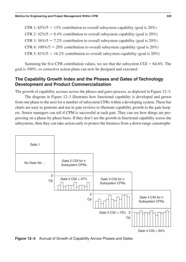
CFR 1: 65%/5 13% contribution to overall subsystem capability (goal is 20%)
CFR 2: 42%/5 8.4% contribution to overall subsystem capability (goal is 20%)
CFR 3: 36%/5 7.2% contribution to overall subsystem capability (goal is 20%)
CFR 4: 100%/5 20% contribution to overall subsystem capability (goal is 20%)
CFR 5: 81%/5 16.2% contribution to overall subsystem capability (goal is 20%)
Summing the five CFR contribution values, we see that the subsystem CGI 64.8%. Thegoal is 100%, so corrective action plans can now be designed and executed.
The Capability Growth Index and the Phases and Gates of TechnologyDevelopment and Product Commercialization
The growth of capability accrues across the phases and gates process, as depicted in Figure 12–3.The diagram in Figure 12–3 illustrates how functional capability is developed and grown
from one phase to the next for n number of subsystem CFRs within a developing system. These barcharts are easy to generate and use in gate reviews to illustrate capability growth to the gate keep-ers. Senior managers can tell if CPM is successful at each gate. They can see how things are pro-gressing on a phase-by-phase basis. If they don’t see the growth in functional capability across thesubsystems, then they can take action early to protect the business from a down-range catastrophe.
Metrics for Engineering and Project Management Within CPM 329
Gate 2 CGI for nSubsystem CFRs
Gate 2 CGI = 47%
Gate 3 CGI = 73%
Gate 1
No Data Yet. . .
2
Cp
2
Cp
2
Cp
Gate 3 CGI for nSubsystem CFRs
Gate 4 CGI for nSubsystem CFRs
Gate 4 CGI = 94%
Figure 12–3 Accrual of Growth of Capability Across Phases and Gates

This page intentionally left blank

C H A P T E R 1 3
Data Acquisition and DatabaseArchitectures in CPM
Data drives the key decisions that are made within the phases of the product developmentprocess. Data helps the gate keepers manage risk during gate reviews. Opinions are second-
ary in this context. Data provides the capacity to define and document criticality. Data is reality.CPM starts with the gathered voice of the customer data. It progresses and enables capa-
bility growth through the measured voice of the product and its supporting network of manufac-turing processes. The voice of the product and process is realized through the measurement ofcritical parameter data. Data is the mechanism used to validate the robustness and capability ofthe critical parameter relationships (ideal/transfer functions, additive models, and variance mod-els). These are the models of Critical Parameter Management:
The ideal/transfer function: Y f(xA, xB,. . . xN)
The additive model: S/nopt. S/navg. [S/nA opt. S/navg.] [S/nB opt. S/navg.] . . . [S/nN opt. S/navg.]
The variance model: 2total 2
A 2B . . . 2
N
Data defines critical dependencies, sensitivities, and linkages all the way down through the system to the manufacturing process set points that constrain the fulfillment of critical-to-function requirements at the component level. Without the proper data, engineering team deci-sions are made at great risk.
Probably the single most important skill in CPM is the ability to define, develop, construct,assess, and use a capable data acquisition system. Without a capable data acquisition system yourability to trust your data will be limited.
Instrumentation, Data Acquisition, and Analysis in CPM
Every single critical functional response in an engineered system must be measured. This appliesto products as well as manufacturing processes. One sure way for management to assess thehealth of a CPM program is to identify how many critical functional responses exist within the
331

new product being developed and then quantify how many of them are being actively measured.This is usually quite a revelation to unsuspecting project managers. In Phase 2 (development ordesign) of either the technology development (I2DOV) or product commercialization (CDOV)processes, the project manager should require that all CFRs be documented and measured byknown data acquisition that can be calibrated.
Data Acquisition Systems
Consider the question, “What is the most fundamental act one can take to attain Six Sigma per-formance during the management of critical parameters?” The answer is all bound up in the actof taking data. Developing a new product with weaknesses and lapses in the proper acquisitionof data is unacceptable in the context of Six Sigma.
Taking data is not always a simple matter during product development. As product com-plexity increases, so do the requirements and demands on data acquisition. In some situationsmeasuring the product’s functions is relatively straightforward and simple. This is the case whenone is developing a popular product like the one-time-use camera. The complex production sys-tem that produces tens of millions of these cameras per year is a whole other matter. The data ac-quisition system for the camera is small, but the one for the production and assembly system isextremely complex. When one is developing complex products like a high-volume digital printeror an automobile, the data acquisition systems for the product itself become complicated. Thedata acquisition systems used in product development are often more involved than the ones usedin production, assembly, and service.
Whatever the case, the data acquisition elements that make up your data acquisition sys-tems should be in harmony with validating the requirements of the product and its production andservice processes. The architecture of your data acquisition system will mirror the architecture ofyour requirements. An excellent way to audit a company for product development capability is tomatch how well its system, subsystem, subassembly, component, and manufacturing process re-quirements are being fulfilled in comparison to the structure of its data acquisition system. Thedata acquisition system elements that are being used to ensure the requirements are being prop-erly fulfilled should pretty much tell the story. Of course the measurement capability of the dataacquisition systems plays an integral role in the credibility of the data. We see from this that twoimportant elements underwrite the integrity of any data acquisition system:
1. For every critical functional requirement, there must be a transducer that measures theCFR within the data acquisition system.
2. For every transducer measuring a CFR, there must be a measurement system analysisconducted to verify the capability of the measurement process (gage R&R and/or precision/tolerance study).
Many types of data acquisition systems are available on the commercial market. You canbuy one designed and ready to use or you can build your own from scratch. If your measurement
332 Chapter 13
needs are relatively simple, buying the elements and integrating them yourself is probably thecheapest way to proceed. If you have a large network of CFRs ranging across a complex systemarchitecture, you are probably better off partnering with a company that can help you design andintegrate a computer-aided data acquisition system.
Transducer Selection and Calibration
Transducers are the elements within data acquisition systems that physically sense the criticalfunctional responses within the system, subsystems, and subassemblies. Since there are no “reli-ability meters” or “yield meters,” we must be realistic about what we measure. Literally dozensof transducer types and hundreds, if not thousands, of versions of transducers can be used in Crit-ical Parameter Management.
One of the harsh realities that will quickly face anyone attempting CPM is the fact that somefunctions are difficult, sometimes even impossible, to measure directly. Sometimes you will haveto invent new transducer technologies. Companies deploying Six Sigma in product developmentare often found to be filing for new patents for measurement technologies.
Other measurement cases will require you to measure a surrogate function that is close tothe fundamental function. An example would be measuring a deflection that is related to a forceyou wish you could measure. The force is impossible to measure, but the deflection is propor-tional to the force so you measure the deflection and calculate the force. This functional com-promise is still far better than measuring quality attributes! We recommend you define a full setof transducers that cover all the types of functions you need to measure. Where you have gaps ordifficulties, define work-around or compromise strategies to handle the data acquisition require-ments. Face these difficulties by thinking with an “out-of-the-box” mentality. Apply the DFSStools to your transducer design problems. Invent or innovate, develop, optimize, and verify newtransducer technologies for your business. Let transducer capability and performance become astrategic part of your product development capability in your business. This is a clear sign ofgrowth and maturity in Six Sigma methods.
Data Processing and Storage
Once a function is acquired by a transducer, it must be processed and saved so it can be used tohelp in the management of critical parameters. A “signal” produced by a transducer can be col-lected in many ways. By far the most common form of signal is an analog voltage. Most trans-ducers convert a function into a voltage. Once the voltage is produced in analog form, it can befurther processed into a form that is useful to a digital computer. This is the well-known analog-to-digital (A/D) conversion of a measured signal. A/D conversion is a serious matter in data ac-quisition system design. Many commercial A/D conversion circuits or “boards” are available. Werecommend you consult with an expert in data acquisition signal processing to guide you on theproper sizing and selection of the boards you should use. Whether you are gathering one or 1,000signals, you need the right A/D board to get the data into your computer or meter.
Data Acquisition and Database Architectures in CPM 333
Data will usually come in the following forms:
High-speed analog signals
Low-speed analog signals
High-speed digital signals
Low-speed digital signals
If you are not accustomed to working with modern data acquisition and processing hard-ware, firmware, and software, you need to become a student of this complex science. Any num-ber of texts provide good places to start. Some recommendations are listed at the end of this chapter.
We also recommend computer-aided data acquisition and processing products such as LabView from National Instruments Corp.
Data Analysis
Data analysis has been greatly improved over the last few years. With the state of the art in mod-ern PCs and data analysis software, it is not difficult to transfer data files between software pro-grams. Statistical analysis tools such as Minitab have become popular software in use by the SixSigma community at large. Minitab can help you evaluate data and get the statistical informationyou need to build and update the models used in Critical Parameter Management.
Minitab can receive data from most modern data acquisition programs. It can perform allof the following analysis (and much more) in support of CPM:
Capability analysis
Measurement system analysis
Design of experiments
• Full and Fractional Factorials (empirical modeling of transfer functions)• Taguchi designs (additive modeling and variance modeling)• Response surface methods (empirical modeling of transfer functions)• Mixture experiments (empirical modeling of transfer functions)
ANOVALinear and nonlinear regressionCorrelationInferential and descriptive statisticsBasic and advanced graphical data plottingSPC charting
Many other statistical analysis software packages are available on the commercial market.Any package that can perform the analysis and plotting listed previously can be used for CPM.
334 Chapter 13

Databases: Architectures and Use in CPM
Structuring, recording, manipulating, updating, and using the complex paths of critical functionalrelationships requires the use of modern software and computing technology. The best way ofconducting Critical Parameter Management is to use a relational database. Relational databasesenable the storage and tracking of the flowing types of relationships between critical parameters:
One-to-one relationships
One-to-many relationships
Many-to-one relationships
Many-to-many relationships
The biggest benefits from CPM come from the ability to identify and track many-to-manyrelationships across complex product and production systems. Product development organiza-tions fall down on cycle-time, cost, and functional performance goals because they fail to under-stand interactions between complex parametric relationships. They underestimate the effects ofcomplexity because they underinvest in the development of the knowledge they need to recog-nize critical relationships. They don’t know about complex interactive relationships that charac-terize the sensitivities that dominate many of the problems they will inevitably face once theproduct is launched. In short, they don’t know what they don’t know.
However, when a product development team knows something of the complexity of rela-tionships across, between, and within their system architectures, it can be quite preventative in itsuse of tools and best practices. Unfortunately, in the beginning stages of using Critical ParameterManagement, the amount of information needed to do product development properly is a bitshocking to novice users of the CPM method. The good news is they quickly adjust their per-spective, dig in, and get used to managing complexity instead of ignoring it. It is always amazingto see how human nature exhibits a “denial of the truth” attribute when confronted with com-plexity. The fact is we need to face complexity with a single-minded focus on being methodical,rigorous, and disciplined in breaking these problems down into manageable “bites.” Critical parameter databases help us do this. It is interesting to see how a CPM database slowly but inex-orably develops in the early phases of product development. Once people get used to methodi-cally constructing such data structures, life gets relatively simple for those who have to track andverify the capability and robustness of the many complex relationships within the system. Thehard part is to get started.
A few databases on the market can help in the performance of CPM:
Microsoft® Access: a capable tool for establishing a CPM database. Easy to learn and useto build your first CPM database. Macros must be written to perform the mathematicalfunctions required to quantify capability calculations, transfer functions, performsensitivity analysis, and achieve variational transmission tracking and modeling.
Data Acquisition and Database Architectures in CPM 335
DOORS: a great requirements database. Staff must take short training classes to learn it.Advanced training is required to perform quantification of capability calculations,transfer functions, sensitivity analysis, and variational transmission tracking andmodeling.
The Six Sigma Cockpit: a new relational database program based on object orientedprogramming. This software is designed to do everything CPM requires:
• Hierarchical requirements documentation• Active linkage between all many-to-many critical parameter relationships• Dynamic linking of all transfer functions for system variational modeling• Easy input and storage of all associated documents for CPM
Six Sigma Cockpit can basically do everything required to conduct CPM on complex systems.
The choice of software to build a relational CPM database needs to be carefully considered.We recommend benchmarking these and other commercially available software packages to seewhich fits your short-term and long-term needs.
References
Beckwith, T. G., Marangoni, R. D., & Lienhard V., J. H. (1993). Mechanical measurements.Reading, Mass.: Addison-Wesley.
Doebelin, E. O. (1990). Measurement systems application and design. New York: McGraw-Hill.
Fraden, J. (1997). Handbook of modern sensors (2nd Ed.). Woodbury, NY: AIP Press.Holman, J. P., & Gajda, Jr., W. J. (1989). Experimental methods for engineers. New York:
McGraw-Hill.Norton, H. N. (1989). Handbook of transducers. New Jersey: Prentice Hall.Wheeler, A. J., & Ganji, A. R. (1996). Introduction to engineering experimentation. New
Jersey: Prentice Hall.
336 Chapter 13

P A R T I V
Tools and Best Practices for Invention, Innovation,
and Concept Development
Chapter 14 Gathering and Processing the Voice of the Customer: CustomerInterviewing and the KJ Method
Chapter 15 Quality Function Deployment: The Houses of QualityChapter 16 Concept Generation and Design for x MethodsChapter 17 The Pugh Concept Evaluation and Selection ProcessChapter 18 Modeling: Ideal/Transfer Functions, Robustness Additive Models, and the
Variance Model
The tools and best practices associated with Design For Six Sigma are what actually deliver re-sults. That is only true if people use the tools and do so with discipline and rigor. The tools andbest practices discussed in this section focus on deliverables required at gate reviews for the firstphases in the I2DOV and CDOV processes. These tools and best practices ensure the new prod-uct requirements are focused on fulfilling the voice of the customer. They also ensure that nu-merous concepts are generated and the superior product concept is selected. Part IV ends with adetailed explanation of the modeling process that DFSS requires to take the superior product con-cept through the phases and gates of product development.
Chapters 14–34 are structured so that the reader can get a strong sense of the process stepsfor applying the tools and best practices. The structure also facilitates the creation of PERT chartsfor project management and critical path management purposes. A checklist, a scorecard, and alist of deliverables are provided at the end of each tools and best practices chapter.
337

Each of these chapters follows a common format.
• A brief description of where the tool resides within the phases of the productdevelopment process:
Where Am I in the Process? Where Do I Apply the Tool Within the Roadmaps?
Linkage to the I2DOV Technology Development Roadmap:
338 Part IV
Invent/Innovate
Develop Optimize Verify
Linkage to the CDOV Product Development Roadmap:
Concept Design Optimize Verify
• A brief description of the purpose of the tool:
What Am I Doing in the Process? What Does the Tool Do at this Point in the Roadmaps?
The Purpose of the Tool in the I2DOV Technology Development Roadmap:
The Purpose of the Tool in the CDOV Product Development Roadmap:• A brief description of the deliverables from using the tool:
What Output Do I Get at the Conclusion of this Phase of the Process? Whatare Key Deliverables From Gathering and Processing the Voice of theCustomer at this Point in the Roadmaps?
• A flow-down of block diagrams that illustrate the major steps in using the tool:
Tool Process Flow Diagram
This visual reference of the detailed steps of the tool illustrates the flow of what to do.
• Text descriptions for each block diagram that explain the step-by-step use of the tool:

Verbal Descriptions for the Application of Each Block Diagram Within the Tool
This feature explains the specific details of what to do, including:
• Key detailed input(s) from preceding tools and best practices• Specific steps and deliverables from each step to the next, within the process flow• Final detailed outputs that flow into follow-on tools and best practices
• Illustration of example checklist and scorecard for the tool being discussed:
Tool Checklist and Scorecards
• A final review of the deliverables from the use of the tool:
What output do I get at the conclusion of this phase of the process? What are key deliverablesfrom the tool at this point in the roadmaps?
• A list of recommended references on the tool.
The intent of the formatting is to show how the tools work, link together, and flow within the con-tinuum of the phases of product development.
Tools and Best Practices for Invention, Innovation, and Concept Development 339

This page intentionally left blank

C H A P T E R 1 4
Gathering and Processing the Voice of the Customer:Customer Interviewing and the KJ Method
Where Am I in the Process? Where Do I Apply VOC Gathering and the KJMethod Within the Roadmaps?
Linkage to the I2DOV Technology Development Roadmap:
341
Develop Optimize VerifyInvent/
Innovate
Gathering and processing the “long-term” voice of the customer is conducted within the Invent/Innovate phase during technology development. It is applied to define, structure, and rank thevoice of the customer for the development of new technology platforms and subsystems that willbe integrated into a new platform or for integration into existing product designs.
Linkage to the CDOV Product Development Roadmap:
Concept Design Optimize Verify
A second, more focused gathering and processing of the voice of the customer is conducted withinthe Concept phase during product development. Here we apply gathering and processing of the voice of the customer to a specific product within the family plan from the strategic product
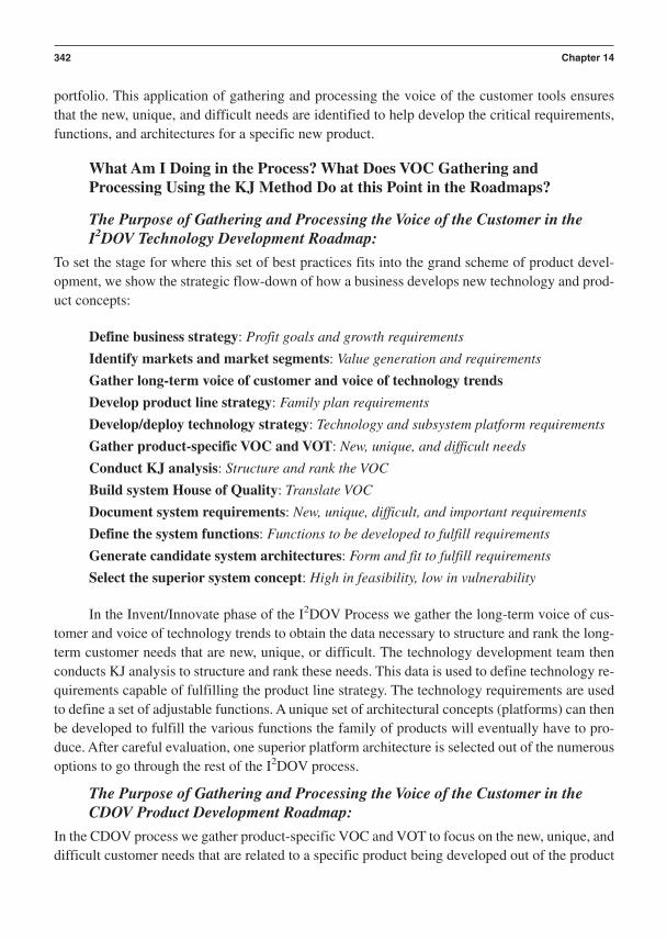
portfolio. This application of gathering and processing the voice of the customer tools ensuresthat the new, unique, and difficult needs are identified to help develop the critical requirements,functions, and architectures for a specific new product.
What Am I Doing in the Process? What Does VOC Gathering andProcessing Using the KJ Method Do at this Point in the Roadmaps?
The Purpose of Gathering and Processing the Voice of the Customer in theI2DOV Technology Development Roadmap:
To set the stage for where this set of best practices fits into the grand scheme of product devel-opment, we show the strategic flow-down of how a business develops new technology and prod-uct concepts:
Define business strategy: Profit goals and growth requirements
Identify markets and market segments: Value generation and requirements
Gather long-term voice of customer and voice of technology trends
Develop product line strategy: Family plan requirements
Develop/deploy technology strategy: Technology and subsystem platform requirements
Gather product-specific VOC and VOT: New, unique, and difficult needs
Conduct KJ analysis: Structure and rank the VOC
Build system House of Quality: Translate VOC
Document system requirements: New, unique, difficult, and important requirements
Define the system functions: Functions to be developed to fulfill requirements
Generate candidate system architectures: Form and fit to fulfill requirements
Select the superior system concept: High in feasibility, low in vulnerability
In the Invent/Innovate phase of the I2DOV Process we gather the long-term voice of cus-tomer and voice of technology trends to obtain the data necessary to structure and rank the long-term customer needs that are new, unique, or difficult. The technology development team thenconducts KJ analysis to structure and rank these needs. This data is used to define technology re-quirements capable of fulfilling the product line strategy. The technology requirements are usedto define a set of adjustable functions. A unique set of architectural concepts (platforms) can thenbe developed to fulfill the various functions the family of products will eventually have to pro-duce. After careful evaluation, one superior platform architecture is selected out of the numerousoptions to go through the rest of the I2DOV process.
The Purpose of Gathering and Processing the Voice of the Customer in theCDOV Product Development Roadmap:
In the CDOV process we gather product-specific VOC and VOT to focus on the new, unique, anddifficult customer needs that are related to a specific product being developed out of the product
342 Chapter 14
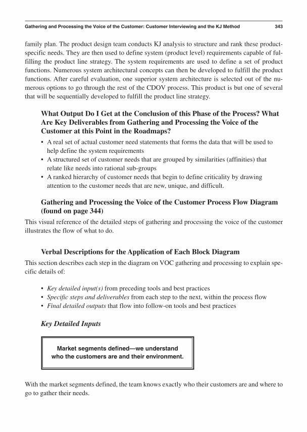
family plan. The product design team conducts KJ analysis to structure and rank these product-specific needs. They are then used to define system (product level) requirements capable of ful-filling the product line strategy. The system requirements are used to define a set of productfunctions. Numerous system architectural concepts can then be developed to fulfill the productfunctions. After careful evaluation, one superior system architecture is selected out of the nu-merous options to go through the rest of the CDOV process. This product is but one of severalthat will be sequentially developed to fulfill the product line strategy.
What Output Do I Get at the Conclusion of this Phase of the Process? WhatAre Key Deliverables from Gathering and Processing the Voice of theCustomer at this Point in the Roadmaps?
• A real set of actual customer need statements that forms the data that will be used tohelp define the system requirements
• A structured set of customer needs that are grouped by similarities (affinities) thatrelate like needs into rational sub-groups
• A ranked hierarchy of customer needs that begin to define criticality by drawingattention to the customer needs that are new, unique, and difficult.
Gathering and Processing the Voice of the Customer Process Flow Diagram(found on page 344)
This visual reference of the detailed steps of gathering and processing the voice of the customerillustrates the flow of what to do.
Verbal Descriptions for the Application of Each Block Diagram
This section describes each step in the diagram on VOC gathering and processing to explain spe-cific details of:
• Key detailed input(s) from preceding tools and best practices• Specific steps and deliverables from each step to the next, within the process flow• Final detailed outputs that flow into follow-on tools and best practices
Key Detailed Inputs
Gathering and Processing the Voice of the Customer: Customer Interviewing and the KJ Method 343
Market segments defined—we understand who the customers are and their environment.
With the market segments defined, the team knows exactly who their customers are and where togo to gather their needs.

Specific Steps and Deliverables
Determine purpose of customer visit. Why are we going?
344 Chapter 14
INPUT . . .
OUTPUT . . .
Market segmentsdefined—we understandwho the customers areand their environment.
Determine purpose ofcustomer visit.
Why are we going?
Identify objectives forcustomer visit.
What do we want to learn?
Develop customerselection matrix.
Who could best inform us?
Create customervisit teams.
Who goes where?
Creatediscussion/interview
guide based on objectives.
Interview and observecustomers to gather the
"voices" and "images" thatrepresent their specific
needs.
Develop "images of need":common images of
customers' environmentand needs.
Create image KJ diagram.
Categorize image KJ needsinto specific need statements
that are new, unique, ordifficult vs. routine.
Develop "significant voices of need,"common voices of customers' stated
needs.
Using a translation worksheet, link voicesto related images, write, and identify
unified customer needs.
Take the full set of unified customerneeds (translated voices and images)
and create a KJ diagram for thesecustomer needs.
Quantify the importanceof each NUD customer need by
reviewing KJ diagram results withkey customers.
NUD VOC needs flow into qualityfunction deployment and construction
of the Houses of Quality.
Gather data to quantify the qualityloss function for appropriate,
critical customer needs.
Document NUD customer needsand importance value (1–10) in the
Critical Parameter Management database.

The purpose of visiting and interviewing a set of customers is to get data. You need to hear whatthey say and see what they do so that you develop a clear understanding of what their new prod-uct needs are. You want to explore and experience their world and come away with the data youneed to develop the right product. The purpose of the visit should be worded in the context of aspecific new product development initiative that the product strategy is suggesting. You may havenew ideas and want to attain customer needs data to refine and focus your ideas for new products.
Identify objectives for customer visit. What do we want to learn?
The objectives of your customer visit are stated in terms of the detailed things you want to learn.In general terms, the critical things a product development team wants to learn are what needs arenew, unique, and difficult. Customers usually don’t want things that are old, common, and easy.If they do—fine, you should attempt to learn about those needs, too. The key is to be data drivenin what you develop.
The details you want to learn are specific customer needs. These can fall into many differ-ent categories. Here are but a few of those categories from Garvin’s eight “dimensions of qual-ity” (1988):
1. Performance—primary operating characteristic of a product or service2. Features—secondary characteristics of a product or service3. Reliability—frequency with which a product or service fails4. Conformance or consistency—match with specifications or standards5. Durability—product life, resistance to problems and deterioration6. Serviceability—speed, courtesy, and competence of repair or support7. Aesthetics—fits and finishes8. Perceived quality—reputation and life cycle ownership experience
Any visit to find out what customers need should explore details within and across these areas. You must be ready to take in whatever needs data is offered to you. You are not trying to“steer” their needs, but to be driven by their needs. If your customers are to drive your productdevelopment process, you need a fairly broad and detailed set of data from them.
Develop customer selection matrix. Who could best inform us?
To obtain a broad and detailed set of customer needs data, you must visit and interview a reason-able cross-section of the customers within your targeted market segments. A good way to ensurethat this happens is to develop a customer selection matrix.
Gathering and Processing the Voice of the Customer: Customer Interviewing and the KJ Method 345
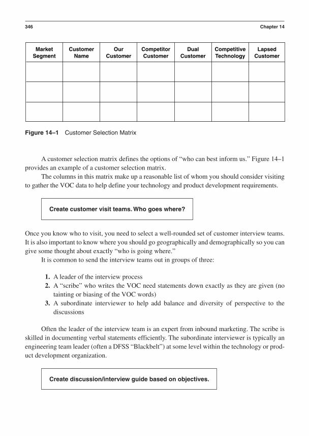
A customer selection matrix defines the options of “who can best inform us.” Figure 14–1provides an example of a customer selection matrix.
The columns in this matrix make up a reasonable list of whom you should consider visitingto gather the VOC data to help define your technology and product development requirements.
Create customer visit teams. Who goes where?
Once you know who to visit, you need to select a well-rounded set of customer interview teams.It is also important to know where you should go geographically and demographically so you cangive some thought about exactly “who is going where.”
It is common to send the interview teams out in groups of three:
1. A leader of the interview process2. A “scribe” who writes the VOC need statements down exactly as they are given (no
tainting or biasing of the VOC words)3. A subordinate interviewer to help add balance and diversity of perspective to the
discussions
Often the leader of the interview team is an expert from inbound marketing. The scribe isskilled in documenting verbal statements efficiently. The subordinate interviewer is typically anengineering team leader (often a DFSS “Blackbelt”) at some level within the technology or prod-uct development organization.
Create discussion/interview guide based on objectives.
346 Chapter 14
Market Customer Our Competitor Dual Competitive LapsedSegment Name Customer Customer Customer Technology Customer
Figure 14–1 Customer Selection Matrix
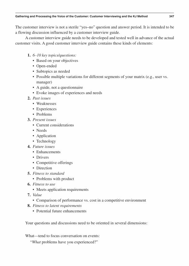
The customer interview is not a sterile “yes–no” question and answer period. It is intended to bea flowing discussion influenced by a customer interview guide.
A customer interview guide needs to be developed and tested well in advance of the actualcustomer visits. A good customer interview guide contains these kinds of elements:
1. 6–10 key topics/questions:• Based on your objectives• Open-ended• Subtopics as needed• Possible multiple variations for different segments of your matrix (e.g., user vs.
manager)• A guide, not a questionnaire• Evoke images of experiences and needs
2. Past issues• Weaknesses• Experiences• Problems
3. Present issues• Current considerations• Needs• Application• Technology
4. Future issues• Enhancements• Drivers• Competitive offerings• Direction
5. Fitness to standard• Problems with product
6. Fitness to use• Meets application requirements
7. Value• Comparison of performance vs. cost in a competitive environment
8. Fitness to latent requirements• Potential future enhancements
Your questions and discussions need to be oriented in several dimensions:
What—tend to focus conversation on events:
“What problems have you experienced?”
Gathering and Processing the Voice of the Customer: Customer Interviewing and the KJ Method 347

How—tend to focus the discussion on a process:
“How do you use. . .?”
Why—requires an explanation, but may elicit a defensive reaction:
“Why is that?”
Could—queries are usually perceived as “gentle” and open:
“Could you give us an example?”
The situation you want to avoid is verbal exchanges that are “closed ended” and result inyes or no answers. Your goal is to elicit responses or “word pictures” that are rich in descriptionsof need.
These answers eventually end up being translated into technical requirements. The moreyou can get your customers to describe their needs in the form of “continuous” variables, the eas-ier it is going to be for you to translate the VOC into technical requirements. Avoid “two-valued”language. Seek to have your customer communicate with you using “Multi-valued” language:
• The room is hot or cold vs. the room is 75 or 65 degrees.• The product needs to react quickly to my input vs. the product needs to react within 10
seconds.
Think of getting the customer to talk to you in terms of the way a light dimmer changes thelevel of intensity of light in a room as opposed to the way a light switch goes from one extremeto another (on-off). Try to get targets and ranges as opposed to “more is better” or “less is better”kinds of need statements. Engineers use physical laws and design principles based on scalars andvectors that create continuous functions to fulfill product requirements. The closer you can getyour customers to express their needs in this continuous variable context, the more likely the fi-nal product will satisfy the customer’s originally stated needs. This is not the time to be vague.
348 Chapter 14
Interview and observe customers to gather the “voices”and “images” that represent their specific needs.
Customer interviews can be extremely enjoyable events. It is quite literally an “open notebook–open mind” discovery process. Use your interview guide to establish a flow of conversation. Beintuitive, not coldly analytical. The engineers will take that tact later in the CDOV process whereit belongs. You should go into the event with a strategy of active listening. Prime the interviewprocess with stimulating questions and open-ended statements that are followed by listening,probing, and observation. Don’t hesitate to ask if what someone just told you was what you ac-tually heard. Go back and be sure you understood what was actually said. It is extremely easy tomisunderstand people. Take the time to get it right. Above all else, be quiet and let your customerstell you their needs. This is not your forum.

Part of the interview process should include actual observation of customers using the prod-uct or process about which you are trying to learn. Watching customers, as opposed to talking withthem, is called contextual inquiry. The data gathered in these sessions is often referred to as animage. The interviewer comes away with perceived images of customer use patterns, behaviors,and conditions. This book was structured, in part, from images we formed by watching how prod-uct development teams struggled to adequately inform themselves as they deployed DFSS.
Gathering and Processing the Voice of the Customer: Customer Interviewing and the KJ Method 349
3. Group the imaged needs into rational associations that are often referred to as affinitygroups. In other words, take the Post-It notes that tend to express similar needs andgroup them together. You should end up with a number of grouped Post-It notes.
Develop “images of need”: common images of customers’environment and needs. Create image KJ diagram.
Now that you have visited your selected set of customers, it is time to begin processing the VOCdata. The first set of data is the transcribed images that were formed during interviews and con-textual inquiry. Images can come from verbal customer statements that illustrate the environmentand context of VOC needs. Mental images that your interview team formed during observed be-haviors should also be documented and discussed as soon as possible after conducting the inter-views. Don’t wait — do this the evening after the interview was conducted, if possible. Be carefulnot to taint the VOC data with your personal biases and aspirations.
The team should create the first of the two forms of KJ diagrams (1. Image and 2. Re-quirements) at this point. An image KJ diagram is structured as follows:
1. Write down your specific images as “statements of need” on a Post-It note.2. After all team members write down their images, adhere them to the wall. There may
be many dozens of Post-It notes.
Many Detailed Imaged Needs on a Wall

First Level Grouping of Imaged Needs on a Wall
350 Chapter 14
2 lone wolves . . .
Named First Level Grouping of Imaged Needs on a Wall
4. For each group of Post-It notes, review the imaged need statements and reduce thenumber by throwing out redundant statements. If two or more are close to saying thesame thing, accurately rewrite the imaged needs on a new Post-It note and throw outall the ones that were condensed into this one new statement.
5. For each group, write an overarching need statement (shaded Post-Its in the figure thatfollows) that summarizes the general topic expressed by the grouped set of imagedneeds. This process is called “creating the ladder of abstraction.” That is to say, you arecreating a hierarchy or layered structure of customer needs by “laddered” categories.In the following figure, you have eight first level groups.
6. With the many single imaged needs now grouped into their first level of need categories,review the wording of first level customer need statements (shaded Post-Its). Look forcommon themes between the first level groups and try to identify the next level ofgrouping. It is common to have 10 to 12 first level groups at this point. If a specific im-aged need or first level group is not related to anything else, it is set aside for the time
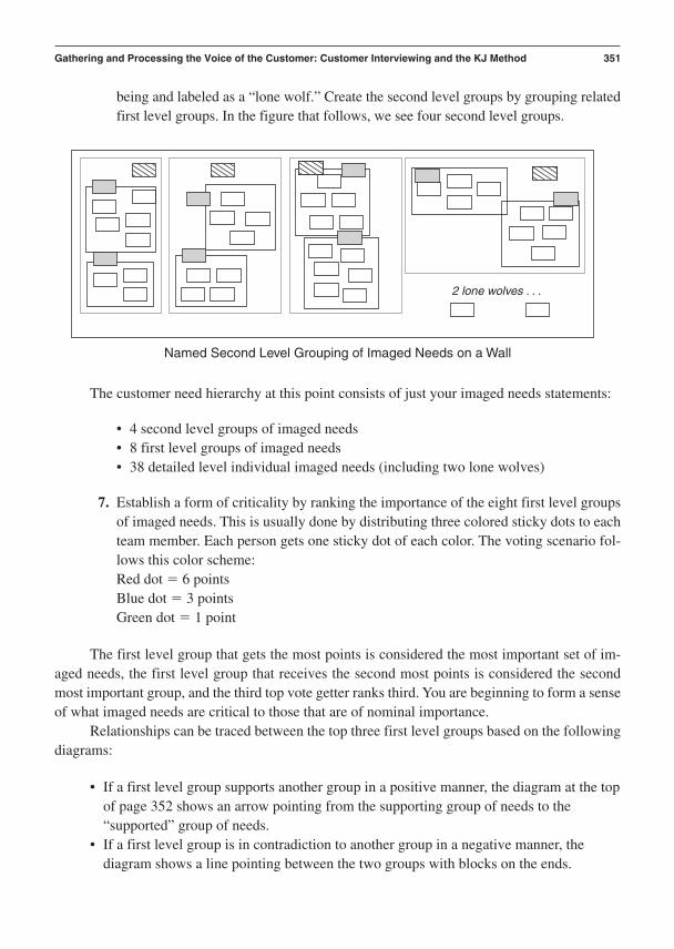
being and labeled as a “lone wolf.” Create the second level groups by grouping relatedfirst level groups. In the figure that follows, we see four second level groups.
Gathering and Processing the Voice of the Customer: Customer Interviewing and the KJ Method 351
2 lone wolves . . .
Named Second Level Grouping of Imaged Needs on a Wall
The customer need hierarchy at this point consists of just your imaged needs statements:
• 4 second level groups of imaged needs• 8 first level groups of imaged needs• 38 detailed level individual imaged needs (including two lone wolves)
7. Establish a form of criticality by ranking the importance of the eight first level groupsof imaged needs. This is usually done by distributing three colored sticky dots to eachteam member. Each person gets one sticky dot of each color. The voting scenario fol-lows this color scheme:Red dot 6 pointsBlue dot 3 pointsGreen dot 1 point
The first level group that gets the most points is considered the most important set of im-aged needs, the first level group that receives the second most points is considered the secondmost important group, and the third top vote getter ranks third. You are beginning to form a senseof what imaged needs are critical to those that are of nominal importance.
Relationships can be traced between the top three first level groups based on the followingdiagrams:
• If a first level group supports another group in a positive manner, the diagram at the topof page 352 shows an arrow pointing from the supporting group of needs to the“supported” group of needs.
• If a first level group is in contradiction to another group in a negative manner, thediagram shows a line pointing between the two groups with blocks on the ends.

Ranking and Tracing Relationships Among First Level Groups
352 Chapter 14
2 lone wolves
3rd Place 1st Place
2nd Place
2 lone wolves
New, Unique, and Difficult Imaged Needs on a Wall
Categorize image KJ needs into specific need statements that are new, unique, or difficult vs. routine.
Develop “significant voices of need,” commonvoices of customers’ stated needs.
The final processing step on the imaged needs is the beginning of the Critical Parameter Man-agement process. The Team looks at each detailed image need and assesses the need to see if it is new, unique, or difficult. In the following figure, we see an example of such needs highlightedin black.
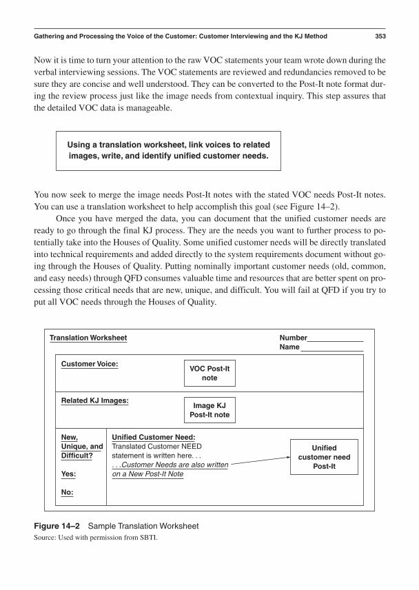
Now it is time to turn your attention to the raw VOC statements your team wrote down during theverbal interviewing sessions. The VOC statements are reviewed and redundancies removed to besure they are concise and well understood. They can be converted to the Post-It note format dur-ing the review process just like the image needs from contextual inquiry. This step assures thatthe detailed VOC data is manageable.
Gathering and Processing the Voice of the Customer: Customer Interviewing and the KJ Method 353
VOC Post-Itnote
Translation Worksheet NumberName
Customer Voice:
Related KJ Images:
New,Unique, andDifficult?
Yes:
No:
Unified Customer Need:Translated Customer NEEDstatement is written here. . .. . .Customer Needs are also writtenon a New Post-It Note
Image KJPost-It note
Unifiedcustomer need
Post-It
Figure 14–2 Sample Translation WorksheetSource: Used with permission from SBTI.
Using a translation worksheet, link voices to related images, write, and identify unified customer needs.
You now seek to merge the image needs Post-It notes with the stated VOC needs Post-It notes.You can use a translation worksheet to help accomplish this goal (see Figure 14–2).
Once you have merged the data, you can document that the unified customer needs areready to go through the final KJ process. They are the needs you want to further process to po-tentially take into the Houses of Quality. Some unified customer needs will be directly translatedinto technical requirements and added directly to the system requirements document without go-ing through the Houses of Quality. Putting nominally important customer needs (old, common,and easy needs) through QFD consumes valuable time and resources that are better spent on pro-cessing those critical needs that are new, unique, and difficult. You will fail at QFD if you try toput all VOC needs through the Houses of Quality.
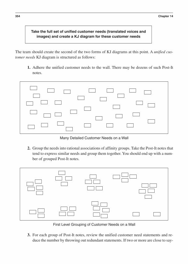
The team should create the second of the two forms of KJ diagrams at this point. A unified cus-tomer needs KJ diagram is structured as follows:
1. Adhere the unified customer needs to the wall. There may be dozens of such Post-Itnotes.
354 Chapter 14
Many Detailed Customer Needs on a Wall
First Level Grouping of Customer Needs on a Wall
2. Group the needs into rational associations of affinity groups. Take the Post-It notes thattend to express similar needs and group them together. You should end up with a num-ber of grouped Post-It notes.
3. For each group of Post-It notes, review the unified customer need statements and re-duce the number by throwing out redundant statements. If two or more are close to say-
Take the full set of unified customer needs (translated voices and images) and create a KJ diagram for these customer needs

ing the same thing, accurately rewrite the unified customer needs on a new Post-It noteand throw out all the ones that were condensed into this one new statement.
4. For each group, write an overarching need statement (shaded Post-Its in the followingfigure) that summarizes the general topic expressed by the grouped set of unified cus-tomer needs. Again, you are creating the ladder of abstraction. This example showseight first level groups.
Gathering and Processing the Voice of the Customer: Customer Interviewing and the KJ Method 355
2 lone wolves
2 lone wolves
Named First Level Grouping of Customer Needs
Named Second Level Grouping of Customer Needs
5. With the many single unified customer needs now grouped into their first level of needcategories, review the wording of first level unified customer need statements (shadedPost-Its). Look for common themes between the first level groups and try to identifythe next level of grouping. It is common to have 10 to 12 first level groups at this point.If a specific unified customer need or first level group is not related to anything else,set it aside for the time being and label it as a lone wolf. Create the second level groupsby grouping related first level groups. In the following figure, we see four second levelgroups.
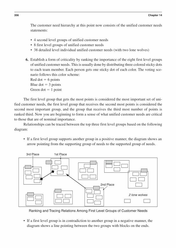
The customer need hierarchy at this point now consists of the unified customer needsstatements:
• 4 second level groups of unified customer needs• 8 first level groups of unified customer needs• 38 detailed level individual unified customer needs (with two lone wolves)
6. Establish a form of criticality by ranking the importance of the eight first level groupsof unified customer needs. This is usually done by distributing three colored sticky dotsto each team member. Each person gets one sticky dot of each color. The voting sce-nario follows this color scheme:Red dot 6 pointsBlue dot 3 pointsGreen dot 1 point
The first level group that gets the most points is considered the most important set of uni-fied customer needs, the first level group that receives the second most points is considered thesecond most important group, and the group that receives the third most number of points isranked third. Now you are beginning to form a sense of what unified customer needs are criticalto those that are of nominal importance.
Relationships can be traced between the top three first level groups based on the followingdiagram:
• If a first level group supports another group in a positive manner, the diagram shows anarrow pointing from the supporting group of needs to the supported group of needs.
356 Chapter 14
2 lone wolves
3rd Place 1st Place
2nd Place
Ranking and Tracing Relations Among First Level Groups of Customer Needs
• If a first level group is in contradiction to another group in a negative manner, thediagram shows a line pointing between the two groups with blocks on the ends.

The final processing step on the unified customer needs is the beginning of the Critical Parame-ter Management process. Now the team looks at each detailed unified customer need and assessesthe need to see if it is new, unique, or difficult. This time, though, you visit your key customersand review these results with them. The following example shows NUD customer needs high-lighted in black.
Gathering and Processing the Voice of the Customer: Customer Interviewing and the KJ Method 357
2 lone wolves
New, Unique, and Difficult Customer Needs
Get the customers to rank (on a scale of 1 to 10) the strength of importance for each need.Also, have the customer rank (on a scale of 1 to 5) the current fulfillment of these needs by yourcurrent product and their perception of how the competitive offerings on the market are fulfillingthese needs. This data will be needed during QFD.
The outcome is a set of ranked, NUD unified customer needs that are worth taking into the QFDprocess. All other unified customer needs that are of nominal importance (old, common, and easy) are directly translated into technical requirements and placed in the system requirements document.
Quantify the importance of each NUD customer need by reviewing KJ diagram results with key customers.
Gather data to quantify the quality loss function for appropriate, critical customer needs.
While the team is visiting a selected set of key customers to validate and rank the KJ results, it isan excellent opportunity for one last interview. This one centers on gathering the data necessaryto quantify Taguchi’s quality loss function:
A0: the dollar loss at the customer’s “fail-to-satisfy” tolerance limits
0: the customer’s “fail-to-satisfy” tolerance limits

The loss (A0) is usually quantified in warranty dollars, cost of poor quality, and any formof cost that accrues due to the product performing off target at or beyond the fail-to-satisfy toler-ance limits.
Some other typical situations that figure into repairing or replacing a product are:
• Loss due to lack of access to the product during repair• The cost of parts and labor needed to make the repair• The costs of transporting the product to a repair center
Regardless of who pays for the losses—the customer, the manufacturer, or a third party—all losses should be included in A0. Substituting for k in the quality loss function L(y) k(y-m)2,we define the general form of the quality loss function as:
L(y) A0/20 (y-m)2
358 Chapter 14
Document NUD customer needs and importance value (1–10) in the Critical Parameter Management database.
We are at the end of the VOC gathering and processing tasks. The final act is to document theNUD customer needs in the Critical Parameter Management relational database. This data willsoon be linked to the system, subsystem, subassembly, component, and manufacturing processrequirements and critical parameters. It is essential for the product development teams to be ableto trace their critical parameters back to the NUD VOC needs that they are fulfilling. These teamsnow know exactly what lies at the root of their requirements and the critical parameters they aredeveloping and measuring to satisfy their customers.
Final Detailed Outputs
NUD VOC needs flow into quality function deployment and construction of the Houses of Quality.
The next process downstream of gathering and processing the VOC is quality function deploy-ment. The results of this VOC process flow directly into the Houses of Quality, which are devel-oped in the QFD process. Remember that we only take the NUD customer needs into QFD. If wetry to take all customer needs through the Houses of Quality, it will be too much information andthe team will bog down and waste its time. Only needs that are new, unique, and difficult areworth processing further during QFD.

VOC Gathering and Processing Checklist and Scorecard
This suggested format for a checklist can be used by a product planning team to help plan its workand aid in the detailed construction of a PERT or Gantt chart for project management of the tasksfor the process of gathering and processing the VOC within the first phase of the CDOV or I2DOVdevelopment processes. These items also serve as a guide to the key items for evaluation withina formal gate review.
Checklist for VOC Gathering and Processing
Was this Excellence Rating:Action Deployed? 1 Poor
Actions: YES or NO 10 Excellent
1. Determine purpose of customer visit. Why are we going? ______ ______
2. Identify objectives for customer visit. What do we want to learn? ______ ______
3. Develop customer selection matrix.Who could best inform us? ______ ______
4. Create customer visit teams. Who goes where? ______ ______
5. Create discussion/interview guide based on objectives. ______ ______
6. Interview and observe customers to gather their “voices” and “images” that represent their specific needs. ______ ______
7. Develop “images of need,” common image of customers’environment and needs. Create image KJ diagram. ______ ______
8. Categorize image KJ needs into specific need statements that are new, unique, or difficult vs. routine. ______ ______
9. Develop “significant voices of need,” common voices of customers’ stated needs. ______ ______
10. Using a translation worksheet, link voices to related images, write, and identify unified customer needs. ______ ______
11. Take the full set of unified customer needs (translated voices and images) and create a KJ diagram for thesecustomer needs. ______ ______
12. Quantify the importance of each NUD customer need by reviewing KJ diagram results with key customers. ______ ______
13. Gather data to quantify the quality loss function for appropriate, critical customer needs. ______ ______
14. Document NUD customer needs and importance value (1–10) in the Critical Parameter Management database. ______ ______
Gathering and Processing the Voice of the Customer: Customer Interviewing and the KJ Method 359
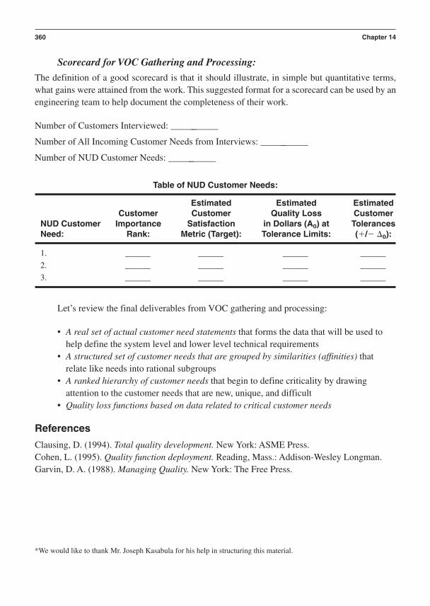
Scorecard for VOC Gathering and Processing:
The definition of a good scorecard is that it should illustrate, in simple but quantitative terms,what gains were attained from the work. This suggested format for a scorecard can be used by anengineering team to help document the completeness of their work.
Number of Customers Interviewed: ___________
Number of All Incoming Customer Needs from Interviews: ___________
Number of NUD Customer Needs: ___________
Table of NUD Customer Needs:
Estimated Estimated EstimatedCustomer Customer Quality Loss Customer
NUD Customer Importance Satisfaction in Dollars (A0) at Tolerances Need: Rank: Metric (Target): Tolerance Limits: (/ 0):
1. ______ ______ ______ ______
2. ______ ______ ______ ______
3. ______ ______ ______ ______
Let’s review the final deliverables from VOC gathering and processing:
• A real set of actual customer need statements that forms the data that will be used tohelp define the system level and lower level technical requirements
• A structured set of customer needs that are grouped by similarities (affinities) thatrelate like needs into rational subgroups
• A ranked hierarchy of customer needs that begin to define criticality by drawingattention to the customer needs that are new, unique, and difficult
• Quality loss functions based on data related to critical customer needs
References
Clausing, D. (1994). Total quality development. New York: ASME Press.Cohen, L. (1995). Quality function deployment. Reading, Mass.: Addison-Wesley Longman.Garvin, D. A. (1988). Managing Quality. New York: The Free Press.
360 Chapter 14
*We would like to thank Mr. Joseph Kasabula for his help in structuring this material.

C H A P T E R 1 5
Quality Function Deployment:The Houses of Quality
Where Am I in the Process? Where Do I Apply QFD Within the Roadmaps?
Linkage to the I2DOV Technology Development Roadmap:
361
Invent/Innovate
Develop Optimize Verify
Concept Design Optimize Verify
QFD is conducted within the Invent/Innovate phase during technology development. It is appliedto translate, align, and quantitatively rank the relationships between the new, unique, and diffi-cult voice of the customer needs and new, unique, and difficult technology requirements.
Linkage to the CDOV Product Development Roadmap:
QFD is conducted within the Concept (at the system level) and Design (down at the subsystem,subassembly, component, and manufacturing process levels) phases during product development.Here we apply QFD to a specific product within the family plan from the strategic product port-folio. This application of QFD assures that the new, unique, and difficult needs are translated intothe new, unique, and difficult requirements for the new product being developed.
What Am I Doing in the Process? What Does QFD Do at this Point in the Roadmaps?
The Purpose of QFD in the I2DOV Technology Development Roadmap:
Once again we need to show the strategic flow-down of how a business develops new productconcepts:
Define business strategy: Profit goals and requirements
Identify markets and market segments: Value generation and requirements
Gather long-term voice of customer and voice of technology trends
Develop product line strategy: Family plan requirements
Develop/deploy technology strategy: Technology and subsystem platform requirements
Gather product-specific VOC and VOT: New, unique, and difficult needs
Conduct KJ analysis: Structure and rank the NUD VOC needs
Build system House of Quality: Translate NUD VOC needs
Document system requirements: Create system requirements document
Define the system functions: Modeling
Generate candidate system architectures: Concept generation
Select the superior system concept: Pugh concept selection process
In the Invent/Innovate Phase of the I2DOV process we build the system House of Qual-ity to establish the requirements that are new, unique, or difficult. The technology developmentteam then translates the new, unique, or difficult customer needs and technology requirementsthat flow down to subsystem, subassembly, components, and manufacturing processes Houses ofQuality. Unlike the CDOV process, all Houses of Quality are derived in Phase 1 of the I2DOVprocess. The technology requirements that are defined in these Houses of Quality should be ca-pable of fulfilling the product line strategy. The technology requirements are used to help definea set of adjustable or tunable functions. A unique set of architectural concepts known as platformscan then be developed to fulfill these functions over their range of projected product family planapplications. After careful evaluation, one superior platform architecture will be selected out ofthe numerous options to go through the rest of the I2DOV process. The value in such an approachis the investment of capital in a platform that can serve as a foundation for a family of productsover a number of models and years. One investment—many products!
The Purpose of QFD in the CDOV Product Development Roadmap:
In the CDOV process we build the system House of Quality to translate the new, unique, anddifficult customer and technology needs into new, unique, and difficult requirements that are re-lated to the specific product being developed out of the product family plan. The product designteam builds the system House of Quality to rank importance and set targets for these product-
362 Chapter 15

specific requirements. The system (product level) requirements should be capable of fulfilling thisspecific product’s contribution to the product line strategy. The system requirements are used todefine a set of product functions. Numerous system architectural concepts can then be developedto fulfill the product functions. After careful evaluation, one superior system architecture (basedon the underlying platform) is selected out of the numerous options to go through the rest of theCDOV process. This product is but one of several that will be sequentially developed to fulfillthe product line strategy, based on the platform developed in the I2DOV process. SubsequentHouses of Quality are developed for the subsystems, subassemblies, components, and manufac-turing processes during Phase 2 (design) of the CDOV process. They define the NUD require-ments at these respective levels within the system hierarchy.
What Output Do I Get at the Conclusion of this Phase of the Process? What Are Key Deliverables from QFD at this Point in the Roadmaps?
• Translated VOC needs that are now documented as technology or system (productlevel) requirements for what is considered new, unique, and difficult
• NUD subsystem, subassembly, component, and manufacturing processrequirements from their respective Houses of Quality
• Customer-based ranking of NUD needs (down to all appropriate levels within thesystem)
• Engineering team-based ranking of NUD requirements (down to all appropriatelevels within the system)
• Critical Parameter Management data that is documented in the CPM relationaldatabase:• Flow-down and linkage of all NUD requirements (down to all appropriate levels
within the platform or system)• NUD requirement targets (with appropriate units of measure)• NUD requirement tolerances (estimated values from VOC data)• NUD requirement synergies and conflicts (from the “roof”)• Customer and engineering benchmark values for NUD needs and requirements
QFD Process Flow Diagram (found on page 364)
This visual reference of the detailed steps of quality function deployment illustrates the flow ofprocesses and responsibilities.
Verbal Descriptions for the Application of Each Block Diagram
This section details each step on the QFD process diagram:
• Key detailed input(s) from preceding tools and best practices• Specific steps and deliverables from each step to the next within the process flow• Final detailed outputs that flow into follow-on tools and best practices
Quality Function Deployment: The Houses of Quality 363

Key Detailed Inputs
Structured and ranked NUD VOC needs from KJ diagram
With the specific new, unique, and difficult voice of the customer needs defined, the team knowsexactly what customers want. Now we need to translate the whats into hows that take the formof system level technical requirements.
364 Chapter 15
INPUT . . .
OUTPUT . . .
Structured and rankedNUD VOC needsfrom KJ diagram.
Translate each NUDcustomer need into a
system level requirement.
Quantify the strength of therelationship between each
VOC need to eachrequirement (9, 3, 1, or 0).
Quantify the strength of therelationship between eachpair of NUD system level
requirements(+ or – 9, 3, 1, or 0).
Quantify and document thecapability of your
competitors to currentlyfulfill each system level
requirement.
Quantify and documentyour current capability tofulfill each system level
requirement.
Identify the direction ofoptimum satisfaction for
each system levelrequirement (smaller, larger,
or target is better).
Define the new target value and theestimated tolerance limits for each system
level requirement.
Define the appropriate unit of measurefor each system level requirement.
Link and channel NUD systemrequirements to develop the appropriate
subsystem level Houses of Quality.
Link and channel NUD subsystemrequirements to develop the appropriate
subassembly level Houses of Quality.
Link and channel NUD subassemblyrequirements to develop the appropriate
component level Houses of Quality.
Link and channel NUD componentrequirements to develop the appropriate
manufacturing process level Housesof Quality.
Document and link all NUD requirements,targets, and tolerance limits in the Critical
Parameter Management database.
NUD hierarchy of requirements, targets,and tolerances used along with other
important requirements in definingfunctions, concept generation, and the
Pugh concept selection process.

Specific Steps and Deliverables
Translate each NUD customer need into a system level requirement.
We are ready to continue the Phase 1 process of developing customer needs into either technol-ogy or product-specific technical requirements. The term translating is commonly used when dis-cussing how a need (what) is converted into a requirement (how). We must be careful whentalking about requirements in terms of “how” a need is met. It is premature to be thinking abouthow a need is physically, architecturally, or conceptually met, but it is not too early to define howa need is measured in terms of fulfillment! So, don’t think that we are talking about “how” interms of design concepts and form/fit architectures; that comes later during the concept genera-tion process. Requirements are specific terms that must be carefully structured to convey the rightfunctional and feature performance information to the product design and technology develop-ment teams.
The biggest mistake one can make in stating a requirement is to structure the words in amanner that suggests or forces one specific solution or fulfilling concept. If your system level re-quirements state solutions, they are not correct. In fact, they are corrupting your ability to be cre-ative. A properly worded requirement suggests a measurable function that can be fulfilled in manydifferent ways. A good requirement will provoke many concepts or fulfilling architectures as can-didate means to be measured as they fulfill the requirement! If your organization includes a “con-cept tyrant” who forces everyone to consider just one concept—his or hers—you need to declarea revolution toward a concept democracy. More on that issue later.
Here’s an example of how a system level requirement can be poorly and properly worded:
• A poor system requirement: Car acoustic damping materials must be able to maintaininternal acoustic noise level at or below 75dBA. (This is too prescriptive; in fact, it isactually a component requirement!)
• A proper system requirement: Internal car acoustic noise level must not exceed 75dBAunder any set of driving environmental conditions. (This is appropriately descriptive,easy to see how to measure if you have met the requirement apart from any concept.)
Quality Function Deployment: The Houses of Quality 365
Technical Requirements
Ranked New,Unique, and
DifficultCustomer
Needs
Relationships BetweenNUD Customer Needs
andTechnical Requirements
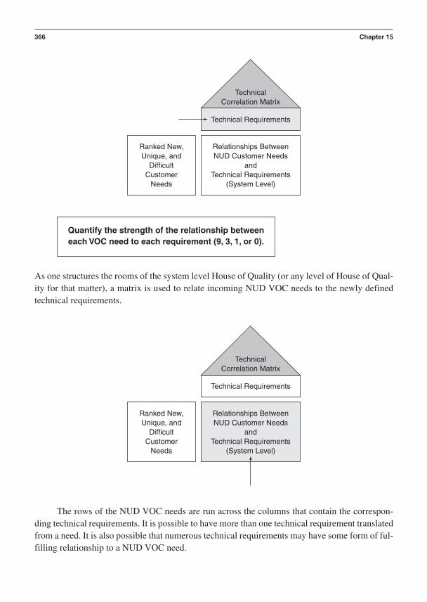
As one structures the rooms of the system level House of Quality (or any level of House of Qual-ity for that matter), a matrix is used to relate incoming NUD VOC needs to the newly definedtechnical requirements.
366 Chapter 15
Technical Requirements
Ranked New,Unique, and
DifficultCustomer
Needs
Relationships BetweenNUD Customer Needs
andTechnical Requirements
(System Level)
TechnicalCorrelation Matrix
Technical Requirements
Ranked New,Unique, and
DifficultCustomer
Needs
Relationships BetweenNUD Customer Needs
andTechnical Requirements
(System Level)
TechnicalCorrelation Matrix
The rows of the NUD VOC needs are run across the columns that contain the correspon-ding technical requirements. It is possible to have more than one technical requirement translatedfrom a need. It is also possible that numerous technical requirements may have some form of ful-filling relationship to a NUD VOC need.
Quantify the strength of the relationship between each VOC need to each requirement (9, 3, 1, or 0).

Once the needs are aligned with the requirements, numerical values are assigned to quan-tify the strength of the relationship that exists between the two statements:
9 A strong fulfilling relationship between need and requirement
3 A moderate fulfilling relationship between need and requirement
1 A weak fulfilling relationship between need and requirement
0 No relationship between need and requirement
Quality Function Deployment: The Houses of Quality 367
Technical Requirements
Ranked New,Unique, and
DifficultCustomer
Needs
9 19
3 3 9
9
3 9
319
1 9 1 3
1 3
1 3 131
3
TechnicalCorrelation Matrix
Relationships BetweenNUD Customer Needs
andTechnical Requirements
These values help establish which technical requirements are critical versus those that areof nominal importance. All NUD technical requirements must be fulfilled, but a few will emergeas the highest priority. Requirements that are particularly difficult to fulfill but are critical to cus-tomer satisfaction must be given the highest attention. They receive the resources necessary to as-sure they are fulfilled. Other requirements may need to yield.
Quantify the strength of the relationship between each pair of NUD system level requirements ( or 9, 3, 1 or 0).
Every set of requirements developed to focus the application of tools, best practices, and an or-ganization’s material and human resources contains synergies and contradictions.
We turn our attention to the technical requirements themselves. You might compare theserequirements to a family. Every family has its tensions, disagreements, and “black sheep.” The roof of the House of Quality is used to numerically quantify both positive ( 9, 3, and 1),

supportive relationships (synergistic interactions) and negative (9, 3, and 1) relationships(antisynergistic interactions). Since we are working with new, unique, and difficult (the blacksheep) requirements, we need to carefully prescreen the requirements to assess where conflictsexist. Unintentional conflicts are frequently designed into new products. These functional con-flicts are called antisynergistic interactions between the control factors within the design as wellas antisynergistic interactions between control factors and noise factors. The problem stems fromdysfunctional performance as two design elements attempt to provide their individual contribu-tion to the design. Because of codependency or some form of physical linkage between the twoengineering control factors, the measured function of the design is different than what is desired.This relationship is called sensitivity and can extend to include poorly behaved relationships be-tween control and noise factors.
The reason we are concerned with these functional codependencies and sensitivities now isbecause this is where many of them are unintentionally created. When conflicting requirementsare allowed to flow down into the concepts that comprise the detailed design elements, a designdefect is born.
We need to address the sensitivities and conflicting relationships at the requirement levelso that the designs developed to fulfill them are as synergistic as possible. As you may have heard,“a house divided against itself cannot stand.”
The roof will identify the synergies and conflicts. Once they are brought to the team’s at-tention, the hard work of creating a set of synergistic, harmonic requirements can then go forward.
368 Chapter 15
Technical Requirements
TechnicalCorrelation Matrix
/ 9 A strong (/) relationship exists between the requirements
/3 A moderate (/) relationship exists between the requirements
/1 A weak (/) relationship exists between the requirements
0 No relationship exists between the requirements
Quantify and document the capability of your competitors to currently fulfill each system level requirement.
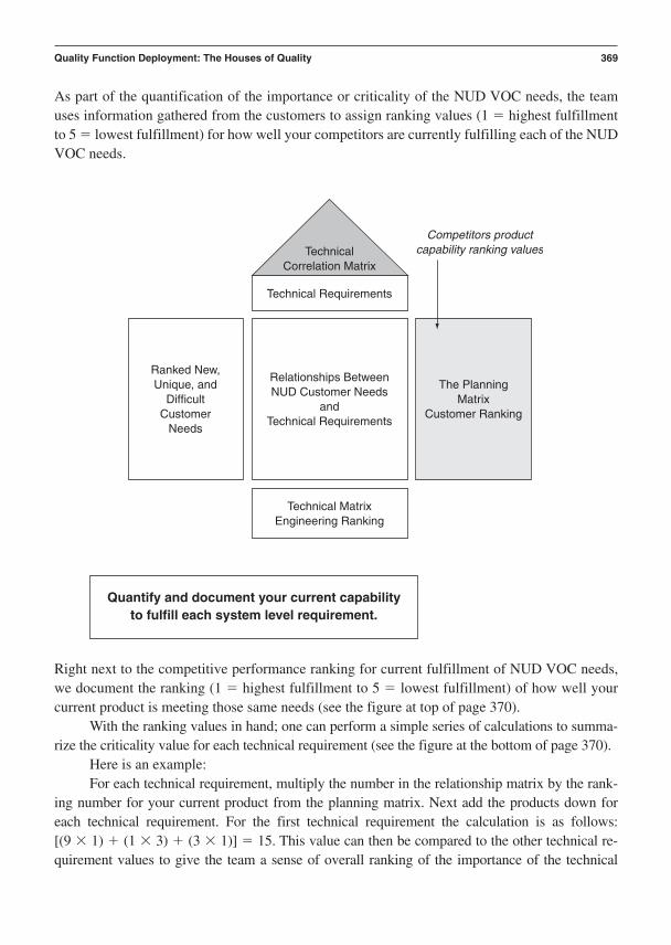
As part of the quantification of the importance or criticality of the NUD VOC needs, the teamuses information gathered from the customers to assign ranking values (1 highest fulfillmentto 5 lowest fulfillment) for how well your competitors are currently fulfilling each of the NUDVOC needs.
Quality Function Deployment: The Houses of Quality 369
Technical Requirements
Competitors productcapability ranking values
Technical MatrixEngineering Ranking
Ranked New,Unique, and
DifficultCustomer
Needs
The PlanningMatrix
Customer Ranking
TechnicalCorrelation Matrix
Relationships BetweenNUD Customer Needs
andTechnical Requirements
Right next to the competitive performance ranking for current fulfillment of NUD VOC needs,we document the ranking (1 highest fulfillment to 5 lowest fulfillment) of how well yourcurrent product is meeting those same needs (see the figure at top of page 370).
With the ranking values in hand; one can perform a simple series of calculations to summa-rize the criticality value for each technical requirement (see the figure at the bottom of page 370).
Here is an example:For each technical requirement, multiply the number in the relationship matrix by the rank-
ing number for your current product from the planning matrix. Next add the products down for each technical requirement. For the first technical requirement the calculation is as follows: [(9 1) (1 3) (3 1)] 15. This value can then be compared to the other technical re-quirement values to give the team a sense of overall ranking of the importance of the technical
Quantify and document your current capability to fulfill each system level requirement.

370
Technical Requirements
Your current productcapability ranking values
Technical MatrixEngineering Ranking
Ranked New,Unique, and
DifficultCustomer
Needs
The PlanningMatrix
Customer Ranking
TechnicalCorrelation Matrix
Relationships BetweenNUD Customer Needs
andTechnical Requirements
Technical Requirements
Ranked New,Unique, and
DifficultCustomer
Needs
Technical RequirementRanking
The Planning MatrixCustomer Ranking
Your Current Performance Ranks
Competitive Performance Ranks
9 19
3 3 9
9
3 9
319
1 9 1 3
1 3
1 35 3 2 13 1 2 42 3 2 33 2 3 45 5 1 54 4 2 32 4 5 42 3 4 34 3 4 12 2 2 23 4 1 5
131
3
15
TechnicalCorrelation Matrix
Relationships BetweenNUD Customer Needs
andTechnical Requirements
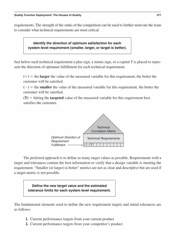
requirements. The strength of the ranks of the competition can be used to further motivate the teamto consider what technical requirements are most critical.
Quality Function Deployment: The Houses of Quality 371
Technical RequirementsOptimum Direction ofRequirementFulfillment + – T
TechnicalCorrelation Matrix
The preferred approach is to define as many target values as possible. Requirements with atarget and tolerances contain the best information to verify that a design variable is meeting therequirement. “Smaller (or larger) is better” metrics are not as clear and descriptive but are used ifa target metric is not possible.
Identify the direction of optimum satisfaction for each system level requirement (smaller, larger, or target is better).
Just below each technical requirement a plus sign, a minus sign, or a capital T is placed to repre-sent the direction of optimum fulfillment for each technical requirement.
() the larger the value of the measured variable for this requirement, the better thecustomer will be satisfied.
() the smaller the value of the measured variable for this requirement, the better thecustomer will be satisfied.
(T) hitting the targeted value of the measured variable for this requirement bestsatisfies the customer.
Define the new target value and the estimated tolerance limits for each system level requirement.
The fundamental elements used to define the new requirement targets and initial tolerances areas follows:
1. Current performance targets from your current product2. Current performance targets from your competitor’s product

3. Improvements desired by your customers (NUD needs)4. New technologies that you have developed that can “delight” customers with unantic-
ipated performance (that is, improved or advanced performance)
These four items can provide great insight as to what your requirement targets should be.They assure you reach for rational, balanced performance in a competitive context.
372 Chapter 15
Technical Requirements
New Targets forthe Requirements
Technical MatrixEngineering Ranking
Ranked New,Unique, and
DifficultCustomer
Needs
The PlanningMatrix
Customer Ranking
TechnicalCorrelation Matrix
Relationships BetweenNUD Customer Needs
andTechnical Requirements
Define the appropriate unit of measure for each system level requirement.
Each technical requirement must have a well-defined unit of measure. It is preferable to expressthe units of measure as some form of continuous variable (a scalar or vector).
Link and channel NUD system requirements to develop the appropriate subsystem level Houses of Quality.

Once the system level House of Quality is defined, it is now possible to use the system level tech-nical requirements as inputs to the various subsystem level Houses of Quality. Each subsystemlevel House of Quality illustrates and quantifies the relationships between the appropriate systemlevel requirements and the subsystem requirements. NUD VOC needs that relate directly to a spe-cific subsystem can also be used as inputs to the subsystem House of Quality.
The subsystem House of Quality is constructed in the same manner as a system House ofQuality. The main difference is that the input is technical in nature and the challenge now is totranslate system requirements into subsystem requirements, relationship and importance rankingvalues, as well as subsystem requirement targets. The planning matrix is typically not requireddown at the lower level Houses of Quality (see figure at the top of page 374).
Quality Function Deployment: The Houses of Quality 373
Technical Requirements
Technical RequirementTarget Units
Ranked New,Unique, and
DifficultCustomer
Needs
The PlanningMatrix
Customer Ranking
TechnicalCorrelation Matrix
Relationships BetweenNUD Customer Needs
andTechnical Requirements
Technical MatrixEngineering Ranking
Link and channel NUD Subsystem requirements to develop the appropriate subassembly level Houses of Quality.
Once the subsystem level Houses of Quality are defined, it is now possible to use the subsystemlevel technical requirements as inputs to the various subassembly level Houses of Quality. Eachsubassembly level House of Quality illustrates and quantifies the relationships between the ap-propriate subsystem level requirements and the subassembly requirements. NUD VOC needs thatrelate directly to a specific subassembly can also be used as inputs to the subassembly House of

374
SubsystemTechnical Requirements
SystemTechnical
Requirements
TechnicalCorrelation Matrix
Relationships BetweenSystem Requirements
andSubsystem Requirements
Technical MatrixEngineering Ranking
SubassemblyTechnical Requirements
SubsystemTechnical
Requirements
TechnicalCorrelation Matrix
Relationships BetweenSubsystem Requirements
andSubassemblyRequirements
Technical MatrixEngineering Ranking
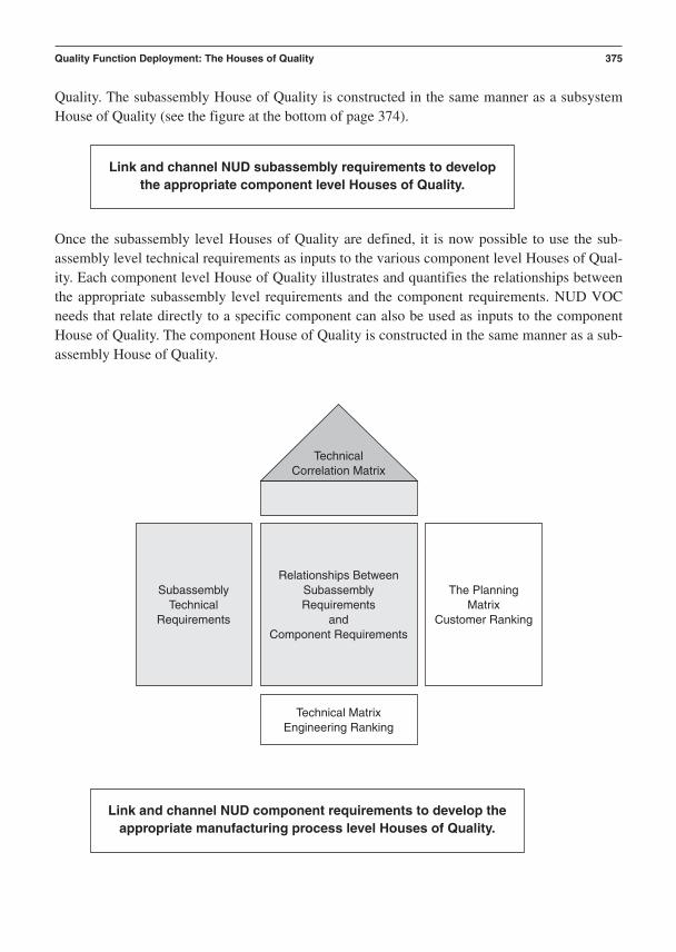
Quality. The subassembly House of Quality is constructed in the same manner as a subsystemHouse of Quality (see the figure at the bottom of page 374).
Quality Function Deployment: The Houses of Quality 375
Technical MatrixEngineering Ranking
SubassemblyTechnical
Requirements
The PlanningMatrix
Customer Ranking
TechnicalCorrelation Matrix
Relationships BetweenSubassemblyRequirements
andComponent Requirements
Link and channel NUD component requirements to develop the appropriate manufacturing process level Houses of Quality.
Link and channel NUD subassembly requirements to develop the appropriate component level Houses of Quality.
Once the subassembly level Houses of Quality are defined, it is now possible to use the sub-assembly level technical requirements as inputs to the various component level Houses of Qual-ity. Each component level House of Quality illustrates and quantifies the relationships betweenthe appropriate subassembly level requirements and the component requirements. NUD VOCneeds that relate directly to a specific component can also be used as inputs to the componentHouse of Quality. The component House of Quality is constructed in the same manner as a sub-assembly House of Quality.

Once the component level Houses of Quality are defined, it is now possible to use the componentlevel technical requirements as inputs to the various manufacturing process level Houses of Qual-ity. Each manufacturing process level House of Quality illustrates and quantifies the relationshipsbetween the appropriate component level requirements and the manufacturing process Require-ments. The manufacturing process House of Quality is constructed in the same manner as a com-ponent House of Quality.
376 Chapter 15
Technical MatrixEngineering Ranking
Manufacturing ProcessTechnical Requirements
ComponentTechnical
Requirements
The PlanningMatrix
Customer Ranking
TechnicalCorrelation Matrix
Relationships BetweenComponent Requirements
andManufacturing Process
Requirements
The Critical Parameter Management relational database can now have all the levels of require-ments loaded into it. We now have the following structure defined, with the many-to-many rela-tionships between the ranked requirements linked for traceability:
1. NUD VOC needs2. System level requirements, targets, and tolerances3. Subsystem level requirements, targets, and tolerances4. Subassembly level requirements, targets, and tolerances5. Component level requirements, targets, and tolerances6. Manufacturing process level requirements, targets, and tolerances
Document and link all NUD requirements, targets, and tolerance limits in the Critical Parameter Management database.

The roofs and relationship matrices from the Houses tell us what requirements are to belinked in the CPM database.
The next set of entries for the Critical Parameter Management database will be the criticalparameters in the form of CFRs, critical adjustment parameters, critical functional parameters,critical-to-function specifications and their hierarchy of linked transfer functions.
Final Detailed Outputs
Quality Function Deployment: The Houses of Quality 377
The deliverables from the QFD process flow into the process of defining critical requirements,their fulfilling functions, generation of numerous concepts to fulfill the critical functions, and fi-nally the Pugh concept selection process.
QFD Checklist and Scorecards
This suggested format for a checklist can be used by an engineering team to help plan its workand aid in the detailed construction of a PERT or Gantt chart for project management of the QFDprocess within the first two phases of the CDOV or the first phase of the I2DOV developmentprocess. These items will also serve as a guide to the key items for evaluation within a formal gatereview.
Checklist for QFD
Was this Excellence Rating:Action Deployed? 1 Poor
Actions: YES or NO 10 Excellent
1. Structured and ranked NUD VOC needs from KJ diagram. ______ ______
2. Translate each NUD customer need into a system level requirement. ______ ______
3. Quantify the strength of the relationship between each VOC need to each requirement (9, 3, 1, or 0). ______ ______
4. Quantify the strength of the relationship between each pair of NUD system level VOC requirements ( or 9, 3, 1 or 0) and technical requirements. ______ ______
5. Quantify strength of relationships between the requirements. ______ ______
NUD hierarchy of requirements, targets, and tolerances used along with other important requirements in defining functions, concept
generation, and the Pugh concept selection process.
(continued)

6. Quantify and document the capability of your competitors to currently fulfill each system level requirement. ______ ______
7. Quantify and document your current capability to fulfill each system level requirement. ______ ______
8. Identify the direction of optimum satisfaction for each system level requirement (smaller, larger, or target is better). ______ ______
9. Define the new target value and the estimated tolerance limits for each system level requirement. ______ ______
10. Define the appropriate unit of measure for each system level requirement. ______ ______
11. Link and channel NUD system requirements to develop the appropriate subsystem level Houses of Quality. ______ ______
12. Link and channel NUD subsystem requirements to develop the appropriate subassembly level Houses of Quality. ______ ______
13. Link and channel NUD subassembly requirements to develop the appropriate component level Houses of Quality. ______ ______
14. Link and channel NUD component requirements to develop the appropriate manufacturing process level Houses of Quality. ______ ______
15. Document and link all NUD requirements, targets, and tolerance limits in the Critical Parameter Management database. ______ ______
16. NUD hierarchy of requirements, targets, and tolerances used along with other important requirements in defining functions,concept generation, and the Pugh concept selection process. ______ ______
Scorecard for QFD
The definition of a good QFD scorecard is that it should illustrate, in simple but quantitativeterms, what gains were attained from the work.
This is a suggested format for a scorecard that can be used by a product planning team tohelp document the completeness of its work.
Total number of system level technical requirements: __________
Total number of subsystem level technical requirements: __________
Total number of subassembly level technical requirements: __________
Total number of component level technical requirements: __________
Total number of manufacturing process level technical requirements: __________
Number of NUD system level technical requirements: __________
Number of NUD subsystem level technical requirements: __________
378 Chapter 15

Number of NUD subassembly level technical requirements: __________
Number of NUD component level technical requirements: __________
Number of NUD manufacturing process level technical requirements: __________
Table of NUD (Critical) System Level Requirements
SystemRequirement Estimated Estimated Unit of Name: Target: Tolerance: USL Tolerance: LSL Measure:
1. ______ ______ ______ ______
2. ______ ______ ______ ______
3. ______ ______ ______ ______
Table of NUD (Critical) Subsystem Level Requirements:
SubsystemRequirement Estimated Estimated Unit of Name: Target: Tolerance: USL Tolerance: LSL Measure:
1. ______ ______ ______ ______
2. ______ ______ ______ ______
3. ______ ______ ______ ______
Table of NUD (Critical) Subassembly Level Requirements:
SubassemblyRequirement Estimated Estimated Unit of Name: Target: Tolerance: USL Tolerance: LSL Measure:
1. ______ ______ ______ ______
2. ______ ______ ______ ______
3. ______ ______ ______ ______
Table of NUD (Critical) Component Level Requirements:
ComponentRequirement Estimated Estimated Unit of Name: Target: Tolerance: USL Tolerance: LSL Measure:
1. ______ ______ ______ ______
2. ______ ______ ______ ______
3. ______ ______ ______ ______
Quality Function Deployment: The Houses of Quality 379
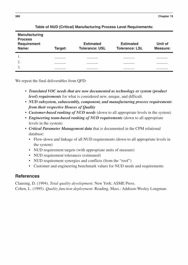
Table of NUD (Critical) Manufacturing Process Level Requirements:
ManufacturingProcessRequirement Estimated Estimated Unit of Name: Target: Tolerance: USL Tolerance: LSL Measure:
1. ______ ______ ______ ______
2. ______ ______ ______ ______
3. ______ ______ ______ ______
We repeat the final deliverables from QFD:
• Translated VOC needs that are now documented as technology or system (productlevel) requirements for what is considered new, unique, and difficult.
• NUD subsystem, subassembly, component, and manufacturing process requirementsfrom their respective Houses of Quality
• Customer-based ranking of NUD needs (down to all appropriate levels in the system)• Engineering team-based ranking of NUD requirements (down to all appropriate
levels in the system)• Critical Parameter Management data that is documented in the CPM relational
database:• Flow-down and linkage of all NUD requirements (down to all appropriate levels in
the system)• NUD requirement targets (with appropriate units of measure)• NUD requirement tolerances (estimated)• NUD requirement synergies and conflicts (from the “roof”)• Customer and engineering benchmark values for NUD needs and requirements
References
Clausing, D. (1994). Total quality development. New York: ASME Press.Cohen, L. (1995). Quality function deployment. Reading, Mass.: Addison-Wesley Longman.
380 Chapter 15

C H A P T E R 1 6
Concept Generation and Designfor x Methods
Where Am I in the Process? Where Do I Apply Concept Generation and DFxWithin the Roadmaps?
Linkage to the I2DOV Technology Development Roadmap:
381
Invent/Innovate
Develop Optimize Verify
Concept Design Optimize Verify
Concepts are generated within the Invent/Innovate phase while design for x (DFx) methods areapplied within the Develop phase during technology development.
Linkage to the CDOV Product Development Roadmap:
Concept generation is conducted within the Concept and Design phases during product develop-ment. Design for x methods are applied in the Design phase.
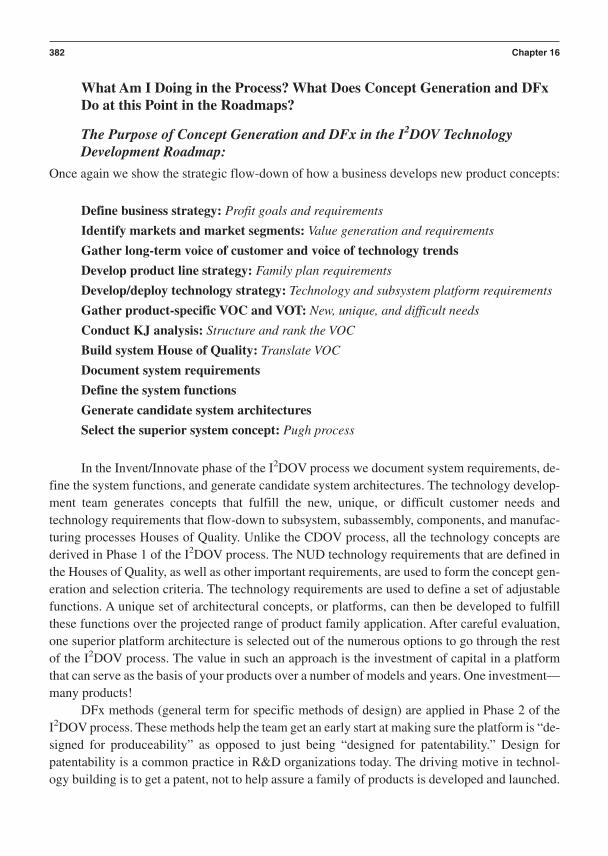
What Am I Doing in the Process? What Does Concept Generation and DFxDo at this Point in the Roadmaps?
The Purpose of Concept Generation and DFx in the I2DOV TechnologyDevelopment Roadmap:
Once again we show the strategic flow-down of how a business develops new product concepts:
Define business strategy: Profit goals and requirements
Identify markets and market segments: Value generation and requirements
Gather long-term voice of customer and voice of technology trends
Develop product line strategy: Family plan requirements
Develop/deploy technology strategy: Technology and subsystem platform requirements
Gather product-specific VOC and VOT: New, unique, and difficult needs
Conduct KJ analysis: Structure and rank the VOC
Build system House of Quality: Translate VOC
Document system requirements
Define the system functions
Generate candidate system architectures
Select the superior system concept: Pugh process
In the Invent/Innovate phase of the I2DOV process we document system requirements, de-fine the system functions, and generate candidate system architectures. The technology develop-ment team generates concepts that fulfill the new, unique, or difficult customer needs andtechnology requirements that flow-down to subsystem, subassembly, components, and manufac-turing processes Houses of Quality. Unlike the CDOV process, all the technology concepts arederived in Phase 1 of the I2DOV process. The NUD technology requirements that are defined inthe Houses of Quality, as well as other important requirements, are used to form the concept gen-eration and selection criteria. The technology requirements are used to define a set of adjustablefunctions. A unique set of architectural concepts, or platforms, can then be developed to fulfillthese functions over the projected range of product family application. After careful evaluation,one superior platform architecture is selected out of the numerous options to go through the restof the I2DOV process. The value in such an approach is the investment of capital in a platformthat can serve as the basis of your products over a number of models and years. One investment—many products!
DFx methods (general term for specific methods of design) are applied in Phase 2 of theI2DOV process. These methods help the team get an early start at making sure the platform is “de-signed for produceability” as opposed to just being “designed for patentability.” Design forpatentability is a common practice in R&D organizations today. The driving motive in technol-ogy building is to get a patent, not to help assure a family of products is developed and launched.
382 Chapter 16

Technology is developed and patents attained, and then nothing comes of the designs. The usualproblem is that the patented technologies are simply not produceable and thus never get com-mercialized.
The Purpose of Concept Generation and DFx in the CDOV ProductDevelopment Roadmap:
In the CDOV process we document system requirements, define the system functions, and gen-erate candidate system architectures. Here the product development team generates system, sub-system, subassembly, component, and manufacturing process concepts. They are conceived tofulfill the new, unique, and difficult customer needs and technical requirements that are related tothe specific product being developed out of the family plan.
The system requirements are used to define a set of product functions. Numerous systemarchitectural concepts can then be developed to fulfill the product functions. After careful evalu-ation, one superior system architecture is selected out of the numerous options to go through therest of the CDOV process.
DFx methods are applied in Phase 2 of the CDOV process. Design for x methods ensurethat the design concepts are able to fulfill the following requirements:
Produceability (manufacturable)
Assembleability
Reliability
Serviceability (maintainable)
Environmentally friendly
Testability (measurable functions)
These attributes of a design are sometimes referred to as “design for the . . . ilities.” It is ex-tremely important to design in the attributes during the Concept and Design phases. If you try toadd these late in the product development process, the costs will be exorbitant and you will def-initely slip your schedule.
What Output Do I Get at the Conclusion of this Phase of the Process? WhatAre Key Deliverables from Concept Generation and DFx at this Point in theRoadmaps?
• Documented candidate concepts at the system level fulfilling what is considered new,unique, and difficult
• Documented candidate concepts at the subsystem, subassembly, component, andmanufacturing process levels fulfilling what is considered new, unique, and difficult
• Designs that are conceptually well rounded, both functionally and architecturally:Documented concept feasibility for produceability (manufacturable)Documented concept feasibility for assembleability
Concept Generation and Design for x Methods 383

Documented concept feasibility for reliabilityDocumented concept feasibility for serviceability (maintainable)Documented concept feasibility for environmental friendlinessDocumented concept feasibility for testability (measurable functions)
Concept Generation and DFx Process Flow Diagram
This visual reference of the detailed steps of concept generation and DFx illustrates the flow ofprocesses and responsibilities at this stage.
384 Chapter 16
INPUT . . .
OUTPUT . . .
Structured and ranked NUDrequirements from QFD and
other important requirements.
Translate each NUDsystem level requirement into
system level functions.
Generate numerous systemlevel concepts to fulfill thesystem requirements and
functions.
Apply DFx methods to thesystem concepts.
Generate numeroussubsystem level concepts to
fulfill the subsystemrequirements and functions.
Apply DFx methods to thesubsystem concepts.
Apply DFx methods to thesubassembly concepts.
Generate numeroussubassembly level concepts
to fulfill the subassemblyrequirements and functions.
Generate numerous component levelconcepts to fulfill the component
requirements and functions.
Apply DFx methods to the componentconcepts.
Generate numerous manufacturing processlevel concepts to fulfill the manufacturing
process requirements and functions.
Apply DFx methods to the manufacturingprocess concepts.
Uniformly document all candidate conceptsand store them in the CPM database.
Numerous, uniformly documented system,subsystem, subassembly, component,and manufacturing process candidateconcepts ready for the Pugh concept
selection process.

Verbal Descriptions for the Application of Each Block Diagram
In this section, we examine each step within the concept generation and DFx processes:
• Key detailed input(s) from preceding tools and best practices• Specific steps and deliverables from each step to the next within the process flow• Final detailed outputs that flow into follow-on tools and best practices
Key Detailed Inputs
Concept Generation and Design for x Methods 385
Structured and ranked NUD requirements from QFD and other important requirements.
With the specific, new, unique, and difficult requirements and other important technical and com-mercialization requirements defined, the team knows exactly how to measure the fulfillment of therequirements. Now we need to generate the form and fit architectures to fulfill the requirements.
1. Convert technical requirements to technical functions that must be engineered.2. Construct input-output-constraint diagrams for each function down through the system
hierarchy during concept generation.3. Link all ideal functions/transfer functions using functional flow diagrams.
Specific Steps and Deliverables
Translate each NUD system level requirement into system level functions.
System level technical requirements, when worded correctly, lead the team to define functionsthat must be engineered to fulfill the requirements. These functions are expressed in engineeringunits that can be measured with known transducers that can be calibrated. The result of this con-version process is the transformation of the system requirements into a complete set of measura-ble system level output functions (as shown in the figure on page 386).
The measurable system functions contain the subset of critical parameters we call systemlevel CFRs (critical functional responses). These requirement-to-function relationships can bemapped for each level down within the system architecture (subsystems, subassemblies, compo-nents, and manufacturing processes).
Generate numerous system level concepts to fulfill the system requirements and functions.
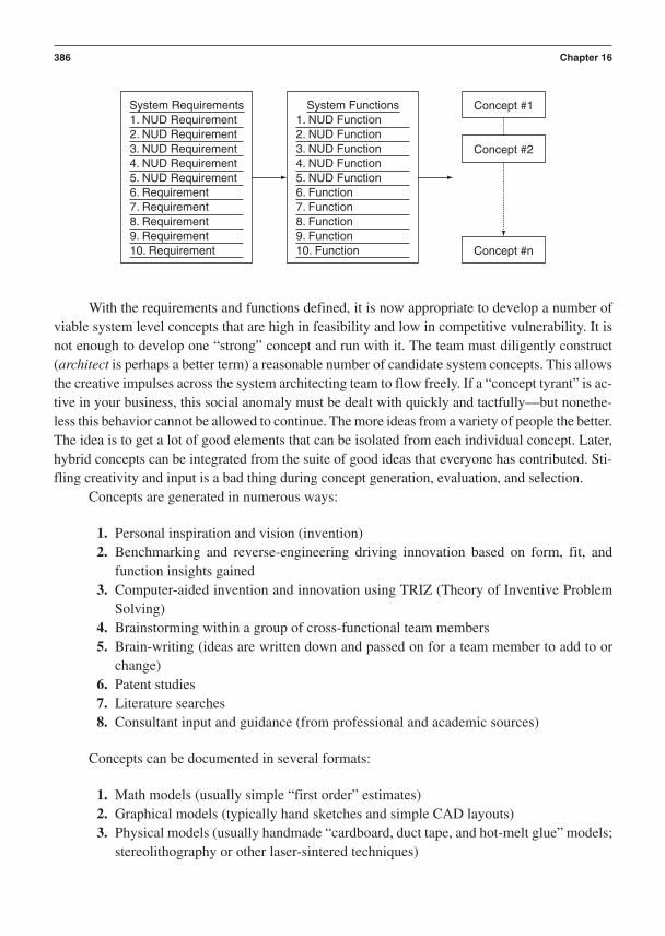
With the requirements and functions defined, it is now appropriate to develop a number ofviable system level concepts that are high in feasibility and low in competitive vulnerability. It isnot enough to develop one “strong” concept and run with it. The team must diligently construct(architect is perhaps a better term) a reasonable number of candidate system concepts. This allowsthe creative impulses across the system architecting team to flow freely. If a “concept tyrant” is ac-tive in your business, this social anomaly must be dealt with quickly and tactfully—but nonethe-less this behavior cannot be allowed to continue. The more ideas from a variety of people the better.The idea is to get a lot of good elements that can be isolated from each individual concept. Later,hybrid concepts can be integrated from the suite of good ideas that everyone has contributed. Sti-fling creativity and input is a bad thing during concept generation, evaluation, and selection.
Concepts are generated in numerous ways:
1. Personal inspiration and vision (invention)2. Benchmarking and reverse-engineering driving innovation based on form, fit, and
function insights gained3. Computer-aided invention and innovation using TRIZ (Theory of Inventive Problem
Solving)4. Brainstorming within a group of cross-functional team members5. Brain-writing (ideas are written down and passed on for a team member to add to or
change)6. Patent studies7. Literature searches8. Consultant input and guidance (from professional and academic sources)
Concepts can be documented in several formats:
1. Math models (usually simple “first order” estimates)2. Graphical models (typically hand sketches and simple CAD layouts)3. Physical models (usually handmade “cardboard, duct tape, and hot-melt glue” models;
stereolithography or other laser-sintered techniques)
386 Chapter 16
1. NUD Requirement2. NUD Requirement3. NUD Requirement4. NUD Requirement5. NUD Requirement6. Requirement7. Requirement8. Requirement9. Requirement10. Requirement
1. NUD Function2. NUD Function3. NUD Function4. NUD Function5. NUD Function6. Function7. Function8. Function9. Function10. Function
System Requirements System Functions
Concept #n
Concept #1
Concept #2

The key rule to which all “concept architects” must adhere is that all candidate conceptsshould be developed and documented to approximately the same level of depth and scope. Prob-lems arise during concept evaluation if one or more of the concepts are underdeveloped and un-derdocumented in comparison to the other concepts. All candidate concepts should be screenedfor consistency in this regard prior to conducting the Pugh concept selection process.
Remember that the requirements and functions should be fairly open-ended statements.They should be worded so that any number of concepts can be generated in an attempt to fulfillthem. If your requirements are so specific that they essentially force you into a concept, they needto be reworded. If your customers have a specific architectural concept they are paying you to de-velop, then fine—go with the preselected concept. As a general rule, though, conceptual freedomis needed to generate alternatives.
Concept Generation and Design for x Methods 387
Apply DFx methods to the system concepts.
If you use the following design for x topics, the likelihood of your various concepts representingfeasible architectural elements is quite high.
Produceability (Manufacturable)
Designs that are structured to be easy to manufacture during the conceptual stage of product development are much more likely to avoid a lot of redesign later when the system is being cer-tified for production readiness. Probably the best way to ensure a concept is produceable is tohave active involvement from the production and supply chain organizations during conceptgeneration and selection. Any number of good texts on design for manufacture are available (seeReferences at the end of this chapter). DFM is mainly concerned with materials and manufac-turing processes. If your conceptual architectures suggest materials and processes that are ex-pensive, fussy, or difficult to control, you may want to reconsider your form and fit alternativesas you attempt to fulfill the functions. Avoid exotic materials and processes unless you reallyneed them.
Assembleability
Design for assembly is a close ally to design for manufacturability. This best practice concernsthe ability of a design to be assembled either by hand or by some form of automation. Many de-sign teams actually worry too much about assembleability to the detriment of functionality. It hasbeen observed many times in industry that subsystem teams judge whether their design is readyfor system integration by the simple check to see if all the parts actually go together. If they do,then the subsystem is ready for integration. This is only part of the story. If the nominal, “on-target” components assemble AND the measured functions of the subsystem are also on targetwith low sensitivity to noise factors—by design (robust design to be specific)—you have earnedthe right to integrate.

Assembleability issues typically arise in the following areas:
1. Ease of assembly motions2. Number of assembly motions3. Number of components4. Complexity of component interfaces5. Number of assembly interfaces6. Type of fastening technology7. Number of fasteners or fastening functions
Assembleability is very much related to nominal dimensions and their tolerances. Anotherenabling set of tools for assembleability analysis is analytical and empirical tolerance design.
Reliability
Design for reliability breaks down into two broad categories (Clausing, 1995).
1. Knowledge-based engineering is the science of designing things to bear appliedloads or transfer heat—in a word, to transform, flow, and constrain the states of mass andenergy according to accepted design engineering principles. If a concept is designed cor-rectly in this context, it will contribute to reliable performance under nominal performanceconditions. Properly sizing design elements for the performance required is a common no-tion in this context.
2. Variation control is the science of adequately accounting for the sources and ef-fects of variation that can affect design functional performance. Variation in performancevs. requirements over some standard measure of time is measured or perceived as reliabil-ity. Designing to control the effects of variation breaks down into several areas:
a. Robust designs that are insensitive to both random and assignable cause noisefactors. Here reliability is enhanced because the physics of noise is either slowed or min-imized by exploiting the interactions that exist between control and noise factors.
b. Compensation techniques that actively correct a design’s functional per-formance when disturbed by an assignable cause of variation. These are feedback orfeed-forward control systems. Another form of compensation is redundancy. If one sub-system is critical to a product’s performance, then two can be placed in the design so thatif one fails to perform properly the second (or third or fourth as in the space shuttle’scomputers) takes over to maintain reliable performance.
c. Noise suppression and elimination. Here the noises themselves are actedupon to either diminish or remove their effect on functional performance. A noise factoris known to cause unacceptable functional performance; some means of isolating thefunctional elements of the design from the source of variation is used to ensure reliable
388 Chapter 16

performance (e.g., thermal insulation, seals on bearings, filtering). A source of variationis measured and acted upon to alter, cancel, or physically remove its effect.
Many tools and best practices in Design For Six Sigma work well to develop and grow re-liability through variability control long before the reliability of the system can actually be mea-sured! Here is a list of tools and best practices that help develop and grow reliability:
1. Reverse engineering highly reliable designs provide models of forms, fits, and func-tions that can be emulated.
2. Design for manufacture and assembly emphasizes the need for fewer parts, interfaces,and overly sensitive materials and processes.
3. Analytical and empirically derived ideal/function models provide Yf(x) relationshipsthat can be measured to identify “impending failures.” An example is to not count jamsin a copier but to measure paper position (X translation, Y translation, and rotationabout Z, the axis down through the center of the flat sheet of paper) as it flows throughthe machine. As the paper moves off target, you can “see” a jam coming. Don’t mea-sure reliability to develop it!
4. Failure modes and effects analysis identifies sources of failure and establishes a cor-rective action to reduce or eliminate the cause of failure.
5. Robust design desensitizes a design’s critical functional responses to sources of varia-tion by exploiting interactivity between control and noise factors.
6. Response surface methods are excellent for finding global optimum set points for plac-ing CFR mean and standard deviation performance on a desired target for active con-trol systems or critical adjustment parameters for assembly and service personnel.
7. Analytical tolerance design is useful in balancing assembly or functional tolerances tolimit variation. It is most commonly applied to component tolerances and the con-straint of part-to-part variation.
8. Empirical tolerance design is helpful in evaluating functional sensitivities inside com-plex, integrated systems. It is able to evaluate functional sensitivities due to all threemajor forms of noise: external, unit-to-unit, and deterioration sources of variation.
9. Capability studies are quite useful as prereliability evaluations that can act as leadingindicators of functional performance at the subsystem and subassembly level long be-fore they are integrated into a functioning system.
10. Multi-vari studies help uncover serious sources of assignable cause variation so thatthese noise factors can be dealt with properly.
11. Statistical process control also helps detect assignable causes of variation in designfunctions and manufacturing processes.
As you can see, there is no shortage of tools that can be proactively applied to develop andmaintain reliability. DFSS concerns itself mainly with tools and best practices that can developreliability before it can be measured.
Concept Generation and Design for x Methods 389

Serviceability (Maintainable)
Designing concepts that are easy to service and maintain is extremely important up-front in prod-uct development. This topic has strong ties to design for assembly. Now the issues extend out intothe service and maintenance process. It is a good idea to have the people who will maintain andservice the new product participate in concept generation and selection.
A few key issues are accessibility, low fastener count, low tool count, one-step service func-tions, and predictable maintenance schedules. Extending the rate of deterioration is always help-ful. Designing a component to fail predictably as opposed to randomly is also useful. If the serviceteam knows when things need maintenance or replacement, they can plan for it. Unplanned ser-vice is costly and annoying to all concerned.
Environmentally Friendly
A modern concern is the design of environmentally friendly systems, subsystems, subassemblies,components, and manufacturing processes. Design elements need to be reusable as much as pos-sible or be recyclable. There is decreasing tolerance for placing large amounts of industrial wastein a landfill.
Testability (Measurable Functions)
Probably the most significant attribute that one can design into a concept is active measurementof its ability to perform its ideal/transfer function. This means a viable data acquisition systemmust be included as an integral part of the concept design. It is best to measure continuous vari-ables that are engineering scalars or vectors. Each concept should have these clearly identifiedalong with the transducers and measurement systems that underwrite the integrity of the metrics.
These DFx items equally apply to all the sublevels of the product being developed and designed.
390 Chapter 16
Generate numerous subsystem level concepts to fulfill the subsystem requirements and functions.
One can take two approaches to subsystem concept generation:
1. After the system concepts are generated, they are evaluated and one superior sys-tem concept selected. Then we can move on to let the superior system architecture drive thesubsystem concept generation process. Numerous subsystem concepts can be generated tofulfill the subsystem requirements.
2. After the system concepts are generated but before they are evaluated, some levelof subsystem concept generation may be required to help define certain key elements of thesystem. This is not unusual and is actually done quite frequently. The system concepts maybe fairly dependent on the architectural attributes of several key subsystems.
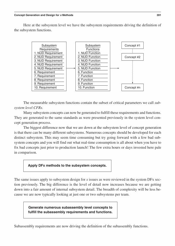
Here at the subsystem level we have the subsystem requirements driving the definition ofthe subsystem functions.
Concept Generation and Design for x Methods 391
1. NUD Requirement2. NUD Requirement3. NUD Requirement4. NUD Requirement5. NUD Requirement6. Requirement7. Requirement8. Requirement9. Requirement10. Requirement
1. NUD Function2. NUD Function3. NUD Function4. NUD Function5. NUD Function6. Function7. Function8. Function9. Function10. Function
SubsystemRequirements
SubsystemFunctions
Concept #n
Concept #1
Concept #2
The measurable subsystem functions contain the subset of critical parameters we call sub-system level CFRs.
Many subsystem concepts can now be generated to fulfill these requirements and functions.They are generated to the same standards as were presented previously in the system level con-cept generation process.
The biggest difference now that we are down at the subsystem level of concept generationis that there can be many different subsystems. Numerous concepts should be developed for eachdistinct subsystem. This may seem time consuming but try going forward with a few bad sub-system concepts and you will find out what real-time consumption is all about when you have tofix bad concepts just prior to production launch! The few extra hours or days invested here palein comparison.
Apply DFx methods to the subsystem concepts.
Generate numerous subassembly level concepts to fulfill the subassembly requirements and functions.
The same issues apply to subsystem design for x issues as were reviewed in the system DFx sec-tion previously. The big difference is the level of detail now increases because we are gettingdown into a fair amount of internal subsystem detail. The breadth of complexity will be less be-cause we are now typically looking at just one or two subsystems per team.
Subassembly requirements are now driving the definition of the subassembly functions.
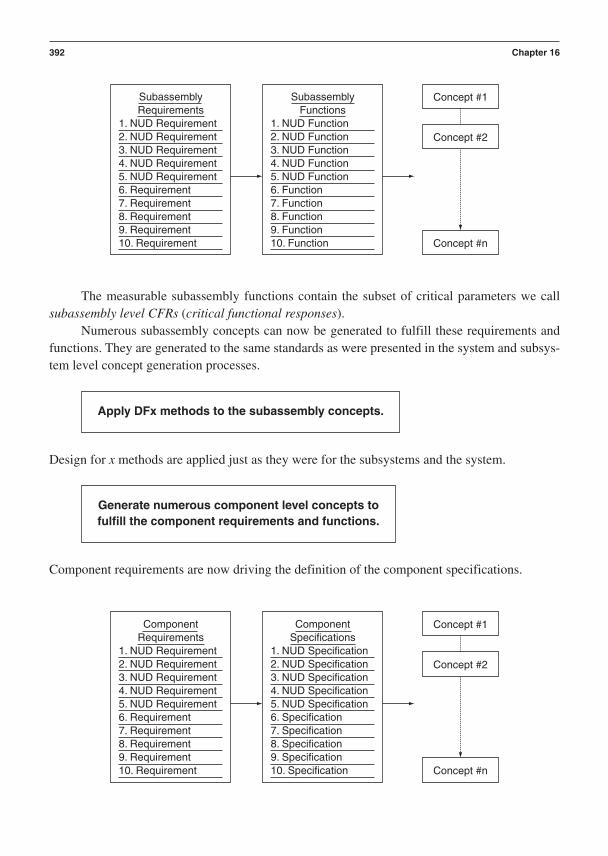
The measurable subassembly functions contain the subset of critical parameters we callsubassembly level CFRs (critical functional responses).
Numerous subassembly concepts can now be generated to fulfill these requirements andfunctions. They are generated to the same standards as were presented in the system and subsys-tem level concept generation processes.
392 Chapter 16
1. NUD Requirement2. NUD Requirement3. NUD Requirement4. NUD Requirement5. NUD Requirement6. Requirement7. Requirement8. Requirement9. Requirement10. Requirement
1. NUD Function2. NUD Function3. NUD Function4. NUD Function5. NUD Function6. Function7. Function8. Function9. Function10. Function
SubassemblyRequirements
SubassemblyFunctions
Concept #n
Concept #1
Concept #2
1. NUD Requirement2. NUD Requirement3. NUD Requirement4. NUD Requirement5. NUD Requirement6. Requirement7. Requirement8. Requirement9. Requirement10. Requirement
1. NUD Specification2. NUD Specification3. NUD Specification4. NUD Specification5. NUD Specification6. Specification7. Specification8. Specification9. Specification10. Specification
ComponentRequirements
ComponentSpecifications
Concept #n
Concept #1
Concept #2
Apply DFx methods to the subassembly concepts.
Generate numerous component level concepts to fulfill the component requirements and functions.
Design for x methods are applied just as they were for the subsystems and the system.
Component requirements are now driving the definition of the component specifications.

The measurable component specifications contain the subset of critical parameters we callcomponent level critical-to-function specifications (CTF specs). The component requirements arewhat the component must provide to enable a subassembly or subsystem to assemble and func-tion properly. A component specification is actually measured on a component to verify that it isfulfilling the requirement. An example is a shaft that has a required diameter of 2 inches /0.0010 inches and a measured CTF spec of 2.0006 inches. Component specifications are used tomeasure dimensions, surface finishes, and bulk properties on or within components.
Numerous component concepts can now be generated to fulfill these requirements andfunctions. They are generated to the same standards as were presented in the previous levels ofconcept generation processes.
Concept Generation and Design for x Methods 393
1. NUD Requirement2. NUD Requirement3. NUD Requirement4. NUD Requirement5. NUD Requirement6. Requirement7. Requirement8. Requirement9. Requirement10. Requirement
1. NUD Specification2. NUD Specification3. NUD Specification4. NUD Specification5. NUD Specification6. Specification7. Specification8. Specification9. Specification10. Specification
Manufacturing ProcessRequirements
Manufacturing ProcessSpecifications
Concept #n
Concept #1
Concept #2
The measurable manufacturing process specifications contain the subset of critical param-eters we call manufacturing process level CTF specs. The manufacturing process requirements arewhat the manufacturing process must provide to enable a component to be formed properly. If amanufacturing process set point is off target, the component dimensions, surface finishes, or bulkproperties will be off-target, resulting in assemble and functional problems. A manufacturing
Apply DFx methods to the component concepts.
Generate numerous manufacturing process level concepts to fulfill the manufacturing process requirements and functions.
Design for x methods are applied just as they were for the higher levels of the system.
Manufacturing process requirements are now driving the definition of the manufacturing processspecifications.

process specification is measured on a manufacturing process to verify that it is fulfilling the requirement. An example is an injection molding machine that has a required cooling water inlet temperature of 60˚ F / 4˚ F and a measured CTF spec of 62˚ F. Manufacturing processspecifications are used to measure process rates, temperatures, forces, pressures—any transfor-mation, flow, or state of energy or mass that controls how components are produced.
394 Chapter 16
Apply DFx methods to the manufacturing process concepts.
Uniformly document all candidate concepts and store them in the CPM database.
Numerous, uniformly documented system, subsystem,subassembly, component, and manufacturing process candidate
concepts ready for the Pugh concept selection process.
Design for x methods have their role in the development of manufacturing processes. Typicallythe technology team is developing a new manufacturing process, while the design teams are sim-ply selecting the best existing manufacturing process for their application to making the compo-nents they need.
As we bring this process to a close, it is worth repeating the importance of developing and docu-menting any set of concepts, at any level within the system hierarchy, to a relatively consistentlevel. This helps assure that as the concepts are taken through the Pugh concept selection process,they all get a fair evaluation against the best-in-class benchmark datum.
The Six Sigma Cockpit database has the ability to store many kinds of documents. This isan excellent place to store the concept files for future reference.
Final Detailed Outputs
At the end of each concept generation process for each level of the system hierarchy the teamswill have a well-developed set of candidate concepts that are ready to take into the Pugh conceptselection process.
Concept Generation and DFx Checklist and Scorecards
This suggested format for a checklist can be used by an engineering team to help plan its workand aid in the detailed construction of a PERT or Gantt chart for project management of the mod-

eling process within the first two phases of the CDOV or the first phase of the I2DOV develop-ment process. These items will also serve as a guide to the key items for evaluation within a for-mal gate review.
Checklist for Concept Generation and DFx
Was this Excellence Rating:Action Deployed? 1 Poor
Actions: YES or NO 10 Excellent
1. Translate each NUD system level requirement intosystem level functions. ______ ______
2. Generate numerous system level concepts to fulfillthe system requirements and functions. ______ ______
3. Apply DFx methods to the system concepts. ______ ______
4. Generate numerous subsystem level concepts to fulfill the subsystem requirements and functions. ______ ______
5. Apply DFx methods to the subsystem concepts. ______ ______
6. Generate numerous subassembly level concepts to fulfill the subassembly requirements and functions. ______ ______
7. Apply DFx methods to the subassembly concepts. ______ ______
8. Generate numerous component level concepts tofulfill the component requirements and functions. ______ ______
9. Apply DFx methods to the component concepts. ______ ______
10. Generate numerous manufacturing process levelconcepts to fulfill the manufacturing process requirements and functions. ______ ______
11. Apply DFx methods to the manufacturing process concepts. ______ ______
12. Uniformly document all candidate concepts and store them in the CPM database. ______ ______
Scorecard for Concept Generation and DFx
The definition of a good concept scorecard is that it should illustrate, in simple but quantitativeterms, what gains were attained from the work. This suggested format for a scorecard can be usedby a product planning team to help document the completeness of its work.
Total number of system level concepts developed: __________
Total number of subsystem level concepts developed: __________
Total number of subassembly level concepts developed: __________
Total number of component level concepts developed: __________
Total number of manufacturing process level concepts developed: __________
Concept Generation and Design for x Methods 395

This forces teams to document numerous concepts and avoid just developing one conceptthat may be inferior or competitively vulnerable to a best-in-class benchmark or other conceptsthat were not developed.
Documented Concept Elements
System level concept documentation:
Math models __________
Graphical models __________
Physical models __________
Subsystem level concept documentation:
Math models __________
Graphical models __________
Physical models __________
Subassembly level concept documentation:
Math models __________
Graphical models __________
Physical models __________
Component level concept documentation:
Math models __________
Graphical models __________
Physical models __________
Manufacturing process level concept documentation
Math models __________
Graphical models __________
Physical models __________
We repeat the final deliverables from concept generation and DFx:
• Documented candidate concepts at the system level fulfilling what is considered new,unique, and difficult as well as other important requirements.
• Documented candidate concepts at the subsystem, subassembly, component, andmanufacturing process levels fulfilling what is considered new, unique, and difficult aswell as other important requirements.
396 Chapter 16

• Designs that are conceptually well rounded, both functionally and architecturally:Documented concept feasibility for produceability (manufacturable)Documented concept feasibility for assembleabilityDocumented concept feasibility for reliabilityDocumented concept feasibility for serviceability (maintainable)Documented concept feasibility for environmental friendlinessDocumented concept feasibility for testability (measurable functions)
References
Boothroyd, G., Dewhurst, P., & Knight, W. (1994). Product design for manufacture andassembly. New York: Marcel Dekker.
Bralla, J. G. (1986). Handbook of product design for manufacturing. New York: McGraw-Hill.Clausing, D. (1995). Total quality development. New York: ASME Press.Otto, K., & Wood, K. (2001). Product design. Upper Saddle River, NJ: Prentice-Hall.Rao, S. S. (1992). Reliability-based design. New York: McGraw-Hill.Trucks, H. E. (1976). Designing for economical production. Dearborn, Mich.: SME Press.Ullman, D. G. (1997). The mechanical design process. New York: McGraw-Hill.Ulrich, K. T., & Eppinger, S. D. (1995). Product design and development. New York:
McGraw-Hill.
Concept Generation and Design for x Methods 397

This page intentionally left blank

C H A P T E R 1 7
The Pugh Concept Evaluationand Selection Process
Where Am I in the Process? Where Do I Apply the Pugh Concept SelectionProcess Within the Roadmaps?
Linkage to the I2DOV Technology Development Roadmap:
The Pugh concept selection process is conducted within the Invent/Innovate phase during tech-nology development. It is applied to evaluate and select superior platform and subsystem con-cepts. Superior concepts are those that score the highest in feasibility in satisfying the voice ofthe customer and the corresponding technology requirements for the new technology platformsand subsystems.
Linkage to the CDOV Product Development Roadmap:
The Pugh concept selection process is conducted within the Concept and Design phases duringproduct development. System level concept selection is conducted in the Concept phase. Alllower level concepts are selected during the Design phase. Here we apply the Pugh concept se-lection process to a specific product within the family plan from the product portfolio. This ap-plication of the Pugh process ensures that superior concepts for the system, subsystems,subassemblies, components, and manufacturing processes are evaluated and selected to fulfill thehierarchy of technical requirements for the new product being developed.
Concept Design Optimize Verify
Invent/Innovate
Develop Optimize Verify
399

What Am I Doing in the Process? What Does the Pugh Concept SelectionProcess Do at this Point in the Roadmaps?
The Purpose of the Pugh Concept Selection Process in the I2DOV TechnologyDevelopment Roadmap:
Once again we show the strategic flow-down of how a business develops new product concepts:
Define business strategy: Profit goals and requirements
Identify markets and market segments: Value generation and requirements
Gather long-term voice of customer and voice of technology trends
Develop product line strategy: Family plan requirements
Develop/deploy technology strategy: Technology and subsystem platform requirements
Gather product-specific VOC and VOT: New, unique, and difficult needs
Conduct KJ analysis: Structure and rank the VOC
Build system House of Quality: Translate VOC
Document system requirements
Define the system functions
Generate candidate system architectures
Select the superior system concept: Pugh process
In the Invent/Innovate phase of the I2DOV process we document the platform and/or sub-system requirements, define the platform and/or subsystem functions, generate candidate plat-form and/or subsystem architectures, and select the superior platform and/or subsystem concepts.
The hierarchy of technology requirements is used to carefully evaluate and select superiorconcepts for and within the platform architecture. The evaluation process is conducted against abest-in-class benchmark datum concept. The superior concepts will go through the rest of theI2DOV process.
The Purpose of the Pugh Concept Selection Process in the CDOV ProductDevelopment Roadmap:
In the CDOV process we document the system, subsystem, subassembly, component, and manu-facturing process requirements; define the system, subsystem, subassembly, component, andmanufacturing process functions; generate candidate system, subsystem, subassembly, compo-nent, and manufacturing process architectures (concepts); and select the superior system, sub-system, subassembly, component, and manufacturing process concepts.
The hierarchy of system requirements are used to carefully evaluate and select superior con-cepts for and within the system architecture. The evaluation process is conducted against best-in-classbenchmark datum concepts. The superior concepts will go through the rest of the CDOV process.
400 Chapter 17

What Output Do I Get at the Conclusion of this Phase of the Process? WhatAre Key Deliverables from the Pugh Concept Selection Process at this Pointin the Roadmaps?
• Superior platform or system level concept to take on into technology development orproduct design:Superior system level conceptSuperior subsystem level conceptsSuperior subassembly conceptsSuperior component conceptsSuperior manufacturing process concepts
• Superiority is documented in terms of concepts that are:Low in competitive vulnerability.High in functional feasibility and capability to fulfill requirements.Well documented in their ability to have their functional performance measured in
terms of CFRs.Low in inherent sensitivity to noise factors.Underwritten by three basic models generated to a common level of completeness for
each candidate concept:Analytical (hand calculations or CAE model)Graphical (hand sketch or CAD model)Physical (early hardware prototype)
The Pugh Concept Selection Process Flow Diagram (found on page 402)
This visual reference of the detailed steps of the Pugh concept selection process illustrates theflow of tasks and responsibilities.
Verbal Descriptions for the Application of Each Block Diagram
This section explains the specific details of the Pugh concept selection process:
• Key detailed input(s) from preceding tools and best practices• Specific steps and deliverables from each step to the next within the process flow• Final detailed outputs that flow into follow-on tools and best practices
Key Detailed Input:
Requirements, functions, and numerous concepts from concept generation.
The Pugh Concept Evaluation and Selection Process 401

With the specific concepts defined, the product planning team uses the requirements to define thecriteria to be used to evaluate and select superior concepts. Concept selection is made by evalu-ating the numerous candidate concepts against a best-in-class benchmark datum.
402 Chapter 17
INPUT . . .
OUTPUT . . .
Requirements, functions,and numerous conceptsfrom concept generation.
Define concept selectioncriteria from a clear and
complete set ofrequirements.
Define a best-in-classbenchmarked datum
concept.
Provide numerous candidateconcepts to evaluate against
the datum.
Evaluate each conceptagainst the datum using
(+)s, (–)s, and (S)s to rankfulfillment of the concept
selection criteria.
Refine criteria as necessaryduring the first cycle of
evaluation.
Identify weakness in low-scoring concepts that can
be turned into (+)s.
Analyze the results from thefirst cycle of evaluation:
Sum of (+)s, (–)s, and (S)s.
Identify weaknesses in high-scoring conceptsthat can be turned into (+)s.
Create hybrid "super concepts" byintegrating the strengths of like concepts
to remove (–)s and (S)s.
Create a hybrid "super concept" byintegrating the strengths of like concepts to
remove (–)s and (S)s.
Analyze the results from the second cycleof evaluation:
Sum of (+)s, (–)s, and (S)s.
Select a new datum based on the scoringthat suggests a superior concept after the
first cycle of evaluation.
Add any new concepts that have beendeveloped.
Repeat the evaluation process through asecond cycle.
Repeat the evaluation process through athird cycle if necessary.
Superior concept is selected and ready togo forward into the development or design
phase.
Specific Steps and Deliverables
The numerous concepts must be evaluated to select the one concept that best fulfills the rationalsubset of the complete set of requirements. The requirements at any level within the system con-tain new, unique, and difficult requirements as well as those that are of nominal importance. It iscommon to select an essential group of concept evaluation criteria from these requirements. It isunrealistic to use every single requirement to evaluate the feasibility of the candidate concepts.Every single requirement will be used to verify the product as it evolves through the phases ofproduct development. One must be careful to recognize that concept selection is not equal to prod-uct design, optimization, and capability certification. We are testing feasibility, not optimality! Thekey issues to evaluate will certainly be embodied within the NUD requirements plus a few selectrequirements that help prove the feasibility of the concepts in terms of competitive vulnerability.
To start the concept selection process, we refer back to the benchmarking information from theQFD process. From customer interviewing and technical benchmarking, the teams should have agood idea about what competitive or internal product or design element is the best in class. Thebest-in-class design is called the datum concept that is to be equaled or surpassed. This can be aproduct, subsystem, subassembly, component, or manufacturing process.
The set of candidate concepts, generated in the previous process, can be brought into the Pughconcept selection process at this time. Any new concepts can also be added, providing they areproperly documented by a reasonable level of modeling:
• Analytical (hand calculations or CAE model)• Graphical (hand sketch or CAD model)• Physical (early hardware prototype)
It is good to remember these are just candidates at this point. None of these concepts islikely to be the winner yet!
Provide numerous candidate concepts to evaluate against the datum.
Define a best-in-class benchmarked datum concept.
Define concept selection criteria from aclear and complete set of requirements.
The Pugh Concept Evaluation and Selection Process 403
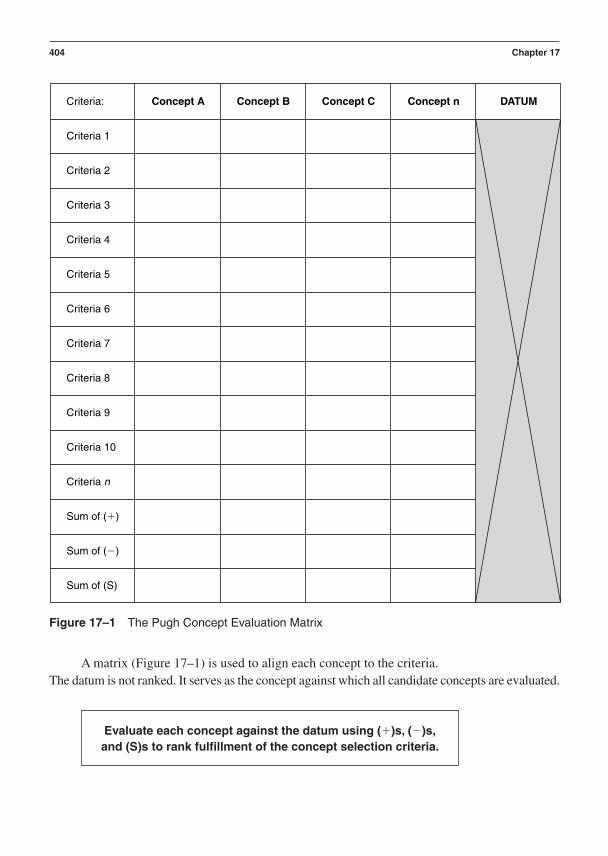
A matrix (Figure 17–1) is used to align each concept to the criteria.The datum is not ranked. It serves as the concept against which all candidate concepts are evaluated.
Evaluate each concept against the datum using ()s, ()s,and (S)s to rank fulfillment of the concept selection criteria.
404 Chapter 17
Criteria: Concept A Concept B Concept C Concept n DATUM
Criteria 1
Criteria 2
Criteria 3
Criteria 4
Criteria 5
Criteria 6
Criteria 7
Criteria 8
Criteria 9
Criteria 10
Criteria n
Sum of ()
Sum of ()
Sum of (S)
Figure 17–1 The Pugh Concept Evaluation Matrix

Each candidate concept is now evaluated against the datum for each concept evaluation criteria.The team uses a simple evaluation technique consisting of a () for a concept that is better at ful-filling the criteria than the datum. A () is assigned to a concept that is worse than the datum, and(S) denotes a concept that is essentially the same as the datum.
Refine criteria as necessary during the first cycle of evaluation.
The Pugh Concept Evaluation and Selection Process 405
Criteria: Concept A Concept B Concept C Concept n DATUM
Criteria 1 S
Criteria 2 S
Criteria 3 S
Criteria 4 S
Criteria 5
Criteria 6 S S
Criteria 7 S
Criteria 8 S
Criteria 9 S
Criteria 10 S
Criteria n
Sum of () 6 4 3 7
Sum of () 3 5 4 2
Sum of (S) 2 2 4 2
It is quite common for the concept selection criteria to be “downsized” when two or more crite-ria are found to be repetitive or redundant. If criteria are found to be unclear, they should be mod-ified. Criteria must be specific and clear. Cost as a general classification is a poor criterion. Theelements that drive cost are good criteria. The same goes for reliability. Lower part count is a rep-resentative criterion that helps identify a concept that is feasible for improving reliability. Try toword criteria so that you can answer the question, “Why, specifically, is this design more feasi-ble than the datum?”
The number of ()s, ()s, and (S)s can be summed for each concept. This indicates which con-cepts are tending toward being superior to the datum. There may actually be one or more con-cepts that are clearly superior to the datum. In any case, the team needs to go to work on makingstrong concepts stronger. There may even be opportunities to convert weaker concepts intostrong concepts. The method of creating hybrid concepts is used to improve Round 1 candidateconcepts.
The team first turns its attention to the weaker concepts to see if their weaknesses can be correctedby altering their architectures, perhaps by adding strengths borrowed from other concepts.
The strong concepts also can benefit from improvements in their architectures. Each strong con-cept should be scrutinized so that its ()s can be turned into ()s. It is common to search throughthe other concepts to see if one of their () attributes can be brought into the strong concept’sstructure.
Create hybrid “super concepts” by integrating thestrengths of like concepts to remove ()s and (S)s.
Identify weaknesses in high-scoring concepts that can be turned into ()s.
Identify weakness in low-scoring concepts that can be turned into ()s.
Analyze the results from the first cycle ofevaluation: sum of ()s, ()s, and (S)s.
406 Chapter 17

From time to time a group of two or more concepts that are similar can be integrated with the re-sulting hybrid concept becoming a “super concept.” A super concept may rise to the top and be-come a good replacement for the current datum.
The team reviews the results of the first round of concept evaluations. If a clearly superior con-cept emerges, then the datum is replaced with this superior candidate concept.
It is perfectly legitimate to generate new concepts and introduce them to the Pugh process at thistime. After the first round of concept evaluation, many new and stimulating ideas tend to be pro-voked. These should be developed and documented to an equal level with the concepts that areabout to go through Round 2.
The set of new and revised candidate concepts are now taken through a new round of evaluationagainst the new datum (or the original datum if it was not surpassed). Additional adjustments tothe criteria should be made prior to Round 2.
After a second round of concept evaluation, the ()s, ()s, and (S)s are summed to reveal whichconcepts are emerging as superior to the datum.
Create a hybrid “super concept” by integrating thestrengths of like concepts to remove ()s and (S)s.
Analyze the results from the second cycleof evaluation: Sum of ()s, ()s, and (S)s.
Repeat the evaluation process through a second cycle.
Add any new concepts that have been developed.
Select a new datum based on the scoring that suggestsa superior concept after the first cycle of evaluation.
The Pugh Concept Evaluation and Selection Process 407

Another round of concept hybridization can be conducted if necessary to build one or more con-cepts that can surpass the datum. It is common to arrive at a superior concept after the secondround of the Pugh process.
A third round of concept amendment and evaluation can be conducted if necessary.
Final Detailed Outputs
Once a superior concept is selected, the team must begin to mature the concept into a viable base-line design that is now worthy and able to be fully modeled.
Pugh Concept Selection Process Checklist and Scorecard
This suggested format for a checklist can be used by an engineering team to help plan its workand aid in the detailed construction of a PERT or Gantt chart for project management of the Pughconcept selection process within the Optimize phase of the CDOV or I2DOV developmentprocess. These items will also serve as a guide to the key items for evaluation within a formal gatereview.
Checklist for the Pugh Concept Selection Process
Was this Action Excellence Rating:Deployed? 1 = Poor
Actions: YES or NO 10 = Excellent
1. Define concept selection criteria from a clear and complete set of requirements. ______ ______
2. Define a best-in-class benchmarked datum concept. ______ ______
3. Provide numerous candidate concepts to evaluate against the datum. ______ ______
4. Evaluate each concept against the datum using ()s, ()s,and (S)s to rank fulfillment of the concept selection criteria. ______ ______
5. Refine criteria as necessary during the first cycle of evaluation. ______ ______
6. Analyze the results from the first cycle of evaluation: Sum of ()s, ()s, and (S)s. ______ ______
Superior concept is selected and ready to goforward into the development or design phase.
Repeat the evaluation process through a third cycle if necessary.
408 Chapter 17

7. Identify weakness in low-scoring concepts that can be turned into ()s. ______ ______
8. Identify weaknesses in high-scoring concepts that can be turned into ()s. ______ ______
9. Create hybrid “super concepts” by integrating the strengths of like concepts to remove ()s and (S)s. ______ ______
10. Select a new datum based on the scoring that suggests asuperior concept after the first cycle of evaluation. ______ ______
11. Add any new concepts that have been developed. ______ ______
12. Repeat the evaluation process through a second cycle. ______ ______
13. Analyze the results from the second cycle of evaluation: Sum of ()s, ()s, and (S)s. ______ ______
14. Create a hybrid “super concept” by integrating the strengths of like concepts to remove ()s and (S)s. ______ ______
15. Repeat the evaluation process through a third cycle if necessary. ______ ______
Scorecard for Pugh Concept Selection Process
The definition of a good concept selection scorecard is that it should illustrate, in simple but quan-titative terms, what gains were attained from the work. This suggested format for a scorecard canbe used by an engineering team to help document the completeness of its work.
Number of candidate concepts evaluated: ___________
Number of selection criteria used: ___________
Number of ()s for superior concept: ___________
Number of ()s for superior concept: ___________
Number of (S)s for superior concept: ___________
We repeat the final deliverables from the Pugh concept selection process:
• Superior platform or system level concept to take on into technology development orproduct designSuperior system level conceptSuperior subsystem level conceptsSuperior subassembly conceptsSuperior component conceptsSuperior manufacturing process concepts
• Superiority is documented in terms of concepts that are:Low in competitive vulnerability.High in functional feasibility and capability to fulfill requirements.Well documented in their ability to have their functional performance measured in
terms of CFRs.
The Pugh Concept Evaluation and Selection Process 409

Low in inherent sensitivity to noise factors.Underwritten by three basic models generated to a common level of completeness for
each candidate concept:Analytical (hand calculations or CAE model)Graphical (hand sketch or CAD model)Physical (early hardware prototype)
References
Clausing, D. (1994). Total quality development. New York: ASME Press.Pugh, Stuart. (1995). Total design. Reading, Mass: Addison-Wesley.Pugh, Stuart. (1996). Creating innovative products using total design. Reading, Mass: Addison-
Wesley.
410 Chapter 17

C H A P T E R 1 8
Modeling: Ideal/TransferFunctions, Robustness AdditiveModels, and the Variance Model
Where Am I in the Process? Where Do I Apply Modeling Within theRoadmaps?
Linkage to the I2DOV Technology Development Roadmap:
411
Invent/Innovate
Develop Optimize Verify
Concept Design Optimize Verify
Modeling of technology concepts is conducted within the Invent/Innovate phase during technol-ogy development. Modeling of technology baseline performance is conducted in the Developphase. Modeling of robustness and tunability of the mean of critical functional responses is doneduring the Optimize phase. Modeling of variational sensitivities across the integrated technologyplatform is conducted in the Verify phase.
Linkage to the CDOV Product Development Roadmap:
Modeling of product design concepts is conducted within the Concept and Design phases duringproduct development. Modeling of the baseline performance is conducted in the later portion of

the Design phase. Modeling of subsystem robustness and tunability of the mean of critical func-tional responses is done during the Optimize phase. Modeling of variational sensitivities acrossthe integrated system is conducted in the Optimize and Verify phases.
What Am I Doing in the Process? What Does Modeling Do at this Point inthe Roadmaps?
The Purpose of Modeling in the I2DOV Technology Development Roadmap:
Once again we begin by showing the strategic flow-down of how a business develops new prod-uct concepts:
Define business strategy: Profit goals and requirements
Identify markets and market segments: Value generation and requirements
Gather long-term voice of customer and voice of technology trends
Develop product line strategy: Family plan requirements
Develop/deploy technology strategy: Technology and subsystem platform requirements
Gather product-specific VOC and VOT: New, unique, and difficult needs
Conduct KJ analysis: Structure and rank the VOC
Build system House of Quality: Translate VOC
Document system requirements
Define the system functions
Generate candidate system architectures
Select the superior system concept: Pugh process
In the Invent/Innovate phase of the I2DOV process we define the platform functions andgenerate candidate platform architectures. The technology requirements will be used to define aset of adjustable or tunable functions. These functions require engineered technology concepts totransform, flow, and change the state of mass and energy. A unique set of architectural concepts,or platforms, are developed to fulfill these functions over an adjustable range of application. Tohelp define the form and fit parameters that will fulfill the functions, initial modeling must bedone. After careful evaluation, one superior platform architecture is selected out of the numerousoptions to go through the rest of the I2DOV process. Much more extensive modeling is then con-ducted on the superior concept during the Develop, Optimize, and Verify phases.
The Purpose of Modeling in the CDOV Product Development Roadmap:
In the CDOV process we define the system functions and generate candidate system architec-tures. The system requirements are used to define a set of product functions. Numerous systemarchitectural concepts are then developed to fulfill the product functions. Modeling is used to helpdefine and underwrite the feasibility of these concepts. After careful evaluation, one superior sys-tem architecture will be selected out of the numerous options to go through the rest of the CDOV
412 Chapter 18

process. When a superior system concept is selected, system modeling is initiated, soon to be fol-lowed by extensive model building down through the subsystems, subassemblies, components,and manufacturing processes. The models are used to define, develop, optimize, and verify theperformance capability of the design’s functions with and without stressful sources of noise ap-plied to the system. Numerous forms of modeling are conducted in the Design, Optimize, andVerify Phases of the CDOV process.
What Output Do I Get at the Conclusion of this Phase of the Process? WhatAre Key Deliverables from Modeling Across the Roadmaps?
Models will be documented at all levels within the system:
System models
Subsystem models
Subassembly models
Component models
Manufacturing process models
Models will be documented in three forms:
Analytical models (equations based on first principles and empirical data)
Geometric or graphical models (CAD files, sketches, drawings, layouts)
Physical models (hardware, firmware, and software prototypes)
Invent/Innovate (I2DOV) and Concept (CDOV) Phase models:
• Rudimentary conceptual modeling conducted to underwrite conceptual feasibility• General equations that express the underlying physical or chemical principles the
concept will employ• Hand sketches and CAD layouts that illustrate the form and fit of the concept• Three-dimensional cardboard, styrofoam, stereo-lithography, or model-shop models
that may possess basic functionality to demonstrate feasibility
Develop (I2DOV) and Design (CDOV) Phase models:
Baseline performance models will be documented internal to the system, subsystems, and sub-assemblies:
System Ideal Functions [Y f(x)]
• Main effects of system engineering parameters• Interactions between system engineering parameters• Linear or nonlinear performance of system engineering parameters
Modeling: Ideal/Transfer Functions, Robustness Additive Models, and the Variance Model 413
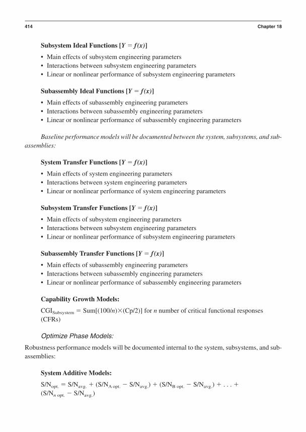
Subsystem Ideal Functions [Y f(x)]
• Main effects of subsystem engineering parameters• Interactions between subsystem engineering parameters• Linear or nonlinear performance of subsystem engineering parameters
Subassembly Ideal Functions [Y f(x)]
• Main effects of subassembly engineering parameters• Interactions between subassembly engineering parameters• Linear or nonlinear performance of subassembly engineering parameters
Baseline performance models will be documented between the system, subsystems, and sub-assemblies:
System Transfer Functions [Y f(x)]
• Main effects of system engineering parameters• Interactions between system engineering parameters• Linear or nonlinear performance of system engineering parameters
Subsystem Transfer Functions [Y f(x)]
• Main effects of subsystem engineering parameters• Interactions between subsystem engineering parameters• Linear or nonlinear performance of subsystem engineering parameters
Subassembly Transfer Functions [Y f(x)]
• Main effects of subassembly engineering parameters• Interactions between subassembly engineering parameters• Linear or nonlinear performance of subassembly engineering parameters
Capability Growth Models:
CGISubsystem Sum[(100/n)(Cp/2)] for n number of critical functional responses(CFRs)
Optimize Phase Models:
Robustness performance models will be documented internal to the system, subsystems, and sub-assemblies:
System Additive Models:
S/Nopt. S/Navg. (S/NA opt. S/Navg.) (S/NB opt. S/Navg.) . . .
(S/Nn opt. S/Navg.)
414 Chapter 18
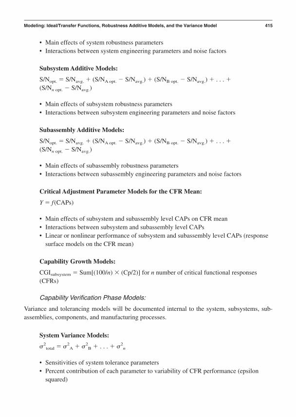
• Main effects of system robustness parameters• Interactions between system engineering parameters and noise factors
Subsystem Additive Models:
S/Nopt. S/Navg. (S/NA opt. S/Navg.) (S/NB opt. S/Navg.) . . .
(S/Nn opt. S/Navg.)
• Main effects of subsystem robustness parameters• Interactions between subsystem engineering parameters and noise factors
Subassembly Additive Models:
S/Nopt. S/Navg. (S/NA opt. S/Navg.) (S/NB opt. S/Navg.) . . .
(S/Nn opt. S/Navg.)
• Main effects of subassembly robustness parameters• Interactions between subassembly engineering parameters and noise factors
Critical Adjustment Parameter Models for the CFR Mean:
Y f(CAPs)
• Main effects of subsystem and subassembly level CAPs on CFR mean• Interactions between subsystem and subassembly level CAPs• Linear or nonlinear performance of subsystem and subassembly level CAPs (response
surface models on the CFR mean)
Capability Growth Models:
CGIsubsystem Sum[(100/n) (Cp/2)] for n number of critical functional responses(CFRs)
Capability Verification Phase Models:
Variance and tolerancing models will be documented internal to the system, subsystems, sub-assemblies, components, and manufacturing processes.
System Variance Models:
2total 2
A 2B . . . 2
n
• Sensitivities of system tolerance parameters• Percent contribution of each parameter to variability of CFR performance (epsilon
squared)
Modeling: Ideal/Transfer Functions, Robustness Additive Models, and the Variance Model 415
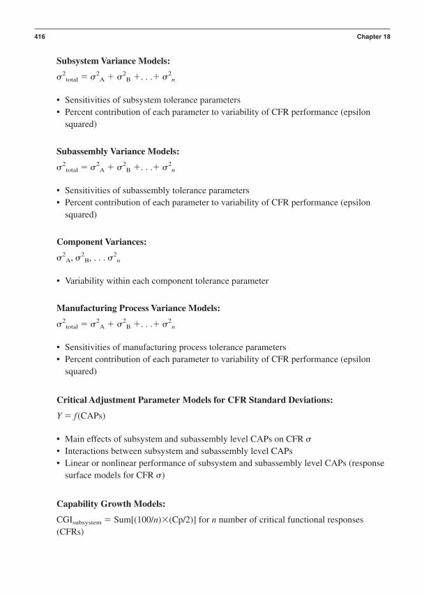
Subsystem Variance Models:
2total 2
A 2B . . . 2
n
• Sensitivities of subsystem tolerance parameters• Percent contribution of each parameter to variability of CFR performance (epsilon
squared)
Subassembly Variance Models:
2total 2
A 2B . . . 2
n
• Sensitivities of subassembly tolerance parameters• Percent contribution of each parameter to variability of CFR performance (epsilon
squared)
Component Variances:
2A, 2
B, . . . 2n
• Variability within each component tolerance parameter
Manufacturing Process Variance Models:
2total 2
A 2B . . . 2
n
• Sensitivities of manufacturing process tolerance parameters• Percent contribution of each parameter to variability of CFR performance (epsilon
squared)
Critical Adjustment Parameter Models for CFR Standard Deviations:
Y f(CAPs)
• Main effects of subsystem and subassembly level CAPs on CFR • Interactions between subsystem and subassembly level CAPs• Linear or nonlinear performance of subsystem and subassembly level CAPs (response
surface models for CFR )
Capability Growth Models:
CGIsubsystem Sum[(100/n)(Cp/2)] for n number of critical functional responses(CFRs)
416 Chapter 18

Critical Parameter Management Data that Is Documented in the CPM RelationalDatabase:
• Flow-down and linkage of all CFRs, CFPs, and CTF specifications (down to allappropriate levels within the system)
• Ideal/transfer functions documented• Additive models documented• Variance models documented• Capability growth indices documented
When modeling is used extensively to develop, design, optimize, and verify a capable prod-uct, we can expect the following results.
1. Requirements that have been converted to functions that make it clear what must beengineered and developed
2. Construction of input-output-constraint diagrams for each function down through thesystem hierarchy during Concept and Design phases
3. Linkage of all ideal/transfer functions using functional flow diagrams4. Definition of the flow and connectivity of models for each function:
Math modelsGraphical modelsPhysical models
5. Development of internal ideal function models for each subsystem and subassembly6. Development of transfer function models between the system, subsystems, and sub-
assemblies (the difference between ideal and transfer functions is subtle but worth noting)7. Verification of all analytical models with empirical models8. Documentation of the ideal and transfer functions and their linkages in the CPM database9. Documentation of additive robustness models
10. Documentation of variance (tolerance) models
Modeling Process Flow Diagram (found on page 418)
The visual reference of the detailed steps of modeling illustrates the flow of these criticalprocesses.
Verbal Descriptions for the Application of Each Block Diagram
This section explains the specific details of each step in the modeling process:
• Key detailed input(s) from preceding tools and best practices• Specific steps and deliverables from each step to the next within the process flow• Final detailed outputs that flow into follow-on tools and best practices
Modeling: Ideal/Transfer Functions, Robustness Additive Models, and the Variance Model 417
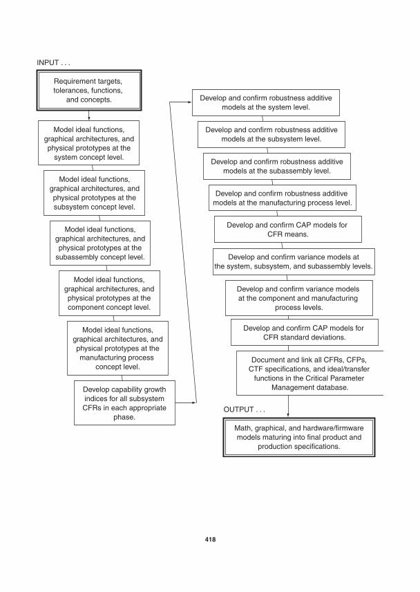
INPUT . . .
OUTPUT . . .
Requirement targets, tolerances, functions,
and concepts.
Model ideal functions,graphical architectures, andphysical prototypes at the
system concept level.
Model ideal functions,graphical architectures, andphysical prototypes at thesubsystem concept level.
Model ideal functions,graphical architectures, andphysical prototypes at the
subassembly concept level.
Model ideal functions,graphical architectures, andphysical prototypes at thecomponent concept level.
Model ideal functions,graphical architectures, andphysical prototypes at themanufacturing process
concept level.
Develop capability growthindices for all subsystemCFRs in each appropriate
phase.
Develop and confirm robustness additivemodels at the system level.
Develop and confirm robustness additivemodels at the subsystem level.
Develop and confirm robustness additivemodels at the subassembly level.
Develop and confirm robustness additive models at the manufacturing process level.
Develop and confirm CAP models for CFR means.
Develop and confirm variance models atthe system, subsystem, and subassembly levels.
Develop and confirm CAP models for CFR standard deviations.
Document and link all CFRs, CFPs, CTF specifications, and ideal/transfer
functions in the Critical Parameter Management database.
Develop and confirm variance models at the component and manufacturing
process levels.
Math, graphical, and hardware/firmwaremodels maturing into final product and
production specifications.
418
Key Detailed Inputs
Requirement targets, tolerances, functions, and concepts.
With the specific new, unique, and difficult technical requirements defined, the team knows ex-actly how the requirements can be measured (targets/tolerances and units of measure) for fulfill-ment. We also use the defined functions, forms, and fits at the system, subsystem, subassembly,component, and manufacturing process levels.
Specific Steps and Deliverables
Modeling: Ideal/Transfer Functions, Robustness Additive Models, and the Variance Model 419
Model ideal functions, graphical architectures,and physical prototypes at the system concept level.
The beginning of the modeling process always starts with a clear well-written set of requirements.This is true no matter whether you are working at the system level or are modeling down throughthe levels of the system hierarchy. At the system level, the first items the system architectural teamdetermines are the functions that must be engineered to fulfill the system requirements. Once thefunctions are defined, the team can concern itself with defining numerous architectural designs(subsystems and interfaces) that can adequately generate the functions. This follows the old ax-iom of form following function. The flow-down of elements that drive the modeling process are:
Needs drive requirements
Requirements drive functions
Functions drive forms
Form and function drive modeling
All this information is used to initiate the construction of math models, graphical models,and physical models. The first models that are done at the system level are graphical. Functionalsystem models are difficult to construct until the subsystems, subassemblies, and components are defined. System math models are constructed later in the Develop (I2DOV) or Design(CDOV) phases. The system math models take form as the critical parameter relational databaseis developed. In Phase 1 of both I2DOV and CDOV processes, physical system models are re-stricted to architectural models of external forms and features (spatial models), functional systemmodels are built and tested in the second part of the Optimize Phase (Phase 3B) in the CDOVprocess and in the third phase of the I2DOV process. The premature integration of system hard-ware frequently causes program delays because of the extra effort it takes to desensitize all the“built-in” cross-boundary conflicts that the other forms of modeling at the lower levels wouldhave prevented had they been conducted prior to system hardware integration.

The ideal or transfer functions at the system level are expressed as Y f(x) models with thefollowing parameter definitions:
Y a measured critical functional response
xCFP critical functional parameters (inputs from subsystems and subassemblies)
xCAP critical adjustment parameters (inputs from subsystems and subassemblies thatare specifically designed to shift the mean of the CFR)
The system math models (ideal/transfer functions) are constructed from “n number of x”inputs from subsystems and subassemblies:
420 Chapter 18
(n) SubsystemInputs to theSystem CFR
SubsystemCAP1 = xCAP1
SubsystemCFP1 = xCFP1
SubsystemCAP2 = xCAP2
SubsystemCFP2 = xCFP2
SubsystemCAPn = xCAPn
Y = f(X1 to n)
SystemCFR = Y
SubsystemCFPn = xCFPn
(n) SubassemblyInputs to theSystem CFR
SubassemblyCAP1 = xCAP1
SubassemblyCFP1 = xCFP1
SubassemblyCAP2 = xCAP2
SubassemblyCFP2 = xCFP2
SubassemblyCAPn = xCAPn
SubassemblyCFPn = xCFPn
These models are derived either by “first principles” or from experimental data from de-signed experiments.
First principles modeling is a good place to begin to define the elements of a model andhow those elements can be integrated to explain functional behavior. Your engineering booksfrom your college or university days contain a wealth of first principles modeling methods andexamples. If you sold them, go buy new ones.

A common approach to first principles modeling is the use of four analogs:
Electrical analogs
Mechanical analogs
Fluid analogs
Thermal analogs
These analogs provide a conceptual framework for any set of input–output relationships to be stated in a generalized block diagram format. This allows one to conceptually lay out the function(input–output relationships) in blocks representing elements from one of the four analog scenarios.
Once the conceptual block diagrams are laid out, the team can write down the mathemati-cal forms of the functional elements representing the input–output relationships. With these inhand, differential equations can be structured and solved on a personal computer.
The process for first principles modeling can be structured as follows:
1. Construct block diagram models based on one of the analogs.• Review how work, power, and energy apply to your case.• Review how basic calculus applies to your case.
2. Set up first order differential equation based on block diagrams.• Solve closed or open form model on PC using Excel or Math/Solver software.
3. Set up second order differential equation based on block diagrams.• Solve closed or open form model on PC using Excel or Math/Solver software.
4. Set up higher order differential equation based on block diagrams as necessary.• Solve closed or open form model on PC using Excel or Math/Solver software.
An excellent text on the market explains the step-by-step process modeling of engineeringsystems. Modeling Engineering Systems, by Jack W. Lewis (1993, published by High Text), pre-sents an easy-to-read explanation of math modeling. This book is a “must-have” to assist any en-gineer in modeling. This is especially true if you are a little rusty and need a gentle refresher.
Empirical modeling methods are covered in Chapters 27 and 29. The construction of the ro-bustness additive models is covered in Chapter 28. Chapters 31 and 32 on analytical and empir-ical tolerancing explain how variance models are constructed. Chapter 10 explains how transferfunctions are linked and used to do system modeling. The Six Sigma Cockpit software packagefrom Cognition Software will enable you to do CPM-based system modeling. It will also enableyou to create capability growth index roll-up models.
Model ideal functions, graphical architectures, and physical prototypes at the subsystem, subassembly, and component concept levels.
Subsystem, subassembly, and component graphical models are first developed during the concepting activities of Phase 1 in the I2DOV process and Phase 2 in the CDOV process. The
Modeling: Ideal/Transfer Functions, Robustness Additive Models, and the Variance Model 421

graphical models for each subsystem, subassembly, and component are matured after superiorconcepts are selected. The graphical models are most commonly documented as CAD files:
• Hand sketches evolve into hand-drawn isometrics and integrated layouts.• Hand-drawn conceptual architectures are then converted to CAD files.
The subsystem math models (ideal/transfer functions) are constructed from “n number ofx” inputs from subassemblies and components:
422 Chapter 18
(n) SubassemblyInputs to the
Subsystem CFR
SubassemblyCAP1 = xCAP1
SubassemblyCFP1 = xCFP1
SubassemblyCAP2 = xCAP2
SubassemblyCFP2 = xCFP2
SubassemblyCAPn = xCAPn
Y = f(X1–n)
SubsystemCFR = Y
SubassemblyCFPn = xCFPn
(n) ComponentInputs to the
Subsystem CFR
ComponentCTF1 = xCTF1
ComponentCTF2 = xCTF2
ComponentCTFn = xCTFn
Y = f(X1–n)
SubassemblyCFR = Y
(n) ComponentInputs to the
Subsystem CFR
ComponentCTF1 = xCTF1
ComponentCTF2 = xCTF2
ComponentCTFn = xCTFn
The subassembly math models (ideal or transfer functions) are constructed from “n num-ber of x” inputs from components:

These models are derived either by first principles or from experimental data from designedexperiments using physical models. They represent the baseline performance of the componentswithout the debilitating effects of noise imposed upon them. That scenario will come later duringthe robustness and variance modeling in the Optimize and Verify Certification phases.
The component math models (ideal/transfer functions) are constructed from “n number ofx” inputs from manufacturing process parameter set points:
VModeling: Ideal/Transfer Functions, Robustness Additive Models, and the Variance Model 423
Y = f(X1–n)
ComponentCTF Spec. = Y
(n) Manufacturing Process Parameter
Inputs to the ComponentCTF Specifications
Manufacturing processCTF1 = xCTF1
Manufacturing processCTF2 = xCTF2
Manufacturing processCTFn = xCTFn
Model ideal functions, graphical architectures, and physical prototypes at the manufacturing process concept level.
Manufacturing processes are usually strong sources of variation to components. All componentmodels (math, graphical, and physical) will reflect the effects of manufacturing process capability.
Even when a manufacturing process is running “perfectly”—that is to say, when the onlyvariation in the components is coming from random, natural sources—the component dimensionsand its bulk and surface properties will vary. This “natural” variation must be evaluated to see ifthe design still functions properly when it is consistently present in the components. These kindsof models are called baseline performance models. They are evaluated in the Develop (I2DOV)or Design (CDOV) phases.
Another set of models must be developed to account for both component assembleabilityand functionality. These models are usually graphical, mathematical, and eventually physical.The effect of manufacturing process set points on component assembleability and functionalitycan and should be modeled. If a manufacturing process is incapable of meeting component func-tional performance and assembleability requirements, the process itself may require redesign ora completely new technology.
The teams in charge of technology and design development must intentionally induce thesignificant forms of variation that are to be expected from the manufacturing processes into thecomponents. This is often done through Monte Carlo simulations during analytical tolerance de-sign (during Phase 2) and designed experiments (using / 1 values or the full tolerance lim-its) during Phase 3 and 4 using empirical tolerance design. These induced sources of componentvariation represent what happens when manufacturing process set points move off target due toassignable causes of variation during production.
If a new manufacturing process is required, then the I2DOV and CDOV processes need tobe applied to the development of a new manufacturing technology and manufacturing process de-sign. In this sense, a new manufacturing process is a “product” and should be developed just likeany other commercial product system.
424 Chapter 18
Develop capability growth indices for all subsystem CFRs in each appropriate phase.
At the end of the Develop/Design, Optimize, and Verify Certification phases, the capabilitygrowth indices for all subsystems should be calculated. This models the current state of capabil-ity for each critical functional response within each subsystem. The CGI keeps a running tally ofthe percentage of completion each subsystem possesses along the way of getting all CFRs up toa common capability of Cp 2. When a subsystem has all its CFR Cp Indices equal to 2, its CGIwill be 100 percent. This is the ideal goal for all subsystems. The CGI is explained in Chapter 12.
Develop and confirm robustness additive models at the system level.
In Phase 4 of the I2DOV process and Phase 3B of the CDOV process, the integrated platform orsystem can be evaluated for its robustness. Each CFR at the system level can be measured usinga capable data acquisition system. The system is built up from subsystems, subassemblies, andcomponents that are intentionally set up at levels that represent real variation that will be experi-enced when the product is in the customer’s use environment. These sources of variation include:
• External variation: Run the system robustness tests in the presence of externalsources of variation (contamination, temperature, humidity, altitude, or barometric pressure).
• Subsystem and subassembly functional variation due to assembly, service criticaladjustment parameter adjustment variation: Intentionally set the critical adjustment pa-rameters off target to simulate adjustment error by assembly or service personnel.
• Component variation: Have component dimensions, surface finishes, and bulkproperties made off target to simulate variation coming in from your supply chain. Thesevariations are usually at / 1 standard deviation of the distribution from the supply chainsample data.

• Deterioration variation: Physically alter components to look like they would after areasonable period of use. Components or component interfaces are forced to deteriorate or toemulate a known amount of deteriorated condition based on time. This time is usually some-where around 6-month to yearly intervals. What will the component or interface look like 6months from now? How will it look 1, 2, or 3 years from now? Make it look that way! If youhave no experience or historical knowledge of mass deformation, material depletion, or degra-dation, you will have to estimate it. Better to do that within reasonable bounds than to do noth-ing at all. If you do nothing at all, you are likely in for some big surprises later on after yourcustomer uses your product.
The appropriate signal-to-noise metrics can be calculated from the mean and/or standard devi-ation from your sample of CFR data. Purposeful changes to critical parameters can be made at the sub-system, subassembly, and component level to improve the S/N values for the CFRs using designedexperimental procedures for robustness optimization. The primary function of the S/N metrics in ro-bust design is to quantify the strength of interactions between control factors and noise factors as theyrelate to a CFR. The additive model for summing the S/N gains takes the following general form:
S/Nopt. S/Navg (S/NA opt. S/Navg) (S/NB opt. S/Navg) . . . .
(S/Nn opt. S/Navg)
Once an optimal level of system CFR robustness is attained, confirmation runs can be con-ducted to validate the additive model for the system CFR S/N values.
Develop and confirm robustness additive models at the subsystem level.
In Phase 3 of the I2DOV process and Phase 3A of the CDOV process the individual subsystemscan be evaluated for robustness. Each CFR at the subsystem level can be measured using a capa-ble data acquisition system. The subsystem is built up from subassemblies and components thatare intentionally set up at levels that represent real variation that will be experienced when thesubsystem is in the customer’s use environment as an integrated part of the system.
These sources of induced variation include:
External variation: Run the subsystem robustness tests in the presence of external sourcesof variation (contamination, temperature, humidity, altitude, or barometric pressure) as wellas incoming noises from other subsystems or from the system environment that is immedi-ately external to the subsystem. These system noises must be emulated and induced by spe-cial means since the system has not yet been assembled.
Subsystem and subassembly functional variation due to assembly, service critical adjust-ment parameter adjustment variation: Intentionally set the subsystem and subassemblycritical adjustment parameters off-target to simulate adjustment error by assembly or ser-vice personnel.
Modeling: Ideal/Transfer Functions, Robustness Additive Models, and the Variance Model 425

Component variation: Have component dimensions, surface finishes, and bulk propertiesmade off target to simulate variation coming in from your supply chain. These variations areusually at / 1 standard deviation of the distribution from the supply chain sample data.
Deterioration Variation: Physically alter components and interfaces to look as they wouldafter a reasonable period of use. Components or component interfaces are forced to deteri-orate or to emulate a known amount of deteriorated condition based on time. This time isusually somewhere around 6-month to yearly intervals. What will the component or inter-face look like 6 months from now? How will it look 1, 2, or 3 years from now? Make it lookthat way! If you have no experience or historical knowledge of mass deformation or mate-rial depletion or degradation, you will have to estimate it. Better to do that within reason-able bounds than to do nothing at all. If you do nothing at all, you are likely in for some bigsurprises later on after you integrate the system.
The appropriate signal-to-noise metrics can be calculated from the mean and/or standarddeviation from your sample of subsystem CFR data. Purposeful changes to critical parameterscan be made at the subsystem, subassembly, and component level to improve the S/N values forthe CFRs using designed experimental procedures for robustness optimization.
Once an optimal level of subsystem CFR robustness is attained, confirmation runs can beconducted to validate the additive model for the system CFR S/N values.
Develop and confirm robustness additive models at the subassembly level.
In Phase 3 of the I2DOV process and Phase 3A of the CDOV process the individual subassem-blies can be evaluated for robustness. Each CFR at the subassembly level can be measured usinga capable data acquisition system. The subassembly is built up from components that are inten-tionally set up at levels that represent real variation that will be experienced when the subsystemis in the customer’s use environment as an integrated part of the system.
These sources of induced variation include:
External variation: Run the subassembly robustness tests in the presence of external sourcesof variation (contamination, temperature, humidity, altitude, or barometric pressure) as well asincoming noises from other subsystems or from the system environment that is immediatelyexternal to the subassembly. These system and subsystem noises must be emulated and inducedby special means since the system or the subsystems have not yet been integrated.
Subassembly functional variation due to assembly, service critical adjustment parameteradjustment variation: Intentionally set the subassembly critical adjustment parameters offtarget to simulate adjustment error by assembly or service personnel.
Component variation: Have component dimensions, surface finishes, and bulk propertiesmade off target to simulate variation coming in from your supply chain. These variations areusually at / 1 standard deviation of the distribution from the supply chain sample data.
426 Chapter 18

Deterioration variation: Physically alter components and interfaces to look as they wouldafter a reasonable period of use. Components or component interfaces are forced to deteri-orate or to emulate a known amount of deteriorated condition based on time. This time isusually somewhere around 6-month to yearly intervals. What will the component or inter-face look like 6 months from now? How will it look 1, 2, or 3 years from now? Make it lookthat way! If you have no experience or historical knowledge of mass deformation or mate-rial depletion or degradation, you will have to estimate it. Better to do that within reason-able bounds than to do nothing at all. If you do nothing, you are likely in for some bigsurprises later on after you integrate the subassembly into the subsystem.
The appropriate signal-to-noise metrics can be calculated from the mean and/or standarddeviation from your sample of subassembly CFR data. Purposeful changes to critical parameterscan be made at the subassembly and component level to improve the S/N values for the CFRs us-ing designed experimental procedures for robustness optimization.
Once an optimal level of subassembly CFR robustness is attained, confirmation runs canbe conducted to validate the additive model for the subassembly CFR S/N values.
Modeling: Ideal/Transfer Functions, Robustness Additive Models, and the Variance Model 427
Develop and confirm robustness additive models at the manufacturing process level.
In Phase 3 of the I2DOV process and Phase 3A of the CDOV process, the individual manufac-turing processes can be evaluated for robustness. Each CFR at the manufacturing processes levelcan be measured using a capable data acquisition system. The manufacturing processes are builtup from subsystems, subassemblies, and components that are intentionally set up at levels thatrepresent real variation that will be experienced when the manufacturing processes are in the pro-duction environment.
These sources of induced variation include:
External variation: Run the manufacturing processes robustness tests in the presence of ex-ternal sources of variation (contamination, temperature, humidity, altitude, or barometricpressure) as well as incoming noises from other inputs of unwanted mass or energy.
Manufacturing processes functional variation due to operator or control system critical ad-justment parameter adjustment variation: Intentionally set the manufacturing processescritical adjustment parameters off target to simulate adjustment error by operations per-sonnel or process controllers.
Raw material variation: Have raw material properties made off target to simulate variationcoming in from your supply chain. These variations are usually at / 1 standard devia-tion of the distribution from the supply chain sample data.
Deterioration variation: Physically alter manufacturing processes elements, tools, fixtures,and interfaces to look as they would after a reasonable period of use. Manufacturing process

elements, tools, fixtures, and interfaces are forced to deteriorate or to emulate a knownamount of deteriorated condition based on time. This time is usually somewhere arounddaily, weekly, monthly, to yearly intervals. What will the component or interface look likea few hours or days from now? How will it look 1, 2, or 3 months from now? Make it lookthat way! If you have no experience or historical knowledge of mass deformation or mate-rial depletion or degradation, then you will have to estimate it. Better to do that within rea-sonable bounds than to do nothing at all. If you do nothing, you are likely in for some bigsurprises later on after you apply the manufacturing process elements, tools, fixtures, andinterfaces to make components.
The appropriate signal-to-noise metrics can be calculated from the mean and/or standarddeviation from your sample of manufacturing process CFR data. Purposeful changes to criticalparameters can be made at the subsystem, subassembly, and component level to improve the S/Nvalues for the CFRs using designed experimental procedures for robustness optimization.
Once an optimal level of manufacturing process CFR robustness is attained, confirmation runscan be conducted to validate the additive model for the manufacturing process CFR S/N values.
Develop and confirm CAP models for CFR means.
All CFRs at the system level and down to the subsystem and subassembly levels are evaluatedfor the presence and need of critical adjustment parameters. Critical adjustment parameters areused to adjust the mean of a CFR back onto its desired target. They are often assembly or serviceadjustments down inside the subsystems or subassemblies. At the system level they are also typ-ically available for the customer to use to adjust the output of the product or production process.
Critical adjustment parameter models [Y f(CAPs)] are initially developed during the De-velop or Design phase and then optimized after robustness optimization is completed for the sub-systems and subassemblies. Empirical DOE in the form of response surface methods is anexcellent way to develop and confirm the optimized set points for critical adjustment parameters.If there is just one CAP controlling a CFR, linear or nonlinear regression can be used to optimizethe CAP-CFR relationship.
Usually there are just a few (1–6) CAPs for any one CFR. Often the CAPs are actively con-trolled by feedback or feed-forward control systems. The RSM data can help clearly define amodel for the controllers to use during adjustments.
428 Chapter 18
Develop and confirm variance models at the system, subsystem, and subassembly levels.
Variance models are developed by technology development teams during Phases 2 and 4 of theI2DOV process.

Variance models are developed by the system and subsystem design teams during Phases2, 3B, and 4A of the CDOV process.
Analytical tolerance models are developed prior to empirical tolerance models. The ana-lytical tolerance models are usually evaluated using Monte Carlo simulations on personal com-puters. A vector loop diagram is generated to model linear or nonlinear tolerance stack-up models.These models can be developed for many different kinds of variational build-up.
The following is the general form of variational models at the system, subsystem, and sub-assembly levels:
System Variance Models:
2total 2
A 2B . . . 2
n
• Sensitivities of system tolerance parameters• Percent contribution of each parameter to variability of CFR performance (epsilon
squared)
Subsystem Variance Models:
2total 2
A 2B . . . 2
n
• Sensitivities of subsystem tolerance parameters• Percent contribution of each parameter to variability of CFR performance (epsilon
squared)
Subassembly Variance Models:
2total 2
A 2B . . . 2
n
• Sensitivities of subassembly tolerance parameters• Percent contribution of each parameter to variability of CFR performance (epsilon
squared)
Empirical tolerance models are developed for complex design functional or assembly rela-tionships that are not easily conducted through analytical modeling. Detailed information on theconstruction of analytical tolerance models can be found in Chapter 31 and in Chapter 32 for em-pirical tolerancing.
Modeling: Ideal/Transfer Functions, Robustness Additive Models, and the Variance Model 429
Develop and confirm variance models at the component and manufacturing process levels.
Component variances are important design parameters to understand and use in the developmentof higher-level functional and assembly capability.

Component Variances:
2A, 2
B, . . . 2n
• Variability within each component tolerance parameter
Manufacturing process variance models account for the build-up of variation in compo-nents due to variation in manufacturing process set points.
Manufacturing Process Variance Models:
2total 2
A 2B . . . 2
n
• Sensitivities of manufacturing process tolerance parameters• Percent contribution of each parameter to variability of CFR performance (epsilon
squared)
Develop and confirm CAP models for CFR standard deviations.
After careful screening experiments and Monte Carlo simulations are conducted on tolerance pa-rameters at all levels in the system, a very few tolerance parameters that are most critical in lim-iting variation can be evaluated in a response surface experiment to optimize variance reduction.In this sense, a few tolerance parameters are used as critical adjustment parameters for the stan-dard deviation of the CFRs.
430 Chapter 18
Document and link all CFRs, CFPs, CTFspecifications, and ideal/transfer functions
in the Critical Parameter Management database.
After each stage of modeling is concluded, the critical functional responses, critical functional pa-rameters, critical-to-function specifications, and their associated ideal/transfer functions shouldbe documented in the Critical Parameter Management database. The ideal/transfer functionsshould also be linked to the appropriate inputs and outputs within the hierarchy of the CPM data-base. The ideal/transfer functions located inside the relational database can be exercised as re-quired to evaluate the effects of induced variation in any term or set of terms. One or more x termscan be varied so that the transmission of variation can be traced up through the linked transferfunctions—all the way to the system CFR level if desired.

Final Detailed Outputs
Modeling: Ideal/Transfer Functions, Robustness Additive Models, and the Variance Model 431
Math, graphical, and hardware/firmware models maturing into final product and production specifications.
The results of modeling enable decisions to be made about improving predicted and measuredfunctional and assembly performance. With the use of a balanced portfolio of modeling tools andbest practices, timely, data-driven decisions can be made throughout the phases of product development.
Modeling Checklist and Scorecard
This suggested format for a checklist can be used by an engineering team to help plan its workand aid in the detailed construction of a PERT or Gantt chart for project management of the mod-eling process within the first two phases of the CDOV or the first phase of the I2DOV develop-ment process. These items will also serve as a guide to the key items for evaluation within aformal gate review.
Checklist for Modeling
Was this Action Excellence Rating:Deployed? 1 = Poor
Actions: YES or NO 10 = Excellent
1. Model ideal functions, graphical architectures, and physical prototypes at the system concept level. ______ ______
2. Model ideal functions, graphical architectures, and physical prototypes at the subsystem concept level. ______ ______
3. Model ideal functions, graphical architectures, and physical prototypes at the subassembly concept level. ______ ______
4. Model ideal functions, graphical architectures, and physical prototypes at the component concept level. ______ ______
5. Model ideal functions, graphical architectures, and physical prototypes at the manufacturing process concept level. ______ ______
6. Develop capability growth indices for all subsystem CFRs in each appropriate phase. ______ ______
7. Develop and confirm robustness additive models at the system level. ______ ______
8. Develop and confirm robustness additive models at the subsystem level. ______ ______
(continued)
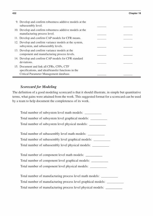
9. Develop and confirm robustness additive models at the subassembly level. ______ ______
10. Develop and confirm robustness additive models at the manufacturing process level. ______ ______
11. Develop and confirm CAP models for CFR means. ______ ______
12. Develop and confirm variance models at the system, subsystem, and subassembly levels. ______ ______
13. Develop and confirm variance models at the component and manufacturing process levels. ______ ______
14. Develop and confirm CAP models for CFR standard deviations. ______ ______
15. Document and link all CFRs, CFPs, CTF specifications, and ideal/transfer functions in the Critical Parameter Management database. ______ ______
Scorecard for Modeling
The definition of a good modeling scorecard is that it should illustrate, in simple but quantitativeterms, what gains were attained from the work. This suggested format for a scorecard can be usedby a team to help document the completeness of its work.
Total number of subsystem level math models: __________
Total number of subsystem level graphical models: __________
Total number of subsystem level physical models: __________
Total number of subassembly level math models: __________
Total number of subassembly level graphical models: __________
Total number of subassembly level physical models: __________
Total number of component level math models: __________
Total number of component level graphical models: __________
Total number of component level physical models: __________
Total number of manufacturing process level math models: __________
Total number of manufacturing process level graphical models: __________
Total number of manufacturing process level physical models: __________
432 Chapter 18

Table of System Level CFRs:
System Estimated Estimated Unit of CFR Name: Target: Tolerance: USL Tolerance: LSL Measure:
1. ______ ______ ______ ______
2. ______ ______ ______ ______
3. ______ ______ ______ ______
Table of Subsystem Level CFRs:
Subsystem Estimated Estimated Unit of CFR Name: Target: Tolerance: USL Tolerance: LSL Measure:
1. ______ ______ ______ ______
2. ______ ______ ______ ______
3. ______ ______ ______ ______
Table of Subassembly Level CFRs:
Subassembly Estimated Estimated Unit of CFR Name: Target: Tolerance: USL Tolerance: LSL Measure:
1. ______ ______ ______ ______
2. ______ ______ ______ ______
3. ______ ______ ______ ______
Table of Component Level CTF Specifications:
ComponentCTF Spec. Estimated Estimated Unit of Name: Target: Tolerance: USL Tolerance: LSL Measure:
1. ______ ______ ______ ______
2. ______ ______ ______ ______
3. ______ ______ ______ ______
Modeling: Ideal/Transfer Functions, Robustness Additive Models, and the Variance Model 433
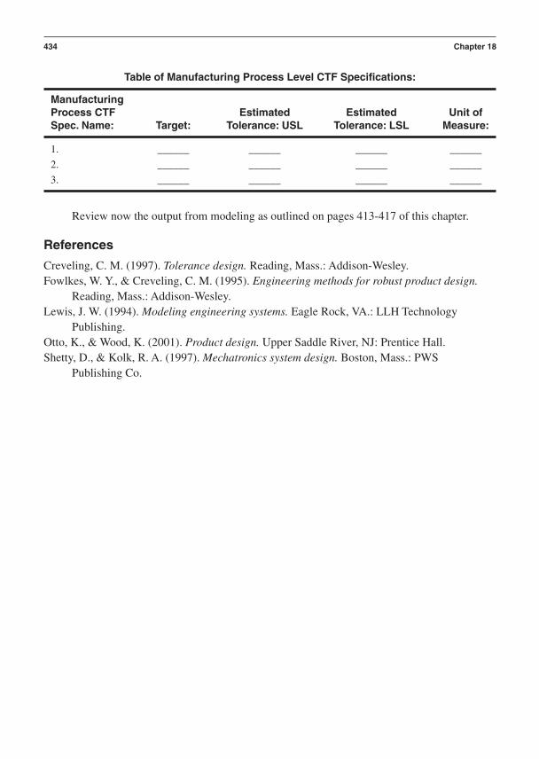
Table of Manufacturing Process Level CTF Specifications:
ManufacturingProcess CTF Estimated Estimated Unit of Spec. Name: Target: Tolerance: USL Tolerance: LSL Measure:
1. ______ ______ ______ ______
2. ______ ______ ______ ______
3. ______ ______ ______ ______
Review now the output from modeling as outlined on pages 413-417 of this chapter.
References
Creveling, C. M. (1997). Tolerance design. Reading, Mass.: Addison-Wesley.Fowlkes, W. Y., & Creveling, C. M. (1995). Engineering methods for robust product design.
Reading, Mass.: Addison-Wesley.Lewis, J. W. (1994). Modeling engineering systems. Eagle Rock, VA.: LLH Technology
Publishing.Otto, K., & Wood, K. (2001). Product design. Upper Saddle River, NJ: Prentice Hall.Shetty, D., & Kolk, R. A. (1997). Mechatronics system design. Boston, Mass.: PWS
Publishing Co.
434 Chapter 18

P A R T V
Tools and Best Practices forDesign Development
Chapter 19 Design Failure Modes and Effects AnalysisChapter 20 Reliability PredictionChapter 21 Introduction to Descriptive StatisticsChapter 22 Introduction to Inferential StatisticsChapter 23 Measurement Systems AnalysisChapter 24 Capability StudiesChapter 25 Multi-Vari StudiesChapter 26 RegressionChapter 27 Design of Experiments
The tools and best practices discussed in this section focus on deliverables required at gate re-views for Phase 2 in the I2DOV and CDOV processes.
The tools and best practices chapters are structured so that the reader can get a strong senseof the process steps for applying the tools and best practices. The structure also facilitates the cre-ation of PERT charts for project management and critical path management purposes. A check-list, scorecard, and list of management questions end each chapter.
435

This page intentionally left blank

C H A P T E R 1 9
Design Failure Modes and Effects Analysis
Where Am I in the Process? Where Do I Apply DFMEA Within theRoadmaps?
Linkage to the I2DOV Technology Development Roadmap:
437
Invent/Innovate
Develop Optimize Verify
Concept Design Optimize Verify
DFMEA is conducted within the Develop phase during technology development. Some technol-ogy development teams may decide to do a cursory version of DFMEA on each candidate tech-nology concept prior to inclusion in the Pugh concept selection process. DFMEA is typically doneon the superior concepts that emerge from the Pugh concept selection process.
Linkage to the CDOV Product Development Roadmap:
DFMEA is conducted within the Design phase during product development. Some product de-sign teams also decide to do a cursory version on each of the candidate concepts prior to inclu-sion in the Pugh concept selection process. DFMEA is typically done on the superior conceptsthat emerge from the Pugh concept selection process.
Design FMEAs are applied to qualitatively define and quantitatively rank the failure modesfor a system and its subsystems, subassemblies, and components. Process FMEAs are conductedon manufacturing processes.

What Am I Doing in the Process? What Does DFMEA Do at this Point in theRoadmaps?
The Purpose of DFMEA in the I2DOV Technology Development Roadmap:
DFMEA is applied to qualitatively define and quantitatively rank the failure modes and effectsfor new technology platforms and subsystems that are being developed for integration into a newplatform or for integration into existing product designs. Preventative application of numeroustools and best practices can then be deployed to improve the resistance to failure modes and thestrategic minimization of their effects.
The Purpose of DFMEA in the CDOV Product Development Roadmap:
Design FMEAs are applied to qualitatively define and quantitatively rank the failure modes for asystem and its subsystems, subassemblies, and components. Preventative application of numer-ous tools and best practices can then be deployed to improve the resistance to failure modes andthe strategic minimization of their effects.
What Output Do I Get at the Conclusion of this Phase of the Process? WhatAre Key Deliverables from DFMEA at this Point in the Roadmaps?
• Design failure modes identified• Effects of a design failure mode identified• Causes of a design failure identified• Linkage of the following ratings to each cause:
Severity ratingOccurrence ratingDetection rating
• Calculated risk priority numbers (RPN) for each cause• Improved risk priority numbers (RPN) for each cause after corrective action
The DFMEA Flow Diagram (found on page 439)
This visual reference of the detailed steps of DFMEA illustrates the flow of tasks and processesemployed at this stage.
Verbal Descriptions for the Application of Each Block Diagram
This section explains the specific details of each step of DFMEA:
• Key detailed input(s) from preceding tools and best practices• Specific steps and deliverables from each step to the next within the process flow• Final detailed outputs that flow into follow-on tools and best practices
438 Chapter 19

Key Detailed Inputs
Superior concept architectures, their functions, and requirements.
The form, fit, and functions and the requirements they seek to fulfill at the system, subsystem,subassembly, and component levels are inputs to the DFMEA process.
Design Failure Modes and Effects Analysis 439
INPUT . . .
OUTPUT . . .
Superior conceptarchitectures, their functions,
and requirements.
Develop a block diagram ofthe design element or
function being analyzed(at system, subsystem,
subassembly, or component level).
Determine the ways in whicheach design element or
function can fail(failure modes).
Determine the effects of thefailure on the customer(s) foreach failure mode associatedwith the element or function.
Identify potential causes ofeach failure mode.
Create severity, occurrence,and detection rating scalesfor each element or function
under evaluation.
List the current designcontrols for each cause or
failure mode.
Assign severity, occurrence, and detectionratings to each cause.
Calculate risk priority numbers (RPN) foreach cause.
Determine recommended actions toreduce high RPNs.
Apply tools and best practices to reducesensitivity to root causes of failure oreliminate root causes of failure and
recalculate RPNs.
Causes of failure qualitatively andquantitatively documented and corrective
action underway. New RPN calculated aftercorrective action results are documented.

Specific Steps and Deliverables
Develop a block diagram of the design element or function being analyzed (at system, subsystem, subassembly, or component level).
A block diagram illustrates the input–output relationships at the system, subsystem, subassembly,or component level. In particular they illustrate the flow of mass, energy, and information intoand out of a design element. For example, a hydraulic subassembly may have fluid (mass), forces(energy), and digital logic and control signals (information) flowing in some form that is associ-ated with its ideal function.
The object of the block diagram in Figure 19–1 is to understand the input to the block, theprocess (function) performed within the block, and the output from the block. It also establishesthe relationship of each item/function to all other associated system elements.
With the design element, its inputs, outputs, and ideal/transfer function defined, the teamhas the information it needs to begin to assess its potential failures modes.
440 Chapter 19
Desired Mass
Undesired Mass
Desired Energy
Undesired Energy
Desired Information
Undesired Information
Desired Mass
Undesired Mass
Desired Energy
Undesired Energy
Desired Information
Undesired Information
Transformations, Flows,or Changes of State
Functional, Architectural, Regulatory, LegalEnvironmental Limitations, and Constraints
Functional Outputs (Y)Functional Inputs (x)
System,Subsystem,Subassembly, orComponent
Ideal/TransferFunctionY = f(x)
Figure 19–1 System Inputs and Outputs
Determine the ways in which each design element or function can fail (failure modes).

The team works together to identify and document all the ways the design can fail. These are re-ferred to as failure modes. The failure modes include all forms of functional failures. Failures canbe associated with how the design transforms mass, energy, and information. These three itemscover everything that is associated with any design’s function. A design can fail to flow, transform,or change the state of mass, energy, and information (digital or analog logic and control signals).
Design Failure Modes and Effects Analysis 441
Functions Failure Modes Effects Causes Design Controls
Function Failure Modes Effects Causes Design Controls
Determine the effects of the failure on the customer(s) for each failure mode associated with the element or function.
The team traces the effects each failure mode has on the customers that use the product or process.Effects can span a wide range. Some examples include:
• Economic loss• Physical safety• Loss of desired function

No matter what the relative impact of the effect, every effect should be documented. Everyeffect should be traceable through its failure mode back to the ideal/transfer function that under-writes the fulfillment of a requirement. There should be clear linkage and traceability betweenfailure effects, failure modes, ideal/transfer functions, and their requirements.
442 Chapter 19
Function Failure Modes Effects Causes Design Controls
Function Failure Modes Effects Causes Design Controls
Identify potential causes of each failure mode.
A thorough root cause analysis should be performed on each failure mode. Root cause analysis isa detailed, fundamental engineering investigation into the physical causes for the failure. Theideal/transfer function for the design element in which the failure occurred is the starting point.Something associated with the transfer, flow, or change of state of the design’s functions has gonewrong. Root cause analysis in this context rigorously documents the reasons why the failure occurred.
List the current design controls for each cause or failure mode.

Three categories can be established to quantify the nature of failures modes and their detection:
1. Severity: importance of the effect on customer requirements; could also be concernedwith safety and other risks if failure occurs.
2. Occurrence: frequency with which a given cause occurs and creates the failure mode.3. Detection: (capability of current design controls) ability of current design control
scheme to detect the causes or the effect of the failure modes.
Assign severity, occurrence, and detection ratings to each cause.
The three categories can now have numerical ratings assigned to quantify the nature of the fail-ure modes and their detection:
Severity: importance of the effect on customer requirements; could also be concernedwith safety and other risks if failure occurs.
1 Not severe, 10 Very severe
After each root cause is unveiled, the team needs to identify the controls available to the designteam to prevent, forecast, or detect the failure mode. Controls for the prevention of design defects(failure modes) or reducing the rate of occurrence include: mathematical modeling, engineeringstress and failure analysis, reliability modeling, robust design, and tolerance design.
Forecasting or detection of either the causes or failure modes are not as desirable as pre-vention but may be necessary. Examples of forecasting or detection include performance testing,lab analysis, prototyping, stress testing, and alpha site testing.
Design Failure Modes and Effects Analysis 443
Function Failure Modes Effects Causes Design Controls
Create severity, occurrence, and detection rating scales for each element or function under evaluation.

Occurrence: frequency with which a given cause occurs and creates the failure mode.
1 Not likely, 10 Very likely
Detection: (capability of current design controls) ability of current design control schemeto detect the causes or the effect of the failure modes.
1 Likely to detect, 10 Not likely at all to detect
The accompanying table illustrates a ranking scale (you can devise your own to suit your business).
Rating Severity of Effect Likelihood of Occurrence Ability to Detect
10 Hazardous without warning Very high: Failure is almost Cannot detectinevitable
9 Hazardous with warning Very remote chance of detection
8 Loss of primary function High: Repeated failures Remote chance of detection
7 Reduced primary function Very low chance of detectionperformance
6 Loss of secondary function Moderate: Occasional failures Low chance of detection
5 Reduced secondary function Moderate chance of detectionperformance
4 Minor defect noticed by Moderately high chance most customers of detection
3 Minor defect noticed by Low: Relatively few failures High chance of detectionsome customers
2 Minor defect noticed by Very high chance of detectiondiscriminating customers
1 No effect Remote: Failure is unlikely Almost certain detection
Source: Used with permission from SBTI.
Calculate risk priority numbers (RPN) for each cause.
The quantified values associated with the severity, occurrence, and detection of failure modes andtheir causes can be used to calculate a summary value called the risk priority number. This as-signs a value to the risk each failure mode represents.
RPN (Severity) (Occurrence) (Detection)
Determine recommended actions to reduce high RPNs.
444 Chapter 19

Once a plan of action is defined, the team members apply the appropriate tools and best practicesthat have been selected to correct the root causes of the failure modes.
Final Detailed Outputs
The team now establishes its plan of action to reduce the risk associated with the effect of eachfailure mode. The highest RPN items are the highest priority for action. The tools and best prac-tices of DFSS are excellent means to correct these risks.
Design Failure Modes and Effects Analysis 445
(continued)
Apply tools and best practices to reduce sensitivity to root causes of failure or eliminate root causes of failure and recalculate RPNs.
Causes of failure qualitatively and quantitatively documented and corrective action underway. New RPN calculated
after corrective action results are documented.
The final, corrective actions produce results that are documented in the FMEA database. NewRPN numbers can now be calculated for each failure mode. The failure modes are still possiblein some cases, but their probability of occurrence is greatly reduced.
DFMEA Checklist and Scorecard
This suggested format for a checklist can be used by an engineering team to help plan its workand aid in the detailed construction of a PERT or Gantt chart for project management of theDFMEA process within the Optimize phase of the CDOV or I2DOV development process. Theseitems also serve as a guide to the key items for evaluation within a formal gate review.
Checklist for DFMEA
Was this Excellence Rating:Action Deployed? 1 Poor
Actions: YES or NO 10 Excellent
1. Develop a block diagram of the design element or function being analyzed (at system, subsystem, subassembly, or component level). ______ ______
2. Determine the ways in which each design element or function can fail (failure modes). ______ ______
3. Determine the effects of the failure on the customer(s) for each failure mode associated with the element or function. ______ ______
4. Identify potential causes of each failure mode.
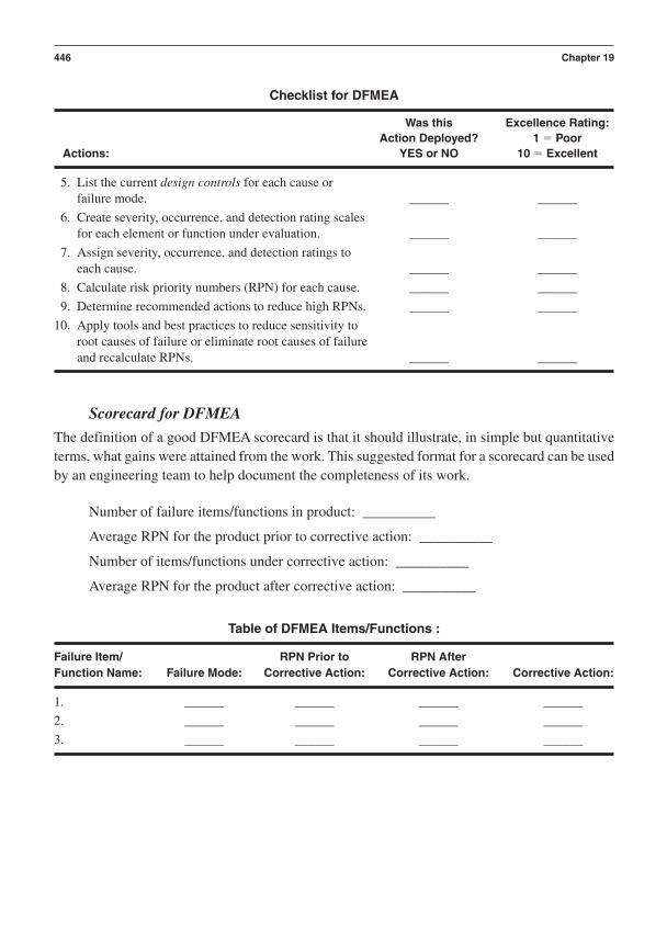
Checklist for DFMEA
Was this Excellence Rating:Action Deployed? 1 Poor
Actions: YES or NO 10 Excellent
5. List the current design controls for each cause or failure mode. ______ ______
6. Create severity, occurrence, and detection rating scales for each element or function under evaluation. ______ ______
7. Assign severity, occurrence, and detection ratings to each cause. ______ ______
8. Calculate risk priority numbers (RPN) for each cause. ______ ______
9. Determine recommended actions to reduce high RPNs. ______ ______
10. Apply tools and best practices to reduce sensitivity to root causes of failure or eliminate root causes of failure and recalculate RPNs. ______ ______
Scorecard for DFMEA
The definition of a good DFMEA scorecard is that it should illustrate, in simple but quantitativeterms, what gains were attained from the work. This suggested format for a scorecard can be usedby an engineering team to help document the completeness of its work.
Number of failure items/functions in product: __________
Average RPN for the product prior to corrective action: __________
Number of items/functions under corrective action: __________
Average RPN for the product after corrective action: __________
Table of DFMEA Items/Functions :
Failure Item/ RPN Prior to RPN After Function Name: Failure Mode: Corrective Action: Corrective Action: Corrective Action:
1. ______ ______ ______ ______
2. ______ ______ ______ ______
3. ______ ______ ______ ______
446 Chapter 19

We repeat the final deliverables from DFMEA:
• Design failure modes identified• Effects of a design failure mode identified• Causes of a design failure identified• Linkage of the following ratings to each cause:
Severity ratingOccurrence ratingDetection rating
• Calculated risk priority numbers (RPN) for each cause• Improved risk priority numbers (RPN) for each cause after corrective action
References
Potential failure mode and effects analysis (3rd ed.). (1995). AIAG (810-358-3003).Stamatis, D. H. (1995). Failure mode and effect analysis. Milwaukee, Wisc.: ASQC Quality
Press.
Design Failure Modes and Effects Analysis 447

This page intentionally left blank

C H A P T E R 2 0
Reliability Prediction
This chapter was written by Edward Hume, a seasoned veteran in Six Sigmamethods. Concurrent with the introduction of Motorola’s Six Sigma initiative, Tedled the development and operation of his business unit’s first Six Sigmamanufacturing operation. He practiced Six Sigma in design and managementpositions over much of his career. Ted is an electrical engineer specializing in thedesign and reliability sciences.
Where am I in the Process? Where Do I Apply Reliability Prediction Withinthe Roadmaps?
Linkage to the I2DOV Technology Development Roadmap:
449
Invent/Innovate
Develop Optimize Verify
Concept Design Optimize Verify
Reliability predictions are conducted within the Develop phase during technology development.
Linkage to the CDOV Product Development Roadmap:
Reliability predictions are conducted within the Design phase during product development.

What Am I Doing in the Process? What Does Reliability Prediction Do atthis Point in the Roadmaps?
The Purpose of Reliability Prediction in the I2DOV Technology DevelopmentRoadmap:
Reliability prediction is applied to qualitatively define and quantitatively predict the baseline re-liability of new technology platforms and subsystems that are being developed for integration intoa new platform or for integration into existing product designs. Preventative application of nu-merous tools and best practices can then be deployed to improve reliability, as required, prior tothe technology being transferred into a commercialization program.
The Purpose of Reliability Prediction in the CDOV Product DevelopmentRoadmap:
Reliability predictions are first applied to predict the reliability of subsystems, subassemblies, andcomponents and then to predict the overall integrated system reliability. Preventative applicationof numerous tools and best practices can also be deployed to improve the reliability as requiredprior to design certification.
What Output Do I Get at the Conclusion of this Phase of the Process? What AreKey Deliverables from Reliability Prediction at this Point in the Roadmaps?
• Predicted reliability performance of subsystems, subassemblies, and components• Predicted reliability performance of the system• Component, subassembly, and subsystem reliability performance improvement
activitiesRequired deliverables from specific tools and best practices that improve reliabilityby reducing variability and sensitivity to deterioration and external noise factors
The Reliability Prediction Flow Diagram (found on page 451)
This visual reference traces the detailed steps of the reliability prediction process.
Applying Each Block Diagram Within the Reliability Prediction Process
This section steps through the specifics of:
• Key detailed input(s) from preceding tools and best practices• Specific steps and deliverables from each step to the next within the process flow• Final detailed outputs that flow into follow-on tools and best practices
Key Detailed Inputs
Reliability requirements for system, historic reliability data, and DFMEA inputs.
450 Chapter 20

System Reliability Requirement Inputs
• Voice of the customer (concept engineering)• Competitor comparisons, best within industry (benchmarking and QFD)• World class, best of all industries, benchmarking• Business unit improvement plans• Government agencies• Reliability data on similar current products• Lessons learned and design rules
Concept Gate Review Question
• What was the basis for the reliability requirements?
Requirements Content
Requirements must be complete and consistent. Otherwise, a great reliability effort can fail to sat-isfy customer and/or business needs. Some key items should be in the requirements.
• Measurable definitions of reliability requirements:• The time to reach 1%, 10%, etc., failures (often referred to as B1, B10, etc., life)• MTTF—mean time to failure
Reliability Prediction 451
INPUT . . .
OUTPUT . . .
Reliability requirements forsystem, historic reliabilitydata, and DFMEA inputs.
Allocate system reliabilityrequirements to subsystems,subassemblies, and critical
components.
Predict system reliabilityfrom current performance of
similar subsystems,subassemblies, and critical
components.
Identify performance gaps,improvement actions, and
reallocation targets.
Predict critical componentreliability.
Identify critical component performancegaps and improvement actions.
Predict subassembly and subsystemreliability.
Identify subassembly and subsystemperformance gaps and improvement
actions.
Reallocate targets, calculate newperformance gaps, and identify
improvement actions.
Model and predict system reliability.
Predicted reliability, new targets,improvement activities defined, updated
DFMEA, and system model.
• MTBF—mean time between failures, used to describe repairable equipment withconstant failure rates
• % per month or year failure rate• Environmental conditions:
• Where is it used: in an office, factory, vehicle, or aircraft?• Is it air-conditioned, subject to ambient temperatures, or subject to raised
temperatures because of its enclosure?• Is it exposed to dust, rain, or ice?• Is it dropped? How is it shipped?• Is it subject to spills, chemicals, or being cleaned with a hose?• If it uses electrical power, will it be used in developed and/or undeveloped countries?
• Governmental agency requirements: All agency requirements from all countries ofintended use must be identified.
Concept Gate Review Questions
• Are reliability requirements measurable?• Can reliability requirements be achieved within the scope of the project?• Are environmental requirements completely described for current and derivative
products?• Are governmental agency requirements completely known for current and derivative
products?
These inputs must be used to generate a detailed environmental specification to guide thedesign and testing. One of the most common causes of significant reliability problems is not de-signing for the appropriate environmental conditions.
Historical Warranty and Reliability Data Inputs
Many companies do not have good historical reliability data. For example:
• No data is collected beyond the warranty period.• Time to failure is not recorded or is difficult to derive because data is kept primarily to
support standard monthly reports with percent failure rates and/or warranty cost.• Cause of failure is not determined or, in many cases, what is reported is a symptom
rather than a root cause.
As an example of symptom vs. cause, let’s look at a cell phone that no longer works prop-erly. The symptom is that the battery won’t hold its charge. Repair includes replacing a circuitboard that controls battery charging operations, the antenna assembly, and the display. All re-placed items have been damaged by what must have been a severe shock. What was the cause ofthe failures? The phone was dropped on concrete producing a stress (high deceleration) that ex-ceeded the strength of solder joints, display, and connections in the antenna assembly. The infor-
452 Chapter 20

mation that often gets reported is that the phone did not hold a charge and sometimes that the cir-cuit board, display, and antenna assembly were replaced. To learn from the repair we need to un-derstand the stress that caused the damage (when possible), all the items that were damaged, andthe nature and the location of the damage.
A system that provides information on time to failure and cause of failure over the expectedlife of the product is a plus when starting the Develop/Design phase. Many companies maintainrecords of all failures that occur in the warranty period. To add cause of failure to all repair recordsand extend them to cover the life of the product would be expensive. It would also be difficult toachieve because of the requirement to train a large number of people on proper failure analysis.Only a representative sample of the repair data is necessary or desirable. As in all Six Sigma ef-forts, small manageable sets of data are used for learning and improvement.
Collection of Field Failure Data
A best practice is to establish a partnership with a few key customers and/or repair depots and trainthem to provide needed field failure information. Those selected should provide a good cross-section of the customer base. Field failure information should be collected over the entire designlife of the product.
Lessons Learned and Design Rules
Another best practice is to turn the experience from each product development and field probleminto lessons learned. Turning the experience into design rules ensures that the lessons will be usedin future designs. Those companies that have a process to learn from each experience clearly willhave steeper learning curves than those companies that don’t.
Concept Gate Review Questions
• Do we have historic reliability data, including the cause of failures, to use as a startingpoint for prediction efforts?
• Do we have a database of lessons learned and has it been reviewed?• Do we turn lessons learned into design rules?
DFMEA Inputs
From a customer system FMEA, failure modes or a combination of failure modes that have a se-vere effect (high effect score) on the customer’s system constitute DFMEA inputs. In system, sub-system, and subassembly DFMEAs, a high RPN number requires special attention during thedesign process, reliability prediction, and reliability testing.
Concept Gate Review Questions
• Has the initial DFMEA been performed on the selected concept?• Has a customer systems FMEA been performed?
Reliability Prediction 453

When the design concept is selected and the targets are identified, it is important to do a first passprediction to identify performance gaps. Since the design is in its infancy, detailed component pre-dictions are not possible. However, the performance of similar subsystems, subassemblies, andcritical components can be used to provide a reasonably accurate estimate of reliability perfor-mance. The reliability performance of similar subsystems, subassemblies, and critical componentsare adjusted to those in the current design concept by comparing the complexity, inherent stresslevels, external stress levels, expected length of life, and base reliability of critical components.
Develop a reliability block diagram (RBD) as described in the last step, “Model and pre-dict system reliability,” to use as the model to contain the estimated information.
If you lack historical information on some of the subsystems, subassemblies, and criticalcomponents, put together an estimate of the bill of materials, then follow the detailed process ofprediction in the steps that follow. In the case of electronics, Military Handbook 217F (MIL-HDBK-217F) offers a part count method of predicting electronics reliability. This is a reasonablemethod of initially establishing relative reliability. Don’t wait for the design to be complete be-fore doing predictions. Once a design is complete, it is too late to prevent the development of aproduct that doesn’t meet reliability requirements.
As soon as the final concept has been determined, the overall system reliability requirementsshould be allocated to each of the subsystems, subassemblies, and critical components to createtargets for reliability development. This initial allocation is based on current knowledge of the re-liability of all the items in the design concept.
Specific Steps and Deliverables
454 Chapter 20
Allocate system reliability requirements to subsystems,subassemblies, and critical components.
Predict system reliability from current performance of similar subsystems, subassemblies, and critical components.
Identify performance gaps, reliability improvement actions, and needed target reallocation.
Gaps between the predictions and targets can lead to a number of actions:
• Reevaluation of the system concept• Reallocation of targets• Prioritized reliability development actions
Predict critical component reliability.
Most products have individual components that, by themselves, are a significant part of the over-all system’s reliability. These components are typically involved in cost or performance vs. reli-ability trade-off and require significant reliability development efforts.
Examples of such components are the following:
Bearings
Fans
Capacitors
Batteries
Structural members that are flexed during operation
Semiconductor power devices
Complex semiconductor devices such as microprocessors
Sources of data to make predictions will include:
• Supplier information• Reference databases:
MIL-HDBK-217F—Available through prediction programsTelcordia (Bellcore 6)—Available through prediction programsPrism, Electronic Parts Reliability Data (EPRD), and Non-Electronic Parts Reliability
Data (NPRD)—Reliability Analysis Center (RAC), raciitri.org, 888-722-8737• Field reliability data• Test data
Supplier information and reference databases usually specify reliability in terms of a con-stant base failure rate for each part. Part failure rate in your application is a function of the basefailure rate modified by stress, quality, and environmental factors. Reliability/survival or cumu-lative failure probability are calculated from the part failure rate.
Field reliability and test data are fit to known statistical distributions. Reliability/survivalor cumulative failure probabilities are calculated from the fitted distribution.
Before we proceed with critical part reliability prediction, let’s consider some basic relia-bility information. Four functions are used to describe reliability performance:
Probability density function—Plot of amount of failures vs. time (or cycles, miles, etc.),f(t). This function would fit a histogram of your data. The most common example of aprobability density function is a standard normal curve.
Cumulative Distribution Function—For any given time, the probability that the part isnot working is F(t) µf(t)dt.
Reliability Prediction 455

Reliability/Survival Function—For any given time, the probability that the part is stillworking is R(t) 1 F(t)
Hazard Function—Rate of failure at any given time is h(t) f(t)/R(t). This failure rate isrepresented in a bathtub curve, as in the following example.
456 Chapter 20
Bathtub Curve
h(t) λ
UsefulLife
Life (hours, cycles, miles, and so on)
Wear-outInfantMortality
Known statistical distributions are used to fit data from field and test data. Some commonlyused distributions are the exponential, Weibull, normal, and lognormal. The pertinent functionsfor the exponential distribution are shown in this equation:
f(t) letl (t 0)
F(t) l etl
R(t) etl
h(t) l
Note that the exponential distribution has some unique properties. R(t) and F(t) are easy tocalculate with a calculator. Since the hazard function is a constant (), failure rate is not a func-tion of time. This makes it natural for modeling the useful life, constant failure rate, portion of thebathtub curve. Mean time between failure (MTBF) is symbolized by and for the exponentialdistribution only, 1/. The pertinent functions for the Weibull distribution are shown in thefollowing equation.
h(t) = a
b a t
b (-1)
R(t) = e- (t )
F(t) = 1 - e- (t )
f(t) =
t (-1) e- (t ) (t 0)

The Weibull distribution also has some interesting properties. It can fit data sets that repre-sent all portions of the bathtub curve. The shape/slope parameter controls the shape of the curve.When 1, the failure rate decreases with time. When 1, the Weibull distribution becomesan exponential distribution and failure rates are constant. When 1, failure rate increases withtime, modeling the wear-out portion of the bathtub curve. The scale parameter alpha ( ), alsocalled characteristic life eta (), represents the point where 63.2% of the units have failed. Thepertinent functions for the normal distribution are shown in this equation:
The location parameter is also the mean time to failure (MTTF) and the mean of the dataset. Scale parameter is the standard deviation of the data set. The pertinent functions for the log-normal distribution are shown as
The location parameter is also the MTTF and the mean of the log of the data set. It iscommonly called the log mean. Scale parameter is the standard deviation of the log of thedata set. It is commonly called the log standard deviation. The lognormal distribution formsa number of different shapes with variation of the scale parameter . Shapes include both theinfant mortality and wear-out portions of the bathtub curve, making it quite useful in reliabil-ity work.
Prediction with Supplier Information and Reference Databases
The MIL-HDBK-217 is used to give an example of the process used to make predictions fromsupplier information and reference databases. Each part type has a base failure rate reported infailures per million hours of operation. This is modified by a number of factors to come up withthe part failure rate in the proposed application.
p b T A R S C CV Q E
p Part failure rate
b Base part failure Rate
T Temperature factor
A Applications factor
R Resistance factor, power rating
F(t) = £[log (t) - ],t 0
f(t) = .4343[(2)12t] exp-[log (t) - ]2(22),t 0
F(y) = [(y - )], -q y q
F(y) = 3y
-q(22)-12 exp [-(y - )2(22)]
f(y) = (22)-12 exp[ - (y - )2(22)],q y q
Reliability Prediction 457
S Voltage applied/voltage rated factor
C Construction factor
CV Capacitance factor
Q Quality factor
E Environment factor
Each part is described by some or all of these factors as specified by MIL-HDBK-217. Eachof these failure rates is a constant and represents the useful life portion of the bathtub curve. The ex-ponential distribution has a constant failure rate and is the one we turn to for calculating reliability.
An aluminum electrolytic capacitor will be used as an example: p b*CV*Q*E.b is a function of voltage and temperature stress. The capacitor is rated at 400f, 85°C,
and 25v. Operating conditions will be 60°C and 17.5v.
b .33 106 failures per hour
CV 1, Q 1, E 2
b (33 106) 1 1 2 .66 106 failures per hour
Exponential distribution: f(t) et (t 0), F(t) 1 et, R(t) et, h(t) . Usinga calculator we can determine F(t) and R(t) at 1 year (8,760 hours) and 10 years (87,600 hours).
R(t) et e8700 (.00000066) .994, probability for survival of 1 year is 99%.
R(t) et e87000 (.00000066) .944, probability for survival of 10 years is 94%.
F(t) 1 R(t) 1 .994 .006, 1 .944 .056, probability for failure at 1 and 10years, respectively, is 1% and 6%.
A similar process can be followed for supplier information and other reference databases.
Tool Summary
Limitations
• Failure rates in the database are not collected under identical conditions to those towhich your product will be exposed.
• Failure rates in the database are collected on parts whose construction andmanufacturing processes may have changed for the parts used in your product.
• Failure rates in the database often do not describe infant mortality and wear-outfailures.
Benefits
• Causes a review of the quality level of selected parts.• Causes a review of all pertinent stress levels on the part in question.
458 Chapter 20

• Provides a first order approximation of part reliability.• Provides input to reliability allocation.
Recommendations
• Use to provide reliability comparisons to known performance of similar products.• Use for reliability allocation.• Use to provide a basis for reliability improvement efforts.• Use to review stress levels applied and inherent quality performance of key parts.• Verify predictions through testing.
Prediction with Field and Test Data
The Minitab program is used to show how a three-step process will take you from data to pre-dicted reliability with confidence intervals. The steps are the following:
1. Fit a known distribution to the data.2. Review the shape of statistical functions f(t), R(t), and h(t) and observe the distribution
parameters.3. Project B1, 10, etc., life and project reliability/survival probabilities at times such as
10 years, 100,000 miles, etc.
We will use the results of a test data from 40 incandescent light bulbs as an example.
Step 1. Fit a known distribution to the data. Open Minitab and enter time to failure for each lightbulb into one column labeled “N hours.” Sample data follows.
3666 6823 4489 7707 5591
6579 8248 5565 4743 5591
6671 5506 2356 1786 4786
5525 7675 7979 1426 4672
7742 3513 3290 5194 6225
4840 3804 803 6627 5267
6243 5990 5729 6466 6019
3949 2806 6282 6466 6019
Using pull-down menus, follow this path—Stat, Reliability/Survival, Distribution ID Plot-Right Cens. Load “N Hours” into the dialog box and run the program. Graphical results showingthe best fit are shown in Figure 20–1.
Use visual feedback showing how well the data points fit the proposed distribution and the Anderson-Darling (adj.) number to determine which distribution provides a better fit. The Anderson-Darling (adj.) number is a goodness of fit measurement, in which smaller is better.
Reliability Prediction 459

Both approaches show the normal distribution is a slightly better fit than the Weibull distribution.The exponential and lognormal distributions are not good enough fits to be considered. Since thenormal distribution fits the best, it will be used for further analysis.
Step 2. Using pull-down menus, follow this path—Stat, Reliability/Survival, DistributionOverview Plot-Right Cens. Load “N Hours” into the dialog box and select the normal distribu-tion. Graphical results are shown in Figure 20–2.
The probability density function, f(t), is the normal curve we are used to seeing. Survivalfunction, R(t), depicts the probability of survival as the hours of use increase. Hazard function,h(t), shows the increasing failure rate of a wear-out function. The location parameter, MTTF, ormean is 5,266.5 hours. Scale parameter or standard deviation is 1,778.7 hours. Some importantinformation found on this graph is the shape of f(t)/probability density function and the shape ofh(t). From h(t) we learn if we have infant mortality, constant failures, or wear-out. This analysisis done one failure mode at a time. Data sets with more than one failure mode are split apart andanalyzed separately.
Step 3. Using pull-down menus, follow this path—Stat, Reliability/Survival, Parametric DistAnalysis Plot-Right Cens. Load “N Hours” into the dialog box and select the normal distribution.Select the Estimate button and load times for which you desire survival probabilities. Sessionwindow output results follow.
460 Chapter 20
Weibull Lognormal base e
ML Estimates - Complete Data
Anderson-Darling (adj)Weibull0.931
Lognormal base e2.540
Exponential8.325
Normal0.818
Exponential Normal
1000
1
23
5
10
20
Per
cent
Per
cent
Per
cent
304050607080
9590
99
10000
1
5
10
20
304050607080
95
99
Per
cent
1
5
10
20
304050607080
95
99
1030
506070
80
90
95
97
98
99
0 5000 10000 15000 20000 25000 0 1000 2000 3000 4000 5000 6000 7000 8000 9000
1000 10000
Figure 20–1 Four-Way Probability Plot for N Hours
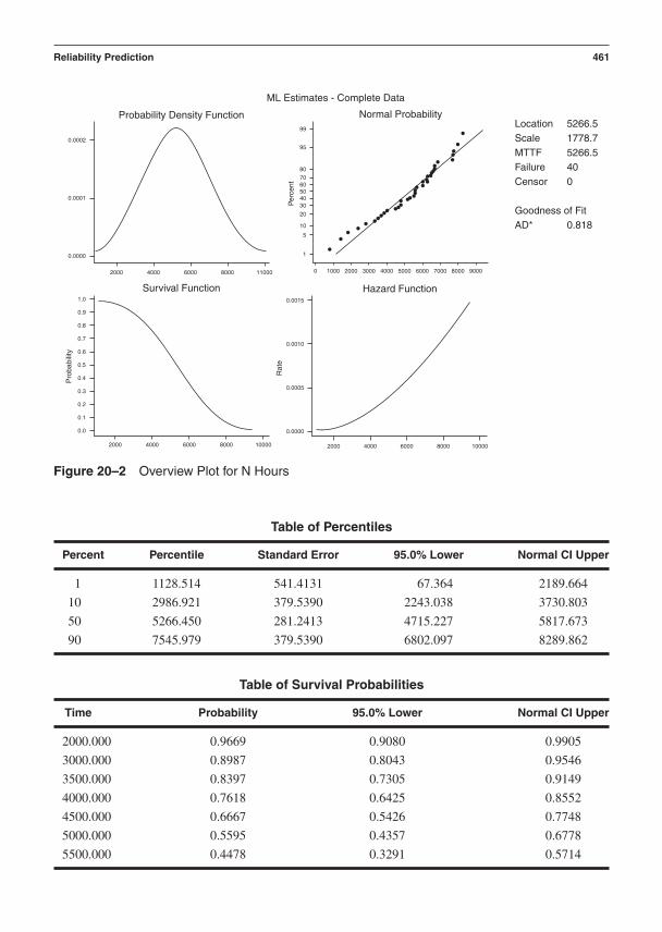
Table of Percentiles
Percent Percentile Standard Error 95.0% Lower Normal CI Upper
1 1128.514 541.4131 67.364 2189.664
10 2986.921 379.5390 2243.038 3730.803
50 5266.450 281.2413 4715.227 5817.673
90 7545.979 379.5390 6802.097 8289.862
Table of Survival Probabilities
Time Probability 95.0% Lower Normal CI Upper
2000.000 0.9669 0.9080 0.9905
3000.000 0.8987 0.8043 0.9546
3500.000 0.8397 0.7305 0.9149
4000.000 0.7618 0.6425 0.8552
4500.000 0.6667 0.5426 0.7748
5000.000 0.5595 0.4357 0.6778
5500.000 0.4478 0.3291 0.5714
Reliability Prediction 461
Probability Density Function
Hazard Function
ML Estimates - Complete Data
Location 5266.5Scale 1778.7MTTF 5266.5Failure 40Censor 0
Goodness of FitAD* 0.818
Survival Function
Normal Probability
2000R
ate
Pro
babi
lity
0.0002
0.0001
0.0000
0.0015
0.0010
0.0005
0.0000
Per
cent
1
5
10
20
304050607080
95
99
1.0
0.9
0.8
0.7
0.6
0.5
0.4
0.3
0.2
0.1
0.0
4000 6000 8000 11000
2000 4000 6000 8000 10000
0 1000 2000 3000 4000 5000 6000 7000 8000 9000
2000 4000 6000 8000 10000
Figure 20–2 Overview Plot for N Hours

Reliability performance in critical components can drive a number of improvement actions:
• Reviewing the basic product concept to find ways of reducing stress on the components• Adding components to reduce stress or provide redundancy• Improving the quality of the component
Predict subassembly and subsystem reliability.
Predictions based on supplier information, reference databases, or other source of constant fail-ure rate information are made using a unique property of the exponential distribution: failure ratesare additive. The failure rate of the subassembly or subsystem is simply the sum of all the indi-vidual failure rates. Once the total failure rate is calculated, F(t) and R(t) are found for the sub-assembly or subsystem using the same equations used in the previous example:
F(t) 1 et, R(t) et
Tool Summary
Limitations
• Requires significant investment in field data collection and/or testing facilities
Benefits
• Time to 1%, 10%, etc., failures is projected with confidence limits• Survival probability at selected times is projected with confidence limits• The hazard function h(t) is defined graphically, providing input to how failure rates
vary over life
Recommendations
• Use to decide on advertised specifications of life, such as a 4,000 hour light bulb• Use to set warranty policy and replacement intervals• Use to predict reliability and time to failure• Use for reliability allocation• Use to provide a basis for reliability improvement efforts
462 Chapter 20
Identify critical component performance gaps and reliability improvement actions.

A number of programs are available that contain one or more reference databases, are ca-pable of importing bills of materials, and can calculate individual failure rates and system or sub-system reliability.
Prediction Software
• Relex Software, www.relexsoftware.com, 724-836-8800• Reliability Analysis Center RAC “Prism,” rac.iitri.org/, 888-722-8737• RelCalc for Windows, www.t-cubed.com, 818-991-0057• Item Software (USA) Inc., www.itemsoft.com/, 714-935 2900
Tool Summary
Limitations
• The same as reported at a component level
Benefits
The same as reported at a component level plus:
• Software tools available make tabulating and storing subsystem and subassemblyreliability relatively easy.
• What-if calculations help to quickly define improvement actions.
Recommendations
• The same as reported at a component level
Reliability Prediction 463
Identify subassembly and subsystem performance gaps and reliability improvement actions.
Reliability performance in subsystems and subassemblies can drive a number of improvement actions:
• Reviewing the subsystem or subassembly design to find ways of reducing stress on thecomponents
• Reducing the number of components in the designs• Improving the quality of the components
Model and Predict System Reliability
System reliability is modeled using a reliability block diagram (RBD). Subsystems, subassemblies,and major components are arranged into series and parallel orientation. All items whose failure will
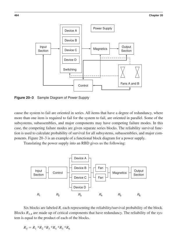
cause the system to fail are oriented in series. All items that have a degree of redundancy, wheremore than one item is required to fail for the system to fail, are oriented in parallel. Some of thesubsystems, subassemblies, and major components may have competing failure modes. In thiscase, the competing failure modes are given separate series blocks. The reliability survival func-tion is used to calculate probability of survival for all subsystems, subassemblies, and major com-ponents. Figure 20–3 is an example of a functional block diagram for a power supply.
Translating the power supply into an RBD gives us the following:
464 Chapter 20
InputSection
OutputSection
Control
Magnetics
Fans A and B
Device APower Supply
Device B
Device C
Device D
Switching
Figure 20–3 Sample Diagram of Power Supply
OutputSection
Control Magnetics
R1 R2 R3 R4 R5 R6
Device A
Device B
Device C
Device D
InputSection
Fan
Fan
Six blocks are labeled R, each representing the reliability/survival probability of the block.Blocks R3,4 are made up of critical components that have redundancy. The reliability of the sys-tem is equal to the product of each of the blocks.
RS R1 *R2 *R3 *R4 *R5 *R6

If blocks R1-6 have a 99 percent probability of surviving for 10 years then the reliability ofthe system would be: RS (.99) (.99) (.99) (.99) (.99) (.99) (.99)6 0.941.
Reliability of blocks R3 and R4 is determined by calculating the probability of survival of at least those items required for successful operation. There are two possible outcomes, survivalR and failure Q. Therefore the probability of R Q 1. If only one fan is required, then the pos-sible outcomes of both fans are RARB RAQB QARB QAQB. The probability of RARB RAQB
QARB QAQB 1. At least one fan is required for survival, so outcomes RARB RAQB QARB
represent survival, and outcome QAQB represents failure. If the probability of survival of both fansis 90 percent, we can calculate the probability of survival of block R4 as follows:
R4 RARB RAQB QARB 1 QAQB 1 (1.90)(1.90)
R4 .99
Using the assumption that each of the switching devices has an equal probability of sur-vival, the equation for all possible outcomes is:
R4 4R3Q 6R2Q2 4RQ3 Q4 1
If three devices are required for operation, R4 4R3Q represents the successful outcomes.If the probability of survival of each device is 95 percent, we can calculate the probability of suc-cess for R3:
R4 4R3Q 1 (6R2Q2 4RQ3 Q4) 1 ((6*(.95)2*(.05)2) 4*(.95)*(.05)3
(.05)4)
R3 .986
Tool Use Summary
Benefits
• All sources of reliability data can be turned into a reliability/survival probability andused in the model.
• Creating an RBD helps identify the critical subsystems, subassemblies, andcomponents that contribute most to lack of success.
Recommendations
• Use of this tool should be initiated after the design concept is selected and updatedcontinuously.
• Reliability performance of the system, subsystems, subassemblies, and criticalcomponents predicted by the model should be tracked against the target.
• Consider using prediction software that creates and maintains complex reliability blockdiagrams (such as Relex Software, www.relexsoftware.com, 724-836-8800).
Reliability Prediction 465
Now system, subsystem, subassembly, and critical component reliability predictions have beencompleted. Performance gaps have been identified. Significant contributors to loss of reliabilityhave been identified. The following summary lists actions that should be taken:
• Reallocate targets that add up to meeting reliability requirements.• Search for additional supplier data, database, field data, and test data that will confirm
failure rates or reliability of critical components.• Design improvement activities to:
Reduce stress on critical partsSelect higher reliability partsReduce complexity
• Plan reliability testing to confirm predictions and improvements.
Final Detailed Outputs
Reallocate targets, calculate new performance gaps,and identify improvement actions.
466 Chapter 20
Predicted reliability, new targets, improvement activities defined, updated DFMEA, and system model.
Outputs of the prediction process should include the following:
1. Targets for the system, subsystems, subassemblies, and critical components2. Predictions for the system, subsystems, subassemblies, and critical components3. Reliability performance gaps4. Improvement activities planned for performance gaps5. Reliability testing plans
Reliability Prediction Checklist and Scorecard
This suggested format for a checklist can be used by an engineering team to help plan its work.The list will also aid in the detailed construction of a PERT or Gantt chart for project manage-ment of the reliability prediction process within the Optimize and Capability Verification Phasesof the CDOV or I2DOV development process. These items also serve as a guide to the key itemsfor evaluation within a formal gate review.

Checklist for Reliability Predictions
Was this Excellence Rating:Action Deployed? 1 Poor
Actions: YES or NO 10 Excellent
1. Allocate system reliability requirements to subsystems, subassemblies, and critical components. ______ ______
2. Predict system reliability from current performance of similar subsystems, subassemblies, and critical components. ______ ______
3. Identify performance gaps, improvement actions, and reallocation targets ______ ______
4. Predict critical component reliability. ______ ______5. Identify critical component performance gaps and
improvement actions. ______ ______6. Predict subassembly and subsystem reliability. ______ ______7. Identify subassembly and subsystem performance gaps
and reliability improvement actions. ______ ______8. Model and predict system reliability. ______ ______9. Reallocate targets, calculate new performance gaps, and
identify improvement actions. ______ ______
Scorecard for Reliability Predictions
The definition of a good reliability prediction scorecard is that it should illustrate, in simple butquantitative terms, what gains were attained from the work. This suggested format for a score-card can be used by an engineering team to help document the completeness of its work.
Table of Documented Reliability Failures and Corrective Actions
System, Subsystem, Improvement Subassembly, or Critical Target Predicted ActionComponent Name: Reliability: Reliability: Gap: and Tools:
1. ______ ______ ______ ______
2. ______ ______ ______ ______
3. ______ ______ ______ ______
Leadership Review Guidelines
A manager should ask these questions at gate reviews to promote problem prevention and forward-looking support issues to foster a problem prevention culture during technology and
Reliability Prediction 467

product development. Questions for the Concept or Invent/Innovate gate review presented earlierin this chapter are listed again here:
• What was the basis for the reliability requirements?• Are reliability requirements measurable?• Can reliability requirements be achieved within the scope of the project?• Are environmental requirements completely described for current and derivative
products?• Are governmental agency requirements completely known/described for current and
derivative products?• Do we have historic reliability data, including the cause of failures, to use as a starting
point for prediction efforts?• Do we have a database of lessons learned and has it been reviewed?• Do we turn lessons learned into design rules?• Has the initial DFMEA been performed on the selected concept?• Has a customer systems FMEA been performed?
Let’s review the best practices again as well:
Collection of Field Failure Data
A best practice is to establish a partnership with a few key customers and/or repair depots andtrain them to provide needed field failure information. Those selected should provide a goodcross-section of the customer base. Field failure information should be collected over the entiredesign life of the product.
Lessons Learned and Design Rules
A best practice is to turn the experience from each product development and field problem intolessons learned. Turning the experience into design rules ensures that the lessons will be used infuture designs. Those companies that have a process to learn from each experience clearly havesteeper learning curves than those companies that don’t.
Asking a lot of questions about the results of reliability predictions at the end of the phasesof development is not useful. By then it is simply too late to do much about what was not attainedor done! Thus, we worry about the questions to be asked prior to conducting reliability predic-tions, so that goes as smoothly as possible. Everything you need to know as an output from reli-ability predictions was stated back in the final step in the reliability predictions process flowdiagram:
Failure rates are qualitatively and quantitatively predicted, improvement action and toolsare identified, and DFMEAs are updated.
468 Chapter 20

Finally, we repeat the final deliverables from reliability predictions:
1. Targets for the system, subsystems, subassemblies, and critical components2. Predictions for the system, subsystems, subassemblies, and critical components3. Reliability performance gaps4. Improvement activities planned for performance gaps5. Reliability testing plans
References
Condra, L. W. (1993). Reliability improvement with design of experiments. New York: MarcelDekker.
Elsayed, E. A. (1996). Reliability engineering. Reading, Mass.: Addison-Wesley.Leitch, R. D. (1995). Reliability analysis for engineers. Oxford: Oxford University Press.O’Connor, P. D. T. (1991). Practical reliability engineering (3rd ed.). Chichester:
J. Wiley & Sons.Military Handbook (MIL-HDBK-217F).
Reliability Prediction 469

This page intentionally left blank

C H A P T E R 2 1
Introduction to DescriptiveStatistics
Where Am I in the Process? Where Do I Apply Descriptive Statistics Withinthe Roadmaps?
Linkage to the I2DOV Technology Development Roadmap:
471
Invent/Innovate
Develop Optimize Verify
Concept Design Optimize Verify
Descriptive statistics are used across all the phases of I2DOV, perhaps to a lesser degree duringthe Invent/Innovate phase.
Linkage to the CDOV Product Development Roadmap:
Descriptive statistics are used across all the phases of CDOV, perhaps to a lesser degree duringthe Concept phase.
The Purpose of Descriptive Statistics in the I2DOV Technology DevelopmentRoadmap:
The purpose of descriptive statistics in I2DOV is to describe and predict technology performanceover the latitude of system parameters and stressful generic noises that it is expected to experi-ence during commercialization and end use.

The Purpose of Descriptive Statistics in the CDOV Product DevelopmentRoadmap:
The purpose of descriptive statistics in CDOV is to describe and predict product performance dur-ing manufacture and end use based on the performance of the few prototypes available duringCDOV.
What Output Do I Get from Using Descriptive Statistics?
• Probability distributions and models of critical responses• Descriptive statistics providing estimates of mean performance and variation• Predictions of performance based on the descriptive statistics• Information needed to calculate capability
What Am I Doing in the Process?
Employing descriptive statistics, we can take measurements of our system’s critical responses toestimate their distributions, means, and variances. We calculate the mean and variance from thesample data. And we use these calculations and distributions to predict the probability of pro-ducing values above or below the specification limits.
Descriptive Statistics Review and Tools
The Mean
As design engineers, we are faced with many challenges during product development. Two ma-jor challenges are described in these questions:
• How can we quantify and control variation in our critical responses?• How can we predict the performance of a “population” of products based on the few
prototypes available during design?
Statistics provide the tools to answer these questions. Let’s begin our review of statisticswith the average. Several types of averages are employed in product design and development. Theequation for an important one, the arithmetic mean, is given in these equations:
The first equation is the familiar formula we use to find our grade point average in school.Add up all the grades and divide by the number of grades. The first equation applies to the sam-
=aN
i=1xi
N
X =a
n
i=1xi
n
472 Chapter 21

ple mean and the second to the population mean µ. A population may be of infinite size whilea sample consists of a finite number of observations, say n, taken from the much larger popula-tion. The mean provides an estimate of central tendency, center of gravity, or point of balance. Weuse the mean to determine one aspect of robustness: Is our critical response on target?
The mean is sensitive to outliers. An outlier is an observation that is unusual in magnitudecompared to the rest of the observations in a sample. For example, the mean of 1, 2, 3, 4, and 5is 3. The mean of 1, 2, 3, 4 and 100 is 22. A single outlying observation has changed the mean bya large amount. We use the mean because we want to detect outliers. An outlier generally has anegative connotation, but it may indicate a condition of extremely good or extremely poor per-formance. We want to know about such a condition so we can stay away from it or strive to op-erate at it.
Two other types of averages are the median and mode. The median is the middle observa-tion when the sample has been put in numeric order. The mode is the most frequently occurringnumber. These types of averages are less sensitive to outliers.
The Variance and Standard Deviation
Next, we discuss the variance and standard deviation. The formulae for the sample variance s2
and the sample standard deviation s are given in the first of the two following equations. The pop-ulation variance 2 and standard deviation are given in the second equation.
The variance tells us whether our observations cluster near the mean or spread far awayfrom the mean. As the variance increases, the observations spread out farther from the mean. Ingeneral, we want a small variance. The square root of the variance is the standard deviation, whichhas the advantage of being in the same units as the measured quantity. We use the variance to de-termine another aspect of robustness: Is the variation in our critical response adequately insensi-tive to noise?
Let’s look at the components of the sample variance equation. The quantity in parenthesis,the deviation, is the distance of each observation from the mean. This is calculated for
all n observations. The next step is to square the deviates. Why square them?If we were to sum up all of the deviations, the sum would be zero. Try it using any set of
numbers. We could sum the absolute value of the deviations to avoid this but absolute values aredifficult for linear operations such as differentiation. The decision to square the deviations ad-dresses these two issues and has the advantage of “penalizing” more heavily as observationsmove farther from the mean, as shown in Figure 21–1.
(xi - X)
2 =aN
i=1(xi - )2
N and = 22
s2 =a
n
i=1(xi - X)2
n - 1 and s = 2s2
X,
Introduction to Descriptive Statistics 473
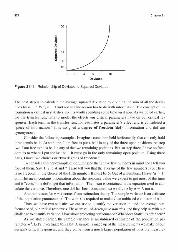
The next step is to calculate the average squared deviation by dividing the sum of all the devia-tions by n 1. Why n 1 and not n? One reason has to do with information. The concept of in-formation is critical in statistics, so it is worth spending some time on it now. As we noted earlier,we use transfer functions to model the effects our critical parameters have on our critical re-sponses. Each term in the transfer function estimates a parameter’s effect and is considered a“piece of information.” It is assigned a degree of freedom (dof). Information and dof are synonymous.
Consider the following examples. Imagine a container, held horizontally, that can only holdthree tennis balls. At step one, I am free to put a ball in any of the three open positions. At steptwo, I am free to put a ball in any of the two remaining positions. But, at step three, I have no free-dom as to where I put the last ball. It must go in the only remaining open position. Using threeballs, I have two choices or “two degrees of freedom.”
To consider another example of dof, imagine that I have five numbers in mind and I tell youfour of them. Say, 1, 2, 3, 4 and ?. I also tell you that the average of the five numbers is 3. Thereis no freedom in the choice of the fifth number. It must be 5. Out of n numbers, I have ‘n 1’dof. The mean contains information about the response value we expect to get most of the timeand it “costs” one dof to get that information. The mean is contained in the equation used to cal-culate the variance. Therefore, one dof has been consumed, so we divide by n 1, not n.
Another reason for n 1 comes from estimation theory. The sample variance is an estimateof the population parameter, 2. The n 1 is required to make s2 an unbiased estimator of 2.
Thus, we have two statistics we can use to quantify the variation in, and the average per-formance of, our critical responses. These are called descriptive statistics, and they help us with ourchallenge to quantify variation. How about predicting performance? What does Statistics offer here?
As we stated earlier, the sample variance is an unbiased estimator of the population pa-rameter, 2. Let’s investigate this a bit. A sample is made up of the measurements we make of ourdesign’s critical responses, and they come from a much larger population of possible measure-
474 Chapter 21
100
2 4 6
Deviates
Sq
uar
ed D
evia
tes
8 100
16
36
64
Figure 21–1 Relationship of Deviates to Squared Deviates

ments. The population is characterized by certain parameters, two of which are the mean andthe variance 2. The population may be finite or it may be infinite, and we may never know thevalues of and 2. The purpose of taking a sample is to estimate them.
Statistical theory tells us that the expected value of the sample mean and sample varianceequals the population mean and variance, respectively. This is shown in the following equationfor the random variable X.
This is true in the long run. However, we usually can’t wait that long and are content to usethe sample mean and variance as estimates of the population mean and variance. This is shownin the following equation, where the “hat” or “roof” is used to indicate an estimate.
If our sample adequately represents the population, we can estimate the population param-eters by the sample statistics. Herein lies the solution to the challenge of predicting performance.If we can estimate the population’s parameters and its distribution from our sample, we can pre-dict the performance of a population of product from our sample. But what is a distribution?
The term distribution is synonymous with the shape of the data when plotted as a histogram.The histogram provides a graphical view of how the data distribute themselves in terms of rela-tive frequency. Sometimes, as with the normal distribution, we have an equation, called a proba-bility density function (pdf), that describes the distribution mathematically.
The distribution has a total area of one. The area under the curve that is below a particularvalue is equal to the probability of getting numbers that are less than or equal to that value. Thearea under the curve that is above a particular value is equal to the probability of getting numbersthat are greater than or equal to that value. Figure 21–2 gives an example of this using the normaldistribution.
X2 = sX
2 and X = X
E(X) = X and E(sX2) = X
2
Introduction to Descriptive Statistics 475
LSL USL
This area equalsthe probability of
exceeding theupper spec limit
This area equalsthe probability ofbeing below thelower spec limit
Response
Figure 21–2 Example of Normal Distribution

Probabilities have been calculated for the important distributions and can be found in theback of most statistics books. Luckily, software packages, such as Minitab, can calculate theseprobabilities for us.
Let’s try a simple example. Say we have a critical voltage with the following characteristics:
• A target value of 10V• An historic standard deviation of 1V• Upper and lower specification limits of 11V and 9V, respectively• Adequately described by the normal distribution
What are the chances of producing voltages above and below the specification limits? Thesituation is shown in Figure 21–3.
We need to determine the area total under the normal distribution, which is below 9 andabove 11. Let’s use Minitab.
We use the Minitab pull-down menu to go to Calc Probability Distributions Normal, andwe get the window shown on page 477. We enter the mean, sd (standard deviation), and the lowerspecification limit. The output is given in Minitab’s session window, shown on opposite page.
Cumulative Distribution Function
Normal with mean 10.0000 and standard deviation 1.00000x P(X x)9.0000 0.1587
Minitab has calculated the probability of getting numbers from a normal distribution thatare less than or equal to 9. This is the area to the left of the LSL. The area to the right of the USLis the same since the limits and the normal distribution are both symmetric about the mean.
476 Chapter 21
LSL USL
Critical Voltage
109 11
Figure 21–3 Critical Voltage

Thus, the probability of not being within the limits is 0.1587 0.1587 0.3174, or31.74%. The probability of being within the limits is 1 0.3174 0.6826 or 68.26%. This, ofcourse, is the familiar area, from a normal distribution, that falls within one standard deviationabove and below the mean. We can now predict that, on average, our product will produce “outof spec” voltages 31.74 percent of the time, or 317,400 parts per million. We have met the designchallenge to predict the performance of a population of products based on the few prototypesavailable during design.
Before we conclude our discussion, we need to review a few additional concepts from ba-sic statistics regarding distributions and the averaging of random samples.
A special case of the normal distribution is the standard normal distribution, also known asthe z-distribution. The z-distribution has the same shape as the normal, but its mean is zero andits standard deviation is one, z 0 and z 1. Therefore, values from the z-distribution are inunits of standard deviations. A normal distribution can easily be converted to the standard normalusing the following equation, where X is a vector of normally distributed values and Z is a vectorof z-distributed values.
As we noted earlier, we do not know the parameters of our population. But we must know and to use the z-distribution. In cases where we do not know but we do know , such as a
Z =X -
Introduction to Descriptive Statistics 477
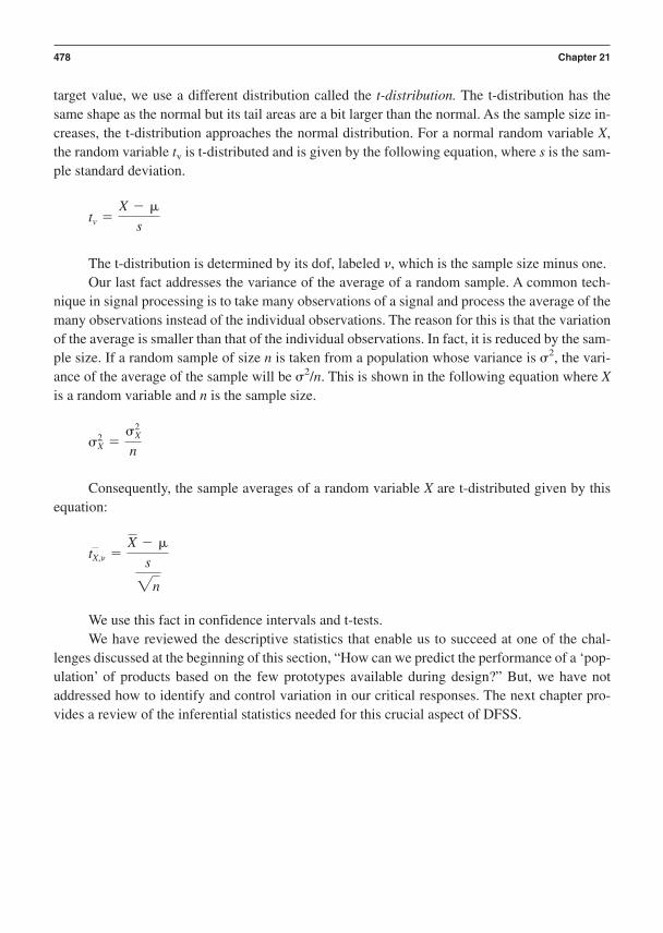
target value, we use a different distribution called the t-distribution. The t-distribution has thesame shape as the normal but its tail areas are a bit larger than the normal. As the sample size in-creases, the t-distribution approaches the normal distribution. For a normal random variable X,the random variable tv is t-distributed and is given by the following equation, where s is the sam-ple standard deviation.
The t-distribution is determined by its dof, labeled , which is the sample size minus one.Our last fact addresses the variance of the average of a random sample. A common tech-
nique in signal processing is to take many observations of a signal and process the average of themany observations instead of the individual observations. The reason for this is that the variationof the average is smaller than that of the individual observations. In fact, it is reduced by the sam-ple size. If a random sample of size n is taken from a population whose variance is 2, the vari-ance of the average of the sample will be 2/n. This is shown in the following equation where Xis a random variable and n is the sample size.
Consequently, the sample averages of a random variable X are t-distributed given by thisequation:
We use this fact in confidence intervals and t-tests.We have reviewed the descriptive statistics that enable us to succeed at one of the chal-
lenges discussed at the beginning of this section, “How can we predict the performance of a ‘pop-ulation’ of products based on the few prototypes available during design?” But, we have notaddressed how to identify and control variation in our critical responses. The next chapter pro-vides a review of the inferential statistics needed for this crucial aspect of DFSS.
tX, =X -
s2n
X2 =
X2
n
tv =X -
s
478 Chapter 21
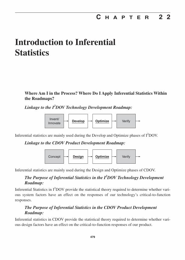
C H A P T E R 2 2
Introduction to InferentialStatistics
Where Am I in the Process? Where Do I Apply Inferential Statistics Withinthe Roadmaps?
Linkage to the I2DOV Technology Development Roadmap:
479
Invent/Innovate
Develop Optimize Verify
Concept Design Optimize Verify
Inferential statistics are mainly used during the Develop and Optimize phases of I2DOV.
Linkage to the CDOV Product Development Roadmap:
Inferential statistics are mainly used during the Design and Optimize phases of CDOV.
The Purpose of Inferential Statistics in the I2DOV Technology DevelopmentRoadmap:
Inferential Statistics in I2DOV provide the statistical theory required to determine whether vari-ous system factors have an effect on the responses of our technology’s critical-to-function responses.
The Purpose of Inferential Statistics in the CDOV Product DevelopmentRoadmap:
Inferential statistics in CDOV provide the statistical theory required to determine whether vari-ous design factors have an effect on the critical-to-function responses of our product.

What Am I Doing in the Process?
Employing inferential statistics allows us to take data from the system and analyze the data to de-termine, with statistical rigor, whether certain factors of a design have an effect on the design’sresponse.
What Output Do I get from Using Inferential Statistics?
Statistical tests and indicators are generated upon deciding which various factors of a design havean effect on the design’s response.
Inferential Statistics Review and Tools
Describing and quantifying variation in a critical response is necessary but not sufficient. We mustalso identify the sources of the variation and quantify how much variation each source con-tributes. Identifying the sources of variation and quantifying their relative contribution is a criti-cal skill that the DFSS practitioner must master. Let’s review the inferential statistics upon whichthis is based.
Assume we measured the heights of 200 people. Half were young children and half wereadults. Our goal is to determine if age affects average height. This is a simple experiment, so let’spose the problem in the terminology of experimentation. We have one factor, called “person.” Ourfactor has been varied between two levels, “child” and “adult.” Our critical response is height ininches. We have two samples of 100 observations each. Let’s look at the data that was collectedin the histogram shown in Figure 22–1.
The effect seems clear. The samples cluster into two distinct groups based on age. It is un-likely that we would be wrong if, assuming a proper experiment was run, we concluded that agedoes affect height. The histogram indicates this because the graphs have no overlap and their
480 Chapter 22
30
20
10
020
Fre
qu
ency
30 40Child Adult
50
Height in inches
60 70 80
Figure 22–1 Histogram of Age Relationship to Height
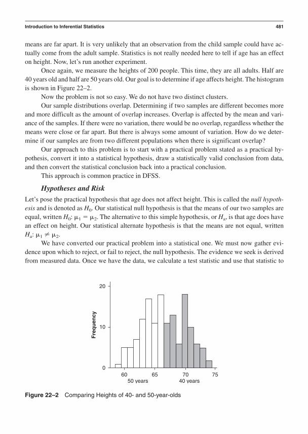
means are far apart. It is very unlikely that an observation from the child sample could have ac-tually come from the adult sample. Statistics is not really needed here to tell if age has an effecton height. Now, let’s run another experiment.
Once again, we measure the heights of 200 people. This time, they are all adults. Half are40 years old and half are 50 years old. Our goal is to determine if age affects height. The histogramis shown in Figure 22–2.
Now the problem is not so easy. We do not have two distinct clusters.Our sample distributions overlap. Determining if two samples are different becomes more
and more difficult as the amount of overlap increases. Overlap is affected by the mean and vari-ance of the samples. If there were no variation, there would be no overlap, regardless whether themeans were close or far apart. But there is always some amount of variation. How do we deter-mine if our samples are from two different populations when there is significant overlap?
Our approach to this problem is to start with a practical problem stated as a practical hy-pothesis, convert it into a statistical hypothesis, draw a statistically valid conclusion from data,and then convert the statistical conclusion back into a practical conclusion.
This approach is common practice in DFSS.
Hypotheses and Risk
Let’s pose the practical hypothesis that age does not affect height. This is called the null hypoth-esis and is denoted as H0. Our statistical null hypothesis is that the means of our two samples areequal, written H0: 1 2. The alternative to this simple hypothesis, or Ha, is that age does havean effect on height. Our statistical alternate hypothesis is that the means are not equal, written Ha: 1 2.
We have converted our practical problem into a statistical one. We must now gather evi-dence upon which to reject, or fail to reject, the null hypothesis. The evidence we seek is derivedfrom measured data. Once we have the data, we calculate a test statistic and use that statistic to
Introduction to Inferential Statistics 481
20
10
060
Fre
qu
ency
6550 years 40 years
70 75
Figure 22–2 Comparing Heights of 40- and 50-year-olds

determine whether we should reject or fail to reject the null hypothesis. Keep in mind that fail toreject is not the same as “accept.” We can never prove that the null is true. We can only seek ev-idence to prove that the null is not true. One instance of “not true” is sufficient to reject the null.However, one, two, or three instances in which the null is found to be true does not mean it is al-ways true. We cannot investigate all possible instances. Nevertheless, in practice when we fail toreject, we act as though the null is true and has been accepted. We even get sloppy and sometimesuse the phrase “accept the null hypothesis.”
Sounds simple? Well, it gets more complicated. Our decision to accept or reject the null isbased on our samples, and we can make two correct decisions or we can make two wrong deci-sions. The correct decisions are to accept or reject the null when we should. The incorrect deci-sions are to accept or reject the null when we shouldn’t. Let’s look at the two types of incorrectdecisions starting with incorrectly accepting the null.
The error of incorrectly accepting the null is called a type II error. For our child/adult heightexample, it is like saying, “Age has no effect on height” when in fact it does. It is also like say-ing, “Based on the absence of complaints, my customers are happy.” This type of error has beenthe death of some companies. Some customers do not complain. They quietly switch to the com-petitor, and the loss of market share is the lagging indicator of the switch. The risk of making atype II error is sometimes called the consumer’s risk. Imagine a company that tests pacemakers.If the null hypothesis is “the device under test is good” and a type II error is made, then a bad unitgets shipped. In the worst case, the consumer gets to test it out in his or her chest.
In short, a type II error is the mistake of saying the null should be accepted when it reallyshould not. To be certain we have not made this error, we need to continue testing until we finallyfind evidence to reject the null. This may take a long time and a lot of money. The market willwait only so long. Instead, we allow a certain risk of making this error. The risk or probability ofmaking the error is called risk.
There’s another error we can make. What if we conclude that we should not accept the nullwhen in fact we should? This is a type I error, and the probability of making this error is termed risk. Alpha risk is sometimes called the manufacturer’s risk. If our pacemaker company makesthis error, it unnecessarily reworks or scraps a device. Typical values for and are 5 percentand 20 percent, respectively; however, like “n-sigma,” each company must determine its ownvalues of and based on the safety, legal, and economic consequences of each type of error.
What about the two correct decisions we can make? We can correctly reject the null and wecan correctly fail to reject the null. These have probabilities of (1-) and (1- ), respectively. Thestatistical power of a test is its ability to correctly reject the null and has a probability of (1-).The probability of correctly failing to reject the null is (1- ). This discussion, in the context ofthe pacemaker manufacturer, is shown in Figure 22–3.
The t-Test
How do we use our hypotheses to determine if age has an effect on height? If the null is true, agedoes not have an effect on height, and both samples are from the same distribution, their meansare equal and the difference between the two population means should be zero. Thus, the null canalso be written as H0: 1 2 0. If the null is not true, age does have an effect on height, and
482 Chapter 22

the samples are from different distributions, their means are not equal, and the difference betweenthe two population means should not be zero.
The alternative hypothesis can be written as Ha: 1 2 0. We can compare the differ-ence with zero to test our hypotheses. This must be a statistical comparison because each samplemean is a random variable and so their difference is also a random variable.
Now let’s choose a value for alpha, the risk of a type I error. Remember, this is saying themeans are different when they are not. In general, this can be true in two ways. The younger meancan be greater than the older mean, or it can be less than the older. The difference 1 2 can bepositive, or it can be negative. So, let’s split in half, 2.5 percent above and 2.5 percent belowzero. This is called a two-tailed test and is shown in Figure 22–4. We use a t-distribution becausewe don’t know .
Introduction to Inferential Statistics 483
DecisionTruth
Device is good Device is bad
Correctly accept Incorrectly rejectthe null the null
(1 ) risk Type I Error risk
Incorrectly accept Correctly rejectthe null the null
Type II Error (1 ) risk risk
Deviceis good
Deviceis bad
H0: the device is goodHa: the device is bad
Figure 22–3 Facing and Risk Errors
Or it could havecome from here
0–t α/2,µ t α/2,µ
The differencecould havecome from here
2.5% of thearea is below
2.5% of thearea is above
The differencecould havecome from here
Figure 22–4 Sample “Two-Tailed” Test

The test statistic for zero difference between two normally distributed random variableswhen is unknown is t-distributed and is given in the following equation.
If the population variances are equal (2 12 2
2), and there are (100 1) (100
1) 198 dof, we use this equation:
where the pooled sd is
The test with equal variances is slightly more powerful than the test with unequal variances.So far, we have our hypothesis, our risk level, our data, and our test statistic. Now we need
a number with which to compare our test statistic, to determine if we should reject or fail to re-ject the null. We do this by comparing the calculated value of the test statistic to the numbers froma t-distribution that have 2.5 percent of the area below it and 2.5 percent of the area above it.
This is a two-tailed test. The magnitude of these two numbers is the same since the t-distribution is symmetric and is termed t( /2,v). In our case dof 198. We can use Minitab to de-termine t( /2,v) t(0.05/2,198). We use the Minitab pull-down menu to go to Calc ProbabilityDistributions t Distribution, and we get the window shown here.
sp = B(n1 - 1)s12 + (n2 - 1)s2
2
n1 + n2 - 2
t =x1 - x2
spB 1n1+
1n2
t =x1 - x2
C s12
n1+
s22
n2
484 Chapter 22
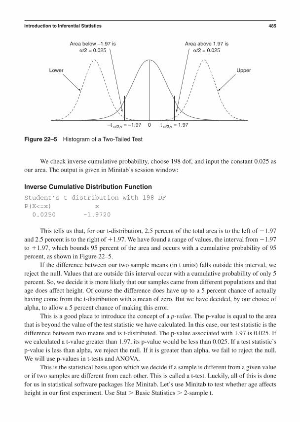
We check inverse cumulative probability, choose 198 dof, and input the constant 0.025 asour area. The output is given in Minitab’s session window:
Inverse Cumulative Distribution Function
Student’s t distribution with 198 DFP(X<=x) x0.0250 -1.9720
This tells us that, for our t-distribution, 2.5 percent of the total area is to the left of 1.97and 2.5 percent is to the right of 1.97. We have found a range of values, the interval from 1.97to 1.97, which bounds 95 percent of the area and occurs with a cumulative probability of 95percent, as shown in Figure 22–5.
If the difference between our two sample means (in t units) falls outside this interval, wereject the null. Values that are outside this interval occur with a cumulative probability of only 5percent. So, we decide it is more likely that our samples came from different populations and thatage does affect height. Of course the difference does have up to a 5 percent chance of actuallyhaving come from the t-distribution with a mean of zero. But we have decided, by our choice ofalpha, to allow a 5 percent chance of making this error.
This is a good place to introduce the concept of a p-value. The p-value is equal to the areathat is beyond the value of the test statistic we have calculated. In this case, our test statistic is thedifference between two means and is t-distributed. The p-value associated with 1.97 is 0.025. Ifwe calculated a t-value greater than 1.97, its p-value would be less than 0.025. If a test statistic’sp-value is less than alpha, we reject the null. If it is greater than alpha, we fail to reject the null.We will use p-values in t-tests and ANOVA.
This is the statistical basis upon which we decide if a sample is different from a given valueor if two samples are different from each other. This is called a t-test. Luckily, all of this is donefor us in statistical software packages like Minitab. Let’s use Minitab to test whether age affectsheight in our first experiment. Use Stat Basic Statistics 2-sample t.
Introduction to Inferential Statistics 485
Area below –1.97 isα/2 = 0.025
Area above 1.97 isα/2 = 0.025
0–t α/2,v = –1.97 t α/2,v = 1.97
Lower Upper
Figure 22–5 Histogram of a Two-Tailed Test

Our samples are in different columns and we assume unequal variances since we don’tknow if they’re equal. Note that the dof is now 165, not 198.
Choose the alternative hypothesis of “not equal.” The session window output follows:
486 Chapter 22
chlid
adult
Two-Sample T-Test and CI: young, old
Two-sample T for young vs old
N Mean StDev SE Meanyoung 100 36.57 5.19 0.52old 100 67.88 3.22 0.32
Difference = mu young - mu oldEstimate for difference: -31.312

95% CI for difference: (-32.517, -30.107)T-Test of difference = 0 (vs not =): T-Value = -51.31 P-Value = 0.000 DF = 165
A t-value of 51.31 is a very large negative value and is way out in the left tail of the t-distribution. Its p-value, reported as “P-value0.000,” is much less than our alpha of 0.05. Thistells us to reject the null. Our practical conclusion is that age does affect height among the peo-ple we sampled in this experiment.
Now we’ll use Minitab to test whether age affects height in our second experiment. We usethe same Minitab utilities and choose 40 years and 50 years for the column names.
The session window output follows:
Two-Sample T-Test and CI: 40 years, 50 years
Two-sample T for 40 years vs 50 years
N Mean StDev SE Mean40 years 100 68.11 3.02 0.3050 years 100 65.17 2.93 0.29
Difference = mu 40 years - mu 50 yearsEstimate for difference: 2.94495% CI for difference: (2.114, 3.773)T-Test of difference = 0 (vs not =): T-Value = 7.00 P-Value = 0.000 DF = 197
The p-value is much less than alpha and so we reject the null. Our two sample t-test enabledus to decide, with a 5 percent chance of being wrong, that age does affect height among the peo-ple we sampled in the experiment.
Let’s compare the “old” group with the “40 year” group. The null hypothesis is that the av-erage heights of the two age groups are the same. That is, age does not affect average height. Thesession window output follows:
Two-Sample T-Test and CI: 40 years, old
Two-sample T for 40 years vs old
N Mean StDev SE Mean40 years 100 68.11 3.02 0.30old 100 67.88 3.22 0.32
Difference = mu 40 years - mu oldEstimate for difference: 0.229
Introduction to Inferential Statistics 487

95% CI of difference: (-0.641, 1.099)T-Test of difference = 0 (vs not =): T-Value = 0.52 P-Value = 0.604 DF = 197
The t-value is relatively small (0.52) and its p-value (0.604) is larger than alpha. We fail toreject the null and conclude that age does not affect height between these two groups.
Analysis of Variance
The t-test is only useful when comparing at most two samples. The test loses statistical power asthe number of paired samples to be tested increases. What do we do if our factor has more thantwo levels or we have many factors, each at many levels? How do we compare the means with-out losing power? The answer is ANOVA, or analysis of variance.
ANOVA is used to test whether the means of many samples differ but it does so using vari-ation instead of the mean. ANOVA can be thought of, as Professor Tom Barker at the RochesterInstitute of Technology would say, as “analysis of the means by way of the variance (Barker1994).” ANOVA compares the amount of variation within the samples to the amount of variationbetween the means of the samples. If the “between” variation is significantly larger than the“within” variation, we conclude that the mean of our response has changed.
Let’s see how ANOVA is used to analyze the result of the experiments we run. The processconsists of:
• Posing a practical and statistical null and alternative hypothesis• Selecting risk levels• Running an appropriate experiment to generate sample data• Calculating a test statistic from the data• Using the probability distribution of the test statistic to determine if we should reject or
fail to reject the null
This sounds like the steps in a t-test. They are! The difference is that we use ANOVA to gen-erate a test statistic that is based on variation unlike the t-test, which is based on the mean.
Let us pose a null and alternative hypothesis. What we want to determine in DFSS iswhether x affects y. That is, do changes in x have an effect on the mean value of y? Our critical-to-function response is y, and x is a critical parameter or factor that we believe affects y. We posethe practical null hypothesis that, “No, x does not have an effect on y.” The alternative hypothe-sis is that x does have an effect on y. We’ll assume a 5 percent alpha risk. But we need a statisti-cal hypothesis that allows a data-driven decision to reject or accept the null. The data generatedfrom an experiment is tightly coupled to the statistical hypothesis to be tested. That is why thestudy of DOE is necessary. Let’s say we ran an experiment involving one factor x and our criti-cal response y. We tested over many levels of x, say n levels, and we took m observations at eachof those n levels. The observation, yi,j is the jth observation at the ith level of x.
488 Chapter 22

We can think of each observation as having come from one single distribution with a meanof plus some error, written as yi,j i,j. But, we can also think of each group of m mea-surements, taken at a particular level of x, as having come from their own distribution with a meanof i plus some error, written as yi,j i ij. There’s a subtle, but profound difference betweenthese two equations. If the first equation is correct, x has no effect on y since is not a functionof x. If the second equation is correct x has an effect on y, since i is a function of x. This is shownin Figure 22–6.
The statistical null hypothesis is H0: 1 2 i …n. All the individual means arethe same regardless of the levels of x. The statistical alternative hypothesis is Ha: i q for atleast one i q. At least one mean is different from the others.
These hypotheses can be stated in another form. The effect we are looking for is the amountby which each t has been moved away from . This effect, for the ith level of x, is called i. Thisis also shown in Figure 22–6. We can now rewrite yi,j i,j to get this equation:
yi,j i ij
By the way, if all the effects are zero then x has no effect on y. So, the null can also be writ-ten as H0: 1 2 i …n 0 and the alternative written as Ha: i 0 for at least one i.
Now let’s calculate a test statistic from the data. We’ll use ANOVA to do this. Our best es-timate of is which is the grand average of all the observations from our experiment. Our bestestimate of 1 is , the average of all m observations taken at the ith level of x. Our best estimateof i is And finally, an estimate for the error ij is the distance of the jth observation takenat the ith level of x from its local mean, given by ij yij
We can substitute these into the previous equation, subtract from both sides, and getSee Figure 22–7 for a graphical view of this equation.(yij - y) = (yi - y) + (yij - yi).
yyi.
(yi - y).yi
y,
Introduction to Inferential Statistics 489
The error inmeasurement jwhen x is atlevel i
τ l = µi – µ
µµ1 µi yij
εij
Distribution ofm observationswhen X is atlevel one
Distribution of allthe observationsfrom the entireexperiment
Distribution of mobservations when xis at level i
Theeffect of x,at level i
yij = µ + δij
Figure 22–6 ANOVA Representation of Possible Effects
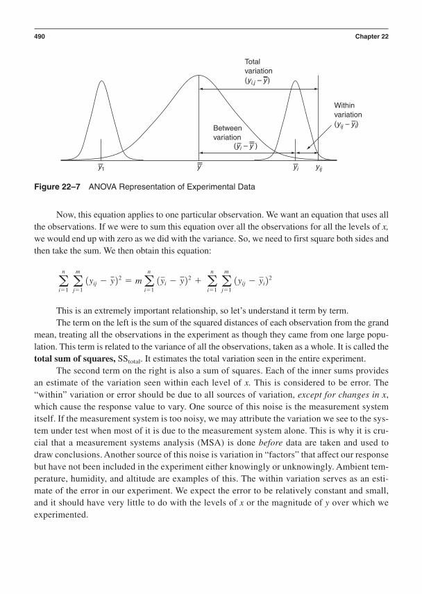
Now, this equation applies to one particular observation. We want an equation that uses allthe observations. If we were to sum this equation over all the observations for all the levels of x,we would end up with zero as we did with the variance. So, we need to first square both sides andthen take the sum. We then obtain this equation:
This is an extremely important relationship, so let’s understand it term by term.The term on the left is the sum of the squared distances of each observation from the grand
mean, treating all the observations in the experiment as though they came from one large popu-lation. This term is related to the variance of all the observations, taken as a whole. It is called thetotal sum of squares, SStotal. It estimates the total variation seen in the entire experiment.
The second term on the right is also a sum of squares. Each of the inner sums providesan estimate of the variation seen within each level of x. This is considered to be error. The“within” variation or error should be due to all sources of variation, except for changes in x,which cause the response value to vary. One source of this noise is the measurement systemitself. If the measurement system is too noisy, we may attribute the variation we see to the sys-tem under test when most of it is due to the measurement system alone. This is why it is cru-cial that a measurement systems analysis (MSA) is done before data are taken and used todraw conclusions. Another source of this noise is variation in “factors” that affect our responsebut have not been included in the experiment either knowingly or unknowingly. Ambient tem-perature, humidity, and altitude are examples of this. The within variation serves as an esti-mate of the error in our experiment. We expect the error to be relatively constant and small,and it should have very little to do with the levels of x or the magnitude of y over which weexperimented.
an
i=1am
j=1(yij - y)2 = ma
n
i=1(yi - y)2 + a
n
i=1am
j=1(yij - yi)
2
490 Chapter 22
Withinvariation(yij – yi)
Totalvariation(yi,j – y)
y
(yi – y )
y1 yi yij
Betweenvariation
Figure 22–7 ANOVA Representation of Experimental Data

The outer sum adds the within variation for all the levels of x to get a “pooled” estimate ofoverall experimental error, 2.
This term is called sum of squares due to error, SSerror. If we divide SSerror by its dof, weget the mean sum of squares, MSerror.
The middle term estimates how different each “local” mean is from the overall mean. Thisis the factor effect we are trying to detect. We sum them all up to get an estimate of how muchthe variation in x has caused the local means to vary compared to the error. This term is calledsum of squares due to treatment, SStrt. If we divide SStrt by its dof, we get the mean sum ofsquares, MStrt. The term treatment is a carryover from the origins of DOE. DOE has its roots inthe field of agriculture (pun intended). The soil was treated with various nutrients to determinetheir effects on plant growth. The term treatment has persisted. A treatment combination isused to describe a unique combination of levels of several factors in a multifactor experiment.For example, 20 percent nitrogen, 10 percent phosphorus, and 5 percent potash is a treatmentcombination.
Back to the story. If MStrt is larger than MSerror, we suspect that x has an effect on y andthat the null hypothesis can be rejected. If MStrt is less than or equal to MSerror, we suspect that x has no effect on y and we fail to reject the null. We are making decisions about meansbased on variation. This is why ANOVA can be thought of as analysis of the means by way ofthe variance.
If MStrt is large compared to MSerror, we suspect that x has caused our response to changeby more than chance or experimental error alone. How large should this ratio be? Statistics pro-vides the answer.
We must impose some restrictions on y if we are to use statistics to obtain the answer. Werequire that the error for any observation, ij, is normally distributed with a mean of zero and avariance of 2. This can be written as ij N(0, 2). If this condition is true, y is also a normalrandom variable. If the null is false, then yij N(j, 2). Now we can use a statistically rigoroustest to determine if MStrt is large enough.
We need a few facts to proceed:
• The mean of a normal random variable is also a normal random variable.• If a standard normal random variable, y, is squared, the new variable y2 is chi-square
distributed.• The ratio of two chi-square distributed random variables is F-distributed.
Please refer to John E. Freund’s Mathematical Statistics (Sixth Edition).The chi-square and F-distribution are special distributions that arise in random sampling
and play a key role in our statistical test.Now, both terms, MSerror and MStrt, involve squaring a normal random variable. Each of
these terms is chi-square distributed. Their ratio is therefore F-distributed.
Introduction to Inferential Statistics 491
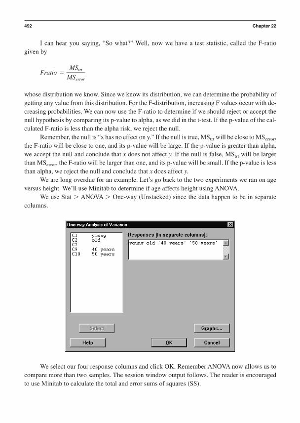
I can hear you saying, “So what?” Well, now we have a test statistic, called the F-ratio given by
whose distribution we know. Since we know its distribution, we can determine the probability ofgetting any value from this distribution. For the F-distribution, increasing F values occur with de-creasing probabilities. We can now use the F-ratio to determine if we should reject or accept thenull hypothesis by comparing its p-value to alpha, as we did in the t-test. If the p-value of the cal-culated F-ratio is less than the alpha risk, we reject the null.
Remember, the null is “x has no effect on y.” If the null is true, MStrt will be close to MSerror,the F-ratio will be close to one, and its p-value will be large. If the p-value is greater than alpha,we accept the null and conclude that x does not affect y. If the null is false, MStrt will be largerthan MSerror, the F-ratio will be larger than one, and its p-value will be small. If the p-value is lessthan alpha, we reject the null and conclude that x does affect y.
We are long overdue for an example. Let’s go back to the two experiments we ran on ageversus height. We’ll use Minitab to determine if age affects height using ANOVA.
We use Stat ANOVA One-way (Unstacked) since the data happen to be in separatecolumns.
Fratio =MStrt
MSerror
492 Chapter 22
We select our four response columns and click OK. Remember ANOVA now allows us tocompare more than two samples. The session window output follows. The reader is encouragedto use Minitab to calculate the total and error sums of squares (SS).
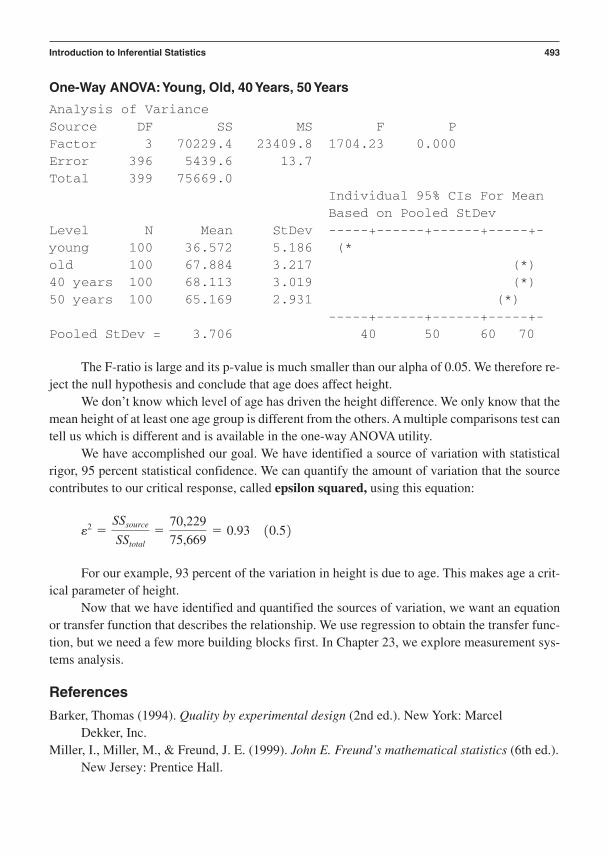
One-Way ANOVA:Young, Old, 40 Years, 50 Years
Analysis of VarianceSource DF SS MS F PFactor 3 70229.4 23409.8 1704.23 0.000Error 396 5439.6 13.7Total 399 75669.0
Individual 95% CIs For MeanBased on Pooled StDev
Level N Mean StDev -----+------+------+-----+-young 100 36.572 5.186 (*old 100 67.884 3.217 (*)40 years 100 68.113 3.019 (*)50 years 100 65.169 2.931 (*)
-----+------+------+-----+-Pooled StDev = 3.706 40 50 60 70
The F-ratio is large and its p-value is much smaller than our alpha of 0.05. We therefore re-ject the null hypothesis and conclude that age does affect height.
We don’t know which level of age has driven the height difference. We only know that themean height of at least one age group is different from the others. A multiple comparisons test cantell us which is different and is available in the one-way ANOVA utility.
We have accomplished our goal. We have identified a source of variation with statisticalrigor, 95 percent statistical confidence. We can quantify the amount of variation that the sourcecontributes to our critical response, called epsilon squared, using this equation:
For our example, 93 percent of the variation in height is due to age. This makes age a crit-ical parameter of height.
Now that we have identified and quantified the sources of variation, we want an equationor transfer function that describes the relationship. We use regression to obtain the transfer func-tion, but we need a few more building blocks first. In Chapter 23, we explore measurement sys-tems analysis.
References
Barker, Thomas (1994). Quality by experimental design (2nd ed.). New York: Marcel Dekker, Inc.
Miller, I., Miller, M., & Freund, J. E. (1999). John E. Freund’s mathematical statistics (6th ed.).New Jersey: Prentice Hall.
e2 =SSsource
SStotal
=70,229
75,669= 0.93 (0.5)
Introduction to Inferential Statistics 493

This page intentionally left blank
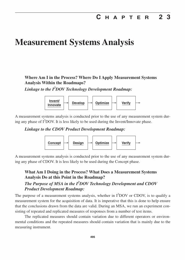
C H A P T E R 2 3
Measurement Systems Analysis
Where Am I in the Process? Where Do I Apply Measurement SystemsAnalysis Within the Roadmaps?
Linkage to the I2DOV Technology Development Roadmap:
495
Invent/Innovate
Develop Optimize Verify
Concept Design Optimize Verify
A measurement systems analysis is conducted prior to the use of any measurement system dur-ing any phase of I2DOV. It is less likely to be used during the Invent/Innovate phase.
Linkage to the CDOV Product Development Roadmap:
A measurement systems analysis is conducted prior to the use of any measurement system dur-ing any phase of CDOV. It is less likely to be used during the Concept phase.
What Am I Doing in the Process? What Does a Measurement SystemsAnalysis Do at this Point in the Roadmap?
The Purpose of MSA in the I2DOV Technology Development and CDOVProduct Development Roadmap:
The purpose of a measurement systems analysis, whether in I2DOV or CDOV, is to qualify ameasurement system for the acquisition of data. It is imperative that this is done to help ensurethat the conclusions drawn from the data are valid. During an MSA, we run an experiment con-sisting of repeated and replicated measures of responses from a number of test items.
The replicated measures should contain variation due to different operators or environ-mental conditions and the repeated measures should contain variation that is mainly due to themeasuring instrument.

What Output Do I get at the Conclusion of Measurement Systems Analysis?What Are Key Deliverables from MSA at this Point in the Roadmap?
• Gage R&R to assess repeatability and reproducibility• Performance to tolerance ratio to compare measurement system error to the tolerance• Number of distinct categories to assess the number of categories into which the
measurement system is capable of “batching” the measurements
MSA Process Flow Diagram
This visual reference of the detailed steps of MSA illustrates the flow of tasks at this stage.
496 Chapter 23
INPUT . . .
OUTPUT . . .
Selection/definition of thesystem to be assessed.
Select the parts/responsesand the range to be
measured.
Select the type ofexperiment to be run during
the MSA.
Acquire and analyze the data.
Calculate Gage R & R, P/T ratio, andthe number of distinct categories.
Gage R & R, P/T ratio, and the numberof distinct categories.
Verbal Descriptions for the Application of Each Block Diagram
This section explains the specific details of measurement systems analysis:
• Key detailed input(s) from preceding tools and best practices• Specific steps and deliverables from each step to the next within the process flow• Final detailed outputs that flow into follow-on tools and best practices
Key Detailed Inputs
A measurement systems analysis (MSA) is an experimental method used to assess the perfor-mance of a measurement system. A measurement system consists of the equipment, fixtures, pro-cedures, gages, instruments, software, environment, and personnel that together make it possibleto assign a number to a measured characteristic or response. It is important to realize that the in-
Selection/definition of the system to be assessed.

strument used to make the measurement, (for example, a voltmeter), is but one component of theoverall measurement system.
An MSA must be done regardless of the precision, accuracy, or cost of the measurement instrument since it is only one component of the entire measurement system. Do not draw conclu-sions from or take action based on data obtained from a measurement system for which an MSAhas not been performed! You cannot detect effects if the variation in the measurement system is ap-proximately equal to the variation in the response. This sounds like an obvious statement. However,this is a common mistake made by many Black Belts when experimentally investigating effects.
Specific Steps and Deliverables
Select the parts/responses and the range to be measured.
A measurement system possesses several characteristics: accuracy, repeatability, reproducibility,linearity, and stability. Accuracy is with reference to a known standard value and is assessedthrough calibration. The measurement system is used to measure a primary, secondary, or terti-ary standard. The difference between the known value of the standard and the average of repeatedmeasurements is a measure of accuracy called bias. Linearity refers to how a measurement sys-tem’s accuracy or precision changes as the magnitude of the measured quantity changes. Stabil-ity refers to how accuracy and precision change over time.
Repeatability and reproducibility pertain to precision. The variation in the measured valuecomes from two sources, the variation due to the response or part being measured and the varia-tion due to the measurement system itself, as shown in this equation.
Measurement system variation, 2ms, can be further broken down into variation due to re-
peatability, estimated by 2rpt , and variation due to reproducibility, 2
rpd:
Repeatability pertains to variation when the same person measures the same test item withthe same instrument many times. Reproducibility allows more variation to enter into the mea-sured value.
Reproducibility pertains to measurements made by different people, at different times onthe same test item. Reproducibility is therefore a measure of variation from operator to operator.Reproducibility can be broken down into two components, one due to the various operators andanother component due to an interaction between an operator and the part being measured, asshown in this equation:
rpd2 = op
2 + op*part2
ms2 = rpt
2 + rpd2
total2 = part
2 + ms2
Measurement Systems Analysis 497

Thus, total measurement variation consists of four variance components:
The goal of an MSA is to estimate the four variance components shown in this equa-tion. The estimates are then used to calculate three critical measures of measurement system performance:
Gage R&R
Performance-to-tolerance ratio (P/T ratio)
Number of distinct categories
Gage R&R, called “% Study Variation” by Minitab, determines what percentage of the to-tal variation is taken up by measurement system variation. The P/T ratio, called “% Tolerance”by Minitab, determines the fraction of the tolerance that is taken up by measurement system vari-ation. The formulae are
The 5.15 multiplier in the P/T ratio is used to span 99 percent of the measurement systemvariation, assuming it is normally distributed.
The third metric considered is the number of distinct categories. This is sometimes calleda discrimination ratio. It identifies how many distinct, 97 percent nonoverlapping normal distri-butions the measurement system is capable of grouping into measurements. Two distinct cate-gories is a go–no-go gage. The formula is as follows:
Select the type of experiment to be run during the MSA.
We need to estimate the variances shown in the total measurement variation equation to calculatethese three metrics. This is accomplished by running a hierarchical experiment. The experimentis designed so that several operators make repeated measurements on a set of parts. A nonde-structive test is one in which the test item is unchanged after the test has been performed and thefeature can be remeasured. The same physical part can be used throughout the test. A destructivetest is one in which the test item is changed by performing the test, so the feature cannot be re-
distinct_cat = round ¢ 1.41*part
ms≤
PT =5.15*ms
Tolerance
gage R&R =ms
total*100%
total2 = part
2 + op2 + op*part
2 + rpt2
498 Chapter 23

measured. In this case, a group of nearly identical parts must be available to simulate repeatedmeasurements. A nondestructive experiment is called crossed, while a destructive case is nested.
The typical hierarchical experimental structure follows for i operators measuring j parts, ktimes each.
Measurement Systems Analysis 499
Op1
Part1
. . . . . . .
. . . . . . .
. . . . . . .
Measurement1
Op2
Part2
Measurementk
Opi
Partj
The operators should not know which part they are measuring during the experiment norshould they know the values the other operators have obtained. This reduces the chance of datacorruption due to an operator’s desire to be consistent within a part or when compared to an op-erator who may be favored or an expert.
The range of the response in the experiment must represent the range expected when themeasurement system is placed into service. If the range is smaller than expected, measurementsystem variation may be a large portion of the total variation and we may erroneously concludethat the measurement system is not capable.
Acquire and analyze the data.
Once the data have been obtained, our estimates of the variance components in the total mea-surement variation equation are obtained from the sums of squares and degrees of freedom ofeach source of the variation. It is worth spending some time on the analysis of the data since it isnot, as they say, intuitively obvious to the casual observer. The necessary information is obtainedfrom Minitab by running a Gage R&R study using the ANOVA method. The Xbar and R methodcannot estimate the operator part (op part) interaction and therefore is not preferred. We willuse a file provided by Minitab to explain the data analysis. The file is “Gageaiag.mtw” and canbe found in Minitab’s data folder.
We begin the analysis using the Minitab pull-down menu to go to Stat Quality Tools Gage R&R (crossed) for nondestructive and get the window that follows. We select Part, Opera-tor, and Response and the default ANOVA method of analysis. Add a tolerance, 1 in this exam-ple, under Options.

500 Chapter 23
Minitab produces the following information. Let’s see how the Gage R&R numbers are obtained.
Gage R&R Study–ANOVA Method
Gage R&R for Response
Two-Way ANOVA Table With Interaction
Source DF SS MS F P
Part 9 2.05871 0.228745 39.7178 0.00000Operator 2 0.04800 0.024000 4.1672 0.03256Operator*Part 18 0.10367 0.005759 4.4588 0.00016Repeatability 30 0.03875 0.001292Total 59 2.24912
Gage R&R
Source VarComp % Contribution (of VarComp)
Total Gage R&R 0.004437 10.67Repeatability 0.001292 3.10Reproducibility 0.003146 7.56Operator 0.000912 2.19Operator*Part 0.002234 5.37
Part-To-Part 0.037164 89.33Total Variation 0.041602 100.00
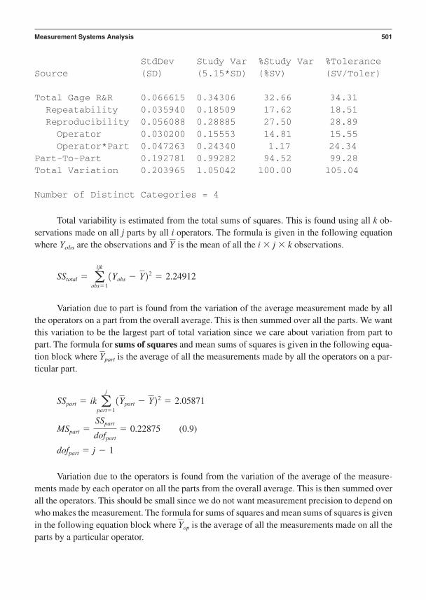
StdDev Study Var %Study Var %ToleranceSource (SD) (5.15*SD) (%SV) (SV/Toler)
Total Gage R&R 0.066615 0.34306 32.66 34.31Repeatability 0.035940 0.18509 17.62 18.51Reproducibility 0.056088 0.28885 27.50 28.89Operator 0.030200 0.15553 14.81 15.55Operator*Part 0.047263 0.24340 1.17 24.34
Part-To-Part 0.192781 0.99282 94.52 99.28Total Variation 0.203965 1.05042 100.00 105.04
Number of Distinct Categories = 4
Total variability is estimated from the total sums of squares. This is found using all k ob-servations made on all j parts by all i operators. The formula is given in the following equationwhere Yobs are the observations and is the mean of all the i j k observations.
Variation due to part is found from the variation of the average measurement made by allthe operators on a part from the overall average. This is then summed over all the parts. We wantthis variation to be the largest part of total variation since we care about variation from part topart. The formula for sums of squares and mean sums of squares is given in the following equa-tion block where is the average of all the measurements made by all the operators on a par-ticular part.
(0.9)
Variation due to the operators is found from the variation of the average of the measure-ments made by each operator on all the parts from the overall average. This is then summed overall the operators. This should be small since we do not want measurement precision to depend onwho makes the measurement. The formula for sums of squares and mean sums of squares is givenin the following equation block where is the average of all the measurements made on all theparts by a particular operator.
Yop
dofpart = j - 1
MSpart =SSpart
dofpart
= 0.22875
SSpart = ik aj
part=1(Ypart - Y)2 = 2.05871
Ypart
SStotal = aijk
obs=1(Yobs - Y)2 = 2.24912
Y
Measurement Systems Analysis 501
Variation due to the operator part or interaction is due to a difference in how an operatormeasures one part compared to how the same operator measures another part. There should bevery little operator part interaction. We want parts to be measured equally well independent ofwho is measuring what part. The formula for sums of squares and mean sums of squares is givenin the following equation block where is the average of the k measurements each operatormakes on each part.
Repeatability, also known as error, is obtained from the repeated measurements each oper-ator makes on the part. We can estimate repeatability by subtracting total variability from all theremaining sources of variability. This is shown in the following equation block, along with themean sum of squares for repeatability.
(0.12)
In summary:
Our estimate of reproducibility is rpd2 = 2
op + op*part2 = 0.003146
Our estimate of operator variation is op2 =
MSop - k*op*part2 - rpt
2
j*k= 0.000912
Our best estimate of op * part variation is op*part2 =
MSop*part - rpt2
k= 0.002234
Our best estimate of repeatability is rpt2 = MSrpt = 0.00129.
dofrpt = doftotal - dofop - dofpart - dofop*part
MSrpt =SSrpt
dofrpt
= 0.001291
SSrpt = SStotal - (SSpart + SSop + SSop*part) = 0.03874
dofop*part = (i - 1)*(j - 1) = (3 - 1)*(10 - 1) = 18
MSop*part =SSop*part
dofop*part
= 0.005759
SSop*part = k aj
part=1a
i
op=1((Ypart,op - Yop) - (Ypart - Y))2 = 0.10367
Ypart,op
dofop = i - 1
MSop =SSop
dofop
= 0.0240
SSop = jkai
op=1(Yop - Y)2 = 0.0480
502 Chapter 23
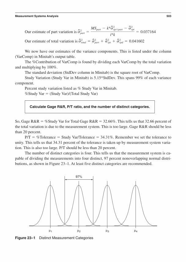
We now have our estimates of the variance components. This is listed under the column(VarComp) in Minitab’s output table.
The %Contribution of VarComp is found by dividing each VarComp by the total variationand multiplying by 100%.
The standard deviation (StdDev column in Minitab) is the square root of VarComp.Study Variation (Study Var in Minitab) is 5.15*StdDev. This spans 99% of each variance
component.Percent study variation listed as % Study Var in Minitab.%Study Var (Study Var)/(Total Study Var)
Calculate Gage R&R, P/T ratio, and the number of distinct categories.
So, Gage R&R %Study Var for Total Gage R&R 32.66%. This tells us that 32.66 percent ofthe total variation is due to the measurement system. This is too large. Gage R&R should be lessthan 20 percent.
P/T %Tolerance Study Var/Tolerance 34.31%. Remember we set the tolerance tounity. This tells us that 34.31 percent of the tolerance is taken up by measurement system varia-tion. This is also too large. P/T should be less than 20 percent.
The number of distinct categories is four. This tells us that the measurement system is ca-pable of dividing the measurements into four distinct, 97 percent nonoverlapping normal distri-butions, as shown in Figure 23–1. At least five distinct categories are recommended.
Our estimate of total variation is total2 = part
2 + rpt2 + rpd
2 = 0.041602
Our estimate of part variation is part2 =
MSpart - k*op*part2 - rpt
2
i*k= 0.037164
Measurement Systems Analysis 503
97%
µ1 µ2 µ3 µ4
Figure 23–1 Distinct Measurement Categories

Minitab also provides a graphical representation of this information given above. This isshown in Figure 23–2. The upper left graph shows three bars located above the label ‘Gage R&R’.They are the percent contribution of measurement system variation, the Gage R&R, and P/T, fromleft to right, respectively.
Final Detailed Outputs
Once we have assessed our measurement system and found it to be capable, it is safe to useit to make measurements from which to draw conclusions and take actions.
MSA Checklist and Scorecard
This suggested format for a checklist can be used by an engineering team to help plan its workand aid in the detailed construction of a PERT or Gantt chart for project management. These itemsalso serve as a guide to identify the key items for evaluation within a formal gate review.
Gage R&R, P/T ratio, and the number of distinct categories.
504 Chapter 23
UCL = 0.1252
R = 0.03833
LCL = 0
UCL = 0.8796Mean = 0.8075LCL = 0.7354
Components of Variation By Part
Gage name:Date of study:Reported by:Tolerance:Misc:
0.4
1 1 2 3 4 5 6 7 8 9 10
1 2 3 4 5 6 7 8 9
Operator123
10
Part
1 2 3Operator
0.50.60.70.80.91.01.1
0.40.50.60.70.80.91.01.1
Part
0.40.50.60.70.80.91.01.1
By Operator
Operator* Part Interaction
R Chart by Operator
Xbar Chart by Operator
GageR and R
100
50
0
0.00
0.30.40.50.60.70.80.91.01.1
0.05
0.10
0.15
Repeat
Per
cent
Sam
ple
Ran
geS
ampl
e M
ean
Reprod Part-to-Part
% Contribution% Study Var% Tolerance
1 2 3
1 2 3
Figure 23–2 Gage R&R (ANOVA) for Response

Checklist for MSA
Was this Action Excellence Rating:Deployed? 1 = Poor
Actions: YES or NO 10 = Excellent
Definition of the system to be assessed. ______ ______
Select the parts/responses and the range to be measured. ______ ______
Select the type of experiment to be run during the MSA. ______ ______
Acquire and analyze the data. ______ ______
Calculate Gage R&R, P/T ratio, and the number of distinct categories. ______ ______
Scorecard for MSA
The definition of a good scorecard is that it should illustrate, in simple but quantitative terms,what gains were attained from the work. This suggested format for a scorecard can be used by aproduct planning team to help document the completeness of its work.
Table of MSA Requirements
Measurement Part/Response # of Distinct System Name: Gage R&R: Tolerance: P/T Ratio: Categories:
1. ______ ______ ______ ______
2. ______ ______ ______ ______
3. ______ ______ ______ ______
We repeat the final deliverables from an MSA:
• Gage R&R to assess repeatability and reproducibility• Performance to tolerance ratio to compare measurement system error to the tolerance• Number of distinct categories to assess the number of categories into which the
measurement system is capable of “batching” the measurements
References
Automotive Industry Action Group (AIAG) and the American Society for Quality Control(ASQC). (1998). Measurement systems analysis. AIAG.
Montgomery, D. C. (1997). Introduction to statistical process control. New York: Wiley & Sons.
Wheeler, D. H., & Lyday, R. W. (1989). Evaluating the measurement process. Knoxville:SPC Press.
Measurement Systems Analysis 505

This page intentionally left blank
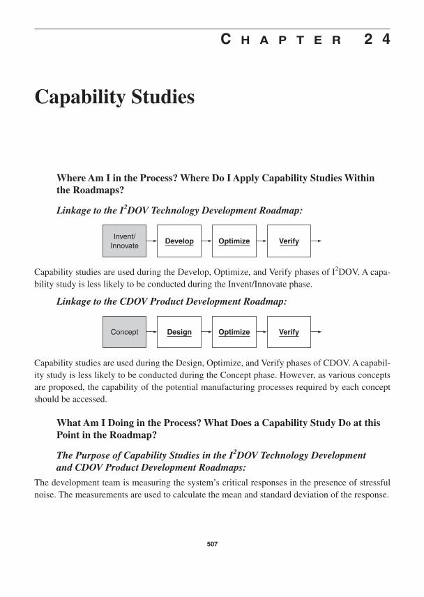
C H A P T E R 2 4
Capability Studies
Where Am I in the Process? Where Do I Apply Capability Studies Withinthe Roadmaps?
Linkage to the I2DOV Technology Development Roadmap:
Capability studies are used during the Develop, Optimize, and Verify phases of I2DOV. A capa-bility study is less likely to be conducted during the Invent/Innovate phase.
Linkage to the CDOV Product Development Roadmap:
Capability studies are used during the Design, Optimize, and Verify phases of CDOV. A capabil-ity study is less likely to be conducted during the Concept phase. However, as various conceptsare proposed, the capability of the potential manufacturing processes required by each conceptshould be accessed.
What Am I Doing in the Process? What Does a Capability Study Do at thisPoint in the Roadmap?
The Purpose of Capability Studies in the I2DOV Technology Developmentand CDOV Product Development Roadmaps:
The development team is measuring the system’s critical responses in the presence of stressfulnoise. The measurements are used to calculate the mean and standard deviation of the response.
Concept Design Optimize Verify
Invent/Innovate
Develop Optimize Verify
507

The mean, standard deviation, together with the specification limits, are then used to cal-culate a capability index. The capability index is used to track improvement in the technology’sor product’s insensitivity to noise and its readiness for use in the next phase of development.
What Output Do I Get at the Conclusion of a Capability Study? What AreKey Deliverables from a Capability Study at this Point in the Roadmap?
• Assessment of the stability of the critical-to-function responses• Estimates of the mean and standard deviation of the critical-to-function responses• Estimate of the capability index Cp and Cpk used to help decide if the system is ready
for the next phase of development
Capability Study Process Flow Diagram
This visual reference of the detailed steps of a capability study illustrates the flow of tasks and re-sponsibilities.
508 Chapter 24
INPUT . . .
OUTPUT . . .
The system to be assessed.
Select the environment inwhich data will be collected.
Select the responses to beassessed.
Select and qualify themeasurement systems used
to acquire the data.
Run the system in theprescribed environment and
acquire the data.
Calculate the sample standard deviationand mean.
Calculate the capability using the speclimits and the appropriate capability index.
Compare the current capability to thedesired capability.
Decision to transfer the system to the nextdevelopment phase or to continue
robustness efforts.
Verbal Descriptions of the Application of Each Block Diagram
This section explains the specific details of what to do in a capability study:
• Key detailed input(s) from preceding tools and best practices• Specific steps and deliverables from each step to the next within the process flow• Final detailed outputs that flow into follow-on tools and best practices
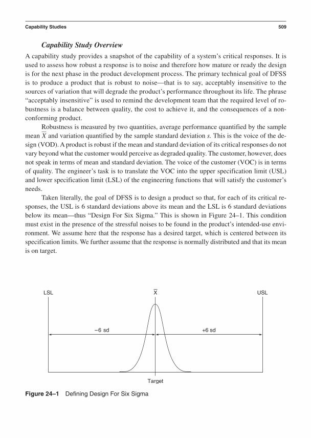
Capability Study Overview
A capability study provides a snapshot of the capability of a system’s critical responses. It isused to assess how robust a response is to noise and therefore how mature or ready the designis for the next phase in the product development process. The primary technical goal of DFSSis to produce a product that is robust to noise—that is to say, acceptably insensitive to thesources of variation that will degrade the product’s performance throughout its life. The phrase“acceptably insensitive” is used to remind the development team that the required level of ro-bustness is a balance between quality, the cost to achieve it, and the consequences of a non-conforming product.
Robustness is measured by two quantities, average performance quantified by the samplemean and variation quantified by the sample standard deviation s. This is the voice of the de-sign (VOD). A product is robust if the mean and standard deviation of its critical responses do notvary beyond what the customer would perceive as degraded quality. The customer, however, doesnot speak in terms of mean and standard deviation. The voice of the customer (VOC) is in termsof quality. The engineer’s task is to translate the VOC into the upper specification limit (USL)and lower specification limit (LSL) of the engineering functions that will satisfy the customer’sneeds.
Taken literally, the goal of DFSS is to design a product so that, for each of its critical re-sponses, the USL is 6 standard deviations above its mean and the LSL is 6 standard deviationsbelow its mean—thus “Design For Six Sigma.” This is shown in Figure 24–1. This condition must exist in the presence of the stressful noises to be found in the product’s intended-use envi-ronment. We assume here that the response has a desired target, which is centered between itsspecification limits. We further assume that the response is normally distributed and that its meanis on target.
X
Capability Studies 509
LSL
Target
USLX
–6 sd +6 sd
Figure 24–1 Defining Design For Six Sigma

These assumptions, combined with some basic statistics, allows the engineer to predict howa population of products will perform based on the performance of a smaller sample. Statisticstells us that:
1. The normal distribution has a density function that exists from negative infinity to pos-itive infinity.
2. The total area under the distribution is unity.3. Area is equivalent to probability.
Based on this, we conclude that:
1. The tails of the distribution must extend beyond the USL and LSL regardless of howmuch or how little variation the response possesses.
2. The area extending beyond the USL and LSL is equal to the probability that our prod-uct will produce a response value outside the specification limits.
3. We can calculate this probability.
For example, assuming a response whose mean is centered between the specification lim-its, if there are 6 standard deviations between the center and each of the specification limits, thenthere is approximately a 2 in a billion chance of exceeding the limits. This is a 6 sigma design.Six standard deviations were determined by Motorola in the 1980s to be acceptable for their busi-ness. This is a very small probability indeed! However, if applied to a digital system operating atnanosecond rates, there is an opportunity for two errors every second. Probabilities must be putin the context of the problem at hand.
If there are three standard deviations between each of the specification limits, then there isapproximately a 0.27 percent chance of exceeding the limits. These probabilities are easily de-termined using a standard normal table or a software package such as Minitab. Readers are en-couraged to determine these values for themselves.
Readers are also encouraged to remember that these probabilities apply only when the dis-tribution is normal and centered between its limits. A centered response is a rare condition, andprobabilities increase dramatically as the response drifts off center. Each time the response is sam-pled, it will have a different average and will only approximate a normal distribution. It is com-mon to assume that a 6 sigma design will have a 3.4 in a million chance of exceeding thespecification limits, not 2 in a billion. This assumes that, on average, over the long term, the meanof the response will vary by 1.5 times its standard deviation. We will discuss this in greater detaillater in this chapter. The message here is that normality should be tested and the mean comparedto the target so that correct probabilities are calculated.
In practice, DFSS does not demand that the limits span /6 standard deviations. This isa matter of economics, technical feasibility, and the legal, health, and societal consequences ofoperating beyond the specification limits. If death is a consequence, such as in the commercialaviation, medical, or pharmaceutical industries, then 6 sigma performance may not be adequate.
510 Chapter 24
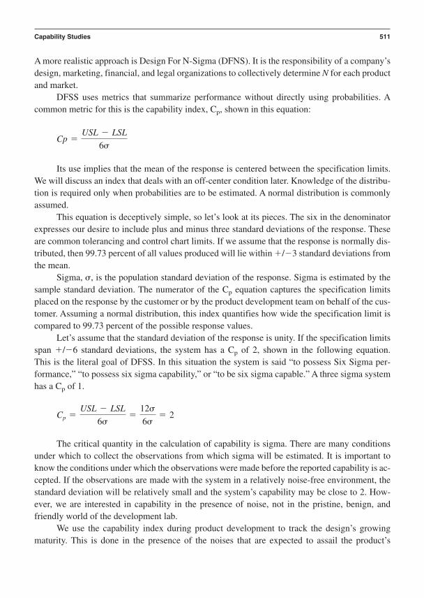
A more realistic approach is Design For N-Sigma (DFNS). It is the responsibility of a company’sdesign, marketing, financial, and legal organizations to collectively determine N for each productand market.
DFSS uses metrics that summarize performance without directly using probabilities. Acommon metric for this is the capability index, Cp, shown in this equation:
Its use implies that the mean of the response is centered between the specification limits.We will discuss an index that deals with an off-center condition later. Knowledge of the distribu-tion is required only when probabilities are to be estimated. A normal distribution is commonlyassumed.
This equation is deceptively simple, so let’s look at its pieces. The six in the denominatorexpresses our desire to include plus and minus three standard deviations of the response. Theseare common tolerancing and control chart limits. If we assume that the response is normally dis-tributed, then 99.73 percent of all values produced will lie within /3 standard deviations fromthe mean.
Sigma, , is the population standard deviation of the response. Sigma is estimated by thesample standard deviation. The numerator of the Cp equation captures the specification limitsplaced on the response by the customer or by the product development team on behalf of the cus-tomer. Assuming a normal distribution, this index quantifies how wide the specification limit iscompared to 99.73 percent of the possible response values.
Let’s assume that the standard deviation of the response is unity. If the specification limitsspan /6 standard deviations, the system has a Cp of 2, shown in the following equation. This is the literal goal of DFSS. In this situation the system is said “to possess Six Sigma per-formance,” “to possess six sigma capability,” or “to be six sigma capable.” A three sigma systemhas a Cp of 1.
The critical quantity in the calculation of capability is sigma. There are many conditionsunder which to collect the observations from which sigma will be estimated. It is important toknow the conditions under which the observations were made before the reported capability is ac-cepted. If the observations are made with the system in a relatively noise-free environment, thestandard deviation will be relatively small and the system’s capability may be close to 2. How-ever, we are interested in capability in the presence of noise, not in the pristine, benign, andfriendly world of the development lab.
We use the capability index during product development to track the design’s growingmaturity. This is done in the presence of the noises that are expected to assail the product’s
Cp =USL - LSL
6=
12
6= 2
Cp =USL - LSL
6
Capability Studies 511

performance in its intended-use environment. All the noises may not be known or able to be sim-ulated during development, but three common noises are ambient temperature, altitude, and hu-midity. If the functions in the product are sensitive to these general noises, an environmentalchamber must be available to assess the design’s decreasing sensitivity to these noises as the de-sign matures. The development team can then assess the readiness of the subsystem to be inte-grated into the evolving engineering model or of the readiness of the product to be transferred tomanufacturing.
So far, our discussion of capability has been simplistic. A response does not remain cen-tered and on target over time. If several samples of a response are taken, the mean of each sam-ple will be different. Some of this is due to measurement error but, assuming that the measurementsystem is capable, most of the variation will be due to the system’s inherent sensitivity to noise.This is the VOD that, as design engineers, we work to control. A study done by Evans (1975)showed that, in general, process means vary by about 1.5 times their standard deviation. Figure24–2 shows this situation. Note that, in what follows, the shift could have been drawn to the leftof the target with the same conclusions.
This situation illustrates the need for a capability index that accounts for an off-target con-dition. If we calculate Cp, we would get a value of 2. Yet the probability of being beyond the up-per specification limit is far greater than a Cp of 2 implies. In this situation, the probability ofbeing to the left of the LSL is negligible and can be assigned a value of 0. The probability of be-ing to the right of the USL is approximately 3.4106 or 3.4 per million. So, a new capability in-dex is needed. The index chosen is Cpk. It is calculated as shown in this equation:
Cpk = min ¢USL - X
3,
X - LSL
3≤
512 Chapter 24
Target
USLLSL X
–7.5 sd +4.5 sd
Figure 24–2 Capability with a 1.5 Shift

For our example, using a 1.5 standard deviation shift in the mean, Cpk 1.5, as shown inthe following equation.
Thus, a design that yields 6 sigma performance (Cp 2) in the short term can be expectedto produce a Cpk of 1.5 in the long term when in production. As Reigle Stewart, a founder of Six Sigma toleracing, would say, “If Design can provide a Cp of 2 then Manufacturing must pro-vide a Cpk of 1.5.” Our focus changes from “Are we meeting the specification” to “What is ourcapability?”
Cp and Cpk allow concise communication regarding the performance of our design’s criti-cal responses. It is assumed that the capability obtained is a conscious and deliberate compromisebetween the required quality, the cost of achieving that quality, and the consequences of operat-ing a nonconforming product.
If the mean of the response is centered between its limits, we use Cp. If it is not, we use Cpk.The value of Cp or Cpk is then compared to the desired value. Typically the values are Cp 2 andCpk 1.5. If these or the agreed-upon values have not been attained, the design team must takeaction. The design is not mature enough to proceed to the next phase of development. The actionto be taken is to center the mean and/or reduce the variation.
The techniques of robust design should be used to determine what region of the overall op-erating space results in system operation that is least sensitive to noise. Synergistic or ordinal in-teractions between control factors and noise are sought and exploited to reduce the system’ssensitivity to the noise. These techniques fall within the domain of Taguchi methods and classi-cal methods of robust design. They are covered in subsequent chapters in this book.
Key Detailed Inputs
Specific Steps and Deliverables
A definition of the noises that are expected in the intended-use environment is crucial so that ca-pability can be assessed under those conditions. Capability may be initially assessed with somenoises held constant. As the design’s maturity evolves, however, its readiness for the next stepmust be determined using capability in a stressful, noisy environment.
Select the environment in which data will be collected.
The system to be assessed.
Cpk = min ¢USL - X
3,
X - LSL
3≤ = min ¢ 6-1.5
3,
1.5-(-6)
3≤ = 1.5
Capability Studies 513

Capability studies are not done on all of a system’s responses, only the critical ones. The first stepis to determine which system responses are critical. This must have been determined in the con-cept and early design phases. The application of critical parameter management beginning withVOC, then QFD, then Pugh concept selection defines and determines which responses are critical.
A capability study, as in any situation where data will be used to make decisions, requires a ca-pable measurement system. The techniques covered in Chapter 23 on MSA should have been ap-plied to the measurement system and its Gage R&R, P/T ratio, and the number of distinctcategories determined.
The response data are acquired over a period of time that allows variation in the response to becaptured. This may take seconds, or it may take hours. It depends on the particular system and therates at which the noises are varied. Once the data have been collected, the sample average andsample standard deviation serve as estimates of and . The data should be plotted in a trendchart or a control chart to look for shifts and drifts in the response over the acquisition time. Shiftsand drifts in the response result in a poor capability index. Charting the response can help deter-mine the root cause of such variation.
The capability indices Cp and Cpk are calculated from the sample and the specification limits.
Calculate the capability using the speclimits and the appropriate capability index.
Calculate the sample standard deviation and mean.
Run the system in the prescribedenvironment and acquire the data.
Select and qualify the measurementsystems used to acquire the data.
Select the responses to be assessed.
514 Chapter 24

Final Detailed Output
A Cp less than 2 indicates that the design team needs to identify the sources of the variationand continue to apply the techniques of robust design and/or empirical tolerancing. A Cp of 2 in-dicates that the design is sufficiently mature and can be safely transferred to Manufacturing.
An Example
An example of determining capability using Minitab will now be given. One hundred observa-tions were taken on the temperature fall time in seconds of a blood analysis system running in anenvironmental chamber in which altitude, temperature, and humidity were varied. The observa-tions were taken every minute for 100 minutes.
The response is well centered between the specification limits, as shown graphically in Fig-ure 24–3. It is also evident by the fact that Cp is very close in value to Cpk. The response appearsto be normally distributed. A normality test can be used to determine this.
Process capability Cp measures the best that the system is capable of. It is associated withshort-term variation. The estimation of short-term variation is determined by the subgroup sizeof the data. In this case the data has not been subgrouped so the subgroup size is 1.
Minitab uses a default moving range of size 2 to determine the short-term standard devia-tion when the subgroup size is 1. The estimate of short-term variation is called within.
The average moving range is a biased estimate of sigma. Minitab uses the bias adjuster d2
to adjust the moving range to obtain an estimate of short-term variation. The equations used tocalculate Cp are shown in the next equation block with a moving range size of 2.
Process performance Pp measures the performance of the system in the long term. It is as-sociated with long-term variation. Long-term capability is calculated in the same way as Cp ex-cept that sigma is the long-term sigma instead of the short-term sigma. The estimation of
Cp =USL - LSL
6within
=12 - 8
6(0.44173)= 1.49
within =AvgMR
d2=
0.5044
1.128= 0.447134
d2 = 1.128
Decision to transfer the system to the nextdevelopment phase or to continue robustness efforts.
Compare the current capability to the desired capability.
Capability Studies 515

long-term variation is based on the pooled sample standard deviation. The pooled sample stan-dard deviation is also a biased estimate of sigma. Minitab uses the bias adjuster c4 to adjust thepooled sample standard deviation to obtain an estimate of the overall variation overall. The equa-tions used to calculate Pp are shown in the following equation block with n 100.
At best the specification limits span 9 sigma, as in:
USL LSL 4 9(within)
There are approximately 4.5 sigma on either side of the mean. The probability, assuming anormal distribution of producing a response value outside the specification limits, is therefore ap-
Pp =USL - LSL
6overall
=12 - 8
6(0.4581)= 1.455
overall =sc4= 0.4581
c4 =4(n - 1)
(4n) - 3= 0.99083
s = R an
i=1(x1 - x)2
n - 1= 0.4570
516 Chapter 24
LSLProcess Data
USL 12.0000Target *LSL 8.0000Mean 9.9766Sample N 100StDev (Within) 0.447134StDev (Overall) 0.458186
Potential (Within) CapabilityCp 1.49CPU 1.51CPL 1.47Cpk 1.47
Cpm *
Overall CapabilityPp 1.46PPU 1.47PPL 1.44Ppk 1.44
Observed PerformancePPM < LSL 0.00PPM > USL 0.00PPM Total 0.00
Exp. "Within" PerformancePPM < LSL 4.92PPM > USL 3.02PPM Total 7.94
PPM < LSL 8.01PPM > USL 5.03PPM Total 13.04
Exp. "Overall" Performance
USL
WithinOverall
98 10 11 12
Figure 24–3 Process Capability Analysis for C2

proximately 7 ppm, or seven out-of-spec values for every million opportunities. This may notsound too bad. However, if the response mean shifts by an average of 1.5 sigma over time, theout-of-spec condition can occur at a rate of 2,700 ppm.
System performance must be improved. The capability must be raised to 2. The techniquesof robust design described in this book should be applied until the capability indices meet the re-quired values.
Capability Study Checklist and Scorecard
Checklist for a Capability Study
Was this Action Excellence Rating:Deployed? 1 = Poor
Actions: YES or NO 10 = Excellent
Select the environment in which data will be collected. ______ ______
Select the responses to be assessed. ______ ______
Select and qualify the measurement systems used to acquire ______ ______the data.
Run the system in the prescribed environment and acquire ______ ______the data.
Calculate the sample standard deviation and mean. ______ ______
Calculate the capability using the spec limits and the appropriate capability index. ______ ______
Compare the current capability to the desired capability. ______ ______
Decision to transfer the system to the next development phase or to continue robustness efforts. ______ ______
Scorecard for a Capability Study
The definition of a good scorecard is that it should illustrate, in simple but quantitative terms,what gains were attained from the work.
This suggested format for a scorecard can be used by a product planning team to help doc-ument the completeness of its work.
Critical to Function Unit of Target Actual Actions to Resolve Response Measure: Capability: Capability: Capability Gap:
1. ______ ______ ______ ______
2. ______ ______ ______ ______
3. ______ ______ ______ ______
Capability Studies 517

We repeat the final deliverables:
• Assessment of the stability of the critical-to-function responses• Estimates of the mean and standard deviation of the critical-to-function responses• Estimate of the capability index Cp and Cpk used to help decide if the system is ready
for the next phase of development
References
Evans, D. H. (1975). Statistical tolerancing: The state of the art. Journal of Quality Technology,7(1), 1–12.
Harry, M., & Stewart, R. (1998). Six Sigma mechanical design tolerancing. Shaumburg, IL:Motorola University Press.
518 Chapter 24

C H A P T E R 2 5
Multi-Vari Studies
Where Am I in the Process? Where Do I Apply Multi-Vari Studies Withinthe Roadmaps?
Linkage to the I2DOV Technology Development Roadmap:
519
Invent/Innovate
Develop Optimize Verify
Concept Design Optimize Verify
Multi-vari studies are conducted during the Develop and Verify phases of I2DOV to identify thefactors that affect the system’s critical-to-function responses.
Linkage to the CDOV Product Development Roadmap:
Multi-vari studies are conducted during the Design phase of CDOV to identify the factors that af-fect the product’s critical-to-function responses. It is conducted during the Verify phase to iden-tify factors that might have been missed in earlier phases.
What Am I Doing in the Process? What Do Multi-Vari Studies Do at thisPoint in the Roadmaps?
The Purpose of Multi-Vari Studies in the I2DOV Technology DevelopmentRoadmap:
Multi-vari studies are conducted during I2DOV technology development and certification toidentify critical and noncritical factors and response of the technology.

The Purpose of Multi-Vari Studies in the CDOV Product DevelopmentRoadmap:
Multi-vari studies are conducted during CDOV product design and capability certification toidentify critical and noncritical factors and response of the product.
What Output Do I Get at the Conclusion of this Phase of the Process? WhatAre Key Deliverables from Multi-Vari Studies at this Point in the Roadmaps?
• The coefficients of correlation between the many inputs and outputs of the system• A list of the inputs and outputs that have been identified as potential critical parameters
and responses• A list of the inputs and outputs that have been eliminated as potential critical
parameters and responses
The key deliverables of a multi-vari study are the coefficients of correlation between themany inputs and outputs of the system. The coefficients are used to eliminate some inputs andoutputs from the list of potential critical parameters and responses. This will reduce the size andnumber of subsequent designed experiments that need to be run, thereby saving time and exper-imental effort.
Multi-Vari Study Process Flow Diagram
This visual reference identifies the detailed steps of multi-vari studies.
520 Chapter 25
INPUT . . .
OUTPUT . . .
The system to be assessed.
Select the environment inwhich data will be collected.
Select the variables to bemeasured.
Select and qualify themeasurement systems used
to acquire the data.
Run the system in theprescribed environment and
acquire the data.
Plot the many pair-wise relationshipsusing scatter plots or a matrix plot.
Inspect the plots for a linear, nonlinear, or alack of correlation.
Complete a table of strength, direction,and type of correlation.
Calculate all the pair-wise correlationcoefficients.
Use the plots, table, and correlations toidentify which variables are important and
which can be eliminated.
A list of critical and noncritical inputs andoutputs.

Verbal Descriptions for the Application of Each Block Diagram
This section explains the specific details of each step of a multi-vari study:
• Key detailed input(s) from preceding tools and best practices• Specific steps and deliverables from each step to the next within the process flow• Final detailed outputs that flow into follow-on tools and best practices
Multi-vari, a term coined by A. B. Seder in the 1950s, refers to a method used to detect correla-tion among many variables in a system. It is used in the Design and Verify Phases of CDOV todetermine which factors and responses should and should not be studied in subsequent designedexperiments. We cannot study all the important parameters and responses in a DOE. There areusually too many of them. We only study the few critical parameters and responses in a DOE.
Multi-vari is a passive experimental technique in that the behavior of the system is measuredwithout purposefully varying the inputs to the system, as we would do in a designed experiment.The system’s inputs and outputs are measured in the presence of everyday variation. The variationcomes from changes in operators, temperature, voltage, pressure, raw materials, and so on.
A multi-vari analysis makes use of both graphical and analytic tools. The key graphicaltools are scatter and matrix plots. The primary analytic tool is the coefficient of correlation.
Key Detailed Inputs
The system to be assessed.
Specific Steps and Deliverables
Select the environment in which data will be collected.
Multi-vari experiments are generally run without altering or adjusting the environment. Data aretaken as the system experiences its “normal, “every-day” sources of variation.
Select the variables to be measured.
Multi-vari studies are not done on all system inputs and outputs, only the suspected critical ones.The first step is to determine which are critical. This must have been determined in the Conceptand early Design phases. The application of Critical Parameter Management beginning withVOC, then QFD, then Pugh concept selection defines and determines which inputs and outputsare critical.
Multi-Vari Studies 521

Select and qualify the measurement systems used to acquire the data.
A multi-vari study, as in any situation where data will be used to make decisions, requires a ca-pable measurement system. The techniques covered in Chapter 23 on MSA should have been ap-plied to the measurement system and its Gage R&R, P/T ratio, and the number of distinctcategories determined.
Run the system in the prescribed environment and acquire the data.
Plot the many pair-wise relationships using scatter plots or a matrix plot.
Let’s consider an example in which six system variables, A, B, C, D, E, and F, were simultane-ously measured over a period of 6 hours. A is an output of the system, and B through F are inputs.A scatter plot can be used to visually indicate relationships between the variables. The scatter plotis a common graphical tool used to visually determine if two variables do or do not depend oneach other. A scatter plot between A and B is shown in Figure 25–1. The plot suggests that a re-lationship does exist. We create scatter plots for all the pair-wise comparisons among all the mea-sured variables. The scatter plots also indicate if the relationship is linear or nonlinear. This isimportant since the analytic measure of correlation we will use later, the Pearson coefficient ofcorrelation, can only detect linear correlation.
A matrix plot is a convenient way to view all the pair-wise scatter plots. Minitab providesthis utility in its graph menu pull-down (see example in Figure 25–2).
The matrix plot indicates that
A appears to be related to B, D, E, and F.
The A and B relationship appears to be nonlinear.
B appears to be related to E and F.
The B and F relationship appears to be nonlinear.
C appears to be related to D.
D appears to be related to E and F.
E appears to be related to F.
Inspect the plots for a linear, nonlinear, or a lack of correlation.
522 Chapter 25

Complete a table of strength, direction, and type of correlation.
These relationships are summarized in Table 25–1. The first entry in a cell is the strength of therelationship, Strong, Medium, or Weak. The next entry is the direction of the relationship, () forpositive and () for negative. A positive relationship means that both variables increase or de-crease together. A negative relationship means that one variable increases as the other variable de-creases. The last entry is the type of relationship, Linear or Nonlinear. An empty cell indicates thatno obvious relationship is seen in the plot.
Table 25–1 suggests that the output, A, is driven by the inputs B, D, E, and F. It is likelythat B will be a critical input since it has a strong influence on A. It also indicates multi-colinearity—that is to say that some of the inputs are related to each other. Perhaps it is not pos-sible to vary one input, say B, without causing or requiring F to vary. This knowledge can be usedto our benefit. We can study only one of the input variables if we know the equation describingthe relationship. We would choose to study the one that is easiest to vary and/or measure.
Multi-vari Studies 523
Figure 25–1 Scatter Plot of A and B Variables

524 Chapter 25
Figure 25–2 Matrix Plot of Variables A–F
Table 25–1 Sample Table of Strength, Direction, and Type of Correlation
Factor A B C D E
B S, , NL
C
D M,, L W, , L S, , L
E M, , L M, , L S, , L
F W, , L S, , NL W, , L M, , L
Calculate all the pair-wise correlation coefficients.
This is very useful information, but we don’t want to make these decisions by visually interpret-ing a chart. We want the decision to be based on a numeric value and some level of statistical sig-nificance. The metric we use is the correlation coefficient, r.

The Pearson correlation coefficient, rx1x 2, is given in the following equation for paired observations of the variables x1 and x2. Sx1 and Sx2 are the standard deviations of x1 and x2,respectively.
The correlation coefficient ranges from 1 to 1. Zero indicates no correlation. Values lessthan 0.8 or greater than 0.8 are considered a strong correlation.
The correlation coefficient only tests for a linear relationship. Two variables, like B and F in our example, can be strongly nonlinearly related and yet have a small magnitude for r. Thisis one reason why we use the matrix plot to visually identify correlation that the coefficient can-not detect.
Minitab can calculate the correlation coefficient for us for all the pair-wise combina-tions. It also reports a p-value for each coefficient. The null hypothesis here is that the correlationcoefficient is zero. The alternative hypothesis is that the correlation coefficient is not zero. Ap-value of 0.05 or less allows us to reject the null hypothesis and accept that the correlation is not zero.
The correlation coefficients for the 15 pair-wise combinations follows. The correlation ofa factor with itself is not shown since it is always unity.
Correlations: A, B, C, D, E, F
A B C D EB -0.690
0.000C 0.156 -0.212
0.448 0.299D 0.401 -0.465 -0.631
0.042 0.017 0.001E -0.587 0.659 0.165 -0.805
0.002 0.000 0.420 0.000F 0.778 -0.810 0.164 0.533 -0.650
0.000 0.000 0.424 0.005 0.000
Cell Contents: Pearson correlation P-Value
Use the plots, table, and correlations to identify whichvariables are important and which can be eliminated.
rx1x2 =a
n
i=1[(x1i - x1)(x2i - x2)]
(n - 1)Sx1Sx2
Multi-vari Studies 525

What conclusions can be drawn from the data in the table? First, the correlation coefficients forAC, BC, CE, and CF cannot be distinguished from zero, at an alpha risk of 5 percent, given thenoise in the data. Their p-values are greater than 0.05 so we do not reject the null hypothesis. Weconclude that these variables are not correlated.
The output A is correlated with the four variables F, B, E, and D, listed in order of strengthof the correlation. These are candidate factors for a DOE. The DOE will provide a more detailedunderstanding of the relationship. A DOE can provide an equation, also known as an empiricalmodel or transfer function, A f(B,D,E,F), that analytically relates the inputs to the output. Weuse the transfer function to determine the relative strength with which variation in a factor causesvariation in the response.
Final Detailed Output
A list of critical and noncritical inputs and outputs.
We see from the table that B is highly correlated with F and that D is highly correlated withE. We could choose to study B or E instead of F or E. We would do this if B or E were easier tomeasure and adjust compared to F or E.
In some situations correlation is all we need to know to direct the work to improve the system’s performance. A detailed transfer function from a DOE may be unnecessary. It may beeconomically possible to tightly tolerance an input that has a high correlation with the output.Sometimes all that is needed is to apply statistical process control to the inputs. If these methodsdo not result in the required performance improvements, more detailed system modeling and robust design techniques may be necessary. These techniques are covered in other sections of this book.
Multi-Vari Study Checklist and Scorecard
Checklist for Multi-Vari
Was this Action Excellence Rating:Deployed? 1 = Poor
Actions: YES or NO 10 = Excellent
Select the environment in which data will be collected. ______ ______
Select the variables to be measured. ______ ______
Select and qualify the measurement systems used to acquire ______ ______the data.
Run the system in the prescribed environment and acquire ______ ______the data.
526 Chapter 25
(continued)
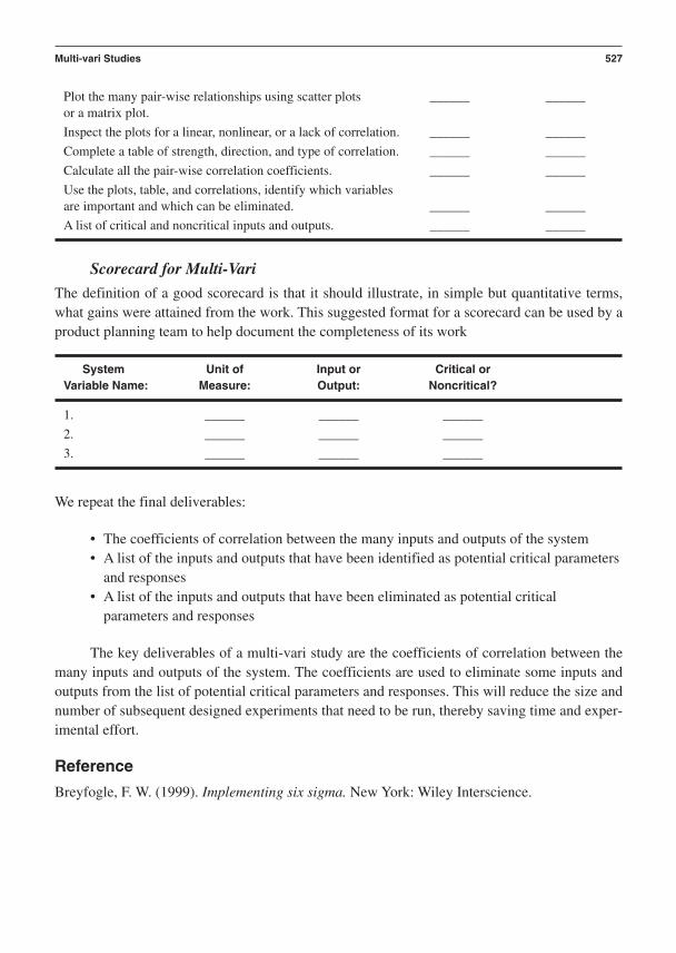
Plot the many pair-wise relationships using scatter plots ______ ______or a matrix plot.
Inspect the plots for a linear, nonlinear, or a lack of correlation. ______ ______
Complete a table of strength, direction, and type of correlation. ______ ______
Calculate all the pair-wise correlation coefficients. ______ ______
Use the plots, table, and correlations, identify which variables are important and which can be eliminated. ______ ______
A list of critical and noncritical inputs and outputs. ______ ______
Scorecard for Multi-Vari
The definition of a good scorecard is that it should illustrate, in simple but quantitative terms,what gains were attained from the work. This suggested format for a scorecard can be used by aproduct planning team to help document the completeness of its work
System Unit of Input or Critical orVariable Name: Measure: Output: Noncritical?
1. ______ ______ ______
2. ______ ______ ______
3. ______ ______ ______
We repeat the final deliverables:
• The coefficients of correlation between the many inputs and outputs of the system• A list of the inputs and outputs that have been identified as potential critical parameters
and responses• A list of the inputs and outputs that have been eliminated as potential critical
parameters and responses
The key deliverables of a multi-vari study are the coefficients of correlation between themany inputs and outputs of the system. The coefficients are used to eliminate some inputs andoutputs from the list of potential critical parameters and responses. This will reduce the size andnumber of subsequent designed experiments that need to be run, thereby saving time and exper-imental effort.
Reference
Breyfogle, F. W. (1999). Implementing six sigma. New York: Wiley Interscience.
Multi-vari Studies 527

This page intentionally left blank
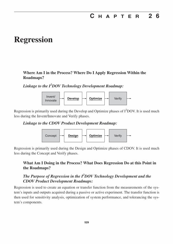
C H A P T E R 2 6
Regression
Where Am I in the Process? Where Do I Apply Regression Within theRoadmaps?
Linkage to the I2DOV Technology Development Roadmap:
Regression is primarily used during the Develop and Optimize phases of I2DOV. It is used muchless during the Invent/Innovate and Verify phases.
Linkage to the CDOV Product Development Roadmap:
Regression is primarily used during the Design and Optimize phases of CDOV. It is used muchless during the Concept and Verify phases.
What Am I Doing in the Process? What Does Regression Do at this Point inthe Roadmaps?
The Purpose of Regression in the I2DOV Technology Development and theCDOV Product Development Roadmaps:
Regression is used to create an equation or transfer function from the measurements of the sys-tem’s inputs and outputs acquired during a passive or active experiment. The transfer function isthen used for sensitivity analysis, optimization of system performance, and tolerancing the sys-tem’s components.
Concept Design Optimize Verify
Invent/Innovate
Develop Optimize Verify
529

What Output Do I Get at the Conclusion of this Phase of the Process? WhatAre Key Deliverables from Regression at this Point in the Roadmaps?
• An estimation of the relative strength of the effect of each factor on the response• An equation that analytically relates the critical parameters to the critical responses• An estimate of how much of the total variation seen in the data is explained by the
equation
Regression Process Flow Diagram
Visual reference of the detailed steps of regression illustrates the flow of tasks and responsi-bilities.
530 Chapter 26
INPUT . . .
OUTPUT . . .
The system to be assessed.
Select the environment inwhich data will be collected.
Select the inputs andoutputs to be measured in
a passive or activeexperiment.
Select and qualify themeasurement systems used
to acquire the data.
Run the system in theprescribed environment and
acquire the data as theinputs vary.
Inspect the data for outliers and removethem if root cause justifies their removal.
Postulate and build a functionalrelationship between the inputs and
output.
Test the statistical adequacy of thefunctional relationship.
Test the predictive ability of the functionalrelationship on the physical system.
The transfer function that analyticallyrelates the inputs to the outputs.
Verbal Descriptions for the Application of Each Block Diagram
This section explains the specific details of the regression process.
• Key detailed input(s) from preceding tools and best practices• Specific steps and deliverables from each step to the next within the process flow• Final detailed outputs that flow into follow-on tools and best practices

The behavior of the systems we design is governed by the laws of physics. An engineer canbe thought of as an applied physicist. Our task is to purposefully manipulate the laws of physics toperform useful work for our customers. The laws we manipulate have been identified and writtendown by many famous men and women throughout history. These are the “famous dead guys andgals” like Newton, Kirchoff, Curie, Faraday, and Fourier. They have given us the ideal functionsthat mathematically describe the physics that underlie the technology we employ in our products.
For example, Ohm told us that the voltage through a resistor is a function of current and re-sistance, v ir. This ideal function is exactly that, ideal. If there were no variation in nature, wewould always obtain the same measured value for each value of current.
However, variation is everywhere. Variation causes repeated measurements of the voltageacross a resistor to be different each time we make a measurement. This is shown in Figure 26–1.The open circles are what Ohm predicted we would measure, and the filled circles are our actualmeasurements.
So, Herr Ohm missed or purposefully left out a term. The missing term accounts for all thevariation that causes the measured voltage to deviate from the voltage predicted by the ideal func-tion. Some sources of variation are measurement system error, temperature variation, humidity,current variation, and self-heating. These sources of variation cannot be eliminated. They canonly be reduced and controlled.
Ohm’s law can now be extended to include this missing term. The resulting equation de-scribes the behavior that we actually observe in addition to the physics embedded in that behav-ior. The “behavioral” version of Ohm’s law is v ri e. Voltage is the sum of Ohm’s law andan error term e. The error term accounts for the difference between what we measure and whatOhm predicted.
Regression 531
Current
What Ohm predicts
What we measure
Volt
age
Figure 26–1 Ohm’s Predictions vs. Actual Measurements

The situation can be generalized for any linearly related set of independent and dependentvariables x and y as y b0 b1x e. The terms y, b0, b1, and the error e are random variables.The dependent variable x is also a random variable, but we treat it as fixed. We assume that x canbe set and reset with great precision compared to its range. In our example, we assume we can setthe current to its various values with great precision.
Our goal is to model or fit an equation to the observed behavior. This is called empiricalmodeling, and the resulting equation is called an empirical model, fitted equation, or transferfunction.
As engineers, we have insight regarding the underlying physics at work in the system weare modeling. This allows us to make assumptions about the structure of the model we seek. Inour example, given that Ohm’s law is at work, a sensible fitted equation is y∧i b0 b1xi. The“hat” above the y indicates that it is an estimate of y. It is called a fitted value, or a prediction.
Notice that in the fitted model the bs have been replaced by bs. The bs serve as esti-mates of the true but unknown values of the coefficients, the bs. Also notice that there is noerror term in the fitted equation. Uncertainty in the fitted equation is accounted for by uncer-tainty in b0 and b1.
The bs are calculated so that there is minimum total error between the values predictedby the equation and the actual observations. An observed value at the ith level of x is yi. A cal-culated value using the fitted equation at the ith level of x is y∧i. The error between the two isei yi y∧i. This is called a residual. A large residual indicates that the predicted value doesnot match the observed value closely. We want our model to have small residuals at all valuesof x. The residual will vary between a positive and a negative value for each observation ateach level of x. However, what we want is an error that increases and decreases monotonically.We can achieve this if we square the residuals and then sum them over all values of x. Our fit-ted model should minimize the sum of the squared errors. This is curve fitting by “leastsquares.”
So, we substitute for the fitted value, square the error, and sum the overall levels of x. We’llassume, for now, that there is only one observation at each level of x. This is shown in this equa-tion block:
Our goal is to minimize the sum of the squared errors. We do this by taking the partial de-rivative with respect to both b0 and b1 and setting them equal to zero, as in the following equa-tion block.
S = an
i=1ei
2 = an
i=1(yi - ı0 - ı1xi)
2
ei2 = (yi - ı0 - ı1xi)
2
ei = yi - yi = yi - (ı0 + ı1xi)
532 Chapter 26
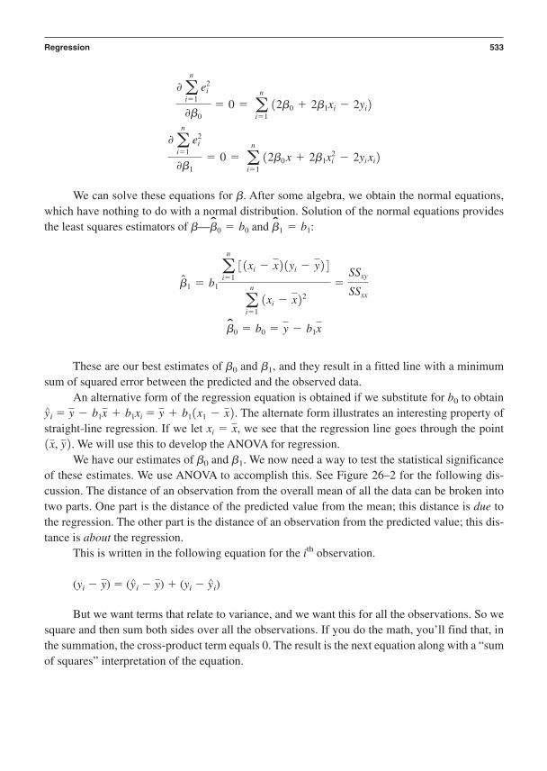
We can solve these equations for b. After some algebra, we obtain the normal equations,which have nothing to do with a normal distribution. Solution of the normal equations providesthe least squares estimators of ı— and
These are our best estimates of b0 and b1, and they result in a fitted line with a minimumsum of squared error between the predicted and the observed data.
An alternative form of the regression equation is obtained if we substitute for b0 to obtainy∧i . The alternate form illustrates an interesting property ofstraight-line regression. If we let , we see that the regression line goes through the point
. We will use this to develop the ANOVA for regression.We have our estimates of ı0 and ı1. We now need a way to test the statistical significance
of these estimates. We use ANOVA to accomplish this. See Figure 26–2 for the following dis-cussion. The distance of an observation from the overall mean of all the data can be broken intotwo parts. One part is the distance of the predicted value from the mean; this distance is due tothe regression. The other part is the distance of an observation from the predicted value; this dis-tance is about the regression.
This is written in the following equation for the ith observation.
(yi ) (y∧i ) (yi y∧i)
But we want terms that relate to variance, and we want this for all the observations. So wesquare and then sum both sides over all the observations. If you do the math, you’ll find that, inthe summation, the cross-product term equals 0. The result is the next equation along with a “sumof squares” interpretation of the equation.
yy
(x, y)xi = x
y + b1(x1 - x)y - b1x + b1xi
ı0 = b0 = y - b1x
ı1 = b1
an
i=1[(xi - x)(yi - y)]
an
i=1(xi - x)2
=SSxy
SSxx
ı1 = b1:ı0 = b0
0an
i=1ei
2
0ı1= 0 = a
n
i=1(2ı0x + 2ı1xi
2 - 2yixi)
0an
i=1ei
2
0ı0= 0 = a
n
i=1(2ı0 + 2ı1xi - 2yi)
Regression 533
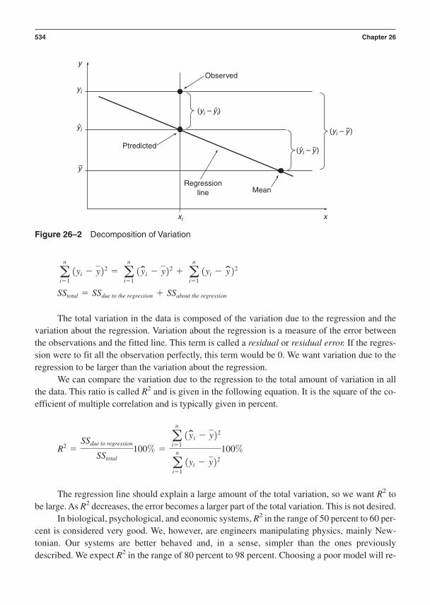
The total variation in the data is composed of the variation due to the regression and thevariation about the regression. Variation about the regression is a measure of the error betweenthe observations and the fitted line. This term is called a residual or residual error. If the regres-sion were to fit all the observation perfectly, this term would be 0. We want variation due to theregression to be larger than the variation about the regression.
We can compare the variation due to the regression to the total amount of variation in allthe data. This ratio is called R2 and is given in the following equation. It is the square of the co-efficient of multiple correlation and is typically given in percent.
The regression line should explain a large amount of the total variation, so we want R2 tobe large. As R2 decreases, the error becomes a larger part of the total variation. This is not desired.
In biological, psychological, and economic systems, R2 in the range of 50 percent to 60 per-cent is considered very good. We, however, are engineers manipulating physics, mainly New-tonian. Our systems are better behaved and, in a sense, simpler than the ones previouslydescribed. We expect R2 in the range of 80 percent to 98 percent. Choosing a poor model will re-
R2 =SSdue to regression
SStotal
100% =a
n
i=1(yi - y)2
an
i=1(yi - y)2
100%
SStotal = SSdue to the regression + SSabout the regression
an
i=1(yi - y)2 = a
n
i=1(yi - y)2 + a
n
i=1(yi - y)2
534 Chapter 26
Observed
xi
yi
yi
y
y
x
Ptredicted
MeanRegression
line
ˆ
ˆ(yi – yi)
ˆ(yi – y)
(yi – y)
Figure 26–2 Decomposition of Variation

duce R2. Sloppy experimentation, including a measurement system that is not capable, also re-duces R2. These situations cause the error term to be large and result in a small R2. Knowledge ofthe underlying physics as well as excellence in experimentation and metrology is imperative.
R2 provides a measure of how much variation our regression equation explains, but we mustalso determine if that variation is statistically significant when compared to the variation due toerror. We can perform a statistically rigorous test if we constrain the error term e that we spokeabout earlier.
Remember we said the behavior we observe is due to the sum of physics and variation. The er-ror term accounts for the deviation of each observation from what the ideal functions of physicswould predict. If we require that e N(0,2), that is, e is normally distributed with a mean of zeroand a variance of 2, then we can devise a statistically rigorous test to determine if the variation dueto regression is merely experimental error or if it models a real relationship.
This is similar to what we did in ANOVA. If e is normally distributed, y is also normallydistributed. If y is normally distributed, its square is chi-square distributed. The ratio of two chi-square variables is F-distributed. So we can calculate an F-ratio given by this equation:
The dof for regression is equal to the number of terms in the equation, not including b0. Thedoferror is easiest to find as doftotal dofregression where doftotal is one less than the number of to-tal observations.
We know the distribution of the F-ratio. It is F-distributed, so we can therefore determinethe probability of getting F values if the null hypothesis were true. The null suggests that the vari-ation explained by the regression is no different from error. This is equivalent to saying that thecoefficients of the equation are 0. So, if the p-value associated with a given F-ratio is greater than0.05, we fail to reject the null and conclude that the regression is no different from noise. If thep-value is less than 0.05, we reject the null and conclude that the regression equation explainsvariation that is greater than noise.
We can also perform a statistical test on the individual coefficients of the regression. Wecan test whether the intercept b0 is equal to 0. We can test whether the slope b1 is equal to 0. Weuse a t-test for b0. If the p-value is greater than 0.05, we fail to reject the null that the coefficientis 0 and conclude that the intercept is 0. If the p-value is less than 0.05, we reject the null and con-clude that the intercept is not 0.
We also use a t-test for b1. If the p-value is greater than 0.05, we fail to reject the null thatthe coefficient is 0 and conclude that the slope is 0. If the p-value is less than 0.05, we reject thenull and conclude that the slope is not 0. We are overdue for an example.
F =MSdue to regression
MSerror
=
an
i=1(yi - y)2
dofregression
an
i=1(yi - yi)
2
doferror
Regression 535

Key Detailed Inputs
The system is a simple electrical network consisting of a resistor and voltage supply.
Specific Steps and Deliverables
In this example the data was acquired on a test bench located in a manufacturing area.
Let’s say we measured the voltage across a 15Ω resistor at current levels from 1 to 5 amps.We measured the voltage three times at each level of current and randomly changed the currentlevel each time. This is a simple, single-factor, single-response experiment. The data are shownin the scatter plot in Figure 26–3. We can “see” Ohm’s law and we can see variation in the plot.No outliers are evident in the data.
Select and qualify the measurementsystems used to acquire the data.
Select the inputs and outputs to bemeasured in a passive or active experiment.
Select the environment in which data will be collected.
The system to be assessed.
536 Chapter 26
80
70
60
50
40
30
20
10
1 2 3 4 5
Volt
age
Current
Figure 26–3 Scatter Plot on Data from Voltage Experiment

Regression, as in any situation where data will be used to make decisions, requires a capablemeasurement system. The techniques covered in Chapter 23 on MSA should have been appliedto the measurement system and its Gage R&R, P/T ratio, and the number of distinct categoriesdetermined.
A scatter plot and individual statistical process control chart can be used to identify potential outliers.If outliers are found, root cause should be sought. They can be removed if it is justifiable. In addition,the analysis can be conducted with and without the outliers and the differences compared.
Our knowledge of the physics, the appropriate ideal function, and the form of the data inthe plot all suggest that a linear, first order equation is a likely model with which to begin. Let’suse Minitab to fit a line through the data. Choose Stat Regression Regression. We get thefollowing window. Our response is Voltage and our single predictor is Current.
The session window shows the result of the regression analysis.
Regression Analysis: Voltage versus Current
The regression equation isVoltage = -0.907187 + 15.0162 Current
S = 4.35971 R-Sq = 96.5 % R-Sq(adj) = 96.2 %
Analysis of Variance
Source DF SS MS F PRegression 1 6764.57 6764.57 355.897 0.000Error 13 247.09 19.01Total 14 7011.67
Postulate and build a functionalrelationship between the inputs and output.
Inspect the data for outliers and removethem if root cause justifies their removal.
Run the system in the prescribed environmentand acquire the data as the inputs vary.
Regression 537

Let’s calculate the coefficients of the equation, using the normal equations presented pre-viously. Try doing this yourself.
Now let’s calculate the various sums of squares. The equations are a bit different since wehave three measurements at each level of current. A particular observation at a particular value ofcurrent is denoted yi,j.
SSerror = SStotal - SSreg = 247.09
SSreg = a5
i=1a
3
j=1(yi,j - yi)
2 = 6,764.57
SStotal = a5
i=1a
3
j=1(yi,j - y)2 = 7,011.67
b0 = y - b1x = 44.1414 - 15.0162∗3 = -0.907187
b1 =a
n
i=1[(xi - x)(yi - y)]
an
i=1(xi - x)2
=SSxy
SSxx
=450.486
30= 15.0162
538 Chapter 26

Now let’s account for the degrees of freedom. The total degrees of freedom is given by
doftotal (#observations 1) (15 1) 14
The regression degrees of freedom is given by
dofreg #terms in the equation 1 (Don’t include b0.)
The error degrees of freedom is given by
doferror doftotal dofreg 14 1 13
Now calculate the mean sums of squares for regression and error.
We can estimate the amount of experimental error from the mean sums of square for error. In thisexample, experimental error is
This tells us that we cannot tell whether an observed change of 4 volts is due to a change inactual resistor voltage or is just experimental error.
The F value for the regression is given by
This is a large F value, and it occurs with a very small probability. It is reported by Minitabas p 0.000, but it is not zero, just very small. The likelihood of getting this F value is very smallif the null hypothesis were true.
The null hypothesis is that the variation due to regression is no different from the variationdue to error. We reject the null since p 0.05 and conclude that the regression equation explainsvariation that is different from error. This is good. Our equation is useful.
F =MSreg
MSerror
=6,764.57
19.01= 355.897
2MSerror = 4.36 volts
Test the statistical adequacy of the functional relationship.
MSerror =SSerror
doferror
=247.09
13= 19.01
MSreg =SSreg
dofreg
=6,764.57
1= 6,764.57
Regression 539
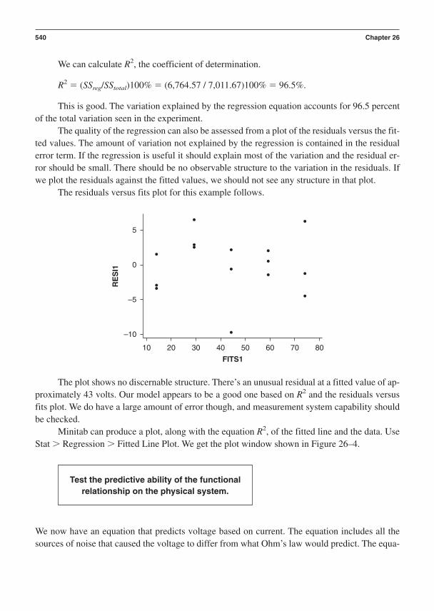
We can calculate R2, the coefficient of determination.
R2 (SSreg/SStotal)100% (6,764.57 / 7,011.67)100% 96.5%.
This is good. The variation explained by the regression equation accounts for 96.5 percentof the total variation seen in the experiment.
The quality of the regression can also be assessed from a plot of the residuals versus the fit-ted values. The amount of variation not explained by the regression is contained in the residualerror term. If the regression is useful it should explain most of the variation and the residual er-ror should be small. There should be no observable structure to the variation in the residuals. Ifwe plot the residuals against the fitted values, we should not see any structure in that plot.
The residuals versus fits plot for this example follows.
540 Chapter 26
5
0
–5
–10
10 30 50 70 80
RE
SI1
FITS1
20 40 60
The plot shows no discernable structure. There’s an unusual residual at a fitted value of ap-proximately 43 volts. Our model appears to be a good one based on R2 and the residuals versusfits plot. We do have a large amount of error though, and measurement system capability shouldbe checked.
Minitab can produce a plot, along with the equation R2, of the fitted line and the data. UseStat Regression Fitted Line Plot. We get the plot window shown in Figure 26–4.
We now have an equation that predicts voltage based on current. The equation includes all thesources of noise that caused the voltage to differ from what Ohm’s law would predict. The equa-
Test the predictive ability of the functionalrelationship on the physical system.

Regression 541
tion is voltage 0.907187 15.0162 current. We can use the equation to predict the voltageto be obtained at current levels throughout the experimental range.
We can assess the predictive ability of the regression model using the PRESS metric.PRESS is the prediction sums of squares. It is found by removing the ith observation from the dataand then creating a new regression equation. The new equation is used to predict the missing ob-servation. The error for the ith case is yi y∧î . This is repeated for all the observations, and PRESSis calculated by summing overall the PRESS values, PRESS (yi y∧î)
2. A small PRESS valueis desired, and the associated model is considered to have good predictive capability.
R-sq(pred) is determined by
In this example R-sq(pred) 95.4 percent, which means that the model predicts new val-ues as well as an observation that is already in the data set. The PRESS value and R-sq(pred) areshown in the following Minitab analysis.
Regression Analysis: Voltage versus Current
The regression equation isVoltage = - 0.91 + 15.0 Current
R2pred = 1 -
PRESS
TotalSS
80
Regression PlotVoltage = 0.907187 + 15.0162 Current
S = 4.35971 R-Sq = 96.5% R-Sq(adj) = 96.2%
70
60
50
40
30
20
10
1 2 3 4 5
Volt
age
Current
Figure 26–4 Fitted Line Plot for the Resistor Example

Predictor Coef SE Coef T PConstant -0.907 2.640 -0.34 0.737Current 15.0162 0.7960 18.87 0.000
S = 4.360 R-Sq = 96.5% R-Sq(adj) = 96.2%PRESS = 323.656 R-Sq(pred) = 95.38%
The system should be run under a given condition and the actual and predicted values com-pared to assess the model’s ability to predict actual behavior. This should be done anytime anequation has been developed to describe the behavior of a physical system.
We can also use the equation to determine the extent to which variation in current causesvariation in voltage. We can determine how tightly we need our control or tolerance current andresistance so that the variation in voltage is kept to an acceptable limit. We will cover this in thesection on optimization.
Final Detailed Outputs
The transfer function that analytically relates the inputs to the outputs is restated below.
voltage 0.907187 15.0162 current
Our discussion so far has been for an extremely simple case. We have looked at a single predic-tor, x, and one response, y. This is simple linear regression. It is instructive but of limited use.
Typically, we are interested in equations in which the predictors are nonlinear, (for exam-ple, squared, cubic, square root, or transcendental). Linear regression can handle this. In fact, lin-ear regression only refers to the coefficients of the equation, not to the predictors. So y b0 b1
(ln(x)) is linear regression while y b0 ln(b1)x and y b0 b1xb1 are not.We are also interested in equations that relate many predictors to many responses. This is
multivariate statistics and is a bit beyond what we will discuss here. We will, however, discussequations that relate many predictors to one response. This is called multiple regression. We mustnow switch from scalar notation to matrix notation if we are to explain even a simple multiple lin-ear regression situation.
Imagine we make many measurements of our single response, y1, y2, . . . yn. Also assumeour model has many terms in it, x1, x2, . . . xr. The xs can be linear or nonlinear but the coefficientsmust be linear. We can represent our behavioral equations as a series of equations shown here.Our response is a function of p predictors, and we have n observations of our response. The zscan be functions of the xs such as .z1 = x1x2
2
The transfer function that analyticallyrelates the inputs to the outputs.
542 Chapter 26

We can write this set of equations in a compact matrix form as Y Zı e. In this repre-sentation, Y, ı, Z, and e are vectors and matrices as defined in the following equation. The matrixZ consists of linear or nonlinear functions of our x variables. For example,
We can fit an equation to the observations. The form of the fitted equation, in matrix nota-tion, is Y ZB, where B is a vector of coefficients that best estimates ı in a least squares sense.We can solve this equation with a little matrix algebra shown below in the following equationblock. Note that, in what follows, we assume Z X with no loss of generality.
Y XB
Premultiply both sides by the transpose of X to get a square matrix:
X′Y X′XB
Now, premultiply both sides by (X′X)1 which is the inverse of X′X to isolate B:
(X′X)1 X′Y (X′X)1 X′XB B
So, we have solved for B:
B (X′X)1 X′Y
We can use matrix math to calculate the sums of squares for the ANOVA table as in the sim-ple regression case. The F-ratio, R2, and p will be the same as in simple regression.
Let’s look at an example of multiple regression. Let’s say we measured the time it took tocool 100l of a fluid contained in a plastic pouch from 90°C to 30°C. The fluid was heated re-sistively and cooled by forced air. The fan speed (RPM) was varied as well as the volume of fluid(l), ambient temperature (degrees C), altitude (m ASL), and humidity (%RH). The experimentwas conducted in an environmental chamber so that altitude, temperature, and humidity couldbe varied.
Thermodynamics tells us that the relationship between the response and the predictors isnonlinear. We therefore expect to have some squared terms in the model. We must run an exper-iment that allows us to estimate linear and squared terms. A central composite design was cho-sen. We’ll discuss how the experiment is related to the form of the equation we can build in thenext chapter on designed experiments.
Y = C y1
oyn
S = ZC1 z1,1 p z1,p
o o ∞ o1 zn,1 p zn,p
SbCb0
obp
S + eC e1
oen
Sz1 = x1
2x33
yn = ı0 + ı1zn,1 + ı2zn,2 + p ıpzn,p + en
o
y2 = ı0 + ı1z2,1 + ı2z2,2 + p ıpz2,p + e2
y1 = ı0 + ı1z1,1 + ı2z1,2 + p ıpz1,p + e1
Regression 543

Analysis of the data using Minitab tells us which effects are statistically significant. Theseare shown in bold in the analysis table that follows. This table was obtained from Minitab’s Stat DOE Response Surface Analyze Response Surface Design.
Response Surface Regression: Cool Time (sec) versus Speed, Vol, . . .
The analysis was done using coded units.Estimated Regression Coefficients for Cool Tim
Term Coef SE Coef T PConstant 5.0513 0.12991 38.883 0.000Speed -0.8413 0.06648 -12.654 0.000Vol 0.7034 0.06648 10.580 0.000Temp 0.4479 0.06648 6.737 0.000Alt -0.0795 0.06648 -1.195 0.257RH 0.0223 0.06648 0.335 0.744Speed*Speed -0.6478 0.06014 -10.771 0.000Vol*Vol 0.0398 0.06014 0.661 0.522Temp*Temp 0.0365 0.06014 0.607 0.556Alt*Alt -0.0296 0.06014 -0.492 0.632RH*RH -0.0899 0.06014 -1.495 0.163Speed*Vol 0.5853 0.08143 7.188 0.000Speed*Temp 0.0755 0.08143 0.927 0.374Speed*Alt -0.0100 0.08143 -0.122 0.905Speed*RH -0.0213 0.08143 -0.262 0.798Vol*Temp 0.0534 0.08143 0.656 0.526Vol*Alt -0.1024 0.08143 -1.258 0.234Vol*RH -0.0410 0.08143 -0.503 0.625Temp*Alt 0.0285 0.08143 0.350 0.733Temp*RH 0.0840 0.08143 1.032 0.324Alt*RH 0.0882 0.08143 1.083 0.302
S = 0.3257 R-Sq = 97.8% R-Sq(adj) = 93.9%
The table tells us that our equation should contain the following terms: fan speed, volume,temperature, fan speed2, and an interaction between speed volume. We can now use Minitab’sregression utility to “build” the equation.
Regression Analysis: Cool Time (sec) versus Speed, Vol, . . .
The regression equation isCool Time (sec) = 5.02 - 0.841 Speed + 0.703 Vol + 0.448 Temp
- 0.645 Speed2 + 0.585 SpeedXvol
544 Chapter 26

Predictor Coef SE Coef T PConstant 5.01675 0.06646 75.48 0.000Speed -0.84127 0.06067 -13.87 0.000Vol 0.70342 0.06067 11.59 0.000Temp 0.44793 0.06067 7.38 0.000Speed2 -0.64488 0.05427 -11.88 0.000SpeedXvo 0.58530 0.07431 7.88 0.000S = 0.2972 R-Sq = 95.7% R-Sq(adj) = 94.9%
The R2 value is large. Approximately 96 percent of the variation in the data is explained bythe regression equation. The experimental error is approximately 0.3 sec. We check the residualsvs. fits plot to further evaluate the regression equation. The plot is shown in Figure 26–5. It doesnot show any obvious patterns. Our regression equation is acceptable.
Let’s talk about the interaction between speed and volume that appears in the equation.This is shown graphically in Figure 26–6. The diagram indicates that the change in the responseas volume varies from low to high is smaller when speed is high than when speed is low. Thereis a change in the response that depends on speed. The slopes of the two lines are not parallel;this is how you recognize an interaction graphically. Now, the lines can be nonparallel, withinthe range studied, in two ways. They can cross or not cross. Figure 26–6 shows a synergistic orbeneficial interaction since the lines do not cross. Figure 26–7 shows a generalized antisyner-gistic interaction.
Let’s see how a synergistic interaction can be beneficial. Fluid volume is difficult to con-trol in this example. Fluid volume is a noise factor. Fan speed, however, can be controlled and isa control factor. The design engineer has the ability to specify and control the speed of the fantightly. Robustness is a measure of how much the mean and variance of the response changes inthe presence of noise. Clearly, cool time changes less when the fan speed is high compared to
Regression 545
0.5
0.0
–0.5
0 2 4 6 7
RE
SI1
FITS1
1 3 5
Figure 26–5 Plotting Residuals vs. Fits Plot

when it is low, as volume changes. The system is more robust and less sensitive to variation influid volume if we operate the system at a high fan speed. The synergistic interaction between anoise factor and a control factor enables robustness. It is precisely interactions of this form thatwe make use of in robust design.
Now we have an equation that models the behavior of our system, but what do we do withit? The transfer function or empirical model is extremely valuable. It tells us quantitatively howthe critical inputs affect the critical output. If an input has a large coefficient, it strongly affectsthe output. Small variation in this input causes large variation in the output. This is a design com-ponent we must control. We will need to make our design less sensitive to it through the param-eter design step of robust design. We may also need to tightly tolerance this critical input. An inputwith a small coefficient means that the response is not as sensitive to this design component. We
546 Chapter 26
Volumelow
∆Yspeedlow∆Yspeedhigh < ∆Yspeedlow
Change in Y whenspeed is low
Change in Y whenspeed is high
∆Yspeedhigh
Speedlow
Speedhigh
Volumehigh
Cool Time
Figure 26–6 A Synergistic Interaction Between Volume
Figure 26–7 A General Antisynergistic Interaction
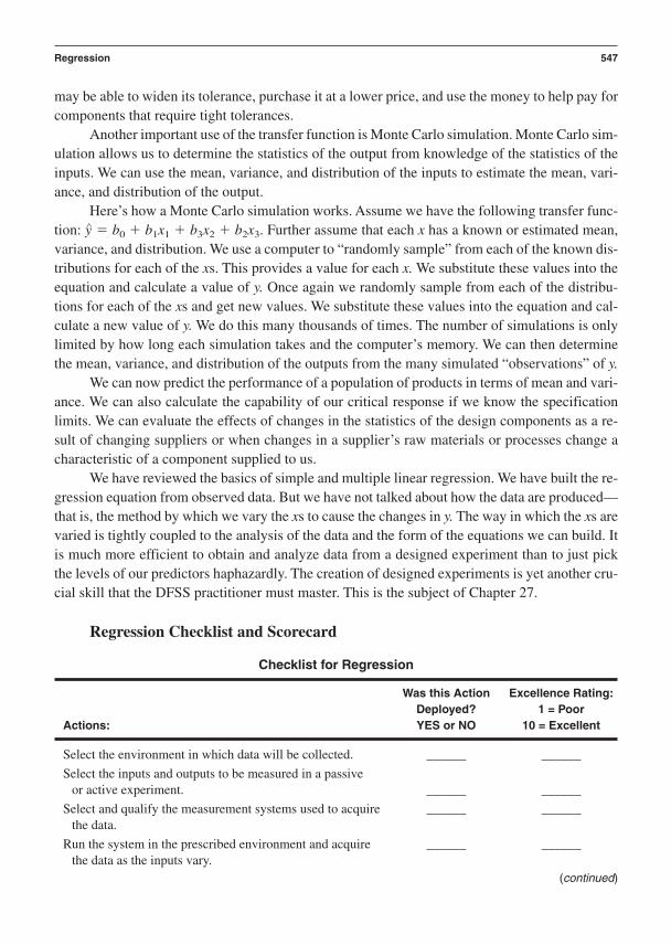
may be able to widen its tolerance, purchase it at a lower price, and use the money to help pay forcomponents that require tight tolerances.
Another important use of the transfer function is Monte Carlo simulation. Monte Carlo sim-ulation allows us to determine the statistics of the output from knowledge of the statistics of theinputs. We can use the mean, variance, and distribution of the inputs to estimate the mean, vari-ance, and distribution of the output.
Here’s how a Monte Carlo simulation works. Assume we have the following transfer func-tion: y∧ b0 b1x1 b3x2 b2x3. Further assume that each x has a known or estimated mean,variance, and distribution. We use a computer to “randomly sample” from each of the known dis-tributions for each of the xs. This provides a value for each x. We substitute these values into theequation and calculate a value of y. Once again we randomly sample from each of the distribu-tions for each of the xs and get new values. We substitute these values into the equation and cal-culate a new value of y. We do this many thousands of times. The number of simulations is onlylimited by how long each simulation takes and the computer’s memory. We can then determinethe mean, variance, and distribution of the outputs from the many simulated “observations” of y.
We can now predict the performance of a population of products in terms of mean and vari-ance. We can also calculate the capability of our critical response if we know the specificationlimits. We can evaluate the effects of changes in the statistics of the design components as a re-sult of changing suppliers or when changes in a supplier’s raw materials or processes change acharacteristic of a component supplied to us.
We have reviewed the basics of simple and multiple linear regression. We have built the re-gression equation from observed data. But we have not talked about how the data are produced—that is, the method by which we vary the xs to cause the changes in y. The way in which the xs arevaried is tightly coupled to the analysis of the data and the form of the equations we can build. Itis much more efficient to obtain and analyze data from a designed experiment than to just pickthe levels of our predictors haphazardly. The creation of designed experiments is yet another cru-cial skill that the DFSS practitioner must master. This is the subject of Chapter 27.
Regression Checklist and Scorecard
Checklist for Regression
Was this Action Excellence Rating:Deployed? 1 = Poor
Actions: YES or NO 10 = Excellent
Select the environment in which data will be collected. ______ ______
Select the inputs and outputs to be measured in a passive or active experiment. ______ ______
Select and qualify the measurement systems used to acquire ______ ______the data.
Run the system in the prescribed environment and acquire ______ ______the data as the inputs vary.
Regression 547
(continued)
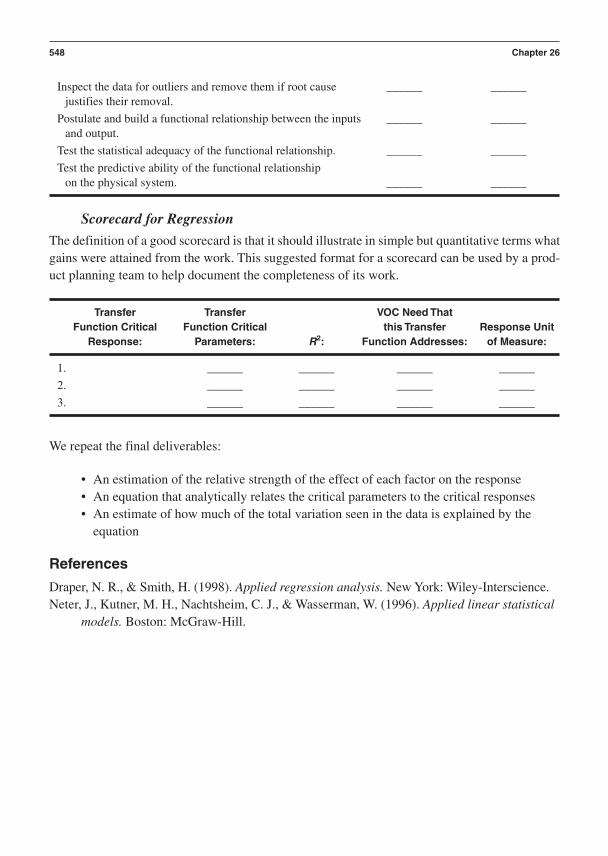
Inspect the data for outliers and remove them if root cause ______ ______justifies their removal.
Postulate and build a functional relationship between the inputs ______ ______and output.
Test the statistical adequacy of the functional relationship. ______ ______
Test the predictive ability of the functional relationship on the physical system. ______ ______
Scorecard for Regression
The definition of a good scorecard is that it should illustrate in simple but quantitative terms whatgains were attained from the work. This suggested format for a scorecard can be used by a prod-uct planning team to help document the completeness of its work.
Transfer Transfer VOC Need That Function Critical Function Critical this Transfer Response Unit
Response: Parameters: R2: Function Addresses: of Measure:
1. ______ ______ ______ ______
2. ______ ______ ______ ______
3. ______ ______ ______ ______
We repeat the final deliverables:
• An estimation of the relative strength of the effect of each factor on the response• An equation that analytically relates the critical parameters to the critical responses• An estimate of how much of the total variation seen in the data is explained by the
equation
References
Draper, N. R., & Smith, H. (1998). Applied regression analysis. New York: Wiley-Interscience.Neter, J., Kutner, M. H., Nachtsheim, C. J., & Wasserman, W. (1996). Applied linear statistical
models. Boston: McGraw-Hill.
548 Chapter 26

C H A P T E R 2 7
Design of Experiments
Where Am I in the Process? Where Do I Apply DOE Within the Roadmaps?
Linkage to the I2DOV Technology Development Roadmap:
Design of experiments is primarily used during the Develop and Optimize phases of I2DOV. It isused much less during the Invent/Innovate and Verify phases.
Linkage to the CDOV Product Development Roadmap:
Design of experiments is primarily used during the Design and Optimize phases of CDOV. It isused much less during the Concept and Verify phases.
What Am I Doing in the Process? What Does DOE Do at this Point in theRoadmaps?
The Purpose of DOE in the I2DOV Technology Development and the CDOVProduct Development Roadmaps:
The purpose of a DOE in I2DOV or CDOV is to obtain data from which to quantitatively estimatethe effects of the factors on the system’s responses without having to measure the system’s re-sponse at every point in its operating space.
Concept Design Optimize Verify
Invent/Innovate
Develop Optimize Verify
549
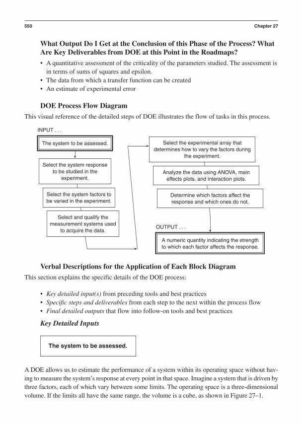
What Output Do I Get at the Conclusion of this Phase of the Process? WhatAre Key Deliverables from DOE at this Point in the Roadmaps?
• A quantitative assessment of the criticality of the parameters studied. The assessment isin terms of sums of squares and epsilon.
• The data from which a transfer function can be created• An estimate of experimental error
DOE Process Flow Diagram
This visual reference of the detailed steps of DOE illustrates the flow of tasks in this process.
550 Chapter 27
INPUT . . .
OUTPUT . . .
The system to be assessed.
Select the system responseto be studied in the
experiment.
Select the system factors tobe varied in the experiment.
Select and qualify themeasurement systems used
to acquire the data.
Select the experimental array thatdetermines how to vary the factors during
the experiment.
Analyze the data using ANOVA, maineffects plots, and interaction plots.
Determine which factors affect theresponse and which ones do not.
A numeric quantity indicating the strengthto which each factor affects the response.
Verbal Descriptions for the Application of Each Block Diagram
This section explains the specific details of the DOE process:
• Key detailed input(s) from preceding tools and best practices• Specific steps and deliverables from each step to the next within the process flow• Final detailed outputs that flow into follow-on tools and best practices
Key Detailed Inputs
A DOE allows us to estimate the performance of a system within its operating space without hav-ing to measure the system’s response at every point in that space. Imagine a system that is driven bythree factors, each of which vary between some limits. The operating space is a three-dimensionalvolume. If the limits all have the same range, the volume is a cube, as shown in Figure 27–1.
The system to be assessed.

This cube defines the space over which we will experiment. We could try to measure thesystem’s performance at every point in the cube. This would take forever since there are an infi-nite number of operating points. Since we can only measure some of the points, the question be-comes, which points and how many? We could test at, say, 10,000 randomly chosen points. ThisMonte Carlo experiment has the drawback of requiring many tests, and it may not cover the spaceevenly, since it is traversed randomly.
Another approach is to divide the range of each factor into some number of increments, say10, and then test at each combination of the increments. Three factors, each at 10 levels, requires10*10*10 1,000 tests. This is better than the Monte Carlo experiment since it may have lesstests and covers the space uniformly. But this is still a large number of tests. We want to find theminimum number of tests to run and still adequately estimate the system’s behavior. How do wedetermine this?
As noted in the previous chapter, the form of the equation we can build is tightly coupledto the way in which the factors are varied in the experiment. What does this mean? Let’s stay withour example of a system that is affected by three factors, x1, x2, and x3, and for now is assumedto be linear. This equation describes all the effects of all the factors on the response:
y∧ b0 b1x1 b2x2 b2x3 b12x1x2 b13x1x3 b23x2x3 b123x1x2x3.
This is a big equation. It contains the effects of the factors by themselves, x1, x2, and x3,called main effects; the 3 two-way interactions, x1x2, x1x3, and x2x3; and the 1 three-way interac-tion, x1x2x3.
Let’s do an information analysis on this equation. Assuming two levels to each factor, eachmain effect accounts for one dof. Each two-way interaction accounts for 1*1 1 dof. The three-way accounts for 1*1*1 1 dof. We can keep track of this in Table 27–1.
Design of Experiments 551
X3
X1
X2
Figure 27–1 Experimental Space for Three Factors

There are seven dof in this equation. If we include the intercept b0 as an additional piece ofinformation, we have a total of eight pieces of information. So, we must estimate eight coeffi-cients, b0 through b7, to completely fill in or parameterize the equation. Where do the estimatescome from? They come from the data generated by an experiment. We get a piece of informationeach time we experiment on a unique combination of the factors. To estimate the eight coeffi-cients, we must test eight unique treatment combinations, no less. We should, of course, takereplicate measurements to estimate error.
What are the eight unique combinations? We can list them in standard or Yates order if weassign a 1 to the factor at its low level and a 1 to the factor when at its high level. Only twolevels are needed for our factors because we are assuming, for now, a linear system (only twopoints are needed to draw a straight line).
We have replaced the physical values of our factors by their experimental units. For exam-ple, if we investigate temperature from 100°C to 200°C, then 1 corresponds to 100°C and 1to 200°C. The experimental design is shown in Table 27–2 where A, B, and C have been substi-tuted for x1, x2, and x3, respectively. The Yates naming scheme is also shown. When a factor ap-pears at its high level, its letter is placed in the Yates list. A 1 is assigned when all the factors areat their low levels.
This experimental design is called a full factorial because it contains all the possible com-binations of the three factors. There are 2*2*2 23 8 unique treatment combinations. We only
552 Chapter 27
Table 27–2 A Three-Factor, Two-Level Experiment in Yates Order
tc Yates A B C
1 (1) 1 1 1
2 a 1 1 1
3 b 1 1 1
4 ab 1 1 1
5 c 1 1 1
6 ac 1 1 1
7 bc 1 1 1
8 abc 1 1 1
Table 27–1 Information Analysis of Equation
Effect DOF
3 main effects at 1 dof each 3
3 two-way interactions at 1 dof each 3
1 three-way interactions at 1 dof 1
Total 7
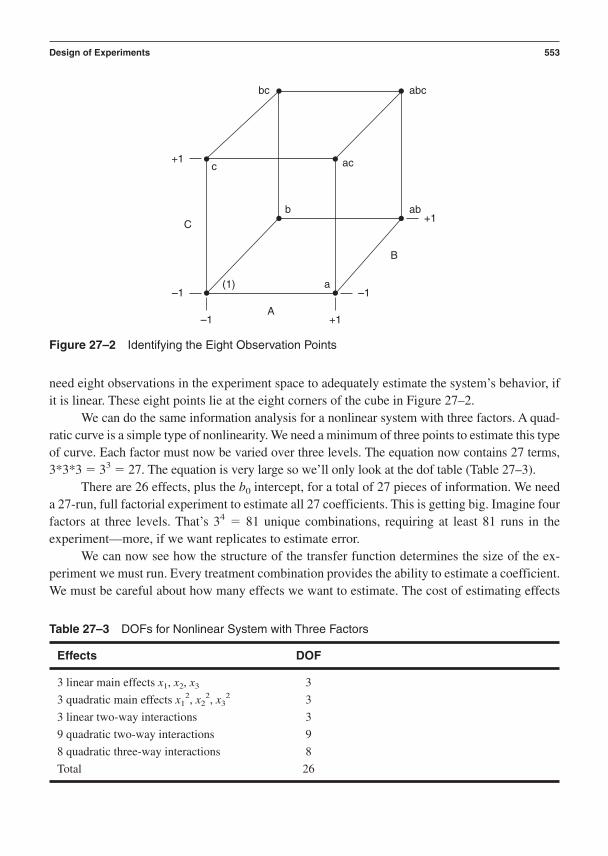
need eight observations in the experiment space to adequately estimate the system’s behavior, ifit is linear. These eight points lie at the eight corners of the cube in Figure 27–2.
We can do the same information analysis for a nonlinear system with three factors. A quad-ratic curve is a simple type of nonlinearity. We need a minimum of three points to estimate this typeof curve. Each factor must now be varied over three levels. The equation now contains 27 terms,3*3*3 33 27. The equation is very large so we’ll only look at the dof table (Table 27–3).
There are 26 effects, plus the b0 intercept, for a total of 27 pieces of information. We needa 27-run, full factorial experiment to estimate all 27 coefficients. This is getting big. Imagine fourfactors at three levels. That’s 34 81 unique combinations, requiring at least 81 runs in the experiment—more, if we want replicates to estimate error.
We can now see how the structure of the transfer function determines the size of the ex-periment we must run. Every treatment combination provides the ability to estimate a coefficient.We must be careful about how many effects we want to estimate. The cost of estimating effects
Design of Experiments 553
C
+1
+1
+1
–1
–1
–1(1)
A
a
c
b ab
abc
ac
bc
B
Figure 27–2 Identifying the Eight Observation Points
Table 27–3 DOFs for Nonlinear System with Three Factors
Effects DOF
3 linear main effects x1, x2, x3 3
3 quadratic main effects x12, x2
2, x32 3
3 linear two-way interactions 3
9 quadratic two-way interactions 9
8 quadratic three-way interactions 8
Total 26
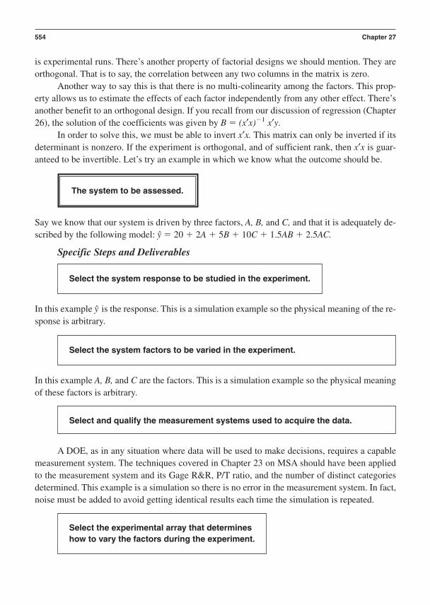
is experimental runs. There’s another property of factorial designs we should mention. They areorthogonal. That is to say, the correlation between any two columns in the matrix is zero.
Another way to say this is that there is no multi-colinearity among the factors. This prop-erty allows us to estimate the effects of each factor independently from any other effect. There’sanother benefit to an orthogonal design. If you recall from our discussion of regression (Chapter26), the solution of the coefficients was given by B (x′x)1 x′y.
In order to solve this, we must be able to invert x′x. This matrix can only be inverted if itsdeterminant is nonzero. If the experiment is orthogonal, and of sufficient rank, then x′x is guar-anteed to be invertible. Let’s try an example in which we know what the outcome should be.
Say we know that our system is driven by three factors, A, B, and C, and that it is adequately de-scribed by the following model: y 20 2A 5B 10C 1.5AB 2.5AC.
Specific Steps and Deliverables
In this example y is the response. This is a simulation example so the physical meaning of the re-sponse is arbitrary.
In this example A, B, and C are the factors. This is a simulation example so the physical meaningof these factors is arbitrary.
A DOE, as in any situation where data will be used to make decisions, requires a capablemeasurement system. The techniques covered in Chapter 23 on MSA should have been appliedto the measurement system and its Gage R&R, P/T ratio, and the number of distinct categoriesdetermined. This example is a simulation so there is no error in the measurement system. In fact,noise must be added to avoid getting identical results each time the simulation is repeated.
Select the experimental array that determines how to vary the factors during the experiment.
Select and qualify the measurement systems used to acquire the data.
Select the system factors to be varied in the experiment.
Select the system response to be studied in the experiment.
The system to be assessed.
554 Chapter 27

Let’s use the equation to determine what type of experiment we should run. The model re-quires the estimation of three main effects and 2 two-way interactions. It is assumed that a lin-ear model will adequately describe the system’s behavior. So we can run a two-levelexperiment. The desired effects account for six degrees of freedom. A three-factor full facto-rial experiment requires eight treatment combinations. We choose to run the full factorial and“waste” two dofs.
We will vary each of the four factors from 1 to 1. The experimental design with the datafollows. Each value of Y is found by substituting the appropriate values of A, B, and C into thetransfer function identified previously.
A B C Y
1 1 1 71 1 1 3
1 1 1 141 1 1 16
1 1 1 221 1 1 28
1 1 1 291 1 1 41
We can use Minitab to analyze the results of this simulated experiment. The session window out-put follows.
Fractional Factorial Fit:Y versus A, B, C
Estimated Effects and Coefficients for Y (coded units)
Term Effect CoefConstant 20.0000A 4.0000 2.0000B 10.0000 5.0000C 20.0000 10.0000A*B 3.0000 1.5000A*C 5.0000 2.5000B*C -0.0000 -0.0000A*B*C 0.0000 0.0000
Analyze the data using ANOVA, main effects plots, and interaction plots.
Design of Experiments 555
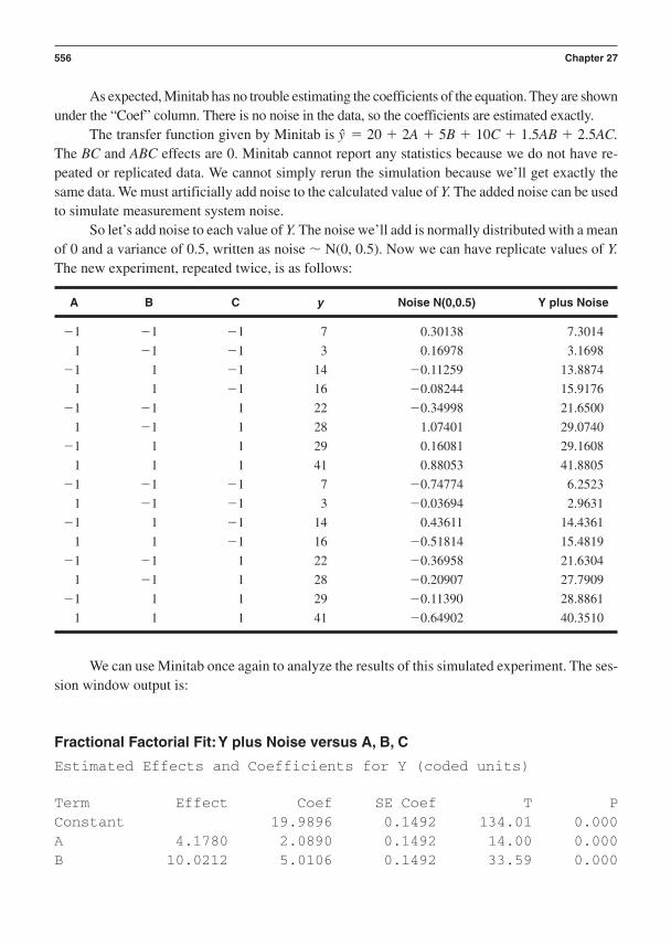
As expected, Minitab has no trouble estimating the coefficients of the equation. They are shownunder the “Coef” column. There is no noise in the data, so the coefficients are estimated exactly.
The transfer function given by Minitab is y 20 2A 5B 10C 1.5AB 2.5AC.The BC and ABC effects are 0. Minitab cannot report any statistics because we do not have re-peated or replicated data. We cannot simply rerun the simulation because we’ll get exactly thesame data. We must artificially add noise to the calculated value of Y. The added noise can be usedto simulate measurement system noise.
So let’s add noise to each value of Y. The noise we’ll add is normally distributed with a meanof 0 and a variance of 0.5, written as noise N(0, 0.5). Now we can have replicate values of Y.The new experiment, repeated twice, is as follows:
A B C y Noise N(0,0.5) Y plus Noise
1 1 1 7 0.30138 7.3014
1 1 1 3 0.16978 3.1698
1 1 1 14 0.11259 13.8874
1 1 1 16 0.08244 15.9176
1 1 1 22 0.34998 21.6500
1 1 1 28 1.07401 29.0740
1 1 1 29 0.16081 29.1608
1 1 1 41 0.88053 41.8805
1 1 1 7 0.74774 6.2523
1 1 1 3 0.03694 2.9631
1 1 1 14 0.43611 14.4361
1 1 1 16 0.51814 15.4819
1 1 1 22 0.36958 21.6304
1 1 1 28 0.20907 27.7909
1 1 1 29 0.11390 28.8861
1 1 1 41 0.64902 40.3510
We can use Minitab once again to analyze the results of this simulated experiment. The ses-sion window output is:
Fractional Factorial Fit:Y plus Noise versus A, B, C
Estimated Effects and Coefficients for Y (coded units)
Term Effect Coef SE Coef T PConstant 19.9896 0.1492 134.01 0.000A 4.1780 2.0890 0.1492 14.00 0.000B 10.0212 5.0106 0.1492 33.59 0.000
556 Chapter 27

C 20.1268 10.0634 0.1492 67.47 0.000A*B 2.6371 1.3186 0.1492 8.84 0.000A*C 5.2643 2.6321 0.1492 17.65 0.000B*C 0.0121 0.0060 0.1492 0.04 0.969A*B*C 0.0129 0.0065 0.1492 0.04 0.967
The coefficients differ from the values of the known transfer function. The difference is dueto the noise we added. We also have p-values since we have replicates.
Here, the null hypothesis is that a coefficient is zero. We reject this hypothesis for all butthe BC and ABC effects. We can also use Minitab’s balanced ANOVA utility to determine if aneffect is statistically significant:
ANOVA:Y plus Noise versus A, B, C
Factor Type Levels ValuesA fixed 2 1 1B fixed 2 1 1C fixed 2 1 1
Analysis of Variance for Y plus N
Source DF SS MS F PA 1 69.82 69.82 196.14 0.000B 1 401.70 401.70 1128.38 0.000C 1 1620.35 1620.35 4551.60 0.000A*B 1 27.82 27.82 78.14 0.000A*C 1 110.85 110.85 311.38 0.000B*C 1 0.00 0.00 0.00 0.969A*B*C 1 0.00 0.00 0.00 0.967Error 8 2.85 0.36Total 15 2233.39
Here the null hypothesis is that a term in the model has no effect on the mean of the re-sponse. We reject this hypothesis for all but the BC and ABC terms since their p-values are greaterthan 0.05. The transfer function reported by Minitab is
y 19.99 2.09A 5.01B 10.06C 1.32AB 2.63AC
Determine which factors affect the response and which ones do not.
Design of Experiments 557

We can use Minitab to look at the factor effects graphically in the main effects plot in Figure 27–3.
We can see from this plot that C has the greatest effect on the response due to its relativelysteep slope. B is next, then A. Keep in mind that we cannot determine statistical significance fromthis plot, only relative strengths. We must refer to the ANOVA table to determine statistical sig-nificance. Also keep in mind that A, B, and C are involved in statistically significant two-way in-teractions. We must therefore inspect the interactions plot to see how the AB and AC interactionsaffect the response before we consider the main effects.
The interaction plot is shown in Figure 27–4.We see that the lines in the interaction plots for AB and AC are not parallel. The BC inter-
action lines are parallel. This indicates that AB and AC interact and that BC do not interact. Wecan use these plots to select the levels of the significant factors to maximize or minimize the re-sponse. Like the main effects plot, we cannot determine statistical significance of these effectsfrom the plot, only relative strengths. We must refer to the ANOVA table to determine statisticalsignificance.
Final Detailed Outputs
We can see that based on the analysis, A, B, C, AB, and AC are statistically significant effects.Their p-values are less than 0.05. This means that the variation caused by each effect is suffi-ciently larger than the experimental noise to be distinguished from noise. But what of their rela-
A numeric quantity indicating the strength with which each factor affects the response.
558 Chapter 27
A
30
25
20
Y p
lus
No
ise
15
10
–1 1 –1 1 –1 1
B C
Figure 27–3 Main Effects Plot—Data Means for Y plus Noise

tive strength to cause a change in the response? We need a measure of practical significance. Wecan use the epsilon2 metric to compare the relative strength of each effect on the response. We usethe sums of squares from ANOVA to calculate epsilon2, as shown in the following table.
Effect Sum of Squares epsilon2 %epsilon2
A 69.82 69.82/2,230.540.031 3.1%
B 401.70 401.70/2,230.540.18 18%
C 1620.35 1620.35/2,230.540.72 72%
AC 27.82 27.82/2,230.540.012 1.2%
AB 110.85 110.85/2,230.540.05 5%
Total 2,230.54
The table indicates that while all the effects are statistically significant, 90 percent of thevariation in the response is caused by B and C alone. B and C, and perhaps A due to its involve-ment in the relatively strong (5 percent) interaction, are the system’s critical to function parame-ters. These parameters must be managed through the method of Critical Parameter Management.
Thus, Minitab performs as expected. Simulation is a helpful way of learning DOE andlearning the limitations of estimating coefficient values as noise increases. The reader shouldpractice this with other transfer functions.
Design of Experiments 559
A 30
20
10
30
20
10–1
1
–1 1 –1 1
–1
1
B
C
Figure 27–4 Interaction Plot (data means) for Y plus Noise
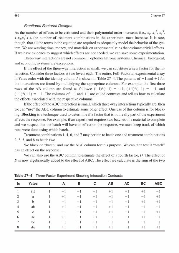
Fractional Factorial Designs
As the number of effects to be estimated and their polynomial order increases (i.e., x1, x12, x1
3,x1x2,x1
2x1), the number of treatment combinations in the experiment must increase. It is rare,though, that all the terms in the equation are required to adequately model the behavior of the sys-tem. We are wasting time, money, and materials on experimental runs that estimate trivial effects.If we have evidence to suggest which effects are not needed, we can save some experimentation.
Three-way interactions are not common in optomechatronic systems. Chemical, biological,and economic systems are exceptions.
If the effect of the three-way interaction is small, we can substitute a new factor for the in-teraction. Consider three factors at two levels each. The entire, Full-Factorial experimental arrayin Yates order with the identity column I is shown in Table 27–4. The patterns of 1 and 1 forthe interactions are found by multiplying the appropriate columns. For example, the first threerows of the AB column are found as follows: (1)*(1) 1, (1)*(1) 1, and(1)*(1) 1. The columns of 1 and 1 are called contrasts and tell us how to calculatethe effects associated with the respective columns.
If the effect of the ABC interaction is small, which three-way interactions typically are, thenwe can “use” the ABC column to estimate some other effect. One use of this column is for block-ing. Blocking is a technique used to determine if a factor that is not really part of the experimentaffects the response. For example, if an experiment requires two batches of a material to completeand we suspect that the batch will have an effect on the response, we must keep track of whichruns were done using which batch.
Treatment combinations 1, 4, 6, and 7 may pertain to batch one and treatment combinations2, 3, 5, and 8 to batch two.
We block on “batch” and use the ABC column for this purpose. We can then test if “batch”has an effect on the response.
We can also use the ABC column to estimate the effect of a fourth factor, D. The effect ofD is now algebraically added to the effect of ABC. The effect we calculate is the sum of the two
560 Chapter 27
Table 27–4 Three-Factor Experiment Showing Interaction Contrasts
tc Yates I A B C AB AC BC ABC
1 (1) 1 1 1 1 1 1 1 1
2 a 1 1 1 1 1 1 1 1
3 b 1 1 1 1 1 1 1 1
4 ab 1 1 1 1 1 1 1 1
5 c 1 1 1 1 1 1 1 1
6 ac 1 1 1 1 1 1 1 1
7 bc 1 1 1 1 1 1 1 1
8 abc 1 1 1 1 1 1 1 1

effects. This is OK if the effect of ABC is small compared to that of D. The factor D is said to bealiased or confounded with ABC.
We write this as D ABC. ABC is called the design generator. We cannot tell if the effectwe measure is due mostly to D or ABC. In fact, if the effects of D and ABC are equal and oppo-site, their sum would be zero and we would conclude that D has no effect, even though both D andABC have profound effects on the response. So, we must be careful when using this technique.
What do we gain by confounding D with ABC? We gain the ability to estimate four factorsin the same number of runs we were using to estimate three factors. The new experiment is shownin Figure 27–5.
As expected, there’s no free lunch. We must give something up. Actually, we give up twothings. We give up the ability to estimate the effect of ABC. This is OK if the ABC effect is small.We also give up the ability to estimate some or all of the two-way interactions. Some or all of thetwo-way interactions are now aliased with each other. We can determine the aliasing scheme byusing the design generator ABC.
If we multiply both sides of the generator by D, we get I ABCD, which is called the defin-ing contrast. I is the identity column. The term on the right is called the word, and the word isgood. It tells us about the aliasing structure of our design and the resolution of our design. Theresolution is the length of the word. It is four in this case, so this is a resolution IV design. Thealiasing of an effect is determined by multiplying both sides of the defining contrast by the effect.For example, to determine what A is aliased with, we multiply both sides by A. The product ofany factor times itself is I, that is, AA I. Also the product of any factor times I is the factor, thatis, AI A.
So, AI AABCD A BCD. This tells us that A is confounded with the three-way in-teraction BCD. In a similar manner, ABI ABABCD AB CD. This tells us that the two-way interaction AB is confounded with the two-way interaction CD. Luckily, we don’t have tocalculate this. Minitab reports the aliasing structure for us. Let’s try it.
Choose from the menu, Stat DOE Factorial Create Factorial Design. The followingwindow will appear.
Design of Experiments 561
Figure 27–5 A Four-Factor Fractional Factorial Experiment
tc A B C D
1 1 1 1 12 1 1 1 13 1 1 1 14 1 1 1 15 1 1 1 16 1 1 1 17 1 1 1 18 1 1 1 1
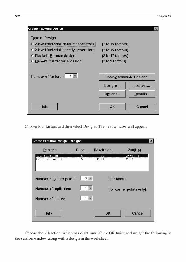
Choose four factors and then select Designs. The next window will appear.
562 Chapter 27
Choose the 1⁄2 fraction, which has eight runs. Click OK twice and we get the following inthe session window along with a design in the worksheet.

Factorial Design
Fractional Factorial Design
Factors: 4 Base Design: 4, 8 Resolution: IVRuns: 8 Replicates: 1 Fraction: 1/2Blocks: none Center pts (total): 0
Design Generators: D = ABC
Alias Structure
I + ABCD
A + BCDB + ACDC + ABDD + ABCAB + CDAC + BDAD + BC
Here we see that Minitab has created a Fractional Factorial design. There are four factorswith eight runs. It is resolution IV and it is a half fraction. It is half of a Full Factorial because ithas only half the number of runs required to estimate four factors in a Full Factorial.
The design generator is D ABC. The aliasing structure is shown in the session window.We see that all the main effects are confounded with three-way interactions. This is good. Three-way effects are rare. We also see that some of the two-way interactions are confounded with eachother. This is bad if those two-way effects are large. A resolution IV design is not a good designto run if you need to estimate effects of all the two-way interactions. In the case of four factors,we must either run the Full Factorial or fold the design (Montgomery, 1997).
It is not until we have a resolution V design that we are safe with regard to two-way inter-actions. Let’s create a design with five factors. Choose from the menu, Stat DOE Factorial Create Factorial Design. The window shown on the top of page 564 will appear.
Choose five factors and then select Display Available Designs. The next window will appear.
We can see that for five factors we can choose a resolution III with 8 runs, a resolution Vwith 16 runs, or a Full Factorial with 25 32 runs.
There’s no selection option in this window. Click OK and choose Designs. The followingwindow shown on the bottom of page 564 appears.
Choose the 16-run resolution V option. Click OK twice, and the information appears in thesession (see top of page 565).
Design of Experiments 563

564
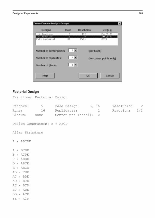
Factorial Design
Fractional Factorial Design
Factors: 5 Base Design: 5, 16 Resolution: VRuns: 16 Replicates: 1 Fraction: 1/2Blocks: none Center pts (total): 0
Design Generators: E = ABCD
Alias Structure
I + ABCDE
A + BCDEB + ACDEC + ABDED + ABCEE + ABCDAB + CDEAC + BDEAD + BCEAE + BCDBC + ADEBD + ACEBE + ACD
Design of Experiments 565

CD + ABECE + ABDDE + ABC
We see that all main effects are aliased with four-way interactions, and all two-way inter-actions are aliased with three-ways. This is very good. Three-ways are rare, and four-ways are al-most unheard-of.
We see that Fractional Factorial designs allow us to estimate the effects of more factors infewer runs. A recommended approach to experimentation is to begin with a two-level FractionalFactorial. Don’t expend all your time, money, and material on one big experiment. An experimentanswers many questions; that is why we run it. However, an experiment also uncovers many newquestions. You’ll probably need to run subsequent experiments to answer the new questions. Therecommendation is to begin with a two-level Fractional Factorial. But what if the system is non-linear? A two-level design can only estimate linear effects. We can, however, run a two-level de-sign and determine if the system is linear. We do this by including a center point in the experiment.A center point is at the center of the experiment space. It is the treatment combination with allfactors set at their zero level.
Let’s take the example of two factors at two levels. The experiment space is the squareshown in Figure 27–6.
In this case, we have two factors at two levels requiring four runs. These are the black dotsin Figure 27–6. We also measure the response at the center point.
The center point is the point in the experiment space where the factors are set to zero. Werun the experiment and analyze the results. We can create the following linear model from thedata: y b0 b1A b2B. This is the dotted line shown in Figure 27–6.
566 Chapter 27
Measured responsewhen all the factorsare set to zero
+1
–1
–1 +1
Factor B
Factor A
Predicted responsewhen all the factorsare set to zero
Figure 27–6 Center Point of Experiment Space

However, we have observations actually measured at the center point. This is shown as theopen triangle. We can use the linear equation to calculate what the response would be at the cen-ter point if the system were linear. Obviously, the calculated value is b0 since A and B are set to0 in the equation.
If the difference between the measured and calculated center point values are statisticallyequal, we say that the system does not have curvature. It is linear and a linear equation is ade-quate. This is the dotted line shown in Figure 27–6. If they are statistically different, we say thesystem has curvature. It is nonlinear. A linear equation is not adequate. We don’t know the sys-tem’s trajectory. We don’t know the form of the nonlinearity. It may be the solid, curved lineshown in the figure or some other curve. The simplest nonlinearity is a squared or quadratic re-lationship. We need to run at least a three-level experiment to estimate a quadratic equation.
There’s another benefit to running center points. If we take replicate measurements at thecenter point, we can get an estimate of pure error. This estimate allows us to obtain p-values inthe ANOVA table from which we can determine the statistical significance of each effect.
If the system is determined to be nonlinear and greater detail is needed about the functionalrelationship of the factors to the response, we move on to the response surface methods of ex-perimentation. This is the subject of the next section.
DOE Checklist and Scorecard
Checklist for DOE
Was this Excellence Rating:Action Deployed? 1 Poor
Actions: YES or NO 10 Excellent
Select the system response to be studied in the experiment. ______ ______
Select the system factors to be varied in the experiment. ______ ______
Select and qualify the measurement systems used to acquire ______ ______the data.
Select the experimental array that determines how to vary the ______ ______factors during the experiment.
Analyze the data using ANOVA, main effects plots, and interaction plots. ______ ______
Determine which factors affect the response and which ones do not. ______ ______
A numeric quantity indicating the strength to which each factor affects the response. ______ ______
Scorecard for DOE
The definition of a good scorecard is that it should illustrate in simple but quantitative terms whatgains were attained from the work. This suggested format for a scorecard can be used by a prod-uct planning team to help document the completeness of its work.
Design of Experiments 567

Statistical Practical Significance, Significance,
Factor Name: p-value: epsilon2: Critical Parameter: Unit of Measure:
1. ______ ______ ______ ______
2. ______ ______ ______ ______
3. ______ ______ ______ ______
We repeat the final deliverables:
• A quantitative assessment of the criticality of the parameters studied. The assessment isin terms of sums of squares and epsilon.
• The data from which a transfer function can be created.• An estimate of experimental error.
Reference
Montgomery, D. C. (1997). Design and analysis of experiments. New York: Wiley & Sons.
568 Chapter 27
P A R T V I
Tools and Best Practices for Optimization
Chapter 28 Taguchi Methods for Robust DesignChapter 29 Response Surface MethodsChapter 30 Optimization Methods
The tools and best practices discussed in this section focus on deliverables required at gate re-views for the third phases in the I2DOV and CDOV processes.
The tools and best practices chapters are structured so that the reader can get a strong senseof the process steps for applying the tools and best practices. The structure also facilitates the cre-ation of PERT charts for project management and critical path management purposes. A check-list, scorecard, and list of management questions concludes each chapter.
569

This page intentionally left blank

C H A P T E R 2 8
Taguchi Methods for Robust Design
Where Am I in the Process? Where Do I Apply Robust Design Within theRoadmaps?
Linkage to the I2DOV Technology Development Roadmap:
Robust design is conducted within the Optimize phase during technology development. It is ap-plied to new technology subsystems that are being developed for integration into a new platformor for integration into existing system designs.
Linkage to the CDOV Product Development Roadmap:
Robust design is also conducted within the Optimize phase during product development. Here weapply robust design to a specific product with specific noises. This focused application of robustdesign assures that the subsystems are insensitive to the specific product delivery and use noisesand specific system integration noise factors that were not clear at technology optimization andverification during the I2DOV process.
Concept Design Optimize Verify
Invent/Innovate
Develop Optimize Verify
571

What Am I Doing in the Process? What Does Robust Design Do at this Pointin the Roadmaps?
The Purpose of Robust Design in the I2DOV Technology DevelopmentRoadmap:
In I2DOV we use the ideal function from the Develop phase for a subsystem technology to definea generic set of product line noise factors, signal factors (critical adjustment parameters), controlfactors (critical functional parameters), and critical functional responses. We conduct analytical(Monte Carlo simulation) and experimental procedures (designed experiments) to develop criticalfunctional parameter set points that provide insensitivity to the generic set of product line noisefactors. We then use a small number of signal factors (CAPs) and one or more other specializedcontrol factors that are capable of changing the slope of the ideal function (beta shifting) to adjustthe mean response on to the desired target, known as the Dynamic Taguchi Method.
The Purpose of Robust Design in the CDOV Product Development Roadmap:
In CDOV we once again use the ideal function for a subsystem to define a specific product fo-cused set of noise factors, signal factors (CAPs), control factors (critical functional parameters),and critical functional responses. We conduct Monte Carlo simulation and experimental proce-dures (designed experiments) to leave the subsystems in a documented state of insensitivity to theset of specific product noise factors. We use a small number of signal factors (CAPs) and one ormore other specialized control factors that are capable of changing the slope of the ideal function(beta shifting) to adjust the mean response on to the desired target.
What Output Do I Get at the Conclusion of Robust Design? What Are KeyDeliverables from Robust Design at this Point in the Roadmaps?
• Optimized signal-to-noise metrics that characterize the useful interactions betweencontrol factor and noise factor interactions for the subsystem critical functionalresponse(s)
• Optimized critical functional parameter set points that control the subsystem’srobustness
• Optimized critical adjustment parameters that tune the mean value of the subsystem’scritical functional response(s) on to its desired targets
• Subsystem Critical Parameter Management data that is documented in the CPMrelational database:CFR meanCFR standard deviationCFR coefficient of variation [(s/mean) 100]CFR S/N ratioCFR Cp index (early quantification of the design’s ability to meet specifications)
The Robust Design Process Flow Diagram (found on page 573)
A visual reference of the detailed steps of robust design illustrating the flow of the process follows.
572 Chapter 28

Verbal Descriptions for the Application of Each Block Diagram
This section explains the specific details of what to do in the robustness optimization process:
• Key detailed input(s) from preceding tools and best practices• Specific steps and deliverables from each step to the next within the process• Final detailed outputs that flow into follow-on tools and best practices
Taguchi Methods for Robust Design 573
INPUT . . .
OUTPUT . . .
Use ideal function.
Define critical functionalresponses and S/N ratio.
Define signal factor(s).
Define noise factors.
Generate noise factordiagrams for each
subsystem.
Generate noise factor mapfor entire system.
Conduct measurementsystems analysis.
Conduct noise vectorexperiment.
Analyze noise vectorexperimental data.
Define compounded noisefactors.
Define control factors andlevel set points.
Identify potential CF×CFinteractions.
Design control factors for additivity.
Select array for robustness experiment.
Conduct measurement systems analysis.
Conduct robustness experiment.
Analyze robustness experimental data.
Identify optimum robustness factors andset points.
Identify optimum tuning factors and setpoints.
Document optimum robustness andtuning factors and set points in Critical
Parameter Management database.
Construct Taguchi's additive S/N model.
Verify Taguchi's additive model.
Move on to technology verification orproduct capability development using
tolerance design.
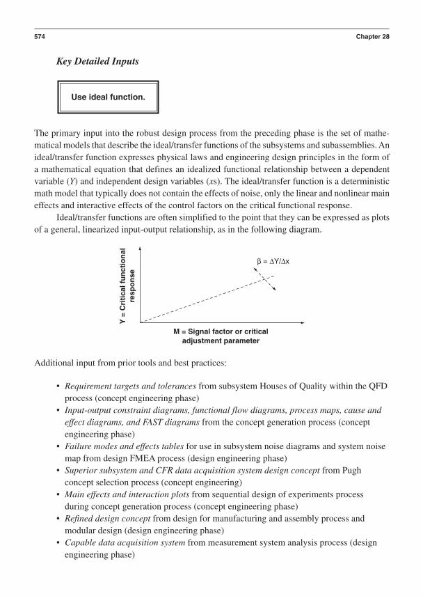
Key Detailed Inputs
The primary input into the robust design process from the preceding phase is the set of mathe-matical models that describe the ideal/transfer functions of the subsystems and subassemblies. Anideal/transfer function expresses physical laws and engineering design principles in the form ofa mathematical equation that defines an idealized functional relationship between a dependentvariable (Y) and independent design variables (xs). The ideal/transfer function is a deterministicmath model that typically does not contain the effects of noise, only the linear and nonlinear maineffects and interactive effects of the control factors on the critical functional response.
Ideal/transfer functions are often simplified to the point that they can be expressed as plotsof a general, linearized input-output relationship, as in the following diagram.
Additional input from prior tools and best practices:
• Requirement targets and tolerances from subsystem Houses of Quality within the QFDprocess (concept engineering phase)
• Input-output constraint diagrams, functional flow diagrams, process maps, cause andeffect diagrams, and FAST diagrams from the concept generation process (conceptengineering phase)
• Failure modes and effects tables for use in subsystem noise diagrams and system noisemap from design FMEA process (design engineering phase)
• Superior subsystem and CFR data acquisition system design concept from Pughconcept selection process (concept engineering)
• Main effects and interaction plots from sequential design of experiments processduring concept generation process (concept engineering phase)
• Refined design concept from design for manufacturing and assembly process andmodular design (design engineering phase)
• Capable data acquisition system from measurement system analysis process (designengineering phase)
Y =
Cri
tica
l fu
nct
ion
alre
spo
nse
M = Signal factor or criticaladjustment parameter
β = ∆Y/∆x
Use ideal function.
574 Chapter 28

Specific Steps and Deliverables
The ideal function relates a variable that must be defined as a measurable critical functional re-sponse to a signal factor, also called a critical adjustment parameter. The critical functional re-sponse must be a continuous, measurable engineering scalar or vector variable that is directlyrelated to the fundamental functionality of the subsystem. It must be directly tied to the efficiencyof the flow and transformation of mass and/or energy of the subsystem. If the mass is not flow-ing or changing phase, its current physical state, under the influence of some form of energy in-put, must be considered to be the CFR, such as deflection or expansion of a solid material. It isimportant that you measure functions and avoid measuring an attribute of quality such as relia-bility, defects, or yield (% acceptable). We avoid these “quality” metrics for three main reasons:
1. They are only indirectly linked to the physical principles that underwrite the funda-mental functionality of the design and its sensitivity to realistic sources of noise.
2. They require larger samples of data to calculate and reach valid statistical conclusionsabout the design’s performance.
3. It is hard to draw concrete engineering conclusions during design using metrics thatwere developed as retrospective, after-the-fact measures of a design’s quality.
We must use metrics that provide immediate feedback about our progress in design per-formance characterization and improvement, while we intentionally stress test the design well be-fore finalizing nominal set points.
Most cases of robust design will be evaluated using the dynamic S/N ratio. The dynamicS/N ratio measures the strength of the power of a proportional, engineered relationship betweena signal factor and the CFR with respect to the power of the variation around that proportional re-lationship. In a word, the “signal” of the ideal function is relative to the noise (assignable causevariation) that is active during a mass/energy conversion process within a design.
Dynamic S/N 10log[2/2]
where [2] is the slope of the best fit line through a set of data relating a CFR to changesof a critical adjustment parameter.
The effect of Taguchi noise factors (assignable causes of variation) on 2 is expressed inthe term 2. We will explore signal and noise factors presently.
Define signal factor(s).
Define critical functional responses and S/N ratio.
Taguchi Methods for Robust Design 575

The signal factor is an “engineered” control factor that has the capacity to adjust the mean of thecritical functional response. That is why it is also referred to as a critical adjustment parameter.It also has a moderate-to-low level effect on the standard deviation of the critical functional re-sponse. If the critical adjustment parameter (CAP) does not have a linear relationship with thecritical functional response (CFR), the CFR data can be transformed using some form of log orexponential function to “linearize” the relationship.
The nonlinear effect in the ideal function has been transformed into a linear effect by usinga natural log transformation on the CFR data.
The subsystem ideal function is used to define and measure inefficiencies and disruptions in theflow, transformation, and state of energy, mass, and information (logic and control signals) foreach subsystem. These disruptive elements can come from three sources.
1. External noise factors: Factors entering the subsystem from outside sources2. Unit-to-unit noise factors: Factors such as material or part-to-part variation3. Deterioration noise factors: Factors causing dynamic wear or temporal degradation
Define noise factor(s).
Y =
CF
R
M = CAPM1 M2 M3
Y = x2
Y =
CF
R
M = CAPM1 M2 M3
Y = Inx
576 Chapter 28

These are referred to as Taguchi noise factors and lie at the root of the physics of variationfor a subsystem. They are special or assignable cause sources of variation. They cause statisti-cally significant variation in critical functional responses, well beyond random or common causesources of variation.
Subsystem noise diagrams are schematic representations of the three sources of variation that as-sail and disrupt each subsystem’s critical functional response. They also contain the output noisesthat can assail and disrupt other subsystems or the user’s environment:
A system noise map is a series and/or parallel network of all the subsystem noise diagrams. Thesemaps illustrate all the key noise flow paths from one subsystem to another throughout the inte-grated system. They document how variation is transmitted across the system (see figure on topof next page).
Although measurement systems analysis has been done previously, prior to the screening designof experiments during concept engineering, it is wise to certify the capability (P/T ratio and GageR&R) of the data acquisition system prior to measuring the subsystem critical functional re-sponses during the noise experiment (see Chapter 23).
Conduct measurement systems analysis.
Generate noise factor map for entire system.
External Noise:1.2.3
Output Noise:1.2.3
Subsystem
Unit-to-Unit Noise:1.2.3
Deterioration Noise:1.2.3
Generate noise factor diagrams for each subsystem.
Taguchi Methods for Robust Design 577
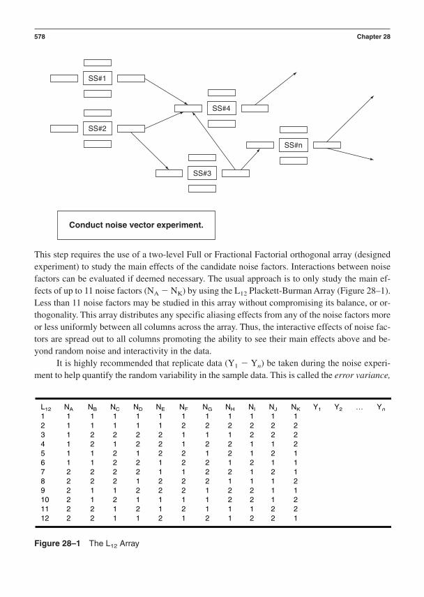
This step requires the use of a two-level Full or Fractional Factorial orthogonal array (designedexperiment) to study the main effects of the candidate noise factors. Interactions between noisefactors can be evaluated if deemed necessary. The usual approach is to only study the main ef-fects of up to 11 noise factors (NA NK) by using the L12 Plackett-Burman Array (Figure 28–1).Less than 11 noise factors may be studied in this array without compromising its balance, or or-thogonality. This array distributes any specific aliasing effects from any of the noise factors moreor less uniformly between all columns across the array. Thus, the interactive effects of noise fac-tors are spread out to all columns promoting the ability to see their main effects above and be-yond random noise and interactivity in the data.
It is highly recommended that replicate data (Y1 Yn) be taken during the noise experi-ment to help quantify the random variability in the sample data. This is called the error variance,
Conduct noise vector experiment.
SS#1
SS#2
SS#4
SS#3
SS#n
578 Chapter 28
L12 NA NB NC ND NE NF NG NH NI NJ NK Y1 Y2 … Yn
1 1 1 1 1 1 1 1 1 1 1 12 1 1 1 1 1 2 2 2 2 2 23 1 2 2 2 2 1 1 1 2 2 24 1 2 1 2 2 1 2 2 1 1 25 1 1 2 1 2 2 1 2 1 2 16 1 1 2 2 1 2 2 1 2 1 17 2 2 2 2 1 1 2 2 1 2 18 2 2 2 1 2 2 2 1 1 1 29 2 1 1 2 2 2 1 2 2 1 110 2 1 2 1 1 1 1 2 2 1 211 2 2 1 2 1 2 1 1 1 2 212 2 2 1 1 2 1 2 1 2 2 1
Figure 28–1 The L12 Array

(2)error. A minimum of three to five replicates per experimental run is recommended. This is usedto calculate the F-ratio (from ANOVA) for each noise factor to assess its statistical significancerelative to its effect on the mean of the CFR.
The main effects plots from a two-level noise experiment will define the magnitude and direc-tional effect of each noise factor on the CFR. In Figure 28–2, we see the results of the analysis ofmeans calculations for the noise factors A and B from a designed experiment.
Note the following details:
• Noise factor A has a positive directional effect () on the mean of the CFR.• Noise factor B has a negative directional effect () on the mean of the CFR.• Noise factor A has a large magnitude effect (A) on the mean of the CFR.• Noise factor B has a small magnitude effect (B) on the mean of the CFR.
Any measurable engineering response that has both magnitude and direction is defined asa vector. Here we see noise factors A and B have plots that define their vector effect.
With vectors defined for each noise factor, we are now ready to perform a grouping function that greatly improves the efficiency of how we induce Taguchi noise during a robust design experiment.
Define compounded noise factors.
Analyze noise vector experimental data.
Taguchi Methods for Robust Design 579
Low
Noise Factor A
CF
R M
ean
CF
R M
ean
Noise Factor B
High
(+)
(–)
Low High
∆A
∆B
Figure 28–2 Analysis of Means Calculations for Noise Factors A and B

As we look at the main effects plots, we see that noise factor A and noise factor B have thefollowing common traits:
• The CFR mean is driven up when noise factor A is at its high level and noise factor B isat its low level.
• We “compound” or group them together because they both have the same directionaleffect on the mean value of the CFR: N1 [NAhigh; NBlow] drives the mean up (seeFigure 28–3).
• The CFR mean is driven down when noise factor A is at its low level and noise factorB is at its high level.
• Similarly, we “compound” or group the same two noise factors together at theiropposite levels because they both have the same directional effect on the mean value ofthe CFR: N2 [NAlow; NBhigh] drives the mean down.
We can now adequately introduce stress to interact with the control factors within a de-signed experiment by applying the compounded noise factors to each Fractional Factorial exper-imental treatment combination in a “Full Factorial” manner:
Taguchi recommends we attempt to expose every run in the robustness experiment to a fulland consistent set of stressful, compounded noise factors. In this approach we allow the control
1.
A B C
1 1 1
1 2 2
2 1 2
2 2 1
N1 N2
2.
3.
4.
ControlFactors
CompoundedNoises
TreatmentCombinations
CFRData
580 Chapter 28
Low
N1 = [NAhigh; NBlow]
Noise Factor A
CF
R M
ean
CF
R M
ean
Noise Factor B
High
(+)
(–)
Low High
∆A
∆B
N2 = [NAlow; NBhigh]
Figure 28–3 Noise Factor A and B Interactions

factors to have a Full Factorial interaction with a consistent set of noise factors. Doing a partialstudy of control factor-to-noise factor interactivity sub-optimizes the intent of robust design ex-perimentation. Our goal is to identify control factor-to-noise factor interactions (usually measuredas changes in S/N values) that can be used to identify set points that leave the CFR minimally sen-sitive to noise. S/N ratios are designed to draw our attention to CFNF interactivity. The biggerthe difference between two S/N values within an experiment, the more interaction is occurringbetween a control factor and a compounded noise factor. This is the major measurement objec-tive within the Taguchi method of designed experimentation for the development of a robust de-sign. Notice that most of the “design” that goes into a Taguchi experiment is not related to thestructure of a complex array but in the nature of the control factors that are loaded into a simplearray and their relationship to compounded noise factors as they influence a critical functional response.
Control factors are the “designed” engineering parameters that, in conjunction with the signal fac-tor(s), control the ideal function of the design. Recall that a signal factor is a special class of con-trol factor that has been designed to have a large effect on the mean of a CFR and a relativelysmall effect on the standard deviation of a CFR. These factors are developed and designed into afunctioning subsystem. We want to make purposeful changes in the set points of these control-lable factors to see how they interact with the Taguchi noise factors. The purpose of robust de-sign is largely focused on provoking opportunities for control factors to interact with noisefactors. When this is allowed to happen we can see the following trend in the interaction plots be-tween CFs and NFs:
Control factors can break down into two categories.
1. Candidate critical functional parameters (CFP): A critical functional parameteris a functional output from an engineered group of component specifications that are notconsidered to be a complete subsystem. They are measurable as scalar or vector quantitiesthat include examples such as force, pressure, stiffness, displacement, velocity, accelera-tion, temperature, or current. We can have a CFP such as the stiffness of a spring.
N1
A1CF A at Level 1 Is Sensitive to Noise!!!
CF A at Level 2 Is Robust to Noise!!!A2σ
of
CF
R
N2
Define control factors and level set points.
Taguchi Methods for Robust Design 581
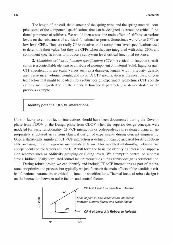
The length of the coil, the diameter of the spring wire, and the spring material com-prise some of the component specifications that can be designed to create the critical func-tional parameter of stiffness. We would then assess the main effect of stiffness at variouslevels on the robustness of a critical functional response. Sometimes we refer to CFPs aslow-level CFRs. They are really CFRs relative to the component-level specifications usedto determine their value, but they are CFPs when they are integrated with other CFPs andcomponent specifications to produce a subsystem level critical functional response.
2. Candidate critical-to-function specifications (CTF): A critical-to-function specifi-cation is a controllable element or attribute of a component or material (solid, liquid, or gas).CTF specifications are scalar values such as a diameter, length, width, viscosity, density,area, resistance, volume, weight, and so on. A CTF specification is the most basic of con-trol factors that might be loaded into a robust design experiment. Sometimes CTF specifi-cations are integrated to create a critical functional parameter, as demonstrated in theprevious example.
Control factor-to-control factor interactions should have been documented during the Developphase from I2DOV or the Design phase from CDOV when the superior design concepts weremodeled for basic functionality. CFCF interaction or codependency is evaluated using an ap-propriately structured array from classical design of experiments during concept engineering.Once a statistically significant CFCF interaction is defined, it can be assessed for its direction-ality and magnitude in rigorous mathematical terms. This modeled relationship between twocodependent control factors and the CFR will form the basis for identifying interaction suppres-sion schemes such as additivity grouping or sliding levels. We attempt to control or suppressstrong, bidirectionally correlated control factor interactions during robust design experimentation.
During robust design we can identify and include CFCF interactions as part of the pa-rameter optimization process, but typically we just focus on the main effects of the candidate crit-ical functional parameters or critical-to-function specifications. The real focus of robust design ison the interaction between noise factors and control factors:
N1
A1CF A at Level 1 Is Sensitive to Noise!!!
Lack of parallel line indicates an interactionbetween Control Factor and Noise Factor
CF A at Level 2 Is Robust to Noise!!!A2σ
of
CF
R
N2
Identify potential CFCF interactions.
582 Chapter 28

To suppress strong, negative interactions during robust design evaluations we must consider us-ing design for additivity techniques to force the control factor main effects to stand out well abovethe effects of interactions and random noise (2
error). In this way we can identify and sum up theiradditive effect on maximizing the robustness of the CFR to the Taguchi noises.
Design for additivity creates a set of control factors that have been intentionally engineeredfor low control factor-to-control factor interactivity. This enhances the likelihood of the success-ful verification of Taguchi’s additive S/N model during the final step of robust design.
When we understand which control factors are strongly interactive, to the point of pos-sessing a lack of unidirectional (monotonic) effect on the CFR (called an antisynergistic interac-tion), we can develop two strategies to suppress this unwanted effect.
This is an example of two control factors that possess a “troublesome” antisynergistic in-teraction we want to suppress.
Two main methods are used to turn interactive control factors into additive control factorswith respect to their unidirectional effect on the CFR: additivity grouping and sliding levels.
Additivity Grouping
Additivity grouping uses engineering knowledge of the functional contributions of two code-pendent control factors to logically align their level set points to derive a unidirectional responsefrom the CFR:
Yav
g o
f C
FR
A1 A2
Yav
g o
f C
FR
B1 B2
Y =
CF
R
A1
B1
Notice Control Factor B is not unidirectional inits behavior from Level 1 to Level 2
B2
A2
Design control factors for additivity.
Taguchi Methods for Robust Design 583
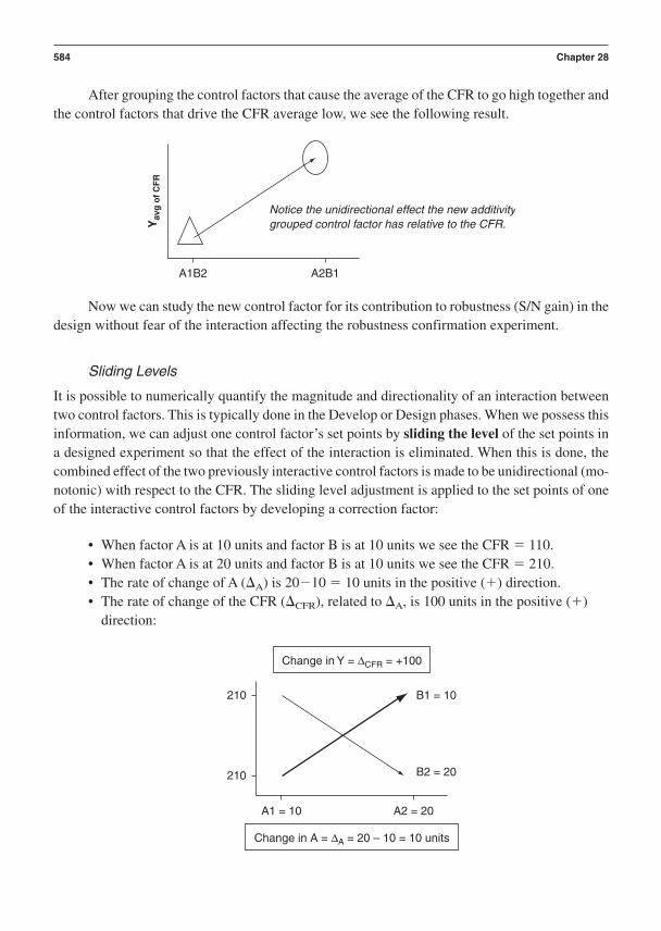
After grouping the control factors that cause the average of the CFR to go high together andthe control factors that drive the CFR average low, we see the following result.
Now we can study the new control factor for its contribution to robustness (S/N gain) in thedesign without fear of the interaction affecting the robustness confirmation experiment.
Sliding Levels
It is possible to numerically quantify the magnitude and directionality of an interaction betweentwo control factors. This is typically done in the Develop or Design phases. When we possess thisinformation, we can adjust one control factor’s set points by sliding the level of the set points ina designed experiment so that the effect of the interaction is eliminated. When this is done, thecombined effect of the two previously interactive control factors is made to be unidirectional (mo-notonic) with respect to the CFR. The sliding level adjustment is applied to the set points of oneof the interactive control factors by developing a correction factor:
• When factor A is at 10 units and factor B is at 10 units we see the CFR 110.• When factor A is at 20 units and factor B is at 10 units we see the CFR 210.• The rate of change of A (A) is 2010 10 units in the positive () direction.• The rate of change of the CFR (CFR), related to A, is 100 units in the positive ()
direction:
A1 = 10
B1 = 10
B2 = 20
210
210
A2 = 20
Change in Y = ∆CFR = +100
Change in A = ∆A = 20 – 10 = 10 units
Yav
g o
f C
FR
A1B2 A2B1
Notice the unidirectional effect the new additivitygrouped control factor has relative to the CFR.
584 Chapter 28
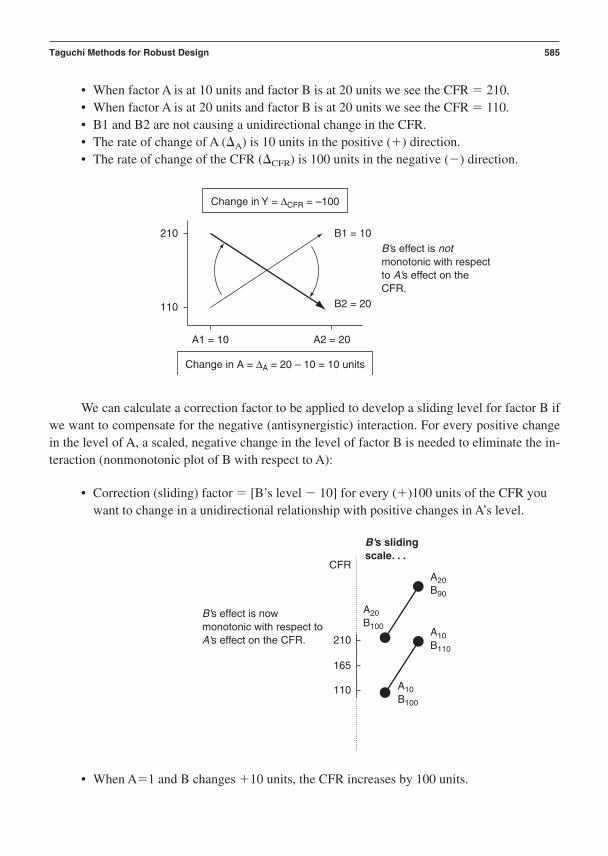
• When factor A is at 10 units and factor B is at 20 units we see the CFR 210.• When factor A is at 20 units and factor B is at 20 units we see the CFR 110.• B1 and B2 are not causing a unidirectional change in the CFR.• The rate of change of A (A) is 10 units in the positive () direction.• The rate of change of the CFR (CFR) is 100 units in the negative () direction.
We can calculate a correction factor to be applied to develop a sliding level for factor B ifwe want to compensate for the negative (antisynergistic) interaction. For every positive changein the level of A, a scaled, negative change in the level of factor B is needed to eliminate the in-teraction (nonmonotonic plot of B with respect to A):
• Correction (sliding) factor [B’s level 10] for every ()100 units of the CFR youwant to change in a unidirectional relationship with positive changes in A’s level.
• When A1 and B changes 10 units, the CFR increases by 100 units.
210
A20B100
A10B100
A20B90
A10B110
CFR
B's effect is nowmonotonic with respect toA's effect on the CFR.
B's slidingscale. . .
165
110
A1 = 10
B1 = 10B's effect is notmonotonic with respectto A's effect on theCFR.
B2 = 20
210
110
A2 = 20
Change in Y = ∆CFR = –100
Change in A = ∆A = 20 – 10 = 10 units
Taguchi Methods for Robust Design 585

• When A2 and B changes 10 units, the CFR decreases by 100 units; to compensatewe can change B’s level to smaller values to cause the CFR to consistently increase.
Monotonicity is attained when we make changes in both A and B levels and the CFR al-ways changes in the same unidirectional way. Sliding scales are often required when we havetime-energy input relationships. Baking is such an example. If we lengthen baking time, we mayhave to lower the energy input or vice versa in some scaled relationship or we may burn up thematerials inadvertently within a designed experiment.
It is important to understand which control factors are strongly antisynergistic as we haveseen for A and B in this example. If we use a sliding scale relationship to assign levels for inter-acting CFs in a robustness experiment, the likelihood of accidentally aliasing or confounding ofthe resulting main effect data will be low. This will help assure that we choose the right controlfactors and level set points for inclusion into Taguchi’s additive model. This process will aid inthe confirmation of our predicted S/N improvements from the individual control factors we havechosen to study.
Once the control factors have been selected and appropriate level set points are assigned, a de-signed experiment can be selected. The orthogonal array (Figure 28–4) is essentially a matrixor table of columns that hold control factors and rows that contain experimental runs of controlfactor combinations to be evaluated in the presence of the compounded noise factors. The CFRis measured for each row under the N1 and N2 noise conditions for each level of the signal fac-tor (typically three to five levels). So, it is quite typical for a robustness experimental run to justrequire two data points per signal factor (CAP) set point. We can take as many replicate datapoints for each noise value as we deem necessary to quantify experimental error in the data, typ-ically due to meter error, inaccuracies in resetting the CF levels, or other unknown random or spe-cial cause sources of variation.
Robust design uses orthogonal or balanced arrays, like the L4 array in Figure 28–4, to pro-vide a balanced opportunity for each control factor to exhibit its effect on the critical functional
Select array for robustness experiment.
B2
A1
110
A2
B1
210–100
+100
+100+10
+10
–100
210
110
586 Chapter 28
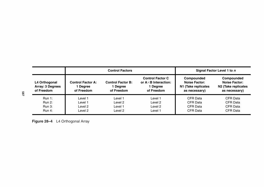
Control Factors Signal Factor Level 1 to n
Control Factor C Compounded Compounded L4 Orthogonal Control Factor A: Control Factor B: or AB Interaction: Noise Factor: Noise Factor:Array: 3 Degrees 1 Degree 1 Degree 1 Degree N1 (Take replicates N2 (Take replicates of Freedom of Freedom of Freedom of Freedom as necessary) as necessary)
Run 1: Level 1 Level 1 Level 1 CFR Data CFR DataRun 2: Level 1 Level 2 Level 2 CFR Data CFR DataRun 3: Level 2 Level 1 Level 2 CFR Data CFR DataRun 4: Level 2 Level 2 Level 1 CFR Data CFR Data
Figure 28–4 L4 Orthogonal Array
587

response under the stressful influence of the Taguchi noise factors. Notice how each of the con-trol factors gets to express its effect twice at level 1 and twice at level 2. This is the balancingproperty known as orthogonality. There is a simple way to calculate how large an orthogonal ar-ray is required to contain all the control factors (and CFCF interactions, if necessary) we wantto study for their effect on the CFR’s robustness.
The number of control factor levels defines how many degrees of freedom (dof) the con-trol factor is exploring in the design space. Design space is the entire range covered by all con-trol factors and the ranges of their level set points. The number of control factor levels minus 1(#CF Levels 1 dof) will equal the number of degrees of freedom required to quantify themain effect of the CF. For CFs with two levels (typical in noise experiments, where noises are theCFs) we require 1 dof and for CFs with three levels, typical in robustness experiments, we requiretwo dof.
For an entire designed experiment consisting of an orthogonal array, the dof required arealways one less than the number of runs in the array. So for our L4 example in Figure 28–4 thedof equal three (4 runs 1). Each CF requires one dof for a total of three and that is exactly howmany dof the L4 in its factorial layout has to offer.
The calculation rule for sizing an array for our selected CF at their respective levels is
dof required [(# of CFs) (# of levels 1)]
If we have some control factors at two levels and others at three levels, we must sum theindividual CFs at two levels and then add their required dof to the sum of the CFs at three levelsto obtain the total required dof.
Once we know the required dof, we can look up an array that possesses a number of dofequal to or greater than the required number of dof. It is not necessary to load a CF in every col-umn in an array. It is not unusual to see designed experiments with empty columns. This does notcompromise the array’s balance. If we want to compromise the array’s balance, we simply alterthe level set points away from their prescribed values or fail to run one or more of the rows. Thatwill sufficiently ruin the orthogonality of the experiment and the integrity of our CFR data (ob-viously we do not recommend this approach)!
We can choose from many orthogonal arrays within the menus of Minitab data analysissoftware. Figure 28–5 offers an example of the architecture of a typical dynamic experimental layout.
Again, although measurement systems analysis has been done prior to the noise experiments, itis wise to certify the capability (P/T ratio and Gage R&R) of the data acquisition system prior tomeasuring the subsystem critical functional responses during the robustness experiment.
Conduct measurement systems analysis.
588 Chapter 28

Once the experiment has been designed and the data acquisition system has been certified as ca-pable to measure the CFRs, we are ready to physically conduct the robustness experiment.
It is important that great care and discipline be exercised as we set up each signal, control,and noise factor set point for each run within the orthogonal array. If we are sloppy in the wayeach set point is adjusted to its specified value from the array, variability will build up in the CFRdata and inflate the error variance within the data. This experimental source of noise is to be sup-pressed and kept to a minimum.
One way to suppress errors in the data from systematic sources of variability outside of thepurposeful changes we are inducing from the control factor levels within the orthogonal array isto randomize the order of the experimental runs. We simply write down the number of each runon a separate piece of paper, place them all in a container, mix the paper slips thoroughly, and thenblindly draw them from the container. This will randomize the run order. Usually this is not nec-essary in a Taguchi experiment because the effects of the compounded noise factors, N1 and N2,far outweigh the much smaller effects of systematic or random sources of experimental error.
In a robustness experiment it is common to load the array and run it in an order that makesthe changes in control factors easy and economical. Notice that in all the Taguchi style arrays(Latin square format as opposed to Yates order format) the first columns have orderly patterns ofchanges in the level set points. The deeper we go across the columns of the array, the more ran-dom and frequent the level set point changes become. We should place any difficult or expensive-to-change control factors in the first few columns in the array. This will save time andmoney during our robustness optimization experiments.
Conduct robustness experiment.
Taguchi Methods for Robust Design 589
A B C N1 N2 N1 N2 N1 N2
Signal FactorLevel 1
D E
Signal FactorLevel 2
Signal FactorLevel 3
Outer array, which containsCFR data as gathered under"Full Factorial " conditions ofsignal and noise factors
Inner array,which containscontrol factorset points
Figure 28–5 Architecture of Dynamic Experimental Layout

In Figure 28–6, we see the most common of all Taguchi experimental layouts, the L18 dy-namic experiment.
Note that the SF (signal factor) values are also called critical adjustment parameter set points.
Analysis of data from a robustness optimization experiment is easy to conduct. Numerous soft-ware products will perform the required calculations in a few milliseconds. This book featuresgraphical and numerical results from Minitab, which is strong in its ability to support extensiveanalysis of robust design data.
The three main statistical measures of critical functional response data, as it represents sam-ple data developed in the presence of stressful sources of Taguchi noise factors, are as follows:
1. The signal–to–noise ratio of the CFR2. The standard deviation of the CFR3. The slope () of the CFR (the family of mean values developed as we adjust the sig-
nal factor or CAP)
Analyze robustness experimental data.
590 Chapter 28
SF 1 SF 2 SF 3
L18 A B C D E F G H N1 N2 N1 N2 N1 N2
1 1 1 1 1 1 1 1 12 1 13 1 14 1 25 1 26 1 27 1 38 1 39 1 310 2 111 2 112 2 113 2 214 2 215 2 216 2 317 2 318 2 3
Figure 28–6 L18 Dynamic Experiment Layout
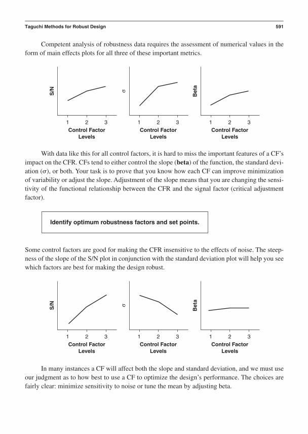
Competent analysis of robustness data requires the assessment of numerical values in theform of main effects plots for all three of these important metrics.
With data like this for all control factors, it is hard to miss the important features of a CF’simpact on the CFR. CFs tend to either control the slope (beta) of the function, the standard devi-ation (), or both. Your task is to prove that you know how each CF can improve minimizationof variability or adjust the slope. Adjustment of the slope means that you are changing the sensi-tivity of the functional relationship between the CFR and the signal factor (critical adjustmentfactor).
Some control factors are good for making the CFR insensitive to the effects of noise. The steep-ness of the slope of the S/N plot in conjunction with the standard deviation plot will help you seewhich factors are best for making the design robust.
In many instances a CF will affect both the slope and standard deviation, and we must useour judgment as to how best to use a CF to optimize the design’s performance. The choices arefairly clear: minimize sensitivity to noise or tune the mean by adjusting beta.
1 2Control Factor
Levels
S/N
3 1 2Control Factor
Levels
σ
3 1 2Control Factor
Levels
Bet
a
3
Identify optimum robustness factors and set points.
1 2Control Factor
Levels
S/N
3 1 2Control Factor
Levels
σ3 1 2
Control FactorLevels
Bet
a
3
Taguchi Methods for Robust Design 591

We use the signal factor to adjust the mean in relatively “gross” terms. The best we can get fromthis kind of adjustment is a local optimum. We use response surface methods to locate a globaloptimum when adjusting the mean.
We use the control factor that has the strongest linear effect on beta to fine-tune the mean value of the CFR relative to a specific target. The target may change as the product’s spec-ifications are changed during the development of the product. A design is considered dynamicwhen it has this built-in dual capability to have the CFR moved at will by slope adjustment (fine-tuning through beta sensitivity adjustment) as well as signal factor adjustment (coarse ad-justment). This works well for local optimization.
Once we have used the main effects plots to help identify which control factors are going to havea significant effect on the optimization of robustness, we can isolate and sum their contributionsto the overall CFR S/N gain. We need to use the overall mean signal-to-noise (S/Navg) values cal-culated by averaging the S/N values from each of the rows of the robustness experiment (in thiscase rows 1 through 4):
Construct Taguchi’s additive S/N model.
1 2Control Factor
Levels
S/N
3 1 2Control Factor
Levels
σ
3 1 2Control Factor
Levels
Bet
a
3
Identify optimum tuning factors and set points.
1 2Control Factor
Levels
S/N
3 1 2Control Factor
Levels
σ
3 1 2Control Factor
Levels
Bet
a
3
592 Chapter 28

The additive model calculates a predicted optimum S/N built on the sum of all the signifi-cant control factor S/N contributions included in the prediction. CFs that have weak S/N gain inthe main effects plots are usually excluded from the additive model. In the following equation,we have included all the factors in the additive model:
S/NPred opt [(S/NA opt) (S/Navg)] [(S/NB opt) (S/Navg)] [(S/NC opt) (S/Navg)]
The predicted optimum S/N value is now in need of confirmation through verification ex-periments at the predicted optimum set points for each control factor.
The predicted optimum S/N value must be verified by two actions. We begin by setting up the de-sign at the optimum set points that have been identified as helpful in improving robustness. Therewill usually be one or two other control factors (beta shifters) that are found to have a significanteffect on shifting beta (), the slope of the “best fit line” that symbolizes the ideal function of thedesign. These fine-adjustment factors allow us to shift the slope to either a higher or lower level,thus tuning the sensitivity of the relationship between the critical adjustment parameter (CAP, orsignal factor) and the critical functional response (CFR).
Once the design has been set up at its optimum levels for robustness and on-target per-formance, we turn our attention once again to properly stressing the design with exactly the samecompounded noise factors used in the original robustness experiment. The new, robust design isnow evaluated under the noise conditions over and over as many times as is deemed necessary toassure the data is truly repeatable. It is common to see the verification runs repeated a minimumof five times.
To confirm the robustness improvements are sufficiently matching the predicted S/N val-ues, we need to calculate a range of acceptability, a tolerance beyond which we say the results arenot confirmed. The verification tolerance is calculated using the following process:
1. Identify the largest and smallest S/N values from the original robust design experiment(S/Nmax and S/Nmin).
Verify Taguchi’s additive model.
1.
A B C
1 1 1
1 2 2
2 1 2
2 2 1
N1 N2
2.
3.
4.
yavg σ S/NControlFactors
S/Navg
TreatmentCombinations
S/N values tobe averaged
Taguchi Methods for Robust Design 593

2. Calculate the difference between these values: (S/Nmax S/Nmin) full scale rangeof S/N across the original experiment.
3. Divide the full scale range of S/N by either 3dB or 4dB, depending on how conserva-tive we want the S/N tolerance limit to be. Note we use 3dB because it represents theamount of change required to cut the variance of the CFR in half.
4. Use the S/N tolerance limit [(S/Nmax S/Nmin)/3] to compare with the average resultsfrom the verification experiments. If the average of the verification S/N is within therange established by the S/N tolerance limit, especially on the low end, we accept the fact that the predicted S/N performance has indeed been confirmed. If the averagefrom the verification data surpasses the S/N tolerance limit, especially on the low side,we conclude that we have not confirmed and that there is either some form of controlfactor interaction or data acquisition or analysis error that must be discovered and corrected.
Now that the design’s critical functional response has been made robust against the compoundedset of noise factors and its critical adjustment parameter used to adjust the mean of the CFR onto the desired target, it is time to document our results. The following items are documentedwithin the Critical Parameter Management database:
1. Optimum S/N value for the CFR after verifying the additive model2. Baseline (benchmark) S/N value of the CFR prior to conducting robust design3. Optimum nominal set points for each control factor that had a significant effect on the
gain in robustness of the CFR4. Optimum set points for the control factors that were used to shift Beta () to place the
mean value of the CFR on to its desired target5. The Cp of the CFR after robustness optimization, which can be quantified with and
without the noise factor effects being present if we desire
The critical parameter database can contain any level of detail beyond this that we feel isimportant to track. The key thing to remember is that we want to be able to define and track re-lationships between all the critical parameters within the entire system. Robust design data typi-cally is associated with system and subsystem level CFRs. System CFRs are measured forrobustness, and their S/N data is stored at the system level within the relational database archi-tecture. Subsystem CFR data related to robustness is stored in the subsystem level within theCPM database. Critical adjustment parameter information relative to a subsystem CFR mean per-formance is stored in the subsystem CAP level within the CPM database.
Document optimum robustness and tuning factors and set points in Critical Parameter Management database.
594 Chapter 28

The components that are significant control factors for robustness and beta shifting are doc-umented as critical-to-function (CTF specs) specifications within the component level critical pa-rameter database.
The following CPM database scorecards help illustrate how to document data.
Documenting System Level CFR Robustness Performance:DFSS-Critical Parameter Management ScorecardSystem Requirement Document Line Items-to-System Critical Functional Response Map
Taguchi Methods for Robust Design 595
(Initiated in System Concept Design Phase–Phase 1)
SRD Line Item: System CFR: Target USL LSL Mean COV S/N Cp Cpk
(Initiated in Subsystem Concept Design and Parameter Optimization Phase–Phase 1)
SRD # System CFR: Subsystem CFR: Target USL LSL Mean COV S/N Cp Cpk
(Initiated in System Integration and Optimization Phase–Phase 2)
Subsys. CAP CAP CAP CAP CFR CFR CFR CFR/SRD # CFR: Spec: Target USL LSL Mean CFRs Cp Cpk CAP
Documenting Subsystem Level CFR Robustness Performance:DFSS-Critical Parameter Management ScorecardSubsystem-to-System Critical Functional Response Relationship Map
Documenting Subsystem-CAP Level CFR Mean Shifting Performance:DFSS-Critical Parameter Management ScorecardCritical Adjustment Parameter-to-Subsystem CFR Relationship Map
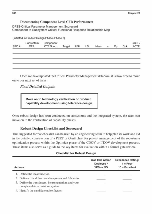
Once we have updated the Critical Parameter Management database, it is now time to moveon to our next set of tasks.
Final Detailed Outputs
Once robust design has been conducted on subsystems and the integrated system, the team canmove on to the verification of capability phases.
Robust Design Checklist and Scorecard
This suggested format checklist can be used by an engineering team to help plan its work and aidin the detailed construction of a PERT or Gantt chart for project management of the robustnessoptimization process within the Optimize phase of the CDOV or I2DOV development process.These items also serve as a guide to the key items for evaluation within a formal gate review.
Checklist for Robust Design
Was This Action Excellence Rating:Deployed? 1 = Poor
Actions: YES or NO 10 = Excellent
1. Define the ideal function. ______ ______
2. Define critical functional responses and S/N ratio. ______ ______
3. Define the transducers, instrumentation, and your ______ ______complete data acquisition system.
4. Identify the candidate noise factors. ______ ______
Move on to technology verification or product capability development using tolerance design.
596 Chapter 28
(Initiated in Product Design Phase–Phase 3)
Subsystem Component CFR/SRD # CFR: CTF Spec: Target USL LSL Mean Cp Cpk CTF
Documenting Component Level CFR Performance:DFSS-Critical Parameter Management ScorecardComponent-to-Subsystem Critical Functional Response Relationship Map

5. Conduct a noise experiment. ______ ______
6. Identify and plot the magnitude and directionality ______ ______of noise factors using analysis of means (ANOM).
7. Identify statistically significant noise factors using ______ ______ANOVA.
8. Compound noise factors for use in main robustness ______ ______experiment (Nl and N2).
9. Identify control factors for the design. ______ ______
10. Select a properly sized orthogonal array to evaluate ______ ______the robustness contribution and mean adjustment capability from each control factor.
11. Run the designed experiment in the presence of the ______ ______uniformly applied, compounded noise factors.
12. Perform analysis of means (ANOM) and plot the ______ ______main effects and selected interactions of the mean, standard deviation, and S/N metric for each control factor.
13. Select the optimum set point for the control factors ______ ______that have a strong effect on the robustness of the critical functional response (these become critical-to-function parameters).
14. Identify critical adjustment parameters, the control ______ ______factors that have a strong effect on the mean of the CFR and a reasonably weak effect on the standard deviation.
15. Construct Taguchi’s additive model from the ______ ______significant control factor signal-to-noise values (units are dBs).
16. Conduct verification runs at the optimum S/N set ______ ______points for the robustness control factors after using the CAPs to put the mean onto the target.
17. If the new S/N values are reasonably close to the ______ ______predicted S/N from the additive model, the robustness set points are confirmed—you are ready for tolerance design.
18. If the new S/N values are well below the predicted ______ ______S/N from the additive model, the robustness set points are not confirmed—you must go back and find the reason why.
Scorecard for Robust Design
The definition of a good robustness scorecard is that it should illustrate in simple but quantitativeterms what gains were attained from the work. This suggested format for a scorecard can be usedby an engineering team to help document the completeness of its work.
Taguchi Methods for Robust Design 597

Subsystem name: __________
Subsystem critical functional response: __________
Specific engineering units of subsystem critical functional response: __________
Number of statistically significant noise factors: __________
Number of control factors evaluated for robustness: __________
Number of control factors selected to include in additive model: __________
Number of control factors selected to adjust beta: __________
Baseline or benchmarked initial subsystem S/N value: __________
Verified optimal subsystem S/N value: __________
Prerobustness design capability (Cp) index for the subsystem CFR: __________
Postrobustness design capability (Cp) index for the subsystem CFR: __________
Table of Critical Parameter Set Points:
Critical Parameter Optimal Nominal Estimated Estimated Used for Robustness Name: Set Point: Tolerance: USL Tolerance: LSL or Beta Shifting:
1. ______ ______ ______ ______
2. ______ ______ ______ ______
3. ______ ______ ______ ______
Table of Critical Noise Factor Set Points:
Critical Noise Magnitude Direction of Effect: % Contribution Factor Name: of Effect: ( or ) F Ratio/Fcrit.: or 2 Value:
______ ______ ______ ______ ______
______ ______ ______ ______ ______
______ ______ ______ ______ ______
We repeat the final deliverables from robust design:
• Optimized signal-to-noise metrics for the critical functional response(s)• Optimized critical-to-function parameter set points that control the subsystem’s
robustness• Optimized critical adjustment factors that tune the mean value of the subsystem’s
critical functional response(s)
598 Chapter 28

• Subsystem critical parameter management data that is documented in the CPMrelational database:CFR meanCFR standard deviationCFR coefficient of variation [(s/mean) 100]CFR S/N ratioCFR Cp index
References
Fowlkes, W. Y., & Creveling, C. M. (1995). Engineering methods for robust product design.Reading, MA.: Addison-Wesley.
Phadke, M. S. (1989). Quality engineering using robust design. Englewood Cliffs, NJ.:Prentice Hall.
Taguchi, G., Chowdhury, S., & Taguchi, S. (2000). Robust engineering. New York: McGraw-Hill.
Taguchi Methods for Robust Design 599

This page intentionally left blank
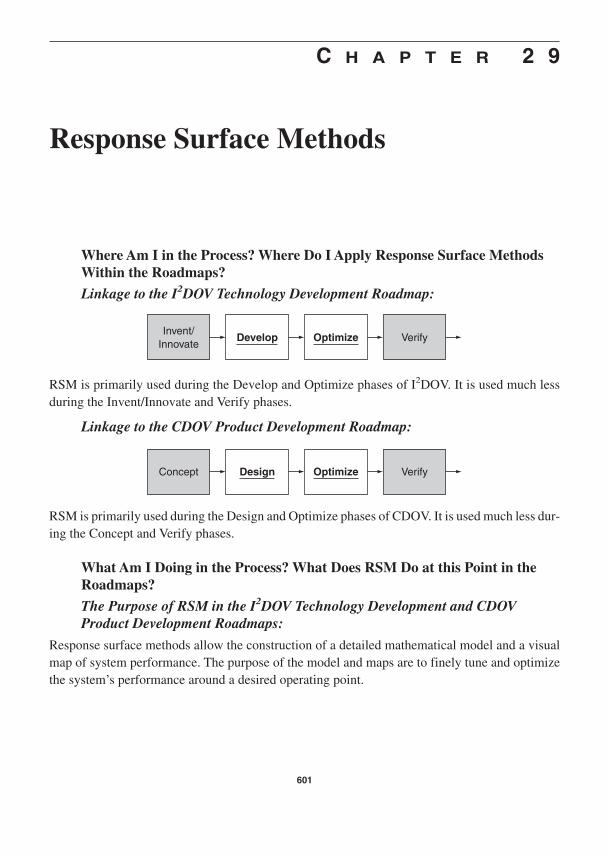
C H A P T E R 2 9
Response Surface Methods
Where Am I in the Process? Where Do I Apply Response Surface MethodsWithin the Roadmaps?
Linkage to the I2DOV Technology Development Roadmap:
601
Invent/Innovate
Develop Optimize Verify
Concept Design Optimize Verify
RSM is primarily used during the Develop and Optimize phases of I2DOV. It is used much lessduring the Invent/Innovate and Verify phases.
Linkage to the CDOV Product Development Roadmap:
RSM is primarily used during the Design and Optimize phases of CDOV. It is used much less dur-ing the Concept and Verify phases.
What Am I Doing in the Process? What Does RSM Do at this Point in theRoadmaps?
The Purpose of RSM in the I2DOV Technology Development and CDOVProduct Development Roadmaps:
Response surface methods allow the construction of a detailed mathematical model and a visualmap of system performance. The purpose of the model and maps are to finely tune and optimizethe system’s performance around a desired operating point.
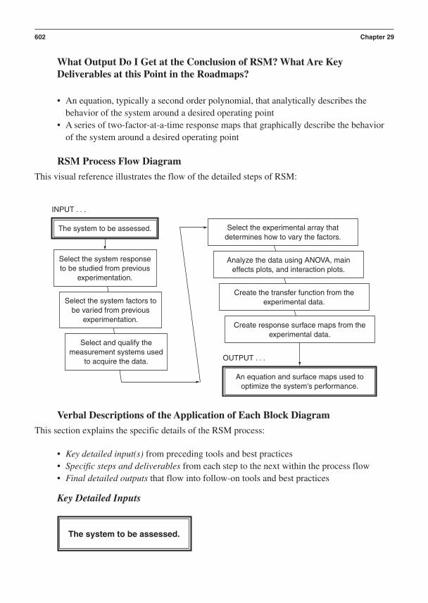
What Output Do I Get at the Conclusion of RSM? What Are KeyDeliverables at this Point in the Roadmaps?
• An equation, typically a second order polynomial, that analytically describes thebehavior of the system around a desired operating point
• A series of two-factor-at-a-time response maps that graphically describe the behaviorof the system around a desired operating point
RSM Process Flow Diagram
This visual reference illustrates the flow of the detailed steps of RSM:
602 Chapter 29
INPUT . . .
OUTPUT . . .
The system to be assessed.
Select the system responseto be studied from previous
experimentation.
Select the system factors tobe varied from previous
experimentation.
Select and qualify themeasurement systems used
to acquire the data.
Select the experimental array thatdetermines how to vary the factors.
Analyze the data using ANOVA, maineffects plots, and interaction plots.
Create the transfer function from theexperimental data.
Create response surface maps from theexperimental data.
An equation and surface maps used tooptimize the system's performance.
Verbal Descriptions of the Application of Each Block Diagram
This section explains the specific details of the RSM process:
• Key detailed input(s) from preceding tools and best practices• Specific steps and deliverables from each step to the next within the process flow• Final detailed outputs that flow into follow-on tools and best practices
Key Detailed Inputs
The system to be assessed.

Response surface methods allow the construction of a detailed mathematical model and a visualmap of system performance. The maps are similar to the topographic maps used for hiking. Atopographic map shows contour intervals that indicate changes in elevation as one moves in anymagnetic heading along the surface of the earth. The topographic map provides a visualization ofthe peaks and valleys of the terrain.
Consider altitude to be a critical response and the X and Y directions of travel to be two crit-ical parameters of the response. The topographic map allows us to determine the values of X andY that place us on the top of a mountain along the Continental Divide or at the bottom of DeathValley. It also tells us where the flat plains of Kansas are located. The mountain peaks and valleybottoms are regions of high sensitivity and poor robustness. Small changes in the X or Y directionresult in large changes in altitude. The plains of Kansas are a region of insensitivity and robust-ness of altitude to changes in X and Y. We can move a large distance in any direction without muchchange in altitude. This is robustness.
What are the experimental methods needed to obtain the detailed mathematical models andresponse surface maps? A response surface, in general, is curved and bumpy. In order to modelthis surface, we need a transfer function with quadratic or higher terms in it. A two-level designis not capable of estimating quadratic effects. We need an experiment with at least three levels.This can get very large. There is, however, an economical design that gives the needed informa-tion. It is called a central composite design (CCD). The CCD is a composite of a Full Factorialwith a center point and additional points called star or axial points.
Let’s look at a simple two-factor CCD, shown in Figure 29–1 for two factors X1 and X2. TheFull Factorial portion of the CCD is shown by the points located at (1, 1), (1, 1), (1, 1),
Response Surface Methods 603
X2
X1
–1.414 –1 0 +1 1.414
r
Figure 29–1 Two-Factor Central Composite Design

(1, 1). The center point of the design is shown by the triangle located at the point (0,0). Sofar, the design can only estimate first order main effects, interactions, and test for curvature. Ageneralized transfer function of this form is shown in this equation.
y b0 b1x1 b2x2 … bnxn b12x1x2 … bijxixj
We discussed this type of experiment earlier in Chapter 27 on DOE. There are several pos-sible outcomes of such an experiment. It is possible that interaction terms are not significant butthe transfer function does not adequately model system behavior. Another possibility is that in-teractions are significant but, even with the interactions in the model, the transfer function stilldoes not adequately model system behavior. Analysis of the residuals, R2, and lack of fit will in-dicate whether the transfer function adequately models system behavior.
These two possible outcomes indicate that the transfer function may be too simple. Addi-tional terms may be required. If a residuals vs. fits plot indicates a curved pattern, a squared orquadratic term is probably needed. However, we need additional experimental data to estimatesquared terms. How can we get the additional information without wasting the runs we have al-ready made? We can accomplish this by adding additional points to the design, called star or al-pha points. These are shown as diamonds in Figure 29–1. Figure 29–1 shows the geometry of theCCD. The alpha points are on the circumference of a circle. The radius of the circle is
So the star points are at (1.4142, 0), (1.4142, 0), (0, 1.4142), and (0, 1.4142). Eachfactor now has five levels: 1.4142, 1, 0, 1, and 1.4142.
The additional axial points now make it possible to estimate squared main effects and in-teractions without aliasing. The general form of the obtainable transfer function is shown in thisfirst equation and in an equivalent form in the second:
y b0 b1x1 … bnxn b11x12 … bnnxn
2 b12x1x2 … bn1,n xn1xn
The discussion for two factors can be extended to three factors and more. The geometry ofa CCD is shown in Figure 29–2 for three factors A, B, and C. The circles are the factorial points,the triangle is the center point, and the diamonds are the axial points.
Minitab can be used to create and analyze response surface experiments. Let’s workthrough an example.
Specific Steps and Deliverables
Select the system response to be studied from previous experimentation.
y = b0 + an
i=1bixi + a
n
i=1biixi + a
n-1
ia
n
j
bijxixj
r = 2(1)2 + (1)2 = 22 = 1.4142
604 Chapter 29

We’ll revisit the cool time experiment from Chapters 26 and 27 on regression and DOE. Thecritical-to-function response is the time it takes to cool the fluid from an upper set point to alower set point.
Select the system factors to be varied from previous experimentation.
Previous experimentation was conducted to determine that fan speed, fluid volume, ambient tem-perature, ambient altitude, and ambient humidity are critical system parameters.
Select and qualify the measurement systems used to acquire the data.
RSM, as with any process where data will be used to make decisions, requires a capable measure-ment system. The techniques covered in Chapter 23 on MSA should have been applied to the mea-surement system and its Gage R&R, P/T ratio, and the number of distinct categories determined.
Select the experimental array that determines how to vary the factors.
Prior experimentation and analysis of the physical principles of thermodynamics indicated that thesystem was nonlinear. This information led to a CCD as the chosen experiment. The experiment wasconducted in an environmental chamber capable of altitude, temperature, and humidity control.
Analyze the data using ANOVA, main effects plots, and interaction plots.
Response Surface Methods 605
A
C
B
Figure 29–2 Three-Factor Central Composite Design
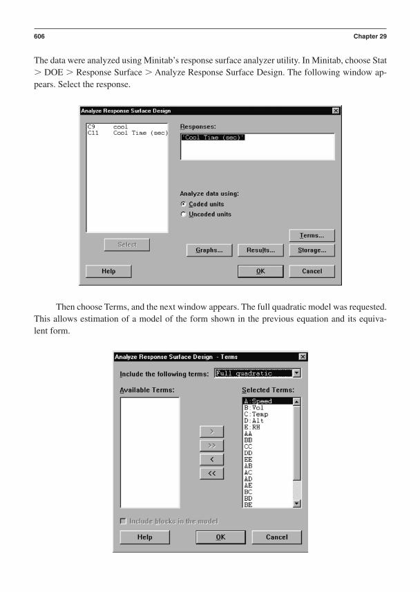
The data were analyzed using Minitab’s response surface analyzer utility. In Minitab, choose Stat DOE Response Surface Analyze Response Surface Design. The following window ap-pears. Select the response.
606 Chapter 29
Then choose Terms, and the next window appears. The full quadratic model was requested.This allows estimation of a model of the form shown in the previous equation and its equiva-lent form.

Select OK and analyze the data to obtain the following session window output. The signif-icant effects are shown in bold.
Response Surface Regression: Cool Time (sec) versus Speed, Vol, Alt, RH
The analysis was done using coded units.
Estimated Regression Coefficients for Cool TimTerm Coef SE Coef T PConstant 5.1358 0.19240 26.693 0.000Speed 0.8487 0.09846 8.620 0.000Vol 0.6878 0.09846 6.986 0.000Temp 0.4476 0.09846 4.546 0.001Alt 0.0979 0.09846 0.994 0.342RH 0.0234 0.09846 0.238 0.816Speed*Speed 0.6243 0.08906 7.010 0.000Vol*Vol 0.0202 0.08906 0.227 0.825Temp*Temp 0.0265 0.08906 0.298 0.771Alt*Alt 0.0214 0.08906 0.241 0.814RH*RH 0.1250 0.08906 1.404 0.188Speed*Vol 0.6086 0.12059 5.046 0.000Speed*Temp 0.0609 0.12059 0.505 0.624Speed*Alt 0.0740 0.12059 0.614 0.552Speed*RH 0.0131 0.12059 0.108 0.916Vol*Temp 0.0440 0.12059 0.365 0.722Vol*Alt 0.0183 0.12059 0.151 0.882Vol*RH 0.0518 0.12059 0.429 0.676Temp*Alt 0.0023 0.12059 0.019 0.985Temp*RH 0.1321 0.12059 1.095 0.297Alt*RH 0.0153 0.12059 0.127 0.901
S 0.4824 R-Sq 95.3% R-Sq(adj) 86.8%Analysis of Variance for Cool Tim
Source DF Seq SS Adj SS Adj MS F PRegression 20 51.9469 51.9469 2.5973 11.16 0.000Linear 5 33.6943 33.6943 6.7389 28.96 0.000Square 5 11.8151 11.8151 2.3630 10.16 0.001Interaction 10 6.4375 6.4375 0.6438 2.77 0.055Residual Error 11 2.5595 2.5595 0.2327Lack-of-Fit 6 1.8222 1.8222 0.3037 2.06 0.223Pure Error 5 0.7373 0.7373 0.1475Total 31 54.5064
Response Surface Methods 607
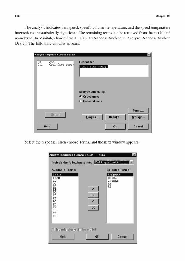
The analysis indicates that speed, speed2, volume, temperature, and the speed temperatureinteractions are statistically significant. The remaining terms can be removed from the model andreanalyzed. In Minitab, choose Stat DOE Response Surface Analyze Response SurfaceDesign. The following window appears.
608 Chapter 29
Select the response. Then choose Terms, and the next window appears.

Choose the five significant terms and select OK to analyze the data. The session windowoutput follows.
Response Surface Regression: Cool Time (sec) versus Speed, Vol,Temp
The analysis was done using coded units.
Estimated Regression Coefficients for Cool Tim
Term Coef SE Coef T PConstant 5.0135 0.08565 58.532 0.000Speed 0.8487 0.07819 10.854 0.000Vol 0.6878 0.07819 8.797 0.000Temp 0.4476 0.07819 5.725 0.000Speed*Speed 0.6141 0.06994 8.781 0.000Speed*Vol 0.6086 0.09576 6.355 0.000
S 0.3831 R-Sq 93.0% R-Sq(adj) 91.7%
Analysis of Variance for Cool Tim
Source DF Seq SS Adj SS Adj MS F PRegression 5 50.6913 50.6913 10.1383 69.09 0.000Linear 3 33.4513 33.4513 11.1504 75.99 0.000Square 1 11.3144 11.3144 11.3144 77.11 0.000Interaction 1 5.9256 5.9256 5.9256 40.38 0.000Residual Error 26 3.8151 3.8151 0.1467Lack-of-Fit 9 0.8705 0.8705 0.0967 0.56 0.812Pure Error 17 2.9446 2.9446 0.1732Total 31 54.5064
The session window information indicates significant terms, relatively high R2, and no sig-nificant lack of fit. This may be a good model. Let’s look at the residuals. The residuals vs. fitsplot (Figure 29–4) looks random and the residuals (Figure 29–3) are normal at an alpha of 0.5.
Create the transfer function from the experimental data.
Based on the analysis, we can create the transfer function shown in this equation:
Cool Time 5.0135 0.8487 Speed 0.6878 Vol 0.4476 Temp
0.6141 Speed2 0.6086 SpeedXVol
Response Surface Methods 609

.999
.99
.95
.80
.50
.20
.05
.01
.001
–1.0
Average: 0.0000000StDev: 0.350809N: 32
Anderson-Darling Normality TestA-Squared: 0.320
P-Value: 0.517
–0.5 0.0
RESI1
Pro
bab
ility
0.5
Figure 29–3 Normal Probability Plot
0.5
0.0
–0.5
–1.0
0.5 1.5 2.5 3.5
Fitted Value
(response is Cool Time)
Res
idu
al
4.5 5.5 6.5
Figure 29–4 Residuals versus the Fitted Values
610

This equation is a mathematical description of the behavior of the system from which wecan create surface plots and optimize the system’s performance.
Create response surface maps from the experimental data.
Surface plots allow us to visualize the system’s behavior. Unfortunately, we can only plot two fac-tors at a time in a surface plot. We have three significant factors so we need three response sur-face plots. We plot speed vs. temperature, speed vs. volume, and volume vs. temperature. Thethree plots are shown in Figures 29–5a, b, and c.
The speed vs. volume and speed vs. temperature plots are curved due to the quadratic ef-fect of speed and the interaction between speed and volume. The volume vs. temperature plot isa plane because volume and temperature appear as linear terms and they do not interact.
Final Detailed Outputs
An equation and surface maps used to optimize the system’s performance.
We can now visually determine the levels of the factors that place the response at a maximum orminimum. We can also see the locations of robustness. For example, using Figures 29–5a and b,we can see that cool time is sensitive to changes in fan speed at high fan speeds.
Response Surface Methods 611
76543210
0
Co
ol T
ime
(sec
)
Vol
Speed
Surface Plot of Cool Time
–11 2
–2–1
01
2
–2
–1–2–3
Hold Values: Temp: 0.0
Figure 29–5a Speed vs. Volume Surface Plot

612 Chapter 29
6
5
4
3
2
1
0
0
Co
ol T
ime
(sec
)
Temp
Speed
Surface Plot of Cool Time
–11 2
–2–1
01
2
–2
Hold Values: Vol: 0.0
Figure 29–5b Speed vs. Temperature Surface Plot
7.5
6.5
5.5
4.5
3.5
2.5
0
Co
ol T
ime
(sec
)
Temp
Vol
Surface Plot of Cool Time
–11 2
–2–1
01
2
–2
Hold Values: Speed: 0.0
Figure 29–5c Volume vs. Temperature Surface Plot
The slope of the surfaces are steep in this region. The flat, inclined plane shown in Figure29–5c indicates that there is no region in which cool time is least sensitive to changes in volumeor temperature. It does indicate, however, that cool time is shortest at low temperature and low volume.
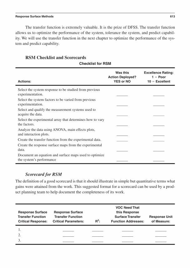
The transfer function is extremely valuable. It is the prize of DFSS. The transfer functionallows us to optimize the performance of the system, tolerance the system, and predict capabil-ity. We will use the transfer function in the next chapter to optimize the performance of the sys-tem and predict capability.
RSM Checklist and ScorecardsChecklist for RSM
Was this Excellence Rating:Action Deployed? 1 Poor
Actions: YES or NO 10 Excellent
Select the system response to be studied from previous experimentation. ______ ______
Select the system factors to be varied from previous experimentation. ______ ______
Select and qualify the measurement systems used to acquire the data. ______ ______
Select the experimental array that determines how to vary the factors. ______ ______
Analyze the data using ANOVA, main effects plots, and interaction plots. ______ ______
Create the transfer function from the experimental data. ______ ______
Create the response surface maps from the experimental data. ______ ______
Document an equation and surface maps used to optimize the system’s performance ______ ______
Scorecard for RSM
The definition of a good scorecard is that it should illustrate in simple but quantitative terms whatgains were attained from the work. This suggested format for a scorecard can be used by a prod-uct planning team to help document the completeness of its work.
VOC Need ThatResponse Surface Response Surface this ResponseTransfer Function Transfer Function Surface Transfer Response UnitCritical Response: Critical Parameters: R2: Function Addresses: of Measure:
1. ______ ______ ______ ______
2. ______ ______ ______ ______
3. ______ ______ ______ ______
Response Surface Methods 613

We repeat the final deliverables:
• An equation, typically a second order polynomial, that analytically describes thebehavior of the system around a desired operating point
• A series of two-factor-at-a-time response maps that graphically describe the behaviorof the system around a desired operating point
Reference
Myers, R. H., & Montgomery, D. W. (1995). Response surface methodology. New York: WileyInterscience.
614 Chapter 29
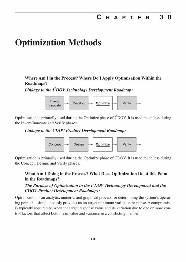
C H A P T E R 3 0
Optimization Methods
Where Am I in the Process? Where Do I Apply Optimization Within theRoadmaps?
Linkage to the I2DOV Technology Development Roadmap:
615
Invent/Innovate
Develop Optimize Verify
Concept Design Optimize Verify
Optimization is primarily used during the Optimize phase of I2DOV. It is used much less duringthe Invent/Innovate and Verify phases.
Linkage to the CDOV Product Development Roadmap:
Optimization is primarily used during the Optimize phase of CDOV. It is used much less duringthe Concept, Design, and Verify phases.
What Am I Doing in the Process? What Does Optimization Do at this Pointin the Roadmaps?
The Purpose of Optimization in the I2DOV Technology Development and theCDOV Product Development Roadmaps:
Optimization is an analytic, numeric, and graphical process for determining the system’s operat-ing point that simultaneously provides an on-target minimum varitation response. A compromiseis typically required between the target response value and its variation due to one or more con-trol factors that affect both mean value and variance in a conflicting manner.
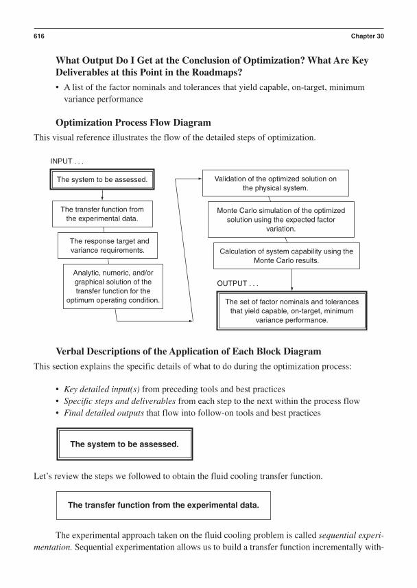
What Output Do I Get at the Conclusion of Optimization? What Are KeyDeliverables at this Point in the Roadmaps?
• A list of the factor nominals and tolerances that yield capable, on-target, minimumvariance performance
Optimization Process Flow Diagram
This visual reference illustrates the flow of the detailed steps of optimization.
616 Chapter 30
INPUT . . .
OUTPUT . . .
The system to be assessed.
The transfer function fromthe experimental data.
The response target andvariance requirements.
Analytic, numeric, and/orgraphical solution of thetransfer function for the
optimum operating condition.
Validation of the optimized solution onthe physical system.
Monte Carlo simulation of the optimizedsolution using the expected factor
variation.
Calculation of system capability using theMonte Carlo results.
The set of factor nominals and tolerancesthat yield capable, on-target, minimum
variance performance.
Verbal Descriptions of the Application of Each Block Diagram
This section explains the specific details of what to do during the optimization process:
• Key detailed input(s) from preceding tools and best practices• Specific steps and deliverables from each step to the next within the process flow• Final detailed outputs that flow into follow-on tools and best practices
Let’s review the steps we followed to obtain the fluid cooling transfer function.
The experimental approach taken on the fluid cooling problem is called sequential experi-mentation. Sequential experimentation allows us to build a transfer function incrementally with-
The transfer function from the experimental data.
The system to be assessed.

out wasting experimental resources estimating unneeded terms. We stop at each step in the se-quence and decide if we have sufficient information to adequately model the behavior of our sys-tem. If not, we continue and run another experiment.
Sequential experimentation begins with a relatively small Fractional Factorial experimentwith a center point that allows estimation of main effects and curvature. If curvature is not sig-nificant and if a “main-effects only” model adequately describes the system, we’re done. The sys-tem is additive and an additive transfer function is sufficient. A general additive transfer functionis shown here:
y b0 b1x1 b2x2 … bnxn
Analysis of the fluid cooling data indicated that the effects of fan speed, fluid volume, andtemperature were significant. However, the center point was also significant, indicating that thesystem was nonlinear. We therefore could not construct a simple additive transfer function. Whencurvature is significant, we must investigate the nature of the nonlinearity. The nonlinearity couldbe due to an interaction like A B or due to a quadratic term like A2 or from several quadraticterms and/or interactions acting together. The next step in the sequence of experimentation is toadd some or all of the treatment combinations from the Full Factorial that are not included in theFractional Factorial. This allows us to determine if any two-way interactions are significant. Ifany two-way interactions are found to be significant, we add them to our transfer function and de-termine if the new transfer function adequately describes the system’s behavior. We use the resid-uals vs. fits plot to see if there is structure to the plot. A general transfer function with interactionsis shown in this equation:
y b0 b1x1 b2x2 … bnxn b12x1x2 … bijxixj
In our fluid cooling example, we ran the remaining eight treatment combinations, resultingin a Full Factorial design. Our transfer function was improved by the addition of an interactionterm between fan speed and fluid volume, but the residuals vs. fits plot showed a pattern. The pat-tern indicated that there was still information in the data that was not being explained by themodel, even with the two-way interaction in the model. The pattern suggested that a quadraticterm may be needed in the transfer function. So, the next step was to run an experiment capableof estimating quadratic terms. We chose a central composite design (CCD).
The CCD allows us to estimate the linear and quadratic main effects and linear two-way in-teractions. The CCD is a Full Factorial with center points and additional star or alpha points. TheFractional Factorial with center point and the added Full Factorial runs provides the “central” partof the CCD. These treatments had already been run. We only need to run the star points to acquirethe additional information needed to complete the CCD and estimate the quadratic terms. The fi-nal transfer function obtained is shown in this equation:
Cool Time 5.0135 0.8487 Speed 0.6878 Vol 0.4476 Temp 0.6141 Speed2 0.6086 SpeedXVol
Optimization Methods 617

The method of sequential experimentation has provided us with a transfer function that ad-equately describes the behavior of our system over a small operating space. But what do we dowith it? One use of the transfer function is to determine the levels at which to set fan speed, fluidvolume, and temperature to optimize cool time. Another use of the transfer function is MonteCarlo simulation. Monte Carlo simulation allows us to determine the descriptive statistics of theresponse. The statistics of the response are a result of how the transfer function combines the sta-tistics of the factors. We can estimate the capability of our design using the descriptive statisticsand the specification limits.
Let’s use the transfer function to determine the factor levels that optimize cool time. The signs ofthe coefficients provide some information concerning how to minimize the response. In this case,speed should be set at its highest level, and volume and temperature should both be set at theirlowest levels. However, a compromise between speed and volume might be required due to theirinteraction.
We can use the transfer function to find the partial derivative of cool time with respect toeach of the five terms in the model, set them to zero, and solve. We would have five equations infive unknowns. We would need starting guesses to begin the optimization search. In general, op-timization by this method can be a tedious task. It is easier to use a software package to do thisthan to solve by hand. We’ll use Minitab.
In the cool time example, we ran a CCD. Minitab can use this type of design to optimize theresponse after we have analyzed the CCD design and obtained our transfer function. Using Stat DOE Response Surface Response Optimizer, we obtain the window at the top of page 619.
Select the response to be optimized and then choose Setup to get the next window, shownon the bottom of page 619.
The minimum value for cool time is zero. Choose a target goal with a target value of zeroseconds. We’ll bound this by a region around 0, 1 to 1 seconds. Click OK and run the optimizerto get the next window at the top of page 620.
Minitab has identified the levels to set the factors at to give an average cool time of zero:
Speed 1.4383 units
Volume 1.5823 units
Temperature 0.4165 units
Analytic, numeric, and/or graphical solution of the transfer function for the optimum operating condition.
The response target and variance requirements.
618 Chapter 30
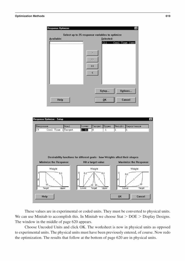
These values are in experimental or coded units. They must be converted to physical units.We can use Minitab to accomplish this. In Minitab we choose Stat DOE Display Designs.The window in the middle of page 620 appears.
Choose Uncoded Units and click OK. The worksheet is now in physical units as opposedto experimental units. The physical units must have been previously entered, of course. Now redothe optimization. The results that follow at the bottom of page 620 are in physical units.
Optimization Methods 619

Speed2.0
[1.4383]–2.0
HiCurLo
OptimalD
1.0000
Cool TimTarg; 0.0y = 0.0
d = 1.0000
Vol2.0
[–1.5823]–2.0
Temp2.0
[–0.4165]–2.0
Speed1500.0
[1499.9074]30
HiCurLo
OptimalD
1.0000
Cool TimTarg; 0.0y = 0.0
d = 1.0000
Vol200.0
[29.4704]0.0
Temp38.0[38.0]14.0
620
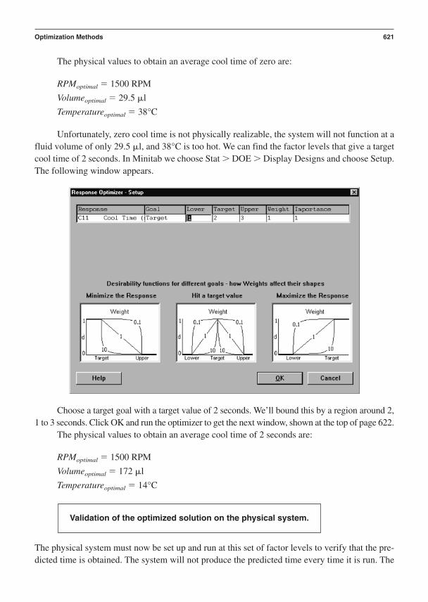
The physical values to obtain an average cool time of zero are:
RPMoptimal 1500 RPM
Volumeoptimal 29.5 l
Temperatureoptimal 38°C
Unfortunately, zero cool time is not physically realizable, the system will not function at afluid volume of only 29.5 l, and 38°C is too hot. We can find the factor levels that give a targetcool time of 2 seconds. In Minitab we choose Stat DOE Display Designs and choose Setup.The following window appears.
Choose a target goal with a target value of 2 seconds. We’ll bound this by a region around 2,1 to 3 seconds. Click OK and run the optimizer to get the next window, shown at the top of page 622.
The physical values to obtain an average cool time of 2 seconds are:
RPMoptimal 1500 RPM
Volumeoptimal 172 l
Temperatureoptimal 14°C
The physical system must now be set up and run at this set of factor levels to verify that the pre-dicted time is obtained. The system will not produce the predicted time every time it is run. The
Validation of the optimized solution on the physical system.
Optimization Methods 621

predicted time is an average time. The system must be run several times at these factor levels. Aconfidence interval on the mean will then confirm if the system is performing as predicted. If itis not performing as predicted, either the prediction is wrong or the system has changed since itwas last tested. A rerun of one or more of the treatment combinations from the original CCD candetermine if the system has changed. The new observations won’t agree with the original obser-vations if the system has changed. If they do agree, the prediction is incorrect. A data entry or ma-nipulation error may be the cause, or the predictive model may be inadequate. Check youranalysis and check your residuals.
We have answered the question, “What are the factor values that produce an optimum and a tar-get response?” A more practical question to ask is “What cool times can I expect from the systemgiven the values of speed, volume, and temperature at which I expect to operate the system?”
We can use the transfer function in a Monte Carlo simulation to answer this question. Weneed two things to accomplish this. We must have a transfer function and we must have the de-scriptive statistics of the factors in the transfer function. We have the transfer function:
Cool Time 5.0135 0.8487 Speed 0.6878 Vol 0.4476 Temp 0.6141 Speed2 0.6086 SpeedXVol
Now for the descriptive statistics of the factors in the transfer function. Fan speed is as-sumed to be normally distributed with a speed of 1200 / 300 RPM. Three sigma control onfan speed was obtained, so its standard deviation is 300/3 100 RPM. Fluid volume is assumed
Monte Carlo simulation of the optimized solution using the expected factor variation.
622 Chapter 30
Speed1500.0[1500.0]300.0
HiCurLo
OptimalD
1.0000
Cool TimTarg; 2.0y = 2.0
d = 1.0000
Vol200.0
[172.0739]0.0
Temp38.0[14.0]14.0

to be normally distributed with a volume of 100 / 20 l. Three sigma control is assumed, soits standard deviation is 20/3 6.7l.
Ambient temperature is assumed to be uniformly distributed with a temperature of 20 /2°C. Temperature will range from 18 to 22 degrees. These descriptive statistics are summarized:
Fan Speed N(1200, 100)
Volume N(100, 6.7)
Temperature U(18, 21)
These physical units must be converted into experimental units. We performed a five-factor CCD. The alpha value for this is 2. We obtained this information from Minitab when wecreated the experimental design. The experimental value for the center point of the experiment isthe point 0, 0, 0, 0, 0 for speed, volume, temperature, altitude, and RH. The analysis indicated thatonly speed, volume, and temperature were significant. The physical values for the center pointfor these three factors are given in Table 30–1 as well as the physical values at the 2 alpha po-sition. So, for speed, the experimental units span 2 0 2 units, while the physical units span1500 900 600 units. The slope is 2/600 0.003 experimental units/physical units. This iscalculated for all three factors in Table 30–1.
Next, we need to convert the physical operating points and variation into experimental op-erating points and variation. This is shown in Table 30–2.
Table 30–3 summarizes the factor distributions in both physical and experimental units. Weuse the experimental units in the Monte Carlo simulation since the transfer function is also in ex-perimental units.
Optimization Methods 623
Table 30–1 Physical and Experimental Relationship Among the Factors
Experimental Physical Physical 2Factor Center Center Alpha Point Slope
Fan Speed (RPM) 0 900 RPM 1500 2/(1500 900) 0.003
Volume (l) 0 100 200 2/(200 100) 0.02
Temperature (˚C) 0 26 38 2/(38 26) 0.167
Table 30–2 Relationship of Physical and Experimental Variation
Physical Operating Experimental Experimental Factor Point and Variation Operating Point Variation
Fan Speed (RPM) 1200 / 100 0 (1200 900)*0.003 1 100*0.003 0.33
Volume (l) 100 / 6.7 0 (100 100)*0.02 0 6.7*0.02 0.134
Temperature (˚C) 20 / 2 0 (20 26)*0.167 1 2*0.167 0.33

We now have all the information needed to run a Monte Carlo simulation. We’ll use Crystal Ball,® which is a statistical package that runs under Microsoft® Excel. Crystal Ball®
makes it easy to conduct Monte Carlo simulations and optimization.Monte Carlo simulation uses a computer to simulate building and running a design thou-
sands of times. The simulations are done under conditions that simulate the variation in the partsand conditions expected during actual use. It is an extremely efficient way to evaluate the effectsof a design’s critical parameters on the design’s critical responses. It is a fantastic what-if tool.
The graphical and tabular output from a 100,000 run Crystal Ball ®Monte Carlo simulationis shown in the following chart using the factor descriptive statistics summarized previously.
This simulation took about 8 minutes to perform, perhaps orders of magnitude faster thanphysically building and testing the system. The graphical output shows 100,000 values of cooltime obtained from repeated random sampling from the assumed distributions for speed, volume,and temperature. These values are substituted into the transfer function, and the function is eval-uated 100,000 times.
The results indicate that cool time is likely to be normally distributed with a mean of 3.5seconds and a standard deviation of 0.8 seconds. This is the performance that can be expectedfrom the system when it is run under the expected operating conditions.
624 Chapter 30
Table 30–3 Experimental and Physical Factor Distributions
Factor Physical Distribution Experimental Distribution
Fan Speed N(1200, 100) N(1, 0.333)
Volume N(100, 6.7) N(0, 0.134)
Temperature U(18, 22) U(1.33, 1.33)

We can use this information to calculate the capability of the system. All we need is the upper andlower specification limits. The upper limit is 6 seconds and the lower bound is 0 seconds. Capa-bility is calculated in this equation:
This is a little better than 3 sigma performance. Assuming a normal distribution, approxi-mately 2,700/2 1,350 per million (this is a one-sided limit) systems would perform outside theupper specification limit, without a mean shift. It would be worse with the expected long-termmean shifts and drifts. This is poor performance. We would like 6 sigma performance, and a ca-pability index of 2. How can we achieve this? We must reduce variation. What must the variationbe reduced to for 6 sigma performance? We solve the capability equation for sigma.
How can we achieve a standard deviation of 0.5? We must search for engineering methodsto reduce the variation in the three factors that affect cool time. Reducing the variation in roomtemperature is not an option. This would require the customer to install expensive HVAC equip-ment just to use the product. Variation in fluid volume could be improved by using a fixture, but
=USL - LSL
6Cp
=6 - 0
6*2= 0.5
Cp =USL - LSL
6=
6 - 0
6(0.8)= 1.25
Calculation of system capability using the Monte Carlo results.
Optimization Methods 625

this would increase the time to fill the system and thereby reduce throughput. Speed control is the best option. Closed-loop speed control is used to reduce the variation from / 300 RPM to/ 100 RPM. Three sigma control on fan speed is obtained so its standard deviation is 100/3 33 RPM. We must convert this to experimental units. We use the formula given in Table30–2. The new tolerance for fan speed is 0.11 in experimental units. Now, let’s rerun the MonteCarlo simulation with the new standard deviation value for fan speed. The simulation results areas follows:
The system variation has been reduced to 0.45 seconds. We can calculate the new capability.
Cp =USL - LSL
6=
6 - 0
6(0.45)= 2.2
626 Chapter 30

We have achieved our goal of 6 sigma performance. However, the response is not centeredbetween the limits. It is closer to the upper limit. We calculate Cpk.
We now have to decide if it is worth increasing the fan speed to center the response to bringthe capability up to 2. Once that decision has been made, we can transfer the design to manufac-turing with confidence. If a control plan, including SPC, is placed on the components that are usedto build the system, the system will perform as designed. Approximately 3.4 per million systemsproduced will have cool times that exceed the upper limit of 6 seconds.
Final Detailed Outputs
The set of factor nominals and tolerances that yield acceptably capable performance with regardto the response target values and variance are summarized here. The tolerances are / threestandard deviations.
Fan Speed 1200 / 100 RPM
Volume 100 / 20 l
Temperature 20 / 2 °C
Optimization Checklist and ScorecardChecklist for Optimization
Was this Excellence Rating:Action Deployed? 1 Poor
Actions: YES or NO 10 Excellent
The transfer function from the experimental data. ______ ______
The response target and variance requirements. ______ ______
Analytic, numeric, and/or graphical solution of the transfer function for the optimum operating condition. ______ ______
Validation of the optimized solution on the physical system. ______ ______
Monte Carlo simulation of the optimized solution using the expected factor variation. ______ ______
The set of factor nominals and tolerances that yield capable, on-target, minimum variance performance.
Cpk =USL - X
3=
6 - 3.55
3(0.45)= 1.8
Optimization Methods 627
(continued)

Calculation of system capability using the Monte Carlo results. ______ ______
The set of factor nominals and tolerances that yield capable, on-target, minimum variance performance. ______ ______
Scorecard for Optimization
The definition of a good scorecard is that it should illustrate in simple but quantitative terms whatgains were attained from the work. This suggested format for a scorecard can be used by a prod-uct planning team to help document the completeness of its work.
Control FactorOptimal Nominal Control Factor Required Control Control Factor
Control Factor: Value: Optimal Tolerance: Factor Capability: Unit of Measure:
1. ______ ______ ______ ______
2. ______ ______ ______ ______
3. ______ ______ ______ ______
We repeat the final deliverable:
• A list of the factor nominals and tolerances that yield capable, on-target, minimumvariance performance
References
Myers, R. H., & Montgomery, D. W. (1995). Response surface methodology. New York: WileyInterscience.
Vanderplaats, G. N. (1984). Numerical optimization techniques for engineering design. New York:McGraw-Hill.
628 Chapter 30
P A R T V I I
Tools and Best Practices forVerifying Capability
Chapter 31 Analytical Tolerance DesignChapter 32 Empirical Tolerance DesignChapter 33 Reliability EvaluationChapter 34 Statistical Process Control
The tools and best practices discussed in this section focus on deliverables required at gate re-views for the fourth phase in the I2DOV and CDOV processes.
These chapters are structured so that the reader can get a strong sense of the process stepsfor applying the tools and best practices. The structure also facilitates the creation of PERT chartsfor project management and critical path management purposes. A checklist, scorecard, and listof management questions end each chapter.
629

This page intentionally left blank

C H A P T E R 3 1
Analytical Tolerance Design
Where Am I in the Process? Where Do I Apply Analytical Tolerance DesignWithin the Roadmaps?
Linkage to the I2DOV Technology Development Roadmap:
Analytical tolerance design is conducted across the Develop and Verify phases during technologydevelopment.
Linkage to the CDOV Product Development Roadmap:
Analytical tolerance design is conducted within the Design, Optimize, and Verify phases duringproduct development.
What Am I Doing in the Process? What Does Analytical Tolerance Design Doat this Point in the Roadmaps?
The Purpose of Analytical Tolerance Design in the I2DOV TechnologyDevelopment Roadmap:
Analytical tolerance design is used in the Develop phase of the I2DOV process to establish theinitial functional and assembly tolerances for the baseline technology concepts that have been
Concept Design Optimize Verify
Invent/Innovate
Develop Optimize Verify
631

selected from the Pugh concept selection process. It is used to understand the sensitivities that ex-ist within and between components, subassembly, and subsystem interfaces.
Analytical tolerance design is used later in the Verify phase to assess integration sensitivi-ties as the platform is integrated and evaluated for performance under nominal (random variationsources) and stressful (induced assignable cause variation sources, or Taguchi noises) noise conditions.
The Purpose of Analytical Tolerance Design in the CDOV ProductDevelopment Roadmap:
Analytical tolerance design is used in the Design phase of the CDOV process to establish the initialfunctional and assembly tolerances for the baseline product design concepts (subsystems, subassem-blies, and components) that have been selected from the Pugh concept selection process. It is used tounderstand the sensitivities that exist between components, subassembly, and subsystem interfaces.
Analytical tolerance design is used later in the Optimize phase to analyze and balance sys-tem-to-subsystem interface sensitivities. It is used during the Verify Certification phase to assessremaining integration sensitivity issues as the final product design certification units are evalu-ated for performance under nominal (random variation sources) and stressful (induced assigna-ble cause variation sources) noise conditions.
What Output Do I Get at the Conclusion of Analytical Tolerance Design?What Are Key Deliverables from Analytical Tolerance Design from itsApplication in the Roadmaps?
• Optimized critical functional parameter tolerance set points that control subsystem andsubassembly form, fit, and function contributions to system level functional andassembly variation
• Optimized critical adjustment parameter tolerances used to tune the mean value of thesystem, subsystem, and subassembly critical functional response(s)
• Optimized critical-to-function specification set points that control componentcontributions to functional and assembly variation
• Critical Parameter Management data that is documented in the CPM relationaldatabase:System level variance modelsSubsystem level variance modelsSubassembly level variance modelsComponent level variance modelsManufacturing process level variance modelsCFP tolerances and their percentage contribution to CFR variationCAP tolerances and their percentage contribution to CFR variationCTF spec tolerances and their percentage contribution to CFR variation
632 Chapter 31

The Analytical Tolerance Design Flow Diagram
This visual reference illustrates the flow of the detailed steps of the analytical tolerance designprocess.
Verbal Descriptions for the Application of Each Block Diagram
This section explains the specific details of what to do in analytical tolerance design:
• Key detailed input(s) from preceding tools and best practices• Specific steps and deliverables from each step to the next within the process flow• Final detailed outputs that flow into follow-on tools and best practices
INPUT . . .
OUTPUT . . .
Requirements, manufacturingprocess capabilities, superiorconcepts, and their baseline
ideal/transfer functions.
Tolerance analysis is done at and betweenthe subsystem, subassembly, and
component levels in support of systemform, fit, and function requirements.
Optimized tolerance set points forproduction and service organizations.
Conduct worst case toleranceanalysis for linear variation
buildup.
Conduct worst case toleranceanalysis for nonlinear
variation buildup.
Conduct RSS toleranceanalysis for linear variation
buildup.
Conduct RSS toleranceanalysis for nonlinear
variation buildup.
Conduct Monte Carlosimulations on ideal/transfer
functions.
Document optimum toleranceset points and variance
models in Critical ParameterManagement database.
Analytical Tolerance Design 633

Key Detailed Inputs
The baseline form, fit, and function models, manufacturing process capabilities, and requirementsthey seek to fulfill define each subsystem, subassembly, and component concept. These are themajor inputs to the analytical tolerancing process.
Specific Steps and Deliverables
The text in this section has been reproduced from the book Tolerance Design (1997) by C. M.Creveling. This book fully explains, illustrates, and provides examples on the details within eachof the following subprocesses.
The worst case method is an extreme representation of how variability will show up in the as-sembly processes. That is to say, there is a low statistical probability that every component willcome in at its high or low tolerance limit in significant numbers. If the component tolerances areset at 6 standard deviations of the component CTF specification distributions, the worst casemethod analyzes component variation contributions at those extreme limits (/ 6).
1. Analyze the geometric and spatial relationships between the components as theyfit together to make an assembly. Then assess the assembly’s geometric and spatial rela-tionships relative to the product’s functional capability. What is the functional purpose ofthe stacked-up components in specific engineering terms and units?
2. Define the specific functional requirement of the assembly. This may be done byquantifying the overall assembly form and fit specifications (where G a Gap, line-to linecontact, or an interference fit—Gnom., Gmax., and Gmin.)
3. Either estimate (from look-up tables, manufacturing process data, or recommen-dations) or allocate (from previously determined overall assembly specifications) an initialtolerance for each component in the assembly. Each component must be assessed on an in-dividual basis for variance contribution.
4. Add or subtract each tolerance from the associated nominal set point so that eachcomponent dimension can then be added to form either a maximum possible assemblyvalue (Gmax.) or a minimum assembly value (Gmin.). All the largest possible componentsare added to arrive at the maximum assembly size. All the smallest components are added
Conduct worst case tolerance analysis for linear variation buildup.
Requirements, manufacturing process capabilities, superior concepts, and their baseline ideal/transfer functions.
634 Chapter 31

to yield the smallest possible assembly size. Select a point on one side or the other of theunknown gap being evaluated as a starting point for the tolerance stack model.
The technique for generating a tolerance stack is called vector chain diagramming.
5. The space or assembly gap, contact point, or interference (G) can now be assessedbecause it is now clear what the extremes of the component assembly can be at the indi-vidual tolerance limits. The nominal gap, contact point, or interference fit dimension(Gnom.) can be calculated and its tolerances documented. Sometimes Gnom. and its toler-ances will be specified as a requirement and the component parts have to be developed tosum up to meet Gnom. and its assigned tolerance values. In this process, the component tol-erances and their nominals will have to be tuned to support the gap, contact point, or inter-ference specifications. This is referred to as tolerance allocation.
Let’s look at a case where linear worst case tolerance analysis can be applied. The case in-volves two mating parts that must fit together. The parts represent an example of pin and hole tol-erance analysis.
Figure 31–1 illustrates the parts. Figure 31–2 shows two worst case scenarios for the twomating parts. Figure 31–3 illustrates one possible set of specifications for Part A and Part B.
We shall explore these tolerances to see if they work for a worst case scenario.In Figure 31–4 the analysis begins at the right edge of the right pin. One must always select
a logical starting point for a stack analysis. Typically, it will be at one side of an unknown criticalgap dimension (distance from the start of a to the end of g) as we have selected in Figure 31–4.
We will step across the assembly from point a to point g to sum up all the stack up dimen-sions according to their sign.
Analytical Tolerance Design 635
Part APin
Part BTop
Figure 31–1 Mating Pin and Hole Assembly
Figure 31–2 Two Worst Case Scenarios

Each arrowed line in Figure 31–4 is called a displacement vector.The displacement vectors and their associated tolerances are quantified in the next
example.Notice that each tolerance for a diameter has been divided by 2 to convert it to a radial
tolerance.
636 Chapter 31
2.00 ± .02-A- 2.00 ± .02 1.00 ± .01
4.00 ± .04
5.00 ± .05
3.00 ± .03
Part A: Pin Part B: Top
1.000 ± .005φ
(2 pins)
1.050 ± .008φ
(2 holes)
-D-
Figure 31–3 Specifications for Part A and Part B
(– Direction)
(+ Direction)
Pins
Gap =
abc
Hole
d
e
f g
-D-
Figure 31–4 Worst Case Tolerance Stack-up Example

a: 1.00/2 0.005/2b: 3.0 0.03 Part A: Pin
Contactc: 1.00/2 0.005/2d: 1.05/2 0.008/2e: 1.0 0.01 Part B: Topf: 4.0 0.04g: 1.05/2 0.008/2
0.05 0.093 for the Worst Case
Analyzing the results we find the following conditions: 0.05 nominal gap and 0.093 tol-erance buildup for the worst case in the positive direction.
This case tells us that the nominal gap is 0.050, and the additional growth in the gap willbe 0.093, due to tolerance buildup, for a total gap of 0.143. Thus, a measurable gap will existwhen all the tolerances are at their largest values.
For the worst case when all dimensions are at their smallest allowable dimensions, we seethe following scenario: 0.05 nominal and 0.093 tolerance buildup for the worst case in thenegative direction.
This case tells us that the nominal gap is 0.050, and the reduction in the gap will be 0.093, due to negative tolerance buildup, for a total of 0. 043 (interference). In this worst casescenario, the parts could not mate.
1. Construct a geometric layout of each component with its nominal set point and theinitial recommended (bilateral) tolerances. Define the critical functional features, sizes, andsurfaces. Some dimensions on the component will not contribute to the assembly stack-up.A common error in tolerance analysis is the inclusion of tolerance parameters that are notfunctionally involved in the assembly tolerance.
2. Construct an assembly drawing of the components. This will graphically illustratethe geometric relationships that exist between the components. Again, define the criticalfunctional features, sizes, and surfaces. At this point, the engineering team should definethe required assembly tolerance. This tolerance range will be the target range for the non-linear tolerance adjustment process to hit.
3. Employ plane geometry, trigonometry, algebra, and calculus as necessary to de-fine the arithmetic (functional) relationship that exists between the component dimensionsand the assembly dimension(s).
y f (1,2,3,… n)
Conduct worst case tolerance analysis for nonlinear variation buildup.
Analytical Tolerance Design 637

The ideal/transfer function math model (vector chain diagram converted to a mathmodel) must directly express the critical path of the functional interfaces.
4. Use the ideal/transfer function math model to solve for the nominal assembly di-mension by using the nominal component values (components with no unit-to-unit varia-tion). Reaffirm the initial assembly tolerance required for proper functional productperformance. This will typically involve some form of engineering functional analysis, in-cluding experimental prototype evaluations.
5. Employ differential calculus to solve for the partial derivatives of the math modelterms that represent the component tolerance sensitivities with respect to the assembly tolerance.
The partial derivatives are solved with the components all set at their nominal values(typically at the tolerance range midpoint). The tolerances can be unilateral or equal bilat-eral. The differentiation is typically done using manual analytical techniques or by usingcomputer-aided numerical analysis techniques. Some problems can be difficult to differen-tiate. Using the definition of the derivative can simplify the process of calculating a sensi-tivity. Also available for help are computer-aided analytical differentiation programs likeMathematica, Macsyma, MathCAD, and Maple.
For linear tolerance stacks, the partial derivatives are all equal to 1.
6. With the values for each component sensitivity quantified, the worst case toler-ance equation can be used to determine how a calculated assembly tolerance range is func-tionally related to the required assembly tolerance range. We do this by inserting the initial(bilateral) component tolerances and their sensitivities into the following equation. Notethat in this process we use the absolute value of the sensitivities.
The evaluation of the recommended initial component tolerances with respect to therequired assembly tolerance, as constrained by the calculated sensitivities, will be an itera-tive process. The goal is to adjust the component tolerances to get the assembly tolerancerange as close to the required range as possible. The ultimate outcome of the iterations willbe a revised set of component tolerances, probably a little different from the original rec-ommended tolerances, that provide an approximate match to the required assembly toler-ance. The tolerance range for the assembly, as calculated by the adjusted componenttolerances, will likely be located either a little above or below the required tolerance range.It is not unusual that the component nominal values must be shifted (called “centering” be-
toly = 2 0f01
2 tol1 + 2 0f02
2 tol2 + 2 0f03
2 tol3 + … + 2 0f0n
2 toln
Nomy L 2 0f01
21 + 2 0f02
2 2 0f03
23 + … + 2 0f0n
2n
638 Chapter 31

tween the tolerance limits) to put the assembly tolerance range on top of the required as-sembly tolerance range (or as close as reasonably possible).
7. After shifting the component tolerances to get the assembly tolerance range nearto the required range, the remaining offset between the required range and calculated rangecan be shifted by carefully shifting the nominal component set point values. The guidingprinciple in component nominal shifting is to do it in proportion to each component toler-ance. Greenwood and Chase (1998) recommend each component be shifted by an equalfraction (f) of each respective tolerance.
The needed shift in the assembly tolerance range must be calculated.
The following equation is then used to determine the amount the assembly will shiftfor given component nominal shifts:
When we know how far the assembly tolerance range is off from the required range(y) we can then go back and solve for how much to shift each component nominal value(x). We establish the proper direction (sign) and amount of nominal shift by the follow-ing expression:
This expression simply states that the change needed in the nominal value of param-eter (i) is going to depend on the sign of the shift change required in the assembly variable(y) and the sign of the sensitivity times the fraction of the tolerance. The equation that willbe used to solve for (f) will be:
8. Once the common shift fraction (f) is determined, the component nominals can berecalculated to define the new midpoint (nominal) values. This is done by using the fol-lowing expression:
(f) =¢y
0(f)0x1(SGN)(SGN)(tol1) +
0(f)0x2(SGN)(SGN)(tol2) + p
¢y =0(f)0x1(SGN)(SGN)(f)(tol1) +
0(f)0x2(SGN)(SGN)(f)(tol2) + p
¢xi = SGN(¢y)SGN0(f)0x1(f)toli
¢y =0(f)01¢1 +
0(f)02¢2 + p
0(f)0n
¢n
¢y = B (yhigh + ylow)
2R
Required
- B (yhigh + ylow)
2R
Actual
Analytical Tolerance Design 639

9. The new shifted nominals and their tolerances can now be used to calculate thenew assembly nominal value and the resulting tolerance range about the assembly nomi-nal. Referring back to the nominal and tolerance equations:
This new assembly tolerance range can then be compared to the required assemblytolerance range for suitability. The match should be reasonably close at this point. Anotheriteration can be performed if necessary to get the actual assembly tolerance range evencloser to the required assembly tolerance range. This iteration can easily be done by re-peating steps 7-9 after recalculating new sensitivity values based on the new shifted com-ponent nominal values (repeat of step 5).
See Creveling (1997) for a complete example of this fairly involved process.
The root sum of squares method is a more realistic representation of how variability will showup in your assembly processes. That is to say, there is a low statistical probability that everycomponent will come in at its high or low tolerance limit in significant numbers. If the component tolerances are set at 6 standard deviations of the component CTF specification dis-tributions, the worst case method analyzes component variation contributions at those ex-treme limits (/ 6). The RSS method analyzes component variation contributions at lessextreme, more likely limits of (/ 1). RSS does not stand for “realistic statistical study,”but it could!
1. Analyze the geometric and spatial relationship between the components as they fittogether to make an assembly. Then assess the assembly’s geometric and spatial relation-ship relative to the product’s functional capability. What is the functional purpose of thestacked-up components in specific engineering terms and units?
2. Define the specific functional requirement of the assembly. This may be done byquantifying the overall assembly form & fit specifications (. . . where G a Gap, line-toline contact, or an interference fit.—Gnom., Gmax., and Gmin.).
Conduct RSS tolerance analysis for linear variation buildup.
toly = 2 0f01
2 tol1 + 2 0f0x2
2 tol2 + 2 0f03
2 tol3 + p + 2 0f0n
2 toln
Nomy L 2 0f01
21 + 2 0f02
22 + 2 0f03
23 + p + 2 0f0n
2n
(i shifted) = (i nominal) ; (f)(toli)
640 Chapter 31

3. Either estimate (from look up tables, manufacturing process data, or recommen-dations) or allocate (from previously determined overall assembly specifications) an initialtolerance for each component in the assembly. Each component must be assessed on an in-dividual basis for variance contribution.
4. Each tolerance is initially assumed to be set at or 3 standard deviations fromthe nominal set point. Thus, the standard deviation of the production process output is as-sumed to be approximately Tol./3. It is highly recommended that one obtain manufacturingdata to support this assumption and make adjustments accordingly. If the tolerances are setat some level greater than or less than 3 standard deviations of production process outputdistribution for the component CTF specifications, this must be used instead of just as-suming 3 standard deviations equal the tolerance limits.
5. The assembly tolerance can be assessed because it is now assumed that the com-ponent part tolerances are based upon 3 sigma levels from reasonably normal distributions.This is done by employing the RSS equation to the vector chain diagram model:
The nominal gap, contact, or interference dimension (Gnom.) can be calculated andits tolerances assigned. Sometimes Gnom. and its tolerances will be specified as a require-ment (usually due to some functional requirement at the subsystem or subassembly level)and the component parts have to be developed to sum up to the meet Gnom. and its toler-ance values. In the case when an allocation process must be used, the component tolerancesand nominals will have to be tuned to support the Gap specifications. This is referred to astolerance allocation. The same disciplined summation process as we defined in the worstcase method, including using the sign convention of displacements to the right being posi-tive, should be used.
6. From Six Sigma literature we have the option to use the relationship:
to state that an adjustable format for assigning tolerances is available for our use based uponthe short-term process capability (Cp). This is done when we have process data to provethat the 3 sigma paradigm is not in effect (Cp does not 1). The known Cp can be used toadjust each component tolerance so that the effect is aggregated up to the assembly toler-ance. Then we can calculate an estimate for the gap standard deviation:
Gap = B ¢Te3Cp ≤ 2
+ am
i=1¢Tpi3Cpi ≤ 2
adjusted =Tolerance
3Cp
TAssy = 2T12 + T2
2 + T32 + p + Tn
2
Analytical Tolerance Design 641

From this expression we can then calculate the probability of being above or belowa specified gap using the Z transform; see Chapters 3 and 5 in Creveling (1997):
and
In general form:
Let’s look at the case where linear RSS case tolerance analysis is applied.1
The case involves two mating parts that must fit together. The parts represent a pin and holetolerance analysis. Figure 31–5 illustrates the parts. Figure 31–6 shows two scenarios for the twomating parts.
ZGap =Gmax or min - Gnominal
Gap
ZGmax =
Gmax - Gnominal
B ¢Te3Cp ≤ 2
+ am
i=1¢Tpi3Cpi ≤ 2
ZGmin =
Gmin - Gnominal
B ¢Te3Cp ≤ 2
+ am
i=1¢Tpi3Cpi ≤ 2
642 Chapter 31
1 This case was developed at Eastman Kodak Company by Margaret Hackert-Kroot and Juliann Nelson.
Part APin
Part BTop
Figure 31–5 Mating Pin and Hole Assembly
Figure 31–6 Two RSS Case Scenarios
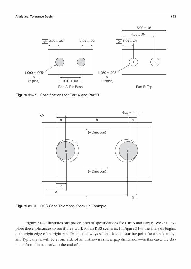
Figure 31–7 illustrates one possible set of specifications for Part A and Part B. We shall ex-plore these tolerances to see if they work for an RSS scenario. In Figure 31–8 the analysis beginsat the right edge of the right pin. One must always select a logical starting point for a stack analy-sis. Typically, it will be at one side of an unknown critical gap dimension—in this case, the dis-tance from the start of a to the end of g.
Analytical Tolerance Design 643
2.00 ± .02-A- 2.00 ± .02 1.00 ± .01
4.00 ± .04
5.00 ± .05
3.00 ± .03
Part A: Pin Base Part B: Top
1.000 ± .005φ
(2 pins)
1.050 ± .008φ
(2 holes)
-D-
Figure 31–7 Specifications for Part A and Part B
(– Direction)
(+ Direction)
Gap =
abc
d
e
f g
-D-
Figure 31–8 RSS Case Tolerance Stack-up Example

We will step across the assembly from point a to point g to sum up all the stack-up dimen-sions according to their sign.
Each arrowed line in Figure 31–8 is called a displacement vector. The sign for each dis-placement vector is illustrated in the figure. The displacement vectors and their associated toler-ances are quantified as follows:
a: 1.00/2 (0.005/2)2
b: 3.0 (0.03)2 Part A: Pin
Contactc: 1.00/2 (0.005/2)2
d: 1.05/2 (0.008/2)2
e: 1.0 (0.01)2 Part B: Topf: 4.0 (0.04)2
g: 1.05/2 (0.008/2)2
0.05 taking the square root of this sum 0.051 for the RSS Case
Notice that each tolerance for a diameter has been divided by 2 to convert it to a radial tolerance.
Analyzing the results we find a 0.05 nominal gap and 0.051 tolerance buildup for theRSS case in the positive direction.
This case tells us that
• The nominal gap is 0.050.• The additional growth in the gap will be 0.051.• Due to tolerance buildup, the total gap will be 0.101.
Thus, when all the tolerances are at their largest values, there will be a measurable gap. Forthe RSS case when all dimensions are at their smallest allowable dimensions, we see the follow-ing scenario: 0.05 nominal and 0.051 tolerance buildup for the RSS case in the negative di-rection. This case tells us that
• The nominal gap is 0.050.• The reduction in the gap will be 0.051, due to negative tolerance buildup.• Total gap will be 0. 001 (interference).
In this scenario the parts could not mate.If the worst case conditions are set up so that the pins are biased toward contacting the in-
ner surfaces of the holes (the second scenario in Figure 31–6), the gap results are the same as thescenario we just worked out, because of the symmetry of the tolerancing scheme in Figure 31–7(this need not be true of other pin–hole situations).
644 Chapter 31
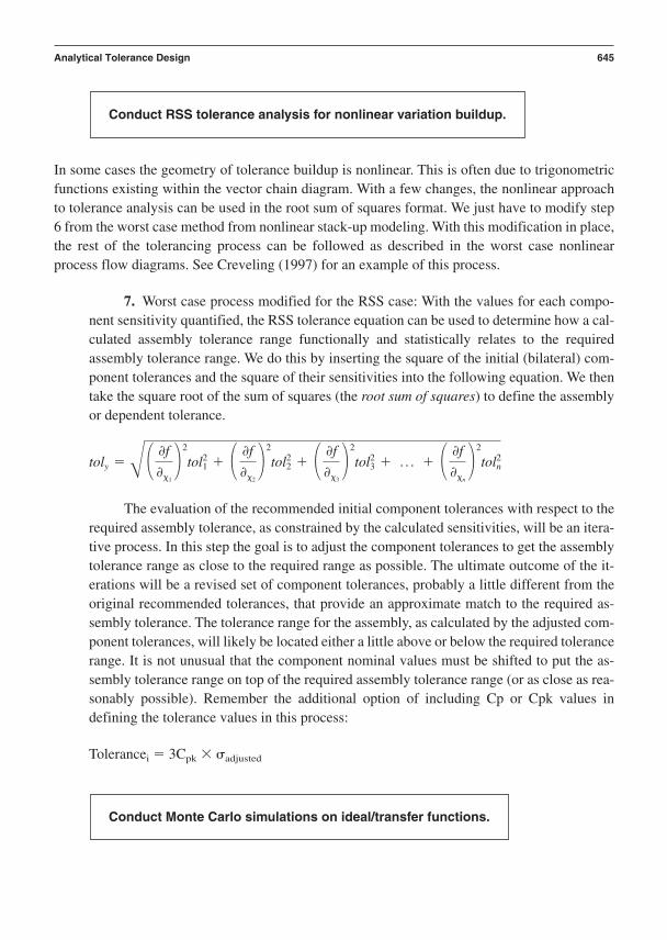
In some cases the geometry of tolerance buildup is nonlinear. This is often due to trigonometricfunctions existing within the vector chain diagram. With a few changes, the nonlinear approachto tolerance analysis can be used in the root sum of squares format. We just have to modify step6 from the worst case method from nonlinear stack-up modeling. With this modification in place,the rest of the tolerancing process can be followed as described in the worst case nonlinearprocess flow diagrams. See Creveling (1997) for an example of this process.
7. Worst case process modified for the RSS case: With the values for each compo-nent sensitivity quantified, the RSS tolerance equation can be used to determine how a cal-culated assembly tolerance range functionally and statistically relates to the requiredassembly tolerance range. We do this by inserting the square of the initial (bilateral) com-ponent tolerances and the square of their sensitivities into the following equation. We thentake the square root of the sum of squares (the root sum of squares) to define the assemblyor dependent tolerance.
The evaluation of the recommended initial component tolerances with respect to therequired assembly tolerance, as constrained by the calculated sensitivities, will be an itera-tive process. In this step the goal is to adjust the component tolerances to get the assemblytolerance range as close to the required range as possible. The ultimate outcome of the it-erations will be a revised set of component tolerances, probably a little different from theoriginal recommended tolerances, that provide an approximate match to the required as-sembly tolerance. The tolerance range for the assembly, as calculated by the adjusted com-ponent tolerances, will likely be located either a little above or below the required tolerancerange. It is not unusual that the component nominal values must be shifted to put the as-sembly tolerance range on top of the required assembly tolerance range (or as close as rea-sonably possible). Remember the additional option of including Cp or Cpk values indefining the tolerance values in this process:
Tolerancei 3Cpk adjusted
Conduct Monte Carlo simulations on ideal/transfer functions.
toly = B ¢ 0f01
≤ 2
tol12 + ¢ 0f
02
≤ 2
tol22 + ¢ 0f
03
≤ 2
tol32 + p + ¢ 0f
0n
≤ 2
toln2
Conduct RSS tolerance analysis for nonlinear variation buildup.
Analytical Tolerance Design 645

Monte Carlo simulations on personal computers are fast, cost-effective ways to explore tolerancesensitivity relationships between the xs and their percent contribution to the Ys in the flow-up ofvariational effects across and within the boundaries of the levels of the system architecture.
Monte Carlo simulations follow a fairly simple process:
1. Generate an ideal/transfer function for the function and assembly requirement un-der evaluation (in assembly cases these are created using the vector chain diagram of thetolerance stack-up).
Y f(x)
This is the model the Monte Carlo simulation exercises as it runs through the assem-bly or function generation process trials or iteration calculations.
2. Gather data to construct a histogram of the distribution of the individual x inputvariables. This provides the team with the x values as represented by the mean and stan-dard deviation of the distribution for the x variables. These are either subsystem or sub-assembly CFPs or component CTF specifications in CPM terms. The normality of thedistributions should also be quantified. The Monte Carlo simulation randomly samplesfrom these x variable distributions and enter their values into the ideal/transfer functionmodel:
Y f(x)
The model is loaded with many hundreds or thousands of trial or sample values of thex variables as randomly generated and placed in the ideal/transfer function model by thesimulation software.
3. Build, load, and run the simulation in the computer. Crystal Ball® Monte Carlosimulation software is a common tool that can be effectively used to conduct the simula-tion process. A complete tutorial description and example of how Monte Carlo simulationis done is documented in Chapter 8 of Creveling’s (1997) Tolerance Design.
4. Analyze the results from the Monte Carlo simulation. The typical output from aMonte Carlo simulation is a forecasted sample distribution of the Y variable. The output dis-tribution has a sample mean and sample standard deviation that is representative of the hun-dreds or thousands of trials that were run in the simulation. Capability (Cp) calculations forthe Y variable can be made to see if the ideal/transfer function is capable with the inducednoise from the variation of the input x variables.
5. Refine the ideal/transfer function nominal (mean) x input values or standard devi-ation input values. Rerun the simulation to compare the Y outputs against the requirements.
646 Chapter 31

How Crystal Ball® uses Monte Carlo Simulation
Crystal Ball® implements Monte Carlo simulation in a repetitive three step process:
1. For every assumption cell, Crystal Ball® generates a number according to theprobability distribution you defined and placed into the spreadsheet.
2. Crystal Ball® commands the spreadsheet to calculate a new response valuefrom the math model you have entered into the Excel forecast cell.
3. Crystal Ball® then retrieves each newly calculated value from the forecast celland adds it to the graph in the forecast windows.
The iterative nature of the Monte Carlo process can be simply illustrated by the flow chartin Figure 31–9.
It would not be unusual to specify that the Monte Carlo routine should be run through 1,000or more iterations. This provides an ample set of data
• Used to help estimate a useful portion of the real-world effects that can occur fromrandom unit-to-unit variation
• Based on an identifiable set of probability distributions that are obtained fromproduction samples
A probability distribution can be determined from two sources:
• Sample data that is truly representative of the nature of variability present in the outputcomponents
• The output of a mathematical function (equation) that is just an estimate that expressesthe output as a probability of occurrence value between 0 and 1 or a percentagebetween 0 percent and 100 percent.
Analytical Tolerance Design 647
Each run throughthe process iscalled a trial
Generate randomnumbers for the
assumption cells.
Calculate the entirespreadsheet.
Display the results in aforecast chart.
Figure 31–9 Monte Carlo Process
The probability is based on independent parameters we typically refer to as sample or pop-ulation statistics.
Typical input parameters for probability distributions are based on whether the distributionsare discrete (binary events) or continuous (analog events). For discrete distributions we often seeinput parameters stated as:
• Probability of an event (P)• Total number of trials (n) available for the event to occur or not occur
There are other parameters for discrete distributions. Consult the Crystal Ball® manual ora text on probability and statistics to obtain additional information concerning the discrete distri-bution statistics.
The continuous distributions typically use the well-known parameters (the populationmean) and (the population standard deviation):
• Sample statistics for the mean and standard deviation are used to estimate thesepopulation parameters.
• You will almost always be working with sample values for the mean and standarddeviation.
Again, you need to consult the Crystal Ball® manual or a text on probability and statisticsto obtain additional information concerning other types of continuous distribution statistics.
In conclusion, the shape of each distribution provides a graphic illustration of how likely aparticular value or range of values is to occur. Probability distributions show us the pattern thatnature has assumed for certain phenomena as they disperse themselves when allowed to occur ina random or unbiased condition.
The following types of probability distributions are available in Crystal Ball®:
Uniform ExponentialNormal Weibull (Rayleigh)Triangular BetaBinomial GammaPoisson LogisticHypergeometric ParetoLognormal Extreme Value
Crystal Ball® also has the ability to permit custom (user-specified) distributions. The softwarepackage has a unique portfolio of user-adjustable distributions, which allows one to provoke a di-verse set of variations in the model trial runs through the program’s random number generator. Eachone of the probability distributions has a specific geometric nature and a set of defining parametersthat give it its distinctive form to represent the range of probabilities for an event or response value.
648 Chapter 31
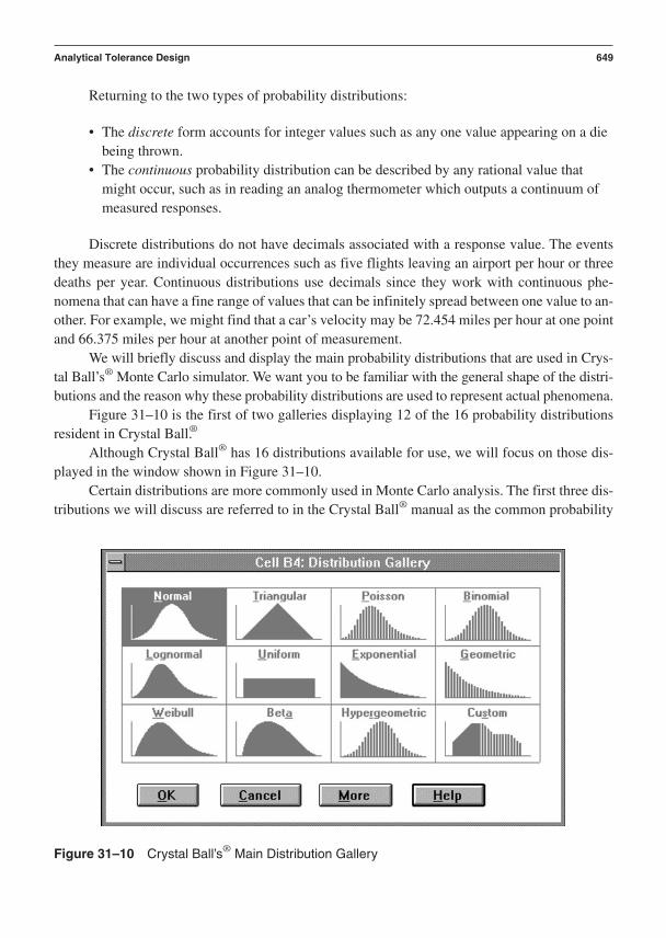
Returning to the two types of probability distributions:
• The discrete form accounts for integer values such as any one value appearing on a diebeing thrown.
• The continuous probability distribution can be described by any rational value thatmight occur, such as in reading an analog thermometer which outputs a continuum ofmeasured responses.
Discrete distributions do not have decimals associated with a response value. The eventsthey measure are individual occurrences such as five flights leaving an airport per hour or threedeaths per year. Continuous distributions use decimals since they work with continuous phe-nomena that can have a fine range of values that can be infinitely spread between one value to an-other. For example, we might find that a car’s velocity may be 72.454 miles per hour at one pointand 66.375 miles per hour at another point of measurement.
We will briefly discuss and display the main probability distributions that are used in Crys-tal Ball’s® Monte Carlo simulator. We want you to be familiar with the general shape of the distri-butions and the reason why these probability distributions are used to represent actual phenomena.
Figure 31–10 is the first of two galleries displaying 12 of the 16 probability distributionsresident in Crystal Ball.®
Although Crystal Ball® has 16 distributions available for use, we will focus on those dis-played in the window shown in Figure 31–10.
Certain distributions are more commonly used in Monte Carlo analysis. The first three dis-tributions we will discuss are referred to in the Crystal Ball® manual as the common probability
Analytical Tolerance Design 649
Figure 31–10 Crystal Ball’s® Main Distribution Gallery

distributions, due to the fact that it is not always easy to assign a distribution to a particular situ-ation without first knowing something about the nature of variability resident in the productionprocess of the component being toleranced. Thus, the common distributions are the default se-lections to employ until one has a better alternative.
Characterizing Probability Distributions for Tolerance AnalysisApplications
The usual method of identifying the distribution type that matches or approximates the behaviorof an input variable, typically a component dimension, being used in a Monte Carlo simulation isto gather a large, statistically valid sample of data (30–100 samples) from a similar componentthat is currently being produced. This data is used to construct a histogram. The histogram canthen be used in comparison with one or more of the distributions displayed in the distributionGallery. The histogram, along with engineering judgment, will generally suffice to make a rea-sonable selection for the tolerance analysis input assumptions. Access to a professional statisti-cian with manufacturing experience can be of significant help in the process of identifying theappropriate probability distribution to use in many different situations.
The Common Probability Distributions Available in Crystal Ball®
The Normal Distribution: The normal or Gaussian distribution is a common method ofexpressing the variation and central tendency of the output from many types of manufacturingprocesses. The normal distribution has three distinctive characteristics about how it expresses uncertainty:
1. Some value of the uncertain (input) variable is the most likely (the mean ofthe distribution).
2. The uncertain (input) variable could as likely be above the mean as it couldbe below the mean (symmetrical about the mean).
3. The uncertain variable is more likely to be in the vicinity of the mean than faraway (accounts for the bell shape of the distribution).
The Uniform Distribution: The uniform distribution is helpful in cases where it is justas likely that the input variable will assume one value in the range of possible values as any other.The uniform distribution has three distinctive characteristics about how it expresses uncertainty:
1. The minimum value (in the range) is fixed.2. The maximum value (in the range) is fixed.3. All values between the minimum and the maximum occur with equal likelihood.
The Triangular Distribution: The triangular distribution accounts for the case wherethere is clear knowledge of a range between which likely values will occur with a single, mostlikely value located somewhere within the range of possible values. The triangular distributionhas three distinctive characteristics about how it expresses uncertainty:
650 Chapter 31

1. The minimum value (in the range) is fixed.2. The maximum value (in the range) is fixed.3. The most likely value falls between the minimum and maximum values,
forming a triangular-shaped distribution, which shows that values near theminimum or the maximum are less likely to occur than those near the mostlikely value.
Step-by-Step Process Diagrams for a Crystal Ball ® Monte CarloAnalysis
Step 1: Open/create a spreadsheet in Excel under the Crystal Ball® function window.
Step 2: Set up the problem by defining the input assumptions.
2.1. Define your assumptions:• An assumption is an estimated value that will come from a specified
probability distribution that you select as an input to the spreadsheet mathmodel.
• Crystal Ball® has 16 different distributions from which you can select.2.2. Select and enter the distribution for your assumption. The selected proba-
bility distribution will represent the nature of the production process outputdistribution for the dimension or characteristic to which you are applying thetolerance. You can select the distribution by using the Cell Menu and the De-fine Assumption Command.
2.3. Repeat Step 2.2 for each component or element in your tolerance designcase.
Step 3: Set up the problem by defining the output forecasts.
3.1. Establish the functional relationships (math models) that exist between thevarious input assumption terms to produce the output response. A forecastis the value taken on by the dependent variable, y, as each independent vari-able, xi (input assumption value), changes as the Monte Carlo simulationruns through each trial.The forecast formula is represented in general form as:
y f1(x1, x2, x3. . .xn)
More than one forecast can be generated by defining several forecast for-mulas within the same spreadsheet:
z f2(x1, x2, x3. . .xn)
3.2. Select Define Forecast from the Cell Menu. Specify the engineering unitsbeing calculated in the forecast formula.
3.3. Repeat Step 3.2 for each forecast formula in your tolerance analysis.
Analytical Tolerance Design 651
Step 4: Run a simulation. Running a Monte Carlo simulation means that you willexercise the spreadsheet math model(s) at least 200 times by using thesoftware’s random number generator in conjunction with the distributions that represent your input assumptions. At least 200 trials will be calculated to represent the uncertainty or likelihood of what can happen in your tolerance case.
4.1. Choose Run Preferences from the Crystal Ball® Run Menu.4.2. Type in the number of trials you would like to run (200 minimum). In our
cases you will not need to provide a seed number.Step 5: Interpret the results. Determine the level of certainty in the forecasted results
desired. Crystal Ball® reports the forecasted outputs from the math models in agraphic display that contains both probability and frequency distributions of theresults. The probability axis (left side vertical axis) of the chart states thelikelihood of each output value or group of values in the range of 0 probabilityto 100 percent probability (0.000 1.000). The frequency axis (right sidevertical axis) of the chart states the number of times a particular value or groupof values occurs relative to the total number of runs in the simulation.
This process involves how to change the Display Range of the forecast, which enables youto look at specific portions of the output response distribution and to identify the probability orfrequency of certain responses of interest occurring.
In tolerance analysis these responses happen to be the values that are occurring within thetolerance range. Crystal Ball® initially shows all the distribution of trials; then it is up to you tomodify the range of values Crystal Ball® includes in the forecast certainty window.
Crystal Ball® allows the user to alter the minimum and maximum values (tolerance range)of the range of output to be selected and evaluated. The Certainty Box responds by displaying thepercent certainty of occurrence of the values within the specified range. In this way we can quan-tify the percentage of values falling within the required range of tolerance for an assembly or sys-tem. This concludes the basic capability of Crystal Ball® to analyze a tolerance problem.
Crystal Ball® has additional capabilities to take the user deeper into the analysis of toler-ances. The user can receive the following statistical information concerning the output responsedata and distribution:
mean
median
mode
standard deviation
variance
skew
kurtosis
652 Chapter 31
coefficient of variability
range minimum
range maximum
range width
standard error of the mean
All of these quantitative statistical measures are defined in Chapter 3. Crystal Ball® can alsoconstruct a table of the distributed results by percentile increments of 10 percent (or by other in-crements one chooses to set). Crystal Ball® allows the user to compare multiple tolerance analy-ses within a large system as one alters the assumptions or tolerance ranges. Crystal Ball® usestrend charts to facilitate this graphical analysis process.
Sensitivity Analysis Using Crystal Ball®
Crystal Ball® allows the user to quantify the effect of each of the input assumptions on the over-all output response. This means the software can calculate the sensitivity coefficients, includingthe proper sign associated with the directionality of their effect. In Crystal Ball® terms, this meanswe can assess the sensitivity of the forecast (output response) relative to each assumption (inputvariable). Some practitioners of tolerance sensitivity analysis may be uncomfortable with theprocess of the derivation and solution of partial derivatives.
Crystal Ball® is a friendly addition to the user’s tolerance analysis tool kit because it doesall the sensitivity analysis within the software algorithms. Crystal Ball® ranks each assumptioncell (tolerance distribution input) according to its importance to each forecast (output responsedistribution) cell.
The Sensitivity Analysis Chart displays these rankings as a bar chart, indicating which as-sumptions are the most important and which are the least important in affecting the output re-sponse. From the Crystal Ball® manual, we find that the Sensitivity Analysis Chart feature providesthree key benefits:
1. You can find out which assumptions are influencing your forecasts the most,reducing the amount of time needed to refine estimates.
2. You can find out which assumptions are influencing your forecast the least, sothat they may be ignored (or at least strategically identified for alternative ac-tion) or discarded altogether.
3. As a result, you can construct more realistic spreadsheet models and greatlyincrease the accuracy of your results because you will know how all of yourassumptions affect your model.
Crystal Ball® uses a technique that calculates Spearman rank correlation coefficients be-tween every assumption and every forecast cell while the simulation is running. In this way thesensitivities are capable of being quantified within Crystal Ball® for any case being considered.
Analytical Tolerance Design 653

Again, quoting from the Crystal Ball® manual regarding how sensitivities are calculated:
Correlation coefficients provide a meaningful measure of the degree to which assumptions and fore-casts change together. If an assumption and a forecast have a high correlation coefficient,. . . it meansthat the assumption has a significant impact on the forecast (both through its uncertainty and its modelsensitivity (from the physical and statistical parameters embodied in the system being analyzed).
The physical parameters are embedded in the math model placed in the forecast cell. Thestatistical parameters are embedded in the distributions selected as assumptions.
To quantify sensitivity magnitude and directionality:
() Positive coefficients indicate that an increase in the assumption is associated with anincrease in the forecast.
() Negative coefficients imply the reverse situation.
The larger the absolute value of the correlation coefficient, the stronger the relationship.
Referring back to the worst case tolerancing material, in which we discussed defining signsfor the directionality of the sensitivity coefficients in nonlinear evaluations, we found that thiscould be a little confusing. With Crystal Ball® the sign is automatically calculated along with thesensitivity value. Again, the concern for the tolerance analyst is
properly setting up the mathematical relationship (forecast) between the assumptions so that CrystalBall correctly calculates the magnitude and direction of the sensitivity coefficient.
Crystal Ball® can be of help if one is assessing tolerance issues between components, sub-assemblies, and major assemblies as one integrates an entire product or system:
Crystal Ball® also computes the correlation coefficients for all pairs of forecasts while the simulationis running. You may find this sensitivity information useful if your model contains several interme-diate forecasts (assemblies or subsystems) that feed into a final forecast (system).
Crystal Ball® has an option that helps clarify the output for sensitivity analysis.
. . . The Sensitivity Preference dialog box lets you display the sensitivities as a percentage of the con-tribution to the variance of the target forecast.
This option, called Contribution to Variance,
• doesn’t change the order of the items listed in the Sensitivity Chart• makes it easier to answer questions such as,. . .. . . . . . “what percentage of the variance or uncertainty in the target forecast is due to assumption x?”
It is important to note that this method is only an approximation!It is not precisely a variance decomposition (such as a formal ANOVA would provide).
654 Chapter 31

Crystal Ball® calculates Contribution to Variance by squaring the rank correlation coefficientsand normalizing them to 100%.
It is important to recognize some scenarios that can occur in the application of CrystalBall’s® sensitivity analysis option.
The sensitivity calculation may be inaccurate for certain correlated assumptions. For example,. . . ifan important assumption were highly correlated with an unimportant one, the unimportant assump-tion would likely have a high sensitivity with respect to the target forecast (output). Assumptions thatare correlated are flagged as such on the Sensitivity Chart. In some circumstances, turning off corre-lations in the Run Preference dialog box may help you to gain more accurate sensitivity information.
For tolerance applications this warning will be valid when a design assembly is made upfrom components that are antisynergistically interactive. This means that one component has adependency on another component for its effect on the response. “In practice, this problematictype of interaction should be identified and corrected long before tolerancing is undertaken,” themanual notes.
Some designs are inherently interactive. In these cases one must be vigilant as to how theseinterdependencies affect the response variable. Sometimes the interactions are necessary andhelpful. A word to the wise is sufficient: Know where the design interactions exist and at whatstrength they act to influence the output response. Fortunately, Crystal Ball® has a mechanism todecouple the assumptions from their correlations so you can assess each one in relative inde-pendence. In general, it is considered good design practice to create and optimize components,subsystems, and subassemblies, and systems that are reasonably free from elements that havestrong antisynergistic interactions.
When design elements act with interdependence that is synergistic and monotonic with respect to one another, then performance generally becomes more stable and predictable (Fig-ure 31–11), especially when strong noises are present. (See Chapter 28 on robust design for helpin developing products and processes that do not possess strong interactions.)
Analytical Tolerance Design 655
A1
Synergistic or super-additiveinteraction between components
Antisynergistic interactionbetween components A and B
A2 A1 A2
B2
B1
B2
B1
Figure 31–11 Assumptions with Interactions

With super-additivity or synergistic interactivity, the correlation is still present, but one can see how the elements work together to drive the response in a useful direction. Antisynergis-tic interactivity between two component contributions to the response is typically counteractive.The directionality of the response is reversed as one factor changes. This situation often forcesthe design team to apply tight tolerances as a countermeasure to this problematic form of sensi-tivity. Additionally, many designers often end up tightening tolerances on unimportant parame-ters because they are correlated to important ones. This leads to unnecessary expense duringmanufacturing.
The sensitivity calculation may be inaccurate for assumptions whose relationships with the target forecast are not monotonic. A monotonic relationship (Figure 31–12) means that . . . anincrease in the assumption (input) tends to be accompanied by a strict increase in the forecast(output), or an increase in the assumption tends to be accompanied by a strict decrease in the forecast.
If you are worried about being dependent on rusty calculus skills and knowledge of pa-rameter interactivity in tolerance analysis, you can relax and focus your mental energy on the is-sues of:
• Properly setting up the assumption cells with the appropriate probability distributions• Defining the right mathematical relationship between each assumption cell (component
tolerance) and the forecast cell (assembly or system tolerance)
This is where the tolerance analysis is either going to be set up right or wrong. You need tolook no further in basic skill requirements and development for competent tolerance analysis thanin these two critical areas. For advanced tolerance analysis, all the math, computer, and experi-mental skills discussed in the text will need to be in the practitioner’s full command.
An Example of How to Use Crystal Ball® Let’s run a Monte Carlo simulation on a lin-ear example:
The simple linear stack problem is shown at the top of page 657.We begin by opening Crystal Ball®. This is done by double clicking on its icon in the ap-
plications window. Crystal Ball® will open in an Excel spreadsheet (Figure 31–13).
656 Chapter 31
Positive LinearMonotonic
Negative NonlinearMonotonic
Non-Monotonic
Figure 31–12 Monotonicity
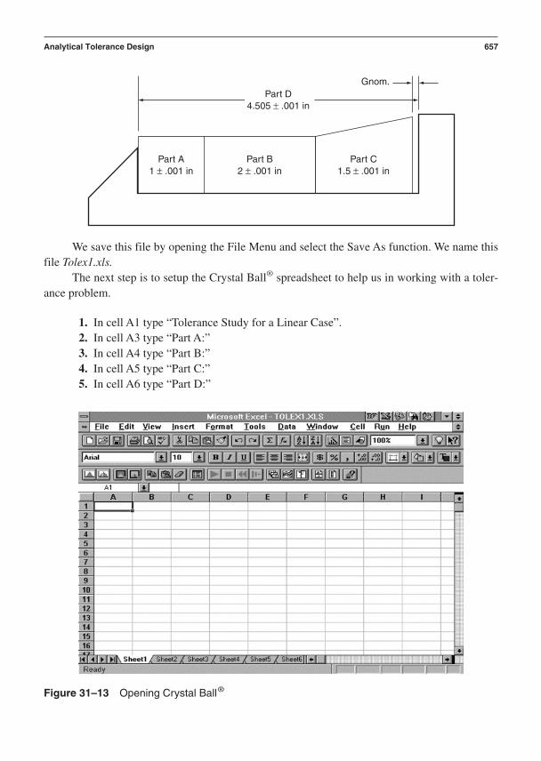
We save this file by opening the File Menu and select the Save As function. We name thisfile Tolex1.xls.
The next step is to setup the Crystal Ball® spreadsheet to help us in working with a toler-ance problem.
1. In cell A1 type “Tolerance Study for a Linear Case”.2. In cell A3 type “Part A:”3. In cell A4 type “Part B:”4. In cell A5 type “Part C:”5. In cell A6 type “Part D:”
Part A1 ± .001 in
Part B2 ± .001 in
Part D4.505 ± .001 in
Gnom.
Part C1.5 ± .001 in
Analytical Tolerance Design 657
Figure 31–13 Opening Crystal Ball®

These are the names of the four components. Next we enter six specific pieces of data thatCrystal Ball® will need as we put it to work doing the tolerance analysis. The six pieces of datathat we enter are as follows:
1. Nominal dimension for each part (Nom.)2. Tolerance on each nominal dimension (Tol.)3. The type of distribution that describes the uncertainty in the nominal dimension (Distr.)4. The tolerance divided by 3 standard deviations (Tol./3)5. The nominal dimension plus the tolerance (Nom.Tol.)6. The nominal dimension minus the tolerance (Nom.Tol.)
To enter and align these six pieces of data with the four components, follow these simplesteps:
1. In cell B2, type “Nom.”2. In cell C2, type “Tol.”3. In cell D2, type “Distr.”4. In cell E2, type “Tol./3”5. In cell F2, type “Nom.Tol.”6. In cell G2, type “Nom.Tol.”
Cells B3 through B6 hold the numbers we call Assumption Values. We can now enter thenominal values 1.0000, 2.0000, 1.5000, and 4.5050 in cells B3 through B6. The appropriate tol-erances can then be entered into the cells C3 through C6. It is assumed that the user understandsthe basics of spreadsheet use and can adjust the cell widths to accommodate the cell entries sothat the Crystal Ball® spreadsheet has an orderly and useful structure. It is also assumed one hasa basic knowledge of how to program a spreadsheet to do calculations. Even so, we will illustratehow this is done.
The next step is to enter the simple linear math model that sums the individual componentcontributions to form a residual assembly gap dimension. We call this output response the fore-cast. It is the uncertainty associated with this gap dimension that we would like to study. The gapcannot be allowed to fall below 0.001 in.
To enter the math model we perform the following process and enter the model informa-tion in the appropriate cell:
1. Select cell B8 and type “B6-B3-B4-B5” (this is the assembly gap math model).2. Click on the check mark in the box to the left of the bar that you used to enter the equa-
tion (note it is made up from the Assumption Value cells).
Cell B8 now holds the tolerance equation that employs values representing probabilisticvalues that will be determined by the random number generator in conjunction with the specific
658 Chapter 31
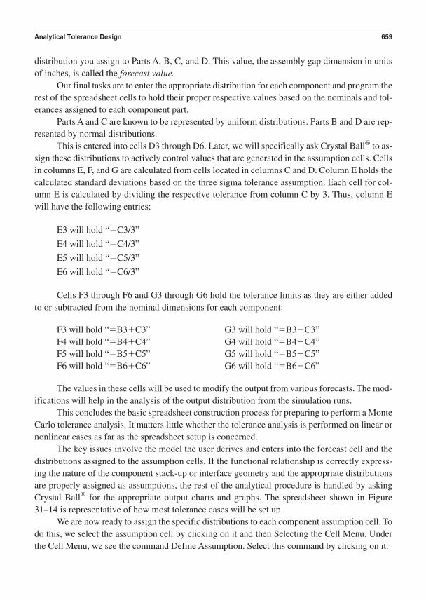
distribution you assign to Parts A, B, C, and D. This value, the assembly gap dimension in unitsof inches, is called the forecast value.
Our final tasks are to enter the appropriate distribution for each component and program therest of the spreadsheet cells to hold their proper respective values based on the nominals and tol-erances assigned to each component part.
Parts A and C are known to be represented by uniform distributions. Parts B and D are rep-resented by normal distributions.
This is entered into cells D3 through D6. Later, we will specifically ask Crystal Ball® to as-sign these distributions to actively control values that are generated in the assumption cells. Cellsin columns E, F, and G are calculated from cells located in columns C and D. Column E holds thecalculated standard deviations based on the three sigma tolerance assumption. Each cell for col-umn E is calculated by dividing the respective tolerance from column C by 3. Thus, column Ewill have the following entries:
E3 will hold “C3/3”
E4 will hold “C4/3”
E5 will hold “C5/3”
E6 will hold “C6/3”
Cells F3 through F6 and G3 through G6 hold the tolerance limits as they are either addedto or subtracted from the nominal dimensions for each component:
F3 will hold “B3C3” G3 will hold “B3C3”F4 will hold “B4C4” G4 will hold “B4C4”F5 will hold “B5C5” G5 will hold “B5C5”F6 will hold “B6C6” G6 will hold “B6C6”
The values in these cells will be used to modify the output from various forecasts. The mod-ifications will help in the analysis of the output distribution from the simulation runs.
This concludes the basic spreadsheet construction process for preparing to perform a MonteCarlo tolerance analysis. It matters little whether the tolerance analysis is performed on linear ornonlinear cases as far as the spreadsheet setup is concerned.
The key issues involve the model the user derives and enters into the forecast cell and thedistributions assigned to the assumption cells. If the functional relationship is correctly express-ing the nature of the component stack-up or interface geometry and the appropriate distributionsare properly assigned as assumptions, the rest of the analytical procedure is handled by askingCrystal Ball® for the appropriate output charts and graphs. The spreadsheet shown in Figure31–14 is representative of how most tolerance cases will be set up.
We are now ready to assign the specific distributions to each component assumption cell. Todo this, we select the assumption cell by clicking on it and then Selecting the Cell Menu. Underthe Cell Menu, we see the command Define Assumption. Select this command by clicking on it.
Analytical Tolerance Design 659

A window appears with the Distribution Gallery. Click on the distribution you want asso-ciated with the component represented in the cell. This window is displayed in Figure 31–15 withthe uniform distribution selected (darkened).
Click OK and the Distribution Gallery disappears. We have selected the uniform distribution.A new window appears as shown in Figure 31–16. This is the window for entering specific
parameter information for the uniform distribution. Enter the values for the upper and lower tol-erances into the boxes labeled Min and Max. Click Enter and then click OK.
We have successfully entered the uniform distribution for the assumption cell for Part A.Now we return to the Crystal Ball® spreadsheet window. We can proceed with defining the as-sumption cell for Part B. Simply repeat the process of opening the Cell Menu and selecting De-fine Assumption.
The window in Figure 31–17 is open. Click on the normal distribution since it representshow Part B will express its uncertainty in the assembly.
Click OK to tell Crystal Ball® to select the normal distribution. The normal distributionwindow appears as in Figure 31–18.
In this window we need to enter the Mean 2.0000 and Std. Dev 0.0003 values for PartB. Click Enter and then click OK. This returns us to the main Crystal Ball® spreadsheet where wecan repeat this process for Parts C and D, respectively.
We are now ready to use the Define Forecast command located in the Cell Menu just be-low the Define Assumption command. First, click on cell B8 to activate the Forecast cell we are
660 Chapter 31
Figure 31–14 Example of Tolerance Case Setup

defining. Then click on the Cell Menu and select the Define Forecast command. The window inFigure 31–19 appears.
The Units box needs to be filled out by typing in inches. Click OK. This returns us to themain Crystal Ball® spreadsheet and signals the successful definition of the Forecast cell.
Analytical Tolerance Design 661
Figure 31–15 Crystal Ball® Distribution Gallery
Figure 31–16 Parameter Window for Uniform Distribution

Running the Monte Carlo Simulation
The first thing required before running the simulation is the specification of a few preferences.These user-defined items are necessary before Crystal Ball® can properly iterate through the calculations.
Select the Run Menu and then select the Run Preferences option. Figure 31–20 displays theRun Preferences window. Note that a number of items can be changed in this window.
662 Chapter 31
Figure 31–17 Setting Distribution for Part B
Figure 31–18 Parameter Window for Normal Distribution

For our case at hand, the only Preferences we need to set are:
Maximum Number of Trials: 5,000
Sampling Method: Monte Carlo
Sensitivity Analysis: Turned on (x in box)
Now that these settings are enabled, click OK.
Analytical Tolerance Design 663
Figure 31–19 Define Forecast Window
Figure 31–20 Run Preferences Window

To run the simulation, follow these steps:
Select the Run Menu.
Select the Run Command to start the simulation.
The Run Menu is altered once the simulation is running. The Run Command is replacedby a Stop Command that enables the simulation to be temporarily interrupted by the user.
Once the simulation is stopped, the Run Menu is once again altered. The Stop Command isreplaced by the Continue Command. This reactivates the simulation exactly where it left off.Once the simulation is running again, the Stop Command is back in place under the Run Menu.
We can stop and start the simulation at will until the specified number of trials is completed.We can view one of two different windows to see how the simulation is progressing during theprocess, which can be an interesting and fun thing to observe!
• Under the View Menu, select the Statistics window to see how the Forecast statisticsare evolving.
• Under the View Menu, select the Frequency Chart window to see how the Forecastfrequency and probability distribution is evolving.
The completed run of the simulation for 5,000 trials is shown in both Frequency Chart (Fig-ure 31–21) and Statistics Table (Figure 31–22) formats.
As we can see, the graphical form of the distribution of response values is generated by thesimulation both in frequency (right side axis) and probability units (left side axis). Notice that two
664 Chapter 31
Figure 31–21 Simulation Frequency Chart
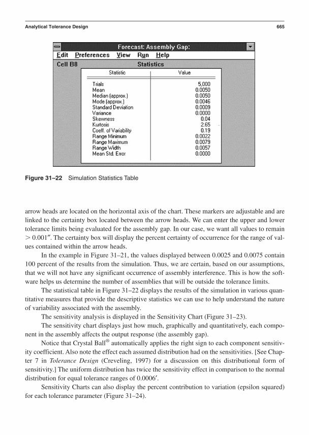
arrow heads are located on the horizontal axis of the chart. These markers are adjustable and arelinked to the certainty box located between the arrow heads. We can enter the upper and lowertolerance limits being evaluated for the assembly gap. In our case, we want all values to remain 0.001″. The certainty box will display the percent certainty of occurrence for the range of val-ues contained within the arrow heads.
In the example in Figure 31–21, the values displayed between 0.0025 and 0.0075 contain100 percent of the results from the simulation. Thus, we are certain, based on our assumptions,that we will not have any significant occurrence of assembly interference. This is how the soft-ware helps us determine the number of assemblies that will be outside the tolerance limits.
The statistical table in Figure 31–22 displays the results of the simulation in various quan-titative measures that provide the descriptive statistics we can use to help understand the natureof variability associated with the assembly.
The sensitivity analysis is displayed in the Sensitivity Chart (Figure 31–23).The sensitivity chart displays just how much, graphically and quantitatively, each compo-
nent in the assembly affects the output response (the assembly gap).Notice that Crystal Ball® automatically applies the right sign to each component sensitiv-
ity coefficient. Also note the effect each assumed distribution had on the sensitivities. [See Chap-ter 7 in Tolerance Design (Creveling, 1997) for a discussion on this distributional form ofsensitivity.] The uniform distribution has twice the sensitivity effect in comparison to the normaldistribution for equal tolerance ranges of 0.0006′.
Sensitivity Charts can also display the percent contribution to variation (epsilon squared)for each tolerance parameter (Figure 31–24).
Analytical Tolerance Design 665
Figure 31–22 Simulation Statistics Table

Epsilon squared is a term used to describe the proportion of the total variance contributedby each of the variables that can significantly affect the measured response in a design. In Figure31–24, one can see that Part C contributes almost 92 percent of all the variation in the gap analy-sis. This is clearly the most significant tolerance term in the model.
Document optimum tolerance set points and variance models in Critical Parameter Management database.
666 Chapter 31
Figure 31–24 Percent Contribution to Variation
Figure 31–23 Simulation Sensitivity Chart
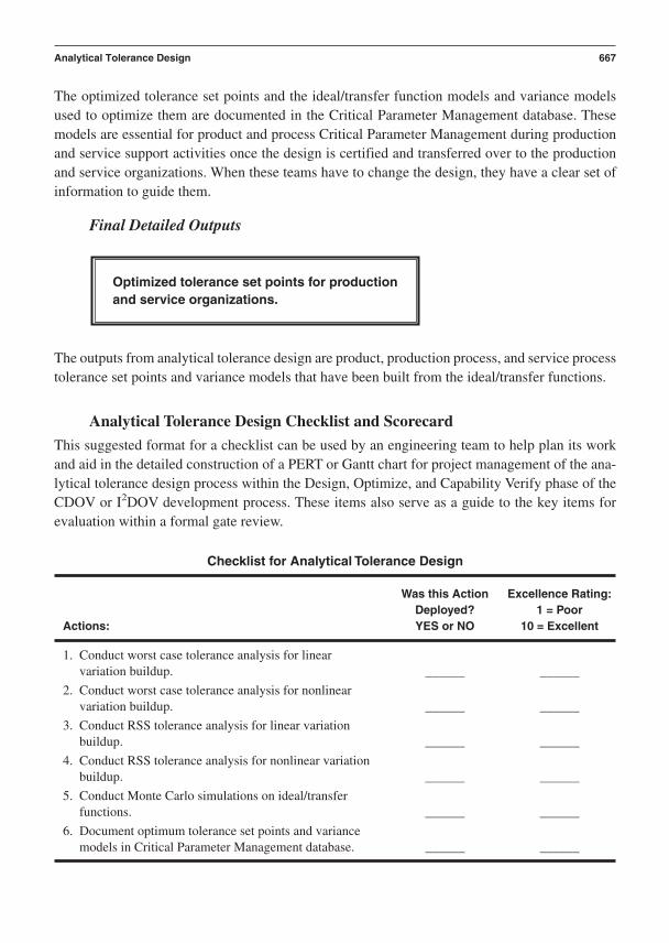
The optimized tolerance set points and the ideal/transfer function models and variance modelsused to optimize them are documented in the Critical Parameter Management database. Thesemodels are essential for product and process Critical Parameter Management during productionand service support activities once the design is certified and transferred over to the productionand service organizations. When these teams have to change the design, they have a clear set ofinformation to guide them.
Final Detailed Outputs
The outputs from analytical tolerance design are product, production process, and service processtolerance set points and variance models that have been built from the ideal/transfer functions.
Analytical Tolerance Design Checklist and Scorecard
This suggested format for a checklist can be used by an engineering team to help plan its workand aid in the detailed construction of a PERT or Gantt chart for project management of the ana-lytical tolerance design process within the Design, Optimize, and Capability Verify phase of theCDOV or I2DOV development process. These items also serve as a guide to the key items forevaluation within a formal gate review.
Checklist for Analytical Tolerance Design
Was this Action Excellence Rating:Deployed? 1 = Poor
Actions: YES or NO 10 = Excellent
1. Conduct worst case tolerance analysis for linear variation buildup. ______ ______
2. Conduct worst case tolerance analysis for nonlinear variation buildup. ______ ______
3. Conduct RSS tolerance analysis for linear variation buildup. ______ ______
4. Conduct RSS tolerance analysis for nonlinear variation buildup. ______ ______
5. Conduct Monte Carlo simulations on ideal/transfer functions. ______ ______
6. Document optimum tolerance set points and variance models in Critical Parameter Management database. ______ ______
Optimized tolerance set points for production and service organizations.
Analytical Tolerance Design 667

Scorecard for Analytical Tolerance Design
The definition of a good tolerance scorecard is that it should illustrate in simple but quantitativeterms what gains were attained from the work. This suggested format for a scorecard can be usedby an engineering team to help document the completeness of its work.
Subsystem, subassembly, or component name: __________
Subsystem, subassembly, or component critical functional response or CTF specification:__________
Specific engineering units of subsystem and subassembly CFRs or component CTF spec:__________
Number of CFPs and CTF specs evaluated for sensitivity: __________
Number of CFPs and CTF specs selected to include in variance model: __________
Number of CFPs and CTF specs selected to adjust CFR capability: __________
Baseline or benchmarked initial subsystem, subassembly, or component CFR or CTF specvariance value: __________
Verified optimal subsystem, subassembly, or component CFR or CTF spec variance value:__________
Pretolerance design capability (Cp) index for the subsystem, subassembly, or componentCFR or CTF spec: __________
Posttolerance design capability (Cp) index for the subsystem, subassembly, or componentCFR or CTF spec: __________
Table of Critical Tolerance Parameter Set Points:
Critical Tolerance Optimal Nominal Final Tolerance: Final Tolerance: Used for Capability Parameter Name: Set Point: USL LSL Improvement:
1. ______ ______ ______ ______
2. ______ ______ ______ ______
3. ______ ______ ______ ______
We repeat the final deliverables from analytical tolerance design:
• Optimized critical functional parameter set points that control subsystem andsubassembly contributions to system level functional and assembly variation
• Optimized critical adjustment parameter tolerances used to tune the mean value of thesystem, subsystem, and subassembly critical functional response(s)
• Optimized critical-to-function specification set points that control componentcontributions to functional and assembly variation
668 Chapter 31

• Critical Parameter Management data that is documented in the CPM relationaldatabase:System level variance modelsSubsystem level variance modelsSubassembly level variance modelsComponent level variance modelsManufacturing process level variance modelsCFP tolerances and their percentage contribution to CFR variationCAP tolerances and their percentage contribution to CFR variationCTF spec tolerances and their percentage contribution to CFR variation
References
Creveling, C. M. (1997). Tolerance design. Reading, MA.: Addison-Wesley.Drake, Jr., P. (1999). Dimensioning and tolerancing handbook. New York: McGraw-Hill.Greenwood, W. H., & Chase, K. W. (1998). Worst case tolerance analysis with non-linear
problems. Manufacturing Review, Vol. 1. No. 1. ASME.Harry, M., & Stewart, R. (1988). Six Sigma mechanical design tolerancing. Schaumberg, IL.:
Motorola University Press.
Analytical Tolerance Design 669

This page intentionally left blank
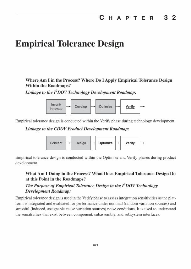
C H A P T E R 3 2
Empirical Tolerance Design
Where Am I in the Process? Where Do I Apply Empirical Tolerance DesignWithin the Roadmaps?
Linkage to the I2DOV Technology Development Roadmap:
Empirical tolerance design is conducted within the Verify phase during technology development.
Linkage to the CDOV Product Development Roadmap:
Empirical tolerance design is conducted within the Optimize and Verify phases during productdevelopment.
What Am I Doing in the Process? What Does Empirical Tolerance Design Doat this Point in the Roadmaps?
The Purpose of Empirical Tolerance Design in the I2DOV TechnologyDevelopment Roadmap:
Empirical tolerance design is used in the Verify phase to assess integration sensitivities as the plat-form is integrated and evaluated for performance under nominal (random variation sources) andstressful (induced, assignable cause variation sources) noise conditions. It is used to understandthe sensitivities that exist between component, subassembly, and subsystem interfaces.
Concept Design Optimize Verify
Invent/Innovate
Develop Optimize Verify
671

The Purpose of Empirical Tolerance Design in the CDOV ProductDevelopment Roadmap:
Empirical tolerance design is used in the Optimize phase to analyze and balance system-to-subsystem interface sensitivities. It is also used to understand the sensitivities that exist be-tween component, subassembly, and subsystem interfaces.
It is used during the Capability Verify phase to assess remaining integration sensitivity is-sues as the final product design certification units are evaluated for performance under nominal(random variation sources) and stressful (induced, assignable cause variation sources) noise conditions.
What Output Do I Get at the Conclusion of Empirical Tolerance Design?What Are Key Deliverables from Empirical Tolerance Design from itsApplication in the Roadmaps?
• Optimized critical functional parameter set points that control subsystem andsubassembly contributions to system level functional and assembly variation
• Optimized critical adjustment parameter tolerances used to tune the mean value of thesystem, subsystem, and subassembly critical functional response(s)
• Optimized critical-to-function specification set points that control componentcontributions to functional and assembly variation
• Critical Parameter Management data that is documented in the CPM relationaldatabase:System level variance modelsSubsystem level variance modelsSubassembly level variance modelsComponent level variance modelsManufacturing process level variance modelsCFP tolerances and their percentage contribution to CFR variationCAP tolerances and their percentage contribution to CFR variationCTF spec tolerances and their percentage contribution to CFR variation
The Empirical Tolerance Design Flow Diagram (found on page 673)
The visual reference illustrates the flow of the detailed steps of the empirical tolerance designprocess.
Verbal Descriptions for the Application of Each Block Diagram
This section explains the specific details of each step in the empirical tolerance design process:
• Key detailed input(s) from preceding tools and best practices• Specific steps and deliverables from each step to the next within the process flow• Final detailed outputs that flow into follow-on tools and best practices
672 Chapter 32

INPUT . . .
OUTPUT . . .
S/N and mean plots fromrobust design process, initialtolerance set point estimates
from analytical tolerancedesign, and distribution data
from the supply chain.
Optimized tolerances based on reducedstandard deviations for the components.
Define the engineering design ormanufacturing process
parameters to be evaluated.
Develop the quality lossfunction for the output
response.
Define the manufacturing orassembly standard deviation
(1s) above and below themean set point for eachcritical parameter under
evaluation.
Select an appropriateorthogonal array with enough
degrees of freedom tofacilitate the proper evaluationof the effect of the 1 standarddeviation set points for eachparameter on the measured
output response.
Align the appropriatecompounded noise factorswith the orthogonal array
experiment.
Set up and run the designedexperiment.
Conduct a formal analysis of variance onthe data using Minitab.
Calculate the total quality loss for thebaseline design.
Quantify the quality loss due to eachparameter in the baseline design.
Calculate the percentage each parametercontributes to the overall variability in the
output response.
Calculate the process capability (Cp) forthe design.
Construct the variance equation.
Use the new, lower parameter variancevalues in the loss function to calculate the
new, lower loss values.
Meet with the manufacturing engineersresponsible for the production processesthat make the components to define theincrease in component costs associated
with the reduction in each parametervariance (s2).
Calculate the new Cp from the customertolerance limits and the new standarddeviation coming from the upgradeddesign data (using the new ANOVA
values) from the verification experiment.
Obtain the new, upgraded componentsand rerun the parameters in the
orthogonal array experiment at the newstandard deviation limits as defined by the
reduction in parameter variances.
673

Key Detailed Inputs
Results from robust design, analytical tolerancing, and manufacturing process capability studieson component variability provide the necessary inputs for empirical tolerance design.
Measurement system analysis must be applied to the data acquisition system to assure thedata is low in measurement system noise.
Specific Steps and Deliverables
The team must review the signal-to-noise, standard deviation, and mean plots from robust design.These will indicate which CFPs and CTF specifications have high sensitivity (large slopes) interms of S/N and mean responses. Parameters that have high sensitivity to both mean and S/N aregood candidates for tolerance tightening. This is so because when small changes in the CFP orCTF specifications are induced, the mean and standard deviation of the CFR are strongly affected.
Parameters that are known to have a small effect on the CFR mean, S/N, and standard de-viation will not deliver useful results when attempting to reduce CFR variability through toler-ance design methods.
S/N σ
Mea
n
S/N σ
Mea
n
Define the engineering design or manufacturing process parameters to be evaluated.
S/N and mean plots from robust design process, initial tolerance set point estimates from analytical tolerance design, and distribution data from the supply chain.
674 Chapter 32

Parameters that exhibit this mild behavior are not good candidates for tolerance design.
To properly account for balancing cost and economical loss associated with performance varia-tion, the team needs to develop the quality loss function for the CFR.
where $ Loss(y) is the dollars lost due to the CFR (y) being off target due to two reasons:
1. Variation (2) about a local mean (yavg) that reduces short-term capability (Cp)2. Variation of the local mean (yavg) away from the desired target that reduces long-term
capability (Cpk)
The economic side of the loss function is embodied in the economic coefficient (k).
This coefficient is developed by two parameters:
1. (A0) is the term for dollars lost due to the variance and mean growing to a level wherea fail-to-satisfy level of CFR performance is reached.
2. 20 is the fail-to-satisfy tolerance range (VOC tolerance limits: USL and LSL values
for a reasonable percentage of customers).
The current state of affairs in loss function development is that most financial managers aresuspicious and unsure that it should be trusted to make significant business decisions. This is be-cause the term (A0) contains “soft” numbers mixed with “hard” numbers. Hard numbers includescrap, rework, cost of poor quality, and warranty dollars. The soft numbers include loss of busi-ness due to lost market share, customer dollar loss due to off-target performance, and repair or re-placement costs. These soft numbers are recognized by financial professionals, but their accuracyis a matter of concern. It is not easy or simple to build accurate soft numbers for estimating (A0).The best we can advise is to invest the time to quantify (A0) for critical functional responses thatare real economic drivers in the product.
Define the manufacturing or assembly standard deviation (1s) above and below the mean set point for each critical parameter under evaluation.
k = A0¢20
$ Loss(y) = k[2 + (yavg - Target)2]
Develop the quality loss function for the output response.
Empirical Tolerance Design 675

With the candidate subsystem and subassembly CFPs and component CTF specifications identi-fied, the team now must determine the variability associated with these x input variables. The goalof the empirical tolerance study is to realistically “wiggle” the critical-to-function x variables andmeasure their percent contribution to the “wiggle” they induce in the Y output variable.
The question to answer is, “How much should each critical input be wiggled?” The answerlies in how the manufacturing process actually puts wiggle in the components. It does so in rec-ognizable patterns over time called distributions. The team must go out and quantify the natureof variation likely to be seen in components by measuring the mean and standard deviation fromdistributions of components that are like the ones being developed. If the components in devel-opment are not in production, the team finds components that have very similar materials, form,and features to stand in as reasonable representations. In this component level case, the standardamount of wiggle we want to induce in an empirical tolerance study is / 1 standard deviation.
If part of our tolerance study includes the adjustment variability associated with a CAP-CFR relationship or critical functional parameter variation from a subassembly or subsystem,then we must estimate what a reasonable amount of expected variation from those input variableswill be. The overriding priority in setting up the wiggle is that it ought to be about one-third ofyour expected worst-case “wiggle” condition. If your UCL and LCL values are equal to 3 stan-dard deviations, then it stands to reason that a reasonable or likely amount of expected variationis 1 standard deviation. This is the basis for root sum of square tolerancing in the previous chap-ter. We are essentially getting ready to run a designed experiment that emulates an RSS toleranceanalysis.
For the purposes of demonstrating how empirical tolerancing is applied to components, we willfocus on the inducement of / 1 variation about the “robust nominals” for these evolving critical-to-function specifications. This means we typically need to select a two-level FractionalFactorial experiment. Often we use a Placket-Burman array to screen through the CTF specs fortheir main effects and (2) values.
The candidate component CTF specs need to be properly loaded into an appropriately sizedorthogonal array (designed experiment). Two issues must be addressed at this point in the process:
Select an appropriate orthogonal array with enough degrees of freedom to facilitate the proper evaluation of the effect of the 1 standard deviation set points for each parameter on the measured output response.
–1σ +1σ
Obtain or makecomponents atthese points
676 Chapter 32

1. Selection of an experiment that has enough degrees of freedom to evaluate the maineffects of the candidate parameters
2. Sizing the experiment to include major interactions between certain CTF specs thatwill play a key role in variance reduction and constraint
Mild interactions that are statistically significant but relatively weak in their contribution(2) to overall variability in the CFR are usually not included in the experiment. This reduces thesize and cost of the experiment without jeopardizing the validity of the results.
The component CTF specs that are being set at their / 1 standard deviation values must beevaluated under the same compounded noise factors that were used during robust design. Thishelps ensure that the unit-to-unit variation noise represented in the component CTF specs beingset at their / 1 standard deviation values are also stressed by external and deteriorative sourcesof variation as well. This helps further the robustness of the design by making sure the tolerancesthat will be derived by the final ANOVA results from the designed experiments are robust.
Once the candidate tolerance control factors are loaded inside the designed experiment and thenoise factors are arranged outside the array in their compounded format, it is time to run the ex-periment and measure the CFR.
Measurement system capability should have been previously confirmed so that noise in thedata due to measuring the CFR is at least 10 times smaller than the magnitude of the CFR differ-ences you are trying to detect.
Figure 32–1 shows what an L12 Placket-Burman Tolerance Experiment might look likewhen saturated (totally loaded) with CTF specs (designated as C):
Please note this is strictly a screening experiment designed specifically to look at main ef-fects only. This is an excellent array to use if you do not have a need to evaluate interactions in atolerance context.
The data from the compounded noise columns from the designed experiment contains the wiggleinformation from the array’s 1s (components at (1) levels) and 2s (components at (1) lev-els) plus the effects of the assignable cause variation embedded in the compounded noise factors.
Conduct a formal analysis of variance on the data using Minitab.
Set up and run the designed experiment.
Align the appropriate compounded noise factors with the orthogonal array experiment.
Empirical Tolerance Design 677

The compounded noise variables data needs to be averaged prior to application of the ANOVAprocess.
The ANOVA table will provide a wealth of information that can be used to determine thefollowing information:
1. Each [SSfactor/ SSTotal] 100 2factor (percent contribution of the tolerance control
factor to total variation of the CFR, or epsilon squared)2. Each [SSfactor/ dofTotal] 2
factor (variance contribution of the tolerance control factoras part of the total variation of the CFR for 2 level experiments only!)
3. The total variance value for the CFR under evaluation [SSTotal/dofTotal] 2Total (the
sum of all the tolerance control factor variances will equal this total variance of theCFR for 2 level experiments only!)
Note: This technique applies to the output from an ANOVA table that is the result of a 2level factorial designed experiment with the replicated data averaged (such as the data for eachcompounded noise factor). It will provide information about differences between the main ef-fects. Weak main effects are pooled to represent the error variance.
Calculate the total quality loss for the baseline design.
678 Chapter 32
1
Candidate Tolerance Control Factors…
NoiseFactors
CA CB CC CD CE CF CG CH CI CJ CK N1 N2
2
1 1 1 1 1 1 1 1 1 1 1
3
1 1 1 1 1 2 2 2 2 2 2
4
1 2 2 2 2 1 1 1 2 2 2
5
1 2 1 2 2 1 2 2 1 1 2
6
1 1 2 1 2 2 1 2 1 2 1
7
1 1 2 2 1 2 2 1 2 1 1
8
2 2 2 2 1 1 2 2 1 2 1
9
2 2 2 1 2 2 2 1 1 1 2
10
2 1 1 2 2 2 1 2 2 1 1
11
2 1 2 1 1 1 1 2 2 1 2
12
2 2 1 2 1 2 1 1 1 2 2
L12
2 2 1 1 2 1 2 1 2 2 1
Figure 32–1 The L12 Array with Compounded Noise Factors (N1 and N2)

The quality loss function can easily be calculated for the CFR by using the total variance (2
Total) from the ANOVA data.Assuming we can adjust the mean onto the target using a critical adjustment parameter, the
loss function for a nominal best case is:
This is the baseline loss of the design prior to adjusting the loss by reducing variability inthe tolerance control factors.
The quality loss contribution due to each tolerance control parameter is calculated as follows:
The total quality loss is therefore
Each parameter contributes its own specific dollar loss due to the magnitude of its variancecontribution. This dollar amount will be used to balance the cost to reduce the baseline variancevs. the cost to lower the variance to a new level.
Each parameter can have its specific percent contribution to total variation in the CFR calculatedby using the following information from the ANOVA table.
This equation represents the percent contribution of the tolerance control factor to totalvariation of the CFR. This helps the team see which parameters are causing the most variation inthe CFR. This further identifies which parameters are critical to function. Parameters that haveweak epsilon squared values are good candidates for tolerance loosening. When a tolerance can
[SSfactorSSTotal] * 100 = e2factor
Calculate the percentage each parameter contributes to the overall variability in the output response.
$ Loss(y) = k[2factor A + 2
factor B + p + 2factor n]
$ Loss(y) = k[2factor]
Quantify the quality loss due to each parameter in the baseline design.
$ Loss(y) = k[2Total]
$ Loss(y) = k[2 + 0]
$ Loss(y) = k[2 + (yavg - Target)2]
Empirical Tolerance Design 679

be relaxed, often its cost can be lowered. These cost savings can be used to help offset the cost ofthe tolerance tightening that will soon occur on the parameters with high epsilon squared values.This is part of the cost balancing that is done in the Optimize and Verify phases of the CDOVprocess.
The ANOVA data provides the SSTotal and the dofTotal, which are needed to calculate the total vari-ance for the CFR.
Taking the square root of the variance provides the standard deviation (2Total) for the CFR. This
can be used, in conjunction with the USL and LSL, to calculate the design performance capability.
This is not the capability under random conditions but rather the capability when unit-to-unit, external, and deterioration noises (assignable cause variation) are intentionally being in-duced at realistic levels. It is wise to measure design CFRs for capability with and withoutassignable cause variation. The goals are for CFRs to attain a Cp 2 without noise (under nom-inal, random conditions) and a minimum Cp 1 with assignable cause noise “turned on.” It isup to each program management team to decide what the acceptable value of Cp with noise is go-ing to be. Typical values range between Cp 1 1.33.
At this point the Cp index for the CFR, under stressful noise conditions, has been calculated andcompared to a desired goal (Cp 1). If the Cp value is less than 1, then corrective action mustbe taken.
The metric used to guide corrective action is the individual component variance. A varianceequation can be constructed from the individual component variances and can be solved to cal-culate a new, lower overall variance for the CFR. The variance equation is used to balance vari-ance reductions across the candidate tolerance control factors.
We must add two factors to the variance equation to help us in the balancing of the overallCFR variation (2
Total). The first factor that must be included in the equation is the epsilonsquared (2
factor) terms for each significant tolerance control factor.
2Total = [2
factor A + 2factor B + p + 2
factor n]
Construct the variance equation.
Cp = [(USL - LSL)62Total]
[SSTotaldofTotal] = 2Total
Calculate the process capability (Cp) for the design.
680 Chapter 32

We need to include just one more term that is new to the process. The variance adjustmentfactor (VAF) is the decimal value of reduction for each tolerance control factor. It is always a dec-imal value less than 1 and greater than 0.
Now we have the current variance, its percent contribution to overall variation, and theamount of variance reduction required to meet the overall variance reduction requirement.
The team can set a Cp goal and then back-calculate the variance adjustment factors throughan iterative process. For a Cp goal of 1, we would set up the equations as follows:
Total USL LSL/6. . . .
Squaring (Total), we establish the new variance target (2Total) for the CFR. Now each in-
dividual variance can be adjusted according to whatever is economically and physically reason-able. This goal must be carefully attained through iterative balancing across all of the significanttolerance control factors.
Each tolerance control factor has a new variance calculated for it based on discussions with rep-resentatives from the supply chain. The team can try to allocate the reduced variance values, butit is wise to seek the input of the people who are actually going to be responsible for consistentlydelivering the components with the reduced variances.
Return to the quality loss function equation and recalculate the new, reduced componentloss values using the reduced variance values. These new loss values can be added to establishthe new total loss value due to the new 1 values that have been reduced from the original 1 val-ues. The reduction in loss will be proportional to the aggregated reduction in the variances toreach the desired Cp value of 1.
Now it is time to “get real” and find out if our suppliers can provide the reduced variances and atwhat cost. This is where negotiations and trade-offs will cause several iterations to balance the
Meet with the manufacturing engineers responsible for the production processes that make the components to define the increase in component costs associated with the reduction in each parameter variance (s2).
Use the new, lower parameter variance values in the loss function to calculate the new, lower loss values.
2Total = [(VAF2) * 2
factor A * (e2factor A)] + p + [(VAF2) * 2
factor n * (e2factor n)]
2Total = [2
factor A * (e2factor A) + p 2
factor n * (e2factor n)]
Empirical Tolerance Design 681

variance equation. Each component cost increase must be compared to the quality loss value for the component to see if it is worth the expense. It is not uncommon for a ratio of 50–100:1 ofloss reduction to cost increase. It all depends on the specific costs and losses that confront us inthis case.
For component costs that are reasonably low in comparison to the quality loss reduction, adecision is made to proceed with the expense. For cases where the cost to reduce variation is highor even exceeds the quality loss reduction, we do not proceed with that variance reduction. We it-erate through all the statistically significant tolerance control factors until we reduce variance ofthe CFR while controlling our costs for the reductions. This can become quite a challenging bal-ancing act!
For factors that are found to be statistically insignificant and that have low epsilon squaredvalues, we consider loosening their current tolerances and use those cost savings to help pay forthe tighter tolerances on the CTF specifications.
Once the balancing process is completed and the new costs are in alignment with our cost vs. qual-ity loss reduction goals, it is time to obtain samples of the new component / 1 values. Theseare new components at the reduced variance levels after the organization has agreed to and paidfor their new, lower variances (as reflected in the / 1 values).
If the components (at / 1) cannot be obtained by part sorting from a productionprocess, then the parts must be made “off-process” as close to the production materials, surfacefinishes, and geometric dimensions as possible.
The original designed experiment can then be rerun at the new, reduced, / 1 set pointswith the same compounded noises.
The ANOVA data allow us to recalculate the quality loss values, the component variances, the ep-silon squared values, and, of most importance, the new Cp index. This verification experimentshould validate that the new, retoleranced components are constraining variation and producingthe desired Cp performance even in the presence of stressful sources of “assignable cause varia-tion.” Now, the team has balanced cost and functional performance in what we hope will be a win-win situation for the organization and our customers. A complete example of this process is foundin Chapter 17 of Tolerance Design (Creveling, 1997).
Calculate the new Cp from the customer tolerance limits and the new standard deviation coming from the upgraded design data (using the new ANOVA values) from the verification experiment.
Obtain the new, upgraded components and rerun the parameters in the orthogonal array experiment at the new standard deviation limits as defined by the reduction in parameter variances.
682 Chapter 32

Final Detailed Outputs
The output is an ability to calculate tolerances based on reduced component variances that enablethe design to meet its Cp goals under both nominal (random variation) conditions and understressful (assignable cause variation) conditions.
Empirical Tolerance Design Checklist and Scorecard
This suggested format for a checklist can be used by an engineering team to help plan its work andaid in the detailed construction of a PERT or Gantt chart for project management of the empirical tolerance design process within the Optimize phase of the CDOV or I2DOV developmentprocess. These items also serve as a guide to the key items for evaluation within a formal gate review.
Checklist for Empirical Tolerance Design
Was this Action Excellence Rating:Deployed? 1 = Poor
Actions: YES or NO 10 = Excellent
1. Define the engineering design or manufacturing process parameters to be evaluated. ______ ______
2. Develop the quality loss function for the output response. ______ ______
3. Define the manufacturing or assembly standard deviation (1s) above and below the mean set point for each critical parameter under evaluation. ______ ______
4. Select an appropriate orthogonal array with enough degrees of freedom to facilitate the proper evaluation of the effect of the 1 standard deviation set points for each parameter on the measured output response. ______ ______
5. Align the appropriate compounded noise factors with the orthogonal array experiment. ______ ______
6. Set up and run the designed experiment. ______ ______
7. Conduct a formal analysis of variance on the data using Minitab. ______ ______
8. Calculate the total quality loss for the baseline design. ______ ______
9. Quantify the quality loss due to each parameter in the baseline design. ______ ______
10. Calculate the percentage each parameter contributes to the overall variability in the output response. ______ ______
Optimized tolerances based on reducedstandard deviations for the components.
Empirical Tolerance Design 683
(continued)

11. Calculate the process capability (Cp) for the design. ______ ______
12. Construct the variance equation. ______ ______
13. Use the new, lower parameter variance values in the loss function to calculate the new, lower loss values. ______ ______
14. Meet with the manufacturing engineers responsible for the production processes that make the components to define the increase in component costs associated with the reduction in each parameter Variance (s2). ______ ______
15. Obtain the new, upgraded components and rerun the parameters in the orthogonal array experiment at the new standard deviation limits as defined by the reduction in parameter variances. ______ ______
16. Calculate the new Cp from the customer tolerance limits and the new standard deviation coming from the upgraded design data (using the new ANOVAvalues) from the verification experiment. ______ ______
Scorecard for Empirical Tolerance Design
The definition of a good empirical tolerance design scorecard is that it should illustrate in simplebut quantitative terms what gains were attained from the work. This suggested format for a score-card can be used by an engineering team to help document the completeness of its work.
Subsystem, subassembly, or component name: __________
Subsystem, subassembly, or component critical functional response or CTF specification:__________
Specific engineering units of subsystem and subassembly CFRs or component CTF spec:__________
Number of CFPs and CTF specs evaluated for sensitivity: __________
Number of CFPs and CTF specs selected to include in variance model: __________
Number of CFPs and CTF specs selected to adjust CFR capability: __________
Baseline or benchmarked initial subsystem, subassembly, or component CFR or CTF specvariance value: __________
Verified optimal subsystem, subassembly, or component CFR or CTF spec variance value:__________
Pretolerance design capability (Cp) index for the subsystem, subassembly, or componentCFR or CTF spec: __________
Posttolerance design capability (Cp) index for the subsystem, subassembly, or componentCFR or CTF spec: __________
684 Chapter 32

Table of Critical Tolerance Parameter Set Points:
Critical Tolerance Optimal Nominal Final Tolerance: Final Tolerance: Used for Capability Parameter Name: Set Point: USL LSL Improvement:
1. ______ ______ ______ ______
2. ______ ______ ______ ______
3. ______ ______ ______ ______
Table of Critical CFR Effects:
Affected Magnitude Direction of Effect: % Contribution CFR Name: of Effect: ( or ) F Ratio/Fcrit.: or 2 Value:
______ ______ ______ ______ ______
______ ______ ______ ______ ______
______ ______ ______ ______ ______
We repeat the final deliverables from empirical tolerance design:
• Optimized critical functional parameter set points that control subsystem andsubassembly contributions to system level functional and assembly variation
• Optimized critical adjustment parameter tolerances used to tune the mean value of thesystem, subsystem, and subassembly critical functional response(s)
• Optimized critical-to-function specification set points that control componentcontributions to functional and assembly variation
• Critical Parameter Management data that is documented in the CPM relationaldatabase:System level variance modelsSubsystem level variance modelsSubassembly level variance modelsComponent level variance modelsManufacturing process level variance modelsCFP tolerances and their percentage contribution to CFR variationCAP tolerances and their percentage contribution to CFR variationCTF spec tolerances and their percentage contribution to CFR variation
Reference
Creveling, C. M. (1997). Tolerance design. Reading, MA: Addison Wesley.
Empirical Tolerance Design 685

This page intentionally left blank
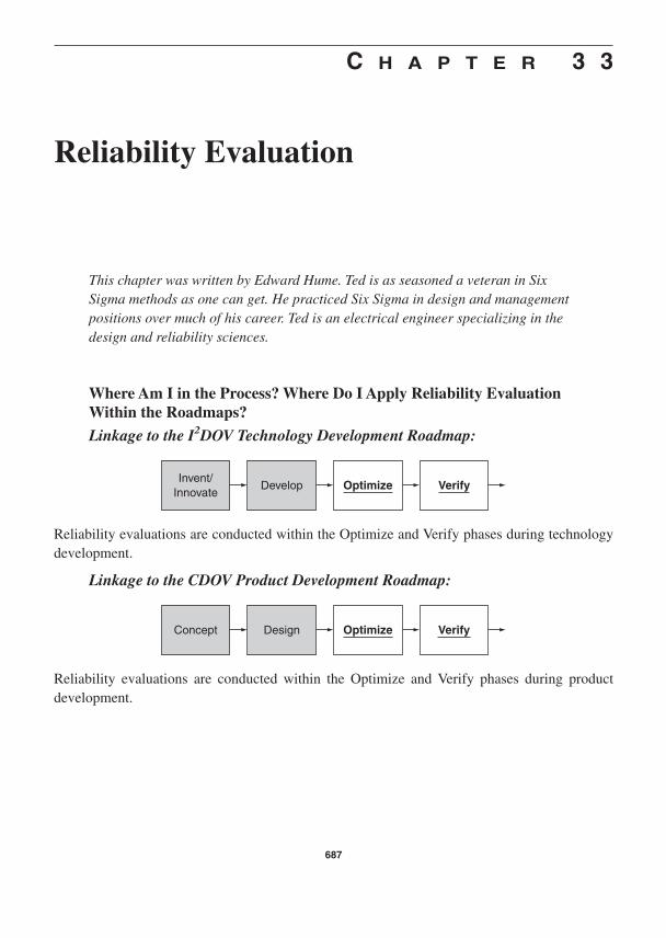
C H A P T E R 3 3
Reliability Evaluation
This chapter was written by Edward Hume. Ted is as seasoned a veteran in SixSigma methods as one can get. He practiced Six Sigma in design and managementpositions over much of his career. Ted is an electrical engineer specializing in thedesign and reliability sciences.
Where Am I in the Process? Where Do I Apply Reliability Evaluation Within the Roadmaps?
Linkage to the I2DOV Technology Development Roadmap:
Reliability evaluations are conducted within the Optimize and Verify phases during technologydevelopment.
Linkage to the CDOV Product Development Roadmap:
Reliability evaluations are conducted within the Optimize and Verify phases during product development.
Concept Design Optimize Verify
Invent/Innovate
Develop Optimize Verify
687
What Am I Doing in the Process? What Does Reliability Evaluation Do atThis Point in the Roadmaps?
The Purpose of Reliability Evaluation in the I2DOV Technology DevelopmentRoadmap:
Reliability evaluation is applied to qualitatively define and quantitatively assess the baseline re-liability of new technology platforms and subsystems being developed for integration into a newplatform or for integration into existing product designs. Preventative application of numeroustools and best practices can then be used to improve reliability, as required, prior to the technol-ogy being transferred into a commercialization program.
The Purpose of Reliability Evaluation in the CDOV Product DevelopmentRoadmap:
Reliability evaluations are first applied to quantify the reliability of subsystems, subassemblies,and components and then applied to the integrated system after robustness optimization of thesubsystems and subassemblies. Preventative application of numerous tools and best practices canalso be used to improve the reliability as required prior to design certification.
What Output Do I Get at the Conclusion of Reliability Evaluations? What AreKey Deliverables from Reliability Evaluations at This Point in the Roadmaps?
• Phase 3B: Measured reliability performance of robust subsystems, subassemblies, andcomponents before and after they are integrated into the system
• Phase 4A: Measured reliability performance of cost balanced product designcertification systems
• Phase 4B: Measured reliability performance of production product systems• Component, subassembly, and subsystem reliability performance
• Predicted reliability vs. measured reliability• Component, subassembly, and subsystem reliability performance improvement
activities• Required deliverables from specific tools and best practices that improve reliability
by reducing variability and sensitivity to deterioration and external noise factors
The Reliability Evaluation Flow Diagram (found on page 689)
The visual description illustrates the flow of the detailed steps of the reliability evaluationprocess.
Detailed Descriptions for the Application of Each Block Diagram
This section explains the specific details of what to do during the reliability evaluation process:
• Key detailed input(s) from preceding tools and best practices• Specific steps and deliverables from each step to the next within the process flow• Final detailed outputs that flow into follow-on tools and best practices
688 Chapter 33

Key Detailed Inputs
These detailed reliability requirements become inputs to defining test requirements:
• Measurable definitions of reliability requirements• Environmental conditions• Governmental agency requirements
These requirements are used to define the type of test, test parameters, sample size, andlength of testing. A detailed test plan is developed and updated throughout the testing process.
Specific Steps and Deliverables
Test to Pass
Customers, regulatory agencies, and company internal documents often specify requirements interms of test to pass. Examples of this are as follows:
• Three relays are to be tested for 100,000 cycles.• Five valves must withstand a 500 pounds per square inch internal pressure.• Ten motors are to be tested for 100,000 hours of operation.
Comparison of test methods: Test to pass and test to failure.
Detailed reliability requirements for system,historic reliability data, and DFMEA inputs.
INPUT . . .
OUTPUT . . .
Detailed reliabilityrequirements for system,
historic reliability data, andDFMEA inputs.
Comparison of testmethods: Test to pass and
test to failure.
Highly accelerated life test(HALT ).
Accelerated life test(ALT ).
Review of acceleration methods:High usage, overstress, degradation,
and censoring.
Reliability evaluation process.
Product meets requirements.
Reliability Evaluation 689

In all cases the products are tested under specified test conditions and must complete thetest without failure.
When are these tests developed and to what purpose? Some of the tests are part of the ini-tial test process developed to ensure product reliability:
• The tests represent an expected design life plus margin.• The tests represent expected stress levels plus margin.
When high failure rates occur in the field, application tests are often added. These new testshave been shown to differentiate between products with high field failures and those that have beenimproved to eliminate the failures. Completing the tests successfully provides a level of confidencethat the product will succeed in its application. As a manufacturer of the product, however, youhave little prior information on the probability of the product passing the test. In addition, you haveno information about the relative performance of two products that pass the test. Relative reliabil-ity provides a credible method of evaluating product even when the correlation to field reliabilityhas not been established. The following are common reasons for product evaluation:
• To evaluate product, material, and process changes• To compare new product to current and competitive products
An exercise that we use in our training is to bend paper clips until they fail. The processused is to open the paper clip up with a 180° bend and then close it with another 180° bend. Each180° bend is counted. The bending process is continued until the clip breaks. This is intended tobe an illustrative process. Suppose our test to pass criteria is that four paper clips must complete11 bends without fail. The following is a set of pass-fail data representing six tests:
As you can see, 92 percent of all the paper clips pass at 11 cycles. However, only 66 percentof the six tests meet our test to pass criterion. After six tests we can see that the paper clips don’tmeet the test to pass requirement, but we ran four tests before finding that out. Suppose the first threetests were part of the development and verification process and the fourth was a part of the final cus-tomer qualification. The most common response to the failure of the fourth test is to launch an ef-fort to find out what has changed in the product or manufacturing process. Little thought is given tothe fact that perhaps nothing has changed and that the failures represent normal variation for theproduct. The bottom line is that testing to pass only provides pass-fail results. No statistics on thetest sample or projections of the population performance are available from this method of testing.
Test 1 P P P PTest 2 P P P PTest 3 P P P PTest 4 P P P FTest 5 F P P PTest 6 P P P P
690 Chapter 33

Many part qualification, design verification, and production validation tests combine capa-bility and reliability/durability tests where the entire set of tests is specified in terms of a test topass. This type of qualification testing is also devoid of statistical thinking. As the complexity in-creases, so does the need for statistical thinking.
Test to Pass Tool Summary
Limitations
• Probability of success is not known for individual tests or for combinations of tests.• Relative performance of products that pass the test is not known.
Benefits
• Passing the test provides a level of confidence that the product will succeed in itsapplication.
Recommendations
• If tests are driven by external test requirements, continue testing beyond passrequirements until enough failures have occurred to establish the probability of success.
• If tests are internal, over time find new statistically based tests to accomplish theintended results.
Test to Failure
Customers, regulatory agencies, and company internal documents also specify reliability in sta-tistical terms. Examples of this are as follows:
• Demonstrate that the relay will have less than 1 percent failures at 20,000 cycles andless than 10 percent failures at 100,000 cycles with 90 percent confidence.
• Demonstrate that the valve will have less than 1 percent failures, due to damage fromthe overpressure, at 500 pounds per square inch pressure with 90 percent confidence.
• Demonstrate that the motor will have less than 1 percent failures at 30,000 cycles andless than 5 percent failures at 100,000 cycles with 95 percent confidence.
We can use the algorithms in Minitab to fit our data with a distribution and predict relia-bility performance just as we did in Chapter 20, Reliability Prediction. The three-step process isrepeated as follows:
1. Fit a known distribution to the data.2. Review the shape of statistical functions f(t), R(t), and h(t), and observe the distribu-
tion parameters.3. Project B1, 10,. . .(1 percent, 10 percent failures), life (months, years, miles), and proj-
ect reliability/survival probabilities at times such as 10 years, 100,000 miles, and so on.
Reliability Evaluation 691

We will use the data from our paper clip experiment again, this time in parametric form, todemonstrate the process. Our specification will be less than 1 percent failures at 9 bends and lessthan 10 percent failures at 11 bends with 90 percent confidence.
Step 1. Fit a known distribution to the data. We will use the first three tests, including 12paper clips, for our initial data set. Open Minitab and enter time to failure for the first 12 paperclips into one column labeled “Paper Clip-I”. The sample data follow:
Using pull-down menus, follow this path: Stat, Reliability/Survival, Distribution ID Plot-Right Cens. Load “Paper Clip-I” into the dialog box and run the program. Graphical results show-ing the best fit are shown in Figure 33–1.
We pick the lognormal distribution because it has the lowest Anderson Darling number andthe best visual fit.
Step 2. Review the shape of statistical functions f(t), R(t), and h(t). Follow this path: Stat,Reliability/Survival, DistributionOverview Plot-Right Cens. Load “Paper Clip-I” into the dialogbox and select the lognormal distribution. Graphical results are shown in Figure 33–2.
Test 1 15 26 14 12Test 2 13 16 13 21Test 3 16 12 16 14Test 4 15 16 15 10Test 5 10 16 15 14Test 6 18 17 16 14
692 Chapter 33
99959080706050403020
10
532
1
9897
90
807060503010
95
99
95
80706050403020
105
1
99
99
95
80706050403020
10
1
5
10
0 10 20 30 40 50 60 70 5 15 25
Weibull
Exponential
Lognormal base e
ML Estimates - Complete Data
Anderson-Darling (adj)
Weibull
1.781
Lognormal base e
1.464
Exponential
4.061
Normal
1.772
Normal
100 10
Per
cen
t
15 20 25
Per
cen
t
Per
cen
t
Per
cen
t
Figure 33–1 Four-Way Probability Plot for Paper Clip-I

The DistributionOverview Plot-Right Cens. has a Hazard Function, h(t), that represents awear-out condition.
Let’s predict reliability performance and compare it to requirements.
Step 3. Using pull-down menus, follow this path: Stat, Reliability/Survival, ParametricDist Analysis Plot-Right Cens. Load “Paper Clip-I” into the dialog box and select the lognormaldistribution. Select the Estimate button and enter into:
• Estimate survival probabilities for these times (value): 11 bends• Confidence Level: 90• Confidence Intervals: Lower
Tabular data from the session window follow:
Table of Percentiles
Percent Percentile Standard Error 90.0% Normal Bound Lower
1 9.1746 1.1157 7.8506
10 11.5314 .9831 10.3379
Reliability Evaluation 693
0.10
0.05
0.00
1.0
0.9
0.8
0.7
0.6
0.5
0.4
0.3
0.2
0.1
0.0
0.4
0.3
0.2
0.1
0.0
0.5
99
9590
80706050403020
10
1
5
10 15 20 25
10 15 20 25 10 15 20 25
Probability Density Function
Survival Function
Lognormal base e Probability
ML Estimates - Complete Data
Location 2.7255Scale 0.2188MTTF 15.634Failure 12Censor 0
Goodness of FitAD* 1.464
Hazard Function
10
Per
cen
t
15 20 25
Rat
e
Pro
bab
ility
Figure 33–2 Overview Plot for Paper Clip-I

A summary of performance vs. specification for 12 paper clips:
Nominal Number Lower 90% Confidence % Failures of Bends Limit Number of Bends
Specification 1% 9.0
Performance 1% 9.2 7.9
Specification 10% 11.0
Performance 10% 11.5 10.3
Return to Minitab and enter time to failure for all 24 paper clips into one column labeled“Paper Clip”. Lognormal is still the best distribution, and the following is the output from Para-metric Dist Analysis Plot-Right Cens.
Table of Percentiles
Percent Percentile Standard Error 90.0% Normal Bound Lower
1 9.2912 0.7362 8.3941
10 11.4700 0.6371 10.6819
A summary of performance vs. specification for 24 paper clips:
Nominal Number Lower 90% Confidence % Failures of Bends Limit Number of Bends
Specification 1% 9.0
Performance 1% 9.3 8.4
Specification 10% 11.0
Performance 10% 11.5 10.7
What Have We Learned?
• Our testing required only 12 paper clips to get a good estimate of population reliability.• Testing with 24 clips only serves to reduce the standard error and thus lower the
confidence limit spread.
Since the nominal performance is above specification, it is possible to test additional clipsuntil the lower confidence limit equals the specification. Using the nominal bends, 90 percentlower confidence requirement, and the standard error, you can estimate the sample size requiredto bring the lower confidence limit into specification. For the 1 percent specification it would re-quire a total sample size on the order of 300, and for the 10 percent specification it would requirea total sample size on the order of 100. Given that the margin is low and any change in materialor process could easily move the performance below specification, it would make sense not to
694 Chapter 33

continue testing but rather to improve the paper clip’s margin to specification. We have learned alot more about margin to specifications and can draw conclusions on how to proceed based ontesting 12 clips to failure.
If the specification that four paper clips must pass 11 cycles with no failures, defined pre-viously in “Test to Pass,” is an external requirement, you can use Minitab to determine the prob-ability of survival for the test. Tabular survival probabilities from the session window follow:
Table of Survival Probabilities
95.0% Normal CI
Time Probability Lower Upper
11.0000 0.9236 0.6716 0.9921
Nominal survival probability of four paper clips tested to pass is (0.9236)4 .73. The prob-ability of passing the test is 73 percent. Stated another way, one of four tests is expected to fail.Again we draw the same conclusion, that the product or process needs to be improved. With thisanalysis there is no hunt for what changed in the product or manufacturing process to cause thefailures. The cause is inherent in the nominal design.
This analysis can be expanded to predict the probabilities of part qualification, design ver-ification, and production validation tests that consist of a number of different capability and reli-ability/durability tests, all requiring zero failures. Treat all of the tests as series elements in areliability block diagram as described in Chapter 20. For the capability tests, collect parametricdata and calculate the probability of passing at specification limits. For reliability/durability tests,test to failure and calculate reliability/survival probabilities at the test limits. Multiply all the pass-ing and survival probabilities to get the probability of passing the qualification, verification, orvalidation test. This process will also highlight the weaknesses in product performance.
Test to Failure Tool Summary
Limitations
• The analysis is intended for one failure mode per data set.
Benefits
• Test to failure moves reliability from the black and white world of test to pass into thereal world with uncertainty managed by statistics.
• Probability of success is known for individual tests or for combinations of tests.• Relative performance of products that are tested can be used for benchmarking
purposes.
Recommendations
• Use test to failure and statistical analysis whenever possible.
Reliability Evaluation 695

You have heard the phrase that a chain is only as strong as its weakest link. HALT is intended tofind the weak links in the design and manufacturing process in a short period of time. Developedby Dr. Greg Hobbs (2000), it provides a unique approach to reliability growth. To find the weaklinks HALT uses every stimulus and combination of stimuli of potential value. Some examplesof stimuli are as follows:
Stress levels are stepped well beyond expected environmental conditions until the fundamentallimits of the product technology or environmental equipment are reached. An example of fundamental limits of technology would be the temperature at which a plastic structure starts tolose its strength. During the process we find operating and destruct limits for temperature andvibration. In addition, a number of failures occur that represent the weak links in the product.The goal is to find and fix all the weak links. They represent weaknesses in the product that arelikely to become failures in its application. The following is an example of a HALT process andsummary of HALT test data. The information is from Summary of HALT and HASS Results atan Accelerated Reliability Test Center and QualMark Corporation training. QualMark special-izes in HALT.
Halt Process
1. Temperature stressa. Cold step stress—Start at 20°C and step in 10°C increments to determine operating
and destruct limits.b. Hot step stress—Start at 20°C and follow same process.
2. Vibration step stress—Start at 3–5 Grms and increase in 3–5 Grm steps until operatingand destruct limits are determined. When possible, modifications are made to the prod-uct to extend the limits.
Destruct Margin
LowerDestruct
Limit
LowerOperating
Limit
UpperOperating
Limit
UpperDestruct
Limit
ProductSpecs
OperatingMargin
Destruct Margin
OperatingMargin
Vibration Temperature Temperature Cycling
Voltage Voltage Cycling Humidity
Highly accelerated life test (HALT).
696 Chapter 33

3. Rapid temperature transitions—Continuously ramp between hot and cold temperaturelimits as fast as the chamber and product will allow. Temperature limits set just belowoperating limits.
4. Combined environment—Test 30-minute temperature profiles with 10-minute dwelltimes at temperatures close to operating limits. Vibration starts at 3–5 Grms during thefirst profile and increases 5–10 Grms in each subsequent profile.
Results2: 47 different products, used in environments from office to airplane, have operat-ing and destruct limits that are summarized in the following table.
As you can see, the range in operating and destruct limits is large. Much of the differenceis due to the products’ different environmental requirements. The differences in operating and de-struct limits, however, provide credible evidence that HALT can differentiate between differentproducts’ expected reliability.
A Pareto analysis of failure modes caused by HALT testing is listed in the following table:
The types of failures found reflect typical field failures. There may be a bias in favor ofthose failures that occur in harsher environments, but not always. Results should prove valid foroffice environments as well.
HALT Tool Summary
Limitations
• Results do not correlate directly with field reliability specifications.• Most experience with HALT is with electronic products.
Failure Mode Qty
Troubleshooting in progress 85Broken lead 53Failed component, cause unknown 24Component fell off (nonsoldered) 9Screws backed out 9Circuit design issue 8Connector backed out 5Tolerance issue 4Broken component 4
HALT Limits
Attribute Thermal Data, °C Vibration Data, Grms
LOL LDL UOL UDL VOL VDL
Average 55 73 93 107 61 65Most Robust 100 100 200 200 215 215Least Robust 15 20 40 40 5 20Median 55 80 90 110 50 52
Reliability Evaluation 697

Benefits
• Short cycle of learning• Low effort to perform the test• Failure modes identified that are caused by interactions between temperature and
vibration stresses
Recommendations
• Use to identify weaknesses in new products, especially when the technology is new tothe company.
• Use to provide a quick reliability estimate by comparing HALT results to those ofknown internal and/or competitor products.
ALT is a test process using acceleration factors to cause product failures in a shorter time thanseen in actual field conditions. It is intended to be an accelerated simulation of field performance.The investment in time and resources to set up and run an ALT program is significant, and a goodsystem to collect field failure data is required. Be prepared to stick with the program for a periodof years before it becomes successful. ALT entails a nine-step process:
1. Review current field and test failure data on similar products.2. Identify all potential failure modes and causes in the products that you are to test.3. Select a comprehensive set of stresses that are significant in causing failures.4. Select high usage and overstress acceleration factors.5. Develop a test that incorporates all significant stresses and planned acceleration factors.6. Run the test with similar products with current field failure information.7. Monitor the test for failures on a real-time basis if possible.8. Do a root cause analysis of each failure.9. Correlate test and field failures to see if they fit the same distribution and have the same
slope on their probability plot (Minitab’s parametric distribution analysis) and thesame distribution of failure modes.a. If the reliability functions and distribution of failure modes are similar, calculate the
acceleration factor.b. If the reliability functions and/or distribution of failure modes are different, then re-
turn to step 5 to modify the test parameters to resolve the differences.
An accelerated life test process provides timely feedback on reliability for newly developedproducts and modified products. Timely feedback allows problems to be identified and fixed dur-ing the Optimize phase and to verify performance during the Verify phase. The ALT process needsto be updated continuously to take into account new failure modes, new environmental condi-tions, new technology, and improving reliability.
Accelerated life test (ALT).
698 Chapter 33

ALT Tool Summary
Limitations
• ALT requires significant resources over a number of years to be able to use internaltesting to predict field reliability.
Benefits
• Relative performance of products that are tested can be used for benchmarking purposes.• Timely feedback on projected field reliability provides the feedback necessary to make
significant improvements in reliability.
Recommendations
• Make the investment to develop an ALT program if reliability is an important customerneed.
• Use ALT to do internal and industry comparisons to establish relative reliability.• Use ALT as a tool to drive reliability improvement.• Update the ALT process to take into account changes in technology and environmental
requirements.• Update the ALT process to increase acceleration as product performance improves.
Acceleration factors are used to shorten the time required to predict field reliability. Eachof these factors is distinctly different in approach, but all accomplish the same result: shortenedtest time.
High Usage
High usage is the easiest and most predictable method to reduce test time. It involves either in-creased speed or reduced off-time without actually changing other operating conditions thatwould result in a stress increase.
Increased speed examples
• Run bearings faster.• Increase the rate of relay closures.• Increase frequency of the AC voltage applied when testing insulation electrical
breakdown.
Reduced off-time example
• Appliances that typically only run a few hours a day are run 24 hours a day.
Review of acceleration methods: High usage,overstress, degradation, and censoring.
Reliability Evaluation 699

In both cases the acceleration factor new speed/original speed, or new on-time/originalon-time. Since high usage reduces test time without changing stress levels it should be used to theextent possible in all cases of accelerated life testing.
Overstress
The product is run at higher-than-normal levels of accelerating stress(es) to shorten product life.Typical accelerating stresses are temperature, voltage, mechanical load, temperature cycling, hu-midity, and vibration. We can apply stresses in a number of ways, as shown in Figure 33–3. Con-stant and cyclic stresses are the most common methods used with accelerated life testing. Stepstress or progressive stress methods are used with HALT testing.
Our intent with accelerated life testing is to simulate field reliability in the shortest periodof time. Increases in stress levels must be done with care to maintain the same failure modes and the same slope of the probability plot. As an example we return to our paper clip, which isexposed to / 30° bends in field operation. We want to accelerate failures by testing at in-creased angles of bend. A fixture is used and the clips are rotated through / 30°, /50°,and /90°, counting the number of rotations it takes for the clip to break. The resulting fail-ure data is shown on the following page.
We will use Minitab’s parametric distribution analysis right-censored algorithm to gener-ate probability plots for all three angles (Figure 33–4). We continue to use lognormal as the dis-tribution to fit the data. Use Minitab’s pull-down menus: Stat, Reliability/Survival, ParametricDist Analysis Plot-Right Cens. Load “Angle Failure Data” and run the algorithm.
Note that the slopes of the lines for 30 and 50 degrees are quite close while the slope for the90 degree line is quite different. This is apparent visually when looking at the curves and also nu-
700 Chapter 33
Constant Stress
Time
Str
ess
Str
ess
Str
ess
Str
ess
Time
Time Time
Step Stress
Cyclic Stress
Progressive Stress
Figure 33–3 Application of Stress Loading

merically when looking at the scale factor. Slope is represented by scale factor with lognormaldistributions and shape factor with Weibull distributions. Output from the session window allowsus to look at 10 percent and 50 percent failure at 30 and 50 degrees to calculate acceleration. Inthis case the acceleration is 2.6 times. With many products it is hard to get large acceleration fac-tors from one overstress condition. Data is presented in the following table.
Reliability Evaluation 701
99
95
90
706050403020
10
5
Per
cen
t
1
10 100
Time to Failure
80
Lognormal base e Distribution - ML Estimates - 95.0% ClComplete Data
305090
Location4.88353.94082.8558
Scale 0.2303 0.2258
0.09745
AD* 0.973 0.8821.54
F/C15/015/015/0
Figure 33–4 Probability Plot for 30–90
Angle 30 Angle 50 Angle 90173.5 47.5 18129.5 69.5 18142.5 69.5 16173.5 34.0 18112.5 44.5 16165.5 40.0 17130.5 72.5 18207.5 62.5 13157.5 49.5 1890.5 53.5 19
111.5 53.5 17101.5 55.5 18102.5 58.5 20119.5 36.5 17117.5 44.5 19
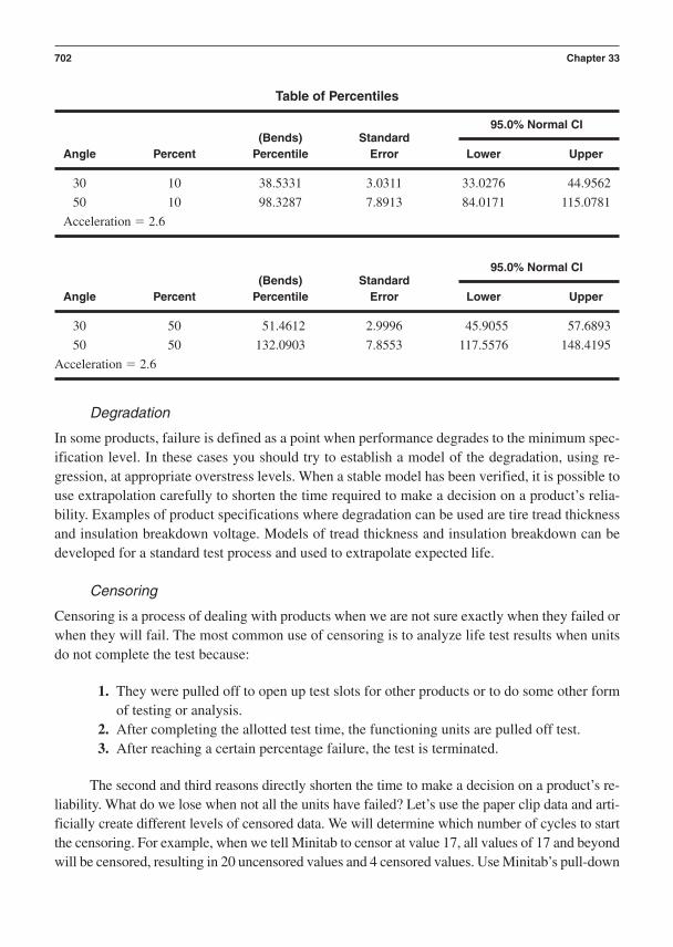
Table of Percentiles
(Bends) Standard95.0% Normal CI
Angle Percent Percentile Error Lower Upper
30 10 38.5331 3.0311 33.0276 44.9562
50 10 98.3287 7.8913 84.0171 115.0781
Acceleration 2.6
(Bends) Standard95.0% Normal CI
Angle Percent Percentile Error Lower Upper
30 50 51.4612 2.9996 45.9055 57.6893
50 50 132.0903 7.8553 117.5576 148.4195
Acceleration 2.6
Degradation
In some products, failure is defined as a point when performance degrades to the minimum spec-ification level. In these cases you should try to establish a model of the degradation, using re-gression, at appropriate overstress levels. When a stable model has been verified, it is possible touse extrapolation carefully to shorten the time required to make a decision on a product’s relia-bility. Examples of product specifications where degradation can be used are tire tread thicknessand insulation breakdown voltage. Models of tread thickness and insulation breakdown can bedeveloped for a standard test process and used to extrapolate expected life.
Censoring
Censoring is a process of dealing with products when we are not sure exactly when they failed orwhen they will fail. The most common use of censoring is to analyze life test results when unitsdo not complete the test because:
1. They were pulled off to open up test slots for other products or to do some other formof testing or analysis.
2. After completing the allotted test time, the functioning units are pulled off test.3. After reaching a certain percentage failure, the test is terminated.
The second and third reasons directly shorten the time to make a decision on a product’s re-liability. What do we lose when not all the units have failed? Let’s use the paper clip data and arti-ficially create different levels of censored data. We will determine which number of cycles to startthe censoring. For example, when we tell Minitab to censor at value 17, all values of 17 and beyondwill be censored, resulting in 20 uncensored values and 4 censored values. Use Minitab’s pull-down
702 Chapter 33

menus: Stat, Reliability/Survival, Parametric Dist Analysis Plot-Right Cens. Load “Paper ClipData.” Select Censor and load the censor value (17, 16) into Censor Value. Run the algorithm.
The results tables and the table of values follow. The tables have been sorted in ascendingorder, and Cs have been added to indicate censoring in this table only. They are not used byMinitab’s algorithm.
Table of Percentiles
Uncensored Right Censored Standard 95.0% Normal CI
Values Values Percent Percentile Error Lower Upper
24 0 10 11.4700 0.6371 10.2869 12.7891
20 4 10 11.2097 0.7453 9.8401 12.7699
14 10 10 11.0462 0.9685 9.3022 13.1173
As you can see, for 10 percent failures the predicted nominal value of bends goes from 10.5to 10 as the number of clips censored goes from 0 to 10. In addition, the 95 percent confidencelimits increase with the number censored. From a practical point of view, results can be analyzed
Paper Clip Data
Censor at 17 Uncensored 20 Censor at 16 Uncensored 14 Cycles to Failure Right Censored 4 Right Censored 10
10 10 1010 10 1012 12 1212 12 1213 13 1313 13 1314 14 1414 14 1414 14 1414 14 1415 15 1515 15 1515 15 1515 15 1516 16 C16 16 C16 16 C16 16 C16 16 C16 16 C17 C C18 C C21 C C26 C C
Reliability Evaluation 703

as additional failures occur and the test can be stopped once an acceptable lower confidence bandhas been reached.
Table of Survival Probabilities
Uncensored Right Censored95.0% Normal CI
Values Values Time Probability Lower Upper
24 0 11.0000 0.9318 0.8181 0.9808
20 4 11.0000 0.9134 0.7850 0.9735
14 10 11.0000 0.9024 0.7660 0.9689
Survival probabilities vary in the same way.
1. Develop a test plan based on detailed inputs:a. Select one or more of the tests that have been described.b. Determine time requirements.c. Develop an initial plan for samples size.
2. Use a control plan and build test units:a. Prototype units should be built with a prototype control plan.b. Pilot units should be built with a start-up control plan.
3. Execute the test plan:a. Complete each of the planned tests.b. Complete a root cause analysis on all failures.c. Project reliability when possible.
4. Evaluate performance to requirements:a. Meets requirements.
i. Document all corrective actions taken.ii. Update reliability models.
iii. Update FMEAs.iv. Document lessons learned.v. Update design rules.
vi. Update scorecards.b. Does not meet requirements.
i. Take corrective actions on the product design or build process.ii. Start the test process over again.
Reliability evaluation process.
704 Chapter 33

Final Detailed Outputs
• Document all corrective actions taken.• Update reliability models.• Update FMEAs.• Document lessons learned.• Update design rules.• Update scorecards.
Reliability Evaluation Checklist and Scorecard
This suggested format for a checklist can be used by an engineering team to help plan its work.The checklist will also aid in the detailed construction of a PERT or Gantt chart for project man-agement of the reliability evaluation process within the Optimize and Verify Phases of the CDOVor I2DOV development process. These items will also serve as a guide to the key items for eval-uation within a formal gate review.
Checklist for Reliability Evaluations
Was this Action Excellence Rating:Deployed? 1 = Poor
Actions: YES or NO 10 = Excellent
1. Comparison of test methods: Test to pass and test to failure. ______ ______
2. Highly accelerated life test (HALT). ______ ______
3. Accelerated life test (ALT). ______ ______
4. Review of acceleration methods: high usage,overstress, degradation, and censoring. ______ ______
5. Reliability evaluation process. ______ ______
6. Document lessons learned ______ ______
7. Update design rules ______ ______
8. FMEAs updated ______ ______
Scorecard for Reliability Evaluations
The definition of a good reliability evaluation scorecard is that it should illustrate in simple butquantitative terms what gains were attained from the work. This suggested format for a scorecardcan be used by an engineering team to help document the completeness of its work:
Product meets requirements.
Reliability Evaluation 705

Table of Documented Reliability Failures and Corrective Actions:
Item/Function Name: Failure Mode: Corrective Action:
1. ______ ______
2. ______ ______
3. ______ ______
We will repeat the final deliverables from reliability evaluations:
• Phase 3B: Measured reliability performance of robust subsystems, subassemblies, andcomponents before and after they are integrated into the system
• Phase 4A: Measured reliability performance of cost balanced product designcertification systems
• Phase 4B: Measured reliability performance of production product systems• Component, subassembly, and subsystem reliability performance
• Predicted reliability vs. measured reliability• Component, subassembly, and subsystem reliability performance improvement
activities• Required deliverables from specific tools and best practices that improve reliability
by reducing variability and sensitivity to deterioration and external noise factors
References
Crowe, D., & Feinberg, A. (2001). Design for reliability. Boca Raton, FL: CRC Press.Hobbs, G. K. (2000). Accelerated reliability engineering. New York: Wiley.Nelson, W. (1983). Vol. 6: How to analyze reliability data. New York: ASQC Quality Press.Nelson, W. (1990). Accelerated testing: Statistical models, test plans and data analyses. New
York: Wiley.
706 Chapter 33
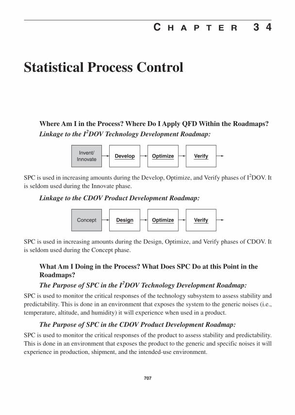
C H A P T E R 3 4
Statistical Process Control
Where Am I in the Process? Where Do I Apply QFD Within the Roadmaps?
Linkage to the I2DOV Technology Development Roadmap:
SPC is used in increasing amounts during the Develop, Optimize, and Verify phases of I2DOV. Itis seldom used during the Innovate phase.
Linkage to the CDOV Product Development Roadmap:
SPC is used in increasing amounts during the Design, Optimize, and Verify phases of CDOV. Itis seldom used during the Concept phase.
What Am I Doing in the Process? What Does SPC Do at this Point in theRoadmaps?
The Purpose of SPC in the I2DOV Technology Development Roadmap:
SPC is used to monitor the critical responses of the technology subsystem to assess stability andpredictability. This is done in an environment that exposes the system to the generic noises (i.e.,temperature, altitude, and humidity) it will experience when used in a product.
The Purpose of SPC in the CDOV Product Development Roadmap:
SPC is used to monitor the critical responses of the product to assess stability and predictability.This is done in an environment that exposes the product to the generic and specific noises it willexperience in production, shipment, and the intended-use environment.
Concept Design Optimize Verify
Invent/Innovate
Develop Optimize Verify
707
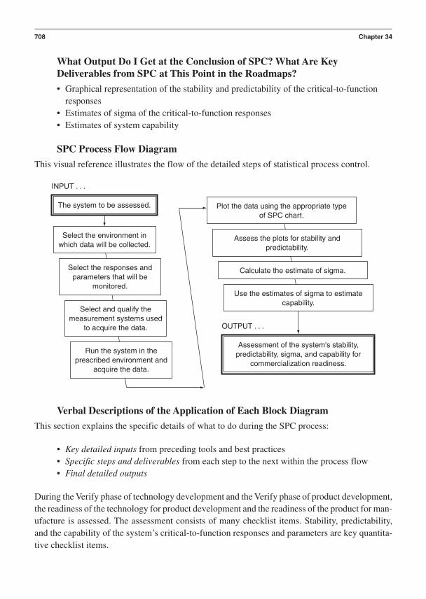
What Output Do I Get at the Conclusion of SPC? What Are KeyDeliverables from SPC at This Point in the Roadmaps?
• Graphical representation of the stability and predictability of the critical-to-functionresponses
• Estimates of sigma of the critical-to-function responses• Estimates of system capability
SPC Process Flow Diagram
This visual reference illustrates the flow of the detailed steps of statistical process control.
Verbal Descriptions of the Application of Each Block Diagram
This section explains the specific details of what to do during the SPC process:
• Key detailed inputs from preceding tools and best practices• Specific steps and deliverables from each step to the next within the process flow• Final detailed outputs
During the Verify phase of technology development and the Verify phase of product development,the readiness of the technology for product development and the readiness of the product for man-ufacture is assessed. The assessment consists of many checklist items. Stability, predictability,and the capability of the system’s critical-to-function responses and parameters are key quantita-tive checklist items.
INPUT . . .
OUTPUT . . .
The system to be assessed.
Select the environment inwhich data will be collected.
Select the responses andparameters that will be
monitored.
Select and qualify themeasurement systems used
to acquire the data.
Run the system in theprescribed environment and
acquire the data.
Plot the data using the appropriate typeof SPC chart.
Assess the plots for stability andpredictability.
Use the estimates of sigma to estimatecapability.
Calculate the estimate of sigma.
Assessment of the system's stability,predictability, sigma, and capability for
commercialization readiness.
708 Chapter 34

Key Detailed Inputs
A system is said to be “in statistical control” when the observed variation is random. This type ofrandom variation is called common cause variation since it is the common, everyday variationthat all systems experience. Common cause variation cannot be eliminated. It can only be reducedand controlled. A system that is not in statistical control exhibits shifts, drifts, and patterns in itsresponses. The means and standard deviations vary over time. This type of variation is called as-signable cause variation since the observed shifts and drifts can be attributed to specific causessuch as changes in input voltage or parameter changes due to changes in temperature.
Stability refers to the statistics of the measured variable over time. The mean, standard de-viation, and distribution remain relatively unchanged when the response is stable.
The product is not safe for product development or manufacture if the mean and standarddeviation of its CTF responses change appreciably in the presence of noise. This is a nonrobustcondition. Shifts and drifts in the mean and standard deviation can easily be seen on an SPC chart.An abrupt upward shift and a gradual upward drift, as shown in the “individual” SPC charts inFigures 34–1 and 34–2, are obvious types of assignable cause variation.
Many types of SPC charts are in use. The two major classes are charts for variables or con-tinuous data and charts for attribute data. In DFSS, we are primarily interested in the charts for
The system to be assessed.
Statistical Process Control 709
8
4
0
UCL = 6.189
Mean = 3.008
LCL = –0.1718
0 50 100 150
Observation Number
I Chart for C3
Ind
ivid
ual
Val
ue
200 250
Figure 34–1 Abrupt Shift in Data: Example of Assignable Cause Variation

continuous data since these are the engineering quantities we manipulate and control. Attributecharts track metrics such as the number of failures and percent pass or reject rates. These laggingindicators of quality measure quantities that are distant from the actual physical functions beingperformed in the system.
This is not to say that attribute charts have no value. They are of tremendous value on themanufacturing floor. They clearly indicate where to allocate a company’s limited resources forprocess improvement activities.
Attribute charts can also be correlated to sources of variation that have affected the product’squality and thereby help in the search for assignable causes. An improvement to attribute charts isthe use of a continuous type of SPC chart to track the system’s continuous CTF responses that wereidentified earlier through CPM. This is still a lagging indicator in that the response is produced af-ter a critical function combines its inputs to form the response. This is an improvement, however,in that these responses are directly tied to the functions being performed in the product.
An even better situation is to use a continuous type of SPC chart to track the continuousCTF parameters that were identified in CPM. These are leading indicators of quality that can beused to predict the response before the function takes place. The transfer functions obtained froma DOE provide the link between the measured quality of the function’s inputs and the unmeasuredquality of the function’s outputs.
We will look at two types of statistical control charts used to chart variables or continuousdata, the Individuals and Moving Range (I&MR) chart and the Xbar&R chart.
Dr. Walter S. Shewhart is credited with proposing the theory of control charts in the 1930s.All SPC charts share a common structure. They display the observations or a function of the
710 Chapter 34
15
10
5
0
0 50
I Chart for drift
Ind
ivid
ual
Val
ue
Observation Number100
UCL = 11.21
Mean = 5.217
LCL = –0.7730
Figure 34–2 Upward Drift in Data: Example of Assignable Cause Variation
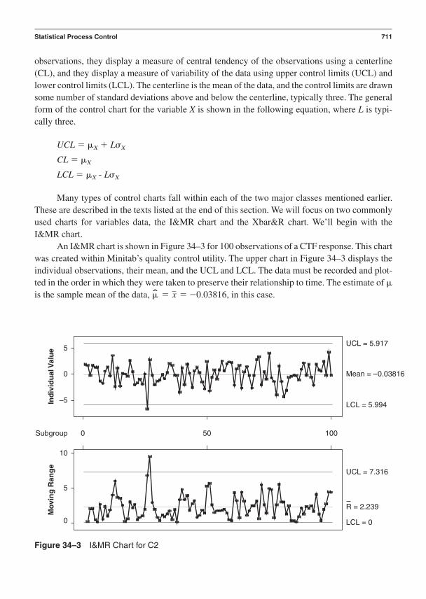
observations, they display a measure of central tendency of the observations using a centerline(CL), and they display a measure of variability of the data using upper control limits (UCL) andlower control limits (LCL). The centerline is the mean of the data, and the control limits are drawnsome number of standard deviations above and below the centerline, typically three. The generalform of the control chart for the variable X is shown in the following equation, where L is typi-cally three.
UCL X LX
CL X
LCL X - LX
Many types of control charts fall within each of the two major classes mentioned earlier.These are described in the texts listed at the end of this section. We will focus on two commonlyused charts for variables data, the I&MR chart and the Xbar&R chart. We’ll begin with the I&MR chart.
An I&MR chart is shown in Figure 34–3 for 100 observations of a CTF response. This chartwas created within Minitab’s quality control utility. The upper chart in Figure 34–3 displays theindividual observations, their mean, and the UCL and LCL. The data must be recorded and plot-ted in the order in which they were taken to preserve their relationship to time. The estimate of is the sample mean of the data, , in this case. = x = -0.03816
Statistical Process Control 711
5UCL = 5.917
Mean = –0.03816
LCL = 5.994
UCL = 7.316
R = 2.239
LCL = 0
0
–5
10
Ind
ivid
ual
Val
ue
Mov
ing
Ran
ge
50 1000Subgroup
5
0
Figure 34–3 I&MR Chart for C2

The estimate of sigma is obtained from the average moving range. A moving range is cre-ated by calculating the difference between the current observation and an observation some dis-tance away from the current observation.
The next observation then becomes current and the difference is calculated again. This isrepeated until the end of the data is reached. Minitab uses a default distance of two for the mov-ing range, but the user can enter a different value. The ith moving range for two successive ob-servations is given in the following equation:
This quantity is calculated for all m moving ranges and the average moving range then iscalculated using this equation:
In the example given, the average moving range is 2.239. This is shown as in the lowerchart in Figure 34–3. The average moving range is a biased estimate of the variation of the re-sponse variable. It must be corrected based on the number of observations used in the movingrange. The correction factor is called d2, and is a lookup value. In this example, there are two ob-servations in each moving range, so d2 1.128. Our estimate of sigma is
The centerline and the 3 sigma UCL and LCL for the individuals chart in Figure 34–3 aregiven in this equation block:
The limits for the moving range chart are found in a manner similar to the individual charts,as shown in this equation:
The average moving range is a biased estimate of the variation of the range of the responsevariable. It must be corrected using two factors, d2 and d3, to obtain an unbiased estimate of the
LCL = MR - 3R
CL = MR
UCL = MR + 3R
LCL = x - 3x = -0.03816 - 3(1.985) = -5.994
CL = x = -0.03816
UCL = x + 3x = -0.03816 + 3(1.985) = 5.917
x =MR
d2=
2.239
1.128= 1.985
R
MR =am
i=1MRi
m
MRi = xi - xi-1
712 Chapter 34

variation in the range. These factors are also found in a lookup table. In this example, there aretwo observations in each moving range, so d2 1.128 and d3 0.853.
Our estimate of sigma is
We can substitute this in to the previous equation block to get the following equation block.
This equation can be simplified if we let
D3 is set to zero if it is less than zero. For a 3 sigma limit chart with a moving range size oftwo, D3 0 and D4 3.267. The range chart centerline and control limits are given in the fol-lowing equation and are shown in Figure 34–3.
The discussion so far has assumed that the response is normally distributed. When this istrue, the probability of observing a response value above, within, or below the control limits canbe determined. The control limits are three standard deviations away from the mean. If the re-sponse is normally distributed, there is a 99.73% chance that an observation will be within thecontrol limits. Therefore, there is a 100% 99.73% 0.27% 0.3% chance that an observa-tion will be outside the control limits. This is a small probability indeed. If observations are seenoutside the limits, it indicates that the statistics of the response are not stable. The mean and/orthe standard deviation are likely to have changed. Therefore, the system is not in control.
However, one observation outside the control limit may not be sufficient to conclude thatthe system is out of control. The probability of an observation being outside the limits is 0.0027,not zero. We expect an observation to be outside the limits for every
1
0.0027= 370.37 observations
LCL = D3MR = 0
CL = MR = 2.239
UCL = D4MR = 3.267(2.239) = 7.315
D4 = ¢ 1 + 3d3
d2≤ and D3 = ¢1 - 3
d3
d2≤
LCL = MR - 3R = MR - 3d3MR
d2= ¢1 - 3
d3
d2≤MR
CL = MR
UCL = MR + 3R = MR + 3d3MR
d2= ¢1 + 3
d3
d2≤MR
R = d3MR
d2=
0.853
1.128MR
Statistical Process Control 713

So, if an individual control chart contains more than 370 observations, we should expect tosee one observation outside the limits, even though the system is in control. Many tests, in addi-tion to being outside the control limits, can be applied to detect out-of-control conditions. Minitabprovides a list of tests that can be selected, shown in Figure 34–4. These tests help determinewhen a system is out of control and when action should be taken to bring the system back intocontrol.
Using the control chart we can graphically observe trends and shifts in the response. We candetermine if the observed variation is just random, common cause variation. If so, no actionshould be taken, assuming the observed mean is on target. We can also determine if the systemhas changed as a result of special cause variation. We can then take action to restore control.
We have assumed normality. If the response is not normally distributed, we can proceed inseveral ways. One approach is to mathematically transform the response so that the transformeddata is normally distributed. The Box-Cox power transformation is a useful transformation whenthe raw data is unimodal (one humped). Another approach is to make use of the central limit theorem.
Recall an implication of the central limit theorem whereby the sum of many nonnormal ran-dom variables tends to be normal. This approach enables the averaging of subsets or groups ofdata that logically belong together. The determination of a logical group is based on the mannerin which the data are produced and the manner in which they are acquired by the measurementsystem. For example, if five observations are made every hour for 20 hours, a grouping of the 100observations into 20 groups of five observations is a logical grouping of the data.
We create an Xbar&R chart by logically grouping the observations, averaging the groupedobservations, determining an estimate of variation of the grouped observations, and then chart-
714 Chapter 34
Figure 34–4 Minitab Tests Window for SPC

ing the centerline and control limits. An Xbar&R chart is shown in Figure 34–5 using the samedata used in the I&MR chart and, in this case, an arbitrarily chosen group size of five.
The Xbar chart plots the average of each group. The centerline is the average of the aver-ages and is . The control limits are determined using the average range . The av-erage range is the average of all the group ranges. A group range is the difference between the maximum observation and the minimum observation within each group. In this example
4.373.The variation must first be corrected, using the standard error of the mean, to account for
the fact that we are using means and not individual observations. The range is a biased estimateof the variation of the response variable.
It must be further corrected using d2 to obtain an unbiased estimate of the variation in theaverage response. In this example, there are five observations in each range, so d2 2.326. Ourestimate of sigma of the mean response is therefore
The centerline and control limits for the Xbar chart are given in this equation:
UCL = x + 3x = x + 3R
d22n= -0.03186 + 3(0.841) = 2.484
x =R
d22n=
4.373
2.32625= 0.841
R
RX = -0.03816
Statistical Process Control 715
3
2
1
0
–1
–2
–3
UCL = 2.484
Mean = 0.03816
LCL = 2.560
UCL = 9.246
R = 4.373
LCL = 0
10
Sam
ple
Mea
nS
amp
le R
ang
e
10 200Subgroup
5
0
Figure 34–5 Xbar&R Chart for C2

The calculation of the centerline and control limits for the R chart are
The previous equation can be simplified if we once again let
In this example, each range is calculated using five observations so d2 2.326 and d3
0.864. Our estimate of sigma is
For a 3 sigma limit chart with a range size of five, D3 0 and D4 2.115. The range chartcenterline and control limits are given in this equation:
These limits are shown in Figure 34–5.If we assume or confirm that the means are normally distributed, there is a 0.27% chance
of the average of five observations being outside the limits. Notice, of course, that the limits aretighter for the Xbar chart than for the individuals. This must be the case since the variation of theaverage is always less than that of the individual observations. Also realize that there is a muchgreater chance that the means are normally distributed than the individual observations due to thecentral limit theorem.
In all cases, we must not confuse or mix specification limits with control limits. We neverplot specification limits on a control chart. A system may be in control and at the same time out
LCL = D3R = 0
CL = R = 4.373
UCL = D4R = 2.115(4.373) = 9.246
R =d3R
d2=(0.864)4.373
2.326= 1.624
D4 = ¢ 1 + 3d3
d2≤ and D3 = ¢1 - 3
d3
d2≤
LCL = R - 3R = R - 3d3R
d2= ¢1 - 3
d3
d2≤R
CL = R
UCL = R + 3R = R + 3d3R
d2= ¢1 + 3
d3
d2≤R
LCL = x - 3x = x - 3R
d22n= -0.03186 - 3(0.841) = -2.56
CL = x = -0.03186
716 Chapter 34

of specification. This is a bad situation, at best a 3 sigma system with a capability close to unity.We can, at best, expect a short-term defect rate of 2,700 ppm.
The system provides 6 sigma performance when the specification limits are three standarddeviations beyond the control limits. This system has a capability close to two. We can, at best, ex-pect a long-term defect rate of 3.4 ppm. This assumes a long-term 1.5 sigma variation in the mean.
We have seen how to use an SPC chart to determine if a system’s critical-to-function re-sponse is in control in the presence of noise. If this is the case and its capability index is two orbetter, the system has earned the right to progress to the next step in the product developmentprocess.
We are now ready to consider an example.
Specific Steps and Deliverables
We want to assess the level of control and stability of the system in an environment that closelysimulates the intended-use environment. This may require an environmental chamber and/orother methods of simulating the intended-use environment.
The primary quality characteristic of interest in this example is the leak rate measured in units ofbar/sec. Leak rate is a nonnegative, continuous random variable. Normality is not expected. TheUSL 12 and LSL 0.
A measurement system analysis was performed on the test fixture. Gage R&R and P/T were ac-ceptable, but a slow drift was observed over a week’s time. It was found to be due to a plastic hosein the test fixture. The plastic tube would expand over time and cause a steady downward drift inmeasured leak rate. A metal tube was installed and the fixture determined to be capable.
The leak rates of 250 units were measured as a trial sample. They are shown in the plot in Figure34–6. The circled observations were due to assembly errors and were removed from the data.
The sample histogram and normality test are shown in Figures 34–7 and 34–8, respectively.
Run the system in the prescribed environment and acquire the data.
Select and qualify the measurement systems used to acquire the data.
Select the responses and parameters that will be monitored.
Select the environment in which the data will be collected.
Statistical Process Control 717

0
0
10
20
50 100 150
Count
Lea
k R
ate
200 250
Figure 34–6 Leak Rate Trial Sample
0
70
60
50
40
30
20
10
0
2 4 6 8
Leak Rate
Leak Rate Trial Sample (250 observations)
Fre
qu
ency
10 12 14 16 18
Figure 34–7 Sample Histogram
718
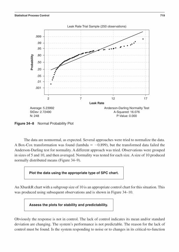
The data are nonnormal, as expected. Several approaches were tried to normalize the data.A Box-Cox transformation was found (lambda 0.899), but the transformed data failed theAnderson-Darling test for normality. A different approach was tried. Observations were groupedin sizes of 5 and 10, and then averaged. Normality was tested for each size. A size of 10 producednormally distributed means (Figure 34–9).
An Xbar&R chart with a subgroup size of 10 is an appropriate control chart for this situation. Thiswas produced using subsequent observations and is shown in Figure 34–10.
Obviously the response is not in control. The lack of control indicates its mean and/or standarddeviation are changing. The system’s performance is not predictable. The reason for the lack ofcontrol must be found. Is the system responding to noise or to changes in its critical-to-function
Assess the plots for stability and predictability.
Plot the data using the appropriate type of SPC chart.
Statistical Process Control 719
2
.999
.99
.95
.80
.50
.20
.05
.01
.001
7
Leak Rate
Leak Rate Trial Sample (250 observations)
Average: 5.23992StDev: 2.72490N: 248
Anderson-Darling Normality TestA-Squared: 16.076
P-Value: 0.000
Pro
bab
ility
12 17
Figure 34–8 Normal Probability Plot

111
11
111
1
11
1
1
111
1 1 1
11
11
1
111
1
11
11
1
1111
1 1
111
11
1
1
1
1
111
1
1
11 1
1
1
1
1
11
11
1111
1
11
111
1
1
1
1
1
1
1
1
15
10
5
0
UCL = 10.86
Mean = 5.688
LCL = 0.5120
UCL = 8.993
R = 2.752LCL = 0
20
Sam
ple
Mea
nS
amp
le R
ang
e
100
Observations 1501 – 3132
1500 50Subgroup
10
0
Figure 34–10 Xbar&R Chart for Leak Rate
.999
.99
.95
.80
.50
.20
.05
.01
.001
4 5 6
Avg Leak Rate7 8
Pro
bab
ility
Average: 5.2348StDev: 1.6721N: 25
Anderson-Darling Normality TestA-Squared: 0.476
P-Value: 0.219
Figure 34–9 Average Leak Rate for n 10
720
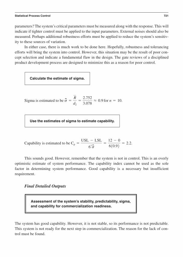
parameters? The system’s critical parameters must be measured along with the response. This willindicate if tighter control must be applied to the input parameters. External noises should also bemeasured. Perhaps additional robustness efforts must be applied to reduce the system’s sensitiv-ity to these sources of variation.
In either case, there is much work to be done here. Hopefully, robustness and tolerancingefforts will bring the system into control. However, this situation may be the result of poor con-cept selection and indicate a fundamental flaw in the design. The gate reviews of a disciplinedproduct development process are designed to minimize this as a reason for poor control.
This sounds good. However, remember that the system is not in control. This is an overlyoptimistic estimate of system performance. The capability index cannot be used as the sole factor in determining system performance. Good capability is a necessary but insufficient requirement.
Final Detailed Outputs
The system has good capability. However, it is not stable, so its performance is not predictable.This system is not ready for the next step in commercialization. The reason for the lack of con-trol must be found.
Assessment of the system’s stability, predictability, sigma,and capability for commercialization readiness.
Capability is estimated to be Cp =USL - LSL
6*=
12 - 0
6(0.9)= 2.2.
Use the estimates of sigma to estimate capability.
Sigma is estimated to be =R
d2=
2.752
3.078L 0.9 for n = 10.
Calculate the estimate of sigma.
Statistical Process Control 721
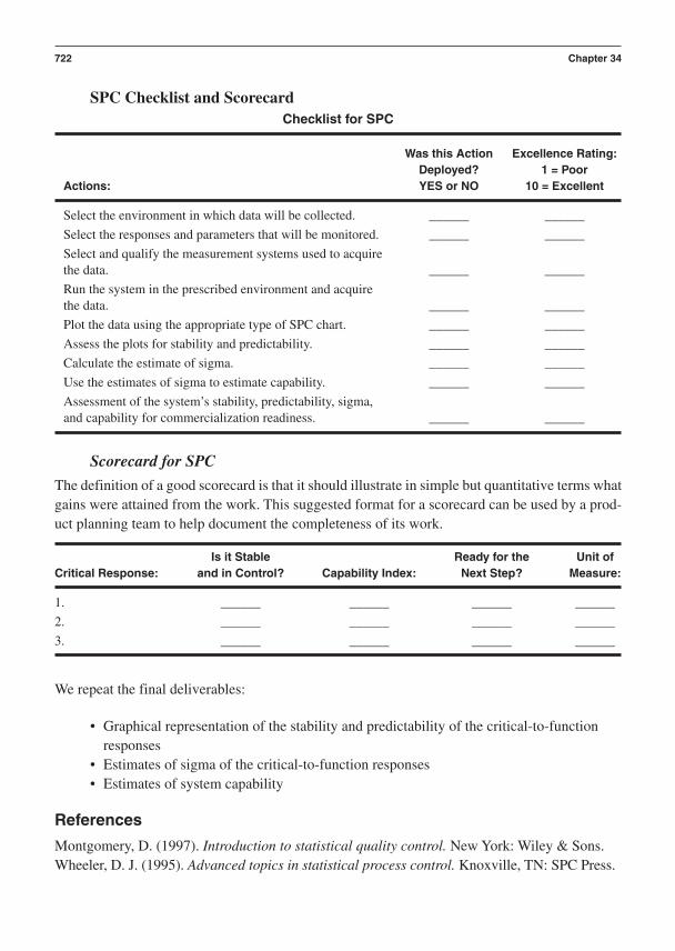
SPC Checklist and ScorecardChecklist for SPC
Was this Action Excellence Rating:Deployed? 1 = Poor
Actions: YES or NO 10 = Excellent
Select the environment in which data will be collected. ______ ______
Select the responses and parameters that will be monitored. ______ ______
Select and qualify the measurement systems used to acquire the data. ______ ______
Run the system in the prescribed environment and acquire the data. ______ ______
Plot the data using the appropriate type of SPC chart. ______ ______
Assess the plots for stability and predictability. ______ ______
Calculate the estimate of sigma. ______ ______
Use the estimates of sigma to estimate capability. ______ ______
Assessment of the system’s stability, predictability, sigma, and capability for commercialization readiness. ______ ______
Scorecard for SPC
The definition of a good scorecard is that it should illustrate in simple but quantitative terms whatgains were attained from the work. This suggested format for a scorecard can be used by a prod-uct planning team to help document the completeness of its work.
Is it Stable Ready for the Unit of Critical Response: and in Control? Capability Index: Next Step? Measure:
1. ______ ______ ______ ______
2. ______ ______ ______ ______
3. ______ ______ ______ ______
We repeat the final deliverables:
• Graphical representation of the stability and predictability of the critical-to-functionresponses
• Estimates of sigma of the critical-to-function responses• Estimates of system capability
References
Montgomery, D. (1997). Introduction to statistical quality control. New York: Wiley & Sons.Wheeler, D. J. (1995). Advanced topics in statistical process control. Knoxville, TN: SPC Press.
722 Chapter 34
E P I L O G U E
Linking Design to Operations
This Epilogue was written by Stephen A. Zinkgraf, Ph.D., CEO and President ofSigma Breakthrough Technologies, Inc.
The penultimate goal of Design For Six Sigma is to create new products, technologies, andprocesses that lead measurably and directly to company growth by meeting or beating the
business plan. The best global metric I’ve seen to describe the success of a commercializationprogram is a simple ratio:
Commercialization success $ spent on R&D / $ in revenue from new products
I love this metric because it reminds us that R&D is a business process with the accounta-bility to generate new revenue. If the ratio is one or greater, your company probably does not havean effective commercialization program. I see large, Fortune 500 companies—even those notedfor product development—produce a very poor ratio for commercialization success. One com-pany I’ve worked with that is known for product innovation saw their commercialization successratio to be about one, which was not a very good return-on-investment for the millions they’dspent on R&D.
Why is this ratio so hard to improve? Anyone who has been involved with operations man-agement in a manufacturing company has had the unique experience of supporting the launch ofa new product or new process. A typical launch of a new product in most companies inflicts enor-mous pain on all parties involved. The product usually has huge production problems with lowyields at all process steps, and with repair loops and repair activities popping up everywhere. Lineoperators and supervisors run amuck screaming for technical assistance. The operations managersclaim that the product was thrown over the wall by design. The design engineers traditionallyspend a large percentage of their time on the plant floor “troubleshooting,” and engineeringchange notices flood the system.
When a company implements a new Six Sigma program, the company will usually start theprocess in their operations functions and focus on cost cutting. About 50 percent to 75 percent of
723
all the operations Six Sigma projects will have a design change on a product or process as a so-lution. In fact, companies that have not implemented Design For Six Sigma (DFSS) will see theirdesign engineers spend 25 percent to 40 percent (or more) working out issues on products alreadylaunched into the manufacturing operations.
Design engineers essentially become part-time operations process engineers. In fact, a lotof factories have a core of engineers that exist to work primarily on product issues. This is a hugecost-of-poor-quality (COPQ) to those companies since these resources are not focused on growthand new products or services but on maintaining current products and processes. Since growth isthe primary success factor for companies today, poor upfront design practices directly impact thecompany’s long-term success.
An example from the Honeywell (formerly AlliedSignal) Six Sigma deployment launchedin late 1994 illustrates the point. In 1995, the Engineered Materials Sector of the former Al-liedSignal earned about $100 million from the first year of its Six Sigma deployment into opera-tions. They estimated that about 75 percent of that result could be tied directly to engineeringchanges in product or process specifications—in other words, from a major product or processredesign.
Had AlliedSignal had a viable DFSS program, their operations program might have onlyproduced $25 million, while the other $75 million would have been earned later from the initiallaunch of the new products. This is also a COPQ that is not tracked by design groups. If it was,companies would move much more rapidly into Design For Six Sigma than they normally do. Wesee companies usually initiating their DFSS programs in 1 to 2 years after they start their opera-tions programs. I’ll say that Six Sigma has become an industry standard in managing companiesprimarily because of poor design processes. These poor design processes allow operationsprocess improvement projects to yield huge benefits because proper upfront preventative workwas not done.
As Robert Copper, author of Winning at New Products, once quoted, “Beating a new prod-uct into submission in operations for a year will save the company six weeks of upfront preven-tative work.” Therein lies the operations goal and focus of Design For Six Sigma: to seamlesslyintroduce new products, technologies, processes, and services into the company. By following theroadmaps and using the tools summarized in this book, companies will be able to move a newproduct into operations quickly and with far less pain.
This methodology sets the stage for the company to meet the business plan goals of the newproduct within a relatively short period of time. I define product launch cycle-time as the time be-tween the initial concept and the product finally meeting the business plan as to cost, quality, anddelivery. The usual definition of product launch cycle-time is the time from developing the ini-tial concept to the first manufacturing run. This latter definition does not take into account thebusiness impact of the new product. DFSS is definitely a major part of the product developmentbusiness process and should be treated accordingly.
Design For Six Sigma is the antithesis of the basic notion of Six Sigma. Six Sigma existsprimarily to remove variability from all systems. Design For Six Sigma actually addresses profi-
724 Epilogue

cient imposition of variability on the system. You see, not all variability is bad and, in fact, if acompany doesn’t aggressively impose variability on itself, the company will cease to exist.
Ford Motor Company nearly went out of business in its early years because Ford insistedon making cars only one color—black. General Motors, in contrast, offered a variety of colorsand captured a large percentage of the automotive market. So, by General Motors foisting thevariability of multiple colors on its manufacturing system, GM was able to go head-to-head witha major competitor. To generalize, if a company is not always introducing the variability associ-ated with new products, technologies, or services, that company will ultimately lose in the mar-ketplace.
However, all variability, whether good (new products or services) or bad (scrap and repaircosts), has an adverse effect on manufacturing operations. If the reader has had any experiencewith paint lines on the manufacturing floor (usually one of the biggest sources of poor yield andhigh COPQ), he or she will readily recognize that GM’s introduction of multiple colors must havehad a huge impact on their manufacturing processes—either forcing them to deploy multiplepaint lines or to go through the pain of complex color changeovers. Variability from multiple col-ors negatively impacted quality, cost, and speed.
With the two concepts in mind: (1) Not all variability is bad and (2) variability—good orbad—negatively impacts manufacturing operations, we can put DFSS into perspective. DFSSidentifies the most predominant sources of variation in the product system. Through Critical Pa-rameter Management (CPM), the important process inputs (X’s) and outputs (Y’s) are identifiedearly in the commercialization process along with a recommended control plan. The CPM processgives the manufacturing operations a head start on planning for new product launches. CPM en-sures operations that the probabilities of a smooth new product launch are high.
While all failure modes cannot be anticipated, by doing the upfront analysis the operationsfolks can deploy the new manufacturing system and iron out any unanticipated problems veryquickly. In a company good at DFSS, Six Sigma in operations will focus on smaller issues. BlackBelts and Green Belts will move away from the traditional project mix of 80 percent reactive proj-ects and 20 percent proactive projects to 20 percent reactive projects and 80 percent proactiveprojects. In fact, companies that are good at DFSS will have more resources in operations avail-able to work with customer and key suppliers than companies that are not good at DFSS.
With a good DFSS program, Six Sigma projects designed to improve operations perfor-mance will take less time and resources to complete. Let’s look at the following table. I havelisted the major steps and tools in a typical Six Sigma improvement project along with a com-parison of the activities with a poor DFSS system and with a good DFSS system. You will no-tice that every step in the Process Improvement Methodology™* is positively affected by goodDFSS practices.
Epilogue 725
*Process Improvement Methodology™ is a federally trademarked term of Sigma Breakthrough Technologies, Inc. Termused with permission of Sigma Breakthrough Technologies, Inc.

Comparison of Process Improvement between Poor and Good DFSS Processes
Process Improvement Step Poor DFSS System Good DFSS System
I. Measure Phase
Process Map
Cause and Effects Matrix
Gage Studies
Capability Studies
II. Analysis Phase
Failure Modes and Effects Analysis
Multi-Vari Study
III. Improve Phase
Experimental Design
Lean Manufacturing Tools
IV. Control
Develop Process Control Plan
Put Performance Metrics in Place
Establish Long-Term Capability
726 Epilogue
Develop from scratch—criticalparameters are unclear
Develop from scratch—criticalparameters unclear
Perform time-consuming gagestudies—project is stalled untilcompleted
Develop from scratch—lack ofclarity of customer requirements
Develop from scratch—time-consuming and necessarilyconstrained
Study has wide scope entailingmore data because of generallack of technical knowledge ofthe process
More experiments—more inputvariables studied because of lackof technical knowledge of theprocess
Lean tools likely to besuccessful because of an initiallypoorly designed process
Develop from scratch—time-consuming to implementsystems
Metrics developed from scratchand systems to collect datadeveloped
Longer study required withmore variables involved
Modify and Update—criticalparameters identified from DFSS
Modify and Update—initialanalysis done by DFSS team
All major measurement systemsanalyzed during DFSS—onlysecondary systems need analysis
Capability data available fromDFSS—customer requirementsare clear and well documented
Update and modify FMEA fromDFSS—critical parameters clearlydefined—FMEA is reviewedrather than created
Study is focused—criticalparameters are clear—datacollection efforts are less intensive
Few experiments—more focusedbecause critical parameters arealready known
Lean tools are unlikely to benecessary because of optimalprocess design during DFSS
Updated and modified—controlsystems in place at product launchbecause of DFSS
Metrics reviewed and modifiedbut data collection systemsalready in place from DFSS
Short studies with the rightvariables from CPM
The Process Improvement Methodology™ roadmap depicted in this table is federally copyrighted by and used withpermission from Sigma Breakthrough Technologies, Inc.

Process improvement efforts in operations will be more focused and much faster in com-panies that define the critical parameters and control systems for new products during the DFSSprocess. Ultimately, operations Black Belts and Green Belts will be focused on preventative ac-tivities rather than reactive activities. Because of minimizing defects early in the new productlaunch cycle, fewer customer complaints and field problems will occur. Operations resources willextend their influence into the customer and supply base, establishing better relationships andstrategic partnerships where everyone is much more successful.
Ultimately, product development engineers will work only a small percentage of the timeto troubleshoot new products in operations. Because new product launches are smoother and busi-ness plan objectives are more quickly met, the company with a good DFSS process is now set tolaunch more new products each year than ever before.
As the saying goes, “In research and development (R&D), research creates surprises anddevelopment prevents surprises.” That is exactly what DFSS has to offer. By clearly understand-ing customer needs using Concept Engineering and identifying critical parameters early in thecommercialization process, creating innovative concepts to meet those needs and providing forseamless new product launches in operations, a DFSS-driven company will have more success-ful products and hit their business plan goals at levels much greater than their competitors.
Enjoy your journey into DFSS. Since product commercialization is the most complex of allbusiness processes, your journey will not be easy. However, if you visualize your company beinga leader in developing successful and innovative new products and being able to commercializeat light speed through seamless new product launches into operations, you’ll be getting close tothe real benefit of DFSS. See you on the road to Six Sigma!
Epilogue 727

This page intentionally left blank
ANOM analysis of meansANOVA analysis of varianceCAD computer-aided designCAPs critical adjustment parametersCCD central composite designCDOV concept, design, optimize, and verifyCF control factorCFPs critical functional parametersCFRs critical functional responsesCGI capability growth indexCL centerline (in SPC charts)CNFs compounded noise factorsCOPQ cost of poor qualityCOV coefficient of variationCp capability indexCpd design capabilityCpk measures long-term performance
capabilityCPM Critical Parameter ManagementCpm manufacturing process capabilityCTF critical-to-functionDFMEA design failure modes and effects
analysisDFNS Design For N-SigmaDFSS Design For Six Sigma
DFx Design For “x”DOE design of experimentsdof degree of freedomESS environmental stress screeningFMEA failure modes and effects analysisFTA fault tree analysisGage R&R repeatability and reproducibilityGnom. nominal gap, contact, or interference
dimensionHALT highly accelerated life testingHAST highly accelerated stress testingHOQ House of QualityI&MR chart Individuals and Moving
Range chartI2DOV invent/innovate, develop, optimize,
and verifyKJ analysis (for Jiro Kawakita)LCL lower control limitLSL lower specification limitLTB larger-the-betterMAIC measure, analyze, improve, and
controlMSA measurement systems analysisMSD mean square deviationMTBF mean time between failure
A P P E N D I X A
Design For Six SigmaAbbreviations
729

MTTF mean time to failureNTB nominal-the-bestNUD new, unique, and difficultpdf probability density functionPLS product line strategyP/T ratio precision-to-tolerancePERT chart (program evaluation review
technique)PRESS prediction sum of squaresQFD quality function deploymentR&D community (research and
development)R&R study (repeatability and
reproducibility)
RBD reliability block diagramRPN risk priority numbersRSM response surface methodsS/N signal-to-noise ratioSPC statistical process controlSRD system requirements documentSTB smaller-the-betterUCL upper control limitUMC unit manufacturing costUSL upper specification limitVOC voice of the customerVOP voice of the product/process
730 Appendix A

Aabsolute zero A property of a quality char-
acteristic that allows all measurements tobegin from the number zero and go up therational number line from that point. Manydesigns have an absolute zero scale ofmeasurement and should have their datameasured relative to that scale.
additive model A mathematical functionthat expresses a dependent variable, y, interms of the sum (simple addition) of func-tions of relatively independent variablesrepresented by the control factors in an op-timization experiment. The additive modelassumes mild-to-moderate interactivity be-tween the control factors and assigns thenumerical contribution to the response forthis interactivity to the error term in themodel: y f(A) g(B) h(C) … er-ror. This model is approximate in natureand is useful for engineering optimizationbut not for rigorous statistical math model-ing to define fundamental functional rela-tionships (ideal/transfer functions).
additivity The natural or intentionally in-duced independence of each individualcontrol factor’s effect on a measured response.
adjustment factor Any control factor thathas a strong effect on the mean perfor-mance of the response. There are two spe-cial types of adjustment factors: scalingfactors and tuning factors. Adjustment fac-tors are used in static and dynamic applica-tions of the two-step optimization process.In Critical Parameter Management, theyare referred to as critical adjustment pa-rameters (CAPs).
aliasing See confounding.ANOM (ANalysis Of the Mean) An analyti-
cal process that quantifies the mean re-sponse for each individual control factorlevel. ANOM can be performed on datathat is in regular engineering units or datathat has been transformed into some formof signal-to-noise ratio or other data trans-form. Main effects and interaction plots arecreated from ANOM data.
A P P E N D I X B
Glossary
731

ANOVA (ANalysis Of the VAriance) An an-alytical process that decomposes the con-tribution each individual control factor hason the overall experimental response. TheANOVA process is also capable of ac-counting for the contribution of interactiveeffects between control factors and experi-mental error in the response, providedenough degrees of freedom are establishedin the experimental array. The value of ep-silon squared (percentage contribution tooverall CFR variation) is calculated usingdata from ANOVA.
antisynergistic interaction An interactionbetween two or more control factors thathave a negative, nonmonotonic effect on ameasured critical functional response.These interactions can either be due tophysical law (real, physical, fundamentalinteraction) or from mismatches betweencontinuous, engineering x variable inputsand attribute or “quality metric” output Yvariables (virtual interaction).
array An arithmetically derived matrix ortable of rows and columns that is used toimpose an order for efficient experimenta-tion. The rows contain the individual ex-periments. The columns contain the exper-imental factors and their individual levelsor set points.
asymmetric loss function A version of thenominal-the-best loss function that ac-counts for the possibility of different eco-nomic consequences as quantified by theeconomic coefficients klower and kupper oneither side of the target value.
average quality loss The application of thequadratic loss function to numerous sam-ples of a product or process resulting in thecalculation of a term called the meansquare deviation (MSD). The average qual-
ity loss approximates the nature of lossover a variety of customer economic sce-narios, thus providing a generalized evalu-ation of the average or aggregated loss.
Bbalanced experiment An experiment where
each experimental factor is provided withan equal opportunity to express its effect onthe measured response. The term balance issynonymous with the orthogonality of amatrix experiment. This property precludesthe ability of multi-colinearity from becom-ing a problem in data analysis.
benchmarking The process of comparativeanalysis between two or more concepts,components, subassemblies, subsystems,products, or processes. The goal of bench-marking is to qualitatively and quantita-tively identify a superior subject within thecompeting choices. Often the benchmark isused as a standard to meet or surpass.Benchmarks are used in building Houses ofQuality, concept generation, and the Pughconcept selection process.
best practice A preferred and repeatable ac-tion or set of actions completed to fulfill aspecific requirement or set of requirementsduring the phases within a product devel-opment process.
beta () The Greek letter, , is used to rep-resent the slope of a best fit line. It indicatesthe linear relationship between the signalfactor(s) (critical adjustment parameters)and the measured critical functional re-sponse in a dynamic robustness optimiza-tion experiment.
blocking A technique used in classical DOEto remove the effects of unwanted, assigna-ble cause noise or variability from the ex-perimental response so that only the effects
732 Appendix B
from the control factors are present in theresponse data. Blocking is a data purifica-tion process used to help assure the integrityof the experimental data used in construct-ing a statistically significant math model.
build-test-fix methods A traditional, undis-ciplined engineering process used to iterateproduct development and design activitiesuntil a “successful” product is ultimatelyproduced. These processes can be lengthyand costly to employ. The main difficultywith this approach is inefficiency and pro-duction of suboptimal results requiringeven more redesign effort into the produc-tion phase of the product life cycle. Build-test-fix produces design waste and rework.
Ccalibration Setting a meter or a transducer
(measurement instrumentation) to a knownstandard reference that assures the quantifi-cation of reliable measures of physical phe-nomena. Calibration makes the accuracyand repeatability of measurements as goodas possible given the inherent capability ofthe instrument.
capability growth index The calculatedpercentage between 0 percent and 100 per-cent that a group of system, subsystem, orsubassembly CFRs have attained in gettingtheir Cp indices to equal a value of 2, indi-cating how well their critical functional re-sponses have attained 6 sigma performanceduring product development.
capability index Cp and Cpk indices thatcalculate the ratio of the voice of the cus-tomer vs. the voice of the product orprocess. Cp is a measure of capabilitybased on short-term or small samples ofdata—usually what is available duringproduct development. Cpk is a measure of
long term or large samples of data that in-clude not only variation about the mean butalso the shifting of the mean itself—usuallyavailable during steady state production.
central composite design (CCD) An ex-perimental design technique used in re-sponse surface methods to build nonlinearmath models of interactive and nonlinearphenomena. A major tool used in theCDOV sequential design of experimentsprocess for design and process optimiza-tion after robust design to place the mean ofa CFR on target with high accuracy. Themain inputs to a CCD are CAPs.
classical design of experiments (DOE) Ex-perimental methods employed to constructmath models relating a dependent variable(the measured critical functional response)to the set points of any number of inde-pendent variables (the experimental controlfactors). DOE is used sequentially to buildknowledge of fundamental functional rela-tionships (ideal/transfer functions) betweenvarious factors and a response variable.
classification factor A parameter that usesintegers, simple binary states, or nonnumer-ical indicators to define the levels that areevaluated in the experimental process.Classes can be stages, groups, or conditionsthat define the level of the classification fac-tor. This type of factor is used in cases wherecontinuous variables cannot adequately de-fine the state of the factor set point. We usu-ally try to avoid using these in DFSS.
coefficient of variation (COV) The ratioobtained when the standard deviation is di-vided by the mean. The COV is often ex-pressed as a percentage by multiplying theratio by 100. It is an indication of howmuch variability is occurring around themean response. Often it is of interest to
Glossary 733
detect a quantitative relationship betweenthe changes in the mean response and thecorresponding changes in the standard de-viation. This will be used in the coopti-mization of certain designs where the vari-ance scales along with the mean. One formof Taguchi’s signal-to-noise ratios is basedon the square of this ratio.
column The part of an experimental arraythat contains experimental factors and theirvarious levels or set points.
commercialization Business process thatharnesses the resources of a company in theendeavor of conceiving, developing, de-signing, optimizing, verifying design andprocess capability, producing, selling, dis-tributing, and servicing a product.
compensation The use of feed-forward orfeedback control mechanisms to intervenewhen certain noise effects are present in aproduct or process. The use of compensa-tion is only done when insensitivity tonoise cannot be attained through robust-ness optimization.
complete The property of a single criticalfunctional response that promotes thequantification of all the dimensions of theideal function of a design element.
component A single part in a subassembly,subsystem, or system. An example wouldbe a stamped metal part prior to havinganything assembled to it.
component requirements document Thedocument that contains all the require-ments for a given component. They are of-ten converted into a quality plan that isgiven to the production supply chain to setthe targets and constrain the variation al-lowed in the incoming components.
compound control factors Control factorsthat have been strategically grouped (addi-
tivity grouping) to help minimize the pos-sibility of strong, disruptive interactivitybetween the individual control factors.Grouped control factors are comprised oftwo or more factors that have their individ-ual effects on the response understood andare grouped together so that they cocon-tribute in the same way to the measured re-sponse. Control factors can also be groupedwhen necessary to allow the use of asmaller orthogonal array. This technique isprimarily used in robust design after theideal function is identified.
compound noise factors Noise factors thathave been strategically grouped by the na-ture of their strength and effect on the di-rectionality of the measured response.They are used to increase the efficiency ofinducing statistically significant noises inrobustness experiments.
concept engineering The initial phase ofthe DFSS approach to product develop-ment. This part of the commercializationprocess is used to link the voice of the cus-tomer with the inventive and technical ca-pabilities of the business (voice of theproduct and process) to help develop anddesign superior product concepts.
concurrent engineering The process of si-multaneously carrying out various productdesign, manufacturing, and service devel-opment activities in parallel rather than inseries. The outcome is reduced cycle time,higher quality, and lower product commer-cialization costs. Concurrent engineering isnoted for its focus on multifunctional teamsthat work closely to improve communica-tion of seemingly conflicting requirementsand priorities. Their goal is to formulate ef-fective synergy around the customers’needs to bring the project to a speedy and
734 Appendix B

optimal conclusion. It prevents problemsand is a baseline competency in DFSS.
confounding The situation created whenone control factor main effect or interactionis numerically blended with one or moreother control factor main effects and/or in-teractive effects by intentionally or unin-tentionally allocating the same degrees offreedom in a matrix experiment to multiplefactors. Often the term aliasing is used in-terchangeably with confounding. Con-founding can be helpful or harmful de-pending on the amount of interactivitybetween the confounded factors.
conservation of energy The physical lawthat states that energy is neither created ordestroyed. It is used as a basis for design-ing experiments to build and understandideal functions and additive robustnessmodels in DFSS. Energy models are addi-tive models due to this “conservative” law(e. g., Bernouli’s equation).
conservation of mass The physical law thatstates that mass is neither created or de-stroyed. It is used as a basis for designing ex-periments to build and understand ideal func-tions and additive robustness models inDFSS. Mass models are additive models dueto this “conservative” law (e. g., Lavosier’sequation).
continuous factor A parameter that cantake on any value within a range of rationalnumbers to define the levels that are evalu-ated in the sequential experimental designprocess. We prefer to use these as x and Yvariables (scalars and vectors) for model-ing in DFSS.
contour mapping A two-parameter graphi-cal output from a computer analysis of themath model created from any number ofclassically designed experiments (usually
response surface experiments). It is used topredict points or areas of local or global op-timum performance based on empiricaldata. It does not typically account for theeffects of noise on the predicted response.
control factor The factors or parameters(CFP or CTF spec) in a design or process thatthe engineer can control and specify to definethe optimum combination of set points forsatisfying the voice of the customer.
critical adjustment parameter (CAP) Aspecific type of CFP that controls the meanof a CFR. CAPs are identified using se-quential DOE and engineering analysis.They are the input parameters for responsesurface methods for the optimization ofmean performance optimization after ro-bust design is completed. They enable Cpkto be set equal to Cp, thus enabling entitle-ment to be approached if not attained.
critical functional parameter (CFP) Aninput variable (usually an engineered addi-tivity grouping) at the subassembly or sub-system level that controls the mean or vari-ation of a CFR.
critical functional response (CFR) Ameasured scalar or vector (complete, fun-damental, continuous engineering vari-able) output variable that is critical to thefulfillment of a critical customer require-ment. Some refer to these critical customerrequirements as CTQs.
Critical Parameter Management (CPM)The process within DFSS that developscritical requirements and measures criticalfunctional responses to design, optimize,and verify the capability of a product andits supporting network of manufacturingand service processes.
critical-to-function specification (CTF) Adimension, surface, or bulk characteristic
Glossary 735

(typically a scalar) that is critical to a com-ponent’s contribution to a subassembly,subsystem, or system level CFR.
criticality A measurable requirement orfunctional response that is highly importantto a customer. All requirements are impor-tant but only a few are truly critical.
crossed array experiment The combina-tion of inner and outer orthogonal arrays tointentionally introduce noise into the ex-periment in a disciplined and strategic fash-ion. This is done to produce data that can betransformed into control factor noisefactor interaction plots to isolate robust setpoints for the control factors. S/N ratios re-place such plots when compounded noisesreplace the outer arrays in a robustness experiment.
Ddegrees of freedom (dof) The capacity of
an experimental factor or an entire matrixexperiment to produce information. Thedoff for an experimental factor is alwaysone less than the number of levels assignedto the factor. The dofexp for an entire matrixexperiment is always one less than thenumber of experimental runs in the experi-ment. Whether accounting for experimen-tal factor dof or matrix experiment dof, onedof is always employed to calculate the av-erage response. This is why one dof is al-ways subtracted from the total.
design capability (Cpd) The Cp index for adesign’s critical functional response in ra-tio to its upper and lower specification lim-its (VOC-based tolerance limits).
design of experiments (DOE) A processfor generating data that uses a mathemati-cally derived matrix to methodically gatherand evaluate the effect of numerous param-
eters on a response variable. Designed ex-periments, when properly used, efficientlyproduce useful data for model building orengineering optimization activities.
deterioration noise factor A source of vari-ability that results in some form of physicaldeterioration or degradation of a product orprocess. This is also referred to as an innernoise because it refers to variation insidethe controllable factor levels.
double dynamic signal-to-noise case Avariation of the dynamic S/N case that em-ploys two signal factors. The two signalfactors (CAPs) are the functional signalfactor, which is a factor that directly andactively controls some form of input en-ergy into the design, and the process signalfactor, which possesses a linear relation-ship to the output response and indirectlycontrols (attenuates) the energy transfor-mation occurring in the design.
drift The tendency of a product or processoutput or set point to move off target.
dynamic signal-to-noise case A method ofstudying the linearity, sensitivity, and vari-ability of a design by relating the perfor-mance of a signal factor (CAP), numerouscontrol factors, and noise factors to themeasured CFR. These cases relate the powerof the proportionality of the signal factor(CAP) to the measured CFR with the powerof the variance in the CFR due to noise.
Eeconomic coefficient The economic coeffi-
cient is used in the quality loss function. Itrepresents the proportionality constant inthe loss function of the average dollars lost(A0) due to a customer reaction to off-target performance and the square of thedeviation from the target response (0
2).
736 Appendix B
This is typically, but not exclusively, calcu-lated when approximately 50 percent of thecustomers are motivated to take somecourse of economic action due to poor per-formance (but not necessarily outrightfunctional failure). This is often referred toas the LD 50 point in the literature.
energy flow map A representation of an en-gineering system that shows the paths ofenergy divided into productive and nonpro-ductive work. Analogous to a free body di-agram from an energy perspective. Theyaccount for the law of conservation of en-ergy and are used in preparation for mathmodeling and design of experiments.
energy transformation The physical pro-cess a design or product system uses toconvert some form of input energy into var-ious other forms of energy that ultimatelyproduce a measurable response. The mea-surable response may itself be a form of en-ergy or the consequence of energy transfor-mations, which have taken place within thedesign.
engineering metrics A scalar or vector thatis usually called a CTF spec, CFP, CAP, orCFR. They are greatly preferred as opposedto quality metrics (yield, defects, and soon) in DFSS.
Engineering Process A set of disciplined,planned, and interrelated activities that areemployed by engineers to conceive, de-velop, design, optimize, and verify the ca-pability of a new product or process design.
environmental noise factors Sources ofvariability that are due to effects that areexternal to the design or product, also re-ferred to as outer noise. They can also besources of variability that one neighboringsubsystem imposes on another neighboringsubsystem or component. Examples in-
clude vibration, heat, contamination, mis-use, or overloading.
epsilon squared Percentage contribution tooverall CFR variation calculated fromANOVA data: (SSfactor/SStotal) 100 2
experiment An evaluation or series of eval-uations that explore, define, quantify, andbuild data that can be used to model or pre-dict functional performance in a compo-nent, subassembly, subsystem, or product.Experiments can be used to build funda-mental knowledge for scientific research,or they can be used to design and optimizeproduct or process performance in the en-gineering context of a specific commercial-ization process.
experimental efficiency This process-relatedactivity is facilitated by intelligent applica-tion of engineering knowledge and theproper use of designed experimental tech-niques. Examples include the use of Frac-tional Factorial arrays, control factors thatare engineered for additivity, and com-pounded noise factors.
experimental error The variability presentin experimental data that is caused by metererror and drift, human inconsistency in tak-ing data, random variability taking place innumerous noise factors not included in thenoise array, and control factors that have notbeen included in the inner array. In theTaguchi approach, variability in the datadue to interactive effects is often but not al-ways included as experimental error.
experimental factors Independent parame-ters that are studied in an orthogonal arrayexperiment. Robust design classifies ex-perimental factors as either control factorsor noise factors.
experimental space The combination of allthe control factor, noise factor, and signal
Glossary 737

factor (CAP) levels that produce the range ofmeasured response values in an experiment.
FF-ratio The ratio formed in the ANOVA
process by dividing the mean square ofeach experimental factor effect by the MSof the error variance. This is the ratio ofvariation occurring between each of the ex-perimental factors in comparison to thevariation occurring within all the experi-mental factors being evaluated in the ex-periment. It is a form of signal-to-noise ra-tio in a statistical sense. The noise in thiscase is random experimental error, not vari-ability due to the assignable cause noisefactors in the Taguchi noise array.
factor effect The numerical measure (mag-nitude) of the contribution an experimentalfactor has on the variation of a functional re-sponse (CFR). In practical terms we use 2
to measure this, and in statistical terms weuse the coefficient in the regression model.
feedback control system A method of com-pensating for the variability in a process orproduct by sampling output response andsending a feedback signal that changes acritical adjustment parameter to put themean of the response back on its intendedtarget.
feed forward control system A method ofcompensating for the variability in aprocess or product by sampling specificnoise factor levels and sending a signal thatchanges an adjustment factor to keep theresponse on its intended target.
Fisher, Sir Ronald The inventor of much ofwhat is known today as classical design ofexperiments. His major focus was on opti-mizing crop yield in the British agriculturalindustry.
fraction defective The portion of an exper-imental or production sample that is foundto be outside of the specification limits.Counting and minimizing defects are notmetrics that best reflect the fundamental,ideal function of a design and its perfor-mance. They are more commonly used inproduction and transactional Six Sigma ap-plications for cost reduction projects.
Fractional Factorial design A family oftwo- and three-level orthogonal arrays thatgreatly aid in experimental efficiency. De-pending on how a Fractional Factorial de-sign is loaded with control factors, it can beused to study interactions or it can be ma-nipulated to promote evaluation of additiv-ity in a design or process. Fractional Facto-rial designs are a subset of all the possibletreatment combinations possible in a FullFactorial array.
frequency distribution table A table of thefrequency of occurrence of measured val-ues within specific ranges that are used togenerate a histogram.
Full Factorial design Two- and three-levelorthogonal arrays that include every possi-ble combination between the experimentalfactors. Full Factorial experimental designsuse degrees of freedom to account for allthe main effects and all interactions be-tween factors included in the experimentalarray. Basically all interactions beyondtwo-way interactions are likely to be ofnegligible consequence; thus, there is littleneed to use large arrays to rigorously eval-uate such rare and unlikely three-way in-teractions and above.
functional signal factor (M) A signal factor(CAP) used in the double dynamic Taguchicase where engineering knowledge is usedto identify an input variable for a design
738 Appendix B

that controls the major energy transforma-tion in the design. This transformation con-trols a proportional relationship betweenthe functional signal factor and measuredresponse. A functional signal factor is usedto tune the design’s performance on to anydesired target. Tunable technology is de-veloped from a concept that possesses afunctional signal factor. RSM is often usedto do final optimization using these kindsof parameters.
fundamental The property of a criticalfunctional response that expresses the basicor elemental physical activity that is ulti-mately responsible for delivering customersatisfaction. A response is fundamental if itdoes not mix mechanisms together and isuninfluenced by factors outside of thecomponent, subassembly, subsystem, sys-tem design, or production process beingoptimized.
Ggate A short period of time during a product
development process when the entire teamreviews and reacts to the results from theprevious phase and proactively plans forthe smooth execution of the next phase. Agate review’s time should be 20 percent re-active and 80 percent proactive. Gate re-views focus on the results from specifictools and best practices and manage the as-sociated risks and problems. They alsomake sure the team has everything it needsto apply the tools and best practices for thenext phase with discipline and rigor.
Gaussian distribution A distribution ofdata that tends to form a symmetrical, bell-shaped curve. See normal distribution.
goal post mentality A philosophy aboutquality that accepts anything within the tol-
erance band (USL-LSL) as equally goodand anything that falls outside of the toler-ance band as equally bad. See soccer,hockey, lacrosse, and football rule books.
grand total sum of squares The value ob-tained when squaring the response of eachexperimental run from a matrix experimentand then adding the squared terms.
Hhalf effect The change in a response value ei-
ther above or below the overall experimen-tal average obtained for an experimentalfactor level change. It is called the half ef-fect because it represents just half of the fac-tor effect. An example would be the averagenumerical response, obtained for a controlfactor that is evaluated exclusively at eitherits high set point or at its low set point, mi-nus the overall experimental average.
histogram A graphical display of the fre-quency distribution of a set of data. His-tograms display the shape, dispersion, andcentral tendency of the distribution of adata set.
House of Quality An input–output relation-ship matrix used in the process of qualityfunction deployment.
hypothesis testing A statistical evaluationthat checks the validity of a statement to aspecified degree of certainty. These testsare done using well-known and quantifiedstatistical distributions.
Iideal/transfer function Fundamental func-
tional relationships between various engi-neering control factors and a measured crit-ical functional response variable. The mathmodel of Y f(x) represents the customer-focused response that would be measured if
Glossary 739

there were no noise or only random noiseacting on the design or process.
independent effect The nature of an exper-imental factor’s effect on the measured re-sponse when it is acting independently withrespect to any other experimental factor.When all control factors are producing in-dependent effects, the design is said to beexhibiting an additive response.
inference Drawing some form of conclu-sion about a measurable functional re-sponse based on representative or sampleexperimental data. Sample size, uncer-tainty, and the laws of probability play amajor role in making inferences.
inner array An orthogonal matrix that isused for the control factors in a designed ex-periment and that is crossed with some formof outer noise array during robust design.
inspection The process of examining a com-ponent, subassembly, subsystem, or productfor off-target performance, variability, anddefects either during product developmentor manufacturing. The focus is typically onwhether the item under inspection is withinthe allowable tolerances or not. Like allprocesses, inspection itself is subject tovariability, and out-of-spec parts or func-tions may pass inspection inadvertently.
interaction The dependence of one experi-mental factor on the level set point of an-other experimental factor for its contribu-tion to the measured response. Interactionmay be synergistic (mild to moderate anduseful in its effect) or antisynergistic(strong and disruptive in its effect).
interaction graph A plot of the interactiverelationship between two experimental fac-tors as they affect a measured response.The ordinate (vertical axis) represents theresponse being measured and the abscissa
(horizontal axis) represents one of the twofactors being evaluated. The average re-sponse value for the various combinationsof the two experimental factors are plotted.The points representing the second factor’slow level are connected by a line. Similarly,the points representing the second factor’snext higher level are connected by a line.
Kk factor The economic constant for Taguchi’s
Quality Loss Function.
Llarger-the-better (LTB) A case where a
larger response value represents a higherlevel of quality and a lower amount of loss.
Latin square design A type of Full or Frac-tional Factorial orthogonal array that hasbeen modified for use in designed experi-ments. There are two kinds of order in de-signed experiments: Yates order and Latinsquare order. Latin squares are most com-monly associated with Taguchi experiments.
level The set point at which a control factor,signal factor (CAP), or noise factor isplaced during a designed experiment.
level average analysis See ANOM (analysisof means).
life cycle cost The costs associated withmaking, supporting, and servicing a prod-uct or process over its intended life.
linear combination This term has a generalmathematical definition and a specificmathematical definition associated withthe dynamic robustness case. In general, alinear combination is the simple summa-tion of terms. In the dynamic case it is thespecific summation of the product of thesignal level and its corresponding response(Miyii,j).
740 Appendix B

linear graph Agraphical aid used to assign ex-perimental factors to specific columns whenevaluating or avoiding specific interactions.
linearity The relationship between a de-pendent variable (the response) and an in-dependent variable (e.g., the signal or con-trol factor) that is graphically expressed asa straight line. Linearity is typically a topicwithin the dynamic cases of the robustnessprocess and in linear regression analysis.
local maximum A point in the experimentalspace being studied, within the constraintsof the matrix experiment, where the re-sponse to a given factor is at a maximumvalue (either in S/N or engineering units).Response surface methods can be used tohunt for global optimum points by first lo-cating these local maximum points.
local minimum A point in the experimentalspace being studied, within the constraintsof the matrix experiment, where the numer-ical response to a given factor is at a mini-mum value (either in S/N or engineeringunits). Response surface methods can beused to hunt for global optimum points byfirst locating these local minimum points.
loss to society The economic loss that societyincurs when a product’s functional perfor-mance deviates from its targeted value. Theloss is often due to economic action taken bythe consumer reacting to poor product per-formance but can also be due to the effectsthat spread out through society when prod-ucts fail to perform as expected. For exam-ple, a new car breaks down in a busy inter-section due to a transmission defect, and 14people are 15 minutes late for work (cascad-ing loss to many points in society).
lower specification limit (LSL) The lowestfunctional performance set point that a design or component can attain before
functional performance is considered unacceptable.
Mmain effect The contribution an experimen-
tal factor makes to the measured responseindependent of experimental error and in-teractive effects. The sum of the half effectsfor a factor is equal to the main effect.
manufacturing process capability (Cpm)The ratio of the manufacturing tolerancesto the measured performance of the manu-facturing process.
matrix An array of experimental set pointsthat is derived mathematically. The matrixis composed of rows (containing experi-mental runs) and columns (containing ex-perimental factors).
matrix experiment A series of evaluationsconducted under the constraint of a matrix.
mean The average value of a sample of data that is typically gathered in a matrixexperiment.
mean square deviation (MSD) A mathe-matical calculation that quantifies the aver-age variation a response has with respect toa target value.
mean square error A mathematical calcu-lation that quantifies the variance within aset of data.
measured response The quality character-istic that is a direct measure of functionalperformance.
measurement error The variability in adata set that is due to poorly calibrated me-ters and transducers, human error in read-ing and recording data, and normal, ran-dom effects that exist in any measurementsystem used to quantify data.
meter A measurement device usually con-nected to some sort of transducer. The meter
Glossary 741

supplies a numerical value to quantify func-tional performance.
monotonicity A functional relationship inwhich the dependent parameter (a re-sponse) changes unidirectionally withchanges in the independent parameter (anexperimental factor). In robust design, thisconcept is extended to include consistencyin the direction of change of the responseeven in the presence of potential interac-tions. Monotonicity is a necessary propertyfor additivity.
multi-colinearity The measure of a re-sponse that is correlated to two or more in-put variables. When data is gathered out-side the context of an orthogonal matrixexperiment, multi-colinearity becomes apotential problem when one is trying toquantify precisely which input variablesare controlling the response.
multidisciplined team A group of peoplepossessing a wide variety of technical andexperiential background and skills workingtogether in the product commercializationprocess. They help form the basis of con-current engineering.
multifunctional team A group of peoplepossessing a wide variety of business andcommercialization responsibilities work-ing together in the product commercializa-tion process. They help form the basis ofconcurrent engineering.
Nnoise Any source of variability. Typically
noise is either external to the product (suchas environmental effects) or a function ofunit-to-unit variability due to manufactur-ing, or it may be associated with the effectsof deterioration. In this context, noise is anassignable, nonrandom cause of variation.
noise directionality A distinct upward ordownward trend in the measured responsedepending on the level at which the noisesare set. Noise factor set points can be com-pounded depending upon the directionaleffect on the response.
noise experiment An experiment designed to evaluate the strength and directionalityof noise factors on a product or process response.
noise factor Any factor that promotes vari-ability in a product or process.
nominal-the-best (NTB) A case in which aproduct or process has a specific nominalor targeted value.
normal distribution The symmetric distri-bution of data about an average point. Thenormal distribution takes on the form of abell-shaped curve. It is a graphic illustra-tion of how randomly selected data pointsfrom a product or process response willmostly fall close to the average responsewith fewer and fewer data points fallingfarther and farther away from the mean.The normal distribution can also be ex-pressed as a mathematical function and isoften called a Gaussian distribution.
Ooff-line quality control The processes in-
cluded in preproduction commercializationactivities. The processes of concept design,parameter design, and tolerance designmake up the elements of off-line qualitycontrol. It is often viewed as the area wherequality is designed into the product orprocess.
on-line quality control The processes in-cluded in the production phase of commer-cialization. The processes of statisticalprocess control (loss function based and
742 Appendix B

traditional), inspection, and evolutionaryoperation (EVOP) are examples of on-linequality control.
one factor at a time experiment An exper-imental technique that examines one factorat a time, determines the best operationalset point, locks in on that factor level, andthen moves on to repeat the process for theremaining factors. This technique is widelypracticed in scientific circles but lacks thecircumspection and discipline provided byFull and Fractional Factorial designed ex-perimentation. Sometimes one factor at atime experiments are used to build knowl-edge prior to the design of a formal facto-rial experiment.
optimize Finding and setting control factorlevels at the point where their mean, stan-dard deviation, or S/N ratios are at the de-sired or maximum value. Optimized per-formance means the control factors are setsuch that the design is least sensitive to theeffects of noise and the mean is adjusted tobe right on the desired target.
orthogonal array A balanced matrix that isused to lay out an experimental plan for thepurpose of designing functional perfor-mance quality into a product or processearly in the commercialization process.
orthogonality The property of an array ormatrix that gives it balance and the capa-bility of producing data that allow for theindependent quantification of independentor interactive factor effects.
outer array The orthogonal array used indynamic robust design that contains thenoise factors and signal factors. Each treat-ment combination of the control factorsspecified in the inner array is repeated us-ing each of the treatment combinationsspecified by the outer array.
Pp-diagram A schematic representation of
the relationship between signal factors,control factors, noise factors, and the mea-sured response. The parameter (P) diagramwas introduced to the robustness processby Dr. Madhav Phadke in his book, QualityEngineering Using Robust Design (1989,Prentice Hall).
parameter A factor used in the design, opti-mization, and verification of capabilityprocesses. Experimental parameters areCFRs, CFPs, CTF specs, and noise factors.
parameter design The process employed tooptimize the levels of control factors againstthe effect of noise factors. Signal factors (dy-namic cases) or tuning factors (NTB cases)are used in the two-step optimization processto adjust the performance onto a specific tar-get during parameter (robust) design.
parameter optimization experiment Themain experiment in parameter design thatis used to find the optimum level for con-trol factors. Usually this experiment isdone using some form of dynamic crossedarray design.
phase A period of time in a product develop-ment process where specific tools and bestpractices are used to deliver specific results.
Phase/Gate product development processA series of time periods that are rationallydivided into phases for the development ofnew products and processes. Gates arecheckpoints at the end of each phase to re-view progress, assess risks, and plan for ef-ficiency in future phase performance.
pooled error Assigning a certain few exper-imental factors, which have low or no sta-tistical significance in the main effect val-ues, to help represent or estimate the
Glossary 743

experimental error taking place in the experiment.
population parameter or statistic A statis-tic such as the mean or standard deviationthat is calculated with all the possible val-ues that make up the entire population ofdata in an experiment. Samples are just aportion of a population.
probability The likelihood or chance thatan event or response will occur out of somenumber (n) of possible opportunities.
process signal factor (M*) A signal factor(CAP) that is a known adjustment factor ina design or process. Typically this factormodifies or adjusts the energy transforma-tion but does not cause the function itself.The process signal factor is used in the dou-ble dynamic robustness case to modify thelinear relationship of the functional signalfactor to the response by changing the slope.
product commercialization The act ofgathering customer needs, defining require-ments, conceiving product concepts, select-ing the best concept, designing, optimizing,and verifying the capability of the superiorproduct for production, delivery, sales, andservice.
product development The continuum oftasks, from inbound marketing to technol-ogy development to certified technologybeing transferred into product design to thefinal step of the certified product design be-ing transferred into production.
project management The methods of plan-ning, designing, managing, and completingprojects. Project management designs andcontrols the micro timing of tasks and ac-tions (underwritten by tools and best prac-tices) within each of the phases of a prod-uct development process.
proximity noise The effect of one or morecomponent, subassembly, or subsystemwithin a system design on a neighboringcomponent, subassembly, or subsystem.
Pugh process A structured concept selectionprocess used by multidisciplinary teams toconverge on superior concepts. The processuses a matrix consisting of criteria based onthe voice of the customer and its relation-ship to specific, candidate design concepts.The evaluations are made by comparing thenew concepts to a benchmark called the da-tum. The process uses the classificationmetrics of “same as the datum,” “better thanthe datum,” or “worse than the datum.”Several iterations are employed whereverincreasing superiority is developed by com-bining the best features of highly rankedconcepts until a superior concept emergesand becomes the new benchmark.
Qquadratic loss function The parabolic rela-
tionship between the dollars lost by a cus-tomer due to off-target product perfor-mance and the measured deviation of theproduct from its intended performance.
quality The degree or grade of excellence,according to the American Heritage Dictio-nary (2nd college edition, 1985). In a prod-uct development context, it applies to aproduct with superior features that per-forms on target with low variabilitythroughout its intended life. In an eco-nomic context it refers to the absence orminimization of costs associated with thepurchase and use of a product or process.
quality characteristic A measured re-sponse that relates to a general or specificrequirement that can be an attribute or a
744 Appendix B
continuous variable. The quantifiablemeasure of performance that directly af-fects the customer’s satisfaction. Often inDFSS, quality characteristics are convertedto an engineering scalar or vector.
quality engineering Most often referred toas Taguchi’s approach to off-line qualitycontrol (concept, parameter, and tolerancedesign) and on-line quality control.
quality function deployment (QFD) A dis-ciplined process for obtaining, translating,and deploying the voice of the customerinto the various phases of technology de-velopment and the ensuing commercializa-tion of products or processes during prod-uct design.
quality loss cost The costs associated withthe loss to customers and society when aproduct or process performs off the tar-geted response.
quality loss function The relationship be-tween the dollars lost by a customer due tooff-target product performance and themeasured deviation of the product from itsintended performance. Usually describedby the quadratic loss function.
quality metrics Defects, time-to-failure,yield, go–no go; see quality characteristics.
quality plan The document that is used tocommunicate specifications to the produc-tion supply chain. Often the componentHouse of Quality is converted into a qual-ity plan.
Rrandom error The nonsystematic variabil-
ity present in experimental data due to ran-dom effects occurring outside the controlfactor main effects. The residual variationin a data set that was induced by unsup-
pressed noise factors and error due to hu-man or meter error.
randomization The technique employed toremove or suppress the effect of systematicor biased order (a form of assignable causevariation) in running designed experi-ments. Randomizing is especially impor-tant when applying classical DOE in theconstruction of math models. It helps en-sure the data is as random as possible.
reference point proportional A case in thedynamic family of robustness experimentsthat uses the same approach as the zeropoint proportional case except that the datadoes not pass through the origin of the co-ordinate system. This case is built aroundthe equation: y mx b, where b repre-sents the non-zero y intercept.
relational database The set of requirementsand fulfilling data that is developed and doc-umented during Critical Parameter Manage-ment. The database links many-to-many re-lationships up and down throughout thehierarchy of the system being developed.
reliability The measure of robustness overtime. The length of time a product orprocess performs as intended.
repeat measurement The taking of datapoints where the multiple measured re-sponses are taken without changing any ofthe experimental set points. Repeat mea-surements provide an estimate of measure-ment error only.
replicate The taking of data in which thedesign or process set points have all beenchanged since the previous readings weretaken. Often a replicate is taken for the firstexperimental run, then again at the middleand end of an experiment (for a total ofthree replicates of the first experimental
Glossary 745
run). Replicate measurements provide anestimate of total experimental error.
reproducibility The ability of a design toperform as targeted throughout the entiredevelopment, design, and productionphases of commercialization. Verificationtests provide the data on reproducibility inlight of the noise imposed on the design.
residual error A statistical term that meansthe same as the mean square error or errorvariance. This is the measure of randomand nonrandom effects due to running ex-periments in a specific environment inde-pendent of the main effects of the controlfactors.
response The measured value taken duringan experimental run. Also called the qualitycharacteristic. In DFSS, we prefer to focuson critical functional responses (CFRs).
Resolution III design A designed experi-ment that is structured such that some or allof the experimental factor main effects areconfounded with the two-way and higherinteractions of the experimental factors. Asaturated array is a Resolution III design.This type of experiment uses the least de-grees of freedom to study the main effectsof the experimental factors. Using a Reso-lution III design in parameter optimizationexperiments requires the heavy use of en-gineering principles to promote additivitybetween the control factors. These designsare only recommended during robust de-sign experiments and only when you al-ready understand the interactions that existin your ideal function. These are screeningexperiments, not modeling experiments!
Resolution IV design A designed experi-ment that is structured such that all the ex-perimental factor main effects are free from
being confounded with the two-way inter-actions of the experimental factors. In aResolution IV design, there is confoundingbetween all the two-way interactions of theexperimental factors. Using a ResolutionIV design in parameter optimization exper-iments requires many more degrees offreedom (treatment combinations) to studythe same number of control factors as com-pared to a Resolution III design. These arealso considered screening experiments.
Resolution V design A designed experimentthat is structured such that all the experi-mental factor main effects are free from be-ing confounded with all the two-way inter-actions of the experimental factors. In aResolution V design, there is also no con-founding between the two-way interactions.There will be confounding between the two-way interactions and the three-way interac-tions, which is typically viewed as being in-consequential. Using a Resolution V designin parameter optimization experiments re-quires many more degrees of freedom tostudy the same number of control factors ascompared to a Resolution IV design. Thesedesigns are excellent for modeling.
robust design A process within the domainof quality engineering for making a productor process insensitive to the effects of vari-ability without actually removing thesources of variability. Synonymous withparameter design.
robustness test fixture A device used in therobust design processes to stress a represen-tation of an element of the production de-sign. They are heavily instrumented to fa-cilitate the direct physical measurement offunction performance as noise is intention-ally imposed during designed experiments.
746 Appendix B

Ssample A select, usually random set of data
points that are taken out of a greater popu-lation of data.
sample size The measure of how many sam-ples have been taken from a larger popula-tion. Sample size has a notable effect on thevalidity of making a statistical inference.
sample statistic A statistic such as the meanor standard deviation that is calculated us-ing a sample from the values that make upthe entire population of data.
saturated experiment The complete load-ing of an orthogonal array with experimen-tal factors. There is the possibility of con-founding main effects with potentialinteractions between the experimental fac-tors within a saturated experiment.
scalar A continuous engineering variablethat is measured by its magnitude alone (nodirectional component exists for a scalar).
scaling factor A critical adjustment param-eter known to have a strong effect on themean response and a weak effect on thestandard deviation. The scaling factor oftenhas the additional property of possessing aproportional relationship to both the stan-dard deviation and the mean.
scaling penalty The inflation of the stan-dard deviation in a response as the mean isadjusted using a CAP.
screening experiment Typically a small,limited experiment that is used to deter-mine which factors are important to the re-sponse of a product or process. Screeningexperiments are used to build knowledgeprior to the main modeling experiments insequential DOE methodology.
sensitivity The change in a CFR based uponunit changes in a CFP, a CAP, or a CTF
spec. Also a measure of the magnitude(steepness) of the slope between the mea-sured response and the signal factor (CAP)levels in a dynamic robustness experiment.
sigma () The standard deviation; techni-cally a measure of the population standarddeviation.
signal factor A critical adjustment parame-ter known to be capable of adjusting the average output response of the design in alinear manner. Signal factors are used indynamic robustness cases as well as in re-sponse surface methods.
signal-to-noise ratio Aratio or value formedby transforming the response data from arobust design experiment using a logarithmto help make the data more additive. Classi-cally, signal-to-noise is an expression relat-ing the useful part of the response to thenonuseful variation in the response.
Six Sigma (6s) A disciplined approach to enterprise-wide quality improvement andvariation reduction. Technically, it is thedenominator of the Cp index.
sliding level technique A method for cali-brating the levels of an experimental factorthat is known to be interacting with anotherrelated experimental factor. Sliding levelsare engineered by analysis of the physicalrelationship between the interacting con-trol factors. This approach is used to im-prove the additivity of the effects of thecontrol factors.
slope Array of data that quantifies the linearrelationship between the measured responseand the signal factor (CAP); see beta.
smaller-the-better (STB) A static case inwhich the smaller the measured responseis, the better the quality of the product orprocess.
Glossary 747

specification A specific quantifiable set pointthat typically has a nominal or target valueand a tolerance of acceptable values associ-ated with it. They are what results when ateam tries to use tools and best practices tofulfill a requirement. Requirements are hope-fully completely fulfilled by a final designspecification, but many times they are not.
standard deviation A measure of the vari-ability in a set of data. It is calculated bytaking the square root of the variance. Stan-dard deviations are not additive while vari-ances are.
static robustness case One of the two majortypes of experimental robustness cases tostudy a product or process response as re-lated to specific design parameters. Thestatic case has no predesigned signal factorassociated with the response. Thus, the re-sponse target is considered fixed or static.Control factors and noise factors are usedto find local optimum set points for staticrobustness performance.
statistical process control (SPC) A methodfor measuring attribute or continuous vari-ables to determine if they are in a state ofstatistical control.
subassembly Any two or more componentsthat can be assembled into a functioning assembly.
subassembly requirements document Adocument that contains the requirement, bothcritical and all others, for a subassembly.
subsystem Agroup of individual componentsand subassemblies that perform a specificfunction within the total product system.Systems consist of two or more subsystems.
subsystem requirements document A doc-ument that contains the requirement, bothcritical and all others, for a subsystem.
sum of squares A calculation techniqueused in the ANOVA process to help quan-tify the effects of the experimental factorsand the mean square error (if replicateshave been taken).
sum of squares due to the mean The cal-culation of the sum of squares to quantifythe overall mean effect due to the experi-mental factors being examined.
supply chain The network of suppliers thatprovide raw materials, components, sub-assemblies, subsystems, software, or com-plete systems to your company.
surrogate noise factor Time, position, andlocation are not actual noise factors butstand in nicely as surrogate “sources ofnoise” in experiments that do not haveclearly defined physical noises. These aretypically used in process robustness opti-mization cases.
synergistic interaction A mild-to-moderateform of interactivity between control fac-tors. Synergistic interactions display mo-notonic but nonparallel relationships be-tween two control factors when their levelsare changed. They are typically not disrup-tive to robust design experiments.
system An integrated group of subsystems,subassemblies, and components that makeup a functioning unit that harmonizes themass, energy, and information flows andtransformations of the elements to providean overall product output that fulfills thecustomer-based requirements.
system integration The construction andevaluation of the system from its subsys-tems, subassemblies, and components.
system requirements document A docu-ment that contains the requirements, bothcritical and all others, for a system.
748 Appendix B
TTaguchi, Genichi The originator of the
well-known system of Quality Engineer-ing. Dr. Taguchi is an engineer, former uni-versity professor, author, and global qualityconsultant.
target The ideal point of performance whichis known to provide the ultimate in customersatisfaction. Often called the nominal setpoint or the ideal performance specification.
technology development The building ofnew or leveraged technology (R&D) inpreparation for transfer of certified tech-nology into Product Design programs.
technology transfer The handing over ofcertified (robust and tunable) technologyand data acquisition systems to the designorganization.
tolerance design The use of analytical andexperimental methods to develop, design,and optimize production tolerances. Thisprocess occurs long before geometric di-mensioning and tolerancing methods (tol-erance communication).
total sum of squares The part of theANOVA process that calculates the sum ofsquares due to the combined experimentalfactor effects and the experimental error.The total sum of squares is decomposedinto the sum of squares due to individualexperimental factor effects and the sum ofsquares due to experimental error.
transducer A device that measures the di-rect physical action that produces func-tional performance in a design or process.Transducers are typically connected to ameter or data acquisition device to pro-vide a readout and/or storage of a measuredresponse.
transfer function Fundamental functionalrelationships between various engineeringcontrol factors and a measured criticalfunctional response variable. The mathmodel of Y f(x) represents the customer-focused response that would be measured ifthere were no noise or only random noiseacting on the design or process. Sometimesthese relationships are called transfer func-tions because they help model how energy,mass, and logic and control signals aretransferred across system, subsystem, andsubassembly boundaries.
treatment combination A single experi-mental run from an orthogonal array.
two-step optimization process The processof first finding the optimum control factorset points to minimize sensitivity to noiseand then adjusting the mean response ontothe customer-focused target.
Uunit manufacturing cost (UMC) The cost
associated with making a product orprocess.
unit-to-unit variability Variation in a prod-uct or process due to noises in the produc-tion and assembly process.
upper specification limit (USL) Thelargest functional performance set pointthat a design or component is allowed be-fore functional performance is consideredunacceptable.
Vvariance The mean squared deviation of the
measured response values from their aver-age value.
variation Changes in parameter values dueto systematic or random effects. Variation
Glossary 749

is the root cause of poor quality and themonetary losses associated with it.
vector An engineering measure that hasboth magnitude and directionality associ-ated with it. They are highly valued metricsfor Critical Parameter Management.
verification The process of validating the re-sults from a model or a designed experiment.
voice of the customer (VOC) The wantsand needs of the customer in their ownwords. The VOC is used throughout theproduct commercialization process to keepthe engineering requirements and the de-signs that fulfill them focused on the needsof the customer.
voice of the process The measured func-tional output of a manufacturing process.
voice of the product (VOP) The measuredfunctional output of a design element atany level within the engineered system.
YYates, Frank British mathematician who
had a significant impact on the early devel-
opment of the science and practice of clas-sical DOE.
Yates order The standard format for layingout a designed experiment. Most experi-mental layouts in Minitab are structured inYates order (prior to randomization).
yield The percentage of the total number ofunits produced that are acceptable; percentgood.
ZZappa, Frank World’s greatest practitioner
of experimental music (not to be confusedwith Zombie, Rob).
zero point proportional A specific andfoundational case in the dynamic approachto technology and product robustness de-velopment. This case focuses on measuringthe linearity, sensitivity, and variability as-sociated with a design that contains a signalfactor, various control factors, noise fac-tors, and a response that is linearly relatedto the signal factor. The model that definesthis case is: y bx. The y intercept is zero.
750 Appendix B

Absolute zero, 322, 731Accelerated life testing (ALT), 698–699Accountability, project management, 60Additive model
CDOV phase s 155–156, 411CPM metrics, 322CPM process, 270, 331description of, 731I2DOV phases, 411robustness design, 592–594robustness test, 100tools/best practices, 414–415, 424–428
Additivitydescription of, 731design for, 89, 155I2DOV phase, 99robust design, 583tools/best practices, 313, 316
Additivity grouping, robust design, 583–584Adjustment factor, description of, 731Adjustment factors certification, I2DOV, 94Adjustment parameters, CPM elements, 268Aesthetics, quality dimension, 31, 345Affinity group, KJ method, 349Aliased, 561, 731Alpha units, 234, 236–237, 243, 246Analytical model, architecting, engineering, and
integration, 188, 189, 190, 191Analytical tolerance design
description of, 632–667roadmaps, 631–632
ANOM, means analysis, 99, 731ANOVA
DOE, 557–558I2DOV Phase 4, 106, 107variance analysis description, 97, 100,
488–493, 732
ANOVA tableempirical tolerance design, 676MSA, 500
Antisynergistic interactions, 368, 732Applied technology, definition of, 83Architecting
functional attributes, 261, 263key issues, 258
Architecture, definition of, 257Array, description of, 732Assembly, DFx methods, 387–388Assignable cause variation, SPC, 710–711Average (mean)
CPM metrics, 326descriptive statistics, 472–473
Average quality loss, description of, 732
Balanced experiment, description of, 732Benchmarking
architecting, engineering, and integration,183–184
CDOV, phase 1, 123–125, 129CDOV phase 2, 135–136, 143description of, 732DFSS key element, 4–5I2DOV, 81–82Pugh process, 403tools/best practices, 312, 316
Best practicesadditive models, 414–415, 424–428additivity, 313, 316analytical tolerance design, 633–667architecting, engineering, and integration phase
1, 194, 195, 196architecting, engineering, and integration phase
2, 206, 209
Index
751
Best practices, (continued)architecting, engineering, and integration phase
3A, 217, 219architecting, engineering, and integration phase
3B, 230–231architecting, engineering, and integration phase
4A, 240–241architecting, engineering, and integration phase
4B, 246–247benchmarking, 312, 316capability studies, 508–513CDOV phase 1, 131, 133, 341–343, 361, 399,
411, 413, 471, 495CDOV phase 2, 147, 150, 361, 399, 411,
413–414, 437–438, 449, 450, 471, 479,495, 507–508, 519, 529, 549, 601,631–632, 707
CDOV phase 3, 158, 160, 163, 165, 411, 471,479, 495, 507–508, 529, 571, 572, 601,615, 631–632, 671–672, 687–688, 707
CDOV phase 4, 57–58, 169, 171, 174, 176,411, 471, 507–508, 519, 549, 631–632,687–688, 707
CDOV process, 54–58CGI, 414, 415, 416, 424checklist example, 117concept generation/DFx, 381–397CPM process, 255description of, 310, 311, 732descriptive statistics, 473–478DFMEA process, 438–445DFSS process, 7, 8, 11DFx, 381–397DOE, 550–567empirical tolerance design, 672–683HOQ, 312, 315, 361–377I2DOV phase 1, 85, 341–342, 361, 362, 381,
399, 400, 411, 471, 495I2DOV phase 2, 91, 93, 381, 382, 411,
437–438, 449–450, 471–472, 479, 495,507–508, 529, 549, 601, 631–632, 707
I2DOV phase 3, 102, 411, 471, 479, 495,507–508, 529, 549, 567, 571, 572, 601,615, 631–632, 688, 707
I2DOV Phase 4, 110, 411, 471, 495, 507–508,631–632, 687–688, 707
ideal/transfer functions, 413–414, 420–423inferential statistics, 480–493
KJ method, 349–357math models, 313, 316MSA, 496, 504multi–vari studies, 520–526noise diagrams, 314, 317optimization, 616–627process steps description, 337–339product commercialization, 311, 315–319product development process, 45, 46Pugh process, 399–408QFD, 363–377regression, 530–547reliability development, 389reliability evaluation, 688–705reliability prediction, 450–466robust design, 572–596RSM, 602–613SPC, 708–721summary list, 52–54technology development, 311–315tunability, 313, 316value of, 310–311variance models, 415–416, 428–430VOC, 341–360VOT, 342–343
“Black box network model,” 129Blocking, description of, 732–733“Book of translated requirements,” 168–169Brainstorming, 313, 316Breadboard, 160Breakthrough, definition of, 72Build–test–fix, 104, 733Business goals, 79, 113Business strategy, DFSS key element, 4–5, 9–10
CAD spatial integration model, 202, 214Calibration, definition of, 733Candidate CFP, robust design, 581–582Candidate concepts, Pugh process, 403–405Candidate CTF, robust design, 582Candidate system architecture, DFSS key element,
9–10Capability growth index (CGI)
CDOV , 167–168, 169CPM database, 276, 282–283, 287, 292, 295,
296, 302, 307CPM metrics, 327–329
752 Index

description of, 733summary statistics, 308tools/best practices, 414, 415, 416, 424
Capability (Cp) indexbest practices, 315, 319CPM database, 278cycle–time calculation, 68, 69description of, 7323project development, 48
Capability phase, tools/best practices, 57–58, 169,171, 174, 176, 411, 471, 507–508, 519,549, 631–632, 687–688, 707
Capability studiesdescription of, 508–513roadmaps, 507–508
CDOVcommercialization roadmap, 72, 412–413product commercialization, 52, 72, 114–116tools/best practices, 54–58, 411, 413–414,
437–438, 449, 450, 471, 479, 495,507–508, 519, 529, 549, 601, 631–632, 707
CDOV phase 1description of, 115, 117–133, 179–196,
315–316tools/best practices, 341–343, 361, 399, 411,
413, 471, 495CDOV phase 2
description of, 115, 133–150, 189–190,193–194, 196–209, 316–317, 332
tools/best practices, 361, 399, 411, 413–414,437–438, 449, 450, 471, 479, 495,507–508, 519, 529, 549, 601, 631–632, 707
CDOV phase 3, tools/best practices 411, 471, 479,495, 507–508, 529, 571, 572, 601, 615,631–632, 671–672, 687–688, 707
CDOV phase 3A, 115, 151–160, 190, 206,210–219, 317–318
CDOV phase 3B, 115, 160–165, 217, 318CDOV phase 4, tools/best practices, 57–58, 169,
171, 174, 176, 411, 471, 507–508, 519,549, 631–632, 687–688, 707
CDOV phase 4A, 115, 165–168, 191, 227,231–241, 319
CDOV phase 4B, 115, 165, 171–174, 191, 231,238, 241–247, 319
Censoring test, reliability evaluation, 702–704Central composite design, description of, 733Central limit theory, 67
Certificationarchitecting, engineering, and integration, 222CDOV, 167, 169, 174I2DOV, 77, 102–104tools/best practices, 311, 314–315, 319,
415–416, 471, 671, 687–688, 707Charts, SPC, 709–717 See also PERT chartsChecklist
analytical tolerance design, 667architecting, engineering, and integration, 194,
196, 206, 209, 219, 230–231, 240–241,246–247
capability studies, 517CDOV phase 1, 131, 133CDOV phase 2, 147, 150CDOV phase 3, 158, 160, 163, 165CDOV, phase 4, 169, 171, 174, 176concept generation/DFx, 394–395description of, 74, 116, 117DFMEA process, 445–446DOE, 567empirical tolerance design, 683–684I2DOV phase 1, 85I2DOV phase 2, 91, 93I2DOV phase 3, 102I2DOV Phase 4, 110modeling, 431–432MSA, 504–504multi–vari studies, 526–527optimization, 627–628Pugh process, 408–409QFD/HOQ, 377–378regression, 548reliability evaluation, 705reliability prediction, 466, 467robust design, 596–597RSM, 613SPC, 722technology development, 74–75VOC, 359
Classification factor, description of, 733Coefficient of variation (COE), 326, 733–734Column, description of, 734Commercialization
definition of, 734as product design, 71tools/best practices, 315–316
Commodity markets, behavior of, 35
Index 753
Common cause variation, SPC, 709Compensation, description of, 734Compensation technique, description of, 388Competitive assessment document, architecting,
engineering, and integration, 233Complete, definition of, 734Complete measures, CPM metrics, 322Component, CPM metrics, 325, 734Component requirement document, description
of, 734Components
architecting, engineering, and integration,213–214
CDOV, 142–147, 196–209concept generation/DFx, 392–393CPM database phase 2, 289–293, 297, 302HOQ, 375modeling, 421–423, 424, 426–427, 429–430performance robustness documentation, 596reliability prediction, 454, 455–462variance models, 416
Compound control factors, description of, 734Compound noise factor
CDOV, 154description of, 97, 734robust design, 578–581
Computer Aided Engineering (CAE) model,202–203, 214–215
Concept. See also System conceptsconcept generation/DFx, 381HOQ/QFD, 361–363modeling, 413Pugh concept selection process, 399VOC/KJ method, 341–342
Concept designarchitecting, engineering, and integration,
196–209CPM database, 271–276I2DOV, 84tools/best practices, 311, 315–316, 341–342
Concept engineering (CE), 16, 40–44, 734Concept evaluation
architecting, engineering, and integration,185–186
CDOV, 137–138I2DOV, 88–89Pugh process, 403–408
Concept ideation, design selection, 41–42
Concept selection, architecting, engineering, andintegration, 187
Concurrent engineering, 142, 145, 734–735Configuration control, architecting, engineering,
and integration, 203, 215Confounding, 561, 735Conservation of energy, description of, 735Conservation of mass, description of, 735Consistency, quality dimension, 31, 345Contextual inquiry, 121, 348Continuous factor, description of, 735Continuous variable, CPM metrics, 322Contour mapping, description of, 735Control factors, 735
CDOV, 154, 156–157description of, 94I2DOV, 96–97robust design, 581–582
Cooper, Robert, 724Cost estimates, architecting, engineering, and
integration, 193, 203, 214, 226, 233Cost of poor quality (COPQ), 5, 146, 724Creveling, C. M., 634, 682Critical adjustment parameters (CAPs)
architecting, engineering, and integration,226–227
CDOV, 156–157, 158CFR standard deviations, 415, 416, 428, 430CPM metrics, 323, 324, 325CPM database, 280description of, 268–269, 575, 576, 735I2DOV, 99
Critical, definition of, 257, 268Critical functional parameters (CFP)
CPM database, 283CPM metrics, 323CPM variable, 87–88description of, 735
Critical functional responses (CFR)architecting, engineering, and integration,
222–223, 226–227, 234, 237, 243CDOV, 124, 151–152, 156, 172–173CPM database phase 2, 280–281, 283, 291CPM metrics, 323, 324, 325description of, 268, 269, 280, 735I2DOV, 95–100, 104–105Six Sigma “Network,” 309subassemblies level, 392
754 Index

subsystem level, 391system level, 385
Critical functional responses, CPM variable,87–88
Critical Parameter Management (CPM)applications of, 259–261architecting, engineering, and integration, 181,
182–183, 225, 226–227, 237, 243architecture of, 249, 257–263balance model, 265, 268CDOV phase 1, 119, 124, 126, 129, 131CDOV phase 2, 135, 136, 139, 142, 143CDOV phase 4, 166, 167, 169, 174data acquisition system, 250, 331–336database, 250, 331–336, 376–377, 394, 417,
430, 594definition of, 72description of, 16–18, 249, 252–254,
256, 279HOQ, 376–377key issues, 254–255metrics of, 250, 322–329process steps, 249–250, 265–308, 258–259,
261–262product development, 265–270product development phase 1, 271–276product development phase 2, 276–302product development phases 3/4, 302–308Samsung Electronics, 6system engineers, 178system flow diagrams, 262, 269, 285, 294,
298, 301, 304, 306tools and practices, 250, 309–320value of, 251, 256x and y parameters, 87–88
Critical pathintegrated program plan, 49PERT chart, 61, 62project management, 58, 61–62
Critical–to–function (CTF) specificationsCDOV phase 2, 144CDOV phase 3, 162, 226–227,CDOV phase 4, 166, 172–173, 234, 243component level, 393CPM metrics, 323, 325, 326CPM, 296description of, 269–270, 279–280, 735–736Six Sigma “Network,” 309
CriticalityCPM, 255, 256, 323definition of, 736KJ method, 351, 356reliability evaluation, 142
Crossed array experiment, description of, 736Crystal Ball Monte Carlo Simulator
description of, 64–65, 66, 67, 68project management, 61, 63, 68–69tolerance analysis, 647–653
Cummins, Inc., 30–31, 36–37Cumulative distribution function
descriptive statistics, 476–478reliability prediction, 455
CustomersDFSS, 1–6interview elements, 347selection matrix, 345–346
Cycle-timeCPM process, 266–267process model, 50product development, 45, 47, 48, 49–50triangular distribution approach, 63–64types of, 51
DataCPM acquisition of, 331–332CPM role, 253–254, 331reliability prediction, 452–453software analysis packages, 334
Data acquisition system(s)architecting, engineering, and integration,
203–204, 215–216, 222CDOV, 161, 332CPM, 332–334I2DOV, 105, 332tools/best practices, 313, 314, 316, 317, 319
Databasescommercialization, 316, 317, 318, 319concept generation/DFx, 394CPM, 271–302relational programs, 274, 275, 335, 417, 430software programs, 335–336technology development, 312, 313, 314, 315
Degree of freedom (DOF), 474, 736Deliverable, work breakdown structures, 59Deliverables. See Key deliverables, ScorecardDependent variable, definition of, 257
Index 755

Descriptive statisticsCrystal Ball, 652–653description of, 473–478roadmaps, 471–472
DesignCDOV phase, 46, 135, 139, 141, 411concept generation/DFx, 381descriptive statistics, 471HOQ/QFD, 361Pugh concept selection process, 399tools/best practices, 55–56, 437–438, 449, 450,
450, 471, 479, 495, 507–508, 519, 529,549, 601, 631–632, 707
types of, 36value of, 29VOC, 37
Design capability, description of, 736Design development, tools/best practices, 311,
312–313, 316–317Design failure modes and effects analysis
(DFMEA)architecting, engineering, and integration, 193,
224, 236–237CDOV, 142, 146–147, 163reliability prediction, 453tools/best practices, 438–445
Design for patentability, 80, 382–383Design for Six Sigma (DFSS)
abbreviations, 729–730benefits of, 1, 725–727capability index, 48commercialization success, 723design of experiment (DOE), 140and executive leadership, 3–6, 7, 11, 12glossary, 731–750implementation goals, 13key elements, 4–5, 9–10MAIC process, 52, 116, 138–139pricing concept, 25product development goals, 45product development strategy, 10–11project types, 8–9
Design generator, DOE, 561Design of experiment (DOE)
description of, 140, 550–567, 733, 736roadmaps, 549
Deterioration noises, description of, 152, 576, 736
DevelopmentI2DOV, 77, 87–93tools/best practices, 381, 382, 411, 437–438,
449–450, 411, 413–414, 437, 471–472,479, 495, 507, 508, 529, 549, 601, 707
Dfx analysisconcept generation, 381–397tools/best practices, 313, 317
Discrimination ratio, MSA, 498Distribution, 475–476, 676Documentation, tools/best practices, 312, 316Doors, relational data base, 274, 335Double dynamic signal–to–noise case, 736Drift, description of, 736Durability, quality dimension, 31, 345Dynamic signal–to–noise case, 736
Economic coefficient, 736–737Empirical modeling, 532Empirical tolerance design
description of, 672–683roadmaps, 671–672
Energy flow map, description of, 737Energy transformation, description of, 736Engineering metrics, description of, 736Engineering process, description of, 736Entitlement net present value, calculation of,
20–21Environment, DFx methods, 390Environmental noise factor, description of, 736Environmental stress screening (ESS), 163Epsilon squared, description of, 736Experiment, description of, 736Experimental efficiency, description of, 736Experimental error, description of, 736Experimental factors, description of, 736Experimental space, description of, 737–738External noises, description of, 152, 576
F–ratio, description of, 738Factor effect, description of, 738Factorial design
DOE, 563–567I2DOV, 99
Failure modescategories of, 443–444DFMEA process, 441–443
756 Index
Failure modes and effects analysis (FMEA), 313,314, 316, 317
Family plansI2DOV, 81product commercialization, 114
Fault tree analysis (FTA), 313, 314, 316, 317Feasability
CDOV, 127–128characteristics of, 127DFx process, 387–394
Features, quality dimension, 31, 345Feedback control system, description of, 738“First principles,” modeling, 420–421Fitness to latent expectations, 36Fitness to standard, 36Fitted value, 532, 609–610Flow diagram
analytical tolerance design, 633–667capability studies, 508–517concept generation/DFx, 384–394CPM, 262, 269, 285, 294, 298, 301, 304, 306DFMEA process, 438–445DOE, 550–567empirical tolerance design, 672–683modeling process, 417–431MSA, 496–504multi–vari studies, 520–526optimization, 616–627Pugh process, 401–408QFD, 363–377regression, 530–547reliability evaluation, 688–705reliability prediction, 450–466robust design, 572–596RSM, 602–613SPC, 708–721VOC, 343, 344, 345–358
Ford Motor Company, 725“Form, fit and function,” 141Fractional factorial design
description of, 738DOE, 560–562
Fractional factorials, DOE, 555–557Frequency distribution table, description of, 738Functional, description of, 268, 324Functional analysis/diagraming, tools/best
practices, 312–313, 316
Functional parameters, CPM elements, 268Functional signal factor, description of, 738–739“Functionality fulfillment,” 83–84Fundamental, definition of, 739Fundamental measures, CPM metrics, 323Fuzzy front end, 84–85
Gate, definition of, 51, 112, 739Gates
architecting, engineering, and integration,194–196, 206–209, 217–219, 227–231,239–241, 244–247
CDOV phase 1, 131CDOV phase 2, 147–150CDOV phase 3, 158–160, 163–165CDOV, phase 4, 169–171, 174–176,CGI, 329CPM database, 272, 274–276, 298–302,
304, 306CPM process, 265–266I2DOV phase 1, 84–85I2DOV phase 2, 91–93I2DOV phase 3, 100–102I2DOV Phase 4, 107product commercialization, 114–115reliability prediction, 451, 452, 453technology development, 72–73
Gauge R&R study, MSA, 495–504Gaussian distribution. See Normal distributionGeneral Electric, 3–4, 5General Motors, 725Geometric models, CDOV, 145Grand total sum of squares, definition of, 739Graphical model, architecting, engineering, and
integration, 188, 189, 190, 191Graphical representation, subsystem concepts, 137Green, gate passage, 73, 112
Half effect, description of, 739Hazard function, reliability prediction, 456Health, safety, and environmental tests,
architecting, engineering, and integration,236, 243–244
High usage test, reliability evaluation, 699–700Highly accelerated life testing (HALT), 163, 224,
233–234, 696–698Highly accelerated stress testing (HAST), 163
Index 757
Histogram, 480–481, 717–718, 739Historical technologies, technology road
map, 79Honeywell Corporation, 724House of Quality (HOQ)
architecting, engineering, and integration, 183CDOV phase 1, 123, 124, 130, 362–363CDOV phase 2, 133–135, 142, 143, 362–363CPM database phase 1, 271, 272, 273CPM database phase 2, 276, 278, 279,
290, 299description of, 81, 739DFSS key element, 9–10tools/best practices, 312, 315, 361–377VOC, 81–82, 353, 358
Hypothesis, inferential statistics, 481–482Hypothesis testing, description of, 739
I2DOVCPM development process, 266, 267
I2DOV Phase 1description of, 77, 78–87, 312tools/best practices, 341–342, 361, 362, 381,
399, 400, 411, 471, 495I2DOV Phase 2
description of, 77, 87–93, 312–313, 332tools/best practices, 381, 382, 411, 437–438,
449–450, 471–472, 479, 495, 507–508,529, 549, 601, 631–632, 707
I2DOV Phase 3description of, 77, 93–102, 314tools/best practices, 411, 471, 479, 495,
507–508, 529, 549, 567, 571, 572, 601,615, 631–632, 688, 707
I2DOV Phase 4description of, 77, 102–110, 314–315,tools/best practices, 411, 471, 495, 507–508,
631–632, 687–688, 707product development, 52technology development roadmap, 72, 79–80
Ideal functions, description of, 298, 739–740Ideal/transfer function,
analytical model, 126CDOV, 130, 139CPM metrics, 322CPM model, 270, 331I2DOV, 90
tolerance analysis, 638, 645tools/best practices, 413–414, 420–423
Image KJ diagram, 182Images and Requirements KJ, design
requirements, 41“Images of need,” 349Images, VOC, 348–357Immelt, Jeffrey, 4Independent effect, description of, 740Independent variable, definition of, 257–258Individual and Moving Range (I&MR) chart,
SPC, 710–714Inference, definition of, 740Inferential statistics
description of, 480–493roadmaps, 479–480
Inner array, description of, 740Innovation
systems requirement document, 83tools/best practices, 311, 312
Inspection, description of, 740Installation, architecting, engineering, and
integration, 243–244Integration
poduct commercialization, 114product development process, 46
Integrated program plancycle-time estimates, 49project management, 58, 61, 68–69, 70
Integration meetings, architecting, engineering,and integration, 211, 213
Interactiondefinition of, 740statistical, 87
Interaction graph, description of, 740Interviews, VOC, 346–348Invention/innovation
descriptive statistics, 471HOQ/QFD, 361I2DOV phase, 77, 78–87models, 413Pugh process, 399VOC/KJ method, 341–342
Inventionsystems requirement document, 82–83tools/best practices, 311, 312
Inverse cumulative distribution function, 485–493
758 Index
JACK: Straight from the Gut, 1Japan, marketing philosophy of, 35John E. Freund’s Mathematical Statistics (Sixth
Edition), 491
K–factor, description of, 740KANO model, 121–122Kawakita, Jiro, 40, 122Key deliverables
analytic tolerance design, 632capability studies, 508concept generation/DFx, 383–384DFMEA process, 438DOE, 550empirical tolerance design, 672modeling processes, 413MSA, 496multi–vari studies, 520optimization, 616Pugh process, 401QFD, 363regression, 530reliability evaluation, 688reliability prediction, 450robust design, 572RSM, 602SPC, 708VOC, 343
KJ methodarchitecting, engineering, and integration,
181–182CDOV, 122–123, 341–342CPM database, 272design requirements, 40–41DFSS key element, 9–10flow diagram, 349–357roadmaps, 341–342
Knowledge based engineering, description of, 388
“Ladder of abstraction,” KJ method, 350, 355Lagging indicators, TQM, 321Larger–the–better (LTB) response, description
of, 740Latin square design, description of, 740Leading indicators, CPM, 321–322Leak rate, SPC, 718, 719, 720Level, definition of, 740
Lewis, Jack W., 421Life cycle cost, description of, 740Life tests, 163, 224, 233–234Linear combination, definition of, 740Linear graph, description of, 741Linearity, definition of, 741Local maximum, description of, 741Local minimum, description of, 741“Lone wolf,” 350–351, 355Long–term process capacity index, CPM
metrics, 327Long–term profit shift, calculation of, 22–23Loss to society, description of, 741Lower specification limits (LSL)
CPM development process, 267definition of, 48, 741product development cycle time, 63
Macro–timing cycle, definition of, 51MAIC, product commercialization, 52, 116,
138–139Main effect, description of, 140, 741Manage, definition of, 258Management, DFSS planning, 6–8Manufacture’s risk, 482Manufacturing process
CDOV , 142–146, 196–209, 231concept generation/DFx, 393–394CPM database, 298–302, 303, 307–308CPM development process, 267CPM metrics, 325–326CTF, 270DFx methods, 387HOQ, 375modeling, 423–424, 427–428, 429, 430variance models, 416
Manufacturing process capability, description of, 741
Manufacturing process capability index (CPM),CPM metrics, 325
Marketscomparative performance measurement, 33–35DFSS key element, 9–10I2DOV, 79product commercialization, 113strategic growth matrix, 9
Material structure estimate, 203, 215
Index 759

Math modelsCDOV, 145I2DOV deliverable, 87tools/best practices, 313, 316
Mathematical equations, subsystem concepts, 137Matrix experiment, description of, 741Matrix plot, multi-vari studies, 522, 524Mean, definition of, 741Mean square deviation (MSD), definition of, 741Mean square error, definition of, 741Measured response, definition of, 741Measurement, CDOV, 139–140Measurement error, description of, 741Measurement systems analysis (MSA)
description of, 496–504noise factor analysis, 577roadmaps, 495–496robust design, 588–589
Meter, description of, 741–742Micro-timing cycle, 51, 59Microsoft Access, relational data base, 274, 335Microsoft Excel, 61, 63, 64–65, 69Microsoft Project, project management, 61, 69Modeling
CDOV/ I2DOV roadmaps, 411–413reliability prediction, 463–465
Modeling Engineering Systems, 421Monotonicity
description of, 742robust design, 586tolerance analysis, 656
Monte Carlo simulationmethodology of, 547optimization, 622–625project management, 58
Monte Carlo simulation techniquecycle-time determination, 48, 49price determination, 25product development cycle–time, 63tolerance analysis, 645–653, 659, 662–667
Motivational drives, 7–8Motorola, 5Multi-colinearity, description of, 742Multi-vari studies
description of, 520–526roadmaps, 519–520
Multidisciplined team, description of, 742
N1/N2, compound noise factors, 97–98Needs
categories/types, 271, 272, 273CPM elements, 268CPM metrics, 323HOQ, 123, 124VOC, 345–357
Net present value (NPV)calculation of, 17–18chemical product case study, 22, 23, 26definition of, 16
New unique and difficult (NUD) needsconcept generation/DFx, 385HOQ, 366VOC/KJ method, 352, 357, 358,
364–365Noise diagrams
architecting, engineering, and integration,200–201, 213, 224, 236–237
CDOV, 152, 153I2DOV, 95–96robust design, 577tools/best practices, 314, 317
Noise directionality, description of, 742Noise experimentation, tools/best practices,
314, 317Noise experiments
CDOV, 152description of, 742I2DOV, 97
Noise factors, 742CDOV, 152, 154empirical tolerance design, 677robust design, 576–577technology development, 71–72
Noise mapsarchitecting, engineering, and integration,
201–202, 213, 224, 225, 236–237CDOV, 152, 153I2DOV, 95–96robust design, 577tools/best practices, 314, 317
Noise suppression, description of, 388–389Noise vector
characterization, 314, 317description of, 154robust design, 578–579
760 Index
Nominal performancearchitecting, engineering, and integration,
187–188, 222, 223–224, 234–235CDOV phase 1, 129–130CDOV phase 2, 138–141, 145CDOV phase 3B, 161–162CDOV phase 4A, 167CPM analytical models, 270I2DOV Phase 4, 105
Nominal–the–best (NTB), description of, 742Nonlinear effects experiments, description of, 140Normal distribution
Crystal Ball’s menu, 65, 67definition of, 742Monte Carlo simulation, 650
Off–line quality control, description of, 742Ohm’s law, 531–532On line quality control, description of, 742–743One factor at a time experiment, description
of, 743Optimization
description of, 616–627, 743roadmaps, 615tools/best practices, 56–57, 311, 314, 317–318,
414–415, 471, 479, 495, 507–508, 529,549, 571, 572, 601, 615, 671, 687–688
Orthogonal arraydescription of, 743robust design, 586–588empirical tolerance design, 677
Orthogonality, 588, 743Outer array, description of, 743Outgoing source of variation, 201
P/T ratio, 95P–diagram, description of, 743P–value, inferential statistics, 485Packaging, architecting, engineering, and
integration, 241–242Parameter design, description of, 743Parameter optimization experiment, description
of, 743Parameter(s), definition of, 257, 268, 743Participation strategy, 123–124Perdue, Frank, 37Performance, quality dimension, 31, 345
PERT chartCDOV, 116description of, 61–62I2DOV, 78project management, 58, 60–61product development process, 46, 50
Phase, definition of, 51, 72, 112, 743Phase/gate discipline, 52, 743Phase/gate structure
product commercialization, 112–116product development, 51technology development, 72–78
Phase timing, project management, 58Phases, CPM development process, 265–266Physical model
architecting, engineering, and integration,188–191
CDOV , 145subsystem concepts, 137
Plackett–Burman array, 154Platform, definition of, 82Polaroid Corporation, 4–5, 8Pooled error, description of, 743–744Population
description of, 744Monte Carlo simulation, 648
“Prevent strategy,” 74, 133, 141, 177Price
chemical product case study, 13, 24–26DFSS concept, 25
PRILOSEC®, value management, 30, 31Probability, definition of, 744Probability density function
descriptive statistics, 475reliability prediction, 455
Probability distributionMonte Carlo simulation, 647types of, 648–649
Process Improvement Methodology™, 725–726Process signal factor, description of, 744Product assembly
architecting, engineering, and integration, 244CDOV, 231
Product commercializationCDOV phase 1, 117–133CDOV phase 2, 133–150CDOV phase 3, 115, 151–165
Index 761

Product commercialization, (continued)CDOV phase 4, 115, 165–168, 171–174definition of, 744preparation for, 113–114
Product design, CPM database, 277–302. See alsoProduct commercialization
Product design certification unitsarchitecting, engineering, and integration, 234,
236–237, 243, 244, 246CDOV, 167, 169
Product developmentCPM database, 272CPM development process, 265–266critical components of, 73, 113definition of, 744price determination, 24–26
Product development process (PDP)description of, 45, 50–69planning, 46, 47–50QFD, 14–15strategy of, 10–11tools/best practices, 311, 315–319waste minimization, 18–24
Product ideas, architecting, engineering, andintegration, 186
Product launch cycle time, definition of, 724Product line strategies (PLS)
DFSS key element, 9–10I2DOV, 81, 83product commercialization, 114
Product performance specification document,architecting, engineering, and integration, 238
Product process & launch certification, tools/bestpractices, 57–58
Production, DFx methods, 387Production parts/units
architecting, engineering, and integration, 234,236–237, 241, 243, 246
CDOV, 171–173Products, quality dimensions, 31, 38, 345Program/project management, product
development process, 45, 47Project management
description of, 744methods, 45product design process, 58software tools, 61
Project types, 8–9Prototypes
architecting, engineering, and integration, 216I2DOV deliverable, 87
Proximity noise, definition of, 744Pugh concept selection process
architecting, engineering, and integration, 187best practices, 313, 317CDOV, 145, 399concept generation/DFx, 394description of, 40, 41–43, 744evaluation matrix, 404–405flow diagram, 401HOQ/QFD, 377I2DOV, 89, 399
Quadratic loss function, description of, 744Quality
characteristics, 744–745definition of, 31, 744engineering description, 745marketing mistakes, 33product dimensions, 31, 38, 345service dimensions, 32
Quality assurance groups, 178–179Quality Council
architecting, engineering, and integration, 205, 216
leadership of, 178Quality Function Deployment (QFD)
CDOV, 123description of, 14–15, 745design requirements, 41–42flow diagram, 363–377quality dimensions, 32, 345roadmaps, 361–363
Quality loss cost, description of, 745Quality loss function, 114, 357–358, 745Quality metrics, description of, 745Quality plan, description of, 745Quality ratio, calculation of, 35Quality–to–price ratio, calculation of, 35
R&R study, 95Random error, definition of, 745Randomization, description of, 745Red, gate passage, 73, 112
762 Index

Regressionanalysis, 537–544, 545–547description of, 530–547roadmaps, 529
Regression response surface, 607–611Regulatory requirements documents, architecting,
engineering, and integration, 235–236Relational database, description of, 745Relative direct cost, comparative performance
variable, 34Relative price, comparative performance
variable, 34Relative technology, comparative performance
variable, 34Reliability
architecting, engineering, and integration, 192,202, 213–214, 225–226, 236, 243
CDOV phase 1, 130–131CDOV phase 2, 141–142, 146–147CDOV phase 3, 158, 162–163CDOV phase 4, 168, 173definition of, 745DFx methods, 388I2DOV, 107important issues, 168quality dimension, 31, 345tools/best practices, 389
Reliability evaluationdescription of, 688–705roadmaps, 687–688
Reliability gap, 141, 454, 462, 466Reliability prediction
four functions of, 455–456tools/best practices, 450–466
Reliability/survival function, reliability prediction, 456
Repeat measurement, description of, 745Replicate, description of, 745–746Reproducibility, description of, 746Requirements
concept generation/DFx, 386–394CPM elements, 268CPM metrics, 323HOQ/QFD, 366–377KJ method, 41, 182, 352–357modeling process, 419Pugh process, 401–403
reliability prediction, 450–451translation problems, 365
Residual error, description of, 746Residuals, 532, 609–610Resolution III design, description of, 746Resolution IV design, description of, 746Resolution V design, description of, 746Response, definition of, 746Response surface analysis, 544–545Response surface experiments (RSM)
CDOV phase 3A, 156–157description of, 140
Response surface maps, 603–604, 611–612Response surface methods (RSM)
description of, 602–613roadmaps, 601
Responses, CPM elements, 268Risk assessment, architecting, engineering, and
integration, 193, 238Risk, inferential statistics, 482, 483Risk priority number (RPN), DFMEA process,
444–445Roadmaps
additive model, 411analytical tolerance design, 631–632capability studies, 507–508CDOV, 72, 114–116concept generation/DFx, 381–383descriptive statistics, 471–472DFMEA process, 437–438DOE, 549empirical tolerance design, 671–672ideal/transfer functions, 411I2DOV, 72, 79–80inferential statistics, 479–480KJ method, 341–342, 343MSA, 495–496multi–vari studies, 519–520optimization, 615Pugh process, 399–401QFD, 361–362regression, 529reliability evaluation, 687–688reliability prediction, 449–450robust design, 572–596RSM, 601–602SPC, 707
Index 763

Roadmaps, (continued)variance model, 411VOC, 341–343
Robust, definition of, 72Robust design
description of, 572–596, 746roadmaps, 571
Robustnessarchitecting, engineering, and integration,
222–224capability studies, 509–513CDOV, 152, 154, 156definition of, 547DFx methods, 388I2DOV, 94–100tools/best practices, 314, 317–318
Robustness experiment, robustness design, 589–591Robustness performance, documentation of,
595–596Robustness test fixtures, 94, 746–747Root cause analysis
architecting, engineering, and integration, 224DFMEA, 442
Root sum of squares (RSS) evaluation, 167,640–645
Run designed experiments, CDOV, 155Run verification experiments, CDOV, 156, 157
Sampledefinition of, 747Monte Carlo simulation, 648
Sample size, description of, 747Sample statistic, description of, 747Samsung Electronics, 6–7Saturated experiment, description of, 747Scalar, 139, 322, 747Scaling factor, description of, 747Scaling penalty, definition of, 747Scatter plot, multi–variate studies, 522, 523Scorecard
analytical tolerance design, 668–669architecting, engineering, and integration phase
1, 194architecting, engineering, and integration phase
2, 206–208architecting, engineering, and integration phase
3, 217, 218, 228
architecting, engineering, and integration phase4, 239, 245
capability studies, 517–518CDOV phase 1, 132CDOV phase 2, 147, 148–149CDOV phase 3, 158, 159, 163, 164CDOV, phase 4, 169, 170, 174, 175concept generation/DFx, 395–397CPM database phase 1, 274–275CPM database phase 2, 281–282, 286, 287,
292, 295, 299, 302description of, 75, 116–117, 118DFMEA process, 446–447DOE, 567–568empirical tolerance design, 684–685I2DOV phase 1, 86I2DOV phase 2, 91, 92I2DOV phase 3, 101I2DOV Phase 4, 107, 108–109management accountability, 4, 11modeling, 432–434MSA, 505multi–vari studies, 527optimization, 628Pugh process, 409–410QFD/HOQ, 378–380regression, 548reliability evaluation, 705–706reliability prediction, 466, 467–469robust design, 597–599RSM, 613–614SPC, 722technology development, 75–77VOC 360
Screening experiments, description of, 140, 747Sensitivity
CPM database, 304–305CPM process, 256definition of, 255, 747HOQ, 368
Sensitivity analysisCrystal Ball, 653–667tools/best practices, 314
Sensitivity chart, tolerance analysis, 665–666Sensitivity model, CPM metrics, 322Sequential experiments, description of, 140Service, DFx methods, 390
764 Index

Service requirements, architecting, engineering,and integration, 244
Services, quality dimensions, 32, 345Share, comparative performance variable,
34, 35Shewhart, Walter, 52, 710Shipping tests, architecting, engineering, and
integration, 241–242, 243–244Short-term process capacity index, CPM
metrics, 327SHTF phase, product development, 50Sigma, definition of, 747Sigma level
calculation of, 21chemical product case study, 21–24definition, 20
Signal factordefinition of, 747robust design, 575–576
Signal-to-noise ratio, 326–327, 747Six Sigma Cockpit, The, software, 274,
335, 421Six-foot deep patent portfolio, 80Sliding level technique
description of, 747robust design, 584–586
Slope, definition of, 747Smaller-the-better (STB), description of, 747Software tools, project management, 61Specification
CPM element, 268definition of, 748
Standard deviationCPM metrics, 326definition of, 748descriptive statistics, 473–476
Static robustness case, description of, 748Statistical analysis, project management, 58“Statistical control,” CDOV phase 2, 138–139Statistical metrics, CPM, 326–329Statistical process control (SPC)
CDOV, 166definition of, 748description of, 708–721roadmaps, 707techniques, 58
Strategic business growth model, 10
Stress testsarchitecting, engineering, and integration,
222–224, 235CPM database phases 3 and 4, 304–305CDOV, 162, 167–168I2DOV, 106–107reliability evaluation, 700–702tools/best practices, 314, 318–319
Subassemblies, 748CDOV phase 2, 142–147, 196–209CDOV phase 3A, 151–152, 157, 158, 210–219CDOV phase 3B, 160–163CDOV, phase 4A, 115, 165, 233concept generation/DFx, 391–392CPM database phase 1, 276, 278, 279CPM database phase 2, 292, 294–297CPM database phases 3, 304CPM database phases 4, 307CPM metrics, 325HOQ, 373–375modeling, 414, 415, 416, 421–422, 424, 425,
426, 429reliability prediction, 454, 462–463
Subsystem(s)architecting, engineering, and integration,
203, 215CDOV phase 1, 133–136, 143CDOV phase 2, 137–138, 196–209CDOV phase 3A, 151–152, 157, 158, 210–219CDOV phase 3B, 160–163, 210CDOV phase 4, 166, 173, 233concept generation/DFx, 390–391CPM database phase 2, 276, 278, 270CPM database phases 3, 304CPM database phases 4, 307CPM metrics, 324–325definition of, 748HOQ, 372–373, 374modeling, 414, 415, 416, 421–422, 424,
425, 429reliability prediction, 454, 462–463
Subsystem(s) requirements document, 136–137,200, 210–211, 595, 748
Subsystem test units, 160, 221Sum of squares, definition of, 748Supply chain, definition of, 748Surrogate noise factor, description of, 748
Index 765

Synergistic interaction, definition of, 748System
CPM metrics, 324definition of, 748
System architect, role of, 178, 179, 183System architecting
CDOV phase 1, 179–196CDOV phase 2, 189–190, 196–209CDOV phase 3A, 190, 206, 210–219CDOV phase 3B, 190–191, 217, 219–231CDOV phase 4A, 227, 231–241CDOV phase 4B, 231, 238, 241–247CDOV process, 177, 180
System architecture, product developmentprocess, 46
System assembly architecting, 226–227, 234System concepts, CDOV, 126–130, 179–196System engineering
CDOV phase 1, 179–196CDOV phase 2, 193–194, 196–209CDOV phase 3A, 206, 210–219CDOV phase 3B, 217, 219–231CDOV phase 4A, 227, 231–241CDOV phase 4B, 231, 238, 241–247CDOV process, 177, 180
System engineersCDOV phase 1, 177–178, 178, 181, 183CDOV phase 2, 199CDOV phase 3, 210, 227CDOD phase 4, 242CPM process, 258DFSS process, 724
System function design, DFSS key element, 9–10System functional performance, 231System integration
CDOV phase 1, 179–196CDOV phase 2, 193–194, 196–209CDOV phase 3A, 206, 210–219CDOV phase 3B, 160–161, 217, 219–231CDOV phase 4A, 227, 231–241CDOV phase, 4B, 231, 238, 241–247CDOV process, 177, 180definition of, 748tools/best practices, 314, 318–319
System integration fixture, 160System Integration and Stress Testing Phase,
tools/best practices, 56–57
System requirements documentarchitecting, engineering, and integration,
184–185, 200, 210–211, 221–222, 238CDOV, 125–126, 127description of, 748DFSS key element, 9–10I2DOV, 82–83
System selection, DFSS key element, 9–10
T–Test, inferential statistics, 482–485, 486–487Taguchi, Genichi, 94, 100, 749Taguchi method, robust design, 575Taguchi nose factors, 576–577Target, definition of, 749Technology development
CPM development process, 265–266CPM role, 72definition of, 749DFSS key element, 4–5, 9–10, 199independence of, 71–72measurement system, 87product development process, 45, 46, 51–52selection process, 89–91tools/best practices, 311–315
Technology Development For Six Sigma(TDFSS), 6, 52
Technology transfer, definition of, 749Test rig, 160Test to failure, reliability evaluation, 689,
691–695Test to pass, reliability evaluation, 689–691Testability, DFx methods, 390Textual descriptions, subsystem concepts, 137Tolerance design
definition of, 749tools/best practices, 314
Tolerance Design, 634, 682Tolerances, 141, 166, 233Tools
additive models, 414–415, 424–428additivity, 313, 316analytical tolerance design, 633–667architecting, engineering, and integration phase
1, 194, 195, 196architecting, engineering, and integration phase
2, 206, 209
766 Index

architecting, engineering, and integration phase3A, 217, 219
architecting, engineering, and integration phase3B, 230–231
architecting, engineering, and integration phase4A, 240–241
architecting, engineering, and integration phase4B, 246–247
benchmarking, 312, 316capability studies, 508–513CDOV phase 1, 131, 133, 341–343, 361, 399,
411, 413, 471, 495CDOV phase 2, 147, 150, 361, 399, 411,
413–414, 437–438, 449, 450, 471, 479,495, 507–508, 519, 529, 549, 601,631–632, 707
CDOV phase 3, 158, 160, 163, 165, 411, 471,479, 495, 507–508, 529, 571, 572, 601,615, 631–632, 671–672, 687–688, 707
CDOV phase 4, 57–58, 169, 171, 174, 176,411, 471, 507–508, 519, 549, 631–632,687–688, 707
CDOV process, 54–58CGI, 414, 415, 416, 424checklist example, 117commercialization, 315–319concept generation/DFx, 381–397descriptive statistics, 472–478DFMEA process, 438–445DFSS process, 7, 8, 11DFx, 381–397DOE, 550–567empirical tolerance design, 672–683HOQ, 312, 315, 361–377I2DOV phase 1, 85, 341–342, 361, 362, 381,
399, 400, 411, 471, 495I2DOV phase 2, 91, 93, 381, 382, 411,
437–438, 449–450, 471–472, 479, 495,507–508, 529, 549, 601, 631–632, 707
I2DOV phase 3, 102, 411, 471, 479, 495,507–508, 529, 549, 567, 571, 572, 601,615, 631–632, 688, 707
I2DOV Phase 4, 110, 411, 471, 495, 507–508,631–632, 687–688, 707
ideal/transfer functions, 413–414, 420–423inferential statistics, 480–493KJ method, 349–357
math models, 313, 316MSA, 496–504multi-vari studies, 520–526noise diagrams, 324, 317optimization, 616–627product development process, 45, 46, 47Pugh process, 399–408QFD, 363–377regression, 530–547reliability development, 389reliability evaluation, 688–705reliability prediction, 450–466robust design, 572–596RSM, 602–613SPC, 708–721summary list, 52–54technology development, 311–315tunability, 313, 316value of, 310–311variance models, 415–416, 428–430VOC, 341–360VOT, 342–343work breakdown structures, 59
Total Quality Management (TQM), 252, 321Total sum of squares, 490, 749Transducer, definition of, 749Transducers, CPM, 333Transfer function
CPM database, 280–281, 283CPM metrics, 324description of, 130, 749RSM, 613tools/best practices, 310
Translation worksheet, VOC, 353Treatment combination, 491, 749Triangle distribution
Crystal Ball’s menu, 65, 66cycle–time variation, 63–64Monte Carlo simulation, 650–651
TRIZ, brainstorming program, 137, 146Tunability
CDOV, 157tools/best practices, 313, 316
“Tunable,” definition of, 72Tuning factors, robustness design, 592Two–step optimization process, 749Type I / Type II errors, 482
Index 767

Unified customer needs, 354–356Uniform distribution
Crystal Ball’s menu, 65Monte Carlo simulation, 650
Unit–management cost (UMC), definition of, 749Unit–to–unit noises, description of, 152, 576Unit–to–unit variability, definition of, 749Units of measurement books, architecting,
engineering, and integration, 192Upper specification limits (USL)
CPM development process, 267definition of, 48, 749product development cycle time, 63
Value, formula for, 31Value analysis, benefit of, 29–31Variance
definition of, 749descriptive statistics, 473–476inferential statistics, 488–493
Variance modelCPM metrics, 322CPM process, 270, 331tools/best practices, 415–416, 428–430
Variationdefinition of, 749–750and DFSS process, 724–725sources of, 424–428
Variation control, description of, 388Vectors, 139, 322, 750Verification, definition of, 750Voice of business, 1, 48Voice of customer (VOC)
architecting, engineering, and integration, 179,181–182, 183, 200
CDOV process, 114, 117, 120–121, 338chemical product case study, 14, 26–27
CPM, 255, 271description of, 750design requirements, 37–39DFSS key element, 1, 4–5, 8, 9–10I2DOV, 80, 81, 338tools/best practices, 312, 315, 341–360
Voice of the product/process (VOP), 8, 744Voice of technology (VOT)
architecting, engineering, and integration, 179,182–183
DFSS key element, 4–5, 9–10tools/best practices, 342–343
WAHBL phase, product development, 50Waste, production minimization, 18–24Welch, Jack, 1, 3–4, 9, 60, 255What/Who Matrix, 38Winning at New Products, 724Work breakdown structure, cycle time, 59Worksheets
component level critical parameters, 293, 297manufacturing process level critical
parameters, 303subassembly level critical parameters, 288subsystem level critical parameters, 284system level critical parameters, 277VOC, 353
Worst case method, tolerance analysis, 634–640
Xbar&R chart, SPC, 710, 714–717, 719, 720
Yates, Frank, 750Yates order, definition of, 750Yellow, gate passage, 73, 112Yield, definition of, 750
Zero point proportional, definition of, 750
768 Index
Copyright © 2022 FDOKUMEN