A Real Option based Six Sigma project evaluation and selection model

Available online at www.sciencedirect.com

International Journal of Project Management 29 (2011) 1091–1102www.elsevier.com/locate/ijproman

A Real Option based Six Sigma project evaluation and selection model

R.K. Padhy ⁎, S. Sahu

Department of Industrial Engineering and Management, Indian Institute of Technology, Kharagpur-721302, India

Received 21 December 2009; received in revised form 15 January 2011; accepted 27 January 2011

Abstract

Identification and selection of Six Sigma projects are one of the most frequently discussed issues in the Six Sigma literatures today. In thispaper a two-stage methodology has been proposed based on (i) Real Option Analysis for evaluating the value of the project to improve themanagerial flexibility (ii) a zero–one integer linear programming model for selecting and scheduling an optimal project portfolio, based on theorganization's objectives and constraints. The methodology is illustrated through a case study from petrochemical industry carried out during2007. The study contributes to managerial practices by identifying a new way of valuing the Six Sigma projects through Real Option Analysis byconsidering various kinds of risks. Resource-constrained environment has been chosen to test the proposed approach of selection of projectportfolio and the model is validated with a detailed discussion.© 2011 Elsevier Ltd. and IPMA. All rights reserved.

Keywords: Six Sigma; Project evaluation and selection; Real option; Project portfolio

1. Introduction

Businesses today are challenged by continually changingbusiness environment. To remain competitive in the globalbusiness, organizations need to continuously upgrade theirtechnologies and processes, comply with the changing statutoryprovisions besides keeping their expenses under control. Undersuch competitive and constrained situations, organizations haveno choice, but to undertake transformational initiatives whichcan facilitate implementation of new business strategies. SixSigma has emerged as the most effective business transforma-tional initiative in recent times. Most of the researches onsuccessful implementation of Six Sigma point to “selection ofright projects” as one of the key success factors. Kwak andAnbari (2006) suggested that among several key factors, theproject selection plays a very vital role in effective introductionand implementation of Six Sigma. Pande et al. (2000) opinedthat good project selection is itself a process and if properlycarried out, the potential benefits of Six Sigma can improvesubstantially. As companies become more mature in their Six

⁎ Corresponding author. Tel.: +91 9437106958; fax: +91 6742397380.E-mail addresses: [email protected] (R.K. Padhy),

[email protected] (S. Sahu).

0263-7863/$ - see front matter © 2011 Elsevier Ltd. and IPMA. All rights reservedoi:10.1016/j.ijproman.2011.01.011

Sigma programs, they start expecting more benefits using fewerresources. Hence it appears that the success of six sigmaprogram lies in, the ability of management to select the rightmix of Six Sigma projects that maximize business impact withfewer resources allocated to them. That apart, the process ofidentification of a subset from a set of projects i.e. portfolio ofprojects, which can successfully achieve the multiple objectivesunder constrained resource conditions is also yet another criticaldecision for any organization to make.

At macro level the investments in Six Sigma projects can beviewed as capital investment projects. Capital investments sharethree common important characteristics; i.e. (1) they can bepartially or completely irreversible, (2) there is uncertainty overthe future rewards from the investment, and (3) the managershave some leeway about timing of the investment (Dixit andPindyck, 1993). Traditional financial theory suggests that firmsshould use Discounted Cash Flow (DCF) approach to analyzecapital allocation requests for projects. Estimated cash flowsfrom an investment are discounted to their present value at adiscount rate commensurate with the project risk. However, theassumptions made in calculating the value of investments areknown to have some drawbacks. According to Miller and Park(2002), these methods require the assumption of certainty ofproject cash flows, but fail, when used to evaluate strategic

d.

http://dx.doi.org/10.1016/j.ijproman.2011.01.011



mailto:[email protected]

mailto:[email protected]


1092 R.K. Padhy, S. Sahu / International Journal of Project Management 29 (2011) 1091–1102

investments where payoff is uncertain or at risk. That apart,DCF technique ignores the need for flexibility to modifydecisions during the course of the project, as and when newinformation arrives. These passive methods may be appropriatein deterministic situation, but might not be so under conditionsof uncertainty. Another limitation in Six Sigma project is thatthe existing literature is silent about the risks associated withproject. The expected payoffs of the projects may fluctuateowing to the risks related both to the project and market. Since,typical Six Sigma project investments could be exposed to morethan one source of risks, it is necessary to find ways to modeland evaluate such investment vis-à-vis the related risks. It is alsovery imperative to impart flexibility in managerial decisions, byidentifying the various options embedded in the project.

A review of literature strongly points towards the RealOption Analysis as a competent approach to overcome theabove demerits. Copeland and Antikarov (2001) have formallydefined real option as: “A real option is the right, but not theobligation, to take an action at a predetermined cost called theexercise price, for a predetermined period of time”. Real OptionAnalysis presents an attractive alternative to the existingvaluation methods as it explicitly accounts for the value offuture flexibility in decision-making (Trigeorgis, 1996). Hencethe option values of the projects not only act as a real value ofthe project, but also augment the flexibility in decision making.Keeping in view the above challenges, the study aims at testingyet another approach for improved and flexible decision makingby the managers under constrained resource conditions andassociated risks. This paper tries to explore the followingquestions:

• How to evaluate Six Sigma project investments, especiallywhen it is exposed to multiple sources of risks

• What are the options embedded in Six Sigma projects andhow it can enhance the managerial flexibility in decision-making and add value to the Six Sigma projects

• How to select and schedule a portfolio of projects based onorganization's objectives and resource constraints to providemaximum value to the Organization

This paper deals with the application of real option approachto evaluate and prioritize a portfolio of Six Sigma projects. Themain contribution of this paper is a model developed throughthe application of methods from operation research andfinancial engineering. Implementing this project selectionmethod will put the Six Sigma program on a sound financialbasis, to ensure that it continues to be the approach forOrganizations, far into the future. The proposed model providesa better understanding of the Six Sigma project valuation inlight of various risks and offers provisions of flexibility inmanagerial decision making and in terms of its investment andpayoff potential.

In the next section we discuss related works, which includework on real options, first on project and then on variousapproaches on project selection. In the section that follows wepresent our methodology, which includes real option approachand portfolio optimization steps. Our approach has then been

tested through a case study, carried out in a petrochemicalindustry. The last section comprises of the summary of results,limitations of the study and conclusion besides throwing lighton the scope for future studies.

2. Review of literature

In this section the works of various authors have beenreviewed under two major heads viz. application of real optionson projects and project portfolio optimization.

2.1. Application of real options on projects

First coined by Meyers in 1977, the real option frameworkfacilitates decision makers with the options to invest, grow orabandon a project contingent upon the arrival of newinformation. The literature available on real options is quiteexhaustive. A review of literature reveals that a lot of researchwork has still date been carried out on applications of realoptions on Research & Development (R&D) and InformationTechnology (IT) projects. The most recent ones being theapplication of real options to R&D projects by Schneider et al.,2008; and Eckhause et al., 2009; while Schwartz and Zozaya-Gorostiza, 2003; Kumar, 2002 in IT projects. Costa and Paixao(2010) has applied real option techniques such as contingentclaim analysis and dynamic programming for project evaluationwhen the project develops stochastically over time and thedecision to invest into this project can be postponed. SimilarlyHelga et al. (2001) have proposed a simple capital budgetingmodel for finding the portfolio of options that has maximumvalue and fulfills the capital expenditure constraints. Howeverthese approaches have some shortcomings regarding itsapplicability in traditional budgeting situations. Though thereare many applications of real options to various types ofprojects, studies pertaining to application of real options on SixSigma projects are conspicuously limited. Mawby (2007)suggested that real option application on Six Sigma projectswill give more dynamicity to the selection of portfolio of SixSigma projects. Recently Tkac and Lyocsa (2009) proposed anew model based on real options approach for evaluating SixSigma projects, which involves the stochastic nature of projectoutcomes, cost and uncertainty regarding future payoffs andmanagerial options. However the usefulness of this model inpractice may be perceived as limited due to its computationalcomplexity and difficulty to use in real life situation.

2.2. Project portfolio optimization

Project selection is the process of evaluating individual projectsor groups of projects, followed bymaking a choice to implement asub set of them, so that the objectives of the organization will beachieved. However from a project selection aspect, the largemajority of published literature relates to the R&D projectselection area (Hu et al., 2008). Six Sigma projects apparentlydiffer from typical R&D project in various aspects. Six Sigmaprojects focus more on application and orientation towards results,shorter time of project execution, more deterministic nature of

Table 1Various methods for project selection (Banuelas et al., 2006).

Author Proposed methods or tools to prioritizeSix Sigma projects

Larson (2003) Pareto analysisDe Feo and Barnard (2004) Reviewing data on potential projects

against specific criteria for projectselection six sigma

Adams et al. (2003) Project ranking matrixKelly (2002) Project selection matrixBreyfogle et al. (2001) Project assessment matrixPyzdek (2000, 2003) Project priority index, analytic hierarchy

process (AHP)Quality function deployment (QFD),Theory Of constraints (TOC)

1093R.K. Padhy, S. Sahu / International Journal of Project Management 29 (2011) 1091–1102

project outcome and necessitates participation of entire stakehold-er. However, very few powerful tools are available forprioritization and selection of six sigma projects (Su and Chou,2008). The selection and prioritization of projects in manyorganizations are still based on pure subjective judgments. Thereports on approaches used by leading organizations in theselection of Six Sigma projects in International Journal are ratherscanty. Surveys carried out in the UK have pointed out severaltools and approaches used by various organizations for selection ofSix Sigma projects (Banuelas et al., 2006). These selectionapproaches are Cost-Benefit Analysis, Cause and Effect Matrix,Pereto Priority Index, Theory of Constraint and various non-numericmodels. However in reported literatureNokia uses ProjectFilter based on Balanced Score Card Framework for the selectionof Six Sigma projects (Breckline, 2003). The types of tool andmethods for selecting Six Sigma projects are shown in Table 1.

The concept of building business portfolios emerged in thelate 1950s and evolved through the 1970s to become anestablished planning tool (Rousel and Erickson, 1991). In the1980s and 1990s, companies extended the use of portfoliomanagement into new product selection and R&D resourceallocation. A survey conducted among major aerospace compa-nies by Aviation Week magazine reveals that 60% of the

STAGE - I

Identify the Real Options in the Project

Model the Risks

Calculate the Real Option Value of the

Project

Project Repository

Fig. 1. Proposed methodology o

companies selected opportunities for improvement on an ad-hocbasis while only 31% relied on portfolio approach (Zimmermanand Weiss, 2005). It was observed that companies that used aportfolio approach gained better results. Very few authors havedealt with the portfolio aspect of the Six Sigma project selection.Kumar et al. (2007) have proposed a non-linear programmingbased Six Sigma portfolios but the focus was on defect reductionand yield enhancement. Similarly in another work Kumar et al.(2007) also proposed data envelopment analysis to identify theportfolio of projects, which results in maximum benefits.

Project portfolio selection is usually a multiple criteriaproblem, where tradeoff must be made among potentiallyconflicting criteria. Few 0–1 ILP models have been suggestedin the literature for project portfolio selection. The modelsproposed by Evans and Fairbairn (1989) and Kira et al. (1990)address many real issues than the other related models. In spiteof their advantages, these models have some shortcomings inthat, they do not take project starting point into consideration.Ghasemzada et al. (1999) proposed a 0–1 integer programmingfor selecting projects but it is based on NPV as input parameter.Against this backdrop the proposed approach has been tailoredfor selecting and scheduling a portfolio of Six Sigma projectstaking real option value of the project as input. Some decisionrules specific to Six Sigma projects have also been applied foroptimization of the selection project portfolios.

3. Proposed methodology

The proposed methodology involves a two stage process. Inthe first stage the Six Sigma project investments have beenevaluated in the light of multiple risks and imperative forflexibility in managerial decision making as available option.The second stage involves a portfolio optimization model inwhich several Six Sigma projects are simultaneously consideredfor funding. At this stage the proposed multiperiod 0–1 integerlinear-portfolio-optimization model that contains binary vari-ables has been tested for the selection of projects over a finiteplanning horizon in the face of resource constraints besides

STAGE - II

Submit the Scenario

Model in Integer

Programming

Compare the results

Selected Portfolio of

Projects

f project portfolio selection.

Table 2Four types of Real Options and Six Sigma projects.

Sl.No Option Implication for Six Sigma projects

1 Growth The option that provides the management an opportunityfor future follow on investments, many of which may notbe foreseen at the time of initiating the Six Sigma project

2 Stage The option that provides the management an opportunityfor sequential investment at different phases of an goingSix Sigma project depending on the success ofprevious one

3 Scale Also called Change of Scale and Expansion andContraction option. The option that provides themanagement the opportunity to expand or reduce thescale of investment in Six Sigma projects in terms ofresources in accordance with the availabilityof information.

4 Defer It is also called Delay option. The option that providesthe management to wait or delay the investment inthe project with a hope that the future informationwill decrease the decision risk.


other business rules. The two stages proposed methodology hasbeen depicted in Fig. 1.

The detailed steps of determining the option value of theproject has been given in steps.

3.1. Categorization the projects

The repository of projects, which are selected over the periodof time, may be categorized based on the ability of the project tosatisfy the goal of the organization. Based on aboveconsideration a scheme for the classification of the projects isproposed. The Six Sigma projects can be classified into as:

• Customer satisfaction• Productivity Improvement/waste minimization• Cost Reduction• Quality Improvement• Process Improvement• Reliability Improvement• Health, Safety and Environment (HSE)• Others: like projects pertaining to employee satisfaction

Depending upon the strategic alignment and statutory natureof the project, the management may define some project asmandatory.

3.2. Application of real options to Six Sigma projects

There are six types of options described in the literature. Priorresearch has identified six real options, based on types of

Identification of Real options in

the Project

Identification of Input

Parameters

Calculation of Option

Parameters

Fig. 2. Procedure for determin

flexibility that has been associated with each options viz:(i) Growth (ii) Stage (iii) Scale (iv) Switch Use (v) Defer and(vi) Abandonment (Trigeorgis, 1996). However, in the presentstudy four primary management options regarding Six Sigmaprojects have been discussed. The summary of various optionsand its implication for Six Sigma projects are summarized inTable 2.

3.3. Collection of the project related information

The information pertaining to each project (both financialand non-financial) need to be collected. Non-financial infor-mation includes duration of the project, human resourcerequirements which include black belts and green beltrequirement. Similarly financial information includes discountrate, working capital requirement or quarterly investment plan,savings potentials of the project or potential project payoffs.However, the expected payoffs of the projects may fluctuate dueto the influence of the uncertainties, which include project andmarket related risks. Market related risk is public risk, whichcomprises of uncertainties that affect the market demand for thefirm's products or services, such as customer acceptance,competitor(s) reactions and other external factors. Risks specificto the project known as private risks are common in Six Sigmaprojects. Private risks are constituted by specific internal factorssuch as team experience, project complexity, planning andcontrolling, including unforeseen technical problems. Thevarious steps for computing the real option value of the projecthave been enumerated below.

3.4. Determination of the option value of the each of the project

Determination of the option value of any project undergoesthree distinct phases, as is illustrated in Fig. 2.

We first address the most important step in a project valuation,that is to build a Project Model representing managerial decisionsdepicting the projects at hand in the context of real world. Afterhaving determined the project structure it is necessary to modelthe inputs correctly (Modeling the Uncertainties) and to representthem in a way that allows for a later valuation. This aspect isexplained in the section on Tree Generation.

3.4.1. Identification of real options in the projectAt the project level, real options often exist in bundles where

in a project can create multiple distinct real options. The optionto wait or defer, is virtually embedded in almost all projects,which has been studied for all the Six Sigma projects in thispiece of work.

Generation of Binomial Tree - Calculation of

Asset Value - Calculation of the

Option value

Analyze the Output

ing the ROV of projects.


3.4.2. Modeling the uncertainties through binomial method

3.4.2.1. Identifying the input parameter. The major challenge apractitioner faces in calculating the option values is, estimatingthe input parameters. The input parameters, their relevance andthe procedure of calculating these parameters for Six Sigmaprojects have been explained below:

3.4.2.1.1. Current value of the underlying asset (So). Thevalue of the underlying security at the time zero represents theunderlying asset value and is easily known for financial options.With real options, the project value is estimated from the cashflows the project is expected to generate over the project lifecycle. The present value of the expected free cash flows based onthe DCF technique is considered to be the same as the value ofthe underlying asset. For example, assuming an annual discountrate of 25%, the present value of the project would be around3.1 million INR (Indian Rupees) which generates a cash flow of1, 1.5, 1, and 0.5 million INR in 9th, 12th, 15th and 18thmonth ofthe project period respectively.

3.4.2.1.2. Strike price/option's exercise price (X). The strikeprice or option's exercise price of Six Sigma or any other projectin general is the present cost of all the investments made for theproject over the project life cycle. For example, if the investmentfor the project in first quarter and 2nd quarter are 1 million and1.5 million INR, respectively, the present value of the investmentwould be 2.3 million INR taking into account an annual discountrate of 25%. Hence the strike price of the project is 2.2 million.

3.4.2.1.3. Option life of the project (T). Generally SixSigma projects are intended to be 3 to 6 months. However wehave considered the duration of certain projects more than that.The 15 months has been taken for option life of the group ofprojects. The reason being as follows.

The time to maturity is clearly known (written in thecontract) for a financial option, but, in most cases, that is nottrue for real options. Often it is not known how long theopportunity will exist to exercise the option. The option life hasto be long enough for the uncertainty to clear, but not so longthat the option value becomes meaningless because of otherexternal factors. The time duration is taken keeping view of theselection of certain projects and in some cases defer option ofthe projects.

3.4.2.1.4. Chosen interval size (δt). The Black–Sholesmodel offers a closed form of analytical solution that does notrequire the life of the option to be split into time increments, asthe binomial or any lattice based method does. With theincrement of time the binomial solution will closely approachBlack–Sholes results with the increments of time in theequation. However five or six time increments will be sufficientand will not be significantly different from the Black–Scholessolution (Kodukula and Papudesu, 2006). Hence time incrementof 3 months has been taken in proposed binomial lattice forcalculation of the option value of the project.

3.4.2.1.5. Volatility of the asset value (σ). Volatility is ameasure of the variability of the total value of the underlyingasset over its lifetime. It signifies the uncertainty associated withthe cash flows that comprises of the underlying asset value. It isan important input variable that can have significant impact on

the option value and is probably the most difficult variable toestimate, for real option problem (Kodukula and Papudesu,2006). There are many approaches described in literature forestimating the volatility of the asset value. These methodsinclude logarithmic cash flow return, Project Proxy Approach,Market Proxy Approach and Management Assumption Ap-proach (Kodukula and Papudesu, 2006). All the aboveapproaches except the Management Assumption Approachnecessitates use past data and complex computatation, whichwe think, is not appropriate for Six Sigma projects. In the presentstudy for calculating volatility of Six Sigma projects, Manage-ment Assumption Approach has been adopted owing to itssimplicity and consensus based approach to decision making. Inthis approach, management estimates optimistic (Sopt), pessimis-tic (Spes) expected payoffs for a given project lifetime (t).Assuming the payoff follows lognormal distribution, it iscomputed with the following formula:

σ = ln Sopt = Spes� �

= 4ffiffit

p Þ:3.4.2.1.6. Risk free interest rate/rate of return on a risk less

asset during the life of the option (r). The risk-free annualinterest rate used in real options model is usually determined onthe basis of the U.S. Treasury spot rate return, with its maturityequivalent to the option's time to maturity. In India, risk freerate can be inferred from 3 to 6 month Treasury bill rate which iscurrently at 5%.

3.4.2.2. Calculation of the option parameter. The up anddown factors, u and d, which are the function of the underlyingasset, are described below:

Up factor = u = exp σffiffiffiffiδt

p� �

Down factor = d = 1=u

Risk neutral probabilityp = exp rδtð Þ−dð Þ= u−dð Þwhere ‘r’ is the risk free interest rate.

3.4.3. Generation of the binomial tree

3.4.3.1. Calculation of the asset values at each node of thetree. The binomial options approach uses a lattice todemonstrate alternative possibilities over time (Dixit &Pindyck, 1993). The starting point is the present value of thefuture cash flows. Over the time, two conditions can result: oneup and one down (hence the term binomial). Fig. 3 shows abinomial lattice with 3 steps. The binomial tree is built based onthe number of time increments selected. Starting from an initialexpected value So moves either up to uSo with probability p ordown to dSo with probability 1-p, in a fixed interval Δt. Thesame will continue for other nodes.

3.4.3.2. Calculation of the option values at each node of the treeby backward induction. Once the lattice of the underlying assethas been developed, it is the time for calculating the option value

Fig. 3. Binomial tree approach.


through a process called backward induction. Starting at the farright side of the binomial tree, the decision rule is applied at eachnode and the optimum decision selected. For example forcalculating the option value at node, the following steps need tobe carried out (Fig. 3):

Compute the option value OVu2 for waiting

Step −1: OVu2 = [ p(OVu3)+ (1−p)(OVu2d )].e− rΔt

And for exercisingStep −2: OVu2 =max(S0u

2−X, 0) For call optionOVu2 =max(X−S0u2,0) For a put option

Select the highest value at step 1 and step 2 and find out theoption value. The same process is repeated until the beginningto the get the option price of the project (OV0). Once the finaloption values of the project are computed, it will serve as inputparameter for the proposed optimization model.

3.5. Portfolio selection

The optimization process is the central component of theproposed portfolio selection model. The major input of theproject is its option price where the flexibility is alreadyembedded. Other input parameters for the projects are:

• Expected project duration or the time horizon for which theproject has been considered

• Available budget over the period of time• Requirement of blackbelt and greenbelt mandays• Interdependencies in the projects (projects which need to bestarted prior to certain projects)

The proposed model suggests a set of projects that should beincorporated in the portfolio. It will also determine the period inwhich each of the selected project should start. The decisionvariables, objective function and constraints of the proposedmodel are as follows.

3.5.1. Decision variables

xij =1 if project i is selected0 otherwise

�

i=1,2,…,P, where P is the total number of projects beingconsidered.j=1,2,…,T, where the planning horizon is divided into Tperiods.

3.5.2. Objective functionThe objective function is given below:

Max Z = ∑P

i=1∑T

j=1oixij; where oi = OptionValue

where, Z is the value function to be maximized and oi is the realoption value of the ith project.

3.5.3. Other constraintsEach project if selected will only start once during the

planning horizon and is ensured by the constraint (1)

∑T

j=1xij ≤ 1;∀ i∈ P: ð1Þ

The constraint (2) endures that the selected projects shouldbe finished within the planning horizon

∑T

j=1jxij + ti≤T + 1 ;∀i ð2Þ

where, ti = duration of completion of the project i.The required budget should be less than equal to the

available budget is given by constraint (3).

∑P

i=1∑k

j=1Ci;k + 1−jxij≤Bk ; k = 1; 2;…T ð3Þ


where, Bk is the total budget available from the first time periodup to time period k and Ci, k+1− j is the budget required byproject i in period k. Constraint (4) guarantees the selection ofthe projects which are mandatory (Health, Safety andCompliance related) in nature i.e.

∑T

j=1xij = 1;∀i∈Sm: ð4Þ

Interdependence among projects is another important issue.For example, if project B is dependent on project A, then projectA must be selected if project B is included in the portfolio. Theconstraints (5) and (6) guarantee the selection of its precursorprojects once a project is selected

∑T

j=1xij≥ ∑

T

j=1xlj ð5Þ

∑T

j=1jxlj + T + 1ð Þ: 1− ∑

T

j=1xlj

!− ∑

T

j=1jxij≥ti ∑

T

j=1xij; ∀i∈Pl ð6Þ

where, Pl is the set of precursor projects for a particular project l(l=1,2,…,L).

Other constraints can be used in the process dependingupon the situation. Keeping in view the above constraint andformulation, a case study is presented herewith. The model hasbeen test evaluated on a petrochemical company of repute inIndia which has been enumerated below.

4. Case study

This case describes a systematic way of evaluating andselecting projects using information from a leading petrochemicalcompany of repute in India. However, the company name has notbeen disclosed in order to protect the company's identity. Themanagement since few years has started implementing Six Sigma.In this case, the management wanted to select a portfolio of SixSigma projects from a set of 16 projects over a period of15 months. The projects have been nominated from multipledisciplines and departmental areas which are affecting the overallcompany performance. The challenge is to select the portfolio ofprojects, delivering the greatest value and lowest risk within thelimitations of available resources. The detailed description of theSix Sigma projects along with its financial information has beenprovided in Table 3. We used the Lingo® 8.0 for computing the0–1 optimization problem and spreadsheet for calculating the RealOption Values of the projects. The scope of the study starts withthe estimation of financial implications pertaining to the projects,which includes estimated quarterly budget requirement andpotential savings after implementation. The same does not includethe detailed calculation with regard to the above parameters.

4.1. Estimation of real option value of the projects

To estimate the real option value of the Six Sigma projects, aproject titled “Reduction in overall cost of spinning consum-ables” has been chosen as an illustration. This comes under

categorization of cost reduction project. The duration of theproject has been estimated as 15 months or 5 quarters. Thedetailed information pertaining to the project has beenillustrated in Table 4 and has been explained below. Thequarterly budget requirement as estimated by the managementteam is 0.4, 0.5, 0.7, 0.8 and 0.6 million INR.

• Quarterly discount of 8% has been taken in order to calculatethe present value of the proposed quarterly investment plan.

• The Quarterly Discount Factor has been calculated based onthe formulae as presented below; the present value ofexpected initial payoff was 1 / (1+8%)n. Where n is thenumber of quarters.

• Hence the present value of the future budget requirementcomes around 2.33 million.

The management believes that by implementation of aboveproject, the company may save substantial amount of revenue.The present value of the future cash flow or the present value ofthe saving potential of the project after its completion isestimated at around 1.98 million INR (as provided by themanagement). However, there existed many uncertain factorsthat may prevent the project from delivering the above monetarybenefits. Some of them may arise from the changing marketenvironment, and the others due to the company's internalfactors, and inherent complexity of the projects.

4.1.1. Identification of the input parameterSo is the current value of the underlying asset (equivalent to

the present value of the future cash flows based on DCFtechniques), which is 1.98 million INR.

X is the Strike Price/Option's exercise price. This is same asthe present value of the investment cost for the Project to beincurred in 5 quarters, which is 2.33 million INR.

T is the Option life of the project, which is around 15 months(5 Quarters).

For calculating Volatility (σ) of the project, ManagementAssumption Approach has been adopted owing to its simplicityand consensus based approach to decision making. Based on theformulae described above the volatility is calculated taking thefollowing information:

• Sopt=3.5 million INR, signifying that there is 98% proba-bility that the payoff will not exceed 3.5 million INR

• Spes = 1 million INR, means that there is only a 2%probability that the payoff will be less than 1 million INR

• t=5 quarters

The volatility of the project (σ) came out to be 14/quarter.Regarding the risk free interest rate, at present it is 5/annum

or 1.3%/quarter.

δt = 1 quarter:

4.1.2. Calculation of the option parameter

Up factor = u = expðσffiffiffiffiffiffiδtÞ

p= 1:15

Table 3Six Sigma projects and financial information.

Pr.no.

Project title Project goaltype (*)

Projectduration(in months)

Budget requirement plan (in million INR) Presentvalue offuture cashflows

3 months(1st quarter)

6 months(2nd quarter)

9 months(3rd quarter)

12 months(4th quarter)

15 months(5th quarter)

1 Cycle time reduction in resultsreporting in chemlab systems

PI 6 0.1 0.15 0.31

2 Introduction and stabilization ofcosmo TiO2

CR 9 0.12 0.2 0.1 0.43

3 Reduction in specific consumptionof spin finish

CR 15 0.1 0.15 0.2 0.15 0.1 0.495

4 To improve bobbin traceabilityin CP-10

PI 9 0.12 0.15 0.15 0 0 0.395

5 Reduction in traverse guideconsumption and cost

CR 15 0.2 0.25 0.3 0.4 0.15 1.04

6 To increase average bobbin weightin CP-9 from 19.20 to 19.40 Kg

PDI 15 0.2 0.25 0.4 0.55 0.3 1.42

7 Production cost reduction in Spinning CR 12 0.25 0.3 0.35 0.1 0 1.418 CP-10 UFPP and FN scrubber

cooler efficiency improvementCR 15 0.1 0.25 0.35 0.2 0.25 0.928

9 Reduction in DM water makeup inHot water tank of CP 10/11

CR 15 0.25 0.3 0.35 0.2 0.25 0.99

10 Improving quality of packing in caseof FDY

CS 12 0.15 0.25 0.35 0.2 0 0.928

11 Improve machine availability atPOY spinning CP10 from 99.10to 99.30%.

RI 12 0.1 0.2 0.35 0.1 0 1

12 Waste Heat recovery from CP 10to generate Refrigeration Load

CR 15 0.3 0.65 0.7 1 0.6 1.98

13 Increase in Loading in CP-10 ABHS PDI 12 0.2 0.35 0.5 0.4 0 1.5414 Reduction in FOF IN CP-10 QI 11 0.3 0.65 0.7 1 0 2.0115 Improving the safety of the bobbin

loading processHSE 15 0.4 0.65 0.7 0.8 0.6 1.98

16 Reduction in overall cost ofspinning consumables

CR 15 0.4 0.5 0.7 0.8 0.6 1.98

Quarterly budget requirement 3.29 5.25 6.2 5.9 2.85Quarterly budget available 3 5 6.2 5.9 2.9

(*) Project category.Customer Satisfaction (CS), Productivity Improvement (PDI), Cost Reduction (CR), Quality Improvement (QI), Process Improvement (PI), Reliability Improvement(RI), HSE Improvement (HSE), Others (Oth).


Down factor = d = 1= u = 0:869

Risk neutral probabilityp = exp rδtð Þ−dð Þ= u−dð Þ = 0:51

4.1.3. Generation of the binomial tree

4.1.3.1. Calculation of the asset values at each node of thetree. The binomial tree has been built as shown in Fig. 4,using a quarter time interval, for 5 quarters. The upper value in

Table 4Esimated financial information of a sampled project.

Project duration (in quarters) 1 2 3 4 5

a Quarterly discount rate in percentage 8%b Quarterly discount factor 0.92 0.85 0.79 0.73 0.67c Quarterly Investment plan (in million INR) 0.4 0.5 0.7 0.8 0.6d Present value of the investment (sum (a*b))

(in million INR)2.33

e Present Value of the potential savings fromthe project (in million INR)

1.98

Fig. 4 at each node represents the asset value at that node.Beginning with this initial value, the expected payoff wasassumed to follow a binomially distributed multiplicativediffusion process. Start with So at the very first node on theleft and multiply it by the up factor and down factor to obtainu∗So (1.15∗1.98=2.27) and d∗So (0.869∗1.98=1.72), re-spectively, for the first time step. The values are depicted in atabular form in Table 5.

4.1.3.2. Calculation of the option value at each node of thetree. The option values at each node of the binomial tree havebeen calculated using a process known as backward induction.The bottom numbers at each node of Fig. 4 represent the optionvalue. The calculation of the option values has been carried outas follows:

a. Start with the terminal nodes representing the last time step first.At node S0u

5, the expected asset value is 3.99 million INR if2.33 million INR for the project will be invested. So the netasset value is 3.99 million −2.33 million=1.66 million INR.Hence the option value at this node will be 1.66 million INR.

3.99S0u

5

1.66

3.01S0u

4d0.68

2.28S0u

3d2

0.00

1.72S0u

2d3

0.00

1.3S0ud4

0.00

0.98S0d

5

0.00

3.47S0u

4

1.17

2.62S0u

3d0.34

1.98S0u

2d2

0.00

1.50S0ud3

0.00

1.13S0d

4

0.00

3.01S0u

3

0.75

2.28S0u

2d0.17

1.72S0ud2

0.00

1.3S0d

3

0.00

2.61S0u

2

0.46

1.98S0ud0.09

1.5S0d

2

0.00

2.28S0u0.28

1.72S0d0.04

1.98S0

0.16

All numbers are in IMR Million.Top numbers are asset value.Bottom italicized numbers are option values.

Fig. 4. Option valuation binomial tree for project 2.


b. At node S0u2d3, the expected asset value is 1.72 million

INR, if an investment of 2.33 million INR is made, resultingin a net loss of 0.61 million INR. Therefore, the decision atthis node will be not to invest in project, which means theoption value at this node will be 0.

c. Next, moving on to the intermediate nodes, one step awayfrom the last time step. Starting at the top, at node S0u

4,theexpected asset value for keeping the option open has beencalculated. This is simply the discounted (at the risk free rate)weighted average of potential future option values using therisk neutral probability. The value at node S0u

4 is:

p S0u5

� �+ 1−pð Þ S0u

4d� ��

*exp −rδtð Þ= 0:51 3:99ð Þ + 1−:51ð Þ 3:01ð Þ½ �*exp −0:013ð Þ 1ð Þ = 3:5:

If the option is exercised at this node by investing2.33 million INR, the payoff would be 3.46 (the asset value atS0u

4), resulting in a net asset value of 1.13 million INR. Sincekeeping the option open shows a higher asset value (3.5 millionINR), it would not exercise the option but instead continue towait. Hence the option value at this node becomes 3.5 million

Table 5Asset valuation lattice of project.

Time period (in quarters) 0 1 2 3 4 5

Valuation of underlying asset(all numbers are in million INR)

1.98 2.27 2.61 3.01 3.46 3.981.72 1.98 2.27 2.61 3.01

1.49 1.72 1.98 2.271.30 1.49 1.72

1.13 1.300.98

INR. In similar way the option value can be calculated at eachnode. The option value at each node has been depicted in atabular form in Table 6.

4.1.4. Analysis of the resultIn DCF method, using a risk adjusted discount rate, a payoff

of the project was arrived at 1.9 million INR for the project,which is expected to cost 2.3 million INR of investments. Thismeans that the Net Present Value (NPV) of the project is minus0.35 million INR, which does not favor the investment.However, the project has an ROV of approximately 0.16 mil-lion INR created by the option characteristic of the projectwhich is due to project flexibility. The additional value createdby the option is the difference between the ROV of 0.16 millionINR and the DCF based negative NPV of 0.35 million INR,which equals to 0.5 million INR. With such additional valuecreated, this project may simply wait until the marketuncertainty clears, at which time the project payoff would bereestimated again. If the payoff is unfavorable, it may stillcontinue to wait or abandon the project idea altogether. On theother hand, under favorable conditions of high expected payoff,it may be prudent enough to invest in the project.

In a similar way the valuation of other Six Sigma projects canbe computed. The addition to the value of the Six Sigmaprojects has been depicted in Fig. 5, due to addition ofmanagerial flexibility. It is evident from the figure that due tomanagerial flexibility the option value of the Six Sigma projectsincreased only with a deferral option. The option value becomesthe input to the optimization model for modeling the projectportfolio and scheduling the project.

image of Fig.�4

0.6

0.8NPV ROV


4.2. Project portfolio selection

The option value thus obtained acted as an input formodeling the portfolio selection. Lingo® has been used to runthe program to arrive at conclusion for selecting the rightportfolios for investment and their scheduling. The portfolio ofthose projects have been selected which are expected to givemaximum return to the organization with available resources.There are some projects like “Improving the safety of theBobbin Loading Process” which is under the category ofprojects related to Safety, Health and Environment, hencemandatory in nature.

Similarly there exist interdependencies between the projectsi.e. projects which start after starting of the some selectedprojects. Here project 2 will be started after starting of theproject 1 (Fig. 6).

5. Implication and contribution of the study

This study makes four important contributions to theliterature and industrial application on Six Sigma projectselection. The first contribution lies in designing real optionsinto the Six Sigma projects which can significantly add valueand flexibility in managerial decision making. Managementpredilection towards use of thumb rules in estimating the crucialparameters of project evaluation and negligence or unscrupu-lous approach to risk, has been reported in literature. Benefitsare envisaged to accrue from the application of structuredapproach in the evaluation and selection of projects. Presently,in majority of the projects characterized by shorter duration,continual improvement in nature due importance is not beinggiven on financial management aspects like viz. profitability,return on investment, IRR, ect which imparts negative influenceon their usual business performance. The managementflexibility, which the real option methodology envisages,towards the exercise of options embedded in the projects maybe used unhindered, there by presenting an opportunity toutilize the benefits of the methodology to its fullest potential, inindustrial sector.

The second contribution is improved approach to valuationof Six Sigma project by rigorous application of the proposedmethodology, based on realistic estimates of cash flowsand risks. Very little precedence is found in literature on thisaspect.

The third contribution of this study is to demonstrate theadvantage of the proposed project portfolio approach over theexistent project selection method. The major issues that are

Table 6Option valuation lattice of project.

Time period (in quarters) 0 1 2 3 4 5

Valuation of option (all numbers are inmillion INR)

0.16 0.28 0.46 0.75 1.17 1.660.04 0.09 0.17 0.34 0.68

0.00 0.00 0.00 0.000.00 0.00 0.00

0.00 0.000.00

addressed by the proposed optimization model is, it not onlyselects the portfolio of Six Sigma projects but also schedules theprojects based on available resources in each time period. It alsotakes care of the time-dependent availability and constraints ofresources, which is frequently encountered in the real worldsituations.

In the fourth contribution this study lies in redefining thetraditional role of the black belt. Traditionally black belts are notusually familiar with the principles of financial evaluation, likethe time value of money, managerial options, market payoffs,market uncertainty, etc. The present study envisages a redefinedrole of Black Belts in project financing. Hence the additionalrole of black belt will include:

▪ Regular collection, analysis and updation of data pertainingto project finance

▪ Regular appraisal to Master Black Belt and SteeringCommittee about the status of Six Sigma projects

▪ Work in de-mitigating the risks involved in the projectexecution

▪ Taking part in process of decision making on switchingbetween various options of the project as new informationarrived along with top management

6. Limitation of the study

The methodology described in this paper has a number ofpitfalls and limitations. Firstly, the proposed Real OptionAnalysis assumes one-time risks, as they relate to aninvestment. Moreover, the risks pertaining to all the SixSigma projects have been assumed to be same, which may notbe the case in reality. The project risks might vary over time andfrom project to project.

Another limitation is that the estimated project benefits usedin this real options model are based on the accuracy of scenario-planning and costing exercises carried out. The fixed real optionvalues of the projects have been calculated ignoring theirinterdependencies. Besides, the determination of volatility isone of the weakest areas of Real Option Analysis. Thedetermination of volatility by Management Assumption Ap-proach may have number of pitfalls compared to project proxyapproach.

-0.6

-0.4

-0.2

0

0.2

0.4

1 2 3 4 5 6 7 8 9 10 11 12 13 14 15 16

PROJECTS

INR

IN

MIL

LIO

N

Fig. 5. Enhancement of values of the Project (NPV vs. ROV).

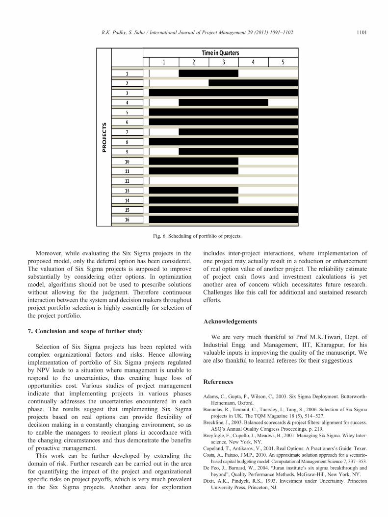
Fig. 6. Scheduling of portfolio of projects.


Moreover, while evaluating the Six Sigma projects in theproposed model, only the deferral option has been considered.The valuation of Six Sigma projects is supposed to improvesubstantially by considering other options. In optimizationmodel, algorithms should not be used to prescribe solutionswithout allowing for the judgment. Therefore continuousinteraction between the system and decision makers throughoutproject portfolio selection is highly essentially for selection ofthe project portfolio.

7. Conclusion and scope of further study

Selection of Six Sigma projects has been repleted withcomplex organizational factors and risks. Hence allowingimplementation of portfolio of Six Sigma projects regulatedby NPV leads to a situation where management is unable torespond to the uncertainties, thus creating huge loss ofopportunities cost. Various studies of project managementindicate that implementing projects in various phasescontinually addresses the uncertainties encountered in eachphase. The results suggest that implementing Six Sigmaprojects based on real options can provide flexibility ofdecision making in a constantly changing environment, so asto enable the managers to reorient plans in accordance withthe changing circumstances and thus demonstrate the benefitsof proactive management.

This work can be further developed by extending thedomain of risk. Further research can be carried out in the areafor quantifying the impact of the project and organizationalspecific risks on project payoffs, which is very much prevalentin the Six Sigma projects. Another area for exploration

includes inter-project interactions, where implementation ofone project may actually result in a reduction or enhancementof real option value of another project. The reliability estimateof project cash flows and investment calculations is yetanother area of concern which necessitates future research.Challenges like this call for additional and sustained researchefforts.

Acknowledgements

We are very much thankful to Prof M.K.Tiwari, Dept. ofIndustrial Engg. and Management, IIT, Kharagpur, for hisvaluable inputs in improving the quality of the manuscript. Weare also thankful to learned referees for their suggestions.

References

Adams, C., Gupta, P., Wilson, C., 2003. Six Sigma Deployment. Butterworth-Heinemann, Oxford.

Banuelas, R., Tennant, C., Tuersley, I., Tang, S., 2006. Selection of Six Sigmaprojects in UK. The TQM Magazine 18 (5), 514–527.

Breckline, J., 2003. Balanced scorecards & project filters: alignment for success.ASQ's Annual Quality Congress Proceedings, p. 219.

Breyfogle, F., Cupello, J., Meadws, B., 2001. Managing Six Sigma. Wiley Inter-science, New York, NY.

Copeland, T., Antikarov, V., 2001. Real Options: A Practioners's Guide. Texer.Costa, A., Paixao, J.M.P., 2010. An approximate solution approach for a scenario-

based capital budgetingmodel. ComputationalManagement Science 7, 337–353.De Feo, J., Barnard, W., 2004. “Juran institute's six sigma breakthrough and

beyond”, Quality Performance Methods. McGraw-Hill, New York, NY.Dixit, A.K., Pindyck, R.S., 1993. Investment under Uncertainty. Princeton

University Press, Princeton, NJ.


Eckhause, J.M., Hughes, D.R., Gabriel, S.A., 2009. Evaluating real options formitigating technical risk in public sector R&D acquisitions. InternationalJournal of Project Management 27 (4), 365–377.

Evans, G.W., Fairbairn, R., 1989. Selection and scheduling of advanced missionsfor NASA using 0–1 integer linear programming. The Journal of theOperational Research Society 40 (1), 971–981.

Ghasemzada, F., Archer, N., Iyogen, P., 1999. A zero one model for projectportfolio selection and scheduling. Journal of the Operational ResearchSociety 50, 745–755.

Helga, M., Nicos, C., Gerry, S., 2001. Capital budgeting under uncertainty−anintegrated approach using contingent claims analysis and integer program-ming. Operations Research 49 (2), 196–206.

Hu, G., Wang, L., Fetch, S., Bidanda, B., 2008. A multi-objective model forproject portfolio selection to implement lean and Six Sigma concepts.International Journal of Production Research 46 (23), 6611–6625.

Kelly, M., 2002. Three steps to project selection. ASQ Six Sigma ForumMagazine 2 (1), 29–33.

Kira, D.S., Kusy, M.I., Murray, D.H., Goranson, B.J., 1990. A specific decisionsupport system (SDSS) to develop an optimal project portfolio mix underuncertainty. IEEE Transactions on Engineering Management 37 (3),213–221.

Kodukula, P., Papudesu, C., 2006. Project Valuation Using Real Options.J. Ross Publishing.

Kumar, R.L., 2002. Managing Risks in IT projects: an option perspective.Information & Management 40 (1), 63–74.

Kumar, U.D., Saranga, H., Marquez, J.E.R., Nowicki, D., 2007. Six sigmaproject selection using data envelopment analysis. The TQM Magazine19 (5), 419–441.

Kwak, Y.H., Anbari, F.T., 2006. Benefits, obstacles, and future of Six Sigmaapproach. Technovation 26 (5–6), 708–715.

Larson, A., 2003. Demystifying Six Sigma. American Management Associa-tion, New York, NY.

Mawby, W.D., 2007. Project Portfolio Selection for Six Sigma. ASQ.Miller, L.T., Park, C.S., 2002. Decision making under uncertainty−real option to

the rescue. The Engineering Economist 47 (2), 105–150.Pande, P., Neuman, R., Cavanaugh, R., 2000. The Six Sigma Way: How GE,

Motorola and Other Top Companies are Honing their Performance.McGraw-Hill, New York, NY.

Pyzdek, T., 2000. “Selecting Six Sigma projects”, Quality Digest, available at: www.qualitydigest.com/sept00/html/sixsigma.html (accessed 16 March 2005).

Pyzdek, T., 2003. The Six Sigma Project Planner. McGraw-Hill, New York, NY.Rousel, P.K.S., Erickson, T., 1991. Third Generation R&D: Managing the Link

to Corporate Strategy. Harvard Bus. School Press, Boston, MA.Schneider, M., Tejeda, M., Dondi, G., Herzog, F., Keel, S., Geering, H.P., 2008.

Making real options work for practitioners: a generic model for valuingR&D projects. R&D Management 38 (1), 85–106.

Schwartz, E.S., Zozaya-Gorostiza, C., 2003. Investment under uncertainty ininformation technology acquisition and development projects. ManagementScience 49 (1), 57–70.

Su, C.-T., Chou, C.-J., 2008. A systematic methodology for the creation of SixSigma projects: a case study of semiconductor foundry. Expert Systems withApplications 34 (2), 2693–2703.

Tkac, M., Lyocsa, S., 2009. On the evaluation of Six Sigma Projects. Qualityand Reliability Engineering International. On line publication.

Trigeorgis, L., 1996. Real Options. MIT Press, Cambridge, MA.Zimmerman, J.P., Weiss, J., 2005. Six Sigma's seven deadly sins. Quality 44 (1),

62–66.

http://www.qualitydigest.com/sept00/html/sixsigma.html

http://www.qualitydigest.com/sept00/html/sixsigma.html

A Real Option based Six Sigma project evaluation and selection model

Documents

Transcript of A Real Option based Six Sigma project evaluation and selection model