Design and Validation of an Electro-Hydraulic Pressure ...

Western Michigan University Western Michigan University

ScholarWorks at WMU ScholarWorks at WMU

Dissertations Graduate College

12-2016

Design and Validation of an Electro-Hydraulic Pressure-Control Design and Validation of an Electro-Hydraulic Pressure-Control

Valve and Closed-Loop Controller Valve and Closed-Loop Controller

Jerry Boza Western Michigan University, [email protected]

Follow this and additional works at: https://scholarworks.wmich.edu/dissertations

Part of the Mechanical Engineering Commons

Recommended Citation Recommended Citation Boza, Jerry, "Design and Validation of an Electro-Hydraulic Pressure-Control Valve and Closed-Loop Controller" (2016). Dissertations. 2490. https://scholarworks.wmich.edu/dissertations/2490

This Dissertation-Open Access is brought to you for free and open access by the Graduate College at ScholarWorks at WMU. It has been accepted for inclusion in Dissertations by an authorized administrator of ScholarWorks at WMU. For more information, please contact [email protected].

http://scholarworks.wmich.edu/


https://scholarworks.wmich.edu/

https://scholarworks.wmich.edu/dissertations

https://scholarworks.wmich.edu/grad

https://scholarworks.wmich.edu/dissertations?utm_source=scholarworks.wmich.edu%2Fdissertations%2F2490&utm_medium=PDF&utm_campaign=PDFCoverPages

http://network.bepress.com/hgg/discipline/293?utm_source=scholarworks.wmich.edu%2Fdissertations%2F2490&utm_medium=PDF&utm_campaign=PDFCoverPages

https://scholarworks.wmich.edu/dissertations/2490?utm_source=scholarworks.wmich.edu%2Fdissertations%2F2490&utm_medium=PDF&utm_campaign=PDFCoverPages

mailto:[email protected]



DESIGN AND VALIDATION OF AN ELECTRO-HYDRAULIC PRESSURE-CONTROL VALVE AND CLOSED-LOOP CONTROLLER

by

Jerry Boza

A dissertation submitted to the Graduate College in partial fulfillment of the requirements for the degree of Doctor of Philosophy Industrial and Mechanical Engineering

Western Michigan University December 2016

Doctoral Committee:

Kapseong Ro, Ph.D., Chair James Kamman, Ph.D. Jennifer Hudson, Ph.D. Ikhlas Abdel-Qader, Ph.D.

DESIGN AND VALIDATION OF AN ELECTRO-HYDRAULIC PRESSURE-CONTROL

VALVE WITH CLOSED-LOOP CONTROLLER

Jerry Boza, Ph.D.

Western Michigan University, 2016

Electro-hydraulic pressure-control valves are used in many applications, such as

manufacturing equipment, agricultural machinery, and aircrafts to name a few. They are often

used to actuate hydraulic clutches, such as those found in power shift transmissions. A

traditional pressure-control valve with open-loop control algorithm is typically used in clutch

applications. This scheme often results in inconsistent or undesirable system behavior due to

the nature of open-loop control as well as the nonlinear system dynamics and uncertainties.

In this research two new electro-hydraulic pressure-control valves were designed in

order to decouple the valve and control port (hydraulic) dynamics. This was achieved by

removing the regulated pressure balancing force utilized in traditional pressure-control valves.

Different closed-loop controllers were designed and tested in parallel in order to achieve the

desired steady-state and dynamic regulated pressure response. A nonlinear dynamic model was

developed for each valve then used to compare the performance characteristics of the valves.

Linear analysis was performed and various control techniques were studied from classical PID

control to modern optimal control. The model was also used to predict performance of the

closed-loop controllers prior to experimental testing and to validate experimentally tuned

controllers afterwards.

Prototype valves were fabricated in order to validate the model and to test the

controller designs experimentally. Different valve and controller combinations were compared

to a traditional pressure-control valve utilizing open-loop control through typical industry

performance tests. This study found that a valve with a traditional pressure-control pilot and a

main stage spool with no pressure balancing force, along with a gain scheduled PID controller,

outperformed the traditional valve in all areas tested. This approach is also feasible within the

existing infrastructure of most applications where the benchmark traditional valve is currently

used.

Copyright by

Jerry Boza 2016

ii

ACKNOWLEDGEMENTS

I would like to start by thanking Dr. Kapseong Ro, first for piquing my interest in control

theory, and second for the time he has invested advising me and acting as chair of my

committee. I would also like to thank the rest of my committee, Dr. James Kamman, Dr.

Jennifer Hudson, and Dr. Ikhlas Abdel-Qader, for their time reviewing my work.

Next, I would like to thank several of my colleagues for helping me throughout the

process, Josh Lambrix for his help designing the valve; Cody Sturgill for assistance with testing

and implementing the controllers; and Jeff Huffman for his continued discussions and

encouragement throughout the process.

Finally I would like to thank my family and especially my wife Ashley for her support at

home. Every hour I spent on this endeavor was an extra hour she spent raising our family.

Jerry Boza

iii

TABLE OF CONTENTS

ACKNOWLEDGEMENTS .................................................................................................................... ii

LIST OF TABLES ................................................................................................................................ vi

LIST OF FIGURES ............................................................................................................................. vii

NOMENCLATURE .............................................................................................................................. x

1 INTRODUCTION ............................................................................................................................ 1

1.1 Valve basics and applications ................................................................................................ 1

1.2 Literature review ................................................................................................................... 7

1.2.1 Dynamics of pressure-control valves ............................................................................. 7

1.2.2 Dynamics of hydraulic conduit and clutch ..................................................................... 9

1.2.3 Controls for electro-hydraulic systems ........................................................................ 11

1.2.4 Controls for electro-hydraulic actuated clutch ............................................................ 12

1.3 Problem description ............................................................................................................ 15

1.3.1 Problem statement ....................................................................................................... 15

1.3.2 Contribution of the present work ................................................................................ 16

2 MODELING AND DESIGN OF SUBSYSTEMS ................................................................................ 18

2.1 Modeling approach and summary ...................................................................................... 18

2.2 Traditional valve model development ................................................................................ 19

2.2.1 Traditional pilot model ................................................................................................. 19

2.2.2 Traditional main stage model development ................................................................ 23

2.2.3 Combining traditional pilot and main stage models .................................................... 27

2.3 Traditional pilot with proposed main stage model development ...................................... 33

2.4 Proposed pilot with proposed main stage model development ........................................ 36

3 NUMERICAL SIMULATIONS AND EXPERIMENTAL VALIDATION ................................................. 41

3.1 Nonlinear numerical AMESim model .................................................................................. 41

3.2 Baseline nonlinear simulations ........................................................................................... 42

iv

Table of Contents - Continued

3.3 Experimental validation of model ....................................................................................... 50

3.3.1 Experimental test setup................................................................................................ 50

3.3.1 Experimental open loop response results .................................................................... 53

3.4 Open loop disturbance rejection simulations ..................................................................... 59

3.5 Frequency response simulations......................................................................................... 61

4 LINEAR ANALYSIS AND INITIAL CONTROLLER DESIGN ............................................................... 65

4.1 Model linearization ............................................................................................................. 65

4.2 Initial controller evaluation ................................................................................................. 68

4.2.1 Closed loop experimental setup ................................................................................... 69

4.2.2 Initial controller experimental results .......................................................................... 70

4.3 Revised controller evaluation ............................................................................................. 72

4.3.1 Further classical control design .................................................................................... 72

4.3.2 Internal model control .................................................................................................. 76

4.3.3 Optimal control design ................................................................................................. 80

4.3.4 Summary of initial controller evaluation ...................................................................... 86

5 CONTROLLER DEVELOPMENT AND FURTHER EXPERIMENTAL TESTING ................................... 88

5.1 Experimental controller tuning under standard operating conditions ............................... 88

5.2 Validation of experimentally tuned controller in nonlinear model .................................... 91

5.3 Frequency domain analysis ................................................................................................. 92

5.4 Further experimental testing .............................................................................................. 94

5.4.1 Repeatability and variation .......................................................................................... 95

5.4.2 Hysteresis ...................................................................................................................... 96

5.4.3 Step response ............................................................................................................... 98

5.4.4 Sensitivity to system parameters ................................................................................. 99

5.4.5 Clutch shift simulation testing .................................................................................... 103

v

Table of Contents - Continued

6 CONCLUSION ............................................................................................................................ 106

6.1 Significance and summary ................................................................................................ 106

6.2 Conclusion and contribution ............................................................................................. 106

6.3 Future work ....................................................................................................................... 108

APPENDIX A - OIL PROPERTIES .................................................................................................... 109

REFERENCES ................................................................................................................................ 111

vi

LIST OF TABLES 1 State Variable Description for Traditional Valve .......................................................... 29

2 State Variable Description for Proposed Pilot with Proposed Main Stage Valve ........ 38

3 Baseline Model Parameters ......................................................................................... 43

4 State Space Representation of Proposed Pilot with Proposed Main Stage at 10bar

Linearization Point ....................................................................................................... 73

5 PID Controller Gains ..................................................................................................... 90

6 Frequency Response Results ........................................................................................ 94

7 Hysteresis Testing Results ............................................................................................ 97

vii

LIST OF FIGURES

1 Pilot Operated 3/2 Proportional Pressure Control Valve ........................................................... 4

2 Block Diagrams of Clutch Phases ................................................................................................ 5

3 Typical Clutch Actuation Sequence ............................................................................................. 6

4 (a) Traditional Open-Loop / (b) Proposed Closed-Loop ............................................................ 16

5 Traditional Pilot: (a) Cross Section and (b) Armature / Flapper Assembly Free Body

Diagram .................................................................................................................................... 20

6 Flapper-Nozzle Hydraulic Schematic, Cross Section, and Resulting Pressure ......................... 22

7 Traditional Main Stage: (a) Cross Section and (b) Spool Free Body Diagram .......................... 24

8 Flow Versus Spool Displacement ............................................................................................. 27

9 Schematic of Traditional Valve ................................................................................................. 29

10 Traditional Pilot Block Diagram................................................................................................ 31

11 Pilot Damping Block Diagram................................................................................................... 32

12 Traditional Main Stage Block Diagram ..................................................................................... 33

13 Schematic of Traditional Pilot with Proposed Main Stage ...................................................... 33

14 Traditional and Proposed Spool Pressure Versus Displacement ............................................. 34

15 Proposed Main Stage Block Diagram ....................................................................................... 36

16 Schematic of Proposed Pilot with Proposed Main Stage ........................................................ 37

17 Proposed Pilot Block Diagram .................................................................................................. 39

18 Proposed Main Stage Block Diagram ....................................................................................... 40

19 Amesim Model for Proposed Pilot with Proposed Main Stage ............................................... 42

20 Steady-state Pressure Versus Current Comparison ................................................................. 43

21 Traditional Valve Step Response at Different Temperatures .................................................. 45

22 Traditional Pilot with Proposed Main Stage Valve Step Response at Different

Temperatures .......................................................................................................................... 46

23 Proposed Pilot with Proposed Main Stage Valve Step Response at Different

Temperatures .......................................................................................................................... 46

24 Traditional Valve Step Response with Different Oil Aeration ................................................. 48

25 Traditional Pilot with Proposed Main Stage Valve Step Response with Different Oil

Aeration ................................................................................................................................... 49

26 Proposed Pilot with Proposed Main Stage Valve Step Response with Different Oil Aeration 49

27 Hydraulic Schematic ................................................................................................................. 50

28 Experimental Test Setup .......................................................................................................... 51

29 Electrical Schematic ................................................................................................................. 52

viii

List of Figures - Continued

30 Electrical Schematic of Current Driver ..................................................................................... 52

31 Electrical Experimental Test Setup .......................................................................................... 53

32 Traditional Valve Pressure versus Current Validation ............................................................. 54

33 Traditional Valve Experimental Step Response ....................................................................... 55

34 Traditional Pilot with Proposed Main Stage Pressure versus Current Validation ................... 56

35 Traditional Pilot with Proposed Main Stage Step Response Validation .................................. 57

36 Proposed Pilot with Proposed Main Stage Pressure versus Current Validation ..................... 58

37 Proposed Pilot with Proposed Main Stage Step Response Validation .................................... 58

38 External Flow Disturbance to Traditional Valve ...................................................................... 60

39 External Flow Disturbance Impulse Response Comparison .................................................... 61

40 Nonlinear Simulation of 1Hz Sinusoidal Voltage Input and Pressure Output ......................... 62

41 Nonlinear Simulation of 10Hz Sinusoidal Voltage Input and Pressure Output ....................... 62

42 Discrete Magnitude versus Frequency of Traditional and Proposed Valves ........................... 63

43 Discrete Phase Angle versus Frequency of Traditional and Proposed Valve .......................... 64

44 Pole Migration of Traditional Valve ......................................................................................... 66

45 Pole Migration of Traditional Pilot with Proposed Main Stage ............................................... 67

46 Pole Migration of Proposed Pilot with Proposed Main Stage ................................................. 68

47 Pressure Feedback Block Diagram ........................................................................................... 69

48 Experimental Components for Closed Loop Control ............................................................... 70

49 Experimental Closed Loop Response of Proposed Pilot with Proposed Main Stage .............. 71

50 Initial Proposed Closed Loop Step Response Compared to Traditional Valve Open Loop

Step Response.......................................................................................................................... 72

51 Step Response Comparison for Proposed Pilot with Proposed Main Stage............................ 74

52 Nonlinear Simulation of Lag Compensator with Integrator .................................................... 76

53 Internal Model Control Structure ............................................................................................ 77

54 Step Response of IMC Compensator with 10bar Linearized Model ........................................ 78

55 IMC Compensator Integrated Into Nonlinear Model .............................................................. 78

56 Error between the Nonlinear Model Regulated Pressure and Linearized Model Regulated

Pressure ................................................................................................................................... 79

57 Block Diagram for Full State Feedback with Integration Augmentation ................................. 80

58 Nonlinear Model with Full State Feedback and Integrator Augmentation ............................. 82

59 Step Response of Nonlinear Model with LQR and Integrator Augmentation ......................... 83

60 Block Diagram for LQG Controller with Integrator Augmentation .......................................... 84

61 Nonlinear Model with LQG Compensator and Integrator Augmentation ............................... 85

ix

List of Figures - Continued

62 Step Response of Nonlinear Model with LQQ and Integrator Augmentation ........................ 86

63 Operating Points for Tuning Controller Gains ......................................................................... 89

64 Closed Loop 2bar Step Response Compared to Traditional Valve Open Loop Step

Response ................................................................................................................................. 90

65 Nonlinear Model with PID and Gain Scheduling ...................................................................... 91

66 Experimental and Numerical Closed Loop Step Response ...................................................... 92

67 Discrete Magnitude versus Frequency of Traditional and Proposed Valve with Controller ... 93

68 Discrete Phase versus Frequency of Traditional and Proposed Valve with Controller ........... 93

69 Regulated Pressure Repeatability Comparison ....................................................................... 96

70 Command Profile for Hysteresis Testing ................................................................................. 97

71 Distribution of Traditional Valve Hysteresis ............................................................................ 98

72 Intermediate Step Response Comparison ............................................................................... 99

73 Control pressure versus control port leakage ....................................................................... 100

74 Control pressure versus supply pressure ............................................................................... 101

75 Temperature sensitivity test setup ........................................................................................ 102

76 Control pressure versus oil temperature ............................................................................... 103

77 Clutch shift simulation testing with traditional valve ............................................................ 104

78 Clutch shift simulation testing with proposed valve and controller ..................................... 105

79 Viscosity versus Temperature ................................................................................................ 109

80 Bulk Modulus versus Temperature ........................................................................................ 109

81 Density versus Temperature .................................................................................................. 110

x

NOMENCLATURE

𝐴𝑑 = Damping area

𝑃𝑑1 = Damping pressure (opposing solenoid)

𝑃𝑑2 = Damping pressure (assisting solenoid)

𝑃𝑐 = Pilot control pressure

𝑃𝑠 = Pilot supply pressure

𝐴𝑛 = Nozzle area

𝑄𝑖𝑛 = Flow into control volume

𝑄𝑜𝑢𝑡 = Flow out of control volume

𝑐𝑑𝑖𝑛 = Discharge coefficient into volume

𝑐𝑑𝑜𝑢𝑡 = Discharge coefficient out of volume

𝜌 = Fluid density

𝜇 = Fluid dynamic viscosity

𝑣 = Fluid velocity

𝛽𝑓𝑙𝑢𝑖𝑑 = Bulk modulus of fluid

𝛽𝑎𝑖𝑟 = Bulk modulus of air

𝛽𝑒𝑓𝑓 = Effective fluid / air bulk modulus

𝑉𝑎𝑖𝑟 = Volume of air in a chamber

𝑉𝑓𝑙𝑢𝑖𝑑 = Volume of fluid in a chamber

𝐴𝑠 = Spool area (pilot side)

𝐴𝑝𝑏 = Spool pressure balancing area

xi

𝑓𝑓𝑟𝑖𝑐 = Friction force

𝐶 = Main control pressure

𝑃 = Main supply pressure

𝛼 = Transitional flow coefficient

𝛾 = Transitional flow coefficient

ℎ = Radial spool clearance

𝑙 = Engagement length

𝑚1 = Pilot mass

𝑘1 = Pilot spring rate

𝑐1 = Pilot damping coefficient

𝑚2 = Main stage mass

𝑘2 = Main stage spring rate

𝑐2 = Main stage damping coefficient

𝑥 = Displacement

𝑉 = Volume

𝑓𝑓𝑟𝑖𝑐 = Friction force

1

CHAPTER 1

INTRODUCTION

1.1 Valve basics and applications

Hydraulic control valves can be divided into three basic categories: directional-control,

flow-control, and pressure-control. Directional-control valves are used to connect and isolate

hydraulic passages by simply opening and closing a flow path. Flow-control valves allow

variable flow rate control to a component. Finally, pressure-control valves regulate variable

pressure to a hydraulic component. Electromechanical solenoids are commonly used to

actuate these hydraulic control valves, this allows for a flow or pressure for a corresponding

input current. This research will focus on electro-hydraulic pressure-control valves.

Power shifting type transmissions have been used in agricultural tractors for over 50

years. These power shift transmissions utilize hydraulic clutches to transmit torque. Since their

inception, continuous improvements have been made to increase number of speeds and full

torque capability to maintain optimum engine speed and power match in order to improve fuel

consumption, noise, and feel [1]. Recently these improvements have been made, in part,

through the use of electro-hydraulic pressure-control valves to actuate the clutches. The

mechanical elements of the transmission are well established and can be considered mature.

So, although there are still improvements being made to these components, there is much

more innovation still to come in the electronics and controls of these systems [2]. For each

2

shift there is typically an on-coming and off-going clutch, the timing of which is critical for shift

quality. These clutches are often controlled by electro-hydraulic pressure-control valves in

order to achieve this timing. Traditional pressure-control valves utilize pressure feedback on

the main spool to achieve a commanded clutch pressure for a corresponding input current.

One problem with this approach lies in the physics of the clutch being controlled. In order to

actuate this clutch a moving volume must be filled and then pressure modulated, so in essence

half of a shift sequence requires a flow-control valve and half requires a pressure-control valve.

This is currently achieved using only a pressure-control valve. Another issue is the impact of the

pressure balancing force acting on the spool. This balancing force significantly increases the

sensitivity of the valve to disturbances in the control port, such as when the clutch is filled and

suddenly stops moving. The clutches are typically actuated using open-loop feed forward

control algorithms. This is not ideal due to uncertain, time-varying, nonlinear system

parameters and the impact of pressure balancing force on valve performance. Both steady

state and transient performance can vary significantly due to changes in oil temperature, air

entrapment, pressure drop through passages, supply pressure and flow capacity, internal

volumes, and performance variation of the valves and clutches.

A significant amount of hardware development is required to achieve desired

performance. This occurs both at a system level and within the pressure-control valve

actuating the clutch. Often times this requires the addition of expensive components to

reduce response time, increase damping, reduce steady-state performance variation, and

reduce sensitivity to variation and changes in system parameters. These improvements are

constant and finite, and often do not completely address design goals. The system level

3

performance cannot be optimized through mechanical changes alone; therefore the need for a

closed-loop controller exists. For example, the clutch volume is often isolated from the

pressure balancing area on the main spool using an orifice in order to reduce the impact of

clutch pressure dynamics on valve performance. This orifice is a fixed size and is not optimum

for all operating conditions, so it is sized to balance performance requirements across the

board. This can be addressed through closed-loop control.

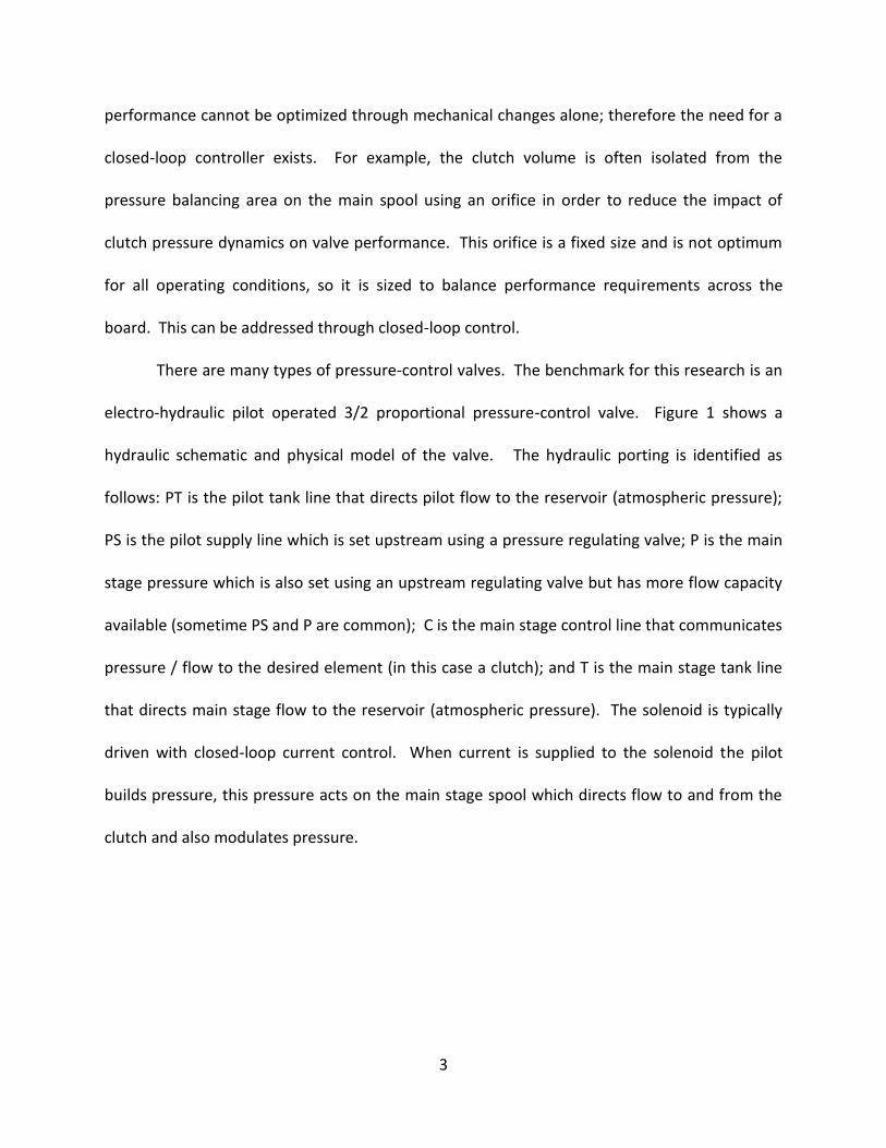
There are many types of pressure-control valves. The benchmark for this research is an

electro-hydraulic pilot operated 3/2 proportional pressure-control valve. Figure 1 shows a

hydraulic schematic and physical model of the valve. The hydraulic porting is identified as

follows: PT is the pilot tank line that directs pilot flow to the reservoir (atmospheric pressure);

PS is the pilot supply line which is set upstream using a pressure regulating valve; P is the main

stage pressure which is also set using an upstream regulating valve but has more flow capacity

available (sometime PS and P are common); C is the main stage control line that communicates

pressure / flow to the desired element (in this case a clutch); and T is the main stage tank line

that directs main stage flow to the reservoir (atmospheric pressure). The solenoid is typically

driven with closed-loop current control. When current is supplied to the solenoid the pilot

builds pressure, this pressure acts on the main stage spool which directs flow to and from the

clutch and also modulates pressure.

4

Figure 1 Pilot Operated 3/2 Proportional Pressure Control Valve

As current to the solenoid increases so does the force output. The armature is opposed

by a mechanical spring and regulated pressure acting on a fixed area. As the solenoid force

overcomes this mechanical spring rate and pressure balancing force the armature strokes and

closes a variable orifice; as this variable orifice is closed off the pressure opposing the solenoid

increases resulting in a proportional pressure vs current characteristic. This pilot pressure acts

on a spool in the main stage of the valve, the main stage spool then strokes as pilot pressure

increases. As the main stage spool strokes, pressure increases in the C port; this is all achieved

through opening and closing variable orifices (flow areas). The pressure in the C port acts on a

differential area on the spool, providing pressure a pressure balancing force. This pressure

balancing force opposes the driving force, in this case the pilot control pressure, resulting in a

consistent steady-state output pressure for a given input.

5

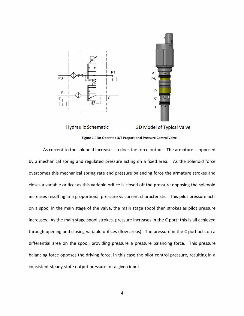
When actuating a clutch with a pressure-control valve there are generally three phases

in an open-loop command scheme, the fill, the pressure modulation, and the emptying. During

the fill phase the valve is actuated with full command for a short duration, this allows the main

stage spool to shift over and provide flow to the clutch. Next, the command is stepped down to

an intermediate pressure, below that required to engage the clutch plates. This command is

held for a short period then ramped up to full command at various rates depending on the

desired torque transfer; this is the pressure modulation phase where the main stage spool is in

the center position. Finally, during the emptying phase the valve is de-energized so that the

main spool shifts back and opens a path from clutch to tank. Figure 2 shows this process flow in

simple block diagram form (a more comprehensive block diagram of the valve can be found in

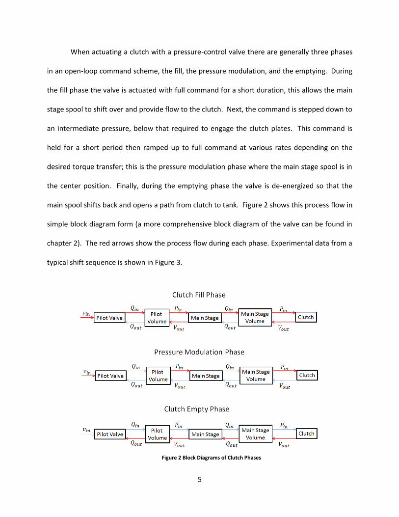
chapter 2). The red arrows show the process flow during each phase. Experimental data from a

typical shift sequence is shown in Figure 3.

Figure 2 Block Diagrams of Clutch Phases

6

Figure 3 Typical Clutch Actuation Sequence

Development of this shift algorithm and coordination with the off-going clutch are

required to achieve a smooth and efficient shift. The fill process is critical and is also a large

source of uncertainty due to variables such as fluid temperature, valve and clutch

characteristics, and line variations, making this process difficult to control [3]. These variables

can lead to overfill or under fill of the on-coming clutch, both of which are undesirable. This is

typically controlled through open-loop, event driven, feedback control, or some combination of

them.

Valve performance variation is inherent in the design due to component and

manufacturing variation. Attempts are made to minimize variation of the critical performance

characteristics, such as the steady state pressure at specified currents, the pressure drop from P

to C and from C to T at a specified flow, the response time, and the coil resistance. These are

7

controlled through dimensioning of component tolerances and precision assembly and adjust

processes.

1.2 Literature review

The use of control systems for actuating clutches has continuously increased over the

last several decades as electrohydraulic pressure-control valves are increasingly implemented

into these systems. Electrohydraulic pressure-control valves have many advantages, one being

their high power-to-weight ratio. Open-loop control is often used to actuate clutches with

pressure-control valves for a variety of reasons, one being the difficulty in developing a closed-

loop controller. The highly nonlinear dynamics, extreme variations in system stiffness, and

unknown system parameters make controllability difficult. In this section, pertinent research is

reviewed, focused on modeling the dynamics of the pressure-control valve, clutch and

passages, and current control strategies for electrohydraulic applications.

1.2.1 Dynamics of pressure-control valves

The pressure-control valve is actuated by an electromechanical solenoid. Solenoids are

a mature technology and have been used in various applications since the early 1900s. The

characteristics, primarily force output, resistance, and inductance, of solenoids can be

calculated using magnetic circuit concepts of magnetomotive force, reluctance, and magnetic

flux [4]. These techniques as applied to actual solenoid design are well established and have

been summarized by Roters [5]. The solenoid characteristics can also be established through

solving the three dimensional Maxwell equations. This is best accomplished using a numerical

software package due to several factors, such as, the nonlinearity of equations, geometric

constraints, magnetic saturation, and eddy current effects. Both of these techniques can

8

require a significant amount of computational effort. Topcu et al showed that lookup tables

could be used to simplify the numerical solutions of electromechanical actuators without loss of

accuracy in dynamic simulations [6]. Use of lookup tables also allows for the incorporation of

experimental data.

The spool position provides the actual pressure regulation, as it controls the flow area

into and out of the control port. Some of the key spool characteristics include leakage, flow

rate, and flow forces. Spool leakage for long annular lengths is fully developed, laminar, and

follows Poiseuille’s law so it can be calculated analytically from the Navier-Stokes equations [7].

For large spool openings the flow is turbulent and can be calculated using the classic orifice

equation. This equation is derived from the Bernoulli equation and incorporates a discharge

coefficient, Cd, which is a loss factor [8]. Dong and Ueno showed that the discharge coefficient

is a function of the Reynolds number for spool valves and that this could be determined

numerically [9]. For high Reynolds number flow at smaller openings they discovered a

reattached flow pattern causing the flow coefficient to increase, but only for flows with a

Reynolds number less than a critical value. The numerical and experimental flow coefficient

and flow force values matched well for several cases. The leakage and flow rate for the

transitional spool opening, between fully developed laminar and fully open turbulent, is not as

straight forward but is the most critical because this is where pressure modulation occurs.

Ferreira et al. used a semi-empirical approach to calculate flow, pressure gain, and leakage [10].

Using a variable equation structure for the area that changed at a critical transition point they

were able to match experimental data by tuning the parameters in the analytical equation.

9

They assumed that valve flow was always turbulent so that the short orifice equation with

pseudo-section area functions could be used.

1.2.2 Dynamics of hydraulic conduit and clutch

The passage communicating the pressure-control valve and clutch is typically long and

cylindrical as it must travel down a shaft. The pressure drop through this passage must be

considered. This will depend on the flow rate, oil properties, geometry and surface, and flow

type (laminar or turbulent) according to Munson et al. [7]. This passage can also be subject to

hydraulic transients during the fill phase due to sudden changes in state. Deng et al. showed

that these transients could be determined analytically for laminar pipeline flow [11]. They

formulated the friction factor as a function of the Reynolds Number of the flow. This was

accomplished using a separation of variables method, which matched well with the numerical

solution obtained by the well-established Method of Characteristics. Taylor et al. developed a

method to incorporate the known frequency dependent friction in hydraulic conduits into both

the Finite Element Method and the Method of Characteristics [12]. This method was found

accurate for both laminar and turbulent flow of incompressible liquids. Soumelidis et al.

compared several numerical techniques for modeling hydraulic transients in pipelines [13].

They evaluated the method of characteristics (MOC), finite element method (FEM),

transmission line method (TLM), and the rational polynomial transfer function approximation

(RPTFA) method. They found the RPTFA model to be the most accurate (when an accurate

solution could be obtained), but to also have significantly longer computation times. The MOC

model provided the most accurate solutions in short computation times. The TLM model was

the most accurate and efficient but was prone to integration problems. Finally, the FEM

10

method was least accurate and efficient but handled nonlinearities and varying parameters and

time steps the best. In real systems, air is present in hydraulic oils to varying degrees and can

have an impact on pressure transients. Jiang et al. incorporated the impact of air content and

release into a model for pressure and flow transients [14]. The model utilized a genetic

algorithm in order to identify the initial air bubble volume in the oil, as well as the air release

and re-solution time constants which are unknown in real systems. Overall they were able to

show good agreement with experimental data.

The clutch dynamics play a large role in overall system performance. Jiang et al.

presented a clutch actuation model with various subsystem models all integrated [15]. They

outlined the modeling of the master cylinder, which is actuated hydraulically. The

characteristics of interest are the pressure acting on the cylinder, cylinder area, spring rate,

friction coefficient, and opposing force. The spring rate consists of both the return spring and

the diaphragm spring. The diaphragm spring is nonlinear and hard to represent so a lookup

table with experimental data was used. A couple of areas that were not addressed were the

flow coefficient, leakage, and fluid compressibility. The flow coefficient is dependent on the

valve geometry and oil characteristics as discussed above. Lazar et al. incorporated oil

compressibility into their model [16]. They showed analytically how the oil compressibility

dictates the break frequency of the clutch chamber. They were able to match experimental

data well and ultimately develop a predictive control scheme using the model. The effective

compressibility must be considered, this is a combination of the air content, bulk modulus of

the oil, and elasticity of the pressure vessel according to Manring [8].

11

1.2.3 Controls for electro-hydraulic systems

Due to the highly nonlinear dynamics of electro-hydraulic systems the classical control

approach has been to linearize these dynamics and use constant gains in a feedback loop [17].

Since this approach is very limited, this has led to the synthesis of robust, adaptive, and

predictive controllers. System nonlinearities and uncertainties in electrohydraulic servo

systems have most recently been handled through robust control synthesis. Weng et al.

developed a Lyapunov-based control algorithm for position control of a hydraulic cylinder using

an electrohydraulic flow-control valve [19]. They incorporated flow vs. pressure nonlinearities

as well as pressure chamber dynamics through a linear parameter varying (LPV) model. The

closed loop cylinder position was asymptotically stable. Milic et al. presented a robust H-

infinity state feedback controller for a similar system [17]. They designed a full state robust H-

infinity observer to estimate internal states such as spool position. The valve and hydraulic

dynamics were modeled and linearized. The linearized coefficients were modeled as

parametric uncertainty in a linear fractional transform (LFT) framework. The integral of the

signal error was introduced as a new state variable due to the steady state errors caused by

disturbances which cannot be eliminated by state feedback gain. Finally they used the

bounded real lemma (BRL) to obtain the H-infinity constraint; they guaranteed stability by

finding a positive-definite matrix as a solution to the bilinear matrix inequality (BMI) using a

general nonlinear transformation. The closed loop system showed good dynamic behavior with

robustness to parameter uncertainty and external load disturbances of the cylinder both in

nonlinear numerical simulations and in experimental trials.

12

A generalized approach for the design of predictive controllers for electrohydraulic

systems was presented by Jadlovska and Jajcisin [20]. The control algorithm consists of two

steps, predictor derivation and computing optimal sequence of control actions. Two input-

output models were evaluated, an Auto Regressive Model with External Output (ARX), and a

Controlled Auto Regressive Moving Average (CARIMA). The generalized algorithms were

designed based on the models such that it was possible to compute the optimal control

sequence by the receding horizon principle. They were able to control hydraulic flow between

two chambers using both algorithms and found the CARIMA model to be preferable unless the

system is noisy, then the ARX model is preferred.

1.2.4 Controls for electro-hydraulic actuated clutch

One difficulty in hydraulic clutch control is the sudden change in hydraulic

characteristics. The transition from the fill phase to the pressure modulation phase is stiff and

highly nonlinear as the clutch piston abruptly stops. The fill phase of the clutch is more suited

for a flow-control valve, but once the clutch piston stops moving a pressure-control valve is

required to proportionally transfer torque. Using two valves is not a realistic solution so a

pressure-control valve is used for the entire sequence. The transition from the fill phase to the

pressure modulation phase is difficult to control due to the sudden change in control port

characteristics and the pressure feedback on the spool of the pressure-control valve.

Lazar et al. designed a predictive control scheme for a wet clutch actuated by an electro-

hydraulic valve [16, 18]. They developed a CARIMA model for the input-output dynamics of the

system, with supply voltage as the input and clutch piston displacement as the output. The

solenoid force was modeled as a polynomial and current as a simple RL circuit. Linearized flow

13

equations with flow coefficients were modeled with all coefficient values for the system

parameters determined experimentally. The objective function for the predictor was based on

the minimization of tracking error balanced with the minimization of controller output. The

dynamic model was accurate when compared to test data. The predictive controller was

developed using the validated model and tested in simulations, not experimentally.

Dutta et al. devised a two-step strategy, called learning predictive control, consisting of an

optimal reference trajectory to handle system nonlinearities and feedback predictive control to

account for time varying system dynamics [21]. The goal was to achieve fast clutch

engagement with minimum torque loss, which are conflicting requirements. This is also

challenging due to the stiff nonlinearities in the system and lack of sensors. Due to the

difficulty in developing the model, they determined a genetic algorithm based optimization

would be ideal, but it is a feedforward scheme and not robust to disturbances or uncertainties.

Therefore a model based predictive control scheme was also used to track reference pressure.

System identification was used to model the filling phase, along with a variable delay based on

the amount of oil in the pipeline and the temperature of the oil. Once the clutch piston is

engaged they used a feedforward current signal that was optimized through several iterations

instead of modeling the clutch due to the linear pressure vs. current relationship. Once the

signal was optimized intermediate sensors were used for feedback. The feedback controller

was also used to track the optimized profile as it changes due to wear, temperature, etc. The

genetic algorithm was used to minimize engagement time and torque loss but was shown

experimentally to not be robust. This was addressed with the feedback controller based on

testing at two different temperatures.

14

Horn et al. designed a nonlinear feedforward controller using a flatness approach with a

linear PD controller to stabilize the system [22]. They simplified the dynamic model by

eliminating the dynamics of the valve piston because they are fast when compared to the

clutch piston dynamics. They were able to show that the nonlinear system was flat but also

required a PD controller because the open loop system was unstable. Clutch piston

displacement was the output and they were able to show accurate trajectory tracking in

experimental testing.

Song and Sun were able to design a sliding mode control to achieve robust control and

avoid chattering, which is a well-known design issue with sliding mode control [23]. They

constructed and validated an electro-hydraulically actuated clutch model and an observer to

estimate clutch piston displacement. The design goals were to achieve fill, then provide

smooth and precise torque control. They selected pressure feedback in the clutch chamber for

3 reasons, pressure is directly related to torque, it is difficult to package a displacement sensor

in the clutch, and it is expensive to measure high resolution displacement in the required range.

The pressure feedback approach differs from previous clutch engagement control schemes that

require displacement feedback. Slip feedback was another option but cannot be used for the

fill phase, while pressure feedback allows for both fill and torque control. They found it

challenging to design a nonlinear robust controller due to the nonlinear 2nd order dynamics of

the system and the fact that care must be taken in sliding mode control to avoid high gain

chattering. Uncertainty bounds of pressure and flow dynamics were determined

experimentally. A high slope saturation function and non-conservative uncertainty bounds

were used to prevent chattering. A nonlinear observer for clutch displacement was

15

transformed into a linear observer design problem by incorporating the derivative of the

pressure measurement. They showed that the sliding mode robust controller was able to track

pressure and that the observer could be used to alleviate high gain demand and diagnose the

clutch fill status.

1.3 Problem description

1.3.1 Problem statement

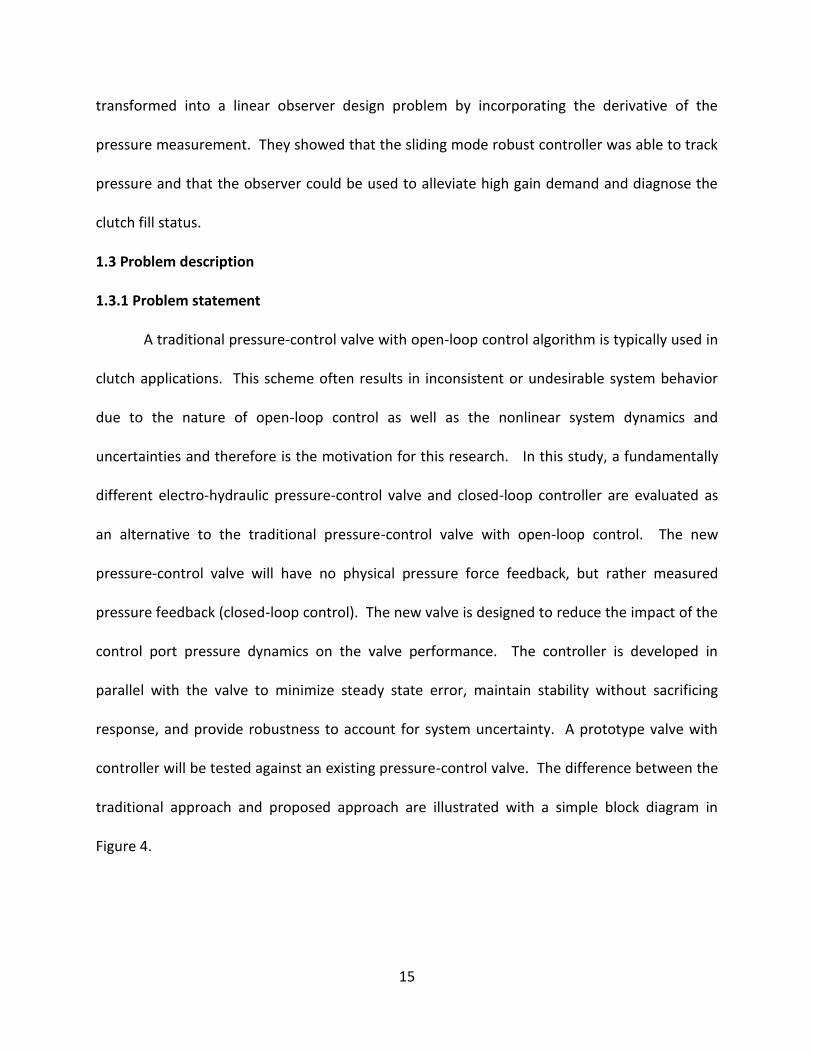
A traditional pressure-control valve with open-loop control algorithm is typically used in

clutch applications. This scheme often results in inconsistent or undesirable system behavior

due to the nature of open-loop control as well as the nonlinear system dynamics and

uncertainties and therefore is the motivation for this research. In this study, a fundamentally

different electro-hydraulic pressure-control valve and closed-loop controller are evaluated as

an alternative to the traditional pressure-control valve with open-loop control. The new

pressure-control valve will have no physical pressure force feedback, but rather measured

pressure feedback (closed-loop control). The new valve is designed to reduce the impact of the

control port pressure dynamics on the valve performance. The controller is developed in

parallel with the valve to minimize steady state error, maintain stability without sacrificing

response, and provide robustness to account for system uncertainty. A prototype valve with

controller will be tested against an existing pressure-control valve. The difference between the

traditional approach and proposed approach are illustrated with a simple block diagram in

Figure 4.

16

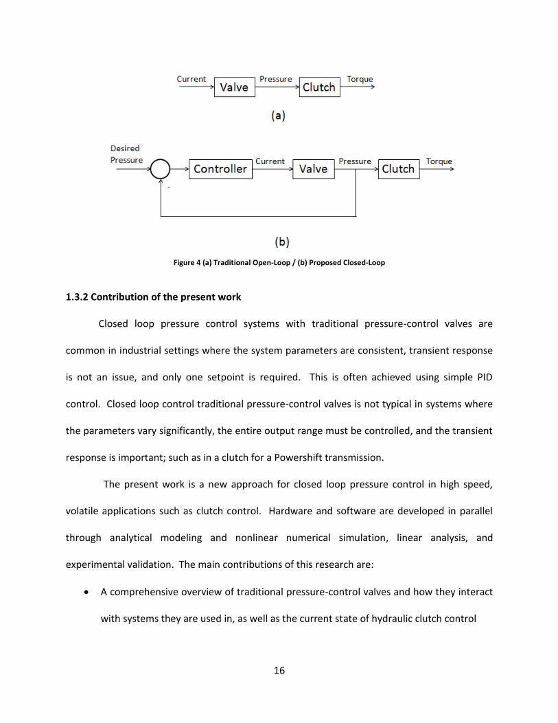
Figure 4 (a) Traditional Open-Loop / (b) Proposed Closed-Loop

1.3.2 Contribution of the present work

Closed loop pressure control systems with traditional pressure-control valves are

common in industrial settings where the system parameters are consistent, transient response

is not an issue, and only one setpoint is required. This is often achieved using simple PID

control. Closed loop control traditional pressure-control valves is not typical in systems where

the parameters vary significantly, the entire output range must be controlled, and the transient

response is important; such as in a clutch for a Powershift transmission.

The present work is a new approach for closed loop pressure control in high speed,

volatile applications such as clutch control. Hardware and software are developed in parallel

through analytical modeling and nonlinear numerical simulation, linear analysis, and

experimental validation. The main contributions of this research are:

A comprehensive overview of traditional pressure-control valves and how they interact

with systems they are used in, as well as the current state of hydraulic clutch control

17

Development of a mathematical model for various pressure-control valves with

experimental validation

Demonstration of the drawback of traditional pressure-control valves for closed-loop

control through linear analysis

Analysis of the influence of a hydraulic system on the performance of a pressure-

control valve

Evaluation of various control techniques and how they relate to different valve designs

A novel valve design that can be controlled with simple linear techniques and

outperform a traditional pressure-control in various industry driven areas of interest.

18

CHAPTER 2

MODELING AND DESIGN OF SUBSYSTEMS

2.1 Modeling approach and summary

In this section the various subsystems are identified and modeled individually. The

system consists of an electro-hydraulic pressure-control pilot, a main stage spool, hydraulic

passages, and a clutch simulator. Each subsystem is also compared to the traditional

counterpart to highlight the differences and reasoning for the new approach.

The solenoid geometry, force output, resistance, and inductance of the solenoid for the

proposed valve were determined numerically using ANSYS Maxwell electromagnetic field

simulation software. The force output was converted to a lookup table as a function of

armature position and current for improved implementation into dynamic simulations. The

resistance and inductance were modeled as a simple RL circuit with uncertainty bounds for

both parameters.

The pilot and main stage spools were modeled as Poiseuille flow when closed and using

the classic orifice equation when open. During the transition from fully closed to open a semi-

empirical analytical equation was developed. The flow forces were determined using the

Reynolds Transport Theorem. Both of these subsystems of the valve were modeled as 2nd order

systems with constant spring rate and viscous damping based on the oil properties and

clearances of the spools.

19

The clutch simulator motion was also modeled as a 2nd order system similar to the pilot

and main stage spools. The return spring and clutch stiffness once engaged are nonlinear and

were incorporated into the model as a lookup table. During pressure modulation of the clutch,

the pressure rise rate equation was used; this is based on the volume and change in volume,

effective bulk modulus of the clutch volume, and net flow rate. Finally a leak in the clutch was

simulated using the classic orifice equation.

2.2 Traditional valve model development

In this section a dynamic model is developed for the traditional pressure-control valve.

The pressure-control valve is actuated by an electromechanical solenoid. The characteristics,

primarily force output, resistance, and inductance, of solenoids can be calculated using

magnetic circuit concepts of magnetomotive force, reluctance, and magnetic flux [4]. These

techniques as applied to actual solenoid design are well established and have been summarized

by Roters [5]. The solenoid characteristics can also be established through solving the three

dimensional Maxwell equations. This is best accomplished using a numerical software package

due to several factors, such as, the nonlinearity of equations, geometric constraints, magnetic

saturation, and eddy current effects. Both of these techniques can require a significant amount

of computational effort. Topcu et al showed that lookup tables could be used to simplify the

numerical solutions of electromechanical actuators without loss of accuracy in dynamic

simulations [6]. Use of lookup tables also allows for the incorporation of experimental data.

2.2.1 Traditional pilot model

The equation of motion for the pilot armature / flapper assembly in the pilot can be

derived from the forces shown in Figure 5. As illustrated in the cross section, the pilot consists

20

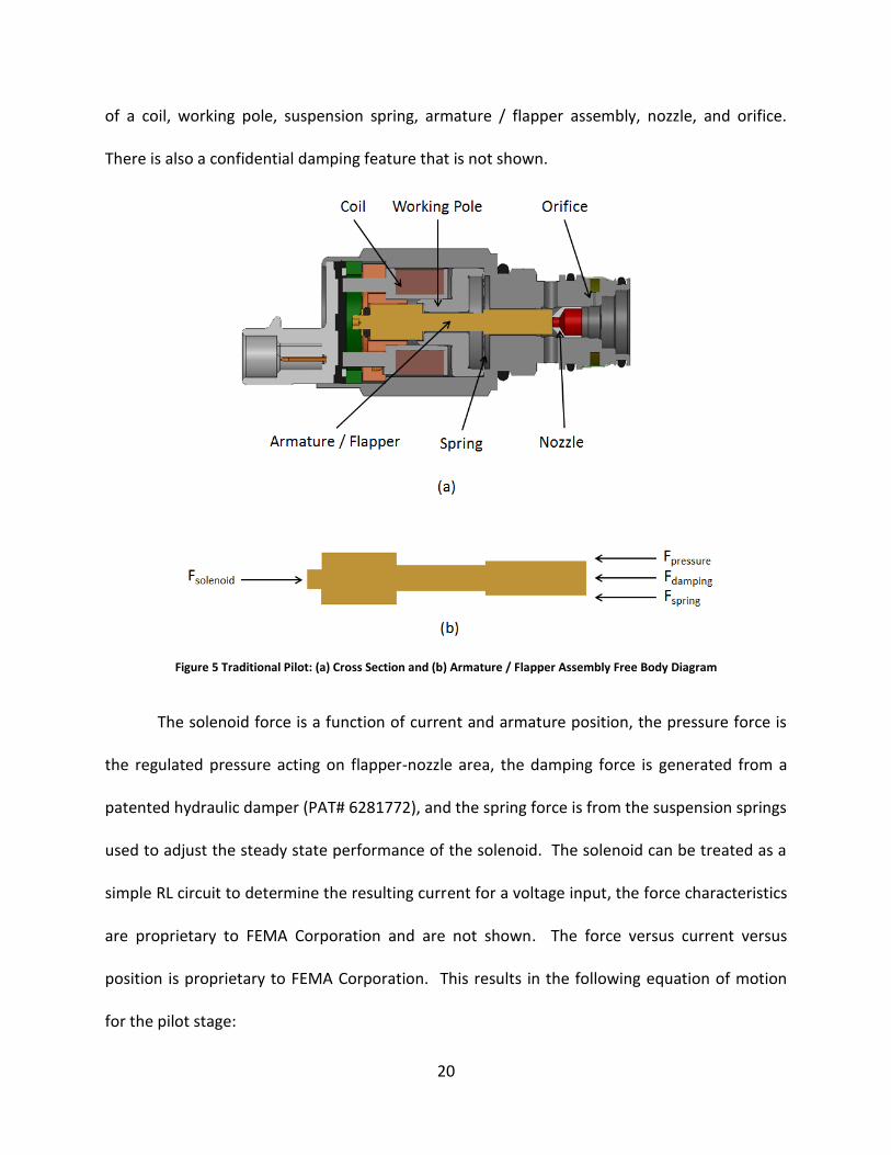
of a coil, working pole, suspension spring, armature / flapper assembly, nozzle, and orifice.

There is also a confidential damping feature that is not shown.

Figure 5 Traditional Pilot: (a) Cross Section and (b) Armature / Flapper Assembly Free Body Diagram

The solenoid force is a function of current and armature position, the pressure force is

the regulated pressure acting on flapper-nozzle area, the damping force is generated from a

patented hydraulic damper (PAT# 6281772), and the spring force is from the suspension springs

used to adjust the steady state performance of the solenoid. The solenoid can be treated as a

simple RL circuit to determine the resulting current for a voltage input, the force characteristics

are proprietary to FEMA Corporation and are not shown. The force versus current versus

position is proprietary to FEMA Corporation. This results in the following equation of motion

for the pilot stage:

21

=𝐹(𝑥, 𝑖)

𝑚−

𝑘𝑥

𝑚−

𝐴𝑑(𝑃𝑑1 − 𝑃𝑑2)

𝑚−

𝑃𝑐𝐴𝑛

𝑚 ( 1 )

where 𝑘 is the spring rate, 𝑚 is the armature / flapper assembly mass, 𝐹(𝑥, 𝑖) is the solenoid

force, 𝐴𝑑 is the damping area, 𝑃𝑑1 is the damping pressure opposing the solenoid force, 𝑃𝑑2 is

the damping pressure assisting the solenoid force, 𝑃𝑐 is the regulated pressure, and 𝐴𝑛 is the

nozzle feedback area that the regulated pressure acts against. The flapper position relative to

the nozzle dictates the regulated pressure, as it controls the flow into and out of the control

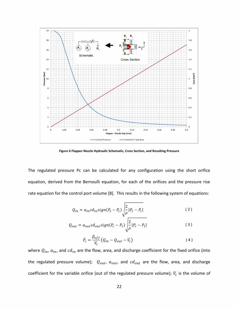
port volume. Figure 6 shows the pressure versus flapper-nozzle gap for a specific configuration.

The cross section is also represented schematically, where Ps is the constant supply pressure, Pc

is the regulated control pressure, and Pt is the tank pressure. In this configuration there is a

fixed orifice between Ps and Pc, and a variable orifice (the flapper-nozzle) between Pc and Pt. As

the flapper-nozzle gap closes down the variable orifice area decreases linearly and Pc pressure

increases accordingly. This is the steady-state pressure versus position for the traditional

pressure-control pilot.

22

Figure 6 Flapper-Nozzle Hydraulic Schematic, Cross Section, and Resulting Pressure

The regulated pressure Pc can be calculated for any configuration using the short orifice

equation, derived from the Bernoulli equation, for each of the orifices and the pressure rise

rate equation for the control port volume [8]. This results in the following system of equations:

𝑄𝑖𝑛 = 𝑎𝑖𝑛𝑐𝑑𝑖𝑛𝑠𝑖𝑔𝑛(𝑃𝑠 − 𝑃𝑐)√2

𝜌|𝑃𝑠 − 𝑃𝑐| ( 2 )

𝑄𝑜𝑢𝑡 = 𝑎𝑜𝑢𝑡𝑐𝑑𝑜𝑢𝑡𝑠𝑖𝑔𝑛(𝑃𝑐 − 𝑃𝑡)√2

𝜌|𝑃𝑐 − 𝑃𝑡| ( 3 )

𝑃 =𝛽𝑒𝑓𝑓

𝑉𝑐(𝑄𝑖𝑛 − 𝑄𝑜𝑢𝑡 − 𝑉) ( 4 )

where 𝑄𝑖𝑛, 𝑎𝑖𝑛, and 𝑐𝑑𝑖𝑛 are the flow, area, and discharge coefficient for the fixed orifice (into

the regulated pressure volume); 𝑄𝑜𝑢𝑡, 𝑎𝑜𝑢𝑡, and 𝑐𝑑𝑜𝑢𝑡 are the flow, area, and discharge

coefficient for the variable orifice (out of the regulated pressure volume); 𝑉𝑐 is the volume of

23

the control port; 𝜌 is the fluid density; and 𝛽𝑒𝑓𝑓 is the effective bulk modulus of the control port

volume. The discharge coefficient of the orifice in Eq. (2) is dependent on the length to

diameter ratio as well as the Reynold’s number and can be determined experimentally [5]. The

Reynold’s number for flow through an orifice can be calculated as:

𝑅𝑒 =𝜌𝑣𝑑ℎ

𝜇=

𝜌𝑄𝑑𝑜

𝐴𝜇=

4𝜌𝑄

𝜋𝑑𝑜𝜇 ( 5 )

where 𝑣 is the fluid velocity, 𝑑ℎ is the hydraulic diameter, 𝑑𝑜 is the orifice diameter, μ is the

dynamic viscosity of the fluid, 𝑄 is the flow rate , and 𝐴 is the orifice area. This approach was

extended to the flapper-nozzle as follows:

𝑅𝑒 =

𝜌𝑣𝑑ℎ

𝜇=

𝜌𝑄𝑑ℎ

𝐴𝜇=

𝜌𝑄 (4𝜋𝑑𝑥

2𝑥 + 2𝜋𝑑𝑛)

𝜋𝑑𝑥𝜇=

𝜌𝑄𝑑𝑛

2𝜇𝑥(𝑥 + 𝜋𝑑𝑛)

( 6 )

where 𝑑𝑛 is the nozzle diameter and 𝑥 is the flapper-nozzle gap. The effective bulk modulus can

be calculated using the following relationship [4]:

1

𝛽𝑒𝑓𝑓=

1

𝛽𝑓𝑙𝑢𝑖𝑑+

𝑉𝑎𝑖𝑟

𝑉𝑓𝑙𝑢𝑖𝑑∙

1

𝛽𝑎𝑖𝑟 ( 7 )

where 𝛽𝑓𝑙𝑢𝑖𝑑 is the bulk modulus of the fluid, 𝑉𝑎𝑖𝑟 is the volume of air trapped in the fluid,

𝑉𝑓𝑙𝑢𝑖𝑑 is the volume of fluid, and 𝛽𝑎𝑖𝑟 is the bulk modulus of the air. In some instances modulus

of the pressure vessel should also be considered, such as with a rubber hose, however in this

instance the vessel is significantly stiffer and not included.

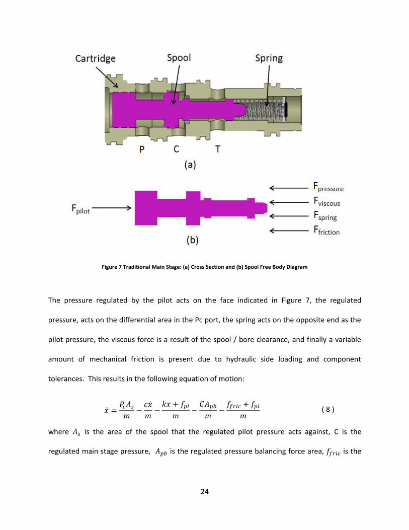
2.2.2 Traditional main stage model development

The equation of motion for the main stage spool can be derived from the forces shown

in Figure 7. As illustrated in the cross section, the main stage consists of a spool, cartridge, and

spring.

24

Figure 7 Traditional Main Stage: (a) Cross Section and (b) Spool Free Body Diagram

The pressure regulated by the pilot acts on the face indicated in Figure 7, the regulated

pressure, acts on the differential area in the Pc port, the spring acts on the opposite end as the

pilot pressure, the viscous force is a result of the spool / bore clearance, and finally a variable

amount of mechanical friction is present due to hydraulic side loading and component

tolerances. This results in the following equation of motion:

=

𝑃𝑐𝐴𝑠

𝑚−

𝑐

𝑚−

𝑘𝑥 + 𝑓𝑝𝑙

𝑚−

𝐶𝐴𝑝𝑏

𝑚−

𝑓𝑓𝑟𝑖𝑐 + 𝑓𝑝𝑙

𝑚 ( 8 )

where 𝐴𝑠 is the area of the spool that the regulated pilot pressure acts against, C is the

regulated main stage pressure, 𝐴𝑝𝑏 is the regulated pressure balancing force area, 𝑓𝑓𝑟𝑖𝑐 is the

25

mechanical friction force, 𝑐 is the viscous damping coefficient, and 𝑓𝑝𝑙 is the spring load at

equilibrium. The viscous damping coefficient can be calculated as follows [24]:

𝑐 =

𝜇

ℎ𝜋𝑑𝑠(𝑙 − 𝑥) ( 9 )

where ℎ is the radial clearance between the spool and bore, 𝑑𝑠 is the spool diameter, and 𝑙 is

the engagement length at zero displacement. Equation 8 is only valid for blocked control ports

with constant volume; therefore flow forces are not included.

The main stage spool is schematically similar to the flapper nozzle, except there are two

variable orifices; therefore Eqs. (2) - (4) also apply to the main stage spool, except 𝑎𝑖𝑛 and 𝑐𝑑𝑖𝑛

also vary as a function of spool displacement. The area versus stroke is more complicated for

the spool than for the flapper-nozzle. When the spool is de-actuated, the P to C flow path is a

long annulus and the C to T flow path is an open area; when the spool is fully actuated the

opposite is true; and when the spool is regulating pressure to C there are short annulus paths

from P to C and from C to T.

Spool leakage for long annular passages is fully developed, laminar, and follows

Poiseuille’s law so it can be calculated analytically from the Navier-Stokes equations [7]. For

large spool openings the flow is turbulent and can be calculated using the classic orifice

equation. Dong and Ueno showed that the discharge coefficient is a function of the Reynolds

number for spool valves and that this could be determined numerically [9]. The leakage and

flow rate for the transitional spool opening, between fully developed laminar and fully open

turbulent, is not as straight forward but is the most critical because this is where pressure

modulation occurs. A semi-empirical approach to calculate flow, pressure gain, and leakage can

be used to develop a variable equation structure for the transitional region by matching

26

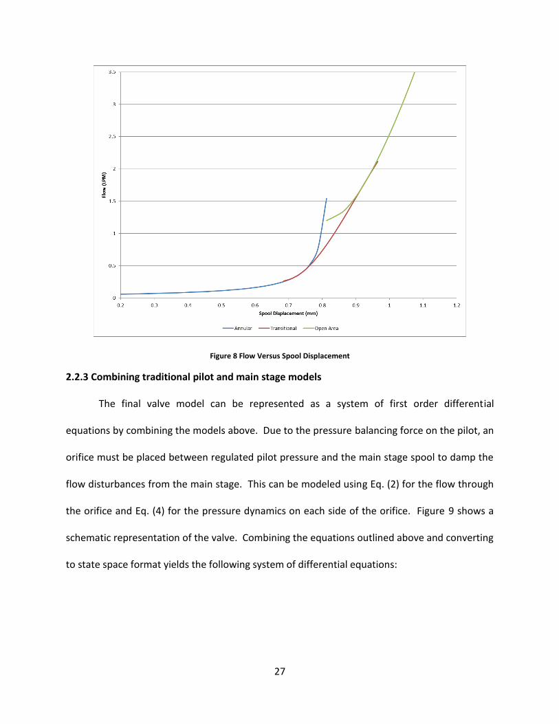
experimental data and tuning the parameters in the analytical equation [10]. Equations (10) -

(12) are used to calculate the annular, transitional, and open area regions of the flow versus

displacement characteristic.

𝑄𝑎 =

𝜋(𝑑𝑠 + 2ℎ)ℎ3(𝑃 − 𝐶)

12𝜇(𝑥𝑝𝑐 − 𝑥) (10)

𝑄𝑡 = 𝛼𝑒𝛾𝑥𝑠𝑖𝑔𝑛(𝑃 − 𝐶)√2

𝜌|𝑃 − 𝐶|

(11)

𝑄𝑜 = 𝜋𝑑𝑠𝑥𝑐𝑑𝑜𝑢𝑡𝑠𝑖𝑔𝑛(𝑃 − 𝐶)√2

𝜌|𝑃 − 𝐶|

(12)

where 𝑄𝑎 is the annulus flow, 𝑥𝑝𝑐 is the engagement length at zero displacement, 𝑄𝑡 is the

transitional, flow 𝛼 and 𝛾 are experimentally tuned coefficients, and 𝑄𝑜 is the open area flow.

These three equations make up the variable structure equation for spool flow or can

alternatively be used to develop a flow area versus displacement lookup table for

computational purposes. This is illustrated graphically in Figure 8 for the P to C variable orifice

in a typical spool.

27

Figure 8 Flow Versus Spool Displacement

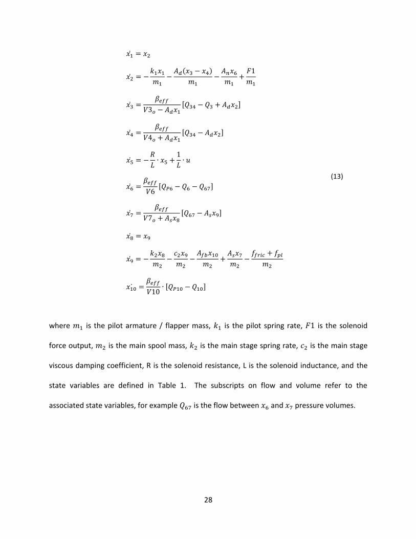
2.2.3 Combining traditional pilot and main stage models

The final valve model can be represented as a system of first order differential

equations by combining the models above. Due to the pressure balancing force on the pilot, an

orifice must be placed between regulated pilot pressure and the main stage spool to damp the

flow disturbances from the main stage. This can be modeled using Eq. (2) for the flow through

the orifice and Eq. (4) for the pressure dynamics on each side of the orifice. Figure 9 shows a

schematic representation of the valve. Combining the equations outlined above and converting

to state space format yields the following system of differential equations:

28

𝑥1 = 𝑥2

𝑥2 = −𝑘1𝑥1

𝑚1−

𝐴𝑑(𝑥3 − 𝑥4)

𝑚1−

𝐴𝑛𝑥6

𝑚1+

𝐹1

𝑚1

𝑥3 =𝛽𝑒𝑓𝑓

𝑉3𝑜 − 𝐴𝑑𝑥1

[𝑄34 − 𝑄3 + 𝐴𝑑𝑥2]


𝑉4𝑜 + 𝐴𝑑𝑥1

[𝑄34 − 𝐴𝑑𝑥2]

𝑥5 = −𝑅

𝐿∙ 𝑥5 +

1

𝐿∙ 𝑢


𝑉6[𝑄𝑃6 − 𝑄6 − 𝑄67]


𝑉7𝑜 + 𝐴𝑠𝑥8

[𝑄67 − 𝐴𝑠𝑥9]

𝑥8 = 𝑥9

𝑥9 = −𝑘2𝑥8

𝑚2−

𝑐2𝑥9

𝑚2−

𝐴𝑓𝑏𝑥10

𝑚2+

𝐴𝑠𝑥7

𝑚2−


𝑚2


𝑉10∙ [𝑄𝑃10 − 𝑄10]

(13)

where 𝑚1 is the pilot armature / flapper mass, 𝑘1 is the pilot spring rate, 𝐹1 is the solenoid

force output, 𝑚2 is the main spool mass, 𝑘2 is the main stage spring rate, 𝑐2 is the main stage

viscous damping coefficient, R is the solenoid resistance, L is the solenoid inductance, and the

state variables are defined in Table 1. The subscripts on flow and volume refer to the

associated state variables, for example 𝑄67 is the flow between 𝑥6 and 𝑥7 pressure volumes.

29

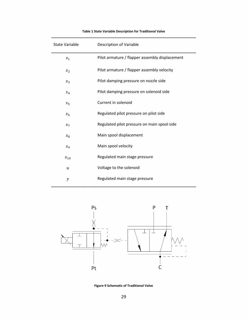
Table 1 State Variable Description for Traditional Valve

State Variable Description of Variable

𝑥1 Pilot armature / flapper assembly displacement

𝑥2 Pilot armature / flapper assembly velocity

𝑥3 Pilot damping pressure on nozzle side

𝑥4 Pilot damping pressure on solenoid side

𝑥5 Current in solenoid

𝑥6 Regulated pilot pressure on pilot side

𝑥7 Regulated pilot pressure on main spool side

𝑥8 Main spool displacement

𝑥9 Main spool velocity

𝑥10 Regulated main stage pressure

𝑢 Voltage to the solenoid

𝑦 Regulated main stage pressure

Figure 9 Schematic of Traditional Valve

30

Several of the equations are coupled, such as the last two for example. The second to

last equation is the equation of motion of the main spool and the last equation is the pressure

response of the control volume. These are coupled through the spool position and regulated

pressure. The physical meaning of this is important; it shows that the spool position impacts

the pressure dynamics and the pressure dynamics impact the spool position. The result of this

coupling is that the transient performance of the traditional valve is highly dependent on the

properties of the control port volume. This is a key point that is revisited later; however this

can also be illustrated through the block diagram of the valve. Due to the number of

components this system is broken into three subsystems; the first subsystem is the pilot; the

second subsystem is the damping chamber of the pilot; and the third subsystem is the main

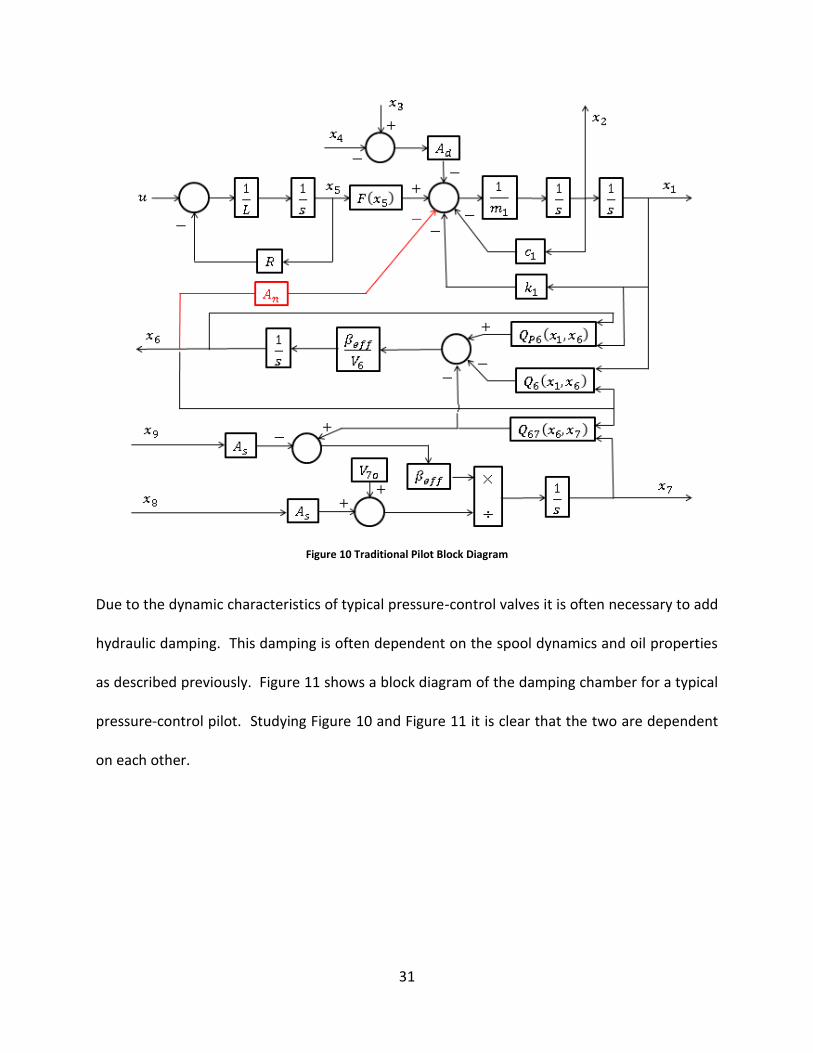
stage. Figure 10 shows the block diagram representation of the traditional pilot. The regulated

pilot pressure balancing force is highlighted in red, this shows the interdependence of the

regulated pressure and the spool dynamics. Also of note is the interaction of system states with

the main stage and the damping chamber of the pilot valve.

31

Figure 10 Traditional Pilot Block Diagram

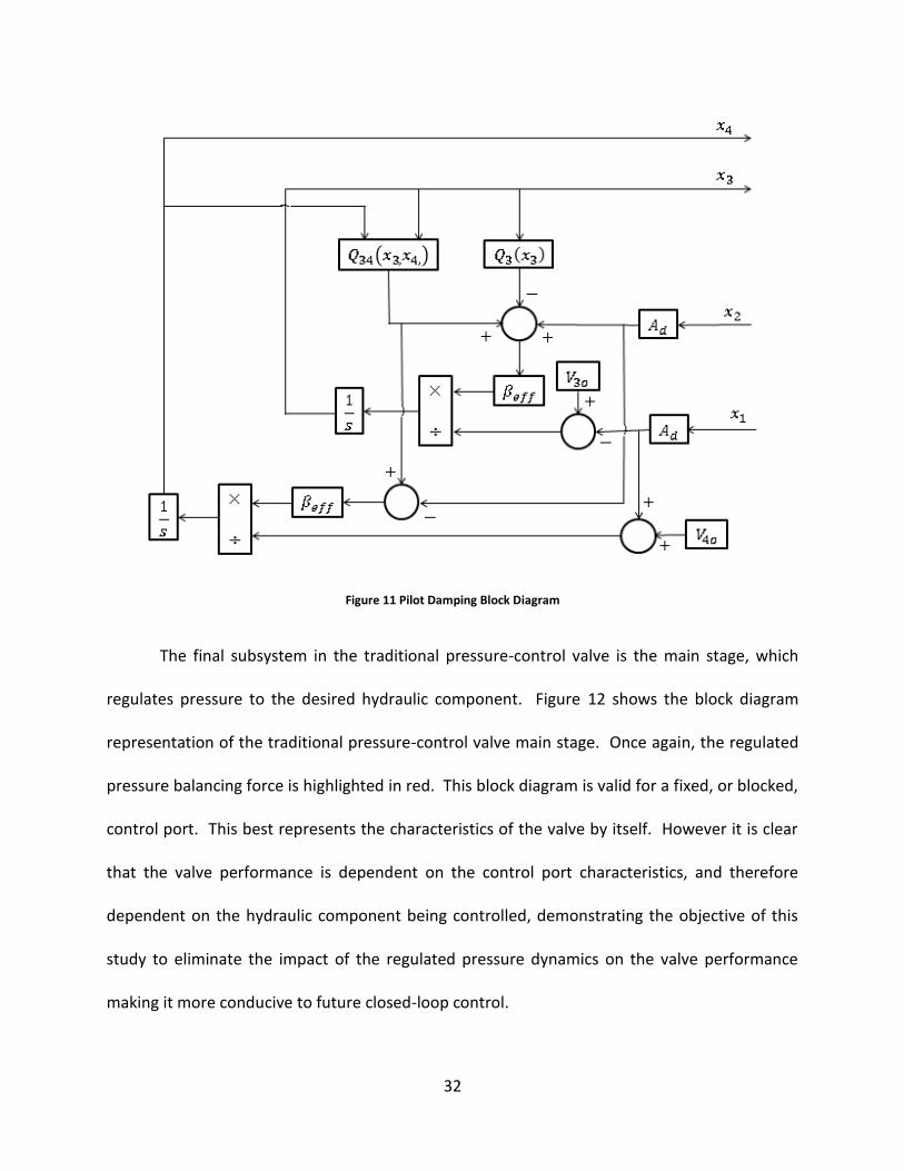
Due to the dynamic characteristics of typical pressure-control valves it is often necessary to add

hydraulic damping. This damping is often dependent on the spool dynamics and oil properties

as described previously. Figure 11 shows a block diagram of the damping chamber for a typical

pressure-control pilot. Studying Figure 10 and Figure 11 it is clear that the two are dependent

on each other.

32

Figure 11 Pilot Damping Block Diagram

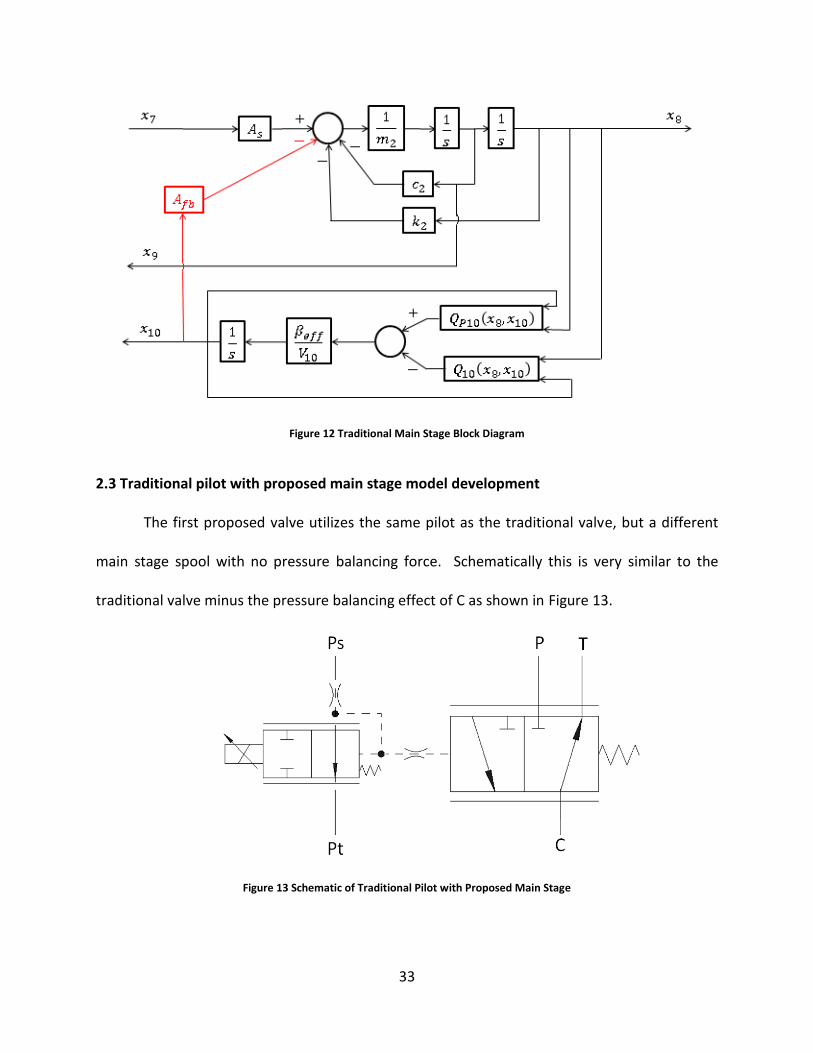
The final subsystem in the traditional pressure-control valve is the main stage, which

regulates pressure to the desired hydraulic component. Figure 12 shows the block diagram

representation of the traditional pressure-control valve main stage. Once again, the regulated

pressure balancing force is highlighted in red. This block diagram is valid for a fixed, or blocked,

control port. This best represents the characteristics of the valve by itself. However it is clear

that the valve performance is dependent on the control port characteristics, and therefore

dependent on the hydraulic component being controlled, demonstrating the objective of this

study to eliminate the impact of the regulated pressure dynamics on the valve performance

making it more conducive to future closed-loop control.

33

Figure 12 Traditional Main Stage Block Diagram

2.3 Traditional pilot with proposed main stage model development

The first proposed valve utilizes the same pilot as the traditional valve, but a different

main stage spool with no pressure balancing force. Schematically this is very similar to the

traditional valve minus the pressure balancing effect of C as shown in Figure 13.

Figure 13 Schematic of Traditional Pilot with Proposed Main Stage

34

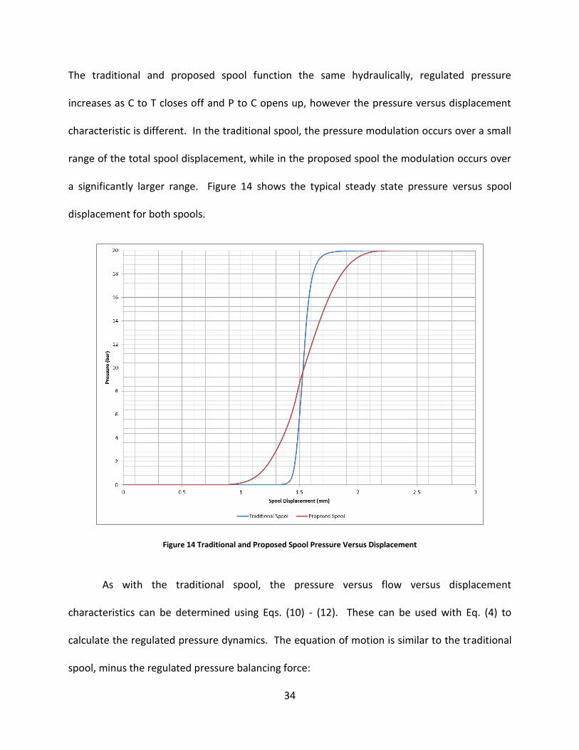
The traditional and proposed spool function the same hydraulically, regulated pressure

increases as C to T closes off and P to C opens up, however the pressure versus displacement

characteristic is different. In the traditional spool, the pressure modulation occurs over a small

range of the total spool displacement, while in the proposed spool the modulation occurs over

a significantly larger range. Figure 14 shows the typical steady state pressure versus spool

displacement for both spools.

Figure 14 Traditional and Proposed Spool Pressure Versus Displacement

As with the traditional spool, the pressure versus flow versus displacement

characteristics can be determined using Eqs. (10) - (12). These can be used with Eq. (4) to

calculate the regulated pressure dynamics. The equation of motion is similar to the traditional

spool, minus the regulated pressure balancing force:

35

=

𝑃𝑐𝐴𝑠

𝑚−

𝑐

𝑚−

𝑘𝑥

𝑚−


𝑚 (14)

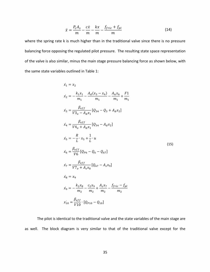
where the spring rate k is much higher than in the traditional valve since there is no pressure

balancing force opposing the regulated pilot pressure. The resulting state space representation

of the valve is also similar, minus the main stage pressure balancing force as shown below, with

the same state variables outlined in Table 1:

𝑥1 = 𝑥2

𝑥2 = −𝑘1𝑥1

𝑚1−

𝐴𝑑(𝑥3 − 𝑥4)

𝑚1−

𝐴𝑛𝑥6

𝑚1+

𝐹1

𝑚1


𝑉3𝑜 − 𝐴𝑑𝑥1

[𝑄34 − 𝑄3 + 𝐴𝑑𝑥2]


𝑉4𝑜 + 𝐴𝑑𝑥1

[𝑄34 − 𝐴𝑑𝑥2]

𝑥5 = −𝑅

𝐿∙ 𝑥5 +

1

𝐿∙ 𝑢


𝑉6[𝑄𝑃6 − 𝑄6 − 𝑄67]


𝑉7𝑜 + 𝐴𝑠𝑥8

[𝑄67 − 𝐴𝑠𝑥9]

𝑥8 = 𝑥9

𝑥9 = −𝑘2𝑥8

𝑚2−

𝑐2𝑥9

𝑚2+

𝐴𝑠𝑥7

𝑚2−

𝑓𝑓𝑟𝑖𝑐 − 𝑓𝑝𝑙

𝑚2


𝑉10∙ [𝑄𝑃10 − 𝑄10]

(15)

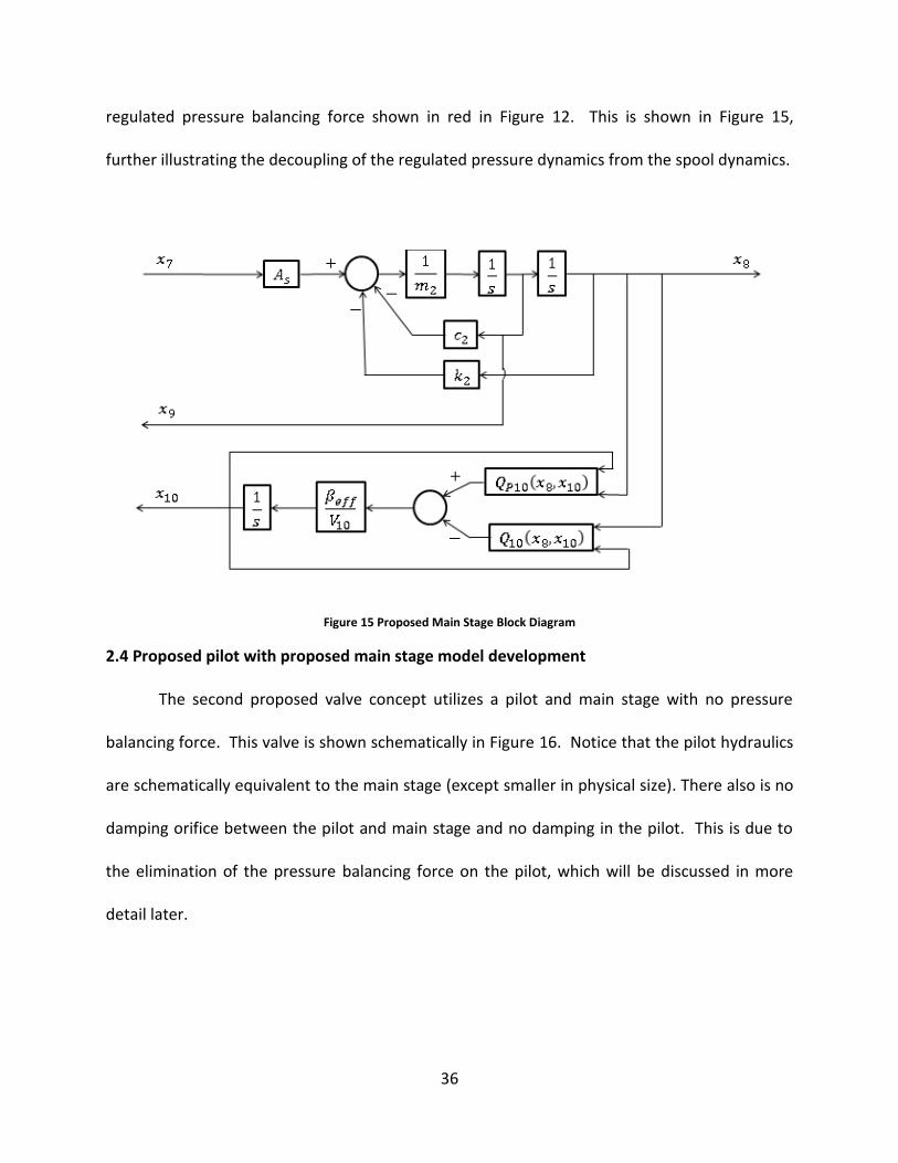
The pilot is identical to the traditional valve and the state variables of the main stage are

as well. The block diagram is very similar to that of the traditional valve except for the

36

regulated pressure balancing force shown in red in Figure 12. This is shown in Figure 15,

further illustrating the decoupling of the regulated pressure dynamics from the spool dynamics.

Figure 15 Proposed Main Stage Block Diagram

2.4 Proposed pilot with proposed main stage model development

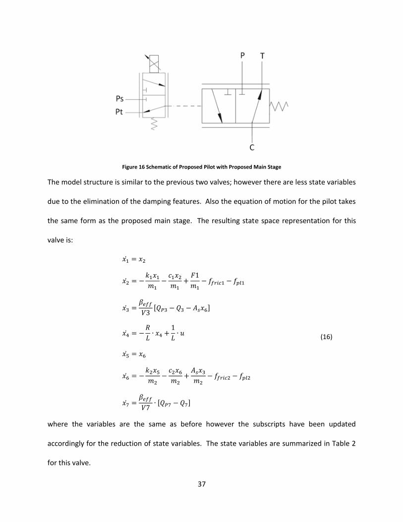
The second proposed valve concept utilizes a pilot and main stage with no pressure

balancing force. This valve is shown schematically in Figure 16. Notice that the pilot hydraulics

are schematically equivalent to the main stage (except smaller in physical size). There also is no

damping orifice between the pilot and main stage and no damping in the pilot. This is due to

the elimination of the pressure balancing force on the pilot, which will be discussed in more

detail later.

37

Figure 16 Schematic of Proposed Pilot with Proposed Main Stage

The model structure is similar to the previous two valves; however there are less state variables

due to the elimination of the damping features. Also the equation of motion for the pilot takes

the same form as the proposed main stage. The resulting state space representation for this

valve is:

𝑥1 = 𝑥2

𝑥2 = −𝑘1𝑥1

𝑚1−

𝑐1𝑥2

𝑚1+

𝐹1

𝑚1− 𝑓𝑓𝑟𝑖𝑐1 − 𝑓𝑝𝑙1


𝑉3[𝑄𝑃3 − 𝑄3 − 𝐴𝑠𝑥6]

𝑥4 = −𝑅

𝐿∙ 𝑥4 +

1

𝐿∙ 𝑢

𝑥5 = 𝑥6

𝑥6 = −𝑘2𝑥5

𝑚2−

𝑐2𝑥6

𝑚2+

𝐴𝑠𝑥3

𝑚2− 𝑓𝑓𝑟𝑖𝑐2 − 𝑓𝑝𝑙2


𝑉7∙ [𝑄𝑃7 − 𝑄7]

(16)

where the variables are the same as before however the subscripts have been updated

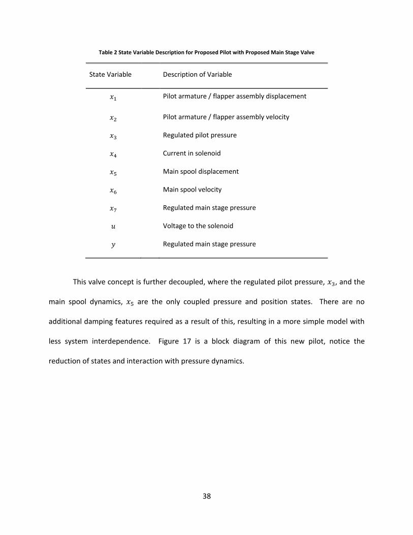
accordingly for the reduction of state variables. The state variables are summarized in Table 2

for this valve.

38

Table 2 State Variable Description for Proposed Pilot with Proposed Main Stage Valve

State Variable Description of Variable

𝑥1 Pilot armature / flapper assembly displacement

𝑥2 Pilot armature / flapper assembly velocity

𝑥3 Regulated pilot pressure

𝑥4 Current in solenoid

𝑥5 Main spool displacement

𝑥6 Main spool velocity

𝑥7 Regulated main stage pressure

𝑢 Voltage to the solenoid

𝑦 Regulated main stage pressure

This valve concept is further decoupled, where the regulated pilot pressure, 𝑥3, and the

main spool dynamics, 𝑥5 are the only coupled pressure and position states. There are no

additional damping features required as a result of this, resulting in a more simple model with

less system interdependence. Figure 17 is a block diagram of this new pilot, notice the

reduction of states and interaction with pressure dynamics.

39

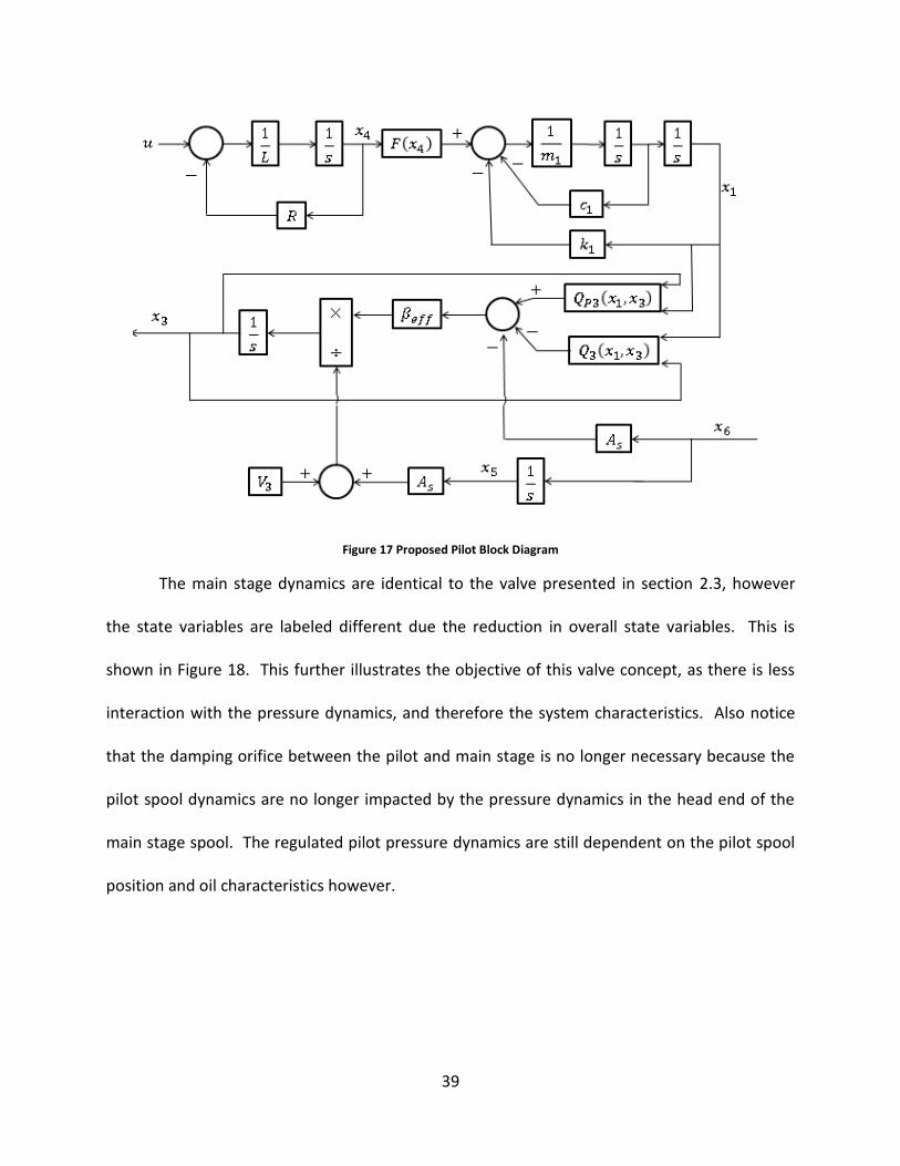
Figure 17 Proposed Pilot Block Diagram

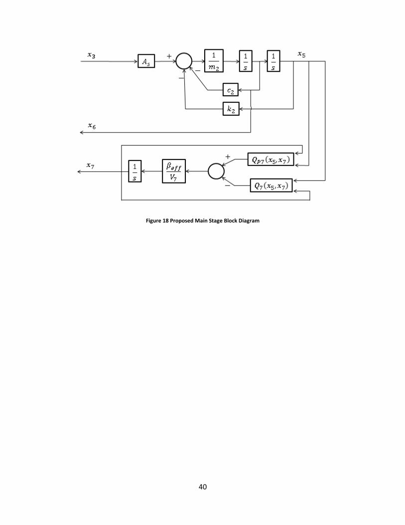
The main stage dynamics are identical to the valve presented in section 2.3, however

the state variables are labeled different due the reduction in overall state variables. This is

shown in Figure 18. This further illustrates the objective of this valve concept, as there is less

interaction with the pressure dynamics, and therefore the system characteristics. Also notice

that the damping orifice between the pilot and main stage is no longer necessary because the

pilot spool dynamics are no longer impacted by the pressure dynamics in the head end of the

main stage spool. The regulated pilot pressure dynamics are still dependent on the pilot spool

position and oil characteristics however.

40

Figure 18 Proposed Main Stage Block Diagram

41

CHAPTER 3

NUMERICAL SIMULATIONS AND EXPERIMENTAL VALIDATION

3.1 Nonlinear numerical AMESim model

Differential equations for hydraulic pressure dynamics, such as Eq. (6), are typically stiff

due to the low compressibility of the fluid [9]. The stiffness can also change drastically due to

changes in volume or fluid aeration. This makes the solution of these equations difficult so a

model was developed in AMESim for each valve. This software has different solution

algorithms to handle such discontinuities and stiff equations allowing for faster simulations.

The AMESim model for the proposed pilot with proposed main stage is shown in Figure 19 (the

traditional valve model is shown in Figure 38 for reference). This model was used to develop

the appropriate valve characteristics such as spring rates and spool geometry. Once an

acceptable design was achieved the models were validated experimentally.

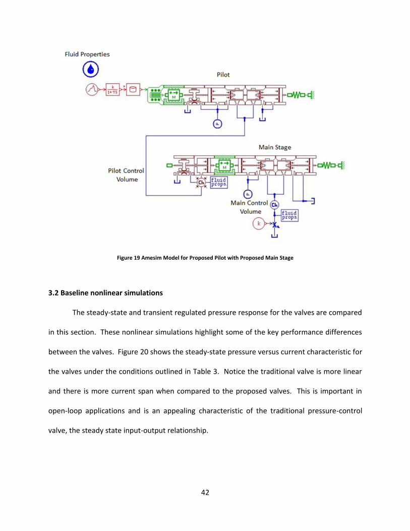
42

Figure 19 Amesim Model for Proposed Pilot with Proposed Main Stage

3.2 Baseline nonlinear simulations

The steady-state and transient regulated pressure response for the valves are compared

in this section. These nonlinear simulations highlight some of the key performance differences

between the valves. Figure 20 shows the steady-state pressure versus current characteristic for

the valves under the conditions outlined in Table 3. Notice the traditional valve is more linear

and there is more current span when compared to the proposed valves. This is important in

open-loop applications and is an appealing characteristic of the traditional pressure-control

valve, the steady state input-output relationship.

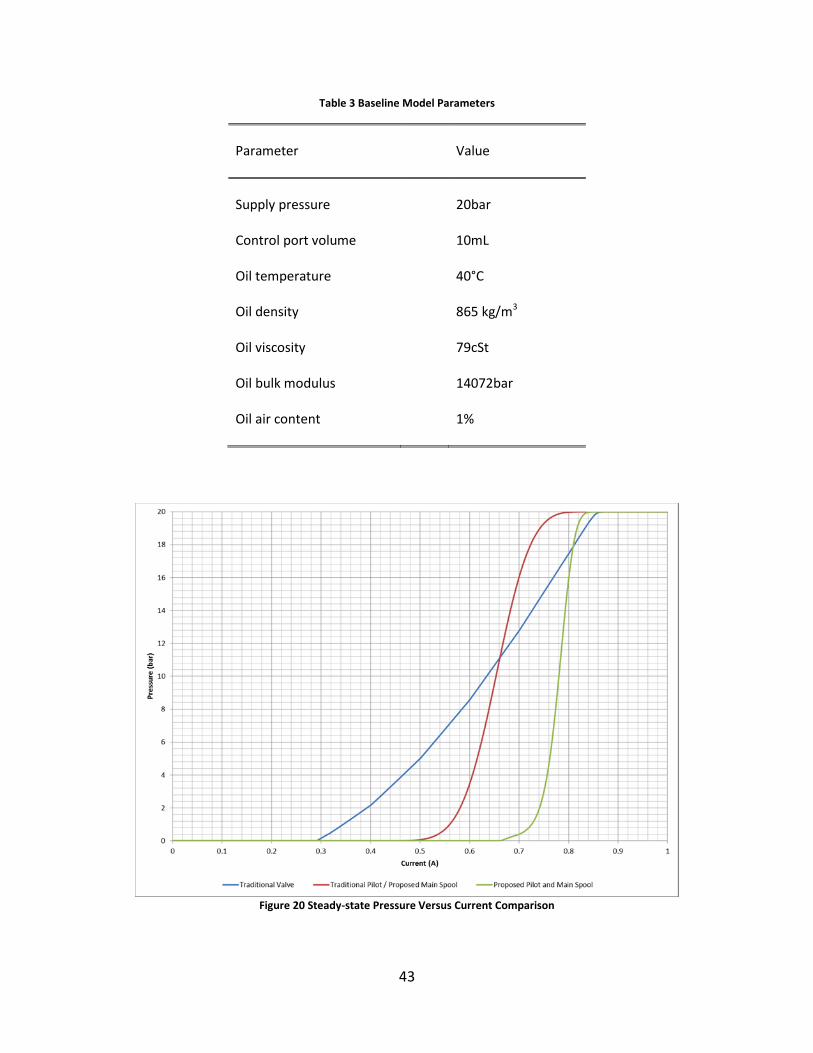
43

Table 3 Baseline Model Parameters

Parameter Value

Supply pressure

20bar

Control port volume 10mL

Oil temperature 40°C

Oil density 865 kg/m3

Oil viscosity 79cSt

Oil bulk modulus 14072bar

Oil air content 1%

Figure 20 Steady-state Pressure Versus Current Comparison

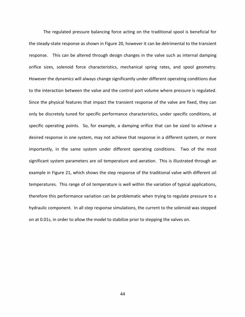
44

The regulated pressure balancing force acting on the traditional spool is beneficial for

the steady-state response as shown in Figure 20, however it can be detrimental to the transient

response. This can be altered through design changes in the valve such as internal damping

orifice sizes, solenoid force characteristics, mechanical spring rates, and spool geometry.

However the dynamics will always change significantly under different operating conditions due

to the interaction between the valve and the control port volume where pressure is regulated.

Since the physical features that impact the transient response of the valve are fixed, they can

only be discretely tuned for specific performance characteristics, under specific conditions, at

specific operating points. So, for example, a damping orifice that can be sized to achieve a

desired response in one system, may not achieve that response in a different system, or more

importantly, in the same system under different operating conditions. Two of the most

significant system parameters are oil temperature and aeration. This is illustrated through an

example in Figure 21, which shows the step response of the traditional valve with different oil

temperatures. This range of oil temperature is well within the variation of typical applications,

therefore this performance variation can be problematic when trying to regulate pressure to a

hydraulic component. In all step response simulations, the current to the solenoid was stepped

on at 0.01s, in order to allow the model to stabilize prior to stepping the valves on.

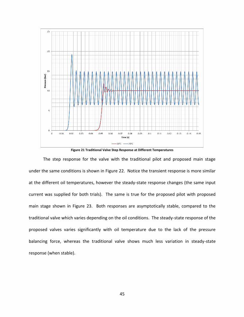
45

Figure 21 Traditional Valve Step Response at Different Temperatures

The step response for the valve with the traditional pilot and proposed main stage

under the same conditions is shown in Figure 22. Notice the transient response is more similar

at the different oil temperatures, however the steady-state response changes (the same input

current was supplied for both trials). The same is true for the proposed pilot with proposed

main stage shown in Figure 23. Both responses are asymptotically stable, compared to the

traditional valve which varies depending on the oil conditions. The steady-state response of the

proposed valves varies significantly with oil temperature due to the lack of the pressure

balancing force, whereas the traditional valve shows much less variation in steady-state

response (when stable).

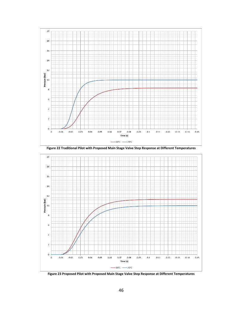
46

Figure 22 Traditional Pilot with Proposed Main Stage Valve Step Response at Different Temperatures

Figure 23 Proposed Pilot with Proposed Main Stage Valve Step Response at Different Temperatures

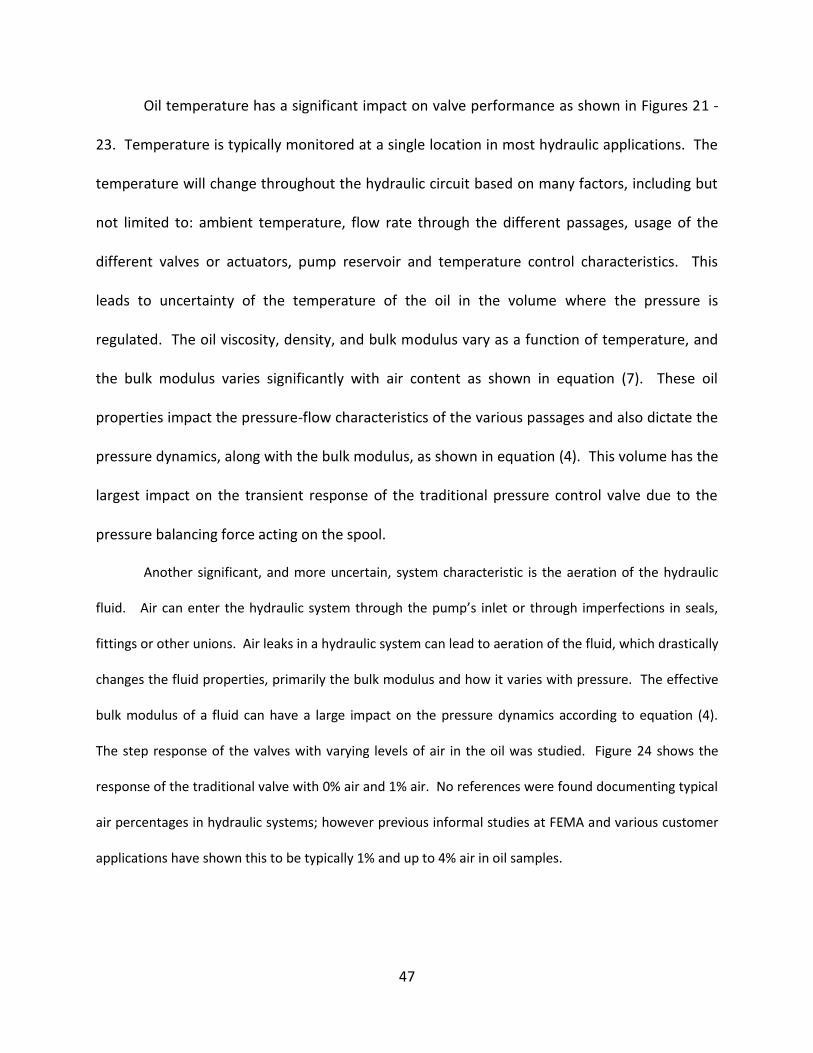
47

Oil temperature has a significant impact on valve performance as shown in Figures 21 -

23. Temperature is typically monitored at a single location in most hydraulic applications. The

temperature will change throughout the hydraulic circuit based on many factors, including but

not limited to: ambient temperature, flow rate through the different passages, usage of the

different valves or actuators, pump reservoir and temperature control characteristics. This

leads to uncertainty of the temperature of the oil in the volume where the pressure is

regulated. The oil viscosity, density, and bulk modulus vary as a function of temperature, and

the bulk modulus varies significantly with air content as shown in equation (7). These oil

properties impact the pressure-flow characteristics of the various passages and also dictate the

pressure dynamics, along with the bulk modulus, as shown in equation (4). This volume has the

largest impact on the transient response of the traditional pressure control valve due to the

pressure balancing force acting on the spool.

Another significant, and more uncertain, system characteristic is the aeration of the hydraulic

fluid. Air can enter the hydraulic system through the pump’s inlet or through imperfections in seals,

fittings or other unions. Air leaks in a hydraulic system can lead to aeration of the fluid, which drastically

changes the fluid properties, primarily the bulk modulus and how it varies with pressure. The effective

bulk modulus of a fluid can have a large impact on the pressure dynamics according to equation (4).

The step response of the valves with varying levels of air in the oil was studied. Figure 24 shows the

response of the traditional valve with 0% air and 1% air. No references were found documenting typical

air percentages in hydraulic systems; however previous informal studies at FEMA and various customer

applications have shown this to be typically 1% and up to 4% air in oil samples.

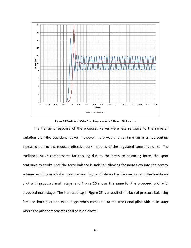
48

Figure 24 Traditional Valve Step Response with Different Oil Aeration

The transient response of the proposed valves were less sensitive to the same air

variation than the traditional valve, however there was a larger time lag as air percentage

increased due to the reduced effective bulk modulus of the regulated control volume. The

traditional valve compensates for this lag due to the pressure balancing force, the spool

continues to stroke until the force balance is satisfied allowing for more flow into the control

volume resulting in a faster pressure rise. Figure 25 shows the step response of the traditional

pilot with proposed main stage, and Figure 26 shows the same for the proposed pilot with

proposed main stage. The increased lag in Figure 26 is a result of the lack of pressure balancing

force on both pilot and main stage, when compared to the traditional pilot with main stage

where the pilot compensates as discussed above.

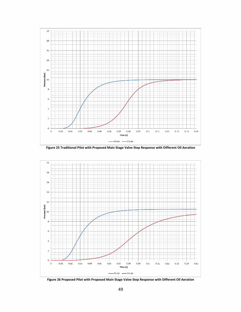
49

Figure 25 Traditional Pilot with Proposed Main Stage Valve Step Response with Different Oil Aeration

Figure 26 Proposed Pilot with Proposed Main Stage Valve Step Response with Different Oil Aeration

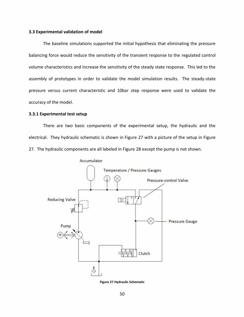
50

3.3 Experimental validation of model

The baseline simulations supported the initial hypothesis that eliminating the pressure

balancing force would reduce the sensitivity of the transient response to the regulated control

volume characteristics and increase the sensitivity of the steady state response. This led to the

assembly of prototypes in order to validate the model simulation results. The steady-state

pressure versus current characteristic and 10bar step response were used to validate the

accuracy of the model.

3.3.1 Experimental test setup

There are two basic components of the experimental setup, the hydraulic and the

electrical. They hydraulic schematic is shown in Figure 27 with a picture of the setup in Figure

27. The hydraulic components are all labeled in Figure 28 except the pump is not shown.

Figure 27 Hydraulic Schematic

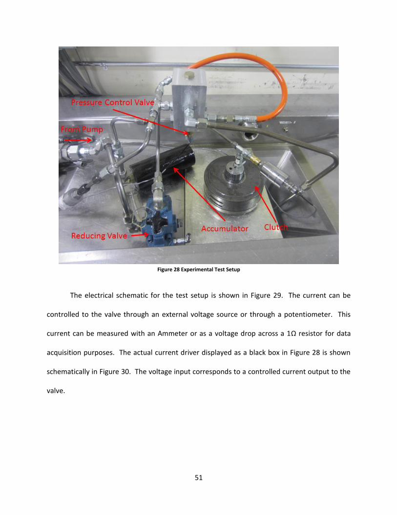
51

Figure 28 Experimental Test Setup

The electrical schematic for the test setup is shown in Figure 29. The current can be

controlled to the valve through an external voltage source or through a potentiometer. This

current can be measured with an Ammeter or as a voltage drop across a 1Ω resistor for data

acquisition purposes. The actual current driver displayed as a black box in Figure 28 is shown

schematically in Figure 30. The voltage input corresponds to a controlled current output to the

valve.

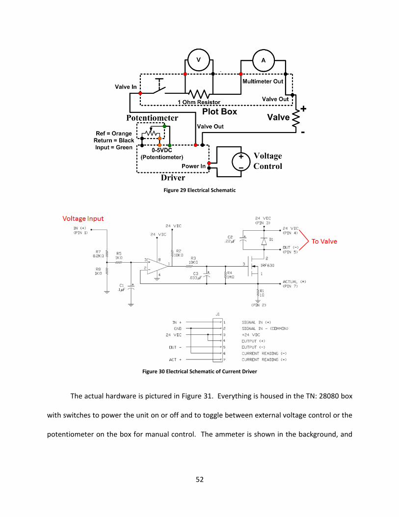
52

Figure 29 Electrical Schematic

Figure 30 Electrical Schematic of Current Driver

The actual hardware is pictured in Figure 31. Everything is housed in the TN: 28080 box

with switches to power the unit on or off and to toggle between external voltage control or the

potentiometer on the box for manual control. The ammeter is shown in the background, and

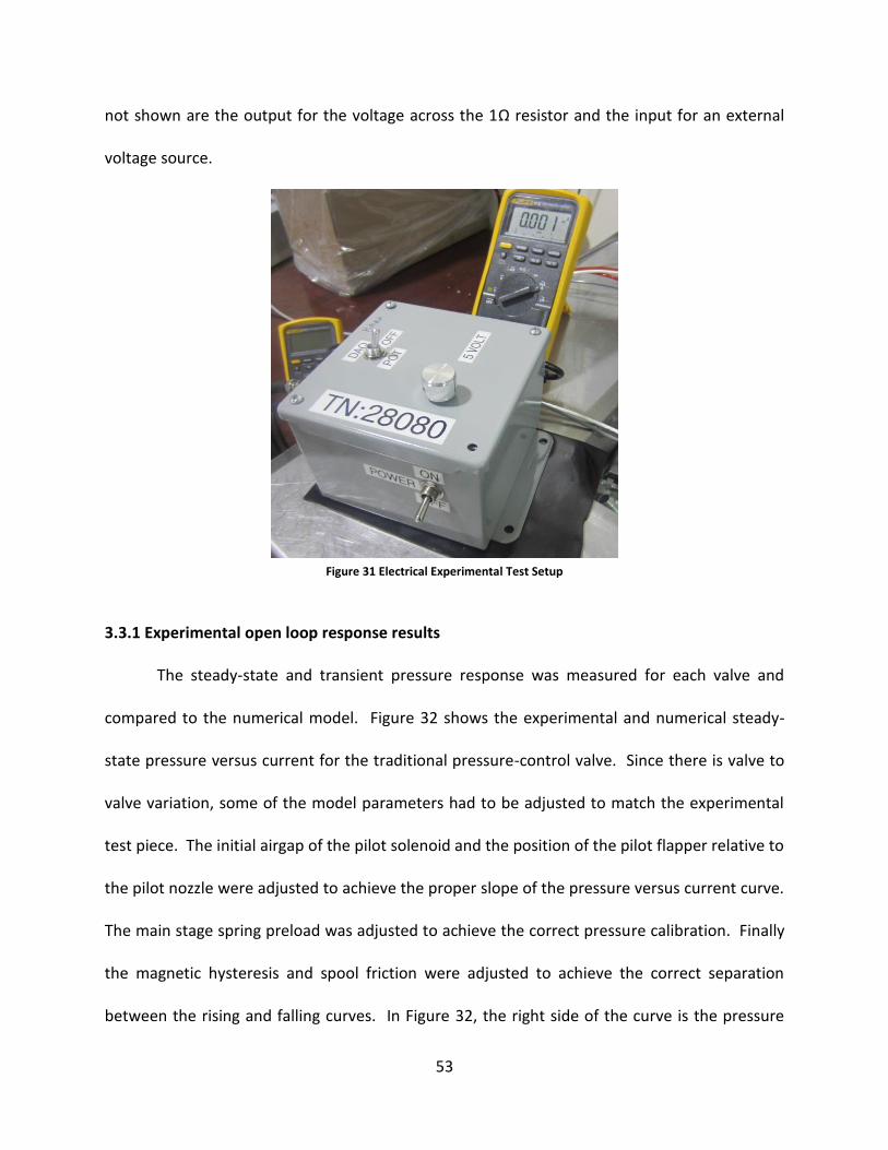
53

not shown are the output for the voltage across the 1Ω resistor and the input for an external

voltage source.

Figure 31 Electrical Experimental Test Setup

3.3.1 Experimental open loop response results

The steady-state and transient pressure response was measured for each valve and

compared to the numerical model. Figure 32 shows the experimental and numerical steady-

state pressure versus current for the traditional pressure-control valve. Since there is valve to

valve variation, some of the model parameters had to be adjusted to match the experimental

test piece. The initial airgap of the pilot solenoid and the position of the pilot flapper relative to

the pilot nozzle were adjusted to achieve the proper slope of the pressure versus current curve.

The main stage spring preload was adjusted to achieve the correct pressure calibration. Finally

the magnetic hysteresis and spool friction were adjusted to achieve the correct separation

between the rising and falling curves. In Figure 32, the right side of the curve is the pressure

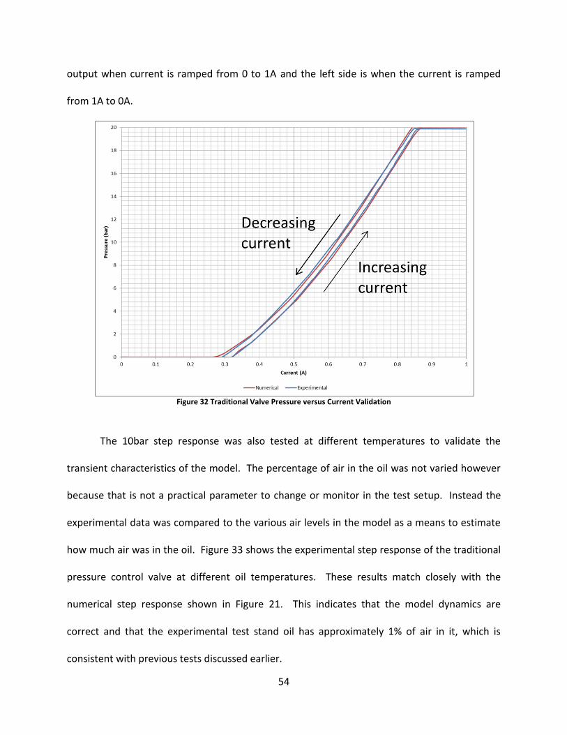
54

output when current is ramped from 0 to 1A and the left side is when the current is ramped

from 1A to 0A.

Figure 32 Traditional Valve Pressure versus Current Validation

The 10bar step response was also tested at different temperatures to validate the

transient characteristics of the model. The percentage of air in the oil was not varied however

because that is not a practical parameter to change or monitor in the test setup. Instead the

experimental data was compared to the various air levels in the model as a means to estimate

how much air was in the oil. Figure 33 shows the experimental step response of the traditional

pressure control valve at different oil temperatures. These results match closely with the

numerical step response shown in Figure 21. This indicates that the model dynamics are

correct and that the experimental test stand oil has approximately 1% of air in it, which is

consistent with previous tests discussed earlier.

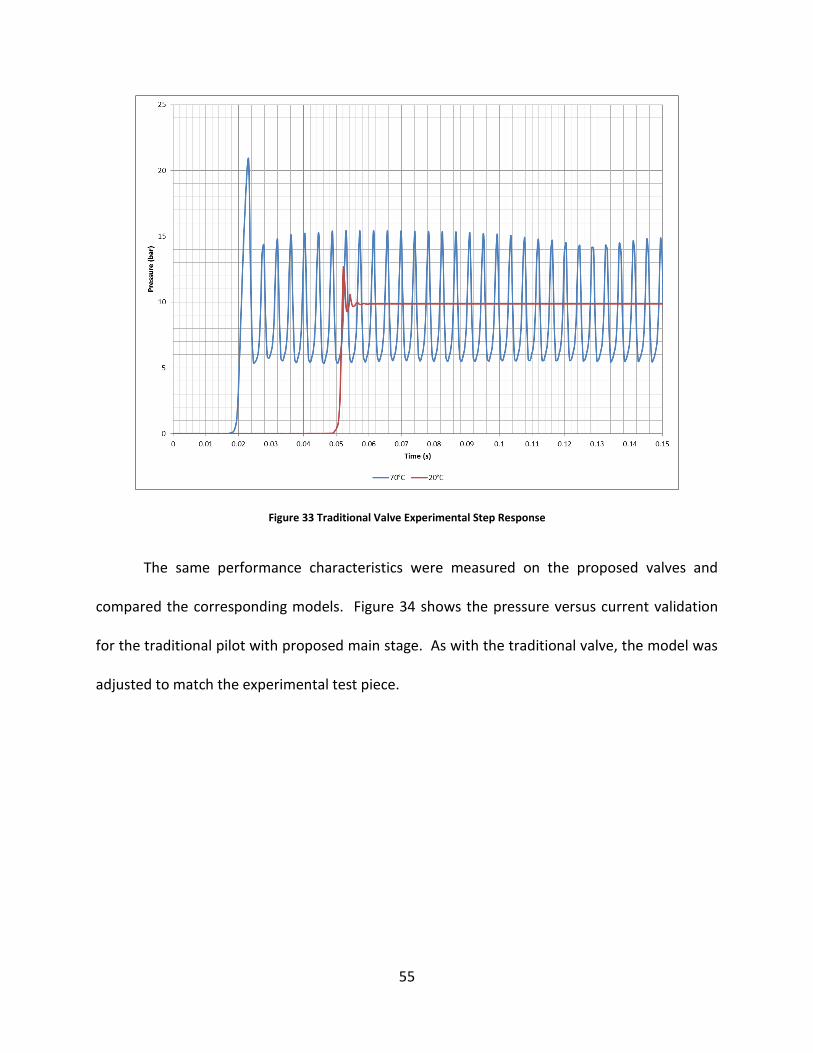
55

Figure 33 Traditional Valve Experimental Step Response

The same performance characteristics were measured on the proposed valves and

compared the corresponding models. Figure 34 shows the pressure versus current validation

for the traditional pilot with proposed main stage. As with the traditional valve, the model was

adjusted to match the experimental test piece.

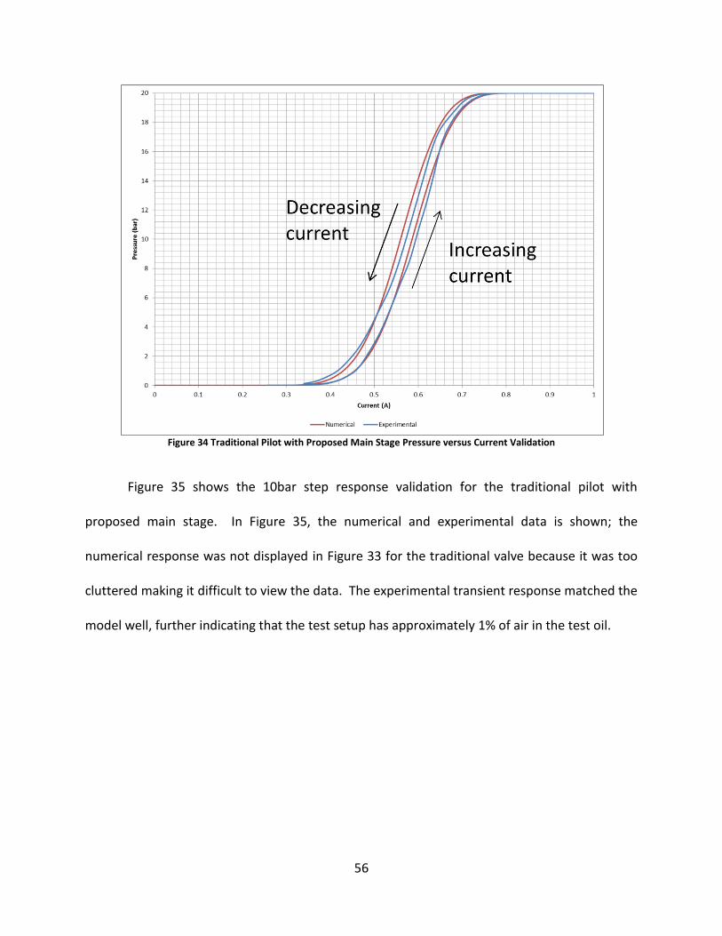
56

Figure 34 Traditional Pilot with Proposed Main Stage Pressure versus Current Validation

Figure 35 shows the 10bar step response validation for the traditional pilot with

proposed main stage. In Figure 35, the numerical and experimental data is shown; the

numerical response was not displayed in Figure 33 for the traditional valve because it was too

cluttered making it difficult to view the data. The experimental transient response matched the

model well, further indicating that the test setup has approximately 1% of air in the test oil.

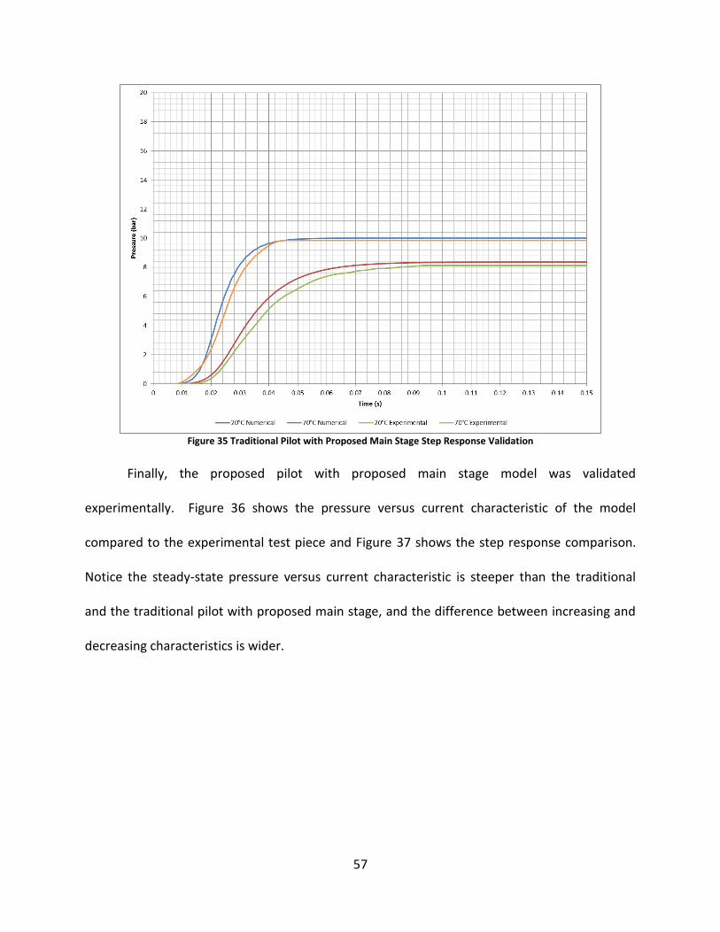
57

Figure 35 Traditional Pilot with Proposed Main Stage Step Response Validation

Finally, the proposed pilot with proposed main stage model was validated

experimentally. Figure 36 shows the pressure versus current characteristic of the model

compared to the experimental test piece and Figure 37 shows the step response comparison.

Notice the steady-state pressure versus current characteristic is steeper than the traditional

and the traditional pilot with proposed main stage, and the difference between increasing and

decreasing characteristics is wider.

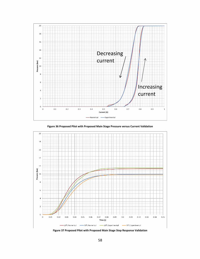
58

Figure 36 Proposed Pilot with Proposed Main Stage Pressure versus Current Validation

Figure 37 Proposed Pilot with Proposed Main Stage Step Response Validation

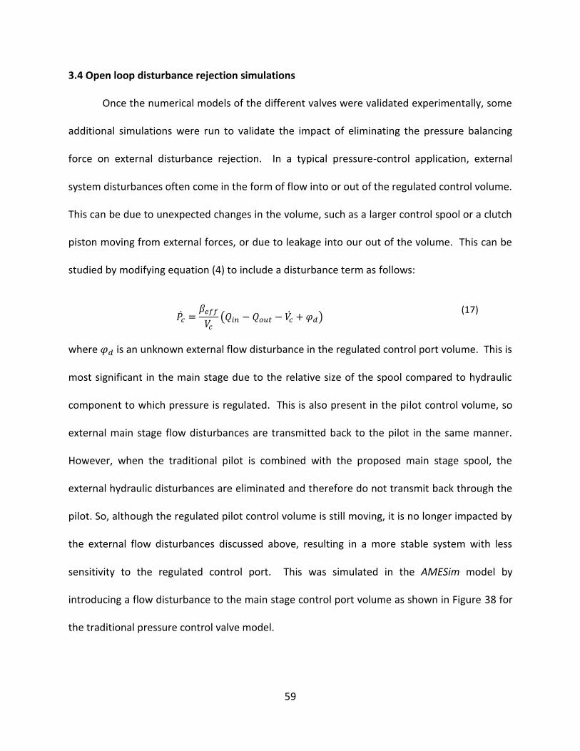
59

3.4 Open loop disturbance rejection simulations

Once the numerical models of the different valves were validated experimentally, some

additional simulations were run to validate the impact of eliminating the pressure balancing

force on external disturbance rejection. In a typical pressure-control application, external

system disturbances often come in the form of flow into or out of the regulated control volume.

This can be due to unexpected changes in the volume, such as a larger control spool or a clutch

piston moving from external forces, or due to leakage into our out of the volume. This can be

studied by modifying equation (4) to include a disturbance term as follows:

𝑃 =𝛽𝑒𝑓𝑓

𝑉𝑐(𝑄𝑖𝑛 − 𝑄𝑜𝑢𝑡 − 𝑉 + 𝜑𝑑)

(17)

where 𝜑𝑑 is an unknown external flow disturbance in the regulated control port volume. This is

most significant in the main stage due to the relative size of the spool compared to hydraulic

component to which pressure is regulated. This is also present in the pilot control volume, so

external main stage flow disturbances are transmitted back to the pilot in the same manner.

However, when the traditional pilot is combined with the proposed main stage spool, the

external hydraulic disturbances are eliminated and therefore do not transmit back through the

pilot. So, although the regulated pilot control volume is still moving, it is no longer impacted by

the external flow disturbances discussed above, resulting in a more stable system with less

sensitivity to the regulated control port. This was simulated in the AMESim model by

introducing a flow disturbance to the main stage control port volume as shown in Figure 38 for

the traditional pressure control valve model.

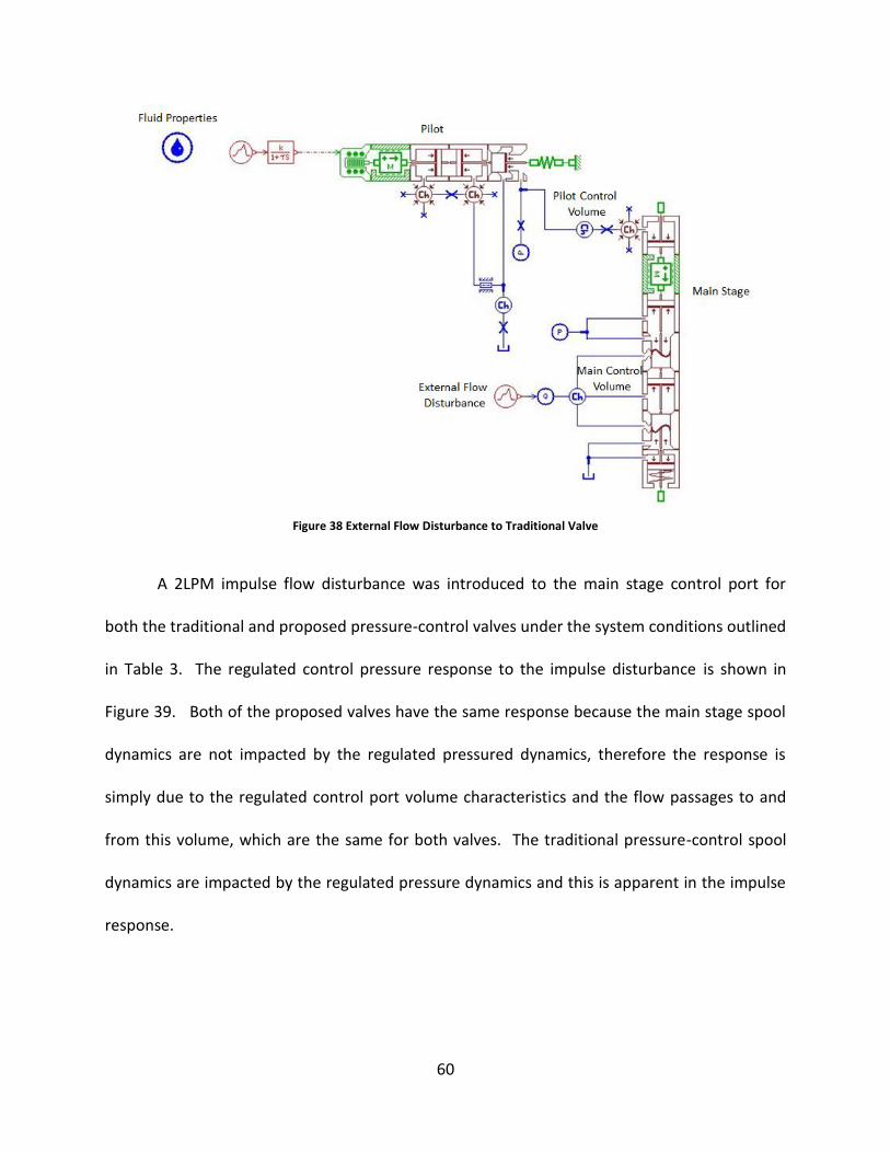
60

Figure 38 External Flow Disturbance to Traditional Valve

A 2LPM impulse flow disturbance was introduced to the main stage control port for

both the traditional and proposed pressure-control valves under the system conditions outlined

in Table 3. The regulated control pressure response to the impulse disturbance is shown in

Figure 39. Both of the proposed valves have the same response because the main stage spool

dynamics are not impacted by the regulated pressured dynamics, therefore the response is

simply due to the regulated control port volume characteristics and the flow passages to and

from this volume, which are the same for both valves. The traditional pressure-control spool

dynamics are impacted by the regulated pressure dynamics and this is apparent in the impulse

response.

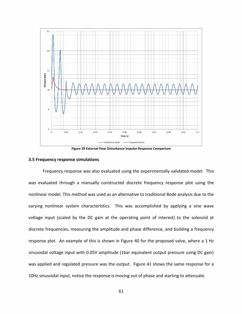
61

Figure 39 External Flow Disturbance Impulse Response Comparison

3.5 Frequency response simulations

Frequency response was also evaluated using the experimentally validated model. This

was evaluated through a manually constructed discrete frequency response plot using the

nonlinear model. This method was used as an alternative to traditional Bode analysis due to the

varying nonlinear system characteristics. This was accomplished by applying a sine wave

voltage input (scaled by the DC gain at the operating point of interest) to the solenoid at

discrete frequencies, measuring the amplitude and phase difference, and building a frequency

response plot. An example of this is shown in Figure 40 for the proposed valve, where a 1 Hz

sinusoidal voltage input with 0.05V amplitude (1bar equivalent output pressure using DC gain)

was applied and regulated pressure was the output. Figure 41 shows the same response for a

10Hz sinusoidal input, notice the response is moving out of phase and starting to attenuate.

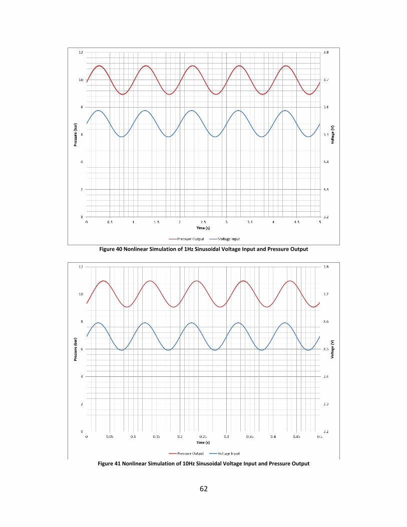
62

Figure 40 Nonlinear Simulation of 1Hz Sinusoidal Voltage Input and Pressure Output

Figure 41 Nonlinear Simulation of 10Hz Sinusoidal Voltage Input and Pressure Output

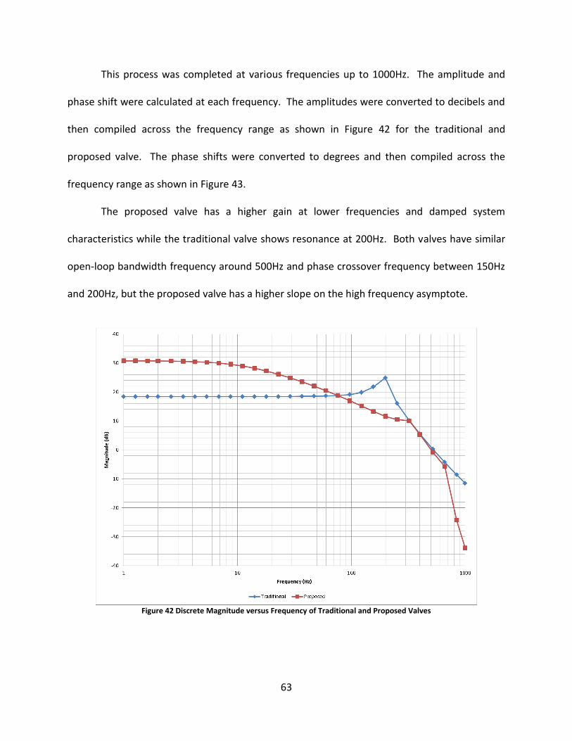
63

This process was completed at various frequencies up to 1000Hz. The amplitude and

phase shift were calculated at each frequency. The amplitudes were converted to decibels and

then compiled across the frequency range as shown in Figure 42 for the traditional and

proposed valve. The phase shifts were converted to degrees and then compiled across the

frequency range as shown in Figure 43.

The proposed valve has a higher gain at lower frequencies and damped system

characteristics while the traditional valve shows resonance at 200Hz. Both valves have similar

open-loop bandwidth frequency around 500Hz and phase crossover frequency between 150Hz

and 200Hz, but the proposed valve has a higher slope on the high frequency asymptote.

Figure 42 Discrete Magnitude versus Frequency of Traditional and Proposed Valves

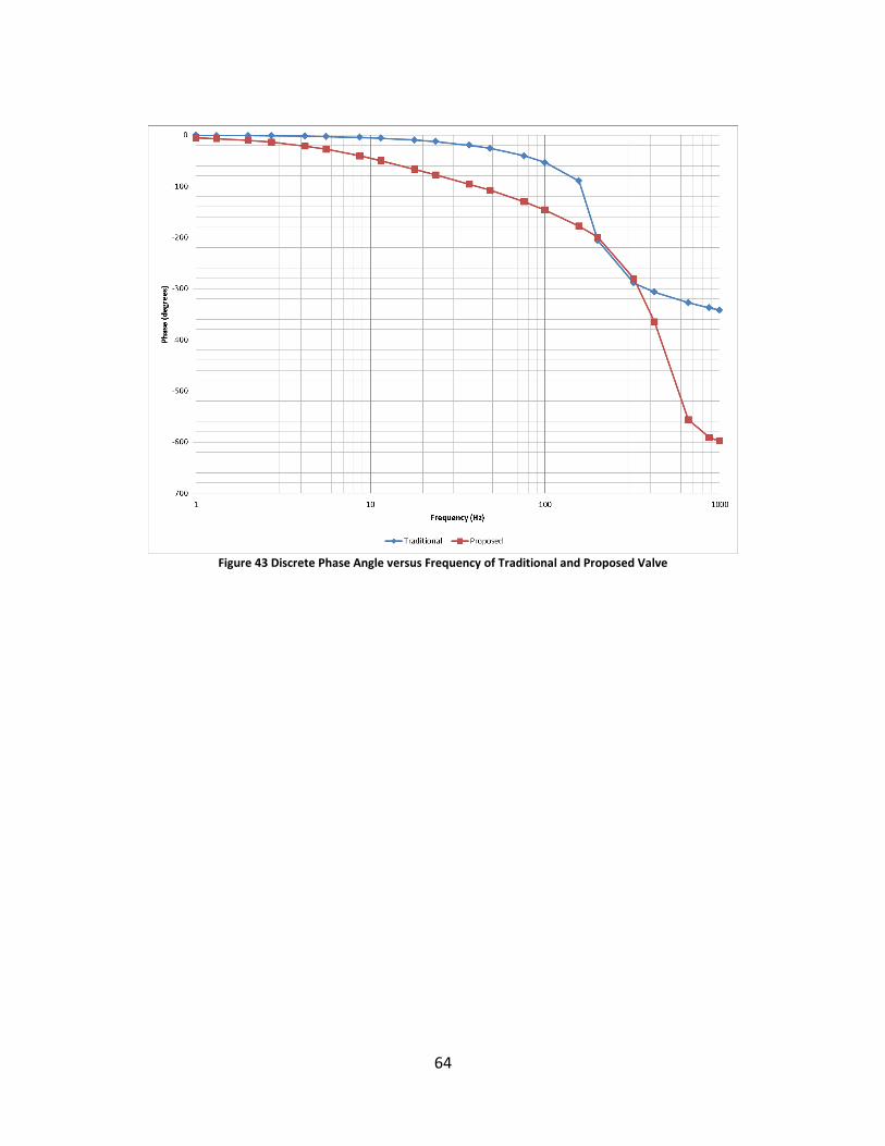
64

Figure 43 Discrete Phase Angle versus Frequency of Traditional and Proposed Valve

65

CHAPTER 4

LINEAR ANALYSIS AND INITIAL CONTROLLER DESIGN

4.1 Model linearization

The ultimate goal of this research is to develop a pressure-control valve that is better

suited for closed loop control than the traditional pressure-control valve, and then follow this

up with the development of the controller. Due to the highly nonlinear dynamics of electro-

hydraulic systems the typical control approach has been to linearize these dynamics at various

operating points and design controller gains for closed loop control [17]. This approach is

limited but allows for the use of a wide array of well-established linear control techniques and

therefore it is a natural starting point prior to attempting more recent nonlinear control

techniques. The different valves have already been modeled above as systems of coupled first-

order differential equations of form

(𝑡) = 𝒉(𝒙(𝑡), 𝑢(𝑡), 𝑡) (18)

in equations 13, 15, and 16. The valves can then be studied at different operating points as

linear time invariant state-space systems:

(𝑡) = A 𝒙(𝑡) + 𝐵𝑢(𝑡) (19)

at various operating points where the A and B matrices are the Jacobians of 𝒉(𝒙𝒐(𝑡), 𝑢𝑜(𝑡), 𝑡)

with respect to 𝒙 and 𝑢 respectively [25]. The valve models were initially linearized at 10bar

under the temperature and aeration conditions evaluated thus far. The dominant poles were

then studied as the system parameters varied. Figure 44 shows the impact that these system

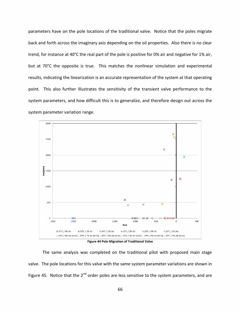
66

parameters have on the pole locations of the traditional valve. Notice that the poles migrate

back and forth across the imaginary axis depending on the oil properties. Also there is no clear

trend, for instance at 40°C the real part of the pole is positive for 0% air and negative for 1% air,

but at 70°C the opposite is true. This matches the nonlinear simulation and experimental

results, indicating the linearization is an accurate representation of the system at that operating

point. This also further illustrates the sensitivity of the transient valve performance to the

system parameters, and how difficult this is to generalize, and therefore design out across the

system parameter variation range.

Figure 44 Pole Migration of Traditional Valve

The same analysis was completed on the traditional pilot with proposed main stage

valve. The pole locations for this valve with the same system parameter variations are shown in

Figure 45. Notice that the 2nd order poles are less sensitive to the system parameters, and are

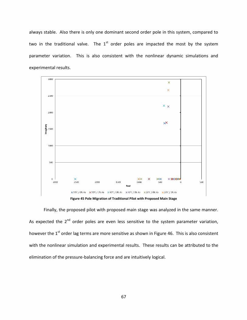
67

always stable. Also there is only one dominant second order pole in this system, compared to

two in the traditional valve. The 1st order poles are impacted the most by the system

parameter variation. This is also consistent with the nonlinear dynamic simulations and

experimental results.

Figure 45 Pole Migration of Traditional Pilot with Proposed Main Stage

Finally, the proposed pilot with proposed main stage was analyzed in the same manner.

As expected the 2nd order poles are even less sensitive to the system parameter variation,

however the 1st order lag terms are more sensitive as shown in Figure 46. This is also consistent

with the nonlinear simulation and experimental results. These results can be attributed to the

elimination of the pressure-balancing force and are intuitively logical.

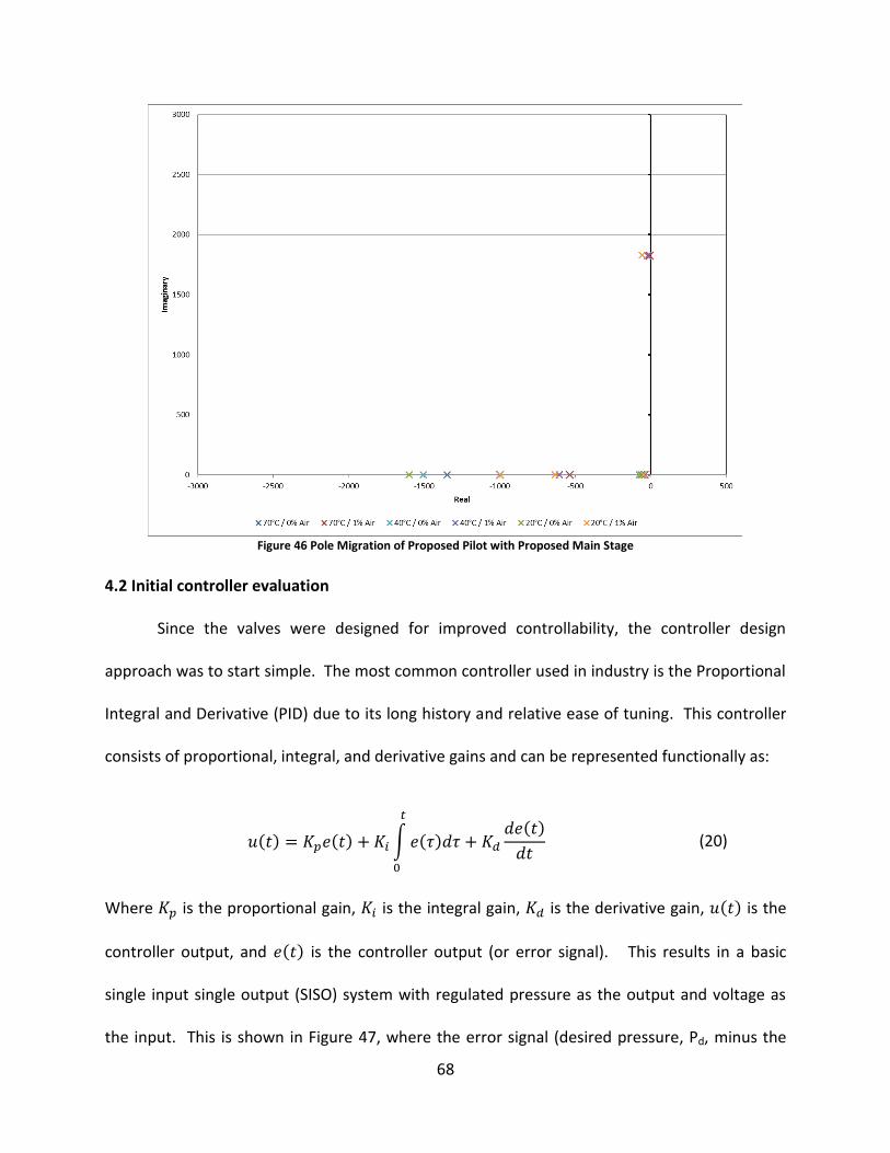
68

Figure 46 Pole Migration of Proposed Pilot with Proposed Main Stage

4.2 Initial controller evaluation

Since the valves were designed for improved controllability, the controller design

approach was to start simple. The most common controller used in industry is the Proportional

Integral and Derivative (PID) due to its long history and relative ease of tuning. This controller

consists of proportional, integral, and derivative gains and can be represented functionally as:

𝑢(𝑡) = 𝐾𝑝𝑒(𝑡) + 𝐾𝑖 ∫𝑒(𝜏)𝑑𝜏

𝑡

0

+ 𝐾𝑑

𝑑𝑒(𝑡)

𝑑𝑡 (20)

Where 𝐾𝑝 is the proportional gain, 𝐾𝑖 is the integral gain, 𝐾𝑑 is the derivative gain, 𝑢(𝑡) is the

controller output, and 𝑒(𝑡) is the controller output (or error signal). This results in a basic

single input single output (SISO) system with regulated pressure as the output and voltage as

the input. This is shown in Figure 47, where the error signal (desired pressure, Pd, minus the

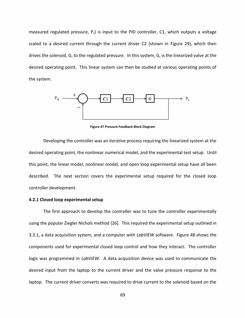
69

measured regulated pressure, Pr) is input to the PID controller, C1, which outputs a voltage

scaled to a desired current through the current driver C2 (shown in Figure 29), which then

drives the solenoid, G, to the regulated pressure. In this system, G, is the linearized valve at the

desired operating point. This linear system can then be studied at various operating points of

the system.

Figure 47 Pressure Feedback Block Diagram

Developing the controller was an iterative process requiring the linearized system at the

desired operating point, the nonlinear numerical model, and the experimental test setup. Until

this point, the linear model, nonlinear model, and open loop experimental setup have all been

described. The next section covers the experimental setup required for the closed loop

controller development.

4.2.1 Closed loop experimental setup

The first approach to develop the controller was to tune the controller experimentally

using the popular Ziegler Nichols method [26]. This required the experimental setup outlined in

3.3.1, a data acquisition system, and a computer with LabVIEW software. Figure 48 shows the

components used for experimental closed loop control and how they interact. The controller

logic was programmed in LabVIEW. A data acquisition device was used to communicate the

desired input from the laptop to the current driver and the valve pressure response to the

laptop. The current driver converts was required to drive current to the solenoid based on the

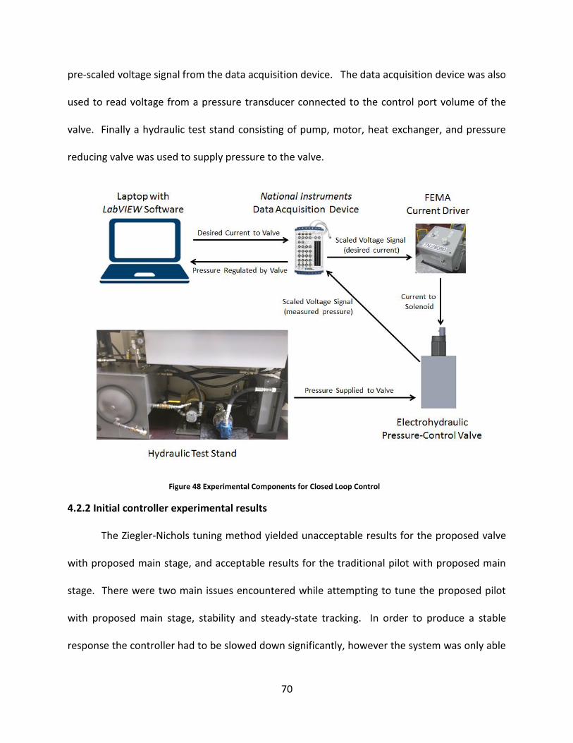
70

pre-scaled voltage signal from the data acquisition device. The data acquisition device was also

used to read voltage from a pressure transducer connected to the control port volume of the

valve. Finally a hydraulic test stand consisting of pump, motor, heat exchanger, and pressure

reducing valve was used to supply pressure to the valve.

Figure 48 Experimental Components for Closed Loop Control

4.2.2 Initial controller experimental results

The Ziegler-Nichols tuning method yielded unacceptable results for the proposed valve

with proposed main stage, and acceptable results for the traditional pilot with proposed main

stage. There were two main issues encountered while attempting to tune the proposed pilot

with proposed main stage, stability and steady-state tracking. In order to produce a stable

response the controller had to be slowed down significantly, however the system was only able

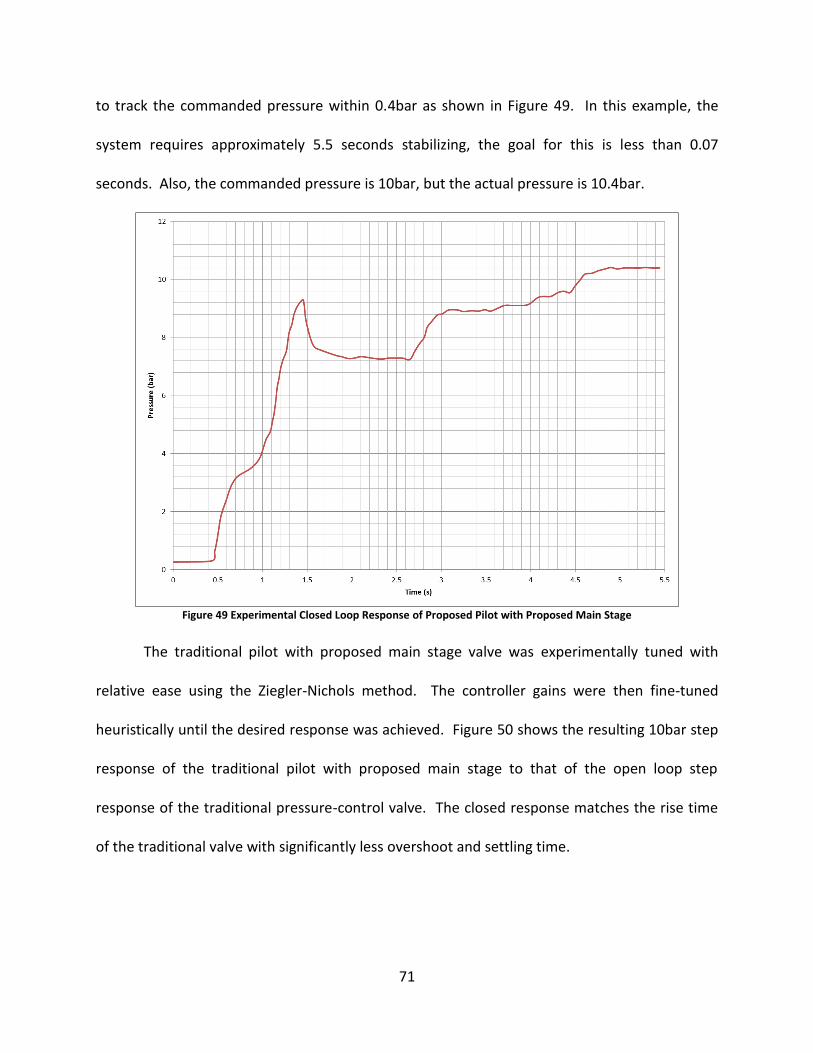
71

to track the commanded pressure within 0.4bar as shown in Figure 49. In this example, the

system requires approximately 5.5 seconds stabilizing, the goal for this is less than 0.07

seconds. Also, the commanded pressure is 10bar, but the actual pressure is 10.4bar.

Figure 49 Experimental Closed Loop Response of Proposed Pilot with Proposed Main Stage

The traditional pilot with proposed main stage valve was experimentally tuned with

relative ease using the Ziegler-Nichols method. The controller gains were then fine-tuned

heuristically until the desired response was achieved. Figure 50 shows the resulting 10bar step

response of the traditional pilot with proposed main stage to that of the open loop step

response of the traditional pressure-control valve. The closed response matches the rise time

of the traditional valve with significantly less overshoot and settling time.

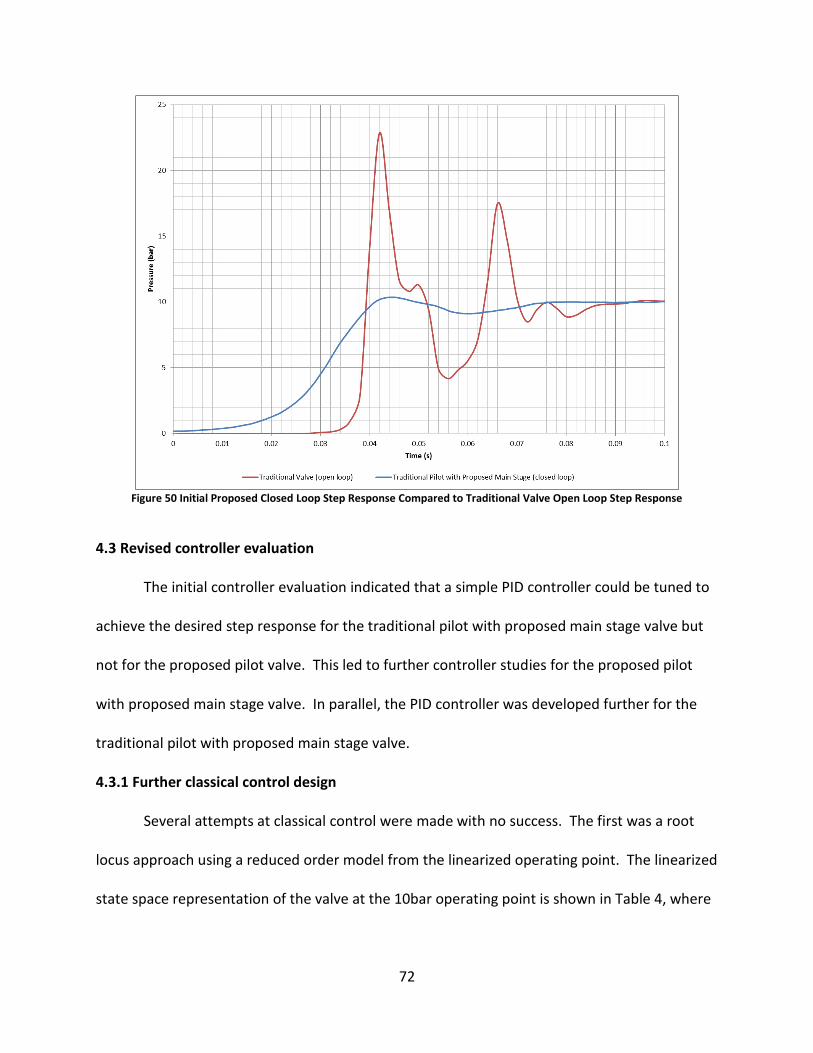
72

Figure 50 Initial Proposed Closed Loop Step Response Compared to Traditional Valve Open Loop Step Response

4.3 Revised controller evaluation

The initial controller evaluation indicated that a simple PID controller could be tuned to

achieve the desired step response for the traditional pilot with proposed main stage valve but

not for the proposed pilot valve. This led to further controller studies for the proposed pilot

with proposed main stage valve. In parallel, the PID controller was developed further for the

traditional pilot with proposed main stage valve.

4.3.1 Further classical control design

Several attempts at classical control were made with no success. The first was a root

locus approach using a reduced order model from the linearized operating point. The linearized

state space representation of the valve at the 10bar operating point is shown in Table 4, where

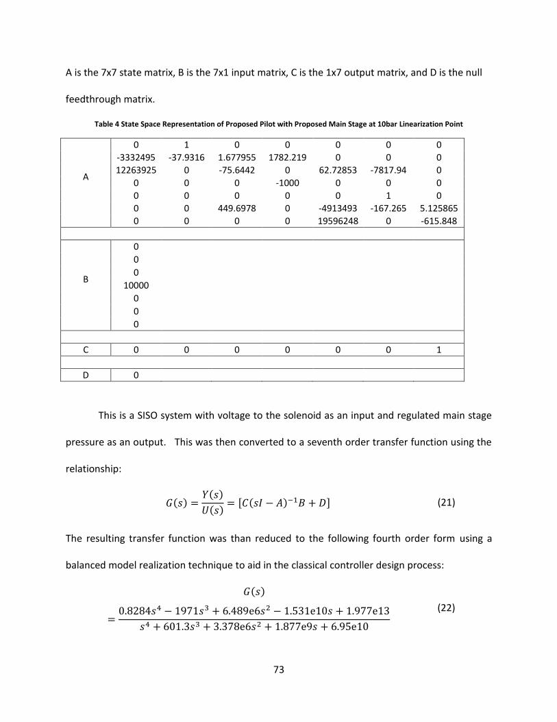
73

A is the 7x7 state matrix, B is the 7x1 input matrix, C is the 1x7 output matrix, and D is the null

feedthrough matrix.

Table 4 State Space Representation of Proposed Pilot with Proposed Main Stage at 10bar Linearization Point

A

0 1 0 0 0 0 0

-3332495 -37.9316 1.677955 1782.219 0 0 0

12263925 0 -75.6442 0 62.72853 -7817.94 0

0 0 0 -1000 0 0 0

0 0 0 0 0 1 0

0 0 449.6978 0 -4913493 -167.265 5.125865

0 0 0 0 19596248 0 -615.848

B

0

0

0

10000

0

0

0

C 0 0 0 0 0 0 1

D 0

This is a SISO system with voltage to the solenoid as an input and regulated main stage

pressure as an output. This was then converted to a seventh order transfer function using the

relationship:

𝐺(𝑠) =𝑌(𝑠)

𝑈(𝑠)= [𝐶(𝑠𝐼 − 𝐴)−1𝐵 + 𝐷] (21)

The resulting transfer function was than reduced to the following fourth order form using a

balanced model realization technique to aid in the classical controller design process:

𝐺(𝑠)

=0.8284𝑠4 − 1971𝑠3 + 6.489e6𝑠2 − 1.531e10𝑠 + 1.977e13

𝑠4 + 601.3𝑠3 + 3.378e6𝑠2 + 1.877e9𝑠 + 6.95e10

(22)

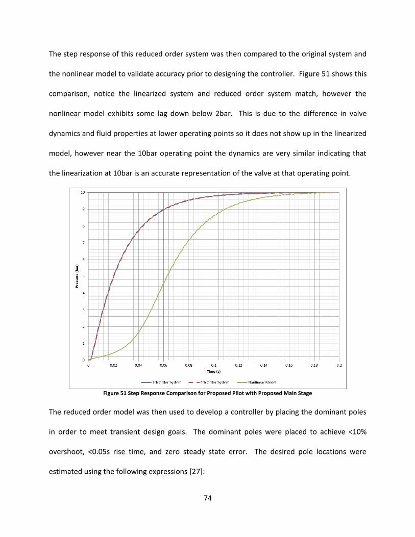
74

The step response of this reduced order system was then compared to the original system and

the nonlinear model to validate accuracy prior to designing the controller. Figure 51 shows this

comparison, notice the linearized system and reduced order system match, however the

nonlinear model exhibits some lag down below 2bar. This is due to the difference in valve

dynamics and fluid properties at lower operating points so it does not show up in the linearized

model, however near the 10bar operating point the dynamics are very similar indicating that

the linearization at 10bar is an accurate representation of the valve at that operating point.

Figure 51 Step Response Comparison for Proposed Pilot with Proposed Main Stage

The reduced order model was then used to develop a controller by placing the dominant poles

in order to meet transient design goals. The dominant poles were placed to achieve <10%

overshoot, <0.05s rise time, and zero steady state error. The desired pole locations were

estimated using the following expressions [27]:

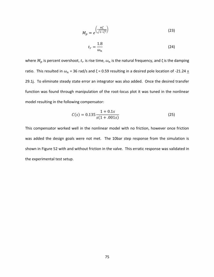
75

𝑀𝑝 = 𝑒

(𝜋𝜁

√1−𝜁2)

(23)

𝑡𝑟 =1.8

𝜔𝑛 (24)

where 𝑀𝑝 is percent overshoot, 𝑡𝑟 is rise time, 𝜔𝑛 is the natural frequency, and ζ is the damping

ratio. This resulted in 𝜔𝑛 = 36 rad/s and ζ = 0.59 resulting in a desired pole location of -21.24 +

29.1j. To eliminate steady state error an integrator was also added. Once the desired transfer

function was found through manipulation of the root-locus plot it was tuned in the nonlinear

model resulting in the following compensator:

𝐶(𝑠) = 0.1351 + 0.1𝑠

𝑠(1 + .001𝑠) (25)

This compensator worked well in the nonlinear model with no friction, however once friction

was added the design goals were not met. The 10bar step response from the simulation is

shown in Figure 52 with and without friction in the valve. This erratic response was validated in

the experimental test setup.

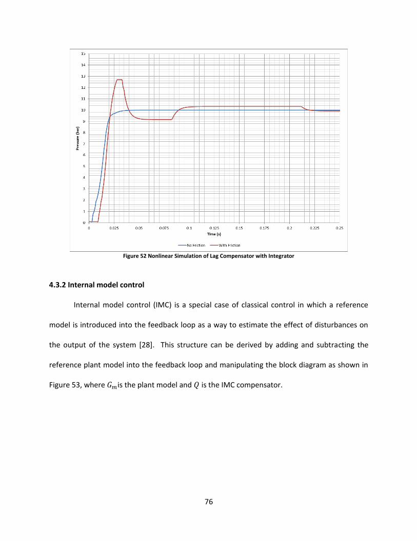
76

Figure 52 Nonlinear Simulation of Lag Compensator with Integrator

4.3.2 Internal model control

Internal model control (IMC) is a special case of classical control in which a reference

model is introduced into the feedback loop as a way to estimate the effect of disturbances on

the output of the system [28]. This structure can be derived by adding and subtracting the

reference plant model into the feedback loop and manipulating the block diagram as shown in

Figure 53, where 𝐺𝑚is the plant model and 𝑄 is the IMC compensator.

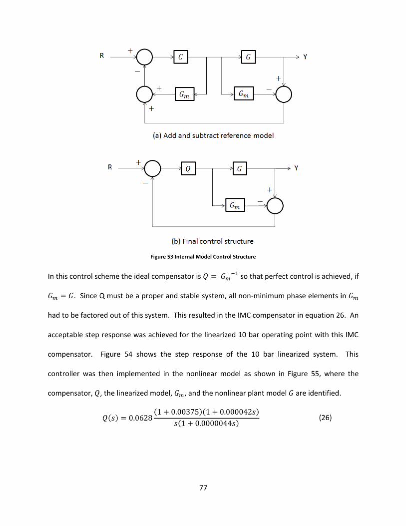
77

Figure 53 Internal Model Control Structure

In this control scheme the ideal compensator is 𝑄 = 𝐺𝑚−1 so that perfect control is achieved, if

𝐺𝑚 = 𝐺. Since Q must be a proper and stable system, all non-minimum phase elements in 𝐺𝑚

had to be factored out of this system. This resulted in the IMC compensator in equation 26. An

acceptable step response was achieved for the linearized 10 bar operating point with this IMC

compensator. Figure 54 shows the step response of the 10 bar linearized system. This

controller was then implemented in the nonlinear model as shown in Figure 55, where the

compensator, 𝑄, the linearized model, 𝐺𝑚, and the nonlinear plant model 𝐺 are identified.

𝑄(𝑠) = 0.0628(1 + 0.00375)(1 + 0.000042𝑠)

𝑠(1 + 0.0000044𝑠) (26)

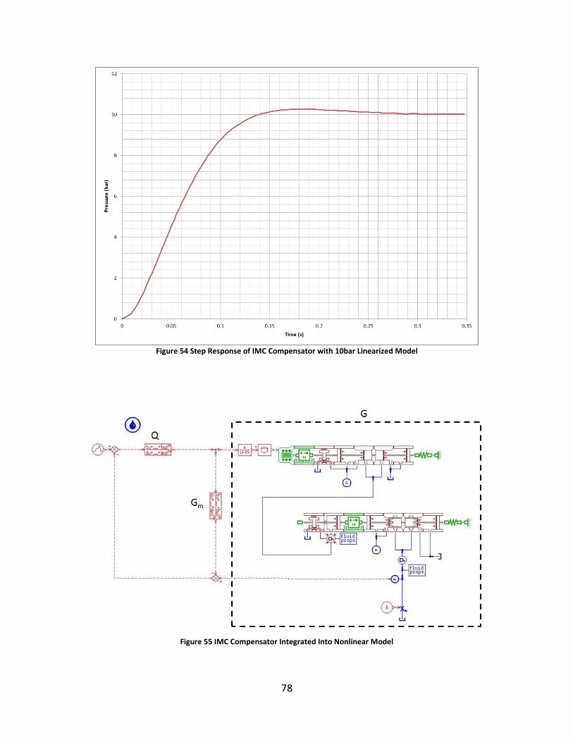
78

Figure 54 Step Response of IMC Compensator with 10bar Linearized Model

Figure 55 IMC Compensator Integrated Into Nonlinear Model

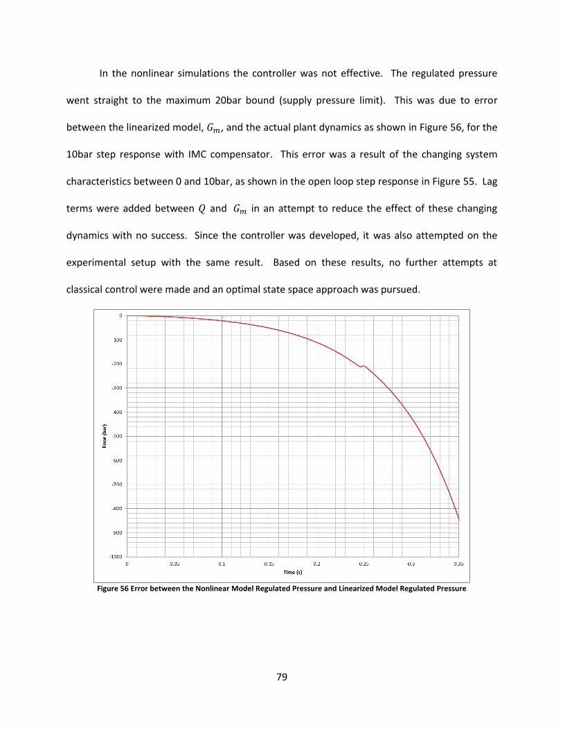
79

In the nonlinear simulations the controller was not effective. The regulated pressure

went straight to the maximum 20bar bound (supply pressure limit). This was due to error

between the linearized model, 𝐺𝑚, and the actual plant dynamics as shown in Figure 56, for the

10bar step response with IMC compensator. This error was a result of the changing system

characteristics between 0 and 10bar, as shown in the open loop step response in Figure 55. Lag

terms were added between 𝑄 and 𝐺𝑚 in an attempt to reduce the effect of these changing

dynamics with no success. Since the controller was developed, it was also attempted on the

experimental setup with the same result. Based on these results, no further attempts at

classical control were made and an optimal state space approach was pursued.

Figure 56 Error between the Nonlinear Model Regulated Pressure and Linearized Model Regulated Pressure

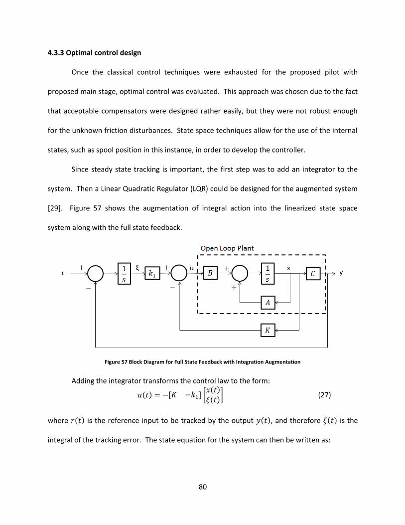
80

4.3.3 Optimal control design

Once the classical control techniques were exhausted for the proposed pilot with

proposed main stage, optimal control was evaluated. This approach was chosen due to the fact

that acceptable compensators were designed rather easily, but they were not robust enough

for the unknown friction disturbances. State space techniques allow for the use of the internal

states, such as spool position in this instance, in order to develop the controller.

Since steady state tracking is important, the first step was to add an integrator to the

system. Then a Linear Quadratic Regulator (LQR) could be designed for the augmented system

[29]. Figure 57 shows the augmentation of integral action into the linearized state space

system along with the full state feedback.

Figure 57 Block Diagram for Full State Feedback with Integration Augmentation

Adding the integrator transforms the control law to the form:

𝑢(𝑡) = −[𝐾 −𝑘1] [𝑥(𝑡)

𝜉(𝑡)] (27)

where 𝑟(𝑡) is the reference input to be tracked by the output 𝑦(𝑡), and therefore 𝜉(𝑡) is the

integral of the tracking error. The state equation for the system can then be written as:

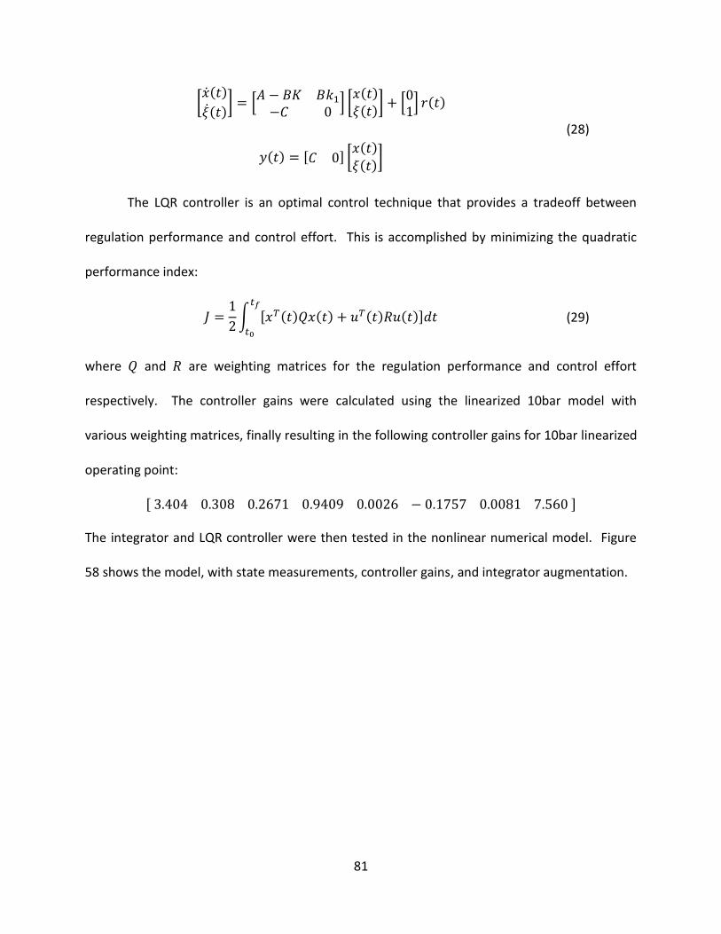
81

[(𝑡)

(𝑡)] = [

𝐴 − 𝐵𝐾 𝐵𝑘1

−𝐶 0] [

𝑥(𝑡)

𝜉(𝑡)] + [

01] 𝑟(𝑡)

𝑦(𝑡) = [𝐶 0] [𝑥(𝑡)

𝜉(𝑡)]

(28)

The LQR controller is an optimal control technique that provides a tradeoff between

regulation performance and control effort. This is accomplished by minimizing the quadratic

performance index:

𝐽 =1

2∫ [𝑥𝑇(𝑡)𝑄𝑥(𝑡) + 𝑢𝑇(𝑡)𝑅𝑢(𝑡)]𝑑𝑡

𝑡𝑓

𝑡0

(29)

where 𝑄 and 𝑅 are weighting matrices for the regulation performance and control effort

respectively. The controller gains were calculated using the linearized 10bar model with

various weighting matrices, finally resulting in the following controller gains for 10bar linearized

operating point:

[ 3.404 0.308 0.2671 0.9409 0.0026 − 0.1757 0.0081 7.560 ]

The integrator and LQR controller were then tested in the nonlinear numerical model. Figure

58 shows the model, with state measurements, controller gains, and integrator augmentation.

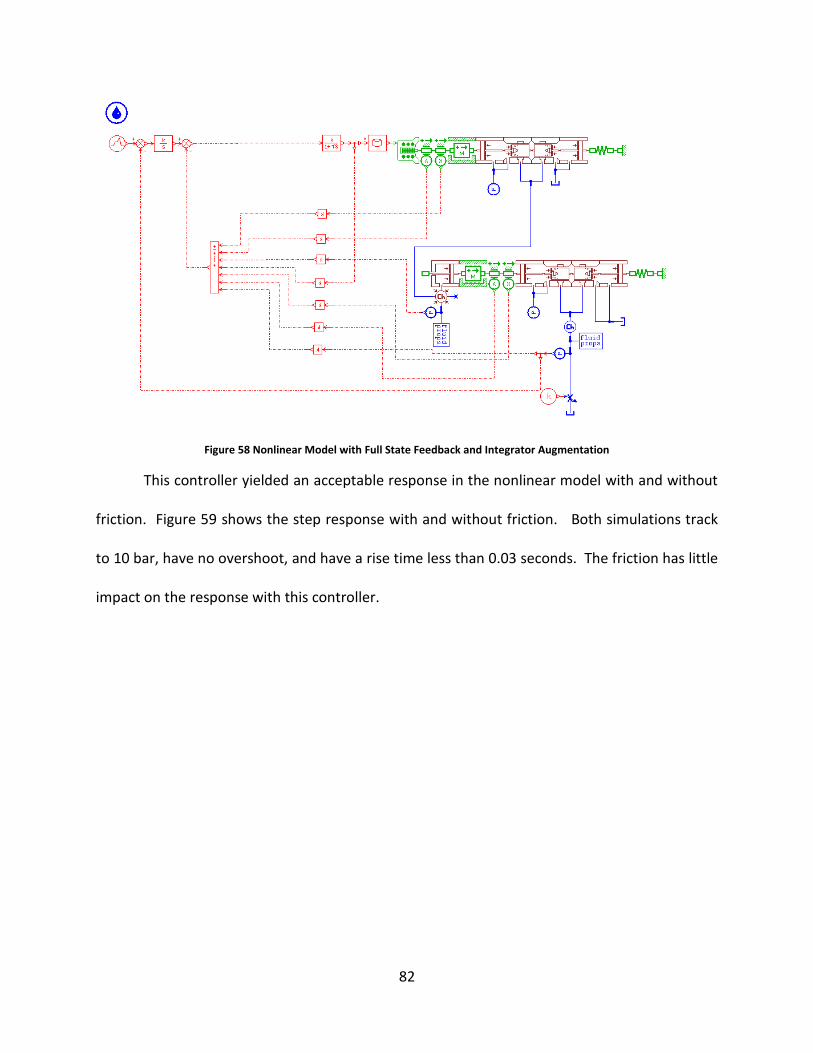
82

Figure 58 Nonlinear Model with Full State Feedback and Integrator Augmentation

This controller yielded an acceptable response in the nonlinear model with and without

friction. Figure 59 shows the step response with and without friction. Both simulations track

to 10 bar, have no overshoot, and have a rise time less than 0.03 seconds. The friction has little

impact on the response with this controller.

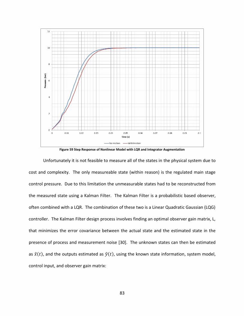
83

Figure 59 Step Response of Nonlinear Model with LQR and Integrator Augmentation

Unfortunately it is not feasible to measure all of the states in the physical system due to

cost and complexity. The only measureable state (within reason) is the regulated main stage

control pressure. Due to this limitation the unmeasurable states had to be reconstructed from

the measured state using a Kalman Filter. The Kalman Filter is a probabilistic based observer,

often combined with a LQR. The combination of these two is a Linear Quadratic Gaussian (LQG)

controller. The Kalman Filter design process involves finding an optimal observer gain matrix, L,

that minimizes the error covariance between the actual state and the estimated state in the

presence of process and measurement noise [30]. The unknown states can then be estimated

as (𝑡), and the outputs estimated as (𝑡), using the known state information, system model,

control input, and observer gain matrix:

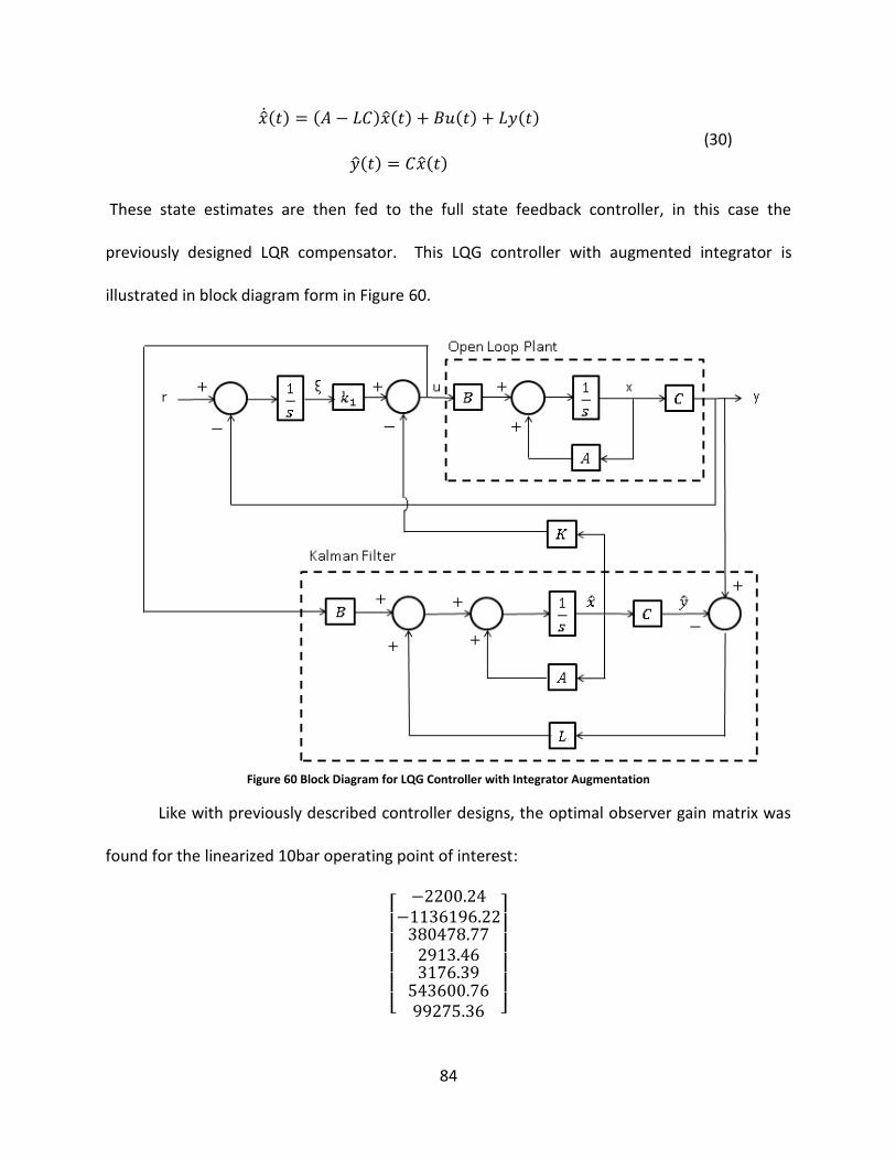
84

(𝑡) = (𝐴 − 𝐿𝐶)(𝑡) + 𝐵𝑢(𝑡) + 𝐿𝑦(𝑡)

(𝑡) = 𝐶(𝑡)

(30)

These state estimates are then fed to the full state feedback controller, in this case the

previously designed LQR compensator. This LQG controller with augmented integrator is

illustrated in block diagram form in Figure 60.

Figure 60 Block Diagram for LQG Controller with Integrator Augmentation

Like with previously described controller designs, the optimal observer gain matrix was

found for the linearized 10bar operating point of interest:

[

−2200.24−1136196.22380478.772913.463176.39

543600.7699275.36 ]

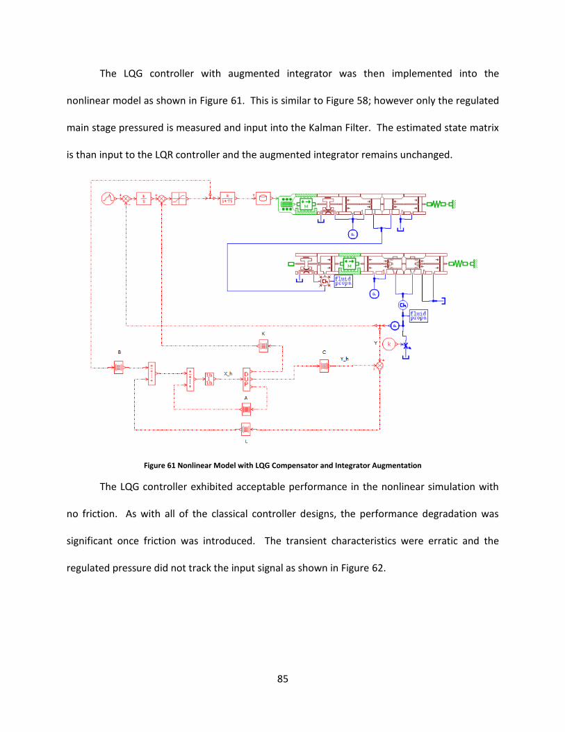
85

The LQG controller with augmented integrator was then implemented into the

nonlinear model as shown in Figure 61. This is similar to Figure 58; however only the regulated

main stage pressured is measured and input into the Kalman Filter. The estimated state matrix

is than input to the LQR controller and the augmented integrator remains unchanged.

Figure 61 Nonlinear Model with LQG Compensator and Integrator Augmentation

The LQG controller exhibited acceptable performance in the nonlinear simulation with

no friction. As with all of the classical controller designs, the performance degradation was

significant once friction was introduced. The transient characteristics were erratic and the

regulated pressure did not track the input signal as shown in Figure 62.

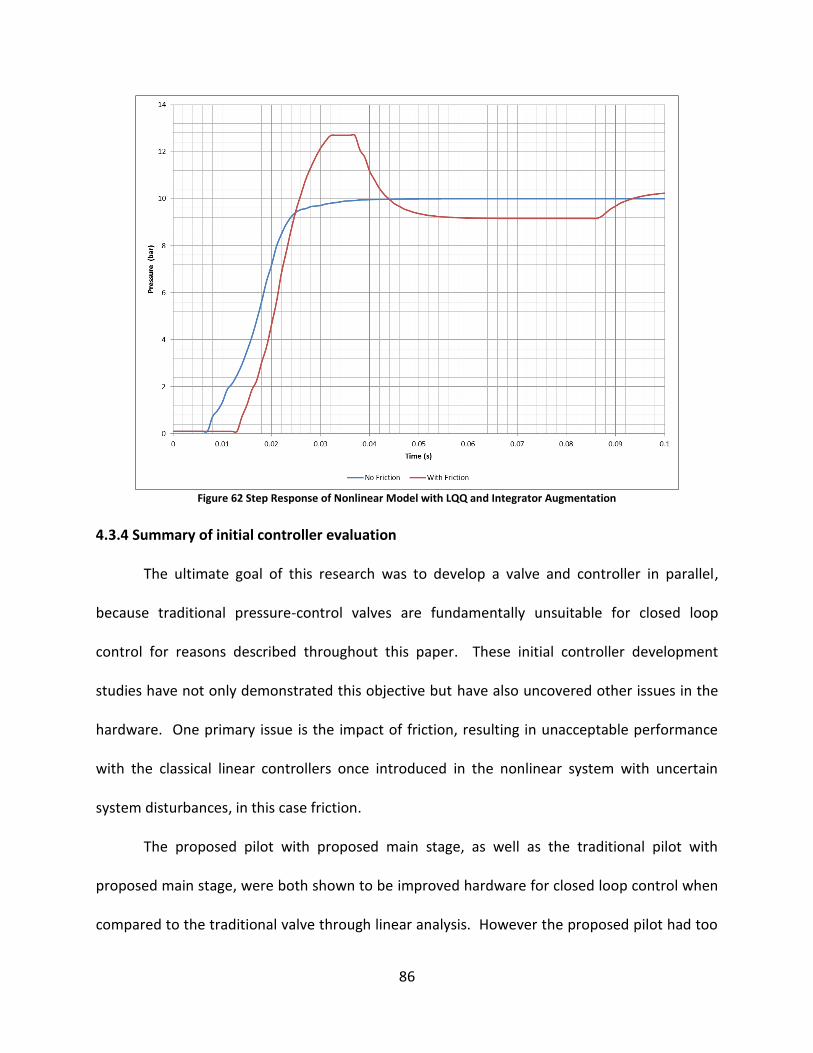
86

Figure 62 Step Response of Nonlinear Model with LQQ and Integrator Augmentation

4.3.4 Summary of initial controller evaluation

The ultimate goal of this research was to develop a valve and controller in parallel,

because traditional pressure-control valves are fundamentally unsuitable for closed loop

control for reasons described throughout this paper. These initial controller development

studies have not only demonstrated this objective but have also uncovered other issues in the

hardware. One primary issue is the impact of friction, resulting in unacceptable performance

with the classical linear controllers once introduced in the nonlinear system with uncertain

system disturbances, in this case friction.

The proposed pilot with proposed main stage, as well as the traditional pilot with

proposed main stage, were both shown to be improved hardware for closed loop control when

compared to the traditional valve through linear analysis. However the proposed pilot had too

87

much friction, as illustrated in Figure 36, for classical control. Full state feedback control yielded

acceptable performance, however the additional sensors required to monitor the states are not

feasible for this application due to cost and complexity. Estimating these states resulted in

similar performance issues as the classical controllers once uncertain friction was introduced.

The traditional pilot with proposed main stage was able to achieve desired performance with

simple classical techniques and only main stage regulated pressure feedback. This is because

the traditional pilot dynamics are not dependent on the main stage control port characteristics,

only the pilot stage control port characteristics, which are internal to the valve, are more

consistent, and are not the dominant factor in the overall system response.

Based on these results, the traditional pilot with proposed main stage was further

developed due to the simplicity of the controller and sensor requirements. The proposed pilot

with proposed main stage valve demonstrated the objective of this research, developing the

hardware and software in parallel, but required additional state measurements that were

outside the scope of this project and not feasible form a cost and packaging standpoint.

Therefore, from this point on the traditional pilot with proposed main stage was further

evaluated using simple classical techniques, for reasons previously described, and the proposed

pilot with proposed main stage was no longer evaluated due to the additional state information

required to develop an acceptable closed loop step response.

88

CHAPTER 5

CONTROLLER DEVELOPMENT AND FURTHER EXPERIMENTAL TESTING

5.1 Experimental controller tuning under standard operating conditions

As outlined in chapter 4, both valve concepts illustrated the need to develop the valve

hardware and controller software in parallel as opposed to the traditional approach of

designing a controller for existing hardware. Both valve designs were better suited for closed

loop control when compared to the traditional valve; however the proposed valve with

proposed main stage had too much uncertainty, in the form of friction, when compared to the

traditional pilot with proposed main stage. In this chapter the controller development for the

final valve design is summarized, followed by experimental testing to compare the new valve

with closed loop control and the traditional valve with open loop control.

Since the system is nonlinear and continuous, it had to be discretized into various

operating points in order to develop controller gains using a linear technique. Figure 63 shows

the operating points at which the controller gains were tuned. It was found that 2bar

increments were adequate for acceptable response using PID control with gain scheduling.

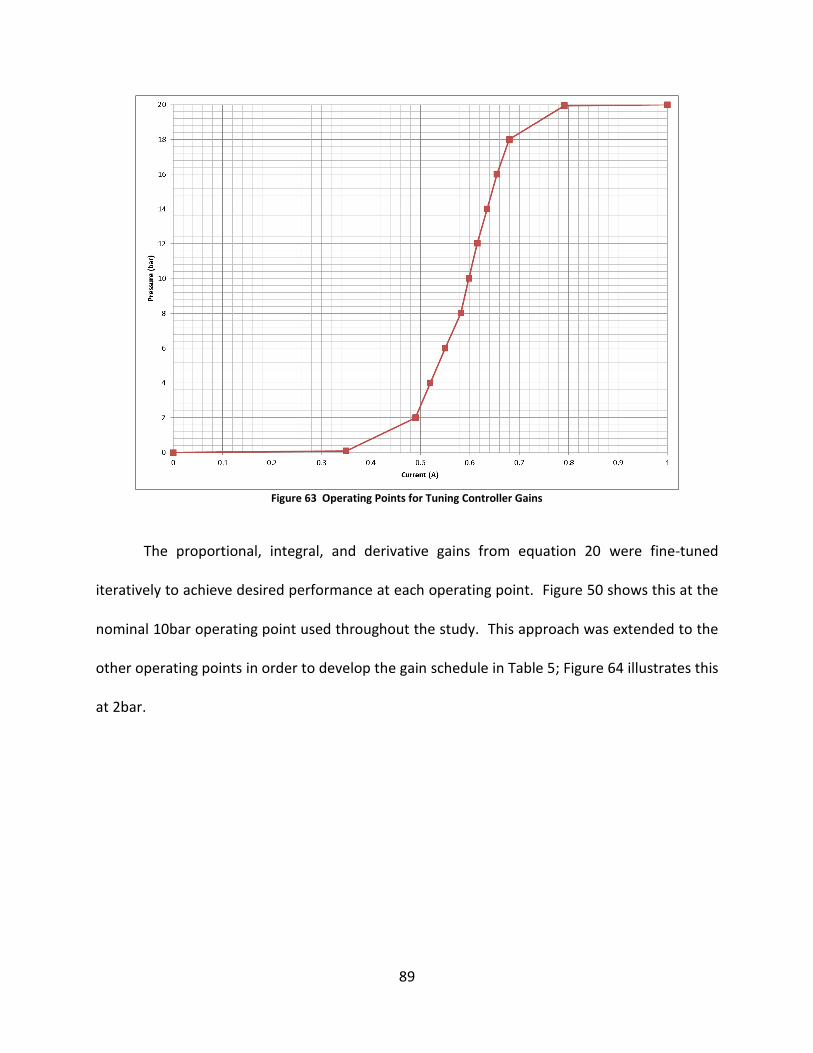
89

Figure 63 Operating Points for Tuning Controller Gains

The proportional, integral, and derivative gains from equation 20 were fine-tuned

iteratively to achieve desired performance at each operating point. Figure 50 shows this at the

nominal 10bar operating point used throughout the study. This approach was extended to the

other operating points in order to develop the gain schedule in Table 5; Figure 64 illustrates this

at 2bar.

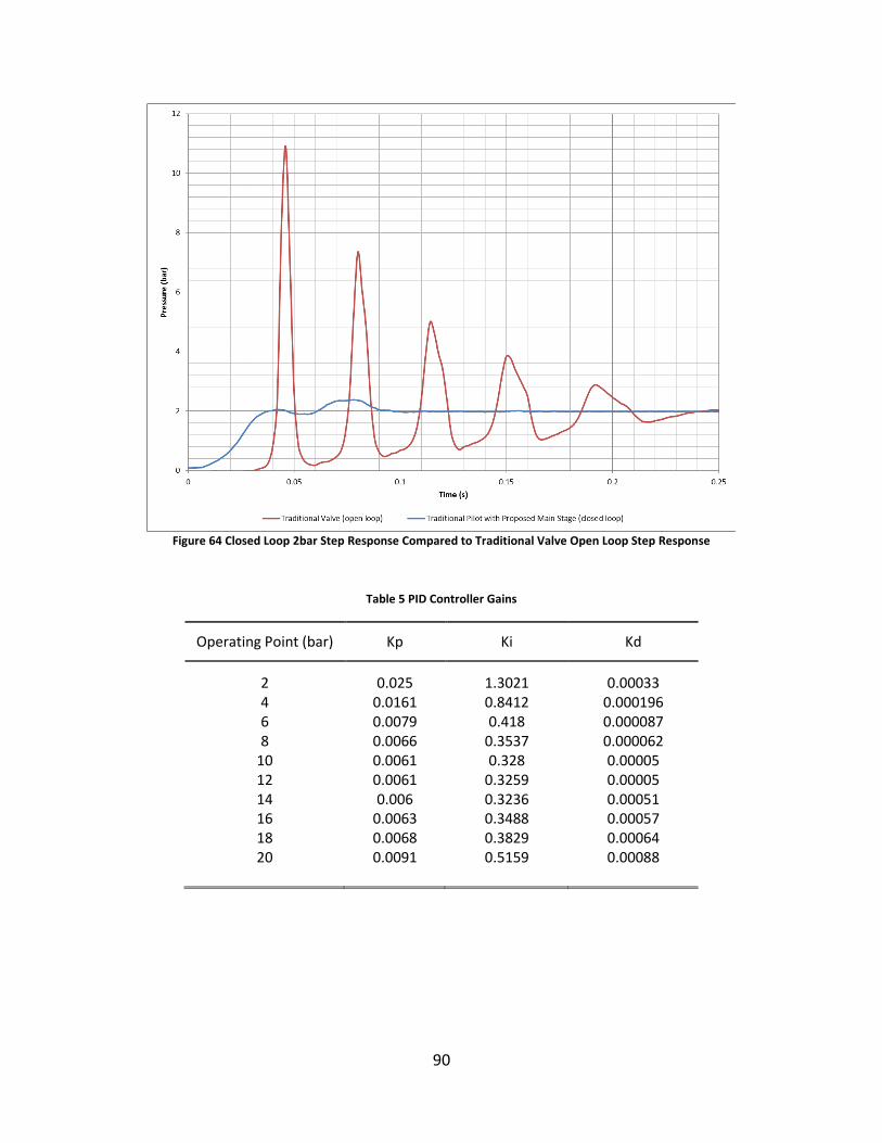
90

Figure 64 Closed Loop 2bar Step Response Compared to Traditional Valve Open Loop Step Response

Table 5 PID Controller Gains

Operating Point (bar) Kp Ki Kd

2 0.025 1.3021 0.00033 4 0.0161 0.8412 0.000196 6 0.0079 0.418 0.000087 8 0.0066 0.3537 0.000062

10 0.0061 0.328 0.00005 12 0.0061 0.3259 0.00005 14 0.006 0.3236 0.00051 16 0.0063 0.3488 0.00057 18 0.0068 0.3829 0.00064 20 0.0091 0.5159 0.00088

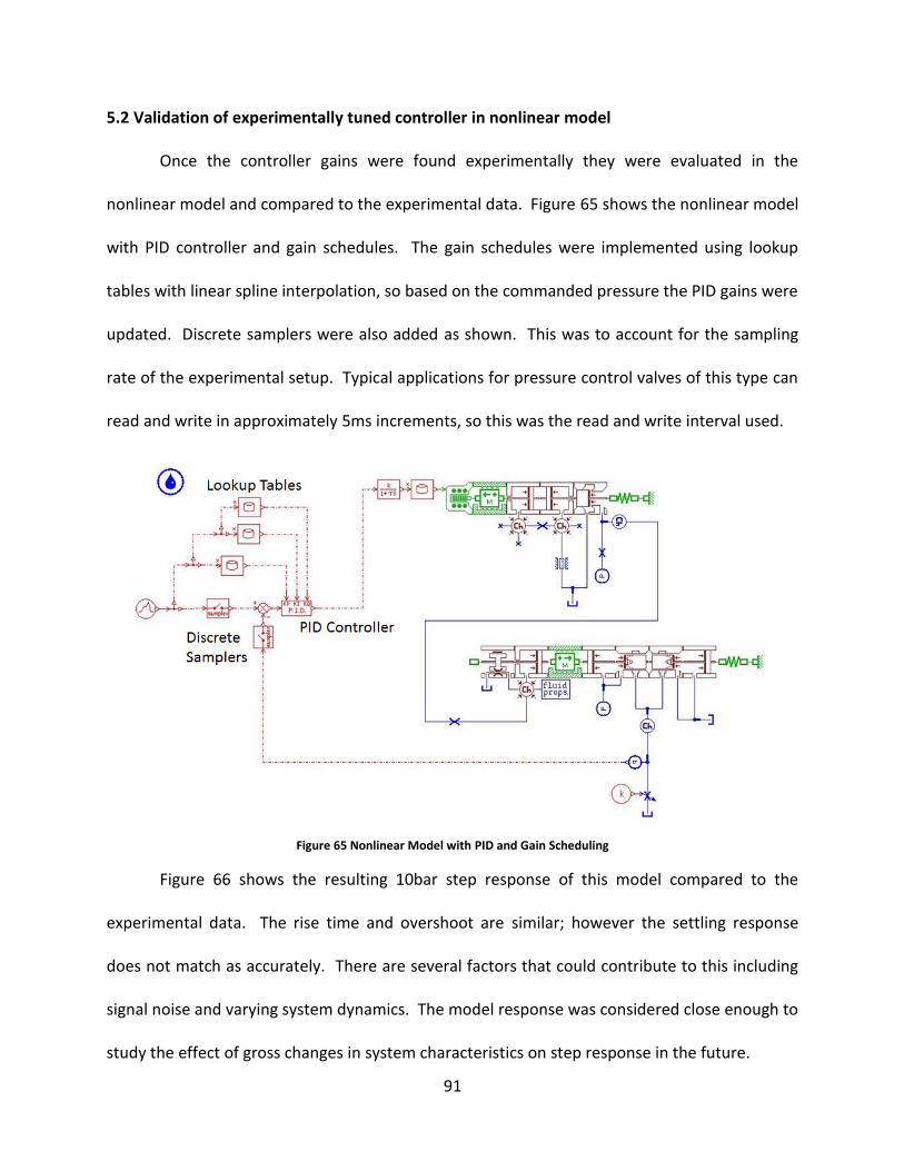
91

5.2 Validation of experimentally tuned controller in nonlinear model

Once the controller gains were found experimentally they were evaluated in the

nonlinear model and compared to the experimental data. Figure 65 shows the nonlinear model

with PID controller and gain schedules. The gain schedules were implemented using lookup

tables with linear spline interpolation, so based on the commanded pressure the PID gains were

updated. Discrete samplers were also added as shown. This was to account for the sampling

rate of the experimental setup. Typical applications for pressure control valves of this type can

read and write in approximately 5ms increments, so this was the read and write interval used.

Figure 65 Nonlinear Model with PID and Gain Scheduling

Figure 66 shows the resulting 10bar step response of this model compared to the

experimental data. The rise time and overshoot are similar; however the settling response

does not match as accurately. There are several factors that could contribute to this including

signal noise and varying system dynamics. The model response was considered close enough to

study the effect of gross changes in system characteristics on step response in the future.

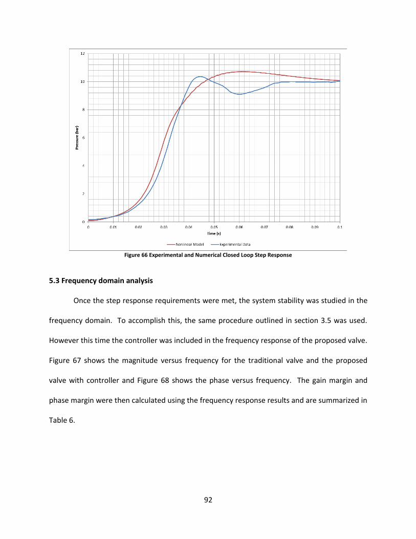
92

Figure 66 Experimental and Numerical Closed Loop Step Response

5.3 Frequency domain analysis

Once the step response requirements were met, the system stability was studied in the

frequency domain. To accomplish this, the same procedure outlined in section 3.5 was used.

However this time the controller was included in the frequency response of the proposed valve.

Figure 67 shows the magnitude versus frequency for the traditional valve and the proposed

valve with controller and Figure 68 shows the phase versus frequency. The gain margin and

phase margin were then calculated using the frequency response results and are summarized in

Table 6.

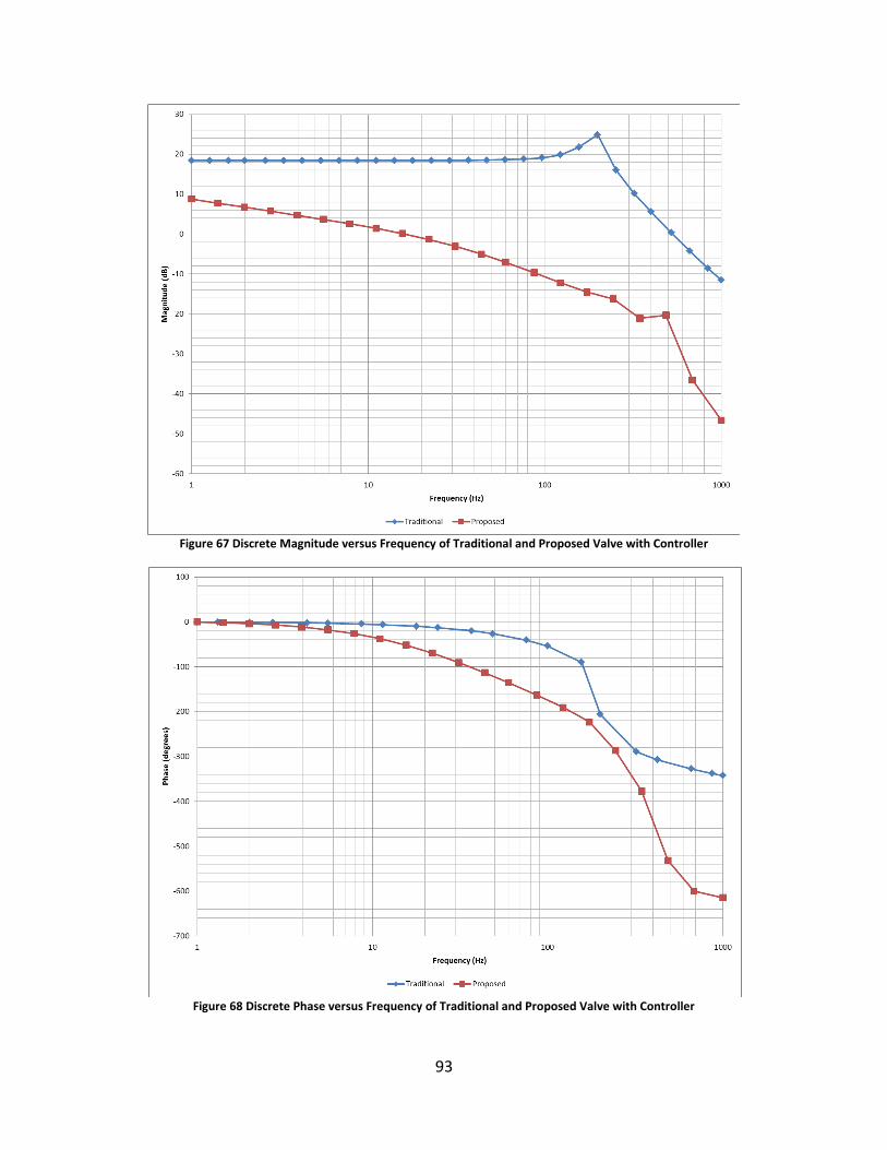
93

Figure 67 Discrete Magnitude versus Frequency of Traditional and Proposed Valve with Controller

Figure 68 Discrete Phase versus Frequency of Traditional and Proposed Valve with Controller

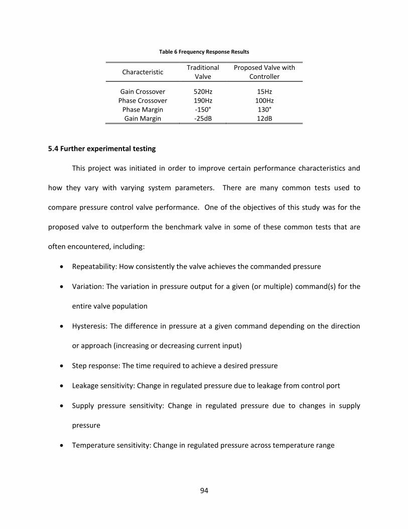
94

Table 6 Frequency Response Results

Characteristic Traditional

Valve Proposed Valve with

Controller

Gain Crossover 520Hz 15Hz Phase Crossover 190Hz 100Hz

Phase Margin -150° 130° Gain Margin -25dB 12dB

5.4 Further experimental testing

This project was initiated in order to improve certain performance characteristics and

how they vary with varying system parameters. There are many common tests used to

compare pressure control valve performance. One of the objectives of this study was for the

proposed valve to outperform the benchmark valve in some of these common tests that are

often encountered, including:

Repeatability: How consistently the valve achieves the commanded pressure

Variation: The variation in pressure output for a given (or multiple) command(s) for the

entire valve population

Hysteresis: The difference in pressure at a given command depending on the direction

or approach (increasing or decreasing current input)

Step response: The time required to achieve a desired pressure

Leakage sensitivity: Change in regulated pressure due to leakage from control port

Supply pressure sensitivity: Change in regulated pressure due to changes in supply

pressure

Temperature sensitivity: Change in regulated pressure across temperature range

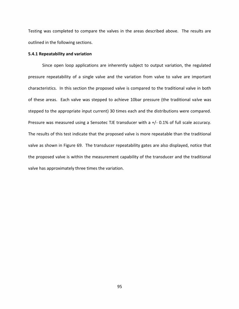
95

Testing was completed to compare the valves in the areas described above. The results are

outlined in the following sections.

5.4.1 Repeatability and variation

Since open loop applications are inherently subject to output variation, the regulated

pressure repeatability of a single valve and the variation from valve to valve are important

characteristics. In this section the proposed valve is compared to the traditional valve in both

of these areas. Each valve was stepped to achieve 10bar pressure (the traditional valve was

stepped to the appropriate input current) 30 times each and the distributions were compared.

Pressure was measured using a Sensotec TJE transducer with a +/- 0.1% of full scale accuracy.

The results of this test indicate that the proposed valve is more repeatable than the traditional

valve as shown in Figure 69. The transducer repeatability gates are also displayed, notice that

the proposed valve is within the measurement capability of the transducer and the traditional

valve has approximately three times the variation.

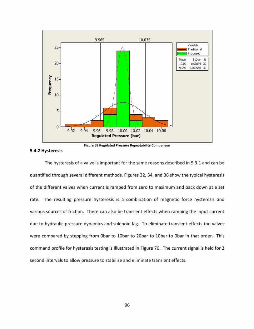
96

Figure 69 Regulated Pressure Repeatability Comparison

5.4.2 Hysteresis

The hysteresis of a valve is important for the same reasons described in 5.3.1 and can be

quantified through several different methods. Figures 32, 34, and 36 show the typical hysteresis

of the different valves when current is ramped from zero to maximum and back down at a set

rate. The resulting pressure hysteresis is a combination of magnetic force hysteresis and

various sources of friction. There can also be transient effects when ramping the input current

due to hydraulic pressure dynamics and solenoid lag. To eliminate transient effects the valves

were compared by stepping from 0bar to 10bar to 20bar to 10bar to 0bar in that order. This

command profile for hysteresis testing is illustrated in Figure 70. The current signal is held for 2

second intervals to allow pressure to stabilize and eliminate transient effects.

Regulated Pressure (bar)

Fre

qu

en

cy

10.0610.0410.0210.009.989.969.949.92

25

20

15

10

5

0

10.0359.965

10.00 0.03094 30

9.999 0.009550 30

Mean StDev N

Traditional

Proposed

Variable

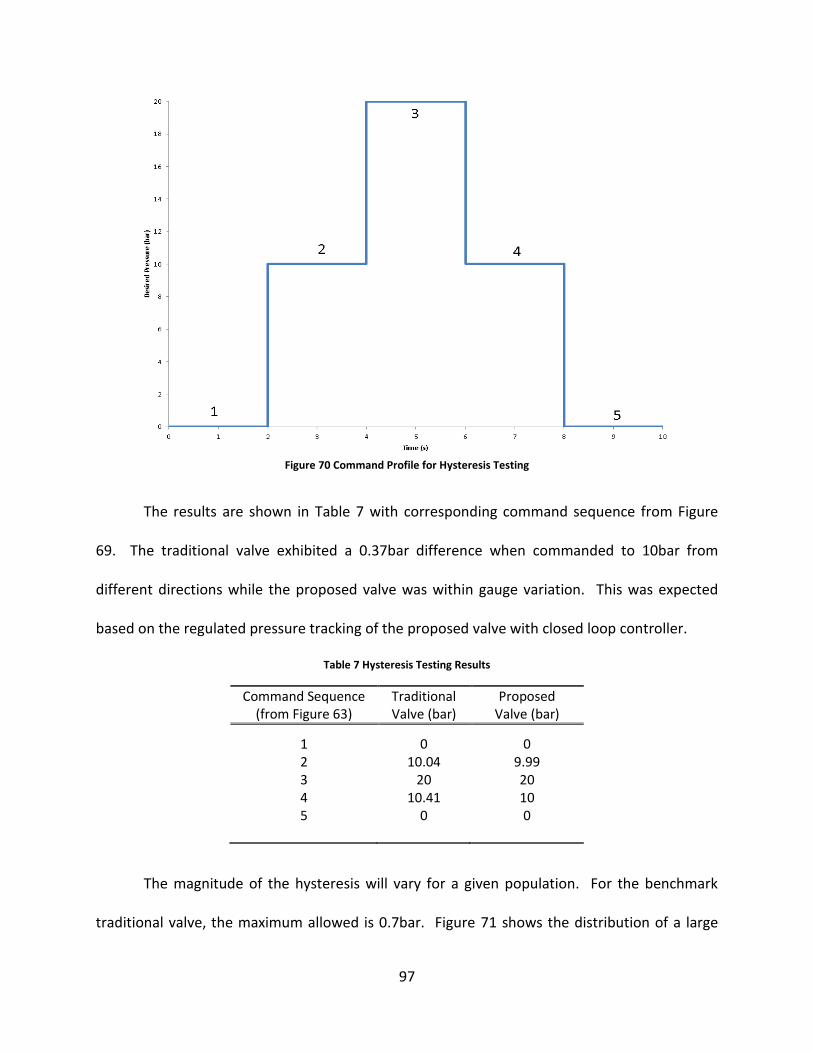
97

Figure 70 Command Profile for Hysteresis Testing

The results are shown in Table 7 with corresponding command sequence from Figure

69. The traditional valve exhibited a 0.37bar difference when commanded to 10bar from

different directions while the proposed valve was within gauge variation. This was expected

based on the regulated pressure tracking of the proposed valve with closed loop controller.

Table 7 Hysteresis Testing Results

Command Sequence (from Figure 63)

Traditional Valve (bar)

Proposed Valve (bar)

1 0 0 2 10.04 9.99 3 20 20 4 10.41 10 5 0 0

The magnitude of the hysteresis will vary for a given population. For the benchmark

traditional valve, the maximum allowed is 0.7bar. Figure 71 shows the distribution of a large

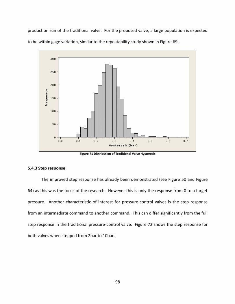
98

production run of the traditional valve. For the proposed valve, a large population is expected

to be within gage variation, similar to the repeatability study shown in Figure 69.

Figure 71 Distribution of Traditional Valve Hysteresis

5.4.3 Step response

The improved step response has already been demonstrated (see Figure 50 and Figure

64) as this was the focus of the research. However this is only the response from 0 to a target

pressure. Another characteristic of interest for pressure-control valves is the step response

from an intermediate command to another command. This can differ significantly from the full

step response in the traditional pressure-control valve. Figure 72 shows the step response for

both valves when stepped from 2bar to 10bar.

H y s t e r e s is ( b a r )

Fr

eq

ue

nc

y

0 .70 .60 .50 .40 .30 .20 .10 .0

3 0 0

2 5 0

2 0 0

1 5 0

1 0 0

5 0

0

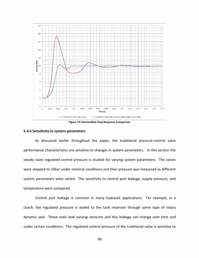
99

Figure 72 Intermediate Step Response Comparison

5.4.4 Sensitivity to system parameters

As discussed earlier throughout the paper, the traditional pressure-control valve

performance characteristics are sensitive to changes in system parameters. In this section the

steady state regulated control pressure is studied for varying system parameters. The valves

were stepped to 10bar under nominal conditions and then pressure was measured as different

system parameters were varied. The sensitivity to control port leakage, supply pressure, and

temperature were compared.

Control port leakage is common in many hydraulic applications. For example, in a

clutch, the regulated pressure is sealed to the tank reservoir through some type of rotary

dynamic seal. These seals leak varying amounts and this leakage can change over time and

under certain conditions. The regulated control pressure of the traditional valve is sensitive to

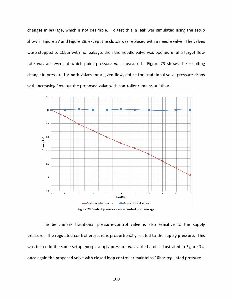
100

changes in leakage, which is not desirable. To test this, a leak was simulated using the setup

show in Figure 27 and Figure 28, except the clutch was replaced with a needle valve. The valves

were stepped to 10bar with no leakage, then the needle valve was opened until a target flow

rate was achieved, at which point pressure was measured. Figure 73 shows the resulting

change in pressure for both valves for a given flow, notice the traditional valve pressure drops

with increasing flow but the proposed valve with controller remains at 10bar.

Figure 73 Control pressure versus control port leakage

The benchmark traditional pressure-control valve is also sensitive to the supply

pressure. The regulated control pressure is proportionally related to the supply pressure. This

was tested in the same setup except supply pressure was varied and is illustrated in Figure 74,

once again the proposed valve with closed loop controller maintains 10bar regulated pressure.

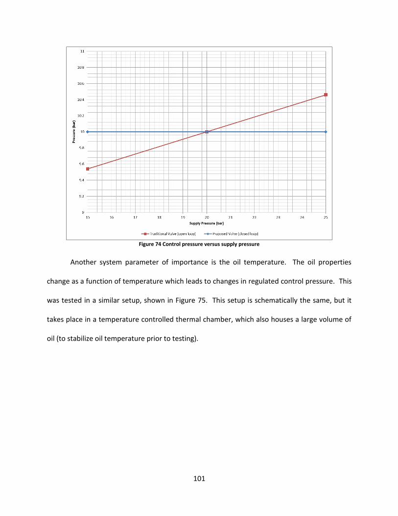
101

Figure 74 Control pressure versus supply pressure

Another system parameter of importance is the oil temperature. The oil properties

change as a function of temperature which leads to changes in regulated control pressure. This

was tested in a similar setup, shown in Figure 75. This setup is schematically the same, but it

takes place in a temperature controlled thermal chamber, which also houses a large volume of

oil (to stabilize oil temperature prior to testing).

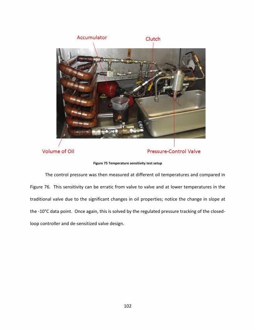
102

Figure 75 Temperature sensitivity test setup

The control pressure was then measured at different oil temperatures and compared in

Figure 76. This sensitivity can be erratic from valve to valve and at lower temperatures in the

traditional valve due to the significant changes in oil properties; notice the change in slope at

the -10°C data point. Once again, this is solved by the regulated pressure tracking of the closed-

loop controller and de-sensitized valve design.

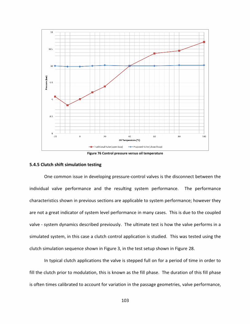
103

Figure 76 Control pressure versus oil temperature

5.4.5 Clutch shift simulation testing

One common issue in developing pressure-control valves is the disconnect between the

individual valve performance and the resulting system performance. The performance

characteristics shown in previous sections are applicable to system performance; however they

are not a great indicator of system level performance in many cases. This is due to the coupled

valve - system dynamics described previously. The ultimate test is how the valve performs in a

simulated system, in this case a clutch control application is studied. This was tested using the

clutch simulation sequence shown in Figure 3, in the test setup shown in Figure 28.

In typical clutch applications the valve is stepped full on for a period of time in order to

fill the clutch prior to modulation, this is known as the fill phase. The duration of this fill phase

is often times calibrated to account for variation in the passage geometries, valve performance,

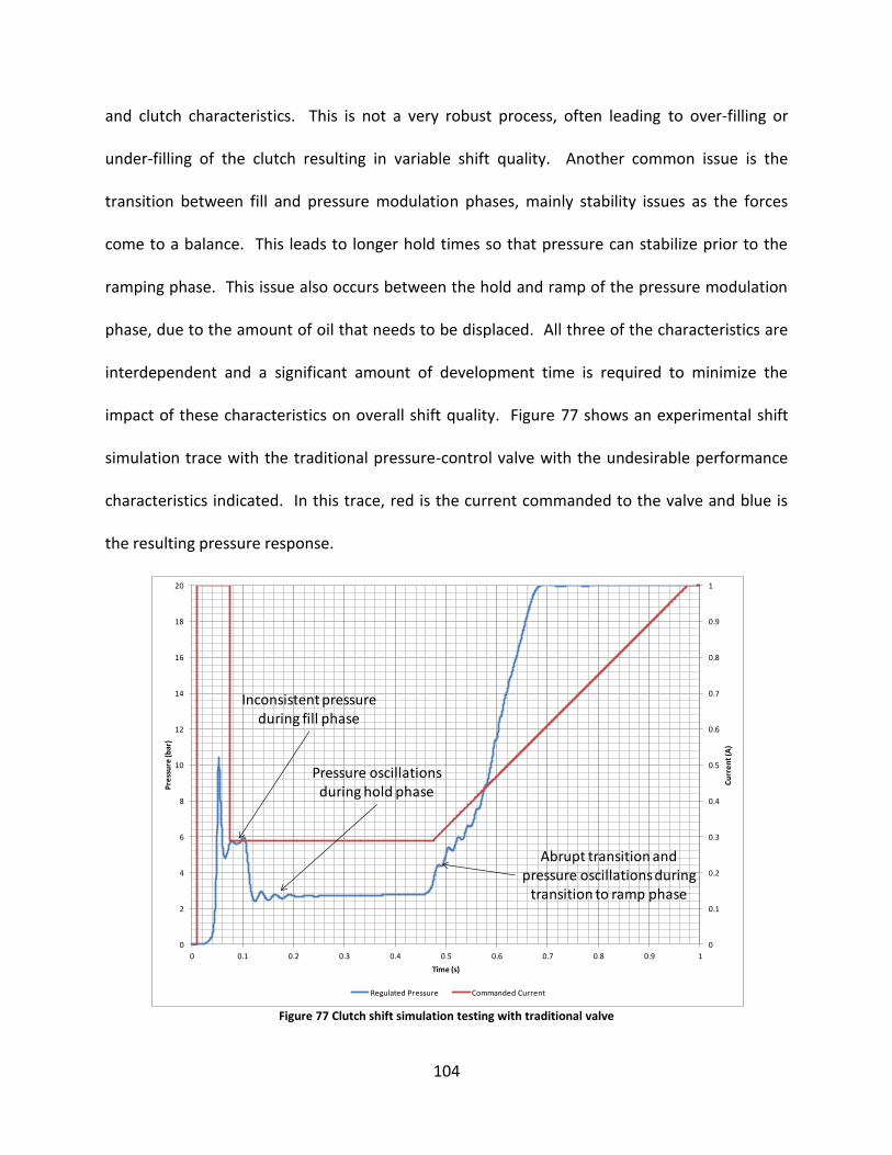
104

and clutch characteristics. This is not a very robust process, often leading to over-filling or

under-filling of the clutch resulting in variable shift quality. Another common issue is the

transition between fill and pressure modulation phases, mainly stability issues as the forces

come to a balance. This leads to longer hold times so that pressure can stabilize prior to the

ramping phase. This issue also occurs between the hold and ramp of the pressure modulation

phase, due to the amount of oil that needs to be displaced. All three of the characteristics are

interdependent and a significant amount of development time is required to minimize the

impact of these characteristics on overall shift quality. Figure 77 shows an experimental shift

simulation trace with the traditional pressure-control valve with the undesirable performance

characteristics indicated. In this trace, red is the current commanded to the valve and blue is

the resulting pressure response.

Figure 77 Clutch shift simulation testing with traditional valve

0

0.1

0.2

0.3

0.4

0.5

0.6

0.7

0.8

0.9

1

0

2

4

6

8

10

12

14

16

18

20

0 0.1 0.2 0.3 0.4 0.5 0.6 0.7 0.8 0.9 1

Cu

rre

nt

(A)

Pre

ssu

re (b

ar)

Time (s)

Regulated Pressure Commanded Current

Inconsistent pressure during fill phase

Pressure oscillations during hold phase

Abrupt transition and pressure oscillations during

transition to ramp phase

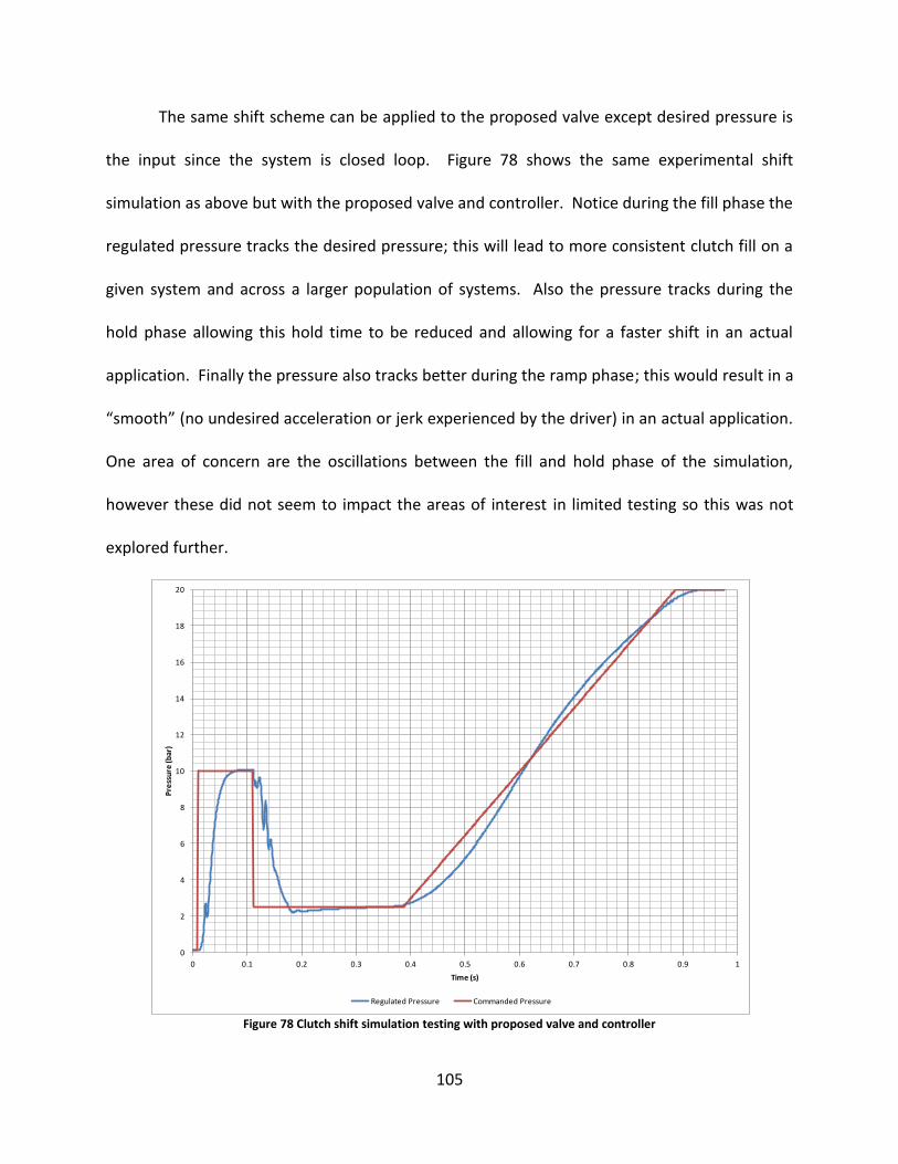
105

The same shift scheme can be applied to the proposed valve except desired pressure is

the input since the system is closed loop. Figure 78 shows the same experimental shift

simulation as above but with the proposed valve and controller. Notice during the fill phase the

regulated pressure tracks the desired pressure; this will lead to more consistent clutch fill on a

given system and across a larger population of systems. Also the pressure tracks during the

hold phase allowing this hold time to be reduced and allowing for a faster shift in an actual

application. Finally the pressure also tracks better during the ramp phase; this would result in a

“smooth” (no undesired acceleration or jerk experienced by the driver) in an actual application.

One area of concern are the oscillations between the fill and hold phase of the simulation,

however these did not seem to impact the areas of interest in limited testing so this was not

explored further.

Figure 78 Clutch shift simulation testing with proposed valve and controller

0

2

4

6

8

10

12

14

16

18

20

0 0.1 0.2 0.3 0.4 0.5 0.6 0.7 0.8 0.9 1

Pre

ssu

re (b

ar)

Time (s)

Regulated Pressure Commanded Pressure

106

CHAPTER 6

CONCLUSION

6.1 Significance and summary

The motivation for this research was to improve pressure-control valve technology

based on observing similar performance issues in different systems, primarily clutch control

applications. These issues have been summarized throughout this dissertation. To this point,

the solutions to these issues have been limited to hardware changes in the valve, which are

difficult to execute in mature products, do not typically address the issue completely, and often

require sacrifices in other areas of the design. Software solutions for these issues have failed

due to the physics of pressure-control valves and interaction with the system; they are

fundamentally not suited for closed loop control (especially in the volatile high speed

applications in which they are typically used). These experiences lead to the development of

new hardware in parallel to software in order to address the most common issues.

Hydraulic systems are highly nonlinear and sensitive to typical parameter variation. This

is especially true in pressure-control valves because the valve dynamics are coupled to the

hydraulic dynamics as discussed previously. This is the underlying reason for the previous

challenges that could not be solved completely through hardware and also why closed loop

control has failed in these applications.

6.2 Conclusion and contribution

In this research two valves were designed to be less sensitive to system parameters and

therefore more suitable for closed loop control. These valves, along with a benchmark

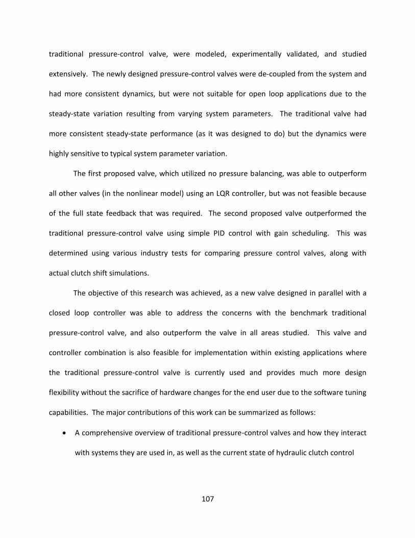
107

traditional pressure-control valve, were modeled, experimentally validated, and studied

extensively. The newly designed pressure-control valves were de-coupled from the system and

had more consistent dynamics, but were not suitable for open loop applications due to the

steady-state variation resulting from varying system parameters. The traditional valve had

more consistent steady-state performance (as it was designed to do) but the dynamics were

highly sensitive to typical system parameter variation.

The first proposed valve, which utilized no pressure balancing, was able to outperform

all other valves (in the nonlinear model) using an LQR controller, but was not feasible because

of the full state feedback that was required. The second proposed valve outperformed the

traditional pressure-control valve using simple PID control with gain scheduling. This was

determined using various industry tests for comparing pressure control valves, along with

actual clutch shift simulations.

The objective of this research was achieved, as a new valve designed in parallel with a

closed loop controller was able to address the concerns with the benchmark traditional

pressure-control valve, and also outperform the valve in all areas studied. This valve and

controller combination is also feasible for implementation within existing applications where

the traditional pressure-control valve is currently used and provides much more design

flexibility without the sacrifice of hardware changes for the end user due to the software tuning

capabilities. The major contributions of this work can be summarized as follows:

A comprehensive overview of traditional pressure-control valves and how they interact

with systems they are used in, as well as the current state of hydraulic clutch control

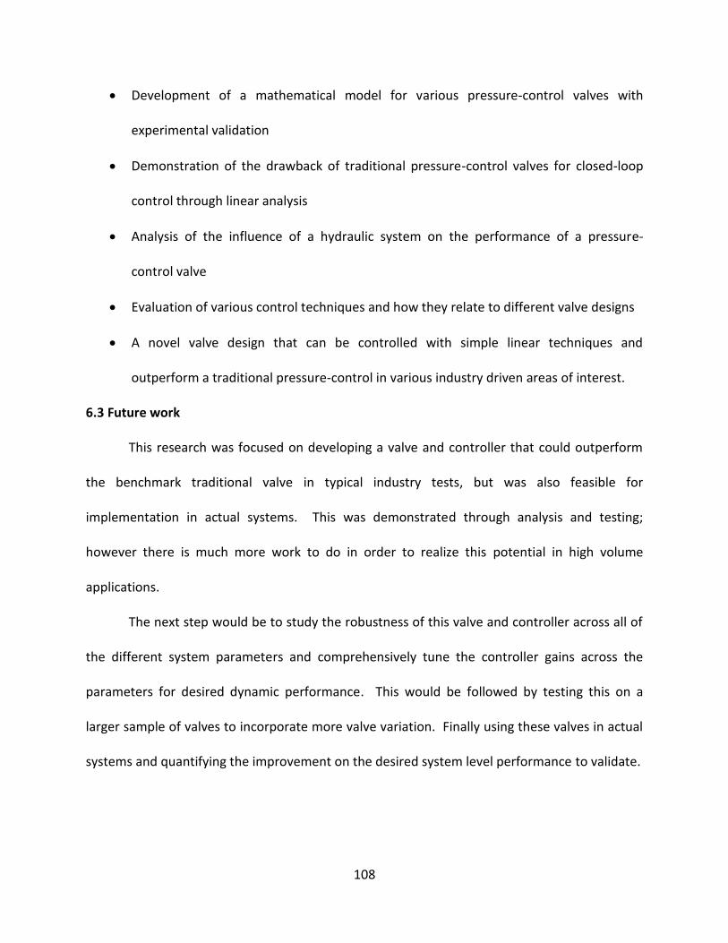
108

Development of a mathematical model for various pressure-control valves with

experimental validation

Demonstration of the drawback of traditional pressure-control valves for closed-loop

control through linear analysis

Analysis of the influence of a hydraulic system on the performance of a pressure-

control valve

Evaluation of various control techniques and how they relate to different valve designs

A novel valve design that can be controlled with simple linear techniques and

outperform a traditional pressure-control in various industry driven areas of interest.

6.3 Future work

This research was focused on developing a valve and controller that could outperform

the benchmark traditional valve in typical industry tests, but was also feasible for

implementation in actual systems. This was demonstrated through analysis and testing;

however there is much more work to do in order to realize this potential in high volume

applications.

The next step would be to study the robustness of this valve and controller across all of

the different system parameters and comprehensively tune the controller gains across the

parameters for desired dynamic performance. This would be followed by testing this on a

larger sample of valves to incorporate more valve variation. Finally using these valves in actual

systems and quantifying the improvement on the desired system level performance to validate.

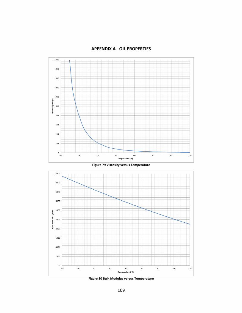
109

APPENDIX A - OIL PROPERTIES

Figure 79 Viscosity versus Temperature

Figure 80 Bulk Modulus versus Temperature

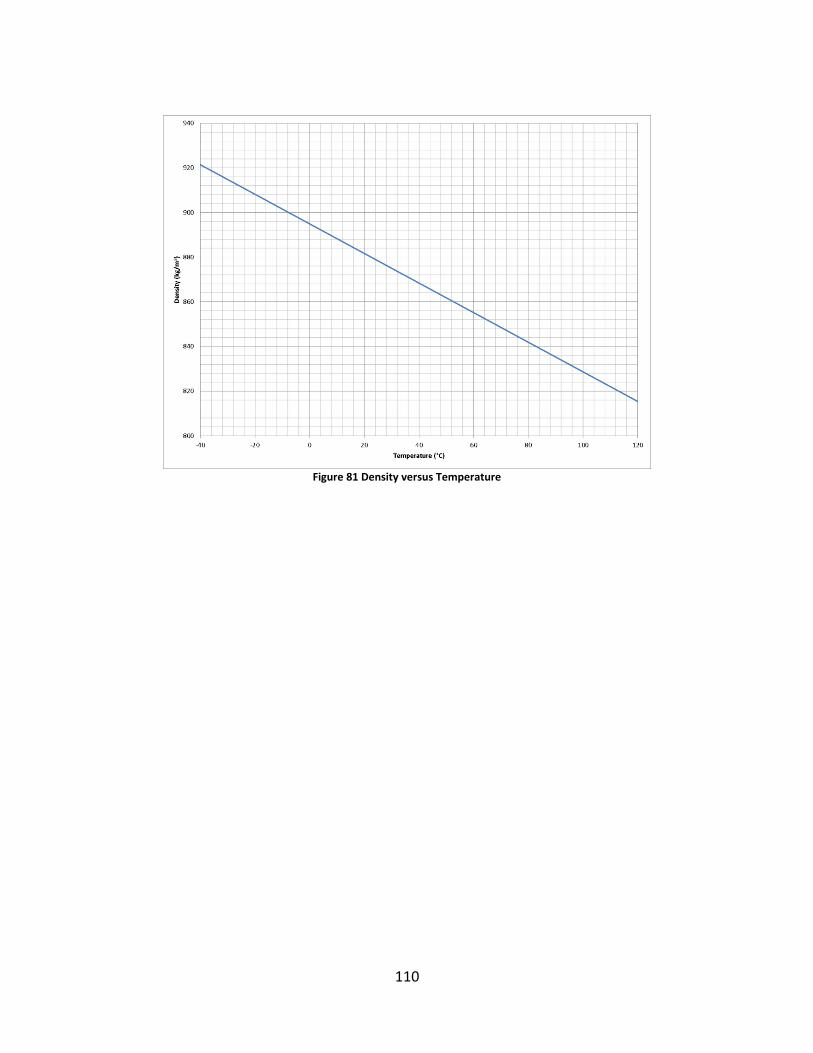
110

Figure 81 Density versus Temperature

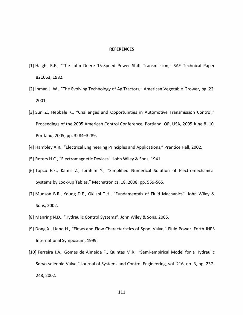
111

REFERENCES

[1] Haight R.E., “The John Deere 15-Speed Power Shift Transmission,” SAE Technical Paper

821063, 1982.

[2] Inman J. W., “The Evolving Technology of Ag Tractors,” American Vegetable Grower, pg. 22,

2001.

[3] Sun Z., Hebbale K., “Challenges and Opportunities in Automotive Transmission Control,”

Proceedings of the 2005 American Control Conference, Portland, OR, USA, 2005 June 8–10,

Portland, 2005, pp. 3284–3289.

[4] Hambley A.R., “Electrical Engineering Principles and Applications,” Prentice Hall, 2002.

[5] Roters H.C., “Electromagnetic Devices”. John Wiley & Sons, 1941.

[6] Topcu E.E., Kamis Z., Ibrahim Y., “Simplified Numerical Solution of Electromechanical

Systems by Look-up Tables,” Mechatronics, 18, 2008, pp. 559-565.

[7] Munson B.R., Young D.F., Okiishi T.H., “Fundamentals of Fluid Mechanics”. John Wiley &

Sons, 2002.

[8] Manring N.D., “Hydraulic Control Systems”. John Wiley & Sons, 2005.

[9] Dong X., Ueno H., “Flows and Flow Characteristics of Spool Valve,” Fluid Power. Forth JHPS

International Symposium, 1999.

[10] Ferreira J.A., Gomes de Almeida F., Quintas M.R., “Semi-empirical Model for a Hydraulic

Servo-solenoid Valve,” Journal of Systems and Control Engineering, vol. 216, no. 3, pp. 237-

248, 2002.

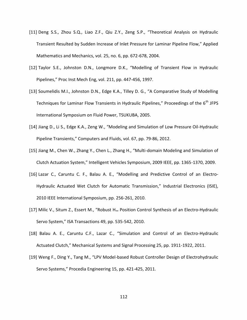
112

[11] Deng S.S., Zhou S.Q., Liao Z.F., Qiu Z.Y., Zeng S.P., “Theoretical Analysis on Hydraulic

Transient Resulted by Sudden Increase of Inlet Pressure for Laminar Pipeline Flow,” Applied

Mathematics and Mechanics, vol. 25, no. 6, pp. 672-678, 2004.

[12] Taylor S.E., Johnston D.N., Longmore D.K., “Modelling of Transient Flow in Hydraulic

Pipelines,” Proc Inst Mech Eng, vol. 211, pp. 447-456, 1997.

[13] Soumelidis M.I., Johnston D.N., Edge K.A., Tilley D. G., “A Comparative Study of Modelling

Techniques for Laminar Flow Transients in Hydraulic Pipelines,” Proceedings of the 6th JFPS

International Symposium on Fluid Power, TSUKUBA, 2005.

[14] Jiang D., Li S., Edge K.A., Zeng W., “Modeling and Simulation of Low Pressure Oil-Hydraulic

Pipeline Transients,” Computers and Fluids, vol. 67, pp. 79-86, 2012.

[15] Jiang M., Chen W., Zhang Y., Chen L., Zhang H., “Multi-domain Modeling and Simulation of

Clutch Actuation System,” Intelligent Vehicles Symposium, 2009 IEEE, pp. 1365-1370, 2009.

[16] Lazar C., Caruntu C. F., Balau A. E., “Modelling and Predictive Control of an Electro-

Hydraulic Actuated Wet Clutch for Automatic Transmission,” Industrial Electronics (ISIE),

2010 IEEE International Symposium, pp. 256-261, 2010.

[17] Milic V., Situm Z., Essert M., “Robust H∞ Position Control Synthesis of an Electro-Hydraulic

Servo System,” ISA Transactions 49, pp. 535-542, 2010.

[18] Balau A. E., Caruntu C.F., Lazar C., “Simulation and Control of an Electro-Hydraulic

Actuated Clutch,” Mechanical Systems and Signal Processing 25, pp. 1911-1922, 2011.

[19] Weng F., Ding Y., Tang M., “LPV Model-based Robust Controller Design of Electrohydraulic

Servo Systems,” Procedia Engineering 15, pp. 421-425, 2011.

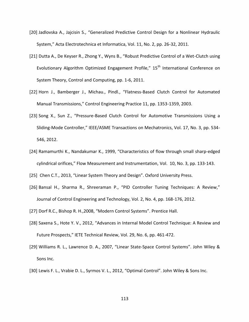
113

[20] Jadlovska A., Jajcisin S., “Generalized Predictive Control Design for a Nonlinear Hydraulic

System,” Acta Electrotechnica et Informatica, Vol. 11, No. 2, pp. 26-32, 2011.

[21] Dutta A., De Keyser R., Zhong Y., Wyns B., “Robust Predictive Control of a Wet-Clutch using

Evolutionary Algorithm Optimized Engagement Profile,” 15th International Conference on

System Theory, Control and Computing, pp. 1-6, 2011.

[22] Horn J., Bamberger J., Michau., Pindl., “Flatness-Based Clutch Control for Automated

Manual Transmissions,” Control Engineering Practice 11, pp. 1353-1359, 2003.

[23] Song X., Sun Z., “Pressure-Based Clutch Control for Automotive Transmissions Using a

Sliding-Mode Controller,” IEEE/ASME Transactions on Mechatronics, Vol. 17, No. 3, pp. 534-

546, 2012.

[24] Ramamurthi K., Nandakumar K., 1999, “Characteristics of flow through small sharp-edged

cylindrical orifices,” Flow Measurement and Instrumentation, Vol. 10, No. 3, pp. 133-143.

[25] Chen C.T., 2013, “Linear System Theory and Design”. Oxford University Press.

[26] Bansal H., Sharma R., Shreeraman P., “PID Controller Tuning Techniques: A Review,”

Journal of Control Engineering and Technology, Vol. 2, No. 4, pp. 168-176, 2012.

[27] Dorf R.C., Bishop R. H.,2008, “Modern Control Systems”. Prentice Hall.

[28] Saxena S., Hote Y. V., 2012, “Advances in Internal Model Control Technique: A Review and

Future Prospects,” IETE Technical Review, Vol. 29, No. 6, pp. 461-472.

[29] Williams R. L., Lawrence D. A., 2007, “Linear State-Space Control Systems”. John Wiley &

Sons Inc.

[30] Lewis F. L., Vrabie D. L., Syrmos V. L., 2012, “Optimal Control”. John Wiley & Sons Inc.

Design and Validation of an Electro-Hydraulic Pressure ...

Documents

Transcript of Design and Validation of an Electro-Hydraulic Pressure ...