�����������������

Citation: Schmidt, L.; Hansen, K.V.

Electro-Hydraulic Variable-Speed

Drive Networks—Idea, Perspectives,

and Energy Saving Potentials.

Energies 2022, 15, 1228. https://

doi.org/10.3390/en15031228

Academic Editor: Rafael J. Bergillos

and Helena M. Ramos

Received: 13 December 2021

Accepted: 28 January 2022

Published: 8 February 2022

Publisher’s Note: MDPI stays neutral

with regard to jurisdictional claims in

published maps and institutional affil-

iations.

Copyright: © 2022 by the authors.

Licensee MDPI, Basel, Switzerland.

This article is an open access article

distributed under the terms and

conditions of the Creative Commons

Attribution (CC BY) license (https://

creativecommons.org/licenses/by/

4.0/).

energies

Article

Electro-Hydraulic Variable-Speed Drive Networks—Idea,Perspectives, and Energy Saving Potentials

Lasse Schmidt 1,* and Kenneth Vorbøl Hansen 2

1 AAU Energy, Aalborg University, Pontoppidanstraede 111, 9220 Aalborg, Denmark2 Bosch Rexroth A/S, Telegrafvej 1, 2750 Ballerup, Denmark; kenneth.hansen1@boschrexroth.dk* Correspondence: lsc@energy.aau.dk; Tel.: +45-2232-2622

Abstract: Electro-hydraulic differential cylinder drives with variable-speed displacement units astheir central transmission element are subject to an increasing focus in both industry and academia.A main reason is the potential for substantial efficiency increases due to avoidance of throttling ofthe main flows. Research contributions have mainly been focusing on appropriate compensationof volume asymmetry and the development of standalone self-contained and compact solutions,with all necessary functions onboard. However, as many hydraulic actuator systems encompassmultiple cylinders, such approaches may not be the most feasible ones with respect to efficiencyor commercial feasibility. This article presents the idea of multi-cylinder drives, characterized byelectrically and hydraulically interconnected variable-speed displacement units essentially allowingfor completely avoiding throttle elements, while allowing for hydraulic and electric power sharing aswell as the sharing of auxiliary functions and fluid reservoir. With drive topologies taking offset incommunication theory, the concept of electro-hydraulic variable-speed drive networks is introduced.Three different drive networks are designed for an example application, including component sizingand controls in order to demonstrate their potentials. It is found that such drive networks mayprovide simple physical designs with few building blocks and increased energy efficiencies comparedto standalone drives, while exhibiting excellent dynamic properties and control performance.

Keywords: electro-hydraulic variable-speed drive networks; Electro-hydraulic Cylinder Drives;energy efficiency; power sharing; hydraulic actuation; linear actuation

1. Introduction

The improvement of energy efficiency of hydraulic drives and systems has beena focus of academia and industry for several decades, with this increasing especiallywithin the past 4–5 years. This trend is confirmed by the recent acquisition of ArtemisIntelligent Power by Danfoss Power Solutions focusing on digital displacement technol-ogy (https://www.danfoss.com/en/about-danfoss/news/dps/danfoss-completes-full-acquisition-of-artemis-intelligent-power/ (accessed on 11 January 2022)), the developmentof digitally flow controlled multi chamber cylinders by Norrhydro and Volvo Construc-tion (https://www.volvoce.com/global/en/news-and-events/press-releases/2020/pioneering-electro-hydraulic-solution-significantly-improving-fuel-efficiency-in-construction-equipm/ (accessed on 11 January 2022)), the development of variable-speed pump basedpower units and linear actuators by e.g., Bosch Rexroth (https://apps.boschrexroth.com/rexroth/en/connected-hydraulics/products/cytrobox/ (accessed on 11 January 2022)) (https://apps.boschrexroth.com/rexroth/en/connected-hydraulics/products/cytroforce/ (ac-cessed on 11 January 2022)), the development of efficient floating cup piston pumps and mo-tors by Innas and produced by Bucher Hydraulics (https://www.bucherhydraulics.com/ax(accessed on 11 January 2022)), and so forth. Furthermore, efforts have been placed on thedevelopment of hydraulic transformer technology, e.g., the IHT developed by Innas. How-ever, this technology remains to be introduced commercially. Hence, the main current trends

Energies 2022, 15, 1228. https://doi.org/10.3390/en15031228 https://www.mdpi.com/journal/energies

Energies 2022, 15, 1228 2 of 33

are related to either digital hydraulics technology and technology based on variable-speedpumps and motors (henceforward abbreviated variable-speed displacement units).

The field of digital hydraulics has mainly evolved via two paths being digital flowcontrol units and digital displacement units. In both cases, the switching valves and theircontrol play a crucial role for system performance and efficiency [1–5]; however, the energysaving perspectives of digital hydraulics are indeed present and potential application areasbroad [6–15].

Considering drive and systems technology based on variable-speed displacementunits, major focus has been placed on their application to differential cylinders for usein both industrial and mobile applications, with special emphasis on standalone cylinderdrives, and the handling of the volume asymmetry in various ways. Here, developments en-compassing single displacement unit drives [16–23], dual displacement unit drives [24–29]and even triple displacement unit drives [30–32], all utilizing a single electric motor havebeen considered. Furthermore, dual displacement unit drives with two motors have alsobeen considered [33–37]. For such drives, the cost of electric components may be considereda challenge for their broad application, and this has been addressed e.g., via componentdownsizing approaches. These include the use of hydraulic energy storages [38] and theuse of valves enabling flow regenerative functionalities [39–42]. Comprehensive reviewson developments of such types of drives are available in [43,44].

In general, developments have mainly concerned individual standalone electro-hydraulic variable-speed drives, and to a high extent self-contained compact versionswith fully enclosed fluid circuits and flexible reservoirs taking only electrical power andcontrol signals as inputs. Hence, their installation and application are somewhat similar tothat of linear electro-mechanical linear actuators such as ball screws, spindles etc., howeverwith higher force density, simpler overload protection and resilience to impact loads. Fur-thermore, similar to electro-mechanical actuators, many developments provide for fourquadrant operation, connection to common DC-bus’, and may be equipped with electricalstorage devices for increased efficiency. From the perspective of multi-cylinder systems,the main drawbacks with standalone drives are that all functionalities are onboard eachdrive and that each electric motor must be designed for the maximum power required bythe individual cylinder. Hence, in case of a system with n actuators, one basically needs nsets of flexible reservoirs (in case of self-contained solutions), n sets of volume asymmetrycompensation mechanisms, n sets of cooling/filtering aggregates, and so forth. Further-more, auxiliary low power functions are not easily integrated into standalone solutions.Hence, if such functions are required, separate actuation systems need to be installed.

Whereas displacement control at multi-cylinder/motor systems level has been con-sidered for several years [45,46], enabling fairly simple inclusion of valve actuated lowpower functions, developments extending beyond standalone cylinder drives with variable-speed displacement units have only recently begun to emerge. These may allow both todownsize electric motors and for easy implementation of valves for low power functions.Here, developments include standalone electro-hydraulic variable-speed drives for eachcylinder/motor, combined with directional valve connections to common pressure rails(CPR) [47–50], and variable-speed drives combined with a common supply pump anddirectional valves [51]. In both cases, control is potentially complicated by the directionalvalves used.

In many industry segments, current key performance indicators are reliable function-ality, cost and efficiency (in that order) (Bosch Rexroth A/S, Denmark). Hence, in order fora broader application of electro-hydraulic variable-speed drive technology, one needs toenable cost reductions, further increased energy efficiency, while reliable functionality obvi-ously is mandatory. Considering the fact that most hydraulic systems include two or morecylinders (or hydraulic motors), it may be appropriate to address these challenges by allow-ing several cylinders to share reservoir, cooling, filtering, etc., to allow for both electric andhydraulic power sharing and storage, with the functionality realized completely withoutthe use of throttle valves. One approach to realize this is to interconnect hydraulic chambers

Energies 2022, 15, 1228 3 of 33

across cylinders either by variable-speed displacement units or by short-circuiting these,while sharing DC-bus’, essentially constituting networks of variable-speed drives. Suchtypes of drives are proposed in the following, and their design, component sizing, energyefficiencies, and control are considered and exemplified in case studies.

2. The Idea of Electro-Hydraulic Variable-Speed Drive Networks

The idea of electro-hydraulic variable-speed drive networks is inspired by the possi-bility for not only allowing electric power sharing, but also hydraulic power sharing inelectro-hydraulic variable-speed drive systems, and to realize this entirely without concep-tual losses (i.e., with losses only related to components). Similar to an electric transformer,a variable-speed displacement unit (VsD) may be considered an electro-hydraulic trans-former where the electric motor/drive is the primary side and the hydraulic displacementunit the secondary side. A VsD allows for transforming electric power to hydraulic powerand with the appropriate choice of displacement unit, a VsD may operate in four quadrantsallowing for passing power back and forth between the primary (electric) and secondary(hydraulic) sides.

The use of four quadrant VsD’s offers the unique possibility to pass flow under pres-sure between any two chambers, i.e., power can be distributed between any two chambers.Hence, systems with multiple chambers interconnected by VsD’s fed by a common electricDC-bus may ideally allow for improved kinetic energy distribution compared to standalonedrive types. However, the possible interconnections may be numerous for a given system,and the most efficient solution may generally not be intuitively clear.

Considering, as an example, the dual cylinder system depicted in Figure 1, any of thecylinder chambers 1, 2, 3, 4 may be interconnected to any other chamber by a VsD. Hence,e.g., chamber 1 may be interconnected to chambers 2, 3, 4, chamber 2 may be interconnectedto chambers 1, 3, 4, chamber 3 may be interconnected to chambers 1, 2, 4 and chamber4 may be interconnected to chambers 1, 2, 3. Noting that, e.g., interconnecting chamber1 with chamber 4 is the same as interconnecting chamber 4 with chamber 1, the numberof chamber interconnections for a dual cylinder system is six. Furthermore, in order toaccount for volume asymmetry, compression and thermal expansion of the fluid and toaccommodate displacement unit drain flows and minor external leakages over cylinderrod seals, at least one VsD should interconnect a chamber to a reservoir, adding at least oneadditional VsD.

Symbol

Symbol

Symbol Symbol

Symbol

3 41 2

EMEM

EM

EM

EM

EM

EM3 41 2

EM

EM

EM

EM

EM

Fully Connected (Mesh) Topology Mesh Topology (Example)

Mains

-

+ Mains

-

+

1 2 3 4

Linear Topology (Example)

3 41 2

EM

EM

EM

EM

Ring Topology (Example)

Mains-

+

1 2 3 4

”Star” Topology (Example)

EM

Mains

-

+

EMEMEM

EM

Mains

-

+

EM EM EMEM

Symbol

1 2 3 4

Point-to-Point Topology (Example)

Mains+

EM EMEM EM

3 41 2

EMEM

EM

EM

EM

EM

EM

-

+ Mains

EM

Figure 1. Electro-hydraulic variable-speed drive network in dual cylinder system with VsD intercon-nections between all four chambers. Here, ×marks possible points at which VsD(s) can be connectedto link the system to a reservoir.

It is notable that electro-hydraulic variable-speed networks (VDN’s) basically can berealized by few building blocks, namely VsD’s, DC-bus’, pipes/hoses, hydraulic cylin-ders/motors. Furthermore, storage devices (electric batteries/hydraulic accumulators)may allow for further increasing efficiency. These building blocks should be combinedin an appropriate manner that enables the desired system functionalities, while controls

Energies 2022, 15, 1228 4 of 33

may realize these functionalities. The strong couplings between the chambers resultingfrom the interconnections and possible over-actuation entails more complex controls thanconventionally used in hydraulic actuator systems. However, with appropriate controldesigns and a sufficient number of VsD’s, the lower chamber pressure may be controlled toa desired level while controlling motion/forces of the individual cylinders concurrently.

The VDN example illustrated in Figure 1 comprises seven VsD’s in the actuationof only two cylinders. This provides maximum power sharing capability and degreesof freedom in regard to control, but also an excessive amount of VsD’s. Indeed, a maindrawback of this example is the cost of realization, especially in relation to the electricalcomponents. However, the potentially high energy efficiency, power distribution ability,few types of building blocks, etc. renders the idea intriguing. From this example, a naturalconsideration is to what extent the number of VsD’s can be reduced. This opens up a largenumber of possible topologies and ways to interconnect chambers.

2.1. Classification of VDN Topologies

Evidently, a high number of possible VDN topologies may exist for any systemcontaining two or more cylinders/motors. The following aims to classify types of VDNtopologies, exemplified with a dual cylinder system; however, the classification also appliesto systems with an arbitrary number of cylinders/motors. Even for a dual cylinder system,there exists a significant number of potential VDN topologies, i.e., topologies related to thehydraulic side. To aid the classification of topologies, consider the classification from datacommunication network theory illustrated in Figure 2 inspired by [52], (https://www.certiology.com/computing/computer-networking/network-topology.html (accessed on 11January 2022)).

2 4

1 3

2 4

1 3

2 4

1 3

2 4

1 3

2 4

1 3

2

1

Fully Connected (Mesh) Topology

Mesh Topology

Linear (Chain) Topology

Ring (Chain)Topology

Star Topology

Point-to-Point Topology

Figure 2. Examples of basic data communication networks.

In Figure 2, the devices (computers) are referred to as nodes, whereas the lines/branchesare links allowing data communication. Adopting this terminology, the correspondingVDN topologies may be depicted as in Figure 3. Here, hydraulic chambers/lines arethe nodes instead of computers/devices, and VsD’s plus adjacent lines are the branches,transmitting power instead of data.

Indeed, the majority of the VDN topologies illustrated in Figure 3 is only examples,as these may be realized in numerous ways, i.e., with many different interconnectionschemes. The main features of the individual topologies are considered in the following.

2.1.1. Fully Connected VDN Topology (VDN-F)

The fully connected VDN topology (VDN-F), which is coincident with the example inFigure 1, is essentially a mesh interconnecting all hydraulic chambers via VsD’s. Hence,hydraulic power may be guided from any chamber to another as desired, but also requiressix VsD’s for a dual cylinder system plus an additional VsD connected to a reservoir toaccount for the asymmetric volume flows, fluid compression, thermal fluid expansion,drain flows, and cylinder rod seal leakages. Furthermore, the tank interconnecting VsDmay be connected to each of the hydraulic lines. Indeed, the high degree of flexibility ofthe topology also comes with a high cost related to the large amount of VsD’s used. Fur-thermore, the seven control inputs cause this to be over-actuated dependent on the numberof control objectives, consequently adding significant complexity to the control design.

Energies 2022, 15, 1228 5 of 33

Symbol

Symbol

Symbol Symbol

Symbol

3 41 2

EMEM

EM

EM

EM

EM

EM3 41 2

EM

EM

EM

EM

EM

Fully Connected (Mesh) Topology Mesh Topology (Example)

Mains

-

+ Mains

-

+

1 2 3 4

Linear Topology (Example)

3 41 2

EM

EM

EM

EM

Ring Topology (Example)

Mains-

+

1 2 3 4

”Star” Topology (Example)

EM

Mains

-

+

EMEMEM

EM

Mains

-

+

EM EM EMEM

Symbol

1 2 3 4

Point-to-Point Topology

Mains+

EM EMEM EM

3 41 2

EMEM

EM

EM

EM

EM

EM

-

+ Mains

EM

Figure 3. Basic electro-hydraulic variable-speed drive network topologies for a dual cylinder system.

2.1.2. Mesh VDN Topology (VDN-M)

The mesh network topology (VDN-M) is similar to the fully connected topology,with the difference that not all individual chambers are connected to all other chambers.Hence, mesh topologies allow for guiding hydraulic power from any one chamber to someof the other chambers, but not all of them. Hence, feasible mesh topologies strongly dependon the specific application and the power requirements locally in the system. As may beevident, there exist numerous possible interconnection schemes that may be classified asmesh topologies. Furthermore, the number of control inputs would generally render thesystem over-actuated, complicating the control design process.

2.1.3. Linear VDN Topology (VDN-L)

A linear network topology (VDN-L) is interconnecting one chamber to a secondchamber, the second chamber to a third chamber and so forth, in a bus-like manner. Similarto the mesh topology, there exist several interconnection schemes depending on the orderin which the lines are chosen to succeed each other. As opposed to the fully connected andmesh topologies, the number of VsD’s equals the number of chambers, when taking intoaccount the VsD interconnecting the system to the reservoir. Hence, if the motion/force andthe pressure levels of the actuators are the control objectives, the system is not over-actuated,simplifying the control design process significantly.

2.1.4. Star VDN Topology (VDN-S)

The start topology (VDN-S) is somewhat similar to a more conventional hydraulicpower distribution system. In the event that VsD’s are connecting the chambers to thetank interconnecting VsD, a conventional-like hydraulic power supply would be achieved.However, in such a case, energy regeneration directly between chambers will not be

Energies 2022, 15, 1228 6 of 33

possible. Control design for this topology is not straightforward, as there are more inputsthan forces/motions and pressure levels to be controlled.

2.1.5. Ring VDN Topology (VDN-R)

The ring topology (VDN-R) is similar to the linear topology with the only differ-ence that an additional VsD is applied to interconnect the end point chambers. Thistopology enables the possibility for a controlled fluid circulation between the chamberconnecting lines and the reservoir, while concurrently controlling the pressure level andpiston forces/motion. The fluid exchange rate depends on pipe/hose lengths and physicalconnection points. Hence, if fluid exchange is a control objective similar to the actuator mo-tion/force and lower pressure level, such a system is not to be considered over-actuated. Inaddition, similar to the linear and mesh topologies, several interconnection schemes exist.

2.1.6. Point-to-Point VDN Topology (VDN-PP)

The point-to-point topology (VDN-PP) was already introduced for more than twodecades ago, and its control and different applications investigated in [34,53–57]. Thistopology includes pairwise interconnected VsD’s, and with the individual actuator controlobjectives defined as e.g., force/motion and the lower pressure at cylinder levels, the controldesign is fairly straightforward.

2.1.7. VDN Topologies with Shared Actuator Chambers

Indeed, several of the topologies above utilize a high number of VsD’s, potentiallycausing these to be commercially infeasible, at least with current cost levels on electriccomponents and if axial piston units are preferred over e.g., external gear units. However,the number of VsD’s may be reduced in the event that chambers can be shared/shortcircuited, as exemplified in Figure 4. The successful realization of such VDN’s stronglydepends on the specific application, but renders these physically simpler and potentiallymore commercially feasible. In addition, the losses may be reduced due to the reducedlevel of loss mechanisms.

Mains

-

+

Symbol

Symbol

3 41 2

EMEM

EM

EM3 41 2

EM

EM

EM

Fully Connected Topology / Ring Topology Mesh Topology (Example)

Mains

-

+ Mains

-

+

1 2 3 4

Linear Topology (Example)

Mains

-

+

EM EMEM

Symbol

Symbol

-

1 2 3 4

”Star” Topology (Example)

EMEM

EM

Figure 4. Examples of electro-hydraulic variable-speed drive network topologies in case ofshared chambers.

3. Design Considerations and Perspectives of VDN Technology

The perspectives of VDN technology are believed by the authors to be substantial.These include their potential significance in the ongoing electrification and e-mobilitytransformation in various industries and in relation to trends like Industry 4.0 including

Energies 2022, 15, 1228 7 of 33

condition monitoring, prognosis, and predictive maintenance. That being mentioned,achieving a feasible VDN design with regard to energy efficiency and commercial as-pects (component sizes and number of components) may not be straightforward. Theseconsiderations and perspectives are discussed in the following.

3.1. Design Aspects

Selection of Feasible Interconnection Schemes As may be evident, the most feasibletopology and especially the most feasible interconnection scheme for a given system maynot be intuitively clear. Whereas this may be analyzed for dual cylinder systems withreasonable efforts when the load is known (as will be exemplified in Section 4), the relatedefforts required for systems with three or more actuators may generally be significant.Hence, the development and utilization of optimization routines may greatly reduce theefforts required for these tasks. Furthermore, in case of existing machines, intelligentdesign methods based on e.g., machine learning methods and online access to the machinesstates such as pressures, speeds, positions, etc., may aid the topology and interconnectionsscheme design process, including component sizing.

Integration of Hydraulic Energy Storages Indeed, the loss mechanisms of VsD’s aresubject to the main VDN losses. Hence, the efficiency of VDN’s may be increased further byreducing the conversion losses, i.e., limiting the necessity for converting hydraulic powerto electric power during operation. This may be achieved by integration of hydraulicaccumulators where this is sensible. If one or more cylinders/motors in a system is/aresubject to two quadrant operation, one or more chamber pressures may be kept a lowerpressure level. If these furthermore are connected to an accumulator, hydraulic powerentering these chambers may be converted to potential hydraulic energy in the accumulator.Even though this process is subject to losses, these may generally be considered significantlylower than the conversion losses of VsD’s. Doing so may also allow for downsizingVsD components.

Drive Compactness The approach of entirely avoiding throttle valves possesses someinteresting perspectives. The lack of throttle control of the main flows by e.g., proportionalvalves with large pressure drops over valve control lands reduces the formation of airbubbles in the fluid substantially and hence the requirements for de-gasification of the fluidat the reservoir level. Hence, the necessary period for fluid relaxation and de-gasification isideally zero. However, VsD leakage flows may be subject to large pressure drops whichshould be taken into account. Compared to valve controlled systems where all flow isthrottled, VsD leakages in VDN’s are limited to a few percentages of the total system flow.Hence, conventional tank solutions may be applied including conventional cooling andfiltration methods, however with volumes amounting only to the total rod volumes of cylin-ders plus some percentages to account for de-gasification of throttled leakage flows, fluidcompression, thermal fluid expansion and minor cylinder rod seal leakages. The resultingtank volume requirements will generally be dramatically reduced, substantially increasingsystem compactness and system level power density. In addition, the potentially highlyincreased system compactness may allow for installation in close proximity of the machineto be actuated, eliminating potentially long fluid lines, the necessity for dedicated factoryspace for large decentralized hydraulic power units, etc. In the event of using accumulatorsas reservoirs, carefully conducted de-gasification procedures should be undertaken similarto existing commercially available self-contained standalone variable-speed drives.

Control Design While it may be evident that VDN architectures should enable adesired system functionality, the VDN controls should enable the functionality. This is notdifferent from many other drive solutions, but the tight hydraulic couplings between thechambers in most VDN topologies/interconnection schemes do not allow common singleaxis controls. Hence, the controls need to be considered at a systems level. One approachis to consider multi-input-multi-output control structures, including e.g., physically moti-vated input/output transformation methods combined with single output control methodsfor motion/force/pressure level control, etc.

Energies 2022, 15, 1228 8 of 33

3.2. Electrification and E-Mobility Transformation

The electrification and E-mobility trends are rapidly expanding in these years. Dueto the inherent electrical interfaces, VDN’s are obvious candidates to bring into play inelectrified machinery similar to existing standalone electro-hydraulic actuators based onvariable-speed drives. Considering E-mobility applications in terms of mobile machin-ery such as construction machines and so forth, the up-time of battery powered electricmachines naturally depend strongly on their loss levels. The energy saving potentialsof VDN’s may play an important role in reducing losses of such machines, and further-more cleverly engineered interconnection schemes may allow for integrating not only theworking hydraulics but also the vehicle transmission.

3.3. Condition Monitoring, Prognosis, Digital Twins, and Predictive Maintenance

Condition monitoring, digital twins, machine prognostics, and predictive maintenanceare also areas for which VDN’s may be especially suitable. The reason for this is the fewcomponent types used, i.e., VsD’s, DC-bus’, hydraulic cylinders/motors, and potentiallyelectric and hydraulic storage, rendering VDN’s physically simple. This significantly limitsthe types of potential component failures, as well as the types of uncertainties. As VsD’sbasically are the only active components, the main failure critical parameters related to thesystems function, besides external leakage, are displacement unit leakages, displacementunit friction, and fluid properties such as viscosity, etc. Generally, a large amount ofinformation about the electric motor, inverter parameters and states may be acquired online,which may be valuable for condition monitoring, etc. In addition, VDN functionalitieswill generally rely on rather sophisticated controls from which much system informationcan be extracted online. Hence, when combined with pressure measurements, cylinderpositions, etc., solid foundations for the development of online monitoring methods, etc.,are present. Such functionalities may indeed allow for the realization of machine prognosistools, digital twin functionalities and to carry out maintenance when necessary, rather thanbeing based on a maintenance schedule.

4. Case Study on VDN’s Used in Crane Application

It may be difficult to gain an overview of how to choose the most feasible intercon-nection scheme for a given VDN topology, how to size components, conduct the controldesign, and the influence on the amount of power to be installed, energy efficiency andpower consumption for a given application. Hence, the following aims to exemplify thisfor a dual cylinder crane application, considering three basic VDN topologies (without theuse of hydraulic storages), namely the point-to-point topology (VDN-PP), linear topology(VDN-L) and the linear topology with shared chambers (VDN-LS).

The crane application in consideration is illustrated in Figure 5. Detailed informationon the crane modeling, dimensions, mass properties, etc. may be found in [31].

The purpose of the case study is to illustrate possible design and control approachesand to demonstrate the energy saving potential of VDN’s. Hence, it is assumed that allpossible component sizes may be chosen, i.e., that arbitrary sizes of hydraulic displacementunits, electric motors and inverters can be chosen. Furthermore, the case study is subject tothe following constraints and limitations:

• Hydraulic displacement units; The type of displacement unit considered in all cases isthe Bosch Rexroth A4FM fixed displacement hydraulic motor that allows operation inall four quadrants.

• Electric motors; The electric motor type considered in all cases is the water cooledBosch Rexroth MS2N permanent magnet synchronous machine (PMSM). Even thoughpotentially conservative, in the following, a given maximum torque suggested by thedisplacement unit sizing is chosen as the nominal torque, when choosing the motor.

• Electric inverters; The losses of the inverter may be difficult to estimate in a reliableway similar to the electric motor and hydraulic displacement unit, and, for this reason,a reference loss model of an electric variable frequency drive proposed in [58] is used.

Energies 2022, 15, 1228 9 of 33

• Electric motor and inverter dynamics; Electric motor and inverter dynamics areexcluded in the following, as industry grade components (which are consideredhere) generally are appropriately controlled with closed loop bandwidths generallycomfortably above dominant frequencies of crane dynamics.

• Safety functions, fluid cooling and filtration; VDN’s, as all other hydraulic systems,should encompass safety components limiting pressures in terms of relief and anti-cavitation valves. These are, however, left out in the following, as these are not activein nominal operation. Furthermore, fluid cooling and filtration may be implementedoffline at a tank/reservoir level similar to conventional systems, and for this reasonleft out in the following.

Cylinder 1280/200-2333 mm

Cylinder 2250/180-2846 mm

4000 [kg]

p1 p2

A1 A2

p3 p4

A3 A4

x1 x2

Figure 5. Hydraulically actuated crane used for case study.

4.1. Design Specification and Commercial Feasibility Considerations for Crane Drive

Even though focus on energy efficiency is increasing, cost remains to be of mainsignificance for obvious reasons. The main costs are related to component types and sizes,but to a high degree also component integration, i.e., the number of components to bebuilt into hydraulic manifolds, electric cabinets, structural machine frames, the amount ofworking hours required to build a given system, and so forth. Hence, the VDN designsconsidered in the following aim to realize the crane drive functionality with the leastpossible amount of displacement and amount of electric motor torque, with the latter prioritizedover the former due to their generally higher cost in comparison. Furthermore, the designsaim to satisfy the following overall specifications:

• Maximum piston speeds of |x1,max| = |x2,max| = |xmax| = 50 mm/s.• Maximum VsD shaft speeds of |ωmax| = 3000 rpm.• A minimum chamber pressure of pmin = 20 bar.

In addition, the loss mechanisms are based on those of existing components, and scaledaccordingly by appropriate scaling laws.

4.2. Main VsD Losses

The main losses of a VsD are related to those of the hydraulic displacement unit,the electric motor and the inverter. Detailed steady state losses of these components aremodeled in the following, including considerations on the scaling of losses to appropriatecomponent sizes.

4.2.1. Hydraulic Displacement Unit Loss Model

As mentioned above, the displacement unit loss model is based on the Bosch RexrothA4FM fixed displacement axial piston motor. The associated loss model is based on theleakage, torque loss and total loss measurements of an A4FM unit with a theoretical

Energies 2022, 15, 1228 10 of 33

displacement of DA4FM = 27.75 ccm, presented in [59]. It is thus assumed that a drainflow is present via both displacement unit ports, i.e., that there is a drain flow from thepressurized ports through the housing to the drain line. In addition, it is assumed that thedrain line is checked, such that only a drain line flow out of the displacement unit can takeplace. Based on measurements, approximations of the torque loss, drain flow, and crossport leakage flow (port 1↔ port 2) as functions of pressure and speed appear are depictedin Figure 6.

400

Pre

ssur

e ba

r

200

40 0

2000 4000

6

Tor

que

Loss

Nm

8

10 400

Pre

ssur

e ba

r

200

0 0 02000 4000

1

Dra

in F

low

l/m

in

2 400

Pre

ssur

e ba

r

200

00 0

2000 4000

2

Cro

ss P

ort L

eak.

l/m

in

4

6

(A) Speed rpm (B) Speed rpm (C) Speed rpm

Figure 6. Losses estimated from [59] with D = Dref = 27.75 ccm. (A) A4FM torque loss; (B) A4FMdrain flow; (C) A4FM cross port leakage flow.

The scaling laws [17] given by Equation (1) are used to scale the reference displacementunit friction torque τF,ref, the drain flow QLd,ref, and the cross-port leakage flow QLc,ref toother displacement unit sizes, where Dref = DA4FM in this case:

τF =D

DrefτF,ref , QLd =

(D

Dref

) 23QLd,ref , QLc =

(D

Dref

) 23QLc,ref (1)

4.2.2. Electric Motor and Inverter Loss Models

The main losses of an electric motor are associated with its copper and core losses.The electric motor loss model is based on the water cooled versions of the Bosch RexrothMS2N series, as mentioned above. The copper loss Pcu for a controlled PMSM, not in fieldweakening, may be described by Equation (2), where Rs, pb, Kτ , is, τL are the stator resis-tance, number of pole pairs, torque constant, stator current and load torque, respectively:

Pcu =32

Rsi2s , is =23

1pbΨm

τL , Ψm =23

Kτ

pb⇒ Pcu = Kcuτ2

L , Kcu =32

Rs

K2τ

(2)

The relation between the core loss Pcore and the rotor speed may be approximated bythe proportionality Pcore ∼ ω3/2

m [60]. In addition, the core loss magnitude may be describedby some scalar εc of the copper loss at nominal conditions, i.e., Pcore,nom = εcPcu,nom.From this, the relation Equation (3) may be established:

Pcore,nom = εcPcu,nom ⇒ Kcoreω3/2m,nom = εcKcuτ2

L,nom ⇒ Kcore =εcKcuτ2

L,nom

ω3/2m,nom

(3)

Considering the water cooled versions of the MS2N series, i.e., the water cooledversions of the MS2N07, MS2N10, and MS2N13, the trend of the copper loss coefficientsKcu as functions of nominal torque and speed, respectively, appear as the discrete pointsdepicted in Figure 7A. In order to be able to choose motors of a desired size, and estimatethe related losses appropriately, the Kcu-coefficients are estimated by a function coveringthe nominal torque and speed ranges of the considered MS2N’s. By curve fitting, the

Energies 2022, 15, 1228 11 of 33

Kcu-trends, the estimate Kcu, and subsequently the estimate Kcore appear as Equation (4),with acu = 39.85, bcu = −1.384:

Kcu = acuτbcuL,nom , Kcore =

εcKcuτ2L,nom

ω3/2m,nom

(4)

The estimates Kcu, Kcore are depicted in Figure 7, with Kcu showing good resemblancewith the trend of the discrete Kcu points.

0 100 200 300(A) Nominal Torque Nm

0

0.2

0.4

0.6

0.8

W/N

m2

0

0.5

W/(

rad/

s)3/

2

1

2000Nominal Speed rpm

0

(B) Nominal Torque Nm

1004000 200300

Figure 7. (A) Water cooled MS2N copper loss coefficient; (B) water cooled MS2N core loss coefficientwith εc = 1.

4.2.3. Total VsD Losses

Considering a VsD with D = Dref = DA4FM = 27.75 ccm with maximum speed andpressure of 4000 rpm and 400 bar, respectively (corresponding to a maximum torque of177 Nm), the electric motor nominal torque and nominal speed chosen are τL,nom = 177 Nmand nm,nom = 4000 rpm. The corresponding total VsD efficiency and the efficiencies of thedisplacement unit, motor, and inverter are illustrated in Figure 8. Here, ηT, ηD, ηM andηI correspond to the total, the displacement unit, the motor, and the inverter efficiencies,whereas ηT and ηT,max correspond to the total mean and total maximum efficiencies.

20 2050

50

6060

7070

8080

82 82

84

84

84

84

0 20 40 60 80 100(A) Flow l/min

0

200

400

Pre

ssur

e ba

r

50 5070 7076 7682828686

8888

90

90

90

9191

0 20 40 60 80 100(B) Flow l/min

0

200

400

Pre

ssur

e ba

r

40 506070

80 80

80

90 90

90

94 949696

97

0 20 40 60 80 100(C) Flow l/min

0

200

400

Pre

ssur

e ba

r

40 50

60

60

70

70

80

80

86

86

92

92

9595

95

95

98

0 20 40 60 80 100(D) Flow l/min

0

200

400

Pre

ssur

e ba

r

Figure 8. (A) Total efficiency of the reference VsD, from inverter inlet to hydraulic outlet; (B) displace-ment unit efficiency; (C) electric motor efficiency; (D) inverter efficiency.

4.3. Design of VDN with Point-to-Point Topology (VDN-PP)

Consider initially the well-known VDN with point-to-point topology (VDN-PP) de-picted in Figure 9A. Indeed, from a cylinder point of view, these are hydraulically discon-nected and only share the electric supply side.

Energies 2022, 15, 1228 12 of 33

EM EM EMEM

p1 p2

A1 A2

x1 x21 2 3 4

EM EM EMEM

(A) (B)

ω1,0 ω1,2

Q1,0 Q1,2

ω3,2 ω3,4

Q3,2 Q3,4D1,0 D1,2 D3,2 D3,4

V1V2

p0

EM EMEM

1 2 3 4

EM EMEM

(A) (B)

ω1,0 ω1,2

Q1,0 Q1,2

ω3,0 ω3,4

Q3,0 Q3,4D1,0 D1,3 D3,0 D3,4

p0

EM EM

p0

EM EMEM

1 23 4

EM EMEM

(A) (B)

ω1,0 ω1,23

Q1,0 Q1,23

ω23,4

Q23,4D1,0 D1,23 D23,4

p0

-

+

EM EMEM

Q1,2 Q1,3 Q3,4

p1 p2

A1 A2

p3 p4

A3 A4

p0

Q3,0

EM

x1 x2p3 p4

A3 A4

V3V4

p1 p2

A1 A2

x1 x2

V1V2

p3 p4

A3 A4

V3V4

p1 p23

A1 A2

x1 x2

V1

V23 p4

A4 V4

Figure 9. (A) Point-to-point VDN topology; (B) specific interconnection scheme with 0↔ 1 and with0↔ 3.

For this topology, a VsD is interconnecting the chambers of each cylinder, while theVsD’s interconnecting each cylinder to tank can be connected to either the piston or rodside chambers.

4.3.1. Possible Displacement Unit Sizes for VDN-PP

The possible displacement unit sizes are investigated based on the specification inSection 4.1, with offset in the static flow continuities. Considering the example with theVDN-PP topology depicted in Figure 9B with 0↔ 1 and 0↔ 3, the pressure dynamicsappear as Equations (5) and (6):

p1 =β

V1(Q1,0 + Q1,2 − A1 x1) , p2 =

β

V2(A2 x1 −Q1,2) (5)

p3 =β

V3(Q3,0 + Q3,4 − A3 x2) , p4 =

β

V4(A4 x4 −Q3,4) (6)

Q1,0 = D1,0ω1,0 , Q1,2 = D1,2ω1,2 , Q3,2 = D3,0ω3,0 , Q3,4 = D3,4ω3,4

Applying the maximum speed specification from Section 4.1, |ω1,0,max| = |ω1,2,max| =|ω3,2,max| = |ω3,4,max| = |ωmax| and maximum piston design velocities |x1,max| = |x2,max| =|xmax|, the necessary displacements under steady state conditions are expressed asEquations (7) and (8), bearing in mind that A1 > A2, A3 > A4, resulting in the dis-placement unit sizes in Equation (9):

D1,0 = ± (A1 − A2)|xmax||ωmax|

≤ (A1 − A2)|xmax||ωmax|

, D1,2 = ±A2|xmax||ωmax|

≤ A2|xmax||ωmax|

(7)

D3,0 = ± (A3 − A4)|xmax||ωmax|

≤ (A3 − A4)|xmax||ωmax|

, D3,4 = ±A4|xmax||ωmax|

≤ A4|xmax||ωmax|

(8)

⇒ D1,0 = 32 [ccm] , D1,2 = 31 [ccm] , D3,0 = 26 [ccm] , D3,4 = 24 [ccm] (9)

Doing similar calculations for the tank interconnection schemes 0↔ 2, 0↔ 4 and 0↔ 1, 0↔ 4 and 0↔ 2, 0↔ 3, the necessary displacements appear as depicted in Table 1.From this, the tank interconnection scheme 0↔ 1, 0↔ 3 appears as the more attractive onedue to the lowest displacement unit sizes.

Table 1. Necessary displacements in crane application for different interconnection schemes withVDN-PP topology. The blue colored case marks the scheme with the lowest displacement sum andthe red colored case marks the scheme with the highest displacement sum.

Configuration 0↔ 1 & 0↔ 3 0↔ 2 & 0↔ 4 0↔ 1 & 0↔ 4 0↔ 2 & 0↔ 3[ccm] [ccm] [ccm] [ccm]

1↔ 2 & 3↔ 4 32, 31, 26, 24 32, 62, 26, 50 32, 31, 26, 50 32, 62, 26, 24

Energies 2022, 15, 1228 13 of 33

4.3.2. Possible Motor Sizes for VDN-PP

Considering the maximum torques for the different VDN-PP interconnection schemesas a result of the necessary displacements, the load, and the desired lower pressure level,these appear as depicted in Table 2 (see Appendix B for the pressure spectrum corre-sponding to the crane load). Evidently, the lowest maximum torques are achieved withthe interconnection scheme 0↔ 1, 0↔ 3 and the largest maximum torques are achievedwith the interconnection scheme 0↔ 2, 0↔ 4. Hence, the interconnection scheme withthe lowest displacement is coincident with the one yielding the lowest displacement unittorque, and hence the lowest electric motor torque.

Table 2. Maximum shaft torques resulting from cylinder loads, lower pressure level, and necessarydisplacements for different interconnection schemes with VDN-PP topology. The Blue colored casemarks the scheme with the lowest torque sum and the red colored case marks the scheme with thehighest torque sum.

Configuration 0↔ 1 & 0↔ 3 0↔ 2 & 0↔ 4 0↔ 1 & 0↔ 4 0↔ 2 & 0↔ 3[Nm] [Nm] [Nm] [Nm]

1↔ 2 & 3↔ 4 67, 56, 38, 57 10, 111, 70, 118 67, 56, 70, 118 10, 111, 38, 57

4.3.3. Choice of VDN-PP Interconnection Scheme

The VDN-PP with the tank interconnection scheme 0↔ 1, 0↔ 3 depicted in Figure 10is found to be the more feasible one in relation to the crane application, as this is subject toboth the lowest total displacement as well as the lowest shaft torques, i.e., with displace-ments D1,0 = 32 [ccm], D1,2 = 31 [ccm], D3,0 = 26 [ccm], D3,4 = 24 [ccm] and nominalmotor torques τ1,0,nom = 67 [Nm], τ1,2,nom = 56 [Nm], τ3,0,nom = 38 [Nm], τ3,4,nom = 57 [Nm].With the nominal shaft speeds equal to ωmax, the ideal nominal installed power is given byPnom = (τ1,0,nom + τ1,2,nom + τ3,0,nom + τ3,4,nom)ωmax = 68.49 [kW].

-

+

EM EM

(B)

ω3,2 ω3,4

Q3,2 Q3,4D3,2 D3,4

EM

(B)

ω3,0 ω3,4

Q3,0 Q3,4D3,0 D3,4

EM

p0

EMω23,4

Q23,4D23,4

-

+

EM EMEM

D1,2 D1,3 D3,4

p1 p2

A1 A2

p3 p4

A3 A4

p0

D3,0

EM

p3 p4

A3 A4

V3V4

x2p3 p4

A3 A4

V3V4

x2p4

A4 V4

+

EM EMω23,4

p1 p23

A1 A2

p4

A3 A4

p0

D3,0

EM

x1 x2

ω1,23D1,23 D23,4 ω3,0

ω1,2 ω1,3 ω3,4 ω3,0

EM EMEMω1,0 ω1,2 ω3,0 ω3,4D1,0 D1,3 D3,0 D3,4

EM

p0

p1 p2

A1 A2

x1 x2p3 p4

A3 A4

p0

Figure 10. Schematic for VDN-PP with interconnection scheme 0↔ 1, 0↔ 3.

The schematic of this VDN-PP is already depicted in Figure 9B, and when includ-ing the cross-port leakage and drain flows, its pressure dynamics may be described byEquations (11)–(13). Here, QL1,0 = QL1,0(ω1,0, p1, p0), QL1,2 = QL1,2(ω1,2, p1, p2), QL3,0 =QL3,0(ω3,0, p3, p0), QL3,4 = QL3,4(ω3,4, p3, p4) and QD1,0|1 = QD1,0|1(ω1,0, p1, p0), QD1,2|1 =QD1,2|1(ω1,2, p1, p0), QD1,2|2 = QD1,2|2(ω1,2, p2, p0), QD3,0|3 = QD3,0|3(ω3,0, p3, p0), QD3,4|3 =QD3,4|3(ω3,4, p3, p0), QD3,4|4 = QD3,4|4(ω3,4, p4, p0) are leakage and drain flows, respectively.

Energies 2022, 15, 1228 14 of 33

p1 =β

V1(D1,0ω1,0 + D1,2ω1,2 − A1 x1 −QL1,0 −QL1,2 −QD1,0|1 −QD1,2|1) (10)

p2 =β

V2(A2 x1 − D1,2ω1,2 + QL1,2 −QD1,2|2) (11)

p3 =β

V3(D3,0ω3,0 + D3,4ω3,4 − A3 x2 −QL3,0 −QL3,4 −QD3,0|3 −QD3,4|3) (12)

p4 =β

V4(A4 x4 − D3,4ω3,4 + QL3,4 −QD3,4|4) (13)

4.4. Design of VDN with Linear Topology (VDN-L)

Consider the linear VDN topology depicted in Figure 11A. In this example, VsD’sare interconnecting chambers 1↔ 2, 2↔ 3 and 3↔ 4; however, several interconnectionschemes exist.

EM EM EMEM

p1 p2

A1 A2

x1 x21 2 3 4

EM EM EMEM

(A) (B)

ω1,0 ω1,2

Q1,0 Q1,2

ω3,2 ω3,4

Q3,2 Q3,4D1,0 D1,2 D3,2 D3,4

V1V2

p0

EM EMEM

1 2 3 4

EM EMEM

(A) (B)

ω1,0 ω1,2

Q1,0 Q1,2

ω3,0 ω3,4

Q3,0 Q3,4D1,0 D1,3 D3,0 D3,4

p0

EM EM

p0

EM EMEM

1 23 4

EM EMEM

(A) (B)

ω1,0 ω1,23

Q1,0 Q1,23

ω23,4

Q23,4D1,0 D1,23 D23,4

p0

-

+

EM EMEM

Q1,2 Q1,3 Q3,4

p1 p2

A1 A2

p3 p4

A3 A4

p0

Q3,0

EM

x1 x2p3 p4

A3 A4

V3V4

p1 p2

A1 A2

x1 x2

V1V2

p3 p4

A3 A4

V3V4

p1 p23

A1 A2

x1 x2

V1

V23 p4

A4 V4

Figure 11. (A) Example of interconnection scheme for linear VDN topology; (B) specific interconnec-tion scheme 1↔ 2↔ 3↔ 4, 0↔ 1 for linear VDN topology.

The possible chamber interconnections, disregarding the tank interconnecting VsD,are shown in Table 3 where the first entry corresponds to the interconnection schemedepicted in Figure 11A. In total, 24 possible interconnection schemes exist, of which half areredundant as e.g., 1↔ 2↔ 3↔ 4 equals 4↔ 3↔ 2↔ 1, and so forth. Hence, 12 uniquechamber interconnection schemes exist. In addition, the reservoir may be interconnected toeither of the four cylinder chambers for each of the 12 chamber interconnection schemes,amounting to a total of 48 unique interconnection schemes for a dual actuator VDN withlinear topology.

Table 3. Possible chamber interconnection schemes of VDN with linear topology in dual cylindercrane application. Blue colored combinations represent redundant interconnection schemes.

1↔2↔3↔4 1↔3↔2↔4 1↔2↔4↔3 1↔4↔3↔2 1↔3↔4↔2 1↔4↔2↔3

2↔1↔3↔4 2↔3↔1↔4 2↔1↔4↔3 2↔4↔1↔3 2↔3↔4↔1 2↔4↔3↔1

3↔1↔2↔4 3↔2↔1↔4 3↔1↔4↔2 3↔4↔1↔2 3↔2↔4↔1 3↔4↔2↔1

4↔1↔2↔3 4↔2↔1↔3 4↔1↔3↔2 4↔3↔1↔2 4↔2↔3↔1 4↔3↔2↔1

4.4.1. Possible Displacement Unit Sizes for VDN-L

Consider the schematics of Figure 11B with chamber 1 connected to 0, i.e., the intercon-nection scheme 1↔ 2↔ 3↔ 4, 0↔ 1. Assuming ideal components, the pressure dynamicsof this VDN-L may be modeled by Equations (14)–(16):

p1 =β

V1(Q1,0 + Q1,2 − A1 x1) , p2 =

β

V2(A2 x1 −Q1,2 −Q3,2) (14)

p3 =β

V3(Q3,2 + Q3,4 − A3 x2) , p4 =

β

V4(A4 x4 −Q3,4) (15)

Q1,0 = D1,0ω1,0 , Q1,2 = D1,2ω1,2 , Q3,2 = D3,2ω3,2 , Q3,4 = D3,4ω3,4 (16)

Energies 2022, 15, 1228 15 of 33

Still applying the design requirement of maximum shaft speeds of|ω1,0,max| = |ω1,2,max| = |ω3,2,max| = |ω3,4,max| = |ωmax| and maximum piston veloci-ties |x1,max| = |x2,max| = |xmax|, the ideal displacement sizes may be found from Equa-tions (14)–(16) under steady state conditions as Equations (17)–(20), noting that A1 > A2,A3 > A4.

D1,0 = ± (A1 − A2)|xmax||ωmax|

± (A3 − A4)|xmax||ωmax|

≤ (A1 − A2)|xmax||ωmax|

+(A3 − A4)|xmax|

|ωmax|(17)

D1,2 = ±A2|xmax||ωmax|

± (A4 − A3)|xmax||ωmax|

≤ A2|xmax||ωmax|

+(A4 − A3)|xmax|

|ωmax|(18)

D3,2 = ± (A3 − A4)|xmax||ωmax|

≤ (A3 − A4)|xmax||ωmax|

(19)

D3,4 = ∓A4|xmax||ωmax|

≤ A4|xmax||ωmax|

(20)

By evaluation, the displacement sizes necessary to realize the desired motion function-ality are given by Equaiton (21):

D1,0 = 57 [ccm] , D1,2 = 56 [ccm] , D3,2 = 26 [ccm] , D3,4 = 24 [ccm] (21)

Doing similar calculations for all 48 unique interconnection schemes, the correspond-ing necessary displacements appear as given in Table 4. Evidently, the necessary dis-placements vary significantly across the 48 interconnection schemes with a least totaldisplacement of 139 [ccm] for the scheme 2↔ 1↔ 3↔ 4, 0↔ 1 (blue font) and a maximumtotal displacement of 320 [ccm] for the scheme 1↔ 3↔ 4↔ 2, 0↔ 2 (red font).

Table 4. Necessary displacements for linear VDN topology interconnection schemes in crane applica-tion. The Blue colored case marks the scheme with the lowest displacement sum and the red coloredcases mark the scheme with the highest displacement sum.

Configuration 0↔ 1 0↔ 2 0↔ 3 0↔ 4[ccm] [ccm] [ccm] [ccm]

1↔ 2↔ 3↔ 4 58, 57, 26, 24 58, 62, 26, 24 58, 62, 32, 24 57, 62, 32, 811↔ 3↔ 2↔ 4 58, 54, 57, 24 58, 112, 62, 24 58, 54, 62, 24 57, 111, 62, 811↔ 2↔ 4↔ 3 58, 57, 26, 50 58, 62, 26, 50 58, 62, 32, 57 57, 62, 32, 501↔ 4↔ 3↔ 2 58, 31, 57, 80 58, 88, 62, 86 58, 31, 62, 86 57, 31, 62, 801↔ 3↔ 4↔ 2 58, 31, 57, 54 58, 88, 62, 112 58, 31, 62, 54 57, 31, 62, 1111↔ 4↔ 2↔ 3 58, 80, 50, 57 58, 86, 50, 62 58, 86, 57, 62 57, 80, 50, 622↔ 1↔ 3↔ 4 58, 31, 26, 24 58, 88, 26, 24 58, 31, 32, 24 57, 31, 32, 812↔ 3↔ 1↔ 4 58, 31, 80, 24 58, 88, 86, 24 58, 31, 86, 24 57, 31, 80, 812↔ 1↔ 4↔ 3 58, 31, 26, 50 58, 88, 26, 50 58, 31, 32, 57 57, 31, 32, 502↔ 4↔ 1↔ 3 58, 50, 54, 31 58, 50, 112, 88 58, 57, 54, 31 57, 50, 111, 313↔ 1↔ 2↔ 4 58, 54, 50, 24 58, 112, 50, 24 58, 54, 57, 24 57, 111, 50, 813↔ 2↔ 1↔ 4 58, 50, 80, 24 58, 50, 86, 24 58, 57, 86, 24 57, 50, 80, 81

4.4.2. Possible Motor Sizes for VDN-L

The pressure differences are dictated by the load and the desired minimum pressurelevel as illustrated in Appendix B. Therefore, the different displacements give rise to verydifferent displacement unit torques, hence the required electric motor sizes. The maximumshaft torques resulting from the load, desired pressure level and the necessary displace-ments are tabulated in Table 5. The interconnection scheme subject to the lowest maximumtorque sum is the scheme 2↔ 1↔ 3↔ 4, 0↔ 3 (blue font), which is not the one with thelowest necessary displacements. The interconnection schemes having the largest maximumtorque sums are the schemes 1 ↔ 3 ↔ 4 ↔ 2, 0 ↔ 2 and 1 ↔ 3 ↔ 4 ↔ 2, 0 ↔ 4 (bothwith red font), with different distributions between the four VsD’s. Hence, for the crane

Energies 2022, 15, 1228 16 of 33

application, the VDN-L scheme with the lowest displacement does not yield the lowestindividual displacement unit torques and hence required motor sizes.

Table 5. Maximum shaft torques for linear VDN topology interconnection schemes in crane applica-tion. The Blue colored case marks the scheme with the lowest torque sum and the red colored casesmark the schemes with the highest torque sum.

Configuration 0↔ 1 0↔ 2 0↔ 3 0↔ 4[Nm] [Nm] [Nm] [Nm]

1↔ 2↔ 3↔ 4 120, 100, 30, 57 18, 111, 30, 57 84, 111, 37, 57 152, 111, 37, 1911↔ 3↔ 2↔ 4 120, 62, 82, 57 18, 128, 91, 57 84, 62, 91, 57 152, 128, 91, 1911↔ 2↔ 4↔ 3 120, 100, 61, 118 18, 111, 61, 118 84, 111, 75, 132 152, 111, 75, 1181↔ 4↔ 3↔ 2 120, 36, 100, 188 18, 102, 111, 203 84, 36, 111, 203 152, 36, 111, 1881↔ 3↔ 4↔ 2 120, 73, 82, 127 18, 207, 91, 261 84, 73, 91, 127 152, 73, 91, 2611↔ 4↔ 2↔ 3 120, 188, 58, 100 18, 203, 58, 111 84, 203, 65, 111 152, 188, 58, 1112↔ 1↔ 3↔ 4 120, 56, 38, 57 18, 158, 38, 57 84, 56, 47, 57 152, 56, 47, 1912↔ 3↔ 1↔ 4 120, 36, 118, 43 18, 102, 127, 43 84, 36, 127, 43 152, 36, 118, 1452↔ 1↔ 4↔ 3 120, 56, 47, 118 18, 158, 47, 118 84, 56, 57, 132 152, 56, 57, 1182↔ 4↔ 1↔ 3 120, 74, 97, 73 18, 74, 199, 207 84, 82, 97, 73 152, 74, 199, 733↔ 1↔ 2↔ 4 120, 97, 74, 57 18, 199, 74, 57 84, 97, 82, 57 152, 199, 74, 1913↔ 2↔ 1↔ 4 120, 58, 143, 43 18, 58, 154, 43 84, 65, 154, 43 152, 58, 143, 145

4.4.3. Choice of the VDN-L Interconnection Scheme

From the above, the most feasible VDN-L interconnection scheme for the crane appli-cation is the one characterized by the interconnections 2↔ 1↔ 3↔ 4, 0↔ 3, viewed inthe context of component sizes and the assumption that the electric motor and associatedinverter in general are the more cost intensive VsD components. Hence, this scheme ischosen for further consideration, with the schematics depicted in Figure 12.

The displacement sizes are D3,0 = 58 [ccm], D1,2 = 31 [ccm], D1,3 = 32 [ccm],D3,4 = 24 [ccm], and the nominal motor torques τ3,0,nom = 84 [Nm], τ1,2,nom = 56 [Nm],τ1,3,nom = 47 [Nm], τ3,4,nom = 57 [Nm]. With the nominal shaft speeds equal to ωmax,the nominal installed power then amounts to Pnom = (τ1,3,nom + τ1,2,nom + τ3,0,nom +τ3,4,nom)ωmax = 76.65 [kW].

EM EM EMEM

p1 p2

A1 A2

x1 x21 2 3 4

EM EM EMEM

(A) (B)

ω1,0 ω1,2

Q1,0 Q1,2

ω3,2 ω3,4

Q3,2 Q3,4D1,0 D1,2 D3,2 D3,4

V1V2

p0

EM EMEM

1 2 3 4

EM EMEM

(A) (B)

ω1,0 ω1,2

Q1,0 Q1,2

ω3,0 ω3,4

Q3,0 Q3,4D1,0 D1,3 D3,0 D3,4

p0

EM EM

p0

EM EMEM

1 23 4

EM EMEM

(A) (B)

ω1,0 ω1,23

Q1,0 Q1,23

ω23,4

Q23,4D1,0 D1,23 D23,4

p0

-

+

EM EMEM

D1,2 D1,3 D3,4

p1 p2

A1 A2

p3 p4

A3 A4

p0

D3,0

EM

x1 x2p3 p4

A3 A4

V3V4

p1 p2

A1 A2

x1 x2

V1V2

p3 p4

A3 A4

V3V4

p1 p23

A1 A2

x1 x2

V1

V23 p4

A4 V4

-

+

EM EMω23,4

p1 p23

A1 A2

p4

A3 A4

p0

D3,0

EM

x1 x2

ω1,23D1,23 D23,4 ω3,0

ω1,2 ω1,3 ω3,4 ω3,0

Figure 12. Schematic for VDN-L with interconnection scheme 2↔ 1↔ 3↔ 4, 0↔ 3.

The describing equations for the pressure dynamics are given by Equations (22)–(25),where QL3,0 = QL3,0(ω3,0, p3, p0), QL1,2 = QL1,2(ω1,2, p1, p2), QL1,3 = QL1,3(ω1,3, p1, p3)and QL3,4 = QL3,4(ω3,4, p3, p4) are the displacement unit cross-port leakage flows andQD3,0|3 = QD3,0|3(ω3,0, p3, p0), QD1,2|1 = QD1,2|1(ω1,2, p1, p0), QD1,2|2 = QD1,2|2(ω1,2, p2, p0),

Energies 2022, 15, 1228 17 of 33

QD1,3|1 = QD1,3|1(ω1,3, p1, p0), QD1,3|3 = QD1,3|3(ω1,3, p3, p0), QD3,4|3 = QD3,4|3(ω3,4, p3, p0),QD3,4|4 = QD3,4|4(ω3,4, p4, p0) are the displacement unit drain flows.

p1 =β

V1(D1,3ω1,3 + D1,2ω1,2 − A1 x1 −QL1,2 −QL1,3 −QD1,2|1 −QD1,3|1) (22)

p2 =β

V2(A2 x1 − D1,2ω1,2 + QL1,2 −QD1,2|2) (23)

p3 =β

V3(D3,0ω3,0 − D1,3ω1,3 + D3,4ω3,4 − A3 x2 −QL3,0 + QL1,3 −QL3,4 (24)

−QD3,0|3 −QD1,3|3 −QD3,4|3)

p4 =β

V4(A4 x2 − D3,4ω3,4 + QL3,4 −QD3,4|4) (25)

4.5. Design of VDN with Linear Topology and Shared Chambers (VDN-LS)

The possibility for sharing chambers will allow for reducing the number of componentscompared to the VDN-PP and VDN-L. If feasible, this may in addition reduce conversionlosses and simplify component integration on a systems level, all features of commercialrelevance.

Consider the linear VDN topology with shared chambers (VDN-LS) depicted inFigure 13A. This is similar to the VDN-L depicted in Figure 11A, with the difference thatthe VsD interconnecting chambers 2 and 3 have been omitted, directly short circuiting these.

EM EM EMEM

p1 p2

A1 A2

x1 x21 2 3 4

EM EM EMEM

(A) (B)

ω1,0 ω1,2

Q1,0 Q1,2

ω3,2 ω3,4

Q3,2 Q3,4D1,0 D1,2 D3,2 D3,4

V1V2

p0

EM EMEM

1 2 3 4

EM EMEM

(A) (B)

ω1,0 ω1,2

Q1,0 Q1,2

ω3,0 ω3,4

Q3,0 Q3,4D1,0 D1,3 D3,0 D3,4

p0

EM EM

p0

EM EMEM

1 23 4

EM EMEM

(A) (B)

ω1,0 ω1,23

Q1,0 Q1,23

ω23,4

Q23,4D1,0 D1,23 D23,4

p0

-

+

EM EMEM

Q1,2 Q1,3 Q3,4

p1 p2

A1 A2

p3 p4

A3 A4

p0

Q3,0

EM

x1 x2p3 p4

A3 A4

V3V4

p1 p2

A1 A2

x1 x2

V1V2

p3 p4

A3 A4

V3V4

p1 p23

A1 A2

x1 x2

V1

V23 p4

A4 V4A3

Figure 13. (A) Example of interconnection scheme for linear VDN topology; (B) specific interconnec-tion scheme 0↔ 1↔ 23↔ 4 for linear VDN topology with shared chambers.

Considering each chamber and its possible interconnections to the other chambers,24 possible interconnection schemes also exist here due to the different possibilities ofsharing chambers. Again, half of these are redundant as illustrated in Table 6. In addition,each of the three resulting chambers may be interconnected to the tank, yielding 36 uniqueVDN-LS interconnection schemes.

Table 6. Possible chamber interconnection schemes of VDN with linear topology and shared cham-bers in dual cylinder crane application. Blue colored combinations represent redundant interconnec-tion schemes.

13↔2↔4 13↔4↔2 2↔13↔4 1↔23↔4 23↔4↔1 23↔1↔4

14↔2↔3 14↔3↔2 2↔14↔3 24↔1↔3 24↔3↔1 1↔24↔3

4↔2↔13 2↔4↔13 4↔13↔2 4↔23↔1 1↔4↔23 4↔1↔23

3↔2↔14 2↔3↔14 3↔14↔2 3↔1↔24 1↔3↔24 3↔24↔1

Energies 2022, 15, 1228 18 of 33

4.5.1. Possible Displacement Unit Sizes for VDN-LS

Considering the interconnection scheme illustrated in Figure 13B, the pressure dynam-ics may be modeled as Equations (26) and (27):

p1 =β

V1(Q1,0 + Q1,23 − A1 x1) , p23 =

β

V23(Q23,4 −Q1,23 + A2 x1 − A3 x2) (26)

p4 =β

V4(A4 x4 −Q23,4), Q1,0 = D1,0ω1,0, Q1,23 = D1,23ω1,23, Q23,4 = D23,4ω23,4 (27)

Again, applying the design specifications, i.e., |ω1,0,max| = |ω23,4,max| = |ω1,23,max| =|ωmax| and |x1,max| = |x2,max| = |xmax|, the necessary displacements may be found asEquation (31) under steady state conditions.

D1,0 = ± (A1 − A2)|xmax||ωmax|

± (A3 − A4)|xmax||ωmax|

(28)

≤ (A1 − A2)|xmax||ωmax|

+(A3 − A4)|xmax|

|ωmax|

D1,23 = ∓ (A4 − A3)|xmax||ωmax|

± A2|xmax||ωmax|

≤ (A4 − A3)|xmax||ωmax|

+A2|xmax||ωmax|

(29)

D23,4 = ±A4|xmax||ωmax|

≤ A4|xmax||ωmax|

(30)

⇒ D1,0 = 58 [ccm] , D1,23 = 57 [ccm] , D23,4 = 24 [ccm] (31)

Doing similar calculations for all 36 unique interconnection schemes, their necessarydisplacements appear as in Table 7. By inspection, especially the six schemes marked byblue font differ from the remaining by exhibiting rather low displacements, with their totalnecessary displacements below 150 [ccm]. For the scheme 2↔ 13↔ 4 with 0↔ 13, the totaldisplacement amounts to 113 [ccm], and for the scheme 13↔ 4↔ 2 with 0↔ 2, the totaldisplacement is 258 [ccm].

Table 7. Necessary displacements for linear VDN topology interconnection schemes with sharedchambers in crane application. The Blue colored cases mark the schemes with displacement sumsbelow 150 [ccm] and the red colored case marks the scheme with the highest displacement sum.

Configuration 0↔ 13 0↔ 2 0↔ 4

13↔ 2↔ 4 54, 58, 24 [ccm] 112, 58, 24 [ccm] 112, 58, 81 [ccm]13↔ 4↔ 2 54, 58, 31 [ccm] 112, 58, 88 [ccm] 112, 58, 31 [ccm]2↔ 13↔ 4 31, 58, 24 [ccm] 88, 58, 24 [ccm] 31, 58, 81 [ccm]

Configuration 0↔ 14 0↔ 2 0↔ 3

14↔ 2↔ 3 80, 58, 50 [ccm] 86, 58, 50 [ccm] 86, 58, 57 [ccm]14↔ 3↔ 2 80, 58, 31 [ccm] 86, 58, 88 [ccm] 86, 58, 31 [ccm]2↔ 14↔ 3 31, 58, 50 [ccm] 88, 58, 50 [ccm] 31, 58, 57 [ccm]

Configuration 0↔ 23 0↔ 1 0↔ 4

23↔ 1↔ 4 86, 58, 24 [ccm] 80, 58, 24 [ccm] 80, 58, 81 [ccm]23↔ 4↔ 1 86, 58, 62 [ccm] 80, 58, 57 [ccm] 80, 58, 62 [ccm]1↔ 23↔ 4 62, 58, 24 [ccm] 57, 58, 24 [ccm] 62, 58, 81 [ccm]

Configuration 0↔ 24 0↔ 1 0↔ 3

24↔ 1↔ 3 112, 58, 50 [ccm] 54, 58, 50 [ccm] 54, 58, 57 [ccm]24↔ 3↔ 1 112, 58, 62 [ccm] 54, 58, 57 [ccm] 54, 58, 62 [ccm]1↔ 24↔ 3 62, 58, 50 [ccm] 57, 58, 50 [ccm] 62, 58, 57 [ccm]

Energies 2022, 15, 1228 19 of 33

4.5.2. Possible Motor Sizes for VDN-LS

The maximum torques corresponding to the necessary displacements, the load andlower pressure setting are shown in Table 8 (see Appendix C for the different pressurespectra corresponding to the crane load). It is found that the maximum torque sum islowest for the scheme 1↔ 23↔ 4, 0↔ 23, whereas the highest torque sum is found for thescheme 13↔ 4↔ 2, 0↔ 4.

Table 8. Maximum shaft torques for linear VDN topology interconnection schemes with sharedchambers in crane application. The Blue colored case marks the scheme with lowest torque sum andthe red colored case marks the scheme with the highest torque sum.

Configuration 0↔ 13 0↔ 2 0↔ 4

13↔ 2↔ 4 97, 120, 94 [Nm] 199, 18, 94 [Nm] 199, 243, 319 [Nm]13↔ 4↔ 2 170, 120, 122 [Nm] 350, 18, 122 [Nm] 350, 243, 122 [Nm]2↔ 13↔ 4 56, 120, 76 [Nm] 158, 18, 76 [Nm] 56, 243, 255 [Nm]

Configuration 0↔ 14 0↔ 2 0↔ 3

14↔ 2↔ 3 143, 152, 165 [Nm] 154, 206, 165 [Nm] 154, 133, 185 [Nm]14↔ 3↔ 2 188, 152, 102 [Nm] 203, 206, 290 [Nm] 203, 133, 102 [Nm]2↔ 14↔ 3 56, 152, 118 [Nm] 158, 206, 118 [Nm] 56, 133, 132 [Nm]

Configuration 0↔ 23 0↔ 1 0↔ 4

23↔ 1↔ 4 127, 84, 57 [Nm] 118, 152, 57 [Nm] 118, 152, 191 [Nm]23↔ 4↔ 1 203, 84,146 [Nm] 188, 152, 132 [Nm] 188, 152, 146 [Nm]1↔ 23↔ 4 91, 84, 57 [Nm] 82, 152, 57 [Nm] 91, 152, 191 [Nm]

Configuration 0↔ 24 0↔ 1 0↔ 3

24↔ 1↔ 3 199, 152, 96 [Nm] 97, 127, 96 [Nm] 97, 84, 107 [Nm]24↔ 3↔ 1 261, 152, 119 [Nm] 127, 127, 107 [Nm] 127, 84, 119 [Nm]1↔ 24↔ 3 111, 152, 118 [Nm] 100, 127, 118 [Nm] 111, 84, 132 [Nm]

The reason for the rather high maximum torque in some cases is a consequence of thepressures resulting from infeasible chamber sharing.

4.5.3. Choice of VDN-LS Interconnection Scheme

With the main design objective being the VDN-LS scheme with the lowest possiblemotor torques, the VDN-LS interconnection scheme 1↔ 24↔ 4, 0↔ 23 is chosen for furtherconsideration, with the schematics shown in Figure 14. For this scheme, the displacementsizes are D23,0 = 58 [ccm], D1,23 = 62 [ccm], D23,4 = 24 [ccm] and the nominal shaft torquesτ23,0,nom = 84 [Nm], τ1,23,nom = 91 [Nm], τ23,4,nom = 57 [Nm]. The ideal nominal power to beinstalled is given by Pnom = (τ1,23,nom + τ23,0,nom + τ23,4,nom)ωmax = 72.88 [kW].

EM EM EMEM

p1 p2

A1 A2

x1 x21 2 3 4

EM EM EMEM

(A) (B)

ω1,0 ω1,2

Q1,0 Q1,2

ω3,2 ω3,4

Q3,2 Q3,4D1,0 D1,2 D3,2 D3,4

V1V2

p0

EM EMEM

1 2 3 4

EM EMEM

(A) (B)

ω1,0 ω1,2

Q1,0 Q1,2

ω3,0 ω3,4

Q3,0 Q3,4D1,0 D1,3 D3,0 D3,4

p0

EM EM

p0

EM EMEM

1 23 4

EM EMEM

(A) (B)

ω1,0 ω1,23

Q1,0 Q1,23

ω23,4

Q23,4D1,0 D1,23 D23,4

p0

-

+

EM EMEM

D1,2 D1,3 D3,4

p1 p2

A1 A2

p3 p4

A3 A4

p0

D3,0

EM

x1 x2p3 p4

A3 A4

V3V4

p1 p2

A1 A2

x1 x2

V1V2

p3 p4

A3 A4

V3V4

p1 p23

A1 A2

x1 x2

V1

V23 p4

A4 V4

-

+

EM EMω23,4

p1 p23

A1 A2

p4

A3 A4

p0

D3,0

EM

x1 x2

ω1,23D1,23 D23,4 ω3,0

ω1,2 ω1,3 ω3,4 ω3,0

Figure 14. Schematic for VDN-L with interconnection scheme 2↔ 1↔ 3↔ 4, 0↔ 3.

Energies 2022, 15, 1228 20 of 33

The corresponding VDN-LS pressure dynamics may be described by Equations (32)–(34)where QL23,0 = QL23,0(ω23,0, p23, p0), QL1,23 = QL1,23(ω1,23, p1, p23), QL23,4 =QL23,4(ω23,4, p23, p4) are cross port leakage flows and QD23,0|23 = QD23,0|23(ω23,0, p23, p0),QD1,23|1 = QD1,23|1(ω1,23, p1, p0), QD1,23|23 = QD1,23|23(ω1,23, p23, p0), QD23,4|23 =QD23,4|23(ω23,4, p23, p0), QD23,4|4 = QD23,4|4(ω23,4, p4, p0) are displacement unit drain flows:

p1 =β

V1(D1,23ω1,23 − A1 x1 −QL1,23 −QD1,23|1) (32)

p23 =β

V23(A2 x1 − A3 x2 + D23,0ω23,0 − D1,23ω1,23 + D23,4ω23,4 −QL23,0 + QL1,23 (33)

−QL23,4 −QD23,0|23 −QD1,23|23 −QD23,4|23)

p4 =β

V4(A4 x2 − D23,4ω23,4 + QL23,4 −QD23,4|4) (34)

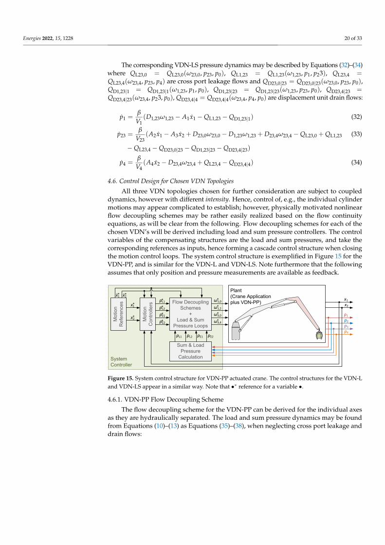
4.6. Control Design for Chosen VDN Topologies

All three VDN topologies chosen for further consideration are subject to coupleddynamics, however with different intensity. Hence, control of, e.g., the individual cylindermotions may appear complicated to establish; however, physically motivated nonlinearflow decoupling schemes may be rather easily realized based on the flow continuityequations, as will be clear from the following. Flow decoupling schemes for each of thechosen VDN’s will be derived including load and sum pressure controllers. The controlvariables of the compensating structures are the load and sum pressures, and take thecorresponding references as inputs, hence forming a cascade control structure when closingthe motion control loops. The system control structure is exemplified in Figure 15 for theVDN-PP, and is similar for the VDN-L and VDN-LS. Note furthermore that the followingassumes that only position and pressure measurements are available as feedback.

Symbol

Symbol

3 4

EM

EM

s

3 4

EM

p1p2p3p4

x1x2

Sum & Load Pressure

Calculation

Flow Decoupling Schemes

+ Load & Sum

Pressure Loops

pΣ2 pΣ1 pL1  pL2 

ω1,0

ω1,2

ω3,0

ω3,4pΣ2 pΣ1 

pL1 pL2 

*

*

*

*Mot

ion

Con

trolle

rs

Mot

ion

Ref

eren

ces x1 *

x2 *

x1 * x2 *. .

System Controller

Plant(Crane Application plus VDN-PP)*

*

*

*

Figure 15. System control structure for VDN-PP actuated crane. The control structures for the VDN-Land VDN-LS appear in a similar way. Note that •∗ reference for a variable •.

4.6.1. VDN-PP Flow Decoupling Scheme

The flow decoupling scheme for the VDN-PP can be derived for the individual axesas they are hydraulically separated. The load and sum pressure dynamics may be foundfrom Equations (10)–(13) as Equations (35)–(38), when neglecting cross port leakage anddrain flows:

Energies 2022, 15, 1228 21 of 33

pL1 = p1 −A2

A1p2 =

β

V1V2 A1(A1V2D1,0ω1,0 + (A1V2 + A2V1)D1,2ω1,2 (35)

− (A21V2 + A2

2V1)x1)

pΣ1 = p1 + p2 =β

V1V2(V2D1,0ω1,0 − (V1 −V2)D1,2ω1,2 − (A1V2 − A2V1)x1) (36)

pL2 = p3 −A4

A3p4 =

β

V3V4 A3(A3V4D3,0ω3,0 + (A3V4 + A4V3)D3,4ω3,4 (37)

− (A43V4 + A4

4V3)x2)

pΣ2 = p3 + p4 =β

V3V4(V4D3,0ω3,0 − (V3 −V4)D3,4ω3,4 − (A3V4 − A4V3)x2) (38)

For the load and sum pressure dynamics, all parameters are generally obtainableexcept from the bulk moduli. Furthermore, the piston velocities are assumed not availableas mentioned above. The flow decoupling scheme is motivated by the idea of enforcingsome desired or reference load and sum pressure dynamics given by Equations (39) and(40):

p∗L1 = ωL1(p∗L1 − pL1) , p∗Σ1 = ωΣ1(p∗Σ1 − pΣ1) (39)

p∗L2 = ωL2(p∗L2 − pL2) , p∗Σ2 = ωΣ2(p∗Σ2 − pΣ2) (40)

However, information on the bulk modulii is uncertain, and the piston velocities arenot measured. Hence, estimates of the bulk modulii and the piston velocity references x∗1 , x∗2 ,together with Equations (35)–(38), are used to estimate the pressure dynamics, with theseestimates given by Equations (41)–(44). Here, x = [x1 x2]

T , ωPP = [ω1,0 ω1,2 ω3,0 ω3,4]T

and •∗ denotes a reference for a given state/input.

˙pL1 = pL1|β=β,x=x∗ ,ωPP=ω∗PP=

β

V1V2 A1(A1V2D1,0ω∗1,0 + (A1V2 + A2V1)D1,2ω∗1,2 (41)

− (A21V2 + A2

2V1)x∗1)

˙pΣ1 = pΣ1|β=β,x=x∗ ,ωPP=ω∗PP=

β

V1V2(V2D1,0ω∗1,0 − (V1 −V2)D1,2ω∗1,2 (42)

− (A1V2 − A2V1)x∗1)

˙pL2 = pL2|β=β,x=x∗ ,ωPP=ω∗PP=

β

V3V4 A3(A3V4D3,0ω∗3,0 + (A3V4 + A4V3)D3,4ω∗3,4 (43)

− (A43V4 + A4

4V3)x∗2)

˙pΣ2 = pΣ2|β=β,x=x∗ ,ωPP=ω∗PP=

β

V3V4(V4D3,0ω∗3,0 − (V3 −V4)D3,4ω∗3,4 (44)

− (A3V4 − A4V3)x∗2)

The combined flow decoupling schemes and load and sum pressure controllers arrivefrom solving p∗L1 = ˙pL1, p∗Σ1 = ˙pΣ1, p∗L2 = ˙pL2, p∗Σ2 = ˙pΣ2 with respect to the shaftspeed references ω∗1,0, ω∗1,2, ω∗3,0 and ω∗3,4. The resulting shaft speed references appear asEquations (45)–(48).

Energies 2022, 15, 1228 22 of 33

ω∗1,0 =A1

D1,0x∗1 +

V1

β(A1 + A2)D1,0(A1 p∗L1 + A2 p∗Σ1)−

D1,2

D1,0ω∗1,2 (45)

ω∗1,2 =A2

D1,2x∗1 +

A1V2

βD1,2(A1 + A2)( p∗L1 − p∗Σ1) (46)

ω∗3,0 =A3

D3,0x∗2 +

V3

β(A3 + A4)D3,0(A3 p∗L2 + A4 p∗Σ2)−

D3,4

D3,0ω∗3,4 (47)

ω∗3,4 =A4

D3,4x∗2 +

A3V4

βD3,4(A3 + A4)( p∗L2 − p∗Σ2) (48)

Combining Equations (35)–(38) and Equations (41)–(44), and substituting ω1,0 = ω∗1,0,ω1,2 = ω∗1,2, ω3,0 = ω∗3,0 and ω3,4 = ω∗3,4, the closed loop pressure dynamics appear asEquations (49) and (50).

pL1 =β

βp∗L1 +

A21V2 + A2

2V1

βV2 A1V1(x∗1 − x1) , pL2 =

β

βp∗L2 +

A23V4 + A2

4V3

βV4 A3V3(x∗2 − x2) (49)

pΣ1 =β

βp∗Σ1 +

A1V2 − A2V1

βV2V1(x∗1 − x1) , pΣ2 =

β

βp∗Σ2 +

A3V4 − A4V3

βV4V3(x∗2 − x2) (50)

Indeed, in the event that β = β, x∗1 = x1, x∗2 = x2, the ideally decoupled desired loadand sum pressure dynamics given by Equations (51) and (52) would be achieved:

pL1 = p∗L1 = ωL1(p∗L1 − pL1) , pΣ1 = p∗Σ1 = ωΣ1(p∗Σ1 − pΣ1) (51)

pL2 = p∗L2 = ωL2(p∗L2 − pL2) , pΣ2 = p∗Σ2 = ωΣ2(p∗Σ2 − pΣ2) (52)

4.6.2. VDN-L Flow Decoupling Scheme

Applying a similar approach as for the VDN-PP to the VDN-L case using the de-scribing equations pressure Equations (22)–(25) and neglecting cross port leakage anddrain flows, the combined flow decoupling and load and sum pressure control schemes inEquations (53)–(56) may be obtained:

ω∗3,0 =A3

D3,0x∗2 +

V3

D3,0 β(A3 + A4))(A3 p∗Σ2 + A4 p∗L2) +

D1,3

D3,0ω∗1,3 −

D3,4

D3,0ω∗3,4 (53)

ω∗1,3 =A1

D1,3x∗1 +

V1

D1,3 β(A1 + A2))(A1 p∗L1 + A2 p∗Σ1)−

D1,2

D1,3ω∗1,2 (54)

ω∗3,4 =A4

D3,4x∗2 +

A4V4

D3,4 β(A3 + A4))( p∗L2 − p∗Σ2) (55)

ω∗1,2 =A2

D1,2x∗1 +

A1V2

D1,2 β(A1 + A2))( p∗L1 − p∗Σ1) (56)

4.6.3. VDN-LS Flow Decoupling Scheme

The VDN-LS differs from the VDN-PP and VDN-L as the load enforces a constraint onthe pressure p23. A sensible approach is therefore to control the sum pressure of the entiresystem. Hence, the load and total sum pressure dynamics appear as Equation (57):

pL1 = p1 −A2

A1p23 , pL2 = p23 −

A4

A3p4 , pΣ = p1 + p23 + p4 (57)

Using the pressure dynamics Equation (57), and constructing the combined flowdecoupling and load and sum pressure control schemes from principles similar to those ofthe VDN-PP and VDN-L, the shaft speed references appear as Equations (58)–(60):

Energies 2022, 15, 1228 23 of 33

ω∗2,34 =A4

D23,4x∗2 +

A4V4(( p∗L1 + p∗L2 − p∗Σ)A1 + p∗L2 A2)

D23,4 β((A3 + A4)A1 + A2 A3)(58)

ω∗1,23 =A1

D1,23x∗1 +

V1((A3 + A4)A1 p∗L1 + A2(A3 p∗Σ + A4 p∗L2))

D1,23 β(A3 + A4)A1 + A2 A3(59)

ω∗23,0 =A3 x∗2 − A2 x∗1 + D1,23ω∗1,23 − D23,4ω∗2,34

D23,0+

A1V23(A3( p∗Σ − p∗L1) + A4 p∗L2)

((A3 + A4)A1 + A2 A3)D23,0 β(60)

4.6.4. Motion Control and Closed Loop Dynamics

All VDN’s considered above allow for controlling the cylinder load pressures andsum pressures on either the cylinder or hydraulic system level. It is notable that thecylinders are mechanically interconnected via the crane structure, inducing mechanicallycoupled dynamics. These couplings are, however, omitted in the dynamic analyses inthe following, and the main emphasis placed on the closed loop input–output dynam-ics. The mechanical couplings are, however, included in the models used as a basis forsimulation results presented.

The motion controls are for all three VDN’s considered, realized as filtered PI velocitycontrollers with velocity feed forward terms and proportional position controllers in cas-cade with the load pressure controllers. These velocity and proportional controllers followthe design principles presented in [27] and are given by Equations (61) with i = 1, 2, wherez is the output of the position controller and velocity feed forward term:

p∗L = ωf( pL − p∗L), pL = Kp(z− xi)) + Ki(z− xi), z = x∗i + Kpp(x∗i − xi) (61)

The first order low pass filter included allows for avoiding the use of the actual velocityfeedback as illustrated by the load pressure control input given by Equation (62), where˙p∗L = p∗L, ˙z = z and ˙xi = xi:

p∗L = ωf(Kp(z− xi) + Ki(z− xi)− p∗L) (62)

For all VDN’s considered, the motion control parameters are identical and available inAppendix A.

Linearizing the dynamics of each VDN considered and combining these with theirassociated flow decoupling schemes and the motion control structure presented above,the linear transfer functions given by Equations (63)–(65) may be obtained, where • denotesthe change variable of a state or reference •:

˙x1˙x∗1(s) = Gx1,PP(s),

˙x2˙x∗2(s) = Gx2,PP(s),

˙x1˙x∗1(s) = Gx1,LS(s),

˙x2˙x∗2(s) = Gx2,LS(s) (63)

˙x1˙x∗1(s) = Gx1,L(s),

˙x2˙x∗2(s) = Gx2,L(s),

pΣ1

p∗Σ1(s) = GΣ1,PP(s),

pΣ1

p∗Σ1(s) = GΣ1,L(s) (64)

pΣ2

p∗Σ2(s) = GΣ2,L(s),

pΣ

p∗Σ(s) = GΣ,L(s) (65)

It may be shown that all poles of each transfer function are placed in the left half ofthe complex plane, hence all closed loop systems are stable. The corresponding closed loopfrequency responses are depicted in Figure 16. It is found that the closed loop bandwidthsare somewhat similar for all VDN’s considered, and that the sum pressure controls generallyexhibit higher bandwidths than the motion control bandwidths.

Energies 2022, 15, 1228 24 of 33

10-2 100 102

(A) Frequency Hz

-100

-50

0

Mag

nitu

de d

B

10-2 100 102

(D) Frequency Hz

-150

-100

-50

0P

hase

°

10-2 100 102

(B) Frequency Hz

-100

-50

0

Mag

nitu

de d

B

10-2 100 102

(E) Frequency Hz

-150

-100

-50

0

Pha

se °

10-2 100 102

(C) Frequency Hz

-100

-50

0

Mag

nitu

de d

B

10-2 100 102

(F) Frequency Hz

-150

-100

-50

0

Pha

se °

Figure 16. (A,D) Closed loop frequency responses for VDN-PP in crane application. (B,E) closedloop frequency responses for VDN-L in crane application; (C,F) closed loop frequency responses forVDN-LS in crane application. All responses are evaluated at mid-strokes.

4.7. Efficiency, Energy Savings, and Performances

The following aims to illustrate the efficiencies of the three VDN’s considered, with thesecompared to the expected efficiency for a valve actuated solution. Furthermore, simula-tion studies demonstrate the energy saving potentials of the VDN’s as well as the controlperformance achieved.

4.7.1. Energy Efficiencies for Typical Crane Load Cycle

The efficiencies are evaluated for two cases. The first concerns moving the payloadaway from the crane base (payload extension), and for the second case the load is movingtowards the crane base (payload retraction). In both cases, the maximum piston velocitymagnitudes are |x1,max| = |x2,max| = 50 mm/s.

In the case of a valve actuated solution as depicted in Figure 17, the study assumes thevalves supplied by a VsD with a maximum speed of 3000 rpm similar to the VDN’s, and thenecessary pump displacement then amounts to Dp = 111 [ccm]. Furthermore, the VsDlosses are based on the same loss model as the VDN’s, and scaled accordingly. The powerunit pressure setting equals the larger pressure of the flow consuming chamber plus 35 baroverhead, similar to [31], and the minimum chamber pressure is 20 bar. The maximumtorque resulting from the load is also used here as the nominal torque in determining theelectric motor. The nominal torque is given by τnom = 297 [Nm], and the correspondingideal nominal power to be installed given by Pnom = τnomωmax = 93.31 [kW].

The efficiency of this solution is depicted in Figure 17 under payload retraction.Under payload extension, the efficiency for this solution is zero as this is a load aidingcase, and no energy recuperation is possible. On the contrary, energy is consumed also inthis case.

303235

38

38

38

41

41

41

44

44

44

44

47

47

47 50

50

50

50

500 1000 1500 2000x

1 mm

1000

1500

2000

2500

x 2 mm

EM

1 2 3 4

Figure 17. Valve actuated crane application with separate metering supplied by variable-speeddisplacement unit, and associated efficiency under payload retraction, x1,max = −x2,max = 50 mm/s.Under payload extension, the efficiency is zero as this is a load aiding situation.

Energies 2022, 15, 1228 25 of 33

For comparison, the efficiency maps for the crane actuated by the VDN-PP, VDN-L,and VDN-LS appear as depicted in Figures 18–20, respectively. The load cycle consideredhere allows for energy regeneration for the VDN’s; however, the obtained efficienciesdiffer from topology to topology. For the VDN-PP, all electric motors need to operatenear their nominal speeds to realize the functionality, whereas the VDN-L and VDN-LSare not due to the hydraulic interconnections between the chambers of the two cylinders.Hence, the increased efficiencies due to lower speed dependent losses. Furthermore, due tothe shared chambers of the VDN-LS, no VsD losses are associated with hydraulic powerexchange between chambers 2 and 3 as opposed to the VDN-L, resulting in a relativeincrease in efficiency in this case. As the efficiency of the valve solution is zero duringpayload extension, it is not sensible to compare efficiencies for this part of the load case.During payload retraction, on the other hand, the increase in average efficiency is 59 [%],66 [%], and 68 [%] for the VDN-PP, VDN-L, and VDN-LS, respectively. Furthermore,the ideal installed power required is reduced by 24 [%], 18 [%], and 22 [%] for the VDN-PP,VDN-L, and VDN-LS, respectively, when compared to the valve solution.

3040

5057

57

59

59

60

60

61

500 1000 1500 2000(A) x

1 mm

500

1000

1500

2000

2500

x 2 mm

60626466

6668

68

69

69

69

70

70

71

7171

71

71

7172

500 1000 1500 2000(B) x

1 mm

500

1000

1500

2000

2500

x 2 mm

Figure 18. Efficiency for VDN-PP in crane application with interconnection scheme 0↔ 1 and 0↔ 3.(A) Total efficiency under payload extension, −x1,max = x2,max = 50 mm/s; (B) total efficiency underpayload retraction, x1,max = −x2,max = 50 mm/s. ηD, ηM, ηI, ηT, ηT,max corresponds to the meandisplacement unit, motor, inverter, total efficiencies, and maximum total efficiency.

4050

6063

63

65

65

66

66 66

67

67

67

68

68

69

500 1000 1500 2000(A) x

1 mm

500

1000

1500

2000

2500

x 2 mm

64666869

69

7171

72

72

73

73

73

7374

74

500 1000 1500 2000(B) x

1 mm

500

1000

1500

2000

2500

x 2 mm

Figure 19. Efficiency for VDN-L in crane application with interconnection scheme 2↔ 1↔ 3↔ 4,0↔ 3. (A) total efficiency under payload extension, −x1,max = x2,max = 50 mm/s; (B) total efficiencyunder payload retraction, x1,max = −x2,max = 50 mm/s. ηD, ηM, ηI, ηT, ηT,max corresponds to themean displacement unit, motor, inverter, total efficiencies and maximum total efficiency.

4.7.2. Performance and Energy Savings for Typical Crane Load Cycle

The VDN performances for a typical load case, where the load is moved away and sub-sequently towards the crane base, are illustrated in Figure 21 (simulation results). From theFigure 21A–F, all VDN’s considered demonstrate similar motion control performance andthe lower chamber pressures are maintained in close proximity of the lower pressure settingof 20 bar by their sum pressure controls. Whereas the VDN-PP and VDN-L chamber pres-sures closely resemble each other, the shared chambers of the VDN-LS cause the pressurein chamber 2 to exceed the lower pressure setting as dictated by the required pressurein chamber 3. Consequently, the pressure in chamber 1 increases due to the load force.

Energies 2022, 15, 1228 26 of 33

Furthermore, from Figure 21G–I, it is notable that the tank interconnecting VsD’s of theVDN-L and VDN-LS operate at low speeds due to VsD interconnections between thechambers of cylinders 1 and 2. As such interconnections are not present for VDN-PP, all itsmotors need to operate near their nominal speeds concurrently.

506062

64

64

66

66

68

68

69

69

69

69

69

6969

70

500 1000 1500 2000(A) x

1 mm

500

1000

1500

2000

2500x 2 m

m6466686970

71

71

72

72

74

74

74

74

7475

75

75

75

75

500 1000 1500 2000(B) x

1 mm

500

1000

1500

2000

2500

x 2 mm

Figure 20. Efficiency for VDN-LS in crane application with interconnection scheme 1↔ 23↔ 4 and 0↔ 23. (A) total efficiency under payload extension, −x1,max = x2,max = 50 mm/s; (B) total efficiencyunder payload retraction, x1,max = −x2,max = 50 mm/s. ηD, ηM, ηI, ηT, ηT,max corresponds to themean displacement unit, motor, inverter, total efficiencies, and maximum total efficiency.

0 20 40 60 80(A) Time s

500

1000

1500

2000

2500

Pis

ton

Pos

ition

mm

0 20 40 60 80(B) Time s

500

1000

1500

2000

2500

Pis

ton

Pos

ition

mm

0 20 40 60 80(C) Time s

500

1000

1500

2000

2500

Pis

ton

Pos

ition

mm

0 20 40 60 80(D) Time s

0

50

100

VD

N-P

P P

ress

ures

bar

0 20 40 60 80(E) Time s

0

50

100

VD

N-L

Pre

ssur

es b

ar

0 20 40 60 80(F) Time s

0

50

100

VD

N-L

S P

ress

ures

bar

0 20 40 60 80(G) Time s

-2000

0

2000

VD

N-P

P S

haft

Spe

eds

rpm

0 20 40 60 80(H) Time s

-2000

0

2000

VD

N-L

Sha

ft S

peed

s rp

m

0 20 40 60 80(I) Time s

-2000

0

2000

VD

N-L

S S

haft

Spe

eds

rpm

Figure 21. (A) Reference and actual cylinder positions for VDN-PP case; (B) reference and actualcylinder positions for VDN-L case; (C) reference and actual cylinder positions for the VDN-LS case;(D) chamber pressures for the VDN-PP case; (E) chamber pressures for the VDN-L case; (F) Chamberpressures for the VDN-LS case; (G) VsD shaft speeds for the VDN-PP case; (H) VsD shaft speeds forthe VDN-L case; (I) the VsD shaft speeds for the VDN-LS case.

The corresponding input and output powers as well as the individual loss componentsat VDN level are depicted in Figure 22. By inspection, the main reasons for the improvedefficiencies of the VDN-L and VDN-LS over the VDN-PP are associated with the speeddependent friction and core losses, whereas the copper and inverter losses are especially

Energies 2022, 15, 1228 27 of 33

somewhat similar for all VDN’s. Indeed, the lower friction and core losses for the VDN-Land VDN-LS are a result of the tank interconnecting VsD’s generally running at lowerspeeds. In addition, the shared chambers of the VDN-LS eliminate the VsD losses otherwiseassociated with the VsD interconnecting chambers 2 and 3 as for the VDN-L.

0 20 40 60 80(A) Time s

-20

0

20

40P

ower

kW

0 20 40 60 80(B) Time s

-20

0

20

40

Pow

er k

W

0 20 40 60 80(C) Time s

-20

0

20

40

Pow

er k

W

0 20 40 60 80(D) Time s

0

0.5

1

1.5

2

Cor

e Lo

sses

kW

0 20 40 60 800

0.5

1

1.5

2

Inve

rter

Los

ses

kW

0 20 40 60 80(F) Time s

0.2

0.4

0.6

0.8

1

1.2

Cop

per

Loss

es k

W

0 20 40 60 80(G) Time s

0

2

4

6

8

Fric

tion

Loss

es k

W

0 20 40 60 80(H) Time s

0.1

0.2

0.3

0.4

(E) Time s

Leak

age

Loss

es k

W0.5

Figure 22. (A) Input and output power of VDN with point-to-point topology; (B) input and outputpower of VDN with linear topology; (C) input and output power of VDN with linear topology withshared chambers; (D) VDN core losses; (E) VDN inverter losses; (F) VDN copper losses; (G) VDNfriction losses; (H) VDN leakage losses.

4.8. Case Study Summary

The installed power for the VDN-PP, VDN-L, and VDN-LS was found to 68.49 [kW],76.65 [kW], and 72.88 [kW], respectively, whereas it was found to 93.31 [kW] for the valveactuated solution. In comparison to the valve solution, there are yield reductions of 27 [%],18 [%], and 22 [%] for the VDN-PP, VDN-L, and VDN-LS, respectively. Even though theVDN-PP here exhibits the lowest installed power, the lower power consumption and fewercomponents may render the VDN-LS the more attractive solution.

5. Conclusions

The idea of electro-hydraulic variable-speed drive networks is introduced, essen-tially constituting interconnected multi-cylinder/motor drives. These interconnectionsare established on both the electrical side as well as on the hydraulic side, enablingthe main drive functionalities without any throttle control. As opposed to standaloneelectro-hydraulic variable-speed drives, this allows for distributing power directly betweencylinder/motor, limiting the level of power conversions (electric-to-hydraulic/hydraulic-to-electric). Inspired by communication theory, six basic drive network topologies areintroduced, and subsequently network topologies with shared/short circuited cylinderchambers exemplified. Perspectives on electro-hydraulic variable-speed drive networksare discussed, including design considerations, integration of hydraulic storages, drivecompactness, and control designs.

Energies 2022, 15, 1228 28 of 33

In order to illuminate potential design approaches for electro-hydraulic variable-speeddrive networks, a case study on a crane application is considered including three differentelectro-hydraulic variable-speed drive network topologies. Related design considerationsdemonstrate that numerous unique architectures exist for each network topology, even fora dual cylinder application, and that care must be taken in the architecture design phasein order to obtain the most feasible one. The cylinder/motor interconnections realizedwith electro-hydraulic variable-speed drive networks cause drive control designs to benon-trivial, and a decoupling control approach is proposed in combination with motioncontrols. The proposed drive controls allow for individual control of cylinder/motormotion/force, while controlling the sum pressure(s) and through this the lower chamberpressure(s) of the drive networks. Furthermore, the case study reveals that electro-hydraulicvariable-speed drive networks allow for significant energy efficiency increases comparedto a valve solution. In addition, higher energy efficiencies are found for electro-hydraulicvariable-speed drive networks with interconnections across actuator chambers as comparedto cases where actuators are only interconnected on the electric side. Whereas the requiredmotor power to be installed is somewhat similar for the case study, short circuiting ofchambers allows for reducing the number of variable-speed displacement units, henceenabling a reduction of component integration costs.

In summary, electro-hydraulic variable-speed drive networks are believed to possesssignificant potentials in the ongoing electrification transformation throughout many in-dustry segments. This is owed to the vast amount of unique drive network architecturesencompassed by electro-hydraulic variable-speed drive network topologies and potentiallylarge energy savings compared to existing valve and variable-speed drive technologies.

Author Contributions: Conceptualization, L.S.; methodology, L.S.; formal analysis, L.S.; investi-gation, L.S.; writing—original draft preparation, L.S.; writing—review and editing, L.S., K.V.H.;visualization, L.S.; project administration, L.S., K.V.H.; funding acquisition, L.S., K.V.H. All authorshave read and agreed to the published version of the manuscript.

Funding: This research was funded by the Danish Energy Agency, the Energy Technology Devel-opment and Demonstration Programme, project: Efficient Cement Handling Systems Based onElectro-Hydraulic Power Regeneration Networks (eCHASPOR), project number 64020-2046.

Institutional Review Board Statement: Not applicable.

Informed Consent Statement: Not applicable.

Data Availability Statement: Not applicable.

Acknowledgments: Not applicable.

Conflicts of Interest: The authors declare no conflict of interest.

AbbreviationsThe following abbreviations are used in this manuscript:

VDN Electro-hydraulic variable-speed drive networkVDN-F Fully connected electro-hydraulic variable-speed drive networkVDN-M Electro-hydraulic variable-speed drive network with mesh topologyVDN-L Electro-hydraulic variable-speed drive network with linear topologyVDN-S Electro-hydraulic variable-speed drive network with star topologyVDN-R Electro-hydraulic variable-speed drive network with ring topologyVDN-PP Electro-hydraulic variable-speed drive network with point-to-point topology

VDN-LSElectro-hydraulic variable-speed drive network with linear topologyand shared chambers

VsD Variable-speed displacement unit

Energies 2022, 15, 1228 29 of 33

Appendix A. Parameters Used in Case Study

The cylinder volumes used are described by V1 = V1,ini + A1x1, V2 = V2,ini + A2(x1,max−x1), V3 = V3,ini + A3x2, V4 = V4,ini + A4(x2,max − x2). Parameters used throughout, whichare not specifically quantified in the text or referred to in references, are outlined in Table A1.

Table A1. Parameters used in the case study.

Parameters Description Value

A1 Bore side area of cylinder 1 615.75 [cm2]A2 Rod side area of cylinder 1 301.59 [cm2]A3 Bore side area of cylinder 3 490.87 [cm2]A4 Rod side area of cylinder 4 236.40 [cm2]Ki Controller integral gain for cyl. 1/cyl. 2 163.26/204.80 [bar/m]Kp Controller prop. gain for cyl. 1/cyl. 2 816.33/1316.60 [bar/m/s]Kpp Position loop prop. gain for both cylinders 7.85 [1/s]Kτ MS2N motor torque constant see [61]pb Number of pole pairs for MS2N motor see [61]Rs MS2N stator resistance see [61]V1,ini Bore side volume of cylinder 1 80 [L]V2,ini Rod side volume of cylinder 1 80 [L]V3,ini Bore side volume of cylinder 3 80 [L]V4,ini Rod side volume of cylinder 4 80 [L]x1,max Stroke of cylinder 1 2333 [mm]x2,max Stroke of cylinder 2 2846 [mm]β Equivalent bulk modulus 8000 barεc Core loss scaling coefficient 1 [−]ωf Filter frequency 78.54 [rad/s]ωL1, ωL2 Load pressure control frequencies 62.83 [rad/s]ωΣ1, ωΣ1, ωΣ Sum pressure control frequencies 62.83 [rad/s]Payload Load handled by crane 4000 [kg]

Appendix B. Pressure Spectrum for VDN-PP & VDN-L in Crane Application

A minimum chamber pressure of pmin = 20 bar is used in the design phase. Con-sequently, with a payload of 4000 [kg], the pressures for chambers 1, 3, and 4 appear asdepicted in Figure A1 over the course of the piston ranges, whereas p2 = pmin = 20 bar asthis is always the lower pressure of cylinder 1.

70

80

90

100

110

120

500 1000 1500 2000(A) x1 mm

500

1000

1500

2000

2500

x 2 mm

304050607080

500 1000 1500 2000(B) x1 mm

500

1000

1500

2000

2500

x 2 mm

406080

100

120

140

160

500 1000 1500 2000(C) x1 mm

500

1000

1500

2000

2500

x 2 mm

Figure A1. Design pressures over the course of piston strokes for individual chamber topologies.(A) p1; (B) p3; (C) p4. Note ; p2 = pmin = 20 bar.

Appendix C. Pressure Spectra for VDN-LS Schemes in Crane Application

Discarding interconnection schemes with short circuited chambers at the cylinderlevel, only four events of chamber sharing exist, namely cases where chambers 1, 3 and1, 4 and 2, 3 and 2, 4 are shared. Indeed, chamber sharing by short circuiting a cylinderchamber has a significant influence in the individual pressures, with these dictated by theload and the desired minimum pressure requirement pmin = 20 bar. The chamber pressuresfor the different VDN-LS interconnection schemes are depicted in Figure A2.

Energies 2022, 15, 1228 30 of 33

70 80

90

100

110

120

500 1000 1500 2000(A) x1 mm

500

1000

1500

2000

2500

x 2 mm

500 1000 1500 2000(B) x1 mm

500

1000

1500

2000

2500

x 2 mm

140160180200220240

260

500 1000 1500 2000(C) x1 mm

500

1000

1500

2000

2500

x 2 mm

100100

110110

120

120

130140150

160

500 1000 1500 2000(D) x1 mm

500

1000

1500

2000

2500x 2 m

m 406080100120140160180200

500 1000 1500 2000(E) x1 mm

500

1000

1500

2000

2500

x 2 mm 40

6080100

120

500 1000 1500 2000(F) x1 mm

500

1000

1500

2000

2500

x 2 mm

304050607080

500 1000 1500 2000(G) x1 mm

500

1000

1500

2000

2500

x 2 mm

70 80

90

100

110120130140150

500 1000 1500 2000(H) x1 mm

500

1000

1500

2000

2500

x 2 mm

20

2020406080100120

140

160

500 1000 1500 2000(I) x1 mm

500

1000

1500

2000

2500

x 2 mm

406080100120

140

160

500 1000 1500 2000(J) x1 mm

500

1000

1500

2000

2500

x 2 mm

110115115

120 120125

125

130

135

140500 1000 1500 2000

(K) x1 mm

500

1000

1500

2000

2500

x 2 mm

304050607080

500 1000 1500 2000(L) x1 mm

500

1000

1500

2000

2500

x 2 mm

Figure A2. Design pressures over the course of piston strokes for shared chamber topologies.(A–C) p13, p2, p4 for the case with chambers 1 and 3 shared; (D–F) p14, p2, p3 for the case withchambers 1 and 4 shared; (G–I) p23, p1, p4 for the case with chambers 2 and 3 shared; (J–L) p24, p1, p3

for the case with chambers 2 and 4 shared.

References1. Scheidl, R.; Gradl, C.; Kogler, H.; Foschum, P.; Plöckinger, A. Investigation of a Switch-Off Time Variation Problem of a Fast

Switching Valve. In Proceedings of the ASME/BATH 2014 Symposium on Fluid Power and Motion Control, Bath, UK, 10–12September 2014; ASME: Bath, UK; p. V001T01A033. [CrossRef]

2. Roemer, D.; Johansen, P.; Schmidt, L.; Andersen, T. Modeling of movement-induced and flow-induced fluid forces in fastswitching valves. In Proceedings of the 2015 International Conference on Fluid Power and Mechatronics (FPM), Harbin, China,5–7 August 2015; pp. 978–983. [CrossRef]

3. Kogler, H.; Scheidl, R.; Schmidt, B.H. Analysis of Wave Propagation Effects in Transmission Lines due to Digital Valve Switching.In Proceedings of the ASME/BATH 2015 Symposium on Fluid Power and Motion Control, Chicago, IL, USA, 12–14 October 2015;ASME: Bath, UK; p. V001T01A057. [CrossRef]

4. Huova, M.; Linjama, M.; Siivonen, L.; Deubel, T.; Försterling, H.; Stamm, E. Novel Fine Positioning Method for Hydraulic DrivesUtilizing On/Off-Valves. In Proceedings of the BATH/ASME 2018 Symposium on Fluid Power and Motion Control, Bath, UK,12–14 September 2018; ASME: Bath, UK; p. V001T01A046. [CrossRef]

5. Karvonen, M.; Heikkilä, M.; Tikkanen, S.; Linjama, M.; Huhtala, K. Aspects of the Energy Consumption of a Digital HydraulicPower Management System Supplying a Digital and Proportional Valve Controlled Multi Actuator System. In Proceedings ofthe ASME/BATH 2014 Symposium on Fluid Power and Motion Control, Bath, UK, 10–12 September 2014; ASME: Bath, UK;p. V001T01A012. [CrossRef]

6. Midgley, W.J.; Abrahams, D.; Garner, C.P.; Caldwell, N. Modelling and experimental validation of the performance of a digitaldisplacement® hydraulic hybrid truck: Proceedings of the Institution of Mechanical Engineers, Part D. J. Automob. Eng. 2022,236, 594–605. [CrossRef]

7. Rampen, W.; Dumnov, D.; Taylor, J.; Dodson, H.; Hutcheson, J.; Caldwell, N. A Digital Displacement Hydrostatic Wind-turbineTransmission. Int. J. Fluid Power 2021, 21, 87–112. [CrossRef]

8. MacPherson, J.; Williamson, C.; Green, M.; Caldwell, N. Energy efficient excavator hydraulic systems with digital displacement®pump-motors and digital flow distribution. In Proceedings of the BATH/ASME 2020 Symposium on Fluid Power and MotionControl, Bath, UK, 9–11 September 2020; ASME: Bath, UK; p. V001T01A035. [CrossRef]

9. Hutcheson, J.; Abrahams, D.; MacPherson, J.; Caldwell, N.; Rampen, W. Demonstration of efficient energy recovery systemsusing digital displacement® hydraulics. In Proceedings of the BATH/ASME 2020 Symposium on Fluid Power and MotionControl, Bath, UK, 9–11 September 2020; ASME: Bath, UK; p. V001T01A033. [CrossRef]

Energies 2022, 15, 1228 31 of 33

10. Budden, J.J.; Williamson, C. Danfoss Digital Displacement® Excavator: Test results and analysis. In Proceedings of theASME/BATH 2019 Symposium on Fluid Power and Motion Control, Longboat Key, FL, USA, 7–9 October 2019; ASME: Bath, UK;p. V001T01A032. [CrossRef]

11. Pedersen, N.H.; Johansen, P.; Schmidt, L.; Scheidl, R.; Andersen, T.O. Control and performance analysis of a digital directhydraulic cylinder drive. Int. J. Fluid Power 2019, 20, 295–322. [CrossRef]

12. Zagar, P.; Kogler, H.; Scheidl, R.; Winkler, B. Hydraulic Switching Control Supplementing Speed Variable Hydraulic Drives.Actuators 2020, 9, 129. [CrossRef]

13. Hansen, A.H.; Asmussen, M.F.; Bech, M.M. Hardware-in-the-loop Validation of Model Predictive Control of a Discrete FluidPower Take-Off System for Wave Energy Converters. Energies 2019, 12, 3668. [CrossRef]

14. Hansen, A.H.; Asmussen, M.F.; Bech, M.M. Model Predictive Control of a Wave Energy Converter with Discrete Fluid PowerTake-Off System. Energies 2018, 11, 635. [CrossRef]

15. Pedersen, N.H.; Johansen, P.; Andersen, T.O. Feedback Control of Pulse-Density-Modulated Digital Displacement TransmissionUsing a Continuous Approximation. IEEE/ASME Trans. Mechatronics 2020, 25, 2472–2482. [CrossRef]

16. Jensen, K.J.; Ebbesen, M.K.; Hansen, M.R. Novel Concept for Electro-Hydrostatic Actuators for Motion Control of HydraulicManipulators. Energies 2021, 14, 6566. [CrossRef]

17. Padovani, D.; Ketelsen, S.; Hagen, D.; Schmidt, L. A Self-Contained Electro-Hydraulic Cylinder with Passive Load-HoldingCapability. Energies 2019, 12, 292. [CrossRef]

18. Imam, A.; Rafiq, M.; Jalayeri, E.; Sepehri, N. Design, Implementation and Evaluation of a Pump-Controlled Circuit for Single RodActuators. Actuators 2017, 6, 10. [CrossRef]

19. Michel, S.; Weber, J. Energy-efficient electrohydraulic compact drives for low power applications. In Proceedings of the BATH2012 Symposium on Fluid Power and Motion Control, FPMC, Bath, UK, 12–14 September 2012.

20. Çalıskan, H.; Balkan, T.; Platin, B.E. A Complete Analysis and a Novel Solution for Instability in Pump Controlled AsymmetricActuators. J. Dyn. Syst. Meas. Control 2015, 137, 091008. [CrossRef]

21. Weber, J.; Beck, B.; Fischer, E.; Ivantysyn, R.; Kolks, G.; Kunkis, M.; Lohse, H.; Lübbert, J.; Michel, S.; Schneider, M.; et al. NovelSystem Architectures by Individual Drives. In Proceedings of the 10th International Fluid Power Conference (IFK), Dresden,Germany, 8–10 May 2016.

22. Wiens, T.; Deibert, B. A low-cost miniature electrohydrostatic actuator system. Actuators 2020, 9, 130. [CrossRef]23. Stawinski, L.; Skowronska, J.; Kosucki, A. Energy Efficiency and Limitations of the Methods of Controlling the Hydraulic

Cylinder Piston Rod under Various Load Conditions. Energies 2021, 14, 7973. [CrossRef]24. Agostini, T.; Negri, V.D.; Minav, T.; Pietola, M. Effect of energy recovery on efficiency in electro-hydrostatic closed system for

differential actuator. Actuators 2020, 9, 12. [CrossRef]25. Zhang, S.; Li, S.; Minav, T. Control and Performance Analysis of Variable Speed Pump-Controlled Asymmetric Cylinder Systems

under Four-Quadrant Operation. Actuators 2020, 9, 123. [CrossRef]26. Casoli, P.; Scolari, F.; Minav, T.; Rundo, M. Comparative energy analysis of a load sensing system and a zonal hydraulics for a

9-tonne excavator. Actuators 2020, 9, 39. [CrossRef]27. Schmidt, L.; Ketelsen, S.; Grønkær, N.; Hansen, K.V. On Secondary Control Principles in Pump Controlled Electro-Hydraulic

Linear Actuators. In Proceedings of the BATH/ASME 2020 Symposium on Fluid Power and Motion Control, Bath, UK, 9–11September 2020; ASME: Bath, UK; p. V001T01A009. [CrossRef]

28. Schmidt, L.; Ketelsen, S.; Padovani, D.; Mortensen, K.A. Improving the efficiency and dynamic properties of a flow control unitin a self-locking compact electro-hydraulic cylinder drive. In Proceedings of the ASME/BATH 2019 Symposium on Fluid Powerand Motion Control, Longboat Key, FL, USA, 7–9 October 2019; ASME: Bath, UK; p. V001T01A034. [CrossRef]

29. Schmidt, L.; Ketelsen, S.; Brask, M.H.; Mortensen, K.A. A Class of Energy Efficient Self-Contained Electro-Hydraulic Drives withSelf-Locking Capability. Energies 2019, 12, 1866. [CrossRef]

30. Schmidt, L.; Groenkjaer, M.; Pedersen, H.C.; Andersen, T.O. Position Control of an Over-Actuated Direct Hydraulic CylinderDrive. Control Eng. Pract. 2017, 64, 1–14. [CrossRef]

31. Ketelsen, S.; Schmidt, L.; Donkov, V.H.; Andersen, T.O. Energy Saving Potential in Knuckle Boom Cranes using a Novel PumpControlled Cylinder Drive. Model. Identif. Control 2018, 39, 73–89. [CrossRef]

32. Schmidt, L.; Roemer, D.B.; Pedersen, H.C.; Andersen, T.O. Speed-variable switched differential pump system for direct operationof hydraulic cylinders. In Proceedings of the ASME/BATH 2015 Symposium on Fluid Power and Motion Control, Chicago, IL,USA, 12–14 October 2015; ASME: Bath, UK; p. V001T01A042. [CrossRef]

33. Helduser, S. Hydraulische Antriebssysteme mit drehzahlverstellbarer pumpe. Ölhydraulik Pneum. 1997, 41, 30.34. Helduser, S. Electric-Hydrostatic Drive Systems and their Application in Injection Moulding Machines. In Proceedings of the 4th

JFPS International Symposium; The Japan Fluid Power System Society: Tokyo, Japan, 1999; Volume 41, pp. 261–266. [CrossRef]35. Ketelsen, S.; Andersen, T.O.; Ebbesen, M.K.; Schmidt, L. Mass Estimation of Self-contained Linear Electro-hydraulic Actuators

and Evaluation of the Influence on Payload Capacity of a Knuckle Boom Crane. In Proceedings of the ASME/BATH 2019Symposium on Fluid Power and Motion Control, Longboat Key, FL, USA, 7–9 October 2019; ASME: Bath, UK; p. V001T01A045[CrossRef]

36. Ketelsen, S.; Michel, S.; Andersen, T.O.; Ebbesen, M.K.; Weber, J.; Schmidt, L. Thermo-hydraulic modelling and experimentalvalidation of an electro-hydraulic compact drive. Energies 2021, 14, 2375. [CrossRef]

Energies 2022, 15, 1228 32 of 33

37. Ketelsen, S.; Andersen, T.O.; Ebbesen, M.K.; Schmidt, L. A self-contained cylinder drive with indirectly controlled hydraulic lock.Model. Identif. Control 2020, 41, 185–205. [CrossRef]

38. Padovani, D.; Ketelsen, S.; Schmidt, L. Downsizing the Electric Motors of Energy-efficient Self-contained Electro-hydraulicSystems by Using Hybrid Technologies. In Proceedings of the BATH/ASME 2020 Symposium on Fluid Power and MotionControl, Virtual, Online, 9–11 September 2020; ASME: Bath, UK; p. V001T01A005. [CrossRef]

39. Qu, S.; Fassbender, D.; Vacca, A.; Busquets, E. A cost-effective electro-hydraulic actuator solution with open circuit architecture.Int. J. Fluid Power 2021, 22, 233–258. [CrossRef]

40. Qu, S.; Fassbender, D.; Vacca, A.; Busquets, E. A high-efficient solution for electro-hydraulic actuators with energy regenerationcapability. Energy 2021, 216, 119291. [CrossRef]

41. Qu, S.; Fassbender, D.; Vacca, A.; Busquets, E. Development of a Lumped-Parameter Thermal Model for Electro-HydraulicActuators. In Proceedings of the 10th International Conference on Fluid Power Transmission and Control (ICFP 2021), Hangzhou,China, 11–13 April 2021.

42. Padovani, D. Leveraging Flow Regeneration in Individual Energy-Efficient Hydraulic Drives. In Proceedings of the ASME/BATH2021 Symposium on Fluid Power and Motion Control, Virtual, Online, 19–21 October 2021; ASME: Bath, UK; p. V001T01A013[CrossRef]

43. Ketelsen, S.; Padovani, D.; Andersen, T.; Ebbesen, M.; Schmidt, L. Classification and Review of Pump-Controlled DifferentialCylinder Drives. Energies 2019, 12, 1293. [CrossRef]

44. Fassbender, D.; Zakharov, V.; Minav, T. Utilization of electric prime movers in hydraulic heavy-duty-mobile-machine implementsystems. Autom. Constr. 2021, 132, 103964. [CrossRef]

45. Busquets, E. An Investigation of the Cooling Power Requirements for Displacement-Controlled Multi-Actuator Machines. Ph.D.Thesis, Purdue University, West Lafayette, IN, USA, 2013.

46. Busquets, E.; Ivantysynova, M. A Multi-Actuator Displacement-Controlled System with Pump Switching—A Study of theArchitecture and Actuator-Level Control. JFPS Int. J. Fluid Power Syst. 2015, 8, 66–75. [CrossRef]

47. Li, P.Y.; Siefert, J.; Bigelow, D. A hybrid hydraulic-electric architecture (HHEA) for high power off-road mobile machines. InProceedings of the ASME/BATH 2019 Symposium on Fluid Power and Motion Control, Longboat Key, FL, USA, 7–9 October2019; ASME: Bath, UK; p. V001T01A011. [CrossRef]

48. Siefert, J.; Li, P.Y. Optimal Operation of a Hybrid Hydraulic Electric Architecture (HHEA) for Off-Road Vehicles over DiscreteOperating Decisions. In Proceedings of the 2020 American Control Conference (ACC), Denver, CO, USA, 1–3 July 2020;pp. 3255–3260. [CrossRef]

49. Siefert, J.; Li, P.Y. Optimal control and energy-saving analysis of common pressure rail architectures: HHEA & STEAM. InProceedings of the BATH/ASME 2020 Symposium on Fluid Power and Motion Control, Virtual, Online, 9–11 September 2020;ASME: Bath, UK; p. V001T01A050 [CrossRef]

50. Khandekar, A.; Wills, J.; Wang, M.; Li, P.Y. Incorporating Valve Switching Losses into a Static Optimal Control Algorithm for theHybrid Hydraulic-Electric Architecture (HHEA). In Proceedings of the ASME/BATH 2021 Symposium on Fluid Power andMotion Control, Virtual, Online, 9–21 October 2021; ASME: Bath, UK; p. V001T01A046 [CrossRef]

51. Fassbender, D.; Minav, T.; Brach, C.; Huhtala, K. Improving the Energy Efficiency of Single Actuators with High EnergyConsumption: An Electro-Hydraulic Extension of Conventional Multi-Actuator Load-Sensing Systems. Proceedings of theScandinavian International Conference on Fluid Power, Linköping, Sweden, 31 May–2 June 2021; pp. 74–89.

52. Behrouz A. Forouzan. Data Communications and Networking, 4th ed.; McGraw-Hill, McGraw-Hill Companies Inc.: New York, NY,USA, 2007; ISBN-13 978-0-07-296775-3.

53. Rühlicke, I. Elektrohydraulische Antriebssysteme mit Drehzahlveränderbarer Pumpe. Ph.D. Thesis, TU Dresden, Dresden,Germany, 1997.

54. Neubert, T. Elektro-hydraulische antriebssysteme mit drehzahlveränderbaren Pumpen. Int. Fluidtechnisches Kolloqu. Aachen 1998,1, 17–18.

55. Helduser, S. Electric-hydrostatic drive—An innovative energy-saving power and motion control system. Proc. Inst. Mech. Eng.Part I J. Syst. Control Eng. 1999, 213, 427–437. [CrossRef]

56. Neubert, T. Untersuchungen von Drehveränderbaren Pumpen. Ph.D. Thesis, RWTH Aachen, Aachen, Germany, 2002.57. Quan, L.; Neubert, T.; Helduser, S. Principle to closed loop control differential cylinder wit double speed variable pumps and

single loop control signal. Chin. J. Mech. Eng. 2004, 17, 85–88. [CrossRef]58. U.S. Department of Energy, Advanced Manufacturing Office. Adjustable Speed Drive Part-Load Efficiency; U.S. Department of

Energy, Advanced Manufacturing Office: Washington, DC, USA, 2012.59. Innas, B.V. Performance of Hydrostatic Machines—Extensive Measurement Report. Technical Report. 2020. Available online:

https://www.innas.com/assets/performance-of-hydrostatic-machines.pdf (accessed on 13 January 2022).

Energies 2022, 15, 1228 33 of 33

60. Schmidt, L.; Ketelsen, S.; Mommers, R.; Achten, P. Analogy between hydraulic transformers & variable-speed pumps. InProceedings of the BATH/ASME 2020 Symposium on Fluid Power and Motion Control, Virtual, Online, 9–11 September 2020;ASME: Bath, UK; p. V001T01A007 [CrossRef]

61. Bosch Rexroth AG. MS2N Synchronous Servomotors Project Planning Manual R911347583, Edition 05, 2020. Available online: https://www.boschrexroth.com/documents/12605/33006371/R91134758307.pdf/43fe3dca-0606-f4b7-03ab-b0e63944cbe3 (accessedon 13 January 2022).