IN DEGREE PROJECT ELECTRICAL ENGINEERING, SECOND CYCLE, 30 CREDITS

, STOCKHOLM SWEDEN 2016

Position Control of an Electro-Hydraulic Servo-ValveIDENTIFICATION, MODELLING, CONTROL AND IMPLEMENTATION

JOHAN NILSSON

KTH ROYAL INSTITUTE OF TECHNOLOGYSCHOOL OF ELECTRICAL ENGINEERING

Position Control of an Electro-HydraulicServo-Valve

Identification, Modelling, Control and Implementation

JOHAN NILSSON, JOHANNI8@KTH.SE

Stockholm 2016

Automatic ControlSchool of Electrical EngineeringRoyal Institute of Technology

XR-EE-RT 2016:036

Abstract

Hydraulic drives, systems that use pressurized fluids as transmis-sion medium, have a wide range of applications are widespread in to-day’s industry. Like many other systems, hydraulic drives can get dra-matically improved performance by an appropriately designed feedbackcontroller. Without any automatic control, these systems are oftenvery difficult for a user to operate.

Olsberg is a Swedish company specialized in hydraulic drives, pre-dominantly for cranes and other heavy machinery. Their product offer-ing includes completely mounted systems, where Olsbergs’ own electro-hydraulic valves are central to providing a pleasant handling for thehuman operator.

The hydraulic valves distribute oil from a hydraulic pump to otherhydraulic mechanisms that customers wish to control. To regulate theoil flow through every channel in the valves, Olsbergs have designed anelectrically driven position controller that actuates the valve openings.The control of this valve is the main focus of this thesis.

Although Olsbergs are satisfied with their products, and their cus-tomers are happy with their solution, they continuously look for im-provements. To this end, this thesis presents an analysis of the com-plete system and suggests, implements and evaluates a new controller.

Due to system limitations, the possibilities for automatic controlare restricted, and a traditional proportional-integral-derivative (PID)controller was found to be the most appropriate control law. The basiccontrol law was modified to support multi-rate reference handling anddecrease the sensitivity to noise and disturbances. Testing in both thelaboratory and in the field demonstrated that this quite simple solutiongave a satisfactory result on today’s systems.

I

Sammanfattning

Anvandning av hydrauliska system inom den industriella sektorn aridag valdigt utbrett. Dessa system, som de flesta andra, har ett behovav en styranordnig som gor det enkelt for en operator att kontrolleradem.

Olsbergs ar ett foretag som har specialiserat sig pa att losa justdetta nar det galler hydrauliska system. Med deras egenproduceradehydraulventiler kan de erbjuda sina kunder en helhetslosning som geroperatorerna en bra korupplevelse. For att styra sina ventiler anvandersig Olsbergs av ett specialdesignat elektro-hydrauliskt servosystem,som de ar valdigt stolta over. Dock onskar man fortfarande forbatt-ra sin produkt for att forsoka na fram till den optimala losningen.

For att fa en battre forstaelse av systemet, samt underlatta valetav reglermetodik, genomfordes en analys av Olsbergs system i dettaexamensarbete.

Pa grund av vissa begransningar i systemet sa reducerades regle-ringsproblemet till att vara relativt latthanterat. Man ansag darfor attde flesta lampliga reglermetoder man overvagt var onodigt komplexafor systemet, som det ser ut idag. Valet blev till foljd av detta attanvanda den valkanda PID (Proportionerlig-Integrerande-Deriverande)metoden.

Efter att nagra mindre modifieringar hade gjorts pa den fran borjantraditionella PID regulatorn kunde man via tester i bade laborations-och falt-miljo se att regulatorn presterade ganska val. Sa pass val attvidare utveckling inte anses ge nagon effekt forran andra forandringarsker i det ovriga systemet.

II

Acknowledgement

I would like to thank all the staff at Olsbergs, who have been sonice to me, especially to John and Tomas, with whom I have had manyinteresting discussions, but also my advisor David and everyone else inthe Development department.

It has been very fun to carry out this thesis, but there have alsobeen times that felt very tough. During these times I have gotten greatsupport from my girlfriend and family, and for that, I am eternallygrateful to them.

Now let’s start the next chapter of the story called life!

III

Contents

1 Introduction 11.1 Background . . . . . . . . . . . . . . . . . . . . . . . . . . . . 21.2 Problem Formulation . . . . . . . . . . . . . . . . . . . . . . . 31.3 Method . . . . . . . . . . . . . . . . . . . . . . . . . . . . . . 41.4 Thesis Outline . . . . . . . . . . . . . . . . . . . . . . . . . . 4

2 System analysis 52.1 Electrics . . . . . . . . . . . . . . . . . . . . . . . . . . . . . . 5

2.1.1 Signals and Units . . . . . . . . . . . . . . . . . . . . . 52.1.2 Digital Amplifier . . . . . . . . . . . . . . . . . . . . . 8

2.2 Magnetics . . . . . . . . . . . . . . . . . . . . . . . . . . . . . 112.3 Hydraulics . . . . . . . . . . . . . . . . . . . . . . . . . . . . . 12

3 Modelling 143.1 Coil- Current . . . . . . . . . . . . . . . . . . . . . . . . . . . 143.2 Magnetic Attraction Force . . . . . . . . . . . . . . . . . . . . 223.3 Hydraulic Pressure Force . . . . . . . . . . . . . . . . . . . . 24

4 Controlling Possibilities 254.1 Limitations . . . . . . . . . . . . . . . . . . . . . . . . . . . . 254.2 Disturbances . . . . . . . . . . . . . . . . . . . . . . . . . . . 274.3 System to control . . . . . . . . . . . . . . . . . . . . . . . . . 284.4 Appropriate Controller . . . . . . . . . . . . . . . . . . . . . . 294.5 Simulation . . . . . . . . . . . . . . . . . . . . . . . . . . . . . 30

5 Implementation 315.1 Lab tests and Control modifications . . . . . . . . . . . . . . 355.2 Crane Tests . . . . . . . . . . . . . . . . . . . . . . . . . . . . 43

6 Discussion 45

7 Conclusions 47

8 Future Work 48

A Measurements 49A.1 Coil Resistance . . . . . . . . . . . . . . . . . . . . . . . . . . 49A.2 Resistance dependency of temperature (cooling) . . . . . . . . 49A.3 Resistance dependency of temperature (thawing) . . . . . . . 50

B Matlab Code 51

C Simulink Model 53C.1 Integrated Matlab functions . . . . . . . . . . . . . . . . . . . 54

IV

List of Figures

1 Valve Q200 . . . . . . . . . . . . . . . . . . . . . . . . . . . . 22 Positioner 8 . . . . . . . . . . . . . . . . . . . . . . . . . . . . 33 Olsbergs system . . . . . . . . . . . . . . . . . . . . . . . . . . 54 Unit communication by CAN-bus . . . . . . . . . . . . . . . 65 CAN Signals . . . . . . . . . . . . . . . . . . . . . . . . . . . 76 DA-module/Positioner Circuit . . . . . . . . . . . . . . . . . . 87 Signals DA- Circuit . . . . . . . . . . . . . . . . . . . . . . . . 98 Cross-section of Positioner 8 . . . . . . . . . . . . . . . . . . . 119 Cross-section sketch of the hydraulics . . . . . . . . . . . . . 1210 Test setup for the coil resistance dependency of temperature . 1611 IR-shoots taken with a Flir i40 camera, during test of resis-

tance dependency. . . . . . . . . . . . . . . . . . . . . . . . . 1712 Graph of resistance dependency of temperature (hotter than

room temperature) . . . . . . . . . . . . . . . . . . . . . . . . 1713 Graph of resistance dependency of temperature (colder than

room temperature) . . . . . . . . . . . . . . . . . . . . . . . . 1714 Test Circuit . . . . . . . . . . . . . . . . . . . . . . . . . . . . 1815 Verification of parameters, by step respond . . . . . . . . . . 1916 Step responds, Reality vs. Model . . . . . . . . . . . . . . . 2017 Connection of subsystems . . . . . . . . . . . . . . . . . . . . 2518 Current speed vs Displacement speed . . . . . . . . . . . . . . 2619 System Controlling . . . . . . . . . . . . . . . . . . . . . . . . 3220 Feedback Controller (Block diagram) . . . . . . . . . . . . . . 3321 Lab rig . . . . . . . . . . . . . . . . . . . . . . . . . . . . . . . 3522 Reference Step . . . . . . . . . . . . . . . . . . . . . . . . . . 3723 Change of error during reference update . . . . . . . . . . . . 3724 Current output from system with simple PI controller . . . . 3825 Verification of current output, when simple PI controller is

implemented . . . . . . . . . . . . . . . . . . . . . . . . . . . 3826 Output signals of the model and real system, after modifica-

tion stage:1 . . . . . . . . . . . . . . . . . . . . . . . . . . . . 4027 Example of reference filtering . . . . . . . . . . . . . . . . . . 4128 Output signals of the model and real system, after modifica-

tion stage:2 . . . . . . . . . . . . . . . . . . . . . . . . . . . . 4129 Test setup for displacement measurement . . . . . . . . . . . 4230 Displacement graphs . . . . . . . . . . . . . . . . . . . . . . . 4231 Sequence test of calm controller . . . . . . . . . . . . . . . . . 4432 Sequence test of aggressive controller . . . . . . . . . . . . . . 4433 Block diagram of system model . . . . . . . . . . . . . . . . . 53

V

Abbreviations

CAN Controller Area NetworkCPU Central processing unitDA Digital AmplifierDC Direct CurrentHV Hydraulic ValveIR Infra-RedLBT Listen Before TalkMOSFET Metal Oxide Semiconductor Field Effect TransistorSMARTFET Smart Field Effect TransistorMCU Micro-controller UnitMPC Model Predictive ControllerPID Proportional-Integral-DerivativePWM Pulse Width ModulationRB Relay Box

VI

Nomenclature

Am Attraction surface on magnetAw Cross-section Area of the Coil wireC ConstantDC Derivative part of PID-controllerDcorr Duty Cycle correction from PID controllerD Approximated Duty Cycle (in percent)e System errorf FrequencyFc Counteracting force from the mechanical feedbackFe Feed-Forward ControllerFm Attraction Force from MagnetFp Hydraulic Pressure ForceFr Feed-Forward ControllerFy Feedback Controller/ PID-ControllerG Control Theoretical variable for the treated Systemi CurrentiAvg Average CurrentIC Integration part of PID-controlleridown(t) Current discharge as a function of timeimax Maximum Currentiup(t) Current charge as a function of timeKd Derivative GainKi Integration Gaink ConstantKp Proportional Gain∆l Displacement of Valve SpoolLm Magnetizing Inductancelm Distance from magnet to anchorlw Length of Coil wirem Integration factorµ PermeabilityN Turns of wirePC Proportional part of PID-controllerr Reference Value of desired RMS currentρcu Resistivity of copperRL Coil ResistanceRm Measurement Resistance

VII

S Samplert Timeτ Time ConstantTfreq Frequency Determinatorts Time when the SMARTFET has switched statetupdate Time interval for the reference signalty Adjustable time interval for measurement updatingu Control-Signal containing Duty cycleUgate Gate Voltage over SMARTFET -transistorUinput Input Voltage DAUmeasure Voltage Measurement in DAWm Magnetic Energyy System Output

VIII

1 Introduction

Throughout history, humans have learned a lot about fluids and their behav-iors in different environments. Just look at all the industries that use heavymachinery, lifting devices or are dependent on transportation. All of themuse hydraulic systems to some extent for many different purposes, such asmoving cranes or other heavy parts in operational mechanics. Using theoriesthat Pascal presented in the middle of the seventeenth century mankind hasunderstood that hydraulics can be of great help to reduce heavy work thatoften requires a lot of energy to perform a small effort[10]. For example,lifting timber back in history required big manual efforts. Today, if one usesa crane that is an electro-hydraulic system, it is just the push of a buttonor some joystick movements for one operator.

The most common way to control this powerful sort of system is by valvesthat regulate the flow through each channel. The flow in turn is regulated bythe input channel and how large its aperture is. By opening a channel in avalve, the fluid either can be released into the system or out from the systemdepending on how the system and the valve are constructed and coupled.Mostly, when fluids are released into a system, they will flow in to some sortof chamber. The more fluid that is entering this chamber, the more it willget subjected to compressive stress, which leads to a rising pressure in thechamber. When that pressure is increased, the mechanics/hydraulics willget the strength to perform a movement. If the fluid instead is allowed toflow out from the system, the opposite effect will occur: the pressure on thefluid will decrease and the movement will work in the opposite direction.

These valves can often be controlled manually, but with all requirementsthat the market has today, that’s not enough. When using this sort ofsystem, one is often in need of doing work at distances and, therefore, thereis a need of a wireless control device that can communicate with the valve.Because of this, it is common that an electronic-magnetic circuit is added tothe system, so they can receive control signals from a desired source that thecircuit converts into magnetic forces, which in turn will have an influenceon the hydraulics.

This connection from an input signal in the electronics to the flows inthe hydraulics is what this thesis will be about. Special focus will be on howone can control the system to make it behave in a desired way.

1

1.1 Background

Olsbergs is a company that produces hydraulic valves that are used to reg-ulate flows in hydraulic systems. Their valves are most commonly used tosteer cranes on trucks, but they are also widely applied in many other areas.

Olsbergs is not the largest company with their approximately 70 em-ployees, but they are very keen to keep their products highly developed andupdated, to be powerful against the competitors on the market.

With their new generation of systems, they have got more centralized andintegrated CPU power than they have had in earlier versions, which givesthem more possibilities to work with more complex calculations and newtechnologies. With this new capacity, the company would like to improvethe properties of their systems, in order to increase the customer satisfaction.

By taking help from outside, Olsbergs wants to get an analysis of theircontrol system with a new point of view. By employing a student to do athesis at the company, they hope to get a good analysis of what possibilitiesand limitations exist in the valve’s control system.

This could help Olsbergs get a better controller for the system and abetter understanding of where the limitations of the system lay. This wouldbe of great help to them, both for the work they are doing at the momentand also for further work.

Figure 1: Olsbergs’ hydraulic valve Q200 with six channels, which all areequipped with two positioners, each, of the type P8.

2

1.2 Problem Formulation

In this thesis, a study will be carried out on a new control system thatOlsbergs Electronics AB are developing. The task of this study is to investi-gate how Olsbergs’ control system works, step by step, in both hardware aswell as in software. With this analysis Olsbergs wishes that information iscollected about the system that can be of use to construct a regulatory al-gorithm. This in turn can help them to get better control of their HydraulicValve (HV). In that way, the company hopes that they can satisfy theircostumers even more than what has been achieved earlier. In the study, anevaluation part will also be included, with the intention to take a closer lookon how other properties in the controller and valves could be improved. Thepurpose of doing this is to see if one can get the whole system to be moreefficient and more suitable in terms of control technology.

Figure 2: Positioner 8 (P8),the hardware device controllingOlsbergs valves.

Olsbergs is very interested to see iftheir new generation of system has thecapacity to use more advanced controlalgorithms.

With a change of control, the com-pany hopes that the system will getmore friendly to use than what it al-ready is. Besides the controlling, Ols-bergs also wants to clarify what sort oflimitations that can be found in the con-trol system and what can be done to getpast them.

These are the questions that this thesis will try to answer:

How does Olsbergs’ Electro- Hydraulic Control System work?

Which limitations exist and what influence do they have on the sys-tem?

What control options and possibilities are available for Olsbergs’ sys-tem?

What changes would be required to give the system the ability to geteven better characteristics and reduce present limitations?

3

1.3 Method

The purpose of this thesis is to analyze and model the electro-hydraulicservo systems produced by Olsbergs, and–based on that–suggest a controlalgorithm in order to obtain an attainable performance. By interviewingemployed staff in the Olsbergs Group, studying drawings and physicallyperforming experimental tests, the hope is to obtain a better understandingabout how the control system works.

With the collected knowledge of the system and possibly a model, anevaluation will be carried out to see which controlling algorithms are relevantfor this sort of system. When all the data are compiled and can be analyzed,it should be much easier to see dependencies in the system which in turncan lead to that one can recognize limitations that exist in the system.

When all this preparation work and studies are completed, the theorieswill be implemented to the system’s software and tried out in reality, or atleast on a test rig. The software will be implemented in the programminglanguage C, which Olsbergs is using most of the time in their software de-velopment. At the end of the project, when a regulator is implemented inthe system code, the final step will be to tune the regulator so it behaves ina way that an operator would enjoy.

1.4 Thesis Outline

A short summary of the thesis main text.

Section 2, System Analysis: This section explains how the electro-hydraulic servo system, produced by Olsbergs, works.

Section 3, Modelling: This section provides an attempt to describethe electro-hydraulic servo system with a mathematical model. Fur-thermore, some experiments are conducted to identify unknown systemvariables.

Section 4, Possibilities of Controlling: In this section, we con-sider which control algorithms are possible to use, for position controlof Olsbergs’ electro-hydraulic servo system and selects one of them.This section also goes through the systems physical limitations anddisturbances.

Section 5, Implementation: In this section, we implement the cho-sen algorithm and modifies it. In addition, experiments are carried outwith the controller to see how well it performs in the different stages.

4

2 System analysis

In this system analysis, a closer look is taken on Olsbergs’ Positioner 8(Figure 2) with its associated electronics. It will be explained how Olsbergs’system works from the operators command, which is converted into a currentin the electronics that is used to regulate a magnetic mechanism in thepositioner’s servo. From there, the servo moves the valve’s spool by buildingup a hydraulic pressure inside the positioner.

2.1 Electrics

2.1.1 Signals and Units

The electronic part of Olsbergs’ system usually consists of four to five units.This thesis will mostly be conducted in a unit called Digital Amplifier (DA),which steers the valve’s positioners by regulating electronic signals. Thisunit controls the input signals to the hydraulic valve, which the positonerswill convert into pressure forces in a number of hydraulic servomechanisms.The DA is, therefore, the unit where the implementation of a controller willbe performed.

Figure 3: The parts of the Olsbergs’ electro-hydraulic control system. Fromthe left top, the HC, the RD and the PB. From the left bottom, the Q200Valve and the DA

5

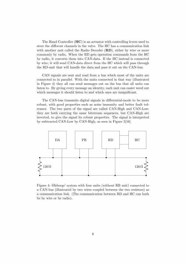
The Hand Controller (HC) is an actuator with controlling levers used tosteer the different channels in the valve. The HC has a communication linkwith another unit called the Radio Decoder (RD), either by wire or morecommonly by radio. When the RD gets operation commands from the HCby radio, it converts them into CAN-data. If the HC instead is connectedby wire, it will send CAN-data direct from the HC which will pass throughthe RD-unit that will handle the data and pass it out on the CAN-bus.

CAN signals are sent and read from a bus which most of the units areconnected to in parallel. With the units connected in that way (illustratedin Figure 4) they all can send messages out on the bus that all units canlisten to. By giving every message an identity, each unit can easier weed outwhich messages it should listen to and which ones are insignificant.

The CAN-bus transmits digital signals in differential-mode to be morerobust, with good properties such as noise immunity and better fault tol-erance. The two parts of the signal are called CAN-High and CAN-Low;they are both carrying the same bitstream sequences, but CAN-High areinverted, to give the signal its robust properties. The signal is interpretedby subtracted CAN-Low by CAN-High, as seen in Figure 5[16].

120 Ω 120 Ω

DA PB RD HC

Figure 4: Olsbergs’ system with four units (without RB unit) connected toa CAN-bus (illustrated by two wires coupled between the two resistors) asa communication link. (The communication between RD and HC can bothbe by wire or by radio).

6

The electrical system get its power supply by an external source, oftena battery or generator that delivers a voltage between 24 V to 28 V. A unitcalled Power Box (PB) takes the voltage as input and distributes it to theother units, so all the electronics get supplied.

The last unit included in the electronics has the name Relay Box (RB),and this unit is very much alike the Digital Amplifier (DA) that has beenmentioned earlier. The RB’s and DA’s major function is to deliver outputsignals that activate some actions in a truck crane or in some other hydraulicmachine. They both have the same functionality but focuses on differentsorts of targets. The RB focus is on delivering electricity by digital on/offsignals to accessory functions, such as working lights and similar. The DAhas instead the big responsibility of distributing and regulating the currentoutputs in forms of DC-equivalent signals that will steer the flow channelsin the valve.

Time (s)0.0752 0.0752 0.0752 0.0752 0.0753 0.0753 0.0753 0.0753 0.0753

Vol

tage

(V

)

-3

-2

-1

0

1

2

3

CAN low - CAN high

CAN high

CAN low

Figure 5: CAN-High, CAN-Low and the decoded output signal, which is thedifference between the two signals (CAN-Low subtracted by CAN-High),according to the CAN specification 2.0 [15].

7

2.1.2 Digital Amplifier

As previously mentioned, this thesis will mainly work with the DA-unitby investigating how it works together with the other components in thesystem and by itself. The purpose is to understand what sorts of regulatorsare suitable to apply, and which actions can be made so that the systemacts in a way the customers would like. Therefore, this subsection will takea deeper look at how the DA works.

From studies of Olsbergs’ circuit drawings over the DA -module, a simpli-fied design sketch has been drawn that shows how the DA-module integrateswith a positioner and forms a closed circuit. This design-drawing is shownin Figure 6.

Rm

RL

L

Uinput

Ugate

Umeasure

Coil(P8)

Figure 6: The circuit shows how the DA-module is coupled to one positionerwhich is illustrated by one resistor (RL) and an inductive component (L) inthe dashed rectangle.

The electrical circuit shows three variables that represent three valuesof voltage: the output Umeasure, the inputs Uinput and Ugate. Uinput is aDC-voltage around 28 V and Ugate is a Pulse Width Modulation (PWM)-signal with the amplitude about 5 V . This, together with the SMARTFET-transistor (which is a form of MOSFET), form an amplified PWM -signalthat will pass through the coil and the measurement resistor (Rm). Umeasure

is the voltage drop over Rm that is used as output for calculating the currentin the circuit by using Ohm’s law (more information about this will beexplained and shown in section 3, Modelling).

8

The PWM-signal that passes through the coil is a rectangular voltagewave that toggles between 0 and Uinput. This behavior is an effect of howthe transistor is used in the circuit because the transistor will act as aswitch when the value of Ugate is toggling between a high and low voltage.A SMARTFET is most commonly used as a switch, but one can see themoperate as variable resistances that adjust by which voltage Ugate is set to,but just within a very small range. A transistor can act like that because of alayer of oxide that is inherited in the transistor’s gate, and by adding voltageto this oxide, it will create an adjustable channel that allows electrons toflow through the transistor. With a higher voltage, the channel’s resistancewill be reduced and give a low resistance that will be close to zero, whichgives the circuit an open gate and access to the voltage source Uinput. By alow voltage (or no voltage at all), the channel will get a high resistance thatwill be almost infinite and that will cause the gate to close and prevent thevoltage source to supply the circuit[2][11].

An advantage of using a PWM -signal is that problems with high heatsin the transistor can be overcome by reducing large voltage drops and highcurrent draw[11].

The green curve in Figure 7 is the current that passes through the po-sitioner’s coil, and that is the result of the rectangular shaped voltage andthe resistive-inductive circuit.

Figure 7: Shapes of the Voltage/PWM-signal (Yellow Curve) and CurrentSignal (Green Curve) that passes over respectively through the positioner’scoil.

9

This current is the electrical key to controlling a positioner on Olsbergs’valves because the current in the circuit that flows through the coil producesa magnetic field that will give a mechanical reaction in the positioner (moreabout that in the next subsection).

In their electronics, Olsbergs’ desire is to control the current towardsa specified level. This can be achieved by choosing the behavior of Ugate

which is set by the MCU that is included in the DA-unit. The MCU can seta frequency f that will tell how long a period of Ugate will last and a dutycycle (D) that says which percent of a period Ugate will deliver a voltage tothe transistor gate, so that the channel through the transistor opens up forthe circuit.

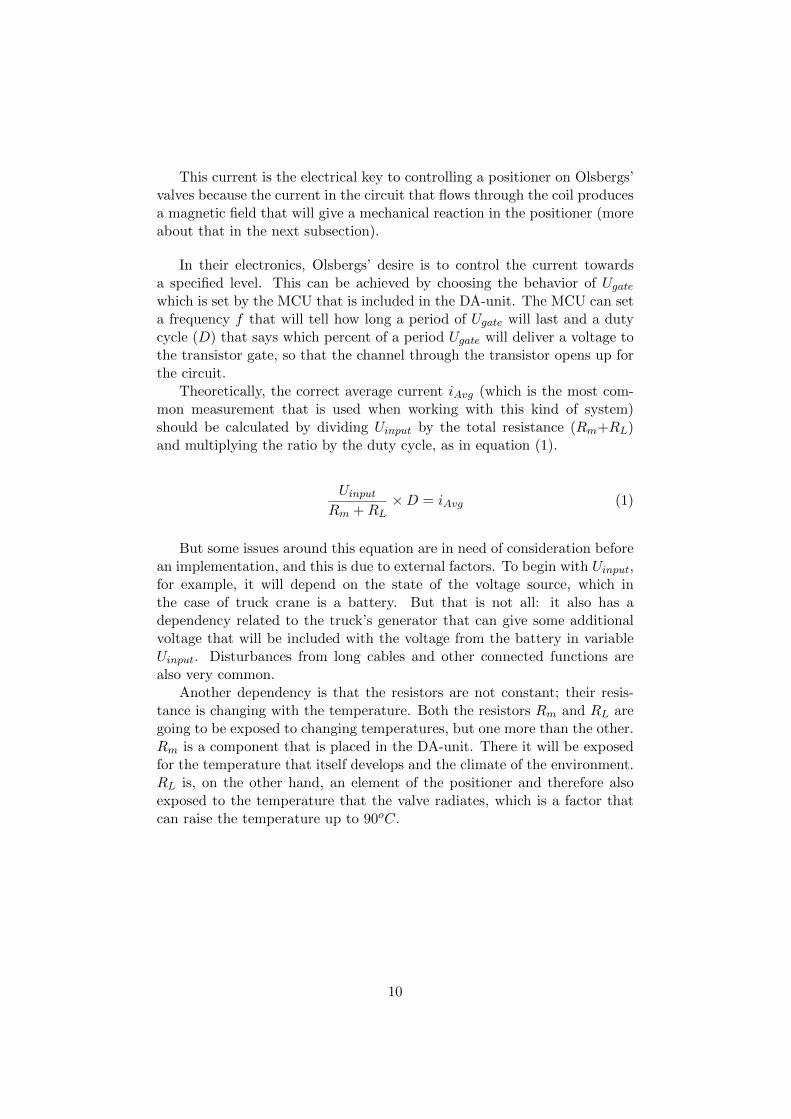
Theoretically, the correct average current iAvg (which is the most com-mon measurement that is used when working with this kind of system)should be calculated by dividing Uinput by the total resistance (Rm+RL)and multiplying the ratio by the duty cycle, as in equation (1).

Uinput

Rm +RL×D = iAvg (1)

But some issues around this equation are in need of consideration beforean implementation, and this is due to external factors. To begin with Uinput,for example, it will depend on the state of the voltage source, which inthe case of truck crane is a battery. But that is not all: it also has adependency related to the truck’s generator that can give some additionalvoltage that will be included with the voltage from the battery in variableUinput. Disturbances from long cables and other connected functions arealso very common.

Another dependency is that the resistors are not constant; their resis-tance is changing with the temperature. Both the resistors Rm and RL aregoing to be exposed to changing temperatures, but one more than the other.Rm is a component that is placed in the DA-unit. There it will be exposedfor the temperature that itself develops and the climate of the environment.RL is, on the other hand, an element of the positioner and therefore alsoexposed to the temperature that the valve radiates, which is a factor thatcan raise the temperature up to 90oC.

10

2.2 Magnetics

The output from the electrical system, as described in Section 2.1.2, is amagnetic field produced by the coil in the positioner and the current runningthrough it. When the coil gets placed in the positioner, the steel casing/corewill reduce the reluctance that the magnetic field experience and therebyhelps the electromagnet to be able to obtain a stronger field[4].

Figure 8: Positioner 8, whole and intersected.

When the strength of magnetic field is changed, it causes a mechanicaldisplacement of a component in the positioner called the anchor. When theanchor is in its neutral position, it is blocking both input and output of thehydraulic servo, which are the channels that allow oil to flow in and out re-spectively from the positioner’s hydraulic pressure chamber/servo chamber.

When the magnetic field gets stronger, it will try to attract the anchor,forcing the anchor to leave its neutral state and by that open up the servoinput. That causes pressure to build up in the servo’s pressure chamber, asoil is released into it. The valve’s spool will be affected by that pressure andbegin to move further into the valve (to the right, in Figure 9).

How large displacement the spool will get is regulated by a mechanicalfeedback (which is described more thoroughly in Olsbergs’ version of thisreport), which is embedded in the servo. This feedback will tell the servo howlarge the displacement is at the present time, by generating a counteractingforce that gets greater the larger the spool’s displacement is. At the momentwhen the desired displacement is reached the counteracting force will cancelout the electromagnet’s attraction force and return the anchor back to itsneutral state, thus maintaining the pressure that has been built up in thepressure chamber.

11

2.3 Hydraulics

Olsbergs’ HV is controlled by electronics, but it is not really the electronicsthat open the valve up. What the electronics control is an embedded servothat is included in the valve’s positioners. With that knowledge, Olsbergs’HV can be categorized to a valve family that is called Electro-HydraulicServo-valves with mechanical feedback[9][18].

Servo output

Servo Input Valve Output

Valve InputSpool

Pressure Chamber Helix Spring

Figure 9: Simplified sketch over the hydraulic machinery (cross-sectionview). There the pressure chamber and the black box are parts of thepositioner.

Sections 2.1 and 2.2 have described how the electronics are used to gen-erate a magnetic attraction force–a force that will have an effect on themagnetizable anchor which will perform mechanical movement when thestrength of the force increases or decreases. This section will describe theconsequences of the movements the anchor provides in the hydraulic ma-chinery.

Activation of the electromagnetic will result in oil filling the pressurechamber. It is this pressure that is the power source that opens up the mainchannels in the valve. By overcoming the force that needs to compress thehelix spring that is connected to the grooved spool (see Figure 9), the spoolwill move longer into the valve and open up a channel in the valve betweenits main input and output. The hydraulic oil will then be allowed to flowthrough the valve from some external pump to a crane or other operationalhydraulic mechanism.

12

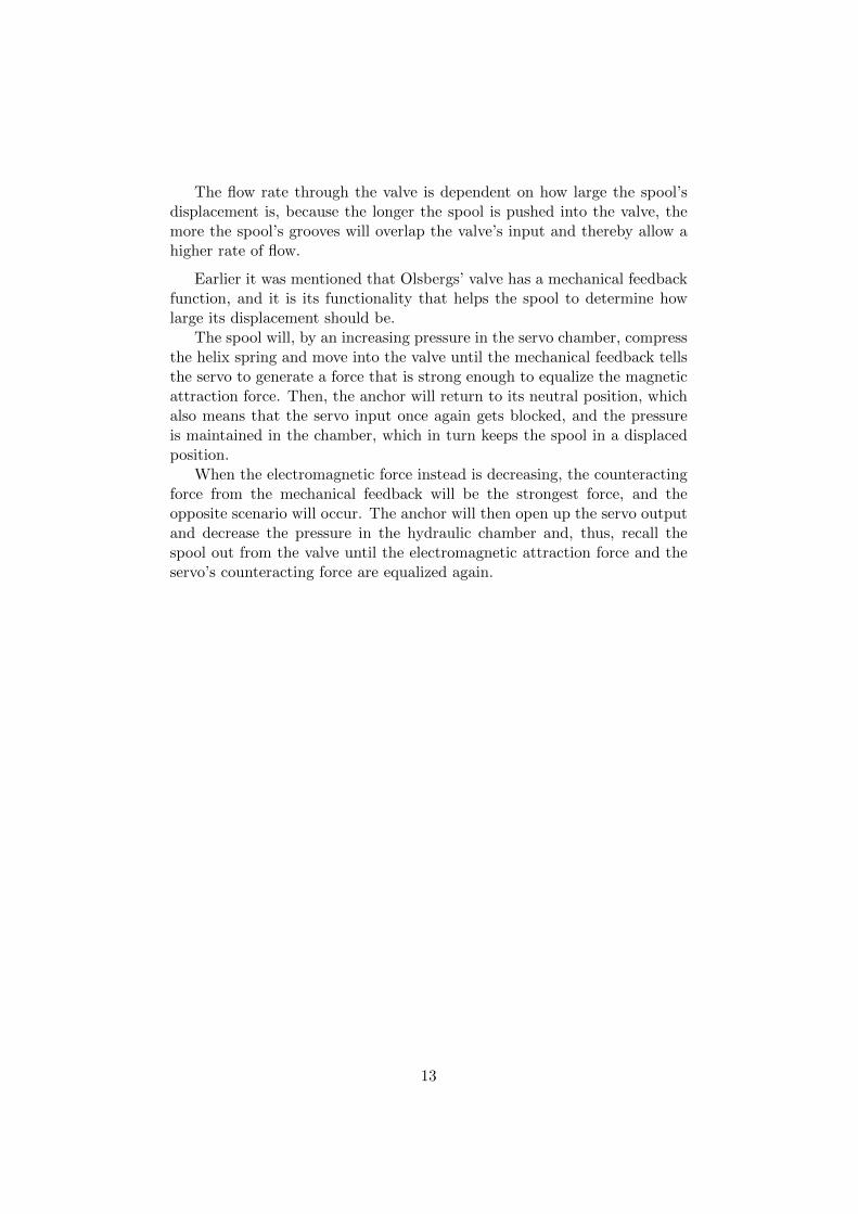
The flow rate through the valve is dependent on how large the spool’sdisplacement is, because the longer the spool is pushed into the valve, themore the spool’s grooves will overlap the valve’s input and thereby allow ahigher rate of flow.

Earlier it was mentioned that Olsbergs’ valve has a mechanical feedbackfunction, and it is its functionality that helps the spool to determine howlarge its displacement should be.

The spool will, by an increasing pressure in the servo chamber, compressthe helix spring and move into the valve until the mechanical feedback tellsthe servo to generate a force that is strong enough to equalize the magneticattraction force. Then, the anchor will return to its neutral position, whichalso means that the servo input once again gets blocked, and the pressureis maintained in the chamber, which in turn keeps the spool in a displacedposition.

When the electromagnetic force instead is decreasing, the counteractingforce from the mechanical feedback will be the strongest force, and theopposite scenario will occur. The anchor will then open up the servo outputand decrease the pressure in the hydraulic chamber and, thus, recall thespool out from the valve until the electromagnetic attraction force and theservo’s counteracting force are equalized again.

13

3 Modelling

After the system analysis in section 2, this section will focus on how thedifferent parts of the system can be modelled mathematically, and how thor-oughly it can be done.

3.1 Coil- Current

What is most interesting in the electrical part of the system, is the currentthat passes through the positioner coil. This is because the magnetic fieldthat the coil produces partially depends on the current strength.

The electrical system is described in Figure 6 and by using Kirchhoff’scircuit laws[6], an equation can be set up (if one disregards the diode) thatexplains how the voltages are related.

Uinput = RL × i+Rm × i+ L× di

dt(2)

In addition to the resistors RL and Rm in this equation there is thecurrent i, the inductance of the coil L and the input voltage Uinput.

By rewrite equation (2), it can be set up in a standard form for differ-ential equations:

di

dt+RL +Rm

L× i =

Uinput

L(3)

After this, an integration factor m, is calculated:

ln(m) =

∫RL +Rm

Ldt⇒

⇒m = exp

(t

τ

)(4)

τ =L

RL +Rm(5)

14

By multiplying equation (3) with the integration factor m, the equationcan be simplified to a more pleasant function:

i = i(t) = exp

(− t

τ

)×

(∫Uinput

Lexp

(t

τ

)dt+ C

)⇒

⇒ i(t) = exp

(− t

τ

)×(exp

(t

τ

)τ × Uinput

L+ C

)⇒

⇒ i(t) = exp

(− t

τ

)×(exp

(t

τ

)Uinput

RL +Rm+ C

)⇒

⇒ i(t) =Uinput

RL +Rm+

(C × exp

(− t

τ

))(6)

Equation (6) is now describing how the current in the electric-circuitbehaves. But there is one more thing that must be taken into considerationthe circuit will be fed by a PWM-signal which leads to different values onUinput. In the case where Uinput = 0, a term is lost in the equation (6) and,thereby, ends up as equation (7).

idown(t) = Cdown × exp(− t

τ

)(7)

idown(t) explains how the current that is passing through the positionercoil will discharge when the PWM-signal goes from high to low. When theopposite situation occurs, the PWM-signal goes from low to high, whichmakes Uinput 6= 0 and therefore, will iup(t)= i(t).

iup(t) =Uinput

RL +Rm+

(Cup × exp

(− t

τ

))(8)

The behaviors are calculated here with variables, which partially areknown and partially unknown. Uinput is known by measurements and canbe seen to be quite stationary with a voltage around 25 V to 28 V . In thismodel, it will be set to 28 V . The second variable that is known is Rm,which is a small chosen resistor with Rm = 0, 22 Ω that is used to calculatethe current with the help of Ohms law. The other variables, RL, L, and Care unknown and are, therefore, in need of examination.

To determine the resistance RL, a series of measurements was done onten coils, with a multimeter (FLUKE 77III) when the temperature of thecopper was 23C. The results of these measurements can be seen in table 1section A in the Appendix. From these measurements, the expected value

15

of the resistance in a coil was calculated to be 32, 21 Ω, which Rm gets setto. Also, the uncertainty of production was calculated and showed that thevariation in the coils is approximately ±0, 41 Ω, around the expected value.That the resistance is most likely correct can also be verified by the equationbelow.

ρcu = 1, 678× 10−8(Ωm)

RL ≈ρcu × lwAw

=ρcu × lwdw2 × π

= 33Ω (9)

Where RL is equal to the length of the coil wire (lw), proportionally withthe resistivity (ρcu), through the cross-section area of the coil wire (Aw).

Figure 10: Test setup, forhow the measurements werecarried out when the coil re-sistance dependency of tem-perature were observed.

One issue that this system will have isthe temperature variations, which can gofrom around −30C to about 80C. Withthese variations, the resistances and possi-bly other properties will change. Therefore,a test was carried out to see how the resis-tance changes in proportion to the temper-ature. By using an infra-red camera (Fliri40), the coil temperature could be loggedand by a multimeter the resistance was ob-served during two tests: one when a wholepositioner was cooled down and one whenit was heated up.

The observations are revealed in the ta-bles 2 and 3 in section A of the appendix,and with some mathematical operations inMatlab, the data are presented in Figure 12and 13. The blue circles represent measure-ments and the red lines are the linear func-tion that minimize the MMSE (minimummean square error) problem.

16

(a) Cooling (b) Thawing

Figure 11: IR-shoots taken with a Flir i40 camera, during test of resistancedependency.

Tempeture (Celsius)20 30 40 50 60 70 80 90

Res

ista

nce

(ohm

)

32

34

36

38

40

42

44

Figure 12: Presentation of data from resistance measurement on a positionercoil at hotter temperatures.

Temperture (Celcius)-10 -5 0 5 10 15 20

Res

ista

nce

(ohm

)

27

28

29

30

31

32

Figure 13: Presentation of data from resistance measurement on a positionercoil at colder temperatures.

17

The test gave a result that said that the resistance changed 0.1683 Ω/C,which gives that the resistivity changes approximately 0.5% per degree Cel-sius. That is good since it is close to the 0.4% that the temperature coeffi-cient for copper is[3].

Now that the RL has been investigated and analyzed, it is time to take acloser look on the inductance L and the constant C. The constant C will bea constant that will be set after boundary conditions. So when the circuitis active and charging up, C will take the form of equation (10).

Cup = i(ts)− imax (10)

For the discharging and inactive circuit, the constant will be equal to thecurrent strength at the time ts when the SMARTFET has switched state,which gives equation (11).

Cdown = i(ts) (11)

The last unknown variable is now L, which is needed to complete theequations. To measure the inductance of the coil, a new test circuit was setup. This because of a lack of trust on the available measuring equipmentthat directly could measure inductance in this matter. The choice fell insteadon a method where one reads out the circuit’s/component’s time constantfrom a step response. The time constant can further be used, in this case, tocalculate the inductance since they have a known mathematical relationship.

Csafe

Rm

RL

L

Uinput

UMeasure

Switch/Button

Coil

Figure 14: Test circuit used to collect data from a step respond.

18

A voltage step with the amplitude of 28 V was applied into the circuit, asillustrated in Figure 14, by a fast switching with a connection button. Dur-ing this quick switch, an oscilloscope(MSO-X 3014A, Agilent Technologies)collected data over a known effect resistor.

By using the collected data from the step respond, the time constant τcould be found. (This is due to the principle that τ is the time it takes forthe current to reach 63% of its end value[17].)

In Figure 15, the current response can be seen as the red line. Fromthe curve, one can calculate the value of τ , when the electromagnet doesnot have any connection with the anchor. By rearranging equation (5), anapproximate value of L can be determined.

L = τ ×R (12)

In the test, the total resistance was measured to be 33.4 Ω in the circuit,which by equation (12) gives an inductance that is about 0, 47 H. Withthis approximated value of L, the equation (8) can be verified by plottinghow it acts when it gets a unit step, with an amplitude of 28 V , as input.By comparing the equation’s curve (blue dashed line in Figure 15) with thedata from the measurements (red line in Figure 15), one sees that they arequite identical.

Time (seconds)0 0.05 0.1 0.15 0.2 0.25

Cur

rent

(A

mpe

re)

-0.1

0

0.1

0.2

0.3

0.4

0.5

0.6

0.7Measurement RespondEquation Respond

Figure 15: Step responses from a positioner coil and a modelled respond ofequation (8) with the calculated values of L,RL, Rm and C set (Both withan input voltage of 28 Volts).

The value of L will, however, be in need of correction. Now when it istime to test all the mathematics together and verify the model against the

19

whole positioner connected to a running valve. In that case, there are somefactors that can have an impact on the inductance, one of them is that themagnetizable anchor now will have a connection to the coil.

With some programming in Matlab (see Appendix Section B), the math-ematical model can be visualized, and with some tuning changes of the valueL the model seems to be quite accurate, aside from the non-linearity thatthe anchor is causing. With L, trimmed and set to 0, 35 H, the resultingmodel can be seen in Figure 16 compared with data collected from a teston a fully operating system. The test set up that was used in this casewas almost identical with the circuit in Figure 14. The only thing that isdifferent is the incoming signal. Instead of a 28 V step in this test, Uinput

will act as a PWM-signal with an amplitude of 28 V , as it also will when aDA-module controls the system. But at this moment a function generator(AFG-2005, GW Intek) was used instead, to keep the duty cycle constant.

Time (seconds)0.05 0.1 0.15 0.2 0.25

Cur

rent

(A

mpe

r)

0.05

0.1

0.15

0.2

0.25

0.3

0.35

0.4

0.45

0.5

Modelsettings: L=0.35Henry, R=32,43Ohm, Dutyon=40%, f=142Hz

Current from system turned on with magnetModel off CurrentRMS value

Figure 16: Graph showing how step respond from the final model matchesthe step respond from the entire running system.

20

By analyzing Figure 16, one sees that the two curves do not follow eachother so perfectly at the beginning of the graph, and that is because ofthe movement the anchor performs in the positioner. It gives a change ofinductance that slows down the rise time of the current when it is fullyattracted. This behavior is hard to compensate for, in the model, in orderto get a perfect result. If one should try to, for example, trim L moreor something similar, the ripple or some other properties of the currentwill become incorrect. One way to compensate for this is to add a time-delay which can be implemented so the model reaches desirable currentafter a slightly longer period of time. This would not complicate the modelespecially much, but will change the time it will take for the current toreach its final value. The second alternative would require a study abouthow the inductance changes while the system is running, which would takesome time to do. It is also possible, that the equipment needed for this isnot available and the non-linearity could be a little tricky to implement inthe model.

21

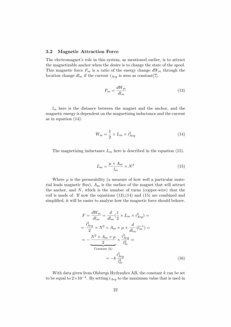
3.2 Magnetic Attraction Force

The electromagnet’s role in this system, as mentioned earlier, is to attractthe magnetizable anchor when the desire is to change the state of the spool.This magnetic force Fm is a ratio of the energy change dWm through thelocation change dlm if the current iAvg is seen as constant[7].

Fm =dWm

dlm(13)

lm here is the distance between the magnet and the anchor, and themagnetic energy is dependent on the magnetizing inductance and the currentas in equation (14).

Wm =1

2× Lm × i2Avg (14)

The magnetizing inductance Lm here is described in the equation (15).

Lm =µ×Am

lm×N2 (15)

Where µ is the permeability (a measure of how well a particular mate-rial leads magnetic flux), Am is the surface of the magnet that will attractthe anchor, and N , which is the number of turns (copper-wire) that thecoil is made of. If now the equations (13),(14) and (15) are combined andsimplified, it will be easier to analyze how the magnetic force should behave.

F =dWm

dlm=

d

dlm(1

2× Lm × i2Avg) =

=i2Avg

2×N2 ×Am × µ×

d

dlm(l−1m ) =

= − N2 ×Am × µ

2︸ ︷︷ ︸Constant (k)

×i2Avg

l2m=

= −ki2Avg

l2m(16)

With data given from Olsbergs Hydraulics AB, the constant k can be setto be equal to 2×10−4. By setting iAvg to the maximum value that is used in

22

the system and lm to the distance between the surfaces of the electromagnetand the anchor, a maximum force could be calculated according to equation(16). The result of this calculation seems to be a very reasonable approxi-mation that was verified by a test that was carried out on the mechanicalfeedback. By using the simple test set-up, the force that the mechanicalfeedback could generate during the largest displacement that the valve han-dles was measured and compared with the result from the equation (16).The calculated value on the force looks alright when comparing it with thetest result, one saw that they were almost the same (The result of this testis included in this Olsbergs’ own version of this report). But then it is alsoknow that other physical counteracting influences exist from the oil and themechanics; by this it seems that the equation is a quite good approximation.

23

3.3 Hydraulic Pressure Force

Because of the small spaces– the moving spool in the valve and positioner–it is extremely hard to model the hydraulic machinery.

Because of this challenge, Olsberg Electronics in Vallentuna is not fo-cused on hydraulics, since the conditions for making measurements in thisway do not exist at the Vallentuna site. Trips to Olsbergs Hydraulics inEksjo , where more suitable equipments are available, has been possible todo. But due to other priorities this has not happened in the large extentthat would have been necessary to make a better model.

By just looking at the whole hydraulic machinery and how it works,one can see that there is one main force moving the spool, and that isthe pressure force Fp in the hydraulic chamber, which is regulated by theposition feedback. When the oil is released into the chamber and buildingup a pressure, it will begin to move the spool, and by the position feedbackcreate a counteracting force that wants to cancel out the magnetic force.This means that the counteracting force Fc, which is dependent on thedisplacement ∆l of the valve spool, always tries to be equal to the magneticforce Fm.

Fm ← Fc(∆l) (17)

24

4 Controlling Possibilities

In this section, I will identify what advantages and disadvantages Olsbergs’system has regarding limitations and disturbances. Based on the informa-tion presented in Section 2 and 3, where the system’s fundamental physicsare explained. The section will cover the main issues that restrict the systemand which possibilities of controlling there are in the system.

At the end of this section, I will also discuss which type of controllers areappropriate to use, according to how the controllable system appears today,and select one of them to simulate and implement.

4.1 Limitations

No system is perfect, so there will always be some factors that limit ordisrupt it in some way. In the case of Olsbergs’ electro-hydraulic valve, onecan see that there are three factors that mainly limit the system.

The first one is that the system only makes measurements in the elec-tronics; no measurements are done in either the magnetic mechanism orin the hydraulics. This means that there is no feedback from any of theclosely related physics that are involved in the displacement of the spool.The only feedback provided from the system is the measured current in theelectronics(as Figure 17 illustrates), more specifically the DA-unit.

Reference

Electronics Magnetics Hyrdraulics

Disp

acem

ent

Mechanical-feedback

Measurment

Figure 17: Block diagram of the subsystems and their connections.

25

This means that there is no opportunity to regulate against any of thephysical quantities at the end of the system. Thus, the control problem willbe reduced to only include the electronics, which simplified can be describedas a switchable RL-circuit (see Figure 6).

The second limitation is found in the hydraulic servo function. Theservo regulates the pressure that causes the spool to move and, therefore, itsproportions are very significant. Due to the small distance that the anchoris moving in the positioner, it can be assumed that the anchor will mostlikely act as a hydraulic switch that is either open or closed (not entirelytrue, since the toggling behavior in the electronics will cause the anchor toshake and that way always let small amounts of oil in and out from theservo chamber, when the anchor is in a neutral state). This means that thedimension of the servo input and its applied pressure is limiting the speedof the system. The question is how the system would react if one tried toincrease its dimension or the applied pressure from the valve, in order tospeed up the system?

0 0.01 0.02 0.03 0.04 0.05 0.06 0.07 0.08 0.09 0.1

Time

0

0.1

0.2

0.3

0.4

0.5

0.6

0.7

0.8

0.9

Cur

rent

/Dis

plac

men

t

DisplacmentCurrent

Figure 18: Comparison between the speed of the current and the displace-ment of a spool in a valve of type Q200 (current has been scaled, to give asimple and comparable graph). By studying the graph it seems that thereexists a smaller potential to speed up the system.

26

The last limitation is caused by the radio communication between thehand controller and the radio decoder. Olsbergs is using a radio functioncalled LBT (Listen Before Talk) that needs to control which channels arenot used for the moment, in a specific frequency spectrum (more aboutthe LBT function can be read in [5]). This functionality requires a certaintime of waiting before sending a message, because of the radio’s need offinding a silent channel within a specific frequency spectrum. This waitingtime, together with some additional safety tolerance, will give a limit for thecontroller’s reference signal. This due to the fact that the reference signalsare collected from the hand controller.

4.2 Disturbances

During the analyses carried out in section 2, some disturbances crossed myway. Some of them are caused internally in the system and some are causedby external influences.

One of these that occurs internally in the system is the shocks that the oilis causing when it is allowed to flow in the valve’s main channel. For example,when the spool starts to open up a channel between the valve’s input andoutput, it will release high pressurized oil into the valve that will give thespool an impact shock that will interfere with the spool’s movement. The oilwill also, when flowing in the main channel, make it more demanding for thespool to move forward into the valve. But the influence of this disturbancehas already been reduced, quite a lot, by the smartly designed positioner.Through the mechanical feedback, the anchor will know that more oil isnecessary to move the spool and, therefore, let the servo input be open alonger time (more about this in Section 2.2 and 2.3).

Another undesirable behavior that the system has, that not really is tobe seen as a disturbance but influences still the system adversely, is thenon-linearity that is caused by the position changes of the anchor. Whenthe anchor is moving in the positioner, its distance to the electromagnetchanges and by that, the electronics will experience inductive changes inthe coil. These changes of the inductance will result in the current getting afaster or slower time constant. This is the reason the two curves in Figure 16don’t follow each other in the beginning of the graph.

The biggest external source that is causing changes in the system is thetemperature difference that both is dependent on the environment temper-ature, but also on the self-generated heat. This can give quite big changeson electrical components that are exposed near the valve. By just look-ing at the climates in Sweden, the outdoor temperature can reach down toabout −30oC to −40oC, and when the valve has been running for a longertime, its self-generated heat can go up to around 70oC or 80oC. With such

27

big differences, some components can change properties up to about ±50%from what they have during room temperature. An example of this can beillustrated by the resistance measurements on the positioner’s coil that weredone in section 3.1 and are documented in the tables 2 and 3, which can bein the appendix.

This also means that the maximum current will decrease, the more thecircuit’s resistance increases. If Ohm’s law is used in combination with thetemperature change that were calculated in section 3.1, one can see thatthe maximum current will approximately be (when Uinput = 28 V ) 1.18 Awhen the temperature lays at −30oC and 0.67 A when the temperature hasreached 80oC.

In the hydraulics, the changes of the viscosity are also partly an effectof the temperature changes, and it will cause the oil to behave differentlyat different temperatures. The oil will flow more easily when it gets warmerversus when it is cooler. The oil will also behave differently if it is kept inmotion or not. If the spool is not in motion, the oil can get sticky and slowdown the system, or even worse get the system to work unevenly. This iswhy the current is toggled, to keep the spool in motion, and thereby reducethe last mentioned issue.

4.3 System to control

The main problems in the system have been revealed in the two subsec-tions above. Two of the limitations have quite big effects on the possibilityof controlling this system. Firstly, one cannot measure anything outsideelectronics, which means that it is only the current that runs through thepositioner’s coil that is possible to control against. This reduces the problemof controlling to just handling the electronics. That simplified is just a smallRL-circuit with a switch, like in Figure 6.

Secondly, the radio communication limits the updating rate of the refer-ence signal, which will slow down a controller’s process.

28

On this basis, the controlling problem can be describe out from thecircuit in Figure 6.

There the input signals are a frequency and a duty cycle that will char-acterize the Ugate signal, which is controlled by the micro-controller inthe DA-unit.

Ugate will by its digital characteristic rectangular wave switch theSMARTFET, on and off, and by that create an identically shapedsignal that has a higher amplitude.

The more powerful rectangular wave will be the source that powersup the RL-circuit and, thereby, creating a current that will flow in thecircuit.

The current running in the circuit will for this problem be the output.

4.4 Appropriate Controller

The system that I want to control has been so much reduced that it is quitesmall and simplified. That means that it would be unnecessary to use atoo complex controlling algorithm, like Kalman or some other model basedcontroller (Model Predictive Controllers MPC).

A desire that one do have here is to construct a closed loop system wherethe output is compared with the reference, to collect the error that is usedto correct the control signals. The results of closed loop controlling areoften that the system responds faster to input signals, has a good propertyfor tracking the reference signal, rejects disturbances more effectively and isoften easily tuned[1].

By studying how others have treated similar controlling problems, onecan see that the usage of ”PI(D) Controllers” generally are applied as thebasis in controlling of Electro-hydraulic systems[19][20].

With this reasoning, the decision became to construct a PID controlleras a feedback mechanism for the system. Together with some feedforwardcontrollers, it should be a good enough solution for this system.

Other factors that were also taken into account here were the facts thatPID controllers are quite easy to implement, they still give a good resulton such a simple system (just the electric circuit) and that the time to thedeadline was running out.

Other alternatives of controlling methods that would be interesting totest on Olsbergs system are the ”fuzzy logical” method and the method of

29

”sliding mode”. Both of these methods are of the non-linear characteristicsand are not dependent on the systems parameters, which in this case wouldbe an advantage. The disadvantages are that these methods need moreinformation, precise information, about the system. For example, a fuzzylogical controller is based most on human experience and intuition. A slidemode controller is instead in need of very well defined sliding conditions.More about these methods can be read in[12].

4.5 Simulation

To be able to compare and verify the result of the implementation. I devel-oped a system model built in Simulink (a graphical programming environ-ment for modelling, simulating and analyzing). The model with integratedMatlab code is accurately designed to match functionalities of Olsbergs sys-tem and the intended controller. A block diagram of the model is visualizedin the Appendix: Section C, together with the integrated Matlab code.

30

5 Implementation

In this section, I will develop a PID (proportional-integral-derivative) con-troller that will give the system a closed loop that feeds back the previoussystem error. Together with two feed-forward controllers, the PID controllerwill be used to manipulate the system, so the output acts in a desired waythat an operator should like.

The controllers gets implemented in the MCU that are located in theDA-unit, and the software code is written in the programming language C.

The reference signal r in the system is a desired average current, whichcomes from a higher level software that collects lever-stroke data sent fromthe hand controller. These data are transformed by an algorithm and passedon to the controlling software. This reference signal is updated with a timeinterval tupdate. However, it is not the current that really is interesting righthere– one wants instead to know how large the PWM signal’s duty cycleis required to be, so that the electronic circuit generates a current wavethat approximately has the desired average value. To get this informationthe reference signal is converted by the first feed-forward controller Fr, bydividing it with what is believed to be the maximum reachable current imax,that the circuit can provide. This way the system gets an approximation ofthe duty cycle D that tells which percent of a period the PWM-signal shallbe active.

D = r × Fr = r × 1

imax(18)

The maximum current will vary because of the dependency of the inputvoltage that will fluctuate, and the resistance that can change when thetemperature increases (or decreases). The input voltage is, therefore, mea-sured at an earlier stage in the system, and this makes that Uinput can bechanged/updated during operation, which reduces some of the interferencethat could be caused by the changeable the input.

imax =Uin

RL +Rm(19)

By looking on Figure 19 one can see how I connect the different partsof the system and how the signals goes. There it can be seen that it is thecontrol signal u that carries the information about the duty cycle into thecontrollable system G, which is the approximated duty cycle D combinedwith the correction Dcorr from the Fy block. The block Fy consists of thePID controller and a feed-forward controller that has a identical function asFr.

31

Dcorr is a correction signal that is calculate from the system error e,which is the difference between the reference signal r and the last averagedpulse from the output signal y.

e = r − yavg (20)

The output current that runs through the electrical circuit (see Figure 6)can approximately be said to be triangular, which can be seen in Figure 7.Due to the signals non-linear and toggling characteristics, the choice is towork with the output signals average level. To know what average value thesignal has, a sampler S is programmed in the microcontroller that during aperiod samples voltage over the measurement resistor Rm, that is mentionedin Section 2.1.2, and counts how many samples are taken. After a period hasended, the sampler calculates the current’s average, by averaging the voltagesamples and using Ohm’s law (since the value of the measurement resistanceRm is known and does not experience any larger changes in temperature).

Fr

r

−+D

Gu

Sy

yavg

y

+−Fy e

DCorr

Tfreq

f

Figure 19: Block digram of the controlled system, integrated with the con-trollers Fr and Fy, the frequency giver Tfreq, the sampler S and the systemG. The signals that are running through the system are the current ref-erence r, the approximated duty cycle D, the correction of the duty cycleDcorr (output of the PID controller), the corrected duty cycle u, the systemerror e, the frequency f (given from a table in Tfreq), the output current yand the last averaged pulse from the output yavg.

32

Although the sampler calculates the average of every pulse of the current,not all of them are used. This is because of some degree of uncertainty ofhow much CPU power the controlling will occupy when multiple channelswill be using it. The signal yavg is instead updated frequently by the lastcalculated average, with an adjustable time interval ty.

As mentioned earlier, the system error is calculated by subtracting thereference r with the averaged output signal, as in equation (20).

The system’s error is also what is going to get feed back into the systemto help it work faster and more reliably. By sending the error througha traditional PID controller in a combination of a feed-forward controller,one can first convert the current into percent (duty cycle) and second thecontroller can be tuned to take more or less notice of different perspectivesof how the systems error is changing.

DCorr =1

imax× (Kpe(tk)︸ ︷︷ ︸

PC

+Ki

k∑s=1

e(ts)∆t︸ ︷︷ ︸IC

+Kde(tk)− e(tk−1)

∆t︸ ︷︷ ︸DC

) (21)

When the error passes through the feedback controller Fy, that is acombination of the feed-forward Fe (that has the exact same function as Fr)and the PID-controller that is visualized in Figure 20 by the blocks PC ,ICand DC , the relationship between Dcorr and e will be as in equation (21).

Fe

eIC

++

+DCorr

PC

DC

Figure 20: Block diagram showing the function of Fy.

The three parts of the PID controller have different properties that helpthe system to react as desired and suppress influences from disturbances.The proportional part PC will especially give the system the possibility toreact faster when larger errors occur. The integration part IC will mainly

33

give the system the characteristics that will compensate for model errors orother continuous deviations. This part is very important for this system,due to that it will compensate for the changes in the resistance that thetemperature differences are going to cause. Finally, there is the derivativepart DC that will by considering the rate of change in the error, help thesystem to find the state where the error is equal to zero faster; this will helpto get control over issues like overshoots.

I have up to this point explained the most components that I am usingto get control of Olsbergs’ system but by looking in Figure 19, it can be seenthat one block has not been mentioned yet. The frequency giver Tfreq is ablock that is used to obtain which frequency f , shall be used in the system.The frequency that shall be used is given from a table that is implemented,based on earlier research that Olsbergs have done. Dependent on whichthe desired current r is, the giver Tfreq will tell the system which frequencyshould be used at the present time t.

The system G in itself consists of the electronic circuit but there is also afunction included that is implemented in the MCU: a function that generatesthe rectangular voltage signal Ugate, which gets its characteristics from theinput signals f and u. Ugate will in the system be amplified to power up thecircuit that generates the triangular current that is the systems output y.More specifics on how this works are described in Section 2.1.2.

34

5.1 Lab tests and Control modifications

Up to this point in the thesis, a basic PID controller has been implementedthat works with the system’s averaged error, together with two feed-forwardcontrollers. In this subsection, I will describe how the system with thecontrol loop integrated gets tested and how the PID controller is modifiedto prevent and suppress further undesirable behaviors.

Figure 21: Laboratory test-rig, that is consisting of an oil pump and anOlsbergs valve of type Q200.

In Olsbergs’ own laboratory, they have one of their valves rigged togetherwith an external pump, which can be seen in Figure 21. With a DA-unitconnected to the valve and a computer, I could simulate a sequence of leverstrokes and study the current that passes through the positioner’s coil byan oscilloscope.

The first tests that were performed were just to see how different tuningsof the coefficients in the PID controller affected the output from the systemand which of them that gave the best result. During those tests, it wasdiscovered that the derivative part of the PID controller did not have anymajor positive impact on the system, which depends on the fact that thesystem does not update especially fast, due to the averaging process andthe limitation from the radio. Therefore, the coefficient Kd was set to zero.

35

Despite the fact that the derivative part is inactive at this point, I did amodification that could be an advantage in the future if the derivative partshould be used. A common inconvenience behavior that occurs when onelooks at the derivative of a system error is that, when the reference makesa fast change during an update, a big error momentarily will arise, whichmakes the PID controller react a bit too powerfully (an example of this canbe seen in Figure 22 and 23).

This can, however, be easily overcome! By expanding the equation de-scribing DC , one sees that it is only the difference in the reference-signalthat causes the peak.

DC = Kde(tk)− e(tk−1)

∆t= Kd

r(tk)− r(tk−1)− yavg(tk) + yavg(tk−1)

∆t(22)

If the change of r instead is considered to always be zero, the equationcan be rewritten to be as equation (23).

DC = −Kd∆yavg

∆t(23)

This basically shows that by looking at the change of the output average,negatively, instead of the error, the undesired peak can be eliminated.

Instead of having a PID controller, there is now only a PI controller!To make it easy to see how the controllers behavior changes during theforthcoming modifications the coefficients Kp and Ki is set to the tuningthat is used in the final version of the controller.

To see how well the PI controller does, as it is at this point, with thecoefficients set. A sequence of reference signals are sent into the system (seethe non-filtered reference signal sequence in Figure 27), and the result is anoutput current that is shown in Figure 24.

By using the simulation that is mentioned in Section 4.5, can the resultalso be verified. This can be seen in Figure 25, where the simulated currentis compared with the real current output.

36

-6 -4 -2 0 2 4 6 8 10

Time (s)

-1

-0.5

0

0.5

1

1.5

Cur

rent

(A

)

Reference SignalMeasurement Output

Figure 22: Example of reference vs measurements from output, during ref-erence update.

-6 -4 -2 0 2 4 6 8 10 12

Time (s)

0

0.5

1

1.5

2

2.5

3

Cur

rent

(A

)

ErrorDerivative of Error

Figure 23: Derivation of the error during a reference update creates a un-desirable pulse.

37

0.2 0.4 0.6 0.8 1 1.2 1.4 1.6 1.8 2

Time

100

200

300

400

Cur

rent

(m

A)

Current OutputReference Signal

Figure 24: Current output from system when the simple PI controller isapplied (The quality of the curve is not the best, due to that the usedoscilloscope just makes 2000 samples during a single sweep, which is quitefew in this case). The red line is the reference signal that is sent into thesystem during this sequence.

Time0 0.2 0.4 0.6 0.8 1 1.2 1.4 1.6 1.8 2

Cur

rent

(m

A)

50

100

150

200

250

300

350

400

450Simulated Current SignalCurrent output from System test

Figure 25: Verification of current output, when simple PI controller is ap-plied.

38

By studying the curve in Figure 24, one can see that especially the firstquarter is interesting. In that part of the output sequence, the system causesseveral overshoots that make the system behave jerky, which is undesirable.Otherwise, the model seems to match reality quite well. The biggest dif-ference is the upstart, where the model gets an overshoot that lasts muchshorter than what the measured output has. This can among other thingsdepend on certain non-linear behaviors that the system has.

Since there is no D-part to use to suppress the overshoots, I need to useother methods.

To begin with, it is known that the Integration part (I-part) will dur-ing updates be a factor that amplifies the overshoots[14]. Another thingthat also is known is that Olsbergs’ system has software functions that willdetect greater errors that happen fast. So the major requirement that theintegration part of the PI controller needs to be compensating for is theslowly changing faults, since some of them can grow large. One example ofthis is the change of resistance (due to temperature differences) which willcause the maximal current to increase or decrease. Therefore, a threshold isset that limits how much the I-part maximum can be changed per update.This means that the I-part not will react so powerfully during a referenceupdate that will give a big error.

Another way to solve this problem would be to use conditional inte-gration. That instead switches off the I-part when it is far from a steadystate[13]. But this has during tests shown to be more unreliable than thelimitation method that is used.

If one now runs the same reference sequence again, that were used earlier,through the system with the modified PI controller applied, the output getsa bit changed. If Figure 25 and Figure 26 are compared, one can see thatthe overshoots are not as bad as before, especially the first and biggest one(both for the system output and the simulated current).

39

Time0 0.2 0.4 0.6 0.8 1 1.2 1.4 1.6 1.8 2

Cur

rent

(m

A)

50

100

150

200

250

300

350

400

450 Simulated Current SignalCurrent output from System test

Figure 26: Output signals of the model and real system, after the imple-mentation of the integration limit.

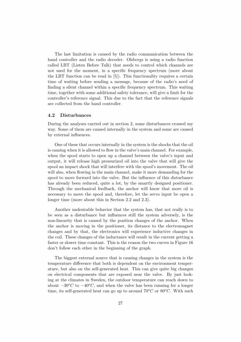
However, the test after the first modification of the system’s controllershows that there are still much of the overshoots and jerkiness left. Thisis because of the limited updating of the reference signal, which is writtenabout in Section 4.1. What is done here to create a better reference signalis that a pre-filter is constructed that linearize one update step into severalsmall steps. This means that the controller does not need to react as hardfor each new update as before, which in hand will make the system to workmore evenly. This implementation is not done in the controlling software; itis implemented in a higher layer of the system code, where the lever strokedata are collected from the hand controller.

When the new update comes, the filter will depending on the desiredamount of new steps, calculate how big a change each step shall have andwith which interval they shall come. An example of how the reference getsfiltered can be seen in Figure 27.

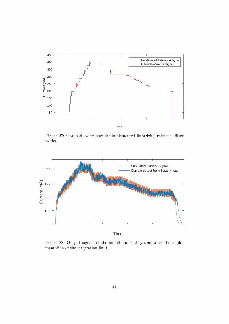
If the reference sequence now is sent through the filter and into thesystem with the modified PI controller instead, the output current looks alot smoother (see Figure 28).

40

0 5 10 15 20

Time ×104

50

100

150

200

250

300

350

400

450

Cur

rent

(m

A)

Non-Filtered Reference SignalFiltered Reference Signal

Figure 27: Graph showing how the implemented linearizing reference filterworks.

0 0.2 0.4 0.6 0.8 1 1.2 1.4 1.6 1.8 2

Time

100

200

300

400

Cur

rent

(m

A)

Simulated Current SignalCurrent output from System test

Figure 28: Output signals of the model and real system, after the imple-mentation of the integration limit.

41

Now it would be very interesting to see how well the PI controller per-forms, from the view of the spool’s displacement, which was of the primaryinterest from the beginning of this thesis. By setting up a new test, witha laser sensor that measures the distance to the spool, it is possible to seehow the spool moves during the simulated sequence. By doing this test withboth the simple PI controller and the modified one, it is possible to see howmuch difference the modifications makes.

Figure 29: Test setup for displacement measurement.

In the Figures 30a and 30b the results of these tests are revealed. Thereit can be seen that the modified and pre-filtered PI controller does a prettygood job and that the modifications reduce a lot of the jerkiness that thesystem has when the simpler PI controller is applied in the system.

Time23.5 24 24.5 25 25.5

Dis

plac

emen

t (m

m)

1

2

3

4

5

6

7

(a) Modified and pre-filtered PI con-troller.

Time14.2 14.4 14.6 14.8 15 15.2 15.4 15.6 15.8 16

Dis

plac

emen

t (m

m)

1

2

3

4

5

6

7

(b) Simple PI Controller.

Figure 30: Displacement graphs for the controller, before and after modifi-cation.

42

5.2 Crane Tests

In the second step of the testing, the whole integrated system that Olsbergsproduces was installed on a truck crane to give the Development departmentof Olsbergs Electronics (myself included) the opportunity to see how the newsystem worked in the most common field of application. Due to some timelimitation and other priorities during this test, we put our focus on testingtwo versions of the controller, one that was set to those tuning parameters(PID coefficients) that had shown the best results during the lab tests, andanother that had significant larger coefficients and, thereby, acted moreaggressively. A current sequence for each version of the controller weredocumented during a simulation (this can be seen in Figure 31 and 32).By viewing these, one can see that the more aggressive version, Figure 32,for example, has much more powerful overshoots and, therefore, acts morefluctuating than the calmer one, Figure 31.

When the two different versions of the controller were applied individu-ally on the truck crane, the development team drove the crane and observedhow the hydraulic valve behaved itself, by studying the valve’s spools andhow they moved. But the team also observed how well the crane followedthe given commands from the hand controller and how it generally felt todrive the crane.

When we compared how the two controllers affected the spool’s move-ment in the valve, we definitely saw a distinguishable difference. The teamsaw that when the more aggressive controller was implemented, the valveworked more unevenly then it did when the calmer controller was imple-mented.

The observations made during driving the crane, on the contrary, showedno difference between the controllers at all. Most of the members of the de-velopment team tested to drive the crane with both the aggressive controllerand with the calmer one, and no one could see or feel any difference at all.

43

Figure 31: Oscilloscope-screen showing the current output from a systemcontrolled by the controller with the parameter set to the tuning collectedfrom the best lab tests.

Figure 32: Oscilloscope-screen showing the current output from the con-troller that was set to be more aggressive.

44

6 Discussion

During this master thesis, which has been really interesting and educational,I have investigated how Olsbergs electro-hydraulic control system works andhow it can be controlled, with the conditions that exist today. I have alsothought through if additional equipment or other supplements could helpthe system to perform better.

By doing the analysis of the whole controlling chain in Olsbergs system,I have needed to use a lot of the knowledge I have gotten under my yearsat the Royal Institute of Technology and more. It has also helped me toget a greater understanding of how all the integrated functions in Olsbergssystem works with each other.

One thing I have discovered with Olsbergs system is that it has a verysmart design. For example, it uses the energy that the additional oil pumpsgive and that way, reduces electricity consumption. This by using the servo,which is powered by a hydraulic pressure, to move the spool and just usesthe electronics to control the servo’s input and output. A proportional valvethat just uses magnetic force to move the spool would most probably requiremuch more electrical power.

There is one thing, however, with this servo function that is a disad-vantage, and that is the fact that it complicates the system’s possibility tomeasure how large the displacement of the spool is. Other types of valveshave the advantage of having better properties to use, for example, induc-tive measuring in the valves, as displacement measurement (more about thiscan be read in [8]). Since the system does not measure anything after theelectronics (which involves only a very small circuit, limiting the controllingopportunities) is a more complex controlling method unnecessary to use, inOlsbergs case. This also seems to be quite common for systems that workwith switching power converting, seeing that the most frequently used meth-ods in this matter are the ones that are of the simpler kind but that usuallyhave modifications that compensate for certain behaviors. Two examples ofthis can be seen in the works [19] and [20].

What about adding some sensor or some similar device to the system?That is absolutely a valid thought, but then the economical aspect kicksin. Because by the result of the ”Crane tests” that were done in Section5.2, the development team at Olsbergs and I realized that it looks like thereis, in some way, such big damping when the oil goes into bigger machinerythrough the valve, that by just changing a little of the controller, the oper-ator will not notice any differences. And if one wants to add some sort ofmeasurement device to Olsbergs system, it would increase the cost of pro-duction significantly, including fixtures for each channel that both will keepthe sensors in their right position and at the same time protect it from rough

45

environments. But the rising costs will not stop there, because it would alsorequire some development time for construction design, programming andmost likely a development of a new electrical unit or further development ofexisting devices. All these costs would make the whole system cost signifi-cantly more on the market than what it does today and probably not manycustomers are ready to pay for that.

(And to control based on something else later in the system is not a goodidea, due to fact that the spools are exchangeable, depending on functionalpurpose.)

If we take a look at the rejection of interferences, it should be possibleto do more implementations that compensate for the non-linearities thatexist in the system. The tricky part of doing this is to get the informationabout how they occur and behave, and how we can make up for them.In this thesis, these factors have not been given priority and; therefore,no experiments have been performed to get that kind of knowledge aboutthe system. Another thing that would be easier to compensate for is thechange of resistance that will occur during operation, either by adding somemeasuring or implementing some computations from other data that alreadyget collected.

In addition to the tests that have been performed during this thesis, itwould have been very interesting to do some more specific tests in both thematters of the magnetics and the hydraulics, as a way to get a deeper insightinto these parts. For example, it would be very interesting to investigate howthe magnetic force, the inductance and the moving parts in the positionerinteract. I’m also very curious about how the pressure in the positioner’shydraulic chamber and the valve’s output channel behave in proportion tothe displacement.

46

7 Conclusions

In this thesis, I have performed a systematic analysis of Olsbergs’ controlsystem. In this system, an electrical circuit influences the displacement of amagnetic spool located in the hydraulic valve channel. It is this displacementthat determines the oil flow through the valve. The analysis, together withan attempt to derive a dynamic model of the complete system, has givena good understanding of the system and used as a basis for finding theappropriate control strategy.

Olsbergs hydraulic valve has excellent mechanical design but is somewhatlimited when it comes to real-time sensors. The only measurements availablein the system are made in the electronics and the whole control problem thusgets reduced to a problem of controlling the current in the electrical circuit(which, itself, affects the displacement of the spool). This simplifies thecontrol problem considerably. A literature review revealed that three controlstrategies are commonly used for similar control problems: PID, fuzzy logic,and sliding mode controllers. Out of these three, it was decided that aPID controller was most appropriate: it is simple to implement and modify,and provides sufficient closed-loop performance. A few modifications of thePID controller, mainly to handle reference signals generated with a slowersampling rate than the controller, and to reduce the sensitivity to noise anddisturbances, were suggested and implemented.

The other limitation that I came across during this work was that thesystem cannot work faster than the current solution. Already today’s solu-tion opens up the servo input fully when a rapid response is requested, andthus, the oil flow cannot be greater by changing anything in the electronicsor the software. Improving the response speed of the system would requiremechanical modifications that would cause big costs for the company, andthese were out of scope for the present thesis. An interesting approachfor improving the operator experience would to implement more advancedpre-filters to the reference signal generated by the operator. By letting theoperator adjust these to his own liking, a more personalized experience couldbe created.

It has been interesting to see that such a simple approach such as amodified PID controller can give such a good result in a complex systemsuch as the hydraulic-drive that are used in, for example, a truck-mountedcrane. It was also interesting to see how the switch of tuning, which dras-tically changed the characteristics of the system’s current, could go largelyunnoticed by the crane operator.

47

8 Future Work

It seems that no significant system improvements can be made by changesto the control system, at least not until the physical (electro-mechanical orhydraulic) valve design is changed, or additional sensors are installed. Nev-ertheless, we believe that the following investigations would be interestingto do:

One should investigate the admissible sampling rates for the averagedoutput, and see if it is possible to get any use of the already imple-mented derivative part.

The inclusion of adjustable pre-filters to the reference signal could bea means of creating a personalized and improved operator experience.

Including a measurement of the coil resistance, or calculating it fromalready collectable data, would be useful for reducing the strain on thecontroller integration work.

If the system were equipped with additional sensors, it would be inter-esting to investigate the nonlinearities in the inductance and the forcesacting on the servo, and to see how these could be exploited and/orcompensated for.

48

A Measurements

A.1 Coil Resistance

Table 1: Resistance Measurements of 10 different Coils by multimeter ofmodel FLUKE 77III.

Coil NR Resistance

1 32,3 Ω2 32,3 Ω3 32,3 Ω4 32,2 Ω5 32,1 Ω6 31,8 Ω7 32,0 Ω8 32,1 Ω9 32,4 Ω10 32,6 Ω

A.2 Resistance dependency of temperature (cooling)

Table 2: Resistance Measurements by multimeter of model FLUKE 77IIIand temperature by IR-camera Flir i40.

Temperature Resistance

90oC 43,5 Ω85oC 42,8 Ω80oC 42 Ω75oC 41,2 Ω70oC 40,3 Ω65oC 39,4 Ω60oC 38,3 Ω55oC 37,5 Ω50oC 36,9 Ω45oC 36,2 Ω40oC 35,4 Ω35oC 34,6 Ω30oC 33,7 Ω25oC 32,7 Ω

49

A.3 Resistance dependency of temperature (thawing)

Table 3: Resistance Measurements by multimeter of model FLUKE 77IIIand temperature by IR-camera Flir i40.

Temperature Resistance

−6oC 27,4 Ω−5oC 27,6 Ω−4oC 27,7 Ω−3oC 27,9 Ω−2oC 28,1 Ω−1oC 28,2 Ω0oC 28,4 Ω1oC 28,6 Ω2oC 28,7 Ω3oC 28,6 Ω4oC 28,8 Ω5oC 29 Ω6oC 29,5 Ω7oC 29,7 Ω8oC 29,8 Ω9oC 30,2 Ω10oC 30,3 Ω11oC 30,5 Ω12oC 30,7 Ω13oC 30,7 Ω14oC 31 Ω15oC 31,1 Ω16oC 31,2 Ω17oC 31,4 Ω18oC 31,6 Ω19oC 32,8 Ω20oC 32 Ω

50

B Matlab Code

function current mod(voltage input,frequens,duty cycle,periods,temp)%Input parmeters sets to simpler variables!T=temp;U=voltage input;f=frequens;cy=duty cycle;loops=periods;

%Setting variables Calculated from test!L=0.35*(1+((T-23)*0.005))R L=32.21*(1+((T-23)*0.005))R=0.22;

%Calculation of time when switch is on and off!dutyc on=cy/f;dutyc off=(1-cy)/f;

%Calculation of timeconstantRtot=R L+R;tao=(L/Rtot)

%Limitation warnings that points out that the calculations gets%no good or dosn't work for certain inputs!if (numel(num2str(cy))-2)>numel(num2str(f))

disp('To precise duty cycle, only 3 digits allowed')return

end

if loops < 8disp('Less then 8 loops are not allowed')return

end

%Preparations of two time strings, one for each state of the MOSFETs step=1000;t1=0:1/(f*s step):dutyc on-1/(f*s step);t2=0:1/(f*s step):dutyc off-1/(f*s step);t=[];

%A loop that joins the time strings to one long string that will%ensure that the right amount of periods will occur at the endl=0;while l < loops

t=[t,t1,t2];l=l+1;

end

%Main Loop that calculates the value off the current in time i(t),

51

%using equation (7) and (8), depending in which state the MOSFET are in.i=zeros(1,length(t));j=1;k=1;bot=0;while j < length(t)

if (j < (s step*(k-1))+length(t1)+1 && j > s step*(k-1)) | | j < length(t1)+1i(j)=((U)/Rtot)-(((U)/Rtot)-bot)*exp(-t(j)/tao);top=i(j);

elsei(j)=top*exp(-t(j)/tao);bot=i(j);

end

j=j+1;if j==s step*k

k=k+1;end

end

i=i(1:length(i)-1);

%Arrangements of plot so time axles gets the propositional compared to the currentplot(0:1/(f*s step):loops/f-((2)/(f*s step)),i,'r --');hold on

%Calculating the Root Mean Square Value for the currentRMS=0;

for i L=i(1000:length(i)-1)RMS=RMS+((i Lˆ2)/length(i));

end

RMS=sqrt(RMS)

%Collecting the top and bottom values from the curve (excluding the first 8%periods)Top and Base Current=[max(i),min(i((length(i)-(loops-8)*f):length(i)))]

%Plotting of the RMS to give a output figure thats easy to analyzeRMS plot=ones(1,length(i))*RMS;plot(0:1/(f*s step):loops/f-((2)/(f*s step)),RMS plot,'r')

disp('Less then 50 periods givs not a accurate RMS')end

52

C Simulink Model

Gnd

-+

I

Current Sensor

SPS

PS-Simulink

Converter

f(x) = 0

Solver

Configuration

-+

Resistor

-+

Resistor1

+ -

L

Gnd1

Controlled Voltage

Source

SPS

Simulink-PS

Converter

Y

Counter

SPS

PS-Simulink

Converter1

f(x) = 0

Solver

Configuration1

12:34

Digital Clock

calc

trig

ton tp

i

Calculater

pulse

t t_on

t_p

t0 t_corr

u

t0_ret

PWM-G

enerator

Memory1

cont

ts r t_avg

y corr_ret

avg_ret

nr_ret

update_counter

y_avg_ret

e_ret

y_avg_prev

e_int

t_on_corr

avg nr

update_counter_ret

y_avg e

y_avg_prev_ret

e_int_ret

Controller

12:34

Digital Clock1

M 2

Scope1

M 3

M 4

Scope2

M 5

Scope4

M 6

Memory7

M 8

M 9

M 10

Scope3

Scope6

filter

t_step

counter2

c_ref_ret

step_ret

t_filter

c_r

c_r_p

t_step_ret

counter2_ret

c_ref

step

r_f

Ramper

M11

M12

M13

Scope7

12:34

Digital Clock2

M14

M15

Scope5

Figure 33: Block diagram of the simulation model of the electronics togetherwith the embedded controller.

53

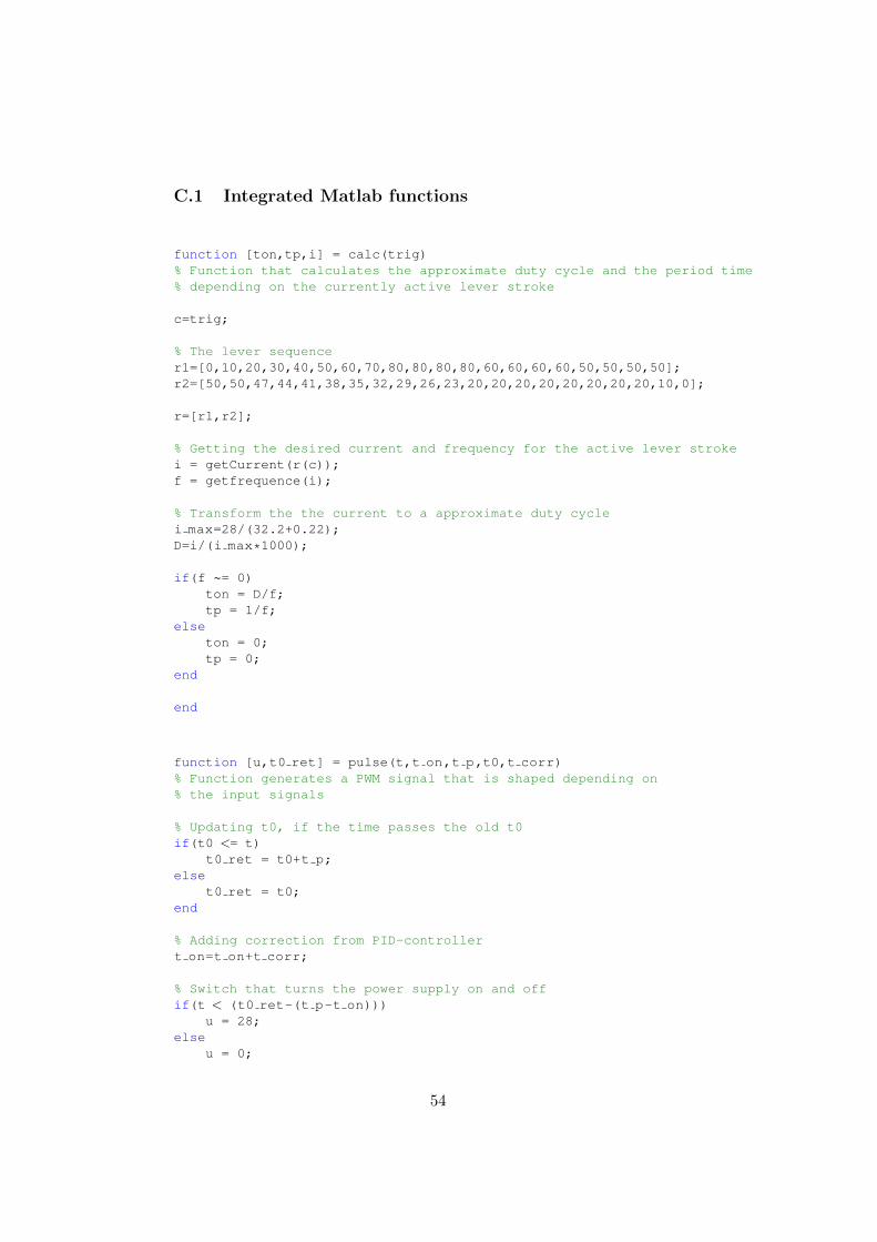
C.1 Integrated Matlab functions

function [ton,tp,i] = calc(trig)% Function that calculates the approximate duty cycle and the period time% depending on the currently active lever stroke

c=trig;

% The lever sequencer1=[0,10,20,30,40,50,60,70,80,80,80,80,60,60,60,60,50,50,50,50];r2=[50,50,47,44,41,38,35,32,29,26,23,20,20,20,20,20,20,20,20,10,0];

r=[r1,r2];

% Getting the desired current and frequency for the active lever strokei = getCurrent(r(c));f = getfrequence(i);

% Transform the the current to a approximate duty cyclei max=28/(32.2+0.22);D=i/(i max*1000);

if(f ~= 0)ton = D/f;tp = 1/f;

elseton = 0;tp = 0;

end

end

function [u,t0 ret] = pulse(t,t on,t p,t0,t corr)% Function generates a PWM signal that is shaped depending on% the input signals

% Updating t0, if the time passes the old t0if(t0 <= t)

t0 ret = t0+t p;else

t0 ret = t0;end

% Adding correction from PID-controllert on=t on+t corr;

% Switch that turns the power supply on and offif(t < (t0 ret-(t p-t on)))

u = 28;else

u = 0;

54

end

function [t on corr,avg,nr,update counter ret,y avg,e,y avg prev ret,e int ret] = cont(ts,r,t avg,y,corr ret,avg ret,nr ret,update counter,y avg ret,e ret,y avg prev,e int)

% Function that updating the controller with a specific time interval

% Condition used to collect samples that are used to calculating the% average of the last completed pulse in the output signalif(t avg < ts)

avg=avg ret+y;nr=nr ret+1;y avg=y avg ret;

elsey avg=avg ret/nr ret;avg=0;nr=0;

end

if( t avg > update counter*update time)

%Calculating the error of the system, and transform it to a duty cyclee=(r/1000)-y avg;

i max=28/(32.2+0.22);y error=(y avg-y avg prev)/i max;y avg prev ret=y avg;D corr=e/i max;f = getfrequence(r);e d=D corr/f;

% Limiting the integration updatingif(e > 0.075)

e d=(0.075/i max)/f;elseif (e < -0.075)

e d=-(0.075/i max)/f;end

% Updating integration sume int ret=e int+e d;

% Calculationg PID correctiont on corr = (Kp*(e d))+(Ki*e int ret*update time)

+(Kd*(y error/update time));

update counter ret=update counter+1;else

% Saving returning/feed backs valuest on corr=corr ret;update counter ret=update counter;

55

e=e ret;y avg prev ret=y avg prev;e int ret=e int;

end

function [t step ret,counter2 ret,c ref,step,r f]= filter(t step,counter2,c ref ret,step ret,t filter,c r,c r p)

% Function filters the reference signal linearly, to give the controller% more frequent and smooth updating.

% Checking changes in the reference signal and if there is one found,% new step-size are calculated, resetting of counter2, saves timestamp and% reference level. If there is no change, old data are returned instead.if(c r p~=c r)

step=(c r p-c r)/steps;c ref=c r;counter2=0;t step ret=t filter;

elsestep=step ret;c ref=c ref ret;t step ret=t step;

end

%Depending on filter level the counter counts up linearlyif(t filter >= t step+(counter2*(main update/steps)))

counter2 ret=counter2+1;else

counter2 ret=counter2;end

%Limitation of the counterif(counter2 > steps)

counter=steps;else

counter=counter2;end

%Calculating the filtered (new) reference signalr f=c ref+(step*counter);

56

References

[1] Arthur G.O Mutambara Design and Analysis of Control Systems, pages262-265, CRC Press LLC 1999

[2] Chenming C. Hu, Modern Semiconductor Devices for Integrated Circuits,Chapter.6, Prentice Hall, 1st Edition, 2010

[3] Cirris Systems, http://www.cirris.com/learning-center/general-testing/special-topics/177- temperature-coefficient-of-copper, Accessed11 Feb 2016

[4] David K. Cheng Field and Wave Electromagnetics, Chapter 6, Addison-Wesley Publishing Company, 2nd edition, 1989.

[5] ETSI, the European Telecommunications Standards Institute Standard300 220-1 V2.4.1, pages 54-56, Accessed 26 Nov 2015

[6] Gunnar Petersson Elkretsanalys, Teoretisk Elektroteknik, KTH, 2004,pages: 12-14

[7] Hans-Peter Nee, Mats Leksell, Stefan Ostlund, Lennart Soder,Eleffektsystem, KTH Elektriska maskiner och effektelektronik, 2011, pa-ges: (5-)4-7

[8] HAWE Hydraulik Inductive position measurement,https://www.hawe.com/fluid-lexicon/inductive-position-measurement/Accessed 8 January 2016

[9] Herbert E. Merritt Hydraulic Control Systems, Chapter 7, Braun-Brumfield Inc, 1967.

[10] Hunter Rouse, Highlights in the History of Hydraulics,http://www.lib.uiowa.edu/scua/bai/hydraul.htm, Accessed 13 May2015

[11] HydroForce, Electronic Control of Hydraulic System, 2011,http://www.hydraforce.com/electro/ElecCont html/3-440-1 Elec Mobile Equip/3-440-1 Elec Mobile Equip.htm,Accessed 2 July 2015

[12] J. Fernando Silva, Control Methods for Power Converters, Power Elec-tronics Handbook, Academic Press 2001, pages:431-487

[13] K.Astrom and T.Hagglund, PID Controllers: Theory, Design and Tu-ning, Instrument Society of America, 2st edition, 1995, pages: 67-69

57

[14] K.Astrom and T.Hagglund, PID Controllers: Theory, Design and Tu-ning, Instrument Society of America, 2st edition, 1995, pages: 70-93

[15] Robert Bosch, CAN Specification, Version 2.0 Bosch, Stuttgart 1991

[16] Steve Carrigan, Introduction to the ControllerArea Network (CAN), Texas Instruments, 2008http://www.ti.com/lit/an/sloa101a/sloa101a.pdfAccessed 30 June 2015

[17] Torkel Glad and Lennart Ljung Reglerteknik, Grundlggande teori, Stu-dentlitteratur, Edition 4:7, 2011, pages: 35-36

[18] W.J. Thayer Transfer Functions For Moog Servovalves, MOOG inc1965.

[19] Xiaohong Yang and Fan Yang, Design and Simulation of Fuzzy Self-Adjusting PID Controller of the Electrohydraulic Servo System, Ad-vanced Computer Control (ICACC), 2010 2nd International Conferenceon (Volume:1), pages: 211-215

[20] Zhilin Dong, Qin Zhang and Shufeng Han, Control an electrohydraulicsteering system using a PID controller with a nonlinear compensationalgorithm, Proc. SPIE 4715, Unmanned Ground Vehicle Technology IV,87 (July 17, 2002)

58

TRITA -EE 2016:036

ISSN 1653-5146

www.kth.se