ADVANCED SERVO CONTROL OF A PNEUMATIC ...

ADVANCED SERVO CONTROL OF A PNEUMATIC ACTUATOR

DISSERTATION

Presented in Partial Fulfillment of the Requirements for

the Degree of Doctor of Philosophy in the Graduate

School of The Ohio State University

By

Michael Brian Thomas, M.S.

* * * * *

The Ohio State University

2003

Dissertation Committee:

Dr. Gary P. Maul, Adviser

Dr David F. Farson

Dr. Blaine Lilly

Approved by

Adviser Industrial, Welding, and Systems

Engineering

ii

ABSTRACT

Pneumatic actuators offer a low-cost alternative to conventional servo technologies. Like

electromagnetic actuators, pneumatics offer clean and reliable operation. Like hydraulic

actuators, pneumatics can be coupled directly to a payload, without the need for power or

motion conversion. Unlike electromagnetics and hydraulics, a pneumatic actuator

exhibits significant nonlinear behavior. These nonlinear characteristics prevent linear

control systems, such as PID, from providing acceptable servo control of the pneumatic

actuator. Relatively recent developments in control strategies, though, allow for

improved control of servopneumatics, making them competitive with traditional servo

technologies.

The objective of this research is to explore advanced control strategies for proportionally-

controlled pneumatic actuators. A significant constraint applied to this study is that the

strategies developed must work within the architecture of an industrial programmable

logic controller (PLC). Two control systems were developed, and their performance

compared to that of a PI controller. A simulation allows for investigation of phenomena

not directly measurable with the experimental apparatus. This research demonstrates the

capabilities and limitations of advanced control strategies with a PLC.

iii

DEDICATION

“Now to him who is able to immeasurably more than all we ask or imagine, according to

his power that is at work within us, to him be glory in the church and in Christ Jesus

throughout all generations, for ever and ever! Amen.”

— Ephesians 3:20 (NIV)

iv

ACKNOWLEDGMENTS

I thank my wife Paula for her love, support, and understanding. I would also

thank my father, whose counsel has been greatly appreciated. I also extend my thanks to

my extended family, who have helped both Paula and myself in many ways.

I thank my adviser, Dr. Gary Maul, for his ongoing encouragement in my

professional and academic endeavors. His friendship and guidance has made this work

possible.

I am grateful to Mary Hartzler for her help and patience.

I thank Dr. John Merrill, Dr. Frank Croft, Dr. John Demel, Dr. David Dickinson,

Dr. Blaine Lilly, and Dr. Allen Miller for the timely advice they have given me.

My appreciation goes to my fellow graduate students: Darrell, Zhaoli, Reza,

Enrico, “Boz”, and Eric. Their friendship has been one of the highlights of graduate

school.

This research was funded, in part, by the Nestlé R&D Center, Inc. of Marysville,

Ohio. My thanks go to Kent Kleinholz for the time he spent with me to start this project.

v

VITA

July 17, 1968 …… Born, Huntsville, Alabama.

1992 …………… B.S., Mechanical Engineering, The Ohio State University.

1995 …………… M.S., Industrial, Welding, and Systems Engineering,

The Ohio State University.

1992 – 1994 …… Graduate Research Assistant, The Ohio State University.

2001 …………… Graduate Teaching Assistant, The Ohio State University.

2001 – present …… Thomas E. French Fellow, The Ohio State University.

vi

PUBLICATIONS

Gary P. Maul and M. Brian Thomas. “An Improved Systems Model of the Vibratory

Bowl Feeder”. Journal of Manufacturing Systems, vol. 16, no. 5, pp. 309-314,

1997.

FIELDS OF STUDY

Major Field: Industrial, Welding, and Systems Engineering.

vii

TABLE OF CONTENTS

Page

Abstract …………………………………………………………………… ii

Dedication ………………………………………………………………… iii

Acknowledgments ………………………………………………………… iv

Vita ………………………………………………………………………… v

List of Tables ……………………………………………………………… x

List of Figures …………………………………………………………… xi

List of Symbols …………………………………………………………… xvi

Chapters:

1. Introduction …………………………………………………………… 1

2. Review of Previous Works …………………………………………… 3

2.1. System Models ……………………………………………… 6

2.2. Friction …..…………………………………………………… 11

2.3. Control Strategies …..…………………………………………15

2.4. Applications ………………………………………………… 28

3. Problem Statement …...………………………………………………… 30

4. Experimental Equipment ……………………………………………… 32

4.1. Proportional Valve …………………………………………… 32

4.2. Pneumatic Cylinder ………………………………………… 54

viii

4.3. Position Encoder …………………………………………… 67

4.4. Programmable Logic Controller …………………………… 69

4.5. Plumbing …………………………………………………… 73

4.6. Data Acquisition …………………………………………… 77

5. System Model ………………………………………………………… 79

5.1. Conventional State Representation ………………………… 79

5.2. Mass-Based System Representation ………………………… 84

5.3. Controllability and Observability …………………………… 91

5.4. Further Considerations on the Linear Model ………………… 103

6. Model Verification …………………………………………………… 107

6.1. PI Tuning …………………………………………………… 108

6.2. Servo Trajectories …………………………………………… 109

6.3. Simulation and Discussion …………………………………… 114

7. Advanced Control Strategies ………………………………………… 133

7.1. Variable Structure Control …………………………………… 134

7.2. Hybrid Fuzzy-Modified PI Control ………………………… 149

7.3. Controller Comparisons ……………………………………… 158

8. Summary and Future Work …………………………………………… 168

Appendices:

Appendix A: MATLAB Simulation Codes ………………………………… 171

A.1. Sim8 Program Code ………………………………………. 172

A.2. ValveFlowInch Subroutine Code ……………………… 183

A.3. FlowIteration Subroutine Code ……………………… 185

A.4. ShortRamp Subroutine Code ……………………………… 187

A.5. ShortProfile Subroutine Code ………………………… 189

A.6. QuadSineShort Subroutine Code ………………………. 191

ix

Appendix B: PLC Configuration and Ladder Logic ……………………… 192

B.1. Programmable Logic Controller Configuration …………… 193

B.2. Programmable Logic Controller Input Wiring ……………… 194

B.3. Main Program, PI Control …………………………………… 195

B.4. Main Program, Variable Structure Control ………………… 196

B.5. Main Program, Hybrid Fuzzy-Modified PI Control ………… 197

B.6. ctrl_PID Subroutine ……………………………………… 198

B.7. ctrl_VSC7_1 Subroutine ………………………………… 199

B.8. ctrl_fuzzy2_1 Subroutine ……………………………… 204

B.9. motion Subroutine ………………………………………… 208

References ………………………………………………………………… 215

x

LIST OF TABLES

Table Page

1 Servopneumatic Component Selection …………………………… 5

2 Proportional Valve Properties …………………………………… 35

3 Calculated Flow Coefficients ……………………………………… 53

4 Flow Coefficient Models ………………………………………… 54

5 Pneumatic Cylinder Properties …………………………………… 55

6 Execution Times for Ladder Objects ……………………………… 71

7 Logic to Determine PHI and PLO for the Cylinder Blind End …… 83

8 Logic to Determine PHI and PLO for the Cylinder Rod End ……… 83

9 Servopneumatic System Pole Locations ………………………… 104

10 PI Control Loop Gains …………………………………………… 108

11 Cam Profile Trajectory Data ……………………………………… 112

12 Quadratic Sine Trajectory Data …………………………………… 113

13 Output Offset Equations for Variable Structure Controller ……… 136

14 Fuzzy Control Gains ……………………………………………… 151

15 Scan Time Statistical Data ………………………………………… 165

16 Programmable Logic Controller Configuration …………………… 193

xi

LIST OF FIGURES

Figure Page

1 Servopneumatic System Components …………………………… 5

2 Common Friction Models ………………………………………… 13

3 Estimated Distubances along a Sinusoidal Trajectory …………… 21

4 Allen-Bradley Logix5550 PLC …………………………………… 31

5 Festo Valve Schematic …………………………………………… 34

6 Flow Rate through Festo Valve …………………………………… 34

7 Flow Rate through Two Orifices ………………………………… 39

8 Models for Flow through a Valve ………………………………… 40

9 Flow Measurement Apparatus …………………………………… 42

10 Volumetric Flow Rate (1 → 4) as a Function of Pressure Ratio … 43

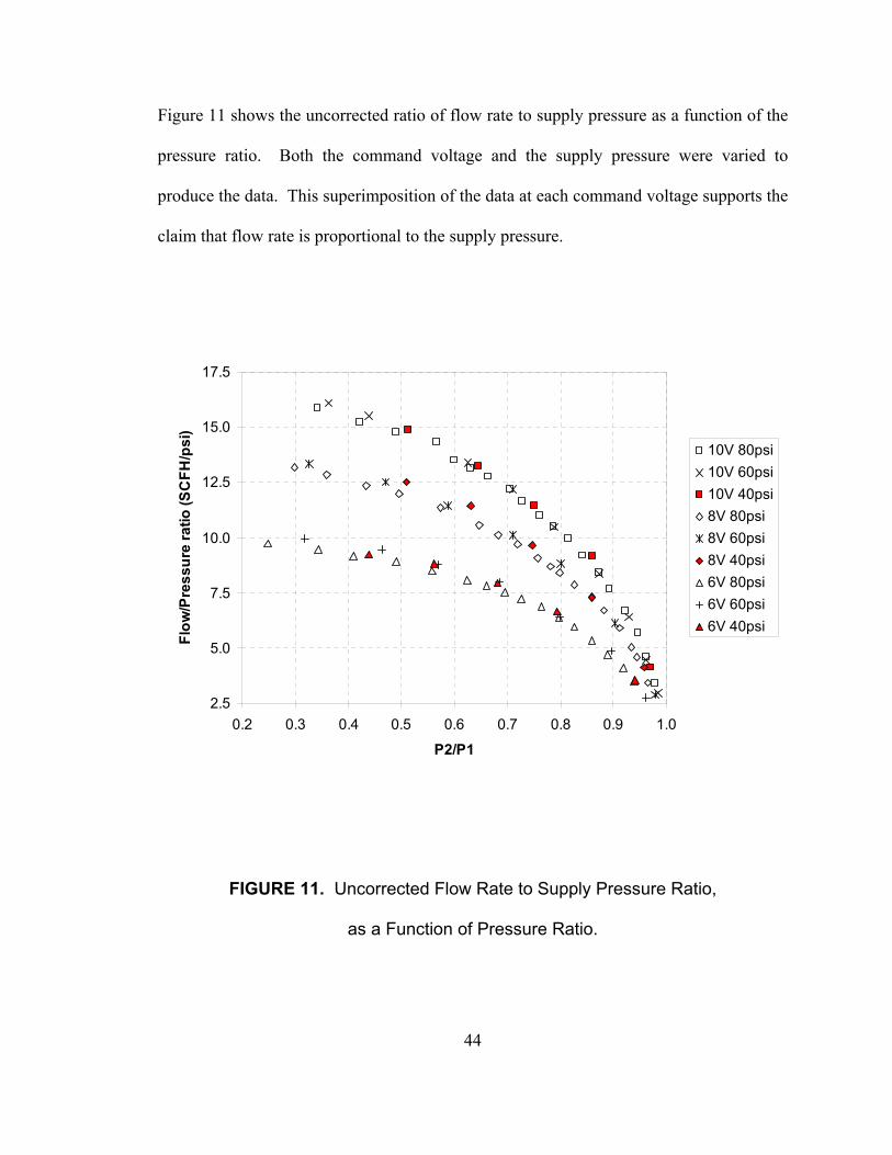
11 Uncorrected Flow Rate to Supply Pressure Ratio, as a

Function of Pressure Ratio ………………………………………… 44

12 Predicted Flow Rate Using the ISA Model ……………………… 46

13 Flow Coefficient as a Function of Command Voltage (1 → 4) … 47




xii

17 Flow Coefficient as a Function of Command Voltage (1 → 2) …… 51



20 Cut-away View of Pneumatic Cylinder …………………………… 56

21 Stiction as a Function of Position ………………………………… 58

22 Stiction as a Function of Time-at-Position ……………………… 59

23 Trajectory of Free-Falling Cylinder Payload ……………………… 62

24 Blue Ox 952QD Position Encoder ………………………………… 67

25 Quadrature Encoded Signal ……………………………………… 68

26 M02AE Control Architecture …………………………………… 72

27 Experimental Apparatus for Measuring Flow Friction …………… 73

28 Pressure Loss in Air Lines as a Function of Flow Rate …………… 74

29 Data Acquisition Hardware ……………………………………… 78

30 Servopneumatic System …………………………………………… 80

31 Block Diagram of the Pneumatic System ………………………… 95

32 Stiffness of a Pneumatic Cylinder versus Equilibrium Position … 98

33 ISA Model for Flow Rate ………………………………………… 101

34 Flow Coefficient Function for (1 → 4) …………………………… 102

35 Block Diagram of the M02AE Servo Controller ………………… 104

36 Ramp Trajectory ………………………………………………… 110

37 Reference Cam Profile Trajectory ………………………………… 111

38 Cam Profile Trajectory …………………………………… 111

39 Quadratic Sine Trajectory ………………………………………… 113

xiii

40 18 in/s Ramp Trajectory ……………………………………………115

41 Pole-Zero Map of Closed-Loop System ………………………… 119

42 Open-Loop Travel Velocities …………………………………… 121

43 10 in/s Ramp Trajectory ……………………………………………123

44 1.0 in/s Ramp Trajectory ………………………………………… 124

45 Cam Profile, 0.5-second Step Period ……………………………… 125

46 Quadratic Sine Trajectory, 1.0-s Half Period ……………………… 126

47 Detail of Open-Loop Travel Velocities …………………………… 128

48 3.2 in/s Ramp Trajectory, Showing Stick-Slip …………………… 129

49 Simulated Volumetric Flow Rates, 10 in/s Ramp Trajectory …… 130

50 Simulated Volumetric Flow Rates, 0.2-second Half Period Quadratic

Sine Trajectory …………………………………………………… 132

51 VSC Command Space …………………………………………… 135

52 VSC Command Voltages ………………………………………… 135

53 10 in/s Ramp Trajectory, VSC …………………………………… 137

54 10 in/s Ramp Trajectory Velocity ………………………………… 138

55 Cam Profile Trajectory, 0.5-seccond Step Period, VSC ………… 139

56 Cam Profile Trajectory Velocity, 0.5-seccond Step Period ……… 140

57 1.0 in/s Ramp Trajectory, VSC …………………………………… 141

58 Cam Profile Trajectory, 2.0-seccond Step Period ………………… 142

59 Quadratic Sine Trajectory, 3.0-s Half Period ……………………… 143

60 Command Signal for 1.8 in/s Ramp Trajectory …………………… 145

61 1.8 in/s Ramp Trajectory, VSC …………………………………… 146

xiv

62 1.8 in/s Ramp Trajectory Velocity, VSC ………………………… 147

63 1.0 in/s Ramp Trajectory Velocity Showing Stick-Slip, VSC …… 147

64 3.2 in/s Ramp Trajectory, Showing PLC-Reported Position,

VSC ……………………………………………………………… 149

65 Hybrid Fuzzy Nominal Command Voltage ……………………… 150

66 Fuzzy Weight Functions ………………………………………… 151

67 10 in/s Ramp Trajectory, Hybrid Fuzzy Control ………………… 152

68 Cam Profile Trajectory, 0.5-seccond Step Period, Hybrid Fuzzy

Control …………………………………………………………… 153

69 Cam Profile Trajectory, 2.0-seccond Step Period, Hybrid Fuzzy

Control …………………………………………………………… 154

70 Quadratic Sine Trajectory, 3.0-second Half Period, Hybrid Fuzzy

Control …………………………………………………………… 155

71 1.0 in/s Ramp Trajectory, Hybrid Fuzzy Control ………………… 156

72 1.0 in/s Ramp Trajectory Velocity, Hybrid Fuzzy

Control …………………………………………………………… 157

73 RMS Position Tracking Errors, Ramp Trajectory ………………… 159

74 RMS Position Tracking Errors, Cam Profile Trajectory ………… 160

75 RMS Position Tracking Errors, Quadratic Sine Trajectory ……… 161

76 RMS Velocity Tracking Errors, Ramp Trajectory ………………… 162

77 Scan Time Distribution …………………………………………… 164

78 Consecutive Scan Times of PI Controller ………………………… 165

79 Programmable Logic Controller Input Wiring …………………… 194

xv

80 Main Program Ladder, PI Control ………………………………… 195

81 Main Program Ladder, Variable Structure Control ……………… 196

82 Main Program Ladder, Hybrid Fuzzy-Modified PI Control ……… 197

83 ctrl_PID Subroutine Ladder …………………………………… 198

84 ctrl_VSC7_1 Subroutine Ladder ……………………………… 199

85 ctrl_fuzzy2_1 Subroutine Ladder …………………………… 204

86 motion Subroutine ladder ……………………………………… 208

xvi

LIST OF SYMBOLS

Symbols.

A Area.

A Constant.

b Coefficient of viscous friction.

DC Discharge coefficient.

VC Flow coefficient.

Pc Specific heat of a gas at constant pressure.

Vc Specific heat of a gas at constant volume.

D Diameter.

E Energy.

F Force.

f Friction factor.

g Acceleration of gravity (386.09 in/s2).

Lh Head loss.

i 1− .

k Ratio of specific heats.

k Gain.

k Spring stiffness.

L Length.

M Payload mass.

m Mass of air.

P Pressure.

xvii

Q Volumetric flow rate.

R Universal gas constant (247·103 in2/s2-ºR).

Re Reynold’s number.

s LaPlace operator.

T Temperature.

t Time.

OFFU Output offset.

V Volume.

V Voltage.

V Mean flow velocity.

W Weight.

X Pressure drop ratio.

TX Critical pressure drop ratio.

x Position.

A State feedback matrix.

B Input effects matrix.

C State output matrix.

U Controllability matrix.

V Observability matrix.

X State vector.

Y Output vector.

χ Characteristic equation.

∆ Delta.

µ Coefficient of friction.

µ Viscosity.

ρ Density.

τ Time constant.

xviii

Embellishments.

x& First derivative of x.

x&& Second derivative of x.

x Constant value of x.

x~ Varying value of x.

Subscripts.

1 Chamber 1, blind end of cylinder.

1→2 Between station 1 to station 2.

2 Chamber 2, rod end of cylinder.

3→4 Between station 3 to station 4.

AIR Air.

ATM Atmospheric.

COM Command.

CORR Corrected.

CRIT Critical.

CYL Cylinder.

DN Downstream.

EQ Equilibrium.

FRIC Friction.

HI High.

I Integral.

LO Low.

MAX Maximum.

MEAS Measured.

NOFLOW No flow conditions.

P Proporional.

REF Reference.

xix

ROD Rod.

S Scaling.

S Supply.

SCFM Standard cubic feet per minute.

SPOOL Spool.

SPRING Spring.

T Total.

T1 Tubing attached to chamber 1.

T2 Tubing attached to chamber 2.

UP Upstream.

VALVE Valve.

VF Velocity feedforward.

X1 Excess of chamber 1.

X2 Excess of chamber 2.

1

CHAPTER 1

INTRODUCTION

Traditionally, servo control in industry – the capability of a mechanism to follow an

arbitrary trajectory – has been limited to two technologies: electromagnetic motors or

hydraulic actuators. Electric servo motors are typically clean and reliable in operation.

However, electric motors are usually high-speed, low-torque actuators, and need

transmission elements to convert power to a more useful form. Mechanical elements are

also required to convert the rotary motion of a motor to linear motion.

Hydraulic actuators have favorable force/speed characteristics, and can be directly

connected to their payload. On the other hand, a hydraulic system often creates

workplace hazards. Personnel working around a hydraulic pump require hearing

protection, and hydraulic systems are well-known for their leakage. One positive aspect

shared by electromagnetic and hydraulic actuators is ease of control. Linear models

provide a good approximation for both systems, and PID-based controllers are often

adequate for control purposes.

2

Pneumatic actuators have properties that can make them favorable for servo applications.

The actuators themselves are of simple construction, widely sourced, and easily

maintained, making them low in cost. They have a high power-to-weight ratio, are fast

acting, and, unlike electric motors, can apply a force at a fixed position over a prolonged

period of time with no ill effects. Compressed air is readily available in most industrial

environments. Like electric motors, pneumatic actuators operate cleanly; like hydraulic

actuators, they may act directly on a payload.

Traditionally, though, pneumatics are not used in servo applications, but rather to move a

payload between two fixed hard stops. Air is highly compressible, which makes the

actuator compliant rather than stiff, and introduces lag in the response. The actual

stiffness of a linear air cylinder is position-dependent. Air cylinders can have relatively

high friction that prevents smooth motion under many circumstances. These nonlinear

behaviors of an air cylinder preclude good control performance through PID or linear

control methods.

The recent availability of low-cost, high-performance computer processors is allowing

servopneumatic actuators to take advantage of advanced control algorithms in industrial

applications. Several manufacturers already offer industrial servopneumatic controllers,

and the technology is finding new applications. Still, there is room for further research

into design and control methodologies for servopneumatic systems.

3

CHAPTER 2

REVIEW OF PREVIOUS WORKS

Servopneumatics present an alternative to electric motors or hydraulics for industrial

servo motion control. Like electric motors, servopneumatics are generally clean and

reliable in operation. Like hydraulic systems, a servopneumatic actuator may be directly

coupled to the payload it is moving. Additionally, servopneumatics offer a high power-

to-weight ratio, and can offer cost benefits as high as 10:1 over traditional technologies

[1] [2]. However, the need for an advanced control system has prevented widespread

application of servopneumatics. Moore and Pu present an overview of the development

of servopneumatic technology in [3], much of which has been summarized in chapter 1.

Many variations of servopneumatic systems have been introduced in the literature.

Figure 1 shows a typical arrangement of hardware, similar to what is used in this study.

The major components are the pneumatic actuator, the valve or valves, the controller, and

the feedback sensors. Table 1 presents common options available for each component.

Analysis of the permutations of actuator-valve-controller combinations shows a possible

175 different studies: the actual number is much higher as varieties exist within each of

these options, especially in the category of control.

4

Traditionally, the term servovalve has referred to valves that have a closed-loop

controller for the spool position, while proportional valve refers to those valves that

operate in the open-loop mode. More recently, this distinction has been blurred as the

spool-controlling electronics have moved onto the valve, making a valve appear

proportional to the control system [4]. The valve used in this work will be referred to as

a proportional valve, because the on-valve feedback control causes the valve behave in a

linear fashion.

The remainder of this chapter is organized as follows: section 2.1 discusses efforts at

creating models of servopneumatic systems; section 2.2 presents works dealing with

friction, a significant nonlinearity in servopneumatics; section 2.3 details control

strategies for servopneumatics, and; section 2.4 describes applications for

servopneumatic actuators.

5

FIGURE 1. Servopneumatic System Components.

Actuator Valve Controller Sensors • Single-rod • Double-rod • Rodless • Rubber air muscle • Rotary

• Proportional • Servovalve • Dual servo • PWM-driven solenoid • Flapper-nozzle

• PID/linear • PID with autotuning • PID with nonlinear modifications • Nonlinear • Adaptive • Fuzzy • Variable structure/ sliding mode

• Linear potentiometer • Rotary potentiometer • LVDT • Quadrature encoder • Tachometer • Accelerometer • Pressure transducer

TABLE 1. Servopneumatic Component Selection

6

2.1. System Models. The works generally recognized as the first significant

presentation on servopneumatics are a pair of papers authored by J. L. Shearer of MIT in

1956 [5] [6]. In these papers, Shearer develops a linear mathematic model of a double-

rod cylinder for small motions about its mid-stroke position. He also presents a

theoretical model of the mass flow rate through a sliding-plate proportional valve,

verifying the model experimentally. While the availability of modern computers has

rendered his linear model obsolete, subsequent researchers in the field have copied his

methodology towards the development of a model.

A paper by Liu and Bobrow expands on Shearer’s work by developing a linear model

based on an arbitrary operating point [7]. A PD controller, applied to the linear model,

may be used to position system poles advantageously. While the actual system behaves

similarly to the model-based simulation, the model is significantly slower than the actual

system tested.

In [8], Kunt and Singh develop a linear time-varying (LTV) model for the open-loop

behavior of a pneumatic cylinder being controlled by a rotary-spool valve, comparing it

to a linear time-invariant (LTI) model. Because the valve rotates at a steady, known

velocity, it is possible to derive exact solutions for the differential equations describing

the LTI model. The LTV models, however, generally require numerical simulation. The

accuracy of their model may be improved by incorporating the effects of friction, which

were ignored. Linear models of a pneumatic actuator are also used in conjunction with

an auto-tuning PI controller [9], and an adaptive controller [1].

7

While linear models are preferable from the standpoint of controller design, pneumatic

cylinders are highly nonlinear due to the effects of air compression, varying air volumes

in the actuator, and friction. Wang and Singh investigate these nonlinearities in a study

of a closed pneumatic piston chamber [10]. They find the nonlinear effects of friction

and compressibility not only shift the resonant frequency of the mechanical system, but

also induce asymmetric oscillatory behavior in the system. A subsequent paper by the

authors expands this analysis to a chamber connected to a substantially large reservoir via

an orifice [11]. Nonlinear models are presented in a number of other papers, notably

Richer and Hurmuzlu in [12]. Their model includes the effects of propagation delay and

friction losses in air hoses, which can be significant over long distances. Kawakami, et

al. compare the performance of linear models, developed using methods described in [5]

and [7], with those of exact nonlinear models [13]. They find that linear models are poor

predictors of the actual performance of a pneumatic system.

Many cylinders contain design features such as integral shock absorbers or air cushions

to prevent mechanical damage from impact at the end of the stroke. Wang, et al. use a

four-control-volume nonlinear model in simulating the motion of a pneumatic cylinder

with end-of-stroke flow restrictions [14]. While the model is qualitatively correct in

predicting motion, many of the coefficients used in the model were engineering estimates

of the actual values. This precludes a proper quantitative comparison of the simulation

results with the experimental data.

8

One issue in the modeling of pneumatic processes is applying an isothermal model or an

adiabatic model towards the expansion of air. The fundamental equations are similar,

with the adiabatic expression being a factor of k1 different than the isothermal

expression. The term k refers to the ratio of specific heats ( 4.1=k for air). While some

researchers have applied the isothermal model, most assume the mechanical processes are

significantly faster than the thermal processes, and thus use an adiabatic process. An

exception worth mentioning is the study conducted by Pu and Weston in [15], in which

the steady-state velocity of a pneumatic actuator may be predicted.

In [12], Richer and Hurzumlu replace k with an intermediate term, α, in a hybrid model.

The α term is bounded by 1 and k, and represents a compromise position between

isothermal and adiabatic processes, though they find the isothermal model better fits their

experimental data. Backé and Ohligschläger investigate heat transfer in an air cylinder in

detail [16]. They find a cylinder in motion initially behaves adiabatically, but heat flow

works to restore isothermal conditions. The authors identify three experimentally-

determined parameters to describe the heat-transfer behavior: an air friction factor, a

forced convention factor, and a natural convention factor. These factors may be

determined by comparing simulated pressure- and temperature-time curves with

measured data. Kawakami, et al. also investigate the differences between isothermal and

adiabatic processes in a pneumatic cylinder in [13]. Their research indicates the practical

differences between the two models is small enough as to be insignificant.

9

The mathematical modeling of flow through a valve is another concern in

servopneumatics. At least four flow models have been presented in the literature: a

model based on the theoretical flow through an orifice; the NFPA approximation of

orifice flow [17]; a similar approximation presented by Esposito [18], and; a model

proposed by the ISA [19]. While different in their formulation, these models share a

number of characteristics. In each, flow is proportional to the supply pressure and a flow

coefficient, VC . Each model also contains two regimes for valve flow. In the subsonic

flow regime, the flow rate increases as the ratio of downstream pressure to upstream

pressure decreases. In the choked flow regime, the flow through the valve is sonic and

does not increase as the downstream pressure drops. In the ISA model, this critical

pressure ratio is determined by a valve design factor, TX ; in the other models, the critical

pressure ratio is calculated from the ratio of specific heats, and is found to be 0.528 for

air. Significantly, experimental data suggests that the assumption of constant flow in the

choked flow regime is not valid. In [20], Bobrow and McDonell tried a least-squares fit

of experimental data with the theoretical flow through an orifice, trying to identify the

flow coefficient. The authors ended up using an empirically-derived function to describe

the valve flow. A more detailed discussion of flow dynamics is conducted in chapter 4.

While most studies of servopneumatics focus on linear actuators, Pu, Moore, and Weston

perform a study on rotary air motors [21]. In terms of developing a mathematical model

of the actuator, the air motor has an advantage over reciprocating cylinders in that its

control volume is relatively constant, removing a large nonlinearity from the actuator

model. This permits the application of a conventional PID controller, with acceleration

10

feedback and velocity feedforward terms added, to the air motor. Another study of rotary

actuators is performed by Wang, Pu, Moore, and Zhang in [22]. In it, the authors use

Fourier series expansion to approximate discontinuous functions as continuous functions

of the actuator’s rotation.

Generally, researchers assume the dynamics of the valves controlling a servopneumatic

axis are significantly faster than the dynamics of the actuator and mass under control, so

that the valve may be treated as a nonlinear gain function. Vaughan and Gamble create a

detailed nonlinear model of the dynamics of a proportional valve in [23], accurately

predicting the open-loop behavior of the valve. This study was conducted in order to

apply a sliding mode controller to the valve in [24]. An investigation of a jet-pipe

servovalve was conducted by Henri and Hollerbach in [25].

A recent approach to the modeling of pneumatic systems comes in the form of computer-

based simulators in which the engineer designs a virtual system. Hong and Tessman

present a commercially available software package that models both pneumatic and

hydraulic circuits [17]. Anglani, et al. present a similar package that works in a CAD

environment, and allows the pneumatic system to interact with external mechanical

elements [26]. Both systems are designed more for the practicing engineer as a tool for

selecting components for a particular application, rather than for fundamental research

into pneumatic systems.

11

2.2. Friction. While the nonlinear dynamics of a pneumatic cylinder have been

discussed in the previous section, the effects of friction warrant particular attention.

Friction has been identified as the most significant nonlinearity in a servopneumatic

actuator [27]. Stick-slip motion caused by friction can prevent certain motions from

being realized. Any number of methods have been developed to model, analyze, and

counteract the effects of friction. The works cited here are representative of the research

being conducted in friction and tribology.

Armstrong-Hélouvry, et al., perform an exhaustive survey of tribology and friction in a

1994 paper [28] that covers models, analysis tools, and compensation techniques for

machines with friction. Their summary of friction models concludes with an integrated

friction model having seven parameters for sliding contact between hard metal parts,

lubricated by oil or grease. In many cases, this model may be extended to dry contact

between surfaces. While there have been successful examples of servo controllers

compensating for friction in both research and industry, the control and compensation

tools are often more advanced than the techniques available to analyze the friction.

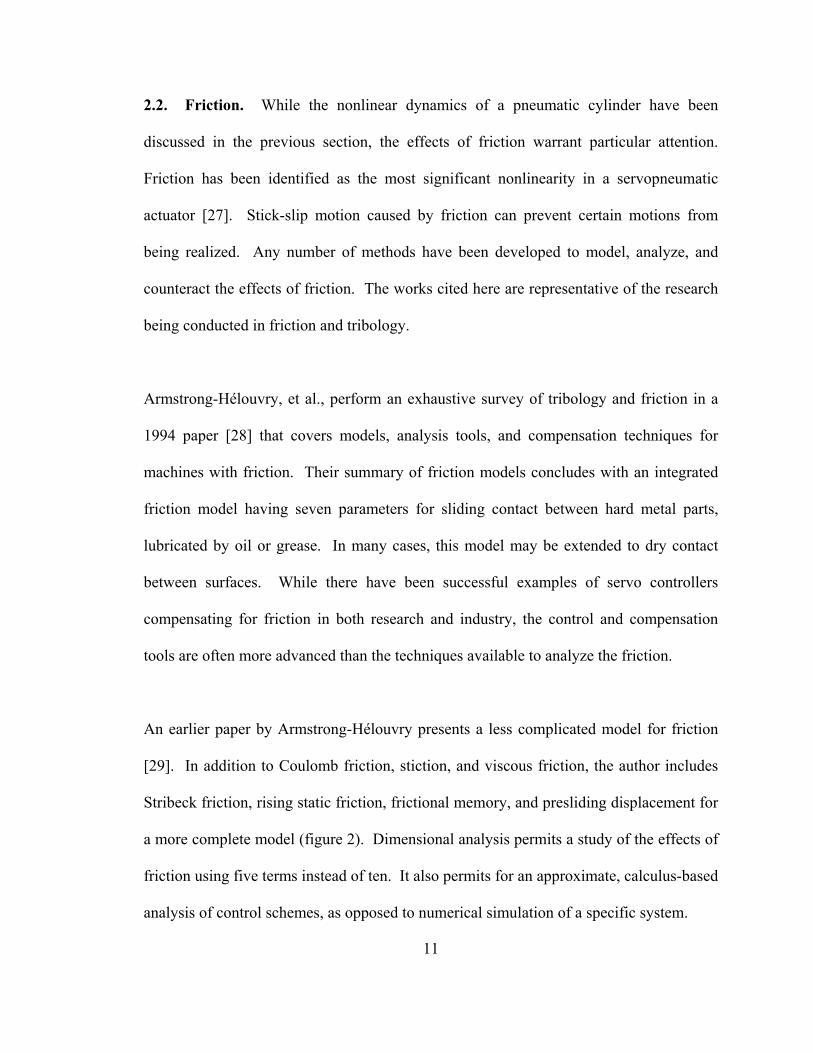
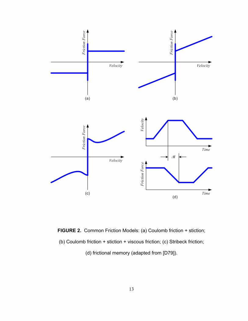
An earlier paper by Armstrong-Hélouvry presents a less complicated model for friction

[29]. In addition to Coulomb friction, stiction, and viscous friction, the author includes

Stribeck friction, rising static friction, frictional memory, and presliding displacement for

a more complete model (figure 2). Dimensional analysis permits a study of the effects of

friction using five terms instead of ten. It also permits for an approximate, calculus-based

analysis of control schemes, as opposed to numerical simulation of a specific system.

12

An empirical model of friction in an optical targeting mechanism is presented by Kang

and Kim [30]. They develop frequency response functions for the mechanism, finding

them to be amplitude-dependent. While their approach is rigorous and thorough, it is not

cost-effective for many industrial applications in which friction is a concern.

Despite the effort to develop an accurate model for friction in mechanisms, in many

applications friction may be an unknown, yet bounded, disturbance to the system. In

their study of pneumatic system nonlinearities, Wang, et al. find that the static friction of

an air cylinder varies as a function of both the cylinder position and direction of applied

force [31]. This variation in friction appears to be a random variable, without an

identifiable trend along the stroke.

13

FIGURE 2. Common Friction Models: (a) Coulomb friction + stiction;

(b) Coulomb friction + stiction + viscous friction; (c) Stribeck friction;

(d) frictional memory (adapted from [D79]).

14

Johnson and Lorenz map friction as a function of velocity, then perform a regression

analysis to identify coefficients for static friction, Coulomb friction, viscous friction, and

exponential friction [32]. Canudas de Wit, et al. discuss adaptive compensation for

friction in [33]. A thorough model for friction includes five empirically-derived terms,

but the authors present a three-term exponential approximation that is generally valid

over the range of speeds considered. For adaptive controllers at low speed, such a model

provides superior results to those of controllers using a Coulomb friction model.

Wang and Longman study stick-slip friction in systems with learning controllers [34]. In

sampled-data systems with significant friction, they find a minimum movement size is

necessary to avoid limit cycling about the reference position. In [35], Dunbar, et al.

present a methodology for identifying dry friction faults in a pneumatic actuator, though

the method can be applied to other systems. An empirical fourth-order model for a

servopnematic system is derived. Residuals calculated from the acceleration are

proportional to the friction. When these residuals exceed their nominal levels, it indicates

the presence of excess friction in the system.

Changes in the conceptual design of the actuator can significantly reduce friction. The

pneumatic muscle actuators of [36] are single-piece devices that mimic biological

muscle, and have no sliding contacts within the actuator. A similar concept is employed

in the bellows actuator of [37]. In the latter, the actuator controls the fine motion of a

gripper, where stick-slip friction cannot be tolerated.

15

Shen, et al. develop a generalized control structure for positioning linear systems with

friction [38]. The controller accepts a degree of uncertainty in the exact values of the

characteristic equation of the linear system and of the friction. The controller is

deactivated in a small band about the command position to prevent chattering.

2.3. Control Strategies. Control has been the single largest hurdle to the application of

servopneumatic systems. Traditional servo actuators – electric motors and hydraulic

cylinders – may be modeled as linear mechanisms without significant error. Linear

control methods, such as proportional-integral-derivative (PID) control, may therefore be

applied to these devices. Pneumatic actuators, on the other hand, have considerable

nonlinearities in their mathematical models. PID control performs poorly in controlling

servopneumatics.

The design objectives for the system are important in selecting a controller. Positioning

control, or point-to-point control, deals with applications in which the exact trajectory is

not as important as the static positioning error of the system. Servo control is defined as

an actuator’s ability to follow an arbitrary trajectory, and is considered more demanding

of the controller.

PID Control

PID control – and, by extension, P, PI, and PD control – is not typically used for servo

control of pneumatic cylinders. Very often, it is used as a baseline of comparison against

16

some other control scheme. A 1995 paper by Pu, Weston, and Moore [39] is an

exception to this rule, and the only found in this literature review. In this paper, the

authors discuss the effectiveness of a PID controller in following specific trajectories,

such as a trapezoidal velocity profile. Their work suggests that the proper selection of a

velocity profile can improve the performance of the servopneumatic axis for a specific

application.

More often, PID control is used in pneumatic positioning systems. Kawamura, et al.

demonstrate the stability of a PI controller in a positioning application [40]. PI control is

also used applied by Noritsugu and Takaiwa in [41]. Here, the controller works in

conjunction with two observers, which provide compensation for the nonlinearities in the

air dynamics, friction, and changes in the system parameters. A dual-loop controller for a

PWM-driven servo actuator is developed by Lai, et al. [42]. An inner loop applies PI

control to the pressure feedback signal, while the outer loop applies PD control to the

cylinder’s position. By varying the pressure on just one chamber of the air cylinder they

are able to reduce the significance of nonlinearities in the control system.

In designing a pneumatic wrist platform, Pfreundschuh, et al. use PD controllers for

positioning each of three pneumatic cylinders [27]. The authors avoided integral control

because its interaction with the friction in the cylinder would have led to limit cycling

behavior. Fok and Ong measure the positioning accuracy of a servopneumatic axis with

a PD controller [43]. Without any consideration of trajectory following capability, they

17

find the positioning error is reduced as the proportional gain increases. With the proper

gain, the positioning error is found to be within ±0.3 mm over a range of payloads.

Often, a PID controller is modified to enhance its performance in certain circumstances.

Using a proportional controller as a reference, Moore, et al. discuss the effects of

modifications to this control scheme on a point-to-point pneumatic controller [44]. The

specific modifications include: output saturation at the initiation of a motion command;

setpoint modification, in which the command position is shifted during a portion of the

axis motion; adding derivative control and increasing its gain at low velocities, and; a

simple learning algorithm applied to the set point modifier. Output saturation is also

applied to the PID controller of Wang, et al. [45]. In this work, acceleration feedback is

substituted for pressure feedback, which is often used to provide full state feedback to the

controller.

PID is applied to a pneumatic positioning axis, regulated by two pulse-width-modulated

solenoid valves, in [46]. In this paper, a compensating constant is added to the output

signal to oppose friction, here modeled as Coulomb friction. The integrator gain is only

active within a pre-defined error band about the set point. A position look-ahead gain,

similar to a velocity feedforward, is also added. The result is a fast, accurate, inexpensive

positioning system. A subsequent paper from the same authors presents an auto-tuning

algorithm for this controller, which is able to set controller gains within a small number

of cycles [47].

18

Autotuning of a PI controller is also discussed by Hamiti, et al., in [9]. The control

scheme is based on a linearization about an arbitrary operating point along the pneumatic

cylinder’s stroke. An inner, analog proportional loop reduced the effects of nonlinearities

in the system, while an outer loop contains a digital PI controller. Autotuning applied on

the integral gain suppresses the limit cycle behavior of the system. This scheme can be

adapted to various PID-based control schemes. Richardson, et al. apply a self-tuning

algorithm to a proportional controller for a low-friction pneumatic cylinder [2]. The

algorithm runs on-line, and can adapt to changes in the plant parameters. The authors

used low-friction cylinders to minimize unknown disturbances from friction.

Feedback linearization can permit conventional PID controllers to achieve adequate

performance with servopneumatics. While third-order and higher-order nonlinear

systems are generally not feedback linearizable, Kimura, at al. demonstrate that a

pneumatic cylinder with an inertia load can be linearized [89]. With feedback

linearization and disturbance rejection, a PID controller can provide adequate point-to-

point control. In [48], inverse function provide exact linearization for the inputs and

outputs of a controller for a rotary vane actuator. These functions eliminate most of the

oscillatory behavior seen in similar controllers that do not have the linearization

functions.

19

Adaptive Control and Learning Control

Adaptive controllers provide a mechanism for dealing with unknown and/or time-varying

parameters in the system being controlled. In addition to processing inputs to determine

a set of output signals, an adaptive controller has an internal model of the system being

controlled. By comparing the state of the model with the measured state of the system,

the values of the system parameters may be estimated. Controller gains are then

recalculated to maintain the controller’s effectiveness.

General works in adaptive control include a paper on stability by Whitcomb, et al. [49],

in which the authors apply adaptive control to a serial-link robot arm. Adaptive

controllers consistently outperform conventional controllers, but only when an accurate

reference model is available. A paper by Sadegh and Horowitz also considers adaptive

control for robot arms [50]. The controller developed is shown to be globally

asymptotically stable, and avoids the need for matrix inversion as had previous adaptive

controllers. Adaptive control is also applied to a robot with non-rigid joints in [51].

Two papers apply adaptive controllers to servopneumatic applications. In [1], Bobrow

and Jabbari use adaptive control for force and position control of a pneumatic axis. The

authors found that a pole-placement model, as opposed to a parameter-reference model,

provides superior performance. They also found that a lower-order model provides better

results than a higher-order model, due to the destabilizing effects of uncertainties in the

higher-order models. McDonnell and Bobrow develop an adaptive controller for a

20

pneumatic cylinder controlling the elbow joint of a serial-link robot in [52]. Their

controller incorporates a forgetting factor to allow for rapid adaptation to changes in the

system parameters. This controller is remarkable in that it can not only adapt to changes

in the payload, but also demonstrated an ability to compensate for a loss of data from one

of the two pressure sensors.

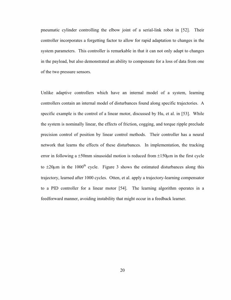
Unlike adaptive controllers which have an internal model of a system, learning

controllers contain an internal model of disturbances found along specific trajectories. A

specific example is the control of a linear motor, discussed by Hu, et al. in [53]. While

the system is nominally linear, the effects of friction, cogging, and torque ripple preclude

precision control of position by linear control methods. Their controller has a neural

network that learns the effects of these disturbances. In implementation, the tracking

error in following a ±50mm sinusoidal motion is reduced from ±150µm in the first cycle

to ±20µm in the 1000th cycle. Figure 3 shows the estimated disturbances along this

trajectory, learned after 1000 cycles. Otten, et al. apply a trajectory-learning compensator

to a PID controller for a linear motor [54]. The learning algorithm operates in a

feedforward manner, avoiding instability that might occur in a feedback learner.

21

FIGURE 3. Estimated Disturbances along a Sinusoidal Trajectory (from [53]).

In applications such as paint spraying and welding, ensuring a constant velocity is critical

to the process. Gross and Rattan develop two learning controllers – multilayer neural

networks (MNN) – for velocity control of a sevopneumatic actuator [55]. The first is an

offline controller designed for the commissioning of an MNN, and for re-training after

significant system changes. Training requires 1400 cycles, which took about an hour

with the hardware being used. The second controller tracks the performance of the

MNN, and will recalculate control weights only if the tracking error is deemed excessive.

The online controller requires two processors: one for the actual control, and a second for

the process monitor and gain recalculation.

22

Fuzzy Control

Fuzzy control of servopneumatics has not been extensively studied in the literature, with

just two papers exploring the subject. In [56], Shih and Ma use fuzzy control for position

control of a pneumatic cylinder. With a properly tuned controller, positioning accuracy is

within 0.1mm. In [57], to be discussed further in this section, a fuzzy controller and a

neuro-fuzzly controller are two of six control schemes evaluated on a servopneumatic

axis.

Variable Structure Control and Sliding Mode Control

Vadim Utkin introduced the concept of sliding mode control (SMC) in his 1977 paper

[58]. Sliding mode control is based on the theory of variable structure control (VSC), in

which a controller is composed of distinct subcontrollers with an appropriate switching

logic scheme. Sliding mode control is a variable structure control in which adjacent

subcontrollers drive the system towards the boundary between the subcontrollers, called

the sliding plane or sliding surface. In this manner, the system tends to follow the sliding

plane to equilibrium. Thus, the gross dynamics of the system will be determined by the

existence and position of the sliding planes, and not by the subcontroller dynamics.

Sliding mode control enhances the advantages of variable structure control, mainly an

insensitivity to plant variance and the ability to achieve state trajectories not available

through conventional control methods. The disadvantages of both variable structure

control and sliding mode control is that they both require a controller capable of high-

23

frequency switching, which is characterized by chattering of the output device. This, in

turn, may excite unmodeled high-frequency behavior in the system. Utkin reviews more

recent developments in VSC in a 1993 paper [59], in which he discusses mathematical

analysis methods, controller designs, and practical applications researchers have

developed. The application of VSC has produced quantifiable economic benefits in

several industries.

VSC and SMC have received a lot of attention from researchers working with DC motors

and robotics. Benjiamin and Kauffmann apply a sliding mode controller to the position

control of a DC motor in [60]. In both analog and digital implementation of the SMC,

the controller was found to be robust with respect to changes in the friction resisting the

motion of the load. A later paper by Benjiaman and Magnuson [61] discusses the same

application. Like a PID controller, SMC has three control gains, but unlike PID these

gains are decoupled, simplifying the tuning procedure. The authors demonstrate that the

trajectory-following capability of the SMC is markedly improved over that of a PID

controller.

A variable-structure controller is applied by Xu, et al. in the control of a two-link robot

[62]. To avoid chattering in the output, the authors employ a linear smoothing function

in a small band about the switching plane. The smoothing function was observed to

greatly reduce the fluctuations in the control torque at each joint. Leung, et al.

demonstrate a sliding mode controller on a two-degree-of-freedom robot arm, with

angular tracking errors of ±1.7° over a 30° move [63].

24

Harashima, et al. present a sliding mode controller for a serial robot arm with direct-drive

actuators [64]. Without the reduction gears in the arm, the actuator dynamics are more

susceptible to outside disturbances and interactions, such as the position-dependent

torque developed by the weight of the arm itself. The variable-structure controller is able

to provide superior performance in spite of these interactions. To avoid chattering about

the sliding plane, the discontinuous control function is replaced with a continuous

function in a small region encompassing the switching plane, in a manner similar to that

described in [62]. Integral control in this region also serves to suppress chattering. A

following paper by Slotine and Hashimoto discusses the details of implementing the

controller in greater detail [65].

More recently, sliding mode control has gained the attention of researchers studying

servopneumatics. Paul, et al. select SMC for control of a servopneumatic axis in [66].

Due to the insensitivity to variations in the plant, the authors are able to use an

approximate model for the airflow. A reduced-order controller eliminates the need for

pressure sensors in the feedback system. Pandian, et al. also apply a reduced-order

controller to a servopneumatic system [67]. In developing a model, the authors ignore

friction and use a simple linear flow model for the proportional valves. Still, the

reduction of order in the controller does not significantly degrade its performance.

However, the results developed by Tang and Walker demonstrate that the model used in

developing the SMC needs to be selected with care, as their results show a need for

model refinement, especially with regards to the pneumatic cylinder dynamics [68].

25

Richer and Harmuzlu also compare a full-order controller with a reduced-order controller

in [69]. The full-order controller provides excellent performance, but at a premium of

computational cost. A reduced-order controller is found to be adequate when

propagation delays are minimized – that is, when the length of plumbing between the

valve and the actuator is as short as possible.

Drakunov, et al. use full state feedback with SMC in [70], demonstrating an excellent

command-following ability. In [71], Acarman, et al. incorporate an input-output

linearization scheme, similar to that of [48]. This permits the use of linear design tools

for developing the sliding mode controller. An observer is also included to provide the

controller with knowledge of system states not directly measured.

Sliding mode control can find application in other fields. Gamble and Vaughan use SMC

for position control of the spool in a proportional hydraulic valve [24]. A nonlinear

switching surface in position error-velocity-acceleration space separates the solenoid

applying full forward and full reverse voltage to the spool. The resulting controller

provides superior performance to an analog PID controller, with virtually no steady-state

positioning error and an insensitivity to flow forces through the valve. A hybrid sliding

mode-adaptive controller for aircraft attitude is developed and simulated by Young in

[72]. Linear model-based adaptive control, by itself, has problems in quantifying design

objectives and accounting for changes in the plant parameters. SMC allows for better

performance and less sensitivity to disturbances in the system.

26

Other Control Schemes

De Almeida, et al. discuss the system architecture for a five degree-of-freedom pneumatic

robot designed to pick plastic parts from an injection molding machine [73]. Variable

structure controller was to be used for short-distance movements of the gripper, while

PID would control larger motions.

Pu and Weston present a hybrid point-to-point controller for servopneumatic actuators

[74]. To minimize positioning time, the controller has a variable structure that starts a

move with a saturated output, inserts a negative input for a period of deceleration, and

applies PID control for final positioning. A learning controller is applied to the

scheduling of the control laws.

Gorce and Guihard develop a hybrid force-position controller for robotic arms in [75].

Impedance control uses external loads on the structure to modify the apparent inertia of

the system inside the controller. Simulated results of the controller are presented.

Takamura, et al. deliver a report on chaotic behavior in digitally-controlled

servopneumatic actuator systems [76]. They observe chaotic behavior in marginally

stable systems, as verified by three different indices. An OGY controller is applied to

minimize the chaos in the system.

27

Controller Comparisons

Brun, et al. compare a linear controller to that of a nonlinear controller for a pneumatic

cylinder [77]. The control signal used controls jerk, the time derivative of acceleration,

to ensure smooth motion starts and stops. In comparing the controllers,the authors find

the nonlinear controller avoids stick-slip behavior in the system, but is much more

complex to establish and requires three sensors to the linear system’s one.

Chillari, et al. perform a comparative study between six control methods for

servopneumatic actuators, applying them to representative, common trajectories [57].

The methods evaluated are PID control, fuzzy control, sliding mode control, and neuro-

fuzzy control. The PID and fuzzy controllers were evaluated both with and without

pressure feedback. In terms of the RMS position tracking error, the fuzzy controller with

pressure feedback generally performed best, though the fuzzy controller with a neural

network did work better on certain trajectories. The neuro-fuzzy controller estimates the

pressure in the cylinder, eliminating the need for pressure sensors.

2.4. Applications. Practically, servopneumatic actuators may be used to replace

electricmagnetic or hydraulic actuators in just about any particular application. In certain

applications, though, servopneumatics may prove to be the best option.

Harrison, et al. [78] surveyed industry to evaluate present and future applications for

pneumatic robots. While robots had already been applied to welding and paint-spraying

28

applications, the companies surveyed indicated an interest in robotics for part handling,

assembly, and quality control. The authors evaluated modular pneumatic robots as a

means of providing flexible automation at a low cost, using two part unload-and-

assemble systems as examples.

Caldwell, et al. discuss the use of pneumatics in the construction of a humanoid robot

[36]. The properties of the pneumatic muscle actuators make them excellent for this

application: high power-to-weight ratio, flexibility, and mechanical behavior similar to

that of human muscle. A light-weight internal combustion engine can provide enough

power for the entire robot, allowing it to explore freely without a power umbilical or

heavy banks of batteries.

Ben-Dov and Salcudean develop a novel pneumatic actuator for fine motion control [79].

Two low-friction air cylinders, each with its own voice-coil flapper valve, form a gripper

for force-controlled manipulation. In a recent work by Bobrow and McDonell, torque

control of pneumatic actuators gives a robot force control at the end effector [20]. Other

applications for servopneumatics include: a number of robot arm designs [7] [52] [64]; a

wrist platform with compliance [27]; a robotic leg [80], and; humanoid robots [36] [81].

29

CHAPTER 3

PROBLEM STATEMENT

Chapter 2 presented a number of schemes for the control of a servopneumatic actuator.

Generally, these control systems have been realized with laboratory data acquisition and

process control hardware, using software custom-designed for the particular controller.

A typical example of such a system is the sliding-mode controller for a servopneumatic

actuator presented in [67], which uses a computer with a 100 MHz Pentium processor for

control.

Industrial control systems, on the other hand, typically use programmable logic

controllers (PLC’s) for equipment control. Initially designed to replace relay logic

control, PLC capabilities have been expanded over the past two decades. A modern,

configurable PLC consists of a chassis with a power supply, processor, and a set of

modules selected for the particular application. Modules are available to handle digital

inputs and outputs, analog inputs and outputs, thermocouple inputs, and communications

using DeviceNet and EtherNet protocols. Furthermore, stand-alone servo controllers,

once required for DC servomotor control tasks, may now be replaced with servo motion

30

control modules that plug into the PLC chassis. Figure 4 depicts one such modern PLC,

an Allen-Bradley Logix5550 PLC1, with a selection of different modules.

FIGURE 4. Allen-Bradley Logix5550 PLC.

The goal of this research is to investigate the performance of various control strategies for

a servopneumatic system consisting of a linear actuator and a single proportional valve.

The control algorithms will be realized within the architecture of a programmable logic

controller similar to that of figure 4, with control tasks being shared between the PLC

controller and a motion control module on the PLC. The limitations imposed on the

system performance by the PLC control architecture will be discussed. A nonlinear

1 DeviceNet is a trademark of the Open DeviceNet Vendor Association. EtherNet is a registered

trademark of Intel Corporation, Xerox Corporation, and Digital Equipment Corporation. Logix5550 is a trademark of Rockwell International Corporation.

31

simulation of the servopneumatic system will be developed in order to evaluate

phenomena that cannot be directly observed in the physical system.

32

CHAPTER 4

EXPERIMENTAL EQUIPMENT

This chapter discusses the properties of the major components of the servopneumatic

control system used in this study (figure 1). Knowledge of these properties is essential in

creating an accurate system model and designing a control algorithm.

4.1. Proportional Valve. A Festo proportional valve controls the pneumatic cylinder

used in this study. The valve comes packaged with electronics to provide closed-loop

control of the spool position. This particular valve is a prototype that accepts a ±10 volt

control signal instead of the 0-10 volt control signal accepted by a standard Festo valve.

Table 2 lists the significant characteristics of the valve. Figure 5 is a schematic of the

Festo valve, showing the ports and their connections. Figure 6 shows the published flow

rate through the valve as a function of the command voltage, for the standard 0-10 volt

valve. Note that figure 6 is separated into two regions: one for flow from port 1 to port 2;

and a second for flow from port 1 to port 4.

33

FIGURE 5. Festo Valve Schematic.

FIGURE 6. Flow Rate through Festo Valve (from [82]).

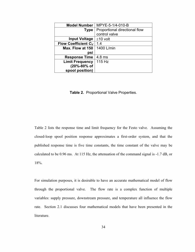
34

Model Number MPYE-5-1/4-010-B Type Proportional directional flow

control valve

Input Voltage ±10 volt Flow Coefficient CV 1.4 Max. Flow at 150

psi1400 L/min

Response Time 4.8 ms Limit Frequency

(20%-80% ofspool position)

115 Hz

Table 2. Proportional Valve Properties.

Table 2 lists the response time and limit frequency for the Festo valve. Assuming the

closed-loop spool position response approximates a first-order system, and that the

published response time is five time constants, the time constant of the valve may be

calculated to be 0.96 ms. At 115 Hz, the attenuation of the command signal is -1.7 dB, or

18%.

For simulation purposes, it is desirable to have an accurate mathematical model of flow

through the proportional valve. The flow rate is a complex function of multiple

variables: supply pressure, downstream pressure, and temperature all influence the flow

rate. Section 2.1 discusses four mathematical models that have been presented in the

literature.

35

One mathematical model for the flow of air through a valve is derived from compressible

flow through a fixed orifice. The equation is divided into two regions based on the ratio

of the downstream pressure to upstream pressure, UPDN PP . The critical pressure is

calculated using the ratio of specific heats for air, k.

1

12 −

+=

kk

CRITUP

DN

kPP

(1).

For air ( 4.1=k ), the critical pressure ratio is found to be 0.528. When the pressure ratio

is higher than the critical pressure ratio, flow through the orifice is subsonic, and

increases as the pressure ratio decreases. At the critical pressure ratio, flow through the

orifice is sonic. At this point the orifice is said to be choked, and further decreases in the

pressure ratio will not increase flow through the orifice. From Drakunov, et al. [70] and

Andersen [83], the mass flow rate through an orifice is given as,

( )

≤

×

>

−

−

=

+

CRITUP

DN

UP

DNUPD

CRITUP

DN

UP

DN

kk

UP

DN

k

UP

DNUPD

PP

PP

RTP

AC

PP

PP

PP

PP

kk

RTP

ACm

:6847.0

:1

2

1

12

1&

(2),

36

where DC is the discharge coefficient and A is the orifice area. The upstream and

downstream pressures are absolute pressures, rather than gauge pressures. The discharge

coefficient reflects a contraction of the flow path downstream of the orifice, reducing the

effective flow area. This equation does not include the flow coefficient VC , which is the

most often used parameter describing the flow capacity of a given valve.

A less complicated equation for flow through a valve is presented by the National Fluid

Power Association (NFPA). The NFPA equation incorporates the flow coefficient. Like

the orifice equation, flow is divided into regions of sonic (choked) and subsonic

(unchoked) flow. The NFPA equation calculates the volumetric flow rate, measured in

standard cubit feet per minute. The mass flow rate may be derived from the volumetric

flow rate through multiplication by air density at standard conditions.

( )

≤

×

>

−×

=

CRITUP

DN

UP

DNUPV

CRITUP

DN

UP

DNDNDNUPV

SCFM

PP

PP

TP

C

PP

PP

TPPP

CQ

:22.11

:48.22

(3),

where the pressure is measured in psia and the temperature in °R. Esposito presents a

similar equation in [18],

37

( )

≤

×

>

−×

=

CRITUP

DN

UP

DNUPV

CRITUP

DN

UP

DNDNDNUPV

SCFM

PP

PP

TP

C

PP

PP

TPPP

CQ

:32.11

:67.22

(4).

Not as well-known as the previous models, the ISA model for flow through a valve

incorporates not only the flow coefficient VC , but also includes an experimentally-

determined critical pressure drop ratio factor TX . This model was developed to account

for the observation that two valves with identical flow coefficients can exhibit different

flow rates under identical pressure conditions. In any valve, the complexity in the

geometry of the flow path corresponds to TX , with more complex geometries yielding

higher values. For example, [84] presents two valves having identical flow coefficients.

For a ball valve with a straight flow path, 14.0=TX ; for a needle valve with a Z-shaped

flow path, 84.0=TX .

For air, the ISA flow equation is,

≥×

<

−×

=

TT

UPV

TT

UPV

SCFM

XXTXPC

XXTX

XXPC

Q:11.15

:3

167.22 (5),

where,

38

−=

−=

UP

DN

UP

DNUP

PP

PPP

X 1 (6).

In the orifice flow and NFPA equations, choked flow occurs when the ratio of

downstream to upstream pressures drops below the critical ratio predicted by equation 1.

The critical ratio for ISA equation, on the other hand, varies according to the valve

design. This behavior may be accounted for by considering flow through a series of

orifices in line with each other. Under steady flow conditions, it is evident from the

principle of the conservation of mass that the flow rate through each orifice is identical.

Contrary to intuition, the pressure drop across each orifice is not necessarily identical. It

is possible for flow through one orifice to be choked, while simultaneously subsonic in

another.

Consider the case of flow through two identical orifices. For a given pressure drop across

the pair, the flow rate may be calculated by finding the intermediate pressure that

equalizes flow through either orifice. Figure 7 shows this flow rate function, and

compares it to flow through a single orifice (using equation 3). The ratio at which the

two-orifice combination becomes choked is approximately 0.43 – smaller than the 0.528

predicted by the single-orifice ratio (equation 1).

39

10

15

20

25

30

35

40

0.4 0.6 0.8 1.0

Pressure ratio

Flow

(SC

FM)

2-orif ice 1-orif ice

Figure 7. Flow Rate through Two Orifices.

From a practical standpoint, if a valve is considered not as a single orifice, but as a set of

orifice-like obstructions to flow, then it is logical to argue that the choked-flow pressure

ratio of the valve, as a whole, is not necessarily 0.528.

40

0

10

20

30

40

50

60

70

80

90

100

0.00 0.20 0.40 0.60 0.80 1.00

Pressure ratio (P2/P1)

Flow

rate

(SC

FM) orifice

NFPAISA, XT=0.75ISA, XT=0.50ISA, XT=0.25Pcrit = 0.528

FIGURE 8. Models for Flow through a Valve.

Figure 8 compares the three models for flow through a valve: the orifice flow model

(equation 2), the NFPA flow model (equation 3), and the ISA flow equation (5), using

three different values for TX . The supply pressure is 120 psia, and the ambient

temperature is 68°F (528°R). For the NFPA and ISA equations, the flow coefficient VC

is 1.4. The orifice flow equation, which does not include a flow coefficient, has its value

41

of ACD adjusted so that its choked-flow value is identical to that predicted by the NFPA

equation. Figure 8 demonstrates that the NFPA model closely approximates the orifice

flow model. Figure 8 also shows the significant effect of TX on the flow rate as

predicted by the ISA model.

Measurements of the flow rate through the Festo valve demonstrate the orifice-flow and

NFPA equations are not accurate for this valve. Figure 9 shows the schematic of the

equipment used to determine the flow rates. All plumbing is polyethylene tubing with a

10mm outside diameter and a 1.5mm wall thickness. Two electronic pressure sensors are

placed in proximity to the valve as to obtain the most accurate measurement of the

pressure drop across the valve. The rotameter exhausts to atmosphere, eliminating the

need for conversions on the measured flow rate. Three rotameters were used for taking

measurements: an Omega FL7314 with a capacity of 2 to 20 SCFM; a Dwyer with a

capacity of 120 to 1200 SCFH, and; a Dwyer with a capacity of 50 to 400 SCFH.

A constant voltage command was sent to the valve. For positive voltage commands, the

air lines were arranged as in figure 9. For negative command voltages, the rotameter was

attached to port 2 instead of port 4. At any given voltage setting, the flow control valve

was adjusted as to vary the pressure drop across the valve. The steady-state flow rate was

measured using the appropriate rotameter.

42

FIGURE 9. Flow Measurement Apparatus.

Figure 10 shows the volumetric flow rate, from port 1 to port 4, as a function of the

command voltage to the Festo proportional valve, at a supply pressure of 80 psig. The

flow rate in figure 10 has been corrected for pressure. It was observed that as the flow

rate increased, the pressure at the regulator dropped. This is attributed to head losses in

the length of tubing connecting the regulator to the compressed air manifold. Since all

flow rate models (equations 2 through 5) are proportional to the supply pressure, the

corrected flow rate may be determined through multiplication of the ratio of the pressure

at no flow rate to the measured supply pressure under flow.

MEAS

NOFLOWMEASCORR P

PQQ = (7).

43

0

200

400

600

800

1000

1200

1400

1600

0.2 0.3 0.4 0.5 0.6 0.7 0.8 0.9 1.0

P2/P1

Flow

(SC

FH)

10V9V8V7V6V5V4V3V2V

FIGURE 10. Volumetric Flow Rate (1 → 4) as a Function of Pressure Ratio.

44

Figure 11 shows the uncorrected ratio of flow rate to supply pressure as a function of the

pressure ratio. Both the command voltage and the supply pressure were varied to

produce the data. This superimposition of the data at each command voltage supports the

claim that flow rate is proportional to the supply pressure.

2.5

5.0

7.5

10.0

12.5

15.0

17.5

0.2 0.3 0.4 0.5 0.6 0.7 0.8 0.9 1.0

P2/P1

Flow

/Pre

ssur

e ra

tio (S

CFH

/psi

)

10V 80psi10V 60psi10V 40psi8V 80psi8V 60psi8V 40psi6V 80psi6V 60psi6V 40psi

FIGURE 11. Uncorrected Flow Rate to Supply Pressure Ratio,

as a Function of Pressure Ratio.

45

A visual comparison of figure 8 with figure 10 shows that neither the orifice flow, NFPA,

nor Esposito equations can accurately predict flow through the Festo proportional valve.

The experimental data lacks the choked-flow region predicted by each of these models.

Examination of the ISA equation, though, shows that values of the flow coefficient VC

and the critical pressure drop ratio TX may be selected so that the ISA model can predict

the flow rate.

Figure 12 shows the ISA model of flow, assuming a supply pressure of 80 psig and a

temperature of 528°R, superimposed over the corrected data set for a 10V command

signal. By minimizing the RMS error between the data and the model, the values of VC

and TX are estimated to be 0.451 and 1.00, respectively.

In a similar fashion, values of the flow coefficient VC and the critical ratio TX may be

estimated for the other command voltages. At each command voltage tested, the best-fit

value for the critical ratio TX was found to be 1.0. Figure 13 shows the flow coefficient

as a function of the command voltage. A quadratic model is fit to the data. The

coefficients of the quadratic model are found in table 4.

46

0

200

400

600

800

1000

1200

1400

1600

0.2 0.3 0.4 0.5 0.6 0.7 0.8 0.9 1.0

P2/P1

Flow

(SC

FH)

data ISA model

FIGURE 12. Predicted Flow Rate Using ISA Model, CV=0.44, XT=1.00.

47

0.00

0.10

0.20

0.30

0.40

0.50

0.0 2.0 4.0 6.0 8.0 10.0

Command Voltage (V)

Cv

data model

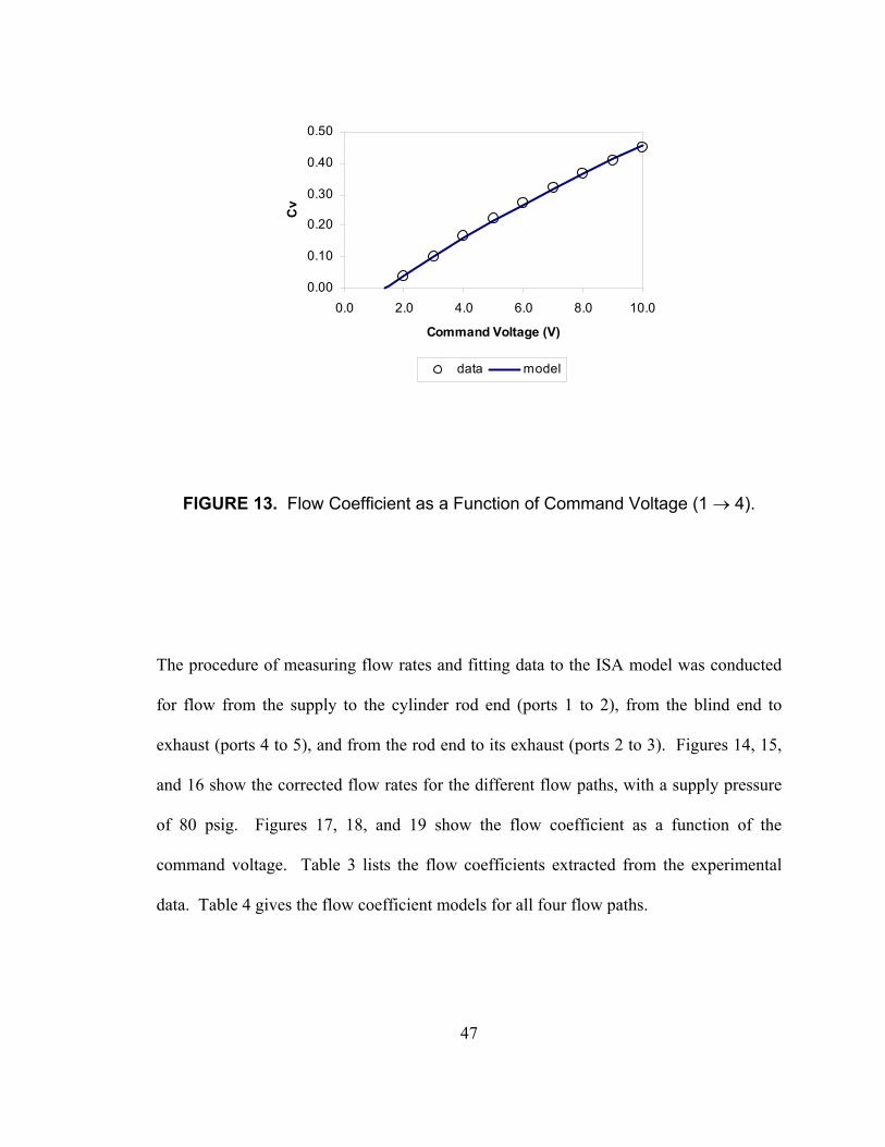
FIGURE 13. Flow Coefficient as a Function of Command Voltage (1 → 4).

The procedure of measuring flow rates and fitting data to the ISA model was conducted

for flow from the supply to the cylinder rod end (ports 1 to 2), from the blind end to

exhaust (ports 4 to 5), and from the rod end to its exhaust (ports 2 to 3). Figures 14, 15,

and 16 show the corrected flow rates for the different flow paths, with a supply pressure

of 80 psig. Figures 17, 18, and 19 show the flow coefficient as a function of the

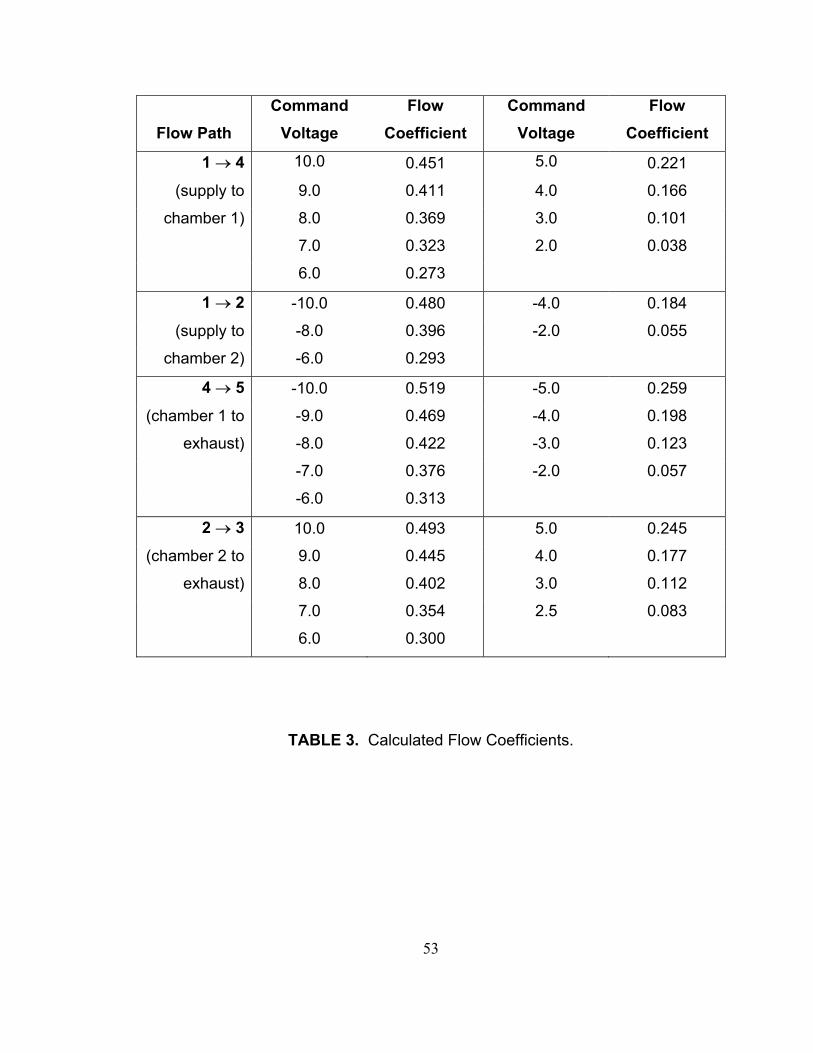
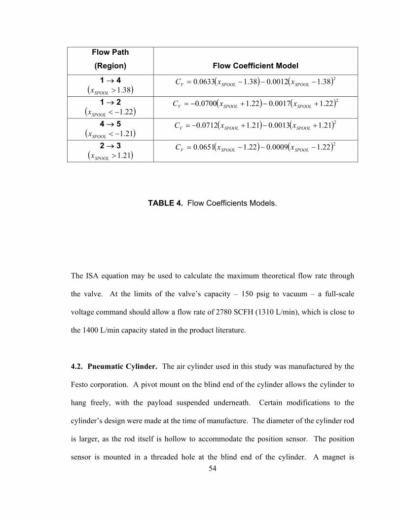
command voltage. Table 3 lists the flow coefficients extracted from the experimental

data. Table 4 gives the flow coefficient models for all four flow paths.

48

0

200

400

600

800

1000

1200

1400

1600

0.2 0.3 0.4 0.5 0.6 0.7 0.8 0.9 1.0

P2/P1

Flow

(SC

FH) -10V

-8V-6V-4V-2V


49

0

200

400

600

800

1000

1200

1400

1600

1800

0.0 0.1 0.2 0.3 0.4 0.5 0.6 0.7 0.8 0.9 1.0

P2/P1

Flow

(SC

FH)

-10V-9V-8V-7V-6V-5V-4V-3V-2V


50

0

200

400

600

800

1000

1200

1400

1600

1800

0.0 0.1 0.2 0.3 0.4 0.5 0.6 0.7 0.8 0.9 1.0

P2/P1

Flow

(SC

FH)

10V9V8V7V6V5V4V3V2.5V


51

0.00

0.10

0.20

0.30

0.40

0.50

-10.0 -7.5 -5.0 -2.5 0.0

Command Voltage (V)

Cv

data model


0.00

0.10

0.20

0.30

0.40

0.50

0.60

-10.0 -7.5 -5.0 -2.5 0.0

Command Voltage (V)

Cv

data model


52

0.00

0.10

0.20

0.30

0.40

0.50

0.0 2.0 4.0 6.0 8.0 10.0

Command Voltage (V)

Cv

data model


53

Flow Path

Command Voltage

Flow Coefficient

Command Voltage

Flow Coefficient

1 → 4 10.0 0.451 5.0 0.221

(supply to 9.0 0.411 4.0 0.166

chamber 1) 8.0 0.369 3.0 0.101

7.0 0.323 2.0 0.038

6.0 0.273

1 → 2 -10.0 0.480 -4.0 0.184

(supply to -8.0 0.396 -2.0 0.055

chamber 2) -6.0 0.293

4 → 5 -10.0 0.519 -5.0 0.259

(chamber 1 to -9.0 0.469 -4.0 0.198

exhaust) -8.0 0.422 -3.0 0.123

-7.0 0.376 -2.0 0.057

-6.0 0.313

2 → 3 10.0 0.493 5.0 0.245

(chamber 2 to 9.0 0.445 4.0 0.177

exhaust) 8.0 0.402 3.0 0.112

7.0 0.354 2.5 0.083

6.0 0.300

TABLE 3. Calculated Flow Coefficients.

54

Flow Path (Region)

Flow Coefficient Model

1 → 4 ( )38.1>SPOOLx

( ) ( )238.10012.038.10633.0 −−−= SPOOLSPOOLV xxC

1 → 2 ( )22.1−<SPOOLx

( ) ( )222.10017.022.10700.0 +−+−= SPOOLSPOOLV xxC

4 → 5 ( )21.1−<SPOOLx

( ) ( )221.10013.021.10712.0 +−+−= SPOOLSPOOLV xxC

2 → 3 ( )21.1>SPOOLx

( ) ( )222.10009.022.10651.0 −−−= SPOOLSPOOLV xxC

TABLE 4. Flow Coefficients Models.

The ISA equation may be used to calculate the maximum theoretical flow rate through

the valve. At the limits of the valve’s capacity – 150 psig to vacuum – a full-scale

voltage command should allow a flow rate of 2780 SCFH (1310 L/min), which is close to

the 1400 L/min capacity stated in the product literature.

4.2. Pneumatic Cylinder. The air cylinder used in this study was manufactured by the

Festo corporation. A pivot mount on the blind end of the cylinder allows the cylinder to

hang freely, with the payload suspended underneath. Certain modifications to the

cylinder’s design were made at the time of manufacture. The diameter of the cylinder rod

is larger, as the rod itself is hollow to accommodate the position sensor. The position

sensor is mounted in a threaded hole at the blind end of the cylinder. A magnet is

55

attached to the back face of the piston, and reduces the stroke of the cylinder by

approximately 25mm. Table 5 lists the cylinder’s properties. Figure 20 shows a cut-

away diagram of the cylinder.

Knowledge of the friction in the cylinder is important in modeling its dynamic motion.

Section 2.2 presents various models for friction between sliding parts. Armstrong-

Hélouvry had presented five- and seven-parameter models for friction in separate papers

[28], [29]. In this work, the friction model will include stiction, Coulomb friction, and

viscous friction (figure 2(b)) as their coefficients may be readily obtained.

Model Number DNG-50-200-P-A

Type Single-rod, double-acting

Piston Diameter 50mm

Rod Diameter 25mm

Stroke 200mm (175mm effective)

Cushioning Length 32mm (7mm effective on

blind end)

Table 5. Pneumatic Cylinder Properties.

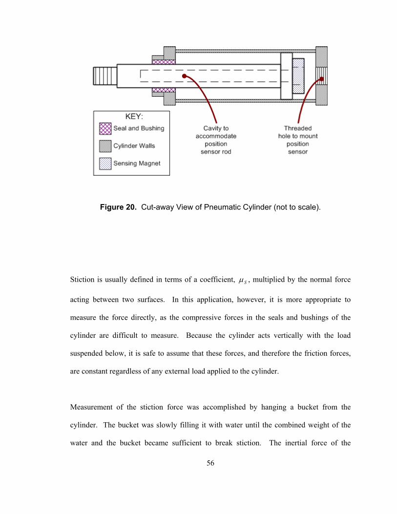
56

Figure 20. Cut-away View of Pneumatic Cylinder (not to scale).

Stiction is usually defined in terms of a coefficient, Sµ , multiplied by the normal force

acting between two surfaces. In this application, however, it is more appropriate to

measure the force directly, as the compressive forces in the seals and bushings of the

cylinder are difficult to measure. Because the cylinder acts vertically with the load

suspended below, it is safe to assume that these forces, and therefore the friction forces,

are constant regardless of any external load applied to the cylinder.

Measurement of the stiction force was accomplished by hanging a bucket from the

cylinder. The bucket was slowly filling it with water until the combined weight of the

water and the bucket became sufficient to break stiction. The inertial force of the

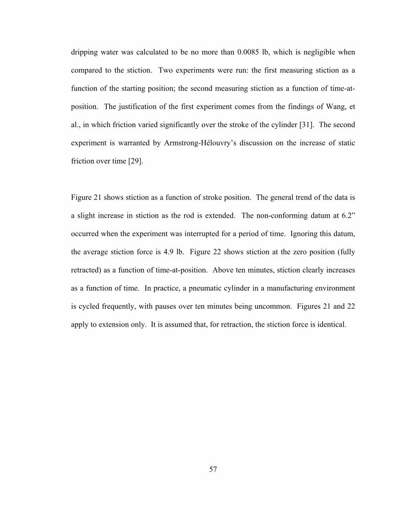
57

dripping water was calculated to be no more than 0.0085 lb, which is negligible when

compared to the stiction. Two experiments were run: the first measuring stiction as a

function of the starting position; the second measuring stiction as a function of time-at-

position. The justification of the first experiment comes from the findings of Wang, et

al., in which friction varied significantly over the stroke of the cylinder [31]. The second

experiment is warranted by Armstrong-Hélouvry’s discussion on the increase of static

friction over time [29].

Figure 21 shows stiction as a function of stroke position. The general trend of the data is

a slight increase in stiction as the rod is extended. The non-conforming datum at 6.2”

occurred when the experiment was interrupted for a period of time. Ignoring this datum,

the average stiction force is 4.9 lb. Figure 22 shows stiction at the zero position (fully

retracted) as a function of time-at-position. Above ten minutes, stiction clearly increases

as a function of time. In practice, a pneumatic cylinder in a manufacturing environment

is cycled frequently, with pauses over ten minutes being uncommon. Figures 21 and 22

apply to extension only. It is assumed that, for retraction, the stiction force is identical.

58

4.00

4.50

5.00

5.50

6.00

6.50

7.00

7.50

0.0 1.0 2.0 3.0 4.0 5.0 6.0 7.0Position (in)

Stic

tion

(lb)

FIGURE 21. Stiction as a Function of Position.

59

4.00

4.25

4.50

4.75

5.00

5.25

5.50

5.75

6.00

0.1 1.0 10.0 100.0 1000.0

Time-at-position (min)

Stic

tion

(lb)

FIGURE 22. Stiction as a Function of Time-at-Position.

To determine the values of Coulomb and viscous friction, the cylinder was allowed to

free-fall with a 22.25-pound load attached to the rod. The weight of the piston and rod is

assumed to be 2.0 lb. Further, it is assumed that the effects of air compression in the rod

end of the cylinder are negligible in this analysis, as the cylinder vents directly to

atmosphere.

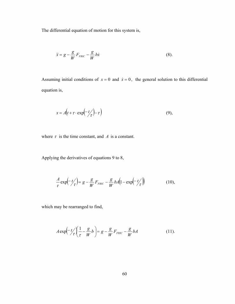
60

The differential equation of motion for this system is,

xbWgF

Wggx FRIC &&& −−= (8).

Assuming initial conditions of 0=x and 0=x& , the general solution to this differential

equation is,

( )( )τττ −−⋅+= ttAx exp (9),

where τ is the time constant, and A is a constant.

Applying the derivatives of equations 9 to 8,

( ) ( )( )τττtbA

WgF

WggtA

FRIC−−−−=− exp1exp (10),

which may be rearranged to find,

( ) bAWgF

Wggb

WgtA FRIC −−=

−−ττ1exp (11).

61

By applying boundary conditions to equation 11, the unknown terms for Coulomb

friction FRICF and viscous friction b may be expressed in terms of A and τ . For 0=t ,

equation 11 simplifies to,

bAWgF

Wggb

WgA FRIC −−=

−τ1 (12).

Rearranging,

−=

τgAWFFRIC 1 (13).

At infinite time ( )∞=t , equation 11 becomes,

bAWgF

Wgg FRIC −−=0 (14),

which allows a quantity for viscous damping to be calculated,

AFW

b FRIC−= (15).

62

0.0

1.0

2.0

3.0

4.0

5.0

6.0

7.0

0.00 0.05 0.10 0.15 0.20

time (sec)

posi

tion

(inch

)

data model

FIGURE 23. Trajectory of Free-Falling Cylinder Payload.

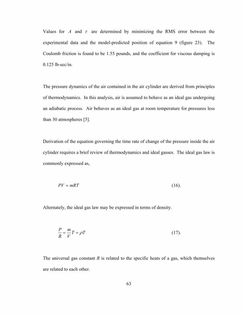
63

Values for A and τ are determined by minimizing the RMS error between the

experimental data and the model-predicted position of equation 9 (figure 23). The

Coulomb friction is found to be 1.55 pounds, and the coefficient for viscous damping is

0.125 lb-sec/in.

The pressure dynamics of the air contained in the air cylinder are derived from principles

of thermodynamics. In this analysis, air is assumed to behave as an ideal gas undergoing

an adiabatic process. Air behaves as an ideal gas at room temperature for pressures less

than 30 atmospheres [5].

Derivation of the equation governing the time rate of change of the pressure inside the air

cylinder requires a brief review of thermodynamics and ideal gasses. The ideal gas law is

commonly expressed as,

mRTPV = (16).

Alternately, the ideal gas law may be expressed in terms of density.

TTVm

RP ρ== (17).

The universal gas constant R is related to the specific heats of a gas, which themselves

are related to each other.

64

VP ccR −= (18).

V

P

cck ≡ (19).

For air, 4.1=k . The relationships of equations 16 through 19 will be exploited in the

following analysis.

Each chamber of the air cylinder is treated as a control volume. The air in a chamber has

an internal energy that is a function of the temperature.

VTcE V ρ= (20).

In an adiabatic process, the time rate of change in the internal energy is equal to the rate

of energy added to the control volume by the incoming air flow, less the rate of work the

control volume performs on the cylinder piston.

( ) VPTcmVTcdtd

PV&& −=ρ (21).

Applying equation 17 to 21 yields,

65

TcmVPPVRc

dtd

PV && =+

(22).

Rearranging terms,

( ) mTcVPPV

dtd

RTcc

PP

V &&

=+ (23).

The derivative of ( )PV is expanded, with equation 19 being applied,

( ) ( ) mVPTckRT

VPkRT P

&&& =

++

111 (24).

Manipulation of 18 and 19 shows,

RckR P

111=+ (25).

Substitution of 25 into 24 yields,

( ) ( ) mVPRT

VPkRT

&&& =

+

11 (26).

Expressing equation 26 in terms of P& ,

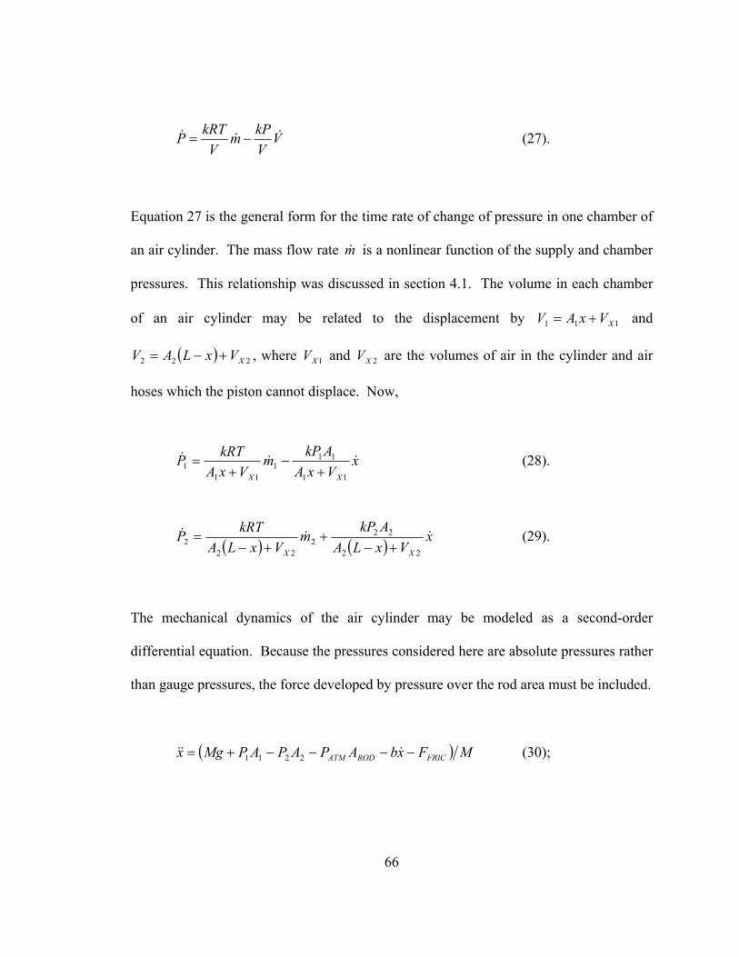
66

VVkPm

VkRTP &&& −= (27).

Equation 27 is the general form for the time rate of change of pressure in one chamber of

an air cylinder. The mass flow rate m& is a nonlinear function of the supply and chamber

pressures. This relationship was discussed in section 4.1. The volume in each chamber

of an air cylinder may be related to the displacement by 111 XVxAV += and

( ) 222 XVxLAV +−= , where 1XV and 2XV are the volumes of air in the cylinder and air

hoses which the piston cannot displace. Now,

xVxAAkP

mVxA

kRTPXX

&&&

11

111

111 +

−+

= (28).

( ) ( ) xVxLA

AkPm

VxLAkRTP

XX

&&&

22

222

222 +−

++−

= (29).

The mechanical dynamics of the air cylinder may be modeled as a second-order

differential equation. Because the pressures considered here are absolute pressures rather

than gauge pressures, the force developed by pressure over the rod area must be included.

( ) MFxbAPAPAPMgx FRICRODATM −−−−+= &&& 2211 (30);

67

4.3. Position Encoder. A Gemco Blue Ox 952QD provides position feedback for the

control system (figure 24). It detects the position of the magnet inside the cylinder, and

sends a quadrature-encoded signal to the control system, in this case the PLC.

FIGURE 24. Blue Ox 952QD Position Encoder.

Position sensing is accomplished through a rod containing a magnetostrictive material,

which is located within a cavity in the piston rod (figure 20). Conceptually similar to a

piezoelectric material, magnetostrictive materials produce a strain in response to a

magnetic field. Every millisecond, a voltage pulse is applied to a conductor located

coaxially with the sensor. The interaction between the electromagnetic fields of the

voltage pulse and the sensing magnet creates a pulse strain in the magnetostrictive

material. A shock wave is created, traveling in both directions along the rod. The time

period between the sending of the voltage pulse to the detection of the shock wave at the

68

base of the rod is converted to distance by multiplication of time by the material’s sonic

velocity.

The Blue Ox output is a quadrature-encoded dual pulse train (figure 25). Counting of the

pulses from channels A and B permit the controller to calculate position and, through

differentiation, velocity. Channels A and B are 90° out of phase from each other to allow

for the determination of the direction of motion. A third channel, Z, flags a zero position

tracked inside the position encoder. Because the output is a pulse train, the encoder

cannot simply instantaneously update a position signal. Instead, the sensor output signal

is linearly interpolated over the next millisecond from the previously scanned position to

the most current position. In this manner the position encoder has a 2 ms total delay in its

output signal – one millisecond to sense, one millisecond to update.

FIGURE 25. Quadrature Encoded Signal.

69

4.4. Programmable Logic Controller. The Allen-Bradley ControlLogix platform

requires two components for motion control. The Logix5550 controller is the main

processor for the ControlLogix PLC. In addition to handling the I/O functions required

for a particular application, it generates a coarse command position for motion control.

The M02AE motion control module actually performs the closed-loop control on the

servo axis.

The Logix5550 controller serves as the main processor for the PLC, running the ladder

logic program for machine control. Inputs and outputs referenced by the Logix5550 may

be identified by their formal address (i.e., Local:2:I.Data.0), or may be assigned to an alias

tag (i.e., HomeLimitSwitch). Unlike older processors, internal objects such as timers and

counters do not have fixed addresses inside the Logix5550 memory, but are assigned with

arbitrary tag names (i.e., FaultResetTimer). Tags may be arranged in arrays with up to

three indices (i.e., GainSelect[3,2,2]).

Ladder logic was originally designed to represent hard-wired relay logic. In relay logic,

each relay “executes” its portion of the control logic simultaneously, limiting the speed of

the controller to the response speed of the individual relays. In PLC-based ladder logic,

the execution of the program is considerably different. First, the processor reads the

inputs and stores their values in a look-up table. Next, the processor executes the ladder

logic sequentially, instead of simultaneously. After going through the ladder once, the

updated output table is sent to the outputs, and the process repeats. In addition to these

70

tasks, the Logix5550 processor performs communication tasks. The scheduling of these

tasks depends on their priority.

The scan time for a processor is a function of overhead from the modules assigned to a

processor, the length of ladder logic to execute, and the number and frequency of

communication tasks. Large scan times can be problematic, as the processor might miss

intermittent signals and not perform as desired. Table 6 lists representative ladder objects

and their associated execution times for the Logix5550.

The M02AE motion control module works with the Logix5550 controller in providing

closed-loop position control of a servo axis. The Logix5550 generates a coarse position

command which is sent to the M02AE. The M02AE then interpolates the coarse position

command to determine the fine position command. The M02AE closes the control loop

at a rate of 5 kHz, which is generally faster than the Logix5550 processor.

Figure 26 shows the control architecture for the M02AE. The structure employs PI

control with a velocity feedforward gain. The command voltage from the M02AE is

given by,

( ) ( ) ( ) OFFSCOMVF

COMICOMPCOM Ukxk

xxkxxkV +⋅

+−⋅+−⋅= ∫ &

25044

(31),

71

COMMAND

DESCRIPTION

TIME IF

TRUE (µs)

TIME IF

FALSE (µs)

XIC Normally Open contact, 0.11 0.05

OTE Boolean output, 0.19 0.19

GRT Greater than comparison, A>B 0.59 0.11

ADD Add two real numbers, A+B 10.7 0.11

MUL Multiply two real numbers, A×B 17.7 0.11

GSV Get system value from controller or

other module

0.16

ActualPosition 160.0

PositionError 110.9

AverageVelocity 250.2

ServoOutputLevel 108.2

SSV Set system value of controller or other

module

0.15

PositionProportionalGain 153.1

VelocityFeedforwardGain 106.1

PositionIntegralGain 218.0

OutputOffset 140.0

Table 6. Execution Times for Ladder Objects.

72

where Pk , Ik , VFk , and Sk are the controller proportional, integral, velocity feedforward,

and output scaling gains, and OFFU is the output offset. The velocity feedforward gain

VFk is expressed as a percentage in the Logix5550 controller, with a gain of 100% being

considered as 1.0 in equation 31. The command output is passed through a 16-bit digital-

to-analog converter. The quadrature pulse train data from the encoder is run though a 16-

bit converter/integrator to determine actual position.

FIGURE 26. M02AE Control Architecture (adapted from [85]).

73

4.5. Plumbing. Friction losses in the plumbing can be significant at high flow rates.

Experimental data can provide the information needed to develop a mathematical model

of the friction loss in the air lines. Figure 27 shows the experimental apparatus used to

measure the pressure drop in the air lines. The length of line between each tee joint is

shown.

Pressure measurements were performed at settings of 80 psig and 60 psig on the

regulator, using the manual flow restriction to vary the flow. Figure 28 shows the

pressure loss from station 1 to station 2 and from station 3 to station 4, as a function of

the standard flow rate.

FIGURE 27. Experimental Apparatus for Measuring Flow Friction.

74

0

0.5

1

1.5

2

2.5

3

3.5

4

0 5 10 15 20

Flow (SCFM)

Loss

(psi

)

1 -> 2, 80 psi 3 -> 4, 80 psi 1 -> 2, 60 psi

3 ->4, 60 psi 1 -> 2 model 3 -> 4 model

Figure 28. Pressure Loss in Air Lines as a Function of Flow Rate.

In figure 28, the difference in the pressure loss from 80 psi to 60 psi is not deemed to be

significant, allowing for a single mathematical model to be developed. The pressure loss

will be modeled as a second-order function of the flow rate. To justify this assumption,

consider friction in incompressible flow in a pipe. In this case, the pipe is air hose having

a 7mm inside diameter. Reynold’s number is given as,

75

µρ DV

=Re (32).

The maximum air flow through the system is about 17 SCFM, as seen in figure 28. The

mean velocity of the air through the air line is given by,

AQV = (33).

For air at standard conditions flowing at 17 SCFM through a 7mm-diameter tube, the

mean velocity is 8200 in/s, or 208 m/s. Note that for air at a constant temperature,

Reynold’s number is independent of density. As density increases, the actual velocity of

the gas decreases by an identical factor, leaving Reynold’s number unchanged. Using

equation 32, the maximum Reynold’s number is approximately 105, well into the

turbulent regime.

In [87], the calculation for head loss in internal flow is given by,

2

2VDLfhL = (34),

76

where f is an experimentally-derived friction factor. L. F. Moody published a chart

detailing the friction factor as a function of Reynolds number and the surface roughness

relative to the pipe diameter [86, as cited in 87].

While the friction factor is a function of Reynold’s number, it will be assumed to be

constant for the purposes of this study. This allows the friction loss in equation 34 to be a

function of the mean fluid velocity, which is proportional to the flow rate. Returning to

figure 28, a best-fit parabola may be assigned to the pressure loss from stations 1 to 2 and

from stations 3 to 4. The equations are,

221 0125.0 QP ⋅=∆ → (35),

243 0037.0 QP ⋅=∆ → (36).

Equation 35 has a R2 value of 0.92, while equation 36 has an R2 of only 0.71. The

smaller confidence in the second equation is due to the range of data being less than one

order of magnitude larger than the resolution of the data.

Equation 35 expresses a coefficient corresponding to the pressure loss over only 1500

mm of tubing. In the experimental system (figure 30), air passes through tubing of

different lengths, in addition to straight and elbowed fittings. Fox and McDonald assign

equivalent lengths to standard fittings. Knowing the equivalent length of a section of

plumbing, one can scale the coefficient of equation 35 to find the appropriate friction loss

equation. For the air line supplying the valve, the coefficient is calculated to be 0.0555.

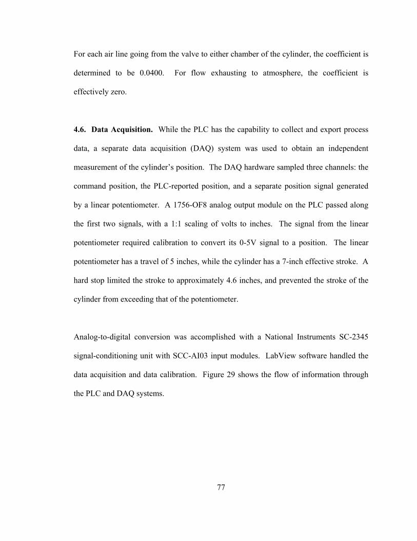
77

For each air line going from the valve to either chamber of the cylinder, the coefficient is

determined to be 0.0400. For flow exhausting to atmosphere, the coefficient is

effectively zero.

4.6. Data Acquisition. While the PLC has the capability to collect and export process

data, a separate data acquisition (DAQ) system was used to obtain an independent

measurement of the cylinder’s position. The DAQ hardware sampled three channels: the

command position, the PLC-reported position, and a separate position signal generated

by a linear potentiometer. A 1756-OF8 analog output module on the PLC passed along

the first two signals, with a 1:1 scaling of volts to inches. The signal from the linear

potentiometer required calibration to convert its 0-5V signal to a position. The linear

potentiometer has a travel of 5 inches, while the cylinder has a 7-inch effective stroke. A

hard stop limited the stroke to approximately 4.6 inches, and prevented the stroke of the

cylinder from exceeding that of the potentiometer.

Analog-to-digital conversion was accomplished with a National Instruments SC-2345

signal-conditioning unit with SCC-AI03 input modules. LabView software handled the

data acquisition and data calibration. Figure 29 shows the flow of information through

the PLC and DAQ systems.

78

FIGURE 29. Data Acquisition Hardware.

79

CHAPTER 5

SYSTEM MODEL

The conventional method for describing the state of a linear pneumatic actuator uses four

parameters that may be measured directly: position x , velocity x& , and pressures 1P and

2P . An alternate representation substitutes mass for pressure in each chamber of the

cylinder. The mass-based representation allows for an analysis of the observability and

controllability of the pneumatic actuator system. For simulation purposes, the

conventional representation is used.

5.1. Conventional State Representation. Figure 30 shows a typical servopneumatic

system. Note the vertical arrangement of the pneumatic cylinder. The nonlinear

differential equations to describe the dynamics of the conventional state variables – x ,

x& , 1P , and 2P – are derived in chapter 4, and restated here.

xVxAAkP

mVxA

kRTPXX

&&&

11

111

111 +

−+

= (28).

80

Figure 30. Servopneumatic System.

81

( ) ( ) xVxLA

AkPm

VxLAkRTP

XX

&&&

22

222

222 +−

++−

= (29).

( ) MFxbAPAPAPMgx FRICRODATM −−−−+= &&& 2211 (30);

The mass flow rate into the blind end of the cylinder, 1m& , may be calculated from

knowledge of the valve spool position and the system pressures. The ISA model is used

to predict flow rates. Equation 5 presents the ISA model in terms of volumetric flow. It

may be expressed as a mass flow rate through multiplying by the density of air at

standard conditions. For the Festo MPYE-5 valve used in this study ( 0.1=TX ),

equation 37 expresses mass flow into chamber 1. Mass flow rate is measured in

lb-s2/in-s, pressure in psia, and temperature in °R.

−×

×=

TXXPCm HIV 3

167.22109.302

131& (37),

where,

−=

−=

HI

LO

HI

LOHI

PP

PPP

X 1 (38).

The flow coefficient VC is a function of the spool position SPOOLx , which is assumed to be

a first-order function of the voltage command COMV sent to the valve. The actual

82

displacement of the spool is unknown; it is assigned an arbitrary unit of measure so that a

one-volt command signal to the valve produces a one-unit steady-state displacement in

the spool. This allows the differential equation for the spool motion to be expressed as,

( )SPOOL

SPOOLCOMSPOOL

xVx

τ−

=& (39).

In equation 38, it is necessary to determine the proper values of HIP and LOP . These

pressures are selected from 1P , SP , and ATMP based on the spool position and the

instantaneous value of 1P . Table 7 shows the switching logic used to determine HIP and

LOP for the blind end of the cylinder.

Equations 37 and 38 may also be applied to determine the mass flow rate into the rod end

of the cylinder, 2m& . Table 8 presents the logic to determine HIP and LOP for the rod end.

83

XSPOOL

Chamber 1 Connection

Pressure relationship

PHI

PLO

Positive Supply P1 > PS P1 PS

P1 < PS PS P1

Negative Atmosphere P1 > PATM P1 PATM

P1 < PATM PATM P1

TABLE 7. Logic to Determine PHI and PLO for the Cylinder Blind End.

XSPOOL

Chamber 2 Connection

Pressure relationship

PHI

PLO

Positive Atmosphere P2 > PATM P2 PATM

P2 < PATM PATM P2

Negative Supply P2 > PS P2 PS

P2 < PS PS P2

TABLE 8. Logic to Determine PHI and PLO for the Cylinder Rod End.

84

5.2. Mass-Based System Representation. Equations 28, 29 and 30 describe the

conventional state representation of a pneumatic cylinder. This representation requires

knowledge of the mass flow rates in equations 28 and 29. However, it is possible to

replace pressure with mass in the state representation of the system by integrating the

mass flow rate of equation 37.

∫∫

−×

×== dt

TXX

PCdtmm HIV11

1,311 3167.22

109.3021

&

(40).

∫∫

−×

×== dt

TXX

PCdtmm HIV22

2,322 3167.22

109.3021

&

(41).

The mechanical dynamics of equation 30 must be related to mass instead of pressure.

Recall the ideal gas law,

mRTPV = (16).

The ideal gas law may be restated to express pressure in terms of mass for each chamber

of the cylinder. It is assumed here that, while the process is adiabatic, the actual

temperature change in the system is negligible.

85

11

11

XVxARTm

P+

= (42).

( ) 22

22

XVxLARTm

P+−

= (43).

The terms 1Tx and 2Tx are introduced to express the excess volumes 1XV and 2XV as

added length at either end of the cylinder.

1

11 A

Vx X

T = (44).

2

22 A

Vx X

T = (45).

Now, equation 30 becomes,

( )

−−−

+−−

++= FRICRODATM

TT

FxbAPxxL

RTmxx

RTmMg

Mx &&&

2

2

1

11

(46).

A mass-based representation of a pneumatic system allows for the calculation of the

system’s equilibrium position, EQx , using 1m and 2m . For a closed pneumatic cylinder

with no leakage, Coulomb friction, nor stiction, equilibrium is established at,

86

2211 APAP = (47).

Application of equations 42, 43, 44, and 45 to 47 yields,

( ) 2

2

1

1

TEQTEQ xxLm

xxm

+−=

+ (48).

Solving for EQx ,

( )21

1221

mmxmxLm

x TTEQ +

−+= (49).

In the real system, there is a region about EQx in which stiction is sufficient to resist the

restoring force in the cylinder.

Knowing the equilibrium position, one can express the mechanical dynamics of the

system (equation 46) as a function of displacement away from equilibrium. The desired

form of the equation is,

( )( )FRICRODATMCYL FAPxbxkMgM

x −−−∆−= &&&~1 (50),

where,

87

EQxxx −=∆ (51).

In 50, CYLk~ is the equivalent, nonlinear spring stiffness of the air entrained in the cylinder,

which may be derived from an energy analysis. Assuming the compression and

expansion of the air in the cylinder is performed adiabatically, the initial (equilibrium)

energy is equal to the displaced energy state of the air plus the potential energy stored in

the compressed air.

SPRINGAIREQ EEE += (52).

The initial energy of the gas is given by equation 20,

VTcE V ρ= (20).

Since mass is equal to density multiplied by volume, equation 20 applied to chamber 1 of

the cylinder may be expressed as,

TmcE VEQ 11, = (53).

Substituting the expression of the ideal gas law as presented in equation 42,

88

( )R

VxAPcE XEQ

VEQ111

1,

+= (54).

Applying equations 18 and 19,

( )1

1111, −

+=

kVxAP

E XEQEQ (55).

When the cylinder is displaced from equilibrium, the energy state of the air changes.

Equation 55 becomes,

( ) ( )( )1

11111, −

+∆+∆+=

kVxxAPP

E XEQAIR (56).

The potential energy stored by the gas in chamber 1, acting as a spring, is given by,

211,

~21 xkESPRING ∆= (57),

where 1~k is the effective nonlinear spring rate for chamber 1, and is defined as the change

in force per unit displacement.

xAP

xFk

∆∆−

=∆∆−

= 111

~ (58).

89

Substituting equations 55, 56, and 57 into 52 yields,

( ) 21111111111111111

~2

1 xkkVPPxAPxAPxAPxAPVPxAP XEQEQXEQ ∆−

+∆++∆∆+∆+∆+=+

(59).

Terms appearing on both sides of equation 55 are eliminated through subtraction, and a

division by x∆ is performed.

xkkA

VxAPx

xAPAPx

xAP X

EQ ∆−

+

∆∆

+∆

∆∆

++

∆∆

= 11

1111111

11 ~2

10

(60).

Substitution of equations 58 and 44 into 60 yields,

−

∆−+=2

3~1111

kxxxkAP TEQ (61).

Equations 42 and 44 are applied to eliminate pressure.

−

∆−+=+ 2

3~11

11

1 kxxxkVxA

RTmTEQ

XEQ

(62).

Rearranging, one finds the spring stiffness of chamber 1 to be,

90

( )

∆

−+++

=xkxxxx

RTmkTEQTEQ 2

3~

11

11 (63).

A similar analysis may be performed on the rod end of the cylinder (chamber 2). Note

that, for the rod end of the cylinder, the mathematical definition of stiffness is the

negative of that in equation 58. A positive x∆ acts in the opposite direction on chamber

2 than on chamber 1, creating the need for a sign change.

xAP

xFk

∆∆

=∆−∆−

= 222

~ (64).

Now, the energy analysis yields,

( )( ) ( )

∆

−++−+−

=xkxxLxxL

RTmkTEQTEQ 2

3~

22

22 (65).

The net stiffness of the air cylinder is the sum of the individual stiffness of each chamber

of the cylinder.

91

( ) ( )( ) ( )

∆

−++−+−

+

∆

−+++

=

+=

xkxxLxxL

m

xkxxxx

mRT

kkk

TEQTEQTEQTEQ

CYL

23

23

~~~

22

2

11

1

21

(66).

Equation 66 shows the stiffness of the cylinder is an inverse function of the positions x

and ( )xL − . The stiffness is also dependent on the magnitude of the displacement.

When the equilibrium position lies near either extreme of motion, the effects of

displacement on the effective stiffness should not be neglected. Around the middle of the

stroke, the displacement from equilibrium has a smaller effect. If displacement were to

be ignored, equation 66 is expressed as,

( ) ( )( )

+−+

+≅ 2

2

22

1

1~

TEQTEQCYL xxL

mxx

mRTk (67).

5.3. Controllability and Observability. While the dynamics of a servopneumatic

actuator are highly nonlinear, analysis of a linearized model allows for discussion of the

controllability and observability of the servopneumatic system. To develop the

controllability and observability matrices, physical processes will be modeled with gains

assumed to be constant, CYLk and EQk . A discussion of the effects of the state-dependent,

varying gains CYLk~ and EQk~ follows the derivation of the linear model.

92

Equation 50 describes the dynamics of the system about equilibrium. For this analysis,

Coulomb friction is neglected, as is the atmospheric pressure acting over the area of the

cylinder rod. Practically, these two forces are significantly lower than the full pressure

developed by the cylinder’s blind end. Static friction develops 5 lb of force; atmospheric

pressure over the rod area develops 11 lb; while the piston develops nearly 300 lb at 95

psia. Additionally, the effect of gravity on the payload is ignored. With these

assumptions in place, equation 50 may now be expressed as,

( ) xMbxx

Mkx EQ

CYL &&& −−−

= (68),

The rate of change of the equilibrium position EQx is also needed to analyze observability

and controllability. Recall the equilibrium position given in equation 49,

( )21

1221

mmxmxLm

x TTEQ +

−+= (49).

Differentiating yields,

( )( )

+−

++= 221

122121 mm

mmmmxxLx TTEQ

&&& (69).

Equation 69 may be simplified by assuming that the mass of air within the cylinder is

constant. This implies the mass flow rate going into one chamber is equal to the mass

93

flow rate going out the other, or 21 mm && −= . This assumption is validated through

consideration of the derivative of the ideal gas law (equation 16), assuming velocity,

pressure, and temperature are constant. Applied to both chambers, the derivative of

equation 16 may be stated as,

RTmxAP 111 && = (70).

RTmxAP 222 && =− (71).

At a constant velocity, the pressure forces on either face of the piston are balanced

(equation 47). Applying equations 70 and 71 to equation 47,

xRTm

xRTm

&

&

&

& 21 −= (72).

It is clear from equation 72 that, under certain conditions, the assumption of constant

mass in the cylinder is valid when the cylinder is moving at a constant velocity. If the

cylinder reaches either hard limit of its stroke, though, this assumption of constant mass

in the cylinder will not be valid.

Applying the constant air mass assumption, equation 69 becomes,

94

1mmL

x TEQ && = (73).

where,

21 TTT xxLL ++= (74),

and,

21 mmm += (75),

The relationship between the command voltage to the valve, the valve spool position, and

the mass flow rate is discussed in detail in section 4.1. For the sake of argument, the

response time of the valve (equation 39) will be assumed to be small enough to be

neglected, and the nonlinear flow function will be assumed to be a linear function of the

command voltage only, so that,

COMVALVEVkm =1& (76).

Equations 73 and 76 may be combined to relate the equilibrium position to the command

voltage sent to the valve.

95

COMEQCOMVALVET

EQ VkVkmLx ==& (77).

Figure 31 shows the block diagram of the linear model of the pneumatic system.

Examination shows the linear transfer function for the pneumatic actuator to be,

( )CYL

CYLEQ

COM kbsMsskk

Vx

++= 2 (78).

FIGURE 31. Block Diagram of the Pneumatic System.

96

Equation 78 may also be expressed as a linear state-space matrix, with the state vector

being defined as [ ]TEQxxx &=X .

COM

EQEQ

CYLCYL

EQ

Vkx

xx

Mk

Mb

Mk

xxx

+

−−=

= 00

000

010&

&

&&

&

&X

(79).

Position is available for feedback control.

[ ] [ ]x== XY 001 (80).

Equations 79 and 80 permit testing of controllability and observability. The pair (A, B) is

controllable when the controllability matrix U is non-singular. Likewise, the pair (A, C)

is observable when the observability matrix V is non-singular.

[ ]

−==

00

0

00

2

EQ

EQCYLEQCYL

EQCYL

kM

kkbM

kkM

kk

BAABBU 2

(81).

97

−−=

=

Mk

Mb

Mk CYLCYL

010001

2CACAC

V (82).

Matrices U and V are singular only when their determinants are zero. From equations 81

and 82, the determinants are found to be,

2

23

Mkk CYLEQ−

=U (83),

MkCYL=V (84).

From equations 83 and 84, it may be said that the ideal servopneumatic axis with position

feedback is always controllable and always observable, as the determinants of both

matrices are strictly nonzero.

Constant, positive gains CYLk and EQk were applied to determine the controllability and

observability of the servopneumatic system. In the real system, these gains are not

constant but vary according to the state of the system. Variable gains CYLk~ and EQk~ may

be substituted into equations 83 and 84 to evaluate the effects of nonlinearities on the

controllability and observability.

98

Figure 32 shows the true stiffness, CYLk~ , as a function of stroke, assuming 0=∆x , for the

cylinder used in this study (equation 67). While the stiffness varies by almost two orders

of magnitude, it is always positive. In applying this to the observability of the system as

given in equation 84, one finds the observability to be strictly positive.

0~

>=M

kCYLV (85).

10

100

1000

0.0 1.0 2.0 3.0 4.0 5.0 6.0 7.0

Position (in)

Stif

fnes

s (lb

/in)

Figure 32. Stiffness of a Pneumatic Cylinder versus Equilibrium Position.

99

The effect of the varying stiffness on the controllability, given in equation 83, is more

dramatic. The term 2~CYLk is again strictly positive, but varies by four orders of magnitude

over the stroke. This implies the cylinder is much less controllable in the mid-stroke

region, as opposed to near the extremes of motion.

The other contributing factor to controllability is the gain EQk~ , relating the equilibrium

position EQx to the command voltage COMV . Equation 77 defined the linear gain EQk as a

product two gains – one for the cylinder dynamics (equation 73), and the other for the

valve dynamics (equation 76).

COMVALVET

EQ VkmLx =& (77).

The consistency of the cylinder dynamics term, mLT , is dependent on the assumption of

a constant mass of air in the air cylinder. As discussed earlier, this assumption is not

strictly true, but is not seriously violated as long as the cylinder does not reach either

physical limit of travel. Of greater concern to the issue of controllability are the valve

dynamics, VALVEk~ , relating the mass flow rate to the command voltage.

The flow relationship is derived in chapter 4, according to the ISA model of flow through

a valve. For chamber 1, this relationship is expressed as,

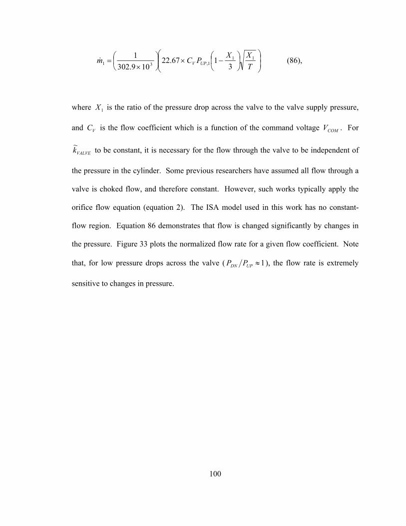
100

−×

×=

TXX

PCm UPV11

1,31 3167.22

109.3021

& (86),

where 1X is the ratio of the pressure drop across the valve to the valve supply pressure,

and VC is the flow coefficient which is a function of the command voltage COMV . For

VALVEk~ to be constant, it is necessary for the flow through the valve to be independent of

the pressure in the cylinder. Some previous researchers have assumed all flow through a

valve is choked flow, and therefore constant. However, such works typically apply the

orifice flow equation (equation 2). The ISA model used in this work has no constant-

flow region. Equation 86 demonstrates that flow is changed significantly by changes in

the pressure. Figure 33 plots the normalized flow rate for a given flow coefficient. Note

that, for low pressure drops across the valve ( 1≈UPDN PP ), the flow rate is extremely

sensitive to changes in pressure.

101

0.0

0.2

0.4

0.6

0.8

1.0

0.0 0.2 0.4 0.6 0.8 1.0

Pdn/Pup

Flow

Figure 33. ISA Model for Flow Rate.

In addition to nonlinear pressure dynamics in flow, the relationship between the flow

coefficient and the command voltage is nonlinear. Section 4.1 derives models for four

flow paths through the valve. Figure 34(a) shows the flow coefficient model for flow

from port 1 to port 4, with the ideal linear relationship superimposed. Figure 34(b) shows

the equivalent gain for both the real and ideal models. The significant conclusion to be

drawn from figure 34 is that the dead band about a null voltage command creates a region

in which the gain describing the valve dynamics, VALVEk~ , is zero. Graphs similar to figure

34 may be developed for the other flow paths.

102

0.0

0.1

0.2

0.3

0.4

0.5

0 10

Vcom (V)

Cv

Cv ideal Cv

0.00

0.01

0.02

0.03

0.04

0.05

0 10

Vcom (V)

gain

(Cv/

V)

Kcv ideal Kcv

(a) (b)

FIGURE 34. Flow Coefficient Function for (1 → 4). (a) VC . (b) COMV VC .

Controllability may now be summarized as follows. The linear model presents the

determinant for the controllability matrix, Mkk CYLEQ23=U , as being a nonzero positive

number, implying controllability always exists. However, the nonlinear controllability

determinant, Mkk CYLEQ23 ~~

=U , is not guaranteed to be nonzero, and can vary by orders of

magnitude. Generally speaking, controllability is lower in the middle of the stroke, and

at low command speeds where the proportional valve operates near its dead band.

103

5.4. Further Considerations on the Linear Model. The linear model developed for

examination of controllability and observability may be used to characterize the

fundamental dynamics of the servopneumatic hardware, and to study closed-loop

behavior of the system with a PI controller.

Equation 79 allows for a brief discussion of the internal dynamics of a servopneumatic

system. The characteristic equation of the system is given as,

sM

ks

Mbs CYL++= 23χ (87).

The roots of equation 87 may be found to be,

0=s , iMb

Mk

Mbs CYL ⋅−±

−= 2

2

42 (88).

For the experimental hardware used in this study, the mass, M, is 0.0628 lb-sec2/in, and

the coefficient of viscous damping, b, is 0.125 lb-sec/in. The stiffness CYLk~ is not

constant, but varies depending of the position of the cylinder (equation 66). For air at 80

psig, the stiffness varies between 11.9 and 1410 lb/in (figure 32). Using these values, the

servopneumatic system is found to have a pole at the origin, and a complex pole pair

which is highly oscillatory over the entire stroke of the cylinder (table 9).

104

x (in) CYLk (lb/in) System Roots

0.5 142.22 0=s is ⋅±−= 6.47995.0

2.0 18.38 0=s is ⋅±−= 1.17995.0 3.5 11.09 0=s is ⋅±−= 3.13995.0

5.0 20.53 0=s is ⋅±−= 1.18995.0

6.5 147.18 0=s is ⋅±−= 4.48995.0

TABLE 9. Servopneumatic System Pole Locations.

FIGURE 35. Block Diagram of the M02AE Servo Controller (from [85]).

105

The servo axis controller used in this study is the Allen-Bradley M02AE. This module is

designed to interface two DC servomotor axes to a programmable logic controller (PLC).

Figure 35 shows the control structure for one channel of the M02AE. With the linear

model of the pneumatic cylinder (equation 78), the transfer function relating the

command signal REFx to x may be derived.

( )( )( ) ( )IEQCYLSPEQCYLSCYL

IPVFEQCYLS

REF kkkkskkkkskbsMskskskkkk

xx

++++

++= 234

2

(89).

By setting certain controller gains to zero, the number of system poles and zeroes

changes, altering the dynamics of the closed-loop system.

Proportional gain only.

( )( )( )PEQCYLSCYL

PEQCYLS

REF kkkkskbsMskkkk

xx

+++= 23 (90).

Proportional gain plus velocity feedforward.

( )( )( )PEQCYLSCYL

PVFEQCYLS

REF kkkkskbsMskskkkk

xx

+++

+= 23 (91).

106

Velocity feedforward only.

( )( )CYL

VFEQCYLS

REF kbsMskkkk

xx

++= 2 (92).

Of these three control schemes, the velocity feedforward-only control structure will not

pursue zero tracking error. Examination of figure 35 shows a feedforward-only structure

eliminates the position feedback from the control loop. While the equation 1=VFEQS kkk

would mathematically guarantee zero tracking error, the variation in eqk~ precludes such a

solution from being realized in practice.

107

CHAPTER 6

MODEL VERIFICATION

Chapter 5 presented a systems model for the pneumatic cylinder and proportional valve

used in this study. Four state variables, having nonlinear differential equations of motion,

describe the pneumatic cylinder. A fifth variable is assigned to the spool position of the

proportional valve, with a first-order linear differential equation describing its dynamics.

In addition, there exists signal lag in the position sensor and the M02AE servo motion

control module. A computer simulation, incorporating these characteristics of the

experimental apparatus, is developed to verify the model of the system.

This chapter is organized as follows. Section 6.1 discusses the tuning of the PI controller

gains on the M02AE module. Section 6.2 describes the servo trajectories studied in this

work. Section 6.3 presents the development and result of the simulation, comparing its

performance with that of the experimental equipment. A discussion of the results appears

in section 6.4.

108

6.1. PI Tuning. The M02AE module is capable of auto-tuning a servo axis. The user

must define the travel limit, travel direction, and maximum velocity for the tuning

motion. In addition, the desired damping factor of the closed-loop system is required.

Allen-Bradley suggests a damping factor of 0.8 as a compromise between fast response

and stability. Using a pneumatic cylinder, the tuning procedure was initiated with the

cylinder near its mid-stroke position.

The auto-tuning procedure determines the values for the closed-loop gains, and other

controller properties. Adjustment of these properties after auto-tuning was done to

improve the performance of the PI loop over the entire stroke of the cylinder. Table 10

lists the relevant properties and their assigned values.

Property Value

Proportional gain 0.00086

Integral gain 0.0006

Velocity feedforward gain 4%

Output scaling gain 1000.0

Friction compensation 0.0 V

Output offset 0.0 V

Output filter bandwidth 1000 Hz

TABLE 10. PI Control Loop Gains.

109

6.2. Servo Trajectories. A family of reference trajectories are used to evaluate

control strategies. The reference trajectories fall into one of three categories: a ramp, a

cam profile, or a quadratic sine trajectory. Each category emphasizes different

performance characteristics of the servopneumatic axis. Recall the positive x-direction of

the servo axis (extension) points down.

The ramp trajectory follows a trapezoidal velocity profile in moving from a 0.5-inch

command position to a 4.0-inch command position and back, with a 0.5-second pause

between each motion (figure 36). Acceleration and deceleration are both set to 50 in/s2.

This trajectory allows for analysis of the controller’s ability to follow a constant velocity

command. Experimental data was collected at maximum command velocities of 0.24,

0.32, 0.42, 0.56, 1.0, 1.8, 3.2, 5.6, and 10 inches per second. Additional data was

collected at a command velocity of 18 inches per second, but the acceleration does not

allow the velocity to reach its maximum value in the length of the stroke.

110

FIGURE 36. Ramp Trajectory. (a) velocity, (b) position.

The cam profile was designed to mimic a command trajectory developed by the sponsors

of this research. Their reference trajectory, shown in figure 37, needed modification as it

was designed for a cylinder with a longer stroke. The cam profile developed for

experimentation uses three triangular velocity steps (figure 38). The time period T to

realize each step of the profile is identical. This trajectory forces the controller to follow

a continuously-varying profile, including an instantaneous stop. Table 11 lists the step

times used in experimentation, with the corresponding accelerations and peak velocities

for each leg.

111

0

2

4

6

8

0 1 2 3

Time (s)

Posi

tion

(in)

FIGURE 37. Reference Cam Profile Trajectory.

FIGURE 38. Cam Profile Trajectory. (a) velocity, (b) position.

112

Step 1

0.5” → 4.0”

Step 2

4.0” → 2.0”

Step 3

2.0” → 0.5”

Step period T (s)

Peak velocity

(in/s)

Accel. (in/s2)

Peak velocity

(in/s)

Accel. (in/s2)

Peak velocity

(in/s)

Accel. (in/s2)

0.2 35 350 20 200 15 150

0.5 14 56 8.0 32 6.0 24

1.0 7.0 14 4.0 8.0 3.0 6.0

2.0 3.5 3.5 2.0 2.0 1.5 1.5

3.0 2.33 1.56 1.33 0.89 1.00 0.67

TABLE 11. Cam Profile Trajectory Data.

A quadratic sine profile (figure 39) mimics a true sine wave pattern using parabolic curve

segments, and was selected to allow for testing of a repeating profile. Its velocity profile

is a triangle wave. The defining time period T for the quadratic sine wave is equal to the

waveform’s half-period. Table 12 lists the peak velocities and accelerations used in this

work.

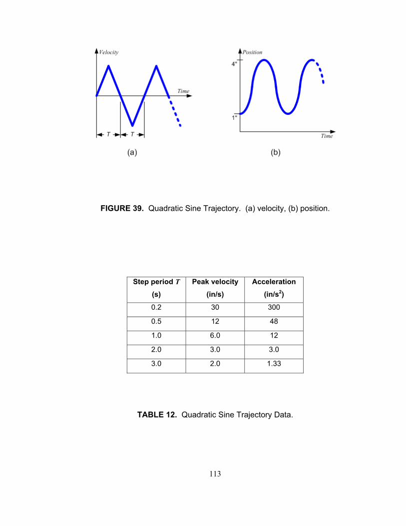
113

FIGURE 39. Quadratic Sine Trajectory. (a) velocity, (b) position.

Step period T (s)

Peak velocity (in/s)

Acceleration (in/s2)

0.2 30 300

0.5 12 48

1.0 6.0 12

2.0 3.0 3.0

3.0 2.0 1.33

TABLE 12. Quadratic Sine Trajectory Data.

114

6.3. Simulation and Discussion. A numerical simulation of the servopneumatic axis

and controller is developed to verify the mathematical model of the system discussed in

Chapter 5. The simulation also allows for examination of processes the experimental

apparatus cannot observe. Two corrective factors were implemented in the model to

allow the simulated dynamics to better match those of the real system. Representative

comparisons between the simulated and actual runs are presented.

The simulation was realized in MATLAB using x , x& , 1P , and 2P as the state variables.

Their derivatives are given by equations 28, 29, and 30. An additional state is added to

incorporate the dynamics of the valve spool position (equation 39). A simultaneous

solution for the mass flow rates (equations 37 and 38) and the pressure losses in the air

lines (figure 28) is needed. An algebraic solution to this system of equations is not

apparent, so an iterative bisection process is used. In development, it was found that any

expected combination of valve spool position and system pressures converges to a 0.1%

error band in 20 iterations or less. The effects of propagation delays in the air lines are

ignored.

Euler integration is used to update the state variables, using a time step of 50 µs. This

time step was selected as to allow for 4 updates of the state variables in each update

period of the M02AE servo motion controller (200 µs). The PLC control loop is updated

every 3000 µs, which is a typical PLC scan time for the programs used in this research.

Data from the simulation is collected in 1.0 ms intervals.

115

0.0

1.0

2.0

3.0

4.0

5.0

0.0 0.5 1.0 1.5 2.0

Time (s)

Posi

tion

(in)

Xcom X

(a)

0.0

1.0

2.0

3.0

4.0

5.0

0.0 0.5 1.0 1.5 2.0

Time (s)

Posi

tion

(in)

Xcom X

(b)

Figure 40. 18 in/s Ramp Trajectory. (a) Simulation, (b) Data.

116

Figure 40(a) shows the simulated servopneumatic axis following the 18.0 in/s ramp

trajectory. Comparing this to the experimental data of figure 40(b), it is observed that the

simulation is much less damped than the real system. Examination of the closed-loop

system pole locations verifies the oscillatory nature of the simulation. In chapter 5, the

linear transfer function of the closed-loop system was determined to be,

( )( )( ) ( )IEQCYLSPEQCYLSCYL

IPVFEQCYLS

REF kkkkskkkkskbsMskskskkkk

xx

++++

++= 234

2

(89).

Chapter 4 discussed the determination of the payload mass M (0.0628 lb-s2/in) and the

coefficient of viscous damping b (0.125 lb-s/in). The controller gains were presented

earlier in this chapter. Recall that their usage in equation 89 must be modified in light of

the discussion in chapter 4 regarding the actual voltage output from the controller.

( ) ( ) ( ) OFFSCOMVF

COMICOMPCOM Ukxk

xxkxxkV +⋅

+−⋅+−⋅= ∫ &

25044

(31).

Equation 89 assumes constant values for the spring stiffness of the air in the cylinder,

CYLk , and the voltage-to-velocity gain EQk . In reality, these gains vary significantly. To

find the instantaneous pole locations of the servopneumatic system, the non-constant

gains CYLk~ and EQk~ will be substituted into equation 89. Chapter 5 discussed the actual

117

cylinder stiffness CYLk~ as a function of position, finding it to vary between 11.9 and 1410

lb/in (figure 32).

The voltage-to-velocity gain EQk~ was defined implicitly in equation 77 as the product of

the valve flow gain and the conversion of mass flow rate to cylinder velocity.

COMEQCOMVALVET

EQ VkVkmLx ==& (77).

The valve flow gain VALVEk is not a true constant, but varies between zero and an upper

limit that is estimated here. Consider flow through the proportional valve from port 1 to

port 4, with a constant 10-volt command signal being applied to the valve. The flow

coefficient, using the appropriate equation from table 4 (equation 93), is calculated to be

0.46.

( ) ( )238.10012.038.10633.0 −−−= SPOOLSPOOLV xxC (93).

For the purposes of calculating a flow rate, assume a supply pressure of 95 psia, pure

vacuum in the cylinder, and no flow losses. With these assumptions, the ISA model

(equations 5 and 6) shows the flow rate into the cylinder to be 28.7 SCFM, or

94.9·10-6 lb-s2/in-s. The upper bound of the valve flow gain VALVEk~ may be calculated to

be 9.5·10-6 lb-s2/in-s using equation 76.

118

COMVALVEVkm =1& (76).

Ignoring for now any volume in the air lines, the equivalent length of the air cylinder TL

is equal to its stroke L , 7.0 in. The mass of the air in the cylinder may be found using

the ideal gas equation,

mRTPV = (16).

Being conservative, the volume will be assumed to be that of the rod end of the cylinder

when the cylinder is fully retracted (16.0 in3), and that atmospheric pressure exists in the

cylinder (14.7 psia). At standard temperature (528 °R), the mass of air inside the cylinder

is calculated to be 1.8·10-6 lb-s2/in.

Knowing the upper bound of VALVEk~ , the equivalent length TL , and a conservative

estimate of the air mass m, the upper bound of the voltage-to-velocity gain EQk~ may be

calculated using equation 94, derived from equation 77. It is found to be

36.9 in/s-V.

MAXVALVET

MAXEQ kmLk ,,

~~= (94).

119

Returning to the linear transfer function of equation 89, the constant value or the limits of

each variable is now known and a range of pole locations of the closed-loop system may

be determined (figure 41). Generally speaking, any combination of EQk~ and CYLk~

produces a real pole near 7.0−=s , another real, negative pole to its left, and a complex

pole pair. In addition, the system has two zeroes that do not change with changes in EQk~

or CYLk~ . One zero, located at 72.0−=s , cancels out the pole near that location. As a

result, the complex pole pair is the dominant pole pair in the system. Its location makes it

highly oscillatory and, in many instances, unstable.

-100 -50 0 50-200

-100

0

100

200

Figure 41. Pole-Zero Map of Closed-Loop System.

120

Increases in the voltage-to-velocity gain EQk~ move the dominant poles to the right in the

S-plane. Increases in the cylinder stiffness CYLk~ , found at the ends of the stroke, move

the dominant poles away from the real axis and increase their natural frequency of

vibration.

The behavior predicted by the pole locations agrees with the behavior of the simulation,

where ringing was observed (figure 40(a)). Some discrepancy is expected, as the linear

model of equation 89 neglects the damping effects of Coulomb friction. However, the

simulation exhibits much more vibration than the actual experimental hardware.

Two correction factors were applied to the simulation. First, the values of the Coulomb

friction and the stiction were increased by the ratio of supply pressure to atmospheric

pressure. It is thought that the friction characteristics of the cylinder change when the

cylinder is pressurized. The pressure differential, particularly at the rod seal, can deform

the seals and increase frictional forces. The second correction factor reduces the

calculated flow rates by a factor of 0.75. This was forces a better fit between the

simulated and experimental open-loop velocity of the cylinder. The open-loop velocity

was calculated by giving the valve a step-input constant command voltage. Average

velocity of the cylinder is measured between the 1.0-inch and 6.0-inch positions. Figure

42 shows the experimental and simulated open-loop velocities.

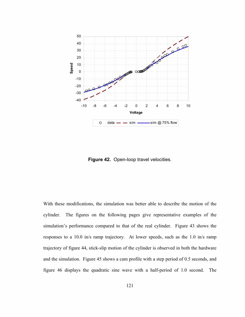
121

-40

-30

-20

-10

0

10

20

30

40

50

-10 -8 -6 -4 -2 0 2 4 6 8 10

Voltage

Spee

d

data sim sim @ 75% flow

Figure 42. Open-loop travel velocities.

With these modifications, the simulation was better able to describe the motion of the

cylinder. The figures on the following pages give representative examples of the

simulation’s performance compared to that of the real cylinder. Figure 43 shows the

responses to a 10.0 in/s ramp trajectory. At lower speeds, such as the 1.0 in/s ramp

trajectory of figure 44, stick-slip motion of the cylinder is observed in both the hardware

and the simulation. Figure 45 shows a cam profile with a step period of 0.5 seconds, and

figure 46 displays the quadratic sine wave with a half-period of 1.0 second. The

122

simulation is able to qualitatively describe the characteristics of the cylinder, under PI

control, to each command trajectory

The mathematical representation of the dynamics of a pneumatic axis, as presented in

chapter 4, generally works well in predicting the motion of the actuator. Unknown or

unmodelled factors prevent a completely accurate representation of the system.

However, the simulation is able to characterize the performance of the system with PI

control.

In the simulation, initial conditions of the cylinder are always identical, starting from a

zero-error position with zero velocity and a perfect pressure balance in the cylinder. In

the physical system, the cylinder never starts from a state of perfect, zero-error

equilibrium. When holding at a steady command position, the lower chamber of the air

cylinder – the rod end – supports the weight of the payload, and has a pressure higher

than that of the blind end. This pressure differential induces leaking in the valve,

lowering the rod end pressure. Eventually, the cylinder moves, and the controller exerts a

restoring command signal to the valve. As a result, there is always a degree of

uncertainty as to the exact position and pressures in the system at the time a motion

command is initiated.

123

0.0

1.0

2.0

3.0

4.0

5.0

0.0 0.5 1.0 1.5 2.0

Time (s)

Posi

tion

(in)

Xcom X

(a)

0.0

1.0

2.0

3.0

4.0

5.0

0.0 0.5 1.0 1.5 2.0

Time (s)

Posi

tion

(in)

Xcom X

(b)

Figure 43. 10 in/s Ramp Trajectory.

(a) Simulation, (b) Data.

124

0.0

1.0

2.0

3.0

4.0

5.0

0.0 2.0 4.0 6.0 8.0

Time (s)

Posi

tion

(in)

Xcom X

(a)

0.0

1.0

2.0

3.0

4.0

5.0

0.0 2.0 4.0 6.0 8.0

Time (s)

Posi

tion

(in)

Xcom X

(b)

Figure 44. 1.0 in/s Ramp Trajectory.


125

0.0

1.0

2.0

3.0

4.0

5.0

0.0 0.5 1.0 1.5

Time (s)

Posi

tion

(in)

Xcom X

(a)

0.0

1.0

2.0

3.0

4.0

5.0

0.0 0.5 1.0 1.5

Time (s)

Posi

tion

(in)

Xcom X

(b)

Figure 45. Cam Profile, 0.5-second Step Period.


126

0.0

1.0

2.0

3.0

4.0

5.0

2.0 2.5 3.0 3.5 4.0

Time (s)

Posi

tion

(in)

Xcom X

(a)

0.0

1.0

2.0

3.0

4.0

5.0

2.0 2.5 3.0 3.5 4.0

Time (s)

Posi

tion

(in)

Xcom X

(b)

Figure 46. Quadratic Sine Trajectory, 1.0-s Half-Period.


127

Another area of model uncertainty is friction. Coulomb friction and stiction were

measured with the cylinder being vented directly to atmosphere, as to eliminate air flow

restrictions. However, it was suggested that the pressure in the cylinder changes its

friction characteristics. The improved performance of the simulation reinforces this

concept, though its exact mechanism is unknown.

There is also a degree of uncertainty in the valve flow model, especially at lower

command voltages. Table 4 presents four models for determining the value of the flow

coefficient VC based on the command voltage and the flow path. The models are similar,

suggesting the differences are the result of variations in the valve manufacturing process.

Each flow coefficient model assumes 0=VC in the null band around 0=SPOOLx .

However, a detailed inspection of the data figure 42 suggests a smoother transition in the

true flow coefficients (figure 47) than the model in table 4 predicts.

128

-10

-5

0

5

10

-3 -2 -1 0 1 2 3

Voltage

Spee

d

data sim @ 75% flow

Figure 47. Detail of Open-Loop Travel Velocities.

The simulation worked well in predicting the onset of stick-slip friction in the cylinder,

which occurs when the flow rate into the cylinder is not sufficient to sustain motion after

breaking stiction. In stick-slip, the cylinder moves a short distance before stopping again

and re-initiating stiction. The experimental data shows stick-slip behavior appearing in

the ramp trajectory at command speeds of 3.2 in/s and lower. The simulation shows

partial stick-slip behavior at 3.2 in/s (figure 48), and full stick-slip at lower velocities.

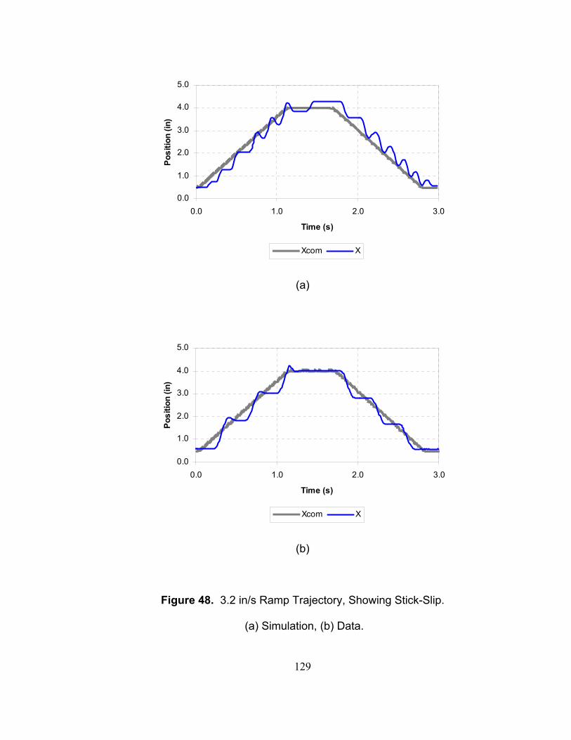
129

0.0

1.0

2.0

3.0

4.0

5.0

0.0 1.0 2.0 3.0

Time (s)

Posi

tion

(in)

Xcom X

(a)

0.0

1.0

2.0

3.0

4.0

5.0

0.0 1.0 2.0 3.0

Time (s)

Posi

tion

(in)

Xcom X

(b)

Figure 48. 3.2 in/s Ramp Trajectory, Showing Stick-Slip.


130

Chapter 5 discusses the controllability of a servopneumatic actuator-single proportional

valve system. A key argument made in the discussion was that, at a constant travel

velocity, the mass flow rate going into one chamber of the cylinder is equal to the mass

flow rate going out of the other. While the experimental apparatus did not allow for flow

rate measurement, the simulation calculates these flow rates.

-4.0

-2.0

0.0

2.0

4.0

0.0 1.0 2.0

Time (s)

Flow

Rat

e (S

CFM

)

Q1 Q2

-4.0

-2.0

0.0

2.0

4.0

-4.0 -2.0 0.0 2.0 4.0

Q1 (SCFM)

Q2

(SC

FM)

(a) (b)

Figure 49. Simulated Volumetric Flow Rates, 10 in/s Ramp Trajectory.

(a) Q vs. time, (b) 2Q vs. 1Q .

131

The simulation supports the claim of opposing mass flow rates in the cylinder. Figure

49(a) presents the mass flow rate into each chamber of the cylinder as a function of time

for the 10 in/s ramp trajectory. Positive values indicate flow into the cylinder. A visual

inspection shows that the simulated flow rate into one chamber is nearly the opposite of

the flow rate into the other chamber. This is better observed in figure 49(b), which plots

the flow rate 2Q as a function of 1Q . The opposing flow assumption states the slope of

this line should be exactly –1. A regression analysis shows the best-fit line has a slope of

–1.103, with an R2 value of 0.987.

Figure 49(b) is typical of all simulations in which the cylinder did not reach the hard

limits of travel, including simulations applying the advanced control strategies discussed

in the following chapter. The largest visual divergence from the ideal flow relationship

occurred in the 0.2-second half-period quadratic sine trajectory under PI control, having a

slope of –1.056 with an R2 value of 0.957 (figure 50). Deviations from the ideal slope are

attributed to acceleration, which violates the restriction of constant velocity, and

asymmetry in the flow coefficient functions (table 4).

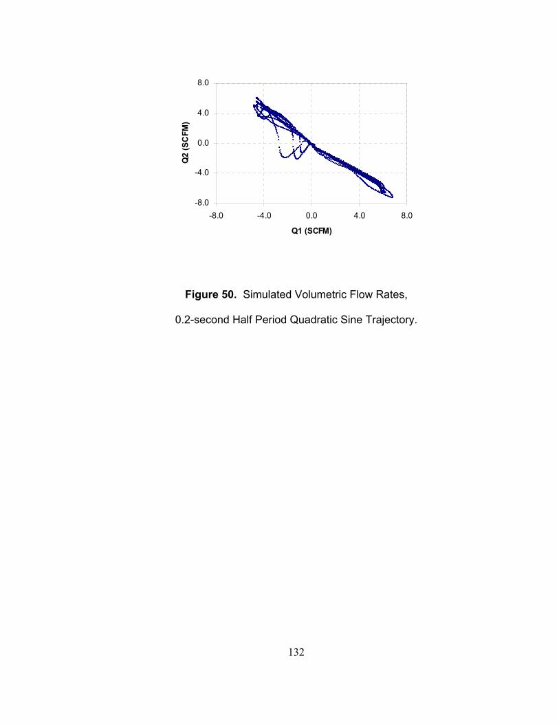
132

-8.0

-4.0

0.0

4.0

8.0

-8.0 -4.0 0.0 4.0 8.0

Q1 (SCFM)

Q2

(SC

FM)

Figure 50. Simulated Volumetric Flow Rates,

0.2-second Half Period Quadratic Sine Trajectory.

133

CHAPTER 7

ADVANCED CONTROL STRATEGIES

PI control is a poor choice for the servo control of a pneumatic actuator via a proportional

valve. The compressibility of air contributes to the dominant pole pair of the closed-loop

system being underdamped, leading to oscillatory behavior in the system at high speeds.

At lower speeds this effect is not as strong, but here friction induces stick-slip motion in

the cylinder. Advanced control strategies can improve the performance of the

servopneumatic system; however, the control strategies developed in this study must be

realized within the framework of a programmable logic controller (PLC).

Two strategies are developed, implemented, and evaluated: a variable structure controller

(VSC), and a hybrid fuzzy-modified PI controller. Both schemes function through the

M02AE servo motion control module by assigning to it closed-loop gains. The

performance characteristics of the control schemes are compared to each other, and to the

baseline PI controller. Additionally, the performance of the PLC in processing these

control schemes is discussed.

134

7.1. Variable Structure Control. Chapter 2.3 reviewed previous research into control

strategies for servo actuators. Variable structure control is commonly offered as an

alternative to PID control, and is selected for implementation on the PLC.

The graph of the open-loop cylinder velocity as a function of a constant command

voltage (figure 42) is the basis of the concept for the VSC used in this study. During the

experimentation to develop figure 42, it was observed that stick-slip occurred at slower

speeds when the command voltage was constant. A control scheme can take advantage

of this by applying the exact voltage needed to develop any given velocity. This

relationship, though, is difficult to define mathematically and is affected by changes in

the load, temperature, and supply pressure.

Rather than finding an exact formula, the VSC control scheme switches between two

control laws that form an envelope for open-loop voltage-velocity relationship. The

control space is divided into two main regions (figure 51). In region 1, the feedback

signal leads the control signal, and a controller output is calculated to slow the motion of

the cylinder. Conversely, in region 2 of figure 51 the cylinder lags the command signal.

Here, the output accelerates the load. A third region is created for command speeds less

than 0.30 in/s. At low speeds, the VSC output becomes less effective, and PI control is

implemented.

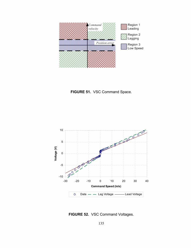
135

FIGURE 51. VSC Command Space.

-10

-5

0

5

10

-30 -20 -10 0 10 20 30 40

Command Speed (in/s)

Volta

ge (V

)

Data Lag Voltage Lead Voltage

FIGURE 52. VSC Command Voltages.

136

Implementation of the VSC in a PLC architecture is not complicated. A limit test

determines if the command velocity is within the bounds for PI control. At low speeds,

the controller assigns PI gains to the M02AE module. At high speeds, the position,

integral, and velocity feedforward gains are set to zero. The ladder logic calculates the

appropriate control voltage, and assigns it to the M02AE module’s output offset. Table

13 lists the equations used in calculating the output offset. Figure 52 shows the control

equations plotted with the open-loop speed data of figure 42.

Command Velocity

Error ( )xxCOM −

Condition (axis to command)

Command Voltage

Positive Positive Lagging 2.1229.0 +⋅= COMCOM xV &

Positive Negative Leading 75.0206.0 +⋅= COMCOM xV &

Negative Positive Leading 75.0258.0 −⋅= COMCOM xV &

Negative Negative Lagging 0.1333.0 −⋅= COMCOM xV &

TABLE 13. Output Offset Equations for Variable Structure Controller.

137

Evaluation of the VSC control scheme applies the same trajectories used to validate the

mathematical model and simulation (section 6.2). Representative examples are discussed

in this chapter. Figure 53 shows the VSC response to a 10 in/s ramp command. In

comparing this to the PI response of figure 43(b), it is noted that the variable structure

controller reduces oscillation in the actuator. The graph of velocity shows the VSC

control eliminates velocity reversal in this trajectory (figure 54). Over all trajectories in

which stick-slip does not occur, the variable structure controller eliminates the oscillation

seen in the PI controller. A similar example is seen in the 0.5-second cam profile under

PI control and VSC control (figures 45(b) and 55). Their corresponding velocities appear

in figure 56.

0

1

2

3

4

5

0 0.5 1 1.5 2

time (s)

posi

tion

(in)

Xcom X

Figure 53. 10 in/s Ramp Trajectory, VSC.

138

-20

-10

0

10

20

30

0.0 0.5 1.0 1.5 2.0

time (s)

Velo

city

(in/

s)

Vcom V

(a)

-20

-10

0

10

20

0.0 0.5 1.0 1.5 2.0

time (s)

Velo

city

(in/

s)

Vcom V

(b)

Figure 54. 10 in/s Ramp Trajectory Velocity. (a) PI Control, (b) VSC.

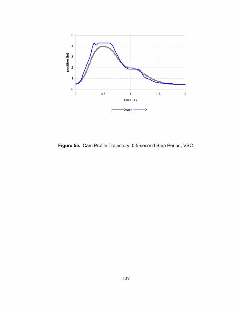
139

0

1

2

3

4

5

0 0.5 1 1.5 2

time (s)

posi

tion

(in)

Xcom X

Figure 55. Cam Profile Trajectory, 0.5-second Step Period, VSC.

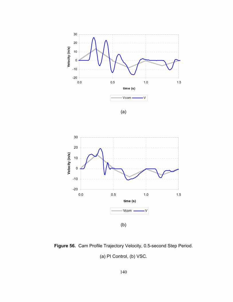
140

-20

-10

0

10

20

30

0.0 0.5 1.0 1.5

time (s)

Velo

city

(in/

s)

Vcom V

(a)

-20

-10

0

10

20

30

0.0 0.5 1.0 1.5

time (s)

Velo

city

(in/

s)

Vcom V

(b)

Figure 56. Cam Profile Trajectory Velocity, 0.5-second Step Period.

(a) PI Control, (b) VSC.

141

The variable structure controller improves low-speed position tracking over that of the PI

controller. This is seen in the 1.0 in/s ramp trajectory, where VSC control (figure 57)

does not exhibit the lag observed in the PI controller (figure 44). The 2.0-second step

cam profile (figure 58) and the 3.0-second half-period quadratic sine trajectories (figure

F59) provide similar examples.

0

1

2

3

4

5

0 1 2 3 4 5 6 7 8

time (s)

posi

tion

(in)

Xcom X

Figure 57. 1.0 in/s Ramp Trajectory, VSC.

142

0

1

2

3

4

5

0 1 2 3 4 5 6 7

time (s)

posi

tion

(in)

Xcom X

(a)

0

1

2

3

4

5

0 1 2 3 4 5 6 7

time (s)

posi

tion

(in)

Xcom X

(b)

Figure 58. Cam Profile Trajectory, 2.0-second Step Period.


143

0.00.5

1.0

1.5

2.0

2.5

3.0

3.5

4.0

4.5

0.0 2.0 4.0 6.0 8.0 10.0

Time (s)

Posi

tion

(in)

Xcom X

(a)

0.0

0.5

1.0

1.5

2.02.5

3.0

3.5

4.0

4.5

0.0 2.0 4.0 6.0 8.0 10.0

Time (s)

Posi

tion

(in)

Xcom X

(b)

Figure 59. Quadratic Sine Trajectory, 3.0-s Half-Period.


144

The switching scheme of the variable structure controller allows it to better track position

at low speeds. Considering a positive 1.8 in/s command velocity, the VSC controller

sends either a 1.61-volt or 1.12-volt command to the proportional valve, depending on the

tracking error. A constant 1.12-volt command signal is just enough to move the cylinder

(figure 47), while the 1.61-volt command should provide a velocity of about 2.5 in/s. It is

expected, then, that the cylinder under VSC control should always be in motion.

Conversely, the proportional gain contributes the most to the command voltage in a PI

controller with velocity feedforward. Using table 10 and equation 31, the contribution of

the velocity feedforward gain, at 1.8 in/s, may be calculated to be 0.29 volts. Assuming a

zero integral error, the proportional error must reach 0.207 inches to generate a 1-volt

command signal from the controller. This suggests a significant error is needed before

the controller can overcome stiction.

Figure 60 compares the command signal from a PI controller with that of a VSC

controller for a 1.8 in/s velocity command. While variations in the command voltage are

similar, switching in the VSC scheme is much faster than the principle frequency seen in

the PI control. In effect, the VSC acts in a manner similar to that of a pulse-width

modulated controller.

145

-3.0

-2.0

-1.0

0.0

1.0

2.0

0.0 2.0 4.0 6.0 8.0

Time (s)

Volta

ge /

Velo

city

Vcom Voltage

(a)

-3.0

-2.0

-1.0

0.0

1.0

2.0

0.0 2.0 4.0 6.0 8.0

Time (s)

Volta

ge /

Velo

city

Vcom Voltage

(b)

Figure 60. Command Signal for 1.8 in/s Ramp Trajectory.


146

The rapid switching in the command signal allows the variable structure controller

operate at slower speeds than the PI controller without stick-slip motion. The PI

controller exhibits full stick-slip behavior at speeds of 3.2 in/s and lower (figure 48). The

VSC controller just avoids stick-slip at 1.8 in/s, and exhibits full stick-slip behavior at 1.0

in/s, while at 1.8 in/s it just avoids stick-slip. Figure 62 shows the variation in velocity at

1.8 in/s, at the threshold of stick-slip. Full stick-slip behavior generates a velocity graph

similar to that of figure 63.

0

1

2

3

4

5

0 1 2 3 4 5

time (s)

posi

tion

(in)

Xcom X

Figure 61. 1.8 in/s Ramp Trajectory, VSC.

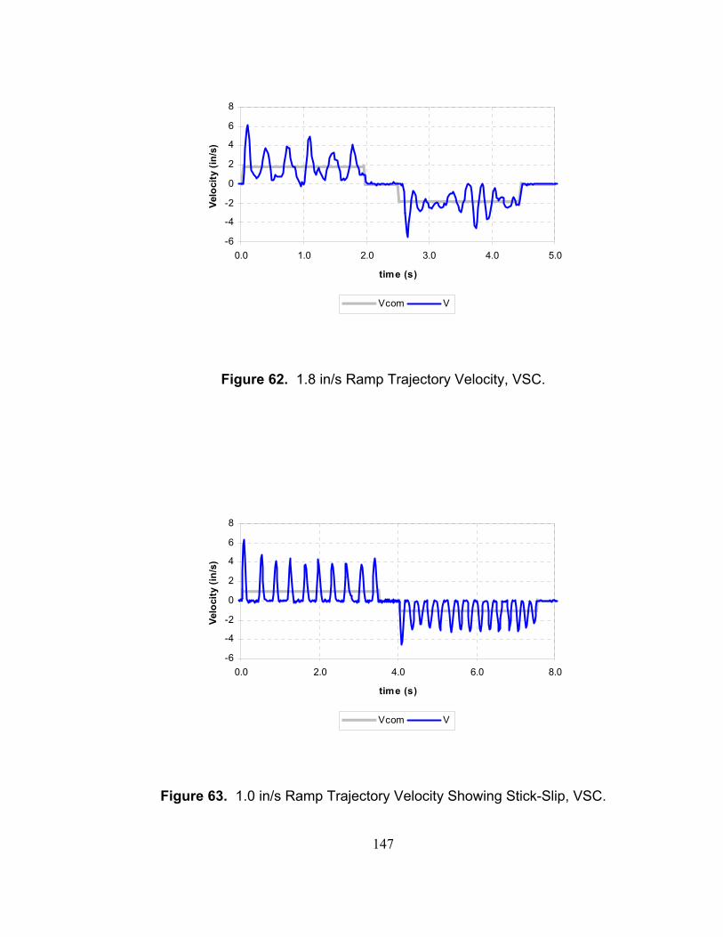
147

-6

-4

-2

0

2

4

6

8

0.0 1.0 2.0 3.0 4.0 5.0

time (s)

Velo

city

(in/

s)

Vcom V

Figure 62. 1.8 in/s Ramp Trajectory Velocity, VSC.

-6

-4

-2

0

2

4

6

8

0.0 2.0 4.0 6.0 8.0

time (s)

Velo

city

(in/

s)

Vcom V

Figure 63. 1.0 in/s Ramp Trajectory Velocity Showing Stick-Slip, VSC.

148

The success of a variable structure controller requires rapid switching between the

subcontrollers. Figure 60(b) shows high-frequency switching of the VSC controller at

1.8 in/s. Similar switching was observed in the controller at all velocities at which stick-

slip did not occur.

At higher speeds, the cylinder’s position under VSC leads the command signal. This is

seen in the 10 in/s ramp trajectory (figure 53), where the payload hits the hard stops on

both extension and retraction. The lead in the position is attributed to delay in the

position reporting from the M02AE module to the PLC processor. Figure 64 shows the

command position as reported by the PLC processor to the data acquisition computer; the

actual position reported by the PLC, and; the position as indicated by the external linear

potentiometer. This data shows a lag of approximately 100 milliseconds between the

position recorded by the potentiometer and the position reported to the PLC by the

M02AE. The data available to the PLC tells it the VSC control is performing as

expected.

149

0

1

2

3

4

5

0 0.2 0.4 0.6 0.8 1 1.2

time (s)

posi

tion

(in)

Command PLC Transducer

Figure 64. 3.2 in/s Ramp Trajectory Showing PLC-Reported Position, VSC.

7.2. Hybrid Fuzzy-Modified PI Controller. A second advanced control scheme was

developed to explore improvements over the variable structure controller, and evaluate

the performance of a fuzzy controller at low command speeds. Like VSC scheme, the

high-speed control structure uses the open-loop voltage-velocity data of figure 42.

Instead of bounding the voltage-velocity relationship, though, a nominal function is

determined, with a proportional gain is added to account for errors in the model. Figure

65 shows the nominal command voltage as a function of the command velocity.

150

-10

-5

0

5

10

-30 -20 -10 0 10 20 30 40

Command Speed (in/s)

Volta

ge (V

)

Data Fuzzy Nominal

Figure 65. Hybrid Fuzzy Nominal Command Voltage.

A fuzzy control scheme determines the gains at positive and negative speeds. To

improve performance, this scheme increases the proportional and integral gains at

command velocities between –0.40 and 0.40 in/s. Figure 66 shows the weight functions

for negative speed, zero speed, and positive speed regions of the fuzzy controller. Table

14 lists the gains assigned in each region of the fuzzy controller. Implementation in the

PLC ladder logic is accomplished by calculating the weights of figure 66 in every

program scan. Each region’s gains are multiplied by the fuzzy weights, and summed to

determine the value of the gain sent to the M02AE module.

151

Figure 66. Fuzzy Weight Functions.

Negative Speed Region

Zero Speed Region

Positive Speed Region

Proportional Gain, Pk 0.00022 0.00100 0.00022

Integral Gain, Ik 0.0000 0.0003 0.0000

Velocity Feedforward

Gain, VFk

7.50% 6.56% 5.62%

Output Offset, OFFU -1.0 0.0 1.0

Scaling Gain, Sk 1000.0 1000.0 1000.0

Table 14. Fuzzy Control Gains.

152

At high speed, the performance of the hybrid fuzzy controller is similar to that of the

VSC controller. The 10 in/s ramp trajectory (figures 67 and 53) and the 0.5-second cam

profile (figures 68 and 55) exemplify this likeness. The hybrid fuzzy controller does not

exhibit the oscillations in velocity seen with the PI controller. At lower speeds, the

hybrid fuzzy controller again performs in a manner similar to the variable structure

controller. This is seen in comparing the low-speed cam profile trajectory (figures 68 and

58(b)) and quadratic sine trajectory (figures 69 and 59(b)).

0

1

2

3

4

5

0 0.5 1 1.5 2

time (s)

posi

tion

(in)

Xcom X

Figure 67. 10 in/s Ramp Trajectory, Hybrid Fuzzy Control.

153

0

1

2

3

4

5

0 0.5 1 1.5 2

time (s)

posi

tion

(in)

Xcom X

Figure 68. Cam Profile Trajectory, 0.5-second Step Period,

Hybrid Fuzzy Control.

154

0

1

2

3

4

5

0 1 2 3 4 5 6 7

time (s)

posi

tion

(in)

Xcom X

Figure 69. Cam Profile Trajectory, 2.0-second Step Period,


155

0.0

0.5

1.0

1.5

2.0

2.5

3.0

3.5

4.0

4.5

0.0 2.0 4.0 6.0 8.0 10.0

Time (s)

Posi

tion

(in)

Xcom X

Figure 70. Quadratic Sine Trajectory, 3.0-second Half Period,


Like the variable structure controller, the hybrid fuzzy-modified PI controller lowers the

speed at which stick-slip behavior is observed for the same reasons discussed in the

previous section. In the baseline PI controller, fully developed stick-slip was observed in

the 3.2 in/s ramp trajectory (figure 48). In the variable structure controller, the stick-slip

speed is inferred to be slightly less than 1.8 in/s (figures 61 and 62). The hybrid fuzzy

controller exhibits stick-slip behavior on retraction at 1.0 in/s, and full stick-slip behavior

at 0.75 in/s. Figures 71 and 72 show position and velocity for the hybrid fuzzy-modified

PI controller at 1.0 in/s.

156

0

1

2

3

4

5

0 1 2 3 4 5 6 7 8

time (s)

posi

tion

(in)

Xcom X

Figure 71. 1.0 in/s Ramp Trajectory, Hybrid Fuzzy Control.

157

-6

-4

-2

0

2

4

6

8

0.0 2.0 4.0 6.0 8.0

time (s)

Velo

city

(in/

s)

Vcom V

Figure 72. 1.0 in/s Ramp Trajectory Velocity, Hybrid Fuzzy Control.

The fuzzy portion of the hybrid fuzzy-modified PI controller acts in the ±0.40 in/s region

of command velocities. The effect of the fuzzy control is to reduce the tracking error at

these low velocities. The increase in the proportional and integral gains serves to make

the controller more responsive near zero velocity, improving its ability to track position.

158

7.3. Controller Comparisons. The RMS position tracking error may be used as a

measure of each controller’s ability to follow a command signal. Figure 73 shows the

position tracking error of all three control schemes for the ramp trajectory. The baseline

PI controller has an RMS tracking error of about 0.3 inches at any given velocity. The

variable structure controller and the hybrid fuzzy-modified PI controller exhibit

comparable errors at all speeds. The advanced controllers offer significant error

reduction at low speeds, but the errors at higher speeds are larger than those of the PI

controller. The higher high-speed errors are attributed to the position-reporting lag in the

PLC control loop, which adds lead to the actual position. The RMS position tracking

error for the cam profile and quadratic sine trajectories are shown in figures 74 and 75.

RMS error may also be calculated for velocity tracking. The variable structure controller

and the hybrid fuzzy controller both reduce the errors in velocity through the elimination

of the oscillatory behavior seen with the PI controller. Figure 76 shows the RMS

velocity-tracking errors in the ramp trajectory for those speeds at which stick-stick

motion is not observed.

159

0.0

0.1

0.2

0.3

0.4

0.5

0.1 1.0 10.0 100.0

Ramp Velocity (in/s)

RM

S Po

sitio

n Er

ror (

in)

PID VSC Fuzzy

Figure 73. RMS Position Tracking Errors, Ramp Trajectory.

160

0.0

0.2

0.4

0.6

0.8

0.0 0.5 1.0 1.5 2.0 2.5 3.0

Cam Profile Step Period (s)

RM

S Po

sitio

n Er

ror (

in)

PID VSC Fuzzy

Figure 74. RMS Position Tracking Errors, Cam Profile Trajectory.

161

0.0

0.2

0.4

0.6

0.8

0.0 0.5 1.0 1.5 2.0 2.5 3.0

QuadSine Half-Period (s)

RM

S Po

sitio

n Er

ror (

in)

PID VSC Fuzzy

Figure 75. RMS Position Tracking Errors, Quadratic Sine Trajectory.

162

0

2

4

6

8

1.0 10.0 100.0

Ramp Velocity (in/s)

RM

S Ve

loci

ty E

rror

(in/

s)

PID VSC Fuzzy

Figure 76. RMS Velocity Tracking Errors, Ramp Trajectory.

Program scan time is not a concern in most industrial PLC applications. A typical

mechanical process under PLC control requires between 100ms and 10s to accomplish,

while the typical PLC program scan time is less than 10ms. Specialized hardware exists

for applications in which a fast control action is required – for example, precise

revolution counting of a rapidly spinning tool. The Allen-Bradley 1756-HSC high-speed

counter is one such device which is compatible with the Logix5550 PLC platform.

The success of the hybrid fuzzy-modified PI controller and, to a greater extent, the

variable structure controller, depends on the rapid detection of and response to the state

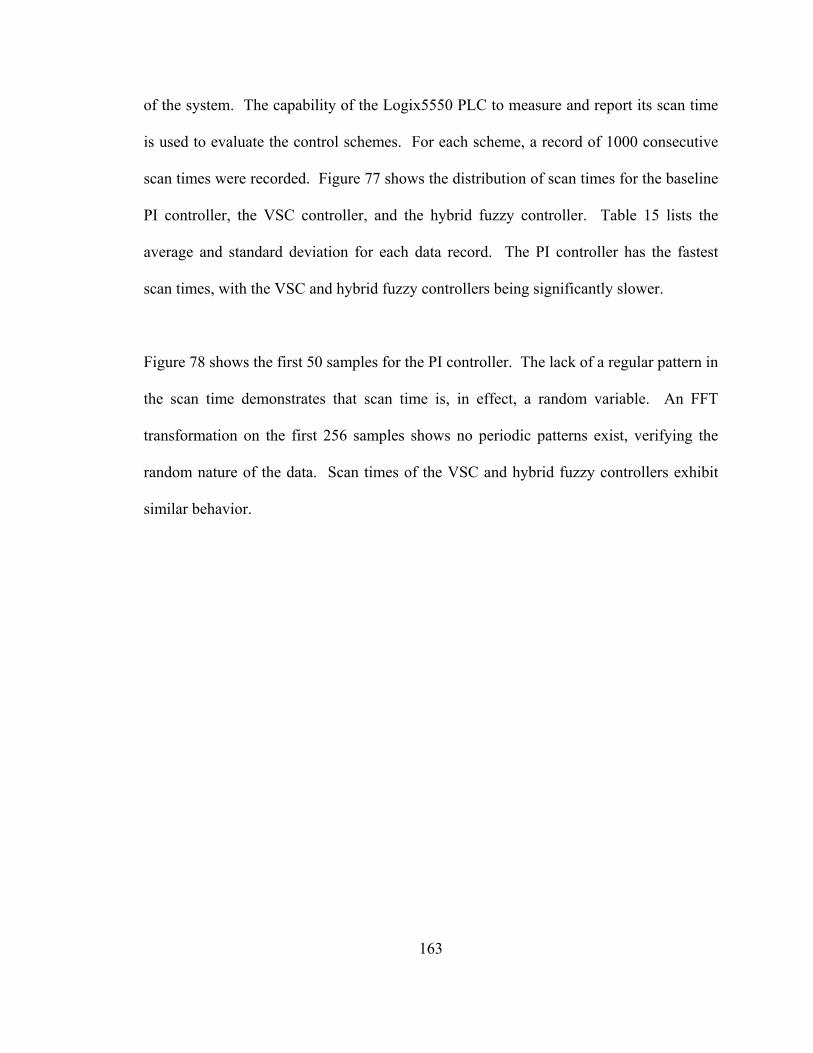
163

of the system. The capability of the Logix5550 PLC to measure and report its scan time

is used to evaluate the control schemes. For each scheme, a record of 1000 consecutive

scan times were recorded. Figure 77 shows the distribution of scan times for the baseline

PI controller, the VSC controller, and the hybrid fuzzy controller. Table 15 lists the

average and standard deviation for each data record. The PI controller has the fastest

scan times, with the VSC and hybrid fuzzy controllers being significantly slower.

Figure 78 shows the first 50 samples for the PI controller. The lack of a regular pattern in

the scan time demonstrates that scan time is, in effect, a random variable. An FFT

transformation on the first 256 samples shows no periodic patterns exist, verifying the

random nature of the data. Scan times of the VSC and hybrid fuzzy controllers exhibit

similar behavior.

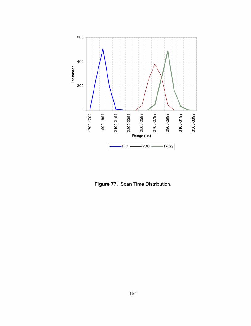
164

0

200

400

600

1700

-179

9

1900

-199

9

2100

-219

9

2300

-239

9

2500

-259

9

2700

-279

9

2900

-299

9

3100

-319

9

3300

-339

9

Range (us)

Inst

ance

s

PID VSC Fuzzy

Figure 77. Scan Time Distribution.

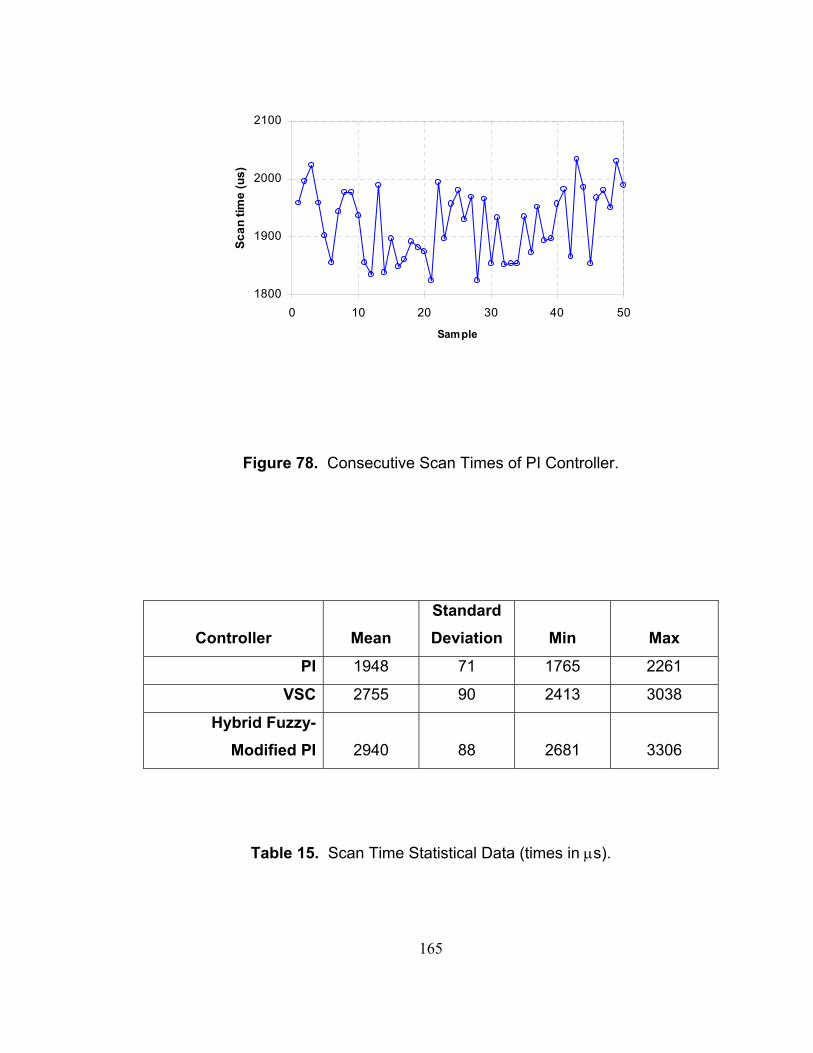
165

1800

1900

2000

2100

0 10 20 30 40 50

Sample

Scan

tim

e (u

s)

Figure 78. Consecutive Scan Times of PI Controller.

Controller

Mean

Standard Deviation

Min

Max

PI 1948 71 1765 2261

VSC 2755 90 2413 3038

Hybrid Fuzzy-Modified PI

2940

88

2681

3306

Table 15. Scan Time Statistical Data (times in µs).

166

Much of the processing time in the PI controller is given to collecting data for this study.

The program contains seven GSV (get system value) commands, which execute in every

program scan. Table 6 showed the GSV command to be time-consuming, requiring

approximately 150 µs to process. Using [88] as a reference, the total overhead for

collection of the experimental data is calculated to be 969.9 µs, or half of the average

scan time.

The VSC program, as implemented on the PLC, requires additional time to examine the

instantaneous state of the actuator and determine gains based on the state. Most of the

increase in the average scan time is attributed to the four SSV (set system value)

commands, which add 617.4 µs to every program scan. The mathematical and

comparative operations account for the rest of the increase. The hybrid fuzzy controller

uses the same set of SSV values, but the mathematics required by the fuzzy algorithm

increases the overall scan time.

The scan time in the controller affects the performance of the control algorithm.

Consider the quadratic sine trajectory with a 0.5-second half period. Its acceleration is

always ±48 in/s2 (table 12). With the variable structure controller, the velocity profile

passes through the PI-control band (±0.30 in/s) in 12.5 ms, or 4.5 average PLC program

scans. VSC is a switching algorithm, so the delay only affects switching between control

modes. In a similar examination of the hybrid fuzzy-modified PI controller, the velocity

passes through the fuzzy region (±0.40 in/s) in 16.7 ms, or 5.7 average scans. The

processing delay here is more significant with respect to the control system, as the gains

167

within the fuzzy region are a function of the command velocity. In the mechanical

system, however, the effect of lag in the changing of gains over 16.7 ms is not significant.

The program scan time for all control schemes may be reduced significantly. The

969.9 µs needed for collecting the data for this study may be eliminated completely from

the PI control, reducing its mean scan time to just 978 µs. Data collection for the

advanced control schemes requires 274.9 µs, providing a net reduction of 695.0 µs. The

VSC program writes gains to the M02AE controller via the SSV commands on every

program scan. It is possible to rewrite the program so that the SSV commands only

execute as needed. Doing so would require use of three OSR (one-shot rising) bit

commands, each having an execution time of 3.7 µs. The estimated mean scan time

would be reduced from 2755 µs to 2071 µs.

Similarly, significant reductions may be realized in the scan time of the hybrid fuzzy

controller. Because fuzzy calculations are required for just a handful of scans in many of

the trajectories tested, a practical approach to reducing scan times is to calculate the fuzzy

gains only at the initiation of a motion command, using the peak velocity as the basis for

the fuzzy logic. This strategy would allow the hybrid fuzzy controller to have an average

scan time similar to that of the PI controller. On program scans in which a motion

command is initiated, a longer scan would be required.

168

CHAPTER 8

SUMMARY AND FUTURE WORK

Pneumatic actuators offer a low-cost alternative to conventional servo technologies.

Their acceptance in industry, though, requires use of advanced control system to account

for the nonlinear behavior of the pneumatic system. This study explores the application

of servo control schemes for a pneumatic cylinder, acting vertically, with a single

proportional valve metering flow, and an encoder providing position feedback. The

control schemes were implemented within the architecture of a programmable logic

controller having a servo motor motion control module.

Two controllers were designed: one using a variable structure control algorithm; the other

a hybrid of a fuzzy and a modified PI controller. The performances of the control

schemes were compared against each other, and against a baseline PI control algorithm

available through the servo motion module. A digital simulation of the servopneumatic

system permitted observation of processes not measurable through the experimental

apparatus. In addition, a linear mathematical analysis allowed for the theoretical

discussion of the behavior of the system.

169

The variable structure and hybrid fuzzy controllers both offer similar gains in

performance over the PI controller. At high speeds, the advanced control schemes

exhibit less oscillatory behavior than the PI controller. At low speeds, they reduce the

RMS position tracking error. Both experimental controllers lower the speed at which

stick-slip behavior manifests itself.

A linear analysis using position x , velocity x& , and equilibrium position EQx as the state

variables suggests the servopneumatic system is always observable and controllable.

When nonlinear effects are considered in this analysis, it is found that controllability is

significantly lower near mid-stroke positions, and may be lost at low command speeds.

A key assumption to this analysis is that the instantaneous mass flow rate into one

chamber of the pneumatic cylinder is equal to the mass flow rate leaving the other. The

simulation demonstrates this assumption is a valid approximation of the actual process, as

long as the actuator does not reach a hard stop. Future research can provide an

experimental verification of this assumption, and explore in depth effects of acceleration,

friction, and valve geometry.

This research purposefully did not address the position-holding capability of a pneumatic

actuator. The cylinder used in this study could not hold an arbitrary position indefinitely.

The vertical orientation of the cylinder, the single-end cylinder design, and leakage in the

proportional valve all contribute to the lack of system equilibrium at a zero command

velocity. One area for future research is to determine economical hardware and sensor

designs that will let a pneumatic actuator hold an arbitrary command position.

170

Another area for future research is in the conceptual design model for a proportional

valve. The valve used in this study has on-board electronics that provide closed-loop

feedback control for spool position, independent of any external control system. The

apparent design paradigm for this valve states that the spool position should be a linear

function of the command voltage. This and previous studies show this paradigm leads to

highly nonlinear flow dynamics through the valve, and complicates the design of a

control system built around it.

From a customer’s standpoint, the better conceptual model is for the mass flow rates

through the valve to be proportional to the command signal. Advances in mechatronics

and microelectromechanical systems (MEMS) make the practical construction of such a

valve possible. A well-designed valve control system can enforce proportionality

between the command signal and the flow rate, and compensate for variations in the

valve manufacturing process.

171

APPENDIX A

MATLAB SIMULATION CODES

172

A.1. SIM8 Program Code.

% **************************** % ** SIM8 ** % ** Last modified 10-21-03 ** % **************************** % ***** ***** ***** ***** ***** ***** ***** ***** ***** ***** % ******************************* % ** KEY SIMULATION PARAMETERS ** % ******************************* ctrl = 'PID'; % CONTROL METHOD % - PID % - VSC % - Fuzzy % - Volt (open-loop, requires Volt_com, t_max) traj = 'Short'; % TRAJECTORY % - Shortramp (requires dx_ramp) % - Short (requires t_short) % - ShortQS (requires t_short) Volt_com = 3; % Volt control command voltage, -10V to +10V t_max = 0.8; % Volt control simulation time, s dx_ramp = 1.8; % Ramp trajectory command speed, in/s t_short = 3.0; % Short trajectory leg duration, s % ***** ***** ***** ***** ***** ***** ***** ***** ***** ***** % ************************* % ** PHYSICAL PROPERTIES ** % ************************* % ** Environment Pa = 14.7; % atmpspheric pressre, psi Ps = 80 + Pa; % supply pressure, psi Ta = 68 + 460; % ambient temperature, R g = 386.09; % gravity, in/sec^2 % ** Air k = 1.4; % ratio of specific heats R = 247000; % gas constant for air, in^2/s^2-R % ** Cylinder L = 7.00; % stroke, in L_stop = L; % default stop position, in

173

dia = 1.969; % piston diameter, in d_rod = 0.984; % rod diameter, m F_stat = 4.9; % static friction, lb F_dyn = 1.55; % dynamic friction, lb b = 0.125; % viscous friction, lb-s/in Vx1 = 0.7; % excess volume 1, in^3 Vx2 = 0.7; % excess volume 2, in^3 W = 22.25 + 2.0; % payload weight, lb A1 = pi/4 * dia^2; % blind end area, in^2 A2 = pi/4 * (dia^2 - d_rod^2); % rod end area, in^2 A_rod = A1 - A2; % rod area, in^2 M = W/g; % payload mass, lb-s^2/in % ** Valve t_spool = 0.00096; % valve spool time constant, s % ** Friction correction F_stat = F_stat * Ps/Pa; F_dyn = F_dyn * Ps/Pa; % ************************ % ** INITIAL CONDITIONS ** % ************************ x = 0.5; % position, in dx = 0.0; % velocity, in/s d2x = 0.0; % acceleration, in/s^2 % ** pressures set for equilibrium P2 = Ps * 0.8; % rod end pressure P1 = (P2*A2 + Pa*A_rod - W)/A1; % blind end pressure, psi x_spool = 0; % valve spool position dm1 = 0; % mass flow rate, lb-s^2/in-s dm2 = 0; % mass flow rate, lb-s^2/in-s t = 0; % elapsed time, s if isequal(lower(traj),'shortqs') x = 1; end if isequal(lower(ctrl),'volt') if Volt_com >= 0 x = 0; else x = 7; end end x_com = x; % command position, in dx_com = 0.0; % command velocity, in/s x_PLC = x; % stored position in PLC x_com_PLC = x; % command position in PLC, in dx_com_PLC = 0.0; % command velocity in PLC, in/sec V_com = 0.0; % command voltage from M02AE to spool, V

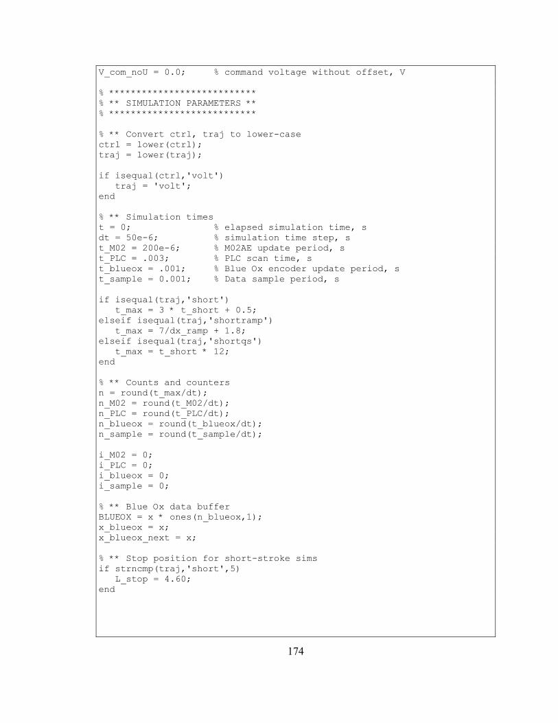
174

V_com_noU = 0.0; % command voltage without offset, V % *************************** % ** SIMULATION PARAMETERS ** % *************************** % ** Convert ctrl, traj to lower-case ctrl = lower(ctrl); traj = lower(traj); if isequal(ctrl,'volt') traj = 'volt'; end % ** Simulation times t = 0; % elapsed simulation time, s dt = 50e-6; % simulation time step, s t_M02 = 200e-6; % M02AE update period, s t_PLC = .003; % PLC scan time, s t_blueox = .001; % Blue Ox encoder update period, s t_sample = 0.001; % Data sample period, s if isequal(traj,'short') t_max = 3 * t_short + 0.5; elseif isequal(traj,'shortramp') t_max = 7/dx_ramp + 1.8; elseif isequal(traj,'shortqs') t_max = t_short * 12; end % ** Counts and counters n = round(t_max/dt); n_M02 = round(t_M02/dt); n_PLC = round(t_PLC/dt); n_blueox = round(t_blueox/dt); n_sample = round(t_sample/dt); i_M02 = 0; i_PLC = 0; i_blueox = 0; i_sample = 0; % ** Blue Ox data buffer BLUEOX = x * ones(n_blueox,1); x_blueox = x; x_blueox_next = x; % ** Stop position for short-stroke sims if strncmp(traj,'short',5) L_stop = 4.60; end

175

% ************************ % ** CONTROL PARAMETERS ** % ************************ err_int = 0.0; % error integrator mode = 0; % default mode (used to track VSC, Fuzzy) if isequal(ctrl,'volt') % ** Volt control Kp = 0.0; % proportional gain Ki = 0.0; % integral gain Kvf = 0.0; % velocity feedforward gain Ks = 1000; % command scaling gain cutoff = 1000 * 2 * pi; % filter cutoff frequency, rad/s U_off = Volt_com; % output offset, V if Volt_com < 0 x = L_stop - 0.5; x_com = x; x_PLC = x; BLUEOX = x * ones(n_blueox,1); x_blueox = x; x_blueox_next = x; end elseif isequal (ctrl,'pid') % ** PID control Kp = 0.00086; % proportional gain Ki = 0.0006; % integral gain Kvf = 0.04; % velocity feedforward gain Ks = 1000; % command scaling gain cutoff = 1000 * 2 * pi; % filter cutoff frequency, rad/s U_off = 0.0; % output offset, V elseif isequal (ctrl,'vsc') % ** VSC control Kp_vsc = [0.0 0.0 0.001]; % proportional gains Ki_vsc = [0.0 0.0 0.0007]; % Kvf_vsc = [0.0 0.0 0.12]; Ks = 860.3; % command scaling gain cutoff = 20.2 * 2 * pi; % filter cutoff frequency, rad/s m_pos = [0.229 0.206 0.0]; % slope for U, dx_com > 0 b_pos = [1.2 0.75 0.0]; % offset for U, dx_com > 0 m_neg = [0.333 0.258 0.0]; % slope for U, dx_com < 0 b_neg = [-1.0 -0.75 0.0]; % offset for U, dx_com < 0 VSC_lim = 0.3; % limiting velocity for low speed region, in/s mode = 3; % mode tracking % 1 = lagging % 2 = leading % 3 = low velocity Kp = Kp_vsc(mode); % initial proportional gain

176

Ki = Ki_vsc(mode); % initial integral gain Kvf = Kvf_vsc(mode); % initial velocity feedforward gain U_off = dx_com * m_pos(mode) + b_pos(mode); % % initial output offset elseif isequal (ctrl,'fuzzy') % ** Fuzzy control Kp_f = [0.00022 0.00100 0.00022]; % proportional gains Ki_f = [0.0 0.003 0.0]; % integral gains Kvf_f = [0.0750 0.0656 0.0562]; % velocity feedforward gains U_off_f = [-1.0 0.0 1.0]; % output offsets fuzzy_wt = [0 1 0]; % fuzzy weights fuzzy_lim_pos = 0.4; % positive fuzzy limit fuzzy_lim_neg = -0.4; % negative fuzzy limit Ks = 1000; % command scaling gain cutoff = 1000 * 2 * pi; % filter cutoff frequency, rad/s Kp = sum(Kp_f .* fuzzy_wt); % initial Kp gain Ki = sum(Ki_f .* fuzzy_wt); % initial Ki gain Kvf = sum(Kvf_f .* fuzzy_wt); % initial Kvf gain U_off = sum(U_off_f .* fuzzy_wt); % initial U_off end % ***************** % ** DATA RECORD ** % ***************** DATA = [x dx x_com dx_com P1 P2 dm1 dm2 V_com x_PLC mode d2x]; % % data storage matrix T = [t]; % data timestamp array % **************** % ** SIM HEADER ** % **************** disp('SIM8'); disp('****'); if isequal(ctrl,'volt') disp([ctrl,', ',num2str(Volt_com),' V']); elseif or(isequal(traj,'ramp'),isequal(traj,'shortramp')) disp([ctrl,'-',traj, ', vel = ',num2str(dx_ramp),' ips']); else disp([ctrl,'-',traj]); end disp(['Time = ', num2str(t_max),' sec']); % ***** ***** ***** ***** ***** ***** ***** ***** ***** ***** % ***** ***** ***** ***** ***** ***** ***** ***** ***** ***** % ***** ***** ***** ***** ***** ***** ***** ***** ***** *****

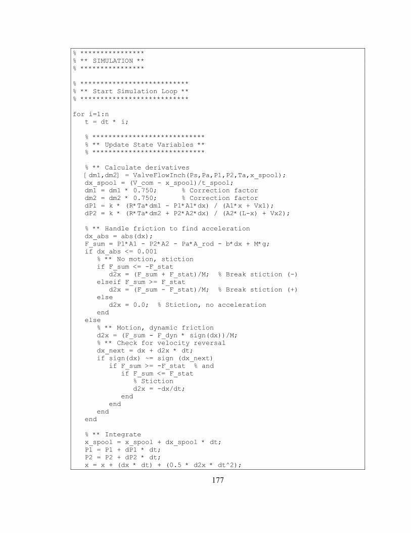
177

% **************** % ** SIMULATION ** % **************** % *************************** % ** Start Simulation Loop ** % *************************** for i=1:n t = dt * i; % **************************** % ** Update State Variables ** % **************************** % ** Calculate derivatives [dm1,dm2] = ValveFlowInch(Ps,Pa,P1,P2,Ta,x_spool); dx_spool = (V_com - x_spool)/t_spool; dm1 = dm1 * 0.750; % Correction factor dm2 = dm2 * 0.750; % Correction factor dP1 = k * (R*Ta*dm1 - P1*A1*dx) / (A1*x + Vx1); dP2 = k * (R*Ta*dm2 + P2*A2*dx) / (A2*(L-x) + Vx2); % ** Handle friction to find acceleration dx_abs = abs(dx); F_sum = P1*A1 - P2*A2 - Pa*A_rod - b*dx + M*g; if dx_abs <= 0.001 % ** No motion, stiction if F_sum <= -F_stat d2x = (F_sum + F_stat)/M; % Break stiction (-) elseif F_sum >= F_stat d2x = (F_sum - F_stat)/M; % Break stiction (+) else d2x = 0.0; % Stiction, no acceleration end else % ** Motion, dynamic friction d2x = (F_sum - F_dyn * sign(dx))/M; % ** Check for velocity reversal dx_next = dx + d2x * dt; if sign(dx) ~= sign (dx_next) if F_sum >= -F_stat % and if F_sum <= F_stat % Stiction d2x = -dx/dt; end end end end % ** Integrate x_spool = x_spool + dx_spool * dt; P1 = P1 + dP1 * dt; P2 = P2 + dP2 * dt; x = x + (dx * dt) + (0.5 * d2x * dt^2);

178

dx = dx + d2x * dt; % ** Apply limits if P1 < 0 P1 = 0; end if P2 < 0 P2 = 0; end if x < 0; x = 0; %dx = -dx; % assumes restitution dx = 0; % assumes no restitution end if x > L_stop x = L_stop; %dx = -dx; % assumes restitution dx = 0; % assumes no restitution end % *************************** % ** M02AE Control Actions ** % *************************** i_M02 = i_M02 + 1; if i_M02 == n_M02 i_M02 = 0; % ** Get command position, velocity from profile if isequal(ctrl,'volt') x_com = 0; dx_com = 0; elseif isequal (traj,'short') [x_com,dx_com] = ShortProfile(t, t_short); elseif isequal (traj,'shortramp') [x_com,dx_com] = ShortRamp(t, dx_ramp); elseif isequal(traj,'shortqs') [x_com,dx_com] = QuadSineShort(t, t_short); else disp('*** INVALID TRAJECTORY, SIM CANCELLED ***'); disp(traj); end % ** Calculate command voltage V_comNF = (4 * Kp * (x_com - x_blueox) + ... 4 * Ki * err_int + Kvf * dx_com/250) * Ks; dV_com = cutoff * (V_comNF - V_com_noU); V_com_noU = V_com_noU + dV_com * t_M02; V_com = V_com_noU + U_off; % ** Apply limits if V_com < -10

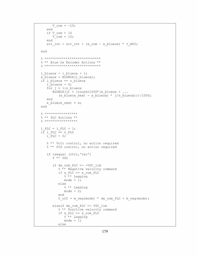
179

V_com = -10; end if V_com > 10 V_com = 10; end err_int = err_int + (x_com - x_blueox) * t_M02; end % ***************************** % ** Blue Ox Encoder Actions ** % ***************************** i_blueox = i_blueox + 1; x_blueox = BLUEOX(i_blueox); if i_blueox == n_blueox i_blueox = 0; for j = 1:n_blueox BLUEOX(j) = (round(1000*(x_blueox + ... (x_blueox_next - x_blueox) * j/n_blueox)))/1000; end x_blueox_next = x; end % ***************** % ** PLC Actions ** % ***************** i_PLC = i_PLC + 1; if i_PLC == n_PLC i_PLC = 0; % ** Volt control, no action required % ** PID control, no action required if isequal (ctrl,'vsc') % ** VSC if dx_com_PLC <= -VSC_lim % ** Negative velocity command if x_PLC >= x_com_PLC % ** Lagging mode = 1; else % ** Leading mode = 2; end U_off = m_neg(mode) * dx_com_PLC + b_neg(mode); elseif dx_com_PLC >= VSC_lim % ** Positive velocity command if x_PLC <= x_com_PLC % ** Lagging mode = 1; else

180

mode = 2; end U_off = m_pos(mode) * dx_com_PLC + b_pos(mode); else % ** Low velocity command mode = 3; U_off = m_pos(mode) * dx_com_PLC + b_pos(mode); end Kp = Kp_vsc(mode); Ki = Ki_vsc(mode); Kvf = Kvf_vsc(mode); elseif isequal (ctrl,'fuzzy') % ** Fuzzy if dx_com_PLC <= fuzzy_lim_neg fuzzy_wt = [1 0 0]; mode = -1; elseif dx_com_PLC <= 0 fuzzy_wt = [(dx_com_PLC/fuzzy_lim_neg)... (1-dx_com_PLC/fuzzy_lim_neg) 0]; mode = -dx_com_PLC/fuzzy_lim_neg; elseif dx_com_PLC <= fuzzy_lim_pos fuzzy_wt = [0 (1-dx_com_PLC/fuzzy_lim_pos)... (dx_com_PLC/fuzzy_lim_pos)]; mode = dx_com_PLC/fuzzy_lim_pos; else fuzzy_wt = [0 0 1]; mode = 1; end Kp = sum (Kp_f .* fuzzy_wt); Ki = sum (Ki_f .* fuzzy_wt); Kvf = sum (Kvf_f .* fuzzy_wt); U_off = sum (U_off_f .* fuzzy_wt); end % ** Update PLC variables x_PLC = x_blueox; % next x in M02AE from transducer x_com_PLC = x_com; dx_com_PLC = dx_com; end

181

% ************************* % ** Sample Data Actions ** % ************************* i_sample = i_sample + 1; if i_sample == n_sample i_sample = 0; DATA = [DATA; x dx x_com dx_com P1 P2 dm1 dm2 V_com x_PLC mode d2x]; T = [T; t]; end % ************************* % ** End Simulation Loop ** % ************************* end % ***** ***** ***** ***** ***** ***** ***** ***** ***** ***** % *************** % ** PLOT DATA ** % *************** % ** DATA variable structure % DATA (:,1) - actual position, in % DATA (:,2) - actual velocity , in/s % DATA (:,3) - command position, in % DATA (:,4) - command velocity, in/s % DATA (:,5) - blind end pressure, psia % DATA (:,6) - rod end pressure, psia % DATA (:,7) - mass flow rate to blind end, SCFM % DATA (:,8) - mass flow rate to rod end, SCFM % DATA (:,9) - Command voltage from M02AE, V % DATA (:,10) - position as seen by PLC, in % DATA (:,11) - VSC control mode / Fuzzy scale % DATA (:,12) - acceleration, in/s^2 DATA(:,7:8) = DATA(:,7:8) * 302900; % Convert flow rate to SCFM Q_limit = [min(DATA(:,7)) max(DATA(:,7))]; % Limits of flow rate subplot (2,3,1), plot(T,DATA(:,3), T,DATA(:,1)); grid on; xlabel('Time (s)'); ylabel('Position (in)'); legend('Xc','X'); subplot (2,3,4), plot(T,DATA(:,4), T,DATA(:,2)); grid on; xlabel('Time (s)'); ylabel('Velocity (in/s)'); legend('Vc','V'); subplot (2,3,2), plot(T,DATA(:,5), T,DATA(:,6)); grid on;

182

xlabel('Time (s)'); ylabel('Pressure (psia)'); legend('P1','P2'); subplot (2,3,5), plot(T,DATA(:,7), T,DATA(:,8)); grid on; xlabel('Time (s)'); ylabel('Flow rate (SCFM)'); legend('Q1','Q2'); subplot (2,3,3), plot(T,DATA(:,9), T,DATA(:,11)); grid on; xlabel('Time (s)'); ylabel('Voltage (V)'); legend('Vcom','mode'); subplot (2,3,6), plot(DATA(:,7),DATA(:,8),'k.', -Q_limit,Q_limit,'b-'); grid on; xlabel('Q1 (SCFM)'); ylabel('Q2 (SCFM)'); % **

183

A.2. ValveFlowInch Subroutine Code.

function [dm1,dm2] = ValveFlowInch(Ps,Pa,P1,P2,T,Xspool) % ValveFlowInch % % [dm1,dm2] = ValveFlowInch(Ps,Pa,P1,P2,T,Xspool) % % Calculates mass flow rates for Festo MPYE-1/4 % proportional control valve. Positive flow rates % indicate flow from valve to cylinder. Pressures % are absolute. Iteration used to account for drop % in supply pressure as flow increases. % % dm1, dm2 - flow (lb-s/in) % Ps, Pa - supply, atmospheric pressure (psia) % P1, P2 - downstream pressures in chambers 1, 2 (psia) % T - temperature (R) % Xspool - spool position, -10 <= Xspool <= 10 % ** Minimum Cv Cv_min = 0.01; % ** Xspool limits enforced if Xspool < -10 Xspool = -10; end if Xspool > 10 Xspool = 10; end % ** Calculate Cv, a, for both flow paths if Xspool < 0 % ports 4-5 Cv1 = -0.0712 * (Xspool+1.21) - 0.0013 * (Xspool+1.21)^2; a_up1 = .0010; a_dn1 = .0400; % ports 2-1 Cv2 = -0.0700 * (Xspool+1.22) - 0.0017 * (Xspool+1.22)^2; a_up2 = .0555; a_dn2 = .0400; else % ports 4-1 Cv1 = 0.0636 * (Xspool-1.38) - 0.0012 * (Xspool-1.38)^2; a_up1 = .0555; a_dn1 = .0400; % ports 2-3 Cv2 = 0.0651 * (Xspool-1.21) - 0.0009 * (Xspool-1.22)^2; a_up2 = .0010; a_dn2 = .0400; end

184

% ** Enforce minimum Cv if Cv1 < Cv_min Cv1 = Cv_min; end if Cv2 < Cv_min Cv2 = Cv_min; end % ** Determine pressure connections if Xspool <= -1.21 P1c = Pa; % chamber 1 connected to atmosphere elseif Xspool >= 1.38 P1c = Ps; % chamber 1 connected to supply else % interpolate P1c = Pa + (Ps-Pa) * (Xspool+1.21)/2.59; end if Xspool <= -1.22 P2c = Ps; % chamber 2 connected to supply elseif Xspool >= 1.22 P2c = Pa; % chamber 2 connected to atmosphere else % interpolate P2c = Ps - (Ps-Pa) * (Xspool+1.22)/2.44; end % ** Calcualte flow rates in SCFM if P1c > P1 Q1 = FlowIteration(P1c,P1,Cv1,T,a_up1,a_dn1); else Q1 = FlowIteration(P1,P1c,Cv1,T,a_dn1,a_up1); Q1 = -Q1; end if P2c > P2 Q2 = FlowIteration(P2c,P2,Cv2,T,a_up2,a_dn2); else Q2 = FlowIteration(P2,P2c,Cv2,T,a_dn2,a_up2); Q2 = -Q2; end % ** Convert from SCFM to lb-s^2/in-s dm1 = Q1/302900; dm2 = Q2/302900; % **

185

A.3. FlowIteration Subroutine Code.

function [Q] = FlowIteration(P_up,P_dn,Cv,T,a_up,a_dn) % FlowIteration % % [Q] = FlowIteration(P_up,P_dn,Cv,T,a_up,a_dn) % % Calculates volumetric flow rates for Festo MPYE-1/4 % proportional control valve, including loss factors % for the plumbing. % % Q - flow rate (SCFM) % P_up - upstream pressure (psia) % P_dn - downstream pressure (psia) % Cv - flow coefficient % T - air temperature (deg R) % a_up - loss coefficient for upstream tubing % a_dn - loss coefficient for downstream tubing % ******************************************************** % NOTES % % * Pressure loss in tubing % % dP = P_in - a * Q^2 % % * Flow through valve % % X = 1 - P_dn/P_up % % Q = 22.67 * Cv * P_up * (1-X/3) * sqrt(X/T) % ******************************************************** % Find initial flow rate based on no pressure drop across valve Q = sqrt((P_up-P_dn)/(a_up+a_dn)); dQ = Q/2; for i = 1:20 % Calculate valve inlet, outlet pressures based on flow rate Pv_up = P_up - a_up * Q^2; Pv_dn = P_dn + a_dn * Q^2; % Find flow rate based on inlet, outlet pressures X = 1 - Pv_dn/Pv_up; Q_test = 22.67 * Cv * Pv_up * (1 - X/3) * sqrt(X/T); % Determine next flow rate iteration if Q >= Q_test Q = Q - dQ; else Q = Q + dQ; end

186

% Smaller iteration step dQ = dQ/2; end % **

187

A.4. ShortRamp Subroutine Code.

function [x,v] = ShortRamp(t,vcom) % Short Ramp Profile % % [xcom,vcom] = ShortRamp(time, command_velocity) % % Generates a command position and velocity based % on a ramp profile from 0.5" to 4.0" and back, with % a 0.5 second pause at extension. For times calculated % to be outside the profile time, [0.5 0.0] will be the % function's output. 50 ips acceleration. vmax = 50 * sqrt(3.5/50); if vcom < vmax % ** Trapezoidal profile t1 = vcom/50; % accel t2 = 3.5/vcom; % steady velocity t3 = t1 + t2; % decel t4 = t3 + 0.5; % hold t5 = t4 + t1; % accel t6 = t4 + t2; % steady velocity t7 = t6 + t1; % decel if t <= 0 x = 0.5; v = 0.0; elseif t <= t1 % accel x = 0.5 + 25 * t^2; v = 50 * t; elseif t <= t2 % steady velocity x = 0.5 + (vcom^2)/100 + vcom * (t-t1); v = vcom; elseif t <= t3 % decel x = 4.0 - 25 * (t-t3)^2; v = vcom - 50 * (t-t2); elseif t <= t4 % hold x = 4.0; v = 0.0; elseif t <= t5 % accel x = 4.0 - 25 * (t-t4)^2; v = -50 * (t-t4); elseif t <= t6 % steady velocity x = 4.0 - (vcom^2)/100 - vcom * (t-t5); v = -vcom; elseif t <= t7 % decel x = 0.5 + 25 * (t-t7)^2; v = -vcom + 50 * (t-t6); else

188

x = 0.5; v = 0.0; end else % ** Triangular profile t1 = sqrt(3.5/50); % accel t2 = t1 + t1; % decel t3 = t2 + 0.5; % hold t4 = t3 + t1; % accel t5 = t4 + t1; % decel if t <= 0 x = 0.5; v = 0.0; elseif t <= t1 % accel x = 0.5 + 25 * t^2; v = 50 * t; elseif t <= t2 % decel x = 4.0 - 25 * (t-t2)^2; v = vmax - 50 * (t-t1); elseif t <= t3 % hold x = 4.0; v = 0.0; elseif t <= t4 % accel x = 4.0 - 25 * (t-t3)^2; v = -50 * (t-t3); elseif t <= t5 % decel x = 0.5 + 25 * (t-t5)^2; v = -vmax + 50 * (t-t4); else x = 0.5; v = 0.0; end end % **

189

A.5. ShortProfile Subroutine Code.

function [x,v] = ShortProfile(t, T) % Ramp Profile % % [xcom,vcom] = ShortProfile(time, period) % % Generates a command position and velocity based % on a triangular velocity profile with three legs, % each with a constant period. For times outside % the three-period window, [0.5 0.0] will be this % function's output. % % Per Start Finish % --- ----- ------ % 1 0.5" 4.0" % 2 4.0" 2.0" % 3 2.0" 0.5" % if T <= 0 T = 1; end if t <= 0 x = 0.5; v = 0.0; elseif t <= 0.5*T a = 4 * 3.5 / T^2; x = 0.5 + 0.5 * a * t^2; v = a * t; elseif t <= T a = 4 * 3.5 / T^2; x = 4.0 - 0.5 * a * (T - t)^2; v = a * (T - t); elseif t <= 1.5*T a = 4 * 2.0 / T^2; x = 4.0 - 0.5 * a * (T - t)^2; v = a * (T - t); elseif t <= 2.0*T a = 4 * 2.0 / T^2; x = 2.0 + 0.5 * a * (2*T - t)^2; v = -a * (2*T - t); elseif t <= 2.5*T a = 4 * 1.5 / T^2; x = 2.0 - 0.5 * a * (2*T - t)^2; v = a * (2*T - t);

190

elseif t <= 3.0*T a = 4 * 1.5 / T^2; x = 0.5 + 0.5 * a * (3*T - t)^2; v = -a * (3*T - t); else x = 0.5; v = 0.0; end % **

191

A.6. QuadSineShort Subroutine Code.

function [xcom,vcom] = QuadSineShort(time,T) % QuadSineShort % % [xcom,vcom] = QuadSineShort(time,Per) % % Generates a repeating quadratic "sine" wave. % T is the half-wave period. per = 2 * T; % actual period acc = 12/T^2; % acceleration % calculate time into period ft = time/per - floor(time/per); % fraction of period tp = ft * per; % time into period % piece-wise equations if ft <= 0.25 xcom = 1 + 0.5 * acc * tp^2; vcom = acc * tp; elseif ft <= 0.75 xcom = 4 - 0.5 * acc * (per/2 - tp)^2; vcom = acc * (per/2 - tp); else xcom = 1 + 0.5 * acc * (per - tp)^2; vcom = -acc * (per - tp); end % **

192

APPENDIX B

PLC CONFIGURATION AND LADDER LOGIC

193

B.1. Programmable Logic Controller Configuration.

Slot Module

0 1756-L1 ControlLogix 5550 Controller

1 N/A

2 1756-IB16D 16 Point 10V-30V DC Diagnostic Input

3 N/A

4 N/A

5 N/A

6 1756-OF8 8 Channel Non-Isolated Voltage/Current Analog Output

7 N/A

8 1756-ENET Ethernet

9 1756-M02AE 2 Axis Analog/Encoder Servo

Table 16. Programmable Logic Controller Configuration.

194

B.2. Programmable Logic Controller Input Wiring.

Figure 79. Programmable Logic Controller Input Wiring.

195

B.3. Main Program, PI Control.

Figure 80. Main Program Ladder, PI Control.

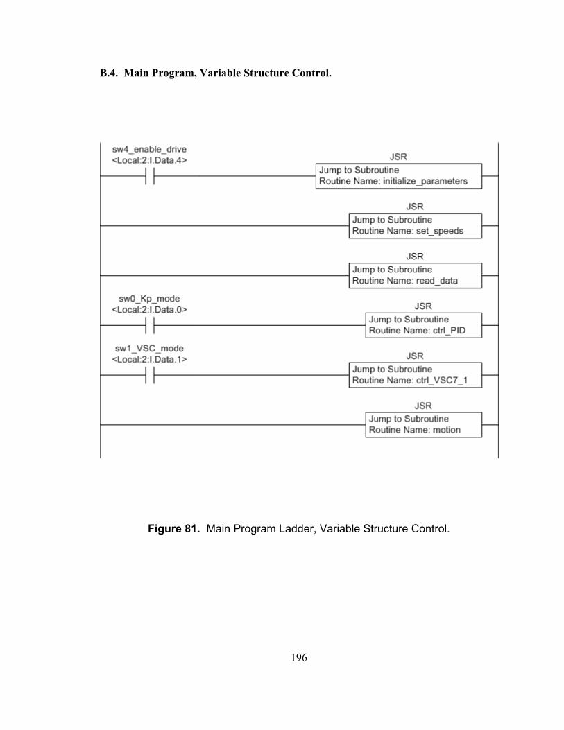
196

B.4. Main Program, Variable Structure Control.

Figure 81. Main Program Ladder, Variable Structure Control.

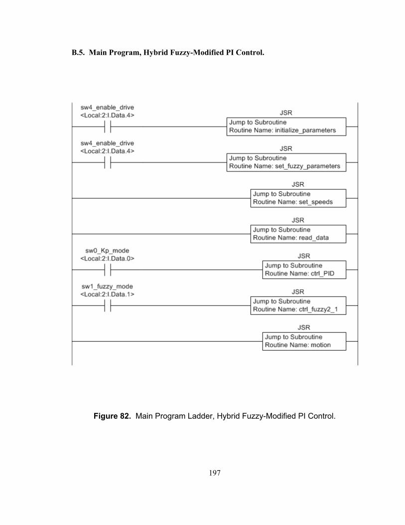
197

B.5. Main Program, Hybrid Fuzzy-Modified PI Control.

Figure 82. Main Program Ladder, Hybrid Fuzzy-Modified PI Control.

198

B.6. ctrl_PID Subroutine.

Figure 83. ctrl_PID Subroutine Ladder.

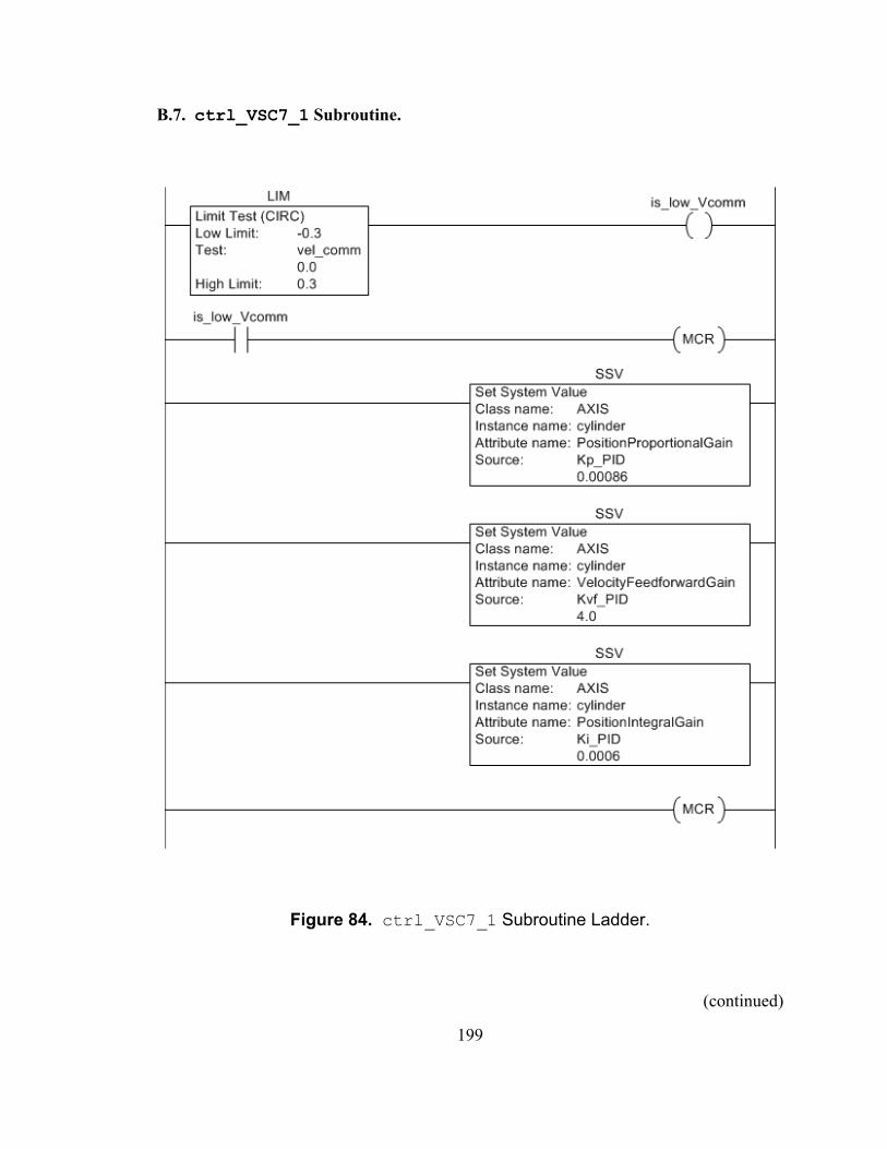
199

B.7. ctrl_VSC7_1 Subroutine.

Figure 84. ctrl_VSC7_1 Subroutine Ladder.

(continued)

200

(Figure 84, continued)

(continued)

201


(continued)

202


(continued)

203


204

B.8. ctrl_fuzzy2_1 Subroutine.

Figure 85. ctrl_fuzzy2_1 Subroutine Ladder.

(continued)

205


(continued)

206


(continued)

207


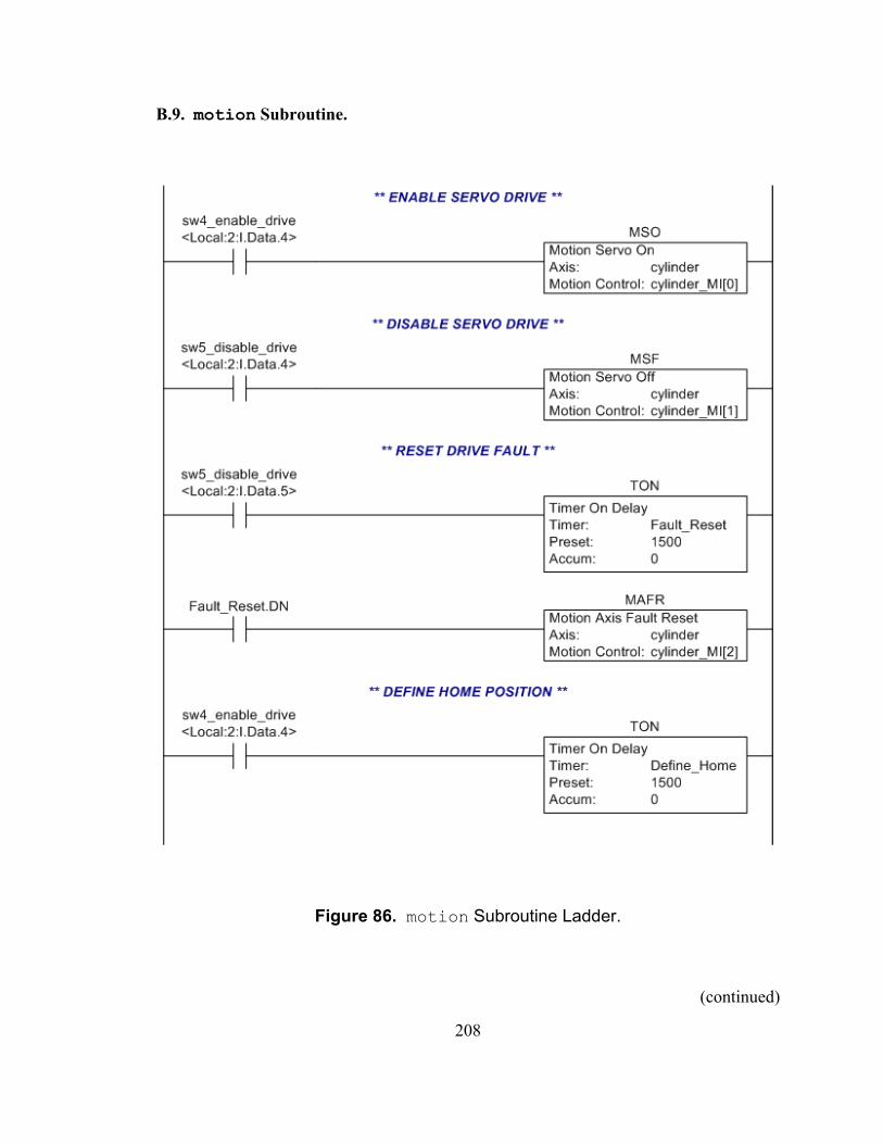
208

B.9. motion Subroutine.

Figure 86. motion Subroutine Ladder.

(continued)

209


(continued)

210


(continued)

211


(continued)

212


(continued)

213


(continued)

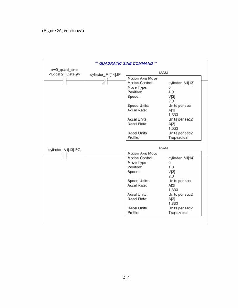
214


215

REFERENCES

[1] Bobrow J. E. and Jabbari F. “Adaptive pneumatic force actuation and position control”. ASME Journal of Dynamic Systems, Measurement, and Control, vol. 113, pp. 267-272. June 1991.

[2] Richardson R., Plummer A. R., and Brown M. D. “Self-tuning control of a low-

friction pneumatic actuator under the influence of gravity”. IEEE Transactions on Control System Technology, vol. 9, no. 2, pp. 330-334. March 2001.

[3] Moore P. R. and Pu J. S. “Pneumatic servo actuator technology”. IEE

Colloquium: Actuator Technology: Current Practice and New Developments, pp. 3/1-3/6. May 1996.

[4] Schneider R. T., ed. “The hazy line between servo and proportional valves”.

Hydraulics & Pneumatics, pp. 34-35. December 2001. [5] Shearer J. L. “Study of pneumatic processes in the continuous control of motion

with compressed air – I”. Transactions of the ASME, vol. 78, pp. 233-242. February 1956.

[6] Shearer J. L. “Study of pneumatic processes in the continuous control of motion

with compressed air – II”. Transactions of the ASME, vol. 78, pp. 243-249. February 1956.

[7] Liu S. and Bobrow J. E. “An analysis of a pneumatic servo system and its

application to a computer-controlled robot”. ASME Journal of Dynamic Systems, Measurement, and Control, vol. 110, pp. 228-235. September 1988.

[8] Kunt C. and Singh R. “A linear time varying model for on-off valve controlled

pneumatic actuators”. ASME Journal of Dynamic Systems, Measurement, and Control, vol. 112, pp. 740-747. December 1990.

[9] Hamiti K., Voda-Besançon A., and Roux-Boisson, H. “Position control of a

pneumatic cylinder under the influence of stiction”. Control Engineering Practice, vol. 4, no. 8, pp. 1079-1088. 1996.

216

[10] Wang Y. T. and Singh R. “Pneumatic chamber nonlinearities”. ASME Journal of Applied Mechanics, vol. 53, pp. 956-958. December 1986.

[11] Wand Y.T. and Singh R. “Frequency response of a nonlinear pneumatic system”.

ASME Journal of Applied Mechanics, vol. 54, pp. 209-214. March 1987. [12] Richer E. and Hurmuzlu Y. “A high performance pneumatic force actuator

system: Part I - Nonlinear mathematical model”. Transactions of the ASME, vol. 122, pp. 416-425. September 2000.

[13] Kawakami Y., Akao J., Kawai S., and Machiyama T. “Some considerations on

the dynamic characteristics of pneumatic cylinders”. Journal of Fluid Control, vol. 19, no. 2, pp. 22-36. Sept. 1988.

[14] Wang Y. T., Singh R., Yu H. C., and Guenther D. A. “Computer simulation of a

shock-absorbing pneumatic cylinder”. Journal of Sound and Vibration, vol. 93, pp. 353-364. 1984.

[15] Pu J. S. and Weston R. H. “Steady state analysis of pneumatic servo drives”.

Proceedings of the Institute of Mechanical Engineers, vol. 204, pp. 377-387. 1990.

[16] Backé W. and Ohligschläger O. “A model of heat transfer in pneumatic

chambers”. Journal of Fluid Control, vol. 20, pp. 61-78. 1989. [17] Hong I. T. and Tessmann R. K. “The dynamic analysis of pneumatic systems

using HyPneu”. International Fluid Power Exposition and Technical Conference, Chicago, IL. April 1996.

[18] Esposito A. Fluid Power with Applications, 4th Edition, Prentice Hall, Inc. 1997. [19] Thomas J. H. “Proper valve size helps determine flow”. Control Engineering.

September 1, 2000. [20] McDonell B. W. and Bobrow J. E. “Modeling, identification, and control of a

pneumatically actuated robot”. IEEE International Conference on Robotics and Automation, pp. 124-129. May 1997.

[21] Pu J. S., Moore P. R., and Weston R. H. “Digital servo motion control of air

motors”. International Journal of Production Research, vol. 29, no. 3, pp. 599-618. 1991.

[22] Wang J., Pu J. S., Moore P. R., and Zhang Z. “Modelling study and servo control

or air motor systems”. International Journal of Control, vol. 71, no. 3, pp. 459-476. 1998.

217

[23] Vaughan N. D. and Gamble J. B. “The modeling and simulation of a proportional

solenoid valve”. ASME Journal of Dynamic Systems, Measurement, and Control, vol. 118, pp. 120-125. March 1996.

[24] Gamble J. B. and Vaughan N. D. “Comparison of sliding mode control with state

feedback and PID control applied to a proportional solenoid valve”. ASME Journal of Dynamic Systems, Measurement, and Control, vol. 118, pp. 434-438. September 1996.

[25] Henri P. D. and Hollerbach J. M. “An analytical and experimental investigation

of a jet pipe controlled electropneumatic actuator”. IEEE International Conference on Robotics and Automation, vol. 1, pp. 300-306. 1994.

[26] Anglani A., Gnoni D., Grieco A., and Pacella M. “A CAD environment for the

numerical simulation of servo pneumatic actuator systems”. 7th International Workshop on Advanced Motion Control, pp. 593-598. 2002.

[27] Pfruendschuh G. H., Kumar V., and Sugar T. G. “Design and control of a 3 DOF

in-parallel actuated manipulator”. IEEE International Conference on Robotics and Automation, pp. 1659-1664. 1991.

[28] Armstrong-Hélouvry B., Dupont, P., and Canudas de Wit C. “A survey of

models, analysis tools, and compensation methods for the control of machines with friction”. Automatica, vol. 30, no. 7, pp. 1083-1183. 1994.

[29] Armstrong-Hélouvry B. “Stick slip and control in low speed motion”. IEEE

Transactions on Automatic Control, vol. 38, no. 10, pp. 1483-1496. 1993. [30] Kang Y. S. and Kim K. J. “Friction identification in a sight stabilisation system at

low velocities”. Mechanical Systems and Signal Processing, vol. 11, no. 3, pp. 491-505. 1997.

[31] Wang J., Wang D. J. D., Moore P. R., and Pu J. S. “Modelling study, analysis,

and robust servocontrol of pneumatic culinder actuator systems”. IEE Process Control Theory and Applications, vol. 148, no. 1, pp. 35-42. January 2001.

[32] Johnson C. T. and Lorenz R. D. “Experimental Identification of friction and its

compensation in precise, position-controlled mechanisms”. IEEE Transactions on Industrial Applications, vol. 28, no. 6, pp. 1392-1398. 1992.

[33] Canudas de Wit, C., Noel P., Aubin A., and Brogliato B. “Adaptive friction

compensation in robot manipulator: low velocities”. International Journal of Robotics Research, vol. 10, pp. 189-199. 1991.

218

[34] Wang Y. T. and Longman R. W. “Limit cycle behavior and convergence to zero error in learning control with stick-slip friction”. IEEE Conference on Systems, Man, and Cybernetics, pp. 2774-2779. 1994.

[35] Dunbar W. B., de Callafon R. A., and Kosmatka J. B. “Coulomb and viscous

friction fault detection with application to a pneumatic actuator”. IEEE/ASME International Conference on Advanced Intelligent Mechatronics, Como, Italy, pp. 1239-1244. July 8-12, 2001.

[36] Caldwell D. G., Badihi T. D., and Medrano-Cerda G. A. “Pneumatic muscle

actuator technology a light weight power system for a humanoid robot”. IEEE International Conference on Robotica and Automation ,Leuven, Belgium, pp. 3053-3058. May 1998.

[37] Ye N., Betemps M., Scavarda S., and Jutard A. “A servocontrolled pneumatic

actuator for small movement - Application to an adaptive gripper”. Fifth International Conference on Advanced Robotics, vol. 2, pp. 1582-1585. 1991.

[38] Shen T., Tamura K., Kaminaga H., Henmi N., and Nakazawa T. “Robust

nonlinear control of parametric uncertain systems with unknown friction and its application to a pneumatic control valve”. ASME Journal of Dynamic Systems, Measurement, and Control, vol. 122, pp. 257-262. June 2000.

[39] Pu J. S., Weston R. H., and Moore P. R. “Digital motion control and profile

planning for pneumatic servos”. ASME Journal of Dynamic Systems, Measurement, and Control,. vol. 114, pp. 634-640. December 1992.

[40] Kawamura S., Miyata K., Hanafusa H., and Isida K. “PI type hierarchical

feedback control scheme for pneumatic robots”. IEEE International Conference on Robotics and Automation, vol. 3, pp. 1853-1858. 1989.

[41] Noritsugu T. and Takaiwa M. “Robust positioning control of pneumatic servo

system with pressure control loop”. IEEE International Conference on Robotics and Automation,. pp. 2613-2618. 1995.

[42] Lai J.-Y., Menq C.-H., and Singh R. “Accurate position control of a pneumatic

actuator”. ASME Journal of Dynamic Systems, Measurement, and Control, vol. 112, pp. 734-739. December 1990.

[43] Fok S. C. and Ong E. K. “Position control and repeatability of a pneumatic

rodless cylinder system for continuous positioning”. Robotics and Computer Integrated Manufacturing, vol. 15, pp. 365-371. 1999.

219

[44] Moore P. R., Ssenkungo F. W., Weston R. H., Thatcher T. W., and Harrison R. “Control strategies for pneumatic servo drives”. International Journal of Production Research, vol. 24, no. 6, pp. 1363-1382. 1986.

[45] Wang J., Pu J. S., and Moore P. R. “A practical control strategy for servo

pneumatic actuator systems”. Control Engineering Practice, vol. 7, no. 12, pp. 1483-1488. 1999.

[46] van Varseveld, R. B. and Bone G. M. “Accurate position control of a pneumatic

actuator using on/off solenoid valves”. IEEE/ASME Transactions on Mechatronics, vol. 2, no. 3, pp. 195-204. September 1997.

[47] Aziz S. and Bone G. M. “Automatic tuning of an accurate position controller for

pneumatic actuators”. IEEE/RSJ International Conference on Intelligent Robots and Systems, Victoria, BC, pp. 1782-1788. 1998.

[48] Richard E. and Scavarda S. “Comparison between linear and non-linear control

of a pneumatic servodrive”. ASME Journal of Dynamic Systems, Measurement and Control, vol. 118, pp. 245-252. 1996.

[49] Whitcomb L. L., Rizzi A. A., and Koditschek D. E. “Comparative experiments

with a new adaptive controller for robot arms”. IEEE Transactions on Robotics and Automation, vol. 9, no. 1, pp. 59-70. February 1993.

[50] Sadegh N. and Horowitz R. “ Stability analysis of an adaptive controller for

robotic manipulators”. IEEE International Conference on Robotics and Automation, Raleigh, NC, pp. 1223-1229. April 1987.

[51] Kim S. M. and Gibson J. S. “Digital adaptive control of robotic manipulators

with flexible joints”. Proceedings of the 1991 American Control Conference, Boston, Mass. June 1991.

[52] McDonell B. W. and Bobrow J. E. “Adaptive tracking control of an air powered

robot actuator”. ASME Journal of Dynamic Systems, Measurement, and Control, vol. 115, pp. 427-433. September 1993.

[53] Hu A.-P., Register A., and Sadegh N. “Using a learning controller to achieve

accurate linear motor motion control”. Proceedings of the IEEE/ASME International Conference on Advanced Intelligent Mechatronics, Atlanta, GA, pp. 611-616. September 1999.

[54] Otten G., de Vries T. J. A., van Amerongen J., Rankers A. M., and Gaal E. W.

“Linear motor motion control using a learning feedforward controller”. IEEE/ASME Transactions on Mechatronics,. vol. 2, pp. 179-187. 1997.

220

[55] Gross D. C. and Rattan K. S. “An adaptive multilayer neural network for trajectory control of a pneumatic cylinder”. IEEE International Conference on Systems, Man, and Cybernetics, vol. 2, pp. 1662-1667. 1998.

[56] Shih M. and Ma M.-A. “Position control of a pneumatic cylinder using fuzzy

PWM control method”. Mechatronics, vol. 8, pp. 241-253. 1998. [57] Chillari S., Guccione S., and Muscato G. “An experimental comparison between

several pneumatic position control methods”. IEEE Conference on Decision and Control, Orlando, FL, 1168-1173. December 2001.

[58] Utkin V. I. “Variable structure systems with sliding modes”. IEEE Transactions

on Automatic Control, vol. AC-22, no. 2, pp. 212-222. 1977. [59] Utkin V. I. “Variable structure systems and sliding mode: State of the art

assessment”. In Studies in Automation and Control 10: Variable Structure Control for Robotics and Aerospace Applications, Young K.-K. D. (ed.), Elsevier Science Publishers, Amsterdam, pp. 9-32. 1993.

[60] Bengiamin N. N. and Kaufmann B. “Variable structure position control”. IEEE

Control Systems Magazine, vol. 4, no. 3, pp. 3-8. August 1984. [61] Bengiamin N. N. and Magnuson, M. H. “Sliding mode motion control”.

Proceedings of the Seventh Annual IEEE Power Electronics Conference and Exposition, pp. 389-394. February 23-27, 1992.

[62] Xu J., Hashimoto H., Slotine J.-J. E., Arai Y., and Harashima F. “Implementation

of VSS control to robotic manipulators - Smoothing modification”. IEEE Transactions of Industrial Electronics, vol. 36, no. 3, pp. 321-329. 1989.

[63] Leung T., Qijie Z., and Chunyi S. “Practical trajectory control of robot

manipulator using adaptive sliding control scheme”. Proceedings of the 28th Conference on Decision and Control, Tampa FL, pp. 2647-2651. December 1989.

[64] Harashima F., Hashimoto H., and Maruyama K. “Practical robust control of robot

arm using variable structure system”, IEEE International Conference on Robotics and Automation, San Fransisco, pp. 532-538. 1986.

[65] Slotine J.-J. E. and Hashimoto H. “Practical design of V.S.S. controller using

balance condition”. IEEE International Conference on Robotics and Automation, pp. 2039-2046. April 1987.

221

[66] Paul A. K., Mishra J. K., and Radke M. G. “Reduced order sliding mode control for pneumatic actuator”. IEEE Transactions on Control System Technology, vol. 2, no. 3, pp. 271-276. 1994.

[67] Pandian S. R., Hayakawa Y., Kanazawa Y., Kamoyama Y., and Kawamura S.

“Practical design of a sliding mode controller for pneumatic actuators”. Transactions of the ASME,. vol. 119, pp. 666-674. 1997.

[68] Tang J. and Walker G. “Variable structure control of a pneumatic actuator”.

ASME Journal of Dynamic Systems, Measurement, and Control, vol. 117, pp. 88-92. March 1995.

[69] Richer E. and Hurmuzlu Y. “ A high performance pneumatic force actuator

system: Part II - Nonlinear controller design”. Transactions of the ASME, vol. 122, pp. 426-434. September 2000.

[70] Drakunov S., Hanchin G. D., Su W. C., and Özgüner U. “Nonlinear control of a

rodless pneumatic servoactuator, or sliding modes versus Coulomb friction”. Automatica, vol. 33, no. 7, pp. 1401-1408. 1997.

[71] Acarman T., Hatipoglu C., and Özgüner U. “A robust nonlinear controller design

for a pneumatic actuator”. Proceedings of the American Control Conference, Arlington, VA, pp. 4490-4495. June 25-27, 2001.

[72] Young K.-K. D. “Design of variable structure system model following control

systems”. IEEE Transactions on Automatic Control, vol. AC-23, no. 6, pp. 1080-1085. 1978.

[73] de Almeida A., Fachada H., Dias J., Amado P., Menezes P., and Nunes U. “Low-

cost, high performance servo-pneumatic manipulators with sensor feedback”. Proceedings of the IEEE Symposium on Intelligent Control, pp. 465-470. 1988.

[74] Pu J. S. and Weston R. H. “A new generation of pneumatic servos for industrial

robots”. Robotica, vol. 7, pp. 17-23. January 1989. [75] Gorce P. and Guihard M. “Joint impedance pneumatic control for multilink

systems”. ASME Journal of Dynamic Systems, Measurement, and Control, vol. 121, pp. 293-297. June 1999.

[76] Takamura N., Konishi Y., Kondo K., and Ishigaki H. “Chaos of a pneumatic

actuator in digital control”. Proceedings for Information Decision and Control, pp. 289-294. 1999.

222

[77] Brun X., Thomasset D., and Bideaux E. “An accurate tracking control of an electropneumatic actuator”. Proceedings of the 1st FPNI-PhD Symposium, Hamburg, Germany, pp. 215-226. 2000.

[78] Harrison R., Weston R. H., Moore P. R., and Thatcher T. W. “A study of

application areas for modular robots”. Robotica, vol. 5, pp. 217-221. 1987. [79] Ben-Dov D. and Salcudean S. E. “A force-controlled pneumatic actuator”. IEEE

Transactions on Robotics and Automation, vol. 11, no. 6, pp. 906-911. December 1995.

[80] Guihard M., Fontaine J. G., and M'Sirdi N. “Comparative study of adaptive

controller applied to a pneumatic driven leg”. IEEE International Workshop on Intelligent Robot and Systems, pp. 1164-1171. September 1994.

[81] Hamerlain M. “An antropomorphic robot arm driven by artificial muscles using a

variable structure control”. IEEE International Conference on Robotics and Automation, pp. 550-555. 1995.

[82] The Pneumatic Catalog. Ref. 7/30-1, Festo USA, Hauppauge, N.Y. 1998. [83] Andersen B. W. The Analysis and Design of Pneumatic Systems, Robert E.

Kreiger Publishing Co., NY. 1976. [84] Thomas J. H. “Proper valve size helps determine flow”. Control Engineering.

September 1, 2000. [85] “ControlLogix Motion Module”. Publication 1756-UM006D-EN-P, Rockwell

Automation. September 2002. [86] Moody L. F. “Friction factors for pipe flow”. Transactions of the ASME, vol. 66,

no. 8, pp. 671-684. November 1944. [87] Fox R. W. and McDonald A. T. Introduction to Fluid Mechanics, Third Edition,

John Wiley & Sons. 1985. [88] “Logix 5000 Controllers Programming Documentation Reference Guide”.

Publication ABT-1756-DRG 70, Rockwell Automation. March 2000. [89] Kimura T., Hara S., Fujita T., and Kagawa T. “Control for pneumatic actuator

systems using feedback linearization with disturbance rejection”. Proceedings of the 1995 American Control Conference, Seattle, WA, pp. 825-829. June 1995.

[90] Doebelin E. O. System Modeling and Response, Wiley, New York. 1980.

ADVANCED SERVO CONTROL OF A PNEUMATIC ...

Documents

Transcript of ADVANCED SERVO CONTROL OF A PNEUMATIC ...