Modelling valve stiction

Control Engineering Practice 13 (2005) 641–658

ARTICLE IN PRESS

$A prelimina

2003, Hong Kon

*Correspondi

2881.

E-mail addre

0967-0661/$ - see

doi:10.1016/j.con

Modelling valve stiction$

M.A.A. Shoukat Choudhurya, N.F. Thornhillb, S.L. Shaha,*aDepartment of Chemical and Materials Engineering, University of Alberta, Edmonton, Canada, AB T6G 2G6bDepartment of Electronic and Electrical Engineering, University College London, London, UK WC1E 7JE

Received 18 January 2003; accepted 13 May 2004

Available online 28 July 2004

Abstract

The presence of nonlinearities, e.g., stiction, and deadband in a control valve limits the control loop performance. Stiction is the

most commonly found valve problem in the process industry. In spite of many attempts to understand and model the stiction

phenomena, there is a lack of a proper model, which can be understood and related directly to the practical situation as observed in

real valves in the process industry. This study focuses on the understanding, from real-life data, of the mechanism that causes

stiction and proposes a new data-driven model of stiction, which can be directly related to real valves. It also validates the simulation

results generated using the proposed model with that from a physical model of the valve. Finally, valuable insights on stiction have

been obtained from the describing function analysis of the newly proposed stiction model.

r 2004 Elsevier Ltd. All rights reserved.

Keywords: Stiction; Stickband; Deadband; Hysteresis; Backlash; Deadzone; Viscous friction; Coulomb friction; Process control; Slip jump

1. Introduction

A typical chemical plant has hundreds or thousandsof control loops. Control performance is very importantto ensure tight product quality and low cost of theproduct in such plants. The economic benefits resultingfrom performance assessment are difficult to quantify ona loop-by-loop basis because each problem loopcontributes in a complicated way to the overall processperformance. Finding and fixing problem loopsthroughout a plant shows reduced off-grade production,reduced product property variability, and occasionallylower operating costs and improved production rate(Paulonis & Cox, 2003). Even a 1% improvement eitherin energy efficiency or improved controller maintenancedirection represents hundreds of millions of dollars insavings to the process industries (Desborough & Miller,2002). Oscillatory variables are one of the main causesfor poor performance of control loops and a key

ry version of this paper was presented at ADCHEM

g, January 11–14, 2004.

ng author. Tel.: +1-780-492-5162; fax: +1-780-492-

ss: [email protected] (S.L. Shah).

front matter r 2004 Elsevier Ltd. All rights reserved.

engprac.2004.05.005

challenge is to find the root cause of distributedoscillations in chemical plants (Qin, 1998; Thornhill,Huang, & Zhang, 2003a; Thornhill, Cox, & Paulonis,2003b). The presence of oscillations in a control loopincreases the variability of the process variables, thuscausing inferior quality products, larger rejection rates,increased energy consumption, reduced averagethroughput and profitability. Oscillations can cause avalve to wear out much earlier than its life period it wasoriginally designed for. Oscillations increase operatingcosts roughly in proportion to the deviation (Shinskey,1990). Detection and diagnosis of the causes ofoscillations in process operation are important becausea plant operating close to product quality limit is moreprofitable than a plant that has to back away because ofvariations in the product (Martin, Turpin, & Cline,1991). Oscillatory feedback control loops are a commonoccurrence due to poor controller tuning, control valvestiction, poor process and control system design, andoscillatory disturbances (Bialkowski, 1992; Ender, 1993;Miao & Seborg, 1999). Bialkowski (1992) reported thatabout 30% of the loops are oscillatory due to controlvalve problems. The only moving part in a control loopis the control valve. If the control valve containsnonlinearities, e.g., stiction, backlash, and deadband,

ARTICLE IN PRESSM.A.A. Shoukat Choudhury et al. / Control Engineering Practice 13 (2005) 641–658642

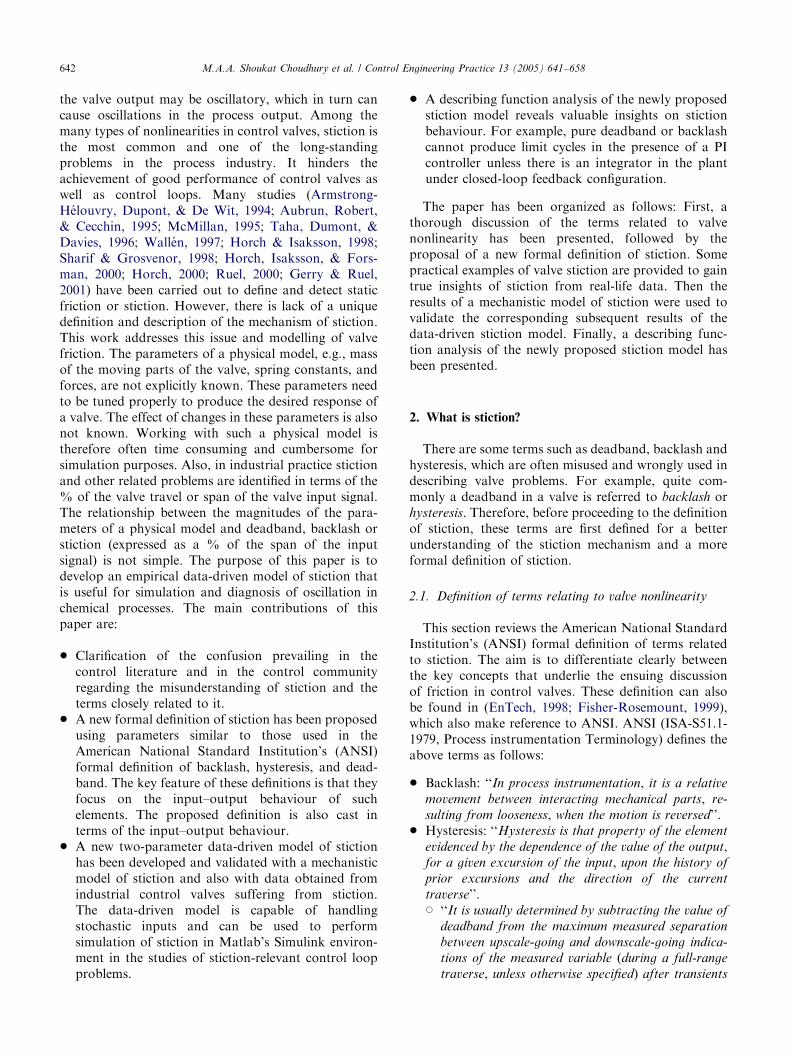
the valve output may be oscillatory, which in turn cancause oscillations in the process output. Among themany types of nonlinearities in control valves, stiction isthe most common and one of the long-standingproblems in the process industry. It hinders theachievement of good performance of control valves aswell as control loops. Many studies (Armstrong-Helouvry, Dupont, & De Wit, 1994; Aubrun, Robert,& Cecchin, 1995; McMillan, 1995; Taha, Dumont, &Davies, 1996; Wallen, 1997; Horch & Isaksson, 1998;Sharif & Grosvenor, 1998; Horch, Isaksson, & Fors-man, 2000; Horch, 2000; Ruel, 2000; Gerry & Ruel,2001) have been carried out to define and detect staticfriction or stiction. However, there is lack of a uniquedefinition and description of the mechanism of stiction.This work addresses this issue and modelling of valvefriction. The parameters of a physical model, e.g., massof the moving parts of the valve, spring constants, andforces, are not explicitly known. These parameters needto be tuned properly to produce the desired response ofa valve. The effect of changes in these parameters is alsonot known. Working with such a physical model istherefore often time consuming and cumbersome forsimulation purposes. Also, in industrial practice stictionand other related problems are identified in terms of the% of the valve travel or span of the valve input signal.The relationship between the magnitudes of the para-meters of a physical model and deadband, backlash orstiction (expressed as a % of the span of the inputsignal) is not simple. The purpose of this paper is todevelop an empirical data-driven model of stiction thatis useful for simulation and diagnosis of oscillation inchemical processes. The main contributions of thispaper are:

* Clarification of the confusion prevailing in thecontrol literature and in the control communityregarding the misunderstanding of stiction and theterms closely related to it.

* A new formal definition of stiction has been proposedusing parameters similar to those used in theAmerican National Standard Institution’s (ANSI)formal definition of backlash, hysteresis, and dead-band. The key feature of these definitions is that theyfocus on the input–output behaviour of suchelements. The proposed definition is also cast interms of the input–output behaviour.

* A new two-parameter data-driven model of stictionhas been developed and validated with a mechanisticmodel of stiction and also with data obtained fromindustrial control valves suffering from stiction.The data-driven model is capable of handlingstochastic inputs and can be used to performsimulation of stiction in Matlab’s Simulink environ-ment in the studies of stiction-relevant control loopproblems.

* A describing function analysis of the newly proposedstiction model reveals valuable insights on stictionbehaviour. For example, pure deadband or backlashcannot produce limit cycles in the presence of a PIcontroller unless there is an integrator in the plantunder closed-loop feedback configuration.

The paper has been organized as follows: First, athorough discussion of the terms related to valvenonlinearity has been presented, followed by theproposal of a new formal definition of stiction. Somepractical examples of valve stiction are provided to gaintrue insights of stiction from real-life data. Then theresults of a mechanistic model of stiction were used tovalidate the corresponding subsequent results of thedata-driven stiction model. Finally, a describing func-tion analysis of the newly proposed stiction model hasbeen presented.

2. What is stiction?

There are some terms such as deadband, backlash andhysteresis, which are often misused and wrongly used indescribing valve problems. For example, quite com-monly a deadband in a valve is referred to backlash orhysteresis. Therefore, before proceeding to the definitionof stiction, these terms are first defined for a betterunderstanding of the stiction mechanism and a moreformal definition of stiction.

2.1. Definition of terms relating to valve nonlinearity

This section reviews the American National StandardInstitution’s (ANSI) formal definition of terms relatedto stiction. The aim is to differentiate clearly betweenthe key concepts that underlie the ensuing discussionof friction in control valves. These definition can alsobe found in (EnTech, 1998; Fisher-Rosemount, 1999),which also make reference to ANSI. ANSI (ISA-S51.1-1979, Process instrumentation Terminology) defines theabove terms as follows:

* Backlash: ‘‘In process instrumentation, it is a relative

movement between interacting mechanical parts, re-

sulting from looseness, when the motion is reversed’’.* Hysteresis: ‘‘Hysteresis is that property of the element

evidenced by the dependence of the value of the output,for a given excursion of the input, upon the history of

prior excursions and the direction of the current

traverse’’.* ‘‘It is usually determined by subtracting the value of

deadband from the maximum measured separation

between upscale-going and downscale-going indica-

tions of the measured variable (during a full-range

traverse, unless otherwise specified) after transients

ARTICLE IN PRESS

o

a b

db

ooutp

utut

outp

utut

outp

utut

outp

utut

(b) deadbandb

d

hysteresis

input

input

input

input

deadband

deadband

(a) hysteresis

deadzone

(d) deadzone(c) hysteresis + deadband

hysteresis + deadband

Fig. 1. Hysteresis, deadband, and deadzone (redrawn from ANSI/

ISA-S51.1-1979).

M.A.A. Shoukat Choudhury et al. / Control Engineering Practice 13 (2005) 641–658 643

have decayed’’. Fig. 1(a) and (c) illustrates theconcept.

* ‘‘Some reversal of output may be expected for any

small reversal of input. This distinguishes hysteresis

from deadband’’.* Deadband: ‘‘In process instrumentation, it is the range

through which an input signal may be varied, upon

reversal of direction, without initiating an observable

change in output signal’’.* ‘‘There are separate and distinct input–output

relationships for increasing and decreasing signals

(see Fig. 1(b))’’.* ‘‘Deadband produces phase lag between input and

output’’.* ‘‘Deadband is usually expressed in percent of span’’.

Deadband and hysteresis may be presenttogether. In that case, the characteristics in thelower left panel of Fig. 1 would be observed.

* Dead zone: ‘‘It is a predetermined range of input

through which the output remains unchanged, irrespec-

tive of the direction of change of the input signal’’.* ‘‘There is but one input–output relationship (see

Fig. 1(d))’’.* ‘‘Dead zone produces no phase lag between input

and output’’.

The above definitions show that the term ‘‘backlash’’specifically applies to the slack or looseness of themechanical part when the motion changes its direction.Therefore, in control valves it may only add deadbandeffects if there is some slack in rack-and-pinion typeactuators (Fisher-Rosemount, 1999) or loose connec-tions in rotary valve shaft. ANSI (ISA-S51.1-1979)definitions and Fig. 1 show that hysteresis and deadband

are distinct effects. Deadband is quantified in terms ofinput signal span (i.e., on the x-axis), while hysteresisrefers to a separation in the measured (output) response(i.e., on the y-axis).

2.2. Discussion of the term ‘‘stiction’’

Different people or organizations have defined stic-tion in different ways. A few of the definitions arereproduced below:

* According to the Instrument Society of America(ISA) (ISA Subcommittee SP75.05, 1979), ‘‘stiction is

the resistance to the start of motion, usually measured

as the difference between the driving values required to

overcome static friction upscale and downscale’’. Thedefinition was first proposed in 1963 in AmericanNational Standard C85.1-1963,‘‘Terminology forAutomatic Control’’, and has not been updated. Thisdefinition was adopted in ISA 1979 Handbook (ISASubcommittee SP75.05, 1979) and remained exactlythe same in the revised 1993 edition.

* According to EnTech (1998), ‘‘stiction is a tendency to

stick-slip due to high static friction. The phenomenon

causes a limited resolution of the resulting control valve

motion. ISA terminology has not settled on a suitable

term yet. Stick-slip is the tendency of a control valve to

stick while at rest, and to suddenly slip after force has

been applied’’.* According to Horch (2000), ‘‘The control valve is

stuck in a certain position due to high static friction.

The (integrating) controller then increases the set

point to the valve until the static friction can be

overcome. Then the valve breaks off and moves to a

new position (slip phase) where it sticks again. The

new position is usually on the other side of the

desired set point such that the process starts in the

opposite direction again’’. This is the extreme case ofstiction. On the contrary, once the valve overcomesstiction it might travel smoothly for some time andthen stick again when the velocity of the valve is closeto zero.

* In a recent paper, Ruel (2000) reported ‘‘stiction as a

combination of the words stick and friction, created to

emphasize the difference between static and dynamic

friction. Stiction exists when the static (starting)friction exceeds the dynamic (moving) friction inside

the valve. Stiction describes the valve’s stem (or shaft)sticking when small changes are attempted. Friction of

a moving object is less than when it is stationary.

Stiction can keep the stem from moving for small

control input changes, and then the stem moves when

there is enough force to free it. The result of stiction is

that the force required to get the stem to move is more

than is required to go to the desired stem position. In

presence of stiction, the movement is jumpy’’.


This definition is close to the stiction as measuredonline by the people in process industries—puttingthe control loop in manual and then increasing thevalve input in little increments until there is anoticeable change in the process variable.

* In Olsson (1996), stiction is defined as short for static

friction as opposed to dynamic friction. It describes the

friction force at rest. Static friction counteracts

external forces below a certain level and thus keeps

an object from moving.

The above discussion reveals the lack of a formal andgeneral definition of stiction and the mechanism(s) thatcauses it. All of the above definitions agree that stiction isthe static friction that keeps an object from moving andwhen the external force overcomes the static friction theobject starts moving. But they disagree in the way it ismeasured and how it can be modelled. Also, there is a lackof clear description of what happens at the moment whenthe valve just overcomes the static friction. Some modellingapproaches described this phenomena using a Stribeckeffect model (Olsson, 1996). These issues can be resolvedby a careful observation and a proper definition of stiction.

2.3. A proposal for a definition of stiction

The motivation for a new definition of stiction is tocapture the descriptions cited earlier within a definitionthat explains the behaviour of an element with stictionin terms of its input–output behaviours, as is done in theANSI definitions for backlash, hysteresis, and dead-band. The new definition of stiction is proposed by theauthors based on careful investigation of real processdata. It is observed that the phase plot of the input–output behaviour of a valve ‘‘suffering from stiction’’can be described as shown in Fig. 2. It consists of fourcomponents: deadband, stickband, slip jump and themoving phase. When the valve comes to rest or changesthe direction at point A in Fig. 2, the valve sticks. After

mov

ing

phas

e

A BC

D

EF

G

mov

ing

phas

e

C

valv

e ou

tput

(m

anip

ulat

ed v

aria

ble)

valve input (controller output)

stickbanddeadband

slipjump, J

stickband + deadband = S

Fig. 2. Typical input–output behaviour of a sticky valve.

the controller output overcomes the deadband (AB) andthe stickband (BC) of the valve, the valve jumps to anew position (point D) and continues to move. Due tovery low or zero velocity, the valve may stick again inbetween points D and E in Fig. 2 while travelling in thesame direction (EnTech, 1998). In such a case, themagnitude of deadband is zero and only stickband ispresent. This can be overcome if the controller outputsignal is larger than the stickband only. It is usuallyuncommon in industrial practice. The deadband andstickband represent the behaviour of the valve when it isnot moving, though the input to the valve keepschanging. Slip jump represents the abrupt release ofpotential energy stored in the actuator chambers due tohigh static friction in the form of kinetic energy as thevalve starts to move. The magnitude of the slip jump isvery crucial in determining the limit cyclic behaviourintroduced by stiction (McMillan, 1995; Piipponen,1996). Once the valve slips, it continues to move untilit sticks again (point E in Fig. 2). In this moving-phase,dynamic friction is present which may be much lowerthan the static friction. As depicted in Fig. 2, this sectionhas proposed a rigorous description of the effects offriction in a control valve. Therefore, ‘‘stiction is a property

of an element such that its smooth movement in response to

a varying input is preceded by a sudden abrupt jump called

the slip-jump. Slip-jump is expressed as a percentage of the

output span. Its origin in a mechanical system is static

friction which exceeds the friction during smooth move-

ment’’. This definition has been exploited in the next andsubsequent sections for the evaluation of practicalexamples and for modelling of a control valve sufferingfrom stiction in a feedback control configuration.

3. Practical examples of valve stiction

The objective of this section is to observe effects ofstiction from the investigation of data from industrialcontrol loops. The observations reinforce the need for arigorous definition of the effects of stiction. This sectionanalyses four data sets. The first data set is from a powerplant, the second and third are from a petroleumrefinery and the other is from a furnace. To preserve theconfidentiality of the plants, all data are scaled andreported as mean-centred with unit variance. In order tofacilitate the readability of the paper by practisingindustrial people, the notations followed by the indus-trial people have been used. For example, pv is used todenote the process variable or controlled variable.Similarly, op is used to denote the controller output,mv is used to denote valve output or valve position, andsp is used to denote set point.

* Loop 1 is a level control loop which controls thelevel of condensate in the outlet of a turbine by

ARTICLE IN PRESS

0 100 200

-1.5

-1

-0.5

0

0.5

1

1.5

sampling instants

pv a

nd o

p

-1.5

-1

-0.5

0

0.5

1

1.5

mv

and

op

-1 0 1

-1

0

1

controller output, op

proc

ess

outp

ut, p

v

0 100 200sampling instants

-1 0 1

-1

0

1

controller output, opva

lve

posi

tion,

mv

A A A A

AA A A

Fig. 3. Flow control cascaded to level control in an industrial setting, the line with circles is pv and mv; the thin line is op:


manipulating the flow rate of the liquid condensate.In total, 8640 samples for each tag were collected at asampling rate of 5 s: Fig. 3 shows a portion of thetime domain data. The left panel shows time trendsfor level ðpvÞ; the controller output ðopÞ which is alsothe valve demand, and valve position ðmvÞ which canbe taken to be the same as the condensate flow rate.The plots in the right panel show the characteristicpv–op and mv–op plots. The bottom figure clearlyindicates both the stickband plus deadband and theslip jump effects. The slip jump is large and visiblefrom the bottom figure, especially when the valve ismoving in a downward direction. It is marked as ‘A’in the figure. It is evident from this figure that thevalve output ðmvÞ can never reach the valve demandðopÞ: This kind of stiction is termed as undershootcase of valve stiction in this paper. The pv–op plotdoes not show the jump behaviour clearly. The slipjump is very difficult to observe in the pv–op plotbecause the process dynamics (i.e., the transferfunction between mv and pv) destroys the pattern.This loop shows one of the possible types of stictionphenomena clearly. The stiction model developedlater in the paper based on the control signal ðopÞ isable to imitate this kind of behaviour.

* Loop 2 is a liquid flow slave loop of a cascade controlloop. The data were collected at a sampling rate of10 s and the data length for each tag was 1000samples. The left plot of Fig. 4 shows the time trendof pv and op: A closer look of this figure shows thatthe pv (flow rate) is constant for some period of8time though the op changes over that period. This isthe period during which the valve was stuck. Once the

valve overcomes deadband plus stickband, the pv

changes very quickly (denoted as ‘A’ in the figure)and moves to a new position where the valve sticksagain. It is also evident that sometimes the pv

overshoots the op and sometime it undershoots. Thepv–op plot has two distinct parts—the lower part andthe upper part extended to the right. The lower partcorresponds to the overshoot case of stiction, i.e., itrepresents an extremely sticky valve. The upper partcorresponds to the undershoot case of stiction. Thesetwo cases have been separately modelled in the data-driven stiction model. This example represents amixture of undershoot and overshoot cases ofstiction. The terminologies regarding different casesof stiction have been made clearer in Section 5.

* Loop 3 is a slave flow loop cascaded with a masterlevel control loop. A sampling rate of 6 s was used forthe collection of the data and a total of 1000 samplesfor each tag were collected. The top panel of Fig. 5shows the presence of stiction with a clear indicationof stickband plus deadband and the slip jump phase.The slip jump appears as the control valve justovercomes stiction (denoted as point ‘A’ in Fig. 5).This slip jump is not very clear in the pv–op plot ofthe closed-loop data (top right plot), because both pv

and op jump together due to the probable presence ofa proportional only controller. But it shows thepresence of deadband plus stickband clearly. Some-times it is best to look at the pv–sp plot if it is acascaded loop and the slave loop is operating underproportional control only. The bottom panel ofFig. 5 shows the time trend and phase plot of sp

and pv where the slip jump behaviour is clearly

ARTICLE IN PRESS

0 200 400

-1

0

1

sampling instants

pv a

nd o

p

-1 0 1

-1

0

1

controller output ,op

proc

ess

outp

ut, p

v

A

A

A A

AA A

A

Fig. 4. Data from a flow loop in a refinery, time trend of pv and op (left)—the line with circles is pv and the thin line is op; and the pv–op plot (right).

0 100 200 300 400

-1

0

1

sampling instants

pv a

nd o

p

-1 0 1

-1

0

1


proc

ess

outp

ut, p

v

0 100 200 300 400

-1

0

1

sampling instants

pv a

nd s

p

-1 0 1

-1

0

1

set point, sp

proc

ess

outp

ut, p

vA

A

A

A

A

A

A

A

A

A

A

Fig. 5. Data from a flow loop in a refinery, time trend of pv and op (top left)—the line with circles is pv and the thin line is op; the pv–op plot (top

right), time trend of pv and sp (bottom left), line with circles is pv and thin line is sp; and the pv–sp plot (bottom right).

M.A.A. Shoukat Choudhury et al. / Control Engineering Practice 13 (2005) 641–658646

visible. This example represents a case of pure stick-slip or stiction with no offset.

* Loop 4 is a temperature control loop on a furnacefeed dryer system at the Tech-Cominco mine in Trail,British Columbia, Canada. The temperature of thedryer combustion chamber is controlled by manip-ulating the flow rate of natural gas to the combustionchamber. A total of 1440 samples for each tag werecollected at a sampling rate of 1 min: The top plot ofthe left panel of Fig. 6 shows time trends of

temperature ðpvÞ and controller output ðopÞ: It showsclear oscillations both in the controlled variable ðpvÞand the controller output. The presence of distinctcycles is observed in the characteristic pv–op plot (seeFig. 6 top right). For this loop, there is a flowindicator close to this valve and these indicator datawere available. In the bottom figure this flow rate isplotted versus op: The flow rate data looks quantizedbut the presence of stiction in this control valve wasconfirmed by the plant engineer. The bottom plots

ARTICLE IN PRESS

0 200 400

-2

-1

0

1

2

pv a

nd o

p

-2 -1 0 1 2

-2

-1

0

1

2

op

pv

0 200 400

-2

-1

0

1

2

sampling instants

flow

rat

e an

d op

-2 -1 0 1 2

-2

-1

0

1

2


flow

rat

e

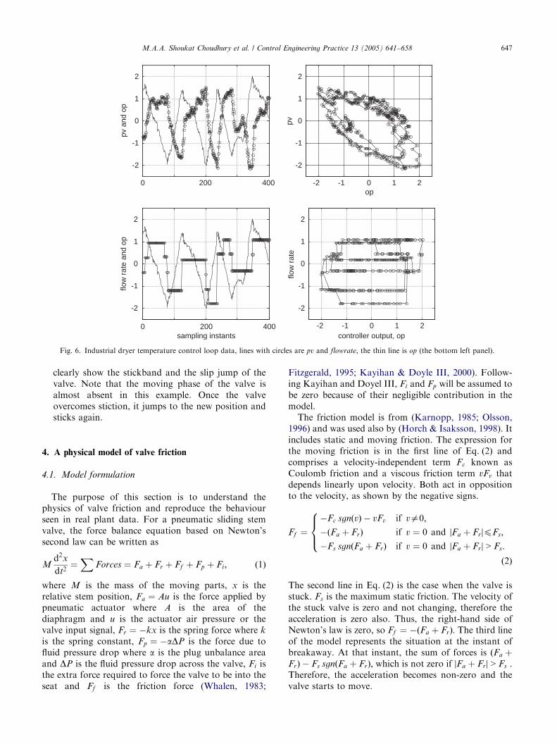
Fig. 6. Industrial dryer temperature control loop data, lines with circles are pv and flowrate; the thin line is op (the bottom left panel).


clearly show the stickband and the slip jump of thevalve. Note that the moving phase of the valve isalmost absent in this example. Once the valveovercomes stiction, it jumps to the new position andsticks again.

4. A physical model of valve friction

4.1. Model formulation

The purpose of this section is to understand thephysics of valve friction and reproduce the behaviourseen in real plant data. For a pneumatic sliding stemvalve, the force balance equation based on Newton’ssecond law can be written as

Md2x

dt2¼

XForces ¼ Fa þ Fr þ Ff þ Fp þ Fi; ð1Þ

where M is the mass of the moving parts, x is therelative stem position, Fa ¼ Au is the force applied bypneumatic actuator where A is the area of thediaphragm and u is the actuator air pressure or thevalve input signal, Fr ¼ �kx is the spring force where k

is the spring constant, Fp ¼ �aDP is the force due tofluid pressure drop where a is the plug unbalance areaand DP is the fluid pressure drop across the valve, Fi isthe extra force required to force the valve to be into theseat and Ff is the friction force (Whalen, 1983;

Fitzgerald, 1995; Kayihan & Doyle III, 2000). Follow-ing Kayihan and Doyel III, Fi and Fp will be assumed tobe zero because of their negligible contribution in themodel.The friction model is from (Karnopp, 1985; Olsson,

1996) and was used also by (Horch & Isaksson, 1998). Itincludes static and moving friction. The expression forthe moving friction is in the first line of Eq. (2) andcomprises a velocity-independent term Fc known asCoulomb friction and a viscous friction term vFv thatdepends linearly upon velocity. Both act in oppositionto the velocity, as shown by the negative signs.

Ff ¼

�Fc sgnðvÞ � vFv if va0;

�ðFa þ FrÞ if v ¼ 0 and jFa þ FrjpFs;

�Fs sgnðFa þ FrÞ if v ¼ 0 and jFa þ Frj > Fs:

8><>:

ð2Þ

The second line in Eq. (2) is the case when the valve isstuck. Fs is the maximum static friction. The velocity ofthe stuck valve is zero and not changing, therefore theacceleration is zero also. Thus, the right-hand side ofNewton’s law is zero, so Ff ¼ �ðFa þ FrÞ: The third lineof the model represents the situation at the instant ofbreakaway. At that instant, the sum of forces is ðFa þFrÞ � Fs sgnðFa þ FrÞ; which is not zero if jFa þ Frj > Fs .Therefore, the acceleration becomes non-zero and thevalve starts to move.


A disadvantage of a physical model of a control valveis that it requires several parameters to be known. Themass M and typical friction forces depend upon thedesign of the valve. Kayihan and Doyle III (2000) usedmanufacturer’s values suggested by Fitzgerald (1995)and similar values have been chosen here apart from aslightly increased value of Fs and a smaller value for Fc

in order to make the demonstration of the slip jumpmore obvious (see Table 1). Fig. 7 shows the frictionforce characteristic in which the magnitude of themoving friction is smaller than that of the static friction.The friction force opposes velocity (see Eq. (2)), thus theforce is negative when the velocity is positive.The calibration factor of Table 1 is introduced

because the required stem position xr is the input tothe simulation. In the absence of stiction effects, thevalve moving parts come to rest when the force due toair pressure on the diaphragm is balanced by the springforce. Thus, Au ¼ kx and so the calibration factorrelating air pressure u to xr is k=A: The consequences ofmiscalibration are discussed below.

Table 1

Nominal values used for physical valve simulation

Parameters Kayihan and Doyle III

(2000)

Nominal case

M 3 lb ð1:36 kgÞ 1:36 kgFs 384 lbf ð1708 NÞ 1750 N

Fc 320 lbf ð1423 NÞ 1250 N

Fv 3:5 lbf s in�1 ð612 N s m�1Þ 612 N s m�1

Spring constant, k 300 lbf in�1 ð52; 500 N m�1Þ 52; 500 N m�1

Diaphragm area, A 100 in2 ð0:0645 m2Þ 0:0645 m2

Calibration factor, k=A — 807; 692 Pa m�1

Air pressure 10 psi ð68; 950 PaÞ 68; 950 Pa

-0.2 -0.1 0 0.1 0.22000

1000

0

-1000

-2000

velocity (ms-1)

fric

tion

forc

e (N

)

Fs

Fc

-

-

Fig. 7. Friction characteristic plot.

4.2. Valve simulation

The purpose of simulation of the valve was todetermine the influence of the three friction terms inthe model. The nonlinearity in the model is able toinduce limit cycle oscillations in a feedback control loop,and the aim is to understand the contribution of eachfriction term to the character and shape of the limitcycles.

4.2.1. Open loop response

Fig. 8 shows the valve position when the valve modelis driven by a sinusoidal variation in op in open loop inthe absence of the controller. The left-hand columnshows the time trends and the right-hand panels areplots of valve demand ðopÞ versus valve position ðmvÞ:Several cases are simulated using the parameters shownin Table 2. The ‘‘linear’’ values are those suggested byKayihan and Doyle III for the best case of a smart valvewith Teflon packing requiring an air pressure of about0:1 psi ð689 PaÞ to start moving.In the first row of Fig. 8, the Coulomb friction Fc and

static friction Fs are small and linear viscous frictiondominates. The input and output are almost in phase inthe first row of Fig. 8 because the sinusoidal input is oflow frequency compared to the bandwidth of the valvemodel and is on the part of the frequency responsefunction where input and output are in phase.Valve deadband is due to the presence of Coulomb

friction Fc; a constant friction which acts in the oppositedirection to the velocity. In the deadband simulationcase the static friction is the same as the Coulomb

mv (thick line) and op (thin line)

0 50 100 150 200time/s

mv vs. op

linear

pure deadband

stiction (undershoot)

stiction (no offset)

stiction (overshoot)

Fig. 8. Open-loop response of mechanistic model. The amplitude of

the sinusoidal input is 10 cm in each case.

ARTICLE IN PRESS

Table 2

Friction values used in simulation of physical valve model

Parameters Linear Deadband Stiction

Undershoot No offset

Open loop Closed loop

Fs ðNÞ 45 1250 2250 1000 1750

Fc ðNÞ 45 1250 1250 400 0

Fv ðN s m�1Þ 612 612 612 612 612


0 100 200 300time/s


mv vs. op


PI gain doubled



Fig. 9. Closed-loop response of mechanistic model.


friction, Fs ¼ Fc: The deadband arises because, onchanging direction, the valve remains stationary untilthe net applied force is large enough to overcome Fc:The deadband becomes larger if Fc is larger.A valve with high initial static friction such that

Fs > Fc exhibits a jumping behaviour that is differentfrom a deadband, although both behaviours may bepresent simultaneously. When the valve starts to move,the friction force reduces abruptly from Fs to Fc: Thereis therefore a discontinuity in the model on the right-hand side of Newton’s second law and a large increase inacceleration of the valve moving parts. The initialvelocity is therefore faster than in the Fs ¼ Fc case,leading to the jump behaviour observed in the third rowof Fig. 8. If the Coulomb friction Fc is absent, then thedeadband is absent and the slip jump allows the mv tocatch up with the op (fourth row). If the valve ismiscalibrated, then swings in the valve position ðmvÞ arelarger than swings in the demanded position ðopÞ: In thatcase, the gradient of the op–mv plot is greater than unityduring the moving phase. The bottom row of Fig. 8shows the case when the calibration factor is too largeby 25%. A slip jump was also used in this simulation.

4.2.2. Closed-loop dynamics

For assessment of closed-loop behaviour, the valveoutput drives a first-order plus dead time process GðsÞand receives its op reference input from a PI controllerCðsÞ where:

GðsÞ ¼3e�10s

10s þ 1; CðsÞ ¼ 0:2

10s þ 1

10s

� �: ð3Þ

Fig. 9 shows the limit cycles induced in this control loopby the valve, together with the plots of valve positionðmvÞ versus valve demand ðopÞ: The limit cycles werepresent even though the set point to the loop was zero.That is, they were internally generated and sustained bythe loop in the absence of any external setpointexcitation.There was no limit cycle in the linear case dominated

by viscous friction or in the case with deadband onlywhen Fs ¼ Fc: It is known that deadband alone cannotinduce a limit cycle unless the process GðsÞ hasintegrating dynamics, as will be discussed further inSection 5.3.1.

The presence of stiction ðFs > FcÞ induces a limit cyclewith a characteristic triangular shape in the controlleroutput. Cycling occurs because an offset exists betweenthe set point and the output of the control loop while thevalve is stuck which is integrated by the PI controller toform a ramp. By the time the valve finally moves inresponse to the controller op signal, the actuator forcehas grown quite large and the valve moves quickly toa new position where it then sticks again. Thus, aself-limiting cycle is set up in the control loop.If stiction and deadband are both present, then the

period of the limit cycle oscillation can become verylong. The combination Fs ¼ 1750 N and Fc ¼ 1250 Ngave a period of 300 s while the combination Fs ¼1000 N and Fc ¼ 400 N had a period of about 140 s (toprow, Fig. 9), in both cases much longer than the timeconstant of the controlled process or its cross-overfrequency. The period of oscillation can also beinfluenced by altering the controller gain. If the gain isincreased the linear ramps of the controller output signalare steeper, the actuator force moves through thedeadband more quickly and the period of the limitcycle becomes shorter (second row, Fig. 9). Thetechnique of changing the controller gain is used byindustrial control engineers to test the hypothesis of alimit cycle induced by valve nonlinearity while the plantis still running in closed loop.In the pure stick-slip or stiction with no offset case

shown in the third row of Fig. 9, the Coulomb friction isnegligible and the oscillation period is shorter becausethere is no deadband. The bottom row in Fig. 9 showsthat miscalibration causes an overshoot in closed loop.


5. Data-driven model of valve stiction

The proposed data-driven model has parameters thatcan be directly related to plant data and it produces thesame behaviour as the physical model. The model needsonly an input signal and the specification of deadbandplus stickband and slip jump. It overcomes the maindisadvantages of physical modelling of a control valve,namely that it requires the knowledge of the mass of themoving parts of the actuator, spring constant, and thefriction forces. The effect of the change of these parameterscannot be determined easily analytically because therelationship between the values of the parameters andthe observation of the deadband/stickband as a percentageof valve travel is not straightforward. In a data-drivenmodel, the parameters are easy to choose and the effects ofthese parameter change are simple to realize.

5.1. Model formulation

The valve sticks only when it is at rest or it is changingits direction. When the valve changes its direction, itcomes to rest momentarily. Once the valve overcomesstiction, it starts moving and may keep on moving forsometime depending on how much stiction is present inthe valve. In this moving phase, it suffers only dynamicfriction, which may be smaller than the static friction. Itcontinues to do so until its velocity is again very close tozero or it changes its direction.In the process industry, stiction is generally measured

as a % of the valve travel or the span of the controlsignal (Gerry & Ruel, 2001). For example, a 2% stictionmeans that when the valve gets stuck it will start movingonly after the cumulative change of its control signal isgreater than or equal to 2%. If the range of the controlsignal is 4–20 mA; then a 2% stiction means that achange of the control signal less than 0:32 mA inmagnitude will not be able to move the valve.In our modelling approach, the control signal has been

translated to the percentage of valve travel with the helpof a linear look-up table. In order to handle stochasticinputs, the model requires the implementation of a PI(D)controller including its filter under a full industrialspecification environment. Alternatively, an exponen-tially weighted moving average (EWMA) filter placedright in front of the stiction model can be used to reducethe effect of noise. This practice is very much consistentwith industrial practices. The model consists of twoparameters—namely the size of deadband plus stickbandS (specified in the input axis) and slip jump J (specifiedon the output axis). Note that the term ‘S’ contains boththe deadband and stickband. Fig. 10 summarizes themodel algorithm, which can be described as:

* First, the controller output (mA) is provided to thelook-up table where it is converted to valve travel %.

* If this is less than 0 or more than 100, the valve issaturated (i.e., fully closed or fully open).

* If the signal is within 0–100% range, the algorithmcalculates the slope of the controller output signal.

* Then the change of the direction of the slope of theinput signal is taken into consideration. If the ‘sign’of the slope changes or remains zero for twoconsecutive instants, the valve is assumed to be stuckand does not move. The ‘sign’ function of the slopegives the following* If the slope of input signal is positive, the sign

(slope) returns ‘+1’.* If the slope of input signal is negative, the

sign(slope) returns ‘�1’.* If the slope of input signal is zero, the sign

(slope) returns ‘0’.

Therefore, when sign(slope) changes from ‘+1’ to‘�1’ or vice versa, it means the direction of the inputsignal has been changed and the valve is in the beginningof its stick position (points A and E in Fig. 2). Thealgorithm detects stick position of the valve at thispoint. Now, the valve may stick again while travelling inthe same direction (opening or closing direction) only ifthe input signal to the valve does not change or remainsconstant for two consecutive instants, which is usuallyuncommon in practice. For this situation, the sign(-slope) changes to ‘0’ from ‘+1’ or ‘�1’ and vice versa.The algorithm again detects here the stick position ofthe valve in the moving phase and this stuck condition isdenoted with the indicator variable ‘I 0 ¼ 1: The value ofthe input signal when the valve gets stuck is denoted asxss: This value of xss is kept in memory and does notchange until the valve gets stuck again. The cumulativechange of input signal to the model is calculated fromthe deviation of the input signal from xss:

* For the case when the input signal changes itsdirection (i.e., the sign(slope) changes from ‘+1’ to‘�1’ or vice versa), if the cumulative change of theinput signal is more than the amount of the deadbandplus stickband ðSÞ; the valve slips and starts moving.

* For the case when the input signal does not changedirection (i.e., the sign(slope) changes from ‘+1’ or‘�1’ to zero, or vice versa), if the cumulative changesof the input signal is more than the amount of thestickband ðJÞ; the valve slips and starts moving. Notethat this takes care of the case when the valve sticksagain while travelling in the same direction (EnTech,1998; Kano, Maruta, Kugemoto, & Shimizu, 2004).

* The output is calculated using the equation:

output ¼ input � signðslopeÞ ðS � JÞ=2 ð4Þ

and depends on the type of stiction present in thevalve. It can be described as follows:* Deadband: If J ¼ 0; it represents pure deadband

case without any slip jump.

ARTICLE IN PRESS

no

no

yes

no

yes

yes

yes

no

no

no

I = 1no

yesyes

yes

Look up table(Converts mA to valve %)

xss=xssy(k)=0

x(k)>0

x(k)<100xss=xssy(k)=100

sign(v_new)=0

xss=x(k-1)y(k)=y(k-1)

Valve sticks

Valve characteristics(e.g., linear, square root, etc.)(Converts valve % to mA)

y(k)

mv(k)

remain stuck

Valve slips and moves

y(k)=x(k)-sign(v_new)*(S-J)/2

I = 0

|x(k)-xss|>S

I = 1 ?|x(k)-xss|>J

y(k)=y(k-1)

sign(v_new)=sign(v_old)

v_new=[x(k)-x(k-1)]/∆t

op(k)

x(k)

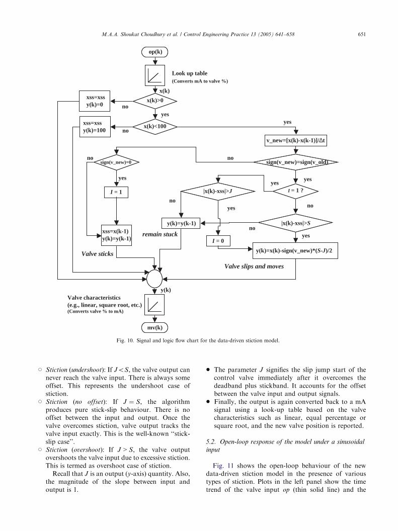
Fig. 10. Signal and logic flow chart for the data-driven stiction model.


* Stiction (undershoot): If JoS; the valve output cannever reach the valve input. There is always someoffset. This represents the undershoot case ofstiction.

* Stiction (no offset): If J ¼ S; the algorithmproduces pure stick-slip behaviour. There is nooffset between the input and output. Once thevalve overcomes stiction, valve output tracks thevalve input exactly. This is the well-known ‘‘stick-slip case’’.

* Stiction (overshoot): If J > S; the valve outputovershoots the valve input due to excessive stiction.This is termed as overshoot case of stiction.Recall that J is an output (y-axis) quantity. Also,

the magnitude of the slope between input andoutput is 1.

* The parameter J signifies the slip jump start of thecontrol valve immediately after it overcomes thedeadband plus stickband. It accounts for the offsetbetween the valve input and output signals.

* Finally, the output is again converted back to a mAsignal using a look-up table based on the valvecharacteristics such as linear, equal percentage orsquare root, and the new valve position is reported.

5.2. Open-loop response of the model under a sinusoidal

input

Fig. 11 shows the open-loop behaviour of the newdata-driven stiction model in the presence of varioustypes of stiction. Plots in the left panel show the timetrend of the valve input op (thin solid line) and the

ARTICLE IN PRESS

0 50 100 150 200time/s

linear

deadband




mv (thick line) and op (thin line) mv vs. op

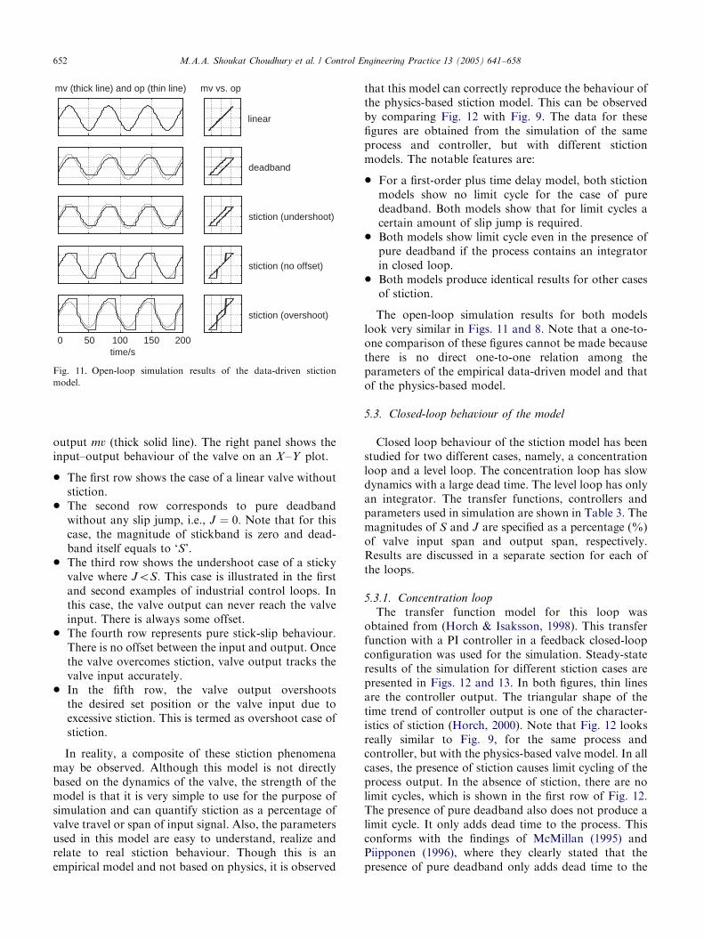
Fig. 11. Open-loop simulation results of the data-driven stiction

model.


output mv (thick solid line). The right panel shows theinput–output behaviour of the valve on an X–Y plot.

* The first row shows the case of a linear valve withoutstiction.

* The second row corresponds to pure deadbandwithout any slip jump, i.e., J ¼ 0: Note that for thiscase, the magnitude of stickband is zero and dead-band itself equals to ‘S’.

* The third row shows the undershoot case of a stickyvalve where JoS: This case is illustrated in the firstand second examples of industrial control loops. Inthis case, the valve output can never reach the valveinput. There is always some offset.

* The fourth row represents pure stick-slip behaviour.There is no offset between the input and output. Oncethe valve overcomes stiction, valve output tracks thevalve input accurately.

* In the fifth row, the valve output overshootsthe desired set position or the valve input due toexcessive stiction. This is termed as overshoot case ofstiction.

In reality, a composite of these stiction phenomenamay be observed. Although this model is not directlybased on the dynamics of the valve, the strength of themodel is that it is very simple to use for the purpose ofsimulation and can quantify stiction as a percentage ofvalve travel or span of input signal. Also, the parametersused in this model are easy to understand, realize andrelate to real stiction behaviour. Though this is anempirical model and not based on physics, it is observed

that this model can correctly reproduce the behaviour ofthe physics-based stiction model. This can be observedby comparing Fig. 12 with Fig. 9. The data for thesefigures are obtained from the simulation of the sameprocess and controller, but with different stictionmodels. The notable features are:

* For a first-order plus time delay model, both stictionmodels show no limit cycle for the case of puredeadband. Both models show that for limit cycles acertain amount of slip jump is required.

* Both models show limit cycle even in the presence ofpure deadband if the process contains an integratorin closed loop.

* Both models produce identical results for other casesof stiction.

The open-loop simulation results for both modelslook very similar in Figs. 11 and 8. Note that a one-to-one comparison of these figures cannot be made becausethere is no direct one-to-one relation among theparameters of the empirical data-driven model and thatof the physics-based model.

5.3. Closed-loop behaviour of the model

Closed loop behaviour of the stiction model has beenstudied for two different cases, namely, a concentrationloop and a level loop. The concentration loop has slowdynamics with a large dead time. The level loop has onlyan integrator. The transfer functions, controllers andparameters used in simulation are shown in Table 3. Themagnitudes of S and J are specified as a percentage (%)of valve input span and output span, respectively.Results are discussed in a separate section for each ofthe loops.

5.3.1. Concentration loop

The transfer function model for this loop wasobtained from (Horch & Isaksson, 1998). This transferfunction with a PI controller in a feedback closed-loopconfiguration was used for the simulation. Steady-stateresults of the simulation for different stiction cases arepresented in Figs. 12 and 13. In both figures, thin linesare the controller output. The triangular shape of thetime trend of controller output is one of the character-istics of stiction (Horch, 2000). Note that Fig. 12 looksreally similar to Fig. 9, for the same process andcontroller, but with the physics-based valve model. In allcases, the presence of stiction causes limit cycling of theprocess output. In the absence of stiction, there are nolimit cycles, which is shown in the first row of Fig. 12.The presence of pure deadband also does not produce alimit cycle. It only adds dead time to the process. Thisconforms with the findings of McMillan (1995) andPiipponen (1996), where they clearly stated that thepresence of pure deadband only adds dead time to the

ARTICLE IN PRESS

Table 3

Process model and controller transfer function, and parameter values used for closed-loop simulation of the data-driven model

Loop type Process Controller Stiction

Deadband Undershoot No offset Overshoot

S J S J S J S J

Concentration3e�10s

10s þ 10:2

10s þ 1

10s

� �5 0 5 2 5 5 5 7

Level1

s0:4

2s þ 1

2s

� �3 0 3 3:5 3 3 3 4:5


0 100 200 300time/s

linear

pure deadband




mv vs. op

Fig. 12. Closed-loop simulation results of a concentration loop in the

presence of the data-driven stiction model.

pv (thick line) and op (thin line)

0 100 200 300time/s

pv vs. op

linear

pure deadband




Fig. 13. Closed-loop simulation results of a concentration loop in the

presence of the data-driven stiction model.


process and the presence of deadband together with anintegrator produces a limit cycle (discussed further inlevel control loop case). Fig. 12 shows the controlleroutput ðopÞ and valve position ðmvÞ: Mapping of mv vs.op clearly shows the stiction phenomena in the valve. Itis common practice to use a mapping of pv vs. op forvalve diagnosis (see Fig. 13). However, in this case, sucha mapping only shows elliptical loops with sharp turnaround points. The reason is that the pv–op mapcaptures not only the nonlinear valve characteristic butalso the dynamics of the process, GðsÞ; which in this caseis a first-order lag plus deadtime. Therefore, if the valveposition data are available, one should plot valveposition ðmvÞ against the controller output ðopÞ: Thepv–op maps should be used with caution except forin-liquid flow low loops where the flow through thevalve ðpvÞ can be taken to be proportional to valveopening ðmvÞ:

5.3.2. A level control loop

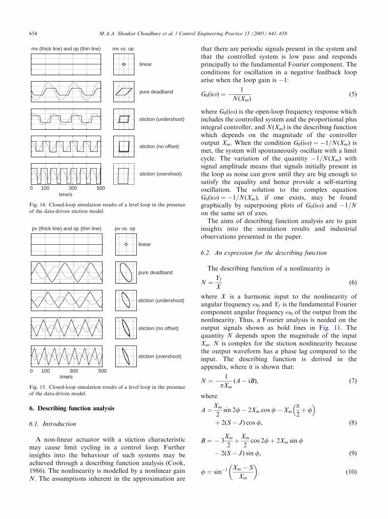
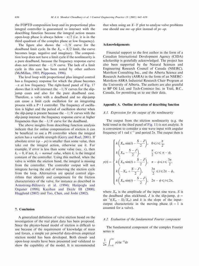
The closed-loop simulation of the stiction model usingonly an integrator as the process was performed toinvestigate the behaviour of a typical level loop in thepresence of valve stiction. Results are shown in Figs. 14and 15. The second row in both Figs. 14 and 15 showsthat the deadband can produce oscillations. Again, it isobserved that if there is an integrator in the processdynamics, then even a pure deadband can produce limitcycles, otherwise the cycle decays to zero. The mv–op

mappings clearly show the various cases of valvestiction. The pv–op plots show elliptical loops withsharp turn around. Therefore, as was noted also in anearlier example, the pv–op map is not a very reliablediagnostic for valve faults in a level loop. A diagnostictechnique, developed by the authors (Choudhury, Shah,& Thornhill, 2004), based on higher order statisticalanalysis of data is able to detect and diagnose thepresence of stiction in control loops.

ARTICLE IN PRESS


0 100 300 500time/s

mv vs. op

linear

pure deadband




Fig. 14. Closed-loop simulation results of a level loop in the presence

of the data-driven stiction model.

pv (thick line) and op (thin line)

0 100 300 500time/s

pv vs. op

linear

pure deadband




Fig. 15. Closed-loop simulation results of a level loop in the presence

of the data-driven model.


6. Describing function analysis

6.1. Introduction

A non-linear actuator with a stiction characteristicmay cause limit cycling in a control loop. Furtherinsights into the behaviour of such systems may beachieved through a describing function analysis (Cook,1986). The nonlinearity is modelled by a nonlinear gainN: The assumptions inherent in the approximation are

that there are periodic signals present in the system andthat the controlled system is low pass and respondsprincipally to the fundamental Fourier component. Theconditions for oscillation in a negative feedback looparise when the loop gain is �1:

G0ðioÞ ¼ �1

NðXmÞð5Þ

where G0ðioÞ is the open-loop frequency response whichincludes the controlled system and the proportional plusintegral controller, and NðXmÞ is the describing functionwhich depends on the magnitude of the controlleroutput Xm: When the condition G0ðioÞ ¼ �1=NðXmÞ ismet, the system will spontaneously oscillate with a limitcycle. The variation of the quantity �1=NðXmÞ withsignal amplitude means that signals initially present inthe loop as noise can grow until they are big enough tosatisfy the equality and hence provide a self-startingoscillation. The solution to the complex equationG0ðioÞ ¼ �1=NðXmÞ; if one exists, may be foundgraphically by superposing plots of G0ðioÞ and �1=N

on the same set of axes.The aims of describing function analysis are to gain

insights into the simulation results and industrialobservations presented in the paper.

6.2. An expression for the describing function

The describing function of a nonlinearity is

N ¼Yf

Xð6Þ

where X is a harmonic input to the nonlinearity ofangular frequency o0 and Yf is the fundamental Fouriercomponent angular frequency o0 of the output from thenonlinearity. Thus, a Fourier analysis is needed on theoutput signals shown as bold lines in Fig. 11. Thequantity N depends upon the magnitude of the inputXm: N is complex for the stiction nonlinearity becausethe output waveform has a phase lag compared to theinput. The describing function is derived in theappendix, where it is shown that:

N ¼ �1

pXm

ðA � iBÞ; ð7Þ

where

A ¼Xm

2sin 2f� 2Xm cos f� Xm

p2þ f

�

þ 2ðS � JÞ cos f; ð8Þ

B ¼ � 3Xm

2þ

Xm

2cos 2fþ 2Xm sin f

� 2ðS � JÞ sin f; ð9Þ

f ¼ sin�1Xm � S

Xm

� �: ð10Þ

ARTICLE IN PRESSM.A.A. Shoukat Choudhury et al. / Control Engineering Practice 13 (2005) 641–658 655

6.3. Asymptotes of the describing function

Fig. 10 indicates that there is no output from thenonlinearity if XmoS=2: Therefore, the two extremecases are when Xm ¼ S=2 and XmbS:When XmbS; the effects of the deadband and slip-jump

are negligible and the nonlinearity in Fig. 17 becomes astraight line at 45�: The output is in phase with the inputand N ¼ 1: Thus, �1=NðXmÞ ¼ �1 when XmbS:In the limit when Xm-S=2; the output is as shown in

Fig. 16. The left-hand plot shows the output for a slip-jump with no deadband ðS ¼ JÞ; while the right-handplot shows a magnified plot of a deadband with no slipjump ðJ ¼ 0Þ: In both cases, the output lags the input byone quarter of a cycle. The output is a square wave ofmagnitude Xm in the S ¼ J case and the describingfunction is N ¼ 4

p e�ip=2: For the deadband with no slip

jump ðJ ¼ 0Þ case, the output magnitude becomes verysmall. The describing function is N ¼ ee�ip=2 where e-0as Xm-S=2: Appendix A provides detailed calculationsof these results and also shows for the general case that

−3 −2 −1 0 1−5

−4

−3

−2

−1

0

1

imag

inar

y ax

is

real axis

J = S

J = S/3J = S /5

J = 0

G(iω)

Fig. 17. Graphical solutions for limit cycle oscillations. Left panel: composi

�1=N curves and the solid line is the frequency response function.

0 2ππ

time/s

3π/2π/2

inp

ut

(th

in li

ne)

an

d o

utp

ut

(hea

vy li

ne)

Fig. 16. Input (thin line) and output (heavy line) time trends for the limiting

deadband only with J ¼ 0: The output in the left plot has been magnified fo

the describing function limit when Xm ¼ S=2 is

N ¼4

p

J

2e�ip=2: ð11Þ

6.4. Insights gained from the describing function

Fig. 17 shows graphical solutions to the limit cycleequation G0ðioÞ ¼ �1=NðXmÞ for the composition con-trol loop (left panel) and level control loop (right panel)presented earlier. The describing function is parameter-ized by Xm and the open-loop frequency responsefunction of the controller and controlled system isparameterized by o: Both systems are closed-loop stableand thus intersect the negative real axis between 0 and�1:The plots explain the behaviour observed in simulation.It is clear from the left-hand panel of Fig. 17 that

there will be a limit cycle for the composition controlloop if a slip-jump is present. The slip-jump forces the�1=N curve onto the negative imaginary axis in theXm ¼ S=2 limit. Thus, the frequency response curve of

−3 −2 −1 0 1−5

−4

−3

−2

−1

0

1

real axis

J = S

J = S /3

J = S /5

J = 0

G (iω)

tion control loop. Right panel: level control loop. Dotted lines are the

0 2ππ

time/s

3π/2π/2

inp

ut

(th

in li

ne)

an

d o

utp

ut

(hea

vy li

ne)

case as Xm ¼ S=2: Left panel: slip-jump only with S ¼ J: Right panel:r visualization; its amplitude becomes zero as Xm approaches S=2:


the FOPTD composition loop and its proportional plusintegral controller is guaranteed to intersect with thedescribing function because the integral action meansopen-loop phase is always below �p=2 (i.e. it is in thethird quadrant of the complex plane at low frequency).The figure also shows the �1=N curve for the

deadband limit cycle. In the Xm ¼ S=2 limit, the curvebecomes large, negative and imaginary. The composi-tion loop does not have a limit cycle if the nonlinearity isa pure deadband, because the frequency response curvedoes not intersect the �1=N curve. The lack of a limitcycle in this case has been noted by other authors(McMillan, 1995; Piipponen, 1996).The level loop with proportional plus integral control

has a frequency response for which the phase becomes�p at low frequency. The right-hand panel of Fig. 17shows that it will intersect the �1=N curves for the slip-jump cases and also for the pure deadband case.Therefore, a valve with a deadband and no slip-jumpcan cause a limit cycle oscillation for an integratingprocess with a P+I controller. The frequency of oscilla-tion is higher and the period of oscillation shorter whenthe slip-jump is present because the �1=N curves with theslip-jump intersect the frequency response curve at higherfrequencies than the �1=N curve for the deadband.The above insights from describing function analysis

indicate that for online compensation of stiction it canbe beneficial to use a PI controller where the integralaction has a variable strength (Gerry and Ruel, 2001). Ifabsolute error ðsp � pvÞ is smaller than some value, thentake out the integral action, otherwise use it. Forexample, if error is less than some value (say, x), thenki ¼ 0; if not, ki ¼ normal value; where ki is the integralconstant of the controller. Using this method, when thevalve is within the stiction band, the integral is missingfrom the controller. The controller output will notintegrate having the end of removing the stiction cyclefrom the loop. Alternatives are special control algo-rithms that identify and compensate for the frictioncharacteristics of the valve, for instance as described inArmstrong-Helouvry et al. (1994); Hatipoglu andOzguner (1998); Kayihan and Doyle III (2000);Hagglund (2002) and Tao, Chen, and Joshi (2002).

7. Conclusion

A generalized definition of valve stiction based on theinvestigation of the real plant data has been proposed.Since the physics-based model of stiction is difficult touse because of the requirement of knowledge of massand forces, a simple yet powerful data-driven empiricalstiction model has been developed. Both closed- andopen-loop results have been presented and validated toshow the capability of the model. It is recommended

that when using an X–Y plot to analyse valve problemsone should use mv–op plot instead of pv–op:

Acknowledgements

Financial support to the first author in the form of aCanadian International Development Agency (CIDA)scholarship is gratefully acknowledged. The project hasalso been supported by the Natural Sciences andEngineering Research Council of Canada (NSERC),Matrikon Consulting Inc., and the Alberta Science andResearch Authority (ASRA) in the form of an NSERC-Matrikon-ASRA Industrial Research Chair Program atthe University of Alberta. The authors are also gratefulto BP Oil Ltd. and Tech-Cominco Inc. in Trail, B.C.,Canada, for permitting us to use their data.

Appendix A. Outline derivation of describing function

A.1. Expression for the output of the nonlinearity

The output from the stiction nonlinearity (e.g. thebold trend in the third panel of Fig. 11) is not analytic. Itis convenient to consider a sine wave input with angularfrequency of 1 rad s�1 and period 2p: The output then is

yðtÞ ¼

k Xm sinðtÞ �S � J

2

� �; 0ptp

p2;

k Xm �S � J

2

� �;

p2ptp p� f;

k Xm sinðtÞ þS � J

2

� �; p� fptp

3p2;

k �Xm þS � J

2

� �;

3p2ptp2p� f;

k Xm sinðtÞ �S � J

2

� �; 2p� fptp2p;

8>>>>>>>>>>>>>>>>><>>>>>>>>>>>>>>>>>:

where Xm is the amplitude of the input sine wave, S isthe deadband plus stickband, J is the slip-jump, f ¼sin�1ððXm � SÞ=XmÞ and k is the slope of the input–output characteristic in the moving phase (k ¼ 1 isassumed for a valve).

A.2. Evaluation of the fundamental Fourier component

The fundamental component of the complex Fourierseries is

1

2p

Z 2p

t¼0yðtÞe�itdt

ARTICLE IN PRESSM.A.A. Shoukat Choudhury et al. / Control Engineering Practice 13 (2005) 641–658 657

where, after substitution of sinðtÞ ¼ 12iðe�it � e�itÞ:Z 2p

t¼0yðtÞe�it dt

¼Z p=2

t¼0k

Xm

2iðeit � e�itÞ �

S � J

2

� �e�it dt

þZ p�f

t¼p=2k Xm �

S � J

2

� �e�it dt

þZ 3p=2

t¼p�fk

Xm

2iðeit � e�itÞ þ

S � J

2

� �e�it dt

þZ 2p�f

t¼3p=2k �Xm þ

S � J

2

� �e�it dt

þZ 2p

t¼2p�fk

Xm

2iðeit � e�itÞ �

S � J

2

� �

e�it dt: ðA:1Þ

Writing it compactly:Z 2p

t¼0yðtÞe�it dt ¼ T1þ T2þ T3þ T4þ T5;

where T1 ¼R p=2

t¼0 k Xm

2iðeit � e�itÞ � S�J

2

� e�it dt; and so

on.Evaluation term by term gives:

T1 ¼k

2ðXm � S þ JÞ þ ik

S � J

2�

ap4

� �;

T2 ¼ � k Xm �S � J

2

� �ð1� sin fÞ � ik

Xm �S � J

2

� �cos f;

T3 ¼ kXm

4ð1þ cos 2fÞ �

S � J

2ð1þ sin fÞ

� �

þ ikXm

4sin 2f�

Xm

2

p2þ f

� þ

S � J

2cos f

� �;

T4 ¼ � k Xm �S � J

2

� �ð1� sin fÞ � ik

Xm �S � J

2

� �cos f;

T5 ¼ � kXm

4ð1� cos 2fÞ þ

S � J

2sin f

� �

� ikXmf2

þd

2�

Xma

4sin 2f�

S � J

2cos f

� �:

ðA:2Þ

Collecting terms gives the wanted fundamental Four-ier component of the output:

1

2p

Z 2p

t¼0yðtÞe�it dt ¼

1

2pðB þ iAÞ;

where

A ¼ kXm

2sin 2f� 2kXm cos f

�

�kXm

p2þ f

� þ 2kðS � JÞ cos f

and

B ¼ � 3k Xm

2þ k Xm

2cos 2f

þ 2kXm sin f� 2kðS � JÞ sin f:

The fundamental component of the complex Fourierseries of the input sine wave is Xm=2i: Therefore, thedescribing function is

N ¼B þ iA

2p

2i

Xm

¼ �1

pXm

ðA � iBÞ:

A.3. Evaluation of limiting cases

There is no output from the nonlinearity whenXmoS=2: The limiting cases considered are thereforeXm ¼ S=2 and XmbS:When XmbS then f ¼ sin�1ððXm � SÞ=XmÞ ¼ p

2; A ¼

�kpXm; B ¼ 0 and thus N ¼ k: This result is to beexpected because the influence of the stickband andjump are negligible when the input has a large amplitudeand the output approximates a sinewave of magnitudekXm: The slope of the moving phase for a valvewith a deadband is k ¼ 1 when the input and outputto the nonlinearity are expressed as a percentage offull range. Therefore, for a valve with stiction, N ¼ 1;when XmbS:When Xm ¼ S=2 the result depends upon the magni-

tude of the slip-jump, J: For the case with no deadbandðS ¼ JÞ; f ¼ �p

2; A ¼ 0; B ¼ �4kXm and N ¼ �ik 4

p ¼k 4

p e�ip=2: For a valve with k ¼ 1; N ¼ 4

p e�ip=2: This

result describes the situation where the output is asquare wave of amplitude Xm lagging the input sinewave by one quarter of a cycle, as shown in Fig. 16.For intermediate cases where both deadband and slip

jump are present such that jS � J j > 0; then the Xm ¼S=2 limit gives f ¼ �p

2; A ¼ 0; B ¼ �2kJ and N ¼

�ik2J=pXm ¼ k2J=pXme�ip=2: For instance, if J ¼ S=2

and k ¼ 1 then the Xm ¼ S=2 limit gives N ¼ 2p e

�ip=2

and the output is a square wave of amplitude Xm=2lagging the input sine wave by one quarter of a cycle.When the nonlinearity has a deadband only and no

slip-jump ðJ ¼ 0Þ; the describing function has a limitgiven by N ¼ ee�ip=2 where e-0 as Xm-S=2:

References

Armstrong-Helouvry, B., Dupont, P., & De Wit, C. C. (1994). A

survey of models, analysis tools and compensation methods for the

control of machines with friction. Automatica, 30(7), 1083–1138.


Aubrun, C., Robert, M., & Cecchin, T. (1995). Fault detection in

control loops. Control Engineering Practice, 3, 1441–1446.

Bialkowski, W. L. (1992). Dreams vs. reality: A view from both sides

of the gap. In Control systems (pp. 283–294). Canada: Whistler BC.

Choudhury, M. A. A. S., Shah, S. L., & Thornhill, N. F. (2004).

Diagnosis of poor control loop performance using higher order

statistics. Automatica to appear in October 2004 issue.

Cook, P. A. (1986). Nonlinear dynamical systems. Englewood cliffs,

NJ: Prentice-Hall.

Desborough, L., & Miller, R. (2002). Increasing customer value of

industrial control performance monitoring—honeywell’s experi-

ence. In AIChE Symposium Series 2001, No. 326 (pp. 172–192).

Ender, D. (1993). Process control performance: Not as good as you

think. Control Engineering, 40, 180–190.

EnTech, . (1998). EnTech control valve dynamic specification (version

3.0).

Fisher-Rosemount, . (1999). Control valve handbook. Marshalltown,

IW, USA: Fisher Controls International Inc.

Fitzgerald, B. (1995). Control valve for the chemical process industries.

New York: McGraw-Hill, Inc.

Gerry, J., & Ruel, M. (2001). How to measure and combat valve stiction

online. Instrumentation, systems and automated society. Houston,

TX, USA. http://www.expertune.com/articles/isa2001/StictionMR.

htm.

Hagglund, T. (2002). A friction compensator for pneumatic control

valves. Journal of Process Control, 12(8), 897–904.

Hatipoglu, C., & Ozguner, U. (1998). Robust control of systems

involving non-smooth nonlinearities using modified sliding mani-

folds. American control conference (pp. 2133–2137). Philadelphia,

PA.

Horch, A. (2000). Condition monitoring of control loops. Ph.D. thesis.

Royal Institute of Technology, Stockholm, Sweden.

Horch, A., & Isaksson, A. J. (1998). A method for detection of stiction

in control valves. In Proceedings of the IFAC workshop on line fault

detection and supervision in the chemical process industry. Session

4B. Lyon, France.

Horch, A., Isaksson, A. J., & Forsman, K. (2000). Diagnosis and

characterization of oscillations in process control loops. In

Proceedings of the control systems 2000 (pp. 161–165). Victoria,

Canada.

ISA Subcommittee SP75.05, (1979). Process instrumentation terminol-

ogy. Technical Report ANSI/ISA-S51.1-1979. Instrument Society

of America.

Kano, M., Maruta, H., Kugemoto, H., & Shimizu, K. (2004). Practical

model and detection algorithm for valve stiction. In Proceedings

of the Seventh IFAC-DYCOPS Symposium, Boston, USA,

to appear.

Karnopp, D. (1985). Computer simulation of stick-slip friction in

mechanical dynamical systems. Journal of Dynamic Systems,

Measurement, and Control, 107, 100–103.

Kayihan, A., & Doyle III, F. J. (2000). Friction compensation for a

process control valve. Control Engineering Practice, 8, 799–812.

Martin, G. D., Turpin, L. E., & Cline, R. P. (1991). Estimating control

function benefits. Hydrocarbon Processing, 68–73.

McMillan, G. K. (1995). Improve control valve response. Chemical

Engineering Progress: Measurement and Control, 77–84.

Miao, T., & Seborg, D.E. (1999). Automatic detection of excessively

oscillatory control loops. In Proceedings of the 1999 IEEE

international conference on control applications. Kohala Coast-

Island of Hawai’i, Hawai’i, USA.

Olsson, H. (1996). Control systems with friction. Ph.D. thesis. Lund

Institute of Technology, Sweden.

Paulonis, M. A., & Cox, J. W. (2003). A practical approach for large-

scale controller performance assessment, diagnosis, and improve-

ment. Journal of Process Control, 13(2), 155–168.

Piipponen, J. (1996). Controlling processes with nonideal valves:

Tuning of loops and selection of valves. In Preprints of Control

Systems ’96 (pp. 179–186). Halifax, Nova Scotia, Canada.

Qin, S. J. (1998). Control performance monitoring—a review and

assessment. Computers and Chemical Engineering, 23, 173–186.

Ruel, M. (2000). Stiction: The hidden menace. Control Magazine.

http://www.expertune.com/articles/RuelNov2000/stiction.html.

Sharif, M. A., & Grosvenor, R. I. (1998). Process plant condition

monitoring and fault diagnosis. Proceedings of the Institute of

Mechanical Engineering, 212(Part E), 13–30.

Shinskey, F. G. (1990). How good are our controllers in absolute

performance and robustness. Measurement and Control, 23, 114–120.

Taha, O., Dumont, G. A., & Davies, M. S. (1996). Detection and

diagnosis of oscillations in control loops. In Proceedings of the 35th

conference on decision and control. Kobe, Japan.

Tao, G., Chen, S., & Joshi, S. M. (2002). An adaptive control scheme

for systems with unknown actuator failures. Automatica, 38,

1027–1034.

Thornhill, N. F., Cox, J. W., & Paulonis, M. A. (2003b). Diagnosis of

plant-wide oscillation through data-driven analysis and process

understanding. Control Engineering Practice, 11(12), 1481–1490.

Thornhill, N. F., Huang, B., & Zhang, H. (2003a). Detection of

multiple oscillations in control loops. Journal of Process Control,

13, 91–100.

Wallen, A. (1997). Valve diagnostics and automatic tuning. In

Proceedings of the American control conference (pp. 2930–2934).

Albuquerque, New Mexico.

Whalen, B. R. (1983). Basic instrumentation (3rd ed.). Austin, TX:

Petroleum Extension Service (PETEX).

Modelling valve stiction

Documents

Transcript of Modelling valve stiction