1 23

LandslidesJournal of the International Consortiumon Landslides ISSN 1612-510X LandslidesDOI 10.1007/s10346-013-0400-x

Delineating and defining the boundariesof an active landslide in the rainforestof Puerto Rico using a combination ofairborne and terrestrial LIDAR data

Guoquan Wang, James Joyce, DavidPhillips, Ramesh Shrestha & WilliamCarter

1 23

Your article is protected by copyright and

all rights are held exclusively by Springer-

Verlag Berlin Heidelberg. This e-offprint is

for personal use only and shall not be self-

archived in electronic repositories. If you wish

to self-archive your article, please use the

accepted manuscript version for posting on

your own website. You may further deposit

the accepted manuscript version in any

repository, provided it is only made publicly

available 12 months after official publication

or later and provided acknowledgement is

given to the original source of publication

and a link is inserted to the published article

on Springer's website. The link must be

accompanied by the following text: "The final

publication is available at link.springer.com”.

LandslidesDOI 10.1007/s10346-013-0400-xReceived: 6 February 2013Accepted: 28 March 2013© Springer-Verlag Berlin Heidelberg 2013

Guoquan Wang I James Joyce I David Phillips I Ramesh Shrestha I William Carter

Delineating and defining the boundaries of an activelandslide in the rainforest of Puerto Rico usinga combination of airborne and terrestrial LIDAR data

Abstract Light detection and ranging (LIDAR) is a remote sensingtechnique that uses light, often using pulses from a laser to mea-sure the distance to a target. Both terrestrial- and airborne-basedLIDAR techniques have been frequently used to map landslides.Airborne LIDAR has the advantage of identifying large scarps oflandslides covered by tree canopies and is widely applied in iden-tifying historical and current active landslides hidden in forestedareas. However, because landslides naturally have relatively smallvertical surface deformation in the foot area, it is practicallydifficult to identify the margins of landslide foot area with thelimited spatial resolution (few decimeters) of airborne LIDAR.Alternatively, ground-based LIDAR can achieve resolution of sev-eral centimeters and also has the advantages of being portable,repeatable, and less costly. Thus, ground-based LIDAR can be usedto identify small deformations in landslide foot areas by differenc-ing repeated terrestrial laser scanning surveys. This study demon-strates a method of identifying the superficial boundaries as wellas the bottom boundary (sliding plane) of an active landslide inNational Rainforest Park, Puerto Rico, USA, using the combina-tion of ground-based and airborne LIDAR data. The method ofcombining terrestrial and airborne LIDAR data can be used tostudy landslides in other regions. This study also indicates thatintensity and density of laser point clouds are remarkably useful inidentifying superficial boundaries of landslides.

Keywords Airborne LIDAR . GPS . Landslide . Rainforest . TLS

IntroductionLandslides are the major geological hazard in Puerto Rico, as wellas in the whole Caribbean region. Mountainous terrain and trop-ical climate combine to make the island one of the most landslide-prone areas in the USA. An active landslide in El Yunque NationalRainforest, Puerto Rico, was investigated in this study. The land-slide is located on a steep, north-facing mountain slope inrainforest. Major displacements of the landslide in 2004 and2005 blocked one of three access roads to the national park. Inorder to reopen the roadway (Puerto Rico 9966), a 100-m-longsteel sheet-piling wall was designed and constructed to restrain thelandslide (Fig. 1). During construction, a portion of the west end ofthe wall failed. The failure was attributed to insufficient depth ofthe support steel piles. The retaining wall was rebuilt with thedepth of the support steel piles having been doubled. The recon-struction was finally completed at the end of 2009. However, thepreviously failed section continued to show slope and flexuraldeformation over the spring and summer of 2010 and finallyruptured in July of 2010, during a heavy rainfall (Fig. 1, bottom).As a result, the road was not reopened. The other two access roadsalso suffer from frequent small-scale landslides and rockfalls. Theloss of the road is a major concern to EL Yunque NationalRainforest administration and the local government.

The failure of the retaining wall implies that the size of thelandslide was larger than the size estimated by the designers of theretaining wall. However, the significant deformation area of theretaining wall was limited to a small section, about 10-m wide(Fig. 1). This suggests that the future motion of landslide might stillbe retained by proper engineering design and construction.Therefore, identifying the true extent and depth of the landslidehas become the key issue for taking further actions. However,landslides occurring under steep and thickly forested areas aredifficult to map with conventional methods. Limited visibility anddifficult access reduce the area that can be directly observed usingstandard aerial photography, satellite imagery, or ground-basedsurveys.

During the past decades, light detection and ranging (LIDAR)technology has been widely used in different disciplines, such asarchaeology, geography, geology, geomorphology, seismology, for-estry, atmospheric physics, airborne laser swath mapping, andlaser altimetry (Wehr and Lohr 1999; Shan and Toth 2008). Laserscanning was developed in three ways, depending on the positionof the sensor: terrestrial laser scanning (TLS), airborne laser scan-ning (ALS), and satellite-based laser scanning (Carter et al. 2007).High-resolution digital elevation maps derived from ALS datahave led to many novel studies in geoscience applications (e.g.,Falls et al. 2004; Bevis et al. 2005; Glenn et al. 2005, 2006; Wootenet al. 2007; Delano and Braun 2007). ALS has been frequentlyapplied in regional landslide mapping, modeling, monitoring,and risk assessment in many parts of the word. The ability ofALS to measure the land surface elevation beneath vegetatedcanopy has significantly advanced landslide studies where theterrain is forested (e.g., Van den Eeckhaut et al. 2007; Razak etal. 2011). In these studies, high-resolution digital terrain models(DTMs), also called 3D “bare-earth models,” derived from ALSdata served as the base data set for creating topographic maps andfor identifying landslide scarps.

TLS, also referred to as ground-based LIDAR, appeared at theend of the 1990s (Heritage and Large 2009). TLS has frequentlybeen applied to the study of small-scale landslides in the last 5 to10 years, particularly in studying active landslides (e.g., Abellan etal. 2006, 2009; Teza et al. 2007, 2008; Travelletti et al. 2009; Corsiniet al. 2009; Dunning et al. 2009; Jaboyedoff et al. 2009; Kasperski etal. 2010; Wang et al. 2011; Fanti et al. 2012). TLS surveys allowresearchers to generate detailed models of a landslide surface.When two or more georeferenced digital surface or terrain modelsobtained by multiple TLS surveys are available, the volume changeof sliding mass, the margins of the deformation area, and thelandslide displacement field, can be computed. Thus, TLS is par-ticularly useful in detecting the margins of creeping landslides.

The number of publications discussing the use airborne andground-based LIDAR in landslide studies has grown considerablyduring the last decade (Derron and Jaboyedoff 2010). Jaboyedoff et

Landslides

Technical Note

Author's personal copy

al. (2012) gave a comprehensive review of applications of ALS andTLS in landslide studies. The majority of ALS applications inlandslide studies were limited to the detection of landslide scarpsbased on hillshades of DTMs derived from ground returns (e.g.,Carter et al. 2001; Haugerud et al. 2003; Ardizzone et al. 2007;Jaboyedoff et al. 2008; Booth et al. 2009; Corsini et al. 2009).Landslides naturally have large vertical deformation in the headareas and insignificant vertical deformation in the foot areas,particularly in the toe areas. The elevation accuracy of airborneLIDAR data is typically at the level of a couple of decimeters forlarge-scale mapping applications (e.g., Adams and Chandler 2002;Bowen and Waltermire 2002; Hodgson et al. 2003; Habib 2008). Asa result, it is difficult to identify margins in landslide foot areafrom DTM models derived from ALS data. Fortunately, foot areasof landslides are often located in downslope areas of hills withpossible ground access, such as along road cuts. So TLS is oftenfeasible to map foot areas of landslides. In this paper we describethe combination of TLS, ALS, and Global Positioning System(GPS) data to identify superficial boundaries as well as the basalfailure plane of an active landslide in a rainforest.

Airborne LIDAR surveying and data processingThe airborne LIDAR scanning was performed by the NationalCenter for Airborne Laser Mapping (NCALM, http://www.ncalm.org) during 13–16 May 2011. This survey wasperformed with an Optech Gemini Airborne Laser TerrainMapper (serial number 09SEN185, http://www.optech.ca) mountedin a twin-engine Cessna 337 Skymaster aircraft. The OptechGemini model is capable of laser pulse rates up to 167 kHz. Itrecords as many as four returns (including the first three and last)per shot and has a switchable beam divergence of 0.25 and 0.80milliradians. The data were collected at flying heights of 600 mwith 50 % overlap between adjacent flight lines. The laser beam

divergence was switched to 0.80 milliradians, which led to a spotsize of 0.48 m in diameter on the ground at 600 m flying height.Simultaneous acquisition of aircraft position and orientation wasperformed using a combination of differential kinematic GPS andInertial Navigation System (INS). Ground coordinates of laserpoints were calculated by combining information from the scan-ner, GPS/INS measurements, and calibration parameters.

Removing trees and vegetation, or identifying “bare-earth”returns, is the primary focus of the data processing for this project.A commercial software package, TerraSolid’s TerraScan (http://www.terrasolid.fi), was used to classify the raw laser point intothree categories: ground, nonground (default), and artifacts (aeri-al/isolated points and multi-path points). An automatic groundclassification procedure, specifically a TerraScan macro, wasperformed initially, and then a manual process, “add point toground,” was conducted to correct classification errors in areaswhere the automatic ground classification did not provide a goodresult. The main purpose of the manual process is to retainsufficient details of the bare-earth surface, while removing lowvegetation and tree trunks. Particular attention is paid to thesegmentation of points near sharp topographic features, such ashead scarps and flanks of the landslide, where it is often possibleto classify ground returns to non-ground returns due to thepronounced topographic gradient.

Density and intensity of point cloudsFigure 2 shows point clouds hit on the flat surface (14×4 m) of ablack asphalt road in front of the retaining wall. The ALS pointdensity on the black road surface is about 10 points/m2. Thestandard deviation of elevation measurements is 22 cm. The pointdensity in the deforested foot area is slightly higher than that of theblack road surface. However, the overall return point density wasalmost doubled inside the rainforest due to multiple returns fromtree canopies and undergrowth. Up to four laser returns werecollected for laser pulses in the dense canopy area as shown inFig. 3. Figure 4 (left) shows the sparse and uneven distribution ofground returns. Ground-point spacing can be larger than 5 m

Fig. 1 Panorama views at the landslide site taken on 25 May 2010 and 5 February2011 during the first and third TLS surveys, respectively. Note that the panoramaview was slightly distorted. The wide-angle landscape was assembled with fournarrow-angle photos taken by the digital camera on the ground-based LIDARscanner using a free photo stitching software (http://hugin.sourceforge.net)

Fig. 2 Airborne LIDAR point clouds hit on the flat black asphalt road surface infront of the landslide. The point density is 10 points/m2. The standard deviation ofvertical coordinates of these points is 21 cm. The unit of the scale in the bottomfigure is meter

Technical Note

Landslides

Author's personal copy

under tree canopies. The average point density inside the forest isabout 1 point/3 m2. However, there are considerably dense groundreturns along head scarps and both eastern and western flanks.This is due to the fact that trees were felled and displaced along themargins of the moving mass and soil was exposed. As a result, alarge number of laser points directly hit the ground surface alongthe head scarps and two flanks, highlighting the boundary inlandslide head and body areas.

LIDAR systems provide both elevation and intensity recordsfor each laser return. LIDAR intensity, a relative measure of thestrength of each return pulse, in theory, is determined by anobject’s reflectance. Intensity values can be used to identify land-cover classes when the data are carefully calibrated (e.g.,Donoghue et al. 2007). Previous investigations have indicated thatLiDAR intensity values also depend on atmospheric transmission,local incidence angle, surface roughness, laser beam divergence,and sensor-to-object distance (e.g., Hodgson and Bresnahan 2004;Mazzarini et al. 2007; Hasegawa 2006; Shrestha et al. 2007). Ingeneral, LIDAR intensity is predominantly dependent on sensor-to-object distance and subordinately dependents on local

incidence angle (e.g., Kaasalainen et al. 2005) and atmosphericabsorption (e.g., Mazzarini et al. 2007). Mazzarini et al. (2007)reported that intensity level changes with the inverse square ofthe distance. While intensity calibrations for the terrain’s direc-tional spectral properties remain an open area of LIDAR research,normalization of intensities based on sensor-to-object is fairlystraightforward to implement. In standard NCALM data process-ing, the original intensities are normalized with the sensor-to-object path lengths (Shrestha et al. 2007). Figure 4 (right) illus-trates the normalized intensities of ground returns. The differ-ences of intensities are mostly caused by the change of surfacematerial types. The high intensities (white) were returnedfrom soil while lower intensities (gray) were returned fromtrees and vegetation.

The laser density and intensity images shown in Fig. 4clearly delineate the margins of the landslide flanks and headarea. Furthermore, these images also define three distinctiveportions of the main landslide. The uppermost portion (head)is characterized by very low point cloud density and intensity,which indicates that the forest remains largely intact. Thelandslide here is behaving as a largely coherent slide masswith little deformation occurring at the surface. In contrast tothis, the middle portion (body) of the landslide is character-ized by a very patchy distribution of point cloud density andintensity indicating significant disruption of the trees byground surface deformation. The distribution of the higherdensity and intensity point clouds is notably arc shapedsuggesting the occurrence of secondary scarps in this portionof the landslide (Fig. 4). The bottom (foot and toe) of thelandslide is characterized by high density and intensity pointclouds as a consequence of the removal of the vegetation andtree cover during earthwork and grading for the constructionof the retaining wall (see Fig. 1).

Accuracy of ALS dataThe error budget for a given ALS is primarily driven by errorsfrom the laser source, the laser rangefinder, the kinematic GPSposition solution, the INS orientation solution, environmentalconditions, land-cover category, and errors involved in post-dataprocessing. Most vendors quote 15–18 cm vertical accuracy and0.5 m horizontal accuracy. Vertical accuracy under 10 cm and

Fig. 3 Multiple returns collected by airborne LIDAR in a tree canopy covering area. Thesetwo trees are located at the top of the graded landslide foot area (see Figs. 1 and 8)

Fig. 4 Images showing 2D distribution of ground returns (point clouds) collected by ALS and their intensities. The margins in the landslide head and body areas can beidentified from both point cloud density and intensity images. The unit of the scale in both figures is meter

Landslides

Author's personal copy

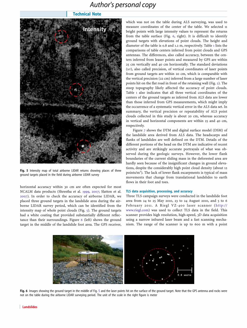
horizontal accuracy within 30 cm are often expected for mostNCALM data products (Shrestha et al. 1999, 2007; Slatton et al.2007). In order to check the accuracy of airborne LIDAR, weplaced three ground targets in the landslide area during the air-borne LIDAR survey period, which can be identified from theintensity map of whole point clouds (Fig. 5). The ground targetshad a white coating that provided substantially different reflec-tance than their surroundings. Figure 6 (left) shows the groundtarget in the middle of the landslide foot area. The GPS receiver,

which was not on the table during ALS surveying, was used tomeasure coordinates of the center of the table. We selected 11bright points with large intensity values to represent the returnsfrom the table surface (Fig. 6, right). It is difficult to identifyground targets with elevations of point clouds. The height anddiameter of the table is 0.8 and 1.2 m, respectively. Table 1 lists thecomparisons of table centers inferred from point clouds and GPSantennas. The differences, also called accuracy, between the cen-ters inferred from leaser points and measured by GPS are within25 cm vertically and 40 cm horizontally. The standard deviations(1σ), also called precision, of vertical coordinates of laser pointsfrom ground targets are within 20 cm, which is comparable withthe vertical precision (22 cm) inferred from a large number of laserpoints hit on the flat road in front of the retaining wall (Fig. 2). Thesteep topography likely affected the accuracy of point clouds.Table 1 also indicates that all three vertical coordinates of thecenters of the ground targets as inferred from ALS data are lowerthan those inferred from GPS measurements, which might implythe occurrence of a systematic vertical error in the ALS data set. Insummary, the vertical precision or repeatability of ALS pointclouds collected in this study is about 20 cm, whereas accuracyin vertical and horizontal components are within 25 and 40 cm,respectively.

Figure 7 shows the DTM and digital surface model (DSM) ofthe landslide area derived from ALS data. The headscarps andflanks of landslides are well defined on the DTM. Details of thedifferent portions of the head on the DTM are indicative of recentactivity and are strikingly accurate portrayals of what was ob-served during the geologic surveys. However, the lower flankboundaries of the current sliding mass in the deforested area arehardly seen because of the insignificant changes in ground eleva-tions, despite the considerably high point cloud density (about 12points/m2). The lack of lower flank escarpments is typical of massmovements that change from translational landslides to earthflows in their foot and toes.

TLS data acquisition, processing, and accuracyThree TLS campaign surveys were conducted in the landslide footarea from 24 to 25 May 2010, 23 to 24 August 2010, and 5 to 6February 2011 . A Riegl VZ-400 laser scanner (http://www.riegl.com) was used to collect TLS data in the field. Thisscanner provides high resolution, high-speed, 3D data acquisitionusing a narrow infrared laser beam and a fast scanning mecha-nism. The range of the scanner is up to 600 m with a point

Fig. 5 Intensity map of total airborne LIDAR returns showing places of threeground targets placed in the field during airborne LIDAR survey

Fig. 6 Images showing the ground target in the middle of Fig. 5 and the laser points hit on the surface of the ground target. Note that the GPS antenna and rocks werenot on the table during the airborne LIDAR surveying period. The unit of the scale in the right figure is meter

Technical Note

Landslides

Author's personal copy

acquisition rate of up to 122,000 measurements/s. The scanner isable to acquire a scene with a field of view of up to 360° horizontaland 100° vertical in a single scan. The Riegl scanner has anintegrated digital compass for accurate north-determination ofthe direction for polar alignment of the Scanner’s OwnCoordinate System (SOCS). A digital camera (NIKON D700) wasmounted on the top of the scanner. The camera was configured totake 6 photos in a 360° view automatically at the end of each singlescan. The camera coordinate system was aligned to the intrinsicreference system (SOCS) of the scanner. All the data collected inthe field by the terrestrial scanner and camera are managed by thecompanion software Riscan PRO (Version 1.6.3). The images werelater registered to the laser scanner data and used as a texturesource in the photorealistic virtual model.

TLS data acquisitionFigure 8 shows point clouds collected during the first TLS cam-paign survey in May 2010. The point clouds were colored with truecolor obtained from photos taken with the digital camera. Thewhite point clouds represent places that were not caught by thedigital camera. The complete coverage of spatially complex objectsby TLS can only be guaranteed, if data collection is done fromdifferent viewpoints. We conducted more than ten single scans

Table1Comparisonsofthecentersofground

targetsinferredfromALSdataandGPSmeasurements

Ground

targets

Pointcloudshito

nthesurface

ofground

targets

GPSantennaa

Accuracy

Numbero

fpoints

Standard

deviation(cm)

Averagecoordinates(m)b

Coordinates(m;16May

2011)

Pointclouds-GPS(cm)

EWNS

UDEW

NSUD

EWNS

UDEW

NSUD

Lowtarget

1116.7

33.4

7.7

206,409.545

2,029,169.257

437.435

206,409.2

2,029,169.18

437.669

34.5

7.7

−23.4

Middletarget

1132.9

30.9

14.6

206,416.666

2,029,125.412

448.711

206,416.482

2,029,125.44

448.793

18.4

−3.1

−8.2

High

target

1143.6

47.5

16.4

206,429.605

2,029,083.961

459.411

206,429.823

2,029,084.05

459.681

−21.8

−8.4

−27

aTheverticalcoordinateofeach

GPSantennahadbeen

adjusted

tothesurface

oftheground

target

bThepositions

ofpointcloudsandGPSaretiedto

North

America

HorizontalD

atum

of1983

(NAD83

andCORS96)and

North

America

VerticalD

atum

of1988

(NAVD88andGEOID03).The

horizontalprojectionisUTMNA

D83Zone

20N

Fig. 7 DSM (outer part) and DTM (inner part) derived from airborne LIDARdata

Fig. 8 Colored point clouds collected by TLS (RIGEL VZ-400) on 25 May 2010during the first TLS survey

Landslides

Author's personal copy

during each TLS campaign survey from different viewpoints locat-ed inside and outside of the landslide foot area. The locations ofthese single scans were carefully selected to capture the completesurface geometry of the graded area. Ten reflective targets (controlpoints) were placed in the landslide area during the TLS survey. Wealso installed three GPS stations in the study area during each TLScampaign survey. GPS0 is outside of the landslide area beyond thetoe. GPS2 and GPS1 are in the high and low parts of the landslide footarea, respectively (see Fig. 11). Three GPS stations were continuouslyoperated during each TLS survey period. OPUS, a free on-line GPSdata processing service provided byNGS (www.ngs.noaa.gov/OPUS),was used to calculate the global positions of these three GPS anten-nas (over 8 h). According to our recent study (Wang and Soler 2012),horizontal accuracy of 1 cm and vertical accuracy of 2 cm areachievable for 8-h or longer sessions in Puerto Rico. Three reflectorswere co-located with these GPS antennas (Fig. 9). Each single-scanhas its own local coordinate system (SOCS) and could identify atleast four reflectors in the field. RISCAN Pro was used to register allsingle scans to a common reference frame, called project coordinatesystem (PRCS).We used the SOCS assigned by the scanner to the firstscan position as the PRCS for each campaign survey. The registrationerrors, root mean error square (RMES), were less than 2 cm for allregistrations. The overall registration was refined based on indepen-dent measurements from these three GPS units. The PRCS coordi-nate system was transferred to a global coordinate system using GPScoordinates. The RMSE generated during the coordinate transfor-mation was less than 3 cm. The density of point clouds in thelandslide area varied considerably. Most areas were scanned morethan three times; some were only scanned once. The shadow-maskedzones (dark holes) in Fig. 8 were not scanned because of irregulartopography. Figure 10 shows point clouds of a segment of flat surfaceof the black asphalt road in front of the landslide. The left edge showsthe density as high as 40 points within a 5×5 cm area, which werescanned five times, while the right part shows the density of 1 to 2points within an area of the same cell size, which were scanned onlyonce. The majority of the deforested landslide foot area was scannedmore than three times and the point density was higher than 5points/25-cm2 cell.

Accuracy of TLS dataThe raw data product of a laser scan survey is a three-dimensional(3D) point cloud, a common coordinate system in which each data

point has X (easting), Y (northing), and Z (relative height) values,intensity, and red, green, and blue color values. According to theestimation from the vendor, Riegl VZ-400 achieves precision andaccuracy at the level of 3 and 5 mm, respectively. Precision in-dicates the degree to which further measurements show the sameresult, also called reproducibility or repeatability. The standarddeviation (1σ) of a group of samples collected on a surface at100-m range is used as the value of precision by vendors. About68 % of the samples will fall within the limit. Accuracy is definedas the degree (one sigma at 100 m range) of conformity of ameasured quantity to its true position. Nevertheless, the precisionand accuracy given by manufacturers were obtained under idealconditions. The instrumental accuracy is usually lower in practicalapplications due to unfavorable conditions such as: poorly reflec-tive or very rough surfaces, bad weather conditions (e.g., raindrops, hot wind, or fog), very bright ambient conditions, parallelincident angles, excessive range, etc. We checked the point-to-point distance between each two reflectors collocated with GPS.The differences of the distance measured by point clouds and GPS

Fig. 9 Colored TLS point clouds showing a pair of collocated GPS antenna andreflector (red round panel) installed for TLS survey

Fig. 10 The top map shows TLS point clouds hit on a piece of flat black asphaltroad surface (5×6 m) in front of the retaining wall. The bottom map is a zoomedin view of the red rectangle area in the top map. The point density was about 40points/25 cm2 (5×5 cm cell) in the left side and 1 to 2 points/25 cm2 in the rightside. The left side was scanned five times from different scan positions

Technical Note

Landslides

Author's personal copy

are within 3 cm for all three TLS campaign surveys. We cut a pieceof flat road surface (14×4 m) in front of the road to study thevertical precision (repeatability) of laser returns. There were about98,000 points (1,500 points/m2). The standard deviation (σ) ofvertical measurements of these points was 2 cm.

The point cloud from each single scan was exported as ASCIIdata using the Riscan Pro software. These data points were un-evenly distributed spatially. In order to generate a raster fromthem or view them as a surface image, interpolation and griddingwas requ i red . The Gener i c Mapp ing Too l s (h t tp : / /gmt.soest.hawaii.edu), a Linux-based open-source software pack-age widely utilized in the geophysical community for manipulatinggeographic and Cartesian data sets (Wessel and Smith 1991, 1998),was used for data gridding and interpolation. A DSM with the cellsize of 5×5 cm was developed by using the uniformly gridded datasets. The detailed method of gridding and interpolation was de-scribed in a previous publication (Wang et al. 2011). The griddingand interpolation process of producing DSM may involve certainerrors. Given the high density of the point cloud (more than 5points/5×5 cm cell), a high-accuracy DSM could be provided. Wedid not try to pursue the details of the accuracy of DSMs derivedfrom TLS data in this study, which may be slightly differentbetween flat and sloped areas, and between deforested and forest-ed areas. We expect that the overall accuracy of DSMs derivedfrom the TLS data collected for this study is within 3 to 5 cm.

Differential TLSIn order to detect the deformation area of the sliding mass, thedifference of the first and third DSMs was calculated. DSMs sub-tractions allow quantifying the variations of topography betweentwo individual TLS surveys: a negative value on the vertical axiscorresponds to subsidence; whereas a positive value correspondsto uplift. Figure 11 illustrates the difference of the last DSM (5February 2011) and the first DSM (25 May 2010), showing thechange of topography (elevation) within the 10-month period.The red patterns represent increased elevations, while the bluepatterns represent decreased elevations. The deforested lower por-tion of the landslide is dominated by red patterns with a few lightblue zones. The vegetated higher portion is marked by very patchydeep red and blue patterns, which indicate large elevation changecaused by the displacement (moving down and forward) of treecanopies and thus serve as a proxy of ground surface movement.The light blue and red interactive color patterns along the left andright sides indicate very slight variations of elevations, which couldbe caused by the swing of tree canopies. In fact, the light and finered and blue intervals indicate the stableness of the ground undertrees. The color patterns inferred from differential TLS data clearlyidentify the superficial boundaries of the sliding mass in thedeforested area.

Combination of airborne LIDAR, TLS, GPS data, and field observationsSince both ALS data and TLS data sets can be tied to a globalcoordinate system by the three GPS stations, it is technically easyto combine ALS and TLS data. Figure 12 illustrates the hillshadedbare-earth topographic map derived from ALS and TLS combineddigital elevation data. The superficial margins of the whole slidingmass are obtained by combining the upper margins delineated byALS (Figs. 4 and 7) and lower margins delineated by differentialTLS (Fig. 11). The head scarps and both flanks can be clearly

identified from the hillshaded topographic map though the reso-lution of points (ground returns) is pretty low, less than 1 point/3 m2 in the head area. The landslide is about 50 m wide and 200 mlong. The head is about 60 m higher than the toe area. The overallsurface slope of the landslide is about 15°. The toe to head profileindicates that the main head scarp is less than 8 m.

Sliding mechanismThe cross topography profile at the landslide head shown in Fig. 12indicates that the western flank is about 2 m high. The east andwest flanks are essentially parallel and trend towards the N–NW.Our followed field investigations indicate that extensively striated1–3 m high escarpments in residual soils characterize both sides.The head scarp is on the order of 6–8 m high and also formed onresidual soils and highly weathered rock. The western portion ofthe head scarp is inclined to the N-NE at about 65°. Striationsindicate slip directions from N–NW to N–NE at angles from 50° to70°. Escarpments along both flanks are steeply inclined from 50° to70° and extensively striated. The flank striations indicate move-ment from N–NW to N along a basal slip plane at angles 40° nearthe head, 25° in the middle and 18° in the lower portions of thelandslide. The parallelism of west and east flanks and the steepscarps are interpreted as the product of bedrock structural controlover the landslide. The occurrence of displaced fractured bedrockin the lower portions of the head scarp also suggests that thelandslide movement is controlled by the joint and fractures inthe underlying bedrock. This leads to the inference that the basalfailure plane lies within the bedrock transition zone below thethick residual soil and colluvium that cover the site.

GPS measurements and TLS data indicate that there was veryslight movement during the period between the second TLS survey(August 2010) and the third TLS survey (February 2011) (Table 2).

Fig. 11 The changes of elevations derived from two TLS DSMs on 5 February 2011and 25 May 2010. Red and blue color patterns indicate increasing anddecreasing of elevations of ground surface, respectively. The dark dashed anddotted lines draw out the superficial margins of the sliding mass in the landslidefoot area

Landslides

Author's personal copy

However, there was certain volume change within the landslide toearea during this period because rainfalls washed away significantsoil mass through the ruptured section of the retaining wall. TheDSMs derived from the differences between the first and secondTLS surveys were used in the following analysis. The total dis-placements measured by GPS2 on the upper portions of the land-slide toe were 3.1, 0.87, and 0.37 m toward north, west, anddownward respectively (Table 2). The component displacementscan be resolved into a N15W net slip of 3.17 m at an angle of 3.6°.The net slip and low angle are consistent with displacement of thetree that stands between GPS2 and GPS1 seen in the TLS data onFig. 11. The sub-horizontal slip angle measured at GPS2 is used toconstrain the angle of the basal slip plane below the toe to the baseof the retaining wall. This angle is consistent with the slip striationdata in implying a smoothly curved basal slip plane whose slipangle diminishes to a horizontal surface. Notably, slip striations of3–5° were observed on the upper portion of the west flank. Theselow angle striations however, are overprinted by a set of muchsteeper striations (35–45°) and are believed to be remnants of theearlier development of the landslide. The total displacements atGPS1 are 2.5, 1, and 0.8 m towards north, west, and downwardrespectively, which can be resolved into a N22W net slip of 2.74 mat angle of 16.8°. The more steeply inclined inferred slip angle, therising of material behind the wall and the deformation at the top ofthe wall (Fig. 11) are suggestive of an additional rotational failuresurface occurring at the base of the toe behind the retaining wall.Earlier investigations during the final grading behind the wallobserved accurate escarpments and uplift behind the wall in thissame area. There were also steeper slip striations measured on the

extensions of both flanks into the toe of the landslide that rangedfrom 18° to 30°. These steeper slip striations support the interpre-tation of a rotational failure mechanism operating in the lower toeportion of the landslide.

Sliding planesThe development of an adequate engineering design to minimizethe impact of the landslide requires an accurate model that in-cludes the depth of the landslide mass, which is essential todetermine the internal stress distribution. Determining the depthof the basal slip plane is usually accomplished by the emplacementand monitoring of inclinometers within the landslide mass.Limited access to landslides often precludes the emplacement ofinclinometers. In such cases geometric models can be constrainedby accurate location of the head and toe of the landslide anddetermination of the slip plane angles as deduced from slip stria-tions on head and flank escarpments.

Interpretations of the depth and form of the basal slip surfaceof the El Yunque landslide are illustrated on the topographicprofile from the toe to head area (Fig. 13). The angles of the slidingplane (failure surface) were inferred from the combination of GPSmeasurements, topographical features, superficial margins, andfield measured slip striation data sets. A model of the internalstructure of the landslide was created, by utilizing the ALS data, todevelop a topographic profile and accurately locate the head scarp.The TLS and GPS data were used to model deformation in the toebehind the wall. The geologic profile model presented in Fig. 13constrains the primary slip surface to initiate at a 60° angle at theALS delineated head scarp and terminate on a flat plane behind

Fig. 12 Hillshaded bare-earth topographic map plotted using ALS and TLS combined elevation data. Three sub-graphics illustrate topographic profiles crossing thelandslide toe area, head area, and from the toe to head area. Green lines indicate the landslide margins in the foot zone derived from TLS data. Red lines indicatelandslide margins in the body and head zones derived from ALS data

Technical Note

Landslides

Author's personal copy

the base of the wall at the elevation of the road. The angles derivedfrom the striation data were established in position along theprofile from the head scarp plane to the toe and a smoothly curvedsurface was drawn to conform to the data (Fig. 13, red curvedlines). The occurrence of additional scarps and slip planes withinthe landslide were inferred from field observations, the pointcloud density and intensity images (Fig. 4) and the TLS-GPS data.The total volume of the landslide based on area above the modeledbasal slip surface and a landslide width of 50 m is estimated to be219,480 m3.

The depth to the basal slip plane below the lower portions ofthe landslide was also estimated using the TLS and GPS data. Thedecrease in displacements between GPS2 to GPS1 (high to lowelevations) and the increase in volume at the toe (Fig. 11) suggestedthat the displacement of the lower portion of the landslide isdriven by the displacement of upper portions of the landslide.This inference was verified by field observations of near metersize displacements all along the head scarp and both flanks. Thevolumetric change of the sliding mass in the foot area was calcu-lated by the difference between the two DSM models derived fromtwo TLS surveys. The increase in volume of the landslide foot areabetween the second and first TLS surveys was about 685 m3 (Wanget al. 2011). The increased volume is considered to represent thesoil mass transferred from the upper portions to lower toe por-tions of the landslide during the period between the two TLSsurveys. We used the 3.2-m displacement of GPS2, 50-m width ofthe sliding mass (see Figs. 11 and 12), and net volume increase of685 m3 at the toe, to estimate the depth of the basal slip surfacebelow GPS2 at about 4.3 m. A model of the basal slip surfaceconstrained to 4.3 m depth and a 3° angle below GPS2 and toterminate at the ALS defined head scarp is illustrated as a dottedcurved line on Fig. 13. The inferred slide plane angle is not con-sistent with striation data and remains very low throughout most

of the landslide, as does the depth. The total volume of thelandslide estimated from this model is only 106,290 m3.Underestimation of the depth and volume of the landslide is aconsequence of assuming the entire toe mass was displaced the3.2 m measured in GPS2. Both the GPS1 data and the TLS dataindicate inhomogeneous deformation (displacement) within thelandslide foot area. Figure 11 shows that the tree to the east of GPS2was only displaced about half of the distance of the tree betweenGPS2 and GPS1. Differential displacement within the toe isexpected if the landslide is moving as an earth flow where thereis greater displacement in the center and less along the sides andbottom of the toe mass. Also, the greater amount and direction ofdisplacement of GPS2 and GPS1 were caused by the deformationand eventual rupture of a section of the retaining wall. More GPSinstruments and/or TLS markers distributed within the toe massmay have allowed for a better determination of the average dis-placement of the toe mass. The depth to the basal slip surfacecalculated using an average displacement of 1 m. A slip surfaceconstrained to this depth and 3° angle below the toe is shown as adashed line on Fig. 13. This modeled slip surface while similar inform to geometric model is 6 m shallower and underestimates thevolume of the landslide at 156,150 m3. Another slip surface modelbased solely on the ALS data was modeled with the only con-straints being that the slip surface end in a 3° angle at the base ofthe retaining wall and to initiate at a steep 60° angle at the headscarp. This model, as shown with a dashed–dotted curve on Fig. 13,is similar in shape and depth to the geometric model generatedusing the slip striations and provides reasonable estimates of 18 mfor the depth and 185,675 m3 for the volume of the slide. Adisplacement of about 0.75 m of the upper slide mass is suggestedby using the estimated depth of about 18 m from the model andthe 685 m3 TLS derived volume change. The significance of this isthat the integrated ALS, TLS, and GPS data and some reasonableassumptions about the shape of landslide slip surfaces haveallowed us to delineate the size and extent of the landslide, esti-mate its depth and volume, as well as recognize recent activity.

Discussion and conclusionsWe estimate that the total volume of the current sliding mass to beover 200,000 m3 based on the 3D geometry of the sliding massderived from this study. The step scarps in the east flank and headarea shown in the DTMs (Figs. 7 and 12) indicate that the landslideis still retreating, which was also verified by our field investiga-tions. The surprising result of this study is that despite the 0.75 mdisplacement of this huge landslide mass, most of the retainingwall remains intact. The TLS data demonstrated that the displacedlandslide mass is piling up behind the retaining wall. The TLS and

Table 2 Relative positions of three GPS antennas during TLS surveys

TLS survey Date GPS0 GPS1 (m) GPS2 (m)EW NS Vertical EW NS Vertical EW NS Vertical

First TLS survey 25 May 2010 0 0 0 −49.84 −35.77 10.06 −30.00 −65.87 18.63

Second TLS survey 24 August 2010 0 0 0 −50.84 −33.29 9.28 −30.87 −62.68 18.26

Third TLS survey 5 February 2011 0 0 0 −50.86 −33.25 9.19 −30.88 −62.61 18.20

Displacement −1.02 2.52 –0.87 −0.88 3.26 −0.43

Fig. 13 A sketch showing slide planes (red curved lines) of the landslideinferred from the integration of GPS measurements, LIDAR data, and fieldmeasurements of slip striations and dip angles observed on both flanks and headscarps. The dark lines represent assumed slip planes based on different scenarios.The details are explained in the “Sliding planes”

Landslides

Author's personal copy

GPS data indicate that the rupture of the western section of thewall was caused by a localized concentration of displacement anda rotational failure mechanism at the toe. Our findings suggest thatit may be possible to repair the ruptured portion of the wall and,with routine maintenance at the toe, prevent failure along theremainder of the wall. A successful rehabilitation design for theretaining wall will require that our findings be augmented by adetailed geotechnical investigation with adequate subsurface datafrom borings and inclinometers within the accessible toe portionof the landslide.

LIDAR technology and modern software have provided prac-ticing geologists a new way to map the Earth’s surface and landcover at unprecedented spatial resolution and accuracy over largeareas, which is opening new ways of investigating landslide phe-nomena. TLS has high resolution and accuracy, but very limitedspatial coverage. ALS has somewhat lower resolution and accura-cy, but basically unlimited spatial coverage. TLS complements ALSby providing high-accuracy and high-resolution data for studyspecific areas that cannot be addressed by ALS alone. The abilityof ALS to acquiring densely sampled bare-earth elevations beneathforest canopies is particularly critical to studying landslide andother topographic features hidden in forest areas which havetraditionally been difficult to study with remote sensing and onsitetechniques. The portability and low-cost advantages of TLS makeit is feasible to conduct repeated surveys and study the deforma-tion of currently active landslides. Many key scientific questionsare setting on high-resolution and high-accuracy topographic data,as well as point cloud density and intensity data. It takes creativeand well-designed data acquisition procedures and data filteringtechniques to meet these standards. Integration of ALS and TLSdata will greatly increase both data density and accuracy, whichwill, in turn, create new challenges in data processing and man-agement, but also new research opportunities.

AcknowledgmentsThe airborne LIDAR data were collected by NCALM engineersMichael Sartori, Abhinav Singhania, and Juan Fernandez. Weappreciate their efforts in the field as well as their assistance inairborne LIDAR data processing. Graduate students Felix O. Rive-ra and Leila Joyce and undergraduates Arlenys Ramirez Rivera,Fernando Martinez, and Francis Hernández at the University ofPuerto Rico Mayaguez campus assisted in field surveys. We ap-preciate their hard work in the field. This study was funded by aNSF CAREER Award (EAR-1229278), and the TLS equipment wasprovided by UNAVCO.

References

Abellan A, Vilaplana JM, Martinez J (2006) Application of a long-range terrestrial laserscanner to a detailed rockfall study at Vall de Nuria (Eastern Pyrenees, Spain). EngGeol 88:136–148. doi:10.1016/j.enggeo.2006.09.012

Abellan A, Jaboyedoff M, Oppikofer T, Vilaplana JM (2009) Detection of millimetricdeformation using a terrestrial laser scanner: experiment and application to rockfallevent. Nat Hazards Earth Syst Sci 9:365–372. doi:10.5194/nhess-9-365-2009

Adams JC, Chandler JH (2002) Evaluation of LIDAR and medium scale photogrammetryfor detecting soft-cliff coastal change. Photogramm Record 17(99):405–418

Ardizzone F, Cardinali M, Galli M, Guzzetti F, Reichenbach P (2007) Identification andmapping of recent rainfall-induced landslides using elevation data collected byairborne LIDAR. Nat Hazards Earth Syst Sci 7:637–650. doi:10.5194/nhess-7-637-2007

Bevis M, Hudnut K, Sanchez R, Toth C, Grejner-Brzezinska D, Kendrick E, Caccamise D,Raleigh D, Zhou H, Shan S, Shindle W, Yong A, Harvey J, Borsa A, Ayoub F, Elliot B,Shrestha R, Carter B, Sartori M, Phillips D, Coloma F, Stark K (2005) The B4Project:scanning the San Andreas and San Jacinto fault zones. Eos Trans AGU 86 (52) FallMeet Suppl, Abstract H34B-01

Booth AM, Roering JJ, Perron JT (2009) Automated landslide mapping using spectralanalysis and high resolution topographic data: Puget Sound lowlands, Washington,and Portland Hills, Oregon. Geomorphology 109:132–147. doi:10.1016/j.geomorph.2009.02.027

Bowen ZH, Waltermire RG (2002) Evaluation of light detection and ranging (LIDAR) formeasuring river corridor topography. J Am Water Resour Assoc 38(1):33–41

Carter WE, Shrestha R, Tuell D, Bloomquist D, Sartori M (2001) Airborne laser swathmapping shines new light on earth’s topography. Eos Trans Am Geophys Union 82(46):549–555

Carter WE, Shrestha R, Slatton KC (2007) Geodetic laser scanning. Phys Today, December,41-42

Corsini A, Cervi F, Daehne A, Ronchetti F (2009) Coupling geomorphic field observationand LIDAR derivatives to map complex landslides. In: Malet JP, Remaître A, Bogaard T(eds) Landslides processes—from geomorphologic mapping to dynamic modelling.Proceedings of the landslide processes conference. CERG Editions, Strasbourg, pp 15–18, ISBN 2-9518317-1-4

Delano HL, Braun DD (2007) PAMAP LIDAR-based elevation data: a new tool for geologicand hazard mapping in Pennsylvania. Geol Soc Am Abstr Programs 39(6):167

Derron MH, Jaboyedoff M (2010) Preface to the special issue. In: LIDAR and DEMtechniques for landslides monitoring and characterization. Nat Hazards Earth SystSci 10:1877–1879

Donoghue DNM, Watt PJ, Cox NJ, Wilson J (2007) Remote sensing of species mixtures inconifer plantations using LIDAR height and intensity data. Remote Sens Environ 110(4):509–522

Dunning S, Massey C, Rosser N (2009) Structural and geomorphological features oflandslides in the Bhutan Himalaya derived from terrestrial laser scanning.Geomorphology 103:17–29. doi:10.1016/j.geomorph.2008.04.013

Falls JN, Wills CJ, Hardin BC (2004) Utility of LIDAR survey for landslide mapping of theHighway 299 corridor, Humboldt County, California. Geol Soc Am Abstr Programs 36(5):331

Fanti R, Gigli G, Lombardi L, Tapete D, Canuti P (2012) Terrestrial laser scanning forrockfall stability analysis in the cultural heritage site of Pitigliano (Italy). Landslides.doi:10.1007/s10346-012-0329-5

Glenn NF, Streutker DR, Chadwick DJ, Thackray GD, Dorsch SJ (2005) Analysis of LIDARderived topographic information characterizing and differentiating landslide morphol-ogy and ac t iv i t y . Geomorpho logy 73(1–2) :131–148 . do i : 10 .1016/j.geomorph.2005.07.006

Glenn NF, Streuker DR, Chadwick DJ, Thackray GD, Dorsch SJ (2006) Analysis of LIDARderived topographic information for characterizing and differentiating landslidemorphology and activity. Geomorphology 73:131–148

Habib A (2008) Accuracy, quality assurance and quality control of LIDAR data, Chap 9. In:Shan J, Toth CK (eds) Topographic laser ranging and scanning: principles andprocessing. CRC Press, Boca Raton, pp. 269–294

Hasegawa H (2006) Evaluations of LIDAR reflectance amplitude sensitivity towards landcover conditions. Bull Geogr Surv Inst 53:43–50

Haugerud RA, Harding DJ, Johnson SY, Harless JL, Weaver CS, Sherrod BL (2003) High-resolution LIDAR topography of the Puget Lowland, Washington—a Bonanza forearth science. GSA Today 13:4–10

Heritage GL, Large ARG (2009) Fundamentals of laser scanning. In: Heritage GL, LargeARG (eds) Laser scanning for the environmental sciences. Wiley-Blackwell, Chichester

Hodgson ME, Bresnahan P (2004) Accuracy of airborne LIDAR-derived elevation: empir-ical assessment and error budget. Photogramm Eng Remote Sens 70(3):331–339

Hodgson ME, Jensen JR, Schmidt L, Schill S, Davis B (2003) An evaluation of LIDAR- andIFSAR-derived digital elevation models in leaf-on conditions with USGS level 1 andlevel 2 DEMs. Remote Sens Environ 84:295–308

Jaboyedoff M, Pedrazzini A, Horton P, Loye A, Surace I (2008) Preliminary slope massmovements susceptibility mapping using LIDAR DEM. In: Proceedings of 61thCanadian geotechnical conference, pp. 419–426

Jaboyedoff M, Oppikofer T, Locat A, Locat J, Turmel D, Robitaille D, Demers D, Locat P(2009) Use of ground-based LIDAR for the analysis of retrogressive landslides insensitive clay and of rotational landslides in river banks. Can Geotech J 46:1379–1390.doi:10.1139/T09-073

Jaboyedoff M, Oppikofer T, Abellán A, Derron MH, Loye A, Metzger R, Pedrazzini A (2012)Use of LIDAR in landslide investigations: a review. Nat Hazards 61:5–28. doi:10.1007/s11069-010-9634-2

Technical Note

Landslides

Author's personal copy

Kaasalainen S, Ahokas E, Hyyppa J, Suomalainen J (2005) Study of surface brightnessfrom backscattered laser intensity: calibration of laser data. Remote Sens Lett 2(3):255–259

Kasperski J, Delacourt C, Allemand P, Potherat P, Jaud M, Varrel E (2010) Application of aterrestrial laser scanner (TLS) to the study of the Séchilienne Landslide (Isère, France).Remote Sens 2:2785–2802. doi:10.3390/rs122785

Mazzarini F, Pareschi M, Favalli M, Isola I, Tarquini S, Boschi E (2007) Lava flowidentification and aging by means of lidar intensity: Mount Etna case. J GeophysRes 112(B2): doi:10.1029/2005JB004166. ISSN: 0148-0227

Razak KA, Straatsma MW, van Westen CJ, Malet JP, de Jong SM (2011) Airborne laserscanning of forested landslides characterization: terrain model quality and visualiza-tion. Geomorphology 126:186–200. doi:10.1016/j.geomorph.2010.11.003

Shan J, Toth K (2008) Topographic laser ranging and scanning: principles and processing.CRC Press, London

Shrestha RL, Carter WE, Lee M, Finer P, Sartori M (1999) Airborne laser swath mapping:accuracy assessment for surveying and mapping applications. J Am Congr Surv Mapp59(2):83–94

Shrestha RL, Carter WE, Slatton KC, Dietrich W (2007) “Research quality” airborne laserswath mapping: the defining factors, Ver.1.2, white paper. Available at http://ncalm.berkeley.edu/reports/NCALM_WhitePaper_v1.2.pdf

Slatton KC, Carter WE, Shrestha RL, Dietrich W (2007) Airborne laser swath mapping:achieving the resolution and accuracy required for geosurficial research. Geophys ResLett 34:L23S10. doi:10.1029/2007GL031939

Teza G, Galgaro A, Zaltron N, Genevois R (2007) Terrestrial laser scanner to detectlandslide displacement fields: a new approach. Int J Remote Sens 28:3425–3446.doi:10.1080/01431160601024234

Teza G, Pesci A, Genevois R, Galgaro A (2008) Characterization of landslide groundsurface kinematics from terrestrial laser scanning and strain field computation.Geomorphology 97:424–437. doi:10.1016/j.geomorph.2007.09.003

Travelletti J, Oppikofer T, Delacourt C, Malet J, Jaboyedoff M (2009) Monitoring landslidedisplacements during a controlled rain experiment using a long-range terrestrial laserscanning (TLS). Int Arch Photogramm Remote Sens 37(B5):485–490

Van Den Eeckhaut M, Poesen J, Verstraeten G, Vanacker V, Moeyersons J, Nyssen J, VanBeek LPH, Vandekerckhove L (2007) Use of LIDAR-derived images for mapping oldlandslides under forest. Earth Surf Process Landforms 32(5):754–769. doi:10.1002/esp.1417

Wang G, Soler T (2012) OPUS for horizontal subcentimeter-accuracy landslide monitor-ing: case study in the Puerto Rico and virgin islands region. J Surv Eng 138(3):143–153. doi:10.1061/(ASCE)SU.1943-5428.0000079

Wang G, Phillips D, Joyce J, Rivera FO (2011) The integration of TLS and continuous GPSto study landslide deformation: a case study in Puerto Rico. J Geodetic Sci 1(1):25–34.doi:10.2478/v10156-010-0004-5

Wehr A, Lohr U (1999) Airborne laser scanning—an introduction and overview. ISPRS JPhotogramm Remote Sens 54:68–82. doi:10.1016/S0924-2716(99)00011-8

Wessel P, Smith WHF (1991) Free software helps map and display data. EOS Trans AGU72:441

Wessel P, Smith WHF (1998) New, improved version of the Generic Mapping Toolsreleased. EOS Trans AGU 79:579

Wooten RM, Latham RS, Witt AC, Douglas TJ, Gillon KA, Fuemmeler SJ, Bauer JB,Nickerson JG, Reid JC (2007) Landslide hazard mapping in North Carolina—geologyin the interest of public safety and informed decision making. Geol Soc Am AbstrPrograms 39(2):76

G. Wang ()) : R. ShresthaDepartment of Earth and Atmospheric Sciences,University of Houston,Houston, TX, USAe-mail: gwang@uh.edu

G. Wang : R. Shrestha :W. CarterDepartment of Civil and Environmental Engineering,University of Houston,Houston, TX, USA

J. JoyceDepartment of Geology,University of Puerto Rico at Mayaguez,Mayaguez, PR, USA

D. PhillipsUNAVCO,Boulder, CO, USA

G. Wang : R. Shrestha :W. CarterThe National Center for Airborne Laser Mapping (NCALM),University of Houston,Houston, TX, USA

Landslides

Author's personal copy