Landslide Modelling in Chittagong Metropolitan Area ...
131
MyCOE/SERVIR Himalayas Fellowship Program UNDERSTANDING THE ISSUES INVOLVED IN URBAN LANDSLIDE VULNERABILITY IN CHITTAGONG METROPOLITAN AREA, BANGLADESH Submitted by- YIASER ARAFAT RUBEL Student Fellow Department of Civil Engineering Bangladesh University of Engineering and Technology (BUET) Dhaka-1000, Bangladesh Email: [email protected] & BAYES AHMED Mentor Institute for Risk and Disaster Reduction (IRDR) University College London (UCL) Gower Street, London WC1E 6BT, United Kingdom Email: [email protected] December, 2013
-
Upload
khangminh22 -
Category
Documents
-
view
1 -
download
0
Transcript of Landslide Modelling in Chittagong Metropolitan Area ...
MyCOE/SERVIR Himalayas Fellowship Program
UNDERSTANDING THE ISSUES INVOLVED IN URBAN
LANDSLIDE VULNERABILITY IN CHITTAGONG
METROPOLITAN AREA, BANGLADESH
Submitted by-
YIASER ARAFAT RUBEL
Student Fellow
Department of Civil Engineering
Bangladesh University of Engineering and Technology (BUET)
Dhaka-1000, Bangladesh
Email: [email protected]
&
BAYES AHMED
Mentor
Institute for Risk and Disaster Reduction (IRDR)
University College London (UCL)
Gower Street, London WC1E 6BT, United Kingdom
Email: [email protected]
December, 2013
i
ABSTRACT
Chittagong Metropolitan Area (CMA) is highly vulnerable to landslide hazard, with an
increasing trend of frequency and damage. The major recent landslide events were related to
extreme rainfall intensities having short period of time. All the major landslide events
occurred as a much higher rainfall amount compared to the monthly average. Moreover rapid
urbanization, increased population density, improper landuse, alterations in the hilly regions
by illegally cutting the hills, indiscriminate deforestation and agricultural practices are
aggravating the landslide vulnerability in CMA.
It is therefore essential to produce the future landslide susceptibility maps for CMA so that
appropriate landslide mitigation strategies can be developed to help combat the impacts of
climate change. In this research Geographic Information System (GIS) and Remote Sensing
(RS) based Weighted Linear Combination (WLC), Logistic Regression (LR) and Multiple
Regressions (MR) models were used to scientifically assess the landslide susceptible areas.
Later the performances of the models were compared using Relative Operating Characteristic
(ROC) method. The area under ROC curves (AUC) is indicating that the WLC_1, WLC_2,
WLC_3, LR and MR models had AUC values of 0.839, 0.911, 0.885, 0.767 and 0.967,
respectively. The verification results showed satisfactory agreement between the
susceptibility maps and the existing data on the 20 landslide locations.
In the second stage of this research, soil samples from 17 different landslide vulnerable areas
were collected to analyse different properties of soil related to shear strength. It is known as
Atterberg Limit/ Soil Consistency Test. Liquid Limit, Flow Index, Plastic Limit, Liquidity
Index, Shrinkage Limit; Linear Shrinkage and Plasticity Index parameters were tested in
laboratory. In all cases, it is found that the locations are highly vulnerable to landslides.
At the end of this research, some recommendations like- understanding the human adaptation
to landslide risks, the processes and mechanism of landslides in CMA; developing a Web-
GIS based early warning system, implementation of the existing master plan, creating
awareness among the local people, increasing cooperation among different public/ private/
autonomous/ NGOs organizations and generating facilities for proper evacuation system in
crisis moment etc. were stated.
The authors believe that the outcome of this research shall help the endangered local
communities, urban planners and engineers to reduce losses caused by the future landslides in
CMA by means of prevention, mitigation and avoidance.

ii
ACKNOWLEDGEMENTS
First of all, I would like to thank AAG, USAID, NASA, ICIMOD and other organizations for
taking such a great initiative named MyCOE/SERVIR Himalayas fellowship program for
inspiring youths to solve climate change induced problems by using geospatial technologies.
I am really glad to have a very friendly, helpful and dedicated mentor like Mr. Bayes Ahmed
without whom I would definitely not be able to finish my research work with such good
outcomes. His knowledge, experience and innovative ideas have given new dimension in my
research work which might be helpful in solving some complex urban disaster related problems.
Thank to all other mentors and fellow mates from different countries for sharing their knowledge
in the capacity building workshop which helped me in developing my research work. They also
encouraged me to work in this project passionately.
My gratitude goes to our beloved professor Dr. Richard A Marston, other staffs of ICIMOD and
AAG for their informative lectures in the time of skill developing workshop held in Kathmandu,
Nepal as a part of the MyCOE/SERVIR Fellowship program. I am very also thankful to Mr.
Basanta Shrestha and Mr. Kabir Uddin of ICIMOD for providing us with the detailed land cover
map of Chittagong Hill Tract (CHT) area. I am also very grateful to Dr. Patricia Solic, Astrid Ng
and Marcela Zeballos for their support from the beginning of the fellowship period.
I would like to thank the authority of Bangladesh University of Engineering & Technology
(BUET) for allowing me to be a part of the fellowship and also giving me the laboratory
facilities in performing soil tests in the Civil Engineering Department laboratory. I would also
like to thank my fellow university mate, Mr. Muntasir Mamun, Moon for assisting me in
conducting field survey and collecting sample soils from the Chittagong Metropolitan Area.
I want to thank the officials of Chittagong Development Authority, especially Planner Md.
Abutalha Talukdar for his support during the field survey. Moreover, I am grateful to the local
people and communities of landslide vulnerable areas of CMA for their kindness and hospitality.
My special gratitude goes to Dr. Hasan Mahmud, the honorable Environment and Forest
Minister of Bangladesh, for his valuable time and suggestions as part of our outreach activities.
In the end, I would like to thank the Ministry of Environment and Forest for their consent to
implement my research suggestions for reducing landslide risks in hilly regions of Bangladesh.
Yiaser Arafat Rubel
iii
UNDERSTANDING THE ISSUES INVOLVED IN URBAN
LANDSLIDE VULNERABILITY IN CHITTAGONG
METROPOLITAN AREA, BANGLADESH
AUTHORS DECLARATION
This is to certify that this research work is entirely our own and not of any other person,
unless explicitly acknowledged (including citation of published and unpublished sources).
All views and opinions expressed therein remain the sole responsibility of the authors
(student fellow and mentor), and do not necessarily represent those of the institutes.
Moreover, it is to declare that the Chapters 1, 2, 3, 4 and 6 are written by Mr. Bayes Ahmed.
Conducting field surveying, soil testing and chapter 5 is written by Mr. Yiaser Arafat Rubel.
We want to thank the International Centre for Integrated Mountain Development (ICIMOD),
Chittagong Development Authority (CDA), Bangladesh Meteorological Department (BMD),
Bangladesh University of Engineering and Technology (BUET), Chittagong University of
Engineering and Technology (CUET) and University College London (UCL) for providing
necessary data and research logistics.
December 30, 2013
_____________________________
YIASER ARAFAT RUBEL
__________________________
BAYES AHMED
1
Chapter 1
INTRODUCTION
1.1. Background of the Research
1.1.1. Land Cover Change and Landslides
Land use and land cover changes have been recognized as world‘s one of the most important
factors stirring rainfall-triggered landslides [1]. As per the definition by Deepak Chapagai
(2011), the term ‗Landslide‘ is used in this research as- the down-slope movement of rock,
debris, organic materials or soil under the effects of gravity in which much of the material
moves with little internal deformation and also the landform that results from such movement
[2]. Mass movement, slope movement, slope failure and mass wasting are some of the
frequently used terminologies for landslide [3].
Landslide incidence as a response to land use/ land cover changes has been identified by
numerous researchers. Thomas Glade (2002) has showed how landslide can take place
because of the change in land use in the context of New Zealand [1]. Mugagga et al. (2011)
has also depicted the impacts of land use changes and its implications for the occurrence of
landslides in mountainous areas of Eastern Uganda [4]. Moreover, expansion of urban
development, deforestation and increased agricultural practices into the hillslope areas are
immensely threatened by landslide hazards [5, 6 and 7].
Land cover changes (e.g. deforestation) cause large variations in the hydro-morphological
functioning of hillslopes, affecting rainfall partitioning, infiltration characteristics and runoff
production. All these factors trigger landslides in hilly areas [8]. Therefore it can be stated
that there is a strong and positive correlation between land-use change and landslides.
1.1.2. Climate Change and Landslides
Climate Change, which is now acknowledged as a major threat to the future society and
environment, is mainly caused by the increasing concentration of three principal Green
House Gases (GHG)- carbon dioxide (CO2), methane (CH4) and nitrous oxide (N2O) [9].
Moreover, land use and land cover (LULC) changes play constitutive role in climate change
at global, regional and local scales [10].
It has been stated, in the Global Report on Human Settlements (2011), that climate change is
2
the outcome of human-induced driving forces (e.g. combustion of fossil fuel and land use
change). An important finding of the report is that the proportion of human-induced Green
House Gas (GHG) emissions resulting from cities could be between 40 to 70% [11].
Therefore, LULC change (e.g. urbanization) is responsible for releasing GHG to the
atmosphere, at global scale, thereby driving global warming [10].
Moreover, the rural-urban migrants and climate refugees, arriving in the already overstressed
cities, are often forced to live in endangered places like- unstable hillsides, floodplains,
swamp areas, wetlands, low-elevation coastal zones etc. Thus the effects of urbanization and
climate change are converging in dangerous ways by threatening peerless negative impacts
upon quality of life, economic and social stability. This is how, urban areas, with high
population density and infrastructure, are more likely to face the severe impacts of climate
change [11].
At this drawback, it is important to understand the impacts of climate change on the urban
environment as well. The impacts of climatic changes are as follows [11]:
i. Increased frequency of heavy precipitation events
ii. Warmer and more frequent hot days and nights
iii. Fewer colds days and nights
iv. Frequency increase in heat waves
v. Increase of drought affected areas
vi. Increase in intense tropical cyclone activity
vii. Increased incidence of extreme sea level rise
The main concern of this research is ‗Heavy Precipitation Events‘ due to climate change, in
specific- ‗Landslides‘.
Heavy precipitation events are defined as the percentage of days with precipitation that
exceeds some fixed or regional threshold compared to an average [12]. It has also been
noticed that heavy one or multiple-day precipitation events have increased in most areas of
the world in the 20th century. This situation is very alarming and it will continue throughout
the 21st century as well [11].
3
The heavy precipitation events are able to give rise to deep-rooted negative socio-economic
consequences through the urban environment, especially through flooding and landslides in
developing countries of the world. Land cover changes, precipitation pattern, slope stability,
slope angle etc. are the factors influencing landslides vulnerability of an area [11].
Urban expansion and clearing vegetation cover, for constructing infrastructure can lead to
soil erosion or soil instability, which can increase the likelihood of landslides. Moreover
rapid urbanization and increased population pressure are forcing the urban development
continuing towards the marginal and dangerous lands. Therefore, the urban poor are
increasingly settling in areas that are unsuitable for residential use and prone to hazardous
landslides (e.g. steep hilly slopes). This is how people living in urban areas are becoming
more and more vulnerable to landslides [11].
1. 2. Statement of the Problem
Urbanization is one of the most significant human induced global changes worldwide. In the
past 200 years, the world population has increased 6 times and the urban population has
multiplied 100 times [13]. By the end of the last decade the world reached a milestone when,
for the first time in urban history, half of the world‘s population lived in urban areas.
Moreover, the fastest rates of urbanization are currently taking place in the least developed
countries, followed by the rest of the developing countries [11].
Like many other cities in the world Chittagong, the port and second largest city of
Bangladesh, is also the outcome of spontaneous rapid growth without any prior or systematic
planning. Chittagong City has undergone radical changes in its physical form, not only in its
vast territorial expansion, but also through internal physical transformations over the last
decades.
In the process of urbanization, the physical characteristics of Chittagong are gradually
changing as plots and open spaces have been transformed into building areas, certain hilly
areas into settlements, low land and water bodies into reclaimed built-up lands etc.
Chittagong is now attracting a huge amount of rural-urban migrants from all over the country
due to well-paid job and business opportunities, better educational, health and other daily life
facilities [14].
4
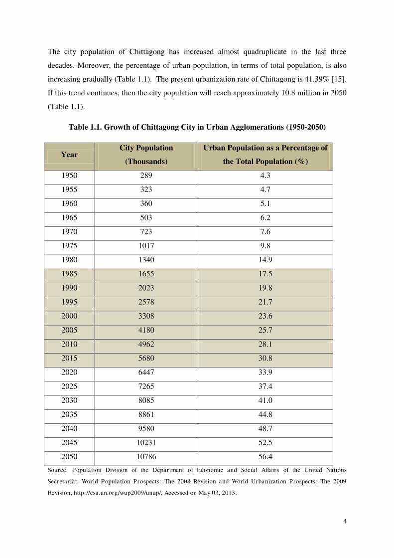
The city population of Chittagong has increased almost quadruplicate in the last three
decades. Moreover, the percentage of urban population, in terms of total population, is also
increasing gradually (Table 1.1). The present urbanization rate of Chittagong is 41.39% [15].
If this trend continues, then the city population will reach approximately 10.8 million in 2050
(Table 1.1).
Table 1.1. Growth of Chittagong City in Urban Agglomerations (1950-2050)
Year City Population
(Thousands)
Urban Population as a Percentage of
the Total Population (%)
1950 289 4.3
1955 323 4.7
1960 360 5.1
1965 503 6.2
1970 723 7.6
1975 1017 9.8
1980 1340 14.9
1985 1655 17.5
1990 2023 19.8
1995 2578 21.7
2000 3308 23.6
2005 4180 25.7
2010 4962 28.1
2015 5680 30.8
2020 6447 33.9
2025 7265 37.4
2030 8085 41.0
2035 8861 44.8
2040 9580 48.7
2045 10231 52.5
2050 10786 56.4
Source: Population Division of the Department of Economic and Social Affairs of the United Nations
Secretariat, World Population Prospects: The 2008 Revision and World Urbanization Prospects: The 2009
Revision, http://esa.un.org/wup2009/unup/, Accessed on May 03, 2013.
5
All these are creating numerous problems like haphazard urbanization, forcing urban-poor to
live in dangerous hill-slopes, landslides, water logging, extensive urban poverty, growth of
urban slums and squatters, traffic jam, environmental pollution and other socio-economic
problems [14].
This rapid urbanization, coupled with the increased intensity and frequency of adverse
weather events (e.g. landslides), is causing devastating effects on the country, which also has
lower capacities to deal with the consequences of climate change [11]. Particularly in
Chittagong, many urban dwellers and their livelihoods, quality of life, property and future
prosperity are being continuously threatened by the risks of cyclones, sea-level rise, tidal
waves, flooding, landslides, earthquakes and other hazards that climate change is expected to
aggravate. These disasters have almost become the day-to-day realities for the poor and
vulnerable populations that inhibit many of the most hazardous areas in the city [11].
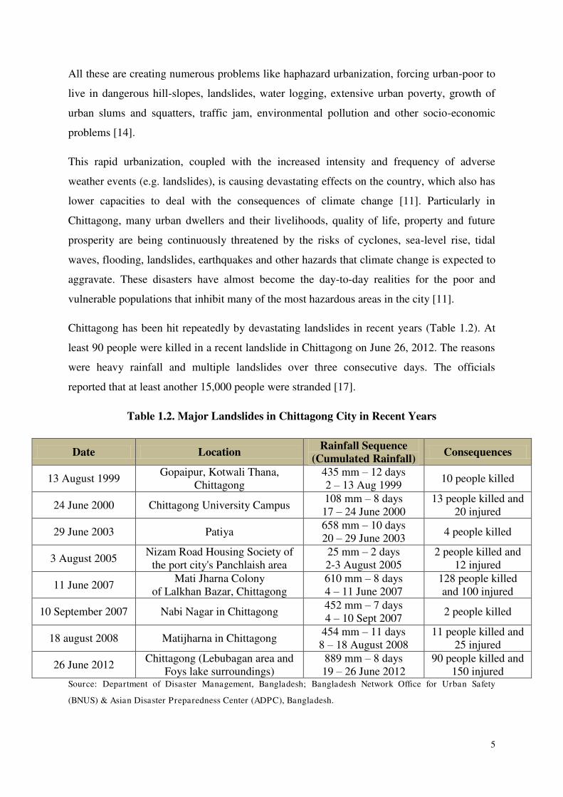
Chittagong has been hit repeatedly by devastating landslides in recent years (Table 1.2). At
least 90 people were killed in a recent landslide in Chittagong on June 26, 2012. The reasons
were heavy rainfall and multiple landslides over three consecutive days. The officials
reported that at least another 15,000 people were stranded [17].
Table 1.2. Major Landslides in Chittagong City in Recent Years
Date Location Rainfall Sequence
(Cumulated Rainfall) Consequences
13 August 1999 Gopaipur, Kotwali Thana,
Chittagong 435 mm – 12 days 2 – 13 Aug 1999
10 people killed
24 June 2000 Chittagong University Campus 108 mm – 8 days 17 – 24 June 2000
13 people killed and 20 injured
29 June 2003 Patiya 658 mm – 10 days 20 – 29 June 2003
4 people killed
3 August 2005 Nizam Road Housing Society of
the port city's Panchlaish area 25 mm – 2 days 2-3 August 2005
2 people killed and 12 injured
11 June 2007 Mati Jharna Colony
of Lalkhan Bazar, Chittagong 610 mm – 8 days 4 – 11 June 2007
128 people killed and 100 injured
10 September 2007 Nabi Nagar in Chittagong 452 mm – 7 days 4 – 10 Sept 2007
2 people killed
18 august 2008 Matijharna in Chittagong 454 mm – 11 days 8 – 18 August 2008
11 people killed and 25 injured
26 June 2012 Chittagong (Lebubagan area and
Foys lake surroundings) 889 mm – 8 days 19 – 26 June 2012
90 people killed and 150 injured
Source: Department of Disaster Management, Bangladesh; Bangladesh Network Office for Urban Safety
(BNUS) & Asian Disaster Preparedness Center (ADPC), Bangladesh.
6
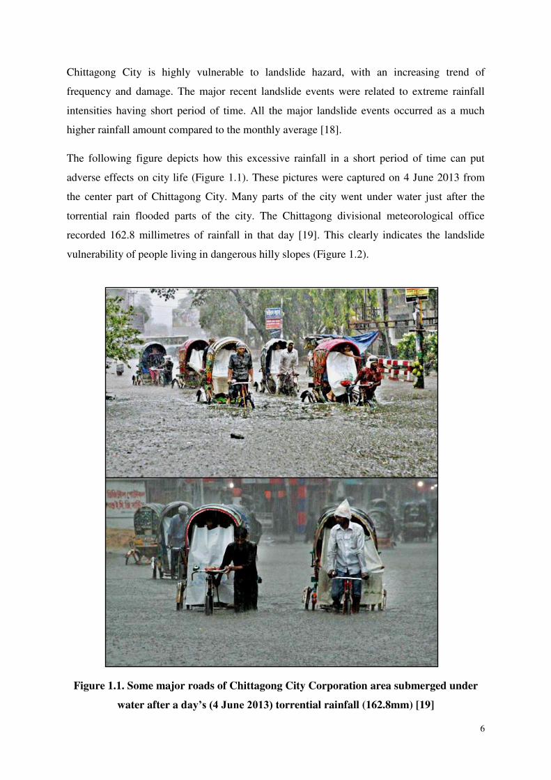
Chittagong City is highly vulnerable to landslide hazard, with an increasing trend of
frequency and damage. The major recent landslide events were related to extreme rainfall
intensities having short period of time. All the major landslide events occurred as a much
higher rainfall amount compared to the monthly average [18].
The following figure depicts how this excessive rainfall in a short period of time can put
adverse effects on city life (Figure 1.1). These pictures were captured on 4 June 2013 from
the center part of Chittagong City. Many parts of the city went under water just after the
torrential rain flooded parts of the city. The Chittagong divisional meteorological office
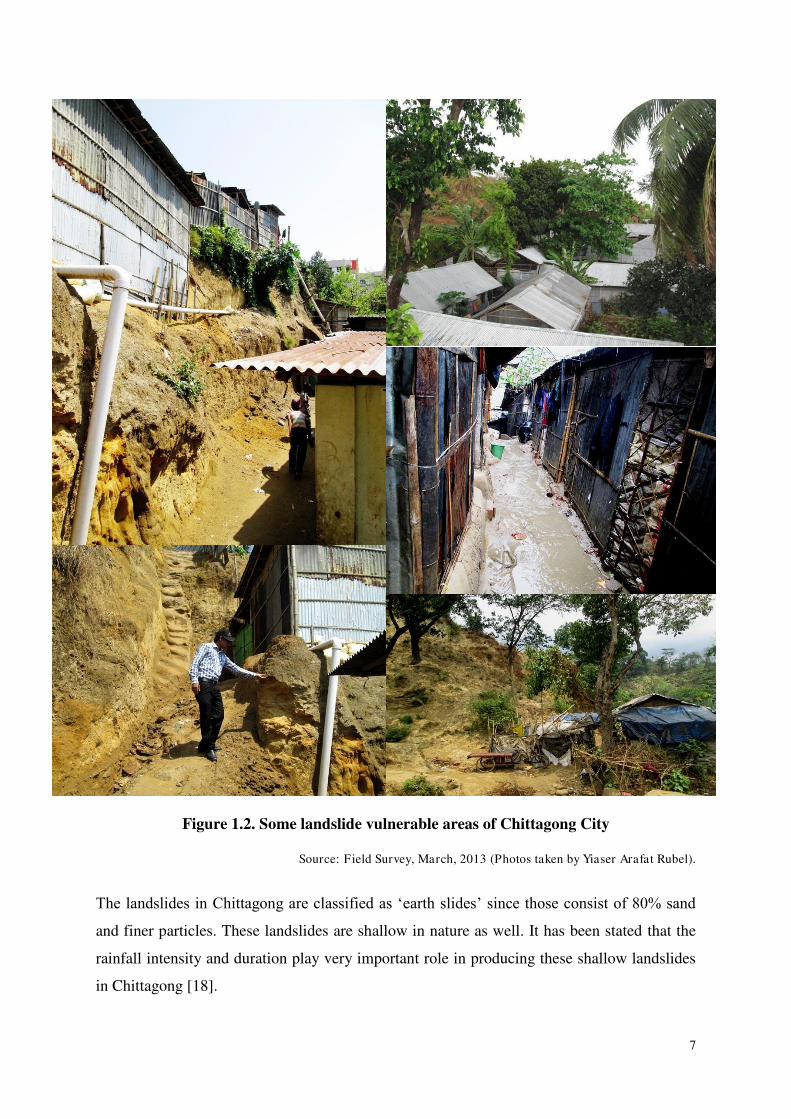
recorded 162.8 millimetres of rainfall in that day [19]. This clearly indicates the landslide
vulnerability of people living in dangerous hilly slopes (Figure 1.2).
Figure 1.1. Some major roads of Chittagong City Corporation area submerged under
water after a day’s (4 June 2013) torrential rainfall (162.8mm) [19]
7
Figure 1.2. Some landslide vulnerable areas of Chittagong City
Source: Field Survey, March, 2013 (Photos taken by Yiaser Arafat Rubel).
The landslides in Chittagong are classified as ‗earth slides‘ since those consist of 80% sand
and finer particles. These landslides are shallow in nature as well. It has been stated that the
rainfall intensity and duration play very important role in producing these shallow landslides
in Chittagong [18].
8
Because of climate change, Bangladesh is experiencing high intensity of rainfall in recent
years which is making the landslide situation worse. Moreover improper landuse, alterations
in the hilly regions by illegally cutting the hills, indiscriminate deforestation and agricultural
practices are aggravating the landslide vulnerability in Chittagong [20].
If this situation continues then Chittagong would soon become an urban-slum with the least
liveable situation for the city dwellers. In this regard, it is much needed to track the land
cover changes over-time, analyse socio-economic impacts and project the future landslide
vulnerability scenario of Chittagong City.
In addition, there is no strict hill management policy within Chittagong City. This has
encouraged many informal settlements along the landslide-prone hillslopes of Chittagong.
These settlements are being considered as illegal by the formal authorities, while the settlers
demand themselves as legal occupants. This is how; there is acute land tenure conflict among
the formal authorities, the settlers and the local communities over the past few decades. This
kind of conflict has also weakened the institutional arrangement for reducing the landslide
vulnerability in Chittagong [21].
It is therefore essential that the trend of land cover changes (e.g. urbanization) in the hilly
areas of Chittagong are assessed so that appropriate landslide mitigation strategies can be
developed to help combat the impacts of climate change.
1.3. Aim of the Research
The aim of this research is to understand the issues involved in urban disaster risk based on
the case study of recent landslide events in Chittagong City, Bangladesh.
1.4. Objectives of the Research
a) To establish the nature of relationships among land-cover change, climate change and
landslide disaster.
b) To produce the predictive landslide susceptibility maps using different methods and
modelling techniques.
c) To understand the geotechnical issues related to landslides.
d) To recommend appropriate mitigation and adaptation policies for landslide disaster
management within Chittagong Metropolitan Area (CMA).
9
Chapter 2
STUDY AREA PROFILE
2.1. General Description
Chittagong is the second-largest and main seaport of Bangladesh, situated on the banks of the
Karnaphuli River; it is the principle city of Chittagong Division [Figure 2.1 (a, b)] and a
major center of commerce and industry in South Asia. The city, under the jurisdiction of the
city corporation, has a population of about 2.5 million and is constantly growing [22].
It is also the Commercial Capital City of Bangladesh. The surrounding mountains and rivers
make the city attractive. Karnaphuli River falls in Chittagong. The largest land port of the
country, ―Chittagong Port‖, situated in Chittagong. That‘s why Chittagong is the city for
export and import. Most of the large industries of Bangladesh are situated in Chittagong.
Chittagong is an ideal vacation spot. Its green hills and forests, its broad sandy beaches and
its fine cool climate always attract the holiday-makers [22].
Chittagong City is not only the principal city of the district of Chittagong but also the second
largest city of Bangladesh. It is situated within 22° 14ʹ and 22° 24ʹ 30 North Latitude and
between 91° 46ʹ and 91° 53ʹ East Longitude.
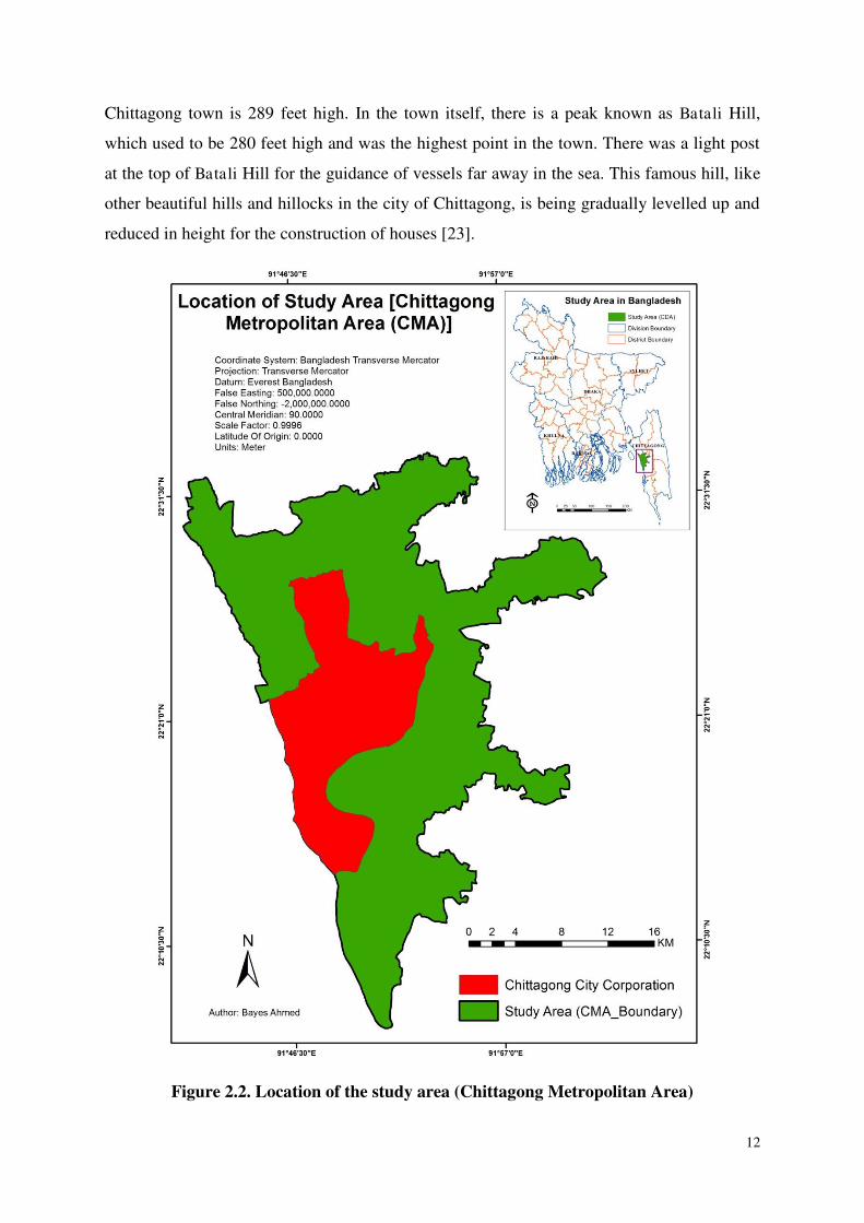
2.2. Location of Study Area
Chittagong City is divided into different administrative boundaries like Chittagong Statistical
Metropolitan Area (SMA), Chittagong Metropolitan Area (CMA) and Chittagong City
Corporation (CCC). The study area for this research is CMA (Figure 2.2). This selected study
area covers the biggest urban agglomeration and is the central part of Chittagong District in
terms of social and economic aspects [14]. Therefore, this area has huge potentiality to
landslide risks in near future based on the current trend of rapid urbanization.
Chittagong Development Authority (CDA) is the statutory planning and development
authority for the CMA was created in 1959, in order to ensure the planned and systematic
growth of the city. It is today the authority for planning, promoting and developing the CMA.
CDA is working under the Ministry of Housing and Public works of the Government [22].
The total area of CMA is approximately 775 square kilometres (Bangladesh Transverse
Mercator projection). The extent of CMA is top 495491.250000 m, bottom 445877.187500
m, left 673293.625000 m and right 709824.000000 m (Figure 2.2).

10
Figure 2.1 (a). Location of Bangladesh
Source: Banglapedia, National Encyclopaedia of Bangladesh, 2013
11
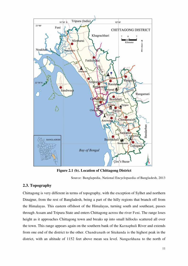
Figure 2.1 (b). Location of Chittagong District
Source: Banglapedia, National Encyclopaedia of Bangladesh, 2013
2.3. Topography
Chittagong is very different in terms of topography, with the exception of Sylhet and northern
Dinajpur, from the rest of Bangladesh, being a part of the hilly regions that branch off from
the Himalayas. This eastern offshoot of the Himalayas, turning south and southeast, passes
through Assam and Tripura State and enters Chittagong across the river Feni. The range loses
height as it approaches Chittagong town and breaks up into small hillocks scattered all over
the town. This range appears again on the southern bank of the Karnaphuli River and extends
from one end of the district to the other. Chandranath or Sitakunda is the highest peak in the
district, with an altitude of 1152 feet above mean sea level. Nangarkhana to the north of
12
Chittagong town is 289 feet high. In the town itself, there is a peak known as Batali Hill,
which used to be 280 feet high and was the highest point in the town. There was a light post
at the top of Batali Hill for the guidance of vessels far away in the sea. This famous hill, like
other beautiful hills and hillocks in the city of Chittagong, is being gradually levelled up and
reduced in height for the construction of houses [23].
Figure 2.2. Location of the study area (Chittagong Metropolitan Area)
13
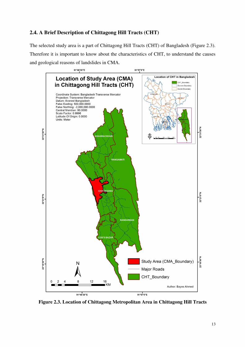
2.4. A Brief Description of Chittagong Hill Tracts (CHT)
The selected study area is a part of Chittagong Hill Tracts (CHT) of Bangladesh (Figure 2.3).
Therefore it is important to know about the characteristics of CHT, to understand the causes
and geological reasons of landslides in CMA.
Figure 2.3. Location of Chittagong Metropolitan Area in Chittagong Hill Tracts
14
2.4.1. Climate
The weather of this region is characterised by tropical monsoon climate with mean annual
rainfall nearly 2540 mm in the north and east and 2540 mm to 3810 mm in the south and
west. The dry and cool season is from November to March; pre-monsoon season is April-
May which is very hot and sunny and the monsoon season is from June to October, which is
warm, cloudy and wet [24].
2.4.2. Soil conditions
The hill soils (dystric cambisols) are mainly yellowish brown to reddish brown loams which
grade into broken shale or sandstone as well as mottled sand at a variable depth. The soils are
very strongly acidic [24].
2.4.3. Vegetation
The hills are unsuitable for cultivation but natural vegetation remains widely. Jhum
cultivation (slash and burn technology of agriculture practiced mainly by the people of pre-
plough age) is being practised on the hill slopes. Cotton, rice, tea and oilseeds are raised in
the valleys between the hills [24].
2.4.4. Physiography
According to the physiography of Bangladesh, the CHT falls under the Northern and Eastern
Hill unit and the High Hill or Mountain Ranges sub-unit. At present, all the mountain ranges
of the Chittagong Hill Tracts are almost hogback ridges. They rise steeply, thus looking far
more impressive than their height would imply. Most of the ranges have scarps in the west,
with cliffs and waterfalls. The region is characterised by a huge network of trellis and
dendritic drainage consisting of some major rivers draining into the Bay of Bengal [24].
Generally the hill ranges and the river valleys are longitudinally aligned. Four ranges, with an
average elevation of over three hundred metres, strike in a north-south direction in the
northern part of the hill tract districts. These are Phoromain range (Phoromain, 463m),
Dolajeri range (Langtrai, 429m), Bhuachhari (Changpai, 611m) and Barkal range
(Thangnang, 735m). South of the Karnaphuli River within the Chittagong Hill Tracts, there
are seven main mountain ranges within Bangladesh [24].
15
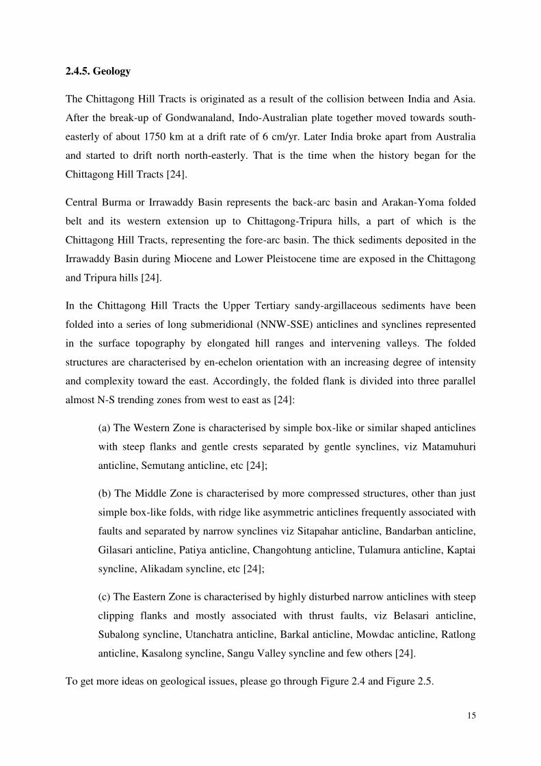
2.4.5. Geology
The Chittagong Hill Tracts is originated as a result of the collision between India and Asia.
After the break-up of Gondwanaland, Indo-Australian plate together moved towards south-
easterly of about 1750 km at a drift rate of 6 cm/yr. Later India broke apart from Australia
and started to drift north north-easterly. That is the time when the history began for the
Chittagong Hill Tracts [24].
Central Burma or Irrawaddy Basin represents the back-arc basin and Arakan-Yoma folded
belt and its western extension up to Chittagong-Tripura hills, a part of which is the
Chittagong Hill Tracts, representing the fore-arc basin. The thick sediments deposited in the
Irrawaddy Basin during Miocene and Lower Pleistocene time are exposed in the Chittagong
and Tripura hills [24].
In the Chittagong Hill Tracts the Upper Tertiary sandy-argillaceous sediments have been
folded into a series of long submeridional (NNW-SSE) anticlines and synclines represented
in the surface topography by elongated hill ranges and intervening valleys. The folded
structures are characterised by en-echelon orientation with an increasing degree of intensity
and complexity toward the east. Accordingly, the folded flank is divided into three parallel
almost N-S trending zones from west to east as [24]:
(a) The Western Zone is characterised by simple box-like or similar shaped anticlines
with steep flanks and gentle crests separated by gentle synclines, viz Matamuhuri
anticline, Semutang anticline, etc [24];
(b) The Middle Zone is characterised by more compressed structures, other than just
simple box-like folds, with ridge like asymmetric anticlines frequently associated with
faults and separated by narrow synclines viz Sitapahar anticline, Bandarban anticline,
Gilasari anticline, Patiya anticline, Changohtung anticline, Tulamura anticline, Kaptai
syncline, Alikadam syncline, etc [24];
(c) The Eastern Zone is characterised by highly disturbed narrow anticlines with steep
clipping flanks and mostly associated with thrust faults, viz Belasari anticline,
Subalong syncline, Utanchatra anticline, Barkal anticline, Mowdac anticline, Ratlong
anticline, Kasalong syncline, Sangu Valley syncline and few others [24].
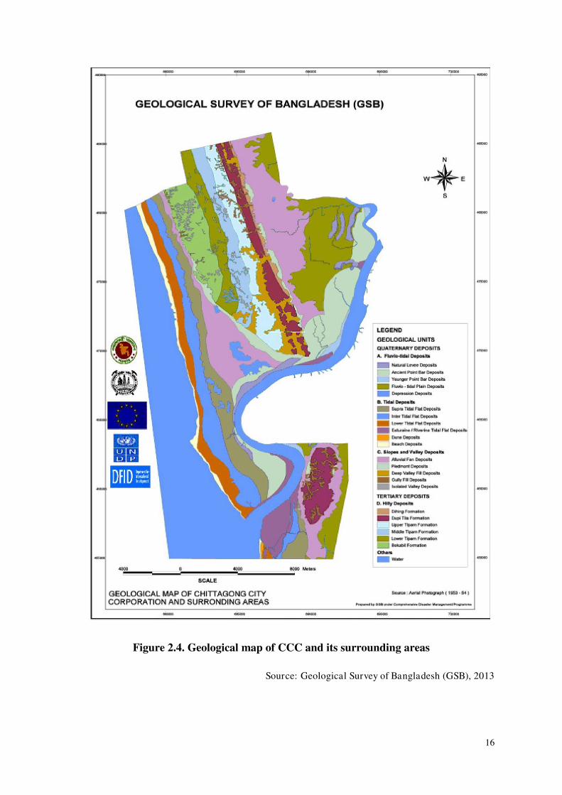
To get more ideas on geological issues, please go through Figure 2.4 and Figure 2.5.
16
Figure 2.4. Geological map of CCC and its surrounding areas
Source: Geological Survey of Bangladesh (GSB), 2013
17
Figure 2.5. Geomorphological map of CCC and its surrounding areas
Source: Geological Survey of Bangladesh (GSB), 2013
Some photos from the field visits are attached in Appendix-I.
18
Chapter 3
LITERATURE REVIEW AND DATA COLLECTION
3.1. Existing Literary Works
Landslides are one of the most significant natural damaging disasters in hilly environments
[25]. Social and economic losses due to landslides can be reduced by the means of effective
planning and management [26]. Landslide hazard assessment is generally based on the
concept that ―the present and the past are keys to the future‖. This is why; most landslide
hazard analyses take into account an up-to-date landslide inventory that represents the
fundamental tool for identifying the hillslope instability factors in triggering landslides [27].
However, in spite of improvements in hazard recognition, prediction, mitigation measures,
and warning systems, worldwide landslide activity is increasing [28]. This trend is expected
to continue for the following reasons in the landslide prone areas [29, 30]:
a) Increased urbanization and illegal hill-cutting
b) Continued deforestation and agricultural activities
c) Increased regional precipitation (heavy rainfall) due to climate change
Various geo-structural as well as causative-factor based approaches have been proposed for
landslide susceptibility zoning [31]. But GIS modeling of landslide phenomena has taken
precedence in recent time. Geospatial technologies like geographic information system (GIS),
global positioning system (GPS) and remote sensing (RS) are useful in the hazard
assessment, risk identification, and disaster management for landslides. The GPS is a space-
based global navigation satellite system which provides the information of position and time
anywhere in the world in all weather conditions [32]. Previous studies showed the application
of GPS for mapping and indentifying landslide zones. GIS is used for collection, storage, and
analysis of processes where geographic information is involved [32]. The use of GIS for
landslide mapping is very common in various studies. Remote sensing is the science in which
information is acquired about the surface of earth without physically being in contact with it.
RS is also used for monitoring and mapping of landslides in various studies [32].
19
Mapping the areas that are susceptible to landslides is essential for proper landuse planning
and disaster management for a particular locality or region. Throughout the years different
techniques and methods have been developed and applied in the literature for landslide
susceptibility mapping. Landslide susceptibility maps can be produced using both the
quantitative or qualitative approach [33].
Qualitative maps weight each factors affecting the landslides based on the practical
experience and expertise of the researcher [33]. Qualitative methods simply portray the
hazard zoning in descriptive terms [34]. The qualitative approaches were used by the
scientists until the late 1970‘s [35]. But because of the developments in computer
programming and geospatial technologies, qualitative techniques have become very popular
in recent decades. Moreover, it incorporates the causes of landslides (instability factors) and
probabilistic methods which give much better results than the quantitative methods [35].
Methods to map landslide susceptibility can be classified into four groups, namely landslide
inventory based probabilistic, deterministic, heuristic, and statistical techniques [34].
Landslide inventory based probabilistic techniques involve the inventory of landslides,
construction of databases, geomorphological analysis, and producing the susceptibility maps
based on the collected data [36]. Deterministic techniques (quantitative methods) involve the
estimation of quantitative values of stability variables and require the creation of a map that
displays the spatial distribution of input data [37, 38]. Heuristic analysis (qualitative method)
is based on the intrinsic properties of the geomorphologists to analyse aerial photographs or
to conduct field surveying [39].
In this kind of analysis, the susceptibility is established by researchers and the analyst uses
expert knowledge to assign weights to a series of parameters for preparing the qualitative
map [38]. Statistical analysis is used to analyse factors affecting landslides in areas with
environmental conditions similar to those where past landslides have been reported [33].
These methods use sample data based on the relationship between the dependent variable (the
presence or absence of landslides), and the independent variables (landslides
triggering/causative factors). Through these statistical techniques, quantitative predictions are
possible to make for areas where there is no landslides and with similar conditions [38].
Within these techniques, the probabilistic and statistical methods have been most commonly
used in recent years. These methods have become more popular, assisted by the geographic
information system (GIS) and remote sensing (RS) techniques [27].
20
The probabilistic (non-deterministic) models like frequency ratio, bivariate analysis,
multivariate analysis, and Poisson probability model [40] are more frequently used to
determine landslide susceptibility zones [41]. Among the most widely used statistical method
is the logistic regression [38]. Many researchers have used different techniques such as
heuristic approach [29] and deterministic models [28].
Moreover, GIS based multi criteria decision analysis (MCDA) provides powerful techniques
for the analysis and prediction of landslide hazards. These include the analytic hierarchy
process (AHP) [42], the weighted linear combination (WLC), the ordered weighted average
(OWA) [42] etc.
Most recently, new non-parametric techniques like cellular automata, fuzzy-logic, artificial
neural networks (ANN) [43], support vector machines (SVM), and neuro-fuzzy models have
been used for landslide modeling [33]. [Please go through Appendix- II, for the detailed
structural literature review]
In most cases the researchers have used the following thematic layers for modelling or
predicting landslide susceptibility maps [28, 32, 33, 43]:
1) Landslide Inventory
2) Precipitation Data/ Rainfall Intensity Map
3) Land Cover Maps
4) Digital Elevation Model (DEM)
5) Aspect
6) Elevation/ Internal Relief
7) Slope
8) Curvature (Plan & Profile)
9) Geology
10) Geomorphology
11) Soil/ Lithology
12) Lineaments/ Distance from Faults
13) Drainage Density
14) Distance to Road
15) Distance to Stream
16) Topographic Wetness Index (TWI)
17) Normalized Difference Vegetation Index (NDVI)
21
18) Stream Power Index (SPI)
19) Seismic Data
20) Surrounding Infrastructure (e.g. Buildings)
If the above mentioned 20 thematic layers/ variables are analysed, then it is clear that the land
cover maps and precipitation data (rainfall pattern) can be changed markedly over time.
Similarly drainage density, distance to road/ stream, TWI, NDVI, SPI and surrounding
infrastructure can change in course of time. Therefore, these variables can be considered as
‗dynamic variables‘. The rest of the layers can be termed as ‗persistent variables‘.
3.2. Data Collection
For landslide susceptibility mapping (LSM), it is very important to collect necessary data
layers. For this research purpose, 9 different GIS layers have been produced for LSM. The
details of the data collection technique and ways of preparing the thematic layers are
described below:
3.2.1. Land Cover Mapping
Landsat Thematic Mapper (TM) satellite images were used for the land cover mapping
(2010) of CHT area. This CHT base map was collected from International Centre for
Integrated Mountain Development (ICIMOD), Kathmandu, Nepal. But the procedure for
preparing the map is described in brief. Initially four scenes were collected to cover the whole
CHT area. TM sensor collects reflected energy in three visible bands (blue = 1, green = 2,
and red = 3) and three infrared bands (two NIR = 4, 5 and one middle infrared = 7). The base
year for this land cover mapping is selected as 2010.
Among the four scenes, three were acquired using the Global Visualization Viewer
(GLOVIS) of United States Geological Survey (USGS) and the one was from GISTDA (Geo-
Informatics and Space Technology Development Agency), Thailand. However, thermal band
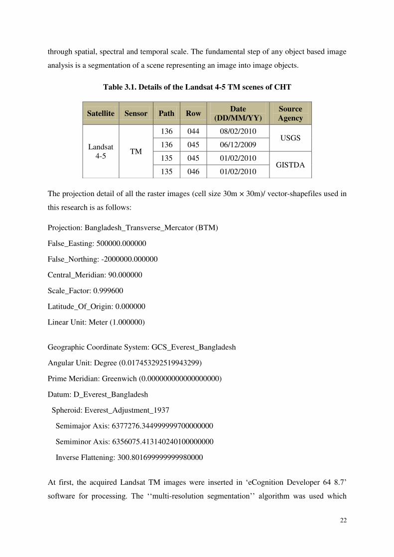
was not used in this particular study. The details of the scenes used are listed in Table 3.1. All
the image-dates are of the dry season in Bangladesh.
The land cover classification methodology for this research is based on ‗Object Based Image
Analysis (OBIA)‘. ‗OBIA‘ is also called ‗Geographic Object-Based Image Analysis
(GEOBIA)‘. ‗OBIA‘ is a sub-discipline of geoinformation science devoted to partitioning
remote sensing imagery into meaningful image objects, and assessing their characteristics
22
through spatial, spectral and temporal scale. The fundamental step of any object based image
analysis is a segmentation of a scene representing an image into image objects.
Table 3.1. Details of the Landsat 4-5 TM scenes of CHT
The projection detail of all the raster images (cell size 30m × 30m)/ vector-shapefiles used in
this research is as follows:
Projection: Bangladesh_Transverse_Mercator (BTM)
False_Easting: 500000.000000
False_Northing: -2000000.000000
Central_Meridian: 90.000000
Scale_Factor: 0.999600
Latitude_Of_Origin: 0.000000
Linear Unit: Meter (1.000000)
Geographic Coordinate System: GCS_Everest_Bangladesh
Angular Unit: Degree (0.017453292519943299)
Prime Meridian: Greenwich (0.000000000000000000)
Datum: D_Everest_Bangladesh
Spheroid: Everest_Adjustment_1937
Semimajor Axis: 6377276.344999999700000000
Semiminor Axis: 6356075.413140240100000000
Inverse Flattening: 300.801699999999980000
At first, the acquired Landsat TM images were inserted in ‗eCognition Developer 64 8.7‘
software for processing. The ‗‗multi-resolution segmentation‘‘ algorithm was used which
Satellite Sensor Path Row Date
(DD/MM/YY)
Source
Agency
Landsat 4-5
TM
136 044 08/02/2010 USGS
136 045 06/12/2009
135 045 01/02/2010 GISTDA
135 046 01/02/2010
23
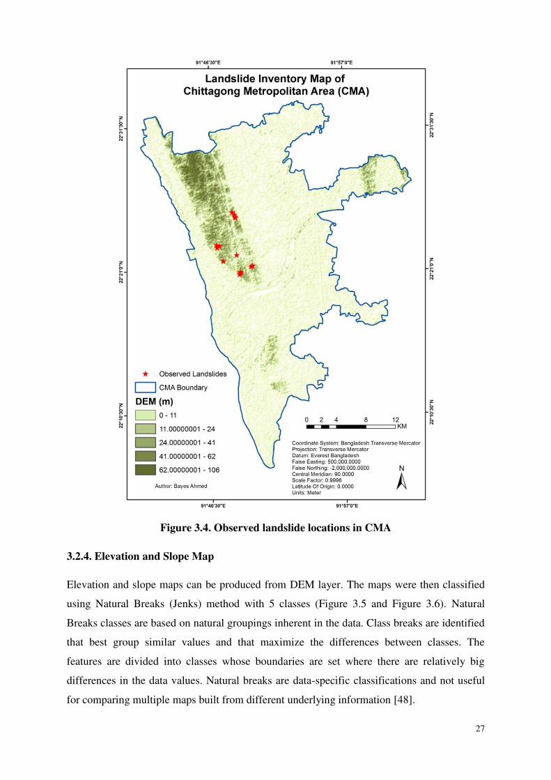
consecutively merges pixels or existing image objects that essentially identifies single image
objects of one pixel in size and merges them with their neighbours, based on relative
homogeneity criteria. Multi-resolution segmentations are those groups of similar pixel values
which merges the homogeneous areas into larger objects and heterogeneous areas in smaller
ones.
During the classification process, information on spectral values of image layers, vegetation
indices like the Normalized Difference Vegetation Index (NDVI) and land water mask which
were created through band rationing, slope and texture information were used. Image indices
are very important during the image classification. Image rationing is a ―synthetic image
layer‖ created from the existing bands of a multispectral image. This new layer often
provides unique and valuable information not found in any of the other individual bands.
Image index is a calculated results or generated product from satellite band/channels. It is
help to identify different land cover from mathematical definition.
NDVI: One of the commonly used indices and it is related to vegetation is that
healthy vegetation reflects very well in the near infrared part of the spectrum. NDVI index
values can range from -1.0 to 1.0. NDVI was calculated using the following formula:
NDVI = (NIR - red) / (NIR + red)
Land and water mask: Land and water mask indices values can range from 0 to 255,
but water values typically range between 0 and 50. The land and water mask was created
using the formula
Land and water mask: IR/Green*100
The next step is to code these image objects according to their attributes, such as
NDVI, Land and water mask, layer value and colour and relative position to other objects
using user-defined rules. In this process, selected object that represent patterns were
recognize with the help from other sources namely already known Ground truthing
information and high resolution Google earth images. Normally similar features observed
similar spectral responses and unique with respect to all other image objects.
After that comparison, features using the ‗2D Feature Space Plot‘ were used for correlation of
two features from the selected image objects. Developing rule sets investigated single image
objects and generated land cover map. Image objects have spectral, shape, and hierarchical

24
characteristics and these features are used as sources of information to define the inclusion-
or-exclusion parameters used to classify image objects. Over each scene rules were generated
for each land cover class and evaluated for their separation, tested for their visual assessment
over Google earth images.
After ascertaining the class separation using segment based approach, classification is
performed to get land cover classification map for each scene. Each scene thus prepared
again evaluated with available field data and Google earth image over randomly selected
points for accuracy assessment. After finalization of classification of each scene, all the
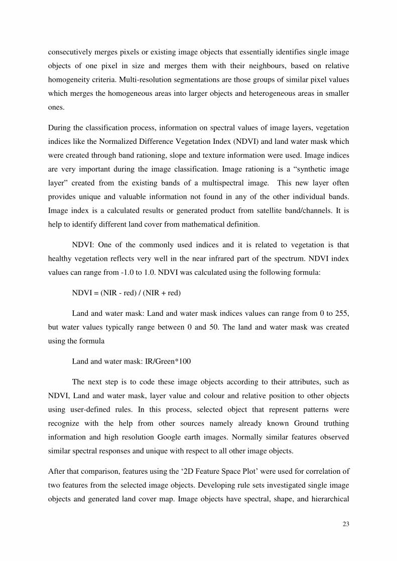
scenes were gone through mosaic to obtain land cover map of CHT area (Figure 3.1).
Figure 3.1 consists of 14 land cover classes. But for this research purpose, only 5 broad land
cover classes (urban area, semi-urban area, water body, vegetation and bare soil) were chosen
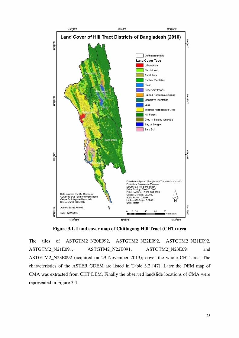
by reclassification technique. Later the study area was extracted from the CHT land cover
map using the CMA boundary. This is the final land cover map of the study area (Figure 3.2).
3.2.2. Precipitation Map
The daily observed precipitation data were collected from Bangladesh Meteorological
Department (1950-2010). Based on the average annual precipitation, the final precipitation
map of CMA was prepared using Kriging overlaying technique (Figure 3.3).
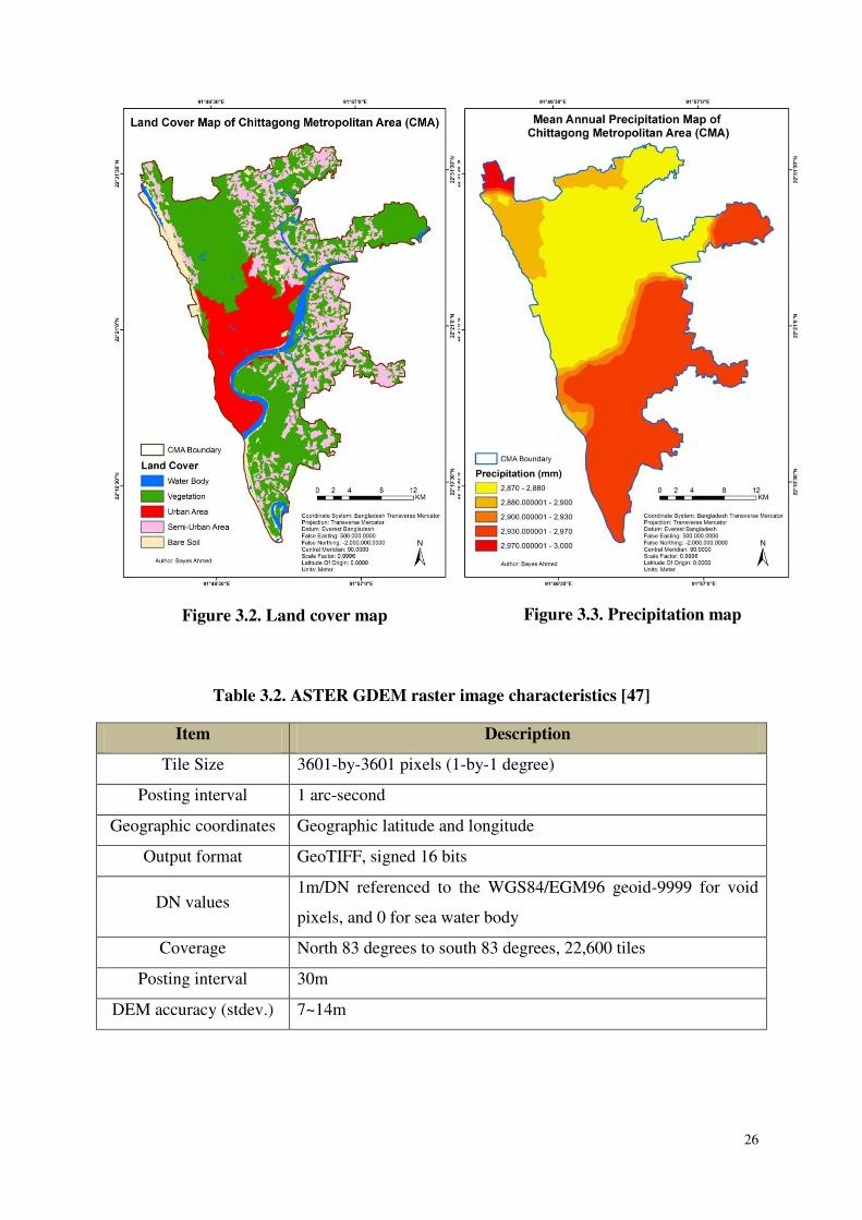
3.2.3. Landslide Inventory Map
A total of 20 landslide locations were identified in the study area through field visit
(Appendix-III). The latitude and longitude values were collected using a Global Positioning
System (GPS) device. Moreover, the Digital Elevation Model (DEM) data were collected
from the ASTER GDEM portal. The Advanced Spaceborne Thermal Emission and Reflection
Radiometer (ASTER) Global Digital Elevation Model (GDEM) was developed jointly by the
Ministry of Economy, Trade, and Industry (METI) of Japan and the United States
National Aeronautics and Space Administration (NASA). The ASTER GDEM was
contributed by METI and NASA to the Global Earth Observation System of Systems
(GEOSS) and is available at no charge to users via electronic download from the Earth
Remote Sensing Data Analysis Center (ERSDAC) of Japan and NASA‘s Land Processes
Distributed Active Archive Center (LP DAAC) [47].
25
Figure 3.1. Land cover map of Chittagong Hill Tract (CHT) area
The tiles of ASTGTM2_N20E092, ASTGTM2_N22E092, ASTGTM2_N21E092,
ASTGTM2_N21E091, ASTGTM2_N22E091, ASTGTM2_N23E091 and
ASTGTM2_N23E092 (acquired on 29 November 2013); cover the whole CHT area. The
characteristics of the ASTER GDEM are listed in Table 3.2 [47]. Later the DEM map of
CMA was extracted from CHT DEM. Finally the observed landslide locations of CMA were
represented in Figure 3.4.
26
Table 3.2. ASTER GDEM raster image characteristics [47]
Item Description
Tile Size 3601-by-3601 pixels (1-by-1 degree)
Posting interval 1 arc-second
Geographic coordinates Geographic latitude and longitude
Output format GeoTIFF, signed 16 bits
DN values 1m/DN referenced to the WGS84/EGM96 geoid-9999 for void
pixels, and 0 for sea water body
Coverage North 83 degrees to south 83 degrees, 22,600 tiles
Posting interval 30m
DEM accuracy (stdev.) 7~14m
Figure 3.2. Land cover map Figure 3.3. Precipitation map
27
Figure 3.4. Observed landslide locations in CMA
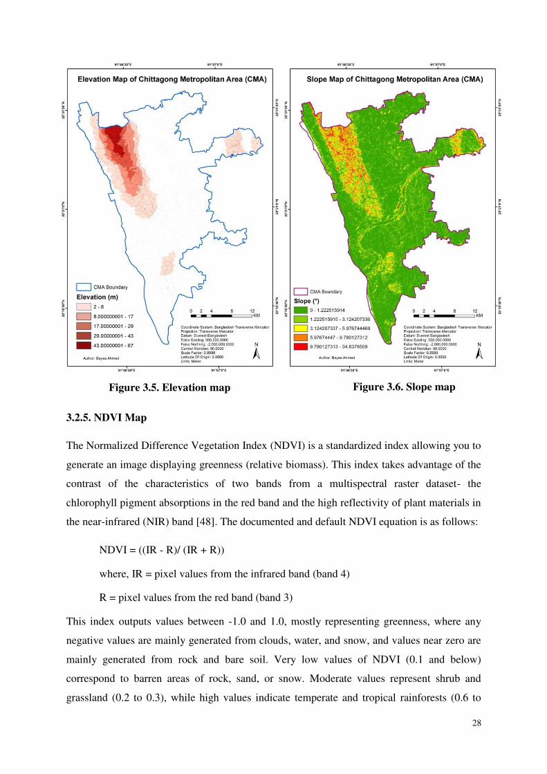
3.2.4. Elevation and Slope Map
Elevation and slope maps can be produced from DEM layer. The maps were then classified
using Natural Breaks (Jenks) method with 5 classes (Figure 3.5 and Figure 3.6). Natural
Breaks classes are based on natural groupings inherent in the data. Class breaks are identified
that best group similar values and that maximize the differences between classes. The
features are divided into classes whose boundaries are set where there are relatively big
differences in the data values. Natural breaks are data-specific classifications and not useful
for comparing multiple maps built from different underlying information [48].
28
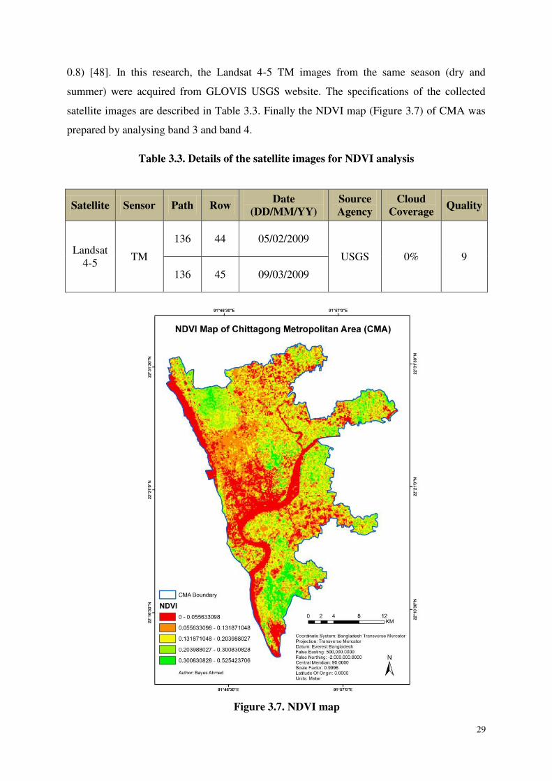
3.2.5. NDVI Map
The Normalized Difference Vegetation Index (NDVI) is a standardized index allowing you to
generate an image displaying greenness (relative biomass). This index takes advantage of the
contrast of the characteristics of two bands from a multispectral raster dataset- the
chlorophyll pigment absorptions in the red band and the high reflectivity of plant materials in
the near-infrared (NIR) band [48]. The documented and default NDVI equation is as follows:
NDVI = ((IR - R)/ (IR + R))
where, IR = pixel values from the infrared band (band 4)
R = pixel values from the red band (band 3)
This index outputs values between -1.0 and 1.0, mostly representing greenness, where any
negative values are mainly generated from clouds, water, and snow, and values near zero are
mainly generated from rock and bare soil. Very low values of NDVI (0.1 and below)
correspond to barren areas of rock, sand, or snow. Moderate values represent shrub and
grassland (0.2 to 0.3), while high values indicate temperate and tropical rainforests (0.6 to
Figure 3.5. Elevation map Figure 3.6. Slope map
29
0.8) [48]. In this research, the Landsat 4-5 TM images from the same season (dry and
summer) were acquired from GLOVIS USGS website. The specifications of the collected
satellite images are described in Table 3.3. Finally the NDVI map (Figure 3.7) of CMA was
prepared by analysing band 3 and band 4.
Table 3.3. Details of the satellite images for NDVI analysis
Satellite Sensor Path Row Date
(DD/MM/YY)
Source
Agency
Cloud
Coverage Quality
Landsat 4-5
TM
136 44 05/02/2009
USGS 0% 9
136 45 09/03/2009
Figure 3.7. NDVI map
30
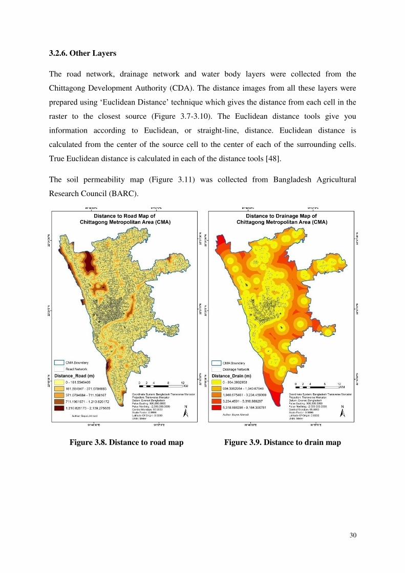
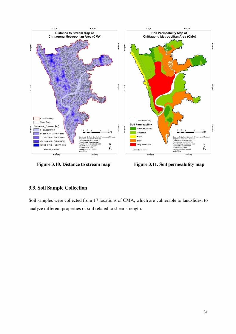
3.2.6. Other Layers
The road network, drainage network and water body layers were collected from the
Chittagong Development Authority (CDA). The distance images from all these layers were
prepared using ‗Euclidean Distance‘ technique which gives the distance from each cell in the
raster to the closest source (Figure 3.7-3.10). The Euclidean distance tools give you
information according to Euclidean, or straight-line, distance. Euclidean distance is
calculated from the center of the source cell to the center of each of the surrounding cells.
True Euclidean distance is calculated in each of the distance tools [48].
The soil permeability map (Figure 3.11) was collected from Bangladesh Agricultural
Research Council (BARC).
Figure 3.8. Distance to road map Figure 3.9. Distance to drain map
31
3.3. Soil Sample Collection
Soil samples were collected from 17 locations of CMA, which are vulnerable to landslides, to
analyze different properties of soil related to shear strength.
Figure 3.10. Distance to stream map Figure 3.11. Soil permeability map
32
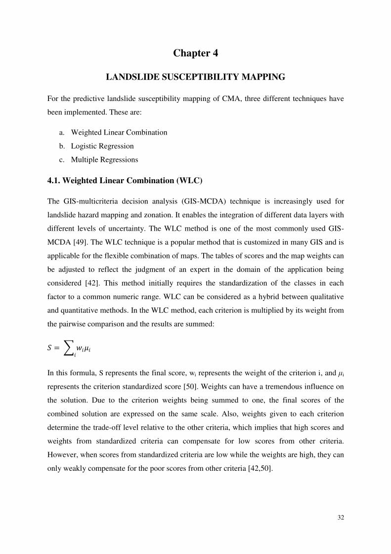
Chapter 4
LANDSLIDE SUSCEPTIBILITY MAPPING
For the predictive landslide susceptibility mapping of CMA, three different techniques have
been implemented. These are:
a. Weighted Linear Combination
b. Logistic Regression
c. Multiple Regressions
4.1. Weighted Linear Combination (WLC)
The GIS-multicriteria decision analysis (GIS-MCDA) technique is increasingly used for
landslide hazard mapping and zonation. It enables the integration of different data layers with
different levels of uncertainty. The WLC method is one of the most commonly used GIS-
MCDA [49]. The WLC technique is a popular method that is customized in many GIS and is
applicable for the flexible combination of maps. The tables of scores and the map weights can
be adjusted to reflect the judgment of an expert in the domain of the application being
considered [42]. This method initially requires the standardization of the classes in each
factor to a common numeric range. WLC can be considered as a hybrid between qualitative
and quantitative methods. In the WLC method, each criterion is multiplied by its weight from
the pairwise comparison and the results are summed:
� = ����
In this formula, S represents the final score, wi represents the weight of the criterion i, and μi
represents the criterion standardized score [50]. Weights can have a tremendous influence on
the solution. Due to the criterion weights being summed to one, the final scores of the
combined solution are expressed on the same scale. Also, weights given to each criterion
determine the trade-off level relative to the other criteria, which implies that high scores and
weights from standardized criteria can compensate for low scores from other criteria.
However, when scores from standardized criteria are low while the weights are high, they can
only weakly compensate for the poor scores from other criteria [42,50].
33
WLC (or simple additive weighting) is based on the concept of a weighted average. The
decision-maker directly assigns the weights of ‗relative importance‘ to each attribute map
layer. A total score is then obtained for each alternative by multiplying the weight assigned to
each attribute by the scaled value given to the alternative on that attribute, and summing the
products of all attributes. When the overall scores are calculated for all of the alternatives, the
alternative with the highest overall score is chosen. The method can be operationalized using
any GIS system with overlay capabilities. The overlay techniques allow the evaluation
criterion map layers (input maps) to be combined, in order to determine the composite map
layer (output map) [42,49].
In this method, criteria may include both weighted factors and constraints. WLC starts by
multiplying each factor by its factor/trade-off weight and then adding the results; constraints
are then applied by successive multiplication to "zero out" excluded areas. This procedure is
characterized by full trade-off between factors and average risk. Factor weights, not used at
all in the case of Boolean intersection (no trade-off), are very important in WLC because they
determine how individual factors will trade-off relative to each other. In this case, the higher
the factor weight the more influence that factor has on the final suitability map. (Contrast this
with method 3 below where the importance of factor weights is variable). Along with full
trade-off, this combination procedure is characterized by an average level of risk, as it is
exactly midway between the minimization (AND operation) and maximization (OR
operation) of areas to be considered suitable in the final result [51].
The class rating within each factor was based on the relative importance of each class
according to experts opinion, practical experience, field observations in the study area and
existing literature, indicating certain conditions as the most favourable to slope failure. For
this research purpose, some assumptions were undertaken for the factors. The susceptibility
to landslides for a certain area increases:
1. The more the distance from drainage network
2. The higher the elevation
3. The closer to urban area land cover type
4. The lower the NDVI
5. The higher the precipitation
6. The farther the distance from road network
7. The steeper the slope
34
8. The slower the soil permeability
9. The closer to water body
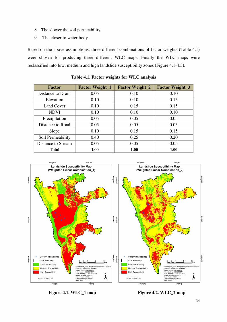
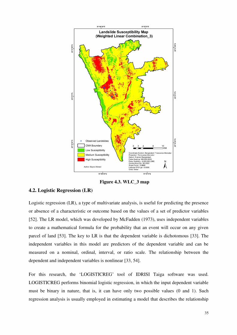
Based on the above assumptions, three different combinations of factor weights (Table 4.1)
were chosen for producing three different WLC maps. Finally the WLC maps were
reclassified into low, medium and high landslide susceptibility zones (Figure 4.1-4.3).
Table 4.1. Factor weights for WLC analysis
Factor Factor Weight_1 Factor Weight_2 Factor Weight_3
Distance to Drain 0.05 0.10 0.10
Elevation 0.10 0.10 0.15
Land Cover 0.10 0.15 0.15
NDVI 0.10 0.10 0.10
Precipitation 0.05 0.05 0.05
Distance to Road 0.05 0.05 0.05
Slope 0.10 0.15 0.15
Soil Permeability 0.40 0.25 0.20
Distance to Stream 0.05 0.05 0.05
Total 1.00 1.00 1.00
Figure 4.1. WLC_1 map Figure 4.2. WLC_2 map
35
4.2. Logistic Regression (LR)
Logistic regression (LR), a type of multivariate analysis, is useful for predicting the presence
or absence of a characteristic or outcome based on the values of a set of predictor variables
[52]. The LR model, which was developed by McFadden (1973), uses independent variables
to create a mathematical formula for the probability that an event will occur on any given
parcel of land [53]. The key to LR is that the dependent variable is dichotomous [33]. The
independent variables in this model are predictors of the dependent variable and can be
measured on a nominal, ordinal, interval, or ratio scale. The relationship between the
dependent and independent variables is nonlinear [33, 54].
For this research, the ‗LOGISTICREG‘ tool of IDRISI Taiga software was used.
LOGISTICREG performs binomial logistic regression, in which the input dependent variable
must be binary in nature, that is, it can have only two possible values (0 and 1). Such
regression analysis is usually employed in estimating a model that describes the relationship
Figure 4.3. WLC_3 map
36
between one or more continuous independent variable(s) to the binary dependent variable.
The basic assumption is that the probability of dependent variable takes the value of 1
(positive response) follows the logistic curve and its value can be estimated with the
following formula [51,55]:
P(y= 1|X) = � �( ��)
1+� �( ��)
where, P = the probability of the dependent variable being 1; X is the independent variables,
X = (x0, x1, x2, … xk), x0 = 1
B is the estimated parameters
B = (b0, b1, b2, …. bk)
To linearize the above model and to remove the 0/1 boundaries for the original dependent
variable (probability), the following transformation are usually applied [51,55]:
P’ = Ln(P/(1-P))
This transformation is referred to as the logit or logistic transformation. Note that after the
transformation P' can theoretically assume any value between minus and plus infinity. By
performing the logit transformation on both sides of the above logit regression model, we
obtain the standard linear regression model [51,55]:
Ln(p/(1-p)) = b0 + b1*x1 + b2*x2 +…….+ bk*xk + error_term
Notice that the logit transformation of dichotomous data ensures that the dependent variable
of the regression is continuous, and the new dependent variable (logit transformation of the
probability) is unbounded. Furthermore, it ensures that the predicted probability will be
continuous within the range from 0-1.
Assumptions of the logistic regression model [51]:
- the dependent random variable, Y, is assumed to be binary, taking on only two
values ( 0 and 1).
- the outcomes on Y are assumed to be mutually exclusive and exhaustive.
37
- Y is assumed to depend on K observable variables Xk and the relationship is non-
linear and follows the logistic curve.
- the data are generated from a random sample of size N, with a sample point denoted
by i, i = 1, ..., N.
- no restriction on the independent variables except that they cannot be linearly
related; (implies that N>K).
- the error term of each observation is assumed to be independent of the error terms of
all other observations.
LOGISTICREG employs Maximum Likelihood Estimation (MLE) procedure to find the best
fitting set of parameters (coefficients). The maximum likelihood function used by
LOGISTICREG is the following [51,55]:
L = ��� *(1-µ 1)(1-y
i)
where, L is the likelihood
µ i is the predicted value of the dependent variable for sample i
µ i = exp ( ���=0 � �� )/(1 + exp �� ����=0 )
yi is the observed value of the dependent variable for sample i
To maximize the above likelihood function, it thus requires the solution for the following
simultaneous nonlinear equations [51,55]: .��=1 (yi - µ i) * xij = 0
Where xij is the observed value of the independent variable j for sample i.
The rest is the same as for the likelihood function. In solving the above equations,
LOGISTICREG uses the Newton-Raephson algorithm [51]. Moreover, the LOGISTICREG
text output includes the following:
The regression equation and the individual regression coefficient;
In the Regression Statistics section [51]:
38
Number of Total Observations: the number of observations used in study area
Number of 0s in Study Area: the number of observations with dependent value as 0 in study area
Number of 1s in Study Area: the number of observations with dependent value as 1 in study area
Percentage of 0s in Study Area: equal to 100*(Number of 0s in study area / Number of observations in study area)
Percentage of 1s in Study Area: equal to 100*(Number of 1s in study area / Number of observations in study area)
Number of Auto-sampled Observations:
the number of observations sampled for analysis
Number of Os in Sampled Area: the number of observations with dependent value as 0 in analysis
Number of 1s in Sampled Area: the number of observations with dependent value as 1 in analysis
Percentage of 0s in Sampled Area: actual percentage of 0s used in analysis
Percentage of 1s in Sampled Area; actual percentage of 1s used in analysis
The basis for testing the goodness of fit in logistic regression is the likelihood ratio principle.
The ratio is based on the following two statistics [51,55]:
-2log(L0)
where L0 is the value of the likelihood function if all coefficients except the intercept are 0;
-2log(Likelihood)
where Likelihood is the value of the likelihood function for the full model as fitted;
Based on the above two statistics, the following two are calculated [51]:
Pseudo R_square = 1- (log(Likelihood )/log(L0);
Thus, pseudo R_square = 1 indicates a perfect fit, where as pseudo R_square = 0 indicates no relationship.
Pseudo R_square greater than 0.2 is considered a relatively good fit [56].
ChiSquare( k) = -2(log(likelihood) –log(L0));
This is also known as the likelihood ratio statistic which follows, approximately, a chi-square
distribution when the null hypothesis is true. This statistic tests the hypothesis that all
coefficients except the intercept are 0. Thus, it is a similar test as the F statistic in liner

39
regression analysis. The degrees of freedom for this chi-square statistic is K (the number of
the independent variables included) [51].
The last statistic in this group that bears some measure of goodness of fit is calculated based
on the difference between the observed and the predicted values of the dependent variable
[51]:
Goodess_of_fit = .��=1 (yi-µ i)2/µ i*(1-µ i)
Thus, the smaller of this statistic, the better fit it indicates. The classification is based on the
predicted probability with 0.5 as the dividing point, i.e., classify a case as 0 if its predicted
probability is less than 0.5 and as 1 otherwise. The odds ratio is calculated from the
classification table with the following formula [51]:
Odds_ratio = (f11 * f22)/(f12 * f21)
where, ------------------------------------------------------------
Observed Pred_0 Pred_1
0 f11 f12
1 f21 f22
------------------------------------------------------------
In the last section, this version of LOGISTICREG offers two additional statistics [51]:
(1) Instead of reclassifying the case using the probability of 0.5 as the cutting point, it offers
an alternative classification of cases based on a new cutting point, which is determined by
matching the quantity of the number of 1s in the observed values of the dependent variable.
Accordingly, an Adjusted Odds Ratio is calculated. In addition, as a transition to the ROC
statistic that follows, True and False Positive are also calculated based on this new
classification, where [51]:
True_Positive= f22 /(f21+ f22) and
False_Positive= f12 /(f11+ f12)
(2) ROC (Relative Operating Characteristic) ROC is an excellent method to compare a
Boolean map of "reality" versus a suitability map (for detailed explanation, see help for the
ROC module). Thus, ROC is included here as an excellent statistic for measuring the
40
goodness of fit of logistic regression. The ROC value ranges from 0 to 1, where 1 indicates a
perfect fit and 0.5 indicates a random fit. A ROC value between 0.5 and 1 indicates some
association between the X variables and Y. The larger the ROC, the better the fit [51,57].
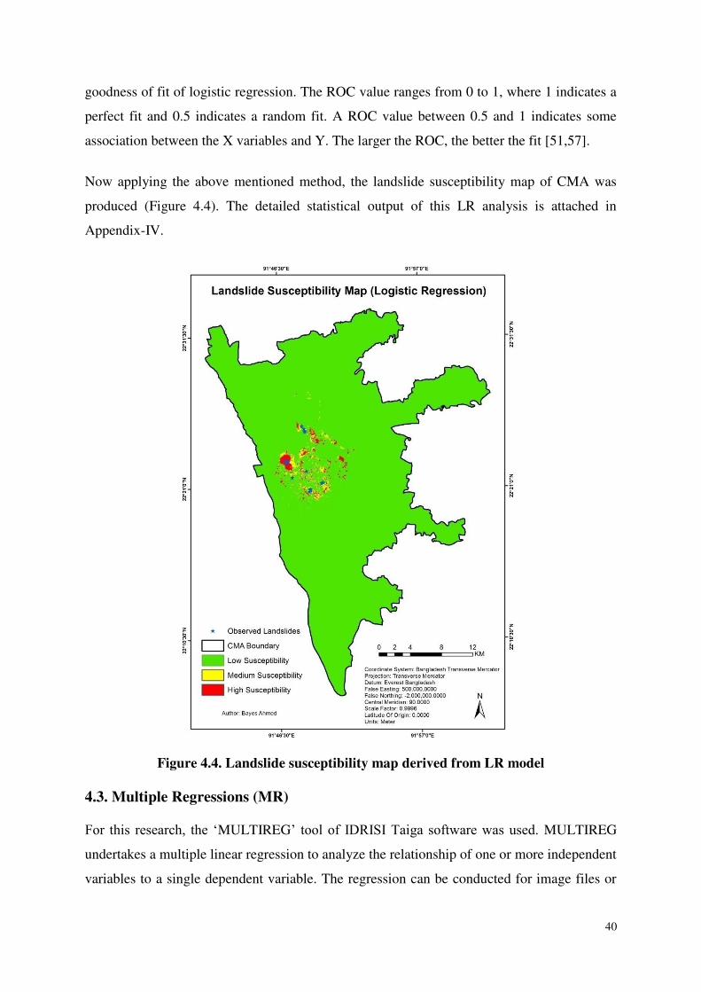
Now applying the above mentioned method, the landslide susceptibility map of CMA was
produced (Figure 4.4). The detailed statistical output of this LR analysis is attached in
Appendix-IV.
Figure 4.4. Landslide susceptibility map derived from LR model
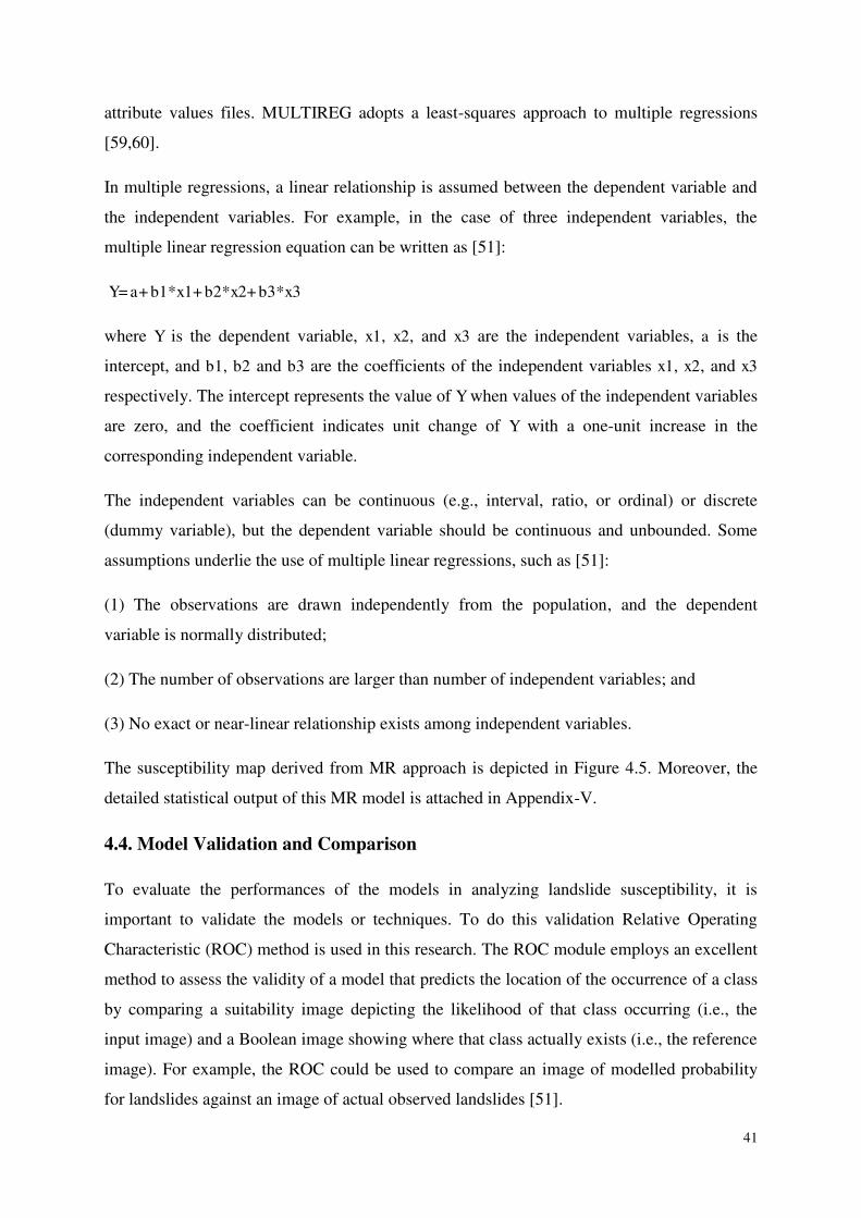
4.3. Multiple Regressions (MR)
For this research, the ‗MULTIREG‘ tool of IDRISI Taiga software was used. MULTIREG
undertakes a multiple linear regression to analyze the relationship of one or more independent
variables to a single dependent variable. The regression can be conducted for image files or
41
attribute values files. MULTIREG adopts a least-squares approach to multiple regressions
[59,60].
In multiple regressions, a linear relationship is assumed between the dependent variable and
the independent variables. For example, in the case of three independent variables, the
multiple linear regression equation can be written as [51]:
Y= a+ b1*x1+ b2*x2+ b3*x3
where Y is the dependent variable, x1, x2, and x3 are the independent variables, a is the
intercept, and b1, b2 and b3 are the coefficients of the independent variables x1, x2, and x3
respectively. The intercept represents the value of Y when values of the independent variables
are zero, and the coefficient indicates unit change of Y with a one-unit increase in the
corresponding independent variable.
The independent variables can be continuous (e.g., interval, ratio, or ordinal) or discrete
(dummy variable), but the dependent variable should be continuous and unbounded. Some
assumptions underlie the use of multiple linear regressions, such as [51]:
(1) The observations are drawn independently from the population, and the dependent
variable is normally distributed;
(2) The number of observations are larger than number of independent variables; and
(3) No exact or near-linear relationship exists among independent variables.
The susceptibility map derived from MR approach is depicted in Figure 4.5. Moreover, the
detailed statistical output of this MR model is attached in Appendix-V.
4.4. Model Validation and Comparison
To evaluate the performances of the models in analyzing landslide susceptibility, it is
important to validate the models or techniques. To do this validation Relative Operating
Characteristic (ROC) method is used in this research. The ROC module employs an excellent
method to assess the validity of a model that predicts the location of the occurrence of a class
by comparing a suitability image depicting the likelihood of that class occurring (i.e., the
input image) and a Boolean image showing where that class actually exists (i.e., the reference
image). For example, the ROC could be used to compare an image of modelled probability
for landslides against an image of actual observed landslides [51].

42
Figure 4.5. Landslide susceptibility map derived from MR model
The ROC module offers a statistical analysis that answers one important question: "How well
is the category of interest concentrated at the locations of relatively high suitability for that
category?" The answer to this question allows the scientist to answer the general question,
"How well do the pair of maps agree in terms of the location of cells in a category?" while
not being forced to answer the question "How well do the pair of maps agree in terms of the
quantity of cells in each category?" Thus the ROC analysis is useful for cases in which the
scientist wants to see how well the suitability map portrays the location of a particular
category but does not have an estimate of the quantity of the category [51].
43
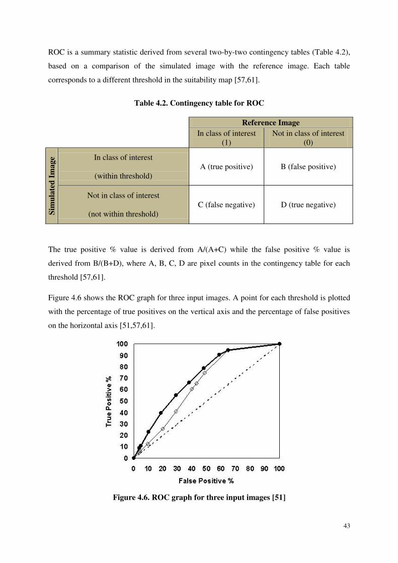
ROC is a summary statistic derived from several two-by-two contingency tables (Table 4.2),
based on a comparison of the simulated image with the reference image. Each table
corresponds to a different threshold in the suitability map [57,61].
Table 4.2. Contingency table for ROC
Reference Image
In class of interest
(1) Not in class of interest
(0)
Sim
ula
ted
Im
age In class of interest
(within threshold) A (true positive) B (false positive)
Not in class of interest
(not within threshold) C (false negative) D (true negative)
The true positive % value is derived from A/(A+C) while the false positive % value is
derived from B/(B+D), where A, B, C, D are pixel counts in the contingency table for each
threshold [57,61].
Figure 4.6 shows the ROC graph for three input images. A point for each threshold is plotted
with the percentage of true positives on the vertical axis and the percentage of false positives
on the horizontal axis [51,57,61].
Figure 4.6. ROC graph for three input images [51]
44
The ROC statistic is the area under the curve that connects the plotted points. IDRISI uses the
trapezoidal rule from integral calculus to compute the area, where xi is the rate of false
positives for threshold i, yi is the rate of true positives for threshold i, and n+1 is the number
of thresholds [57,61].
The dashed diagonal line derives (Figure 4.6) from an input image in which the locations of
the image values were assigned at random (AUC=0.50). The other two lines derive from
different models. The model that produced the thin line with open squares (AUC=0.65) is
shown to be performing more poorly than the model that produced the thin line with closed
circles (AUC=0.70).
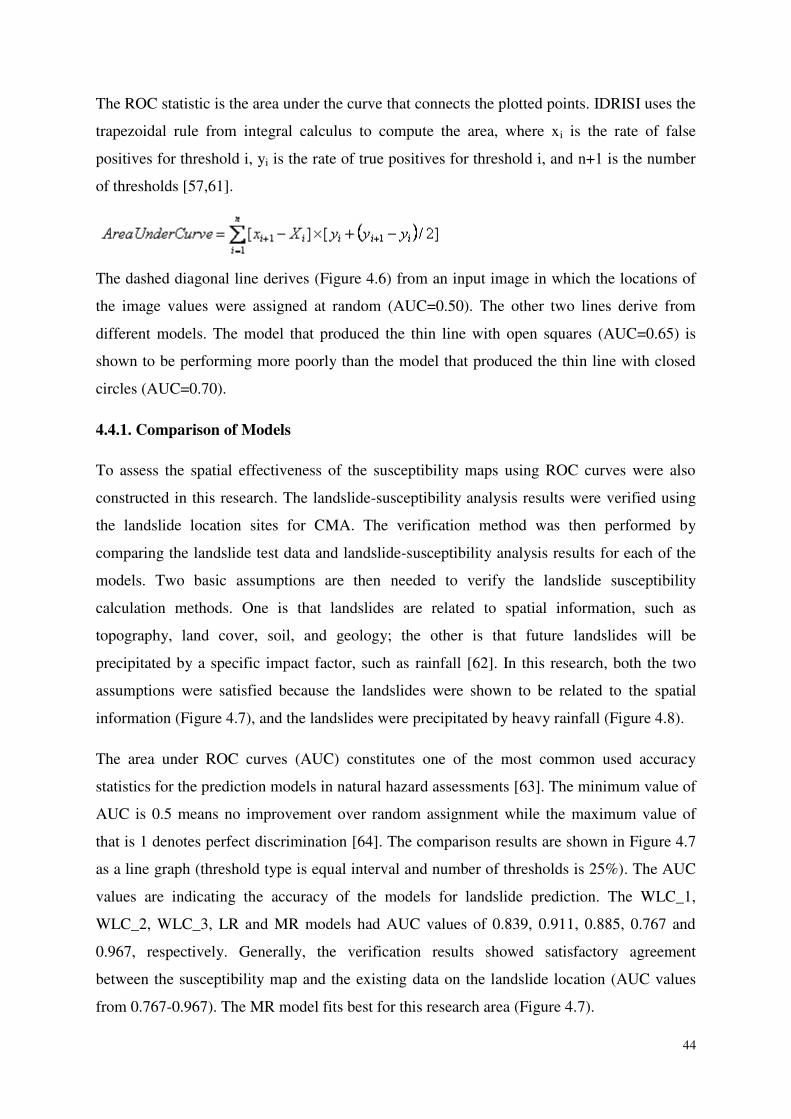
4.4.1. Comparison of Models
To assess the spatial effectiveness of the susceptibility maps using ROC curves were also
constructed in this research. The landslide-susceptibility analysis results were verified using
the landslide location sites for CMA. The verification method was then performed by
comparing the landslide test data and landslide-susceptibility analysis results for each of the
models. Two basic assumptions are then needed to verify the landslide susceptibility
calculation methods. One is that landslides are related to spatial information, such as
topography, land cover, soil, and geology; the other is that future landslides will be
precipitated by a specific impact factor, such as rainfall [62]. In this research, both the two
assumptions were satisfied because the landslides were shown to be related to the spatial
information (Figure 4.7), and the landslides were precipitated by heavy rainfall (Figure 4.8).
The area under ROC curves (AUC) constitutes one of the most common used accuracy
statistics for the prediction models in natural hazard assessments [63]. The minimum value of
AUC is 0.5 means no improvement over random assignment while the maximum value of
that is 1 denotes perfect discrimination [64]. The comparison results are shown in Figure 4.7
as a line graph (threshold type is equal interval and number of thresholds is 25%). The AUC
values are indicating the accuracy of the models for landslide prediction. The WLC_1,
WLC_2, WLC_3, LR and MR models had AUC values of 0.839, 0.911, 0.885, 0.767 and
0.967, respectively. Generally, the verification results showed satisfactory agreement
between the susceptibility map and the existing data on the landslide location (AUC values
from 0.767-0.967). The MR model fits best for this research area (Figure 4.7).
45
Figure 4.7. Assessment of the model performance based on the ROC curves
The detailed statistics of the ROC results for all the models are attached in Appendix VI.
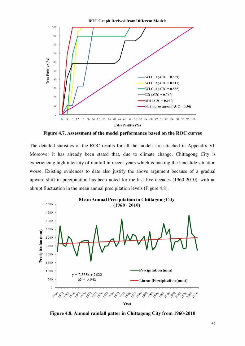
Moreover it has already been stated that, due to climate change, Chittagong City is
experiencing high intensity of rainfall in recent years which is making the landslide situation
worse. Existing evidences to date also justify the above argument because of a gradual
upward shift in precipitation has been noted for the last five decades (1960-2010), with an
abrupt fluctuation in the mean annual precipitation levels (Figure 4.8).
Figure 4.8. Annual rainfall patter in Chittagong City from 1960-2010
46
Chapter 5
GEOTECHNICAL ISSUES
5.1. Geotechnical Causes of Landslides
Many approaches for classifying landslide have been introduced by many resource persons
and institutions. Almost all the soils are clayey in test samples. Amount of clay in any type of
soil has a strong contribution in landslide occurrence. The greater the amount of clay in soil
the lesser the drainage means soil cannot drain out water properly. Therefore the remaining
water in clayey soils increase pore water pressure by losing effective strength and finally
trigger landslides. Shear strength of soil is a function of different parameters like natural
water content, ground water level, cohesion, particle size, Atterberg indexes, permeability
etc. In this paper only those parameters have been considered whose are responsible for water
triggering landslides. As different parameters of soil are responsible for landslide so a brief of
its type, strength and component has been described here.
5.2. Soil
5.2.1. Definition
Soil is an important element of earth without which we can‘t think our existence in the world.
From the inception of the earth different types of soil has furnished the world with many
shapes. This clearly indicates the different types and formation process of soil.
5.2.2. Component of Soil
Atoms Oxygen, Silicon, Hydrogen organized in various crystalline forms along with calcium,
sodium, potassium, magnesium, and carbon constitute over 99 percent of the solid mass of
soils. It also contains air void and water in small portion.
5.2.3. Types of Soil
If we see around we could find two things which are rock and soil. Rock is considered to be
the natural aggregate of mineral grains with strong binding materials (cohesive force) that
tied the rock forming elements together. In the other hand soil is the aggregate of minerals
with relatively low cohesive force and binding materials among the elements. Upon the
presence of organic matter the soils are termed as inorganic or organic soil.

47
In engineering perspective soils mainly classified in two groups that are coarse grain and fine
grain soil. Coarse soils are subdivided into sand and gravel where fine soils are subdivided
into clay and silt.
These two basic types of inorganic soils are formed due to the weathering of rock. Coarse
grained soil is formed by the physical weathering of rock whereas the fine grained is formed
by chemical weathering process. The basic difference of these two types‘ soils arises because
of the variation of size and shape of the soil particles. Smaller fine grained soils are often
called cohesive soil as they influenced by physiochemical interactions resulting plastic
deformation in different moisture content. Coarse grained soils are cohesion less soils
dominated by the physical characteristics of the particles.
The common clay minerals are montmorillonite or smectite, illite, and kaolinite or kaolin.
These minerals tend to form in sheet or plate like structures, with length typically ranging
between 10−7 m and 4x10⁻⁶ m and thickness typically ranging between 10−9 m and 2x10⁻⁶
m, and they have a relatively large specific surface area. The specific surface area (SSA) is
defined as the ratio of the surface area of particles to the mass of the particles. Clay minerals
typically have specific surface areas in the range of 10 to 1,000 square meters per gram of
solid. Due to the large surface area available for chemical, electrostatic, and van der Waals
interaction, the mechanical behaviour of clay minerals is very sensitive to the amount of pore
fluid available and the type and amount of dissolved ions in the pore fluid.
5.2.4. Strength of Soils
Soils are subjected to normal and shear stress in every geotechnical aspects (e.g. - slope
stability, foundation engineering, retaining wall, dam, and embankment). Shear strength and
stiffness of soils denotes the stability of soils or its deformation due to stress. Soil strengths
are the contribution of interlocking angles, frictional resistance, cohesion, minerals as well as
type of the soil. Shear strength enables soil to remain its equilibrium when the surface is not
horizontal. Therefore knowledge of the strength is necessary to determine if a slope will be
stable.
5.2.5. Indicating Parameters of Soil Strength
It is important to know the strength of soil prior to any modification or development of the
soil. Various tests are being performed to know the strength of soils. In this research different
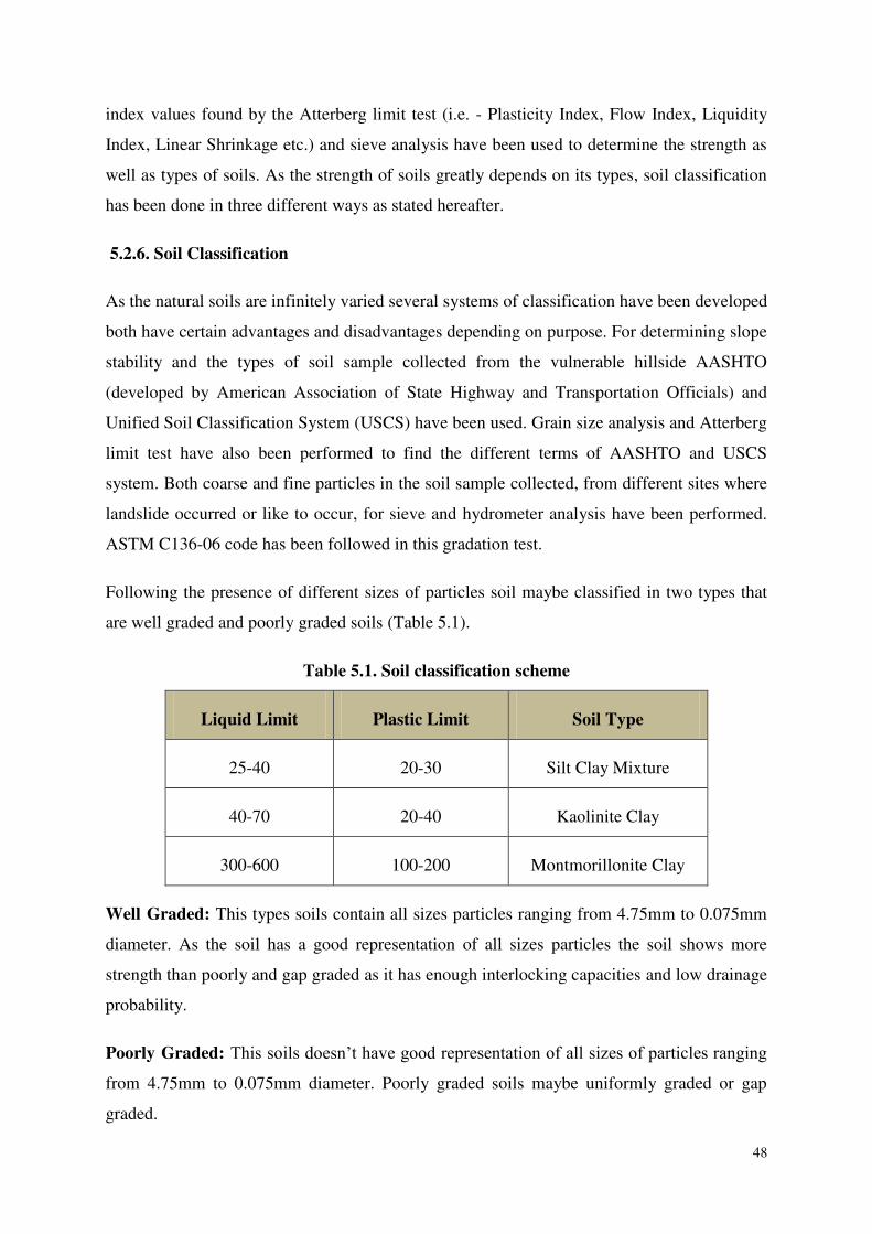
48
index values found by the Atterberg limit test (i.e. - Plasticity Index, Flow Index, Liquidity
Index, Linear Shrinkage etc.) and sieve analysis have been used to determine the strength as
well as types of soils. As the strength of soils greatly depends on its types, soil classification
has been done in three different ways as stated hereafter.
5.2.6. Soil Classification
As the natural soils are infinitely varied several systems of classification have been developed
both have certain advantages and disadvantages depending on purpose. For determining slope
stability and the types of soil sample collected from the vulnerable hillside AASHTO
(developed by American Association of State Highway and Transportation Officials) and
Unified Soil Classification System (USCS) have been used. Grain size analysis and Atterberg
limit test have also been performed to find the different terms of AASHTO and USCS
system. Both coarse and fine particles in the soil sample collected, from different sites where
landslide occurred or like to occur, for sieve and hydrometer analysis have been performed.
ASTM C136-06 code has been followed in this gradation test.
Following the presence of different sizes of particles soil maybe classified in two types that
are well graded and poorly graded soils (Table 5.1).
Table 5.1. Soil classification scheme
Liquid Limit Plastic Limit Soil Type
25-40 20-30 Silt Clay Mixture
40-70 20-40 Kaolinite Clay
300-600 100-200 Montmorillonite Clay
Well Graded: This types soils contain all sizes particles ranging from 4.75mm to 0.075mm
diameter. As the soil has a good representation of all sizes particles the soil shows more
strength than poorly and gap graded as it has enough interlocking capacities and low drainage
probability.
Poorly Graded: This soils doesn‘t have good representation of all sizes of particles ranging
from 4.75mm to 0.075mm diameter. Poorly graded soils maybe uniformly graded or gap
graded.
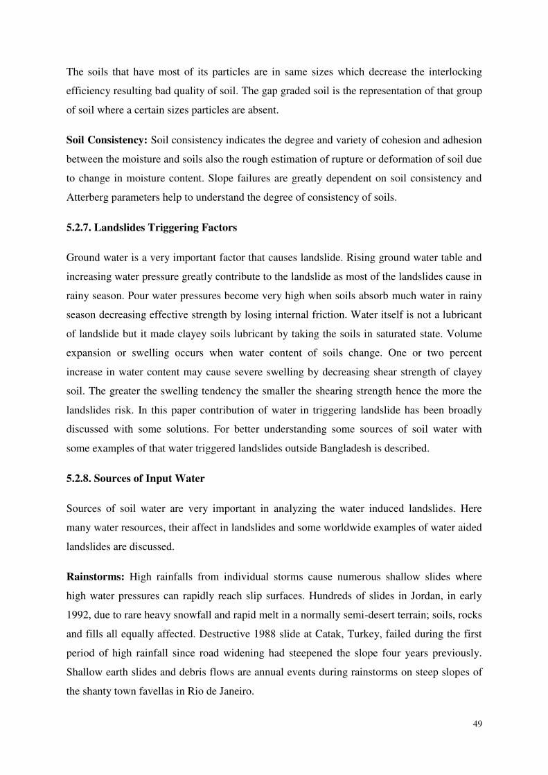
49
The soils that have most of its particles are in same sizes which decrease the interlocking
efficiency resulting bad quality of soil. The gap graded soil is the representation of that group
of soil where a certain sizes particles are absent.
Soil Consistency: Soil consistency indicates the degree and variety of cohesion and adhesion
between the moisture and soils also the rough estimation of rupture or deformation of soil due
to change in moisture content. Slope failures are greatly dependent on soil consistency and
Atterberg parameters help to understand the degree of consistency of soils.
5.2.7. Landslides Triggering Factors
Ground water is a very important factor that causes landslide. Rising ground water table and
increasing water pressure greatly contribute to the landslide as most of the landslides cause in
rainy season. Pour water pressures become very high when soils absorb much water in rainy
season decreasing effective strength by losing internal friction. Water itself is not a lubricant
of landslide but it made clayey soils lubricant by taking the soils in saturated state. Volume
expansion or swelling occurs when water content of soils change. One or two percent
increase in water content may cause severe swelling by decreasing shear strength of clayey
soil. The greater the swelling tendency the smaller the shearing strength hence the more the
landslides risk. In this paper contribution of water in triggering landslide has been broadly
discussed with some solutions. For better understanding some sources of soil water with
some examples of that water triggered landslides outside Bangladesh is described.
5.2.8. Sources of Input Water
Sources of soil water are very important in analyzing the water induced landslides. Here
many water resources, their affect in landslides and some worldwide examples of water aided
landslides are discussed.
Rainstorms: High rainfalls from individual storms cause numerous shallow slides where
high water pressures can rapidly reach slip surfaces. Hundreds of slides in Jordan, in early
1992, due to rare heavy snowfall and rapid melt in a normally semi-desert terrain; soils, rocks
and fills all equally affected. Destructive 1988 slide at Catak, Turkey, failed during the first
period of high rainfall since road widening had steepened the slope four years previously.
Shallow earth slides and debris flows are annual events during rainstorms on steep slopes of
the shanty town favellas in Rio de Janeiro.
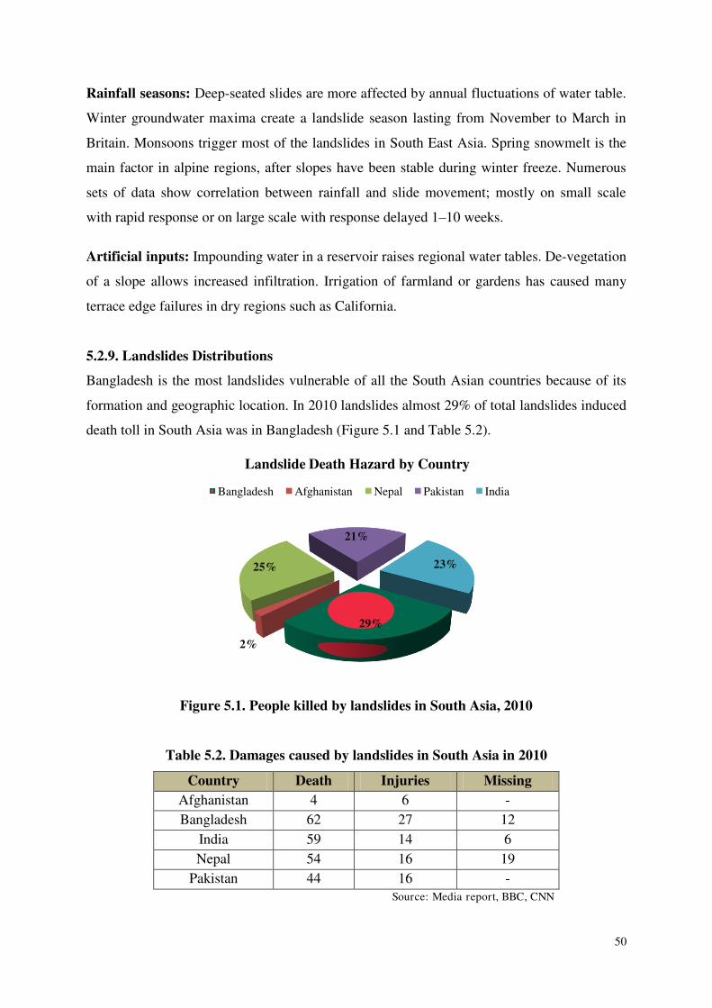
50
Rainfall seasons: Deep-seated slides are more affected by annual fluctuations of water table.
Winter groundwater maxima create a landslide season lasting from November to March in
Britain. Monsoons trigger most of the landslides in South East Asia. Spring snowmelt is the
main factor in alpine regions, after slopes have been stable during winter freeze. Numerous
sets of data show correlation between rainfall and slide movement; mostly on small scale
with rapid response or on large scale with response delayed 1–10 weeks.
Artificial inputs: Impounding water in a reservoir raises regional water tables. De-vegetation
of a slope allows increased infiltration. Irrigation of farmland or gardens has caused many
terrace edge failures in dry regions such as California.
5.2.9. Landslides Distributions
Bangladesh is the most landslides vulnerable of all the South Asian countries because of its
formation and geographic location. In 2010 landslides almost 29% of total landslides induced
death toll in South Asia was in Bangladesh (Figure 5.1 and Table 5.2).
Figure 5.1. People killed by landslides in South Asia, 2010
Table 5.2. Damages caused by landslides in South Asia in 2010
Country Death Injuries Missing
Afghanistan 4 6 -
Bangladesh 62 27 12
India 59 14 6
Nepal 54 16 19
Pakistan 44 16 -
Source: Media report, BBC, CNN
29%
2%
25%
21%
23%
Landslide Death Hazard by Country
Bangladesh Afghanistan Nepal Pakistan India
51
5.2.10. General Causative Factors of Landslides
Rainfall: From statistics it has been found that most of the landslide occurred during the
rainy season which indicates the strong relation between landslide and rainfall. In one single
event in 2011, about 90 people were killed by landslide triggered by heavy rainfall in port
city Chittagong. In rainy season people living beside hill pass their every moment in anxiety.
Many researchers have published many research papers where they showed strong
relationship between landslide and rainfall. Neil Caine of Institute of Arctic and Alpine
Research, University of Colorado, USA, mentioned the relation between rainfall and
landslide in 1980 by the following equation:
I = 14.83* D-0.39
Where I = Rainfall intensity in mm/hr
D = Duration of rainfall in hours
We can estimate the threshold rainfall intensity for 24 hours that can create landslide.
Landslide occurs for duration of less than 12 hours at 6mm/hr intensity but the rainfall
continues for more than 100 hours then 2mm/hr intensity is enough to cause landslide. If
precipitation continued for 1 month then 1mm/hr precipitation intensity is more than enough
for triggering landslide in that condition landslide may occur anytime at any intensity [58].
Earthquake: Frequent earthquake impart shearing stress also reduce the resistance of slope
materials hence slopes become unstable. The greater the steepness of slopes is the greater the
degree of amplifications of intensity of earthquake. As Chittagong lies in the low seismic
danger zone it doesn‘t have great influence in Chittagong landslide.
Water Level Change: When water level falls drastically then the pore water pressure
dissipates imparting instability of slope. Detailed analysis of this term is presented in the case
study pages.
Artificial Reasons: These include-
- Changing landcover
- Agricultural practice on steep slope
- Housing
- Water reservoir which increase pore water pressure decreasing effective pressure of soil
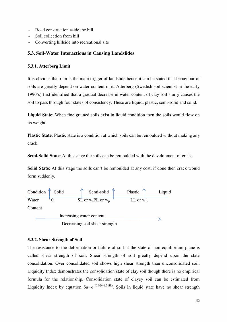
52
- Road construction aside the hill
- Soil collection from hill
- Converting hillside into recreational site
5.3. Soil-Water Interactions in Causing Landslides
5.3.1. Atterberg Limit
It is obvious that rain is the main trigger of landslide hence it can be stated that behaviour of
soils are greatly depend on water content in it. Atterberg (Swedish soil scientist in the early
1990‘s) first identified that a gradual decrease in water content of clay soil slurry causes the
soil to pass through four states of consistency. These are liquid, plastic, semi-solid and solid.
Liquid State: When fine grained soils exist in liquid condition then the soils would flow on
its weight.
Plastic State: Plastic state is a condition at which soils can be remoulded without making any
crack.
Semi-Solid State: At this stage the soils can be remoulded with the development of crack.
Solid State: At this stage the soils can‘t be remoulded at any cost, if done then crack would
form suddenly.
Condition Solid Semi-solid Plastic Liquid
Water 0 SL or wsPL or wp LL or wL
Content
Increasing water content
Decreasing soil shear strength
5.3.2. Shear Strength of Soil
The resistance to the deformation or failure of soil at the state of non-equilibrium plane is
called shear strength of soil. Shear strength of soil greatly depend upon the state
consolidation. Over consolidated soil shows high shear strength than unconsolidated soil.
Liquidity Index demonstrates the consolidation state of clay soil though there is no empirical
formula for the relationship. Consolidation state of clayey soil can be estimated from
Liquidity Index by equation Su= e (0.026-1.21IL). Soils in liquid state have no shear strength
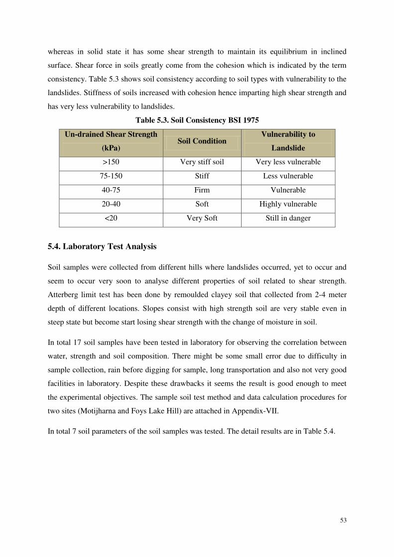
53
whereas in solid state it has some shear strength to maintain its equilibrium in inclined
surface. Shear force in soils greatly come from the cohesion which is indicated by the term
consistency. Table 5.3 shows soil consistency according to soil types with vulnerability to the
landslides. Stiffness of soils increased with cohesion hence imparting high shear strength and
has very less vulnerability to landslides.
Table 5.3. Soil Consistency BSI 1975
Un-drained Shear Strength
(kPa) Soil Condition
Vulnerability to
Landslide
>150 Very stiff soil Very less vulnerable
75-150 Stiff Less vulnerable
40-75 Firm Vulnerable
20-40 Soft Highly vulnerable
<20 Very Soft Still in danger
5.4. Laboratory Test Analysis
Soil samples were collected from different hills where landslides occurred, yet to occur and
seem to occur very soon to analyse different properties of soil related to shear strength.
Atterberg limit test has been done by remoulded clayey soil that collected from 2-4 meter
depth of different locations. Slopes consist with high strength soil are very stable even in
steep state but become start losing shear strength with the change of moisture in soil.
In total 17 soil samples have been tested in laboratory for observing the correlation between
water, strength and soil composition. There might be some small error due to difficulty in
sample collection, rain before digging for sample, long transportation and also not very good
facilities in laboratory. Despite these drawbacks it seems the result is good enough to meet
the experimental objectives. The sample soil test method and data calculation procedures for
two sites (Motijharna and Foys Lake Hill) are attached in Appendix-VII.
In total 7 soil parameters of the soil samples was tested. The detail results are in Table 5.4.
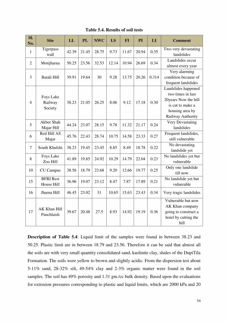
54
Table 5.4. Results of soil tests
Sl.
No. Site LL PL NWC LS FI PI LI Comment
1 Tigerpass
wall 42.39 21.45 28.75 9.73 11.67 20.94 0.35
Two very devastating
landslides
2 Motijharna 50.25 23.56 32.53 12.14 10.94 26.69 0.34 Landslides occur
almost every year
3 Batali Hill 39.91 19.64 30 9.28 13.75 20.26 0.314
Very alarming
condition because of
frequent landslides
4
Foys Lake
Railway
Society
38.23 21.05 26.25 8.06 9.12 17.18 0.30
Landslides happened
two times in last
20years Now the hill
is cut to make a
housing area by
Railway Authority
5 Akber Shah
Majar Hill 44.24 23.07 28.15 9.78 11.32 21.17 0.24
Very Devastating
landslides
6 Red Hill AS
Majar 45.76 22.43 28.74 10.75 14.58 23.33 0.27
Frequent landslides,
still vulnerable
7 South Khulshi 38.23 19.45 23.45 8.85 8.49 18.78 0.22 No devastating
landslide yet
8 Foys Lake
Zoo Hill 41.89 19.85 24.92 10.29 14.79 22.04 0.23
No landslides yet but
vulnerable
10 CU Campus 38.56 18.79 23.68 9.20 12.66 19.77 0.25 Only one landslide
till now
15 BFRI Rest
House Hill 36.96 19.07 23.12 8.47 7.87 17.89 0.21
No landslide yet but
vulnerable
16 Jharna Hill 46.45 23.02 31 10.65 15.63 23.43 0.34 Very tragic landslides
17 AK Khan Hill
Panchlaish 39.67 20.48 27.5 8.93 14.92 19.19 0.36
Vulnerable but now
AK Khan company
going to construct a
hotel by cutting the
hill
Description of Table 5.4: Liquid limit of the samples were found in between 38.23 and
50.25. Plastic limit are in between 18.79 and 23.56. Therefore it can be said that almost all
the soils are with very small quantity consolidated sand, kaolinite clay, shales of the DupiTila
Formation. The soils were yellow to brown and slightly acidic. From the dispersion test about
5-11% sand, 28-32% silt, 49-54% clay and 2-3% organic matter were found in the soil
samples. The soil has 49% porosity and 1.31 gm./cc bulk density. Based upon the evaluations
for extrusion pressures corresponding to plastic and liquid limits, which are 2000 kPa and 20
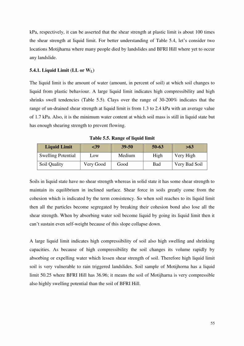
55
kPa, respectively, it can be asserted that the shear strength at plastic limit is about 100 times
the shear strength at liquid limit. For better understanding of Table 5.4, let‘s consider two
locations Motijharna where many people died by landslides and BFRI Hill where yet to occur
any landslide.
5.4.1. Liquid Limit (LL or WL)
The liquid limit is the amount of water (amount, in percent of soil) at which soil changes to
liquid from plastic behaviour. A large liquid limit indicates high compressibility and high
shrinks swell tendencies (Table 5.5). Clays over the range of 30-200% indicates that the
range of un-drained shear strength at liquid limit is from 1.3 to 2.4 kPa with an average value
of 1.7 kPa. Also, it is the minimum water content at which soil mass is still in liquid state but
has enough shearing strength to prevent flowing.
Table 5.5. Range of liquid limit
Liquid Limit <39 39-50 50-63 >63
Swelling Potential Low Medium High Very High
Soil Quality Very Good Good Bad Very Bad Soil
Soils in liquid state have no shear strength whereas in solid state it has some shear strength to
maintain its equilibrium in inclined surface. Shear force in soils greatly come from the
cohesion which is indicated by the term consistency. So when soil reaches to its liquid limit
then all the particles become segregated by breaking their cohesion bond also lose all the
shear strength. When by absorbing water soil become liquid by going its liquid limit then it
can‘t sustain even self-weight because of this slope collapse down.
A large liquid limit indicates high compressibility of soil also high swelling and shrinking
capacities. As because of high compressibility the soil changes its volume rapidly by
absorbing or expelling water which lessen shear strength of soil. Therefore high liquid limit
soil is very vulnerable to rain triggered landslides. Soil sample of Motijhorna has a liquid
limit 50.25 where BFRI Hill has 36.96; it means the soil of Motijharna is very compressible
also highly swelling potential than the soil of BFRI Hill.
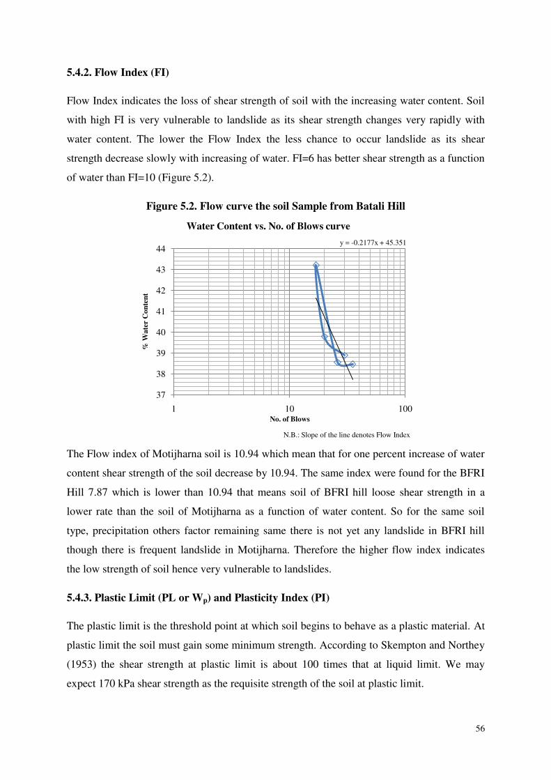
56
5.4.2. Flow Index (FI)
Flow Index indicates the loss of shear strength of soil with the increasing water content. Soil
with high FI is very vulnerable to landslide as its shear strength changes very rapidly with
water content. The lower the Flow Index the less chance to occur landslide as its shear
strength decrease slowly with increasing of water. FI=6 has better shear strength as a function
of water than FI=10 (Figure 5.2).
Figure 5.2. Flow curve the soil Sample from Batali Hill
The Flow index of Motijharna soil is 10.94 which mean that for one percent increase of water
content shear strength of the soil decrease by 10.94. The same index were found for the BFRI
Hill 7.87 which is lower than 10.94 that means soil of BFRI hill loose shear strength in a
lower rate than the soil of Motijharna as a function of water content. So for the same soil
type, precipitation others factor remaining same there is not yet any landslide in BFRI hill
though there is frequent landslide in Motijharna. Therefore the higher flow index indicates
the low strength of soil hence very vulnerable to landslides.
5.4.3. Plastic Limit (PL or Wp) and Plasticity Index (PI)
The plastic limit is the threshold point at which soil begins to behave as a plastic material. At
plastic limit the soil must gain some minimum strength. According to Skempton and Northey
(1953) the shear strength at plastic limit is about 100 times that at liquid limit. We may
expect 170 kPa shear strength as the requisite strength of the soil at plastic limit.
y = -0.2177x + 45.351
37
38
39
40
41
42
43
44
1 10 100
% W
ate
r C
on
ten
t
No. of Blows
Water Content vs. No. of Blows curve
N.B.: Slope of the line denotes Flow Index
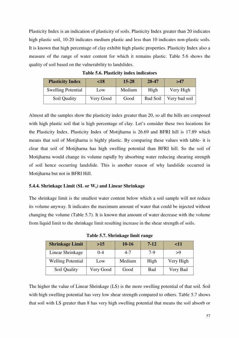
57
Plasticity Index is an indication of plasticity of soils. Plasticity Index greater than 20 indicates
high plastic soil, 10-20 indicates medium plastic and less than 10 indicates non-plastic soils.
It is known that high percentage of clay exhibit high plastic properties. Plasticity Index also a
measure of the range of water content for which it remains plastic. Table 5.6 shows the
quality of soil based on the vulnerability to landslides.
Table 5.6. Plasticity index indicators
Plasticity Index <18 15-28 28-47 >47
Swelling Potential Low Medium High Very High
Soil Quality Very Good Good Bad Soil Very bad soil
Almost all the samples show the plasticity index greater than 20, so all the hills are composed
with high plastic soil that is high percentage of clay. Let‘s consider these two locations for
the Plasticity Index. Plasticity Index of Motijharna is 26.69 and BFRI hill is 17.89 which
means that soil of Motijharna is highly plastic. By comparing these values with table- it is
clear that soil of Motijharna has high swelling potential than BFRI hill. So the soil of
Motijharna would change its volume rapidly by absorbing water reducing shearing strength
of soil hence occurring landslide. This is another reason of why landslide occurred in
Motijharna but not in BFRI Hill.
5.4.4. Shrinkage Limit (SL or Ws) and Linear Shrinkage
The shrinkage limit is the smallest water content below which a soil sample will not reduce
its volume anyway. It indicates the maximum amount of water that could be injected without
changing the volume (Table 5.7). It is known that amount of water decrease with the volume
from liquid limit to the shrinkage limit resulting increase in the shear strength of soils.
Table 5.7. Shrinkage limit range
Shrinkage Limit >15 10-16 7-12 <11
Linear Shrinkage 0-4 4-7 7-9 >9
Welling Potential Low Medium High Very High
Soil Quality Very Good Good Bad Very Bad
The higher the value of Linear Shrinkage (LS) is the more swelling potential of that soil. Soil
with high swelling potential has very low shear strength compared to others. Table 5.7 shows
that soil with LS greater than 8 has very high swelling potential that means the soil absorb or
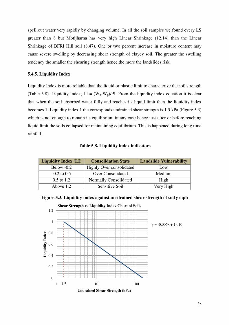
58
spell out water very rapidly by changing volume. In all the soil samples we found every LS
greater than 8 but Motijharna has very high Linear Shrinkage (12.14) than the Linear
Shrinkage of BFRI Hill soil (8.47). One or two percent increase in moisture content may
cause severe swelling by decreasing shear strength of clayey soil. The greater the swelling
tendency the smaller the shearing strength hence the more the landslides risk.
5.4.5. Liquidity Index
Liquidity Index is more reliable than the liquid or plastic limit to characterize the soil strength
(Table 5.8). Liquidity Index, LI = (Wn-Wp)/PI. From the liquidity index equation it is clear
that when the soil absorbed water fully and reaches its liquid limit then the liquidity index
becomes 1. Liquidity index 1 the corresponds undrained shear strength is 1.5 kPa (Figure 5.3)
which is not enough to remain its equilibrium in any case hence just after or before reaching
liquid limit the soils collapsed for maintaining equilibrium. This is happened during long time
rainfall.
Table 5.8. Liquidity index indicators
Figure 5.3. Liquidity index against un-drained shear strength of soil graph
y = -0.006x + 1.010
0
0.2
0.4
0.6
0.8
1
1.2
1 10 100
Liq
uid
ity
In
dex
Undrained Shear Strength (kPa)
Shear Strength vs Liquidity Index Chart of Soils
1.5
Liquidity Index (LI) Consolidation State Landslide Vulnerability
Below -0.2 Highly Over consolidated Low
-0.2 to 0.5 Over Consolidated Medium
0.5 to 1.2 Normally Consolidated High
Above 1.2 Sensitive Soil Very High
59
If LI is 1 then the soil in its liquid limit with un-drained shear strength of 1.5kPa and if the
value of LI becomes zero then the soil is said to be in its plastic limit with un-drained shear
strength of 150kPa. Most soil deposits show the liquidity index in between 0 to 1. Liquidity
Index provides a reliable indication of the degrees of consolidation of clayey soils. IL is zero
for over consolidated soil and IL is negative for highly over consolidated soil.
From Table 5.4 it is found that Liquidity Index of Motijhorna soil is 0.34 and for BFRI hill
the index value is 0.21. This means soil of Motijharna has lower shear strength than soil of
BFRI hill. For the same intensity precipitation the soil of Motijhorna would reach to its liquid
limit very faster than the soil of BFRI Hill. This is another reason for the landslide in
Motijhorna than the BFRI Hill.
5.5. Causes of Water Induced Landslides from Experiment
From the experiment with the soils that collected from landslides prone areas, several causes
for water induced landslides have been identified as the description stated above. Hills
composed of the soils that have following properties are very vulnerable to landslide in
moderate long precipitation in rainy season.
1. High Liquidity
2. High Flow Index
3. High Plasticity Index
4. High percentage of clay
5. High Liquidity Index
6. High Liner Shrinkage
7. Soil surface directly expose to air
8. High Ground Water Level
9. Low drainage capacity of soil
10. Disturbed soil
11. Soil Particle Size Distribution

60
5.6. Some Engineering and Technological Solutions for Landslides
Now in Bangladesh the only technology which is used to stable slope is Retaining wall.
Constructing and maintaining retaining wall is very costly also recent failures of retaining
wall prove its insufficiency in withstanding soil pressure. Therefore we need to explore new
affordable and sustainable technology to stable hill slopes.
5.6.1. Landslides Susceptibility Maps
From above discussion it is clear that soil properties have much more effect in causing
landslides than other parameters like land cover and surroundings. Therefore landslide
susceptibility maps should be prepared in such a way that the maps include all the
geotechnical parameters with the physical parameters of the landslide vulnerable areas. While
identifying and categorizing landslide prone areas these parameters might help to identify
more correctly and precisely.
5.6.2. Wire Mesh
Figure 5.4. Roadside Slope Stabilization by wire mesh (Source: ROTEC Intl, USA)
In unstable slope wire mesh covering is a sustainable solution for landslide risk. Wire mesh
stabilize risky slope by imparting shear strength in the soils. This would be very useful for
protecting road networks passing through the hill in hilly region from landslide destructions.
Many countries have already been started this technology to stabilize roadside slope which
could protect huge landslides brought damages. Depending on landslide susceptibility maps
produces base on soil properties different sizes wire net would be designed by civil engineer.
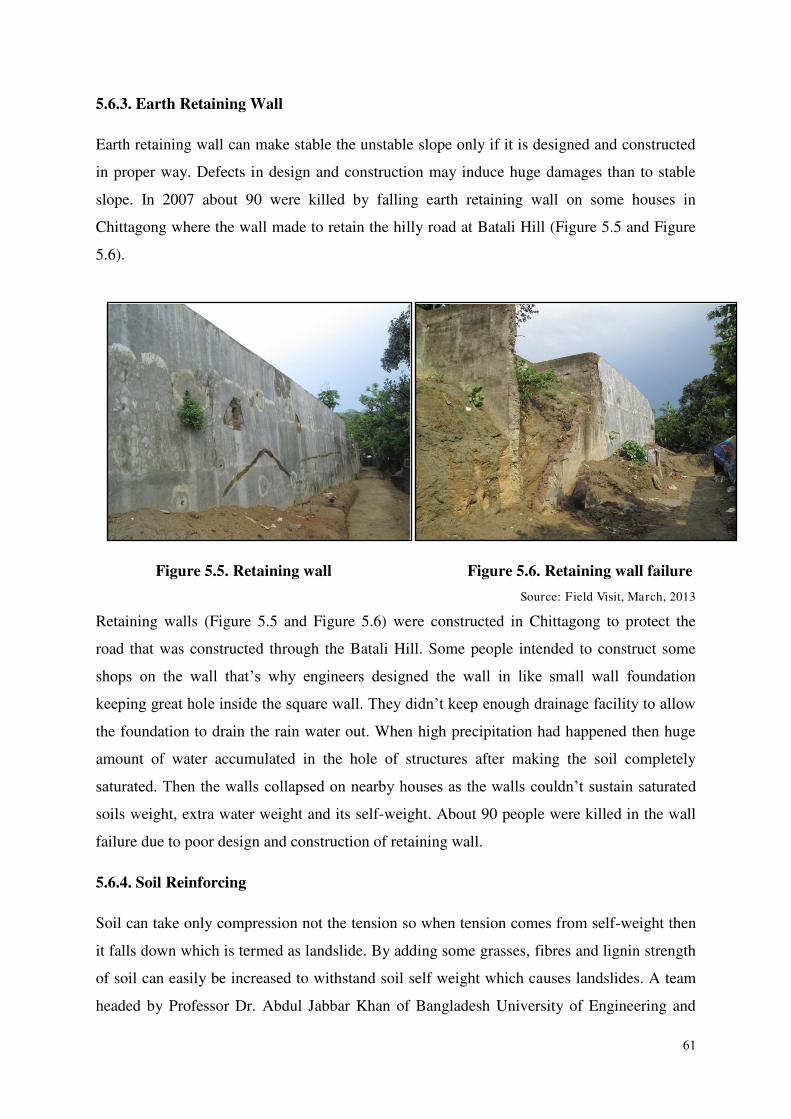
61
5.6.3. Earth Retaining Wall
Earth retaining wall can make stable the unstable slope only if it is designed and constructed
in proper way. Defects in design and construction may induce huge damages than to stable
slope. In 2007 about 90 were killed by falling earth retaining wall on some houses in
Chittagong where the wall made to retain the hilly road at Batali Hill (Figure 5.5 and Figure
5.6).
Figure 5.5. Retaining wall Figure 5.6. Retaining wall failure
Source: Field Visit, March, 2013
Retaining walls (Figure 5.5 and Figure 5.6) were constructed in Chittagong to protect the
road that was constructed through the Batali Hill. Some people intended to construct some
shops on the wall that‘s why engineers designed the wall in like small wall foundation
keeping great hole inside the square wall. They didn‘t keep enough drainage facility to allow
the foundation to drain the rain water out. When high precipitation had happened then huge
amount of water accumulated in the hole of structures after making the soil completely
saturated. Then the walls collapsed on nearby houses as the walls couldn‘t sustain saturated
soils weight, extra water weight and its self-weight. About 90 people were killed in the wall
failure due to poor design and construction of retaining wall.
5.6.4. Soil Reinforcing
Soil can take only compression not the tension so when tension comes from self-weight then
it falls down which is termed as landslide. By adding some grasses, fibres and lignin strength
of soil can easily be increased to withstand soil self weight which causes landslides. A team
headed by Professor Dr. Abdul Jabbar Khan of Bangladesh University of Engineering and
62
Technology has been trying to use local Jute fibre in reinforcing unstable soils to make them
strength reducing landslides vulnerability. The team has gone so far and likely to publish
their report very soon. The process would be very easy and economically feasible as the
fibres are locally produced and cheap.
5.6.5. Tree Plantation and Vegetation
Land cover type has a great effect on landslides as infiltration is a function of soil type and
land use type. Hill soil directly exposed to rain has high infiltration rate because of low
surface run off. Exposed soil get saturated by water earlier than the soil covered with plants.
Also roots of trees reinforced soil increasing shear strength. So vegetation and planting more
trees in landslides prone hills are the sustainable solutions.
5.6.6. Geotechnical Properties based Landslides Warning System
In developed countries peizometric warning is being used to get a probability of landslide for
a certain precipitation. In USA Emergency Alert System (EAS) is established to alert the
vulnerable people in any emergency case. Existing landslide early alert system is based on
precipitation rate considering the existing water level of soil. If precipitation for a certain
period exceeds the limit then a signal is sent to the central server then the signal dissipated to
the government emergency departments concerning disasters to taka necessary initiatives.
Installation and maintenance of the system is costly also very lengthy. People living in
vulnerable areas don‘t get the instant alarm to go to safe places. As the system is costly
developing countries government have some limitations to install the alarming system.
Considering these drawbacks we propose an economically feasible, user friendly and
effective alarming system.
Considering every possible causes and parameters that trigger landslides a model would be
formed for different landslides prone areas. From the model equation required precipitation to
reach the soils liquid limit would be measured. Simple and low cost rainfall measure
instrument would be installed in every vulnerable area which would also be connected with a
local siren to alert local people. When rainfall pot will be poured to the calibrated water mark
then the siren would sound to alert people for moving into safe place. Geotechnical properties
based Landslide susceptibility maps can help the stakeholders to establish a landslide early
warning system.
The outreach activities are described in Appendix-VIII.

63
Chapter 6
RECOMMENDATIONS AND CONCLUSION
In general, the term ‗Natural Disaster‘ refers to extreme natural events like tsunami,
earthquakes, landslides, floods etc. But it has been argued that these events are not disasters
until a vulnerable group of people is exposed [65]. At this drawback, it is important to
understand the main reasons for this progression of urban landslide vulnerability in
Chittagong Metropolitan Area (CMA). Moreover, even being aware of the landslide risks
people are living in those areas. This situation needs to be analysed.
As discussed earlier, the highly urbanized hilly city like CMA is experiencing more and more
rainfall-induced fatal landslides (RFLs) in recent years. Moreover, the rate of urbanization
and population growth is also increasing quite evidently in these areas. In this situation it is
important to reveal the consequences of landslides in those affected areas. Some major
consequences can be as follows:
a) Loss of life and property
b) Economic instability
c) Lower living standard
d) Degraded social norms and values
e) Political unrest
f) Declining community feelings
g) Fear of becoming landless or losing a job
h) Change in economic activities
i) Environmental threats
Therefore, based on the predicted landslide vulnerable zones and its relations with the
geotechnical issues, some recommendations and ideas for future research are demonstrated.
6.1. Recommendations
6.1.1. To understand human adaptation to landslide risks under the condition of rapid
urbanization in a fast growing city like CMA.
To achieve this goal, it is important to know-
a) Why and how long people are living in this area?
64
b) Why they do not want to leave this risky place?
c) What will be the consequences of leaving this place?
d) What steps the local people are taking to stay here for longer?
e) What are the possible threats or risks living here?
f) How these areas can be planned in a proper way incorporating sustainable
development strategies?
Filed level questionnaire survey can be carried out in this case. Different
questionnaires should be produced to conduct the survey- the inhabitants living in
risky zones, the local community or committee, local political groups, expert
opinion survey and concerned institution or organizations.
6.1.2. To understand the processes and mechanism of landslides in CMA.
The followings steps can be performed to achieve this objective:
i. Landslide classification (using different available schemes)
ii. Landslide dimensions (different widths and lengths)
iii. Landslides activity and its distribution (advancing, enlarging, moving,
widening etc)
iv. Rate of movement of landslides (extremely slow to extremely rapid)
v. Potential causes of landslides (geological, morphological, physical, human
induced etc)
vi. Landslide triggering mechanism (excessive rain, water level change,
earthquake, human activities)
vii. Factors influencing slope stability (gradient, slope geometry, stress,
vegetation, disturbance etc)
Extensive filed surveying and soil testing is recommended be perform for this
section.
6.1.3. To develop a Web-GIS based dynamic model to warn the people in landslide
vulnerable zones.
After knowing how people are living with landslide risks, the mechanisms of landslides
and producing the predictive vulnerability maps (as done in this research); it is possible to
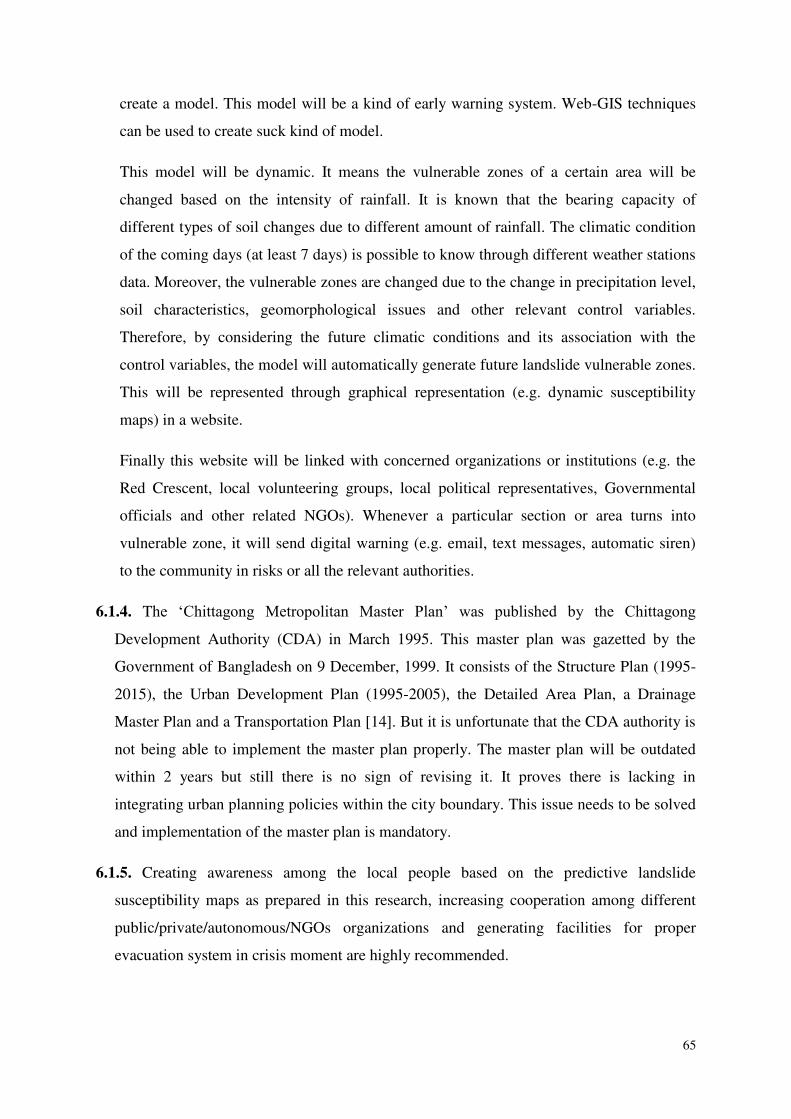
65
create a model. This model will be a kind of early warning system. Web-GIS techniques
can be used to create suck kind of model.
This model will be dynamic. It means the vulnerable zones of a certain area will be
changed based on the intensity of rainfall. It is known that the bearing capacity of
different types of soil changes due to different amount of rainfall. The climatic condition
of the coming days (at least 7 days) is possible to know through different weather stations
data. Moreover, the vulnerable zones are changed due to the change in precipitation level,
soil characteristics, geomorphological issues and other relevant control variables.
Therefore, by considering the future climatic conditions and its association with the
control variables, the model will automatically generate future landslide vulnerable zones.
This will be represented through graphical representation (e.g. dynamic susceptibility
maps) in a website.
Finally this website will be linked with concerned organizations or institutions (e.g. the
Red Crescent, local volunteering groups, local political representatives, Governmental
officials and other related NGOs). Whenever a particular section or area turns into
vulnerable zone, it will send digital warning (e.g. email, text messages, automatic siren)
to the community in risks or all the relevant authorities.
6.1.4. The ‗Chittagong Metropolitan Master Plan‘ was published by the Chittagong
Development Authority (CDA) in March 1995. This master plan was gazetted by the
Government of Bangladesh on 9 December, 1999. It consists of the Structure Plan (1995-
2015), the Urban Development Plan (1995-2005), the Detailed Area Plan, a Drainage
Master Plan and a Transportation Plan [14]. But it is unfortunate that the CDA authority is
not being able to implement the master plan properly. The master plan will be outdated
within 2 years but still there is no sign of revising it. It proves there is lacking in
integrating urban planning policies within the city boundary. This issue needs to be solved
and implementation of the master plan is mandatory.
6.1.5. Creating awareness among the local people based on the predictive landslide
susceptibility maps as prepared in this research, increasing cooperation among different
public/private/autonomous/NGOs organizations and generating facilities for proper
evacuation system in crisis moment are highly recommended.

66
6.2. Research Gap and Future Work
Till now, in all cases, the researchers have used the previous or existing land cover images to
project/predict the landslide susceptibility maps. But land use/ land cover map can be treated
as a dynamic variable. Because within few decades, the land use of a particular area can be
abruptly changed (e.g. CMA). This change in land use pattern (e.g. deforestation, hill-cutting)
can put positive impacts occurring landslides [44]. Therefore, while modelling landslide
hazard maps, it is very important to take into account a new thematic layer-‗the future
projected land cover map‘.
Same thing can happen for the trend in precipitation. It is already indicated that due to
climate change, a significant increase of annual and pre-monsoon rainfall in Bangladesh is
observed [45]. Moreover, the recent landslide events were related to the extreme rainfall
intensities (40 mm/day) having short period of time (2-7 days). All the major landslide events
occurred at much higher rainfall amount compared to the normal monthly average as well
[46]. Therefore, it is also important to consider future rainfall pattern while producing
landslide susceptibility maps for the future. These are the current research gaps in landslide
modelling.
In this drawback, future research should try to take into consideration the dynamic variables
like- the simulated land cover map and future rainfall pattern, to predict the future landslide
scenario of CMA. This will be a new kind of analysis. It will help answering whether using
the simulated dynamic variables will give much better results or not. It is expected that
preparing landslide hazard maps, using this kind of new modelling concept will add new
knowledge to the landslide susceptibility mapping in modern science. The flowchart of this
new idea is depicted in Figure 6.1.
6.3. Conclusion
The outcome of this research shall help the endangered local inhabitants/communities, urban
planners and engineers to reduce losses caused by existing and future landslides by means of
prevention, mitigation and avoidance. The results will also be useful for explaining the
driving factors of the known existing landslides, for supporting emergency decisions and
upholding the efforts on the mitigation of future landslide hazards in CMA, Bangladesh.
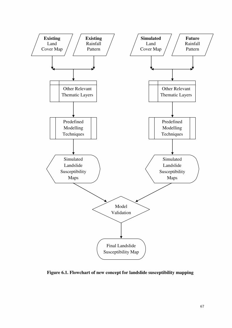
67
Figure 6.1. Flowchart of new concept for landslide susceptibility mapping
Model
Validation
Existing
Land Cover Map
Existing
Rainfall Pattern
Simulated
Land Cover Map
Future
Rainfall Pattern
Predefined
Modelling
Techniques
Simulated
Landslide
Susceptibility
Maps
Other Relevant
Thematic Layers
Other Relevant
Thematic Layers
Predefined
Modelling
Techniques
Simulated
Landslide
Susceptibility
Maps
Final Landslide
Susceptibility Map
68
REFERENCES
[1] Thomas Glade, Landslide occurrence as a response to land use change: a review of evidence from New Zealand, Catena, 51 (2003) 297–314.
[2] Deepak Chapagai, Landslide problem of South Asia and vis-a-vis Global Scenario, SAARC training program on landslide risk management in South Asia, SAARC Disaster Management Centre (SDMC), New Delhi, May 02-08, 2011.
[3] SAARC EXPERT GROUP MEETING ON LANDSLIDE TERMINOLOGY, CLASSIFICATIONS, DOCUMENTATION AND HAZARD MAPPING; Published by the SAARC Disaster Management Centre (SDMC), New Delhi, 2011.
[4] F. Mugagga, V. Kakembo and M. Buyinza, Land use changes on the slopes of Mount Elgon and the implications for the occurrence of landslides, Catena, 90 (2012) 39–46.
[5] Xiaojun Yang and Liding Chen, Using multi-temporal remote sensor imagery to detect earthquake-triggered landslides, International Journal of Applied Earth Observation and
Geoinformation, 12 (2010) 487–495.
[6] I. Alcantara-Ayala, O. Esteban-Chavez and J.F. Parrot; Landsliding related to land-cover change: A diachronic analysis of hillslope instability distribution in the Sierra Norte, Puebla, Mexico; Catena, 65 (2006) 152–165.
[7] H.L. Perotto-Baldiviezo, T.L. Thurow, C.T. Smith, R.F. Fisher & X.B. Wu; GIS-based spatial analysis and modeling for landslide hazard assessment in steeplands, southern Honduras; Agriculture, Ecosystems and Environment, 103 (2004) 165–176.
[8] José M. García-Ruiz, Santiago Beguería, Luis Carlos Alatorre & Juan Puigdefábregas; Land cover changes and shallow landsliding in the flysch sector of the Spanish Pyrenees; Geomorphology, 124 (2010) 250–259.
[9] Kirschbaum MUF, et al, Quantifying the climate-change consequences of shifting land use between forest and agriculture, Sci Total Environ (2013), http://dx.doi.org/10.1016/j.scitotenv.2013.01.026
[10] Quaas, J., 2011. Global warming: the soot factor. Nature 471, 456-457.
[11] Cities and climate change: global report on human settlements, 2011, United Nations Human Settlements Programme.
[12] IPCC (2007) ‗Climate change 2007: Synthesis report‘, in R. K. Pachauri and A. Reisinger (eds) Contribution of Working Groups I, II, and III to the Fourth Assessment Report of the Intergovernmental Panel on Climate Change, Cambridge University Press, Cambridge, UK; URL:
www.ipcc.ch/publications_and_data/publications_ipcc_fourth_assessment_report_synthesis_report.htm, last accessed 23 April 2013.
[13] Bayes Ahmed, 2011, Urban land cover change detection analysis and modeling spatio-temporal Growth dynamics using Remote Sensing and GIS Techniques: A case study of Dhaka, Bangladesh; unpublished MSc thesis, Erasmus Mundus Program, Universidade Nova de Lisboa (UNL), Instituto Superior de Estatística e Gestão de Informação (ISEGI), Lisboa, Portugal.
69
[14] Chittagong Metropolitan Master Plan, 1995, Urban Development Plan, Chittagong Development Authority, the Government of the People‘s Republic of Bangladesh.
[15] BANGLADESH POPULATION AND HOUSING CENSUS 2011, COMMUNITY REPORT, ZILA: CHITTAGONG, June 2012, POPULATION AND HOUSING CENSUS 2011, BANGLADESH BUREAU OF STATISTICS, STATISTICS AND INFORMATICS DIVISION, MINISTRY OF PLANNING, GOVERNMENT OF THE PEOPLE‘S REPUBLIC OF BANGLADESH.
[16] Smyth, C. and S. Royle (2000) ‗Urban landslide hazards: Incidence and causative factors in Niterói, Rio de Janeiro State, Brazil‘, Applied Geography 20(2): 95–117.
[17] ―Heavy rains and landslides in Bangladesh kill 90‖, 27 June 2012, BBC News.
[18] Younus Ahmed Khan, Habibah Lateh, M. Azizul Baten & Anton Abdulbasah Kamil, Critical antecedent rainfall conditions for shallow landslides in Chittagong City of Bangladesh, Environmental Earth Sciences, September 2012, Volume 67, Issue 1, pp 97-106.
[19] Rain causes water logging in Chittagong city, Sunday, May 05, 2013, The Daily Star, Assessed on 6 May 2013.
http://www.thedailystar.net/beta2/news/rain-causes-waterlogging-in-ctg-city/
http://www.eprothomalo.com/contents/2013/2013_05_05/content_zoom/2013_05_05_3_0_b.jpg
[20] Amanullah Bin Mahmood & Mamunul H. Khan, Landslide Vulnerability of Bangladesh Hills and Sustainable Management Options: A Case Study of 2007 Landslide in Chittagong City, paper presented in the International Seminar on “Management and Mitigation of Water Induced Disaster”, 21-22 April 2008, Kathmandu, Nepal.
[21] Ronju Ahammad, 2009, Understanding Institutional Changes for Reducing Social Vulnerability to Landslides in Chittagong City, Bangladesh, Unpublished Master‘s thesis; Ecosystems, Governance and Globalization programme 2007/2009, Stockholm Resilience Center, Stockholm University, Sweden.
[22] Introduction & History, Chittagong and CDA, the official website of Chittagong Development Authority (CDA). Assessed on 10 September, 2013.
http://portal.cda.gov.bd/index.php?option=com_content&view=article&id=85&Itemid=107
[23] Shireen Hasan Osmany, Chittagong City, BANGLAPEDIA, National Encyclopaedia of Bangladesh, Asiatic Society of Bangladesh, Dhaka, Bangladesh. Assessed on 12 September, 2013. http://www.bpedia.org/C_0208.php
[24] Sifatul Quader Chowdhury, Chittagong City, BANGLAPEDIA, National Encyclopaedia of Bangladesh, Asiatic Society of Bangladesh, Dhaka, Bangladesh. Assessed on 14 September, 2013. http://www.bpedia.org/C_0215.php
[25] I. Alcantara-Ayala, O. Esteban-Chavez, J.F. Parrot. Landsliding related to land-cover change: A diachronic analysis of hillslope instability distribution in the Sierra Norte, Puebla, Mexico. Catena 65 (2006) 152–165.
70
[26] R. RAJAKUMAR, S. SANJEEVI, S. JAYASEELAN, G. ISAKKIPANDIAN, M. EDWIN, P. BALAJI AND G. EHANTHALINGAM. LANDSLIDE SUSCEPTIBILITY MAPPING IN A HILLY TERRAIN USING REMOTE SENSING AND GIS. Journal of the Indian Society of Remote Sensing, Vol. 35, No. 1, 2007.
[27] Saro Lee & Touch Sambath. Landslide susceptibility mapping in the Damrei Romel area, Cambodia using frequency ratio and logistic regression models. Environ Geol (2006) 50: 847–855.
[28] Ram Avtar, C. K. Singh, Gulab Singh, R. L. Verma, S. Mukherjee & H. Sawada. Landslide susceptibility zonation study using remote sensing and GIS technology in the Ken-Betwa River Link area, India. Bull Eng Geol Environ (2011) 70:595–606.
[29] F. Karsli, M. Atasoy, A. Yalcin, S. Reis, O. Demir & C. Gokceoglu. Effects of land-use changes on landslides in a landslide-prone area (Ardesen, Rize, NE Turkey). Environ Monit Assess (2009) 156:241–255.
[30] Prabin Kayastha, Megh Raj Dhital & Florimond De Smedt. Landslide susceptibility mapping using the weight of evidence method in the Tinau watershed, Nepal. Nat Hazards (2012) 63:479–498.
[31] Christine Gassner, Catrin Promper, Helene Petschko, and Thomas Glade. Scenarios of future landslide susceptibility - incorporating changes in land cover and climate. Geophysical Research Abstracts, Vol. 15, EGU2013-6786, 2013.
[32] Tahir Ali Akbar & Sung Ryong Ha. Landslide hazard zoning along Himalayan Kaghan Valley of Pakistan—by integration of GPS, GIS, and remote sensing technology. Landslides, December 2011, Volume 8, Issue 4, pp 527-540.
[33] Soyoung Park, Chuluong Choi, Byungwoo Kim & Jinsoo Kim. Landslide susceptibility mapping using frequency ratio, analytic hierarchy process, logistic regression, and artificial neural network methods at the Inje area, Korea. Environ Earth Sci (2013) 68:1443–1464.
[34] Fausto Guzzetti, Alberto Carrara, Mauro Cardinali & Paola Reichenbach. Landslide hazard evaluation: a review of current techniques and their application in a multi-scale study, Central Italy. Geomorphology 31 1999 181–216.
[35] Shi-Biao Bai, Jian Wang, Guo-Nian Lü, Ping-Gen Zhou, Sheng-Shan Hou & Su-Ning Xu. GIS-based logistic regression for landslide susceptibility mapping of the Zhongxian segment in the Three Gorges area, China. Geomorphology 115 (2010) 23-31.
[36] Duman TY, Can T, Emre O, Kecer M, Dogan A, Ates S, Durmaz S (2005) Landslide inventory of north-western Anatolia, Turkey. Eng Geol 77:99–114.
[37] Godt JW, Baum RL, Savage WZ, Salciarini D, Schulz WH, Harp EL (2008) Transient deterministic shallow landslide modeling: Requirements for susceptibility and hazard assessment in a GIS framework. Eng Geol 102:214–226.
[38] Isik Yilmaz, Landslide susceptibility mapping using frequency ratio, logistic regression, artificial neural networks and their comparison: A case study from Kat landslides (Tokat—Turkey). Computers & Geosciences 35 (2009) 1125–1138.
71
[39] Yilmaz I, Yildirim M (2006) Structural and geomorphological aspects of the Kat landslides (Tokat-Turkey), and susceptibility mapping by means of GIS. Environ Geol 50(4):461–472.
[40] Dieu Tien Bui, Biswajeet Pradhan, Owe Lofman, Inge Revhaug & Øystein B. Dick. Regional prediction of landslide hazard using probability analysis of intense rainfall in the Hoa Binh province, Vietnam. Nat Hazards (2013) 66:707–730.
[41] J.L. Zêzere, R.A.C. Garcia, S.C. Oliveira & E. Reis. Probabilistic landslide risk analysis considering direct costs in the area north of Lisbon (Portugal). Geomorphology 94 (2008) 467–495.
[42] Bakhtiar Feizizadeh & Thomas Blaschke. GIS-multicriteria decision analysis for landslide susceptibility mapping: comparing three methods for the Urmia lake basin, Iran. Nat Hazards (2013) 65:2105–2128.
[43] Chandra Prakash Poudyal, Chandong Chang, Hyun-Joo Oh & Saro Lee. Landslide susceptibility maps comparing frequency ratio and artificial neural networks: a case study from the Nepal Himalaya. Environ Earth Sci (2010) 61:1049–1064.
[44] F. Mugagga, V. Kakembo & M. Buyinza. Land use changes on the slopes of Mount Elgon and the implications for the occurrence of landslides. Catena 90 (2012) 39–46.
[45] Shamsuddin Shahid. Trends in extreme rainfall events of Bangladesh. Theor Appl Climatol (2011) 104:489–499.
[46] Younus Ahmed Khan, Habibah Lateh, M. Azizul Baten & Anton Abdulbasah Kamil. Critical antecedent rainfall conditions for shallow landslides in Chittagong City of Bangladesh. Environ Earth Sci (2012) 67:97–106.
[47] T. Tachikawa, M. Hato, M. Kaku and A. Iwasaki, 2011, The characteristics of ASTER GDEM version 2, IGARSS, July 2011. Assessed on 23 October, 2013. http://www.jspacesystems.or.jp/ersdac/GDEM/E/1.html
[48] ArcGIS® 10 Help; Environmental Systems Research Institute: Redlands, CA, USA, 2012. Available online: http://help.arcgis.com/en/arcgisdesktop/10.0/help/ (accessed on 7 November 2013).
[49] Malczewski J (2000). On the use of weighted linear combination method in GIS: common and best practice approaches. Trans GIS 4(1):5–22.
[50] Gorsevski PV, Jankowski P, Gessler PE (2006) An heuristic approach for mapping landslide hazard by integrating fuzzy logic with analytic hierarchy process. Control Cybern 35:21–141.
[51] Ron Eastman, The IDRISI Selva Help, 2012 Clark Labs, Clark University 950 Main Street, Worcester MA 01610-1477 USA.
[52] Lee S, Sambath T (2006) Landslide susceptibility mapping in the damrei romel area, cambodia using frequency ratio and logistic regression models. Environ Geol 50:847–855.
[53] McFadden D (1973) Conditional logit analysis of quantitative choice behavior. In: Zarembka P (ed) Frontiers in Econometrics. Academic Press, New York, pp 105–142.
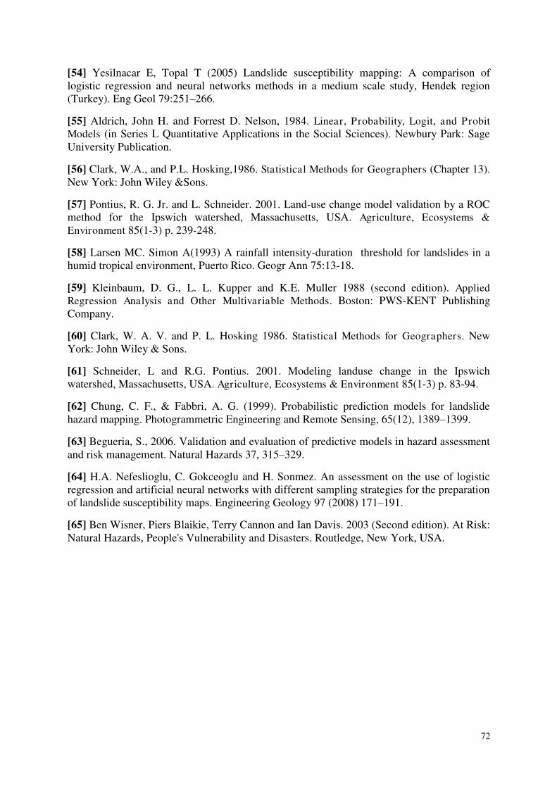
72
[54] Yesilnacar E, Topal T (2005) Landslide susceptibility mapping: A comparison of logistic regression and neural networks methods in a medium scale study, Hendek region (Turkey). Eng Geol 79:251–266.
[55] Aldrich, John H. and Forrest D. Nelson, 1984. Linear, Probability, Logit, and Probit
Models (in Series L Quantitative Applications in the Social Sciences). Newbury Park: Sage University Publication.
[56] Clark, W.A., and P.L. Hosking,1986. Statistical Methods for Geographers (Chapter 13). New York: John Wiley &Sons.
[57] Pontius, R. G. Jr. and L. Schneider. 2001. Land-use change model validation by a ROC method for the Ipswich watershed, Massachusetts, USA. Agriculture, Ecosystems &
Environment 85(1-3) p. 239-248.
[58] Larsen MC. Simon A(1993) A rainfall intensity-duration threshold for landslides in a humid tropical environment, Puerto Rico. Geogr Ann 75:13-18.
[59] Kleinbaum, D. G., L. L. Kupper and K.E. Muller 1988 (second edition). Applied
Regression Analysis and Other Multivariable Methods. Boston: PWS-KENT Publishing Company.
[60] Clark, W. A. V. and P. L. Hosking 1986. Statistical Methods for Geographers. New York: John Wiley & Sons.
[61] Schneider, L and R.G. Pontius. 2001. Modeling landuse change in the Ipswich watershed, Massachusetts, USA. Agriculture, Ecosystems & Environment 85(1-3) p. 83-94.
[62] Chung, C. F., & Fabbri, A. G. (1999). Probabilistic prediction models for landslide hazard mapping. Photogrammetric Engineering and Remote Sensing, 65(12), 1389–1399.
[63] Begueria, S., 2006. Validation and evaluation of predictive models in hazard assessment and risk management. Natural Hazards 37, 315–329.
[64] H.A. Nefeslioglu, C. Gokceoglu and H. Sonmez. An assessment on the use of logistic regression and artificial neural networks with different sampling strategies for the preparation of landslide susceptibility maps. Engineering Geology 97 (2008) 171–191.
[65] Ben Wisner, Piers Blaikie, Terry Cannon and Ian Davis. 2003 (Second edition). At Risk: Natural Hazards, People's Vulnerability and Disasters. Routledge, New York, USA.
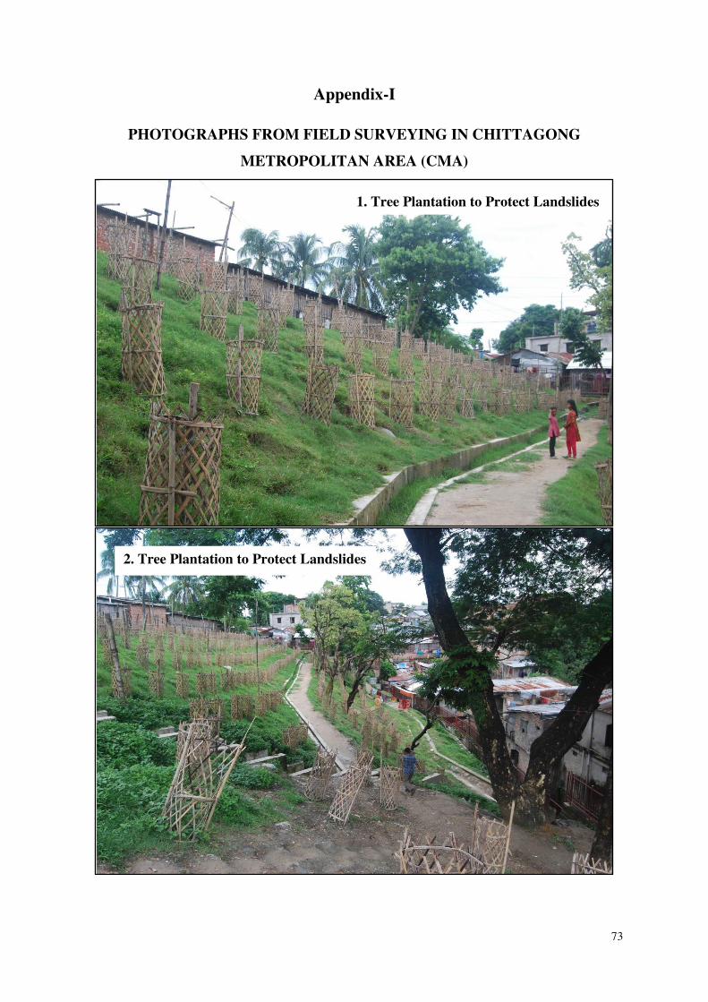
73
Appendix-I
PHOTOGRAPHS FROM FIELD SURVEYING IN CHITTAGONG
METROPOLITAN AREA (CMA)
1. Tree Plantation to Protect Landslides
2. Tree Plantation to Protect Landslides
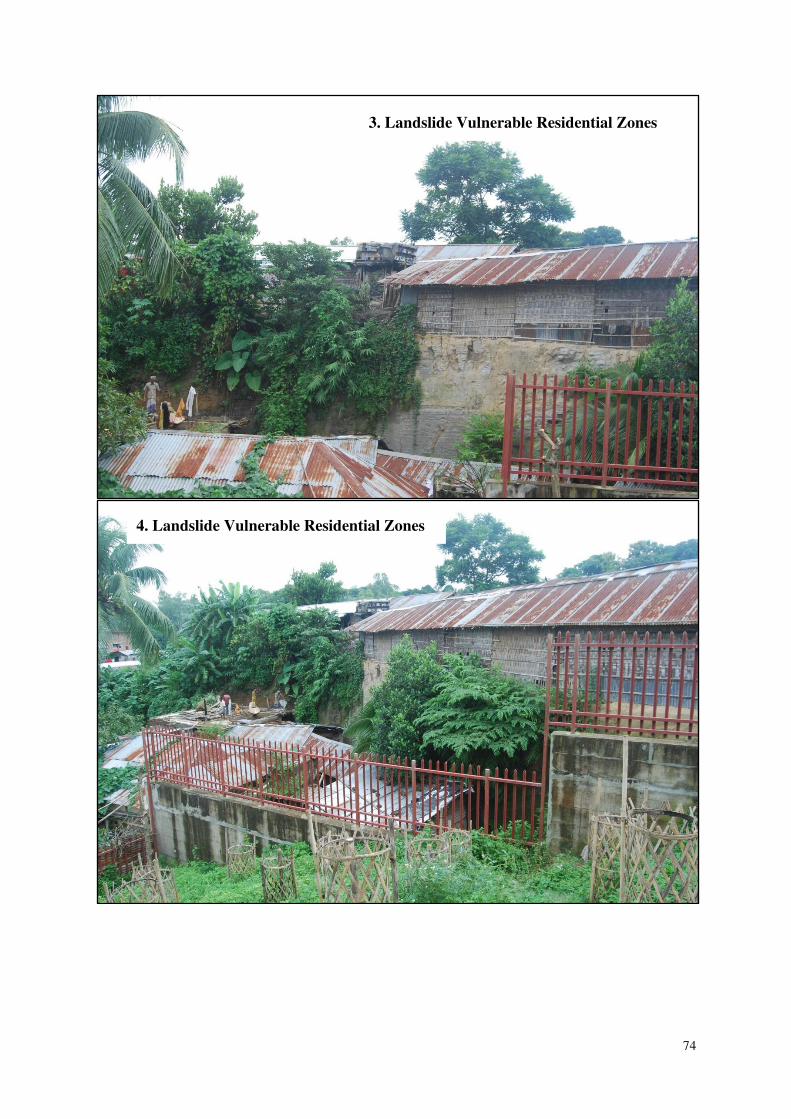
74
3. Landslide Vulnerable Residential Zones
4. Landslide Vulnerable Residential Zones
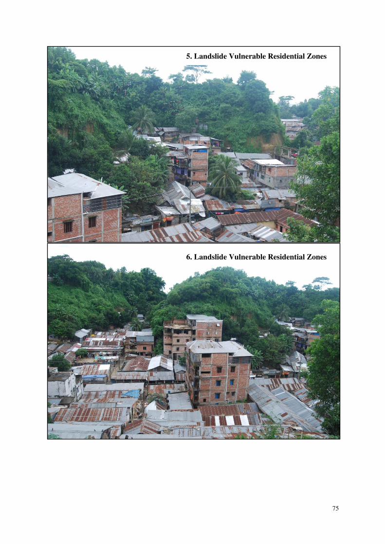
75
5. Landslide Vulnerable Residential Zones
6. Landslide Vulnerable Residential Zones
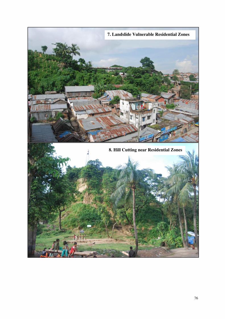
76
7. Landslide Vulnerable Residential Zones
8. Hill Cutting near Residential Zones

77
© Bayes Ahmed (Photographs 1-10)
9. Temporary Accommodation for the Landslide Vulnerable People
10. Mr. Bayes Ahmed (Mentor) with the Landslide Refugees
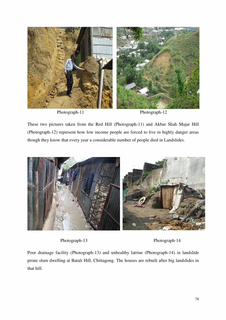
78
Photograph-11 Photograph-12
These two pictures taken from the Red Hill (Photograph-11) and Akbar Shah Majar Hill
(Photograph-12) represent how low income people are forced to live in highly danger areas
though they know that every year a considerable number of people died in Landslides.
Photograph-13 Photograph-14
Poor drainage facility (Photograph-13) and unhealthy latrine (Photograph-14) in landslide
prone slum dwelling at Batali Hill, Chittagong. The houses are rebuilt after big landslides in
that hill.
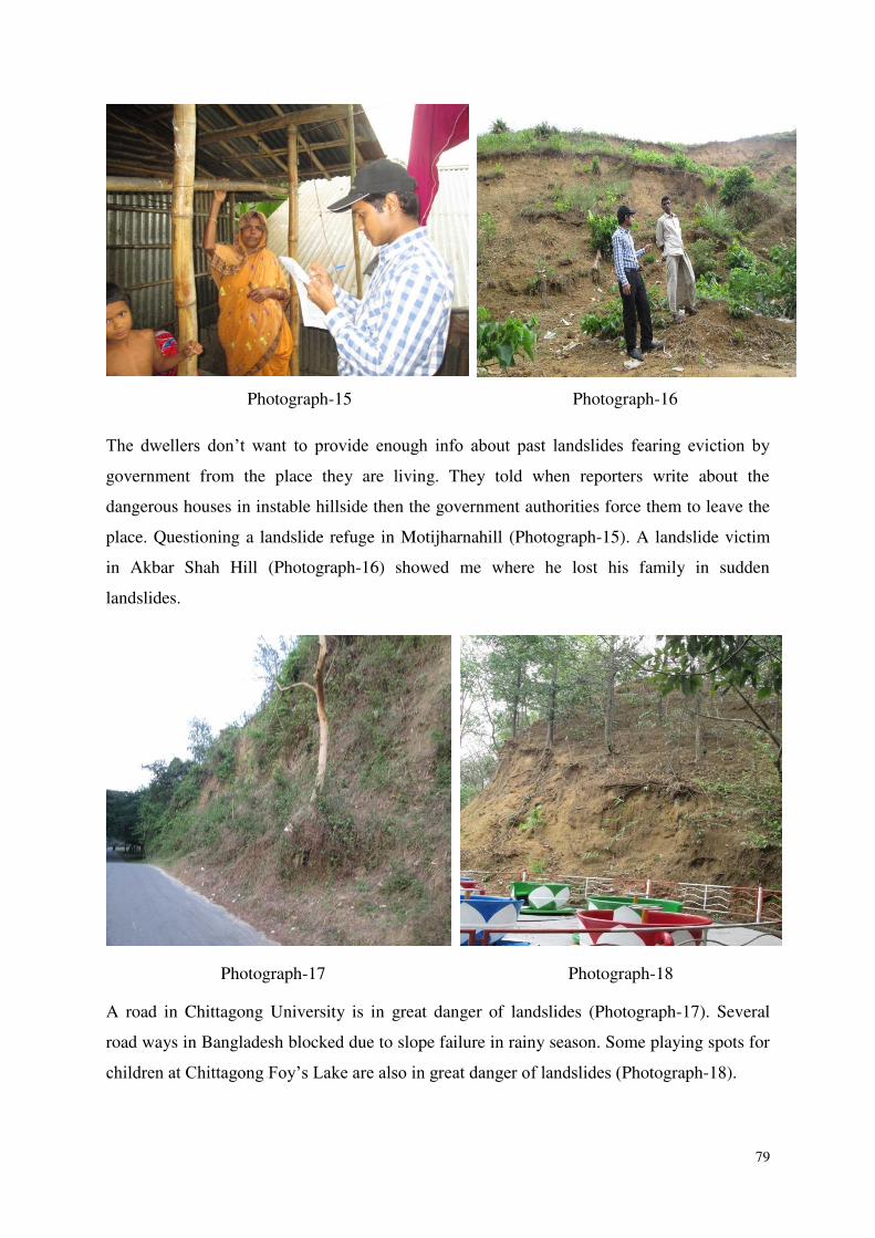
79
Photograph-15 Photograph-16
The dwellers don’t want to provide enough info about past landslides fearing eviction by
government from the place they are living. They told when reporters write about the
dangerous houses in instable hillside then the government authorities force them to leave the
place. Questioning a landslide refuge in Motijharnahill (Photograph-15). A landslide victim
in Akbar Shah Hill (Photograph-16) showed me where he lost his family in sudden
landslides.
Photograph-17 Photograph-18
A road in Chittagong University is in great danger of landslides (Photograph-17). Several
road ways in Bangladesh blocked due to slope failure in rainy season. Some playing spots for
children at Chittagong Foy’s Lake are also in great danger of landslides (Photograph-18).
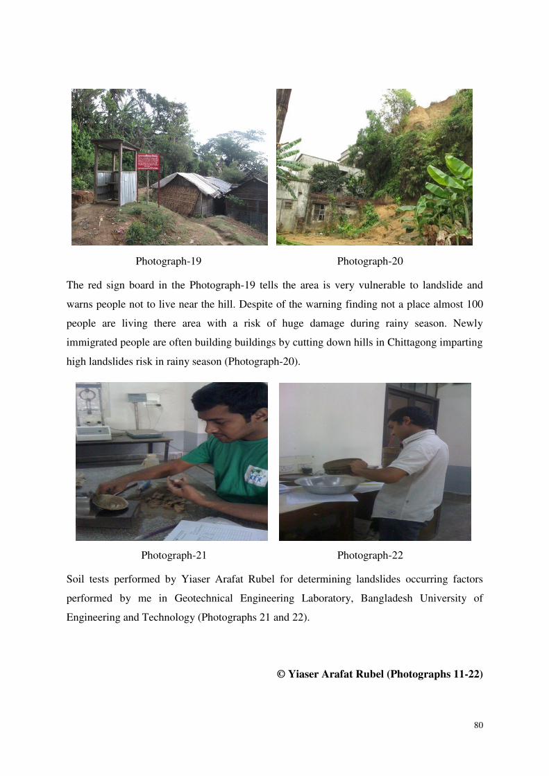
80
Photograph-19 Photograph-20
The red sign board in the Photograph-19 tells the area is very vulnerable to landslide and
warns people not to live near the hill. Despite of the warning finding not a place almost 100
people are living there area with a risk of huge damage during rainy season. Newly
immigrated people are often building buildings by cutting down hills in Chittagong imparting
high landslides risk in rainy season (Photograph-20).
Photograph-21 Photograph-22
Soil tests performed by Yiaser Arafat Rubel for determining landslides occurring factors
performed by me in Geotechnical Engineering Laboratory, Bangladesh University of
Engineering and Technology (Photographs 21 and 22).
© Yiaser Arafat Rubel (Photographs 11-22)
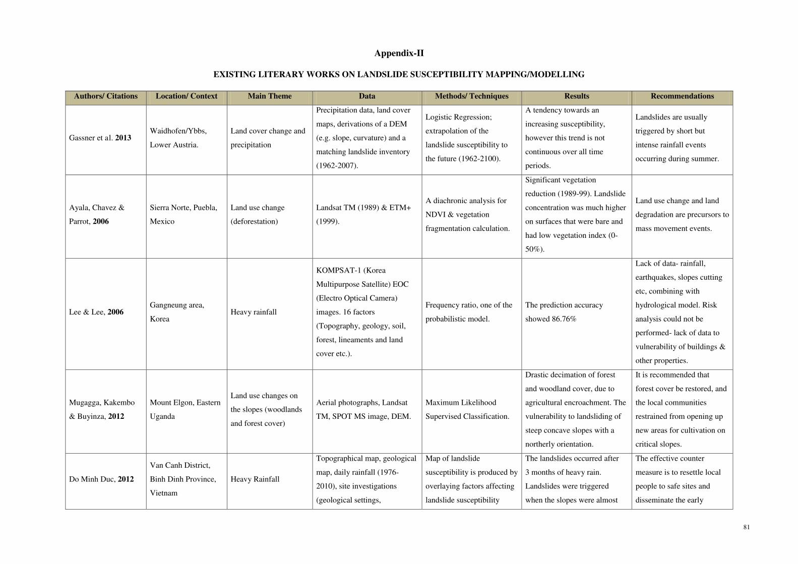
81
Appendix-II
EXISTING LITERARY WORKS ON LANDSLIDE SUSCEPTIBILITY MAPPING/MODELLING
Authors/ Citations Location/ Context Main Theme Data Methods/ Techniques Results Recommendations
Gassner et al. 2013 Waidhofen/Ybbs,
Lower Austria.
Land cover change and
precipitation
Precipitation data, land cover
maps, derivations of a DEM
(e.g. slope, curvature) and a
matching landslide inventory
(1962-2007).
Logistic Regression;
extrapolation of the
landslide susceptibility to
the future (1962-2100).
A tendency towards an
increasing susceptibility,
however this trend is not
continuous over all time
periods.
Landslides are usually
triggered by short but
intense rainfall events
occurring during summer.
Ayala, Chavez &
Parrot, 2006
Sierra Norte, Puebla,
Mexico
Land use change
(deforestation)
Landsat TM (1989) & ETM+
(1999).
A diachronic analysis for
NDVI & vegetation
fragmentation calculation.
Significant vegetation
reduction (1989-99). Landslide
concentration was much higher
on surfaces that were bare and
had low vegetation index (0-
50%).
Land use change and land
degradation are precursors to
mass movement events.
Lee & Lee, 2006 Gangneung area,
Korea Heavy rainfall
KOMPSAT-1 (Korea
Multipurpose Satellite) EOC
(Electro Optical Camera)
images. 16 factors
(Topography, geology, soil,
forest, lineaments and land
cover etc.).
Frequency ratio, one of the
probabilistic model.
The prediction accuracy
showed 86.76%
Lack of data- rainfall,
earthquakes, slopes cutting
etc, combining with
hydrological model. Risk
analysis could not be
performed- lack of data to
vulnerability of buildings &
other properties.
Mugagga, Kakembo
& Buyinza, 2012
Mount Elgon, Eastern
Uganda
Land use changes on
the slopes (woodlands
and forest cover)
Aerial photographs, Landsat
TM, SPOT MS image, DEM.
Maximum Likelihood
Supervised Classification.
Drastic decimation of forest
and woodland cover, due to
agricultural encroachment. The
vulnerability to landsliding of
steep concave slopes with a
northerly orientation.
It is recommended that
forest cover be restored, and
the local communities
restrained from opening up
new areas for cultivation on
critical slopes.
Do Minh Duc, 2012
Van Canh District,
Binh Dinh Province,
Vietnam
Heavy Rainfall
Topographical map, geological
map, daily rainfall (1976-
2010), site investigations
(geological settings,
Map of landslide
susceptibility is produced by
overlaying factors affecting
landslide susceptibility
The landslides occurred after
3 months of heavy rain.
Landslides were triggered
when the slopes were almost
The effective counter
measure is to resettle local
people to safe sites and
disseminate the early
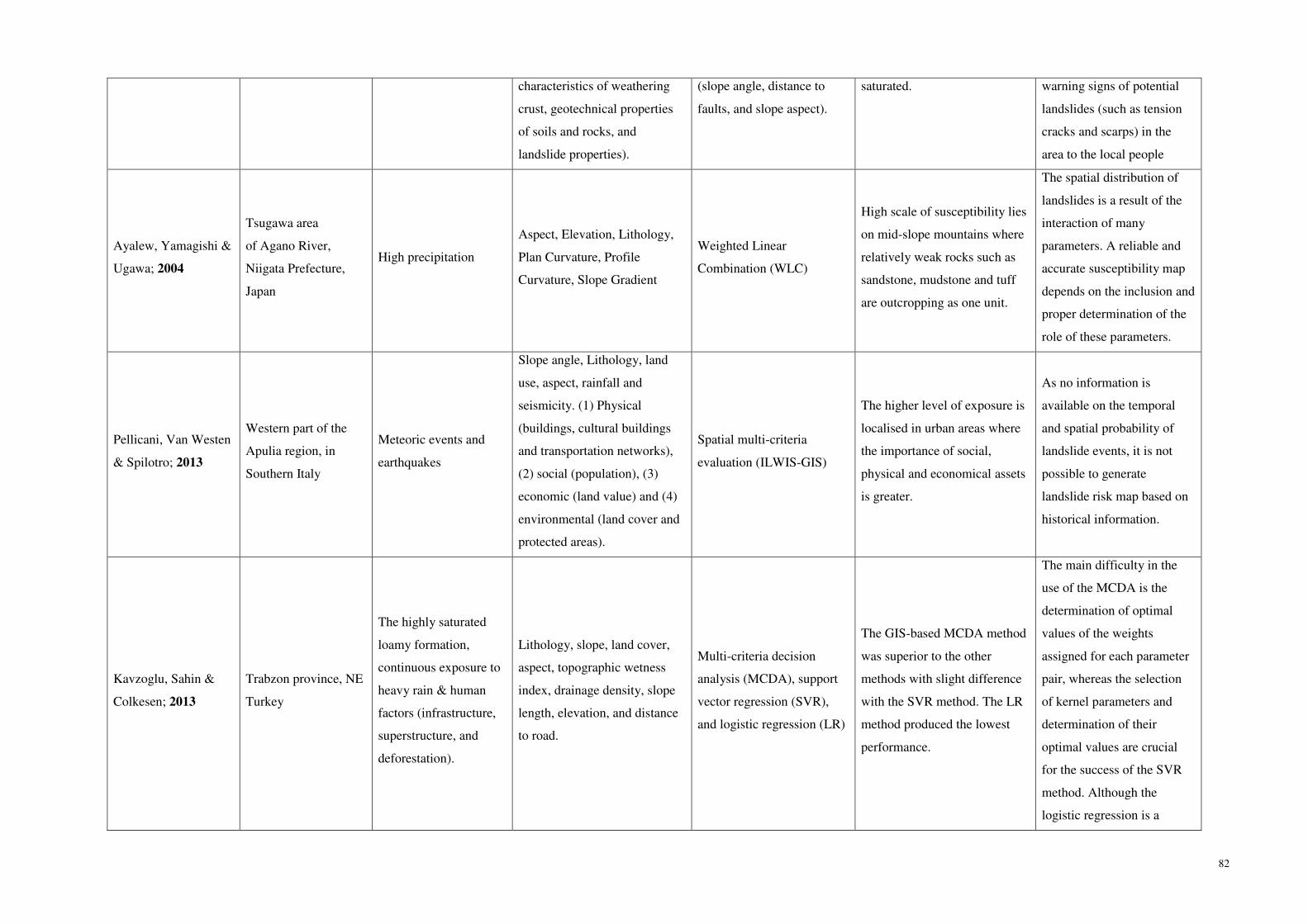
82
characteristics of weathering
crust, geotechnical properties
of soils and rocks, and
landslide properties).
(slope angle, distance to
faults, and slope aspect).
saturated. warning signs of potential
landslides (such as tension
cracks and scarps) in the
area to the local people
Ayalew, Yamagishi &
Ugawa; 2004
Tsugawa area
of Agano River,
Niigata Prefecture,
Japan
High precipitation
Aspect, Elevation, Lithology,
Plan Curvature, Profile
Curvature, Slope Gradient
Weighted Linear
Combination (WLC)
High scale of susceptibility lies
on mid-slope mountains where
relatively weak rocks such as
sandstone, mudstone and tuff
are outcropping as one unit.
The spatial distribution of
landslides is a result of the
interaction of many
parameters. A reliable and
accurate susceptibility map
depends on the inclusion and
proper determination of the
role of these parameters.
Pellicani, Van Westen
& Spilotro; 2013
Western part of the
Apulia region, in
Southern Italy
Meteoric events and
earthquakes
Slope angle, Lithology, land
use, aspect, rainfall and
seismicity. (1) Physical
(buildings, cultural buildings
and transportation networks),
(2) social (population), (3)
economic (land value) and (4)
environmental (land cover and
protected areas).
Spatial multi-criteria
evaluation (ILWIS-GIS)
The higher level of exposure is
localised in urban areas where
the importance of social,
physical and economical assets
is greater.
As no information is
available on the temporal
and spatial probability of
landslide events, it is not
possible to generate
landslide risk map based on
historical information.
Kavzoglu, Sahin &
Colkesen; 2013
Trabzon province, NE
Turkey
The highly saturated
loamy formation,
continuous exposure to
heavy rain & human
factors (infrastructure,
superstructure, and
deforestation).
Lithology, slope, land cover,
aspect, topographic wetness
index, drainage density, slope
length, elevation, and distance
to road.
Multi-criteria decision
analysis (MCDA), support
vector regression (SVR),
and logistic regression (LR)
The GIS-based MCDA method
was superior to the other
methods with slight difference
with the SVR method. The LR
method produced the lowest
performance.
The main difficulty in the
use of the MCDA is the
determination of optimal
values of the weights
assigned for each parameter
pair, whereas the selection
of kernel parameters and
determination of their
optimal values are crucial
for the success of the SVR
method. Although the
logistic regression is a
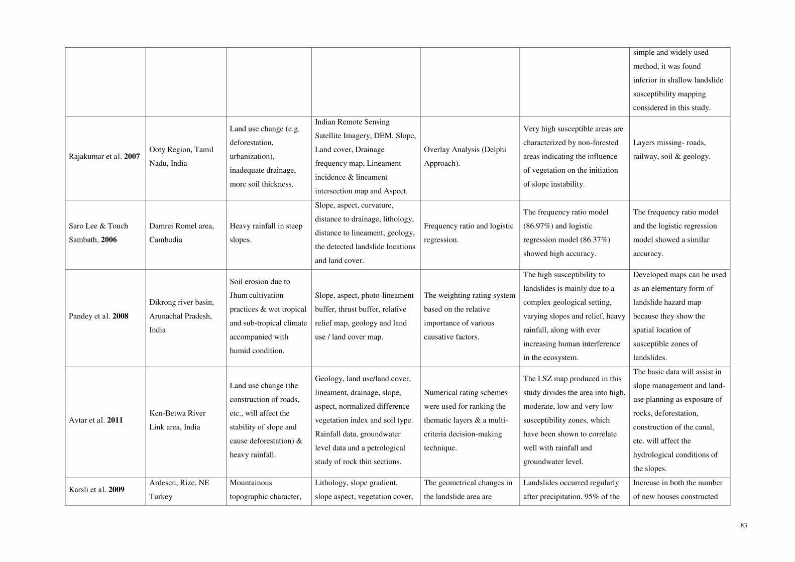
83
simple and widely used
method, it was found
inferior in shallow landslide
susceptibility mapping
considered in this study.
Rajakumar et al. 2007 Ooty Region, Tamil
Nadu, India
Land use change (e.g.
deforestation,
urbanization),
inadequate drainage,
more soil thickness.
Indian Remote Sensing
Satellite Imagery, DEM, Slope,
Land cover, Drainage
frequency map, Lineament
incidence & lineament
intersection map and Aspect.
Overlay Analysis (Delphi
Approach).
Very high susceptible areas are
characterized by non-forested
areas indicating the influence
of vegetation on the initiation
of slope instability.
Layers missing- roads,
railway, soil & geology.
Saro Lee & Touch
Sambath, 2006
Damrei Romel area,
Cambodia
Heavy rainfall in steep
slopes.
Slope, aspect, curvature,
distance to drainage, lithology,
distance to lineament, geology,
the detected landslide locations
and land cover.
Frequency ratio and logistic
regression.
The frequency ratio model
(86.97%) and logistic
regression model (86.37%)
showed high accuracy.
The frequency ratio model
and the logistic regression
model showed a similar
accuracy.
Pandey et al. 2008
Dikrong river basin,
Arunachal Pradesh,
India
Soil erosion due to
Jhum cultivation
practices & wet tropical
and sub-tropical climate
accompanied with
humid condition.
Slope, aspect, photo-lineament
buffer, thrust buffer, relative
relief map, geology and land
use / land cover map.
The weighting rating system
based on the relative
importance of various
causative factors.
The high susceptibility to
landslides is mainly due to a
complex geological setting,
varying slopes and relief, heavy
rainfall, along with ever
increasing human interference
in the ecosystem.
Developed maps can be used
as an elementary form of
landslide hazard map
because they show the
spatial location of
susceptible zones of
landslides.
Avtar et al. 2011 Ken-Betwa River
Link area, India
Land use change (the
construction of roads,
etc., will affect the
stability of slope and
cause deforestation) &
heavy rainfall.
Geology, land use/land cover,
lineament, drainage, slope,
aspect, normalized difference
vegetation index and soil type.
Rainfall data, groundwater
level data and a petrological
study of rock thin sections.
Numerical rating schemes
were used for ranking the
thematic layers & a multi-
criteria decision-making
technique.
The LSZ map produced in this
study divides the area into high,
moderate, low and very low
susceptibility zones, which
have been shown to correlate
well with rainfall and
groundwater level.
The basic data will assist in
slope management and land-
use planning as exposure of
rocks, deforestation,
construction of the canal,
etc. will affect the
hydrological conditions of
the slopes.
Karsli et al. 2009 Ardesen, Rize, NE
Turkey
Mountainous
topographic character,
Lithology, slope gradient,
slope aspect, vegetation cover,
The geometrical changes in
the landslide area are
Landslides occurred regularly
after precipitation. 95% of the
Increase in both the number
of new houses constructed

84
land cover change and
high frequency of
heavy rain.
land class, climate, rainfall and
proximity to roads.
determined by using the
photogrammetric
techniques.
landslides identified in the
region occurred in highly or
completely decomposed rock
(tea agriculture).
and in the length of road
network affect the stability
of slopes negatively and thus
causes new landslide
developments.
Kayastha, Dhital &
Smedt, 2012
Tinau watershed,
Nepal.
Adverse geological
conditions, prolonged
and high-intensity
rainfall and
anthropogenic factors.
Slope angle, slope aspect, slope
shape, relative relief, geology,
distance from faults, land use,
distance from drainage and
mean long-term annual
precipitation.
The weight of evidence
method.
72 % of the observed landslides
fall on the high and very high
susceptible zones, which that
constitute 30 % of the study
area.
Due to the dynamic nature
of precipitation, rapid
urbanization, deforestation
and anthropogenic activities,
the presented landslide
susceptibility map is
subjected to change.
Feizizadeh &
Blaschke, 2013
Urmia lake basin,
Iran.
Unstable slopes
combined with the
geological tectonic
settings.
Lithology, distance to fault,
distance to roads, distance to
stream, elevation, slope,
aspect, land use/cover,
precipitation & the landslides
inventory database.
Analytic hierarchy process
(AHP), weighted linear
combination (WLC) and
ordered weighted average
(OWA). Dempster-Shafer
theory for uncertainty
analysis.
The AHP performed best in the
landslide susceptibility
mapping closely followed by
the OWA method while the
WLC method delivered
significantly poorer results.
It is evident that each
method has its advantages
and inherent limitations that
must be fully understood
and accepted by the decision
maker before applying it.
Bui et al. 2013 Hoa Binh province,
Vietnam.
Heavy rainfall, clear-
cut logging,
deforestation, and
infrastructural
expansion.
Landslide inventory map,
rainfall data & five landslide
susceptibility maps.
The rainfall threshold
Model, Poisson probability
model, support vector
machines, logistic
regression, evidential belief
functions, Bayesian
regularized neural networks,
and neuro-fuzzy models.
A total of 15 specific landslide
hazard maps were generated
considering three time periods
of 1, 3, and 5 years.
The details of soil thickness
and soil strength properties
are not available. An
assessment of the change of
land use and road system
should be carried out for the
considered period.
Mohamed O. Arnous,
2011
Wadi Watier area,
South Sinai, Egypt.
Earthquakes, poor
quality soils, diverse
geomorphology, and
steep slope gradient.
Lithology, structural
lineaments, land-cover/land-
use, terrain analysis, seismic
map, slope, aspect, height
elevation, and 3D.
The weighting-rating system
based on the relative
importance of various
causative factors.
The distribution of landslides is
largely governed by the
combined effect of various geo-
environmental conditions.
Detail investigation on
existing infrastructure or
communities can provide
information to ensure a
stable design.
Poudyal et al. 2010 Panchthar district, Groundwater, Slope angle, slope aspect, Frequency ratio and Most of the highly hazardous The respective accuracy of
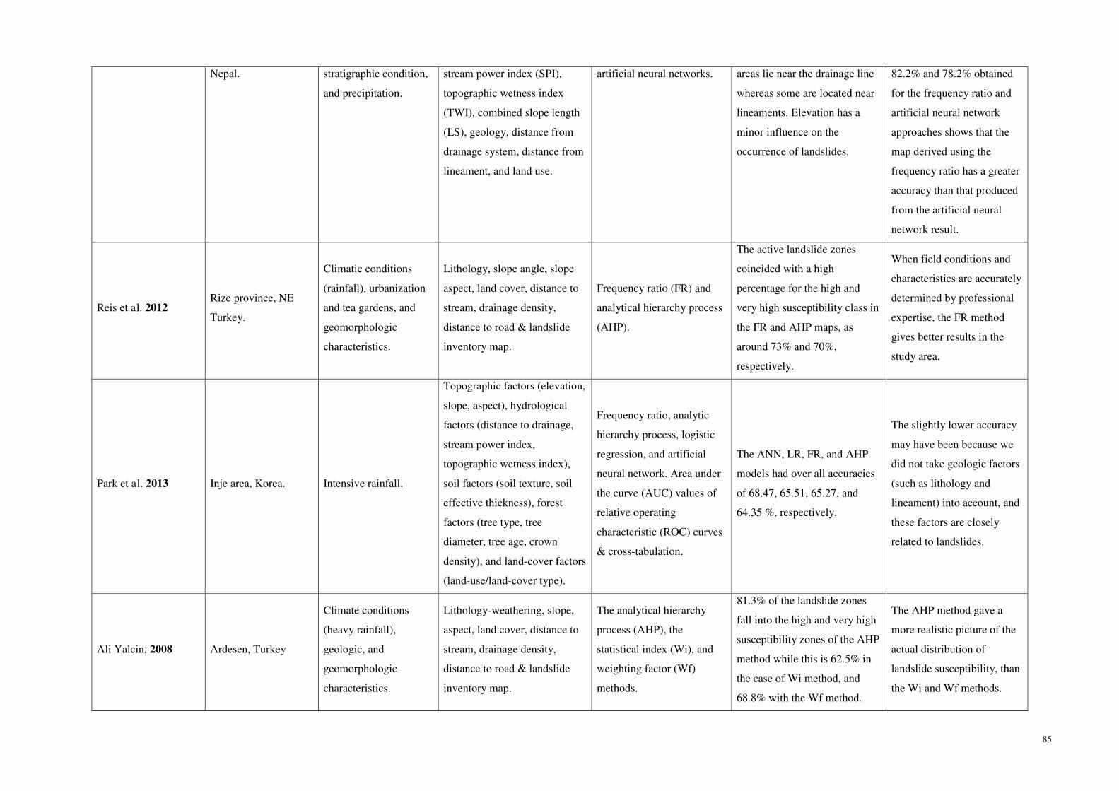
85
Nepal. stratigraphic condition,
and precipitation.
stream power index (SPI),
topographic wetness index
(TWI), combined slope length
(LS), geology, distance from
drainage system, distance from
lineament, and land use.
artificial neural networks. areas lie near the drainage line
whereas some are located near
lineaments. Elevation has a
minor influence on the
occurrence of landslides.
82.2% and 78.2% obtained
for the frequency ratio and
artificial neural network
approaches shows that the
map derived using the
frequency ratio has a greater
accuracy than that produced
from the artificial neural
network result.
Reis et al. 2012 Rize province, NE
Turkey.
Climatic conditions
(rainfall), urbanization
and tea gardens, and
geomorphologic
characteristics.
Lithology, slope angle, slope
aspect, land cover, distance to
stream, drainage density,
distance to road & landslide
inventory map.
Frequency ratio (FR) and
analytical hierarchy process
(AHP).
The active landslide zones
coincided with a high
percentage for the high and
very high susceptibility class in
the FR and AHP maps, as
around 73% and 70%,
respectively.
When field conditions and
characteristics are accurately
determined by professional
expertise, the FR method
gives better results in the
study area.
Park et al. 2013 Inje area, Korea. Intensive rainfall.
Topographic factors (elevation,
slope, aspect), hydrological
factors (distance to drainage,
stream power index,
topographic wetness index),
soil factors (soil texture, soil
effective thickness), forest
factors (tree type, tree
diameter, tree age, crown
density), and land-cover factors
(land-use/land-cover type).
Frequency ratio, analytic
hierarchy process, logistic
regression, and artificial
neural network. Area under
the curve (AUC) values of
relative operating
characteristic (ROC) curves
& cross-tabulation.
The ANN, LR, FR, and AHP
models had over all accuracies
of 68.47, 65.51, 65.27, and
64.35 %, respectively.
The slightly lower accuracy
may have been because we
did not take geologic factors
(such as lithology and
lineament) into account, and
these factors are closely
related to landslides.
Ali Yalcin, 2008 Ardesen, Turkey
Climate conditions
(heavy rainfall),
geologic, and
geomorphologic
characteristics.
Lithology-weathering, slope,
aspect, land cover, distance to
stream, drainage density,
distance to road & landslide
inventory map.
The analytical hierarchy
process (AHP), the
statistical index (Wi), and
weighting factor (Wf)
methods.
81.3% of the landslide zones
fall into the high and very high
susceptibility zones of the AHP
method while this is 62.5% in
the case of Wi method, and
68.8% with the Wf method.
The AHP method gave a
more realistic picture of the
actual distribution of
landslide susceptibility, than
the Wi and Wf methods.

86
Ermini, Catani &
Casagli, 2005
The Reno River,
Northern Apennines,
Italy.
Geomorphological and
geological settings.
Lithology, slope angle, profile
curvature, land cover, up-slope
contributing area & landslide
inventory.
Artificial Neural Networks
(ANNs): Multi-Layered
Perceptron (MLP) the
Probabilistic Neural
Network (PNN).
Geographic representations of
the model predictions show
satisfactory results for both
networks.
Estimation errors can be due
to the following causes:
Problems in the network
construction, Wrong or
insufficient variables &
Noisy data.
Pradhan, Lee &
Buchroithner, 2010
Penang Island,
Cameron Highland
and Selangor;
Malaysia.
Tropical rainfall, flash
floods, continuous
development and
urbanization lead to
deforestation and
erosion of the covering
soil layers.
Landslide inventory, the slope,
aspect, curvature, altitude,
distance from drainage, stream
power index, distance from
road, distance from faults,
geology, land use, normalized
difference vegetation index
(NDVI), topography,
topographic wetness index, soil
texture and soil material.
An artificial neural network
(ANN) method. Verification
through ‘‘area under the
curve” (AUC) method.
The verification results showed
satisfactory agreement between
the susceptibility map and the
existing data on the landslide
location.
If data on rainfall,
earthquake shaking, or slope
cutting existed, then the
possibility analysis could be
performed. Similarly, if the
factors relevant to the
vulnerability of buildings
and other property were
available, the risk analysis
could also be performed.
Chau et al. 2004 Hong Kong Island Rainfall
Terrain data (slope angle and
elevation), environmental
effect (rainfall), geology
information (soil deposit and
lithology), landslide
information (potential run-out
coverage and landslide
inventory. Population map for
risk analysis.
A frequency–volume
relation & multi-
dimensional regression
analysis.
Strong correlation between
rainfall and landslide
occurrence is obtained.
In terms of being hit by a
landslide, squatter areas and
roads are at the highest risk.
Blahut, Westen &
Sterlacchini, 2010
The Valtellina Valley,
the Central Italian
Alps.
Rainfall-induced small
slides and soil slips
which are the sources
for debris flows.
Land use, geology, faults,
altitude, aspect, internal relief,
planar curvature, profile
curvature, slope and flow
accumulation.
The Weights-of-Evidence
modelling technique
(WofE), Success rate curves
& Prediction rate curves.
[An ArcGIS 9.2 extension
SDM—Spatial Data
Modeller]
The spatial distribution of
susceptible areas in the best
performing maps disagrees by
20% to 30%. It is highly
variable and dependent on the
combination of the factor maps
used.
It is better not to perform
statistical analysis over a
large area because particular
differences in susceptibility
conditions are not shown.
Nefeslioglu, The town Ispir and its Geomorphometric Lithology, land use, Logistic regression and The susceptibility maps To find out the best
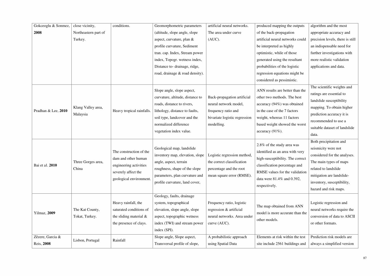
87
Gokceoglu & Sonmez,
2008
close vicinity,
Northeastern part of
Turkey.
conditions. Geomorphometric parameters
(altitude, slope angle, slope
aspect, curvature, plan &
profile curvature, Sediment
tran. cap. Index, Stream power
index, Topogr. wetness index,
Distance to- drainage, ridge,
road, drainage & road density).
artificial neural networks.
The area under curve
(AUC).
produced mapping the outputs
of the back-propagation
artificial neural networks could
be interpreted as highly
optimistic, while of those
generated using the resultant
probabilities of the logistic
regression equations might be
considered as pessimistic.
algorithm and the most
appropriate accuracy and
precision levels, there is still
an indispensable need for
further investigations with
more realistic validation
applications and data.
Pradhan & Lee, 2010 Klang Valley area,
Malaysia Heavy tropical rainfalls.
Slope angle, slope aspect,
curvature, altitude, distance to
roads, distance to rivers,
lithology, distance to faults,
soil type, landcover and the
normalized difference
vegetation index value.
Back-propagation artificial
neural network model,
frequency ratio and
bivariate logistic regression
modelling.
ANN results are better than the
other two methods. The best
accuracy (94%) was obtained
in the case of the 7 factors
weight, whereas 11 factors
based weight showed the worst
accuracy (91%).
The scientific weights and
ratings are essential to
landslide susceptibility
mapping. To obtain higher
prediction accuracy it is
recommended to use a
suitable dataset of landslide
data.
Bai et al. 2010 Three Gorges area,
China
The construction of the
dam and other human
engineering activities
severely affect the
geological environment.
Geological map, landslide
inventory map, elevation, slope
angle, aspect, terrain
roughness, shape of the slope
parameters, plan curvature and
profile curvature, land cover,
Logistic regression method,
the correct classification
percentage and the root
mean square error (RMSE).
2.8% of the study area was
identified as an area with very
high-susceptibility. The correct
classification percentage and
RMSE values for the validation
data were 81.4% and 0.392,
respectively.
Both precipitation and
seismicity were not
considered for the analyses.
The main types of maps
related to landslide
mitigation are landslide-
inventory, susceptibility,
hazard and risk maps.
Yilmaz, 2009 The Kat County,
Tokat, Turkey.
Heavy rainfall, the
saturated conditions of
the sliding material &
the presence of clays.
Geology, faults, drainage
system, topographical
elevation, slope angle, slope
aspect, topographic wetness
index (TWI) and stream power
index (SPI).
Frequency ratio, logistic
regression & artificial
neural networks. Area under
curve (AUC).
The map obtained from ANN
model is more accurate than the
other models.
Logistic regression and
neural networks require the
conversion of data to ASCII
or other formats.
Zêzere, Garcia &
Reis, 2008 Lisbon, Portugal Rainfall
Slope angle, Slope aspect,
Transversal profile of slope,
A probabilistic approach
using Spatial Data
Elements at risk within the test
site include 2561 buildings and
Prediction risk models are
always a simplified version
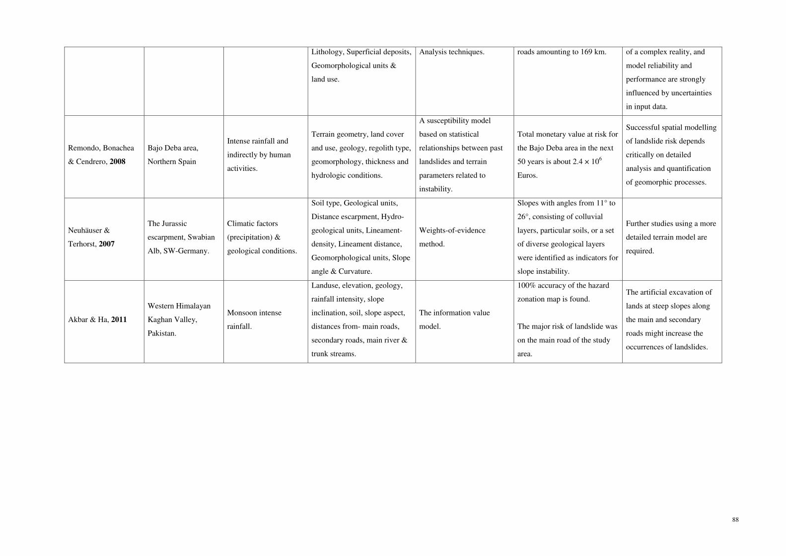
88
Lithology, Superficial deposits,
Geomorphological units &
land use.
Analysis techniques. roads amounting to 169 km. of a complex reality, and
model reliability and
performance are strongly
influenced by uncertainties
in input data.
Remondo, Bonachea
& Cendrero, 2008
Bajo Deba area,
Northern Spain
Intense rainfall and
indirectly by human
activities.
Terrain geometry, land cover
and use, geology, regolith type,
geomorphology, thickness and
hydrologic conditions.
A susceptibility model
based on statistical
relationships between past
landslides and terrain
parameters related to
instability.
Total monetary value at risk for
the Bajo Deba area in the next
50 years is about 2.4 × 10⁶
Euros.
Successful spatial modelling
of landslide risk depends
critically on detailed
analysis and quantification
of geomorphic processes.
Neuhäuser &
Terhorst, 2007
The Jurassic
escarpment, Swabian
Alb, SW-Germany.
Climatic factors
(precipitation) &
geological conditions.
Soil type, Geological units,
Distance escarpment, Hydro-
geological units, Lineament-
density, Lineament distance,
Geomorphological units, Slope
angle & Curvature.
Weights-of-evidence
method.
Slopes with angles from 11° to
26°, consisting of colluvial
layers, particular soils, or a set
of diverse geological layers
were identified as indicators for
slope instability.
Further studies using a more
detailed terrain model are
required.
Akbar & Ha, 2011
Western Himalayan
Kaghan Valley,
Pakistan.
Monsoon intense
rainfall.
Landuse, elevation, geology,
rainfall intensity, slope
inclination, soil, slope aspect,
distances from- main roads,
secondary roads, main river &
trunk streams.
The information value
model.
100% accuracy of the hazard
zonation map is found.
The major risk of landslide was
on the main road of the study
area.
The artificial excavation of
lands at steep slopes along
the main and secondary
roads might increase the
occurrences of landslides.
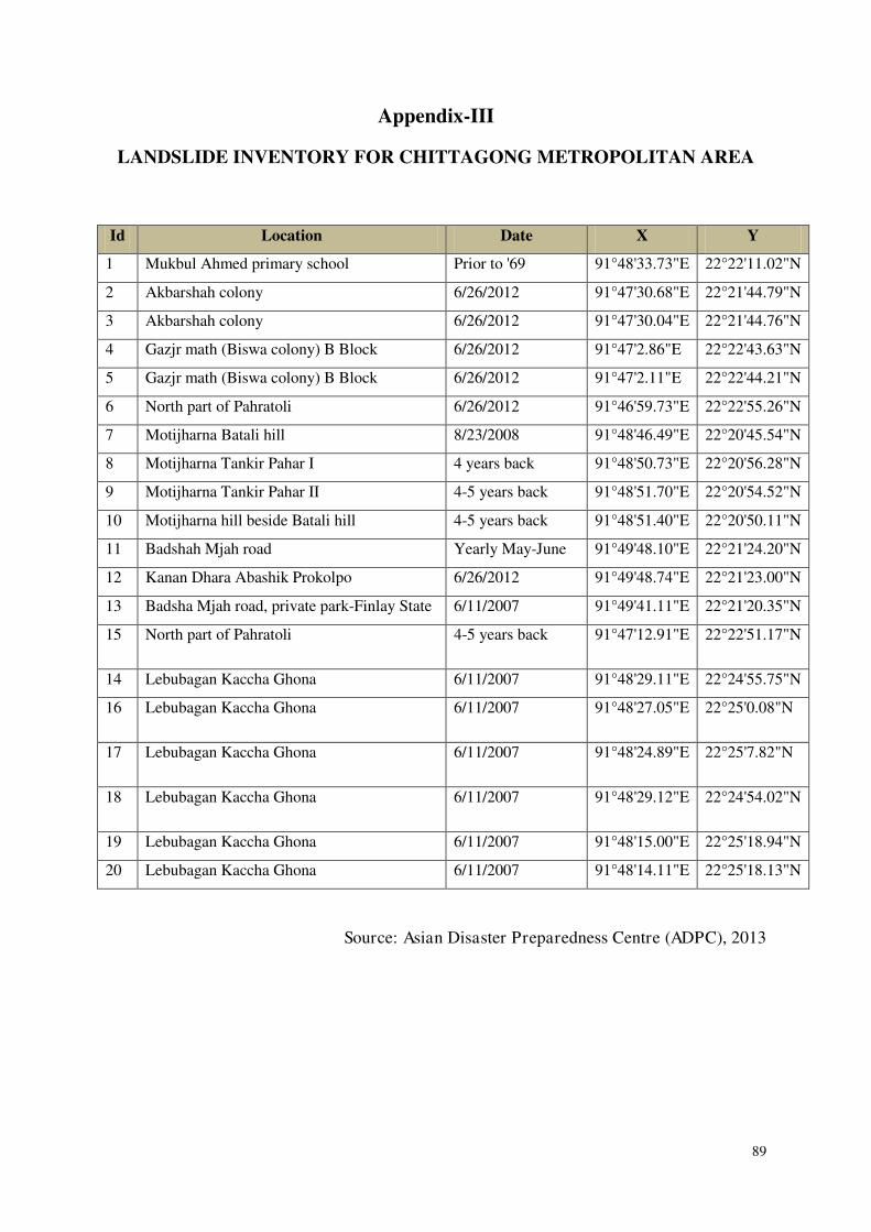
89
Appendix-III
LANDSLIDE INVENTORY FOR CHITTAGONG METROPOLITAN AREA
Id Location Date X Y
1 Mukbul Ahmed primary school Prior to '69 91°48'33.73"E 22°22'11.02"N
2 Akbarshah colony 6/26/2012 91°47'30.68"E 22°21'44.79"N
3 Akbarshah colony 6/26/2012 91°47'30.04"E 22°21'44.76"N
4 Gazjr math (Biswa colony) B Block 6/26/2012 91°47'2.86"E 22°22'43.63"N
5 Gazjr math (Biswa colony) B Block 6/26/2012 91°47'2.11"E 22°22'44.21"N
6 North part of Pahratoli 6/26/2012 91°46'59.73"E 22°22'55.26"N
7 Motijharna Batali hill 8/23/2008 91°48'46.49"E 22°20'45.54"N
8 Motijharna Tankir Pahar I 4 years back 91°48'50.73"E 22°20'56.28"N
9 Motijharna Tankir Pahar II 4-5 years back 91°48'51.70"E 22°20'54.52"N
10 Motijharna hill beside Batali hill 4-5 years back 91°48'51.40"E 22°20'50.11"N
11 Badshah Mjah road Yearly May-June 91°49'48.10"E 22°21'24.20"N
12 Kanan Dhara Abashik Prokolpo 6/26/2012 91°49'48.74"E 22°21'23.00"N
13 Badsha Mjah road, private park-Finlay State 6/11/2007 91°49'41.11"E 22°21'20.35"N
15 North part of Pahratoli 4-5 years back 91°47'12.91"E 22°22'51.17"N
14 Lebubagan Kaccha Ghona 6/11/2007 91°48'29.11"E 22°24'55.75"N
16 Lebubagan Kaccha Ghona 6/11/2007 91°48'27.05"E 22°25'0.08"N
17 Lebubagan Kaccha Ghona 6/11/2007 91°48'24.89"E 22°25'7.82"N
18 Lebubagan Kaccha Ghona 6/11/2007 91°48'29.12"E 22°24'54.02"N
19 Lebubagan Kaccha Ghona 6/11/2007 91°48'15.00"E 22°25'18.94"N
20 Lebubagan Kaccha Ghona 6/11/2007 91°48'14.11"E 22°25'18.13"N
Source: Asian Disaster Preparedness Centre (ADPC), 2013
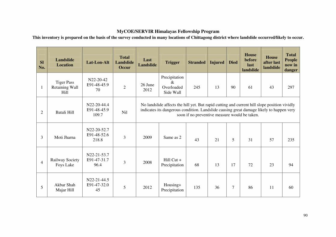
90
MyCOE/SERVIR Himalayas Fellowship Program
This inventory is prepared on the basis of the survey conducted in many locations of Chittagong district where landslide occurred/likely to occur.
Sl
No.
Landslide
Location
Lat-Lon-Alt
Total
Landslide
Occur
Last
Landslide
Trigger
Stranded
Injured
Died
House
before
last
landslide
House
after last
landslide
Total
People
now in
danger
1
Tiger Pass
Retaining Wall Hill
N22-20-42 E91-48-45.9
70
2
26 June
2012
Precipitation &
Overloaded Side Wall
245
13
90
61
43
297
2
Batali Hill
N22-20-44.4 E91-48-45.9
109.7
Nil
No landslide affects the hill yet. But rapid cutting and current hill slope position vividly indicates its dangerous condition. Landslide causing great damage likely to happen very
soon if no preventive measure would be taken.
3
Moti Jharna
N22-20-52.7 E91-48-52.6
218.8
3
2009
Same as 2
43
21
5
31
57
235
4
Railway Society
Foys Lake
N22-21-53.7 E91-47-31.7
96.4
3
2008
Hill Cut +
Precipitation
68
13
17
72
23
94
5
Akbar Shah Majar Hill
N22-21-44.5 E91-47-32.0
45
5
2012
Housing+
Precipitation
135
36
7
86
11
60
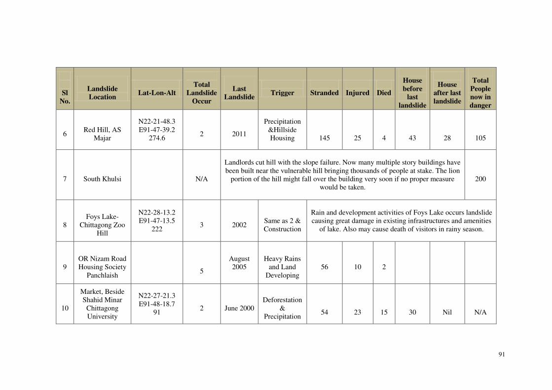
91
Sl
No.
Landslide
Location
Lat-Lon-Alt
Total
Landslide
Occur
Last
Landslide
Trigger
Stranded
Injured
Died
House
before
last
landslide
House
after last
landslide
Total
People
now in
danger
6
Red Hill, AS
Majar
N22-21-48.3 E91-47-39.2
274.6
2
2011
Precipitation &Hillside Housing
145
25
4
43
28
105
7
South Khulsi
N/A
Landlords cut hill with the slope failure. Now many multiple story buildings have been built near the vulnerable hill bringing thousands of people at stake. The lion
portion of the hill might fall over the building very soon if no proper measure would be taken.
200
8
Foys Lake-
Chittagong Zoo Hill
N22-28-13.2 E91-47-13.5
222
3
2002
Same as 2 & Construction
Rain and development activities of Foys Lake occurs landslide causing great damage in existing infrastructures and amenities
of lake. Also may cause death of visitors in rainy season.
9
OR Nizam Road Housing Society
Panchlaish
5
August 2005
Heavy Rains
and Land Developing
56
10
2
10
Market, Beside Shahid Minar
Chittagong University
N22-27-21.3 E91-48-18.7
91
2
June 2000
Deforestation
& Precipitation
54
23
15
30
Nil
N/A

92
Sl
No.
Landslide
Location
Lat-Lon-Alt
Total
Landslide
Occur
Last
Landslide
Trigger
Stranded
Injured
Died
No. of
Houses
before
last
landslide
No. of
Houses
after last
landslide
Total
People
now in
danger
11
Foys Lake
Observation Tower Hill
N22-22-06.8 E91-47-34.4
186.8
2
2011
Land Development
and Rain
105
20
10
26
Nil
N/A
12
Dr.Yunus
Bhaban Road Chittagong Univrsity
N22-28-23.0 E91-47-16.8
96
N/A
The connecting road between hostel area and academic building of Chittagong University is
in dangerous position because of aside steeper slope hill. If high precipitation occurs for several hours continuously after long period of no-rain the road network would be crumbled
due to landslide.
13
Shantinagar
Bayezid Bostami
3
October
2005
Rain and Housing
25
3
5
32
20
85
14
Nabinagar, Chittagong
N23-21-45.7 E90-44-78.8
September
2007
Monsoon
Rain
13
0
2
26
56
140
15
Forest Research
Institute Rest House Hill
N/A
No landslide yet but likely to occur because of rapid destruction of Bamboo and other tress
roots.
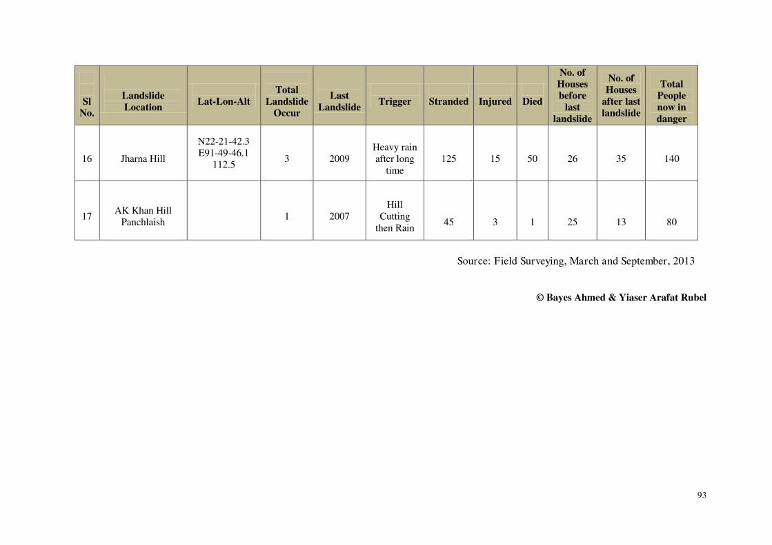
93
Sl
No.
Landslide
Location
Lat-Lon-Alt
Total
Landslide
Occur
Last
Landslide
Trigger
Stranded
Injured
Died
No. of
Houses
before
last
landslide
No. of
Houses
after last
landslide
Total
People
now in
danger
16
Jharna Hill
N22-21-42.3 E91-49-46.1
112.5
3
2009
Heavy rain after long
time
125
15
50
26
35
140
17
AK Khan Hill
Panchlaish
1
2007
Hill
Cutting then Rain
45
3
1
25
13
80
Source: Field Surveying, March and September, 2013
© Bayes Ahmed & Yiaser Arafat Rubel
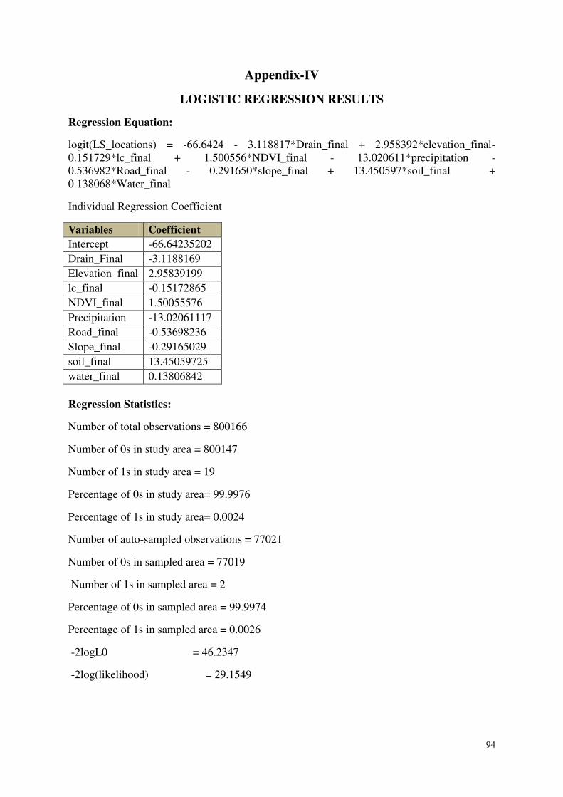
94
Appendix-IV
LOGISTIC REGRESSION RESULTS
Regression Equation:
logit(LS_locations) = -66.6424 - 3.118817*Drain_final + 2.958392*elevation_final-
0.151729*lc_final + 1.500556*NDVI_final - 13.020611*precipitation -
0.536982*Road_final - 0.291650*slope_final + 13.450597*soil_final +
0.138068*Water_final
Individual Regression Coefficient
Variables Coefficient
Intercept -66.64235202
Drain_Final -3.1188169
Elevation_final 2.95839199
lc_final -0.15172865
NDVI_final 1.50055576
Precipitation -13.02061117
Road_final -0.53698236
Slope_final -0.29165029
soil_final 13.45059725
water_final 0.13806842
Regression Statistics:
Number of total observations = 800166
Number of 0s in study area = 800147
Number of 1s in study area = 19
Percentage of 0s in study area= 99.9976
Percentage of 1s in study area= 0.0024
Number of auto-sampled observations = 77021
Number of 0s in sampled area = 77019
Number of 1s in sampled area = 2
Percentage of 0s in sampled area = 99.9974
Percentage of 1s in sampled area = 0.0026
-2logL0 = 46.2347
-2log(likelihood) = 29.1549
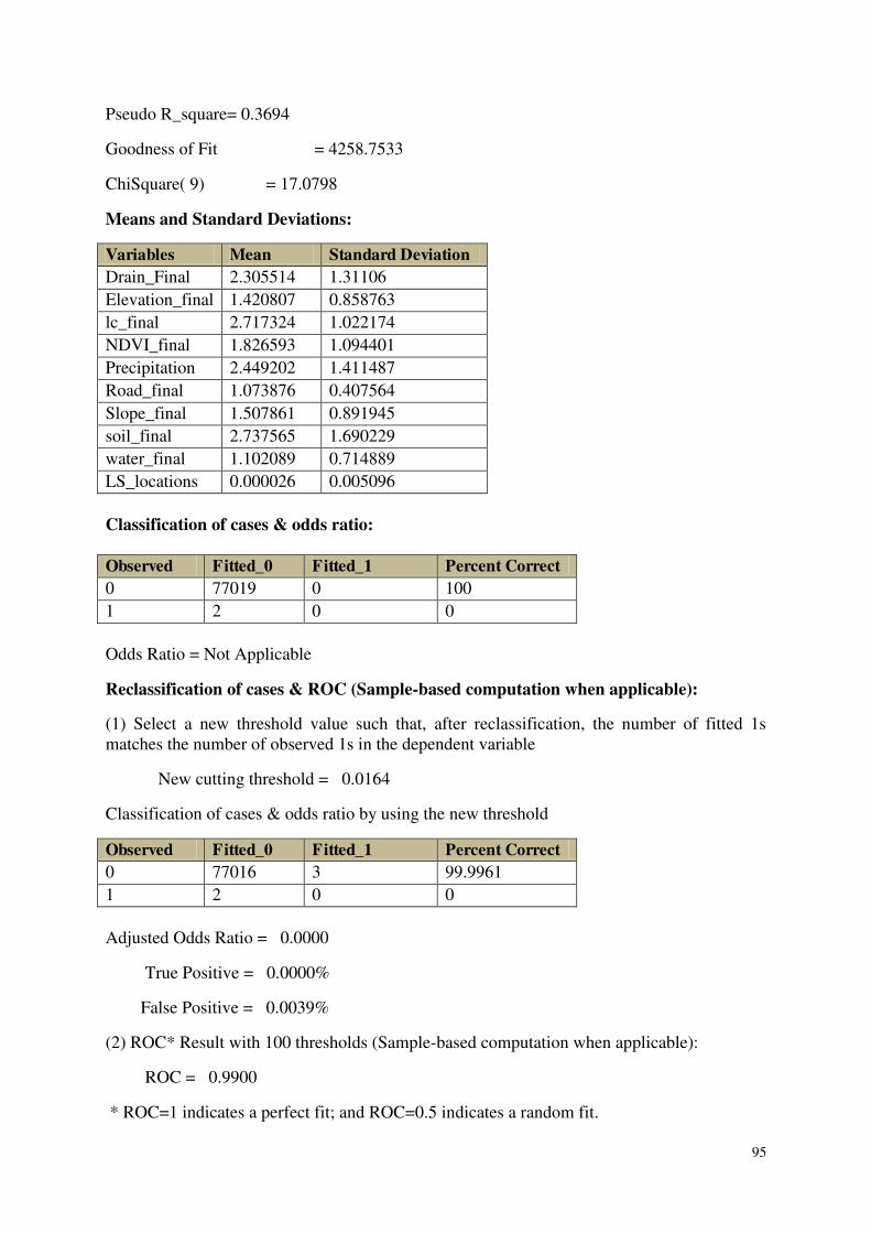
95
Pseudo R_square= 0.3694
Goodness of Fit = 4258.7533
ChiSquare( 9) = 17.0798
Means and Standard Deviations:
Variables Mean Standard Deviation
Drain_Final 2.305514 1.31106
Elevation_final 1.420807 0.858763
lc_final 2.717324 1.022174
NDVI_final 1.826593 1.094401
Precipitation 2.449202 1.411487
Road_final 1.073876 0.407564
Slope_final 1.507861 0.891945
soil_final 2.737565 1.690229
water_final 1.102089 0.714889
LS_locations 0.000026 0.005096
Classification of cases & odds ratio:
Observed Fitted_0 Fitted_1 Percent Correct
0 77019 0 100
1 2 0 0
Odds Ratio = Not Applicable
Reclassification of cases & ROC (Sample-based computation when applicable):
(1) Select a new threshold value such that, after reclassification, the number of fitted 1s
matches the number of observed 1s in the dependent variable
New cutting threshold = 0.0164
Classification of cases & odds ratio by using the new threshold
Observed Fitted_0 Fitted_1 Percent Correct
0 77016 3 99.9961
1 2 0 0
Adjusted Odds Ratio = 0.0000
True Positive = 0.0000%
False Positive = 0.0039%
(2) ROC* Result with 100 thresholds (Sample-based computation when applicable):
ROC = 0.9900
* ROC=1 indicates a perfect fit; and ROC=0.5 indicates a random fit.
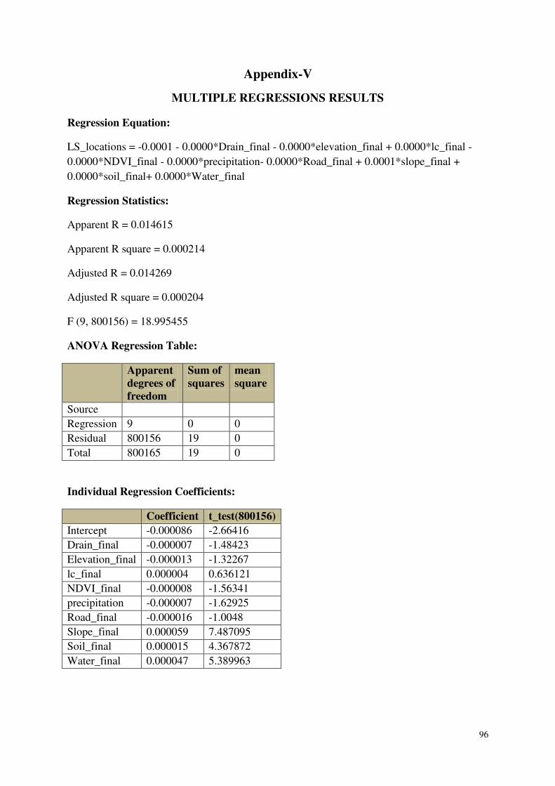
96
Appendix-V
MULTIPLE REGRESSIONS RESULTS
Regression Equation:
LS_locations = -0.0001 - 0.0000*Drain_final - 0.0000*elevation_final + 0.0000*lc_final -
0.0000*NDVI_final - 0.0000*precipitation- 0.0000*Road_final + 0.0001*slope_final +
0.0000*soil_final+ 0.0000*Water_final
Regression Statistics:
Apparent R = 0.014615
Apparent R square = 0.000214
Adjusted R = 0.014269
Adjusted R square = 0.000204
F (9, 800156) = 18.995455
ANOVA Regression Table:
Apparent
degrees of
freedom
Sum of
squares
mean
square
Source
Regression 9 0 0
Residual 800156 19 0
Total 800165 19 0
Individual Regression Coefficients:
Coefficient t_test(800156)
Intercept -0.000086 -2.66416
Drain_final -0.000007 -1.48423
Elevation_final -0.000013 -1.32267
lc_final 0.000004 0.636121
NDVI_final -0.000008 -1.56341
precipitation -0.000007 -1.62925
Road_final -0.000016 -1.0048
Slope_final 0.000059 7.487095
Soil_final 0.000015 4.367872
Water_final 0.000047 5.389963
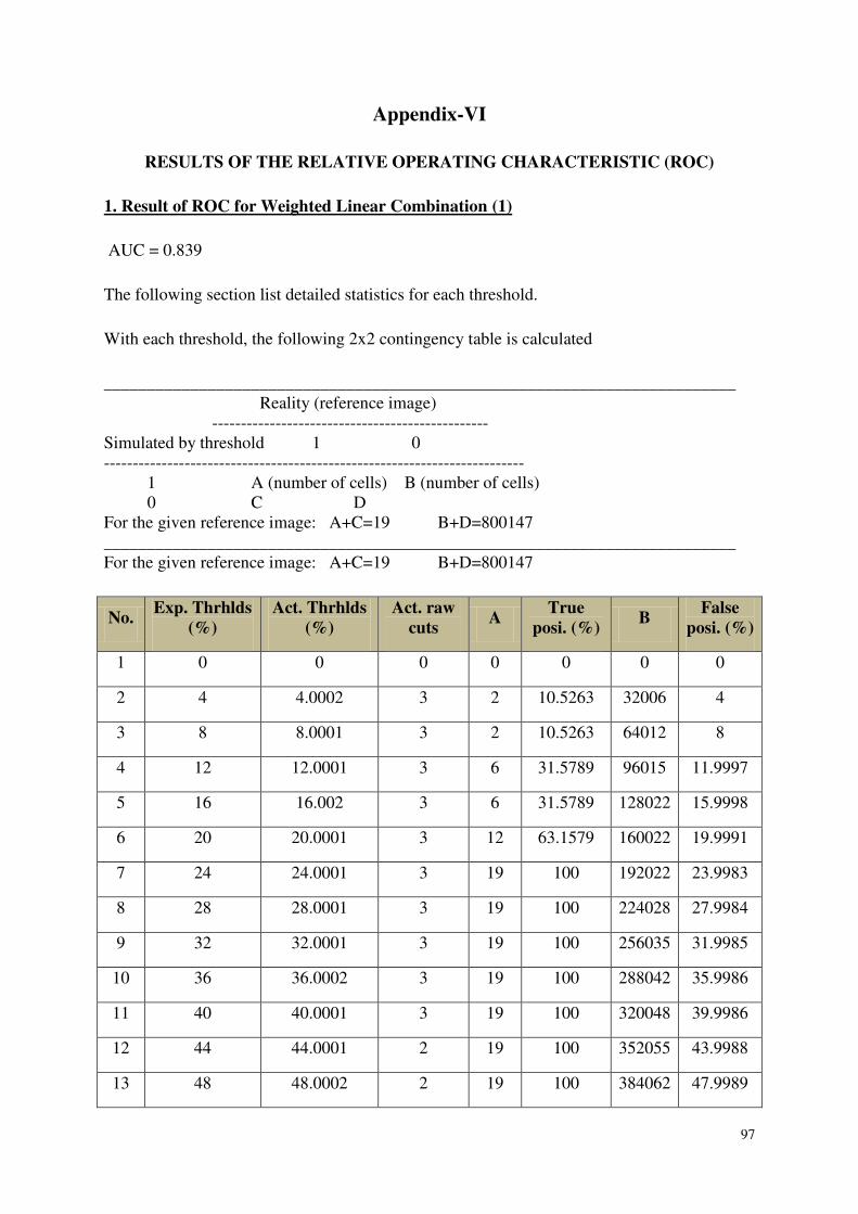
97
Appendix-VI
RESULTS OF THE RELATIVE OPERATING CHARACTERISTIC (ROC)
1. Result of ROC for Weighted Linear Combination (1)
AUC = 0.839
The following section list detailed statistics for each threshold.
With each threshold, the following 2x2 contingency table is calculated
_________________________________________________________________________
Reality (reference image)
------------------------------------------------
Simulated by threshold 1 0
-------------------------------------------------------------------------
1 A (number of cells) B (number of cells)
0 C D
For the given reference image: A+C=19 B+D=800147
_________________________________________________________________________
For the given reference image: A+C=19 B+D=800147
No. Exp. Thrhlds
(%)
Act. Thrhlds
(%)
Act. raw
cuts A
True
posi. (%) B
False
posi. (%)
1 0 0 0 0 0 0 0
2 4 4.0002 3 2 10.5263 32006 4
3 8 8.0001 3 2 10.5263 64012 8
4 12 12.0001 3 6 31.5789 96015 11.9997
5 16 16.002 3 6 31.5789 128022 15.9998
6 20 20.0001 3 12 63.1579 160022 19.9991
7 24 24.0001 3 19 100 192022 23.9983
8 28 28.0001 3 19 100 224028 27.9984
9 32 32.0001 3 19 100 256035 31.9985
10 36 36.0002 3 19 100 288042 35.9986
11 40 40.0001 3 19 100 320048 39.9986
12 44 44.0001 2 19 100 352055 43.9988
13 48 48.0002 2 19 100 384062 47.9989
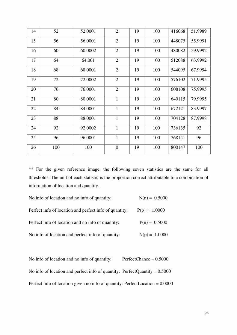
98
14 52 52.0001 2 19 100 416068 51.9989
15 56 56.0001 2 19 100 448075 55.9991
16 60 60.0002 2 19 100 480082 59.9992
17 64 64.001 2 19 100 512088 63.9992
18 68 68.0001 2 19 100 544095 67.9994
19 72 72.0002 2 19 100 576102 71.9995
20 76 76.0001 2 19 100 608108 75.9995
21 80 80.0001 1 19 100 640115 79.9995
22 84 84.0001 1 19 100 672121 83.9997
23 88 88.0001 1 19 100 704128 87.9998
24 92 92.0002 1 19 100 736135 92
25 96 96.0001 1 19 100 768141 96
26 100 100 0 19 100 800147 100
** For the given reference image, the following seven statistics are the same for all
thresholds. The unit of each statistic is the proportion correct attributable to a combination of
information of location and quantity.
No info of location and no info of quantity: N(n) = 0.5000
Perfect info of location and perfect info of quantity: P(p) = 1.0000
Perfect info of location and no info of quantity: P(n) = 0.5000
No info of location and perfect info of quantity: N(p) = 1.0000
No info of location and no info of quantity: PerfectChance = 0.5000
No info of location and perfect info of quantity: PerfectQuantity = 0.5000
Perfect info of location given no info of quantity: PerfectLocation = 0.0000

99
No. M(m) N(m) P(m) M(p) M(n)
1 1 1 1 1 0.5
2 0.96 0.96 0.96 1 0.5
3 0.92 0.92 0.92 1 0.5
4 0.88 0.88 0.88 1 0.5
5 0.84 0.84 0.84 1 0.5
6 0.8 0.8 0.8 1 0.5
7 0.76 0.76 0.76 1 0.5
8 0.72 0.72 0.72 1 0.5
9 0.68 0.68 0.68 1 0.5
10 0.64 0.64 0.64 1 0.5
11 0.6 0.6 0.6 1 0.5
12 0.56 0.56 0.56 1 0.5
13 0.54 0.54 0.54 1 0.5
14 0.48 0.48 0.48 1 0.5
15 0.44 0.44 0.44 1 0.5
16 0.4 0.4 0.4 1 0.5
17 0.36 0.36 0.36 1 0.5
18 0.32 0.32 0.32 1 0.5
19 0.28 0.28 0.28 1 0.5
20 0.24 0.24 0.24 1 0.5
21 0.2 0.2 0.2 1 0.5
22 0.16 0.16 0.16 1 0.5
23 0.12 0.12 0.12 1 0.5
24 0.08 0.08 0.5 1 0.5
25 0.04 0.04 0.04 1 0.5
26 0 0 0 1 0.5
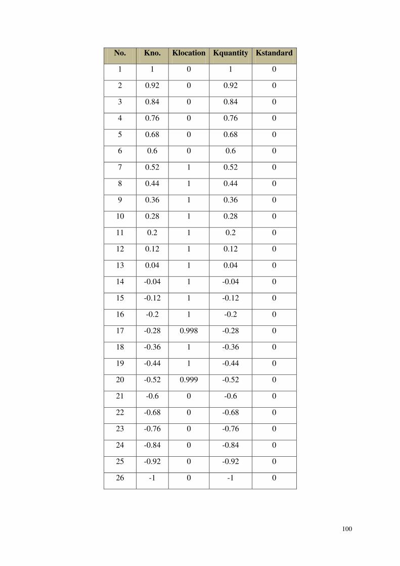
100
No. Kno. Klocation Kquantity Kstandard
1 1 0 1 0
2 0.92 0 0.92 0
3 0.84 0 0.84 0
4 0.76 0 0.76 0
5 0.68 0 0.68 0
6 0.6 0 0.6 0
7 0.52 1 0.52 0
8 0.44 1 0.44 0
9 0.36 1 0.36 0
10 0.28 1 0.28 0
11 0.2 1 0.2 0
12 0.12 1 0.12 0
13 0.04 1 0.04 0
14 -0.04 1 -0.04 0
15 -0.12 1 -0.12 0
16 -0.2 1 -0.2 0
17 -0.28 0.998 -0.28 0
18 -0.36 1 -0.36 0
19 -0.44 1 -0.44 0
20 -0.52 0.999 -0.52 0
21 -0.6 0 -0.6 0
22 -0.68 0 -0.68 0
23 -0.76 0 -0.76 0
24 -0.84 0 -0.84 0
25 -0.92 0 -0.92 0
26 -1 0 -1 0
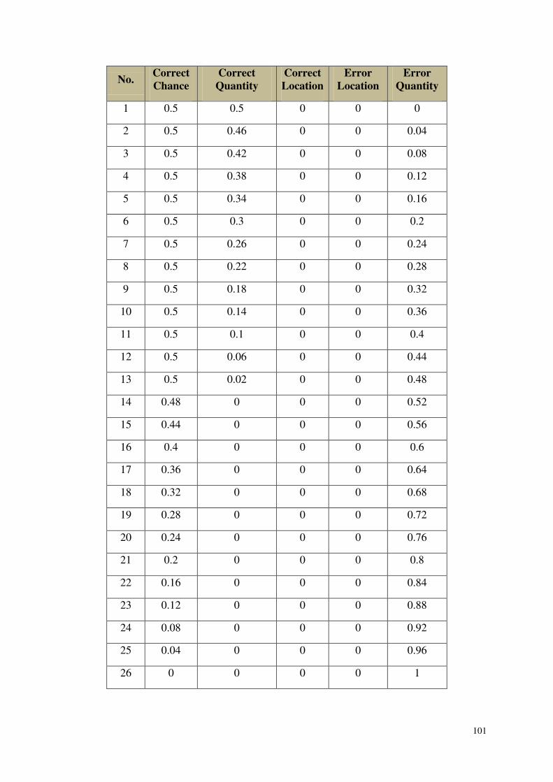
101
No. Correct
Chance
Correct
Quantity
Correct
Location
Error
Location
Error
Quantity
1 0.5 0.5 0 0 0
2 0.5 0.46 0 0 0.04
3 0.5 0.42 0 0 0.08
4 0.5 0.38 0 0 0.12
5 0.5 0.34 0 0 0.16
6 0.5 0.3 0 0 0.2
7 0.5 0.26 0 0 0.24
8 0.5 0.22 0 0 0.28
9 0.5 0.18 0 0 0.32
10 0.5 0.14 0 0 0.36
11 0.5 0.1 0 0 0.4
12 0.5 0.06 0 0 0.44
13 0.5 0.02 0 0 0.48
14 0.48 0 0 0 0.52
15 0.44 0 0 0 0.56
16 0.4 0 0 0 0.6
17 0.36 0 0 0 0.64
18 0.32 0 0 0 0.68
19 0.28 0 0 0 0.72
20 0.24 0 0 0 0.76
21 0.2 0 0 0 0.8
22 0.16 0 0 0 0.84
23 0.12 0 0 0 0.88
24 0.08 0 0 0 0.92
25 0.04 0 0 0 0.96
26 0 0 0 0 1
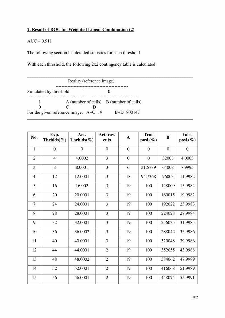
102
2. Result of ROC for Weighted Linear Combination (2)
AUC = 0.911
The following section list detailed statistics for each threshold.
With each threshold, the following 2x2 contingency table is calculated
_________________________________________________________________________
Reality (reference image)
------------------------------------------------
Simulated by threshold 1 0
-------------------------------------------------------------------------
1 A (number of cells) B (number of cells)
0 C D
For the given reference image: A+C=19 B+D=800147
_________________________________________________________________________
No. Exp.
Thrhlds(%)
Act.
Thrhlds(%)
Act. raw
cuts A
True
posi.(%) B
False
posi.(%)
1 0 0 0 0 0 0 0
2 4 4.0002 3 0 0 32008 4.0003
3 8 8.0001 3 6 31.5789 64008 7.9995
4 12 12.0001 3 18 94.7368 96003 11.9982
5 16 16.002 3 19 100 128009 15.9982
6 20 20.0001 3 19 100 160015 19.9982
7 24 24.0001 3 19 100 192022 23.9983
8 28 28.0001 3 19 100 224028 27.9984
9 32 32.0001 3 19 100 256035 31.9985
10 36 36.0002 3 19 100 288042 35.9986
11 40 40.0001 3 19 100 320048 39.9986
12 44 44.0001 2 19 100 352055 43.9988
13 48 48.0002 2 19 100 384062 47.9989
14 52 52.0001 2 19 100 416068 51.9989
15 56 56.0001 2 19 100 448075 55.9991
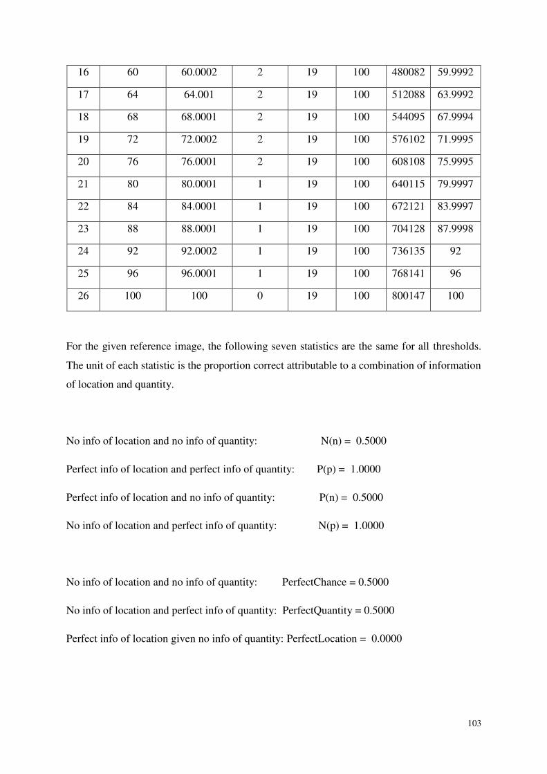
103
16 60 60.0002 2 19 100 480082 59.9992
17 64 64.001 2 19 100 512088 63.9992
18 68 68.0001 2 19 100 544095 67.9994
19 72 72.0002 2 19 100 576102 71.9995
20 76 76.0001 2 19 100 608108 75.9995
21 80 80.0001 1 19 100 640115 79.9997
22 84 84.0001 1 19 100 672121 83.9997
23 88 88.0001 1 19 100 704128 87.9998
24 92 92.0002 1 19 100 736135 92
25 96 96.0001 1 19 100 768141 96
26 100 100 0 19 100 800147 100
For the given reference image, the following seven statistics are the same for all thresholds.
The unit of each statistic is the proportion correct attributable to a combination of information
of location and quantity.
No info of location and no info of quantity: N(n) = 0.5000
Perfect info of location and perfect info of quantity: P(p) = 1.0000
Perfect info of location and no info of quantity: P(n) = 0.5000
No info of location and perfect info of quantity: N(p) = 1.0000
No info of location and no info of quantity: PerfectChance = 0.5000
No info of location and perfect info of quantity: PerfectQuantity = 0.5000
Perfect info of location given no info of quantity: PerfectLocation = 0.0000
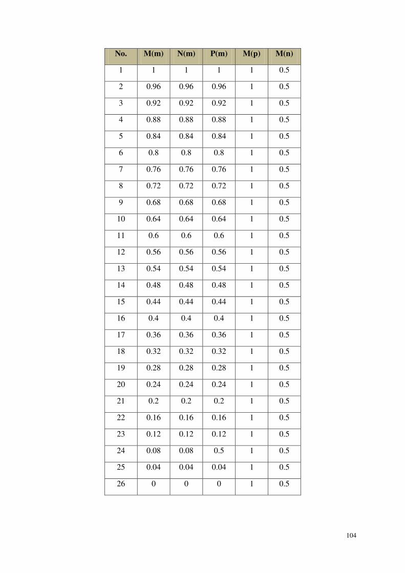
104
No. M(m) N(m) P(m) M(p) M(n)
1 1 1 1 1 0.5
2 0.96 0.96 0.96 1 0.5
3 0.92 0.92 0.92 1 0.5
4 0.88 0.88 0.88 1 0.5
5 0.84 0.84 0.84 1 0.5
6 0.8 0.8 0.8 1 0.5
7 0.76 0.76 0.76 1 0.5
8 0.72 0.72 0.72 1 0.5
9 0.68 0.68 0.68 1 0.5
10 0.64 0.64 0.64 1 0.5
11 0.6 0.6 0.6 1 0.5
12 0.56 0.56 0.56 1 0.5
13 0.54 0.54 0.54 1 0.5
14 0.48 0.48 0.48 1 0.5
15 0.44 0.44 0.44 1 0.5
16 0.4 0.4 0.4 1 0.5
17 0.36 0.36 0.36 1 0.5
18 0.32 0.32 0.32 1 0.5
19 0.28 0.28 0.28 1 0.5
20 0.24 0.24 0.24 1 0.5
21 0.2 0.2 0.2 1 0.5
22 0.16 0.16 0.16 1 0.5
23 0.12 0.12 0.12 1 0.5
24 0.08 0.08 0.5 1 0.5
25 0.04 0.04 0.04 1 0.5
26 0 0 0 1 0.5
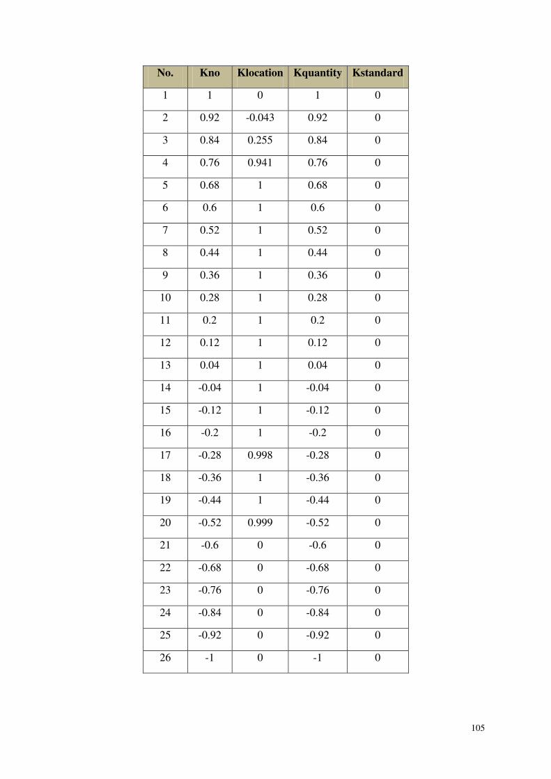
105
No. Kno Klocation Kquantity Kstandard
1 1 0 1 0
2 0.92 -0.043 0.92 0
3 0.84 0.255 0.84 0
4 0.76 0.941 0.76 0
5 0.68 1 0.68 0
6 0.6 1 0.6 0
7 0.52 1 0.52 0
8 0.44 1 0.44 0
9 0.36 1 0.36 0
10 0.28 1 0.28 0
11 0.2 1 0.2 0
12 0.12 1 0.12 0
13 0.04 1 0.04 0
14 -0.04 1 -0.04 0
15 -0.12 1 -0.12 0
16 -0.2 1 -0.2 0
17 -0.28 0.998 -0.28 0
18 -0.36 1 -0.36 0
19 -0.44 1 -0.44 0
20 -0.52 0.999 -0.52 0
21 -0.6 0 -0.6 0
22 -0.68 0 -0.68 0
23 -0.76 0 -0.76 0
24 -0.84 0 -0.84 0
25 -0.92 0 -0.92 0
26 -1 0 -1 0
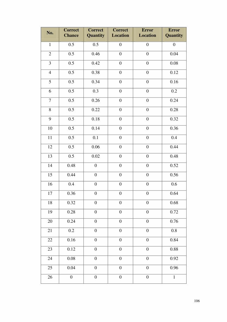
106
No. Correct
Chance
Correct
Quantity
Correct
Location
Error
Location
Error
Quantity
1 0.5 0.5 0 0 0
2 0.5 0.46 0 0 0.04
3 0.5 0.42 0 0 0.08
4 0.5 0.38 0 0 0.12
5 0.5 0.34 0 0 0.16
6 0.5 0.3 0 0 0.2
7 0.5 0.26 0 0 0.24
8 0.5 0.22 0 0 0.28
9 0.5 0.18 0 0 0.32
10 0.5 0.14 0 0 0.36
11 0.5 0.1 0 0 0.4
12 0.5 0.06 0 0 0.44
13 0.5 0.02 0 0 0.48
14 0.48 0 0 0 0.52
15 0.44 0 0 0 0.56
16 0.4 0 0 0 0.6
17 0.36 0 0 0 0.64
18 0.32 0 0 0 0.68
19 0.28 0 0 0 0.72
20 0.24 0 0 0 0.76
21 0.2 0 0 0 0.8
22 0.16 0 0 0 0.84
23 0.12 0 0 0 0.88
24 0.08 0 0 0 0.92
25 0.04 0 0 0 0.96
26 0 0 0 0 1
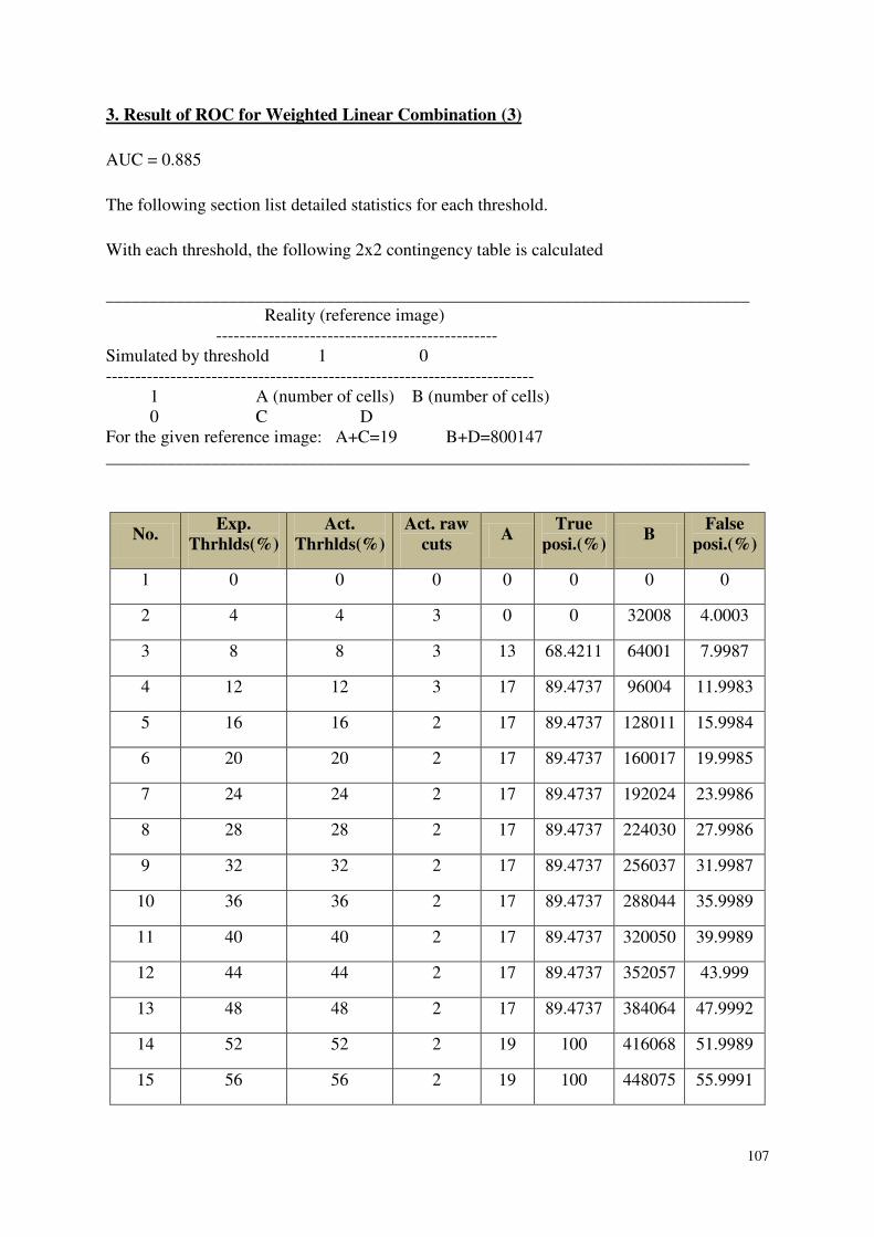
107
3. Result of ROC for Weighted Linear Combination (3)
AUC = 0.885
The following section list detailed statistics for each threshold.
With each threshold, the following 2x2 contingency table is calculated
_________________________________________________________________________
Reality (reference image)
------------------------------------------------
Simulated by threshold 1 0
-------------------------------------------------------------------------
1 A (number of cells) B (number of cells)
0 C D
For the given reference image: A+C=19 B+D=800147
_________________________________________________________________________
No. Exp.
Thrhlds(%)
Act.
Thrhlds(%)
Act. raw
cuts A
True
posi.(%) B
False
posi.(%)
1 0 0 0 0 0 0 0
2 4 4 3 0 0 32008 4.0003
3 8 8 3 13 68.4211 64001 7.9987
4 12 12 3 17 89.4737 96004 11.9983
5 16 16 2 17 89.4737 128011 15.9984
6 20 20 2 17 89.4737 160017 19.9985
7 24 24 2 17 89.4737 192024 23.9986
8 28 28 2 17 89.4737 224030 27.9986
9 32 32 2 17 89.4737 256037 31.9987
10 36 36 2 17 89.4737 288044 35.9989
11 40 40 2 17 89.4737 320050 39.9989
12 44 44 2 17 89.4737 352057 43.999
13 48 48 2 17 89.4737 384064 47.9992
14 52 52 2 19 100 416068 51.9989
15 56 56 2 19 100 448075 55.9991
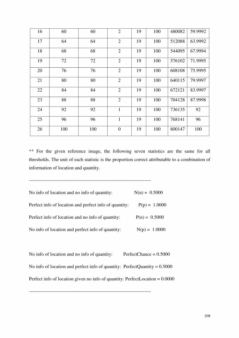
108
16 60 60 2 19 100 480082 59.9992
17 64 64 2 19 100 512088 63.9992
18 68 68 2 19 100 544095 67.9994
19 72 72 2 19 100 576102 71.9995
20 76 76 2 19 100 608108 75.9995
21 80 80 2 19 100 640115 79.9997
22 84 84 2 19 100 672121 83.9997
23 88 88 2 19 100 704128 87.9998
24 92 92 1 19 100 736135 92
25 96 96 1 19 100 768141 96
26 100 100 0 19 100 800147 100
** For the given reference image, the following seven statistics are the same for all
thresholds. The unit of each statistic is the proportion correct attributable to a combination of
information of location and quantity.
----------------------------------------------------------------------------
No info of location and no info of quantity: N(n) = 0.5000
Perfect info of location and perfect info of quantity: P(p) = 1.0000
Perfect info of location and no info of quantity: P(n) = 0.5000
No info of location and perfect info of quantity: N(p) = 1.0000
No info of location and no info of quantity: PerfectChance = 0.5000
No info of location and perfect info of quantity: PerfectQuantity = 0.5000
Perfect info of location given no info of quantity: PerfectLocation = 0.0000
----------------------------------------------------------------------------

109
No. M(m) N(m) P(m) M(p) M(n)
1 1 1 1 1 0.5
2 0.96 0.96 0.96 1 0.5
3 0.92 0.92 0.92 1 0.5
4 0.88 0.88 0.88 1 0.5
5 0.84 0.84 0.84 1 0.5
6 0.8 0.8 0.8 1 0.5
7 0.76 0.76 0.76 1 0.5
8 0.72 0.72 0.72 1 0.5
9 0.68 0.68 0.68 1 0.5
10 0.64 0.64 0.64 1 0.5
11 0.6 0.6 0.6 1 0.5
12 0.56 0.56 0.56 1 0.5
13 0.52 0.52 0.52 1 0.5
14 0.48 0.48 0.48 1 0.5
15 0.44 0.44 0.44 1 0.5
16 0.4 0.4 0.4 1 0.5
17 0.36 0.36 0.36 1 0.5
18 0.32 0.32 0.32 1 0.5
19 0.28 0.28 0.28 1 0.5
20 0.24 0.24 0.24 1 0.5
21 0.2 0.2 0.2 1 0.5
22 0.16 0.16 0.16 1 0.5
23 0.12 0.12 0.12 1 0.5
24 0.08 0.08 0.08 1 0.5
25 0.04 0.04 0.04 1 0.5
26 0 0 0 1 0.5
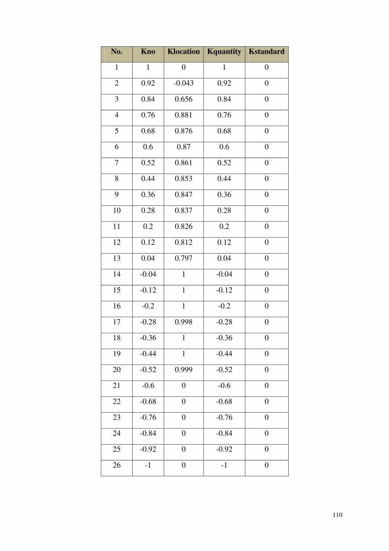
110
No. Kno Klocation Kquantity Kstandard
1 1 0 1 0
2 0.92 -0.043 0.92 0
3 0.84 0.656 0.84 0
4 0.76 0.881 0.76 0
5 0.68 0.876 0.68 0
6 0.6 0.87 0.6 0
7 0.52 0.861 0.52 0
8 0.44 0.853 0.44 0
9 0.36 0.847 0.36 0
10 0.28 0.837 0.28 0
11 0.2 0.826 0.2 0
12 0.12 0.812 0.12 0
13 0.04 0.797 0.04 0
14 -0.04 1 -0.04 0
15 -0.12 1 -0.12 0
16 -0.2 1 -0.2 0
17 -0.28 0.998 -0.28 0
18 -0.36 1 -0.36 0
19 -0.44 1 -0.44 0
20 -0.52 0.999 -0.52 0
21 -0.6 0 -0.6 0
22 -0.68 0 -0.68 0
23 -0.76 0 -0.76 0
24 -0.84 0 -0.84 0
25 -0.92 0 -0.92 0
26 -1 0 -1 0
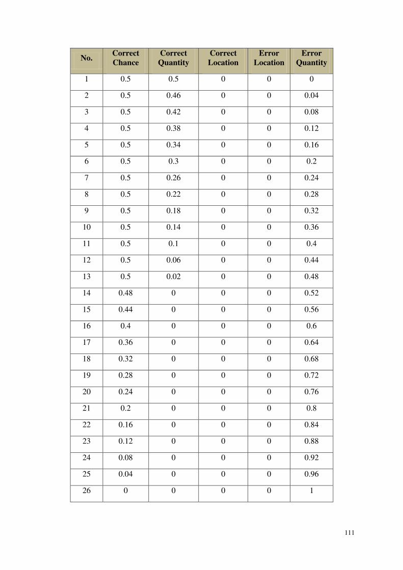
111
No. Correct
Chance
Correct
Quantity
Correct
Location
Error
Location
Error
Quantity
1 0.5 0.5 0 0 0
2 0.5 0.46 0 0 0.04
3 0.5 0.42 0 0 0.08
4 0.5 0.38 0 0 0.12
5 0.5 0.34 0 0 0.16
6 0.5 0.3 0 0 0.2
7 0.5 0.26 0 0 0.24
8 0.5 0.22 0 0 0.28
9 0.5 0.18 0 0 0.32
10 0.5 0.14 0 0 0.36
11 0.5 0.1 0 0 0.4
12 0.5 0.06 0 0 0.44
13 0.5 0.02 0 0 0.48
14 0.48 0 0 0 0.52
15 0.44 0 0 0 0.56
16 0.4 0 0 0 0.6
17 0.36 0 0 0 0.64
18 0.32 0 0 0 0.68
19 0.28 0 0 0 0.72
20 0.24 0 0 0 0.76
21 0.2 0 0 0 0.8
22 0.16 0 0 0 0.84
23 0.12 0 0 0 0.88
24 0.08 0 0 0 0.92
25 0.04 0 0 0 0.96
26 0 0 0 0 1
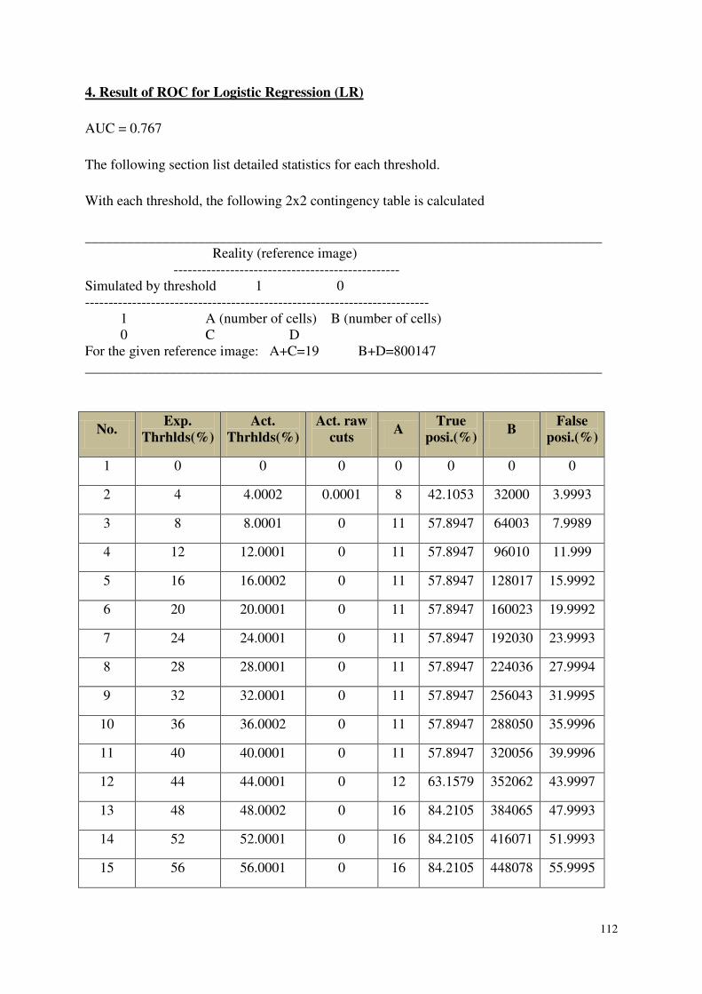
112
4. Result of ROC for Logistic Regression (LR)
AUC = 0.767
The following section list detailed statistics for each threshold.
With each threshold, the following 2x2 contingency table is calculated
_________________________________________________________________________
Reality (reference image)
------------------------------------------------
Simulated by threshold 1 0
-------------------------------------------------------------------------
1 A (number of cells) B (number of cells)
0 C D
For the given reference image: A+C=19 B+D=800147
_________________________________________________________________________
No. Exp.
Thrhlds(%)
Act.
Thrhlds(%)
Act. raw
cuts A
True
posi.(%) B
False
posi.(%)
1 0 0 0 0 0 0 0
2 4 4.0002 0.0001 8 42.1053 32000 3.9993
3 8 8.0001 0 11 57.8947 64003 7.9989
4 12 12.0001 0 11 57.8947 96010 11.999
5 16 16.0002 0 11 57.8947 128017 15.9992
6 20 20.0001 0 11 57.8947 160023 19.9992
7 24 24.0001 0 11 57.8947 192030 23.9993
8 28 28.0001 0 11 57.8947 224036 27.9994
9 32 32.0001 0 11 57.8947 256043 31.9995
10 36 36.0002 0 11 57.8947 288050 35.9996
11 40 40.0001 0 11 57.8947 320056 39.9996
12 44 44.0001 0 12 63.1579 352062 43.9997
13 48 48.0002 0 16 84.2105 384065 47.9993
14 52 52.0001 0 16 84.2105 416071 51.9993
15 56 56.0001 0 16 84.2105 448078 55.9995
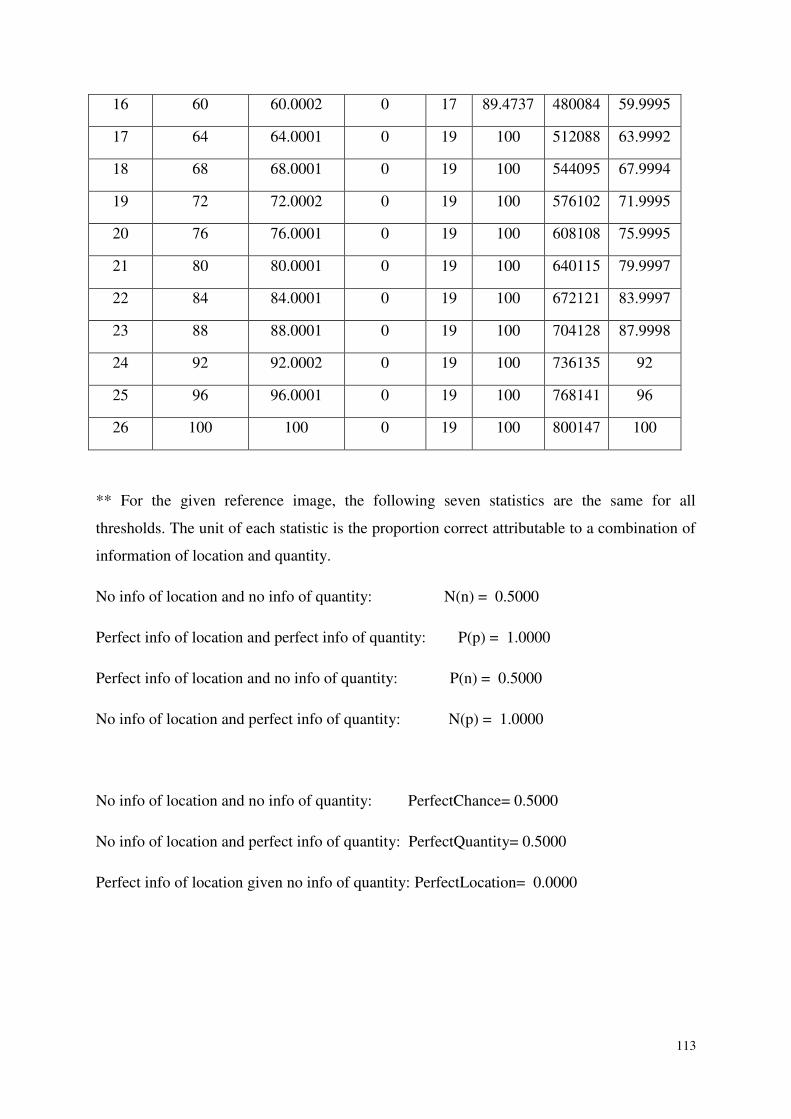
113
16 60 60.0002 0 17 89.4737 480084 59.9995
17 64 64.0001 0 19 100 512088 63.9992
18 68 68.0001 0 19 100 544095 67.9994
19 72 72.0002 0 19 100 576102 71.9995
20 76 76.0001 0 19 100 608108 75.9995
21 80 80.0001 0 19 100 640115 79.9997
22 84 84.0001 0 19 100 672121 83.9997
23 88 88.0001 0 19 100 704128 87.9998
24 92 92.0002 0 19 100 736135 92
25 96 96.0001 0 19 100 768141 96
26 100 100 0 19 100 800147 100
** For the given reference image, the following seven statistics are the same for all
thresholds. The unit of each statistic is the proportion correct attributable to a combination of
information of location and quantity.
No info of location and no info of quantity: N(n) = 0.5000
Perfect info of location and perfect info of quantity: P(p) = 1.0000
Perfect info of location and no info of quantity: P(n) = 0.5000
No info of location and perfect info of quantity: N(p) = 1.0000
No info of location and no info of quantity: PerfectChance= 0.5000
No info of location and perfect info of quantity: PerfectQuantity= 0.5000
Perfect info of location given no info of quantity: PerfectLocation= 0.0000
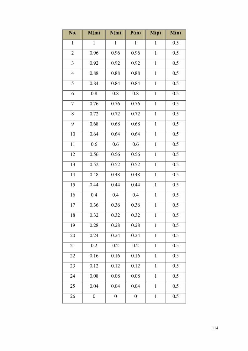
114
No. M(m) N(m) P(m) M(p) M(n)
1 1 1 1 1 0.5
2 0.96 0.96 0.96 1 0.5
3 0.92 0.92 0.92 1 0.5
4 0.88 0.88 0.88 1 0.5
5 0.84 0.84 0.84 1 0.5
6 0.8 0.8 0.8 1 0.5
7 0.76 0.76 0.76 1 0.5
8 0.72 0.72 0.72 1 0.5
9 0.68 0.68 0.68 1 0.5
10 0.64 0.64 0.64 1 0.5
11 0.6 0.6 0.6 1 0.5
12 0.56 0.56 0.56 1 0.5
13 0.52 0.52 0.52 1 0.5
14 0.48 0.48 0.48 1 0.5
15 0.44 0.44 0.44 1 0.5
16 0.4 0.4 0.4 1 0.5
17 0.36 0.36 0.36 1 0.5
18 0.32 0.32 0.32 1 0.5
19 0.28 0.28 0.28 1 0.5
20 0.24 0.24 0.24 1 0.5
21 0.2 0.2 0.2 1 0.5
22 0.16 0.16 0.16 1 0.5
23 0.12 0.12 0.12 1 0.5
24 0.08 0.08 0.08 1 0.5
25 0.04 0.04 0.04 1 0.5
26 0 0 0 1 0.5
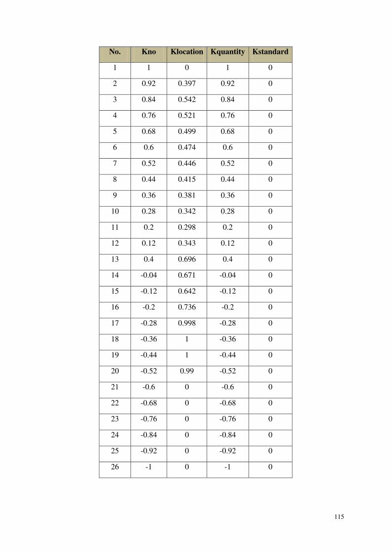
115
No. Kno Klocation Kquantity Kstandard
1 1 0 1 0
2 0.92 0.397 0.92 0
3 0.84 0.542 0.84 0
4 0.76 0.521 0.76 0
5 0.68 0.499 0.68 0
6 0.6 0.474 0.6 0
7 0.52 0.446 0.52 0
8 0.44 0.415 0.44 0
9 0.36 0.381 0.36 0
10 0.28 0.342 0.28 0
11 0.2 0.298 0.2 0
12 0.12 0.343 0.12 0
13 0.4 0.696 0.4 0
14 -0.04 0.671 -0.04 0
15 -0.12 0.642 -0.12 0
16 -0.2 0.736 -0.2 0
17 -0.28 0.998 -0.28 0
18 -0.36 1 -0.36 0
19 -0.44 1 -0.44 0
20 -0.52 0.99 -0.52 0
21 -0.6 0 -0.6 0
22 -0.68 0 -0.68 0
23 -0.76 0 -0.76 0
24 -0.84 0 -0.84 0
25 -0.92 0 -0.92 0
26 -1 0 -1 0
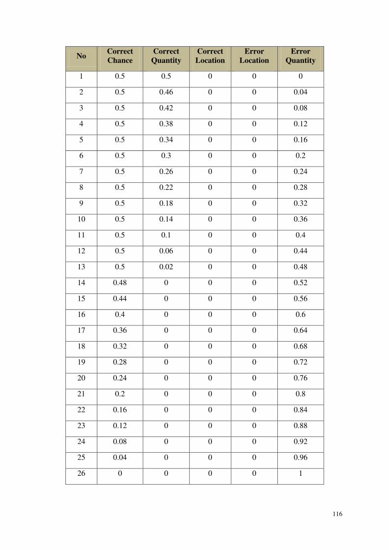
116
No Correct
Chance
Correct
Quantity
Correct
Location
Error
Location
Error
Quantity
1 0.5 0.5 0 0 0
2 0.5 0.46 0 0 0.04
3 0.5 0.42 0 0 0.08
4 0.5 0.38 0 0 0.12
5 0.5 0.34 0 0 0.16
6 0.5 0.3 0 0 0.2
7 0.5 0.26 0 0 0.24
8 0.5 0.22 0 0 0.28
9 0.5 0.18 0 0 0.32
10 0.5 0.14 0 0 0.36
11 0.5 0.1 0 0 0.4
12 0.5 0.06 0 0 0.44
13 0.5 0.02 0 0 0.48
14 0.48 0 0 0 0.52
15 0.44 0 0 0 0.56
16 0.4 0 0 0 0.6
17 0.36 0 0 0 0.64
18 0.32 0 0 0 0.68
19 0.28 0 0 0 0.72
20 0.24 0 0 0 0.76
21 0.2 0 0 0 0.8
22 0.16 0 0 0 0.84
23 0.12 0 0 0 0.88
24 0.08 0 0 0 0.92
25 0.04 0 0 0 0.96
26 0 0 0 0 1
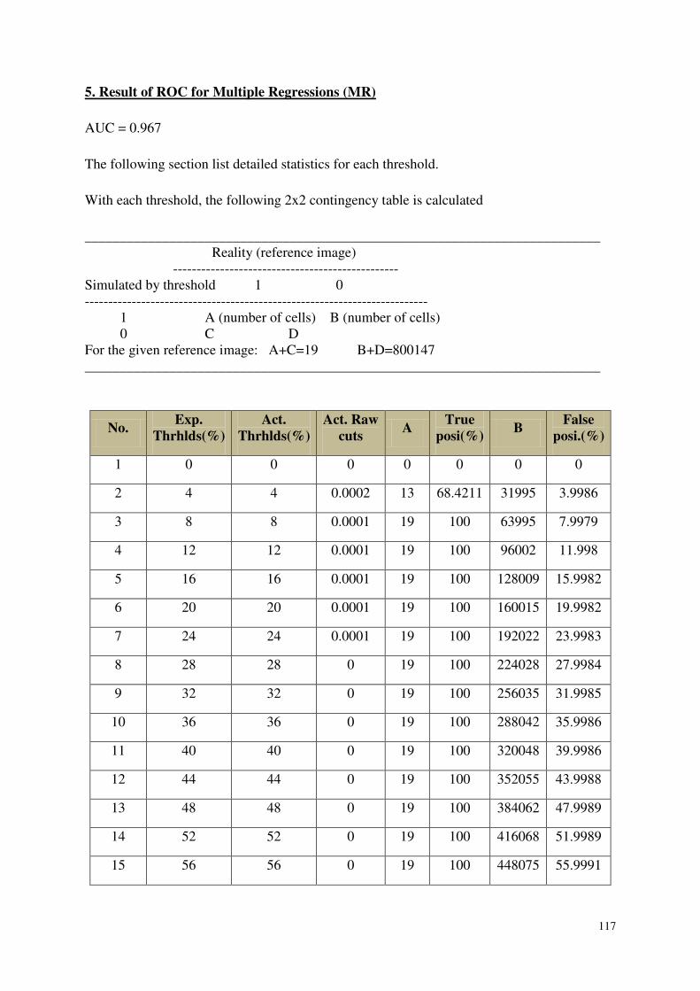
117
5. Result of ROC for Multiple Regressions (MR)
AUC = 0.967
The following section list detailed statistics for each threshold.
With each threshold, the following 2x2 contingency table is calculated
_________________________________________________________________________
Reality (reference image)
------------------------------------------------
Simulated by threshold 1 0
-------------------------------------------------------------------------
1 A (number of cells) B (number of cells)
0 C D
For the given reference image: A+C=19 B+D=800147
_________________________________________________________________________
No. Exp.
Thrhlds(%)
Act.
Thrhlds(%)
Act. Raw
cuts A
True
posi(%) B
False
posi.(%)
1 0 0 0 0 0 0 0
2 4 4 0.0002 13 68.4211 31995 3.9986
3 8 8 0.0001 19 100 63995 7.9979
4 12 12 0.0001 19 100 96002 11.998
5 16 16 0.0001 19 100 128009 15.9982
6 20 20 0.0001 19 100 160015 19.9982
7 24 24 0.0001 19 100 192022 23.9983
8 28 28 0 19 100 224028 27.9984
9 32 32 0 19 100 256035 31.9985
10 36 36 0 19 100 288042 35.9986
11 40 40 0 19 100 320048 39.9986
12 44 44 0 19 100 352055 43.9988
13 48 48 0 19 100 384062 47.9989
14 52 52 0 19 100 416068 51.9989
15 56 56 0 19 100 448075 55.9991
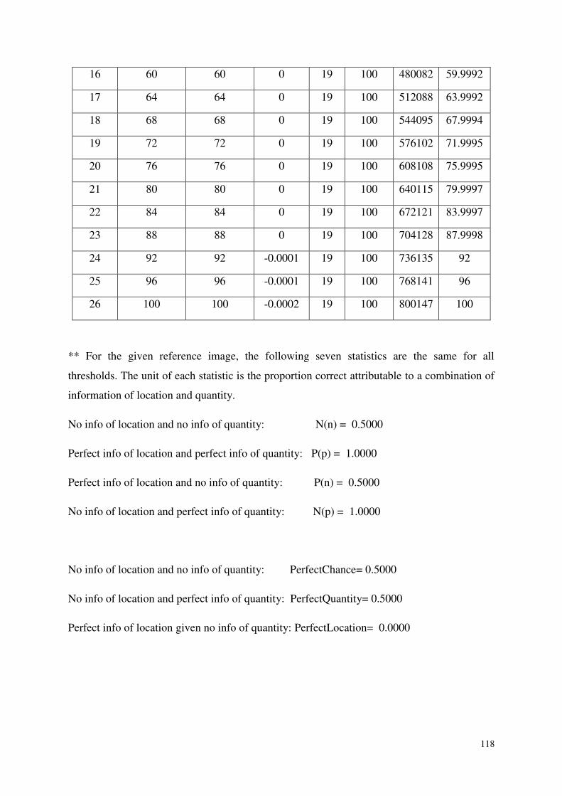
118
16 60 60 0 19 100 480082 59.9992
17 64 64 0 19 100 512088 63.9992
18 68 68 0 19 100 544095 67.9994
19 72 72 0 19 100 576102 71.9995
20 76 76 0 19 100 608108 75.9995
21 80 80 0 19 100 640115 79.9997
22 84 84 0 19 100 672121 83.9997
23 88 88 0 19 100 704128 87.9998
24 92 92 -0.0001 19 100 736135 92
25 96 96 -0.0001 19 100 768141 96
26 100 100 -0.0002 19 100 800147 100
** For the given reference image, the following seven statistics are the same for all
thresholds. The unit of each statistic is the proportion correct attributable to a combination of
information of location and quantity.
No info of location and no info of quantity: N(n) = 0.5000
Perfect info of location and perfect info of quantity: P(p) = 1.0000
Perfect info of location and no info of quantity: P(n) = 0.5000
No info of location and perfect info of quantity: N(p) = 1.0000
No info of location and no info of quantity: PerfectChance= 0.5000
No info of location and perfect info of quantity: PerfectQuantity= 0.5000
Perfect info of location given no info of quantity: PerfectLocation= 0.0000

119
No. M(m) N(m) P(m) M(p) M(n)
1 1 1 1 1 0.5
2 0.96 0.96 0.96 1 0.5
3 0.92 0.92 0.92 1 0.5
4 0.88 0.88 0.88 1 0.5
5 0.84 0.84 0.84 1 0.5
6 0.8 0.8 0.8 1 0.5
7 0.76 0.76 0.76 1 0.5
8 0.72 0.72 0.72 1 0.5
9 0.68 0.68 0.68 1 0.5
10 0.64 0.64 0.64 1 0.5
11 0.6 0.6 0.6 1 0.5
12 0.56 0.56 0.56 1 0.5
13 0.52 0.52 0.52 1 0.5
14 0.48 0.48 0.48 1 0.5
15 0.44 0.44 0.44 1 0.5
16 0.4 0.4 0.4 1 0.5
17 0.36 0.36 0.36 1 0.5
18 0.32 0.32 0.32 1 0.5
19 0.28 0.28 0.28 1 0.5
20 0.24 0.24 0.24 1 0.5
21 0.2 0.2 0.2 1 0.5
22 0.16 0.16 0.16 1 0.5
23 0.12 0.12 0.12 1 0.5
24 0.08 0.08 0.08 1 0.5
25 0.04 0.04 0.04 1 0.5
26 0 0 0 1 0.5
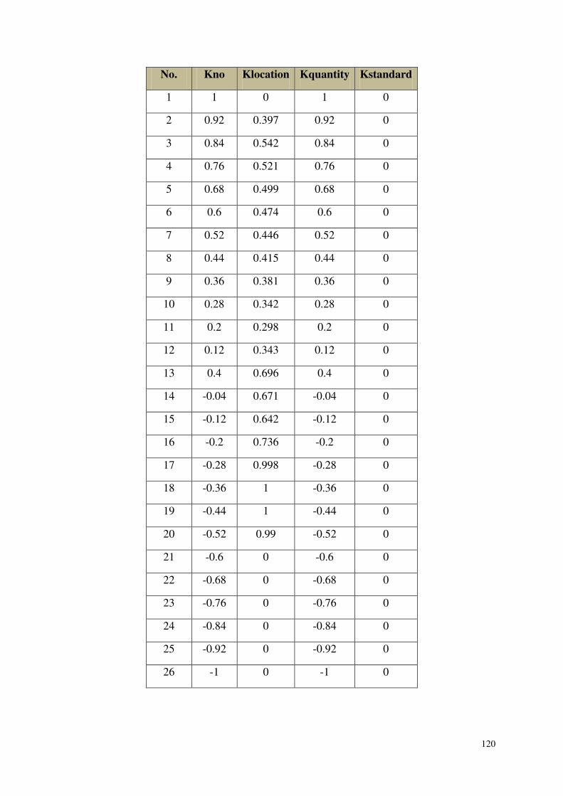
120
No. Kno Klocation Kquantity Kstandard
1 1 0 1 0
2 0.92 0.397 0.92 0
3 0.84 0.542 0.84 0
4 0.76 0.521 0.76 0
5 0.68 0.499 0.68 0
6 0.6 0.474 0.6 0
7 0.52 0.446 0.52 0
8 0.44 0.415 0.44 0
9 0.36 0.381 0.36 0
10 0.28 0.342 0.28 0
11 0.2 0.298 0.2 0
12 0.12 0.343 0.12 0
13 0.4 0.696 0.4 0
14 -0.04 0.671 -0.04 0
15 -0.12 0.642 -0.12 0
16 -0.2 0.736 -0.2 0
17 -0.28 0.998 -0.28 0
18 -0.36 1 -0.36 0
19 -0.44 1 -0.44 0
20 -0.52 0.99 -0.52 0
21 -0.6 0 -0.6 0
22 -0.68 0 -0.68 0
23 -0.76 0 -0.76 0
24 -0.84 0 -0.84 0
25 -0.92 0 -0.92 0
26 -1 0 -1 0
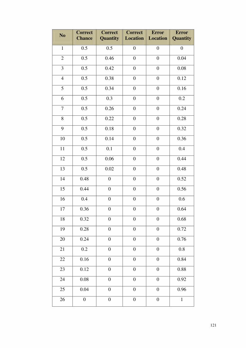
121
No Correct
Chance
Correct
Quantity
Correct
Location
Error
Location
Error
Quantity
1 0.5 0.5 0 0 0
2 0.5 0.46 0 0 0.04
3 0.5 0.42 0 0 0.08
4 0.5 0.38 0 0 0.12
5 0.5 0.34 0 0 0.16
6 0.5 0.3 0 0 0.2
7 0.5 0.26 0 0 0.24
8 0.5 0.22 0 0 0.28
9 0.5 0.18 0 0 0.32
10 0.5 0.14 0 0 0.36
11 0.5 0.1 0 0 0.4
12 0.5 0.06 0 0 0.44
13 0.5 0.02 0 0 0.48
14 0.48 0 0 0 0.52
15 0.44 0 0 0 0.56
16 0.4 0 0 0 0.6
17 0.36 0 0 0 0.64
18 0.32 0 0 0 0.68
19 0.28 0 0 0 0.72
20 0.24 0 0 0 0.76
21 0.2 0 0 0 0.8
22 0.16 0 0 0 0.84
23 0.12 0 0 0 0.88
24 0.08 0 0 0 0.92
25 0.04 0 0 0 0.96
26 0 0 0 0 1
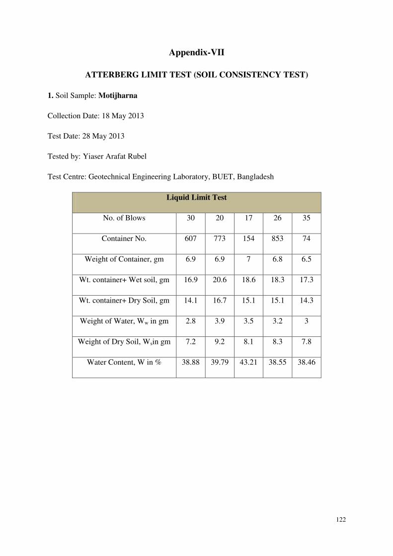
122
Appendix-VII
ATTERBERG LIMIT TEST (SOIL CONSISTENCY TEST)
1. Soil Sample: Motijharna
Collection Date: 18 May 2013
Test Date: 28 May 2013
Tested by: Yiaser Arafat Rubel
Test Centre: Geotechnical Engineering Laboratory, BUET, Bangladesh
Liquid Limit Test
No. of Blows 30 20 17 26 35
Container No. 607 773 154 853 74
Weight of Container, gm 6.9 6.9 7 6.8 6.5
Wt. container+ Wet soil, gm 16.9 20.6 18.6 18.3 17.3
Wt. container+ Dry Soil, gm 14.1 16.7 15.1 15.1 14.3
Weight of Water, Ww in gm 2.8 3.9 3.5 3.2 3
Weight of Dry Soil, Wsin gm 7.2 9.2 8.1 8.3 7.8
Water Content, W in % 38.88 39.79 43.21 38.55 38.46

123
Plastic Limit Test
Container No. 828 4444
Weight of Container, gm 7.3 7.2
Wt. container+ Wet soil, gm 18.6 18.4
Wt. container+ Dry Soil, gm 16.8 16.7
Weight of Water, Ww in gm 1.8 1.7
Weight of Dry Soil, Wsin gm 9.5 9.5
Water Content, W in % 18.37 17.89
Liquid Limit, LL from graph=39.9085
Plastic Limit, PL=19.635
Shrinkage Limit, SL=30
Plasticity Index, PI=LL-PL=39.9-19.635=20.265
Liquidity Index, LI = wn- wp/PI =26-19.636/20.265=0.314
Flow Index from flow curve, FI= Slope of Flow Curve= (39.9-38.82)/log (30/25) =13.747
(for 25 blow w=39.9 and for 30 blows w=38.82)
Activity, Ac=PI/%of clay size particles (<0.002mm)
Toughness Index, TI= PI/FI=20.265/13.747=1.474
Linear Shrinkage, LS=(1-Final length/Initial Length)*100=(1-127/140)*100=9.2857
Plasticity Index, PI=2.13LS=2.13*9.2857=19.778
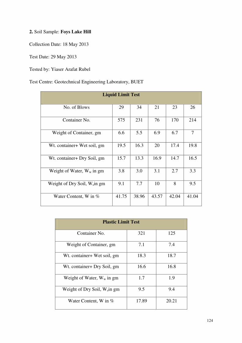
124
2. Soil Sample: Foys Lake Hill
Collection Date: 18 May 2013
Test Date: 29 May 2013
Tested by: Yiaser Arafat Rubel
Test Centre: Geotechnical Engineering Laboratory, BUET
Liquid Limit Test
No. of Blows 29 34 21 23 26
Container No. 575 231 76 170 214
Weight of Container, gm 6.6 5.5 6.9 6.7 7
Wt. container+ Wet soil, gm 19.5 16.3 20 17.4 19.8
Wt. container+ Dry Soil, gm 15.7 13.3 16.9 14.7 16.5
Weight of Water, Ww in gm 3.8 3.0 3.1 2.7 3.3
Weight of Dry Soil, Wsin gm 9.1 7.7 10 8 9.5
Water Content, W in % 41.75 38.96 43.57 42.04 41.04
Plastic Limit Test
Container No. 321 125
Weight of Container, gm 7.1 7.4
Wt. container+ Wet soil, gm 18.3 18.7
Wt. container+ Dry Soil, gm 16.6 16.8
Weight of Water, Ww in gm 1.7 1.9
Weight of Dry Soil, Wsin gm 9.5 9.4
Water Content, W in % 17.89 20.21
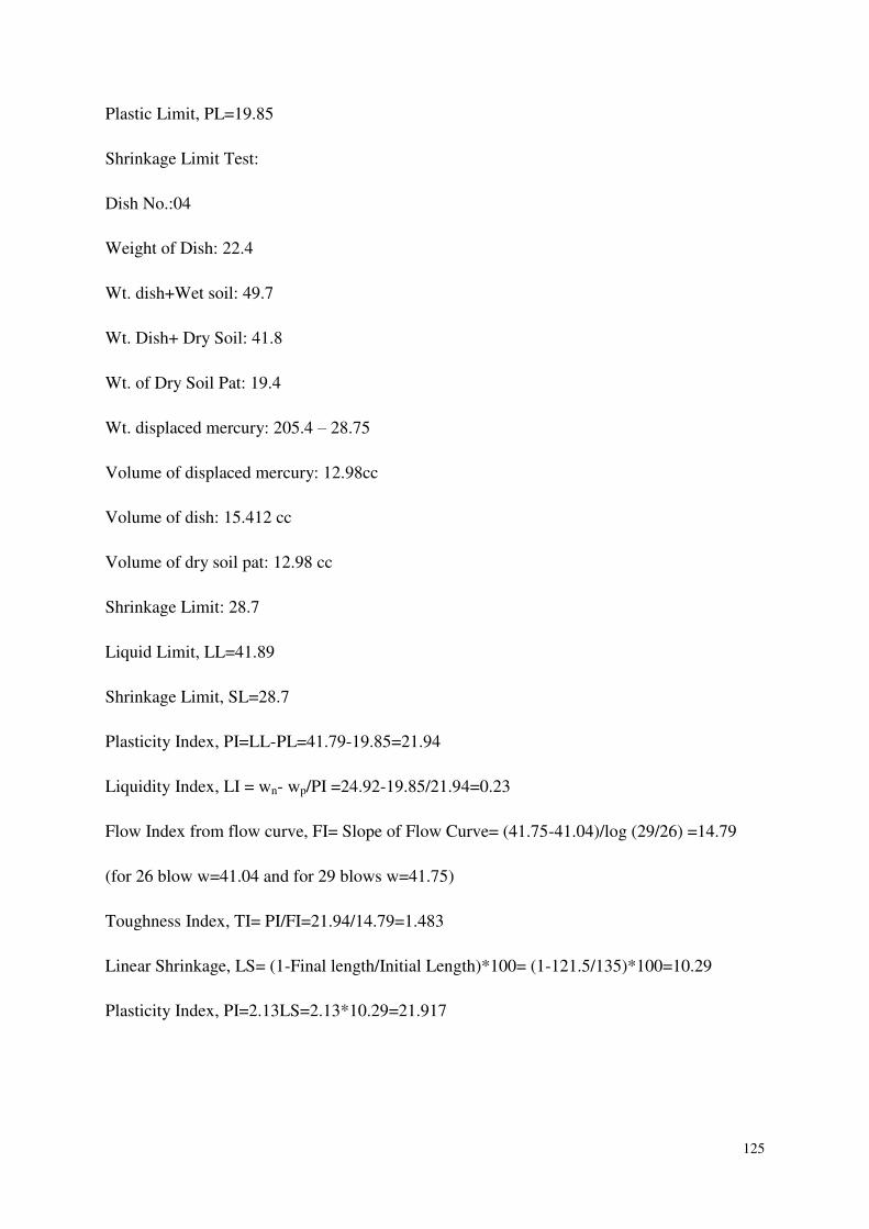
125
Plastic Limit, PL=19.85
Shrinkage Limit Test:
Dish No.:04
Weight of Dish: 22.4
Wt. dish+Wet soil: 49.7
Wt. Dish+ Dry Soil: 41.8
Wt. of Dry Soil Pat: 19.4
Wt. displaced mercury: 205.4 – 28.75
Volume of displaced mercury: 12.98cc
Volume of dish: 15.412 cc
Volume of dry soil pat: 12.98 cc
Shrinkage Limit: 28.7
Liquid Limit, LL=41.89
Shrinkage Limit, SL=28.7
Plasticity Index, PI=LL-PL=41.79-19.85=21.94
Liquidity Index, LI = wn- wp/PI =24.92-19.85/21.94=0.23
Flow Index from flow curve, FI= Slope of Flow Curve= (41.75-41.04)/log (29/26) =14.79
(for 26 blow w=41.04 and for 29 blows w=41.75)
Toughness Index, TI= PI/FI=21.94/14.79=1.483
Linear Shrinkage, LS= (1-Final length/Initial Length)*100= (1-121.5/135)*100=10.29
Plasticity Index, PI=2.13LS=2.13*10.29=21.917
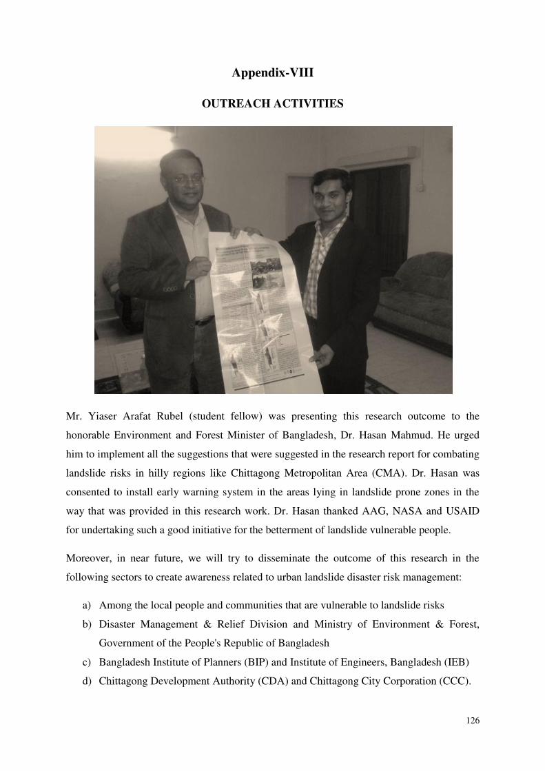
126
Appendix-VIII
OUTREACH ACTIVITIES
Mr. Yiaser Arafat Rubel (student fellow) was presenting this research outcome to the
honorable Environment and Forest Minister of Bangladesh, Dr. Hasan Mahmud. He urged
him to implement all the suggestions that were suggested in the research report for combating
landslide risks in hilly regions like Chittagong Metropolitan Area (CMA). Dr. Hasan was
consented to install early warning system in the areas lying in landslide prone zones in the
way that was provided in this research work. Dr. Hasan thanked AAG, NASA and USAID
for undertaking such a good initiative for the betterment of landslide vulnerable people.
Moreover, in near future, we will try to disseminate the outcome of this research in the
following sectors to create awareness related to urban landslide disaster risk management:
a) Among the local people and communities that are vulnerable to landslide risks
b) Disaster Management & Relief Division and Ministry of Environment & Forest,
Government of the People's Republic of Bangladesh
c) Bangladesh Institute of Planners (BIP) and Institute of Engineers, Bangladesh (IEB)
d) Chittagong Development Authority (CDA) and Chittagong City Corporation (CCC).
Thanks for Reading this Report!
© Bayes Ahmed & Yiaser Arafat Rubel