DECISION TREE PRUNING USING EXPERT KNOWLEDGE

A Dissertation

Present to

The Graduate Faculty of The University of Akron

In Partial Fulfillment

of the Requirements for the Degree

Doctor of Philosophy

Jingfeng Cai

December, 2006

DECISION TREE PRUNING USING EXPERT KNOWLEDGE

Jingfeng Cai

Dissertation

Approved: Accepted:

————————————– ————————————Advisor Department ChairDr. John Durkin Dr. Alex De Abreu Garcia

————————————– ————————————Committee Member Dean of the CollegeDr. Chien-Chung Chan Dr. George K. Haritos

————————————– ————————————–Committee Member Dean of the Graduate SchoolDr. James Grover Dr. George R. Newkome

————————————– ————————————–Committee Member DateDr. Narender P. Reddy

————————————–Committee MemberDr. Shiva Sastry

————————————–Committee MemberDr. John Welch

ii

ABSTRACT

Decision tree technology has proven to be a valuable way of capturing human decision

making within a computer. It has long been a popular artificial intelligence(AI) technique.

During the 1980s, it was one of the primary ways for creating an AI system. During the

early part of the 1990s, it somewhat fell out of favor, as did the entire AI field in general.

However, during the later 1990s, with the emergence of data mining technology, the technique

has resurfaced as a powerful method for creating a decision-making program.

How to prune the decision tree is one of the research directions of the decision tree tech-

nique, but the idea of cost-sensitive pruning has received much less attention than other

pruning techniques even though additional flexibility and increased performance can be ob-

tained from this method. This dissertation reports on a study of cost-sensitive methods for

decision tree pruning. A decision tree pruning algorithm called KBP1.0, which includes four

cost-sensitive methods, is developed. The intelligent inexact classification is used for first

time in KBP1.0 to prune the decision tree. Using expert knowledge in decision tree pruning is

discussed for the first time. By comparing the cost-sensitive pruning methods in KBP1.0 with

other traditional pruning methods, such as reduced error pruning, pessimistic error pruning,

cost complexity pruning, and C4.5, on benchmark data sets, the advantage and disadvantage

of cost-sensitive methods in KBP1.0 have been summarized. This research will enhance our

understanding of the theory, design and implementation of decision tree pruning using expert

knowledge. In the future, the cost-sensitive pruning methods can be integrated into other

pruning methods, such as minimum error pruning and critical value pruning, and include new

iii

pruning methods in KBP. Using KBP to prune the decision tree and getting the rules from

the pruned tree to help us build the expert system is another direction of our future work.

iv

ACKNOWLEDGEMENTS

I want to express my sincerest gratitude to my advisor, Dr. John Durkin, for his guidance

throughout my doctoral studies. Thanks to his encouraging and forbearing attitude I was able

to finish this dissertation. I learned a lot from him and he is the reason I came to University

of Akron.

Thanks to all my doctoral dissertation committee members. You taught me so much over

the years. Thank you to Dr. Chien-Chung Chan, Dr. James Grover, Dr. Narender P. Reddy,

Dr. Sastry, and Dr. John Welch. Thanks to the other faculty in our Electrical and Computer

Engineering Department and College of Engineering, especially Dr. George K. Haritos and

Dr. S.I. Hariharan. During my Ph.D. studies, I was financially supported by our Electrical

and Computer Engineering Department and College of Engineering.

Thanks to my wonderful parents, Zixing and Huan, my parents-in-law, Haiquan and

Zhanru, and to my brother and sister-in-law, Yufeng and Xiaoxue, for their continuous support

during my studies. This Ph.D. is a result of their extraordinary will, and sacrifices.

My final, and most heartfelt, acknowledgment must go to my wife Qingbo. Her patience,

encouragement, love and guidance were essential for my joining and smooth-sailing through

the Ph.D. program. For all that, and for being everything I am not, she has my everlasting

love. Qingbo and I also want to thank our oncoming baby who is our angel and brings luck

to us.

v

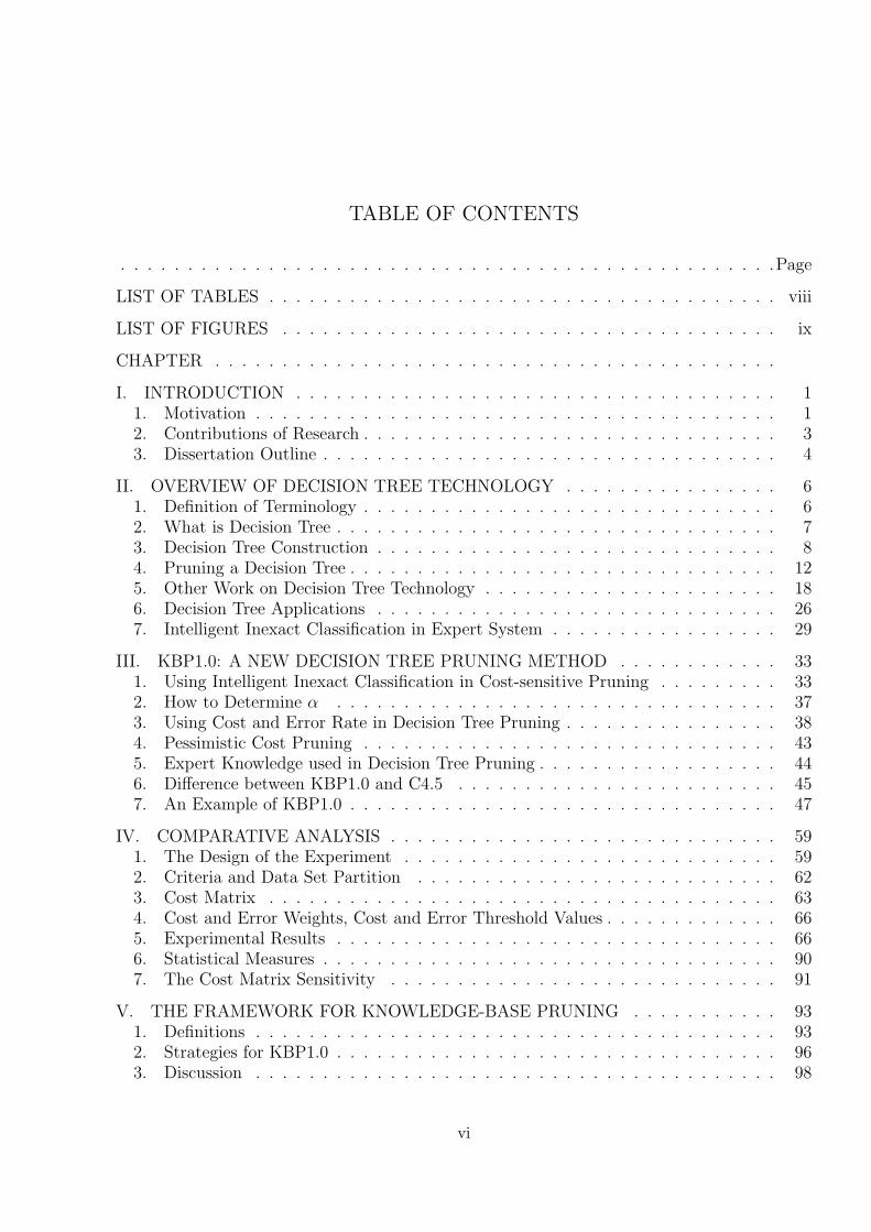
TABLE OF CONTENTS

. . . . . . . . . . . . . . . . . . . . . . . . . . . . . . . . . . . . . . . . . . . . . . . . .Page

LIST OF TABLES . . . . . . . . . . . . . . . . . . . . . . . . . . . . . . . . . . . . . . viii

LIST OF FIGURES . . . . . . . . . . . . . . . . . . . . . . . . . . . . . . . . . . . . . ix

CHAPTER . . . . . . . . . . . . . . . . . . . . . . . . . . . . . . . . . . . . . . . . . .

I. INTRODUCTION . . . . . . . . . . . . . . . . . . . . . . . . . . . . . . . . . . . . 11. Motivation . . . . . . . . . . . . . . . . . . . . . . . . . . . . . . . . . . . . . . . 12. Contributions of Research . . . . . . . . . . . . . . . . . . . . . . . . . . . . . . . 33. Dissertation Outline . . . . . . . . . . . . . . . . . . . . . . . . . . . . . . . . . . 4

II. OVERVIEW OF DECISION TREE TECHNOLOGY . . . . . . . . . . . . . . . . 61. Definition of Terminology . . . . . . . . . . . . . . . . . . . . . . . . . . . . . . . 62. What is Decision Tree . . . . . . . . . . . . . . . . . . . . . . . . . . . . . . . . . 73. Decision Tree Construction . . . . . . . . . . . . . . . . . . . . . . . . . . . . . . 84. Pruning a Decision Tree . . . . . . . . . . . . . . . . . . . . . . . . . . . . . . . . 125. Other Work on Decision Tree Technology . . . . . . . . . . . . . . . . . . . . . . 186. Decision Tree Applications . . . . . . . . . . . . . . . . . . . . . . . . . . . . . . 267. Intelligent Inexact Classification in Expert System . . . . . . . . . . . . . . . . . 29

III. KBP1.0: A NEW DECISION TREE PRUNING METHOD . . . . . . . . . . . . 331. Using Intelligent Inexact Classification in Cost-sensitive Pruning . . . . . . . . . 332. How to Determine α . . . . . . . . . . . . . . . . . . . . . . . . . . . . . . . . . 373. Using Cost and Error Rate in Decision Tree Pruning . . . . . . . . . . . . . . . . 384. Pessimistic Cost Pruning . . . . . . . . . . . . . . . . . . . . . . . . . . . . . . . 435. Expert Knowledge used in Decision Tree Pruning . . . . . . . . . . . . . . . . . . 446. Difference between KBP1.0 and C4.5 . . . . . . . . . . . . . . . . . . . . . . . . 457. An Example of KBP1.0 . . . . . . . . . . . . . . . . . . . . . . . . . . . . . . . . 47

IV. COMPARATIVE ANALYSIS . . . . . . . . . . . . . . . . . . . . . . . . . . . . . 591. The Design of the Experiment . . . . . . . . . . . . . . . . . . . . . . . . . . . . 592. Criteria and Data Set Partition . . . . . . . . . . . . . . . . . . . . . . . . . . . 623. Cost Matrix . . . . . . . . . . . . . . . . . . . . . . . . . . . . . . . . . . . . . . 634. Cost and Error Weights, Cost and Error Threshold Values . . . . . . . . . . . . . 665. Experimental Results . . . . . . . . . . . . . . . . . . . . . . . . . . . . . . . . . 666. Statistical Measures . . . . . . . . . . . . . . . . . . . . . . . . . . . . . . . . . . 907. The Cost Matrix Sensitivity . . . . . . . . . . . . . . . . . . . . . . . . . . . . . 91

V. THE FRAMEWORK FOR KNOWLEDGE-BASE PRUNING . . . . . . . . . . . 931. Definitions . . . . . . . . . . . . . . . . . . . . . . . . . . . . . . . . . . . . . . . 932. Strategies for KBP1.0 . . . . . . . . . . . . . . . . . . . . . . . . . . . . . . . . . 963. Discussion . . . . . . . . . . . . . . . . . . . . . . . . . . . . . . . . . . . . . . . 98

vi

VI. SUMMARY . . . . . . . . . . . . . . . . . . . . . . . . . . . . . . . . . . . . . . . 1001. Summary . . . . . . . . . . . . . . . . . . . . . . . . . . . . . . . . . . . . . . . . 1002. Discussion . . . . . . . . . . . . . . . . . . . . . . . . . . . . . . . . . . . . . . . 1033. Future Work . . . . . . . . . . . . . . . . . . . . . . . . . . . . . . . . . . . . . . 105

BIBLIOGRAPHY . . . . . . . . . . . . . . . . . . . . . . . . . . . . . . . . . . . . . . 106

APPENDIX . . . . . . . . . . . . . . . . . . . . . . . . . . . . . . . . . . . . . . . . . . 114

vii

LIST OF TABLES

Table . . . . . . . . . . . . . . . . . . . . . . . . . . . . . . . . . . . . . . . .Page

1 Attribute Information. . . . . . . . . . . . . . . . . . . . . . . . . . . . . 49

2 Major properties of the data sets considered in the experimentation . . 60

3 Values for I1, I2, Cth and Eth . . . . . . . . . . . . . . . . . . . . . . . . 66

4 Test results on cost between the cost-sensitive pruning methods KBP1.0-1,KBP1.0-2, KBP1.0-3, and KBP1.0-4, and the other non-cost sensitivepruning methods . . . . . . . . . . . . . . . . . . . . . . . . . . . . . . . 67

5 Test results on error rate (percent) between the cost-sensitive pruningmethods KBP1.0-1, KBP1.0-2, KBP1.0-3, and KBP1.0-4 and the othernon-cost sensitive pruning methods . . . . . . . . . . . . . . . . . . . . 73

6 Test results on size between the cost-sensitive pruning methods KBP1.0-1,KBP1.0-2, KBP1.0-3, and KBP1.0-4, and the other non-cost sensitivepruning methods . . . . . . . . . . . . . . . . . . . . . . . . . . . . . . . 77

7 Test results on cost between the cost-sensitive pruning methods KBP1.0-1,KBP1.0-2, KBP1.0-3, and KBP1.0-4, and the C4.5 pruning method . . 80

8 Test results on error rate (percent) between the cost-sensitive pruningmethods KBP1.0-1, KBP1.0-2, KBP1.0-3, and KBP1.0-4, and the C4.5pruning method . . . . . . . . . . . . . . . . . . . . . . . . . . . . . . . 84

9 Test results on size between the cost-sensitive pruning methods KBP1.0-1,KBP1.0-2, KBP1.0-3, and KBP1.0-4, and the C4.5 pruning method . . 88

10 Experimental results on cost according to different cost matrices . . . . 91

11 Experimental results on the percentage of cost changes . . . . . . . . . . 92

12 Values for I1 and I2 in KBP1.0 . . . . . . . . . . . . . . . . . . . . . . . 96

viii

LIST OF FIGURES

Figure . . . . . . . . . . . . . . . . . . . . . . . . . . . . . . . . . . . . . . . .Page

1 Test results on cost between the cost-sensitive pruning methods KBP1.0-1,KBP1.0-2, KBP1.0-3, and KBP1.0-4, and the other non-cost sensitivepruning methods for all the data sets . . . . . . . . . . . . . . . . . . . 68

2 Test results on cost between the cost-sensitive pruning methods KBP1.0-1, KBP1.0-2, KBP1.0-3, and KBP1.0-4 and the other non-cost sensitivepruning methods for the Hepatitis data set . . . . . . . . . . . . . . . . 69

3 Test results on cost between the cost-sensitive pruning methods KBP1.0-1,KBP1.0-2, KBP1.0-3, and KBP1.0-4, and the other non-cost sensitivepruning methods for the Iris data set . . . . . . . . . . . . . . . . . . . 70

4 Test results on cost between the cost-sensitive pruning methods KBP1.0-1,KBP1.0-2, KBP1.0-3, and KBP1.0-4, and the other non-cost sensitivepruning methods for the Vote data set . . . . . . . . . . . . . . . . . . . 71

5 Test results on error rate (percent) between the cost-sensitive pruningmethods KBP1.0-1, KBP1.0-2, KBP1.0-3, and KBP1.0-4, and the othernon-cost sensitive pruning methods for all the data sets . . . . . . . . . 74

6 Test results on error rate (percent) between the cost-sensitive pruningmethods KBP1.0-1, KBP1.0-2, KBP1.0-3, and KBP1.0-4, and the othernon-cost sensitive pruning methods for the Hypothyroid data set . . . . 75

7 Test results on size between the cost-sensitive pruning methods KBP1.0-1,KBP1.0-2, KBP1.0-3, and KBP1.0-4, and the other non-cost sensitivepruning methods for all the data sets . . . . . . . . . . . . . . . . . . . 78

8 Test results on cost between the cost-sensitive pruning methods KBP1.0-1,KBP1.0-2, KBP1.0-3, and KBP1.0-4, and the C4.5 pruning method for allthe data sets . . . . . . . . . . . . . . . . . . . . . . . . . . . . . . . . . 81

9 Test results on cost between the cost-sensitive pruning methods KBP1.0-1,KBP1.0-2, KBP1.0-3, and KBP1.0-4, and the C4.5 pruning method forthe Hypothyroid data set . . . . . . . . . . . . . . . . . . . . . . . . . . 82

10 Test results on cost between the cost-sensitive pruning methods KBP1.0-1,KBP1.0-2, and KBP1.0-3, and the C4.5 pruning method for the Vote dataset . . . . . . . . . . . . . . . . . . . . . . . . . . . . . . . . . . . . . . . 83

11 Test results on error rate between the cost-sensitive pruning methodsKBP1.0-1, KBP1.0-2, KBP1.0-3, and KBP1.0-3, and the C4.5 pruningmethod for all the data sets . . . . . . . . . . . . . . . . . . . . . . . . . 85

ix

12 Test results on error rate between the cost-sensitive pruning methodsKBP1.0-1, KBP1.0-2, KBP1.0-3, and KBP1.0-4, and the C4.5 pruningmethod for Hypothyroid data set . . . . . . . . . . . . . . . . . . . . . . 86

13 Test results on error rate between the cost-sensitive pruning methodsKBP1.0-1, KBP1.0-2, KBP1.0-3, and KBP1.0-4, and the C4.5 pruningmethod for the Iris data set . . . . . . . . . . . . . . . . . . . . . . . . . 87

14 Test results on size between the cost-sensitive pruning methods KBP1.0-1,KBP1.0-2, KBP1.0-3, and KBP1.0-4, and the C4.5 pruning method for allthe data sets . . . . . . . . . . . . . . . . . . . . . . . . . . . . . . . . . 89

x

CHAPTER I

INTRODUCTION

1. Motivation

“An expert system is a computer system which emulates the decision-making ability of a

human expert.” [101] The power behind an expert system is its knowledge. However, obtain-

ing the knowledge from an expert can be a very difficult task in real-world problems. The

knowledge engineer must be versed in the techniques of eliciting knowledge, which requires

good communication skills and some understanding of the psychology of human interaction.

Acquiring these skills, and being able to practice them effectively, can be difficult [1]. An-

other challenge with extracting knowledge occurs when the expert is not consciously aware of

the knowledge used [1]. The third difficulty occurs for expert system applications where no

real experts exist [1]. Though knowledgeable individuals exist who can predict some event,

they usually rely upon past events to aid their prediction. Therefore, the domain knowledge

rests in past examples, and not with human expertise. In these applications, the knowledge

engineer must again use some techniques that can uncover the knowledge contained within

the examples. Induction technique can be used to acquire knowledge from a set of examples.

There are many such induction techniques and the decision tree is only one of them. Every

induction technique has its advantages and disadvantage [97]. For example, a neural network

is better than a decision tree in accuracy [120], while a decision tree is more robust than a

neural network [121]. No single technique has been found to be superior over all others for all

data sets.

1

Decision tree technology has proven to be a valuable way of capturing human decision

making within a computer. But it often suffers the disadvantage of developing very large

trees making them incomprehensible to experts. To solve this problem, researchers in the

field have much interest in decision tree pruning. Decision tree pruning methods transform

a large tree into a smaller one, making it easily understood. Many decision tree pruning

algorithms have been shown to yield simpler or smaller trees.

One main problem for many traditional decision tree pruning methods is that when they

are used to prune a decision tree, it is always assumed that all the classes are equally probable

and equally important. However, in real-world classification problems, there is also a cost

associated with misclassifying examples from each class. For example, granting a credit to an

unreliable applicant may be more expensive for a bank than refusing it to a good applicant.

This is the reason that a cost-sensitive pruning method is needed to prune the decision tree.

Unfortunately, the idea of cost-sensitive pruning has received much less attention than other

pruning techniques even though additional flexibility and increased performance can be ob-

tained from this method. The research in this dissertation focuses on cost-sensitive pruning.

In the dissertation, expert knowledge is used to improve the performance of cost-sensitive

pruning. Cost is domain-specific and is quantified in arbitrary units [46]. In this sense, an

expert is needed.

The Merriam-Webster dictionary defines cost as “loss or penalty incurred especially in

gaining something”. Although there are many types of costs in the real world, such as cost of

time and cost of memory, only misclassification cost is considered in this dissertation. Almost

every error will cause cost. For example, in decision trees, there are misclassification errors.

If this misclassification is used in applications, it will certainly cause cost. A matrix is used

to define the misclassifications cost in decision tree pruning. In this matrix, the element in

row i and column j specifies the cost of assigning a case to class i when it actually belongs

2

to class j. When i equals to j, the cost is zero which means there is no misclassification

for this class. The cost matrix will be discussed in more detail later. There are not only

misclassification errors but also other kinds of errors. For example, nuclear power stations

might not be safe, i.e., a nuclear leak will threaten our life. However, in this dissertation, error

only refers to misclassification error in decision tree. Hereinafter, unless specified otherwise,

cost of a pruning algorithm means the misclassification cost.

2. Contributions of Research

This research focuses on decision tree pruning. The main contributions of this dissertation,

in the author’s opinion, are the following:

(1) The major contribution of the research is the use of expert knowledge in cost-sensitive

pruning. In the cost-sensitive pruning, the misclassification cost is provided by domain

experts and represented as a cost matrix. An example is used to explain how expert

knowledge is used to help define the cost matrix. To the best of the author’s knowledge,

the use of expert knowledge in cost-sensitive pruning of decision trees has not been

reported in the literature.

(2) There are many decision tree pruning methods, but most of them only consider error

rate or cost during pruning. Another contribution of the research is that two ways to

integrate error rate and cost in the pruning method are proposed. One method uses

intelligent inexact classification (IIC) and the other uses a threshold to integrate error

rate and cost. To the best of the author’s knowledge, IIC and threshold value in deci-

sion tree pruning have not been used thus far in this context. Moreover, the proposed

pruning method is more general than other non-cost sensitive pruning methods. For

example, the cost weight can be set to value 0 and the cost-sensitive pruning can be

changed to an error based non-sensitive pruning.

3

(3) A decision tree pruning algorithm called KBP1.0, which includes four cost-sensitive

pruning methods, was developed and its framework was introduced. KBP1.0 and some

well-known traditional pruning methods, such as reduced error pruning, pessimistic

error pruning, and C4.5, are compared on data sets from the UCI Machine Learning

Repository and the results are reported and discussed.

(4) The framework for knowledge-base pruning method was introduced. Then, the strate-

gies under the framework were discussed.

(5) There is a preliminary discussion on the sensitivity of the pruning method to the cost

matrix. To the best of the author’s knowledge, it is the first time that this kind of

sensitivity is analyzed.

The decision tree pruning algorithm KBP1.0 provides us more options to prune the decision

tree, especially when cost is too important to be ignored. Its potential application includes

most problems which should take into account misclassification cost, such as medical diagnosis,

stock prediction, credit grant, and so on. Another value of the cost-sensitive pruning methods

is that designers can form a balance between error and cost in decision tree pruning by defining

the weights of cost and error under the guidance of experts.

Most of this dissertation is from the point of view of machine learning and has an experi-

mental flavor. Experiments are carefully designed and controlled from the basis of observations

and conclusions. An experimental analysis is given in the dissertation.

3. Dissertation Outline

This dissertation is organized as follows. Chapter 2 is devoted to an overview of decision

tree classifier methodology. Chapter 3 introduces new methods for cost-sensitive decision tree

pruning under the program name KBP1.0. An example of KBP 1.0 is also provided in Chapter

3. Comparative analysis of KBP1.0 and other traditional methods for pruning a decision tree

is described and the sensitivity of the pruning method to the cost matrix is investigated in

4

Chapter 4. Chapter 5 introduces the framework for KBP1.0. Finally, a summary of the

research is given in Chapter 6, which discusses some concerns of the research and answers

some questions. It also discusses the future work of the research.

5

CHAPTER II

OVERVIEW OF DECISION TREE TECHNOLOGY

This chapter is an overview of decision tree technology which is not author’s original

contribution.

1. Definition of Terminology

To avoid possible confusion with the textual description in this dissertation, the follow-

ing definitions are provided(these definitions are cited from some dictionaries, websites, and

books):

Tree: “A tree is a connected acyclic graph.” [102] In this dissertation, every tree is a deci-

sion tree. “The decision tree is a tree diagram which is used for making decisions in business

or computer programming and in which the branches represent choices with associated risks,

costs, results, or probabilities.” [103]

Class: “The class is a group or set sharing common attributes. In a decision tree, classes

are the categories to which cases are to be assigned.” [104]

Object: “The object is something material that may be perceived by the senses.” [105]

Set: “a number of things of the same kind that belong or are used together.” [106]

Path: “A path in a graph is an ordered list of distinct vertices v1,...,vn such that vi−1vi is

an edge for all 2 <= i <= n.” [98]

Subtree: “A tree structure created by arbitrarily denoting a node to be the root node in

a tree. A subtree is always part of a whole tree.” [98]

6

Node: “In a tree structure, a node is a point at which subordinate items of data originate.”

[98]

Leaf: “In a tree, a leaf is a node without children.” [98]

Root: “In a decision tree, a root is a node that has no parent. All other nodes of a tree

are descendants of the root.” [98]

Attribute: “An inherent characteristic.” [122]

Subset: “A set each of whose elements is an element of an inclusive set.” [123]

Entropy: “The degree of disorder or uncertainty in a system.” [124]

2. What is Decision Tree

A decision tree gets its name because it is shaped like a tree and can be used to make

decisions. “Technically, a tree is a set of nodes and branches and each branch descends from a

node to a another node. The nodes represent the attributes considered in the decision process

and the branches represent the different attribute values. To reach a decision using the tree

for a given case, we take the attribute values of the case and traverse the tree from the root

node down to the leaf node that contains the decision.” [109]

A critical issue in artificial intelligence(AI) research is to overcome the so-called “knowledge-

acquisition bottleneck” in the construction of knowledge-based systems. Decision tree can be

used to solve this problem. Decision trees can acquire knowledge from concrete examples

rather than from experts [1]. In addition, for knowledge-based systems, decision trees have

the advantage of being comprehensible by human experts and of being directly convertible

into production rules [13]. A decision tree not only provides the solution for a given case, but

also provides the reasons behind its decision. So the real benefit of decision tree technology is

that it avoids the need for human expert. Because of the above advantages, there are many

successes in applying decision tree learning to solve real-world problems.

7

Durkin, J. summarized that decision tree technology has several advantages and disadvan-

tages [60][118]. The advantages include:

(1) Discovers rules from examples,

(2) Avoids knowledge elicitation problems,

(3) Can discover new knowledge,

(4) Can uncover critical decision factors,

(5) Can eliminate irrelevant decision factors,

(6) Robust to noisy data.

The disadvantages of the technology are:

(1) Often difficult to choose good decision factors,

(2) Difficult to understand rules generated from large trees,

(3) Often leads to an overfitting problem when decision tree is big or there is not much

training data.

Decision tree technology has proven to be a valuable way of capturing human decision

making within a computer. Unfortunately, as AI fell out of favor, so did decision tree tech-

nology. Fortunately, with the emergence of the relatively new field of data mining, which

includes decision tree technology as one of the primary ways of capturing human decision

making, there is renewed interest in the technology.

3. Decision Tree Construction

Several algorithms have been developed to create a decision tree. Some of the more

popular ones are ID3 (Quinlan 1986), C4.5 (Quinlan 1993), CART(Brieman et al., 1984) and

CHAID(Kass 1980). While they all differ in some way, they all share the common idea of

building the tree using a technique based on information theory. In this section, only Quinlan’s

ID3 algorithm for constructing a decision tree is introduced. In decision tree construction, the

8

set of cases with known classes from which a decision tree is constructed is called the training

set and other collections of cases not seen while the tree was being developed are known as

test sets.

A decision tree building algorithm determines the classification of objects by testing the

values of their attributes. The tree is built in a top down direction. An attribute is tested

at each node of the tree and the results is used to partition the object set. This process is

recursively done till the set in a given subtree only contains objects belonging to the same

category or class- in other words it becomes a leaf node [110].

ID3 consists of the following steps [111]:

(1) Select the attribute with the most gain

(2) Create the subsets for each value of the attribute

(3) For each subset

1) if not all the elements of the subset belongs to same class repeat the steps

1-3 for the subset

2) if all the elements of the subset belongs to same class end

Entropy in information gain is used to measure which attribute is most informative. En-

tropy is a measure from information theory. It characterizes the impurity or homogeneity,

of an arbitrary collection of examples [127]. Mathematicians know that information is maxi-

mized when entropy is minimized. Entropy determines the extent of randomness or chaos in

data. The development of the idea of entropy of random variables and processes by Shannon

provided the beginning of information theory and of the modern age of ergodic theory [56].

This concept is key to decision tree construction, as is shown in the following.

The process of building a decision tree starts with the selection of an attribute A as the

root node of the tree that does the best job of dividing the set of samples S into subsets

s1,s2,...,sn, in which many samples belong to the same class C.

9

To measure the total disorder, or inhomogeneity in the subsets, the entropy of attribute

A can be calculated as follows [41]

Average Entropy(A) =∑

(nb

nt

) ∗∑

−(nbc

nb

) log2(nbc

nb

) (1)

where:

nb is the number of samples in branch b,

nt is the number of samples in all branches,

nbc is the total number of samples in branch b of class c.

After calculating the entropy of each attribute, the one which has minimal entropy is

chosen because minimal entropy means largest information gain.

To understand how the average entropy equation can be used to generated the decision

tree, let us start by considering the set of samples at the end of branch b. We want an equation

containing nb and nbc that gives us a high number when the set is highly inhomogeneous and a

low number when the set is highly homogeneous. Fortunately, the following entropy equation

borrowed from information theory can be used to accomplish this:

Entropy =∑

−(nbc

nb

) log2(nbc

nb

) (2)

To get a feel on how this equation works, let’s look at some examples. First suppose

we have only two classes: C1 and C2 in a sample set. Further assume that the sample set

contains an equal number of samples from both classes. It then follows that the entropy is 1,

the maximum possible value:

10

Entropy =∑

−(nbc

nb

) log2(nbc

nb

)

= −1

2log2(

1

2)− 1

2log2(

1

2)

=1

2+

1

2

= 1

(3)

For the next example, let’s assume that the sample set contains only samples from C1 or

C2. In this case, the set is perfectly homogeneous and it follows that the entropy is 0, the

minimum possible value:

Entropy =∑

−(nbc

nb

) log2(nbc

nb

)

= −1 log2(1)− 0 log2(0)

= −0− 0

= 0

(4)

It is clear that entropy varies smoothly between zero and one when the sample set moves

from perfect balance to perfect homogeneity [41].

The prior discussion shows how to measure the entropy in one set. We next need to obtain

the average entropy of the sets at the ends of the branches under the attribute A. To obtain

this measure, the entropy in each branch’s set is weighted by the size of the set relative to

the total size of all the branches’ sets. Therefore, given that nb is the number of samples in

branch b and nt is the total number of samples in all branches, it follows that

Average Entropy(A) =∑

−(nb

nt

) ∗ (Entropy in the branch b set) (5)

which is the same as equation (1).

11

Using this idea we take each attribute and compute its average entropy, and then select the

one for the root node that has the minimum entropy value. As the tree is further developed,

the same idea is followed in node selection.

The use of entropy for attribute selection is just one of several methods employed in

building a decision tree. A good review of available methods can be found in Breimann et al.,

(1984) and in Mingers (1989).

Once a decision tree is constructed, it is easy to convert it into a set of equivalent rules.

We just trace each path in the decision tree, from root node to leaf node, recording the test

outcomes as antecedents and the leaf-node classification as the consequent. However, if the

tree is large, then the rules created are likewise large and difficult to understand. This is

where pruning becomes important.

4. Pruning a Decision Tree

Although the decision trees generated by methods such as ID3 and C4.5 are accurate

and efficient, they often suffer the disadvantage of providing very large trees that make them

incomprehensible to experts [12]. To solve this problem, researchers in the field have consid-

erable interest in tree pruning. Tree pruning methods convert a large tree into a small tree,

making it easier to understand. Such methods “typically use statistical measures to remove

the least reliable branches, generally resulting in faster classification and an improvement in

the ability of the tree to correctly classify independent test data.” [107] It is necessary for us

to know the advantage and disadvantage of every decision tree pruning method before it is

decided that which pruning method will be selected. The following are some main methods

to simplify decision trees.

(1) Reduced Error Pruning

This method was proposed by Quinlan [12]. It is the simplest and most under-

standable method in decision tree pruning. For every non-leaf subtree S of the original

12

decision tree, the change in misclassification over the test set is examined. The mis-

classification would occur if this subtree were replaced by the best possible leaf which

is the majority of leaf. If the error rate of the new tree would be equal to or smaller

than that of the original tree and that subtree S contains no subtree with the same

property, S is replaced by the leaf. Otherwise, stop the process. The constraint that

the subtree S contains no subtree with the same property guarantees reduced error

pruning in bottom-up induction [11].

Since each node is visited only once to evaluate the opportunity of pruning it, the

advantage of this method is its linear computational complexity [11]. However, this

method requires a test set separate from the cases in the training set from which the

tree was constructed [12]. When the test set is much smaller than the training set,

this method may lead to overpruning. Many researchers found that Reduced Error

Pruning performed as well as most of the other pruning methods in terms of accuracy

and better than most in terms of tree size [11].

(2) Pessimistic Error Pruning

This method was also proposed by Quinlan [12] and was developed in the context

of ID3. Quinlan found that it is too optimistic for us to use a training set to test

the error rate of a decision tree, because decision trees have been tailored to the

training set. In this case, the error rate can be 0. But some data other than the

training set is used, the error rate will increase dramatically. To solve this problem,

Quinlan used continuity correction for the binomial distribution to get an error rate

which is more realistic. In statistics, continuity correction is a useful method in the

application of the normal distribution to the computation of binomial probabilities.

“When the normal distribution (a continuous distribution) is used to find approximate

answers to problems arising from the binomial distributions (discrete distribution),

13

an adjustment is made for the mismatch of types of distribution. This is called the

continuity correction.” [108]

Quinlan uses the following equations to obtain the number of misclassifications:

n′(t) = e(t) + (

1

2) (6)

n′(Tt) = e(Tt) + (

NT

2) (7)

Equation(6) is the number of misclassifications for node t and equation(7) is the

number of misclassifications for subtree T .

where:

NT is the number of leaves for subtree T ,

e(t) is the number of misclassifications at node t,

e(Tt) is the number of misclassifications for subtree T .

The 1/2 in the equation (6) and (7) is a constant which indicates the contribution

of a leaf to the complexity of the tree. This pruning method only keeps the subtree

if its corrected figure (from equation 7) is more than one standard error better than

the figure for the node (from equation 6).

This method is much faster than Reduced Error Pruning and also provides higher

accuracies. Its disadvantage is that, in the worst case, when the tree does not need

pruning at all, each node will still be visited once [11].

(3) Cost-Complexity Pruning

This method was proposed by Breiman et al., [7]. It takes account of both the

number of errors and the complexity of the tree. The size of the tree is used to

14

represent the complexity of the tree. It is also known as the CART pruning method

and Floriana Esposito, et al, describe it in two steps [11]:

1) Selection of a parametric family of subtrees of { T0, T1, . . . , TL }, according to

some heuristics. T0 is the original decision tree and each Ti+1 is obtained by replacing

one or more subtrees of Ti with leaves by pruning those branches that show the lowest

increase in apparent error rate per pruned leaf until the final tree TL is just a leaf.

2) Choice of the best tree according to an estimate of the true error rates of the

trees in the parametric family.

For example, consider subtree T used to classify each of the N cases in the training

set and E of N examples are wrongly classified if subtree T is replaced by the best

leaf. Let NT be the number of leaves in subtree T . the following equation is used to

define the total cost-complexity of subtree T :

cos− complexity = (E

N) + α ∗NT (8)

where α is the cost of one extra leaf in the tree and gives the reduction in error

per leaf.

If the subtree is pruned, the new tree would misclassify M more of the cases in

the training set but would contain NT − 1 fewer leaves. the same cost-complexity will

be obtained when

α = (M

N ∗ (NT − 1)) (9)

From the above equation, α can be calculated for each subtree and the subtree(s)

with the smallest value of α is selected for pruning. Continue to process this until the

15

leaf is obtained. The next job is to select one of the trees. The standard error (SE)

of the misclassification rate is

SE = (R ∗ (100−R)

N) (10)

where:

R=misclassification rate of the pruned tree,

N=number of examples in the test data.

The smallest tree whose observed number of errors on the test set does not exceed

R + SE is selected.

This method requires a pruning set distinct from the original training set. Its

disadvantage is that it can only choose a tree in the set { T0, T1, . . . , TL },which is

obtained in the first step, instead of the set of all possible subtrees [11]. It also seems

anomalous that the cost-complexity model used to generate the sequence of subtrees

is abandoned when the best tree is selected [12].

(4) Minimum Error Pruning

This method was developed by Niblett and Brotko [48]. It is a bottom-up approach

which seeks a single tree that minimizes the expected error rate on an independent

data set.

Assume that there are k classes for a set of data which number is n and nc is the

class c with the greatest number of data. If it is predicted that all future examples

will be in class c, the following equation is used to predict the expected error rate:

Ek = (n− nc + k − 1

n + k) (11)

16

where:

k is the number of classes for all data,

Ek is the expected error rate if we predict that all future examples will be in class

c.

The method consist of three steps [112]:

1) At each non-leaf node in the decision tree, use equation(11) to calculate the

expected error rate if that subtree is pruned.

2) Calculate the expected error rate if the node is not pruned, combined by

weighting according to the proportion of observations along each branch [11][48].

3) If pruning the node leads to a greater expected error rate, then keep the

subtree; otherwise, prune it.

J. Mingers [8] points out that there are several disadvantages in this method. First,

it is seldom true in practice that all the classes are equally likely. Second, this method

produces only a single tree. This is a disadvantage in the context of expert systems,

where it will be more helpful if several trees, pruned to different degrees, are available.

Third, the number of classes strongly affects the degree of pruning, leading to unstable

results.

Minimum error pruning was improved by Cestnik and Bratko [48] and the most

recent version of minimum error pruning overcomes two problems of original method:

optimistic bias and dependence of the expected error rate on the number of classes.

(5) Critical Value Pruning

This method was proposed by Mingers [43]. In this method, a threshold, named

the critical value, is set to estimate the importance or strength of a node. When the

node does not reach the critical value, it will be pruned. But when a node meets the

pruning condition but its children do not all meet the pruning condition, this branch

17

should be kept because it contains relevant nodes. If a larger critical value is selected,

a smaller resulting tree will be obtained because of the more drastic pruning.

Mingers describes the critical value pruning as two main steps [43]:

1) Prune subtree for increasing critical values,

2) Measure the significance of the pruned trees as a whole and their predictive

ability and choose the best tree among them.

The disadvantage of this method is its strong tendency to underprune and this

method selects trees with comparatively low predictive accuracy [42].

(6) Optimal Pruning

Breiman et al., introduce a convenient terminology used to state and verify the

mathematical properties of optimal pruning [7]. They also introduce an algorithm

to select a particular optimally pruned subtree from among the k candidates [7].

Bratko and Bohanec [73] and Almuallim [74] address the issue of finding optimal

pruning in another way. Bohanes et al., [73] introduced an algorithm guaranteeing

optimal pruning (OPT), and Almuallim [74] further improved OPT in terms of the

computational complexity. Their motivation for simplifying decision trees is different

from the typical motivation for pruning decision trees when learning from noisy data.

Both [73] and [74] assume that the initial, unpruned decision trees are completely

correct. However, in learning from noisy data, which is our case, it is assumed that the

initial, unpruned decision tree is inaccurate and appropriate pruning would improve

its accuracy.

5. Other Work on Decision Tree Technology

Currently, the research in decision tree technology mainly focuses on the following direc-

tions:

18

(1) Integrating decision trees with other AI techniques

How to integrate the decision tree technique with other new techniques is one of

the hottest topics in decision tree research. this work is summarized as follows:

(a) Integrating decision trees with neural networks

Neural networks offer a exciting computational paradigm for cognitive machines

and are successful in acquiring hidden knowledge in data sets. But the knowledge

which they acquire is represented in a form not understandable to humans. O. Boz

dealt with this shortcoming by extracting decision trees from trained neural networks

[17]. A new decision tree extraction technique (DecText) is developed to extract

classical decision trees from trained neural networks and the tree is pruned in a way

to maximize the fidelity between the tree and the Neural Network. I. Sethi [18] did

this research in another way: a decision tree is restructured as a three-layer neural

network, called an entropy network. A mapping method is used to map a decision

tree into a multilayer neural network structure. An entropy network architecture has

many advantages, such as fewer neural connections and faster progressive training

procedure.

(b) Integrating decision trees with fuzzy logic

“Decision trees have already shown to be interpretable, efficient, problem-independent

and able to treat large scale applications. But they are also recognized as highly un-

stable classifiers with respect to minor perturbations in the training data, in other

words, methods presenting high variance” [113]. Fuzzy logic brings an improvement

due to the elasticity of fuzzy sets formalism. C. Olaru, et al., propose a new method of

fuzzy decision trees called soft decision trees(SDT) [20]. SDT is a variant of classical

19

decision tree inductive learning using fuzzy set theory. M. Dong and R. Kothari pre-

sented a computationally efficient way of incorporating look-ahead into fuzzy decision

tree induction which leads to smaller decision trees and better performance [19].

(c) Integrating decision trees with evolutionary algorithms, genetic algorithms

and genetic programming

Evolutionary algorithms(EA) are stochastic search methods based on the mechan-

ics of natural selection and genetics. E. Cautu-Paz and C. Kalles substituted the

greedy search technique in traditional decision tree technology with two evolutionary

algorithms [21]. This EA-based tree inducer resulted in faster training time. EAs can

also find oblique trees with a similar or higher accuracy than existing algorithms. EAs

are a promising technique to build oblique trees for the following reasons [21]:

(1) Scalability to high dimensional spaces,

(2) Tolerance to noise,

(3) Parallel implementations,

(4) More sophisticated optimizers,

(5) Use of problem-specific knowledge such as seeding the initial population

of the Evolutionary Algorithm (EA) with “good” solutions.

Genetic algorithms(GA) have been used for classification. A. Papagelis and D.

Kalles used GAs to directly evolve classification decision trees [22][23]. Their method

shows the potential advantages of GAs over other greedy heuristics, especially when

there are irrelevant or strongly dependent attributes. D. Carvalho and A. Freitas

proposed a hybrid decision tree/genetic algorithm method to deal with the problem

of small disjuncts [24]. In this method, when examples belong to large disjuncts, they

are classified by rules produced by a decision tree, otherwise, they are classified by

rules produced by a specifically designed genetic algorithm. The quality of the rules

20

discovered by this hybrid algorithm is much better than that of the rules discovered

by C4.5 alone. The disadvantage of the hybrid decision tree/genetic algorithm is that

it is much more computationally expensive.

Genetic programming(GP) is a method of adaptive automatic program induction.

The difference between GP and GA is that, for GP, individuals are no longer strings

but parse trees of the programs [128]. GP is a effective way of overcoming the limi-

tations of the standard greedy decision tree induction algorithms. Each individual of

the population in GP can be a decision tree. The functions to be used in the GP are

the attributes of the decision tree and classes form the terminal set. G. Tur and H.

A. Guvenir did some work in this respect [25]. They found that decision trees created

using genetic programming can find the optimum solution for a small sized data set.

(d) Integrating decision trees with a multiagent system

Mutiagent System(MAS) has emerged as an active subfield of Artificial Intelligence

in recent years. MAS aims to provide both principles for construction of complex

systems involving multiple agents and mechanisms for coordination of independent

agents behaviors [114]. Because machine learning has the potential to provide robust

mechanisms that leverage upon experience to equip agents with a large spectrum of

behavior, machine learning is a promising area to merge with multiagent systems [27].

P. Stone and M. Veloso published some papers on this research [27][28][29]. They

proposed a novel technique for agent control in a complex multiagent domain based

on the confidence factors provided by the C4.5 decision tree algorithm. It was realized

in robotic soccer [28].

There are some other research directions for decision tree technology as follows:

21

(2) Looking for better methods to construct decision trees

Several algorithms have been developed to create a decision tree. Some of the

more popular ones are ID3, C4.5, CART and CHAID. While they all differ in some

way, they all share the common idea of building the tree using a technique based on

information theory. M. Ankerst, et al., introduced a fully interactive method based

on a multidimensional visualization technique and appropriate interaction capabilities

[31]. In this construction method, domain knowledge of an expert can be effectively

included in the tree construction phase to reduce the tree size and improve the un-

derstandability of the resulting decision tree.

(3) Looking for better methods to simplify decision trees

There are mainly two research directions in decision tree pruning. One is compar-

ing the different methods for decision tree pruning. The other is looking for better

methods to simplify decision trees. For the first area, J. Mingers and F. Esposito, et

al., published some important papers [11][43]. For the second area, many researchers

are trying to use new techniques to help simplify decision trees. For example, D.

Fournier and B. Cremilleux found a new pruning method called DI pruning that takes

into account the complexity of subtrees [30]. Even some subtrees created using this

method do not increase the classification efficiency. DI pruning can assess the quality

of the data used for the knowledge discovery task.

(4) Doing research on the impact of data size and quality on decision tree performances

Different from the previous research directions, this direction focus is on the impact

of data size and data quality on decision tree performances. It is clear that increasing

the training set size often results in a linear increase in tree size even without a

significant increase in classification accuracy [15]. In this sense, a data reduction

technique, which is different from a pruning technique, is very important for a decision

22

tree’s quality. On the other hand, improving the quality of the training data results in

an increasing classification accuracy. M. Sebban [14], T. Oates [15] and C. E. Brodley

[16] performed research in this area.

(5) Decision trees in an uncertain environment

Although the decision tree technique is one of the most popular and efficient su-

pervised learning approaches, a major problem faced in the standard decision tree

algorithms results from the uncertainty encountered in the data [44]. This uncer-

tainty can appear either in the construction or in the classification phase. In many

cases, the uncertainty may affect the classification results and may even result in er-

roneous decisions, therefore it can’t be ignored. There are mainly two ways to deal

with the uncertainty: one is probabilistic decision trees and the other is fuzzy decision

trees. Z. Elouedi, et al., developed a belief decision tree which integrates the advan-

tages of both the decision tree technique and the belief function theory to deal with

the uncertainty [44]. B. Crmilleux, et al., also did some work in uncertain domains

and decision trees [45].

(6) Computational Complexity of Decision trees

Algorithms based on the decision tree technique can reach a high computational

complexity. Catlett [83] and Fifield [92] proposed some methods to reduce the com-

putational complexity. However, their methods all require that all data will be loaded

into main memory before induction. Chan and Stolfo’s method [93] reduces the com-

putational complexity, but the classification accuracy decreases. There are some other

important researches in reducing computational complexity of decision trees. For ex-

ample, Mehta et al. [94] proposed SLIQ, Shafer [95] et al. presented SPRINT, and

Gehrke [96] et al. introduced RainForest to deal with the computational complexity.

23

(7) Cost-Sensitive Decision Tree Pruning

One main problem for many decision tree pruning methods is that when a deci-

sion tree is pruned, it is always assumed that all the classes are equally probable and

equally important. However, in real-world classification problems, there is also a cost

associated with misclassifying examples from each class. Unfortunately, the method

of cost-sensitive pruning has received much less attention even though additional flex-

ibility and increased performances have been obtained from this method. Currently,

the most common method for cost-sensitive pruning method is to use techniques in

statistics to deal with the problem. Because the research in the dissertation focuses

on cost-sensitive pruning, the statistical method for cost-sensitive pruning is discussed

here.

The use of probability models and statistical methods for analyzing data has be-

come common practice in virtually all scientific disciplines. For example, M. Jordan

used a statistical approach to build a decision tree model [53]. A parameter can be

estimated from sample data either by a single number (a point estimate) or an entire

interval of plausible values (a confidence interval). Frequently, however, the objective

of an investigation is not to estimate a parameter but to decide which of two con-

tradictory claims about the parameter is correct (some cost-sensitive pruning method

makes use of this [10]). Methods for accomplishing this comprise the part of statis-

tical inference called hypothesis testing. The null hypothesis, denoted by H0, is the

claim about one or more population characteristics that is initially assumed to be true.

The alternative hypothesis, denoted by Ha, is the assertion that is contradictory to

H0. The null hypothesis will be rejected in favor of the alternative hypothesis only if

sample evidence suggests that H0 is false. If the sample does not strongly contradict

H0, we will continue to believe in the truth of the null hypothesis. The two possible

24

conclusions from a hypothesis-testing analysis are then rejecting H0 or fail to reject

H0. A test of hypothesis is a method for using sample data to decide whether the

null hypothesis should be rejected. For example, we might test H0 : R = 0.75 against

the alternative Ha : R 6= 0.75. Only if sample data strongly suggests that R is some-

thing other than 0.75 should the null hypothesis be rejected. In the absence of such

evidence, H0 should not be rejected, since it is still quite plausible. Sometimes an

investigator does not want to accept a particular assertion unless and until data can

provide strong support for the assertion. As an example, suppose a bank is consider-

ing whether to grant a credit to an unreliable applicant. The bank would not want to

grant a credit to this applicant unless evidence strongly suggested that this applicant

is a good applicant because granting a credit to an unreliable applicant may be more

expensive for a bank than refusing it to a good applicant. The conclusion that the

applicant is not a good applicant is identified with H0, while that the applicant is

a good applicant is identified with Ha. It would take conclusive evidence to justify

rejecting H0 and granting a credit to the applicant. Of course, it is also possible to

take conclusive evidence to not reject H0 and deny granting a credit to the applicant.

A test procedure is specified by the following [33]:

(a) A test statistic, a function of the sample data on which the decision (reject H0 or

do not reject H0) is to be based.

(b) A rejection region, the set of all test statistic values for which H0 will be rejected.

The null hypothesis will then be rejected if and only if the observed or computed

test statistic value falls in the rejection region.

The basis for choosing a particular rejection region lies in an understanding of the

errors that one might be faced with in drawing a conclusion. It is possible that H0

25

may be rejected when it is true or that H0 may not be rejected when it is false. There

are definitions for these two errors [33]:

A type I error consists of rejecting the null hypothesis H0 when it is true.

A type II error involves not rejecting H0, when H0 is false.

Instead of demanding error-free procedures, we must look for procedures for which

either type of error is unlikely to occur. A good procedure is one for which the

probability of making either type of error is small. The choice of a particular rejection

region cutoff value fixes the probability of type I and type II errors [33]. These

error probabilities are traditionally referred to as α and β, respectively. There is a

proposition in statistics: Suppose an experiment and a sample size are fixed, and a

test statistic is chosen. Then decrease the size of the region to obtain a smaller value

of α results in a larger value of β for any particular parameter value consistent with

Ha [115]. So a region must be chosen to affect a compromise between α and β. How

to choose α and β in decision tree pruning is very important. Conclusively, in this

method, we will construct our test procedure in the following three steps [115]:

(a) Specify a test statistic.

(b) Decide on the general form of the rejection region.

(c) Select the specific numerical critical value or values that will separate the rejection

region from the acceptance region.

There are many ways to choose α and β. For example, A. Bradley and B. Lovell

used the ROC (receiver operating characteristic) to choose α and β in cost-sensitive

decision tree pruning [10].

6. Decision Tree Applications

The decision tree technique has been used in many applications. Here are several successful

applications of the technology across multiple disciplines.

26

(1) Soybean Diagnosis

Michalski and others [50] developed a program called AQ11 for diagnosing soybean

diseases. From 630 examples of diseased soybean plants, the system was built using

290 of the examples along with 35 decision factors. The remaining 340 examples were

used for testing. AQ11 formulated a set of rules for classifying a new example into

one of 15 different disease categories.

In a parallel effort, the designers of AQ11 developed a rule-based system on the

same problem. Knowledge for this system came from a plant pathologist. A study

was then performed to compare the performance of the rule-based and the induction

systems. The 340 examples not used in the formulation of the induction system were

used for the comparative testing. The rule-based system gave the correct result 71.8%

of the time, while AQ11 scored 97.6%.

(2) Thunderstorm Prediction

Severe thunderstorms in the United States annually cause loss of lives and millions

of dollars in property damage. Forecasting thunderstorms is done by expert meteo-

rologists with the National Severe Storms Forecast Center(NSSFC). This task is time

consuming and involves the continuous analysis of vast amount of data. A decision

tree program called WILLARD was developed to aid this task [51].

WILLARD was developed using 140 examples of thunderstorm weather data. The

system uses a hierarchy of 30 modules, each with a single decision tree. It queries the

user about pertinent weather conditions for the area and then produces a complete

forecast with supporting justification. The system characterizes the certainty of a

severe thunderstorm occurrence as: none, approaching, slight, moderate or high, with

each prediction given with a numerical probability range.

27

WILLARD was tested over a one-week period in late spring of 1984, in a region

including west and central Texas, Oklahoma and Colorado. During this period, five

severe thunderstorms passed through this region. WILLARD’s forecasts were found

to compare favorably with those made by a meteorologist expert from NSSFC.

(3) Customer Support

NORCOM, a software company located in Juneau, Alaska, markets a software

product called SCREENIO [116]. SCREENIO allows the users to design IBM PC

screens for their Realia COBOL programs. NORCOM has over 500 customers for

this product who will often contact NORCOM for product support. To help alleviate

the workload associated with their customer support, NORCOM developed a decision

tree program to aid their support personnel.

NORCOM had nine months of data on typical customer problems and associated

solutions. The examples contained nine decision factors. Using this information, the

decision tree program was developed in one day.

In operation, the system is used by support personnel who ask the customer for

values for each of the decision factors. According to NORCOM general partner John

Anderson, the system has “made a major improvement in our customer support re-

sponsiveness and efficiency.” Another value of the system is that entry-level personnel

can use the system effectively since it leads them through consultation.

(4) Predicting Stock Market Behavior

Predicting stock market behavior is a difficult challenge. Analysts use techniques

such as trend analysis, cycle analysis, charting techniques or other types of historical

data analysis. Each of these techniques provides the analyst with information that

can be used for predicting future trends. However, each technique provides a degree

of uncertainty that may make it unreliable.

28

Braun [52] developed a decision tree program to improve the reliability of stock

market prediction. An investment analyst was used as the expert for the study. The

problem chosen focused on predicting intermediate fluctuations in the movement of

the market for nonconservative investors.

Twenty decision factors were chosen for producing the system. Values for these

factors were determined over a time period between March 20, 1981 to April 9, 1983.

Most of the information was obtained from the Wall Street Journal, while some data

was found from interpretations of trend-charting techniques. Three different results

were used to categorize the prediction: Bullish(forecasting an upward trend), bear-

ish(forecasting a downward trend), and neural(indicating that either call was too

risky). These predictions were interpreted for each of the 108 weeks of the study.

Data was collected on the actual market movement during this period and the move-

ment predicted by the expert analyst. In tests, the system correctly predicted the

actual market movement 64.4 percent of the time while the expert analyst was correct

60.2 percent.

7. Intelligent Inexact Classification in Expert System

We confront uncertainty every day. Uncertainty is a problem because it may prevent us

from making the best decision and may even cause a bad decision. In medicine, uncertainty

may prevent the best treatment for a patient or contribute to an incorrect therapy. In business,

uncertainty may mean financial loss instead of profit. Uncertainty in decision tree pruning

may develop a decision tree with high misclassification error.

A number of theories have been devised to deal with uncertainty which include classical

probability, Bayesian probability, Hartley theory based on classical sets [56], Shannon theory

based on probability [57], Dempster-Shafer theory [58] and Zadeh’s fuzzy theory [59].

29

A number of different methods have been proposed for dealing with uncertainty to aid

in picking the best conclusion. It is the responsibility of the expert system designer to pick

the most appropriate method depending on the application. There are many expert systems

applications, such as MYCIN [54] for medical diagnosis and PROSPECTOR [55] for mineral

exploration, that use inexact reasoning involving uncertain facts.

John Durkin proposed an intelligent inexact classification method in 1991 [60]. This ap-

proach can be used of in cost-sensitive pruning. We often encounter problems where the task

is to decide which of several categories a given object best belongs. By “best” we mean the

category in which the object appears to best fit, even it appears to also fit into other categories.

To get the best category, Durkin developed an inexact classification technique that forms

“belief” values for category matches. One method is to use an expert system approach along

with an evaluation function that performs the matching task in an intelligent fashion. To

illustrate the method, he considered the problem of selecting a product best suited to the

needs of a customer.

Assume we have N different products and I different factors for each product. Our task

is to determine how well a given product matches a buyer’s needs. Durkin accomplish this

by forming an evaluation function F that returns a value Fn for product n representing a

degree of match between the buyer and the product. The greater the value of Fn the better

the match.

this evaluation can be calculated from

Fn =

∑Ii=1 αiβin∑n

i=1 αi

(12)

where:

αi is the importance of factor i,

βin is a measure of the user’s desire for factor-value i of product n,

30

We assume that both α and β are bound by 0 and 1, so Fn is also bound by 0 and 1.

0 ≤ α ≤ 1, 0 ≤ β ≤ 1, 0 ≤ Fn ≤ 1 (13)

where, when:

α = 0 priority is definitely not important

α = 1 priority is definitely important

β = 0 match is definitely not true

β = 1 match is definitely true

We will recommend the product with the largest F value. Durkin described that there are

three types of factor values for β, i.e., numeric, symbolic and boolean. He also explored ways

of determining this belief value.

It is clear the decision which we make from equation 12 is context-based. αi and βin can

reflect the context because for different customers, the importance of a specific factor and the

measure of the desire for that factor value will change. Even for the same customer these two

parameters can change under different conditions.

Now, an example is given to demonstrate this intelligent inexact classification technique.

Assume we want to buy a used car and we have two cars to select from and two factors to

consider: price and color. Further assume we know the importance of each factor, as given by

α1 = 0.8 importance of car’s price

α2 = 0.6 importance of car’s color

Next, assume we are able to determine the closeness of match between the user’s desire of

a product’s factor value, as given by

β11 = 0.4 belief that price of car1 matches buyer’s desire price

β12 = 0.6 belief that price of car2 matches buyer’s desire price

β21 = 0.8 belief that color of car1 matches buyer’s desire color

31

β22 = 0.3 belief that color of car2 matches buyer’s desire color

From equation(12) we obtain

F1 = (α1β11 + α2β21)/(α1 + α2) = 0.57, belief that car1 matches buyer’s desires

F2 = (α1β12 + α2β22)/(α1 + α2) = 0.47, belief that car2 matches buyer’s desires

Since F1 > F2, we would then recommend car1.

In the same way, equation (12) can be used when the task is to decide which of several

errors of a given object are the least cost.

32

CHAPTER III

KBP1.0: A NEW DECISION TREE PRUNING METHOD

This chapter focuses on developing practical algorithms to deal with the cost-sensitive clas-

sification problem when there are costs for making misclassification errors. Many traditional

pruning methods assume that all the classes are equally probable and equally important, so

they only consider the error rate during pruning. However, in real-world classification prob-

lems, there is also a cost associated with misclassifying examples from each class and only

considering error rate during pruning tends to generate a decision tree with a large misclas-

sification cost. A new algorithm called KBP1.0 is proposed to solve this dilemma. Another

key motivation of the cost-sensitive pruning in the dissertation is “trading error and cost”.

When both cost and error rate should be considered, the cost-sensitive pruning methods are

useful. Two ways are proposed to integrate error rate and cost in the pruning method. One

method uses intelligent inexact classification (IIC) and the other uses threshold to integrate

error rate and cost. An example is also used to explain how expert knowledge helps define the

cost matrix. An experiment is designed to investigate the sensitivity of the pruning method to

the cost matrix. It is the first time that the use of expert knowledge in cost-sensitive pruning

of decision trees and the sensitivity of the pruning method to the cost matrix are discussed.

1. Using Intelligent Inexact Classification in Cost-sensitive Pruning

Just as intelligent inexact classification is used in an expert system, it can be used when

the task is to decide which of several errors of a given object are the least cost. The only

difference for the intelligent inexact classification used in an expert system and that used in

33

cost-sensitive pruning is that expert system needs the importance of the factors, while cost-

sensitive technique needs the seriousness of the errors. As mentioned earlier, there are two

kinds of errors in decision tree pruning. One is the null hypothesis H0 may be rejected when it

is true, the other is H0 may not be rejected when it is false. Assume i is the kind of classes in

the data set and j is the kind of classes that the decision tree classifies. error(ij) is defined as

the error that the decision tree misclassifies class i as class j. Then for decision tree pruning

the error cost can be evaluated from

C =

∑ni,j=1 αijpij∑n

i,j=1 αij

(14)

where:

αij is the seriousness of error(ij)

pij is a measure of the error possibility of error(ij) if tree is pruned

where, when,

αij = 0 error(ij) is definitely not serious

αij = 1 error(ij) is definitely serious

pij = 0 there is no error if we prune node n

pij = 1 it’s absolutely wrong if we prune node n

When i = j, αij = 0. The following cost matrix is used to define the αij for different

error(ij).

34

Cost Matrix:

Classified As

1 2 3 ....................... j ............. n < −classified as

−− −− −− −− −−

α11 α12 α13 ................ α1j............α1n 1

α21 α22 α23 .................. α2j............α2n 2

α31 α32 α33 .................. α3j............α3n 3 Actual Class

..........................................................................

αi1 αi2 αi3 .................. αij..............αin i

..........................................................................

αn1 αn2 αn3 .................. αnj...........αnn n

Now, how error(ij) and pij are calculated is illustrated as follows:

For example, assume a dataset has two classes: class 1 and class 2. Also assume the number

of the instances is 50 and the decision tree correctly classifies 40 instances. Further assume

for the misclassification, three class 1 instances are misclassified as class 2 and seven class 2

instances are misclassified as class 1. Therefore, error(1, 2)=3, error(2, 1)=7, p12 = 3/50, and

p21 = 7/50.

The cost evaluation function in equation 14 can be used to replace the error rate in

reduced error pruning. For every non-leaf subtree S of the original decision tree, the change

in misclassification cost over the test set, which would occur if this subtree were replaced by

the best possible leaf or its most frequently used branch, is examined. If the cost of the new

tree would be equal to or be smaller than that of original tree and that subtree S contains

no subtree with the same property, S is replaced by the leaf or branch. Otherwise, stop the

process [9]. This method is called “ Reduce Cost Pruning (RCP)”. The difference between

35

reduced error pruning and reduce cost pruning is that reduced error pruning considers error

change with it prunes the decision tree, but reduce cost pruning considers cost change with it

prunes the decision tree.

Another method is provided to deal with cost-sensitive decision tree pruning. In this

method, for every non-leaf subtree S of the original decision tree, the change in misclassifica-

tion cost over the test set, which would occur if this subtree were replaced by every possible

leaf or its every branch, is examined. If the cost of the new tree would be equal to or be

smaller than that of the original tree and that subtree S contains no subtree with the same

property, S is replaced by the leaf or branch. Otherwise, stop the process. If more than one

leaf or branch can replace the subtree, we select the one with least cost (Pruning a decision

tree to lower cost or reducing tree size can be done. We prefer to get the cost as low as possible

in KBP1.0-1, so KBP1.0-1 selects the one with least cost. This does not deny that selecting

the smallest size is also acceptable. It can be applied in another pruning method). If there

are more than one subtree with the same least cost, we select the one with smallest size. This

method is called KBP1.0-1. In this method, the expert is relied upon to set the values of αij

in the cost matrix. KBP1.0-1 can get a simpler tree than does reduce cost pruning method.

Reduce cost pruning only tries to replace the subtree with majorities of leaf or branch. When

majorities of leaf or branch can not replace the subtree, reduce cost pruning will stop pruning.

However, KBP1.0-1 tries to replace the subtree with any leaf and branch (not only majorities

of leaf or branch), so even when the majorities of leaf or branch can not replace the subtree,

other leaves and branches still have chance to replace it. Therefore, KBP1.0-1 tends to get a

simpler tree than does reduce cost pruning method.

The difference between reduced cost pruning and KBP1.0-1 is that reduce cost pruning

only tries to replace the subtree with majorities of leaf or branch, while KBP1.0-1 tries to

replace the subtree with any leaf and branch (not only majorities of leaf or branch).

36

The cost of a certain type of error may be conditional on the circumstances. Turney [34]

summarized four types of conditional error cost, i.e., error cost conditional on individual case,

on time of classification, on classification of other cases and on feature value. In this sense,

the error cost is context-based.

2. How to Determine αij

It is very easy for us to calculate pij in equation 14. But how can we get the αij value? How

to determine the αij values appears to very important for us. αij is defined as the seriousness

of a given error when pruning a node. It can be determined in the following ways:

(1) User determines αij values.

In some applications, we rely on the user to specify the seriousness of a given error

when deciding whether to prune or not. In this situation, we can directly ask the user

for the αij value.

EXAMPLE

QUESTION: In the range of 0 to 1, how serious is it if you misdiagnose disease A

as disease B?

αij= 0.9

(2) Expert determines αij values.

In other applications, we rely upon the expert to set the αij value. That is, we rely

upon the expert’s judgement with setting the seriousness of the various errors when

pruning a node.

37

EXAMPLE

EXPERT: If a bank grants a credit to an unreliable applicant, it is a very serious

mistake.

αij=0.9

(3) Expert system determines αij value.

In some cases we may need to rely upon an expert system to establish the αij value.

EXAMPLE

IF Patient is old than 60

AND Patient’s health is very bad

THEN The seriousness of misdiagnosis is high

AND αij=0.9

Else IF Patient is young than 60

AND Patient’s health is good

THEN The seriousness of misdiagnosis is low

AND αij=0.3

3. Using Cost and Error Rate in Decision Tree Pruning

Most pruning techniques only consider the error rate while cost-sensitive pruning only

considers the cost. But it is not a good system if only its cost is low but its error rate is

too high, or its error rate is low but its cost is too high. So some other pruning methods are

proposed to deal with this. These pruning methodes use intelligent inexact classification to

prune decision tree and are based on not only considering the error rate but also considering

the cost of the error. Two methods are proposed to deal with it:

38

(1) Using the following equation to calculate the evaluation of pruning

F = I1 ∗ C + I2 ∗ E (15)

where:

F is the evaluation value used in decision tree pruning,

I1 is the importance of cost,

I2 is the importance of error rate,

C is the cost which we get from equation (14),

E is the error rate.

The decision tree is selected to be pruned if the result of equation (15) is decreased

after pruning, otherwise it is not pruned. If more than one leaf or branch can replace

the subtree, the one with least cost is select. If there are more than one subtree with

the same least cost, the one with smallest size is selected. This pruning method is

called KBP1.0-2. The assignment of I1 and I2 is problem dependent and needs domain

knowledge. In some cases, for example, in medical diagnosis, misclassification, i.e.,

misdiagnosis, can critically damage the patient, so I1 should be high. In some cases,

for example, when different cost misclassifications are roughly the same, C is not very

critical, so I1 can be set to a low value. Therefore, this pruning method is more general

than other non-cost sensitive pruning methods. For example, I1 can be set to value

0 and get an error based non-sensitive pruning. Notice that KBP1.0-1 is the specific

case of KBP1.0-2, because I1 can be set to value 1 and I2 can be set to value 0 which

transfers KBP1.0-2 to KBP1.0-1.

The KBP1.0-2 algorithm is expressed as follows:

39

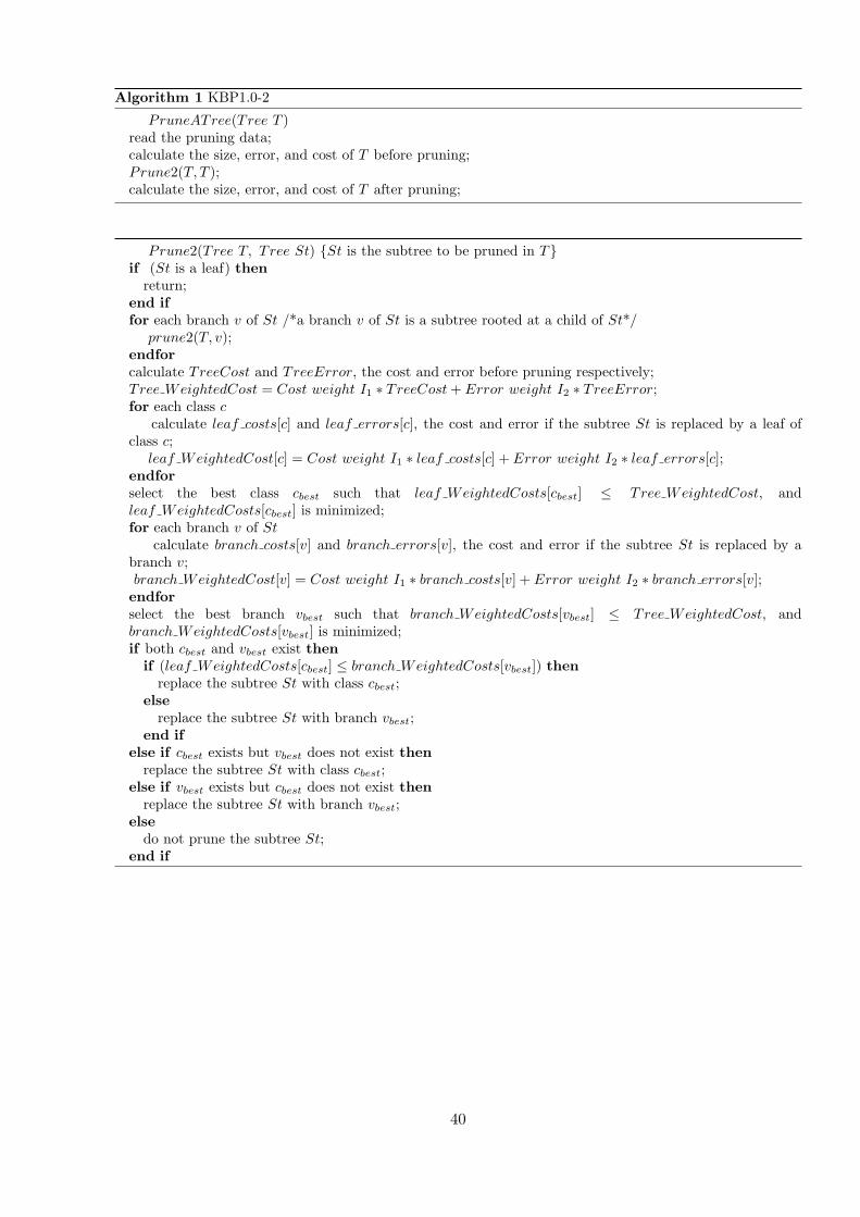
Algorithm 1 KBP1.0-2

PruneATree(Tree T )read the pruning data;calculate the size, error, and cost of T before pruning;Prune2(T, T );calculate the size, error, and cost of T after pruning;

Prune2(Tree T, Tree St) {St is the subtree to be pruned in T}if (St is a leaf) then

return;end iffor each branch v of St /*a branch v of St is a subtree rooted at a child of St*/

prune2(T, v);endforcalculate TreeCost and TreeError, the cost and error before pruning respectively;Tree WeightedCost = Cost weight I1 ∗ TreeCost + Error weight I2 ∗ TreeError;for each class c

calculate leaf costs[c] and leaf errors[c], the cost and error if the subtree St is replaced by a leaf ofclass c;

leaf WeightedCost[c] = Cost weight I1 ∗ leaf costs[c] + Error weight I2 ∗ leaf errors[c];endforselect the best class cbest such that leaf WeightedCosts[cbest] ≤ Tree WeightedCost, andleaf WeightedCosts[cbest] is minimized;for each branch v of St

calculate branch costs[v] and branch errors[v], the cost and error if the subtree St is replaced by abranch v;branch WeightedCost[v] = Cost weight I1 ∗ branch costs[v] + Error weight I2 ∗ branch errors[v];endforselect the best branch vbest such that branch WeightedCosts[vbest] ≤ Tree WeightedCost, andbranch WeightedCosts[vbest] is minimized;if both cbest and vbest exist then

if (leaf WeightedCosts[cbest] ≤ branch WeightedCosts[vbest]) thenreplace the subtree St with class cbest;

elsereplace the subtree St with branch vbest;

end ifelse if cbest exists but vbest does not exist then

replace the subtree St with class cbest;else if vbest exists but cbest does not exist then

replace the subtree St with branch vbest;else

do not prune the subtree St;end if

40

(2) Setting the threshold value to make the pruning decision

In this method, threshold means the point at which a subtree can be pruned.

Advice can be obtained from experts to set the threshold value for the cost defined

in equation (14) and another threshold value for the error rate. Let c represent

the threshold value for cost and e represent the threshold value for error rate. The

following rules are used to make the pruning decision:

(1) IF both the error rate E and error cost C decreases THEN prune

(2) IF both the error rate E and error cost C increases THEN do not prune

(3) IF error rate E decreases and error cost C increases THEN:

(a) IF the error cost C is equal to or less than c THEN prune

(b) IF the error cost C is larger than c THEN do not prune

(4) IF the error rate E increases and error cost C decreases THEN:

(a) IF the error rate E is equal to or less than e THEN prune

(b) IF the error rate E is larger than e THEN do not prune

This method is called KBP1.0-3 and rely upon the expert to set the threshold values. There

are some methods to set the threshold values. For example, traditional pruning methods, such

as reduced error pruning or pessimistic pruning, can be used to prune the decision tree and

test the pruned decision tree to get it error rate e1. Then the threshold value for error e can

be set as e1. In the same way, KBP1.0-1 can be used to prune the decision tree and test the

pruned decision tree to get its cost c1. Then the threshold value for cost c can be set as c1.

The KBP1.0-3 algorithm is expressed as follows:

41

Algorithm 2 KBP1.0-3

PruneATree(Tree T )read the pruning data;calculate the size, error, and cost of T before pruning;Prune3(T, T );calculate the size, error, and cost of T after pruning;

Prune3(Tree T, Tree St) {St is the subtree to be pruned in T}if (St is a leaf) then

return;end iffor each branch v of St /*a branch v of St is a subtree rooted at a child of St*/

prune3(T, v);endforcalculate TreeCost and TreeError, the cost and error before pruning respectively;for each branch v of St

calculate branch costs[v] and branch errors[v], the cost and error if the subtree St is replaced by thebranch v;endforfor each branch v of Stif ((branch costs[v] ≤ TreeCost) and (branch errors[v] ≤ TreeError)) or ((branch costs[v] ≤TreeCost) and (branch errors[v] > TreeError) and (branch errors[v] ≤ ErrorThreshold ∗ TreeError))or ((branch costs[v] > TreeCost) and (branch errors[v] ≤ TreeError) and (branch costs[v] ≤CostThreshold ∗ TreeCost)) then

set branchPrune F lag[v] to be true, i.e., the subtree can be replaced by the branch v;else

set branchPrune F lag[v] to be false;end ifendforselect the branch vbest such that branchPrune F lag[vbest] = true and branch costs[vbest] is minimized;for each class c

calculate leaf costs[c] and leaf errors[c], the cost and error if the subtree St is replaced by a leaf ofclass c;endforfor each class cif ((leaf costs[c] ≤ TreeCost) and (leaf errors[c] ≤ TreeError)) or ((leaf costs[c] ≤ TreeCost) and(leaf errors[c] > TreeError) and (leaf errors[c] ≤ ErrorThreshold ∗ TreeError)) or ((leaf costs[c] >TreeCost) and (leaf errors[c] ≤ TreeError) and (leaf costs[c] ≤ CostThreshold ∗ TreeCost)) then

set leafPrune F lag[c] to be true, i.e., the subtree can be replaced by class c;else

set leafPrune F lag[c] to be false;end ifendforselect the best class cbest such that leafPrune F lag[cbest] = true and leaf costs[cbest] is minimized;

42

if both cbest and vbest exist thenif (leaf costs[cbest] ≤ branch costs[vbest]) then

replace the subtree St with class cbest;else

replace the subtree St with branch vbest;end if

else if cbest exists but vbest does not exist thenreplace the subtree St with class cbest;

else if vbest exists but cbest does not exist thenreplace the subtree St with branch vbest;

elsedo not prune the subtree St;

end if

4. Pessimistic Cost Pruning

In Chapter 2, pessimistic error pruning(PEP) which was proposed by Quinlan and devel-

oped in the context of ID3 is introduced. Compared with other traditional pruning methods,

PEP has a better performance in respect to cost. Sometimes, it is even better than KBP1.0-1,

KBP 1.0-2, and KBP1.0-3 (The comparison will be discussed in detail in Chapter 5). Learning

from PEP, a new pruning method called Pessimistic Cost Pruning(PCP) is proposed. The

difference between PEP and PCP is that the error in PEP is replaced by the cost in PCP.

When the original tree T is used to classify the N cases in the training set from which it

was generated, let some leaf account for K of these cases with J of them misclassified. The

equation(14) is used to calculate the misclassification cost C. Same as in PEP, a more realistic

cost might be obtained using the continuity correction for the binomial distribution in which

C is replaced by C + 1/2.

Let S be a subtree of T containing L(S) leaves. If S were replaced by the best leaf, let

C ′ be the misclassification cost from the training set. The pessimistic cost pruning method

replaces S by the best leaf whenever C ′+1/2 is within one standard error of C+ L(S)2

. All non-

leaf subtrees are examined just once to see whether they should be pruned but sub-subtrees

of pruned subtrees need not be examined at all.

This method can keep the advantages of PEP such as faster and high accuracies. Unlike

other pruning methods in KBP1.0, it does not require a pruning set separate from the cases

43

in the training set from which the tree was constructed. It has the same disadvantage with

PEP, i.e., in the worst case, when the tree does not need pruning at all, each node will still

be visited once [11]. This method is called KBP1.0-4.

The KBP1.0-4 algorithm is expressed as follows:

Algorithm 3 KBP1.0-4

PruneATree(Tree T )read the pruning data;calculate the size, error, and cost of T before pruning;Prune4(T, T );calculate the size, error, and cost of T after pruning;

Prune4(Tree T, Tree St) {St is the subtree to be pruned in T}if (St is a leaf) then

return;end iffor each branch v of St /*a branch v of St is a subtree rooted at a child of St*/

prune4(T, v);endforcalculate TreeCost, the cost before pruning;for each class c

calculate leaf costs[c], the cost if the subtree St is replaced by a leaf of class c;endforselect the best class cbest such that leaf costs[cbest] − TreeCost ≤ number of leaves in St − 1

2 +√TreeCost + number of leaves in St

2 , and leaf costs[cbest] is minimized;if cbest exists then

replace the subtree St with class cbest;else

do not prune the subtree St;end if

5. Expert Knowledge used in Decision Tree Pruning

In Section 3.4, how to determine α is discussed and one of methods is using an expert

system to determine which cost matrix we should use. The cost matrix is different in different

applications. Therefore, the expert is relied upon to set the values of αij in the cost matrix

according to the different applications.

Experts use their knowledge to define the cost matrix. For example, when a doctor diag-

noses whether a patient has hepatitis or not, the doctor considers the following items when

he/she defines the cost matrix:

44

(1) Will the misdiagnosis hurt the patient’s health? How serious?

(2) Will the patient spend more money if the misdiagnosis happens? How much?

(3) Will the patient spend more time to treat his/her illness? How much?

EXAMPLE

IF misdiagnosis will badly hurt the patient’s health

THEN the αij is 0.9

Else

IF misdiagnosis will make patient spend much more money

THEN the αij is 0.5

Else

IF misdiagnosis will make patient spend much more time

THEN the αij is 0.6

6. Difference between KBP1.0 and C4.5

C4.5 is a software extension of the basic ID3 algorithm designed by Quinlan [41]. It is

one of the most successful decision tree generators. Generally, it can construct decision trees,

prune decision trees and generalize rules from decision trees.

C4.5 can be freely downloaded and freely used for research. You can get C4.5 from Quin-

lan’s homepage:http://www.rulequest.com/Personal/.

KBP1.0, is a cost-sensitive decision tree pruning algorithm based on C4.5. KBP1.0 inte-

grates intelligent inexact classification to deal with cost-sensitive pruning.

KBP1.0 uses the same method as that of C4.5 to construct the original decision tree.

But its pruning method is different from that of C4.5. KBP1.0-1, KBP1.0-2, and KBP1.0-3,

which use separate pruning sets to prune the original tree, while KBP1.0-4 does not use a

separate pruning set to prune the original tree. KBP1.0 considers cost during pruning. When

a decision tree has been constructed, the rules can be obtained from the tree, as does C4.5.

45

KBP1.0 has one more files than C4.5. This file is used to define the cost matrix. The training

data, pruning data, and testing data are saved in three files respectively. KBP1.0 can split

the data set into training set and pruning set.

Since KBP1.0 originated from C4.5, they have some similarities. For example, KBP1.0

uses the same methods as C4.5 to construct decision trees and obtain rules from the trees.

KBP1.0 also uses the same methods as C4.5 on dealing with missing attribute values. But

KBP1.0 is a cost-sensitive decision tree pruning algorithm and has many differences with C4.5,

especially in tree pruning. Their differences is summarized as follows:

(1) In C4.5, the number of predicted errors of leaves and subtrees is calculated and

compared to decide whether to prune the tree or not. In KBP1.0, not only the errors

but also the misclassification cost of the original trees and pruned trees are compared to

decide whether to prune the tree or not.

(2) C4.5 does not require a pruning set separated from the cases in the training set from

which the tree was constructed. In KBP1.0, some pruning methods such as KBP1.0-

1, KBP1.0-2, and KBP 1.0-3 use a pruning set to simplify the decision tree, but KBP

1.0-4(PCP) doesn’t use a pruning set separate from the training set.

(3) KBP1.0 can randomly split the data set into three subsets: training set, pruning

set, and testing set. There is a small program called convert which can randomly divide

the data. It is much more convenient for users when they need to divide the data set. In

KBP1.0, you have to split the data set by yourself.

(4) There are four pruning methods in KBP1.0 and the user can select one of them to

prune decision tree.

KBP1.0 uses the same method as that of C4.5 to construct the original decision tree, with

slight code modifications to support the KBP1.0 pruning technique.

46

The pruning code in C4.5 has been modified to realize the pruning methods in KBP1.0.

The big difference between KBP1.0’s pruning code and C4.5’s pruning code is that the pruning

method in C4.5’s is based on error, while the pruning method in KBP1.0 is based on cost, or on

both error and cost. In addition, C4.5’s pruning code can only calculate the misclassification

error during pruning, while KBP1.0’s pruning code can calculate both the misclassification

error and misclassification cost during pruning.

7. AN EXAMPLE OF KBP1.0

In this chapter an example is shown to illustrate how KBP1.0 works. The pruning method

used in this example is KBP1.0-2.

(1) KBP1.0-2

Because the pruning method used in this example is KBP1.0-2, we review the KBP1.0-2

which has been introduced in Chapter 3.

KBP1.0-2 uses the following equation to calculate the evaluation of pruning.

F = I1 ∗ C + I2 ∗ E (16)

where:

F is the evaluation value used in decision tree pruning,

I1 is the weight of cost,

I2 is the weight of error rate,

C is the cost which we get from equation (17),

E is the error rate.

The decision tree is select to be pruned if the result of equation (16) is decreased after

pruning, otherwise it is not select to be pruned. If more than one subtree satisfies the pruning

requirement, the one with the smallest size is selected.

47

error(ij) is defined as the error that the decision tree classifies class i as class j. Then for

decision tree pruning the cost can be obtained from

C =

∑ni,j=1 αijpij∑n

i,j=1 αij

(17)

where:

αij is the seriousness of error(ij),

pij is a measure of the error possibility of error(ij) if tree is pruned.

(2) The Data Set Used in this Example

In this example, the goal is to predict the result of a vote. The data set used in this

example is from the 1984 United States congressional voting records database [38]. This data

set includes votes for each of the U.S. House of representatives congressmen on the 16 key

votes identified by the Congressional Quarterly Almanac(CQA). The CQA lists nine different

types of votes: voted for, paired for, and announced for (these three are simplified to y that

represents a yes vote), voted against, paired against, and announced against (these three are

simplified to n that represents a no vote), voted present, voted present to avoid conflict of

interest, and did not vote or otherwise make a position known (these three are simplified to

u). The number of instances in the data set is 435 (267 democrats, 168 republicans) and the

number of attributes is 16 and the number of classes is 2 (Democrat and Republican). There

are 392 missing values in the data set. The main attributes which are used in the decision

tree are shown in Table 1. Ten attributes are not used in the decision tree because they are

irrelevant for predicting the final result.

48

Table 1. Attribute Information.

Attributes Values of Attributehandicapped infants y, n, u

water project cost sharing y, n, uadoption of the budget resolution y, n, u

physician fee freeze y, n, ueducation spending y, n, u

synfuels corporation cutback y, n, u

(3) The Cost Matrix and Weights

The cost weight is defined as 0.7 (I1 in equation 16) and error weight as 0.3 (I2 in equation

16). The cost matrix is also defined as follows.

Cost Matrix:

Classified As

(democrat) (republican) < −classified as

−− −−

0.0 0.2 (democrat): class democrat

0.8 0.0 (republican): class republican

In the matrix, “democrat” and “republican” in the first row represent the classes that the

decision tree classifies, “democrat” and “republican” in the last column represent the classes

in fact. For the numbers in the matrix, 0.2 is the seriousness if the decision tree misclassifies

class “democrat” as class “republican”, 0.8 is the seriousness if the decision tree misclassifies

class “republican” as class “democrat”. How this cost matrix is gotten is not discussed here

and just used in the example.

(4) Dividing the Data Set

A program called “convert” is used to randomly divide the data set into three parts:

training set (150 cases), pruning set (150 cases), and testing set (135 cases).

49

(5) Constructing the Original Decision Tree

KBP1.0 uses the same method as C4.5 to create the original decision tree. The following

tree was constructed using the 150 cases in the training set. The (N) or (N/E) appearing after

a leaf indicates that the leaf covers N training cases among which E cases are misclassified.

Original Decision Tree

physician fee freeze = n:

| adoption of the budget resolution = y: democrat(77.0)

| adoption of the budget resolution = u: democrat (1.0)

| adoption of the budget resolution = n:

| | education spending = n: democrat (3.0)

| | education spending = y: democrat (5.0)

| | education spending = u: republican (1.0)

physician fee freeze = y:

| synfuels corporation cutback = n: republican (48.0)

| synfuels corporation cutback = u: republican (2.0)

| synfuels corporation cutback = y:

| | handicapped infants = y: republican (2.0)

| | handicapped infants = u: republican (0.0)

| | handicapped infants = n:

| | | adoption of the budget resolution = n: republican (5.0/1.0)

| | | adoption of the budget resolution = y: democrat (2.0)

| | | adoption of the budget resolution = u: republican (0.0)

physician fee freeze = u:

| water project cost sharing = n: democrat (0.0)

50

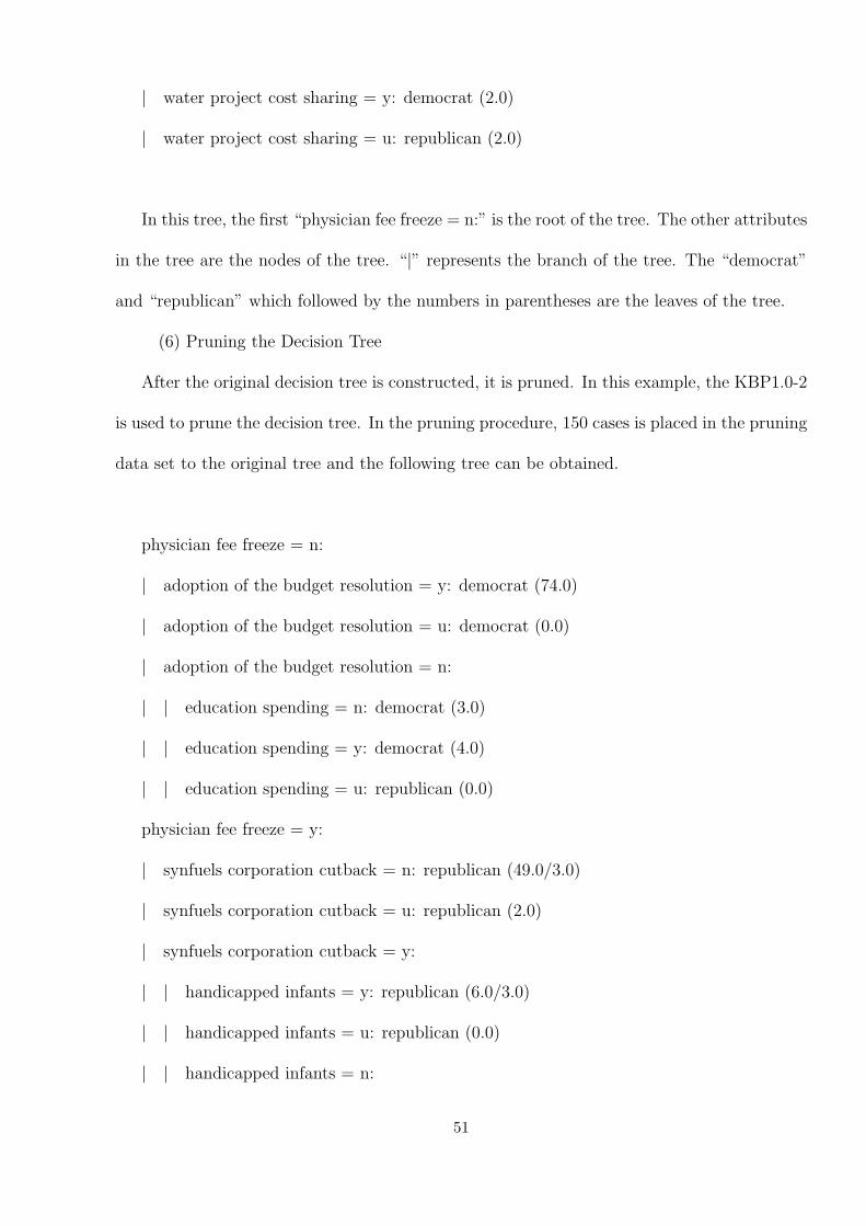
| water project cost sharing = y: democrat (2.0)

| water project cost sharing = u: republican (2.0)

In this tree, the first “physician fee freeze = n:” is the root of the tree. The other attributes

in the tree are the nodes of the tree. “|” represents the branch of the tree. The “democrat”

and “republican” which followed by the numbers in parentheses are the leaves of the tree.

(6) Pruning the Decision Tree

After the original decision tree is constructed, it is pruned. In this example, the KBP1.0-2

is used to prune the decision tree. In the pruning procedure, 150 cases is placed in the pruning

data set to the original tree and the following tree can be obtained.

physician fee freeze = n:

| adoption of the budget resolution = y: democrat (74.0)

| adoption of the budget resolution = u: democrat (0.0)

| adoption of the budget resolution = n:

| | education spending = n: democrat (3.0)

| | education spending = y: democrat (4.0)

| | education spending = u: republican (0.0)

physician fee freeze = y:

| synfuels corporation cutback = n: republican (49.0/3.0)

| synfuels corporation cutback = u: republican (2.0)

| synfuels corporation cutback = y:

| | handicapped infants = y: republican (6.0/3.0)

| | handicapped infants = u: republican (0.0)

| | handicapped infants = n:

51

| | | adoption of the budget resolution = n: republican (6.0/2.0)

| | | adoption of the budget resolution = y: democrat (1.0/1.0)

| | | adoption of the budget resolution = u: republican (0.0)

physician fee freeze = u:

| water project cost sharing = n: democrat (0.0)

| water project cost sharing = y: democrat (2.0)

| water project cost sharing = u: republican (3.0/2.0)

Again, the (N) or (N/E) appearing after a leaf indicates that the leaf covers N pruning

cases among which E cases are misclassified. From the original tree, KBP1.0 uses the cost

matrix, the equation 16 and 17, and cost weight and error weight to calculate the evaluation

value as follows

C = 0.8 ∗ (1/150) + 0.2 ∗ (10/150) = 0.018667 (18)

F = I1 ∗ C + I2 ∗ E = 0.7 ∗ 0.018667 + 0.3 ∗ (1 + 10)/150 = 0.035067 (19)

Then KBP1.0 replaces the subtree

| | education spending = n: democrat (3.0)

| | education spending = y: democrat (4.0)

| | education spending = u: republican (0.0)

with its three leaves separately. Now, KBP1.0 calculates the new evaluation value if the

replacement happens. From equation 16, KBP 1.0 can calculate their evaluation value, i.e.,

52

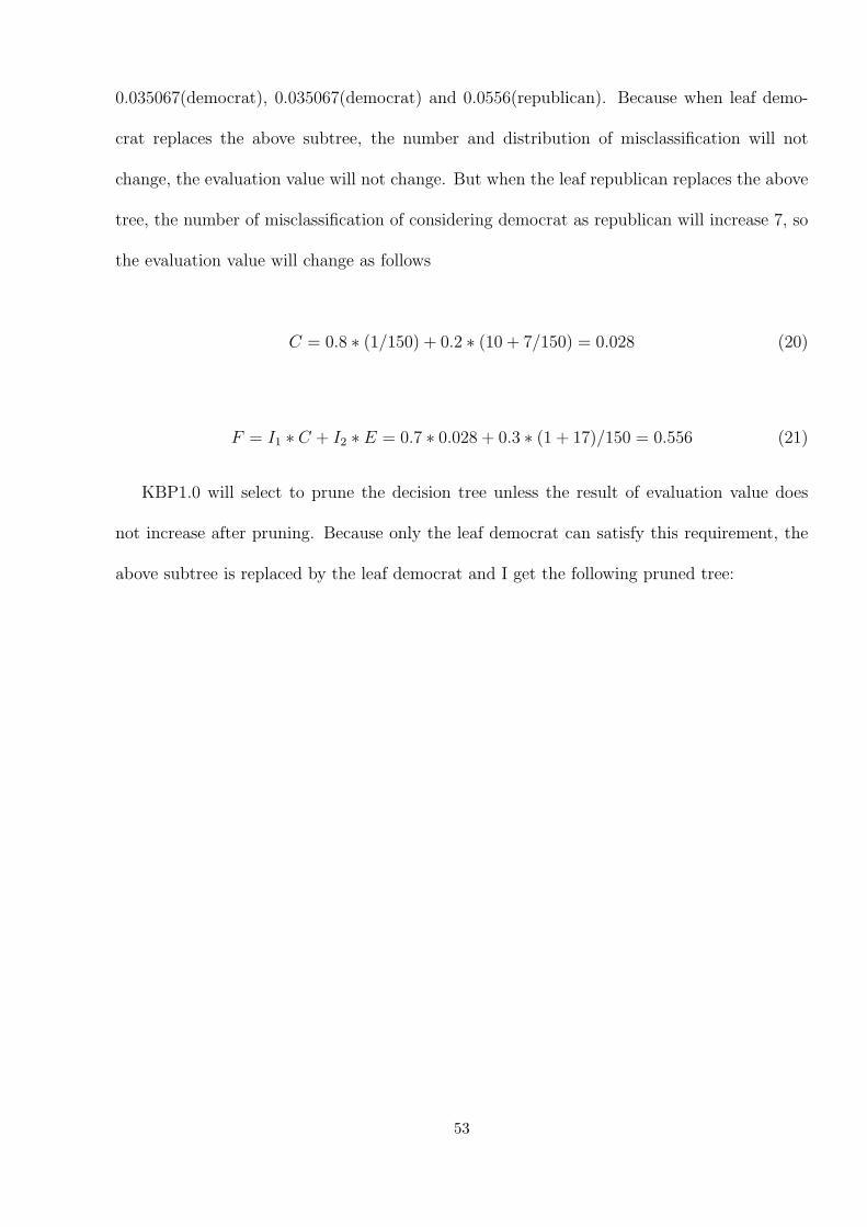
0.035067(democrat), 0.035067(democrat) and 0.0556(republican). Because when leaf demo-

crat replaces the above subtree, the number and distribution of misclassification will not

change, the evaluation value will not change. But when the leaf republican replaces the above

tree, the number of misclassification of considering democrat as republican will increase 7, so

the evaluation value will change as follows

C = 0.8 ∗ (1/150) + 0.2 ∗ (10 + 7/150) = 0.028 (20)

F = I1 ∗ C + I2 ∗ E = 0.7 ∗ 0.028 + 0.3 ∗ (1 + 17)/150 = 0.556 (21)

KBP1.0 will select to prune the decision tree unless the result of evaluation value does

not increase after pruning. Because only the leaf democrat can satisfy this requirement, the

above subtree is replaced by the leaf democrat and I get the following pruned tree:

53

physician fee freeze = n:

| adoption of the budget resolution = y: democrat (74.0)

| adoption of the budget resolution = u: democrat (0.0)

| adoption of the budget resolution = n: democrat (7.0)

physician fee freeze = y:

| synfuels corporation cutback = n: republican (49.0/3.0)

| synfuels corporation cutback = u: republican (2.0)

| synfuels corporation cutback = y:

| | handicapped infants = y: republican (6.0/3.0)

| | handicapped infants = u: republican (0.0)

| | handicapped infants = n:

| | | adoption of the budget resolution = n: republican (6.0/2.0)

| | | adoption of the budget resolution = y: democrat (1.0/1.0)

| | | adoption of the budget resolution = u: republican (0.0)

physician fee freeze = u:

| water project cost sharing = n: democrat (0.0)

| water project cost sharing = y: democrat (2.0)

| water project cost sharing = u: republican (3.0/2.0)

KBP1.0 will continue to prune the above decision tree in the same way until it gets the

following simplest tree:

54

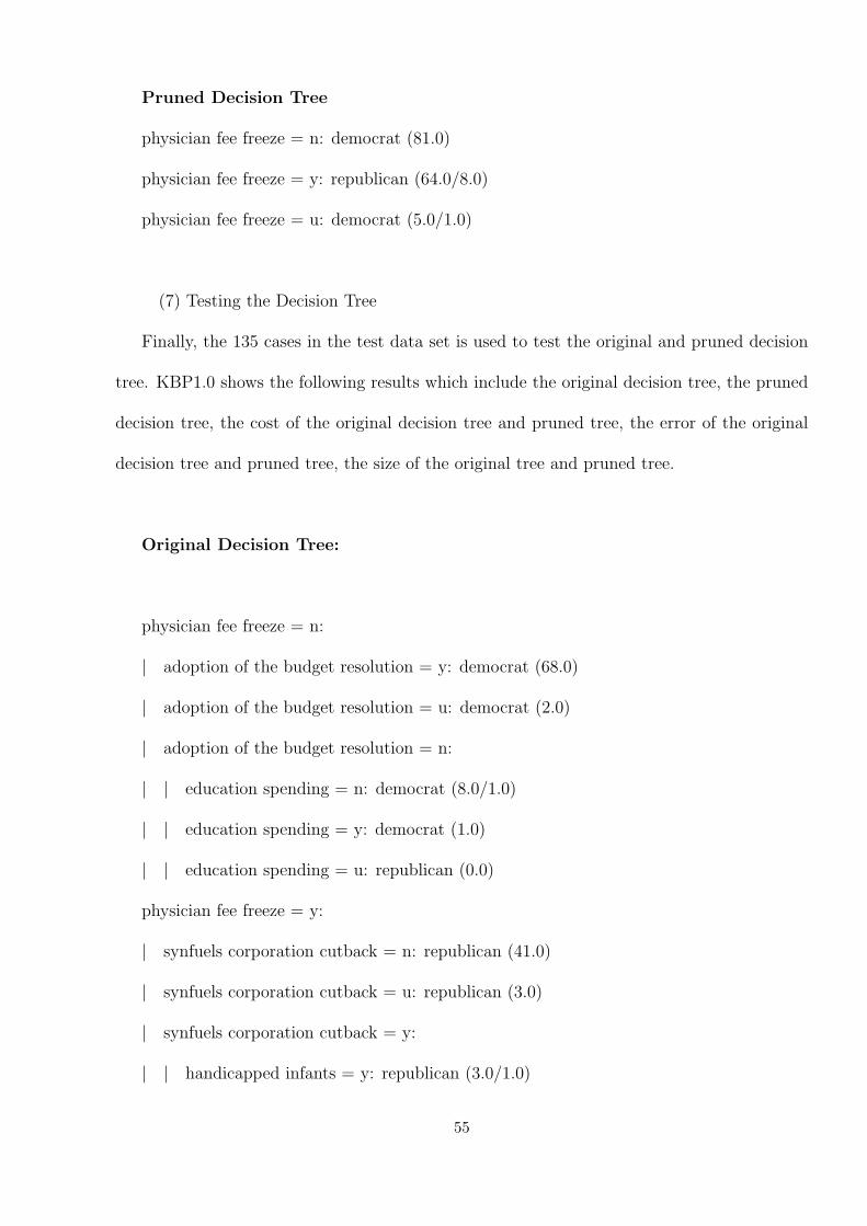
Pruned Decision Tree

physician fee freeze = n: democrat (81.0)

physician fee freeze = y: republican (64.0/8.0)

physician fee freeze = u: democrat (5.0/1.0)

(7) Testing the Decision Tree

Finally, the 135 cases in the test data set is used to test the original and pruned decision

tree. KBP1.0 shows the following results which include the original decision tree, the pruned

decision tree, the cost of the original decision tree and pruned tree, the error of the original

decision tree and pruned tree, the size of the original tree and pruned tree.

Original Decision Tree:

physician fee freeze = n:

| adoption of the budget resolution = y: democrat (68.0)

| adoption of the budget resolution = u: democrat (2.0)

| adoption of the budget resolution = n:

| | education spending = n: democrat (8.0/1.0)

| | education spending = y: democrat (1.0)

| | education spending = u: republican (0.0)

physician fee freeze = y:

| synfuels corporation cutback = n: republican (41.0)

| synfuels corporation cutback = u: republican (3.0)

| synfuels corporation cutback = y:

| | handicapped infants = y: republican (3.0/1.0)

55

| | handicapped infants = u: republican (0.0)

| | handicapped infants = n:

| | | adoption of the budget resolution = n: republican (5.0)

| | | adoption of the budget resolution = y: democrat (2.0/2.0)

| | | adoption of the budget resolution = u: republican (0.0)

physician fee freeze = u:

| water project cost sharing = n: democrat (0.0)

| water project cost sharing = y: democrat (1.0)

| water project cost sharing = u: republican (1.0/1.0)

Cost before pruning for testing data: 0.02074

Pruned Tree:

physician fee freeze = n: democrat (79.0/1.0)

physician fee freeze = y: republican (54.0/1.0)

physician fee freeze = u: democrat (2.0)

Cost after pruning for testing data: 0.00741

56

Evaluation on test data (135 items):

Before Pruning After Pruning

−−−−−−− −−−−−−−−

Size Errors Size Errors

22 5( 3.7%) 4 2( 1.48%) <<

Class distribution for test data in original tree

Classified As

(democrat) (republican) < −classified as

−− −−

79 2 (democrat): class democrat Actual Class

3 51 (republican): class republican

Class distribution for test data in pruned tree

Classified As

(democrat) (republican) < −classified as

−− −−

80 1 (democrat): class democrat Actual Class

1 53 (republican): class republican

From the class distribution for the test data in the original tree, it is clear that 2 classes

“democrat” are misclassified as “republican” and 3 classes “republican” are misclassified as

“democrat”. The class distribution for the test data in the pruned tree tells us that 1 class

57

“democrat” is misclassified as “republican” and 1 class “republican” is misclassified as “de-

mocrat”.

In the next chapter, the results from KBP1.0 and C4.5 is compared.

58

CHAPTER IV

COMPARATIVE ANALYSIS

Comparing the different methods for pruning a decision tree and summarizing the advan-

tage of the knowledge-based pruning technique is one of the most important tasks in this

dissertation. In this chapter, an experiment is designed to make a comparative study be-

tween some of the well known decision tree pruning techniques and the cost-sensitive pruning

methods in KBP1.0. From the comparison, the strengths and weaknesses of KBP1.0 can be

identified.

The C4.5’s pruning code is modified to get the KBP1.0’s pruning code and other traditional

pruning methods’ codes.

1. The Design of the Experiment

The main characteristics of the data sets used in this experiments are reported in Table

2. All these data sets are available from the UCI Machine Learning Repository [38]. They

are also very common in decision tree pruning experiments [11][47]. The data sets chosen

are Pima, Hepatitis, Cleveland, Vote, Iris, and Glass. Almost the same data sets as used

[11][47] are selected, because it is very convenient to make use of the results from [11] and

[47] and compare them with ones in our experiment. Table 2 shows the main characteristics

of the databases used for the experimentation. In Table 2, the columns headed “real” and

”multi” concern the number of attributes that are treated as real-value and multi-value discrete

attributes, respectively. The column “Base error” means the percentage error obtained if the

most frequent class is always predicted. The column “Null Values” means whether there are

59

miss values or not. The last column “Uniform Distrib” states whether the distribution of

examples per class is uniform or not.

Table 2. Major properties of the data sets considered in the experimentation

data set No.Classes

No. At-tributes

Real Multi NullValues

Baseerror

UniformDistrib

Glass 7 9 9 0 no 64.49 yesCleveland 2 14 5 5 yes 45.21 approx.Hepatitis 2 19 6 0 yes 10.65 no

Hypo 4 29 7 1 yes 7.7 noIris 3 4 4 0 no 66.67 yes

Pima 2 8 8 0 no 34.9 noVote 2 16 0 16 yes 45.2 no

The six data sets is described in detail as follows. All the information is from the UCI

Machine Learning Repository [38].

(1) Glass

This is a glass identification database which is used to classify the type of glass.

The study of classification of glass types was motivated by criminological investiga-

tion [38]. At the scene of the crime, the glass left can be used as evidence, if it is

correctly identified. Number of instances in the data set is 214, number of attributes

is 9, and number of classes is 7 including 163 Window glass (building windows and

vehicle windows), 87 float processed, 70 building windows, 17 vehicle windows, 76

non-float processed, 76 building windows, 0 vehicle windows, 51 Non-window glass,

13 containers, 9 tableware, and 29 headlamps. There are no missing values in this

data set.

(2) Heart Disease Domain(Cleveland)

This data set is used to diagnose whether a patient has heart disease or not.

It is one of the 4 databases(Cleveland, Hungarian, Switzerland, and Long Beach)

concerning heart disease diagnosis. Number of instances in the data set is 303, number

60

of attributes is 76, and number of classes is 5 classes from value 0 to value 4. To

create a 2-class problem, I grouped values 1, 2, 3, 4 together as class 1(sich=presence

of heart disease), and retained value 0(absence of heart disease). 160 of the examples

are healthy and the others have heart disease. There are 6 missing values in this data

set.

(3) Hepatitis

This data set is used to diagnose whether a hepatitis patient will die or live.

Number of instances in the data set is 155, number of attributes is 20, and number

of classes is 2 including DIE and LIVE. There are 123 LIVE instances and 32 DIE

instances. There are 168 missing values in this data set.

(4) Hypothyroid

This thyroid disease data set comes from the Garavan Institute of Medical Re-

search, Sydney. This data set is used to diagnose whether a patient has thyroid

disease or not. There are six data sets in this database and I only selected one of

them, hypothyroid, in my experiment. Number of instances in the data set is 3163,

number of attributes is 25, and number of class is 2 including 151 hypothyroid and

3012 negative. There are many missing values in this data set.

(5) Iris

This is perhaps the best known data set to be found in the pattern recognition

literature. The data set is used to predict the class of an iris plant. Number of

instances in the data set is 50, number of attributes is 4, and the number of classes is

3. There is no missing values in this data set.

(6) Pima Indians Diabetes Domain (pima)

This data set is used to diagnose whether a patient has diabetes or not. All patients

in the data set are females, at least 21 years old, and of Pima Indian heritage. Number

61

of instances in the data set is 768, number of attributes is 8, and number of classes is

2 (0=health, 1=tested positive for diabetes). There are 500 of the examples which are

healthy and the others are tested positive for diabetes. There is no missing attribute

values.

(7) Vote

This data set is used to predict the result of a vote. It is from 1984 united

states congressional voting records database. This data set includes votes for each

of the U.S. House of representatives congressmen on the 16 key votes identified by

the Congressional Quarterly Almanac(CQA). The CQA lists nine different types of

votes: voted for, paired for, and announced for (these three simplified to yea), voted

against, paired against, and announced against (these three simplified to nay), voted

present, voted present to avoid conflict of interest, and did not vote or otherwise

make a position known (these three simplified to an unknown disposition). Number

of instances is 435 (267 democrats, 168 republicans), number of attributes is 16, and

number of classes is 2. There are 392 missing values in this data set.

2. Criteria and Data Set Partition

Ideally, the pruned decision tree should be much more comprehensible than the original

decision tree but should not be significantly less accurate when classifying unseen cases [12].

These are two important criterions, which are size and accuracy, to test how well a pruning

method works [11]. The cost is added as the third criterion to test the pruning methods. The

behavior of the new cost-sensitive pruning methods was analyzed in a series of experiments.

The data set is randomly split into three subsets. The three subsets are the training set (49

percent), the pruning set (21 percent), and the testing set (30 percent). The reason that the

data set was partitioned in this way is that a decision tree is created in two phases: tree

building phase, i.e., repeatedly partitioning the training data until all the examples in each

62

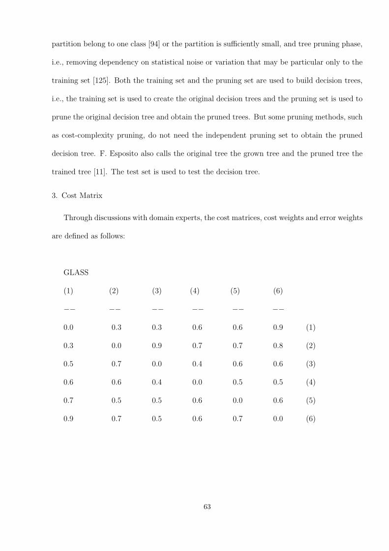
partition belong to one class [94] or the partition is sufficiently small, and tree pruning phase,

i.e., removing dependency on statistical noise or variation that may be particular only to the

training set [125]. Both the training set and the pruning set are used to build decision trees,

i.e., the training set is used to create the original decision trees and the pruning set is used to

prune the original decision tree and obtain the pruned trees. But some pruning methods, such

as cost-complexity pruning, do not need the independent pruning set to obtain the pruned

decision tree. F. Esposito also calls the original tree the grown tree and the pruned tree the

trained tree [11]. The test set is used to test the decision tree.

3. Cost Matrix

Through discussions with domain experts, the cost matrices, cost weights and error weights

are defined as follows:

GLASS

(1) (2) (3) (4) (5) (6)

−− −− −− −− −− −−

0.0 0.3 0.3 0.6 0.6 0.9 (1)

0.3 0.0 0.9 0.7 0.7 0.8 (2)

0.5 0.7 0.0 0.4 0.6 0.6 (3)

0.6 0.6 0.4 0.0 0.5 0.5 (4)

0.7 0.5 0.5 0.6 0.0 0.6 (5)

0.9 0.7 0.5 0.6 0.7 0.0 (6)

63

CLEVELAND

(heart disease) (no heart disease)

−− −−

0.0 0.8 (heart disease)

0.3 0.0 (no heart disease)

I1 = 0.8, I2 = 0.2

HEPATITIS

(LIVE) (DIE)

−− −−

0.0 0.9 (LIVE)

0.4 0.0 (DIE)

HYPOTHYROID

(thyroid) (no thyroid)

−− −−

0.0 0.8 (thyroid)

0.3 0.0 (no thyroid)

64

IRIS

(Setosa) (Versicolour) (Virginica)

−− −− −−

0.0 0.3 0.9 (Setosa)

0.3 0.0 0.9 (Versicolour)

0.7 0.7 0.0 (Virginica)

PIMA

(diabetes) (no diabetes)

−− −−

0.0 0.9 (diabetes)

0.3 0.0 (no diabetes)

VOTE

(democrat) (republican)

−− −−

0.0 0.2 (democrat)

0.8 0.0 (republican)

65

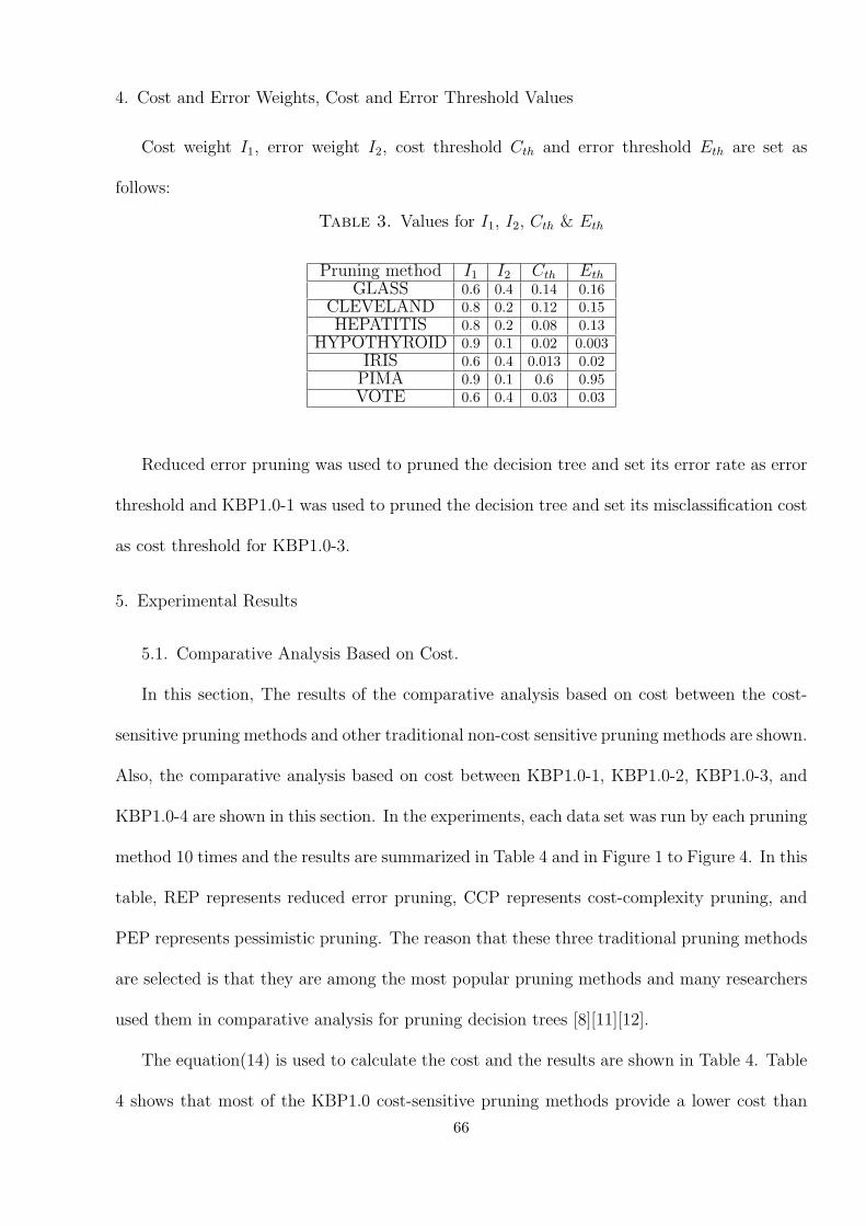
4. Cost and Error Weights, Cost and Error Threshold Values

Cost weight I1, error weight I2, cost threshold Cth and error threshold Eth are set as

follows:

Table 3. Values for I1, I2, Cth & Eth

Pruning method I1 I2 Cth Eth

GLASS 0.6 0.4 0.14 0.16CLEVELAND 0.8 0.2 0.12 0.15HEPATITIS 0.8 0.2 0.08 0.13

HYPOTHYROID 0.9 0.1 0.02 0.003IRIS 0.6 0.4 0.013 0.02

PIMA 0.9 0.1 0.6 0.95VOTE 0.6 0.4 0.03 0.03

Reduced error pruning was used to pruned the decision tree and set its error rate as error

threshold and KBP1.0-1 was used to pruned the decision tree and set its misclassification cost

as cost threshold for KBP1.0-3.

5. Experimental Results

5.1. Comparative Analysis Based on Cost.

In this section, The results of the comparative analysis based on cost between the cost-

sensitive pruning methods and other traditional non-cost sensitive pruning methods are shown.

Also, the comparative analysis based on cost between KBP1.0-1, KBP1.0-2, KBP1.0-3, and

KBP1.0-4 are shown in this section. In the experiments, each data set was run by each pruning

method 10 times and the results are summarized in Table 4 and in Figure 1 to Figure 4. In this

table, REP represents reduced error pruning, CCP represents cost-complexity pruning, and

PEP represents pessimistic pruning. The reason that these three traditional pruning methods

are selected is that they are among the most popular pruning methods and many researchers

used them in comparative analysis for pruning decision trees [8][11][12].

The equation(14) is used to calculate the cost and the results are shown in Table 4. Table

4 shows that most of the KBP1.0 cost-sensitive pruning methods provide a lower cost than

66

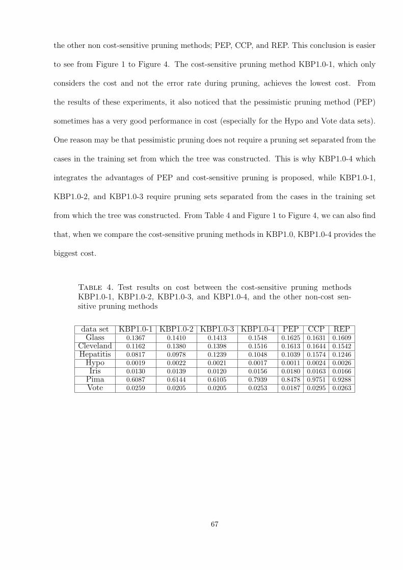
the other non cost-sensitive pruning methods; PEP, CCP, and REP. This conclusion is easier

to see from Figure 1 to Figure 4. The cost-sensitive pruning method KBP1.0-1, which only

considers the cost and not the error rate during pruning, achieves the lowest cost. From

the results of these experiments, it also noticed that the pessimistic pruning method (PEP)

sometimes has a very good performance in cost (especially for the Hypo and Vote data sets).

One reason may be that pessimistic pruning does not require a pruning set separated from the

cases in the training set from which the tree was constructed. This is why KBP1.0-4 which

integrates the advantages of PEP and cost-sensitive pruning is proposed, while KBP1.0-1,

KBP1.0-2, and KBP1.0-3 require pruning sets separated from the cases in the training set

from which the tree was constructed. From Table 4 and Figure 1 to Figure 4, we can also find

that, when we compare the cost-sensitive pruning methods in KBP1.0, KBP1.0-4 provides the

biggest cost.

Table 4. Test results on cost between the cost-sensitive pruning methodsKBP1.0-1, KBP1.0-2, KBP1.0-3, and KBP1.0-4, and the other non-cost sen-sitive pruning methods

data set KBP1.0-1 KBP1.0-2 KBP1.0-3 KBP1.0-4 PEP CCP REPGlass 0.1367 0.1410 0.1413 0.1548 0.1625 0.1631 0.1609

Cleveland 0.1162 0.1380 0.1398 0.1516 0.1613 0.1644 0.1542Hepatitis 0.0817 0.0978 0.1239 0.1048 0.1039 0.1574 0.1246

Hypo 0.0019 0.0022 0.0021 0.0017 0.0011 0.0024 0.0026Iris 0.0130 0.0139 0.0120 0.0156 0.0180 0.0163 0.0166

Pima 0.6087 0.6144 0.6105 0.7939 0.8478 0.9751 0.9288Vote 0.0259 0.0205 0.0205 0.0253 0.0187 0.0295 0.0263

67

Res

ult

s o

f te

sts

on

co

st

0

0.2

0.4

0.6

0.81

1.2

KB

P1.

0-1

KB

P1.

0-2

KB

P1.

0-3

KB

P1.

0-4

PE

PC

CP

RE

P

cost

GLA

SS

CLE

VE

LAN

D

HE

PA

TIT

IS

HY

PO

IRIS

PIM

A

VO

TE

Figure 1. Test results on cost between the cost-sensitive pruning methodsKBP1.0-1, KBP1.0-2, KBP1.0-3, and KBP1.0-4, and the other non-cost sensi-tive pruning methods for all the data sets68

HEPATITIS

0

0.02

0.04

0.06

0.08

0.1

0.12

0.14

0.16

0.18

KBP1.0-1 KBP1.0-2 KBP1.0-3 KBP1.0-4 PEP CCP REP

HEPATITIS

Figure 2. Test results on cost between the cost-sensitive pruning methodsKBP1.0-1, KBP1.0-2, KBP1.0-3, and KBP1.0-4 and the other non-cost sensitivepruning methods for the Hepatitis data set

69

IRIS

0

0.002

0.004

0.006

0.008

0.01

0.012

0.014

0.016

0.018

0.02

KBP1.0-1 KBP1.0-2 KBP1.0-3 KBP1.0-4 PEP CCP REP

IRIS

Figure 3. Test results on cost between the cost-sensitive pruning methodsKBP1.0-1, KBP1.0-2, KBP1.0-3, and KBP1.0-4, and the other non-cost sensi-tive pruning methods for the Iris data set

70

VOTE

0

0.005

0.01

0.015

0.02

0.025

0.03

0.035

KBP1.0-1 KBP1.0-2 KBP1.0-3 KBP1.0-4 PEP CCP REP

VOTE

Figure 4. Test results on cost between the cost-sensitive pruning methodsKBP1.0-1, KBP1.0-2, KBP1.0-3, and KBP1.0-4, and the other non-cost sensi-tive pruning methods for the Vote data set

71

5.2. Comparative Analysis Based on Error Rate.

In this section, the result of the comparative analysis based on error rate between the

cost-sensitive pruning methods and other traditional non-cost sensitive pruning methods is

shown. Also, the comparative analysis based on error rate between KBP1.0-1, KBP 1.0-2,

KBP1.0-3, and KBP1.0-4 are shown in this section. In the experiments, each data set was

run by each pruning method 10 times and the results are summarized in Table 5 and in

Figure 5 to Figure 6. In this table, REP represents reduced error pruning, CCP represents

cost-complexity pruning, and PEP represents pessimistic pruning.

From Table 5 and Figure 5 to Figure 6, it is noticed that KBP1.0-1, which only considers

cost and not the error rate in pruning, shows a larger error rate than KBP1.0-2, KBP1.0-3,

and KBP1.0-4, which consider both cost and error rate in pruning. In most cases, the other

well-known non-cost sensitive pruning methods are of superior accuracy to the KBP1.0 cost-

sensitive pruning methods. This is reasonable because the non-cost sensitive pruning methods

only consider error rate during pruning. But, as shown in the prior section, we obtain lower

cost from cost-sensitive pruning. From this, it is clear that we should find a balance between

error rate and cost. We can change the cost matrix, the cost weight, or the error weight to

adjust the error rate and cost.

From Table 5 and Figure 5 to Figure 6, it is noticed that, compared with the other cost-

sensitive pruning methods in KBP1.0, KBP1.0-4 achieves the lowest error, while KBP1.0-1

gets the highest error rate.

72

Table 5. Test results on error rate (percent) between the cost-sensitive pruningmethods KBP1.0-1, KBP1.0-2, KBP1.0-3, and KBP 1.0-4 and the other non-cost sensitive pruning methods

data set KBP1.0-1 KBP1.0-2 KBP1.0-3 KBP1.0-4 PEP CCP REPGlass 49.2 39.85 36.46 36.25 33.74 37.17 38.91

Cleveland 30.11 30.76 27.66 26.02 26.91 24.89 25.57Hepatitis 45.22 20.23 20.77 19.56 20.22 20.43 21.09

Hypo 0.82 0.76 0.72 0.49 0.33 0.83 0.74Iris 5.67 6.35 4.33 5.78 7.34 7.36 7.62

Pima 38.52 36.46 37.12 25.82 27.41 27.46 27.01Vote 6.13 5.22 4.72 4.65 4.67 6.58 4.98

73

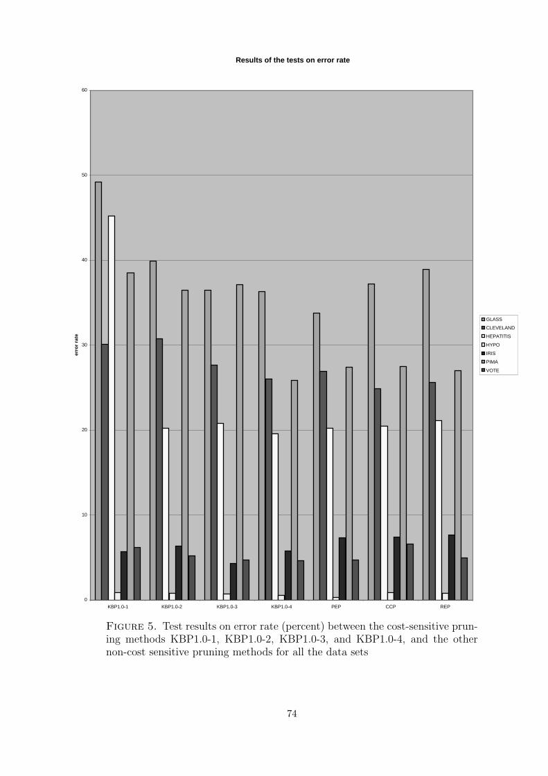
Results of the tests on error rate

0

10

20

30

40

50

60

KBP1.0-1 KBP1.0-2 KBP1.0-3 KBP1.0-4 PEP CCP REP

erro

r ra

te

GLASS

CLEVELAND

HEPATITIS

HYPO

IRIS

PIMA

VOTE

Figure 5. Test results on error rate (percent) between the cost-sensitive prun-ing methods KBP1.0-1, KBP1.0-2, KBP1.0-3, and KBP1.0-4, and the othernon-cost sensitive pruning methods for all the data sets

74

HYPO

0

0.1

0.2

0.3

0.4

0.5

0.6

0.7

0.8

0.9

KBP1.0-1 KBP1.0-2 KBP1.0-3 KBP1.0-4 PEP CCP REP

erro

r ra

te

HYPO

Figure 6. Test results on error rate (percent) between the cost-sensitive prun-ing methods KBP1.0-1, KBP1.0-2, KBP1.0-3, and KBP1.0-4, and the othernon-cost sensitive pruning methods for the Hypothyroid data set

75

5.3. Comparative Analysis Based on Size.

In this section, the result of the comparative analysis based on size between the cost-

sensitive pruning methods and other traditional non-cost sensitive pruning methods is shown.

The number of leaves and nodes is used to represent the size of decision tree. Also, the

comparative analysis based on size between KBP1.0-1, KBP1.0-2, KBP 1.0-3, and KBP1.0-

4 are shown in this section. In the experiments, each data set was run by each pruning

method 10 times and the results are summarized in Table 6 and in Figure 7. In this table,

REP represents reduced error pruning, CCP represents cost-complexity pruning, and PEP

represents pessimistic pruning.

The number of leaves together with the number of nodes is used to represent the size of

decision tree. From the results shown in Table 5, it is clear that most cost-sensitive pruning

methods tend to produce a larger decision tree than the other well-known non-cost sensitive

pruning methods which are selected. It is reasonable because most pruning methods in KBP1.0

need to consider both cost and error when deciding whether to prune subtrees or not. But the

other traditional non-cost sensitive pruning methods only consider the error when deciding to

prune. For example, for most non-cost sensitive pruning methods, when error rate decreases,

they can prune the decision tree, but for most cost-sensitive pruning methods, only when

both error rate and cost decrease, they can prune the decision tree. It is noticed that the size

difference between cost-sensitive pruning methods and non-cost sensitive pruning methods is

not very big, the size of the decision trees which are pruned by the cost-sensitive pruning

methods is acceptable for us. In many cases, a small decision tree with high cost or error is

unacceptable.

From Table 6 and Figure 7, it is noticed that, compared with the other cost-sensitive

pruning methods in KBP1.0, KBP1.0-1 gets the smallest decision tree. It is because that,

76

among the new cost-sensitive pruning methods, KBP1.0-1 is the only one which only considers

cost when deciding whether to prune subtree or not.

Table 6. Test results on size between the cost-sensitive pruning methodsKBP1.0-1, KBP1.0-2, KBP1.0-3, and KBP1.0-4, and the other non-cost sen-sitive pruning methods

data set KBP1.0-1 KBP1.0-2 KBP1.0-3 KBP1.0-4 PEP CCP REPGlass 13.6 17.2 16 10.8 10.2 11 14.2

Cleveland 16.2 20.5 20.5 7.1 9 8.1 21.7Hepatitis 5 8.2 6.8 7.4 4.6 1.4 5.8

Hypo 9.4 10 10 13.4 13.4 9.8 8.8Iris 5 5.8 10 5.8 5.6 5 5

Pima 11.6 10 12 8 8.2 6.4 15.2Vote 4 4 4.9 4 4 4 4.3

77

Results of the tests on size

0

5

10

15

20

25

KBP1.0-1 KBP1.0-2 KBP1.0-3 KBP1.0-4 PEP CCP REP

size

GLASS

CLEVELAND

HEPATITIS

HYPO

IRIS

PIMA

VOTE

Figure 7. Test results on size between the cost-sensitive pruning methodsKBP1.0-1, KBP1.0-2, KBP1.0-3, and KBP1.0-4, and the other non-cost sensi-tive pruning methods for all the data sets

78

5.4. Comparison of KBP1.0 Pruning with C4.5 Pruning.

C4.5 is the most popular decision tree algorithm. It is often used as a test benchmark for

decision tree algorithms [90][91]. In this section, the results of the comparative analysis based

on size, error rate, and cost of the pruned decision trees created by KBP1.0 cost-sensitive

pruning methods and C4.5 pruning methods are shown.

It is known that Pessimistic Error Pruning (PEP) increases the number of errors observed

at each leaf by 0.5 [12]. C4.5 employs a far more pessimistic estimate than PEP. In C4.5,

when N training cases are covered by a leaf and E of them are misclassified, the number of

predicted errors of that leaf will be N ∗ UCF (E,N) [13]. CF is the confidence level (C4.5’s

default confidence level is 25%). UCF is the upper limit on the E/N for a given confidence

level CF . C4.5 calculates the change of the number of predicted errors when deciding to prune

or not. The detailed information about how C4.5 prunes the decision tree can be found in

[13].

The equation(14) is used to calculate the cost and compared the results with what is

obtained from each pruning method. C4.5 was executed in a default setting environment, in

which the filename is specified and the tree evaluation on the test set is enable. The results

are shown in Table 7 and in Figure 8 to Figure 10. The results show that every KBP1.0

cost-sensitive pruning method obtained a lower cost than C4.5. Even compared with other

well-known non-cost sensitive pruning methods, C4.5 has the worse performance in cost.

79

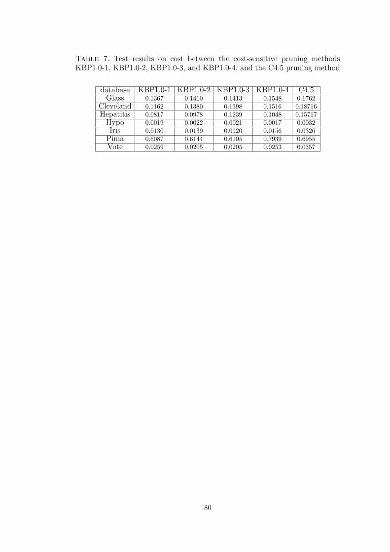
Table 7. Test results on cost between the cost-sensitive pruning methodsKBP1.0-1, KBP1.0-2, KBP1.0-3, and KBP1.0-4, and the C4.5 pruning method

database KBP1.0-1 KBP1.0-2 KBP1.0-3 KBP1.0-4 C4.5Glass 0.1367 0.1410 0.1413 0.1548 0.1762

Cleveland 0.1162 0.1380 0.1398 0.1516 0.18716Hepatitis 0.0817 0.0978 0.1239 0.1048 0.15717

Hypo 0.0019 0.0022 0.0021 0.0017 0.0032Iris 0.0130 0.0139 0.0120 0.0156 0.0326

Pima 0.6087 0.6144 0.6105 0.7939 0.6955Vote 0.0259 0.0205 0.0205 0.0253 0.0357

80

0

0.1

0.2

0.3

0.4

0.5

0.6

0.7

0.8

0.9

GLASS CLEVELAND HEPATITIS HYPO IRIS PIMA VOTE

CO

ST

KBP1.0-1

KBP1.0-2

KBP1.0-3

KBP1.0-4

C4.5

Figure 8. Test results on cost between the cost-sensitive pruning methodsKBP1.0-1, KBP1.0-2, KBP1.0-3, and KBP1.0-4, and the C4.5 pruning methodfor all the data sets

81

HYPO

0

0.0005

0.001

0.0015

0.002

0.0025

0.003

0.0035

KBP1.0-1 KBP1.0-2 KBP1.0-3 KBP1.0-4 C4.5

CO

ST

HYPO

Figure 9. Test results on cost between the cost-sensitive pruning methodsKBP1.0-1, KBP1.0-2, KBP1.0-3, and KBP1.0-4, and the C4.5 pruning methodfor the Hypothyroid data set

82

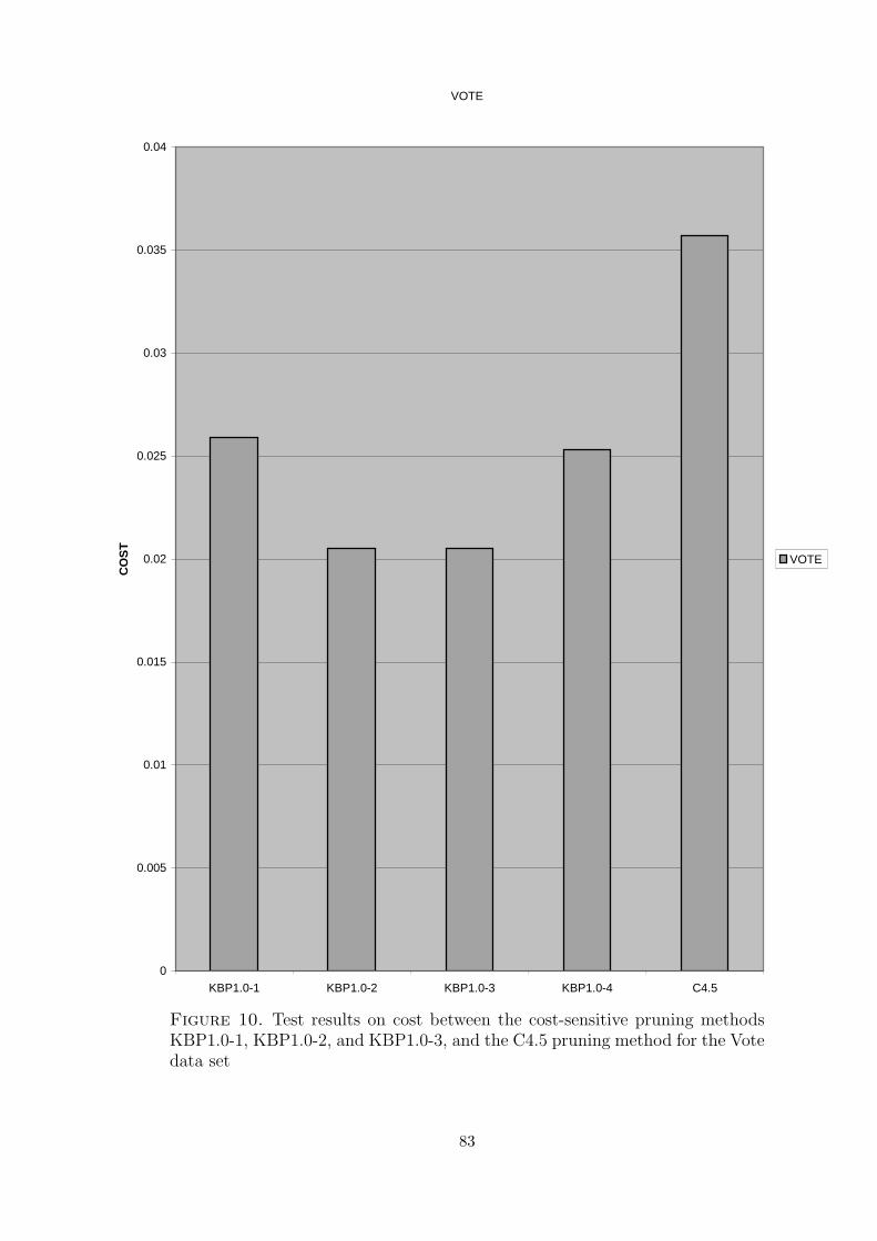
VOTE

0

0.005

0.01

0.015

0.02

0.025

0.03

0.035

0.04

KBP1.0-1 KBP1.0-2 KBP1.0-3 KBP1.0-4 C4.5

CO

ST

VOTE

Figure 10. Test results on cost between the cost-sensitive pruning methodsKBP1.0-1, KBP1.0-2, and KBP1.0-3, and the C4.5 pruning method for the Votedata set

83

The results of the tests on error rate between KBP1.0 cost-sensitive pruning methods and

C4.5 are compared. The results are shown in Table 8 and in Figure 11 to Figure 13. From

Table 6, it is noticed that, in most cases, C4.5 is of superior accuracy to the cost-sensitive

pruning. C4.5 has good performance in reducing error as well as other traditional non-cost

sensitive pruning methods.

Table 8. Test results on error rate (percent) between the cost-sensitive pruningmethods KBP1.0-1, KBP1.0-2, KBP1.0-3, and KBP 1.0-4, and the C4.5 pruningmethod

data set KBP1.0-1 KBP1.0-2 KBP1.0-3 KBP1.0-4 C4.5Glass 49.2 39.85 36.46 36.25 32.82

Cleveland 30.11 30.76 27.66 26.02 25Hepatitis 45.22 20.23 20.77 19.56 23.48

Hypo 0.82 0.76 0.72 0.49 0.6Iris 5.67 6.35 4.33 5.78 6.87

Pima 38.52 36.46 37.12 25.82 27.9Vote 6.13 5.22 4.72 4.65 5.77

84

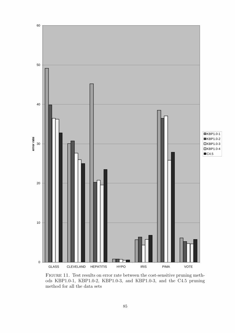
0

10

20

30

40

50

60

GLASS CLEVELAND HEPATITIS HYPO IRIS PIMA VOTE

erro

r ra

te

KBP1.0-1

KBP1.0-2

KBP1.0-3

KBP1.0-4

C4.5

Figure 11. Test results on error rate between the cost-sensitive pruning meth-ods KBP1.0-1, KBP1.0-2, KBP1.0-3, and KBP1.0-3, and the C4.5 pruningmethod for all the data sets

85

HYPO

0

0.1

0.2

0.3

0.4

0.5

0.6

0.7

0.8

0.9

KBP1.0-1 KBP1.0-2 KBP1.0-3 KBP1.0-4 C4.5

erro

r ra

te

HYPO

Figure 12. Test results on error rate between the cost-sensitive pruning meth-ods KBP1.0-1, KBP1.0-2, KBP1.0-3, and KBP1.0-4, and the C4.5 pruningmethod for Hypothyroid data set

86

IRIS

0

0.005

0.01

0.015

0.02

0.025

0.03

0.035

CC4.5-1 CC4.5-2 CC4.5-3 CC4.5-4 C4.5

CO

ST

IRIS

Figure 13. Test results on error rate between the cost-sensitive pruning meth-ods KBP1.0-1, KBP1.0-2, KBP1.0-3, and KBP1.0-4, and the C4.5 pruningmethod for the Iris data set

87

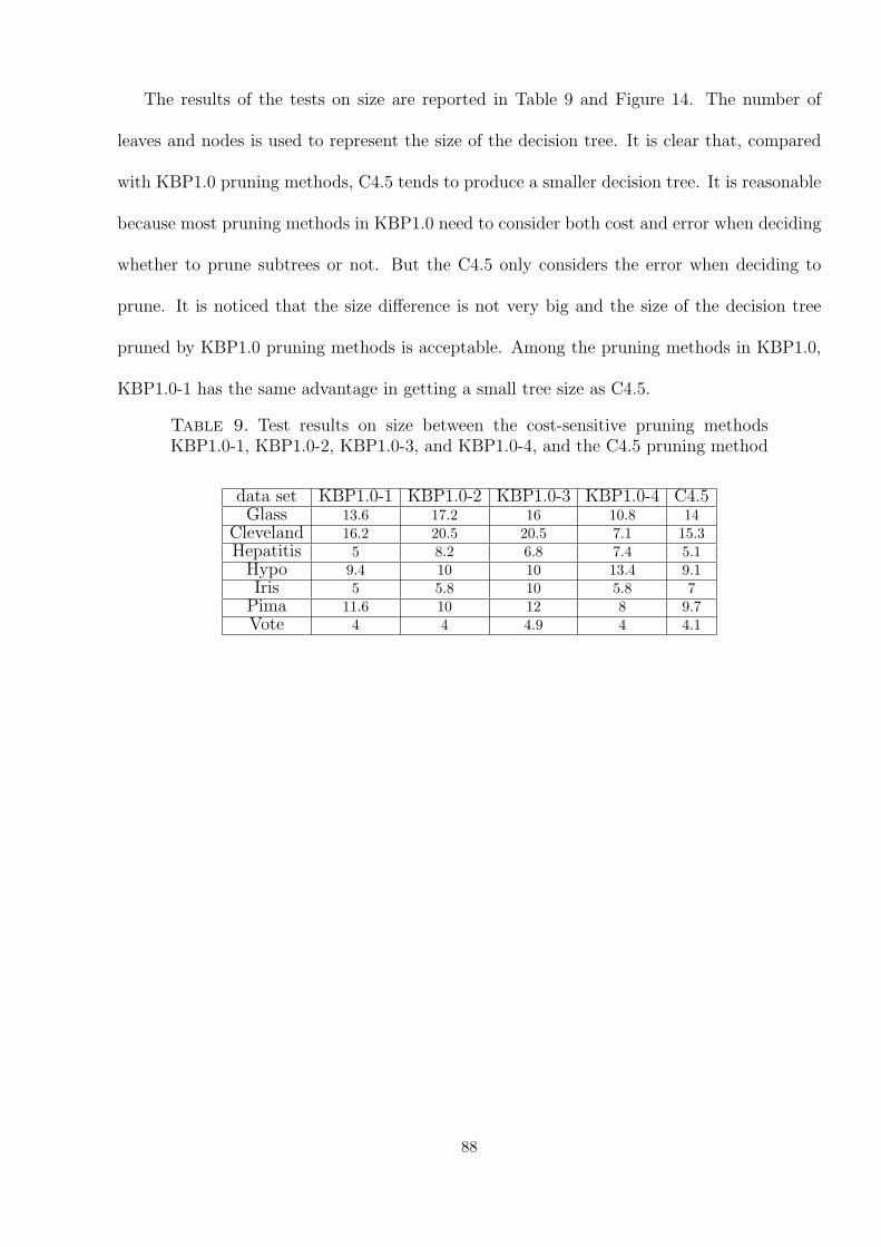
The results of the tests on size are reported in Table 9 and Figure 14. The number of

leaves and nodes is used to represent the size of the decision tree. It is clear that, compared

with KBP1.0 pruning methods, C4.5 tends to produce a smaller decision tree. It is reasonable

because most pruning methods in KBP1.0 need to consider both cost and error when deciding

whether to prune subtrees or not. But the C4.5 only considers the error when deciding to

prune. It is noticed that the size difference is not very big and the size of the decision tree

pruned by KBP1.0 pruning methods is acceptable. Among the pruning methods in KBP1.0,

KBP1.0-1 has the same advantage in getting a small tree size as C4.5.

Table 9. Test results on size between the cost-sensitive pruning methodsKBP1.0-1, KBP1.0-2, KBP1.0-3, and KBP1.0-4, and the C4.5 pruning method

data set KBP1.0-1 KBP1.0-2 KBP1.0-3 KBP1.0-4 C4.5Glass 13.6 17.2 16 10.8 14

Cleveland 16.2 20.5 20.5 7.1 15.3Hepatitis 5 8.2 6.8 7.4 5.1

Hypo 9.4 10 10 13.4 9.1Iris 5 5.8 10 5.8 7

Pima 11.6 10 12 8 9.7Vote 4 4 4.9 4 4.1

88

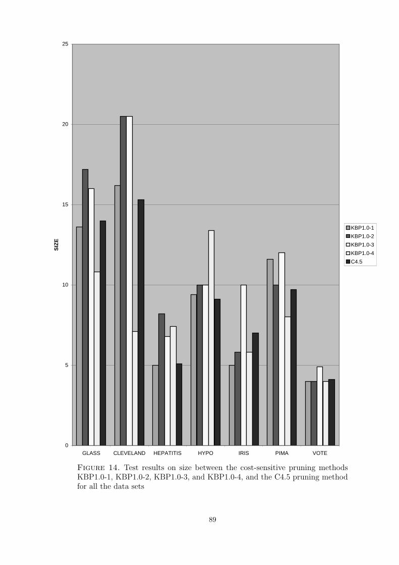
0

5

10

15

20

25

GLASS CLEVELAND HEPATITIS HYPO IRIS PIMA VOTE

SIZ

E

KBP1.0-1

KBP1.0-2

KBP1.0-3

KBP1.0-4

C4.5

Figure 14. Test results on size between the cost-sensitive pruning methodsKBP1.0-1, KBP1.0-2, KBP1.0-3, and KBP1.0-4, and the C4.5 pruning methodfor all the data sets

89

6. Statistical Measures

In previous sections in this chapter, the different results between KBP1.0 and other tra-

ditional pruning methods are compared. But the comparison methods used are not enough

to conclude that KBP1.0 has a higher performance than other traditional non-cost sensitive

pruning methods. The problem is that we can only make a finite number of measurements on

the real world, called a sample, as we seek to gain information about it. It is possible that the

sample may not actually represent what is typical in the real world. We would like to be able

to get an idea of what level of confidence can be placed on the ability of the measurements to

represent what is really going on in the world. That is why statistical measures are needed.

When there are more than two groups, the ANOVA can be used to test the hypothesis that

the means among two or more groups are equal, under the assumption that the sampled

populations are normally distributed.

To complete the analysis of cost, the significance of differences among the cost-sensitive

methods in KBP1.0 and the non-cost sensitive pruning methods in REP, PEP, CCP, and C4.5

is investigated. ANOVA is used to do this comparison.

(1) ANOVA

ANOVA is a general technique that can be used to test the hypothesis that the means

among two or more groups are equal, under the assumption that the sampled populations are

normally distributed [33].

(2) ANOVA results

A statistical tool called Minitab is used to do the ANOVA work. The significance level

is 0.05. The ANOVA results can be found in Appendix B. From the ANOVA results, it is

noticed that the cost obtained from KBP1.0 is statistically different from the cost obtained

from the traditional pruning methods. Most of the KBP1.0 cost-sensitive pruning methods

provide a lower cost than the other non cost-sensitive pruning methods: i.e., PEP, CCP, REP,

90

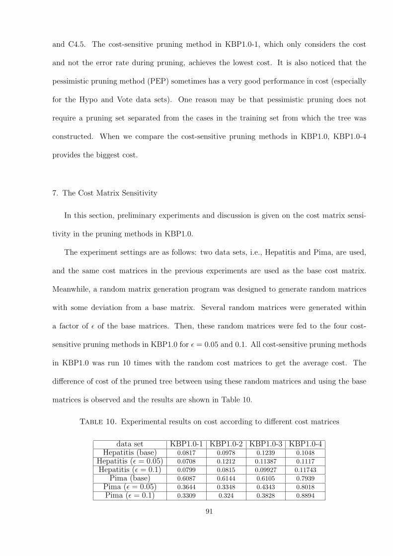
and C4.5. The cost-sensitive pruning method in KBP1.0-1, which only considers the cost

and not the error rate during pruning, achieves the lowest cost. It is also noticed that the

pessimistic pruning method (PEP) sometimes has a very good performance in cost (especially

for the Hypo and Vote data sets). One reason may be that pessimistic pruning does not

require a pruning set separated from the cases in the training set from which the tree was

constructed. When we compare the cost-sensitive pruning methods in KBP1.0, KBP1.0-4

provides the biggest cost.

7. The Cost Matrix Sensitivity

In this section, preliminary experiments and discussion is given on the cost matrix sensi-

tivity in the pruning methods in KBP1.0.

The experiment settings are as follows: two data sets, i.e., Hepatitis and Pima, are used,

and the same cost matrices in the previous experiments are used as the base cost matrix.

Meanwhile, a random matrix generation program was designed to generate random matrices

with some deviation from a base matrix. Several random matrices were generated within

a factor of ε of the base matrices. Then, these random matrices were fed to the four cost-

sensitive pruning methods in KBP1.0 for ε = 0.05 and 0.1. All cost-sensitive pruning methods

in KBP1.0 was run 10 times with the random cost matrices to get the average cost. The

difference of cost of the pruned tree between using these random matrices and using the base

matrices is observed and the results are shown in Table 10.

Table 10. Experimental results on cost according to different cost matrices

data set KBP1.0-1 KBP1.0-2 KBP1.0-3 KBP1.0-4Hepatitis (base) 0.0817 0.0978 0.1239 0.1048

Hepatitis (ε = 0.05) 0.0708 0.1212 0.11387 0.1117Hepatitis (ε = 0.1) 0.0799 0.0815 0.09927 0.11743

Pima (base) 0.6087 0.6144 0.6105 0.7939Pima (ε = 0.05) 0.3644 0.3348 0.4343 0.8018Pima (ε = 0.1) 0.3309 0.324 0.3828 0.8894

91

From Table 10, equation (22) is used to calculate the percentage of cost changes when

random matrices are used, and the results are shown in Table 11.

Percentage of cost change =|Cbase − Crandom|

Cbase

(22)

where:

Cbase is the cost based on the base matrices,

Crandom is the cost based on the random matrices

Table 11. Experimental results on the percentage of cost changes

data set KBP1.0-1 KBP1.0-2 KBP1.0-3 KBP1.0-4Hepatitis (ε = 0.05) 13 23 8 6.58Hepatitis (ε = 0.1) 2 16.7 19.88 12.1Pima (ε = 0.05) 40.1 45.5 28.9 10Pima (ε = 0.1) 45.6 47.3 37.3 12

From Table 10 and Table 11, it is found that the cost matrix sensitivity in the pruning

methods is problem dependent. For example, the percentage of cost changes is much bigger

in the Pima data set than in the Hepatitis data set. In most cases, except for the Hepatitis

data set in KBP1.0-1 and KBP1.0-2, the percentage of cost changes for a random cost matrix

with ε = 0.1 is bigger than that for a random cost matrix with ε = 0.05 of the base matrices

to the cost based on the base matrices. Further research on the cost matrix sensitivity in the

pruning methods, such as the strict definition of sensitivity and the underlying reason for the

experiment results, may be done in future work.

92

CHAPTER V

The Framework for Knowledge-base Pruning

This chapter introduces the framework for knowledge-base pruning. Then, the strategies

for KBP1.0 are given. Finally, some future researches are discussed.

1. Definitions

This section contains the definitions needed for later sections.

Definition: Let αij be the cost of misclassifying a class i object as a class j object and

satisfies

αij

> 0, if i 6= j;

= 0, if i = j.

αij ∈ [0, +∞).

The probability that a sample in node t falls into class i can be given as follows:

p(i|t) =p(i, t)

p(t)(23)

where∑

i p(i|t) = 1,

p(i, t) is the probability that a sample will both be in class i and fall into node t,

p(t) is the probability that any sample falls into node t and can be defined as follows:

p(t) =∑

i

p(i, t) (24)

93

During the pruning procedure, let node be replaced by the class j which minimizes the

misclassification cost. Therefore, given the samples under node t, the total misclassification

cost for node t can be defined as follows:

r(t) = minj

∑i

αijp(i|t) (25)

Let∑

j αij = ki and∑

i ki = K, equation(25) can be normalized as

r(t) =1

K(min

j{∑

i

αijp(i|t)}) (26)

Definition: Let R(t) be the misclassification cost for node t given as

R(t) = r(t)p(t) (27)

Then, let R(T ) be the total misclassification cost for tree T given as

R(T ) =∑t∈T

R(t) (28)

Definition: When αij = 1 (i 6= j), let E(t) be the error rate for node t given as

E(t) = K ∗R(t) (29)

Furthermore, let E(T ) be the total error rate for tree T given as

E(T ) = K ∗R(T ) = K ∗∑t∈T

R(t) (30)

Most pruning techniques only consider the error rate while cost-sensitive pruning only

considers the cost. But it may lead to a poor system performance if only its cost is low

but its error rate is too high, or its error rate is low but its cost is too high. So some other

94

pruning methods are proposed to deal with this. The pruning method in this dissertation uses

intelligent inexact classification to prune decision tree and is based on not only considering

the error rate but also considering the cost of the error. The following equation is used to

deal with it:

F (T ) = I1 ∗R(T ) + I2 ∗ E(T ) (31)

where:

F (T ) is the evaluation value for tree T used in decision tree pruning;

I1 is the weight of cost, I1 ∈ [0, 1];

I2 is the weight of error rate, I2 ∈ [0, 1];

I1 + I2 = 1;

R(T ) is the misclassification cost of the tree T ;

E(T ) is the total error rate by tree T .

The assignment of I1 and I2 is problem dependent and needs domain knowledge. In some

cases, for example in medical diagnosis, misclassification, i.e., misdiagnosis, can critically

damage the patient, so I1 should be high. In some other cases, for example when different

cost misclassifications are roughly the same, cost is not very critical, so I1 can be set to a low

value. Therefore, this pruning method is more general than other non-cost sensitive pruning

methods. For example, I1 can be set to value 0 and get an error based non-sensitive pruning.

It is clear that I1 and I2 can be changed to adjust the error rate and cost.

KBP1.0 uses equation(31) in the pruning procedure. It is discussed in more detailed in

the next section.

Definition: Let F (t) be the evaluation value for node t given as

F (t) = I1 ∗R(t) + I2 ∗ E(t) (32)

95

It is clear that

F (T ) =∑t∈T

F (t) (33)

2. Strategies for KBP1.0

In this section the strategy for KBP1.0 is introduced. The definitions in the previous

sections have been used in this section to make the description clear.

The main strategy for KBP1.0 is that F (T ) in equation(31) is used in the pruning pro-

cedure. I1 and I2 have different values for different pruning methods in KBP1.0 as shown in

table 12.

Table 12. Values for I1 & I2 in KBP1.0

Pruning method F (t) = I1 ∗R(t) + I2 ∗ E(t)KBP1.0-1 I1 = 1, I2 = 0KBP1.0-2 I1 ∈ [0, 1], I2 ∈ [0, 1]KBP1.0-4 I1 = 1, I2 = 0

Let Tmax be the initial tree without being pruned. For an initial tree Tmax, KBP1.0 com-

putes F (t) for each node t (t ∈ Tmax) in a bottom-up fashion. Therefore, Tmax is progressively

pruned upward to its root node. For KBP1.0-1 and KBP1.0-2, tree T will be pruned if

F (T′) < F (T ) (T

′is the pruned tree of T and is obtained from T by successively pruning off

branches).

Let Rth(T ) be the threshold value for misclassification cost and Eth(T ) be the threshold

value for error rate.

The idea behind KBP1.0-3 is as follows:

For each stage of the pruning process, KBP1.0-3 computes R(T ) and E(T ). The following

rules are used to make the pruning decision:

(1) Tree T will be pruned when R(T′) < R(T ) and E(T

′) < E(T ).

(2) Tree T will not be pruned when R(T′) > R(T ) and E(T

′) > E(T ).

96

(3) When R(T′) > R(T ) and E(T

′) < E(T ), tree T will be pruned only when R(T

′) <

Rth(T ).

(4) When R(T′) < R(T ) and E(T

′) > E(T ), tree T will be pruned only when E(T

′) <

Eth(T ).

There are different ways to set the values of Rth(T ) and Eth(T ). For example, traditional

pruning methods, such as reduced error pruning or pessimistic pruning, can be used to prune

the decision tree and get its error rate e1. Then Eth(T ) can be set as e1. In the same way,

KBP1.0-1 can be used to prune the decision tree and get its cost c1. Then Rth(T ) can be set

as c1.

KBP1.0-4’s pruning procedure is similar to that of the pessimistic error pruning(PEP).

The only difference between KBP1.0-4 and PEP is that: F (t) replaces E(t) in each stage of

pruning, i.e., PEP calculates the error rate, while KBP1.0-4 calculates the misclassification

cost during pruning. Note that in the unit misclassification cost case(i.e., αij = 1 when i 6= j),

KBP1.0-4 is equivalent to PEP.

Definition: For any subtree T , Let |T | be the number of terminal nodes in T which represent

the complexity of subtree T . The cost-complexity measure is defined as

R′(T ) = R(T ) +

|T |2

(34)

Definition: Let t be the node of subtree T , if subtree T is replaced by the node t, let the

misclassification cost obtained be Rt. The pessimistic misclassification measure is defined as

R′t = Rt +

1

2(35)

For each subtree, KBP1.0-4 computes R′(T ) and R

′t(t is node of subtree T ). Then, KBP1.0-

4 tests whether the following equation is satisfied

97

R′t ≤ R

′(T ) + [R

′(T )]1/2 (36)

When equation(36) is satisfied, subtree T is replaced by node t.

3. Discussion

KBP1.0 uses F (T ) as the criterion to prune the decision tree. From equation (31), it is

clear that I1 and I2 need to be set before pruning. Through discussions with the experts, I

find that it is hard for experts to give the exact values for I1 and I2. The experts can only set

the fuzzy value for I1 and I2. Although the experiments for KBP1.0 have good results, how

to set more reasonable values for I1 and I2 can be for future research.

Threshold values Rth(T ) and Eth(T ) need to be set in KBP1.0-3. In experiments, reduced

error pruning was used to help us set Eth(T ) and KBP1.0-1 was used to help us set Rth(T ).

How to get some other better methods to set more reasonable values for Rth(T ) and Eth(T )

can be for future research.

Breiman, et al., concluded that the right sized tree Tk0 can be selected by the following

rule [7]:

R(Tk0) = mink

R(Tk) (37)

where Tk is the sequence of trees.

In KBP1.0, the best subtree Tk0 could be defined as the subtree that minimizes F (Tk) as

follows

R(Tk0) = mink

F (Tk) (38)

98

Because F (Tk) = I1∗R(Tk)+I2∗E(Tk) and E(Tk) is the special case of R(Tk), equation(38)

is determined by I1, I2 and R(Tk). The analysis of optimal pruning based on expert knowledge

can be for future research.

99

CHAPTER VI

SUMMARY

1. Summary

The idea of cost-sensitive pruning has received much less attention than other pruning tech-

niques even though additional flexibility and increased performance can be obtained from this

method. In this dissertation, a cost-sensitive decision tree pruning algorithm called KBP1.0,

which includes four cost-sensitive pruning methods, has been introduced. In these four cost-

sensitive pruning methods, two ways are proposed to integrate error rate and cost in the

pruning methods. One method uses intelligent inexact classification (IIC) and the other uses

threshold to integrate error rate and cost. It is the first time that IIC and threshold are used

in this way in pruning the decision tree. By comparing the cost-sensitive pruning methods in

KBP1.0 with other traditional pruning methods, such as reduced error pruning, pessimistic

error pruning, cost complexity pruning, and C4.5, on benchmark data sets, the advantage and

disadvantage of cost-sensitive methods in KBP1.0 have been summarized. The sensitivity of

the pruning method to the cost matrix is first discussed in this dissertation. The central prob-

lem investigated in this dissertation is the problem of minimizing the cost of misclassification

or balancing the error and the cost of misclassification when the cost is too important to be

ignored.

In particular, KBP1.0’s performance has been compared with those of several well-known

pruning methods including Reduced Error Pruning, Pessimistic Error Pruning, Cost-Complexity

Pruning, and C4.5. The strengths and weaknesses of KBP1.0 have also been pointed out.

100

From the comparative analysis based on cost between the cost-sensitive pruning methods

and non-cost sensitive pruning methods, it is clear that most of the KBP1.0 cost-sensitive

pruning methods provide a lower cost than the other non cost-sensitive pruning methods.

The cost-sensitive pruning method KBP1.0-1, which only considers the cost and not the error

rate during pruning, achieves the lowest cost. Compared with the other cost-sensitive pruning

methods in KBP1.0, KBP1.0-4 provides the biggest cost.

From the comparative analysis based on error rate between the cost-sensitive pruning

methods and other traditional non-cost sensitive pruning methods, it is noticed that KBP1.0-

1, which only considers cost and not the error rate in pruning, shows a larger error rate than

KBP1.0-2, KBP1.0-3, and KBP1.0-4, which consider both cost and error rate in pruning. In

most cases, the other well-known non-cost sensitive pruning methods are of superior accu-

racy to the KBP1.0 cost-sensitive pruning methods. Compared with the other cost-sensitive

pruning methods in KBP1.0, KBP1.0-4 achieves the lowest error, while KBP1.0-1 gives the

highest error rate.

From the comparative analysis based on size between the cost-sensitive pruning methods

and other traditional non-cost sensitive pruning methods, it is clear that most cost-sensitive

pruning methods tend to produce a larger decision tree than the other well-known non-cost

sensitive pruning methods selected. But the size difference between cost-sensitive pruning

methods and non-cost sensitive pruning methods is not that large, the size of the decision

trees which are pruned by the cost-sensitive pruning methods is acceptable to the author. In

many cases, a small decision tree with high cost or error is unacceptable. When comparing

the cost-sensitive pruning methods in KBP1.0, KBP1.0-1 gives the smallest decision tree.

From the comparative analysis based on size, error rate, and cost of the pruned decision

trees created by KBP1.0 cost-sensitive pruning methods and C4.5 pruning methods, it is clear

that every KBP1.0 cost-sensitive pruning method obtained a lower cost than C4.5. It is also

101

found that, in most cases, C4.5 is of superior accuracy to the cost-sensitive pruning. C4.5

has good performance in reducing error as well as other traditional non-cost sensitive pruning

methods. Compared with KBP1.0 pruning methods, C4.5 tends to produce a smaller decision

tree. But the size difference is not that large and the size of the decision tree pruned by

KBP1.0 pruning methods is acceptable. Among the pruning methods in KBP1.0, KBP1.0-1

has the same advantage in getting a small tree size as C4.5.

The statistical measures are also used to test that cost-sensitive pruning methods in

KBP1.0 tend to provide lower cost than the other non-cost sensitive pruning methods. The

results confirm the above conclusions.

It is clear that some of the new cost-sensitive pruning methods (KBP1.0-1, KBP1.0-2,

and KBP1.0-3) require pruning sets separate from the training sets from which the tree was

constructed. But KBP1.0-4 does not require the separated pruning set because it integrates

PEP with cost-sensitive pruning method.

The decision tree pruning algorithm KBP1.0 provides more options to prune the decision

tree, especially when cost is too important to be ignored. It is believed that many real-world

classification problems involve more than merely maximizing accuracy. In certain applica-

tions, a decision tree that merely maximizes accuracy (e.g., trees generated by C4.5) may be

far from the performance that is possible with an algorithm that considers such realistic con-

straints as misclassification cost [46]. KBP1.0 can be applied to solve real-world data mining

problems and its potential application includes almost all applications of the decision tree,

especially some problems which should take into account misclassification cost, such as med-

ical diagnosis, stock prediction, credit-risk analysis, and so on. KBP1.0 can also be applied

to some applications in which the accuracy of a classification or prediction is the only thing

that matters, because it is convenient to set I1 in KBP1.0-2 to value 0 and get an error-based

non-sensitive pruning. In the future, a decision tree pruned by KBP1.0 can be converted to

102

rules and these rules can be used to build an expert system. Generally, future applications of

KBP1.0 include banking (e.g., predictive and risk assessment models for the financial services

industry), fraud detection (e.g., uncovering network intrusions), health care (e.g., data ware-

housing solutions for health care industry), and stock and investment analysis and prediction

(e.g., predicting stock price changes).

2. Discussions

This section discusses some concerns of the research in this dissertation.

(1) The expert knowledge used in cost matrix

To the best of the author’s knowledge, the use of expert knowledge in cost-sensitive

pruning of decision trees has not been discussed before in the literature. In this work,

the cost matrices are defined through discussions with domain experts. It may be a

concern for this research to place a burden on domain experts. Actually, expert system

design relies upon domain experts much more heavily than this work [1]. Furthermore,

expert system can determine α values.

Most experts are skillful at solving problems within their narrow area of expertise,

but have limited ability outside this area. Therefore, finding the right experts to help

define the cost matrices is important for this work.

(2) Experimental results

In this dissertation, KBP1.0’s performance has been compared with those of sev-

eral well-known pruning methods including Reduced Error Pruning, Pessimistic Error

Pruning, Cost-Complexity Pruning, and C4.5. From the results, it is clear that most

of the KBP1.0 cost-sensitive pruning methods provide a lower cost than the other non

cost-sensitive pruning methods. However, there are some exceptions. For example,

in Hepatitis data set, KBP1.0-3 gets a higher cost than PEP and REP. This is not

103

unusual because there is no overall best algorithm. One can improve KBP1.0’s per-

formance in several ways, i.e., adjusting the cost matrix by changing the threshold

values which were set. Another concern for the comparison presented here is that the

datasets selected in the experiment are not very large datasets. Will KBP1.0 have a

good performance in a very large dataset? This will be future work of the author’s

research.

(3) ANOVA results

The ANOVA is used to investigate the significance of differences among the cost-

sensitive methods in KBP1.0 and non-cost sensitive pruning methods in REP, PEP,

CCP, and C4.5. From ANOVA results, it can be found that there are statistical

differences between the performance of the cost-sensitive methods in KBP1.0 and that

of non-cost sensitive pruning methods in REP, PEP, CCP, and C4.5. The ANOVA,

other than the t-test, is selected to analyze the experimental results because the major

difference between ANOVA and t-test is that, where the t-test measures the difference

between the means of two groups, an ANOVA tests the difference between the means

of two or more groups [126]. The advantage of using ANOVA rather than multiple

t-tests is that it reduces the probability of a type-I error [126]. However, one potential

drawback to an ANOVA is that specificity is lost: all an ANOVA tells you is that there

is a significant difference between groups, not which groups are significantly different

from each other [117]. In future work, the t-test may be used to find out where the

differences are, i.e., which groups are significantly different from each other and which

are not.

(4) Cost matrix sensitivity in the pruning methods

To the best of our knowledge, the cost matrix sensitivity in the pruning methods

is first discussed in this dissertation. An experiment is designed to test the cost

104

matrix sensitivity. However, the results obtained are preliminary in the sense that the

definition of sensitivity is not well-defined. In the experiment, when the cost matrix is

changed, the pruned tree is also changed because the pruning methods in KBP1.0 are

guided by the cost matrix. Another concern for the sensitivity of the pruning methods

to the cost matrix is whether or not the sensitivity is relevant to the size of the cost

matrix. In future work, a clear definition for the sensitivity of the pruning method to

the cost matrix may be given and further research on sensitivity to the cost matrix

with different sizes may be done.

3. Future work

Some of future work is mentioned in above discussion section. For example, the KBP1.0

will be used in some very large data set and analyze its performance, and a clear definition for

the sensitivity of the pruning method to the cost matrix may be given. There are also other

directions for future work. Future work will also focus on the integration of cost-sensitive

pruning methods in other pruning methods, such as Minimum Error Pruning and Critical

Value Pruning and compare KBP1.0 pruning methods to other pruning methods. It will also

include the Ontology and why an Ontology would aid us in obtaining reasonable cost matrices

in the future. A prototype expert system to define the cost matrix will be developed. Using

KBP1.0 to prune the decision tree and getting the rules from the pruned trees to help us build

the real-world expert system is another important direction for future work.

105

BIBLIOGRAPHY

[1] J. Durkin. Expert Systems: Design and Development, Prentice Hall, Englewood Cliffs, NJ, 1994.

[2] Z. X. Cai, G. Y. Xu. Artificial Intelligence: Principles and Applications (3rd Edition), Beijing: TsinghuaUniversity Press, 2003.

[3] A. Freitas. T. Data Mining and Knowledge Discovery with Evolutionary Algorithm, Springer-Verlag Hei-delberg, 2002.

[4] K. Leila, Naudts Bart, R. Alex. Theoretical Aspects of Evolutionary Computting, Springer-Verlag Heidel-berg, 2001.

[5] W. Spears. Evolutionary Algorithms, Springer-Verlag Heidelberg, 2000.

[6] T. Gong, J. Cai, and Zixing Cai. A coding and control mechanism of natural computation, Proceedings

of 2003 IEEE 18th International Symposium on Intelligent Control(ISIC), Houston, Texas, pp. 727-732,

2003.

[7] L. Briemann, J. Friedman, R. Olshen and C. Stone. CART: Classification and Regression Trees, EBelmont,CA:Wadsworth Statistical Press, 1984.

[8] J. Mingers. An Empirical Comparison of Selection Measures for Decision Tree Induction, Machine Learn-ing, 3 (3): pp. 319-342, 1989.

[9] U. Knoll, G. Nakhaeizadeh and B. Tausend. Cost Sensitive Pruning of Decision Trees, Proceedings ofECML-94: pp. 383-386, 1994.

[10] B. Andrew, L. Brain C., Cost-Sensitive Decision Tree Pruning Use of the ROC Curve, Proceedings EightAustralian Joint Conference on Artificial Intelligence, pp.1-8, November 1995.

[11] F. Esposito, D. Malerba, and G. Semeraro. A comparative Analysis of Methods for Pruning DecisionTrees, IEEE transactions on pattern analysis and machine intelligence, 19(5): pp. 476-491, 1997.

[12] J. Quinlan. Simplifying decision trees, Int. J. Human-Computer Studies, (1999)51, pp. 497-491, 1999.

[13] J. Quinlan. C4.5 Programs for Machine Learning, San Mateo, CA:Morgan Kaufmann, 1993.

[14] M. Sebban, R. Nock, J. H. Chauchat and R. Rakotomalala. Impact of Learning Set Quality and Size onDecision Tree Performances, IJCSS, 1(1), pp. 85-105, 2000.

106

[15] T. Oates and D. Jensen. The effects of Training Set Size on Decision Tree Complexity, InternationalConference on Machine Learning, pp. 254-262, 1997.

[16] C. E. Brodley and M. A. Friedl. Identifying and Eliminating Mislabeled Training Instances, Proceedingsof the Thirteenth National Conference on Artificial Intelligence, 1996.

[17] O. Boz. Extracting Decision trees from trained neural networks, SIGKDD’02, July 2002.

[18] L. Sethi. Entropy nets: From decision trees to neural networks, Proc. 1EEE 78, pp. 1605-1613, 1990.

[19] M. Dong and R. Kothari. Look-ahead based fuzzy decision tree induction, IEEE Transactions on FuzzySystems, Vol.9(3), pp. 461-468, 2001.

[20] C. Olaru and L. Wehenkel. A complete fuzzy decision tree technique, Fuzzy Sets and Systems 138, pp.221-254, 2003.

[21] E. Cantu-Paz and C. Kamath. , Inducing oblique decision tres with evolutionary algorithms, IEEE Trans-actions on Evolutionary Computation, 7(1), pp. 54-68, 2003.

[22] A. Papagelis and D. Kalles. Breeding decision trees using evolutionary techniques, Proceedings of ICML’01,USA, 2001.

[23] A. Papagelis and D. Kalles. GATree: Genetically evolved decision trees, Proceedings of ICTAI’00, USA,2000.

[24] D. R. Carvalho and A. A. Freitas A hybrid decision tree/genetic algorithm for coping with the problem ofsmall disjuncts in data mining, Proceedings of Genetic and Evolutionary Computation Conference, USA,pp. 1061-1068, 2000.

[25] G. Tur and H. A. Guvenir. Decision tree induction using genetic programming, Proceedings of the FifthTurkish Symposium on Artificial Intelligence and Neural Networks, pp. 187-196, 1996.

[26] J. Eggermont. Evolving fuzzy decision trees with genetic programming and clustering, Proceedings of the4th European Conference on Genetic Programming, 2002.

[27] P. Stone and M. Veloso. Using decision tree confidence factors for multiagent control, Proceedings of the2nd International Conference on Autonomous Agents, 1998.

[28] P. Stone and M. Veloso. Multiagent system: A survey from a machine learning perspective, AutonomousRobots, pp. 8(3), 2000.

[29] P. Stone and M. Veloso, A layered approach to learning client behaviors in the RoboCup soccer server,Applied Artificial Intelligence (AAI), 12, 1998.

[30] D. Fournier and B. Cremilleux. A quality index for decision tree pruning, Knowledge-Based Systems 15,pp. 37-43, 2002.

107

[31] M. Ankerst, C. Elsen, M. Ester, and H. Kriegel. Visual classification: An interactive approach to decisiontree construction, In Proceedings of A CM SIGKDD International Conference on Knowledge Discoveryand Data Mining, pp. 392-396, 1999.

[32] H. Almuallim. Development and applications of decision trees, In Expert Systems: The technology ofknowledge management and decision making for the 21st century(Volume I), pp. 53-77, 2002.

[33] J. L. Devore. Probability and statistics for engineering and the sciences, fifth edition, Duxbury Press,2000.

[34] J. Giarratano and G. Riley. Expert Systems: Principles and Programming, second edition, PWS PublishingCompany, 1994.

[35] P. D. Turney. Types of Cost in Inductive Concept Learning, Workshop on Cost-Sensitive Learning at theSeventeenth International Conference on Machine Learning (WCSL at ICML-2000), Stanford University,California, 2000.

[36] P. Brezillon. Context-Based Intelligent Assistant Systems: A discussion based on the Analysis of TwoProjects, In Proceedings of the 36th Hawaii International Conference on System Sciences, 2002.

[37] J. Durkin. Intelligent Inexact Classification, In Expert System Note.

[38] C. Blake and C. Merz. UCI Repository of Machine Learning Databaseshttp://www.ics.uci.edu/~mlearn/MLRepository.html, Department of Information and Computer Sci-ences, University of California, Irvine, 1998.

[39] A. Appice, M. Ceci., and D. Malerba. KDB2000: An integrated knowledge discovery tool, In A. Zanasi, C.A. Brebbia, N.F.F. Ebecken, P. Melli (Eds.) Data Mining III, Series Management Information Systems,Vol 6, pp. 531-540, WIT Press, Southampton, UK, 2002.

[40] E. Friedman-Hill. Jess in Action: Rule-Based Systems in Java, Manning Publication Co., 2003.

[41] H. Hamilton. http://www2.cs.uregina.ca/~hamilton/courses/831/notes/ml/dtrees/4 dtrees1.html, Depart-ment of Computer Sciences, University of Regina, Canada.

[42] L. A. Breslow and D. W. Aha. Simplifying Decision Trees: A Survey, Technical Report No. AIC-96-014,Navy Center for Applied Research in Artificial Intelligence, Naval Research Laboratory Washington, DC.,1996.

[43] J. Mingers. An Empirical Comparison of Pruning Methods for Decision Tree Induction, Machine Learning,4: pp. 227-243, 1989.

[44] Z. Elouedi, K. Mellouli, and Ph. Smets. Belief Decision Trees: Theoretical Foundations, InternationalJournal of Approximate Reasoning, 28: pp. 91-124, 2001.

[45] B. Crmilleux, C. Robert, and M. Gaio. Uncertain Domains and Decision Trees : ORT versus CM crite-ria, Seventh Conference on Information Processing and Management of Uncertainty in Knowledge-BasedSystems (IPMU 98), pp. 540-546,Editions EDK, Paris, France, July 1998.

108

[46] P. D. Turney. Cost-Sensitive Classification: Empirical Evaluation of a Hybrid Genetic Decision TreeInduction Algorithm, Journal of Artificial Intelligence Research 2, pp. 369-409, 1995.

[47] D. Malerba, F. Esposito, and G. Semeraro. A Futher Comparison of Simplification Methods for Decision-Tree Induction, Chapter 35 in D. Fisher and H.-J.Lenz (Eds.), Learning from Data: AI and Statistics V,Lecture Notes in Statistics, 112, pp. 365-374, Springer-Verlag, Berlin, Germany, 1996.

[48] B. Cestnik, and I. Bratko. On Estimating Probabilities in Tree Pruning, EWSL, pp. 138-150, 1991.

[49] T. Niblett and I. Bratko. Learning Decision Rules in Noisy Domains, Proc. Expert Systems 86, Cambridge:Cambridge University Press, 1986.

[50] R. S. Michalski, J. H. Davis, V. S. Bisht, and J. B. Sinclair, PLANT/ds: An Expert Consulting Systemfor the Diagnosis of Soybean Diseases, ECAI, pp. 133-138, 1982.

[51] D. Michie. Current Developments in Expert Systems, In J. R. Quinlan(Ed.), Applications of expert systems(Vol. 2), Wokingham, UK: Addison-Wesley, pp. 1987.

[52] H. Braun and J. Chandler. Predicting Stock Market Behavior through Rule Induction: An Application ofthe Learning-from-examples Approach, Decision Sciences, Vol. 18, No. 3, pp. 415-429, 1987.

[53] M. I. Jordan. A Statistical Approach to Decision Tree Modeling, Proceedings of the Seventh Annual ACM

Conference on Computational Learning Theory, New York: ACM Press, 1994.

[54] B.G. Buchanan and E.H. Shortliffe (eds.). Rule-Based Expert Systems: The MYCIN Experiments ofthe Stanford Heuristic Programming Project, SRI Report, Stanford Research Institute, 333 RavenswoodAvenue, Menlo Park, CA, Sept. 1979.

[55] R.O. Duda, P. Hart, K. Konolige, and R. Reboh. A Computer-Based Consultation for Mineral Exploration,Addison-Wesley, Reading Mass., 1984.

[56] R. V. L. Hartley. Transmission of Information, Bell System Technical Journal, pp. 535, July 1928.

[57] C. E. Shannon. A mathematical theory of communication, Bell Syst. Tech. J., vol. 27, pp. 379-423, 623-656,July-Oct. 1948.

[58] Shafer and Glenn. A Mathematical Theory of Evidence, Princeton University Press, 1976.

[59] L. Zadeh. Fuzzy Sets, Information and Control 8: pp. 338-353, 1965.

[60] J. Durkin. Designing an Induction Expert System, AI Expert, Vol. 6, No. 12, pp. 29-35, Dec., 1991.

[61] S. R. Safavin and D. Landgrebe. A survey of decision tree classifier methodology, IEEE Trans. Syst., Man,Cybern., vol. 21, no. 3, pp. 660C674, July, 1991.

109

[62] S. K. Murthy. Automatic construction of decision trees from data: a multidisciplinary survey, Data MiningKnowl. Disc., vol. 2, no. 4, pp. 345C389, 1998.

[63] R. Kohavi and J.R. Quinlan. Decision-tree discovery, in Handbook of Data Mining and Knowledge Dis-covery, W.Klosgen and J.M.Zytkow, Eds. London, U.L.:Oxford Univ.Press, ch.16.1.3, pp.267-276, 2002.

[64] H. Zantema and H. L. Bodlaender. Finding small equivalent decision trees is hard, Int. J. Found. Comput.Sci., vol. 11, no. 2, pp. 343C354, 2000.

[65] J. Quinlan. Induction of decision trees, Machine Learning, vol. 1, pp. 81C106, 1986.

[66] S. B. Gelfand, C. S. Ravishankar, and E. J. Delp. An iterative growing and pruning algorithm for classi-fication tree design, IEEE Trans. Pattern Anal. Mach. Intell., vol. 13, no.2, pp.163-174, 1991.

[67] J. Quinlan. Decision trees and multivalued attributes, Machine Intelligence, J. Richards, Ed. London,U.K.: Oxford Univ. Press, vol. 11, pp. 305-318, 1988.

[68] R. Lopez de Mantras. A distance-based attribute selection measure for decision tree induction, Mach.Learn., vol. 6, pp. 81-92, 1991.

[69] U. M. Fayyad and K. B. Irani. The attribute selection problem in decision tree generation, Proc. 10thNat.Conf. Artificial Intelligence, Cambridge, MA, pp. 104-110, 1992.

[70] J. H. Friedman. A recursive partitioning decision rule for nonparametric classifiers, IEEE Trans. Comput.,vol. C26, no. 4, pp. 404-408, Apr. 1977.

[71] E. Rounds. A combined nonparametric approach to feature selection and binary decision tree design,Pattern Recognit., vol. 12, pp. 313-317, 1980.

[72] I. K. Sethi and J. H. Yoo. Design of multicategory, multifeature split decision trees using perceptronlearning, Pattern Recognit., vol. 27, no.7, pp. 939-947, 1994.

[73] I. Bratko and M. Bohanec. Trading accuracy for simplicity in decision trees, Mach. Learn., vol. 15, pp.223-250, 1994.

[74] H. Almuallim. An efficient algorithm for optimal pruning of decision trees, Artif. Intell., vol. 83, no. 2,pp. 347-362, 1996.

[75] J. Quinlan and R. L. Rivest. Inferring decision trees using the minimum description length principle,Inform. Comput., vol. 80, pp.227-248, 1989.

[76] C. Wallace and J. Patrick. Coding decision trees, Mach. Learn., vol.11, pp. 7-22, 1993.

[77] M. Kearns and Y. Mansour. A fast, bottom-up decision tree pruning algorithm with near-optimal gener-alization, Proc. 15th Int. Conf. Machine Learning, J. Shavlik, Ed., pp. 269-277, 1998.

110

[78] J. Quinlan. Unknown attribute values in induction, Proc. 6th Int. Machine Learning Workshop, A. Segre,Ed., Cornell, New York, pp. 164-168, 1989.

[79] G. Pagallo and D. Hassler. Boolean feature discovery in empirical learning, Mach. Learn., vol. 5, no. 1,pp. 71-100, 1990.

[80] J. C. Schlimmer. Efficiently inducing determinations: a complete and systematic search algorithm thatuses optimal pruning, Proc. Int. Conf. Machine Learning, San Mateo, CA, pp. 284-290, 1993.

[81] P. Langley and S. Sage. Oblivious decision trees and abstract cases, Proc. Working Notes of the AAAI-94Workshop on Case-Based Reasoning, Seattle, WA, pp. 113C117, 1994.

[82] M. Last, O. Maimon, and E. Minkov. Improving stability of decision trees, Int. J. Pattern Recognit. Artif.Intell., vol. 16, no. 2, pp. 145-159, 2002.

[83] J. Catlett. Mega Induction: Machine Learning on Vary Large Databases, Ph.D. thesis, Univ. of Sydney,Sydney, Australia, 1991.

[84] J. Gehrke, V. Ganti, R. Ramakrishnan, and W. Loh. BOAT-optimistic decision tree construction, Proc.SIGMOD Conf., pp.169-180, 1999.

[85] P. E. Utgoff. Incremental induction of decision trees, Mach. Learn., vol. 4, pp. 161-186, 1989.

[86] P. E. Utgoff. Decision tree induction based on efficient tree restructuring, Mach. Learn., vol. 29, no. 5,1997.

[87] W. Muller and F. Wysotzki. DAutomatic construction of decision trees for classification, Ann. Oper. Res.,vol. 52, pp. 231-247, 1994.

[88] C. E. Brodley and P. E. Utgoff. Multivariate decision trees, Mach. Learn., vol. 19, pp. 45-77, 1995.

[89] L. Rokach and O. Maimon. Top-down induction of decision trees classifiers-A survey, IEEE Transactionson systems, man, and cybernetics-part c:applications and reviews, vol. 35, No. 4, November 2005.

[90] T. K. Ho. C4.5 decision forests, Proceedings of the 14th International Conference on Pattern Recognition,Vol 1, pp. 545, 1998.

[91] A. Tveit. Empirical Comparison of Accuracy and Performance for the MIPSVM classifier with ExistingClassifiers, Technical Report, IDI, NTNU, Trondheim, Norway, November 2003.

[92] D. J. Fifield. Distributed Tree Construction From Large Datasets, B.S. honor thesis, Australian Nat. Univ.,Canberra, Australia, 1992.

[93] P. Chan and S. Stolfo. On the accuracy of meta-learning for scalable data mining, J. Intell. Inform. Syst.,vol. 8, pp. 5-28, 1997.

111

[94] M. Mehta, R. Agrawal, and J. Rissanen. SLIQ: a fast scalable classifier for data mining, Proc. 5th Int.Conf. Extending Database Technology (EDBT), Avignon, France, pp. 18-32, Mar. 1996.

[95] J. C. Shafer, R. Agrawal, and M. Mehta. SPRINT: a scalable parallel classifier for data mining, Proc.22nd Int. Conf. Very Large Databases, T. M. Vijayaraman, A. P. Buchmann, C. Mohan, and N. L. Sarda,Eds., pp. 544-555, 1996.

[96] J. Gehrke, R. Ramakrishnan, and V. Ganti. RainForesta framework for fast decision tree construction oflarge datasets, Data Mining Knowl. Discov., vol. 4, no. 2/3, pp. 127C162, 2000.

[97] J. F. Elder IV and D. W. Abbott. A Comparison of Leading Data Mining Tools, Fourth InternationalConference on Knowledge Discovery and Data Mining, August 28, 1998.

[98] D. B. West. Introduction to Graph Theory, Prentice Hall, 1996.

[99] R. J. Wilson, J. J. Watkins. Graphs: an introductory approach, John Wiley & Sons, Inc, 1990.

[100] http://dms.irb.hr/index.php, Rudjer Boskovic Institute.

[101] Cornelius T. Leondes. Expert Systems, Six-Volume Set: The Technology of Knowledge Management andDecision Making for the 21st Century , Academic Press.

[102] http://en.wikipedia.org/wiki/Glossary of graph theory#Trees,

[103] http://www.webster.com/dictionary/decision%20tree,

[104] http://www.webster.com/dictionary/class,

[105] http://www.webster.com/dictionary/object,

[106] http://www.webster.com/dictionary/set,

[107] www.isys.uni-klu.ac.at/ISYS/Courses/,

[108] http://www.mathsnet.net/asa2/modules/s23concor.html,

[109] http://www.cs.ualberta.ca/ aixplore/learning/DecisionTrees/InterArticle/2-DecisionTree.html,

[110] http://www.cs.fiu.edu/ ezeng001/datamining/class.html,

[111] users.aber.ac.uk/smg/Modules/CS16010-2003-2004/machineLearning.ppt,

[112] Esposito F., Malerba D., Semeraro G. A Comparative Analysis of Methods for Pruning Decision Trees,IEEE Transactions on Pattern Analysis and Machine Intelligence, VOL. 19, NO. 5, 1997, P. 476-491

112

[113] M. Garca, E. Lpez, V. Kumar, A. Valls A Multicriteria Fuzzy Decision System to Sort ContaminatedSoils, Modeling Decisions for Artificial Intelligence(MDAI 2006), : Tarragona, Spain. P. 105-116

[114] Blackmore, S. The Meme Machine, Oxford University Press Inc., New York. 1999

[115] S. S. Lee www.webpages.uidaho.edu/ stevel/outreach/sta301/lectures/PPCh08.pps,University of Idaho

[116] www.norcomsoftware.com/gui screenio/gs programming.htm,

[117] http://www.georgetown.edu/departments/psychology/researchmethods/statistics/inferential/anova.htm,

[118] Durkin, J. Induction Via ID3, AI Expert, Vol. 7, No. 4., pp48-53, April 1992

[119] http://www.statsoft.com/textbook/stcart.html,

[120] L. O. Hall, X. Liu, K. W. Bowyer, and R. BanLeld Why are Neural Networks Sometimes Much MoreAccurate than Decision Trees: An Analysis on a Bio-Informatics Problem, Modeling Decisions for ArtificialIEEE International Conference on Systems, Man & Cybernetics, Washington, D.C., pp. 2851-2856, October5-8, 2003

[121] James Shih-Jong Lee, Jenq-Neng Hwang, Daniel T. Davis, and Alan C. Nelson. Integration of neuralnetworks and decision tree classifiers for automated cytology screening, Modeling Decisions for Artificial InProceedings of the International Joint Conference on Neural Networks, volume 1, pages 257–262, Seattle,July 1991.

[122] http://www.m-w.com/dictionary/attribute+,

[123] http://www.m-w.com/dictionary/Subset,

[124] http://www.m-w.com/dictionary/Entropy,

[125] Amir Bar-Or, Assaf Schuster, Ran Wolff and Daniel Keren. Hierarchical Decision Tree Induction inDistributed Genomic Databases, Modeling Decisions for Artificial IEEE Transactions on Knowledge andData Engineering, Volume 17 , Issue 8 (August 2005), Pages: 1138 - 1151

[126] http://www.georgetown.edu/departments/psychology/researchmethods/statistics/inferential/anova.htm,

[127] http://decisiontrees.net/?q=node/27,

[128] David E. Goldberg. Genetic Algorithms in Search, Optimization, and Machine Learning, Addison-WesleyProfessional, 1989

113

APPENDIX

114

APPENDIX A

PUBLICATIONS DURING PhD STUDY

Book Chapters

• J. Cai, Chapter 5 Computational Intelligence (2): Evolutionary and Artificial Life in

“Artificial Intelligence: Principles and Applications(undergraduate edition)” Z. Cai,

G. Xu, (ed.), Tsinghua University Press, China, 2004. Pages 128-148.

• J. Cai, Section 4.2 Neural Computation, Section 4.3 Fuzzy Computation in “Artificial

Intelligence: Principles and Applications(graduate edition)” Z. Cai, G. Xu, (ed.),

Tsinghua University Press, China, 2003. Pages: 126-148.

Journals

• J. Durkin, J. Cai, Z. Cai, Decision Tree Technique and Its Current Research, Journal

of Control Engineering of China, 2005, 12(1):15-18, 21.

• J. Cai, J. Durkin, Q. Cai. Opportunities, Applications and Suggestions for Data

Mining. Journal of Computer Science of China, 2002, 29(9):225-228.

Conferences

• J. Cai, J. Durkin, Use of Expert Knowledge for Decision Tree Pruning, AAAI 2005

Conference, Pittsburgh, Pennsylvania, July 9-13, 2005. Pages 1600-1601.

• J. Cai, J. Durkin, Q. Cai CC4.5: Cost-Sensitive Decision Tree Pruning, Data Mining

2005 Conference, Skiathos, Greece, May 25 - 27, 2005. Pages 239-245.

• Z. Cai, Z. Duan, J. Cai, X. Zou, J. Yu, A Multiple Particle Filters Method for Fault

Diagnosis of Mobile Robot Dead-Reckoning System, 2005 IEEE/RSJ International

Conference on Intelligent Robots and Systems, Edmonton, Alberta, Canada, August

2 - 6, 2005. Pages 480-485

115

• T. Gong, J. Cai, Z. Cai, A Coding and Control Mechanism of Natural Computation.

Proceedings of 2003 IEEE 18th International Symposium on Intelligent Control(ISIC),

Houston, Texas, October 5-8, 2003. Pages 727-732.

116

APPENDIX B

PRUNING PROGRAM for KBP1.0-1 and KBP1.0-2

C4.5 can be freely downloaded and freely used for research.

You can get C4.5 from Quinlan’s homepage:

http://www.rulequest.com/Personal/.

KBP1.0 uses the same method as that of C4.5 to construct

the original decision tree, with slight code modifications

to support the KBP1.0 pruning technique.

The pruning code in C4.5 was modified to realize the pruning

methods in KBP1.0. The big difference between KBP1.0’s

pruning code and C4.5’s pruning code is that the pruning

method in C4.5’s is based on error, while the pruning method

in KBP1.0 is based on cost, or on both error and cost. In

addition, C4.5’s pruning code can only calculate the

misclassification error during pruning, while KBP1.0’s

pruning code can calculate both the misclassification error

and misclassification cost during pruning.

In Appendix A, B, and C, the source codes are not complete because

of the license and rules for redestribution for C4.5.

117

/***************************************************************/

/* */

/* KBP1.0-1,2 pruning method */

/* ------------------------------------------------ */

/* */

/***************************************************************/

void TestPruned(T, raw)

/* ----- */

Tree T;

Tree raw;

{

float CalculateCostTest(), ComputeCostAndError();

void ClearTree();

printf("Tree before pruning:\n");

/*ClearTree(raw);

InitialiseWeights();

showPruningDistr(raw, 0, MaxItem, 0, true);*/

printf("\n Cost before pruning for testing data: %f \n",

CalculateCostTest(raw, true));

//PrintTree(raw);

118

printf("Tree after pruning:\n");

/*ClearTree(T);

InitialiseWeights();

showPruningDistr(T, 0, MaxItem, 0, true);*/

printf("\n Cost after pruning for testing data: %f \n",

CalculateCostTest(T, true));

//PrintTree(T);

}

/*************************************************************************/

/* */

/* Compute the costs and errors of pruning a given subtree ST */

/* */

/*************************************************************************/

float ComputeCostAndError(T, ST, Fp, Lp, Sh, UpdateTree)

/* -------------- */

Tree T;

Tree ST; //subtree

ItemNo Fp, Lp;

short Sh;

Boolean UpdateTree;

{

119

ItemNo i, Kp, Ep, Group(); //Group defined in build.c

ItemCount Cases, KnownCases, *LocalClassDist, LeafErrors,

CountItems(), Factor;

DiscrValue v, MaxBr, tmpBest, tmpBestLeaf;

ClassNo c, BestClass, tmpLeaf;

Boolean PrevAllKnown;

float cost = 0, *classDist, *fork_costs, CalculateCost(),

TreeCost, BranchCost,

*leaf_costs, tmpCost, LeafCost;

Tree *tmpBranch, *tmpST;

short tmpNodeType;

if ( ! ST->NodeType ) /* leaf */

{ //LocalVerbosity(1)

{ printf("Leaf node! Items: %f\n", ST->Items);

}

if ( UpdateTree )

{

LocalVerbosity(1)

{

Intab(Sh);

printf("%s (%.2f:%.2f/%.2f)\n", ClassName[ST->Leaf],

ST->Items, LeafErrors, ST->Errors);

}

120

}

return 0;

}

//LocalVerbosity(1)

{ printf("Node type: %d, Items: %f, Forks: %hd \n",

ST->NodeType, ST->Items, ST->Forks);

}

Kp = Group(0, Fp, Lp, ST) + 1;

KnownCases = CountItems(Kp, Lp);

PrevAllKnown = AllKnown;

if ( Kp != Fp ) AllKnown = false;

fork_costs = (float *) calloc (ST->Forks + 1, sizeof(float));

leaf_costs = (float *) calloc (MaxClass + 2, sizeof(float));

tmpBranch = (char *) calloc (ST->Forks, sizeof (Tree*));

memcpy((char *)tmpBranch, (char *)ST->Branch, ST->Forks * sizeof(Tree*));

/*Here, unknown data are disregarded.*/

/* ForEach(v, 1, ST->Forks)

{

Ep = Group(v, Kp, Lp, ST);

121

if ( Kp <= Ep )

{

ComputeCostAndError(T, ST->Branch[v], Fp, Ep, Sh+1, UpdateTree);

}

}*/

/*Unknown data are taken into account*/

ForEach(v, 1, ST->Forks)

{

Ep = Group(v, Kp, Lp, ST);

if ( Kp <= Ep )

{

Factor = CountItems(Kp, Ep) / KnownCases;

ForEach(i, Fp, Kp-1)

{

Weight[i] *= Factor;

}

ComputeCostAndError(T, ST->Branch[v], Fp, Ep, Sh+1, UpdateTree);

Group(0, Fp, Ep, ST);

122

ForEach(i, Fp, Kp-1)

{

Weight[i] /= Factor;

}

}

}

TreeCost = CalculateCost(T, false); //calculate cost before pruning.

printf("Tree Cost: %f \t", TreeCost);

tmpNodeType = ST->NodeType;

tmpLeaf = ST->Leaf;

ST->NodeType = 0;

//ST->Forks = 0;

//cost improvement by replace ST with a leaf

ForEach(c, 0, MaxClass)

{

ST->Leaf = c;

leaf_costs[c] = CalculateCost(T, true) - TreeCost;

printf("***leaf_costs[%hd]: %f***", c, leaf_costs[c]);

}

ST->NodeType = tmpNodeType;

ST->Leaf = tmpLeaf;

tmpBestLeaf = 0;

LeafCost = leaf_costs[tmpBestLeaf];

123

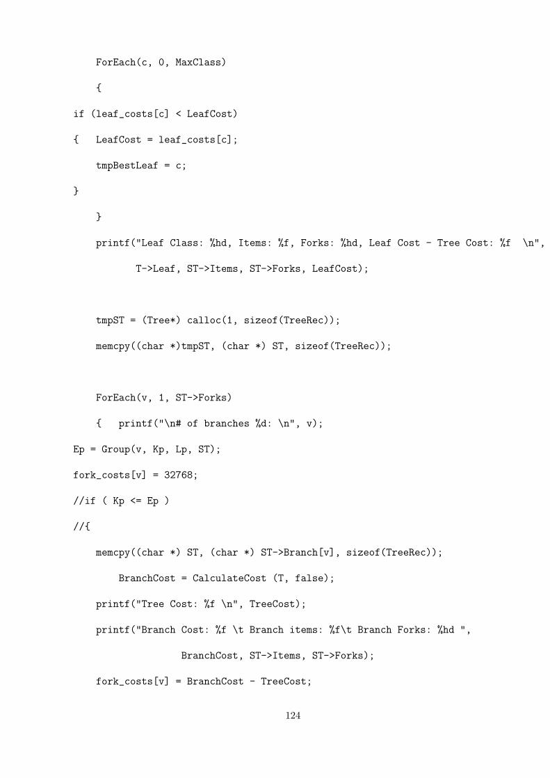
ForEach(c, 0, MaxClass)

{

if (leaf_costs[c] < LeafCost)

{ LeafCost = leaf_costs[c];

tmpBestLeaf = c;

}

}

printf("Leaf Class: %hd, Items: %f, Forks: %hd, Leaf Cost - Tree Cost: %f \n",

T->Leaf, ST->Items, ST->Forks, LeafCost);

tmpST = (Tree*) calloc(1, sizeof(TreeRec));

memcpy((char *)tmpST, (char *) ST, sizeof(TreeRec));

ForEach(v, 1, ST->Forks)

{ printf("\n# of branches %d: \n", v);

Ep = Group(v, Kp, Lp, ST);

fork_costs[v] = 32768;

//if ( Kp <= Ep )

//{

memcpy((char *) ST, (char *) ST->Branch[v], sizeof(TreeRec));

BranchCost = CalculateCost (T, false);

printf("Tree Cost: %f \n", TreeCost);

printf("Branch Cost: %f \t Branch items: %f\t Branch Forks: %hd ",

BranchCost, ST->Items, ST->Forks);

fork_costs[v] = BranchCost - TreeCost;

124

memcpy((char *) ST, (char *) tmpST, sizeof(TreeRec));

//}

Group(0, Fp, Ep, ST);

}

tmpBest = 1;

tmpCost = fork_costs[tmpBest];

ForEach(v, 1, ST->Forks)

{

if (fork_costs[v] < tmpCost)

{ tmpCost = fork_costs[v];

tmpBest = v;

}

}

if ( (LeafCost <= 0) && (LeafCost <= tmpCost) )

{

LocalVerbosity(1)

{

Intab(Sh);

printf("Replaced with leaf %s\n", ClassName[tmpBestLeaf]);

}

printf("---------Replaced with leaf %s, LeafCost: %f\n",

ClassName[tmpBestLeaf], LeafCost);

ST->NodeType = 0;

125

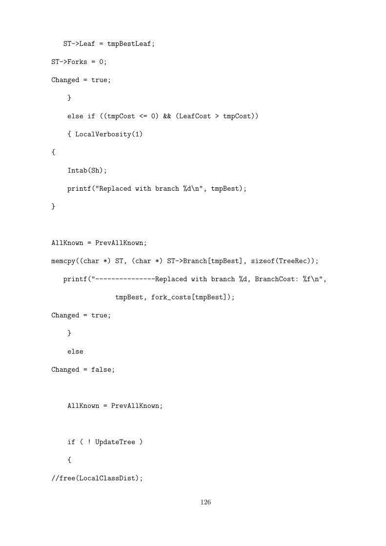
ST->Leaf = tmpBestLeaf;

ST->Forks = 0;

Changed = true;

}

else if ((tmpCost <= 0) && (LeafCost > tmpCost))

{ LocalVerbosity(1)

{

Intab(Sh);

printf("Replaced with branch %d\n", tmpBest);

}

AllKnown = PrevAllKnown;

memcpy((char *) ST, (char *) ST->Branch[tmpBest], sizeof(TreeRec));

printf("---------------Replaced with branch %d, BranchCost: %f\n",

tmpBest, fork_costs[tmpBest]);

Changed = true;

}

else

Changed = false;

AllKnown = PrevAllKnown;

if ( ! UpdateTree )

{

//free(LocalClassDist);

126

//free(classDist);

if (fork_costs != NULL) free(fork_costs);

return TreeCost;

}

AllKnown = PrevAllKnown;

if (fork_costs) free(fork_costs);

if (leaf_costs) free(leaf_costs);

if (tmpST) free(tmpST);

return 0;

}

/*************************************************************************/

/* */

/* Calculate the costs in a given subtree */

/* */

/*************************************************************************/

float CalculateCost(T, print)

Tree T;

Boolean print;

{

127

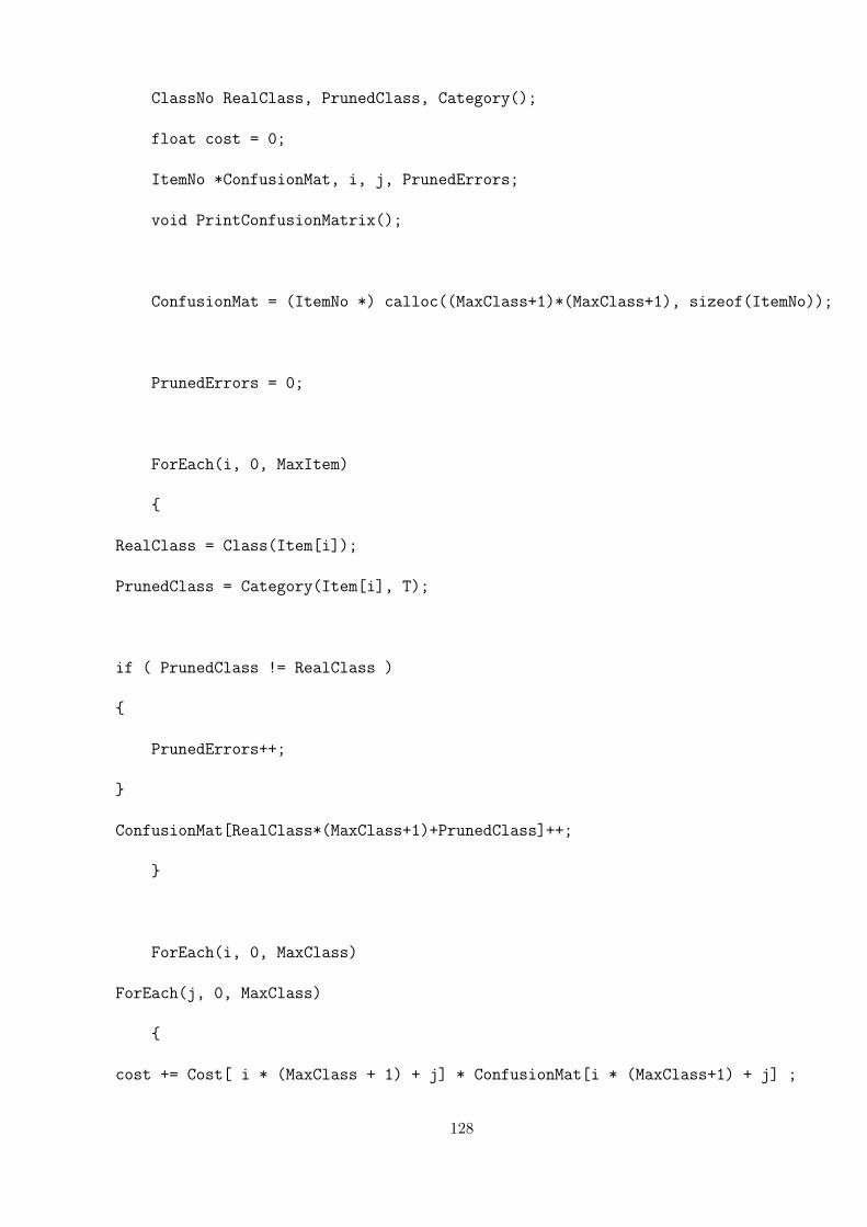
ClassNo RealClass, PrunedClass, Category();

float cost = 0;

ItemNo *ConfusionMat, i, j, PrunedErrors;

void PrintConfusionMatrix();

ConfusionMat = (ItemNo *) calloc((MaxClass+1)*(MaxClass+1), sizeof(ItemNo));

PrunedErrors = 0;

ForEach(i, 0, MaxItem)

{

RealClass = Class(Item[i]);

PrunedClass = Category(Item[i], T);

if ( PrunedClass != RealClass )

{

PrunedErrors++;

}

ConfusionMat[RealClass*(MaxClass+1)+PrunedClass]++;

}

ForEach(i, 0, MaxClass)

ForEach(j, 0, MaxClass)

{

cost += Cost[ i * (MaxClass + 1) + j] * ConfusionMat[i * (MaxClass+1) + j] ;

128

}

cost /= (float) (MaxItem + 1); //normalization

printf("Errors: %d \t", PrunedErrors);

if (print)

PrintConfusionMatrix(ConfusionMat);

cost=Cost_Weight * cost + Error_Weight * PrunedErrors / (float) (MaxItem + 1);

free(ConfusionMat);

return cost;

}

/*************************************************************************/

/* */

/* Calculate the costs in a given subtree */

/* */

/*************************************************************************/

float CalculateCostTest(T, print)

Tree T;

Boolean print;

{

ClassNo RealClass, PrunedClass, Category();

float cost = 0;

ItemNo *ConfusionMat, i, j, PrunedErrors;

129

void PrintConfusionMatrix();

ConfusionMat = (ItemNo *) calloc((MaxClass+1)*(MaxClass+1), sizeof(ItemNo));

PrunedErrors = 0;

ForEach(i, 0, MaxItem)

{

RealClass = Class(Item[i]);

PrunedClass = Category(Item[i], T);

if ( PrunedClass != RealClass )

{

PrunedErrors++;

}

ConfusionMat[RealClass*(MaxClass+1)+PrunedClass]++;

}

ForEach(i, 0, MaxClass)

ForEach(j, 0, MaxClass)

{

cost += Cost[ i * (MaxClass + 1) + j] * ConfusionMat[i * (MaxClass+1) + j] ;

}

cost /= (float) (MaxItem + 1); //normalization

printf("Errors: %d \t", PrunedErrors);

130

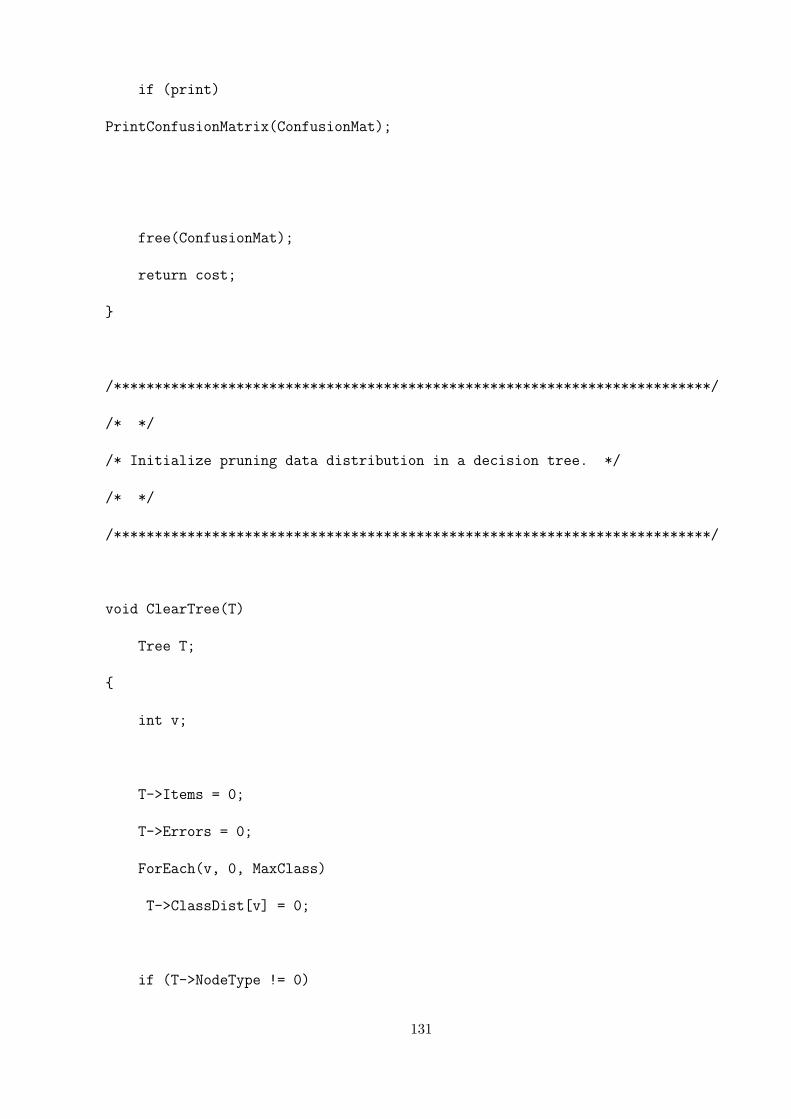
if (print)

PrintConfusionMatrix(ConfusionMat);

free(ConfusionMat);

return cost;

}

/*************************************************************************/

/* */

/* Initialize pruning data distribution in a decision tree. */

/* */

/*************************************************************************/

void ClearTree(T)

Tree T;

{

int v;

T->Items = 0;

T->Errors = 0;

ForEach(v, 0, MaxClass)

T->ClassDist[v] = 0;

if (T->NodeType != 0)

131

ForEach(v, 1, T->Forks)

ClearTree(T->Branch[v]);

else T->Forks = 0;

return;

}

/*************************************************************************/

/* */

/* Show pruning data distribution in a decision tree. comparable to */

/* classify in classify.c */

/* */

/*************************************************************************/

showPruningDistr(T, Fp, Lp, Sh, UpdateTree)

Tree T;

ItemNo Fp, Lp;

short Sh;

Boolean UpdateTree;

{

DiscrValue v, dv;

float Cv;

Attribute a;

ClassNo c, BestClass;

ItemNo i, Kp, Ep, Group();

132

ItemCount Cases, KnownCases, count, LeafErrors,

*LocalClassDist, CountItems(), Factor;

Boolean PrevAllKnown;

/* Generate the class frequency distribution */

Cases = CountItems(Fp, Lp);

LocalClassDist = (ItemCount *) calloc(MaxClass+1, sizeof(ItemCount));

ForEach(i, Fp, Lp)

{

LocalClassDist[ Class(Item[i]) ] += Weight[i];

}

/* Find the most frequent class and update the tree */

BestClass = 0;

ForEach(c, 0, MaxClass)

{

if ( LocalClassDist[c] > LocalClassDist[BestClass] )

{

BestClass = c;

}

}

LeafErrors = Cases - LocalClassDist[BestClass];

if ( UpdateTree )

133

{

T->Items = Cases;

T->Leaf = BestClass;

memcpy(T->ClassDist, LocalClassDist, (MaxClass + 1) * sizeof(ItemCount));

}

if ( ! T->NodeType ) /* leaf */

{ T->Errors = LeafErrors;

if ( UpdateTree )

{

LocalVerbosity(1)

{

Intab(Sh);

printf("%s (%.2f:%.2f/%.2f)\n", ClassName[T->Leaf],

T->Items, LeafErrors, T->Errors);

}

}

free(LocalClassDist);

return;

}

Kp = Group(0, Fp, Lp, T) + 1;

KnownCases = CountItems(Kp, Lp);

PrevAllKnown = AllKnown;

134

if ( Kp != Fp ) AllKnown = false;

ForEach(v, 1, T->Forks)

{

Ep = Group(v, Kp, Lp, T);

if ( Kp <= Ep )

{

Factor = CountItems(Kp, Ep) / KnownCases;

ForEach(i, Fp, Kp-1)

{

Weight[i] *= Factor;

}

showPruningDistr(T->Branch[v], Fp, Ep, Sh+1, UpdateTree);

Group(0, Fp, Ep, T);

ForEach(i, Fp, Kp-1)

{

Weight[i] /= Factor;

}

}

}

135

AllKnown = PrevAllKnown;

free(LocalClassDist);

return;

}

136

APPENDIX C

PRUNING PROGRAM for KBP1.0-3

C4.5 can be freely downloaded and freely used for research.

You can get C4.5 from Quinlan’s homepage:

http://www.rulequest.com/Personal/.

KBP1.0 uses the same method as that of C4.5 to construct

the original decision tree, with slight code modifications

to support the KBP1.0 pruning technique.

The pruning code in C4.5 was modified to realize the pruning

methods in KBP1.0. The big difference between KBP1.0’s

pruning code and C4.5’s pruning code is that the pruning

method in C4.5’s is based on error, while the pruning method

in KBP1.0 is based on cost, or on both error and cost. In

addition, C4.5’s pruning code can only calculate the

misclassification error during pruning, while KBP1.0’s

pruning code can calculate both the misclassification error

and misclassification cost during pruning.

In Appendix A, B, and C, the source codes are not complete because

of the license and rules for redestribution for C4.5.

137

/*********************************************************/

/* */

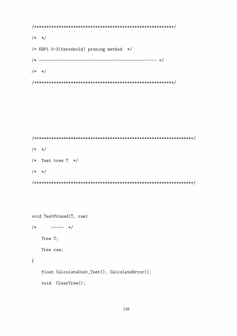
/* KBP1.0-3(threshold) pruning method */

/* ------------------------------------------------ */

/* */

/*********************************************************/

/*****************************************************************/

/* */

/* Test tree T */

/* */

/*****************************************************************/

void TestPruned(T, raw)

/* ----- */

Tree T;

Tree raw;

{

float CalculateCost_Test(), CalculateError();

void ClearTree();

138

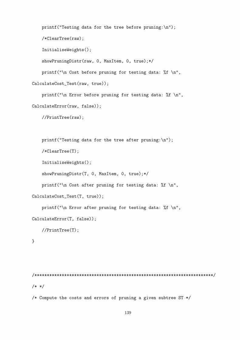
printf("Testing data for the tree before pruning:\n");

/*ClearTree(raw);

InitialiseWeights();

showPruningDistr(raw, 0, MaxItem, 0, true);*/

printf("\n Cost before pruning for testing data: %f \n",

CalculateCost_Test(raw, true));

printf("\n Error before pruning for testing data: %f \n",

CalculateError(raw, false));

//PrintTree(raw);

printf("Testing data for the tree after pruning:\n");

/*ClearTree(T);

InitialiseWeights();

showPruningDistr(T, 0, MaxItem, 0, true);*/

printf("\n Cost after pruning for testing data: %f \n",

CalculateCost_Test(T, true));

printf("\n Error after pruning for testing data: %f \n",

CalculateError(T, false));

//PrintTree(T);

}

/************************************************************************/

/* */

/* Compute the costs and errors of pruning a given subtree ST */

139

/* */

/************************************************************************/

float ComputeCostAndError(T, ST, Fp, Lp, Sh, UpdateTree)

/* -------------- */

Tree T;

Tree ST; //subtree

ItemNo Fp, Lp;

short Sh;

Boolean UpdateTree;

{

ItemNo i, Kp, Ep, Group(); //Group defined in build.c

ItemCount Cases, KnownCases, *LocalClassDist, LeafErrors,

CountItems(), Factor;

DiscrValue v, BestLeaf, BestBranch;

ClassNo c, c1, BestClass, tmpLeaf;

Boolean PrevAllKnown, *LeafPrune_Flag, *BranchPrune_Flag;

float cost = 0, *fork_costs, *fork_errors, CalculateError(),

CalculateCost(), TreeCost,

BranchCost, TreeError, BranchError, *leaf_costs, *leaf_errors,

LeafCost, LeafError;

Tree *tmpBranch, *tmpST;

short tmpNodeType;

if ( ! ST->NodeType ) /* leaf */

140

{ printf("Leaf node! Items: %f\n", ST->Items);

/*LocalVerbosity(1)

{ printf("Leaf node! Items: %f\n", ST->Items);

}*/

if ( UpdateTree )

{

LocalVerbosity(1)

{

Intab(Sh);

printf("%s (%.2f:%.2f/%.2f)\n", ClassName[ST->Leaf],

ST->Items, LeafErrors, ST->Errors);

}

}

return 0;

}

printf("Node type: %d, Items: %f, Forks: %hd \n",

ST->NodeType, ST->Items, ST->Forks);

Kp = Group(0, Fp, Lp, ST) + 1;

KnownCases = CountItems(Kp, Lp);

PrevAllKnown = AllKnown;

141

if ( Kp != Fp ) AllKnown = false;

/*Unknown data are taken into account*/

ForEach(v, 1, ST->Forks)

{

Ep = Group(v, Kp, Lp, ST);

if ( Kp <= Ep )

{

Factor = CountItems(Kp, Ep) / KnownCases;

ForEach(i, Fp, Kp-1)

{

Weight[i] *= Factor;

}

ComputeCostAndError(T, ST->Branch[v], Fp,

Ep, Sh+1, UpdateTree);

Group(0, Fp, Ep, ST);

ForEach(i, Fp, Kp-1)

{

Weight[i] /= Factor;

}

}

142

}

fork_costs = (float *) calloc (ST->Forks + 1, sizeof(float));

fork_errors = (float *) calloc (ST->Forks + 1, sizeof(float));

leaf_costs = (float *) calloc (MaxClass + 2, sizeof(float));

leaf_errors = (float *) calloc (MaxClass + 2, sizeof(float));

tmpBranch = (Tree *) calloc (ST->Forks, sizeof (Tree*));

memcpy((char *)tmpBranch, (char *)ST->Branch, ST->Forks * sizeof(Tree*));

TreeCost = CalculateCost(T, false); //calculate cost before pruning.

TreeError = CalculateError(T, false); //calculate error before pruning.

printf("Tree Cost before pruning: %f \t", TreeCost);

printf("Tree Error before pruning: %f \t", TreeError);

tmpNodeType = ST->NodeType;

tmpLeaf = ST->Leaf;

//cost improvement by replace ST with a leaf

LeafPrune_Flag = (Boolean *) calloc (MaxClass + 2, sizeof(Boolean));

ST->NodeType = 0;

ForEach(c, 0, MaxClass)

{

ST->Leaf = c;

printf("Leaf Class: %hd\n", ST->Leaf);

leaf_costs[c] = CalculateCost(T, true) - TreeCost;

leaf_errors[c] = CalculateError(T, false) - TreeError;

143

//get the leaves that is good for pruning

if ((leaf_costs[c] <= 0) && (leaf_errors[c] <= 0))

LeafPrune_Flag[c] = true;

else if ((leaf_costs[c] <= 0) && (leaf_errors[c] > 0) &&

(leaf_errors[c] <= Error_Thres * TreeError))

LeafPrune_Flag[c] = true;

else if ((leaf_costs[c] > 0) && (leaf_errors[c] <= 0) &&

(leaf_costs[c] <= Cost_Thres * TreeCost))

LeafPrune_Flag[c] = true;

else LeafPrune_Flag[c] = false;

printf("***leaf_costs[%hd]: %f***", c, leaf_costs[c]);

printf("***leaf_errors[%hd]: %f***; LeafPrune_Flag: %s.\n", c,

leaf_errors[c], LeafPrune_Flag[c]== true?"true":"false");

}

ST->NodeType = tmpNodeType;

ST->Leaf = tmpLeaf;

//pruning conditions for leaves

c = 0;

while ((LeafPrune_Flag[c] == false) && (c <= MaxClass))

c++;

if (LeafPrune_Flag[c] == true)

{ BestLeaf = c;

LeafCost = leaf_costs[BestLeaf];

ForEach(c, 0, MaxClass)

144

{

if ((leaf_costs[c] < LeafCost) && (LeafPrune_Flag[c] == true))

{ LeafCost = leaf_costs[c];

BestLeaf = c;

}

}

//printf("Leaf Class: %hd, Items: %f, Forks: %hd,

Leaf Cost - Tree Cost: %f \n",

ST->Leaf, ST->Items, ST->Forks, LeafCost);

}

else BestLeaf = -1;

printf("BestLeaf after comparing all leaves: %hd\n", BestLeaf);

tmpST = (Tree*) calloc(1, sizeof(TreeRec));

memcpy((char *)tmpST, (char *) ST, sizeof(TreeRec));

BranchPrune_Flag = (Boolean *) calloc (ST->Forks + 1, sizeof(Boolean));

ForEach(v, 1, ST->Forks)

{ printf("\n# of branches %d: \n", v);

fork_costs[v] = 32768;

memcpy((char *) ST, (char *) ST->Branch[v], sizeof(TreeRec));

fork_costs[v] = CalculateCost (T, false) - TreeCost;

fork_errors[v] = CalculateError(T, false) - TreeError;

//get the branches that is good for pruning

if ((fork_costs[v] <= 0) && (fork_errors[v] <= 0))

145

BranchPrune_Flag[v] = true;

else if ( (fork_costs[v] <= 0) && (fork_errors[v] > 0) &&

(fork_errors[v] <= Error_Thres * TreeError) )

BranchPrune_Flag[v] = true;

else if ( (fork_costs[v] > 0) && (fork_errors[v] <= 0) &&

(fork_costs[v] <= Cost_Thres * TreeCost) )

BranchPrune_Flag[v] = true;

else BranchPrune_Flag[v] = false;

//printf("Tree Cost: %f ; Tree Errors: %f \n", TreeCost, TreeError);

printf("Branch Cost: %f \t Branch errors: %f\t Branch items:

%f\t Branch Forks: %hd \n",

fork_costs[v], fork_errors[v], ST->Items, ST->Forks);

memcpy((char *) ST, (char *) tmpST, sizeof(TreeRec));

}

//pruning conditions for branches

v = 1;

while ((BranchPrune_Flag[v] == false) && (v <= ST->Forks))

v++;

if (BranchPrune_Flag[v] == true)

{ BestBranch = v;

BranchCost = fork_costs[BestBranch];

ForEach(v, 1, ST->Forks)

{

if ((fork_costs[v] < BranchCost) && (BranchPrune_Flag[v] == true))

146

{ BranchCost = fork_costs[v];

BestBranch = v;

}

}

printf("Branch Class: %hd, Items: %f, Forks: %hd,

Branch Cost - Tree Cost: %f \n",

ST->Leaf, ST->Items, ST->Forks, BranchCost);

}

else BestBranch = -1;

printf("BestBranch after comparing all leaves: %hd\n", BestBranch);

if ( ((BestLeaf >= 0) && (BestBranch == -1)) || ((BestLeaf >= 0) &&

(BestBranch >= 0) && (leaf_costs[BestLeaf] <= fork_costs[BestBranch])) )

{

LocalVerbosity(1)

{

Intab(Sh);

printf("Replaced with leaf %s\n", ClassName[BestLeaf]);

}

printf("----Replaced with leaf %s, LeafCost: %f\n", ClassName[BestLeaf],

leaf_costs[BestLeaf]);

ST->NodeType = 0;

ST->Leaf = BestLeaf;

ST->Forks = 0;

Changed = true;

147

}

else if ( ((BestLeaf == -1) && (BestBranch >= 0)) || ((BestLeaf >= 0) &&

(BestBranch >= 0) && (leaf_costs[BestLeaf] > fork_costs[BestBranch])) )

{ LocalVerbosity(1)

{

Intab(Sh);

printf("Replaced with branch %d\n", BestBranch);

}

AllKnown = PrevAllKnown;

memcpy((char *) ST, (char *) ST->Branch[BestBranch], sizeof(TreeRec));

printf("-------------------------Replaced with branch %d, BranchCost: %f\n",

BestBranch, fork_costs[BestBranch]);

Changed = true;

}

else

Changed = false;

AllKnown = PrevAllKnown;

if ( ! UpdateTree )

{

//free(LocalClassDist);

if (fork_costs != NULL) free(fork_costs);

return 0;

148

}

AllKnown = PrevAllKnown;

if (fork_costs) free(fork_costs);

if (leaf_costs) free(leaf_costs);

if (leaf_errors) free(leaf_errors);

if (fork_errors) free(fork_errors);

if (LeafPrune_Flag) free(LeafPrune_Flag);

if (BranchPrune_Flag) free(BranchPrune_Flag);

if (tmpST) free(tmpST);

if (tmpBranch) free (tmpBranch);

return 0;

}

/*****************************************************************/

/* */

/* Calculate the cost of a given subtree */

/* */

/*****************************************************************/

float CalculateCost(T, print)

Tree T;

Boolean print;

{

149

ClassNo RealClass, PrunedClass, Category();

float cost = 0;

ItemNo *ConfusionMat, i, j, PrunedErrors;

void PrintConfusionMatrix(), PrintDescription();

ConfusionMat = (ItemNo *) calloc((MaxClass+1)*(MaxClass+1), sizeof(ItemNo));

PrunedErrors = 0;

ForEach(i, 0, MaxItem)

{

RealClass = Class(Item[i]);

PrunedClass = Category(Item[i], T);

//PrintDescription(Item[i]);

//printf("Real Class: %hd, PrunedClass %hd\n", RealClass, PrunedClass);

if ( PrunedClass != RealClass )

{ if (print) {}

PrunedErrors++;

}

ConfusionMat[RealClass*(MaxClass+1)+PrunedClass]++;

}

ForEach(i, 0, MaxClass)

ForEach(j, 0, MaxClass)

150

{

cost += Cost[ i * (MaxClass + 1) + j] * ConfusionMat[i * (MaxClass+1) + j] ;

}

cost /= (float) (MaxItem + 1); //normalization

if (print)

PrintConfusionMatrix(ConfusionMat);

cost = Cost_Weight*cost+Error_Weight*PrunedErrors/(float)(MaxItem + 1);

free(ConfusionMat);

//printf("cost returned from CalculateCost: %f\n", cost);

return cost;

}

/*****************************************************************/

/* */

/* Calculate the cost of a given subtree for testing data */

/* */

/*****************************************************************/

float CalculateCost_Test(T, print)

Tree T;

Boolean print;

{

ClassNo RealClass, PrunedClass, Category();

float cost = 0;

151

ItemNo *ConfusionMat, i, j, PrunedErrors;

void PrintConfusionMatrix(), PrintDescription();

ConfusionMat = (ItemNo *) calloc((MaxClass+1)*(MaxClass+1), sizeof(ItemNo));

PrunedErrors = 0;

ForEach(i, 0, MaxItem)

{

RealClass = Class(Item[i]);

PrunedClass = Category(Item[i], T);

//PrintDescription(Item[i]);

//printf("Real Class: %hd, PrunedClass %hd\n", RealClass, PrunedClass);

if ( PrunedClass != RealClass )

{ if (print) {}

PrunedErrors++;

}

ConfusionMat[RealClass*(MaxClass+1)+PrunedClass]++;

}

ForEach(i, 0, MaxClass)

ForEach(j, 0, MaxClass)

{

cost += Cost[ i * (MaxClass + 1) + j] * ConfusionMat[i * (MaxClass+1) + j] ;

152

}

cost /= (float) (MaxItem + 1); //normalization

if (print)

PrintConfusionMatrix(ConfusionMat);

//cost=Cost_Weight*cost+Error_Weight*PrunedErrors/(float)(MaxItem+1);

free(ConfusionMat);

//printf("cost returned from CalculateCost: %f\n", cost);

return cost;

}

/*********************************************************/

/* */

/* Calculate errors of a given subtree */

/* */

/*********************************************************/

float CalculateError(T, print)

Tree T;

Boolean print;

{

ClassNo RealClass, PrunedClass, Category();

float error = 0;

ItemNo *ConfusionMat, i, j, PrunedErrors;

153

void PrintConfusionMatrix();

ConfusionMat = (ItemNo *) calloc((MaxClass+1)*(MaxClass+1), sizeof(ItemNo));

PrunedErrors = 0;

ForEach(i, 0, MaxItem)

{

RealClass = Class(Item[i]);

PrunedClass = Category(Item[i], T);

if ( PrunedClass != RealClass )

{

PrunedErrors++;

}

ConfusionMat[RealClass*(MaxClass+1)+PrunedClass]++;

}

ForEach(i, 0, MaxClass)

ForEach(j, 0, MaxClass)

{ if (i != j)

error += ConfusionMat[i * (MaxClass+1) + j] ;

}

if (print)

154

PrintConfusionMatrix(ConfusionMat);

free(ConfusionMat);

//printf("error returned from CalculateError: %f\n", error);

return error;

}

/*****************************************************************/

/* */

/* Initialize pruning data distribution in a decision tree. */

/* */

/*****************************************************************/

void ClearTree(T)

Tree T;

{

int v;

T->Items = 0;

T->Errors = 0;

ForEach(v, 0, MaxClass)

T->ClassDist[v] = 0;

if (T->NodeType != 0)

155

ForEach(v, 1, T->Forks)

ClearTree(T->Branch[v]);

else T->Forks = 0;

return;

}

/*************************************************************************/

/* */

/* Show pruning data distribution in a decision tree. comparable to */

/* classify in classify.c */

/* */

/*************************************************************************/

showPruningDistr(T, Fp, Lp, Sh, UpdateTree)

Tree T;

ItemNo Fp, Lp;

short Sh;

Boolean UpdateTree;

{

DiscrValue v, dv;

float Cv;

Attribute a;

ClassNo c, BestClass;

ItemNo i, Kp, Ep, Group();

156

ItemCount Cases, KnownCases, count, LeafErrors,

*LocalClassDist, CountItems(), Factor;

Boolean PrevAllKnown;

// Generate the class frequency distribution

Cases = CountItems(Fp, Lp);

LocalClassDist = (ItemCount *) calloc(MaxClass+1, sizeof(ItemCount));

ForEach(i, Fp, Lp)

{

LocalClassDist[ Class(Item[i]) ] += Weight[i];

}

/* Find the most frequent class and update the tree */

BestClass = 0;

ForEach(c, 0, MaxClass)

{

if ( LocalClassDist[c] > LocalClassDist[BestClass] )

{

BestClass = c;

}

}

LeafErrors = Cases - LocalClassDist[BestClass];

if ( UpdateTree )

157

{

T->Items = Cases;

T->Leaf = BestClass;

memcpy(T->ClassDist, LocalClassDist, (MaxClass + 1) * sizeof(ItemCount));

}

if ( ! T->NodeType ) /* leaf */

{ T->Errors = LeafErrors;

if ( UpdateTree )

{

LocalVerbosity(1)

{

Intab(Sh);

printf("%s (%.2f:%.2f/%.2f)\n", ClassName[T->Leaf],

T->Items, LeafErrors, T->Errors);

}

}

free(LocalClassDist);

return;

}

Kp = Group(0, Fp, Lp, T) + 1;

KnownCases = CountItems(Kp, Lp);

PrevAllKnown = AllKnown;

158

if ( Kp != Fp ) AllKnown = false;

ForEach(v, 1, T->Forks)

{

Ep = Group(v, Kp, Lp, T);

if ( Kp <= Ep )

{

Factor = CountItems(Kp, Ep) / KnownCases;

ForEach(i, Fp, Kp-1)

{

Weight[i] *= Factor;

}

showPruningDistr(T->Branch[v], Fp, Ep, Sh+1, UpdateTree);

Group(0, Fp, Ep, T);

ForEach(i, Fp, Kp-1)

{

Weight[i] /= Factor;

}

}

}

159

AllKnown = PrevAllKnown;

free(LocalClassDist);

return;

}

void PrintDescription(CaseDesc)

Description CaseDesc;

{ int i;

String name, CopyString();

short Dv;

float Cv;

ForEach(i, 0, MaxAtt)

{

if ( MaxAttVal[i] || SpecialStatus[i] == DISCRETE )

{

/* Discrete value */

Dv = DVal(CaseDesc,i);

if ( Dv == 0)

{

printf ("%s", "?,");

}

160

else

{

name = CopyString(AttValName[i][Dv]);

printf ("%s,", name);

}

}

else

{

/* Continuous value */

Cv = CVal(CaseDesc,i);

if ( Cv == Unknown )

printf ("%s", "?,");

else

printf ("%g,", Cv);

}

}

Dv = Class(CaseDesc);

printf("%s.\n", ClassName[Dv]);

return;

}

161

APPENDIX D

APPENDIX C: PRUNING PROGRAM for KBP1.0-4

C4.5 can be freely downloaded and freely used for research.

You can get C4.5 from Quinlan’s homepage:

http://www.rulequest.com/Personal/.

KBP1.0 uses the same method as that of C4.5 to construct

the original decision tree, with slight code modifications

to support the KBP1.0 pruning technique.

The pruning code in C4.5 was modified to realize the pruning

methods in KBP1.0. The big difference between KBP1.0’s

pruning code and C4.5’s pruning code is that the pruning

method in C4.5’s is based on error, while the pruning method

in KBP1.0 is based on cost, or on both error and cost. In

addition, C4.5’s pruning code can only calculate the

misclassification error during pruning, while KBP1.0’s

pruning code can calculate both the misclassification error

and misclassification cost during pruning.

In Appendix A, B, and C, the source codes are not complete because

of the license and rules for redestribution for C4.5.

162

/***************************************************************/

/* */

/* KBP1.0-4(pessimistic cost pruning) pruning method */

/* ------------------------------------------------ */

/* */

/**************************************************************/

/*************************************************************************/

/* */

/* Test tree T */

/* */

/*************************************************************************/

void TestPruned(T, raw)

/* ----- */

Tree T;

Tree raw;

{

float CalculateCostTest();

163

printf("Tree before pruning on testing data:\n");

printf("\n Cost before pruning for testing data: %f \n",

CalculateCostTest(raw, Cost, true));

printf("Tree after pruning on testing data:\n");

printf("\n Cost after pruning for testing data: %f \n",

CalculateCostTest(T, Cost, true));

}

/*************************************************************************/

/* */

/* Calculate number of leaves in subtree T */

/* */

/*************************************************************************/

int LeafCount(T)

Tree T;

{ int v, n=0;

if ( ! T->NodeType ) /* leaf */

return 1;

else

{ ForEach(v, 1, T->Forks)

n += LeafCount(T->Branch[v]);

return n;

164

}

}

/*************************************************************************/

/* */

/* Compute errors of pruning a given subtree ST */

/* */

/*************************************************************************/

float ComputeCostAndError(T, ST, Fp, Lp, Sh, UpdateTree)

/* -------------- */

Tree T;

Tree ST; //subtree

ItemNo Fp, Lp;

short Sh;

Boolean UpdateTree;

{

ItemNo i, Kp, Ep, Group(); //Group defined in build.c

ItemCount Cases, KnownCases, *LocalClassDist, LeafError,

CountItems(), Factor;

DiscrValue v, MaxBr, tmpBest, tmpBestLeaf;

ClassNo c, BestClass, tmpLeaf;

Boolean PrevAllKnown, firstLeaf;

float cost = 0, *classDist, *fork_errors, CalculateCost(),

165

TreeError, TreeCost, BranchCost,

*leaf_errors, *leaf_costs, tmpCost, LeafCost, CalculateError();

Tree *tmpBranch, *tmpST;

short tmpNodeType;

if ( ! ST->NodeType ) /* leaf */

{ //LocalVerbosity(1)

{ printf("Leaf node! Items: %f\n", ST->Items);

}

if ( UpdateTree )

{

LocalVerbosity(1)

{

Intab(Sh);

printf("%s (%.2f:%.2f/%.2f)\n", ClassName[ST->Leaf],

ST->Items, LeafError, ST->Errors);

}

}

return 0;

}

//LocalVerbosity(1)

{ printf("Node type: %d, Items: %f, Forks: %hd \n", ST->NodeType,

166

ST->Items, ST->Forks);

}

Kp = Group(0, Fp, Lp, ST) + 1;

KnownCases = CountItems(Kp, Lp);

PrevAllKnown = AllKnown;

if ( Kp != Fp ) AllKnown = false;

//fork_errors = (float *) calloc (ST->Forks + 1, sizeof(float));

leaf_errors = (float *) calloc (MaxClass + 2, sizeof(float));

leaf_costs = (float *) calloc (MaxClass + 2, sizeof(float));

//tmpBranch = (char *) calloc (ST->Forks, sizeof (Tree*));

//memcpy((char *)tmpBranch, (char *)ST->Branch, ST->Forks *

sizeof(Tree*));

/*Unknown data are taken into account*/

ForEach(v, 1, ST->Forks)

{

Ep = Group(v, Kp, Lp, ST);

if ( Kp <= Ep )

{

Factor = CountItems(Kp, Ep) / KnownCases;

167

ForEach(i, Fp, Kp-1)

{

Weight[i] *= Factor;

}

ComputeCostAndError(T, ST->Branch[v], Fp, Ep, Sh+1, UpdateTree);

Group(0, Fp, Ep, ST);

ForEach(i, Fp, Kp-1)

{

Weight[i] /= Factor;

}

}

}

TreeCost = CalculateCost(T, false);

printf("Tree Error: %f \t Tree Cost: %f \t", TreeError, TreeCost);

tmpNodeType = ST->NodeType;

tmpLeaf = ST->Leaf;

ST->NodeType = 0;

//error improvement by replace ST with a leaf

ForEach(c, 0, MaxClass)

168

{

ST->Leaf = c;

leaf_costs[c] = CalculateCost(T, true) - TreeCost;

printf("***leaf_errors[%hd]: %f;\t leaf_costs[%hd]: %f ***\n", c,

leaf_errors[c], c, leaf_costs[c]);

}

ST->NodeType = tmpNodeType;

ST->Leaf = tmpLeaf;

tmpBestLeaf = 0;

firstLeaf = true;

ForEach(c, 0, MaxClass)

{

if ((firstLeaf == true)

&& (leaf_costs[c] <= (LeafCount(ST) - 1)/2.0 + sqrt(TreeCost +

LeafCount(ST) /2.0)) )

{ firstLeaf = false;

tmpBestLeaf = c;

}

else if ((firstLeaf == false)

&& (leaf_costs[c] <= (LeafCount(ST) - 1)/2.0 + sqrt(TreeCost +

LeafCount(ST) /2.0))

&& (leaf_costs[c] <= leaf_costs[tmpBestLeaf]) )

{ tmpBestLeaf = c;

}

}

169

if (firstLeaf == true)

LeafError = -1;

else

LeafError = leaf_errors[tmpBestLeaf];

printf("Leaf Class: %hd, Items: %f, Forks: %hd, Leaf Error - Tree

Error: %f \n", ST->Leaf, ST->Items, ST->Forks, LeafError);

printf("(LeafCount(ST) - 1)/2 : %f\n",(LeafCount(ST) - 1)/2.0);

if (leaf_costs[tmpBestLeaf] <= (LeafCount(ST) - 1)/2.0 + sqrt(TreeCost

+ LeafCount(ST) /2.0))

{

LocalVerbosity(1)

{

Intab(Sh);

printf("Replaced with leaf %s\n", ClassName[tmpBestLeaf]);

}

printf("-------------------------Replaced with leaf %s, LeafError:

%f\n", ClassName[tmpBestLeaf], LeafError);

ST->NodeType = 0;

ST->Leaf = tmpBestLeaf;

ST->Forks = 0;

Changed = true;

}

else

Changed = false;

170

AllKnown = PrevAllKnown;

if ( ! UpdateTree )

{

//free(LocalClassDist);

//free(classDist);

if (fork_errors != NULL) free(fork_errors);

return TreeError;

}

AllKnown = PrevAllKnown;

//if (fork_errors) free(fork_errors);

if (leaf_errors) free(leaf_errors);

//if (tmpST) free(tmpST);

return 0;

}

/*************************************************************************/

/* */

/* Calculate errors for each of the trials */

/* */

171

/*************************************************************************/

float CalculateError(T, print)

Tree T;

Boolean print;

{

ClassNo RealClass, PrunedClass, Category();

ItemNo *ConfusionMat, i, j, PrunedErrors;

void PrintConfusionMatrix();

ConfusionMat = (ItemNo *) calloc((MaxClass+1)*(MaxClass+1),

sizeof(ItemNo));

PrunedErrors = 0;

ForEach(i, 0, MaxItem)

{

RealClass = Class(Item[i]);

PrunedClass = Category(Item[i], T);

if ( PrunedClass != RealClass )

{

PrunedErrors++;

}

ConfusionMat[RealClass*(MaxClass+1)+PrunedClass]++;

172

}

//printf("Errors: %d \t", PrunedErrors);

if (print)

PrintConfusionMatrix(ConfusionMat);

free(ConfusionMat);

return PrunedErrors;

}

/*************************************************************************/

/* */

/* Calculate the costs in a given subtree */

/* */

/*************************************************************************/

float CalculateCost(T, print)

Tree T;

Boolean print;

{

ClassNo RealClass, PrunedClass, Category();

float cost = 0;

ItemNo *ConfusionMat, i, j, PrunedErrors;

void PrintConfusionMatrix();

173

ConfusionMat = (ItemNo *) calloc((MaxClass+1)*(MaxClass+1),

sizeof(ItemNo));

PrunedErrors = 0;

ForEach(i, 0, MaxItem)

{

RealClass = Class(Item[i]);

PrunedClass = Category(Item[i], T);

if ( PrunedClass != RealClass )

{

PrunedErrors++;

}

ConfusionMat[RealClass*(MaxClass+1)+PrunedClass]++;

}

ForEach(i, 0, MaxClass)

ForEach(j, 0, MaxClass)

{

cost += Cost[ i * (MaxClass + 1) + j] * ConfusionMat[i * (MaxClass+1)

+ j] ;

}

cost /= (float) (MaxItem + 1); //normalization

174

printf("Errors: %d \t", PrunedErrors);

if (print)

PrintConfusionMatrix(ConfusionMat);

cost = Cost_Weight * cost + Error_Weight * PrunedErrors / (float)

(MaxItem + 1);

free(ConfusionMat);

return cost;

}

/*************************************************************************/

/* */

/* Calculate the costs in a given subtree in the test */

/* */

/*************************************************************************/

float CalculateCostTest(T, print)

Tree T;

Boolean print;

{

ClassNo RealClass, PrunedClass, Category();

float cost = 0;

ItemNo *ConfusionMat, i, j, PrunedErrors;

void PrintConfusionMatrix();

175

ConfusionMat = (ItemNo *) calloc((MaxClass+1)*(MaxClass+1),

sizeof(ItemNo));

PrunedErrors = 0;

ForEach(i, 0, MaxItem)

{

RealClass = Class(Item[i]);

PrunedClass = Category(Item[i], T);

if ( PrunedClass != RealClass )

{

PrunedErrors++;

}

ConfusionMat[RealClass*(MaxClass+1)+PrunedClass]++;

}

ForEach(i, 0, MaxClass)

ForEach(j, 0, MaxClass)

{

cost += Cost[ i * (MaxClass + 1) + j] * ConfusionMat[i * (MaxClass+1)

+ j] ;

}

cost /= (float) (MaxItem + 1); //normalization

176

printf("Errors: %d \t", PrunedErrors);

if (print)

PrintConfusionMatrix(ConfusionMat);

//cost = Cost_Weight * cost + Error_Weight * PrunedErrors / (float)

(MaxItem + 1);

free(ConfusionMat);

return cost;

}

177

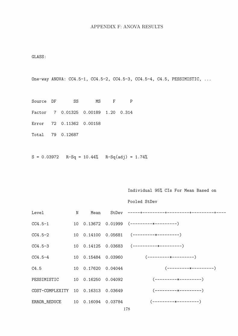
APPENDIX F: ANOVA RESULTS

GLASS:

One-way ANOVA: CC4.5-1, CC4.5-2, CC4.5-3, CC4.5-4, C4.5, PESSIMISTIC, ...

Source DF SS MS F P

Factor 7 0.01325 0.00189 1.20 0.314

Error 72 0.11362 0.00158

Total 79 0.12687

S = 0.03972 R-Sq = 10.44% R-Sq(adj) = 1.74%

Individual 95% CIs For Mean Based on

Pooled StDev

Level N Mean StDev -----+---------+---------+---------+----

CC4.5-1 10 0.13672 0.01999 (---------*---------)

CC4.5-2 10 0.14100 0.05681 (---------*---------)

CC4.5-3 10 0.14125 0.03683 (----------*---------)

CC4.5-4 10 0.15484 0.03960 (---------*---------)

C4.5 10 0.17620 0.04044 (---------*---------)

PESSIMISTIC 10 0.16250 0.04092 (---------*---------)

COST-COMPLEXITY 10 0.16313 0.03649 (---------*---------)

ERROR_REDUCE 10 0.16094 0.03784 (---------*---------)

178

-----+---------+---------+---------+----

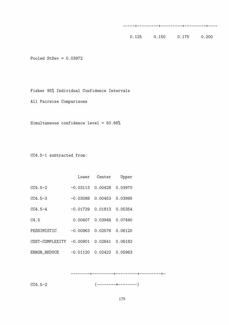
0.125 0.150 0.175 0.200

Pooled StDev = 0.03972

Fisher 95% Individual Confidence Intervals

All Pairwise Comparisons

Simultaneous confidence level = 50.66%

CC4.5-1 subtracted from:

Lower Center Upper

CC4.5-2 -0.03113 0.00428 0.03970

CC4.5-3 -0.03088 0.00453 0.03995

CC4.5-4 -0.01729 0.01813 0.05354

C4.5 0.00407 0.03948 0.07490

PESSIMISTIC -0.00963 0.02578 0.06120

COST-COMPLEXITY -0.00901 0.02641 0.06182

ERROR_REDUCE -0.01120 0.02422 0.05963

--------+---------+---------+---------+-

CC4.5-2 (--------*--------)

179

CC4.5-3 (--------*--------)

CC4.5-4 (--------*-------)

C4.5 (--------*--------)

PESSIMISTIC (-------*--------)

COST-COMPLEXITY (--------*-------)

ERROR_REDUCE (--------*--------)

--------+---------+---------+---------+-

-0.040 0.000 0.040 0.080

CC4.5-2 subtracted from:

Lower Center Upper

CC4.5-3 -0.03516 0.00025 0.03566

CC4.5-4 -0.02157 0.01384 0.04926

C4.5 -0.00021 0.03520 0.07062

PESSIMISTIC -0.01391 0.02150 0.05691

COST-COMPLEXITY -0.01329 0.02213 0.05754

ERROR_REDUCE -0.01548 0.01994 0.05535

--------+---------+---------+---------+-

CC4.5-3 (--------*--------)

CC4.5-4 (-------*--------)

C4.5 (--------*--------)

PESSIMISTIC (-------*--------)

180

COST-COMPLEXITY (--------*-------)

ERROR_REDUCE (--------*--------)

--------+---------+---------+---------+-

-0.040 0.000 0.040 0.080

CC4.5-3 subtracted from:

Lower Center Upper

CC4.5-4 -0.02182 0.01359 0.04901

C4.5 -0.00046 0.03495 0.07037

PESSIMISTIC -0.01416 0.02125 0.05666

COST-COMPLEXITY -0.01354 0.02188 0.05729

ERROR_REDUCE -0.01573 0.01969 0.05510

--------+---------+---------+---------+-

CC4.5-4 (-------*--------)

C4.5 (--------*--------)

PESSIMISTIC (--------*--------)

COST-COMPLEXITY (-------*--------)

ERROR_REDUCE (--------*--------)

--------+---------+---------+---------+-

-0.040 0.000 0.040 0.080

181

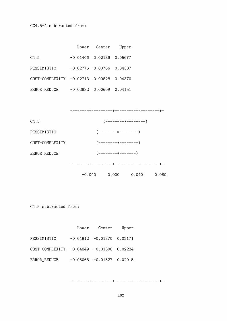
CC4.5-4 subtracted from:

Lower Center Upper

C4.5 -0.01406 0.02136 0.05677

PESSIMISTIC -0.02776 0.00766 0.04307

COST-COMPLEXITY -0.02713 0.00828 0.04370

ERROR_REDUCE -0.02932 0.00609 0.04151

--------+---------+---------+---------+-

C4.5 (--------*--------)

PESSIMISTIC (--------*--------)

COST-COMPLEXITY (--------*--------)

ERROR_REDUCE (--------*-------)

--------+---------+---------+---------+-

-0.040 0.000 0.040 0.080

C4.5 subtracted from:

Lower Center Upper

PESSIMISTIC -0.04912 -0.01370 0.02171

COST-COMPLEXITY -0.04849 -0.01308 0.02234

ERROR_REDUCE -0.05068 -0.01527 0.02015

--------+---------+---------+---------+-

182

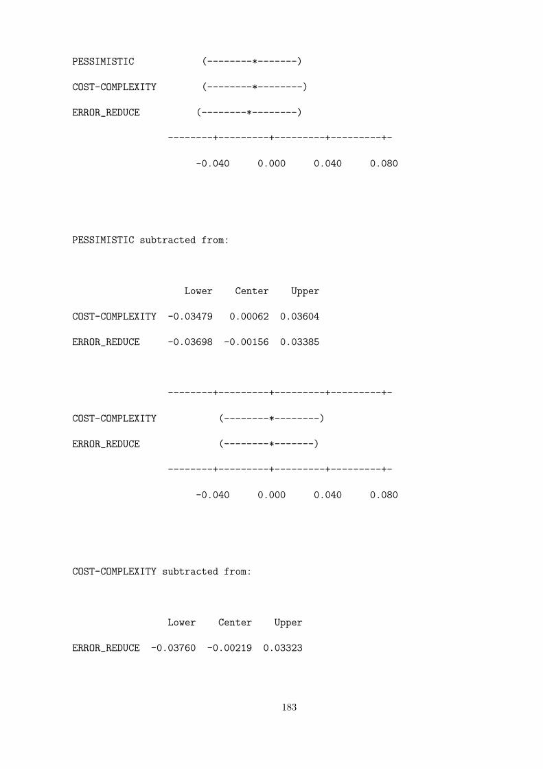
PESSIMISTIC (--------*-------)

COST-COMPLEXITY (--------*--------)

ERROR_REDUCE (--------*--------)

--------+---------+---------+---------+-

-0.040 0.000 0.040 0.080

PESSIMISTIC subtracted from:

Lower Center Upper

COST-COMPLEXITY -0.03479 0.00062 0.03604

ERROR_REDUCE -0.03698 -0.00156 0.03385

--------+---------+---------+---------+-

COST-COMPLEXITY (--------*--------)

ERROR_REDUCE (--------*-------)

--------+---------+---------+---------+-

-0.040 0.000 0.040 0.080

COST-COMPLEXITY subtracted from:

Lower Center Upper

ERROR_REDUCE -0.03760 -0.00219 0.03323

183

--------+---------+---------+---------+-

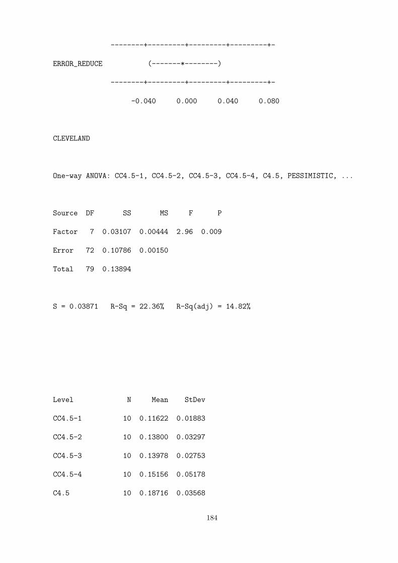
ERROR_REDUCE (-------*--------)

--------+---------+---------+---------+-

-0.040 0.000 0.040 0.080

CLEVELAND

One-way ANOVA: CC4.5-1, CC4.5-2, CC4.5-3, CC4.5-4, C4.5, PESSIMISTIC, ...

Source DF SS MS F P

Factor 7 0.03107 0.00444 2.96 0.009

Error 72 0.10786 0.00150

Total 79 0.13894

S = 0.03871 R-Sq = 22.36% R-Sq(adj) = 14.82%

Level N Mean StDev

CC4.5-1 10 0.11622 0.01883

CC4.5-2 10 0.13800 0.03297

CC4.5-3 10 0.13978 0.02753

CC4.5-4 10 0.15156 0.05178

C4.5 10 0.18716 0.03568

184

PESSIMISTIC 10 0.16133 0.03750

COST-COMPLEXITY 10 0.16444 0.05437

ERROR_REDUCE 10 0.15422 0.03834

Individual 95% CIs For Mean Based on

Pooled StDev

Level ---------+---------+---------+---------+

CC4.5-1 (-------*-------)

CC4.5-2 (-------*-------)

CC4.5-3 (--------*-------)

CC4.5-4 (--------*-------)

C4.5 (-------*--------)

PESSIMISTIC (-------*-------)

COST-COMPLEXITY (-------*-------)

ERROR_REDUCE (-------*--------)

---------+---------+---------+---------+

0.120 0.150 0.180 0.210

Pooled StDev = 0.03871

Fisher 95% Individual Confidence Intervals

All Pairwise Comparisons

Simultaneous confidence level = 50.66%

185

CC4.5-1 subtracted from:

Lower Center Upper

CC4.5-2 -0.01273 0.02178 0.05628

CC4.5-3 -0.01095 0.02356 0.05806

CC4.5-4 0.00083 0.03533 0.06984

C4.5 0.03643 0.07093 0.10544

PESSIMISTIC 0.01060 0.04511 0.07962

COST-COMPLEXITY 0.01372 0.04822 0.08273

ERROR_REDUCE 0.00349 0.03800 0.07251

-------+---------+---------+---------+--

CC4.5-2 (------*------)

CC4.5-3 (------*------)

CC4.5-4 (------*------)

C4.5 (------*------)

PESSIMISTIC (------*------)

COST-COMPLEXITY (------*------)

ERROR_REDUCE (------*------)

-------+---------+---------+---------+--

-0.050 0.000 0.050 0.100

186

CC4.5-2 subtracted from:

Lower Center Upper

CC4.5-3 -0.03273 0.00178 0.03628

CC4.5-4 -0.02095 0.01356 0.04806

C4.5 0.01465 0.04916 0.08366

PESSIMISTIC -0.01117 0.02333 0.05784

COST-COMPLEXITY -0.00806 0.02644 0.06095

ERROR_REDUCE -0.01828 0.01622 0.05073

-------+---------+---------+---------+--

CC4.5-3 (------*------)

CC4.5-4 (------*------)

C4.5 (------*------)

PESSIMISTIC (------*------)

COST-COMPLEXITY (------*------)

ERROR_REDUCE (------*------)

-------+---------+---------+---------+--

-0.050 0.000 0.050 0.100

CC4.5-3 subtracted from:

Lower Center Upper

CC4.5-4 -0.02273 0.01178 0.04628

187

C4.5 0.01287 0.04738 0.08188

PESSIMISTIC -0.01295 0.02156 0.05606

COST-COMPLEXITY -0.00984 0.02467 0.05917

ERROR_REDUCE -0.02006 0.01444 0.04895

-------+---------+---------+---------+--

CC4.5-4 (------*------)

C4.5 (-----*------)

PESSIMISTIC (------*------)

COST-COMPLEXITY (------*------)

ERROR_REDUCE (------*------)

-------+---------+---------+---------+--

-0.050 0.000 0.050 0.100

CC4.5-4 subtracted from:

Lower Center Upper

C4.5 0.00109 0.03560 0.07011

PESSIMISTIC -0.02473 0.00978 0.04428

COST-COMPLEXITY -0.02162 0.01289 0.04740

ERROR_REDUCE -0.03184 0.00267 0.03717

-------+---------+---------+---------+--

C4.5 (------*------)

188

PESSIMISTIC (------*------)

COST-COMPLEXITY (------*-----)

ERROR_REDUCE (------*-----)

-------+---------+---------+---------+--

-0.050 0.000 0.050 0.100

C4.5 subtracted from:

Lower Center Upper

PESSIMISTIC -0.06033 -0.02582 0.00868

COST-COMPLEXITY -0.05722 -0.02271 0.01180

ERROR_REDUCE -0.06744 -0.03293 0.00157

-------+---------+---------+---------+--

PESSIMISTIC (------*------)

COST-COMPLEXITY (-----*------)

ERROR_REDUCE (-----*------)

-------+---------+---------+---------+--

-0.050 0.000 0.050 0.100

PESSIMISTIC subtracted from:

Lower Center Upper

189

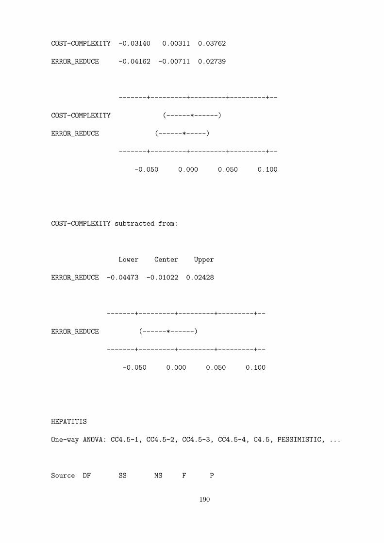
COST-COMPLEXITY -0.03140 0.00311 0.03762

ERROR_REDUCE -0.04162 -0.00711 0.02739

-------+---------+---------+---------+--

COST-COMPLEXITY (------*------)

ERROR_REDUCE (------*-----)

-------+---------+---------+---------+--

-0.050 0.000 0.050 0.100

COST-COMPLEXITY subtracted from:

Lower Center Upper

ERROR_REDUCE -0.04473 -0.01022 0.02428

-------+---------+---------+---------+--

ERROR_REDUCE (------*------)

-------+---------+---------+---------+--

-0.050 0.000 0.050 0.100

HEPATITIS

One-way ANOVA: CC4.5-1, CC4.5-2, CC4.5-3, CC4.5-4, C4.5, PESSIMISTIC, ...

Source DF SS MS F P

190

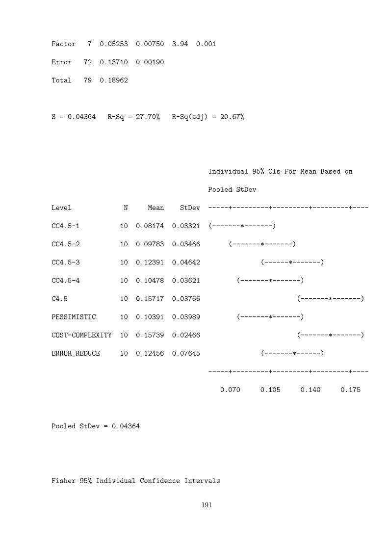
Factor 7 0.05253 0.00750 3.94 0.001

Error 72 0.13710 0.00190

Total 79 0.18962

S = 0.04364 R-Sq = 27.70% R-Sq(adj) = 20.67%

Individual 95% CIs For Mean Based on

Pooled StDev

Level N Mean StDev -----+---------+---------+---------+----

CC4.5-1 10 0.08174 0.03321 (-------*-------)

CC4.5-2 10 0.09783 0.03466 (-------*-------)

CC4.5-3 10 0.12391 0.04642 (------*-------)

CC4.5-4 10 0.10478 0.03621 (-------*-------)

C4.5 10 0.15717 0.03766 (-------*-------)

PESSIMISTIC 10 0.10391 0.03989 (-------*-------)

COST-COMPLEXITY 10 0.15739 0.02466 (-------*-------)

ERROR_REDUCE 10 0.12456 0.07645 (-------*------)

-----+---------+---------+---------+----

0.070 0.105 0.140 0.175

Pooled StDev = 0.04364

Fisher 95% Individual Confidence Intervals

191

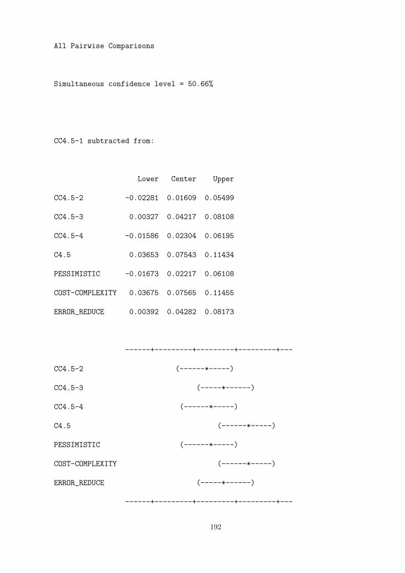
All Pairwise Comparisons

Simultaneous confidence level = 50.66%

CC4.5-1 subtracted from:

Lower Center Upper

CC4.5-2 -0.02281 0.01609 0.05499

CC4.5-3 0.00327 0.04217 0.08108

CC4.5-4 -0.01586 0.02304 0.06195

C4.5 0.03653 0.07543 0.11434

PESSIMISTIC -0.01673 0.02217 0.06108

COST-COMPLEXITY 0.03675 0.07565 0.11455

ERROR_REDUCE 0.00392 0.04282 0.08173

------+---------+---------+---------+---

CC4.5-2 (------*-----)

CC4.5-3 (-----*------)

CC4.5-4 (------*-----)

C4.5 (------*-----)

PESSIMISTIC (------*-----)

COST-COMPLEXITY (------*-----)

ERROR_REDUCE (-----*------)

------+---------+---------+---------+---

192

-0.060 0.000 0.060 0.120

CC4.5-2 subtracted from:

Lower Center Upper

CC4.5-3 -0.01281 0.02609 0.06499

CC4.5-4 -0.03195 0.00696 0.04586

C4.5 0.02045 0.05935 0.09825

PESSIMISTIC -0.03281 0.00609 0.04499

COST-COMPLEXITY 0.02066 0.05957 0.09847

ERROR_REDUCE -0.01216 0.02674 0.06564

------+---------+---------+---------+---

CC4.5-3 (-----*------)

CC4.5-4 (-----*------)

C4.5 (------*-----)

PESSIMISTIC (-----*-----)

COST-COMPLEXITY (------*-----)

ERROR_REDUCE (-----*------)

------+---------+---------+---------+---

-0.060 0.000 0.060 0.120

CC4.5-3 subtracted from:

193

Lower Center Upper

CC4.5-4 -0.05803 -0.01913 0.01977

C4.5 -0.00564 0.03326 0.07216

PESSIMISTIC -0.05890 -0.02000 0.01890

COST-COMPLEXITY -0.00542 0.03348 0.07238

ERROR_REDUCE -0.03825 0.00065 0.03955

------+---------+---------+---------+---

CC4.5-4 (------*-----)

C4.5 (------*-----)

PESSIMISTIC (------*-----)

COST-COMPLEXITY (------*-----)

ERROR_REDUCE (-----*------)

------+---------+---------+---------+---

-0.060 0.000 0.060 0.120

CC4.5-4 subtracted from:

Lower Center Upper

C4.5 0.01349 0.05239 0.09129

PESSIMISTIC -0.03977 -0.00087 0.03803

COST-COMPLEXITY 0.01371 0.05261 0.09151

ERROR_REDUCE -0.01912 0.01978 0.05868

194

------+---------+---------+---------+---

C4.5 (------*-----)

PESSIMISTIC (------*-----)

COST-COMPLEXITY (------*-----)

ERROR_REDUCE (-----*------)

------+---------+---------+---------+---

-0.060 0.000 0.060 0.120

C4.5 subtracted from:

Lower Center Upper

PESSIMISTIC -0.09216 -0.05326 -0.01436

COST-COMPLEXITY -0.03868 0.00022 0.03912

ERROR_REDUCE -0.07151 -0.03261 0.00629

------+---------+---------+---------+---

PESSIMISTIC (-----*------)

COST-COMPLEXITY (-----*------)

ERROR_REDUCE (------*-----)

------+---------+---------+---------+---

-0.060 0.000 0.060 0.120

195

PESSIMISTIC subtracted from:

Lower Center Upper

COST-COMPLEXITY 0.01458 0.05348 0.09238

ERROR_REDUCE -0.01825 0.02065 0.05955

------+---------+---------+---------+---

COST-COMPLEXITY (------*-----)

ERROR_REDUCE (-----*------)

------+---------+---------+---------+---

-0.060 0.000 0.060 0.120

COST-COMPLEXITY subtracted from:

Lower Center Upper

ERROR_REDUCE -0.07173 -0.03283 0.00607

------+---------+---------+---------+---

ERROR_REDUCE (------*-----)

------+---------+---------+---------+---

-0.060 0.000 0.060 0.120

196

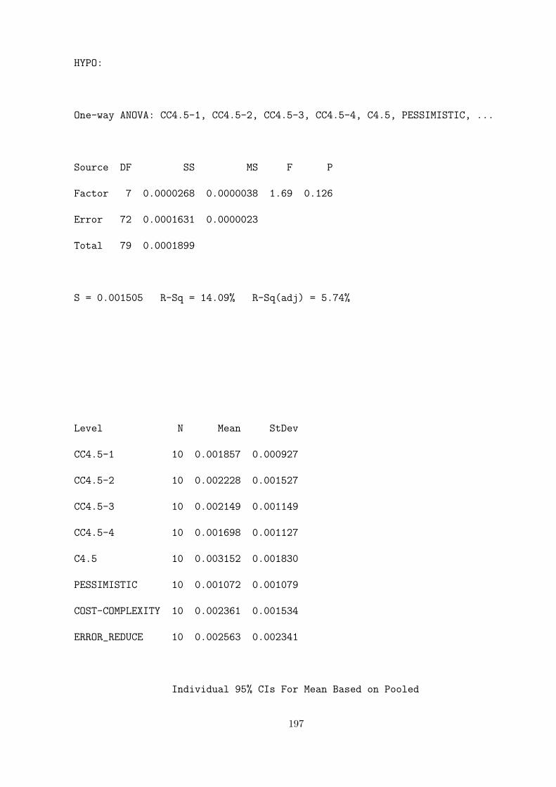
HYPO:

One-way ANOVA: CC4.5-1, CC4.5-2, CC4.5-3, CC4.5-4, C4.5, PESSIMISTIC, ...

Source DF SS MS F P

Factor 7 0.0000268 0.0000038 1.69 0.126

Error 72 0.0001631 0.0000023

Total 79 0.0001899

S = 0.001505 R-Sq = 14.09% R-Sq(adj) = 5.74%

Level N Mean StDev

CC4.5-1 10 0.001857 0.000927

CC4.5-2 10 0.002228 0.001527

CC4.5-3 10 0.002149 0.001149

CC4.5-4 10 0.001698 0.001127

C4.5 10 0.003152 0.001830

PESSIMISTIC 10 0.001072 0.001079

COST-COMPLEXITY 10 0.002361 0.001534

ERROR_REDUCE 10 0.002563 0.002341

Individual 95% CIs For Mean Based on Pooled

197

StDev

Level ---------+---------+---------+---------+

CC4.5-1 (---------*--------)

CC4.5-2 (--------*---------)

CC4.5-3 (--------*---------)

CC4.5-4 (---------*--------)

C4.5 (---------*--------)

PESSIMISTIC (---------*--------)

COST-COMPLEXITY (---------*--------)

ERROR_REDUCE (---------*--------)

---------+---------+---------+---------+

0.0010 0.0020 0.0030 0.0040

Pooled StDev = 0.001505

Fisher 95% Individual Confidence Intervals

All Pairwise Comparisons

Simultaneous confidence level = 50.66%

CC4.5-1 subtracted from:

Lower Center Upper

198

CC4.5-2 -0.000971 0.000371 0.001713

CC4.5-3 -0.001050 0.000292 0.001634

CC4.5-4 -0.001501 -0.000159 0.001183

C4.5 -0.000047 0.001295 0.002637

PESSIMISTIC -0.002127 -0.000785 0.000557

COST-COMPLEXITY -0.000838 0.000504 0.001846

ERROR_REDUCE -0.000636 0.000706 0.002048

-------+---------+---------+---------+--

CC4.5-2 (------*------)

CC4.5-3 (-----*------)

CC4.5-4 (------*------)

C4.5 (-----*------)

PESSIMISTIC (------*------)

COST-COMPLEXITY (------*-----)

ERROR_REDUCE (------*-----)

-------+---------+---------+---------+--

-0.0020 0.0000 0.0020 0.0040

CC4.5-2 subtracted from:

Lower Center Upper

CC4.5-3 -0.001422 -0.000080 0.001262

CC4.5-4 -0.001872 -0.000530 0.000811

199

C4.5 -0.000419 0.000923 0.002265

PESSIMISTIC -0.002498 -0.001156 0.000185

COST-COMPLEXITY -0.001209 0.000133 0.001475

ERROR_REDUCE -0.001007 0.000335 0.001677

-------+---------+---------+---------+--

CC4.5-3 (------*-----)

CC4.5-4 (-----*------)

C4.5 (------*-----)

PESSIMISTIC (-----*------)

COST-COMPLEXITY (------*-----)

ERROR_REDUCE (------*-----)

-------+---------+---------+---------+--

-0.0020 0.0000 0.0020 0.0040

CC4.5-3 subtracted from:

Lower Center Upper

CC4.5-4 -0.001793 -0.000451 0.000891

C4.5 -0.000339 0.001003 0.002345

PESSIMISTIC -0.002419 -0.001077 0.000265

COST-COMPLEXITY -0.001130 0.000212 0.001554

ERROR_REDUCE -0.000927 0.000415 0.001756

200

-------+---------+---------+---------+--

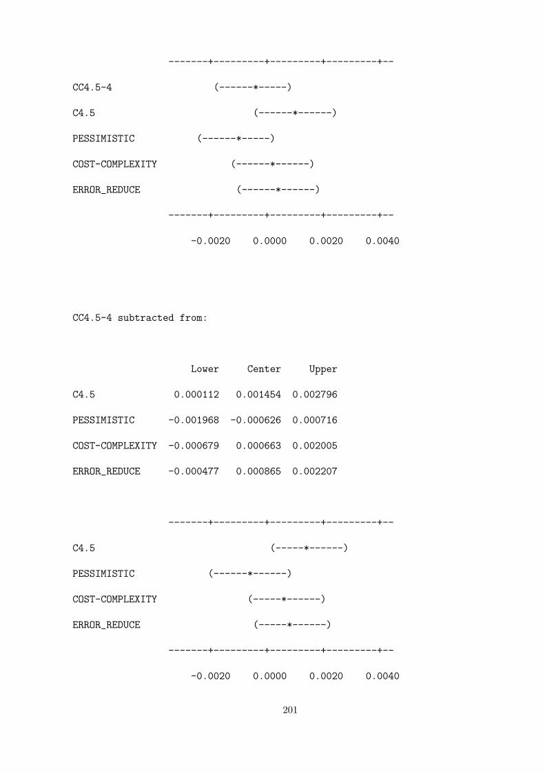
CC4.5-4 (------*-----)

C4.5 (------*------)

PESSIMISTIC (------*-----)

COST-COMPLEXITY (------*------)

ERROR_REDUCE (------*------)

-------+---------+---------+---------+--

-0.0020 0.0000 0.0020 0.0040

CC4.5-4 subtracted from:

Lower Center Upper

C4.5 0.000112 0.001454 0.002796

PESSIMISTIC -0.001968 -0.000626 0.000716

COST-COMPLEXITY -0.000679 0.000663 0.002005

ERROR_REDUCE -0.000477 0.000865 0.002207

-------+---------+---------+---------+--

C4.5 (-----*------)

PESSIMISTIC (------*------)

COST-COMPLEXITY (-----*------)

ERROR_REDUCE (-----*------)

-------+---------+---------+---------+--

-0.0020 0.0000 0.0020 0.0040

201

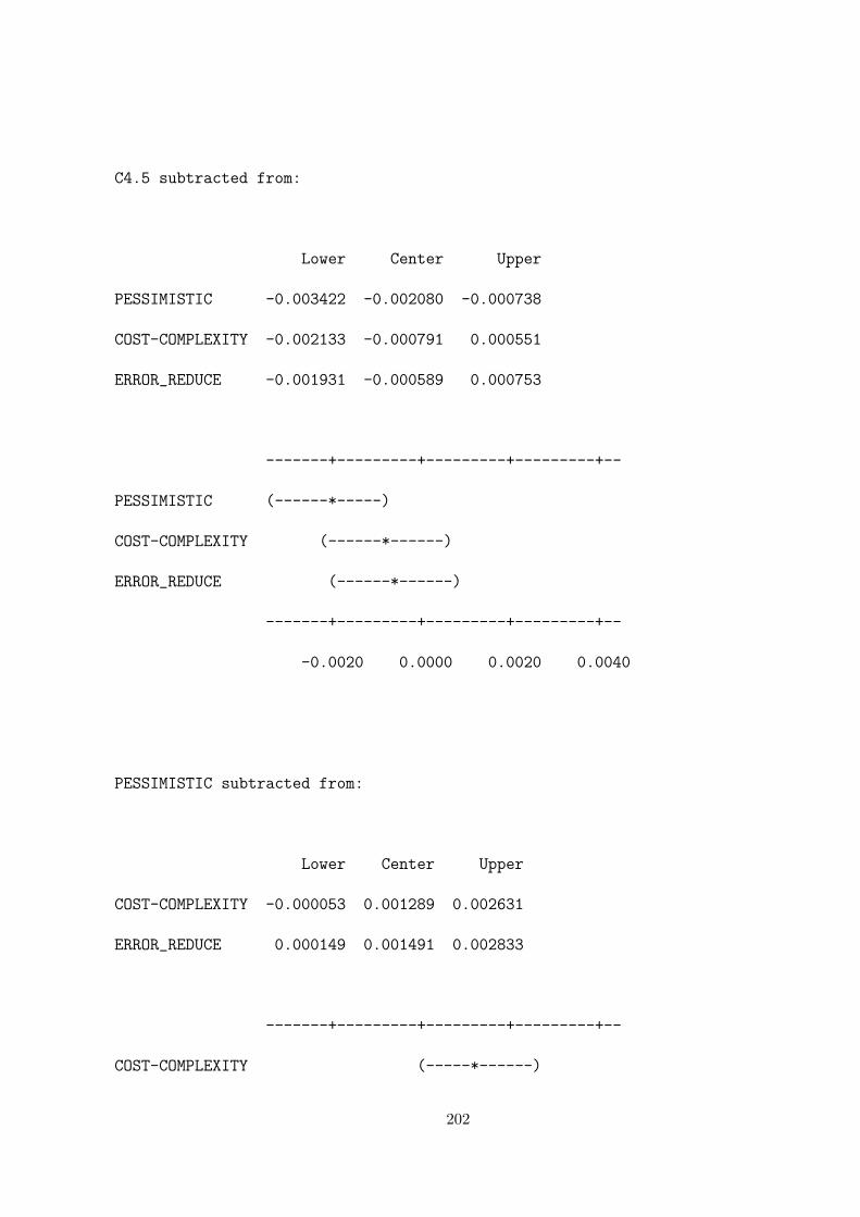
C4.5 subtracted from:

Lower Center Upper

PESSIMISTIC -0.003422 -0.002080 -0.000738

COST-COMPLEXITY -0.002133 -0.000791 0.000551

ERROR_REDUCE -0.001931 -0.000589 0.000753

-------+---------+---------+---------+--

PESSIMISTIC (------*-----)

COST-COMPLEXITY (------*------)

ERROR_REDUCE (------*------)

-------+---------+---------+---------+--

-0.0020 0.0000 0.0020 0.0040

PESSIMISTIC subtracted from:

Lower Center Upper

COST-COMPLEXITY -0.000053 0.001289 0.002631

ERROR_REDUCE 0.000149 0.001491 0.002833

-------+---------+---------+---------+--

COST-COMPLEXITY (-----*------)

202

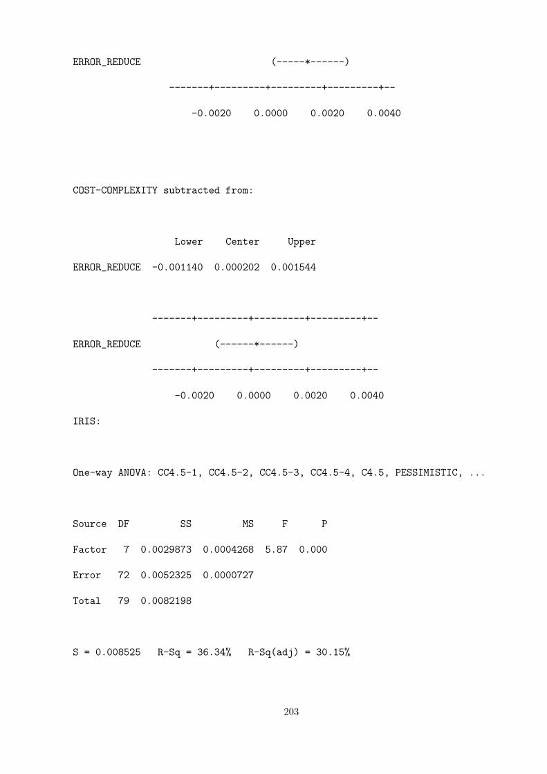
ERROR_REDUCE (-----*------)

-------+---------+---------+---------+--

-0.0020 0.0000 0.0020 0.0040

COST-COMPLEXITY subtracted from:

Lower Center Upper

ERROR_REDUCE -0.001140 0.000202 0.001544

-------+---------+---------+---------+--

ERROR_REDUCE (------*------)

-------+---------+---------+---------+--

-0.0020 0.0000 0.0020 0.0040

IRIS:

One-way ANOVA: CC4.5-1, CC4.5-2, CC4.5-3, CC4.5-4, C4.5, PESSIMISTIC, ...

Source DF SS MS F P

Factor 7 0.0029873 0.0004268 5.87 0.000

Error 72 0.0052325 0.0000727

Total 79 0.0082198

S = 0.008525 R-Sq = 36.34% R-Sq(adj) = 30.15%

203

Level N Mean StDev

CC4.5-1 10 0.012955 0.005144

CC4.5-2 10 0.013864 0.004476

CC4.5-3 10 0.012046 0.010335

CC4.5-4 10 0.015555 0.003920

C4.5 10 0.032644 0.018221

PESSIMISTIC 10 0.018000 0.006411

COST-COMPLEXITY 10 0.016318 0.004963

ERROR_REDUCE 10 0.016591 0.003870

Individual 95% CIs For Mean Based on

Pooled StDev

Level --+---------+---------+---------+-------

CC4.5-1 (------*------)

CC4.5-2 (-----*------)

CC4.5-3 (------*------)

CC4.5-4 (-----*------)

C4.5 (------*------)

PESSIMISTIC (------*-----)

COST-COMPLEXITY (-----*------)

ERROR_REDUCE (------*-----)

--+---------+---------+---------+-------

204

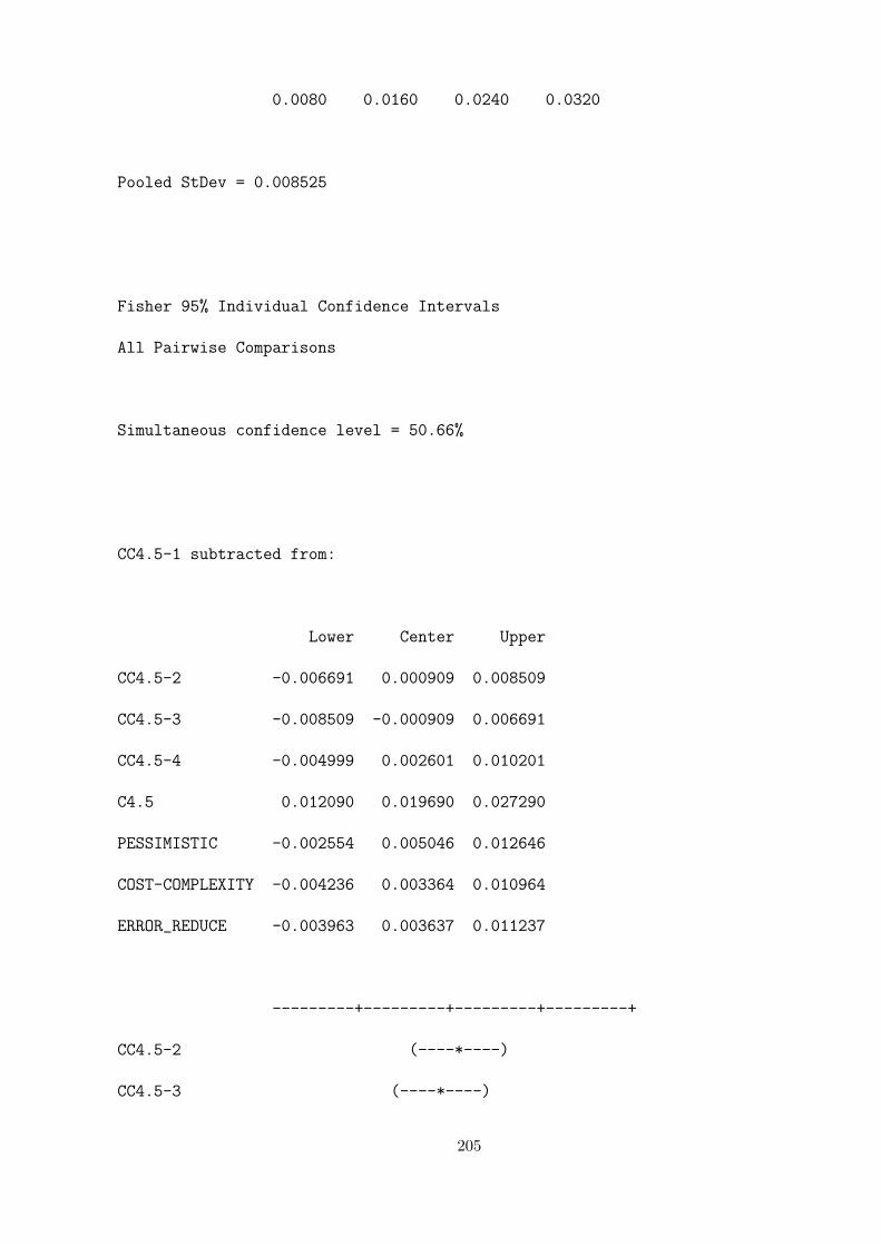
0.0080 0.0160 0.0240 0.0320

Pooled StDev = 0.008525

Fisher 95% Individual Confidence Intervals

All Pairwise Comparisons

Simultaneous confidence level = 50.66%

CC4.5-1 subtracted from:

Lower Center Upper

CC4.5-2 -0.006691 0.000909 0.008509

CC4.5-3 -0.008509 -0.000909 0.006691

CC4.5-4 -0.004999 0.002601 0.010201

C4.5 0.012090 0.019690 0.027290

PESSIMISTIC -0.002554 0.005046 0.012646

COST-COMPLEXITY -0.004236 0.003364 0.010964

ERROR_REDUCE -0.003963 0.003637 0.011237

---------+---------+---------+---------+

CC4.5-2 (----*----)

CC4.5-3 (----*----)

205

CC4.5-4 (----*----)

C4.5 (----*----)

PESSIMISTIC (----*----)

COST-COMPLEXITY (----*----)

ERROR_REDUCE (----*----)

---------+---------+---------+---------+

-0.015 0.000 0.015 0.030

CC4.5-2 subtracted from:

Lower Center Upper

CC4.5-3 -0.009418 -0.001818 0.005782

CC4.5-4 -0.005908 0.001692 0.009292

C4.5 0.011181 0.018781 0.026381

PESSIMISTIC -0.003463 0.004137 0.011737

COST-COMPLEXITY -0.005145 0.002455 0.010054

ERROR_REDUCE -0.004872 0.002728 0.010327

---------+---------+---------+---------+

CC4.5-3 (----*----)

CC4.5-4 (----*----)

C4.5 (-----*----)

PESSIMISTIC (----*----)

COST-COMPLEXITY (----*----)

206

ERROR_REDUCE (----*----)

---------+---------+---------+---------+

-0.015 0.000 0.015 0.030

CC4.5-3 subtracted from:

Lower Center Upper

CC4.5-4 -0.004090 0.003510 0.011110

C4.5 0.012999 0.020599 0.028199

PESSIMISTIC -0.001645 0.005955 0.013555

COST-COMPLEXITY -0.003327 0.004273 0.011873

ERROR_REDUCE -0.003054 0.004546 0.012146

---------+---------+---------+---------+

CC4.5-4 (----*----)

C4.5 (----*----)

PESSIMISTIC (----*----)

COST-COMPLEXITY (----*----)

ERROR_REDUCE (----*----)

---------+---------+---------+---------+

-0.015 0.000 0.015 0.030

CC4.5-4 subtracted from:

207

Lower Center Upper

C4.5 0.009489 0.017089 0.024689

PESSIMISTIC -0.005155 0.002445 0.010045

COST-COMPLEXITY -0.006837 0.000763 0.008363

ERROR_REDUCE -0.006564 0.001036 0.008636

---------+---------+---------+---------+

C4.5 (----*----)

PESSIMISTIC (----*----)

COST-COMPLEXITY (-----*----)

ERROR_REDUCE (----*----)

---------+---------+---------+---------+

-0.015 0.000 0.015 0.030

C4.5 subtracted from:

Lower Center Upper

PESSIMISTIC -0.022244 -0.014644 -0.007044

COST-COMPLEXITY -0.023926 -0.016326 -0.008726

ERROR_REDUCE -0.023653 -0.016053 -0.008453

---------+---------+---------+---------+

PESSIMISTIC (----*----)

208

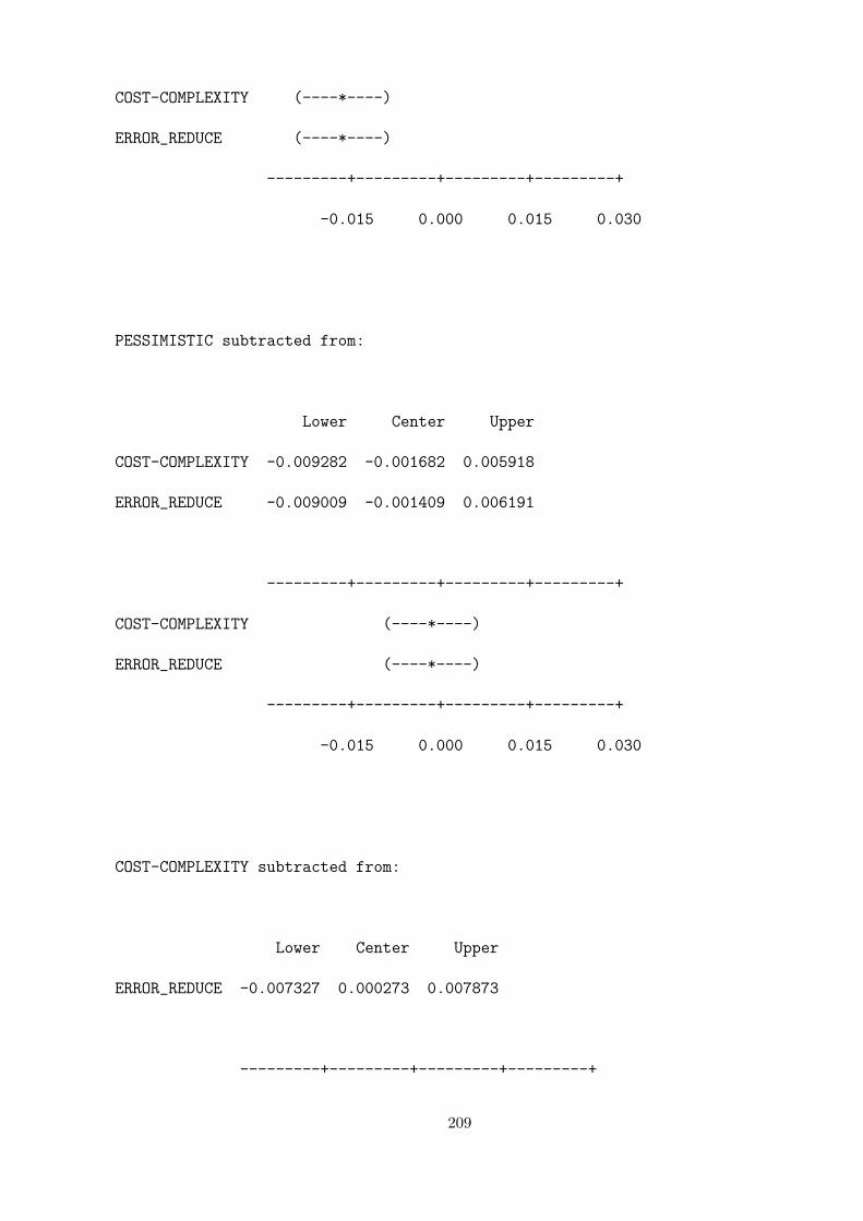
COST-COMPLEXITY (----*----)

ERROR_REDUCE (----*----)

---------+---------+---------+---------+

-0.015 0.000 0.015 0.030

PESSIMISTIC subtracted from:

Lower Center Upper

COST-COMPLEXITY -0.009282 -0.001682 0.005918

ERROR_REDUCE -0.009009 -0.001409 0.006191

---------+---------+---------+---------+

COST-COMPLEXITY (----*----)

ERROR_REDUCE (----*----)

---------+---------+---------+---------+

-0.015 0.000 0.015 0.030

COST-COMPLEXITY subtracted from:

Lower Center Upper

ERROR_REDUCE -0.007327 0.000273 0.007873

---------+---------+---------+---------+

209

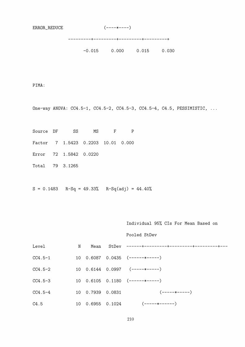
ERROR_REDUCE (----*----)

---------+---------+---------+---------+

-0.015 0.000 0.015 0.030

PIMA:

One-way ANOVA: CC4.5-1, CC4.5-2, CC4.5-3, CC4.5-4, C4.5, PESSIMISTIC, ...

Source DF SS MS F P

Factor 7 1.5423 0.2203 10.01 0.000

Error 72 1.5842 0.0220

Total 79 3.1265

S = 0.1483 R-Sq = 49.33% R-Sq(adj) = 44.40%

Individual 95% CIs For Mean Based on

Pooled StDev

Level N Mean StDev ------+---------+---------+---------+---

CC4.5-1 10 0.6087 0.0435 (------*-----)

CC4.5-2 10 0.6144 0.0997 (-----*-----)

CC4.5-3 10 0.6105 0.1180 (------*-----)

CC4.5-4 10 0.7939 0.0831 (-----*-----)

C4.5 10 0.6955 0.1024 (-----*------)

210

PESSIMISTIC 10 0.8478 0.1509 (------*-----)

COST-COMPLEXITY 10 0.9751 0.2704 (-----*-----)

ERROR_REDUCE 10 0.9288 0.1924 (-----*-----)

------+---------+---------+---------+---

0.60 0.75 0.90 1.05

Pooled StDev = 0.1483

Fisher 95% Individual Confidence Intervals

All Pairwise Comparisons

Simultaneous confidence level = 50.66%

CC4.5-1 subtracted from:

Lower Center Upper

CC4.5-2 -0.1266 0.0057 0.1379

CC4.5-3 -0.1305 0.0017 0.1340

CC4.5-4 0.0529 0.1852 0.3174

C4.5 -0.0455 0.0867 0.2190

PESSIMISTIC 0.1069 0.2391 0.3713

COST-COMPLEXITY 0.2341 0.3664 0.4986

ERROR_REDUCE 0.1878 0.3201 0.4523

211

+---------+---------+---------+---------

CC4.5-2 (----*-----)

CC4.5-3 (----*----)

CC4.5-4 (----*-----)

C4.5 (----*-----)

PESSIMISTIC (-----*----)

COST-COMPLEXITY (-----*----)

ERROR_REDUCE (----*----)

+---------+---------+---------+---------

-0.50 -0.25 0.00 0.25

CC4.5-2 subtracted from:

Lower Center Upper

CC4.5-3 -0.1362 -0.0039 0.1283

CC4.5-4 0.0473 0.1795 0.3117

C4.5 -0.0512 0.0811 0.2133

PESSIMISTIC 0.1012 0.2334 0.3657

COST-COMPLEXITY 0.2285 0.3607 0.4929

ERROR_REDUCE 0.1822 0.3144 0.4467

+---------+---------+---------+---------

CC4.5-3 (----*----)

212

CC4.5-4 (----*----)

C4.5 (----*-----)

PESSIMISTIC (----*-----)

COST-COMPLEXITY (----*-----)

ERROR_REDUCE (-----*----)

+---------+---------+---------+---------

-0.50 -0.25 0.00 0.25

CC4.5-3 subtracted from:

Lower Center Upper

CC4.5-4 0.0512 0.1834 0.3157

C4.5 -0.0472 0.0850 0.2172

PESSIMISTIC 0.1051 0.2373 0.3696

COST-COMPLEXITY 0.2324 0.3646 0.4969

ERROR_REDUCE 0.1861 0.3183 0.4506

+---------+---------+---------+---------

CC4.5-4 (----*-----)

C4.5 (----*-----)

PESSIMISTIC (----*-----)

COST-COMPLEXITY (-----*----)

ERROR_REDUCE (-----*----)

+---------+---------+---------+---------

213

-0.50 -0.25 0.00 0.25

CC4.5-4 subtracted from:

Lower Center Upper

C4.5 -0.2307 -0.0984 0.0338

PESSIMISTIC -0.0783 0.0539 0.1862

COST-COMPLEXITY 0.0490 0.1812 0.3134

ERROR_REDUCE 0.0027 0.1349 0.2671

+---------+---------+---------+---------

C4.5 (----*----)

PESSIMISTIC (----*----)

COST-COMPLEXITY (----*-----)

ERROR_REDUCE (----*-----)

+---------+---------+---------+---------

-0.50 -0.25 0.00 0.25

C4.5 subtracted from:

Lower Center Upper

PESSIMISTIC 0.0201 0.1523 0.2846

COST-COMPLEXITY 0.1474 0.2796 0.4119

214

ERROR_REDUCE 0.1011 0.2333 0.3656

+---------+---------+---------+---------

PESSIMISTIC (----*----)

COST-COMPLEXITY (----*----)

ERROR_REDUCE (----*-----)

+---------+---------+---------+---------

-0.50 -0.25 0.00 0.25

PESSIMISTIC subtracted from:

Lower Center Upper

COST-COMPLEXITY -0.0050 0.1273 0.2595

ERROR_REDUCE -0.0512 0.0810 0.2132

+---------+---------+---------+---------

COST-COMPLEXITY (----*----)

ERROR_REDUCE (----*-----)

+---------+---------+---------+---------

-0.50 -0.25 0.00 0.25

COST-COMPLEXITY subtracted from:

215

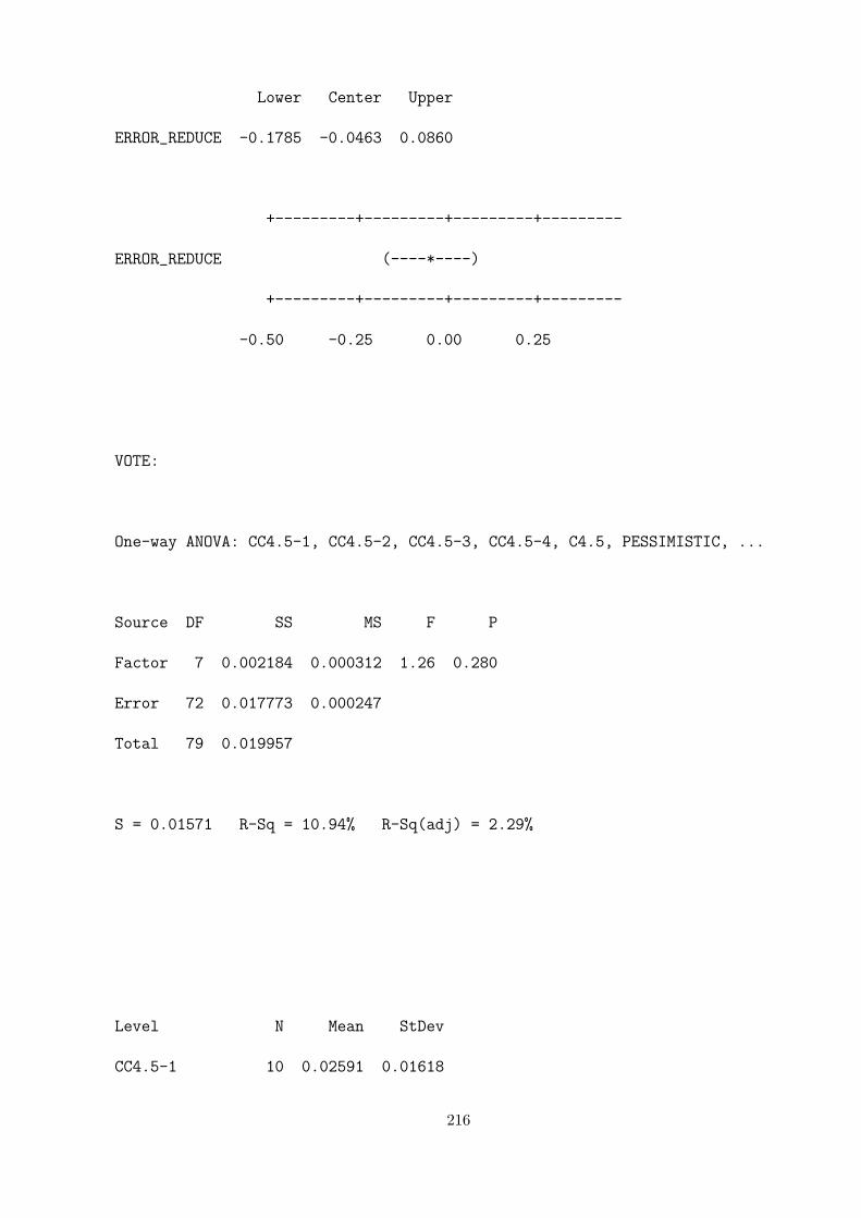
Lower Center Upper

ERROR_REDUCE -0.1785 -0.0463 0.0860

+---------+---------+---------+---------

ERROR_REDUCE (----*----)

+---------+---------+---------+---------

-0.50 -0.25 0.00 0.25

VOTE:

One-way ANOVA: CC4.5-1, CC4.5-2, CC4.5-3, CC4.5-4, C4.5, PESSIMISTIC, ...

Source DF SS MS F P

Factor 7 0.002184 0.000312 1.26 0.280

Error 72 0.017773 0.000247

Total 79 0.019957

S = 0.01571 R-Sq = 10.94% R-Sq(adj) = 2.29%

Level N Mean StDev

CC4.5-1 10 0.02591 0.01618

216

CC4.5-2 10 0.02045 0.01055

CC4.5-3 10 0.02045 0.01441

CC4.5-4 10 0.02533 0.01391

C4.5 10 0.03569 0.02028

PESSIMISTIC 10 0.01867 0.01418

COST-COMPLEXITY 10 0.02955 0.01473

ERROR_REDUCE 10 0.02636 0.01926

Individual 95% CIs For Mean Based on

Pooled StDev

Level -+---------+---------+---------+--------

CC4.5-1 (---------*---------)

CC4.5-2 (--------*---------)

CC4.5-3 (--------*---------)

CC4.5-4 (---------*---------)

C4.5 (---------*---------)

PESSIMISTIC (---------*---------)

COST-COMPLEXITY (---------*--------)

ERROR_REDUCE (---------*---------)

-+---------+---------+---------+--------

0.010 0.020 0.030 0.040

Pooled StDev = 0.01571

217

Fisher 95% Individual Confidence Intervals

All Pairwise Comparisons

Simultaneous confidence level = 50.66%

CC4.5-1 subtracted from:

Lower Center Upper

CC4.5-2 -0.01946 -0.00545 0.00855

CC4.5-3 -0.01946 -0.00545 0.00855

CC4.5-4 -0.01458 -0.00058 0.01343

C4.5 -0.00423 0.00978 0.02379

PESSIMISTIC -0.02125 -0.00724 0.00676

COST-COMPLEXITY -0.01037 0.00364 0.01764

ERROR_REDUCE -0.01355 0.00045 0.01446

---------+---------+---------+---------+

CC4.5-2 (--------*-------)

CC4.5-3 (--------*-------)

CC4.5-4 (--------*-------)

C4.5 (--------*--------)

PESSIMISTIC (-------*--------)

COST-COMPLEXITY (-------*--------)

ERROR_REDUCE (-------*--------)

218

---------+---------+---------+---------+

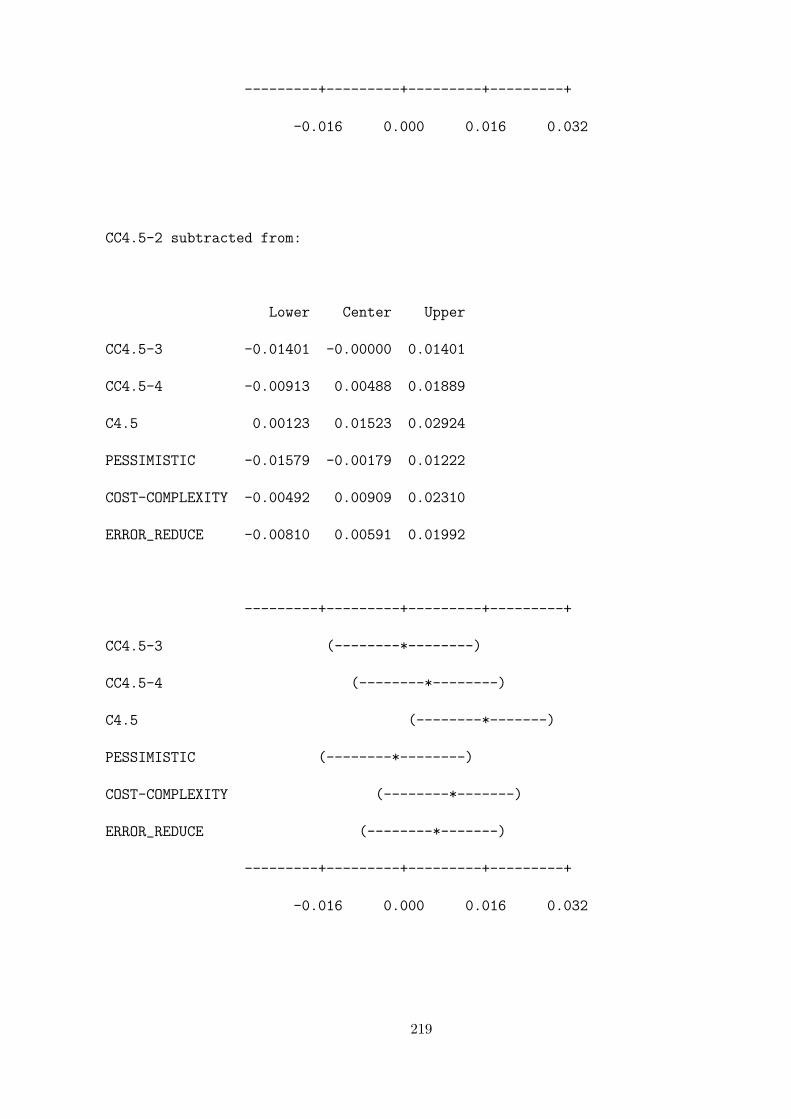
-0.016 0.000 0.016 0.032

CC4.5-2 subtracted from:

Lower Center Upper

CC4.5-3 -0.01401 -0.00000 0.01401

CC4.5-4 -0.00913 0.00488 0.01889

C4.5 0.00123 0.01523 0.02924

PESSIMISTIC -0.01579 -0.00179 0.01222

COST-COMPLEXITY -0.00492 0.00909 0.02310

ERROR_REDUCE -0.00810 0.00591 0.01992

---------+---------+---------+---------+

CC4.5-3 (--------*--------)

CC4.5-4 (--------*--------)

C4.5 (--------*-------)

PESSIMISTIC (--------*--------)

COST-COMPLEXITY (--------*-------)

ERROR_REDUCE (--------*-------)

---------+---------+---------+---------+

-0.016 0.000 0.016 0.032

219

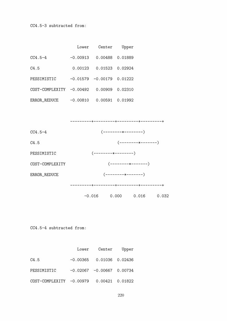
CC4.5-3 subtracted from:

Lower Center Upper

CC4.5-4 -0.00913 0.00488 0.01889

C4.5 0.00123 0.01523 0.02924

PESSIMISTIC -0.01579 -0.00179 0.01222

COST-COMPLEXITY -0.00492 0.00909 0.02310

ERROR_REDUCE -0.00810 0.00591 0.01992

---------+---------+---------+---------+

CC4.5-4 (--------*--------)

C4.5 (--------*-------)

PESSIMISTIC (--------*--------)

COST-COMPLEXITY (--------*-------)

ERROR_REDUCE (--------*-------)

---------+---------+---------+---------+

-0.016 0.000 0.016 0.032

CC4.5-4 subtracted from:

Lower Center Upper

C4.5 -0.00365 0.01036 0.02436

PESSIMISTIC -0.02067 -0.00667 0.00734

COST-COMPLEXITY -0.00979 0.00421 0.01822

220

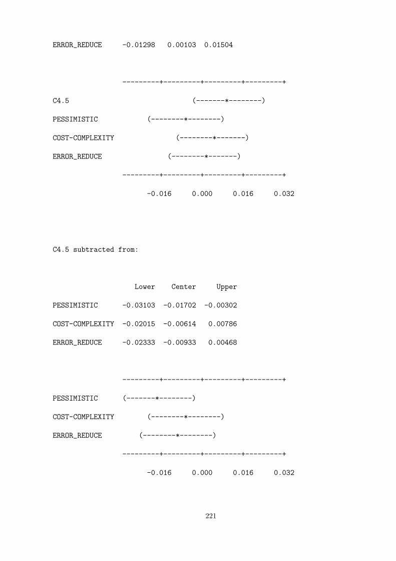
ERROR_REDUCE -0.01298 0.00103 0.01504

---------+---------+---------+---------+

C4.5 (-------*--------)

PESSIMISTIC (--------*--------)

COST-COMPLEXITY (--------*-------)

ERROR_REDUCE (--------*-------)

---------+---------+---------+---------+

-0.016 0.000 0.016 0.032

C4.5 subtracted from:

Lower Center Upper

PESSIMISTIC -0.03103 -0.01702 -0.00302

COST-COMPLEXITY -0.02015 -0.00614 0.00786

ERROR_REDUCE -0.02333 -0.00933 0.00468

---------+---------+---------+---------+

PESSIMISTIC (-------*--------)

COST-COMPLEXITY (--------*--------)

ERROR_REDUCE (--------*--------)

---------+---------+---------+---------+

-0.016 0.000 0.016 0.032

221

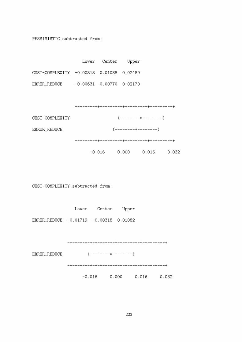
PESSIMISTIC subtracted from:

Lower Center Upper

COST-COMPLEXITY -0.00313 0.01088 0.02489

ERROR_REDUCE -0.00631 0.00770 0.02170

---------+---------+---------+---------+

COST-COMPLEXITY (--------*--------)

ERROR_REDUCE (--------*--------)

---------+---------+---------+---------+

-0.016 0.000 0.016 0.032

COST-COMPLEXITY subtracted from:

Lower Center Upper

ERROR_REDUCE -0.01719 -0.00318 0.01082

---------+---------+---------+---------+

ERROR_REDUCE (--------*--------)

---------+---------+---------+---------+

-0.016 0.000 0.016 0.032

222