Decision Making among Alternative Routes for UAVs in Dynamic Environments

José J. Ruz*, Orlando Arévalo* (*)Dept. of Computer Architecture and

Automatic Control Universidad Complutense de Madrid

[jjruz, ojareval]@fis.ucm.es

Gonzalo Pajares**, Jesús M. de la Cruz*

(**)Dept. of Software Engineering and Artificial Intelligence

Universidad Complutense de Madrid [pajares, jmcruz]@fis.ucm.es

Abstract

This paper presents an approach to trajectory generation for Unmanned Aerial Vehicles (UAV) by using Mixed Integer Linear Programming (MILP) and a modification of the A* algorithm to optimize paths in dynamic environments, particularly having pop-ups with a known future probability of appearance. Each pop-up leads to one or several possible evasion maneuvers, characterized with a set of values used as decision making parameters in an Integer Linear Programming (ILP) model that optimizes the final route by choosing the most suitable alternative trajectories, according to the imposed constrains such as maximum fuel consumption and spent time. The model of the system in MILP and A* algorithms is presented, as well as the ILP formulation for decision making. Results and discussions are given to promote future real time implementations.

1. Introduction

An unmanned aerial vehicle (UAV) is an aircraft without onboard pilot that can be remotely controlled or fly autonomously based on pre-programmed flight plans [5]. UAVs are currently receiving much attention in research because they can be used in a wide variety of fields, both civil and military, such as reconnaissance, geophysical survey, environmental and meteorological monitoring, aerial photography, and search-and-rescue tasks. Most of these missions are usually carried out in threatened environments, where it is very important to fly along a route which keeps the UAV away from known threats. Detection radars are one of the main threats for an UAV, but there are others that should also be avoided, such as fires, electric storms, radio shadowing zones, no flight zones, and so on. One of the main goals in many UAV’s projects has been to establish the route that maximizes the likelihood of successful mission completion taking into account all known information about technological constraints, obstacles and threat zones on a static environment [8]. Some papers that investigate path

planning for UAVs presume that the location of the threats and their presence are deterministically known at planning-time, and interpret a path which avoids possible threat regions as an optimal path [3]. However more recent projects are examining the possibilities of UAVs as realistic autonomous agents working on dynamic environments where threat zones called pop-up are present [13]. The true presence of these types of zones is only known at flying-time, but the location and knowledge about the probability of appearance can be known at planning-time.

The work presented in this paper extends our preliminary results on trajectory generation over static environment [9], taking into account the knowledge about pop-ups in the trajectory design. The route planner that is proposed in this work allows the UAV to make a decision among several alternative routes considering both, current state of the UAV and probabilities of pop-up threats appearance in future time. The planning is carried out in three steps. First, an optimal route is designed with the static and known elements of the environment using Mixed Integer Linear Programming (MILP) and/or a modification of the A* algorithm, depending on the elements present in the environment. The MILP alternative to plan a static route will be mainly used when the environment contains threats that put under certain risk the UAV’s mission, for instance the tracking and the shooting of missiles guided by radars. Second, alternative routes are calculated using MILP or A* algorithm to bypass each pop-up zone having an appearance probability greater than zero and less that one, provided by expert knowledge. Finally, a decision making process, modeled with Integer Linear Programming (ILP), is carried out among the several alternative routes calculated for each pop-up.

The paper is organized as follows. Section 2 briefly recapitulates the MILP formulation for path planning of a single UAV. Section 3 describes the path planning approach based on a modification of the A* algorithm. Section 4 explains how the planner presented in this paper deals with the decision making to avoid pop-up threats. In section 5, we present the implementation

1-4244-0826-1/07/$20.00 © 2007 IEEE 997

and some results of the planner. Finally, remarks and conclusions are provided in section 6.

2. UAV’s trajectory generation using MILP

The approach to optimal path planning based on Mixed Integer Linear Programming was introduced in [10]. Here, the UAV’s trajectory generation is faced as a 3D optimization problem under certain conditions (see figure 1) in the Euclidean space, characterized by a set of decision variables, a set of constraints and the objective function. The decision variables are the UAV’s state variables, i.e. position and speed. The constraints are derived from a simplified model of the UAV and the environment where it has to fly. These constraints include:

• Dynamics, such as a maximum turning force which causes a minimum turning radius, as well as a maximum flying speed and climbing rate.

• Box obstacles avoidance, like no-flight zones or approximations of the surface contour.

• The reaching of a specific waypoint or target. • Radar’s detection, tracking, or missile shooting. The objective function includes different measures

of the quality in the solution of this problem, although the most important criterion is the minimization of the total flying time to reach the target.

0

50

100

150

200

0

50

100

150

200

0

2

4

x [Km]

Obstacle1

Target

Radar1

y [Km]

UAVOrigin

Obstacle2

z [K

m]

Figure 1. Trajectory generation by solving a constrained optimization with a MILP 3D model.

2.1. UAV’s dynamic constraints The trajectory optimization is constrained by a time-

discrete dynamics to obtain the state of the system on every time t + 1, from its previous state at time t. This model represents the UAV with its limits in speed and turning rate, caused by of a maximum magnitude in the input force u(t) that the aircraft might be put under [1].

Therefore the dynamics is expressed in (1).

( 1) ( )( )

( 1) ( )v t v t

A B u tx t x t

+⎡ ⎤ ⎡ ⎤= ⋅ + ⋅⎢ ⎥ ⎢ ⎥+⎣ ⎦ ⎣ ⎦

(1)

The matrices A and B are the state matrices (kinematics matrices) of the UAV, and t the discrete time. Speed and force magnitudes are constrained by the following equations which are convenient linearizations of the original quadratic form:

MmNnMmNn

uuuu

vvvv

mn

mzmnymnx

mzmnymnx

,...3,2,1;,...3,2,1/,/2

)cos()sin()sin()sin()cos(

)cos()sin()sin()sin()cos(

max

max

====

≤++

≤++

πθπϕ

θθϕθϕ

θθϕθϕ, (2)

where the maximum speed and input force are in the right side of (2). N and M are the number of points used to approximate the spherical space closed by all the possible directions of a vector in 3D [11].

Additionally, in order to model the climbing rate of a UAV, the components of speed and acceleration in the Z axis must be constrained according to its maneuvering capabilities (3).

max_min_

max_min_

)(

)(

zzz

zzz

utuu

vtvvt

≤≤

≤≤∀

(3)

At the same time the third component of the UAV’s position must be limited to one side of the Z axis, which in our case is the positive one because the implemented referential frame has been the ENU (East-North-Up {x,y,z}).

2.2. Obstacles avoidance constraints As mentioned in the beginning of this section, the

optimization considers box obstacles avoidance, which is modeled by knowing the lower south west and the upper north east vertices of the no-flight zones [7], as expressed by the constraints in (4):

)()(

)()(

max

min

tMxtx

tMxtxki

kii

ki

kii

δ

δ

⋅−≥

⋅+≤, (4)

where k identifies the obstacle, (x1min,x2min,x3min) is its lower south west corner and (x1max,x2max,x3max) its upper north east corner, M is a bound for xi(t) to enable/disable some of the constraints, and δi

k are the indicator variables. The ith condition is then relaxed when δi

k = 1, and enabled when δik = 0. By (5) it is

imposed that at least one of these constraints is active.

6

1

max

( ) 5

/ 1,2,..., , / 0,1,...,

ki

i

obst

t

k k K t t T

δ=

≤

∀ = ∧ ∀ =

∑ (5)

2.3. Target reaching constraints The constraints in (6) must be satisfied at all instants

during the flight, to impose the UAV to get to its final destination, such as a waypoint or a target.

998

ttt

Mxtx

Mxtx

arrival

T

t

tii

tii

f

f

∀≤⋅

−−≥−

−≤−

∑ ,

)1()(

)1()(

0

λ

λ

λ (6)

In the arrival constraints (xf,yf,zf) is the target location, λt is a binary indicator variable to enable/disable each constraint, and tarrival is the time to be included as a term of the objective function to be minimized [9].

2.4. Radars avoidance constraints The treatment developed to avoid threat zones

where there are enemy units such as tracking radars and missile launchers is based on a distribution which corresponds to the probability for the UAV to be detected, tracked and shot. This probability distribution is characteristic for every single type of tracking radar (7), where c1 and c2 are constants obtained by a curve fitting routine. This fit is previously made using the information provided by the radar’s specifications.

( ) 1421

1ct

RcP

σ+= (7)

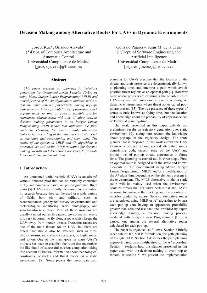
In the tracking probability distribution the value σ represents the RCS (radars cross section) in squared meters, while the variable R is the distance in meters between the UAV and the radars. In figure 2 it is observed that a radius equal to 50Km could be considered as the maximum radar’s range, from which Pt totally diminishes.

Thus, for any maximum accepted value of detection, tracking, or killing probability its corresponding minimum radius Rmin to avoid the radar’s zones is computed. This avoidance condition is then expressed in (8), where a linearization of the quadratic form of all the possible directions for a vector in the Euclidean space is used once again to define the constraints in the MILP model.

MmNnMm

NnRz

yx

m

nm

mnmn

,...2,1;,...2,1;/

;/2/)cos(

)sin()sin()sin()cos(

min

===

=≥

++

πθ

πϕθ

θϕθϕ (8)

The coordinates x, y and z are the relative

coordinates of the UAV to each radar, making the aircraft able to approximate then differently, depending on the types of radars and on the interests in any mission in particular.

0 1 2 3 4 5 6

x 104

0

0.2

0.4

0.6

0.8

1

R (m)

Pt

Figure 2. Profile of a tracking probability distribution with a RCS = 1.0m2.

3. UAV’s trajectory generation using A*

It is well known that the A* is a general AI search algorithm which is highly competitive with other path finding algorithms, and yet very easy to implement [4, 12]. For UAV’s trajectory generation it has the advantage to present a good performance when the terrain is quite irregular and the maneuvers must be done close to the ground’s surface. The main drawback is its high computational cost in 3D path planning problems, but it is reasonable to deal with this fact when an appropriate scaling is done. In the case under study the A* algorithm has been modified to adapt it and improve its capabilities to optimize trajectories for UAVs under conditions like no-flight zones, scarped terrains, and radars, also called ADUs (air defense units) which might appear dynamically during the flight. The modifications done to the original A* algorithm are mainly logical restrictions which evaluate whether the successors of every possible node of the UAV’s trajectory build a minimum turning radius curve, while avoiding physical obstacles and threats.

3.1. Flying direction constraint The constraint imposed on the flying direction is the

computation of the angle between the arriving direction and every possible departing direction, for all the nodes of the trajectory. The angle φ is calculated supported by the definition of the dot product (9).

⎟⎟

⎠

⎞

⎜⎜

⎝

⎛

⋅

⋅=

if

if

VV

VVarccosφ (9)

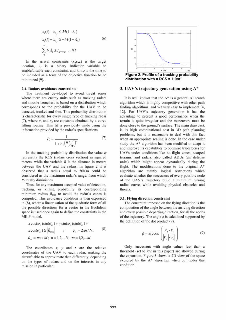
Only successors with angle values less than a threshold (set to π/2 in this paper) are allowed during the expansion. Figure 3 shows a 2D view of the space explored by the A* algorithm when put under this condition.

999

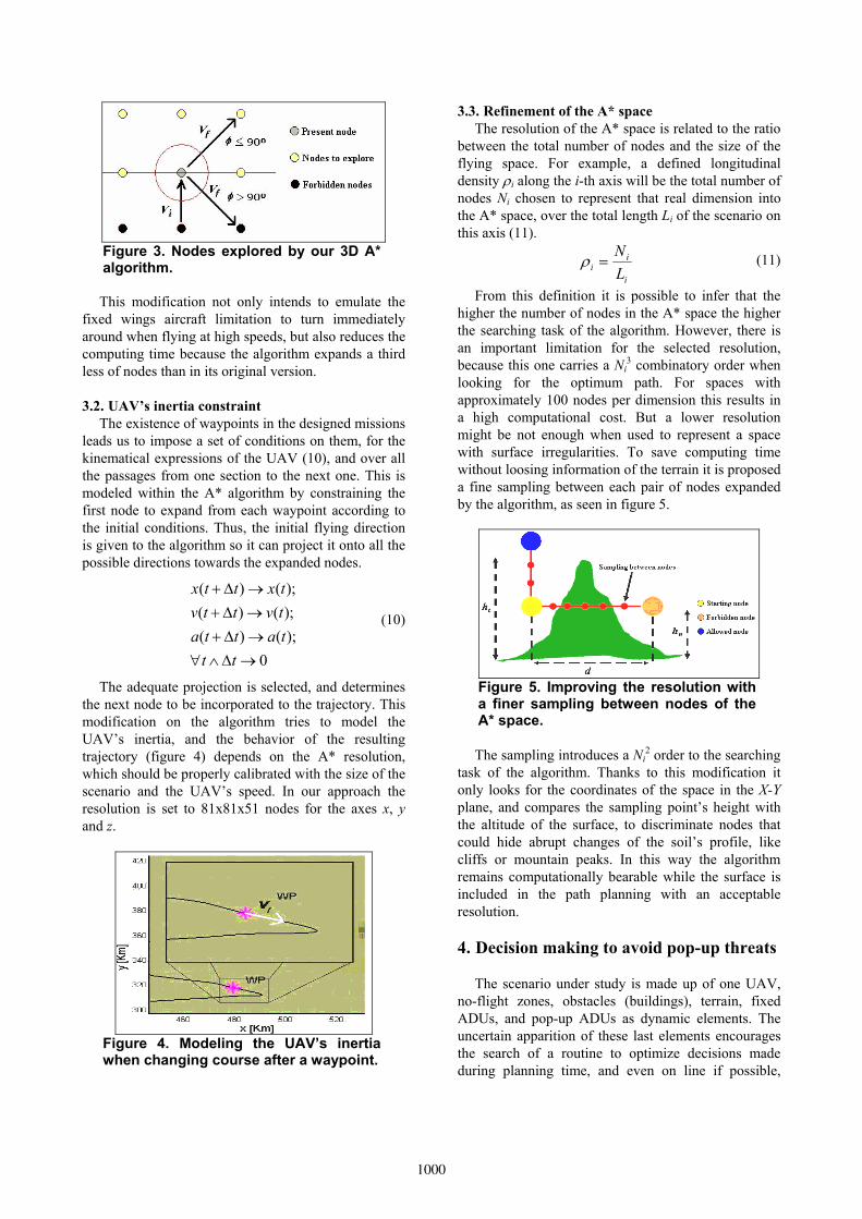
Figure 3. Nodes explored by our 3D A* algorithm.

This modification not only intends to emulate the

fixed wings aircraft limitation to turn immediately around when flying at high speeds, but also reduces the computing time because the algorithm expands a third less of nodes than in its original version.

3.2. UAV’s inertia constraint The existence of waypoints in the designed missions

leads us to impose a set of conditions on them, for the kinematical expressions of the UAV (10), and over all the passages from one section to the next one. This is modeled within the A* algorithm by constraining the first node to expand from each waypoint according to the initial conditions. Thus, the initial flying direction is given to the algorithm so it can project it onto all the possible directions towards the expanded nodes.

( ) ( );( ) ( );( ) ( );

0

x t t x tv t t v ta t t a t

t t

+ Δ →+ Δ →+ Δ →

∀ ∧ Δ →

(10)

The adequate projection is selected, and determines the next node to be incorporated to the trajectory. This modification on the algorithm tries to model the UAV’s inertia, and the behavior of the resulting trajectory (figure 4) depends on the A* resolution, which should be properly calibrated with the size of the scenario and the UAV’s speed. In our approach the resolution is set to 81x81x51 nodes for the axes x, y and z.

Figure 4. Modeling the UAV’s inertia when changing course after a waypoint.

3.3. Refinement of the A* space The resolution of the A* space is related to the ratio

between the total number of nodes and the size of the flying space. For example, a defined longitudinal density ρi along the i-th axis will be the total number of nodes Ni chosen to represent that real dimension into the A* space, over the total length Li of the scenario on this axis (11).

i

ii L

N=ρ (11)

From this definition it is possible to infer that the higher the number of nodes in the A* space the higher the searching task of the algorithm. However, there is an important limitation for the selected resolution, because this one carries a Ni

3 combinatory order when looking for the optimum path. For spaces with approximately 100 nodes per dimension this results in a high computational cost. But a lower resolution might be not enough when used to represent a space with surface irregularities. To save computing time without loosing information of the terrain it is proposed a fine sampling between each pair of nodes expanded by the algorithm, as seen in figure 5.

Figure 5. Improving the resolution with a finer sampling between nodes of the A* space. The sampling introduces a Ni

2 order to the searching task of the algorithm. Thanks to this modification it only looks for the coordinates of the space in the X-Y plane, and compares the sampling point’s height with the altitude of the surface, to discriminate nodes that could hide abrupt changes of the soil’s profile, like cliffs or mountain peaks. In this way the algorithm remains computationally bearable while the surface is included in the path planning with an acceptable resolution.

4. Decision making to avoid pop-up threats

The scenario under study is made up of one UAV, no-flight zones, obstacles (buildings), terrain, fixed ADUs, and pop-up ADUs as dynamic elements. The uncertain apparition of these last elements encourages the search of a routine to optimize decisions made during planning time, and even on line if possible,

1000

depending on how the mission is evolving. Figure 6 shows the way the UAV updates information about previously known dynamic elements and re-launches the decision making ILP routine if needed, or even discovers new pop-ups and, if it has enough computing resources, re-executes the planning from the bypassing up to the decision making process, trying always to get again into the main trajectory.

Figure 6. Layout of the path generator.

4.1. Decision parameters The original trajectory is modified according to a

decision which is made based on the following three elements: mean risk, flying time, and fuel consumption. The ILP formulation computes the optimum alternatives to be chosen.

4.1.1 Cumulative mean risk parameter We start from the computation of the kill probability

(PK) on each point of a trajectory, from which a measure of the cumulative mean risk for that particular trajectory is computed. This computation of the probability of kill can be made by any available analytical, statistical, or even empirical model of the interactions between the aircraft and the enemy defense units, as seen before in (7). It is also possible to count with tabled values of PK, for several ranges of the variables that affect this probability such as UAV’s position and RCS.

From the kill probability PKi at any trajectory point, the survival probability PSi associated to the enemy i-th ADU is computed as follows in (12).

),(1),( vrPvrP KiSi −= (12)

The total survival probability PST is computed by multiplying the following three factors (13):

1- The PSi product from 1 to the number N of known ADUs.

2- The Pop-Up ADU survival probability affecting the point.

3- A weighting α factor embedding the Pop-Up appearance probability when flying towards its location.

We have chosen the product combination based in the assumption that all the ADUs work in cooperation.

∏=

=N

iSiSPUST vrPvrPvrP

1

),(),(),( α (13)

The weighting factor α, ranging in (0, 1), is defined as the complementary probability of the pop-up appearance probability PAPU, at any state ),( vr of the aircraft (14). It should be strictly less than one because the fact to exactly assign the value one to a PAPU probability makes the ADU turn into a fixed one, already considered in the product.

APUP−= 1α (14)

Then, it is clear that the more probable a pop-up arises in front of the UAV during the flight the less probable the UAV will survive to it, bringing a greater cumulative mean risk to the chosen trajectory.

Once the total survival probability to a set of N cooperating ADUs is computed, including the unexpected activation of more threats, the total probability of kill PKTm in the state m = ),( vr is given by the complement to one (15).

( , ) 1 ( , )KTm STmP r v P r v= − (15)

Hence, we define the cumulative mean risk of a trajectory RK as the average of the total kill probabilities of all the M points which form this trajectory (16). This concept will be used as a parameter to characterize the group of alternatives to build a final trajectory under a decision making formulation.

∑=

=M

mKTmK vrP

MR

1),(1 (16)

The risk is calculated as a mean value, based on the time discrete system assumption. The points of the trajectory are approximately equally spaced since the flying speed is constant. If the time were continuous the integral form to calculate a mean value would be used instead of the sum showed in (16).

4.1.2 Cumulative flying time parameter The flying time parameter is simply a way to

characterize alternative trajectories in terms of the cumulative time needed by the aircraft to achieve them, assuming a constant flying speed. Thus, for an M-points time discrete path, with all points equally spaced in time Δt, the total flying time T is given by (17).

tMtTM

mm Δ=Δ= ∑

=1

(17)

1001

There is also a way to normalize the cumulative time parameter, with the aim to compare different alternatives of a trajectory or even different trajectories. If we define the amount τ as the time to go along the minimum length/time trajectory between any pair of points (straight line), it is possible to define a normalized cumulative flying time factor ft (18), where the zero value represents a characterization for the mentioned minimum path.

Tft

τ−=1 (18)

4.1.3 Cumulative fuel factor parameter Since the UAV’s trajectory generation is

represented as a 3D optimization problem, it might be formulated with an objective function and a set of constraints in a Cartesian referential frame where (x,y,z) is the UAV’s position. Among the constraints there are kinematical and dynamical limitations of the system, which is an air vehicle unable to make stationary flights. Furthermore, the linear approach and the time discrete character of the solution lead us to the matrix representation already shown in (1), with the limits that produce a minimum turning radius possible to achieve, for which the aircraft is designed.

A more convenient expression for the limits of speed and acceleration as a function of their components in R3 is in (19), where again the maximum limits are in the right side of the inequalities.

2max

222

2max

222

uuuu

vvvv

zyx

zyx

≤++

≤++ (19)

It is possible to reorder the constraint for the maximum input force making normalizations for each of the acceleration’s components (20), where the angle θ is the zenith and the angle ϕ is the azimuth of vector u represented in spherical coordinates.

tzyx Cu

uu

uu

u=++

maxmaxmax

)cos()sin()sin()sin()cos( θθϕθϕ (20)

Thus, in (21) it is shown the constraint for the signal Ct, which is a normalized input signal for each discrete time t. It represents a way to measure the acceleration applied to the system, needed to change the flying direction. This signal can be considered directly bounded to the aircraft fuel consumption because it might be the control signal, or the actuator signal used to change the UAV’s course.

tCt ∀≤1 (21)

Finally, in (22) we define the fuel consumption factor as the average of the fuel consumed along the t trajectory points.

∑=

=T

ttc C

TF

1

1 (22)

4.2 Decision making scenario

In every mission the path designers might count with very accurate information about most of the elements involved in the flying environment, which can be provided and confirmed by several sources during the planning time. However, it is also possible to possess a minimum knowledge about uncertain or dynamic elements characterized by a probability of appearance, and that might represent a threat for the UAV’s path.

The strategy proposed here implements an initial path planning taking into account only the well known and fixed components of the scenario, to obtain the main optimum trajectory which will be followed by the UAV. After having a main route, the knowledge of non-static elements, such as pop-up radars, is included in the scenario for treating only those pop-ups that actually may be a serious threat for the UAV. Once the actual threats have been discriminated from all the originally counted, a local avoidance strategy is computed, using MILP or A* algorithm, to bypass the pop-ups. Although with this local strategy the trajectory optimality decreases, the computational complexity doesn’t increase. These alternatives are all attached to the original flying plan, and given to an upper layer module in charge of making decisions according to the imposed limitations; let’s say fuel consumption, time, and risk. It is right here where an optimum decision making process will increase the chances of a successful mission.

Suppose there is a mission to go from a starting point to an objective, as seen in figure 7, and that the originally planned trajectory might be affected by three independent unforeseen threats, characterized by their corresponding appearance probability PPU. Therefore, each of them has an associated probability factor α, which assigns certain weight to the survival probability of the aircraft against those pop-ups.

Figure 7. Trajectory decision map with three possible pop-ups and their corresponding alternatives.

If the number na of alternatives is the same for every

pop-up in particular, it’s easy to compute the total amount of combined alternatives. In this case, the combinatory leads us to a total amount of alternatives

1002

(naNpu), which is the number of alternatives by pop-up

powered to the total number of pop-ups Npu. All the alternatives have their characteristic

parameters to be processed in a decision making algorithm that seeks and finds the optimum final trajectory, based not only on the recent and past information at the moment of the decision, but also on the probability of future events.

4.3 The decision making as an ILP model

The choice of the optimal sequence of alternatives that will compose the final planned route can be posed as an ILP (Integer Linear Programming) problem. The cumulative time and fuel consumption parameters will be the constraints, and the cumulative mean risk the objective (minimum) function. The mentioned objective function is given by (23), where L is the total number of pop-ups affecting the original trajectory (pre-planned trajectory without pop-ups), and the indexes {i,j,…,w} range over all the alternatives for each one of the affecting pop-ups.

⎟⎟⎠

⎞⎜⎜⎝

⎛+++= ∑∑∑

wLwKLw

jjjK

iiiK RRRJ δδδ ...2211

(23)

In this objective function the coefficients RKlm are the cumulated mean risk of each alternative, and the variables δlm binary variables associated to the chosen alternative among all the possible ones for each pop-up. Therefore, the variables must be constrained (24), to guarantee that only one of the alternatives is selected at the time of making a specific decision.

1...;;1;111

21

1 === ∑∑∑===

W

wLw

J

jj

I

ii δδδ (24)

The rest of the constraints refer to the upper limit assigned to the accepted cumulative time factor (25), and to the maximum cumulative fuel consumption factor (26). Both limits can be set based on the UAV’s dynamics, and on its fuel consumption model.

max

2211 ...T

L

TTTw

LwLwj

jji

ii

≤⎟⎟⎠

⎞⎜⎜⎝

⎛+++ ∑∑∑ δδδ

(25)

The Tlm coefficients are the cumulative time factor of every computed alternative, and Tmax is the limit accepted for the time factor of the mission.

max

2211 ...

cw

LwcLwj

jjci

iic

FL

FFF≤

⎟⎟⎠

⎞⎜⎜⎝

⎛+++ ∑∑∑ δδδ

(26)

The coefficients Fclm are the cumulated fuel consumption factor of every computed alternative, and Fcmax is the upper limit for the mean fuel consumption along the global trajectory.

5 Implementations and results

A path planning software platform was developed implementing both, MILP and A* algorithm trajectory optimizers. The MILP model takes advantage of the powerful CPLEX 9.0 solver through the ILOG OPL package [6], to find the solution for optimum trajectories in the space of the continuous UAV’s variables of state. The A* algorithm was coded in JAVA language, using the JRE system library jre1.5.0_06. The metric used as the heuristic was the euclidean distance. Figure 8 shows the resulting trajectory computed in a scenario where there are mountains, waypoints, and pop-up radars only. The black solid line would be the optimum path whenever the pop-ups don’t get enabled during the UAV’s approximation. The yellow dashed line is an alternative calculated during the planning time to safely escape from the threat that possibly causes a mission fail.

Figure 8. Computed trajectory (solid line), and the alternative to avoid one pop-up (dotted line). A Monte Carlo simulation was done to evaluate the

decision making strategy proposed in this paper [2], where a probability of future appearance assigned to every threat pop-up is taken into account to activate them, while the parameters of risk, time and fuel are constrained in an ILP model. This strategy was compared with the simple decision made on the basis of the consumed fuel and the spent time, which are only past and present sources of information. Figure 9 shows the cumulative mean risk of both strategies, after 107 iterations, where there were three pop-ups, with three alternative trajectories each. The probabilities of appearance were 0.5, 0.2, and 0.8, for the pop-ups affecting the original trajectory in that chronological order. As mentioned in section 1 these probabilities are provided by expert knowledge prior to the mission design. Depending on the selected alternative the mean risk accumulated different values. The more direct is the route, the more risky it is, while the less time it spends. The greater the turning radius of the route is, the less the fuel is consumed. It might be possible to find trajectories with the maximum time spent along it without having the higher fuel consumption. Constraints over the time factor (0.35)

1003

and the fuel consumption (0.40) were imposed into the ILP decision making model, to obtain the optimum final global path.

100 101 102 103

0.115

0.12

0.125

0.13

# iteration x 104

Mea

n R

isk

Optimized decision

100 101 102 103

0.474

0.476

0.478

0.48

# iteration x 104

Mea

n R

isk

Non optimized decision

Figure 9. Cumulative mean risk after 107 Monte Carlo simulations. The histograms in figure 10 of the two simulated

strategies show the advantages of choosing the optimum decision plan, because the constraints over spent time and fuel consumption are never violated, while the cumulated risk in minimized. The strategy that only considers past and present information doesn’t violate the time and fuel criteria either, but its response to the cumulated risk is poorer because the most probable pop-ups is not the necessary the first one to appear.

0 0.1 0.2 0.3 0.4 0.5 0.6 0.7 0.8 0.9 10

100

200

300

Risk (probability)

frequ

ency

x 1

04

Optimized decision

0 0.1 0.2 0.3 0.4 0.5 0.6 0.7 0.8 0.9 10

100

200

300

Risk (probability)

frequ

ency

x 1

04

Non optimized decision

Figure 10. Histogram of the mean risk after 107 Monte Carlo simulations.

6 Conclusions

We have presented an approach to trajectory generation for UAVs using MILP and a modification of the A* algorithm that considers dynamic environmental elements, particularly pop-ups. Both alternative methods have been implemented and a Monte Carlo simulation was done to evaluate the decision making strategy proposed. The results showed the advantages of choosing the optimum decision plan that considers the known values of the probability of appearance of pop-up threats in the future. The possibility to update the information concerning the pop-up’s appearance probabilities, available fuel, time,

and even the assumed risk, and then re-launch a decision making routine to optimize the chosen alternatives has been proven, since the ILP model provides a solution affordable in real time (~1s).

7 Acknowledgements

This research was funded by the Community of Madrid, project “COSICOLOGI” S-0505/DPI-0391, by the Spanish Ministry of Education and Science, project “Planning, simulation and control for cooperation of multiple UAVs and MAVs” DPI2006-15661-C02-01, and by EADS (CASA), project 353/2005.

References

[1] J. Bellingham, A. Richards and J. How, “Receding Horizon Control of Autonomous Aerial Vehicles”, Proc. of American Control Conference, 2002.

[2] B. Berg, and M. Chain, “Monte Carlo Simulations and their Statistical Analysis”, World Scientific (ISBN 981-238-935-0), 2004.

[3] S.A. Borto, “Path planning for UAVs”. Proc. of the American Control Conference, pp. 364-368, 2000.

[4] M. Deloura, “Game Programming Gems”, Charles River Media, Inc., chapters 3.3 to 3.6, 2000.

[5] J. How, E. King, and Y. Kuwata, “Flight Demonstrations of Cooperative Control for UAV Teams”, AIAA 3rd Unmanned Unlimited Technical Conference, Workshop and Exhibit, 2004.

[6] ILOG, ILOG CPLEX 9.1 User’s guide, 2003. [7] Y. Kuwata and J. How, “Three Dimensional Receding

Horizon Control for UAVs”, AIAA Guidance, Navigation, and Control Conference and Exhibit, 2004.

[8] A. Richards, and J. How, “Aircraft Trajectory Planning with Collision Avoidance Using MILP”, Proc. Of the IEEE American Control Conference, pp. 1936-1941, 2002.

[9] J. Ruz, O. Arévalo, J. de la Cruz and G. Pajares, “Using MILP for UAVs Trajectory Optimization under Radar Detection Risk”, Proc. of the 11th IEEE Conference on Emerging Technologies and Factory Automation, 2006.

[10] T. Schouwenaars, B. De Moor, E. Feron, and J. How, “Mixed Integer Programming for Multi-Vehicle Path Planning”. Proc. of the 2001 European Control Conference, 2001.

[11] T. Schouwenaars, J. How and E. Feron, “Receding Horizon Path Planning with Implicit Safety Guarantees”, Proc. of American Control Conference, 2004.

[12] B. Stout, “Smart Moves: Intelligent Path-Finding”, Game Developer Magazine, 1996.

[13] U. Zengin, and A. Dogan, “Probabilistic Trajectory Planning for UAVs in Dynamic Environments”. Proc. of AIAA 3rd "Unmanned Unlimited" Technical Conference, Workshop and Exhibit, pp. 1-12, 2004.

1004