CYCLOTRON RADIATION PROU WOTRON STREAUS GYRATING

IN THE JOVIAN UAGNETOSPHERE, THE

STRLtL

EXOSPHERE AND THE SOLAR ACTIVE CORONA

by

Peter Chin Wan Pung, DSc. (Hons.)

A thesis submitted in fulfillment of

the requirements for the Degree of

Doctor of Philosophy

in the

University of Tasmania

HOBART

April, 1966

CONTENTS

Chapter Page

INTRODUCTION 1

(A) Plasma . 1

(B) The Dispersion Equation 0000bi 66 O 3

(C) The Basic Equations of the Kinetic

Approach

(D) Macroscopic Desoription of the

Response of a Plasma to Electromag-

netic Disturbance

(23) Different /lodes of Electromagnetic

Disturbance in a Plasma ...... .

(P) Identification of the Pour Uodes in

the Graphical Presentation of the

Dispersion Equation

(G) Generation of High Prequenoy Waves

in a Plasma 00**6400******** ... *id ( 3

(H) Emissions from the Sun and Planets bo

(I) Two Common Features in the Obser-

vational Data of the Sun, Jupiter

and Earth 22

II EXCITATION OF LLECTROUAGNLTIO IAVES IN

A STREAM-I:LA= SYSTEL 25

(11

(A) Introduction

(D) Formulation of Radiative /notability

Theory in a Helical-Stream-Plasma

System

(0) Instability Theory of a Stream-Plaana. System when the Temperature Effects in

the Stream have been Included 3'

(1)) The "Negative.rAbsorption" Approach in Solving the Instability Problem ST

(E) Two Types of Instability•...... SY

(P) Conclusions

/II AMPLIFICATION OP FORWARD-SHIPTED CYCLOTRON

RADIATION IN ThT EXTRAORDINARY-EODE ADD ITS

APPLICATION TO JUEITEIVS DECAUETRIC

EMISSIONS 6,1

(A) Introduction

(B) Theory and Analysis 63

(0) Discussions sta.:Pose. ..... * ....e...... (78

IV TEL ORIGIN OF VLY DISCRETL EflI3SION3 IN THE

TERRESTRIAL EXOSPH124 8+

(A) Review 8+

(B) Excitation of Backward Doppler-shifted

Cyclotron Radiation in a Pagnetoactive

Plasma by a Helical Bleotron Stream gqr

(C) Discussions . cif

V A 1tEVI10 OF TEE iiral0Mtiur OF SOLAR

TYPE I NOISE STORE 110

(A) Solar Radio Emissions IIP

(B) Characteristics of Type I Eoise Storms • /1/

(0) Existing Theories of Type I Noise

storms /31

VI VODLI1 CP TEE GCLAR CORONA •... 137

(A) Radial Distribution of Electron Density

in the Corona • 137

(B) VOdels of Spot-field, Configurations 140

VII COUPLING COUDITIOWO IN TEL GOLAU OCR= 6 tgf

(A) Introduction

.(B) Transformation of Plaima Waves to Radio

Waves through Rayleigh Scattering and

Combination Scattering 152

• (C) Coupling , of Characoteristio Waves in the

Solar Corona • is+

VIII CYMOTRON RADIATION mon 'ELECTRON STRUTS GYRATING IN GPOT.FILD CONAGURATIOM • • /67

(A) Emitted Frequency Range from Electrons • ((07

(B) Power Spectrum of'a Single Electron 173

(C) Amplification of Electromagnetic Waves

in a Stream4lasma.System tg6

(D) Resonance Absorption at the First Three

Earmonics 203

ad)

(E) Reflection Levels and Escape

Conditions for the Two Characteristic

Waves 212

(F) Predictions of the Theory 227

IX TEEORETICAL DYNAtIC SPEOffiA OP STORM BURSTS

(A) Rey Traoing in the Corona Z33

(B) Theoretioal Dynamic Spectra of Storm

Bursts

z37

CONCLUDING RWARKG ON TEE INTERPRETATION OF

SOLAR TYPE I NOISE STORMS 24'

CONCLUSIONS ** 0 ** ................... ** • 260

(A) General Concluding Remarks

•* *•• 26o

2(23

(B) Suggestions for Further Research

Appendix A DERIVATION OF TEE VLASOV &NATION OW* 265-

Appendix B THE TRANSPORT EqUATIONS IN THE

MACROSCOPIC APPROACH OP DESCRIBING WIVE

PROPAGATION IN A. PLASMA oiAboill40*-4, z72

Appendix C DISPELSION EQUATION OF PLANE WAVES

PROPAGATING IN A WARM, OOLLISIONLESS,

MAGNETOACTIVE PLASUA. 27-f

Appendix D TWO LETHODS OF SOLVING TEL RADIATIVE

INSTABILITY PROBLEM OF A STREA2-PLA3UA

SYSTEM WITHIN TEE KINETIC REGIBE z7 7

Li\f

Acknowledgements z93

Publication

References z8C,

Symbols 2/6

t

ClIAPTIZ

ILT.2110a1CTI Oi

All identified radio sources, except for line emissions,

are regions of plasma, and the study of radio astronomy is,

therefore, inherently linked up with the study of behaviour

of waves in a plasma. In this chapter, we will thus firstly

outline some basic concepts concerning the description of a

plasma and its response to electromagnetic disturbances (sections

(A) to (G)). An introduction to the problems attacked in this

thesis is then given in sections 01) and (I). Gaussian units

will be used in this thesis.

(A) Plasma Smtrd, 405 )

A plasma is a gas which is macroscopically neutral and

microscopically ionized. When a static external magnetio field

is present, the plasma is said to be magnetouctive. The

behaviour of a plasma is controlled mainly by the electrostatic

forces between its constituent charged particles. The •ffaot

of the electric field on the behaviour of a plasma differs in

a qualitative manner at distances and wavelengths which are

larger or smaller than the "radius", called the Debye length of

the space charge around the positive ions. This length is

Die (/4n Nei '

where h%= Boltzman's constant.

T = kinetic temperature.

= particle density of electron.

e = Charge of an electron.

For distances and wavelengths 7 ,,4. Do the electrostatic

force of individual ions dominates while :Zor 2t, ;> Do the

electrostc;ic force . is the cumulative . lon&orange effect due

to many ions, and this gives the plasma its macroscopic

properties, i.e. coherent motions of electrons and the

corresponding wave-particle interactions which allow energy

exchange between particles and waves in the plasma. ben the

plasma is magnetoactive, the situation is complicated by the

presence of the "ix ro term (; = velocity of charged particle and 1% = magnetic intensity of the static maLmetio field) of

the Loreutz force. If Tro is large and the temperature of the charged particles not too high, the predominant macroscopic

be motion of the particles will Athe helical motion along the

static maametie field.

For radio frequencies, we specify a plasma macroscopically

by several basic quantities; its particle density 11, kinetic

temperature T o and external mulg netio field intensity no (if it exists). The following quantities which are expressed in

terms of the mentioned basic ones are normally employed in the

study of a plasmas

3

, V2 electron plasma frequency fp tor/2 Tr = (liel /v), where mo = rest mass of electron.

electron gyro-frequency f =Wii /2 Ti = ell on2

where c = speed of light in vaamm.

electron-ion collision frequency .3 2. 4.

= Z (

mo aj (e n 80(1-) „ — 5 ?)]

3 V:r) hlo(Tr where = degree of ionization, f = wave frequency,

y = 0.577 4.... is Euleris constant, and Ni = particle

density of ions.

root mean square value of the thermal velocity of electrons

OLT/m0P

(B) The DispersionEguation

Wave of angular frequency tv propagatioila-g in the

z direction in a plasma are normally assumed to take the

form of monochromatic plane waves, the electrostatic field

1.; of Which being specified by i(Z 3._at) (-94-6 -6 )

Er; Eo e u (1.1)

r - where k: = 2117L is the real part of wave

number

= wavelength

n6a refractive index (real part)

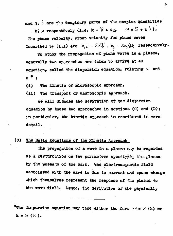
and q, b are the imaginary parts of the complex quantities

k,c respectively (1.e, k = • iq, W *CZ; ).

The phase velocity, group velocity for plane waves

described by (1.1) are Vik , v = ottAk respectively.

To study the propagation of plane waves in a plasma,

generally two ap L roachee are taken to arrive at an

equation, called the dispersion equation, relating bo and

k *

(i) The kinetic or microsooplo approach.

(ii) The transport or macroscopic avroach.

We will discuss the derivation of the dispersion

equation by these two approaches in sections (C) and (1))1

in particular, the kinetic approach is considered in more

detail.

(C) The Basic Equations of the Kinetio Avoroach,

The propagation of a wave in a plasma may be regarded

as a perturbation on the parametere specifyitc tie. plasma

by the passaze of the wave, The electromagnetic field

associated with the wave is due to =rent and space charge

which themselves represent the response of the plasma to

the wave field. Hence, the derivation of the physically

*The dispersion equation may take either the form co* (&) (k) or

k = k (G0 ),

existing wavy modes in a plasma is a self-consistent

electromagnetic field problem.

The response of an ensemble of particles of different

speoies j g mass mj, °barge e l p radius vector F and velocity to an external force can be described in a kinetic approach

by the Holtzman equation:

) 47i F . (1.2) Jib /cothsion

where f is the particle density in phase space. In our case

the external force is

= e s + ÷- x (Ft; + R)) (1.3)

where Iro is the static magnetic induction of the magnetoactive

plasma. The electromagnetic wAve field and lie related

to the macroscopic charge density r and current density lr through the well known Maxwell equations:

girL,

vxr = 0 3 t (1 . 4)

17 4 -rr while f and '3' are given by

p = J ATI

Im most astrophysical problems the changes in the

(1.5)

distribution function due to collisions are mudh slower

than those due to the wave electromagnetic field, and the

term (-46-tais;„ is usually neglected in (14) in practice.

With the external force Vdescribed by (1.3), the wave

field satisfying the naval, equations, together with r and

3 given by (1.5), the collision-free Boltaman equation is called the Vlasov equation. Vlasov pointed out that the

Holtzman equation -itself is an approximation to a many-body

problem and one of the assumption taken in the derivation of

the equation is thQt the interaction between particles consists.

only of binary- interaction. This assumption clearly does not

apply to the eaulomb force between many charged particles.

A rigorous derivation of the Vlasov equation is reviewed in

Appendix A.

When the wave disturbance in the plasma is small, the

particle distribution function f can be written in the form

f = f f o p (1.6)

where fa is the unperturbed dicAT:Txtion function and f is

the perturbation term due to the presence of the wave. In

this presentation if the effect of f on f is wall such p o that the perturbation theory is valid, the Vlasov equation'

(with f given by (1.6)) is said to be lineavized. Yrom the

linearized Vlasov equation, tLe dispersion equation W.I.&

7

describes the behaviour of waves in a plasma oan be

derived. Eowever# in a number of problems in astrophysics;

the description of the plasma can be simplified further

if the macroscopic approach is employed.

(D) Lacromaqpic Description of the Response of a num& to

Eltstnemagattkaakatukamt The relevant macroscopic quantities describing a

plasma are obtained as moments of the microscopic

distribution functions. The plasma can then be treated

as a fluid and the changes of states are specified by the

hydrodynamic equations which can be obtained as successive

momenta of the first BDGKY equation (equation (ht5)ji nee

Delcroix # chapter, 1963 # for detail discussion). These

hydrodynamic equations may be called transport equations

and two transport equations together with the Faxwell

equations are essential in the derivation of the dispersion

equation. A brief discussion on two transport equations

is given in Appendix B,

The macroscopic approach is used more often in practice

to describe electromagnetic phenomena in a plasma because

the mathematics involved is more simple. Lowever# it must

be pointed out that some phenomena are masked theoretically

by this approach if the occurrences of such phenomena

depedd on the microscopic distribution, of the particle

velocity., Two well known examples are the Landau

damping and the cyclotron damping. Some discussions on

these two damping mechanisms have been given by Ginsburg

(1964) and Stix (1962) and the cyclotron damping process

will be considered in more detail in the later part of

this thesis.

(E) aligatedagimatileAkmagatkl LIAM

A study of the dispersion equation indicates that,

in general, there are four distinct modes of electro

magnetic disturbance capable of propagating in aware

megnstoactive plasma (Astrom, 1950$ Addington, 1955)..

Two of the four modes tend to be longitudinal or pressure

waves and they arise only if the plasma is not at absolute

sero temperature,. The existence of thee, two asides depend

partly on the osourrence of elastic forces due to

compression of the plasma..

One of these longitudinal modev oalled the ion mode or

magnetic sound mode, appears when thermal motions of the

heavy plasma particles, both ions and atoms, are Included

such that the whole plasma has a finite pressure. The

plasmasation of the disturbance is the longitudinal type

and the velooity of disturbance is of the order of the

velocity of sound. When the propagation of the wave

is along the external static magnetio field, the wave is

almost a pure sound wave, having an associated electric

field only.

The second longitudinal mode, called the electron mode

or p-mode, appears when electron thermal motion and electron

gas pressure are taken into account. ):ihen the external statio

maznetio field exists and the electron pressure is finite, the

electron wave or p wave becomes a travelling electromagnetic

wave. If the p wave propagates along the static magnetic

field, it becOmes a pure electric wave and is quite independent

of the other two transverse modes. The p wave changes its

physical character from a pare longitudinal wave (refractive

index >> 1) to a transverse electromagnetic wave extraordinary

mode, refractive index 1) (Wild, Smerd and Weiss, p. 342,

1963).

The two tranverse modes are termed the ordinary mode

(0.-mode) and extraordinary mode (x-mode). The polarization of

the transverse waves is in general elliptical (Ratcliffe, 1959).

The two ellipses correspond to the two modes are identical in

shape, but with the major and minot axes interchanged and with

opposite senses of rotation. When the o and x waves are

propagating along the static magnetic field of a mapetoactive

plasma, the waves are circularly polarized; the sense of the

x-mode is the sense of rotation of an electron in the same

magnetic field. When the phase velocities propagate in

directions transverse to the static magnetic field, the

polarization of the two modes tend to be linear polarized.

At low frequencies where the motion of the ions is

important, the phase velocities of the ion mode and the two transverse modes remain almost constant for change of

plasma density (see Figur01.1(0)and the waves Of these three modes are grouped together as hydromagnetic waves.

In the case of transverse waves the plasma acts as a

dielectric medium and it changes the propagation constant

or the refractive index only. For longitudinal waves the

plasma takes part in the wave motion itself and the waves

cannot exist outside the plasma. When the static magnetic

'field is absent, the ordinary and extraordinary modes are

purely transverse electromagnetic waves while the electron

and ion modes are purely longitudinal waves. An external static magnetic field provides coupling between transverse

and longitudinal field vectors of the disturbances.

(F) Identification of the Four Modes in the Gra hical

Presentation of the Dispersion Eauation

Using the linearized macroscopic treatment, Denisse

and Deleroix (1963) derived the dispersion equation for

plane waves in a warm collisionless magnetoaotive plasma.

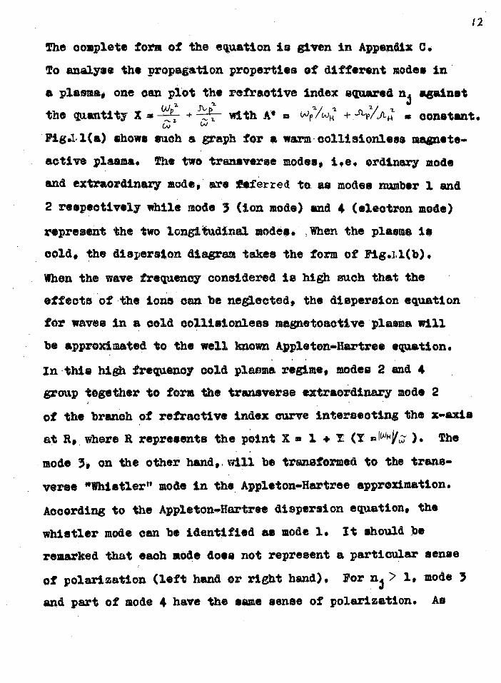
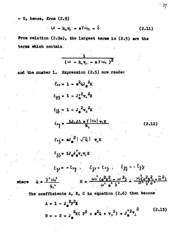
70

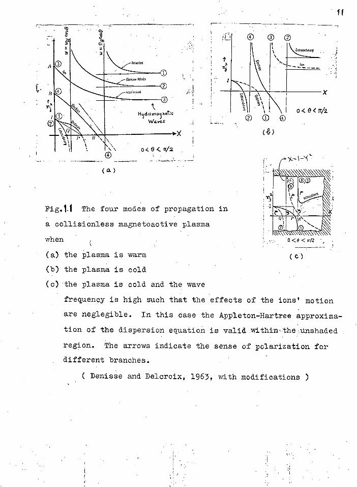
I t -

Extomftm

X

< 0< rr/2. 0 0

)

0 < 0 < Tr/2

( a )

Fig.1.1 The four modes of propagation in

a collisionless magnetoactive plasma

when

(a) the Plasma is warm

(b) the plasma is cold

(c) the plasma is cold and the wave

frequency is high such that the effects of the ions' motion

are neglegible. In this case the Appleton-Hartree approxima-

tion of the dispersion equation is valid within , the unshaded

region. The arrows indicate the sense of polarization for

different branches.

( Denisse and Delcroix, 1963, with modifications )

12

The complete fora of the equation is given in Appendix C. To analyse the propagation properties of different modes in

a plasma, one can plot the refractive index squared n i against the quantity X .01 (4- with e = (44,4 + se constant. Pig.1.1(a) shows such a graph for a warm-collisionless magnets-

active plasma. The two transverse modes, i.e. ordinary mode

and extraordinary mode, are geferred to as modes number 1 and

2 respectively While mode 3 (ion mode) and 4 (electron mode)

represent the two longitudinal modes: When the plasma is

cold, the dispersion diagram takes the form of Pig.i.1(b).

When the wave frequency considered is high such that the effects' of the ions can be neglected, the dispersion equation

for waves in a cold collisionless magnetoactive plasma will

be approximated to the well known Appletonmaartree equation.

In this high frequency cold plasma regime, modes 2 and 4

group together to form the transverse extraordinary mode 2

of the branch of refractive index curve intersecting the x-axis

at R, where R represents the point X= 1 • 2201,;- ). The

mode 3, on the other hand,,will be transformed to the trans-

verse "Whistler" mode in the Appletonmaartree approximation.

According to the Appleton.Hartree dispersion equation, the

whistler mode can be identified as mode 1. It Should be

remarked that each mode does not represent a particular sense

of polarization (left hand or right hand). Por n 3 > 1, mode 3

and part of mode 4 have the same sense of polarization. As

mode 4 transits through the point n. = 1 $ its sense

of polarization reverses. In Figure3.1(c), the states of

polarisation in various branches arc indicated by the

arrows.

So far we have considered the propagation of waves

in a plasma. Since only high frequency waves (i.e.

effects:of ions can be neglected) are studied in this

thesis, we will discuss briefly in the next section the

physical pictures of the basic generating mechanisms in

the high frequency regime.

(G) Generation of high Frequency Waves in a Plasma

Due to various momentum distributions of charged

particles and different types of motion of particles in

the plasma, various waves can be generated.

When two charged particles in a plasma approach close

to each other on account of thermal motion (speed = pT iqr ),

the energy lost in particles deceleration is emitted in the

form of electromagnetic wave disturbance this type

of radiation in a plasma is called Dremeetrahlung radiation.

In fact, this radiation is emitted in "close" or binary

encounters as well as in "distant" or multiple encounters,

each ion interacts with an electron as in a binary

encounter (Gcheuer„ 1960). Oince the motion of the charged

particles is of random nature (due to thermal agitation),

the observed radiation railatlen will be unpolarized.

If a charged particle is moving through a medium

containing neutral atoms in a certain direction with

velocity the so called 6erenkov waves, which are

transverse waves, are emitted on the surface of a cone if

the velccity of the particle is greater than the phase

velocity of quanta in this medium; the unpolarized radiation

is observed only at a particular value of wave-normal angle&

(with respect to i) such that

COS

(1.7)

where ni = refractive index in the medlui and o = speed of

light in vacuum (Jelley, 1958). When the medium is a plasma,

the aerenkov effect (i.e. coo 0 = may be satisfied also • 3

if the refractive index n is greater than 1. This condition

is satisfied for modes 3 and 4 (see Pig. 1) and the

"aerenkov name wave's° are in general longitudinal waves,

in contrast to the transverse waves emitted in a microscopically

neutral medium. An unusual feature of the wave disturbance

emitted by the Oerenkov effect is that waves of a given

frequency are propagated only at a particular angle 0 which

defines the emission cone. Cohen (1961) has calculated the

intensity of waves emitted by this process.

In the presence of a significant magnetic field with _

intensity IL . . a plasma, an electron of charge e and

rest mass mo will gyrate in a helix in general, where the

gyration frequency is given by f 41E41 P; ) olio

ao 0 .411 0 0

for normalized thermal velocity (37 —171-T.— c 1. In a

helical trajeotory, since a charged particle is undergoing

acceleration at all instants on the plane perpendicular to

the external magnetic field where the motion is circular,

the particle radiates electromagnetic energy as it gyrates

along.

First of all, we will consider the emission from an

electron rotating about a static magnetic field in a vacuum.

When the speed A .110 of the electron is notrelativistic ( p. - 0), the electric field of the wave disturbance E(t) received by an observtr at the orbital plane shows the farm

of a simple harmonic wave, The spectrum of the received

radiation is the Fourier transform of the simple harmonic

wave (Fig.2,2(4)) and the radiated frequency is confined to

the gyrofrequency fH only. At mildly relativistic sppeds

( (3 1), the wave form of the electric wave field is

distorted and the Fourier transform of 11(t) indicates that

the received energy is significant at the first few harmonics

of the relativistic gyrofrequenoy Where r (3 2- P-

15

(Fig0,(b)). The radiation from such a rotating electron

(or in general an electron gyrating in a heltoal path)

with nonrelativistic or mildly relativistic speeds is

called cyclotron radiation.

At highly relativistic speeds (1 - 1, or energy

of electron > 1 Rev.), the classical equations which describe

the distant field radiated by an accelerating electron

• indicate that the emission is sharply beamed along the

direction of the particle's motion (see, for example, Jackson,

chapterJA, 1962), and is highly polarized with the electric

vector of the wave perpendicular to the external magnetic

line of force. hence, an observer at the orbital plane

receives the radiated energy not in the form of a simple

harmonio wave but in dhort Sharp packets at the instant when

the partiole's velocity is directed towards him. The spectrum

of the received radiation is then the Fourier transform of

the reguhar pulse train; its form is that a long series of

harmonics of the frequency Y ffi , all contained within an

envelope defined by the Fourier transform of an individual

pulse (4ld, Smerd and Weiss, p. 353, 1963), The higher

the energy of electrons, the greater the number of harmonics

and close is their spacing. The individual harmonics in the

spectrum due to an assemblage of electrons are broadened by

various effects, with the result that the spectrum being

.Fig.2.2 Diagram illustrating the origin of cyclotron and

• synchrotron radiation. E(t) represents the eleCtric field

at a stationary observer in the orbital plane of an electron

rotating at velocity/3c. The emission spectrum P(f) is the

Fourier transform. of E(t). The critical frequency, which is

a measure ofthe duration of the pulses, is given by 3e E \2 - 7.07373; Ho ( m ) ,where E is the energy of the eleetron

in ergs.

( Wild,Smerd and Weiss,p.352,1963 )

smeared into a continuum. This type of radiation is called

synchrotron radiation (Fig.2.2(c)).

In the general case, the motion of the electron is

helical and the medium of interest is a plasma. By virtue

of the Doppler effect, the frequency of radiation as

received by an observer in a reference system fixed in the

plasma is given by the Doppler equations

s H

Ci s I — p nj cos&

If the condition

130 323 cosO < 1 (1.9)

is satisfied, the Doppler effect is said to be normal.

Using the quantum treatment, Ginsburg and Prank (1947) have

shown that the radiation of a quantum in the normal Doppler

effect is accompanied by a change of the electron to a state

with a smaller value of transverse momentum here the

direction perpendicular to the static 1,:p‘etic field is

assigned the transverse direction. In this case, the observed

frequency may be higher or lower than the frequency s

depending on whether the electron is moving towards (0 9 < , )

or away ( < 0 if ) from the observer;

When

ni cos 1 (1.10)

holds, the Doppler efTect is said to be anomalous. In this

case, the component of v 8 in the direction of the emitted

wave is larger than the phase velocity vo l _ of this wave

and the electron leaves a polarised wake which radiates

electromagneitc energy into the forward hemisphere. When

a quantum is emitted with a frequency corresponding to the

anomalous Dappler effect, the radiating electron is changed

into a state with a larger transverse momentum fi (see, for

example, Ginzbarg, 3heleznyakov and Eidman, 1962). It is

Clear from (1,9) that for radiation corresponding to the

anomalous Doppler effect, we must have n, > 1 and the waves

can only propagate in the whistler mode and some part of the

electron mode.

In the case of synchrotron radiation, the refractive

index is close to 1 for moot plasmas of interest and the

radiation characteristics are the same as in vacuum. The

intensity of this radiatton has been calculated by Sohwinger

(1949)* For cyclotron radiation, the refractive index can

be far away from 1 and the mathematics involved in the study

of radiation properties is much more complicated. A detailed

study of the cyclotron process under various conditions will

bo made in the later chapters.

We will consider only the frequencyrae from the order

of Kc/s to the order of 100 I2c/s in this thesis and tile only

relevant generation mechanisms for such frequencieu are the

ones described briefly above* All these processes can occur

in a plasma, depending on different physical conditions

of the radiators and background medium. For example, in

a magnetoactivv plasma there may be the case when the

temperature of the particles is so high that before a

particle has a chance of gyrating once along the external

magnetic field and radiate cyclotron radiation, it has

already collided with another particle. In such

circumstance, the only signifiCant radiation will be the

Breasstrahlung radiation. On the other hand, if the

temperature of the background magnetoactive plasma is low

and highly 'relativistic charged particles streams are

present, the synchrotron mechanism will predominate.

Consequently, the investigation of the generating mechanism

for waves coming from a .radio source requires the knowledge

of the physical conditions of the generating region.

Conversely, postulating the correct theory of emission will

lead us to understand. the physical situations of the region

where the radiators reside. Hence, the theoretical study

of plausible generating, mechanisms is a very important

part of radio astronomy..

(H) Emissions from the Sun and Planets

Most planets have no remarkable internal source of

energy end Are, thus, weak radio eaurces in general. On

account of the ir:Tingement of sunlight, the atmosrheres of

the planets are beinz heated up to several hundred decrees

Zelvin, and all planets emit weak thermal radiation in the

microwave range. however, among them 117ereury and Venue

emit more radio power at some ranges of frequencies than

would otherwise be observed from Bremsatrahlung radiation

due to siEple heating of the planets by the incident solar

rays. Vere surprisingly still, Jupiter has been discovered

lately to be a very strong source of radio waves in the decametrie range, A good review on the emissions from the

planets was given by Roberts (1963). Intense WO and LW

electromagnetic waves, which are believed to be generated

in the terrestrial magnetosphere, have been received an

Barth (for example, Ellis, 1959 and Mainetone and iloNicol,

/962). One or more generating meannieme rather thal the

Bremsetrahlung radiation must be reeponaible for these

abnormally high intensi;V radiatione from the two planets.

The Sun has been known for a long time as a very active

radio source for waves of wavelengths ranging from centimetre

to decametre* Up to the observed daa of tne present del',

therefore, the most interesting objecte in the solar system,

according to a radio astronomer, are the Dun, Jupiter and

the Earth.

-21

22

(I) TIT_gogga_Egmuip. the Observational Data of the

Sunjupijer and

Because of the difference in generating mechanism,

the variai,lon in physical conditions of the source

region, and the difference in propagatiaa conditions,

the observed characteristics of various types of emissions 109.MA

from the three atia-s show a large variety of forms.

However, among all the observed features of Wri011.0

radiations from these three objects, the following two

features are common and have presented difficulties to

radio astronomers

(1) very narrowobanded emissions are observed-.

Solar type I noise bursts, VIIV discrete emissions

from terreetrial magnetostbere, and Jupiter's

Decametric bursts radiation;

(ii) all these narrow-banded emissions are aseociated

with much intensive power th= uould otherwise be

obtailled from inooherent radiation of all the listed

generatine mechanisme exoept synchretron radiation,

which is not a likely generating process because

the bandwidth of emiseion from this radiation is

wide.

These two eListine problems etiaiulate my interest in

studying the plausible generatine mechanisms for the three

23

types of narrow-band emissions stated, and thus, to

look for a solution. Seeing the theory of cyclotron

radiation from electron bunches has been applied to

explain VLF discrete emissions (Dowden, I962a t;b) and

Jupiter's Decametrie bursts radiation (Mis t 1965)

successfully in several important aspects, the author

examines the conditions under which the two mentioned

features will appear; the solution to these problems is

also a strong test to the cyclotron theory.

In solving the first problem, one has to know the

power spectrum of the radiating system. It is well known

that in the cyclotron mechanism one electron will radiate

a wide range of frequencies in almost all directions. Thus,

one must know what range of frequency is associated with

the majority of the electromagnetic power before one can

estimate the bandwidth of emission. adman's equation (1958),

corrected by Liemohn (1964), gives cyclotron radiation power

spectra from single electrons. This equation has not been

well explored yet. Moreover, when the gyrating, radiating

particles form a stream or bunch, some particles may radiate

in phase gradually, so that, waves in the radiating system

are perceived to grow according to an observer outside the

system, and the resulting power spectrum will be different

from that of single electrons. When one considers this

effect one is led to the problem of radiative instability

of a streqm-plasma system. Hence, the author starts off

to investigate the conditions of instability in a stream..

plasma system in chapter II. Vihen the collective power

spectrum is obtained, the two stated problems may be solved

consequently.

In chapters III and IV, the instability theory is applied

to solved the mentioned two problems in Jupiter's Becametric

Burst radiation and terrestrial VLF discrete emissions

respectively. In considering solar type I noise storms

radiation, the first proposal of the theory of cyclotron

radiation in the ordinary mode is made and the theory is

investigated in detail (chapters V to X ). It is found that

not only the two features can be accounted for by the cyclotron

mechanism and the instability theory, many other important

observed characteristics of both Burst radiation and Continuum

radiation can be explained.

The last chapter concludes the thetis and gives

suggestiens for further research.

CLAkT II

1.2.Z.V21210E1 ,;11V1,3

ET A YkaLAL.PLLOLA

(A) Introduction

Using the classical kinetic approach (chopter I),.

the radiative instability proble:: of a streem-plarma

system has been studied by a number of authors. The

main features of these investigations vary according

to the form of momentum distribution tPicen for the stream,

the wave-normal angle assumed, the frequency domain

chosen and the types of waves excited (loncitudinal or

transverse electromagnetic waves). The momentum distribu-

tion functioas of the obk:red particle strevm considered

are chiefly of four typoo:

(a) The mean longitudinal momentum of the stream is

finite and the transverse momentac of each

particle is zero, i.e., the str(go is Aot gyrating.

Rere we assi3v, the direction parallel to the static

mcmetio field to be the lonfrItudinal direction

and the one perpendicular to it the transverse

direction* .

+In ease the plasma is not zaGnetoactive, Vie lonitudinal

direction is referred to tho direction where the stream is

travelling.

(b) A delta distribution in momentum space for both

components of momentum 1,4. and f , where 11 i 0 0 1,

and 1311 0* A stream of this cl;str;htion is called hehcal.

, (0) A. distribation function where there is dispersion

of particles over the longitudinal and transverse

momenta and 10 2.. ,0 whereas f: is non-zero 0

• n are values of momenta where the

distribution curve shows the Maximum,

(d) In case (c) Where e1 0.

The homogeneous background plasma is usUslly assumed

either to be cold, or cold and magnetoactive. We

refer to the treatments where the wave frequency is very

much higher than, and of the order of the ion gyros.

frequency as the high frequency treatment and low

frequency treatment respectively. The wave.normal angle

0 assumed generally fall into three classes:

( G( ) strictly longitudinal propagation, lie* 0.= 0°

or 180°

(g) 0 olose to 0° or'180°

U) general 0

With above specifications, the characteristics of

various treatments are summarized in Table 2.11

f:

ft.

8

E4

saolary •

6,6i ilt,ivactuved .1!"OZATIVI1

fe09e1. kitoratutsetaq?

WET 44ozattamet

ft1961. `,2 voci, •aettaoy

-Stepanov Eitsenko t

19 61

IOU

•

Aoaatuvut-;t:--1(

•

1961. uvw -411'n(t ti*E1:1

!•AWA & triebt, 11644

196,412

pemnssy

coin o0

o001 400

ttueue9

7I genoral 0 tor 1 .1,1erenkov Inetai-bility wall 0 but CY" for oyolotron That

tr.Aulue$

eat (00

0001. 400

rall.T047 8841.13*

Jo sativog

MCA •41°8

VUTIMTPUOT

•

90AU4 °Wee

8818A8=1;

P

longitudinal. & transverse

e.n. waves

Sc

804&VA

teuTvntVuot

80AIIM

81=841,0=44

uTuNINT touenbaze.

high _frequency

4couertbeaj Mat

4auetibea; traTti

ilt

0

alouor:.;eaj 1#101-

Vilatn4 ounoarion

Amend Roo

1 cold magnstoactive plasma

0

mmitanl ;o 11.4TCt tut-luestol

(*)

(q)

)

(0)

(0 )

(e)

,

(q)

28

It is obvious that with type (a) distribution function

of the stream, oyolotron waves cannot be excited. When the

distribution function of the stream is as type (c), most

nonthermal particles in the system acquire zero or very

small values of hence, the excitation of cyolotron

waves will not be important in such a system. On the other

hand, the exaltation of longitudinal plasma waves will be

pronounced in a system with a stream of type (a) or (c).

As far as excitation of cyclotron waves is concerned,

distribution function types (b) and (d) of the stream are

more important, in particular the latter, for it is most

likely the realistic case. With these two distribution

functions, it Is clear from Table 2.1 that only the case of

longitudinal propagation (0 = 0 °, 180°) has been investigated.

Since cyclotron radiation is emitted in all direotions by a

gyrating charged particle, the instability theory for

general 0 is therefore highly desirable and it is only

when such a theory is available that we can estimate the

frequency spectrum of radiation emitted by a gyrating stream.

Hence, to start off, we will derive the dispersion equation

for general 0 and, thus, the expression for the growth rate

in time (excitation coeffielent) for a "helical stream

magnetoactive plasma" system in section (B). This is the

limiting situation for the case where the stream has a

narrow spread in momentum distribution and will be found to

be important in application. When the temperature of

the stream is included, i.e. taking tnto account the

spread in momentum distribution of the stream, the

dispersion equation for the . .stream*plasms system is

then derived in section (C). In this chapter, we will

give the essential mathematical expressions wily. The

numerical analysis of the radiative unstable system is achieved in chapters XXI, IV, and VIII, where the

instability theory 18 applied to various particular

oases of interest in radio astronomy.

(B) Po ation Of Radiative Instabi t Theo

Relical.Strealasma Systea

• In the investigation Of this seotion, the more

general case of a helical. electron stress is considered,

i.e.. each electron in the stream lima with the same

non-zero transverse - velocity vijo and the same

longitudinal velocity ft. sx vii /o; the direction along

the static magnetic field Is assigned the longitudinal

direction. The particle density in the stream is

assumed to be very small compared with that in the

background plasma and the stream-plasma system is

assumed to be electrically neutral.

The dispersion equation for an eleotromsgnetic •c-w)t

- wave specified by e L(A propagating in a sodium

211

Vlb fx .5.

lE\ g

- rt. + \E)

11 2i. exx

rghk Ebx

O 2.1)

with dielectric tensor E.i.AC (.0 • 2) us given by

det(nt — ro14t — cuM = 0 (2.1)

where a = okjw , E = wave vector, (.0 w angular frequency

of the electromagnetio wais t ' and c m speed of light in

vacuum. 5 Kro'nec.key delta.

For cycltron radiation from a charged particle gyrating

about a static magnetic field line, the wave vector 2 gyrates with the gyrating radiator and g forms a cone for

one complete gyration of the charged particle, If the

static magnetio field is along the z direction, an account

of symmetry, we can, thus, let ky 0, The dispersion equation, namely eqmation (24), in matrix form becomes

The dielectric tensor for a growing electromagnetic wave

in a plasma permeated by a static magnetic field, specified

by an unperturbed distribution function fo•is of the form

(Stepanov and Eitsenko, 1961)*.

*In this study, relativistic effects have been inoluded.

j A ujol T ; coti2 mo r.i. I 2 c)., dp

I + .4 (4% * s2j 12

IV fT j 312. ?J. .1. 41% • w° 2

())°:

Loa( 1 + 2Trf?.1.1 pi otpidp .— 2

•- a , 2 Tr w 0 s . j's ' LAI rtio .111 6.1fil • .

. = A' W "kl.

Ap J

...: TIT co: T. j-s2'p (A)N mo rya. t . (4 3. AI 1 is

W2 T 7S 3S 1 lb.fli '6111411 ' • ITT 1U/01

.Ifire le

(*awe%) m„ angular plasma frequency, 4: ptic.k densit3

= angular wave frequency

components of wave vector along and perpendicular to

re *Pi =

the direction of the static magnetic field respectively

corresponding momenta of particle

m a 01: 4. Wet ejo2A, is the relativistic saes of a

charged particle of rest mass mo in the plasma

wo st angular gyro-frequency and negative for negatively

charged particles

• harmonic number

and Js are Besselia function and its derivative; the

argument being

a a WHIN)

It ahould be noted that expression (2.3) can be obtained

from the general expression for EA which was derived (by

Shafranov, 1958) under the condition that the part of the

distribution function f (5, 01, which is connected with the

electromagnetic disturbance, tends to zero with t --0 - co.

Evidently, this means that the wave disturbance grows with

time.

Now suppose the radiators constitute a helical stream;

the unperturbed distribution function takes the fora

fo( s ft.

p,')4 (2.4)

We can simplify (2.3) through integration by parts

assuming to tends to zero sufficiently quickly with & and

If0 tending to infinity, With a delta function distribution

as in expression (2+4), the dielectric tensor becomes:

32

gs.

Per a non-trivial solution, equation (L) can be

written as

An4 + Bn2

4.0WO • S

where A at Sinl e E rs - co?e + 2.s;n13 cos eN,

B 2 s ; n e tos 9 ( - En. EA),) + Ex ,)2" - Exx Ejk

- eas'e ( E3,3„ + - Sili ze (EXxEla + EAse),2)

C E(E sxE3.1, + t)(1') Exx + 2 -£J1 Ex;

Solving for no2 $

2 ± n * (2.6) . 2 A

here we use the subscript a to indicate that n; le the square of the refractive index for the "stream static magnetic field" system. In (2.6)

F p ?J., PH / -k) W, 0.41 Goo)

So far we have net yet considered the ambient plasma. Since we have assumed the density of the stream to be

very mach smaller than that of the ambient plasma, n; can be considered as a perturbation ter a in the overall refractive

index expression for the streaa-magnetoactive.plassa systea. Following Zheleanyakev (1960a), we assumes

- 1 (2.7) n * nj • ne

34-

where ii = overall refractive index

na refractive index of the ambient plasma a The validity of the above aseumption is discussed in Appendix

D.

Equation (2.6) can then be written ass

PP

Po m 0

where P = o2k2 2 1

(2.8a)

P°' uul/P

We employ* the real.k method, i.e. we assume the wave

.vector to be real and the frequency complex in order to find

the growth of the electromagnetic wave in time. We let

( 2 .9)

where ai • the ocharacteristio frequency", is real and S

being complex, assuming. .

ur I >> I Si (2.9a)

With above approximation, one has (Zheleznyakov, 1960a;

Neufeld and Wright, 19644

01_9S +(r)aa, o k )(A) Ez„

(2.10)

The equation (PL 0 in fact gives the dispersion

equation for electromagnetic mire of frequency 'a in the

ambient plasma alone. With a thin stream as assumed, we have

35-

(2.10a) hence we can take (25) F' = 0 )(A) a

We now refer back to equation (2.5). Since we are

considering an electron stream, will be negative.

Physically, for a non-zero harmonic number, the only possible

non-thermal radiation from a gyrating charged particle is

gyro-radiation. In the frame of reference where the radiator

is at rest, the frequency radiated is equal to the gyro-fre-

quency of the radiator. Por an observer in a system fixed

to the background medium, the radiated frequency will be

Doppler-shifted to a frequency higher than IsnAid in the

forward direction and Doppler-shifted to a frequency lower

than 1 sru4d in the backward direction, For gyro-radiation

from a single particle, the Doppler equation gives (4; k v n sYc41.4 ) 0. In ease of eleotrons where (.014 is taken to be

negative, negative integers of s represent normal cyclotron

radiation, while a positive'integer of s represents the s th

harmonic of the anomalous cyclotron radiation. Per the thole

2 system, as kio is assumed to be small (thin stream), we can

see that unless the Ulu (4 k v sYwn ) is small,

Exx = = , E)( =.E . 0

and nit im 1, implying that the stream has a negligible effect

on the refractive index of the system. We let verk , 1v11 -s‘wii

£5.0. ,

142'

Ey3

wo2 (o2A w (41 02 S i

where

= 0, hence, from (2.9)

(2.11)

from relation (2.9a), the largest terms in (2.5) are the

terms which contain

1 ea k47-31 ,

and the number 1. Expression (2,5) now reads:

42414/821( ' Exxxs 1

E u * 1 NI 2v2K v o .

e3k to I - J0121,4 21

El • J.cTs Vs 01( I WH

(2.12)

Ev sJI Altai vil IC

a • iJ eV V K l e A. 11

The coefficients Al B e C in equation (2.6) then become

A 1 - Ji2P2K

2K( P2 + s2Q + v„2) + Joi2v,i2 (2.13)

2K7 2 J .2v

3s

The perturbation term P' on the dispersion equation (2 100:can be calculated*

2.

I 2- 2 1111 2 s;'1 1 0) K + K

sin 2 (! ?/)2

•

~ .... p a

1 + SJs ir 12 c

a os ti

( s )

(2.14)

With the difinition of 21* given by expression (2.14),

and the definition of P given by relation (2.80, equation (2.10a), therefore, gives the complete form of the dispersion

equation in a helical.stream.plassa system. Here, 2 and

thus P and are left in the most general form. atA)

The expression for n.2 depends on the type of ambient plasma

under consideration and will be written in chapters III and

IV Whitn we discuss different particular oases of application

of the theory.

whore P2 v2 cos2 0 (s s )

K '13:"

(C) Instability Theory of a Stream-plasma System when the

Temperature Effects in the Stream have been Included

Instead of a strictly umonoenergetio" charged

particle stream, we consider a stream having momentum .4% 0 4. 0

spread in both components fl 4 and are

supposed to be the values of momentum components where

the distribution curve reaches its maximum. More

precisely, the unperturbed particle distribution function

f 0) of the stream is given by 0

.12) ) ai 41 4 ( 245) 1 40 l

A

where 2173/2

constant of fo . 2 = 2 mo K T 2

a1= 2M0 X • H

is the normalization

m = rest mass of radiating particle

X = Boltzmann constant

T4 , T" a transverse and longitudinal temperatures

respectively

+For Simplicity, we consider one species of radiating

particles only.

and

40

with 5o =

Leaving the expression for the ambient plasma

refractive index =specified, we will now derive the

dispersion equation for electromagnetio waves in a stream-

plasma system when the distribution function of the radiat-

ing particles is given by relation (2.15)4 The method

employed here follows that in section (11) of this chapter

and the work of Zheleznyakov (1960b).

Before using expressions (2.3) and (2.15) to derive

the relations of the dielectric tensor components, we have

to define several quantities:

Let _ C1)11 -

)

ar I I

f3i = Loc; _furic;_sft4ti -k„ (2.16)

8414.1 =, s ( ss) vutil- La -

4211

where the sign indicates that the corresponding value

NIur quantity is equivalent to the quantity defined

by aelesmyakov, in order to distinguish it from the

normalized frequency = w/IWI-11which will be introduced

later.

41

es 0

fl is taken at the point =r y g, .e. I-set us now consider an integral of the form

2

.11"/' pa —(is)

orvitotit

The contour of inteexation runs along the real axis of

from -00 to 4* C.° by-passing from above or below the

singularities of the integrand. The integrand of the above integral will have

■ singularities at two points specified by 51, 2, such that

- 31, z , (2.18)

ci Ci

We note that we have changed the variables in expression (2.16) in order to deal with the denominator in relation (2.3); in fact, equation (2.18) is equivalent to i. - 0. -which -is the Doppler equation.

(2 .17 )

It has been pointed out by Zheleznyakov that

when I 3- _Sol 1 and

42

(2.19)

we have ipa j »Im;s)1 »

and the integral (2.17) can be simplified to

VS, e2-- --1-1; ( )€ 6t1S 4. 2 09S(19i 2 p 13 3 S' •

L 1,2.

- *0 -00

(2.20)

with an accuracy up to terms of order fj

where = + 1 if the contour of integration in

(2,17) by-passes the singularity from below and

St = - 1 if the contour by-passes the singularity

• from above.

The sass of the radiating particle can be expressed e in terns of S ) as:

t 20150;Q p al te p a Dt (2.21)

fl c c 511 c

" Let us assume that P" Si changes little in the

, range . 5015.1. We can now express 01 L,3 in the form:

,z g 1. a'u( s 50) C, ( 2 . 22) '

It is easy to see that the angular plasma frequency can be written as;

we 21. ,,' 30); 2:41. 1cifevrSoj (2.23) CVO ( S, S) :=-" (-41 I 11121- I S '1.. 012 ,50(t

t

In writing down expressions (2.22) and (2.23), we have taken:

43

rna 7: rni 1

l a II Fir 1 << 1 ...„, ve. ; [ I a 111 << 1 vn c (2.24)

Since the denominator w _ S mo wt., in

expression (2.3) can be written as iz ti a„ — S',3g and the quantities u4, m are expressed as functions of S I

(given in (2.22), (2023)1, all the integrals in (2.3) fall

into the type specified by(2.17), when integration is

carried out with respect to • Let VW note that on

can be approximated to

-1-13 f 0) otS 1 — s

—

We now substitute relations (2.16), (2.17),.(2.22),

(2.23) and (2.25) into the expression for dielectric tensor

- components (expression (2.3)) and perform the integration with

respect It has been pointed out in section (B) that

account of the inequalities given in (2.19), the integral

CS. ,

(2.25)

the largest terms in the dielectric tensor components are the

ones containing 1/Incvm - kqu 7S1110 (402 and the number 1.

Confining ourselves to this approximation, we have:

-4 1...

a t 1

-.1---'`-"--4wiR G-2S;dc3—scj2. etS —R4u-s2S (S-54 ic3— Sot 4 fa \ ads 3 Isij U.. Sj26. re

4S- 5042. ...... cO • Coo

I - eGO t co

a42, W 2,53e.43..svi r )23(

D GT., ojs 3 -1 1.3. S

00

S C3-304 1 2 3 a -(3-S

00 _Cs—s.)2 R=1.1-sli'S 2CS — go) e ckS s a.„W[Rifjo_s)sati-05- Sce

;■ 1 1f- G70 0

- R3 Vs's/ S2( S - SJ2e,443- Sj :CS A4

co o

-So12517s2S CS - .50)e-c S7 5°)Is 0. -(3- Sor

° (2 .26)

- gq7s2SCS-50)e_-, LS i -a— .

E -1- W kR41-I2S;,(3-3°)2.1s D

eO

2 2 IS —so) 20ts rne UJH fifsw ft RI

-co. D" Fv-,.

(Ls - R3 i'Ts15( 5 -30)1e7 ts "s4a 1.

0 .0

- R 2. 1e;s 2S CS - 5.)-e-c-5°)2 a5 .• 0

roW f( _ 711'

D2 60 tik"c?

oO

R 5 '(5 - S o) e-(3 - 3° )2,0 - R cUs '32(S - -( S.)4,2. 5 °

As the argument of the BesselLs function and its

_ S , derivative is ct, = is a function of

Tri 0 WH cu. III

S ., all the J J J8, s and Js" have to be kept inside

the integrals. In (2.26), we define

- 2

R1 = I 011

4 cp.- I ol a L 2..SQ

R2 = ieC 2

2 a A. = 3 2-

( 2.27)

R = 0 2

3a, 1 5 is, 1°1 o -, 'ca 4 j a

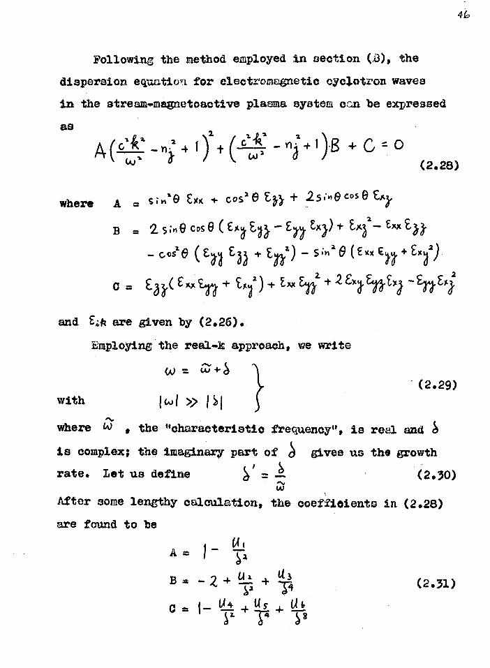
Following the method employed in section (0), the

dispersion equation for electromagnetic cyclotron waves

in the stream-magnetoactive plasma system can be expressed

as

A( cP -n: 4 1 )2 t ( 4R2 - )1;- + 1)8 + C = 0 (14 0 k GO a 0

(2.28)

where A = ste Cxx + cos ) +9 E33. + 25;.ecose

B = 2 s;n8 cps ( — En. exx

cosi° (En E 3) Ella) — s ;h a 9 ( E + Exi)

= E3( X)(?.An 1.12 )9( EApj, + 2 ElEnZxj,

and Ezi; are given by (2.26).

Employing the real-k approach, we write

(2.29) with (col > ISI

where a the "characteristic frequenoy", is real and S

is complex; the imaginary part of gives us the growth rate. Let us define (2.30)

After some lengthy calculation, the coeffieients in (2.28)

are found to be (A

a= 1 -

T c I— + s. + s l u

s 4 so

(2.31)

with E xx tan2 0 ( + s )2.

where III 0 =Tz + 2 sin e cos 0 T 1 - cos2 Ts. - sinl e T7

II2 = T + 2 sin cos 0T8 + cos a T4. fr sin2 e TG

= sinl e E xa + cost 0 + 2 sin e cos 0T s,

= T E 3

tr s. + T6 E1/,

= T E

= U5 .* + E' - Ts 51

= -U-E, E'' *2 T Exn

T = E x ,a (R4N, -

T 2. =

T 3 = E xx „

T4 = E n + E.

Tc E ll En, + E TG = Exx + E4

E xx Eu + O1

Wt 1 a 41

o

and

R8

2 .2 21 0 0o° 5 aA wf

ilZ 2 2 tan 0 ( "is )2 C

■■•••■•■

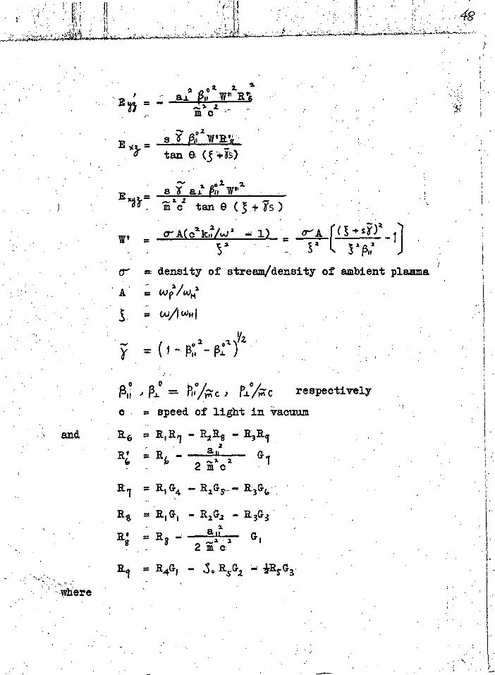
2 2 *' 2 p a al 11 W"

2. a M C -

tan a (s -+io

•■• o 2. Es I al

11 2. 02 tan 9 ( )

(r A( 021E,2t AAP 1) O A 2 (( " i]

S 2 3 2

cr- = density of stream/density of ambient plaama = Wp

= GUA (A)H I Yz _ 4 D o 2 a o%

1"-1- /

A: „ 0 = „ 0 p,. c respectively

o = speed of light in vacuum

R.6 = RI R / - RIR1 ;RI 2

R' = R - a

2 mc

= Ri G4 R:3G4

Rs = R I G I R1G2 R 3G 3 a

= • s Rs —2.2 2 m

Ra = - S. R5 G2

•■ Sas

WI

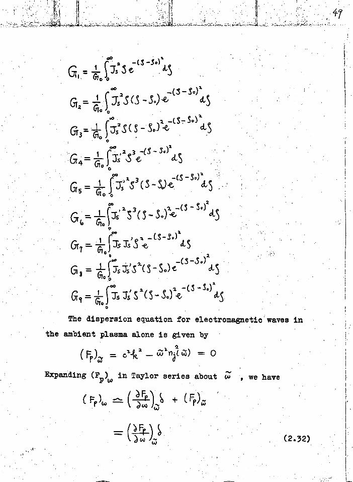
1

e° -cs-sx s2 3t Ls

-s.)% G6= ro fS -se)..e, 4,5

G3 = ko f Js2 .5

G4= fas.2.S3f:"- 3°)26t 0 S

G5= i fj[s3 (s (s - sorcis

G ‘ =- icus' / S 3 (3- sof:€7 (3 3°245

Gri fa., T' ss

G 3 =

= irTs 3s) S a (3— S0)2.R: Cs —s °)2. 0

. The dispersion equation for electromagnetic waves in

the ambient plasma Alone is given by 2 Fda, = 07-41, 2 — cenjoz) =-- o

Expanding (FIA0 in Taylor series about co ,.we have

rd,

(17rFAr)...., S w . (2. 32)

Writing (dimensionless) (2.33)

we can simplify equation (2.28) into the folbowing form:

) 0; • 4 I 3 , 2

S, I

4 W2 W3 S 4 W4 Vtig 0 (2.34)

Where W I im p l

PIU3

W3 = r(u 2 aro = U2 • U3 • U4

Wg = pu i

"6 = 1/1 Wi =

Solving equation (2.34) for complex S , one can

calculate the growth rate 15111()1 1

Taking only terms containing 1/(11)m - sm0 (41 )

and the number 1 in the dieleotric tensor ocmponents and other

assumptions as stskted, the dispersion equation has been

derived (equation (2.28)). Using perturbation theory, we

have expressed the dispersion equation as a polynomial in S i = (equation (2.34)), where S = (A) is complex.

The remaining work, therefore, is to solve equation (2.34).

Before attempting to solve (2.34) which is complicated

as it stands we consider the oase of strictly longitudinal

propagation, i.e. 0 = 00 or 1800 . Horeover, we confine

ourselves to the first harmonic only, so that 8 2 • It

while 3 = P(U2 2U3)

ag-S111---' zCS R I G4 R G. '

1 5" H 3G ) C, (2.35) 2Gom

Sf

is found that when sin 0 = 0, V4 2. = = i5 lc

Where t 3 _(— !) ao

?:j

S. S 3 (S - 5 0) t43-80)243 00

S 3 (S - Soft -CS-3°)OtS

The dispersion equation now reads

a w '4 ( R I GA . El2G; 2PG 0it-1.0 2 (2.36)

After some simple manivilation, one realizes that equation (2.36) agrees with aeleznyakovls result (equation (2.12)) if the following assumptions or approzt-qationa hold:

(1)

(ii)VG0 l(R, . 1) 02/G0 - H2GWG0 R3G1/Go l

(iii)terms containing 1!, - * are negligible, C .

The terms containing 1/(cui 0

k 917. tisZ are

small in comparison to the terms containing

1/( - k „ r„° .•

52

We consider the validity of the above four

approximations now. If the spread in pi (specified by

a l ) is of the order of the spread in PI , (specified by 2 ), we have OVG,, >> 3. in cases when the spread in fj.

is not too large. Vore precisely, we want S o = > 3.

j (the least value of So should be about 3) in order that(1)

is valid. Approximationw (ii) and (iii) are taken also by

Zhelesn,yekov and approximation (iv) is the well knoym

assumption in radiative instability problem of a stream-

plasma system if the growth rate be small .(i.e. ).

For another example, we consider the stream to be cold, i.e. al ail = 0, and we have a delta momentum distribution

for the partioles in the stream. In this .ease, where the wave normal angle assumes general values, one hae in

equation (2.34):

= W 5 =bJ 4 4: W =

therefore, equation (2.34) reads

/ 3 W k W 3

6 4.-77 0 ti 0 (2.37)

(3: 1 ( In this particular case W2tdi • s 351ck- A C4731 0 1 t 1 t is) 2

2. 01( sii+ s;n2 0 EY' 7 13 ' I P° go

and Ws/W I gt-n--k(( s.gt3)1 _1 s J. 4. 5 • SI. P130 (Si+ *gt) fri,I 2

One sees that this equation is, in fact, exactly the

53

equation derived in section (13) (equation (2.10a) with

the definition of (2.14)). We may, thus, conclude that

the dispersion equation derived in this investigation

agrees with that obtained by Zheleanyakov on transition

from general 0 to 0 = 0° or 180° (under the approximations

stated), and when the temperature of the stream is taken

to zero, the dispersion equation (2.34) is simplified to

the one derived in section (D).

valuating the coefficients of the dispersion

equation (2.34) in the case of VLF emission in the

terrestrial magnetosphere indicate that only the first

three terms are significant, i.e. the dispersion equation

Can be approximated. to

c3 wa W3

* * = 0

This is of the same form as the dispersion equation

for the case of a strictly helical stream in a magnetoaotive

plasma as derived in section (D). Kence, if the dispersion

equation of the system can be approximated. in the form as

in equation (2.38)0 one can have an exaot solution for

readily by Oarden's method; otherwise, one has to take

equation (2.34) and work for complex numerical solutions.

'Under different conditions, electromagnetic waves

generated by normal or anomalous cyclotron radiation processes

by partioles in the strerm may grow in the atrean-macneto-

aotive-plaema system and the power of the waves may be

(2.38)

*. 54

amplified enormously. This radiative instability may in

foot happen in many natural radio emissions in radio astronomy. The study of such instability problem will

help to understand various vhenomena in plasma radiation.

As far as cyclotron radiation is concerned, the

distribution function of the stream considered in section

(C) seems to be a realistic and important one. however,

when "almost mono-energetio streams" are present as in the came of VLF emissions in the terrestrial magnetoaphere,

distribution of elsotron stream described by relation (2.4)

becomes more convenient in application on account of the siplicity in the corresponding dispersion equation. The

general qualitative behaviour of the stream-plasma system

is the same if the epread in momentum distribution of the stream is not too wide'.

• "Negative-Absorption" Apr

kroblem The discussions in the previous sections are based on

the classical kinetic treatment. ;Fe will consider below the

44hen the momentum spread is wide, the bandwidth of emission

will be broad and the harmonics may not be resolved.

general deductions from another approach.

Twigs (1958) employed the quantum formulation for

deriving the macroscopic radio absorption coefficient'

and indicated that amplification of waves occur when the absorption coefficient is negative. The conditions for negative absorption are elven in terms of energy distribut-ion Ile ) of the source electrons and the mean electron emissivity Q(E ) for the effective radiating mechanism in

concern. Here Q(6) is defined as the mean power delivered by each electron of energy E per unit time per unit frequency interval in one polarisation per unit solid angle into any direction.

Smerd (1963) then developed the theory and derived the

general expression for the absorption coefficient K in an

anisotropio medium. Defining g( 6) de as the statistical

weight of energy levels, Smerd obtained two necessary

conditions for amplification to occurs

Xi) A positive gradient in the electron enorgy distribut-

ion . ( E).

(ii) A negative gradient in g(E ) Q( E).

Assuaing that the refractive index is equal to 1, the above

+A quantity defined as the difference between the total

stimulated absorption and the total stimulated emissions.

55"

He) g (E)C

FIGT.Tiii 2.1 Examples of electron energy distributions F(e), the product of statistical weight g(e), and electron : emissivity, (Me), which lead to positive'and negative absorption. (a) Positive absorption when dF/cle is nega-

tive; a thermal source of radiation is an example. . (b) Positive absorption when (d/de) [g(e) Qi(d)) is positive; bremsstrahlung is an example, (c) and (d) Two situations which lead to negative absorption where dFicie . is positive and (d/de) (g(e) Ch(4)] is negative as in conditions (a) and (b); this can apply to gyro-radiation.

mord , 19 63 )• Pos;rve absorrVen. fey ro. rtscNo..t;a-ot, ( 4,..guamsomA. reo71..a.11766 , absorptzow . )

(4)

idea about the conditions for negative absorption is

illustrated in Pig. 241(a) - (d). Uote that in Pig. 2.1(0) 4

the electron energy dietributien can be considered to be composed of a 11 2!axwe11ian background -plasma and a stream

with quite wide momentum spread. If 10(E) and g(E ) Q(E ) vary with C as in Pig. 2.1(e), positive absorption will

result. We see, therefore, that either amplifioation or absorption can take place for a particular type of generat-

ing mechanism, depending on the distribution function of

the system. alereas as stream gyrating in a cold magneto-

active plasma can give rise to cyclotron instability and amplification as discussed in sections (1)) and (0, trans-

verse electromagnetic waves can be absorbed in aLaxwellian or cold mametoactive plasma due to the fact that the total

stimulated absorption exceeds the total stimulated emission.

This coltioionleas absorption is called harmonic resonance

absorption and will be discussed again in chapter VIII.

(1 ) ILNIA-LtIALIBILVALUX Twise (1952) pointed out that the general conclusions

of instability from studying the dispersion equatiGn could be misleading; for instance, it may not be possible to

distingaieh an apparent wave growth in one direction from

an actual damping of the reflected wave in the opposite

direction without introducing the appropriate initial and

boundary conditions. To overcome the above difficulty,

Sturrock (1956) put forward an elegant method by Which, .

it is possible to distinguish amplifying fro n evanescent

waves by investigation of the dispersion equation acne.

In discussing simple dynamical systems, one interprets

the existence of a normal node which grows exponentially

in time as signifying that the system cannot persist in a

quiescent state, since arbitrarily small initial disturbances

will lead to the generation of large scale disturbances.

Theoretical analysis of the travelling-wave or two-stream

amplifier (Pierce, 1950) shows the existence of tine growing

modea, but we know experimentally that such systems can

persist in a quiescent state. The backward-wave oscillator

(Bech t 1956), on the other hand, will not remain in a

quiescent state. Based an the above ideas, Sturrock (1958)

went on to study the kinematics of a growing system and

found that in general there are two types of instability:

(i) Convective Instability

If a propc.gatinc system exhibits convective

instability, a finite length of the system mey persist

in a quiescent state, even in the presence of small

random disturbances, since these disturbances, although

amplified, are carried away from the region in which

they originate. Uuch systems may be used as amplifiers.

(ii) Ronconvective or Absolute Instability

53

If a propagating system exhibits nonconvective

instability, an arbitrary perturbation of the

system will give rise to a disturbance which grows

in amplitude at the point at which the perturbat-

ion originated; we also expect that the disturbance

will spread until it extends over an arbitrary

large region of the system-. Such system may be

used as oscillatOrs.

Assuming 0 = 00 or 1800, it has been foand by

Sturrock's method that the Cerenkov, anomalous oyclotron

and forward cyclotron (0 < 900) instabilities are

conveotive whereas the backward cyclotron (8 >90) •

.instability is nonoonveative.

(F)

Even though the instability theory of a stream-

plasma has been solved for general 0, it is by no

means the end of our study on this subject. It will

be fruitful in the future to carry out research on

the correspondence between the kinetic approach and

the negative-absorption approach. In the kinetic

treatment we have assign the boundary conditions for

growing waves: f,(3, F, t) 0 as t -4 oo

Now if we have the reverse boundary conditions, i.e.

f t (11, Fp .0.-3-0 as t--›cy, for the dielectric tensor,

we are looking for a damming wave and it will be interest-

ing to calculate the damping coefficient to seQ whether it

i0 of any significant valuecoopared to the excitation

coefficient, for the purpose of checking our theory.

Horeover, we have employed the linearized theory so far,

i.e. the distribution function associated with the

electromagnetic) disturbance 1'4, Fp t) is asemmed to be

small compared to the 'unperturbed distribution function

fo ( B, ). This assumption holds only when the growth

or damping is small, so that, the energy of the electrons

in the stream remain practically constant. Therefore,

strictly speaking, the linearized theory is valid at the

onset of the excitation procees only. The nonlinear

instability theory for general 0 for various radiating

systems will be a challenging problem in plema phySics.

In fact, pioneering work in this topic has teen started

a few years ago (e.g. Shapiro and Shevehenko, 1962; Engel,

1965; Shapird, 1963: Painborg and Shapiro, 1965).

It should be remarked that a radiative instability

is in fact in the macro0cOpic sense a tendency to coherent

radiation, i.e. more and more particles in the system will

radiate in phase. In a birefringent medium like a magneto-

active plasna, it is, thas, poeoible that both the o. and

x-mode waves are excited at the same time.

60

OWLI-Till. III

EallIOATIC1j CP P011.WiLiD-LadV2L.P., CYOILTileri R,U.IIITION IN

Ir23 41211IOP,TIOTI T.0 tit

(A) Introduction

Since most planets are radio inactive, intense

emissions in the deoametric ranee from Jupiter have

amused great excitement in the late years (Shain,

1956; Gardner and Shain, 1958; Smith and Douglas,

1959; Warwick, 1961; Oarr et al, 1961; Barrow, 1962;

Ellis, 1962a). The dynamic spectra of the decametric

emissions show the form of burst° with a duration of

about 0.2 sec. onwards, with a minimum bandwidth of

about 1 Ec/e. The centre frequency of an event changes

in time in the upward sense (frequency increases in the

course of time) or downward sense, and the frequency

range extends from a few Mois to more than 35 Vc/a.

Among the proposed theories to explain this phenomenum

(Gardner and Main, 1958; Zheleznyakov, 1958; Warwick,

1963), the cyclotron theory put forward by Olio (1962)

is the most plausible one. This theory was studied in

detail later by Line (1963), and Lille aad EcCulloch

(1963); very good agreements betwedn observations and

theoretical predictions are found. By that time, a

stream-plamna system has already found to be unstable, but

the instability theory for general emission angle has not

been derived. Bidman derived the expression for the power

spectrum radiated by a single electron in a magnetoactive

plasma in l95e, hence, the only existing knowledge

concerning radiation from gyrating electron bunches or

electron streams was the radiation spectrum from a single

electron. Ellis and FoCulloch used the propertycof the

radiation pattern from a single electron, together with the

focussing effects in the magnetoacttve plasma, to explain the

existanoe of an emission cane which is necessary to explain

what is observed. If we assume all the electrons radiate are

incoherently, we are forced to assume that there,about 10 5

electrons per cm3 in the radiating bunch. Comparing to

electron stream density of the order of 10 -4 el/ce observed

in the terrestrial magnetosphere, it is, thus, not probable

to have such dense electron bunches existing in an exospherio

ionised medium which is taken to be siailar to that of the

Barth. We are led to the conclusion that in order to explain

the observed high intensity, at least some of the electrons

must be radiating coherently. then some particles are

radiating coherently, the emitted wave may induce other

particles to radiate in phase, so that, more particles are

The equation derived by Littman was found later to contain

a few errors by Liemohn (1965).

62-

radiating coherently. 'or an observer outside the

stream-plasma system, the amplitude of the wave is

observed to be growing; the system is radiatively

unstable. A mathematical treatment of the instability

theory has been given in chapter II. It is found

that waves emitted by the cyclotron radiation

mechanism can be unstable in a stream-plasma system

if the momentum spread of the stream is not too wide.

In order to study the significance of the growing

process and to investigate the behaviour of the

growth with respect to emission direction, we will evaluate the growth rate for parameters appropriate

to JoVian decametrio bursts emission in this chapter.

The mode of wave considered in this chapter is a x-

mode wave the frequency of which is Doppler-shifted

in the forward direction, as saggested by

(D) Theory and Analysis

Ellis and Ilcaulloch assume that due to disturb-

ances near the outer boundary of the Jovian exosphere,

bunches or streams of electrons are accelerated and,

thereafter, travel down the high-latitude field lines.

Those electrons travel at almost the same velocity

and pitch angle will form a stream having a small

spread in momentum distribution. Since very narrow-

band emissions emissions ( A f/f - 0.1) are observed in many cases,

the spread in momentum distribution of the streams must be

very narrow in these circumstances* For simplicity in

calculation, and without less of generality in behaviour,

we will assume the radiators to form a helical electron stream. In the case we are considering, the wave and ray

are moving in the forward direction. In the kinematics terminology of a radiative unstable system, the instability of normal cyclotron waves in the forward direction is

convective(e.g. Neufeld and Wright, 1964a); the amplitude of the electromagnetic disturbance increases as it is carried

along the system and the amplitude remains finite at each

point. Fence, both the concept of growth in time (excitation)

and the concept of growth in distance (amplification)have real physical meaning.

• The Jovian exospheric plasma is assumed to be cold and

magnetoaotive. Neglecting the effecte of heavy positive

ions, the refractive index for an electromagnetic wave in

the background plasma alone is given by the Appleton-Hartree

relation:

X ( 1 - X )

y ; Y4+(1 . con2Or

21 2

A)2 cou'o 4-s4

4s

where X := 4401 Y = IGvtiVa) angular plasma frequency

(Al = angular wave frequency GV = angular plasma gyro-freqnenoy

Taking the negative sign before the discrininent, one has

the refractive index expression for the x-mode.

With the definition of given by (3.1), we have in

equation (2.10a)

(3.2)

where

Using relations (3.2) and (2.14), after some manipulation,

equation (2 10a) is re-arranged into;

(1-)3 4 fr. (1) CS (3.3) +4=0

c 6

where

and

17,=--a-A3s2i(s")2 P:cc''°29 L Pill' (--sx) 2

.(sx—simt 1 e.) § scr A

r--1)2 11 173-11t1 13" st:...x8 --I)2]

(AL -2, S 1 )

with 0- = uu://40 2 =density of stream/density of ambient

plasma

We note here that the harmonic number s and the argument

of Dessel's function a have been transformed into positive

numbers.

The quantity A = orf7041% describes the relative import-

ance of the plasma frequency and the gyro -frequency in a

magnetoactive plasma. Following the model of aovian

exosphere as proposed by Ellis (1962), a typical value of

A at the source region is 0.03. Before solving for the

imaginary part of angular wave frequency 14, , we must

find the characteristic angular frequency (7; * which is

real. This is done by solving the Doppler equation

(3. 4)

and relation (3.1) timultanecuply. In doing so for s = 1,

for small values of A(4:0.2), there exists a cut-off angle

O , greater than which no real solution can be found for a (Ellis. 1962; Ellie and IcOulloch, 1963). The angle e o ,

therefore, forms the surface of a solid cone within which

radiation in the fundamental harmonic is allowed. Por

higher harmonics, i.e. s 2, this restriction need

not exist. One example of the frequency-wave-mrmal angle

plot appropriate to the Jovian magnetosphere is given in Fig. 3.1.

The growth rate can then be calculated from equation

(3.3):

5,(1)=± cl(ki -c 4 ) (3.5 )

where N =

b I dL + "IT

d b 3 "J r .1- %7

We can also take the quantity

3.1 341 wti to specify the growth rate. Pig. 3.2 gives graphs of the

quantity F'bil vs wave-normal 0 for different values of

energies and pitch angles of the electron stream appropriate

to the theory suggested by Ulis (1963), where the Jovian

magnetosphere is specified by the quantity A = 0.03, and

the .density of the stream is specified by ar = density of

stream/density of ambient plasma = 10' 7 . If P be the power

of the electromagnetic wave at time t = 0 and P be the

1

C

power after 1 msec., we can calculate the db power

gain ( = 10 logio(P/P0)) as a function of wave-normal

angle A, taking the electron gyro-frequency to be

IfHl = PrOn = 5 Mc/s; Fig. 3.3 show these graphs.

The relation of the angle of maximum growth rate Qin

and the pitch angle of the stream 0 for the fundamental

harmonic is shown in Fig. 3.4 for i3j. = 0.1, 0.2. To

indicate how the pitch angle 0 and the angle of

maximum growth rate Om behave with respect to change

of cut-off angle 90 for the fundamental harmonic, we

have Fig. 3.5 and 3.6. The relation of (0 0 - 9m) and

pitch angle 0 is shown in Pig. 3.7 indicating the fact

that for a constant value of pl , the growth rate maximizes at an angle close to the cut-off angle when

the pitch angle is small. To illustrate how the growth

rate and power gain varies with the normalized frequency

fLi and hence, to estimate the band width of wt4

emission, we have Fig. 3.8 and 3.9.

(0) Discussions

It has been aseamed in the cyclotron theory that the

electron density in the Jovian exosphere is nearly

proportional to magnetic intensity H, so that planes of

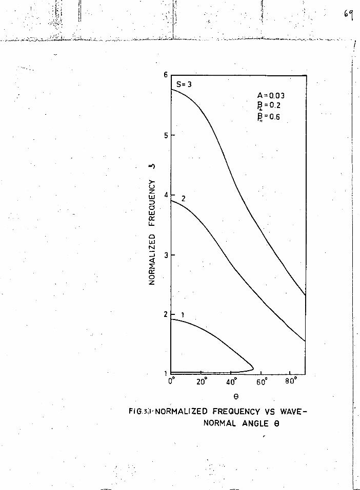
d)

FRE

QU

ENCY

N

ORM

ALI

ZE

D

20° 40°

FIG 5:1-NORMALIZED FREQUENCY VS WAVE- NORMAL ANGLE

8 0°

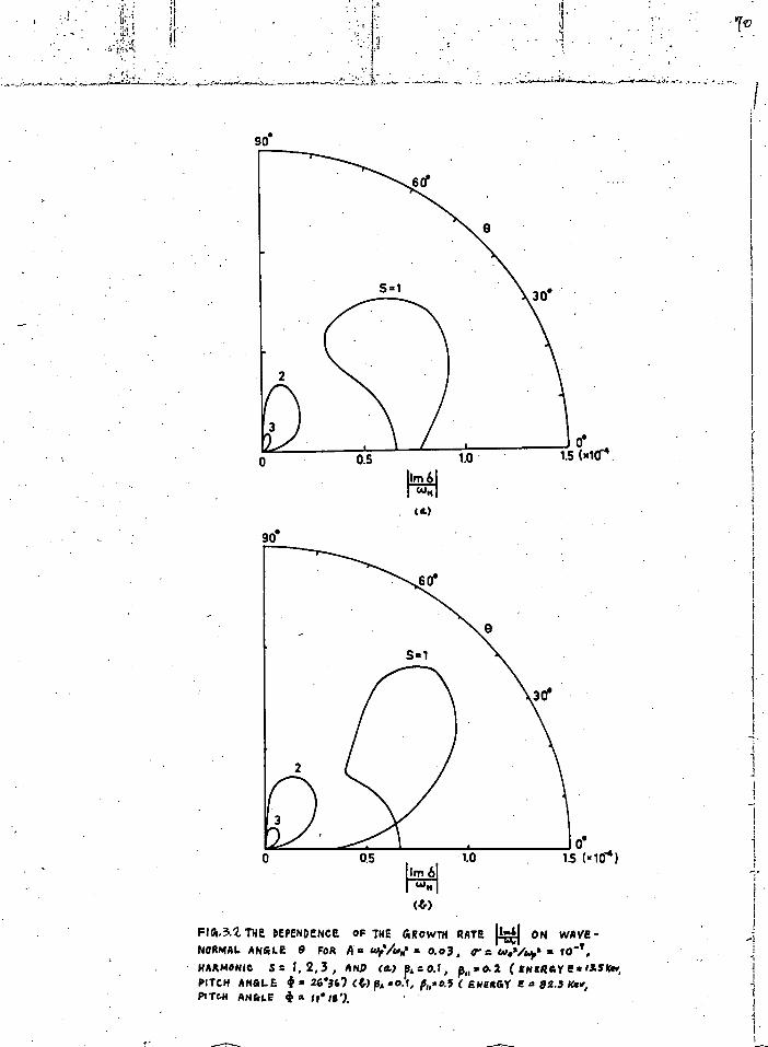
906

0.5 1.0

im

(a)

1.5 (x10-4 ,

'fy

90.

(.er)

FIG1.3.2 THE DEPENDENCE OF THE GRowTH RATE 14 ON WAVE-

NORMAL ANGLE 9 FoR A = WA* o.o3 • e r coo/eio HARMONIC S I. 2, 3 , AND (co ft, r: 0.1 pi, • 0.2 ( EmerRay MSICev, PITCH ANGLE • 26.347 Cf.) pegt5 ( ENERGY E 82.3 Kew, PITcN ANC/LE f1 . /52

„

1.5 0

2.0.(.MF)

:7 1

0.5 1.0 •

o.a. •

(4)

FIG 3.2- THE DEPENDENCE OF THE GROWTH RATE ON WAVE- . 110

NORMAL ANGLE 9. FOR A 2 "%JAI U 0.03, r e.t.Worz = , .

HARMONIC a I, 2, 3 , • AND 0. 5 ( ENERGY E = 47 Key, PITCH ANGLE 27•46)

(413,. 0 , ph =o.G E ER6IY E 150 Ker, PITCH ANELE la .10.

-

10 20

POWER GAIN (db ) ce.)

30

900

10 20 30

POWER GAIN (db ) (4,)

PIG, 3.3 THE DEPENDENCE OF POWER GAIN IN 4 AFTER I *see ON WAVE-NoRMAL ANGLE e FOR A • $01,2/04 = 0.03, r= &Am+. = (04,

HARMONIC s • 1, 2, 3, &YRO- FREQueNcy J = 5 , AND

(0.) =6. p, 0.2 cfr) a 1, f3„= 0.5.

2

4.:

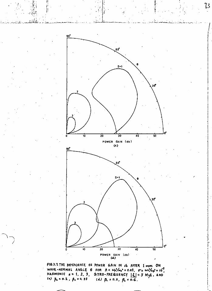
POWER GAIN (db (6 )

10 20 30 40 50

POWER GAIN (db) CA)

go'

906

FIG 3.3 THE DEPENDENCE OD POWER GAIN IN ell) AFTER 1 Inn ON WAVE-NORMAL ANETLE 0 FOR A: cdpViont = 0.03, r= ca/641 = IO HARMONIC a 1, 2, 3, °TYRO-FREQUENCY M , AND (4) p, a o. 2. , p„ = 0. 3S (4) Fs, o. .2, A,= 0. 6 .

1

174-

FIG 3-1-THE RELATION OF THE ANELE OF MAX-IMuM GROWTH RATE

Cc AND THE PITCH ANGLE OF THE STREAM

FOR THE FUNDA -MENTAL RARMONIC, A= 0.03, roe,

co

PI = 0.1, 0.2.

3e 20°

PITCH ANGLE t 30°

03. FIG3.5THE RELATION OF THE PITCH ANGLE OF THE STREAM 47 AND THE CUT-OFF ANGLE 90 FOR THE FUNDAMENTAL HARMONIC,

A= 0.03, 131.x.a1, 0.2.

sd' 55° 60°

CUT-OFF ANGLE 13,

i !

• - :

100 2 0° 30°

so°

40° 500 55° 60°

CUT-OFF ANGLE et F/43.6 THE RELATION OF THE ANGLE OF MAXIMUM GROWTH RATE an

AND THE CUT- OFF ANGLE ec FOR s 1, A = 0.03, AND fil.=

PITCH ANGLE • FI63.7THE DEPENDENCE OF THE 0..ILANTITY em) ON THE pacu ,ANaLE OF THE STREAM FOR

A = 0. 03. 0.1, 0.2.

uo 1.0

-7 (T=10 A =0.03

= 0.1 = 0.5

fl=a2 g=a35

=0.2 =0.6 .■'-',..\

/ : \

. I i S=2 I I 1 \ 1 1 '.I

• 0.5 •••■■•■

• I\ '\ • • • • • • •

1.5 2.0 2.5 3.0 3.5 4.0 0.

1.0

I •

+.1 -

(x10-4 2.0

s=1

1.5

NORMALIZED FREQUENCY 3

FIG 3.8 GROWTH RATE 13m6/wHI VS NORMALIZED FREQUENCY S FOR A= 0.03, Tr-10-7, HARMONIC s =1,2 AND p=o.i, ft---- 0.2; (4.= 0.1, ft=05; poi 0.2, ft=0.35.; pz =0.2., pect6.

10

0 I .

Il

60

S=1

(••=10 A=0.03

1 41 1 =5 Mcdt

p . = 0.l =0.2

11=0.1 13 .z.0.5

g=az 8 =0.35 Ut

= o.1 p =0.6

30

a_ 20

S=2

50

40

NORMALIZED FREQUENCY

FIG 3.9 POWER GAIN IN ell) AFTER I msec VS NORMALIZED FREQUENCY S FOR A = 0.03, oiO, GrYRO— FREQUENCY -7- 5 Meats, HARMONIC s1,2 AND DIFFERENT VELOCITIES AS

INDICATED,

constant refractive index will be normal to H vector

and the final direction of the radiation after

refraction is approximately given by

sin o( = nj sin 0

(3.6)

where oC is the wave-normal angle after refraction.

Consequently, the initially power W(0) radiated by a

single electron will be modified by refraction and

focussing effects in the magnetoactive plasma and the

final distribution of power W(0() will be given by

W(Q) d9 = WO( ) do( (3.7)

do< From the relation of of and 0, it occurs that dO 0( 6, -s 0 for a range of 0 so that the radiation within this range of 0( 15° ) will be confined to a direction

= c4 m46, after refraction. It was assumed that the

greatest amount of power per unit solid angle is emitted

at c4 = nit — ma.% and for other directions there is

negligible radiation. However, we note that the polar

diagram of radiation considered was that for a single

electron. When there is a bunch or stream radiates, it

absorbs radiation, and re-radiates, so that, the polar

plot of radiation may have a different appearance than that

liz

calculated for single electron.

In this chapter, we have found that for the fundamental

harmonic the growth rate u iz;es at Qm where Om ranges

from about 40° to 500 for values of pitch angle, energy

and model of Jovian magnetosphere appropriate to that

suggested by Ellis. In fact, Gra has been found to occur

close tooe mani. so that, after refraction almost all the

radiated energy is concentrated at 0(ni evA . That is, the

angular distribation of tbu radiation used by Ellis would

appear to be justified by the results of the present

investigation.

Prom Fig. 3.9, we observe that the half-power bandwidtb

before refraction ranee from about 0.08 to 0.45 fox

the first harmonic. This result is consistent with the

observed bandwidth. The corresponding bandwidth for the

seaond harmonic is in general a few tiues larger. It should

be remarked that in Pig. 3.6 and 3.9 the range of frequency

excited corresi,onde to different directions. Eowever, as

waves in a cone of about 15 ° centred at Om initially will

be confined to almost one direction (0(Thois) after refraction

in the Jovian magnetosphere, the above estimated bandwidth

is the bandwidth that would bo received.

Among the higher harmonica, the growth rate of the

second harmonic can assume significant values only when

the energy of the electron is high. (It should be noted

that we consider energy greater than 100 Kev. to be high

/in this context. When the energy is exeater thLn several

hundred Zev. synchrotron radiaticrm occurs and the situation

will be different.) Thus, for a more energetic stream, we

may have two bends of frequencies excited simultaneously, .

the ratio of the two centre-frequencies being always less

than 2(^- 1.6) and the second harmonic carrieo less energy

and broader bandwidth. The growth rate for the third

harmonic is seen to be negligible.

Under the above formulation, the growing factor is iSmSit • It is well known that in an aniectropic medium

(e.g. magnetoactive plasma) the directions of the phase

velocity of the wave and the group velocity of the wave

packet do not, in general, 'coincide. A catre packet grows ISr4dt

in the course of time as e ' is moving in sp(Ice along

the direction of the group vep, say,. the z' direction, 1.5n41111Vgf

and will be growing in space as .c a, • Along

the direction of the wave vector r (* direction) the growing factor is

2,-/orx eez ( 4- ) 303 ( 3.8)

where q is the growth rate in space. It can be shown that

(Ginzburg, 1964)

1 z 0( w Ar2rt c 6114)

( 3.9 )

So

S I

Cue then finds that

2A A na. 1 2 (

/..1)(2A.t tz (3.10)

wheren . is given by relation (3.1), D, B ac defined under a

equation (3.2), and E is given by

AO sin4 2 cos

2Q (1 . 2A )(1 _111_ )

s4

Knowing the growth rate in title, we can thus calculate

the growth in space readily.

If we assume that the density of the helical electron

stream causing Jupiter's burst radiation is the same as that

observed in the terrestrial magnetosphere, namely, 10 -4/cm 3 ,

and the density of the background plasma to be of the order

of 10 3/em as estinated by Ellis and ijcCulloch, we can then

estimate roughly what magnitude of power gain is needed in

order to account for the high flux intensity observed on the -

Larth —10 21 watts 11 -2/(c/a) for frequency 5 inWs.

Let US suppose that for a particular frequency the radiating part of the Stream has a cross-sectional area of

10 5 011 2 and a length of 600:Kn. Total 'number of electrons

radiating is then 6 y 104 With the knowledge of the order

of magnitude of ISnll the maximum power gain after an

interaction length of 600 Km. can be calculated from relation

for the fundamental harmonic radiation (f fm ): 2

(3.10) and it is found to be of the order of le. The

maiimum power radiated by a single electron for a frequenoy

of 5 Ws in the forward x-mode is about 4 x 10 -21 watts/

sterad. Confining radiation to a solid cone of 15 the

total power radiated by the stream for a particular

frequency after amplification is about 6 x 10 watts. It

has been pointed out that the power radiated initially in

a range of 15° will be confined to about 1 ° after focussing

in the ionized medium. For a frequency 5 20/a, the

theoretical flux density received on the Earth will be of

the order of 10-21

watts

The above estimate indicates that in order to produce

the observed high intensity of radiation, the interaction

distance needed is ^- 600 Km or alternatively the inter-

acticn time needed is < 10 msec.

Finally, we note that with a model of Jovian magneto-

sphere as set out by Ellis (A ranges from 1.6 x 1.0 -3 to -z 9 x 10 ), the value of X at the source region is small

A

3 - 1.6 10 — 9 x 10

With such small values of X, the harmonic resonance

absorption for the x-mode is small unless G is very

large (0 > 70°, say), while that for the o-mode is

entirely negligible (Gershman, 1960). since the radiation

power for the x-mede is about one to two orders of magnitude

larger than that of the o-mode, the radiation received will

be predominant in the x-mode in this case. here, of course,

the source position for a particular frequency must be

situated above the reflection level X= 1 . Y in order that

the radiation may escape.

4'The basic concept of harmonic resonance absorption is

discussed in chapters I nd VIII.

CHAPTER IV

THE ORIGIN OF VLF DISCRETE ELIS'0IONS

IN THE TERRESTRIAL EXCSFUERE

(A) Review

Very Low Freqeunoy emissions which are believed to

be generated in the terrestrial exosphere, have caused

great excitement in the past ten years (e.g. Watts, 1957i

Gallet, 1959; Ellis, 1960; Helliwell and Carpenter, 1961;

Dowden, 1964 Harang and Larsen, 1965) 4% These emissions

are generally classified into two main types, the quasi-

continuous or continuous type which is wide-band noise

lasting for hours and the discrete emissions which are

short-lived (with a duration of about one second), narrow-

banded and have reproducible frequency-time variations.

The study in this chapter will be centred on the discrete

type. Dowden (1962a, 1962b) suggested that discrete

emissions, in particular the "Hooks", are produced by

backward Doppler-shifted cyclotron radiation from electron

These papers describe observations of VLF emissions only.

gf-

bunches travelling along field lines in the terrestrial

exosphere. On the assumption of strict longitudinal emission (19 = 180° ), Dowden calculated dynamic spectra which Showed

good agreement with those observed. Later, Hansen (1963) investigated Dowden's theory and found that the calculated theoretical dynamic spectra of Hooks can generally explain

the observed frequency-time shape. However, she pointed out

that many Hooks are triggered by whistlers and produced an interaction mechanism to explain the triggering process. The disorepencies between observed and theoretical dynamic

spectra are also accounted for qualitatively by the resonance

mechanism. Another similar resonance process to explain

-triggered emissions is produced by Brice (1963). Helliwell

(1963) observed whilstler-triggered periodic VLF emissions in

several stations. lie found from the observational data that

a sequence of emissions is initiated, or triggered by a whistler

and the period between emissions is the same as the Whistler-

mode echoing period at some frequency within the range of the

emission. To explain these results it is proposed that the

triggering of the emissions is controlled by packets of electro-

magnetic waves echoing in the whistler node. In this triggering

hypothesis it is supposed that the wave packets act to organize

temporarily the particles in existing streams of charge, so that,

their radiation is coherent. Brice (1964) studied the founds-

mentals of the wave-electron interaction process and found that

energy can be transferred between a wave-packet and an

electron gyrating in resonance with the wave when they

propagate in opposite directions". Even though the

non-triggered emissions may be caused by cyclotron

radiation from helical streams or small bunches and that

the triggered emissions may be explained by the inter-

action or resonance process, three problems still remain

unsolved: •

(i) In all the existing radiation and interaction

theories for explaining Yid emissions, it has been

assumed, without any justification, that the emission

angle is 100. Since a gyrating electron emits

• cyclotron radiation in all directions and the wave-

particle interaction process does not necessarily

occur only along the field line direction, we need

to investigate the validity of the longitudinal

propagation assumption.

(ii) since a vide range of Doppler frequencies is radiated

by a single electron at any instant, a process which

has a frequency selective effect must exist, in order

to explain the very narrow band structure of discrete emissions.

+However, he did not clarify the direction of the process,

i.e. under what conditions energy io transferred from wave

to particle and vice versa.

(iii) The quantitative explanation of the high intensity

received 10-1° watts mi l/(c/s) at the base of

the exosphere).

Before we solve these three problems, we will

first of all analyse numerically the excitation process

of normal backward Doppler-shifted cyclotron, waves in a

stream-plasma system for general (4 which has been derived

in the-last chapterIL ance the bandwidth of discrete

emissions is so narrow, the radiating stream must be

very close to helical: )11or simplicity in calculation,

the discussion in section (5) is carried outlander the

assumption that the stream is strictly helical.

It should be remarked that besides the three

mentioned problems, the explanations for the origin of

triggered "emissions van by Eelliwell (1964), Brice

(1964), and, Bell and Duneman (1964) have been incomplete

and sometimes confusings this respect will be discussed

in section (C).

(B) Excitation of Backwasulemrphifted Cyclotron

Radiation in a t1:24petoactive

Blectron stream

In this investiion the particle density in the

stroa is assumed to be very small compared with that

in tile backgFigund plasna an4 only the fundamental

harmonic is considered+. The collisionleas Appletan-Hartree

equation for the whistler mode is assumed to be applicable

to the propagation of electromagnetic waves in the background plasma alone:

A (loos 01- )

With the definition of :4 given by (4.1), relation (3.2) is

sislplified into

I ces wrVEAPH (lccra, st i — 1) 2'

(4.2)

The dispersion equation for the helical-stream-plasma

system now reads

+di =0 (4 .3)

cr 3.1 2' A (3112- Co.22 e (T-1)1

^1- 13111

where . b =

+ s asSumption is valid due to (i) The radiated frequency

must be smaller than J f Hleo that the wave will not be trapped

at the resonance region f (ii) 'or high harmonic

number, the growth factor is found to be small.

38

(4.1)

with =

sin't))1 1,. Ji pi. 4- K2. )

1

I ce2.e 1

_ d_

It should be noted that in the expression for d we have

negleoted the term 5:;14 • This approximation is valid in

ease of VW emissions 171 the terrestrial upper atmosphere.

The rate of growth, being repreeented by the dimensionless S quantity ,34-.:7), oan readily be solved fro la (4.3):

((ii (c) —r ( (4.4)

where M = /d2 3

b 3 *

_ _2 pi In the partioul,,r case = 180°, b 0, d = LAIG

4%)

and we get (c7422-- I )13 I s S1= 4 2.. ( rf.A. I (4.5)

This result agree with that found by Zheleenyakov (1960a) for this ease.

We nOW evaluate the growth rate for 3eneral 0, for

parameters appropriate to VLP emissions in the terrestrial

exosphere. .

To solve for the characteristic frequencyw we have

to solve Appleton-Rartree equation (i.e. equation (4.1))

and Doppler equation -a- -41 14141=0 simultaneously.

Fig. 4.1 gives an example of the graph ois u4/141

againot wave-normal an:7:1e O. The parameter is transverse

velocity pl and each line represents a particular value of longitudinal velocity 13,, ; we repeat this for two values of

A = 041/04IL = 25, 100 which May be considered as a

quantity specifying the ambient plasma. We can also take

the quantity 151m(WIA41)1 to specify the growth rate. 13m( 14)1

is plotted against wave-normal angle 9 in Fig. 4.2 for -7 e = density of stream/density of ambient plasma = 1 X 10 ,

for various values of .A, pi and Let Po be the power of

the electromagnetic wave at time t = 0, and P be the

power rfter 0.016 second. Pig. 4.5 shows graphs of the power

gain in 0.016 second against wave-normal aaLlle 0 for growth

rates sbown in rig. 4.2. The electron aro-frequency is

taken to bel fHl = 1 (4 /271 ,= 10 Ws. Corresponding to

Pig. 4.3, the power gain after 0.016 second is also plotted

against the excited frequency normalized to the gyro-frequency

in Pig. 4.4. An the growth rate maximizes Rt 9 = 1600, the

"open end" point of eachcurve in lig. 4.4 given um the

frequency excited and the power Cain of the electromagnetic,

wave when the wave-no u. m5le is 1800 . The small circle

on each curve indicates the frequency and power gain for

0 = 150° . The narrow bandwidth of the radiation inplied

by Pig. 4.4 is illuotrated more clearly in Fig. 4.5.

From the analysis of the dispersion equaticn for whistler-

mode waves, we observe that:

(i) The growth rate matimizec at 0 = leo° .

(ii) Sinee the frequeacj is almost constant for a range of

wave-normal angles (ebaut 1800 - 1500) in most cases,

in particular for large pitch angleo, the excitation

theory indicate thcA for large pitch angles, the very

narrow band of frequencieo (theoretical bandwidth

< 0.01(A) when one considers the half-power bandwidth

in Fig. 4.5) emitted with 0 betaeen about 1800 and

1500 may be excited a much greater extent than other

frequencies, resulting in a frequency selective effect.

(iii)For constant energy of radiating electron, the larger

the pitch angle, the greater the radiation power.

(C) Discussions

e have obtained the radiation characteristics of a

stream-plasma eyetem. It is interesting to compare this

result with the power spectrum radiated by a single electron.

Mer]ohn (1965) icas corrected Lidman's equation (Bidman, 1958)

0.5

Aio

- 41

.4••••t

180° 140°

Fig. 4.1 Normalized wave frequency ; vs wave-normal

angle e with p, as parameter for .two cases: A 25, 100.

1 00° 4

°fa

o'=10-7

11 =0.2 A=25 A=100 ------

5

1

180°

3

Pig. 4.2 Dependence of the growth rate 1.51%S/cot-I on wave-ncrnal angle e for a- = 16 T, A = 25, 100 and

p„ = 0.1, 0.3, 0.5 A, v.. 0.1, 0.3, 0.5 (31, = 0.1 1; 0.3.

(a) f3. = 0.2; (b) 12, = 0.4; (o) L = 0.6;

F.;3. 4. 2 ""

14e loe 1 8 0°

F1.4. 2. (-e-)

-;.

cr =10-7 R. =0.6 A = 25 A = 100 OM. =1. MI WI MO •

=0.1

0.1

• • • • • • • • • • • • • • •

• • •

• ••• • • • 0.3 .•

•

• • • • • • • • • • • •

x10

180°

140°

-

5.4. 2(c)

(a)

Fig. 4.3 Dependence of the power gain P/P0

after 0.016 sec. on wave-normal angle 0 for

cr- = 10-7 15d= 10 Kc/e, A= 25, 100 and

(a)pl . 0.2; = 0.1, 0.3, 0.5 (b) = 0,4; /3 = 0.1, 0.3, 0.5

(c) (34, = pH = 0.1, 0.3.

6/6

140° 0

180° 100°

F:3 .4.3C-er) /7

= 0.1

.... . 0.3 . . . . - 4 . . _ \

O. • . , , .. . s N.% I e t t # 10 ,..., t . s a. I , I , a .

. 8 i

s s .

. 0 I • • I ••

. I I • I • dr I I

•* .. • • .5*

I • I •

I o o # I • .

v / • • .0'.... •

0.3

al•

0 1

POW

ER

GAIN

01 0.3

NORMALIZED FREQUENCY S

Pig. 4.4 Power gain P/P 0 after 0.016 sec. vs norma-

lized wave frequency for cr= 10 „O fd= 10 Ke/s

A = 25, 100 and

(a)f 0.2; f3u = 0.1, 0.3, 0.5

(b) = 0.4; pa = 0.1, 0.3, 0.5 (0) j3 0.6; ig n = 0.1, 0.3.

The little circle on each curve indicates the frequency emttted at e = 1500.

0.5

F• 44(1')

0.1 0.3 0.5

104

o 102

ce

NORMA LI ZED 17 11EQUE) IV(

0.1 0.3 0.5

106

0.5 0.1

0.3 •

0.3 I Ii I I I II II I

I I I I I It

0.1

NORMALIZED F. R.EO.UENCY Fig. 4.5 Power gain P/P o after 0.016 sec. as a function

of normalized wave frequency , indicating the narrow

band structure of the growing wave. The parameters are

the same as in Fig. 4.4(c).

te,3

(which gives the power spectrum radiated a single electron

gyrating in a mkmetcactive plasma) and evaluated the

radiation pattern from a single electron (energy = 10 Key.

and 1,000 Key.) for parameters appropriate to the lower

exosphere 5). His result indicates that the maximum

power occurs at about 110° and the wave propagating along

the field line carries minimum power. however, it should be

pointed out that Liemohn has taken a pitch angle of 30 0

( 0 = arc tan EA ) for the radiating electron whereas Dowden Po

(1962d) measured from experimental data that the pitch angle

of the source electrons generating a Hook is generally large,

being grepter than 60° in most cases. Using the appropriate

value of A in the exosphere (A = 25) and fixing A, for the

helical stream to be 0.4, we show in Fig. 4.6 the power • spectrum radiated, by a single electron for different values

of 13„ . 4e observe that for large value of Ned and, hence, large pitch angle $ t the power is lexge and maximizes at 1800,

As the pitch angle decreasea, the emission angle corresponding

to maximtm power shifts rapidly away fron the field line.

The result of the instability theory, together c.ith the

radiation pattern of single electron, indicates that the

assumption of lon6itudinal propagation (as taken by previous

VI& workers) is fortunately correct, and thus, the first

problem is solved.

Me frequency selective effect has been explained by the

(o4

Fig. 4.6 . Power spectrum radiated by a single electron

for various values of energy (specified by /3 , (3u ) and pitch angle for A = (AWL411;1 = 25. The dotted parts

indiCate that4 refractive index is greater than 20.

result in section (B). Assuming a strict helical stream,

the theory shows that a bandwidth smaller than 0.01 f is

possible. This result, which Is consistent with observation, suggests that the radiating stream is in fact very much close

to helical. The existence of a small finite temperature in

the stream will result a relatively broader bandwidth, which

is observed in rare cases. The second problem, hence, has

been accounted for.

Assume the cross.seotional area of the stream and the

ionized column to be

ts61 — 10 2 Kiti 2 (4.6)

at the equatorial plane. Suppose the length of the part of the stream radiating a particular frequency (in this oase

the minimum frequency of a Rook f0 ) to be

.6 $ 10 Km (4.7)

Let the particle density of the stream to be 10 -4. elicm3

and that of the background plasma to be 100 el/cm, giving -6 0' = 10'. Then the number of radiating electrons in a

volume bounded by area A and length L is s

6 x 10 • (4 .8)

It has been found that in the ionosphere and exosphere the

ray direction of a whistler mode wave is guided along the

field line (e.g. Budden, 1961). We may, therefor*, assume

that all the electromagnetice energy radiated in the is co.hca.trautt &11O $44. • ,

ionized column,Aiemohn, 1965), The cross-sectional area

of the ionized tube at the base of the magnetosphere is 1 estimated to be -or that at the equatorial plane

(expression (4.6)). Now if each radiating electron emiti

a power of 10 -30 watts/(c/s) (Liemohn, 1965), the power

flux received at the base of the magnetosphere is

P -- 6 )( 10 watts m /(o/s) (4.9)

• Since the observed value of power flux at the base of -10

the magnetosphere is of the order of 10 watts

(Dowden, 19620, we need a power gain of the order

p 1010 (4.10)

Using the method as described in section (B), the

interaction time needed for this value of power gain is

-- 25 msec., if the pitch angle of the stream is greater

than 500 and the energy of each electron is of the order of

100 Key. We note that for longitudinal propagation, the

wave and ray directions coincide. If the refractive index

for the whistler wave is taken to be 15, the wave will take

30 meets. to travel a distance of 6 X 10 Km. We will, .

thus, conclude that with the assumed values of stream

density and interaction time, the high intensity of VLF

emissions can readily be explained quantitatively with the

result of the instability theory the third problem has

been dealt with.

ib(,

(07

From the existing interaotion theories, it seems that

it has not been realized that in fact there are In

interaction processes taking place in steps. We can understand the above statement readily with the knowledge

of chapter

We have discussed briefly the possibility of excitation

and damping of oyclotron waves; the controlling factor is the distribution function of the electron stream. When the electron stream has a very wide momentum spread or when the

stream is absent (leaving a "%mein= background plasma),

part of the energy of the propagating electromagnetic waves

are absorbed by the medium and particles are accelerated.

This process is called harmonio resonance absorption (section

(D) of chapter II). Consequently, when an electron stream of

high temperature encounters a strong whistler signal (either

a whistler or an artificial whistler-mode code signal), the

macroscopic absorption is positive and in average l energy is

fed from the wave to the particles such that some particles

will gyrate in phase with the wave; this process is in fact

the harmonic resonance absorption mechanism. The affected

particles, being organised, form a stream which is close to

helical. The particles in this stream emit cyclotron

radiation continuously as they have always been, but now the

stream-plasma system becomes radiatively unstable and the

waves radiated by the cyclotron mechanism will grow as a

tog

function of time (absorption is negative). After some

interaction time, the waves acquiring sufficiently large

amplitude, are received as triggered VLF emissions. As

the stream radiates, the interaction process sustains for

some time, while the energy of the electrons is decreasing

(causing an increase in p. 11 and a larger decrease in RI, ),

until the distribution function of the stream is far from

helical and the radiation is insignificant to be observed.

When the echo of the previous triggering whittler signal

encounters the stream again, the two interaction processes

repeat and we may receive triggered periodic VLF emissions.

It has been found that VLF discrete emissions can

readily be triggered by artificial Whistler-mode signals of

single frequency when the signal Is long enough * (Helliwell,

1964)* In average, the time interval between the leading

edge of the transmitted signal and the commencement of a

triggered emission is 100 msec. Based on our previous

estimated interaction time for the excitation process

(-, 25 msec.), we see that the interaction time for the

organising process (harmonic resonance absorption) is

When the duration of the transmitted signal is 45 lasso.

(a dot) no triggered emissions are observed. If the

' transmitted signal lasts for 145 mseo. (a dash) VLF discrete

emission are triggered in most cases.

is "1 75 msec. We mast note that our estimation has been

crude and our instability theory is a linearized one.

When nonlinear effects come into being (which will be the

realistic case), the growth rate will be smaller and the

interaction time needed will be larger than our previously

calculated values. We can only state here that the inter-

action times for both processes are of the same order of

magnitude, being equal to several tens of wee.

During magnetic disturbed periods, energetic electrons

are dumped from the radiation belts to the exosphere. Those

electrons travelling with about the same velocity and same

direction will farm a stream with very narrow momentum

spread. Non-triggered VLF discrete emissions will be

radiated and excited in the same manner as described before

in such a stream-plasma system.

With the results of the investigation in this chapter,

we conclude here that the three existing problems mentioned

are solved and the origins of both non-triggered and triggered

emissions are explained.

+Since the received intesnity is almost constant during the

duration of an event (a Hook, say), the unstable stream-plasma

system must have come to an equilibrium situation; this will

be the case only when nonlinear effects occur.

01,1AP2kia V

A REVIEU OP2 ii -IELOOkari] OP SOLAR TYP4 I NOM STOR1]

(A) Solar Radio amissions (e *g * Eux444 1964)

Radio emiesions from the Sun come from both thermal

and nonthermal sourcee. The thermal emission can be

separated into two components:

(1) The quiet San component which originates from the

solar atmosphere at temperatures of the order of 4 u 0 K (chromosphere) and 10 6 K (corona) and is

the radiation which still oocurs in the absence of

localised sources in the atmosphere of the Sun.

(2) The slowly varying component which arises in high

density regions of the corona (called condensations)

with temperature of about 2)(10 6 ° KJ these regions

exist over sunspots and plage regions.

The nonthermal emissions, which consist of wide-band and

narrow-band radio bursts, are generally associated with

solar flares or sunspots. They originate from all levels

of the solar atmosphere between the lower chromosphere

(millimetre and centimetre waves) and the outer corona

to heights of several solar radii (metre and decametric

waves)* The equivalent brightness temperature of the

110

source in these emissions can be as high as 10 11° X. Such nonthermal burst emissions an metre waves are characterised by great variety and complexity; based

on their spectral characteristics, they are olassified

as types I, II, III, IV and V. Wild, Smerd and Weiss

(1963) have summarized their characteristics, geophysical associations and probable mechanisms of generation (Table 5.1).

(B) Attij_itictiot&p_e_j_a_dele( .1_Chara aorms

During solar disturbed periods, the most common radio events on metre waves are the oocurrences of

type / radio emissions or type I "noise storms". This

type of radiation consists of a slowly varying, broad.

band emission (called "background continuum") lasting

even up to hours or days, on which are superimposed

series of intense narrow-band, short-lived bursts (called

"storm bursts"). Some exauples of dynamic spectra and

single" frequency records of noise storms are shown in

Pig. 5.1. The radiation is usually strongly circularly

polarized and its occurrence is always associated with

a sunspot Group, Even though this common nonthermal

radiation has been observed since 1942 (e.g. ney, 1946;

Ryle and Vonberg, 1946; Wartyn, 1946; Pawsey, 1950), the

III

Table 5-1

CHARACTERISTICS OF METRE-WAVE BURSTS ( W;Lci 5 'nerd & Weiss, 1943)

Type of burst

Circular polari- zation

Tentative identification

of mode Duration Variability

Apparent angular size (min of arc)

Height of source above photosphere

Cone of emission

Tentative identification Relationship with other phenomena

Exciting agency Emission process

II None — 5-30 min Complex 6-12 0.2-1.0 Roll Wide Ascending shock front vel --10.1 km/sec

Plasma Solar protons. geo-magnetic storms

_

III None or partial

? Burst: --, 10s Group:

Group of simple bursts

3-12a 0.2-2.0 Roa Wide Ascending elec- tron stream vel •••-,c/2

Plasma Initial expansion of flare

,---.1 min

V Weak ? ---, 1 min Smooth" Similar to Similar to Wide? Same as III ? Same as III III .III

IV mA (moving)

Weak Extraordinary 10 min- 2 hr

Smooth 6-12 0.5-5 R(D ascending at speeds ^-103 km/sec

Wide Electrons trapped in expelled plasma

Synchro-troll

Solar protons, geo-magnetic storms

IV m lib (stationary)

Strong Ordinary Few lirs to days

Slow van- ations with some fine structure

3-6a 0.2-1 .0 Roa Narrow Descending elec- tron stream trapped in field

Plasma Synchro-troll?

i

I Strong Ordinary Burst: Slow Burst: 1-6 0. 2-1.0Roa Narrow? ? Plasma? —Is Storm: few hrs to days

Storm centre 5-10a

Synchro-tron?

Increase with X. b Includes continuum storms.

Ti me (minutes) 5 10

, 15 20

II I . I —L— 1 I--- I I L-

, 41. -

•r?"413&,* ._4••• •P"se. Irr■Iiinvitp•

(a)

MINUTES

F3

90 -

•••1411144■••••• ••••111440■■••••••• ' 180-

580-

(b

F. 5.1 Some dynamic spectrum records of storm bursts (O.) ;r1 the 2g — 210 lick

range (Wild et at, 1963) and (b) in the. 100-680 &Is range. (kundu, 1964).

Ssoc. ZERO LEVEL

1057, 007.11

07.51

4t ()Ulf 7 SUN

(c

‘JvAif • 3 see. 7 ZERO LEVEL 1958, JUL Y 5 15.29 if OWE , SUN

(c) Examples of h;511-sreed s;n5le 5re3uenaj record a,t ZOO ("Ids (Fokker, 1961).

250

200

3

X 150

I . o 100

0

Z 50

theoretical interpretations of this cozplex phenomemmm so

far published have been unsatisfactory. Before we put

forward a theory to explain this type of solar emission,

we will summarize the importaat observed featureu below:

(1) Frequency Range

Uormally the frequency range lies between 50 Va/s

and 300 2C/a for background continuum radiation, but

for bursts, it is shorter. however, a frequency as

low as 6 L:c/s and as hith as 400 Pc/s has been observed

in rare cases (e.g. Fokker, 1961; Kundu, 1964).

(2) Bandwidth

The bandwidth of background continuum radiation

usually extends to 100 Lois while that of a burst is

very narrow, typically around 4 Ec/s (Payne-Goott,

Yabsley and Dolton, 1947; Ryle end Vonberg, 1948; Wild,

1951; Elgarog', 1961; see Pig. 5.2). Rowevor, wide-band

bursts having bandwidths up to 35 Ec/a have been observed

less frequently (Vitkevich and Gorelova 1961).

"4 4

a 10 • II 3 4 5 6 7 B 9 BANDWIDTH (M2/92

Fig. 5.2—Histogram showing the distribution of recorded storm bu'rete with bandwidth. ( Mici,1 9 51 )

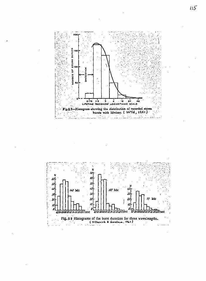
200-

O•75 1.5 3 6 • 12 24 48 LIFETIME (SECONDS) LOGARITmmIC SCALE .• •

Fig.53--I(istograrn.showing the distribution of recorded storm bursts with lifetime. C WI4, ii El )

•

• 70 -

• • SO 60-

50 — SO- N

/40 Mc 40- 40/07 Mc • 40

JO JO- JO — 1 — — —

— — 7

.20 28- 1 ZO 77 Mc

' /0— --- tO - ! 10 4-

0 i 0- -h-1..,_ Olia501111/2141511ZOrsec ant osama a riliZorsec

o a a4010110121415182Orsec

• Fig. 5.3 Histograms of the burst duration for three wavelengths. . ( val.ev;c11 Si Giovele.va.., 19I)

"5"

(3) Duration

When a noise storm is in progress, the spectrum

shows a Slowly- varying wide-band steady level lasting

for hours or days. Above this continuum emission, short-

lived bursts appear; the duration ranges from some tenths

of a second to several seconds (Pig. 5.3).

(4) Frequency Drift of Bursts

In most cases, the mid.drequency of a burst stays

constant (Wild, 1951; Vitkevich and Gorelova, 1961;

Fig. 5.4). However, high epeed sweep-frequency records

of Elgaroy (1961) indicates that sometimes the frequency

of a burst can increase or deorcase in the course of

tine and the drift velocities ranze from 1 flap per

second up tp tens of flo/e per second (see also work of

Vitkevich and Gorelova, 1961). tioreover, some "U.-bursts"

:(in a event of a burst the frequency firstly .decreases

and than increases or vice verge) occur at tires. *

Pig. 5.5 Elves some examples of such events. MC I$O

145 CD:. CD CD Ca= /40 cs (Cft) a+ 0o. 0 a)c.c. cxxcip

41.5 (=Cicog=5) azO aCtr-9> c0• cp 00

I 13 0 0 (0 00 CZD 4 CZ)00 (a0 0 CC:00 C, Ce Q. 0 C:=) ... . . • , • • , •

/far, S 10 /520 25, JO ..75 40 4550 SS t, sec

Fig. 5.4 Dynamic spectrum of narrow-band and wide-

band bursts. (Vitkevich and Gorelova, 1961).

+There is also the possibility that the U.bursts are some

particular oases of type III bursts.

.111140.000100000.0 440r OW to* 'I" 4t 1 4gre rt iilI4M110011 -

•

I SEC

Fici. ES Some sweep-frecrencj records o .f storm bursts in the NO - 2.15- rids ronije (El9aro/, 1960.

(5) Relation between the Occurrence of Background Continuum

and that of Storm Bursts

(1) There is good general daily correlation between

the occurrences of the two components (Fokker, 1961).

However, during some periods- a strong continuum

radiation is detected with Mb appreciable buret

emission, and vice versa (Wild, 1951),

(ii) There is no apparent correspondenoe between the

integrated •spectrum of bursts and the observed

spectrum of continuum radiation (Wild, 1951;

Fokker, 1961). However, as pointed out by Wild,

by postulating a suitable amplitude distribution

of the bursts (i.e.. a suitable relationship between

the amplitude 0 of individual bursts and the

occurrence probability of a burst of amplitude

between A and A + dA occurring in unit time), With

the shape of the distribution being allowed to

change *lolly with time, the integrated spectrum

of bursts may approach the observed speotrum of

continuum radiation.

(6) Polarization (Suzuki, 1961; Kai, 1962)

(i) Referring to the magnetic polarity of the stronger

+A denotes the maximum amplitude reached at a particular frequency by an individual buret.

member (normally the proceeding spot) of a sunspot

group, in most cases, the polarization of both back

ground continuum and bursts corresponds to the

ordinary *ode radiation in the magneto.ionic theory.

The sense of polarization of both storm bursts and

baokground continuum at an instant during a noise

storm are the slum.

(11) The majority of storm bursts are °lose to one hundred

per cent eireularly polarized. However, sometimes

there are noise storms being composed of partially

polarized, mixed polarized, or completely =polarized

bursts. A partially .polarized storm may occur

sporadically near the solar disk centre between days

of completelY.polarized , stormo .but it occurs very

.often near the lumb. This situation is indicated in

Pig. 5.6. There is also a tendency that the peroentage

polarisation, of the storm correlating to one spot

- group decreases rather suddenly at the limb. Pig. 5.7

shows some single•frequency records for various degrees

of polarization. Note that there are threo sources

(situated at 0.1E, 0.6E and 1.5W radii on the solar

disc) in the event observed by Hai.

• • -

fi. ,

-;?

-7, izo 100

R+

••■•

50—

201 Mc

.••••

o0

r+ 50—

41.

50— ■Im

0 E L5 R o 1.0 0.5 0 0.5 1.0 1.5 RE) W

Fig.5-.6 Distribution of the polarized noise storms on the solar surface. Three groups of noise storms are given according to the degree of polarization.

R, L — Stvo11 ipstko.A4 , c ■rculavIl polar;rd respectvely

r, 1. — part:alf, rihthavt4 leftkand crculizvl j folatled vosrectivell

N Ct - pola 4.3,ed

S1i3u.k: , 1941 )

•

tit

0133U :T. 0134 0135

0256 0255 0254 ILL

\ / I.3W 0.1 E (C

/ \ 1 \

L. W Compound I /

/ / \ 0;1 1 Q6E -).11

NOV. 18,1959.

20 1 M c/s

(b) NOV. 21,1959

Fig. 5.7 Records for the unpolarized land polarized storm bursts on Nov. 18 and 21, 1959.

( Ste .rk, 190)

R

0224

FIG. 5.7 An example of a limb event (Mar. 23, 1989). The upper record is the rigit-handed polarized component and the lower one the left-handed component. The number indicates the position of a source. C K a., 6 2.)

200 Mei: 0225 0226 0227 0 228 " U .T.

(7) Apparent Source Positions (Suzuki, 1961; Fokker, 1961;

Kai, 1962)

The experimental result on apparent storms centres,

as observed on earth with respect to the position on the , solar disc, indicates that . the number of occurrence of

noise storms decreases from the central meridian towards

the limb (Pig. 5,0, This means that the storm radiation

A HIGHER BURST ACTIVITY

—20

cc C/).. CO

V)

CO

- 0 Ce w

=

z •

1.5 1.0 • 0.5 0.5 1.0 1.5 RoW

•

. 5.8. East west clistr;64tior. o Noise StormS ( . 5 1 9 6t).

has a narrow directivity. Moreover, the concentration

of the noise storms is biased to the west, in contrast

to the east predominancy of type III bursts (Wild,

Sheridan and Neylan, 1959), During a storm both bursts

and background continuum are normally observed to come

122.

r

1 ••

I .

123

from the same source which has the size of 4 sunspot. To

measure positions of bursts. Suzuki (1961) and Kai (1962)

used multiphase interferometers whose accuracy in absolute

position measurement is about 1. arc. One of such records

is shown in Fig. 5.9 Where the positions of sunspots and

the instantaneous positions (circles) of storm bursts on

200 Mc/s in the course of a noise storm are indicated. The

dotted line gives the centrold position of the background

continuum and the line marked "transit' indicates the true

local noon time.

Prom interferometric observations. Fokker (1961)

measured the source positions of 255 and 169 Ws near the

limb and found that the source position .for 169 Mae is

situated systematically higher than the source for 255 Mae

(M. 5.10). The source positions for the two frequencies

near the centre of the disc were found, homer, to be more

or less coincide. Since the source has a finite size, this

result is understandable when one considers the difference

in visibility. In, general. the 'obierved frequency of a noise

storm decreases with increasing apparent source height.

Morimoto and Kai (1961) investigated statistically

the hkights of type I bursts on 200 Mo/s from a comparison

of the apparent positions of bursts with those of the

corresponding optical phenomena (sunspots). The mean height

of the source was faane to be about 0.2 i (Ro = solar o radius) above the photosphere near the centre of the

disc . and to increase towards the limb (Pig. 5.11). A

number of workers (e.g. Hunda, 1964) have saggested

that this effect may be due to the fact that the height

of the reflection. level increases from centre to lib.

Elost storm centres are not situated exactly radially

with respect to the optical centres of the leading spots,

but are not far away. froz them (Ealinge, 1963).

The averaGe altitude of the apparent source for a

particular frequency is observed to be higher for the

unpoiarized storms than that of the polarized ones.

ierhaps the most interesting resat in position

observation is that storm centres are located near, but

slightly above, the correarendinG plasma levels (kundu,

1964; Weies, 1965).

(8) Association of Occurrence of Eloise Storms with Solar Plare

and Sunspots

(1) Post noise storms are redeived Aithin two hours after

the occurrence of a flare and the most probable .

delay time between noise storms and flares is found

to be approximately 30 min. (Pig. 5.12). however,

simultaneous occurrence of a noise storm and a flare

4 !

123-

U T 0130

0200

0230

0300

0330

044 o • o •

o cbo

o 0

• • ico

centroic1

I

ba.ckrovi copti.m.

c/o

1:0 0.5 b 1.0 Ro FIG. 5.9 Jan. 12, 1960. Each circle represents a instantaneous position of type

I burst, and broken line represents that of the associating continuum. Individual bursts are completely polarized, while the continuum is partially polarized (80-90 %). The sense of polarization is the same both for burst and continuum. ( Kai, 1962 )

z

lb. ;SS

• $

195Z JUNE IS

255 169

1957. AUG. 6

255 169

1957. SEPT.13

F.'

169 255

Fi9 . 5.1o. Source positions of 255 and 169 Mots radiotion viea.r the

The straLlkt lines indicate the source fosi,tions and. tke dots

YeFresent the positlons of 5 Loispot 9r0aps aprearin, at the ti me .

( Fokker, 196 1 )

Fig. 5.11 Centre-to-limb variation of average height

of type I bursts. Dots and circles correspond to type

I and type III bursts respectively. Dashed curve

represents the computed variation of height of turning

point (reflection point) on 200 Mc/s for the Baumbach- ----

Allen corona. Solid curve represents the same for a

model with ten times the electron density given by the

Baumbach-Allen model (Morimoto and Kai, 1961).

80

50

20

I. -6 -4 -2

j . 1 2 4 Hours

Fig. 5.12 Superposed-epoch diagram of the start of noise

storms with respect to the start of optical flares (Malinge,

1963).

has been observed (Fokker, 1961; 41d, 1951;

see Pig. 5.13).

(ii) Voise storms are always associated with sun

spots-group when the maximum area of the group

is greater than about 6x10 the solar disc

and when the maximum area of the largest spot

in the group is greater than about 4 x 10-4

of

the solar disc. Per sunspots of areas greater

than 7,5 l0 the solar disc, the probability

of association between the occurrence of noise

storms and sunspots increases with the maximum

magnetic field strength associated with the spots

(Ualinge, 1963; Payn..Soott and Little, 1951).

(0) Angular Size of Apparent orm Centres

(1) Using two-element interferometers, Tohickaohev .

(1956) and Fokker (1961) observed that the storm

centres on 200 Ob/s oocypy diameters between 4'

and 7' arc while storm centres on 150 T'o/o have

and averat5e size of es aro, The fact that the

average source size of a noise etorm decreases

with increaeing frequency has also been observed

by Uld and Sheridan (1950.

(ii) The ancular sizes of storm bursts were found to be

mach smaller then those oO storm centres, being less

1225 n

ID 1957, June 28

tuz

1957, Sep. 19

n.59

1957, ° July 17

I251.

• .1957, Dec. 14

lo.54

1957, Aug. 10 •

.1957, Dec. 16

1114

1957, Aug. 31

E

. 1959, May 9 . 1959, Mar. 11 1959, may 9

Fig;5:13

1958, mar. 24 1958, Oct. 14

1.5S

1958, Oct. 24

11.52 1959, Dec. 12

"130

f — Positions of flare-assoriated outbursts. 255 , .7he cross indicaLtas the res;C:w...o tIVt. flare ( Poldcav, 19(0i )•

pus usTusqosis Etuueasus3 eta 9aTuaeouoo sows% ;a asqunu

sermzedoset psAaseqo p0sTT •q4, so ued uTevixo oz

SWAM OWN IOdAy so seTaosu musTsg (0)

•(P96.1) mpuns Act muqTavuols usilq

set/ (suoTvqsadsowT pus soustmoszeqo pseassqo

woo O9qta s% so meTAcx aATsusqsasoo ta•A

V 'COM asxxog Aq usATO sT =sow, *Emu sdA*

so seam's; psAassqo Suss so 1p0s ps/Ts•p y

*(1961 ggintRoi •B.$) (11/0)/z_al

Ot 04. (o/o)/ wi OT Vloqs stoz; eausi %An uo

ponTsosa t1s0s esTous so ATsuop xotT *god *RI

•pal4a0.11.47eufbaxing (WO •AluTasneos 0 sup sq Arm= Ave

pseaseqo as sorTs ammo 0TuTs sto. ossAsaoH

°COVE "P(usus)

suarq pssIzetod ATEtuoAs so usq4 /Oast

Artessa0 sT pasTasTodtm to Animist! saw

goTqa 0ssuct so SSTS 00=08 VUOZW111 =GU •ql (AT)

s(g96t 4T1I)

TsupTLTpuT sq; so auss Sularnsoa sm. es

sass Ota sq o. pm); U*941 WWQ W.104.2 OOTOU

UT I1MUTV100 punoaxosq sql. so osTs sqL (TTT)

•*(6g6t

•ulnepto0) 11/011 Ott-GOT uo oz. 9,1 ummt

132,

propagation condition has been proposed. The theory of

cyclotron radiation from fast electrons in the corona

(relativistic or mildly relativistic) has been investigated

by Kiepenheuer (1946), Kruse, Marshall and klatt (1956),

Takakura (1956) and Twins and Roberts (1958)40 However, all

these theories are qualitative only and none of them explains

why the o.mode waves is observed, instead of the x-mode wave

which carries more power according to Eidman's equation + .

Ginsburg and Zheleanyakov (1959) suggested that the

background continuum radiation would be caused by coherent

radiation from the coronal plasma permeated by a magnetic

field H>1 gauss, mainly in the o-mode. The burst are

thought to be generated during the damiing of free oscillation

in the corona.

Denisse (1960a, 1960b) suggested that the charged

particles, which have been trapped in some magnetic field

configuration in the active region, diffuse along the solar

streamer slowly towards the Sun and excite plasma waves which

then couples to electromagnetic waves in the ordinary made.

+This equation gives the power radiated in both modes by a

single electron in a magnetoaotive plasma. The equation was

later rederived by Liemohn (1966) who corrected a few errors

in Eidmanis work.

1 33

Ginsburg and Zhelemnytkov (1961) re-examined the possible generating medhanisma for sporadic solar emissions In light of emission power consideration and they concluded that incoherent cyclotron radiation from weakly relativistic electrons (energy — lO 103 Key. and density-- lt electroa/ em 3 ) might be responsible for the background contlamum radiation, while storm bursts cannot be related to incoherent emission from either cyclotron, synchrotron or 0erodkav, radiation.

According to Malinges theory (1963)0 for a storm centre situating above the plasma level, the continuum radiation arrives on earth directly from the source whereas the type

bursts radiation arrives indirectly after reflection at a

reflection level Which is lower than the generating position. The reflection stated is assumed to occur at density inhomogeneitlea which do not have a stable form in time and a small change in the configuration of such inhomogeneities could account for the large fluctuation of intensity and

change in position of type I bursts.

Recently, Takakura (1963) employed the "combination 5e scattering" theory (Rayleigh,soattering of coherent plasma

waves) put forward by Ginsburg and Zhelesnaykov (applied to type III bursts) to explain type / burets. According to his theory, the coherent plasma waves are excited by a stream of electrons with a group velocity which is a few times the

734-

electron mean thermal velocity. The electron strews is supposed to be created and accelerated at a collision of two Airven wave packets travelling in opposite directions.

So far, all the theories Proposed have been speculative

only. Each theory is suocessfa in explaining a few aspects of the observed properties. To put forward a successful theory, one has to study the theory in great detail, in a

quantitative way. Prom radiation power consideration, the Bremestrahlung

process is out of the way. Since plasma waves oannot exist outside the plasma, any plasma wave hypothesis necessitates the existence of an efficient coupling mechanism (from plasma waves to transverse eleotromagnetio waves). After setting up some models for density distribution and spot-field configuration in the active corona (chapter VI), me, therefore, study the coupling conditions in the possible source region

(chapter VII/). The result indicates that in the corona,

the two possible 'coupling mechanisms are inefficient, i.e.

only a very small fraction of the energy associated with

plasma waves is transferred to the transverse electromagnetic

+One of these mechanisms is the transfer of plasma waves into Vm electromagnetic waves through Reyleigh Asoattering. The other

process is the coupling of characteristic modes (o4.mode and x-mode).

;o Ame ma samoul gra :pess2y4seAuyazSepOW laoq Jo;

(=moo ma qfttosta guoytypuoo *Isom, ma) eumypuoo umegedoad

sAnuarbesque moyika somas ma ul sows° IsoydA* mos .to; popeulshe ay wnoto smes/d.mseau s uy imp= gam*

onetesmos4one pinwIpwa ma so; fovea lamoa9 ma iiiapvisqo uy podo/eAsp &oat% Arnow; tuegwypsa ma woad seep= laoq

to; (euwaoo) mond timmosoqauftw w uy umnotece s/guye aAq

peopypwaumatvoode *mod ma.,uto put;o. peao/dme ey uoymbe gowning mix •moy3.4ocie at. uy2uTusivls =save uoa;olins

ma Jo seyilasus ousuyst pus selgus govid mow Buymuses Sq

•epow-o pus .x ao; soyoustbesu ;0 Ousa peWme •yssod ma Apme om 4/11A aindego u/ •uouwypita 4esuct pus wunuywoo

punoaxosq ma taoq ;o mot= ma sae suoussayvoo p/sT;

.40ds uy flumexon masearte uos404/6 q.sq.4 1.morits

stTelalp W NeAss onouftwompoels wmittesqus

;o uoulawdoad eq pug &roma uousypsa uaropAo wqq.

spaummuy of4, imam ipusum si •spoyaed ;mum atScrcaup

Alas/mused ssuoaoo aspe aj uy suoymuoo rsoyetqd ma io

uoypszylsea ameq w o.at uonsWedoad pus weyumpow

Suussouta ma SuTpuvq.szapun •spoyawd awnov =Tog gulan4 Anumibea; .sow snood ewaol.w soy= / scip, ssuoyesyma asIow ;o

esdAs Ile Bums 'psalm/ •gesooad Buyvasus9 mywuntd (mom

ma 4.qnop puotsq IT moyumpom uo.novAo eq. .aq'nee2Ons.

InumwAaseqo uommyssIod taym amaan *lames rpm 'lama

SF/

reflection levsls and the first three harmonic resonance

absorption levels. To end that chapter, we list the

important predictions from the cyclotron theory. The ray

tracing problem and theoretical dynamic spectra of storm

bursts are investigated in chapter IX. Chapter X concludes

the interpretation of solar type I noise storms.

1 36

137

CHAPTER VI

MODEL OF THE SOLAR CORONA

• In order to investigate the coupling conditions as well as to study a plausible generating mechanism and the wabsequent

propagation conditions in a quantitative way, we need some 'models for the electron density distribution and spot-field

• cOnfigurstions in the corona. In the source region, the Sun's

• general :magnetic field is very much smaller than the sunspot

field and we will paglect the effects of the general field.

(A) Radial Distribution of Electron Density in he Corona

Allen (1947) modified the formula given by Baumbach

(1947) for the radial distribution of electron density

in the corona:

N se 106 (1.55 10 + 2.99 r ) *won

(6.1)

where 10 Is R/R0 ,•R ss.distanoe from centre of the San.

. Corresponding to eleotron density N, the electron plasma frequency is given by f 1, agiNe2/(Trao )e The Baumbach0Allen model is the well known conventional one

for the background or normal corona.

Situated above an optical centre of activity (sun-

spots and plages), there is a region of enhanced plasma

density permeated by the sunspot magnetic field. Such

a region in the corona is called an "active region".

Prom radio observations of the positions for type II

and type III bursts, the electron densities in the source

regions are found to be around ten times over the values

given by the Haumbach.Allen model (Weiss, 10631 Shain and

Higgins, 19591 Wild, Sheridan and Neylan, 1959; Morimoto

and Kai, 1962). The required model for the source regions

of type II and type III bursts agrees with that deduced for

typical -coronal streamers', which have been observed

optically (Newkirk, 1959). This result suggests that

type II and type III disturbances may travel auteards

along coronal streamers (Pig. 6.1). Note that between the

altitudes 0.2 - 0.5 Ro (most noise storm are observed to

occur within this region), the electron densities given

by Newkirk's model are about five times that of Baumbach-

Allen's model. For the purpose of numerical calculation,

Newkirk's model within the region 0.2 0 0.5 R o may be

assumed to be;

8 -6 N * 5 x 10 (1.55 r 4. 2.99 p) .18/cm (6.2)

+Corona streamers are formations of plasma emerging slowly,

almost radially from the Sun in the active regions.

iø

200

Proposed Model density distribution

100

Corona ./". (Bournbach —Allen)

2

•

'6■••■••■11

25

Coronet streamer ( Newkirk )

12•

• _

0.5R0 1•0R0 1•5R0 2•0R0 Radial distance above photcophere

FIG.6.1 Average electron densities in the corona as a function of height. The plotted points give the measured height of origin of type II and type Ill bursts. 0—

type Ill bursts (Morimoto; Wild, Sheridan .& Neylan; Shah! & Higgins). •—type 11

bursts (Weiss); the bar represents the probable error of the 50 Mc/s point and is

typical of the errors in all four points for type II bursts. The full curves represent

model electron density distributions •(the standard Baumbach-Allen corona, the density of the average coronal streamer as given by Newkirk (v15q), and a streamer with twice the density given by Newkirk). The results suggest that type 11 and type

Ill disturbances may travel outwards along corona! streamers [Weiss 11633

W4d, ssier4 S. vve;sis, 1963 )

14-0

(B) Models of Scot-field Configurations

Before we set up our theoretical models for the spot-

field configurations which tarn out to be necessary in Gut

later investigationo, we will outline briefly some observed

data about sunspots,

Sunspots are regions of intense magnetic field from

the visible surface of the sun. As a result of the

extensive observations of Hale and his collaborators at

Mt.- Wilson, we have a classical picture of the sagnetio

• field configuration inside the surface of a regular, single

• spoti

• (il The spot is circular in area on the Bun'. mesas •

and the field is syametricel around the axis of the

spot.

(ii) The field line of force is maximum at the centre of

the umbra and it is almost perpendicular to the solar

surface at this point.

(iii)Away from the centre of the umbra the field becomes

smaller and inclined to the verticalwAn inaination

• of about 700 being attained at the cuter border of

the penumbra.

• All sunspots have detectable magnetic field strength

and the maximum field strength of the spot is directly

proportional to the spot area. The maximum field strength

141 •

on the photosphere is found to be about 4,000 gauss for

the largest spots and is of the order of 100 gauss for

the small spots (Hale and Nicholson, 1938)0 A systematic attempt has been made (van Kluber, 1948)

experimentally to investigate the variations in field

strength as well as brightness across spots. A typical

example of the variation of light intensity and magnetic

field strength along a diameter through a sunspot is given

in Pig. 6.2.

:Sunspot, occur as individuals or in groups of two or

more. Many spots tend to appear in associated pairs, with

the polarities of the two poles being of opposite signs.

The single spot is know as unipolsr sunspot while an

associated pair is referred to as bipolar sunspots groups

During every polar eyelet spots appear firstly at a solar

latitude of about 30° north and south, then the sons. where the spots occur axe slowly displaced towards the equator.

The number of spots attains a maximum value when the *ones reach 100 north and 5O South latitudes. In such motion of

a bipolar group, the member which "leads" the way is termed

the "leading spot", whereas the other member is called the

"following spot", Usually, the leading spot is the magnetically stronger one in the associated patT.

The unipolar and bipolar sunspots are the simplest types.

It has been pointed out (Bray and Loughhead, 1962, 1964) that

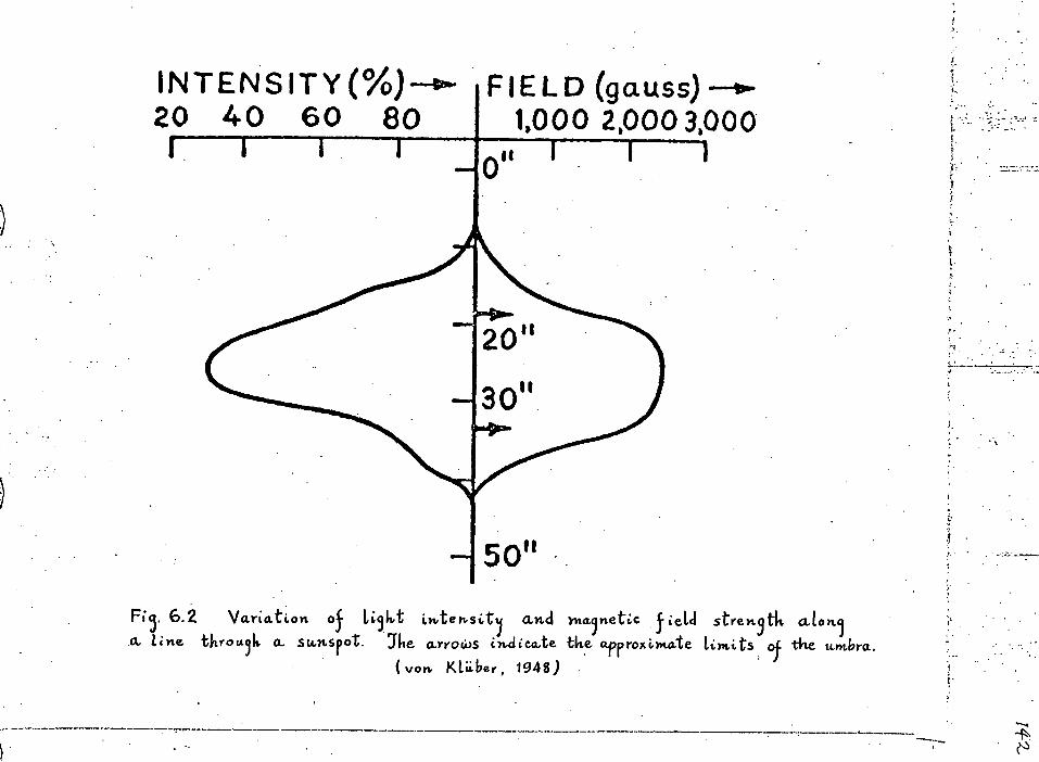
INTENSITY(%)-40- FIELD (gauss) 20 40 60 80 1 ,000 2,0003,000

II

F. 6.2 Va.naton o5 LI.111.t intensi.t1 and rnagnetix jielcl strength, aloni Lt Line throulk ct. swnspot. The o-rrows indicate the. approxi.rnate Limits , of the. umbra.

( von. Kliiber, 1948)

I4-

experimental results have indicated that regions of opposite

polarity may frequently appear even within a single isolated

spot. No matter how complicated the structure of the spot's

field is, the field line can only either stretch straight

into the corona as coming from a unipolar spot, or go up and

bend down to join a region of opposite polarity which can be

the following spot in a bipolar spot...group or a region in

some spot near by, or in the leading spot itself. Consequently,

if we take that the electron stream (which is supposed to be

responsible for the noise storm emissions) is trapped in the strongest field line of a magnetic field structure Whioh is either of the unipolar nature or belongs to a bipolar

character, the description of the generating mechanism and escape conditions will be physically meaningful. We will

devote the rest of this chapter to setting up two models for

spot-field configurations. It mast be pointed author* that

up to the present, there is no experimental result giving the

magnitude and the exact nature of spot magnetic fields above the

photosphere. Our models, therefore, are empirical only.

Referring to Pig. 60, we assume an imaginary dipole

situated at a point P, at a distance PB below the photosphere.

Some lines of !ores originating from this dipole emerge from

a oircular area a (spot area) on the Sun's surface. By

choosing a suitable orientation of the imagninary dipole with

respect to the radius of the Sun and the distance PE, one

can obtain a situation where the field intensity at the point

Pig.63, Geometry showing the calculation of a theoretical bipolar spot-field configuration.

0 is the centre of the Sun and P is the mid-point of the imaginary dipole. The line

represents the field line passing through the centre a of the leading spot of area a..

PR is perpendicular to the axis of the dipole.

• IINIMMI

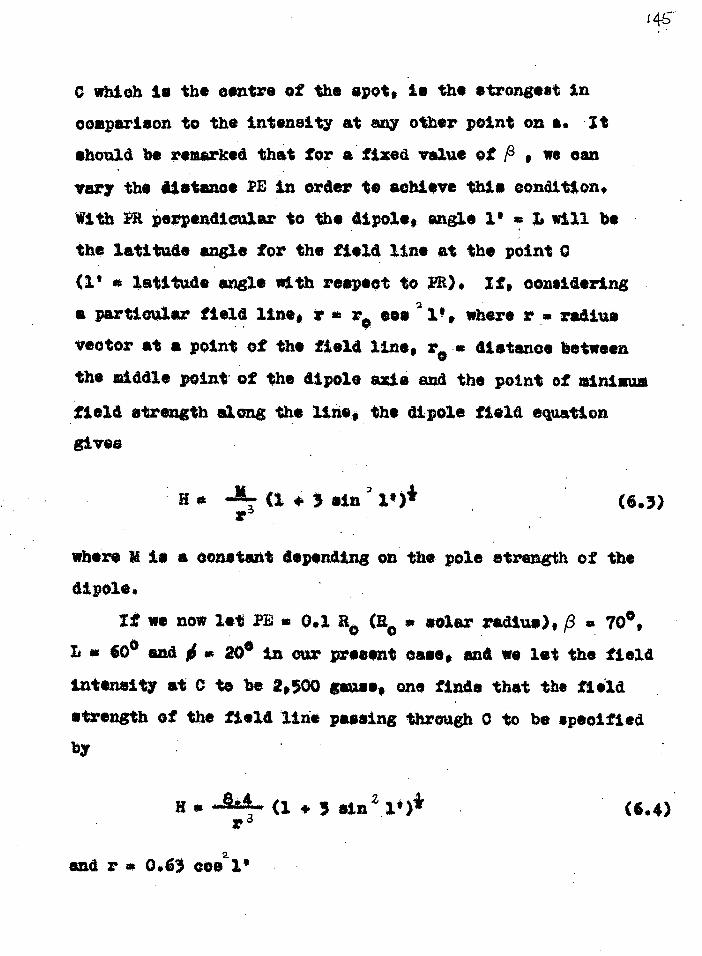
a 900 £9.0 * I Pug

IS 41. "

tq

pouToode oq o Onsiq$ Itulsood own p/oT; •q$ so q$Suoave

PM; 00 WM *put; ouo isom9 00543 Et o0 ve A$TououT

oq$ IA/ SA pug •ess° tU0smad an0 TIT 00a * Pug 009 s

`00L d qiintEmt xeto. * 510 % V0 it It Amu OM SI •IrtOdTp

014 :0 4142u041.0 0t0d .114 uo Buipuodop $uw$ouoo 19. IT 11 wog*

(C9)

iSsTcuTii+

oahT9

u0T4wabo plow opdTP 644. wall •q$ 9uo/o Wituoapt

susTuTe so $ulod oq$ pus wpm o/odTp oq$ so Iplod fropTa oq$

uomilmiq soulmoTp 41, 0.2 •on/ my; oq$ so $uTod stv a0t00A

sun= se aCUM* 4.tt flee °A oeuTT ivy; annoWed

OuTaopTouoo osx quz o$ $oodooa q$To oltn$T$o/ a)

0 $uTod oq$ vs sun mou oq$ aos otituo opu$T$o/ oq$

•oq TIT* 1;; 41 grams orrodTp oql o$ sernaTpuodsod va q$TA

•uompuoo oTq$ amoTqou o$ sopa° uT az souovelp sq$ lavA

uso sA Ei 30 warm peva V aos twit Imovsvisaeq move

t/

•v uo tuTod asqto Aus to A$TounuT oq$ o$ uooTaodwoo

uT $ooltuoa$4 oq$ oT •$ode oq$ go eawvo •q$ qoTqm 0

5:171

The field direction at any point along the field line is

given by

tan ck s * opt (6.5)

where ck angle between the field line and the radius

vector passing through the point in question. Prom

geometry, it is elementiry to Show that at the point C,

the field line is making an angle of 22.7 0 with the solar

radius vector passing through C.

Pollowing the same method one can Calculate the field

intensity (equation similar to 6.4)) and the direction of

the field vector if of any point along all the field lines

emerging froi the spot area a, These lines will terminate

on the other spot of the associated sunspot pair. It ie .

found that with this model, the field intensity on the spot

area fellows a very similar pattern as observed experiment-

ally by von Kluber (Fig. 6.2). However, we note here that

although the field intensity at the centre of the spot on

the photosphere is maximum, the field line passing through

this point may not be the strongest field line emerging

through the spot. We note here that a very similar • magnetic field model, like the one described above, was

introduced by Takekurs (1961).

When we consider a nnipolar spot, we will assume the axis of the imaginary dipole is along a radius vector of

14-7

the Sun, and only some lines of force from the pole

nearer to the photosphere will emerge through an area

(spot area) on the surface. These field lines are supposed

to be straight, extending to the corona and the line passing

through the centre of the spot will be the strongest line,

whose magnetic intensity at a height (f) - 1) being specified

by (Gingburg, po 4130 1964)1

k( 1 (6.6)

where b is the radius of sunspot in units of solar radii

and I1 . Is the maximum field intensity of the spot*

Following Ginsburg, we take b to be 0.05.

Some examples of theoretical spot-field configurations

and electron density distributions are indicated in Fig. 6.4.

Fig.. 6.4(a) Variation of the plasma frequency f p (Baumbach-

Allen's model), gyro-frequency .fH and A along the strongest

field line of a unipolar spot with H s = 2,000 gauss. The

variation of fH with p when Hs = 4,000 gauss is a/go plotted for comparison..

!!

,1

1 0

103 1

FREQ

UENC

Y

164

10 1.1 1.2 1.3 1.4 1.5 1.6

10a -

Fig. 6.4(b) Variation of the plasma frequency f p (Newkirk's

model), gyro-frequency fH and A along the strongest field

line of a unipolar spot specified by H s = 2,000 gauss.

_

••■■■•

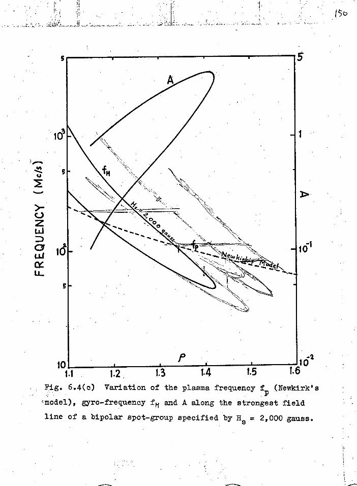
FREQ

UENC

Y

-

10 i P i t

1.610 2

1.1 . 1.2 . 1:3 1.4 1.5 , Pig. 6.4(o) Variation of the plasma frequency fp (Newkirk's

.;.model), gyro-frequency fH and A along the strongest field

line of a bipolar spot-group specified by H s = 2,000 gauss.

(So

l c I

CHAI-Ta. VII

COMING CONDITIONS 111 Tire, SOLAR CORONA

(A) Introduction

In the type I noise storm source region where

appreciable spot magnetic fields prevail, the two more

plausible generating mechanisms are the cyclotron

mechanism and the Cerenkov radiation process', whereas

the former process generates radio waves whieh can

propagate through the corona and be received on the Depth,

the latter meohanism generates plasma waves which are

longitudinal or compression waves, which do not exist

outside the plasma medium. Referring to Fig. 1.1(o),

these Gerenkav plasma waves can only exist in modes

number 3 and 4, and cannot propagate directly above the

level N:= 1 - Yl++, where Xi, T Conse'

vently, if radiation from the Cerenkov plasma process

+We exclude the synchrotron mechanism since the bandwidth of

this radiation is wide whereas the bandwidths of storm

bursts are narrow.

"This statement, of course, assumes no coupling °wars. It

should be noted again that the physical nature of the staves

propagating along mode 3 changes from longitudinal plasma

waves (n. >) 1) to transverse eleotromailletic waves (a. 1).

1 52,

is to be received outside the corona, the plasma waves

need to be transformed into radio waves through some

coupling or transformation mechanisms. Two such

mechanisms are known to exist; one is the transformation

of plasma waves to radio waves through Rayleigh type of

scattering and the other Is the coupling or interaction

of characteristic waves. Since for an electron gyrating

along a magnetic field with a pitch angle. which is not

too small ( 10°, say), the power radiated by the

Cerenkov plasma mechanism is of the same order as that

of cyclotron radiation (Ginsburg and Zheleznyakov,

1961), the efficiency of the coupling mechanisms will

tell, as far as producing radio waves is concerned,

whether the Oerenkcv process will be as significant as

the oyclotron radiation in the source region. It is,

thus, the purpose of this chapter to discuss in a

quantitative manner the two possible coupling mechanisms.

(B) throuh

Rayleigh Scattering and Combination Scattering (Ginsburg

and Zheleznyakov, 1958, 1959 and 1961)

It has been pointed out by Ginsburg and Zheleznyakov

(1958) that in a plasma specified by diel•otric constant

8 , plasma waves can be transformed into transverse

electromagnetic waves through scatterinff c) the lakJj.fala 1 .

plasma waves due to fluctuation of the dielectric =stunt

SE • The fluctuation of the dielectric constant is induced

by the variation of electron concentration S N which can be

separated into two components:

SN = Nr° S N" (7.1)

where SIP is associated with quasi-neutral plasma density

fluotuation (mainly due to motion of electrons). When a plasma wave is incident on a scattering volume,

the amount of scattered signal is determined by the spectrum

of the fluctuations. The spectrum of the scattered signal is

obtained by the oonvolution of the incident spectrum with the

fluctuation spectrum. The result of this convolution is that

there is scattering both due to the density fluctuation ( . (511 1 )

and the charge fluctuation (SN"). Since the variation of

plasma density occurs quite slowly, scattering by Ski° does

not result in any appreciable change of the incident frequency.

This scattering process is called Rayleigh scattering. The

scattering of a plasma wave with frequency wo due to Charge

fluctuation results in a transverse electromagnetic wave of

frequency = 2(4. This scattering is called "combination

scattering". The transformation coefficient, i.e. (i4"ci9

of transformed radio waves)/( ect7 of incident plasma

waves), has been found for both types of scattering to be of -G the order of 10 (e.g. Kundu, 1964).

- 53

(C) Coupling of Characteristic Waves in the Solar Corona

In general, there are four distinct modes of waves

capable of propagating in a warm magnetoacttve plasma

(chapter I). In the Cold-plasma, high-frequency

approximations, the four modes are reduced into two ---

the o- and x-modes. Since each male is represented by

two branches of the refractive index curves (Fig. 1.1(0)),

we will still adopt the 4-mode indentification for

convenience of discussion. The process of coupling

between different branches of the o- and x-modes of

electromagnetic waves is studied in this section for

parameters appropriate to the backbround solar corona as

well as active corona and frequenoies appropriate to solar

type I noise storms.

It has been found (Ratcliffe, 1959; Budden, 1961;

Ginsburg, 1964) that under wUitable conditions, coupling

between the two characteristic modes can take place; these

coupling conditions may be stated as: (i) The values of

refractive index for the two modes coupled are close to

each other. In other words, the coupled waves must travel

at almost the same phase velocities. (ii) The values of

the polarization constants Ro 1%1 of the two modes

must be near to each other. To study the first condition

of coupling, we will consider the behaviour of the refract-

ive indices of the two modes in the corona; the compute-

tion will be based on the collisionless Appleton.Hartree

equation, i.e. equation (3.0. Considering a unipolar spot

field model with field intensity at the centre of the spot

H = 2,000 gauss, we show in Fig. (7.1) the refractive

index squared as a function of distance p = R/R0 along the central field line for two frequencies (f = 50, 100 Uchis)

when the electron density distribution follows relation (6.1)

(normal background corona model). When Hs = 350 gauss, other

parameters being the same, we have Fig. 7.2. The electron

density of the regions above 'sunspot groups and plagee have

been found from both optical and radio observaticns to be

several to ten times the normal background coronal density

(chapter VI). We will now take Newkirk's model (relation

(6.2)) and investigate the behaviour, of the refractive index

in this case. For frequency = 100 and 150 robs, these

graphs are shown in Fig. 7.3 (Hs = 2,000 gauss) and Fig. 7.4 (H 500 gauss).

The polarization constants for o and x-mves in a, magnetoaotive plasma are given by (e.g. Budden, 1961):

4 yLs;n2

R = - / y4 S:049 rcoet9

yoose 1 2( I- X -,4Z) 14(1-)< - 2)1

( 7.2) y 2voixe ■I(.4 5,;n4e

Rx = — Y COS et 2.(1-x-AZ) +J4(

—x—ar ,A,R,„fruL, z = v/f I ceRf0,4, it/r-cAl. .2e S ("1"t fercir

To specify the coupling region precisely, w need to

calculate the polarizations of different modes alms a Veld

I 55

_

centre- of

thro,911 the

a, stronj lAfl-

Fatal, spot ( H, = 2,000

jso.xss) for

(a.) f = 50 Mcis

(6) = 100 Mcis

when the eiectron density

-,•••■•• •■i.,-; , •

He 2000 gauss -

f =50 Mc/5 o MODE—x MODE -- BoAyou.nd Como

...N. mow ••• # -- - - -

••■• 1

(a.)

1.6 1.7 1.4

Fij.7.1 76 variation ok

refractive index stared.

0,Lon, the radi,al Line "

cr—J// 45:—/-1 90 —f-4

S ii

•

1:4 1.5

-follows 13044.2nbeek -A Ilek 's

STL

ER

MO

DE

2000 gauss

f =100 Mc/s o MODE

x MODE

Corona

Hs = 350 gauss

f = 50 MC/S

0 MODE — x MODE --- Backlreand Corona.

(a.)

Y=1 X =1+Y . . 1.1 1.2

ei xsi*

/ 0

I // 0 I /P .

1 \.,(:),', / / Ill 1 / / ill— cf_

111 o

k 4.° / 90e --- 45

k / 45° Ilr-- 90°

\9k)/ III III • III

• 1.5

—WHISTLER MODE

hi I I

iii iii

Hs= 350 gauss

f =100 Mcis

0 MODE —x MODE --- Backyou.ncl Corona,

450 90°

0° 45°

Y=1 90°

1.1 `VI 12 1.3 1.4 1.5

ti /4

.—s

2

0

Fij• 7.2 Ike var:ation of Yes r.ctive index srared n; aloft/ tile v-adio.l. lane p pa.ss tn throuill. -Hie centre.

of a. weak anipoLor spot (H, = 350 9 0.44.53) foy (a) f= 5o Mcb cio,f = ,

Luken. the eteetron, densitl distribiction follows Baccs‘1,4,c,k - -Allen's model.

io°

H,= 2000 gauss

f =100 Mc s o MODE x MODE —L.— DE NSE REGION

/1"

,X=1 if"

Hs= 2000 gauss

f =150 Mcs 0 MODE — x MODE---

DENSE REGION'

4P. /44

/* /a)

i 1.1 12 13 14

0°

45°

4-1-0° II 10° n t-45"

X=1 1.5

Fij. 7.3 /1 va.riation of refractLve ivt.clex scro-reci vi; alovil the. radial 1.,:pte 13 pass in,'

throf.91% the. centre of o.. strorl unipoiar spot (H 5 =2,000 io.u.ss) lay (co 5 = 100 1■40/s .

t-to S. 15 0 . Mc/s , when. the electron. demsit/ distribu.tion. follows N

Hs = 500 gauss f =150 Mo/s . o MODE x MODE ---

DENSE REGION. . (-to

X =1-I-Y

Y=1 nil

0 - 1•1 1.2 x 1.3 1.4 1.5

ill

•■.■

0° e

45° 450 I

Hs = 500 gauss

f =100 Mc/5

o MODE —

x MODE ---

DENSE REGION (04

f Y=1 X=1+Y 0 . ■..t .,..

1.1 1.2 1 x. 1.5 /

01 ill III

I‘ / i /

‘‘‘ o° III— o° . Oa /

\

x % II \

\ / DI

\ / 111, . 111 0

'14 3ke variation of refractive index stu.aveci rt; atom) t he, ra4;a1 tine p

throulh the centre of a weak Lott:polar spot ( Hs =500 9...ss) for a) sf fooltfcis

(I) 150 Mils, when. the electron. cien.siti clistribm.tion, follows Newkirk 's

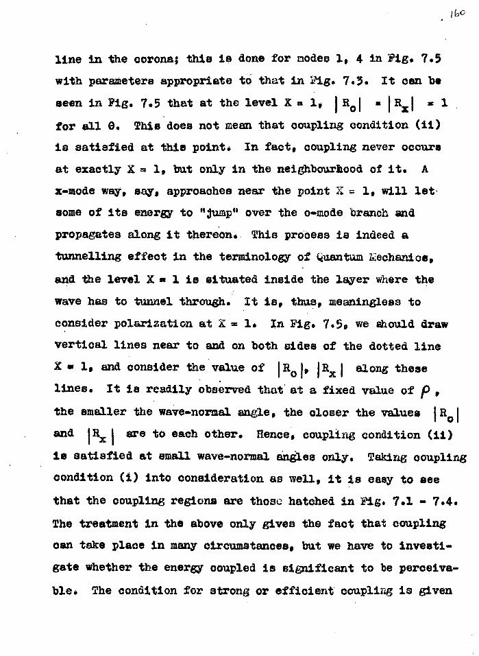
line in the corona; this is done for modes 1, 4 in Pig. 7.5

with parameters appropriate to that in Pig. 7.3. It can be

seen in Pig. 7.5 that at the level X= 1, RO 11 R:C I sc for all 0. This does not mean that coupling condition (ii)

is satisfied at this point. In fact, coupling never occurs

at exactly X= 1, but only in the neighbourhood of it. A

x-mode way, say, approaohes near the point Z. 1, will let

some of its energy to "jump over the o-mode branch and

propagates along it thereon. This prooess is indeed a

tunnelling effect in the terminology of Wantam Mechanics,

and the level X a 1 is situated inside the layer where the

wave has to tunnel through. It is, thus, meaningless to

consider polarization at X= 1. In Pig. 7.5, we *head draw

vertical lines near to and on both sides of the dotted line

X = 1, and consider the value of IR0 1, pax ! along these

lines. It is readily observed that at a fixed value of f),

the smaller the wave-normal angle, the closer the values 'Ro l

and IRx are to each other. Hence, coupling condition (ii)

is satisfied at small wave-normal angles only. Taking coupling

condition (i) into consideration as well, it is easy to see

that the coupling regions are those hatched in Pig. 7.1- 7.4.

The treatment in the above only gives the fact that coupling

can take place in many circumstances, bat we have to investi-

gate whether the energy coupled is significant to be perceiva-

ble. The condition for strong or efficient oaapling is given

0.5 1.7 1.3 1.5

_ -

H,=2000 gauss f =100 Mc's

o MODE x MODE ---

5°

15°

Cr

enow■

•••■•

9= 3cr He 2000 gauss f =150 Mcis o MODE x MODE --- —

E ...Ma ...Nob

mma,

para.lneterS

(V 15 0 MO

30° \\

0.5' 30°

1 .1

F— X =1 I .

1.3 1.5 1.7

Fi5. 7.5 5ke.,dependence of tlite, polo-n:30.ton, constants 1R01,

oyb Korma.li)ed radial distance r is indicated for

in. F:3 . T3 lor two freren,cies (a.) 100 .

(62-

by (Ginzburg, 1964):

= 0 (7.3)

fu Sin20 where f is the critical frequency, given by - c r 2 cos O•

In the solar corona Where the plasma is highly ionized and

the temperature high, the collision frequency V can be

calculated from (Ginzburg, 1964):

Y. 5 N ( 220 N-7) y = 7 3/2

It is found that Y is less than the order of c/a in most

regions (both active region and background corona) in the

corona and the condition for efficient coupling is satisfied

only if the wave-normal angle 0 is extremely. small. This

idea is illustrated in rig. 7.6. We observed from Fig. 7.6

that the inequality

(7.5)

holds if the wave-normal angle 0 is not extremely small. If

inequality (7.5) is satisfied for active region density, it

must also be satisfied in the normal background plasma.

Under assumption (7.5), 0inzburg (p. 320, 1964) gives

the coupling transmission coefficient for weak coupling . from

the o-mode (modes 1, 3) to x-mode (modes 2, Ow vice versa oi < 1

= p — ani s;13 n' R D AX

2ca. ( — )3/21) (TO

(7 .4)

' •

.

'Tap= solapimax mottos oq. patansev

ala • (serre2 000iz

aawao atq. lartoal4 RuTssvd

1-6

sT uoTqa1qTaq.sTp

-q.ods aviodTun Stro.4.13

Cr,

and from the x-mode to o-moderm vice versa i0Y S . > :

2. TI.

where

[I acoo. ( 171. D3/4

where a = 4.1) and N0 electron density at the - 2_

Physically, DI - represents the amplitude of

when the amplitude of the "incident" wave is

If the electron density varies along the corona according

to either the normal background model or the active region

model undertaken, an estimation indicates that the coupling

coefficient is hardly of any significance. However, it is

reasonable to believe that irregularities of density distribution

occur at times in the •oorona, particularly during highly

disturbed periods, and some fluctuations in electron density

Can easily introduce a value of )14 being 104 times that

of the steady state. Taking this factor into account, we plot

the coupling transmission coefficient j Di l as a function of

wave-normal angle ' O in Pig. 7.7 When(it9 is increased by

1044 times.

in Pig. 7.3(b) and 7.4(b), the frequency of the wave considered

(150 no/s) is greater than the gyro-frequency I' m at the

coupling regions. Pig. 7.7(b) gives the coupling coefficient

for the coupling processes shown in Pigq1(a) andT1(b), where

§ = < 1 at the coupling level.

1L4

7.7)

coupling region.

the coupled wave

taken as 1.

4' tic In Pig. 7.7(e), equivalent to the coupling regions

N 01-e, tkAt tft.-s c„se ontl COL between vkodes I 4 possible .

10

0.8

0.

0

0.6

fano mcs >1

He 2000 gauss

Hs= 500 gauss' 111■•• ■1■1

(a)

1

1 I.

0.01 0.1 1

10

0.1 1 9 (DEGREE)

9 (DEGREE)

7.7 7he dependence of the transmission, couplinl coefficient 1D1 2 On wave-normal, anjle 0 for (a) > , (b) 3 < .

1 00

Even with the assumption of large value of : N1 19 • it

is obvious from Fig. 7.7 that the coupling process is very

inefficient in the corona; only waves (of one mode) propagat-

ing with wave-normal angle 0 smaller than about 0.5 ° will be

coupled to the other mode. If we assume the x..mode radiation

power to be confined to one solid angle about the maGnetic

field line, then after coupling only 10-4 4' of the power

will be associated to the o-mode waves.

Since the incoherent radiation power of the 0erankov

process is of the same order as that of the cyclotron

mechanism, we conclude from the results of sections (B) and

(0) that in regions where strong magnetic fields prevail (as

in the source regions of type I noise storms), the oyolotron

radiation process is the much more significant one. "We will,

therefore, proceed to study the characteristics of the cyclotron

radiation in the next chapter.

-7 aN +This value will be less than 10 if assumes the

normal value (fluctuation In density is absent).

CHAPTER VIII

CYCLOTRON RADIATION FROM ELECTRON STREAMS

GYTRATING IN SPOT-FIELD CONFIGURATIONS

(A) Emitted Frequenoy Range from Electrons

We will, first of all, assume the existence of

electrons spiralling along spot magnetic field lines in

the source region,. When the spot-field configuration

is of bipolar nature, electrons gyrating along a particular

field line will be mirrored—and trapped for some time

before diffusing away. It is well known that each electron

will.radiate a range of frequonoy at an instant. If the

electron acquires a kinetic energy of the order of Mev.,

synchrotron radiation results and the bandwidth of

emission will be very wide, which is not observed. We

will, therefore, assume that the energy of the radiating

electron is of the order of 10 - 100 Key. (cyclotron

radiation will be emitted for this order of energy), and

we will discuss the possible range of frequency emitted

from such eleotrons.

In considering the cyclotron process, we will assume

that the oollisionless Appleton*Eartree equation is valid

+The question on the presence of such electrons will be

discussed in chapter X.

(SA)

A 2 A

( A /1 1 _ A sin2 e j A )2 cosle

2 r- + 4 1-72. r

in the solar corona, based on the fact that the mama

thermal velecitY AT of electrons in the corona is very

small, being — 10 (Ginsburg, P. 121, 1964). The

refractive index n, for an eleotromagnetio wave in the

corona alone is thus given by

16$

All quantities have their usual meanings as defined in

chapter II.

In the above dispersion equation the distribution of

plasma density N and hence plasma frequency f

relation (6.1) (background corona model) or (6.2) (Newkirk's

model) in the corona, while the relation between the gyro-

frequency fh and position in the corona depends on the

model and position of the spot-field undertaken.

Since majority of noise storms are observed to occur

at altitudes between 0.2 and 0.5 Ro and a typical value of

the maximum field intensity on the spot area is Nip 2,000

gauss for a noise storm to occur, we can set up limits for

the quantity A in the possible source region. Here, of

course, we have to assume that in most oasts, the apparent

source positions are the real source positions. As to

electron density distribution in the source region, we will

take both possibilities (relations (6.1) and (6.2)) into

consideration. Within the regime of the above assumptions,

from Pig. 6.084-smd-61r0b) A is found to range from about

0.2 to 5, To Show a typical example of the form of equation (8.1), we plot the refractive index n, as a function of

normalised frequancy, filffilfer wave..normal angle 0 = 10 °

and 750 in case where A • 1, in Pig. 8.1. The lines marked

x and o are refractive index curves for the x and o modes

respectively.

It is easy to show from the refractive index expression

that for all values of 0 in the x.mode, When n i m 0, ,N is

given by

IL?

(8.2)

In the o-mode, for all values of 0 not equal to 0 0,

§ when n, 0:

R (8.3)

For an observer in a reference system fixed to the

background magnetbactive plasma in which an electron is gyrating, the observed radiated frequency is given by the

+This expression is equivalent to stating nj = 0 when

X f 1.

0.5 1.0 - 1.5 2.0 2.5 3.0 3.5 4.0 4.5 N 0 RMALI Z ED FREQUENCY

Refractive index n for the o--mode and x-mode against normalized frequency r: A . = 1, and 8 = 10 ° , 75 ° . The Doppler equation is also plotted as a function

c..r: . ; for 134 =. 0.3, • A, = 0.7 and harmonic s = 1, 2.

Doppler equation

s (8.4) 1 - n- cos()

where n, must satisfy equation (8.1).

The frequency corresponding to n s g. 0 is independent

of 0 and is given by

1.71

(8.5)

The Doppler equation is plotted for the first two

harmonics (s = 1, 2), taking 0sr 10 ° and 75° , pi s 0.3, 13, 0.7 in Fig. 8.1.

It is clear from Pig. 84 that there can be one or

two simultaneous solutions (i.e. points of intersection) of

the dispersion and Doppler equations depending on whether

= sY LA- (8.6a)

or s X < (8.6b)

We refer to these two oases as the Simple (8.6a) and

Double (8.6b) friquenoy solutions respectively. These two

different solutions show up clearly in Fig. 8.2 where

simultaneous solutions of equations (8.1) and (8.4) are

plotted for the o.mode (Fig. 842a) and the x-mode (Pig. 8.2b).

The Double solutions have a limited 0-range. We denote the

upper limit by the eqt-Off angle 00 which corresponds to

the Doppler equation being a tangent to the dispersion

s=2 13=0.7

o MODE

A = 1 - '2=01

x MODE. q=c).7 , A = 1

=0.3

r , s=3

,

ji=0.1 NI

0 s =1 =a7 Z 3

s.2 \

, 11 , 0 Li Cr 1 u_ 4 0

1■I=O1 s=2 =0.3

P0 0 800

------

5=

Fig. 8.2 The relation of the

normalized frequency and -

wave-normal angle e for A = 1,

different values of RI. , s, and

s=2 Et0.7 '

8d

(a) o-mode wave;

(b) x-mode wave.

An example of the cut-off angle ec is also indicated.

equation. These two typos of solution for the normalized

frequently are very important in the explanation of

bursts and continuo radiations and should always be kept in mind. It Should be noted that for given pl. and pH

a Double solution for the x*mode usually occurs at a harmonic number which is one unit larger than that for the

Double solution of the osimode.

(B) :Power SDI:citrus of a Sinsle Electron

An electron emits cyclotron radiation in both ordinary

and extraordinary, mods,. It is necessary to investigate .

whether only one of the two modes, Or both carries significant

energy end capable of escaping through. the corona. With

various values of Ai and 1=1 1. f= the radiating electron, the emitted characteristic normalized frequency has been

obtained as a function of the wave-normal angle 0 in section

(A) for three values of A.* 0.25. 1 ''A:nd 1.5 (we have shown

an example of graph for the case A. m I only). , We will, first

Of all, evaluate the power spectra emitted by single electrons

in the twe modes for those cases. Per in electron gyrating

with pitch angle 0 and with guiding centre along: the z.

direction (Pig. 8.3). the Eidman equation (Mutant 1965)

gives the power radiated at 0 per unit solid angle in the •th harmonics

i73

(-r ' (x s /x + 01 )1(x)) 164;4_ 1 — c os ( 1 +

'w

2- Where K = ( + 040 )

0( 0 cos 1- 0(1( s -in e

044, cos° - o&9n'9

cos°

1 11•3

1) Sine

A- X

1 2 (3.1. Sin e

w A [.2 (1 - 2A/ 3)1.1 +( -44 3)(2AA24 s;?0 +1:2.

(R.7a.)

here the positive sign corresponds to o.mode and

the negative corresponds the x-mode.

D= 1 _ A sia 8 1/2

s;r14A E a IY, co-42 9 ( 1_2A )( I

g -) _ inziA 8 6, 5 U .f Cas'e ( i_ A )2 4 -s 4

(AK —

,

. . '...'ilt. The position and velocity coordinistes of an electron on a . '.,1 • The components of the electric vector E of the radiation'0 ') • .,, • . helical trajectory.. .' , • :: : : - -... ..,-.. : -• . .;.''.,., f 7... ' . field in a tnagnetoplasma. • • • , ;

. . ., ,..... • . : ,• ._,..„...,,....__,•J .The wave norrnal k and the Poysting vector 9 are not penile, in getters?. 1.* , • •

•With coordinate system (k,x,8) as specified by Fig. 8.3,

the polarization coefficient are defined by

E x Ek

( ,e )

E x

( 8 8 )

when Ee/Ex = .1, or = 0, the electromagnetic wave is

circularly polarized. If = 0 the wave is linearly

polarized.

•

The result of the computations for the two lowest .

. harmonics (s = 1, 2) and for various values of electron

energy and pitch angles (specified by pi = 0.1,A = 0.5, 0.7 and 13.1. = . 0.1, 0.3, 0.5, 0.7) and for

different background plasmas specified by A = 0.25, - 14 1.5

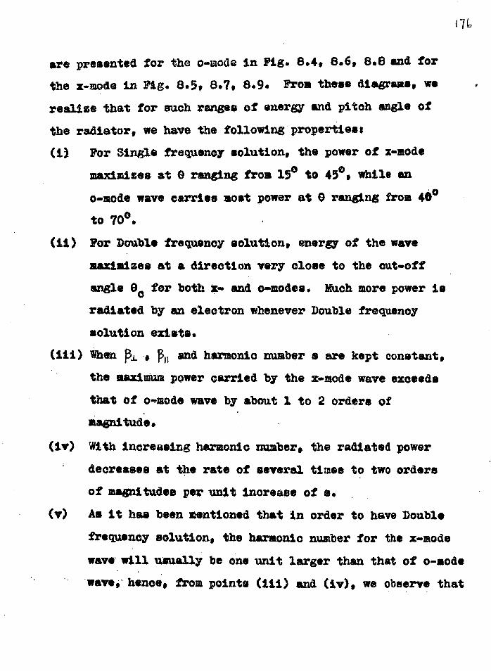
I 7L

are presented for the o-mode in Fig. 8.4, 8.6, 8.8 and for

the x-mode in Pig. 8.5, 8.7, 8.9. From these diagrams, we

realize that for such ranges of energy and pitch angle of

the radiator, we have the following properties:

(i) For Single frequency solution, the power of x-mode

maximises at 0 ranging from 15 ° to 45°, while an

o-mode wave carries most power at 0 ranging from 40 0

to 700 .

(11) For Double frequency solution, energy of the wave

maximizes at a direction very close to the cut-off

angle 00 for both v. and c-modes. Mich more power is

radiated by an electron whenever Double frequency

solution exists.

(11i) When N. pH and harmonic number s are kept constant, the maximum power carried by the x-mode wave exceeds

that of o-mode wave by about 1 to 2 orders of

magnitude.

(1v) With increasing harmonic number, the radiated power

decreases at the rate of several times to two orders

of magnitudes per unit increase of s.

(v) As it has been mentioned that in order to have Double

frequency solution, the harmonic number for the x-mode

wave will usually be one unit larger than that of 0-mode

wave, hence, from points (111) and (iv), we observe that

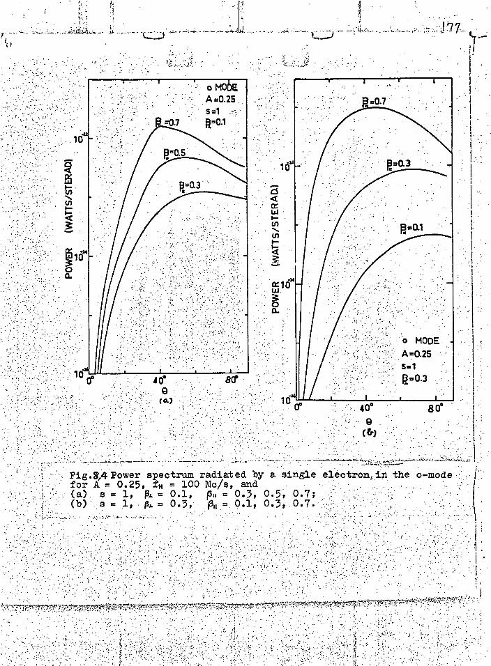
• • .• . . • Fig.8,4Power spectrum radiated by a single electron s.in the

for A. = 0.25, H = 100 Mc/s, and . (a). s = 1, PI= 0.1, p, = 0.3, 0.3, , 0.7;

:(b) s = 1, (34. = 0.3,• A, = 0.1, 0.3, . 0.7.

-

••• . 17

o MODE 'A.0.25 szt2 1:1=0.3

40° 80*•

(A) .

--Pig. 9.4-Power spectrum radie.-.,6foy a single electron in the o-mode for A = 0.25, fH = 100 Mc/s, and (c) s = 2, 13,. = 0.1, p„ = 0.3, 0.5, 0.7; (d) s = 2, /3, = 0.3, pn = 0.1, 0.3, 0.7.

,

x MODE A =0.25 S =1 ft = 0.1

p=o3

0° 40° 9

(c)

R=05

=0.3

x MODE A =0.25 s= 2 13= 0.1

13 40° 80°

(k)

40° 9 •

(a.)

s o°

x MODE A = 0.25 s = 2 R=0.3

Fig.8'S Power s' ectrum radiated. by a single electron in the x-mode for A = 0.25, ?E H = 100 Lic/s, and (a) s = 1, ('o) s = 2, (o) s = 2,

f3 = 0.1, p„= 0.7; p . = '0.1, p = 0.3, 0.5, 0.7; pi. = 0.3, p = 0 , 0.3, 0.7.

(t)

Fig.$.6Power spectrum radiated by a single electron in the o-mode for A .= 1, = 100 Mc/s, and (a) (b)

s•= 1, s = 1,.

1= p, = 0.1,. 0.3,

= p„ •=--

0.3, 0.3,

0.5, 0.5,

0.7; 0.7.

(WAT

TS/S

TERA

D.)

(c)

Pi-g. 9- 1. Power spectrum radiated by a single electron in the 0-mode for. A = 1 , fH = 100 Mc/s, and

(c) s = 2, 13L= 0.1, 13, . 0.3, 0.5, 0.7; (d) s = 2, rel . 0.3, . 0.1, 0.3, 0.7.

400 80°

(S)

8 00 0° 400

Fig.S./ Power spectrurri radiated by a single electron in the x-mode for A = 1,f = 100 Mc/s, and (a) s = 2, /3.1. = 0.1,

0.3, 0.5, 0.7;

(b), s = 2, p, = 0.1, 0.3, 0.5, 0.7.

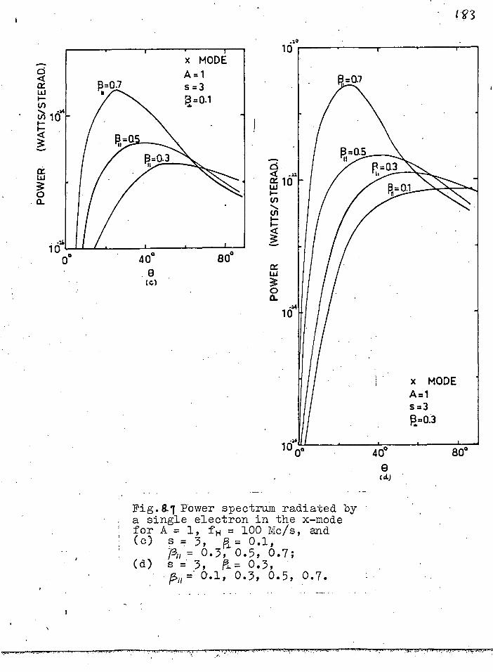
le o°

•tg3

ct)

Fig.8,1 Power spectrum radiated by a single electron in the x-mode for A = 1, f 1 = 100 Mc/s, and (o) s =, 3, fl= 0.1,

pi , = 0.3, 0.5, 0.7; (d) s = 3, a= 0.3,

=- 0-.1, 0.3, 0.5, 0.7.

•

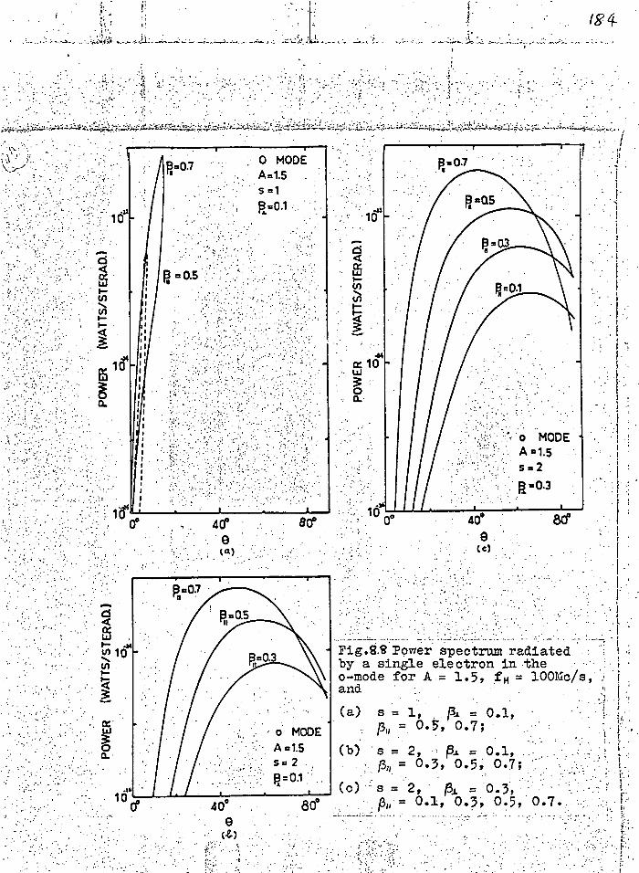
•I'

44 cc 10

40° 9 to -

Fig.8.9 Power spectrum radiated by a single electron in the - o-mode for A.= 1.5, f H = 100hic/s, and

o MODE -. A =1.5

s=2 R=0.1

(a) s = 1, pi. = 0.1, = 0.5, 0.7;

(b) s 2, =0.1, = 0.5; 0.7;

(c) s = 2, pt, = 0.3, = 0.1, 0.3, 0.7. 8cf

184. '

FigS7 Power spectrum radiated by a single electron in the x-mode for A = 1.5, f H =100 Mc/s, and

(a) s = 2, = 0.1, po . 0.3, 0.5;

(b) s = 3, f3J.= 0.1, Isll . 0.3, 0.5, 0.7;

(c) s = • 3, pi 0.3, pH = 0.1, 0.3, 0.5, 0.7.

the power radiated by both characteristic modes can be

of the same order of magnitude for cases with Double

frequency solution. .

(0) Amel,ification of Electromagnetic Waves in a Stream-

plasma System

So far we hmve considered radiation spectra from

*single electrons only, When the radiating electrons

form a stream, the streactoplasma system can be roliatively

unstable: an electromagnetic wave will grow as a function

of time. We will assume here that gyrating electron

streams prevail in the source regiont. Since the band-

width of a burst radiation is very narrow (Alit— 04),

the spread in momentum distribution, of the radiating

stream mast be very small for many cases. In another

terminology, we say that such an electron stream has a'

finite temperature which is a measure of the momentum

spread. The instability . problem of such a etreem.plasma

system (when the temperature effect is taken into account)

. has been discussed in chapter II, On account of the

complexity in mathematics for such a system, we will

assume here that the temperature of the electron stream

is zero. i.e. every electron in the stream has the same

••••••■•■•••••••ftunimr......hoopinorommer■••■■••■■■■•••••■•...

'Discussion on this point will be given in chapter Xe

1,5) 4

values of PI it P10 and P o sa Po ° and the stream is ()ailed

"helissal". Even though such a stream is the limiting sass

of a realistic one, the instability theory gives the same

general behaviour of the growth rate as in the case when

temperature is included. Is will, therefore, without loss

of generality in the outcome of the result, assume that the

stream is helical, and the distribution function of the

stream will then be given by relation (2.4)

f (V erp 121 — — fu° (8.9) 2irpjf

• Misusing the particle density of the stream to be small

compared with that of the ambient plasma, the growth rate of

an electromagnetic wave in the streaa-plasaa system is given

by equation (3.5 )$

$

=44-1- ( vv3 c- 6)

(8.10)

where °"1 C 60. v)y2

+

—T-A7:fl-n:.tj13: c vsze cs _ ser

+ = o/ ((si". 3)1 Ps' 2132. 1214,2-.1 cp'—sz...ze,ifl 13111 3 2 ) ( A 219

54A'ae -11

This statement is true only when the temperature of the

streams is low; when the momentum spread is wide, the band-

width of emission will be broad and the harmonics may not

be resolved.

157

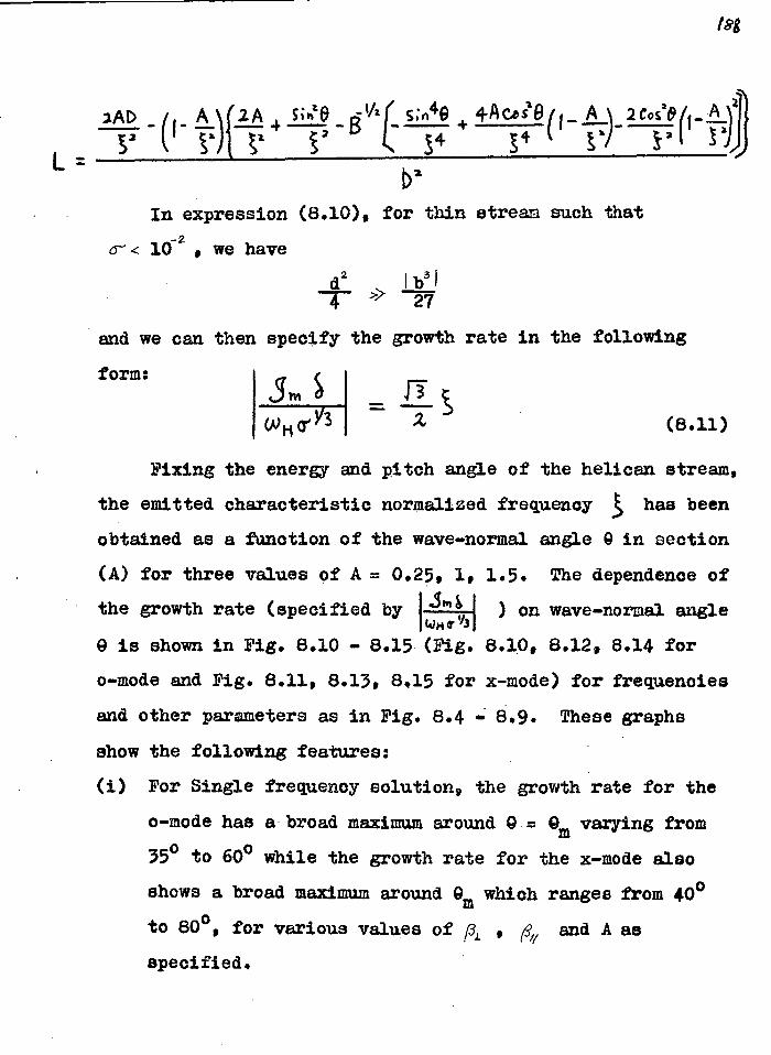
Isg

In expression (8.10), for thin stream such that

a- 4 10-2 , we have

c12 b3 4 27

and we can then specify the growth rate in the following

form:

(8.11)

Fixing the energy and pitch angle of the helioan stream,

the emitted characteristic normalized frequency has been

obtained as a function of the wave-normal angle Q in section

(A) for three values of A = 0.25, 1 • 1.5. The dependence of

the growth rate (specified by ) on wave-normal angle (41043

O is shown in Fig. 8.10 - 8.15 (Fig. 8.10, 8.12, 8.14 for

o-mode and Fig. 8.11, 8.13, 8.15 for x-mode) for frequencies

and other parameters as in Fig. 8.4 - 8.9. These graphs

show the following features:

(i) For Single frequency solution, the growth rate for the

o-mode has a broad maximum around 0 = Om varying from

35° to 60° while the growth rate for the x-mode also

shows a broad maximum around Gm which ranges from 400

to 800 , for various values of p and A as

specified.

(x161 )

. . . _. .__ .. 1 Fig.9I0 The dependence Of the growth i rate 14q ' on wave-normal angle

0 in the o-mode for A . 0.25, and

I (a) s = 1, 13., = 0.1,

i pH = 0.3, 0.7;

1 (b) S = 1, p.„ = 0.3, & = 0.1, 0.7.

o MODE A = 0.25 S =1 R=0.3

0.1

1

40° 8 (4)

saa

to

(1.) -I-)

0

(1)

ct-.1 0 Ts r7-1 F-1 C.

80° 40°

C)

Fig.8.11 The dependence of the I 311-) 8 growth rate Ion cri

wave-normal angle G in the

x-mode for A = 0.25, and

11(

o°

x MODE A =0.25 s = 1 1E1= 0.1

8

(x10-1)

11=0.7

R=0.7

0.3 • 0.1

x MODE A =0.25 s = 2 11=0.3

(a) s = 1,

(b) S = 2,

(c) s =2,

f3..= 0.1, Ph = 0.7;

= 0.1, /3„ = 0.1, 0.5 0.7;

PI= 0.3, /30 = 0.1, 0.3, 0.7.

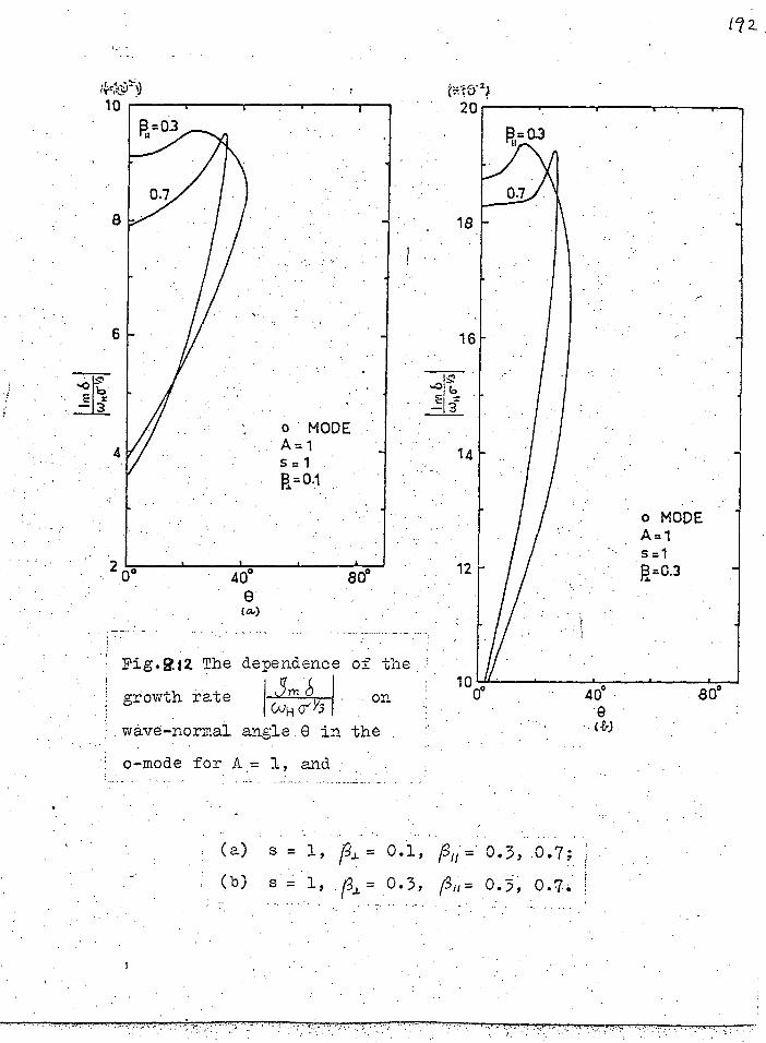
Fig.$12 The dependence of the ' m t;

cul-i o'Y3 on

wave-normal angle in the

growth rate 80°

o MODE A=1 ,s=1 R=0.3

I? 2_

o-mode for A . = 1, and

(a) s = 1, = 0.1, t =•0.3, .0.7;

(b) s = 1, 131. = 0.3, =

(AY

400 - 0 (C)

Fig.8.12 The dependence of the SYY)

0-1 V3 growth rate on

wave-normal angle e in the

o-mode for A = 1, and

(c) s = 2, pj. = 0.1,

pn = 0.3, 0.7;

(d) s = .2, /31 = 0.3,

= 0.1, 0.3, 0.7.

0

4e 80°

lg.& 13 The dependence of the

I cum 0-Y3 I . growth rate

wave-normal angle e in the

x-mode for A = 1, and

4

(a) s = 2, 13J.

(b) s =2, 13.1

= 0.1, /3u= 0.3, 0.7;

= 0.3, /3„= 0.1, 0.5.

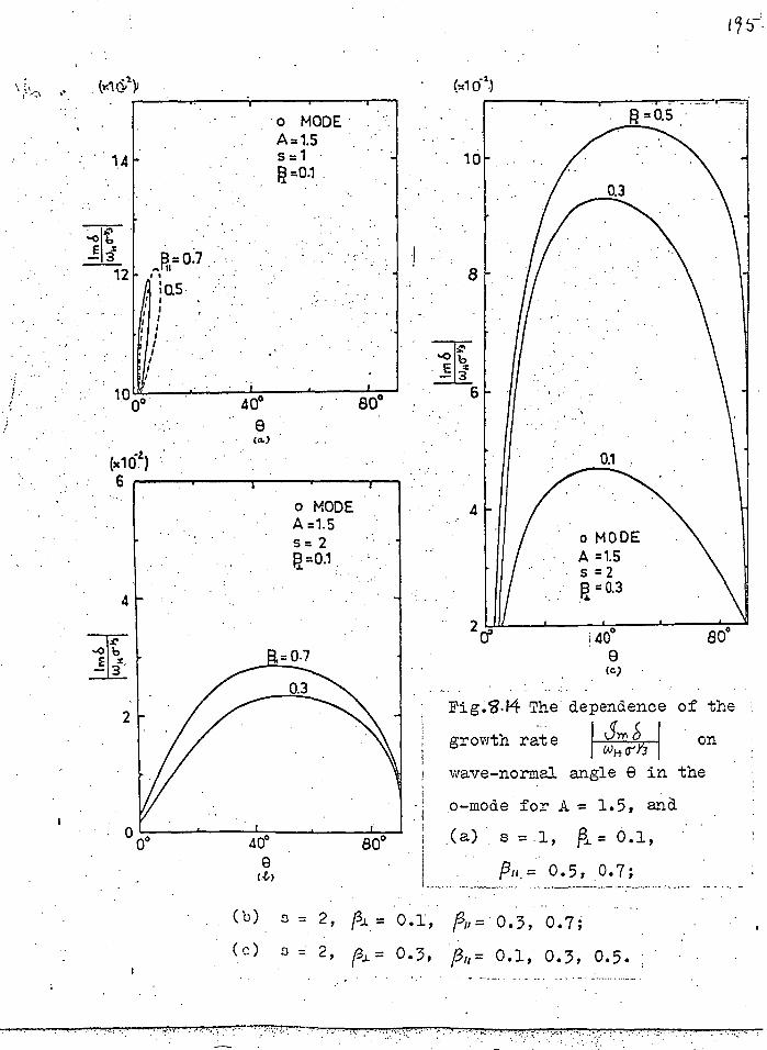
so° 400

(t)

(b) = 2, = 0 • 1 ,

(c) = 2, = 0.3,

Pi g.8-14 The dependence of -the J)1, eS growth rate

wave-normal angle e in the

o -mode for A = 1.5 , and

(a) s = 1, 13,. = 0.1,

P .= 0 • 5 3, .0. 7 ; _

;

, 0 • 5 •

v = 0 • 3 , • 0 •7

= 0 • 1 , 0 •3

1 0

40° 0 (e)

80°

o MODE A =1.5 s = 2

=0.3

%.0

o MODE A=1.5 s= 2 11=0.1

Ft= o.7

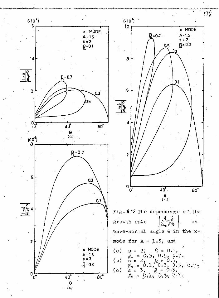
We) 6

(x1 62)

x MODE A=1.5 s=2 ft =0.1

Fig. 8•15 The dependence of the

growth rat e I $7 „6 on c),./H ei I wave-normal angle e in the x-.

mode for A = 1.5, and

(a) s = 2, P., = 0.1, p, = 0.3, 0.5, 0.7.

(b) s = 2, fj. = 0.3, p, = 0.1, 0.3, 0.5, .0.7 ;

(c) s = 3, ks= 0.3,

c77

(ii) For both modes, whenever the Double frequency solution

exists, the growth rate is large and Om occurs near the

cut-off angle Go . For a constant value of AL • Gm

approaches towards Go as the pitch angle of the stream

decreases (i.e. increasing Od ). Eoreover, when (34 is

fixed, the value of maximum growth rate increases with

Increasing A, up to an optimum value of ; then the

maximum growth decreases with still increasing g, (iii)With the range of value for A as assigned (0.25 - I.5),

the growth rates for both modes are of the same order

' of magnitude. •

(iv) The growth rate decreases rapidly with increasing

harmonic number for electron energy of the order of

10 - 100 Kev.

• In this stream-plasma system, the electromagnetic wave

grows exponentially as a function of time. If we take that -2 -3

the wave interacts for 10 meec. (or 5x 10 msec.) with the

stream, and that the gyro-frequency 4 = Wm/27 = 100 Mc/s, -3

0"7= density of stream/density of embient plasma = 10 (or - 6

10 ), we can calculate the power gain after this short

period of interaction.. We show some examples of the relation

between the power gain in db and the wave-normal angle Q in

Fig. 8.16. To show how the power gain behaves with respect

to change of frequency, and thus, to estimate the bandwidth

of emission, we have Fig. 8.17 corresponding to Fig. 8.16.

Note that in Fig. 8.17 the range of frequency amplified

corresponds to different directions. However, if we consider

a half-power or quarter-power emission cone and let the

range of frequencies radiated within this cone to be the

estimated bandwidth, then this estimated bandwidth is the

maximum bandwidth which can be received on Earth, since the

emission cone may be too wide and only part of the radiation

will "strike" the Earth on account of geometrical factor+ .

Pig. 8.17 shows that:

(i) Por both Single and Double types of frequency solution,

the bandwidth is small when the pitch angle is large.

(ii) When A, and pa are fixed, the bandwidth for Double

frequency solution is much narrower than that for

Single frequency solution. Obviously, in this case, 3

the harmonic number for the Single frequency solution

is one unit higher.

(iii)A bandwidth as narrow as 0.09 is possiblet+

+In this argument, we have assumed that the wave is refracted

only slightly in the corona.

"Note that in Pig. 17(c), the pitch angle is 45 ° ; if the pitch

angle is increased to greater than 60 0 , a half-power bandwidth

of <0.03 is possible. Note also that the theoretical

bandwidth decreases when the power gain is increased, i.e.

allowing a longer interaction time or denser stream.

tl?

500

z 300

o_ Fig. &IL The relation of the

power gain (db) after 10 sec.

and the wave-normal angle .6

for 0 = (.0027wP2 ; = 10 -3 1

fH = 100 Mc/a, A = 1, 131 = 0.1

and

(a) •o-mode, iell = 0.7,

s = 1, 2;

(b) x-mode, j,, = 0.3, 0.7,

s = 2.

• 10 0

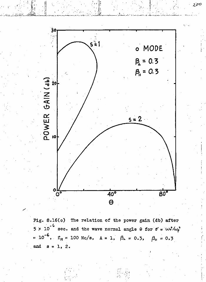
- 2jav

s=1

•••••■ -Ct

40° 806

Fig. 8.16(c) The relation of the power gain (db) after .4

5 )( 10 sec. and the wave normal angle 0 for'al="AW4

= 10-6 ,. fm = 100 Mc/s, A = 1, pi. = 0.3, pn = 0.3

and s = 1, 2.

500 13=0.7 • . s= 1

o MODE

0 300

g=0.7. s= 2 •

5

x MODE s = 2 =0.7 .

=0.3

200

(-€4

-Z 0

Pig. 8.17 The relation of the

power gain (db) after 10-5

sec. and the normalized

frequency 3 for 0". = Gue:Ap z

= 10 ,f f4 = 100 lic/8 1

A = 1, = 0.1, and

(a) o-mode, =0.7, s = 1,2;

(b) x-mode, j3 = 0.3, 0.7, s =

2-02

Fig. 8.17(c) The relation of the power gain (db) . after 5x 16 6 sec -

, and the normalized frequency for Or = = 106

,

fH = 100 Mc/s, A = 1, /34 = 0.3,. = 0.3 and 8 = 1, 2.

2o3

(D) Resonance Absorption at the First Three Harmonics

It is well known from both cleasical and quantum

theories that when an electron emits cyclotron

radiation at some particular frequency, it can also

absorb radiation of the same frequency(e.g. Gingbarg,

1964)., When an electromagnetic wave passes through a

magnetoactive plasma, some electrons "feel" the wave

gyrating at their own frequenoy and either excitation

or damping can take place depending on the energy

distribution of the electrons as discussed in chapter II.

Hence, whereas electromagnetic waves satisfying the

resonance condition.' sYLum = 0 will grow.in

a stream-plasma system (section (0)), they will be damped

in a background plasma of "slow" electrons and lone (the,

resonance condition is now,approrimated to CAT- s(1oH=r, 0)•

Consequently, absorption *Ill take place when WI electro-

magnetic wave ef angular frequency I; ,,propagating in

the active corona with varying magnetic fields in space,

encounters angular gyro-frequency wlm such that

•••■•• • CA) (8.12)

where a 1, 2, 3

This type of collielonleee absorption is called resonance

absorption. It has been pointed out by Gerehman (1960)

that since the collision frequency in the corona is very

small ( )1 ,-10 - 10-3 I, chapter VII), the only important

absorption for transverse electromagnetic waves is the

resonance absorption.

Let an electromagnetic wave be specified by 4,

where z is distance along which °the phase velocity ie

travelling, If we amniae the frequenoy to be real and wave

vitiator complex so as to look for a damping in space, we can

write

k iq

and the dainping factor will be eler. According to Gershman

(1960),, the rate of the first harmonic absorption ( (A)

is given by

= ATOTAn#g cose {0— (1 — 14—T s? • 0 )X))1 J. k4 2 X - 2 — s ih2 +

— (2 +X

+ r _ 3X X 2 (1_ tcoixe ) 4 X3 ta,■,1219 `• 2 2, 4- ) (8.13)

,Y2 ( TAm o c,1)) is normalized thermal velocity. The width of the line biz 4 is of the order of

10,),., top 1-1 . cos 0 col/f)c -r T 7Y10

. cos 9 (8.14)

where

In studying the first harmonic abeorption, we consider

1 0'4

' 0.8 X •

Fig.L4(a) Variation of the resonance specific absorption with X = topYwl for the first harmonic in t“e o-mode and different values of the wave-normal angle p..

Fig.8.18(b) Variation of the power loss (db) with X =ui/4' for the first harmonic. in

! the omode, taking the thick-ness of the absorptilon layer • to be 10 Kt. , Ar = 10 -4 , for different values of the wave-normal angle e.

- - - - -

2-o6

the absorption for the od.mode wavy only since an xmitode wave

cannot escape through the level X: 1 Y if it passes through

the level Y * 1 (here ! is defined by Y 1/j). The

dependence of the resonance specifio absorption (specified by

14 N ) for the first harmonic on the quantity Xis shown

in Pig. 848(a) and the corresponding power loss in db is

indicated in Pig. 8016(b), assuming the thiohness of the

absorption. level 4 s m 10 Km. In the graphs for power loss -

the value of AT is token to be 10 2 (Gershman, 1960) and the

waveimnormal angle 0 is taken to be the parameter for each line.

Prom these diagrams, we observe that the absorption increases

from increasing value4 of X and in3reasing wave-normal angle 0.

We have seen in section (C) that for cyclotron radiation caused

by gyrating electron stream with energy of the order of 10 -

100 Keit'. per electron, , a typical value of 0 for maximum power

(80) in ease of Double frequency solution is 35 °. With this

value of 0, the resonance absorption is not large exoept when

X is amAll (soy, 4 0.2, Pig. 8.18(b)). This means that the.

source region for osimode radiation is limitted to the region

above the level Y

The resonance specific absorption for the second and third

harmonics are given by (Gershman, 1960; Ginzburg, 1964):

piv.r 12 k 2137.2yTasze) (8.15)

2-0 7

3B 2 n?- s4i2 e (1-3/0' Fiv FT 2),P 2 .2.

a, a 8 X 0214 • c s2v "3-

(8.16)

Where V x c;na ePrrjS

= cos /2(1- i -X-t 3 co4.2e)1-(20-x) 2 + + eos269f

{n

ifa. O v (i+ s;n1 +d ,_ -tfAk 2, r si:el 0_1 x I k I+ )

In calculating the second harmonic resonance absorption, we pat MI ta 2 in (8.15) and we substitute a 3 in (8.16) for the third harmonic. Assuming 0 1 0, 8 jl, nj —1, we have the following rough estimation:

(--1) x p r for o-mode s=1

(4) z9.7 X (3T for x-mcc.e (8.17)

ell = c1 ).(13T3 for x-mode

For accurate calculation, we can uie (q/(I 131- )) and (q/(f (3-r3 » to describe the second and third harmonic resonance specific absorption respectively. The relation between (q/(k PT )) and X a tut?. Aj z is shown in Pig. 8.19(a) and 8.19(b) for the

second harmonic Of the o•mode wave and the x-mode wave respeot-ively. The corresponding graphs for the third harmonic ((q/(iPT3 )) vs X) are given in Pig. 8.20(a) and 8•20(b).

0 0.4 0.8

(4) . . . _ Fig.51 Variation of the resonance : specificabsorption with X .we'A.0). for the • second. harmonic, different values of the wave-normal angle 0, and •

.(a) o-mode wave; - (b)- x-mode wave.

104

1

= 800

40°

30°

159

5

id 0 0.4 0.8 0 0,4 . 0.8

X X 1.2

• Fig.8. 20 Variation of the resonance specific absorption with X = Gyp' for the third harmonic, different values of the wave-normal angle 0, and

(a) o-mode wave; (b) x-mode wave.

(qP) SSO1 2:13MOd

I •

_21 0

(cin SSO1 tl3Mad

• -••••

J:1

10

10 164 0 . 0A 0.8 0

X _ - -

Fig.8. 22 Variation of the power loss (db) with X = wrYce for the third harmonic, 1. taking the thickness of the absorption layer to be 10 Km, p= 1O2, for

different 'values- of the wave-normal angle. and •• • :• • _

(a) o-m6de wave; ;(b) x-hode wave.

0.4 08 U .

212

Taking PT ft 10 which is a typical number in the

corona, s = 10 Km as thickness of the absorptiodlayer,

one can calculate the power loss of an electromagnetic

wave passing through the absorption level; these graphs

are given in Pig. 8.21 and 8.22. In all these graphs,

the parameter of each line is the wave-normal angle 0.

An inspection of pig. 8.19 4. 8.22 indicates that the

resonance specific absorption for the mummode is at least

two orders of magnitude higher than that of (3-mode and

the corresponding power loss in db for the x-mode exceeds

that of 0-mode by several orders of magnitude (Ginsburg

and Zheleznyakov (1961) have already mentioned this

result in a qualitative way). This is a very important

fact concerning the escape conditions for the two modes

and will be reftrred to later on.'

(E) Reflection Levels and Bsca e Conditions for the Two

Characteristic Waves

It is well known from the magnetoionio theory that

the refractive index: = 0 at the level X: = 1 - Y for

the x-mode for all 0 and at the level X..ft 1 for the o-

mode for all values of 0 except 0 = 0 °. One usually

refers to the levels X: = 1 - Y and X= 1 as the reflection

levels in a magnetoactive plasma. However, the last

statement is not always true. Jaeger and Westiold

2(3

(1950) have shown that only when a ray entering - normally to

the X = 1 level is reflected from this level and rays not

normal to the stratification of refractive index are deviated

according to Snell's law. In the solar atmosphere where the

electron density decreases radially and gradually, the reflect-

ion levels for large ray incident angles (with respect to the

radius vector) will be shifted to higher altitudes where n i

is not equal to zero. or a particular frequency, the reflect-

ion levels for both modes are, therefore, higher at the limb

than near the centre of the solar disc. This situation for

the o.-mode is shown clearly in Pig. 8.23. However, for wave-

normal direction not greater than 35 °+ with respeot to the

radius vector, the levels corresponding nj = 0 can be assumed as the true reflection levels and this aesumption, unless

otherwise stated, will be taken in the discussion of the rest

of this chapter.

To study the escape conditions in the corona for the two

characteristic waves, a conventional method is to relate * for

a particular, wave frequency * the quantities X and Y in graph-

lea]. form (e.g. Pawsey and Bracewell, 1955). ,4e will discuss

one each example below,

+It will be seen later that in most cases the ray direction

differs from the wave direction only by a few desrees (chapter

IX); we can„therefore, assume the two directions to be the

same for such estimation.

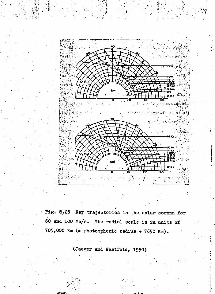
1111111111111j

'11.11001.1-.404.0

,b1-7

111111111111111 IN "Ma eleraint "IN *#0$4001 "a■MatioSvAtftlilllaV 'Wvir jrAtaat

Nviwailwrtwjer *fesavosim•-roON • irtgaimto#

(0561 4Piop.malA pum aoSamp)

.(mx og92, + enTpeu oTaolldsoq.otg.=) TEDI 0oog5oL ;o sq.Tan uT sT grins retTplim OT.ta93/011 001 Pula 09

zo; muo400 amioe Gtp, UT saTaoq.oaPmaq. Smu ce9,.sTa

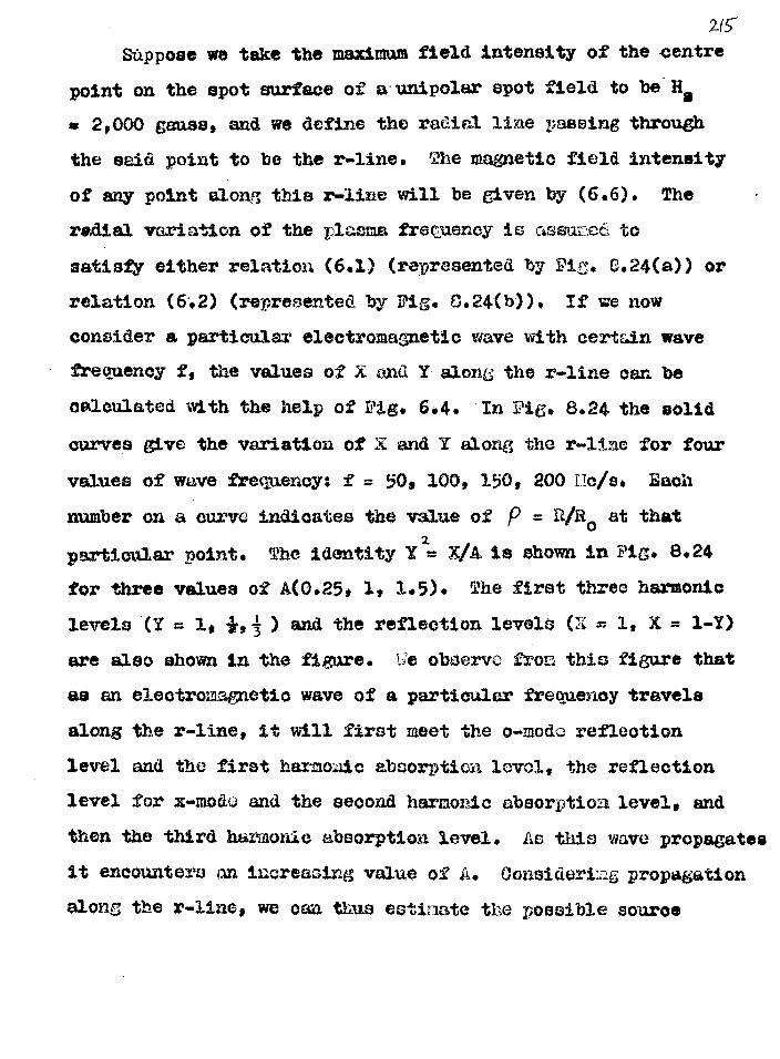
Sappose we take the maximum field intensity of the centre

point on the spot surface of a . unipolar spot field to be Ha

a 2,000 gauss, and we define the radial line passing through

the amid point to be the r-line. The magnetic field intensity

of any point along this rwline will be given by (6.6). The

radial variation of the plasma frecueney is assuzeta to

satisfy either relation (6.1) (represented by Pie. 0.24(a)) or

relation (6.2) (represented by Pig. C.24(b)). If we now

consider a partiettlar electromagnetic wave with certain wave

• frequency f, the values of X and Y alone the r-line can be

calculated with the help of Pig. 6.4. In Pig, 8.24 the solid

curves give the variation of X and Y along the r-line for four

values of wave frequency; f = 50, 100 9 150. 200 no/s. Each

number on a curve indicates the value of P = R/R 0 at that 2

particular point. The identity Y = VA is shown in Pig. 8.24

for three values of A(0.25, 1, 1.5). The first three harmonic

levels (Y = 1, +6 ) and the reflection levels (N = 1, X = 1-Y)

are Also shown in the figure. observe from this figure that

as an electromagnetic wave of a particular frequency travels

along the r-line, it will first meet the o-mode reflection

level and the first harmonic absorptien lova, the reflection

level for x-modo and the second harmonic absorption level, and

then the third harmonic absorption level. Ac this wave propagates

it encounters an increasing value of A. Oonsiderie propagation

along the x'-line, we can thus estimate the possible source

Pig. 8424 The relstiOn , wm /EZ; sad X *curl Al

slang the riaine of aunipolsr spot specified by

Hs • 2.000 VUOS tor four frequencies as indicated

when the electron density distribution follows (a)

Baumbaebpillenis model and (b) Nevikirles model. The dotted lines represent the three harmonic

resonance levels and the line . ---------represents

the identity X I 11 XI A • The 1111100X11 on the solid

lines 'hew the positions in units of solar radii,

' ,` •

11

,

„.

'

•

'

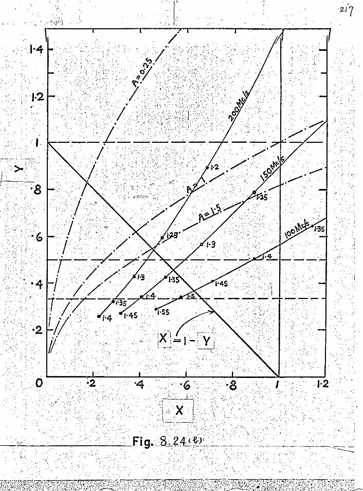
positions for x- and o-mode waves from which the radio

waves can escape. From Pig. 8.24, we realize that there

is a much larger pcssible source region (in the square bounded by X= 1 and Y = 1) from which an o-mode can escape

without meeting the first harmonic absorption level and the

reflection level, while an x-mode wave must be generated at

a much higher level in order to escape from being reflecttd

In most oases, an escaping x wave will have to encounter the

second and third harmonic absorption levels, where the loss

of energy is in general high..

3o far, we have considered briefly the propagation along

a field line of a unipolar spot only. It has been found in

section (0) that the emission angle 0 where maximum power

occurs is not at 0 = 0° , but ranging from 50 to 500 . A two-

dimensional picture of the various reflection and absorption

levels is needed when we consider radiation at the surface of

a cone. Therefore, a more detailed discussion on the escape

conditions for the two characteristic waves in two dimensions

will be given below. ge will take the example of a bipolar

spot field; the argament is similar and simpler when a uni-

polar field is used instead.

After some tediaas calculations, We show various levels

of reflection and absorption for frequencies = 100, 150, 200

Vc/s in Pig. 8.25 (Baumbach-Allen t s model of electron density

distribution) and in Pig, 8.26 (Newkirk's model and 10 ttmes

2(7

Baumbach-Allen's model of electron density distribution) when the value of Hs is taken to be 2,500 gauss. The solid field line shown in each of these diagrams is the strongest field line of the associated spot pair, and need

not be the line passing through the centre of tte spot area where He is specified.

The result of investigation in section (A) indicates that when Al:, 1, Double frequency solution always exists for

the first harmonic which carries more energy than any other

harmonic in cyclotron radiation. It has been pointed out that

when Double frequency solution ocours, the emission is in

general narrow-band and the radiation power is intense. We

may, therefore, consider the location specified by A == 1+

to be the best position where intense noise bursts are emitted.

Moreover, the radiated frequency corresponding to maximum

power for Double solution is always close to but greater than

H 2% H (i.e. 3., ?, 11; section (A) and section (C)).

Hence, the gyro-frequency at the source position must be

+When A is greater than 1, Double frequency solution may

still exist for a higher harmonic. In this case, the

radiation power will be leas. We should, therefore, keep

in mind that the level at which A 1 is not the only possible

location where bursts are radiated.

Fig. 8.25 isalz14.3 = 2.00 ,Ilaos Tor the Gtranger

syyt og t7.:e associatea pair* di2torent levels og in-

terest arc shown i two diasians ger

() .7, 100 'Co/o

(t)) 2 150 :Ws

(e)

3j3 = 712 — 1 = —

S: 1 Ti:= 1 1aa astked.

ate stranect gield line ia xt.. ,prixented by the solid

't7Ack line and tie th14k aotted line is mother

line og t1e1.1.ssooiElted air. Ate yoints 6) in41locA0

lame leculities 'where 1. The corona electron

density is L., ,sctraeLl to gollyw ":7,t3zb3o.-4111en'8 nodel.

.22:0 '

1 oo MO

BACKGROUND CORONA;

SUN

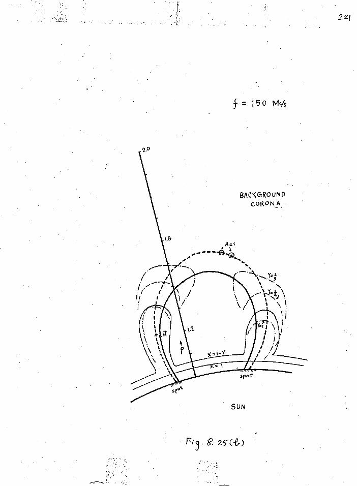
221

SUN

A. 1 d

•

Jhe level X=1

i5 within -tile diremosphere

spot

SUN

F,..3 8.25 (e)

•••

2_2-2

= 2oo Mc/s

BACK no UN

CORONA

-■••■••

Yig. 6.26 Assumingi l = 2,500 gauss for the stronGer

spot of tIle associated pair, different levels oZ in-

tcrest arc shown in two di:lent:11one for

(a)f in 100 Ceis

(b)f a 150 VA:Vs

(o) = zoo Lei's y 313 y y

Per Lewkirk 4 model of active regions

o marked and A = 1 ,

9or 10 Laumbach-Allen's model (or 2 ewkirkts uodel)

of electron demity in the active re,gioa:

= 1

marked, and = 1 x

he field lines are revesenteCt 4 the thick c:aves

with arrows; the complete loop indicates the strong.

eat field line. i;oicts 6 1 , 01 , U3 and 34 are possible

souxce positions wheee the "iate:ase burst radiation

conditions" are sGtisfied. Cho tin straight lime

with arrows ehow the poselb e wave paths.

: •,

• :• , : 4 •••••

2 1-3

• To E tit

spot

SUN

Acrivg REGION

3. (.26 (et,)

•

= 150 M

SUN

F1-9. 8•

2c(e,A)

2-1-5-

S- = 200 Mc/s

SUN

slightly smaller than the assumed radiated frequency f (so

that the normalized radiated frequency which is

slightly greater than 1, when multiplied by the lccal fH

which is slightly snaller than f, will give exactly the value 2

of f assumed). Note that for A = fp/fm 1, j = f/IfH,,; 1,

we have f -.4.- fp at the source. The source for inteane burst

radiation should, therefore, be situated slightly above the

plasma level of f.. We will call these three conditions the

"intense burst radiation conditions'. Consequently, to look

for a source position for intense burst radiation at frequency

f three conditions must be 'satisfied:

(1) A must be close to 1.

(11) The source position must be near and above the level

tfHl= f.

(111) The source position must be situated above the reflection

level X= 1.

An inspection on Pig, 8.25 shows that with our model of

spot field configuration, there is hardly any location where

the three mentioned conditions are satisfied.

When we examine Fig. 8.26(8), we will notice that for

Newkirk's model, a point like Si will satisfy all the intense

burst radiation conditions and the o-node radiating, Buffering

little less at the second and third harmonic levels, will

escape, while the xi.mode will be reflected at the level X =1.Y.

Referring to Pig. 8.26(b) and taking 10x Baumbach-Allen's

217

model of electron density distribution, an electron

stream gyrates through the point S i can readily radiate

an intense noise burst of centre frequency 150 Lo/s.

Using Newkirk's model, S3 could well be another possible

source. In Fig. 8.26(c), the intense burst radiation

conditions are satisfied at a point like 5 4 for 10 X

Bsumbech4i1len's model. We remark that with H s 302,500

gauss as taken in this case, the source position is

always below the x-mode reflection level, implying that

the x-mode radiation can never escape through the corona. (-c-)

Consider the region (marked W . in Fig. 8.26) above

the weaker spot of the bipolar group. Using 10x Baumbach-

Allen's model of electron density distribution , since the

level corresponding to A = 1 Is well below both reflection

levels, no• significant radiation (for frequency 100 - 200

Ws) of any mode will escape the region above the weaker spot.

The implications of all the important restate

discovered in this chapter will be summarized in the

following section.

(P) Predictions of the Theory

Shen all theories, properties and variables are

taken into consideration in the study of escape conditions

and the possible source positions for particular frequencies,

2-24

the study and hence the discussion is extremely complicated.

In the above discussion we have only demonstrated one method

by which the problem is analysed. Investigation on =iv oases

like the one just considered give the following predictions

subsequent to the theory of cyclotron radiation from electron

streams:

(1) In oases when the source is not too high, the x . .mode wave

radiated is either reflected at the level X= 1 - Y or

suffering heavy loss of energy due to second and third

harmonics resonance absorption; this result holds for any

of the electron density models taken in the investigation.

The o-omode radiation, on the other hand, can be excited

readily by an electron stream gyrating at heights greater

than the levels X = 1 and Y = 1. When the source is

high enough, however, radiation in both modes may escape.

Bat in this circumstance the harmonic of radiation will be

high (due to large value of A) and the radiation power small.

Hence, in general, only the o-mode radiation will assume

significant power.

(2) Prom sections (A) and (C), the radiation power associated

with Double frequency solution is much greater than the

power of radiation for Single frequency solution. We sug6est

that radiation in the former case, in the o-mode, is the

origin of the storm burst phenomenum.

(3) If Single frequency solution is satisfied for the generating

process, the bandwidth and emission cone are broad,

if the pitch angle of the stream is not too large.

Since this case is always met with (whenever there is

Double grequency'solution there is always Single

frequency solution with a greater harmonic number Whereas

the reverse may not be 'true), many such events will occur

simultaneously and all these broad-hand. emissions will

superimpose to form a long-lived, broad-band radiation

(type 'I backgroUnecontinuum). Fluctuations in plasma

density and magnetic field will not result in any

significant Change in the superimposed radiation. Based

on(1) 0 . the background continuum radiation. is also in

the 0-mode.

(4) In order to have intense storm.bursts radiated 'near the

centre Of the solar disc, the electron density distribut-

ion needs to follow Wewkirkis model or l0.x Eaumbach-

Allen's model; in particular, the latter model is more

favourable and all the following discussions will be

based on this model.

(5). No significant radiation will escape through the region

above the weaker Spot of the bipolar group when H e

(associated with the stronger spot) is less than about

3,500 gauss. This result indicates that in majority

of cases the received radiation will be polarized in

2,30

the o-mode with respect to the polarity of the stronger

spot in the sunspot group.

(6) Prom points (2) and (3) above, the background continuum

radiation may not be able to survive through absorption

along the corona and be observed on earth. On the other

hand, Double frequency solution is not always met with.

As a result, storm bursts may be observed alone while

at times continuum radiation may not be accompanied by

storm bursts.

(7) Prom section (E), we observe that for source near the

centre of the disc, the source position of intense

storm burst radiation at frequency f is always near and

above the plasma level of the frequency L.

It has been mentioned that when the source (for a

particular frequency f) is near the limb, the true

reflection level (for ray e to reach the Earth) is

situated above the level X = 1. Isoept whe-n the value

Us

is extraordinary lar6e ( > 3,500 gauss), the intense

burst radiation conditions, in general, will not be

satisfied above the true reflection level. Now consider

the space above the true reflection level (where A is

greater than 1) for a particular frequency f. Since the

value of A increases with height and (for a particular

gyrating electron stream) the lowest possible harmonic

2-3/

radiation increases with A (equations (8.3). (8.5)

and (8.6)), the radiation at lower heights will be more

signifioant than that at greater heights'. The lowest

possible altitude for the source (radiating frequency f)

Is, obviously, just above the critical or true reflection

level for f. Bence, according to our theory, we have the

following important prediction:

At an instant, the soured position of a buret radiat-

ion with instantaneous centre frequency f is situated

slightly above the true reflection level of the frequency

f, no matter the source is near the centre of the disc or

near the limb.

(8) Based on the discussion given in (7), the radiation power

of bursts coming from the centre of the disc should be

greater than that from the limb.

(9) For burst radiation in a particular spot field configurat-

ion, the higher the emitted frequency (corresponding to

maximum power) the lower the source position (Pig. 8.26).

When the source region is near the centre of the solar

disc, the source height for 200 Oc/e burst radiation

ranges from about 0.25 R o to 0.35 Flo for Ho ranging from

1,500 gauss to 3,500 gauss. The altitude of a limb source

for 200 Mas is about 0.5 Re

'The reason being that for cyclotron radiation, the radiation

power decreases with increasing harmonic number.

(10) For spot sizes ranging from 1,500 gauss to 3,500

gauss and energy of electron in the stream of the

order of 10 - 100 Key., the limits of emitting

frequency are about 10 Ncfs and several hundred Mo/s.

(11) The bandwidth of the au;erimposed broad-band radiation

can be as high as several hundred Mole while the band-

width of a narrow-banded event can be us low as several

Uc/s.

(12) In general, the source position is not exactly on the

radial line passing through the associated spot, but

it should not be far away.

CHAPTER IX

THEORETICAL DYNAMIC SPECTRA OF STORM PURSTS

A genuine theory mast be able to produce theoretical

dynamic spectra which agree with that observed. Since

storm bursts are considered to be individual events ., we

will attempt to produce some typical theoretical dynamic

spectra of storm bursts in this chapter. To start off, we

need to consider the geometry of the ray path along which

energy and time information is travelling. This, in its

essence, is the problem of ray tracing.

(A) )Ray. Tracing in the Corona

Firstly, we will consider the tracing of ray paths

from the emission radiated by a point source along a

unipolar field. The active region assooiated with

• this sunspot is assumed to consist of a conical region

of apex angle 6 ° (Newkirk, 1959), with the axis of the

cone passing through the centre of the spot. The

distribution of magnetic intensity inside the sunspot

• is supposed to take the form as observed by van Kluber

*Meaning that one storm burst is produced by one stream or bunch of electrons.

2,33

234

(rig. 0.z) and the variation of magnetic intensity along

any field line is assumed to obey relation (6,04, The

maximum field intensity of the spot area is taken to be

2,000 gauss. The radial distribution of electron density

in the active region is assumed to follow Newkirk's model

(relation (6.2)) While that in the background corona is

supposed to satisfy relation (6.1). The effects of the

general magnetic field of the San will be neglected in the

calculations.

We will begin with the ray tracing inside the active

region. Referring to Pig. (9.1), let Q('D • 10), the point

source, be situated at a point along the central field line;

the subscript no" indicates initial quantities and 1 is the

solar longitude angle. Suppose a wave of frequency f is

radiated with wave-normal angle 00 at CI (Pig. 9.1). Por

gradual variation of electron density and magnetic field

intensity, the phase or wave path can be approximated to be

straight over a short distance; let , QP be each a short path

length. Now consider area 411"14.0 bounded by two radial lines

OP% OP(of longitudes 10 and 1 respectively) and two arcs

QQ' and PP (of radii e and 8 respectively). Within this

small area, the magnetic field intensity is assumed to be

constant along each of these two arcs. Under the assumptions

stated, both electron density distribution and magnetic field

intensity distribution are then spherically symmetrical within

C5>

LL

II

235

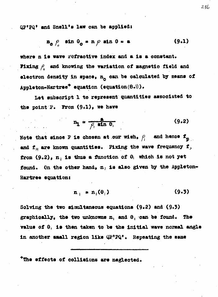
4,po$0sTWou sae suoyemoo ;o wisp, mu+

mom eq% itiovesdau **tam) sityy uoyBox 40t14,0uu uT

oT9us Ism= salmi yvy$yuy sq$ oilO maim tom sy le 0 •trim

au •vuno; aq ram 'e pus 'us-mamma Gm ou$ IATIsov4dsa9

(V6) We (a06) suoyvembo =wean/not:Is om ova BuyATog

(c6)

tuayvertbs osa$awg

-uo$syddy sq$ Aq =AV' oar' sy Uspusg atm° $q$ uo sputto;

$0A $ou ay- qoyqg le Jo umoutl; scrq$ GT 1u '(I) moa;

c; Avuwaboa; SAWA sq$ Buyxyd **immune, umouR sale 14; pus

d •ouott putt U Noy& 2110'4.11 U$11010 sty d soup' $sq4 s$011

I 9 161 lou •./ 401

smog em +(1 6) MO21 *6 WIWI sq$

o$ popyposre sounuelib us ex c$ T $dyaosqus $sT

4,((t.19)uousubs) uoimibs 4,ssawmg.uototddy

;o moss Aq pomnstgo oq us° 011 •oosds uy Aysusp uoasoote

pT1 s ploy; onoultes io uouloyasA Gt 9u1sou4 pus Yguyxyd

.1,unsuo9 it my V pus mopuy eAnoitta;ea SAVA sy u oasqm

It :24 0 Up, d U 10 °O Wye °U

Ipsyydds sq uso met satsug pus ,basab

process, the phase path can be traced inside the active

region readily. Outside the active region the refractive index can

be written as 6

81x 10 N (9.4)

where /1, the electron density expressed in unite of

eleotrons/cm 3 is a function off only. Snell's law becomes

0 arc sin n

'and 8 is a function of f' only* In this case tracing is

done mach more easily .

To show some examples of the dependence of the incident wave-normal angle 8 on p (for both inside and outside the active region) for different values of the constant a, we have Pig. (9.2).

In a stagnatoactive plasma, the ray direction is in gensial‘different from the phase direction. Pros magneto-ioniq theory, at a point where the phase direction is specified by wave-normal angle 0k, the angle between the ray and phase directions is given by (Budden, 1961):

tah =( 114) nab° 6:4

( 1- rl, .1

— 2( I -X) i y4 sin4e ty z %

Y 1 S:...0 Cc4.9 1 4. ( I -X) 2

2 37

2_ 3 8

cr) 3

•

0

0 4-)

(18' - a

e

111 0 co

•0

cu

•VONV 1111480N- 3AVM

'

Using (9.5) 0 the ray path corresponding, to a known phase

path can be traced. in the background comma, we have

Y 0 and it is clear from (9.5) that both the phase

and ray directions ooincide.

(B) Theore cal

S e tra of Sto ate

We will, first of all, assume a helical bunch of

electrons gyrating along the strongest field line of a

unipoler spot. The magnetic field intensity along the

length of the bunch is assumed constant, so that,' the radiation characteristics of the bunch may be described

in terms of a single electron. Let 0 0 and fH. be the

initial pitch angle and gyro-frequency of the electron

respectively. On aocount of the property of constancy

in magnetic moment, the pitch angle 0 at eny point with

gyro-frequency tpi is given by (e.g. Gold, 1959)1

2. 2 _IA sin P. (9.6)

here the velocity /3 of the electron is assumed constant.

Prom (9.6) we can write the longitudinal velocity of the

electron Puas:

i2 I 2 2

(1 4. sin- 0 fm ) 0 —we (9.7)

237

The travelling time for the electron from point S o to

point e is then

ds c f3n

(3c/so(I - s;n1 -514404. )Yz

where de is elementary path length *long the magnetic field

line of force.

The time taken by a wave packet to travel from a point

rc to mother point r is

t j r g re

vip (9.9)

where dr is an element of ray path, and the group or ray

velocity is given by (Ginzbury, 1964),

, vCP inc(n +fol'24.) • (9.10)

where in in this case = 'If

4 4 d\ YJ è w J j

and is given by relation (8.7(a)). once a ray is ni traced, the group velocity at any point on the ray trajectory

can be calculated numerically by means of (9.10) and the

'Here So and S are points on the magnetic field line along

Which the electron is spirally.

24.0

tR.

00E8

MEW •••• cts (9.8)

2/(1

group travelling tiae between the source and the observer

can be evaluated by numerical integration (equation (9.9).

At any point on the electron bunch's trajectory, we have a set of known parameters 430 and A* f;A: •

With these values, the emitted frequenoy range is calculated as in *gotten (A) of chapter VIII. Prom the vs 0 graph

we select the values of and Om at Which the growth rate is maximum (section (C), chapter VIII). Employing the technique dismissed in section (A), a ray of trequsnay fo =3, 1 ;1 and with initial phase angle 00= Om can then be traced. This isly of frequency fo , when received on the Earth (if geometry permits), corresponds to the centre frequency at an instant of .a burst event', WO repeat the some procedure for other points along the electron hutch's trajectory. The electron travelling time between two such points plus the group delay time for the two corresponding rays (of frequencies fo , say) gives the total delay time for the two frequencies fo and ft .

Assuming a helical electron bunch start& radiating at 17 1.21. 0 with pt.t m 0.3 & sa 0.157, the Ms (correspond- lag to wave-normal angle Om ) will fora the surface of a cone.

'Wo choose such a location that A is around 1, so that, Double frequency solution exists a burst can be radiated.

I (9 (a)

1

(C

SUN SPOT

24- 2 2.0

I i 1.4 i 1 I I

I 1 I I i 1 II .41±--- ACTIVE IR GION

1 (AteurfuVe.:4. ML) erd I I I I

CORONA 1.2 pOSI T I ONS

1

1.6

BACKGRouNID souRcE 3(

1.0

F. 9.3 R atj paths in, the solar (a) f= 1GS Kis

f 159 Mcis (c) f = 153 MO.

C OY Ona:

243

tit 43

0 43 43

0 Ca.5 43*

lig. 9.3 allows in two dimensions three acts of ray paths

as the electron bunch gyrates along. If all the three rays

are received on the Earth, the theoretic dynamic spectrum

will have the shape marked burst 1 in Pig. 9.4. When pl. and (38 of the bunch take the values 0.3, 0.7 respectively,

the theoretical dynamic spectrum takes the form as lab elled

burst 2 in Fig. 9.4*. Table 9.1 summarizes the significant

numbers in deducting the theoretical spectra of these two

hypothetical storm bursts.

If the spot..field configuration is of bipolar nature,

the 'tracing of ray paths" . and calculation of group

velocitiec are much more tedious. In Pig. 9.5 ws thew

three sets of rays radiated by an electron bunch at throe

points along a bipolar lield line of force. Kota that in

this case the rays will travel most of the time inside the

aotive region and the rays a', b' and 0 are almost parallel.

The theoretical dynamic spectrum corresponding to the Ms

46 V and o• is also shown in Fig. 9.4 (burst 3).

Over a short distance SC— , 0.05 R00 say) along a

magnetic field line, the Pitch angle of the bunch changes

by a few per cent, while the parameter A changes by ever

'Hero, of cornrow, we assume that all the three rays will

roach the Earth.

We use the same technique as described before for the

unipolar case.

Pig. 9.4 Theoretical dyncmic speotra a

storm bursts. The characteristic nuvabers

icr bursto 1 and 2 re given in Table 9.1.

Durst 3 corresponds to the rays at and b'

(radiated by a tanch) in Vic. 9.5 and

burst 4 to radicted by c> lonc stream

( lereth= 1.35)(10 5 2n ) CyratinG tEruugh.

the poinc:; i of Pic,. 9.5.

BURST 3

BURST 4

0.2 0.4 0.6 . TIME ( SEC.)

Fig. ct.4

130

110 0.8 1.0

190

170

FREQ

UEN

CY

150

(4) (a) (C)

(c) (a')

CJIYE_RE6ttQN ,'

NEWKIRK!S MODEL /

2.0

1.6

1

1

1 BA C K GRO u.N D

COR0 NA BIPOLAR SUNSPOT GROUP

1.0

Q-,

1.4

21(0

Oig. 9.5 Ray paths in the solar corona: (a) f = 135 Mc/s (b) f = 129 Mc/s (c) f = 116 Mc/s. At SI , p_L = 0.3, AI = 0.5 for the slectron stream.

Z47

ten per cent. This change of A, will cause a great *hangs

in the value Of Om and hence the ray direction, with the

result that the me may diverge from the source region 5

(Pig. 9.3 and rays a, b, c of Pig. 9.5). Ibis means that,

on account of geometry, only the rays emitted within an

extremely short length 4LS along S can reach the Earth.

Consequently, if the radiating Aystmn is a bunch, a storm

burst ae observed will show an extremely short duration,

being '< 0.05 sec., which is inconsistent with the observed

duration of most bursts ( -- 1 see.). Vie, thus, conclude

that in the case where the rays from the source region

diverge, a storm burst cannot be radiated by an electron

bunch. However, if a helical electron stream gyrates through

S, then radiation by the electrons as they pass through 4 3

will be of the same frequency (this is true when 4$ can be

approximated to a point) and same direction. According to this

theory, no frequenoy drift will appear in the dynamic spectrum

of a.burst ---- this, in fact, Si observed in most oases. In

such a circumstance, the durations of a burst t can be related

to the length of the stream L and the longitudinal velooity

of the electrons at A S 1

(9,11)

If we take t m I etc., the lengths of the radiating stream

corresponding to Yo 040 and 0,70 are z- 0,04 Re and

0,3 R respectively* It is suggested that the wane of

can hardly be as high as 0.7o, but 0:1c or 04c are

more likely. The theoretical dynamic spectrum of a burst

radiated by a helical stream in given in Pig, 9.4 (burst 4).

When the rays do not diverge in the source region (e.g.

rays a', b'. in Pig, 9.5) and the radiating electrons

form a bunch+, they may all be observed and there will be

frequency shift in the spectrum of the burst. Our estimated

drift rates for this case (17 Mo/s per sec. to 52 Mo/s per

see. for (

ranging from about 0.15 to 0.7) egret with the

observation of Vitkevich (1961). It should be noted that

when the radiating wefts is moving away from the Sun as we

have assumed so far, the noise burst will have a frequency

drift given by ÷-1- < O. However, when an electron

Astral= or bunch enemata increasing gyro.frequency in its

motion, the rays under suitable geometrical conditions may

reach the Barth after reflecting from the oritioal levels;

• in this case the frequ•noy drift will bes > O.

Both types of freauency drift have been observed (Pig, 5.5).

*If a stream is radiating in this case, the bandwidth of

emission will be broad, instead of being narrow for most

storm bursts,

2.4?

CHAR X

CONCLUDING LIWARai ON THL ILTLRFIlaATIOU

OP SOLAR TYPL I LOISL STGREZ

In this chapter we will give a general picture of the

proposed cyclotron theory and sone concluding remarks on the

explanation of the noise storm phenomenum.

On the basis of the currently accepted theories (e.g.

De Jager, 1963; Wild, 1963), a flare, which results from the

annihilation of large volume of intense magnetic fields in the

chromosphere or lower corona, gives rise to the production of

high energy electrons and protons in different states. At

the first stage the explosion ejects charged particles in all

directions, but majority of the electrons (with energy of the

order of 10 . 100 Key.) are ejected along the neutral plane

of a sunspot group (Pig. 10.1). They travel in a radial

direction and excite type III bursts. Some of the energetic

electrons are trapped in the nearby magnetic fields and those

particles arriving at a field line in about the same direction

and with almost equal velocities will form an electron stream

(or bunch) with a narrow momentum spread. When such a stream

gyrates through the corona and whenever Double frequency

solution is satisfied, a storm burst is radiated. The

radiation power is strongest when the stream spirals through

a region where the "intense burst radiation conditions" are

Pig. 10.1 An evolutionary model of the active

region and the flare event as a whole. The

model corresponds to the magnetic field

configuration described by Sweet (1958)

(Runda, 1964, with addition of type I event)

73p.- (cidot-on..)

pe I

(a) Several hours earlier

• 8 .(b) t=0

10 sec —30 sec

• Gyro-resonon to' absorption •

Big increase in intensity and polarization of the pre-existing cm-X source

Start of the Ha flare • Thermal . Bremsstrahlung (local heating):.:.,,..

cm-X bursts -"gradual rise and fall

Low energy X-ray bursts (<20 Key).

Outgoing electrons ("•100 Key- I MeV) Type III .bursts (plasma waves)

Type IC bursts

- { Electrical discharge in overdense plasma -

Explosive phase of Ha flare

:2

Expanding cloud of ionized gas ,

Downcoming electrons (100 Kev-Mev) •

Non-thermal Bremsstrahlung and Synchrotron Impulsive cm .-X burst •

Generalized fast-drift bursts on dm-X (prob. plasma) High energy X-ray burst (>20 Key) •

Fermi-acceleration of electrons and protons" (solar cosmic rays 100 Mey ~several Bev)

(d) t 30 sec — l min

L___) • •

-

Shock front--• (plasma waves) Type II burst

Trapped fast electrons (Type MB) and protons

i . Trapp'ed fast electrons (Type IZA an cm-X - t _

' and dm-X)

(e) 5 min — 10 min

• .43,----. -Shock wave' (magnetic storm cloud )

• • • • • • . •

• • •• •

• •

• •

• 32 Type

tron

Tjpe I

Type El A

(f) t 10 min — 1 hour

{

Trapped protons (PCA) . Trapped electrons --• Type rir C and. continuum storms

Ha loop prominence

Active region on cm-X and dm-X

(g) . t 1 to several hours •

0.

•

satisfied. All the radiation from a number of streams

satisfying the Single frequency solution will superimpose

to form a weak intensity, wide-band, continuous radiation—

the background continuum. With suitable geometry conditions,

the rays of the radiation will be observed on the Earth as a

flare-related solar type I noise storm. In the radiation of

a burst, when the rays from a relatively small source region

diverge, the detected spectrum will show no frequency drift,

which is often the case. when the rays propaaate in almost

parallel directions, the dynamic spectrum of a burst may

indicate upward or downward frequency drift as discussed in

chapter IX.

As it has been mentioned before that most noise storms

are preceeded by flares and the most probable dels/ time is

30 minutes. It seems, therefore, that there is a lapse of

time 30 minutes-during which either source electrons are

as yet unavailable, or that propagation conditions do not

allow the radiated waves to escape. The flare phenomenum is

very complex and is not well understood yet. Prom the more

popular proposed theories of the flare evolution, it seems

that the existence of trapped electrons with mercy-- 10 -

100 Key. in the source region after -- 30 minutes of the

initial explosive phase of the flare is possible. This idea

is illustrated in Pig. 10.1 which is self-explanatory. Woise

storms will be radiated in this case in the se manner as

1,513

described above.

As a noise storm may go on for hours or days, either

the radiating electron streams remain trapred in the spot-

field configurations all the time or that there is a

continuous supply of nonthermal electrons to keep the emission

process in progress. The first possibility is opposed by the

fact that an electron stream with narrow momentum spread can-

not remain in the same state for such a long time on account .

of diffusion, gredient drift and curvature drift. Apart from

direct ejection of high energy electrons (energy > 10 Key.)

in the flare phenomenum, a number of mechanisms have been

proposed for the production of high energy charged particles.

The high energy corpuscles may be emitted through the action

Of an electric field arising as a result of unipolar induction

and creating high voltages (Alfven, 1937), as a consequence of

thermo-nuclear reactions taking place near the photosphere

(Wild, Roberts and .Iiirray, 1954), or as a result of certain

processes which originate in regions of intense turbUlance in

the solar atmosphere (Ginzvurg, 1953)0 Besides the mentioned

theories, Xolpakov (1957, 1959) has shown that if the magnetic

fields of a unipolar spot increase with time -

1

and if there exists a pressure gradient and an magnetic

intensity gradient directed towards the axis of the unipolat

spot field configuration, a net transverse (with respect to

magnetic field direction) induced electric 2ield will exist,

Due to the acticn of this induced field E l , the particles at

the tail of the Liaxwellian distribution of the chromosphere

background plasma will be accelerated to energies up to the

order of I Lev. It seems therefore that hija energy electrons

are produced fromtime to time by various processes and a flare

may be thern trigering mechanism to bring these operations to

high efficiency.

The investigation in section (P) of chapter VIII indicates

that the intense burst radiation conditions are quite easily •

satisfied in the source region if the electron density is ten

times the normal corona background density. Working independ-

ently, this result on magnitude of electron density agrees

with the type II and type III radio observations of Weiss and

others (chapter VI).

A comparisOn on the predictions of the cyclotron theory

(chapter VIII) with the observational data (chapter V) will

show that the mode of radiation, the observed frequency range,

the narrow-band structure of storm bursts, the relation between

the background continuum and storm bursts, the source positions,

the association of noise storms with sunspots and the relative

angular sizes of storm burst and background continuum are all

well accounted for with our presented theory. The dynamic)

spectra of storm bursts have been explained in chaptor Ix.

Based on the very limited knowledge of the flare phenomenum,

the flare association property has been discussed in this chapter.

There remains, however, two features which have not yet

been discussed: These are the polarizaticn properties and

the estimation of electron density in the stream needed in

order to account for the radio flux density received. ge

will consider these two features below.

Por lengitudinal propagation of radio waves in a mag-

netoactive plasma, the polarizations of both modes are

circular aad the polarization constants 'Ro l and I Rx I are both equal to 1. or transverse propagation, I Rol = °

and I = and the waves are linearly polarized.

Piddington aad'annett(1951) have ohown that the polarization

of radio waves tends to be circular as the quantity 1/(1 - X)

tends towards zero except for 0 very close to 90 0 . In the

solar atmosphere, both X and 1. and hence 1/(1 X) decrease

with height. Consequently, for 0 not very close to 90° at

the boundary where Y/(1 0, the limitinc polarization

of the emergent wave (either mode) is circulox, the sense

being depending upon whether the value of (3, is greater than

or smaller than 900 in the boundary level. The above

situation is clearly shown in PiG. 10.2 where R o is plotted

against 6 for various values of Y/(1 - X). Consider the

ciruumstance when the source is near the centre of the disc.,

Referring to Fig. 10.3, it is not difficult to see that

except when the source is very near the to of a bipolar

field line, the wave-normal cksle of the wave will not take

00 60 90 1200 .1500 1800

• 1 1,1 • I-, •

• -

• `• •

Fig. 10.2 Variation of the ordinary mode polarization

Ro as a function of wave-normal angle Q for various

values of the parameter 1 x.

(Piddington and Minnett, 1951)

1

Fig. 10.3 Geometry showing wave paths (represented by

arrows) which would reach the Earth. S i , Sz & 53 are

possible source positions and the wave-normal angle

is 100 at generation in each case.

2 S- &

the value of 900 as it proragates through the corona (here

we assume the wave path to be straight). The polarisation

detected in general will be circular. For a limb source,

the probability that 0 will sesame 90° at the boundary

level (where Y/1 - X.) ---0) is very mach higher. The

emergent wave will be linearly polarized in many oases.

The linearly polarized waves from a finite source will

be depolarized due to the Faraday rotation effect and we

will receive unpolarized noise storms from the limb. More-

over, When the received radiation comes from two sources,

we may receive mixed polarised waves (as observed by

Fokker, 1961) or =polarized waves due to the difference

in polarity of the spots associatectwith the sources or due

to the fact that the values of GI for waves frola one source

are smaller than 900 while that from the other source are

greater than 900 at the boundary levels. 4th these views

in mind, the polarization properties of different noise

storms may well be explained.

Pinally, to estimate roughly the density of stream and

the interaction tire needed in order to account for the

observed maximum flux density, we perform the following

calculation. Assume that electrons in a volume of 100 m 5

of the streams radiate a particular frequency. Let No be

the density of the stream. The maximum power radiated by _I)

a single electron in the o-mode is about 10 watts/sterad.

Then the total power associated with a particular

frequenoy is about 10 NoG watts/sterad., where G is

the power gain in the stream-plasma system. The theoreti-

cal flux density received on the Earth for frequenoy of

100 Ecis would then be 5x 10 -619 140 watts ni 2/(o,4). q, 3

Assuming the active region density to be 10 /cm and 3 .

= 1074

, giving IIo = 10 /om3

we have theoretical flux -41

density -- 5)( 10 G, Blasting this value to the observed

maximum flax density (10 ° watts m-2/(c/s)), we need a

power gain of G 2 21 db). We observe from

Pig. 8.16(o) that the interaction time needed is only about

5 x 10 sec. Note that if the stream density is much

smaller, we can still explain the observed flax density

by allowing a longer interaction time. The above

estimation is very crude, but it seems that all the numbers

involved are physically realizable.

2(2 0

CHAPTER XI

CONCLUSIONS

(A) General Concluding Remarks

Employing the kinetic approach as firstly suggested

by Zhelesnyakov for longitudinal propagation, the

linearized dispersion equation for a stream-magnetoactive-

plasma system for general 0 has been derived for two

distribution fUnctions of the stream: (i) A helical

stream, (ii) a stream with bi-Maxwellian distribution

function associated with both el_ and e h . The

corresponding expressions for the growth rate have been obtained.

The instability theory has been applied successfully

to explain the two existing problems (chapter I) in some

emissions of Jupiter, the Earth and the Sun: (i) Narrow

band structure, and (ii) extraordinary higher power

associated with these emissions. Some doubts in the

radiation characteristics of terrestrial VLF discrete

emissions (triggered and non-triggered) are clarified

and the reason for the existence of emission cone in

Jupiter's decametric burst radiation is clearly accounted

far, The origin of solar type / noise storm, which has

been in doubt for more than twenty years, is explained

in detail.

2_C(

Studying the cyclotron radiation process by an electron

stream in the atmospheres of Jupiter, the Earth and the Sun

shows that under different background plasma conditions

(specified by the quantity A), the cyclotron radiation

characteristics have different forms according to a distant

observer. For example, in the Jovian magnetosphere where

A is very mach smaller than 1 (0.09 - 0.0016), the forward

radiation is predominant in the x-mode since the harmonic o x

resonance absorption is small ,c and the x.mode electromagnetic

power is generally one to two orders of magnitude larger.

For A < 1, it is elementary to show from the Appleton-

Hartree equation that for the whistler mode, n,----7a° as

5: It is easy to see that for A <K. 1, there is

generally no simultaneous solution for the backward Doppler o equation (180 ;. 0 2> 90° ) and the corresponding Appleton-

Hartree equation. Consequently, with the model of Jovian

exosphere as proposed by Ellis, radiation of whistler mode

waves is hardly possible. Hence, the forward cyclotron

radiation in the xrmode (being observed as Jupiter's

decametric burst emisoion) by a gyrating electron stream

is the only Significant form of cyclotron radiation in the

Jovian magnetosphere.

When A >> 1 as in the terrestrial exosphere, the

lowest possible harmonic number of radiation for both

characteristic modes in the forward radiation is large

(chapter VIII) and the oyolotron radiation power will

be small. Thus, the Larth is not a good external

radiator*. This property has been pointed aut by

Ellis (1964). Cyclotron radiation in the backward

direction, however, can easily be significant. Where-

as the "backward waves" propagating along mode 4 cannot

penetrate the ionosphere (Liemohn, 1965), the waves

propagating in the whistler mode can reach the Earth,

being detected as VLF emissions.

When A 1 as in some parts of the active solar

corona regions, the harmonic resonance absorption for

the x-mode is very large and the x-mode reflection

'level for fundamental harmonic radiation is high, so

that, the forward radiation in the o-mode will be

prodominant (chapter VIII). Backward shifted cyclotron

radiation is alio significant for Az 1 and we should

expect strong whistler waves reaching the chromosphere

or the photosphere. Since the coupling mechanism in

the solar corona is very inefficient, the whistler

mode wave can hardly transfer significant electro-

magnetic energy to the o-mode branch. As a result,

the 0-mode cyclotron wave radiated in the forward

Ileaning radiating waves into the outer space.

direction is the only type of cyclotron waves that

will carry significant power and propagate to the

outer space we reoeive the radiation as solar

type I noise storm.

We can, thus, see that knowino the value of A

in the possible source region, the cenoral cyclotron

radiation characteristics from a plasma can be

predicted, with the knowledge of the investigation in

this thesis. These properties will give a guide to

future reseurch on cyclotron radiation in the atmospheres

of heavenly objects or thermal nuolear reactor plasmas.

(B) 5uggestions for Further Research

Based on the results of this investigation, we

may suggest the following items for further research:

(i) Concerning the instability probleu of a stream-

plasma system, study the correspondence between

the kinetic approach end the negative absorption

approach as suggested in chapter II. Following

either approach, investigate the non-linear

theory.

(ii) The origin of hiss is not yet fully understood.

We may seek a solution in the form of cyclotron

radiation by electron streaus,having smaller pitch

angles and different distribution functions from

2. 6 (f

that associated with discrete emissions. Attention

should be focussed on the oontinuous supply of the

energetic electrons, since a "Miss storm" lasts

for hours. The dynamic spectra of other types of

VIA discrete emissions have not been explained

quantitatively; this deserves sane attention.

(iii) 3ince solar type IV emission is in many cases

strongly polarized and the radiation is also in

the o-mode, the origin may be siriler to that of

type I radiation. A detailed study of the radiation

characteristics in the possible source region of

type /V radiation, following the same line as

described in chapter . VIII, would be fruitful.

(iv) Garry out laboratory experiment to study the

radiative behaviour of a streem-plasma system.

Appendix A

Derivation of the Vlasov Equation (Deloroix, 1963; Smerd, 1965; Vlasov, 1918)

(a) The Distribution Functions

Strictly speaking, in a many-body problem Where there

are N particles of one species electrons, say, one

should work with a N-particle distribution function Fp

where at time t, Fi dF1 dF2 dFici dri2 ...a dill is

the probability of finding particle 1 in the volume element

= dii d i dil centred at with velocity in the

range dii = d Yi diia centred at i1, particle 2 in dF2 at F2 with velocity range dira2 at ri2 up to the Nth

particle, Since the number N is usually very large, we

have to use a coarser description of the plasma in practice.

The distribution function usually used in kinetic theory

is the one particle distribution fl(F, 417, t).

Now the probability that particle 1 will ()envy the

volume element el at with velocity in the range al

at while at that time all the other (N 1) particles

may be anywhere in the phase space of the system is

(A,1)

-21s-

Since all N particles are of the same type, this

probability is also the probability that any other one

particle will occupy the volume element dr i avi in phase space. Therefore, the probable number of particles in

volume element dri 171 , i.e. fl aii amii is N times the

probability (Al) and we then have

JP U• arr N 2 2

(A.2)

Similarly, from the probability of finding particle 1

in the volume element vi 1;1 and, at the same time, particle 2 in the volume element *Ea Ti2, while all tha

other N-2 particles being anywhere In the available phase

space, we can find the probable number of pairs of particles

In the volume element Vi abii and '6'2 1V2 respectively. We will now have a 2.particle distribution itnotion f 12(F, t)

which can be shown to relate the N.particle distribution

function in the form

t12 0 N(N •1K4 (A.3)

This process can be continued for three particle distribution

function 1123 and so on. We note here that the 2-particle

distribution function f12 will already enable us to determine

the macroscopic effects such as the internal fields and

pressures due to the interaction forces between the particles.

7-6

Such distribution functions describe the state of the

plasma at time t to varying degrees of accuracy. We

need now to describe the microscopic state of the plasma

in the course of time in terms of the microscopio

distribution functions.

(b) The Kinetic Eauatl'en

In the system under consideration, assuming all forces

are conservative and independent of velooity, the Liouville

theorem describes the changes of Pk as a function of time

in phase space Co. t. Deloroix, chapter 7, 1963):

)FIN) v.7 )FN

t 1

Fs, _ 0 ■;-; CA.4)

where the total force acting on the ith particle consists

of the external force 71. and the forces 713 (i j) due to

the interaction of the ith particle with each of the other

(N - 1) particles.

In order to simplify calculation which becomes

impossible when N is large, a regression method has been

developed to describe the evolution of the plasma in terms

of suoceseive pairs fi, f12/ f12, f1231 f123. 11234/ of the one-particle and multiple-particle distribution

functions. Thus, one has to know f12 in order to determine

fie to know fi23 to determine f12 so on. This method

z (a7

26 k

La called the BHGKY-method which bears the initials of

its originator.

The first and the simplest of these Liouville-type

equations is (Dolcroix t chapter 7, 1963):

j 4 + AI + + XII ./1_61720117,i.,-0 (A.5)

-1 )7, ill 4) ii■ 111 (7°- In most problems, only the first BBGKY -equation i.e.

equation (A.5) is employed.

Neglecting the interactions between particles,

equation (A.5) becomes

• 11_ +TriAi t x f. 41 = 0 ?et

- and one sees that this is in fact the collision-free

Holtzman equation.

( A E )

(0) cosre weLor_tice_s

In above, we arrive at a kinetic equation (A5) which

is the approximated form of the complete one. To obtain

the Views, equation, a few more approximations have to be

taken. Before we consider these approximations, we need

to define the concept of "correlation" between particles.

(0 f. Delcroix, chapter 6, 1963).

The N particles of a. ppecies are said not to be

correlated or independent if the N-partiole distribution

211

function can be written as the product of U single-particle

distribution functional

F = Fo a ui 1* o 2* t)F (7 2'

; •.•s• Fo(Fo t) (A7) N 1*

, These functions are funotionslly identical since all particles

of one kind are quite the equivalent of each other. The

probability of finding the plasma to be in some state of

phase space is 1:

t) 11.7 E = 1 (Ap)

From equations (A?), (A7) and (AO, one finds that for

the one-particle distribution function,

f= NFo (A9)

From (A7) and (A9), one realizes that if f 2 m t).

3 = ( 3 V3 . t) •,0044 than

1 • 41, eum.f1 f2 f3 ,

In the case of the 2-particle distribution function,

we have from equations (A3) (A7), (48) and (A9) that for

no correlation

fi2 1° 1) 21 f2

fl f2 for N>> 1 (A10)

(d) The Vlasov Equation

If we assume that there is interaction bat no

correlation between the particles in a plasma subject to

electromagnetic disturbance, relation (A10) holds and the

lest term of equation (45) becomes

270

11•101■1.

X i2- 4Ia A -172:61‘7- ?-41 x 'l L-771 With X12 independent of velocity, we can carry out the integration with respeOt to /5 :2 to get the density, ne

cITI12 ( A.1 1 )

it2 172 (Al2)

In other wards, the probable:number of particles with any

Velocity in the volume element '3;2 is n2 3F2 , and relation (All)

becomes

i1)1 2., x1 d r-7i )17ri

(A.13)

where Yi is the electrostatic force due to space charge

(Deloroix, equation (6.49) of chapter 6, 1963) and is

equivalent to the term e s of relation (1.3). With (43).

equation (45) reads

+ i7 -AL - 31T m

This is the Vlasiov equation with an external forge; and

an electrostatic force ri due to space charge. Including

= 0 (A .14 )

e, a magnetic force —Ir y x (Bo 4. ib as in (1.3) rewires a

relativistic treatment of the Liouville equation and will

not be dealt here.

In the derivation of the Vlasov equation, we have assumed

that there is interaction but no correlaSion between particles.

This means that the interaction is of a collective or macroscopic

nature and acts continuously and equally an all particles like

an external force. It is worth remarked here that when we

assume that the interaction occurs only in binary collisions

With no interaction force acting on the particles between the

period of such collieions, equation (A5) is appnoximated to

the well known Boltzaan equation.

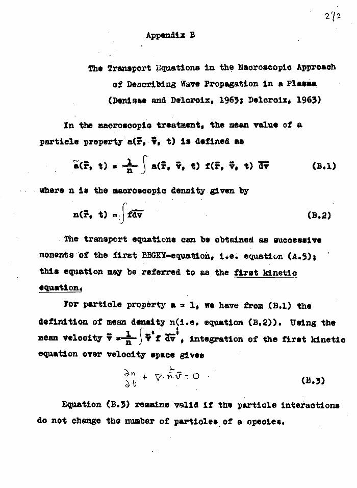
Appendix B

The Transport Equations in the Macroscopic Approach

of Describing Wave Propagation in &Plasma

(Denise, and Deloroix, 1965: Delcroix, 1963)

In the macroscopic treatment, the mean value of a

particle property a(,•, t) is defined as

t) as ÷S t) t) (B.1)

where n is the macroscopic density given by

na, t) =SAT (B.2)

The transport equations can be obtained as successive

moments of the first BBUY-equatioi, i.e. equation (A.5);

this equation may be referred to as the first kinetic

equation.

For particle property a = 1, we have from (B.1) the

definition of mean density n(i.e. equation

mean velocity v ii÷cVf agi'. integration equation over velocity space gives

• V.ix.* IT:: 0 •

(B.2)). Using the

of the first kinetic

(13.3)

Equation (B.3) remains valid if the particle interactions

do not change the number of particles of a opeoies.

273

Por particle property Ismi, integration of equation (A5)

with respect to velocity gives

nm ( + TrvIc7) — k"-; V-3+- 13 k t

(13.4)

where rim fat y° dvt \Jdl3/ htjxGOtIO fl

't is the kinetic pressure tensor and it is usually

assumed that I can be reduced to an isotropic soalar

pressure p nx,T.

IT is the external force.

7 is the interaction force devided by the mesa density

and it consists or two parts: (1) a collective interaction which is added to the external force 74 (ii) a collision interaction which adds, in part, to the pressure tensor "r due to collisions

between Like particles, while the remaining term -fr*a_ —

represents the momentum transfer due to collisions between

particles of different speoies. In deriving the Vlasov equation,

all collision effects are neglected.

Equations (A3) and (B) are two transport equations. Prom

these two equations and the Maxwell equations, the dispersion

equation can be derived.

*here AT so 41-, u)"."121 - r1.2 - wit- a

AL (1- lt)(1

Appendix C

Dispersion Lquation of Plane riaves Propagating in

a Warm, Collisionless, Vagnetoactive klasma

Using the macroscopic approach * Maltese and Deloroix give

the dispersion equation foe plane waves propaeating in awarm,

collisionless, magnetoactive plasma:

6TAL+53""+hs: 0 (Cl) 2 7.

— (A) L y) - 1 + ‘'

U 2.

LPL L (A; pl

CU - nit

• 1 + 1--- (2=qt (T):2- + ‘g.)- (AJ

) a UJ 2'

W GA,

c + it4) + cu. )

Oj ES/

= Cu 6

co m.4;2. w 4. li at i

4 ss nj -1+X

(A-)H Cog

I n

j).' = JLH C0SO

4021+ g■ nA9

1 74-

e Ho H = me

e.H 1114 .. mio

e, ei = charge of electron, ion, respectively.

me, me mass of electron, ion respectively.

'o = speed of light in vacuum.

Ho = static ma5netic field strength in gauss.

0 = angle between static magnetic field (which is on y-s plane)

and wave vector E = nj refractive index.

= 4 1 ne e 2- c/3118

= 4 ol/ mi

and are average particle densities of electron and ion

in the plasma respectively.

Ei = 0 2/ 2- Vi

Es C3

with Ve, Vi are the average tievmal velocity for electron and

ion respectively. 2

2 Vs 2

(Ale 4 -n-p X WD /Le

UJ0 1 =- j111

The above dispersion can be arranged into an equation of

the fourth degree in and hence for one value of angular

frequency there corresponds in genera]. four values of the

refractive index squared. In other words, this medium is

. quadruply refracting-- four distinct modes of waves can therefore propagate through this medium.

177

Appendix D

Two I:Sthods of 3o1ving the Radiative Instability 1 -rob1em

of a Stream-Plaama System within the Xinetic Regime

To attack a radiative instability probleil of a stream-

plasma systeo, two methods are generally used within the

classical kinetic regime: (1) assuming the wave vector to

be real and solve the dispersion nuatien of the system for

complex frequency, considering the dielectric tensor of the

system to be made up of two parts --- one due to the

ambient magnetoactive plasma and the other due to the

presence of the-strea0(e.g. Stepanov and. Ateenko. 1961)

(ii) assuming the wave Vector to be real,derive the

dispersion equatien.tor an electromagnetic wave in a system

of a stream travelling in vacuum in the presence of a static

• magnetic field, and then include the presence of the ambient

plasma by assuming

n :n,2 + ns ,.. 1

(D .1)

where n = overall refractive index for the combined system

n = refractive index for the ambient plasma alone,

and

ns= refractive index for the stream alone (in the

presence of the static magnetic field.

The presence of the term ill" in relation (i.1) cones from

the fact that each of the refractive indices ne n s has

included the effect of a vacuum (the refractive index for

an electromagnetic wave in vacuum is 1). This approach

WAS firstly introduced by Zhelesnydkov . (1960a).

It is interesting to find out whether the two approaches

are exactly equivaleut, or one being the approximated form

of the other. We investigate the case when the stream is a

helical electron stream, i.e. each electron in the stream

moves with the sane non-zero transverse velecity A L =1/1/0

arid the same longitudinal velooity R =IA; /c, o being the ro

velocity of light in vacuum. The particle density in. the

stream is assumed to be very small compared with that in

the background plasma and the stream-plasma system is assumed

to be electrically neutral.. The colliaionless Appleton-

Hartree equntion is assumed to be applicable to the propagation

of electromagnetic waves in the background plasma alone. To

simplify calculation, we consider longitudinal propagation

only i.e. the wave-normal angle 9 is either 0 ° or 180°, with

respect to the static magletio field. -The electromarmetio

wave is assumed to vary according to .e .."'"trb and we consider

the first harmonic only. Tho refractive index for the

electromagnetic in a system of helical strecmaand static

.magaetic field is (9 = 0 45or 180° ) (Zheleznyakov, 1960a)

(D.2)

where Exs and Esw are dielectric tensor components

for this system and are given by

with E (AA: f12-(c/1443*-1)

4 S2

41.17 is angular plasma frequency of rno

the electron stream

No = particle deneity of electron stream

a = "characteristic frequency" of the emitted complex

wave angalar frequency, given by

cu = + real and S ,complex

(D.3)

assuming I Gu l >> II

(D.3a)

Taking negative sign in equation (Da), we have

03.4)

Taking into account the effect of the background plasma as

specified by relation (D.1), the second approach gives the

overall refractive index:

2 2 J (D.5)

Taking the first approach we must know the dielectric

tensor components for the electromacnetic in the ambient

plasma alone (Stepanov and Kitsenko, 1961):

Eg: = 1-H =

whore 1.4 —LA41 .1

— r 707116-0- , GuP7-= 4TrNza

N = particle density of ambient plasma .

The overall dielectric tensor components for the whole

stream.plasma system are then+

Exx E 4- EXX H

zgo

(D.7)

The overall refractivs index is then given by

2=' Ex 114- =

S 2

(D.8)

here we have taken into account the fact that we ere

considering a thin stream and thus

. +ge hay,' written down three dielectric tencor components only

because the dispersion equation does not involve any other

component for case of 9 = 00, le

Ez

and 1111

_Taking negative sign, relation (!.S) gives:

281

(D.9)

0.90 <‹ 1

2

(Alp - 2

Gt) t tAiN Cu (D.10)

— 2E nathematically, we have seen that with a thin stream

such that inequalitiee (DA) and (D 9a) are valid ' the two

approaches give the same dispersion equation for the case

of longitudinal propagation. Once the dispersion iu

derived, the growth rate can be calculated readily.

rormulating the radiative instability problem with the

second method means that we assume that the refractive

indices nt and n of the two interpenetrating media, i.e.

the stream and the ambient plasma, are non..interzoting and

this is valid only when the density of the stream is small

compered to that of the background plasma ouch that the

presence of the stream is represented by a small perturbation

term ) in the dispersion eqaation of the whole system.

When we investigate the radiative instability problem of

more complicated systems (e.g. including temperature effect

of the stream, considering a general wave ,normalEAngle 8)

the second method has the great advantage of being simple

in mathematics. It ha e been La-and numerically that both

methods give the same zeneral behaviour of the growth

spectra:1 for both baokw6rd 61-li1ted kind forward shifted

noraal cyclotron radiation.

7g2

am indebted to my supervisorsrofessor

Lllis (during my whole poriod of research - April,

1964 to April, 1966) and Dr. R.L. Dowden (April, 1964

to December, 1965) for their encouragement, criticisms

and advice. I also wish to express my sincere gratitude

to Dr. S.F. Smerd, Radiophysics, Sydney, for

his stimulating discussions and criticisms an the

instability theory and solar work. Parts of the

numerical computation in the theoretical study of solar

type I noise storm were carried out jointly with Wr. 4.

K. Yip.

Apart from those acknowledged above and in the body

of the thesis all the ideas and calculations are my

own.

During the period of these investigations, I have

been awarded the University Postgraduate Scholarship.

• (Peter Fang)

April, 1966.

2 3

284

PUBLICATION

Sons parts of this thesis have been pet in paper

forms and have been accepted by appropriate journals

for publication:

(1) P.O.W. Rung "excitation of Backward Doppler-

shifted Cyclotron Radiation in a

Lagnetoactive Plasma by an Eleotron

Stream", PlanetarY & Space Science

(in press).

(2) P.G.W. Pang "Excitation of Cyclotron Radiation

in the Vorward Subluminous Kode and

its Application to Jupiter's Decametric

Emissions", Planetary Space Solana*

(in press),

(3) P.O.W. Pang "Excitation of Cyclotron lAeotronag-

natio raves in a Yagnetoaotive Plasma

by a Stream of Charged Particles

including Temperature Effects in the

stream", Australian Journal of Physics,

(in press).

Other papers being prepared for publication are:

(4) P.C.W. Pang "On Two rethods of solving the Radiative

Instability Theory of a Stream-Plasma

System".

zg .S"

(5) P.O.. Yung êZ. Yip "Cyclotron Radiation froa

Electron Streams as the Oricin of Solar

Type I Noise storm".

(6) P.C.J. Pang & W.K. Yip "Theoretical Dynamic Spectra

of Solar Storm Bursts".

(7) 2.C.W. Pung "The dole of Cyclotron Radiation in

Radio Astronomy".

REFERENCES

1. Astrom, - Arkiv f. Fysik, 2, 443,1950.

2. Akhiezer, Fainberg, Ya.B. - Doklady, Akad.

Nauk, §A, 555, 1949.

3. , Allen, C.W. - Monthly Notices Roy Astron. Soc.,

107, 386 9 ,1947.

4. Alfven,.H.-Z., Physik, 10., 633, 1937.

5., Bell, T.V. & Buneman O. - Thy. Review, 122,

A1300, 1964.

6.. Beck,,A.H.W. "Space-charge Waves", Pergamon

Press, Ltd., London 1958.

Barrow, C.H. - Astrophys. J. 13.5. 847, 1962.

8., Brice,. N, - J.,Geophys. Res., 68 4626, 1963.

9. . Brice,. N, - J. Geophys. Res. .§.2, 4515, 1964.

IC.. Baumbach,, S.,

Astronomische Nachnchtan, m y 121,

1937.

11. Bray, R.J. & Loughhead R.E. - Australian J. Phys.,

12, 482, 1962.

12. Bray, R.J. & Loughhead, R.E. - "Sunspots", chap. 5,

sect. 4, Chapman & Hall Ltd., 1964.

13. Bidden, K.G. - "Radio Waves in the Ionosphere",

Cambridge Press, 1961.

14. Cohen, N.H. - Phys. Rev., =Et 711, 1961. 15. Carr, T.D., Smith, A.G., Bollhagen, H., Six, N.P.,

Jr. & Chatterton, N.E. Astrophys. J., 114., 105, 1961.

2 q,

287

16, Denies° J.P. Deloroix, "Theorie des

Ondes daus les Plasmas", Dumod„

Paris, 1960. English translation:

"Plasma Waves", Interscienoe

Publishers, .TJ[4., 1963.

17t Deloroix, J.L. - "Physique des Plasmas", Dunod,

Paris, 1963.

- 18. Dowden, a.L. - J. Geophys. Res., 611, 1745, 1962a.

19. Dowden, Nature, 2,211.085, 1962b.

20. Deniese, J.P. - Inf. Bull. Europ. 5o1ar Radio gin..

No. 4, 1960a.

21. Denies*, JJ.- XIII 11.11.S.I. General Assembly,

London, 19601)0,

22. Dowden R.4. - Australian J. Phys., 12, 114, 1962o.

23. Dowden, 11.L. Australian J. aye., 12, 490, 1962d.

24. De Jager. O. - Space Science Reviews, 1, 487, 1963.

25. Ellis, G.R.A. - Planet. Space Soi. 1, 253, 1959.

26. Ellis, G.R.A. Vedic) Flicience, 091., ro, 12, 1513,

• 1965.

27. Eidman, Vas.

soviet Phys., J.E.T.P., 21, 91,

1958.

28. 'adman, Vas. - Soviet Phys., J.E.T.P., 26., 947,

1959.

29 0 Engel, i. The Phys. Pluide, 8, 939, 1965.

30. Ellis, - Nature, 124, 667, 1962e.

1 88

31. Ellis, - Australian Phys., 12, 344, 1962b.

32. Ulla, G.U.A. - Australian J. Phys., 16, 74, 1963.

33. Sins, G.R.A. &-2COulloch, P.1J.- Australian J.

Phys., 16, 360, 1963.

34. Ellis, G.R.A. - J. Geophys.Res.,filp 1705, 1960.

35. Elgaroy, 0. - Astrophysics Norveuia, 2, 123, 1961.

36. Mlle, G.U.A. - Australian J. Phys., IL 63, 1964.

37. Painberg, Ya.D. & Shapiro, V.. Gov.

20, 937, 1965.

38. Fokker, A.D. Jr. - studies of Enhanced Solar Radio

Emission at Frequencies,

Netherlands at, Flection 10110s.

sphere and Radio Astronomy, 1961.

39. Ginsburg, VZ., aelesnyakov, V.V. & Eidman, V. Ya.

Phil. Vag., 1, 451 1962.

40. Ginsburg, V.L. - "The Propagation of Electromagnetic

Waves in Plasma" Pergamon Prese t

1964.

41. Gardner, P.P. & Shain,

- Australian J. Phys.,

11* 55, 1958.

42. Gerahman, B.L. . Soviet Phys., J.E.T.P., 11,, 657, 1960.

43. Gallet, R.L. . Proc. IRTI, AL 211, 1959. 44, Goldstein, Jr., S.J. Astrophys. J., 2211 393, 1959.

45. Ginsburg, V.:). & Zheleznyakov, V.V. . Sov. Astron.,

AJ, 2, 235* 1959.

287

46. Ginsburg, V.Y. & Zheleznyakov, V.V.- Soviet

Astronomy, AJ, 1, 1961.

47. Ginsburg, V.1. & Zheleznyakov, V.V. - Soviet

Astronomy, AJ, 2, 653, 1958.

48. Ginsburg, V.. & Zheleznyakov, V.V. - Paris

Symposium on:Radio Astronomy, Stanford

University Press, p. 574, 1959b.

49. Gold, T •- Nature, m oo 355, 1959,

50. Ginsburg, V L. & Prank, J.N. - C.R. Acad. Soi.,

ji& 583, 1947.

51. Ginsburg, V.1.- Doklady Akad. 512,0

727, 1953.'

52. Helliwell, R.A. & Carpenter, D.L. - "Whistlers-

West IGY-X0C synoptic program," SL

Final Report, Stanford University,

L7ar. 20, 1961.

53. Harang L. &Larsen, R. - 17., 481, 1965.

54, Hansen, 0.V. . J. Geophys. Res., 68, 5925, 1963,

55. Lelliwell, R.A.-- J. Geophys. Res., 68, 5567, 1963,

56. Helliwell, R.h. J. Geophys. Res.. .06 2391, 1964.

57. Hey. J.0. - Nature, AU+ 47, 1946.

58. Hale, ELL.& Hichotson, U.B. . Pub. Carnegie lust.,

No. 498, 1938.

59. Jelley, "Cerenkov Radiation and Its

Applications; Pergamon Press, London,

1958.

I 10

60. Jaeger, J.C. & Weetfold, K.C.- Lust. J. of Phys.

Sol. Res., Alt, 376 * 1950.

61. Jackson, J.D. - "Classical laectrodynemios",

Aley, 1962.

62. ovner fl.S. - News of higher educational

institutions, U.Z.O.N. Radiophysics

series, A, 118, 1961a.

63. Loner,

. News of higher educational

institutions, U.G.Z.U. Radiophysics

• seriss,A, 97, 196116

64. Rundu, u.a. . "Solar Radio Astronomy", Report

no. 64 - 4, The University of

• Olohigan, Radio, Aetronom observatory,

1964.

65. Kiepenheuer, Z.O. - Nature. MAD 340, 1946.

66. ;Kruse, U.Wo, arshall, L. & Platt, J.R. Aetrophys.

J., la, 601, 1956,

67. Xolpakov, P.L. .- soviet Astronomy, AJ, 3, 218, 1957.

68. Xolpakov, .1'kwiet Astronomy, Aj, / 692 1959.

69. Rol, X. - Publ. Aetron. Soc. Japan, 1A, 1, 1962.

70. amain, E.B. - Radio Science, 020 741, 1965.

71. Mainatone, J.S. & . Proc. Ionosphere

Conf., p. 163, The Physiosl Society,

London, 1962.

72. flakhan'kov, V.G.

Soy. 174ys., Tech. Phys., 8 * 673,

1964.

2,1

73. Uartyn, D.V. Vature, 12m, 632, 1946.

74. Ucriuoto, J. & Kai,

2ubl. Astron. Soc. Japan,

11, 294, 1961.

75. Lalinge, A.L.- Ann. d* Astropbys., 26, 97, 1963.

76. Lorimoto,

& Uai, L . J. 2hys. Soo. Japan,

Supplement A - 11, 22, 220, 1962.

77. Newfeld, J. t Wright, 5.

Phys. Review, 115.,

A1175, 1964s.

18. Newteld, J. 61wAght„ H. - 2, 1527,

1964b.

79. Uewkirk, G. - 2aria Symposium on'audio Astronomy

(ed. R.N.Bracewell, Standford

University, Standford), p. 149, 1959.

80. Fiddington, J.U. - 2141. 'Lags, 4-go., 1037, 1955.

81. :lerce j.11. "Tmvelling-wave 2ubes", D. Van

Vostrand Company, Inc., Prinoeton,

1950.

82. 1,awsey, J.L.

I.L.B., London, l'art III, 320

290, 1950 *

83. iwne-Ocott, L, Yabsley, & Bolton, J.G. -

Nature, 2.02, 256, 1947.

64. 144yue-cott, i. &little, A.G. . Australian J. Soi.

Res., MA 508, 1951.

85. Yawsey, J.L. & Bracewell, R.N. - "Radio AstroneMY,

Clarendon Yress, N.Y., 1955.

241

66. riddington, don. &ainnett, U.G. - Australian

J. 'Joie N.es., Ab 131, 1951.

87. Ratcliffe, J.A. - The Lagnetc-Ionic Theory and its

Applications to the Ionosphere,

Cambridge, 1959.

88: 2oberte, . Planet. Space ci., lit 221, 1963. 89. IIyle, . t Vonberg, L.D. Vature, 121, 339, 1946.

90. Ryle s Vonberg, p.Bd rroo. Roy. Soo., Aasa, 98, 1448.

91. Roberts, J.A. - Australian 3. Phys., 11, 215, 1958.

92. Suerd, S.F. - Private communication, 1965.

93. .6cheuer, P.A.G. - Mon. Tiot. Roy. Astron. Soo.,

laz 231, 1960. 94. Schwinger, 3. - Phys. Rev., 211 1912, 1949.

95. Stepanov, n,N4 & Kiteenko, A,h3. - Sov. Phys. Tech.

Phys., 6, 120, 1961.

96., Snerd 0.41-0 WA-Symposium on "The Physios of Solar

Plares", NASA Si)-50, p. 349, 1963.

97. Sturrook, P.A. . Phys. , Rev., lag,. 1488, 1958.

98. Shapiro, V.D..A iihevohanko, V.I. - Sov. Phys.,

11, No. 4. p. 731, 1962.

99. Shapiro, V.D. - Gov. Phys.,JET I7, No. 2, 416,

1963.

. 100. Shaine U Australian J. rhys., 61, 1956.

2. 7 3

101. Shain, C.A. & Higgins, C.S. - Australian J. Phys.,

12, 357, 1959.

102. Smith, H.J. & Douglas, J.N. - "Paris Symposium

on Radio Astronomy", p. 53 (ed. R.N.

Bracewell), Stanford University Press,

Stanford, Calif., 1959.

193. Suzuki, S. - Annals of the Tokyo Astronomical

Observatory, University of Tokyo,

sec. series, VII, No. 2, 75, 1961.

104. Sweet, R.A. - I.A.U. Symposium No. 6 on "Electro-

magnetic Phenomena in Cosmical

Physics", ed. Lehnert, B.P., Cambridge

University Press, p.123, 1958.

105. Twiss, R.Q. - Australian J. Phys., 11, 564, 1958.

106. Twiss, R.Q. - Phys. Rev., 88, 1392, 1952.

107. Tchickachev, B.M. - 5th Colloquium on Cosmogony,

Moscow, p. 245, 1956.

108. Takakura, T. - Publ. Astron. Soc. Japan, 8, 182, 1956.

109. Twiss, R.Q. & Roberts, J.A. - Australian J. Phys.,

11, 424, 1958.

110. Takakura, T. - Astron. Soc. Japan, Publ., 12, 462,

1963.

111. Takakura, T. - Publ. Astron. Soc. Japan, 13, 166,

1961.

112. Vlasov, A.A. - Zh. Eksp. and Teor. Piz., 8, 291,

1938.

115. Vitkevidh, V.V. et Gorelova, L.V. tiov. Astron.,

595, 1961.

114. von Tluber, E. - • A3tropi4e.. gt, 121, 1948.

115. 411d,

Smerd, ;,;,2. a Weise, 4.A. ,"Solar

Bursts", Annual Review of Astronow and

itetrop4eics, 1, 291, 1965.

116. Warwick, 1.stroOlys. d., 117., 41, 1965.

117. 'jarwick, j.. Ann. N.Y. Acad. Uci., 21,• 59, 1961.

118. Watts, J..- J. Geophys.. lieu., 62, 199, 1957.

119. Uld, J.P. - Australian J. ei. Res., AA 56, 1951. 120. Wild, J.P., Gheriden, R.V. ilsylan, A.A. - Austra-

tan J. Itys.,.12, 369, 1959.

121. Weles, A.A. - Taublished data, 1965.

122. eiu, A.A. . Australian J. 17-hjs., lAp, 240, 1963.

123.. Wild, J.2. & Sheridan, 1a ?roo. Aft. 160 0 1958.

1246 Vvild, 1.2. & aria, h. Australian J. Aye.,

315, 1956.

125. raid, J.:.

-

"The ',audio 'Atacama from Solar Flexes-4 ,

J. Physioal Soo. Japan, SupPle-

nent A . XI, y. 249, 1962.

126. Wild ▪ "The Oolar Corona", ed. Evans, J.4.,

Aoademio-i=resa, p. 115, 1963.

127. Lid, J.:P., Roberts j.A. & Lbrray. J.D. - Nature,

p. 552, 1954.

128. Zheleagyakov, 1, 57, 1960a.

129: Sholoriniakov, 3oviet &Aron., AgT, 2, 206,

1958.

130. ghaemlyakov, - Radiofisika, 180, 1960b.

All synbols Lre defined in the body of the thesis

wLen they first occur. Those Which are used more exten-

eively and which may appear somewhere apart fron their

definitions are listed below:

al = 2m0X T a 2 = 2mO A = cup'/Gu h2*

= speed of light in vacuum

e = charge of an electron a

fp = wpAyq = imjTP = eleotron 121asma frequiek2cy

f H = AAJHAn = elion2ir moo) = electron Gyro-lrequeAy Ea = static ma6netic field intensity

ns = magnetic 'field intensity at the centre of a sunspot k = complex wave number

km = transverse and longitudinal components of

wave vector k resoctively

= characteristic ligwe nuober, is real

mo = rest mass 'of a electron

U = electron particle density

nj = refractive iiddex

p = power of eleetrouajnetic wave

= transverse and lonzitudinal compaceAs of

nomentam p re5pectivoly

k ti

o = solar radtas

= handout° n=ber

= temperature in degrees

va = tramsverae and louGitudinal velocities respeotively

X

I

13-L m,v1/0

vdc (31

s W

S I = S/0) c*= dielectric temor of a system

4-2 PA0111

1)(2„

So IT. _gx = ±.1 ita )/2

S = artanf34 1 = pitch anGle of aratinz particle = wave-normal wile, i.e. ante between stukic

magnetic field and wave vector

Om = wave-normal anrAe at which the i:7rowtli rate for

the stream-plasma systea le maxima

pc = cutoff" anGle

ctio = angular electron plasa froquency of the stream

/9 = ittlo = radial distance from centre of the in

5 = / al

=

y = electron-ion collision frequency

X = Boltzman's constant

(A) :: 2Tr5 coltdal olnaracter;st ■ G wave frereticy

2.7i?