Cyclic Loading Behavior of CFRP-Wrapped Non-Ductile ...

Portland State University Portland State University

PDXScholar PDXScholar

Dissertations and Theses Dissertations and Theses

Spring 5-4-2016

Cyclic Loading Behavior of CFRP-Wrapped Non-Cyclic Loading Behavior of CFRP-Wrapped Non-

Ductile Reinforced Concrete Beam-Column Joints Ductile Reinforced Concrete Beam-Column Joints

Ali S. H. Zerkane Portland State University

Follow this and additional works at: https://pdxscholar.library.pdx.edu/open_access_etds

Part of the Civil and Environmental Engineering Commons

Let us know how access to this document benefits you.

Recommended Citation Recommended Citation Zerkane, Ali S. H., "Cyclic Loading Behavior of CFRP-Wrapped Non-Ductile Reinforced Concrete Beam-Column Joints" (2016). Dissertations and Theses. Paper 3000. https://doi.org/10.15760/etd.3001

This Thesis is brought to you for free and open access. It has been accepted for inclusion in Dissertations and Theses by an authorized administrator of PDXScholar. Please contact us if we can make this document more accessible: [email protected].

https://pdxscholar.library.pdx.edu/

https://pdxscholar.library.pdx.edu/open_access_etds

https://pdxscholar.library.pdx.edu/etds

https://pdxscholar.library.pdx.edu/open_access_etds?utm_source=pdxscholar.library.pdx.edu%2Fopen_access_etds%2F3000&utm_medium=PDF&utm_campaign=PDFCoverPages

http://network.bepress.com/hgg/discipline/251?utm_source=pdxscholar.library.pdx.edu%2Fopen_access_etds%2F3000&utm_medium=PDF&utm_campaign=PDFCoverPages

http://library.pdx.edu/services/pdxscholar-services/pdxscholar-feedback/

https://doi.org/10.15760/etd.3001

mailto:[email protected]

Cyclic Loading Behavior of CFRP-Wrapped Non-

Ductile Reinforced Concrete Beam-Column Joints

by

Ali S. H. Zerkane

A thesis submitted in partial fulfillment of the

requirements for the degree of

Master of Science

in

Civil and Environmental Engineering

Thesis Committee:

Franz Rad, Chair

Evan Kristof

Patrick McLaughlin

Portland State University

2016

i

Abstract

Use of fiber reinforced polymer (FRP) material has been a good solution for many

problems in many fields. FRP is available in different types (carbon and glass) and

shapes (sheets, rods, and laminates). Civil engineers have used this material to overcome

the weakness of concrete members that may have been caused by substandard design or

due to changes in the load distribution or to correct the weakness of concrete structures

over time specially those subjected to hostile weather conditions. The attachment of FRP

material to concrete surfaces to promote the function of the concrete members within the

frame system is called Externally Bonded Fiber Reinforced Polymer Systems. Another

common way to use the FRP is called Near Surface Mounted (NSM) whereby the

material is inserted into the concrete members through grooves within the concrete cover.

Concrete beam-column joints designed and constructed before 1970s were characterized

by weak column-strong beam. Lack of transverse reinforcement within the joint reign,

hence lack of ductility in the joints, and weak concrete could be one of the main reasons

that many concrete buildings failed during earthquakes around the world. A technique

was used in the present work to compensate for the lack of transverse reinforcement in

the beam-column joint by using the carbon fiber reinforced polymer (CFRP) sheets as an

Externally Bonded Fiber Reinforced Polymer System in order to retrofit the joint region,

and to transfer the failure to the concrete beams. Six specimens in one third scale were

designed, constructed, and tested. The proposed retrofitting technique proved to be very

effective in improving the behavior of non-ductile beam-column joints, and to change the

final mode of failure. The comparison between beam-column joints before and after

ii

retrofitting is presented in this study as exhibited by load versus deflection, load versus

CFRP strain, energy dissipation, and ductility.

iii

Acknowledgment

I would like to I extend my thanks and gratitude to my academic advisor Professor Franz

Rad for his effort represented by his supervision and support of this work. I want to thank

the committee members: Professor Evan Kristof and Professor Patrick McLaughlin for

serving on the thesis defense committee. I would like to give a special thank you Mr.

Tom Bennett for his advice and help throughout the experimental work, and for his help

in facilitating the data acquisition system set-up. Moreover, I express my gratitude to my

friends who worked and supported me to finish this project: Hayder Alkhafaji, Yasir

Saeed, Maysoun Hameed, Salih Mahmmod, Alaa Hameed, Mohamed Al-Saadi, Anas

Yosefani, Omid Abbas, Wisam Aules, Ali Hafes, Ranj Rafeeq and Aqeel Al-Bahadli.

I am very grateful to my parents and my wife for their support and encouragement.

Finally, I would like to extend my gratitude to my financial sponsor (The Higher

Committee for Education Development in Iraq).

iv

Table of Contents

Abstract……………………………………………………..…………....…..……………i

Acknowledgment………………………………….………..………………….…..…….iii

List of Table………………………………………………………………………..…...viii

List of Figures………………………………………..……………………..……...…….x

Notations………………………………………………………………..…………..…XVII

Introduction ................................................................................................... 1

1.1. General ................................................................................................................. 1

1.2. Beam-Column Joint.............................................................................................. 3

1.3. Fiber Reinforced Polymer (FRP) Sheets .............................................................. 6

1.4. Research Objective and Scope ............................................................................. 9

1.5. Research Presentation Layout ............................................................................ 10

Literature Review........................................................................................ 11

2.1. Introduction ............................................................................................................ 11

2.2. Retrofitting Techniques for Beam-Column Joint .................................................. 12

2.3. Seismic Behavior of the Concrete Beam Column Joint with Slab ..................... 51

2.4. Summary of the Literature Review .................................................................... 55

Experimental Work ..................................................................................... 57

3.1. General ............................................................................................................... 57

v

3.2. Design of Specimens .......................................................................................... 57

3.3. Details of Specimens .......................................................................................... 58

3.4. Materials ............................................................................................................. 62

3.4.1. Cement ............................................................................................................ 62

3.4.2. Fine and Coarse Aggregate ......................................................................... 62

3.4.3. Mixing Water: ............................................................................................. 63

3.5. Steel Reinforcement: .......................................................................................... 63

3.6. Strain Gages ....................................................................................................... 71

3.7. Molds .................................................................................................................. 74

3.8. Properties of Concrete: ....................................................................................... 75

3.9. Concrete Mixing Procedure ............................................................................... 75

3.10. Curing Age of Specimens ............................................................................... 78

3.11. Mechanical Properties of the Hardened Concrete .......................................... 79

3.11.1. Compressive Strength Testing ................................................................ 79

3.11.2. Flexural Strength ..................................................................................... 80

3.11.3. Splitting Tensile Strength (𝒇𝒄𝒕 ) ............................................................. 82

3.11.4. Modulus of Elasticity (𝑬𝒄) ...................................................................... 83

3.12. Carbon Fiber Reinforced Polymer (CFRP) Sheets ......................................... 86

3.13. Surface Preparation: ....................................................................................... 87

vi

3.14. Epoxy .............................................................................................................. 89

3.14.1. MasterBrace P 3500 or Primer Layer ...................................................... 90

3.14.2. MasterBrace F 2000 or Putty Layer ........................................................ 91

3.14.3. MasterBrace SAT 4500 or Saturant Layer .............................................. 93

3.15. Attaching of the CFRP Sheets ........................................................................ 94

3.16. Rehabilitation Schemes .................................................................................. 95

3.17. Test Setup ....................................................................................................... 97

3.18. Load Sequence ................................................................................................ 98

Experimental Results ................................................................................ 100

4.1. General ............................................................................................................. 100

4.2. Behavior of Specimens..................................................................................... 100

4.2.1. Ductile Specimen J1 ................................................................................. 100

4.2.2. Non-Ductile Specimen J2 ......................................................................... 112

4.2.3. Retrofitted Specimen J3 ............................................................................ 124

4.2.4. Retrofitted Specimen J4 ............................................................................ 131

4.2.5. Retrofitted Specimen J5 and J6................................................................. 138

4.3. Effect of Carbon Fiber Reinforced Polymer (CFRP) Sheets on Joint’s Strength

145

4.4. Load versus Displacement ............................................................................... 148

vii

4.5. Carbon Fiber Reinforced Polymer (CFRP) Sheet Strain ................................. 156

4.6. Energy Dissipation ........................................................................................... 159

4.7. Ductility Factor ................................................................................................ 166

........................................................................................................................ 174

5.1. Summary: ......................................................................................................... 174

5.2. Conclusion:....................................................................................................... 174

5.3. Recommendations: ........................................................................................... 176

References ....................................................................................................................... 177

APPENDIX A ................................................................................................................. 180

APENDIX B ................................................................................................................... 187

viii

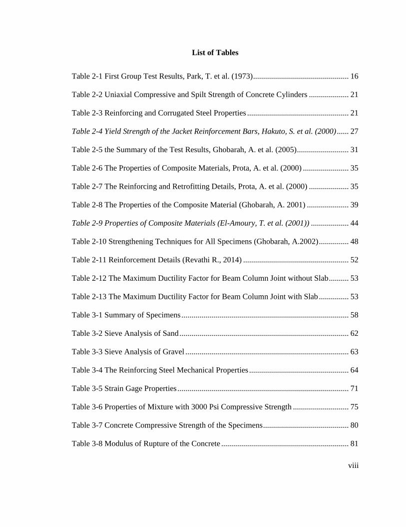
List of Tables

Table 2-1 First Group Test Results, Park, T. et al. (1973) ................................................ 16

Table 2-2 Uniaxial Compressive and Spilt Strength of Concrete Cylinders .................... 21

Table 2-3 Reinforcing and Corrugated Steel Properties ................................................... 21

Table 2-4 Yield Strength of the Jacket Reinforcement Bars, Hakuto, S. et al. (2000) ...... 27

Table 2-5 the Summary of the Test Results, Ghobarah, A. et al. (2005) .......................... 31

Table 2-6 The Properties of Composite Materials, Prota, A. et al. (2000) ....................... 35

Table 2-7 The Reinforcing and Retrofitting Details, Prota, A. et al. (2000) .................... 35

Table 2-8 The Properties of the Composite Material (Ghobarah, A. 2001) ..................... 39

Table 2-9 Properties of Composite Materials (El-Amoury, T. et al. (2001)) ................... 44

Table 2-10 Strengthening Techniques for All Specimens (Ghobarah, A.2002) ............... 48

Table 2-11 Reinforcement Details (Revathi R., 2014) ..................................................... 52

Table 2-12 The Maximum Ductility Factor for Beam Column Joint without Slab .......... 53

Table 2-13 The Maximum Ductility Factor for Beam Column Joint with Slab ............... 53

Table 3-1 Summary of Specimens .................................................................................... 58

Table 3-2 Sieve Analysis of Sand ..................................................................................... 62

Table 3-3 Sieve Analysis of Gravel .................................................................................. 63

Table 3-4 The Reinforcing Steel Mechanical Properties .................................................. 64

Table 3-5 Strain Gage Properties ...................................................................................... 71

Table 3-6 Properties of Mixture with 3000 Psi Compressive Strength ............................ 75

Table 3-7 Concrete Compressive Strength of the Specimens ........................................... 80

Table 3-8 Modulus of Rupture of the Concrete ................................................................ 81

file:///H:/Final%20Thesis%204-22-16.docx%23_Toc449093203







ix

Table 3-9 Splitting Tensile Strength of the Concrete ....................................................... 83

Table 3-10 Concrete Modulus of Elasticity ...................................................................... 84

Table 3-11 Tensile Properties of the CFRP Sheet ............................................................ 86

Table 3-12 Physical Properties of the CFRP Sheets ......................................................... 87

Table 3-13 Mechanical Properties of MasterBrace P 3500 .............................................. 91

Table 3-14 Mechanical Properties of MasterBrace F 2000 ............................................. 92

Table 3-15 Mechanical Properties of MasterBrace SAT 4500 ......................................... 93

Table 3-16 Designation and Rehabilitation of the Specimens .......................................... 96

Table 4-1 The Maximum Values of the Loads and Displacements at Each Cycle, J1 .. 110

Table 4-2 The Values of the Loads and Displacements at Each Cycle, J2 ..................... 123

Table 4-3 The Values of the Loads and Displacements at Each Cycle, J3 ..................... 129

Table 4-4 The Values of the Loads and Displacements at Each Cycle, Specimen J4 .... 136

Table 4-5 Values of Loads and Displacements at Each Cycle, J5 .................................. 141

Table 4-6 Values of Loads and Displacements at Each Cycle, J6 .................................. 143

Table 4-7 Summary of the Test Results .......................................................................... 145

Table 4-8 Maximum Stress Developed in the CFRP Sheet ............................................ 159

Table 4-9 Maximum Ductility Factor for All Specimens ............................................... 167

x

List of Figures

Figure 1-1 Beam-Column Joint Shear Failure, Kocaeli Earthquake .................................. 2

Figure 1-2 Joint Failure, Kocaeli Earthquake ..................................................................... 2

Figure 1-3 Joint Types ........................................................................................................ 5

Figure 1-4 Forces Acting on Joint ...................................................................................... 7

Figure 2-1 Action at an External Reinforced Concrete Joint, Park, T. et al. (1973) ........ 12

Figure 2-2 Details of First Group Specimens, Park, T. et al. (1973) ................................ 13

Figure 2-3 Details of the Second Group, Park, T. et al. (1973) ........................................ 14

Figure 2-4 The Applied Load versus the Ductility Factor for Specimen (M3), ............... 15

Figure 2-5 The Applied Loads versus the Beam Displacement, Specimen R3 ................ 17

Figure 2-6 The Applied Loads versus Beam Displacement, Specimen P3 ...................... 17

Figure 2-7 Dimensions of Specimens, Biddah, A. et al. (1997) ....................................... 18

Figure 2-8 Proposed Rehabilitation Technique, Biddah, A. et al. (1997) ........................ 19

Figure 2-9 Details of Reinforcement, Biddah, A. et al. (1997) ........................................ 20

Figure 2-10 Test Setup, Biddah, A. et al. (1997) .............................................................. 22

Figure 2-11 Cumulative Energy Dissipation, Biddah, A. et al. (1997) ............................ 23

Figure 2-12 The Dimensions and Reinforcement Details of the Specimens, Hakuto, S.

2000................................................................................................................................... 25

Figure 2-13 Test Setup for the External and Internal Beam-Column Joint, Hakuto, S.

2000................................................................................................................................... 28

Figure 2-14 The Dimensions and Reinforcement Details of the Specimens, Ghobarah, A.

et al. (2005) ....................................................................................................................... 29






















xi

Figure 2-15 The Retrofitting Details of All Specimens, Ghobarah, A. et al. (2005) ........ 30

Figure 2-16 Cumulative Energy Dissipation, Ghobarah, A. et al. (2005) ........................ 32

Figure 2-17 Stiffness Degradation, Ghobarah, A. et al. (2005) ....................................... 33

Figure 2-18 Typical Test Specimen and Reinforcement Used by Prota, A. et al. (2000) 34

Figure 2-19 Test Arrangement, Prota, A. et al. (2000) ..................................................... 36

Figure 2-20 Compression between (1a and 1c) Specimens, Prota, A. et al. (2000) ......... 37

Figure 2-21 The Reinforcement Bar Details and The Dimensions ................................... 38

Figure 2-22 The Test Setup and the Instrumentation (Ghobarah, A. (2001)) ................... 40

Figure 2-23 Envelopes of the Beam Tip Load-Displacement Curves, (Ghobarah, A. 2001)

........................................................................................................................................... 41

Figure 2-24 Energy Cumulative- Ductility Factor for Specimens (T1 and TR1),

(Ghobarah, A. 2001) ......................................................................................................... 41

Figure 2-25 Specimens Dimensions and Reinforcement Details ..................................... 42

Figure 2-26 The Proposed Technique to Strengthen ........................................................ 43

Figure 2-27 Load Routing, El-Amoury, T. et al. (2001) ................................................... 44

Figure 2-28 Apparatus Details for Testing Specimen (El-Amoury, T. et al. (2001)) ....... 45

Figure 2-29 Hysteretic Loop Envelopes of the Test Specimens, El-Amoury, T. (2001) . 46

Figure 2-30 Cumulative Energy Dissipation, El-Amoury, T. (2001) ............................... 46

Figure 2-31 Test Setup for Specimen TR1 (Ghobarah, A. 2002) ...................................... 48

Figure 2-32 Envelop of the Hysteretic Loops, Ghobarah, A. (2002) ............................... 49

Figure 2-33 Cumulative Energy Dissipation, Ghobarah, A. (2002) ................................. 50

Figure 2-34 Failure Modes of Specimens, Ghobarah, A. (2002)..................................... 50



















xii

Figure 2-35 Test Specimens with and without the Slab (Revathi R., 2014) ..................... 51

Figure 2-36 Energy Dissipation Curves for Beam-Column Joint without Slab ............... 53

Figure 2-37 Energy Dissipation Curves for Beam-Column Joint with Slab .................... 54

Figure 2-38 Cracks Patterns of the Specimens ................................................................. 54

Figure 3-1 Details of Specimen J1, the “Ductile” Specimen ............................................ 60

Figure 3-2 Details of Specimen J2, Non-ductile Specimen .............................................. 61

Figure 3-3 Stress-Strain Diagrams of the Reinforcement Bars ........................................ 65

Figure 3-4 End Hook Dimensions .................................................................................... 66

Figure 3-5 The Difference between Shear Reinforcement in Seismic and Non-Seismic

Specimens ......................................................................................................................... 67

Figure 3-6 “U” Shape Rebar Detail .................................................................................. 68

Figure 3-7 Column Section Details................................................................................... 69

Figure 3-8 Beam Section Details ...................................................................................... 69

Figure 3-9 Reinforcement Cage of Specimen J1 .............................................................. 70

Figure 3-10 Reinforcement Cage of Specimen J2 ............................................................ 70

Figure 3-11 Strain Gage Instullation................................................................................. 72

Figure 3-12 Strain Gages Locations ................................................................................. 73

Figure 3-13 Wood Molds .................................................................................................. 74

Figure 3-14 Concrete Mixing Steps .................................................................................. 77

Figure 3-15 Curing Condition of Specimens .................................................................... 78

Figure 3-16 Compressive Testing Machine ...................................................................... 79

Figure 3-17 Modulus of Rupture Test .............................................................................. 81






















xiii

Figure 3-18 Splitting Test ................................................................................................. 82

Figure 3-19 Modules of Elasticity Test ............................................................................ 84

Figure 3-20 Stress-Strain Diagram of the Concrete .......................................................... 85

Figure 3-21 The Concrete Surface Preparations of the Specimens .................................. 88

Figure 3-22 Holes on the Concrete Surface ..................................................................... 89

Figure 3-23 Applying the Prime Layer to the Concrete Surface ...................................... 90

Figure 3-24 Applying the Putty Layer to the Concrete Surface ....................................... 92

Figure 3-25 Specimen Wrapped by CFRP Sheets ............................................................ 94

Figure 3-26 Retrofitting Steps .......................................................................................... 96

Figure 3-27 Test Setup ...................................................................................................... 97

Figure 3-28 Load Sequence Diagram ............................................................................... 99

Figure 4-1 Test Setup of Joint J1 .................................................................................... 101

Figure 4-2 The Development of the First Cracks at the First Cycle, J1 ......................... 102

Figure 4-3 Development of the Flexural Cracks after Cycle 4, J1 ................................. 103

Figure 4-4 Specimen J1 at the End of First Set of Cycles. ............................................. 104

Figure 4-5 Crack Patterns Developed During Second Set of Applied Cyclic Load, J1 . 105

Figure 4-6 Crack Pattern of Cycle 1, Strain Control, J1 ................................................ 106

Figure 4-7 Concrete Cover Splitting, J1 ......................................................................... 107

Figure 4-8 Specimen J1 (final crack pattern) .................................................................. 108

Figure 4-9 Load-Displacement Diagram, J1 ................................................................... 109

Figure 4-10 Test Setup of Specimen J2 .......................................................................... 112

Figure 4-11 The Development of the First Crack, J2 ..................................................... 113























xiv

Figure 4-12 The Cracks of Joint J2 at the End of Cycle 1 .............................................. 114

Figure 4-13 The Cracks of Joint J2 at the End of Cycle 2 .............................................. 115

Figure 4-14 The Backside of Joint J2 at the End of Cycle 2 .......................................... 115

Figure 4-15 Developed Cracks at Cycle No. 4, J2 .......................................................... 116

Figure 4-16 Cycle 21, J2 ................................................................................................. 117

Figure 4-17 First Shear Cracks, J2 .................................................................................. 118

Figure 4-18 Developed Cracks within the Load Control Phase, J2 ................................ 119

Figure 4-19 The Failure Pattern of Specimen J2 ........................................................... 121

Figure 4-20 Load - Displacement Diagram, J2 ............................................................... 122

Figure 4-21 Test Setup of Specimen J3........................................................................... 124

Figure 4-22 Specimen J3 at the End of cycle 20 ............................................................ 125

Figure 4-23 Specimen J3 at the End of Cycle 20, Strain Control Phase ........................ 126

Figure 4-24 Specimen J3 at the Failure .......................................................................... 127

Figure 4-25 Load-Displacement Diagram, J3 ................................................................. 128

Figure 4-26 Test Setup of Specimen J4 .......................................................................... 131

Figure 4-27 Specimen J4 at the End of Load Control .................................................... 132

Figure 4-28 Specimen J4 at the Failure ......................................................................... 133

Figure 4-29 Areas under CFRP Sheets at the End of the Test, Specimen J4 ................. 134

Figure 4-30 Load versus Displacement, J4 ..................................................................... 135

Figure 4-31 Failure of Specimen J4 ................................................................................ 137

Figure 4-32 Load-Displacement Diagram, J5 ................................................................. 139

Figure 4-33 Cyclic Load-Displacement, J6 .................................................................... 140























xv



Figure 4-36 Maximum Moment at Face of the Column, Pushing Down Case............... 146

Figure 4-37 Envelop Cyclic Load- Vertical Displacement of the Ductile Specimen, J1 148

Figure 4-38 Envelop Cyclic Load- Vertical Displacement of the Non-Ductile Specimen,

J2 ..................................................................................................................................... 149

Figure 4-39 Envelop Cyclic Load- Vertical Displacement, Specimen J3 ...................... 149

Figure 4-40 Envelop Cyclic Load- Vertical Displacement of the Specimen, J4 ............ 150

Figure 4-41 Envelop Cyclic Load- Vertical Displacement of the Specimen, J5 ............ 150

Figure 4-42Envelop Cyclic Load- Vertical Displacement of the Specimen, J6 ............. 151

Figure 4-43 Cyclic Load- Vertical Displacement Relationship of All Specimens Tested

Under Same Axial Loads (20% of the Column Capacity) .............................................. 152

Figure 4-44 Cyclic Load- Vertical Displacement Relationship of Specimens (J3 and J5)

Tested under a Different Axial Load (20% and 40% of the Column Capacity) ............. 154


Tested under a Different Axial Load (20% and 40% of the Column Capacity) ............. 155

Figure 4-46 CFRP Joint Strain versus Load for Specimen J3 ........................................ 156

Figure 4-47 CFRP Joint Strain versus Cyclic Load for Specimen J4 ............................. 157



Figure 4-50 The Cumulative Energy Dissipation of Specimen J1 ................................ 160























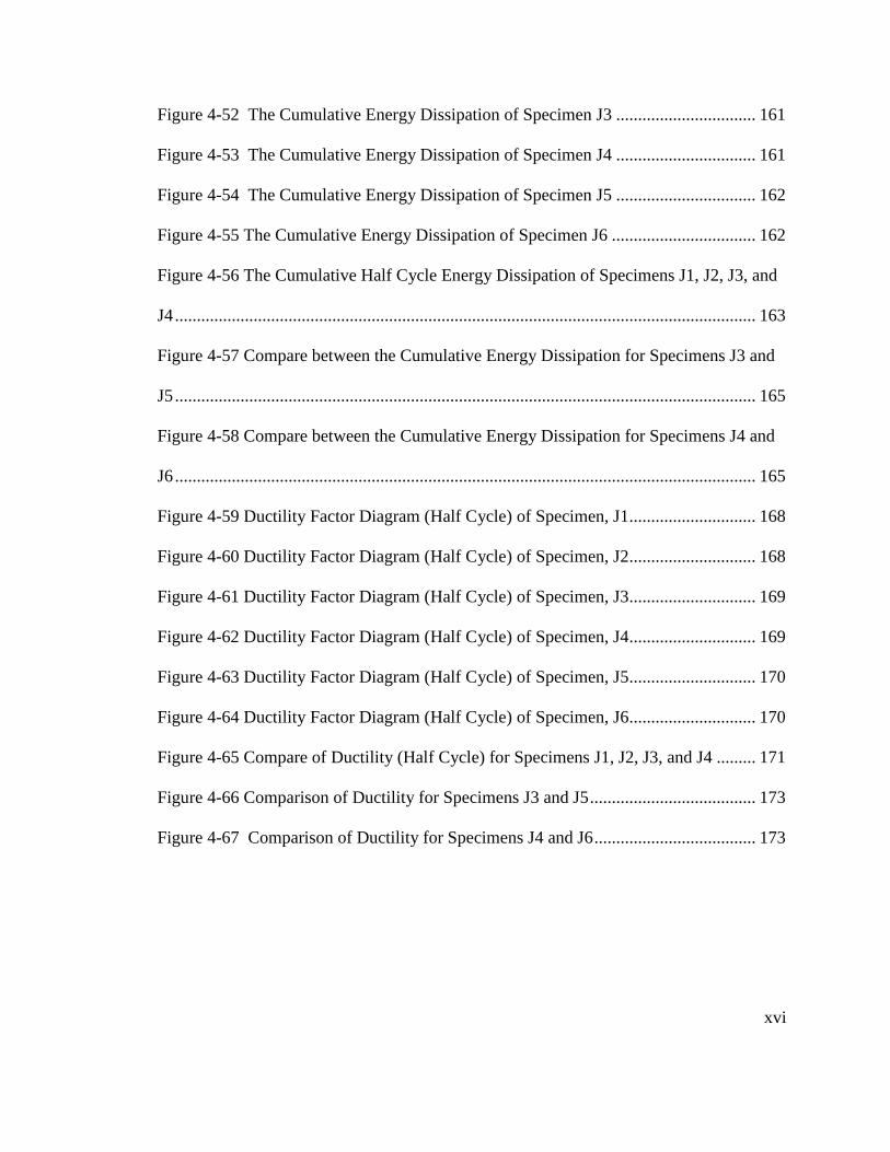
xvi




Figure 4-55 The Cumulative Energy Dissipation of Specimen J6 ................................. 162

Figure 4-56 The Cumulative Half Cycle Energy Dissipation of Specimens J1, J2, J3, and

J4 ..................................................................................................................................... 163

Figure 4-57 Compare between the Cumulative Energy Dissipation for Specimens J3 and

J5 ..................................................................................................................................... 165

Figure 4-58 Compare between the Cumulative Energy Dissipation for Specimens J4 and

J6 ..................................................................................................................................... 165

Figure 4-59 Ductility Factor Diagram (Half Cycle) of Specimen, J1............................. 168






Figure 4-65 Compare of Ductility (Half Cycle) for Specimens J1, J2, J3, and J4 ......... 171

Figure 4-66 Comparison of Ductility for Specimens J3 and J5 ...................................... 173

Figure 4-67 Comparison of Ductility for Specimens J4 and J6 ..................................... 173



















xvii

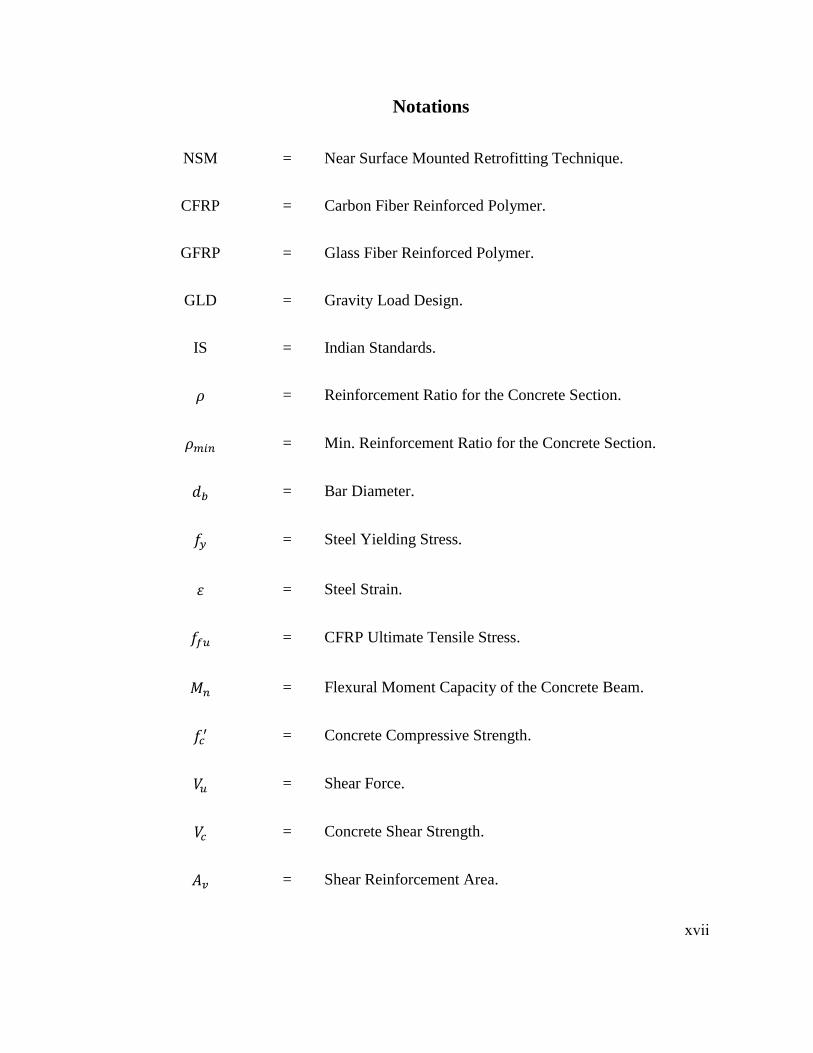
Notations

NSM = Near Surface Mounted Retrofitting Technique.

CFRP = Carbon Fiber Reinforced Polymer.

GFRP = Glass Fiber Reinforced Polymer.

GLD = Gravity Load Design.

IS = Indian Standards.

𝜌 = Reinforcement Ratio for the Concrete Section.

𝜌𝑚𝑖𝑛 = Min. Reinforcement Ratio for the Concrete Section.

𝑑𝑏 = Bar Diameter.

𝑓𝑦 = Steel Yielding Stress.

𝜀 = Steel Strain.

𝑓𝑓𝑢 = CFRP Ultimate Tensile Stress.

𝑀𝑛 = Flexural Moment Capacity of the Concrete Beam.

𝑓𝑐′ = Concrete Compressive Strength.

𝑉𝑢 = Shear Force.

𝑉𝑐 = Concrete Shear Strength.

𝐴𝑣 = Shear Reinforcement Area.

xviii

𝐴𝑏 = Shear Reinforcement Bar Area.

𝑉𝑠 = Demanded Shear Force.

𝐸𝑐 = Modulus of Elasticity for Concrete.

S = Space Between Stirrups or Ties.

𝐸𝑠 = Steel Modulus of Elasticity.

𝐴𝑔 = Cross Sectional Area.

𝑙𝑜 = Confinement Length.

𝐴𝑠 = Cross Sectional Area of Tensile Steel Reinforcement.

𝐴𝑠ℎ = Total Cross Sectional Area of Rectangular Hoop

Reinforcement.

C = The Depth of Compressive Concrete Section.

𝑑𝑡 = The Depth of Tensile Steel Reinforcement.

𝑀𝑐 = Concrete Bending Moment Capacity.

𝑀𝑝𝑟 = Approximate Joint Moment.

𝐴𝑗 = Cross Sectional Area of the Joint.

𝑓𝑟 = Concrete Flexural Strength.

𝑓𝑐𝑡 = Concrete Splitting Tensile Strength.

xix

FEM = Finite Element Model.

CSA A23.3-94 = Canadian Concrete Design code 1994.

LVDT = Linear Variable Differential Transformer.

1

Introduction

1.1. General

The annual average of successful concrete frames constructed world-wide is on the order

of hundreds of thousands. On the other hand, there are a large number of these frames

that are unsafe in seismic resistance capacity, especially the buildings that were

constructed prior to the 70s. Evidence shows that from earthquakes such as the one in

Kocaeli, Turkey, 1999, and the one in Chi-Chi, Taiwan, 1999, that there has been severe

damages or complete collapse in these kinds of buildings that were designed and built

prior to modern building codes. Most of the buildings designed and constructed based on

the earlier codes were characterized by non-ductile performance during the earthquakes

because the earlier codes did not include the required reinforcement details for ductility.

As a result, non-ductile behavior of these buildings during the earthquakes was expected.

Figure 1-1 and 1-2 show an example of this sort of damage that happened after Kocaeli

earthquake.

Most older buildings were designed to carry the gravity loads and resist wind lateral

loads. The results of the examination of the collapsed buildings during earthquakes have

shown the weakness of these buildings to resist the lateral loads created by earthquakes.

Furthermore, it has been observed that the weakest part in such structures was the beam-

column joints as shown in Figure 1-1 and 1-2, where the beams and columns were intact

whereas the joints were crushed.

2

According to earlier codes most beam-column joints in the existing buildings that were

constructed before the 1970s were characterized by non-ductile reinforcement details

where inadequate or no shear reinforcement was provided in the joint region. Moreover,

the design of the strong beam caused high shear force on the joint and this may have

caused a brittle shear failure at the joint regions.

Figure 1-2 Joint Failure, Kocaeli Earthquake

Figure 1-1 Beam-Column Joint Shear Failure, Kocaeli Earthquake

3

The behavior of the joint region is one of the most important factors controlling the

performance of the whole concrete structure. If the beam-column joints show non-ductile

performance, then the whole frame will be weakened, even though its beams and

columns may have adequate capacity.

1.2. Beam-Column Joint

A beam–column joint could be defined as “that portion of the column within the depth of

the beam(s) that frame into column”. In general, there are two types of joints (type I and

II) based on the concrete frame type. If the concrete frame is designed to carry gravity

loads and no inelastic deformations is required, then the joints are called type I. If the

concrete frame is designed to carry the gravity loads and resist lateral loads and inelastic

deformations required, then the joints are called type II. The earlier codes required the

framing members of the joint to be designed according to their prevailing stresses, but the

design of the joints was ignored in these codes. Many buildings were destroyed during

earthquakes caused by deficiency of the shear reinforcement in the joint regions. Most

type I joints have no reinforcement to resist the shear force through the joints that are

characterized by:

1. Lack of transverse of reinforcement in the joint region.

2. Weak column-strong beam condition.

3. Weak concrete.

4

Type II joints that are constructed in accordance with the modern codes are characterized

by:

1. Adequate transvers reinforcement ties within the joint as shear reinforcement.

2. Adequate ductility in the joint rejoins.

3. Strong column-weak beam joints.

All these features will prevent or delay the failure in the beam-column joint and provide

opportunity for the plastic hinge to form in the flexural member(s).

The beam-column joints could also be classified based on the joint position as internal

and external joints or joint shape within the concrete frame. Figure 1-3 shows the

different types of beam-column joints based on the shape and position.

5

(a) Corner Joint

(b) Corner Joint

(b) Internal Joint

(b) Internal Joint

(c) External Joint

(c) External Joint

Figure 1-3 Joint Types

6

1.3. Fiber Reinforced Polymer (FRP) Sheets

About two decades ago, a new material came onto the markets. This material is called

“Fiber Reinforced Polymer” (FRP). These composite materials have been successfully

used in a variety of industries. Civil engineers also used this material and found it could

be a solution for many structural problems. The most common types of this material are

Carbon Fiber Reinforced Polymer (CFRP) and Glass Fiber Reinforced Polymer (GFRP).

The fiber reinforced polymer (FRP) materials have a number of great features:

1. Lightweight and ease of installation.

2. Immunity to corrosion.

3. Extremely high tensile strength.

4. Available in many forms.

5. Short construction time.

In the civil engineering field, the Fiber Reinforced Polymer (FRP) sheets have been used

extensively in the past decade as externally bonded reinforcement concrete and

prestressed concrete structures.

7

In order to gain a better understanding of the effects of CFRP sheets on the joint when the

external forces were acting on it, it is useful to examine the general mechanism of the

joint and the reasons that lead to failure of non-ductile joints. Per R. Park and T. Paulay

(1973), the internal forces that are acting within the joint region as a result of the external

actions from the beam and columns are shown in Figure 1-4.

Figure 1-4 shows that when lateral load acts on the concrete structure, compressive and

tensile stresses are generated at the same time within the joint. When the tension forces

are very high, the tensile stress within the joint was very high as well. By developing the

Figure 1-4 Forces Acting on Joint

8

ultimate moment capacity of the adjoining members, these tensile stresses are very high

and cause diagonal cracks. At this stage of loading, the shear and compression forces are

transferred by diagonal compression struts.

As known, concrete is strong in compression, but very weak tension where the

compression strength of the concrete is approximately ten times larger than the tension

strength. This is the key issue for those joints that were constructed prior to 1970s. In

order to upgrade their behavior, one needs to understand how to reduce the tensile

stresses acting on the joint region until one of the adjoining member (beam) reaches its

ultimate capacity and fails. The technique used in this research included an “L” shape

CFRP sheet attached to both sides of the beam in order to take most of the tension that

came from one of the adjoining members, and transferred it to the other one out side of

the joint.

9

1.4. Research Objective and Scope

The problem in most of the existing beam-column joints in concrete frames that were

designed before the development of the modern codes is that these joints lack shear

strength, energy dissipation, and ductility required to resist earthquakes.

This study will focus the behavior of concrete beam-column joints. Three types of joints

will be tested to investigate their behavior under cyclic loading:

1- A non-ductile joint representing a design based on older codes.

2- A ductile joint representing a design based on current (modern) codes.

3- A non-ductile joint a design based on older codes (same as case 1) but retrofitted

with CFRP sheet.

Comparison of behavior of joints before and after retrofitting, as well as with the ductile

joint designed based on modern codes, will be presented. Behavior will be investigated

by load versus deflection, load versus CFRP strain, energy dissipation, and ductility.

10

1.5. Research Presentation Layout

This Presentation includes the following chapters:

Chapter One:

Presents the introduction of the problem.

Chapter Two:

Reviews the available literature and research works that are related to the present study.

Chapter Three:

Deals with the properties of the construction materials used in the experiment, as well as

the details of the experimental work.

Chapter Four:

Presents the analysis of the data from the experimental work.

Chapter Five:

Presents a summary and conclusions drawn from this study, and recommendations for

further studies.

11

Literature Review

2.1. Introduction

In the earlier design codes, the principles of design and structural behavior of the main

members, such as the columns and the beams are well established. As known the

development of codes is always in progress. In the current, ACI 318-14 code, Chapter 18,

deals with seismic issues by addressing the design requirements of structural members in

order to provide ductility and strength to absorb and dissipate the seismic loads. Most

buildings that were designed before the1970s did not have seismic reinforcement in the

joints. Moreover, most of these buildings are characterized by a weak column-strong

beam structure. It is clear that columns represent the overall strength and stability of the

framed structures especially in multistory reinforced concrete structures. Moreover, the

joints in these buildings are characterized by the deficiency of the shear reinforcements in

the columns. These reasons lead one to expect a non-ductile behavior and severe

consequences of failure.

Over the past two decades, Externally Bonded Reinforcement, along with several other

techniques, have been used to strengthen the joint regions. Each technique has its pros

and cons. For instance, the use of the steel jacketing to strength the joints provides

flexural capacity in order to change brittle behavior to ductile behavior, but over time,

steel may corrode which would be a disadvantage of this technique.

12

2.2. Retrofitting Techniques for Beam-Column Joint

One of the earlier studies by Park, R. et al. (1973) was to test and analyze the behavior of

the beam-column joint under simulated severe seismic loading. Thirteen specimens were

constructed in full scale. The transverse joint reinforcement and the anchorage length of

the beam reinforcement were the main parameters in this experiment. The ACI 318-71

was the main reference for the design of these specimens. The general shape of the

specimens consisted of a column with a beam framing one side at mid-height. All of the

specimens were tested under small or no axial loads on the column, and an applied cyclic

load on the free end on the beam. The external and internal actions in the external beam-

column joints are shown in Figure 2-1.

The specimens were tested in two groups. The first group consisted of six specimens,

where no axial load was applied to the column during the test. Figure 2-2 shows the

dimensions and reinforcement details of this group of the specimens. In these specimens

the flexural capacity of the beam was less than the flexural capacity of the column. As a

consequence, the plastic hinge was expected to form in the beams. Also the concrete

Figure 2-1 Action at an External Reinforced Concrete Joint, Park, T. et al. (1973)

13

compressive strength of specimens (M1, M2, and M3) was between 4 to 5 ksi whereas the

concrete compressive strength of specimens (S4, S5, and S6) was 3ksi.

From Figure 2-2, it is clear that the transverse reinforcement within the joint region is

different. M1 and M2 specimens had a normal amount of shear reinforcement within the

joint according to ACI 318-71, whereas S4 and S6 specimens had a greater amount, and

M3 and S5 specimens had less than the required amount. The second group consisted of

seven specimens, and an axial load was applied to the column during the test equal to

16% of the axial load capacity of the column. Figure 2-3 shows the dimensions and

reinforcement details of this group of specimens. These specimens were characterized by

a flexural capacity of the column was less than the flexural capacity of the beam. As a

consequence, the plastic hinge was expected to form in the column. The ties in specimen

Figure 2-2 Details of First Group Specimens, Park, T. et al. (1973)

14

R1, and R2 were normal, based on ACI Code requirements, but spaces between ties were

closer in the rest of the specimens R3, R4, P1, P2, and P3. Specimens P1, P2, and P3 had a

back stub at the joint region from the back side of the column to give more room in order

to add extra reinforcement. The concrete compressive strength of specimens was changed

3.4 to 5.6 ksi.

Figure 2-3 Details of the Second Group, Park, T. et al. (1973)

15

The test results of first group showed poor behavior during the test cycles due to the

deterioration of the moment capacity and anchorage breakdown. Figure 2-4 shows the

relations between the applied loads versus the ductility factor for specimen M3, and Table

2-1 shows the maximum moment of each cycle versus the ductility factor of each

specimen in the first group.

Figure 2-4 The Applied Load versus the Ductility Factor for Specimen

(M3),

Park, T. et al. (1973)

16

Table 2-1 First Group Test Results, Park, T. et al. (1973)

Cycle 3 4 5 6 7 8 9 10 11 12 13

Section

ductility

2.5 -5 5 -5 ------ ------ 10 -10 13 -25 ----

M1 0.98 1.08 1.05 0.89 0.72 0.72 0.67 0.61 ------ ------ ----

M2 0.91 0.80 0.54 0.44 0.58 0.58 ------ ------ ------ ----- ----

M3 1.03 1.05 0.94 0.74 0.71 0.71 0.47 0.63 0.35 0.32 -----

Section

ductility

2.5 -5 5 -5 ------ ------ 10 -10 15 -15 20

S4 1.04 0.97 0.85 0.65 0.53 0.62 0.66 0.55 0.32 0.47 0.31

S5 095 0.90 0.66 0.53 ------ ------ 0.54 0.47 0.44 0.37 0.44

S6 1.04 0.98 1.05 0.78 0.74 0.73 1.11 0.79 0.79 0.61 0.55

On the other hand, the results of the second group showed that the specimens R1, R2, and

R3 reached 71-75% of the theoretical ultimate flexural capacity of the column whereas

specimens P1, P2, and P3 reached 90% of the theoretical ultimate flexural capacity of the

column. This means that the anchorage length of the beam reinforcement affected the

joint performance. Figure 2-5 and 2-6 show the applied load versus displacement.

17

Figure 2-5 The Applied Loads versus the Beam Displacement, Specimen R3

Figure 2-6 The Applied Loads versus Beam Displacement, Specimen P3

18

After the observation of the failure modes and behavior, it was clear that the plastic hinge

did not occur where designed, and that all failures occurred in the joint region. This could

cause the collapse of the entire building.

Biddah, A. et al. (1997) constructed and tested six specimens in one-third scale under

static cyclic loading. The specimens represented an external joint of a two story concrete

frame in a nuclear power generation plant constructed in 1969. All of the specimen

dimensions were identical. Figure 2-7 shows the general shape and the dimensions of the

specimens.

This experiment proposed a technique using corrugated steel to strengthen an external

joint that was designed before the 1970s as shown in Figure 2-8. This technique could

also be applied to undamaged joints. The parameters that were investigated in this

Figure 2-7 Dimensions of Specimens, Biddah, A. et al. (1997)

19

experimental work the shear reinforcement in the joint, the development length of the

beam longitudinal bars, the retrofitting plate thickness, and the retrofitting style.

Specimens J1, J3, and J5 represented existing joints in terms of reinforcement details in

the concrete frame. J3 was retrofitted by using the steel jacket to confine the column and

beam, whereas J5 was retrofitted by using the steel jacket to confine the column only. In

both specimens, the steel jacket thickness was 2.8 mm. J2 was designed in accordance

with CSA A23.3-94, where shear reinforcement was placed within the joint region. J4

and J6 were designed with no shear reinforcement in the joint region, and an inadequate

development length of the positive beam reinforcement. J6 was retrofitted by using a

steel jacket thickness of 3.5mm around the column, in addition to two steel plates

anchored between the beam and the joint. The longitudinal reinforcement of all

Figure 2-8 Proposed Rehabilitation Technique, Biddah, A. et al. (1997)

20

specimens was identical, except for J4 and J6 where the bottom beam reinforcement had

a shorter development length. The details of the stirrups are shown in Figure 2-9. The

concrete cover was 30 mm in all specimens. Also non-shrink grout of 25 mm used to fill

the gap between the concrete and steel jackets. Table 2-2 shows the compressive and

tensile strength of the concrete, and Table 2-3 shows the reinforcing and the corrugated

steel properties.

Figure 2-9 Details of Reinforcement, Biddah, A. et al. (1997)

21

Time Specimen

J1 J2 J3 J4 J5 J6

Twenty-eight days compressive strength (Mpa) 21.5 22.0 21.5 24.0 22.0 24.0

Twenty-eight days split tensile strength (Mpa) 2.85 2.40 2.85 2.42 2.40 2.42

Compressive strength at time of test (Mpa) 23.6 22.0 25.0 24.0 23.0 25.5

Item 𝑓𝑦 (Mpa) 𝜀𝑢 % 𝑓𝑢 (Mpa)

M10 rebar 500 12.0 750

M15 rebar 440 14.5 697

6.35-mm-diameter smooth bar 448 13.8 534

4.7-mm-diameter smooth bar 648 5.0 706

2.8-mm-corrugated steel sheet 363 2.8 397

3.5-mm-corrugated steel sheet 342 2.9 390

The general set-up of the test is shown in Figure 2-10. A constant axial load of 505 KN

was applied to the column to simulate the gravity load, whereas the cyclic load was

applied on the free end of the beam. After testing all specimens, the specimens

representing the existing joints performed poorly under the cyclic load. The final failure

mode was brittle at the joint. On the other hand, the joint that was designed according to

CSA A23.3-94 exhibited considerable improvement in joint behavior, and the plastic

hinge was formed within the beam section. Moreover, the energy dissipation of the

Table 2-2 Uniaxial Compressive and Spilt Strength of Concrete Cylinders

Table 2-3 Reinforcing and Corrugated Steel Properties

22

specimen J3 was the highest, and the specimen J1 was the lowest as shown in Figure 2-

11. In general, the proposed technique was considered effective because the undamaged

retrofitted specimens showed desirable results in terms of shear strength and energy

dissipation.

Figure 2-10 Test Setup, Biddah, A. et al. (1997)

23

Hakuto, S. et al. (2000) proposed and ran an analysis using concrete jacking to

investigate the retrofitting of the exterior and interior joints of an existing seven story

reinforced concrete building designed and built in New Zealand at the end of the 1950s.

Eight specimens in full scale were constructed, where six specimens O1, R1, R2, R3, O4,

and O5 represented the internal joints, and two specimens O6, O7 represented the

external joints. After the comparison between the old codes and the current codes, one of

the main differences was the concept of weak beam-strong column. The design in the

codes previous 1970s accounted for gravity loads and moderate wind loads. These

buildings were characterized by a lack of ductility and shear strength at the joint regions.

To change the existing buildings to conform to the current codes (New Zealand and U.S.

standards), a comprehensive exam was conducted in order to propose an effective

procedure to strengthen the joints, to achieve the concept of week beam-strong column,

and to ensure that the plastic hinge will form in the desirable spot. This paper reported the

Figure 2-11 Cumulative Energy Dissipation, Biddah, A. et al. (1997)

24

results from testing some poorly detailed concrete interior and exterior beam-column

joints. Tests on interior beam-column joints retrofitted by jacketing with new reinforced

concrete were investigated in this study. The researchers analyzed the theoretical

behavior of the joint before the experimental stage. Their results showed that after the

tensile cracks occurred, the forces in the joint region were transferred by diagonal

compressive struts. According to NZS 3101:1995 and ACI 318-95, the normal horizontal

shear stresses should not exceed 0.2𝑓′𝑐 , so the researchers stated that the diagonal cracks

is more likely to occur before the horizontal shear stresses in the joint reached 0.2𝑓′𝑐 .

Their recommendation was to consider the diagonal cracks within the joint to be the

failure citation instead of the horizontal shear stresses. With regard to the experimental

work, the general parameters in the experimental portion were the behavior of the

concrete joint that had been designed before the development of the current codes under

seismic loads, the retrofitting of the existing beam-column joints before and after

damage, and the anchorage of the longitudinal beam bars through the concrete joint core.

Figure 2-12 shows the dimensions and reinforcement details of the specimens.

25

Specimen O1 Specimen R1 and R2

Specimen O4 and O5

Specimen O6 Specimen O7

Figure 2-12 The Dimensions and Reinforcement Details of the Specimens, Hakuto, S. 2000

Specimen R3

26

The reinforcement details of specimen O1 were identical to the internal joint in that

building. The theoretical flexural strength of the column represented 70% of the

theoretical flexural strength of the beam, so the plastic hinge was expected to form in the

column. The only difference between the actual and the model joints before the mid-

1960s, was that plain round bars were used as a longitudinal reinforcement, whereas in

the experiment, the longitudinal reinforcement bars were deformed (fy = 47100 psi), and

the transverse reinforcement stirrups were plain round (fy = 49200 psi). Also, the concrete

compressive strength of the specimen (f'c) was 5950 psi. R1 and R2 specimens were

similar to O1 in terms of the reinforcement details and dimensions, and the difference

between R1 and R2 was that the damaged specimen O1 was retrofitted by jacketing the

beam, column, and the joint with new reinforced concrete to become specimen R1.

Specimens O4 and O5 were similar to O1 but with a bigger column section in order to

exam how the ratio between diameter of the longitudinal beam bar to column section

affected the performance of the joint. It should be noted that the increase of the column

section led to expectation that the plastic hinge would be located within the beam instead

of the column. The concrete compressive strength of specimens O4 and O5 were 7690

and 4790 psi respectively and the longitudinal reinforcement yield strength was (fy =

44700 psi for 0.94 in diameter, 46500 psi for 1.10 in diameter, and 44400 psi for 1.26 in

diameter) and the transverse reinforcement yield strength was (fy = 57700 psi).

Specimens O6 and O7 represented the external column-beam joint. These two specimens

were used to investigate the effect of the development length details on the general

behavior of the external joints that were common in the design codes before the 1970s, in

27

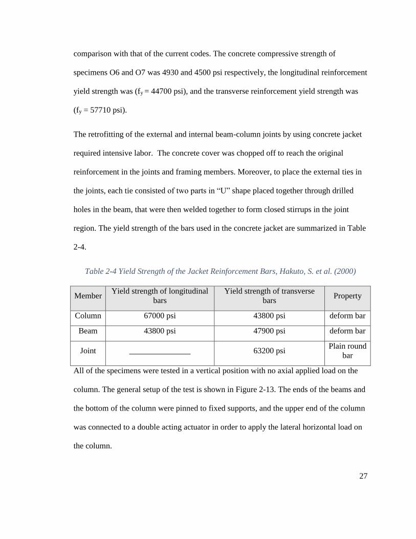
comparison with that of the current codes. The concrete compressive strength of

specimens O6 and O7 was 4930 and 4500 psi respectively, the longitudinal reinforcement

yield strength was (fy = 44700 psi), and the transverse reinforcement yield strength was

(fy = 57710 psi).

The retrofitting of the external and internal beam-column joints by using concrete jacket

required intensive labor. The concrete cover was chopped off to reach the original

reinforcement in the joints and framing members. Moreover, to place the external ties in

the joints, each tie consisted of two parts in “U” shape placed together through drilled

holes in the beam, that were then welded together to form closed stirrups in the joint

region. The yield strength of the bars used in the concrete jacket are summarized in Table

2-4.

Table 2-4 Yield Strength of the Jacket Reinforcement Bars, Hakuto, S. et al. (2000)

Member Yield strength of longitudinal

bars

Yield strength of transverse

bars Property

Column 67000 psi 43800 psi deform bar

Beam 43800 psi 47900 psi deform bar

Joint _______________ 63200 psi Plain round

bar

All of the specimens were tested in a vertical position with no axial applied load on the

column. The general setup of the test is shown in Figure 2-13. The ends of the beams and

the bottom of the column were pinned to fixed supports, and the upper end of the column

was connected to a double acting actuator in order to apply the lateral horizontal load on

the column.

28

The test results showed that the existing joints that had been designed three decades ago

behaved poorly under the cyclic loads because the design of these regions (joints) had

been done to resist gravity loads only. There was no transverse reinforcement placed at

this joint to resist the tension cracks that could affect the shear strength of the joint. The

proposed retrofitting procedure to strengthen the joint by using concrete jacket was

effective and applicable to enhance the strength, stiffness, and ductility of these joints,

but it is difficult to do.

a- The Internal Joint

b- The External Joint

Figure 2-13 Test Setup for the External and Internal Beam-Column Joint,

Hakuto, S. (2000)

29

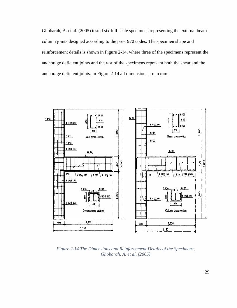
Ghobarah, A. et al. (2005) tested six full-scale specimens representing the external beam-

column joints designed according to the pre-1970 codes. The specimen shape and

reinforcement details is shown in Figure 2-14, where three of the specimens represent the

anchorage deficient joints and the rest of the specimens represent both the shear and the

anchorage deficient joints. In Figure 2-14 all dimensions are in mm.

Figure 2-14 The Dimensions and Reinforcement Details of the Specimens,

Ghobarah, A. et al. (2005)

30

Two types of materials were used in order to retrofit these joints. Carbon Fiber

Reinforced Polymer (CFRP) type (CF130) and Glass Fiber Reinforced Polymer (GFRP)

type (Tyfo BC and MBrace EG 900) were used as composite materials, and the rods and

sheets were used for the steel materials. Figure 2-15 shows the techniques used to retrofit

these specimens in order to change the general behavior of the joints from brittle (non-

ductile) to ductile, and to compensate for the lack in the reinforcement details and their

names. Specimens (T-B10 and T-SB3) were tested as the control specimens.

The specimens were tested in the vertical position. There was an axial constant load equal

to (0.2 Ag f’c= 600 KN) applied to the top of the column, and the cyclic load was applied

Joint T-B12 Joint T-B11

Joint T-SB8 Joint T-SB7

Figure 2-15 The Retrofitting Details of All Specimens, Ghobarah, A. et al. (2005)

31

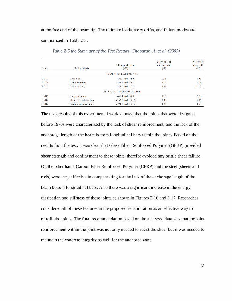
at the free end of the beam tip. The ultimate loads, story drifts, and failure modes are

summarized in Table 2-5.

The tests results of this experimental work showed that the joints that were designed

before 1970s were characterized by the lack of shear reinforcement, and the lack of the

anchorage length of the beam bottom longitudinal bars within the joints. Based on the

results from the test, it was clear that Glass Fiber Reinforced Polymer (GFRP) provided

shear strength and confinement to these joints, therefor avoided any brittle shear failure.

On the other hand, Carbon Fiber Reinforced Polymer (CFRP) and the steel (sheets and

rods) were very effective in compensating for the lack of the anchorage length of the

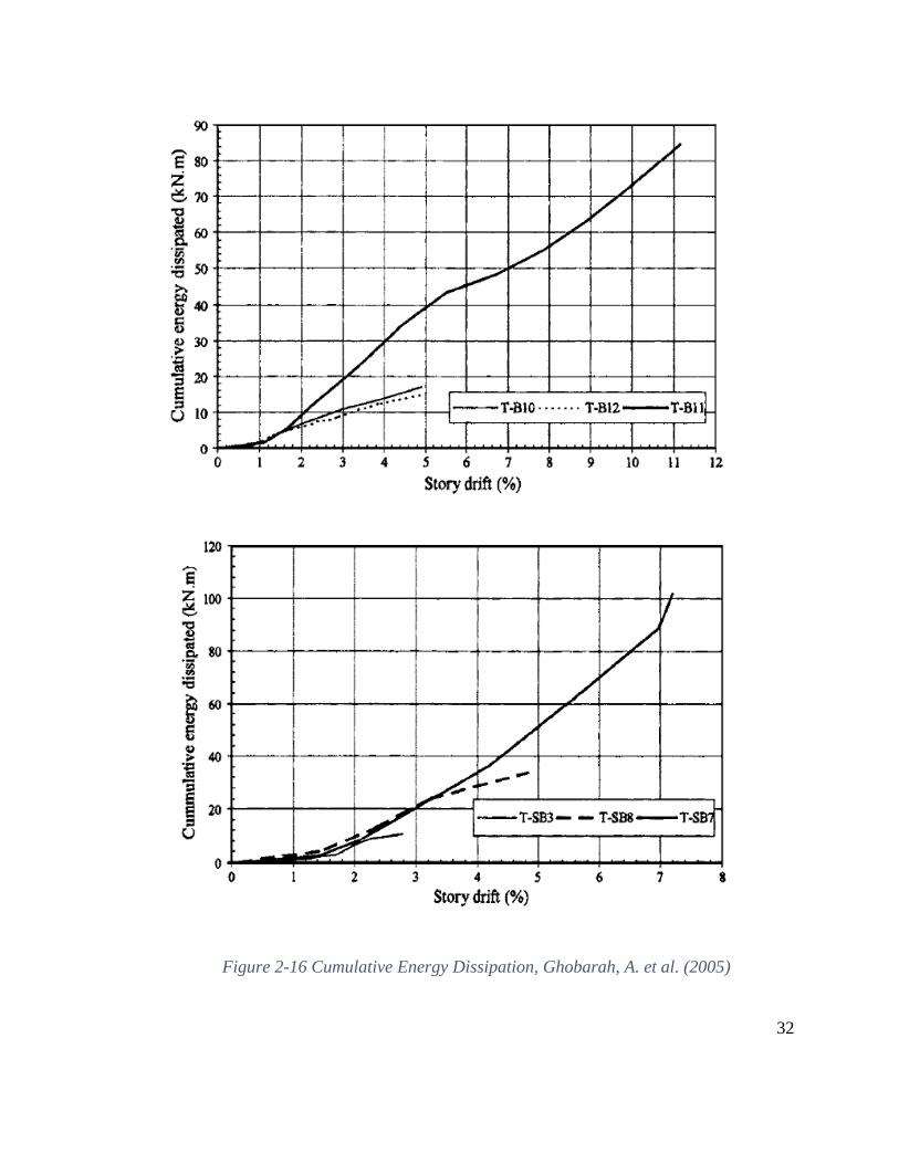
beam bottom longitudinal bars. Also there was a significant increase in the energy

dissipation and stiffness of these joints as shown in Figures 2-16 and 2-17. Researches

considered all of these features in the proposed rehabilitation as an effective way to

retrofit the joints. The final recommendation based on the analyzed data was that the joint

reinforcement within the joint was not only needed to resist the shear but it was needed to

maintain the concrete integrity as well for the anchored zone.

Table 2-5 the Summary of the Test Results, Ghobarah, A. et al. (2005)

32

Figure 2-16 Cumulative Energy Dissipation, Ghobarah, A. et al. (2005)

33

Figure 2-17 Stiffness Degradation, Ghobarah, A. et al. (2005)

34

Prota, A. et al. (2000) used the composite materials Fiber Reinforced Polymer (FRP) in

both forms (rods and sheets) to upgrade the existing beam-column concrete joints that

were designed and constructed according to early codes ACI318-63. A new theory was

investigated by this study. The theory was to use rods to increase the flexural strength of

the column by following the near surface mounted technique (NSM), whereas the FRP

was used as a jacket to increase the shear strength and the confinement at the joint. Two

series of specimens were constructed. Figure 2-18 shows the typical test specimens and

reinforcement details. All dimensions were chosen to represent a typical frame

dimension.

The experiment program in this study consisted of twelve specimens divided into groups,

where each group consisted of six specimens. The only difference between these two

groups was the axial applied load. Table 2-7 includes these values of the axial loads. The

Figure 2-18 Typical Test Specimen and Reinforcement Used by Prota, A. et al. (2000)

35

concrete compressive strength (f’c) was 4530 psi and the yield strength of the steel (fy)

was 6000 psi. The following Table 2-6 shows the properties of composite materials.

Table 2-6 The Properties of Composite Materials, Prota, A. et al. (2000)

Material Size Modulus of Elasticity

(Efr)

Ultimate Tensile Strength

(fsu)

CFRP Rod #3 (0.375 in. dia.) 15200 ksi 272 ksi

CFRP sheet 0.0065 in. thick. 32800 ksi 495 ksi

All specimens were designed without any seismic details at the joint. Some specimens

were retrofitted or strengthened by wrapping CFRP sheets around 15 in. of the column,

and the others retrofitted by using both the rods and sheets. The retrofitting technique is

summarized in the following Table 2-7.

Table 2-7 The Reinforcing and Retrofitting Details, Prota, A. et al. (2000)

36

These specimens were tested in the horizontal position. A plywood sheet was placed

between the specimen and the floor in order to limit the friction, and to allow for the free

movement of the beam and column. Figure 2-19 shows the test arrangement.

The loading process started by applied the axial load to the column at a constant value.

As shown in Figure 2-19, two actuators were used to apply the cyclic load on each end of

the transverse beam in order to generate the shear force and flexural moment in the

column.

Figure 2-19 Test Arrangement, Prota, A. et al. (2000)

37

It was confirmed by this experimental study that the combined action of FRP jacketing

and NSM rods was a successful technique to retrofit the connections in gravity load

designed (GLD) buildings. The retrofitting techniques could be adopted in more than one

way to get the desirable failure mode. Figure 2-20 shows the increase of column strength

between the control specimen (1a) and the retrofired specimen (1c). The ultimate column

shear strength (1c) increased 1.6% compared to the control specimen (1a).

Figure 2-20 Compression between (1a and 1c) Specimens, Prota, A. et al. (2000)

(1a)

(1c)

38

Ghobarah, A. et al. (2001) used the Glass Fiber Reinforced Polymer (GFRP) laminates as

a retrofitting material to retrofit the external beam-column joint. One specimen in full

scale was constructed in the experimental work with no shear reinforcement within the

joint region. It was expected that the joint would fail before the plastic hinge formation.

The reinforcement bar details and the dimensions of this specimen are shown in Figure 2-

21. The compressive strength of the concrete was 30.8 Mpa1 and the yield strength of the

reinforcement bars was (454 and 425 Mpa) for M10 and M20 2 bars, respectively.

1 Mpa = 145 psi. 2 M10 = 11.3 mm, M20 = 19.5 mm.

Figure 2-21 The Reinforcement Bar Details and The Dimensions

(Ghobarah, A. et al. (2001))

All dimensions are

in mm

39

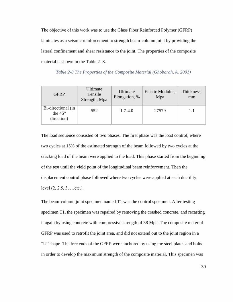
The objective of this work was to use the Glass Fiber Reinforced Polymer (GFRP)

laminates as a seismic reinforcement to strength beam-column joint by providing the

lateral confinement and shear resistance to the joint. The properties of the composite

material is shown in the Table 2- 8.

GFRP

Ultimate

Tensile

Strength, Mpa

Ultimate

Elongation, %

Elastic Modulus,

Mpa

Thickness,

mm

Bi-directional (in

the 45°

direction)

552 1.7-4.0 27579 1.1

The load sequence consisted of two phases. The first phase was the load control, where

two cycles at 15% of the estimated strength of the beam followed by two cycles at the

cracking load of the beam were applied to the load. This phase started from the beginning

of the test until the yield point of the longitudinal beam reinforcement. Then the

displacement control phase followed where two cycles were applied at each ductility

level (2, 2.5, 3, …etc.).

The beam-column joint specimen named T1 was the control specimen. After testing

specimen T1, the specimen was repaired by removing the crashed concrete, and recasting

it again by using concrete with compressive strength of 38 Mpa. The composite material

GFRP was used to retrofit the joint area, and did not extend out to the joint region in a

“U” shape. The free ends of the GFRP were anchored by using the steel plates and bolts

in order to develop the maximum strength of the composite material. This specimen was

Table 2-8 The Properties of the Composite Material (Ghobarah, A. 2001)

40

named T1R. Both the control and retrofitting specimens were tested in the vertical

position, where the axial load represented 0.2 𝐴𝑔𝑓′𝑐 applied to the column and the cyclic

load applied at the free end of the beam. Figure 2-22 shows the test setup and the

instrumentation.

The test results showed that the control specimen T1 exhibited a very high rate of shear

deterioration represented by brittle shear failure in the joint whereas the retrofitted

specimen T1R showed an increase in the shear resistance, a higher ductility (increased by

60%), and it developed the plastic hinge in the beam as shown in Figure 2-23 . Regarding

Figure 2-22 The Test Setup and the Instrumentation (Ghobarah, A. (2001))

41

the energy dissipation, the repaired specimen T1R showed improvement compared to the

un-retrofitted specimen T1. Figure 2-24 shows the energy dissipation of two specimens.

Figure 2-24 Energy Cumulative- Ductility Factor for Specimens (T1 and TR1),

(Ghobarah, A. 2001)

Figure 2-23 Envelopes of the Beam Tip Load-Displacement Curves, (Ghobarah, A. 2001)

42

El-Amoury, T. et al. (2001) proposed a new technique to strengthen the exterior beam-

column joint by using Glass Fiber Reinforced Polymer (GFRP) sheets as a jacket because

the exterior beam-column joints were more vulnerable to seismic deformation than

interior joints. Three specimens in full scale were designed according to pre- 1970s codes

to resist the gravity loads and light lateral loads. These specimens were characterized by a

lack of shear strength and by a deficiency in the development length of the beam

longitudinal reinforcement. Specimen T0 represented the control specimen while the

others TR1 and TR2 represented the retrofitted specimens. There was no difference

between TR1 and TR2 in terms of dimensions and reinforcement details as shown in

Figure 2-25. The yield strength of steel bars #10, #15, and #20 3 was 450, 408, and 425

Mpa respectively and the concrete compressive strength was 30.6, 43.5, and 39.5 Mpa for

T1, TR1, and TR2 respectively.

3 #10 = 9.5 mm, #15 = 15 mm , #20 = 20 mm

Figure 2-25 Specimens Dimensions and Reinforcement Details

(El-Amoury, T. et al. (2001))

43

TR1 was a damaged specimen. After testing specimen T0, the cracked concrete was

removed from the joint region and the adjoining members. The specimen was laid inside

the wooden form again and new concrete was poured to replace the removed materials.

The specimen was retrofitted and tested again as TR1, whereas TR2 was the undamaged

specimen which was already retrofitted and tested. The proposed technique to retrofit

these specimens by using the Glass Fiber Reinforced Polymer (GFRP) sheets is shown in

Figure 2-26, and the properties of the fiber sheets given by the manufacturer are given in

Table 2-9. Two layers were used to confine the joint. The first layer was a bi-directional

sheet, and the second layer was a unidirectional sheet.

TR1 TR2

Figure 2-26 The Proposed Technique to Strengthen the Specimens

(El-Amoury, T. et al. (2001))

44

The load sequence that used in this test consisted of two phases as shown in the Figure 2-

27. Figure 2-28 shows the general test setup in this experimental work. The specimens

were tested in the vertical position, where the specimen was pinned at the end of

columns. An axial load was applied to the top of the column and this load was constant

and equal to 0.2Ag f’c. At the free end of the beam, the static cyclic load was applied and

required data were recorded.

Table 2-9 Properties of Composite Materials (El-Amoury, T. et al. (2001))

Figure 2-27 Load Routing, El-Amoury, T. et al. (2001)

45

After the test, the results showed that the control specimen exhibited two types of failures

as expected. This failure was represented by a brittle joint shear failure and slippage of

the beam bottom bars. On the other hand, the retrofitted specimens showed a change in

the general behavior of the joint in comparison with the control one, where the brittle

joint shear failure was eliminated and slippage of the beam bottom bars was delayed with

the improvement in the load carrying capacity. Moreover, the use of the GFRP jacket

increased the energy dissipation of the joint by six times, and reduced the stiffness

degradation. Figures 2-29 and 2-30 show the differences between specimens.

Figure 2-28 Apparatus Details for Testing Specimen (El-Amoury, T. et al. (2001))

46

Figure 2-29 Hysteretic Loop Envelopes of the Test Specimens, El-Amoury, T. (2001)

Figure 2-30 Cumulative Energy Dissipation, El-Amoury, T. (2001)

47

Ghobarah, A. et al. (2002) suggested a new technique to strengthen the beam-column

joint that was simple to install, and create minimum disruption to the function of

building. Four beam-column joints in full scale were constructed representing the pre-

1970s design, where these specimens were characterized by strong beam-weak column,

and no transverse reinforcement was provided within the joint region. The column cross

section was 250×400 mm and 3000 mm height, whereas the beam cross section was

250×400 mm and 1750 length from the column face. Six #20 bars used as the

longitudinal bars in the column, in addition to two #15 bars. Rectangular closed ties # 10

with a single # 10 central leg were used as shear reinforcement in column. In the beam,

four # 20 bars used as the longitudinal bars in each beam and #10 rectangular stirrups

were used as a shear reinforcement. Within the joint region, there was no reinforcement

placed to simulate the existing joints. The concrete compressive strength was 25 Mpa.

These specimens were named as T1, T2, T4, and T9. The specimens T1 and T2 were the

control specimens, where the only difference between them was the axial applied load on

the column. In specimen T1, the axial applied load on the column was 600 KN (KN =

224.8 Ib) representing 20% of the column section capacity, and in the specimen T2, the

axial applied load on the column was 300 KN representing 10% of the column section

capacity. The two control specimens were repaired after the testing and rehabilitated and

tested again as TR1 and TR2. Two layers of GFRP sheets were used as a jacket to retrofit

these specimens with anchored steel plates at the free ends of the composite material. The

general technique is summarized in Table 2-10 for all specimens.

48

All of the specimens were tested in the vertical position as shown in Figure 2-31 where

the vertical load was applied directly to the column, while the cyclic load was applied at

the free end of the beam.

Table 2-10 Strengthening Techniques for All Specimens (Ghobarah, A.2002)

Figure 2-31 Test Setup for Specimen TR1 (Ghobarah, A. 2002)

49

Figures 2-32 and 2-33 show the results of this experiment, where the retrofitting

technique by using Glass Fiber Reinforced Polymer (GFRP) as a jacket to the beam-

column joint successfully improved the behavior of the joints, and moved the failure from

the joint region to the beam as shown in Figure 2-34. This gave the plastic hinge

opportunity to form in the beam, thereby increasing the shear strength of the joint and

providing the confinement of the column. The only issue in the experimental test was the

bulging of the GFRP sheets because this effect allowed cracks to form under the fiber

sheets. The control specimens T1 and T2 that were tested under two different axial loads

exhibited exactly the same kind of the shear failure at the joint at a relatively low ductility

factor comparing to retrofitted specimens.

Figure 2-32 Envelop of the Hysteretic Loops, Ghobarah, A. (2002)

50

Figure 2-33 Cumulative Energy Dissipation, Ghobarah, A. (2002)

Failure Mode of Joint T2R Failure Mode of Joint T9

Figure 2-34 Failure Modes of Specimens, Ghobarah, A. (2002)

51

2.3. Seismic Behavior of the Concrete Beam Column Joint with Slab

According to the ACI 318-83 code under service loads, the slab worked as an integral

part of the beam, and this led to an increase in the load capacity of the beam. On the other

hand, in order to investigate the effects of the slab on the seismic performance, Revathi,

R. et al. (2014) constructed and tested two specimens in one fourth scale. The reinforced

concrete corner with the slab was called BCJS, and the reinforced concrete corner

without the slab was called BCJ. These specimens were designed in accordance with

Indian standards (IS) 1893(part1), 2002 and (IS) 13920: 1993.

The general shape of each specimen was comprised of column and two beams. The first

beam connected to the joint at the north side and the second beam connected with the

joint from east side as shown in Figure 2-35. The beam and column section dimensions

were 100×100 mm, and the slab thickness was 40 mm.

Specimen BCJ Specimen BCJS

Figure 2-35 Test Specimens with and without the Slab (Revathi R., 2014)

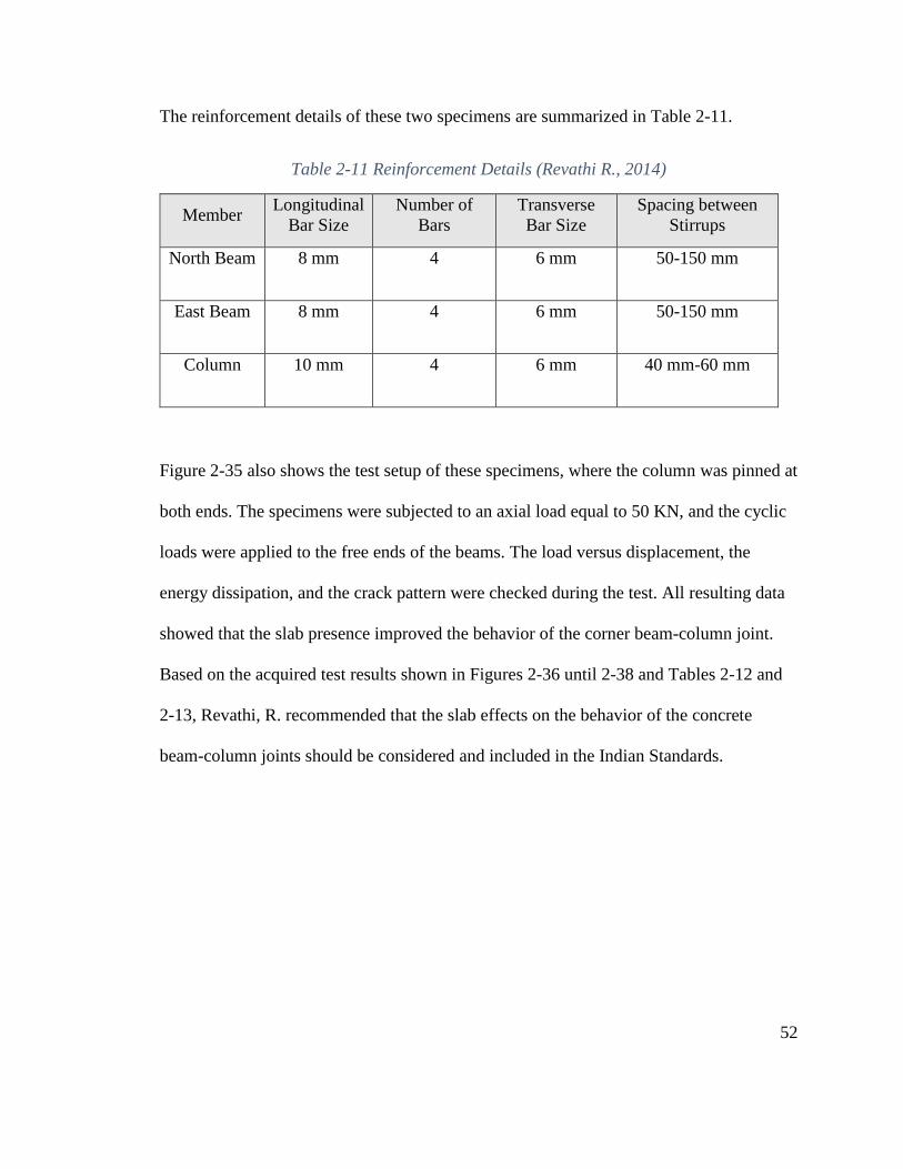
52

The reinforcement details of these two specimens are summarized in Table 2-11.

Table 2-11 Reinforcement Details (Revathi R., 2014)

Member Longitudinal

Bar Size

Number of

Bars

Transverse

Bar Size

Spacing between

Stirrups

North Beam 8 mm 4 6 mm 50-150 mm

East Beam 8 mm 4 6 mm 50-150 mm

Column 10 mm 4 6 mm 40 mm-60 mm

Figure 2-35 also shows the test setup of these specimens, where the column was pinned at

both ends. The specimens were subjected to an axial load equal to 50 KN, and the cyclic

loads were applied to the free ends of the beams. The load versus displacement, the

energy dissipation, and the crack pattern were checked during the test. All resulting data

showed that the slab presence improved the behavior of the corner beam-column joint.

Based on the acquired test results shown in Figures 2-36 until 2-38 and Tables 2-12 and

2-13, Revathi, R. recommended that the slab effects on the behavior of the concrete

beam-column joints should be considered and included in the Indian Standards.

53

Table 2-12 The Maximum Ductility Factor for Beam Column Joint without Slab

No. Direction

Displacement

At Yield (mm) At Ultimate

(mm)

Ductility

Factor

1 North 4 14.5 3.63

2 East 3.8 15.3 4.03

Table 2-13 The Maximum Ductility Factor for Beam Column Joint with Slab

No. Direction

Displacement

At Yield (mm) At Ultimate

(mm)

Ductility

Factor

1 North 5.2 33.3 6.4

2 East 5.4 32.8 6.63

Figure 2-36 Energy Dissipation Curves for Beam-Column Joint without Slab

54

Figure 2-37 Energy Dissipation Curves for Beam-Column Joint with Slab

Figure 2-38 Cracks Patterns of the Specimens

a- Beam-Column Joint without Slab b- Beam-Column Joint with Slab

55

2.4. Summary of the Literature Review

Based on the literature review, it was clear that, many techniques and materials have been

used to rehabilitate column-beam joints since 1970. Column-beam joints designed before

1970s that were used in concrete frames were the weakest link in a structure, and this

weakness could cause building failure during the earthquakes because these joints were

characterized by non-ductile behavior due to a lack of shear reinforcement in these

regions. The first material that was as external reinforcement was steel plates as steel

jackets. These jackets consisted of flat or corrugated steel plates. This technique was

successful in increasing the flexural capacity within limited range by attaching the steel

plates to the concrete surface with epoxy or bolts, but there were disadvantages in using it

due to the cost and the availability of steel in some countries, the corrosion exposure, and

the fact that it wasn’t fireproof. The other technique used to change the non-ductile

behavior of the beam-column joint was concrete jacketing. Many experimental tests were

performed using concrete and reinforcement bars in order to confine the joints. But in the

field, reinforced concrete jacketing needed an extensive labor with specialized skills.

Moreover, concrete jackets increased the dimensions and the weight of the structures.

More than two decades ago, the use of Fiber Reinforced Polymer (FRP) as an externally

bonded reinforcement to retrofit the beam-column joint was proposed. The main feature

of this material is the flexural strength. FRP composites have high strength, which makes

them suitable for this purpose. The use of Fiber Reinforced Polymer (FRP) to retrofit the

concrete beam-column joints offers many advantages: it is fast to apply, light weight,

56

resistant to corrosion, does not affect the function of the buildings, requires simple skills

to do the retrofitting, and the cost and availability are not a problem in many countries.

57

Experimental Work

3.1. General

The experimental research, including the specimens’ design, materials properties, mix

proportions, casting techniques, curing conditions, test setup, and instrumentation is

discussed in this chapter. Experimental tests were performed in the South Greenhouse

Lab at Portland State University.

3.2. Design of Specimens

The objective of this study was to investigate the behavior of a retrofitted concrete beam-

column joint that was designed and constructed prior to the 1970s, with a deficiency of

shear reinforcement within the joint region. Retrofitting was accomplished by using

Carbon Fiber Reinforced Polymer (CFRP) sheets as an exterior bonded reinforcement.

Because these types of joints are more vulnerable to failure during earthquakes, both the

beam and column were designed according to ACI 318-14 to resist the gravity loads, and

the shear reinforcement within the joint region was eliminated in order to ensure that the

majority of the cracking and damage would occur within the joint region.

In this experimental work, six specimens in one third- scale were designed to represent a

joint in a typical multi-story concrete building. Table 3-1 shows a summary of the six

specimens.

58

Table 3-1 Summary of Specimens

Specimen Comments

J1 Control Specimen, joint designed according to ACI 318-14, Chapter 18

J2 Control Non-Ductile Specimen, joint designed according to old codes

J3 Non-Ductile Specimen Retrofitted by Using One Layer of the CFRP Sheet

J4 Non-Ductile Specimen Retrofitted by Using Two Layers of the CFRP Sheet

J5 Non-Ductile Specimen Retrofitted by Using One Layer of the CFRP Sheet

J6 Non-Ductile Specimen Retrofitted by Using Two Layers of the CFRP Sheet

All specimens contained beams 5 in. wide × 6 in. deep, and square columns 5 in. × 5 in. cross sections.

All specimens had identical dimensions. The general shape of the specimen was a “T”

shape, where the two columns connected with a transverse beam at mid height to form

the exterior joint because these types of joints are more vulnerable to fail during the

earthquakes.

3.3. Details of Specimens

The six specimens in one third scale were named as J1, J2, J3, J4, J5, and J6 represented

an exterior beam-column joint in multi-story building, and were constructed and tested

under a constant axial load and cyclic flexural loading. All specimens had the same

shape. The J1 specimen was different from the others in terms of the reinforcement

details. The J1 specimen was designed in accordance with ACI 318-14, Chapter 18. The

seismic provisions were included and were represented by using the shear reinforcement

59

in the joint region and the confinement within the beam and columns. This specimen was

considered as a “ductile” specimen, and the plastic hinge was expected to form in the

beam since the confinement was provided by adding the closed ties in the columns and

joint. Also, this joint represents one of the control specimens, and its general behavior

represented the behavior of a ductile seismic joint. Figure 3-1 shows the dimensions and

the reinforcement details of the specimen J1. On the other hands, the rest of the

specimens J2, J3, J4, J5, and J6 were designed in accordance with older ACI codes (prior

to 1970s) to resist the gravity loads only and the failure was expected to occur in the

joints due to lack of confinement in the joint. Specimen J2 represented a control

specimen J2, and represented the behavior of the non-ductile joint. Figure 3-2 shows the

dimensions and the reinforcement details of the specimens J2.

The beam had a cross section of 5×6 in and the transverse beam length was 20 in,

whereas the column section had a cross section of 5×5 in and the total length of the

column was 46 in where the beam connected to the column at the mid-height to form the

joint.

60

Figure 3-1 Details of Specimen J1, the “Ductile” Specimen

61

Figure 3-2 Details of Specimen J2, Non-ductile Specimen

62

3.4. Materials

3.4.1. Cement

Ordinary Portland Cement Type (II) provided by (Mason Supply Company) was used

throughout this study. It was stored in air-tight plastic container at the Greenhouse Lab to

avoid exposure to humidity.

3.4.2. Fine and Coarse Aggregate

Sand from Mason Supply was used. The grading of the sand is shown in Table 3-2.

Uncrushed gravel with maximum size 3/8 in. was used. The grading of coarse aggregate

is shown in Table 3-3.

Table 3-2 Sieve Analysis of Sand

No. Sieve size % passing of coarse aggregate

1 4.75mm sieve (#4) 97.81%

2 passing 2.00 mm (#10) 84.67%

3 0.85 mm (#20) 72.99%

4 0.425 mm (#40) 49.64%

5 0.150 mm (#100) 5.11%

6 0.075 mm (#200) 0.73%

63

Table 3-3 Sieve Analysis of Gravel

No. Sieve size % passing of coarse aggregate

1 19 mm (0.75 in.) 100%

2 12.5 mm (1/2 in.) 99.36%

3 4.75 mm (3/8in.) 1.32%

4 4.25 mm (#4) 0.54%

3.4.3. Mixing Water:

Tap water was used to cast and cure all specimens during the 28 maturation period.

3.5. Steel Reinforcement:

The longitudinal bars in all of the specimens were deformed bars grade 60, and were

represented by #4 bars as longitudinal reinforcement in the column, and #3 bars as

longitudinal reinforcements in the beam in each specimen. Steel bar size #2 (0.25 in.

diameter unreformed) was used as a transverse reinforcement in both beam and column

in each specimen. Tensile tests were performed on three samples of each bar size to

determine the reinforcing steel mechanical properties. The tensile strength and modulus

of elasticity were obtained by testing 3 ft specimens according to ASTM for #3 and #4

bars and 9 in. for #2 bars. For #3 and #4 specimens, the specimens were prepared with

strain gages at the middle to obtain the tensile stress-strain diagram, and tests were

performed using MTS machine in the iSTAR laboratory. The #2 bar specimens were

64

tested in the Infrastructure Materials Lab, Room 370 in the Engineering Building at PSU.

Table 3-4 shows the steel properties. Figure 3-3 shows stress-strain diagrams of bars.

Table 3-4 The Reinforcing Steel Mechanical Properties

Bar size Diameter (in) Area (in2) 𝑓𝑦 (Ksi) 𝜀𝑦 ES

#4 bar 0.375(3/8) 0.11 74 0.0027 27407

#3 bar 0.5(4/8) 0.4 74 0.0027 27407

Wire gage (0.25 in.) 0.25 0.049 38 0.00214 20416

65

0

20

40

60

80

100

120

140

0.00 0.01 0.02 0.03 0.04 0.05

Str

ess

(ksi

)

Strain(in./in.)

#3 Stress-Strain Digram

0

20

40

60

80

100

120

0 0.01 0.02 0.03 0.04 0.05

Str

ess

(ksi

)

Strain(in./in.)

#4 Strian-Stress Diagram

0

10

20

30

40

50

0 0.01 0.02 0.03 0.04 0.05

Str

ess

(ksi

)

Strain (in./in.)

#2 (0.25 in.) Wire Stress-Strain Diagram

Figure 3-3 Stress-Strain Diagrams of the Reinforcement Bars

66

Since the design represented an external beam-column joint, the longitudinal

reinforcement of the beam was bent at the ends at the intersection region between the

beam and the column where the upper rebar bent down and the lower rebar bent up. The

hook length was 6 in. according to the ACI 318-14 as shown in Figure 3-4.

Used end hooked

length

Figure 3-4 End Hook Dimensions

67

Figures 3-7 to 3-10 show the reinforcement details of all specimens that had been

designed and tested throughout this experimental work. The longitudinal reinforcement

bars in all specimens were the same, and the differences between the specimens were

represented by the spacing between the transverse reinforcement bars and the stirrup’s

end hook details. In the non-seismic specimens, the space between the ties in the column

was 5 in., and the space between the stirrups in the beam was 2.5 in. In seismic specimen,

the space between the ties in the column within the confinement length was 1.3 in. and 3

in. out the confinement length. The space between the stirrups in the beam within the

confinement length (hinge zone) was 1.3 in. and 2.5 in. outside of the confinement

length. Figure 3-5 shows the details of shear reinforcement in seismic and non-seismic

specimens where the length of hooked ends was equal to 6db.

Figure 3-5 The Difference between Shear Reinforcement in Seismic and Non-Seismic

Specimens

68

In order to avoid unexpected failure by lack of development length, a special “U” shape

#3 rebar was used at the end of the longitudinal beam rebar to insure that this bar would

develop the tensile strength as shown in the Figure 3-6.

#3 U shape rebar detail

a- Seismic design b- Non-Seismic design

Figure 3-6 “U” Shape Rebar Detail

69

Section details of Non-seismic column Section details of seismic column

Section details of seismic beam Section details of non-seismic beam

Figure 3-7 Column Section Details

Figure 3-8 Beam Section Details

70

Figure 3-9 Reinforcement Cage of Specimen J1

Figure 3-10 Reinforcement Cage of Specimen J2

71

3.6. Strain Gages

When the reinforcement cages were ready, for the control specimens J1and J2, four steel

strain gages were attached to the beam longitudinal reinforcement of each one. The strain

gage types “KFH-20-120-C1-11L1M2R” were purchased from Omega Engineering, Inc.

The properties of these strain gages as provided by the company are shown in Table 3-5.

Steel bar surface preparation was done by using a manual grinder and sand paper to

ensure that the proper bonding of the strain gage was done perfectly. Epoxy glue was

used to attach the strain gages to the steel bars, then duct tape was used to wrap both the

strain gages and bars to protect them. A voltmeter was used to check these strain gages

regularly to detect any potential problem before the casting of the concrete. There were

six steel strain gages in each of retrofitted specimens. Four steel strain gages were

attached to the beam longitudinal reinforcement, and the other two gages were attached

directly to the Carbon Fiber Reinforced Polymer (CFRP) sheets (one on each side of the

joint) in order to measure the CFRP strain up to the failure. Figures 3-11 and 3-12 show

strain gage locations, preparation and attaching.

Table 3-5 Strain Gage Properties

Strain Gage Types Resistance Gage Factor (K)

Transverse

Sensitivity

KFH-20-120-C1-11L1M2R 120.4Ω ± 0.35% 2.07 ± 1.0 % - 0.6 %

72

Figure 3-11 Strain Gage Instullation

a- Surface Preparation

b- Strain Attachment

73

Figure 3-12 Strain Gage Locations

74

3.7. Molds

Six wood molds were used to cast all of the specimens, all at one time at the Greenhouse

Lab. The molds were manufactured from 1.5 in. thickness lumber purchased from Home

Depot Inc. Figure 3-13 shows one of these molds. In order to avoid any unnecessary

drainage of the water during the casting process, these molds were cleaned by an air

compressor and then (DAP) waterproof silicone was used to fill the joints in the molds.

Figure 3-13 Wood Molds

75

3.8. Properties of Concrete:

The concrete mix was designed in accordance with the Design and Control of Concrete

Mixture, 14th Edition, Portland Cement Association (PCA). The mix was designed for a

compressive strength of 3000 psi at 28-day of age. Mixtures details are given in Table 3-

6.

Table 3-6 Properties of Mixture with 3000 Psi Compressive Strength

No. Parameter Weight (Ib per ft3)

1 Water / cement ratio 0.67

2 Water (Ib/ft3) 12

3 Cement (Ib/ft3) 18

4 Sand (Ib/ft3) 61

5 Coarse aggregate (Ib/ft3) 46

3.9. Concrete Mixing Procedure

When the wood molds were ready, the reinforcement cages were placed inside of the

molds. All of the molds were then placed in the front yard of the lab on the ground as

shown in Figure 3-14. A concrete mixer of 2.25 ft3 capacity available in the South

Greenhouse Lab was used. The interior surface of the mixer was cleaned and moistened

before placing the materials inside. While the mixer was running, half of the coarse

aggregates were put in, and then the water was added to the aggregate. After 30 seconds,

76

the cement was added to the mixture followed by half of the sand amount. One and a half

minutes later, the rest of the coarse aggregate was added and same procedure was

repeated. After all of the materials were put into the mixer, it took about three minutes for

the mixture to be ready for slump test, which was done in order to check the workability

of the mixture before casting the concrete in molds. The desired slump was 7-8 in., which

was achieved by the mixtures.

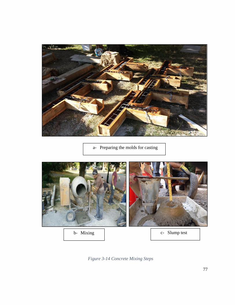
77

a- Preparing the molds for casting

b- Mixing c- Slump test

Figure 3-14 Concrete Mixing Steps

78

3.10. Curing Age of Specimens

The temperature was 99 F° at casting time and the humidity was 55%. Right after casting

the specimens and cylinders, three layers of natural burlap and one layer of plastic sheets

were used to cover all specimens in order to keep the moisture as long as possible. After

five days, the wood molds were removed and all of the cylinders and flexural samples

were placed beside the specimens to subject them to the same weather conditions as

shown in Figure 3-15. Tap water was used to spray the specimens twice a day. This

process continued up to first month age of specimens then the curing depended on the

humidity of the atmosphere where all of the specimens and cylinders were placed inside

the Greenhouse Lab.

Figure 3-15 Curing Condition of Specimens

79

3.11. Mechanical Properties of the Hardened Concrete

3.11.1. Compressive Strength Testing

The compressive strength of concrete was carried out in accordance with ASTM-C39

using 6×12 in. concrete cylinders loaded uniaxial by a compressive strength machine as

shown in Figure 3-16. This was available at South Greenhouse Lab where the maximum

compressive capacity of the machine is 250 kips. For each specimen, one cylinder was

tested on the same day of the test. The results are given in Table 3-7.

Figure 3-16 Compressive Testing Machine

80

Table 3-7 Concrete Compressive Strength of the Specimens

No. Age of the Test (day) Compressive Peak Load (kips) Compressive Stress (ksi)

1 29 80.35 2.80

2 39 91 3.14

3 96 124.9 4.4

4 110 126 4.46

5 145 124 4.4

6 150 1125 4

3.11.2. Flexural Strength

Flexural strength (modulus of rupture) tests were carried out on three normal concrete

specimens in accordance with ASTM- C 78. These specimens were casted and cured

under the same conditions as the main specimens at the Greenhouse Lab and were tested

after 42 days. The flexural strength tests are made on 6×6×18 in. simple beam specimens

loaded at third points. The experimental results are shown in Table 3-8 where all of the

failures occurred within the middle third of span length of the beams as shown in Figure

3-17. Moreover, Table 3-8 also shows the comparison between the experimental and

theoretical results. The theoretical calculations were done by using the ACI 318 equation:

𝑓𝑟 = 7.5 𝜆 √𝑓′𝑐

81

Table 3-8 Modulus of Rupture of the Concrete

Specimen No. Experimental Result (ksi)

𝑓𝑟1 0.391

𝑓𝑟2 0.417

𝑓𝑟3 0.450

Experimental Average Flexural Strength = 0.42 ksi

Theoretical Result based on ACI = 0.41 ksi

Experimental/ Theoretical = 1.02

a- Test Setup b- Failure Modes

Figure 3-17 Modulus of Rupture Test

82

3.11.3. Splitting Tensile Strength (𝒇𝒄𝒕 )

The indirect tensile strength (splitting tensile strength) tests were carried out in

accordance with ASTM- C 496 by using the compressive machine that is available at the

iSTAR Lab. Splitting tensile strength tests were made on 6×12 in. (diameter × height)

cylinders as shown in Figure 3-18. Table 3-9 summarizes the splitting tensile strength of

concrete and shows the comparison between the theoretical and experimental tests. The

following equation was used to estimate the experimental splitting strength:

𝑓𝑐𝑡 =2 𝑝

𝜋 𝑙 𝑑

Where: 𝑓𝑐𝑡 ∶ 𝑠𝑝𝑙𝑖𝑡𝑡𝑖𝑛𝑔 𝑡𝑒𝑛𝑠𝑖𝑙𝑒 𝑠𝑡𝑟𝑒𝑛𝑔𝑡ℎ, 𝑝𝑠𝑖

P: max. applied load

l: length, in

d: diameter, in

Figure 3-18 Splitting Test

83

Table 3-9 Splitting Tensile Strength of the Concrete

3.11.4. Modulus of Elasticity (𝑬𝒄)

Measurement of static modulus of elasticity of concrete (𝐸𝑐) was carried out in

accordance with ASTM-C 469, using 6×12 in. concrete cylinders tested in compression at

constant strain rate as shown in Figure 3-19. The same testing machine, which is

employed in compressive strength tests of concrete, was used in this test. Two

displacement transducers (LVDTs) were used to measure the deformation in the concrete

cylinders as shown in the Figure 3-19. The theoretical values were determined by using

the ACI code equation, 57000√𝑓′𝑐. Table 3-10 summarizes the modulus of elasticity of

the concrete and the stress-strain diagrams are shown in Figure 3-20.

Age (day)

𝑓𝑐𝑡 (𝑝𝑠𝑖)

Deviation

Experimental Theoretical

55 387 374 3.5 %

150 442 424 4.25%

84

Table 3-10 Concrete Modulus of Elasticity

No.

Age of the

Concrete at the

Test (Days)

Concrete Modulus of Elasticity (𝐸𝑐), ksi

Deviation

Theoretical Experimental

1 39 3122 3350 7%

2 150 3605 3420 5%

3 150 3605 3242 10%

LVDT to measure

the length deformation

Figure 3-19 Modules of Elasticity Test

85

Figure 3-20 Stress-Strain Diagram of the Concrete

0

0.5

1

1.5

2

2.5

3

3.5

0 0.001 0.002 0.003 0.004 0.005 0.006 0.007 0.008

Str

ess

(ksi

)

strain (in./in.)

Stress-Strain Diagram, E1

0

0.5

1

1.5

2

2.5

3

3.5

4

4.5

0 0.001 0.002 0.003 0.004 0.005 0.006 0.007 0.008

Str

ess

(ksi

)

Srain (in./in.)

Stress-Strain Diagram, E3

0

0.5

1

1.5

2

2.5

3

3.5

4

4.5

0 0.001 0.002 0.003 0.004 0.005 0.006 0.007

Str

ess

(ksi

)

strain (in./in.)

Stress-Strain Daigram, E2

86

3.12. Carbon Fiber Reinforced Polymer (CFRP) Sheets

CFRP sheets were used as an exterior bonded reinforcement to compensate for the

missing reinforcement within the joint rejoin. FRP in general is very strong in tensile

strength in the longitudinal direction and it is relatively weak in the transverse direction.

In this experimental work, the MasterBrace FIB 300/50 CFS, CFRP unidirectional high

strength carbon fiber sheets were purchased from BASF Company. The tensile properties

of these sheets are shown in Table 3-11, and the physical properties are shown in Table

3-12 as described by the manufacturer.

Table 3-11 Tensile Properties of the CFRP Sheet

No. Property Requirement

1 Ultimate tensile strength , (𝑓𝑓𝑢) 550 ksi

2 Tensile modulus,(𝐸𝑓) 33000 ksi

3 Ultimate tensile strength per unit width, (𝑓𝑓𝑢 𝑡𝑓) 3.57 kips/in/ply

4 Tensile modulus per unit width, (𝐸𝑓 𝑡𝑓) 215 kips/in/ply

5 Ultimate rupture strain, (𝜀𝑓𝑢) 1.67 %

87

Table 3-12 Physical Properties of the CFRP Sheets

No. Property Requirement

1 Fiber material High strength carbon

2 Fiber tensile strength 720 ksi

3 Areal weight 0.062

4 Fabric width 20 in.

5 Nominal thickness, 𝑡𝑓 0.0065 in.

In order to verify the provided properties, the tensile tests was performed in Material

Science Lab, Mechanical and Materials Engineering Department at Portland State

University. Seven identical specimens were tested in accordance with ASTM D 3039/ D

3039M, and the results are summarized in Appendix B.

3.13. Surface Preparation:

Four of the non-seismic specimens were strengthened by using CFRP sheets, where the

sheets were attached to the specimens by a special epoxy recommended by the

manufacturer. In order to achieve the best bond between the concrete surface and the

CFRP sheet, a special preparation of the concrete surface was needed. The concrete

surface preparation was done by using a manual grinder. The concrete surface was

roughened, as shown in the Figure 3-21, in order to gain the highest adhesion between the

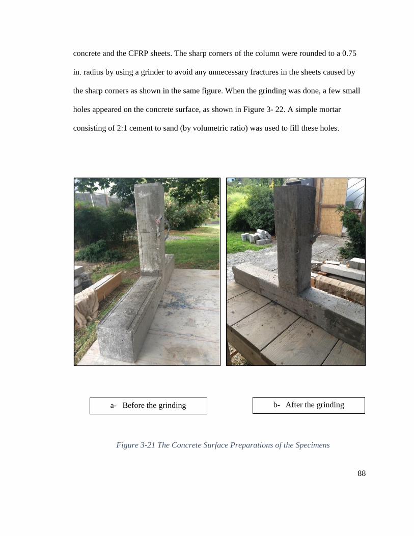
88

concrete and the CFRP sheets. The sharp corners of the column were rounded to a 0.75

in. radius by using a grinder to avoid any unnecessary fractures in the sheets caused by

the sharp corners as shown in the same figure. When the grinding was done, a few small

holes appeared on the concrete surface, as shown in Figure 3- 22. A simple mortar

consisting of 2:1 cement to sand (by volumetric ratio) was used to fill these holes.

a- Before the grinding b- After the grinding

Figure 3-21 The Concrete Surface Preparations of the Specimens

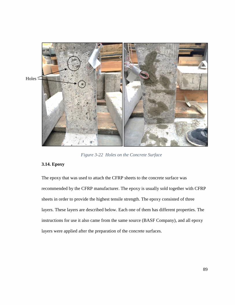
89

3.14. Epoxy

The epoxy that was used to attach the CFRP sheets to the concrete surface was

recommended by the CFRP manufacturer. The epoxy is usually sold together with CFRP

sheets in order to provide the highest tensile strength. The epoxy consisted of three

layers. These layers are described below. Each one of them has different properties. The

instructions for use it also came from the same source (BASF Company), and all epoxy

layers were applied after the preparation of the concrete surfaces.

Figure 3-22 Holes on the Concrete Surface

Holes

90

3.14.1. MasterBrace P 3500 or Primer Layer

After the preparation of the concrete member was done as recommended by the

manufacturer, the primer layer, which is the first layer of the MasterBrace System, was

applied to the concrete member. The primer layer was applied in order to provide good

adhesion between the MasterBrace System and the member, as shown in Figure 3-23.

The mechanical properties were provided by the manufacturer as shown in the Table 3-

13.

This layer consists of two parts A and B. These parts were mixed based on the provided

mix ratio of 3:1 (part A to part B) by volume or 100:30 (part A to part B) by weight.

Before the mixing process, the concrete surface was cleaned with water, and then sun-

dried. On the day of application, the concrete member was cleaned by using an air

compressor that was available at the Greenhouse Lab, then the MasterBrace P 3500 was

applied by using a paint brush. Spray paint is not recommended with this product. The

recommended curing time for this layer was twenty four hours.

Figure 3-23 Applying the Prime Layer to the Concrete Surface

91

Table 3-13 Mechanical Properties of MasterBrace P 3500

No. Property Compressive Tensile

1 Yield strength (psi) 3800 2100

2 Strain at yield 4.0% 2.0%

3 Elastic modulus (ksi) 97 105

4 Ultimate strength (psi) 4100 2500

5 Rupture strain 10% 40%

6 Poisson’s ratio N/A 0.48

3.14.2. MasterBrace F 2000 or Putty Layer

After twenty four hours, the second layer of the MasterBrace F 2000 was applied over the

primer layer. The main purpose of this layer was to level out the small surface defects,

and to provide a smooth surface where the MasterBrace System was attached to the

specimen, as shown in Figure 3-24. The mechanical properties were provided by the

manufacturer as shown in the Table 3-14. This layer also consists of two parts A and B.

These parts were mixed based on the provided mix ratio of 3:1 (part A to part B) by

volume or 100:30 (part A to part B) by weight. The MasterBrace F 2000 was applied by

using a steel trowel. The recommended curing time for this layer was twenty four hours.

92

Table 3-14 Mechanical Properties of MasterBrace F 2000






5 Rupture strain 10% 7%


Figure 3-24 Applying the Putty Layer to the Concrete Surface

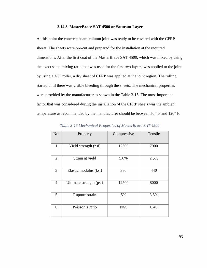
93

3.14.3. MasterBrace SAT 4500 or Saturant Layer

At this point the concrete beam-column joint was ready to be covered with the CFRP

sheets. The sheets were pre-cut and prepared for the installation at the required

dimensions. After the first coat of the MasterBrace SAT 4500, which was mixed by using

the exact same mixing ratio that was used for the first two layers, was applied to the joint

by using a 3/8” roller, a dry sheet of CFRP was applied at the joint region. The rolling

started until there was visible bleeding through the sheets. The mechanical properties

were provided by the manufacturer as shown in the Table 3-15. The most important

factor that was considered during the installation of the CFRP sheets was the ambient

temperature as recommended by the manufacturer should be between 50 ° F and 120° F.

Table 3-15 Mechanical Properties of MasterBrace SAT 4500






5 Rupture strain 5% 3.5%


94

3.15. Attaching the CFRP Sheets

The process that was used to attach the CFRP sheets for all of the retrofitted specimens

was similar. After the preparation of the concrete surface, as described in the previous

section, applying the CFRP sheets was the final step of this process. This step started by

using the Saturant layer to paint the areas to be strengthening. After the painting these

areas with MasterBrace SAT 4500, the CFRP sheets were attached to the concrete

surface. A plastic roller was used to make sure that all of the CFRP sheets were attached

to the concrete surface, and that the leftover epoxy bled through the CFRP fibers. The

CFRP sheets were left to cure for at least seven days at room temperature. The previous

procedure was followed for one layer of the Carbon Fiber Reinforced Polymer (CFRP)

sheet. In order to use two layers or more, the same procedure is usually used. Figure 3-25

shows the wrapped specimen that was retrofitted and left for curing as recommended by

the manufacturer.

Figure 3-25 Specimen Wrapped by CFRP Sheets

95

3.16. Rehabilitation Schemes

In adding CFRP sheets to the joint, one rehabilitation technique used consisted of adding

an “L” shape of CFRP sheets at the corners on both sides of the beam in order to

compensate the missing leg of the ties at the interface between the beam and column

joint. The column was then wrapped with one layer of CFRP sheet at 0 ° with the

horizontal beam axis in “U”-shape form. Finally, CFRP sheets were wrapped around the

beam to provide 100% confinement and to delay any unexpected deboning. For all

specimens, the technique was the same as the first one, but the number of layers used was

different. Table 3-16 shows the rehabilitation of the joints and Figure 3-26 shows the

details of the technique used to retrofit the joints. The reason for attaching the CFRP

sheets at 0 ° with the horizontal beam axis at the joint region was to simulate the shear

reinforcement position in the joint.

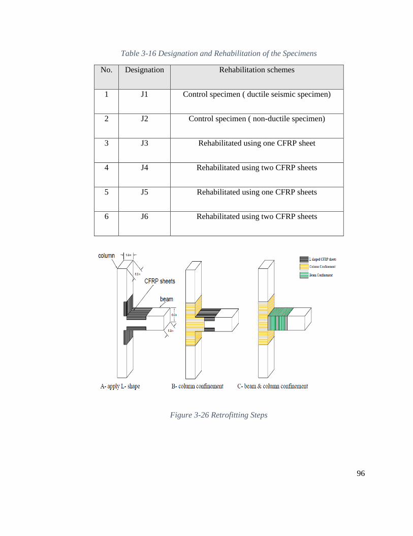
96

Table 3-16 Designation and Rehabilitation of the Specimens

No. Designation Rehabilitation schemes

1 J1 Control specimen ( ductile seismic specimen)

2 J2 Control specimen ( non-ductile specimen)

3 J3 Rehabilitated using one CFRP sheet

4 J4 Rehabilitated using two CFRP sheets

5 J5 Rehabilitated using one CFRP sheets

6 J6 Rehabilitated using two CFRP sheets

Figure 3-26 Retrofitting Steps

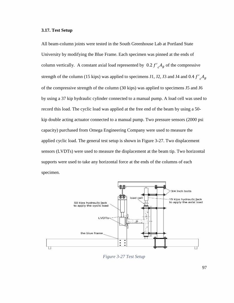
97

3.17. Test Setup

All beam-column joints were tested in the South Greenhouse Lab at Portland State

University by modifying the Blue Frame. Each specimen was pinned at the ends of

column vertically. A constant axial load represented by 0.2 𝑓′𝑐𝐴𝑔 of the compressive

strength of the column (15 kips) was applied to specimens J1, J2, J3 and J4 and 0.4 𝑓′𝑐𝐴𝑔

of the compressive strength of the column (30 kips) was applied to specimens J5 and J6

by using a 37 kip hydraulic cylinder connected to a manual pump. A load cell was used to

record this load. The cyclic load was applied at the free end of the beam by using a 50-

kip double acting actuator connected to a manual pump. Two pressure sensors (2000 psi

capacity) purchased from Omega Engineering Company were used to measure the

applied cyclic load. The general test setup is shown in Figure 3-27. Two displacement

sensors (LVDTs) were used to measure the displacement at the beam tip. Two horizontal

supports were used to take any horizontal force at the ends of the columns of each

specimen.

Figure 3-27 Test Setup

98

3.18. Load Sequence

The selected load history consists of two phases. The first phase was load-controlled

followed by a strain –controlled phase. The first phase consisted of twenty “full” cycles.

“Full Cycle” refers to producing both positive and negative moments in one cycle. In the

first ten cycles, a 2.4-kip load, which created 75% of the maximum theoretical flexural

capacity of the beam, was applied at each load cycle. For the second ten cycles, a 2.8-kip

load, which represented 90% of the maximum theoretical flexural capacity of the beam,

was applied at each load cycle. Then the second phase (strain controlled) started. For the

strain controlled phase of the load sequence, the cyclic load was applied in each direction

until the strain in the longitudinal flexural beam bars was 0.4% in twenty cycles. This

strain corresponding to twice the yield strain. The applied cyclic load was then increased

until the strain reached 0.6% (representing 3 times the yield strain). Figure 3-28 shows

the load sequence. During the test of each specimen, the axial load was applied and

maintained at the upper end of the column. The cyclic load was applied at the free end of

the beam, which was represented by pushing the free end down and releasing, then up

and releasing for each cycle. The applied force and deflection at each cycle were

recorded in addition to the strain gages readings.

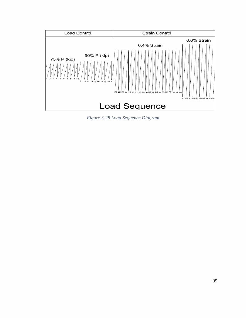
99

Figure 3-28 Load Sequence Diagram

100

Experimental Results

4.1. General

This chapter presents the data collected throughout the experimental tests of specimens

described in Chapter Three. To evaluate the proposed retrofitting technique of using

CFRP sheets, the behavior of the control and retrofitted specimens are described in terms

of applied beam load versus displacement. This provides the information about the

strength, energy dissipation, and ductility of the joints. Moreover, the failure modes and

crack patterns are expressed by drawings and photographs.

4.2. Behavior of Specimens

4.2.1. Ductile Specimen J1

The general behavior of the seismic joint J1 which was the control specimen representing

a ductile joint that designed based on the seismic provisions in the current code (ACI

318-14). As described in previous chapters, this specimen was prepared and cast at

Greenhouse Lab at Portland State University and tested two and half months after

casting. All specimens were tested using the Blue Frame that was first modified to have

the loading system to perform the tests. Loading system was designed to simulate the

type of stress that the joint would be subjected to during an earthquake. Figure 4-1 shows

how the specimen was placed in the frame and set for the test.

101

After the specimen was placed in the Blue Frame, and all of the wires connected to the

data acquisition system, the specimen was ready to test. A systematic procedure for the

load sequence was used to test the specimen. For specimen J1, the test started by

applying an axial load of 15 kips (representing 0.2f’c Ag) on the top of the column, and

the load was kept constant during the test. Beam load was then applied and cycled to

produce positive and negative beam moments. After applying the first load cycle, a few

flexural cracks developed along the hinge region of the beam starting from the interface

between the column and the beam, as shown in Figure 4-2. The largest crack in terms of

Figure 4-1 Test Setup of Joint J1

102

the length and the width was the one closest to the column face. The crack width was 1

mm and 0.5 mm at the loading and at the release respectively.

For the next three cycles, a few more flexural cracks developed within the same beam

region. The crack width increased to 1.2 mm and 0.9 mm at loading and at the release

respectively. The same crack pattern formed on the lower beam face, and these cracks

proceeded toward the middle of the beam depth. A few hairline cracks formed during

these four cycles because the applied cyclic load at second cycle was accidentally

increased to 10% greater than the maximum theoretical strength of the beam. Figure 4-

3 shows the cracks that developed in the first four cycles.

Figure 4-2 The Development of the First Cracks at the First Cycle, J1

103

For the rest of the first set of cycles, no new cracks developed. The only change was in

crack widths, especially in the crack that formed at the interface between the beam and

column. This crack width was 1.6 mm by the end of cycle 10 within the load control.

Figure 4-4 shows the specimen J1 at the end of first set of load cycles.

Figure 4-3 Development of the Flexural Cracks after Cycle 4, J1

104

In order to visually recognize the new cracks within the second set of cycles, red

colored markers were used to highlight the cracks, whereas a black marker was used for

the first set. Similar to the previous test procedure, the applied cyclic load on the free

end of the beam in the second set was equal to 90% of the maximum theoretical load of

the beam capacity. As expected in these cycles, the joint did not show any degradation

in strength despite showing a few cracks within the joint region. Some of the existing

cracks in the beam developed further, as shown in Figure 4-5.

Figure 4-4 Specimen J1 at the End of First Set of Cycles.

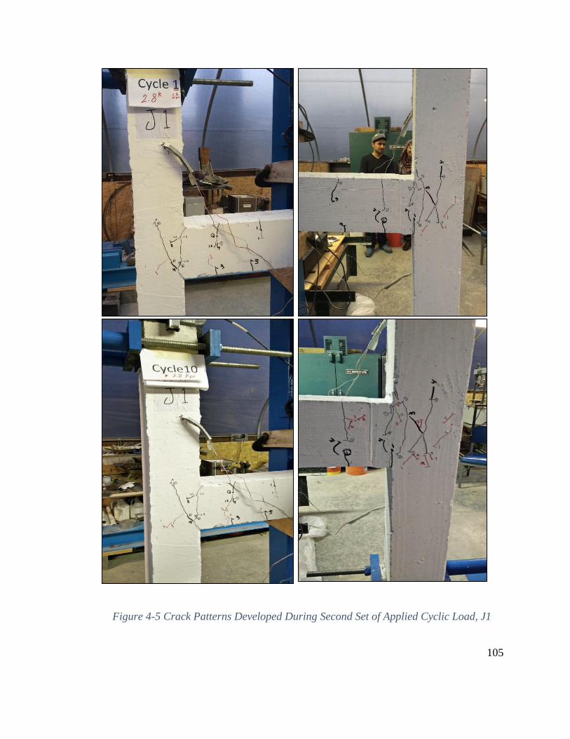
105

Figure 4-5 Crack Patterns Developed During Second Set of Applied Cyclic Load, J1

106

In the first two sets of cycles (from cycle 1 until cycle 20), the specimen behavior

showed that there was no degradation in the strength of the joint.

The next set of cycles represented the strain control where the cyclic load was applied

to the free end of the beam until the strain was two times the yield strain to find out

how the specimen would behave under severe earthquake effects. The first cycle in this

phase developed the cracks within the joint region and formed diagonal cracks in “X”

shape on both sides of the joint. The average cyclic load used in this phase was two

times greater than used in the first set of load (75% maximum theoretical beam

capacity). Blue Markers were used to highlight these cracks. Figure 4-6 shows the crack

pattern at the first cycle within strain control phase.

Figure 4-6 Crack Pattern of Cycle 1, Strain Control, J1

107

As the strain control cycles progressed, the flexural crack that developed at the interface

between the column and the beam became wider. Meanwhile, the side concrete covers

started to gradually crack on both sides, especially at the seventh cycle in this set. Figure

4-7 shows cracking of concrete within the joint region.

Figure 4-7 Concrete Cover Splitting, J1

108

This specimen showed very good ductility. There was no degradation of the strength

recorded through this set of cycles. After nineteen cycles in strain control, the jack

stroke maxed out and this was the only reason why the test was stopped. At this point,

the back side of the column was still intact with no crack. Figure 4-8 shows the final

crack pattern of ductile specimen J1.

The applied load versus displacement was recorded and plotted in Figure 4-9. This

figure shows that this beam-column joint was subjected to thirty-nine loading cycles.

Table 4-1 shows the values of the loads and displacements at each cycle for the free end

of the beam.

Figure 4-8 Specimen J1 (final crack pattern)

109

Figure 4-9 Load-Displacement Diagram, J1

-9

-7

-5

-3

-1

1

3

5

7

9

-4 -3 -2 -1 0 1 2 3 4

Cycl

ic L

oad

(k

ips)

Displacement (in.)

Cyclic Load - Displacement Diagram, J1

Pushing Up, J1 Pushing Down, J1

110

Table 4-1 The Maximum Values of the Loads and Displacements at Each Cycle, J1

Cycle Down F. Disp. Up F. Disp.

0 0 0 0 0

1 2.6381 0.13093 -2.48314 -0.11433

2 2.4027 0.3225 -2.49272 -0.10126

3 2.41088 0.32366 -2.41603 -0.14237

4 2.4433 0.2433 -2.41603 -0.13801

5 2.42712 0.36504 -2.55984 -0.14972

6 2.419003 0.37702 -2.5 -0.144

7 2.42712 0.3770202 -2.4 -0.14427

8 2.419 0.40369 -2.42561 -0.16034

9 2.532 0.40369 -2.4543 -0.16415

10 2.402768 0.35415 -2.502 -0.15299

11 2.83 0.44 -2.78993 -0.18048

12 2.808 0.45868 -2.88581 -0.2009

13 2.8 0.46059 -2.809 -0.2322

14 2.7924 0.4265 -2.857 -0.23737

15 2.784 0.4976 -2.742 -0.19872

16 2.8086 0.4023 -2.83787 -0.24445

17 2.8411 0.453 -2.8858 -0.2256

18 2.83299 0.48971 -2.78035 -0.21723

19 2.84111 0.4927 -2.80911 -0.2417

20 2.8248 0.5267 -2.972 -0.23928

21 3.027 0.7932 -5.762 -0.67238

22 4.9 0.60296 -5.666 -0.86157

23 4.96 0.63862 -5.1196 -0.89723

24 4.919 0.8623 -4.9758 -1.0227

25 5 0.95466 -5.04297 -1.1493

26 5.154 0.94949 -5.1196 -1.2571

27 5.235 0.91628 -5.0142 -1.3229

28 5.77 1.0191 -5.1005 -1.39429

29 5.787 1.054 -5.0429 -1.4988

30 5.178 1.01319 -5.167 -1.68911

31 5.138 0.9944 -5.09091 -1.876

32 5.024 1.033 -4.525 -1.91

33 5.43 1.1283 -4.1321 -1.91341

34 5.609 1.3379 -3.662 -1.9175

35 5.527 1.5459 -3.3843 -1.91477

36 4.45 2.018 -3.288 -2.018

111

37 4.36 2.09 -3.25972 -2.046

38 5.55 2.6603 -5.04297 -3.48

39 2.037 2.4926 -3.02 -3.55

Figure 4-9 showed the load versus displacement. Unfortunately during the test, two

problems occurred: (1) One of the pressure sensors that was recording the load from the

pushing hydraulic line, and this caused an erratic response in this part of the figure. (2)

In the second phase of loading (strain control phase), some displacement data were not

recorded because the tip of the beam moved away from the LVDT plunger. In these

cases, data were not recorded, hence the plot shows no displacement for the earlier

portion of loading in this phase. Based on the pushing up part in the Figure 4-9 above,

specimen J1 showed that the load and displacement changed in a linear manner within

the first twenty load cycles. After first cycles, flexural cracks at the interface between

the column and the beam were created where the plastic hinge was supposed to form

according to the design. The cracks’ width at this plane increased as the load progressed

in the cycles. Meanwhile, some diagonal cracks developed within the joint region as

well. As expected, at the start of the strain control phase of the load sequence, the

specimen was still healthy, and not losing any strength especially in the first load cycle.

The maximum load that the specimen was subjected to was at this cycle. At cycle 39

which represented last cycle in this test, the cyclic load dropped to about half compared

with the maximum load. This could be a sign that the strength was beginning to

deteriorate.

112

4.2.2. Non-Ductile Specimen J2

The general behavior of the non-seismic joint specimen J2 represented the behavior of

the control specimen of non-ductile concrete beam-column joint, similar to those

designed before modern seismic codes. This specimen was prepared and cast at

Greenhouse Lab at Portland State University. After two and a half months, this specimen

was tested by using the Blue Frame. Figure 4-10 shows how the specimen was placed in

the frame and set for the test.

After the four strain gauges of the specimen were connected to the data logger, the

specimen was ready to test. The test was started by applying a 15 kip axial directly onto

Figure 4-10 Test Setup of Specimen J2

113

the column followed by the cyclic load on the free end of the beam. Each cycle load

consisted of pushing the free end of the concrete beam downward and then releasing it,

followed by pushing the beam up. The first ten cycles of the load were applied by using

75 % of the maximum theoretical capacity of the beam section, which was equal to 2.4

kips. When the first cycle was applied, a single hairline crack started to develop from the

upper corner of the specimen, between the beam and column, to the middle of the beam

width vertically as shown in Figure 4-11. When the load was applied, the crack width

measured 0.2 mm, and after the load was released the crack closed completely.

First crack at

the first cycle

Figure 4-11 The Development of the First Crack, J2

114

During the first cycle, when the pushing up force was applied, the same type of crack

developed at the lower corner of the joint in opposite direction. The only difference

between these cracks was the crack length. The lower crack was longer than the upper

crack. Figure 4-12 shows these cracks at the end of cycle one. After the release of all

loads at the end of cycle one, the crack closed completely. This meant that no permanent

deformation happened in this cycle.

When the second cycle was applied, both the upper and lower cracks elongated until they

connected with each other. Moreover, the cracks’ width increased. The upper crack width

changed from 0.2 mm to 0.3 mm, whereas the lower crack width changed from 0.2 mm to

Figure 4-12 The Cracks of Joint J2 at the End of Cycle 1

115

0.25 mm. Figures 4-13 and 4-14 show the cracks in joint J2 at the second cycle on both

sides of the specimen.

Figure 4-13 The Cracks of Joint J2 at the End of Cycle 2

Figure 4-14 The Backside of Joint J2 at the End of Cycle 2

116

Within the first ten cycles, when the maximum applied load was 2.4 kips, and after the

third cycle, no cracks formed except at fourth cycle. Two 2-in. vertical cracks appeared

within the joint area on one side of the specimen, as shown in Figure 4-15. The rest of the

cycles caused an increase in the width of cracks. The crack width was 0.2 mm at cycle

one, and increased to 0.58 mm and 0.4 mm at tenth cycle for the upper and lower cracks,

respectively. All cracks closed at the end of all cycles, and this gave an indication that no

permanent deformation had occurred.

Figure 4-15 Developed Cracks at Cycle No. 4, J2

117

For the next ten cycles, the load value was increased to represent 90% of the maximum

theoretical beam capacity. The maximum applied load was 2.8 kips at each cycle of this

set (from cycle 11 to cycle 20). The method used to apply the cyclic load was the same as

described for the first ten cycles, and all of the cracks in these ten cycles were marked by

a red marker. In the first phase of cycle eleven, a small 2-in. crack developed at 45 °

within the joint region because the shear force that acted on the joint region. Figure 4-16

shows first shear crack that appeared on the joint.

Figure 4-16 Cycle 21, J2

Shear Crack

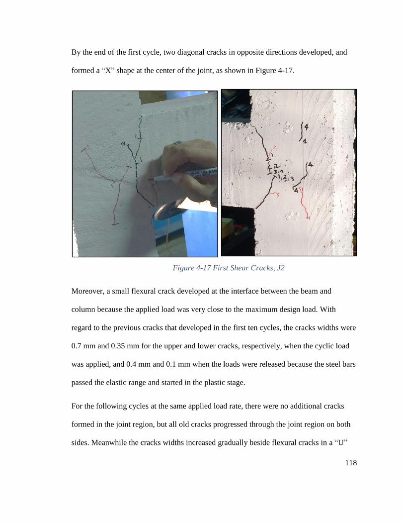
118

By the end of the first cycle, two diagonal cracks in opposite directions developed, and

formed a “X” shape at the center of the joint, as shown in Figure 4-17.

Moreover, a small flexural crack developed at the interface between the beam and

column because the applied load was very close to the maximum design load. With

regard to the previous cracks that developed in the first ten cycles, the cracks widths were

0.7 mm and 0.35 mm for the upper and lower cracks, respectively, when the cyclic load

was applied, and 0.4 mm and 0.1 mm when the loads were released because the steel bars

passed the elastic range and started in the plastic stage.

For the following cycles at the same applied load rate, there were no additional cracks

formed in the joint region, but all old cracks progressed through the joint region on both

sides. Meanwhile the cracks widths increased gradually beside flexural cracks in a “U”

Figure 4-17 First Shear Cracks, J2

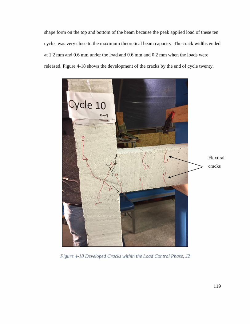
119

shape form on the top and bottom of the beam because the peak applied load of these ten

cycles was very close to the maximum theoretical beam capacity. The crack widths ended

at 1.2 mm and 0.6 mm under the load and 0.6 mm and 0.2 mm when the loads were

released. Figure 4-18 shows the development of the cracks by the end of cycle twenty.

Flexural

cracks

Figure 4-18 Developed Cracks within the Load Control Phase, J2

120

The second ten cycles represented a moderate earthquake. Based on the loads and cracks

patterns, such non-ductile concrete beam-column joints could have survived this kind of

seismic effect. At this stage of the test, the load control phase was over and second phase

(strain control) was started. In this stage, the joint would exhibit its behavior under a

severe earthquake. The load cycle was applied in each direction until the strain in the

beam longitudinal bars reached 0.004, which represented two times the yield strain of the

steel bar. At the first cycle, the free end of the beam pushed down until the strain in the

upper beam steel bars reached 0.004 as planned. The specimen showed the highest

strength and ductility during the test. The maximum applied load was 4.55 kips, which

represented more than 1.4% of the theoretical design strength of the concrete beam

section, whereas the deflection was 0.5 in. Once the load released, deflection decreased to

zero. During the next four cycles, this specimen showed significant degradation in the

strength of the joint where the specimen lost load capacity. It also experienced a large

deflection under low loads. The test was ended when the strain reached 0.1% (indicating

a steel stress of half yield capacity), and the maximum deflection was 1.25 in. The

degradation in the strength was 50%. Figure 4-19 shows the deformation of the joint at

the end of the joint. The increase in crack widths, the slippage of reinforcement, and the

loss of the concrete cover caused severe strength degradation.

121

Figure 4-19 The Failure Pattern of Specimen J2

122

The applied load versus displacement was recorded and plotted in Figure 4-20. This

figure shows that this beam-column joint was subjected to twenty five loading cycles.

Table 4-2 shows the maximum values of the loads and displacements at each cycle.

Figure 4-20 Load - Displacement Diagram, J2

-9

-7

-5

-3

-1

1

3

5

7

9

-4 -3 -2 -1 0 1 2 3 4

Cycl

ic L

oad

(kip

s)

Displacement (in.)

Cyclic Load-Displacement Diagram, J2

Pushing Down, J2 Pushing Up, J2

123

Table 4-2 The Values of the Loads and Displacements at Each Cycle, J2


0 0 0 0 0

1 2.4064 0.12152 -2.4064 -0.0684

2 2.4064 0.11803 -2.416 -0.07205

3 2.433 0.1276 -2.41602 -0.0857

4 2.444 0.1563 -2.4352 -0.08467

5 2.4256 0.1718 -2.4735 -0.08832

6 2.4064 0.188 -2.4352 -0.095

7 2.4064 0.197 -2.4064 -0.1

8 2.416 0.18411 -2.416 -0.106

9 2.4064 0.1876 -2.416 -0.101

10 2.4064 0.182 -2.4064 -0.107

11 2.8091 0.2158 -2.8091 -0.143

12 2.8282 0.2274 -2.8474 -0.14925

13 2.81869 0.208 -2.857 -0.172

14 2.8 0.2591 -2.8186 -0.178

15 2.828 0.2199 -2.8187 -0.18195

16 2.8 0.251 -2.847 -0.19225

17 2.847 0.23175 -2.818 -0.2

18 2.8 0.2355 -2.876 -0.1932

19 2.924 0.2621 -2.81869 -0.2017

20 2.9816 0.271 -2.8 -0.204

21 4.544 0.4998 -4.995 -0.548

22 4.065 0.555 -4.1225 -0.77

23 3.882 0.6541 -4.026 -1.0371

24 3.202 1.0611 -3.8157 -1.318

25 2.75 1.1674 -2.29139 -1.25

Figure 4-20 shows the load versus displacement. First the cracks started within the joint

region, and then flexural cracks appeared along the beam. Since first cycles when the

load was represented by 75% and 90% of the maximum theoretical beam capacity, the

joint showed strength against the applied cyclic load in the load control phase. It was

clear based on the J2’s behavior that non- ductile specimens designed for gravity load

124

could only survive light earthquakes. Once the strain control phase started, the

degradation of the strength was clear. But the slip of the longitudinal flexural bar within

the joint region on the last two cycles occurred where the maximum strain was 0.1%

(about half yield strain) meant the steel stopped working effectively.

4.2.3. Retrofitted Specimen J3

The general behavior of strengthened joint J3 represented the behavior of the non-ductile

concrete beam-column joint which was designed according to the pre-seismic codes. This

specimen was retrofitted by using one layer of CFRP sheet. The way the specimen was

retrofitted has been described in previous chapters. Figure 4-21 shows how the specimen

was placed in the frame and set for the test.


125

Two additional strain gages were used in this test on either sides of the joint at the middle

of the joint region in order to measure the strain would develop in the CFRP sheets before

the start of the test. The same load sequences were followed where the test started by

applying the axial column load, then the cyclic loads on the beam. Because the joint and

surrounding areas were wrapped with CFRP sheets, it was not possible to track the

cracks. In the first two sets (twenty cycles) of the cyclic loads (phase 1), which

represented 75% P and 90% P, there was no deterioration in the specimen’s strength.

Figure 4-22 shows the specimen J3 at the end of cycle twenty.

Figure 4-22 Specimen J3 at the End of cycle 20

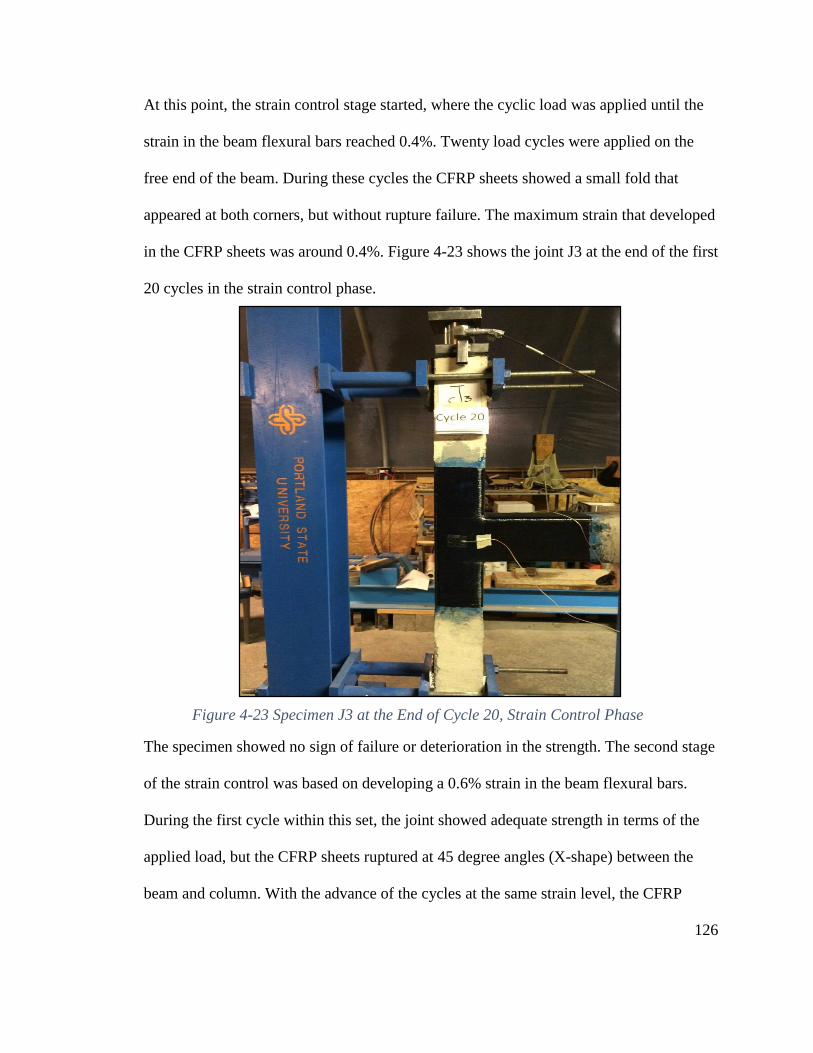
126

At this point, the strain control stage started, where the cyclic load was applied until the

strain in the beam flexural bars reached 0.4%. Twenty load cycles were applied on the

free end of the beam. During these cycles the CFRP sheets showed a small fold that

appeared at both corners, but without rupture failure. The maximum strain that developed

in the CFRP sheets was around 0.4%. Figure 4-23 shows the joint J3 at the end of the first

20 cycles in the strain control phase.

The specimen showed no sign of failure or deterioration in the strength. The second stage

of the strain control was based on developing a 0.6% strain in the beam flexural bars.

During the first cycle within this set, the joint showed adequate strength in terms of the

applied load, but the CFRP sheets ruptured at 45 degree angles (X-shape) between the

beam and column. With the advance of the cycles at the same strain level, the CFRP

Figure 4-23 Specimen J3 at the End of Cycle 20, Strain Control Phase

127

sheets started to rupture and gave a clear sign that the failure was close. After five cycles

within this stage of loading, the CFRP sheet in the joint region ruptured completely. The

concrete covers on both sides were taken off when the maximum strain that developed on

the CFRP sheets was around 0.6%. On the other hand, the beam and the wrapped areas

around the column above and below the joint were still intact. Consequently, it was

observed that the general behavior of the wrapped specimen J3 was improved

significantly over the control specimen J2. Figure 4-24 shows specimen J3 at failure.

Figure 4-24 Specimen J3 at the Failure

128

The applied cyclic load versus displacement of the free end of the beam was recorded and

plotted in Figure 4-25. This figure shows that this beam-column joint was subjected to

forty five loading cycles. Table 4-3 shows the values of the loads and displacements at

each cycle.

-9

-7

-5

-3

-1

1

3

5

7

9

-4 -3 -2 -1 0 1 2 3 4Cycl

ic L

oad

(kip

s)

Displacement (in.)




129

Table 4-3 The Values of the Loads and Displacements at Each Cycle, J3

cycle Down F. Disp. Up F. Disp.

0 0 0 0 0

1 2.483 0.0718 -2.4831 -0.0722

2 2.444 0.075 -2.416 -0.082

3 2.4543 0.074 -2.406 -0.0896

4 2.4352 0.0702 -2.435 -0.085

5 2.4064 0.0751 -2.444 -0.0907

6 2.4064 0.0737 -2.40644 -0.09046

7 2.4064 0.0789 -2.4256 -0.09019

8 2.4064 0.0745 -2.40644 -0.091

9 2.416025 0.0819 -2.444 -0.09019

10 2.406 0.0811 -2.425 -0.091

11 2.8091 0.102 -2.837 -0.0975

12 2.8091 0.102 -2.828 -0.0953

13 2.837 0.105 -2.8378 -0.09944

14 2.818 0.1091 -2.828 -0.1005

15 2.837 0.1107 -2.8187 -0.0953

16 2.8186 0.1121 -2.8378 -0.10216

17 2.8474 0.1146 -2.8187 -0.10325

18 2.8378 0.11514 -2.857 -0.113

19 2.8091 0.12059 -2.80911 -0.1038

20 2.8091 0.12059 -2.80911 -0.1038

21 5.3977 0.3555 -7.133 -0.4555

22 4.956 0.3786 -6.854 -0.471

23 4.91833 0.3996 -6.7878 -0.49089

24 4.8895 0.4099 -6.586 -0.5017

25 4.7361 0.41839 -6.5386 -0.51239

130

26 4.6978 0.42683 -6.4139 -0.52

27 4.7457 0.4317 -6.4235 -0.53091

28 4.745 0.4374 -6.4139 -0.54125

29 4.4581 0.4431 -6.2893 -0.54588

30 4.7553 0.4483 -6.327 -0.5496

31 4.619 0.4497 -6.394 -0.5589

32 4.4677 0.457052 -6.366 -0.5619

33 4.448 0.46 -6.327 -0.5717

34 4.5348 0.4668 -6.327 -0.57528

35 4.69782 0.4769 -6.337 -0.5829

36 4.6307 0.4864 -6.3276 -0.59106

37 4.76 0.5 -6.2 -0.5992

38 4.7553 0.5117 -6.327 -0.6087

39 4.7553 0.5172 -6.327 -0.6158

40 4.7553 0.528647 -6.289 -0.6204

41 5.8674 0.6829 -7.89 -0.82272

42 5.5511 0.693 -7.928 -0.92

43 5.3114 0.7526 -7.775 -1.14911

44 5.1676 0.8242 -6.728 -1.355

45 3.624 1.25 ---------- ----------

Based on the load- displacement diagram for specimen J3, it is clear that until the final

failure there was no deterioration in the strength along the load sequence. The maximum

load was about 8 kips whereas the maximum theoretical capacity of the beam strength

was 3 kips. This improvement in the strength of the specimen J3 was due to the

confinement provided by the CFRP sheet.

131

4.2.4. Retrofitted Specimen J4

The general behavior of retrofitted joint J4 represents the behavior of the non-ductile

concrete beam-column joint, which was designed according to the earlier codes used

before the development of modern seismic code. This specimen was retrofitted using two

layers of the carbon fiber reinforced polymer sheet. This specimen was prepared and cast

at Greenhouse Lab at Portland State University. After three months, this specimen was

tested using the Blue Frame in the lab. Figure 4-26 shows how the specimen was placed

in the frame and set for the test.

Two additional strain gages were used in this test, as well on either sides of the joint at

the middle of the joint region in order to measure the strain that developed in the CFRP


132

sheets before starting the test. The same load sequences were followed where the test

started by applying the axil load, and then the cyclic loads as usual. Because the joint and

surrounding areas were wrapped in CFRP sheets, it was not possible to observe the

cracks. In the first two sets (twenty cycles) of the cyclic loads at 75% and 90% of the

beam capacity, there was no deterioration in the specimen’s strength. Figure 4-27 shows

the specimen J4 at the end of twentieth cycle.

Figure 4-27 Specimen J4 at the End of Load Control

133

The specimen did not show any sign of failure or strength deterioration during the load

control stage. When the second stage of the load sequence started, the load was supposed

to be applied until the strain in the flexural reinforcement reached 0.4%. But, the beam

failed near the free end in the unwrapped section. The maximum push down load was 8

kips, and the maximum steel strain at the interface between the beam and the column was

0.334%. Shear failure in the beam near the free end occurred when the applied moment

at the beam-column intersection reached its ultimate theoretical moment. The load then

dropped rapidly to 5 kips, the steel bars buckled and the concrete broke to small pieces.

Figure 4-28 shows the free end failure of the specimen.

Figure 4-28 Specimen J4 at the Failure

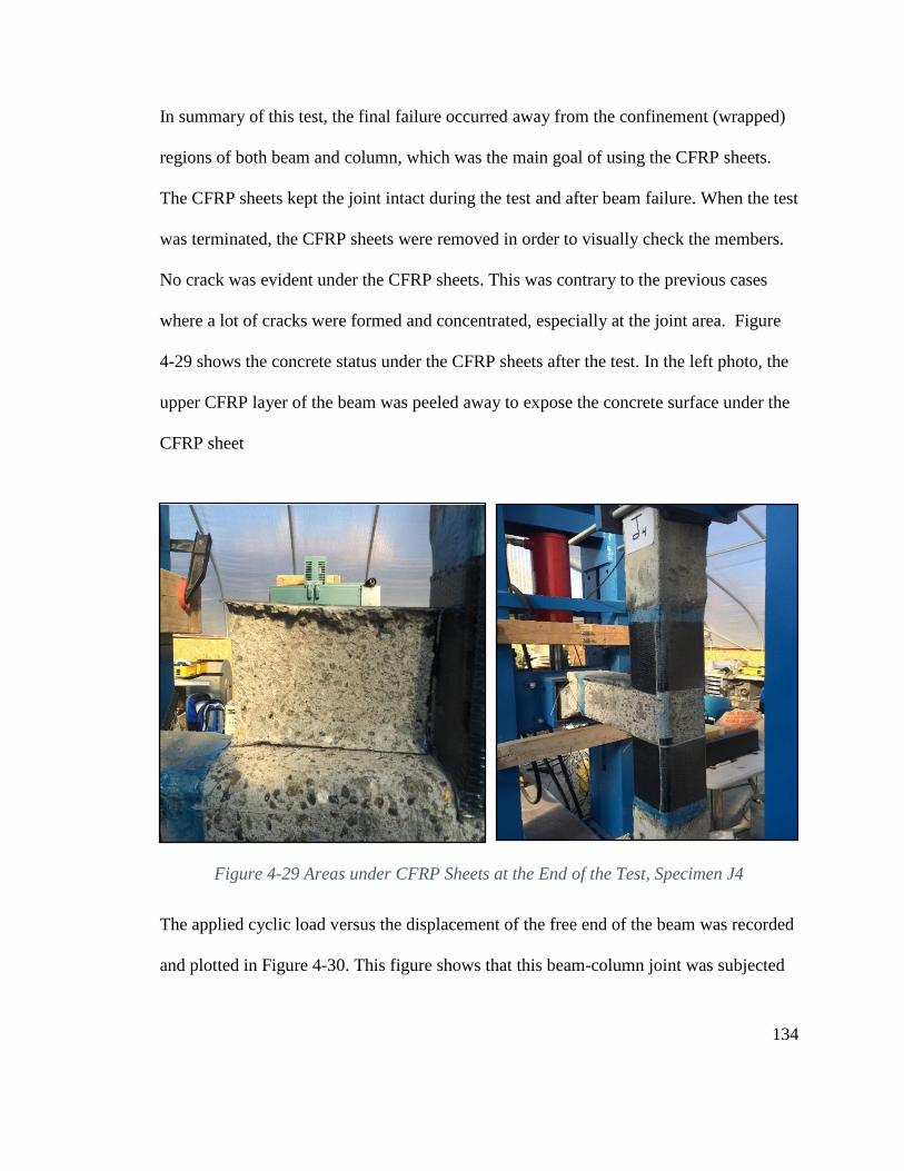
134

In summary of this test, the final failure occurred away from the confinement (wrapped)

regions of both beam and column, which was the main goal of using the CFRP sheets.

The CFRP sheets kept the joint intact during the test and after beam failure. When the test

was terminated, the CFRP sheets were removed in order to visually check the members.

No crack was evident under the CFRP sheets. This was contrary to the previous cases

where a lot of cracks were formed and concentrated, especially at the joint area. Figure

4-29 shows the concrete status under the CFRP sheets after the test. In the left photo, the

upper CFRP layer of the beam was peeled away to expose the concrete surface under the

CFRP sheet

The applied cyclic load versus the displacement of the free end of the beam was recorded

and plotted in Figure 4-30. This figure shows that this beam-column joint was subjected

Figure 4-29 Areas under CFRP Sheets at the End of the Test, Specimen J4

135

to twenty-three loading cycles. Table 4-4 shows the values of the loads and

displacements at each cycle.

-10

-8

-6

-4

-2

0

2

4

6

8

10

-2 -1.5 -1 -0.5 0 0.5 1 1.5 2

Cycl

ic L

oad

(kip

s)

Displacement (in.)

Cyclic Load-Displacement Diagram, J4


Figure 4-30 Load versus Displacement, J4

Failure point (cycle 21)

136

Table 4-4 The Values of the Loads and Displacements at Each Cycle, Specimen J4


0 0 0 0 0

1 2.406 0.0944 -2.483 -0.106

2 2.4352 0.101265 -2.463 -0.105

3 2.4352 0.107253 -2.435 -0.116

4 2.521487 0.113242 -2.5 -0.125

5 2.406438 0.110792 -2.406 -0.109

6 2.387263 0.100176 -2.483 -0.12

7 2.607773 0.107798 -2.483 -0.099

8 2.492725 0.10317 -2.492 -0.098

9 2.444788 0.10562 -2.454 -0.103

10 2.339326 0.092281 -2.4352 -0.102

11 2.99127 0.159791 -2.82828 -0.12107

12 2.828284 0.154619 -2.82828 -0.12433

13 2.828284 0.15135 -2.82828 -0.12651

14 2.809109 0.15135 -2.82828 -0.12787

15 2.799521 0.150264 -2.8187 -0.12733

16 2.809109 0.152441 -2.83787 -0.13032

17 2.828284 0.151353 -2.8187 -0.13005

18 2.99127 0.166052 -2.83787 -0.13141

19 2.837871 0.160063 -2.83787 -0.13468

20 2.837871 0.156525 -2.83787 -0.13413

21 7.938369 0.678092 -5.3536 -0.31851

22 5.378533 0.811206 -5.35936 -0.36851

23 5.06214 1.1297 ---------- ---------

In Figure 4-30, the load versus displacement shows that in the first twenty cycles, the

load and displacement changed in a linear manner because the specimen was within the

elastic range. Once the load passed the theoretical capacity of the beam, the load –

displacement curve started to lose stiffness. This meant that the beam started to deform

out of the elastic range, and moved to failure. When the beam section in the weakest

region of the beam (at 7 in. from the free end of the beam) reached the maximum strength

137

during cycle twenty-one in the strain control stage, the load dropped. The load cycles

after that represented the post crack cycles where the beam lost strength gradually until

most of the concrete spalled, and the steel bars buckled. Figure 4-31 shows more details

about this failure.

Figure 4-31 Failure of Specimen J4

138

4.2.5. Retrofitted Specimen J5 and J6

The behavior of specimens J5 and J6 was almost as same as the behavior of specimens J3

and J4, respectively, despite the fact that the axial load applied on the column is different.

The axial force applied on the specimens J3 and J4 represented 20% of the load capacity

index (f’c Ag) of the column, whereas in J5 and J6 represented 40% of the load capacity

index. The reason to test specimens J5 and J6 under a higher axial load was to investigate

how the proposed technique would be affected by a higher level of gravity load that

represents joints in a building with a larger number of stories. Figure 4- 32 and 4-33 show

load versus displacement for specimens J5 and J6, respectively.

139

-9

-7

-5

-3

-1

1

3

5

7

9

-4 -3 -2 -1 0 1 2 3 4

Cycl

ic L

oad

(kip

s)

Displacement (in.)


Pushing Down Load, J5 Pushing Up Load, J5


140

Figure 4-33 Cyclic Load-Displacement, J6

-9

-7

-5

-3

-1

1

3

5

7

9

-4 -3 -2 -1 0 1 2 3 4

Cycl

ic L

oad

(k

ips)

Displacement (in.)



141

Tables 4-5 and 4-6 show the load values and displacement for specimens J5 and J6 at

each cycle.

Table 4-5 Values of Loads and Displacements at Each Cycle, J5

Cycle Down F. Down Disp. Up. F Up Disp.

0 0 0 0 0

1 2.416 0.083 -2.531 -0.0552

2 2.4352 0.089 -2.444 -0.0506

3 2.4064 0.089 -2.483 -0.05009

4 2.4831 0.0873 -2.4 -0.05172

5 2.435 0.089 -2.377 -0.05281

6 2.4064 0.102 -2.52149 -0.0588

7 2.444 0.103 -2.56 -0.05036

8 2.4064 0.1064 -2.41603 -0.054

9 2.4064 0.10344 -2.4639 -0.056

10 2.416 0.1064 -2.49272 -0.05335

11 2.8666 0.12467 -2.8378 -0.0634

12 2.828 0.12658 -2.99127 -0.062

13 2.809 0.118124 -2.828 -0.0658

14 2.8666 0.1298 -2.8282 -0.06724

15 2.7899 0.1249 -2.83787 -0.0677

16 2.8 0.1325 -2.83787 -0.072

17 2.828 0.1412 -2.8282 -0.06751

18 2.8666 0.147 -2.8278 -0.07214

19 2.8474 0.1464 -2.8378 -0.068

20 2.8378 0.1437 -2.8378 -0.07187

21 6.366 0.5172 -7.133 -0.4

22 6.078 0.54 -6.77 -0.4124

142

23 5.934 0.55 -6.99 -0.4352

24 5.69 0.56 -6.97 -0.455

25 5.8 0.574 -6.96 -0.467

26 5.55 0.586 -7.08 -0.4807

27 5.74 0.5964 -6.97 -0.4965

28 5.56 0.605 -6.97 -0.504

29 5.234 0.605 -6.787 -0.512

30 5.53 0.621 -6.8 -0.524

31 5.215 0.6489 -6.89 -0.5335

32 5.09 0.6576 -6.672 -0.54498

33 5.215 0.6631 -6.7399 -0.5534

34 5.388 0.666 -6.922 -0.561

35 5.3114 0.672 -6.739 -0.565

36 5.1484 0.6786 -6.67 -0.574

37 5.119 0.683 -6.55 -0.586

38 5.01 0.682 -6.55 -0.59

39 5.119 0.69 -6.51 -0.59

40 5.06 0.694 -6.596 -0.602

41 6.797 0.9429 -8.57 -1.0164

42 6.346 1.04 -8.273 -1.18

43 5.56 1.156 -7.09 -1.167

44 5.186 1.3428 -4.486 -1.1988

45 4.678 1.448 -4.266 -1.215

46 4.084 1.523 -4.103 -1.244

47 3.806 1.5919 -4.44 -1.31

48 3.56 1.678 -4.1 -1.353

49 3.652 1.73 -4.01 -1.379

50 -------- -------- -3.88 -1.497

143

51 -------- -------- -3.49 -1.529

52 -------- -------- -3.096 -1.696

Table 4-6 Values of Loads and Displacements at Each Cycle, J6

Cycle Down F. Down Disp. Up F. Up Disp.

0 0 0 0 0

1 2.4064 0.0658 -2.3776 -0.0345

2 2.444 0.08629 -2.4165 -0.0416

3 2.4927 0.0832 -2.49272 -0.0528

4 2.42561 0.0941 -2.45438 -0.05172

5 2.4352 0.091737 -2.49272 -0.0579

6 2.4927 0.09364 -2.41603 -0.0528

7 2.4352 0.09255 -2.41603 -0.05281

8 2.4064 0.09255 -2.49272 -0.0539

9 2.41602 0.092554 -2.47355 -0.049

10 2.5502 0.11242 -2.4064 -0.05009

11 2.8282 0.1219 -2.80911 -0.06479

12 2.8282 0.1214 -2.837 -0.06697

13 2.83787 0.1249 -2.8378 -0.06479

14 2.81869 0.126036 -2.822 -0.0637

15 2.8282 0.12522 -2.8282 -0.06261

16 2.81869 0.12875 -2.8378 -0.06452

17 2.8858 0.1347 -2.80911 -0.0637

18 2.8953 0.135 -2.8378 -0.068

19 2.818 0.13012 -2.8378 -0.0664

20 2.8282 0.131208 -2.83787 -0.06424

21 7.62 0.629 -------- ----------

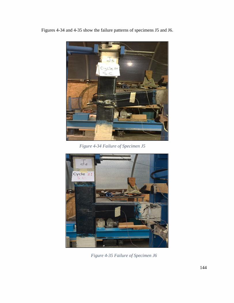
144

Figures 4-34 and 4-35 show the failure patterns of specimens J5 and J6.



145

4.3. Effect of Carbon Fiber Reinforced Polymer (CFRP) Sheets on Joint’s Strength

All joints were tested up to failure under the axial and cyclic load at the same time. The

maximum cyclic load that each specimen carried, and the cycle number regarding to load

sequence are summarized in Table 4-7 and Figure 4-36.

Table 4-7 Summary of the Test Results

Specimen Property

Maximum

Pushing

Down load

(kips)

Cycle

number

Maximum

Pushing Up

load

(Kips)

Cycle

Number

Load sequence

Phase at failure

J1 Control

Ductile 5.7 39 5.7 39

Strain control

(0.4%)

J2 Control

Non-ductile 4.5 25 5 25

Strain control

(0.4%)

J3 One CFRP

Layer 5.8 45 7.9 44

Strain control

(0.6%)

J4 Two CFRP

Layers 8 21 N/A 20

Strain Control

(0.4%)

J5 One CFRP

Layer 6.8 49 8.6 52

Strain Control

(0.6%)

J6 Two CFRP

Layers 7.6 21 N/A 20

Strain Control

(0.4%)

146

As shown in Table 4-7 and Figure 4-36, the maximum strength for all joints wrapped by

CFRP were larger than the control specimens because the weakest joint area of all

retrofitted specimens was confined by CFRP sheets, so that the failure either transferred

to the beam or occurred at larger load. In terms of the comparison with the ductile and

non-ductile specimens, specimens J4 and J6 that were retrofitted by using two CFRP

layers had changed the non-ductile one (J2) from weak column-strong beam to strong

column-weak beam. The desirable goal was achieved by keeping the joint area of the

specimens intact during the test. Regarding the specimens J3 and J5 that were wrapped

0

20

40

60

80

100

120

140

160

180

1 2 3 4 5 6

Max. M

om

ent

(kip

.in

.)

Joint

Maximum Moment Generated by Pushing Down Load

Non-Ductile

N=25 Cycle

Non-Ductile

1 layer of

CFRP

N=45 Cycle

Non-Ductile

2 layers of

CFRP

N=20 Cycle

Non-Ductile

1 layer of

CFRP

N= 52 Cycle

Non-Ductile

2 layesrs of

CFRP

N= 20 Cycle

Ductile

N=39 Cycle

Figure 4-36 Maximum Moment at Face of the Column, Pushing Down Case

Axial Load = 15 kips Axial Load = 30 kips

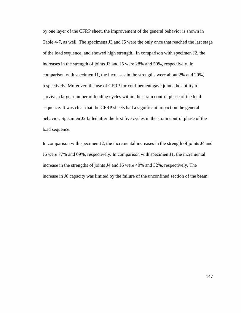
147

by one layer of the CFRP sheet, the improvement of the general behavior is shown in

Table 4-7, as well. The specimens J3 and J5 were the only once that reached the last stage

of the load sequence, and showed high strength. In comparison with specimen J2, the

increases in the strength of joints J3 and J5 were 28% and 50%, respectively. In

comparison with specimen J1, the increases in the strengths were about 2% and 20%,

respectively. Moreover, the use of CFRP for confinement gave joints the ability to

survive a larger number of loading cycles within the strain control phase of the load

sequence. It was clear that the CFRP sheets had a significant impact on the general

behavior. Specimen J2 failed after the first five cycles in the strain control phase of the

load sequence.

In comparison with specimen J2, the incremental increases in the strength of joints J4 and

J6 were 77% and 69%, respectively. In comparison with specimen J1, the incremental

increase in the strengths of joints J4 and J6 were 40% and 32%, respectively. The

increase in J6 capacity was limited by the failure of the unconfined section of the beam.

148

4.4. Load versus Displacement

The load vs the vertical displacement of the free end of the beam at each cycle in both

upward and downward directions during the loading sequences for all specimens are

shown in Figures 4-37 to 4-42.

Figure 4-37 Envelop Cyclic Load- Vertical Displacement of the Ductile Specimen, J1

-10

-8

-6

-4

-2

0

2

4

6

8

10

-4 -3 -2 -1 0 1 2 3 4

Load

(kip

s)

Displacement (in.)

Load- Displacement Diagram, J1

Pushing Down Pushing Up

149

-10

-8

-6

-4

-2

0

2

4

6

8

10

-4 -3 -2 -1 0 1 2 3 4

Load

(kip

s)

Displacement (in.)

Load-Displacement Diagram, J2


-10

-8

-6

-4

-2

0

2

4

6

8

10

-4 -3 -2 -1 0 1 2 3 4

Load

(kip

s)

Displacement (in.)

Load-Displacement Diagram, J3


Figure 4-38 Envelop Cyclic Load- Vertical Displacement of the Non-Ductile Specimen, J2

Figure 4-39 Envelop Cyclic Load- Vertical Displacement, Specimen J3

150

-10

-8

-6

-4

-2

0

2

4

6

8

10

-2 -1.5 -1 -0.5 0 0.5 1 1.5 2

Load

(kip

s)

Displacement (in.)


Pushing Down Pushing Down

-10

-8

-6

-4

-2

0

2

4

6

8

10

-2 -1.5 -1 -0.5 0 0.5 1 1.5 2

Load

(kip

s)

Displacement (in.)


Pushing Down Pushing Up

Figure 4-40 Envelop Cyclic Load- Vertical Displacement of the Specimen, J4

Figure 4-41 Envelop Cyclic Load- Vertical Displacement of the Specimen, J5

151

-10

-8

-6

-4

-2

0

2

4

6

8

10

-1 -0.8 -0.6 -0.4 -0.2 0 0.2 0.4 0.6 0.8 1

Load

(kip

s)

Displacement (in.)



Figure 4-42Envelop Cyclic Load- Vertical Displacement of the Specimen, J6

152

A comparison of the specimens in terms of the vertical displacement of all specimens is

shown in Figure 4-43.

-9

-8

-7

-6

-5

-4

-3

-2

-1

0

1

2

3

4

5

6

7

8

9

-4 -3.5 -3 -2.5 -2 -1.5 -1 -0.5 0 0.5 1 1.5 2 2.5 3 3.5 4

Load

(kip

s)

Displacement(in.)

Load vs Displacemnt Diagram

Pushing Down, J1 Pushing Up, J1 Pushing Down, J2 Pushing Up, J2


Pushing Up

Figure 4-43 Cyclic Load- Vertical Displacement Relationship of All Specimens Tested

Under Same Axial Loads (20% of the Column Capacity)

Pushing Down

153

For specimens J1, J2, J3, and J4 as shown in Figure 4-43, at the first load stage of the

load sequence when the load was 75% of the maximum theoretical beam capacity, all of

the curves are identical because only the concrete and the steel bars carried the applied

load. For the stage of the load sequence that represented 90% of the maximum theoretical

beam capacity, the difference between the retrofitted specimens and the control

specimens started to clearly apparent. The non-retrofitted specimens developed more

displacement than strengthened specimens. The reason was that the applied cyclic load

was very close to the maximum beam capacity, and this led to a development of

extensive tensile stresses in the joint region for the non-ductile specimen as represented

by J2. The lack of transverse reinforcement caused many diagonal cracks and severe

deterioration in the joint strength. With regard to the ductile specimen represented by J1,

at these load cycles, the plastic hinge started to form right on the face of column. In spite

of this, all of the specimens were able to survive during the first phase of the load

sequence, but the non-ductile specimen J2 developed severe diagonal cracks within the

joint region. This specimens failed after the first five cycles within the strain control

phase of the load sequence. This is an evidence of the weakness in these kinds of joints

that were designed and constructed prior to modern seismic codes. From Figure 4-43

above that J1, during the strain control stage of the load sequence, at strain of 0.4%, the

specimen J1 showed great flexibility, and showed no deterioration in the strength despite

the gradual increase in the displacement. With regard to specimens J3 and J4, their

behaviors were also identical even at the strain control stage of the load sequence. The

retrofitted specimens showed very high level of strength in comparison to the non-

154

retrofitted specimens (control specimens). The reason was that the confinement provided

by attaching the CFRP sheets to these specimens, and a change in the tension load path,

were the main causes to develop the ultimate moment capacity of the beam section. In

terms of the maximum strength, the maximum load that both of the retrofitted specimens

developed was 8 kip where specimen J3 was not able to maintain this load, and this led to

joint failure because the “L” shapes of the CFRP were not able to handle the large

amount of tension. Whereas specimen J4 was able handle the load since two layers of

CFRP sheets were used, and the failure occurred out of the confinement region.

In order to judge the effects of the axial load on the column, a comparison between

retrofitted specimens was required. Figures 4-44 and 4-45 show how the axial load

affected the behavior of these specimens in terms of load-displacement behavior.

-10

-8

-6

-4

-2

0

2

4

6

8

10

-4 -3 -2 -1 0 1 2 3 4

Load

(kip

s)

Displacement (in.)

Load-Displacement Diagram


Figure 4-44 Cyclic Load- Vertical Displacement Relationship of Specimens (J3 and

J5) Tested under a Different Axial Load (20% and 40% of the Column Capacity)

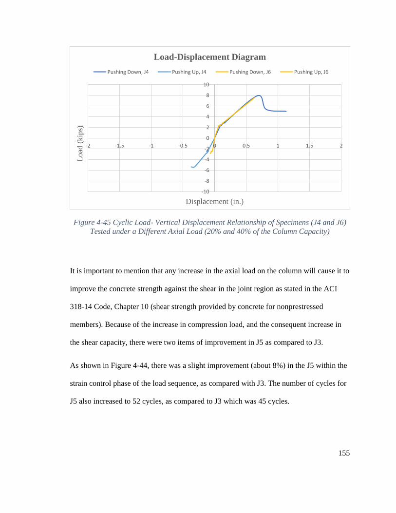
155

It is important to mention that any increase in the axial load on the column will cause it to

improve the concrete strength against the shear in the joint region as stated in the ACI

318-14 Code, Chapter 10 (shear strength provided by concrete for nonprestressed

members). Because of the increase in compression load, and the consequent increase in

the shear capacity, there were two items of improvement in J5 as compared to J3.

As shown in Figure 4-44, there was a slight improvement (about 8%) in the J5 within the

strain control phase of the load sequence, as compared with J3. The number of cycles for

J5 also increased to 52 cycles, as compared to J3 which was 45 cycles.


Tested under a Different Axial Load (20% and 40% of the Column Capacity)

-10

-8

-6

-4

-2

0

2

4

6

8

10

-2 -1.5 -1 -0.5 0 0.5 1 1.5 2

Lo

ad (

kip

s)

Displacement (in.)

Load-Displacement Diagram


156

For specimens J4 and J6, the confinement provided by the two layers of CFRP sheets was

enough to make the joint area stronger than the beam outside the confinement region. The

behavior of both J4 and J6 were similar. The failure of each frame was in the strain

control phase (first cycle) and was caused by failure of the un-wrapped portion of the

beam. After failure, the joints were inspected and there were no cracks.

4.5. Carbon Fiber Reinforced Polymer (CFRP) Sheet Strain

As described in Chapter Three, two strain gages were used and installed in the middle of

the joint region of all retrofitted specimens in order to measure the average strain within

the joint that would develop during loading. Figures 4-46 to 4-49 show the CFRP sheets

strain at the different load levels.

Figure 4-46 CFRP Joint Strain versus Load for Specimen J3

0

1

2

3

4

5

6

7

0 0.001 0.002 0.003 0.004 0.005 0.006 0.007

Cycl

ic L

oad

(kip

s)

CFRP Strain

Load vs CFRP Sheet Strain, J3

157

Figure 4-48 CFRP Joint Strain versus Cyclic Load for Specimen J5


0

1

2

3

4

5

6

7

8

9

0 0.0005 0.001 0.0015 0.002 0.0025 0.003 0.0035 0.004

Load

(kip

s)

CFRP Strain


0

1

2

3

4

5

6

0 0.002 0.004 0.006 0.008 0.01 0.012

Load

(kip

s)

CFRP Strain


158

Figures 4-46 and 4-48, show specimens J3 and J5, within the load control. The strain was

very small, and it started and ended at the same strain values. By starting the strain

control phase of the load sequence, the strain started and ended close to 0.15% and this

indicated that the confinement was not enough to keep the concrete under the CFRP

sheets without cracks. On the other hand, with regard to specimens J4 and J6 during the

load sequence of the test, the strain of the beam flexural reinforcement matched the strain

at the joint region. This meant that all confinement regions worked as one unit. The

figures show that there was no permanent deformation in the CFRP sheets and the

concrete under them where the strains start from zero and this return to the same value at

each cycle. This is confirmed when the CFRP sheets were removed from the concrete,

there were no cracks. The maximum stress that developed in the CFRP sheet of each

retrofitted specimen is summarized in Table 4-8.

0

1

2

3

4

5

6

7

8

0 0.0005 0.001 0.0015 0.002 0.0025 0.003 0.0035 0.004

Load

(kip

s)

CFRP Strain

Pushing Down Load vs CFRP Strain, J6


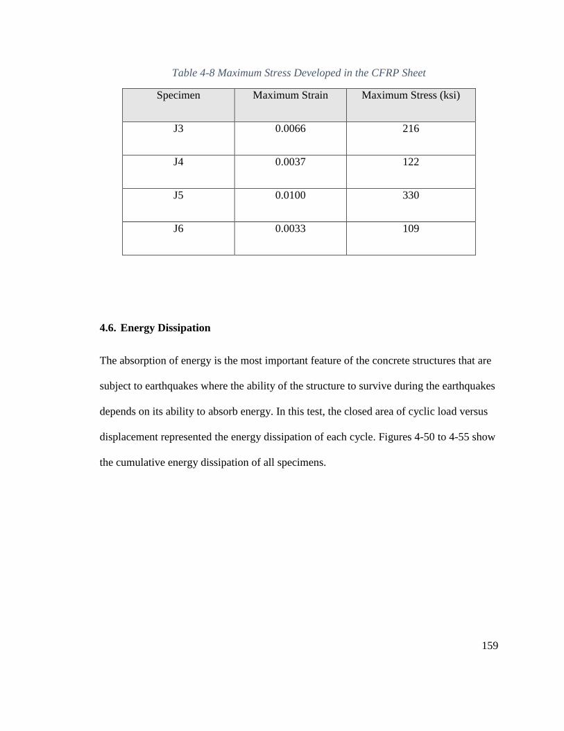
159

Table 4-8 Maximum Stress Developed in the CFRP Sheet

Specimen Maximum Strain Maximum Stress (ksi)

J3 0.0066 216

J4 0.0037 122

J5 0.0100 330

J6 0.0033 109

4.6. Energy Dissipation

The absorption of energy is the most important feature of the concrete structures that are

subject to earthquakes where the ability of the structure to survive during the earthquakes

depends on its ability to absorb energy. In this test, the closed area of cyclic load versus

displacement represented the energy dissipation of each cycle. Figures 4-50 to 4-55 show

the cumulative energy dissipation of all specimens.

160

Figure 4-50 The Cumulative Energy Dissipation of Specimen J1


-150

-100

-50

0

50

100

150

-50 -40 -30 -20 -10 0 10 20 30 40 50

Ener

gy D

issi

pat

ion (

kip

.in.)

Cycles

Energy Dissipation Diagram, J1


-150

-100

-50

0

50

100

150

-50 -40 -30 -20 -10 0 10 20 30 40 50

Ener

gy D

issi

pat

ion (

kip

.in.)

Cycles



161



-150

-100

-50

0

50

100

150

-50 -40 -30 -20 -10 0 10 20 30 40 50

Ener

gy D

issi

pat

ion (

kip

.in.)

Cycles



-150

-100

-50

0

50

100

150

-50 -40 -30 -20 -10 0 10 20 30 40 50

Ener

gy D

issi

pat

ion (

kip

.in)

Cycles



162



-150

-100

-50

0

50

100

150

-60 -50 -40 -30 -20 -10 0 10 20 30 40 50 60

Ener

gy D

issi

pat

ion (

kip

.in.)

Cycles



-150

-100

-50

0

50

100

150

-50 -40 -30 -20 -10 0 10 20 30 40 50

Ener

gy D

issi

pat

ion (

kip

.in.)

Cycles



163

Figure 4-56 shows a comparison of all specimens J1, J2, J3, and J4 tested under same

load conditions in terms of the cumulative half cycle energy dissipation.

Figure 4-56 The Cumulative Half Cycle Energy Dissipation of Specimens J1, J2, J3,

and J4

0

20

40

60

80

100

120

140

160

0 5 10 15 20 25 30 35 40 45 50

Ener

gy D

issi

pat

ion (

kip

.in.)

cycles

Energy Dissipation Diagram

Pushing Down, J4 Pushing Down, J2 Pushing Down, J3 Pushing Down, J1

164

Within the load control phase of the load sequence, specimens J1 and J2 showed that the

absorbed energy of the control specimens was more than retrofitted specimens J3 and J4.

The behaviors of specimens J3 and J4 was identical. It was clear that the energy

dissipation was increasing consistently and regularly from cycle number one until cycle

twenty. This meant that all of the cycles for each specimen were almost equal, and the

behavior was result of the absence of a sudden deterioration in the resistance to the

specimens. The difference in the behavior of specimens J1 and J2 was because specimen

J1 started forming the plastic hinge within the ductile zone since the first cycle and

consequently the absorbed energy increased comparing with specimen J2 that started

forming diagonal cracks within the joint region. In general the behavior of the control

specimens represented the behavior of the concrete and steel only. On the other hand, the

similarity in the behavior of specimens J3 and J4 was because CFRP sheets affected the

cyclic behavior of the retrofitted specimens and caused to increase the strength of these

specimens and reduced their deflections in both directions. In general, specimen J1

showed very high level of energy dissipation because it was designed with high ductility

according to the current ACI Code. Moreover, specimen J2 also showed good ductility as

compared to retrofitted specimens J3 and J4, because the CFRP sheets remained within

the elastic range until failure. This reduced the ability of the retrofitted joints to dissipate

the energy. Overall, specimen J2 performed poorly in terms of energy dissipation because

of the rapid failure according to the deficiency of the transverse reinforcement at the joint

region. This led to a very brittle shear failure and slip of the longitudinal reinforcement

beam bars. The energy dissipation of J1 was about 7 times larger than J2. Using one layer

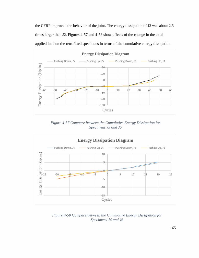
165

the CFRP improved the behavior of the joint. The energy dissipation of J3 was about 2.5

times larger than J2. Figures 4-57 and 4-58 show effects of the change in the axial

applied load on the retrofitted specimens in terms of the cumulative energy dissipation.

-15

-10

-5

0

5

10

-25 -20 -15 -10 -5 0 5 10 15 20 25

Ener

gy D

issi

pat

ion (

kip

.in.)

Cycles



-150

-100

-50

0

50

100

150

-60 -50 -40 -30 -20 -10 0 10 20 30 40 50 60

Ener

gy D

issi

pat

ion (

kip

.in.)

Cycles



Figure 4-58 Compare between the Cumulative Energy Dissipation for

Specimens J4 and J6

Figure 4-57 Compare between the Cumulative Energy Dissipation for

Specimens J3 and J5

166

The dissipation ability of the energy for specimen J5 increased, as shown in Figure 4-57,

by about 70% as compared to specimen J3 because the increase in the axial load on the

column helped to improve the shear strength of the concrete for the joint region. Due to

this, the development of cracks was delayed, and this helped specimen J5 to go through

more loading cycles before the failure. Figure 4-58 shows the opposite situation, where

the cumulative energy dissipation of specimen J4 was larger than the cumulative energy

dissipation in specimen J6. This was due to the increase in the concrete shear strength,

and provided the proper confinement for the joint region helped to reduce the initial

displacement for the free end of the beam. This made the energy dissipation for the

specimen J6 less than the energy dissipation for the specimen J4.

4.7. Ductility Factor

As Revathi, R. et al. (2014) stated, the ductility factor is the ability of the element to

deform beyond the yield point without losing a lot of the resisting strength. If the ductility

factor is very large, this means the structure could show a sufficient deformation beyond

the yield point. The ductility factor is actually expressed as a ratio between the

displacements at each cycle with respect to the displacement at the yield of the beam

longitudinal reinforcement. Table 4-9 shows the maximum ductility factor of each

specimen that developed during this experimental work.

167

Table 4-9 Maximum Ductility Factor for All Specimens

In the pushing down instance:

Specimen (J) Max. Disp.(in.) Yield Disp.(in.) Max. Ductility Factor

1 2.49 0.307 8.1

2 1.16 0.170 6.8

3 1.25 0.173 7.2

4 1.12 0.288 3.9

5 1.73 0.241 7.2

6 0.62 0.261 2.4

In the pushing up instance:

Specimen (J) Max. Disp.(in.) Yield Disp.(in.) Max. Ductility Factor

1 -3.55 0.379 -9.4

2 -1.25 0.245 -5.1

3 -1.35 0.239 -5.6

4 -0.37 N/A N/A

5 -1.70 -0.181 -9.4

6 -0.06 N/A N/A

168

Figures 4-59 to 4-64 show more details about the ductility (half cycle) of each specimen

with respect to the cycle number.

Figure 4-59 Ductility Factor Diagram (Half Cycle) of Specimen, J1


0

1

2

3

4

5

6

7

8

9

10

0 10 20 30 40 50 60

Duct

ilit

y (

in./

in.)

Cycle No.

Ductility Diagram, J1

0

1

2

3

4

5

6

7

8

9

10

0 10 20 30 40 50 60

Duct

ilit

y (

in./

in.)

Cycle No.


169

0

1

2

3

4

5

6

7

8

9

10

0 10 20 30 40 50 60

Duct

ilit

y (

in./

in.)

Cycle No.



0

1

2

3

4

5

6

7

8

9

10

0 10 20 30 40 50 60

Duct

ilit

y (

in./

in.)

Cycle No.



170


0

1

2

3

4

5

6

7

8

9

10

0 10 20 30 40 50 60

Duct

ilit

y (

in./

in.)

Cycle No.


0

1

2

3

4

5

6

7

8

9

10

0 10 20 30 40 50 60

Duct

ilit

y (

in./

in.)

Cycle No.



171

Figure 4-65 shows the comparison of specimens J1, J2, J3, and J4, which were subjected

to the same load condition.

From the Figure 4-65 above, it is clear that specimen J1 showed the highest ductility as

compared to the other specimens despite the fact it reached the yield point during the first

cycles when the applied cyclic load was lower than the maximum capacity of the beam.

The behavior of specimen J2 was identical to the behavior of specimen J1 within the first

twenty cycles, but the lack of transverse reinforcement within the joint region caused loss

of strength in the joint. This forced the test to be terminated at the early cycles of the

strain control phase. The ductility factor in the last three cycles for the specimen J2

cannot be trusted because severe cracks developed in the joint beside the slip in the

flexural beam reinforcement. The specimens that were wrapped in CFRP sheets behaved

Figure 4-65 Compare of Ductility (Half Cycle) for Specimens J1, J2, J3, and J4

0

1

2

3

4

5

6

7

8

9

10

0 5 10 15 20 25 30 35 40 45 50

Duct

ilit

y (

in./

in.)

Cycle No.

Ductility Diagram

Joint 1 Joint 2 Joint 3 Joint 4

172

identically as well. They showed a low ductility within the load control phase of the load

sequence because the composite system increased the overall strength of the specimen,

and this led to a reduction in the displacement under the same load sequence. No yield

was reached within the load control, as shown the figures. Specimen J3, which was

strengthened with one layer of the CFRP sheet, increased the final ductility to about 40%

as compared to the non-ductile specimen J2. The specimen reached the final ductility at

the strain control phase of the load sequence after fortieth cycle where the strain in the

longitudinal was 0.6%. Specimen J4 developed a low ductility within the load control

phase, as well. Once the strain control phase started, the beam member crashed because

the beam was weakest than the column and the joint.

Figures 4-66 and 4-67 show the effect of an increase in the axial load on the column by

comparing specimens J5 and J6 with specimens J3 and J4. The figures also take into

consideration the CFRP layers, and show that the specimens behaved identically under

different axial loads. As known, shear strength of the concrete subjected to the

compression will increase and this will improve the behavior of the specimen. Since the

ductility factor is actually an expression as a ratio between the displacements at each

cycle with respect to the displacement at the yield, any increase in the joint rejoin

strength will affect both the displacement at each cycle and the displacement at yield.

This was the reason for the similarity between the specimens under different axial loads.

173

0

1

2

3

4

5

6

7

8

0 10 20 30 40 50 60

Duct

ilit

y (

in./

in.)

Cycle No.

Ductility Diagram

Joint 3 Joint 5

0

0.5

1

1.5

2

2.5

3

3.5

4

4.5

0 5 10 15 20 25

Duct

ilit

y (

in./

in.)

Cycle No.

Ductility Diagram

Joint 4 Joint 6

Figure 4-66 Comparison of Ductility for Specimens J3 and J5

Figure 4-67 Comparison of Ductility for Specimens J4 and J6

174

5.1. Summary:

This experimental work was conducted in order to evaluate a proposed technique by

using CFRP sheets to retrofit non-ductile joints constructed prior to the modern codes.

Six specimens were tested; two were tested as control specimens (specimen J1 and

specimen J2) and the rest were retrofitted by using CFRP sheets. The variable factors in

this research were the number of CFRP layers and the level of applied axial force in the

column. Two specimens were wrapped with one layer, and two with two layers. Based on

the experimental results, the following conclusions are drawn:

5.2. Conclusion:

1- The non-ductile specimen J2, which was designed based on older codes, was

structurally deficient to resist the lateral loads due to the lack in the transverse

reinforcement at the joint region. This caused to a brittle shear failure in the joint.

2- The ductile specimen J1, which was designed based on the current codes (ACI

318-14), was structurally sufficient to eliminate the failure in the joint region and

resulting in formatting of the plastic hinge within the beam instead of the joint

region.

3- Retrofitting the specimens with CFRP sheets improved the behavior of non-

ductile joints by increasing the joint capacity, and changed the final failure mode.

4- For the specimens that were retrofitted by only one layer of CFRP, failure was

mainly by the CFRP rupture at the joint, however, without de-bonding.

175

5- The general behaviors of retrofitted specimens were similar in terms of shear

strength, ductility, and energy dissipation.

6- Using an “L” shape technique at the intersection corners between the beam and

column appeared effective to strengthen the joints.

7- The proposed CFRP wrapping technique was successful to change the weak

column- strong beam to the strong column- weak beam situation, and to push the

failure out of the confining area.

8- Since the measured strain of the longitudinal bars at the interface between the

adjoining members and CFRP sheets at the center of the joint panel were nearly

identical (specimens J4 and J6), the composite system appeared to act as fully

composite.

9- Based on the test results, the proposed technique could be used for joints in low-

rise and medium-rise buildings.

176

5.3. Recommendations:

The following recommendations are suggested for further research:

1- Investigate the validation of the proposed technique with the internal beam-

column joints.

2- Investigate the performance of the proposed technique on the joints in the

presence of the concrete slab.

3- Investigate by using bidirectional CFRP sheets.

4- Investigate the validation of the proposed technique to repair the damaged joints.

5- Further investigation is needed for the circular column- rectangular beam joints.

6- Create an analytical FEM model to predict the performance of joints retrofitted

with CFRP sheets.

7- Since the ACI 440.2R-08 “Guide for the Design and Construction of Externally

Bonded FRP Systems for Strengthening Concrete Structures” is not included a

specific procedure to retrofit the beam-column joint by using FRP, a theoretical

and an experimental work to develop a specific procedure to retrofit the existing

joints is still an open area for further studies.

177

References

ACI Committee 440. (2008). Guide for the Design and Construction of Externally

Bonded FRP Systems for Strengthening Concrete Structures. American Concrete

Institute.

ACI Commiitee 318-14. (2014). Building Code Requirements for Structural Concrete.

Farmington Hills: American Concrete nstitute.

Alobaidi, S. (2015). Behavior of Reinforced Concrete Beams Retrofitted in Flexure Using

CFRP-NSM Technique. Portland.

ASTM 39/39M. (2008). Standard Test Method for Compressive Strength of Cylinderical

Concrete Specimens. ANNUAL BOOK OF ASTM STANDARDS.

ASTM C 469. (2008). Standard test method for Static Modulus of Elasticity and

Poisson's Ratio of concrete in Compression. ANNUAL BOOK OF ASTM

STANDARDS.

ASTM C 496/C 496M. (2008). Standerd Test Method for Splitting Tensile Strength of

Cylindrical Concrete Specimens. ANNUAL BOOK OF ASTM STANDARDS.

ASTM C 78. (2008). Standard Test for Flexural Strength of Concrete (Using Simple

Beam with Third-point Loading). ANNUAL BOOK OF ASTM STANDARDS.

ASTM D 3039/ 3039M. (1995). Standerd Test Mathod for Tesnsile Properties of

Polymer Matrix Composite Materials. ANNUAL BOOK OF STANDARDS.

178

Ghobarah, A., & El-Amoury, T. (2005). Siesmic Rehabilitation of Deficient Exterior

Concrete Frame Joints. journal of composites for construction, 408-416.

GHOBARAH, A., & SAID, A. (2001). Seismic Rehabilitation of Beam-Column Joint

Using FRP Laminates. Journal of Earthquake Engineering, 5, 113-129.

Ghobarah, A., & Said, A. (2002). Shear Strengthening of beam-column joint.

Engineering Structures, 881-888.

Hakuto, S., Park, R., & Tanaka, H. (2000). Seismic Load Tests on Interior and Exterior

Beam-column Joints with Substanderd Reinfocing Details. ACI STRUCTURAL

JOURNAL, 97(1), 11-25.

Mukherjee, A., & Joshi, M. (2005). FRPC reinforced concrete beam-column joints under

cyclic excitation. science and direct, 185-199.

Murate, E., Lawrence, K. F., & Abdul-Hamid, Z. (2005). Repair and Strengthening of

Reinforced Concrete Beam-Column Joints: State of Art. ACI STRUCTURAL

JOURNAL, 102.

park, R., & Paulay, T. (1973). BEHAVIOR OF REINFORCED CONCRETE

EXTERNAL BEAM-COLUMN JOINTS UNDER CYCLIC LOADING. 772-

781.

Pinkham, C. W. (1985). Rocomendations for design of beam-column joints in monolithic

reinforced concrete structures. Journal of American Concrete INstitute, 82, 266-

283.

179

Prota, A., Nanni, A., Manfredi, G., & Cosenza, E. (2000). Seismic Upgrade of Beam-

Column joints with FRP reinforcement. Indsutria del Cemento, 1-17.

REVATHI R., S. V. (2014). Flexural Behavior of Corner Beam–Column Joint with and

without Slab. International Journal of, 3.

Xinbao, Y., Antonio, N., Stephen, H., & Chung Leung, S. (2002). Strength and Modulus

Degradtion of Carbon Fiber-Reinforced Ploymer Laminates from Fiber

Misalignment. MATERIALS IN CIVIL ENGINEERING, 14(4).

180

APPENDIX A

JOINT DESIGN

Beam-Column Joint Design According to ACI 318-14 Code

Beam flexural strength:

𝑓′𝑐= 3000 psi

𝐴𝑠 = 0.22 𝑖𝑛2 Tensile reinforcement in the section (#3 bar size)

𝜌 =𝐴𝑠

𝑏. 𝑑=

0.22

5.25 ∗ 5= 8.38 ∗ 10−3

𝜌𝑚𝑖𝑛 = 𝑡ℎ𝑒 𝑙𝑎𝑟𝑔𝑒𝑠𝑡 𝑜𝑓 3 ∗ √𝑓′

𝑐

𝑓𝑦=

3 ∗ √3000

60000= 2.74 ∗ 10−3

𝑜𝑟 200

𝑓𝑦=

200

60000= 3.3 ∗ 10−3( 𝑐𝑜𝑛𝑡𝑟𝑜𝑙) < 𝜌 𝑂. 𝐾

B1= 0.85

𝜌𝑏 = 0.85 ∗ 𝐵1 ∗𝑓′

𝑐

𝑓𝑦∗ [

87000

87000 + 𝑓𝑦] = 0.85 ∗ 0.85 ∗

3000

60000∗ [

87000

87000 + 60000]

= 0.0214

𝜌𝑚𝑎𝑥. = 0.75𝜌𝑏 = 0.75 ∗ 0.0214 = 0.016

𝜌𝑚𝑎𝑥. > 𝜌 → 𝑂. 𝐾

𝑎 =𝐴𝑠∗𝑓𝑦

0.85∗𝑓′𝑐∗𝑏

= 0.22∗60000

0.85∗3000∗5= 1.035

181

𝑐 =𝑎

𝐵1=

1.035

0.85= 1.217

Check:

𝑐

𝑑𝑡=

1.217

5.25= 0.232 < 0.375 𝑂. 𝐾

𝑀𝑛 = 𝐴𝑠 ∗ 𝑓𝑦 (𝑑 −𝑎

2) = 0.22 ∗ 60 (5.25 −

1.035

2) ≅ 62.5 𝑘𝑖𝑝𝑠 ∗ 𝑖𝑛𝑐ℎ

Shear reinforcement beam design:

Let’s assume that this beam will fail at a concentrated load (P) = 1.25*3.125= 4 kips

Use Vu=4 kips

Form shear force diagram of the cantilever

𝑉𝑢 = 𝑃 = 4 𝑘𝑖𝑝𝑠

∅𝑉𝑐 = 0.75 ∗ 2 ∗√𝑓′

𝑐

1000∗ 𝑏 ∗ 𝑑 = 0.75 ∗ 2 ∗

√3000

1000∗ 5 ∗ 5.25 = 2.15𝐾𝑖𝑝𝑠

𝑉𝑢 > ∅𝑉𝑐 → 𝑢𝑠𝑒 𝑠ℎ𝑒𝑎𝑟 𝑟𝑒𝑖𝑛𝑓𝑜𝑟𝑐𝑒𝑚𝑛𝑡 , use wire, diameter =0.25 in

𝑓𝑦 = 38 𝐾𝑠𝑖

Bar diameter = 0.25 in

𝐴𝑏 = 0.049 𝑖𝑛2

𝐴𝑣 = 0.098 𝑖𝑛2

182

Check:

∅𝑉𝑠 = 𝑉𝑢 − ∅𝑉𝑐 = 4 − 2.15 = 1.85 𝑘𝑖𝑝𝑠

8 ∗ ∅ ∗√𝑓′

𝑐

1000∗ 𝑏 ∗ 𝑑 = 8 ∗ 0.75 ∗

√3000

1000∗ 5 ∗ 5.25 = 8.626 𝑘𝑖𝑝𝑠 ≫ ∅𝑉𝑠 = 1.85 𝑘𝑖𝑝𝑠

→ 𝑂. 𝐾

𝑆𝑟𝑒𝑞𝑢𝑖𝑟𝑒𝑑 = ∅ ∗ 𝐴𝑣 ∗ 𝑓𝑦 ∗ 𝑑

𝑉𝑢 − ∅𝑉𝑐=

0.75 ∗ 0.098 ∗ 38 ∗ 5.25

4 − 2.15= 8 𝑖𝑛

𝑆 = 8 ≤ 𝑑2⁄ =

5.25

42= 2.625 𝑖𝑛 ( 𝑐𝑜𝑛𝑡𝑟𝑜𝑙) 𝑜𝑟 24 𝑖𝑛

Use Wire 0.25 in. Diameter (#2 bar) @ 2.5 in. O.C.

Beam seismic requirement details:

18.6.4. Over lengths equal to twice the member depth on both sides of a sections where

the flexural yielding is likely to occur in connection with inelastic displacement of frame.

2𝑑 = 2 ∗ 5.25 = 10.5 𝑖𝑛𝑐ℎ

First hoop is within (2 in.) from the face of the column

Spacing between hoops is the smallest of:

𝑑

4=

5.25

4= 1.3 𝑖𝑛𝑐ℎ (𝑐𝑜𝑛𝑡𝑟𝑜𝑙)

6 ∗ 𝑑𝑏 = 6 ∗ 0.375 = 2.25 𝑖𝑛𝑐ℎ

6 𝑖𝑛𝑐ℎ

183

18.6.4.6. Where hoops are not required, stirrups with seismic hooks at both ends shall be

spaced at distance not more than (d/2) through the length of the member.

𝑑

2=

5.25

2= 2.625 𝑖𝑛𝑐ℎ

Column design:

Assume: 𝑀𝑛 𝑐𝑜𝑙𝑢𝑚𝑛 =1

2𝑀𝑛 𝑏𝑒𝑎𝑚 =

1

2∗ 62 = 31 𝑘𝑖𝑝𝑠 . 𝑖𝑛

Assume 𝜌 = 0.03 𝑎𝑛𝑑 𝑡ℎ𝑒 𝑙𝑜𝑛𝑔𝑡𝑢𝑖𝑑𝑖𝑛𝑎𝑙 𝑟𝑒𝑖𝑛𝑓𝑜𝑟𝑐𝑒𝑚𝑛𝑡 𝑏𝑎𝑟 𝑠𝑖𝑧𝑒 𝑖𝑠 #4

𝐴𝑠 𝑟𝑒𝑞𝑢𝑖𝑟𝑒𝑑 = 𝜌 ∗ 𝐴𝑔 = 0.03 ∗ 25 = 0.75 𝑖𝑛2

𝐴𝑠 𝑏𝑎𝑟 = 0.2 (# 4 bar)

Number of required bars= 0.75/0.2= 3.75 ≈ 4 bars

𝐴𝑠 𝑝𝑟𝑜𝑣𝑖𝑑𝑒𝑑 = 4 ∗ 0.2 = 0.8𝑖𝑛2

Wire diameter =0.25 in (tie diameter)

𝛾ℎ = 5 − 05 ∗ 2 ∗ 0.25 ∗ 2 − 0.5 = 3 𝑖𝑛, ℎ = 5 𝑖𝑛

𝛾 =3

5= 0.6

Based on chart R4-60-60

∅𝑀𝑛

𝐴𝑔 ∗ ℎ=

0.7 ∗ 31

25 ∗ 5= 0.174 & 𝜌 = 0.03

184

∅𝑃𝑛

𝐴𝑔= 2.4 𝑓𝑟𝑜𝑚 𝑖𝑛𝑡𝑟𝑎𝑐𝑡𝑖𝑜𝑛 𝑑𝑖𝑎𝑔𝑟𝑎𝑚 → 𝑃𝑛 = 85 𝑘𝑖𝑝𝑠

Tie design in column

The wire bar that is used (diameter 0.25 in.)

25.7.2: Vertical spacing of ties shall not exceed:

16*longitudinal bar diameter = 16* (0.5 in)= 8 in

48* lie bar or wire = 48*0.25 = 12 in

Least dimension of column = 5 in (control)

Column Seismic requirement details:

Column confinement

𝑙𝑜 = 𝑡ℎ𝑒 𝑙𝑎𝑟𝑔𝑒𝑠𝑡 𝑜𝑓

Distance equal to the larger dimension of column = 5 in.

1/6 of the clear span = 1/6 * 40 in. ≈7 in

18 in (control)

18.7.5.3: Spacing of transverse reinforcement shall not exceed:

¼ min dimension of column section = ¼ * 5=1.25 in (control)

6* longitudinal bar diameter = 6*0.5 = 3 in

c- 6 ≥ 𝑆𝑜 = 4 + (14−ℎ𝑥

3) ≥ 4 , ℎ𝑥 = 3.75 𝑖𝑛

185

6 ≤ 𝑆𝑜 = 4 + (14− ℎ𝑥

3) ≥ 4 𝑆𝑜 = 7.41 𝑖𝑛 > 6 𝑖𝑛

→ 𝑆𝑜 = 6 𝑖𝑛

The total cross section area:

𝐴𝑠ℎ = 0.3 ∗𝑠 ∗ 𝑏𝑐 ∗ 𝑓′

𝑐

𝑓𝑦𝑡 [

𝐴𝑔

𝐴𝑐ℎ− 1] = 0.3 ∗

1.25 ∗ 3.75 ∗ 3

38∗ [

25

3.752− 1]

= 0.0863 𝑖𝑛2 ( 𝑐𝑜𝑛𝑡𝑟𝑜𝑙)

𝐴𝑠ℎ = 0.09 ∗𝑠 ∗ 𝑏𝑐 ∗ 𝑓′

𝑐

𝑓𝑦𝑡 = 0.3 ∗

1.25 ∗ 3.85 ∗ 3

38= 0.034 𝑖𝑛2

𝐴𝑠 = 2 ∗𝜋

4∗ (𝑑𝑏)2 = 2 ∗

𝜋

4∗ (0.25)2 = 0.098 𝑖𝑛2 > 𝐴𝑠ℎ = 0.0863 𝑖𝑛2

18.7.5.5: Beyond the confinement length (𝑙0), the column shall contain spiral or hoop

reinforcement with center-to-center spacing (S) not exceeding the smaller of six times the

diameter of the smallest longitudinal column bars and 6 in.

6*0.5 = 3 in. (control) or 6 in.

186

Column shear strength (check for seismic requirements)

𝐴𝑠 = 2 ∗𝜋

4𝑑2 = 2 ∗

𝜋

4(0.375)2 = 0.22 𝑖𝑛2

𝑇 = 𝐴𝑠 ∗ (1.25 𝑓𝑦) = 0.22 ∗ 1.25 ∗ 60 = 16.5 𝑘𝑖𝑝𝑠

𝑎 =𝐴𝑠 ∗ (1.25 𝑓𝑦)

0.85 ∗ 𝑓′𝑐

∗ 𝑏=

16.5

0.85 ∗ 3 ∗ 5= 1.3 𝑖𝑛

𝑀𝑝𝑟 = 𝑇 ∗ (𝑑 − 𝑎

2) = 16.5 ∗ (5.25 −

1.3

2) = 75.9 𝑘𝑖𝑝𝑠 ∗ 𝑖𝑛

𝐴𝑝𝑝𝑟𝑜𝑥𝑚𝑎𝑡𝑒 𝑐𝑜𝑙𝑢𝑚𝑛 𝑠ℎ𝑒𝑎𝑟 ∶

𝑉𝑛 = 𝑀𝑝𝑟

𝐿𝑎𝑏𝑜𝑣𝑒 + 𝐿𝑏𝑒𝑙𝑙𝑜𝑤

2

= 75.9

40= 1.9 𝑘𝑖𝑝

𝐽𝑜𝑖𝑛𝑡:

𝑉𝑢 = 𝑇 − 𝑉𝑛 = 16.5 − 1.9 = 14.6 𝑘𝑖𝑝𝑠

𝑚𝑎𝑥. 𝑎𝑙𝑙𝑜𝑤𝑒𝑑 ∅𝑉𝑐 = 0.75 ∗ 12 ∗√𝑓′

𝑐

1000 𝐴𝑗 … … … … … … … … … … … … . . 𝑜𝑡ℎ𝑒𝑟 𝑐𝑎𝑠𝑒𝑠

𝐴𝑗 = 5 ∗ 5 = 25𝑖𝑛2

∅𝑉𝑐 = 12 ∗√3000

1000∗ 25 = 16.43 𝑘𝑖𝑝𝑠 > 𝑉𝑢 = 14.6 𝑘𝑖𝑝 o.k

187

APENDIX B

Tensile Test Results for the CFRP Specimens

Seven tests were carried out in accordance with the ASTM D 3039/ D 3039M at the

Portland State University Lab in order to verify the tensile properties provided by

manufacturer of this material and the test results represented by the stress-strain diagram

are summarized in figures below:

0

100

200

300

400

500

600

0 0.005 0.01 0.015 0.02

𝝈, k

si

𝝴 in/in

sample S-1

0

100

200

300

400

500

600

0 0.005 0.01 0.015 0.02

𝝈, k

si

𝝴 in/in

sample S-2

188

0

100

200

300

400

500

600

0 0.005 0.01 0.015 0.02

𝝈, k

si

𝝴 in/in

sample S-3

0

100

200

300

400

500

600

0 0.005 0.01 0.015 0.02

𝝈, k

si

𝝴 in/in

sample S-4

0

100

200

300

400

500

600

0 0.005 0.01 0.015 0.02

𝝈, k

si

𝝴 in/in

sample S-5

189

As shown in the stress-strain diagrams of all specimens, the only specimen that matched

the manufacturer properties was specimen (S-1) where the failure for this specimen had

occurred at the middle of the strip. Regarding to the rest of the specimens, all of the

results were a little less than the manufacturer criteria. The reason for this was because

the ruptures of the strips occurred close to the grips, and the strain gages were placed at

the middle of the models.

0

100

200

300

400

500

600

0 0.005 0.01 0.015 0.02

𝝈, k

si

𝝴 in/in

sample S-6

0

100

200

300

400

500

600

0 0.005 0.01 0.015 0.02

𝝈, k

si

𝝴 in/in

sample S-7

Cyclic Loading Behavior of CFRP-Wrapped Non-Ductile ...

Documents

Transcript of Cyclic Loading Behavior of CFRP-Wrapped Non-Ductile ...