HAL Id: tel-02860800https://hal.univ-lorraine.fr/tel-02860800

Submitted on 8 Jun 2020

HAL is a multi-disciplinary open accessarchive for the deposit and dissemination of sci-entific research documents, whether they are pub-lished or not. The documents may come fromteaching and research institutions in France orabroad, or from public or private research centers.

L’archive ouverte pluridisciplinaire HAL, estdestinée au dépôt et à la diffusion de documentsscientifiques de niveau recherche, publiés ou non,émanant des établissements d’enseignement et derecherche français ou étrangers, des laboratoirespublics ou privés.

Dynamic response of porous ductile materials containingcylindrical voids

Manoj Subramani

To cite this version:Manoj Subramani. Dynamic response of porous ductile materials containing cylindrical voids. Me-chanics of materials [physics.class-ph]. Université de Lorraine, 2019. English. NNT : 2019LORR0310.tel-02860800

AVERTISSEMENT

Ce document est le fruit d'un long travail approuvé par le jury de soutenance et mis à disposition de l'ensemble de la communauté universitaire élargie. Il est soumis à la propriété intellectuelle de l'auteur. Ceci implique une obligation de citation et de référencement lors de l’utilisation de ce document. D'autre part, toute contrefaçon, plagiat, reproduction illicite encourt une poursuite pénale. Contact : ddoc-theses-contact@univ-lorraine.fr

LIENS Code de la Propriété Intellectuelle. articles L 122. 4 Code de la Propriété Intellectuelle. articles L 335.2- L 335.10 http://www.cfcopies.com/V2/leg/leg_droi.php http://www.culture.gouv.fr/culture/infos-pratiques/droits/protection.htm

THESE

de

DOCTORAT DE L'UNIVERSITE DE

LORRAINE

Ecole Doctorale C2MPChimie-Mécanique-Matériaux-Physique

Spécialité de doctorat : Sciences des MatériauxDiscipline : Mécanique des Matériaux

Soutenue publiquement le 06/12/2019 par :

Manoj Subramani

DYNAMIC RESPONSE OF POROUS

DUCTILE MATERIALS CONTAINING

CYLINDRICAL VOIDS

Devant le jury composé de :

Nicolas Jacques Maître de Conférences-HDR, ENSTA Bretagne, France Rapporteur

Patrice Longère Professeur, ISAE-SUPAERO, France Rapporteur

Laurent Berthe Directeur de Recherche, Arts et Métiers ParisTech, France Examinateur

Guadalupe Vadillo Martín Associate Professor, Université Carlos III de Madrid, Espagne Examinateur

Jean-François Molinari Professeur, Ecole Polytechnique Fédérale de Lausanne, Suisse Examinateur

Alain Molinari Professeur Emérite, Université de Lorraine, France Examinateur

Christophe Czarnota Maître de Conférences-HDR, Université de Lorraine, France Co-directeur de thèse

Sébastien Mercier Professeur, Université de Lorraine, France Co-directeur de thèse

LABORATOIRE D'ETUDE DES MICROSTRUCTURES

ET DE MECANIQUE DES MATERIAUX

LEM3-UMR CNRS 7239

AcknowledgementFirstly, I would like to express my sincere gratitude to my advisors Sébastien

Mercier and Christophe Czarnota for the continuous support of my Ph.D studyand related research, for their patience, motivation, and immense knowledge. Theirguidance helped me in all the time of research and writing of this thesis. I could nothave imagined having a better advisors and mentors for my Ph.D study.

Besides my advisors, I gratefully acknowledge Dr. José Antonio Rodríguez for in-cluding me as a Early Stage Researcher for the project OUTCOME: A EuropeanMarie Sklodowska-Curie Innovative Training Network (ITN-ETN). My thanks toEuropean Union Horizon 2020 research and innovation programme for funding myPhD under the Marie Sklodowska-Curie grant agreement N0675602. I also extendmy thanks to Université de Lorraine, France, two international universities (UC3M,Spain and Technion, Israël) and four industries to be part of this project. I thankthe Professors and Engineers from the respective universities and industries whoprovided me an opportunity to join their team as a part of my secondments as wellas industrial visits, to learn and share scientific knowledge between the researchers.

I would like to thank also my thesis committee: Prof N. Jacques, Prof P. Longère,Prof J.F. Molinari, Prof G. Vadillo and Prof L. Berthe for their insightful commentsand encouragement, but also for questions which incented me to widen my researchfrom various perspectives.I thank my fellow labmates from LEM3 and OUTCOME project members for thestimulating discussions and for all the work, fun and travel we have had in the lastthree years. In particular, I am grateful to Prof. Alain Molinari for supporting andgiving valuable guidance in our research.

Last but not the least, I would like to thank my family: specially my mother,my father and my loved ones for supporting me spiritually throughout writing thisthesis and my life in general.

Contents

1 Résumé des travaux de thèse en Français 3

1.1 Contexte et objectifs de la thèse . . . . . . . . . . . . . . . . . . . . . . . . . 3

1.2 Modèle analytique . . . . . . . . . . . . . . . . . . . . . . . . . . . . . . . . 6

1.2.1 Volume Elémentaire Représentatif . . . . . . . . . . . . . . . . . . . 8

1.2.2 Contributions statique et dynamique du tenseur des contraintes . . . . 9

1.3 Résultats . . . . . . . . . . . . . . . . . . . . . . . . . . . . . . . . . . . . . 11

1.4 Conclusion et perspectives . . . . . . . . . . . . . . . . . . . . . . . . . . . 15

2 Literature review 23

2.1 Introduction . . . . . . . . . . . . . . . . . . . . . . . . . . . . . . . . . . . 23

2.2 Experimental works . . . . . . . . . . . . . . . . . . . . . . . . . . . . . . . 23

2.3 Modeling . . . . . . . . . . . . . . . . . . . . . . . . . . . . . . . . . . . . 30

2.3.1 Quasi-static analysis on void growth . . . . . . . . . . . . . . . . . . 30

2.3.1.1 Introduction . . . . . . . . . . . . . . . . . . . . . . . . . 30

2.3.1.2 McClintock Model . . . . . . . . . . . . . . . . . . . . . . 31

2.3.1.3 Gurson model . . . . . . . . . . . . . . . . . . . . . . . . 33

1

2.3.1.4 Gurson Tvergaard and Needleman model (GTN model) . . 37

2.3.2 Dynamic analysis for porous materials . . . . . . . . . . . . . . . . . 38

2.3.2.1 Introduction . . . . . . . . . . . . . . . . . . . . . . . . . 38

2.3.2.2 Carroll and Holt Model . . . . . . . . . . . . . . . . . . . 43

2.3.2.3 Molinari and Mercier Model-2001 . . . . . . . . . . . . . 45

2.3.2.4 Leblond and Roy Model . . . . . . . . . . . . . . . . . . . 50

2.3.2.5 Molinari et. al Model . . . . . . . . . . . . . . . . . . . . 52

2.3.3 Conclusion . . . . . . . . . . . . . . . . . . . . . . . . . . . . . . . 54

3 Modeling 57

3.1 Geometry of the RVE and formulation of the velocity field . . . . . . . . . . 57

3.1.1 Formulation of the admissible velocity field . . . . . . . . . . . . . . 62

3.2 Formulation of the micro-inertia dependent term Σdyn . . . . . . . . . . . . . 65

3.2.1 Plane strain case . . . . . . . . . . . . . . . . . . . . . . . . . . . . 68

3.2.2 Uniaxial deformation . . . . . . . . . . . . . . . . . . . . . . . . . . 69

3.3 Quasistatic stress tensor Σstatic . . . . . . . . . . . . . . . . . . . . . . . . . 69

4 Results 71

4.1 Introduction . . . . . . . . . . . . . . . . . . . . . . . . . . . . . . . . . . . 71

4.2 Axisymmetric loading . . . . . . . . . . . . . . . . . . . . . . . . . . . . . 71

4.3 Plane strain . . . . . . . . . . . . . . . . . . . . . . . . . . . . . . . . . . . 73

4.4 Hydrostatic loading . . . . . . . . . . . . . . . . . . . . . . . . . . . . . . . 78

2

4.5 Additional loading cases . . . . . . . . . . . . . . . . . . . . . . . . . . . . 87

4.6 Conclusion . . . . . . . . . . . . . . . . . . . . . . . . . . . . . . . . . . . 97

5 Finite element modeling 101

5.1 Introduction . . . . . . . . . . . . . . . . . . . . . . . . . . . . . . . . . . . 101

5.2 Plane strain configuration . . . . . . . . . . . . . . . . . . . . . . . . . . . . 102

5.3 Hydrostatic loading . . . . . . . . . . . . . . . . . . . . . . . . . . . . . . . 105

5.3.1 Boundary conditions inherited from the analytical model . . . . . . . 105

5.3.2 Closed unit-cell . . . . . . . . . . . . . . . . . . . . . . . . . . . . . 107

5.3.3 Validation on the reference case . . . . . . . . . . . . . . . . . . . . 111

5.3.4 Thin cylinder, l0=10µm . . . . . . . . . . . . . . . . . . . . . . . . . 112

5.4 Additional loading cases . . . . . . . . . . . . . . . . . . . . . . . . . . . . 113

5.4.1 Imposed axial strain rate (D33=constant) with combined stress imposed

on the lateral surface . . . . . . . . . . . . . . . . . . . . . . . . . . 113

5.4.2 Uniaxial loading: Case 1, χ=1/3 . . . . . . . . . . . . . . . . . . . . 114

5.4.3 Biaxial loading: Case 2, χ=2/3 . . . . . . . . . . . . . . . . . . . . . 115

5.5 Influence of the elastic properties . . . . . . . . . . . . . . . . . . . . . . . . 116

6 Conclusion and perspectives 121

A Formulation of the macroscopic dynamic stress tensor, Σdyn. 125

A.1 General formulation . . . . . . . . . . . . . . . . . . . . . . . . . . . . . . . 125

A.2 Case where Ω = 0 . . . . . . . . . . . . . . . . . . . . . . . . . . . . . . . 130

3

A.3 Axisymmetric case . . . . . . . . . . . . . . . . . . . . . . . . . . . . . . . 131

B Analytical relationships for the quasi-static macroscopic stress, Σstatic. 135

C Formulation of the macroscopic dynamic stress tensor (Σdyn) for 2D approach. 137

Bibliography 146

1

2

Chapter 1

Résumé des travaux de thèse en Français

1.1 Contexte et objectifs de la thèse

La thèse est réalisé dans le cadre d’un projet ITN–H2020 “OUTCOME”, numéro de convention

675602. Le consortium est formé de l’Université Carlos III Madrid, Espagne (coordinateur du

projet), de Technion, Israël, de l’Université de Lorraine, France et de partenaires industriels

CIMULEC, France et AEROSERTEC, Espagne. L’objectif de ce projet est de former huit doc-

torants sur la thématique de la tenue des matériaux en conditions extrêmes notamment sous

chargement dynamique.

La rupture des matériaux ductiles résulte de l’interaction de trois mécanismes, à savoir la

nucléation, la croissance et la coalescence des vides. Dans ce doctorat, nous nous intéressons

à l’endommagement des matériaux poreux contenant des vides cylindriques, sous chargement

dynamique. Cette étude intéresse de nombreux domaines d’application civile et militaire (dans

le cadre du développement de structures absorbantes de choc) ou spatiale (par exemple dans

l’étude de l’effet d’impacts de débris sur des satellites). Enfin, du fait du développement de la

fabrication additive, la conception de matériaux contenant des vides cylindriques est une voie

3

possible pour créer des matériaux légers à haut pouvoir dissipatif. Ce travail s’attèle à décrire

le comportement dynamique de matériaux architecturés tels que des nids d’abeille faiblement

poreux.

Sous chargement dynamique, les particules matérielles situées à proximité des cavités subis-

sent de grandes accélérations. Les effets demicro-inertie, induits par ces accélérations dévelop-

pées à l’échelle locale, jouent un rôle prépondérant dans la réponse macroscopique et le déve-

loppement de l’endommagement dans les matériaux poreux. La prise en compte de ces effets

a permis de décrire en particulier l’effet retard plus marqué lorsque les vides sont initiale-

ment plus gros. Les approches classiques (e.g. de type GTN) développées pour des cas de

chargements quasi-statiques, et utilisées encore souvent pour la modélisation d’une réponse

dynamique, ne révèlent pour la plupart que l’effet de porosité.

Les travaux précurseurs de Carroll and Holt [5], portant sur la réponse d’une sphère creuse

soumise à un chargement en pression appliqué à l’extérieur du motif, ont conduit à l’expression

analytique de la contrainte hydrostatique en chargement dynamique. Celle-ci est la somme

d’une contribution statique, liée à la résistance de la matrice (considérée parfaitement plas-

tique), et d’une partie reflétant les effets micro-inertiels. Cette partie dynamique se trouve

proportionnelle à la masse volumique de la matrice et au carré du rayon du vide. A partir d’une

approche d’homogénéisation en dynamique, Molinari and Mercier [26] ont développé un mod-

èle analytique pour une matrice viscoplastique contenant des cavités sphériques. Ces travaux

permettent d’ouvrir plus largement les champs d’application, ne se limitant pas à des charge-

ments purement hydrostatiques [voir également 46, 48]. Tout comme le modèle de Carroll and

Holt [5], l’approche analytique de Molinari and Mercier [26] met en évidence que la contrainte

macroscopique est la somme d’une contribution quasi-statique et d’une partie dynamique pro-

portionelle à la masse volumique et au carré du rayon du vide. Ce modèle a vu de nombreuses

4

évolutions au sein du LEM3 et de la communauté scientifique en général pour la description

du phénomène d’écaillage [e.g. 9, 8, 16, 45], la propagation dynamique de fissures [e.g. 17] ou

encore la propagation d’ondes de choc dans les matériaux poreux et mousses métalliques [e.g.

1, 10].

Le modéle de Molinari and Mercier [26] a été récemment adapté à la prise en compte de

la forme plus complexe des cavités par Sartori et al. [36, 34]. Les auteurs ont alors adopté le

champ de vitesse proposé par Gologanu et al. [14] pour des vides ellispoïdaux afin d’évaluer la

contribution inertielle. Ils ont mis ainsi en évidence que les effets de micro-inertie sont mod-

ulés par la masse volumique de la matrice et deux paramètres de longueur (demi-axes du vide).

En effet, ce type de géométrie est caractérisé par deux paramètres de longueur (ou de façon

équivalente par la dimension d’un des demi-axes et le facteur de forme du vide), alors que le

vide sphérique n’est défini géométriquement que par son rayon.

Dans ce travail de thèse, nous considérons des matériaux contenant des cavités cylindriques

parallèles, représentatifs de structures perforées ou décrivant des matériaux architecturés de

type nid d’abeille. Ce type de géométrie est également caractérisée par deux paramètres de

longueur, (le rayon et la longueur du vide) qui vont influencer la réponse du matériau poreux

en sollicitation dynamique. Peu d’études ont été menées sur les effets micro-inertiels pour des

cavités cylindriques. Citons les travaux de Molinari et al. [25], portant sur la phase de coales-

cence en présence des effets de micro-inertie, pour lesquels le trajet de chargement étudié corre-

spond à une déformation uniaxiale. Citons également Leblond and Roy [20] qui ont proposé un

modèle analytique pour une matrice viscoplastique en tenant compte des effets micro-inertiels

pour des vides de forme cylindrique. Les auteurs ont adopté le champ de vitesse de Gurson

[15] pour décrire la réponse du matériau sous un chargement dynamique en déformation plane

généralisée. Le terme d’accélération axiale (dans la direction de l’axe du vide cylindrique) a

5

été négligé dans l’approche et la contrainte dynamique se trouve influencée par la masse volu-

mique et une unique longueur interne, le rayon du vide. Par conséquent, le modèle ne permet

pas de restituer l’influence d’un second paramètre qui est la longueur du vide.

L’objectif de ce travail de thèse est de proposer un modèle théorique prenant en compte les

effets de micro-inertie pour la croissance des cavités cylindriques afin de mettre en évidence

l’influence du rayon et de la longueur des vides pour des sollicitations dynamiques. Le stade

ultime du processus de rupture ductile n’est pas abordé dans ce doctorat et les instabilités de

type bandes de cisaillement, ou de localisation, ne sont pas prises en compte dans l’analyse que

l’on développera, voir par exemple Longère [21], Dorothy and Longère [11]. La coalescence

est supposée se produire par empiètement géométrique (les cavités croissent jusqu’à ce que

leur paroi se rencontre). Le critère ainsi retenu pour définir l’apparition de la rupture est une

valeur critique de porosité. L’approche théorique, qui sera résumée dans la section suivante,

est validée par une comparaison à des résultats obtenus par simulations numériques sur des cel-

lules unitaires développées dans le cadre de la thèse. Des cas de chargements axisymmétriques

variés ont été considérés dans notre travail. Dans cette partie résumant nos travaux, nous avons

sélectionné un cas de déformation plane, pour illustrer la diminution de la contrainte axiale

lors de l’évolution de l’endommagement ainsi qu’un cas de chargement hydrostatique afin de

mettre en lumière l’influence de la longueur du vide sur le comportement macroscopique.

1.2 Modèle analytique

Notre approche théorique s’appuie sur le modèle d’homogénéisation en dynamique proposé par

Molinari and Mercier [26] que nous adaptons au cas de vides cylindriques. Selon les auteurs,

en considérant des conditions de contraintes ou de déformations homogènes au bord du Volume

6

Elémentaire Représentatif (VER), la contrainte macroscopique Σ est définie par :

Σ = 〈σ〉+

⟨ργ ⊗ x

⟩(1.1)

où 〈•〉 = 1|V |

∫V• dV , ρ représente la masse volumique de la matrice, γ l’accélération. |V |

désigne le volume duVER, ’⊗’ est le produit tensoriel etx la position d’une particulematérielle.

La définition classique quasi-statique où la contrainte est obtenue par moyenne volumique dans

le VER, i.e. Σ=〈σ〉 n’est alors plus valide en dynamique (lorsque γ 6= 0).

Nous considérons le motif de cylindres concentriques commeVER de notre matériau poreux

au bord duquel un champ de vitesse de déformation homogène est appliqué :

v = D · x , (1.2)

où D est le tenseur macroscopique des vitesses de déformation (supposé homogène) et ” · ”

représente le produit simplement contracté. En adoptant un champ cinématiquement admissi-

ble et en utilisant le principe des puissances virtuelles, il est possible de montrer que la con-

trainte macroscopique Σ s’exprime comme la somme de deux contributions :

Σ = Σstatic + Σdyn . (1.3)

Σdyn représente la partie tenant compte des effets de micro-inertie et Σstatic tient compte de la

réponse rhéologique de la matrice (incluant par exemple les effets visqueux), mais est indépen-

dante des effets micro-inertiels. Σstatic peut s’obtenir à partir de tout potentiel ou surface de

charge statique de la littérature. Lorsque les effets de micro-inertie sont négligeables, Σdyn = 0

et Σ = Σstatic. Précisons également que dans le cadre général la contrainte micro-inertielle

7

Figure 1.1: Représentation schématique d’un matériau poreux contenant des cavités cylin-driques parallèles. Le VER adopté est décrit par un cylindre creux à section circulaire (longueur2l, rayon interne a, rayon externe b).

peut être non symmétrique.

Dans la suite, nous considérons des cavités cylindriques entourées d’une matrice parfaite-

ment plastique incompressible. Nous adoptons la surface de charge et le champ de vitesse de

Gurson [15] pour décrire d’une part la réponse statique du matériau poreux Σstatic et établir

d’autre part une relation explicite pour la contribution dynamique Σdyn.

1.2.1 Volume Elémentaire Représentatif

Le Volume Elementaire Représentatif (VER) du matériau poreux considéré correspond à un

cylindre creux (à section circulaire) de rayon interne a, rayon externe b, de longueur 2l, voir

Fig. 1.1. La géométrie initiale est caractérisée par a0, b0 et 2l0 respectivement. La porosité

courante (resp. initiale) est définie par f = a2/b2 (resp. f0 = a20/b

20).

Puisque lamatrice est incompressible et l’élasticité est négligée dans notre approche, l’évolution

de la porosité se trouve donnée par la relation :

f = 3(1− f)Dm (1.4)

8

où Dm = tr(D)/3 désigne le taux de déformation volumique macroscopique, tr(·) correspon-

dant à la trace de (·).

La théorie est développée dans le manuscrit pour des cas de chargement quelconque. Nous

proposons, dans cette partie, de nous focaliser sur des cas de chargement axisymmétrique pour

lesquels les tenseurs des contraintes et de vitesses de déformation macroscopiques s’écrivent

dans la base orthonormée (e1, e2, e3), voir Fig. 1.1:

Σ =

Σ11 0 0

0 Σ11 0

0 0 Σ33

D =

D11 0 0

0 D11 0

0 0 D33

. (1.5)

1.2.2 Contributions statique et dynamique du tenseur des con-

traintes

La partie quasi-statique du tenseur des contraintes Σstatic est obtenue à partir de la surface de

charge proposée par Gurson [15] pour des cavités cylindriques :

Φ(Σstatic, σ0, f) =

(Σstatic

eq

σ0

)2

+ 2f cosh

(√3

Σ11

σ0

)− (1 + f 2) = 0 (1.6)

avec σ0 la limite élastique de la matrice (supposée ici parfaitement plastique) et où Σstaticeq =√

32Σstatic′ : Σstatic′ est la contrainte (quasi-statique) macroscopique équivalente, (·)′ désignant

la partie déviatorique du tenseur de second ordre (·) et l’opérateur ’:’ représentant le produit

doublement contracté.

Pour des chargements axisymmétriques, les tenseurs des contraintes quasi-statiques et des

vitesses de déformation sont liés de façon explicite par les relations proposées dans Sartori et al.

9

[35], voir Annexe B.

En configuration de déformation plane oùD33 = 0 (i.e. la longueur du cylindre est constante

au cours de la déformation l = l0), le tenseur des contraintes quasi-statiques est sphérique :

Σstatic11 = Σstatic

22 = Σstatic33 =

σ0√3

ln

(1

f

)sgn(D11) , (1.7)

l’opérateur ’sgn(·)’ désignant le signe de (·). A partir de l’Eq (1.3), lorsque les effets de micro-

inertie sont négligés, le tenseur des contraintes macroscopiques Σ coïncide avec Σstatic et par

conséquent est sphérique en déformation plane. Cela n’est en revanche plus le cas lorsque les

effets d’inertie sont importants.

Le tenseur des contraintes dynamiquesΣdyn a été évalué de façon explicite à partir du champ

de vitesse proposé par Gurson [15], voir Annexe A pour les détails. Dans le cas de chargements

axisymmétriques définis en Eq (1.5) les composantes non nulles deΣdyn peuvent se mettre sous

la forme :

Σdyn11 = Σdyn

22 = ρa2F ,Σdyn33 = ρa2G+

ρl2

3(1− f)

(D33 +D2

33

)(1.8)

où les fonctions F et G, voir Eqs (A.31-A.32), dépendent de la porosité f , de termes quadra-

tiques en D11 et D33, et de termes linéaires contenant les dérivées en temps D11 et D33.

La relation (1.8) confirme la dépendance particulière à la vitesse de déformation héritée des

effets de micro-inertie, et relevée aussi pour les vides sphériques et sphéroïdaux [26, 36].

L’equation (1.8) révèle également que la réponse dynamique du matériau est intimement liée

à la taille du VER. Ici, pour les vides cylindriques, il apparaît que la contrainte dynamique est

proportionnelle à la masse volumique de la matrice ρ et dépend du carré de deux longueurs

caractéristiques : le rayon du vide a et la demi-longueur l. Plus particulièrement, un résultat

10

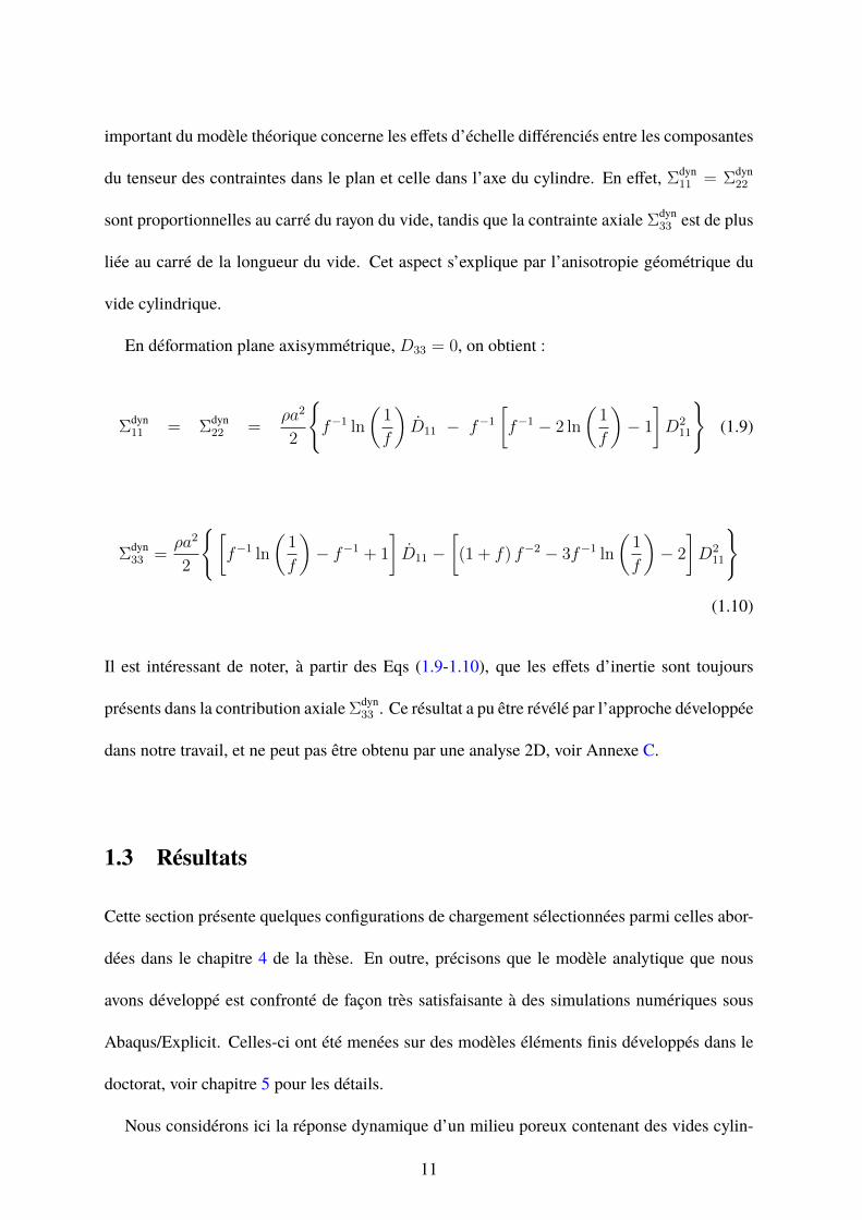
important du modèle théorique concerne les effets d’échelle différenciés entre les composantes

du tenseur des contraintes dans le plan et celle dans l’axe du cylindre. En effet, Σdyn11 = Σdyn

22

sont proportionnelles au carré du rayon du vide, tandis que la contrainte axiale Σdyn33 est de plus

liée au carré de la longueur du vide. Cet aspect s’explique par l’anisotropie géométrique du

vide cylindrique.

En déformation plane axisymmétrique, D33 = 0, on obtient :

Σdyn11 = Σdyn

22 =ρa2

2

f−1 ln

(1

f

)D11 − f−1

[f−1 − 2 ln

(1

f

)− 1

]D2

11

(1.9)

Σdyn33 =

ρa2

2

[f−1 ln

(1

f

)− f−1 + 1

]D11 −

[(1 + f) f−2 − 3f−1 ln

(1

f

)− 2

]D2

11

(1.10)

Il est intéressant de noter, à partir des Eqs (1.9-1.10), que les effets d’inertie sont toujours

présents dans la contribution axiale Σdyn33 . Ce résultat a pu être révélé par l’approche développée

dans notre travail, et ne peut pas être obtenu par une analyse 2D, voir Annexe C.

1.3 Résultats

Cette section présente quelques configurations de chargement sélectionnées parmi celles abor-

dées dans le chapitre 4 de la thèse. En outre, précisons que le modèle analytique que nous

avons développé est confronté de façon très satisfaisante à des simulations numériques sous

Abaqus/Explicit. Celles-ci ont été menées sur des modèles éléments finis développés dans le

doctorat, voir chapitre 5 pour les détails.

Nous considérons ici la réponse dynamique d’un milieu poreux contenant des vides cylin-

11

a) 0

0.05

0.1

0.15

0.2

0.25

0.3

0.35

0 200 400 600 800 1000 1200

Po

ros

ity

, f

Time (ns)

10MPa/ns 10MPa/ns

250MPa/ns 250MPa/ns

QuasistaticDynamic

b)

Figure 1.2: Evolutions de a) la porosité f et b) des contraintes Σ11 = Σ22, Σ33 en fonctiondu temps. Le chargement est axisymmétrique en déformation plane (D33=0 est imposé) etΣ11 = Σ22 = pt avec p =10 et 250MPa/ns en a) et p =10MPa/ns en b). Lamatrice entourant lesvides est rigide parfaitement plastique, de limite d’élasticité σ0=100MPa, de masse volumiqueρ=2700kg/m3. La géométrie de la cellule élémentaire est telle que a0=50µm, b0=1500µm,conduisant à une porosité initiale f0=1.1 10−3.

driques de rayon initial a0=50µm. Le rayon extérieur de la cellule élémentaire est b0=1500µm

conduisant à une porosité initiale f0=1.1 10−3. Les paramètres matériau de la matrice sont

σ0=100MPa, ρ=2700kg/m3. Deux types de chargement axisymmétrique sont considérés dans

cette partie:

• un chargement de déformation plane où l’on impose D33 = 0 et Σ11 = Σ22 = pt et pour

lequel la réponse est indépendante de la longueur l0,

• un chargement sphérique où Σ11 = Σ22 = Σ33 = pt et pour lequel nous étudions

l’influence de la demi-longueur initiale l0;

Le paramètre p est positif (vide en expansion) et représente le taux de chargement en contraintes

Déformation plane La Fig. 1.2a présente l’évolution de la porosité en fonction du temps

pour deux valeurs de taux de chargement: p =10 et 250MPa/ns. La réponse quasi-statique est

également reportée sur la figure. Les effets stabilisants de la micro-inertie sont clairement mis

12

en évidence, l’évolution en régime dynamique étant considérablement retardée comparative-

ment à la réponse quasi-statique. Notons que cette dernière prédit une croissance instantanée

du vide lorsque la contrainte appliquée Σ11 = pt atteint la valeur limite obtenue à partir de la

surface de charge de Gurson (1.6), i.e. lorsque Σ11 = σ0√3

ln(

1f0

). Compte tenu des paramètres

considérés, le temps correspondant à l’expansion en régime quasi-statique est approximative-

ment t =39ns (resp. 1.57ns) lorsque p =10MPa/ns (resp. p =250MPa/ns), voir Fig. 1.2a.

Précisons enfin que, bien que la croissance de l’endommagement s’initie plus tôt lorsque p est

plus grand, les effets de micro-inertie sont plus marqués pour les taux de chargement plus im-

portants. En effet, la contrainte à appliquer pour observer un endommagement significatif au

sein du matériau poreux est plus élevée lorsque p =250MPa/ns.

La Fig. 1.2b nousmontre l’évolution des composantes du tenseur des contraintes totales pour

le cas où p =10MPa/ns. Les contraintes dans le plan sont imposées, tandis que la contrainte ax-

iale est obtenue à partir de la théorie, Eq (1.10). En raison des effets micro-inertiels, il apparaît

que la contrainte axiale nécessaire pour maintenir le VER à sa longueur initiale, diminue aux

grands temps, bien que le chargement dans le plan continue de croître. Cette tendance, vérifiée

par calculs éléments finis, est un résultat marquant du travail de thèse, et a pu être révélé par

l’approche théorique que nous avons développée. Un modèle construit à partir d’une approche

2D ne permet pas de restituer ces effets d’inertie dans la direction longitudinale, la contrainte

dans cette direction ne pouvant être déterminée. Ce point est abordé en Annexe C.

Chargement sphérique La Fig. 1.3a présente l’évolution de la porosité en fonction du temps

pour ρ, a0, f0 fixés, considérant plusieurs valeurs de longueur intiale l0 dans l’intervalle [0-

20 000]µm. Il apparaît que les effets d’inertie sont plus importants pour les vides longs, l’évo-

lution de l’endommagement étant retardée lorsque l0 augmente. La Fig. 1.3a révèle également

13

a) 0

0.05

0.1

0.15

0.2

0.25

0.3

0.35

0.4

0 200 400 600 800 1000 1200

Po

ros

ity

, f

Time (ns)

l0=1µm, l0=10µm

l0=500µm

l0=1000µm

l0=2000µm

l0=20000µm

(l0→0) (l0→∞)

b) 0

200

400

600

800

1000

1200

1400

1600

0 100 200 300 400 500 600 700 800 900 1000

Ex

tern

al

an

d I

nte

rna

l ra

dii

, (µ

m)

Time (ns)

a

b

l0→0

l0=1000 µm

Figure 1.3: Effet de la longueur initiale de vide sur l’évolution a) de la porosité lorsque l0 variedans l’intervalle [1:20 000]µm et b) des rayons intérieur et extérieur du VER pour l0 → 0 etl0 =1000µm. Le chargement est sphérique: Σ11 = Σ22 = Σ33 = pt, avec p=10MPa/ns. Lama-trice entourant les vides est rigide parfaitement plastique, de limite d’élasticité σ0=100MPa, demasse volumique ρ=2700kg/m3. La géométrie de la cellule élémentaire est telle que a0=50µm,b0=1500µm, conduisant à une porosité initiale f0=1.1 10−3.

que pour une cellule de longueur l0 donnée, l’évolution de la porosité est encadrée par deux

réponses asymptotiques. La première, obtenue pour l0 ≥20 000µm correspond à la réponse de

vides cylindriques très longs. Dans ce cas, l’évolution de la porosité coïncide avec le résultat

illustré en Fig. 1.2a pour lequel Σ11 = Σ22 = pt et D33 =0 (déformation plane). Cependant,

la contrainte axiale Σ33 est différente pour les deux cas de chargement. Il a en effet été montré

qu’en raison des effets de micro-inertie, la contrainte axiale calculée en déformation plane est

différente de pt, cf. Fig. 1.2b.

La seconde réponse asymptotique illustrée en Fig. 1.3a est obtenue pour l0 ≤1µm. Dans ce

cas, le modèle permet la description de vides cylindriques très minces pour lesquels la so-

lution devient indépendante de la longueur initiale. Ce résultat peut être anticipé à partir de

l’Eq (1.8) indiquant que les effets d’inertie liés à la longueur des vides disparaissent lorsque

l → 0. L’étude du cas de vides cylindriques très minces en expansion dynamique a révélé

une situation tout à fait particulière illustrée en Fig. 1.3b montrant les évolutions des rayons

intérieur a et extérieur b pour l0 → 0 et l0 =1000µm. Dans le cas de matériaux poreux minces

i.e l → 0, l’augmentation de la porosité se réalise via une croissance du rayon de la cavité ac-

14

compagnée d’une réduction de la taille de l’enveloppe extérieure du VER. Cette tendance, tout

à fait contrintuitive, n’est pas observée lorsque les effets d’inertie développés dans la direction

longitudinale jouent un rôle important, comme c’est le cas par exemple pour l0 =1000µm sur

la Fig. 1.3b.

1.4 Conclusion et perspectives

L’objectif de cette thèse est de proposer une modélisation de l’endommagement par croissance

de cavités, pour des chargements dynamiques. Les matériaux poreux considérés contiennent

des vides cylindriques parallèles représentatifs de structures perforées ou de matériaux archi-

tecturés de type nid d’abeille. Nous nous sommes particulièrement intéressés à l’influence de

deux paramètres géométriques caractéristiques de la taille de la cellule (rayon et longueur),

pour des cas de chargement axisymmétriques variés.

Les résultats obtenus par le modèle ont été vérifiés par comparaison à des simulations

numériques menées sur des modèles éléments finis développés dans le doctorat. De nombreux

cas de chargement ont été considérés et des résultats nouveaux ont été obtenus dans le cadre

de la thèse. En particulier, lors d’un chargement de déformation plane, nous montrons que la

contrainte axiale diminue alors que les contraintes dans le plan continuent d’augmenter. Ce ré-

sultat, traduisant que la contrainte nécessaire pourmaintenir une structure poreuse à sa longueur

initiale est réduite en raison des effets micro-inertiels, peut servir à préciser des éléments de

dimensionnement de machines d’essais pour des essais dynamiques. Le cas du comportement

sous chargement sphérique dynamique de structures minces a également révélé un comporte-

ment inattendu. L’endommagement croît par augmentation du rayon de vide, conjointement

avec la réduction du rayon extérieur. Cette tendance est à attribuer uniquement aux effets de

micro-inertie.

15

Au delà des cas de chargement abordés dans cette partie, le modèle a été testé pour des

configurations supplémentaires pour révéler des tendances particulières. A titre d’exemples, le

vide s’effondre lors d’une expansion biaxiale rapide alors qu’en traction dynamique, après une

augmentation initiale, la porosité semble saturer lorsque les cavités sont suffisamment longues

et les effets d’inertie importants.

Les travaux de doctorat appellent naturellement à poursuivre de nombreuses investigations.

Nous n’en citerons que quelques unes. Tout d’abord, la matrice est considérée ici parfaite-

ment plastique. Les effets stabilisants liés au chargement dynamique résulte donc, dans notre

approche, uniquement des effets d’inertie liés à la taille des vides. La littérature a révélé que

les effets visqueux peuvent jouer un rôle important dans l’évolution de l’endommagement en

régime dynamique qui dépend, de ce fait, de l’influence combinée des effets visqueux et micro-

inertiels. L’objectif premier, en poursuite de ce travail, consiste alors à inclure la sensibilité à

la vitesse de déformation dans la réponse rhéologique de la matrice. Précisons d’ores et déjà

que cela conduira à un ajustement de la contribution quasi-statique (i.e. indépendant des ef-

fets de micro-inertie) et n’affectera pas les expressions analytiques de la contribution inertielle

obtenues dans ce travail. Après avoir étendu l’approche à la prise en compte des effets visqueux,

il nous semble pertinent de mettre en œuvre le modèle à des fins de comparaison à des essais

expérimentaux menés sur des matériaux ductiles dont le comportement dynamique de la ma-

trice serait à identifier.

Dans notre approche, le VER adopté et champ de vitesse associés sont définis pour un cylin-

dre creux. Cette configuration élémentaire nous permet notamment de mettre en évidence les

effets de micro-inertie différenciés entre la contribution macroscopique dans le plan, et dans

la direction longitudinale du cylindre. Une voie intéressante à l’extension de notre modélisa-

tion consiste à considérer des vides cylindriques noyés dans la matrice. Nous appuyant sur

16

des approches de la littérature, nous visons à adopter comme cellule élémentaire un domaine

contenant le vide entouré d’une matrice déformable, à l’image du VER considéré par Morin

et al. [27].

Enfin, les résultats obtenus au LEM3 pour le cas de vides sphériques ont révélé l’importance

significative des paramètres de distribution de tailles de vides sur la réponse dynamique de

matériaux poreux. Il serait alors également intéressant de considérer les effets de distribution

en tailles (a) et en rapports de forme (l/a) sur la réponse dynamique d’une structure poreuse

contenant une population hétérogène de vides cylindriques.

17

18

Context and Motivation of the thesis

This PhD is a part of the project “OUTCOME: A European Marie Curie Innovative Training

Network (ITN-ETN)”. The project has received funding from the European Union Horizon

2020 research and innovation programme under the Marie Sklodowska-Curie grant agreement

n0 675602. The consortium is a collaboration between University Carlos III Madrid, Spain

(project coordinator), Technion, Israel, University of Lorraine, France and industrial partners

CIMULEC, France and AEROSERTEC, Spain. The aim of this project is to train and develop

eight Early Stage Researchers (PhD students) in developing novel solutions for the analysis and

design of aerospace, defense and civilian structures subjected to extreme dynamic loading con-

ditions.

Fracture in materials is due to action of thermo-mechanical loadings. Depending on the abil-

ity of materials to deform plastically before fracture determines whether the damage is ductile

or brittle. The ductile damage in materials results from the interaction of three mechanisms:

nucleation, growth and coalescence of voids. In this thesis, we are interested in damage of

porous ductile materials under dynamic loading. This study concerns a wide range of fields

such as civilian and military application (in the framework of the development of shock ab-

sorbing structures) or space application (for the study of the impact effect on satellites). For

example, the aircraft sructures are vulnerable against loadings from impact, crash or explo-

sion. These problems result in understanding the energy absorption in the structure and its

19

implementation in aircraft design. Safety is the major factor for the aircraft manufacturers.

The aircraft industries are under deep investigation to employ different lightweight energy ab-

sorbers for suitable loading. When it comes to low weight and energy dissipation ability, honey

comb structures are the state of the art structures for such applications. In biomechanics, the

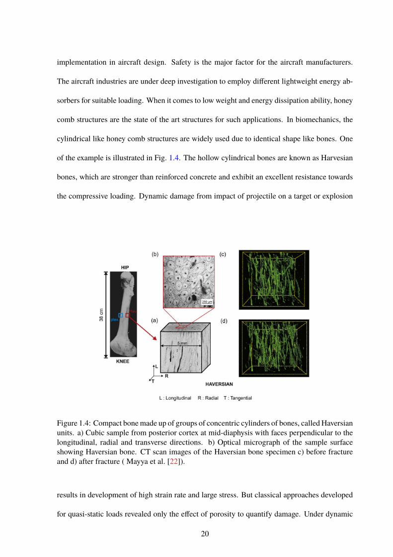
cylindrical like honey comb structures are widely used due to identical shape like bones. One

of the example is illustrated in Fig. 1.4. The hollow cylindrical bones are known as Harvesian

bones, which are stronger than reinforced concrete and exhibit an excellent resistance towards

the compressive loading. Dynamic damage from impact of projectile on a target or explosion

Figure 1.4: Compact bonemade up of groups of concentric cylinders of bones, called Haversianunits. a) Cubic sample from posterior cortex at mid-diaphysis with faces perpendicular to thelongitudinal, radial and transverse directions. b) Optical micrograph of the sample surfaceshowing Haversian bone. CT scan images of the Haversian bone specimen c) before fractureand d) after fracture ( Mayya et al. [22]).

results in development of high strain rate and large stress. But classical approaches developed

for quasi-static loads revealed only the effect of porosity to quantify damage. Under dynamic

20

loading, material particles situated near the cavities undergo strong acceleration. The micro-

inertia effects induced by these strong acceleration developed at the local level play a major role

in the macroscopic response and the development of damage in porous materials. Up to now,

these effects at the local scale were mainly evaluated for porous materials containing spheri-

cal or spheroidal voids. Voids in metallic materials may reveal complex shapes which are not

spherical or spheroidals. Within this context, we aim to consider cylindrical voided cells as

representative of thick wall honeycomb structures or porous materials containing drilled holes.

Finally, due to the development of additive manufacturing, the design of materials containing

cylindrical voids is a possible way to create lightweight materials with high energy dissipation.

The aim of this work is to develop an analytical model for porous materials containing cylin-

drical voids. The goal is to elucidate several key points which are still under discussion (ac-

celeration effect in the axial direction, micro-inertia effects, lengthscale effects, loading condi-

tions, ...). In addition, the results obtained from the modeling are validated through compari-

son with finite element calculations conducted on unit cells using the finite element software

Abaqus/Explicit.

The manuscript is organized as follows. A literature review is proposed in chapter 2. Then,

the main steps of the dynamic homogenization procedure for porous materials are recalled in

chapter 3. The trial velocity for the adopted cylindrical unit cell is also presented, followed

by the expression of the macroscopic stress tensor that includes micro-inertia effects. To be

noted, the matrix material is taken as rigid perfectly plastic (no strain hardening and no rate

dependence of the matrix material). In chapter 4, we restrict the attention to axisymmetric

loadings and present the results. The micro-inertia effects are exemplified considering various

loading configurations such as plane strain case, hydrostatic case and various other loading

paths. All results obtained from the approach are validated against finite element calculations

21

as presented in chapter 5. Finally, some conclusion and perspectives are discussed at the end

of the manuscript.

22

Chapter 2

Literature review

2.1 Introduction

From decades, the description of void growth in ductile materials has received much attention

around the scientific community mainly in quasi-static condition. But nature is dynamic, so

it is significantly evident that the ductile fracture under intense dynamic loading is controlled

to some extent by micro-inertia effects i.e, the kinetic energy stored in the matrix material

in the vicinity of the void. The proposed literature review presents different aspects starting

from ductile fracture in experimental works, theoretical studies about quasi-static and dynamic

analysis of the void growth and importance of void shape. From the review, some conclusions

will be drawn which will motivate my research.

2.2 Experimental works

Various researchers showed that the physical mechanisms of the ductile fracture are nucleation,

growth and coalescence of voids, a scenario confirmed by experimental studies. Depending

upon material and void configurations, different failure models are observed. The dynamic

23

fracture is visible in different situations associated with the impact of projectile on a target,

detonation of an explosive or a sudden deposition of intense pulses of energy on the target. The

ductile material undergoes very intensive loading which may exhibit high strain rates (in the

order of 107 s−1) and large stress levels (>10GPa) resulting in micro-voiding inside the mate-

rial. Contrary to most quasi-static situations, in dynamic condition under large stress triaxiality

voids are considerably growing, inducing large plastic deformation. In addition, the coales-

cence stage is mostly due to direct impingment (neigbhouring voids meet) while in quasi-static

analyses, shear bands may connect small voids. The phenomenon of direct impingement is a

consequence of micro-inertia effect, which stabilizes the flow in the neighbourhood of voids

and prevent from early localization [17].

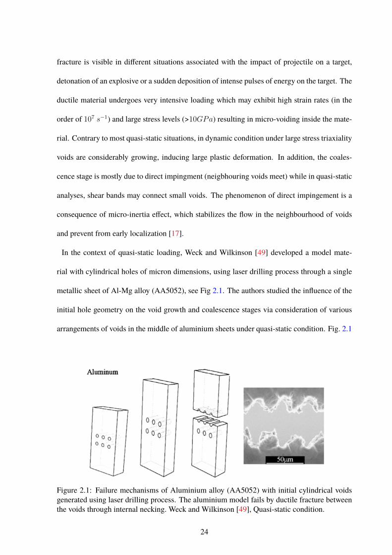
In the context of quasi-static loading, Weck and Wilkinson [49] developed a model mate-

rial with cylindrical holes of micron dimensions, using laser drilling process through a single

metallic sheet of Al-Mg alloy (AA5052), see Fig 2.1. The authors studied the influence of the

initial hole geometry on the void growth and coalescence stages via consideration of various

arrangements of voids in the middle of aluminium sheets under quasi-static condition. Fig. 2.1

Figure 2.1: Failure mechanisms of Aluminium alloy (AA5052) with initial cylindrical voidsgenerated using laser drilling process. The aluminium model fails by ductile fracture betweenthe voids through internal necking. Weck and Wilkinson [49], Quasi-static condition.

24

Figure 2.2: Ductile fracture in an initially dense steel due to void growth and coalescence ofvoids, Benzerga and Leblond [3], Quasi-static condition.

shows an array of 6 voids in 2 lines, the lines are oriented at 900 with respect to the tensile

loading direction. In Fig. 2.1, it is visible that voids grow and coalescence occurs by internal

necking of the ligament between voids.

Fig. 2.2 picturizes the ductile fracture observed for a round notched bar of low alloy steel, the

material is initially considered as a dense steel with no crack. The zigzag crack goes "slant" as

it approaches the free surfaces forming the shear lips that shows cup-cone fracture. The exper-

iment was carried out by Benzerga et al. [2] and the authors observed that the damage occurs

due to the evolution of voids (larger than 1µm in size). In this case, the void nucleates and

grows. Coalescence is due to strain localization. The above two experimental works reveal that

void growth and failure of ductile porous materials in quasi-static condition are interlinked.

Meyers and Aimone [24] studied the fracture behavior of nickel (Ni-200) during impact tests.

In Fig. 2.3(a), the study revealed that the material undergoes ductile fracture due to spalling

(spalling is a material failure due to the interaction of tensile stresses that develop inside a

body when two rarefaction waves interact). In this study, Meyers and Aimone [24] observed

that spherical voids grow, coalesce each other (mostly by direct impingement) and leads to frac-

ture. Numerous spherical voids have been found during experiments, containing approximately

0.5 percent impurities in the material. Fig. 2.3(b) shows the formation of voids along the rolling

direction like a string of particles. Later in the deformation process, voids are growing until

25

26 CHAPTER 2. LITERATURE REVIEW

Figure 2.3: Dynamic fracture in nickel by spalling. (a) Spherical voids are induced duringimpact. They grow and coalesce by direct impingement mechanism. (b) Formation of a stringof voids in nickel. Meyers and Aimone [24],

Figure 2.4: Dynamic damage in ductile material under impact test. (a) Ductile fracture by voidcoalescence. (b) Impingement of voids in impact-loaded specimens of 1145 aluminium. Curranet al. [7]

Figure 2.5: Voids coalescence by void sheet formation in AISI 4340 steel strained plasti-cally. Curran et al. [7]

coalescence stage takes place leading to final failure by the creation of a scab.

The microscopic observations of Curran et al. [7] revealed that the coalescence process can be

classified into two groups: direct impingement and localization between voids (strain localiza-

tion). In Fig. 2.4(a), the coalescence process is simply direct impingement of the voids. In pure

ductile metals (such as copper) after nucleation, void grows in a spherical manner to near di-

rect impingement before localized ligament stretching completes the coalescence process. The

above process occurs under dynamic loading, when the sample is submitted to planar impact

(high stress triaxiality). Fig. 2.4(b) represents the void distribution in the spall plane in a 1145

aluminium. In some cases, the coalescence observed may occur through strain localization be-

tween voids, see Fig. 2.5.

Roy [33] investigated dynamic damage of high purity grade tantalum. Plate impact tests at

various speeds and considering various target thicknesses were performed to generate dam-

age and fracture in tantalum. The three main stages of damage and fracture (nucleation, void

growth and coalescence) have been explained. Nevertheless, Roy studied particularly the prob-

lem of nucleation and growth of microvoids. Plate impact tests were carried out using a 80mm

27

28 CHAPTER 2. LITERATURE REVIEW

a)V=185m/s

5

b)

5mm

V=207m/s

c)

Figure 2.6: Dynamic damage observed in tantalum under planar impact test at various impactvelocites. Development of micro-voiding along the spall plane parallel to the impacted surface.The level of porosity is growing with increase in impacted velocity V. Complete fracture isobserved at V=306m/s. Roy [33]

single stage gas gun providing a tensile stress as 5GPa < σshock < 30GPa and a shock rise

time as 0.5 µs < ∆tshock < 1.5 µs. The damage was observed from optical metallographic

analyses. Fig. 2.6 illustrates the effect of impact velocity on the damage and fracture for the

initially dense high purity grade tantalum. In Fig. 2.6(a), (v=185m/s) nucleation is observed to

be randomly distributed in the vicinity of the spall plane parallel to the impacted surface. The

investigation revealed that the voids remain spherical with diameter in the range 15µm to 400

µm. Fig. 2.6(b) shows as impact velocity increases (v=207m/s), the coalescence process is

due to direct impingement mechanism. The interaction between voids during the growth stage

seems to be delayed due to the micro-inertia effect. Fig. 2.6(c) shows that the complete fracture

happens when the impact velocity is v=306m/s. In that case, the target is splitted in two parts.

Under dynamic conditions, micro-inertia promotes rapid and large expansion which generates

strong local acceleration of particles in the vicinity of cavities. As a consequence, the micro-

inertia influences the overall behavior of the material. When micro-inertia is under considera-

tion, the behavior of the porous material completely changes from quasi-static to dynamic (i.e,

micro-inertia independent to micro-inertia dependent). Before presenting models in dynamic

conditions, it is still interesting to focus on pioneering works dedicated to quasi-static condi-

tions. Section 2.3.1 will focus on quasi-static theoretical studies. In section 2.3.2, a deeper

analysis of works dedicated to dynamic conditions will be proposed.

29

2.3 Modeling

2.3.1 Quasi-static analysis on void growth

2.3.1.1 Introduction

The behavior of porous materials under quasi-static loading has been analyzed by several au-

thors, since early works of McClintock [23], Rice and Tracey [32], Gurson [15], Budiansky

et al. [4], Tvergaard [43] and Needleman and Tvergaard [28].

McClintock [23] investigated the growth of cylindrical and elliptical pores in an infinite vis-

cous material. The author developed an approximate closed-form analytical expression for the

void radius evolution and fracture criterion. Rice and Tracey [32] investigated the stage of

void growth for mostly spherical void in an infinite matrix under general stress conditions. A

variational principle has been proposed where the matrix is rigid-plastic (perfectly plastic or

strain hardening). Results of McClintock [23] were retrieved for cylindrical voids when adopt-

ing the variational principle. Both analyses of McClintock [23] and Rice and Tracey [32] have

revealed the exponential amplification of void growth by stress triaxiality. Budiansky et al.

[4] have considered a viscous power law constitutive relationship for the matrix behavior, to

identify the influence of the stress-triaxiality on the void radius growth. McClintock [23], Rice

and Tracey [32], Budiansky et al. [4] were all considering dilute voids. In an engineering

material, as observed in Fig. 2.1 to Fig. 2.6, voids are not isolated in the matrix phase, so

the volume fraction of voids has to be integrated in the modelling. For that purpose, using

a micro-mechanical approach, Gurson [15] derived an approximate yield criterion based on

a trial velocity for porous materials with spherical and cylindrical voids under static condi-

tions. The GTN ( Tvergaard [43] and Needleman and Tvergaard [28]) model is extending the

30

Gurson model, which has been widely used for quasi-static investigation of fracture process in

finite element calculations. Gologanu et al. [14] proposed a yield surface for porous material

containing prolate voids, known as GLD model. The GLD yield surface can be viewed as an

extension of the Gurson [15] model. A brief explanation of the quasi-static investigation from

some of the previous works are pointed out in next pages.

2.3.1.2 McClintock Model

McClintock [23] developed a criterion for the fracture of cylindrical pores under prescribed

stress at infinity. The criterion was developed for perfectly plastic, linear viscous materials

and also extended to strain hardening material by extrapolation of the analysis. McClintock

[23] observed that fracture takes place for very small porosity for both plastic and viscous

flow with very strong inverse dependence of fracture strain on hydrostatic tension. McClintock

[23] considered a porous medium subjected to stress loading at infinity. Calculations are done

Figure 2.7: Cylindrical unit cell with inner radius R subjected to axial strain rate ˙εz and radialstrain rate ˙εr. The resulting strain rates are due to imposed stress at infinity, McClintock [23].

31

in the principal direction frames. McClintock [23] investigated the case of generalized plane

strain with a hole in an infinite medium. The coalescence stage (and the associated fracture) is

triggered when the radius of the hole reaches the mean spacing between voids. The problem

is solved adopting cylindrical coordinates r, θ, z (Fig. 2.7). From the conservation of linear

momentum in quasi-static conditions one obtains:

∂σr∂r

+σr − σθ

r= 0 (2.1)

For a von Mises material, Eq 2.1 becomes:

∂σr∂r

= −2σ

3r

(εr˙ε− εθ

˙ε

)(2.2)

where σ and ˙ε are the equivalent stress and strain rate.

From compatibility condition and incompressibility of the matrix, the velocity components are

expressed as:

vr =A

r−

˙εz2r (2.3)

vz = ˙εzz (2.4)

where A = −R2( ˙εr + ˙εz/2). ˙εr and ˙εz are the local strain rate at the void surface. The strain

rate components in the matrix material are defined as:

εr = −(R2

r2

)(˙εθ +

˙εz2

)−

˙εz2

(2.5)

32

εθ =

(R2

r2

)(˙εθ +

˙εz2

)−

˙εz2

(2.6)

where the condition ( ˙εθ + ˙εz + ˙εr = 0) has been used. R is the radius of the cylindrical void.

Using Eqs (2.2), (2.5), (2.6) and substituting in the equilibrium equation, Eq (2.1), the void

growth is expressed as:

R

R0

=√

3ε∞r sinh

[ √3σ∞r

σ∞r − σ∞z

]+ ε∞r (2.7)

The ductile fracturemodel ofMcClintock has been recently used as the basis for the formulation

of a damage plasticity model by Reboul and Vadillo [31]. Adopting a hollow cylinder as the

unit cell and based on Taylor series expansion, the authors provided a closed form macroscopic

expression for the response of strain rate power-law materials.

2.3.1.3 Gurson model

Gurson [15] developed an approximate plastic constitutive theory for porous materials. An

approximate velocity field is adopted, similar to Rice and Tracey [32] in such a way that the

velocity field satisfies the kinematic boundary conditions on the external surface of the unit

cell. Homogenous kinematic boundary conditions are considered:

v = D · x (2.8)

where D is the macroscopic strain rate tensor. The material is assumed incompressible and

the volume change of the RVE is only due to void growth. The approximate yield criterion is

initially proposed for rigid perfectly plastic materials. Gurson studied the case of a matrix ma-

terial containing both long circular cylindrical voids (Fig. 2.8) and spherical voids (Fig. 2.9).

33

Figure 2.8: Long circular cylindrical unit cell (inner radius ’a’ and outer radius ’b’) with cylin-drical void embedded inside. The porosity of the unit cell is f = (a/b)2. The matrix is rigidperfectly plastic, Gurson [15].

The approximate velocity is developed in such a manner that the shear and dilatation compo-

nents are independent. The velocity field for cylindrical void is expressed as:

v = D · x+Bx (2.9)

where B = tr(D)2

(br

)2 − D33

2, x = x1e1 + x2e2 and x = x1e1 + x2e2 + x3e3

D is a strain rate tensor expressed as:

D =

D11−D22

2D12 D13

D12D22−D11

2D23

D13 D23 D33

, (2.10)

Based on the plastic dissipation evaluated from the velocity field, Gurson develops a yield

34

Figure 2.9: Hollow spheremodel with a spherical void embedded inside a spherical shell havinginner radius ’a’ and outer radius ’b’. The porosity of the unit cell is f = (a/b)3, Gurson [15].

function for the circular cylindrical void which takes the analytic form:

Φ = Ceqv

(Σeqv

σ0

)2

+ 2f cosh

(√3

2

Σγγ

σ0

)− 1− f 2 (2.11)

where Σ represents the stress tensor and σ0 is the matrix yield stress (constant for perfectly

plastic material). Σγγ = Σ11 + Σ22, Σeqv =√

32Σ

′ijΣ

′ij , where Σ

′ is the deviatoric part of

the cauchy stress tensor. Ceqv is function of f (volume fraction of pores). When f tends to

zero, the yield function reduces to the von Mises yield function. The Gurson yield function for

cylindrical voids in plane strain flow for rigid perfectly plastic material is presented in Fig. 2.10,

see more details in Gurson [15]. One can observe that as the porosity increases, the elastic

domain shrinks.

Even though the Ph.D focuses only on cylinder, one has to mention that in the literature, most of

the works are dealing with spherical void shape. For spherical void, the microscopic velocity

35

Figure 2.10: Gurson yield function for cylindrical voids in plane strain loading conditions.The yield loci are presented for three different loading cases. Axi-symmetric, plane strain andgeneralized plane strain conditions are represented by solid lines, dashed lines and dotted linesrespectively for various porosities (f in the range 0.005 to 0.3). In the present figure T = Σ/σ0

is the normalized macroscopic stress tensor, Gurson [15]

field usually adopted in the literature can be split into two parts:

v = vs + vv (2.12)

where the first part represents shape change at constant volume (vs) and the second part repre-

sents the volume change at constant shape (vv), similar like cylindrical void. In that case, the

yield function for spherical voids takes the form:

Φ =

(Σeqv

σ0

)2

+ 2f cosh

(1

2

Σnn

σ0

)− 1− f 2 (2.13)

where Σnn = tr(Σ) = 0, ’tr’ represents the trace operator. Again, when f=0, the von Mises

yield function is retrieved.

36

Under spherical loading, the yield stress of porous material with spherical voids is:

Σnn = 2σ0 ln

(1

f

)(2.14)

The approximate yield functions proposed by Gurson for spherical and cylindrical voids have

been adopted widely in the literature.

2.3.1.4 Gurson Tvergaard and Needleman model (GTN model)

Needleman and Tvergaard [28] have modified the Gurson model by comparing the prediction of

the model with FE cylindrical unit cell containing a spherical void. Needleman and Tvergaard

[28] introduce three parameters so that the approximate yield function takes the form:

Φ =

(Σeqv

σ0

)2

+ 2fq1 cosh

(q2

2

Σnn

σ0

)− 1− q3f

2 (2.15)

where q1, q2 and q3 are parameters that adopt various forms in the literature. Needleman and

Tvergaard [28] proposed the following constant values q1=1.5, q2=1, q3=q21 while other authors

showed that the q-parameters are depending on triaxiality (Vadillo and Fernández-Sáez [44]).

When q1=q2=q3=1, then Eq (2.15) takes the form of Gurson model Eq (2.13). From the asso-

ciated flow rule, the macroscopic strain rate is perpendicular to the yield surface:

D = κ∂Φ

∂Σ(2.16)

The parameter κ represents the plastic multiplier satisfying the Kuhn-Tuker conditions (Simo

and Hughes [37]): Φ ≤ 0, κ ≥ 0, Φκ = 0. To analyse the porosity evolution during loading,

37

an evolution law for f is defined based on the incompressibility of the matrix material:

f = (1− f)trD (2.17)

In the above works, micro-inertia effects are not considered. In case of very high strain rates

applications such as ballistic impacts, high speed forming processes, design of shock wave

mitigation devices, crash tests, etc. the above quasi-static approaches have some limitations,

the overall response being not related to the size of voids. The next section focuses on the

dynamic behavior of porous materials investigated by several researchers aiming at overcome

these limitations.

2.3.2 Dynamic analysis for porous materials

2.3.2.1 Introduction

Under dynamic conditions, intense local acceleration fields are developed in the vicinity of the

void surface which will influence the overall behavior of the material. Several authors proved

that micro-inertia tends to delay the porosity growth. I will briefly discuss some of the works

and later in this section, I will propose a more extensive description of a limited number of

contributions.

Carroll and Holt [5] investigated the inertia effect on the behavior of porous aluminium media

(with spherical voids) under spherical compressive loading. The work is restricted to elastic

perfectly plastic matrix. Carroll and Holt [5] constructed a rate-dependent pore-collapse re-

lationship which involves the matrix material properties, the pore geometry and the loading.

The above study revealed an analytical void collapse law including micro-inertia effects under

pure hydrostatic compression. The macroscopic pressure was found to be sum of a quasistatic

38

part (micro-inertia independent) and a dynamic part (micro-inertia dependent) scaled by the

square of the void radius and the matrix mass density. The comparison of the model prediction

with finite-difference calculations was carried out. Klöcker and Montheillet [18] analyzed the

void growth in a viscoplastic material. Cylindrical and spherical geometries under axisymmet-

ric and spherical loadings were considered respectively. The authors investigated both static

and dynamic responses. The matrix was linear viscous. Cortes [6] performed the analytical

modeling of the dynamic growth of microvoids, which is an extension of the static and dy-

namic pore-collapse relationship obtained for ductile porous materials by Carroll and Holt [5].

The study was carried out under hydrostatic loading, including the effect of material viscosity,

strain hardening and thermal dependency. Cortes [6] concluded that the porosity evolution is

governed by viscous effect at the beginning stage and controlled by micro-inertia at the late

stage of the deformation process. The investigation also revealed that the thermal softening has

only very small influence on the dynamic behavior at high strain rate due to the localization of

heat near the surface of the voids. The authors considered aluminium and copper-like materi-

als. Ortiz and Molinari [30] considered a spherical void in an unbounded solid under spherical

tensile loading to investigate the effect of micro-inertia. In this case, the study included both

viscous and micro-inertia effects, adding the strain hardening sensitivity. The study revealed

that both effects play an important role in the porosity growth i.e, the early stage is governed

by viscous effects and the late stage is dominated by micro-inertia, confirming the conclusion

of Cortes [6]. The main objective of the authors was to define a dimensionless parameter able

to capture the interaction between the viscous and inertia effects and at the same time to clarify

the role of both effects in the dynamic growth. Tong and Ravichandran [38, 39] investigated

the dynamic behavior of spherical pores in porous materials under spherical loading for elastic-

viscoplastic materials. The quasistatic and dynamic responses were examined. The quasistatic

39

analysis was developed for both rate-independent and rate-dependent matrix. The dynamic

part or micro-inertia inherited part was evaluated by an approximate method. The effect of

the dynamic loading rate, strain rate sensivity, strain hardening and thermal softening was also

investigated by the authors.

From the previous mentioned contributions, the dynamic behavior of porous material was

mostly investigated under spherical loading. To consider more general loading conditions, dy-

namic homogenization schemes have been proposed. Wang [46] studied the dynamic behavior

of porous materials, considering a hollow sphere as the representative volume element of the

medium. This model is not restricted to spherical loading. Surface energy effect and temper-

ature softening are accounted for. When temperature and surface energy are disregarded, the

relation proposed by Carroll and Holt [5] is retrieved. The numerical analyses were carried

out for various initial distentions, initial temperature and material rate sensitivities, to illustrate

the temperature dependency, the role of the matrix viscoplastic behavior and inertial effects on

void growth. Note that the distention α is linked to the porosity f via the relationship:

α =1

1− f(2.18)

Wang [47] and Wang and Jiang [48] revisited the work of Wang [46], by adopting the general

trial velocity field of Rice and Tracey [32]. From the energy conservation, part of the external

work is dissipated by plastic deformation while the stored kinetic energy ensures the balance.

In Wang and Jiang [48] axisymmetric loading conditions were treated and for the first time,

the dynamic stress was not only spherical. So an extension of the Gurson model to dynamic

condition was obtained. In Wang [47], a definition for the macroscopic stress and strain rate

was proposed, both quantities being work conjugated. The proposition was still exemplified by

40

considering axisymmetric loadings (spherical and shear loadings).

Following the series of work proposed by Wang [46, 47] and Wang and Jiang [48], Molinari

andMercier [26] proposed a dynamic homogenization for the behavior of porous materials with

spherical void. An explicit relationship was proposed between themacroscopic stress and strain

rate tensors. The micro-mechanical modeling accounting for micro-inertia and viscoplasticity

was obtained for general states of stress. The macroscopic stress was found to be the sum of two

contributions: a static contribution and a dynamic part. The static part can be evaluated using

any yield potential or flow surface. The micro-inertia part was derived from the trial velocity

field of Gurson [15] and Rice and Tracey [32] for spherical voids. Like the work of Cortes [6]

or Ortiz and Molinari [30], here also the results prove that the early stage of the void growth is

governed by viscous effect and late stage by the micro-inertia effect. This modeling is further

extended by Czarnota et al. [9, 8], Jacques et al. [16, 17], Czarnota et al. [10].

More specifically, Czarnota et al. [9] adopted the model of Molinari and Mercier [26] to inves-

tigate spall fracture due to microvoiding in tantalum. They extended the theoretical model to

account also for nucleation of voids. Czarnota et al. [8] implemented the model in FE software

(ABAQUS) so the configuration of Roy [33] was analyzed in details. The experimental veloc-

ity profiles of the free surface for various impact velocities were retrieved. Jacques et al. [16]

adopted themicro inertia model for the same grade of tantalum. In this work, the mean void size

evaluated from the theory was found to correlate with experiments of planar impact. Jacques

et al. [17] proposed to illustrate the effect of micro-inertia on dynamic crack propagation. It

was known from the literature that when adopting Gurson model, the strain localization pro-

cess develops in a single row of elements. It is shown that when revisiting the dynamic crack

propagation in a notch specimen or in a plate, the porosity development is spread in the vicinity

of the crack surface. Therefore, finite element calculations in dynamic conditions are shown to

41

be mesh insensitive when mesh is dense enough. This aspect clearly illustrates the regulariza-

tion feature of micro-inertia. Indeed with micro-inertia, the delay in porosity growth enables

such regularization process. As main outcome of the work of Jacques et al. [16], the size of

the damage zone in a notched specimen was found to be scaled by the size of the pre-existing

voids. For pre-cracked plate, the fracture toughness was shown to be related to the initial void

size. The crack speed is also limited due to micro-inertia and can be compared to experiments.

Czarnota et al. [10] investigated the shock wave propagation in a porous material. From the

dynamic analysis, the shock width is also controlled to some extent by the characteristic size of

the voids. An interesting finding is the amount of plastic dissipation which increases in porous

material under dynamic conditions when compared to dense materials. It is also shown that

the shock width in porous material can be larger than in dense materials. A scaling law was

finally proposed for the shock width with a clear link to the initial size and initial porosity. With

porous materials containing sufficiently large voids, one can have plastic dissipation combined

with lower acceleration. These are beneficial aspects for shock mitigation.

After a rapid presentation of a limited selection of papers of the literature, I propose in the fol-

lowing section to develop in more details four contributions which are of fundamental interest

for my PhD. First, I will summarize the contribution of Carroll and Holt [5] to highlight the

structure of micro-inertia term. Secondly, I will detail the homogenization procedure of Moli-

nari andMercier [26]. Next, I will present the Leblond and Roy [20] approach, which considers

a porous materials with cylindrical voids subjected to dynamic loading. Finally, the investiga-

tion proposed by Molinari et al. [25] for the coalescence stage with a cylindrical RVE will be

shortly discussed.

42

2.3.2.2 Carroll and Holt Model

As mentioned in the introduction part of section 2.3.2, Carroll and Holt [5] investigated the

dynamic compaction of porous aluminium. For that purpose, the RVE is a hollow sphere model

(see Fig. 2.9), with inner radius ’a’ and outer radius ’b’. Under dynamic compression P , the

mechanical analysis of the pore-collapse can be splitted in three phases: the first part where

the RVE remains elastic, a second stage where the inner part of the RVE (r < c) is under

plastic regime while the outer part (r > c) remains elastic. The surface r = c denotes the

interface between elastic and plastic regions. Finally when the loading is large, the RVE is

entirely under plastic regime. The authors defined the governing equation of the three stages

from the conservation of linear momentum (with the acceleration term) assuming also that the

matrix phase is perfectly plastic (Y being the yield stress):

(i) Elastic phase:

τ 2Y Q(α, α, α) = P − 4G(α0 − α)

3α(α− 1)(2.19)

where,

τ 2 = ρa02/[3Y (α0 − 1)2/3] (2.20)

Q(α, α, α) = −α[(α− 1)−1/3 − α−1/3] +1

6α2[(α− 1)−4/3 − α−4/3] (2.21)

ρ represents the matrix mass density, τ has the physical dimension of time and α the distention

as defined in Eq 2.18.

(ii) Elastic-plastic phase:

τ 2Y Q(α, α, α) = P − 2

3Y (1− [2G(α0−α)]/(Y α) + ln[2G(α0−α)]/[Y (α− 1)]) (2.22)

43

where G represents the shear modulus.

(iii) Plastic phase:

τ 2Y Q(α, α, α) = P − 2

3Y ln[α/(α− 1)] (2.23)

From the above expressions, the dynamic pore collapse model leads to an expression of the

form:

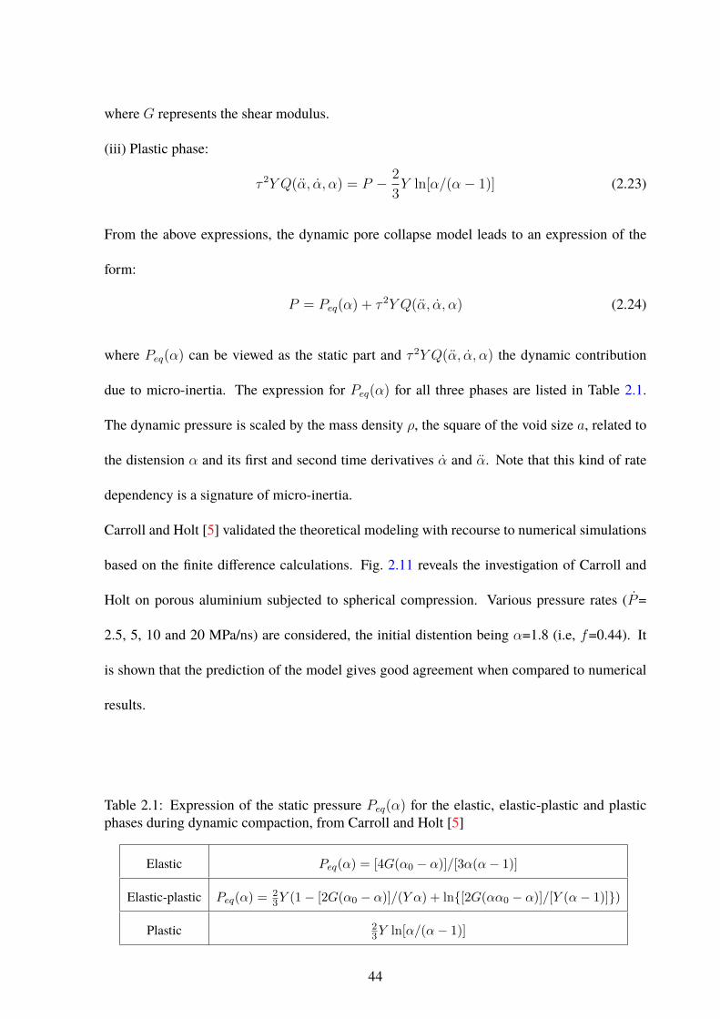
P = Peq(α) + τ 2Y Q(α, α, α) (2.24)

where Peq(α) can be viewed as the static part and τ 2Y Q(α, α, α) the dynamic contribution

due to micro-inertia. The expression for Peq(α) for all three phases are listed in Table 2.1.

The dynamic pressure is scaled by the mass density ρ, the square of the void size a, related to

the distension α and its first and second time derivatives α and α. Note that this kind of rate

dependency is a signature of micro-inertia.

Carroll and Holt [5] validated the theoretical modeling with recourse to numerical simulations

based on the finite difference calculations. Fig. 2.11 reveals the investigation of Carroll and

Holt on porous aluminium subjected to spherical compression. Various pressure rates (P=

2.5, 5, 10 and 20 MPa/ns) are considered, the initial distention being α=1.8 (i.e, f=0.44). It

is shown that the prediction of the model gives good agreement when compared to numerical

results.

Table 2.1: Expression of the static pressure Peq(α) for the elastic, elastic-plastic and plasticphases during dynamic compaction, from Carroll and Holt [5]

Elastic Peq(α) = [4G(α0 − α)]/[3α(α− 1)]

Elastic-plastic Peq(α) = 23Y (1− [2G(α0 − α)]/(Y α) + ln[2G(αα0 − α)]/[Y (α− 1)])

Plastic 23Y ln[α/(α− 1)]

44

Figure 2.11: Evolution of distension with time during the pore collapse of an aluminium mate-rial of initial distention, α=1.8, with applied loading rates P=2.5, 5, 10 and 20 MPa/ns. Solidline shows the predictions of the analytical model. Dashed lines show the results of the finitedifference calculations, Carroll and Holt [5].

2.3.2.3 Molinari and Mercier Model-2001

Molinari and Mercier [26] investigated the dynamic behavior of porous material with spheri-

cal voids by means of a micro-mechanical approach. From the principle of virtual work, the

macroscopic stress was defined which accounts for the acceleration contribution. The explicit

relationship was derived starting from the conservation of linear momentum in dynamic con-

dition:

divσ = ργ (2.25)

where ρ is the mass density, γ is the acceleration field and σ is the Cauchy stress tensor.

A homogenous kinematic boundary condition is applied on the external boundary of the RVE,

so that

v = D · x (2.26)

45

” · ” denotes the simple contracted or dot product.

From the principle of virtual work including the acceleration term, Molinari and Mercier [26]

found that the macroscopic stress Σ and macroscopic strain rate D are work conjugated:

Σ : D = 〈σ : d〉+

⟨1

2ρd|v|2

dt

⟩(2.27)

where (:) denotes the twice contracted product.

The macrostress was found to be defined by:

Σ = 〈σ〉+

⟨ργ ⊗ x

⟩(2.28)

The macroscopic strain rate D is the volume average of microscopic strain rate, d:

D = 〈d〉 (2.29)

where 〈•〉 = 1|V |

∫V• dV , |V | denotes the volume of the RVE, ’⊗’ is the tensor product and

’x’ the position of the particle. As the problem is dynamic (inertia dependent), so the static

definition Σ=〈σ〉 is no more valid. This statement is the main difference with a previous study

developed by Wang [47]. In Eq (2.28), σ is the solution of the dynamic problem. As a con-

sequence, under general loading condition of type Eq (2.26), it is impossible to find the exact

solution. One can obtain such solution for instance by considering a hollow sphere RVE under

spherical loading.

A second approach was proposed in Molinari and Mercier [26] using a trial velocity field.

The local material behavior was assessed by the introduction of a potential Φ(x,d), so that the

46

microscopic stress and strain rate tensors are connected through the relation:

σ =∂Φ(x,d)

∂d(2.30)

Applying once again the principle of virtual work to the RVE subjected to an increment of

macroscopic strain rate δD, the symmetric part of macroscopic stress Σ is expressed as the

sum of micro inertia independent term, Σstatic and micro inertia independent term, Σdyn.

(Σ)s = Σstatic + (Σdyn)s (2.31)

where,

Σstatic =∂〈Φ〉∂D

and (Σdyn)s =1

Ω

∫Ω

ργ.K(x,D)dΩ (2.32)

where γ represents here the acceleration of a material particle evaluated from the trial velocity

field and (·)s represents the symmetric part of the tensor. K(x,D) is a third order tensor which

links the increment of the macro-strain rate δD to the increment of velocity δv:

δv = K(x,D) : δD (2.33)

To evaluate the static term, Molinari and Mercier [26] adopted the macroscopic potential, 〈Φ〉

proposed by Olevsky and Skorohod [29]:

〈Φ〉 =A

m+ 1(1− f)Wm+1 (2.34)

where W =√ϕγ2 + ψe2, ϕ = (1− f), ψ = 2

3(1− f)2/f , γ =

√D′ : D′ , e = tr(D) and D

′

represents the deviatoric part of the macroscopic strain rate D.

47

Figure 2.12: A hollow sphere as a representative volume element with internal radius a andexternal radius b. The matrix behavior is viscoplastic and the porosity f = a3/b3. Molinariand Mercier [26].

To obtain an analytical expression of Σdyn, Molinari and Mercier [26] considered the approxi-

mate velocity field proposed by Gurson (1977) or Rice and Tracey [32]:

v = D′.x+Bx (2.35)

where,B = Dm

(b/r

)3

andDm = 13tr(D). After somemathematical developments, Molinari

and Mercier [26] obtain:

(Σdyn)s = ρa2

[1

5(f−2/3 − f)

(D

′+ C− 1

3tr(C)I

)+ (f−2/3 − 1)DmD

′

+1

6(f−2/3 − 1)(D

′: D

′)I− (f−2/3 − f−1)DmI

+

(3f−1 − 5

2f−2/3 − 1

2f−2

)D2mI

](2.36)

with C = D′: D

′ and I is the second order tensor.

This term is scaled by the mass density ρ, the square of the void radius a. It contains quadratic

terms in D and linear terms in D. Once again, this is the classical signature of micro-inertia

48

Figure 2.13: Porosity versus time evolution for both quasi-static and dynamic models. Theinitial porosity is f0=0.01. Two loading rates (p=10MPa/ns, 250MPa/ns) and two strain ratesensitivities (m=0.05, 0.15) are tested for spherical loading. Molinari and Mercier [26]

for porous material. The relation is designed in such a way that as inertia effect is reduced to

zero, the total macroscopic stress is completely controlled by the static term (see Eq (2.31)).

The evolution of the porosity is evaluated using the incompressibility of the matrix, Eq (2.17).

Molinari and Mercier [26] considered a viscous plastic porous matrix under various loading

conditions: hydrostatic expansion, compression and axisymmetric loadings. For hydrostatic

condition, Fig. 2.13 presents the porosity evolution for a material representative of an alu-

minium for two loading rates, p=10MPa/ns and 250MPa/ns and for two strain rate senstivities,

m=0.05 and 0.15. Due to micro-inertia effect, the void growth is delayed in the dynamic analy-

sis. For higher loading rate, the porosity evolves earlier. Nevertheless, the stress level necessary

to trigger the expansion is larger. For larger strain rate senstivity, the void growth is delayed.

Most of the investigations are accounting for porous material containing spherical voids. But

recently Sartori et al. [36, 34] considered spheroidal RVE with prolate and oblate voids (see

Fig. 2.14). The authors used the Gologanu et al. [14] model to capture the static reponse of the

porous material. The trial velocity field of Gologanu et al. [14] was used to derive the dynamic

49

stress tensor which appeared to be scaled by the matrix mass density and two internal lengths

parameters related to the size of the void (semi axes of the spheroids). Indeed, for this type of

geometry, the shape is charaterized by two length parameters, whereas for spherical voids, the

shape is defined solely by the radius.

Few studies of the literature are dedicated to cylindrical voids under dynamic loading. One

can cite Leblond and Roy [20] for the growth stage and Molinari et al. [25] for the coalescence

stage.

2.3.2.4 Leblond and Roy Model

Leblond and Roy [20] proposed a simplified model for dynamic ductile behavior of porous

materials containing cylindrical pores. For the investigation, Leblond and Roy [20] considered

a cylindrical unit cell (RVE similar to Fig. 2.8) of internal radius a, external radius b. The

Figure 2.14: Prolate (a) and oblate (b) spheroidal void embedded inside a confocal spheroid.Homogenous kinematic boundary conditions are applied on the external boundary of the unitcell, Sartori et al. [36, 34]. The RVE is similar to the Gologanu et al. [13] work.

50

length of the RVE is l. The porosity is defined as:

f =a2

b2(2.37)

The unit cell is loaded under axisymmetric generalized plane strain and shearing is neglected.

The matrix behavior is viscoplastic. The flow stress is linked to the effective strain rate via a

powerlaw, σeq = σ0(deq/ε0)n. From the J2 flow rule:

d

ε0

=3

2

(σeqσ0

)n−1σ

′

σ0

(2.38)

where, d represents the strain rate tensor, σ′ represents the deviatoric part of the stress tensor

(σ), σeq represents the equivalent stress (von Mises) and ε0, σ0, n are material constants. The

velocity field in the cylindrical coordinate system is:

vr =A

r− Br

2, vz = Bz (2.39)

where, A = 32b2Dm, B = D33, Dm = tr(D)/3. Note that under axisymmetric loading

D11 = D22. The authors assume that the acceleration in the axial direction is negligible,

γz ≈ 0. Using the flow rule and equation of motion, the components of macroscopic stress in

the plane direction are:

Σ11

σ0

=Σ22

σ0

=1

2√

3

n

n+ 1

(|D33|ε0

)1/n

[I(X) +XI′(X)] + τ 2Qc(f , f , f) (2.40)

51

The component of the macrostress in the axial direction is:

Σ33 − Σ11

σ0

=1

n+ 1sgn(D33)

(|D33|ε0

)1/n

X[I(X)− nXI ′(X)] (2.41)

where, X =

√3

2

Dm

|D33|, I(X) =

∫ 2X/f

2X

2(1 + x2)(n+1)/2ndx/x2

(2.42)

Note that the micro-inertia contribution is represented by the term τ 2Qc:

τ 2Qc(f , f , f) =ρa2

0

4σ0f0

[ln

(1

f

)f − f 2

2f

](2.43)

where a0, f0 denote the initial void radius and the initial porosity. From Eq (2.40), it is clear

that once the term τ 2Qc(f , f , f) is neglected, the quasi static approach of Leblond et al. [19]

is retrieved. With the assumption of neglecting the axial acceleration, the dynamic stress is

spherical. This contribution is scaled by the square of radius of the void cross-section but the

effect of the void length is not accounted for in the model.

2.3.2.5 Molinari et. al Model

Molinari et. al [25] investigated the dynamic behavior of porous material with cylindrical void

in the coalescence stage. The dynamic homogenization procedure for the porous viscoplas-

tic material used here is similar to the one proposed by Molinari and Mercier [26] (see sec-

tion 2.3.2.3). Here the representative volume element is considered as a cylindrical unit cell

embedding a coaxial cylindrical void, see Fig. 2.15. The dimensions 2H and 2L represent the

height and diameter of the cylindrical unit cell while 2h and 2R are the height and diameter

52

Figure 2.15: Representative volume element adopted for the coalescence analysis. The RVEhas a cylindrical shape (height, 2H and diameter, 2L) with a cylindrical void (height, 2h anddiameter, 2R) inside, Molinari et al. [25]

of the cylindrical void inside the unit cell. The cell is divided into a central part (Ωlig), shown

in Fig. 2.15 complemented by two plates on the top and bottom of Ωlig. During coalescence,

both top and bottom plates of the RVE remain rigid. In addition, it is assumed that the only

non vanishing macroscopic strain rate isD33 so thatD11 = D22 = 0. The authors proposed an

explicit relation for the dynamic stress:

Σdyn33 = ρ

D33

2c

[L2 ln

(L

R

)−3

4L2− R4

(4L)2+R2

]−ρD

233

c2

[(1

4− c

2

)L2 ln

(L

R

)+

(−9

16+

3

8c

)L2

+

(−3

16+c

8

)R4

L2+

(5

8− c

2

)R2 +

1

8

L4

R2

]+ρh2

3c(D33 +D2

33)

(1− R2

L2

)(2.44)

where, c = h/H is a dimensionless parameter. The macroscopic stress components in the

plane direction, Σdyn11 and Σdyn

22 are undefined because the condition D11 = 0 andD22 = 0 was

adopted for the coalescence stage analysis. The authors pointed out that for high loading rates,

53

micro-inertia influences strongly the macroscopic stress in the axial direction Σ33. Based on

this approach, the effect of length of the void in the inertia contribution is present and is playing

an important role in the dynamic problem.

2.3.3 Conclusion

To conclude from the literature review, it is evident that void shape/void geometry is an impor-

tant parameter which influences the behavior of ductile porous solids for quasi-static conditions

but also in dynamic conditions. At this stage, most of the works dedicated to micro-inertia ef-

fects have been done considering a spherical shape for the voids (Carroll and Holt [5], Rice

and Tracey [32], Ortiz and Molinari [30], Wang [46, 47], Molinari and Mercier [26], Czarnota

et al. [9],...). Recently Sartori et al. [34, 36] accounted for void shape effects on the dynamic

response, the representative volume element being spheroidal. Indeed, for this type of geome-

try, the shape is characterized by two length parameters whereas for spherical voids, the shape

is defined solely by the radius. Cylindrical voids are also defined by two length parameters, the

radius and the length of the void which are expected to play a role in the dynamic response.

Few authors investigated the dynamic behavior of porous material with cylindrical voids. The

work of Molinari et al. [25], focused on the coalescence stage in presence of micro-inertia.

The analysis by Molinari et al. [25] has shown that the length is influencing the axial dynamic

stress and is modulating the coalescence stage. The cylindrical void in a finite matrix under

dynamic loading has also been considered by Leblond and Roy [20]. Nevertheless, it is to be

noted that in the work of Leblond and Roy [20], the component of the acceleration field in the

axial direction was neglected, so that the dynamic stress remains unaffected by the length of the

cylinder. Therefore, the modeling suffers from restituting the influence of the second internal

length which is the length of the void. So our goal is to define a new model for the dynamic

54

growth of cylindrical voids in a porous material which accounts for both length scales: the size

and the length of the voids, under general loading conditions.

To reveal the influence of micro-inertia, the theory is developed for general kinematic boundary

conditions. However one has to keep in mind that the velocity field adopted here supposes that

the section of the void keeps a circular shape. The dynamic homogenization theory proposed

by Molinari and Mercier [26] is used here. So the macroscopic stress have two contributions:

static part (micro-inertia independent) and dynamic part (micro-inertia dependent). The Gur-

son [15] model for cylindrical voids is adopted for the quasi-static part. For dynamic part, the

explicit relationship proposed by Molinari and Mercier [26] is adopted with the approximate

velocity inherited from Gurson [15] for cylindrical shells. The results are shown for rigid per-

fectly plastic matrix under axisymmetric loading. The analytical modeling is validated with

finite element simulations for different boundary conditions. The next chapter presents the an-

alytical modeling for the porous material containing cylindrical voids under dynamic loading.

55

56

Chapter 3

Modeling

In this chapter, the analytical modeling developed for the dynamic response of porous materials

containing cylindrical voids is presented. Our approach is founded on the dynamic homoge-

nization scheme proposed by Molinari and Mercier [26] which is recalled in chapter 1, sec-

tion 2.3.2.3. Within this framework, the macroscopic stress tensor is found to be the sum of a

quasi-static part and a dynamic part which contains micro-inertia effect, see Eqs (2.31), (2.32).

The Representative Volume Element consisting of a cylindrical shell and the admissible veloc-

ity field adopted for our model are presented in the first section of this chapter. In the second

and third sections, explicit relationship are given for the dynamic part and the quasi-static one,

respectively.

3.1 Geometry of the RVE and formulation of the velocity field

The representative volume element (RVE) of the porous material corresponds to a hollow cylin-

der (circular cross section) of current internal radius a, external radius b, length 2l, see Fig. 3.1.

The current porosity is defined as:

f =a2

b2(3.1)

57

e2 2l

b

O

e3

e1

a

Figure 3.1: Schematic representation of the porous material. A cylindrical unit cell (length2l, void radius a, external radius b) is taken as the representative volume element. A cartesiancoordinate system is adopted for the derivation of the model with −l < x3 < l.

The rate of change of volume fraction is obtained from Eq (3.1) as:

f = 2f

(a

a− b

b

)(3.2)

The volume of the RVE is V = 2πb2l see Fig. 3.1. The rate of volume change is obtained as:

V = 4πlbb+ 2πb2l (3.3)

The volumetric part of the macroscopic strain rate tensor, Dm is defined as:

Dm =V

3V=

1

3

(2b

b+l

l

)(3.4)

As D33 = lland since Dm = trD

3, one clearly sees from Eq. (3.4), that :

b

b=D11 +D22

2. (3.5)

58

Obviously, this relation is valid when the RVE does not deviate too much from its initial cylin-

drical shape so that its volume can still be approximated by V = 2πb2l. This relation is in

fact an approximate relation and is fully consistent when the circular shape of the cross-section

is preserved. Indeed, when D11 and D22 differ, the circular shape will not pertain during the

deformation process. This is satisfied at least for axi-symmetric loadings. The matrix is in-

compressible and the volume of matrix material Vm = 2πl(b2−a2) is not evolving. Therefore,

from Vm=0, one gets:

l

l= −2

(bb− aab2 − a2

)(3.6)

After some manipulations, Eq (3.6) can be written differently:

D33 +D11 +D22

(1− f)= 2

a

a

(1

f−1 − 1

)(3.7)

For the case of axi-symmetric loading, D11 = D22 and Eq (3.7) becomes:

D33 +2D11

(1− f)= 2

a

a

(1

f−1 − 1

)(3.8)

As the matrix surrounding the cylindrical cavity is assumed incompressible and elasticity being

neglected, from Eqs (3.2), (3.4) and (3.6) the evolution law for the porosity, f = (1 − f)trD

(see Eq 2.17) is retrieved.

An approximate velocity, denoted by v has to be defined, satisfying the incompressibility

condition and the kinematic condition at the boundary ∂V of the RVE:

v = D · x on ∂V , (3.9)

59

The cylinder is loaded under general strain rate condition with D written in the orthonormal

frame basis (e1, e2, e3) as:

D =

D11 D12 D13

D12 D22 D23

D13 D23 D33

. (3.10)

Based on the analysis of Gurson [15] and assuming uniform shear components of the strain rate

tensor within the matrix material (see also Torki et al. [40, 41]), the admissible velocity field

of the following form is adopted:

v =(Dd + Ds + Du) · x (3.11)

where Ds and Du are traceless tensors (inducing no dilatation); Ds represents the change of

shape of the void (including evolution of the cross section) whereasDu is describing the stretch-

ing or elongation of the void preserving the shape of the cross section (assumed circular) at

constant porosity. Both are uniform and only depending on the macroscopic strain rate tensor

components:

Ds =

D11−D22

2D12 D13

D12D22−D11

2D23

D13 D23 0

, (3.12)

and

Du =

−D33

20 0

0 −D33

20

0 0 D33

. (3.13)

60

The last contribution to the approximate velocity field of Eq (3.11) expressed as:

Dd =

tr(D)

2

(br

)20 0

0 tr(D)2

(br

)20

0 0 0

(3.14)

is inducing porosity evolution, since trDd 6= 0. Note that the trial velocity field given by

Eqs (3.11-3.14) supposes that the shape of voids remains cylindrical with a circular cross sec-

tion. Therefore, the tensor Ds, related to the shape change, has to be overwhelmed by the other

contributions in our applications. Let us remark that various trial velocity fields found in the lit-

erature for the dynamic response of porous materials fall within the formulation adopted here.

For instance, the velocity field used in Leblond and Roy [20] is retrieved for Ds = 0. This

is also the case for the velocity field adopted in Molinari et al. [25] for the description of the

coalescence stage.

From Eqs (3.11-3.14), the trial velocity can also be put in the form of Eq (2.9):

v = D · x+Bx (3.15)

where D is a strain rate tensor expressed in the frame basis (e1, e2, e3), see Eq (2.10) and

B = trD2

( br)2 − D33

2. x = x1e1 + x2e2 represents the projection in the plane (e1, e2), along

e3 of the position vector x defined in chapter 1, section 2.3.2.3. This expressions are recalled

here to make the reading easier. The derivative of Eq (3.15) based on Gurson [15] is presented

next in section 3.1.1.

61

3.1.1 Formulation of the admissible velocity field

In this section, we detail how the approximate velocity field was proposed by Gurson [15]. We

will use it to evaluate the dynamic response of porous material containing cylindrical voids.

In the analysis of Gurson [15], the general form of the velocity fields in the cylindrical coordi-

nates is defined as:

v = vrer + vθeθ + vzez (3.16)

Gurson [15] proposes the following expression for the three components:

vr =(c1r

3 + c2r +c3

r+c4

r3

)cos 2θ+

c7

r+c9r sin 2θ−c8

r

2+c9r sin 2θ+c10z sin θ+c11z cos θ

(3.17)

vθ = (−2c1r3 − c2r + c4r

−3) sin 2θ + c9r cos 2θ + c10z sin θ − c11z cos θ (3.18)

vz = c10r sin θ + c11r cos θ + c8z (3.19)

where ci are constants to be defined according to boundary conditions. Note that the velocity

field defined by Eqs (3.17), (3.18), (3.19) fulfills the incompressibility condition (div(v) = 0).

At the boundary ∂V of the RVE, since the kinematic condition Eq (3.9) prevails with D given

by Eq (3.10), the velocity components are written as:

v1 = D11x1 +D12x2 +D13x3 (3.20)

v2 = D12x1 +D22x2 +D23x3 (3.21)

62

v3 = D13x1 +D23x2 +D33x3 (3.22)

The prescribed boundary conditions Eq (3.9) can be expressed in cylindrical coordinate system

(at r = b):

vr(b) =

(D11 −D22

2

)b cos 2θ +

(D11 +D22

2

)b+D12b sin 2θ + (D23 sin θ +D13 cos θ)z

(3.23)

vθ(b) = D12b cos 2θ +

(D22 −D11

2

)b sin 2θ + (D23 sin θ −D13 cos θ)z (3.24)

vz(b) = D13b cos θ +D23b sin θ +D33z (3.25)

By comparing Eqs (3.17-3.19, 3.23-3.25), conditions for the unknowns are obtained:

(D11 −D22

2

)b cos 2θ +

(D11 +D22

2

)b+D12b sin 2θ + (D23 sin θ +D13 cos θ)z

=(c1b

3 + c2b+c3

b+c4

b3

)cos 2θ +

c7

b

+ c9b sin 2θ − c8b

2+ (c10 sin θ + c11 cos θ)z (3.26)

D12b cos 2θ +

(D22 −D11

2

)b sin 2θ + (D23 sin θ −D13 cos θ)z

= (−2c1b3 − c2b+ c4b

−3) sin 2θ + c9b cos 2θ + (c10 cos θ − c11 sin θ)z (3.27)

D13b cos θ +D23b sin θ +D33z = c10b sin θ + c11b sin θ + c8z (3.28)

63

As the functions 1, sin(θ), cos(θ), sin(2θ), cos(2θ) are orthogonal, unknowns c7, c8, c9, c10,

c11 are identified. Unknowns: c9 = D12, c7 =(trD

2

)b2, c10 = D23, c11 = D13 and c8 = D33.

From Gurson [15], c1 = 0 since when the porosity is small, the velocity field should be linear

in r for r >> a. In addition it is supposed, as in Gurson [15] that c3 and c4 are set to zero.

Therefore, c2 = D11−D22

2. As a consequence in general loading conditions, the velocity field is

defined as in Gurson [15]:

v =

(D11 −D22

2

)r cos 2θ +D12r sin 2θ −D33

r

2+

(trD

2

)b2

r+D23zsinθ +D13zcosθ

er

+

D12r cos 2θ +

(D22 −D11

2

)r sin 2θ +D23zcosθ −D13zsinθ

eθ

+ D13rcosθ +D23rsinθ +D33z ez. (3.29)

which in the cartesian coordinate system becomes:

v =

(D11 −D22

2

)x1e1 +D12x2e1 +D13x3e1

+D12x1e2 +

(D22 −D11

2

)x2e2 +D23x3e2

+D13x1e3 +D23x2e3 +D33x3e3

+

(trD

2

(b

r

)2

− D33

2

)(x1e1 + x2e2). (3.30)

or in a condensed form:

v = D · x+

(trD

2

(b

r

)2

− D33

2

)x (3.31)

So Eq (3.15) is retrieved. In our work, when the more general boundary condition v = L.x is

64

considered, the trial velocity field will be of the form:

v = L · x+

(trL

2

(b

r

)2

− L33

2

)x (3.32)

Eq (3.31) or Eq (3.32) will be used to calculate the components of the dynamic stress tensor

Σdyn, see Appendix A for more details.

3.2 Formulation of the micro-inertia dependent term Σdyn

To evaluate Σdyn, we determine explicitly the integral term proposed by Molinari and Mercier

[26], 1/|V |∫Vργ · δvdV (see chapter-1, section 2.3.2.3, Eqs (2.32), (2.33)) with use of the

boundary condition v = L · x (where L represents the macroscopic velocity gradient) instead

of Eq (3.31). Indeed it can be easily shown that 1/|V |∫Vργ · δvdV = Σdyn : δtL. Within this

context, the antisymmetric part of the dynamic stress tensor is also defined. From the general

case of Appendix A, the restrition to the boundary condition defined by Eq (2.26) is straight

forward by simply considering that L is symmetric or L = D. In that case, the components of

the dynamic stress tensor are:

Σdyn11 =

ρa2

4

[ (f−1 − f

) ( ˙D11 + C11 −D33D11

)− 9

2

(f−2 − f−1

)D2

m

+ 3f−1 ln

(1

f

)(Dm + 3D2

m −DmD33

)+(f−1 − 1

)(D233

2− D33 + C11 + C22 + 6DmD11

)](3.33)

65

Σdyn22 =

ρa2

4

[ (f−1 − f

) ( ˙D22 + C22 −D33D22

)− 9

2

(f−2 − f−1

)D2

m

+ 3f−1 ln

(1

f

)(Dm + 3D2

m −DmD33

)+(f−1 − 1

)(D233

2− D33 + C11 + C22 + 6DmD22

)](3.34)

Σdyn33 =

ρa2

4

[ (f−1 − f

)(D33

2− D2

33

4− C11 + C22

2

)− 9

2

(f−2 − f−1

)D2

m

+(f−1 − 1

)(C11 + C22 + 3DmD33 +

D233

2− 9D2

m − D33 − 3Dm

)+ 3f−1 ln

(1

f

)(Dm +

9

2D2

m −DmD33

)]+ρl2

3(1− f)

(D33 + C33

)(3.35)

Σdyn12 = Σdyn

21 =ρa2

4

[(f−1 − f

)(D12 + C12 −D33D12) + 6

(f−1 − 1

)DmD12

](3.36)

Σdyn13 =

ρl2

3

[(1− f)

(D13 + C13 −

D33

2D13

)+

3

2ln

(1

f

)DmD13

](3.37)

Σdyn23 =

ρl2

3

[(1− f)

(D23 + C23 −

D33

2D23

)+

3

2ln

(1

f

)DmD23

](3.38)

Σdyn31 =

ρa2

4

[(f−1 − f

)(D13 + C13 −

D33

2D13) + 3

(f−1 − 1

)DmD13

](3.39)

66

Σdyn32 =

ρa2

4

[(f−1 − f

)(D23 + C23 −

D33

2D23) + 3

(f−1 − 1

)DmD23

](3.40)

where C = D · D.

The expression of the dynamic stress tensor reveals particular aspects that are further com-

mented. The influence of quadratic and time derivative terms involving strain rate tensor com-

ponents are also present for the RVE consisting of a hollow cylinder. This illustrates the specific

rate dependencies brought by the micro-inertia to the overall response of porous materials. This

has already been observed for spherical voids (Molinari andMercier [26]) and spheroidal voids

(Sartori et al. [36]).

As revealed for other geometries, the dynamic response is closely related to the cell size.

Here, for cylindrical voids, it appears from Eqs (3.33-3.40) that the dynamic stress tensor is

scaled, by the mass matrix density ρ and is involving the square of two characteristic lengths

of the unit cell: the void radius a and half the void length l.

The macroscopic stress tensor Σ is the sum of the static and the dynamic contributions, with

Σstatic being a symmetric tensor describing the static response of the porous material. As a con-

sequence, from Eqs (3.37-3.40), the macroscopic stress tensor Σ is shown to be nonsymmetric.

This reminds the results obtained byMolinari and Mercier [26] for porous materials containing

spherical voids, where the loss of symmetry was only due to spin effects. Here, however, even

when spin effects vanish (i.e. Ω = 0 is imposed), owing to the anisotropy of the cell geometry,

the macroscopic stress tensor may remain non symmetric. In the following sections, we derive

the macroscopic dynamic stress tensor for plane strain case and for uniaxial deformation case.

Shear contributions are also disregarded.

67

3.2.1 Plane strain case

Under plane strain D33 = 0 without shear components (D12 = D13 = D23 = 0), the dynamic

macroscopic stress tensor Eqs (3.33-3.35) reduces to:

Σdyn11 =

ρa2

4

[ (f−1 − f

) ( ˙D11 + C11

)− 9

2

(f−2 − f−1

)Dm

2

+ 3f−1 ln

(1

f

)(Dm + 3Dm

2)

+(f−1 − 1

) (C11 + C22 + 6DmD11

)](3.41)

Σdyn22 =

ρa2

4

[ (f−1 − f

) ( ˙D22 + C22

)− 9

2

(f−2 − f−1

)Dm

2

+ 3f−1 ln

(1

f

)(Dm + 3Dm

2)

+(f−1 − 1

) (C11 + C22 + 6DmD22

)](3.42)

Σdyn33 =

ρa2

4

[ (f−1 − f

)(C11 + C22

2

)− 9

2

(f−2 − f−1

)D2

m

+(f−1 − 1

) (C11 + C22 − 9D2

m − 3Dm

)+ 3f−1 ln

(1

f

)(Dm +

9

2D2

m

)](3.43)

68

3.2.2 Uniaxial deformation

When D33 6= 0 and all other components being zero, Eqs.( 3.33-3.35) reduce to:

Σdyn11 = Σdyn

22 = ρa2

[(1

4f−1ln

(1

f

)− 1

4(f−1 − 1)

)D33

+

(1

8(f−1 − 1)− 1

8(f−2 − f−1)

)D2

33

](3.44)

Σdyn33 = ρl2

[(1− f)

3(D33 +D2

33)

]+ ρa2

[(1

4f−1ln

(1

f

)− 3

8(f−1 + f) +

1

2

)D33

+

(1

8f−1ln

(1

f

)+

3

16(f−1 + f)− 1

8(f−2 + 1)

)D2

33

](3.45)

It is observed that Eq (3.45) is coinciding with the one proposed by Molinari et al. [25] for the

dynamic coalescence, when h = H = l, R = a and L = b in Eq (2.44), (compare Fig. 2.15

and Fig. 3.1).

3.3 Quasistatic stress tensor Σstatic

The quasi-static stress depicts the response of porous materials under static loading, when

micro-inertia effects are neglected. The matrix material is rigid perfectly plastic, with σ0 being

the yield stress. The quasi-static stress tensor Σstatic is derived here from the yield function

Eq (2.11) proposed by Gurson [15] for cylindrical voids:

Φ(Σstatic, σ0, f) = Ceqv

(Σstatic

eq

σ0

)2

+ 2f cosh

(√3

2

Σstaticγγ

σ0

)− (1 + f 2) = 0 (3.46)

69

where Ceqv is a function of f whose expression is depending on the loading state and boundary

conditions, see Gurson [15] for details. Σstaticγγ is the macroscopic transverse stress defined by:

Σstaticγγ = Σstatic

11 + Σstatic22 (3.47)

and Σstaticeq is the macroscopic equivalent stress expressed as:

Σstaticeq =

√3

2Σstatic′ : Σstatic′ , (3.48)

The quasistatic stress Σstatic and the macroscopic plastic strain rate D are related by the flow

law:

D = κ∂Φ(Σstatic, σ0, f)

∂Σstatic , (3.49)

where κ is the plastic multiplier subjected to the Kuhn-Tucker complementary conditions: Φ ≤

0, κ ≥ 0, Φκ = 0 ( Simo and Hughes [37]).

In chapter 4, we restrict our attention to axisymmetric loading conditions that have been

selected to reveal important effects brought by the micro-inertia contribution. In that case as

reported in Gurson [15], Ceqv = 1 in Eq (3.46). Within this context, the static stress is related

to the strain rate tensor by explicit relationships, Gurson [15] and Leblond et al. [19]. In the

present work, we adopt the one proposed by Sartori et al. [35], see Appendix B.

70

Chapter 4

Results

4.1 Introduction

In this section, different axisymmetric remote loading conditions will be explored. All the ana-

lytical results shown and discussed in this manuscript have been verified against finite element

calculations conducted with Abaqus/Explicit. Section 5.1 provides details on the various nu-

merical models developed for the comparative study accompanied by some validation cases.

The analytical modeling proposed in this manuscript was developed for general loading condi-

tions. Recall that the velocity field used to derive the dynamic and static stresses assume that

the cross section of voids remain circular, so that the contribution Ds has to be of negligible

magnitude, see Eqs (3.11-3.14).

4.2 Axisymmetric loading

For application purpose, we restrict the attention to axisymmetric loading paths without shear

contributions. Thus Ds vanishes. Consequently, D22 = D11 and the macroscopic stress tensor

71

Σ satisfies Σ22 = Σ11, Σij = 0 for all i 6= j. The same applies for the static and dynamic

contributions, Σstatic and Σdyn respectively.

The dynamic stress tensor for axisymmetric loading still reveals the influence of both a2 and

l2. Its explicit form, given in Eqs (3.33-3.35) or in appendix A, can be written in the following

condensed way:

Σdyn11 = Σdyn

22 = ρa2F ,Σdyn33 = ρa2G+

ρl2

3(1− f)

(D33 +D2

33

)(4.1)

where functions F and G, see Eqs (A.31-A.32), are depending on the porosity f , quadratic

terms in D11 and D33, and linear terms implying the time derivatives D11 and D33.

Of particular interest, it appears from Eq (4.1) that the influence of l vanishes when one of

the following two conditions is fulfilled:

l = 0 (4.2)

or

D33 +D233 = 0 (4.3)

which, upon time integration, leads to:

D33 =D0

33

1 +D033t

(4.4)

with D033 = D33(t = 0). Note that since v3 = D33x3 (see Eqs 3.15-2.10), Eq (4.3) also cor-

responds to a nil acceleration in the axial direction, γ3(x3, t) = 0. It is therefore interesting to

notice that prescribing a constant axial velocity v03 at x3 = l (a similar condition but of opposite

sign is found for the bottom of the cylinder) induces the fact that Eq (4.3) is satisfied and the

72

length of the cylinder is no more present in the expressions (4.1). Note that the particular case

when D33 =0 (plane strain) fulfills also the condition (4.3).

In the following, the RVE is initially at rest and axisymmetric loading is prescribed by im-

posing in the plane, the stress amplitude:

Σ22 = Σ11 = pt , p = constant ≥ 0 (positive in tension) (4.5)

where p denotes the stress rate. Various types of conditions (in stress or in velocity) imposed

in the axial direction (x3 = ±l) will also be considered.

4.3 Plane strain

We first focus on the dynamic expansion of porous materials under plane strain (D33=0) con-

figuration with Σ11 = Σ22 = pt. So the length of the cylinder is fixed. Under axisymmetric

plane strain loading conditions, as mentioned by Gurson [15], the static stress is spherical with

the mean static stress under void expansion (i.e. when Dm > 0) expressed as:

Σm = Σstaticm =

σ0√3

ln

(1

f

)(4.6)

As a consequence, when micro-inertia is neglected, plane strain with axisymmetric loading

condition is akin to the hydrostatic loading path. This situation is no more valid when micro-

inertia effects are included since Σdyn33 is different from Σdyn

22 = Σdyn11 , see Eqs (3.41-3.43). Con-

sequently, the macroscopic stress tensor is no more spherical and Σ33 6= Σ11.

A reference material is defined as being representative of porous aluminium. The yield

stress of the matrix material σ0 =100MPa and the matrix mass density ρ =2 700kg/m3. For

the reference material, the initial void radius a0 =50µm and the initial porosity f0 =0.0011.

73

Therefore the external radius of the RVE b0 =1 500µm, see Table 4.1. Recall that under plane

strain configuration, the length of the cylinder does not play a role so that no specific value of

l0 is needed in this section to define the material.

Fig. 4.1a (resp. Fig. 4.1b) represents the evolution of the porosity f versus time (resp.

macroscopic stress Σ11 = p t) for two values of the loading rate p =10 and 250MPa/ns.

The porosity is limited to values below 0.3 because it is assumed that fracture occurs by di-

rect impingement when the porosity f reaches this value. The results of the dynamic analysis

(micro-inertia included) and the quasistatic approach (micro-inertia disregarded) are provided

on Fig. 4.1. The stabilizing effect of micro-inertia is clearly highlighted, the dynamic void evo-

lution being significantly delayed. This trend is well known from the literature for porous ma-

terials with spherical voids, for e.g. Glennie [12], Ortiz and Molinari [30], Tong and Ravichan-

dran [39], Molinari and Mercier [26], Wu et al. [50], Czarnota et al. [9]. Note that the static

analysis, for perfectly plastic matrix material, predicts an instantaneous void expansion once the

yield limit is reached. Reminding that the plane strain and hydrostatic configurations coincide

for the static approach, the stress at yield from Eq (4.6) is: Σ11 = σ0√3

ln(

1f0

). With the set of

parameters of Table 4.1, one obtains 0.39GPa leading to a time around t =39ns (resp. 1.57ns)

when p =10MPa/ns (resp. p =250MPa/ns). Note that even if the void evolution is triggered

earlier when p is larger, the micro-inertia effects are stronger. Indeed, Fig. 4.1b shows that the

porous material sustains a much larger stress when p =250MPa/ns. This is attributed to the

sole effect of micro-inertia, since the matrix response is perfectly plastic (no viscosity).

Fig. 4.2 shows the time evolution of the macroscopic stress components Σ11 = Σ22 = pt

ρ [kg/m3] a0 [µm] b0 [µm] f0 = a20/b

20 σ0 [MPa]

2 700 50 1 500 0.0011 100

Table 4.1: Reference material parameters, representative for porous aluminium.

74

4.3. PLANE STRAIN 75

a)

0

0.05

0.1

0.15

0.2

0.25

0.3

0.35

0 200 400 600 800 1000 1200

Po

rosit

y, f

Time (ns)

10MPa/ns 10MPa/ns

250MPa/ns 250MPa/ns

QuasistaticDynamic

b)

0

0.05

0.1

0.15

0.2

0.25

0.3

0.35

0 10 20 30 40 50 60 70 80 90

Po

rosit

y, f

Macroscopic stress, Σ11 (GPa)

P

.

=250MPa/nsP

.

=10MPa/ns

Dynamic

Static

Figure 4.1: Evolution of the porosity f versus a) time and b)macroscopic stressΣ11 = Σ22 = ptunder plane strain loading. A comparison between dynamic (micro-inertia dependent) andstatic (micro-inertia independent) analyses is carried out for two stress rates: p =10 MPa/nsand p =250 MPa/ns. Material parameters are provided in Table 4.1. For D33 =0, results areindependent from the void length.

Figure 4.2: Time evolution of the macroscopic stress Σ33 under plane strain loading. Themacroscopic stress Σ11 = Σ22 = pt is imposed with p=10MPa/ns. Material parameters arelisted in Table 4.1. The time to fracture (i.e. when f =0.3 is reached) is strongly influencedby micro-inertia (around 1020ns in the micro-inertia dependent calculation). Under quasistaticapproach (micro-inertia being neglected), the porous material sustains very limited stress up tofracture which occurs at a time around 39ns.

(prescribed) and Σ33 calculated from the theory Eq (3.43) when plane strain case is adopted.

From Fig. 4.2, it appears that the stress amplitude needed to maintain the cylinder at a constant

length l0 happens to decrease at large deformation stage even when the lateral stress is still

increasing. This finding, which could have been hardly anticipated without the proposed ana-

lytical approach, clearly highlights the peculiar role of micro-inertia in the dynamic response

of porous materials containing cylindrical voids.

Next the pore collapse is also discussed briefly. Here the RVE is subjected to axisymmetric

compression loading with the stress rate, p < 0 in Eq (4.5) (negative in compression). The

reference configuration represented in Table 4.1, is also used. Two axisymmetric compressive

loading are prescribed with p=-10MPa/ns and p=-250MPa/ns. Fig. 4.3 shows the significant

effect of micro-inertia for both stress rates. For a stress rate, p=-10MPa/ns, it is visible that

the pore collapse time for quasi-static condition is 13.3ns while for the dynamic case due to

76

0

0.01

0.02

0.03

0.04

0.05

0.06

0.07

0.08

0.09

0.1

0 20 40 60 80 100 120 140 160 180

Po

rosit

y, f

Time (ns)

10MPa/ns

250MPa/ns

QuasistaticDynamic

Figure 4.3: Collapse of the pore under plane strain loading, porosity f versus time. Σ11 =Σ22 = pt. Comparison of dynamic (micro-inertia dependent) and quasi-static (micro-inertiaindependent) analyses is carried out for two stress rates: p =-10 MPa/ns and p =-250 MPa/ns.Material parameters are provided in Table 4.1. ForD33 =0, results are independent of the voidlength (similar to Fig. 4.1).

micro-inertia effect, the pore collapse is delayed and pore closure occurs at 156.7ns. When the

magnitude of stress rate is increased from p=-10MPa/ns to p=-250MPa/ns, the pore collapse

is faster from 156.7ns to 49.3ns for the dynamic case and in quasi-static analysis the collapse

happens at 0.53ns.

A parametric study is now conducted under plane strain configuration in order to figure out

the effects of micro-inertia and of material properties on the time evolution of porosity. Fig. 4.4

portrays the influence of various material parameters on the dynamic void expansion. Results

are obtained by varying the mass density, the flow stress level, the initial void radius and the

initial porosity. Recall that the micro-inertia effects are scaled by the mass matrix density. As

a consequence, when ρ is reduced, the stabilizing effect of micro-inertia is less pronounced

and the rate of porosity is increased. The case with ρ =0.27kg/m3 is hardly distinguishable

from the static analysis conducted on the reference material. An increase of the flow stress

delays the void expansion. This is due to the higher static stress carrying capacity of the porous

material (see Eq (4.6)), and is not entirely attributed to micro-inertia effects. When the initial

77

0

0.05

0.1

0.15

0.2

0.25

0.3

0 500 1000 1500 2000

Po

rosit

y, f

Time (ns)

ρ=0.27kg/m3, Quasi-static

f0=0.01

a0=20µm

reference

σ0=1000MPa,

Figure 4.4: Effects of the mass density, of the initial radius, of the initial porosity and of the flowstress level, on the porosity evolution for dynamic expansion under plane strain configuration.The parameters of the reference material are listed in Table 4.1. The stress rate is p =10MPa/ns.

porosity is increased (from f0 =0.0011 to 0.01) or the initial cavity radius is reduced (from

a0 =50 to 20µm), the void expansion is accelerated. The first configuration reflects a porous

material containing more voids of initial size a0. In that case, the static stress is lower and the

micro-inertia is reduced, because the void is surrounded by less matrix. The second case is

representative of a porous material containing smaller voids for which the micro-inertia effects

are also reduced. The results provided in Fig. 4.4 again confirm previous trends found in the

literature for spherical and spheroidal voids.

4.4 Hydrostatic loading

We now consider hydrostatic loading with:

Σ11 = Σ22 = Σ33 = Σm = p t p > 0 (4.7)

where p coincides here with the mean stress rate Σm. Note that since Σdyn33 6= Σdyn

11 , see Eq (4.1),

the dynamic stress tensor is not spherical, and consequently the same applies for the static stress

78

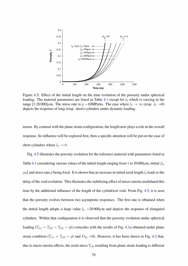
0

0.05

0.1

0.15

0.2

0.25

0.3

0.35

0.4

0 200 400 600 800 1000 1200

Po

rosit

y, f

Time (ns)

l0=1µm, l0=10µm

l0=500µm

l0=1000µm

l0=2000µm

l0=20000µm

(l0→0) (l0→∞)

Figure 4.5: Effect of the initial length on the time evolution of the porosity under sphericalloading. The material parameters are listed in Table 4.1 except for l0 which is varying in therange [1:20 000]µm. The stress rate is p =10MPa/ns. The case where l0 → ∞ (resp. l0 →0)depicts the response of long (resp. short) cylinders under dynamic loading.

tensor. By contrast with the plane strain configuration, the length now plays a role in the overall

response. Its influence will be explored first, then a specific attention will be put on the case of

short cylinders where l0 → 0.

Fig. 4.5 illustrates the porosity evolution for the reference material with parameters listed in

Table 4.1 considering various values of the initial length ranging from 1 to 20 000µm, initial f0,

ρa20 and stress rate p being fixed. It is shown that an increase in initial axial length l0 leads to the

delay of the void evolution. This illustrates the stabilizing effect of micro-inertia modulated this

time by the additional influence of the length of the cylindrical void. From Fig. 4.5, it is seen

that the porosity evolves between two asymptotic responses. The first one is obtained when

the initial length adopts a large value l0 =20 000µm and depicts the response of elongated

cylinders. Within that configuration it is observed that the porosity evolution under spherical

loading (Σ11 = Σ22 = Σ33 = pt) coincides with the results of Fig. 4.1a obtained under plane

strain condition (Σ11 = Σ22 = pt and D33 =0). However, it has been shown in Fig. 4.2 that,

due to micro-inertia effects, the axial stress Σ33 resulting from plane strain loading is different

79

0

200

400

600

800

1000

1200

1400

1600

0 100 200 300 400 500 600 700 800 900 1000

Exte

rnal an

d I

nte

rnal ra

dii,

(µm

)

Time (ns)

a

b

l0→0

l0=810 µm

l0=1000 µm

Figure 4.6: Time evolution, under spherical loading, of the external and internal radii for l0 →0,l0 =810 and 1 000µm. Material parameters, displayed in Table 4.1, are those of Fig. 4.5 withstress rate, p =10MPa/ns.

from pt (which is the case here under spherical loading).

The second asymptotic response, revealed with l0 =1µm, describes the response of short

cylinders (l0 → 0) under dynamic loading. This situation can be retrieved from Eq (4.2) which

also implies that the dynamic stress expressed by Eq (4.1) is not depending on l0. This case of

short cylinders under dynamic loading is investigated now more deeply.

From Fig. 4.5, we isolate the cases l0 →0 and l0 =1 000µm which are obtained for material

parameters listed in Table 4.1 and p =10MPa/ns. Fig. 4.6 displays the time evolution of the

external (b) and internal (a) radii for l0 → 0 and l0 =1 000µm. For further insight, the case

where l0 =810µm is also presented. When the initial length is large enough, e.g. l0 =1 000µm

or larger, the porosity growth is characterized by the increase of the external (b) and internal (a)

void radii. This result is classically expected under quasistatic conditions also. Interestingly,

when l0 →0, the evolution of damage results from the reduction of the external radius b, while

the internal radius a is still increasing. As a consequence, D11 = b/b is negative (after some

time) when l0 →0 and positive when l0 is large, as reflected by Fig. 4.7 where the time evolution

of D11 is displayed. This observation in configuration evolution, revealed for short cylinders,

80

4.4. HYDROSTATIC LOADING 81

a)

-1.2

-1

-0.8

-0.6

-0.4

-0.2

0

0.2

0.4

0 100 200 300 400 500 600 700 800 900 1000

Str

ain

ra

te, D

11, (1

06s

-1)

Time (ns)

l0→0

l0=810µm

l0=1000µm

b)

-0.02

-0.015

-0.01

-0.005

0

0.005

0.01

0.015

0.02

0 100 200 300 400 500 600 700 800 900 1000

Str

ain

rate

, D

11 (

10

6 s

-1)

Time (ns)

l0=810µm

l0=1000µm

l0→0

Figure 4.7: Time evolution, under spherical loading, of D11 for l0 →0, l0 =810 and 1 000µm.Material parameters are displayed in Table 4.1, and the stress rate, p =10MPa/ns. A magnifiedscale, where the y-axis is reduced, is proposed in b).

is counterintuitive and brings new insights in the behavior of porous materials under dynamic

loading. This effect is due to micro-inertia and cannot be observed under quasistatic conditions.

For intermediate values, it is expected that the strain rate oscillates due to the change of sign of

D11. This is confirmed in Fig. 4.7b for l0 =810µm. For this case,D11 is shown to first increase,

then decrease, adopting negative values, and finally increase up to the final stage of the growth

process. Note, from Fig. 4.6, that the late stage of the porosity growth for l0 =810µm is quite

similar to the case where l0 =1 000µm.

In an attempt to identify by analytical means the critical length, denoted by lcr, approx.0 , at which

the porosity evolution switches from onemechanism (increase of the external radius) to another

one (decrease of the external radius), an approximate analysis is proposed. Regarding the large

stress amplitude developed during the process, we first assume that the static stress components

are negligible when compared to the dynamic ones. Under spherical loading, this implies that

Σdyn33 = Σdyn

11 = pt. For the approximate analysis, we also assume that the quadratic terms inD11

and D33 are negligible and that only linear terms in D11 and D33 are held in Eqs (A.31,A.32)

of Appendix A. These assumptions lead to the following relationships:

pt = Σdyn11 = Σdyn

22 =ρa2

4

2f−1 ln

(1

f

)D11 +

[1− f−1 + f−1 ln

(1

f

)]D33

(4.8)

pt = Σdyn33 =

ρa2

4

2

[1 + f−1 ln

(1

f

)− f−1

]D11

+

[f−1 ln

(1

f

)− 1

2

(f−1 − 1

)(3− f)

]D33

+ρl2

3(1− f) D33 (4.9)

82

which give after some manipulations:

(2l2

3b2− 1− f

4

)D33 = D11 (4.10)

where relationship b = f−1/2a has been used. One can substitute D11 expressed by Eq (4.10)

into Eq (4.8) to get:

D33 =4pt

ρb2

[(l2

3b2+

1 + f

2

)ln

(1

f

)+ f − 1

]−1

(4.11)

It can be seen that D33 is strictly positive when p >0 (see Fig. 4.8a). Therefore Eq. (4.10)

reveals that D11 < 0 when l→ 0. The critical length lcr, approx.0 is evaluated from Eq (4.10) with

the conditon D11 =0. Assuming in addition that the porosity and length have slightly evolved,

one obtains:

lcr, approx.0 =

√3 (1− f0)

8b0 (4.12)

Using this last equation with f0 =0.0011, b0 =1 500µm, one has lcr, approx.0 =916µm which is

well compared to 810µm shown in Fig. 4.7.

Eq (4.12) indicates that the critical length solely involves b0 and f0, while being independent

from the stress rate p and other material parameters. Various configurations have been consid-

ered serving at testing the validity of the analytical approximation. From Table 4.2, compiling

all tested cases, one notes that the critical length lcr, approx.0 obtained from the analytical approxi-

mation (4.12), is relatively well predicting the value lcr0 obtained from the complete theory. The

analytical approximation supposes that the micro-inertia effects are strong enough so that the

static stress can be neglected. As a matter of fact, when p is increased, the micro-inertia effects

are enhanced and the value of lcr, approx.0 becomes closer to the value lcr0 captured by the model.

83

p ρ a0 b0 f0 = a20/b

20 σ0 lcr0 l

cr, approx.0

[MPa/ns] [kg/m3] [µm] [µm] / [MPa] [µm] [µm]

ref 10 2 700 50 1 500 0.0011 100 810 916

#1 100 2 700 50 1 500 0.0011 100 880 916

#2 10 2 700 50 1 500 0.0011 200 760 916

#3 10 2 700 150 1 500 0.01 100 800 914

#4 10 2 700 25 750 0.0011 100 390 457

#5 10 2 700 50 750 0.0044 100 390 458

Table 4.2: Various configurations used to compute the critical length for l0 < lcr0 , D11 < 0.The critical value lcr0 , obtained from the complete modeling, is well compared to the analyticalapproximation lcr, approx.0 given by Eq (4.12)

By contrast, when σ0 is increased, one notices from Table 4.2 that the gap between lcr0 and

lcr, approx.0 is getting larger. When b0 is half the reference value, lcr0 obtained from the complete

theory is reduced by a factor of two, thus validating the mathematical dependence on b0 in the

analytical approximation. Finally, lcr0 is also shown to be little sensitive to a variation in f0, as

reflected also from the analytical approximation of Eq (4.12).

The void growth to some extent is controlled by micro-inertia effect, i.e. kinetic energy

stored in the matrix material in the vicinity of the void. For axisymmetric loadings without

shear, the kinetic energy K stored in the unit cell is:

K = Kaxial +Kplane =1

2

∫V

ρv2zdV +

1

2

∫V

ρv2rdV (4.13)

where V = 2πb2l is the volume of the unit cell, vz = D33z and vr =

(2D11+D33

2

)(b2

r

)− D33

2r.

Therefore, the two contributions Kaxial and Kplane can be evaluated in closed form:

Kaxial = ρπD233l

3 b2−a23

(4.14)

Kplane = ρπl[

(trD)2

2b2 ln b

a− tr(D)D33

2b2(b2 − a2) +

D233

8(b4 − a4)

](4.15)

84

4.4. HYDROSTATIC LOADING 85

a)

-1

0

1

2

3

4

5

6

7

8

0 200 400 600 800 1000 1200 1400

Str

ain

rate

, D

33,

(10

6s

-1)

Time (ns)

l0=1µm

l0=500µm

l0=1000µml0=2000µml0=20000µm

b)

-2

0

2

4

6

8

10

12

14

16

0 200 400 600 800 1000 1200

Sp

ecif

ic p

ow

ers

(M

Pa/n

s)

Time (ns)

Kplane/V .

2Σ11dyn D11

l0=500µml0=1000µml0=2000µm

b)

-10

0

10

20

30

40

0 200 400 600 800 1000 1200

Sp

ec

ific

po

wers

(M

Pa/n

s)

Time (ns)

Kaxial/V .

Σ33dynD33

l0=500µml0=1000µml0=2000µm

Figure 4.8: a) Time evolution of D33 under spherical loading, the initial length ranging from1 to 20000µm - Specific powers in b) the plane, see Eq. (4.17), and c) the axial direction, seeEq. (4.18), for l0=500, 1000, 2000µm. Other material parameters are displayed in Table 4.1with stress rate, p =10MPa/ns.

Note that for plane strain loading, or when the initial length adopts very large values,Kaxial = 0

andKplane = 2ρπD211b

2l ln ba. The kinetic energy in the RVE is purely planar. From Eqs (4.14)

and (4.15), expressions for Kaxial and Kplane can be found. Since the matrix material is volume

preserving, then one has: l(b2 − a2) = cst. Therefore, the rate of kinetic energy in the axial

direction is:

Kaxial = 2ρπl3(b2 − a2)

3(D33D33 +D3

33) (4.16)

Similarly, Kplane has been evaluated (results not presented here). For axisymmetric loadings

without shear, the macroscopic dynamic stress is given in Eq (A.33) of Appendix A. The rate

of kinetic energy in the plane direction is found to be related to the dynamic stress as:

Kplane = V (2Σdyn11 D11 + ρa2GD33) (4.17)

The rate of kinetic energy in the axial direction is given by:

Kaxial = V (Σdyn33 D33 − ρa2GD33) (4.18)

So it has been checked that:

Kplane + Kaxial = V Σdyn : D (4.19)

The term V ρa2GD33, which is vanishing under plane strain loading, corresponds to a transfer

term between the two contributions Kplane and Kaxial of the total kinetic energy.

Fig. 4.8a shows the macroscopic strain rate D33 versus time, for the reference material under

spherical loading with parameters listed in Table 4.1 considering various values of the initial

length l0 ranging from 1 to 20 000µm. An increase in initial length l0 induces a decrease in

86

macroscopic strain rateD33 (see Fig. 4.8a). Next, we compare in Fig. 4.8b the rate of work per

unit volume done by the dynamic stress in the plane, 2Σdyn11 D11, to the rate of kinetic energy in

the plane per unit volume Kplane

Vfor three initial lengths l0 = 500, 1000, 2000µm. Fig. 4.8c

displays the corresponding quantities for the axial direction, i.e. Σdyn33 D33 compared to the

rate of external work in the axial direction Kaxial

V. Note that under such high level of imposed

spherical loading (p =10MPa/ns), the static stress playing almost no role in the overall response,

the dynamic stress is closed to pt. As a consequence, the rates of work per unit volume done

by the dynamic stress in the plane 2Σdyn11 D11, and in the axial direction Σdyn

33 D33 could have

been deduced from the time evolution of the strain rate components D11 and D33. The results

of Figs 4.8b and 4.8c illustrate the importance of the transfer term for various lengths. As l0

becomes large, the magnitude of D33 is reduced, so is the magnitude of the transfer term. In

plane strain loading, the rate of external work per unit volume in the plane 2Σ11D11 and the rate

of kinetic energy in the plane per unit volume Kplane

Vwill almost coincide, as the contribution

of the static term is small.

4.5 Additional loading cases

In this section we complement the analysis by first considering the following boundary condi-

tions: (i) homogeneous stress different from hydrostatic loading and (ii) imposed axial strain

rate and homogeneous pressure on the lateral surface.

Stress boundary conditions of two different types are first explored, see Table 4.3. Case 1

corresponds to Σ11 = Σ22 = 0 and Σ33 = pt. Case 2 is obtained for Σ11 = Σ22 = pt, Σ33 = 0.

The stress triaxiality, defined by χ = ΣmΣeq

, is equal to 1/3 and 2/3 for Case 1 and Case 2, re-

spectively. In Case 1, which corresponds to uniaxial stress loading, the void axis is aligned

with the loading direction andD33 is naturally positive under remote extension. For Case 2, the

87

cylinder is stretched in the radial direction. The two cases serve as complementing the spherical

loading addressed previously. Note that within the adopted study, the macroscopic equivalent

stress is pt for both χ = 1/3 (Case 1) and 2/3 (Case 2), while vanishing under spherical load-

ing. A fixed value of the stress rate, p =10MPa/ns, is adopted in this section. The reference

material parameters listed in Table 4.1 are first considered.

Fig. 4.9 shows the time evolution of the porosity for Case 1 and Case 2 when l0 = 2 000µm

(Fig. 4.9a) and l0 =10µm (Fig. 4.9b). The response under spherical loading is also reported

for comparison purpose. The initial porosity is f0 =0.0011 in all calculations. Since a static

analysis provides for the porous material a time to fracture around 10ns for both Case 1 and

Case 2, Fig. 4.9 clearly illustrates that micro-inertia effects are important for all stress triaxial-

ities. Note the stabilizing effect of the length of the cylinder during uniaxial loading (Case 1),

due to an enhancement of global inertia at large value l0 =2 000µm, see Fig. 4.9a. It is seen by

comparing Figs 4.9a and b, that the response under spherical loading is slightly sensitive to a

reduction in l0, see also Fig. 4.5. By contrast, for the two other cases, the porosity evolution is

strongly depending on l0.

Of particular situation, Fig. 4.9a and b show that the void may collapse under loading Case 2

(χ = 2/3). To have a better explanation of the situation, Fig. 4.10a provides the time evolu-

tion of the internal a and external b radii and Fig. 4.10b shows the time evolution of D11 and

D33. In fact, when the top and bottom surfaces of the cylinder are traction-free with p >0

χ = ΣmΣeq

Σ11 = Σ22 Σ33

Spherical loading ∞ p t p t

Case 1 1/3 0 p t

Case 2 2/3 p t 0

Table 4.3: Loading configurations and corresponding triaxialities.

88

4.5. ADDITIONAL LOADING CASES 89

a)

0

0.05

0.1

0.15

0.2

0.25

0.3

0.35

0 500 1000 1500 2000

Po

rosit

y, f

Time (ns)

Spherical loading (χ=∞)

Case 1 (χ=1/3)

Case 2 (χ=2/3)

l0=2000µm

b)

Figure 4.9: Time evolution of the porosity for spherical loading and for Case 1 and Case 2 underdynamic conditions, see Table 4.3. The stress amplitude is pt with p =10MPa/ns. The initiallength is a) l0 =2 000µm, b) l0 =10µm. Other material parameters are listed in Table 4.1.

90 CHAPTER 4. RESULTS

a)

0

500

1000

1500

2000

2500

3000

3500

4000

4500

0 200 400 600 800 1000 1200 1400 1600

Ex

tern

al

an

d I

nte

rna

l ra

dii

, (µ

m)

Time (ns)

Case 2 (χ=2/3)

a

b

b)

-4

-3

-2

-1

0

1

2

0 200 400 600 800 1000 1200 1400 1600

Str

ain

ra

te (

10

6 s

-1)

Time (ns)

Case 2 (χ=2/3)

D11

D33

c)

-0.4

-0.3

-0.2

-0.1

0

0.1

0.2

0.3

0.4

0.5

0.6

0 200 400 600 800 1000 1200 1400 1600

D3

3+

(2D

11)/

(1-f

)

Time (ns)

Case 2 (χ=2/3)

Figure 4.10: Time evolution of a) the void radius a and external radius b and b) the macroscopicstrain rate components D11 and D33 c) D33 + 2 D11

(1−f), for Case 2: Σ11 = Σ22 = pt with

p =10MPa/ns, Σ33 = 0. The initial length is l0 =2 000µm, other material parameters beinglisted in Table 4.1.

imposed in the radial direction (Case 2), the length of the cylinder is naturally reduced (i.e.

D33 <0). At the same time, the external radius is always increased whereas the internal void

radius is first increased before void collapse occurs at the final stage. From Fig. 4.10c, the term

D33 + 2D33/(1 − f) is negative after some time. From Eq (3.8), this means that a <0. This

peculiar behavior results only from micro-inertia. Indeed, in a quasistatic analysis, it can be

easily shown from the Gurson model, that when Σγγ = Σ11 + Σ22 is positive, then Dm > 0.

So the porosity is increasing and no void collapse can occur within a micro-inertia indepen-

dent approach. In addition, in the quasistatic approach l is decreasing while a and b are both

increasing.

Case 2 is investigated more deeply by varying ρ (l0 =2 000µm being fixed, Fig. 4.11a) and l0

(ρ =2 700kg/m3 being fixed, Fig. 4.11b). When ρ is reduced (smaller effects of micro-inertia),

the porosity growth is triggered for earlier time and develops faster. Note that micro-inertia

effects are always included in the complete theory and that void collapse occurs even for low

values of ρ. The static response would be obtained with a very low value of ρ for which, as

previously stated, one would observe an instantaneous growth without collapse (at t '10ns).

The effect of l0 portrayed in Fig. 4.11b confirms the important role of the axial length of the

cylinder on the dynamic response. As l0 is reduced, the collapse process is triggered earlier.

Indeed it can be shown that as l decreases, D33 is still negative but with larger absolute value

(D33 < 0), so the quantity D33 + 2D11/(1 − f) become negative earlier. Remind that the

micro-inertia stress is the sum of two terms, the first being scaled by ρa2, the second by ρl2.

Thus, when l0 → 0 micro-inertia is solely dependent upon the void radius. One finally notes

from Fig. 4.11b that the response obtained with a large value of l0, e.g. l0 =10 000µm, coincide

with the plane strain case of Fig. 4.1, in terms of porosity evolution only.

The uniaxial stress loading (Case 1) is next explored by varying the mass matrix density

91

92 CHAPTER 4. RESULTS

a)

0

0.02

0.04

0.06

0.08

0.1

0.12

0.14

0.16

0 200 400 600 800 1000 1200 1400 1600 1800

Po

rosit

y, f

Time (ns)

ρ=2700kg/m3

ρ=270kg/m3

ρ=27kg/m3

ρ=2.7kg/m3

ρ=0.027kg/m3

→ 1

→ 2

→ 3

→ 4

→ 5

1

2

3

4

5

•

Case 2 (χ=2/3)

b)

0

0.02

0.04

0.06

0.08

0.1

0.12

0.14

0.16

0 200 400 600 800 1000 1200 1400 1600

Po

rosit

y,

f

Time (ns)

Case 2 (χ=2/3)

Plane strain(l0→∞)

l0=10000 µm

l0=2000 µm

l0=1500 µm

l0=1000 µm

l0=10 µm

Figure 4.11: Influence of a) the mass matrix density with l0=2000µm and b) the initial voidlength with ρ=2700kg/m3 for Case 2: Σ11 = Σ22 = pt with p =10MPa/ns, Σ33 = 0. The othermaterial parameters are displayed in Table 4.1. The response with l0 =10 000µm provides theplane strain case of Fig. 4.1, in terms of porosity evolution only.

(with fixed l0 =2 000µm in Fig. 4.12a) and the initial length of the cylinder (ρ =2 700kg/m3

being fixed in Fig.4.12b). Again, when l0 is fixed and ρ is reduced, the micro-inertia effects

are lowered down, and the porosity growth occurs earlier. But, most interestingly, when ρ is

lower than 270kg/m3, the critical porosity fc =0.3 (for which fracture is assumed to occur) is

not reached during the dynamic process. Instead of continuously increasing up to the ultimate

fracture at f = fc, the porosity is reduced and tends to a stabilized value. This plateau is

characterized by the collective decrease of a and b, f being constant. Fig. 4.13a illustrates the

evolution of the internal and external cell radii while Fig. 4.13b presents the time evolution of

D11 and D33. Note from the last figure, that since f ' 0 at late stage of the process, D11 is

close to −D33/2.

Increasing l0 with fixed ρ also favors the occurrence of a plateau. Indeed, from Fig. 4.12b

obtained with ρ =2700kg/m3, it appears that when l0 =5 000µm, the porosity is frozen after

some time (t > 8 000ns) while the cell internal and external radii are still decreasing. When l0

is reduced, the porosity growth is faster and the critical porosity is reached prior to any decrease

in f . Note that a plateau could have been observed by adopting a larger critical porosity fc for

lower values of l0.

The length of the cylinder plays an important role in the dynamic response of cylindrical

voids. In the last two examples, the dynamic behavior may be characterized by a saturation in

porosity evolution or a collapse process. These effects are solely due to micro-inertia.

We now consider the loading path where homogeneous pressure is prescribed on the lateral

surface, Σ11 = Σ22 = pt, while a constant strain rate D33 is imposed in the longitudinal direc-

tion. In that case the displacement of the top surface is following the law: l = l0 exp(D33t).

Fig. 4.14 shows the evolution of the porosity for various values of D33 up to 106s−1 with

p =10MPa/ns (Fig. 4.14a) and p =100MPa/ns (Fig. 4.14b). The reference material of Ta-

93

94 CHAPTER 4. RESULTS

a)

b)

0

0.05

0.1

0.15

0.2

0.25

0.3

0.35

0 1000 2000 3000 4000 5000 6000 7000 8000

Po

rosit

y, f

Time (ns)

Case 1 (χ=1/3)

ρ=2700kg/m3

l0=5000 µm

l0=2000 µm

l0=1000 µm

l0=10 µm

Figure 4.12: Influence of a) the mass matrix density with l0=2 000µm and b) the initial voidlength with ρ=2700kg/m3 on porosity evolution for loading Case 1 (uniaxial stress). The othermaterial parameters are displayed in Table 4.1. The evolution of the axial stress is given byΣ33 = pt with p =10MPa/ns.

4.5. ADDITIONAL LOADING CASES 95

a)

0

200

400

600

800

1000

1200

1400

1600

0 500 1000 1500 2000 2500 3000

Ex

tern

al

an

d I

nte

rna

l ra

dii

, (µ

m)

Time (ns)

Case 1 (χ=1/3)

ρ=270kg/m3

a

b

b)

-1

-0.5

0

0.5

1

1.5

2

2.5

0 500 1000 1500 2000 2500 3000

Str

ain

ra

te (

10

6 s

-1)

Time (ns)

Case 1 (χ=1/3)

ρ=270kg/m3

D33

D11

Figure 4.13: Time evolution of a) the void radius a and external radius b and b) the macro-scopic strain rate components D11 and D33 for loading Case 1 (uniaxial stress with Σ33 = pt,p =10MPa/ns). The initial length is l0 =2 000µm, the mass matrix density is ρ =270kg/m3,other material parameters being listed in Table 4.1.

96 CHAPTER 4. RESULTS

a)

0

0.05

0.1

0.15

0.2

0.25

0.3

0 200 400 600 800 1000 1200

Po

rosit

y, f

Time (ns)

D33=0

D33=10 s-1

,

D33=104 s

-1

D33=105 s

-1

D33=106 s

-1

P

.

=10MPa/ns

b)

0

0.05

0.1

0.15

0.2

0.25

0.3

0 200 400 600 800 1000 1200

Po

rosit

y, f

Time (ns)

D33=10 s-1

, D33=0

D33=104 s

-1

D33=105 s

-1

D33=106 s

-1

P

.

=100MPa/ns

Figure 4.14: Time evolution, under imposed constant strain rate D33 and prescribed Σ11 =Σ22 = pt with a) p =10MPa/ns b) p =100MPa/ns. The initial length is l0 =100µm, othermaterial parameters being listed in Table 4.1.

ble 4.1 is adopted with l0 =100µm. As expected, when the strain rateD33 increases, the poros-

ity growth is accelerated. Most interestingly, when comparing Fig. 4.14a and b, one notes that

whenD33 =106s−1 the evolution of the porosity is almost identical for the two applied pressure

rates, p=10MPa/ns (Fig. 4.14a) and p=100MPa/ns (Fig. 4.14b). In such situation (i.e. under

intense imposed constant strain rate), the void evolution appears to be mostly governed byD33

and quite irrespective of the value of p. Naturally, when D33 =0, the growth process is solely

driven by the stress rate p. For intermediate values, the evolution of the porosity results from

both the influences of p and D33. One has to mention also that if the stress rate p is further

increased, it is expected that for the effect of the lateral stress (pt) to be negligible, larger values

of the strain rate D33 have to be considered.

In the last example, the in-plane macroscopic stress tensor components are stillΣ11 = Σ22 =

pt while a constant velocity v3 = ±v03 is prescribed at x3 = ±l. The corresponding nominal

strain rate isD033 = v0

3/l0 and the displacement at the top boundary is l = l0(1 +D033t). It was

demonstrated from the analysis of Eqs (4.1) and (4.4) conducted at the beginning of section 4.1,

that the term related to l2 in Σdyn33 vanishes. This is exemplified in Fig. 4.15 for the reference

material (parameters given in Table 4.1) considering two cylinder lengths l0 =1 000, 2 000µm

andD033 =105s−1, 106s−1. Note that, as for the configuration of an imposed constant strain rate

addressed previously, the growth process is less dependent on p and is largely influenced by the

imposed axial strain rate when D033 is large, e.g. D0

33=106s−1 in Fig. 4.15.

4.6 Conclusion

It is interesting to highlight the influence of the two geometrical characteristics of the cylin-

drical voids (i.e. length and radius) on damage evolution. It is worth noting that the effects of

void length and radius can be separated. Indeed, the macroscopic dynamic stress in the axial

97

0

0.05

0.1

0.15

0.2

0.25

0.3

0.35

0 100 200 300 400 500 600 700 800 900

Po

ros

ity

, f

Time (ns)

106 s

-110

5 s

-1

v3=100 m/s, l0=1000 µm

v3=200 m/s, l0=2000 µm

v3=1000 m/s, l0=1000 µm

v3=2000 m/s, l0=2000 µm

Figure 4.15: Time evolution of the porosity under imposed in-plane stress Σ11 = Σ22 = ptand constant velocity v0

3 . Calculations are performed for D033 =105s−1 and 106s−1 consider-

ing l0 =1000 and 2000µm which infers various applied constant velocities. Other materialparameters are given in Table 4.1.

direction appears as the summation of two terms: the first (resp. second) term is scaled by the

matrix mass density and the square of the void radius (resp. void length).

A parametric study has been conducted under plane strain configuration, confirming the re-

fraining effect of micro-inertia when modulated by the mass matrix density and the initial void

size. In addition, under plane strain, the axial stress component is found to be decreasing with

time at large deformation. This reflects that the stress needed to constrain the length of the

cylinder is reduced because of micro-inertia.

The influence of the length of the cylindrical void has been revealed. In particular, for spher-

ical stress loading, it has been shown that micro-inertia effects are more important for longer

voids. At the same time, it was shown that two asymptotic responses in the time evolution of

the porosity are emerging from the spherical loading path: the plane strain case is retrieved

when l0 →∞ and the case of short cylinders is obtained from l0 → 0.

The case of short cylinders reveals a peculiar damage evolution. In fact, the porosity is found

to increase due to a reduction of the external radius and an increase of the void radius. This

situation is solely due to micro-inertia effects.

98

The modeling has been applied to stress states with various triaxialities. Under radial ex-

pansion with traction free top and bottom surfaces, the void was found to collapse, at least for

the reference set of material parameters. Under uniaxial stress loading, after an initial void

growth, the porosity may decrease and reach a plateau. Under such case, the late stage of the

deformation process is characterized by a continuous decrease of the internal and external radii.

Predictions of the present model have now to be verified against numerical simulations for

various axisymmetric loading paths. This is the main goal of the next chapter.

99

100

Chapter 5

Finite element modeling

5.1 Introduction

To validate the proposed constitutive model, dynamic micromechanical computations based

on cylindrical unit cells have been carried out with the finite element code ABAQUS/Explicit.

Various axisymmetric models have been developed to depict the dynamic response under i)

plane strain condition ii) hydrostatic loading conditions and iii) other loading cases considered

in the thesis work. Since the matrix material is taken as rigid in the model, a large value of the

Young’s modulus has been adopted (6 300GPa). In addition, to approach the incompressibil-

ity condition for the matrix, a value of 0.499 for the Poisson’s ratio has been used. Otherwise

stated, these values, (E=6300GPa, ν=0.499) are adopted in finite element simulations. We pro-

pose at the end of this chapter, to investigate the influence of both elastic constants on FEM

results.

For all configurations addressed in the thesis, the proposed analytical approach has been ac-

curately compared to results obtained from numerical simulations. Here, only some important

examples from each loading case have been selected to bring the comparison.

101

Figure 5.1: Finite element cylindrical unit cell of length l, inner radius a and external ra-dius b used for various loading cases. The mesh is made with 4 node axisymmetric elements(CAX4R). The element size is 20µm×40µm.

5.2 Plane strain configuration

In this section, the goal is to validate results presented in section 4.3 (Fig. 4.1). For this case,

the unit cell, illustrated on Fig. 5.1, is meshed with 4 node axisymmetric elements with re-

duced integration (CAX4R). The initial element size is about 20µm×40µm. Since the unit cell

is expanded in the radial direction, elements are initially elongated in the axial direction, so

as to prevent the element aspect ratio from excessive values during the deformation process.

Kinematic conditions of the following form are considered on the boundary:

v3(x, t) = 0 on ∂B0, v3(x, t) = 0 on ∂Bl (5.1)

102

which account for the condition of symmetry at ∂B0 and ensure the plane strain condition at

∂Bl. In addition, the following stress boundary conditions prevail (expressed in the cylindrical

coordinate system):

Σr3(x, t) = Σθ3(x, t) = 0 on ∂Bl (5.2)

and

Σrr(x, t) = pt, Σθr(x, t) = Σ3r(x, t) = 0 on ∂Bb (5.3)

while the inner surface ∂Ba is traction free.

For the configuration of section 4.3, Fig. 4.1a, the loading rate is p =10MPa/ns, and material

parameters are listed in Table 4.1. Fig. 5.2 shows that analytical results (solid line) coincidewith

Finite Element simulations (dots). In particular, the reduction of the axial stress Σ33 occurring

at large deformation while the lateral stress is still increasing, is reproduced by both approaches,

as observed in Fig 5.2b. Note that Σ33 is evaluated from the ratio of the axial force on ∂Bl

divided by the current area πb2.

It can be of interest to investigate whether a 2D FEM could provide consistent results in case

of plane strain. Indeed, the length of the cylinder is not playing a role in the response, in terms

of porosity and stress as observed in Eq (A.34) and (A.35). The cell, illustrated in Fig. 5.3a,

is meshed with 4 node plane strain elements with reduced integration (CPE4R). The mesh is

refined in the vicinity of void. More specifically, the mesh size at ∂Ba (resp. at ∂Bb) is 20µm

x 92µm (resp. 589µm x 918µm). The following conditions of symmetry are considered:

vx(x, t) = 0 on ∂By, vy(x, t) = 0 on ∂Bx (5.4)

103

104 CHAPTER 5. FINITE ELEMENT MODELING

0

0.05

0.1

0.15

0.2

0.25

0.3

0 200 400 600 800 1000 1200

Po

rosit

y, f

Time (ns)

Plane strain loading

FEMAnalytical

0

0.5

1

1.5

2

2.5

3

3.5

4

4.5

0 200 400 600 800 1000 1200

Macro

sco

pic

str

ess,

Σ3

3 G

Pa

Time (ns)

FEMAnalytical

Figure 5.2: Comparison between FEM and analytical results for plane strain loading. Timeevolution of a) the porosity and b) the axial stress. The stress rate is p =10MPa/ns. Thereference material with parameters listed in Table 4.1 is considered.

while stress boundary conditions are prescribed as:

Σθr(x, t) = 0, Σrr(x, t) = pt, Σ3r(x, t) = 0 on ∂Bb (5.5)

The inner face ∂Ba remains traction free. As in section 5.2, the stress rate is p=10MPa/ns and

the material parameters of Table 4.1 are considered. Fig. 5.3b shows that the 2D plane strain

model of Fig. 5.3a and axisymmetric model of Fig. 5.1 give identical results.

5.3 Hydrostatic loading

Let us consider the axisymmetric model of Fig. 5.1. Prescribing Σ11 = Σ22 at the external

boundary of the unit cell (r = b) presents no difficulties. Imposing uniform Σ33 on the top sur-

face (0 ≤ r ≤ b) where a void is present for 0 ≤ r ≤ a is not straightforward. To overcome this

difficulty, two strategies have been developed aiming at defining a model able to verify the pro-

posed approach in case of hydrostatic loading. They give identical results and for completeness

purpose, both will be presented in this section.

5.3.1 Boundary conditions inherited from the analytical model

The first approach relies on a two-step formalism. The solution of the considered configuration

(prescribed hydrostatic loading condition) is searched by using the analytical approach pre-

sented in this manuscript. The resulting velocity field in the axial direction, denoted by vth.3 , is

collected and used as boundary condition in the finite element model of Fig. 5.1. Including the

condition of symmetry, the set of kinematic boundary conditions is expressed as:

v3(x, t) = 0 on ∂B0, v3(x, t) = vth.3 on ∂Bl (5.6)

105

106 CHAPTER 5. FINITE ELEMENT MODELING

a)

b)

0

0.05

0.1

0.15

0.2

0.25

0.3

0 200 400 600 800 1000 1200

Po

rosit

y, f

Time (ns)

Plane strain loading

FEM, CAX4RFEM, CPE4R

Analytical

c)

0

0.5

1

1.5

2

2.5

3

3.5

4

4.5

0 200 400 600 800 1000 1200

Macro

sco

pic

str

es

s,

Σ3

3 G

Pa

Time (ns)

FEM, CAX4RFEM, CPE4R

Analytical

Figure 5.3: a) Finite Element model of 2D unit cell of inner radius a and external radius b usedfor the plane strain problem. The mesh is made with 4 node plane strain elements with reducedintegration (CPE4R). Comparison between FEM plane strain model (CPE4R), FEM axisym-metric model (CAX4R) and the analytical approach for the time evolution of b) porosity, f andc) axial stress, Σ33. The reference material with parameters listed in Table 4.1 is considered.The stress rate is p =10MPa/ns.

complemented with the stress boundary conditions expressed by Eqs (5.2-5.3) and assuming

that the void surface is traction free.

One has to mention that under intense imposed velocity vth.3 , the shape of the unit cell can

strongly deviate from its cylindrical shape. As a consequence, a supplementary constraint

turned out to be necessary to prevent the unit cell from unexpected shape change. Specifically,

the nodes located at the inner and outer vertical boundaries of the cylindrical void (∂Ba and

∂Bb in Fig. 5.1) are linked through a set of linear multi-point constraints so that, at each time

of the deformation process, these surfaces remain vertical.

To illustrate the evolution of the cell when inner and outer surfaces are not forced to remain

parallel, we consider the case where both constraints are removed. Fig 5.4a illustrates the

shape change of the unit cell of Fig. 5.1 when linear multi-point constraint equation at the inner

boundary ∂Ba and outer boundary ∂Bb are removed. Correspondingly, Fig. 5.4b illustrates the

time evolution of the ratio a2/b2 evaluated at ∂B0 and ∂Bl superimposedwith the time evolution

of the porosity obtained with the FEM calculation where kinematic constraints (ensuring that

∂Ba and ∂Bb remain planar) are implemented. It will be shown in Fig. 5.7, that this last result

coincides with the analytical approach. Clearly, the ratio a2/b2, which stands as the porosity

when the unit cell keeps its cylindrical shell is heterogeneous along the cylindrical axis when

kinematic constraints are disregarded.

5.3.2 Closed unit-cell

The second approach consists of adopting a closed unit cell composed of a thin layer added at

the top of the cylindrical void, see Fig. 5.5. If the top layer thickness, denoted by tp in Fig. 5.5,

is sufficiently small, the additional domain is of negligible mass. Therefore it should not affect

the overall response of the unit cell under dynamic loading. Thus, imposing the macroscopic

107

108 CHAPTER 5. FINITE ELEMENT MODELING

a)

b)

0

0.05

0.1

0.15

0.2

0.25

0.3

0 100 200 300 400 500 600 700 800 900 1000

Po

rosit

y, f

Time (ns)

a2∂Bl

/b2∂Bl

a2∂B0

/b2∂B0

with constraintswithout constraints

Figure 5.4: a) Shape of the deformed unit cell at the end of the FE calculations for spheri-cal loading achieved by using boundary condition inherited from the analytical model withoutmulti-point constraints on inner ∂Ba and outer ∂Bb boundaries of the unit cell depicted inFig. 5.1. b) Time evolution of the ratio a2/b2 measured at ∂B0 and ∂Bl when multiple kine-matic constraints are disregarded. The evolution of the porosity obtained from the analyticalapproach, which will be shown to coincide with the FEM results when multiple kinematicconstraints are imposed, is superimposed.

Figure 5.5: Closed cylindrical unit cell of length l, inner radius a and external radius b havinga thin plate of thickness tp on the top. CAX4R elements with initial size of 20µm x40µm areused.

stress tensor component at the top layer is immediate. This strategy however requires addi-

tional kinematic constraints in order to prevent the unit cell from excessive and unexpected

distortion. Specifically, the inner surfaces identified by ∂Ba and ∂Btp on Fig. 5.5 as well as the

outer surfaces ∂Bl and ∂Bb remain planar. In addition, the condition of symmetry on ∂B0 still

prevails. The lateral stress pt is prescribed according to Eq (5.3), and the axial stress Σ33 = pt

is imposed at the top surface. The void boundary is stress free.

To show the necessity of above constraints on ∂Ba, ∂Btp , ∂Bl and ∂Bb to remain planar,

FEM calculations have been conducted by removing the kinematic constraints. Fig. 5.6a illus-

trates the irregular distortion due to the lack of multi-point constraint on the outer boundary

∂Bb of the closed unit cell of Fig. 5.5. Fig. 5.6b shows the unexpected distortion of the top plate

because of the removal of multi-point constraint on the top boundary ∂Bl of the closed unit cell.

Similarly the unit cell is unable to remain cylindrical during the deformation stage when the

109

110 CHAPTER 5. FINITE ELEMENT MODELING

a)

b)

c)

Figure 5.6: FEM calculations for hydrostatic loading achieved by applying stress on the topsurface and lateral direction of the closed unit cell of Fig. 5.5. a) without multi-point constrainton the outer boundary ∂Bb, b) without multi-point constraint on the top boundary ∂Bl and c)without multi-point constraint on the inner boundaries ∂Bl and ∂Btp .

0

0.05

0.1

0.15

0.2

0.25

0.3

0 200 400 600 800 1000

Po

rosit

y, f

Time (ns)

hydrostatic loading

FEM-analytical inhertiedFEM-closed unit cell

Analytical

Figure 5.7: Time evolution of the porosity for a porous medium with cylindrical void underspherical loading with p =10MPa/ns and considering the reference material of Table 4.1 withl0 =2000µm. Comparison between analytical results and FEM calculations. The approachbased on the analytically inherited velocity field and the closed unit cell give comparable results.

multi-point constraints on the inner boundaries (∂Ba and ∂Btp) are removed, Fig. 5.6c. The

above case studies prove the necessity of multi-point constraints on the boundaries ( ∂Ba, ∂Btp ,

∂Bl and ∂Bb) of the closed unit cell, so that predictions of FEM calculation and of the model

can be compared.

5.3.3 Validation on the reference case

The two strategies described in previous sections, are compared against analytical results of

Fig. 4.5 obtained for p =10MPa/ns. The half length of the void is l0 =2000µm, other material

parameters are listed in Table 4.1. In our finite element calculation using the closed unit cell

of Fig. 5.5, the thickness of the top layer is tp=10 µm. It was checked that a smaller value do

not affect the response of the unit cell. Fig. 5.7 shows the evolution of the porosity versus time

and serves at verifying the analytical approach. It illustrates also the equivalence between the

two finite element models of sections 5.3.1 and 5.3.2.

111

a)

0

0.05

0.1

0.15

0.2

0.25

0.3

0 100 200 300 400 500 600 700 800

Po

rosit

y, f

Time (ns)

Hydrostatic loading

l0=10µm

FEMAnalytical

b)

0

200

400

600

800

1000

1200

1400

1600

0 100 200 300 400 500 600 700 800

Inte

rnal a

nd

exte

rnal ra

dii,(

µm

)

Time (ns)

Hydrostatic loading

l0=10µm

a

b

FEMAnalytical

Figure 5.8: FEM calculations and analytical results for thin cylinder (l0=10µm) subjected tospherical loading, a) Porosity versus time and b) Internal and external radii vs time. The stressrate is p =10MPa/ns. The reference material with parameters listed in Table 4.1 is considered.The FEM calculations and analytical results give good agreement.

5.3.4 Thin cylinder, l0=10µm

Here we validate the analytical results obtained when considering a thin cylinder with initial

half length l0=10µm. This case has been discussed in section 4.4 (Fig. 4.5 and Fig. 4.6, l0 →0).

The hydrostatic loading is achieved using the strategy developed in section 5.3.1 (boundary

condition inherited from the analytical velocity). As revealed in section 4.4, for thin cylinder

under spherical loading the porosity growth results from a decrease of external radius b and an

112

0

0.05

0.1

0.15

0.2

0.25

0.3

0 200 400 600 800 1000

Po

rosit

y, f

Time (ns)

P.=10MPa/ns

l0=100µm

D33=105 s

-1

AnalyticalFEM

Figure 5.9: Time evolution of porosity validation of analytical results with FEM calculation.A constant strain rate is imposed on the top surface ∂Bl D33=105s−1 and a prescribed stressΣ11=Σ22=pt is applied on ∂Bb. The initial length is l0 =100µm, other material parameters listedin Table 4.1 are considered. The FEM calculation and analytical results are in good agreement.

increase of internal radius a. Here we compare the evolution of the porosity and damage growth

mechanism predicted by the analytical approach and the results obtained from FEM. Fig. 5.8

illustrates the perfect match between the two approaches (FEM and analytical) regarding the

porosity growth (Fig. 5.8a) and the evolution of the internal and external void radii (Fig. 5.8b).

5.4 Additional loading cases

Additional loading cases considered in the thesis are verified against numerical results obtained

using the axisymmetric unit cell of Fig. 5.1.

5.4.1 Imposed axial strain rate (D33=constant) with combined stress

imposed on the lateral surface

In this section, we validate the analytical results obtained when the loading path consists of a

homogeneous stress prescribed on the lateral surface, Σ11=Σ22=pt, while a constant strain rate

D33 is imposed in the longitudinal direction. In section 4.5 (Fig. 4.14a) the porosity evolution

113

0

0.05

0.1

0.15

0.2

0.25

0.3

0 500 1000 1500 2000 2500 3000

Po

rosit

y, f

Time (ns)

Case 1 (χ=1/3)

FEMAnalytical

Figure 5.10: Time evolution of porosity comparison of FEM calculations and analytical re-sult for uniaxial stress loading configuration: Σ11=Σ22=0 and Σ33=pt (Case 1, χ=1/3). Thestress rate is p=10MPa/ns. Parameters for the reference material are listed in Table 4.1 withl0=2000µm and ρ=270Kg/m3.

has been illustrated for D33 ranging from 0 to 106s−1 under stress rate p=10MPa/ns. The case

whereD33=105s−1 is selected here considering the material parameters of Table 4.1 with initial

void half length, l0 = 100µm. Fig 5.9 clearly provides a validation of the analytical modeling

from the very good comparison with the finite element calculations.

5.4.2 Uniaxial loading: Case 1, χ=1/3

As explained in section 4.5, Case 1 corresponds to Σ11=Σ22=0, Σ33=pt and reflects the uniaxial

stress loading configuration for which the triaxiality χ = Σm

Σeqis equal to 1/3. Numerical results

are obtained using the axisymmetric unit cell of Fig. 5.1, therefore, the boundary condition

Σ33 = pt is replaced by a kinematic velocity field derived from the analytical model.

We have chosen a matrix mass density of ρ = 270kg/m3 for validation with FEM calculations.

The initial length is l0=2000µm and the loading rate is p=10MPa/ns, see also Fig. 4.12a. Other

material parameters of Table 4.1 are considered. This case is particularly selected because

as observed in Fig. 4.12a, after reaching a maximum porosity (less than the critical porosity

114

a)

0

0.02

0.04

0.06

0.08

0.1

0.12

0.14

0.16

0 200 400 600 800 1000 1200 1400 1600

Po

rosit

y, f

Time (ns)

Case 2 (χ=2/3)

l0=2000µ m

FEMAnalytical

b)

0

0.0002

0.0004

0.0006

0.0008

0.001

0.0012

0 50 100 150 200 250

Po

ros

ity, f

Time (ns)

Case 2 (χ=2/3)

l0=10µ m

FEMAnalytical

Figure 5.11: FEM calculations and analytical result comparison for loading case Σ11=Σ22=ptand Σ33=0 (case 2, χ=2/3) a) l0=2000µm b) l0=10µm. The stress rate is p=10MPa/ns. Thereference material with parameters listed in Table 4.1 is considered.

fc=0.3 for which fracture is assumed to occur), the porosity falls and reaches a stabilized value

(a plateau is observed). Fig. 5.10 illustrates this peculiar response under uniaxial loading and

very good agreement between FEM and analytical results.

5.4.3 Biaxial loading: Case 2, χ=2/3

In this section, we consider the loading Case 2 and two values of the initial length: l0=10µm

and 2000µm, see section 4.5. Recall that Case 2 corresponds to a biaxial loading where

Σ11=Σ22=pt, Σ33=0. The corresponding triaxiality is 2/3. In that case, the unit cell is expand-

115

ing in the radial direction. Under such loading configuration, the void is shown to collapse for

the two values of l0, considered in Figs 4.9a and 4.9b. Figs 5.11a and 5.11b illustrate the vali-

dation of the two above analytical cases with FEM calculations. The model provides accurate

prediction since FEM and analytical model results coincide. In particular, when l0=2000µm

(Fig. 5.11a), the porosity is first increasing up to 0.1415 obtained from FEM, while a very close

value of 0.14 is revealed with the analytical approach.

5.5 Influence of the elastic properties

In all examples investigated above, a large value of the Young modulus E=6300GPa and of the

Poisson ratio ν=0.499 has been adopted. In this section, we discuss the effect of elastic proper-

ties by varying E and v, considering still the axisymmetric model of Fig. 5.1. Again, plane strain

and hydrostatic loading conditions are selected with material parameters listed in Table 4.1. To

illustrate the effect of elastic compressibility of the matrix in FEM calculation, two values of

the Poisson ratio have been tested (ν=0.33 and ν=0.499). So FEM calculations are carried out

for (i) E=70GPa and ν=0.33 (representative of aluminium) and (ii) E=70GPa and ν=0.499 (to

approach incompressibility condition). Fig. 5.12 illustrates the time evolution of the porosity

obtained from numerical simulations considering both sets of elastic constants compared to the

analytical result. It is clear that the FEM calculation with E=70GPa and ν=0.499 shows very

close agreement with the analytical model for plane strain (Fig. 5.12a) and hydrostatic loadings

(Fig. 5.12b). This figure has motivated our choice of adopting ν=0.499 for all loading cases.

The Young modulus is now varied, adopting the value of ν = 0.499. Fig. 5.13 shows the

FEM results for E=0.7, 6.3, 70 and 6300GPa. Plane strain loading (Fig. 5.13a-b) corresponding

to results of Fig. 5.2 and hydrostatic loading (Fig. 5.13c) corresponding to results of Fig. 5.7 are

tested. The FEM calculations show that the variation of the Young modulus has only a slight

116

5.5. INFLUENCE OF THE ELASTIC PROPERTIES 117

a)

0

0.05

0.1

0.15

0.2

0.25

0.3

0 200 400 600 800 1000 1200

Po

rosit

y, f

Time (ns)

Plane strain loading

E=70GPa

FEM, ν=0.33FEM, ν=0.499

Analytical

b)

0

0.05

0.1

0.15

0.2

0.25

0.3

0 100 200 300 400 500 600 700 800

Po

rosit

y,

f

Time (ns)

Hydrostatic loading

E=70GPa

FEM, ν=0.33FEM, ν=0.499

Analytical

Figure 5.12: Time evolution of the porosity. FEM calculations for two Poisson’s ratio=0.499and 0.33 with Young’s modulus E=70GPa under a) plane strain loading b) hydrostatic load-ing. Model predictions are also displayed. The loading rate is p =10MPa/ns. The materialparameters listed in Table 4.1 are considered.

118 CHAPTER 5. FINITE ELEMENT MODELING

a)

0

0.05

0.1

0.15

0.2

0.25

0.3

0 200 400 600 800 1000 1200

Po

rosit

y, f

Time (ns)

Plane strain loading

ν=0.499

E=6300GPaE=70GPa

E=6.3GPaE=0.7GPa

b)

0

0.5

1

1.5

2

2.5

3

3.5

4

4.5

5

0 200 400 600 800 1000 1200

Macro

sco

pic

ax

ial str

ess,

Σ G

Pa

Time (ns)

Plane strain loading

ν=0.499

E=0.7GPaE=6.3GPaE=70GPa

E=6300GPa

c)

0

0.05

0.1

0.15

0.2

0.25

0.3

0 100 200 300 400 500 600 700 800 900 1000

Po

ros

ity, f

Time (ns)

Hydrostatic loading

ν=0.499

E=6300GPaE=70GPa

E=6.3GPaE=0.7GPa

Figure 5.13: Comparison of FEM calculations for various Young modulus, E=0.7, 6.3, 70 and6300GPa under a) Plane strain loading b) Hydrostatic loading. The Poisson ratio is 0.499.Time evolution of the porosity for p =10MPa/ns. The material parameters listed in Table 4.1is considered.

effect on the porosity evolution as depicted in Fig. 5.13a) and c). The perfect match between

the analytical prediction and FEM calculations are observed for the highest value E=6300GPa.

It has been checked that a further increase in Young modulus gives the same response as in

the case E=6300GPa. More important is the corresponding evolution of the macroscopic axial

stress Σ33, see Fig. 5.13b. It is observed that the macroscopic axial stress shows some oscilla-

tions when E≤70GPa. In fact, one can correlate the time period of oscillations to the time for

an elastic wave to go back and forth from the outer to the inner boundaries of the cylindrical

cell. In addition, since ν=0.499 is kept fixed for all calculations, the elastic wave speed is pro-

portionnal to the Young modulus. As a consequence:

- when E is multiplied by approx. 10 (from 0.7 to 6.3), the number of oscillations is multi-

plied by approx.√

10.

- When E is multiplied by 100 (from 0.7 to 70), the number is multiplied by 10.

In the case where E=6300GPa, the oscillation is vanished until the porosity reaches 0.3. At

the end, to be consistent with the analytical results and to avoid oscillations, we have selected

the largest Young modulus value, E=6300GPa for all loading cases in this thesis.

119

120

Chapter 6

Conclusion and perspectives

The objective of this thesis was to propose a model of damage by growth of cavities for dy-

namic loading. The porous materials considered in this work contain parallel cylindrical voids.

These voids are representative of perforated structures or honeycomb architectural materials.

The goal was to highlight the influence of two characteristic lengthscales of the unit cell (radius

and length).

The results obtained from the model were checked by comparison with numerical simu-

lations performed on finite element models developed in the PhD. Many loading cases were

considered and new results were presented in the thesis. In particular, during a plane strain

loading, we show that the axial stress decreases while the stresses in the plane direction con-

tinue to increase. This result reflecting that the stress required to maintain a porous structure

at its initial length is reduced due to micro-inertial effects, can be used to design elements for

machines for dynamic testing. The case where thin structures are subjected to dynamic spheri-

cal loading revealed unexpected behavior. The damage increases by increasing the void radius

together with the reduction of the external radius. This trend can only be attributed due to

micro-inertia.

121

In addition to plane strain and hydrostatic conditions, the model has been tested for addi-

tional loading configurations to reveal particular tendencies. For example, the void collapses

during rapid biaxial expansion. In dynamic traction after an initial increase, the porosity seems

to saturate when the voids are long enough and the inertial effects are significant.

The PhD work opens new perspectives. We will mention only some of them. First of all, the

matrix was considered here as rigid perfectly plastic. The stabilizing effects related to dynamic

loading in our approach results only from the inertia effects related to the size of the voids. The

literature has shown that viscous effects can play an important role in the evolution of dynamic

damage. Therefore it is expected that for real material, porosity evolution depends on the com-

bined influence of viscous and micro-inertial effects. The first continuation of this work could

be to include strain rate sensitivity in the rheological response of the matrix. It is important

to note that this will lead to an adjustment in the quasi-static contribution (i.e. independent

of micro-inertia effects) and will not affect the analytical expressions of the inertial contribu-

tion that are obtained in this work. After taking into account viscous effects in the extended

approach, it seems appropriate to us to implement the model for comparison purposes to ex-

perimental tests conducted on ductile materials whose dynamic behavior of the matrix would

have to be identified. The effect of hardening and thermal softening could be also of interest.

In our approach, the adopted RVE and associated velocity fields are defined for a hollow

cylinder. This elementary configuration allows us to highlight the differential micro-inertia

effects between the macroscopic contribution in the plane, and in the axial direction of the

cylinder. An interesting way to extend our model is to consider cylindrical voids fully embed-

ded in the matrix. Based on approaches from the literature, we aim to adopt an elementary unit

cell domain containing a void surrounded by deformable matrix, similar to the RVE considered

by Morin et al. [27].

122

Finally, the results obtained at LEM3 for spherical voids showed the significant importance

of void size distribution parameters on the dynamic response of porous materials. It could also

be interesting to consider distribution in size (a) and shape ratio (l/a) on the dynamic response

of a porous structure containing a heterogeneous population of cylindrical voids.

123

124

Appendix A

Formulation of the macroscopic dynamic

stress tensor, Σdyn.

A.1 General formulation

The macroscopic dynamic stress tensor Σdyn is evaluated in this section with use of the follow-

ing kinematic boundary condition:

v = L · x on ∂V , (A.1)

with x being the position vector. L is the macroscopic velocity gradient tensor, related to the

macroscopic strain rate D and spin tensor Ω by the following relationships:

D =L + tL

2, Ω =

L− tL

2. (A.2)

125

With the boundary condition (A.1), Eqs (2.27) and (2.32) become:

Σ : tL = 〈σ : d〉+1

2〈ρd|v|

2

dt〉 , (A.3)

Σ : tδL =∂〈Φ〉∂D

: δD + Σdyn : tδL , (A.4)

with

Σdyn : tδL = 〈ργ · δv〉 =1

|V |

∫V

ργδvdV . (A.5)

More information can be found in Molinari and Mercier [26].

The dynamic stress tensor Σdyn is evaluated considering that the porous material is repre-

sented by the hollow cylinder and that the approximate velocity field is of the form:

v = L · x+Bx (A.6)

where B = 3Lm

2

(br

)2 − L33

2and L is defined as in Eq (2.10). The adopted velocity field

satisfies the kinematic condition (A.1) together with the matrix incompressibility condition.

From Eq (A.6), the variation of the velocity δv due to the change δL of L at the boundary and

the acceleration are:

δv = δL · x+ δBx , (A.7)

γ =˙L · x+ L · v + Bx+Bv , (A.8)

126

where v = v1e1 + v2e2. In Eq (A.8), the term B is given by:

B =3

2

(b

r

)2[Lm + 3Lm

2 − 3

(b

r

)2

Lm2

]− L33

2(A.9)

Combining Eqs (A.6-A.8), the integral term I = 1|V |

∫Vργδv of Eq (A.5) can be written as:

I =1

|V |

∫V

ργδvdV =1

|V |

∫V

ρ(x · t ˙L · δL · x+ v · tL · δL · x+ BδBx · x+BδBv · x

+ Bx · δL · x+Bv · δL · x+ δBx · ˙L · x+ δBx · L · v)dV (A.10)

The volume |V | of the RVE is 2lπb2. Note that particles are present only for a ≤ r ≤ b. After

some calculations leading to an explicit relation for I = 1|V |

∫VργδvdV , using the following

decomposition of δL:

δL = δL(12) + δL(x3) + δL(3x) + δL33e3 ⊗ e3 (A.11)

with

δL(12) =

δL11 δL12 0

δL21 δL22 0

0 0 0

δL(x3) =

0 0 δL13

0 0 δL23

0 0 0

δL(3x) =

0 0 0

0 0 0

δL31 δL32 0

(A.12)

127

I is written as:

I =ρa2

4

(f−1 − f

) ( ˙L + C−D33 L

)+ 6

(f−1 − 1

)Dm L

+

[ (f−1 − 1

)(C11 + C22 − D33 +

D233

2

)− 9

2

(f−2 − f−1

)D2

m

+ 3f−1 ln

(1

f

)(Dm + 3D2

m −DmD33

)]I

: tδL(12)

+ρa2

4

[ (f−1 − f

)( ˙L + C− D33

2L

)+ 3

(f−1 − 1

)Dm L

]: tδL(3x)

+ρl2

3

[(1− f)

(˙L + C− D33

2L

)+

3

2ln

(1

f

)Dm L

]: tδL(x3)

+

ρa2

4

[ (f−1 − f

)(D33

2− D2

33

4− C11 + C22

2

)− 9

2

(f−2 − f−1

)D2

m

+(f−1 − 1

)(C11 + C22 + 3DmD33 +

D233

2− 9D2

m − D33 − 3Dm

)+ 3f−1 ln

(1

f

)(Dm +

9

2D2

m −DmD33

)]+ρl2

3(1− f)

(D33 + C33

)δL33 (A.13)

where

L =

L11−L22

2L12 L13

L21L22−L11

2L23

L31 L32 L33

, (A.14)

C = L · L.

C =

C11−C22

2C12 C13

C21C22−C11

2C23

C31 C32 C33

. (A.15)

By identification (the components of δL, being independent terms), the dynamic macroscopic

128

stress tensor Σdyn is obtained from Eq (A.5):

Σdyn11 =

ρa2

4

[ (f−1 − f

) ( ˙D11 + C11 −D33D11

)− 9

2

(f−2 − f−1

)Dm

2

+ 3f−1 ln

(1

f

)(Dm + 3Dm

2 −DmD33

)+(f−1 − 1

)(D332

2− D33 + C11 + C22 + 6DmD11

)](A.16)

Σdyn22 =

ρa2

4

[ (f−1 − f

) ( ˙D22 + C22 −D33D22

)− 9

2

(f−2 − f−1

)Dm

2

+ 3f−1 ln

(1

f

)(Dm + 3Dm

2 −DmD33

)+(f−1 − 1

)(D332

2− D33 + C11 + C22 + 6DmD22

)](A.17)

Σdyn33 =

ρa2

4

[ (f−1 − f

)(D33

2− D2

33

4− C11 + C22

2

)− 9

2

(f−2 − f−1

)D2

m

+(f−1 − 1

)(C11 + C22 + 3DmD33 +

D233

2− 9D2

m − D33 − 3Dm

)+ 3f−1 ln

(1

f

)(Dm +

9

2D2

m −DmD33

)]+ρl2

3(1− f)

(D33 + C33

)(A.18)

Σdyn12 =

ρa2

4

[(f−1 − f

)(L12 + C12 −D33L12) + 6

(f−1 − 1

)DmL12

](A.19)

Σdyn21 =

ρa2

4

[(f−1 − f

)(L21 + C21 −D33L21) + 6

(f−1 − 1

)DmL21

](A.20)

129

Σdyn13 =

ρl2

3

[(1− f)

(L13 + C13 −

D33

2L13

)+

3

2ln

(1

f

)DmL13

](A.21)

Σdyn23 =

ρl2

3

[(1− f)

(L23 + C23 −

D33

2L23

)+

3

2ln

(1

f

)DmL23

](A.22)

Σdyn31 =

ρa2

4

[(f−1 − f

)(L31 + C31 −

D33

2L31) + 3

(f−1 − 1

)DmL31

](A.23)

Σdyn32 =

ρa2

4

[(f−1 − f

)(L32 + C32 −

D33

2L32) + 3

(f−1 − 1

)DmL32

](A.24)

Note that L11 = D11, L22 = D22, L33 = D33 and Lm = Dm = (D11 + D22 + D33)/3.

The dynamic stress tensor reveals particular aspects that are commented in the main text, see

section 3.2.

A.2 Case where Ω = 0

The case where L is symmetric, i.e. L = D, corresponds to the velocity field (3.15) of

section 3.1. The dynamic stress tensor components Σdyn11 , Σdyn

22 and Σdyn33 are still given by

Eqs (A.16), (A.17) and (A.18) respectively. Since C = D · D in this case, and thus is symmet-

ric, the other components are obtained directly from Eqs (A.19-A.24), leading to:

Σdyn12 = Σdyn

21 =ρa2

4

[(f−1 − f

)(D12 + C12 −D33D12) + 6

(f−1 − 1

)DmD12

](A.25)

130

Σdyn13 =

ρl2

3

[(1− f)

(D13 + C13 −

D33

2D13

)+

3

2ln

(1

f

)DmD13

](A.26)

Σdyn23 =

ρl2

3

[(1− f)

(D23 + C23 −

D33

2D23

)+

3

2ln

(1

f

)DmD23

](A.27)

Σdyn31 =

ρa2

4

[(f−1 − f

)(D13 + C13 −

D33

2D13) + 3

(f−1 − 1

)DmD13

](A.28)

Σdyn32 =

ρa2

4

[(f−1 − f

)(D23 + C23 −

D33

2D23) + 3

(f−1 − 1

)DmD23

](A.29)

Relationships (3.33-3.40) of chapter 2, section 3.2 are therefore retrieved. As also stated in

section 3.2, the dynamic stress tensor is not symmetric even when spin effects are disregarded.

This result is due to the geometrical configuration of the RVE which is not isotropic. Note

that for spherical voids, Molinari and Mercier [26] showed that without spin contribution the

dynamic stress tensor is symmetric.

A.3 Axisymmetric case

For an axisymmetric configurationwithout shear contributions, the velocity field used by Tracey

[42] is of the form of Eq (3.15) with D expressed as:

D =

D11 0 0

0 D11 0

0 0 D33

, (A.30)

131

From Eqs (A.16-A.18, A.25-A.29), the only non zero components of Σdyn are:

Σdyn11 = Σdyn

22 =ρa2

4

2f−1 ln

(1

f

)D11 +

[1− f−1 + f−1 ln

(1

f

)]D33

− 2

[f−2 − f−1 − 2f−1 ln

(1

f

)]D2

11 −1

2(1− f)2 f−2D2

33

− 2

[f−2 − f−1 − f−1 ln

(1

f

)]D11D33

(A.31)

Σdyn33 =

ρa2

4

2

[1 + f−1 ln

(1

f

)− f−1

]D11 +

[f−1 ln

(1

f

)− 1

2

(f−1 − 1

)(3− f)

]D33

−2

[(1 + f) f−2 − 3f−1 ln

(1

f

)− 2

]D2

11−1

4

[f−2 (1− f)3 + f−2 − 1− 2f−1 ln

(1

f

)]D2

33

− 2

[f−2 − 1− 2f−1 ln

(1

f

)]D11D33

+ρl2

3(1− f)

(D33 +D2

33

)(A.32)

For the purpose of concise notation, we can also write:

Σdyn11 = Σdyn

22 = ρa2F ,Σdyn33 = ρa2G+

ρl2

3(1− f)

(D33 +D2

33

)(A.33)

where functions F and G, identified from Eqs (A.31-A.32), are related to the porosity f , the

strain rate components D11 and D33 and their time derivative D11 and D33.

In addition to the previous axisymmetric configuration, under plane strain conditions,D33 =

0, the following relationships are obtained:

Σdyn11 = Σdyn

22 =ρa2

2

f−1 ln

(1

f

)D11 − f−1

[f−1 − 2 ln

(1

f

)− 1

]D2

11

(A.34)

132

Σdyn33 =

ρa2

2

[f−1 ln

(1

f

)− f−1 + 1

]D11 −

[(1 + f) f−2 − 3f−1 ln

(1

f

)− 2

]D2

11

(A.35)

Note that when D33 = 0 (i.e. the length of the cylinder remains constant, l = l0), the porosity

evolution is solely governed by D11 through f = 2(1 − f)D11. Using in addition Eq (A.34)

and a/a = D11/f (matrix volume preserving) and since the static stress is expressed in terms

ofD11 and f , it appears that under imposed in plane stress (i.e. Σ11 is known), the radial strain

rate componentD11 can be obtained. As a consequence, whenD33 = 0, one can determine the

porosity evolution from knowing the stress components in the (e1, e2) plane. But, interestingly,

inertia effects are transferred also to the axial component of the stress tensor Σdyn33 . This implies

that limiting the analysis to the 2D plane configuration may leave aside substantial information

on the role played by micro-inertia. As a matter of fact, the axial stress needed to constrain the

length of the cylinder in a dynamic problem cannot be captured by such 2D in plane approach,

see Appendix C.

133

134

Appendix B

Analytical relationships for the

quasi-static macroscopic stress, Σstatic.

The analytical expression for the static stress tensor Σstatic proposed by Sartori et al. [35] is

specified in this appendix. Consider the unit cell of Fig. 3.1 and the Gurson yield function for

cylindrical void embedded into a perfectly plastic matrix (see Eq (3.46)). Under axisymmetric

loading (Ceq=1 in Eq 3.46), following Sartori et al. [35], the closed form expressions for quasi-

static macroscopic stress tensor components are given as:

Σstatic11 = Σstatic

22 = σ0β1 (B.1)

Σstatic33 = σ0(β1 + β2) (B.2)

with,

β1 =1√3

ln(W +√

W2 − 1)sgn(trD) (B.3)

135

β2 =D33

√3

trDf sinh(

√3β1) (B.4)

W =

−1 +

√1 + 3

(D33

trD

)21 + f 2 + 3f 2

(D33

trD

)23f

(D33

trD

)2 (B.5)

where sgn(·) stands for the sign of (·). In addition to the previous axisymmetric condition,

under plane strain condition,D33=0 in Eqs (B.3-B.4), the following relationships are obtained:

β1 =1√3

ln

(1

f

), β2 = 0 (B.6)

Σstatic11 = Σstatic

22 = Σstatic33 =

σ0√3

ln

(1

f

)sgn(D11) (B.7)

It thus appears that under plane strain loading, the quasi-static stress tensor Σstatic is spherical.

As explained in detail in chapter 3, this is not the case for the total macroscopic stress tensor

Σ = Σstatic + Σdyn.

136

Appendix C

Formulation of the macroscopic dynamic

stress tensor (Σdyn) for 2D approach.

In this appendix, the 2D case problem under axisymmetric loading is investigated. Therefore

the main differences between 3D and 2D approaches can be presented in a clear way. Of course

this analysis makes sense only for plane strain configuration.

Under plane strain axisymmetric loadingwithout shear contributions, themacroscopic strain

rate is:

D =

D11 0 0

0 D11 0

0 0 0

, (C.1)

As a consequence, from incompressibility condition the radial component of v is:

vr =D11b

2

r(C.2)

137

From the conservation of momentum, one has

∂σrr∂r

+σrr − σθθ

r= ργr,

∂σzz∂z

= 0 (C.3)

By integration from a to b with |σrr − σθθ| = 2√3σ0 and σθθ > σrr.

σrr(r = b) =

∫a

b 2√3σ0dr

r+

∫a

b

ργrdr (C.4)

From Eq (C.2), the radial acceleration γr is:

γr = (D11 + 2D211)b2

r−D2

11

b4

r3(C.5)

Therefore one gets

σrr(r = b) =2√3σ0 ln

(b

a

)+ρa2

2(D11 + 2D2

11)1

fln

(1

f

)+ ρ

D211

2

a2

f

(1− 1

f

)(C.6)

Finally one obtains the following macroscopic dynamic stress components:

Σdyn11 = Σdyn

22 =ρa2

2

[f−1 ln

(1

f

)D11 −D2

11

1

f 2− 1

f− 2f−1 ln

(1

f

)](C.7)

which is equivalent to Eq (A.34).

Alternatively, Σdyn is also defined from:

Σdyn : δD =1

|V |

∫ργ · δvdV (C.8)

138

With Eq (C.2), one obtains:

δvr =b2

rδD11, and Σdyn : δD = 2Σdyn

11 δD11 (C.9)

With recourse to the definition of γ given by Eq (C.5), the right hand side of Eq (C.8) is

evaluated, leading to Eq (C.7).

Note that from Eq (C.8) combined to Eq (C.1) which restricts the analysis to a 2D approach,

Σdyn33 cannot be evaluated. In fact, one has to use the complete theory developed in the PhD

which allows an explicit relationhip for Σdyn33 valid under plane strain loading.

139

140

Bibliography

[1] Barthélémy, R., Jacques, N., Kerampran, S., and Vermeersch, F. (2016). Modelling of

micro-inertia effects in closed-cell foams with application to acoustic and shock wave prop-

agation. International Journal of Solids and Structures, 97-98:445 – 457.

[2] Benzerga, A. A., Besson, J., and Pineau, A. (1999). Coalescence-Controlled Anisotropic

Ductile Fracture. Journal of Engineering Materials and Technology, 121:221.

[3] Benzerga, A. A. and Leblond, J. B. (2010). Ductile Fracture by Void Growth to Coales-

cence. Advances in Applied Mechanics, 44:169–305.

[4] Budiansky, B., Hutchinson, J. W., and Slutsky, S. (1982). Void growth and collapse in vis-

cous solids. in H. G. Hopkins, M. J. Sewell (Eds.), Mechanics of Solids. Oxford: Pergamon

Press.

[5] Carroll, M. M. and Holt, A. C. (1972). Static and Dynamic Pore Collapse Relations for

Ductile Porous Materials. Journal of Applied Physics, 43:1626–1636.

[6] Cortes, R. (1992). The growth of microvoids under intense dynamic loading. International

Journal of Solids and Structures, 29:1339–1350.

[7] Curran, D. R., Seaman, L., and Shockey, D. A. (1987). Dynamic failure of solids. North-

Holland, Amsterdam, 147, Nos. 5-6:253–388.

141

[8] Czarnota, C., Jacques, N., Mercier, S., and Molinari, A. (2008). Modelling of dynamic

ductile fracture and application to the simulation of plate impact tests on tantalum. Journal

of the Mechanics and Physics of Solids, 56:1624–1650.

[9] Czarnota, C., Mercier, S., and Molinari, A. (2006). Modelling of nucleation and void

growth in dynamic pressure loading, application to spall test on tantalum. International

Journal of Fracture, 141:177–194.

[10] Czarnota, C., Molinari, A., and Mercier, S. (2017). The structure of steady shock waves

in porous metals. Journal of the Mechanics and Physics of Solids, 107:204–228.

[11] Dorothy, H. L. and Longère, P. (2019). Unified modelling of adiabatic shear banding

and subsequent micro-voiding driven dynamic failure of viscoplastic solids. International

Journal of Impact Engineering, 132:103322.

[12] Glennie, E. B. (1972). The dynamic growth of a void in a plastic material and applica-tion

to fracture. Journal of the Mechanics and Physics of Solids, 3:415–429.

[13] Gologanu, M., Leblond, J. B., and Devaux, J. (1993a). Approximate models for duc-

tile metals containing non-spherical voids-Case of axisymmetric prolate ellipsoidal cavities.

Journal of the Mechanics and Physics of Solids, 41:1723–1754.

[14] Gologanu, M., Leblond, J. B., Devaux, J., andMolinari, A. (1993b). Approximate models

for ductile metals containing nonspherical voids - case of axisymmetric prolate ellipsoidal

cavities. Journal of the Mechanics and Physics of Solids, 41:1723–1754.

[15] Gurson, A. L. (1977). Continuum theory of ductile rupture by void nucleation and growth.

Journal of Engineering Materials and Technology, 99:2–15.

142

[16] Jacques, N., Czarnota, C., Mercier, S., and Molinari, A. (2010). A micromechanical con-

stitutive model for dynamic damage and fracture of ductile materials. International Journal

of Fracture, 162:159–175.

[17] Jacques, N., Mercier, S., and Molinari, A. (2012). Effects of microscale inertia on dy-

namic ductile crack growth. Journal of the Mechanics and Physics of Solids, 60:665–690.

[18] Klöcker, H. and Montheillet, F. (1988). Modeling the Ductile Growth of Voids At High

Strain Rates. Le Journal de Physique Colloques, 49:C3–313–318.

[19] Leblond, J. B., Perrin, G., and Suquet, P. (1994). Exact results and approximate models

for porous viscoplastic solids. International Journal of Plasticity, 10:213–235.

[20] Leblond, J. B. and Roy, G. (2000). A model for dynamic ductile behavior applicable for

arbitrary triaxialities. Comptes Rendus de l’Académie des Sciences - Series IIB - Mechanics,

328:381–386.

[21] Longère, P. (2018). Adiabatic shear banding assisted dynamic failure: Some modeling

issues. Mechanics of Materials, 116:49 – 66.

[22] Mayya, A., Banerjee, A., and Rajesh, R. (2018). Role of porosity and matrix behavior on

compressive fracture of haversian bone using random spring network model. Journal of the

Mechanical Behavior of Biomedical Materials, 83:108–119.

[23] McClintock, F. M. (1968). On Void Coalescence Under Combined Tension and Shear.

Journal of Applied Mechanics, 82:71005–71015.

[24] Meyers, M.A. andAimone, C. T. (1983). Dynamic fracture (spalling) ofmetals. Materials

Science, 28:1–96.

143

[25] Molinari, A., Jacques, N., Mercier, S., Leblond, J. B., and Benzerga, A. A. (2015). A

micromechanical model for the dynamic behavior of porous media in the void coalescence

stage. International Journal of Solids and Structures, 71:1–18.

[26] Molinari, A. and Mercier, S. (2001). Micromechanical modelling of porous materials

under dynamic loading. Journal of the Mechanics and Physics of Solids, 49:1497–1516.

[27] Morin, L., Leblond, J.-B., and Benzerga, A. A. (2015). Coalescence of voids by internal

necking: Theoretical estimates and numerical results. Journal of the Mechanics and Physics

of Solids, 75:140 – 158.

[28] Needleman, A. and Tvergaard, V. (1984). An analysis of ductile rupture in notched bars.

Journal of the Mechanics and Physics of Solids, 32:461–490.

[29] Olevsky, E. and Skorohod, V. (1988). Some questions of sintering kinetics under external

forces influence. In: Technological and Design Plasticity of Porous Materials. IPMS NAS,

Ukraine,, pages 97–103.

[30] Ortiz, M. and Molinari, A. (1992). Effect of strain hardening and rate sensitivity on the

dynamic growth of a void in a plastic material. Journal of Applied Mechanics, 114:48–53.

[31] Reboul, J. and Vadillo, G. (2018). Homogenized gurson-type behavior equations for strain

rate sensitive materials. Acta Mechanica, 229:3517–3536.

[32] Rice, J. R. and Tracey, D. M. (1969). On the ductile enlargement of voids in triaxial stress

fields*. Journal of the Mechanics and Physics of Solids, 17:201–217.

[33] Roy, G. (2003). Vers une modélisation approfondie de l’endommagement ductile dy-

namique, Investigation expérimentale d’une nuance de tantale et développements théoriques.

144

Ph.D. thesis, Ecole Nationale Supérieure de Mécanique et d’Aéronautique, Université de

Poitiers, France,.

[34] Sartori, C., Mercier, S., Jacques, N., and Molinari, A. (2016). On the dynamic behavior

of porous ductile solids containing spheroidal voids. International Journal of Solids and

Structures, 97-98:150–167.

[35] Sartori, C., Mercier, S., and Molinari, A. (2019). Analytical expression of mechani-

cal fields for Gurson type porous models. International Journal of Solids and Structures,

163:25–39.

[36] Sartori, C., Mercier, S., Molinari, A., and Jacques, N. (2015). Constitutive behavior of

porous ductile materials accounting for micro-inertia and void shape. Mechanics of Mate-

rials, 80:324–339.

[37] Simo, J. C. and Hughes, T. J. R. (1988). Computational inelasticity. Interdisciplinary

applied mathematics, volume 91. Springer.

[38] Tong, W. and Ravichandran, G. (1993). Dynamic pore collapse in viscoplastic materials.

Journal of Applied Physics, 74:2425–2435.

[39] Tong, W. and Ravichandran, G. (1995). Inertial Effects on Void Growth in Porous Vis-

coplastic Materials. Journal of Applied Mechanics, 62:633.

[40] Torki, M. E., Benzerga, A. A., and Leblond, J. B. (2015). On Void Coalescence Under

Combined Tension and Shear. Journal of Applied Mechanics, 82:71005–71015.

[41] Torki, M. E., Tekoglu, C., Leblond, J.-B., and Benzerga, A. A. (2017). Theoretical and

numerical analysis of void coalescence in porous ductile solids under arbitrary loadings.

International Journal of Plasticity, 91:160–181.

145

[42] Tracey, D. M. (1971). Strain-hardening and interaction effects on the growth of voids in

ductile fracture. Engineering Fracture Mechanics, 3:301–315.

[43] Tvergaard, V. (1982). On localization in ductile materials containing spherical voids.

International Journal of Fracture, 32:157–169.

[44] Vadillo, G. and Fernández-Sáez, J. (2009). An analysis of gurson model with parameters

dependent on triaxiality based on unitary cells. European Journal of Mechanics - A/Solids,

28:417–427.

[45] Versino, D. and Bronkhorst, C. A. (2018). A computationally efficient ductile damage

model accounting for nucleation and micro-inertia at high triaxialities. Computer Methods

in Applied Mechanics and Engineering, 333:395–420.

[46] Wang, Z. P. (1994). Growth of voids in porous ductile materials at high strain rate. Journal

of Applied Physics, 76:1535–1542.

[47] Wang, Z. P. (1997). Void-containing nonlinear materials subject to high-rate loading.

Journal of Applied Physics, 81:7213–7227.

[48] Wang, Z. P. and Jiang, Q. (1997). A Yield Criterion for Porous Ductile Media at High

Strain Rate. Journal of Applied Mechanics, 64:503–509.

[49] Weck, A. and Wilkinson, D. S. (2008). Experimental investigation of void coalescence

in metallic sheets containing laser drilled holes. Acta Materialia, 56:1774–1784.

[50] Wu, X. Y., Ramesh, K. T., andWright, T. W. (2003). The dynamic growth of a single void

in a viscoplastic material under transient hydrostatic loading. Journal of the Mechanics and

Physics of Solids, 51:1–26.

146

List of Figures

1.1 Représentation schématique d’un matériau poreux contenant des cavités cylin-

driques parallèles. Le VER adopté est décrit par un cylindre creux à section

circulaire (longueur 2l, rayon interne a, rayon externe b). . . . . . . . . . . . 8

1.2 Evolutions de a) la porosité f et b) des contraintes Σ11 = Σ22, Σ33 en fonction

du temps. Le chargement est axisymmétrique en déformation plane (D33=0 est

imposé) et Σ11 = Σ22 = pt avec p =10 et 250MPa/ns en a) et p =10MPa/ns en

b). La matrice entourant les vides est rigide parfaitement plastique, de limite

d’élasticité σ0=100MPa, de masse volumique ρ=2700kg/m3. La géométrie de

la cellule élémentaire est telle que a0=50µm, b0=1500µm, conduisant à une

porosité initiale f0=1.1 10−3. . . . . . . . . . . . . . . . . . . . . . . . . . . 12

1.3 Effet de la longueur initiale de vide sur l’évolution a) de la porosité lorsque

l0 varie dans l’intervalle [1:20 000]µm et b) des rayons intérieur et extérieur

du VER pour l0 → 0 et l0 =1000µm. Le chargement est sphérique: Σ11 =

Σ22 = Σ33 = pt, avec p=10MPa/ns. La matrice entourant les vides est rigide

parfaitement plastique, de limite d’élasticité σ0=100MPa, de masse volumique

ρ=2700kg/m3. La géométrie de la cellule élémentaire est telle que a0=50µm,

b0=1500µm, conduisant à une porosité initiale f0=1.1 10−3. . . . . . . . . . 14

147

1.4 Compact bone made up of groups of concentric cylinders of bones, called

Haversian units. a) Cubic sample from posterior cortex at mid-diaphysis with

faces perpendicular to the longitudinal, radial and transverse directions. b)

Optical micrograph of the sample surface showing Haversian bone. CT scan

images of the Haversian bone specimen c) before fracture and d) after fracture

( Mayya et al. [22]). . . . . . . . . . . . . . . . . . . . . . . . . . . . . . . . 20

2.1 Failuremechanisms ofAluminium alloy (AA5052)with initial cylindrical voids

generated using laser drilling process. The aluminium model fails by ductile

fracture between the voids through internal necking. Weck andWilkinson [49],

Quasi-static condition. . . . . . . . . . . . . . . . . . . . . . . . . . . . . . 24

2.2 Ductile fracture in an initially dense steel due to void growth and coalescence

of voids, Benzerga and Leblond [3], Quasi-static condition. . . . . . . . . . . 25

2.3 Dynamic fracture in nickel by spalling. (a) Spherical voids are induced dur-

ing impact. They grow and coalesce by direct impingement mechanism. (b)

Formation of a string of voids in nickel. Meyers and Aimone [24], . . . . . . 26

2.4 Dynamic damage in ductile material under impact test. (a) Ductile fracture by

void coalescence. (b) Impingement of voids in impact-loaded specimens of

1145 aluminium. Curran et al. [7] . . . . . . . . . . . . . . . . . . . . . . . 26

2.5 Voids coalescence by void sheet formation in AISI 4340 steel strained plasti-

cally. Curran et al. [7] . . . . . . . . . . . . . . . . . . . . . . . . . . . . . . 27

148

2.6 Dynamic damage observed in tantalum under planar impact test at various im-

pact velocites. Development of micro-voiding along the spall plane parallel to

the impacted surface. The level of porosity is growing with increase in im-

pacted velocity V. Complete fracture is observed at V=306m/s. Roy [33] . . . 28

2.7 Cylindrical unit cell with inner radius R subjected to axial strain rate ˙εz and

radial strain rate ˙εr. The resulting strain rates are due to imposed stress at

infinity, McClintock [23]. . . . . . . . . . . . . . . . . . . . . . . . . . . . . 31

2.8 Long circular cylindrical unit cell (inner radius ’a’ and outer radius ’b’) with

cylindrical void embedded inside. The porosity of the unit cell is f = (a/b)2.

The matrix is rigid perfectly plastic, Gurson [15]. . . . . . . . . . . . . . . . 34

2.9 Hollow sphere model with a spherical void embedded inside a spherical shell

having inner radius ’a’ and outer radius ’b’. The porosity of the unit cell is

f = (a/b)3, Gurson [15]. . . . . . . . . . . . . . . . . . . . . . . . . . . . . 35

2.10 Gurson yield function for cylindrical voids in plane strain loading conditions.

The yield loci are presented for three different loading cases. Axi-symmetric,

plane strain and generalized plane strain conditions are represented by solid

lines, dashed lines and dotted lines respectively for various porosities (f in

the range 0.005 to 0.3). In the present figure T = Σ/σ0 is the normalized

macroscopic stress tensor, Gurson [15] . . . . . . . . . . . . . . . . . . . . . 36

2.11 Evolution of distension with time during the pore collapse of an aluminium

material of initial distention, α=1.8, with applied loading rates P=2.5, 5, 10 and

20 MPa/ns. Solid line shows the predictions of the analytical model. Dashed

lines show the results of the finite difference calculations, Carroll and Holt [5]. 45

149

2.12 A hollow sphere as a representative volume element with internal radius a and

external radius b. The matrix behavior is viscoplastic and the porosity f =

a3/b3. Molinari and Mercier [26]. . . . . . . . . . . . . . . . . . . . . . . . 48

2.13 Porosity versus time evolution for both quasi-static and dynamic models. The

initial porosity is f0=0.01. Two loading rates (p=10MPa/ns, 250MPa/ns) and

two strain rate sensitivities (m=0.05, 0.15) are tested for spherical loading.Moli-

nari and Mercier [26] . . . . . . . . . . . . . . . . . . . . . . . . . . . . . . 49

2.14 Prolate (a) and oblate (b) spheroidal void embedded inside a confocal spheroid.

Homogenous kinematic boundary conditions are applied on the external bound-

ary of the unit cell, Sartori et al. [36, 34]. The RVE is similar to the Gologanu

et al. [13] work. . . . . . . . . . . . . . . . . . . . . . . . . . . . . . . . . . 50

2.15 Representative volume element adopted for the coalescence analysis. The RVE

has a cylindrical shape (height, 2H and diameter, 2L) with a cylindrical void

(height, 2h and diameter, 2R) inside, Molinari et al. [25] . . . . . . . . . . . 53

3.1 Schematic representation of the porous material. A cylindrical unit cell (length

2l, void radius a, external radius b) is taken as the representative volume ele-

ment. A cartesian coordinate system is adopted for the derivation of the model

with −l < x3 < l. . . . . . . . . . . . . . . . . . . . . . . . . . . . . . . . 58

150

4.1 Evolution of the porosity f versus a) time and b) macroscopic stress Σ11 =

Σ22 = pt under plane strain loading. A comparison between dynamic (micro-

inertia dependent) and static (micro-inertia independent) analyses is carried out

for two stress rates: p =10 MPa/ns and p =250 MPa/ns. Material parameters

are provided in Table 4.1. For D33 =0, results are independent from the void

length. . . . . . . . . . . . . . . . . . . . . . . . . . . . . . . . . . . . . . . 75

4.2 Time evolution of the macroscopic stress Σ33 under plane strain loading. The

macroscopic stress Σ11 = Σ22 = pt is imposed with p=10MPa/ns. Material

parameters are listed in Table 4.1. The time to fracture (i.e. when f =0.3 is

reached) is strongly influenced by micro-inertia (around 1020ns in the micro-

inertia dependent calculation). Under quasistatic approach (micro-inertia being

neglected), the porous material sustains very limited stress up to fracture which

occurs at a time around 39ns. . . . . . . . . . . . . . . . . . . . . . . . . . . 76

4.3 Collapse of the pore under plane strain loading, porosity f versus time. Σ11 =

Σ22 = pt. Comparison of dynamic (micro-inertia dependent) and quasi-static

(micro-inertia independent) analyses is carried out for two stress rates: p =-10

MPa/ns and p =-250 MPa/ns. Material parameters are provided in Table 4.1.

For D33 =0, results are independent of the void length (similar to Fig. 4.1). . 77

4.4 Effects of the mass density, of the initial radius, of the initial porosity and of

the flow stress level, on the porosity evolution for dynamic expansion under

plane strain configuration. The parameters of the reference material are listed

in Table 4.1. The stress rate is p =10MPa/ns. . . . . . . . . . . . . . . . . . 78

151

4.5 Effect of the initial length on the time evolution of the porosity under spherical

loading. The material parameters are listed in Table 4.1 except for l0 which

is varying in the range [1:20 000]µm. The stress rate is p =10MPa/ns. The

case where l0 → ∞ (resp. l0 →0) depicts the response of long (resp. short)

cylinders under dynamic loading. . . . . . . . . . . . . . . . . . . . . . . . 79

4.6 Time evolution, under spherical loading, of the external and internal radii for

l0 →0, l0 =810 and 1 000µm. Material parameters, displayed in Table 4.1, are

those of Fig. 4.5 with stress rate, p =10MPa/ns. . . . . . . . . . . . . . . . . 80

4.7 Time evolution, under spherical loading, ofD11 for l0 →0, l0 =810 and 1 000µm.

Material parameters are displayed in Table 4.1, and the stress rate, p =10MPa/ns.

A magnified scale, where the y-axis is reduced, is proposed in b). . . . . . . 81

4.8 a) Time evolution of D33 under spherical loading, the initial length ranging

from 1 to 20000µm - Specific powers in b) the plane, see Eq. (4.17), and c)

the axial direction, see Eq. (4.18), for l0=500, 1000, 2000µm. Other material

parameters are displayed in Table 4.1 with stress rate, p =10MPa/ns. . . . . . 85

4.9 Time evolution of the porosity for spherical loading and for Case 1 and Case 2

under dynamic conditions, see Table 4.3. The stress amplitude is ptwith p =10MPa/ns.

The initial length is a) l0 =2 000µm, b) l0 =10µm. Other material parameters

are listed in Table 4.1. . . . . . . . . . . . . . . . . . . . . . . . . . . . . . 89

4.10 Time evolution of a) the void radius a and external radius b and b) the macro-

scopic strain rate componentsD11 andD33 c)D33 + 2 D11

(1−f), for Case 2: Σ11 =

Σ22 = pt with p =10MPa/ns, Σ33 = 0. The initial length is l0 =2 000µm,

other material parameters being listed in Table 4.1. . . . . . . . . . . . . . . 90

152

4.11 Influence of a) the mass matrix density with l0=2000µm and b) the initial void

length with ρ=2700kg/m3 for Case 2: Σ11 = Σ22 = pt with p =10MPa/ns,

Σ33 = 0. The other material parameters are displayed in Table 4.1. The re-

sponse with l0 =10 000µm provides the plane strain case of Fig. 4.1, in terms

of porosity evolution only. . . . . . . . . . . . . . . . . . . . . . . . . . . . 92

4.12 Influence of a) the mass matrix density with l0=2 000µm and b) the initial void

length with ρ=2700kg/m3 on porosity evolution for loading Case 1 (uniaxial

stress). The other material parameters are displayed in Table 4.1. The evolution

of the axial stress is given by Σ33 = pt with p =10MPa/ns. . . . . . . . . . . 94

4.13 Time evolution of a) the void radius a and external radius b and b) the macro-

scopic strain rate components D11 and D33 for loading Case 1 (uniaxial stress

with Σ33 = pt, p =10MPa/ns). The initial length is l0 =2 000µm, the mass

matrix density is ρ =270kg/m3, other material parameters being listed in Ta-

ble 4.1. . . . . . . . . . . . . . . . . . . . . . . . . . . . . . . . . . . . . . 95

4.14 Time evolution, under imposed constant strain rate D33 and prescribed Σ11 =

Σ22 = pt with a) p =10MPa/ns b) p =100MPa/ns. The initial length is

l0 =100µm, other material parameters being listed in Table 4.1. . . . . . . . 96

4.15 Time evolution of the porosity under imposed in-plane stress Σ11 = Σ22 = pt

and constant velocity v03 . Calculations are performed for D0

33 =105s−1 and

106s−1 considering l0 =1000 and 2000µm which infers various applied con-

stant velocities. Other material parameters are given in Table 4.1. . . . . . . 98

153

5.1 Finite element cylindrical unit cell of length l, inner radius a and external radius

b used for various loading cases. The mesh is made with 4 node axisymmetric

elements (CAX4R). The element size is 20µm×40µm. . . . . . . . . . . . . 102

5.2 Comparison between FEM and analytical results for plane strain loading. Time

evolution of a) the porosity and b) the axial stress. The stress rate is p =10MPa/ns.

The reference material with parameters listed in Table 4.1 is considered. . . . 104

5.3 a) Finite Element model of 2D unit cell of inner radius a and external radius b

used for the plane strain problem. The mesh is made with 4 node plane strain

elements with reduced integration (CPE4R). Comparison between FEM plane

strain model (CPE4R), FEM axisymmetric model (CAX4R) and the analytical

approach for the time evolution of b) porosity, f and c) axial stress, Σ33. The

reference material with parameters listed in Table 4.1 is considered. The stress

rate is p =10MPa/ns. . . . . . . . . . . . . . . . . . . . . . . . . . . . . . . 106

5.4 a) Shape of the deformed unit cell at the end of the FE calculations for spheri-

cal loading achieved by using boundary condition inherited from the analytical

model without multi-point constraints on inner ∂Ba and outer ∂Bb boundaries

of the unit cell depicted in Fig. 5.1. b) Time evolution of the ratio a2/b2 mea-

sured at ∂B0 and ∂Bl whenmultiple kinematic constraints are disregarded. The

evolution of the porosity obtained from the analytical approach, which will be

shown to coincide with the FEM results when multiple kinematic constraints

are imposed, is superimposed. . . . . . . . . . . . . . . . . . . . . . . . . . 108

5.5 Closed cylindrical unit cell of length l, inner radius a and external radius b

having a thin plate of thickness tp on the top. CAX4R elements with initial

size of 20µm x40µm are used. . . . . . . . . . . . . . . . . . . . . . . . . . 109

154

5.6 FEM calculations for hydrostatic loading achieved by applying stress on the top

surface and lateral direction of the closed unit cell of Fig. 5.5. a) without multi-

point constraint on the outer boundary ∂Bb, b) without multi-point constraint

on the top boundary ∂Bl and c) without multi-point constraint on the inner

boundaries ∂Bl and ∂Btp . . . . . . . . . . . . . . . . . . . . . . . . . . . . 110

5.7 Time evolution of the porosity for a porous mediumwith cylindrical void under

spherical loading with p =10MPa/ns and considering the reference material of

Table 4.1 with l0 =2000µm. Comparison between analytical results and FEM

calculations. The approach based on the analytically inherited velocity field

and the closed unit cell give comparable results. . . . . . . . . . . . . . . . 111

5.8 FEM calculations and analytical results for thin cylinder (l0=10µm) subjected

to spherical loading, a) Porosity versus time and b) Internal and external radii vs

time. The stress rate is p =10MPa/ns. The reference material with parameters

listed in Table 4.1 is considered. The FEM calculations and analytical results

give good agreement. . . . . . . . . . . . . . . . . . . . . . . . . . . . . . . 112

5.9 Time evolution of porosity validation of analytical results with FEM calcula-

tion. A constant strain rate is imposed on the top surface ∂Bl D33=105s−1

and a prescribed stress Σ11=Σ22=pt is applied on ∂Bb. The initial length is

l0 =100µm, other material parameters listed in Table 4.1 are considered. The

FEM calculation and analytical results are in good agreement. . . . . . . . . 113

5.10 Time evolution of porosity comparison of FEM calculations and analytical re-

sult for uniaxial stress loading configuration: Σ11=Σ22=0 and Σ33=pt (Case 1,

χ=1/3). The stress rate is p=10MPa/ns. Parameters for the reference material

are listed in Table 4.1 with l0=2000µm and ρ=270Kg/m3. . . . . . . . . . . 114

155

5.11 FEMcalculations and analytical result comparison for loading caseΣ11=Σ22=pt

andΣ33=0 (case 2,χ=2/3) a) l0=2000µmb) l0=10µm. The stress rate is p=10MPa/ns.

The reference material with parameters listed in Table 4.1 is considered. . . . 115

5.12 Time evolution of the porosity. FEM calculations for two Poisson’s ratio=0.499

and 0.33 with Young’s modulus E=70GPa under a) plane strain loading b) hy-

drostatic loading. Model predictions are also displayed. The loading rate is

p =10MPa/ns. The material parameters listed in Table 4.1 are considered. . . 117

5.13 Comparison of FEM calculations for various Young modulus, E=0.7, 6.3, 70

and 6300GPa under a) Plane strain loading b) Hydrostatic loading. The Poisson

ratio is 0.499. Time evolution of the porosity for p =10MPa/ns. The material

parameters listed in Table 4.1 is considered. . . . . . . . . . . . . . . . . . . 118

156

List of Tables

2.1 Expression of the static pressure Peq(α) for the elastic, elastic-plastic and plas-

tic phases during dynamic compaction, from Carroll and Holt [5] . . . . . . . 44

4.1 Reference material parameters, representative for porous aluminium. . . . . . 74

4.2 Various configurations used to compute the critical length for l0 < lcr0 , D11 < 0.

The critical value lcr0 , obtained from the complete modeling, is well compared

to the analytical approximation lcr, approx.0 given by Eq (4.12) . . . . . . . . . . 84

4.3 Loading configurations and corresponding triaxialities. . . . . . . . . . . . . 88

157

RésuméLa rupture des matériaux ductiles résulte de l’interaction de trois mécanismes,

à savoir la nucléation, la croissance et la coalescence des vides. Dans ce doctorat,nous nous intéressons à l’endommagement des matériaux poreux par croissance devides cylindriques, sous chargement dynamique. Cette étude a un intérêt partic-ulier notamment pour l’atténuation des ondes de choc dans le cadre de la protectiondes structures. Par ailleurs, du fait du développement de la fabrication additive, laconception de matériaux contenant des vides cylindriques est une voie possible pourcréer des matériaux légers à haut pouvoir dissipatif. Ce travail s’attèle à décrirele comportement dynamique de matériaux architecturés tels que des nids d’abeillefaiblement poreux.En conditions dynamiques, les vides sont soumis à une expansion rapide, induisantlocalement (au voisinage de la cavité) de très fortes accélérations. Cet effet d’inertielocale, ou micro-inertie, est connu pour influencer fortement la réponse macro-scopique mais aussi le développement de la porosité. En fait, il a été montréprécédemment que le tenseur des contraintes macroscopiques est la somme d’untenseur des contraintes statiques (dans le sens indépendant de la micro inertie) etd’un tenseur des contraintes dynamiques. Ce dernier terme va contenir toutes lesinformations liées aux accélérations et sera intrinsèquement relié à la microstructure(taille et forme des vides).Dans ce travail, un volume élémentaire représentatif cylindrique est adopté (rayonsinterne a et externe b, hauteur 2l). Les contraintes statiques dérivent d’un modèlede la littérature. Les contraintes dynamiques sont évaluées à partir d’un champcinématiquement admissible. On observe in fine que les contraintes dynamiquessont proportionnelles à la masse volumique de la matrice, sont liées à la porosité, autenseur vitesse de déformation de manière quadratique, à sa dérivée temporelle demanière linéaire mais surtout fait intervenir deux longueurs internes (rayon internedu vide et longueur de celui-ci). Pour des chargements axisymétriques, on montreque les contraintes dynamiques dans le plan ne dépendent que du rayon du videalors que les contraintes dynamiques hors plan font apparaître les deux longueursinternes.Les prédictions du modèle ont été testées en considérant de nombreux exemplesparmi lesquels le chargement sphérique, en contraintes planes, déformations planes,traction uniaxiale, chargement biaxial. En déformation plane sous chargement ax-isymétrique, le modèle quasi-statique prédit que le tenseur des contraintes associéest sphérique. En chargement dynamique, en revanche la contrainte axiale est dif-férente de la composante radiale. Nous avons aussi observé pour un chargementsphérique que l’accroissement de la porosité résulte d’une augmentation du rayondu vide et d’une diminution du rayon externe du VER. Cette observation est propreaux effets de micro-inertie. De nombreuses tendances originales sont illustrées dansce document. A noter que l’ensemble des prédictions du modèle a été validé par con-frontation avec des calculs éléments finis sur des cellules élémentaires cylindriques.

Mots clés: Homogénéisation dynamique, micro-inertie, longueurs internes, en-dommagement, matériaux poreux

AbstractThe fracture of ductile materials is often the result of the nucleation, growth and

coalescence of microscopic voids. In this thesis, we mainly focus on the dynamic voidevolution in porous media containing cylindrical voids. This study covers a problemthat is of particular interest in many areas of research (e.g. development of shockmitigation devices for civil or military applications). Owing to the development ofadditive manufacturing, the processing of porous material with cylindrical voids isan option to create lightweight materials having interesting properties in terms ofenergy dissipation. Therefore, our work aims at describing the dynamic response ofarchitectured materials such as honeycomb structures. In dynamic loading, micro-voids sustain an extremely rapid expansion which generates strong acceleration ofparticles in the vicinity of cavities. These micro-inertia effects are known to playa significant role in the macroscopic response and the development of damage inporous media. In fact, the overall macroscopic stress is found to be the sum of twocontributions: a static term (micro-inertia independent term) and a dynamic term(micro-inertia dependent term), the latter being related to the microstructure (e.g.size and aspect ratio of voids).In our work, a cylindrical shell is adopted as a Representative Volume Element (in-ternal and external radii a and b, length 2l) for the porous material. The staticterm is derived from a yield function available in the literature. The dynamic stressis evaluated analytically using a trial velocity field for cylindrical voids combinedwith the multi-scale approach developed in the literature in LEM3. It is shownthat the dynamic stress is scaled by the mass density, two characteristic lengths ofthe voids, the porosity, the macroscopic strain rate tensor and the time derivativeof the strain rate tensor. An important outcome of the model is the differentiallengthscale effect which exists between in- plane and out of plane components of themacroscopic stress. Namely, it is observed for axisymmetric loading that in-planedynamic stress components are only related to the void radius a while the out ofplane stress component is linked to a and the length of the RVE, l.In the thesis, we present the dynamic response of the porous medium when sub-jected to various loading conditions: spherical loading, axisymmetric plane strainloading, uniaxial loading and biaxial loading. While for plane strain loading underquasi static condition, the overall axial stress is spherical, in dynamic conditions, theinertia contribution hinders the overall stress tensor from being spherical. Anotherimportant result of the proposed theory is the effect of the void length, which doesnot exist in quasi static conditions where the overall response is solely modulatedby the porosity. The case of thin cylinders under dynamic loading reveals a peculiardamage kinetics. In fact, the damage developed in such porous materials resultsfrom an increase of the void radius and a reduction of the external radius. Thevoid collapse for uniaxial as well as for biaxial loadings are new observations. Theanalytical model predictions are validated based on comparisons with finite elementcalculations (Abaqus/Explicit).

keywords: Dynamic homogenization, micro-inertia, length-scale effect, damage,porous material