1

Coriolis Mass Flow Metering for Three-Phase Flow: A Case Study

Manus Henry, Michael Tombs, Mayela Zamora, Feibiao Zhou, University of Oxford

Corresponding Author: Manus Henry

Department of Engineering Science

Parks Road, Oxford OX1 3PJ.

Tel +44 1865 273913

Fax +44 1865 273021

manus.henry@eng.ox.ac.uk

Abstract

Previous work has described the use of Coriolis mass flow metering for two-phase (gas/liquid) flow. As the

Coriolis meter provides both mass flow and density measurements, it is possible to resolve the mass flows of

the gas and liquid in a two-phase mixture if their respective densities are known. To apply Coriolis metering

to a three-phase (oil/water/gas) mixture, an additional measurement is required. In the work described in this

paper, a water cut meter is used to indicate what proportion of the liquid flow is water. This provides

sufficient information to calculate the mass flows of the water, oil and gas components. This paper is

believed to be the first to detail an implementation of three-phase flow metering using Coriolis technology

where phase separation is not applied.

Trials have taken place at the UK National Flow Standards Laboratory three-phase facility, on a commercial

three-phase meter based on the Coriolis meter / water cut measurement principle. For the 50mm metering

system, the total liquid flow rate ranged from 2.4 kg/s up to 11 kg/s, the water cut ranged from 0% to 100%,

and the gas volume fraction (GVF) from 0 to 50%. In a formally observed trial, 75 test points were taken at

a temperature of approximately 40 °C and with a skid inlet pressure of approximately 350 kPa. Over 95% of

the test results fell within the desired specification, defined as follows: the total (oil + water) liquid mass

flow error should fall within ± 2.5%, and the gas mass flow error within ± 5.0%. The oil mass flow error

2

limit is ± 6.0% for water cuts less than 70%, while for water cuts between 70% and 95% the oil mass flow

error limit is ± 15.0%.

These results demonstrate the potential for using Coriolis mass flow metering combined with water cut

metering for three-phase (oil/water/gas) measurement.

Keywords: Coriolis; Mass Flow; Neural Net; Multi Phase Flow; Two Phase Flow; Oil and Gas.

3

Highlights

A three-phase metering skid is described, based on Coriolis Mass Flow and Water Cut metering.

Formal trials have taken place at the UK National Flow Laboratory, TUV-NEL.

The water cut ranged from 0 to 100% and the gas volume fraction ranged from 0 to 50%.

The liquid mass flow error was within ± 2.5%, and the gas mass flow error within ± 5.0%.

The oil mass flow error was ± 6.0% for water cuts less than 70%.

4

Introduction

Coriolis mass flow metering is a widely-used technique for industrial flow measurement. A Coriolis meter

consists of an electronic transmitter and a mechanical flow tube. The meter operates by oscillating the flow

tube (typically 1-300 mm in diameter), at the natural frequency of a selected mode of mechanical vibration.

Two sensors monitor the flow tube vibration as the process fluid passes through. The frequency of

oscillation (in the range 50 Hz – 1 kHz depending on flow tube geometry) is determined by the overall mass

of the vibrating system. For a given flow tube of fixed mass, the overall mass (flow tube plus process fluid)

varies with the density of the process fluid. Accurate determination of the frequency of vibration thus

enables the process fluid density to be calculated. The geometry of the flow tube is further arranged so that

Coriolis forces act to generate a phase difference between the two sinusoidal sensor signals, which is

essentially proportional to the mass flow of the process fluid. The Coriolis transmitter, which monitors and

maintains flow tube oscillation, extracts the sensor signals and derives the flow and density measurements.

The last decade has seen rapid developments in Coriolis mass flow metering with the introduction of digital

technology to implement key aspects of transmitter functionality, particularly the generation of the drive

signal [1, 2, 3]. Enhancements have included improving the dynamic response of the meter [4, 5, 6].

However, perhaps the most important recent development has been establishing the capability of Coriolis

meters to measure two-phase flows. Previous Coriolis metering transmitters were unable to maintain flow

tube oscillation in the highly damped conditions generated by the mixing of liquid and gas. However, using

a digital drive, it has proved possible to continue operation through most gas/liquid mixtures, including the

onset of liquid into an empty flow tube and the draining of a full flow tube back to the empty state.

Unfortunately, maintaining oscillation is insufficient to ensure good measurement, as two-phase (gas/liquid)

conditions induce potentially large errors into the mass flow and density measurements. However, it has

proved possible to model these errors, based on parameters observable within the meter itself, and a number

of two-phase flow Coriolis applications have been developed [7].

5

Several physical approaches to modelling the effects of two-phase flow have been reported in the literature,

of which the most important are: the inertial/buoyancy effect [8,9], the compressibility effect [10,11] and the

(asymmetric) damping effect [12,13]. While the development of such physical models is essential, they are

unable at present to give good predictions of mass flow and density errors over practical industrial

conditions. Nevertheless, the repeatability of such errors indicates that valuable measurements can be

provided, and accordingly in this study a purely empirical approach is adopted. The error behaviour is

recorded, modelled, and predicted, based on internally observed parameters, without assuming any particular

physical process underlies the effect.

As discussed in more detail below, further steps are required to attempt three-phase measurement, where the

liquid component is further separated into measurements of (usually) oil and water. This is believed to be the

first description of such a system developed by an academic group; however, given the substantial

commercial interest in three-phase flow within the oil and gas industry, there have been a number of

commercial developments, typically involving partial separation. For example, Agar Corporation has

developed a commercial system using a similar combination of Coriolis and water cut meters [14].

A first approach to the empirical modelling of two-phase flow effects in a Coriolis meter [15] is to consider

the mass of the gas to be negligible; this is a reasonable assumption for low pressure applications where only

the mass flow of the liquid is of interest. Assuming a constant true liquid density, the two-phase flow can be

characterised by the true liquid mass flow rate and the Gas Volume Fraction (GVF), defined as the

percentage of gas by volume. A variety of parameters internal to the Coriolis meter may be used to correct

the mass flow and density readings and to provide a corrected liquid mass flow and an estimate of the GVF.

These include the observed mass flow rate and density, the “density drop” i.e. the drop in density from a

configured liquid-only density (as discussed below) and the drive gain.

A second approach to modelling two-phase flow is to consider both the liquid and gas mass flows [16]. This

can prove necessary in high GVF and/or high pressure applications, where the mass of gas is not negligible,

6

or where the flow rate of gas itself is of interest. Here additional information is needed. To perform PVT

calculations for the gas, knowledge of the gas density is required (for example based on its composition),

along with on-line readings of temperature and pressure. Composition and/or density information for gas

and liquid (and how these vary with temperature and pressure) can be considered part of the system

configuration, while on-line readings of temperature and pressure require additional instrumentation. Models

of mass flow and density errors can be reworked to take the mass of gas into account, and the resulting

calculation of liquid mass flow and GVF can be transformed to provide the mass flow of both the liquid and

gas phases.

An obvious extension is to provide three-phase metering for the upstream oil and gas industry, where the

three phases are water, oil and gas respectively. To a first approximation, this can be treated as a two phase

(liquid/gas) problem, where the density of the liquid varies with the water cut. Here water cut is taken to

represent the proportion by volume of the water in the total liquid. Thus if the water cut is 0%, the liquid is

pure oil (irrespective of GVF) and if the water cut is 100%, the liquid is pure water (irrespective of GVF). In

practice it is now possible to measure the water cut of a three-phase mixture with reasonable accuracy (for

example the device used in this paper is specified as having ±3% absolute error in water cut reading, for

water cut less than 95% [17]) using a commercial water cut meter, and it is further possible to include water

cut variation in the modelling of the mass flow and density errors; accordingly a three-phase metering

system based on Coriolis mass flow metering has been developed. As previously, measurement of

temperature and pressure are required for PVT calculations, while the configuration data must be extended

to provide the densities of the pure water and pure oil, together with their variations with temperature and

pressure.

A three-phase mixture can be specified in a number of ways; two will be used frequently throughout this

paper. The first is to specify the mass flows of the oil, water and gas components; at the low operating

pressures used in this work the oil and water flows are stated in kg/s, while the gas flow rate is stated in g/s.

The alternative description is to specify the total liquid flow rate (usually in kg/s), water cut (between 0%

7

and 100%) and GVF (from 0% up to 50% and beyond). Where it is assumed that the density of each phase is

known along with temperature and pressure conditions, and that there is no slip between phases, it is

straightforward to convert from one of these specifications to the other. Typically, the first description (mass

flows of each phase) is used for specifying the accuracy of final results, while the latter description (liquid

flow/water cut/GVF) is used for describing experimental conditions, particularly during model development.

In this paper we describe a three-phase metering system which combines Coriolis mass flow metering with a

water cut measurement to provide separate measurements of oil, water and gas flow. While the long-term

goal of our research is to develop a Coriolis-based solution to cover the complete range of three-phase

conditions, our experience suggest the best performance is obtained by designing particular implementations

for more limited operating envelopes. The current system is designed for good measurement performance at

up to 50% GVF, for any water cut, and with a 6:1 turndown on the liquid mass flow rate.

An overview of the three-phase metering system is provided in section 2. Aspects of the three-phase

modelling of mass flow and density errors are described in section 3. Trials at TUV-NEL’s multi-phase flow

facility in the UK are explained in section 4, while the results are summarised in section 5.

2 Net Oil and Gas Skid Overview

The term ‘Net Oil’ is used in the upstream oil and gas industry to describe the oil flow rate within a three-

phase or a liquid (oil/water) stream. A Net Oil and Gas Skid (from here on referred to as the Skid) would be

expected to measure the oil and gas flow-rates, and hence also the produced water, in a three-phase

produced fluid. The Skid has been designed by the authors and their industrial associates as a replacement

for three-phase separator measurement systems conventionally used for well testing and production

monitoring in the field. The Skid has been used in pilot trials in oil field applications; this work will be

described in future publications.

8

Figure 1 shows the design of the Skid. The pipework dimensions and internal diameter (50mm) are the same

for a range of Coriolis meter inlet diameters from 15mm to 50mm. Adaptors are provided on the down-leg

to accommodate flow tubes smaller than 50mm diameter; all experimental work described in this paper is

for the 50mm flow tube, but similar trials and results have been carried out for a 15 mm flow tube at NEL,

and a new skid design with 80mm flow tube and pipework has been tested at the VNIIR Institute for Flow

Metering, a Russian National Flow Laboratory.

The process fluid flow is conditioned to minimise slip through the rising and falling of the pipework and by

an integrated flow straightener [17] in the horizontal top section, with the Coriolis meter positioned on the

downward and outward leg of the skid. The water cut meter is placed immediately below it. The design was

developed through field experience with low pressure well testing applications, and helps to ensure that

where flow rates are low, liquid passes through the Coriolis meter in relatively substantial slugs, which

provides better measurement performance; a discussion of Coriolis meter performance with two-phase

slugging is presented in [7]. This paper describes two-phase trials at NEL working with nitrogen gas and a

high viscosity (200cSt) oil, in which only liquid flow measurement is provided. At GVFs above 40%,

significant slugging was observed, but the Coriolis meter was able to track the slugs successfully and over

80% of test measurements fell within 2% liquid mass flow accuracy.

In addition to the Coriolis flow tube and transmitter, the instrumentation on the skid consists of the water cut

meter and a pressure and temperature transmitter. The latter reads the pressure at the inlet to the Coriolis

meter and the temperature of an RTD (resistance temperature detector) sensor in a thermal well, positioned

at the top of the skid. The Communications / Compute Unit acts as a communication master for all the

devices, using the Modbus RTU industrial communications protocol, commonly used in the oil and gas

industry. The compute unit performs three-phase flow measurement calculations based on the data received,

provides a user interface (for providing, for example, gas and fluids density information) and also carries out

data archiving. Real-time data is available to the user’s data acquisition system via a Modbus interface, with

an update rate of 1 second.

9

The pressure and temperature measurements are based on standard industrial sensing technology, with

uncertainties of 0.05 % for the absolute pressure and 0.28 °C for temperature. While these measurements are

made available to the user via the Modbus interface they are essentially mundane and, other than their role

in providing PVT calculations for the gas phase and density calculations for the liquid phases, are not

considered further.

Several water cut meter technologies have been evaluated for measurement accuracy when gas is present in

the process fluid. The chosen meter [18] provides a good measurement of water cut which may be further

improved using error correction techniques similar to those described in section 3. The device operates using

near-infrared absorption spectroscopy, with four or five wavebands measured simultaneously to distinguish

water, oil, gas and other components. The water cut meter was calibrated using samples of the NEL flow

loop water and oil, following the manufacturer’s instructions for the device.

The Hardware/Software architecture of the Skid is shown in Figure 2. The Display Computer provides three

communication interfaces: an internal Modbus for the Skid instrumentation, an external Modbus interface to

provide final measurement values to the user, and an Ethernet interface to enable remote configuration,

monitoring and archival data retrieval. The Display Computer further provides a touch screen user interface

to enable local configuration, data display, etc.

Figure 2 further shows an overview of the flow calculation algorithm. The uncorrected data from the

instruments is gathered via the Modbus interface. Here, ‘uncorrected’ refers to the effects of multi-phase

flow: the mass flow, density and water cut readings are calculated based on their single-phase calibration

characteristics. The liquid and gas densities are calculated based on the temperature, pressure and water cut

readings and configuration parameters, based on data provided by NEL. Corrections are applied to the

Coriolis meter mass flow and density readings based on the three-phase flow measurement models. Finally,

10

the oil, water and gas measurements are calculated from the corrected mass flow, density and water cut

readings.

Given regular updates of the following measurements from the instruments:

ma the apparent mixture density from the Coriolis mass flow meter (kg/m3)

mam the apparent mass flow rate from the Coriolis mass flow meter (kg/s)

wc the water cut from the water cut meter, after any correction has been applied (%)

T the process fluid temperature from the RTD sensor (K)

P the absolute pressure at the inlet to the Coriolis mass flow meter, measured by the pressure

sensor (kPa),

the following calculations are carried out. Firstly, the fluid densities are calculated based on configured

parameters, and the latest temperature and pressure measurements. These calculations may be specified in

full or in part by national standards (e.g. AGA-8/ISO 12213[19], or MP113[20] for gas, or API MPMS

Chapter 11.1-2004 [21] for liquids).

),,( PTconfigfunction gasg

),,( PTconfigfunction oilo (1)

),,( PTconfigfunction waterw ,

where g , o and w are the densities of the gas, oil and water respectively, and config is the configuration

data providing density information for each fluid.

Next, the density of the liquid-only mixture l is calculated, based on the water cut:

owc

wwc

l 100100

100 (2)

11

The apparent density of the three-phase mixture ma , is lower than l if any gas is present. A useful

parameter is the density drop dd, the percentage difference between the liquid-only mixture density l and

the observed density ma

%100.l

maldd (3)

Intuitively, dd is related to the GVF, increasing from zero as the gas proportion increases from zero in the

three-phase mixture. However as the GVF can only be calculated accurately after corrections have been

applied to the mass flow and density readings, the dd provides a useful index of gas content for the purposes

of generating corrected mass flow and density values.

The next step of the calculation is to generate the corrected three-phase mixture mass flow mcm and density

mc measurements, based on the three phase neural net (NN) models as discussed in more detail in section 3.

,,,, ddwcmNNm mamammc (4)

,,,, ddwcmNN mamamc (5)

In effect, equations (4) and (5) provide three-phase calibration curves, mapping apparent density and mass

flow values to corrected density and mass flow values. The accuracy of the results depends upon the

repeatability of these calibration curves under the range of three-phase conditions for which they are used.

Given mcm , mc and wc (and hence l ), the mass flow rates of each of the individual components can now

be calculated. The gas volume fraction based on corrected data, c , is calculated as:

%100.gl

mcl

c

(6)

12

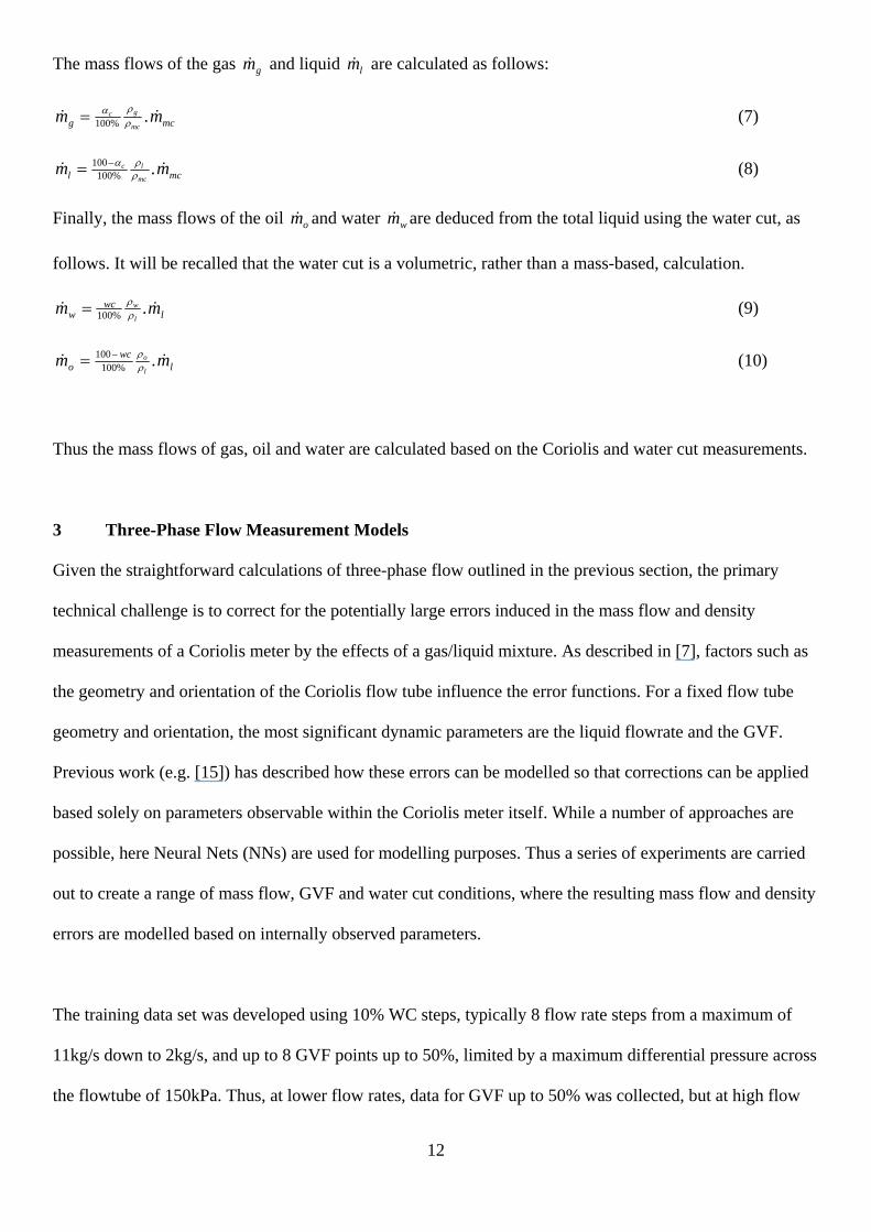
The mass flows of the gas gm and liquid lm are calculated as follows:

mcg mmmc

gc .%100 (7)

mcl mmmc

lc .%100100

(8)

Finally, the mass flows of the oil om and water wm are deduced from the total liquid using the water cut, as

follows. It will be recalled that the water cut is a volumetric, rather than a mass-based, calculation.

lwc

w mml

w .%100 (9)

lwc

o mml

o .%100100

(10)

Thus the mass flows of gas, oil and water are calculated based on the Coriolis and water cut measurements.

3 Three-Phase Flow Measurement Models

Given the straightforward calculations of three-phase flow outlined in the previous section, the primary

technical challenge is to correct for the potentially large errors induced in the mass flow and density

measurements of a Coriolis meter by the effects of a gas/liquid mixture. As described in [7], factors such as

the geometry and orientation of the Coriolis flow tube influence the error functions. For a fixed flow tube

geometry and orientation, the most significant dynamic parameters are the liquid flowrate and the GVF.

Previous work (e.g. [15]) has described how these errors can be modelled so that corrections can be applied

based solely on parameters observable within the Coriolis meter itself. While a number of approaches are

possible, here Neural Nets (NNs) are used for modelling purposes. Thus a series of experiments are carried

out to create a range of mass flow, GVF and water cut conditions, where the resulting mass flow and density

errors are modelled based on internally observed parameters.

The training data set was developed using 10% WC steps, typically 8 flow rate steps from a maximum of

11kg/s down to 2kg/s, and up to 8 GVF points up to 50%, limited by a maximum differential pressure across

the flowtube of 150kPa. Thus, at lower flow rates, data for GVF up to 50% was collected, but at high flow

13

rates, the GVF was limited by the differential pressure across the flow tube. These same limits were

reflected in the test matrix – see Figure 12. Given the large data set, which was intended to provide

reasonable coverage of the entire operating range of the skid, data recording at each training point was

limited to 120s, which was found to be sufficient for model-building purposes. The temperature range was

similar for the collection of the training data set and for the formal trials, all falling within the range 32°C -

43°C. Similarly, the supply pressure for training and testing data all fell within the range 280kPa – 460kPa

(a few test points with 0% GVF fell outside this pressure).

For example, figures 3 and 4 show the mass flow and density errors for the 50mm Coriolis meter (positioned

within the Skid), with water cut varying from 0 to 100% in steps of 10%, where the true mass flow rate is

maintained at 6.3 kg/s, and where the GVF is increased up to 50%. Similarly, figures 5 and 6 show the same

errors with the mass flow rate kept at 4.0 kg/s. This data was collected at TUV-NEL as described in the next

section. These graphs show the influence of GVF and water cut on the mass flow and density errors. While

the broad pattern of behaviour is similar for all graphs, with GVF having the most significant influence on

the mass flow and density errors, both water cut and the flow rate itself introduce further variation-.

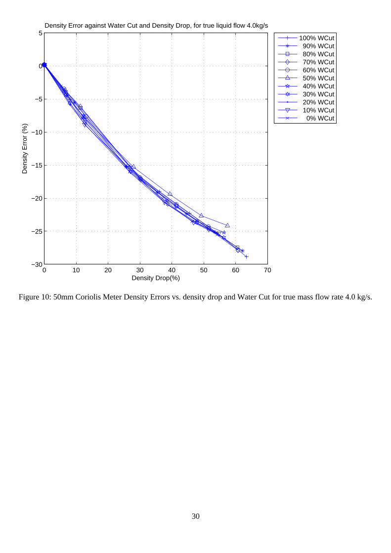
Of course when the Skid is operating in real-time the true GVF is not available, however the density drop

(i.e. the observed drop in density reading from the pure liquid density as a result of gas entrainment) is

observable. The same data are shown in figures 7 – 10 with density drop as the x axis. Such data is used to

build NNs to predict the mass flow and density errors, given the observed raw mass flow rate and density

drop. Further details of the techniques used to model the multiphase error surfaces are given in [16], such as

handling the interaction between models of the Coriolis meter errors and the water cut meter error. This

patent further includes discussion of the use of superficial velocity to model flow meter behaviour where slip

is significant.

4 FORMAL TRIALS AT TUV-NEL

14

A formal series of trials were carried out on a 50mm Skid in January 2012 at TUV-NEL’s three-phase flow

facility. The intention was to demonstrate compliance with the measurement performance requirements of

the Russian Standard GOST 8.165 [22], which has the following key specifications:

• Total liquid flow accuracy requirement ± 2.5%

• Total gas flow accuracy requirement ± 5.0%

• Total oil flow accuracy requirement dependent upon water cut:

o For water cuts less than 70%, oil accuracy requirement ± 6.0%

o For water cuts between 70% and 95%, oil accuracy requirement ± 15.0%

o For water cuts above 95%, no oil accuracy requirement is specified, but an indication of

performance may be given.

It is understood that the requirement for gas accuracy is a relatively recent introduction to the standard, and

it is noteworthy that the gas accuracy requirement is not specified on a sliding scale, while the oil accuracy

does vary with water cut. This offers particular difficulties at low GVFs and for mass-based instrumentation.

For example, consider a mixture of pure water and gas, where the water density is taken as 1000kg/m3, the

gas density at line temperature and pressure is 5kg/m3, and the GVF is 5%. Then in every cubic meter of

gas/liquid mixture, there are 950kg of water, and only 250g of gas; the GOST standard requires the latter is

to be measured to within ± 12.5g. To achieve such a resolution for the gas which is dispersed within 950kg

of water is an extremely challenging requirement. Nevertheless, this performance has been broadly achieved

in the tests carried out at TUV-NEL.

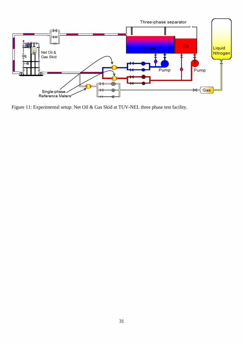
Figure 11 shows the Skid positioned in the three-phase test facility at TUV-NEL. The separator system

provides water and oil streams, while a liquid nitrogen store is used to supply the test gas. Each phase is

metered separately, before being combined and passed through the skid. As the flow ranges of the individual

phases were less than the calibrated ranges of the standard volumetric reference meters used at TUV-NEL,

15

additional mass flow meters were employed. These were calibrated at TUV-NEL, and a detailed uncertainty

analysis was provided at each test point, as discussed below. For each experiment performed, steady

conditions were established for the desired oil, water and gas flow rates, and then the reference single phase

measurements was compared with the outputs of the Skid averaged over a fixed duration. During the model-

building stage the duration was 120s, but for the final tests a 300s duration was used, the minimum advised

by NEL for formal trials. During the formal trials the operating pressure at the Skid inlet was typically 350

kPa , while the operating temperature ranged between 35 °C and 44 °C.

The test matrix is shown in Figures 12 and 13. A total of 75 tests were carried out, mostly at intermediary

flow rates between the modelling data points. Figure 12 shows the nominal GVF and mass flow rates used

for each test; in practice, the recorded values varied within a few percent from the nominal, due to the

limited accuracy of the experimental flow control. The total (water + oil) liquid mass flow rates range from

11kg/s down to 2.3kg/s. The maximum GVF decreases as the liquid mass flow rate increases, reflecting a

practical limitation on the pressure drop across the Skid of approximately 1.5bar. Figure 13 shows the mass

flow and water cut values used for the tests. Water cuts were tested in steps of 10% between 10% and 90%,

with further tests at 2%, 5%, 95% and 98% water cuts. Tests on pure water or pure oil were not possible

given the low levels of cross-contamination in the water and oil supplies from TUV-NEL’s separator

system. This cross-contamination was, however, monitored and included in the calculation of Skid errors

and system uncertainties.

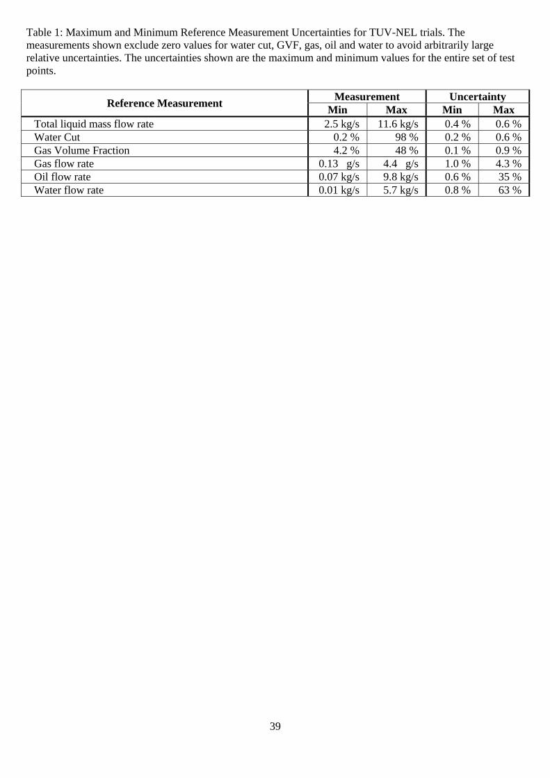
Particular care has been taken over the uncertainty of the reference measurement system, which proved to be

a challenging aspect of the trial. Given the wide range of flow rates, GVFs and water cuts, and the relatively

small size (50mm) of the Skid, TUV-NEL’s conventional reference meters were unable to cover the full

range of flows required, and so mass flow meters were used to monitor the single phase gas, water and oil

streams. Each of these alternative reference meters were calibrated against the National Flow Standard at

TUV-NEL prior to use in the trial. The uncertainty of each of the reference measurements varies with test

points, and was calculated by TUV-NEL. In all cases, expanded uncertainties are given, based on a standard

16

uncertainty multiplied by a coverage factor k=2. Table 1 lists the maximum and minimum values and

corresponding relative uncertainties of the key reference measurements. The turndown required for the total

liquid mass flow rate (i.e. the ratio of maximum to minimum flow rate) is relatively small – a factor of just

over 4:1 – and accordingly the uncertainty range for this reference measurement is relatively steady, varying

between 0.4% and 0.6%. Similarly, the water cut and GVF uncertainties are relatively steady. However, the

turn-down ratios of the individual gas water and oil flow rates are much higher – over 500:1 in the case of

the water flow rate – and so at the lowest water flow rate of 0.01kg/s, the uncertainty is 63%. Note that in all

test cases the uncertainties of the reference measurements are less than the target accuracy, and in most cases

by a healthy margin. Specifically, for the total liquid mass flow rate, where the target accuracy is ±2.5%, the

maximum reference uncertainty is 0.6% as shown in Table 1. For the gas flow rate, where the target

accuracy is ±5.0%, the maximum reference uncertainty shown in Table 1 is 4.3%, but as detailed in NEL’s

report, in only three cases does the reference uncertainty exceed 2.5%. For the oil flow rate, the maximum

reference uncertainty is 35%, but this occurs at high water cut (98%) where there is no target accuracy. For

water cuts where a target accuracy is defined (95% water cut or less), the largest reference uncertainty is

accuracy is 6.1% at 90% water cut, where the target accuracy is 15%.

Figures 14 – 18 give a summary of the results obtained in these test trials. Figure 14 shows the total liquid

flow errors against water cut. The total liquid flow performance is similar across all water cuts, 97% of the

points fall within the GOST specification of ±2.5%, and all points fall within ±4%. Figure 15 shows the

same results presented as a probability distribution, i.e. the percentage of test points having an absolute error

in the liquid mass flow reading of less than a certain value. Thus 66% of the test points have an error of less

than ± 1%, and 85% of the test points have an error of less than ± 1.5%.

The results and probability distribution for the gas mass flow rate are shown in Figure 16 and 17. Again the

results fall substantially within the GOST specification, with 93% of the test points falling within the ±5%

limit. As discussed above, the GOST standard specifies a maximum oil error which varies with water cut.

For water cuts below 70%, the permitted oil mass flow error is ±6%; between 70% and 95% water cut, the

17

oil mass flow error limit is ±15%; and above 95% water cut, no oil mass flow error limit is specified. As

shown in Figure 18, all test points match this performance requirement. No probability plot is shown as the

error requirement is not constant across all experiments.

Finally, table 2 provides the complete set of results for all 75 tests, giving the reference measurements and

Skid errors for the oil, water, gas and total liquid flow rates.

5. DISCUSSION

This paper has described a new commercial three-phase metering system based on Coriolis mass flow

metering combined with water cut metering. The results from laboratory trials suggest that this technology

has promise for applications in the oil and gas industry. Further formal lab trials are taking place on different

sized Skids. However, three-phase metering is a notoriously complex problem, and we anticipate further

technical challenges arising as field trial experience is acquired.

Specifically, it is important to determine for what range of parameters (particularly pressure, temperature

and fluid properties e.g. oil viscosity, the velocity of sound) a model proved in a flow laboratory can provide

good performance in the field. Early field experience suggests that both the water cut and Coriolis meter

models will require field tuning: the techniques needed to do so will emerge in time. More generally, it is

desirable to reduce the empirical nature of the correction models by quantifying as far as possible the

influence of physical parameters (for example as discussed in the literature discussed above ([7-15]);

hopefully the most influential factors will emerge through further experimental and field experience.

To a large extent, the current limit of 50% GVF is set by the communication speed of the Modbus

communication protocol, together with the observed pattern of flow. Rapid slugs of (say) less than two

seconds duration are difficult to measure accurately with only a 1Hz update rate. The Coriolis meter at least

is generating measurement data at a much higher rate (typically at 160Hz), and with higher communication

and computation bandwidth, accurate tracking of higher GVF multiphase flows may become possible.

18

While combining Coriolis meter and water cut meter has generated good measurement performance in this

paper, it is possible that other technology combinations may be advantageous, and will be the subject of

future research. Of particular benefit would be a means of detecting and measuring slip between the gas and

liquid phases, which could lead to significant improvement in the understanding and exploitation of this

technology.

19

Nomenclature

c gas volume fraction based on corrected data (%)

g gas density at local temperature and pressure (kg/m3)

o oil density at local temperature and pressure (kg/m3)

w water density at local temperature and pressure (kg/m3)

l liquid only (oil and water) mixture density at local temperature and pressure (kg/m3)

ma apparent mixture density from the Coriolis mass flow meter (kg/m3)

mc corrected mixture density from the Coriolis mass flow meter (kg/m3)

dd difference between the liquid-only mixture density l and the observed density ma (%)

gm mass flow rate of gas (kg/s)

lm mass flow rate of liquid (kg/s)

om mass flow rate of oil (kg/s)

wm mass flow rate of water (kg/s)

mam apparent three-phase mixture mass flow rate from the Coriolis mass flow meter (kg/s)

mcm corrected three-phase mixture mass flow rate from the Coriolis mass flow meter (kg/s)

P the absolute pressure at the inlet to the Coriolis mass flow meter (kPa),

T the process fluid temperature from the RTD sensor (K)

wc the water cut from the water cut meter, after any correction (%)

20

Figure Captions Figure 1: Net Oil Skid Design Figure 2: Hardware/Software Architecture of Net Oil and Gas System Figure 3: 50mm Coriolis Meter Mass Flow Errors vs. GVF and Water Cut for true mass flow rate 6.3 kg/s. Figure 4: 50mm Coriolis Meter Density Errors vs. GVF and Water Cut for true mass flow rate 6.3 kg/s. Figure 5: 50mm Coriolis Meter Mass Flow Errors vs. GVF and Water Cut for true mass flow rate 4.0 kg/s. Figure 6: 50mm Coriolis Meter Density Errors vs. GVF and Water Cut for true mass flow rate 4.0 kg/s. Figure 7: 50mm Coriolis Meter Mass Flow Errors vs. density drop and Water Cut for true mass flow rate 6.3 kg/s. Figure 8: 50mm Coriolis Meter Density Errors vs. density drop and Water Cut for true mass flow rate 6.3 kg/s. Figure 9: 50mm Coriolis Meter Mass Flow Errors vs. density drop and Water Cut for true mass flow rate 4.0 kg/s. Figure 10: 50mm Coriolis Meter Density Errors vs. density drop and Water Cut for true mass flow rate 4.0 kg/s. Figure 11: Experimental setup: Net Oil & Gas Skid at TUV-NEL three phase test facility. Figure 12: Experimental grid – mass flow rate vs. GVF. Figure 13: Experimental grid – liquid mass flow rate vs. water cut. Figure 14: Total liquid mass flow rate errors against water cut. The target limit is ± 2.5% (red boundary). Figure 15: Total Liquid Error probability distribution. Figure 16: Gas mass flow error against gas volume fraction. The target limit is ± 5% (red boundary). Figure 17: Gas mass flow error probability distribution. Figure 18: Oil mass flow error against water cut. The target performance (red boundary) is ± 6.0% for water cuts less than 70%, ± 15.0% for water cuts between 70% and 95%.

21

Figures

Figure 1: Net Oil Skid Design

Flow Flow

22

Figure 2: Hardware/Software Architecture of Net Oil and Gas System

P/T Transmitter * Pressure * Temperature

Water Cut Meter * Water Cut

Measurements

Coriolis Meter * Mass Flow * Density

Flow Calculations

Receive uncorrected measurements from instruments

Calculate base Liquid and Gas component densities from fluid pressure, temperature, water cut and configured fluid properties and density models.

Calculate corrected mass flow and density measurements based on three phase flow models.

Calculate oil, gas and water mass flows based on mass flow, density and water cut measurements

Inte

rnal

Mod

bu

s

Outputs

Ext

ern

al M

odb

us

* Oil Mass Flow * Gas Mass Flow * Water Mass Flow * Others

* User interface * Configuration * Data Archiving * Remote access via Ethernet

Display Computer

Ethernet

23

0 5 10 15 20 25 30 35 40−25

−20

−15

−10

−5

0

5

Gas Volume Fraction (%)

Mas

s F

low

Err

or (

%)

Mass Flow Error against Water Cut and GVF, for true liquid flow 6.3kg/s

100% WCut 90% WCut 80% WCut 70% WCut 60% WCut 50% WCut 40% WCut 30% WCut 20% WCut 10% WCut 0% WCut

Figure 3: 50mm Coriolis Meter Mass Flow Errors vs. GVF and Water Cut for true mass flow rate 6.3 kg/s.

24

0 5 10 15 20 25 30 35 40−35

−30

−25

−20

−15

−10

−5

0

5

Gas Volume Fraction (%)

Den

sity

Err

or (

%)

Density Error against Water Cut and GVF, for true liquid flow 6.3kg/s

100% WCut 90% WCut 80% WCut 70% WCut 60% WCut 50% WCut 40% WCut 30% WCut 20% WCut 10% WCut 0% WCut

Figure 4: 50mm Coriolis Meter Density Errors vs. GVF and Water Cut for true mass flow rate 6.3 kg/s.

25

0 5 10 15 20 25 30 35 40 45 50−30

−25

−20

−15

−10

−5

0

5

Gas Volume Fraction (%)

Mas

s F

low

Err

or (

%)

Mass Flow Error against Water Cut and GVF, for true liquid flow 4.0kg/s

100% WCut 90% WCut 80% WCut 70% WCut 60% WCut 50% WCut 40% WCut 30% WCut 20% WCut 10% WCut 0% WCut

Figure 5: 50mm Coriolis Meter Mass Flow Errors vs. GVF and Water Cut for true mass flow rate 4.0 kg/s.

26

0 5 10 15 20 25 30 35 40 45 50−30

−25

−20

−15

−10

−5

0

5

Gas Volume Fraction (%)

Den

sity

Err

or (

%)

Density Error against Water Cut and GVF, for true liquid flow 4.0kg/s

100% WCut 90% WCut 80% WCut 70% WCut 60% WCut 50% WCut 40% WCut 30% WCut 20% WCut 10% WCut 0% WCut

Figure 6: 50mm Coriolis Meter Density Errors vs. GVF and Water Cut for true mass flow rate 4.0 kg/s.

27

0 10 20 30 40 50 60−25

−20

−15

−10

−5

0

5

Density Drop (%)

Mas

s F

low

Err

or (

%)

Mass Flow Error against Water Cut and Density Drop, for true liquid flow 6.3kg/s

100% WCut 90% WCut 80% WCut 70% WCut 60% WCut 50% WCut 40% WCut 30% WCut 20% WCut 10% WCut 0% WCut

Figure 7: 50mm Coriolis Meter Mass Flow Errors vs. density drop and Water Cut for true mass flow rate 6.3 kg/s.

28

0 10 20 30 40 50 60−35

−30

−25

−20

−15

−10

−5

0

5

Density Drop(%)

Den

sity

Err

or (

%)

Density Error against Water Cut and Density Drop, for true liquid flow 6.3kg/s

100% WCut 90% WCut 80% WCut 70% WCut 60% WCut 50% WCut 40% WCut 30% WCut 20% WCut 10% WCut 0% WCut

Figure 8: 50mm Coriolis Meter Density Errors vs. density drop and Water Cut for true mass flow rate 6.3 kg/s.

29

0 10 20 30 40 50 60 70−30

−25

−20

−15

−10

−5

0

5

Density Drop (%)

Mas

s F

low

Err

or (

%)

Mass Flow Error against Water Cut and Density Drop, for true liquid flow 4.0kg/s

100% WCut 90% WCut 80% WCut 70% WCut 60% WCut 50% WCut 40% WCut 30% WCut 20% WCut 10% WCut 0% WCut

Figure 9: 50mm Coriolis Meter Mass Flow Errors vs. density drop and Water Cut for true mass flow rate 4.0 kg/s.

30

0 10 20 30 40 50 60 70−30

−25

−20

−15

−10

−5

0

5

Density Drop(%)

Den

sity

Err

or (

%)

Density Error against Water Cut and Density Drop, for true liquid flow 4.0kg/s

100% WCut 90% WCut 80% WCut 70% WCut 60% WCut 50% WCut 40% WCut 30% WCut 20% WCut 10% WCut 0% WCut

Figure 10: 50mm Coriolis Meter Density Errors vs. density drop and Water Cut for true mass flow rate 4.0 kg/s.

31

Figure 11: Experimental setup: Net Oil & Gas Skid at TUV-NEL three phase test facility.

32

0 2 4 6 8 10 120

5

10

15

20

25

30

35

40

45

50

Gas

Vol

ume

Fra

ctio

n (%

)

Liquid Mass Flow Rate (kg/s)

Experimental Test Points

Figure 12: Experimental grid – mass flow rate vs. GVF.

33

0 10 20 30 40 50 60 70 80 90 1000

2

4

6

8

10

12

Water Cut (%)

Liqu

id M

ass

Flo

w R

ate

(kg/

s)Experimental Test Points

Figure 13: Experimental grid – liquid mass flow rate vs. water cut.

34

0 10 20 30 40 50 60 70 80 90 100−15

−10

−5

0

5

10

15

Water Cut (%)

Liqu

id M

ass

Flo

w E

rror

(%

)Liquid Mass Flow Rate against Water Cut

Figure 14: Total liquid mass flow rate errors against water cut. The target limit is ± 2.5% (red boundary).

35

0 0.5 1 1.5 2 2.5 3 3.5 40

10

20

30

40

50

60

70

80

90

100

Absolute Liquid Mass Flow Error (%)

Cum

ulat

ive

Per

cent

age

of P

oint

s (%

)

Figure 15: Total Liquid Error probability distribution.

36

0 5 10 15 20 25 30 35 40 45 50−20

−15

−10

−5

0

5

10

15

20

Gas Volume Fraction (%)

Gas

Mas

s F

low

Err

or (

%)

Gas Mass Flow Rate against Gas Volume Fraction

Figure 16: Gas mass flow error against gas volume fraction. The target limit is ± 5% (red boundary).

37

0 1 2 3 4 5 6 7 8 9 100

10

20

30

40

50

60

70

80

90

100

Absolute Gas Mass Flow Error (%)

Cum

ulat

ive

Per

cent

age

of P

oint

s (%

)

Figure 17: Gas mass flow error probability distribution.

38

0 10 20 30 40 50 60 70 80 90 100−60

−40

−20

0

20

40

60

Water Cut (%)

Oil

Mas

s F

low

Err

or (

%)

Oil Mass Flow Rate Error against Water Cut

Figure 18: Oil mass flow error against water cut. The target performance (red boundary) is ± 6.0% for water cuts less than 70%, ± 15.0% for water cuts between 70% and 95%.

39

Table 1: Maximum and Minimum Reference Measurement Uncertainties for TUV-NEL trials. The measurements shown exclude zero values for water cut, GVF, gas, oil and water to avoid arbitrarily large relative uncertainties. The uncertainties shown are the maximum and minimum values for the entire set of test points.

Reference Measurement Measurement Uncertainty

Min Max Min Max Total liquid mass flow rate 2.5 kg/s 11.6 kg/s 0.4 % 0.6 % Water Cut 0.2 % 98 % 0.2 % 0.6 % Gas Volume Fraction 4.2 % 48 % 0.1 % 0.9 % Gas flow rate 0.13 g/s 4.4 g/s 1.0 % 4.3 % Oil flow rate 0.07 kg/s 9.8 kg/s 0.6 % 35 % Water flow rate 0.01 kg/s 5.7 kg/s 0.8 % 63 %

40

Table 2: Trial results of Net Oil & Gas Skid at TUV-NEL.

  

Nominal Experimental Conditions    Oil Mass Flow  Gas Mass Flow  Water Mass Flow  Liquid Mass Flow 

Liq Mflow  Water Cut  GVF     NEL Reference (kg/s)

Skid     Error  (%)

NEL Reference 

(g/s)

Skid Error (%)

NEL Reference (kg/s)

Skid Error  (%)

NEL Reference (kg/s)

Skid  Error  (%) Tag  (kg/s)  (%)  (%) 

2‐40‐F  2.30  40.0  0.0     1.2861  1.55%  0.0000  0.00%  1.0145  ‐2.15%  2.3005  ‐0.08% 2‐40‐Z  2.30  40.0  50.0     1.2894  2.56%  9.5630  ‐0.20%  1.0343  ‐5.62%  2.3237  ‐1.08% 2‐40‐A  2.30  40.0  45.0     1.2753  3.38%  7.8299  1.54%  1.0319  ‐4.98%  2.3072  ‐0.36% 2‐40‐B  2.30  40.0  35.0     1.2724  1.81%  5.4337  0.97%  1.0047  ‐4.69%  2.2771  ‐1.06% 2‐40‐C  2.30  40.0  25.0     1.2925  2.37%  3.3711  ‐0.44%  1.0275  ‐1.38%  2.3200  0.71% 2‐40‐D  2.30  40.0  15.0     1.2864  0.53%  1.7127  ‐1.14%  1.0190  ‐2.86%  2.3054  ‐0.97% 2‐40‐E  2.30  40.0  5.0     1.2865  0.75%  0.4899  ‐3.42%  1.0234  ‐3.29%  2.3099  ‐1.04% 3‐80‐F  3.50  80.0  0.0     0.5935  ‐4.55%  0.0000  0.00%  2.8879  0.98%  3.4815  0.04% 3‐80‐A  3.50  80.0  45.0     0.5946  1.96%  12.2696  ‐5.24%  2.8807  ‐4.71%  3.4753  ‐3.57% 3‐80‐B  3.50  80.0  35.0     0.5942  3.18%  8.0861  ‐1.64%  2.9600  ‐0.81%  3.5542  ‐0.14% 3‐80‐C  3.50  80.0  25.0     0.5835  ‐4.04%  4.4988  ‐0.43%  2.8960  0.35%  3.4795  ‐0.39% 3‐80‐D  3.50  80.0  15.0     0.5974  ‐4.65%  2.3827  0.95%  2.9111  1.16%  3.5086  0.17% 3‐80‐E  3.50  80.0  5.0     0.5867  ‐4.62%  0.7672  4.07%  2.8752  0.68%  3.4619  ‐0.22% 3‐5‐F  3.50  5.0  0.0     3.3183  ‐0.68%  0.0000  0.00%  0.1726  13.88%  3.4909  0.04% 3‐5‐A  3.50  5.0  45.0     3.3451  ‐0.20%  11.7132  ‐0.05%  0.1753  29.12%  3.5204  1.26% 3‐5‐B  3.50  5.0  35.0     3.3359  ‐1.01%  7.7067  ‐1.25%  0.1750  27.48%  3.5109  0.41% 3‐5‐C  3.50  5.0  25.0     3.3400  ‐0.78%  4.7714  ‐1.24%  0.1704  30.53%  3.5104  0.74% 3‐5‐D  3.50  5.0  15.0     3.3139  ‐1.34%  2.5278  ‐1.37%  0.1559  36.94%  3.4698  0.38% 3‐5‐E  3.50  5.0  5.0     3.3535  ‐1.74%  0.8635  ‐1.22%  0.1378  49.96%  3.4912  0.30% 4‐2‐F  4.60  2.0  0.0     4.6018  ‐2.51%  0.0000  0.00%  0.0150  786.50%  4.6169  0.06% 4‐2‐A  4.60  2.0  45.0     4.6663  ‐1.18%  16.7201  1.25%  0.0119  1072.31%  4.6782  1.56% 4‐2‐B  4.60  2.0  35.0     4.6688  ‐6.47%  11.1260  ‐3.78%  0.0121  1006.18%  4.6809  ‐3.86% 4‐2‐C  4.60  2.0  25.0     4.6253  ‐3.54%  6.1195  ‐2.25%  0.0131  932.70%  4.6385  ‐0.89% 4‐2‐D  4.60  2.0  15.0     4.6121  ‐2.43%  3.2408  0.42%  0.0127  953.33%  4.6247  0.19% 4‐2‐E  4.60  2.0  5.0     4.5816  ‐3.09%  0.9654  3.58%  0.0123  985.10%  4.5939  ‐0.45% 4‐10‐F  4.60  10.0  0.0     4.1223  ‐3.08%  0.8121  0.00%  0.4315  39.03%  4.5538  0.91% 4‐10‐A  4.60  10.0  45.0     4.1800  ‐5.92%  15.6991  ‐3.14%  0.4413  41.94%  4.6212  ‐1.35% 4‐10‐B  4.60  10.0  35.0     4.1940  ‐5.22%  10.3238  ‐1.11%  0.4348  44.07%  4.6288  ‐0.59% 4‐10‐C  4.60  10.0  25.0     4.2551  ‐4.93%  6.0126  ‐1.52%  0.4448  43.78%  4.6998  ‐0.32% 

41

Table 2: Trial results of Net Oil & Gas Skid at TUV-NEL (continued).

  

Nominal Experimental Conditions    Oil Mass Flow  Gas Mass Flow  Water Mass Flow  Liquid Mass Flow 

Liq Mflow  Water Cut  GVF     NEL Reference (kg/s)

Skid     Error  (%)

NEL Reference 

(g/s)

Skid Error (%)

NEL Reference (kg/s)

Skid Error  (%)

NEL Reference (kg/s)

Skid  Error  (%) Tag  (kg/s)  (%)  (%) 

4‐10‐D  4.60 10.0  15.0 4.1573 ‐4.39% 3.1866  0.27% 0.4292 43.70% 4.5865  0.11% 4‐10‐E  4.60  10.0  5.0    4.2537  ‐4.44%  0.9503  1.32%  0.4447  40.89%  4.6984  ‐0.15% 4‐95‐F  4.60  95.0  0.0    0.1894  ‐8.39%  0.0000  0.00%  4.3934  0.46%  4.5828  0.09% 4‐95‐A  4.60  95.0  45.0     0.1725  ‐1.12%  12.5570  ‐2.21%  4.4007  1.73%  4.5732  1.62% 4‐95‐B  4.60  95.0  35.0     0.1758  10.60%  8.2667  ‐1.55%  4.4524  0.85%  4.6281  1.22% 4‐95‐C  4.60  95.0  25.0     0.1772  14.70%  5.1101  0.40%  4.5323  0.85%  4.7095  1.37% 4‐95‐D  4.60  95.0  15.0     0.1733  19.24%  2.8166  ‐0.15%  4.4248  0.69%  4.5981  1.39% 4‐95‐E  4.60  95.0  5.0     0.2011  2.76%  0.8855  1.23%  4.3087  1.40%  4.5098  1.46% 4‐98‐F  4.60  98.0  0.0     0.0622  33.42%  0.0001  0.00%  4.5692  ‐0.38%  4.6314  0.07% 4‐98‐A  4.60  98.0  45.0     0.0599  27.37%  13.0798  0.38%  4.6202  2.02%  4.6801  2.34% 4‐98‐B  4.60  98.0  35.0     0.0701  55.94%  8.6061  ‐1.90%  4.5571  0.41%  4.6272  1.25% 4‐98‐C  4.60  98.0  25.0     0.0711  40.55%  5.3281  ‐1.49%  4.7304  0.10%  4.8015  0.70% 4‐98‐D  4.60  98.0  15.0     0.0746  42.83%  2.8215  ‐1.79%  4.5698  0.51%  4.6444  1.19% 4‐98‐E  4.60  98.0  5.0     0.0744  20.85%  0.8645  ‐1.72%  4.4977  0.53%  4.5721  0.86% 5‐20‐F  5.70  20.0  0.0     4.5200  ‐2.45%  0.0003  0.00%  1.2107  9.00%  5.7307  ‐0.03% 5‐20‐A  5.70  20.0  45.0     4.5065  ‐2.56%  19.2667  1.00%  1.2116  6.12%  5.7181  ‐0.72% 5‐20‐B  5.70  20.0  35.0     4.3877  ‐1.74%  12.7030  0.24%  1.2249  6.60%  5.6126  0.08% 5‐20‐C  5.70  20.0  25.0     4.4620  ‐3.00%  7.8778  ‐2.64%  1.2631  5.75%  5.7250  ‐1.07% 5‐20‐D  5.70  20.0  15.0     4.4885  ‐2.51%  4.1703  ‐3.46%  1.2779  6.65%  5.7664  ‐0.48% 5‐20‐E  5.70  20.0  5.0     4.4385  ‐2.10%  1.2391  ‐3.72%  1.2534  6.89%  5.6919  ‐0.12% 5‐90‐F  5.70  90.0  0.0     0.4471  8.79%  0.0000  0.00%  5.2457  ‐0.80%  5.6927  ‐0.05% 5‐90‐A  5.70  90.0  45.0     0.4986  1.56%  16.0306  2.45%  5.1555  2.42%  5.6541  2.34% 5‐90‐B  5.70  90.0  35.0     0.4780  3.83%  10.6482  ‐3.74%  5.2508  ‐0.08%  5.7288  0.25% 5‐90‐C  5.70  90.0  25.0     0.4335  4.49%  6.9862  ‐4.83%  5.2430  1.08%  5.6766  1.34% 5‐90‐D  5.70  90.0  15.0     0.4597  8.89%  3.7031  ‐6.01%  5.3120  ‐0.47%  5.7716  0.28% 5‐90‐E  5.70  90.0  5.0     0.4662  3.07%  1.1050  ‐2.54%  5.2144  0.53%  5.6806  0.74% 6‐30‐F  6.90  30.0  0.0     4.5891  ‐2.49%  0.0000  0.00%  2.3098  4.74%  6.8989  ‐0.07% 6‐30‐B  6.90  30.0  35.0     4.5466  ‐1.81%  17.6429  4.93%  2.3088  4.60%  6.8554  0.35% 

42

Table 2: Trial results of Net Oil & Gas Skid at TUV-NEL (continued).

  

Nominal Experimental Conditions    Oil Mass Flow  Gas Mass Flow  Water Mass Flow  Liquid Mass Flow 

Liq Mflow  Water Cut  GVF     NEL Reference (kg/s)

Skid     Error  (%)

NEL Reference 

(g/s)

Skid Error (%)

NEL Reference (kg/s)

Skid Error  (%)

NEL Reference (kg/s)

Skid  Error  (%) Tag  (kg/s)  (%)  (%) 

6‐30‐C  6.90  30.0  25.0     4.6597  ‐2.99%  9.4757  ‐2.41%  2.2456  4.85%  6.9053  ‐0.44% 6‐30‐D  6.90  30.0  15.0     4.6671  ‐3.27%  4.3756  ‐3.53%  2.2871  5.03%  6.9542  ‐0.54% 6‐30‐E  6.90  30.0  5.0     4.6452  ‐2.67%  1.1968  ‐1.96%  2.2508  5.88%  6.8960  0.12% 6‐70‐F  6.90  70.0  0.0     1.8367  ‐0.37%  0.0000  0.00%  5.0483  ‐0.23%  6.8851  ‐0.27% 6‐70‐B  6.90  70.0  35.0     1.7557  ‐1.52%  12.9744  ‐3.43%  5.1389  ‐2.43%  6.8946  ‐2.20% 6‐70‐C  6.90  70.0  25.0     1.7974  ‐0.42%  7.2511  ‐9.63%  5.0529  ‐1.91%  6.8504  ‐1.52% 6‐70‐D  6.90  70.0  15.0     1.7964  2.57%  3.8374  ‐4.66%  5.0697  ‐1.09%  6.8661  ‐0.13% 6‐70‐E  6.90  70.0  5.0     1.7703  2.96%  1.3790  ‐8.66%  5.1673  ‐2.49%  6.9376  ‐1.10% 8‐60‐F  8.00  60.0  0.0     2.8492  ‐1.62%  0.0000  0.00%  5.1322  1.05%  7.9814  0.10% 8‐60‐C  8.00  60.0  25.0     2.7882  2.20%  8.8870  4.89%  5.2021  1.34%  7.9903  1.64% 8‐60‐D  8.00  60.0  15.0     2.8499  ‐1.54%  4.7072  ‐5.85%  5.1991  ‐1.94%  8.0490  ‐1.80% 8‐60‐E  8.00  60.0  5.0     2.8257  ‐2.75%  1.2181  ‐0.74%  5.1836  ‐1.16%  8.0093  ‐1.72% 9‐10‐F  9.25  10.0  0.0     8.2802  ‐2.03%  0.0000  0.00%  0.9092  18.79%  9.1894  0.03% 9‐10‐D  9.25  10.0  15.0     8.3106  ‐3.36%  7.6071  ‐3.57%  0.8121  38.09%  9.1227  0.33% 9‐10‐E  9.25  10.0  5.0     7.8002  ‐3.96%  2.0278  ‐2.87%  0.6680  49.67%  8.4681  0.27% 11‐50‐F  11.00  50.0  0.0     5.0280  ‐3.50%  0.0000  0.00%  5.8252  3.02%  10.8532  0.00% 11‐50‐E  11.00  50.0  5.0     5.0904  ‐2.85%  2.5162  0.52%  5.7912  2.49%  10.8815  ‐0.01% 

43

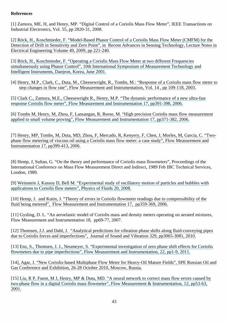
References [1] Zamora, ME, H, and Henry, MP. “Digital Control of a Coriolis Mass Flow Meter”, IEEE Transactions on Industrial Electronics, Vol. 55, pp 2820-31, 2008. [2] Röck, H., Koschmieder, F. “Model-Based Phasor Control of a Coriolis Mass Flow Meter (CMFM) for the Detection of Drift in Sensitivity and Zero Point”, in Recent Advances in Sensing Technology, Lecture Notes in Electrical Engineering Volume 49, 2009, pp 221-240. [3] Röck, H., Koschmieder, F. “Operating a Coriolis Mass Flow Meter at two different Frequencies simultaneously using Phasor Control”, 10th International Symposium of Measurement Technology and Intelligent Instruments, Daejeon, Korea, June 2001. [4] Henry, M.P., Clark, C., Duta, M., Cheesewright, R., Tombs, M.: “Response of a Coriolis mass flow meter to

step changes in flow rate”, Flow Measurement and Instrumentation, Vol. 14 , pp 109-118, 2003. [5] Clark C., Zamora, M.E., Cheesewright R., Henry, M.P. “The dynamic performance of a new ultra-fast response Coriolis flow meter”, Flow Measurement and Instrumentation 17, pp391-398, 2006. [6] Tombs M, Henry, M, Zhou, F, Lansangan, R, Reese, M. “High precision Coriolis mass flow measurement applied to small volume proving”, Flow Measurement and Instrumentation 17, pp371-382, 2006. [7] Henry, MP, Tombs, M, Duta, MD, Zhou, F, Mercado, R, Kenyery, F, Chen, J, Morles, M, Garcia, C. “Two-phase flow metering of viscous oil using a Coriolis mass flow meter: a case study”, Flow Measurement and Instrumentation 17, pp399-413, 2006. [8] Hemp, J, Sultan, G. “On the theory and performance of Coriolis mass flowmeters”, Proceedings of the International Conference on Mass Flow Measurement Direct and Indirect, 1989 Feb IBC Technical Services, London, 1989. [9] Weinstein J, Kassoy D, Bell M. “Experimental study of oscillatory motion of particles and bubbles with applications to Coriolis flow meters”, Physics of Fluids 20, 2008. [10] Hemp, J. and Kutin, J. “Theory of errors in Coriolis flowmeter readings due to compressibility of the fluid being metered”, Flow Measurement and Instrumentation 17, pp359-369, 2006. [11] Gysling, D. L. “An aeroelastic model of Coriolis mass and density meters operating on aerated mixtures, Flow Measurement and Instrumentation 18, pp69-77, 2007. [12] Thomsen, J.J. and Dahl, J. “Analytical predictions for vibration phase shifts along fluid-conveying pipes due to Coriolis forces and imperfections”, Journal of Sound and Vibration 329, pp3065-3081, 2010. [13] Enz, S., Thomsen, J. J., Neumeyer, S. “Experimental investigation of zero phase shift effects for Coriolis flowmeters due to pipe imperfections”, Flow Measurement and Instrumentation, 22, pp1-9, 2011. [14], Agar, J. “New Coriolis-based Multiphase Flow Meter for Heavy-Oil Mature Fields”, SPE Russian Oil and Gas Conference and Exhibition, 26-28 October 2010, Moscow, Russia. [15] Liu, R P, Fuent, M J, Henry, MP & Duta, MD. “A neural network to correct mass flow errors caused by two-phase flow in a digital Coriolis mass flowmeter”, Flow Measurement & Instrumentation, 12, pp53-63, 2001.

44

[16] Tombs, MS, Henry, MP, Duta, MD, Lansangan, R, Dutton, RE, Mattar, WM, “Multiphase Coriolis Flowmeter”, US Patent 7,188,534. 2007. [17] Vortab Product Brochure. http://www.vortab.com/pdfs/Vortab-Brochure-RevE.pdf . Accessed 14/12/12. [18] Weatherford. Red Eye MP Water Cut Meter. Product Brochure. http://www.weatherford.com/weatherford/groups/web/documents/weatherfordcorp/wft096554.pdf, Accessed 14/12/12. [19] EN ISO 12213-2:2005: Natural gas – calculation of compression factor. 2005. [20] GSSSD MP 113-03. “Determination of the density, compressibility factor, the adiabatic index and the coefficient of dynamic viscosity of the wet gas in the temperature range 263 ... 500 K at pressures to 15 MPa.” All-Russian Research Center for Standardization, Information and certification of raw materials and substances of Gosstandart of Russia (Federal State Unitary Enterprise VNITSSMV), 2003. (in Russian) [21] API MPMS Chapter 11.1-2004. “Manual of Petroleum Measurement Standards Chapter 11—Physical Properties Data Section 1—Temperature and Pressure Volume Correction Factors for Generalized Crude Oils, Refined Products, and Lubricating Oils.”. May 2004, Addendum 1 Sept 2007. American Petroleum Institute, API Publishing Services, 1220 L Street, N.W., Washington, D.C. 20005. [22] GOST R 8.615, Amended 2008. State system for ensuring uniformity of measurements. Measurement of quantity of oil and petroleum gas extracted from subsoil. General metrological and technical requirements. Federal Agency for technical regulation and metrology. 2008. (in Russian)